Performance of Brownian Motors

Zur Erlangung des akademischen Grades einesDoktors der Naturwissenschaften

der Mathematisch–Naturwissenschaftlichen Fakultatder Universitat Augsburg vorgelegte

Dissertation

von

Łukasz Machura

aus

Zawiercie

Augsburg, im Januar 2006

Betreuer:

Prof. Dr. Peter HanggiTheoretical Physics IUniversity of Augsburg, Germany

Prof. Dr. Peter TalknerTheoretical Physics IUniversity of Augsburg, Germany

Prof. Dr. Jerzy ŁuczkaDepartment of Theoretical PhysicsUniversity of Silesia, Katowice, Poland

Erster Berichter: Prof. Dr. Peter HanggiZweiter Berichter: Prof. Dr. Jerzy ŁuczkaTag der mundlichen Prufung: 15 Marz 2006

Contents

1 Introduction 5

2 Stochastic model of a tilted rocked ratchet 132.1 Langevin equation . . . . . . . . . . . . . . . . . . . . . . . . . . . . . . . .132.2 Scaling . . . . . . . . . . . . . . . . . . . . . . . . . . . . . . . . . . . . .142.3 Fokker-Planck Equation . . . . . . . . . . . . . . . . . . . . . . . . . . . .142.4 Potential Profiles . . . . . . . . . . . . . . . . . . . . . . . . . . . . . . . .162.5 Numerical method . . . . . . . . . . . . . . . . . . . . . . . . . . . . . . .17

3 Quantifiers characterizing the optimal transport 193.1 Effective Diffusion and Peclet number . . . . . . . . . . . . . . . . . . . . . 193.2 Rectification Efficiency . . . . . . . . . . . . . . . . . . . . . . . . . . . . .19

4 Zero bias force 234.1 Generic Ratchet . . . . . . . . . . . . . . . . . . . . . . . . . . . . . . . . .23

4.1.1 Deterministic dynamics . . . . . . . . . . . . . . . . . . . . . . . .234.1.2 Noisy dynamics: Fluctuations versus driving strength . . . . . . . . .274.1.3 Noisy dynamics: Fluctuations versus noise strength . . . . . . . . . .32

4.2 Optimization of the performance . . . . . . . . . . . . . . . . . . . . . . . .36

5 Inertial motor under load 415.1 Biasing the ratchet . . . . . . . . . . . . . . . . . . . . . . . . . . . . . . .41

5.1.1 Current-load behavior . . . . . . . . . . . . . . . . . . . . . . . . .415.1.2 Efficiency of forced and rocked Brownian motors . . . . . . . . . . .42

5.2 Absolute negative mobility in a symmetric potential . . . . . . . . . . . . . .43

6 Summary 49

A Effective Diffusion 51

B Efficiency 53

Bibliography 55

3

Contents

4

1 Introduction

Isn’t it sometimes that a facadeof randomness and chaosconceals a demonof order and harmony.

(Łuczka)

Historical remarksIn 1827 Robert Brown (1773–1858), a leading British botanist observed under the micro-

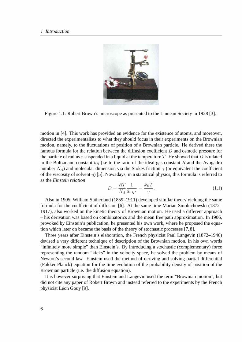
scope irregular motion of pollen grains and spores of mosses suspended in water(see Fig. 1.1)1. Puzzled by the phenomenon he performed a number of further experiments,using different organic and inorganic objects, different surrounding fluids like water or alcoholand different microscopes. One year later he published his findings [1] where he concludedthat this kind of motion is caused by the bombardments by the small particles, which he calls”active molecules”. His theory, however, has one weakness: He claimed that the motion ofactive molecules originates from the molecules themselves and not that it is caused by heat.He knew that he was not the first to discover this kind of mobility and in his 1829 paper [2]he referred to a number of experiments and observations done earlier, however, for organicbodies only. Although Brown was not the first observer of this kind of motion, he was the pi-oneering experimentalist who made systematic investigations, trying to understand the originof this random motion. His study showed that this kind of motion is universal and in particularnot restricted to living matter. He turned the story of the neverending inanimate bodies dancesin fluids from biology to a problem of physics. Brown was not aware of the work of the Dutchphysiologist, botanist and physicist Jan Ingen-Housz (1730–1799), who in 1785 had madesome observations of the irregular motion of carbon dust on alcohol.

After Brown other scientists performed their own experiments and proposed new theories,in order to give a quantitative description of the phenomenon. Unfortunately, the experimen-talists usually measured the instantaneous velocities of the frisky particles and ended up withirreproducible average values. There were also several attempts to explain of this kind ofmotion, mostly as an effect of external forces, like the most popular temperature gradientproduced by the light illuminating the probe and the convection connected with it.

The breakthrough came with Albert Einstein (1879–1955) in hisannus mirabilis1905,when he published, beside others outstanding papers, his theoretical explanation of Brownian

1 The picture of Robert’s Brown microscope (Fig. 1.1) used on the courtesy of Prof. Brian J. Ford (http://www.brianjford.com ).

5

1 Introduction

Figure 1.1:Robert Brown’s microscope as presented to the Linnean Society in 1928 [3].

motion in [4]. This work has provided an evidence for the existence of atoms, and moreover,directed the experimentalists to what they should focus in their experiments on the Brownianmotion, namely, to the fluctuations of position of a Brownian particle. He derived there thefamous formula for the relation between the diffusion coefficientD and osmotic pressure forthe particle of radiusr suspended in a liquid at the temperatureT . He showed thatD is relatedto the Boltzmann constantkB (i.e to the ratio of the ideal gas constantR and the AvogadronumberNA) and molecular dimension via the Stokes frictionγ (or equivalent the coefficientof the viscosity of solventη) [5]. Nowadays, in a statistical physics, this formula is referred toas theEinstein relation

D =RT

NA

1

6πηr=

kBT

γ. (1.1)

Also in 1905, William Sutherland (1859–1911) developed similar theory yielding the sameformula for the coefficient of diffusion [6]. At the same time Marian Smoluchowski (1872–1917), also worked on the kinetic theory of Brownian motion. He used a different approach– his derivation was based on combinatorics and the mean free path approximation. In 1906,provoked by Einstein’s publication, he presented his own work, where he proposed the equa-tion which later on became the basis of the theory of stochastic processes [7,8].

Three years after Einstein’s elaboration, the French physicist Paul Langevin (1872–1946)devised a very different technique of description of the Brownian motion, in his own words“infinitely more simple” than Einstein’s. By introducing a stochastic (complementary) forcerepresenting the random “kicks” in the velocity space, he solved the problem by means ofNewton’s second law. Einstein used the method of deriving and solving partial differential(Fokker-Planck) equation for the time evolution of the probability density of position of theBrownian particle (i.e. the diffusion equation).

It is however surprising that Einstein and Langevin used the term ”Brownian motion”, butdid not cite any paper of Robert Brown and instead referred to the experiments by the Frenchphysicist Leon Gouy [9].

6

The experimental confirmation of the kinetic theories of Brownian motion came with JeanBaptiste Perrin (1870–1942) [10], who won the 1926 Nobel Prize for his work on the discon-tinuous structure of matter.

The two approaches, based on the Fokker-Planck and the Langevin equations, are nowwidely used as the equivalent formulation of continuous Markov processes in many differentbranches of science like physics, chemistry, economy and even in social sciences.

Ratchet introducedIn 1912 Smoluchowski published a paper [11] where he designed in a thought experiment

a gadget showing the possibility of rectifying thermal energy using a ratchet and pawl mecha-nism. In other words - he proposed a device that far from the equilibrium state is able to convertthe thermal motion of Brownian particles into directed motion, just by using the breaking ofsymmetry. The small section in [11] was like a kind of response to the postulate of L. Gouywho had insinuated that the molecular ratchet mechanism would violate the second law ofthermodynamics [12]. The same idea was reformulated and elucidated in the early 1960 byRichard Feynman (1918–1988) in his famous ”Lecture of Physics” [13].

Figure 1.2:A schematic cartoon of the Smoluchowski-Feynman ratchet and pawl device.

Let us briefly examine the apparatus we call Smoluchowski-Feynman ratchet presented inthe Fig. 1.2. The machine consists of an axle with vanes at one of its ends and a ratchet at theother. The pawl restricts the motion in one direction. Both ends of the instrument placed in

7

1 Introduction

different ”boxes” with gas temperaturesT1 andT2, undergo random motion due to collisionswith molecules. The first impression is that at even the same temperaturesT1 = T2, the axlemay only turn in one direction because of the pawl mechanism and on the average a directedmotion is generated by means of the thermal fluctuations. It looks like that we have justconstructed aperpetuum mobileof the second kind or a specific Maxwell demon is seeminglyat work. The paradox was explained by Feynman [13]: Every single part of the device issubjected to the neverending bombardments of equal intensity in all directions. It is thereforepossible that due to the Brownian motion, the pawl would rise above the ratchet’s teeth andcause turns in both directions with the same probability. The net motion is then obviouslyzero. A critical analysis of the Smoluchowski-Feynman construction is presented in [14, 15].On the other hand, if the two temperatures are different,T1 6= T2, the resulting average motionis nonzero. In this case, the macroscopic difference of temperature causes the net motion ofthe axle.

This analysis can be a motivation for an abstract mathematical formulation [16] of theratchet deviceillustrated in Fig 1.2:

a) The ratchet (wheel) presents a spatially periodic system. It corresponds to a spatiallyperiodic potentialV (x) = V (x + L).

b) The symmetry of the ratchet is broken, because of the pawl mechanism (the teeth areasymmetrical). It corresponds to a breaking of a reflection symmetry of the potential:there is no real numberx0, such that the relationV (x0 − x) = V (x0 + x) is fulfilled.

c) The average random force acting on the vanes and caused by collisions of gas moleculesis zero. It corresponds to the zero-mean thermal fluctuations.

d) The directed motion can be induced by a temperature gradient or a constant bias force.However, these are trivial cases and instead we would drive the system out of the equi-librium state with a nonthermal force of a zero mean.

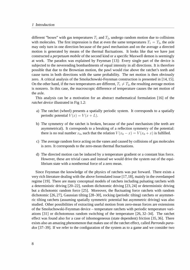
Since Feynman the knowledge of the physics of ratchets was put forward. There exists avery rich literature dealing with the above formulated issue [17,18], mainly in the overdampedregime [19]. There are many conceptual models of ratchets including pulsating ratchets witha deterministic driving [20–22], random dichotomic driving [23, 24] or deterministic drivingbut a dichotomic random force [25]. Moreover, the fluctuating force ratchets with randomdichotomic [26, 27], Gaussian tilting [28–30], rocking (periodic tilting) ratchets or asymmet-ric tilting ratchets (assuming spatially symmetric potential but asymmetric driving) was alsostudied. Other possibilities of extracting useful motion from zero-mean forces are extensionsof the Smoluchowski-Feynman device – temperature ratchets with periodic temperature vari-ations [31] or dichotomous random switching of the temperature [26, 32–34]. The ratcheteffect was found also for a case of inhomogeneous (state dependent) friction [35, 36]. Thereexists also an amazing phenomenon that makes use of the ratchet effect, calledParrondo para-dox [37–39]. If we refer to the configuration of the system as to a game and we consider two

8

fair games, we can expressed this paradox as the following: by random switching betweentwo fair random games one can end up with a game that is no longer fair.

Another important family of ratchet-based systems are molecular motors. The name refersto proteins or protein complexes that are able to transduce chemical energy, usually stored inthe ATP (AdenosineTriPhosphate), into mechanical work and directed motion in an asymmet-ric environment at the molecular scale. There are transporting proteins (translationary motors)which move along the intracellular, polar “highways”, like tubulin filaments (with kinesinwalking towards the positive and dynein to the negative end) or active filaments (with cor-responding myosin advancing in the positive extremity). The filaments are asymmetric andperiodic structures with period of about8nm. Other motor proteins perform rotatory motions,like theF1F0ATPase which produces (with nearly 100% efficiency [40, 41]) the life-essentialnucleotide ATP. It is stunning that every day we produce and burn a half of our body weightin ATP. In fact it is not at all easy to move in a cellular environment. Due to the relatively highviscosity of the surrounding fluid the motor has to struggle against the strong friction force. Onthe other hand due to the heat bombardments by particles of the solution the motor perceivesstrong kicks in every direction. For the molecular motor it is like to “walk in a hurricane andswim in molasses” [42,43].

Many different aspects of the molecular motors were studied in great detail. The model ofa motor with two feet and its manner of walking (stepping) along tubulin was addressed bothexperimentally [44–46] and theoretically [47–52]. A one dimensional model of the motor inan open tube, with dynamics alternating between two configurations, when the motor moveson a tubulin using the ratchet effect (bounded state) and the free diffusive motion in the tube(unbounded state) was studied in [53–55]. The mechanical properties of a motor was examinedby use of an optical tweezers technique [56–58] and the conformational changes of a motorsimulated by means of molecular dynamics [59], to name but a few.

The overdamped dynamics is a valid approximation for many physical applications [60]. Itis particularly well suited to describe the motion of molecular motors. In other situations theinertial effects, however, can play an important role. Examples are the diffusion of adatomson a crystal surface [61–63], dissipation in threshold devices [64,65], dislocation of defects inmetals [66,67] and in a hysteretic Josephson junction [68,69].

Subject of this thesisIn this thesis we will study transport of aninertial Brownian particle in a periodic ratchet-

type potential additionally subjected to an external, time periodic force, i.e. rocked ratchet.The vast majority of works focused on rocking ratchets is concentrated on the behavior of theoverdampedregime [70–72] and the control of the emerging directed transport as a functionof control parameters such as temperature, external load (yielding the load-current character-istics), or some other control variable, for reviews see [17,18,43,73–76].

A notable exception is the first work on an inertial rocking ratchet [77] wherein the higher-order, statistical cumulant properties of the stochastic position variable have been explored.The deterministic aspects of the inertial rocked dynamics has extensively been studied withinthe last few years. We give a short review of the present state of art in the section 4.

9

1 Introduction

In contrast, the role of the fluctuations of the directed current has not attracted much atten-tion in the literature [62]. Here, we fill this gap and focus in more detail on the fluctuatingbehavior of the Brownian motor position and current. The average drift motion together withits fluctuation statistics are salient features when characterizing the performance of a Brownianmotor.

When we study the motion of Brownian motors, the natural transport measure is a conve-niently defined average asymptotic velocity〈〈v〉〉 of the Brownian particle. It describes howmuch time a typical particle needs to overcome a given distance in the asymptotic (long-time)regime. This velocity, however, is not the only appropriate transport criterion and other at-tributes can also be important.

The goal of this work is to constitute the most significant characteristics relevant for op-timization of the Brownian motormodus operandi. In order to establish them, we considerthe two following aspects: the quality of the transport and the energetic efficiency of such asystem.

B

Axx

0

x1

xx

tt

0

x1

t1

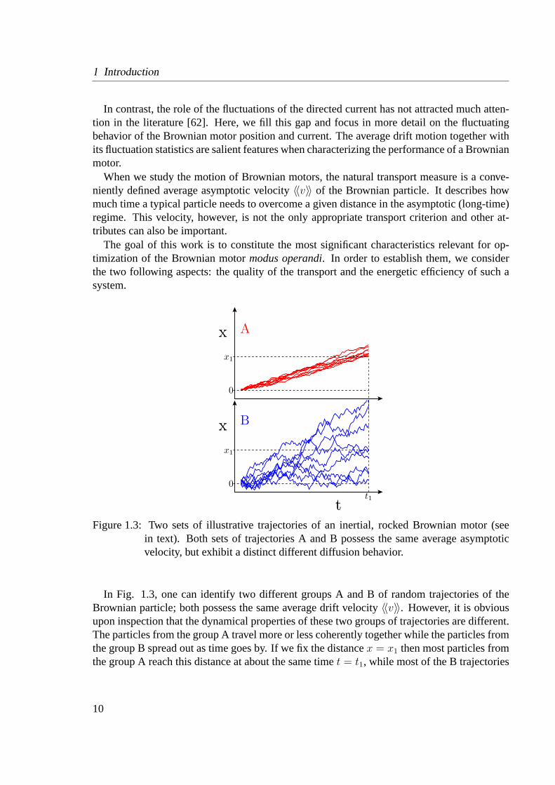
Figure 1.3: Two sets of illustrative trajectories of an inertial, rocked Brownian motor (seein text). Both sets of trajectories A and B possess the same average asymptoticvelocity, but exhibit a distinct different diffusion behavior.

In Fig. 1.3, one can identify two different groups A and B of random trajectories of theBrownian particle; both possess the same average drift velocity〈〈v〉〉. However, it is obviousupon inspection that the dynamical properties of these two groups of trajectories are different.The particles from the group A travel more or less coherently together while the particles fromthe group B spread out as time goes by. If we fix the distancex = x1 then most particles fromthe group A reach this distance at about the same timet = t1, while most of the B trajectories

10

either stay behind or have already proceeded to more distant positions. It is thus evident thatthe noise-assisted, directed transport for the particles in the group A is more organized than inthe group B.

D

Cxx

xx

tt

Figure 1.4: Typical trajectories of an inertial, rocking Brownian motor; both sets assume thesame average velocity but differing velocity fluctuations.

There is still another aspect related to Brownian motor transport. This refers to the externalenergy input into the system which may be essential in practical applications. We would like toknow how much of this input energy is converted into useful work, namely into directed cargotransport, and how much of it gets wasted. Since motors move in a dissipative environment,we need to know how much of the input energy is being spent for moving a certain distanceagainst the acting friction force. If the particle additionally proceeds against a bias force wecan also ask how much energy is exploited for this purpose.

Fig. 1.4 depicts trajectories representing different motor scenarios. The motor C movesforward unidirectionally. The motor D moves in a more complicated manner: its motion alter-nates between small oscillations and fast running episodes mostly in the positivex direction,but sometimes also in the opposite one. Again the mean velocity in both cases is the same,however, the particle C uses energy pumped from the environment to proceed constantly for-ward while the particle D wastes part of its energy to perform oscillations and back-turns. Bysimply inspecting these schematic pictures one can guess immediately when directed transportis more effective.

We note that in Fig. 1.3, the cases A and B can be characterized by the effective diffusioncoefficientDeff , i.e., by the spreading of fluctuations in the position space at a fixed timewhile the cases C and D in Fig. 1.4 can be characterized by the variance of velocityσ2

v =

11

1 Introduction

〈〈v2〉〉−〈〈v〉〉2. The three quantities〈〈v〉〉, Deff andσ2v can be combined to define two important

characteristics of transport, namely the efficiency of noise rectification [78, 79] and the so-called Peclet number [80–83].

OutlineThe thesis is organized as the following: In the next chapter we present the typical model

of titled rocked Brownian particle, its dimensionless form and the potential profiles used inthis work. Next, in the second chapter we discuss the quantifiers of interest. In the chapter 4we present the result of the numerical analysis of the unbiased, noisy inertial dynamics andidentify the optimal driving parameters of the discussed system. In the chapter 5 the inertialbiased rocked dynamics is addressed. In the last chapter we summarize the thesis.

12

2 Stochastic model of a tilted rocked ratchet

The archetype of the inertial Brownian motor is represented by a classical particle of massmmoving in a spatially periodic potentialV (x) = V (x + L) with periodL and barrier height∆V [77,84]. The particle is driven by an external, unbiased, time-periodic force of amplitudeA and angular frequencyΩ (or periodTΩ = 2π/Ω). The system is additionally subjectedto the thermal noiseξ(t) and the constant load forceF . The thermal fluctuations due to the

3 π2 ω

0

π2 ω

πω

.

.

.

.

.V(x,t)V(x,t)

xx

Figure 2.1:Schematic picture of a rocking ratchet with the potentialV (x, t) = V (x) −xa cos(ωt), cf. Eqs (2.3) with zero bias (F = 0) and a ratchet potentialV (x)defined in (2.19).

coupling of the particle with the environment are modeled by a Gaussian white noiseξ(t) of azero mean

〈ξ(t)〉 = 0 (2.1)

and the auto-correlation function satisfying Einstein’s fluctuation-dissipation relation

〈ξ(t)ξ(s)〉 = δ(t− s). (2.2)

We mentioned in the introduction that there are two equivalent descriptions of stochasticdynamics. One is the Langevin equation of motion that describes the time evolution of apositionx(t) and a velocityv(t) of the Brownian particle. The second is the Fokker–Planckequation that describes the time evolution of a probability densityP (x, v, t).

2.1 Langevin equation

The dynamics of the system is modeled by the Langevin equation [85]

mx + γx = −V ′(x) + F + A cos(Ωt) +√

2γkBT ξ(t), (2.3)

13

2 Stochastic model of a tilted rocked ratchet

where a dot denotes differentiation with respect to time and a prime denotes a differentiationwith respect to the Brownian motor coordinatex. The parameterγ denotes the Stokes frictioncoefficient,kB stands for the Boltzmann constant andT is the temperature.

2.2 Scaling

Upon introducing characteristic length- and time-scales, Eq. (2.3) can be rewritten in dimen-sionless form, namely

¨x + γ ˙x = −V ′(x) + F + a cos(ωt) +√

2γD0 ξ(t), (2.4)

with [78]

x =x

L, t =

t

τ0

, τ 20 =

mL2

∆V. (2.5)

The characteristic timeτ0 is the time a particle of massm needs to move the distanceL/2under the influence of the constant force∆V/L when starting with a zero velocity. The re-maining re-scaled parameters are:

• the friction coefficientγ = (γ/m)τ0 = τ0/τL is the ratio of the two characteristic times,τ0 and the relaxation time of the velocity degree of freedom, i.e.,τL = m/γ,

• the potentialV (x) = V (x)/∆V = V (x + 1) has unit period and unit barrier height∆V = 1,

• the load forceF = FL/∆V ,

• the amplitudea = AL/∆V and the frequencyω = Ωτ0 (or the periodT = 2π/ω),

• the zero-mean white noiseξ(t) has auto-correlation function〈ξ(t)ξ(s)〉 = δ(t− s) withre-scaled noise intensityD0 = kBT/∆V .

From now on, for the sake of simplicity, we will use only the dimensionless variables and shallomit the “hat” for all quantities in Eq. (2.4).

2.3 Fokker-Planck Equation

The statistically equivalent Fokker-Planck equation corresponding to eq. (2.4) describing thetime evolution of the probability densityP (x, v, t) is given by the formula

∂

∂tP (x, v, t) = LFP (t) P (x, v, t), (2.6)

14

2.3 Fokker-Planck Equation

with the time periodic Fokker-Planck operator

LFP (t) = − ∂

∂xv − ∂

∂v

[F − γv − V ′(x) + a cos(ωt)

]+ γD0

∂2

∂v2, (2.7)

LFP (t + T ) = LFP (t). (2.8)

Using the Fokker-Planck equation (2.6) with the given initial conditions we get the probabilitydensityP (x, v, t) and define the averages

〈g(x(t), v(t))〉 =

∫dx

∫dv g(x, v) P (x, v, t), (2.9)

e.g. the n-th moment of the positionx(t)

〈xn(t)〉 =

∫dx

∫dv xn P (x, v, t). (2.10)

The integration ofP (x, v, t) over the positionx of the particle defines the time dependentvelocity distribution

P (v, t) =

∫dx P (x, v, t), (2.11)

and as a consequence the mean velocity

〈v(t)〉 =

∫dv v P (v, t). (2.12)

For large times the periodically driven stochastic process approaches an asymptotic periodicvelocity probability distributionPas(v, t) (the positive and periodic function of time),

Pas(v, t + T ) = Pas(v, t), (2.13)

with normalization ∫dv Pas(v, t) = 1. (2.14)

The asymptotic averages can be then defined as

〈g(v(t))〉as =

∫dv g(v) Pas(v, t), (2.15)

so the asymptotic average velocity is given by

〈v(t)〉as =

∫dv v Pas(v, t). (2.16)

For later use we introduce the time averaged asymptotic velocity distribution

Pas(v) =1

T

∫ T

0

dt Pas(v, t), (2.17)

and the time averaged mean velocity

〈〈v〉〉 =1

T

∫ T

0

dt 〈v(t)〉as = limt→∞

1

t

∫ t

0

ds 〈v(s)〉. (2.18)

15

2 Stochastic model of a tilted rocked ratchet

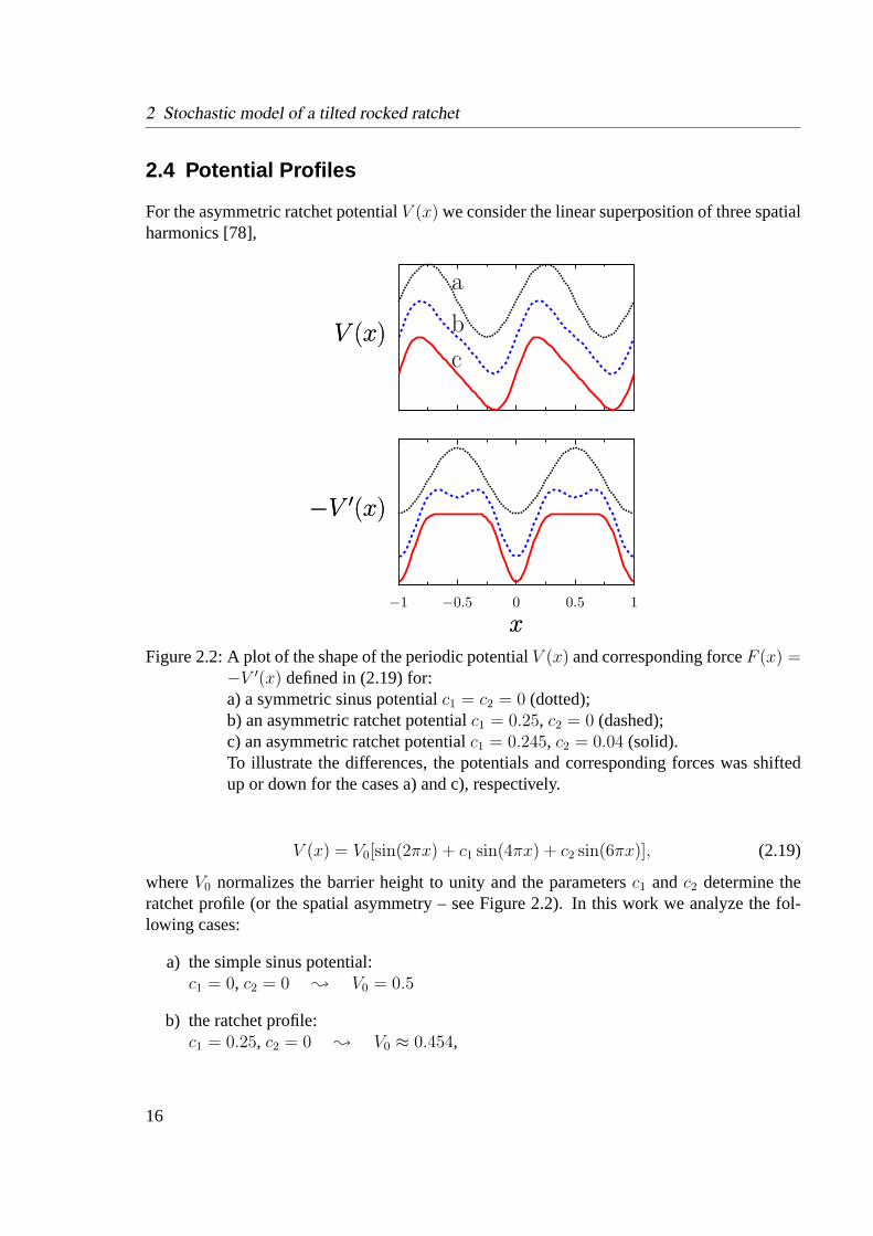
2.4 Potential Profiles

For the asymmetric ratchet potentialV (x) we consider the linear superposition of three spatialharmonics [78],

−V ′(x)−V ′(x)

−1 −0.5 0 0.5 1

xx

V (x)V (x)

a

b

c

Figure 2.2:A plot of the shape of the periodic potentialV (x) and corresponding forceF (x) =−V ′(x) defined in (2.19) for:a) a symmetric sinus potentialc1 = c2 = 0 (dotted);b) an asymmetric ratchet potentialc1 = 0.25, c2 = 0 (dashed);c) an asymmetric ratchet potentialc1 = 0.245, c2 = 0.04 (solid).To illustrate the differences, the potentials and corresponding forces was shiftedup or down for the cases a) and c), respectively.

V (x) = V0[sin(2πx) + c1 sin(4πx) + c2 sin(6πx)], (2.19)

whereV0 normalizes the barrier height to unity and the parametersc1 andc2 determine theratchet profile (or the spatial asymmetry – see Figure 2.2). In this work we analyze the fol-lowing cases:

a) the simple sinus potential:c1 = 0, c2 = 0 ; V0 = 0.5

b) the ratchet profile:c1 = 0.25, c2 = 0 ; V0 ≈ 0.454,

16

2.5 Numerical method

c) the ratchet profile:c1 = 0.245, c2 = 0.04 ; V0 ≈ 0.461.

There is also a possibility to extract the effective force acting on the molecular motor andtherefore reproduce the corresponding effective ratchet potential. One can perform this cal-culation by means of the analysis of the time series [86] using the recorded single-moleculeexperimental data [40, 56]. In this thesis, however, we will deal with the three hypotheticpotential profiles given above.

2.5 Numerical method

The noiseless, deterministic inertial rocked ratchet shows rather complex behavior and, indistinct contrast to overdamped rocked Brownian motors, often exhibits a chaotic dynamics.By adding noise, one typically obtains a diffusive dynamics, thus allowing stochastic escapeevents among possibly coexisting attractors.

As analytical methods to handle these situations effectively do not exist, we carried outextensive numerical simulations. We have numerically integrated Eq. (2.4) by the Stochas-tic Runge Kutta (SRK) method of the second order [87] with time steph = 10−3–10−4 T .The initial conditions for the coordinatex(t) were chosen according to a uniform distribu-tion within one cell of the ratchet potential. The starting velocities of the particles were alsodistributed uniformly in the interval[−0.2, 0.2].

The first103 periodsT of the external force were skipped in order to eliminate transienteffects. For the estimation of the quantities of interest the usual averages over the time (106 T )and333 different realizations were taken.

When simulating the deterministic equation (4.3) one has to choose among the several pos-sibilities of initiations of runs. By doing this one has to be sure, that computed averages arerelevant and do not differ much for another set of initial conditions. If there is only one at-tractor present (like e.g.. the case shown on the Fig. 5.3) for given driving parameters weneed only one runde facto. If there are more attractors the calculated quantities can vary forthe different sets of initial conditions due to an often fractal structure of the basins of attrac-tion. However, one can enlarge the number of runs and compare the calculated quantifiers forthis different sets. We did this for five different forms of uniform distributions of the initialconditions:

• x = x0 andv ∈ [−0.2, 0.2], wherex0 is a position of the local minimum of the spatialperiodic potential,

• x ∈ [0, L] andv = 0,

• x ∈ [0, L] andv ∈ [−0.2, 0.2],

• x ∈ [0, L] andv ∈ [−2, 2],

• a circle in the phase space with the origin at (x,v)=(x0,0) and radiusr = 0.2.

17

2 Stochastic model of a tilted rocked ratchet

We have increased the number of runs up to the point where we have obtained the satisfactoryagreement of maximal 1% difference between the calculated averages of the specific quantity(e.g. velocity〈〈v〉〉) for the above given sets of initial conditions.

18

3 Quantifiers characterizing the optimal transport ofBrownian motors

As already elucidated in the introduction , there are several quantities that characterize theeffectiveness of directed transport [88]. A global transport measure is an asymptotic meanvelocity 〈〈v〉〉 of the Brownian motor averaged over one cycle of the external, time periodicdrive and over all noise realizations, see eq. (2.18).

3.1 Effective Diffusion and P eclet number

The effective diffusion coefficient, describing the fluctuations around the average position ofthe particles, is defined as

Deff = limt→∞

〈x2(t)〉 − 〈x(t)〉2

2t, (3.1)

The coefficientDeff can also be introduced via a generalized Green-Kubo relation, which wedetail in Appendix A. Intuitively, if the stationary velocity is large and the spread of trajectoriesis small, the diffusion coefficient is small and the transport is more effective. To quantify this,we can introduce the dimensionless ratio – the Peclet number Pe [80, 81, 89] by use of adouble-averaging procedure, i.e.,

Pe=l〈〈v〉〉Deff

, (3.2)

Originally, the Peclet number Pe has arisen in problems of heat transfer in fluids and standsfor the ratio of heat advection to diffusion [89]. When the Peclet number is small, the randommotion dominates; when it is large, the ordered and regular motion prevails. The value of thePeclet number depends on a characteristic length scalel of the system. Dealing with ratchetsthe most adequate choice for such length scale is the period of the periodic potential, which inre-scaled units (see section 2.2) is equal tol = 1.

3.2 Rectification Efficiency

The second aspect of the motor trajectories we want to control is related to the fluctuations ofthe velocityv(t). In the long-time regime, it is characterized by the varianceσ2

v = 〈〈v2〉〉 −〈〈v〉〉2. The Brownian motor moves with an actual velocityv(t), which is typically containedwithin the interval

v(t) ∈ (〈〈v〉〉 − σv, 〈〈v〉〉+ σv) . (3.3)

19

3 Quantifiers characterizing the optimal transport

Now, if σv > 〈〈v〉〉, the Brownian motor may possibly move for some time in the directionopposite to its average velocity〈〈v〉〉 and the directed transport becomes less efficient.

If we want to optimize the effectiveness of the motor motion we must introduce a measurefor the efficiencyη that accounts for the velocity fluctuations. Assume, that the motor worksagainst the given forceF (not yet define). The efficiency of a machine is defined as the ratioof the powerP = F〈〈v〉〉 done on the surroundings and the input powerPin, η = P/Pin. Ifthe motor is working against the constant external load forceF , one can define theefficiencyof energy conversion[18,75,76,86,90,91]; reading,

ηE =|F 〈〈v〉〉|

Pin

. (3.4)

A grave disadvantage of such a characterization is that it yields a vanishing measure (i.e.ηE = 0) in the absence of a load forceF . In many cases, however, like e.g. for proteintransport within a cell, the Brownian motor operates at a zero bias regime (F = 0) and itsobjective is to carry a cargo across a viscous media. Clearly, the energy input required tomove a particle with the friction coefficientγ by a given distance depends on the velocity,tending to zero at slow motion. Since we are interested in delivering the cargo in a finite timeone should require that the transport is accomplished at an average motor velocity〈〈v〉〉. In thiscase, the necessary energy input is finite. Thus, we put forF the average viscous forceγ〈〈v〉〉to obtain the so-calledStokes efficiency[86,92]; i.e.,

ηS =γ〈〈v〉〉2

Pin

. (3.5)

There is no overall consensus on the numerator in (3.5) [79,90–100]. If we put in the numer-ator the rate of work done on the fluid by the Brownian motor motion, then the correspondingefficiencyηS is not an appropriate measure because numerator is' 〈v2〉. This quantity canbe relatively large even if there occurs no transport of the motor, i.e. even if〈v〉 = 0 ! Moresuitable information on the efficiency of the transport is gained when [92, 96] the numerator' 〈v〉, as proposed here. Upon combining the two above given notions we recover therec-tification efficiencyoriginally proposed by Suzuki and Munakata [79, 101] or its equivalentversion presented by Derenyiet al. [96]

ηR =γ〈〈v〉〉2 + |F 〈〈v〉〉|

Pin

. (3.6)

It is made up of the sum of the efficienciesηS andηE. Therefore, it accounts for both, thework that the Brownian motor performs against the external biasF as well as the work that isnecessary to move the object a given distance in a viscous environment at the average velocity〈〈v〉〉.

The average input power for a tilted rocking ratchet is given by [78,82]:

Pin = γ|〈〈v2〉〉 −D0|. (3.7)

20

3.2 Rectification Efficiency

This expression follows from an energy balance of the underlying equation of motion (2.4).The derivation of the above formula can be found in Appendix B. If the second moment ofvelocity 〈〈v2〉〉 is reduced, i.e. the varianceσv diminishes, the rectification efficiency (3.6)increases and the transport of the Brownian motor becomes more efficient.

To experimentally determine either of the above given efficiencies of any molecular motor(like kinesin) it is sufficient to determine the average velocity of the motor with its varianceand the temperature of the thermal bath [102].

21

3 Quantifiers characterizing the optimal transport

22

4 Performance with zero bias force

In this chapter we put the constant bias force of the driven system (2.4) equal to zero (F = 0).It means that there is no apparent preferred direction of the Brownian particle to travel. Thedynamics is now governed by the following equation of motion:

x + γx = −V ′(x) + a cos(ωt) +√

2γD0 ξ(t). (4.1)

We would like to identify conditions for the optimal performance of the above defined rock-ing ratchet. We follow the arguments given in the introduction and search for the operationregimes where the whole set of particles would advance in a coherent manner, utilizing asmuch of the input energy as possible for a directed motion, without back turns or intrawelloscillations.

For the overdamped dynamics given by

γx = −V ′(x) + a cos(ωt) +√

2γD0 ξ(t). (4.2)

we can identify two thresholds of the external force strengths: the lower thresholdac1 and theupper thresholdac2. The first corresponds to the force that is needed to overcome the barrierof the potential from the side with the smaller slope. The second threshold corresponds thento the force that the particle needs to overcome the barrier of the potential from side with thesteeper slope. Note that for the inertial dynamics these two strengths are not that relevant,since the particle can accumulate kinetic energy and therefore is able to make a transition overone of the barriers of the ratchet potential for weaker driving strengths thanac1 or ac2.

4.1 Generic Ratchet

The roots of the noisy ratchet effect lie in the evolution of the Newton equation (eq. (4.1) withD0 = 0). First of all we recall the analysis of the deterministic dynamics of a particle movingin a typical ratchet profile, widely investigated in the literature [77,103–115].

4.1.1 Deterministic dynamics

As the generic ratchet potential we take the one that consist of two spatial harmonics (i.e.c2 = 0, see Fig. 2.2 (b)). The corresponding Newton equation reads

x + γx = −2π(cos(2πx) +1

2cos(4πx)) + a cos(ωt). (4.3)

23

4 Zero bias force

Since we have an explicit time dependence, the phase space is three dimensional. The nonlin-earity of the noiseless equation (4.3) then allows chaotic attractors to appear. For the attractorthat takes a particle alongn spatial periodsL of potential ink time periodsT

v(t + kT ) = v(t),

x(t + kT ) = x(t) + nL, (4.4)

we can define the winding numberW as a ratio

W =n

k. (4.5)

For locked orbits the particle stays in one well of potential forever and thereforen = 0 andcorresponding winding number is alsoW = 0. For running solutions the winding number canassume any number, depending on the dynamics. This measure corresponds to the character-istic average velocity of a particle beeing translocating by a given attractor

v =nL

kT= W

L

T. (4.6)

If we reduce the system to an overdamped one (cf. eq. (4.2) withD0 = 0), the dimension-ality of the state space become two and it prevents the particle to act in a chaotic manner.

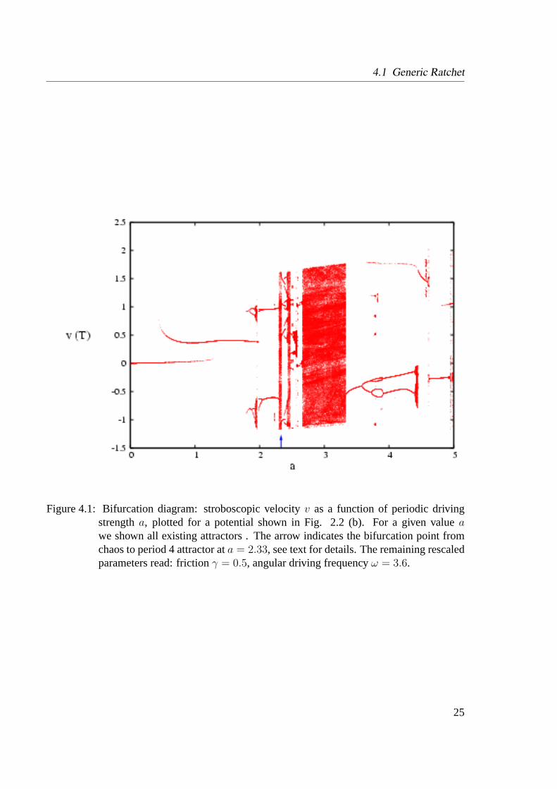
In the Fig. 4.1 we show stroboscopically the instantaneous velocities of the deterministicparticles with different starting conditions (for details see section 2.5) and therefore we plottedall attractors existing at a given value of a control parametera. As a stroboscopic time intervalwe took the period of the driving forceT . We plot this so-called bifurcation diagram as afunction of the driving strengtha. To eliminate transient effects106 periodsT of the externaldriving were disregarded. Other parameters of the system (4.3) are fixed to the values:γ = 0.5andω = 3.6.

For small driving strengthsa the massive particle possesses not enough kinetic energy tomake a transition over any barrier of the ratchet potential. As we increasea the particlecan eventually accumulate enough kinetic energy to go over one of the barriers and runningsolutions emerge. Therefore, for small values ofa the transport is regular. If we increasethe control parameter for values larger thana = 1.8 we can notice several transitions from aregular periodic motion to chaos and back from chaos to a periodic motion. At the bifurcationpointab ' 2.33 the transition from chaotic to regular, periodic attractor of period four occurs(this point is indicated by an arrow in Fig. 4.1). Note that for the noisy dynamics (cf. Fig. 4.3),we reveal the first current reversal at this very pointa ' 2.33. Very close to this bifurcationpoint the deterministic system exhibits intermittent dynamics of type I (cf. the second columnin Fig. 4.2) [116, 117] reflecting the reciprocation of one chaotic and one periodic attractors[103]. For smaller values thanab, say fora = 2.25 there exists one periodic orbit of periodone, that transports the particles in the negativex direction, cf. the first column in Fig. 4.2. Fora = 2.25 the particle crossn = 1 spatial period ink = 1 time period so the winding numberW = 1 and characteristic velocityv = 3.6/2π. For a stronger thanab, say fora = 2.35,

24

4.1 Generic Ratchet

Figure 4.1: Bifurcation diagram: stroboscopic velocityv as a function of periodic drivingstrengtha, plotted for a potential shown in Fig. 2.2 (b). For a given valueawe shown all existing attractors . The arrow indicates the bifurcation point fromchaos to period 4 attractor ata = 2.33, see text for details. The remaining rescaledparameters read: frictionγ = 0.5, angular driving frequencyω = 3.6.

25

4 Zero bias force

−57.5

−55

−52.5

−50

x(t)x(t)

6 · T6 · T

−15

−12.5

−10

−7.5

6 · T6 · T

34

36

38

40

6 · T6 · T

−2

0

2

v(t)v(t)

0 1

x(t)x(t)

a = 2.25

−2

0

2

0 1

x(t)x(t)

a = 2.33

−2

0

2

0 1

x(t)x(t)

a = 2.35

Figure 4.2:Deterministic motion shown for the same set of parameters as in the Fig. 4.1 andthe three driving strengthsa = 2.25, 2.33, 2.35.Upper row: The phase space (instantaneous velocity versus position). Fora =2.25 one can note the negative periodic attractor of period oneT ; for a = 2.33 theintermittent chaotic attractor emerge; fora = 4.6 the positive, period two regularattractor is shown.Lower row: Trajectories of the particles shown as an illustration of the attractorsplotted in the upper row for a time interval6T .

26

4.1 Generic Ratchet

after the bifurcation point, we find one regular attractor (see the third column in Fig. 4.2)that transports the particle in the positivex direction overn = 1 period of potential ink = 2time periods and therefore the winding numberW = 1/2 andv = 3.6/4π. In general: If thecorresponding pre- and post-bifurcation attractors can transport the particles in the oppositedirections then it is likely that after the bifurcation point the current reversal appears.

Due to very complicated structure of the basins of attraction it is however not clear how tocompute averages in the deterministic case and e.g. the mean velocity would strongly dependon the chosen set of initial conditions. For some sets of control parameters and dependingon the initial conditions, we can reveal multiple attractors in the phase space. Again, if theycan transport the particle in the opposite direction, we would gain the possibility of separateparticles, by choosing the appropriate attractor via its basin of attraction i.e. by choosing theappropriate starting conditions [112].

Plugging the noise into the system, one get rid of this problem, allowing the Brownianparticle to visit all existing attractors, depending on the noise intensity but independent of theinitial conditions. In the following we deal with a relatively low temperature of the heat bathso the deterministic architecture of attraction still affects the noisy driven dynamics (4.1).

4.1.2 Noisy dynamics: Fluctuations versus driving strength

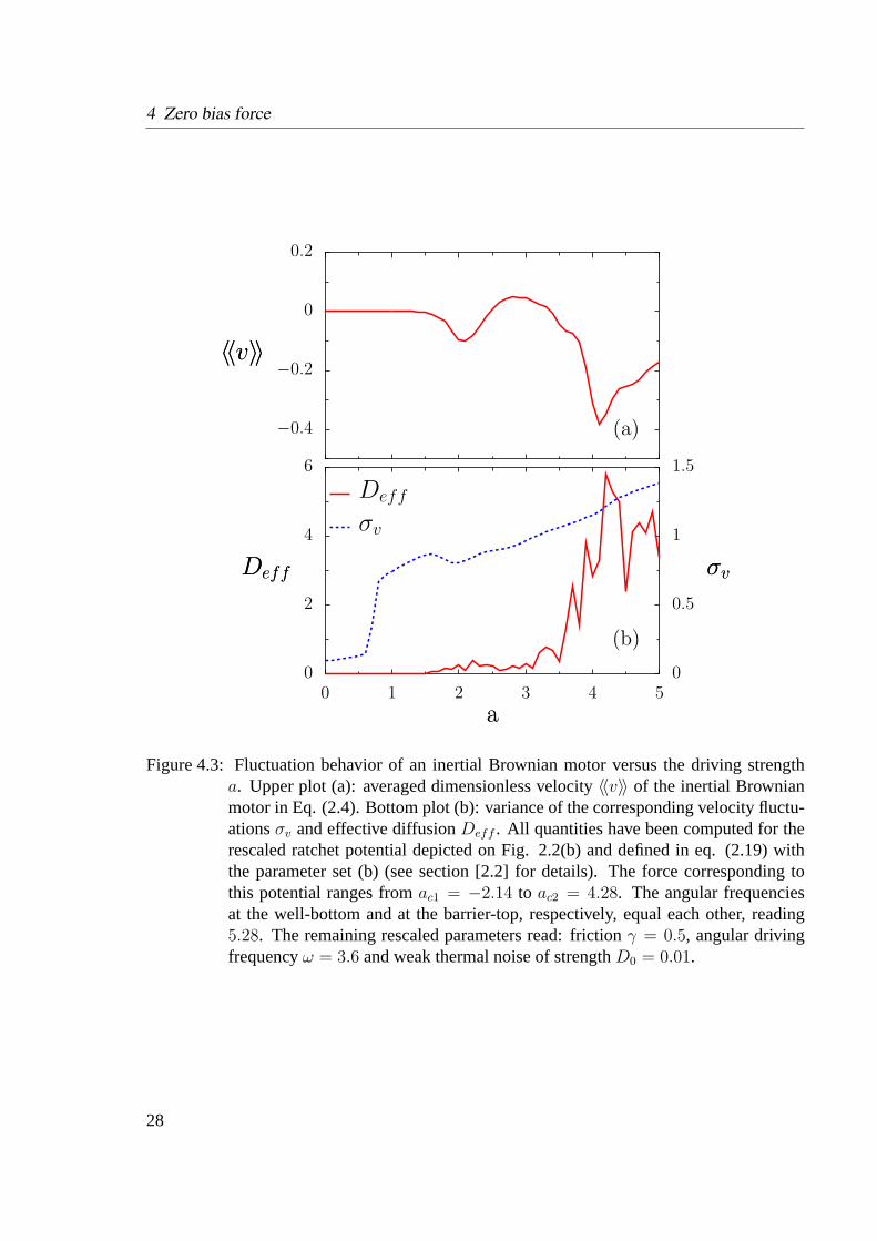
We start out to study the role of fluctuations in both position and velocity space, by varyingthe amplitudea of the sinusoidal driving force. In doing so, we assume a relatively smalltemperature, so that the Brownian motor dynamics is not far from a deterministic behavioras described in prior works. To put it all into numbers, we choose the following set of theparameters: frictionγ = 0.5, angular driving frequencyω = 3.6 and weak thermal noise ofstrengthD0 = 0.01. The average asymptotic long-time velocity is shown in Fig. 4.3 (a). Itreveals that for an amplitudea ' 1.5 the directed,inertial transport sets in before the lowerthreshold of the ratchet forceac1 ' 2.14 is reached. The mean velocity assumes a first localextremum near the lower threshold of the potential forcea ' ac1. Note that in the presence ofsmall noise, the current is strictly speaking never zero. However, the noise induced transitionsover the potential barriers for a weak driving strength are extremely rare and the system mainlydwells in the locked state, so we can characterize the outcome of our Langevin simulation asa deterministic, zero-current result. Upon closer inspection, we notice that in the vicinity ofa ' 0.6, the velocity fluctuationsσv shown in Fig. 4.3(b) undergo a rapid increase. We willdiscuss this feature afterwards.

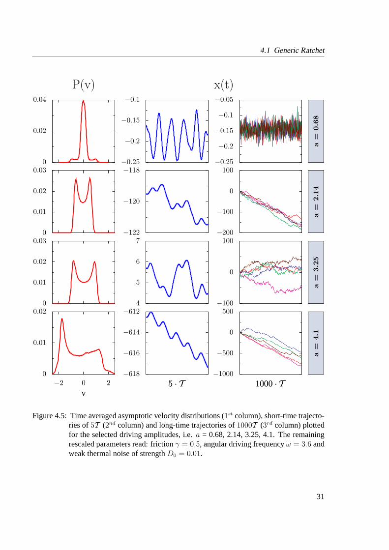
Upon further increasing the amplitude of driving,a > 1.5, the Brownian motor generatesa directed transport behavior. We also observe that the corresponding width of the weaklyasymmetric, time averaged asymptotic velocity distributionPas(v) slightly decreases (see thefirst column on Fig. 4.5), meaning that the velocity fluctuations become smaller. The follow-ing explanation thus applies: Because ata < 1.5 escape jumps between the neighboring wellsare rare, i.e., the average directed current is very small (note also the accompanying, veryweak asymmetry in the distributionPas(v) shown in the first row in the Fig 4.5 fora = 0.68).The input energy is pumped primarily into the kinetic energy of the intra-well motion and

27

4 Zero bias force

0

2

4

6

DeffDeff

0 1 2 3 4 5

aa

0

0.5

1

1.5

σvσv

Deff

σv

(b)

−0.4

−0.2

0

0.2

〈〈v〉〉〈〈v〉〉

(a)

Figure 4.3: Fluctuation behavior of an inertial Brownian motor versus the driving strengtha. Upper plot (a): averaged dimensionless velocity〈〈v〉〉 of the inertial Brownianmotor in Eq. (2.4). Bottom plot (b): variance of the corresponding velocity fluctu-ationsσv and effective diffusionDeff . All quantities have been computed for therescaled ratchet potential depicted on Fig. 2.2(b) and defined in eq. (2.19) withthe parameter set (b) (see section [2.2] for details). The force corresponding tothis potential ranges fromac1 = −2.14 to ac2 = 4.28. The angular frequenciesat the well-bottom and at the barrier-top, respectively, equal each other, reading5.28. The remaining rescaled parameters read: frictionγ = 0.5, angular drivingfrequencyω = 3.6 and weak thermal noise of strengthD0 = 0.01.

28

4.1 Generic Ratchet

0

0.25

0.5

0.75

1

PePe

0 1 2 3 4 5

aa

(b)

0

0.025

0.05

0.075

0.1

ηη

(a)

Figure 4.4:Dimensionless factors describing the performance of the Brownian motor depictedversus the driving strengtha. Upper plot (a): rectification efficiency (or Stokesefficiency) defined in Eq. (3.6). Bottom plot (b): the Peclet number defined in(3.2). Rescaled parameters and the ratchet profile are the same as in the Fig. 4.3.

29

4 Zero bias force

eventually is dissipated. Asa is increased further, the Brownian motor mechanism starts towork, and some part of energy contributes to the net motion of the particle. Therefore, less en-ergy remains available to drive intra-well oscillations and consequently the distributionPas(v)shrinks and the motor optimizes its performance. Above the upper threshold value of the po-tential forceac2 ' 4.28 the current starts to decrease because of the weakened influence of theratchet potential at large rocking amplitudes.

The occurrence of multiple reversals of the directed current, as it is depicted in Fig. 4.3 (a),is a known, interesting feature of inertial Brownian motors. Several prior studies did elucidatein greater detail the corresponding mechanism [77,103,104,107–113]. Here, we take insteada closer look at the current fluctuations and the effective diffusion. We observe that for thechosen set of parameters the maximal absolute stationary velocity on the Fig. 4.3 (a) does notexceed the value 0.4. In contrast, its fluctuations keep growing as the driving amplitude risesmostly due to the complicated way of motion – see the2nd column on the Fig 4.5. Generallybeside the usual transitions consistent with the mean velocity the particle sometimes goesin the opposite direction and performs intra-well oscillations. At large driving, the particlehardly feels the potential and undergoes a rocked, almost free Brownian motion with velocityfluctuations growing proportional toa, cf. the dashed line in the Fig. 4.3 (b). Within thisdirected transport regime, the rectification efficiency (3.6) and the equivalent Stokes efficiency(3.5) remain rather small, cf. the Fig. 4.4 (a). Such small rectification efficiency is the rule forthis driven inertial Brownian motor.

For the small driving, with almost no transitions present, it is clear that the effective dif-fusion almost vanishes. When the motor starts to transport (a ' 1.5) the Brownian particlesgain enough energy to cross the potential barrier, but due to the undirected thermal forces, theyspread out as time goes by. The effective diffusion starts to grow as we increase the drivingstrength. For the highest〈〈v〉〉 we notice that the diffusion gets suppressed reflecting the moreregular motion of the particles, which now proceed in a more coherent manner, cf. the thirdcolumn on the Fig 4.5 fora = 4.1.

Moreover, one can observe two current reversals on the Fig. 4.3 (a), so there are two addi-tional points where average velocity equals zero, but we perceive no corresponding vanishingof the effective diffusion. It means that there are still transitions present in the system forthis driving strengths. The mean velocity equals zero according to the fact that the number ofjumps to the right and to the left are equal.

The above described behavior has its reflection in a Peclet number cf. the Fig. 4.4 (b).Its maximal value for the generic driving parameters is found of about Pe' 1. It indicatesthe typical high relative randomness of the transport, i.e. the highly diffusive motion of theparticles. The best performance is not surprisingly found for the largest value of the velocityand corresponding largest values of Pe andηR.

Let us next inspect the distributionPas(v) shown on the first column of the Fig. 4.5. Theseprobabilities look rather symmetric; however, a finite ratchet velocity requires a certain amountof asymmetry either in the location or the width of the velocity peaks. Here, the current resultsmainly due to a slight shift of the maxima location.

The most peculiar feature of the current distributions shown in the first column of Fig. 4.5

30

4.1 Generic Ratchet

0

0.01

0.02

−2 0 2

vv

−618

−616

−614

−612

5 · T5 · T

−1000

−500

0

500

1000 · T1000 · T

a=

4.1

0

0.01

0.02

0.03

4

5

6

7

−100

0

100

a=

3.2

5

0

0.01

0.02

0.03

−122

−120

−118

−200

−100

0

100

a=

2.1

4

0

0.02

0.04

−0.25

−0.2

−0.15

−0.1

−0.25

−0.2

−0.15

−0.1

−0.05

P(v) x(t)

a=

0.6

8

Figure 4.5:Time averaged asymptotic velocity distributions (1st column), short-time trajecto-ries of5T (2nd column) and long-time trajectories of1000T (3rd column) plottedfor the selected driving amplitudes, i.e.a = 0.68, 2.14, 3.25, 4.1. The remainingrescaled parameters read: frictionγ = 0.5, angular driving frequencyω = 3.6 andweak thermal noise of strengthD0 = 0.01.

31

4 Zero bias force

is the emergence of two additional side-peaks fora & 0.6 centered nearv = ±1, whicheventually dominatePas(v) at larger driving amplitudes. Of course, for zero drive we recoverthe strictly symmetric single-peaked Maxwell distribution, with the maximum atv = 0.

What is the origin of those three peaks in the distributionPas(v)? Our first conjecture toconnect it with the ’running’ solutions turned out to be incorrect. This is so, because fora . 1the particle rarely leaves the confining potential well and thus cannot significantly contributeto the side peaks of the distribution function. Further, we checked the outcome for the distri-butionPas(v) when reflecting barriers were placed at the maxima of the potential. Under suchconstraints, the three-peak-structure is recovered as well. Moreover, the sinusoidally drivendamped particle in a harmonic potential can exhibit both, a singly-peaked as well a double-peaked averaged velocity distribution [118]. However, for the parabolic potential that fits bestthe wells of our ratchet potential around its minima, we found a single peakedPas(v).

We therefore do conclude that the characteristic behavior for the additional side-peaks isrooted in the nonlinear, anharmonic character of the corresponding well of the periodic asym-metric ratchet profile.

4.1.3 Noisy dynamics: Fluctuations versus noise strength

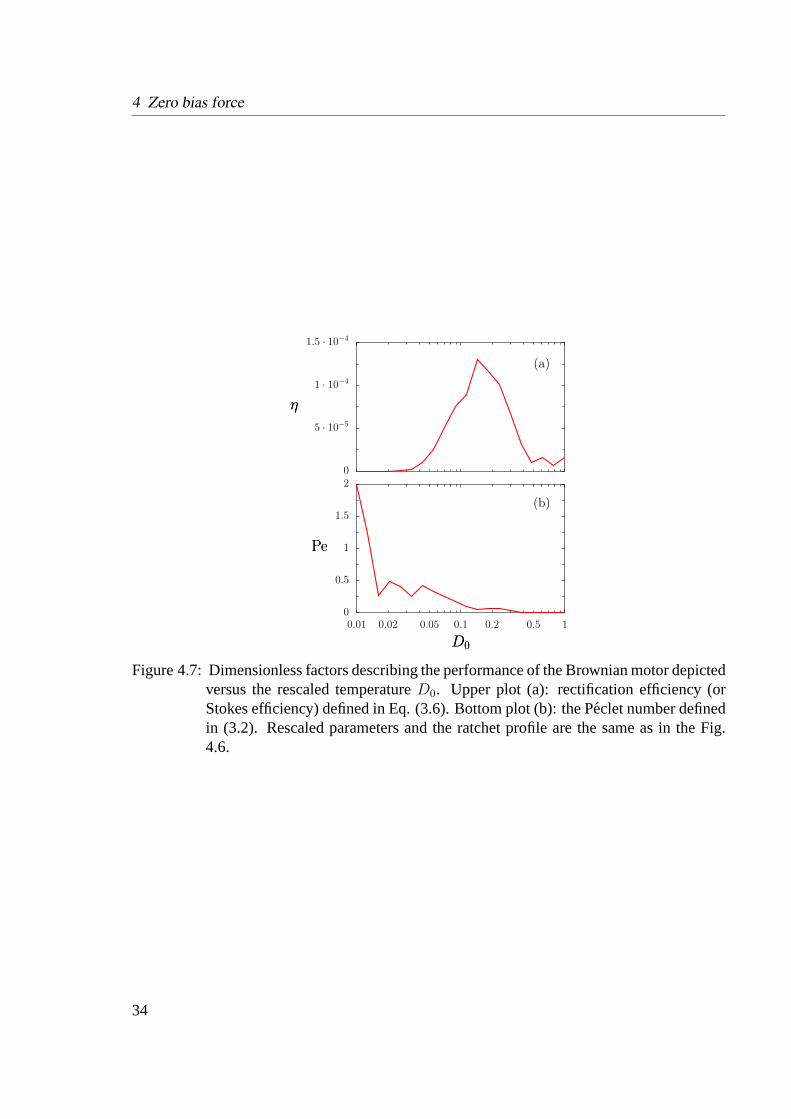
In the Fig. 4.6, we present the results of the numerical analysis of the directed transport versusthe rescaled temperatureD0. We chose a sub-threshold driving strength for which the thermalnoise plays a constructive role by inducing noise activated jumps across the potential barriers.We seta = 0.8 and the other parameters remain the same as in the previous section. Inthe Figures 4.6 and 4.7 we have plotted the calculated quantifiers as a function of rescaledtemperatureD0 in the range from small rescaled temperatureD0 = 0.01 up to the thermalenergy comparable with the barrier height∆V of the ratchet potential (i.e.D0 = ∆V = 1). Afurther increase of temperature suppress the influence of the asymmetric ratchet potential and,consequently, the directed transport degrades.

Moreover, the time-averaged velocity distribution depicted in the first column of the Fig.4.8 approaches the equilibrium velocity distribution as we increase temperature. For smallD0

the movement is typically bounded to oscillations inside the well of the ratchet potential withaccompanying very rare transitions. For the high temperatures all the characteristics reflectsthe highly random motion, see also the third column of Fig. 4.8. A shallow, local minimumoccurs for the velocity fluctuations, cf. dashed line in Fig. 4.6 (b) where the average currentitself is maximal. These fluctuations are, however, notably three orders of magnitudelargerthan the directed current. Accordingly the rectification efficiency shown in Fig. 4.7 (a) is quitesmall.

The effective diffusion (solid line on the Fig. 4.6 (b)) exhibits rather large values and thecorresponding Peclet number (see Fig. 4.7 (b)) has therefore small values. At any temperature,for a small driving amplitudea, the particle possesses very small efficiency and act in a ratherrandom manner performing rare transitions. The spatial spreading over the wells of the ratchetpotential is therefore large. Again, the Brownian motor is not operating efficiently.

32

4.1 Generic Ratchet

0

0.25

0.5

0.75

1

1.25

DeffDeff

0.01 0.02 0.05 0.1 0.2 0.5 1

D0D0

0.6

0.7

0.8

0.9

1

1.1

σvσv

Deff

σv

(b)

−0.006

−0.004

−0.002

0

〈〈v〉〉〈〈v〉〉

(a)

Figure 4.6: Fluctuation behavior of an inertial Brownian motor versus the noise strengthD0.Upper plot (a): averaged dimensionless velocity〈〈v〉〉 of the inertial Brownian mo-tor in Eq. (2.4). Bottom plot (b): variance of the corresponding velocity fluc-tuationsσv and effective diffusionDeff . All quantities have been computed forthe rescaled ratchet potential depicted on Fig. 2.2(b) and defined in eq. (2.19)with the parameter set (b) (see section [2.2] for details). The angular frequenciesat the well-bottom and at the barrier-top, respectively, equal each other, reading5.28. The remaining rescaled parameters read: frictionγ = 0.5, angular drivingfrequencyω = 3.6 and weak driving strengtha = 0.8.

33

4 Zero bias force

0

0.5

1

1.5

2

PePe

0.01 0.02 0.05 0.1 0.2 0.5 1

D0D0

(b)

0

5 · 10−5

1 · 10−4

1.5 · 10−4

ηη

(a)

Figure 4.7:Dimensionless factors describing the performance of the Brownian motor depictedversus the rescaled temperatureD0. Upper plot (a): rectification efficiency (orStokes efficiency) defined in Eq. (3.6). Bottom plot (b): the Peclet number definedin (3.2). Rescaled parameters and the ratchet profile are the same as in the Fig.4.6.

34

4.1 Generic Ratchet

0

0.001

0.002

0.003

−2 0 2

vv

420

422.5

425

427.5

5 · T5 · T

−250

0

250

500

750

1000 · T1000 · T

kT

=10

0

0.02

0.04

48

49

50

51

−250

0

250

kT

=2

0

0.005

0.01

0.015

−2.75

−2.5

−2.25

−2

−1.75

−20

0

20

kT

=0.1

0

0.0025

0.005

0.0075

−0.6

−0.4

−0.2

0

0.2

−1

0

1

P(v) x(t)

kT

=0.0

1

Figure 4.8:Time averaged asymptotic velocity distributions (1st column), short-time trajecto-ries of5T (2nd column) and long-time trajectories of1000T (3rd column) plottedfor the for selected noise strengths, i.e.D0 = 0.01, 0.1, 2, 10. The remainingrescaled parameters are the same as on Fig 4.6.

35

4 Zero bias force

4.2 Optimization of the performance

Thus far, changing the temperature of the ratchet environment or the driving strength did notlead to a large enhancement of the rectification efficiency. What is needed in achieving a largerectification efficiency is a sizable Brownian motor current which is accompanied by smallcurrent fluctuations, see Eq. (3.6). It is also highly desirable to have a small spatial spreadingof the realizations of the process described by the Langevin equation (2.4). This scenarioseemingly implies that the Brownian particles should proceed in a persistent manner withvery few, occasional back-turns only. This in turn causes small fluctuations in the velocityand, additionally, provides a dominating asymmetry of the time averaged asymptotic velocitydistribution.

Such a behavior can be realized by a combined tailoring of the asymmetry of the ratchetpotential together with the use of appropriate driving conditions. In the quest for achievingsuch a favorable situation we use the three-harmonics ratchet potential plotted in the Fig. 2.2for the set (c). Our hope is that upon minimizing the noise further we can achieve a substantialimprovement of the efficiency.

At very weak noiseand large, nonadiabatic rocking frequencies, this inertial Brownian mo-tor starts moving efficiently for the values of the driving strenght of abouta = 3.7, see Fig.4.9 (a). Because the directed velocity becomes maximal and simultaneously the fluctuationsin both position and velocity space are locally minimal, see in Fig. 4.9 (b), we indeed find thedesired enhancement of the rectification efficiency, see Fig. 4.10 (a).

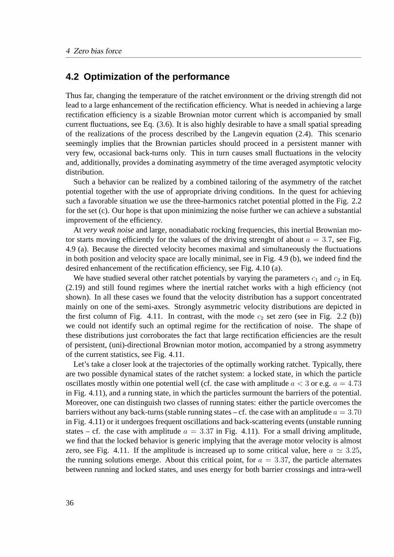
We have studied several other ratchet potentials by varying the parametersc1 andc2 in Eq.(2.19) and still found regimes where the inertial ratchet works with a high efficiency (notshown). In all these cases we found that the velocity distribution has a support concentratedmainly on one of the semi-axes. Strongly asymmetric velocity distributions are depicted inthe first column of Fig. 4.11. In contrast, with the modec2 set zero (see in Fig. 2.2 (b))we could not identify such an optimal regime for the rectification of noise. The shape ofthese distributions just corroborates the fact that large rectification efficiencies are the resultof persistent, (uni)-directional Brownian motor motion, accompanied by a strong asymmetryof the current statistics, see Fig. 4.11.

Let’s take a closer look at the trajectories of the optimally working ratchet. Typically, thereare two possible dynamical states of the ratchet system: a locked state, in which the particleoscillates mostly within one potential well (cf. the case with amplitudea < 3 or e.g.a = 4.73in Fig. 4.11), and a running state, in which the particles surmount the barriers of the potential.Moreover, one can distinguish two classes of running states: either the particle overcomes thebarriers without any back-turns (stable running states – cf. the case with an amplitudea = 3.70in Fig. 4.11) or it undergoes frequent oscillations and back-scattering events (unstable runningstates – cf. the case with amplitudea = 3.37 in Fig. 4.11). For a small driving amplitude,we find that the locked behavior is generic implying that the average motor velocity is almostzero, see Fig. 4.11. If the amplitude is increased up to some critical value, herea ' 3.25,the running solutions emerge. About this critical point, fora = 3.37, the particle alternatesbetween running and locked states, and uses energy for both barrier crossings and intra-well

36

4.2 Optimization of the performance

0

5

10

15

20

DeffDeff

0 1 2 3 4 5

aa

0

0.25

0.5

0.75

1

σvσv

Deff

σv

(b)

0

0.25

0.5

0.75

1

〈〈v〉〉〈〈v〉〉

(a)

Figure 4.9:Top: the average, dimensionless velocity〈〈v〉〉 of the inertial, rocked Brownian mo-tor under nonadiabatic driving conditions. Bottom: corresponding velocity fluc-tuationsσv (dotted line) and corresponding diffusion coefficientDeff (solid line).Values of the remaining parameters are the same as in Fig. 4.11.

37

4 Zero bias force

0

0.5

1

1.5

PePe

0 1 2 3 4 5

aa

(b)

0

0.2

0.4

0.6

0.8

ηη

(a)

Figure 4.10:Top: Brownian motor efficiencyη. Bottom: depicted is the Peclet number Pe,being proportional the inverse of the Fano factor. All quantities are plotted versusthe external driving amplitudea. Values of the remaining parameters are the sameas in Fig. 4.11.

38

4.2 Optimization of the performance

0

0.005

0.01

0.015

−2 0 2

vv

1.75

2

2.25

2.5

2.75

5 · T5 · T

−10

0

10

20

30

40

1000 · T1000 · T

a=

4.7

3

0

0.01

0.02

0.03

754

756

758

760

0

500

1000

a=

3.7

0

0

0.01

0.02

511

512

513

514

515

0

250

500

750

a=

3.3

7

0

0.02

0.04

−0.4

−0.2

0

−0.4

−0.35

−0.3

−0.25

P(v) x(t)

a=

1

Figure 4.11:Time averaged asymptotic velocity distributions (1st column), short-time trajectories of5T (2nd

column) and long-time trajectories of1000T (3rd column) of the rocked particle moving in the

asymmetric ratchet potential shown on Fig. 2.2 (c). The forces stemming from such a potential

range between−4.67 and1.83. The two angular frequencies at the well-bottom and at the barrier-

top are the same, reading5.34. The remaining parameters are:γ = 0.9, ω = 4.9 andD0 =0.001. One can see that fora = 1 and4.73 the particles usually oscillate in a potential well,

most of the time performing none or only a few steps. This results in an almost zero mean

velocity, a very small effective diffusion but with rather large velocity fluctuations. For another

set of driving amplitudes:a = 3.37 the mean velocity is large,σv becomes suppressed, but

the effective diffusion exhibits an enlargement due to a “battle between attractors”. The case

a = 3.70 corresponds to the optimalmodus operandiof the inertial Brownian motor - the net

drift is maximal and fluctuations are suppressed.

39

4 Zero bias force

oscillations (see the second row in Fig. 4.11). This behavior is reflected in an enormousenhancement of the effective diffusion [65,83,119–121].

If the driving amplitude is further increased, a regime of optimal transport sets in. Therapid growth of the average velocity is accompanied by a decline of both the position and thevelocity fluctuations. It means that the different realizations of the process (2.4) stay closelytogether; note the casea = 3.70 in Fig. 4.11. Because there are no intra-well oscillations, theenergy that is dissipated per unit distance, is minimal.

At even larger drive amplitudes an upper threshold is approached, where the velocity sharplydecreases to a value close to zero. Moreover, the diffusion coefficient is small and the velocityfluctuations are large, cf. the case with amplitudea = 4.73 in the Fig. 4.11. In this regime, theparticle dangles around its actual position, as it occurs fora < 3, meaning that its motion isconfined mostly to one well. We note, however, that the amplitude of the intra-well oscillationsbecomes much larger so that the corresponding velocity fluctuations are also large.

We conclude that the diffusion coefficient is small for cases when the particle performseither locked motion or stable running motion.

All these considerations are accurately encoded and described by the two previously dis-cussed measures, namely, the efficiencyη (3.6) and the Peclet number Pe in (3.2). It is foundthat the optimal regime for the ideal modus operandi of the Brownian motor is achieved whenboth the efficiency and the Peclet number become maximal, see in Fig. 4.10. Indeed, in thisregime of optimal performance, the particle moves forward steadily, undergoing rare back-turns [105], see the casea = 3.70 in the Figures 4.11 – 4.10.

40

5 Inertial motor under load

We explore now how an external static load force influences the driven noisy dynamics 2.4. Inparticular this chapter treats the behavior of the noise-activated, directed current of an inertialBrownian motor as a function of an external bias, thus yielding the velocity-load behavior andperformance in presence of an external conservative load force when inertial effects dominate.Varying the load force from negative to positive values the current of the inertial Brownianparticle goes through zero at what is defined as the stall forceFstall. If the particle moveswith a positive mean velocity for negative load forces, than for the intervalF ∈ [|Fstall|, 0] theparticle does work against the external load.

We will demonstrate that a rocked, inertial Brownian particle, if put to work against a load,can exhibitnegative differential mobility[122] and evenabsolute negative mobility[123] i.e.that the current decreases with increasing force or that the particle moves in the opposite di-rection of the force, respectively. This extraordinary phenomenon has been observed within aquantum mechanical setting for electron transfer phenomena [124], for ac-dc-driven tunnellingtransport [125], in the dynamics of cooperative Brownian motors [126–128], Brownian trans-port with complex topology (entropic ratchets) [129–134] and in some stylized, multistatemodels with state-dependent noise [135,136], to name but a few.

5.1 Biasing the ratchet

5.1.1 Current-load behavior and negative differential mobility

The complex inertial Brownian evolution can manifest its counterintuitive nature when we testits response to a constant external load force. In Fig. 5.1 we depict the load-velocity charac-teristics of a particular Brownian motor (2.4). Contrary to the familiar, monotonic dependencefound for overdamped ratchet dynamics [73, 137], the velocity-load-behavior becomes nowconsiderably more complex, exhibiting distinct non-monotonic characteristics. Around theforcesF ' −1.4 andF ' 0 an increase of the biasF results in a corresponding decreaseof the average velocity. This behavior is termednegative differential mobility. The effect isextremely pronounced for small positive load forces.

Let us elucidate the underlying working mechanism in greater detail: For the parameter val-ues specified as in Fig. 5.1, at zero load the corresponding deterministic dynamics possesses asingle stable attractor of period one which translocates the particle to the neighboring ratchetpotential well during one periodT of driving (see the section 4.2)

x(t + T ) = x(t) + 1,

v(t + T ) = v(t). (5.1)

41

5 Inertial motor under load

−2

0

2

〈〈v〉〉〈〈v〉〉

−2 −1 0 1 2

FF

〈〈v〉〉

=F/γ

0

0.25

0.5

0.75

Fstall 0 0.1 0.2 0.3

FF

Figure 5.1:Average velocity of the inertial Brownian motor (2.4) as a function of an external,constant forceF . The system parameters are:a = 3.7, ω = 4.9, γ = 0.9 andD = 0.001. The dotted line denotes the average velocity of a particle moving inthe absence of a periodic potential, being the limiting case for the Brownian motordynamics atF →∞. One can notice a few regimes where the differential mobility(∂〈〈v〉〉/∂F ) assumes a negative value. The most pronounced such behavior occursfor small positive values of the biasF (depicted in the inset). For bias forcesF ∈ (Fstall, 0), Fstall ' −0.074, the Brownian motor performs against the externalload.

In the presence of weak noise, this periodic motion is robust in the sense that the eq. (5.1)still holds in distribution. The particle moves with a high Stokes efficiency as a consequenceof small fluctuations of the velocity from its average value. To realize this periodic regime,however, requires that all system parameters are precisely tuned. Any small external loadF ,regardless of its sign, drives the system away from this most efficient regime and the aver-age velocity starts dropping to smaller values. In particular a small positive force leads to adecrease of the average velocity and consequently to a negative differential mobility. In con-trast, at very large magnitudes of the load forceF , the periodic potential force becomes lessimportant and the velocity eventually assumes its its asymptotic value, reading〈v〉 = F/γ.

5.1.2 Efficiency of forced and rocked Brownian motors at optimal drivingconditions

As we remarked already above with the parameters of Fig 5.1, the Brownian motor operatesoptimally near the biasF ' 0. With Fig. 5.2 (a), we depict the behavior of the Stokes ef-ficiency within an interval of bias forcesF ∈ (Fstall, 0) where the motor does work againstthe external force. The Stokes efficiency assumes a value of about0.75 at F = 0, and mono-tonically decreases with decreasing load, reaching zero at the stall forceFstall ' −0.074,where the average velocity vanishes. For loads within the interval(Fstall, 0), the ratchet de-vice pumps particles against the bias, cf. Fig. 5.1. The behavior of the rectification efficiencyin this regime closely matches the behavior of the Stokes efficiency. Indeed, within this forcing

42

5.2 Absolute negative mobility in a symmetric potential

regime the efficiency of energy transductionηE assumes much smaller values than the StokesefficiencyηS, see Fig. 5.2 (b). Within this forcing regime the bell-shaped character ofηE is animmediate consequence of its definition in eq. (3.4): It acquires vanishing values at the stallforce, where the velocity becomes zero and atF = 0, where the output power vanishes. Inbetween the average input powerPin varies only slightly.

0

0.25

0.5

0.75

1

ηη

Fstall −0.06 −0.04 −0.02 0

FF

ηR

ηS

(a)

0

0.02

0.04

Fstall −0.06 −0.04 −0.02 0

FF

ηE

(b)

Figure 5.2:Behavior of different efficiency measures within the regime of ”uphill motion”.Depicted are the efficiency of rectificationηR, the closely related Stokes efficiencyηS, in panel (a), and the efficiency of energy conversionηE, panel (b), versusthe external loadF , varying between the stall forceFstall and the vanishing biasF = 0. The Stokes efficiency assumes much larger values than the correspondingenergetic one; it is therefore dominating the viscous, noise-assisted transport. Thedriving parameters are the same as in Fig. 5.1.

5.2 Absolute negative mobility in a symmetric potential

In the following the influence of noise and load on the motion of the particle in a symmetricsinus potential is addressed

V (x) = sin(2πx). (5.2)

It is obvious that for a zero tilt and a symmetric potential one cannot produce any directedmotion in the system. If we tilt the system, we break the symmetry and net motion appears,usually in the direction given by the tilt. Sometimes, however, the dynamics turns out to bevery counterintuitive.

In this section we set the system parameters as follows: the strength of the external drivinga = 4.2 with the angular frequencyω = 4.9, the frictionγ = 0.9 and the low temperatureD0 = 0.001. We can identify the stall forces asF±

stall ' ±0.17. For strong loads the averagevelocity is not much different from that of a free particle i.e.〈〈v〉〉 = F/γ. It means that theparticle does not feel the potential anymore, and slides down more or less freely.

The solid line on the Fig. 5.3 corresponds to the current – load plot for the Brownian particlein a symmetric sinus potential. One can notice that for a small load forces the Brownian parti-

43

5 Inertial motor under load

cles move against the force. This behavior is calledabsolute negative mobility. This stunningbehavior is a purely noise-induced feature. In the range of load force between[F−

stall, F+stall],

for a deterministic part of equation 2.4 (see the dashed line in the Fig. 5.3) the particle dwellsin one place resulting in a zero net motion.

−5

−2.5

0

2.5

5

〈〈v〉〉〈〈v〉〉

−5 −2.5 0 2.5 5

FF

kT = 0

kT 6= 0

−0.05

−0.025

0

0.025

0.05

−0.2 −0.1 0 0.1 0.2

FF

F−stall F+stall

Figure 5.3:Average velocity of the inertial Brownian particle in a symmetric sinus potential(2.19 a) depicted as a function of an external, constant forceF for the deterministic(dashed line) and noisy (solid line) dynamics. The system parameters are:a = 4.2,ω = 4.9, γ = 0.9 andD = 0.001. The dotted line denotes the average velocity ofa particle moving in the absence of a periodic potential, being the limiting case forthe Brownian motor dynamics atF →∞. The most prominent regime where theabsolute mobility (〈〈v〉〉/F ) assumes a negative value is shown in the center plot.The most pronounced such behavior occurs for small absolute values of the biasF . For bias forcesF ∈ [F−

stall, F+stall] with F±

stall ' ±0.17, the Brownian particleperforms against the external load.

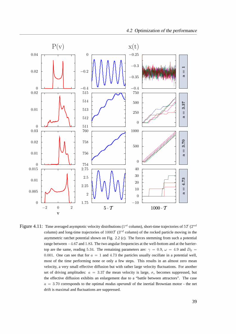
Although this feature is purely noise induced, it still has, its roots in the deterministic struc-ture of attractors. The situation is completely symmetric with respect toF = 0, so we willfocus on the small positive loadF = 0.1. For a given driving strengtha = 4.2 there existsone stable attractor, which causes the particle to dwell in one potential well according to theexternal periodic driving, see first column in Fig. 5.4. If we, however, heat up the system abit, the thermal random force kicks out the particle from the stable attractor, and impose thedynamics to relax again and again. The structure of the deterministic phase space for smalltimes (including the transient effects) is shown in the second column in Fig. 5.4. It meansthat with noise the particle is able to proceed with a negative velocity while in a deterministiccase, after relaxation, it stays in a locked state forever. For a noisy dynamics we can see thissituation as the ghost attractors of a negative direction on a phase space, see Fig. 5.5. Bothsituations, deterministic with transient effects and noisy, give almost the same picture of thephase space, c.f. second column in Fig. 5.4 and Fig. 5.5.

44

5.2 Absolute negative mobility in a symmetric potential

−20

−10

0

10

20

x(t)x(t)

1000 · T1000 · T

−20

−10

0

10

50 · T50 · T

−2.5

0

2.5

v(t)v(t)

0 1

x(t)x(t)

D0 = 0 stable

−2

−1

0

1

2

0 1

x(t)x(t)

D0 = 0 transient

Figure 5.4:Deterministic motion shown for the parameters:γ = 0.9, ω = 4.9, F = 0.1 anda = 4.2. We took uniformly distributed initial conditions in rangesx0 ∈ [0, 1] andv0 ∈ [−0.2, 0.2].Upper row: The phase space (instantaneous velocity versus position). On the leftwe show period one locked attractor that produces zero current. On the right weshow the transient effects, resulting in a very complicated picture of the phasespace.Lower row: Trajectories of the particles shown as an illustration of the attractorsplotted in the upper row. To show transient effects in more details we used only 50periodsT long runs of the deterministic motion.

45

5 Inertial motor under load

−60

−40

−20

0

20

1000 · T1000 · T

−2

−1

0

1

2

0 1

x(t)x(t)

D0 = 0.001

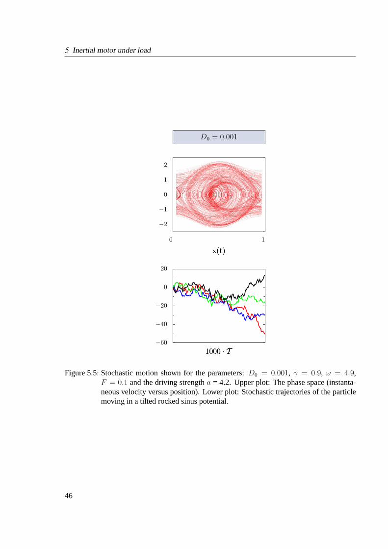
Figure 5.5:Stochastic motion shown for the parameters:D0 = 0.001, γ = 0.9, ω = 4.9,F = 0.1 and the driving strengtha = 4.2. Upper plot: The phase space (instanta-neous velocity versus position). Lower plot: Stochastic trajectories of the particlemoving in a tilted rocked sinus potential.

46

5.2 Absolute negative mobility in a symmetric potential

We now take a look at the efficiency of the Brownian particle in the periodic symmetricpotential under influence of the the load force. As already said zero bias means zero currentresulting in the zero efficiency. For a non vanishing bias we can determine the efficienciesdefined in the section 3.2. In the Fig. 5.6 we showed the relative amount of work doneagainst all forces together (solid line) and also against the load and viscous forces separately(the dashed and dotted line, respectively). We notice that all three efficiencies are very smallcompared to the optimally working ratchet, with maximal values of the order of10−3. Theweakest effect is found for the Stokes efficiencyηS. It means that almost all average outputpower is used for a motion against the load, cf. the efficiency of the energy conversionηE

(the dashed line in Fig 5.6). It is a completely different situation of what we have found fora ratchet potential with the optimal driving conditions, presented in the previous section. Thework done by the Brownian motor against the load was very small and the particle strugglesmostly against the Stokes force.

0

5 · 10−4

1 · 10−3

1.5 · 10−3

ηη

F−stall −0.1 0 0.1 F+stall

FF

ηR

ηE

ηS

Figure 5.6:Different efficiencies measures as defined in section 3.2, of the inertial Brownianparticle in a symmetric sinus potential (2.19 a) plotted as a function of an exter-nal, constant forceF ∈ [F−

stall, F+stall]. Note that the plotted curves are strictely

symmetric with respect toF = 0. The system parameters the same as in the Fig.5.3.

47

5 Inertial motor under load

48

6 Summary and Conclusions

In this thesis the properties of the transport of amassiveBrownian particle moving in a periodicpotential with and without spatial symmetry are addressed. The system is driven out of anequilibrium state by an external, time periodic force. The case with an additional constantbias force was also investigated.

Strongly nonlinear systems far from equilibrium driven inertial ratchets belong to the classof extremely complex and complicated issues. Our model implies a large, 7-dimensional, pa-rameter space, which is made up of: frictionγ, external driving strengtha and frequencyω,load forceF , noise strengthD0 and two constantsc1 andc2 that define the potential shape.As a tool for the analysis of the above formulated problem the numerical simulation of thecorresponding Langevin equation (2.4) was used. This method, however, requires a relativelylong CPU time to estimate all of the relevant quantifiers. It is therefore not possible to system-atically explore totality of the parameter space. In order to achieve a deeper understanding ofthe system, we elucidated the dynamics for a few representative points of the parameter spacein greater detail. In the numerical analysis we kept frictionγ, frequencyω and both potentialconstantsc1, c2 fixed. We used the driving strengtha, temperatureD0 and load forceF ascontrol parameters.

For inertial ratchets two characteristic times, the period of the external driving forceT =2π/ω and the rescaled Stokes timeτL/τ0, are relevant. In this thesis both were chosen to be ofthe same order. Being more specific: in the section 4.1 the time periodT = 2π/3.6 ' 1.745and the Langevin timeτL/τ0 = 2; in the section 4.2T = 2π/4.9 ' 1.282 andτL/τ0 ' 1.111.It means that we do not neglect the influence neither of the external driving nor of the inertiaof the particle. In fact we need both of them incorporating to enhance the transport properties.

In this work, criteria for the optimal transport of an inertial rocked ratchet were establishedby means of two relevant quantifiers: the efficiencyη and thePeclet numberPe. We can defineseveral different efficiency measures that reflect the forces that a particle has to work against.Here the forces are: average Stokes forceγ〈〈v〉〉 and loadF so we can define an adequateefficiency for each of them. We have therefore Stokes efficiencyηS and efficiency of energyconversionηE, that describe how much energy is used to proceed against the respective force.The sum of these two defines therectification efficiencyηR, that describes how much of totalenergy pumped into the system is effectively used. From the numerical analysis it followsthat the most efficient and regular transport is obtained when Peclet number and rectificationefficiency are simultaneously large.

Performance of Brownian MotorsFor a generic ratchet presented in the section 4.1, in the considered regime of the controlparameters, the efficiency of maximum 10% and relatively random manner of motion was

49

6 Summary

found. The potential parameters can be adjusted to obtain a potential form with relatively flatslopes, like the potential used in the section 4.2. For this particular profile the characteristicsof the motion are greatly enhanced, resulting in a rectification efficiency of about 70% andrelatively high Peclet number at the optimal driving strength. For this particular strength weinspected the influence of a external static load force. We found that for small loads, regardlessthe sign, the velocity of the particle drops to zero when we increase the bias. The externalload destroys therefore the regular and efficient ratchet dynamics. For small positive loads anegative differential mobility, (i.e.∂〈〈v〉〉/∂F < 0) was found.

Absolute negative mobilityNext we investigated the response of a particle moving in a symmetric sinusoidal potential toa static load force. Here, we have found another intriguing interplay between the deterministicand noisy dynamics, revealing in an absolute negative mobility (〈〈v〉〉/F < 0). This featureappears to be completely noise induced, as for the deterministic motion the averaged velocityequals zero for small loads.

ConclusionsThough the physics of these systems has been extensively studied in many different aspectsfor 25 years, there are still new and interesting phenomena waiting to be discovered. Up to ourknowledge there exist no analysis ofunderdampednoisy systems where the influence of thefriction force can be neglected. There are several papers exploring the deterministic propertiesof Hamiltonian ratchets [138–140] in both classical and quantum regime. The influence of theheat bath and therefore of thermal noise on a dynamics of systems with a very weak dumpingis definitely interesting and promising topic.

The possibility of revealing the phenomenon of the absolute negative mobility in ratchets isdefinitely an interesting problem. For the ratchets known and well understood feature are cur-rent reversals (i.e. the change of sign of the current for different values of control parameter).It is highly probable that one could find absolute negative mobility in this very points, wherethe current change its sign.

50

A Effective Diffusion

In this thesis we have considered the effective diffusion coefficient, which is defined as

Deff = limt→∞

〈x2(t)〉 − 〈x(t)〉2

2t, (A.1)

where the brackets〈·〉 denote an average over the initial conditions of position and velocityand over all realizations of the thermal noise. Another definition of the diffusion coefficient isgiven by the formula

D = limt→∞

〈[δx(t)− δx(0)]2〉2t

, (A.2)

whereδx(t) = x(t)− 〈x(t)〉. By inspection one finds

Deff = D (A.3)

if

limt→∞

1

t〈δx(t)δx(0)〉 = 0. (A.4)

In our case, this term vanishes because of the presence of thermal noise and dissipation. Moregenerally,|〈δx(t)δx(0)〉| may increase at most ast1/2 if the diffusion coefficientD as definedin (A.2) is finite. Consequently, for such processes the equation (A.3) also holds.

We now show that the diffusion constantD is related to the auto-correlation function of thevelocity via a Green-Kubo relation, in spite of the fact that the system is far from equilibrium.For a system with periodic driving,D takes the form

D =

∫ ∞

0

ds C(s), (A.5)

where

C(s) =1

T

∫ T

0

dτ Cas(τ, s) (A.6)

denotes the time average of the velocity correlation functionCas(τ, s) over one periodT =2π/ω of the driving and where

Cas(t, s) = 〈δv(t)δv(t + s)〉as (A.7)

is the nonequilibrium asymptotic velocity-velocity correlation function. In the case of periodicdriving, this function is periodic with respect to the first argument, i.e.,

C(t, s) = C(t + T , s). (A.8)

51

A Effective Diffusion

To show the Green-Kubo relation, we start from the expressionx(t) = v(t) from which itfollows that

δx(t)− δx(0) =

∫ t

0

ds δv(s). (A.9)

Therefore (A.2) takes the form

2D = limt→∞

1

t

∫ t

0

ds1

∫ t

0

ds2 〈δv(s1)δv(s2)〉

= limt→∞

1

t

∫ t

0

ds1

∫ t

0

ds2 C(s2, s1 − s2), (A.10)

where

C(t, s) = 〈δv(t)δv(t + s)〉. (A.11)

Changing the integration variables(s1, s2) → (s = s1 − s2, τ = s2) and exploiting thesymmetry of the correlation function,C(t, s) = C(t + s,−s), one obtains

D = limt→∞

1

t

∫ t

0

ds

∫ t−s

0

dτ C(τ, s)

= limt→∞

1

t

∫ t

0

ds

∫ t

0

dτ C(τ, s)− limt→∞

1

t

∫ t

0

ds

∫ t

t−s

dτ C(τ, s). (A.12)

We assume that the diffusion coefficient is finite. Therefore the second term in the second lineof (A.12) tends to zero ast →∞, so that

D =

∫ ∞

0

ds limt→∞

1

t

∫ t

0

dτ C(τ, s). (A.13)

For t = KT , one splits the second integral into sum over subsequent periods,

limt→∞

1

t

∫ t

0

dτ C(τ, s) = limK→∞

1

KT

K∑k=1

∫ kT

(k−1)Tdτ C(τ, s)

=1

T

∫ T

0

dτ Cas(τ, s) = C(s) (A.14)

where

Cas(τ, s) = limK→∞

1

K

K∑k=0

C(τ + kT , s). (A.15)

The Eqs. (A.11), (A.13)-(A.15) represent the Green-Kubo relation for the diffusion constant ofsuch periodically driven processesx(t); notably, theseper seconstitute far from equilibriumprocesses.

52

B Efficiency

With this appendix we present the derivation of the expression (3.6) for the average inputpower. As already elaborated we combine the arguments in [79, 92, 96] and establish theefficiencyηR as in eq. (3.6)

ηR =γ〈〈v〉〉2 + |F 〈〈v〉〉|

Pin

. (B.1)

In the denominator,Pin denotes the rate of the energy input to the system. To calculatePin,let us recast (2.4) into the form

dx = vdt , (B.2)

dv = −(γv + V ′(x, t)

)dt +

√2γD0dW (t) , (B.3)

whereV (x, t) = V (x)− ax cos(ωt)− Fx (B.4)

andW (t) is the Wiener process

〈W (t)〉 = 0, 〈W 2(t)〉 = t. (B.5)

Now, we evaluate the ensemble and temporal averages of the re-scaled kinetic energyG(v) = v2/2, v = v(t). To this aim, first we apply Ito’s differential calculus to the func-tion G(v) to obtain

d(v2/2

)= −

(γv2 + vV ′(x, t)− γD0

)dt

+√

2γD0vdW (t). (B.6)

The ensemble average (i.e. the average over all realization of the Wiener process denoted by〈·〉) for the rate of change of the kinetic energy results in

d

dt〈v2/2〉 = −

[γ〈v2〉+ 〈vV ′(x)〉

−〈v a cos(ωt)〉 − 〈Fv〉 − γD0

],

where we exploited the (Ito)-martingale property (for the part containing the Wiener process).Next, we average over the temporal period as in (2.18) (periodic time-dependence of asymp-totic probability). In doing so, we evaluate

〈〈 d

dtv2〉〉 =

1

T

[〈v2(t + T )〉 − 〈v2(t)〉

]= 0 . (B.7)

53

B Efficiency

Likewise, for the contribution

〈〈vV ′(x)〉〉 =1

T

[〈V (x(t + T ))〉 − 〈V (x(t))〉

]= 0 . (B.8)

Consequently, we obtain

0 = −γ[〈〈v2〉〉 −D0

]+ F 〈〈v〉〉+ 〈〈va cos(ωt)〉〉. (B.9)

We define the average input power as

Pin := |F 〈〈v〉〉+ 〈〈va cos(ωt)〉〉|, (B.10)

i.e. the input energy to the system per unit time. From eq. (B.9) it follows

Pin = γ|〈〈v2〉〉 −D0|. (B.11)

Thus, upon combining (B.1) and (B.11) the relation for the rectification efficiency (3.6) emerges

ηR =γ〈〈v〉〉2 + |F 〈〈v〉〉|γ|〈〈v2〉〉 −D0|

. (B.12)

We also emphasize here, that our scheme for the efficiency of rectification at zero bias (F = 0)is independentof the transport friction-coefficientγ. This feature is in agreement with thecorresponding result by Suzuki and Munakata [79].

54

Bibliography

[1] R. Brown. A brief account of microscopical observations made in the months of June,July, and August, 1827, on the particles contained in the pollen of plants, and on thegeneral existence of active molecules in organic and inorganic bodies.Philos. Mag. N.S., 4:161, 1828.

[2] R. Brown. Additional remarks on active molecules.Philos. Mag. N. S., 6:161, 1829.

[3] B. J. Ford. Brown’s observations confirmed.Nature, 359:265, 1992.

[4] A. Einstein. Uber die von der molekularkinetischen Theorie der Warme geforderteBewegung von in ruhenden Flussigkeiten suspendierten Teilchen.Ann. Phys. (Leipzig),17:549, 1905.

[5] A. Einstein. Eine neue Bestimmung der Molekuldimensionen.Ann. Phys. (Leipzig),19:289, 1906.

[6] W. Sutherland. A dynamical theory of diffusion for non-electrolytes and the molecularmass of albumin.Philosophical Magazine, 9:781, 1905.

[7] M. Smoluchowski. Zur kinetischen Theorie der brownschen Molekularbewegung undder Suspensionen.Ann. Phys., 21:756, 1906.

[8] M. Smoluchowski. Drei Vortrageuber Diffusion, brownsche Molekularbewegung undKoagulation von Kolloidteilchen.Physik. Zeitschr., 17:557–561 and 585–599, 1916.

[9] L. Gouy. Note sur le mouvement brownien.J. de Phys. Serie 2, 7:561, 1888.

[10] J. Perrin. Les atomes.Comptes Rendues Acad. Sci. Paris, 158:1168, 1914.

[11] M. Smoluchowski. Experimentell nachweisbare, derublichen Thermodynamik wider-sprechende Molekularphanomene.Physik. Zeitschr., 13:1069, 1912.

[12] L. Gouy. Sur le mouvement brownien.Comptes Rendues Acad. Sci., Paris, 109:102,1889.

[13] R. P. Feynman, R. B. Leighton, and M. Sands.The Feynman Lectures Of Physics,volume 1. Addison Wesley, Reading, MA, 1963.

[14] J.M.R. Parrondo and P. Espanol. Criticism of Feynman’s analysis of the ratchet as anengine.Am. J. Phys., 64:1125, 1996.

55

Bibliography

[15] M. O. Magnasco and G. Stolovitzky. Feynman’s ratchet and pawl.J. Stat. Phys., 93:615,1998.

[16] J. Łuczka. Application of statistical mechanics to stochastic transport.Physica A,274:200, 1999.

[17] F. Julicher, A. Ajdari, and J. Prost. Modeling molecular motors.Rev. Mod. Phys.,69:1269, 1997.

[18] P. Reimann. Brownian motors: Noisy transport far from equilibrium.Phys. Rep.,361:57, 2002.

[19] J Łuczka, R. Bartussek, and P. Hanggi. White-noise-induced transport in periodic struc-tures.Europhys. Lett, 31:431, 1995.

[20] J. Prost, J. F. Chauwin, L. Peliti, and A. Ajdari. Asymmetric pumping of particles.Phys. Rev. Lett., 72:2652, 1994.

[21] R. D. Astumian and M. Bier. Fluctuation driven ratchets: Molecular motors.Phys. Rev.Lett., 72:1766, 1994.

[22] C. S. Peskin, G. B. Ermentrout, and G. F. Oster.The correlation ratchet: A novelmachanism for generating directed motion by ATP hydrolysis, page 479. Springer,New York, 1994.

[23] J. Kula, T. Czernik, and J Łuczka. Transport generated by dichotomous fluctuations.Phys. Lett. A, 214:14, 1996.

[24] J. Kula, M. Kostur, and J. Łuczka. Brownian motion controlled by dichotomic andthermal fluctuations.Chem. Phys, 235:27, 1998.

[25] I. Bena, M. Copelli, and C. Van den Broeck. Stokes’ drift: A rocking ratchet.J. Stat.Phys, 101:415, 2000.

[26] J. Luczka, T. Czernik, and P. Hanggi. Symmetric white noise can induce directed cur-rent in ratchets.Phys. Rev. E., 56:3968, 1997.

[27] M. Kostur, G. Knapczyk, and J. Luczka. Optimal transport and phase transition indichotomic ratchets.Physica A, 325:69, 2003.

[28] M. M. Millonas and M. I. Dykman. Transport and current reversal in stochasticallydriven transport.Phys. Lett. A, 185:65, 1994.

[29] C. R. Doering, W. Horsthemke, and J. Riordan. Nonequilibrium fluctuation-inducedtransport.Phys. Rev. Lett., 72:2984, 1994.

56

Bibliography

[30] R. Bartussek, R. Reimann, and P. Hanggi. Precise precise numerics versus theory forcorrelation ratchets.Phys. Rev. Lett., 76:1166, 1996.

[31] P. Reimann, R. Bartussek, R. Haussler, and P. Hanggi. Brownian motors driven bytemperature oscillations.Phys. Lett. A, 215:26, 1996.

[32] M. Buttiker. Transport as a consequence of state-dependent diffusion.Z. Phys. B,68:161, 1987.

[33] Y. X. Li. Transport generated by fluctuating temperature.Physica A, 238:245, 1997.

[34] Y. D. Bao. Directed current of Brownian ratchet randomly circulating between twothermal sources.Physica A, 273:286, 1999.

[35] A. M. Jayannavar. Simple model for Maxwell’s-demon-type information engine.Phys.Rev. E., 53:2957, 1996.

[36] P. Lancon, G. Batrouni, L. Lobry, and N. Ostrowsky. Drift without flux: Brownianwalker with a space-dependent diffusion coefficient.Europhys. Lett, 54:28, 2001.

[37] G. P. Harmer and D. Abbott. Parrondo’s paradox.Stat. Sci., 14:206, 1999.

[38] G. P. Harmer and D. Abbott. Game theory: Losing strategies can win by Parrondo’sparadox.Nature, 402:864, 1999.

[39] J. M. R. Parrondo, G. P. Harmer, and D. Abbott. New paradoxical games based onBrownian ratchets.Phys. Rev. Lett., 85:5226, 2000.

[40] R. Yasuda, H. Noji, K. Kinosita, and M. Yoshida.F1-Atpase is a highly efficient molec-ular motor that rotates with discrete120o steps.Cell, 93:1117, 1998.

[41] K. Jr. Kinosita, R. Yasuda, H. Noji, S. Ishiwata, and M. Yoshida.F1-Atpase: A rotarymotor made of a single molecule.Cell, 93:21, 1998.

[42] R. D. Astumian. Making molecules into motors.Sci. Am., 285:56, 2001.

[43] R. D. Astumian and P. Hanggi. Brownian motors.Phys. Today, 55:33, 2002.

[44] M. Rief, R. S. Rock, A. D. Mehta, M. S. Mooseker, R. E. Cheney, and J. A. Spudich.Myosin-v stepping kinetics: A molecular model for processivity.Proc. Nat. Acad. Sci.,97:9482, 2000.

[45] C. L. Asbury, A.N. Fehr, and S.M. Block. Kinesin moves by an asymmetric hand-over-hand mechanism.Science, 302:2130, 2003.

[46] A. Yildiz, M. Tomishige, R. D. Vale, and P.R. Selvin. Kinesin walks hand-over-hand.Science, 303:676, 2004.

57

Bibliography

[47] I. Derenyi and T. Vicsek. The kinesin walk: A dynamic model with elastically coupledheads.Proc. Nat. Acad. Sci., 93:6775, 1996.

[48] G. N. Stratopoulos, T. E. Dialynas, and G. Tsironis. Directional Newtonian motion andreversals of molecular motors.Phys. Lett A, 252:151, 1999.

[49] M. Bier. Processive motor protein as an overdamped Brownian stepper.Phys. Rev.Lett., 91:148104, 2003.

[50] J. L. Mateos. Walking on ratchets with two Brownian motors.Fluct. Noise Lett.,4:L161, 2004.

[51] H. C. Fogedby, R. Metzler, and A. Svane. Exact solution of a linear molecular motormodel driven by two-step fluctuations and subject to protein friction.Phys. Rev. E.,70:021905, 2004.

[52] J. L. Mateos. A random walker on a ratchet.Physica A, 351:79, 2005.

[53] R. Lipowsky, S. Klumpp, and T. M. Nieuwenhuizen. Random walks of cytoskeletalmotors in open and closed compartments.Phys. Rev. Lett., 87:108101, 2001.

[54] S. Klumpp and R. Lipowsky. Traffic of molecular motors through tube-like compart-ments.J. Stat. Phys, 113:233, 2003.

[55] M. J. I. Muller, S. Klumpp, and R. Lipowsky. Molecular motor traffic in a half opentube.J. Phys.: Condens. Matter, 17:S3839, 2005.

[56] K. Visscher, M. J. Schnitzer, and S. M. Block. Single kinesin molecules studied with amolecular force clamp.Nature, 400:184, 1999.

[57] M. J. Schnitzer, K. Visscher, and S. M. Block. Force production by single kinesinmotors.Nat. Cell Biol., 2:718, 2000.

[58] S. Jeney, E. H. K. Stelzer, H. Grubmuller, and E. L. Florin. Mechanical properties ofsingle motor molecules studied by three-dimensional thermal force probing in opticaltweezers.ChemPhysChem, 5:1150, 2004.

[59] M Karplus. Molecular dynamics of biological macromolecules: A brief history andperspective.Biopolymers, 68:350, 2002.

[60] E. M. Purcell. Life at low Reynolds number.Am. J. Phys., 45:3, 1976.

[61] E. Pollak, J. Bader, B. J. Berne, and P. Talkner. Theory of correlated hops in surfacediffusion. Phys. Rev. Lett., 70:3299, 1993.

[62] M. Borromeo and F. Marchesoni. Backward-to-forward jump rates on a tilted periodicsubstrate.Phys. Rev. Lett., 84:203, 2000.

58

Bibliography

[63] O. M. Braun and R. Ferrando. Role of long jumps in surface diffusion.Phys. Rev. E.,65:061107, 2002.

[64] M. Borromeo, G. Costantini, and F. Marchesoni. Critical hysteresis in a tilted wash-board potential.Phys. Rev. Lett., 82:2820, 1999.

[65] G. Costantini and F. Marchesoni. Threshold diffusion in a tilted washboard potential.Europhys. Lett, 48:491, 2000.

[66] O. M. Braun, A. R. Bishop, and J. Roder. Hysteresis in the underdamped drivenFrenkel-Kontorova model.Phys. Rev. Lett., 79:3692, 1997.

[67] C. Cattuto and F. Marchesoni. Unlocking of an elastic string from a periodic substrate.Phys. Rev. Lett., 79:5070, 1997.

[68] E. Ben-Jacob, D. J. Bergman, B. J. Matkowsky, and Z. Schuss. Lifetime of oscillatorysteady states.Phys. Rev. A., 26:2805, 1982.

[69] E. Ben-Jacob, D. J. Bergman, and Z. Schuss. Thermal fluctuations and lifetime of thenonequilibrium steady state in a hysteretic Josephson junction.Phys. Rev. B., 25:519,1982.

[70] R. Bartussek, P. Hanggi, and J. G. Kissner. Periodically rocked thermal ratchets.Euro-phys. Lett, 28:459, 1994.

[71] S. Savel’ev, F. Marchesoni, P. Hanggi, and F. Nori. Nonlinear signal mixing in a ratchetdevice.Europhys. Lett, 67:179, 2004.

[72] S. Savel’ev, F. Marchesoni, P. Hanggi, and F. Nori. Transport via nonlinear signalmixing in ratchet devices.Phys. Rev. E., 70:066109, 2004.

[73] P. Hanggi and R. Bartussek. Brownian rectifiers: How to convert Brownian motion intodirected transport.Lect. Notes Phys., 476:294, 1996.

[74] R. D. Astumian. Thermodynamics and kinetics of a Brownian motor.Science, 276:917,1997.

[75] P. Reimann and P. Hanggi. Introduction to the physics of Brownian motors.Appl. Phys.A: Mater. Sci. Process., 75:169, 2002.

[76] H. Linke, editor.Ratchets and Brownian motors: Basics, experiments and applications,Appl. Phys. A: Mater. Sci. Process.volume 75, 2002.

[77] P. Jung, J. G. Kissner, and P. Hanggi. Regular and chaotic transport in asymmetricperiodic potentials: Inertia ratchets.Phys. Rev. Lett., 76:3436, 1996.

59

Bibliography

[78] L. Machura, M. Kostur, P. Talkner, J. Łuczka, F. Marchesoni, and P. Hanggi. Brownianmotors: Current fluctuations and rectification efficiency.Phys. Rev. E., 70:061105,2004.

[79] D. Suzuki and T. Munakata. Rectification efficiency of a Brownian motor.Phys. Rev.E., 68:021906, 2003.

[80] E. Peclet.Ann. Chim. Phys., 3:107, 1841.

[81] E. Peclet.Traite de la Chaleur Consideree dans ses Applications, volume 3. Hachette,Paris, 1843.

[82] L. Machura, M. Kostur, F. Marchesoni, P. Talkner, P. Hanggi, and J. Łuczka. Opti-mal strategy for controlling transport in inertial Brownian motors.J. Phys.: Condens.Matter, 17:S3741–S3752, 2005.

[83] B. Lindner, M. Kostur, and L. Schimansky-Geier. Optimal diffusive transport in a tiltedperiodic potential.Fluct. Noise Lett., 1:R25, 2001.

[84] B. Lindner, L. Schimansky-Geier, P. Reimann, P. Hanggi, and M. Nagaoka. Inertiaratchets: A numerical study versus theory.Phys. Rev. E., 59:1417, 1999.

[85] P. Hanggi and H. Thomas. Stochastic processes: Time-evolution, symmetries and linearresponse.Phys. Rep., 88:207, 1982.

[86] H. Wang. Chemical and mechanical efficiencies of molecular motors and implicationsfor motor mechanisms.J. Phys.: Condens. Matter, 17:S3997, 2005.

[87] R. L. Honeycutt. Stochastic Runge-Kutta algorithms. I. White noise.Phys. Rev. A.,45:600, 1992.

[88] H. Linke, M. T. Downton, and M. J. Zuckermann. Performance characteristic of Brow-nian motors.Chaos, 15:026111, 2005.

[89] L. D. Landau and E. M. Lifshitz.Fluid Dynamics. Pergamon Press, Oxford, 1959.

[90] H. X. Zhou and Y. D. Chen. Chemically driven motility of Brownian particles.Phys.Rev. Lett., 77:194, 1996.

[91] K. Sekimoto. Kinetic characterization of heat bath and the energetics of thermal ratchetmode.J. Phys. Soc. Jpn., 66:1234, 1997.

[92] H. Wang and G. Oster. The Stokes efficiency for molecular motors and its applications.Europhys. Lett, 57:134, 2002.

[93] H. Kamegawa, T. Hondou, and F. Takagi. Energetics of a forced thermal ratchet.Phys.Rev. Lett., 80:5251, 1998.

60

Bibliography

[94] I. M. Sokolov and A. Blumen. Thermodynamical and mechanical efficiency of a ratchetpump.Chem. Phys., 235:39, 1998.

[95] J. M. R. Parrondo, J. M. Blanco, F. J. Cao, and R. Brito. Efficiency of brownian motors.Europhys. Lett, 43:248, 1998.

[96] I. Derenyi, M. Bier, and R. D. Astumian. Generalized efficiency and its application tomicroscopic engines.Phys. Rev. Lett., 83:903, 1999.

[97] A. Parmeggiani, F. Julicher, A. Ajdari, and J. Prost. Energy transduction of isothermalratchets: Generic aspects and specific examples close to and far from equilibrium.Phys.Rev. E., 60:2127, 1999.

[98] K. Sekimoto, F. Takagi, and T. Hondou. Carnot’s cycle for small systems: Irreversibilityand cost of operations.Phys. Rev. E., 62:7759, 2000.

[99] J. M. R. Parrondo and B. J. de Cisneros. Energetics of brownian motors: A review.Appl. Phys. A: Mater. Sci. Process., 75:179, 2002.

[100] M. Asfaw and M. Bekele. Current, maximum power and optimized efficiency of abrownian heat engine.Eur. J. Phys. B, 38:457, 2004.

[101] D. Suzuki and T. Munakata. Rectification efficiency of the Feynman ratchet.J. Phys.Soc. Jpn., 74:550, 2005.

[102] T. Harada. Phenomenological energetics for molecular motor.Europhys. Lett, 70:49,2005.

[103] J. L. Mateos. Chaotic transport and current reversal in deterministic ratchets.Phys. Rev.Lett., 84:258, 2000.

[104] M. Barbi and M. Salerno. Phase locking effect and current reversals in deterministicunderdamped ratchets.Phys. Rev. E., 62:1988, 2000.

[105] M. Porto, M. Urbakh, and J. Klafter. Molecular motor that never steps backwards.Phys.Rev. Lett., 85:491, 2000.

[106] S. Flach, O. Yevtushenko, and Y. Zolotaryuk. Directed current due to broken time-spacesymmetry.Phys. Rev. Lett., 84:2358, 2000.

[107] J. L. Mateos. Current reversals in chaotic ratchets.Acta. Phys. Pol. B, 32:307, 2001.

[108] C. M. Arizmendi, F. Family, and A. L. Salas-Brito. Quenched disorder effects on de-terministic inertia ratchets.Phys. Rev. E., 63:061104, 2001.

[109] J. L. Mateos. Current reversals in deterministic ratchets: Points and dimers.Physica D,168-169:205, 2002.

61

Bibliography

[110] M. Borromeo, G. Costantini, and F. Marchesoni. Deterministic ratchets: Route to dif-fusive transport.Phys. Rev. E., 65:041110, 2002.

[111] H. A. Larrondo, F. Family, and C. M. Arizmendi. Control of current reversal in singleand multiparticle inertia ratchets.Physica A, 303:67, 2002.

[112] J. L. Mateos. Current reversals in chaotic ratchets: The battle of attractors.Physica A,325:92, 2003.

[113] H. A. Larrondo, C. M. Arizmendi, and F. Family. Current basins of attraction in inertiaratchets.Physica A, 320:119, 2003.

[114] S. Sengupta, R. Guantes, S. Miret-Artes, and P. Hanggi. Controlling directed trans-port in two-dimensional periodic structures under crossed electric fields.Physica A,338:406, 2004.

[115] F. Family, H. A. Larrondo, D. G. Zarlenga, and C. M. Arizmendi. Chaotic dynamicsand control of deterministic ratchets.J. Phys.: Condens. Matter, 17:S3719, 2005.

[116] W. S. Son, I. Kim, Y. J. Park, , and C. M. Kim. Current reversal with type-I intermittencyin deterministic inertia ratchets.Phys. Rev. E., 68:067201, 2003.

[117] B. Hu and J. Rudnick. Exact solutions to the Feigenbaum renormalization-group equa-tions for intermittency.Phys. Rev. Lett., 48:1645, 1982.

[118] P. Jung and P. Hanggi. Invariant measure of a driven nonlinear oscillator with externalnoise.Phys. Rev. A., 41:2977, 1990.

[119] M. Schreier, P. Reimann, P. Hanggi, and E. Pollak. Giant enhancement of diffusion andparticle selection in rocked periodic potentials.Europhys. Lett, 44:416, 1998.

[120] P. Reimann, C. Van den Broeck, H. Linke, P. Hanggi, J. M. Rubi, and A. Perez-Madrid.Giant acceleration of free diffusion by use of tilted periodic potentials.Phys. Rev. Lett.,87:010602, 2001.

[121] P. Reimann, C. Van den Broeck, H. Linke, P. Hanggi, J. M. Rubi, and A. Perez-Madrid.Diffusion in tilted periodic potentials: Enhancement, universality, and scaling.Phys.Rev. E., 65:031104, 2002.

[122] M. Kostur, L. Machura, P. Hanggi, J. Łuczka, and P. Talkner. Forcing inertial Brownianmotors: Efficiency and negative differential mobility.accepted to Phys. Rev. E, 2006.

[123] M. Kostur, L. Machura, P. Hanggi, J. Łuczka, and P. Talkner. Absolute negative mobilityin inertial tilted periodic potential.unpublished, 2006.

[124] F. Nava, C. Canali, F. Catellani, G. Gavioli, and G. Ottaviani. Electron-drift velocity inhigh-purity ge between 8 and 240 k.J. Phys. C: Solid State Phys., 9:1685, 1976.

62

Bibliography

[125] L. Hartmann, M. Grifoni, and P. Hanggi. Dissipative transport in dc-ac driven tightbinding lattices.Europhys. Lett, 38:497, 1997.

[126] C. Van den Broeck, I. Bena, P. Reimann, and J. Lehmann. Coupled Brownian motorson a tilted washboard.Ann. Phys. (Leipzig), 9:713, 2000.

[127] C. Van den Broeck, B. Cleuren, R. Kawai, and M. Kambon. A Trio of BrownianDonkeys.International Journal of Modern Physics C, 13:1195, 2002.

[128] R. Eichhorn and P. Reimann. Meandering Brownian donkeys.Acta. Phys. Pol. B,35:1407, 2004.

[129] S. R. White and M. Barma. Field-induced drift and trapping in percolation networks.J. Phys. A, 17:2995, 1984.

[130] V. Balakrishnan and C. Van den Broeck. Transport properties on a random comb.Phys-ica A, 217:1, 1995.

[131] G. A. Cecchi and M. O. Magnasco. Negative resistance and rectification in Browniantransport.Phys. Rev. Lett., 76:1968, 1996.

[132] G. W. Slater, H. L. Guo, and G. I. Nixon. Bidirectional transport of polyelectrolytesusing self-modulating entropic ratchets.Phys. Rev. Lett., 78:1170, 1997.

[133] R. Eichhorn, P. Reimann, and P. Hanggi. Brownian motion exhibiting absolute negativemobility. Phys. Rev. Lett., 88:190601, 2002.

[134] R. Eichhorn, P. Reimann, and P. Hanggi. Paradoxical motion of a single Brownianparticle: Absolute negative mobility.Phys. Rev. E., 66:066132, 2002.

[135] B. Cleuren and C. Van den Broeck. Random walks with absolute negative mobility.Phys. Rev. E., 65:030101, 2002.

[136] A. Haljas, R. Mankin, A. Sauga, and E. Reiter. Anomalous mobility of Brownianparticles in a tilted symmetric sawtooth potential.Phys. Rev. E., 70:041107, 2004.

[137] I. Zapata, R. Bartussek, F. Sols, and P. Hanggi. Voltage rectification by SQUID ratchet.Phys. Rev. Lett., 77:2292, 1996.

[138] T. Dittrich, R. Ketzmerick, M. F. Otto, and H. Schanz. Classical and quantum transportin deterministic hamiltonian ratchets.Ann. Phys. (Leipzig), 9:755, 2000.

[139] S. Denisov and S. Flach. Dynamical mechanisms of dc current generation in drivenHamiltonian systems.Phys. Rev. E., 64:056236, 2001.

[140] H. Schanz, M. F. Otto, R. Ketzmerick, and T. Dittrich. Classical and quantum Hamil-tonian ratchets.Phys. Rev. Lett., 87:070601, 2001.

63

Bibliography

64

Acknowledgments

First of all, I would like to thank Prof. Dr. Peter Hanggi for giving me a possibility of workingin his group, for his constant support during all these years in Ausgburg.

My whole adventure with the science, in particular with the physics of ratchets would not bepossible without Prof. Dr. Jerzy Łuczka. I am grateful for his introduction to this fascinatingtopic, for talks and lectures, and always having time for solving my problems.

I am also very thankful to Prof. Dr. Peter Talkner for his dedicated support, always objective,precise answering my questions and also for reading and improvement of this manuscript.

Many thanks go to Dr. Marcin Kostur for our never ending and fruitful talks (though notalways on physics), his complaining and arguing, but, the most important, for his friendship.

I appreciate all of the constructive discussions with Dr. Gerhard Schmid and all his commentsto this thesis.

I would like to express my gratitude to Prof. Dr. Jose Mateos for his remarks and explanationof the deterministic dynamics of the rocking ratchets.

I would like to thank every single member of the group of the Theoretical Physics I at theUniversity of Augsburg for a very motivating and comfortable atmosphere.

I gratefully acknowledge the financial support by the Graduiertenkolleg GRK 283 “Nichtlin-eare Probleme in Analysis, Geometrie und Physik” and the year DAAD grant.

At last, but not least, I would like to thank my parents for their constant support and myeducation. Special thanks go to my wife Ania and daughter Agata for their love and patience.

65

Curriculum Vitae

Łukasz Machura

Date of Birth: 1 December 1977Place of Birth: Zawiercie, PolandStatus: Married, one daughterParents: Julian and Stefania Machura

EDUCATION:

• 1984-1992 Primary School, Zawiercie, Poland.

• 1992-1996 High School, the biological-chemical profile, Zawiercie, Poland.

• 1996-1999 general physics study, University of Silesia, Katowice, Poland.

• 1999-2001 theoretical physics study, The Department of Theoretical Physics, Uni-versity of Silesia, Katowice, Poland.

• 2001 MSc in theoretical physics (stochastic processes), thesis: ”Inertial Effects InDichotomic Ratchets”, advisor: Prof. Dr. Jerzy Łuczka.

• 2001-2002 Ph.D. study, Department of Theoretical Physics, University of Silesia,Katowice, Poland.

• 2002-2003 research in the group of Prof. Dr. Peter Hanggi, Augsburg University,Germany – a year DAAD grant.

• 2003-2006 Ph.D. study, Theoretical Physics I, Augsburg University, Germany – athree year Graduiertenkolleg 283 scholarship.

MEMBERSHIP: Polish Physical Society.

67