ENERGY EFFICIENCY PROJECTS - Summary Report

DECE MBER 2014 CE C-500-2014-XXX

LBN L-1004139

Prepared for: California Energy Commission Prepared by: Lawrence Berkeley National Laboratory

E n e r g y R e s e a r c h a n d D e v e l o p m e n t D i v i s i o n F I N A L P R O J E C T R E P O R T

ENERGY EFFICIENCY PROJECTS Summary Report

PREPARED BY: Primary Author(s): Various contributors at Lawrence Berkeley National Laboratory Lawrence Berekeley National Laboratory 1 Cyclotron Road MS 90R4000 Berkeley, CA 94720 Phone: 510-486-5910 | Fax: 510-486-6658 http://www.lbl.gov Contract Number: 500-10-052 Prepared for: California Energy Commission Heather Bird Contract Manager Virginia Lew Office Manager Energy Efficiency Research Office Laurie ten Hope Deputy Director ENERGY RESEARCH AND DEVELOPMENT DIVISION Robert P. Oglesby Executive Director DISCLAIMER

This report was prepared as the result of work sponsored by the California Energy Commission. It does not necessarily represent the views of the Energy Commission, its employees or the State of California. The Energy Commission, the State of California, its employees, contractors and subcontractors make no warranty, express or implied, and assume no legal liability for the information in this report; nor does any party represent that the uses of this information will not infringe upon privately owned rights. This report has not been approved or disapproved by the California Energy Commission nor has the California Energy Commission passed upon the accuracy or adequacy of the information in this report. This document was prepared as an account of work sponsored by the United States Government. While this document is believed to contain correct information, neither the United States Government nor any agency thereof, nor The Regents of the University of California, nor any of their employees, makes any warranty, express or implied, or assumes any legal responsibility for the accuracy, completeness, or usefulness of any information, apparatus, product, or process disclosed, or represents that its use would not infringe privately owned rights. Reference herein to any specific commercial product, process, or service by its trade name, trademark, manufacturer, or otherwise, does not necessarily constitute or imply its endorsement, recommendation, or favoring by the United States Government or any agency thereof, or The Regents of the University of California. The views and opinions of authors expressed herein do not necessarily state or reflect those of the United States Government or any agency thereof, or The Regents of the University of California. Ernest Orlando Lawrence Berkeley National Laboratory is an equal opportunity employer.

ACKNOWLEDGEMENTS

Funding was provided by the California Energy Commission, Public Interest Energy Research Program, Energy Related Environmental Research Program, through contract 500-10-052. The authors thank: Heather Bird and Chris Scrutin at the Energy Commission for overall program management; Martha Brook, Dustin Davis, Jeffrey Doll, Rajesh Kapoor, Golam Kibrya, Bradley Meister, Marla Mueller, Leah Mohney, Paul Roggenstock, Felix Villanueva, and David Weightman at the Energy Commission for task management; Kristina LaCommare and Margarita Kloss at Lawrence Berkeley National Laboratory for project management; and Mark Wilson for technical writing and editing.

i

PREFACE

The California Energy Commission Energy Research and Development Division supports public interest energy research and development that will help improve the quality of life in California by bringing environmentally safe, affordable, and reliable energy services and products to the marketplace.

The Energy Research and Development Division conducts public interest research, development, and demonstration (RD&D) projects to benefit California.

The Energy Research and Development Division strives to conduct the most promising public interest energy research by partnering with RD&D entities, including individuals, businesses, utilities, and public or private research institutions.

Energy Research and Development Division funding efforts are focused on the following RD&D program areas:

• Buildings End-Use Energy Efficiency

• Energy Innovations Small Grants

• Energy-Related Environmental Research

• Energy Systems Integration

• Environmentally Preferred Advanced Generation

• Industrial/Agricultural/Water End-Use Energy Efficiency

• Renewable Energy Technologies

• Transportation

Energy Efficiency Projects: Summary Report is the final report for the Lawrence Berkeley National Laboratory Energy Efficiency Research Projects project (contract number 500-10-052) conducted by Lawrence Berkeley National Laboratory. The information from this project contributes to Energy Research and Development Division’s Buildings End-Use Energy Efficiency Program.

For more information about the Energy Research and Development Division, please visit the Energy Commission’s website at www.energy.ca.gov/research/ or contact the Energy Commission at 916-327-1551.

iii

http://www.energy.ca.gov/research/

ABSTRACT

Since 2011, under contract 500-10-052, Lawrence Berkeley National Laboratory completed 19 energy-efficiency research projects for the California Energy Commission to help meet the goals of the California Long Term Energy Efficiency Strategic Plan. Covering a range of energy-related topics, the research focused on three components: increasing end-use and building/facility energy efficiency; tools for energy use monitoring; and energy use simulation and rating tools. The end-use and building/facility energy efficiency work addressed air cleaners, urban heat islands, residential hot water distribution systems, combined heat and power, audio-video, building air-tightness and appliance venting standards, small server rooms, data centers, residential programmable thermostats, and residential heating and cooling. The tools for energy use monitoring work focused on end-use meter development and efficient electronics. And the energy use simulation and rating tools work addressed Title 24 credits for efficient evaporative cooling, Title 24 compliance systems, water heating systems, energy-efficient building system design, a graphical user interface for EnergyPlus, EnergyIQ action-oriented benchmarking, and a rating method for roofing aggregate. This work’s benefits are widespread, and accrue through reductions of energy and water use, decreased greenhouse gas emissions, and lower ratepayer costs. Results of this work can be used to upgrade equipment, evaluate building system energy performance, support compliance to standards such as California’s Title 24 and inform improved standards, and increase the use of combined heat and power systems. Results also support the selection of efficient computer equipment and IT cooling systems, as well as controls that can shut down idle electronics. This work also supports water and natural gas savings through the development of efficient technologies. And to extend electricity, natural gas, and water savings into the future, results from these projects support a designer’s ability to design efficient buildings and technologies quickly and with confidence.

Keywords: benchmarking, buildings, energy efficiency, heating, ventilating, air conditioning, measurements, models, sensors, tools, standards, technology, water heating

Please use the following citation for this report:

Lawrence Berkeley National Laboratory. 2014. Energy Efficiency Projects: Summary Report. California Energy Commission. Publication number: CEC-500-2014-XXX.

v

CONTRIBUTORS

Task Ch. Tech Task Title Authors 1, 5 Kristina LaCommare and Mark Wilson 2.1 2.1 Innovative Air Cleaner for Improved IAQ

and Energy Savings William J. Fisk, Sebastian Cohn, Hugo Destaillats, Victor Henzel, Meera Sidheswaran, Douglas Sullivan

2.2

3.1 Improved Standards through End-Use Meter Development

Steven Lanzisera, Richard Brown, Anna Liao, Andrew Weber, Margarita Kloss

2.3

4.1 Gaining Title 24 Credit for Efficient Evaporative Cooling

Spencer Maxwell Dutton, Jonathan Woolley, Nelson Dichter

2.4

4.2 Performance Data for Improving Title 24 Compliance Systems

Liping Wang, Tianzhen Hong, Philip Haves

2.5

2.2 Urban Heat Island Mitigation Phase 2 Haley Gilbert, Ronnen Levinson, Benjamin Mandel, Dev Millstein, Melvin Pomerantz, Pablo Rosado

2.6

4.3 Simulation Models for Improved Water Heating Systems

Jim Lutz, Peter Grant, Margarita Kloss

2.7

2.3 Reducing Waste in Residential Hot Water Distribution Systems

Jim Lutz, Steven Lanzisera, Anna Liao, Christian Fitting, Chris Stiles, Margarita Kloss

2.8

2.4 Encouraging Combined Heat and Power in California Buildings

Michael Stadler, Markus Groissböck, Gonçalo Cardoso, Andreas Müller, Judy Lai

2.9

3.2 Efficient Electronics through Measurement and Communication

Alan Meier, Steven Lanzisera, Andrew R. Weber, Anna Liao, Chris Stiles

2.10

4.4 Enabling Tools for Design of Energy-Efficient Building Systems

Michael Wetter, Xiufeng Pang, Wangda Zuo, Thierry Nouidui, Kaustubh Phalak

2.11

2.5 Improved Audio-Video Efficiency through Inter-Device Control

Bruce Nordman

2.12

2.6 Building Air-Tightness through Appliance Venting Standards

Craig Wray, Vi Rapp, David Lorenzetti, Brett Singer

2.13

2.7 Energy Efficiency in Small Server Rooms H. Y. Iris Cheung, Steve E. Greenberg, Roozbeh Mahdavi, Richard Brown, William Tschudi

2.14

2.8 Data Center Energy Efficiency Demonstration Projects

Henry Coles, Steve Greenberg, William Tschudi

2.15

— Energy Savings through Data Center Waste Heat Reuse - TERMINATED

No chapter, as this task was terminated.

2.16

4.5 Graphical User Interface for EnergyPlus Philip Haves, Richard See (Digital Alchemy, Seattle, Washington), Kevin Settlemyre (Sustainable IQ, Boston, Massachusetts)

2.17

4.6 EnergyIQ Action-Oriented Benchmarking Evan Mills

2.18

2.9 Improving Residential Programmable Thermostats

Alan Meier, Emmanuelle Revillion

2.19

2.10 More Efficient Residential Heating/Cooling by Airflow Instrument Analysis

Iain S. Walker, J. Chris Stratton

2.20

4.7 Rating Method for Roofing Aggregate Ronnen Levinson, Sharon Chen, Paul Berdahl, Pablo Rosado, Louis Medina (A-1 Grit Company, Riverside, California)

Unless noted, the authors are affiliated with Lawrence Berkeley National Laboratory

vi

TABLE OF CONTENTS

Acknowledgements ................................................................................................................................... i

PREFACE .................................................................................................................................................. iii

ABSTRACT ................................................................................................................................................ v

Contributors ............................................................................................................................................. vi

TABLE OF CONTENTS ....................................................................................................................... viii

LIST OF FIGURES ................................................................................................................................ xiii

LIST OF TABLES .................................................................................................................................. xiv

EXECUTIVE SUMMARY ........................................................................................................................ 2

CHAPTER 1: Introduction .................................................................................................................... 18

1.1 Focus on Three Research Areas ............................................................................................. 18

1.1.1 Energy Efficiency Technologies for Buildings, Facilities, and Equipment .............. 19

1.1.2 Tools for Energy Use Monitoring .................................................................................. 20

1.1.3 Energy Use Simulation and Rating Tools ..................................................................... 20

1.2 Organization of This Summary .............................................................................................. 21

CHAPTER 2: Energy Efficiency Technologies for Buildings, Facilities, and Equipment ........ 22

2.1 Innovative Air Cleaner for Improved Indoor Air Quality and Energy Savings ............. 22

2.1.1 Goal .................................................................................................................................... 22

2.1.2 Methods ............................................................................................................................. 22

2.1.3 Results ................................................................................................................................ 23

2.1.4 Conclusions ....................................................................................................................... 27

2.1.5 Project Benefits ................................................................................................................. 28

2.2 Urban Heat Island Mitigation Phase 2 .................................................................................. 29

2.2.1 Goal .................................................................................................................................... 29

2.2.2 Methods ............................................................................................................................. 29

2.2.3 Results ................................................................................................................................ 32

2.2.4 Conclusions and Recommendations ............................................................................. 34


viii

2.3 Reducing Waste in Residential Hot Water Distribution Systems ..................................... 39

2.3.1 Goal .................................................................................................................................... 39

2.3.2 Methods ............................................................................................................................. 39

2.3.3 Results ................................................................................................................................ 43

2.3.4 Conclusions ....................................................................................................................... 43


2.4 Encouraging Combined Heat and Power in California Buildings.................................... 45

2.4.1 Goal .................................................................................................................................... 45

2.4.2 Methods ............................................................................................................................. 45

2.4.3 Results ................................................................................................................................ 48

2.4.4 Conclusions ....................................................................................................................... 52


2.5 Improved Audio-Video Efficiency through Inter-Device Power Control ....................... 55

2.5.1 Goal .................................................................................................................................... 55

2.5.2 Methods ............................................................................................................................. 55

2.5.3 Results ................................................................................................................................ 56

2.5.4 Conclusions ....................................................................................................................... 60


2.6 Building Air-Tightness through Appliance Venting Standards ........................................ 62

2.6.1 Goal .................................................................................................................................... 62

2.6.2 Methods ............................................................................................................................. 62

2.6.3 Results ................................................................................................................................ 63

2.6.4 Conclusions ....................................................................................................................... 65


2.7 Energy Efficiency in Small Server Rooms............................................................................. 67

2.7.1 Goal .................................................................................................................................... 67

2.7.2 Methods ............................................................................................................................. 67

2.7.3 Results ................................................................................................................................ 68

ix

2.7.4 Conclusions and Recommendations ............................................................................. 71


2.8 Data Center Energy Efficiency Demonstration Projects ..................................................... 73

2.8.1 Goals .................................................................................................................................. 73

2.8.2 Methods ............................................................................................................................. 73

2.8.3 Results ................................................................................................................................ 76

2.8.4 Conclusions ....................................................................................................................... 77

2.8.5 Next Steps .......................................................................................................................... 79


2.9 Improving Residential Programmable Thermostats ........................................................... 82

2.9.1 Goal .................................................................................................................................... 82

2.9.2 Methods ............................................................................................................................. 82

2.9.3 Results ................................................................................................................................ 84

2.9.4 Conclusions ....................................................................................................................... 86


2.10 More Efficient Residential Heating/Cooling by Airflow Instrument Standards ............ 88

2.10.1 Goal .................................................................................................................................... 88

2.10.2 Methods ............................................................................................................................. 88

2.10.3 Results ................................................................................................................................ 91

2.10.4 Conclusions ....................................................................................................................... 93


CHAPTER 3: Tools for End Use Monitoring ..................................................................................... 96

3.1 Improved Standards through End-Use Meter Development ............................................ 96

3.1.1 Goal .................................................................................................................................... 96

3.1.2 Methods ............................................................................................................................. 96

3.1.3 Results ................................................................................................................................ 97

3.1.4 Conclusions and Next Steps ......................................................................................... 101

3.1.5 Project Benefits ............................................................................................................... 101

x

3.2 Efficient Electronics through Measurement and Communication.................................. 102

3.2.1 Goal .................................................................................................................................. 102

3.2.2 Methods ........................................................................................................................... 102

3.2.3 Results .............................................................................................................................. 105

3.2.4 Conclusions ..................................................................................................................... 106


CHAPTER 4: Energy Use Simulation and Rating Tools ................................................................ 109

4.1 Title 24 Credit for Efficient Evaporative Cooling .............................................................. 109

4.1.1 Goal .................................................................................................................................. 109

4.1.2 Methods ........................................................................................................................... 109

4.1.3 Results .............................................................................................................................. 112

4.1.4 Conclusions ..................................................................................................................... 115


4.2 Performance Data for Improving Title 24 Compliance Systems ..................................... 118

4.2.1 Goal .................................................................................................................................. 118

4.2.2 Methods ........................................................................................................................... 118

4.2.3 Results and Conclusions ............................................................................................... 120


4.3 Simulation Models for Improved Water Heating Systems .............................................. 126

4.3.1 Goal .................................................................................................................................. 126

4.3.2 Methods ........................................................................................................................... 126

4.3.3 Results .............................................................................................................................. 128

4.3.4 Conclusions and Recommendations ........................................................................... 131


4.4 Enabling Tools for Design of Energy-Efficient Building Systems ................................... 135

4.4.1 Goal .................................................................................................................................. 135

4.4.2 Methods ........................................................................................................................... 135

4.4.3 Results and Conclusions ............................................................................................... 137

xi


4.5 Simergy: A Graphical User Interface for EnergyPlus ....................................................... 142

4.5.1 Goal .................................................................................................................................. 142

4.5.2 Methods ........................................................................................................................... 142

4.5.3 Results .............................................................................................................................. 145



4.6 EnergyIQ Action-Oriented Benchmarking ......................................................................... 151

4.6.1 Goal .................................................................................................................................. 151

4.6.2 Methods ........................................................................................................................... 151

4.6.3 Results .............................................................................................................................. 152

4.6.4 Conclusions and Accomplishments ............................................................................ 156


4.7 Rating Method for Roofing Aggregate ............................................................................... 158

4.7.1 Goal .................................................................................................................................. 158

4.7.2 Methods ........................................................................................................................... 158

4.7.3 Results .............................................................................................................................. 159



CHAPTER 5. Conclusions and Recommendations......................................................................... 162

GLOSSARY ............................................................................................................................................ 163

REFERENCES ........................................................................................................................................ 168

APPENDIX ................................................................................................................................................. 1

xii

LIST OF FIGURES

Figure 2.1.1: VOC data from field studies in House 1 with and without operation of ITAC1 ..... 24 Figure 2.1.2: Formaldehyde data from field studies in House 1 with and without operation of two ITAC1 air cleaners ............................................................................................................................ 25 Figure 2.1.3: VOC concentrations from field studies in House 2 with and without operation of ITAC2 ......................................................................................................................................................... 26 Figure 2.1.4: Formaldehyde concentrations from the field studies in House 2 with and without operation of ITAC2 .................................................................................................................................. 26 Figure 2.3.1: Schematic of Wireless Sensor Network .......................................................................... 40 Figure 2.4.1: Schematic of energy flows in DER-CAM ....................................................................... 47 Figure 2.4.2: High-level CHP results for 2020 ...................................................................................... 49 Figure 2.4.3: High-level CHP results for 2030 ...................................................................................... 50 Figure 2.4.4: Installed CHP capacity by utility service territory, for most optimistic case (4d4), 2020 ............................................................................................................................................................ 50 Figure 2.4.5: Installed CHP capacity by forecasting climate zone, most optimistic case (4d4), 2020 ............................................................................................................................................................ 51 Figure 2.4.6: Installed CHP capacity by utility service territory, run set case (4e10) for 2030 ...... 51 Figure 2.4.7: Installed CHP capacity by forecasting climate zone, run set (4e10) for 2030 ............ 52 .................................................................................................................................................................... 59 Figure 2.5.1. State diagram for stable and transitional stream states ............................................... 59 Figure 2.8.1: Asetek system supplying liquid to IT equipment ......................................................... 74 Figure 2.8.2: The four different servers evaluated in the third-year demonstration ...................... 76 Figure 2.10.1: Multi-branch return flow experimental apparatus ..................................................... 90 Figure 3.1.1 Flow turbine water meter design ..................................................................................... 98 Figure 3.1.2 Fabricated, assembled flow meter .................................................................................... 98 Figure 3.1.3 Whole-building gas meter ................................................................................................. 99 Figure 3.1.4 Conceptual drawing of data collection system ............................................................ 100 Figure 4.1.1 HBBM model component description ........................................................................... 115 Figure 4.4.1: Resistor capacitor network for the radiant slab model. Along the flow path, multiple instances of this model are used to take into account the change in fluid temperature. .................................................................................................................................................................. 138 Figure 4.4.2: Schematic view of overhang and side fin models. ...................................................... 138 Figure 4.4.3: Room air temperature and absolute humidity for different direct evaporating coils .................................................................................................................................................................. 139 Figure 4.5.1: Import of building geometry using IFC ....................................................................... 145 Figure 4.5.2: Import of building geometry using gbXML ................................................................ 145 Figure 4.5.3: Import of building geometry using 2-D floor plans ................................................... 146 Figure 4.5.4: Use of the zone HVAC group template workspace to create a zone HVAC group with radiant heating and cooling and demand controlled ventilation .......................................... 147 Figure 4.6.1 a–k: Key screenshots ........................................................................................................ 153

xiii

Figure 4.7.1: Aggregate bed, opaque granule pile, and shingle prepared from white ballast .... 159 Figure 4.7.2: Aggregate bed albedos predicted from shingle albedo (red circles) closely matches those measured via pyranometer method E1918 (green squares). ................................................. 160

LIST OF TABLES

Table 2.3.1: Guidelines for installing sensor units ............................................................................... 41 Table 2.5.1. Use case example: DVD player powers up ...................................................................... 58 Table 2.7.1: Detailed site assessment summary................................................................................. 69 Table 2.7.2: Detailed assessment sites - power use breakdown (in kW) ...................................... 69 Table 2.7.3: Energy efficiency measures (EEMs) and estimated annual energy bill savings ........ 70 Table 2.10.1 Insertion effect caused by each flow measurement device .......................................... 92 Table 2.10.2: Difference between measured and reference flow for individual and summed measurements for each device under test ............................................................................................ 92 Table 2.10.3: Percentage of individual branch and total flow measurements within 10% of reference flow for each device under test ............................................................................................. 93 Table 3.2.1: Communication protocols ................................................................................................ 104 Table 3.2.2: Estimates of U.S. electricity savings from communicating power supplies ............. 108 Table 4.2.1: Template of results for HVAC test cases ....................................................................... 122

xiv

EXECUTIVE SUMMARY

Introduction When California enacted the Global Warming Solutions Act of 2006 (also known as AB 32), state agencies began to determine what actions they could take to help meet that legislation’s goals. A primary strategy that emerged from evaluations by the California Energy Commission (Energy Commission), California Air Resources Board (ARB), and California Public Utilities Commission (CPUC) was to support the widespread research, development, and use of energy-efficient technologies and practices throughout the state.

In 2008, the CPUC adopted its Long Term Energy Efficiency Strategic Plan. Developed in collaboration with the state’s regulated utilities and more than 500 stakeholders, and updated in 2011, this plan outlines a vision to achieve energy savings within all major California sectors. Part of that plan is to support the development and advancement of new, energy-efficient technologies, to bridge the gaps preventing the successful deployment of energy-saving measures and achieve the plan’s goals.

As a result, in 2011, Lawrence Berkeley National Laboratory (LBNL) began to conduct 19 end-use and building/facility energy-efficiency research projects for the Energy Commission to help meet those goals.

Project Purpose This project’s purpose was threefold; to increase end-use and building/facility energy efficiency; develop tools for energy use monitoring; and develop energy use simulation and rating tools. LBNL proposed a number of projects in response to an Energy Commission solicitation, and several projects were selected for support. To maximize administrative efficiency, the selected projects were bundled to create this program of research on energy efficiency technologies and practices.

Table ES-1 shows the tasks chosen for the project.

2

Table ES-1. Energy Efficiency Projects

Energy Efficiency Technologies for Buildings, Facilities, and Equipment • Innovative Air Cleaner for Improved Indoor Air Quality and Energy Savings • Urban Heat Island Mitigation Phase 2 • Reducing Waste in Residential Hot Water Distribution Systems • Encouraging Combined Heat and Power in California Buildings • Improved Audio-Video Efficiency through Inter-Device Power Control • Building Air-Tightness through Appliance Venting Standards • Energy Efficiency in Small Server Rooms • Data Center Energy Efficiency Demonstration Projects • Improving Residential Programmable Thermostats • More Efficient Residential Heating/Cooling by Airflow Instrument Analysis

Tools for Energy Use Monitoring

• Improved Standards through End-Use Meter Development • Efficient Electronics through Measurement and Communication

Energy Use Simulation and Rating Tools

• Gaining Title 24 Credit for Efficient Evaporative Cooling • Performance Data for Improving Title 24 Compliance Systems • Simulation Models for Improved Water Heating Systems • Enabling Tools for Design of Energy Efficient Building Systems • Graphical User Interface for EnergyPlus • EnergyIQ Action-Oriented Benchmarking • Rating Method for Roofing Aggregate

Project Results This portfolio of work resulted in many advancements in energy-efficiency technologies and approaches. Because of the breadth of the work, only selected highlights can be presented here. Please see each full report for a much more detailed presentation of the results.

Energy Efficiency Technologies for Buildings, Facilities, and Equipment

Innovative Air Cleaner for Improved Indoor Air Quality and Energy Savings

Two energy-efficient integrated technology air cleaners (ITACs) were designed and fabricated. In short-term laboratory tests, both units performed as expected, effectively removing formaldehyde and other volatile organic compounds. Single-pass formaldehyde removal efficiencies were approximately 50 to 60 percent. In field studies with the ITAC units deployed in two homes, concentrations of most volatile organic compounds and of particles were reduced during air cleaner operation. However, reductions in indoor formaldehyde concentrations and single-pass formaldehyde removal efficiencies were much lower than in the laboratory studies. Subsequent laboratory tests confirmed that formaldehyde can be produced by incomplete decomposition of volatile organic compounds by the catalyst-treated filters in the ITAC units, which may explain the low formaldehyde removal efficiencies in the field.

3

Subsequent experiments examined strategies for obtaining more complete decomposition of volatile organic compounds and associated lower rates of formaldehyde production. Using the results of the laboratory tests together with a model, the researchers found that a modified version of one of the ITAC air cleaners—with a larger amount of catalyst (10 grams per square meter of filter media or higher) and with a lower air velocity through the catalyst treated filter—will simultaneously reduce indoor formaldehyde concentrations and concentrations of other volatile organic compounds when initial concentrations of volatile organic compounds other than formaldehyde are low or moderate. However, model results suggest that increasing the amount of catalyst and decreasing the air velocity are not sufficient measures for homes with initially high concentrations of volatile organic compounds other than formaldehyde, as formaldehyde concentrations may be increased during air cleaner use.

Urban Heat Island Mitigation Phase 2

Measurements in Fresno, California, found that a home with cool tile roofing used 2.8 kilowatt-hours per square meter (26 percent) less site cooling energy each year than a similar home with standard asphalt roofing. In a cool pavement demonstration, the more reflective pavement surfaces decreased the pavement temperature and thus reduced the heat transferred to the local environment. A meteorological model was used to simulate the benefits of a cool community and found up to 0.3 degrees Celsius reduction in maximum temperature over downtown Bakersfield when the average urban albedo was increased from approximately 0.14 to 0.30. The team successfully incorporated many improvements to an existing cool roof consumer website hosted at CoolCalifornia.org, including updates to the California building code content. Partnerships were extremely helpful in developing and presenting both training presentations and brochures/handouts on cool roofs and cool pavements. LBNL continues to work with various partners to develop resources and conduct outreach and technical assistance.

This work also led to the development of a cool schoolyard pilot program; a city-wide building code update to require residential cool roofs; testing and development of three novel cool pavement products; statewide legislation for cool pavements; and statewide guidance on the implementation of cool community measures to mitigate human health exposure during extreme heat events.

Reducing Waste in Residential Hot Water Distribution Systems

The research team developed a wireless sensor network technology to measure water temperature and flow rate at indoor end uses and deployed it in 21 houses. Preliminary analysis demonstrates that for some shower, kitchen sink, and dishwasher events, only half of the hot water energy inserted into the hot water distribution systems at the water heater is actually being delivered at the end use, with the remaining energy lost in the piping system. Overall, the project demonstrated that hot water energy use for dishwashers in the homes studied was very inefficient.

Encouraging Combined Heat and Power in California Buildings

4

This task had numerous findings based on a large number of simulations of combined heat and power (CHP) systems. Optimization results, distributed energy resources adoption, and results for the restaurant sector are detailed in the full report. Among the results: Carbon dioxide (CO2) minimization strategies of building owners can also elevate CHP-enabled fuel cell adoption. Zero net energy buildings can support CHP technology adoption; however, those results were quite sensitive to investment costs, efficiencies, and payback periods. The total amounts of CHP technology adoption for the most optimistic case in 2020 is about 2,385 megawatts (MW) of CHP and about 2,116 MW of fuel cells with heat exchangers. The total CHP capacity is 1,961 MW in 2030. The most optimistic case for 2020 shows about 2.1 gigawatts (GW) of fuel cells with heat exchangers, and the case for 2030 shows about 1.1 GW of fuel cells with heat exchangers, which effectively means a 50 percent reduction of fuel cells with heat exchangers by 2030 due to grid de-carbonization.

Improved Audio-Video Efficiency through Inter-Device Control

This project developed a new audio-video (A/V) power control architecture that builds on existing technologies and includes key changes and additions to address how a device knows when its state should change. The team developed a sleeping stream concept, based on several guiding principles:

• There is no central control. • Devices inform each other about their power and functional state, and use that

information to determine in which power and functional state they need to be. • Named content streams (and their characteristics) define the outcomes that each device

helps to implement. • Successful technologies with wide market penetration are used as a basis for future

products, to increase their overall use and their chance of being used into the future. • The widely accepted “sleep” metaphor is used to promote easy understanding among

both technical audiences and ordinary users. Building Air-Tightness through Appliance Venting Standards

Although air sealing of homes is among the most cost-effective home retrofit measures to reduce energy consumption and associated greenhouse gas (GHG) emissions, tighter homes more readily depressurize when exhaust ventilation equipment is operated. Therefore, combustion appliances are more prone to backdraft and spill harmful exhaust gases into the living space. One solution to reducing or eliminating health and safety risks associated with spillage is to use sealed combustion appliances or to locate them outside the pressure boundary of the occupied space. However, when that is not cost effective, a diagnostic procedure should be used to assess the risks of spillage for the house and appliances, both as found and as they might operate if retrofits such as house air tightening were to be implemented. This project showed that existing diagnostic tests for characterizing the risk of venting system failures in natural-draft combustion appliances based on “worst-case depressurization” are fundamentally flawed. New tests need to be developed; (1) to identify when flows stall in combustion

5

appliance vents, and (2) to assess the statistical variation of spilled pollutant concentrations and associated health risks.

Energy Efficiency in Small Server Rooms

This project identified common efficiency issues across the small server rooms and institutions surveyed. Among them were that most small server rooms were not initially designed to operate as such; they tend to contain older, less efficient, IT equipment; and their cooling systems are inefficient and unnecessarily use high amounts of energy.

Opportunities to improve energy efficiency at these sites included better airflow management; raising room temperatures; consolidating and virtualizing servers; moving servers to a more centralized, energy-efficient location; and eliminating or optimizing power backup and conditioning whenever possible. Efficiency measures ranged from simple to more complex, and inexpensive to more costly. Fact sheets that describe efficiency measures that server room operators can adopt to significantly reduce energy use were developed and disseminated.

Data center owners and operators can use the findings of this task to improve the energy efficiency of small server rooms. The results also serve as a guide for the design and configuration of new spaces.

Data Center Energy Efficiency Demonstration Projects

This project’s demonstration of a liquid cooling technology in a data center showed that it saved energy, but that the fraction of the heat removed by liquid was smaller than originally expected.

The project’s data center modeling software demonstration showed that the modeled predicted performance closely matched actual performance. The calibrated model provided an overall site power variance of negative 1.2 percent comparing the software results (722 kilowatt (kW)) to the meter readings (731 kW). Once the model was determined to accurately represent actual performance, it was used to perform “what-if” scenarios for various system modifications, which was useful in predicting potential energy savings for various efficiency measures.

The server efficiency comparison showed that at high server compute loads, all brands using the same processors and memory had similar results. The power consumption variability caused by the key components as a group is similar to all other components as a group. Data suggest that a proprietary power supply control feature termed cold redundancy can provide energy savings at low power levels.

The results of this task were presented at the Silicon Valley Leadership Group Data Center Summit in 2014 and in separate reports for each demonstration.

Improving Residential Programmable Thermostats

This task sought to create a metric to measure the effectiveness of Internet-based algorithms in residential programmable thermostats. Researchers evaluated four different metrics.

Tracking savings through changes in utility meters initially appeared to be the most credible metric; however, further investigations revealed numerous analytical and practical

6

shortcomings that, together, make a metric based on meter data unattractive for routine testing. The meter readings must be normalized, and the uncertainty in those normalizations may be as great (or greater) than the savings. The metric also has numerous practical problems, such as a lack of access to utility data by the thermostat service providers (or other programs), no pre-retrofit year baseline data, a potential need for a second control group, a long evaluation period, and a high evaluation cost.

A second metric based on calibrated simulations was investigated. The major drawbacks to a metric based on simulations are that that they require two simulations for each home, and for users to achieve the most accurate results, they must obtain average local weather data for each home. The simulation also inserts an extra layer of complexity, making tracing the actual impacts more complicated. Ultimately, uncertainty remains, because the outcomes are not physically linked to real homes. Also, information such as security system status and geolocation data may affect equipment operation, and more field investigations are needed to verify the robustness of the calibrated simulation approach.

A metric based on furnace run-time has three major drawbacks: (1) energy consumption does not necessarily scale with equipment operating time, (2) networked thermostat providers do not know the furnace (or air conditioner) input capacities in the homes they serve, and (3) networked thermostat providers do not have operating data for pre-installation conditions. These are detailed in the full report.

A fourth metric, based on a new concept of “savings degree-hours,” was also developed and evaluated. This metric is simple and understandable, using an absolute reference temperature as the control. The cumulative deviation of each house from the reference temperature, measured in degree-hours, is the metric of a networked thermostat’s success in wringing out savings through more intelligent control. More details are provided in the full report.

More Efficient Residential Heating/Cooling by Airflow Instrument Standards

This task developed guidance for use in Title 24 applications and a test procedure for determining the errors associated with airflow measurement tools, based on the results of laboratory testing a range of flow hoods and return system configurations.

Results showed that typical errors for devices used to measure airflows in residential heating and cooling systems ranged from minor (5 percent or less) to significant (up to 25 percent), indicating a need to distinguish between airflow measurement devices in Title 24 and other standards that require residential register airflow measurement.

The research team prepared a draft test method for determining the uncertainty of airflow measurements at residential air supply registers and return grilles, and assembled a working group to pursue airflow measurement tool standardization through the American Society of Testing and Materials.

Tools for End Use Monitoring

Improved Standards through End-Use Meter Development

7

For this task, the research team reviewed six types of flow meters and other gas metering technologies to determine the best technologies and develop the basic tools needed to obtain end-use metering information for gas and water end-uses in homes, so those data can be used to inform end-use studies, energy-efficiency standards, and other efforts to control and reduce energy consumption.

The team developed new gas and water metering systems and a wireless data collection framework to manage meter data from these systems. The whole-building gas metering system designed by the team can read a utility gas meter at 10-second intervals and a resolution of 150 W (0.5 kBtu/hour). It was chosen due to its low cost, easy installation process and likely ready acceptance by homeowners. The best water flow measurement was determined to be the turbine method because it can work over a relatively large flow range, requires simple electronics, and has virtually no standby power when there is no water flow, which is particularly important for battery-operated sensors.

The components were tested in field deployments, and both the water meter and the data collection system are being used in projects at LBNL. Use of the wireless data system architecture includes a telemetry data management system for demand response, and for the gas meter data collection system. Closely related, derivative systems are being used for transactional control at LBNL and other national laboratories as a result of the initial work done in this project.

Efficient Electronics through Measurement and Communication

LBNL developed a "communicating power supply," a low cost means of measuring the energy use of a wide range of plugged-in devices, with the additional capability of communicating that consumption data to a central entity. This project proved the technical feasibility of a communicating power supply that easily accommodated diverse electrical products, including lights and consumer electronics, whose power consumption ranged from approximately 0 to 20 watts. Accuracy and unit-to-unit variability is still undefined because a limited number of units were used. This project also demonstrated that it was possible to transmit control signals to the communicating power supplies, establishing two-way communication and greatly broadening its application. The design allows for easy adoption by manufacturers and expansion to mass production.

Energy Use Simulation and Rating Tools

Title 24 Credit for Efficient Evaporative Cooling

This project developed and validated a software system incorporating a Hybrid-Black-Box model (HBBM) for modeling energy efficient evaporative cooling systems with the EnergyPlus program. Without such a software system for predicting energy savings, these energy efficient cooling systems will be little used in California. The research team demonstrated that the model developed for this project functions correctly in EnergyPlus and compared the modeled system performance against measured system performance from field data. The simulation results compared acceptably well with field data. The model was developed as an EnergyPlus “plug-

8

in,” and as a result, it can be trialed by external partners using the current version of EnergyPlus without requiring that it be fully integrated into a formal EnergyPlus release.

The team also developed an empirical model of the Coolerado H80 hybrid evaporative cooling system that compared well with the field data. The second-order performance curves developed for the Coolerado H80 compared sufficiently well with the field data to proceed with testing of the HBBM. When these curves were used within the HBBM framework and tested using input data from the field study, the model predicted the systems operating mode and delivery of sensible cooling to an acceptable level of accuracy. The team also stress-tested the model in the EnergyPlus implementation. For a simple single-zone EnergyPlus building model, the Coolerado H80 model delivered sufficient cooling to meet the cooling load requirements of the space. The team is currently working with industry partners to configure model inputs for additional hybrid air conditioner systems and to validate that the modeling framework appropriately accommodates a variety of hybrid system types. The model, user manual and engineering reference guide are available online at (http://hybridcooling.lbl.gov/)

Most of the evaporative cooling technologies studied in the field trials showed substantial energy savings, especially at peak cooling loads; however, the performance and savings are different for every technology, and can even differ for a particular technology. Generally, the potential for savings from these systems is higher for buildings that have high ventilation rates.

The Coolerado field data demonstrated the broad range of part-load capacity operation for the equipment, and that performance is most significantly related to mode, airflow, and environmental conditions. Most notable, cooling capacity for the system varies significantly compared to standard constant-volume single-speed vapor compression equipment.

Initial validation testing of the EnergyPlus simulation highlighted some control issues still needs to be addressed, this is detailed in the full report.

Performance Data for Improving Title 24 Compliance Systems

For this task, researchers created a new suite of alternate calculation method reference tests using EnergyPlus. The research team identified twelve types of heating, ventilation, and air-conditioning (HVAC) systems, covering all Title 24 standard HVAC systems in typical California climate zones to define a suite of HVAC test cases for use in accreditation.

For each conventional HVAC system, three test cases were created, and for each non-conventional HVAC system, two test cases were created. The reference data sets were generated from the simulation results. Test criteria are recommended to provide impartial accreditation based on the capability of the candidate program to model a subset of the full range of HVAC systems. The reference data sets are included in a spreadsheet that is set up to receive output data from candidate programs and perform predefined comparisons in order to be certified for the use of Title 24 code compliance.

9

Simulation Models for Improved Water Heating Systems

The research team improved and extended the Modelica Buildings library to allow design firms and manufacturers to rapidly analyze new low energy systems and their control sequences for system configuration and controls that are not possible with conventional building simulation programs. The team conducted a scoping study of the current models for hot water systems and identified preferred capabilities of new models. The Modelica modeling environment was chosen because model developers can use it to build models of water heaters and hot water distribution systems out of models of simpler components or individual features. The team also conducted a literature review and ruled out some existing models for future model development.

Laboratory tests provided the measured data that enabled researchers to study how water heaters behave, create and validate simulation models, and undertake deeper analysis of the units’ efficiency.

The research team developed both a storage tank water heater model and tankless water heater model. It also created simulation models for hot water distribution systems—pipe models, end use models, and a flow reduction model. These simulation tools will be included in the Modelica Buildings library for use in whole-building energy simulations.

Studies of storage tank water heaters focused on draw mixing, burn mixing, changing thermal efficiency, gas consumption, thermostat control, heat loss coefficient control, and excess air. The tankless water heater work focused on characterization, firing delays, and excess air. A second set of data was collected for validating models of storage tank water heaters, and those validation data are available for all four heaters.

Finally, the team evaluated existing methods and calculations used in Title 24 that pertain to water heating, to determine how current research could be used to help shape future revisions to the Title 24 standards. The team focused on calculations of hot water use in Title 24, improving the calculation of hot water energy use, simulation models, and installation issues.

Enabling Tools for Design of Energy-Efficient Building Systems

The research team improved and extended the Modelica Buildings library to allow design firms and manufacturers to rapidly analyze new low energy systems and their control sequences for system configuration and controls that are not possible with conventional building simulation programs.

The research team developed three models: a radiant slab model, a shading model, and a direct evaporating cooling coil model. The radiant slab model computes transient heat flow between the fluid inside the pipe and the surfaces of the construction. The shading model outputs the fraction of the window area that is sun-exposed for a window that may have an overhang and side fins. The direct evaporating cooling coil model can be used to model a coil with a variable-speed compressor or with a compressor with multiple stages.

10

Improvements were also made to several other models of energy-efficient building systems. For example, the fan and pump models were improved to better handle very small mass flow rates, and the research team expanded documentation of models for controllers, multi-zone air exchange and contaminant transport, fans and pumps, and valves. The team also developed a user guide and tutorials to help users get started and to use best practices when developing models for the Modelica Buildings library.

Two case studies conducted for this task resulted in actionable information. For a classroom, the simulation revealed that the use of evaporative cooling is sufficient to maintain thermal comfort during the hottest period of the day. Analysis for a hypothetical data center found that the chiller plant would be more effective using a water-side economizer than it would be without one, and that its use would reduce the facility electrical energy use by 10 percent, resulting in a $90,000 annual reduction in electricity costs for the facility studied.

Simergy: A Graphical User Interface for EnergyPlus

This task continued the development of Simergy—a free graphical user interface for the U.S. Department of Energy’s EnergyPlus whole-building energy simulation program. Simergy includes a “drag and drop” component-level schematic editor for HVAC systems. Building envelope geometry can be imported from computer-aided design tools using standard industry formats or can be generated internally.

Simergy v. 1.0 includes a set of libraries of façade constructions and a set of libraries and templates for HVAC systems, including thermally activated heating and cooling systems. The team also identified ways to adapt Simergy for early stage design and ways to link code compliance software to Simergy, including a method of interfacing the Energy Commission’s Software Developers Toolkit for performance-based code compliance.

EnergyIQ Action-Oriented Benchmarking

This third phase of development of the EnergyIQ Action-oriented benchmarking tool expanded functionality and improved the user interface. The tool now allows for new and more customizable benchmarking techniques and more flexible peer-group definitions. In addition, the underlying methods and robustness of the benchmarking process have been improved. In addition, the infrastructure was improved by porting the system to the Amazon cloud, resulting in higher reliability, easy scalability as utilization increases, and lower hosting costs. The team also improved the application programming interfaces, enabling third-party software developers to incorporate the EnergyIQ methods in derivative user interfaces. Finally, improvements were made to the technical and tutorial documentation for users of the EnergyIQ user interface, as well as for the third-party application programming interfaces.

As of October 2014, the EnergyIQ website had been visited 45,000 times by 25,000 individuals from 38 states and from 135 countries. More than 1,300 users have registered to compare their buildings, and these users have entered over 900 buildings into the database, representing 135 million square feet of floor area.

Rating Method for Roofing Aggregate

11

By comparing albedometer measurements of aggregate bed albedo to reflectometer measurements of aggregate pile, granule pile, and faux shingle albedo, the research team developed and demonstrated three methods that use a solar reflectometer to determine the albedo of roofing aggregate. Method A measures the initial and aged albedos of a small aggregate pile; aggregate bed albedo is equal to aggregate pile albedo. Method B measures the initial albedo of an opaque pile of finely crushed aggregate, and requires preparation of granules. Method C creates faux shingles from aggregate crushed to the size of conventional roofing granules, which requires preparation of both granules and faux shingles.

When applied to the 17 specimens tested in this study, Method A worked well for all but the largest aggregates; Methods B and C worked well for all aggregates.

Project Benefits

Energy Efficiency Technologies for Buildings, Facilities, and Equipment

Innovative Air Cleaner for Improved Indoor Air Quality and Energy Savings The project’s technical advances, and the associated knowledge gained, advance progress toward having a residential air cleaner that maintains or improves indoor air quality when outdoor air ventilation rates are reduced to save energy. In response to the project team’s outreach efforts, several air cleaner manufacturers expressed interest in incorporating filters treated with LBNL’s manganese oxide catalyst in their products. One has licensed the technology and is actively evaluating catalyst-treated filters for potential incorporation in its air cleaners. Urban Heat Island Mitigation Phase 2

Increasing the albedo of roofs and pavements in California has been estimated to provide an additional one-time GHG offset of 470–1,130 million metric tons of carbon dioxide equivalents—17 times the annual GHG reduction yielded by all voluntary measures. Demonstrated co-benefits for California residents include reduced utility bills, improved air quality, and enhanced urban livability. The cool roof study demonstrated that in Fresno, that cool tile roofs offer substantial annual energy cost savings and emission reductions relative to standard asphalt shingle roofs, and that they belong in the state’s portfolio of energy-efficiency technologies. Benefits include energy and cost reductions, lowered grid demand, and reduced CO2, nitrogen oxide, and sulfur dioxide emissions. The cool pavement study demonstrated several cool pavement characteristics that qualify them as a potential mitigation measure for urban heat islands. It is inferred that high albedo pavements will result in lower air temperatures close to the pavement surface. The analysis of cool community benefits using a meteorological model to simulate the effect of the adoption of cool roofs and cool pavements in an urban setting yielded a reduction in the average summer afternoon temperature of up to 0.3°C.

12

Improved web-based targeted resources for key stakeholders are expected to increase the voluntary use of cool community strategies, which have been identified as having potential statewide emission reductions of 4 million metric tons of carbon dioxide equivalents per year. This project showed that targeted courses and materials can connect key stakeholders with resources that drive interest and increase the voluntary use of cool community strategies. Reducing Waste in Residential Hot Water Distribution Systems

Benefits to ratepayers will accrue from improved hot water distribution systems designs for new homes and major retrofits to existing homes based on the findings of this research. Results also can be used to initiate upgrades of existing plumbing and building energy efficiency codes. Encouraging Combined Heat and Power in California Buildings

Because the techological, environmental, economical, and policy issues that need to be considered to expand California’s CHP capacity are so numerous, it is necessary to employ integrated analyses to evaluate potential options. This project’s analyses can be used to develop the most promising pathways to reach California’s goal of an additional 6.5 gigawatts of CHP by 2030. Improved Audio-Video Efficiency through Inter-Device Control

This project developed new technology standards that voluntary and mandatory public energy-efficiency programs will be able to reference. The energy savings could be substantial. In the United States, A/V power control technology could save on the order of 10 percent of consumption of the core A/V devices today, or 13 terawatt-hours (TWh)/year, and 5 percent of energy of the PC and related devices could be saved, for another 8 TWh/year. Together, this could total about 20 TWh/year. Assuming that California is typical of the United States, and reflects 12 percent of the population, this amounts to a total of about 2.4 TWh/year for the state. Building Air-Tightness through Appliance Venting Standards

Several benefits result directly from this study or will accrue over time as necessary information and infrastructure develops further. The most important benefit from this work is the new knowledge about risk-based approaches to combustion appliance diagnostics for protecting health and safety, all of which could be used to update California’s Title 24 standards. In particular, this work identified risk-based metrics (e.g., vent flow stall rather than worst-case depressurization) that can be used to better characterize the circumstances necessary for safe operation of combustion appliances in houses. Worst-case depressurization is the wrong metric; depressurization beyond that which corresponds to vent flow stall actually reduces indoor pollutant concentrations by providing dilution airflow through the vent. This project resulted in six key instances of public dissemination of this new knowledge—three formal reports or papers and three industry-facing presentations and articles. These are detailed in the full report.

13

Energy Efficiency in Small Server Rooms

Results from this project will help operators of small server rooms more quickly and accurately identify energy saving opportunities in those facilities. Key among the findings was that inefficiencies are more often due to organizational factors than to technical factors, so some promising solutions are potentially low-cost ones. The fact sheets created for this project offer a simple and effective way for this project’s results to be disseminated to the large population of small server room operators, who can use them to support implementation of efficiency measures and improve power usage effectiveness in their facilities. Data Center Energy Efficiency Demonstration Projects

The energy use and performance measurement methods developed in this project can assist those specifying IT equipment to select models and configurations that have the optimum fan speed controls, efficient power supplies, and power supply controls that result in superior energy efficiency. The methods presented apply to situations where very small sample sizes and limited instrumentation are available for performing a comparison, and they can be performed using equipment commonly available in many data centers found in California.

The demonstration of a prototype server liquid cooling system that can be applied in data centers characterized the fraction of heat removed by the direct cooling technology, quantified the energy savings for a number of cooling infrastructure scenarios, and provided information that could be used to investigate heat reuse opportunities.

Data center energy modeling software accurately predicted energy use as verified through metering. This modeling software can be used to estimate overall site energy use for various retrofit scenarios and in one case predicted energy savings of approximately 20 percent if the center were to be retrofit per the model.

Improving Residential Programmable Thermostats

Energy savings from the work described in this report occur in two steps:

1. People install networked thermostats in California homes (which is already happening) 2. This research improves energy-saving algorithms through the following actions:

a. Regulators, operators of utility programs, ENERGY STAR, and other stakeholders recognize providers with the most-effective algorithms through an ENERGY STAR endorsement or inclusion on a list of approved services eligible for rebates

b. Providers of networked thermostats improve their algorithms (by using a recognized metric for internal development)

The research team estimates that the energy savings in California will be roughly 1.6 x 106 gigajoules (15 million therms or 1.6 trillion British thermal units) per year (see the full report for this estimate’s assumptions). This estimate is likely to be conservative because the creation of a

14

metric to measure effectiveness of the algorithms will also increase consumer confidence in networked thermostats. Also, the number of homes with a constant, reliable broadband connection is likely to increase significantly in the next few years. More Efficient Residential Heating/Cooling by Airflow Instrument Standards

This project’s results will help California homeowners ensure that their homes perform as designed, help ensure that heating and cooling equipment will operate as intended, improve comfort with verified HVAC airflows, and improve heating and cooling equipment longevity. Potential natural gas savings for correcting furnace flow is estimated at 1 to 2 percent. In addition, there are indirect natural gas savings associated with reduced electricity use for air conditioning, when natural gas is a fuel for electricity generation. Electric savings also derive from improved air conditioner performance with correct airflow.

Tools for End Use Monitoring

Improved Standards through End-Use Meter Development

This project helped to develop prototype meters that, once commercialized, can be used to provide homeowners with the information they need to adjust their appliance usage or modify technologies to reduce water and energy use. Feedback on electricity use has been shown to reduce use, and it seems reasonable to expect 5–10 percent savings through feedback on gas usage. Achieving 5 percent savings across all residential natural gas use would result in more than $200 million in savings to California ratepayers annually. The development of efficient residential water technologies could help residents reduce water use. In addition, homeowners will reduce the amount of energy used to heat water that is ultimately wasted. These tools will lead to significant energy savings and are critical for policy decisions. Efficient Electronics through Measurement and Communication

Communicating power supplies save energy in two ways: (1) they provide additional information to consumers to more carefully monitor (and therefore adjust) consumption; and (2) they control usage by directly switching off equipment that would otherwise draw power.

Energy savings from improved feedback could be substantial—as much as 12 percent from real-time measurement and feedback. The authors further estimated that feedback programs, if broadly implemented throughout United States, could save the equivalent of 100 TWh by 2030. Switching off equipment performing no useful function also brings savings. A study estimated that about 3 percent of total residential electricity is wasted by electronic products that are not switched off, even when they are not performing useful services.

The results of this work offer a number of benefits:

• Commercial communicating power supplies allow energy using devices to be aware of their identity and to share energy information over IP networks.

15

• Added functionality could be available at reasonable price points, even for low-cost devices.

• The design allows for easy adoption by manufacturers and expansion to mass production.

• Energy awareness enables new sets of interactive energy-saving behaviors, where devices control their power state to meet user needs while minimizing energy use.

• Communicating power supplies are integrated directly into the product, maintaining native controls, and automatically including product identity information.

Title 24 Credit for Efficient Evaporative Cooling

The EnergyPlus model framework developed for this task can accommodate simulation of a wide array of hybrid evaporative cooling systems. It should support simulations for Title 24 and the evaluation of programs and efforts that support the California Energy Efficiency Strategic Plan goal to advance the market transfer of “climate appropriate” cooling strategies. As a result, it should facilitate broader adoption of these technologies and lead to significant statewide energy savings. Widespread adoption could reduce California electricity consumption by up to 300 gigawatt-hours annually.

Future energy savings are anticipated to come from the incremental direct replacement of existing conventional packaged direct expansion cooling units with hybrid units that provide a significant improvement in efficiency. Laboratory and field studies of the Coolerado heat and mass exchanger demonstrated dramatic cooling energy savings with a sensible space cooling coefficient of performance more than twice that of standard rooftop units under typical Western climate conditions. Given an assumed market penetration of 35 percent of any newly installed rooftop units, projected energy savings (reductions in energy use compared to baseline conventional rooftop units) in the first year, are estimated to be 1.45E+08 kilowatt-hours (kWh). Savings are expected to increase to a further 1.5E+08 kWh annually until they reach 3.0E+09 kWh savings once peak market penetration is realized.

Performance Data for Improving Title 24 Compliance Systems

The development of a new suite of alternative calculation method reference tests will help those accustomed to demonstrating performance-based compliance with Title 24 based on the DOE-2 building energy analysis program to transition to a new method using EnergyPlus. The project verified the capabilities of alternative calculation method software to analyze input and output data and produce acceptable results for HVAC applications.

Simulation Models for Improved Water Heating Systems

Information from this project will facilitate improved water heating system designs and support Title 24 standards improvements that will drive more widespread savings. Cost savings from improved system designs will provide a strong economic benefit to the state; if the efficiency of all water heaters could be improved to an energy factor of 0.82, the estimated energy cost

16

savings would be $500 million per year. Improved hot water distribution systems will lead to reduced energy and water use, lower costs, greater water conservation, and higher efficiencies.

Enabling Tools for Design of Energy-Efficient Building Systems

The model additions to the Modelica Buildings library—along with the user guide, tutorials, and case studies—will help commercial building designers model existing new and existing technologies, more quickly and at a system level. As a result, California will be more likely to meet its timetables for improving building energy efficiency for new and existing commerical buildings. In particular, users of the Modelica Buildings library will be able to more rapidly prototype innovative HVAC systems, and in particular, design and test the performance of actual supervisory and local loop control algorithms. The case studies have validated the models, tested their usability, and demonstrated the library’s capabilities.

Simergy: A Graphical User Interface for EnergyPlus

In the first 48 hours of its release, Simergy v1.0 was downloaded approximately 1,000 times, indicating a strong, pent-up demand for a free, practitioner-oriented interface for EnergyPlus. The ~4,000 downloads to date indicate a growing interest and opportunity to achieve substantial adoption of EnergyPlus through Simergy. Simergy’s public release provided California design practitioners with a free tool to enable them to make efficient use of the low-energy systems modeling capabilities of EnergyPlus. More energy-efficient building design is expected to lead to lower actual building energy consumption, which benefits California by helping to mitigate climate change, reduce air pollution, and reduce utility bills.

EnergyIQ Action-Oriented Benchmarking

Users of EnergyIQ benefit from being able to benchmark a building’s energy use and use that information to characterize that building’s energy performance, compare it to similar buildings, and identify the potential for energy-efficiency improvements. The improvements made in this phase of EnergyIQ research and development improve its interoperability with other tools, peer group definitions, benchmarking metrics and feature definitions, documentation, and infrastructure and data. These improvements have made the tool easier to use, greatly expanded the ability to compare building energy performance against other buildings, and enabled third-party software developers to incorporate EnergyIQ’s methods in derivative user interfaces. Ultimately, these additions and modifications have increased a user’s ability to reduce energy use in his or her building.

Rating Method for Roofing Aggregate

The project’s three reflectometer-based methods can be used to measure the albedo of roofing aggregate. Of these, two could be incorporated into the Cool Roof Rating Council’s Product Rating Program, CRRC-1. Availability of Cool Roof Rating Council-approved ratings for roofing aggregate albedo will permit accurate evaluation of aggregate roofing products for Title 24 performance compliance.

17

CHAPTER 1: Introduction By the time California passed the Global Warming Solutions Act of 20061 (also known as AB 32) to reduce greenhouse gases (GHGs) in the State, energy-efficiency researchers had already identified numerous areas that were ripe for energy savings. In fact, since the 1960s, California’s per capita energy use has been lower than the U.S. per capita average, despite the State’s population growth and strong economy over much of that time. Many of those energy savings have stemmed from energy-efficiency research, development, and demonstrations supported by the California Energy Commission (Energy Commission) over the past few decades.

In 2008, in response to AB 32, the California Public Utilities Commission (CPUC), in coordination with the Energy Commission and the California Air Resources Board, developed the California Long Term Energy Efficiency Strategic Plan. This plan provides a roadmap of activities to achieve maximum energy savings across all major groups and sectors in the State, and is intended to overcome technical and market barriers to energy-efficient technologies and practices over the long term.

In 2011, the U.S. Department of Energy contracted with Lawrence Berkeley National Laboratory (LBNL) to conduct a group of energy-efficiency research projects for the Energy Commission. The intent of this work was to bridge gaps between technology development and widespread market acceptance, thereby facilitating greater energy and GHG reductions.

1.1 Focus on Three Research Areas The research for this project focused on three components that would help California meet its GHG-reduction goals:

1. Energy Efficiency Technologies for Buildings, Facilities, and Equipment 2. Tools for Energy Use Monitoring 3. Energy Use Simulation and Rating Tools

A broad project portfolio was developed to address energy efficiency in each focus area, with projects ranging from power management for residential audio-visual devices to major energy savings in data centers. LBNL proposed a number of projects in response to an Energy Commission solicitation, and several projects were selected for support. To maximize administrative efficiency, the selected projects were bundled to create this program of research on energy-efficiency technologies and practices.

1 Assembly Bill 32 (Nuñez), Chapter 488, Statutes of 2006

18

1.1.1 Energy Efficiency Technologies for Buildings, Facilities, and Equipment Nationwide and in California, energy use in buildings is responsible for approximately 40 percent of U.S. GHG emissions. Therefore, increasing end-use and building/facility energy efficiency has the potential to produce significant savings.

The chosen projects spanned across residential and commercial sectors:

• Innovative Air Cleaner for Improved Indoor Air Quality (IAQ) and Energy Savings (Task 2.1). Design, fabricate, and test improved air cleaning methods for use in tandem with reduced building ventilation to save energy and maintain or improve IAQ.

• Urban Heat Island Mitigation Phase 2 (Task 2.5). Advance cool communities measures for California governments, cities, and residents.

• Reducing Waste in Residential Hot Water Distribution Systems (Task 2.7). Improve the efficiency of residential hot water distribution systems in California by understanding the operation of existing hot water distribution systems with detailed field monitoring.

• Encouraging Combined Heat and Power in California Buildings (Task 2.8). Stimulate and expand natural gas-fired combined heat and power (CHP) systems with absorption cooling into the small- to medium-size commercial building population.

• Improved Audio-Video Efficiency through Inter-Device Power Control (Task 2.11). Create a technology standard for inter-connected control of audio-visual components.

• Building Air-Tightness through Appliance Venting Standards (Task 2.12). Improve energy efficiency while maintaining occupant health and safety by developing a risk-based management approach to mitigating combustion appliance safety hazards associated with increased air tightening.

• Energy Efficiency in Small Server Rooms (Task 2.13). Improve data center energy efficiency in small server rooms.

• Data Center Energy Efficiency Demonstration Projects (Task 2.14). Improve data center energy efficiency through three demonstration projects supporting the Silicon Valley Leadership Group’s Data Center Summit.

• Improving Residential Programmable Thermostats (Task 2.18). Improve the usability of residential programmable thermostats and other energy features on electronic devices, to facilitate more-efficient space conditioning energy use.

• More Efficient Residential Heating/Cooling by Airflow Instrument Standards (Task 2.19). Conduct laboratory testing and develop rigorous standards for air flow measurement tools used in commissioning California heating, ventilating, and air conditioning (HVAC) systems, and facilitate their adoption into Title 24.

One project (Energy Savings through Data Center Waste Heat Reuse, Task 2.15) originally scheduled for this group was cancelled after it had begun since the planned data center waste heat source did not materialize. The remaining funds were transferred to Task 14 in order to perform an additional demonstration related to data center energy efficiency.

19

1.1.2 Tools for Energy Use Monitoring End-use monitoring provides the data necessary to establish baselines, determine if energy-efficiency improvements meet design goals, and conduct research. These two projects sought to (1) develop the basic tools needed to obtain end-use metering information for gas and water end-uses in homes that could be used to inform end-use studies, energy-efficiency standards, and other efforts to control and reduce energy consumption; and (2) greatly increase the ability to monitor energy use in buildings and identify opportunities to reduce energy usage by incorporating standard power measurement and reporting capability into power supplies.

• Improved Standards through End-Use Meter Development (Task 2.2). Develop monitoring and communication tools to measure end-use natural gas and water equipment consumption that can move into research and consumer markets.

• Efficient Electronics through Measurement and Communication (Task 2.9). Develop measurement and communication tools to measure end-use natural gas, water, and plug-load electronic equipment electrical consumption that can move into production and consumer markets.

1.1.3 Energy Use Simulation and Rating Tools Accurate building modeling tools, and the reliable building performance data needed to populate those models, are essential to the design of more energy-efficient buildings. These projects sought to improve the use of modeling tools such as the U.S. Department of Energy’s EnergyPlus, as well as to develop additional models to improve modeling of building systems.

• Title 24 Credit for Efficient Evaporative Cooling (Task 2.3). Develop an EnergyPlus model that can be used to represent novel evaporative cooling systems, to facilitate increased market penetration of low-energy evaporative cooling systems.

• Performance Data for Improving Title 24 Compliance Systems (Task 2.4). Provide reference data sets for a range of building HVAC systems for use in accrediting tools other than EnergyPlus for use in Title 24 compliance.

• Simulation Models for Improved Water Heating Systems (Task 2.6). Improve domestic water heater (WH) and hot water distribution system models for use in the California Code of Regulations (CCR) Title 24 California’s Energy Efficiency Standards for Residential and Nonresidential Buildings (Title 24, part VI).

• Enabling Tools for Design of Energy-Efficient Building Systems (Task 2.10). Develop a system-level design and operation analysis tool to be used by design firms to effectively evaluate new HVAC system configurations—either stand-alone or integrated into EnergyPlus.

• Graphical User Interface for EnergyPlus (Task 2.16). Add additional features to the Simergy graphical user interface for EnergyPlus, to enhance usability and expand adoption of the tool.

• EnergyIQ Action-Oriented Benchmarking (Task 2.17). Improve the usability and ensure the sustainability of the EnergyIQ action-oriented energy benchmarking tool.

20

• Rating Method for Roofing Aggregate (Task 2.20). Facilitate rating by the Cool Roof Rating Council (CRRC) of the initial and aged solar reflectances of roofing aggregate.

1.2 Organization of This Summary Each subsequent section summarizes one of these research projects; putting the project into context and discussing its goals, methods, results, conclusions, and benefits.

Please note that that each chapter in this report is just a summary of the project and its methods, results, conclusions, recommendations, and benefits; much greater detail is available in each project’s final reports, which are provided as appendices to this report.

21

CHAPTER 2: Energy Efficiency Technologies for Buildings, Facilities, and Equipment 2.1 Innovative Air Cleaner for Improved Indoor Air Quality and Energy Savings Reductions in outdoor-air ventilation rates to save energy will increase concentrations of indoor-generated air pollutants. While many types of pollutants are emitted from indoor sources, ventilation rates have a small impact on exposures to some types of pollutants. Also, many houses and most commercial buildings have insignificant indoor combustion sources of inorganic gaseous pollutants, such as unvented combustion equipment and tobacco smoking. Consequently, in a substantial fraction of California buildings, minimum ventilation requirements are driven by the need to control indoor concentrations of indoor-generated particles (emitted from a variety of sources) and volatile organic compounds (VOCs), also from a variety of sources.

2.1.1 Goal The goal of this task was to maintain or improve IAQ through improved air cleaning technology, while enabling a reduction in building ventilation with associated energy savings. The primary objective was to design, build, and test a prototype air cleaner for residential use that has the potential to meet this goal.

2.1.2 Methods Project researchers designed and fabricated two Integrated Technology Air Cleaners (ITACs) based on modifications to an existing energy-efficient air cleaner. One air cleaner (ITAC1) used a high-efficiency particle filtration system and a catalyst-treated low-efficiency particle filter. The catalyst-treated filter was included based on results of prior research showing that the catalyst (a form of manganese oxide) was highly effective in destroying formaldehyde and moderately effective in destroying several other VOCs. The second air cleaner (ITAC2) added a filter containing granular activated carbon to that design.

Design targets were selected based on review of existing technologies, calculations of the air cleaning capacity needed in houses to maintain IAQ when ventilation rates are decreased by approximately 50 percent, and a review of the costs of existing air cleaners. The final design targets included an air flow rate of 71 liters per second (L/s), a removal efficiency of 70 percent for a range of VOCs and for 0.3 micrometer-size particles, a time-average power consumption of 60 watts (W), and an estimated product cost of less than $600 with mass production.

A third air cleaner design—which featured a high-efficiency particle filter system, a catalyst-treated low-efficiency particle filter, and an activated carbon fiber (ACF) cloth—was designed but not fabricated because it did not meet the cost target. The ACF cloth would need to be

22

regenerated each day using a small amount of heated air, and the regeneration hardware increased the air cleaner’s projected cost above the target.

The airflow and pollutant removal efficiencies were indicated via mass balance modeling to be sufficient to substantially reduce indoor pollutant levels even in large houses. Depending on the size of the home and its existing ventilation rate, smaller or larger air cleaners, or installation of multiple air cleaners, would be appropriate.

The air cleaners were first tested in a laboratory, then in two residential settings: a two-story single-family house with a floor area of approximately 180 square meters (m2) and a single-story apartment with a floor area of approximately 80 m2. Further details are available in the report (Fisk et al. 2014).

2.1.3 Results 2.1.3.1 Laboratory Test Results In the laboratory tests for the ITAC1 and ITAC2, both units showed a single-pass formaldehyde removal efficiency of approximately 50 to 60 percent. An earlier laboratory test for a catalyst-treated filter showed a formaldehyde removal efficiency of approximately 80 percent. The higher formaldehyde removal efficiency in the prior study may have been attributable to a thicker filter media to which the catalyst was applied, which allowed the formaldehyde and the catalyst to be in contact for a longer time. In that earlier study, formaldehyde removal efficiency decreased to 50 percent after 100 days. The activated carbon in the ITAC2 unit did not contribute substantially to formaldehyde removal.

Single-pass removal efficiencies for VOCs differed between the units. The ITAC1 showed removal efficiencies of several of the VOCs in the 30 to 40 percent range. Efficiencies for hexane, butanal, and benzene varied highly over time, and the variability was not fully attributable to estimated measurement uncertainty. For most VOCs, the removal efficiency appeared to increase over time, but the increase was unexplained. The ITAC2 showed initial VOC removal efficiencies of approximately 40 percent for benzene and 70 to 90 percent for other VOCs. The higher initial VOC removal efficiencies of ITAC2 are likely a consequence of VOC adsorption on the activated carbon. With the limited quantity of activated carbon in ITAC2, it is likely that VOC removal efficiencies for the lower-molecular-weight VOCs would not be maintained unless the carbon-containing filter was replaced frequently.

2.1.3.2 House Test Results House 1 At the single-family, two-story house (House 1), two ITAC1 air cleaners were placed upstairs in the same room for 40 days. Concentrations of formaldehyde and other VOCs were measured during periods with and without the air cleaners operating. A tracer gas was injected into the indoor air at a constant rate, and the tracer gas concentration was monitored at times when formaldehyde and other VOCs were measured. The changes of tracer gas concentration indicate changes in ventilation rate over time, which also affect indoor concentrations of VOCs. The resulting data are shown in figures 2.1.1 and 2.1.2. A larger temporal variability in indoor VOC emission rates made it difficult to determine how much the air cleaners actually lowered indoor

23

VOC concentrations; however, the data shown in Figure 2.1.1 suggest significant decreases with air cleaner operation. Formaldehyde levels were reduced with air cleaner operation (Figure 2.1.2), but not by nearly as much as anticipated based on the results of prior laboratory studies. The single-pass formaldehyde removal efficiencies were typically 15 to 20 percent and sometimes 0 percent—rather than the 60 percent shown in laboratory tests. This discrepancy (also shown in the data from House 2) was suspected to be the consequence of incomplete decomposition of some of the VOCs passing through the air cleaner, with formaldehyde as a product of incomplete decomposition. Indoor particle count concentrations were clearly and substantially decreased during ITAC1 operation.

Figure 2.1.1: VOC data from field studies in House 1 with and without operation of ITAC1

24

Figure 2.1.2: Formaldehyde data from field studies in House 1 with and without

operation of two ITAC1 air cleaners

House 2 Two ITAC2 units were installed in House 2, which was a two-bedroom, single-floor apartment. As in House 1, VOC levels varied considerably over time (Figure 2.1.3), and there was no clear evidence that the ITAC2 units performed any better than the ITAC1 units, despite the activated carbon filter element in ITAC2. Just as in House 1, formaldehyde removal rates (Figure 2.1.4) were lower than anticipated (single-pass efficiencies were 22 percent or lower, and essentially 0 percent on one day). Again the results suggest that formaldehyde was being produced from incomplete decomposition of some of the VOCs entering the air cleaner. Another possibility is that formaldehyde adsorbed on the air cleaning media in the ITAC units during periods without air cleaner operation and was released during the subsequent periods of air cleaner operation. Ignoring a few periods with very high periodic particle emissions rates, there was a roughly 50 percent decrease in indoor particle concentrations during ITAC2 operation.

25

Figure 2.1.3: VOC concentrations from field studies in House 2 with and without operation of

ITAC2

Figure 2.1.4: Formaldehyde concentrations from the field studies in House 2

with and without operation of ITAC2

26

2.1.3.3 Laboratory Tests of Methods to Increase VOC Destruction Follow-on laboratory tests to the house tests confirmed that formaldehyde can be produced by incomplete decomposition of some VOCs by the catalyst-treated filters. Thus, incomplete VOC decomposition and associated formaldehyde production may explain why the formaldehyde removal efficiencies in the field studies were much less than expected. This phenomenon likely occurred more in the field studies because of the broader range of VOCs present in the houses, as opposed to in the laboratory studies. A series of laboratory studies were performed to evaluate methods of more fully decomposing VOCs. The methods evaluated included increasing the amount of catalyst on the filter, reducing air velocities, and applying a mixture of catalyst and powdered activated carbon to the filter. In each case, the goal was to increase the contact between VOCs and catalyst, enabling more complete breakdown of the VOCs.

With mixtures of VOCs but no formaldehyde entering sections of catalyst-treated filters, the amount of formaldehyde produced per unit of VOC decomposition was substantially diminished by increasing the amount of catalyst on the filter and also by decreasing the air velocity. Together, these two measures reduced formaldehyde yield (formaldehyde production, per unit VOC removal) by a factor of four, while increasing the VOC removal efficiency by a factor of 1.4. Limited testing indicated that substituting powdered activated carbon for a portion of the catalyst had a modest effect on VOC removal efficiency and formaldehyde yield; however, this measure may be attractive because the powdered activated carbon costs less than the catalyst.

Using the results of the laboratory tests as model inputs, the researchers found that a modified ITAC1 air cleaner—with a larger amount of catalyst (10 grams per square meter [g/m2] or higher) or with at least 10 g/m2 catalyst plus additional powdered activated carbon, and with a lower air velocity through the catalyst treated filter—will simultaneously reduce indoor formaldehyde concentrations and concentrations of other VOCs when initial concentrations of VOCs other than formaldehyde are low or moderate. However, model results suggest that increasing the amount of catalyst and decreasing the air velocity are not sufficient measures for homes with initially high concentrations of VOCs other than formaldehyde (i.e., strong indoor VOC sources), as formaldehyde concentrations may be increased during air cleaner use.

Additional experiments, including field trials, are needed to determine how well a modified air cleaner will work in practice.

2.1.4 Conclusions • While the air cleaners removed formaldehyde as expected in short-term laboratory

studies, their formaldehyde removal performance was much less effective than anticipated during air cleaner operation in houses.

• The laboratory study data showed that the catalyst-treated filters were moderately effective in removing a range of VOCs other than formaldehyde. Few prior data were available on removal of VOCs other than formaldehyde. Data from field studies also indicated VOC removal, but were not conclusive due to considerable temporal variability in indoor VOC emission rates.

27

• The field study data indicated that the air cleaners reduced indoor particle concentrations; particularly the concentrations of small particles. These findings are consistent with prior data showing that similar air cleaners with high efficiency particulate air (HEPA) filters are effective in reducing indoor particle concentrations in homes.

• Controlled studies in the laboratory, following the field studies, confirmed that the catalyst-treated filters, similar to the filters used in ITAC1 and ITAC2, can produce formaldehyde via incomplete decomposition of some VOCs.

• Controlled laboratory studies showed that the amount of formaldehyde produced from incomplete VOC decomposition, per unit VOC destroyed, can be decreased by a factor of four by increasing the amount of catalysts applied to the filter and decreasing the air velocity.

• Modeling indicates that a modified version of ITAC1, with catalyst applied to a filter with a larger surface area, will be effective in simultaneously reducing formaldehyde concentrations and concentrations of other VOCs in homes when initial concentrations of VOCs (other than formaldehyde) are low and/or initial concentrations of formaldehyde are high. However, further experiments are necessary to determine how well this design will work in practice.

2.1.5 Project Benefits The technical advances of this project, and the associated knowledge gained, bring us substantially closer to the goal of having a residential air cleaner that maintains or improves indoor air quality when outdoor air ventilation rates are reduced to save energy. In response to outreach efforts to industry, several air cleaner manufacturers expressed interest in incorporating filters treated with LBNL’s manganese oxide catalyst in their products. One company is actively evaluating catalyst-treated filters for potential incorporation in their air cleaners and has licensed the catalyst technology.

28

2.2 Urban Heat Island Mitigation Phase 2 The summer urban heat island (UHI) effect is a daytime elevation in the outdoor urban air temperature that results in part from buildings, roads, and other heat-absorbing infrastructure. Urban heat islands result in greater energy use, from an increased need to air condition buildings. It impairs air quality because warmer air accelerates the formation of smog (ozone), and increased electricity generation for cooling can result in more pollution. In addition, it leads to a higher incidence of illness, from both heat-related and respiratory illnesses. Each of these impacts also carries with it a financial burden, for individuals and the state.

California’s Global Warming Solutions Act (Assembly Bill 32) requires the state to decrease GHG emissions by 174 million metric tons of carbon dioxide equivalent per year (MMT CO2e/y). About 16 percent (27.3 MMT CO2e/y) of these reductions are expected to come from voluntary programs (ARB 2008a). California Air Resources Board (ARB) staff estimate that about 15 percent of these voluntary reductions, or 4 MMT CO2e/y, could be achieved through “cool-community” measures (ARB 2008b).

Several cool community strategies—including cool roofs, cool pavements, cool walls, and urban vegetation—have been identified as effective voluntary measures to reduce emissions and save energy. Shade trees and cool roofs specifically have been identified as strategies to improve energy efficiency and meet green building criteria. To achieve these savings and improve the health and environment of California’s communities, LBNL was tasked with advancing the science and implementation of cool community strategies through pilot and demonstration projects and through community outreach efforts throughout California.

2.2.1 Goal This task’s goal was to advance the full suite of heat island mitigation measures—cool roofs, cool pavements, and shade trees—through expansion and dissemination of research about their benefits, including energy savings, carbon dioxide (CO2) emission reduction, and global cooling.

2.2.2 Methods A prior phase of this project (Cool Communities Phase 1, 2009–2011) promoted heat island mitigation measures through a broad portfolio of activities, including the initial development of cool roof and cool pavement demonstrations, a cool roof website, and cool communities courses. The initial scope of the current project (Cool Communities Phase 2, 2011–2014) included the following:

• Continue and advance the original Cool Communities project, including: o The cool roof study and demonstration. o The cool pavement study and demonstration. o The cool roof website for consumers. o Cool community courses and resources.

• Expand outreach, develop model codes, and provide technical assistance. 29

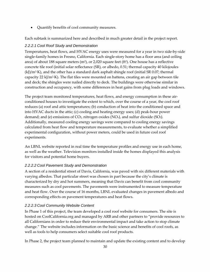
• Quantify benefits of cool community measures. Each subtask is summarized here and described in much greater detail in the project report.

2.2.2.1 Cool Roof Study and Demonstration Temperatures, heat flows, and HVAC energy uses were measured for a year in two side-by-side single-family homes in Fresno, California. Each single-story home has a floor area (and ceiling area) of about 188 square meters (m2), or 2,020 square feet (ft2). One house has a reflective concrete tile roof (initial solar reflectance (SR), or albedo, 0.51; thermal capacity 40 kilojoules (kJ)/m2·K), and the other has a standard dark asphalt shingle roof (initial SR 0.07; thermal capacity 22 kJ/m2·K). The flat tiles were mounted on battens, creating an air gap between tile and deck; the shingles were nailed directly to deck. The buildings were otherwise similar in construction and occupancy, with some differences in heat gains from plug loads and windows.

The project team monitored temperatures, heat flows, and energy consumption in these air-conditioned houses to investigate the extent to which, over the course of a year, the cool roof reduces (a) roof and attic temperatures; (b) conduction of heat into the conditioned space and into HVAC ducts in the attic; (c) cooling and heating energy uses; (d) peak-hour power demand; and (e) emissions of CO2, nitrogen oxides (NOx), and sulfur dioxide (SO2). Additionally, measured cooling energy savings were compared to cooling energy savings calculated from heat flow and temperature measurements, to evaluate whether a simplified experimental configuration, without power meters, could be used in future cool roof experiments.

An LBNL website reported in real time the temperature profiles and energy use in each home, as well as the weather. Television monitors installed inside the homes displayed this analysis for visitors and potential home buyers.

2.2.2.2 Cool Pavement Study and Demonstration A section of a residential street of Davis, California, was paved with six different materials with varying albedos. That particular street was chosen in part because the city’s climate is characterized by dry and hot summers, meaning that Davis can benefit from cool community measures such as cool pavements. The pavements were instrumented to measure temperature and heat flow. Over the course of 16 months, LBNL evaluated changes in pavement albedo and corresponding effects on pavement temperatures and heat flows.

2.2.2.3 Cool Community Website Content In Phase 1 of this project, the team developed a cool roof website for consumers. The site is hosted on CoolCalifornia.org and managed by ARB and other partners to “provide resources to all Californians in order to reduce their environmental impact and take action to stop climate change.” The website includes information on the basic science and benefits of cool roofs, as well as tools to help consumers select suitable cool roof products.

In Phase 2, the project team planned to maintain and update the existing content and to develop 30

new content on cool community strategies—cool roofs, cool pavements, and urban vegetation— for the website’s local government audience. The team worked with ARB to solicit its feedback and comments on the existing web content and reviewed the website to check for content that needed to be updated—most notably the cool roof product search wizard, the cool roof building codes section, and the utility rebate section. All of the existing codes and utility rebates were reviewed to identify changes.

The team developed new content for urban vegetation, cool pavements, and cool roofs for local governments responsible for broad decision-making about city infrastructure. This development mirrored the approach used for the cool roof content. The goal was to convey research to the local government audience in a way that clearly communicates the science and empowers them to implement cool community projects or policies.

To develop new content, the team reviewed journal publications, popular press articles, websites, and presentations from industry and stakeholder groups, and conducted interviews with people who helped implement cool community strategies in their localities. Their experiences were then written up as case studies tailored to the local government audience. The team reviewed all new web content with ARB staff.

2.2.2.4 Cool Community Courses and Resources In Phase 1 of this project, the LBNL team developed training presentations and accompanying brochures/handouts on cool roofs and cool pavements, collaborating with industry groups and Pacific Gas and Electric Company (PG&E) to present on these topics to roofing contractors, and with California’s Department of Transportation (Caltrans) to present to local government officials and design professionals. In Phase 2, the team expanded its outreach by presenting materials in new forums, working with different groups to optimize outreach efforts, revising and updating materials for future outreach opportunities, and developing a cool pavement showcase on the LBNL premises.

2.2.2.5 Codes and Technical Assistance To increase the adoption of cool community strategies more broadly among new California stakeholders, the LBNL team developed new resources; counseled pavement manufacturers on the development of new cool pavement products; coordinated technical assistance to school districts; provided technical review of papers, policies and resources; and guided communities and stakeholders through the steps of implementation for cool community policies and programs. The team also developed model building code language for cool roofs and cool pavements; formed strategic partnerships to leverage outreach and technical assistance resources; and provided technical assistance to entities and individuals interested in adopting cool community strategies or promoting their beneficial use.

2.2.2.6 Quantify Benefits of Cool Community Measures The team used the Weather Research and Forecast model version 3.4.1 (Skamarock 2008) with a nested two-way model configuration centered at Bakersfield, CA. This work applied aerial

31

imagery (1 m2 resolution) to develop model inputs that accurately describe the current roofing stock. Furthermore, this detailed input data allowed estimation of potential albedo enhancement that is spatially resolved throughout the city of Bakersfield. Roofs were divided into two types, flat and sloped, which are considered representative of commercial and residential roofs, respectively. For each grid cell, a weighted average (by roof area) albedo value for sloped and flat roofs was created. As measurements of city-wide pavement albedo were not available, all paved areas were assumed to have an intial albedo of 0.14.

2.2.3 Results 2.2.3.1 Cool Roof Study and Demonstration Relative to the standard home, the home with cool tile roofing saved 2.82 kilowatt-hours per square meter (kWh/m2) each year —a 26 percent savings in annual site cooling energy use.

On representative summer and winter days, maximum roof top, roof bottom, and attic air temperatures in the cool home were lower than in the standard house. Maximum rates of ceiling, HVAC duct, and ceiling + HVAC duct heat gain in the cool home were lower than in the standard house. Minimum roof top, roof bottom, and attic air temperatures in the cool home were higher than in the standard house.

In the cooling season, the mean rates of ceiling and duct heat gain were lower in the cool home than in the standard home; however, mean rates of ceiling and duct heat gain in the heating season were greater in the cool home, thanks to the higher thermal capacity of the cool roof.

Mean reductions in roof top, roof bottom, and attic air temperatures in the cooling season were roughly twice those of the heating season. Above-sheathing ventilation cooling the deck of the cool tile roof may have made the temperature difference at roof bottom larger than that at roof top.

Cool-roof energy savings in the cooling and heating seasons were computed two ways. Method A divides the difference (standard – cool) in ceiling + duct heat gain by the HVAC’s coefficient of performance (COP). Method B measures the difference in HVAC energy use, corrected for differences in plug and window heat gains. Methods A and B agreed well in the cooling season, but not in the heating season. Therefore, all savings are reported based on Method B, which yielded more conservative savings in winter.

The cool roof home achieved annual cooling (compressor + fan), heating fuel, and heating fan energy savings; annual conditioning source energy savings; annual conditioning CO2, NOx, and SO2 emission reductions; and peak-hour cooling power demand reduction.

2.2.3.2 Cool Pavement Study and Demonstration In the cool pavement demonstration, the more reflective pavement surfaces were found to decrease the pavement temperature and thus reduce the heat that is transferred to the local environment and atmosphere by convection and thermal radiation.

32

The site also served to test new pavement technologies, understand proper installation methods, and assess their performances, over time, under realistic conditions.

2.2.3.3 Cool Community Website Content The team successfully incorporated many improvements to the existing cool roof consumer website, including updates to the California building code content. The updated material is listed in Table 5 of the project report. The team also developed extensive web content on cool community strategies for the local government audience. The team encountered problems with the cool roof product search wizard, and efforts are under way to address them.

2.2.3.4 Cool Community Courses and Resources Partnerships were extremely helpful in developing and presenting training presentations and accompanying brochures/handouts on cool roofs and cool pavements. Some key partners were Graniterock, Climate Resolve, and Acterra. The team presented at the California Chip Seal Association’s annual conference, as well as a co-sponsored cool pavement seminar for local government staff in the Bay Area.

Climate Resolve,2 a nonprofit that focuses on creating and communicating ideas to mitigate and adapt to climate change in Los Angeles, sought LBNL input on an initial report for cool roof and cool pavement strategies for Los Angeles. This precipitated their decision to focus on promoting cool surfaces as a strategy for both climate mitigation and climate adaptation. They subsequently invited project team members to present at their Hot City, Cool Roofs3 conference, and they continue to consult on LBNL efforts to advance local government action toward adoption of cool surfaces in Los Angeles.

An active partner in the South Bay has been Acterra,4 a nonprofit focused on environmental education and action. Their Green@Home5 program trains volunteers to go door-to-door to help residents understand options for simple energy-saving techniques and create home energy conservation plans. The LBNL team collaborated with Acterra to develop resources for South Bay residents and their volunteer trainers.

The Public Affairs Department and Facilities Division at LBNL have also been integral partners. Public Affairs has invited the Heat Island Group for several years to host a booth at the LBNL’s Open House event, where it has showcased the science behind cool surfaces to the general public. More recently, the Heat Island Group collaborated with the Facilities Division to turn a new parking lot into a cool pavement showcase.

2 http://climateresolve.org 3 http://climateresolve.org/hot-city-cool-roofs/ 4 http://acterra.org 5 http://acterra.org/programs/greenathome/index.html

33

http://climateresolve.org/

http://climateresolve.org/hot-city-cool-roofs/

http://acterra.org/

http://www.acterra.org/programs/greenathome/index.html

http://climateresolve.org/

http://climateresolve.org/hot-city-cool-roofs/

http://acterra.org/

http://acterra.org/programs/greenathome/index.html

These outreach and technical assistance activities drove interest in voluntary adoption of these measures and led to the inception of several new pilot projects, policies, and programs.

2.2.3.5 Codes and Technical Assistance These efforts led to the development of a cool schoolyard pilot program in the Los Angeles Unified School District (LAUSD), a city-wide building code update to require residential cool roofs, testing and development of three novel cool pavement products, statewide legislation for cool pavements, and statewide guidance on the implementation of cool community measures to mitigate human health exposure during extreme heat events.

2.2.3.6 Quantify Benefits of Cool Community Measures The addition of cool roofs and pavements reduced average afternoon air temperatures across the Bakersfield urban area. Average temperature reductions of 0.3°C were modeled over the downtown Bakersfield area, while smaller average temperature reductions (0.1 – 0.2°C) were found in Bakersfield’s residential neighborhoods. Interestingly, the magnitude of temperature reductions was constant across both summer and winter seasons.

2.2.4 Conclusions and Recommendations 2.2.4.1 Cool Roof Study and Demonstration This study was of particular importance, as it examined the combined benefits of high-SR, high-thermal mass, and above-sheathing ventilation—all inherent to cool tile roofing, the second most popular roofing product in California.

Choosing a cool tile roof in place of a standard asphalt shingle roof offers substantial benefits. For the homes studied (ceiling area 188 m2), annual savings were $167 in energy costs; 307 kilograms (kg) CO2, 117 g NOx, and 8.69 g SO2 reductions; and peak-hour power demand reduction of 165 W.

In the cooling season, energy savings calculated from heat flow and temperature measurements (Method A) closely matched those based on measured energy use (Method B). The two methods did not agree well in the heating season.

The study showed that in a hot California climate such as Fresno, substituting a cool tile roof for a standard asphalt shingle roof can offer substantial annual energy cost savings. To quantify the potential savings, LBNL recommends exploring the following questions:

1. In a climate like that of Fresno, how does the life-cycle cost of a cool tile roof compare to that of an asphalt shingle roof?

2. Could Title 24-approved building-energy simulation tools be used to estimate annual savings in California’s other 15 climate zones, using savings measured in Fresno as a check? Also, is there enough information about the construction, operation, and HVAC equipment of the state’s existing homes to model savings upon re-roofing?

34

3. Based on the number and locations of homes in California, what are the potential statewide energy savings, emission savings, and peak demand reductions if cool tile products were selected in place of asphalt shingle products in (a) all climates or (b) in all climates for which the life-cycle cost of the cool tile roof is less than that of an asphalt shingle roof?

4. Should Title 24 promote the use of cool tile roofing through prescriptive requirement?

5. To what extent can cool tile roofs mitigate the summer urban heat island (lower summer day and night outside air temperatures), and thereby increase comfort, slow the formation of smog, contribute to global cooling (negative radiative forcing of the atmosphere), and further reduce air conditioning demand?

Meanwhile, the team recommends that this study be shared with California’s utilities, so that considerations can be made to update rebate and incentive programs to promote the use of cool tile roofing. Outreach to roofing manufacturers, professionals, and consumers would be helpful. Information about cool tile benefits could be shared through utility billing literature, utility websites, the Cool California website, and the cool roofing courses initially developed by LBNL.

2.2.4.2 Cool Pavement Study and Demonstration The pavement study served two purposes: (1) to determine the ability of various pavement types to reduce solar heat gain, and thereby stay cooler than conventional paving materials; and (2) to test the initial and long-term performances of new pavement technologies, with attention to both materials and installation practices.

To address its first purpose, measurements proved that higher-albedo pavements reduce surface and subsurface temperatures, and reduce daytime heat conducted downward. The results suggest that if the albedo can be raised from 0.1, its current U.S. average, to a value of about 0.3, the result might be, on average, a 12 degree Celsius (22 degree Fahrenheit) decrease in pavement temperature. If the pavements can be kept cooler even when the sunlight is maximal, the air will be cooler, which will reduce the demand for air-conditioning energy and help mitigate the air-polluting effects of high air temperatures.

As for the performance of new pavement technologies, some of the pavements installed initially had albedos well below the expected values and underperformed with regard to soiling resistance. The team then tested other pavement technologies and surface treatment methods. Some problems encountered may have been due to the paving industry’s unfamiliarity with cool pavements, so these experiences may help pavement technology manufacturers improve their current products and installation practices in the future.

The research team recommends that measurements continue to be made at the test site and that manufacturers continue to explore new cool paving technologies. It is also recommended that the Cool Pavement Demonstration be continued as an experimental site, to allow new products

35

to be tested as they are developed and to gain experience using and monitoring potentially promising cool pavement technologies.

Other recommendations include the following:

• Continue research on the self-cleaning capabilities of products. • Ensure that the mix ratios will result in the specified pavement albedo. • Continue to test all curing compounds and sealants under various climate and pavement

use applications to ensure that they do not negatively affect the pavement albedo after placement.

2.2.4.3 Cool Community Website Content The Heat Island Group promotes the cool roof consumer website on flyers, in public presentations, and on its own website. The group often receives calls, especially during summer, from the public with inquiries about cool roofs, so the cool roof consumer website now provides a place to direct them to learn more about tailored solutions. The new content for the local government stakeholders on cool communities will bring these resources to a new audience. There is growing interest in these strategies to help adapt to a changing climate, and easy-to-find resources will aid communities in thinking through these strategies and communicating them to their residents.

Recommendations are as follows: • Continue to search for a solution to the issue with the cool roof search wizard. • Set aside a maintenance fund to address website technical issues as they arise. • Continue to connect consumers and local governments with cool communities

resources. • For the cool roof consumer website, target outreach efforts to audiences that implement

roofing choices. • Connect homeowners with suppliers and service providers informed about cool roofing

products. • Target local government organizations that share resources and best practices among

California localities to increase visibility. • Increase visibility by presenting at local government events.

2.2.4.4 Cool Community Courses and Resources The team successfully continued the Phase 1 outreach efforts and developed new resources to aid stakeholders. Table 7 of the project report includes a complete list of the Phase 2 outreach events; other activities include the development of a new brochure, a cool roof fact sheet, several recorded and web-accessible presentations, and a video on cool pavements. With the addition of the cool pavement showcase, this task created a new resource to help stakeholders engage with the various cool pavement technologies and witness firsthand the cooling effect of

36

these technologies.

2.2.4.5 Codes and Technical Assistance The LBNL outreach efforts have helped drive interest in the topic of cool communities, and the technical assistance and guidance activities have aided key stakeholders in turning their interest into actual cool community programs, policies, and projects. Through these activities, the team was able to provide more tailored support to these stakeholders. City of Los Angeles invited LBNL to explore ideas and products for a cool pavement pilot project, which, if successful, could lead to widespread adoption across the city.

From the initiation of the project to its conclusion, the number of inquiries from the public, policy makers, manufacturers, and other stakeholder groups has grown significantly. Although the number of cool community projects has increased across the state, there is a continued need to provide technical assistance. The project team found this to be especially true of organizations and stakeholder groups that have difficulty sifting through the existing resources and understanding product claims. These groups require tailored resources that help them make the most responsible decisions for their unique applications, projects, or policies.

In addition, the development of additional cool pavement pilot projects can help demonstrate proof of concept and lessen or eliminate uncertainties that prevent wider adoption of cool pavements. To complement pilot projects, manufacturers of cool pavement products need continued technical guidance to develop products that can meet more diverse applications and structural demands in cities and communities.

2.2.4.6 Quantify Benefits of Cool Community Measures A meteorological model was successfully able to quantify the benefits of a cool community. The widespread addition of cool roofs and pavements would likely reduce afternoon temperatures in Bakersfield, lowering air conditioning usage and decreasing the ozone formation rate in downtown Bakersfield. Similar benefits would be expected in other California cities that are alike in size and meteorology to Bakersfield.

2.2.5 Project Benefits Increasing the albedo of roofs and pavements statewide has been estimated to provide an additional one-time GHG offset estimate of 470–1130 MMT CO2e through the process of negative radiative forcing, also known as “global cooling” (Akbari et al. 2008; Akbari et al. 2009; VanCuren 2010). This would equal 17 times the annual GHG reduction yielded by all voluntary measures. All of these activities help California take strides toward meeting its emission reduction goals and conserving energy. But the project components also demonstrated co-benefits for California residents, such as reduced utility bills, improved air quality, and enhanced urban livability.

37

2.2.5.1 Cool Roof Study and Demonstration This study demonstrates that relative to standard asphalt single roofs, cool tile roofs offer substantial annual energy cost savings and emission reductions in Fresno, and that they belong in the state’s portfolio of energy-efficiency technologies. Homeowners benefit from the annual conditioning energy cost savings (20 percent), while the public benefits from reduced emissions of CO2 (15 percent), NOx (10 percent), and SO2 (22 percent) yielded by these annual conditioning energy savings. The electric grid also benefits from the 37 percent reduction in peak-hour cooling and fan energy use.

2.2.5.2 Cool Pavement Study and Demonstration This project demonstrated several characteristics of cool pavements that qualify them as a potential mitigation measure for urban heat islands. Pavement technologies with high albedos were shown to absorb less heat through the surface and achieve lower pavement temperatures at depths close to the surface. It is inferred from this research that high albedo pavements will result in lower air temperatures close to the pavement surface. 2.2.5.3 Cool Community Website Content Web-based targeted resources for key stakeholders can drive interest in, and increase the voluntary use of, cool community strategies. Such strategies have been identified as effective voluntary measures with potential statewide emission reductions of 4 MMT CO2e/y (ARB 2008b). 2.2.5.4 Cool Community Courses and Resources This project showed that targeted courses and materials can connect key stakeholders with resources that drive interest and increase the voluntary use of cool community strategies.

2.2.5.5 Codes and Technical Assistance This project showed the effectiveness of spreading the word about the benefits of cool community strategies through tailored technical assistance and guidance; in fact, this interest is turning into new projects. The continued voluntary adoption of cool community strategies will help California meet its emission reduction goals and conserve energy, but also produce co-benefits for residents, such as reduced utility bills, improved air quality, and enhanced urban livability. 2.2.5.6 Quantify Benefits of Cool Community Measures Cool roofs and pavements offer benefits to California cities such as Bakersfield, and California as a whole, by reducing air temperature and building energy demand during hot summer days.

38

2.3 Reducing Waste in Residential Hot Water Distribution Systems Residential hot water distribution systems (HWDS) deliver hot water from a WH to end uses such as showers and sinks. Heating water accounts for approximately 49 percent of California’s residential natural gas consumption (KEMA 2010), so increasing the efficiency of these systems in California houses could help to reduce the state’s natural gas load significantly.

The efficiency of a residential HWDS is the ratio of energy delivered to the end use by the hot water to the energy leaving the WHas hot water. Previous work suggests that efficiencies for specific end uses may be surprisingly low, but because measuring this efficiency has been difficult, it has only been done a limited number of times. However, recent advances in wireless sensor network (WSN) technology and software for streaming data to a remote server provide an efficient, low-cost system for studying HWDS efficiency.

2.3.1 Goal The goal of this task was to improve the efficiency of hot water distribution systems in California.

2.3.2 Methods For this project, LBNL evaluated waste of water and energy in indoor water use in 21 California homes for up to eight months by measuring the temperature and flow rates of hot and cold indoor water use at the end-use points and at the WH in each house. These measurements were used to calculate the waste of water and energy caused by the HWDS.

To measure water temperature and flow rate at indoor end uses and the WH, LBNL developed a wireless sensor network technology. Monitoring systems installed in the homes from July 2013 to February 2014 metered 5–21 end uses in each house. Water temperatures and flow rates were recorded once per second whenever water was flowing. Water flow and temperature data were successfully collected and uploaded to the data server.

Stakeholder involvement included feedback during an Energy Commission Residential Water Heating Program Advisory Committee meeting, input from plumbers, and presentations of interim results at the American Council for an Energy-Efficient Economy Hot Water Forum and Summer Study.

2.3.2.1 Field Study Plan A field study plan was developed to enroll houses in the project. The plan also described the development, calibration, and installation of the wireless sensor networks and data analysis methodologies used in this study.

Recruitment and selection of study participants took place concurrently with the design and development work. Recruitment materials explained the project to potential volunteers, and interested participants were referred to a website that included a web survey. The survey was used to screen potential study sites and ensure as wide a diversity of building types and occupants as possible. The field study included a range of housing types (single family,

39

townhouse, condo, multi-level, foundation type); WH types; number and range of residents; home size; and number of sinks, toilets, showers, dishwashers, and clothes washers.

Deployment began after the development of the WSN was complete, and the first access agreement was obtained and continued until February 2014. Ongoing debugging services were provided to the network and the homeowner, to allow as complete data collection as possible at each house.

2.3.2.2 Wireless Sensor Network Architecture The project team drew upon previous LBNL work on WSNs—including a pilot-phase study on hot water distribution system for the California Department of Water Resources (Lutz, Biermayer, and King 2009) and miscellaneous electrical end-use loads (Lanzisera et al. 2013)—to design the wireless sensor network. The design was also influenced by available sensors and housings, as determined in the development stage. Design of the network covered the data collection, aggregation, and analysis methodology.

The team began to develop prototype units as the WSN specifications were being completed, and design and programming began after the WSN specifications were complete. The characteristics of low-cost sensors and housings affected the specifications for the WSN. Included in the development phase were the debugging, commissioning, and calibration of the sensors and the wireless network components, which were conducted at LBNL prior to deploying the units to the houses. A crucial aspect of development was a shakedown installation at two test houses to ensure that all aspects of the network and data collection system were working as intended.

See the full project report for more details.

2.3.2.3 Wireless Sensor Network Deployment The WSN consisted of sensor units, each containing a flow meter and thermistor (a type of resistor whose resistance varies significantly with temperature), connected to wireless motes transmitting data to a central “manager” mote. The manager mote posted data to a server at LBNL via the Internet. Figure 2.3.1 shows a schematic of the wireless sensor network.

Source: LBNL

Figure 2.3.1: Schematic of Wireless Sensor Network

40

Initial laboratory testing measured the accuracy of the temperature and flow rate measurements of the first sensor units. The flow rates were accurate for all sensor units tested initially; however, the temperature data from testing the first sensor units indicated that calibration was needed. Therefore, all the sensor units were tested with hot water in the laboratory before being installed the field. The temperatures recorded by the sensor units were corrected to match the temperatures measured by the reference equipment during the laboratory testing for each sensor unit.

The temperature calibration process consisted of: (1) accounting for the unsynchronized clock in the reference temperature data logger, and (2) calculating the coefficients to correct the sensor unit temperature data.

This research project monitored a total of 21 houses, with 5–21 end uses metered in each, with a median of 9 end uses per house. At each house, the researchers followed the same protocol for installation: meeting with the homeowner and walking through the residence with the homeowner. The field research staff and plumber then conducted a general walkthrough of the home to identify the water end uses to be metered, and assessed the feasibility of installing the meters. If any unresolvable issues arose, the house was not included in the study.

The sensor units were installed according the guidelines specified in Table 1.

While the plumber installed the sensor units, the field specialist set up the communication system. Once the monitoring system was installed, the field specialist tested the data connection and functionality of the meters and verified reception of temperature and flow data at the server. The visit concluded by summarizing the installation for the homeowner and talking with the homeowner about how to contact the team. Throughout the study, the researchers checked in with the homeowners periodically to inquire on the status of their installation.

Table 2.3.1: Guidelines for installing sensor units

Site Guidelines

Water Heater Attach one sensor unit to the hot water outlet of the water heater and one to the cold water inlet.

Sink Install two sensor units at each sink; one on the hot water line and the other on the cold water line. Sensor units were installed after the angle stop, and the mote for the two sensor units was placed beneath the sink.

Shower Place one sensor unit between the showerhead and the shower arm. Attach the mote to the wall outside the shower.

Clothes Washer Install two sensor units and one mote at each clothes washer.

Dishwasher Install one sensor unit and a single mote at each dishwasher.

Bathtub Installation of sensor units on tub spouts was not feasible. Source: LBNL

41

2.3.2.4 Data Collection and Analysis Methodology The HWDS monitoring systems yielded as much as eight months of data at each house. Occasionally an anomalous temperature or flow rate was recorded, and obviously inaccurate data readings were detected and deleted. If the inaccurate readings were sporadic and did not appear to indicate any systematic error, they were modified to reflect reasonable values or deleted.

Once the data were screened and cleaned, several data analysis tasks were conducted to analyze (1) water flow volume and temperature, and (2) energy efficiency.

The daily volumes of water measured at the inlet and outlet of the WH were compared for each house. The total amount of water entering a WH can differ slightly from the total volume of water leaving the WH; reasons for this are discussed in more detail in the full report. Problems were found with the outlet flow meters at three houses.

The research team did not measure hot water flow at all showerheads or bathtub spouts. The team reasoned that, if no other flow meters were indicating that flow and hot water were leaving the WH, it is likely that it was going out a tub spout, especially if it was followed directly by a shower.

The energy efficiency of the hot water distribution system depends on the timing of hot water uses and the system’s configuration and insulation levels. The energy content (enthalpy) of water flowing through a sensor unit can be calculated relative to a reference temperature. Using the energy content of the water at the outlet of the WH and the energy content of the water at the end uses, the HWDS energy efficiency can be calculated, either for the entire house’s HWDS for one or more days, or for just one draw or end use.

Dishwasher: Dishwashers are rated for energy efficiency under a test protocol that supplies an inlet water temperature of 140°F (60°C). They have internal heaters to ensure that the water temperature is adequate for cleaning. If the temperature of the water a dishwasher uses in the field is less than the temperature measured when it is tested, that dishwasher’s efficiency will be less than its rated efficiency. A weighted average temperature of the hot water drawn for entire dishwashing cycles can be calculated. This field temperature can be compared with the temperature specified in the test protocol to see how well the test procedure matches field conditions.

Shower: Calculating the energy and water efficiency of a shower event requires several steps. One additional step is to determine the useful portion of the shower event. The time the showering started can be estimated as the time when both the temperature and flow of water at the showerhead become stable, with a temperature in the range of 95 degrees Fahrenheit to 105 degrees Fahrenheit (35 degrees Celsius to 40.5 degrees Celsius). For energy calculations of water used in showers, a reasonable reference temperature is the temperature of the cold water entering the WH at the end of the shower. This would be the temperature of water coming directly from the water supply, as it will not have had a chance to pick up heat from the house or the WH.

42

Data indicated that people routinely run water through the tub spout until hot, and then adjust the temperature before diverting water through the showerhead to start their shower. Sensor units connected at the showerhead of this type of shower will not capture these initial events. Data from open or stall type showerheads will be able to measure this behavior directly. The other way to capture these data is at the WH (for hot water flow) prior to and during shower events.

The water efficiency of a shower event can be calculated according to the following equation.

𝜂𝜂𝑤𝑤𝑤𝑤𝑤𝑤𝑤𝑤𝑤𝑤 =∑ (𝑉𝑉𝑠𝑠ℎ𝑜𝑜𝑤𝑤𝑤𝑤𝑤𝑤ℎ𝑤𝑤𝑤𝑤𝑒𝑒)𝑠𝑠ℎ𝑜𝑜𝑤𝑤𝑤𝑤𝑤𝑤𝑜𝑜𝑜𝑜𝑜𝑜

∑ (𝑉𝑉𝑤𝑤𝑤𝑤𝑤𝑤𝑤𝑤𝑤𝑤ℎ𝑤𝑤𝑤𝑤𝑤𝑤𝑤𝑤𝑤𝑤.𝑜𝑜𝑜𝑜𝑤𝑤)𝑜𝑜𝑜𝑜𝑤𝑤𝑜𝑜𝑢𝑢 𝑠𝑠ℎ𝑜𝑜𝑤𝑤𝑤𝑤𝑤𝑤ℎ𝑤𝑤𝑤𝑤𝑒𝑒𝑤𝑤𝑤𝑤𝑤𝑤𝑤𝑤𝑤𝑤ℎ𝑤𝑤𝑤𝑤𝑤𝑤𝑤𝑤𝑤𝑤 + ∑ 𝑉𝑉𝑠𝑠ℎ𝑜𝑜𝑤𝑤𝑤𝑤𝑤𝑤ℎ𝑤𝑤𝑤𝑤𝑒𝑒𝑠𝑠ℎ𝑜𝑜𝑤𝑤𝑤𝑤𝑤𝑤ℎ𝑤𝑤𝑤𝑤𝑒𝑒

where;

Vshowerhead = volume of water at the showerhead, and Vwaterheater.out = volume of hot water leaving the WH.

When water is not measured at the tub spout, the amount of water can be approximated by the flow of water from the WH just prior to flow at the showerhead. The volume of flow at any other hot water end uses during this time must be subtracted.

Similarly, the energy efficiency of the hot water distribution system for a shower event is the energy content of only the water at the showerhead during the actual showering divided by the energy content of all the water leaving the WH for the showering event.

These methods of calculating the water and energy efficiency of shower events are approximate. More details are included in the full report.

2.3.3 Results LBNL developed a wireless sensor network technology to measure water temperature and flow rate at indoor end uses, and deployed it in 21 houses. Water flow and temperature data were collected and uploaded to a data server.

Preliminary analysis demonstrates that for some shower, kitchen sink, and dishwasher events, only half of the hot water energy inserted into the HWDS at the WH is actually being delivered at the end use. For example, the energy efficiency of the HWDS for a shower described in the full report was calculated to be 53.8 percent. Similarly, the delivered energy efficiency of the HWDS for a kitchen sink in this study was 52.3 percent. The delivered energy efficiency of the HWDS for a dishwasher in this study was 47.4 percent. Efficency of dishwashers is the most inefficient, but showers, sinks and dishwashers are all very inefficient.

2.3.4 Conclusions This research suggests that the efficiency of hot water distribution systems in California homes can be disturbingly low. These findings support the notion that there is significant opportunity to improve the energy efficiency of the HWDS through better design.

43

2.3.4.1 Recommendations Further analysis of the impact of the hot water distribution system should be used to inform revisions to the plumbing codes and the building energy-efficiency codes.

The data gathered from this study could also be used to improve hot water distribution system simulation modeling tools. As part of another task for the Public Interest Energy Research Program, LBNL developed a computer simulation modeling tool for hot water distribution systems (Grant and Lutz 2013). The monitoring in the current task was done in existing buildings, and the team was not able to directly determine detailed characteristics of the plumbing systems, such as the layout, length, diameter, and material of the hot- and cold-water pipes. However, it should be possible to reverse-engineer the key characteristics of the hot water distribution system. This could be done by imposing the flow rates of the observed draw patterns on a simplified model of the HWDS and comparing the temperature profiles at the end uses in the simulation to the observed temperature profiles. By iteratively adjusting the characteristics of the links in the plumbing tree until the simulated temperature profiles best match the observed temperature profiles, it would be possible to calculate an optimized simplified model of the HWDS for each house. These simplified simulation models could be used for creating design guidelines or improving building energy-efficiency standards.

2.3.5 Project Benefits Benefits to ratepayers will accrue from improved HWDS designs for new homes and major retrofits to existing homes based on the findings of this research. The findings also can be used to initiate upgrades of existing plumbing and building energy-efficiency codes.

44

2.4 Encouraging Combined Heat and Power in California Buildings CHP systems produce both electricity and usable heat. The heat is used to increase the total system efficiency of the electricity generation by also supplying building heating or cooling, and steam to industrial processes. Because the heat generated by electricity production is utilized, rather than just expelled as “waste” heat, CHP is prized as a growing, efficient technology.

Governor Brown’s research priorities in the areas of clean energy and energy efficiency call for the development of an additional 6.5 gigawatts (GW) of CHP by 2030 (Neff 2012). As of 2009, the Self-Generation Incentive Program (SGIP) database showed roughly 250 megawatts (MW) of small natural gas- and biogas-fired CHP in the state. Therefore, it is necessary to identify promising approaches for reaching California’s ambitious 6.5 GW goal by 2030. Given the potential for many different generation technologies to contribute to the resource mix during that time frame, it is necessary to take an integrated optimization approach, to optimize the adoption of a variety of technologies for the commercial sector:

• Fuel cells, with and without a heat exchanger for waste heat utilization • Internal combustion engines, with and without a heat exchanger for waste heat

utilization • Microturbines, with and without a heat exchanger for waste heat utilization • Gas turbines, with and without a heat exchanger for waste heat utilization • Photovoltaic • Solar thermal • Electric storage • Heat storage • Absorption chillers • Zero net energy homes; since zero net energy homes will play a role in the future

2.4.1 Goal The goal of this task is to stimulate economic and environmentally sound natural gas-fired CHP and combined cooling, heating, and electric power (CCHP) adoption in California's medium-sized commercial building sector.

2.4.2 Methods 2.4.2.1 Distributed Energy Resources Customer Adoption Model This study used the Investment & Planning version of the Distributed Energy Resources Customer Adoption Model (DER-CAM), a Mixed Integer Linear Programming (MILP) model developed by LBNL. The DER-CAM model has been used extensively to address the problem of optimally investing and scheduling distributed energy resources (DERs) under multiple settings. The Investment & Planning DER-CAM picks optimal microgrid / building equipment combinations based on either 36 or 84 typical days, representing a year of hourly energy loads and technology costs and performance, fuel prices, and utility tariffs.

The objective of using DER-CAM is typically to minimize the annual costs or CO2 emissions for providing energy services to the modeled site, including utility electricity and natural gas

45

purchases, plus amortized capital and maintenance costs for any distributed generation (DG) investments. Other objectives, such as a combination of the formerly mentioned ones, are also possible. The approach is fully technology-neutral and can include energy purchases, on-site conversion, and both electrical and thermal on-site renewable harvesting. Furthermore, this approach considers the simultaneity of results; for example, building cooling technologies are chosen such that the results reflect the benefit of electricity demand displacement by heat-activated cooling, which lowers building peak load and disproportionately benefits consumers because of time-of-use (TOU) energy charges.

The key inputs in the Investment & Planning DER-CAM are:

• hourly electricity, heating, cooling, domestic hot water, and cooking demand for the selected representative commercial buildings; the building load profiles within this project are taken from the California Commercial End-Use Survey (CEUS) 2006 and have been modified and formatted to fit DER-CAM

• electric and natural gas tariffs • technology performance data and costs for the selected DER technologies • CO2 emissions of the macro-grid to assess the CO2 mitigation potential of CHP and

CCHP and other DER • solar radiation for different locations in California, to enable consideration of the impact

of photovoltaic (PV) and solar thermal on CHP/CCHP adoption Figure 2.4.1 shows a high-level schematic of the possible building energy flows modeled in DER-CAM, showing how loads can be met by different resources at given efficiencies, and offering a full view of possible resources that can be considered within the optimization. The arrows represent energy flows, and DER-CAM optimizes those energy flows to minimize costs and/or CO2 emissions. Blue arrows represent natural gas or any biofuel, yellow represents electricity, and light blue represents heat and waste heat.

The Investment & Planning DER-CAM solves the mixed integer linear problem over a given time horizon (e.g., a year) and selects the economically or environmental optimal combination of utility electricity purchase, on-site generation, storage, and cooling equipment required to meet the site’s end-use loads at each time step.

The outputs include the optimal DG/storage adoption and an hourly operating schedule, as well as the resulting costs, fuel consumption, and CO2 emissions. All available technologies compete and collaborate, and simultaneous results are derived.

46

Figure 2.4.1: Schematic of energy flows in DER-CAM

2.4.2.2 Distributed Energy Resources Customer Adoption Model The starting point for the load profiles used within DER-CAM is the CEUS database. The database excludes the Los Angeles Department of Water and Power (LADWP) customers, and some other small zones were excluded for this study. The researchers also eliminated building types for which there was insufficient information for simulation and buildings outside of the focus area: mid-sized buildings above 100 kW (or 50 kW in the case of restaurants). That left 37 percent of the total commercial electric demand in the service territories of PG&E, Southern California Edison (SCE), and San Diego and Gas Electric (SDG&E) (CEUS 2006).

Because CEUS buildings each represent a certain segment of the commercial building sector, results from typical buildings can readily be scaled up to the state level to provide policymaking insights.

2.4.2.3 Assumptions The electric rates and natural gas prices are important drivers for CHP adoption. The tariffs used for the study are based on 2012 observations and kept constant in real terms.

In the case of natural gas, the current low prices seemed like unrealistic estimates to apply to 2020 and 2030, therefore, different price assumptions were tested. Note that only natural gas was used as an input fuel for internal combustion engines, microturbines, and fuel cells; no biogas was considered.

47

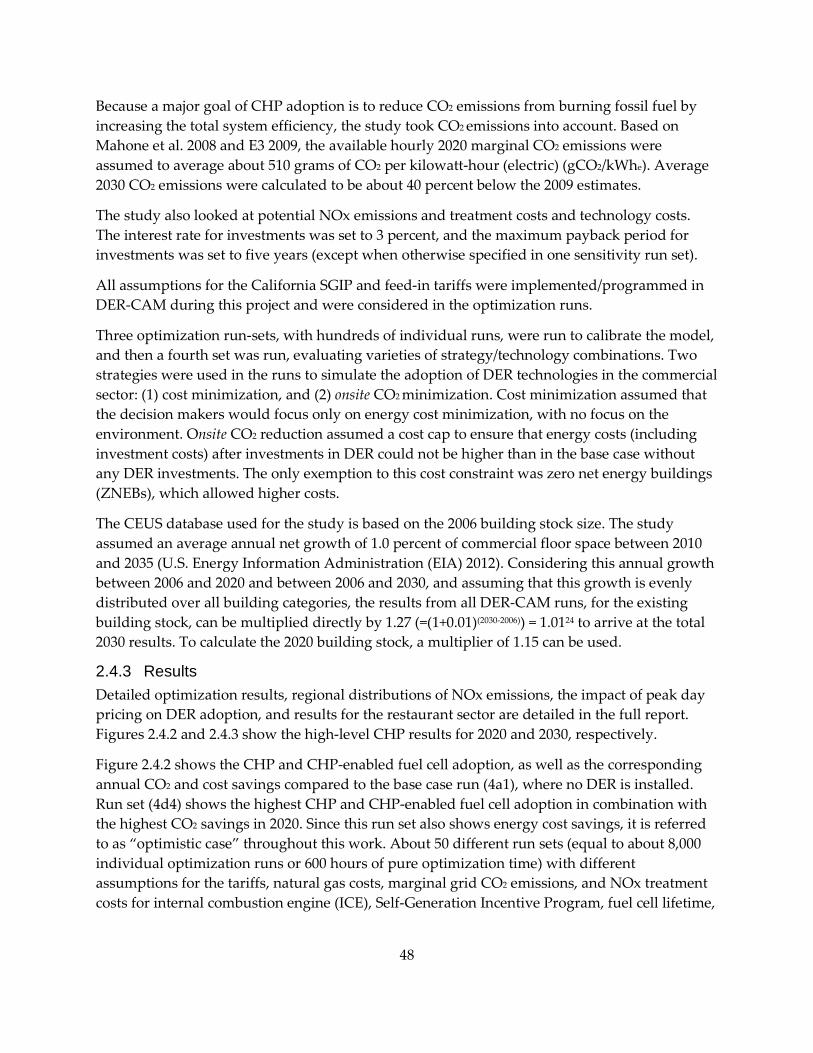
Because a major goal of CHP adoption is to reduce CO2 emissions from burning fossil fuel by increasing the total system efficiency, the study took CO2 emissions into account. Based on Mahone et al. 2008 and E3 2009, the available hourly 2020 marginal CO2 emissions were assumed to average about 510 grams of CO2 per kilowatt-hour (electric) (gCO2/kWhe). Average 2030 CO2 emissions were calculated to be about 40 percent below the 2009 estimates.

The study also looked at potential NOx emissions and treatment costs and technology costs. The interest rate for investments was set to 3 percent, and the maximum payback period for investments was set to five years (except when otherwise specified in one sensitivity run set).

All assumptions for the California SGIP and feed-in tariffs were implemented/programmed in DER-CAM during this project and were considered in the optimization runs.

Three optimization run-sets, with hundreds of individual runs, were run to calibrate the model, and then a fourth set was run, evaluating varieties of strategy/technology combinations. Two strategies were used in the runs to simulate the adoption of DER technologies in the commercial sector: (1) cost minimization, and (2) onsite CO2 minimization. Cost minimization assumed that the decision makers would focus only on energy cost minimization, with no focus on the environment. Onsite CO2 reduction assumed a cost cap to ensure that energy costs (including investment costs) after investments in DER could not be higher than in the base case without any DER investments. The only exemption to this cost constraint was zero net energy buildings (ZNEBs), which allowed higher costs.

The CEUS database used for the study is based on the 2006 building stock size. The study assumed an average annual net growth of 1.0 percent of commercial floor space between 2010 and 2035 (U.S. Energy Information Administration (EIA) 2012). Considering this annual growth between 2006 and 2020 and between 2006 and 2030, and assuming that this growth is evenly distributed over all building categories, the results from all DER-CAM runs, for the existing building stock, can be multiplied directly by 1.27 (=(1+0.01)(2030-2006)) = 1.0124 to arrive at the total 2030 results. To calculate the 2020 building stock, a multiplier of 1.15 can be used.

2.4.3 Results Detailed optimization results, regional distributions of NOx emissions, the impact of peak day pricing on DER adoption, and results for the restaurant sector are detailed in the full report. Figures 2.4.2 and 2.4.3 show the high-level CHP results for 2020 and 2030, respectively.

Figure 2.4.2 shows the CHP and CHP-enabled fuel cell adoption, as well as the corresponding annual CO2 and cost savings compared to the base case run (4a1), where no DER is installed. Run set (4d4) shows the highest CHP and CHP-enabled fuel cell adoption in combination with the highest CO2 savings in 2020. Since this run set also shows energy cost savings, it is referred to as “optimistic case” throughout this work. About 50 different run sets (equal to about 8,000 individual optimization runs or 600 hours of pure optimization time) with different assumptions for the tariffs, natural gas costs, marginal grid CO2 emissions, and NOx treatment costs for internal combustion engine (ICE), Self-Generation Incentive Program, fuel cell lifetime,

48

fuel cell efficiency, PV installation costs, and maximum payback period have been performed in this project.

(Source: DER-CAM runs)

Figure 2.4.2: High-level CHP results for 2020

Figure 2.4.3 shows the same results for all 2030 run sets. From this figure it becomes evident that only CO2 minimization strategies (run sets 4e) of building owners can elevate the CHP-enabled fuel cell adoption (the green line in Figure 2.4.3). Run set (4e10) shows a considerable amount of CHP and CHP-enabled fuel cells in combination with cost and CO2 reductions. Thus run set (4e10) is frequently used in the final report. Run set (4e12), the ZNEB run set, is interesting since it demonstrates that ZNEB can support the CHP-enabled fuel cell adoption. However, run sets (4e5) and (4e6), also ZNEB runs, do not show CHP-enabled fuel cell adoption, demonstrating how sensitive the results are to investment costs, efficiencies, and payback periods.

49


Figure 2.4.3: High-level CHP results for 2030

2.4.3.1 High-level Comparison of 2020 and 2030 Results Figures 2.4.4 through 2.4.7 below show the most optimistic run sets for 2020 and 2030. The total amounts for the most optimistic case in 2020 are about 2,385 MW of CHP and about 2,116 MW of fuel cells with heat exchangers. The total CHP capacity is 1,961 MW in 2030.


Figure 2.4.4: Installed CHP capacity by utility service territory, for most optimistic case (4d4),6 2020

6 Assumption for the run set 4d4: carbon minimization strategy with SGIP, higher electrical fuel cell efficiency of 46 percent, and a maximum payback period of 10 years.

50

Note: FCZXX refers to different climate zones within the service territory of the considered utility. (Source: DER-CAM runs)

Figure 2.4.5: Installed CHP capacity by forecasting climate zone, most optimistic case (4d4), 2020


Figure 2.4.6: Installed CHP capacity by utility service territory, run set case (4e10)7 for 2030

7 Assumption for the run set 4e10: carbon minimizing strategy and increased lifetime of fuel cells (from 10 to 20 years), overall fuel cell efficiency of 92 percent (60 percent electric efficiency), and a 10-year maximum payback period for investments.

51


Figure 2.4.7: Installed CHP capacity by forecasting climate zone, run set (4e10) for 2030

The most optimistic case for 2020 shows about 2.1 GW of fuel cells with heat exchangers, and the case for 2030 shows about 1.1 GW of fuel cells with heat exchangers, which effectively means a 50 percent reduction of fuel cells with heat exchangers by 2030 due to grid decarbonization. The 2030 run set does not consider any SGIP.

2.4.4 Conclusions About 8,000 individual optimization runs were performed with the Distributed Energy Resources Customer Adoption Model (DER-CAM), focusing on commercial facilities with a peak electricity load above 100 kW, and 50 kW for restaurants. To analyze the role of DER in CO2 reduction, 147 representative sites in different climate zones were selected from the CEUS.

Two major customer adoption DER adoption strategies were simulated with DER-CAM: (1) cost reduction as a primary goal, and (2) CO2 reduction as a primary goal.

2.4.4.1 2020 The 2020 cost reduction runs showed no major fuel cell adoption except when a SGIP, a high fuel cell efficiency, and 10-year payback period is considered (run set 4b4). The 2030 cost reduction runs showed CHP adoption but no significant CHP-enabled fuel cell adoption. Because most of the cost reduction runs showed no significant reduction in environmental impacts (except run set 4b4), CO2 reduction strategies are most favorable to consider.

However, a SGIP extension until 2020 shows promising results in terms of CHP fuel cell adoption. Assuming a 10-year payback period, fuel cells that reach 46 percent electric efficiency and sustain 10 years without a stack replacement, and CO2 reduction as the prime goal, roughly 2.1 GW of CHP-enabled fuel cells are possible in currently existing commercial buildings with electric peak loads above 100 kW (50 kW for restaurants). Microturbines could also play a role. Some 125 MW of CHP-enabled microturbines could help the restaurant sector reduce its CO2

52

emissions by 15 percent and save 6 percent of costs. In addition to fuel cells, CHP-enabled microturbines also play a role, and the total CHP capacity, considering the building stock growth, could reach 2.7 GW in 2020. The CHP potential in combination with PV and solar thermal could reduce CO2 emissions by 37 percent and save building owners 5 percent in total building energy costs. If the fuel cell adoption rate were as high as estimated, NOx emissions would not seem to pose a problem. A rough simulation of the recently introduced Peak Day Pricing scheme in the San Francisco Bay Area indicates increased CHP potential. However, further research will be needed to confirm this result.

2.4.4.2 2030 The 2030 results are more complicated. Assuming an expired SGIP and fulfillment of the expected grid decarbonization, the runs show fewer fuel cells in 2030 compared to 2020. Further assuming a 60 percent electric efficiency and 20-year lifetime of fuel cells, a payback period of 10 years, and a CO2 minimization strategy, 1 GW of CHP-enabled fuel cells are possible in the existing commercial building stock considered for this study. The CHP-enabled fuel cell adoption could reach more than 1.4 GW if zero net energy buildings are considered. In a ZNEB scenario, PV and solar thermal adoption is high, but CHP-enabled fuel cell adoption will also increase, and this is an indication that natural-gas-fired engines would not be eliminated in a ZNEB environment. Some 47 MW of CHP-enabled microturbines could help the restaurant sector reduce CO2 emissions by 14 percent and save 7 percent of costs. Considering the building stock growth, the fuel cell adoption could go up to 1.3 GW, and up to 1.8 GW with some ZNEB setups.

In addition to fuel cells, CHP-enabled microturbines also play a role, and the total CHP capacity, considering the building stock growth, could reach 2.5 GW in 2030. This CHP potential, in combination with PV and solar thermal, reduces CO2 emissions by 25 percent and saves building owners 11 percent in total building energy costs. The used commercial building stock roughly represents 37 percent of the statewide commercial sector electricity consumption. Thus, 2.5 GW of CHP in 2030 would contribute 38 percent to California’s goal of 6.5 GW of additional CHP in 2030. The 2.5 GW of CHP in 2030 can only be reached if fuel cell technologies have payback periods of 10 years, reach very optimistic system efficiencies of 92 percent, can sustain 20 years without any stack replacement, and if policies are in place to support CO2 reduction objectives of investors.

Finally, the possible CHP potential in 2030 shows a significant variance, between 0.2 GW and 2.5 GW, and demonstrates the complex interactions between different DER technologies and customer objectives. Such situations underscore the need for integrated optimization/simulation approaches as those used by DER-CAM.

2.4.5 Project Benefits Because the techological, environmental, economical, and policy issues that need to be considered to expand California’s CHP capacity are so numerous, it is necessary to employ integrated analyses to evaluate potential options. The results from this project can be used to

53

develop the most promising pathways to reach California’s goal of an additional 6.5 GW of CHP by 2030. Moreover, the DER-CAM can continue to be used to further refine these analyses.

54

2.5 Improved Audio-Video Efficiency through Inter-Device Power Control An audio-video (A/V) system is a collection of devices that delivers audio content (usually on loudspeakers) and/or video content (usually on a television). These systems are used in many different ways that require different sets of devices to be switched on and active, and many of these devices often remain on long after the time they are needed, wasting energy sometimes for hours or days.

Most A/V devices exist in local networks, where more than one device (such as a media player or set-top box) is involved in any particular stream of content. Some current technologies can pass power control signals from one device to another and some exchange functional information so that a device can make its own decisions about power control, but they cannot cover all usages. Manually managing the power state (for example, using the remote control power button) can be non-intuitive, cumbersome, and annoying, so neither users nor devices can reliably control power, and many devices remain on.

Audio and video devices in U.S. homes are estimated to consume about 140 terawatt-hours per year (TWh/year) (Urban et al. 2010). If these devices are left on unintentionally even 10 percent of the time, the electricity demand from that unnecessary usage amounts to more than 1 TWh/year—resulting in well over $1 billion/year in wasted energy. By devising means to enable consumers to manage A/V devices more easily, this energy use and its associated costs could be greatly reduced. Anticipated costs to consumers for adding power management to A/V devices is negligible or low, making these strategies highly cost-effective.

2.5.1 Goal This task’s goal was to save substantial electricity by creating a technology standard for how interconnected audio/video devices manage their own power state, and incorporate this into communication standards and future products.

2.5.2 Methods Initial phases of research included assessing the features and capabilities of relevant products for sale today and evaluating communication technologies currently used in A/V systems. This baseline provided an understanding of individual device behavior and inter-device coordination among available technologies and products.

Each A/V system consists of a source (such as a digital video disc (DVD) player), an intermediate device (such as a receiver), and a sink (such as a television). Each of these devices has its own power controls and set of interfaces for communications. The research team characterized each element of these systems—devices, power states, interfaces and links, streams, sources, sinks, intermediate devices, and control signals—to identify the ways that the A/V data streams are passed to one another.

The research team developed a set of use cases to cover usage scenarios that a technology solution would need to implement. In parallel, the team created a new technology concept of

55

persistent or “sleeping” content streams as the mechanism for inter-device communication. This concept appeared to satisfy all the use case needs. Technology standard developers and committees reviewed the sleeping stream concept and offered comments.

The team sought to affect the behavior of future A/V devices by changing the communication standards used to pass A/V data streams. Additional data exchanged between devices could provide information so that devices can make better decisions about their own power state. While ensuring that a device can know when it can power down has long been a concern for energy policy, this technology also addresses the other part of device behavior—knowing when a device should power up. Communication standards would require specific features, which manufacturers would then need to implement in products. Thus, changing the standards is a way to change future products. Communication standards are created by committees with representatives from A/V manufacturers, so this project aimed to make it as easy as possible for manufacturers to recognize the value of the team’s research conclusions (and include the new technology in their products) by minimizing their burden. This approach was embedded in the project from the beginning.

The core approach of this project was to do the time-consuming work of coming up with a technology solution in this area, then present it, mostly complete, to companies and standards organizations.

2.5.3 Results 2.5.3.1 Improved A/V Power Control Architecture This project’s new A/V power control architecture builds on existing technologies, and includes key changes and additions. Power control is primarily about transitions: how a device knows when its state should change.

To address power control, the team developed the sleeping stream concept, which is detailed in Appendix C of the full project report. That appendix covers use cases for device and stream operation, the needed device behaviors, and particular issues requiring special attention.

Sleeping streams are based on several guiding principles:

• There is no central control. • Devices inform each other about their power and functional state, and use that

information to determine in which power and functional state they need to be. • Named content streams (and their characteristics) define the outcomes that each device

helps to implement. • Successful technologies with wide market penetration are used as a basis for future

products, to increase their overall use and their chance of being used into the future. • The widely accepted “sleep” metaphor is used to promote easy understanding among

both technical audiences and ordinary users. An alternative to the sleeping stream approach would be a central control device that would manage the power state of all A/V devices in a local network. However, this approach appears

56

to be more costly, less effective, and more likely to fail than the sleeping stream approach. One could require that all devices participate in a single network protocol, but this is unlikely, at least for the foreseeable future (principally due to the very different link technologies involved), and in comparison to the sleeping stream model, seems unnecessary. Sleeping streams create a distributed network of intelligent devices, each aiming to minimize energy use.

The project built on lessons learned over the last several decades on how to manage digital devices in a network context. Key among these are:

• Use a three-state power state model and make this model clear in the user interface • Maintain network connectivity in sleep • Ensure that power management is as automatic as possible • Require delays on device wakeup to be short (a few seconds at most)

These lead to several conclusions about devices; they should:

• Be aware of the power state of other A/V devices in the local network • Be aware of the functional state of other A/V devices in the local network • Mostly toggle between on and sleep • Be quick to wake and (relatively) slow to go to sleep

Additional goals include a distributed solution, with devices controlling their own state. The technology should be automatic, enabled by default, and require no configuration. Central control can be implemented through layering on top of automatic distributed control; a key concept is that the central control can stop operating, and the system will continue to work.

The fundamental principle describing how a device should operate is that it should “wake up when it needs to, and go to sleep when it can.”

2.5.3.2 Use Case Analysis In constructing the use cases, a design criterion was that users primarily desire that devices are on and available when they are wanted, so it is important to minimize or avoid forcing people to power up devices manually. To maximize user convenience and fulfill user expectations, the devices need to always wake if they need to (or may possibly need to). If devices fail to respond instantly, users will likely disable power saving features, leading to much energy waste.

The analysis began with an extensive assessment of abstracted use cases of device operation that affect power states in the context of sleeping streams. Use cases that cover up to three devices are sufficient, because cases with more than three simply involve multiple intermediates and so can be mapped into one of the three-device cases.

Table 2.5.1 shows an example use case with two devices and one content stream. The START and END lines show the power state of each device, while the intermediate lines show the sequence of actions taken by individual entities. If the TV had already been on at the start of the process, the resulting sequence would be effectively the same, since waking the stream would

57

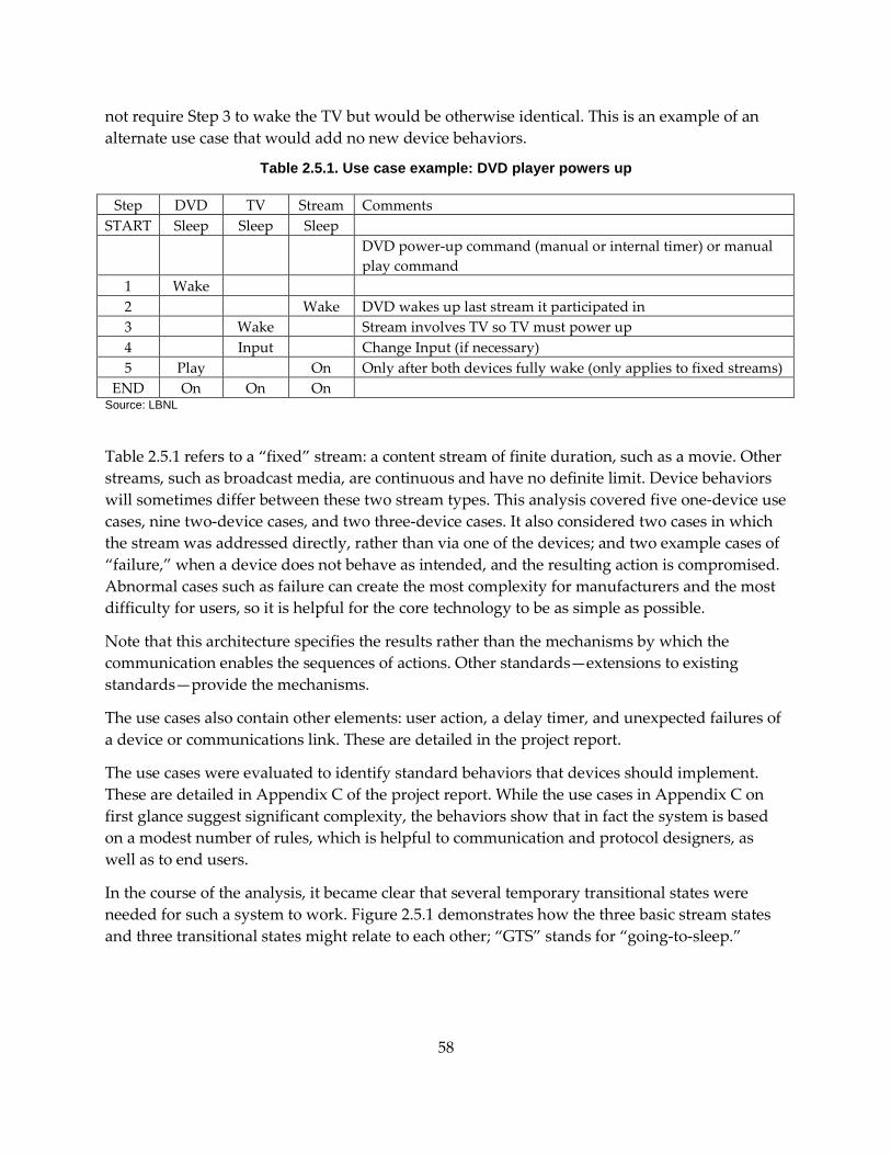
not require Step 3 to wake the TV but would be otherwise identical. This is an example of an alternate use case that would add no new device behaviors.

Table 2.5.1. Use case example: DVD player powers up

Step DVD TV Stream Comments START Sleep Sleep Sleep

DVD power-up command (manual or internal timer) or manual play command

1 Wake 2 Wake DVD wakes up last stream it participated in 3 Wake Stream involves TV so TV must power up 4 Input Change Input (if necessary) 5 Play On Only after both devices fully wake (only applies to fixed streams)

END On On On Source: LBNL

Table 2.5.1 refers to a “fixed” stream: a content stream of finite duration, such as a movie. Other streams, such as broadcast media, are continuous and have no definite limit. Device behaviors will sometimes differ between these two stream types. This analysis covered five one-device use cases, nine two-device cases, and two three-device cases. It also considered two cases in which the stream was addressed directly, rather than via one of the devices; and two example cases of “failure,” when a device does not behave as intended, and the resulting action is compromised. Abnormal cases such as failure can create the most complexity for manufacturers and the most difficulty for users, so it is helpful for the core technology to be as simple as possible.

Note that this architecture specifies the results rather than the mechanisms by which the communication enables the sequences of actions. Other standards—extensions to existing standards—provide the mechanisms.

The use cases also contain other elements: user action, a delay timer, and unexpected failures of a device or communications link. These are detailed in the project report.

The use cases were evaluated to identify standard behaviors that devices should implement. These are detailed in Appendix C of the project report. While the use cases in Appendix C on first glance suggest significant complexity, the behaviors show that in fact the system is based on a modest number of rules, which is helpful to communication and protocol designers, as well as to end users.

In the course of the analysis, it became clear that several temporary transitional states were needed for such a system to work. Figure 2.5.1 demonstrates how the three basic stream states and three transitional states might relate to each other; “GTS” stands for “going-to-sleep.”

58

Source: LBNL

Figure 2.5.1. State diagram for stable and transitional stream states

Devices commonly have internal transitional states, but the system architecture may not need to represent them externally in the way that it recognizes detailed stream states. Current content streams are usually simple, but it is quite possible, and even likely, that future streams will include branches into or out of the core stream, as well as being longer than three devices. It is not apparent that such complexity needs to change the basic operation of streams sleeping and waking, except for how failure modes are treated.

2.5.3.3 Sleeping Streams The research team chose the term sleeping streams as the overarching concept of this project as it simply and effectively summarizes the concept; an equivalent term is persistent streams, to indicate that the streams exist over long periods of time. A “sleeping” stream maintains its representation within devices and networks, but no media content is communicated. This enables new functionality, and what is desired by the user can more easily match the power and functional state of devices. Sleeping can extend for months or years, and waking a sleeping stream requires few steps. An attribute of the sleeping stream concept is that when a new stream is to be created, all of the involved devices must be fully awake. This reduces the complexity that a sleeping device must implement. For example, security and authentication present significant challenges, and these are only addressed by devices that are fully on.

The use case and behavior analysis showed that the combination of sleeping devices and sleeping streams provides needed flexibility for a variety of current and emerging usage scenarios while keeping the complexity of the system manageable for both devices and the people that use them. The previous parts of the project set the stage for it, by clarifying the current context of technologies and devices, but this part of the project fleshed out the persistent stream concept, and demonstrated that it works well for a wide variety of contexts.

2.5.3.3 User Interfaces Past experience with power control of electronics has shown that unclear or inconsistent user interfaces are a barrier to saving energy. In addition, standardizing user interfaces has very little, to no, effect on manufacturing cost, and improves the overall user experience. One need is to clearly embody the three-state power model into A/V devices, in hardware (including

59

indicator lights), and software controls (Institute of Electrical and Electronics Engineers (IEEE) 2004; Nordman 2003). Also, user interfaces for device control should include device power state information, so that when available devices are shown, there are subtle distinctions made between those that are fully on and those that are asleep (currently, off devices are generally not visible at all on user interfaces). This distinction can help alert users when there are functionality differences between sleeping and on devices. It can also help a user diagnose problems, such as identifying devices that are fully on, unnecessarily. Many users do not normally see A/V devices, as they are often stored in cabinets, closets, or elsewhere.

A further user interface challenge is how to represent content streams other than those actively being viewed. It remains to be seen what overall principles and approaches manufacturers will bring to this use case, so it is premature to comment on it from the energy perspective. However, a clear visual distinction between streams that are on or asleep is needed, and this can be standardized.

2.5.3.3 Other Considerations The analysis examined other considerations, such as named streams, occupancy, failures, multiple streams in a network, multiple streams per device, multiple sinks and/or sources, creating and maintaining streams, emergency broadcasts, and transitioning legacy devices. These issues are detailed in the project report.

2.5.4 Conclusions Once the technology concept was developed, the team brought it to individuals who work in the relevant product and technology areas—to confirm that the idea was sound, valuable, and compatible with existing technologies, and to develop support in the standards arena. The team had extensive discussions with individuals and with standards committees, including those representing HDMI, IEEE 1722.1 (for audio video bridging (AVB) systems), UPnP, DisplayPort, and mobile high-definition link (MHL). As a result, it became clear that current technologies do not have all the elements needed for sleeping streams, but there was no conflict between existing standards and sleeping streams. In some cases, existing elements of technologies could be expanded to implement sleeping streams.

The Consumer Electronics Association (CEA) ultimately created a working group to address this topic area, with the intent that it will write an umbrella standard to implement persistent streams. Individual technology standards will be able to add necessary features identified in the CEA standard. Device manufacturers can then include behaviors specified by the standard.

2.5.5 Project Benefits Public energy-efficiency programs, whether voluntary or mandatory, will be able to reference the new technology standards developed in this project. The energy savings could be substantial. In the United States, it seems quite plausible that A/V power control technology could save on the order of 10 percent of consumption of the core A/V devices today, or 13 TWh/year. It also seems plausible that 5 percent in the PC and related device energy could be saved, for another 8 TWh/year. The total of both groups would be about 20 TWh/year.

60

Assuming that California is typical of the United States, and reflects 12 percent of the population, this amounts to a total of about 2.4 TWh/year for the state.

61

2.6 Building Air-Tightness through Appliance Venting Standards Air sealing of homes to reduce the uncontrolled entry of outdoor air is typically among the most cost-effective home retrofit measures to reduce energy consumption and associated GHG emissions. However, when exhaust ventilation equipment is operated in tighter homes, combustion appliances are more prone to backdraft and spill harmful exhaust gases into the living space. Backdrafting and spillage result from a confluence of contributing physical factors that include appliance characteristics and location; vent materials, design, and configuration; airtightness of the house in general and the combustion appliance zone in particular; weather conditions; characteristics of other mechanical systems in the house; and use patterns of the appliance and other mechanical systems.

Many tests and assessment protocols have been developed to identify appliances and housesthat present a backdrafting hazard. The two most common tests are (1) short-term (stress) tests and (2) monitoring. Stress tests, performed under induced conditions, indicate the possibility of backdrafting and capture the effects of outdoor temperature and wind on venting potential only at the time of the test. Monitoring seeks to capture a larger sample by assessing operation under actual conditions over a longer period of time. However, both test methods may produce misleading results and fail houses when backdrafting is not actually a problem or pass houses that actually may have a problem under certain conditions.

Backdrafting and spillage occur only with some confluence or coincidence of physical processes, so it is relevant to consider both statistical and physical characteristics. Currently, there is no clearly stated, statistically rooted risk mitigation target for existing combustion safety diagnostic protocols. Specifying a clear risk mitigation objective is important—not only to assess whether an appliance and venting configuration is problematic, but also to assess whether a test is effective at finding problematic installations.

2.6.1 Goal The goal of this task is to improve energy efficiency while maintaining occupant health and safety by reducing the combustion appliance barrier to increased air tightening.

2.6.2 Methods Our approach to overcoming some of the limitations associated with stress tests and monitoring was to use physics-based computer models to simulate the operation of an appliance and other exhaust systems over a typical location-specific weather year. In practice, many of the relevant physical parameters have a probabilistic nature: that is, they vary over time or from house to house. With all of this information and a model that appropriately captures the physical relationships, one can predict the occurrence and frequency of sustained backdrafts and spillage and the associated indoor pollutant concentrations. This information can in turn provide input for defining airtightness, air change rate, and unbalanced ventilation constraints that enable combustion appliances to vent properly while minimizing associated energy penalties.

To that end, this project used a literature review, field measurements, and computer simulations to identify and evaluate tests and protocols for assessing combustion safety.

62

2.6.2.1 Literature Review The research team first conducted a literature review to summarize the metrics and diagnostics used to assess combustion safety, document their technical basis, and investigate their ability to identify risk mitigations.

2.6.2.2 Field Measurements Using VENT-II VENT-II software is designed to simulate vent shaft thermal performance, including the airflow and pressure dynamics associated with heating the vent, and it has been used to generate vent sizing tables in the National Fuel Gas Code. The purpose of this effort was to assess its ability to predict combustion gas spillage events due to house depressurization by comparing VENT-II simulated results with experimental data for four appliance configurations.

2.6.2.3 Computer Simulation The team carried out three related simulation studies—a spillage study, an airflow driver study, and a yearly distribution study—to better understand the risk associated with house depressurization and combustion spillage, and to provide a solid knowledge base for future development of improved diagnostics.

The spillage study was designed to bound the problem under realistic conditions, the airflow driver study to relate depressurization to airflows, and the yearly distribution study to combine the airflow and concentration models under realistic weather conditions. The yearly distribution study puts the results of the other two studies into context by accounting for the actual distributions of the wind and temperature conditions that help set airflow.

The simulations used a simple box model and then a more elaborate multizone airflow-pressure-contaminant transport analysis program (CONTAM).

2.6.3 Results The results show that existing diagnostic tests based on “worst-case depressurization” are fundamentally flawed. New tests need to be developed to identify when (1) flows stall in combustion appliance vents, and (2) to assess the statistical variation of spilled pollutant concentrations and associated health risks.

Detailed results are presented in the full report.

2.6.3.1 Literature Review The literature review found that the objectives of available stress and monitoring test methods are not clearly defined. Three of the most important other findings are as follows:

• Venting systems that meet NFPA 54 (National Fire Protection Association) standards are much more likely to properly vent than those that do not meet the standards.

• Carbon monoxide (CO) output under downdraft conditions can be reduced if combustion appliances are properly cleaned and tuned.

• WHs have greater backdrafting potential than furnaces, but available data indicate that conventional storage WHs very rarely have high CO emissions.

63

2.6.3.2 Field Measurements Using VENT-II The validation of VENT-II resulted in two very important findings:

• VENT-II correctly predicted spillage depressurization for appliances operating in cold and mild outdoor conditions, but could not accurately predict spillage depressurization for hot outdoor conditions.

• Due to inconsistent errors with the solver, an exact spillage depressurization could not be determined for a few cases. Therefore, VENT-II may not properly identify appliances that are spilling in practice.

Although VENT-II provides a first step toward modeling vent systems, further development is required to produce a reliable program that can correctly predict spillage caused by depressurization.

2.6.3.3 Computer Simulation The simulations showed that current diagnostics tests are fundamentally flawed. Broadly speaking, they suggest that current limits on fan-induced pressure change should be considered only rules of thumb. They probably lead to overly cautious air tightening and remediation, and do not necessarily represent worst cases that occur at modest rather than maximum depressurization. Some of the most important findings of the simulations are as follows:

• For short (≤ 5 minutes) spillage events, current combustion safety protocols are protective against life-threatening CO conditions, even in the case when the appliance is malfunctioning and has repeated intermittent spillage. However, the protocols likely establish CO thresholds that are too conservative for large houses with infrequent spillage events.

• Prolonged or continuous spillage events in a moderately airtight house could result in an acute hazard if the burner is malfunctioning. Therefore, combustion safety protocols should ensure that conditions of sustained spillage and high emissions do not exist without high ventilation.

• Reaching life-threatening conditions in a moderately tight house with a natural draft appliance is rare and almost impossible for an induced draft appliance. However, in a very tight house, the combination of low air change rate and increased risk of spillage significantly increases the potential for prolonged pollutant exposure that could lead to a life-safety hazard.

• The most dangerous conditions result from stalled flow in the appliance vent shaft. While strong depressurization and negative (inward) airflows bring combustion products into the occupied space, these airflows also dilute the combustion products.

• Fan-induced pressure change—the metric used in current stress testing—does not directly assess whether flow will stall or reverse in the vent shaft. The pressure change needed to reverse flow in the vent shaft depends not only on fan-induced pressure

64

differences, but also on naturally induced weather-related pressure differences, which vary throughout the year.

• A large enough fan-induced pressure change does imply backdrafting. However, by the time fan-induced pressure change is large enough to guarantee backdrafting, it is almost never of concern in terms of indoor air quality, due to the dilution that it contributes by outdoor air entering through the vent.

• Regardless of fan-induced depressurization, the building professional should always ensure that the appliance burner is clean, the appliance is functioning properly, the vent system is connected to the appliance, and draft is established in a short period of time.

2.6.4 Conclusions Although air sealing of homes is among the most cost-effective home retrofit measures to reduce energy consumption and associated GHG emissions, tighter homes more readily depressurize when exhaust ventilation equipment is operated. Therefore, combustion appliances are more prone to backdraft and spill harmful exhaust gases into the living space. New tests need to be developed to identify when flows stall in combustion appliance vents and to assess the statistical variation of spilled pollutant concentrations and associated health risks.

One solution to reducing or eliminating health and safety risks associated with spillage is to use sealed combustion appliances or to locate them outside the pressure boundary of the occupied space. However, when that is not cost effective, a diagnostic procedure should be used to assess the risks of spillage for the house and appliances, both as found and as they might operate if retrofits such as house air tightening were to be implemented. New tests need to be developed to identify when flows stall in combustion appliance vents and to assess the statistical variation of spilled pollutant concentrations and associated health risks.

2.6.4.1 Recommendations This report outlines a series of seven recommended changes to current combustion safety diagnostics, based on the literature review and simulation studies.

1. Eliminate comparisons of worst-case depressurization test results to threshold limits by appliance type.

2. Ensure that diagnostic protocols include inspections of air supply, appliance operation, and venting.

3. Include a draft test under challenge (but not worst case) depressurization conditions.

4. Apply assurance procedures to all appliances used as heat sources in the house.

5. Include kitchen ventilation in combustion safety assessments.

6. Coordinate with American National Standards Institute (ANSI) to reduce allowable CO levels in new appliances.

65

7. Develop a condition assessment / calculation procedure that considers burner size, dilution volume, and air change rate.

In addition, the VENT-II’s solver should be investigated further and more detailed instructions be provided when modeling single-appliance vent systems.

The recommendations are detailed further in the full report.

2.6.5 Project Benefits Several benefits result directly from this study or will accrue over time as necessary information and infrastructure develops further. The most important benefit from this work is the new knowledge about risk-based approaches to combustion appliance diagnostics for protecting health and safety, all of which could ultimately be used to update California’s Title 24 standards. In particular, this work identified risk-based metrics (e.g., vent flow stall rather than worst-case depressurization) that can be used to better characterize the circumstances necessary for safe operation of combustion appliances in houses. Worst case depressurization is the wrong metric; depressurization beyond that which corresponds to vent flow stall actually reduces indoor pollutant concentrations by providing dilution airflow through the vent.

This project resulted in six key instances of public dissemination of this new knowledge—three formal reports or papers and three industry-facing presentations and articles. These are detailed in the full report.

66

2.7 Energy Efficiency in Small Server Rooms Historically, energy-efficiency efforts have focused on large data centers, while small server rooms have received little attention. However, 57 percent of U.S. servers are housed in small server rooms, and these rooms account for 99.3 percent of U.S. server spaces (Bailey et al. 2007). These data suggest that it is necessary to put forth a similar effort toward achieving energy efficiency in small server rooms as that given to larger data centers.

When server operations comprise a core part of an operation’s business, significant resources can be dedicated to data center design and operation, to ensure efficiency and minimize operating costs. However, many server rooms are brought into operation by organizations without the resources or desire to focus on energy efficiency. In some situations, server rooms are added on an ad hoc basis, driven by an organization’s growth in computing needs, and energy efficiency often is not a primary consideration in their design and operation. Server rooms come in many sizes and configurations, and are widely distributed in various types of organizations, which further complicate the search for solutions that can apply to them all.

2.7.1 Goal This task’s goal was to improve overall energy efficiency over current practice for IT resources and their support systems when deployed in small server closets and rooms.

2.7.2 Methods The project investigated how IT equipment was deployed, powered, and cooled in small server rooms, and developed strategies to improve energy efficiency. Specifically, the project had three objectives:

1. Survey a sample of small server rooms found in a variety of institutions, investigate whether there were common efficiency issues, and identify any technical and institutional barriers to efficiency.

2. From the overall survey and preliminary assessments, select four room configurations for detailed assessments and energy measurements.

3. Based on initial and more detailed assessments, develop efficiency measures and potential savings estimates that can be applied to similar small server room spaces.

2.7.2.1 Preliminary Survey, Assessments, and Findings The research team conducted a survey of 30 small server rooms across eight different institutions, including high-tech companies, academic institutions, health care, local governments, and small businesses. A 30-minute walk-through assessment of the server space was conducted with the owner/operator, and data were collected on room configuration, equipment operations, and background information about the room, with an eye to determining potential barriers to energy-efficiency improvements. The server spaces that were surveyed varied significantly in room configurations, server types and volume, software applications, rack arrangements, and power and cooling schemes.

67

2.7.2.2 Detailed Assessments Four configurations were selected for more detailed assessment from among the 30 server spaces initially assessed. The project team chose spaces that represented observed room configurations and had the highest potential for efficiency improvements. Two other selection factors included ease of site access and the operators’ interest in participating in further studies, as these considerations would likely affect data collection quality.

2.7.2.3 Efficiency Measures and Potential Savings Based on the assessments and energy measurements, a number of efficiency measures and their estimated annual savings were determined for each site.

2.7.3 Results Research results provide resources that data center owners and operators can use to begin to improve the energy efficiency of existing small server rooms. They also serve as a guide for the design and configuration of new spaces.

2.7.3.1 Preliminary Survey, Assessments, and Findings The following common efficiency issues were identified across the rooms and institutions surveyed:

• Most small server rooms were not initially designed to operate as server spaces. • Utility bills were not paid by server operators/owners. • Business operations took priority over energy efficiency. • IT-specific issues:

o Equipment in small server rooms was often older, occupied a larger footprint, and consumed more energy than that in larger server rooms.

o The equipment often was not utilized frequently. o Server owners wanted to keep their servers physically close to them, and

they had little incentive to relocate servers to more efficient locations.

• Cooling-specific issues: o Small server rooms are often operated at low room temperature setpoints,

resulting in overcooling with unnecessarily high energy use. o Room size and configurations were not set up for hot/cold air separation,

resulting in suboptimal cooling. o The observed small server rooms often operated dedicated mechanical

cooling around the clock, without using outside air to cool server spaces, where local climate allows.

2.7.3.2 Detailed Assessments Tables 2.7.1 and 2.7.2 summarize the main characteristics and power use breakdown for the four detailed assessment sites. The research team observed many opportunities to significantly improve the energy efficiency at these sites. These included: better airflow management; lowering room temperatures; consolidating and virtualizing servers; moving servers to a more

68

centralized, energy-efficient location; and eliminating or optimizing power backup and conditioning whenever possible.

Table 2.7.1: Detailed site assessment summary

Description

Stanford Univ.,

333 Bonair Siding

Stanford Univ., Alumni Center

Lawrence Berkeley National Lab (LBNL)

Rm. 90-2094

City of Walnut Creek, California

Area, square meters 70.6 9.3 18.6 53.4

Raised floor 12" none none none

No. of racks 12 3 3 23

Uninterruptible Power Supplies

(UPS)

In rack (mostly A and

B feeds) In rack

Only a few pieces of equipment connected

to individual UPS

Main UPS for all equipment

UPS efficiency 0.85 (assumed)

0.85 (assumed)

0.9 (estimated)

0.92 (measured)

Cooling 3 split-system units

Fan coil w/ house chilled water

system

3 window-mounted units

2 roof-mounted package units

Supply Air Temperature, °C 5.5 18.3 N/A 22.2

Lighting 26–32 watt, T8 4–32 watt, T8 8–60 watt, T8 17–54 watt, T5

Lighting density, watt/square foot 1.1 1.3 0.51 0.21

Table 2.7.2: Detailed assessment sites - power use breakdown (in kW)

Server Room Stanford Univ.,

333 Bonair Siding



Rm. 90-2094

City of Walnut Creek,

California

IT Load, kW 10.2 9.9 6.9 15.1

Cooling, kW 8.5 5.5 3.3 14.9

Lighting,1 kW 0.8 0.1 0.1 0.1

UPS loss, kW 1.8 1.7 0.1 1.3

Total load, kW 21.3 17.2 10.4 31.3

PUE 2.1 1.8 1.5 2.1 1 This assumed lighting was on 10 percent of the year.

Note: Power Utilization Effectiveness (PUE) is defined as total server room power use (including IT, cooling, lighting, and power conversion losses) divided by IT power use.

69

2.7.3.3 Efficiency Measures and Potential Savings Efficiency measures (Table 2.7.3) ranged from simple ones (such as server consolidation and identifying unused servers) to ones that would involve a higher initial cost but would generate energy savings over time, (such as including “free cooling” using an air economizer). These sample efficiency measures, in conjunction with the extensive list developed for the Improving Energy Efficiency in Server Rooms and Closets fact sheets,8 provide a useful guide for existing and new small server room owner/operators.

Table 2.7.3: Energy efficiency measures (EEMs) and estimated annual energy bill savings

EEM Stanford Univ.,

333 Bonair Siding



Rm. 90-2094

City of Walnut Creek,

California EEM-1

Turn off unused computers,

virtualization, and consolidation

With 10% IT energy use reduction:

$1,300

With 10% IT energy use

reduction: $1,400

With 10% IT energy use reduction: $500

With 10% IT energy use reduction:

$1,600

EEM-2

Increase temperature setpoint

If one unit is off: $500

Not measurable.

Not considered

(difficult to estimate in conjunction with

EEM-5)

Not considered

(difficult to estimate in conjunction with EEM-5)

EEM-3a

Assumed 50% removal of UPS

$900

$1,000

Not considered

(low savings)

Not applicable

(see EEM-3b)

EEM-3b

Switched from double conversion to bypass

mode

Not applicable

Not applicable

Not applicable

$8001

EEM-4

Install lighting control

$200

$35

Not applicable (low savings)

Not applicable (low savings)

EEM-5

Install air-side economizer

Not applicable

Not applicable

$6002

$11,6003

(plus $8,700 PG&E 1st year

rebate)

For footnotes, see Table 5 in the final project report.

8 See http://hightech.lbl.gov/documents/data_centers/fact-sheet-ee-server-rooms-3.pdf (short version) or http://hightech.lbl.gov/documents/data_centers/fact-sheet-ee-server-rooms.pdf (detailed version).

70

http://hightech.lbl.gov/documents/data_centers/fact-sheet-ee-server-rooms-3.pdf

http://hightech.lbl.gov/documents/data_centers/fact-sheet-ee-server-rooms.pdf

2.7.3.4 Market Connections As part of the effort to raise awareness on server room energy efficiency, a workshop was held at the 2011 Silicon Valley Leadership Group (SVLG) Data Center Summit. An objective of the workshop was to recruit participants to take part in the small server room survey. In collaboration with Stanford University (Stanford) and the Natural Resources Defense Council (NRDC), the Improving Energy Efficiency in Server Rooms and Closets fact sheets were developed (Appendices E and F of the final project report). Available in both a short and detailed version, the fact sheets describe efficiency measures that server room operators can adopt to significantly reduce energy use. Project findings and copies of these fact sheets were provided at the October 2012 Consortium for Energy Efficiency (CEE) meeting in Portland, Oregon, and at the 2012 SVLG Data Center Summit. Participants in both events provided feedback that the information was very useful.

2.7.4 Conclusions and Recommendations This project took the first steps in identifying and characterizing energy-efficiency issues found in small server rooms. A key conclusion was that improvements in efficiency in small server rooms was not restricted by technology, but primarily resulted from organizational disincentives:

• Principal-agent problem: Owners of small server rooms often do not pay the energy bill directly, creating disincentives to achieve high efficiency.

• Server room operators’ job descriptions do not include energy efficiency as an objective. • Few organizational policies are in place to create and promote efficiency incentives. • Owners and operators prefer to keep their equipment in close proximity for security

reasons, even though centralized data centers may be more secure and reliable. • There is a lack of training and awareness in server room operation.

Suggested future work includes efforts to raise awareness about server room energy efficiency and convey efficiency practices such as the ones listed on the Improving Energy Efficiency in Server Rooms and Closets fact sheets. Further research on the effectiveness of vendor-based and open platform tools that track server utilization has the potential to greatly improve server energy use. Finally, demonstrations or case studies of actual improvements made by consolidating and/or virtualizing IT equipment, improving power or cooling performance, or eliminating server closets by relocating equipment to central data centers or cloud operations can inform server room operators and provide assurance that these actions will not have a negative effect on their mission.

2.7.5 Project Benefits Results from this project will help operators of small server rooms more quickly and accurately identify energy-saving opportunities in those facilities. Key among the findings was that inefficiencies are more often due to organizational factors than to technical factors, so some promising solutions are potentially low-cost ones. The fact sheets created for this project offer a simple and effective way for this project’s results to be disseminated to the large population of

71

small server room operators, who can use them to support implementation of efficiency measures and improve power usage effectiveness in their facilities.

72

2.8 Data Center Energy Efficiency Demonstration Projects It is estimated that U.S. data centers currently consume approximately 2 percent of the nation’s electrical energy. There is a growing need for more data centers to accommodate the demanding needs of the information economy, and efficient management of this energy consumption will be essential to maintain productivity and profitability, as well as to reduce carbon emissions.

2.8.1 Goals This task’s goal was to accelerate the adoption of energy- and demand-saving emerging or underutilized technologies in data centers. LBNL collaborated with the SVLG to identify energy-saving technologies that could be implemented in data centers operated by their member companies. In addition, it provided guidance and technical support for demonstration case studies performed by SVLG member companies and industry leaders.

2.8.2 Methods Each year, the SVLG hosts a Data Center Summit where over 400 professionals share information on data center energy efficiency through presentation of case studies and other topics. As part of the summit planning committee, LBNL identified technologies in need of demonstration and quantification of benefits and helped to match technologies with SVLG member companies’ data centers. The member companies then implemented the technologies and presented the results of their projects at the annual summits.

The scope of this project also included development of demonstration projects that LBNL conducted and presented at the yearly SVLG Data Center Summits. Under this task, three demonstrations were performed—one each year. Topics included liquid cooling, data center modeling software, and comparing server energy use. For these demonstrations, the technology provider furnished the technology, and the host site participated in implementing the demonstration. Two of the technologies were hosted by LBNL’s Information Technology (IT) Department in LBNL’s data center. Lawrence Livermore National Laboratory (LLNL) hosted the third technology. LBNL’s roles included project management, measurement and verification, benefits and barriers identification, and reporting—including presentations at the annual SVLG Data Center Summits.

This activity is important because of its direct influence in improving the energy efficiency of one of the largest electricity growth areas in the state: computing equipment and its support systems. The summit showcases innovative technologies, and through the summit, LBNL helps to encourage further innovation to improve energy efficiency. The data center summit typically reaches more than 400 data center professionals and has influenced many data centers within California to implement best practices. In addition, the data center summit brings California's high-tech community together to share energy-efficiency information that strengthens California high-tech businesses.

73

2.8.2.1 Year 1 Demonstration – Liquid Cooling The liquid cooling solution offered by Asetek (Figure 2.8.1) was selected for the first-year demonstration.

Liquid cooling solutions in data centers offer large potential energy savings because the capacity for heat transport using liquids is much greater than those using air. Liquid cooling close to the heat source (e.g., near the processor) can be very effective, even when using higher temperature liquids, so it enables very efficient cooling without the use of compressor-based cooling (i.e., chillers or computer room air conditioners).

Asetek, a start-up company, offers a liquid cooling solution called RackCDU (rack cooling distribution unit) that enables the use of high-temperature liquid cooling, which reduces data center cooling energy use. This product is cost effective and can be retrofit into existing servers and data centers with a very short payback period, potentially enabling rapid adoption and realizing major energy impacts within this sector.

This project involved significant industry cost share, with Asetek providing their technology, Cisco providing a rack of servers, and Intel providing processors. The demonstration was hosted in LBNL’s data center by the LBNL IT department, which provided in-kind support for its installation, testing, and operation of the IT equipment executing normal production workloads.

The technology was evaluated through a number of “stress” tests.

Figure 2.8.1: Asetek system supplying liquid to IT equipment

2.8.2.1 Year 2 Demonstration – Data Center Modeling Software The Romonet energy modeling software was selected for the second-year demonstration.

74

Optimizing data center design is very complex due to the large variation in options for various systems and their equipment design. Tools for simulating data center systems have been fragmented, typically focusing only on certain systems. A new modeling tool developed by United Kingdom start-up company Romonet was demonstrated, and it showed how a comprehensive model of an entire data center could be developed rapidly. Using existing metering, estimations of energy performance were compared to actual measured values. The model’s results were found to be quite accurate.

LLNL hosted a demonstration of this software in one of its existing data centers dedicated to running business-type applications. Since the center has energy and environmental monitoring capability, it was possible to compare modeled energy performance to actual performance. LBNL coordinated the demonstration, and Romonet provided necessary technical support and training. Syska Hennessy, an LBNL subcontractor, had a license to use this modeling software since it routinely uses it to model new data center construction projects. The project team developed a model of the existing LLNL data center based upon its current configuration. LBNL, LLNL, and Syska Hennessy then obtained actual measured energy performance and compared it to the model’s predictions.

2.8.2.3 Year 3 Demonstration – Server Efficiency Comparison A comparison of server efficiency was selected for the third-year demonstration.

In past demonstrations, LBNL and the data center industry have investigated various data center infrastructure energy-efficiency solutions. These projects focused on reducing power utilization effectiveness (PUE)—a metric commonly used in data centers to assess infrastructure efficiency. It is defined as the ratio of total data center energy use to IT equipment energy use. This demonstration focused on evaluation of the energy consumed by the IT equipment. A reduction in the IT equipment energy use also has the potential to lower the infrastructure systems’ energy use.

Efficiency claims by server manufacturers are common. Much of the technical basis for the improved efficiency often involves intellectual property. The areas that server manufacturers control include the motherboard, selection of power supplies, fans, and firmware controls. Other significant efficiency gains occur in each generation of computing equipment due to the additional computing capability made available by Moore’s Law and other advancements.

This demonstration was designed to compare server efficiency of equivalent servers common in the market (Figure 2.8.2). The demonstration used the same software to “load” each server being evaluated using High Performance LINPACK software. This software allows the computational load to be varied from idle to full power (100 percent utilization). The demonstration ran for approximately one month to gather data for combinations of server power load and environmental conditions.

75

Figure 2.8.2: The four different servers evaluated in the third-year demonstration

Energy use comparisons were made for the servers “as delivered,” and then the major components were swapped to determine the impact if installed in the other servers. The research team compared energy use for various computing loads and environmental conditions.

2.8.3 Results 2.8.3.1 Year 1 Demonstration – Liquid Cooling The demonstration results were presented at the 2012 Data Center Summit and in a separate report entitled Direct Liquid Cooling for Electronic Equipment. While the technology was shown to save energy, the fraction of the heat actually removed by liquid was somewhat smaller than originally expected.

In terms of maximum heat removed using direct cooling, the following was observed: ● For all power levels, the fraction of heat captured increases as the supply water

temperature is lowered. ● At higher supply water temperatures, the fraction of heat captured becomes distinctly

different among the three power levels. At lower supply water temperatures, the fraction of heat captured is less different.

In terms of heat reuse from direct cooling, the following was observed:

● For a given supply water temperature, a higher flow rate corresponds to a greater fraction of heat captured.

● When considering reuse of the server heat, the return water temperature is the most important variable.

● Setting a desired return water temperature for heat reuse applications results in an inconsistent heat capture percentage across the power levels.

See the full report for more details. 2.8.3.2 Year 2 Demonstration – Data Center Modeling Software The demonstration results were presented at the 2013 SVLG Data Center Summit and in a report entitled, Demonstration of Data Center Energy Use Prediction Software.

76

The predicted performance closely matched actual performance and helped to identify some faulty metering. The calibrated model provided an overall site power variance of negative 1.2 percent comparing the software results (722 kW) to the meter readings (731 kW). Once the model was determined to be an accurate representation of the actual performance, it was used to perform “what-if” scenarios for various system modifications. This was useful in predicting potential energy savings for efficiency measures that LLNL was considering.

See the full report for more details.

2.8.3.3 Year 3 Demonstration – Server Efficiency Comparison The demonstration results were presented at the SVLG Data Center Summit in 2014 and in a separate report entitled, Comparing Server Energy Use and Efficiency Using Small Sample Sizes.

At high server compute loads, all brands using the same processors and memory had similar results; therefore, from these results, it could not be concluded that one brand is more efficient than the others. The power consumption variability caused by the key components as a group is similar to all other components as a group. However, some differences were observed. The Supermicro server used 27 percent more power at idle compared to the other brands. Also, the Intel server had a power supply control feature called cold redundancy, and the data suggest that cold redundancy can provide energy savings at low power levels.

See the full report for more details.

2.8.4 Conclusions 2.8.4.1 Year 1 Demonstration – Liquid Cooling This direct cooling technology should provide a significant reduction (~14–20 percent) in total data center site energy consumed if implemented as modeled for an average IT server load of 50 percent.

Applying this direct cooling technology to heat reuse applications should be analyzed closely. If the server power level is low, the heat that can be supplied may not justify the resources needed to provide that heat.

Because the reduction in server energy consumed is about 40 percent of the overall savings, first obtain an accurate estimate of this in-server energy reduction, using specific hardware and software, when planning a retrofit using this technology.

Capturing heat appears to be more difficult as the supply or return water temperature is increased. This is especially true for the case of high return water temperature.

Significant site-level energy savings (16–20 percent for the 50 percent server power case) were shown as feasible using this technology, even though it does not capture 100 percent of the server heat. Increasing the fraction of heat captured is desirable, especially if considering heat-reuse applications requiring high return-water temperatures.

For more details, see the full report.

77

2.8.4.2 Year 2 Demonstration – Data Center Modeling Software Because most variances found in this demonstration were substantially resolved by correcting inputs to the model or by accounting for incorrect on-site meter readings, the underlying model appeared to be sound.

The largest resulting variation at a particular point for this demonstration using the initial model was approximately 10 percent, resulting in a variance of 4.7 percent overall. This prediction quality is more than adequate for data center energy use analysis. After calibration, the overall variation was even better, at 1.2 percent, with a worst point variance of 7.5 percent. In all three pre-calibration, high-variance comparisons, most of the variation was traced to incorrect meter display values and the chiller needing specific performance information.

The activities to determine the cause of the variances are straightforward but can require a considerable amount of time from appropriate subject matter experts to resolve.

Because the variance among the calibrated model comparison points was low, the variance between predicted and actual values for other conditions should be low, and therefore useful.

The data center predictive modeling software, using simplified data input, can produce results that are useful for energy-use prediction.


2.8.4.3 Year 3 Demonstration – Server Efficiency Comparison Considering the measured results and small sample size of three brands, it cannot be concluded that one is more computationally efficient than either of the other two at a high software load.

The tested Supermicro model population has higher idle power than the other brands; however, Supermicro may be able to address this by changing server fan control with a Basic Input/Output System (BIOS) upgrade.

Idle power is more easily compared by measuring power at a given load, since specialized load-producing software is not required. If testing resources are limited, idle power comparison testing alone should be considered, and may yield useful results.

The as-received power differences across the three Intel servers indicated that a significant power use variance was related to processors and memory. The variations were on the order of +/- 3 to 4.5 percent each of the mean server power value at 100 percent load. There are significant opportunities to improve server efficiency outside of the constraints provided by using commodity processors and memory components.

This study found that the best set of 8 processors and 16 DIMMS consumed about 45 W less power than the worst set, out of the three sets available. By going board-by-board or component-by-component to select the best boards or individual components, it should be possible to construct a set of components that significantly outperforms any of the three sets.

78

Each of the three tests performed measured the power used, and in some cases, efficiency, when one component subset was tested in two or three servers while all other components remained constant. This type of testing can provide insight into the power use of certain components or component subsets without measuring power at various locations inside the server.

Individual BIOS settings or combinations of settings can affect the power use and efficiency of a server significantly; therefore, understanding the BIOS setting options across the servers being compared is an important part of server energy use and performance comparison testing.

Each server has two power supplies. The power was measured at each power supply inlet. For the Dell and Supermicro servers, both power supplies shared the total load equally. In contrast, at the idle power level, the Intel server power supplies were not equally loaded. As mentioned, the power supplies in the Intel servers were managed using cold redundancy, which puts one power supply in a standby mode and transfers virtually the entire load to one power supply. This should provide better overall efficiency, since power supply efficiency typically is better at higher load factors. Analysis of the Intel server power data showed a 5 percent reduction of power use at idle compared to the Dell server. This suggests the cold redundancy scheme may be effective at reducing idle power.

When selecting server-type IT equipment, purchasers should test models from different brands or within the same brand to find those that meet the computational needs at high overall energy efficiency. Simple testing, as described in the full report, can identify models that have low energy use at idle and good efficiency at high computational loads.

The processor model selected has a significant effect on computational efficiency. Purchasers should become aware of the processor and memory technology differences as technology changes to specify components with better efficiency. For example, efficiency improvements in the newer Ivy Bridge processors are significant compared to the Sandy Bridge processors.

Energy use at low computational loads or at idle is significant. Selecting servers that have efficient power supplies or power supply controls, such as cold redundancy, is a key factor for saving energy.


2.8.5 Next Steps 2.8.5.1 Year 1 Demonstration – Liquid Cooling

Understanding the heat paths for the server power not captured by the Asetek cooling system is an area suggested for future study.

A closed-form solution, based on measurements, that relates supply water temperature, return water temperature, ambient room conditions, and server power level to the heat captured would be very valuable for comparing different direct-cooling solutions similar to this technology.

79

2.8.5.2 Year 2 Demonstration – Data Center Modeling Software A suggested area for future study is to evaluate the software with an expanded set of inputs at the same site, relative to what was used for this demonstration. In addition, demonstrate the software at a number of data center sites of varied infrastructure design, to obtain additional empirical data to validate the prediction accuracy and ease of use over a wider application.

Additional future research would be to compare the actual IT server power to the values predicted based on the software’s IT equipment library, to provide confidence in predicting data center energy use when the actual server power is not easily measureable or for future deployments.

2.8.5.3 Year 3 Demonstration – Server Efficiency Comparison A more in-depth study of this subject is suggested for future work, to better understand and improve server energy efficiency and test methods, and to provide additional guidance to help purchasers select IT equipment with optimum energy efficiency. To confirm that cold redundancy may be effective at reducing idle power, future experiments could be performed to test the Intel servers with the cold redundancy disabled.

2.8.6 Project Benefits 2.8.6.1 Direct Liquid Cooling for Electronic Equipment This report documents an empirical method for determining the fraction of server heat that is removed using this liquid cooling technology, thereby reducing the heat load on existing, less-efficient, computer room air conditioning systems.

A number of cooling infrastructure retrofit scenarios were investigated, using modeling to explore the change in overall data center energy use if this technology were to be implemented in a commercial data center. Because the climate is a model input, it is important to note that San Jose, California, climate data were used in the models. The modeled cooling infrastructure modifications were selected as reasonable for a retrofit scenario for data centers located in many California locations.

Heat-capture performance results and overall energy use estimates will help data center owners make informed decisions regarding a change to this type of hybrid-cooling equipment for electronics in their data center.

2.8.6.2 Demonstration of Data Center Energy Use Prediction Software The demonstrated energy modeling software provides several benefits. First, models can be rapidly constructed representing common data center equipment. Models can be very accurate if specific equipment models are input but are reasonably accurate even if only the equipment function is known (e.g., computer room air handlers). Second, once the models are constructed, any number of “what-if” scenarios can be rapidly performed to see the energy savings potential. Third, model results can provide justification for return on investment to help justify energy-efficiency measures.

80

2.8.6.3 Comparing Server Energy Use The energy use and performance measurement methods used in this demonstration can assist those specifying IT equipment to select models and configurations that have superior energy efficiency.

When selecting servers, the purchaser will benefit by testing models from different brands or within the same brand to find those that meet the user’s computational needs, have low energy use at idle, and are efficient at high computational loads.

Energy use at low computational loads or at idle is significant. Purchasers will benefit from selecting servers that have optimum fan speed controls, efficient power supplies, and power supply controls.

The methods presented apply to situations where very small sample sizes and limited instrumentation are available for performing a comparison.

81

2.9 Improving Residential Programmable Thermostats Internet-connected thermostats are increasingly being offered by service providers whose primary function is to manage thermostats with the intent of helping consumers use less natural gas and electricity for heating and cooling. These providers claim up to a 20 percent reduction in heating energy use; however, in the last ten years, energy savings accruing to programmable thermostats have been lower than expected, and frequently programmable thermostats have actually increased space heating energy use. At present, there is no way to compare the effectiveness of different algorithms and services provided by these vendors. Therefore, users, utilities, code officials, and researchers cannot determine which service providers have developed more-effective energy-saving algorithms. This gap is important, because the networked thermostat market is growing rapidly and is likely to become the norm in California homes.

Fortunately, an Internet-connected (networked) thermostat can collect far more data about settings and system operation than a stand-alone thermostat can. Most units collect and are able to transmit thermostat setpoints, actual temperatures, and furnace run-time. The ability to collect, store, and analyze these data not only gives providers new insights into each home’s energy consumption habits and possible approaches to reducing energy use, it also provides researchers with the data necessary to evaluate the effectiveness of these products.

2.9.1 Goal The goal of this task is to reduce energy use by improving usability of programmable thermostats and other energy features on electronic devices, thereby improving efficiency in space conditioning energy use in gas-heated homes and providing both performance improvements and energy savings in California houses.

2.9.2 Methods The objective of this research was to create a metric to measure the effectiveness of Internet-based algorithms in residential programmable thermostats to save energy in homes. No strict criteria were used to evaluate each formulation, but they were generally assessed with respect to several requirements. The researchers sought to identify an approach that is technically robust when applied to a single home and programmatically robust, in that the metric can be easily applied to thousands of homes. Researchers evaluated four different metrics:

• metered savings through field measurements • estimated savings based on calibrated simulations • furnace run-time • savings degree-hours

The following sections offer an overview of these evaluations, and the full report provides a more detailed discussion of the benefits and drawbacks of each metric.

82

2.9.2.1 Metered Savings through Field Measurements This metric is energy, e.g., kilowatt-hours (kWh) per year. It is attractive because it reflects the stated goal of saving energy, and it accommodates all types of algorithms (driven by thermal models, occupancy, outdoor temperature, etc.) because it takes into account only the ultimate impact—energy savings. A consumer can easily estimate the cost-effectiveness of the service with this metric.

2.9.2.2 Estimated Savings Based on Calibrated Simulations This metric also is a form of energy savings, though in this case, those savings are simulated. A house’s thermostat setpoint history is collected for a year (or other suitable time period), and those data are entered into a simulation model for a prototype home and simulated for an average year. The simulation’s output is the predicted space heating energy consumption under specified conditions. The metric can be obtained by simulating the house a second time, but with standard thermostat setpoints. The difference in energy consumption between the two simulations is the metric of energy savings.

2.9.2.3 Furnace Run-time Several networked thermostat providers estimate energy savings by examining the elapsed time of furnace operation. Furnace run-time is an intuitively attractive metric for evaluating energy savings because a reduction in run-time corresponds directly to reduced energy use. This approach appears nearly ideal because it links thermostat usability directly to reductions in energy consumption and costs.

2.9.2.4 Savings Degree-Hours The savings degree-hour (SDH) metric considers the combination of usability enhancements and intelligent algorithms that a networked thermostat can apply to lower the indoor temperature while keeping the occupants thermally satisfied. This includes accounting for a building’s thermal mass, outside temperature, or occupancy to lower or raise settings in advance of when the temperatures are actually desired.

Because there is no information about what occupant settings would have been without the networked thermostat, an absolute reference temperature can serve as the control. The reference temperature can be a single temperature or a thermostat schedule that includes night setbacks. The cumulative deviation of each house from the reference temperature, measured in degree-hours, would be the metric of a networked thermostat’s success in wringing out savings through more intelligent control. Thus the metric “savings degree-hours” would be:

𝑆𝑆𝑆𝑆𝑆𝑆𝑆𝑆𝑆𝑆𝑆𝑆𝑆𝑆 𝑑𝑑𝑑𝑑𝑆𝑆𝑑𝑑𝑑𝑑𝑑𝑑 ∙ ℎ𝑜𝑜𝑜𝑜𝑑𝑑𝑆𝑆, 𝑆𝑆𝑆𝑆𝑆𝑆 = � (𝑇𝑇𝑤𝑤𝑤𝑤𝑟𝑟 −𝑤𝑤𝑜𝑜𝑜𝑜𝑤𝑤𝑤𝑤𝑤𝑤

𝑤𝑤𝑢𝑢𝑢𝑢 ℎ𝑤𝑤𝑤𝑤𝑤𝑤𝑜𝑜𝑜𝑜𝑜𝑜 ℎ𝑜𝑜𝑜𝑜𝑤𝑤𝑠𝑠

𝑇𝑇𝑜𝑜𝑜𝑜𝑠𝑠)

𝑇𝑇𝑤𝑤𝑤𝑤𝑟𝑟 = 𝑑𝑑𝑑𝑑𝑟𝑟𝑑𝑑𝑑𝑑𝑑𝑑𝑆𝑆𝑟𝑟𝑑𝑑 𝑡𝑡ℎ𝑑𝑑𝑑𝑑𝑒𝑒𝑜𝑜𝑆𝑆𝑡𝑡𝑆𝑆𝑡𝑡 𝑆𝑆𝑑𝑑𝑡𝑡𝑡𝑡𝑆𝑆𝑆𝑆𝑆𝑆

𝑇𝑇𝑜𝑜𝑜𝑜𝑠𝑠 = 𝑜𝑜𝑜𝑜𝑆𝑆𝑑𝑑𝑑𝑑𝑆𝑆𝑑𝑑𝑑𝑑 𝑡𝑡ℎ𝑑𝑑𝑑𝑑𝑒𝑒𝑜𝑜𝑆𝑆𝑡𝑡𝑆𝑆𝑡𝑡 𝑆𝑆𝑑𝑑𝑡𝑡𝑡𝑡𝑆𝑆𝑆𝑆𝑆𝑆

83

It is worthwhile to work through examples of situations to understand the impact of different strategies and effectiveness of networked thermostats.

To include cooling, a second reference temperature would be necessary; for example 22.2 degrees Celsius (72 degree Fahrenheit). It is also necessary to reverse the temperatures to maintain positive savings degree-hours for successful thermostat management. Combining heating and cooling SDH gives:

𝑆𝑆𝑆𝑆𝑆𝑆 = � (𝑇𝑇𝑤𝑤𝑤𝑤𝑟𝑟 −𝑤𝑤𝑜𝑜𝑜𝑜𝑤𝑤𝑤𝑤𝑤𝑤


𝑇𝑇𝑜𝑜𝑜𝑜𝑠𝑠) + � (𝑇𝑇𝑜𝑜𝑜𝑜𝑠𝑠 −𝑠𝑠𝑜𝑜𝑠𝑠𝑠𝑠𝑤𝑤𝑤𝑤

𝑤𝑤𝑢𝑢𝑢𝑢 𝑐𝑐𝑜𝑜𝑜𝑜𝑢𝑢𝑜𝑜𝑜𝑜𝑜𝑜 ℎ𝑜𝑜𝑜𝑜𝑤𝑤𝑠𝑠

𝑇𝑇𝑤𝑤𝑤𝑤𝑟𝑟)

Inserting the hypothetical reference values, the SDH would be:

𝑆𝑆𝑆𝑆𝑆𝑆 = � (22.2−𝑤𝑤𝑜𝑜𝑜𝑜𝑤𝑤𝑤𝑤𝑤𝑤


𝑇𝑇𝑜𝑜𝑜𝑜𝑠𝑠) + � (𝑇𝑇𝑜𝑜𝑜𝑜𝑠𝑠 −𝑠𝑠𝑜𝑜𝑠𝑠𝑠𝑠𝑤𝑤𝑤𝑤

𝑤𝑤𝑢𝑢𝑢𝑢 𝑐𝑐𝑜𝑜𝑜𝑜𝑢𝑢𝑜𝑜𝑜𝑜𝑜𝑜 ℎ𝑜𝑜𝑜𝑜𝑤𝑤𝑠𝑠

22.2)

Additional Trefs may be used for daytime/nighttime conditions, but this may introduce new, unpredictable, dynamics.

2.9.3 Results 2.9.3.1 Metered Savings through Field Measurements Some drawbacks make the metered savings metric unattractive for routine testing. Significantly, the energy use must be normalized to account for differences in weather and operating conditions, and the uncertainty in those normalizations (typically around 10 percent) may be as great (or greater) than the savings themselves. In addition, the metric has numerous practical problems, including the following:

• a lack of access to utility data for programs • no pre-retrofit year • a potential for need a second control group • a long evaluation period • a high cost of evaluation

2.9.3.2 Estimated Savings Based on Calibrated Simulations One drawback to the simulation approach is that it requires two simulations for each home. A second is that for users to achieve the most accurate results, they must obtain average local weather data for each home, to simulate its energy use. The simulation also inserts an extra layer of complexity, making it more complicated to trace the actual impacts, although this

84

uncertainty could be minimized if all thermostat providers applied the same simulation tool. Ultimately, uncertainty remains, because the outcomes are not physically linked to real homes.

A final complication is that more “exotic” sources of information, such as security system status and geolocation data, may affect equipment operation. More field investigations are needed to verify the robustness of the calibrated simulation approach.

2.9.3.3 Furnace Run-time Researchers determined that the furnace run-time approach has three major drawbacks:

• Energy consumption does not necessarily scale with equipment operating time. An increasing number of heating and cooling systems operate in several modes, and for fuel-fired heating equipment, operating time does not include electricity consumed by fans and controls. As a result, the simple relationship between equipment operating time and energy consumption will fail.

• Networked thermostat providers do not know the furnace (or air conditioner) input capacities in the homes they serve. A lack of information about furnace capacities means that they cannot convert furnace run-time into energy consumption. Various assumptions regarding fuels and auxiliary use could be applied, but the resulting factor, converting run-time to energy consumption, would be close to arbitrary.

• Networked thermostat providers do not have operating data for pre-installation conditions. An estimate of energy savings requires equipment run-times before the installation of the networked thermostats. There is no obvious control or reference case from which to estimate energy savings; however, a hypothetical reference run-time could be constructed for each home. Some networked thermostat providers use this but apply different assumptions for their algorithm. A usability metric based on reduced furnace run-time is feasible, but it requires many assumptions or obtaining data that may be expensive, time-consuming, and unreliable.

2.9.3.4 Savings Degree-Hours The SDH metric will not always correlate with energy savings. For example,

• a networked thermostat may achieve reduced HVAC energy use through more efficient operation (and not through lower temperatures),

• the algorithm may select the less-efficient resistance back-up heat to shorten recovery times and maximize SDHs, and

• a networked thermostat may recognize that outside air in summer is cool enough to replace air conditioner compressor operation and circulate outside air; which would reduce energy consumption but leave inside temperatures (and SDH) unchanged.

More details are provided in the full report.

85

2.9.4 Conclusions The research team identified (and in one case created) several approaches to assess the effectiveness of algorithms; that is, a metric. The “gold standard” is observed metered savings. The observed savings are especially credible, but the requirement of long monitoring periods (and collection of ancillary data) makes the approach more suitable for periodic program-wide verifications than as a metric. Simulations of energy use in prototype homes driven by data provided by thermostats offer standardized results. This approach is attractive in terms of standardizing energy savings, but the results are not connected to actual savings in real homes. Furnace run-time is an excellent first-order estimate of energy use and the difference in run-time is an excellent indicator of savings. Unfortunately, it is difficult to translate changes in run-time into actual energy savings and to compare results across homes. Furthermore, the increasing popularity of multi-speed systems undermines the definition of run-time.

Although all four metrics were found to have drawbacks, the SDH method appears to be the most promising. It is intuitively simple and provides a simple number that allows easy comparisons of different algorithms, even when differences exist among the homes. It captures the reductions in indoor temperature achieved by more careful management of the thermostat. It also uses a fixed reference setpoint from which to measure savings, so no measurement prior to installation of the service is required, which dramatically shortens the monitoring period. It should be noted, however, that the SDH method suffers from drawbacks too, in the same way that heating degree-days has limitations. It probably does not change in a predictable way with the choice of reference temperature, and it does not account for humidity or sunlight.

2.9.4.1 Recommendations for Future Work Future work should focus on testing different metrics on real data collected by actual networked thermostats. The goal is to test metrics on thousands of different homes, to identify any weaknesses of the metrics. The ancillary data would include location, home size, age, heating system type, and so on. Ideally, thermostat data would be supplemented with metered data from the utilities or obtained via furnace submetering.

The following research questions should be pursued:

• What is the ideal reference temperature? • Does the metric perform differently in especially mild climates or efficient homes? • When does the heating season begin? • How should results from one climate to be compared with another? • How should the impact of behavioral feedback be treated?

Obtaining data is extremely difficult, owing to proprietary algorithms and privacy concerns. The networked thermostat providers have generally supported attempts to develop evaluation procedures for their products. The challenge, however, is to create a metric that is technically fair and economically feasible to apply. If successful, there is a strong likelihood that the metric will be adopted quickly.

86

2.9.5 Project Benefits About 8 million California single-family homes use natural gas for space heating, and the average consumption is 5,390 kWh (184 therms) per year (Kema, Inc. 2010). However, only 73 percent of the homes have central heating systems, and this research assumes that half of all California homes have a robust broadband connection suitable for a networked thermostat. Thus, a low estimate for total energy consumption available for saving with networked thermostats is about 55 x 106 gigajoules (GJ) (520 million therms) per year. The energy savings from the work described in this report occur in two steps:

1. People install networked thermostats in California homes (which is already happening) 2. This research improves energy-saving algorithms through the following actions:

a. Regulators, operators of utility programs, ENERGY STAR, and other stakeholders recognize providers with the most-effective algorithms through an ENERGY STAR endorsement or inclusion on a list of approved services eligible for rebates

b. Providers of networked thermostats improve their algorithms (by using a recognized metric for internal development)

Estimates of potential energy savings assumed the following:

• Current networked thermostats could save 10 percent per affected home. • Improved algorithms (identified by the metric) will raise savings 30 percent (that is,

3 percent of space heating use). • Fifty percent of homes have a constant broadband connection suitable for a networked

thermostat. • Only homes with central air conditioning systems install a networked thermostat (so as

to obtain the dual benefits)—that is, 49 percent of California single-family homes. • No credit is taken for reduced electricity use by furnace fan or reduced air conditioning

electricity use during the summer. Based on these assumptions, the statewide savings will be roughly 1.6 x 106 GJ (15 million therms or 1.6 trillion British thermal units) per year. This estimate is probably conservative because the creation of a metric to measure effectiveness of the algorithms will also increase consumer confidence in networked thermostats. Also, the number of homes with a constant, reliable broadband connection is likely to be much higher in the next few years.

87

2.10 More Efficient Residential Heating/Cooling by Airflow Instrument Standards California’s Building Energy Efficiency Standards (Title 24) and other building standards are in place to promote energy-efficient building performance that helps to reduce energy consumption, costs, and emissions while providing comfortable, healthy indoor environments. Building systems are tested after new construction or retrofits, to confirm that they meet the design intent. To ensure that they do, it is essential that the measurement processes and technologies deliver accurate results.

Research by LBNL (Walker et al. 2001) and observations from other practitioners showed that flow hoods—which are used to measure return airflows—can have significant errors when measuring those flows. The errors can result from two areas: (1) uncertainty of the measurement of the actual airflow through the hood, and (2) the insertion loss effects of performing the measurement. Insertion losses are caused by measurement devices that introduce additional airflow resistance, leading to reduced total system airflows, or, more significantly for multiple branch systems, reduced airflow only through the branch currently being measured.

These sources of potential errors raised concerns about the use of this measurement technique in California’s building standards. Because manufacturers’ accuracy estimates for their equipment do not include many of the sources of errors found in actual field measurements, there is a need for a test method that can determine the actual uncertainty in this specific application. 2.10.1 Goal The goal of this task is to develop rigorous standards for airflow measurement tools used in commissioning California heating and air conditioning systems and facilitating their adoption into Title 24, to improve system performance and efficiency in California residences.

2.10.2 Methods This project included (1) development of guidance for use in Title 24 applications, and (2) development of a test procedure for determining the errors associated with airflow measurement tools, based on the results of laboratory testing a range of flow hoods and return system configurations.

The experimental work comprised a series of tests where airflow was measured against a reference measurement using a range of measurement techniques and devices, to identify which methods of measuring airflows at return grilles of residential HVAC systems have acceptable accuracy. Several measurement devices were used to demonstrate the applicability of the test procedure and to provide guidance on acceptable test procedures.

To best represent a realistic flow rate and airflow pattern, the tests were performed on a full-scale return duct system. An experimental apparatus was built that could be configured as a one-, two-, or three-branch return system. It used a typical gas furnace with two different

88

blower motors—one permanent split capacitor (PSC) motor and one brushless permanent magnet (BPM) motor. Two different motors were used because they have different responses in terms of changed airflow rate with changing system airflow resistance. The measured airflows were compared to reference airflow measurements using inline airflow meters built into the test apparatus. The tests were performed under controlled conditions in the Duct Test Laboratory at LBNL in Berkeley, California.

A draft test method was written and efforts to create an official American Society of Testing and Materials (ASTM) test method began, including the formation of a working group from a range of interested constituents.

2.10.2.1 Devices and Methods Evaluated A sample of powered and non-powered flow hoods were evaluated. They differ by the way the flow is captured and how the airflow through the device is measured. The team followed the manufacturer’s operating instructions for all the tested devices, except for the testo 417 device, where further instructions were supplemented by a Testo representative. The team evaluated the following flow hoods:

• TSI/Alnor® Analog Balancing Tool (ABT) Balometer® (ABT701), a non-powered flow hood with a standard 0.61 m x 0.61 m (24 in. x 24 in.) opening hood (other opening sizes are available).

• TSI/Alnor® Electronic Balancing Tool (EBT) (EBT721), which is similar to the ABT701 except that the airflow is measured using a pressure array rather than a hot-film sensor, and the flow is indicated on a digital scale that auto-ranges.

• Testo 417, a 10.2 cm (4-in.) diameter vane anemometer that provides velocity measurements and can calculate volumetric airflow measurements if the open area of the grille is entered.

• The Energy Conservatory FlowBlaster® (TECFB), an accessory kit for the company’s Duct Blaster® fan.

• Cardboard + Fan/Flowmeter (CFF), a common method of testing duct system leakage. The tester fabricates a seal to cover a return grille and uses a flange to attach a calibrated fan/flowmeter device directly or via a 25.4 cm (10-in.) diameter flex duct.

• LBNL Hybrid, which combines a 0.61 m x 0.61 m (24 in. x 24 in.) cloth flow capture hood similar to those of the TSI/Alnor devices with a calibrated fan/flowmeter.

2.10.2.2 Test Apparatus The test apparatus was designed to emulate a residential multi-branch return system. The inlet side of a furnace air handler cabinet was attached to a 0.41 m (16-inch) diameter rigid duct via a two-foot-long section of duct. The furnace was a Carrier model 58CVA/58CVX that can be operated with either a PSC or BPM blower. No gas was connected to the furnace, but the furnace heat exchanger was retained on the supply side of the blower. The plenum was then connected to a nozzle pitot array airflow meter. The apparatus is shown in Figure 2.10.1.

89

Main trunk on bottom right connecting to central plenum (center), which radiates to the three branches Photo Credit: LBNL

Figure 2.10.1: Multi-branch return flow experimental apparatus

2.10.2.3 Test Procedure The accuracy of each flow hood was determined by comparing it to a reference flow meter. The airflow meter in the system’s main trunk provided a reference total airflow through the system, and three iris damper orifice flow meters provided reference airflows for each branch inlet.

To disaggregate the two different sources of measurement errors, the reference system airflows were recorded with and without the flow hood present. The change with the flow hood over the grille indicated how the flow hood measurement affected the system’s airflows (insertion loss). The fundamental normal operating condition error compared the indicated flow from the flow hood to the reference system flow without the flow hood present.

Device accuracy was evaluated in two ways:

1. Individual branch measurements: comparing the device measurement of the branch flow to the reference branch flow.

2. Total air handler airflow: summing the device branch measurements to get total system flow and comparing that measurement to the trunk reference flow.

Tests were performed for:

Grille A

Main trunk

Nozzle/pitot array reference flow meter

Grille B Iris damper/branch reference flow meters

Grille C

90

• six apparatus air flow configurations: single branch, two branches (with two different flow ratios between the branches), or three branches (with three different flow ratios);

• both PSC and BPM motor types; and • both high and low motor speeds/system air flows.

The team also tested for apparatus leakage and developed calibrations for the iris damper flows. These procedures are detailed in the full report.

2.10.2.4 Measurement Corrections All air flows were converted to the measurement conditions using measured air temperatures and manufacturer’s instructions. To correct for apparatus air leakage, one half of the leakage was presumed to be in the section of the apparatus downstream of the branch reference meters and before the trunk reference meter. The other half of the leakage was presumed to be distributed equally among the three branches upstream of the branch reference meter and before the terminal. The experimental uncertainties for the reference flow meters and related temperature and pressure measurement devices were based on manufacturers’ literature and analysis of the calibrations of the iris flow meters. The total experimental uncertainty was 3 to 4 percent of measured airflow and was dominated by the uncertainty in the reference airflow meter.

2.10.2.5 Step-by-Step Test Procedure Each test followed the same procedure. For each of the six air flow/branch configurations, the following steps were performed:

1. Adjust branch iris dampers to achieve the desired flows in each branch. 2. Configure the air handler to use motor type 1. 3. Set the air handler to low speed. 4. For each device being tested, measure the flow at each branch return grille. 5. Set the air handler to high speed. 6. Repeat step 4. 7. Configure the air handler to use motor type 2. 8. Repeat steps 3-6.

The individual test procedures for each device are detailed in the full report.

2.10.3 Results The experimental results showed that some devices had reasonable results (typical errors of 5 percent, or less) but others had much bigger errors (up to 25 percent), indicating a need to distinguish between airflow measurement devices in Title 24 and other standards that require residential register airflow measurement.

Table 2.10.1 summarizes the changes in system airflow (insertion effect) due to flow resistance of the measurement devices.

91

Table 2.10.1 Insertion effect caused by each flow measurement device

Percent difference between branch airflow with and without device in place

Mean % RMS %

ABT701 (n=54) -5.1 6.0

CFF (n=55) -0.9 6.5

EBT721 (n=56) -1.8 2.5

LBNL Hybrid (n=55) -1.9 5.2

TECFB (n=38) 11.3 16.2

Testo 417 (n=56) 0.0 1.7

Source: LBNL

For each device the mean and root mean squared (RMS) differences between indicated airflow and actual airflow were calculated for all the testing configurations (Table 2.10.2). The results were split into individual branch measurements that are useful when assessing system balance or comfort issues and the total system airflow that is used in Title 24 HVAC system assessments.

The bias indicates the uncertainty expected over a wide range of homes and is useful for programmatic assessments where the results of many homes are combined. The RMS is more useful for the assessment of individual homes and is the metric that is most important for Title 24 compliance testing.

Table 2.10.2: Difference between measured and reference flow for individual and summed measurements for each device under test

Device-measured branch flows are compared to branch reference flow for that configuration. Summed branch flows are compared to trunk reference flow for that configuration. Source: LBNL.

Individual Branch Airflow Total System Airflow

mean (bias) RMS (accuracy) mean (bias) RMS (accuracy)

Flow hood % cfm L/s % cfm L/s % cfm L/s % cfm L/s ABT701 -2.8 -13.1 -6.2 4.8 24.9 11.7 -3.6 -32.6 -15.3 4.2 39.0 18.3 CFF 2.5 6.8 3.2 7.5 34.4 16.2 1.7 17.6 8.3 5.7 58.1 27.3 EBT721 9.3 42.3 19.9 10.1 52.1 24.5 9.6 95.5 45.1 10.1 104.5 49.1 LBNL Hybrid 7.5 30.3 14.3 10.1 46.1 21.6 6.3 59.2 27.9 7.7 73.1 34.3 TECFB 15.6 27.1 12.7 16.4 28.9 13.6 21.4 112.1 52.7 21.4 112.1 52.7 Testo417 16.5 73.6 34.6 19.7 98.8 46.4 17.3 147.4 69.3 18.3 174.6 82.1

92

Table 2.10.3 shows the percentage of each device’s measurements that were within ±10 percent of the reference branch or total airflow. In parentheses next to the percentage is the number of data points for each device.

Table 2.10.3: Percentage of individual branch and total flow measurements within 10% of reference flow for each device under test

Individual Branch Sums Percent within ±10% of reference flow

ABT701 98% (n=58) 100% (n=22)

CFF 96% (n=55) 96% (n=23)

EBT721 38% (n=56) 42% (n=24)

LBNL Hybrid 64% (n=55) 74% (n=23)

TECFB 83% (n=12) 0% (n=2)

Testo 417 26% (n=55) 13% (n=23)

Source: LBNL

The research team prepared a draft test method for determining the uncertainty of airflow measurements at residential air supply registers and return grilles, and assembled a working group to pursue standardization through ASTM.

2.10.4 Conclusions Currently, there are no specifications for acceptable accuracy for the measurements in Title 24 or in other codes and standards. This is primarily due to a lack of evaluation data9 and lack of a test method that could be used to rate different test equipment and methods. This study addressed both these issues. The results may be used directly to inform potential changes to Title 24. The draft ASTM test method that describes how to test flow hoods over a wide range of airflow conditions could be referenced in the future in Title 24, together with specified accuracy limits, to allow the selection or specification of measurement methods based on performance rather than limiting them by individual technique or type of measurement device.

The total system RMS uncertainty results indicate that there is a significant range of performance between the devices, with all but the ABT701 tending to overpredict airflows. There is a clear need to evaluate these devices for suitability in the Title 24 applications: with an acceptable accuracy requirement of +/-10 percent, three of the six hoods were not acceptable. This indicates the need for some sort of performance testing and evaluation, such as the ASTM test method developed in this study. Both the powered flow hoods and the traditional large passive flow hoods (if we allow the EBT721 error of 10.1 percent) had acceptable performance

9 Previous LBNL studies focused on supply airflows rather than the return airflows in the current study. Energy codes and standards have not required the measurement of supply air flows, so accuracy issues have not been addressed for that application. The requirements in Title 24 for total system airflows that use measurements at return grilles mean that measurement accuracy needs to be addressed.

93

and, in the absence of ASTM-rated hoods, could be recommended for total airflow measurement applications.

For the individual branch flows, the applications (except for duct leakage estimates) require less accuracy, and all the tested devices would be acceptable. With duct leakage limits of 6 percent of total flow (and further restricted if we assume 3 percent supply and 3 percent return leakage), the approach of using measured grille airflows will generally not have sufficient accuracy with any of the tested devices. Given the additional uncertainty of the air handler flow measurement, we recommend that this technique not be used for measuring duct leakage.

When measuring airflows at larger grilles, the technique of masking uncovered areas with tape proved to be an acceptable method for testing.

The full report provides detailed conclusions about each device tested.

2.10.4.1 Recommendations The ASTM method should continue to be developed and completed so that future Title 24 test methods can require the use of devices that are evaluated using the ASTM method. Until the ASTM test method is available, it is recommended that only powered flow hoods or traditional high-capacity (maximum flow rate greater than 500 cubic feet per minute) passive flow hoods be allowed for Title 24 airflow measurements at return grilles.

The tested devices gave acceptable results for other applications, such as airflow balancing and comfort; therefore, it is recommended that their use be restricted to these applications.

Some devices are limited in their maximum airflow, and thus their use is restricted to a limited set of systems. Be aware of these limitations before testing, and determine from test equipment manufacturers if they can produce test equipment with higher maximum flow capability.

2.10.5 Project Benefits Benefits to California ratepayers are as follows:

1. Improved compliance with Title 24, ensuring that homes perform as well as California homeowners expect.

2. Heating and cooling equipment will operate as intended, ensuring that expected energy and financial savings from high-efficiency equipment are actually achieved.

3. Improved comfort from having verified HVAC airflows to match design specifications. 4. Improved heating and cooling equipment longevity.

Potential natural gas savings for correcting furnace flow is about 1 to 2 percent. There are indirect natural gas savings associated with reductions in natural gas used for electricity generation for air conditioning. Electric savings also derive from improved air conditioner performance with correct airflow. Recently published Public Interest Energy Research (PIER)-sponsored field research in California (Proctor et al. 2010) found that most systems have too little airflow from a combination of poor duct design and installation and filter implementation.

94

On average, the airflows were about 25 percent too low and correcting this airflow improved the field-measured Energy Efficiency Ratio (EER) (and therefore energy savings) by 18 percent.

95

CHAPTER 3: Tools for End Use Monitoring 3.1 Improved Standards through End-Use Meter Development Inexpensive end-use electricity meters let consumers see how much electricity each of their appliances is using, so they can modify their use or replace them with more efficient appliances to reduce their electricity consumption. However, comparable meters are not available for natural gas or water end uses. As a result, consumers lack the information needed to save energy and water by changing usage patterns or appliances. In addition, researchers and developers do not have the granular data necessary to identify areas of waste and develop more efficient technologies and strategies.

Californians spend $4.5 billion annually on residential natural gas, with an average household spending of about $500 each year on appliances such as furnaces, WHs, stoves, fireplaces, and clothes dryers. However, even the latest utility gas smart meters do not provide data with high enough resolution or fine enough sampling rate to be highly useful. Similarly, understanding and reducing water use and the corresponding energy used to heat water that is ultimately not used is another significant issue for California. Yet, available water flow and temperature sensors are too costly and energy expensive for use in most field studies, and available water meters either limit the length of studies to days or require household power, either hard-wired or from a wall outlet.

3.1.1 Goal The goal of this task was to develop the basic tools needed to obtain end-use metering information for gas and water end-uses in homes, so those data can be used to inform end-use studies, energy-efficiency standards, and other efforts to control and reduce energy consumption.

3.1.2 Methods To identify the information gaps, this project reviewed real-time, higher-resolution, low-cost gas and water metering technologies for use in California residences. The research team developed a gas meter that could be installed by a consumer to receive feedback on how changes in behavior or appliance upgrades would impact their utility bills, and a real-time, low-power, low-cost water flow and temperature sensor for use in water use field studies.

Project researchers evaluated automated data collection needs and considered systems capable of filling those needs. They selected system components and filled in missing pieces for a cloud-based data management system where data are passed to the cloud over the Internet at the time the measurements are taken.

The project report provides a review of gas and water metering technologies available on the market or in published academic literature, and also includes a discussion of the designs of water and gas meters. The final report reviews the metering technology options explored,

96

describes the design of a water end-use meter and a whole-house gas meter, profiles the wireless data collection system, and offers conclusions and suggestions for next steps.

3.1.3 Results 3.1.3.1 Metering Technology Options The project team reviewed and summarized the advantages and disadvantages of six types of flow meters: displacement, thermal, turbine, ultrasonic, vortex, and venturi. In addition they reviewed other gas metering technologies, such as the GasSense concept that uses a microphone mounted to the utility gas meter’s pressure regulator to detect sound when gas is flowing. GasSense was able to identify flow rate and end-use but needs modification to make it reliable.

The turbine method of flow measurement was chosen as the best water flow measurement tool because it can work over a relatively large flow range, requires simple electronics, and has virtually no standby power when there is no water flow, which is particularly important for battery-operated sensors.

In addition, the team developed a whole-building gas metering system that provides fine flow-rate and temporal resolution suitable for end-use disaggregation and time-resolved gas use analysis. The gas utility provides a high-quality, displacement-type gas meter at homes across California, and the developed meter optically reads the finest resolution dial position every ten seconds. A combination of a low-cost camera, an embedded computer, and custom software enabled a whole-building metering system which read the utility gas meter with a resolution of 150 W (0.5 kBtu/hour). This method was chosen due to its low cost, easy installation process and likely ready acceptance by the homeowner.

3.1.3.2 Design of an End-Use Water Meter It is rare to find a water meter that provides both flow rate and water temperature. The ones that do exist are not robust, have an unappealing appearance, are costly, and consume more power than can be supported by a typical battery for a multi-month field study. The available meters identified for this study could not provide low-power performance in a visually appealing, robust package, so the team designed an integrated water meter package optimized for measuring flow and temperature data at water end-uses in homes.

The team selected a Sika water turbine with a specified geometry of the flow chamber, and then custom-designed the rest of the housing (Figure 3.1.1), including the flow turbine, the housing, the electronics board, and the thermistor.

97

Source: LBNL

Figure 3.1.1 Flow turbine water meter design

The team added a reasonably priced, custom-manufactured, small, potable water-safe thermistor assembly to the flow chamber. More details are available in the full report.

The research team conducted a 3.4 MPa (500 psi) stress test, thermal cycling test, and tests of flow and temperature repeatability and accuracy on 600 flow meters before deploying more than 250 of them in homes. Figure 3.1.2 shows the fabricated, assembled unit. They found that the flow sensors have adequate repeatability and accuracy; however, temperature sensor accuracy was found to be insufficient without calibration, so researchers individually calibrated the sensors. More details are available in the full report.

Source: LBNL

Figure 3.1.2 Fabricated, assembled flow meter

3.1.3.3 Design of a Whole-Building Gas Meter The team designed and built a proof-of-concept prototype for a low-cost (< $200) whole-building gas meter capable of gathering data at frequent intervals and distinguishing between

98

individual loads. The meter also was designed to be easily installed by anyone and built with readily available components. Figure 3.1.3 shows the completed assembly.

Source: LBNL

Figure 3.1.3 Whole-building gas meter

The whole-house meter design overcame the disadvantages of individual metering: high cost, the need for professional installation, and homeowner perception of danger when gas connections are manipulated. In addition, the data showed that loads are relatively easy to distinguish from one another through software disaggregation of whole-house gas metering data. It also showed that the frequency and resolution of a typical Smart Meter data collection (one measurement a day with one therm resolution) are insufficient to distinguish between loads. The gas flow meter designed for this project measures gas use rates at 10-second intervals at a resolution of 150 W (0.5 Btu/hour). The higher data resolution allows a user to see what is using gas (and how much) in real time with an Internet-based data aggregation and plotting service. Data are archived in the Cloud as they are reported, so the meter does not need to store data locally.

The meter uses a low-cost, commercially available ARM-based Raspberry PI (RPi), a credit-card sized computer, running a lightweight version of Linux as the main control entity. A small universal serial bus (USB) wireless fidelity (Wi-Fi) adapter enables it to communicate with the data management service over the homeowner’s Internet connection. A USB endoscope camera reads the meter. Components and costs are listed in the full report.

All software is written in a Python script running on the RPi with the exception of the image capture process, which is run from a Linux shell script. The script uploads the current rate of consumption to the cloud-based data aggregation and visualization server. The data can be shown in real time on the website, or they can be used by an external service through the use of the simple measurement and actuation profile (sMAP) application programming interface (API). Uploading and archiving usage data on this server allows the disaggregation component to run on a device outside of the user’s home, which makes use of a lower-power computer possible.

Extensive work was not performed on the disaggregation component of the software development, but enough data were collected to indicate that the effort will be worthwhile,

99

since the end-use appliances generate distinctive load shapes. With further development, the software could work in parallel with the data collection system, enabling real-time remote analysis of both what is using gas and how much is being consumed.

3.1.3.4 Wireless Data Collection System Homeowners and researchers alike need low-cost sensors that enable them to access data easily. Meters currently in use, like the meter that measures aggregate gas usage, are limited in their usefulness because it is impossible to determine when the resource was used. And meters that log data at fixed intervals must have a data logger connected to a computer, have data downloaded, and then have those data plotted or analyzed, which is costly and time consuming.

The cloud-based system for data management and real-time data reporting that the team created for this project is easy to use. Figure 3.1.4 shows a conceptual schematic for the water meter data collection system. The gas meter system replaces the wireless mesh network and manager with a Wi-Fi connection directly to the home router but is otherwise the same as that for the water meter.

Source: LBNL

Figure 3.1.4 Conceptual drawing of data collection system

100

3.1.4 Conclusions and Next Steps The project team developed new water and gas metering systems and a data collection framework to manage meter data from these systems. All three of these components have been tested in field deployments, and both the water meter and the data collection system are actively being used in one or more projects at LBNL. Use of the wireless data system architecture includes a telemetry data management system for demand response, and for the gas meter data collection system. Closely related, derivative systems are being used for transactional control at LBNL and other national laboratories as a result of the initial work done in this project.

In the future, water meter applications could be expanded to save water and energy in the small and medium commercial, agricultural, and industrial sectors. The gas metering system would benefit from additional research on the automatic identification of the type of equipment using the gas so that end-use profiles could be generated from the whole-building gas flow data. 3.1.5 Project Benefits This project helped to provide the technologies that California ratepayers can use to obtain the information necessary to modify their end-use decisions or appliance technologies to reduce water and energy use.

Feedback on electricity use has been shown to reduce use by about 10 percent in residential settings; although this figure requires more experimental validation, it seems reasonable to expect 5–10 percent savings through feedback on gas usage. Achieving 5 percent savings across all residential natural gas use would result in over $200 million in savings to California ratepayers annually. This would require 100 percent market penetration, but even a 10 percent market penetration could lead to tens of millions of dollars of savings.

The development of efficient residential water technologies could help residents reduce water use and meet mandated water restrictions throughout the state, a high priority during drought. In addition, homeowners will reduce the amount of energy used to heat water that is ultimately wasted; however, the specific benefits for reducing water use were not quantified.

This project aimed to develop prototype meters rather than a finished product, so the energy savings potential requires commercialization to be achieved. However, this technology will be useful for energy research even before commercialization. The data collected in future metering studies will have significant impact on building codes, appliance energy standards, and energy forecasts. These tools lead to significant energy savings or are critical for policy decisions.

101

3.2 Efficient Electronics through Measurement and Communication Saving energy in buildings is often hampered by a lack of adequate information about what is using energy and how much is being used. This problem is especially acute for the large number of smaller energy-using devices, such as plug loads, in buildings. In California homes, plug loads represent roughly 30 percent of total electricity use, and the fraction is similar for commercial buildings. It is essential to develop ways to economically monitor and control plug loads, but current technology solutions do not meet the need, and these loads cannot be managed until more is known about energy consumption.

Some existing technologies can measure electricity use and communicate that information to a network, but these approaches are too expensive ($50-plus per point), too awkward to use, or inappropriate for broad application. Furthermore, they need to be individually installed, programmed, and networked, and even small adjustments can lead to labor-intensive reprogramming. In summary, there is no cheap method to know and control the energy consumption of plugged-in devices.

3.2.1 Goal The goal of this task was to develop a communicating power supply (CPS)—a low cost means of measuring the energy use of plugged-in devices that also can communicate that consumption data to a central entity and, ideally, be able to receive commands to shut off or switch on power.

3.2.2 Methods The approach was to directly incorporate these measurement and communication features into power supplies as part of the original manufacturing process, instead of as a retrofit. Each power supply or device would be assigned a unique identifier that can be recognized by a monitoring/management system. The power supply will measure energy use, and transmit these data to a central entity. The “proof of concept” was demonstrated by designing, fabricating, and testing a communicating power supply that could, ultimately, be scaled up to mass production.

The project team worked with two key manufacturers (Power Integrations and ARM Electronics) to ensure that the solutions were technically feasible and had strong market potential, and to speed progress through the manufacturing and adoption pipeline.

Power Integrations is one of the world’s largest designers and providers of power supply solutions, and a few billion of its products are connected to new electronic devices every year. Power Integrations understands the technical, economic, and business aspects of high-efficiency power supplies. ARM is the industry’s leading supplier of microprocessor technology, offering a wide range of microprocessor cores. Billions of ARM processors are powering new devices each year. ARM provided the measurement and processing electronics, as well as trade show floor space; developed the graphical user web interface that ran on the tablet for data display; and consulted on the development of the communicating power supply. These firms were ideal collaborators because of their focus on solutions that could scale up to billions of products.

102

3.2.2.1 Design Considerations The team first conducted a literature survey to develop design considerations for the two principal features of the communicating power supply: energy measurement and communications. The goal was to determine the most feasible means of obtaining power measurements. Various options were then considered for communicating the information from the power supply to the central entity.

Potential Interfaces. The team concluded that using the pulse width modulation (PWM) signal is the simplest and least expensive solution, because it requires just a single digital input and timing circuit.

Communication Strategies. The two most promising communication technologies for communicating power supplies are wireless communication and power line carrier communication. Wireless communication relies on the use of a radio transmitter and receiver. Experiments in real environments have not found a significant difference between lower and higher frequency systems in typical buildings, but differences are seen when penetrating high-density materials, such as reinforced concrete. Radios can be contained almost entirely on a single silicon chip with only an external timing reference (i.e., crystal), antenna, and a handful of low-cost passive components required for operation. They can be easily designed to be bi-directional, can co-exist with other wireless systems in the same space, and can provide low or high data rates at varying power consumption levels and communication ranges. Given the moderate to high density of devices present in a building, a wireless communicating power supply is likely to be able to have a communication range that touches several nearby devices.

Power line carrier communication (PLC) uses a building’s existing power distribution wiring as the communication medium. These solutions have had reliability problems due to the noisy nature of power lines, but they can enable communication over large distances with no new infrastructure. The primary issue with PLC is that a significant number of large and expensive off-chip components are required for operation (e.g., transformers, high-voltage passives) along with a timing reference and low-voltage passives. It is possible that with increasing market growth, the cost of these components may decrease significantly.

Communication Protocols. The team considered wireless, PLC, and hybrid communication protocol options (listed in Table 3.2.1). Hybrid options combine wireless with PLC to enhance reliability. Because there is a wide diversity in standards, there is no obvious first choice or market winner. However, the team decided to focus on an IP-based solution, based on the belief that people will benefit when more devices are on IP networks. The work focused on wireless solutions, and also explored low-cost PLC communications.

103

Table 3.2.1: Communication protocols

Type Standard Advantages Disadvantages

Wireless WiFi (IEEE 802.11)

Very common, excellent interoperability, established security, IP based

High cost, relatively high power

ZigBee Low cost, some interoperability, high market potential

Interoperability issues remain, security issues,

6LoWPAN CSMA

IP based, low cost, simple software

Limited commercial use, unproven reliability

6LoWPAN TSCH

IP based, low cost, high reliability Limited commercial use

Z-wave Low cost, good interoperability North America only, closed standard

433 MHz Wireless Very low cost. North America only, non-standard,

Power line carrier

IEEE 1901 (Home plug AV)

IP based, good reliability High cost, high power

IEEE 1901 (Home plug Green PHY)

IP based, good reliability Moderate cost

Hybrid X10 (PLC, wireless) Established standard, low cost Poor reliability

INSTEON (PLC, wireless)

Established standard, enhanced reliability Moderate cost

G.hn (PLC, coax, twisted pair)

Flexible, enhanced reliability. Uncommon, high cost and unknown power

Source: LBNL

3.2.2.2 Prototype Development Once the design features were identified, the research team began to develop a prototype communicating power supply and network by investigating the most feasible means of measuring power consumption, developing communications capability, and developing a network capability.

Power Measurement. The goal was to measure power use in a way that was reasonably accurate but technically simple to implement. The technical constraints were that the power conversion hardware and design could not be significantly modified, and the additional

104

components and modifications must be very cheap (in mass production). Power Integrations provided a power supply module to facilitate measurements.

To be able to measure power consumption and communicate that information to other devices in the building, a microcontroller was used to detect the switching frequency signal, and that signal was used to infer the power consumption of the power supply.

Because the research team did not have access to the signal driving the switching transistor, the output of the transistor (i.e., the drain voltage) was used. The team used the PWM signal at the field effect transistor (FET) drain and the rectified input voltage as the two variables for estimating power. An oscilloscope was used to trace the voltage for low and high loads, and the duty cycles were compared to the measured power entering the module. A second power supply module was fabricated to facilitate connection to communications components.

Communication. To communicate power measurements to the outside world, the team created a communicating power supply ecosystem consisting of five components: individual device nodes, a hub, an RPi, cloud data and storage web hosting, and a tablet user interface. The device nodes measured the device’s power consumption and sent that information to the hub, which acts as the network traffic controller. Inclusion of the RPI was not essential, but it made it easier to communicate with both the hub and Internet-based data reporting system. The cloud data storage and web hosting archived the data and enabled other programs to access and display the data and send signals to the RPi. The tablet user interface acted as the user’s main point of interaction.

3.2.3 Results This project proved the technical feasibility of a communicating power supply. This was accomplished and demonstrated in both laboratory and trade-show environments. The system easily accommodated diverse electrical products, including lights and consumer electronics whose power consumption ranged from approximately 0 to 20 W.

For the communicating power supplies, the error ranges from 2 to 5 percent of the reading for values over 20 W and +/- 1 W at lower levels. Accuracy and unit-to-unit variability is still undefined because of the limited number of units.

Exceeding the original project objectives, this project demonstrated that it was possible to transmit control signals to the communicating power supplies. Thus, true, two-way communication was established. This is valuable because the products already sleep at less than 1 W, and they retain their normal functionality. These features greatly increase the potential applications and energy-saving capabilities for the communicating power supply.

By using mbed, a platform and operating system for internet-connected devices based on 32-bit ARM Cortex-M microcontrollers, and other open-source systems, relatively few resources and staff were needed to design and construct the prototype. Furthermore, the design allows for easy adoption by manufacturers and expansion to mass production.

105

3.2.4 Conclusions The ultimate goal is to incorporate the communicating power supply in all products equipped with switched mode power supplies. This goal can be achieved only if the cost is greatly reduced and incentives are introduced to make the installation attractive to both manufacturers and consumers.

For manufacturers, further improvements in hardware and software are still required to ensure that the system is as reliable and robust as the rest of the power supply in which it will be installed. The major steps are—as always in electronics development—miniaturization, reduction in parts count, and standardization. For example, products need to be able to self-identify on the network in a standard way after they are plugged into a building’s electrical system.

Even then, the communicating power supply will still cost more than a “dumb” power supply. For that reason, other interested entities—ENERGY STAR, utilities, regulators—may need to initially offer incentives to overcome manufacturer reluctance.

To extract the greatest possible benefit, consumers also need an environment to support the communicating power supply. Although this project’s goal was to enable consumers to observe energy use of all their plugged electrical devices, higher-priority services need to be developed. These higher-priority services could include fault detection, safety alerts, and inventory management. Ideally, a new service will arise that is so attractive that consumers will want to pay extra for communications and control functionality, and energy monitoring becomes essentially free.

3.2.5 Project Benefits This project offers a number of benefits:

• Commercial communicating power supplies will allow energy using devices to be aware of their identity and to share energy information over IP networks.

• Added functionality could be available at reasonable price points, even for low-cost devices.

• The design allows for easy adoption by manufacturers and expansion to mass production.

• Energy awareness enables new sets of interactive energy-saving behaviors, where devices control their power state to meet user needs while minimizing energy use.

• Communicating power supplies are integrated directly into the product, maintaining native controls, and automatically including product identity information.

Transmitting control signals to communicating power supplies greatly increases the potential applications and energy-savings capabilities for the communicating power supply.

Communicating power supplies save energy in two ways: (1) they provide additional information to consumers to more carefully monitor (and therefore adjust) consumption; and (2) they control usage by directly switching off equipment that would otherwise draw power.

106

If the CPS ecosystem were to be fully built into a large number of devices in a building, consumers could track consumption and issue control commands through a smartphone or computer. Specially designed applications might manage some of the more routine commands. These technologies are already available for some add-on metering/control units.

Energy savings from improved feedback could be substantial. Ehrhardt-Martinez et al. (2010) surveyed the energy savings resulting from feedback technologies in the United States and found savings as much as 12 percent for real-time measurement and feedback. The authors further estimated that feedback programs, if broadly implemented throughout United States, could save the equivalent of 100 TWh by 2030. However, these estimates include substantial (though unspecified) savings in space heating, air-conditioning, and water heating, which are end uses where the CPS is unlikely to save much.

Switching off equipment performing no useful function also brings savings. Meyers et al. (2010) estimated that about 3 percent of total residential electricity use is wasted by electronic products and other small products that are not switched off even though they are not performing useful services. This estimate appears low, given results from careful examinations of individual homes and commercial buildings.

Pigg et al. (2010) estimated that about 500 kWh/year—5 percent of total residential electricity use—could be saved by a combination of consumer information and smart power strips. Parker et al. (2010) measured consumption and savings in two homes with instantaneous power meters designed to provide the occupants feedback. In one home, they installed switches on specific circuits to allow the occupants to switch off appliances (e.g., lights, office equipment, and other consumer electronics) with standby power consumption. This arrangement crudely simulated the capabilities of communicating power supplies. The occupants were able to reduce fixed loads in the home by 90 W, which corresponds to over 800 kWh/year.

Acker et al. (2012) examined plug loads in several commercial buildings. They estimated that plug loads could be reduced 20 percent using smart power strips and by educating occupants; however, they noted difficulties in achieving these savings. The communicating power supply would make these savings more likely to be achieved by facilitating both identification and control of unneeded equipment.

Table 3.2.2 shows the national U.S. electricity savings from the use of CPS, by end use.

107

Table 3.2.2: Estimates of U.S. electricity savings from communicating power supplies

End Use

Primary Electric (EJ)10

Estimated savings

(%)

Calculated Savings

(Prim. EJ)

Electricity Savings

(TWh/year) Space Heating 1.87 0.5 0.01 0.9

Lighting 4.91 3.0 0.15 13.5 Space Cooling 4.85 0.5 0.02 2.2 Water Heating 1.80 0.5 0.01 0.8

Refrigeration 2.56 0.5 0.01 1.2 Electronics 2.05 15.0 0.31 28.3 Ventilation 1.71 1.0 0.02 1.6 Computers 1.20 3.0 0.03 3.3

Wet Cleaning 1.03 0.1 0.00 0.1 Cooking 0.43 0.2 0.00 0.1

Other 5.59 5.0 0.28 25.7 Adjust to SEDS 2.00 0.1 0.00 0.2

Total 30.03 0.84 77.9 Note: EJ = exajoules (1018 joules). SEDS is the Stochastic Energy Deployment System that represents a long-range model of the U.S. energy markets. Source: LBNL

10 From U.S. Department of Energy, 2011 Buildings Energy Data Book. http://buildingsdatabook.eren.doe.gov/default.aspx

108

http://buildingsdatabook.eren.doe.gov/default.aspx

CHAPTER 4: Energy Use Simulation and Rating Tools 4.1 Title 24 Credit for Efficient Evaporative Cooling In California, almost 30 percent of commercial building energy use is attributable to cooling and ventilation, and national surveys have shown that energy use in the commercial building sector is growing faster than that of any other building sector (CEC 2006). To meet California’s commitments to reduce carbon emissions by 25 percent by 2020 and 80 percent by 2050 (AB 32 2006), new commercial buildings will need to dramatically reduce HVAC energy consumption.

Hybrid cooling systems that integrate multiple cooling components have the potential to use substantially less energy than conventional air conditioning systems. However, there are currently no modeling tools or methods to accurately project energy savings for these systems. Consequently there is no accurate Title 24 compliance pathway to give appropriate credit to the variety of indirect evaporative and hybrid system architectures. Although the 2013 Title 24 alternative calculation method (ACM) (CEC 2013) does include a compliance pathway for hybrid air conditioners, it does not fully capture performance of these complex and varied systems. In addition, potential customers, engineers, and utility programs are not currently able to project the value of these systems with confidence, which further hinders the technology’s broader adoption.

4.1.1 Goal The goal of this task was to develop an improved EnergyPlus indirect evaporative cooling model that would provide sufficient flexibility to allow modeling of various advanced hybrid evaporative systems, given sufficient performance data.

4.1.2 Methods The research team developed the flexible model in three steps.

First, the team collected field data from several hybrid Coolerado H80 evaporative cooling systems installed throughout California. These data enabled the team to characterize the functional and operational behavior of the various systems in real-world settings. The team then used those measured performance data to develop an empirical model of the performance for each major system component. Once developed, they used the model to develop a partially synthetic set of performance data that covered the complete range of operating and environmental conditions in which the system could be required to operate. The team then used this partially synthetic data set to develop performance curves that describe how the hybrid system would operate as a whole under a given set of conditions.

Second, the team developed a modeling framework (a model that does not represent any specific system but can be tailored to meet the user’s requirements) that is flexible enough to allow users with sufficient system performance data to model any currently anticipated hybrid

109

cooling systems within the EnergyPlus software. The modeling framework is called the Hybrid-Black-Box model (HBBM).

Third, the team configured the HBBM model to represent the Coolerado H80 system, and then performed a series of validation exercises to assess the performance of both the HBBM itself and the Coolerado H80 model represented within it.

This process is detailed further below and in the full report.

4.1.2.1 Field trials In cooperation with industry partners, the research team conducted field trials of multiple hybrid cooling systems installed in a mix of office, retail, and food service buildings in locations across California. The trials focused on mapping real-world equipment performance in all operating modes over the course of time. They measured energy and mass flow characteristics for all system inputs and outputs. For each trial, a package of instrumentation was deployed to measure key performance variables and characterize equipment performance.

Monitoring took place over several months, to observe system behavior and performance over a broad range of operating conditions and to assess performance variation over time. The technologies studied included packaged hybrid rooftop units (RTUs) and indirect evaporative cooling retrofits for existing conventional rooftop air conditioners. The field study methods characterized performance with the intent to feed the modeling efforts in development. Key independent variables included outside air temperature and humidity, return air temperature and humidity, outside air fraction, and supply airflow. The team measured a range of parameters to determine system operating mode, sensible cooling capacity, sensible heat ratio, and electrical power. The studies also collected information about ancillary variables to help describe system operation and response.

4.1.2.2 Component-by-component empirical model for Coolerado H80 The team developed a parameterized numerical model of the Coolerado H80 using empirical formulae to describe the performance of each component. This model was used to generate a comprehensive set of synthetic performance data by mode, which was subsequently used to generate polynomial curves for the HBBM.

4.1.2.3 Development of second-order performance curves The team used the component-by-component model of the Coolerado H80 to generate performance data for the whole system, across a wide range of possible operating conditions. This comprehensive matrix of synthetic performance data was used as input to a least squares regression to generate the second-order polynomial curves required for definition of the system in the HBBM.

4.1.2.4 HBBM implementation The research team developed the HBBM as a flexible shell that does not represent any specific system, but can be tailored by users with sufficient system performance data to model any currently anticipated hybrid cooling system within EnergyPlus.

110

The development of the HBBM was guided by three core requirements:

1. The model must be flexible enough to accommodate performance characteristics for a wide range of system types.

2. The model configuration for any particular system must be relatively easy for the user to define.

3. Any model that is produced by a user must be easily distributable to other users, and accessible in a common and comparable structure.

Based on these requirements, the team determined that it would be unrealistic to attempt to develop a first-principals model that mirrors the approach used to model the other evaporative cooling models in EnergyPlus. Instead the team developed an empirical modeling framework that can manage all of the input and output conditions for a wide variety of system types, regardless of their internal components. Through consultation with manufacturing partners, the team established that manufacturers would be able and willing to publish certified performance maps for new hybrid equipment to support specification, design, and application of their technology.

The approach that was developed mirrors some of the methods used in the current direct expansion (DX) cooling coil model in EnergyPlus. The performance curves used for the new model have more terms than those typically used to describe a DX cooling coil, but the basic approach is similar. The HBBM currently does not incorporate the type of part load runtime fraction calculations that are employed for the DX cooling coil model because the physics to describe transient characteristics associated with system cycling have not been well explored.

4.1.2.5 Validation against field measurements The team used the performance curves it developed and an appropriate nominal capacity to define a model configuration for the HBBM. Then they compared model-predicted sensible cooling capacity against measured cooling capacity for 300 hours worth of one-hour averaged increment measurements from a field evaluation in Ridgecrest, California. The period of data used for validation was separate from the periods of data used to train the regression models. To cancel out any disparities in performance caused by a difference in cooling demand between the simulated zone and the cooling demand in the field study building, measured cooling capacity from each hour was used as the requested load input to the model.

4.1.2.6 Model-to-model evaluation The team used the model to simulate cooling to a single zone in EnergyPlus, to verify that the model selects an appropriate mode of operation for the cooling load conditions and that cooling setpoints are met. High internal loads and ventilation rates were modeled based on California Title 24, using a climate zone 15 weather file. To demonstrate a full range of mode transitions throughout the day, this simulation addressed a day with comparatively low outdoor temperatures for that climate zone.

111

The team compared simulated HVAC energy use and average indoor temperatures, again for a single zone building model using the Coolerado H80 model and then a reference packaged air conditioning (PAC) system, using the EnergyPlus object HVACTemplate:System:PackagedVAV. A limited set of simulations compared the performance of these two system models when operating during the summer design day, which represents the worst case cooling load conditions and is commonly used to size HVAC equipment.

4.1.3 Results The research team demonstrated that the model developed for this project functions correctly in EnergyPlus and compared the modeled system performance against measured system performance from field data. Results showed that the simulation results compared acceptably well with field data. The model was developed as an EnergyPlus “plug-in,” and as a result, it can be trialed by external partners using the current version of EnergyPlus without requiring that it be fully integrated into a formal EnergyPlus release.

The team also developed an empirical model of the Coolerado H80 that compared well with the field data. This model was used to populate a 60,000-point table of synthetic performance data, which was used to develop the second-order polynomial equations used by the HBBM to choose mode and operating conditions and to output performance characteristics to EnergyPlus. This approach to developing performance curves was used out of necessity rather than design. Ideally, a performance data table would be developed by a manufacturer of a cooling system under controlled conditions, over the complete range of operating conditions the system is capable of supporting. Consequently, the performance maps that were derived from the field data are somewhat limited by the operating and environmental conditions observed in the field.

Despite the limitation of this approach, the second-order performance curves developed for the Coolerado H80 compared sufficiently well with the field data to proceed with testing of the HBBM. This was based on acceptability criteria of < 20 percent RMS error in both delivered cooling capacity and electrical power use. A comparison of the predicted and measured performance characteristics found RMS error in the power consumption of 18 percent, 1 percent, and 1 percent for the Coolerado heat and mass exchanger (HMX) only, HMX plus stage 1 cooling, and HMX plus stage 2 cooling, respectively. These figures verify that the second-order curves used to define the Coolerado H80 model are sufficiently accurate (< 20 percent RMS error). However, it should be reiterated that the purpose of developing the Coolerado model was for the purpose of testing the HBBM framework, and that the accuracy of this Coolerado model is only significant in that it provides a realistic test model to verify that the HBBM functions as intended.

When these curves were used within the HBBM framework and tested using input data from the field study, the model predicted mode selection and delivery of sensible cooling to an acceptable level of accuracy. Comparing 300 test points of field data to model predictions, the average predicted sensible cooling aligned with field data with a difference of less than 1 percent, and average electricity use differed by less than 10 percent.

112

The research team stress-tested the model in the EnergyPlus implementation. For a simple single zone EnergyPlus building model, the Coolerado H80 model delivered sufficient cooling to meet the cooling load requirements of the space. An initial comparison of HVAC energy consumption for the Coolerado and a conventional PAC system found energy use savings of 39 percent, and the average occupied zone temperatures were effectively identical. These preliminary tests were intended to demonstrate the HBBM functioning within EnergyPlus; however, the results cannot be generalized to indicate typical or potential energy savings.

The team is currently working with industry partners to configure model inputs for additional hybrid air conditioner systems and to validate that the modeling framework appropriately accommodates a variety of hybrid system types. The model, user manual and engineering reference guide are available online at (http://hybridcooling.lbl.gov/).

4.1.3.1 Field trials Most of the technologies studied showed substantial energy savings, especially at peak cooling loads. However, the performance and savings are different for every technology, and can even differ for a particular technology, according to application and climate.

The studies have developed great clarity about the specific performance characteristics for each technology in order to quantify performance at particular conditions in comparison to standard equipment. Measurements for the DualCool system in Palmdale indicate COP improvement, and a rough empirical projection of savings for the Coolerado H80 in Davis and Ridgecrest predict cooling season savings of approximately 20 percent. A recent study of the Coolerado and Climate Wizard equipment in Bakersfield measured full load sensible efficiency for cooling outside air at EER >50, with part load efficiency exceeding an EER of 85. The Western Cooling Challenge conducted several laboratory evaluations that projected savings at peak conditions, compared to a conventional rooftop unit, that range from 20 to 65 percent.

Generally, the potential for savings from these systems is higher for buildings that have high ventilation rates. This is partly because high ventilation rates result in high cooling loads, but also because the indirect evaporative systems are most efficient at cooling hot air. The sensible room cooling generated by indirect evaporative equipment is substantial, and generally generated at a higher efficiency than cooling from vapor compression equipment, but the difference in efficiency is smaller for room cooling applications

4.1.3.2 Coolerado field data The Coolerado field data demonstrated the broad range of part-load capacity operation for the equipment, and that performance is most significantly related to mode, airflow, and environmental conditions. Most notable, cooling capacity for the system varies significantly compared to standard constant-volume single-speed vapor compression equipment. Conventional air conditioning equipment can be characterized quite accurately by a linear regression as a function of outside air temperature alone.

113

4.1.3.3 Coolerado H80 component empirical model The research team plotted the results of the model fitting of the component-by-component empirical model against the recorded field data at identical input conditions. The data showed that the component-level empirical model accurately predicts the system power consumption in all three modes. The team also performed error analysis to determine how well the component model agreed with the measured field data, repeating it for each of the three curves and three operation modes.

4.1.3.4 Coolerado second-order curves and constraints The Coolerado H80 model developed for this project is comprised of a set of second-order curves, and a set of environmental and operating conditions across which the model can be applied with confidence. The second-order curves that were developed represent the performance of the H80 for three of the Coolerado’s main cooling modes of operation, HMX only, HMX with a single-stage compressor, and HMX with a stage-two compressor. The Coolerado system can also operate in at least three additional modes not modeled in this work, including a ventilation-only mode and two different heating modes. While definition of all possible modes of operation is important for an annual evaluation of equipment performance, demonstration of model function for the three active cooling modes is sufficient to test functionality of the HBBM.

4.1.3.5 Second-order performance curve validation The research team compared the electricity demand in each operating mode predicted by the second-order performance curves to the measured observations at the same input conditions. The modeled data and predictions generally aligned, indicating that the model broadly behaves as expected. The most significant differences between modeled and measured data emerge from transient system performance associated with mode-switching events. Initial analysis suggests that the model does not capture the effect of changes in the humidity ratio as well as would be desired. Further analysis is planned to improve the second-order curves with a view to using the improved model in future studies.

The team performed error analysis to determine how well the model based on the second-order curves agreed with the measured field data.

4.1.3.6 Implementation The HBBM makes use of EnergyPlus’s native ability to interface with external models or simulation programs which implement the Functional Mockup Interface (FMI) standard version 1.0 (Nouidui 2013). The FMI is an independent and nonproprietary standard to support both model exchange and co-simulation of dynamic models. A model or a simulation program which implements the FMI standard is called a Functional Mock-up Unit (FMU). Figure 4.1.1 shows the relationship between EnergyPlus, the .idf building model definition file, the FMU, and the model configuration file.

114

Figure 4.1.1 HBBM model component description

During 77 percent of the time, the HBBM predicted the same mode of operation that was observed for equipment operation in the field. The modeled sensible cooling and power consumption are highly dependent on the mode of operation the model chooses. On average, the model predicted a 0.3 percent higher delivered sensible cooling capacity and 10 percent higher electricity use than the real system. On average, mass flow rates were predicted to be 0.4 percent higher than observed. These disparities occurred under three conditions: (1) at low cooling demands, (2) when the model was found to select the wrong mode (which it did approximately 23 percent of the time), and (3) when the cooling demand exceeded the peak capacity of the HMX-only model but was below the minimum delivered cooling capacity of the next-highest mode satisfied by “HMX+S1” or “HMX+S2.”

The assessment demonstrated that the HBBM functions as intended to select the optimal mode and operating conditions, given the performance curves used. The differences between modeled and predicted data occur as a result of inaccuracy in the empirical equations under certain operating conditions. For cases where the test points coincided with actual field conditions, the model outputs aligned very well with field observations, resulting in highly accurate predictions of mode, power use, and sensible cooling capacity.

4.1.3.7 Validation of EnergyPlus Simulation Initial validation testing has highlighted some control issues that will need to be addressed. Towards the end of the test day the model switched rapidly between modes. Future improvements could introduce a delayed transition from mode to mode that would limit this effect. This would also align well with the control for the Coolerado H80, at least, which gradually transitions between modes as the system seeks to meet the cooling demand. A comparison was made between the HVAC electrical power used for a Coolerado and a conventional PAC being used to condition a simple one-zone test building. The total energy used to condition the zone was 39 percent lower for the Coolerado-based model.

These initial validation exercises represent the first stage of testing the HBBM. The results presented here cannot be generalized to alternative building models or different climates.

4.1.4 Conclusions The energy-saving potential of these hybrid cooling solutions is great, but the ability to reap the benefits will be based on a sophisticated understanding of the specific opportunities and

EnergyPlusIDFfile

FMU

HybridModel

Config.file

115

differences inherent in each technology. Tools capable of accurately projecting the value of each strategy in each application must be developed.

General conclusions are as follows: • The research team successfully developed and tested the new plug-in Hybrid Black Box

Model for EnergyPlus. It allows users to model multi-mode hybrid cooling systems using empirical performance curves.

• The team used field data from a Coolerado H80 to develop one set of performance curves that, when used in EnergyPlus via the HBBM, were found to accurately capture the performance of the H80 under three discrete modes of operation.

• The research team developed a detailed user guide to enable manufactures of novel high-efficiency cooling systems to develop the performance curves needed to model their systems using this tool.

• The model is undergoing stability testing and trials with an industry partner before its public release by the end of 2014.

4.1.4.1 Recommendations

• Future improvements can be made in the HBBM by tuning variables such as timing within the logic and minimum runtime for each mode.

• For the model in its current state, HBBM users should only use short time steps, ideally one minute. With modifications, future versions could potentially allow longer time steps, and therefore, shorter simulation runtimes.

• Future studies should utilize the HBBM to assess the potential for energy savings and water use in a variety of applications.

4.1.5 Project Benefits This EnergyPlus model framework can accommodate simulation of a wide array of hybrid systems. It should support simulations for Title 24 and the evaluation of programs and efforts that support the California Energy Efficiency Strategic Plan goal to advance the market transfer of “climate appropriate” cooling strategies. As a result, it should facilitate broader adoption of these technologies and lead to significant statewide energy savings. Widespread adoption could reduce California electricity consumption by up to 300 gigawatt-hours annually.

Future energy savings are anticipated to come from the incremental direct replacement of existing conventional packaged DX cooling units with hybrid units that provide a significant improvement in efficiency. Laboratory and field studies of the Coolerado HMX have demonstrated dramatic cooling energy savings with a sensible space cooling COP more than twice that of standard rooftop units under typical Western climate conditions. Given an assumed market penetration of 35 percent of any newly installed RTUs, projected energy

116

savings (reductions in energy use compared to baseline conventional RTUs) in the first year are estimated to be 1.45E+08 kWh. Savings are expected to increase to a further 1.5E+08 kWh annually until they reach 3.0E+09 kWh savings once peak market penetration is realized.

117

4.2 Performance Data for Improving Title 24 Compliance Systems California’s Title 24 establishes energy-efficiency standards that must be met when constructing new buildings or making additions and alterations to existing buildings in the state. For years, DOE-2, the U.S. Department of Energy’s (DOE’s) building energy analysis software, has been used to determine compliance. However, California is transitioning from a method of demonstrating performance-based Title 24 compliance based on DOE-2 simulation to a generic method that enables different simulation programs to be assessed more objectively to determine whether they can be certified to be used for Title 24 code compliance.

With the reference simulation engine switching from DOE-2.1E to DOE’s EnergyPlus whole-building energy simulation program in the 2013 version of Title 24, there is a need to develop new reference data sets using EnergyPlus for use in certifying other simulation programs.

4.2.1 Goal The goal of this task was to enable the accreditation of simulation programs for use in Title 24, by providing a subset of reference innovative building energy systems.

4.2.2 Methods This project created a new suite of ACM reference tests using EnergyPlus, which enables the accreditation of other simulation programs for use in Title 24 code compliance, including accreditation for a subset of the HVAC systems addressed by Title 24.

Because there are so many varieties of HVAC system configurations, it is not feasible to develop a complete set of HVAC models for all designs. Instead, the research team identified 12 types of conventional and non-conventional HVAC systems in typical California climate zones to define a suite of HVAC test cases for use in accreditation:

• Packaged Terminal Air Conditioner (PTAC)

• Packaged Terminal Heat Pump (PTHP)

• Packaged Single Zone System (PSZ)

• Packaged Variable-Air-Volume (PVAV) system

• Single duct built-up Variable-Air-Volume (VAV) system

• Fan coil unit

• Water loop heat pump (WLHP)

• Evaporative cooling system

• Natural ventilation

• Hydronic radiant system

• Under-floor air distribution system

118

• Variable Refrigerant Flow (VRF) system

The test cases covered four climate zones: two mild zones (one suitable for natural ventilation), a hot zone, and a cold zone. The tests were performed on four building model prototypes: small office, medium office, large office, and strip mall. The test cases assessed the impact of one or more key inputs of HVAC systems on energy consumption in comparison with baseline models.

The conventional HVAC systems tested cover all Title 24 standard HVAC systems. For each conventional HVAC system, the team created three test cases: (1) the baseline HVAC system compliant with Title 24-2008, (2) a low-efficiency alternate HVAC system, and (3) a high-efficiency alternate HVAC system, with a selected set of design and operation parameters adjusted from the code baseline HVAC system.

The non-conventional HVAC systems include typical low-energy HVAC systems used in California: VRF, natural ventilation, hydronic radiant slab, and underfloor air distribution. For each non-conventional HVAC system, the team created two test cases: (1) the typical design of the non-conventional HVAC system, and (2) the code baseline HVAC system. The test cases were simulated using multiple California climates to evaluate the sensitivity of HVAC system inputs on energy performance due to the change in weather conditions.

Appendix A of the project report features summaries of the key inputs for the developed test cases of each HVAC system type. Detailed EnergyPlus input files of the Reference baseline and test case models are available from the Energy Commission’s Building Energy Efficiency Software Consortium webpage.11 The key inputs representing the low efficiency and the high efficiency for conventional HVAC systems are listed in Tables 3 through 8 of the project report. A total of 54 tests were conducted for the HVAC systems.

Baseline models and test cases were simulated using EnergyPlus version 7.0 for the selected climate zones. EnergyPlus was chosen to be the reference engine replacing DOE-2 mainly due to its continuous development and support from DOE, and its more powerful calculation capabilities, which include the zone heat balance method, small time steps, configurable HVAC systems, and the ability to model innovative low-energy designs. The reference data sets were generated from the simulation results.

These tests were developed for verification of the capabilities of the ACM software to analyze input and output data and produce acceptable results for HVAC systems. The Energy Commission requires reference data sets of simulation results, against which users can compare the results from programs that are candidates for accreditation. In this project, LBNL generated the reference data sets for HVAC systems using EnergyPlus by executing three technical subtasks:

11 CBECC-Com Nonresidential Compliance Software. http://bees.archenergy.com/referencemethod.html.

119

http://bees.archenergy.com/referencemethod.html

• Identify a set of building and HVAC system designs and climate zones that define the test cases for use in accreditation. Develop a set of design documents that can be used to generate the input files for a candidate program.

• Develop a set of EnergyPlus reference building models for the identified HVAC systems in Subtask 1.

• Generate reference data sets based on the simulation results of the reference building models for the selected climate zones. The reference data set is included in a spreadsheet that is set up to receive output data from candidate programs and perform predefined comparisons. Test criteria are also recommended to provide partial accreditation based on the capability of the candidate program to model a subset of the full range of HVAC systems.

The research team simulated the baseline models and test cases using EnergyPlus v7.0 for the selected climate zones and generated the reference data sets based on the simulation results.

4.2.3 Results and Conclusions The reference data sets are included in a spreadsheet that is set up to receive output data from candidate programs and perform predefined comparisons. The spreadsheet is included with related spreadsheets in the California Nonresidential Alternate Calculation Method (NACM) Reference Method Documentation (v2b). Compiled results include annual site energy consumption for each end use, overall site energy consumption, total unmet load hours, and the time-dependent valuation (TDV) energy and percentage variation of the TDV and total end use site energy. The twenty items of simulation results listed below (inch-pound units are retained to maintain consistency with the actual parameter names in the task’s final report) were summarized in the spreadsheet for comparison between reference software and applicant software. The spreadsheet can be found in Appendix B of the project report.

• Annual TDV Energy Use Intensity (EUI) (kBtu/ft2)

• Annual TDV EUI- Electricity (kBtu/ft2)

• Annual TDV EUI- Natural Gas (kBtu/ft2)

• Annual Total End Use Site Energy EUI (kBtu/ft2)

• Annual End Use Site Energy: Heating (kBtu/ft2)

• Annual End Use Site Energy: Cooling (kBtu/ft2)

• Annual End Use Site Energy: Interior Lighting (kBtu/ft2)

• Annual End Use Site Energy: Interior Equipment (kBtu/ft2)

• Annual End Use Site Energy: Exterior Lighting (kBtu/ft2)

• Annual End Use Site Energy: Fans (kBtu/ft2)

• Annual End Use Site Energy: Pumps (kBtu/ft2)

120

http://bees.archenergy.com/Documents/Reference_Method_Package_v2b.zip

http://bees.archenergy.com/Documents/Reference_Method_Package_v2b.zip

• Annual End Use Site Energy: Refrigeration (kBtu/ft2)

• Annual End Use Site Energy: Water Heating (kBtu/ft2)

• Annual End Use Site Energy: Heat Rejection (kBtu/ft2)

• Annual End Use Site Energy: Exterior Equipment (kBtu/ft2)

• Variation from Baseline: TDV % variation

• Variation from Baseline: Total End Use Site Energy % variation

• The number of unmet load hours during occupied periods

• Area per cooling capacity (ft2/ton)

• Area per heating capacity (ft2/kBtu/h)

The annual TDV percentage variation is calculated using the formula:

TDV% = (TDVb – TDVn) / TDVb Where TDV% is the TDV percent variation, TDVb is the annual TDV for the baseline case run, and TDVn is the annual TDV for test case number n. A series of quantitative tests called the compliance margin tests were performed, and the results were compared against predetermined Reference results to demonstrate that the applicant software is acceptable for use in code compliance. All the test cases were performed, and the results are summarized in the forms contained in Appendix B of the full project report.

4.2.3.1 Test Criteria

Test criteria provide impartial accreditation based on the capability of the candidate program to model a subset of the full range of HVAC systems. Applicant software vendors performed a series of computer runs. The applicant test case results were compared to the reference results to verify that applicant software met the test criteria. Simulation results for each test case were compiled in the forms provided in Appendix B of the project report. To be accepted, the applicant software should fulfill the passing criteria as determined by the Energy Commission:

For each test case,

When Reference Model TDV%r ≤ 1%, Allowed Maximum Applicant Model TDV%a =1%

When Reference Model TDV%r > 1%, Allowed Applicant Model TDV%a shall be within ± 10% of

Reference Model TDV%r

121

Where the subscript “a” represents the applicant results and the subscript “r” represents the reference results. 4.2.3.2 Testing Template Table 4.2.1 shows an HVAC testing template. It lists the variations of annual TDV and total end use site energy for HVAC test cases compared with baselines. The Reference Model columns summarize the simulation results of variations in annual TDV and total end use site energy for HVAC test cases using results from EnergyPlus as the reference data set. The research team simulated baseline and test cases using applicant software, and the simulation results on variations in annual TDV and total end use site energy are recorded in the Applicant Model column. The reference data sets are compared with the received output data from applicant software based on predefined test criteria. If the test results for a particular HVAC system type meet the test criteria, the applicant software will be accepted for compliance use for this HVAC system type. Otherwise, it will not be accepted for compliance use.

Note that the numbering of the HVAC system test cases starts at 79 because it is a continuation of other test cases conducted in other projects for building envelope, lighting, and equipment.

Table 4.2.1: Template of results for HVAC test cases

Test Case

Variation from Baseline

Pass/Fail TDV % Variation Total End Use Site

Energy % Variation Reference Model

Applicant Model

Reference Model

Applicant Model

PTAC Stripmall CZ-6 Baseline

79 PTAC Test Stripmall CZ-6 Low Eff 46% 48% 80 PTAC Test Stripmall CZ-6 High Eff -6% -4%





PTHP Stripmall CZ-6 Baseline

85 PTHP Test Stripmall CZ-6 Low Eff 45% 47% 86 PTHP Test Stripmall CZ-6 High Eff -6% -4%


87 PTHP Test Stripmall CZ-15 Low Eff 54% 54% 88 PTHP Test Stripmall CZ-15 High Eff -7% -6%


89 PTHP Test Stripmall CZ-16 Low Eff 49% 54%

122

90 PTHP Test Stripmall CZ-16 High Eff -4% -3%

PSZ Stripmall CZ-6 Baseline

91 PSZ Test Stripmall CZ-6 Low Eff 42% 42% 92 PSZ Test Stripmall CZ-6 High Eff -18% -18%





PVAV MediumOffice CZ-6 Baseline

97 PVAV Test MediumOffice CZ-6 Low Eff 101% 95%

98 PVAV Test MediumOffice CZ-6 High Eff -20% -20%







VAV LargeOffice CZ-6 Baseline 103 VAV Test LargeOffice CZ-6 Low Eff 53% 84% 104 VAV Test LargeOffice CZ-6 Low Eff -9% -16% VAV LargeOffice CZ-15 Baseline 105 VAV Test LargeOffice CZ-15 Low Eff 43% 66% 106 VAV Test LargeOffice CZ-15 Low Eff -6% -9% VAV LargeOffice CZ-16 Baseline 107 VAV Test LargeOffice CZ-16 Low Eff 62% 87% 108 VAV Test LargeOffice CZ-16 Low Eff -7% -9%

FanCoil Stripmall CZ-6 Baseline

109 FanCoil Test Stripmall CZ-6 Low Eff 0% -1% 110 FanCoil Test Stripmall CZ-6 High Eff 0% 0%


111 FanCoil Test Stripmall CZ-15 Low Eff 0% 0% 112 FanCoil Test Stripmall CZ-15 High Eff 0% 0%


123

113 FanCoil Test Stripmall CZ-16 Low Eff 0% 0% 114 FanCoil Test Stripmall CZ-16 High Eff 0% -1%


115 VRF Test Stripmall CZ-6 Low Eff -18% -14% 116 VRF Test Stripmall CZ-6 High Eff -24% -19%






121 WLHP Test Strip Mall CZ-6 Low Eff -21% -15% 122 WLHP Test Strip Mall CZ-6 High Eff -21% -15%






127 EvaporativeCooling Test Medium Office CZ-6 EvaporativeCooling 0% 0%






130 RadiantSlab Test Medium Office CZ-6 RadiantSlab -10% -9%


131 NaturalVentilation Test Medium Office CZ-3 NaturalVentilation -27% -22%


132 UFAD Test Medium Office CZ-3 UFAD -17% -18%

124

4.2.4 Project Benefits The development of a new suite of ACM reference tests will help those accustomed to demonstrating performance-based compliance with Title 24 based on DOE-2 to transition to a new method using EnergyPlus. The project verified the capabilities of ACM software to analyze input and output data and produce acceptable results for HVAC applications.

125

4.3 Simulation Models for Improved Water Heating Systems Natural gas fuels nearly 90 percent of California’s residential water heating, which consumes a significant amount of natural gas—nearly 0.2 exajoule (EJ) (2 billion therms) per year. Improved designs for WHsand hot water distribution systems can help reduce this consumption and help California meet its energy and carbon emission-reduction goals.

In California, a new building’s WHs and hot water distribution systems must meet a minimum stipulated efficiency. However, the simulation tools currently used to model hot water generation and distribution systems are separate, independent models—some decades old—that do not support accurate simulation of new technologies.

If models could be developed and integrated into LBNL’s Modelica Buildings library, they could be incorporated into modern, whole-building efficiency modeling. The modeling capabilities, once developed, could also inform the California Title 24 development process directly or be used to develop specific calculation methods.

4.3.1 Goal The goal of this task was to improve the design of computer simulation models for WHs and HWDS, to increase their accuracy and flexibility, and to allow for future inclusion of new technologies.

4.3.2 Methods 4.3.2.1 Scoping Study The research team improved and extended the Modelica Buildings library to allow design firms and manufacturers to rapidly analyze new low energy systems and their control sequences for system configuration and controls that are not possible with conventional building simulation programs. The research team conducted a scoping study of currently used WH and HWDS simulation models. For WH models, these included TANK, WATSIM, HEATER, and TRNSYS. The HWDS models included HWSIM and models by Oak Ridge National Laboratory, the National Association of Home Builders, the Florida Energy Center, and The American Society of Heating and Air-Conditioning Engineers. The team also considered all of the simulation models’ modeling strategies to compare equations, better understand modeling techniques, and determine various model strengths and shortcomings.

4.3.2.2 Literature Review The team reviewed the existing literature on simulation of WH and hot water distribution systems, to identify the optimal algorithms and equations used to model components of these systems. The WH models reviewed included TANK, WATSIM, TRNSYS, and HEATER. The review also examined associated topics such as baffles, heat transfer, computational fluid dynamics, water mixing and stratification, heat convection, and others, and included tankless WHs. The review of HWDS simulation focused on the system as a dynamic and stochastic process; looking at its three stages—delivery, use, and cool-down—since any simulation model of segments of pipe in an HWDS must be able to handle all these situations. The team looked at HWSIM and HWSIM combined with TANK, and a hot water systems model based on MatLab

126

and Simulink, as well as algorithms on a simplified HWDS model, calculation of heat flows and temperatures along a series of pipe segments, and the flow of hot water into a pipe filled with still, cooler water.

4.3.2.3 Laboratory Testing The research team tested three non-condensing storage tank WHs (A. O. Smith GNR-40-200 and GPNH-40, and a Rheem 22V40FN); one condensing storage tank WH (A. O. Smith GPHE-50-100); and one non-condensing tankless WH. The measured data enabled researchers to study how the heaters behaved, to create and validate simulation models, and to undertake deeper analysis of the efficiency of the units. The researchers constructed an experimental apparatus to enable collection of the data. The tests performed on the condensing model were identical to the tests performed on the non-condensing models.

Four tests were performed to collect the necessary data for each heater: a repeated draw test, open flue heat loss coefficient (UA)12 test, plugged flue UA test, and validation test. Each of these tests is detailed in the final project report, and the results are described below.

4.3.2.4 Water Heater Simulation Models Simulation models were created for two types of WH simulation models—non-condensing storage tank WHs and a non-condensing tankless WH—as well as for components that contribute to those models. The team used the Modelica13 language to create these simulation tools, which will be included in the LBNL Buildings library for use in whole-building energy simulations (Wetter et al. 2011). Creating models for WHs in Modelica using the Dymola development studio allows easy connections with hot water distribution system models (Tiller 2001; Dynasim AB 2009). These models could be used to inform the Title 24 revision process and are capable of being expanded to accommodate new technologies. The models were validated using the data gathered from the laboratory tests discussed above.

4.3.2.5 Simulation Model for Hot Water Distribution Systems The team also created models in Modelica that can be used to perform HWDS simulations. Several component models describe parts of the system, and the HWDS package utilizes a drag-and-drop methodology wherein users can construct their own models rapidly by dragging and dropping components that characterize their situation. The models have varying levels of complexity, allowing users to choose between more detailed results or faster simulation times. Using the Dymola development studio to create the models facilitates easy connections with the WH models (Tiller 2001; Dynasim AB 2009).

12 UA is commonly used to refer to a heat loss coefficient.

13 Modelica is a non-proprietary, object-oriented, equation-based language that uses differential, algebraic, and discrete equations to model the dynamic behavior of complex physical systems consisting of components, such as mechanical, electrical, electronic, hydraulic, thermal, control, and electric power.

127

4.3.2.6 Future Title 24 Revisions The team also examined the parts of California’s Building Energy Efficiency Standards that pertain to water heating and explored how work being done at LBNL and elsewhere could be used to help shape future revisions to California’s Title 24 building energy-efficiency standards. The information from this effort also recently supported a Title 24 office staff workshop on scoping water heating systems for future building energy-efficiency standards.14

4.3.3 Results 4.3.3.1 Scoping Study Based on study of the current models, the project team identified the preferred capabilities of the new models:

• Be capable of being integrated into the building simulation models.

• Use open source programs to encourage future expansion and continuous improvement.

• Use modular code, enabling others to easily add new calculations and features.

• Allow for easy expansion and upgrades to accommodate future technologies.

To meet those goals, the project team chose the Modelica modeling environment.15 Model developers can use Modelica to build models of WHs and hot water distribution systems out of models of simpler components or individual features.

The models developed in this project are linkable to building energy simulation models with either the Building Controls Virtual Test Bed16 or the Functional Mock-Up Interface.17

4.3.3.2 Literature Review The literature review revealed that the algorithms, correlations, and code from some existing models were proprietary, difficult to decipher, or inappropriately applied so they could not be used for future model development. However, much research on the topics listed in Section 4.3.2.2 was found to be valuable, and was used in the new model development.

4.3.3.3 Laboratory Testing The laboratory tests provided the measured data that enabled researchers to study how the heaters behave, create and validate simulation models, and undertake deeper analysis of the efficiency of the units. This information can be used to create the next generation of WH simulation models. These test results are detailed in the final project report.

14 Staff Workshop on Scoping Water Heating Systems for Future Building Energy Efficiency Standards. July 16, 2013. www.energy.ca.gov/title24/documents/.

15 Modelica website: https://modelica.org/

16 Building Controls Virtual Test Bed website: http://simulationresearch.lbl.gov/bcvtb/

17 Functional Mock-up Interface website: http://www.functional-mockup-interface.org/

128

http://www.energy.ca.gov/title24/documents/

https://modelica.org/

http://simulationresearch.lbl.gov/bcvtb/

http://www.functional-mockup-interface.org/

Storage Tank Water Heaters Draw Mixing. Results varied dramatically among the three tested WHs in burner time to fire during a draw, temperature loss at the bottom of the tank, and in mixing characteristics.

Burn Mixing. The Rheem heater showed a distinct stratification layer, where temperatures above the stratification layer exhibit minor gain, but those below that layer gained temperature rapidly. Also in the Rheem, the temperatures at the bottom of the tank spiked above the temperature of the stratification layer.

Changing Thermal Efficiency. The thermal efficiency of a condensing storage tank WH depends on the temperature of the water in the storage tank.

Gas Consumption. The experimental data on pilot light and burner gas consumption for three non-condensing storage tank WHs can be used to generate input parameters to create simulation models for the tested heaters. The gas consumption for the condensing tank-type WH was collected during the Changing Thermal Efficiency test.

Thermostat Control. The repeated mixing tests provided several data sets that could be used to identify the thermostat deadband.

UA Tests. The test results enable identification of the overall UA value (i.e., overall heat transfer coefficient), the stratification behavior in the tank between draws, and the percentage of heat loss out the flue instead of through the jacket. The results indicated that the behavior during open and plugged flue tests is similar; with the primary difference being that heat is lost at a lower rate when the flue is plugged. The collected data will enable model developers to correctly determine the two heat flow rates.

Excess Air. The concentration of CO2 in the flue gas was measured during firing and pilot-only operation. Those measurements, combined with the gas consumption rates, will enable calculation of the excess air rates, and thus the flue gas mass flow rate.

Validation Data. A second set of data was collected for validating models of storage tank WHs, and those validation data are available for all four heaters.

Tankless Water Heaters Characterization Test. Repeated Draws: The data collected in this phase can be used in the following ways:

• The gas consumption, water flow rate, and temperature difference through the heater during a draw can be used to identify the steady-state efficiency.

• The rate of temperature decay observed in the outlet water after the draw flow is reduced indicates the capacitance of the heat exchanger.

• The gas consumption data during transient portions at the start of a draw can be used to identify the proportional-integral-derivative (PID) constants that characterize the heater.

129

Firing Delay Tests. These tests showed that the reaction of the heater is delayed on both ends of the draw. This delay increases the temperature of the heat exchanger and affects the results of the UA decay tests. There is also a delay between the beginning of the water flow and when the heater begins to burn natural gas. Data are available for several different delays between draws. The different delays can be used to study and characterize the control logic of the heater. The characterized values can then be entered into a simulation model to perform simulations emulating the tested Rheem 84-DVLN (the only tankless model tested).

Excess Air. Measurements of CO2 concentration in the flue gas that was measured during firing and pilot-only operation, combined with the gas consumption rates, will enable calculation of the excess air rates, and thus the flue gas mass flow rate.

Validation Data. A separate test protocol was performed to collect a second set of data for validating models of storage tank WHs, and those data are available for all four heaters.

4.3.3.4 Water Heater Simulation Models

Storage Tank Water Heater Model Users specify parameters in this top-level model to describe a specific WH. Some parameters specific to one of the component models are: draHeaTra (draw heat transfer), cirHeaTra (circulation heat transfer), buoHeaTra (buoyant flow heat transfer), and uALos (UA heat loss). The parameters are detailed in the full project report.

Tankless Water Heater Model The new model of a non-condensing gas tankless WHwas based on previous tankless WH models (Grant 2011) but incorporated the following improvements: It better characterized the standard feedback controller, based on test data; simplified fluid flow by using previously developed models for fluid flow rather than real variables; developed several component models to improve usability of the controller model; added a model to emulate the delay between a draw beginning and the warming of the heater; added a model to the controller that characterizes the heater’s electric energy consumption; conducted preliminary work to include a sensor delay in the controller; and created a model to identify efficiency as a function of entering water temperature.

The non-condensing gas tankless WH model contains two component models: one for a heat exchanger and one for a controller. The heat exchanger model determines the heat absorbed, heat transferred to the water, and heat lost to the environment. The model also accounts for inefficiency losses. The controller model simulates the logic in the controller of a typical non-condensing gas tankless WH. Several experimentally derived parameters are entered in the model to describe the heat exchanger and controller for a specific WH.

4.3.3.5 Simulation Model for Hot Water Distribution Systems The following models were created for HWDS: pipe models (BasePipe, PipeR, PipeLumpedCap, PipeLumpedCapNoInsul), end use models (EndUse and EndUseTwoBranch), and a flow reduction model (FlowReduction). Three tests were used to validate the PipeLumpedCap model, and the end-use and flow reduction models were verified. Details are in the project report. These

130

simulation tools eventually will be included in the LBNL Buildings library for use in whole-building energy simulations (Wetter 2011).

4.3.3.6 Future Title 24 Revisions The research team evaluated existing methods and calculations used in Title 24 that pertain to water heating, to determine how current research could be used to help shape future revisions to the Title 24 standards. The team focused on calculations of hot water use in Title 24 (including hourly adjusted recovery load, hourly standard end use, distribution loss multiplier, and hourly recirculation distribution loss for central water heating systems), improving the calculation of hot water energy use, simulation models, and installation issues. Details are available in the final project report.

4.3.4 Conclusions and Recommendations Conclusions and recommendations are given for each objective. The models and algorithms are described in detail in the final project report.

4.3.4.1 Scoping Study The recommendations that grew out of the scoping study informed subsequent model development.

• Use techniques developed in earlier simulation models and more recent algorithms, where appropriate, to develop modern, open-source models of WHs and hot water distribution systems.

• Use better modeling tools. In particular use the computing language Modelica to develop the new models. Well-documented, easily available source code will speed the adoption, improvement, and capabilities of the models. • Create detailed simulation models and compare their results against results

generated by earlier models and laboratory testing of selected advanced WHs. • Consider using the Building Controls Virtual Test Bed software or the Functional Mock-

Up Interface to connect the water heating and hot water distribution system simulation models to models for simulating residential building energy. This connection will enable simulations to capture interactions among systems that are now treated independently. For example, how does the warm, moist air created by a resident’s shower affect a home’s HVAC system?

4.3.4.2 Literature Review The algorithms and equations identified by the literature review serve as the foundation for developing new simulation models.

The algorithms described in the Arthur D. Little model (ADL 1982a) will serve as the starting point for modeling storage WHs. The algorithms used by Grant (2011) and by Burch et al. (2008) will be the foundation of the simulation models for tankless WHs. Improvements to the original models will be based on techniques described in the reviewed literature.

131

For the simulation models of hot water distribution systems, the key algorithms will be based on the models implemented in HWSIM and the Oak Ridge National Laboratory model (Baskin et al. 2007). The algorithms will be modified to account for the dynamics of the delivery phase of draw events, as detailed by Hiller’s studies (Hiller 2006a,b; 2008a,b; and 2011a,b).

4.3.4.3 Laboratory Testing Only one condensing storage tank WH and one non-condensing tankless WH were tested. Performing the same tests on additional heaters from different manufacturers would expand and enrich the available information.

No condensing tankless WHs or hybrid WHs were tested. Future efforts should test those types of heaters before their popularity increases.

4.3.4.4 Water Heater Simulation Models LBNL’s new water heating simulation models enable researchers to study questions that have previously been unanswerable. Some of the studies that are now possible are described briefly below.

• Because the water heating section of the current Title 24 is not based on simulation studies, there is no way to identify its effectiveness. Simulation studies using LBNL’s new models can support significant increases in water heating energy efficiency throughout California.

• The in situ efficiency of tankless WHs currently is a major discussion topic in the hot water community (Grant et al. 2010). Tankless WHsare not as efficient as predicted by the U.S. Department of Energy energy factor test; however, no significant study has been performed to identify the effect of draw profile on efficiency. Performing such a study would enable researchers and code developers to better identify an effective efficiency derating factor and allow installers to better determine whether to install a storage tank or tankless WH.

• Base models are now available to study the best way to redesign WHs. By changing parameters or quickly modifying control logic, simulation can identify how much energy could be saved by adding insulation to WHs, decreasing capacitance of tankless WHs, or varying the control strategy. Such studies can inform manufacturing decisions or be used to require higher-efficiency models, and thus drive design changes.

4.3.4.5 Simulation Model for Hot Water Distribution Systems Simulation models for studying a hot water distribution system are tools the hot water research community needs to continue to improve the understanding of residential hot water systems. New models enable users to simulate the piping distribution system, fixtures in a building, and occupant behavior, which will enable researchers to investigate several significant topics.

1. By predicting the delay time between the start of a draw and hot water reaching the fixture, researchers can predict occupant satisfaction with various plumbing configurations.

132

2. As water passes through the distribution pipes it loses heat to the environment, causing a decrease in the temperature of the water that reaches the fixture. In some cases, the losses may be significant enough that the water reaching the fixture is not hot enough to satisfy the occupant. Researchers can now perform simulations to identify when such situations may occur.

3. One major current research topic concerns how much hot water remaining in the pipes is still useful at the start of the next draw. Because the model simulates heat losses to ambient conditions and the temperature of the water in the pipes between draws, researchers will be able to identify the temperature of water in the pipes at the start of a draw. This knowledge makes it possible to characterize the amount of heat in the pipes that is still useful at the start of any given draw.

4. EndUseTwoBranch models (described in the report) enable researchers to include user actions in models. Researchers can model occupant behavior by stating the flow rate and temperature the user wants at the outlet of the fixture. This capability allows modelers to simulate the impact of consumer behavior on water and energy waste.

5. Because the hot water distribution system model was created in the Modelica environment (as were the WH models), all the models necessary to study a house’s complete hot water system are available in the same location. Those models can be used to quickly construct a hot water distribution system by dragging and dropping the appropriate components. Because the LBNL Buildings library is also available in Modelica, it will be possible to include hot water systems in whole-building simulations.

4.3.4.6 Future Title 24 Revisions The process of developing the 2016 Title 24 standards already has begun.

• Now is a good time to systematically review the equations and assumptions behind the hourly adjusted recovery load. The robustness of the factors and terms in those calculations should be subjected to uncertainty analysis.

• Many of the Energy Commission’s projects could offer approaches and results for improving the calculations for water heating energy use. The effect of different sizes and layouts of hot water distribution systems could be investigated further using the new computer models.

• The hourly energy consumption predicted from the water heating energy use calculations in Title 24 could be retroactively compared to results of recent field monitoring.

• The simulation models for WHs and hot water distribution systems still contain significant shortcomings. Longer-term efforts to improve the models should address computational speed; validation of results; and quality (open, reliable, efficient, and maintainable source code). The ability to quickly model different types of advanced WHs is important, as is the ability to model recirculation systems and drain water heat recovery.

133

• One goal should be to improve the simulation models to the point where they could be used as compliance software for Title 24 requirements.

4.3.5 Project Benefits Information from this project will facilitate improved water heating system designs and support Title 24 improvements that will drive more widespread savings. Cost savings from improved system designs will provide a strong economic benefit to the state; if the efficiency of all WHs could be improved to an energy factor of 0.82, the estimated energy savings would be $500 million per year. Improved hot water distribution systems will lead to reduced energy and water use, lower costs, greater water conservation, and higher efficiencies.

134

4.4 Enabling Tools for Design of Energy-Efficient Building Systems Approaches to building design and operation will need to change substantially if California hopes to attain its energy-efficiency goals for new and existing commercial buildings. The lengthy time required to add new modeling capabilities to conventional whole-building energy simulation programs is inconsistent with the quick turnaround necessary to meet the State’s timetable of energy goals, or to influence construction project design decisions. Moreover, conventional building simulation programs are difficult to extend; they primarily contain models of established technologies that have been on the market long enough to be included in these programs. As a result, they do not meet the needs of design firms that want to test the performance of innovative emerging technologies, test new arrangements for heat recovery and energy harvesting, and develop and test innovative strategies for controlling buildings as a system, at a pace that is compatible with the building delivery cycle. Users would benefit from flexible energy modeling tools that can identify expected performance and can run automated scenarios at the system and subsystem level, to learn why more energy is used than anticipated.

The Modelica Buildings library, a free, open-source library with dynamic simulation models for building energy and control systems, facilitates flexible simulation, and allows users to add new modules quickly and combine existing components as long as the connections are physically consistent. This flexibility supports the design and operation of complex engineered building systems at the system level, whether the technologies they include are new or have been used for decades.

The library contains models for: • air-based HVAC systems, • water-based heating systems, • controls, • heat transfer among rooms and the outside, and • multi-zone airflow, including natural ventilation and contaminant transport.

4.4.1 Goal The goal of this task was to accelerate the invention, development, design, and rate of adoption of very-low-energy building systems by developing a system-level design and operation analysis tool to be used by design firms to effectively evaluate new HVAC system configurations.

4.4.2 Methods This project built upon and extended the existing Modelica Buildings library, and focused on the following:

• Enabling design firms to rapidly test new ways of integrating heat recovery into systems and integrating ambient sources and sinks for heating and cooling through thermal integration and advanced controls.

135

• Enabling design firms to develop and test the performance of control sequences such as those for the integration of renewable energy systems, chiller sequencing, and fan static pressure reset.

• Enabling design firms to rapidly add models of new components and systems without a software developer. This will allow design firms to expand the tools themselves, so they can test new system-integration ideas more quickly—even for little-known or not-well-understood systems.

• Enabling measurement and verification tool developers and providers to add physics-based models of products, subsystems, and whole-building systems to augment their statistical methods with physics-based models that compute the expected performance under various operational scenarios.

The modeling infrastructure was also further developed for the analysis of control sequences for standard HVAC systems, either linked to EnergyPlus or as a stand-alone tool.

A Technical Advisory Group (TAG) was established to ensure that the models developed meet the needs of design firms and support future Title 24 standards. Input from design firms was obtained to prioritize the addition of models to the existing open-source Buildings library and to expand requirements used to develop this library. Additional documentation was written to move the research version of the Buildings library from research groups to design firms. Usability testing on actual building projects provided input to the development of models and documentation.

The team identified the following as priorities:

• Expansion of the library documentation • Development of a tutorial with step-by-step instructions for how to build system models

using existing components • Development of a user guide with best practices • Focus on controls design, in particular of building systems that use thermal mass, night

ventilation, and/or radiant slabs

4.4.2.1 Technical Work This project developed new component models for radiant slabs, shading devices, and direct evaporating cooling coils.

4.4.2.2 Documentation A user guide and tutorials were developed to assist users in getting started and in using best practices when developing models for the Buildings library. In addition, two tutorials were developed—one on hydronic heating systems and one on air-based HVAC systems.

4.4.2.3 Case Studies In response to the TAG’s recommendation, researchers developed two case studies to address controls design of building systems using thermal mass, night ventilation, and/or radiant slabs.

136

One case study, at the Kirsch Center in Cupertino, California, focused on maintaining thermal comfort while reducing energy use for the space conditioning. Researchers developed a radiant slab model and used it in combination with other models in the Modelica Buildings library to develop a zone model for a real classroom. The classroom is primarily ventilated naturally, with a radiant floor slab system for supplementary cooling or heating. For this study, researchers identified the design-intent controls of the system for this classroom, calibrated and validated the zone model using measured data, and analyzed different control options for a classroom.

The other case study, of a chilled water plant used to cool a data center in San Francisco, California, focused on improving the energy efficiency of the chilled water plant by optimizing the control setpoints. The data center has a constant cooling load of 500 kilowatts. This case study illustrates how Modelica can be used to implement, test, and improve the performance of a user-defined control sequence. Researchers analyzed two models: one with a water-side economizer and one without. The control objective was to maintain the temperature of the supply air to the room, while reducing energy consumption of the chilled water plant. The energy efficiency of the chilled water plant system was evaluated using the (PUE)18 as described in Belady et al. (2008).

The final report discusses both case studies in much more detail.

4.4.3 Results and Conclusions 4.4.3.1 Technical Work Radiant Slab Model: The radiant slab model developed for the project is a finite difference model that computes transient heat flow between the fluid inside the pipe and the surfaces of the construction. The heat conduction is computed using a finite difference model. The model computes a fictitious temperature, which is an average temperature of the plane that contains the pipes. Figure 4.4.1 shows the resistor-capacitor network. The model allows an arbitrary number of these heat transfer computations to be placed along the water flow direction, and the model allows multiple parallel circuits. A detailed description of the model can be found at: http://simulationresearch.lbl.gov/modelica/releases/v1.2_build1/help/Buildings_Fluid_HeatExchangers_RadiantSlabs.html.

18 The PUE is the ratio of the total facility power usage, including power usage for the IT and cooling system, divided by the power usage for the IT.

137

http://simulationresearch.lbl.gov/modelica/releases/v1.2_build1/help/Buildings_Fluid_HeatExchangers_RadiantSlabs.html

http://simulationresearch.lbl.gov/modelica/releases/v1.2_build1/help/Buildings_Fluid_HeatExchangers_RadiantSlabs.html

Figure 4.4.1: Resistor capacitor network for the radiant slab model. Along the flow path, multiple

instances of this model are used to take into account the change in fluid temperature.

Shading Model: The shading model developed for the project outputs the fraction of the window area that is sun-exposed for a window that may have an overhang and side fins. Figure 4.4.2 shows the configuration of the overhang and the side fins that can be modeled with this component. The model also has been integrated into the room model and is used as part of multi-zone building models. It has been validated using the ANSI/American Society of Heating, Refrigerating, and Air-Conditioning Engineers (ASHRAE) BESTEST validation. The detailed model description can be found at: http://simulationresearch.lbl.gov/modelica/releases/v1.2_build1/help/Buildings_HeatTransfer_Windows.html.

Figure 4.4.2: Schematic view of overhang and side fin models.

Direct Evaporating Cooling Coil Model: The direct evaporating cooling coil model developed for the project can be used to model a coil with a variable-speed compressor or with a compressor with multiple stages. The model is based on steady-state performance curves. A library of performance curves is available. The model can be configured as a steady-state or dynamic model. The latent degradation due to reevaporation of water from the coil when the coil is off is computed using a dynamic mass transfer model. The model has been validated using comparative model validation with EnergyPlus. Figure 4.4.3 shows, for three models of a simple room with time-varying heat load, the room air temperature and humidity for a coil with a single-speed (blue), dual-speed (red), and variable-speed (green). For the case of a coil

138

http://simulationresearch.lbl.gov/modelica/releases/v1.2_build1/help/Buildings_HeatTransfer_Windows.html

http://simulationresearch.lbl.gov/modelica/releases/v1.2_build1/help/Buildings_HeatTransfer_Windows.html

with a single speed, the room has the highest absolute humidity because of the latent degradation of the coil. The dual-speed and variable speed coil have similar room air because they have similar cycling ratios.

Figure 4.4.3: Room air temperature and absolute humidity for different direct evaporating coils

Improvements were also made to several other models. For example, the fan and pump models (http://simulationresearch.lbl.gov/modelica/releases/v1.2_build1/help/Buildings_Fluid_Movers.html) were improved to better handle very small mass flow rates. Furthermore, the research team expanded documentation of models for controllers, multi-zone air exchange and contaminant transport, fans and pumps, and valves. We also validated the room model using the ANSI/ASHRAE BESTEST 140-2007. All test models are available in: http://simulationresearch.lbl.gov/modelica/releases/v1.2_build1/help/Buildings_Rooms_Examples_BESTEST.html. The results are in the range of other building simulation programs.

4.4.3.2 Documentation The team developed a user guide and tutorials to help users get started and to use best practices when developing models for the Buildings library.

User Guide

The user guide focused on the following elements:

• Getting Started (literature for users, literature for developers, software requirements, running the first simulations)

• Best Practices (package organization, building large system models, start values of iteration variables, avoiding events, controls, and numerical solvers)

• Work-Arounds (avoiding step changes, breaking algebraic loops, prescribed mass flow rate, and avoiding overspecified initialization problems)

• Pre- and Post-Processing

139

http://simulationresearch.lbl.gov/modelica/releases/v1.2_build1/help/Buildings_Fluid_Movers.html

http://simulationresearch.lbl.gov/modelica/releases/v1.2_build1/help/Buildings_Fluid_Movers.html

http://simulationresearch.lbl.gov/modelica/releases/v1.2_build1/help/Buildings_Rooms_Examples_BESTEST.htm

http://simulationresearch.lbl.gov/modelica/releases/v1.2_build1/help/Buildings_Rooms_Examples_BESTEST.htm

• Developing (adding a new class) Each of these topics is detailed in the main report. The guide itself is available at http://simulationresearch.lbl.gov/modelica/userGuide/. Not included in the guide were physical assumptions, the equations the models are based on, and advice as to which models may be used if multiple models may be available for similar equipment or physical phenomena. However, they are available in the Modelica model documentation at http://simulationresearch.lbl.gov/modelica/releases/latest/help/Buildings.html.

Tutorials

The two tutorials explain, step-by-step, how to build system models for a hydronic heating system and for an air-based HVAC system.

For the hydronic heating system tutorial, the model consists of:

• a room with a heating load, approximated as steady-state heat transfer with the environment,

• a heating loop with a constant bypass and a three-way valve, which is modulated to track the room temperature setpoint, and

• a boiler loop with constant mass flow rate, boiler on/off control, and control valve to ensure a minimum return water temperature.

The model was created in the following stages:

1. Buildings.Examples.Tutorial.Boiler.System1 implements the room model without any heating.

2. Buildings.Examples.Tutorial.Boiler.System2 adds a radiator that is fed with water at a constant temperature and flow rate. The pump is switched on and off depending on the room temperature.

3. Buildings.Examples.Tutorial.Boiler.System3 adds the boiler circuit with open loop control for the boiler and the mixing valves.

4. Buildings.Examples.Tutorial.Boiler.System4 adds closed loop control for the boiler and the pumps.

5. Buildings.Examples.Tutorial.Boiler.System5 adds closed loop control for the two valves. 6. Buildings.Examples.Tutorial.Boiler.System6 replaces the constant outdoor temperature

with weather data from a file, and changes the valve control from P-control to PI-control.

7. Buildings.Examples.Tutorial.Boiler.System7 replaces the boiler and pump control using a state machine.

For the air-based HVAC system tutorial, the model consists of:

• a room with a cooling load due to internal heat gains and due to conductive heat gains from the environment, and

• a fresh air supply with a heat recovery, a cooling coil, and a fan. The fan operates continuously at full speed. The room air temperature is controlled by a controller that

140

http://simulationresearch.lbl.gov/modelica/userGuide/

http://simulationresearch.lbl.gov/modelica/releases/latest/help/Buildings.html

http://simulationresearch.lbl.gov/modelica/releases/v1.2_build1/help/Buildings_Examples_Tutorial_Boiler.html%23Buildings.Examples.Tutorial.Boiler.System1







switches the water flow rate through the coil on and off with a dead-band of 1 degree Kelvin.

The model was created in the following stages:

1. Buildings.Examples.Tutorial.SpaceCooling.System1 implements the room model without air supply.

2. Buildings.Examples.Tutorial.SpaceCooling.System2 implements the air supply with open-loop control.

3. Buildings.Examples.Tutorial.SpaceCooling.System3 adds closed-loop control.

4.4.3.1 Case Studies Kirsch Center Classroom

For the classroom in the Kirsch Center, the implemented control sequences were found to be different from the design intent. The measured data indicate that the operable windows were not operated to utilize the cross-ventilation capability. Three control options were analyzed, and their performances were communicated to the building owner. All control options allow manual operation of the windows. The simulation results show that the use of evaporative cooling is sufficient to maintain thermal comfort during the hottest period.

Chilled Water Plant for a San Francisco Data Center

The chilled water plant case study found that the chiller plant was more effective using a water-side economizer (WSE) than it was without one. Systems with a WSE showed a PUE of 1.14 to 1.18, and those without a WSE showed a PUE of 1.21 to 1.27. Researchers concluded that compared to a cooling plant without a WSE, an optimized WSE reduces the facility electrical energy use by 10 percent. For a 500 kW data center, such as the one studied, assuming electricity cost of $0.2/kWh, this 10 percent reduction would result in a $90,000 annual reduction in electricity costs. The study also found that the savings are sensitive to the supply air temperature and chiller leaving water temperature.

More details are provided in the full report.

4.4.4 Project Benefits The model additions to the Modelica Buildings library, along with the user guide, tutorials, and case studies, will help commercial building designers model existing new and existing technologies, more quickly and at a system level. As a result, California will be more likely to meet its timetables for improving building energy efficiency for new and existing commerical buildings. In particular, users of the Modelica Buildings library will be able to more rapidly prototype innovative HVAC systems, and in particular, design and test the performance of actual supervisory and local loop control algorithms. The case studies have validated the models, tested their usability, and demonstrated the library’s capabilities.

141

http://simulationresearch.lbl.gov/modelica/releases/v1.2_build1/help/Buildings_Examples_Tutorial_SpaceCooling.html%23Buildings.Examples.Tutorial.SpaceCooling.System1



4.5 Simergy: A Graphical User Interface for EnergyPlus Part of the CPUC’s “big, bold” energy-efficiency goals is to ensure that all new buildings constructed in California produce as much energy onsite as they use (i.e., be zero net energy)—by 2020 for residential buildings and by 2030 for commercial buildings. It is an ambitious time frame that requires rapid advancement in the ability to design more-efficient buildings. A new generation of more powerful and effective design analysis tools is required to support the integrated design process that will be necessary to meet the state’s goals, and building simulation software is a key part of that toolkit.

Building simulation software is used both for evaluating new technology for inclusion in California’s Title 24 building energy standards and for demonstrating compliance with those standards. The DOE’s EnergyPlus whole-building energy simulation program is widely viewed as the premier building simulation engine for low-energy design. However, the widespread adoption of EnergyPlus has been hindered by its lack of a free, comprehensive graphical user interface (GUI)—the windows and icons on a screen that computer users generally rely on to manipulate their computers. As a result, users have found it to be time-consuming, complicated, and expensive to use.

Despite its lack of a GUI, EnergyPlus offers great improvements over its predecessor—DOE-2—so the Energy Commission selected it to play a key role in Title 24, both in the analysis for 2013 California Building Energy Efficiency Standard compliance and beyond. In the latest standards revision, EnergyPlus also was chosen as the reference model for demonstrating compliance. To support widespread use of the tool, and to simplify its use, the Energy Commission supported the development of a GUI for EnergyPlus.

4.5.1 Goal This task’s goal was to add interface features to the graphical user interface for EnergyPlus, leading to better usability and higher adoption of advanced envelope, heating, cooling, and hot water distribution systems in California buildings.

4.5.2 Methods Simergy—the GUI developed by this project—was developed with support from the Energy Commission, the U.S. Department of Energy, Infosys Technologies, Trane, the Northwest Energy Efficiency Alliance, and Hydro-Québec.

The project’s primary objectives were to:

• Extend support for high-performance envelope components and configurations in Simergy

• Extend the support for HVAC systems in Simergy, including advanced heating systems and thermally activated cooling systems

• Support domestic hot water systems in Simergy • Identify how Simergy could be extended to enable EnergyPlus to be used effectively in

the early stage design

142

• Determine how the Energy Commission-funded compliance software toolkit can be utilized in Simergy

4.5.2.1 Simergy Modeling Capabilities For the building envelope, the research team decided to implement two methods of generating the building’s geometrical description: (1) importing three-dimensional (3-D) geometry from the building information model (BIM), and (2) internally generating the building geometry by a vertical extrusion of the floor plans. In the first case, construction descriptions for walls, windows, etc. may be imported from the BIM, along with the geometrical description. If not, and in the second case, the construction descriptions are selected from previously defined library entities, allowing a wide range of façade constructions, including exterior shading and operable windows for natural ventilation. Categories of materials and constructions in the Simergy libraries include: materials, doors, material and glazing layers, windows, material and glazing layer sets, and solar shades.

For HVAC systems, the project team created libraries for the main classes of HVAC components modeled explicitly in EnergyPlus, including coils, air terminals, fans, pumps, boilers, and chillers. The HVAC templates define how components connect together to define subsystems: air loops, water loops, and combinations of terminal units and other zone equipment. In Simergy, the templates define the supply-side equipment and their connections, and the demand side is generated automatically.

The HVAC systems and components supported by Simergy were selected to provide designers with a range of low-energy system options that either reduce the demand of the building for natural gas or use it more efficiently than conventional systems. They include radiant slab heating and cooling, heat pumps, and absorption chillers.

4.5.2.2 Early Stage Design The research team held discussions with individuals in organizations with an interest in the use of analysis tools in early stage design, including HOK Architects, Institute for Sustainable Building Performance, Sustainable-IQ, and the University of California, Berkeley, Department of Architecture. The consensus was that it is desirable to use a detailed simulation tool for analysis in early design, as long as the interface is simple enough and the simulation runs fast enough to keep up with the rate at which ideas are generated in the early meetings, at which most key design decisions are made.

Two reasons were given in favor of a more detailed simulation tool: (1) it could treat interactions between the different design aspects, which is necessary to meet aggressive performance targets, and (2) it would help the model grow incrementally without having to be re-implemented in another tool as the design progresses.

The input from design practitioners was that, increasingly, energy modeling is necessary in the early stages of design, to meet client demands, to have a more profound effect on the design, and to lower the cost of design changes, which are less expensive early in the process.

143

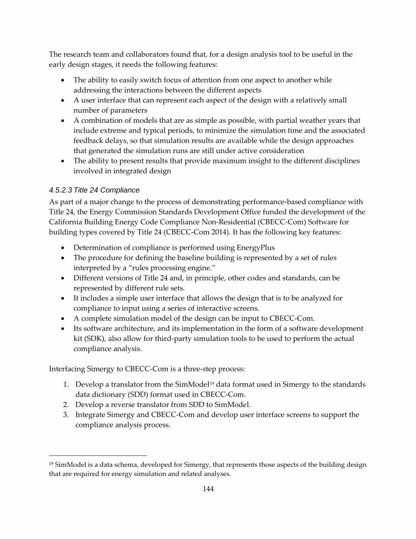
The research team and collaborators found that, for a design analysis tool to be useful in the early design stages, it needs the following features:

• The ability to easily switch focus of attention from one aspect to another while addressing the interactions between the different aspects

• A user interface that can represent each aspect of the design with a relatively small number of parameters

• A combination of models that are as simple as possible, with partial weather years that include extreme and typical periods, to minimize the simulation time and the associated feedback delays, so that simulation results are available while the design approaches that generated the simulation runs are still under active consideration

• The ability to present results that provide maximum insight to the different disciplines involved in integrated design

4.5.2.3 Title 24 Compliance As part of a major change to the process of demonstrating performance-based compliance with Title 24, the Energy Commission Standards Development Office funded the development of the California Building Energy Code Compliance Non-Residential (CBECC-Com) Software for building types covered by Title 24 (CBECC-Com 2014). It has the following key features:

• Determination of compliance is performed using EnergyPlus • The procedure for defining the baseline building is represented by a set of rules

interpreted by a “rules processing engine.” • Different versions of Title 24 and, in principle, other codes and standards, can be

represented by different rule sets. • It includes a simple user interface that allows the design that is to be analyzed for

compliance to input using a series of interactive screens. • A complete simulation model of the design can be input to CBECC-Com. • Its software architecture, and its implementation in the form of a software development

kit (SDK), also allow for third-party simulation tools to be used to perform the actual compliance analysis.

Interfacing Simergy to CBECC-Com is a three-step process:

1. Develop a translator from the SimModel19 data format used in Simergy to the standards data dictionary (SDD) format used in CBECC-Com.

2. Develop a reverse translator from SDD to SimModel. 3. Integrate Simergy and CBECC-Com and develop user interface screens to support the

compliance analysis process.

19 SimModel is a data schema, developed for Simergy, that represents those aspects of the building design that are required for energy simulation and related analyses.

144

4.5.3 Results 4.5.3.1 Simergy Modeling Capabilities Geometry Import from BIM. Simergy can import a 3-D description of the geometry of the building fabric from an object-based computer-aided design (CAD) tool (sometimes referred to as a BIM tool). Figure 4.5.1 illustrates import from Graphisoft’s object-based 3-D CAD tool, ArchiCAD, using the Industry Foundation Classes (IFC) format.

Figure 4.5.1: Import of building geometry using IFC

Figure 4.5.2 illustrates import of a file in green building XML (gbXML) format.

Figure 4.5.2: Import of building geometry using gbXML

145

Generation of Building Geometry from Two-dimensional Floor Plans. The most widely used method of importing geometrical information from CAD is to draw over two-dimensional (2-D) floor plans, imported in either .dwg or .dxf format, snapping to vertices and intersections in the floor plan, and then extruding vertically (Figure 4.5.3). This process can be repeated for each floor.

Figure 4.5.3: Import of building geometry using 2-D floor plans

Building Envelope Libraries and Templates. The libraries of constructions are implemented in a three-level hierarchy:

• Material Layer Sets – e.g., Concrete Floor: 6” Medium Weight Concrete + Carpet • Material Layers – e.g., 6” Medium Weight Concrete • Materials – e.g., Medium Weight Concrete

Glazings (single and multi-pane constructions) use the same three-layer scheme. The constructions templates consist of library entries for different generic types of construction elements. A template consisting of a set of construction library entries can be prepared for any construction practice or energy code baseline construction set for a particular building type and climate zone.

HVAC Systems. HVAC systems in Simergy fall into two categories: (1) zone-level unitary equipment, such as window air-conditioners; and (2) central system, typically multi-zone. The central systems are described in terms of coupled loops: air loops, chilled water loops, condenser water, and hot water. Domestic hot water systems are modeled in EnergyPlus using a variant of the hot water loop. Steam systems are implemented as a special loop type in EnergyPlus—the return part of the loop consists of piping and a pump for the condensate, all of which is assumed to return to the boiler.

146

The demand side of each loop is generated automatically when the components are assigned by the user to the appropriate loop (note that there can be more than one of each type of loop). The zones in each Zone HVAC Group are assigned by selecting them from the tree in the top left side pane of the Create/Edit Zone HVAC Groups workspace. The supply side of each loop can either be created by dragging and dropping individual components in the Diagram workspace or by using, and possibly modifying, a previously defined template. Pre-defining templates is usually a more effective way to work—the configuration and connections of the template can be validated before inserting it into the loop and, once saved, it is readily available for reuse.

The Diagram Zone HVAC Groups workspace is used to generate Zone HVAC Groups with different equipment configurations. Figure 4.5.4 shows the generation of a Zone HVAC Group in which each zone has a radiant ceiling slab and demand controlled ventilation based on measured CO2 concentration.

Figure 4.5.4: Use of the zone HVAC group template workspace to create a zone HVAC group with radiant heating and cooling and demand controlled ventilation

Radiant slab heating and cooling is supported in v1.0 of Simergy. Heat pumps and absorption chillers are partially supported, and it is planned to support them fully in a subsequent version.

4.5.3.2 Extension of Simergy for Early Stage Design Based on the consensus of the collaborators mentioned earlier, the research team developed a preliminary design for a fast-running, detailed simulation tool with a simple interface. The new components of this design include climate analysis, site analysis, and preliminary energy analysis. None of these components are currently included in Simergy or under development. They are detailed in the project report.

147

4.5.3.3 Title 24 Compliance Once Simergy is interfaced to CBECC-Com through the process described in Section 4.5.2.3, users can develop a translator from the SimModel data format used in Simergy to the SDD format used in CBECC-Com.

1. Develop a reverse translator from SDD to SimModel. 2. Integrate Simergy and CBECC-Com and develop user interface screens to support the

compliance analysis process. Once the design model has been converted to SDD format, it is referred to as the User Model. The CBECC-Com rules processing engine uses it to generate two models:

• The Proposed Model replaces the occupancy and operation schedules in the User Model with standard schedules, defined in the Title 24 ACM. Any construction U-factors or equipment efficiencies that do not meet Title 24 mandatory requirements for the climate zone and building type are replaced with the minimum code-compliant values.

• The Standard Model (sometimes referred to as the Baseline Model) is generated from the Proposed Model by substituting a standard HVAC system, based on the building type and size, and replacing any construction U-factors or equipment efficiencies that exceed Title 24 minimum requirements for the climate zone and building type with the minimum code-compliant values.

These models are then translated into EnergyPlus and simulations are run to compare their performance, based on TDV of the energy consumption, which takes into account the variation in the value of electricity by time of day, day of the week, season, and climate zone, as well as the variation in the value of natural gas by season and climate zone.

For future development, the research team recommended development of the following:

• SimModel to SDD Translator, to convert the model developed by the designer in Simergy to the SDD format that is used as the input data format in the CBECC-Com.

• SDD to SimModel Translator, to implement the translation from SDD to IDF via the Simergy SimModel format.

• Simergy ─ CBECC-Com Integration and User Interface, to incorporate the rules processing modules and data in Simergy without significant changes to the Simergy software architecture.

An additional requirement is to synchronize the versions of EnergyPlus used by Simergy and CBECC-Com, as they now use different versions.

To implement the above, a contract has now been signed between the lead software developer for Simergy, Digital Alchemy, and Southern California Edison, representing a group of California utilities that also includes Pacific Gas and Electric, San Diego Gas & Electric, and the Sacramento Municipal Utilities District.

148

4.5.4 Conclusions and Recommendations Version 1.0 of Simergy was released at http://simergy.lbl.gov/ in July 2013. Approximately 4,000 copies were downloaded in the first three months. The release included the following:

• A set of libraries of façade constructions and templates for façade configurations • A set of libraries and templates of thermally activated heating and cooling components

systems • Ways to adapt Simergy for early-stage design • Ways to link code compliance software to Simergy

Version 1.1 was released in April 2014, and version 1.2 was released in September 2014.

It is recommended that the Energy Commission continue to support the development of Simergy, both through direct funding and by continuing to advocate for the support and adoption of Simergy, in particular by the CPUC and investor- and publicly owned utilities.

4.5.4.1 Simergy Modeling Capabilities Building Envelope

Version 1 of Simergy can create building geometry using one of four different methods:

1. Internal generation of building geometry by vertical extrusion of standard floor plan shapes

2. Importing two-dimensional (2-D) floor plans from architectural CAD tools and extruding vertically

3. Importing 3-D geometry from BIM in IFC format 4. Importing 3-D geometry from BIM in green building XML (gbXML) format

Method 1 is applicable in schematic design, before interior layouts are available from the architect. Methods 2 through 4 are applicable from 50 percent detailed design and later. Method 2 is currently the most widely used import method. Import of 3-D geometry is still subject to two difficulties: (1) imprecise drawing in the CAD tool (guidelines are needed), and (2) CAD tool export problems.

When used in conjunction with the substantial number of materials and constructions in the library, these geometry creation methods provide the user with a range of options for modeling building envelopes easily and efficiently.

HVAC Systems

Simergy has graphical tools for creating diagrammatic representations of HVAC systems. These tools enable users to edit predefined templates or to create new system descriptions that resemble conventional mechanical system drawings. The system configurations can be validated with Simergy, trapping a range of input errors before running EnergyPlus and preventing the need to deal with EnergyPlus error messages. Simergy ships with a number of HVAC templates that can be used to model the baseline systems required for ASHRAE

149

http://simergy.lbl.gov/

Standard 90.1 Appendix G and California Title 24 analyses and includes an extensive library structure to support the efficient use of these templates. These capabilities make it considerably easier to define HVAC systems in Simergy than when using the text-based editor (IDF Editor) that ships with EnergyPlus.

4.5.4.2 Early Stage Design An approach to making Simergy an effective tool for use in early stage design was identified. It could form the basis of a work plan to define detailed user requirements, generate a functional specification, and produce a prototype implementation. It is anticipated that several iterations of the cycle of testing, modification of user requirements, and re-implementation would be required. The active participation of practitioners of integrated design and specialists in interface design, including visualization, would be required to tackle this challenging problem.

4.5.4.3 Title 24 Compliance A detailed review of the current state of the CBECC-Com software was performed and is summarized in the project report.

4.5.5 Project Benefits In the first 48 hours of its release, Simergy v1.0 was downloaded approximately 1,000 times, indicating a strong, pent-up demand for a free, practitioner-oriented interface for EnergyPlus. Approximately 4,000 downloads, to date, indicate a growing interest and opportunity to achieve substantial adoption of EnergyPlus through Simergy. It continues to be developed by an LBNL-led team and guided by six leading architecture and engineering firms, with programming from a team of professional software developers.

Simergy’s public release provided California design practitioners with a free tool to enable them to make efficient use of the low-energy systems modeling capabilities of EnergyPlus. More energy-efficient building design is expected to lead to lower actual building energy consumption, which benefits California by helping to mitigate climate change, reduce air pollution, and reduce utility bills.

Linking CBECC-Com to Simergy will enable California practitioners to get immediate feedback on Title 24 compliance and exceedance for low-energy building designs. Supplementing the Title 24 rule set with a closely related rule set to enable calculation of potential utility incentive payments will provide further useful feedback to the designer during the course of the design.

150

4.6 EnergyIQ Action-Oriented Benchmarking Energy benchmarking is essential to the multi-faceted process of improving a building’s energy efficiency. It helps those responsible for the building, identify and implement energy-saving opportunities and understand how the building’s performance compares to that of similar buildings. During the design process, benchmarking can inform the establishment of efficiency targets based on how the best comparable buildings perform. As state and local governments promulgate requirements for energy use disclosure, benchmarking also is needed to give meaning to these otherwise raw data. Market transactions such as real estate appraisals and sales, green insurance underwriting (Mills 2012), and energy audits all benefit from benchmarking.

Traditional whole-building energy benchmarking does not provide practical guidance on how to improve energy efficiency. Those benchmarks provide general context, but do not illuminate which end-uses or fuels may be particularly fertile candidates for intervention. Action-oriented benchmarking improves on simple, traditional benchmarking by providing a low-effort bridge between limited whole-building benchmarks and investment-grade audits and professional engineering calculations. At the other end of the spectrum, investment-grade audits are highly costly, and building owners can be reluctant to make that expenditure decision with only whole-building benchmark results in hand.

4.6.1 Goal The goal of this task was to improve and ensure sustainability of the EnergylQ action-oriented energy benchmarking tool in support of California Energy Commission/Public Interest Energy Research and broader California policy objectives for improving the energy efficiency of the commercial building stock in general, and widespread benchmarking of buildings in particular.

4.6.2 Methods With sponsorship from the Energy Commission, LBNL built, deployed, and supported EnergyIQ—the first web-based, action-oriented benchmarking tool for non-residential buildings. EnergyIQ provides a standardized opportunity assessment based on benchmarking results, along with decision-support information to help refine action plans. It benchmarks energy use, costs, and features for an array of building types and provides a carbon-emissions calculation for the energy consumed in the building, an important part of a building’s overall carbon footprint. It is available for free at http://energyiq.lbl.gov.

In developing EnergyIQ, LBNL surveyed potential users representing half a billion square feet of building floor area. It also incorporated best practice recommended for energy benchmarking and tool design published by ASHRAE.

Development of EnergyIQ has proceeded under three phases. In Phase I, a conceptual design was developed, grounded in extensive focus groups and other methods of assessing the needs of target audiences. An initial web implementation was deployed with simplified functionality.

151

http://energyiq.lbl.gov/

Phase II gathered feedback on the initial deployment and, based on the feedback, the site was modified to better serve user needs (Mills and Mathew 2012). Major additional technical features were added in tandem with substantial investment in improving the usability and graphic design of the tool. The tool was not actively promoted, pending user testing and subsequent refinements.

In Phase III, key features were added, and the tool was formally launched. The APIs were released, allowing third-party developers to incorporate the analytics into other software tools (the functionality and licenses of the APIs are presented in Appendices A and B of the full report, EnergyIQ for Action-Oriented Benchmarking of Non-Residential Buildings). The system was moved to a cloud-based infrastructure, allowing for high reliability and dynamic scalability to accommodate changes in user load (detailed in Appendix C of the full report). An additional objective was to identify ways to sustain the EnergyIQ service into the future. Hosting costs were reduced, and concerted efforts were made to find new hosts; however, no organization has yet signaled a willingness to assume stewardship of the service from the Energy Commission.

4.6.3 Results Figures 4.6.1 a–k provide a walkthrough of the tool’s primary functionality and presentation of results. A variety of databases are incorporated within EnergyIQ from which users can specify peer groups for comparison. Users can browse data visually and use them as a backdrop against which to view energy benchmarking metrics for their own building. Users can save their project information and return at a later date to continue their exploration.

Databases include the most thorough survey of its kind ever conducted—CEUS, which provides details on energy use and characteristics for about 2,800 buildings and 62 building types—and the Commercial Buildings Energy Consumption Survey (CBECS), which provides nationwide data. Users can import their own building’s data from the U.S. Environmental Protection Agency’s Portfolio Manager.

The choice of metrics can strongly influence benchmarking findings. For example, energy use per seat versus per square foot in a restaurant may yield very different qualitative conclusions about efficiencies. With this in mind, EnergyIQ offers an array of easily selectable benchmark metrics, with visual as well as tabular display. These include energy, costs, GHG emissions, and a large variety of physical characteristics (e.g., building components or operational strategies). The tool supports cross-sectional benchmarking, so that users can compare their building to its peers at one point in time, as well as longitudinal benchmarking for tracking the performance of an individual building or enterprise portfolio over time.

Based on user inputs, the tool’s “Act” module generates a list of efficiency opportunities and recommended actions, providing a range of savings for approximately 130 measures achieved by large-scale parametric analysis of similarly filtered CEUS buildings. Users can then explore various decision-support links for helpful information on how to refine action plans, create design-intent documentation, and implement improvements. These include information on best practices, links to other energy analysis tools, and more.

152

Figure 4.6.1 a–k: Key screenshots

HOME PAGE (a)

(b)

(c)

BENCHMARK: Pick metrics or features

• Choose population to benchmark against (California; other U.S. locations)

• Benchmark energy or characteristics

• Choose metric, and normalization units (e.g., floor area, employees, hotel beds)

a) Whole building b) By fuel

BENCHMARK: Define peer group

• Filter by a) floor area b) hours of operation c) vintage d) location e) certifications

• Choose any combination of 62 building types

153

CHARTS

• Choose among several benchmarking views…

ο Cross-sectional

ο Longitudinal (if multi-year data is entered)

• Add your building

When choosing “Features” instead of energy benchmarks, an analysis is shown of the frequency of types of features (lighting, HVAC, envelope, etc.) in the user-selected peer group.

(d) (e)

(f) (g)

(h)

154

TRACK: Results Dashboard

• Benchmark vs. peers • Progress toward

targets (if specified) • Progress over time • A wide range of

metrics can be displayed

• Details on the “bullet graph” and “sparkline” styles

ACT: Upgrade Recommendations

• 130 potentially applicable energy upgrades for each user building => 65,000 bldg+measure combinations

• Ranges of savings shown, based on simulation results for all peer-group buildings (California buildings only)

(i)

(k)

(j)

155

4.6.4 Conclusions and Accomplishments During this third project phase, an array of user-oriented improvements were made to EnergyIQ.20 The LBNL team selected and prioritized the improvements based on the original market research conducted for this project, as well as from ongoing user feedback.

• Interoperability with other tools. Users can import their building data from the ENERGY STAR Portfolio Manager.

• Improved and more flexible peer group definitions. Users can: benchmark their buildings against other users of EnergyIQ; benchmark a single building against their own portfolio of buildings; associate their building with a larger number of building features; and filter their peer groups by hours of occupancy for the California peer-group data set and occupancy and building ownership for the U.S. peer-group data sets. The peer group definition selection process is now much easier.

• Improved benchmarking metrics and feature definitions. A significantly expanded set of normalization options (new metrics) has been added to the tool. Added feature specifications allow for the identification of more relevant upgrade recommendations.

• More widely applicable recommendations. Recommendations are now provided for buildings outside of California.

• Improved user experience and documentation. A number of improvements have been made: an online user guide improved context-sensitive tooltips,21 a downloadable input form, expanded APIs,22 enhanced documentation, and third-party testing.

• Infrastructure and data enhancements. The entire system has been moved to a cloud-based platform and source energy conversion factors have been updated.

• Communications and technology transfer. Coverage in the trade press contributed to growth of traffic to the website (ACHRN 2013; Buildings Magazine 2013; EETD News 2013; ElectricityPolicy.com 2013; GreenBiz.com 2013). In addition, the Energy Commission‘s Small and Medium Building (SMB) Efficiency Toolkit now utilizes EnergyIQ to guide users toward efficiency opportunities, and the APIs were made available for third-party licensing.

More details are available in the full report.

4.6.4.1 Market Impact As of October 2014, the EnergyIQ website had been visited 45,000 times (a four-fold increase since the close of Phase II) by 25,000 individuals, viewing over 150,000 pages of information. While California was the dominant source of traffic, visitors came from 38 states and from 135 countries. Users who wish to compare their buildings to peers must register and open a no-cost account, and more than 1,300 users have registered. These users have entered over 900 buildings into the database, representing 135 million square feet of floor area.

20 A full list of updates is maintained at this web address: https://sites.google.com/a/lbl.gov/energyiq/re.

21 See https://sites.google.com/a/lbl.gov/energyiq/.

22 See https://developers.buildingsapi.lbl.gov/eiq.

156

https://sites.google.com/a/lbl.gov/energyiq/re

https://sites.google.com/a/lbl.gov/energyiq/

https://developers.buildingsapi.lbl.gov/eiq

In addition, 32 users have signed up to the API portal, and there have been 42 additional inquiries. Five licenses have been issued. The ARB has initiated the use of EnergyIQ within its CoolCalifornia carbon footprint tool.

4.6.4.2 Sustainability To support users, EnergyIQ will need to continue to be supported and maintained. In addition to its own use, at least one other Energy Commission project depends on it. Moreover, users and other parties have identified many opportunities for improving the functionality and infrastructure of the EnergyIQ system.

This project’s development and hosting of APIs has lowered the costs of market entry radically for software developers seeking to offer energy benchmarking tools, and ongoing outreach is needed to grow the user base and make potential licensees of the APIs aware of the offering.

Currently, no one has yet signaled a willingness to assume stewardship of the service from the Energy Commission. See the full report for more details.

4.6.5 Project Benefits Users of EnergyIQ benefit from being able to benchmark a building’s energy use and use that information to characterize that building’s energy performance, compare it to similar buildings in California and throughout the United States, and identify the potential for energy-efficiency improvements.

The improvements made in this third phase of EnergyIQ research and development built upon the tool’s earlier success by improving its interoperability with other tools, peer group definitions, benchmarking metrics and feature definitions, documentation, and infrastructure and data. These improvements have made the tool easier to use, greatly expanded the ability to compare building energy performance against other buildings, and enabled third-party software developers to incorporate EnergyIQ’s methods in derivative user interfaces. Ultimately, these additions and modifications have increased a user’s ability to reduce energy use in his or her building.

157

4.7 Rating Method for Roofing Aggregate Many U.S. and international energy standards, codes, and programs—including the 2013 California Title 24 and the 2010 California Green Building Standards Code—reference the CRRC’s Product Rating Program CRRC-1 for initial and aged values of the solar reflectance (albedo) and thermal emittance of roofing products. The CRRC-1 process works well for roofing products that can be represented by an easily measured and transported coupon,23 such as single-ply membranes, cap sheets, clay and concrete tiles, asphalt shingles, metal products, wood shingles, and field-applied coatings (on substrate).

However, the process does not work well for roofing aggregate—loose rock covering the surface of the roof to provide ultraviolet protection, ballast, thermal mass, and/or high albedo. Roofing product albedo is often determined with a solar reflectometer, and if the surface is irregular, with a roughness scale comparable to the diameter of the reflectometer’s sample port, displacement of the surface from the port can reduce sample illumination. This can lead the instrument to underestimate the albedo of the surface.

4.7.1 Goal This task’s goal was to facilitate rating by the CRRC of the initial and aged solar reflectances of roofing aggregate.

4.7.2 Methods A solar reflectometer is commonly used to determine the albedo of roofing products. This study validated against pyranometer24 measurements of albedo, three new methods for solar reflectometer measurement of the albedo of the irregular surface, presented by a bed of roofing aggregate.

Specifically, it explored whether it is possible to (1) accurately measure the albedo of an aggregate bed by averaging many solar reflectometer measurements; (2) relate the albedo of an aggregate bed to reflectometer measurements of the albedo of an opaquely thick pile of finely crushed aggregate; and/or (3) prepare a durable coupon of finely crushed aggregate bound to a substrate whose albedo can be related to that of the aggregate bed.

These reflectometer methods would serve generally as techniques for laboratory measurement of roofing aggregate albedo, and specifically to evaluate albedo within the context of a roofing product rating program.

The research team prepared 17 large beds of different specimens of roofing aggregate. After measuring the albedo of each bed with an albedometer (ASTM E1918-06: Standard Test Method for Measuring Solar Reflectance of Horizontal and Low-Sloped Surfaces in the Field), the team collected a sample of the aggregate and crushed some of the sample to fine granules. Following ASTM method C1549-09 (Standard Test Method for Determination of Solar Reflectance Near

23 A coupon is a small sample of a material to be tested.

24 A pyranometer is an instrument that is used to measure solar irradiance on a planar surface.

158

Ambient Temperature Using a Portable Solar Reflectometer), the researchers used a solar reflectometer to measure the albedos of opaque piles of aggregate and opaque piles of granules. The team adhered granules to metal substrates to produce faux shingles, and then measured the albedo of each shingle with the solar reflectometer. Figure 4.7.1 shows an aggregate bed, opaque granule pile, and faux shingle prepared from white ballast. The durability of the shingles was gauged by measuring granule retention after each shingle was exposed to cycles of heat, moisture, and ultraviolet radiation in a weatherometer.

Figure 4.7.1: Aggregate bed, opaque granule pile, and shingle prepared from white ballast

4.7.3 Results By comparing albedometer measurement of aggregate bed albedo to reflectometer measurements of aggregate pile, granule pile, and faux shingle albedo, the research team developed and demonstrated three methods that can be used to determine the albedo of roofing aggregate with a solar reflectometer. Reflectance measurement is simple in each case, but the methods vary in complexity of sample preparation, and in the durability and transportability of the sample.

Method A measures the initial and aged albedos of a small aggregate pile; aggregate bed albedo equals aggregate pile albedo. For the 17 specimens test in this study, this method predicted aggregate bed albedo with a mean error of 0.006 and RMS error of 0.021.

Method B measures the initial albedo of an opaque pile of finely crushed aggregate. Aggregate bed albedo is computed from one curve fit for non-white aggregate and another for white aggregate. For the 14 non-white aggregates tested in this study, this method predicted aggregate bed albedo with zero mean error and an RMS error of 0.015. For the 3 white aggregates tested in this study, mean error was -0.006 and RMS error was 0.021. Method B requires preparation of granules.

aggregate bed

1 m

1 cm

1 cm

opaque granule pile faux shingle

159

Method C creates faux shingles from aggregate crushed to the size of conventional roofing granules. Aggregate bed albedo is computed from a series of curve fits. For the 17 specimens test in this study, this method predicted aggregate bed albedo with a mean error of -0.002 and an RMS error of 0.019 (Figure 4.7.2). This method requires preparation of both granules and faux shingles.

Figure 4.7.2: Aggregate bed albedos predicted from shingle albedo (red circles) closely matches

those measured via pyranometer method E1918 (green squares).

When applied to the 17 specimens tested in this study, Method A worked well for all but the largest aggregates; Methods B and C worked well for all aggregates. The absolute mean error of each method was less than 0.01, and the RMS error of each method did not exceed 0.021.

4.7.4 Conclusions and Recommendations Within the context of the CRRC-1 product rating program referenced by 2013 California Title 24 and the 2010 California Green Building Standards Code, Method A is practical only if test farms are permitted to operate as test labs. Method C is compatible with the existing program, since coupons can be exposed at the test farm but measured at the test lab. Method B is not recommended since it is suited only to determination of initial albedo. The authors have proposed Methods A and C to the CRRC for potential incorporation within the CRRC-1 product rating program and are under consideration.

While these methods do not address measurement of the thermal emittance of roofing aggregate, all roofing aggregate, clean or soiled, is expected to have high thermal emittance. The role of the CRRC is to report measured values. However, it would be reasonable for 2013 California Title 24 and the 2010 California Green Building Standards Code to assign a default thermal emittance of 0.9 to roofing aggregate in the absence of a measured value. The research team recommends that the Energy Commission staff consider this option.

01

02

03

05,06,07,04

08

09 10,1411

12

13

15

16

17

0.0

0.1

0.2

0.3

0.4

0.5

0.6

0.7

0.8

0.9

1.0

0.0 0.1 0.2 0.3 0.4 0.5 0.6 0.7 0.8 0.9 1.0

Alb

edo

of a

ggre

gate

bed

SSR G1 albedo of shingle

R_a (measured via E1918)R_a (predicted from R_s)

y = xRg = 0.190 Rs2 + 0.898 Rs

white specimens:

Ra= Rg - 0.173 log10(da/dg)

non-white specimens:

Ra = 0.723 Rg0.899

hollow - white specimens (marble)

160

4.7.5 Project Benefits The project’s three reflectometer-based methods can be used to measure the albedo of roofing aggregate. Of these, Methods A and C could be incorporated into the CRRC-1 product rating program. Availability of CRRC-approved ratings for roofing aggregate albedo will permit accurate evaluation of the aggregate roofing for Title 24 performance compliance.

161

CHAPTER 5. Conclusions and Recommendations Because this report covers 19 tasks, the conclusions and recommendations for each task are provided in the chapter for that task, so they can be read in the appropriate context. Please consult the individual chapters for the conclusions and recommendations of this work.

162

GLOSSARY

Term Definition

2-D two-dimensional

ANSI American National Standards Institute

ACF activated carbon fiber

ACM alternate calculation method

API application programming interface

ARB Air Resources Board

ASHRAE American Society of Heating, Refrigerating and Air Conditioning Engineers

ASTM American Society for Testing and Materials

A/V audio-video

AVB audio video bridging

BIM building information model

BIOS Basic Input/Output System

BPM brushless permanent magnet motor

CAD computer-aided design

CBECC California Building Energy Code Compliance

CCHP combined cooling, heating, and electric power

CEA Consumer Electronics Association

CEUS California Commercial End-Use Survey

CFF cardboard + fan/flowmeter

cfm cubic feet per minute

CHP combined heat and power

CO carbon monoxide

CO2 carbon dioxide

CO2e/y carbon dioxide equivalent per year

163

COP coefficient of performance

CPS communicating power supply

CPUC California Public Utilities Commission

CRRC Cool Roof Rating Council

DER distributed energy resources

DER-CAM Distributed Energy Resources Customer Adoption Model

DG distributed generation

DOE U.S. Department of Energy

DVD digital video disc

DX direct expansion

EEMs energy efficiency measures

EER energy efficiency ratio

EIA U.S. Energy Information Administration

Energy Commission

California Energy Commission

EJ Exajoule

EUI energy use intensity

FMI functional mockup interface

FMU functional mockup unit

gbXML green building XML

GHG greenhouse gas

GJ Gigajoule

GUI graphical user interface

GW Gigawatt

HBBM hybrid-Black-Box model

HMX heat and mass exchanger

HVAC heating, ventilation, and air conditioning

HWDS hot water distribution systems

164

IAQ indoor air quality

IEEE Institute of Electrical and Electronics Engineers

IFC Industry Foundation Classes

IT information technology

ITAC integrated technology air cleaner

ITAC 1 Integrated technology air cleaner with design number 1, incorporating a high-efficiency particle filtration system and a catalyst-treated low-efficiency particle filter.

ITAC 2 Integrated technology air cleaner with design number 2, incorporating a high-efficiency particle filtration system, a catalyst-treated low-efficiency particle filter, and a filter containing granular activated carbon.

kJ Kilojoules

kW Kilowatt

kWh kilowatt-hour

LBNL Lawrence Berkeley National Laboratory

LLNL Lawrence Livermore National Laboratory

L/s liters per second

MMT millions of metric tons

MW Megawatt

NOx nitrogen oxide

PAC packaged air conditioning

PG&E Pacific Gas and Electric

PLC power line carrier communication

PSC permanent split capacitor motor

PSZ packaged single zone system

PTAC packaged terminal air conditioner

PTHP packaged terminal heat pump

PUE power usage effectiveness / power utilization effectiveness

PV Photovoltaic

165

PVAV packaged variable-air-volume

PWM pulse width modulation

RMS root-mean-square

RPi Raspberry Pi mini computer

RTU rooftop unit

SDD standards data dictionary

SDH savings degree-hour

SGIP Self-Generation Incentive Program

SO2 sulfur dioxide

SR solar reflectance

SVLG Silicon Valley Leadership Group

TAG technical advisory group

TDV time-dependent valuation

TECFB The Energy Conservatory FlowBlaster®

TWh terawatt-hour

UA heat loss coefficient

UHI urban heat island

UPnP universal plug and play

UPS Uninterruptible Power Supplies

VAV variable-air-volume

UA overall heat transfer coefficient

USB universal serial bus

VOCs volatile organic compounds

VRF variable refrigerant flow

W Watt

WH water heater

WLHP water loop heat pump

166

WSE water-side economizer

WSN wireless sensor network

ZNEB zero net energy building

167

REFERENCES

Acker, Brad, Carlos Duarte, and Kevin Van Den Wymelenberg. 2012. “Office Space Plug Load Profiles and Energy Saving Interventions.” In The Proceedings of the ACEEE Summer Study in Buildings. Pacific Grove (Calif.): American Council for an Energy Efficient Economy (Washington, D.C.).

ADL. 1982a. Engineering Computer Models for Refrigerators, Freezers, Furnaces, Water Heaters, Room and Central Air Conditioners. Arthur D. Little, Cambridge, Mass. No. 83528-20 under DE-AC01-78CS20420, November.

Assembly Bill 32 (California Global Warming Solutions Act of 2006). 2006. Nuñez, Chapter 488, Statutes of 2006. http://www.leginfo.ca.gov/pub/05-06/bill/asm/ab_0001-0050/ab_32_bill_20060927_chaptered.pdf.

Bailey, M., M. Eastwood, T. Grieser, L. Borovick, V. Turner, and R. C. Gray. 2007. Special Study: Data Center of the Future. New York, NY: IDC. IDC #06C4799. April.

Baskin, E., W. G. Craddick, R. Lenarduzzi, R. L. Wendt, and K. A. Woodbury. 2007. Hot Water Distribution System Program Documentation and Comparison to Experimental Data. Oak Ridge National Laboratory. September. http://info.ornl.gov/sites/publications/files/Pub8207.pdf.

Belady, C., A. Rawson, J. Pflueger, and T. Cader. 2008. Green Grid Data Center Power Efficiency Metrics: PUE and DCIE, The Green Grid. White Paper #6. http://www.thegreengrid.org/~/media/WhitePapers/White_Paper_6_-_PUE_and_DCiE_Eff_Metrics_30_December_2008.pdf?lang=en [Last accessed September, 14, 2012].

CEC (California Energy Commission). 2006. California Commerical End-Use Survey. Consultant Report. CEC-400-2006-005.

CEC. 2013. Nonresidential Alternative Calculation Method (ACM) Approval Manual. CEC-400-2012-006-CMF-REV.

CEUS. 2006. California Commercial End-Use Survey (CEUS). http://www.energy.ca.gov/ceus/ and http://capabilities.itron.com/ceusweb/.

Dynasim. 2009. “Dymola Multi-Engineering Modeling and Simulation.“ Lund, Sweden: Dynasim AB.

E3 Energy+Envirnomental Economics. 2009. GHG Tool for Buildings in California April 09 v. 2. http://www.ethree.com/public_projects/ghg.php.

EIA (U.S. Energy Information Administration). 2012. Annual Energy Outlook 2012 (AEO2012). Reference case. http://www.eia.gov/forecasts/aeo/er/pdf/0383er%282012%29.pdf.

168

http://www.leginfo.ca.gov/pub/05-06/bill/asm/ab_0001-0050/ab_32_bill_20060927_chaptered.pdf

http://www.leginfo.ca.gov/pub/05-06/bill/asm/ab_0001-0050/ab_32_bill_20060927_chaptered.pdf

http://info.ornl.gov/sites/publications/files/Pub8207.pdf

http://www.thegreengrid.org/%7E/media/WhitePapers/White_Paper_6_-_PUE_and_DCiE_Eff_Metrics_30_December_2008.pdf?lang=en

http://www.thegreengrid.org/%7E/media/WhitePapers/White_Paper_6_-_PUE_and_DCiE_Eff_Metrics_30_December_2008.pdf?lang=en

http://www.energy.ca.gov/ceus/

http://capabilities.itron.com/ceusweb/

http://www.ethree.com/public_projects/ghg.php

http://www.eia.gov/forecasts/aeo/er/pdf/0383er%282012%29.pdf

Ehrhardt-Martinez, Karen, Kat Donelly, and John Laitner. 2010. Advanced Metering Initiatives and Residential Feedback Programs: A Meta-Review for Household Electricity-Saving Opportunities. Report No. E105. Washington, D.C.: American Council for an Energy Efficient Economy.

Fisk, William J., Sebastian Cohn, Hugo Destaillats, Meera Sidheswaran, Victor Henzel, and Douglas Sullivan (Lawrence Berkeley National Laboratory). 2014. Integrated Technology Air Cleaners (ITAC): Design And Evaluation. California Energy Commission.

Grant, P. Evaluation of the Performance of Gas Tankless Water Heaters. 2011. Thesis submitted for the Degree of Master of Science. Boulder, Colorado: University of Colorado at Boulder, Department of Civil, Environmental and Architectural Engineering.

Grant, Peter, and James Lutz. 2013. HWDS Simulation Model Report. Lawrence Berkeley National Laboratory for California Energy Commission. April 26.

Grant, P., J. Burch, and M. Krarti. 2010. “Modeling Gas Tankless Water Heaters and Studying the Impacts of Draw Profile on System Efficiency.” National Renewable Energy Laboratory.

Hiller, C. C. 2006a. Hot Water Distribution System Piping Time, Water, and Energy Waste- Phase I: Test Results. ASHRAE Transactions 112: 415–425. http://www.techstreet.com/cgi-bin/detail?product_id=1718782.

Hiller, C. C. 2006b. Hot Water Distribution System Piping Heat Loss Factors- Phase I: Test Results. ASHRAE Transactions 112: 436–446. http://www.techstreet.com/cgi-bin/detail?product_id=1718783.

Hiller, C. C. 2008a. Hot Water Distribution System Piping Heat Loss Factors, Both In Air and Buried - Phase II Test Results. ASHRAE Transactions 114 http://www.techstreet.com/cgi-bin/detail?product_id=1715429.

Hiller, C. C. 2008b. Hot Water Distribution System Piping Time, Water, and Energy Waste - Phase II Test Results. ASHRAE Transactions 114 http://www.techstreet.com/cgi-bin/detail?product_id=1712122.

Hiller, C. C. 2011a. Hot-Water Distribution System Piping Time,Water, and Energy Waste - Phase III: Test Results. ASHRAE Transactions 117 http://www.techstreet.com/cgi-bin/detail?product_id=1801416.

Hiller, C. C. 2011b. Hot-Water Distribution System Piping Heat Loss Factors - Phase III: Test Results. ASHRAE Transactions 117 http://www.techstreet.com/cgi-bin/detail?product_id=1801456.

Institute for Electrical and Electronic Engineers. 2004. Microprocessor Standards Committee of the IEEE Computer Society. P1621, Standard for User Interface Elements in Power Control of Electronic Devices Employed in Office/Consumer Environments. (approved December 2004; reaffirmed December 2009).

169

http://www.techstreet.com/cgi-bin/detail?product_id=1718782












KEMA, Inc. 2010. 2009 California Residential Appliance Saturation Study, Executive Summary. Sacramento: California Energy Commission. http://www.energy.ca.gov/2010publications/CEC-200-2010-004/CEC-200-2010-004-ES.PDF.

Lutz, James, Peter Biermayer, and Derek King. 2009. Pilot Phase of a Field Study to Determine Waste of Water and Energy in Residential Hot Water Distribution Systems. Sacramento, California: Lawrence Berkeley National Laboratory for the California Energy Commission. July. http://www.energy.ca.gov/2013publications/CEC-500-2013-135/CEC-500-2013-135.pdf.

Lanzisera, Steven, Stephen Dawson-Haggerty, H. Y. Iris Cheung, Jay Taneja, David Culler, and Richard Brown. 2013. “Methods for Detailed Energy Data Collection of Miscellaneous and Electronic Loads in a Commercial Office Building.” Building and Environment 65 (July): 170–77. doi:10.1016/j.buildenv.2013.03.025.

Mahone, A., S. Price, W. Morrow. 2008. Developing a Greenhouse Gas Tool for Buildings in

California: Methodology and Use. Energy and Environmental Economics, Inc. and PLEXOS Production Simulation Dispatch Model.

Meyers, Robert J., Eric D. Williams, and H. Scott Matthews. 2010. “Scoping the Potential of Monitoring and Control Technologies to Reduce Energy Use in Homes.” Energy and Buildings 42 (5): 563–69. doi:10.1016/j.enbuild.2009.10.026.

Mills, Evan. 2012. “The Greening of Insurance.” Science 338, 1424. http://insurance.lbl.gov/opportunities/ro-12-summary.html.

Mills, Evan, and Paul Mathew. 2012. “Web Services that Foster Innovation in Buildings Energy Analysis Tools.” 2012. Proceedings of the 2012 ACEEE Summer Study on Energy Efficiency in Buildings. American Council for an Energy-Efficient Economy: Washington, D.C. http://evanmills.lbl.gov/pubs/pdf/APIs-ACEEE-2012.pdf.

Neff, B. 2012. A New Generation of Combined Heat and Power: Policy Planning for 2030. California Energy Commission. CEC-200-2012-005.

Nordman, Bruce. 2003. The Power Control User Interface Standard. Final Report. Prepared for the California Energy Commission, Public Interest Energy Research Program. LBNL-52526.

Nouidui, Thierry Stephane, Michael Wetter, and Wangda Zuo. 2013. Functional Mock-Up Unit Import in EnergyPlus For Co-Simulation. The 13th Conference of International Building Performance Simulation. Chambery, France, 2013.

Parker, Danny, David Hoak, Jamie Cummings, and Florida Solar Energy Center. 2010. “Pilot Evaluation of Energy Savings and Persistence from Residential Energy Demand Feedback Devices in a Hot Climate.” In The ACEEE Summer Study on Energy Efficiency in Buildings. Pacific Grove (Calif.): American Council for an Energy Efficient Economy (Washington, D.C.).

170

http://www.energy.ca.gov/2010publications/CEC-200-2010-004/CEC-200-2010-004-ES.PDF

http://www.energy.ca.gov/2010publications/CEC-200-2010-004/CEC-200-2010-004-ES.PDF

http://www.energy.ca.gov/2013publications/CEC-500-2013-135/CEC-500-2013-135.pdf


http://insurance.lbl.gov/opportunities/ro-12-summary.html

http://evanmills.lbl.gov/pubs/pdf/APIs-ACEEE-2012.pdf

http://eetd.lbl.gov/publications/author/6401



http://eetd.lbl.gov/publications/functional-mock-up-unit-import-in-ene

http://eetd.lbl.gov/publications/functional-mock-up-unit-import-in-ene

Pigg, Scott, Ingo Bensch, and Karen Koski. 2010. “Energy Savings Opportunities with Home Electronics and Other Plug-Load Devices: Results from a Minnesota Field Study.” In ACEEE Summer Study on Energy Efficiency in Buildings. Pacific Grove (Calif.): American Council for An Energy Efficient Economy (Washington, D.C.).

Proctor, J., R. Chitwood, and B. Wilcox. 2010. Efficiency Characteristics and Opportunities for New California Homes. Public Interest Energy Research Program Project Final Report. Sacramento, California: California Energy Commission.

Tiller, M. 2001. “Introduction to Physical Modeling with Modelica.“ The Springer International Series in Engineering and Computer Science.

Urban, Bryan, Verena Tiefenbeck, and Kurt Roth. 2011. Energy Consumption of Consumer Electronics in U.S. Homes in 2010. Final Report by Fraunhofer Center for Sustainable Energy Systems for the Consumer Electronics Association.

U.S. Department of Energy. 2011. 2011 Buildings Energy Data Book. http://buildingsdatabook.eren.doe.gov/default.aspx.

Walker, I. S., C. P. Wray, D. J. Dickerhoff, and M. H. Sherman. 2001. Evaluation of Flow Hood Measurements for Residential Register Flows. Berkeley California: Lawrence Berkeley National Laboratory. LBNL 47382.

Wetter, M., W. Zuo, and T. Nouidou. 2011. “Recent Development of the Modelica Buildings Library for Building Heating, Ventilation and Air-Conditioning Systems.“ Proceedings of the 8th International Modelica Conference. Technical University, Dresden, Germany, March 20–22.

171

http://buildingsdatabook.eren.doe.gov/default.aspx

APPENDIX

• Innovative Air Cleaner for Improved IAQ and Energy Savings. 2014. William J. Fisk, Sebastian Cohn, Hugo Destaillats, Victor Henzel, Meera Sidheswaran, and Douglas Sullivan. http://www.osti.gov/scitech/biblio/1163741/

• Urban Heat Island Mitigation Phase 2. 2014. Haley Gilbert, Ronnen Levinson, Benjamin

Mandel, Dev Millstein, Melvin Pomerantz, and Pablo Rosado. The report will be available at http://www.energy.ca.gov/contracts/pier/contractors/.

• Reducing Waste in Residential Hot Water Distribution Systems. 2014. Jim Lutz, Steven

Lanzisera, Anna Liao, Christian Fitting, Chris Stiles, and Margarita Kloss. The report will be available at http://www.energy.ca.gov/contracts/pier/contractors/.

• Encouraging Combined Heat and Power in California Buildings. 2014. Michael Stadler,

Markus Groissböck, Gonçalo Cardoso, Andreas Müller, and Judy Lai. https://der.lbl.gov//sites/der.lbl.gov/files/LBNL-6267E_0.pdf.

• Improved Audio-Video Efficiency through Inter-Device Power Control. 2014. Bruce

Nordman. Publication number: CEC-500-2014-099. • Building Air-Tightness through Appliance Venting Standards. 2014. Craig Wray, Vi

Rapp, David Lorenzetti, and Brett Singer. The report will be available at http://www.energy.ca.gov/contracts/pier/contractors/.

• Energy Efficiency in Small Server Rooms. 2014. H. Y. Iris Cheung, Steve E. Greenberg,

Roozbeh Mahdavi, Richard Brown, and William Tschudi. http://datacenters.lbl.gov/sites/all/files/PIER_Task2.13_SmallServerRooms_FinalReport_v1.pdf.

• Data Center Energy Efficiency Demonstration Projects. 2014. Henry Coles, Steve

Greenberg, and William Tschudi. The report will be available at http://www.energy.ca.gov/contracts/pier/contractors/.

• Improving Residential Programmable Thermostats. 2014. Alan Meier, and Emmanuelle

Revillion. The report will be available at http://www.energy.ca.gov/contracts/pier/contractors/. • Evaluation of Air Flow Measurement Methods for Residential HVAC Returns. 2014. Iain

S. Walker, and J. Chris Stratton. The report will be available at http://www.energy.ca.gov/contracts/pier/contractors/.

A-1

http://www.osti.gov/scitech/biblio/1163741/

http://www.energy.ca.gov/contracts/pier/contractors/


https://der.lbl.gov/sites/der.lbl.gov/files/LBNL-6267E_0.pdf



http://datacenters.lbl.gov/sites/all/files/PIER_Task2.13_SmallServerRooms_FinalReport_v1.pdf

http://datacenters.lbl.gov/sites/all/files/PIER_Task2.13_SmallServerRooms_FinalReport_v1.pdf




• Improved Standards through End-Use Meter Development. 2014. Steven Lanzisera, Richard Brown, Anna Liao, Andrew Weber, and Margarita Kloss. The report will be available at http://www.energy.ca.gov/contracts/pier/contractors/.

• Efficient Electronics through Measurement and Communication. 2014. Alan Meier,

Steven Lanzisera, Andrew R. Weber, Anna Liao, and Christopher Styles. The report will be available at http://www.energy.ca.gov/contracts/pier/contractors/.

• Title 24 Credit for Efficient Evaporative Cooling. 2014. Spencer Maxwell Dutton,

Jonathan Woolley, and Nelson Dichter. The report will be available at http://www.energy.ca.gov/contracts/pier/contractors/.

• Performance Data for Improving Title 24 Compliance Systems. 2014. Liping Wang,

Tianzhen Hong, and Philip Haves. The report will be available at http://www.energy.ca.gov/contracts/pier/contractors/.

• Simulation Models for Improved Water Heating Systems. 2014. Jim Lutz, Peter Grant,

and Margarita Kloss. The report will be available at http://www.energy.ca.gov/contracts/pier/contractors/.

• Enabling Tools for Design of Energy-Efficient Building Systems. 2014. Michael Wetter,

Xiufeng Pang, Wangda Zuo, Thierry Nouidui, and Kaustubh Phalak. Publication number: CEC-500-2014-055.

• Graphical User Interface for EnergyPlus. 2014. Philip Haves, Richard See, and Kevin

Settlemyre. The report will be available at http://www.energy.ca.gov/contracts/pier/contractors/. • EnergyIQ Action-Oriented Benchmarking of Non-Residential Buildings. 2014. Evan

Mills. The report will be available at http://www.energy.ca.gov/contracts/pier/contractors/. • Reflectometer Measurement of Roofing Aggregate Albedo. 2014. Ronnen Levinson,

Sharon Chen, Paul Berdahl, Pablo Rosado, and Louis Medina. Publication number: CEC-500-2014-110.

A-2











ENERGY EFFICIENCY PROJECTS - Summary Report

Documents

Transcript of ENERGY EFFICIENCY PROJECTS - Summary Report