arX

iv:c

ond-

mat

/050

6798

v1 [

cond

-mat

.sof

t] 3

0 Ju

n 20

05

Anticipated synchronization in coupled inertia ratchets with

time-delayed feedback: a numerical study

Marcin Kostur,1 Peter Hanggi,1 Peter Talkner,1 and Jose L. Mateos2

1Institut fur Physik, Universitat Augsburg,

Universitatsstrasse 1, D-86135 Augsburg, Germany

2Instituto de Fısica, Universidad Nacional Autonoma de Mexico,

Apartado Postal 20-364, 01000 Mexico, D.F., Mexico

(Dated: February 2, 2008)

Abstract

We investigate anticipated synchronization between two periodically driven deterministic, dissi-

pative inertia ratchets that are able to exhibit directed transport with a finite velocity. The two

ratchets interact through an unidirectional delay coupling: one is acting as a master system while

the other one represents the slave system. Each of the two dissipative deterministic ratchets is

driven externally by a common periodic force. The delay coupling involves two parameters: the

coupling strength and the (positive-valued) delay time. We study the synchronization features for

the unbounded, current carrying trajectories of the master and the slave, respectively, for four

different strengths of the driving amplitude. These in turn characterize differing phase space dy-

namics of the transporting ratchet dynamics: regular, intermittent and a chaotic transport regime.

We find that the slave ratchet can respond in exactly the same way as the master will respond in

the future, thereby anticipating the nonlinear directed transport.

PACS numbers: 05.45.Xt, 05.45.Ac, 05.40.Fb, 05.45.Pq

1

I. INTRODUCTION

The intriguing concept of synchronization in nonlinear systems is relevant for a wide range

of topics in physics, chemistry and biology. Recently, it has received much attention and

first, comprehensive reviews and books have appeared [1, 2]. The case of synchronization,

in particular of chaotic systems, represents a challenge, since a chaotic system is extremely

sensitive to small perturbations. Nevertheless, it has been established repeatedly that the

synchronization of chaotic systems is possible under certain conditions [3].

The situation when the coupling involves a delay in time is the focus here, and may lead

to anticipated synchronization [4, 5, 6, 7, 8, 9]. In this case, one deals with two systems: a

“master” and a “slave”, which are coupled unidirectionally via a time-delay term, in such

a way that, under some circumstances, the slave system anticipates the response of the

master system. The regime of anticipated synchronization and its stability has been studied

theoretically previously for a variety of systems: we mention here the case of linear set

ups with delay [10], coupled chaotic maps with delays [11, 12], excitable systems [13] and

nonlinear systems of practical interest, such as semiconductor lasers operating in a chaotic

regime [14]. Recently, the phenomenon of anticipated synchronization has been vindicated

experimentally in a semiconductor laser running in the chaotic regime [16, 17].

In different context, we witness an increasing interest during recent years in the study

of intriguing transport phenomena of nonlinear systems that can extract usable work from

unbiased non-equilibrium fluctuations. These, so called Brownian motor systems (or Brow-

nian ratchets) [18] can be modelled by a Brownian particle undergoing a random walk in a

periodic asymmetric potential, and being acted upon by an external time-dependent force

of zero average. The recent burst of work is motivated by both, (i) the challenge to model

unidirectional transport of molecular motors within the biological realm and, (ii) the poten-

tial for novel technological applications that enable an efficient scheme to shuttle, separate

and pump particles on the micro- and even nanometer scale [18].

Although the vast majority of the literature in this field considers the presence of noise,

there have been attempts to model the transport properties of classical deterministic inertial

ratchets [19, 20, 21]. These ratchets generally possess parameter regions where the classical

dynamics is chaotic; the latter in turn then decisively determines the transport properties.

In contrast to the case with two coupled oscillators possessing confined position trajec-

2

tories, the position in a driven ratchet dynamics is able to undergo directed, unbounded

motion with a finite transport velocity. In the following, we shall explore the case of a

coupling between two deterministic, dissipative ratchets in parameter regimes where each

ratchet system is individually able to exhibit either current-carrying, regular transport tra-

jectories (which in turn possess a periodic velocity), or also a chaotic or even an intermittent,

directed transport behavior [19, 20, 21]. One of the ratchet devices then acts as the “master

system” while the remaining one acts as the “slave”. The coupling between the two ratchets

is unidirectional, meaning that the master affects the slave, but not vice versa. We shall

explore the possibility of anticipated synchronization in various tailored parameter regimes

of a regular, chaotic and intermittent dynamics.

II. TWO COUPLED INERTIAL RATCHETS WITH A TIME DELAY

To start out, let us consider a one-dimensional problem of an inertial particle driven by

a periodic time-dependent external force in an asymmetric (with respect to the reflection

symmetry) periodic, so called ratchet potential. In order to have no net bias at work the

time average of the external force equals zero. Here, we do not take into account any sort of

noise, meaning that the dynamics is deterministic. We thus deal with a rocked deterministic

ratchet [19, 22] that obeys the following dimensionless inertial dynamics [20]:

x + bx +dU(x)

dx= a cos(ωt), (1)

where b denotes the friction coefficient, V (x) is the asymmetric ratchet periodic potential,

a is the amplitude of the external force and ω is the frequency of the external driving force.

The dimensionless potential (which is shifted by an amount x0 ≃ −0.19 in order that its

minimum is located at the origin) is given by:

U(x) = C − U0

[

sin 2π(x − x0) +1

4sin 4π(x − x0)

]

(2)

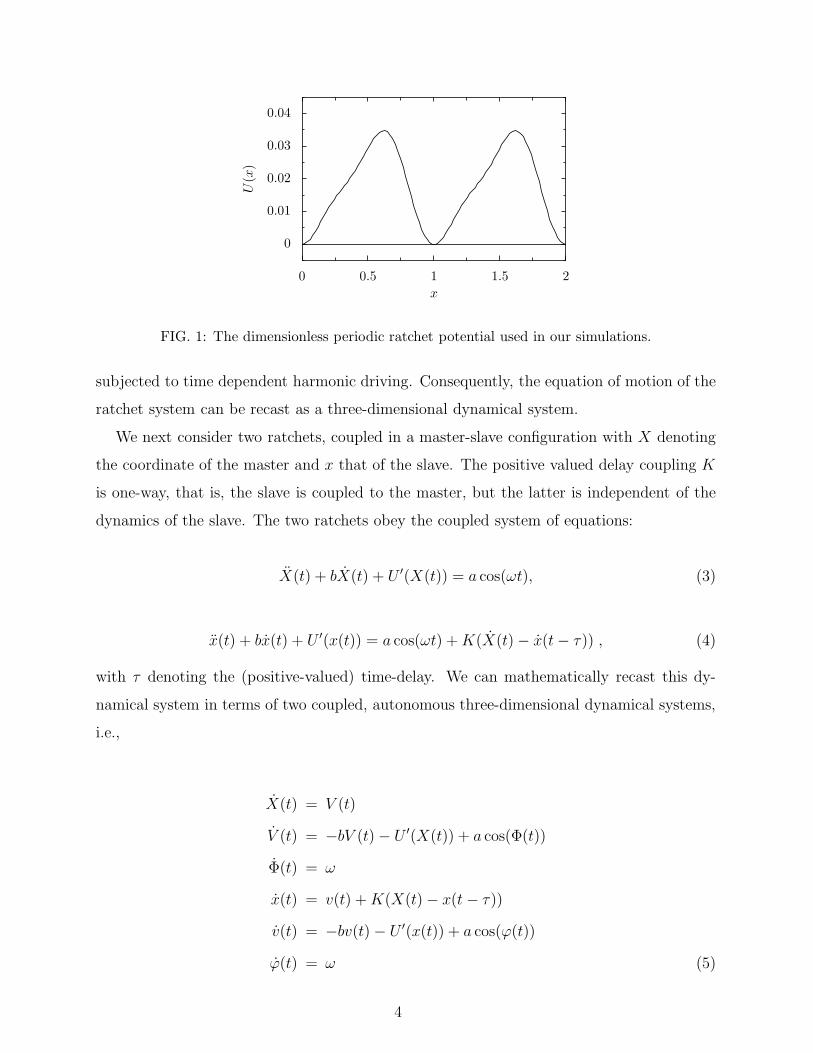
and is depicted in Fig. 1. The constant C is chosen such that U(0) = 0, and is given by

C = −U0(sin 2πx0 +0.25 sin 4πx0), where U0 = 1/4π2(sin(2π|x0|)+sin(4π|x0|)). In this case

U0 ≃ 0.0158 and C ≃ 0.0173, see also [20, 22].

This time-dependent dynamics can be embedded into a corresponding three-dimensional

autonomous phase space dynamics because we are dealing with a Newtonian dynamics

3

0

0.01

0.02

0.03

0.04

U(x

)

0 0.5 1 1.5 2

x

FIG. 1: The dimensionless periodic ratchet potential used in our simulations.

subjected to time dependent harmonic driving. Consequently, the equation of motion of the

ratchet system can be recast as a three-dimensional dynamical system.

We next consider two ratchets, coupled in a master-slave configuration with X denoting

the coordinate of the master and x that of the slave. The positive valued delay coupling K

is one-way, that is, the slave is coupled to the master, but the latter is independent of the

dynamics of the slave. The two ratchets obey the coupled system of equations:

X(t) + bX(t) + U ′(X(t)) = a cos(ωt), (3)

x(t) + bx(t) + U ′(x(t)) = a cos(ωt) + K(X(t) − x(t − τ)) , (4)

with τ denoting the (positive-valued) time-delay. We can mathematically recast this dy-

namical system in terms of two coupled, autonomous three-dimensional dynamical systems,

i.e.,

X(t) = V (t)

V (t) = −bV (t) − U ′(X(t)) + a cos(Φ(t))

Φ(t) = ω

x(t) = v(t) + K(X(t) − x(t − τ))

v(t) = −bv(t) − U ′(x(t)) + a cos(ϕ(t))

ϕ(t) = ω (5)

4

Given this system, we notice that the manifold X(t) = x(t−τ) presents an exact solution

of the system, when the period of the external force is equal to the time delay τ . The situation

when we attain anticipated synchronization yields X(t) = x(t− τ), or X(t+ τ) = x(t). This

implies that the slave ratchet acts at time t in exactly the same way as the master will do

in the future time, t + τ , thus anticipating the dynamics.

We note, that the phase difference Φ(t) − ϕ(t) of the driving forces remains fixed during

its time evolution. Thus, the only way to achieve the synchronization – with anticipation

time τ – is to choose the initial phase ϕ(0) of the slave to match precisely

Φ(0) = ϕ(0) + ωτ. (6)

This dynamical system is similar to the excitable system studied in [13], where the Adler

equation [23] is considered for a particle in a tilted symmetric (non-ratchet) periodic poten-

tial. In our case the number of degrees of freedom is increased since we are addressing the

inertial dynamics. We remark, however, that in the limit of two over-damped ratchets, our

system dynamics becomes similar to the one studied previously in [13], except that we deal

here with a common periodic forcing instead of a common random external forcing used in

[13].

III. ANTICIPATED SYNCHRONIZATION: NUMERICAL RESULTS

In the following, we numerically analyze thoroughly the dynamics of the two coupled

ratchets (5). Let us consider the case where both ratchets, master and slave, are identical,

that is, they have the same parameters a, b, and ω; the parameters that enter in the ratchet

potential are also identical. In Fig. 2 we depict transporting trajectories for the master and

the slave ratchet, when a = 0.08, b = 0.1 and ω = 0.67. The delay coupling involves two

parameters: the coupling strength K = 0.6 and the delay time τ = 1.3. We notice that the

master and the time-shifted slave essentially coincide; that is, the slave is anticipating the

response of the master system, see in the blow up in Fig. 2.

The parameter space of the full nonlinear dynamical system is far too large for a sys-

tematic numerical analysis. In this paper we will choose the dynamics of the master to be

in one of the following representative regimes: regular, chaotic and intermittent transport

dynamics. Then, the relevant parameter space for synchronization (τ, K) will be scanned

5

14

15

16

800 825

10

15

20

25

x(t

),X

(t)

400 500 600 700 800 900

t

FIG. 2: (Color online) Trajectories for the master (red line) and slave (black line) ratchets in a

typical synchronization scenario. The magnified part of the trajectory reveals the anticipation

effect. The parameters are: a = 0.08, b = 0.1, ω = 0.67, K = 0.6, τ = 1.3.

numerically. We also seek a quantity that can characterize the quality of synchronization.

A first natural candidate would be the position correlation function. We found, however,

that this measure does not provide an intuitive answer whether the master and the slave are

synchronized. Instead, we will use the fraction of the time during which the two ratchets

are synchronized within some prescribed accuracy. That is, we consider that the master and

the slave attain a regime of anticipated synchronization when the difference between their

trajectories is smaller than some small given value ǫ, that is, |x(t) − X(t + τ)| ≤ ǫ. We

always have set this value to read ǫ = 0.01.

In the following, we calculate the trajectories for both ratchet dynamics, compute the

amount of time that they stay synchronized (according to the above criterion), and then de-

termine the ratio p between the synchronized and total timespan of the considered trajectory.

This measure of synchronization p therefore varies between zero and one.

¿From the literature it is known [4, 5, 9] that the delay coupling scheme used here requires

some constraints on the positive anticipation time τ and the coupling strength K for the

anticipated synchronization to occur. Thus, we investigate the stability regions, in the

parameter space (K, τ), for coupled chaotic ratchets as described by eq. (5). In Fig. 3 we

show the synchronization properties for the case b = 0.1 and ω = 0.67, for four values of

the amplitude a. These values, indicated in the figure, correspond to regular, intermittent

and a chaotic regime of the master dynamics [20]. The gray-scale depicts the value of the

6

K

τ

unstable

K

τ

unstable

a=0.08 chaotic

K

unstable

K

unstable

a=0.0823 intermittent

ττ

a=0.074 regular

a=0.081 regular

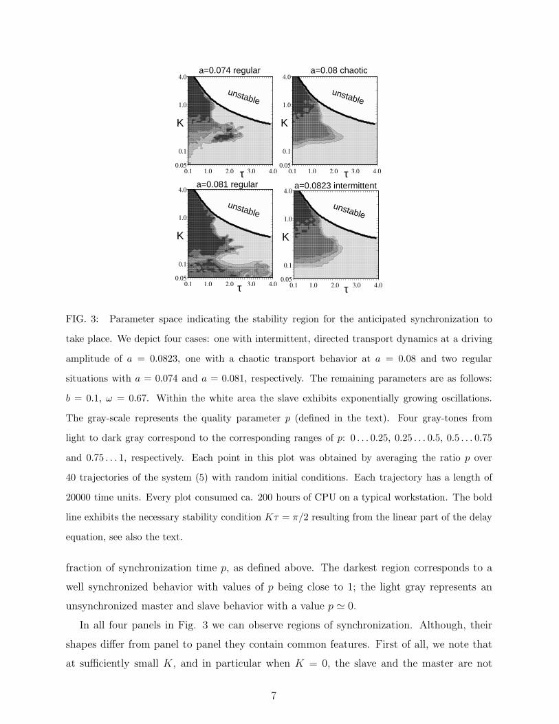
FIG. 3: Parameter space indicating the stability region for the anticipated synchronization to

take place. We depict four cases: one with intermittent, directed transport dynamics at a driving

amplitude of a = 0.0823, one with a chaotic transport behavior at a = 0.08 and two regular

situations with a = 0.074 and a = 0.081, respectively. The remaining parameters are as follows:

b = 0.1, ω = 0.67. Within the white area the slave exhibits exponentially growing oscillations.

The gray-scale represents the quality parameter p (defined in the text). Four gray-tones from

light to dark gray correspond to the corresponding ranges of p: 0 . . . 0.25, 0.25 . . . 0.5, 0.5 . . . 0.75

and 0.75 . . . 1, respectively. Each point in this plot was obtained by averaging the ratio p over

40 trajectories of the system (5) with random initial conditions. Each trajectory has a length of

20000 time units. Every plot consumed ca. 200 hours of CPU on a typical workstation. The bold

line exhibits the necessary stability condition Kτ = π/2 resulting from the linear part of the delay

equation, see also the text.

fraction of synchronization time p, as defined above. The darkest region corresponds to a

well synchronized behavior with values of p being close to 1; the light gray represents an

unsynchronized master and slave behavior with a value p ≃ 0.

In all four panels in Fig. 3 we can observe regions of synchronization. Although, their

shapes differ from panel to panel they contain common features. First of all, we note that

at sufficiently small K, and in particular when K = 0, the slave and the master are not

7

coupled and evolve independently of each other. Secondly, the increase of the coupling

strength K causes the onset of synchronization for small and moderate values of the delay

time τ . Synchronization is lost, however, for too large values of the delay time τ regardless

of the coupling K. The third common feature is the loss of the stability of the slave, if both

K and τ are too large. The origin of the instability derives from the linear delay equation

x(t) = −Kx(t−τ), resulting from eq. (5) upon neglecting the velocity v(t), see also Ref. [10].

For K · τ > π/2 the trajectories of this linear equation grow exponentially. This criterion

agrees perfectly well with our numerical findings. The unstable region can be neighboring to

the synchronized or to unsynchronized one, depending on the delay τ . Hence, two scenarios

have been observed: increasing K at larger τ first de-synchronizes the system until the slave

finally becomes unstable (see e.g. a = 0.08, τ = 1.7 and K = 0.2 . . . 4); at smaller values of

τ the synchronized state becomes unstable with growing K (see e.g. a = 0.08, τ = 1.0 and

K = 0.2 . . . 4).

One can distinguish two regions of synchronization in these four plots in Fig. 3. The first

one is present in all cases for coupling strengths K > 0.1. It has a similar shape although

the underlying dynamics may differ dramatically. The second region for K < 0.1 exists in

the case of a regular dynamics with a = 0.081. Remarkably, in this regime the system can

reach synchronization for delay times τ much larger than in the other cases, and it takes

place even at a small coupling strength K ≃ 0.06.

Clearly, the parameter p does not provide the full information on the dynamics. If we

know that e.g. 50% of time a slave synchronizes with a master, we still do not know much

about the nature of these events. Thus, we shall next investigate in more detail for each of

the above four characteristic situations the representative time series.

At the driving strength a = 0.074, the master possesses a stable regular trajectory, being

characterized by a period-two orbit in the corresponding Poincare section, see e.g. Fig. 2

in [20]). Starting with independent random initial conditions within the same period of the

potential for the master and the slave, the master reaches the stable orbit after a transient

time. This is depicted in Fig. 4. Already before the master has reached its stable orbit the

slave starts to synchronize at t = 600. Only at t = 750 both the master and the slave reach

the regular orbit and the synchronization becomes even better, note the drop of the value

ln |x(t)−X(t+ τ)|. In this case p = 1 , the slave will never de-synchronize from the master.

Yet another scenario is possible: depending on the chosen initial conditions, the slave and

8

a)

b)

−20

−15

−10

−5

0

ln|x

(t)−

X(t

+τ)|

0 250 500 750 1000

t

0

5

10

15

20

25

x(t

),X

(t+

τ)

0 250 500 750 1000

FIG. 4: (Color online) Regular regime at the driving amplitude a = 0.074. (a): Trajectories for the

master (black line) and slave (red line) ratchet dynamics. (b): The logarithm of the absolute value

of the difference between the future position of the master and the present one of the slave. In the

depicted scenario the slave already synchronizes to the transient of the master; later both systems

together reach the growing, regular (period-2) orbit, see text. The parameters are: a = 0.074,

b = 0.1, ω = 0.67, K = 0.2, τ = 1.8.

the master may reach their regular orbits while keeping a spatial separation equal to one

period of the potential (which in our case is 1.0). Apparently, the attractor is strong enough

to dominate the coupling term K ≃ 1.0 and the system, although not synchronized, evolves

periodically (modulo the spatial period of the potential). This mechanism is responsible for

the irregular shape of the dark area in Fig. 3.

At a = 0.081, as in the previous case, the attractor of the master exhibits a stable regular

trajectory possessing a periodic orbit in the Poincare section (with period four [20]). There

exists, however, a dramatic difference in the synchronization behavior. In Fig. 3 one can

detect the appearance of an additional, well synchronized region for small coupling strengths

9

a)

b)

−10

−5

0

ln|x

(t)−

X(t

+τ)|

1.5 × 104 2 × 104 2.5 × 104 3 × 104

t

0

2

4

x(t

)−

vt,

X(t

+τ)−

vt

1.5 × 104 2 × 104 2.5 × 104 3 × 104

FIG. 5: (Color online) Regular regime for a driving amplitude a = 0.081. (a): Trajectories for

the master (black line) and slave (red line) ratchets (b): The logarithm of the absolute value of

the difference between the respective positions. In this case the master has already reached the

regular orbit. The slave occasionally synchronizes and desynchronizes again. The parameters are:

a = 0.081, b = 0.1, ω = 0.67, K = 0.0981, τ = 3.4. The symbol v stands for the average velocity of

the ratchet dynamics. The trajectories are depicted in the frame moving with velocity v ≃ −0.025

in order to pronounce the oscillations.

K, which spreads to relatively large values of τ . Also the temporal dynamics exhibits

another behavior. Let us inspect more closely the system dynamics for the parameters

K = 0.0981 and τ = 3.4. In Fig. 5 we present a small portion of the trajectory at large

times. First, one can observe that the master system has already reached the period-4

orbit. The slave, however, in contrast to the behavior in the previous case, synchronizes

and de-synchronizes in an intermittent manner. Another observation is that the “distance”

parameter ln |X(t + τ) − x(t)| is around −5 when synchronization takes place, compared

to a typical values −15 characterizing synchronization in other parameter regimes. We also

10

checked the behavior of the system at K = 0.25 and τ = 1.6, i.e. where synchronization is

observed for all parameter values shown in Fig. 3. In that case the scenario resembles the

one at a = 0.074, the slave and the master reach the regular orbit and stay there forever.

A typical chaotic transporting trajectory (possessing a small, positive-valued transport-

velocity) at the amplitude strength of a = 0.08 is depicted with Fig. 6. Similarly to the case

shown in Fig. 5 we notice bursts of de-synchronization (or synchronization, respectively,

depending on the chosen parameters). The “distance” parameter exhibits a random walk

pattern, of the type discussed in chapter 13 of Ref. [1].

−10

0

10

20

500 600 700

x(t),X(t + τ)

ln|x(t) − X(t + τ)|−20

0

20

ln|x

(t)−

X(t

+τ)|

,x(t

)an

dX

(t+

τ)

0 500 1000 1500 2000 2500

t

FIG. 6: (Color online) Directed transport in the chaotic regime with a driving strength of a = 0.08.

Depicted are the trajectories for the master and slave (upper curves, black and red lines, respec-

tively) and the logarithm of the absolute value of the difference between the two positions (lower

curves). The slave occasionally synchronizes with, and subsequently de-synchronizes again from

the master. The distance ln |X(t + τ)− x(t)| exhibits a random walk like pattern. The magnifica-

tion in the upper panel depicts a short desynchronization event at t = 500. The parameters are:

a = 0.08, b = 0.1, ω = 0.67, K = 0.305, τ = 1.6.

The directed, transporting ratchet dynamics of the driven ratchet at the driving strength

a = 0.0823 (see Fig. 2 in [20]) is intermittent. The region of synchronization (Fig. 3) does not

11

significantly differ from the case at a = 0.08. The trajectory (see Fig. 7), however, exhibits

typical features of the intermittency: the regular behavior is intermittently interrupted by

finite “bursts” in which the orbit behaves in a chaotic manner [20]. Similarly to the chaotic

case the slave occasionally synchronizes with the master, and subsequently de-synchronizes

again from the master. Those (de)synchronization events are not directly connected with

the “bursts” of the master dynamics! However, we have observed some regularities. In Fig.

7 at t = 7200 the master changes its dynamics from a neighborhood of a period-two orbit to

the period-four orbit. Simultaneously, the value of ln |X(t + τ)− x(t)| rises by ten orders of

magnitude. For this particular event, however, the slave does not loose its synchronization

with the master.

a)

b)

−20

−15

−10

−5

0

ln|x

(t)−

X(t

+τ)|

5000 6000 7000 8000

t

−70

−60

−50

−40

−30

x(t

),X

(t+

τ)

5000 6000 7000 8000

FIG. 7: (Color online) Intermittent transport regime for the driving strength a = 0.0823. (a):

Trajectories for the master (black line) and the slave (red line). (b): The logarithm of the absolute

value of the difference between the two positions. The slave occasionally de-synchronizes from the

master. The parameters are: a = 0.0823, b = 0.1, ω = 0.67, K = 0.305, τ = 1.6.

12

IV. RESUME

In summary, we numerically studied two deterministic ratchets coupled unidirectionally

via a time delay. We established the conditions under which one can obtain anticipated

synchronization for the two coupled transporting ratchet trajectories and postulated a nec-

essary stability criterion for the motion of the slave which is perfectly confirmed by our

numerical results. A further necessary condition for the occurrence of synchronization is a

strict relation between the phases of the driving forces of the master and the slave.

Within the stable parameter region Kτ < π/2, we quantified the degree of synchro-

nization by means of its relative frequency p. For p values close to unity the slave ratchet

anticipates the dynamics of the master in an almost perfect way irrespectively of whether it

moves regularly or performs an intermittent or fully chaotic motion. These results allow one

to predict the directed transport features of particles on a ratchet potential using a copy of

the same system that acts as a slave.

Acknowledgments

JLM gratefully acknowledges financial support from the Alexander von Humboldt Foun-

dation and UNAM through project DGAPA-IN-111000. PH acknowledges the support by

the Deutsche Forschungsgemeinschaft via project HA1517/13-4.

[1] A. Pikovsky, M. Rosenblum, and J. Kurths, Synchronization: A universal concept in nonlinear

sciences (Cambridge University Press, Cambridge, 2001).

[2] S. Boccaletti, J. Kurths, G. Osipov, D. L. Valladares, and C. S. Zhou, Phys. Rep. 366, 1

(2002).

[3] H. Fusiaka and T. Yamada, Prog. Theor. Phys. 69, 32 (1983); A. S. Pikovsky, Z. Physik

B: Cond. Matter 55, 149 (1984); L. M. Pecora and T. L. Carroll, Phys. Rev. Lett. 64, 821

(1990); L. M. Pecora and T. L. Carroll, Phys. Rev. A 44, 2374 (1991); K. M. Cuomo and

A. V. Oppenheim, Phys. Rev. Lett. 71, 65 (1993); S. Callenbach, S. J. Linz, and P. Hanggi,

Phys. Lett. A 287, 90 (2001); N. F. Rulkov, M. M. Sushchik, L. S. Tsimring, and H. D.

13

I. Abarbanel, Phys. Rev. E 51, 980 (1995); L. Kocarev and U. Parlitz, Phys. Rev. Lett. 76,

1816 (1996).

[4] H. U. Voss, Phys. Rev. E 61, 5115 (2000).

[5] H. U. Voss, Phys. Rev. Lett. 87, 014102 (2001).

[6] H. U. Voss, Phys. Lett. A 279, 207 (2001).

[7] H. U. Voss, Int. J. Bifur. Chaos 12, 1619 (2002).

[8] M. Ciszak, O. Calvo, C. Masoller, C. R. Mirasso, and R. Toral, Phys. Rev. Lett. 90, 204102

(2003).

[9] R. Toral, C. Masoller, C. R. Mirasso, M. Ciszak, and O. Calvo, Physica A 325, 192 (2003).

[10] O. Calvo, D. R. Chialvo, V. M. Eguıluz, C. R. Mirasso, and R. Toral, Chaos 14, 7 (2004).

[11] C. Masoller and D. H. Zanette, Physica A 300, 359 (2001).

[12] E. Hernandez-Garcıa, C. Masoller, C. R. Mirasso, Phys. Lett. A 295, 39 (2002).

[13] M. Ciszak, F. Marino, R. Toral, and S. Balle, Phys. Rev. Lett. 93, 114102 (2004).

[14] C. Masoller, Phys. Rev. Lett. 86, 2782 (2001).

[15] Y. Liu, Y. Takiguchi, P. Davis, T. Aida, S. Saito, and J. M. Liu, Appl. Phys. Lett. 80, 4306

(2002).

[16] S. Sivaprakasam, E. M.Shahverdiev, P. S. Spencer, and K. A. Shore, Phys. Rev. Lett. 87,

154101 (2001); Phys. Rev. Focus 8, story 18 (2001).

[17] S. Tang and J. M. Liu, Phys. Rev. Lett. 90, 194101 (2003).

[18] P. Hanggi and R. Bartussek, Lect. Notes Phys. 476, 294 (1996); P. Reimann, Phys. Rep. 361,

57 (2002); R.D. Astumian and P. Hanggi, Physics Today 55 (11), 33 (2002); P. Reimann and

P. Hanggi, Appl. Phys. A 75, 169 (2002); H. Linke, Appl. Phys. A 75, 167 (2002), special

issue on Brownian motors; P. Hanggi, F. Marchesoni, and F. Nori, Ann. Physik (Leipzig) 14,

51 (2005).

[19] P. Jung, J. G. Kissner, and P. Hanggi, Phys. Rev. Lett. 76, 3436 (1996).

[20] J. L. Mateos, Phys. Rev. Lett. 84, 258 (2000).

[21] J. L. Mateos, Physica D 168-169, 205 (2002).

[22] R. Bartussek, P. Hanggi and J. G. Kissner, Europhys. Lett. 28, 459 (1994); S. Savel’ev, F.

Marchesoni, P. Hanggi, and F. Nori, Europhys. Lett. 67, 179 (2004); S. Savel’ev, F. March-

esoni, P. Hanggi, and F. Nori, Phys. Rev. E 70, 066109 (2004).

[23] P. Hanggi and P. Riseborough, Am. J. Physics 51, 347 (1983); R. Adler, Proc. Inst. Radio

14

Engineers (IRE) 34, 351 (1946).

15