
MASTER DEGREE THESIS Self-sensing inertial actuators for ...
119
Politecnico di Milano SCHOOL OF INDUSTRIAL AND INFORMATION ENGINEERING Department of Aerospace Science and Technology Master Degree in Space Engineering MASTER DEGREE THESIS Self-sensing inertial actuators for vibroacoustic plate control: design, analysis and testing Supervisor Prof. Lorenzo DOZIO Candidate Sebastiano Bertini Matr. 928299 Academic Year 2020-2021
-
Upload
khangminh22 -
Category
Documents
-
view
0 -
download
0
Transcript of MASTER DEGREE THESIS Self-sensing inertial actuators for ...
Politecnico di Milano
SCHOOL OF INDUSTRIAL AND INFORMATION ENGINEERINGDepartment of Aerospace Science and Technology
Master Degree in Space Engineering
MASTER DEGREE THESIS
Self-sensing inertial actuators for vibroacoustic platecontrol: design, analysis and testing
SupervisorProf. Lorenzo DOZIO
CandidateSebastiano BertiniMatr. 928299
Academic Year 2020-2021


Contents
1 Introduction 1
1.1 Motivation of the work . . . . . . . . . . . . . . . . . . . . . . . . . . . . . 1
1.2 Aim of this thesis . . . . . . . . . . . . . . . . . . . . . . . . . . . . . . . . 2
1.3 Structure of the thesis . . . . . . . . . . . . . . . . . . . . . . . . . . . . . . 4
2 Mathematical Models 5
2.1 Vibration speakers . . . . . . . . . . . . . . . . . . . . . . . . . . . . . . . 5
2.1.1 Dynamics equations . . . . . . . . . . . . . . . . . . . . . . . . . . 6
2.1.2 State space realization . . . . . . . . . . . . . . . . . . . . . . . . . 7
2.1.3 Static residualization of the electrical dynamics . . . . . . . . . . 8
2.1.4 Rigid base . . . . . . . . . . . . . . . . . . . . . . . . . . . . . . . . 9
2.1.5 Proof-mass acceleration response . . . . . . . . . . . . . . . . . . . 10
2.1.6 Electrical input impedance . . . . . . . . . . . . . . . . . . . . . . 12
2.2 Reconstruction of the velocities . . . . . . . . . . . . . . . . . . . . . . . . 14
2.2.1 Plate transverse velocity . . . . . . . . . . . . . . . . . . . . . . . . 14
2.2.2 Inertial mass velocity . . . . . . . . . . . . . . . . . . . . . . . . . . 17
2.3 Pseudo-integrator . . . . . . . . . . . . . . . . . . . . . . . . . . . . . . . . 18
2.4 Power amplifiers . . . . . . . . . . . . . . . . . . . . . . . . . . . . . . . . 19
2.5 Plate Model . . . . . . . . . . . . . . . . . . . . . . . . . . . . . . . . . . . 19
2.5.1 The Sublaminate Generalized Unified Formulation . . . . . . . . 20
2.5.2 Constitutive equations . . . . . . . . . . . . . . . . . . . . . . . . . 22
2.5.3 Gradient equations . . . . . . . . . . . . . . . . . . . . . . . . . . . 24
2.5.4 Ritz approximation . . . . . . . . . . . . . . . . . . . . . . . . . . . 25
2.5.5 Expansion and assembly . . . . . . . . . . . . . . . . . . . . . . . . 27
iii
2.5.6 Equivalent single degree of freedom model . . . . . . . . . . . . . 29
2.6 SDOF plate model with one inertial actuator . . . . . . . . . . . . . . . . 29
2.6.1 Dynamics equations . . . . . . . . . . . . . . . . . . . . . . . . . . 30
2.6.2 State space realization . . . . . . . . . . . . . . . . . . . . . . . . . 32
3 Experimental Characterization 35
3.1 Inertial actuators: Dayton DAEX25VT-4 exciters . . . . . . . . . . . . . . 35
3.1.1 Proof-mass acceleration response . . . . . . . . . . . . . . . . . . . 38
3.1.2 Electrical input impedance . . . . . . . . . . . . . . . . . . . . . . 44
3.2 Current sensor . . . . . . . . . . . . . . . . . . . . . . . . . . . . . . . . . . 46
3.3 Power amplifiers . . . . . . . . . . . . . . . . . . . . . . . . . . . . . . . . 50
3.4 Plate . . . . . . . . . . . . . . . . . . . . . . . . . . . . . . . . . . . . . . . 53
4 Sensor-actuator model: Numerical Testing 57
4.1 Transverse plate velocity . . . . . . . . . . . . . . . . . . . . . . . . . . . . 57
4.1.1 High frequency behaviour . . . . . . . . . . . . . . . . . . . . . . . 59
4.1.2 Low frequency behaviour . . . . . . . . . . . . . . . . . . . . . . . 67
4.1.3 Discrete realization . . . . . . . . . . . . . . . . . . . . . . . . . . . 70
4.1.4 S-GUF plate simulation . . . . . . . . . . . . . . . . . . . . . . . . 74
4.2 Inertial mass velocity . . . . . . . . . . . . . . . . . . . . . . . . . . . . . . 77
5 Sensor-actuator model: Experimental Testing 79
5.1 Control scheme . . . . . . . . . . . . . . . . . . . . . . . . . . . . . . . . . 79
5.2 Data acquisition system and real-time control . . . . . . . . . . . . . . . . 81
5.3 Filters . . . . . . . . . . . . . . . . . . . . . . . . . . . . . . . . . . . . . . . 82
5.3.1 Low frequency filtering . . . . . . . . . . . . . . . . . . . . . . . . 82
5.3.2 High frequency filtering . . . . . . . . . . . . . . . . . . . . . . . . 85
5.4 Closed loop control . . . . . . . . . . . . . . . . . . . . . . . . . . . . . . . 89
5.5 Double loop control logic . . . . . . . . . . . . . . . . . . . . . . . . . . . 95
5.6 First order low-pass filter . . . . . . . . . . . . . . . . . . . . . . . . . . . . 98
6 Conclusions 101
6.1 Future work . . . . . . . . . . . . . . . . . . . . . . . . . . . . . . . . . . . 102
List of Figures
1.1 Vibration speaker . . . . . . . . . . . . . . . . . . . . . . . . . . . . . . . . 2
2.1 Schematic representation of the lumped-parameters model of the iner-tial actuator, when it is attached to a flexible surface. . . . . . . . . . . . . 5
2.2 Schematic representation of the lumped-parameters model of the iner-tial actuator, when it is attached on a fixed, rigid surface. . . . . . . . . . 9
2.3 On the left: comparison of the proof-mass acceleration response for avoltage driven actuator with complete and residualized electrical dy-namics. On the right: proof-mass acceleration response for a currentdriven actuator. . . . . . . . . . . . . . . . . . . . . . . . . . . . . . . . . . 11
2.4 Comparison of the electrical input impedance of an actuator when com-plete and residualized electrical dynamics are considered. . . . . . . . . 13
2.5 Schematic representation of the lumped-parameters model of the iner-tial actuator, when it is attached on a flexible surface. . . . . . . . . . . . 14
2.6 S-GUF geometric description . . . . . . . . . . . . . . . . . . . . . . . . . 20
2.7 Schematic of the SDOF plate model with an installed inertial actuator. . 30
3.1 Dayton DAEX25VT-4. . . . . . . . . . . . . . . . . . . . . . . . . . . . . . 35
3.2 Dayton DAEX25VT-4 electrodynamic exciters: manufacturer specifica-tions. . . . . . . . . . . . . . . . . . . . . . . . . . . . . . . . . . . . . . . . 36
3.3 Scheme of the experimental setup adopted for the actuators characteri-zation. . . . . . . . . . . . . . . . . . . . . . . . . . . . . . . . . . . . . . . 38
3.4 Proof-mass acceleration response computed from experimental data forDayton A and B. . . . . . . . . . . . . . . . . . . . . . . . . . . . . . . . . . 40
3.5 Comparison of the proof-mass acceleration response computed from ex-perimental data (HaV(jω)) and the lumped parameters model (HaV(s)),for Dayton A and B. . . . . . . . . . . . . . . . . . . . . . . . . . . . . . . . 42
3.6 Comparison of the proof-mass acceleration response computed from ex-perimental data (Hai(jω)) and the lumped parameters model (Hai(s)),for Dayton A and B. . . . . . . . . . . . . . . . . . . . . . . . . . . . . . . . 43
v
3.7 Comparison of the electrical input impedance computed from experi-mental data (HVi(jω)) and the lumped parameters model (HVi(s)), forDayton A and B. . . . . . . . . . . . . . . . . . . . . . . . . . . . . . . . . . 45
3.8 Current sensor. . . . . . . . . . . . . . . . . . . . . . . . . . . . . . . . . . 46
3.9 Current transducer installed on the breadboard, front and rear. . . . . . . 47
3.10 Hall effect current sensor generic scheme. . . . . . . . . . . . . . . . . . . 47
3.11 Hysteresis curve. . . . . . . . . . . . . . . . . . . . . . . . . . . . . . . . . 48
3.12 Current sensor connection scheme. . . . . . . . . . . . . . . . . . . . . . . 48
3.13 Current sensor sensitivity connection scheme. . . . . . . . . . . . . . . . 49
3.14 Lepai LP-2020A+. . . . . . . . . . . . . . . . . . . . . . . . . . . . . . . . . 50
3.15 Scheme of the experimental setup adopted for the amplifiers characteri-zation. . . . . . . . . . . . . . . . . . . . . . . . . . . . . . . . . . . . . . . 51
3.16 Lepai LP-2020A+. . . . . . . . . . . . . . . . . . . . . . . . . . . . . . . . . 52
3.17 Reference plate. . . . . . . . . . . . . . . . . . . . . . . . . . . . . . . . . . 53
3.18 Experimental plate mode shapes. . . . . . . . . . . . . . . . . . . . . . . . 54
3.19 Numerical plate mode shapes. . . . . . . . . . . . . . . . . . . . . . . . . . 55
4.1 Comparison of the wi(s) and wv(s) terms. . . . . . . . . . . . . . . . . . . 58
4.2 Plate velocity reconstruction with different errors in the actuator param-eters. . . . . . . . . . . . . . . . . . . . . . . . . . . . . . . . . . . . . . . . 59
4.3 Bode plot of the two transfer functions for the transverse plate velocityreconstruction, both in the complete and statically residualized formu-lation. . . . . . . . . . . . . . . . . . . . . . . . . . . . . . . . . . . . . . . . 60
4.4 Electrical admittance simulated for the simple SDOF plate coupled withthe lumped parameters model of the inertial actuator. . . . . . . . . . . . 61
4.5 Frequency response to the input voltage of the two terms for the trans-verse plate velocity reconstruction, both in the complete and staticallyresidualized formulation. . . . . . . . . . . . . . . . . . . . . . . . . . . . 62
4.6 Reconstructed velocity frequency response, obtained both with the com-plete and statically residualized formulation, compared with the real ve-locity of the plate. . . . . . . . . . . . . . . . . . . . . . . . . . . . . . . . . 63
4.7 Reconstructed velocity frequency response, obtained with different highfrequency poles, compared with the real velocity of the plate. . . . . . . 66
4.8 Reconstructed velocity frequency response, obtained with different highfrequency poles, compared with the real velocity of the plate, when a 1%error in the actuator’s parameters is introduced. . . . . . . . . . . . . . . 67
4.9 Bode plot of the two transfer functions for the transverse plate velocityreconstruction, for different frequencies of the low frequency poles. . . . 68
4.10 Reconstructed velocity frequency response, obtained with different lowfrequency poles, compared with the real velocity of the plate. . . . . . . 69
4.11 Reconstructed velocity frequency response, obtained with different lowfrequency poles, compared with the real velocity of the plate, when a 1%error in the actuator’s parameters is introduced. . . . . . . . . . . . . . . 70
4.12 Comparison of the reconstructed velocity frequency response, obtainedboth with the modified and the original expression, with the real veloc-ity of the plate. . . . . . . . . . . . . . . . . . . . . . . . . . . . . . . . . . . 75
4.13 Comparison of the velocity reconstructed with the original expressionand the real transverse velocity of the plate at the actuator location. . . . 76
4.14 Comparison of the velocity reconstructed with the modified expressionand the real transverse velocity of the plate at the actuator location. . . . 76
4.15 Comparison of the reconstructed inertial mass velocity frequency re-sponse, with the real velocity. . . . . . . . . . . . . . . . . . . . . . . . . . 77
4.16 Comparison of the velocity reconstructed with the modified expressionand the real velocity of the inertial mass of the control actuator. . . . . . 78
5.1 Scheme of the experimental setup used for the testing of the skyhookcontrol logic with the reconstruction of the plate velocity. . . . . . . . . . 80
5.2 Velocity frequency response: comparison filtered and unfiltered, withthe one obtained by pseudo-integration of the acceleration. . . . . . . . . 83
5.3 Effect of the filter cutting frequency on the transient of the velocity. . . . 83
5.4 Effect of the filter cutting frequency on the transient of the voltage. . . . 84
5.5 High-pass filter for current and tension. . . . . . . . . . . . . . . . . . . . 85
5.6 Comparison of the velocity frequency response for the reconstructedplate velocity and the one obtained by pseudo-integration of the accel-eration. . . . . . . . . . . . . . . . . . . . . . . . . . . . . . . . . . . . . . . 86
5.7 Voltage to the control actuator acquired when the control gain is zero. . 87
5.8 Comparison of the velocity frequency response for the reconstructedplate velocity when voltage and current are filtered, with the velocityobtained by pseudo-integration of the acceleration. . . . . . . . . . . . . 88
5.9 Band-pass filter for current and tension. . . . . . . . . . . . . . . . . . . . 88
5.10 Comparison of the velocity frequency response for the reconstructedplate velocity and the pseudo-integration acceleration, when the distur-bance is filtered. . . . . . . . . . . . . . . . . . . . . . . . . . . . . . . . . . 89
5.11 Acceleration frequency response at different control gains, when thepseudo-integration method is used. . . . . . . . . . . . . . . . . . . . . . 90
5.12 Acceleration frequency response at different gains, if no filtering of cur-rent and voltage is introduced. . . . . . . . . . . . . . . . . . . . . . . . . 90
5.13 Acceleration frequency response at different gains, if band-pass filteringof current and voltage is introduced. . . . . . . . . . . . . . . . . . . . . . 91
5.14 Band-pass filter transfer function. . . . . . . . . . . . . . . . . . . . . . . . 92
5.15 Comparison of the two band-pass filter transfer function. . . . . . . . . . 93
5.16 Acceleration frequency response at different gains, if the second band-pass filter for current and voltage is used. . . . . . . . . . . . . . . . . . . 94
5.17 Acceleration frequency response at different gains, if the second band-pass filter for current and voltage is used and if the disturbance is filtered. 94
5.18 Comparison between the real and the reconstructed transverse plate ve-locity in time domain. . . . . . . . . . . . . . . . . . . . . . . . . . . . . . 95
5.19 Experimental setup used to test the inertial mass velocity reconstruction. 96
5.20 Acceleration frequency response for different control gains and a localgain of 5. . . . . . . . . . . . . . . . . . . . . . . . . . . . . . . . . . . . . . 97
5.21 Bode plot of the band-pass filter, composed by a first order low-pass inaddition to a second order high-pass. . . . . . . . . . . . . . . . . . . . . . 99
5.22 Acceleration frequency response with a first order filtering of currentand voltage. . . . . . . . . . . . . . . . . . . . . . . . . . . . . . . . . . . . 99

List of Tables
2.2 Pseudo-integrator parameters. . . . . . . . . . . . . . . . . . . . . . . . . 18
3.1 Parameters computed through the voltage driven proof-mass accelera-tion response approach, for both the Dayton exciters. Those on the rightend of the table are assumed from the datasheet. . . . . . . . . . . . . . . 41
3.2 Parameters computed through the current driven proof-mass accelera-tion response approach, for both the Dayton exciters. Those on the rightend of the table are assumed from the datasheet. . . . . . . . . . . . . . . 44
3.3 Parameters computed through the electrical input impedance approach,for both the Dayton exciters. Those on the right end of the table areassumed from the datasheet. . . . . . . . . . . . . . . . . . . . . . . . . . . 45
3.4 Parameters used for the real-time simulation. . . . . . . . . . . . . . . . . 46
3.5 Parameters computed for the two power amplifiers. . . . . . . . . . . . . 52
3.6 Test plate properties. . . . . . . . . . . . . . . . . . . . . . . . . . . . . . . 54
3.7 1-DOF parameters. . . . . . . . . . . . . . . . . . . . . . . . . . . . . . . . 55
4.1 Approximation error of Hi res(s) with respect to Hi(s). . . . . . . . . . . . 64
ix

Abstract
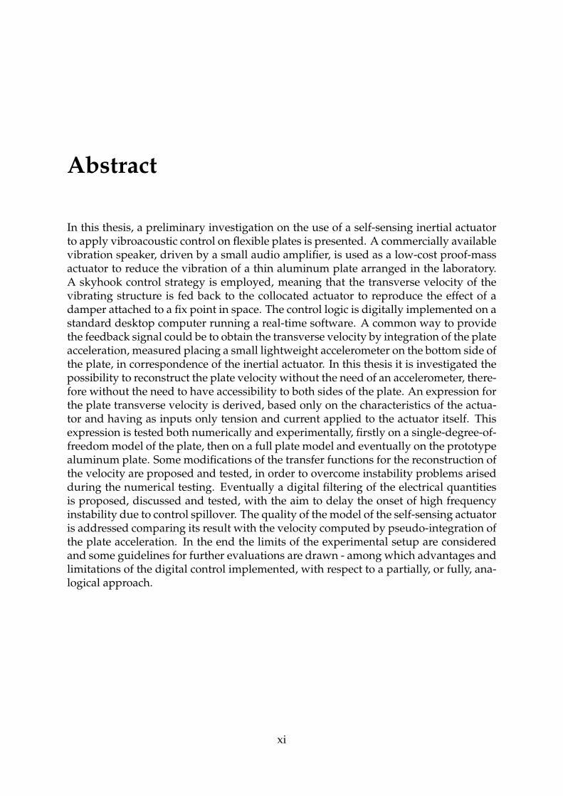
In this thesis, a preliminary investigation on the use of a self-sensing inertial actuatorto apply vibroacoustic control on flexible plates is presented. A commercially availablevibration speaker, driven by a small audio amplifier, is used as a low-cost proof-massactuator to reduce the vibration of a thin aluminum plate arranged in the laboratory.A skyhook control strategy is employed, meaning that the transverse velocity of thevibrating structure is fed back to the collocated actuator to reproduce the effect of adamper attached to a fix point in space. The control logic is digitally implemented on astandard desktop computer running a real-time software. A common way to providethe feedback signal could be to obtain the transverse velocity by integration of the plateacceleration, measured placing a small lightweight accelerometer on the bottom side ofthe plate, in correspondence of the inertial actuator. In this thesis it is investigated thepossibility to reconstruct the plate velocity without the need of an accelerometer, there-fore without the need to have accessibility to both sides of the plate. An expression forthe plate transverse velocity is derived, based only on the characteristics of the actua-tor and having as inputs only tension and current applied to the actuator itself. Thisexpression is tested both numerically and experimentally, firstly on a single-degree-of-freedom model of the plate, then on a full plate model and eventually on the prototypealuminum plate. Some modifications of the transfer functions for the reconstruction ofthe velocity are proposed and tested, in order to overcome instability problems arisedduring the numerical testing. Eventually a digital filtering of the electrical quantitiesis proposed, discussed and tested, with the aim to delay the onset of high frequencyinstability due to control spillover. The quality of the model of the self-sensing actuatoris addressed comparing its result with the velocity computed by pseudo-integration ofthe plate acceleration. In the end the limits of the experimental setup are consideredand some guidelines for further evaluations are drawn - among which advantages andlimitations of the digital control implemented, with respect to a partially, or fully, ana-logical approach.
xi

Chapter 1
Introduction
1.1 Motivation of the work
In recent years noise pollution has become more and more a topic of significant con-cern, partially due to the higher and higher anthropic density, and partially becausepeople are becoming increasingly aware of the concept of vibroacustic comfort. Re-cent studies have demonstrated the detrimental effect that prolonged exposure to noisesource can have on both the psychological and physical health - going from nuisanceand discomfort, troubled sleeping, reduced working performances and lower speechintelligibility in the least severe circumstances [1] - to hypertension, hearing deteriora-tion and ischemic heart disease in the worst cases [2, 3].Noise pollution affects people’s everyday life, their homes, the transportation they use,their working places. Indeed residential and business buildings frequently have largewindow-like surfaces, often constituting the primary path for external noises, whilecabin thin panels and shell structures generate acoustic vibrations inside cars, trainsand aircrafts [4].
The unceasing need of relying on thinner and thinner structural elements has exacer-bated the problem. The classical approach for noise and vibration reduction consistsin the passive addition of mass or damping material over a large area of the radiatingstructure [5, 6, 7], but this is often not feasible, due to mass or volume requirements.Moreover surface treatments are usually effective in suppressing high frequency vi-bration, but they would require the addition of too much mass to work in the lowfrequency range. It is in fact in this peculiar - but not rare - conditions, in which theactive vibration controls are a viable option [8]. One of the main drawbacks of activecontrol of radiating surfaces is the fact that a suitable measure of the vibration of thestructure is needed. Classically it’s obtained with collocated accelerometers, but theyoften require double accessibility on the structure. It is in this context that sensorless orself-sensing actuators became an interesting solution [9, 10].
1

2 Chapter 1. Introduction
1.2 Aim of this thesis
The present work can be considered as a preliminary study aimed to asses the pos-sibility to obtain a digitally implemented active vibration control, using self-sensinginertial actuators, to damp the resonance frequencies of an host structure subjected tobroadband random disturbances.This thesis follows from the work of Di Girolamo [11], who developed an active vibra-tion control using commercial and low-cost voice-coil vibration speakers as proof-massactuators.Vibration speakers are electromechanical transducers capable of turning surfaces intoloudspeakers, Figure 1.1.
Figure 1.1: Vibration speaker
They are mainly composed by a base plate - to be attached to the host structure andsolidal to a reversible voice coil - and a free-to-move permanent magnet. The voice coilis essentially an electromagnet that, when the actuator is powered with a time varyingvoltage, generates an induced magnetic fields that interacts with the permanent mag-net. The result of this interaction is a force acting on both components with oppositedirection, such that if the permanent magnet is pushed away from the host structure,the voice coil is pushed towards it. When the driving voltage changes sign, the forcesare reversed. Taking advantage of this phenomenon the vibration speaker is able tocause a vibration on the host structure - usually with the aim of transforming it intoa sound radiating surface. According to this physical mechanism, the idea is to use avibration speaker as a control device instead of a sound device, i.e., introduce vibrationwaves into the attached surface which can suppress the vibration induced by externalnoise sources, instead of generating sound.
Vibration speakers could be implemented in different strategies to achieve active vi-broacoustic control, according to the specific application [12], but since the currentwork is focused on the response to broadband random disturbances, the most viable
1.2. Aim of this thesis 3
option is to implement a feedback strategy. The implementation of a feedforward con-troller, on the contrary, would provides good effects for tonal disturbances, which canbe easily characterized in advance allowing to build a reference signal well correlatedto the disturbance to be controlled [13].A feedback logic for vibroacustic control can be implemented using only one actua-tor - obtaining a single-input single-output system (SISO) - or using more - obtaininga multi-input multi-output system (MIMO). In the latter case a distinction can be in-troduced between centralized and decentralized configuration. In the first case thecontrol action provided by one actuator is computed taking into account the read-ings of all sensors, in the second case each collocated sensor/actuator pair acts in-dependently from the others. The implementation of decentralized control strategies,for which no communication between the control units is permitted, is particularlyrelevant since the stability is ensured [10]. Previous works on decentralized controlof flexible structures, has focused on providing active damping by velocity feedback[14, 15, 16, 17]. This strategy, often called skyhook control since it is equivalent of havingviscous dampers attached to a fixed point in the sky [18, 17, 19, 20], leads to an un-conditionally stable closed-loop system when ideal collocated sensor/actuators pairsare used. Of course in practice both sensors and actuators are far from being ideals,actuators have internal dynamics and the velocity is usually obtained from integrationof acceleration measurements.
In the context of decentralized skyhook control, one of the limit is often to achievetruly collocated sensor/actuator pairs, one possibility to overcome this problem and toreduce the complexity of the installation is to use self-sensing actuators. A self-sensingactuator is basically a reversible electromechanical transducer which uses simultane-ously the function of sensing and actuation [9]. The self-sensing actuation concept wasdeveloped by Hagood et al. [21] and Dosch et al. [22], at the end of the last century.At the beginning only PZT elements were used as self-sensing actuators, reducing im-plementation, complexity and cost, and achieving truly collocated control. The ideawas then expanded to active vibration control on beams [23], plates [24] and vibrationdamping [25]. Finally in 2000, Leo et al. [26], extended the sensorless concept to electro-dynamic loudspeakers, and Hanson et al. used electromagnetic actuators in 2004 [27].It shall be pointed out that the vast majority of the works about self-sensing actuatorsimplement fully analogical controls, this could lead to very complex system if a largedecentralized self-sensing skyhook control logic has to be implemented on a real struc-ture. It’s a relatively new research area and many aspect has to be analyzed yet. Thiswork tries to fill a hole in the present knowledge, focusing on digital implementationof a self-sensing actuator control logic for broadband noise rejection. Indeed as saidbefore only few works have been done using a digital implementation, but for whathas been found in literature, they had considered only harmonic disturbances [28].None of them addresses the combined problem of digital implementation and randomdisturbances together, that, how will be seen later, give raise to peculiar complications.

4 Chapter 1. Introduction
1.3 Structure of the thesis
1 - Introduction A brief introduction regarding the motivation, the aim and the struc-ture of the thesis is presented. The focus is placed on the reasons for choosing a sen-sorless approach, on its difficulties and on how this work is innovative.
2 - Mathematical Models The mathematical derivation of the models used to de-scribe the main components of the experimental system is presented. At first, thelumped-parameters models for the vibration speaker and the audio amplifier are in-troduced, dynamics equations are derived and peculiar characteristics are presented.Then the core of this work - the formulation that allows to reconstruct the plate trans-verse velocity and the actuator proof-mass velocity from only current and voltage mea-surements - is derived. Finally the plate model and the S-GUF formulation on whichis based is briefly presented.
3 - Experimental Characterization The prototype arranged in the laboratory - plate,actuators and amplifiers - is presented and the experimental characterization performedto build the mathematical models is described.
4 - Numerical Testing The velocity reconstruction formulation derived in Chapter 2is tested numerically. Firstly over a simple model where the plate is described onlywith its first natural frequency, than on the complete flexible model of the structure,both in frequency and time domain. Some modification to the self-sensing actuatorequation will be needed in order to achieve stability even in real operating conditions.
5 - Experimental Testing The reconstruction of the velocity derived in Chapter 4 isimplemented in a real-time skyhook control logic in laboratory. Many criticalities arefound, filters are designed allowing to improve the performances and the basis forfuture developments are layed.

Chapter 2
Mathematical Models
In this chapter the mathematical models used in the following are derived. Firstly thelumped-parameter model of the inertial actuator is described along with the experi-mental method used to obtain its parameters - then the sensor-actuator formulation ispresented. For the vibrating plate two different models are used: at first an advancedsublaminate formulation, then a single degree of freedom model. Although much lesscomplete, the latter can be useful to gain some insight on the problem under analysis.Eventually plate and actuator models are merged together, giving rise to a completedescription of the problem under analysis, that can be implemented both in frequencyand in time domain.
2.1 Vibration speakers
plate
ka ca
ma
fc(t)
fc(t)
kem
i(t) R L
v(t)w(t)
z(t)
Figure 2.1: Schematic representation of the lumped-parameters model of the inertial actuator,when it is attached to a flexible surface.
5

6 Chapter 2. Mathematical Models
The vibration speakers used in this work can be modeled as proof-mass electrody-namic actuators, also called inertial actuators in the following. A proof-mass actuatoris a device able to provide a force on the supporting structure, by accelerating a sus-pended mass. Such a device can be schematized as a mass, elastically connected to thestructure on which control has to be obtained, bound to move perpendicularly to thestructure itself. If the movable mass - also called inertial mass in the following - is apermanent magnet, and if it is subjected to a variable magnetic field produced by a coilattached to the support structure, then the device is called an electrodynamic actuator.The magnetic field generated by the coil is proportional to the current flowing in it,such a current can be directly provided by a current source or can arise from a voltageapplied by a voltage source. In the former case the actuator can be defined as currentdriven, in the latter as voltage driven.A single degree of freedom lumped-parameters model is adopted to describe the elec-tromechanical dynamics of the actuator as shown in Figure 2.1.
2.1.1 Dynamics equations
In this section the dynamics equations for the inertial actuator are derived in the contestof the lumped-parameter approach depicted in Figure 2.1. As reported in Ref. [29],Lagrange’s equations can be used for the task. The following relevant quantities aredefined:
T∗ =12
maz2 Complementary kinetic energy (2.1)
V =12
ka(z − w)2 Potential energy (2.2)
W∗m =
12
Lq2 + kem(z − w)q Complementary magnetic energy (2.3)
D =12
ca(z − w)2 +12
Rq2 Dissipation function (2.4)
δWnc = δq v Virtual work by non-conservative forces (2.5)
Where:
ma Proof mass of the actuator [kg]
ca Damping of the actuator [Ns m−1]
ka Suspension stiffness of the actuator [N m−1]
R Coil resistance [Ω]
L Coil inductance [H]
kem Electromagnetic coupling factor [NA−1]
2.1. Vibration speakers 7
q(t) Electric charge in the coil [F]
i(t) Electric current flowing in the coil [A]
v(t) Electric voltage source [V]
z(t) Absolute displacement of the proof mass [m]
w(t) Absolute displacement of the support structure [m]
The Lagrangian of the system is defined as:
L = T∗ − V + W∗m =
12
maz2 − 12
ka(z − w)2 +12
Lq2 + kem(z − w)q (2.6)
The Lagrange’s equations read:
ddt
(∂L∂z
)− ∂L
∂z+
∂D∂z
= Qz (2.7)
ddt
(∂L∂q
)− ∂L
∂q+
∂D∂q
= Qq (2.8)
Leading to the following dynamics equations:maz(t) + ca[z(t)− w(t)] + ka[z(t)− w(t)]− kemq(t) = 0
Lq(t) + Rq(t) + kem[z(t)− w(t)] = v(t)(2.9)
That can be rewritten considering q(t) = i(t) as:maz(t) + ca[z(t)− w(t)] + ka[z(t)− w(t)]− kemi(t) = 0
Ldi(t)
dt+ Ri(t) + kem[z(t)− w(t)] = v(t)
(2.10)
The first equation describes the mechanical behavior, whereas the second is referred tothe dynamics of the electrical part. The actuator is mechanically equivalent to a spring-mass-damper system subjected to a control force due to the electromechanic couplingfc(t) = kemi(t). The current i(t) arises from the electrical equation if the actuator isvoltage driven. If current driven, instead, it is directly provided by the current sourceand the electrical equation is discarded.
2.1.2 State space realization
The system in Eq. 2.10 can be conveniently rewritten in state space introducing thefollowing substitutions:

8 Chapter 2. Mathematical Models
x1 = z
x2 = z
x3 = i
u1 = w
u2 = w
u3 = v
(2.11)
Obtaining three first order differential equations, as follows.
x1 = x2
x2 = − ka
max1 −
ca
max2 +
kem
max3 +
ka
mau1 +
ca
mau2
x3 = −kem
Lx2 −
RL
x3 +kem
Lu2 +
1L
u3
(2.12)
x1
x2
x3
=
0 1 0
− ka
ma− ca
ma
kem
ma
0 −kem
L−R
L
x1
x2
x3
+
0 0 0
ka
ma
ca
ma0
0kem
L1L
u1
u2
u3
(2.13)
That can be written in the form
x = Ax + Bu (2.14)
Where A =
0 1 0
− ka
ma− ca
ma
kem
ma
0 −kem
L−R
L
and B =
0 0 0
ka
ma
ca
ma0
0kem
L1L
The state space realization has been used in MATLAB to couple the different dynamicsystem described in this chapter. Of course it is not the only way - for instance every-thing could be done through transfer functions obtaining exactly the same results. Theprocess for obtaining the state space model of a system is straightforward and has beendescribed above, therefore - for the sake of brevity - it will not be repeated for everysystem.
2.1.3 Static residualization of the electrical dynamics
If the electrical dynamics is faster enough than the mechanical dynamics, a static resid-ualization of the former can be introduced. Starting from the dynamics system in Eq.
2.1. Vibration speakers 9
2.10 and introducing the approximation ofdi(t)
dt= 0, the electrical equation is simpli-
fied as follows.
maz(t) + ca[z(t)− w(t)] + ka[z(t)− w(t)]− kemi(t) = 0
i(t) = −kem
R[z(t)− w(t)] +
1R
va(t)(2.15)
Substituting the expression of i(t) from the electrical equation into the mechanicalequation, it can be obtained the following differential expression for the actuator withresidualized electric dynamics.
maz(t) +
(ca +
k2emR
)[z(t)− w(t)] + ka[z(t) + w(t)] =
kem
Rva(t) (2.16)
2.1.4 Rigid base
ground
ka ca
ma
fc(t)
fc(t)
kem
i(t) R L
v(t)
z(t)
Figure 2.2: Schematic representation of the lumped-parameters model of the inertial actuator,when it is attached on a fixed, rigid surface.
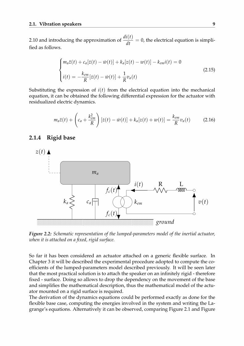
So far it has been considered an actuator attached on a generic flexible surface. InChapter 3 it will be described the experimental procedure adopted to compute the co-efficients of the lumped-parameters model described previously. It will be seen laterthat the most practical solution is to attach the speaker on an infinitely rigid - thereforefixed - surface. Doing so allows to drop the dependency on the movement of the baseand simplifies the mathematical description, thus the mathematical model of the actu-ator mounted on a rigid surface is required.The derivation of the dynamics equations could be performed exactly as done for theflexible base case, computing the energies involved in the system and writing the La-grange’s equations. Alternatively it can be observed, comparing Figure 2.1 and Figure

10 Chapter 2. Mathematical Models
2.2, that the only difference between the two systems is the dependency on the struc-tural degree of freedom w(t). Therefore it is enough to drop the terms in w(t) and w(t)from Eq. 2.10, to obtain the dynamics equation for the actuator when mounted on arigid base, Eq. 2.17.
maz(t) + caz(t) + kaz(t)− kemi(t) = 0
Ldi(t)
dt+ Ri(t) + kemz(t) = v(t)
(2.17)
2.1.5 Proof-mass acceleration response
In this section the actuator dynamics is described through the proof-mass accelerationresponse, defined as the transfer function between the electrical source and the accel-eration of the moving mass. Dependently on how the electromagnetic inertial actuatoris driven - in current or in voltage - different transfer functions are obtained.In both cases the derivation starts form the dynamics equations in Eq. 2.17. In the volt-age driven case both equations are used, whereas in the current driven case the secondone can be dropped.
Voltage driven
Taking the Laplace transform of Eq. 2.17
(mas2 + cas + ka)z(s)− kemi(s) = 0
(Ls + R)i(s) + kemz(s) = v(s)(2.18)
Computing i(s) form the second equation and substituting it in the first, the followingexpression is obtained:
(mas2 + cas + ka +
k2ems
R + sL
)z(s)− kem
R + sLv(s) = 0 (2.19)
The dependency of the proof-mass acceleration on the driving voltage can now bereadily obtained isolating z(s) and taking the second time derivative:
z(s) =s2keem
(R + sL)(mas2 + cas + ka) + sk2em
v(s) (2.20)
The proof-mass acceleration response for the voltage driven actuator can now be madeexplicit, writing the following transfer function:
HaV(s) =z(s)v(s)
=s2keem
(R + sL)(mas2 + cas + ka) + sk2em
(2.21)
2.1. Vibration speakers 11
If the frequency separation between the mechanical and the electrical poles is highenough, it could be computationally useful to introduced the static residualization de-scribed before. Doing so the proof-mass acceleration response reads:
HaV res(s) =z(s)v(s)
=s2keem
R(mas2 + cas + ka) + sk2em
(2.22)
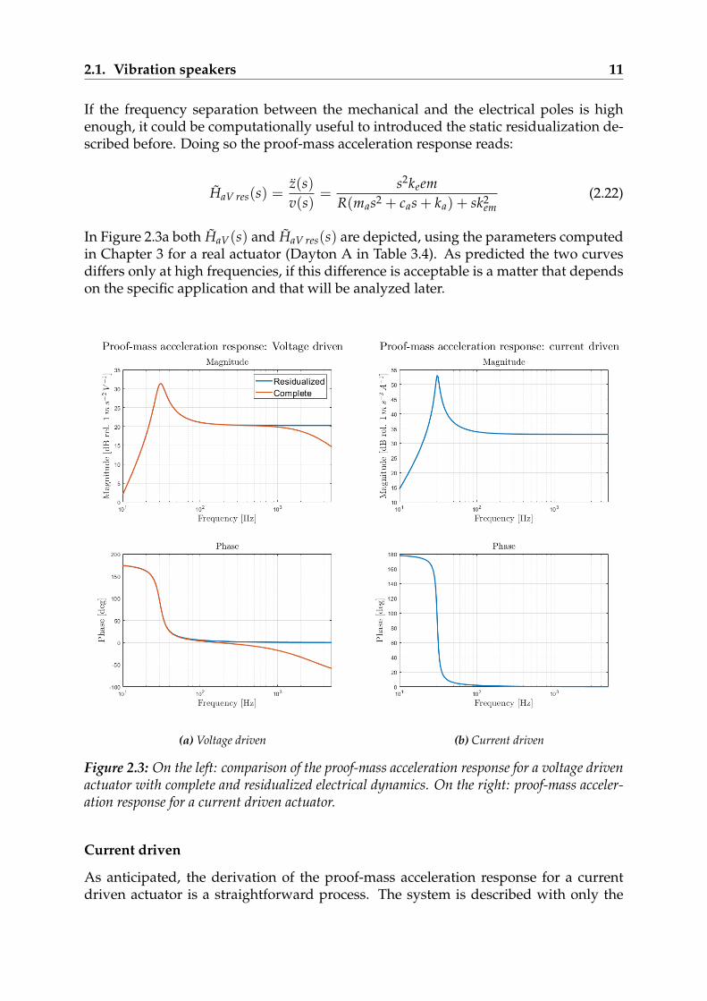
In Figure 2.3a both HaV(s) and HaV res(s) are depicted, using the parameters computedin Chapter 3 for a real actuator (Dayton A in Table 3.4). As predicted the two curvesdiffers only at high frequencies, if this difference is acceptable is a matter that dependson the specific application and that will be analyzed later.
(a) Voltage driven (b) Current driven
Figure 2.3: On the left: comparison of the proof-mass acceleration response for a voltage drivenactuator with complete and residualized electrical dynamics. On the right: proof-mass acceler-ation response for a current driven actuator.
Current driven
As anticipated, the derivation of the proof-mass acceleration response for a currentdriven actuator is a straightforward process. The system is described with only the
12 Chapter 2. Mathematical Models
mechanical equation, therefore the dynamics of the actuator is reduced to the firstequation of Eq. 2.18:
(mas2 + cas + ka)z(s)− kemi(s) = 0 (2.23)
It can be immediately computed z(s), derived two times and rearranged to obtainthe transfer function that describes the proof-mass acceleration response of a currentdriven actuator. Figure 2.3b shows its plot.
Hai(s) =z(s)i(s)
=s2kem
mas2 + cas + ka(2.24)
The plots in Figure 2.3a and 2.3b anticipate the behaviour of one of the actuator thatwill be used in this work. Note that both voltage and current driven responses show aresonance peak at the same frequency, around 30Hz. This is the fundamental frequencyof the single degree of freedom model used to describe the actuator.
2.1.6 Electrical input impedance
Another way of characterizing the electromechanic dynamics of a proof-mass actuatoris to study its electrical input impedance. The electric circuit composing the driver ofthe vibration speaker is well described by a RL circuit. The electrical impedance ofsuch a circuit is an extension of the concept of electric resistance in simple resistivecircuit, therefore the ratio of the applied voltage over the flowing current. As donein the context of the proof-mass acceleration response, the derivation of the electricalinput impedance transfer function starts from the dynamics equations of the actuatorwhen it is attached on a fixed surface, Eq. 2.17. The Laplace transform of the system isthe same as before and it’s reported here for the sake of clarity:
(mas2 + cas + ka)z(s)− kemi(s) = 0
(Ls + R)i(s) + kemz(s) = v(s)(2.25)
The aim is to obtain an expression depending only on i(s) and v(s). It can be easilydone isolating z(s) in the second equation.
(mas2 + cas + ka)z(s)− kemi(s) = 0
z(s) =1
kemsv(s)− R + sL
kemsi(s)
(2.26)
Substituting z(s) back in the mechanical equation the following expression is obtained:
(mas2 + cas + ka)v(s) =[(R + sL)(mas2 + cas + ka)− k2
ems]
i(s) (2.27)
2.1. Vibration speakers 13
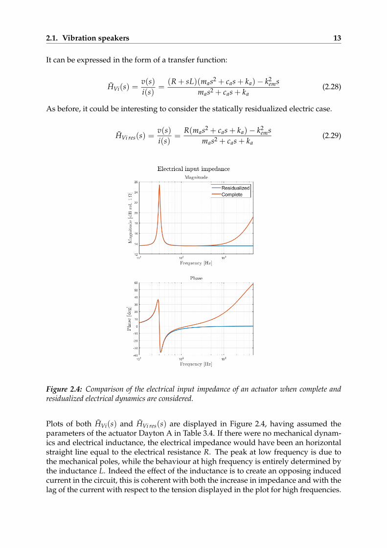
It can be expressed in the form of a transfer function:
HVi(s) =v(s)i(s)
=(R + sL)(mas2 + cas + ka)− k2
emsmas2 + cas + ka
(2.28)
As before, it could be interesting to consider the statically residualized electric case.
HVi res(s) =v(s)i(s)
=R(mas2 + cas + ka)− k2
emsmas2 + cas + ka
(2.29)
Figure 2.4: Comparison of the electrical input impedance of an actuator when complete andresidualized electrical dynamics are considered.
Plots of both HVi(s) and HVi res(s) are displayed in Figure 2.4, having assumed theparameters of the actuator Dayton A in Table 3.4. If there were no mechanical dynam-ics and electrical inductance, the electrical impedance would have been an horizontalstraight line equal to the electrical resistance R. The peak at low frequency is due tothe mechanical poles, while the behaviour at high frequency is entirely determined bythe inductance L. Indeed the effect of the inductance is to create an opposing inducedcurrent in the circuit, this is coherent with both the increase in impedance and with thelag of the current with respect to the tension displayed in the plot for high frequencies.
14 Chapter 2. Mathematical Models
2.2 Reconstruction of the velocities
Aim of this section is to derive the mathematical formulation on which the sensor-actuator concept described in Chapter 1 is based. The objective is to obtain an ex-pression that, by receiving as inputs only current and voltage, allows to reconstructthe transverse velocity of the plate to be used in the skyhook control strategy. Thederivation follows what proposed in Ref. [9, 10], with the purpose to remove the needof accelerometers to obtain the transverse plate velocity. The same procedure will bealso applied to reconstruct the velocity of the inertial mass of the actuator that couldbe needed in more advanced control logic to increase stability limits. Note that in thefollowing, whenever a velocity is call reconstructed, reference is always made to thevelocity obtained by current and voltage measurements.
2.2.1 Plate transverse velocity
plate
massless base
ka ca
ma
fc(t)
fc(t)
kem
i(t) R L
v(t)w(t)
z(t)
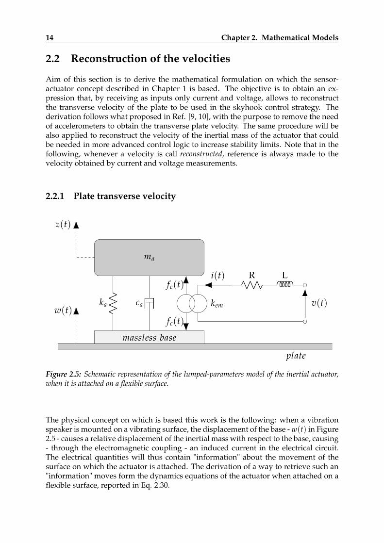
Figure 2.5: Schematic representation of the lumped-parameters model of the inertial actuator,when it is attached on a flexible surface.
The physical concept on which is based this work is the following: when a vibrationspeaker is mounted on a vibrating surface, the displacement of the base - w(t) in Figure2.5 - causes a relative displacement of the inertial mass with respect to the base, causing- through the electromagnetic coupling - an induced current in the electrical circuit.The electrical quantities will thus contain "information" about the movement of thesurface on which the actuator is attached. The derivation of a way to retrieve such an"information" moves form the dynamics equations of the actuator when attached on aflexible surface, reported in Eq. 2.30.
2.2. Reconstruction of the velocities 15
maz(t) + ca[z(t)− w(t)] + ka[z(t)− w(t)]− kemi(t) = 0
Ldi(t)
dt+ Ri(t) + kem[z(t)− w(t)] = v(t)
(2.30)
Rewriting the same equations in the Laplace’s domain:
s2maz(s) + sca[z(s)− w(s)] + ka[z(s)− w(s)]− kemi(s) = 0
sLi(s) + Ri(s) + skem[z(s)− w(s)] = v(s)(2.31)
The aim is now to obtain an equation where the plate degree of freedom w(s), dependsonly on the applied voltage v(s), and on the flowing current i(s). To do so it has to beeliminated the dependency on the inertial mass degree of freedom z(s). Rearrangingthe electrical equation z(s) can be isolated:
z(s) = w(s)− R + sLskem
i(s) +1
skemv(s) (2.32)
Substituting it into the mechanical equations it is obtained an expression in w(s), v(s)and i(s) alone.
s2maw(s)−
(R + sL)(
s2ma + sca + ka
)skem
+ kem
i(s) +s2ma + sca + ka
skemv(s) = 0
(2.33)
It’s now possible to isolate w(s):
w(s) =
(R + sL)(
s2ma + sca + ka
)+ sk2
em
s3makem
i(s)−[
s2ma + sca + ka
s3makem
]v(s) (2.34)
Taking the first time derivative, the desired transverse plate velocity is obtained:
w(s) =
(R + sL)(
s2ma + sca + ka
)+ sk2
em
s2makem
i(s)−[
s2ma + sca + ka
s2makem
]v(s) (2.35)
= Hi(s)i(s)− Hv(s)v(s)
16 Chapter 2. Mathematical Models
Eq. 2.35 allows to reconstruct the plate velocity - in the point where the actuator isplaced - measuring only voltage and current.It has to be pointed out that the current related transfer function - Hi(s) - is not proper,being the numerator of higher order than the denominator. This problem - amongothers - will be extensively addressed later. One possible way to overcome it, consistsin the static residualization of the electric dynamic.
Static residualization
The equation for the reconstruction of the plate transverse velocity in a statically resid-ualized framework could be obtained intuitively just removing sL from Eq. 2.35, butfor the sake of completeness it’s hereby analytically derived. The derivation shall movefrom the dynamics equations for a statically residualized actuator attached on a flexiblesurface, Eq. 2.36.
maz(t) + ca[z(t)− w(t)] + ka[z(t)− w(t)]− kemi(t) = 0
Ri(t) + kem[z(t)− w(t)] = va(t)(2.36)
Rewriting the same equations in the Laplace’s domain:
s2maz(s) + sca[z(s)− w(s)] + ka[z(s)− w(s)]− kemi(s) = 0
Ri(t) + skem[z(s)− w(s)] = va(s)(2.37)
From the electrical equation can be obtained z(s):
z(s) = w(s)− Rskem
i(s) +1
skemv(s) (2.38)
Substituting it into the mechanical equations:
s2maw(s)−
R(
s2ma + sca + ka
)skem
+ kem
i(s) +
[s2ma + sca + ka
skem
]v(s) = 0 (2.39)
Isolating w(s):
w(s) =
R(
s2ma + sca + ka
)+ sk2
em
s3makem
i(s)−[
s2ma + sca + ka
s3makem
]v(s) (2.40)

2.2. Reconstruction of the velocities 17
And deriving it:
w(s) =
R(
s2ma + sca + ka
)+ sk2
em
s2makem
i(s)−[
s2ma + sca + ka
s2makem
]v(s) (2.41)
As anticipated the only difference with the complete electrical dynamics case is theabsence of the sL contribution.
2.2.2 Inertial mass velocity
As anticipated before it’s possible to apply the same method and derive a formulationfor the velocity of the inertial mass, depending only on the voltage applied to the iner-tial actuator and on the current flowing in it.As before the derivation moves from the dynamics equations for the inertial actuatormounted on a flexible surface.
maz(t) + ca[z(t)− w(t)] + ka[z(t)− w(t)]− kemi(t) = 0
Ldi(t)
dt+ Ri(t) + kem[z(t)− w(t)] = v(t)
(2.42)
Rewriting the same equations in the Laplace’s domain:
s2maz(s) + sca[z(s)− w(s)] + ka[z(s)− w(s)]− kemi(s) = 0
sLi(s) + Ri(s) + skem[z(s)− w(s)] = v(s)(2.43)
As above the electrical equation can be rearranged isolating, this time, the transverseplate velocity w(s):
w(s) = z(s) +R + sL
skemi(s)− 1
skemv(s) (2.44)
Substituting it into the mechanical equation is obtained an expression in z(s), v(s) andi(s) alone:
s2maz(s)−((R + sL) (sca + ka)
skem+ kem
)i(s) +
sca + ka
skemv(s) = 0 (2.45)
Isolating z(s):
18 Chapter 2. Mathematical Models
z(s) =
[(R + sL) (sca + ka) + sk2
ems3makem
]i(s)−
[sca + ka
s3makem
]v(s) (2.46)
Taking the first derivative the velocity of the inertial mass of the actuator is obtained:
z(s) =
[(R + sL) (sca + ka) + sk2
ems2makem
]i(s)−
[sca + ka
s2makem
]v(s) (2.47)
The statically residualized version of the previous equation can be easily obtained justdropping the inductance related term sL.
z(s) =
[R (sca + ka) + sk2
ems2makem
]i(s)−
[sca + ka
s2makem
]v(s) (2.48)
2.3 Pseudo-integrator
In a skyhook control strategy the transverse velocity of the plate is usually obtainedby integration of the transverse acceleration. In later chapters, the performances of thereconstruction of the velocity obtained in the context of the self-sensing actuator, willbe often compared to the classical approach. In this section is thus briefly describedhow to properly integrate the acceleration signal to obtain the velocity, as done in [11].In the Laplace domain, the transfer function of a pure integrator would be:
yvel(s)yacc(s)
=1s
If the acceleration signal presents a DC components - such the gravity - or even a smalloffset due to acquisition errors, a pure integral action is not recommended. Instead,the following pseudo-integration can be adopted.
yvel(s)yacc(s)
=s
s2 + 2ξpiωpis + ω2pi
(2.49)
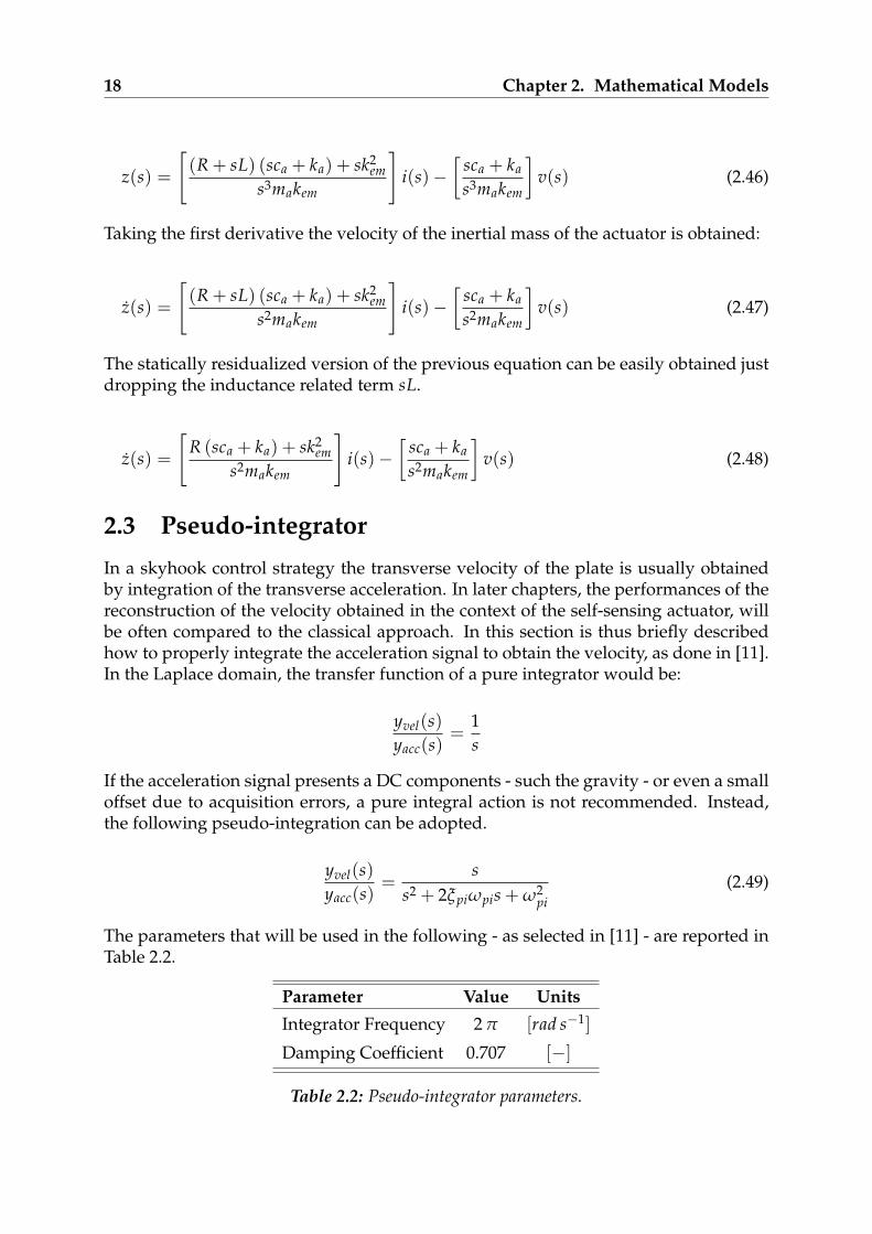
The parameters that will be used in the following - as selected in [11] - are reported inTable 2.2.
Parameter Value Units
Integrator Frequency 2 π [rad s−1]
Damping Coefficient 0.707 [−]
Table 2.2: Pseudo-integrator parameters.

2.4. Power amplifiers 19
2.4 Power amplifiers
In the experimental setup object of this work, the vibrations speakers are driven bysignals generated by a computer. Although the PC could provide a sufficiently largevoltage output to drive directly the speakers - ±10V - it can not produce the requiredcurrent due to it’s high output impedance - therefore neither the required power -that’s why a power amplifier is required. A power amplifier is a common device thatreproduces low power signals at levels that are strong enough for powering the mostvarious items. Not only they provide enough current do drive low impedance devices,but they also give a mean to amplify the driving voltage. While the former aspect sim-ply allows the speaker to work properly and does not require any mathematical mod-elling, the latter introduces a voltage gain that has to be quantified, if the behaviour ofthe amplifier has to be simulated numerically.As will be discussed in Chapter 3, the speakers used in this work have an input impedanceof 4Ω, allowing to drive them with common audio amplifiers.Broadly speaking, an audio amplifier can be modeled as a band pass filter, whose be-haviour is represented by the following transfer function:
H(s) = gamps
(s + a)(s + b)
Where gamp is the voltage gain described above and a and b are respectively the lowfrequency and high frequency poles of the band pass filter. Taking into account that therange of human hearing spans form 20Hz to 20kHz [30], it’s foreseeable that the highfrequency pole of the amplifier would be around 20kHz, far higher than the frequencyrange of interest of this work. Then, for the purpose of this thesis, the high frequencypole can be ignored and the audio amplifier transfer function can be reduced as fol-lows:
H(s) = gamps
s + a
2.5 Plate Model
As outlined before, the plate has been modeled relying on the sublaminate generalizedunified formulation (S-GUF) [31], developed through a collaboration between Politec-nico di Milano and Université of Paris X. Although such a complex formulation wouldnot be strictly required to model the thin homogeneous aluminum plate object of thiswork, it has been chosen because its versatility allows to promptly extend the resultsof the present work to more complex vibrating structures, in particular to multilay-ered composite and sandwich panels. In the following the key points of the S-GUFformulation are described, for the complete derivation make reference to [31].
20 Chapter 2. Mathematical Models
2.5.1 The Sublaminate Generalized Unified Formulation
The majority of the nowadays available approaches to plate modeling are based onreducing the 3-D problem to a 2-D problem, introducing in advance some kinematicassumptions about the behaviour of the displacement field in the thickness direction ofthe plate. Such a modelling strategy is known as axiomatic displacement-based approachand the resulting 2-D models are called displacement-based plate theories.
The most used displacement-based plate theories are the Calssical Plate Theory (CPT)and the First-order Shear Deformation Theory (FSDT). These theories originally ad-dressed the need of working with computational economical models that could behandled by limited computational capabilities, however they could lead to inaccu-rate results when thick or multilayered structures are considered. These inaccuraciesarise because a simple 2-D model can’t properly catch some relevant 3-D effects suchas transverse shear and normal deformations, cross-section warping, boundary layerstresses and through-the-thickness zig-zag behaviour of the displacement field. Indeeda formulation able to account in some way for these effects while keeping a relativelysimple 2-D model of the plate - avoiding the need to resort to a cumbersome fully 3-Dformulation - would be a powerful and interesting tool, that’s in fact the case of theS-GUF approach.
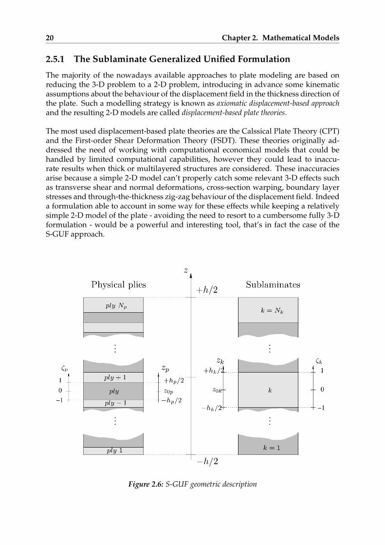
Figure 2.6: S-GUF geometric description
2.5. Plate Model 21
A peculiar characteristic of the S-GUF formulation is the fact that the kinematic de-scription can be enriched when needed, introducing different 2-D kinematic theoriesof arbitrary order in different sub-regions of the plate thickness, so that a virtually in-finite amount of plate models can be derived from a single general formulation. Thisapproach shows its full potential with multilayered plates, when the concept of sub-laminate - a group of adjacent physical plies with a specific kinematic description - can beintroduced. The concept of sublaminates can be seen in Figure 2.6: a plate of thicknessh, composed by Np physical plies of homogeneous orthotropic material, is subdividedinto k = 1, 2, · · · , Nk sublaminates of thickness hk, numbered from bottom to top.
As previously said, in the S-GUF approach the user can introduce a different kine-matic description in each sublaminate. Such an approach is called layerwise (LW) andit’s formal expression is
up,k
x (x, y, zk, t) = Fαux (zk)up,kxαux
(x, y, t) (αux = 0, 1, · · · , Nx)
up,ky (x, y, zk, t) = Fαuy (zk)u
p,kyαuy
(x, y, t) (αuy = 0, 1, · · · , Ny)
up,kz (x, y, zk, t) = Fαuz (zk)u
p,kzαuz
(x, y, t) (αuz = 0, 1, · · · , Nz)
(2.50)
Where up,kr (x, y, zk, t) are the displacements components (r = x, y, or z), Fαur(zk) are
thickness functions defined in terms of the sublaminate coordinate zk, and up,krαur
(x, y, t)are the kinematic variables for layerwise description in the ply p = 1, 2, · · · , Nk
p of thesublaminate k. Nr is the order of expansion of the ur component. Eq. 2.50 represent themost general case. If the same kinematics is adopted for all the plies of one sublaminatethan the approach is said equivalent single-layer (ESL) and can be expressed droppingthe index p. It’s worth to be noted that a specific local kinematics can be specified ineach sublaminate, with the possibility to obtain a multiple-kinematics model of theplate in a straightforward way. For instance a sandwich panel can be divided in threesublaminates: two low-order sublaminates describing the stiff laminated skins andone higher-order sublaminate for the soft thick core. Of course also common singlekinematic model can be obtained as special cases when a single sublaminate is used todescribe the whole plate. In particular, the thin isotropic aluminum plate object of thiswork can be described by a full ESL model, whose S-GUF parameters are defined asfollows
p = 1k = 1
Nx = 1Ny = 1Nz = 0
F0 = 0F1 = z
(2.51)
22 Chapter 2. Mathematical Models
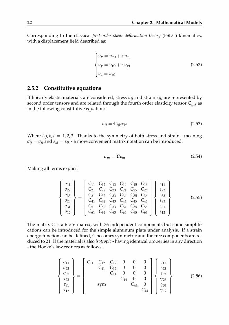
Corresponding to the classical first-order shear deformation theory (FSDT) kinematics,with a displacement field described as:
ux = ux0 + z ux1
uy = uy0 + z uy1
uz = uz0
(2.52)
2.5.2 Constitutive equations
If linearly elastic materials are considered, stress σij and strain εij, are represented bysecond order tensors and are related through the fourth order elasticity tensor Cijkl asin the following constitutive equation:
σij = Cijklεkl (2.53)
Where i, j, k, l = 1, 2, 3. Thanks to the symmetry of both stress and strain - meaningσij = σji and εkl = ε lk - a more convenient matrix notation can be introduced.
σm = Cεm (2.54)
Making all terms explicit
σ11σ22σ33σ23σ31σ12
=
C11 C12 C13 C14 C15 C16C21 C22 C23 C24 C25 C26C31 C32 C33 C34 C35 C36C41 C42 C43 C44 C45 C46C51 C52 C53 C54 C55 C56C61 C62 C63 C64 C65 C66
ε11ε22ε33ε23ε31ε12
(2.55)
The matrix C is a 6 × 6 matrix, with 36 independent components but some simplifi-cations can be introduced for the simple aluminum plate under analysis. If a strainenergy function can be defined, C becomes symmetric and the free components are re-duced to 21. If the material is also isotropic - having identical properties in any direction- the Hooke’s law reduces as follows.
σ11σ22σ33τ23τ31τ12
=
C11 C12 C12 0 0 0C11 C12 0 0 0
C11 0 0 0C44 0 0
sym C44 0C44
ε11ε22ε33γ23γ31γ12
(2.56)
2.5. Plate Model 23
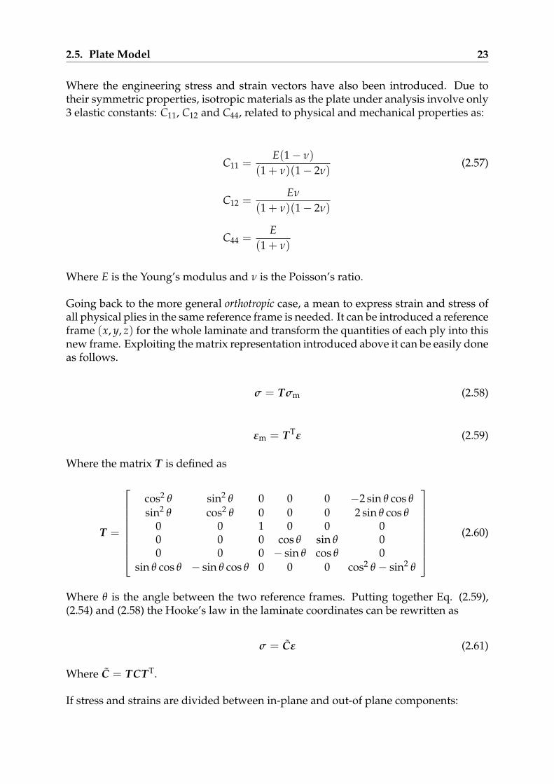
Where the engineering stress and strain vectors have also been introduced. Due totheir symmetric properties, isotropic materials as the plate under analysis involve only3 elastic constants: C11, C12 and C44, related to physical and mechanical properties as:
C11 =E(1 − ν)
(1 + ν)(1 − 2ν)(2.57)
C12 =Eν
(1 + ν)(1 − 2ν)
C44 =E
(1 + ν)
Where E is the Young’s modulus and ν is the Poisson’s ratio.
Going back to the more general orthotropic case, a mean to express strain and stress ofall physical plies in the same reference frame is needed. It can be introduced a referenceframe (x, y, z) for the whole laminate and transform the quantities of each ply into thisnew frame. Exploiting the matrix representation introduced above it can be easily doneas follows.
σ = Tσm (2.58)
εm = TTε (2.59)
Where the matrix T is defined as
T =
cos2 θ sin2 θ 0 0 0 −2 sin θ cos θ
sin2 θ cos2 θ 0 0 0 2 sin θ cos θ0 0 1 0 0 00 0 0 cos θ sin θ 00 0 0 − sin θ cos θ 0
sin θ cos θ − sin θ cos θ 0 0 0 cos2 θ − sin2 θ
(2.60)
Where θ is the angle between the two reference frames. Putting together Eq. (2.59),(2.54) and (2.58) the Hooke’s law in the laminate coordinates can be rewritten as
σ = Cε (2.61)
Where C = TCTT.
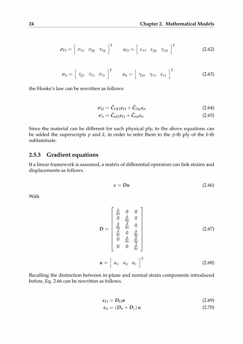
If stress and strains are divided between in-plane and out-of plane components:
24 Chapter 2. Mathematical Models
σΩ =[
σxx σyy τxy
]TεΩ =
[εxx εyy γxy
]T(2.62)
σn =[
τyz τxz σzz
]Tεn =
[γyz γxz εzz
]T(2.63)
the Hooke’s law can be rewritten as follows:
σΩ = CΩΩεΩ + CΩnεn (2.64)
σn = CnΩεΩ + Cnnεn (2.65)
Since the material can be different for each physical ply, to the above equations canbe added the superscripts p and k, in order to refer them to the p-th ply of the k-thsublaminate.
2.5.3 Gradient equations
If a linear framework is assumed, a matrix of differential operators can link strains anddisplacements as follows.
ε = Du (2.66)
With
D =
∂∂x 0 00 ∂
∂y 0∂
∂y∂
∂x 0∂∂z 0 ∂
∂x0 ∂
∂z∂
∂y0 0 ∂
∂z
(2.67)
u =[
ux uy uz
]T(2.68)
Recalling the distinction between in-plane and normal strain components introducedbefore, Eq. 2.66 can be rewritten as follows.
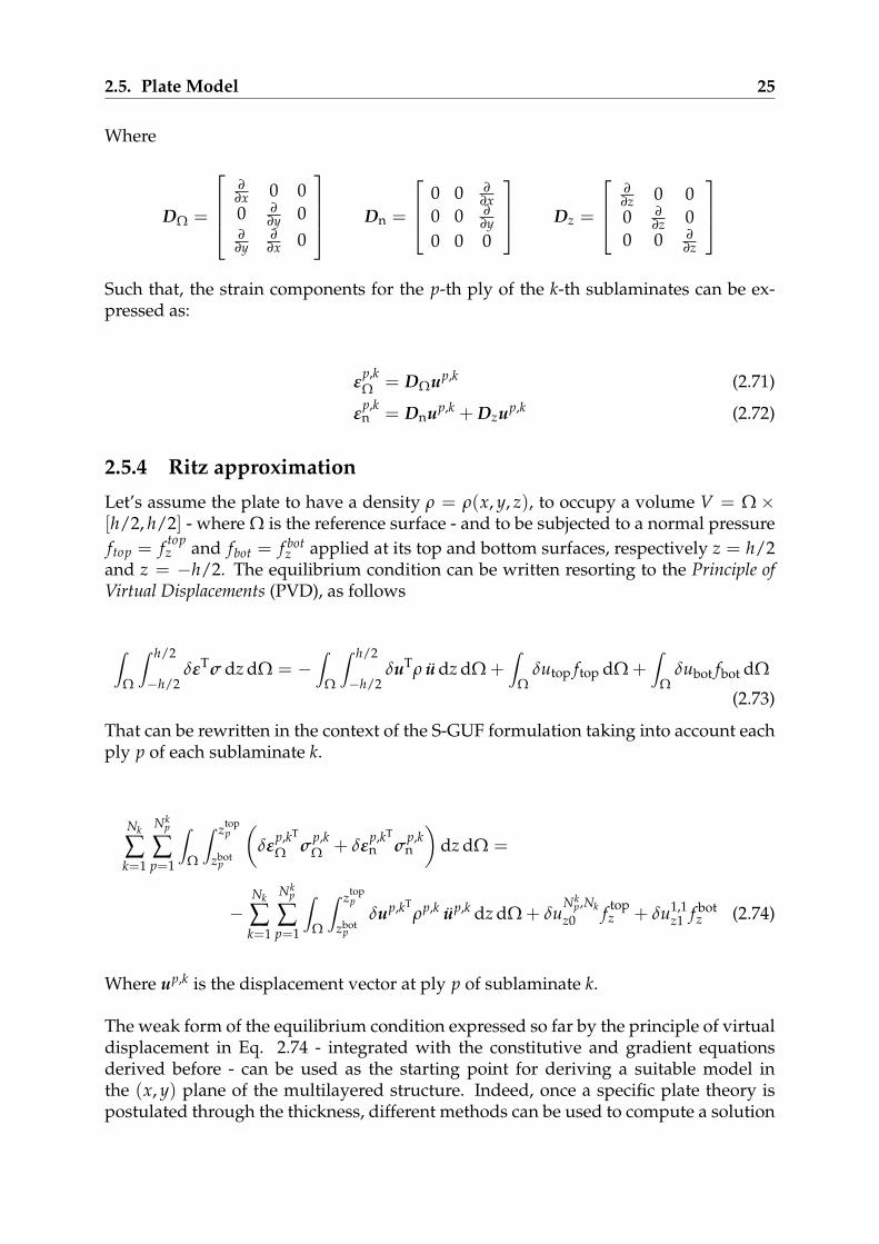
εΩ = DΩu (2.69)εn = (Dn + Dz) u (2.70)
2.5. Plate Model 25
Where
DΩ =
∂
∂x 0 00 ∂
∂y 0∂
∂y∂
∂x 0
Dn =
0 0 ∂∂x
0 0 ∂∂y
0 0 0
Dz =
∂∂z 0 00 ∂
∂z 00 0 ∂
∂z
Such that, the strain components for the p-th ply of the k-th sublaminates can be ex-pressed as:
εp,kΩ = DΩup,k (2.71)
εp,kn = Dnup,k + Dzup,k (2.72)
2.5.4 Ritz approximation
Let’s assume the plate to have a density ρ = ρ(x, y, z), to occupy a volume V = Ω ×[h/2, h/2] - where Ω is the reference surface - and to be subjected to a normal pressureftop = f top
z and fbot = f botz applied at its top and bottom surfaces, respectively z = h/2
and z = −h/2. The equilibrium condition can be written resorting to the Principle ofVirtual Displacements (PVD), as follows
∫Ω
∫ h/2
−h/2δεTσ dz dΩ = −
∫Ω
∫ h/2
−h/2δuTρ u dz dΩ +
∫Ω
δutop ftop dΩ +∫
Ωδubot fbot dΩ
(2.73)
That can be rewritten in the context of the S-GUF formulation taking into account eachply p of each sublaminate k.
Nk
∑k=1
Nkp
∑p=1
∫Ω
∫ ztopp
zbotp
(δε
p,kT
Ω σp,kΩ + δε
p,kT
n σp,kn
)dz dΩ =
−Nk
∑k=1
Nkp
∑p=1
∫Ω
∫ ztopp
zbotp
δup,kTρp,k up,k dz dΩ + δu
Nkp,Nk
z0 f topz + δu1,1
z1 f botz (2.74)
Where up,k is the displacement vector at ply p of sublaminate k.
The weak form of the equilibrium condition expressed so far by the principle of virtualdisplacement in Eq. 2.74 - integrated with the constitutive and gradient equationsderived before - can be used as the starting point for deriving a suitable model inthe (x, y) plane of the multilayered structure. Indeed, once a specific plate theory ispostulated through the thickness, different methods can be used to compute a solution
26 Chapter 2. Mathematical Models
for the reduced 2-D problem in the (x, y) plane. In the S-GUF formulation this task isperformed though the discretization using the Ritz approach. The Ritz approximationof the 2-D kinematic variables can be written as follows
up,k
xαux(x, y, t) = Nux j(x, y)up,k
xαux j(t)
up,kyαuy
(x, y, t) = Nuy j(x, y)up,kyαuy j(t)
up,kzαuz
(x, y, t) = Nuz j(x, y)up,kzαuz j(t)
j = 1, 2, . . . , M (2.75)
Where Nuri is the i-th admissible function related to ur (r = x, y, z). Note that in Eq.2.75 the summation over the repeated index i is implied.Eq. 2.75 shows that the assumed solutions are in the form of a linear combination ofundetermined parameters with appropriate chosen functions. The number of terms ofthe combination is given by M, which is called the Ritz order. The generic admissiblefunction can be expressed - mapping the physical (x, y) domain into the computational(ξ, η) domain defined in the interval [−1, 1]× [−1, 1] - as follows
Nuri(ξ, η) = ϕurm(ξ)ψurn(η) (m = 1, . . . , R; n = 1, . . . , S)
Where R · S = M, i = S(m − 1) + n and
ϕurm(ξ) = fur(ξ)pm(ξ) (2.76)ψurn(η) = gur(η)pn(η)
The completeness of the Ritz functions is guaranteed by pm and pn, taken as Legendreorthogonal polynomials. The compliance with the geometric boundary conditions isachieved thanks to the boundary functions fu−r and gu−r, expressed in the followingform.
fur(ξ) = (1 + ξ)e1r(1 − ξ)e2r
gur(η) = (1 + η)e1r(1 − η)e2r
Where the value of the exponents e1r and e2r are selected according to the boundaryconditions.
The following compact notation for the integrals of the Ritz functions can be intro-duced.
Ide f gurusij =
∫Ω
∂d+eNuri
∂xd∂ye
∂ f+gNus j
∂x f ∂yg dΩ (d, e, f , g = 0, 1) (2.77)
2.5. Plate Model 27
The Ritz approximate form of the PVD derived before can now be expressed as in Eq.2.78, where many elastic terms are omitted for the sake of brevity.
Nk
∑k=1
Nkp
∑p=1
[δup,k
xαux iρp,kZpαux βux
uxux I0000uxuxiju
p,kxβux j + δup,k
yαuy iρp,kZ
pαuy βuyuyuy I0000
uyuyijup,kyβuy j (2.78)
+ δup,kzαuz iρ
p,kZpαuz βuzuzuz I0000
uzuzijup,kzβuz j
]+
Nk
∑k=1
Nkp
∑p=1
[δup,k
xαux iCp,k11 Zpαux βux
uxux I1010uxuxiju
p,kxβux j + δup,k
xαux iCp,k12 Z
pαux βuyuxuy I1001
uxuyijup,kyβuy j
+ δup,kxαux iC
p,k16 Zpαux βux
uxux I1001uxuxiju
p,kxβux j + δup,k
xαux iCp,k16 Z
pαux βuyuxuy I1010
uxuyijup,kyβuy j + . . .
+ · · ·+ δup,kzαuz iC
p,k33 Zpαuz βuz
∂uz∂uzI0000
uzuzijup,kzβuz j
]=
δuNk
p,Nkz0i
∫Ω
Nuzi f topz dΩ + δu1,1
z1i
∫Ω
Nuzi f botz dΩ
2.5.5 Expansion and assembly
From the indicial form shown in Eq. 2.78, can be constructed the matrices and the loadvectors o a virtually infinite number of plate models, trough a procedure consistingin successive expansion and assembly steps of elementary blocks of the formulationcalled kernels end defined as follows.
Cp,kRS Zpαur βus
(∂)ur(∂)usIde f g
urusij (elastic terms) (2.79)
ρp,kZpαur βusurus Ide f g
urusij (inertial terms) (2.80)
In the following are schematized the four cycles from the fundamental kernels to themass and stiffness matrices of the plate model.
1. Summation over the repeated indexes αur and βus , arising from the order of thekinematic description assumed in each sublaminate. Symbolically it can be ex-pressed as
Zpαur βus(∂)ur(∂)us
theory expansion−−−−−−−−−−→(αur ,βus ) cycling
Zp,k(∂)ur(∂)us
(r, s = x, y, z)
2. Summation of the contribution of each ply inside a specified sublaminate, cyclingover p. Symbolically it can be expressed as
Cp,kRSZp,k
(∂)ur(∂)us
ply assembly−−−−−−−−→p cycling
Zk(∂)ur(∂)usRS
28 Chapter 2. Mathematical Models
ρp,kZp,kurus
ply assembly−−−−−−−−→p cycling
Zkurusρ
3. Summation over all the sublaminates - index k - imposing the continuity of thedisplacements at the interfaces of adjacent sublaminates. Symbolically it can beexpressed as
Zk(∂)ur(∂)usRS
sublaminate assembly−−−−−−−−−−−−−→k cycling
Z(∂)ur(∂)usRS
Zkurusρ
sublaminate assembly−−−−−−−−−−−−−→k cycling
Zurusρ
Finally the following matrices for each i and j are obtained.
Mij =
Muxuxij 0 00 Muyuyij 00 0 Muzuzij
(2.81)
Kij =
Kuxuxij Kuxuyij KuxuzijKuyuxij Kuyuyij KuyuzijKuzuxij Kuzuyij Kuzuzij
(2.82)
Where
Muxuxij = ZuxuxρI0000uxuxij
Muyuyij = ZuyuyρI0000uyuyij
Muzuzij = ZuzuzρI0000uzuzij
Kuxuxij = Zuxux11I1010uxuxij + Zuxux16(I1001
uxuxij + I0110uxuxij) + Zuxux66I0101
uxuxij
+ Z∂ux∂ux55I0000uxuxij
Kuxuyij = Zuxuy12I1001uxuyij + Zuxuy16I1010
uxuyij + Zuxuy26I0101uxuyij + Zuxuy66I0110
uxuyij
+ Z∂ux∂uy45I0000uxuyij
Kuxuzij = Z∂uxuz55I0010uxuzij + Z∂uxuz45I0001
uxuzij + Zux∂uz13I1000uxuzij + Zux∂uz36I0100
uxuzij
Kuyuxij = Zuyux12I0110uyuxij + Zuyux26I0101
uyuxij + Zuyux16I1010uyuxij + Zuyux66I1001
uyuxij
+ Z∂uy∂ux45I0000uyuxij
Kuyuyij = Zuyuy22I0101uyuyij + Zuyuy26(I0110
uyuyij + I1001uyuyij) + Zuyuy66I1010
uyuyij
2.6. SDOF plate model with one inertial actuator 29
+ Z∂uy∂uy44I0000uyuyij
Kuyuzij = Z∂uyuz45I0010uyuzij + Z∂uyuz44I0001
uyuzij + Zuy∂uz23I0100uyuzij + Zuy∂uz36I1000
uyuzij
Kuzuxij = Zuz∂ux55I1000uzuxij + Zuz∂ux45I0100
uzuxij + Z∂uzux13I0010uzuxij + Z∂uzux36I0001
uzuxij
Kuzuyij = Zuz∂uy45I1000uzuyij + Zuz∂uy44I0100
uzuyij + Z∂uzuy23I0001uzuyij + Z∂uzuy36I0010
uzuyij
Kuzuzij = Zuzuz55I1010uzuzij + Zuzuz45(I1001
uzuzij + I0110uzuzij) + Zuzuz44I0101
uzuzij
+ Z∂uz∂uz33I0000uzuzij
4. Summation over the i and j indices related to the Ritz series approximation of thekinematic quantities, obtaining the final mass and stiffness matrices of the plate.Symbolically it can be expressed as
MijRitz expansion−−−−−−−−−→(i,j) cycling
M
KijRitz expansion−−−−−−−−−→(i,j) cycling
K
Finally - after applying a similar procedure to compute the load vector - the gov-erning equations in the classical form are obtained.
Mu + Ku = Ltop f top0 + Lbot f bot
0 (2.83)
2.5.6 Equivalent single degree of freedom model
The S-GUF model described above can be used to simulate the dynamic response ofa wide class of plates with different boundary conditions. However, for some specificpurposes, it could be enough to use a much simpler model, in order to gain insighton the problem without being confused by the complete complex dynamics well de-scribed by the S-GUF model.As a matter of fact, in Chapter 4 some considerations will be drawn looking firstly at asimple equivalent single degree of freedom (SDOF) plate model.
The adopted mathematical description is the same derived by Di Girolamo in [11],where only the first natural mode of the plate is described with a simple mass-spring-dashpot model.
2.6 SDOF plate model with one inertial actuator
The SDOF model of the plate consist in a simple mass ms, connected to the ground bymean of a spring of elastic constant ks and a dashpot of damping coefficient cs. It’simmediate to notice the similarity with the mechanical part of the lumped parameter

30 Chapter 2. Mathematical Models
model of the actuator described at the beginning of this chapter. Thanks to this similar-ity the dynamics equations governing the coupled system can be derived in the sameway described before, just modifying the system as show in Figure 2.7.
ks cs
ms
ka ca
ma
fc(t)
fc(t)
kem
i(t) R L
v(t)w(t)
z(t)
fd(t)
Figure 2.7: Schematic of the SDOF plate model with an installed inertial actuator.
2.6.1 Dynamics equations
The coupled model is composed by a single degree of freedom mass-spring-dashpotsystem representing the plate, on top of which is mounted the inertial actuator, mod-eled as described before.The dynamics equations can be derived again through the Lagrange formalism, takingcare to add the terms due to the new plate degree of freedom. The energetic quantitiesare modified as follows.
T∗ =12
maz2 +12
msw2 Complementary kinetic energy (2.84)
V =12
ka(z − w)2 +12
ksw2 Potential energy (2.85)
W∗m =
12
Lq2 + kem(z − w)q Complementary magnetic energy (2.86)

2.6. SDOF plate model with one inertial actuator 31
D =12
ca(z − w)2 +12
csw2 +12
Rq2 Dissipation function (2.87)
δWnc = δw fd + δqv Virtual work by non-conservative forces (2.88)
Where
ms Equivalent mass of the plate [kg]
cs Equivalent damping of the plate [Ns m−1]
ks Equivalent suspension stiffness of the plate [N m−1]
ma Proof mass of the actuator [kg]
ca Damping of the actuator [Ns m−1]
ka Suspension stiffness of the actuator [N m−1]
R Coil resistance [Ω]
L Coil inductance [H]
kem Electromagnetic coupling factor [NA−1]
q(t) Electric charge in the coil [F]
i(t) Electric current flowing in the coil [A]
v(t) Electric voltage source [V]
fd(t) Disturbance acting on the plate [N]
z(t) Absolute displacement of the proof mass [m]
w(t) Absolute displacement of plate degree of freedom [m]
The Lagrangian of the system is defined as:
L = T∗ − V + W∗m =
12
maz2 +12
msw2 − 12
ka(z − w)2 − 12
ks(w)2 +12
Lq2 + kem(z − w)q(2.89)
The Lagrange’s equations read:
ddt
(∂L∂w
)− ∂L
∂w+
∂D∂w
= Qw
ddt
(∂L∂z
)− ∂L
∂z+
∂D∂z
= Qz
ddt
(∂L∂q
)− ∂L
∂q+
∂D∂q
(2.90)
32 Chapter 2. Mathematical Models
Leading to the following dynamics equations.
msw(t) + (cs + ca)w(t) + (ks + ka)w(t)− caz(t)− kaz(t) + kemq(t) = fd
maz(t) + ca[z(t)− w(t)] + ka[z(t)− w(t)]− kemq(t) = 0
Lq(t) + Rq(t) + kem[z(t)− w(t)] = v(t)
(2.91)
That can be rewritten considering q(t) = i(t) as:
msw(t) + (cs + ca)w(t) + (ks + ka)w(t)− caz(t)− kaz(t) + kemi(t) = fd
maz(t) + ca[z(t)− w(t)] + ka[z(t)− w(t)]− kemi(t) = 0
Li(t) + Ri(t) + kem[z(t)− w(t)] = v(t)
(2.92)
The first equation describes the mechanical behavior of the SDOF plate, the seconddescribes the dynamic of the actuator and the third is referred to the dynamics of theelectrical part.
2.6.2 State space realization
Defining:
x1 = w
x2 = z
x3 = w
x4 = z
x5 = i
u = va
ud = fd
(2.93)
The previous set of equation (Eq. 2.92) can be written in state space, obtaining five firstorder differential equations, as follows:

2.6. SDOF plate model with one inertial actuator 33
x1 = x3
x2 = x4
x3 = −ks + ka
msx1 +
ka
msx2 −
cs + ca
msx3 +
ca
msx4 −
kem
msx5 +
1ms
ud
x4 =ka
max1 −
ka
max2 +
ca
max3 −
ca
max4 +
kem
max5
x5 =kem
Lx3 −
kem
Lx4 −
RL
x5 +1L
u
(2.94)
x1
x2
x3
x4
x5
=
0 0 1 0 0
0 0 0 1 0
−ks + ka
ms
ka
ms− cs + ca
ms
ca
ms−kem
mska
ma− ka
ma
ca
ma− ca
ma
kem
ma
0 0kem
L−kem
L− 1
L
x1
x2
x3
x4
x5
+
0
0
0
0
1L
u +
0
0
1ms
0
0
ud
(2.95)
That can be written in the form:
x = Ax + Buu + Bdud (2.96)
Where
A =
0 0 1 0 0
0 0 0 1 0
−ks + ka
ms
ka
ms− cs + ca
ms
ca
ms−kem
mska
ma− ka
ma
ca
ma− ca
ma
kem
ma
0 0kem
L−kem
L− 1
L
Bu =
0
0
0
0
1L
Bd =
0
0
1ms
0
0
(2.97)


Chapter 3
Experimental Characterization
In this chapter the generic mathematical models derived previously, are completedwith the computation of all the involved parameters and validated comparing exper-imental and numerical results. Some experiments are therefore carried out on eachsingle component, firstly with the aim of computing the characteristic parameters, sec-ondly to assess the validity of the mathematical models.
3.1 Inertial actuators: Dayton DAEX25VT-4 exciters
(a) Front view (b) Side view
Figure 3.1: Dayton DAEX25VT-4.
In this work the Dayton DAEX25VT-4 electrodynamic exciters (Figure 3.1) are em-ployed as low cost proof-mass actuators. They are small vibration speakers, with high
35

36 Chapter 3. Experimental Characterization
sensibility and low power requirements if compared to similar size exciters. Theirefficiency is due to the neodymium magnets used to create maximum magnetic fluxaround the voice coil, allowing the speakers to be driven also by small and cheep au-dio amplifiers, as done in this thesis. The transducer are provided with pre-applied 3MVHB (Very High Bond), but here some Loctite SuperAttak has been added to ensuremaximum energy transfer between the speaker and the plate surface.
The characterization of the inertial actuators consists in the estimation of the free pa-rameters described in Chapter 2, reported here for the sake of clarity:
• ma: proof mass of the actuator
• ca: damping coefficient of the suspension of the proof-mass
• ka: suspension stiffness of the proof-mass
• R: total equivalent internal resistance of the electrical system of the actuator
• L: total equivalent internal inductance of the electrical system of the actuator
• kem: electromagnetic coupling factor
Figure 3.2: Dayton DAEX25VT-4 electrodynamic exciters: manufacturer specifications.
3.1. Inertial actuators: Dayton DAEX25VT-4 exciters 37
The characterization is carried out following the same procedure as in [11], measuringsome physical quantities strictly dependent on the above parameters. The main differ-ence here is that instead of considering only the proof mass acceleration response in thevoltage driven case, also the acceleration response in the current driven case and theelectrical input impedance will be computed. The aim of such a redundant approachis firstly to asses how much the values obtained are dependent on the method used tocompute them, secondly - in the case slightly different results are obtained - to averagethe values.
The three approaches are similar in the procedure, but due to the different transferfunction by which they are described, they allow to estimate a different number of pa-rameters. In particular, the proof-mass acceleration response in the current driven caseallows to retrieve the three mechanical parameters: ma, ca and ka, while in the voltagedriven case also the inductance L is computable. The electrical impedance gives the re-sistance R in addition to all the previous, but in any case the electromagnetic couplingfactor kem has to be obtained from the datasheet in Figure 3.2. How the parameters arecomputed and why their number change will be cleared in the following.
The experimental setup is kept the same for any of the three analysis performed. It iscomposed as in Figure 3.3: a desktop PC generates a digital signal and converts it toanalog through the PCI-6213 digital-to-analog converter. The PCI-MIO-16E-1 board,instead, is responsible for the analog-to-digital conversion of all the quantities that thePC shall acquire. All PC performed operations are done with a 20kHz sampling fre-quency. BNC-2110 and BNC-2090 are adapters that allow to connect BNC cables tothe PC boards and do not modify in any way the signal coming across them. Theanalog signal produced by the PC is first filtered with the KEMO BENCH-MASTER21M filter to limit it’s bandwidth to 10kHz, and then fed to the audio amplifier (LEPAILP-2020A+) that, dependingly on the setting of the volume knob, amplifies it’s inputvoltage.The output tension of the audio amplifier is directly applied to the terminals of theinertial actuators, this voltage is also measured and sent to the acquisition board bythe PICO TA043 differential probe. In this chapter, whenever input voltage is namedwithout other clarifications, reference is always made to the tension provided as inputto the speaker by the audio amplifier. In theory the direct measure of such a tensionwould not be required in this phase, because it could have been reconstructed know-ing the output from the PC board and the transfer function that describes the amplifierbehaviour; in practice it has been chosen to acquire it, in order to eliminate as much aspossible any source of errors.One of the cables that connect the amplifier to the speaker is severed by the LPRS 6-NPcurrent transducer; it maps the current to be measured in a tension at it’s exit pins,proportional to the current as Vout(t) = 2.5+ 0.417 i(t). Such tension is acquired by thedata acquisition system.The acceleration of the proof-mass is measured by means of a small PCB 333B32 ac-celerometer of mass 4g, glued on top of the actuator.
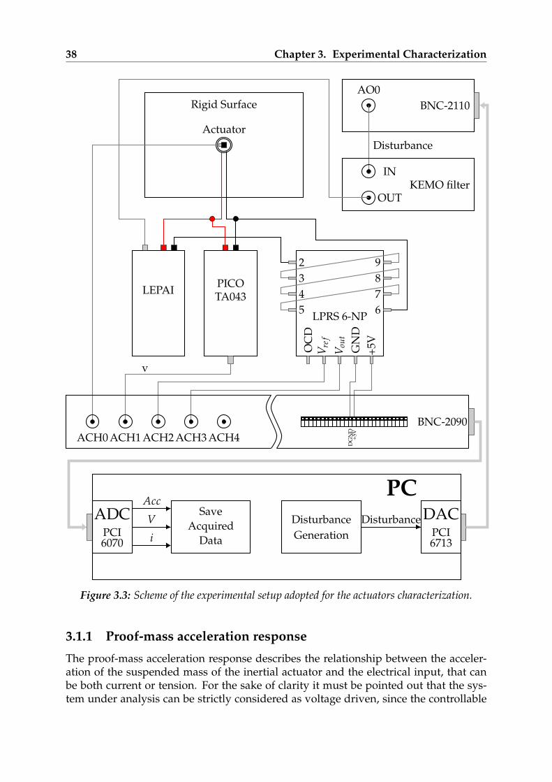
38 Chapter 3. Experimental Characterization
Rigid Surface
Actuator
BNC-2110AO0
Disturbance
KEMO filterIN
OUT
LEPAI PICOTA043
v
LPRS 6-NP
2345
9876
OC
DV r
ef
Vou
t
GN
D+5
V
BNC-2090ACH0 ACH1 ACH2 ACH3 ACH4
DG
ND
+5V
PCADC
PCI6070
Acc
V
i
SaveAcquired
Data
DisturbanceGeneration
Disturbance DACPCI6713
Figure 3.3: Scheme of the experimental setup adopted for the actuators characterization.
3.1.1 Proof-mass acceleration response
The proof-mass acceleration response describes the relationship between the acceler-ation of the suspended mass of the inertial actuator and the electrical input, that canbe both current or tension. For the sake of clarity it must be pointed out that the sys-tem under analysis can be strictly considered as voltage driven, since the controllable

3.1. Inertial actuators: Dayton DAEX25VT-4 exciters 39
quantity is the voltage and no method to achieve direct control of the current has beenapplied. However, since both voltage and current are measured, it’s possible to seekthe relationship between current and acceleration of the proof-mass, as it would havebeen done if the actuator was current driven.
Voltage driven
In this section the voltage driven case is presented while the current driven will bebriefly discussed later, mainly for comparative purposes. Note that the procedure out-lined in the following is rather general: it has been applied also to the current drivenacceleration response and to the electrical impedance, with only minor modifications.
The frequency response function is computed using as input a random white noise,filtered by the KEMO BENCH-MASTER to limit it’s bandwidth to 0 − 10kHz. It can becomputed as:
HaV(jw) =SaV(ω)
SVV(ω)
where SaV(ω) is the cross spectral density of the voltage V and acceleration of the proofmass a, and SVV(ω) is the power spectral density of V.Such elaboration of the acquired data has been performed using the MATLAB functiontfestimate. It takes as inputs the time series of two quantities and reconstruct theinput-output relation in the frequency domain. The results for the two Dayton devicesused in this work are reported in Figure 3.4.
The acceleration response obtained above still lacks a clear link with the parametersneeded for the complete characterization of the inertial actuator. What has to be doneis to find the coefficients of a transfer function that gives a frequency response suchas the one obtained with tfestimate. Once it is done, the transfer function can becompared with the analytical acceleration response HaV - derived in Chapter 2 andreported in Eq. 3.1 with the addition of the accelerometer mass ms - and the speakers’lumped model’s parameters can be computed.
HaV(s) =s2kem
(R + sL)(s2(ma + ms) + sca + ka) + skem(3.1)
Eq. 3.1 can be rewritten highlighting the coefficients of the complex variable, keepingin mind that for the next passages is needed to have the highest order coefficient of thedenominator equal to one.
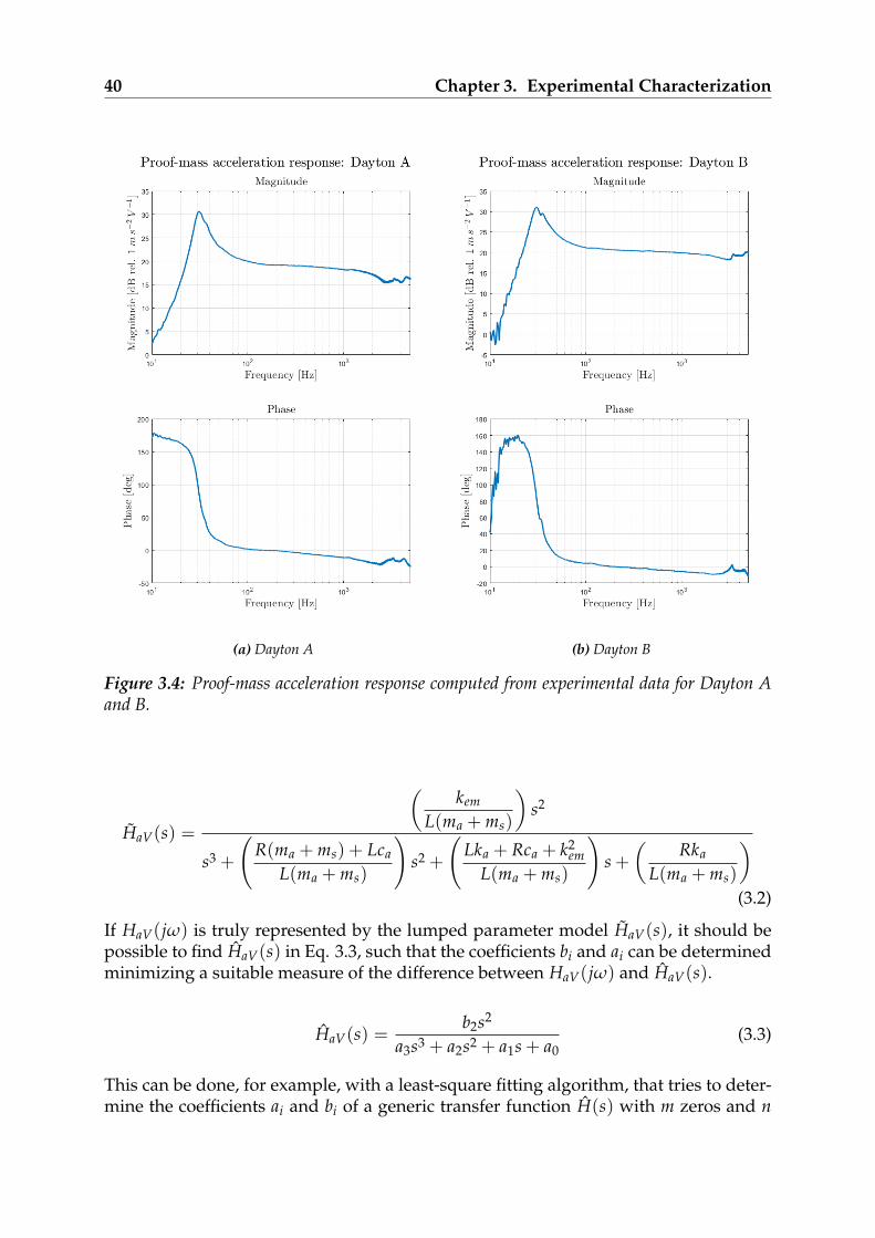
40 Chapter 3. Experimental Characterization
(a) Dayton A (b) Dayton B
Figure 3.4: Proof-mass acceleration response computed from experimental data for Dayton Aand B.
HaV(s) =
(kem
L(ma + ms)
)s2
s3 +
(R(ma + ms) + Lca
L(ma + ms)
)s2 +
(Lka + Rca + k2
emL(ma + ms)
)s +
(Rka
L(ma + ms)
)(3.2)
If HaV(jω) is truly represented by the lumped parameter model HaV(s), it should bepossible to find HaV(s) in Eq. 3.3, such that the coefficients bi and ai can be determinedminimizing a suitable measure of the difference between HaV(jω) and HaV(s).
HaV(s) =b2s2
a3s3 + a2s2 + a1s + a0(3.3)
This can be done, for example, with a least-square fitting algorithm, that tries to deter-mine the coefficients ai and bi of a generic transfer function H(s) with m zeros and n
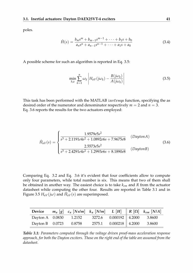
3.1. Inertial actuators: Dayton DAEX25VT-4 exciters 41
poles.
H(s) =bmsm + bm−1sm−1 + · · ·+ b1s + b0
ansn + an−1sn−1 + · · ·+ a1s + a0(3.4)
A possible scheme for such an algorithm is reported in Eq. 3.5:
minb,a
n
∑k=1
ωk
∣∣∣∣∣HaV(jωk)−B(jωk)
A(jωk)
∣∣∣∣∣ (3.5)
This task has been performed with the MATLAB invfreqs function, specifying the asdesired order of the numerator and denominator respectively m = 2 and n = 3.Eq. 3.6 reports the results for the two actuators employed:
HaV(s) =
1.9579e5s2
s3 + 2.1191e4s2 + 1.0892e6s + 7.9675e8(DaytonA)
2.5573e5s2
s3 + 2.4291e4s2 + 1.2993e6s + 8.1890e8(DaytonB)
(3.6)
Comparing Eq. 3.2 and Eq. 3.6 it’s evident that four coefficients allow to computeonly four parameters, while total number is six. This means that two of them shallbe obtained in another way. The easiest choice is to take kem and R from the actuatordatasheet while computing the other four. Results are reported in Table 3.1 and inFigure 3.5 HaV(jω) and HaV(s) are superimposed.
Device ma [g] ca [Ns/m] ka [N/m] L [H] R [Ω] kem [N/A]
Dayton A 0.0830 1.2152 3272.6 0.000192 4.2000 3.8600
Dayton B 0.0723 0.8758 2575.1 0.000218 4.2000 3.8600
Table 3.1: Parameters computed through the voltage driven proof-mass acceleration responseapproach, for both the Dayton exciters. Those on the right end of the table are assumed from thedatasheet.
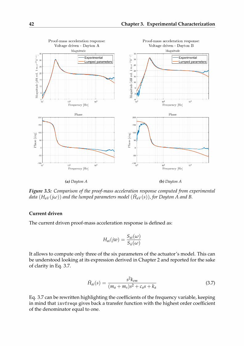
42 Chapter 3. Experimental Characterization
(a) Dayton A (b) Dayton A
Figure 3.5: Comparison of the proof-mass acceleration response computed from experimentaldata (HaV(jω)) and the lumped parameters model (HaV(s)), for Dayton A and B.
Current driven
The current driven proof-mass acceleration response is defined as:
Hai(jw) =Sai(ω)
Sii(ω)
It allows to compute only three of the six parameters of the actuator’s model. This canbe understood looking at its expression derived in Chapter 2 and reported for the sakeof clarity in Eq. 3.7.
Hai(s) =s2kem
(ma + ms)s2 + cas + ka(3.7)
Eq. 3.7 can be rewritten highlighting the coefficients of the frequency variable, keepingin mind that invfreqs gives back a transfer function with the highest order coefficientof the denominator equal to one.
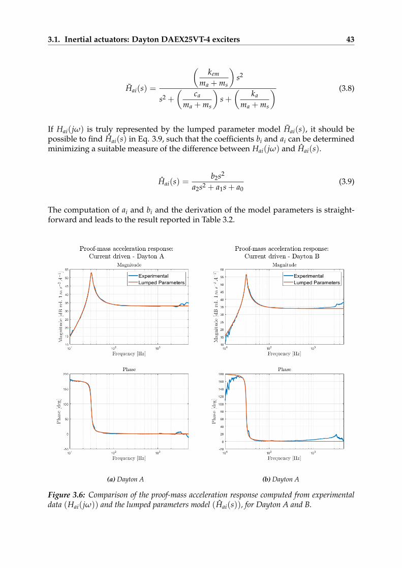
3.1. Inertial actuators: Dayton DAEX25VT-4 exciters 43
Hai(s) =
(kem
ma + ms
)s2
s2 +
(ca
ma + ms
)s +
(ka
ma + ms
) (3.8)
If Hai(jω) is truly represented by the lumped parameter model Hai(s), it should bepossible to find Hai(s) in Eq. 3.9, such that the coefficients bi and ai can be determinedminimizing a suitable measure of the difference between Hai(jω) and Hai(s).
Hai(s) =b2s2
a2s2 + a1s + a0(3.9)
The computation of ai and bi and the derivation of the model parameters is straight-forward and leads to the result reported in Table 3.2.
(a) Dayton A (b) Dayton A
Figure 3.6: Comparison of the proof-mass acceleration response computed from experimentaldata (Hai(jω)) and the lumped parameters model (Hai(s)), for Dayton A and B.
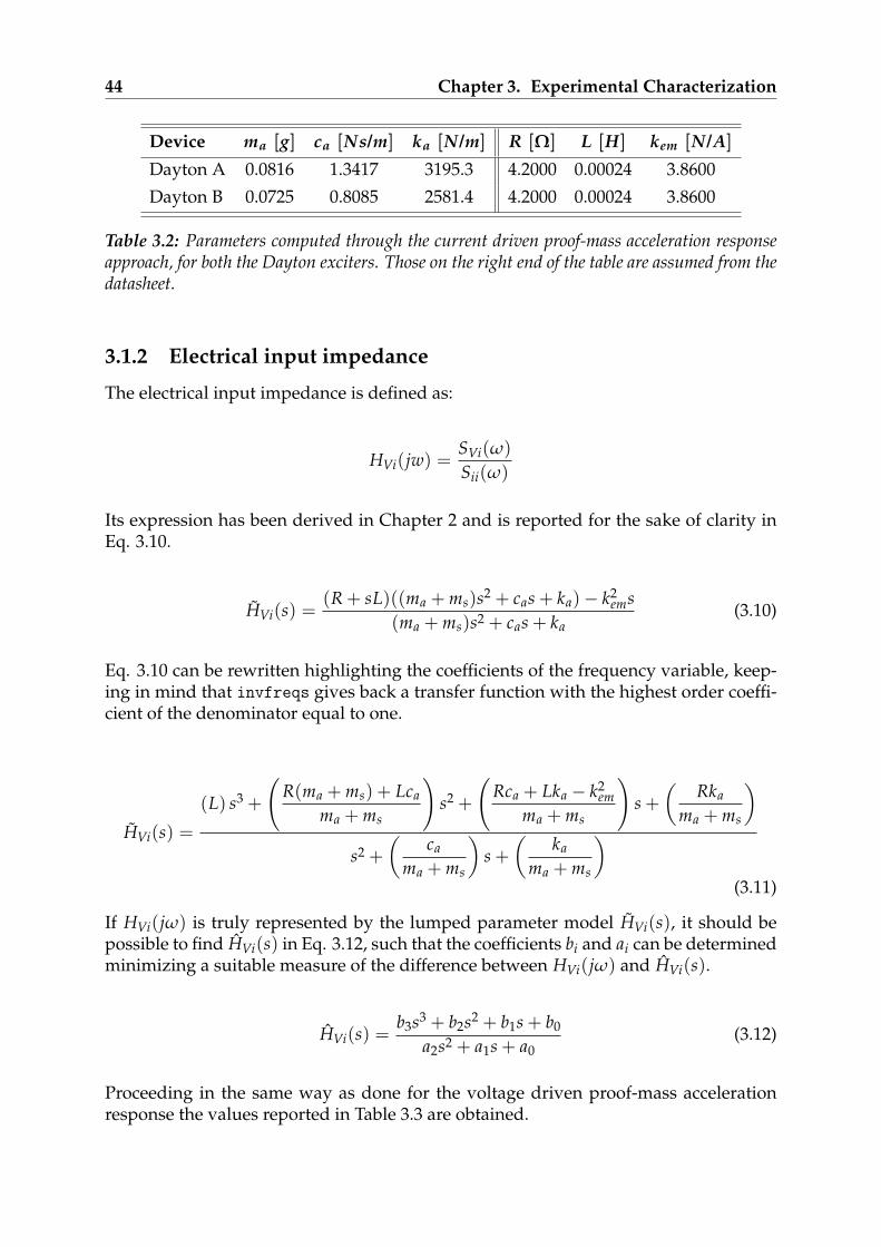
44 Chapter 3. Experimental Characterization
Device ma [g] ca [Ns/m] ka [N/m] R [Ω] L [H] kem [N/A]
Dayton A 0.0816 1.3417 3195.3 4.2000 0.00024 3.8600
Dayton B 0.0725 0.8085 2581.4 4.2000 0.00024 3.8600
Table 3.2: Parameters computed through the current driven proof-mass acceleration responseapproach, for both the Dayton exciters. Those on the right end of the table are assumed from thedatasheet.
3.1.2 Electrical input impedance
The electrical input impedance is defined as:
HVi(jw) =SVi(ω)
Sii(ω)
Its expression has been derived in Chapter 2 and is reported for the sake of clarity inEq. 3.10.
HVi(s) =(R + sL)((ma + ms)s2 + cas + ka)− k2
ems(ma + ms)s2 + cas + ka
(3.10)
Eq. 3.10 can be rewritten highlighting the coefficients of the frequency variable, keep-ing in mind that invfreqs gives back a transfer function with the highest order coeffi-cient of the denominator equal to one.
HVi(s) =
(L) s3 +
(R(ma + ms) + Lca
ma + ms
)s2 +
(Rca + Lka − k2
emma + ms
)s +
(Rka
ma + ms
)s2 +
(ca
ma + ms
)s +
(ka
ma + ms
)(3.11)
If HVi(jω) is truly represented by the lumped parameter model HVi(s), it should bepossible to find HVi(s) in Eq. 3.12, such that the coefficients bi and ai can be determinedminimizing a suitable measure of the difference between HVi(jω) and HVi(s).
HVi(s) =b3s3 + b2s2 + b1s + b0
a2s2 + a1s + a0(3.12)
Proceeding in the same way as done for the voltage driven proof-mass accelerationresponse the values reported in Table 3.3 are obtained.

3.1. Inertial actuators: Dayton DAEX25VT-4 exciters 45
Device ma [g] ca [Ns/m] ka [N/m] R [Ω] L [H] kem [N/A]
Dayton A 0.0859 1.4040 3353.7 4.8206 0.00026 3.8600
Dayton B 0.0745 0.8262 2645.9 4.8094 0.00023 3.8600
Table 3.3: Parameters computed through the electrical input impedance approach, for both theDayton exciters. Those on the right end of the table are assumed from the datasheet.
(a) Dayton A (b) Dayton A
Figure 3.7: Comparison of the electrical input impedance computed from experimental data(HVi(jω)) and the lumped parameters model (HVi(s)), for Dayton A and B.
The superposition of each experimental frequency responses to the related analyticallumped parameters model, shows that the model gives a good description of the un-derlying physics. The magnitude approximation is very good in a wide range span-ning at least from 20 to 2000Hz. The frequency description is a little less satisfactory athigher frequencies.Looking at the parameters obtained with the three methods and reported in Tables 3.1,3.2 and 3.3, it can be noticed that the results slightly differ from one method to another.If the purpose was only to build a numerical model to simulate the dynamics of the ex-
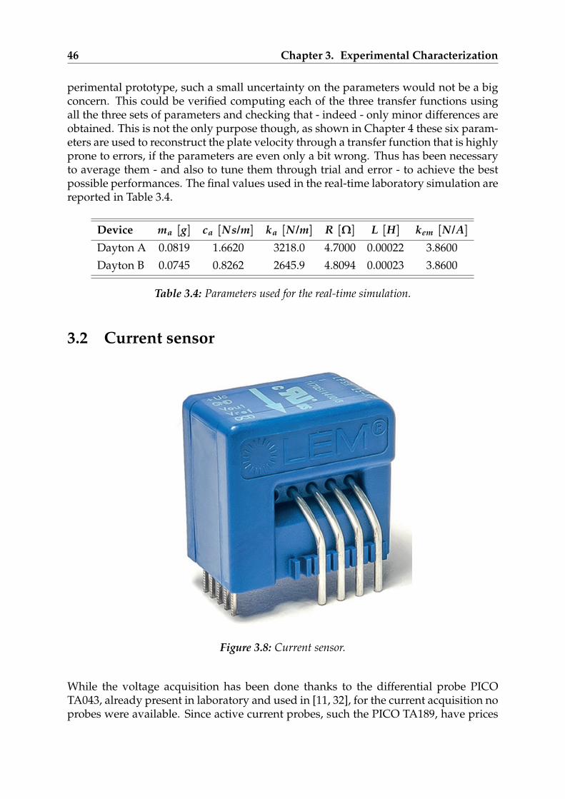
46 Chapter 3. Experimental Characterization
perimental prototype, such a small uncertainty on the parameters would not be a bigconcern. This could be verified computing each of the three transfer functions usingall the three sets of parameters and checking that - indeed - only minor differences areobtained. This is not the only purpose though, as shown in Chapter 4 these six param-eters are used to reconstruct the plate velocity through a transfer function that is highlyprone to errors, if the parameters are even only a bit wrong. Thus has been necessaryto average them - and also to tune them through trial and error - to achieve the bestpossible performances. The final values used in the real-time laboratory simulation arereported in Table 3.4.
Device ma [g] ca [Ns/m] ka [N/m] R [Ω] L [H] kem [N/A]
Dayton A 0.0819 1.6620 3218.0 4.7000 0.00022 3.8600
Dayton B 0.0745 0.8262 2645.9 4.8094 0.00023 3.8600
Table 3.4: Parameters used for the real-time simulation.
3.2 Current sensor
Figure 3.8: Current sensor.
While the voltage acquisition has been done thanks to the differential probe PICOTA043, already present in laboratory and used in [11, 32], for the current acquisition noprobes were available. Since active current probes, such the PICO TA189, have prices
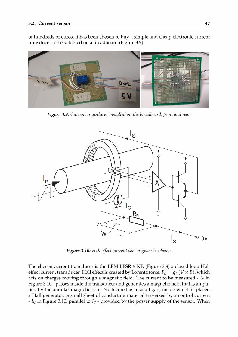
3.2. Current sensor 47
of hundreds of euros, it has been chosen to buy a simple and cheap electronic currenttransducer to be soldered on a breadboard (Figure 3.9).
Figure 3.9: Current transducer installed on the breadboard, front and rear.
Figure 3.10: Hall effect current sensor generic scheme.
The chosen current transducer is the LEM LPSR 6-NP, (Figure 3.8) a closed loop Halleffect current transducer. Hall effect is created by Lorentz force, FL = q · (V × B), whichacts on charges moving through a magnetic field. The current to be measured - IP inFigure 3.10 - passes inside the transducer and generates a magnetic field that is ampli-fied by the annular magnetic core. Such core has a small gap, inside which is placeda Hall generator: a small sheet of conducting material traversed by a control current- IC in Figure 3.10, parallel to IP - provided by the power supply of the sensor. When
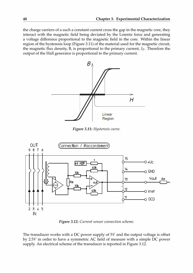
48 Chapter 3. Experimental Characterization
the charge carriers of a such a constant current cross the gap in the magnetic core, theyinteract with the magnetic field being deviated by the Lorentz force and generatinga voltage difference proportional to the magnetic field in the core. Within the linearregion of the hysteresis loop (Figure 3.11) of the material used for the magnetic circuit,the magnetic flux density, B, is proportional to the primary current, IP. Therefore theoutput of the Hall generator is proportional to the primary current.
Figure 3.11: Hysteresis curve.
Figure 3.12: Current sensor connection scheme.
The transducer works with a DC power supply of 5V and the output voltage is offsetby 2.5V in order to have a symmetric AC field of measure with a simple DC powersupply. An electrical scheme of the transducer is reported in Figure 3.12.
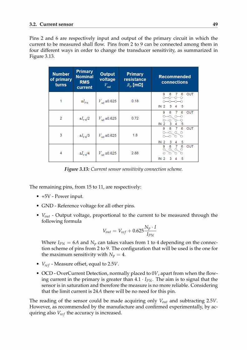
3.2. Current sensor 49
Pins 2 and 6 are respectively input and output of the primary circuit in which thecurrent to be measured shall flow. Pins from 2 to 9 can be connected among them infour different ways in order to change the transducer sensitivity, as summarized inFigure 3.13.
Figure 3.13: Current sensor sensitivity connection scheme.
The remaining pins, from 15 to 11, are respectively:
• +5V - Power input.
• GND - Reference voltage for all other pins.
• Vout - Output voltage, proportional to the current to be measured through thefollowing formula
Vout = Vre f + 0.625Np · IIPN
Where IPN = 6A and Np can takes values from 1 to 4 depending on the connec-tion scheme of pins from 2 to 9. The configuration that will be used is the one forthe maximum sensitivity with Np = 4.
• Vre f - Measure offset, equal to 2.5V.
• OCD - OverCurrent Detection, normally placed to 0V, apart from when the flow-ing current in the primary is greater than 4.1 · IPN. The aim is to signal that thesensor is in saturation and therefore the measure is no more reliable. Consideringthat the limit current is 24A there will be no need for this pin.
The reading of the sensor could be made acquiring only Vout and subtracting 2.5V.However, as recommended by the manufacture and confirmed experimentally, by ac-quiring also Vre f the accuracy is increased.
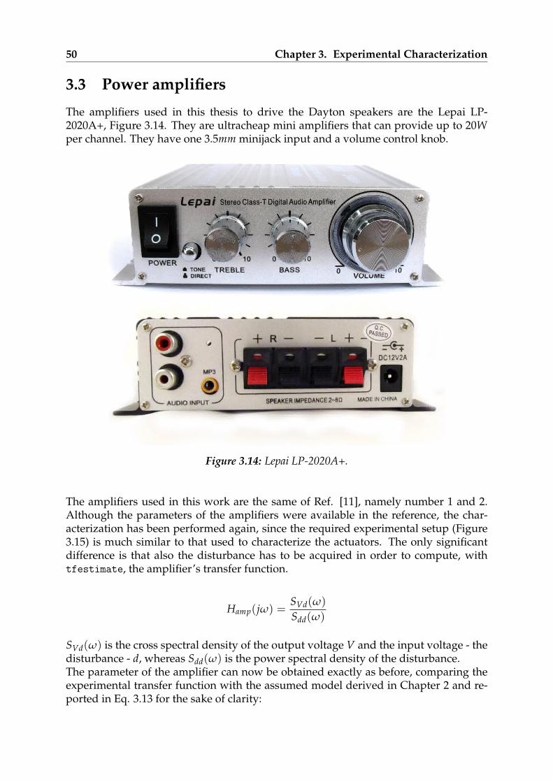
50 Chapter 3. Experimental Characterization
3.3 Power amplifiers
The amplifiers used in this thesis to drive the Dayton speakers are the Lepai LP-2020A+, Figure 3.14. They are ultracheap mini amplifiers that can provide up to 20Wper channel. They have one 3.5mm minijack input and a volume control knob.
Figure 3.14: Lepai LP-2020A+.
The amplifiers used in this work are the same of Ref. [11], namely number 1 and 2.Although the parameters of the amplifiers were available in the reference, the char-acterization has been performed again, since the required experimental setup (Figure3.15) is much similar to that used to characterize the actuators. The only significantdifference is that also the disturbance has to be acquired in order to compute, withtfestimate, the amplifier’s transfer function.
Hamp(jω) =SVd(ω)
Sdd(ω)
SVd(ω) is the cross spectral density of the output voltage V and the input voltage - thedisturbance - d, whereas Sdd(ω) is the power spectral density of the disturbance.The parameter of the amplifier can now be obtained exactly as before, comparing theexperimental transfer function with the assumed model derived in Chapter 2 and re-ported in Eq. 3.13 for the sake of clarity:
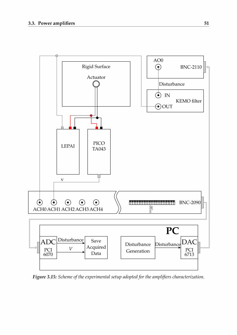
3.3. Power amplifiers 51
Rigid Surface
Actuator
BNC-2110AO0
Disturbance
KEMO filterIN
OUT
LEPAI PICOTA043
v
BNC-2090ACH0 ACH1 ACH2 ACH3 ACH4
DG
ND
+5V
PCADC
PCI6070
Disturbance
V
SaveAcquired
Data
DisturbanceGeneration
Disturbance DACPCI6713
Figure 3.15: Scheme of the experimental setup adopted for the amplifiers characterization.

52 Chapter 3. Experimental Characterization
H(s) = gamps
s + a(3.13)
It must be pointed out that while the low frequency pole of the amplifier is fixed, thegain depends on the setting of the volume knob. During the experimental charac-terization, the volume has been set approximately to 3/4 of the maximum, to avoidsaturation. The results are reported in Table 3.5 and are in good agreement with thoseof Ref. [11]. The fact that the numerical model of the amplifier must be changed when-ever the volume knob is moved is the main reason for which it has been chosen toactively measure the voltage. Indeed it could have been possible, knowing the distur-bance that is generated by the PC, to compute the voltage after the amplifier, but fordoing so, one should have been absolutely sure to do not move the volume knob.
Device gamp[−] a[Hz]
Lepai 1 −4.5 45
Lepai 2 −4.42 45
Table 3.5: Parameters computed for the two power amplifiers.
Figure 3.16: Lepai LP-2020A+.
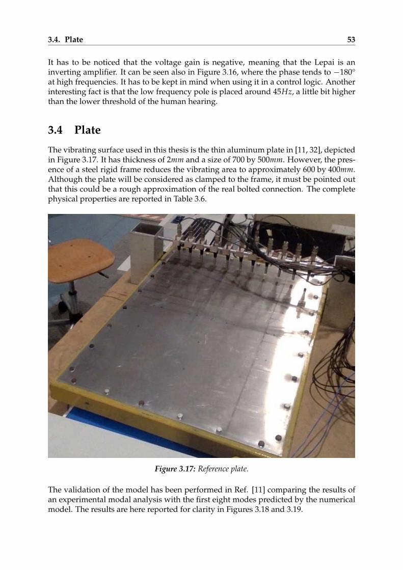
3.4. Plate 53
It has to be noticed that the voltage gain is negative, meaning that the Lepai is aninverting amplifier. It can be seen also in Figure 3.16, where the phase tends to −180°at high frequencies. It has to be kept in mind when using it in a control logic. Anotherinteresting fact is that the low frequency pole is placed around 45Hz, a little bit higherthan the lower threshold of the human hearing.
3.4 Plate
The vibrating surface used in this thesis is the thin aluminum plate in [11, 32], depictedin Figure 3.17. It has thickness of 2mm and a size of 700 by 500mm. However, the pres-ence of a steel rigid frame reduces the vibrating area to approximately 600 by 400mm.Although the plate will be considered as clamped to the frame, it must be pointed outthat this could be a rough approximation of the real bolted connection. The completephysical properties are reported in Table 3.6.
Figure 3.17: Reference plate.
The validation of the model has been performed in Ref. [11] comparing the results ofan experimental modal analysis with the first eight modes predicted by the numericalmodel. The results are here reported for clarity in Figures 3.18 and 3.19.
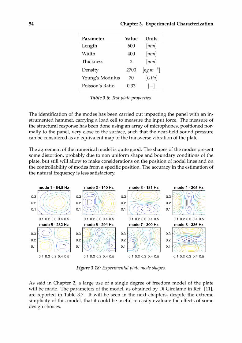
54 Chapter 3. Experimental Characterization
Parameter Value UnitsLength 600 [mm]
Width 400 [mm]
Thickness 2 [mm]
Density 2700 [kg m−3]
Young’s Modulus 70 [GPa]
Poisson’s Ratio 0.33 [−]
Table 3.6: Test plate properties.
The identification of the modes has been carried out impacting the panel with an in-strumented hammer, carrying a load cell to measure the input force. The measure ofthe structural response has been done using an array of microphones, positioned nor-mally to the panel, very close to the surface, such that the near-field sound pressurecan be considered as an equivalent map of the transverse vibration of the plate.
The agreement of the numerical model is quite good. The shapes of the modes presentsome distortion, probably due to non uniform shape and boundary conditions of theplate, but still will allow to make considerations on the position of nodal lines and onthe controllability of modes from a specific position. The accuracy in the estimation ofthe natural frequency is less satisfactory.
Figure 3.18: Experimental plate mode shapes.
As said in Chapter 2, a large use of a single degree of freedom model of the platewill be made. The parameters of the model, as obtained by Di Girolamo in Ref. [11],are reported in Table 3.7. It will be seen in the next chapters, despite the extremesimplicity of this model, that it could be useful to easily evaluate the effects of somedesign choices.
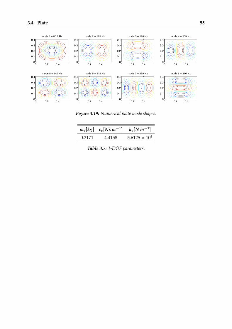
3.4. Plate 55
Figure 3.19: Numerical plate mode shapes.
ms[kg] cs[Ns m−1] ks[N m−1]
0.2171 4.4158 5.6125 × 10⁴
Table 3.7: 1-DOF parameters.

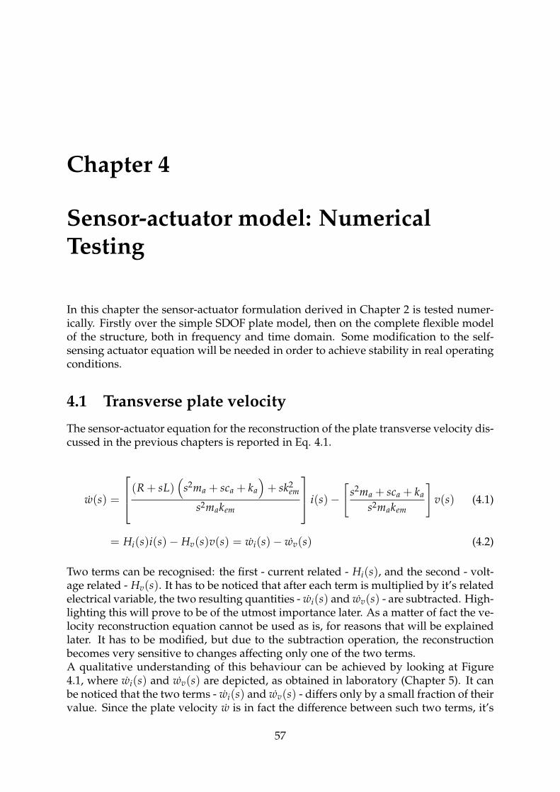
Chapter 4
Sensor-actuator model: NumericalTesting
In this chapter the sensor-actuator formulation derived in Chapter 2 is tested numer-ically. Firstly over the simple SDOF plate model, then on the complete flexible modelof the structure, both in frequency and time domain. Some modification to the self-sensing actuator equation will be needed in order to achieve stability in real operatingconditions.
4.1 Transverse plate velocity
The sensor-actuator equation for the reconstruction of the plate transverse velocity dis-cussed in the previous chapters is reported in Eq. 4.1.
w(s) =
(R + sL)(
s2ma + sca + ka
)+ sk2
em
s2makem
i(s)−[
s2ma + sca + ka
s2makem
]v(s) (4.1)
= Hi(s)i(s)− Hv(s)v(s) = wi(s)− wv(s) (4.2)
Two terms can be recognised: the first - current related - Hi(s), and the second - volt-age related - Hv(s). It has to be noticed that after each term is multiplied by it’s relatedelectrical variable, the two resulting quantities - wi(s) and wv(s) - are subtracted. High-lighting this will prove to be of the utmost importance later. As a matter of fact the ve-locity reconstruction equation cannot be used as is, for reasons that will be explainedlater. It has to be modified, but due to the subtraction operation, the reconstructionbecomes very sensitive to changes affecting only one of the two terms.A qualitative understanding of this behaviour can be achieved by looking at Figure4.1, where wi(s) and wv(s) are depicted, as obtained in laboratory (Chapter 5). It canbe noticed that the two terms - wi(s) and wv(s) - differs only by a small fraction of theirvalue. Since the plate velocity w is in fact the difference between such two terms, it’s
57

58 Chapter 4. Sensor-actuator model: Numerical Testing
easy to understand that if one, for any reason, is modified, the reconstructed velocitywould be heavily affected.
Figure 4.1: Comparison of the wi(s) and wv(s) terms.
As anticipated the aim of this chapter is to modify Eq. 4.1 in order to obtain a formula-tion that can be implemented in real-time laboratory testing. In fact, implementing Eq.4.1 would give good results only in numerical simulations, while the performances inlaboratory would be completely unsatisfying. This asymmetry between numerical andexperimental analysis is due to different phenomena that affect only the experimentalsetup, that have to be included in the numerical simulation if significant results are tobe drawn. The main problems and uncertainties taken into account in the followingare:
• Offset in the current and voltage measures.
• High frequency noise in the measurements.
• Low frequency components due to unmodelled dynamics.
• Uncertainties on the actuator parameters computed in Chapter 3.
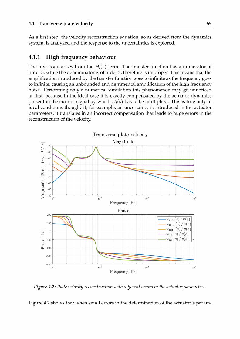
4.1. Transverse plate velocity 59
As a first step, the velocity reconstruction equation, so as derived from the dynamicssystem, is analyzed and the response to the uncertainties is explored.
4.1.1 High frequency behaviour
The first issue arises from the Hi(s) term. The transfer function has a numerator oforder 3, while the denominator is of order 2, therefore is improper. This means that theamplification introduced by the transfer function goes to infinite as the frequency goesto infinite, causing an unbounded and detrimental amplification of the high frequencynoise. Performing only a numerical simulation this phenomenon may go unnoticedat first, because in the ideal case it is exactly compensated by the actuator dynamicspresent in the current signal by which Hi(s) has to be multiplied. This is true only inideal conditions though: if, for example, an uncertainty is introduced in the actuatorparameters, it translates in an incorrect compensation that leads to huge errors in thereconstruction of the velocity.
Figure 4.2: Plate velocity reconstruction with different errors in the actuator parameters.
Figure 4.2 shows that when small errors in the determination of the actuator’s param-
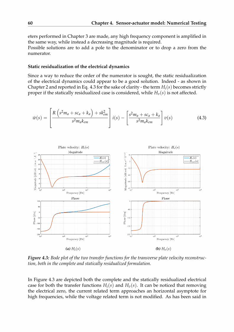
60 Chapter 4. Sensor-actuator model: Numerical Testing
eters performed in Chapter 3 are made, any high frequency component is amplified inthe same way, while instead a decreasing magnitude is required.Possible solutions are to add a pole to the denominator or to drop a zero from thenumerator.
Static residualization of the electrical dynamics
Since a way to reduce the order of the numerator is sought, the static residualizationof the electrical dynamics could appear to be a good solution. Indeed - as shown inChapter 2 and reported in Eq. 4.3 for the sake of clarity - the term Hi(s) becomes strictlyproper if the statically residualized case is considered, while Hv(s) is not affected.
w(s) =
R(
s2ma + sca + ka
)+ sk2
em
s2makem
i(s)−[
s2ma + sca + ka
s2makem
]v(s) (4.3)
(a) Hi(s) (b) Hv(s)
Figure 4.3: Bode plot of the two transfer functions for the transverse plate velocity reconstruc-tion, both in the complete and statically residualized formulation.
In Figure 4.3 are depicted both the complete and the statically residualized electricalcase for both the transfer functions Hi(s) and Hv(s). It can be noticed that removingthe electrical zero, the current related term approaches an horizontal asymptote forhigh frequencies, while the voltage related term is not modified. As has been said in

4.1. Transverse plate velocity 61
the previous chapters, the goodness of the statically residualized model has to be as-sessed for the specific application under analysis. Assuming that the frequency rangeof interest of this work is upper bounded at about 1kHz, it could seem that the staticresidualization should not alter significantly the performances in the range of inter-est, being Hi(s) ≈ Hi res(s) below 1kHz. Unfortunately this is not the case, and whatbefore has been only anticipated qualitatively - that any modification introduced ononly one of Hi(s) or Hv(s) could heavily compromise the velocity reconstruction - it’sdemonstrated in the following.
Eq. 4.2 can be rewritten as:
w(s) = Hi(s)i(s)− Hv(s)v(s)
=
(Hi(s)
i(s)v(s)
− Hv(s)
)v(s)
=(
Hi(s)Y(s)− Hv(s))
v(s)
Where has been introduced the electrical admittance Y(s), defined as the inverse of theelectrical impedance and depicted in Figure 4.4.
Figure 4.4: Electrical admittance simulated for the simple SDOF plate coupled with the lumpedparameters model of the inertial actuator.
The plate model employed in these simulations is the simple single-degree-of-freedom,
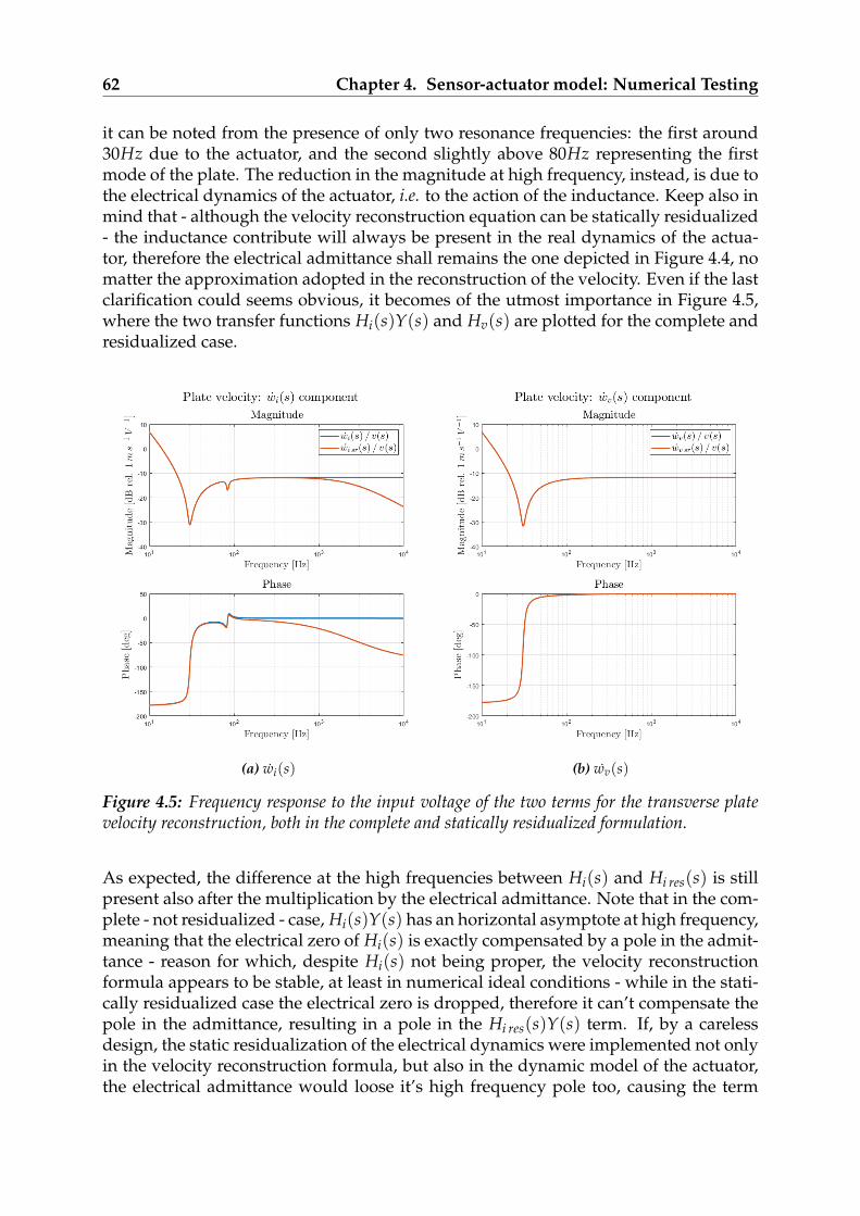
62 Chapter 4. Sensor-actuator model: Numerical Testing
it can be noted from the presence of only two resonance frequencies: the first around30Hz due to the actuator, and the second slightly above 80Hz representing the firstmode of the plate. The reduction in the magnitude at high frequency, instead, is due tothe electrical dynamics of the actuator, i.e. to the action of the inductance. Keep also inmind that - although the velocity reconstruction equation can be statically residualized- the inductance contribute will always be present in the real dynamics of the actua-tor, therefore the electrical admittance shall remains the one depicted in Figure 4.4, nomatter the approximation adopted in the reconstruction of the velocity. Even if the lastclarification could seems obvious, it becomes of the utmost importance in Figure 4.5,where the two transfer functions Hi(s)Y(s) and Hv(s) are plotted for the complete andresidualized case.
(a) wi(s) (b) wv(s)
Figure 4.5: Frequency response to the input voltage of the two terms for the transverse platevelocity reconstruction, both in the complete and statically residualized formulation.
As expected, the difference at the high frequencies between Hi(s) and Hi res(s) is stillpresent also after the multiplication by the electrical admittance. Note that in the com-plete - not residualized - case, Hi(s)Y(s) has an horizontal asymptote at high frequency,meaning that the electrical zero of Hi(s) is exactly compensated by a pole in the admit-tance - reason for which, despite Hi(s) not being proper, the velocity reconstructionformula appears to be stable, at least in numerical ideal conditions - while in the stati-cally residualized case the electrical zero is dropped, therefore it can’t compensate thepole in the admittance, resulting in a pole in the Hi res(s)Y(s) term. If, by a carelessdesign, the static residualization of the electrical dynamics were implemented not onlyin the velocity reconstruction formula, but also in the dynamic model of the actuator,the electrical admittance would loose it’s high frequency pole too, causing the term
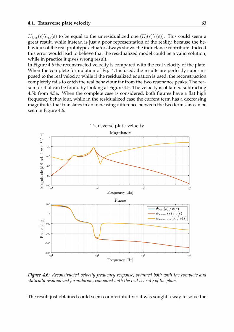
4.1. Transverse plate velocity 63
Hi res(s)Yres(s) to be equal to the unresidualized one (Hi(s)Y(s)). This could seem agreat result, while instead is just a poor representation of the reality, because the be-haviour of the real prototype actuator always shows the inductance contribute. Indeedthis error would lead to believe that the residualized model could be a valid solution,while in practice it gives wrong result.In Figure 4.6 the reconstructed velocity is compared with the real velocity of the plate.When the complete formulation of Eq. 4.1 is used, the results are perfectly superim-posed to the real velocity, while if the residualized equation is used, the reconstructioncompletely fails to catch the real behaviour far from the two resonance peaks. The rea-son for that can be found by looking at Figure 4.5. The velocity is obtained subtracting4.5b from 4.5a. When the complete case is considered, both figures have a flat highfrequency behaviour, while in the residualized case the current term has a decreasingmagnitude, that translates in an increasing difference between the two terms, as can beseen in Figure 4.6.
Figure 4.6: Reconstructed velocity frequency response, obtained both with the complete andstatically residualized formulation, compared with the real velocity of the plate.
The result just obtained could seem counterintuitive: it was sought a way to solve the
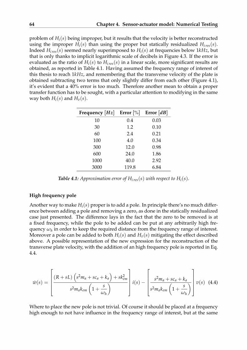
64 Chapter 4. Sensor-actuator model: Numerical Testing
problem of Hi(s) being improper, but it results that the velocity is better reconstructedusing the improper Hi(s) than using the proper but statically residualized Hi res(s).Indeed Hi res(s) seemed nearly superimposed to Hi(s) at frequencies below 1kHz, butthat is only thanks to implicit logarithmic scale of decibels in Figure 4.3. If the error isevaluated as the ratio of Hi(s) to Hi res(s) in a linear scale, more significant results areobtained, as reported in Table 4.1. Having assumed the frequency range of interest ofthis thesis to reach 1kHz, and remembering that the transverse velocity of the plate isobtained subtracting two terms that only slightly differ from each other (Figure 4.1),it’s evident that a 40% error is too much. Therefore another mean to obtain a propertransfer function has to be sought, with a particular attention to modifying in the sameway both Hi(s) and Hv(s).
Frequency [Hz] Error [%] Error [dB]
10 0.4 0.0330 1.2 0.1060 2.4 0.21
100 4.0 0.34300 12.0 0.98600 24.0 1.861000 40.0 2.923000 119.8 6.84
Table 4.1: Approximation error of Hi res(s) with respect to Hi(s).
High frequency pole
Another way to make Hi(s) proper is to add a pole. In principle there’s no much differ-ence between adding a pole and removing a zero, as done in the statically residualizedcase just presented. The difference lays in the fact that the zero to be removed is ata fixed frequency, while the pole to be added can be put at any arbitrarily high fre-quency ωh in order to keep the required distance from the frequency range of interest.Moreover a pole can be added to both Hi(s) and Hv(s) mitigating the effect describedabove. A possible representation of the new expression for the reconstruction of thetransverse plate velocity, with the addition of an high frequency pole is reported in Eq.4.4.
w(s) =
(R + sL)(
s2ma + sca + ka
)+ sk2
em
s2makem
(1 +
sωh
) i(s)−
s2ma + sca + ka
s2makem
(1 +
sωh
) v(s) (4.4)
Where to place the new pole is not trivial. Of course it should be placed at a frequencyhigh enough to not have influence in the frequency range of interest, but at the same

4.1. Transverse plate velocity 65
time it is reasonable to keep it as low as possible in order to better reject high frequencynoise. The latter requirement is not easily analysable in the frequency domain, and willbe shortly addressed later in a time simulation. However, it can be anticipated that itwill not be found to be much constraining.
Note that if it is imposed
ωh =R(
s2ma + sca + ka
)+ sk2
em
L(s2ma + sca + ka
)it can be obtained again the static residualization of the Hi(s) term
Hi(s) =(R + sL)
(s2ma + sca + ka
)+ sk2
em
s2makem
(1 +
sωh
)
=(R + sL)
(s2ma + sca + ka
)+ sk2
em
s2makem
1 +s
R(
s2ma + sca + ka
)+ sk2
em
L(s2ma + sca + ka
)
=(R + sL)
(s2ma + sca + ka
)+ sk2
em
s2makem
1 +Ls(
s2ma + sca + ka
)R(s2ma + sca + ka
)+ sk2
em
R(
s2ma + sca + ka
)+ sk2
em
R(s2ma + sca + ka
)+ sk2
em
=
[(R + sL)
(s2ma + sca + ka
)+ sk2
em
] [R(
s2ma + sca + ka
)+ sk2
em
]s2makem
[R(s2ma + sca + ka
)+ sk2
em + Ls(s2ma + sca + ka
)]
=
[(R + sL)
(s2ma + sca + ka
)+ sk2
em
] [R(
s2ma + sca + ka
)+ sk2
em
]s2makem
[(R + sL)
(s2ma + sca + ka
)+ sk2
em
]
=R(
s2ma + sca + ka
)+ sk2
em
s2makem= Hi res(s)
with an additional compensation of Hv(s) so as not to run into the problem describedabove.

66 Chapter 4. Sensor-actuator model: Numerical Testing
Note, in Figure 4.7, that this peculiar case does not offer better performances than theothers, therefore there’s no reason to implement it.
Figure 4.7: Reconstructed velocity frequency response, obtained with different high frequencypoles, compared with the real velocity of the plate.
Comparing Figure 4.7 with Figure 4.6 it is evident that modifying both Hi(s) and Hv(s)dramatically improves the performance of the reconstruction of the velocity. With anyωh higher than about 2kHz a proper transfer function is obtained with no detrimentaleffects in the frequency range of interest.
It has been demonstrated so far that the pole addition does not have detrimental ef-fects on the reconstruction of the transverse plate velocity in ideal numerical condi-tions. However, it should be checked if its behaviour remains satisfactory even whenan error in the actuator’s parameters is introduced. Figure 4.8 depicts a comparisonwhen the error is fixed at 1%. As anticipated, the lower the value of ωh, the betterthe reconstruction of the velocity in case of error in the parameters. As said before,the frequency analysis is not the best tool to understand how low the new pole has tobe placed to reject the high frequency noise. Indeed it could appear from Figure 4.8that also 1kHz is too high to obtain a perfect reconstruction of the velocity. Although
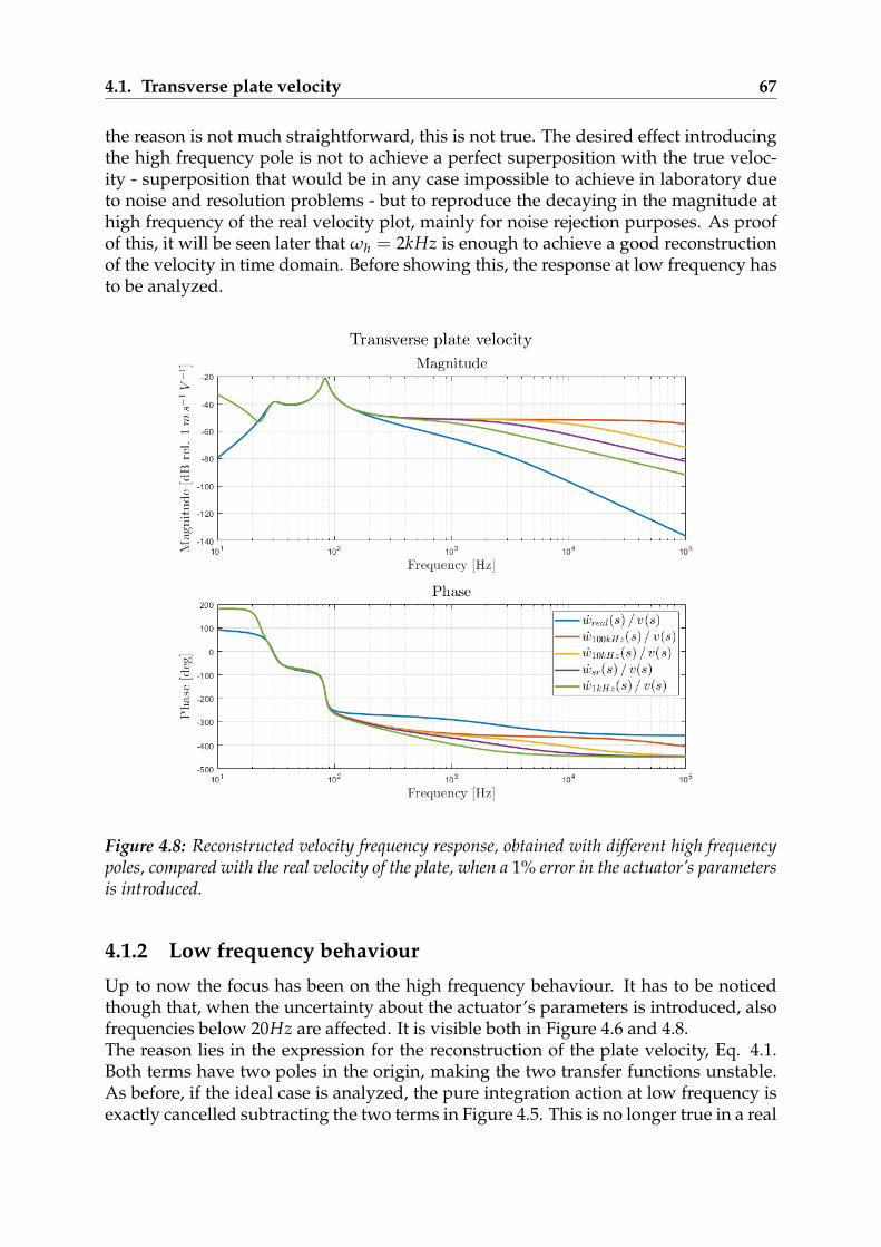
4.1. Transverse plate velocity 67
the reason is not much straightforward, this is not true. The desired effect introducingthe high frequency pole is not to achieve a perfect superposition with the true veloc-ity - superposition that would be in any case impossible to achieve in laboratory dueto noise and resolution problems - but to reproduce the decaying in the magnitude athigh frequency of the real velocity plot, mainly for noise rejection purposes. As proofof this, it will be seen later that ωh = 2kHz is enough to achieve a good reconstructionof the velocity in time domain. Before showing this, the response at low frequency hasto be analyzed.
Figure 4.8: Reconstructed velocity frequency response, obtained with different high frequencypoles, compared with the real velocity of the plate, when a 1% error in the actuator’s parametersis introduced.
4.1.2 Low frequency behaviour
Up to now the focus has been on the high frequency behaviour. It has to be noticedthough that, when the uncertainty about the actuator’s parameters is introduced, alsofrequencies below 20Hz are affected. It is visible both in Figure 4.6 and 4.8.The reason lies in the expression for the reconstruction of the plate velocity, Eq. 4.1.Both terms have two poles in the origin, making the two transfer functions unstable.As before, if the ideal case is analyzed, the pure integration action at low frequency isexactly cancelled subtracting the two terms in Figure 4.5. This is no longer true in a real
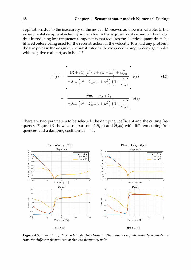
68 Chapter 4. Sensor-actuator model: Numerical Testing
application, due to the inaccuracy of the model. Moreover, as shown in Chapter 5, theexperimental setup is affected by some offset in the acquisition of current and voltage,thus introducing low frequency components that requires the electrical quantities to befiltered before being used for the reconstruction of the velocity. To avoid any problem,the two poles in the origin can be substituted with two generic complex conjugate poleswith negative real part, as in Eq. 4.5.
w(s) =
(R + sL)(
s2ma + sca + ka
)+ sk2
em
makem
(s2 + 2ξlωls + ω2
l
)(1 +
sωh
) i(s) (4.5)
−
s2ma + sca + ka
makem
(s2 + 2ξlωls + ω2
l
)(1 +
sωh
) v(s)
There are two parameters to be selected: the damping coefficient and the cutting fre-quency. Figure 4.9 shows a comparison of Hi(s) and Hv(s) with different cutting fre-quencies and a damping coefficient ξl = 1.
(a) Hi(s) (b) Hv(s)
Figure 4.9: Bode plot of the two transfer functions for the transverse plate velocity reconstruc-tion, for different frequencies of the low frequency poles.
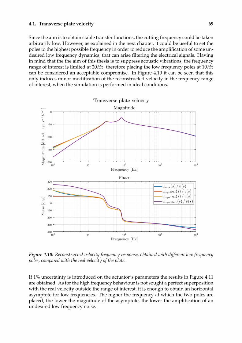
4.1. Transverse plate velocity 69
Since the aim is to obtain stable transfer functions, the cutting frequency could be takenarbitrarily low. However, as explained in the next chapter, it could be useful to set thepoles to the highest possible frequency in order to reduce the amplification of some un-desired low frequency dynamics, that can arise filtering the electrical signals. Havingin mind that the the aim of this thesis is to suppress acoustic vibrations, the frequencyrange of interest is limited at 20Hz, therefore placing the low frequency poles at 10Hzcan be considered an acceptable compromise. In Figure 4.10 it can be seen that thisonly induces minor modification of the reconstructed velocity in the frequency rangeof interest, when the simulation is performed in ideal conditions.
Figure 4.10: Reconstructed velocity frequency response, obtained with different low frequencypoles, compared with the real velocity of the plate.
If 1% uncertainty is introduced on the actuator’s parameters the results in Figure 4.11are obtained. As for the high frequency behaviour is not sought a perfect superpositionwith the real velocity outside the range of interest, it is enough to obtain an horizontalasymptote for low frequencies. The higher the frequency at which the two poles areplaced, the lower the magnitude of the asymptote, the lower the amplification of anundesired low frequency noise.
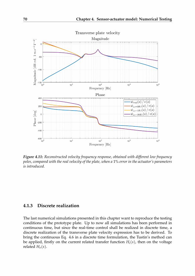
70 Chapter 4. Sensor-actuator model: Numerical Testing
Figure 4.11: Reconstructed velocity frequency response, obtained with different low frequencypoles, compared with the real velocity of the plate, when a 1% error in the actuator’s parametersis introduced.
4.1.3 Discrete realization
The last numerical simulations presented in this chapter want to reproduce the testingconditions of the prototype plate. Up to now all simulations has been performed incontinuous time, but since the real-time control shall be realized in discrete time, adiscrete realization of the transverse plate velocity expression has to be derived. Tobring the continuous Eq. 4.6 in a discrete time formulation, the Tustin’s method canbe applied, firstly on the current related transfer function Hi(s), then on the voltagerelated Hv(s).
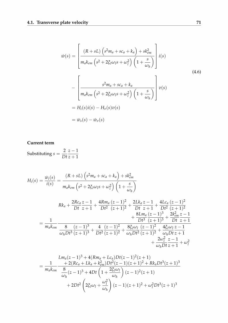
4.1. Transverse plate velocity 71
w(s) =
(R + sL)(
s2ma + sca + ka
)+ sk2
em
makem
(s2 + 2ξlωls + ω2
l
)(1 +
sωh
) i(s)
−
s2ma + sca + ka
makem
(s2 + 2ξlωls + ω2
l
)(1 +
sωh
) v(s)
(4.6)
= Hi(s)i(s)− Hv(s)v(s)
= ws(s)− wv(s)
Current term
Substituting s =2
Dtz − 1z + 1
Hi(s) =wi(s)i(s)
=(R + sL)
(s2ma + sca + ka
)+ sk2
em
makem
(s2 + 2ξlωls + ω2
l
)(1 +
sωh
)
=1
makem
Rka +2Rca
Dtz − 1z + 1
+4Rma
Dt2(z − 1)2
(z + 1)2 +2Lka
Dtz − 1z + 1
+4Lca
Dt2(z − 1)2
(z + 1)2
+8Lma
Dt3(z − 1)3
(z + 1)3 +2k2
emDt
z − 1z + 1
8ωhDt3
(z − 1)3
(z + 1)3 +4
Dt2(z − 1)2
(z + 1)2 +8ξlωlωhDt2
(z − 1)2
(z + 1)2 +4ξlωlωhDt
z − 1z + 1
+2ω2
lωhDt
z − 1z + 1
+ ω2l
=1
makem
Lma(z − 1)3 + 4(Rma + Lca)Dt(z − 1)2(z + 1)+ 2(Rca + Lka + k2
em)Dt2(z − 1)(z + 1)2 + RkaDt3(z + 1)3
8ωh
(z − 1)3 + 4Dt(
1 +2ξlωl
ωh
)(z − 1)2(z + 1)
+ 2Dt2
(2ξlωl +
ω2l
ωh
)(z − 1)(z + 1)2 + ω2
l Dt3(z + 1)3
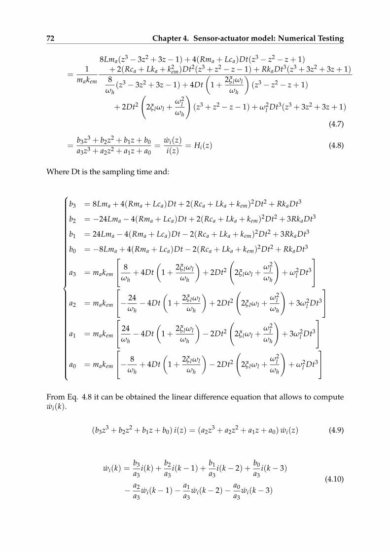
72 Chapter 4. Sensor-actuator model: Numerical Testing
=1
makem
8Lma(z3 − 3z2 + 3z − 1) + 4(Rma + Lca)Dt(z3 − z2 − z + 1)+ 2(Rca + Lka + k2
em)Dt2(z3 + z2 − z − 1) + RkaDt3(z3 + 3z2 + 3z + 1)8
ωh(z3 − 3z2 + 3z − 1) + 4Dt
(1 +
2ξlωlωh
)(z3 − z2 − z + 1)
+ 2Dt2
(2ξlωl +
ω2l
ωh
)(z3 + z2 − z − 1) + ω2
l Dt3(z3 + 3z2 + 3z + 1)
(4.7)
=b3z3 + b2z2 + b1z + b0
a3z3 + a2z2 + a1z + a0=
wi(z)i(z)
= Hi(z) (4.8)
Where Dt is the sampling time and:
b3 = 8Lma + 4(Rma + Lca)Dt + 2(Rca + Lka + kem)2Dt2 + RkaDt3
b2 = −24Lma − 4(Rma + Lca)Dt + 2(Rca + Lka + kem)2Dt2 + 3RkaDt3
b1 = 24Lma − 4(Rma + Lca)Dt − 2(Rca + Lka + kem)2Dt2 + 3RkaDt3
b0 = −8Lma + 4(Rma + Lca)Dt − 2(Rca + Lka + kem)2Dt2 + RkaDt3
a3 = makem
8ωh
+ 4Dt(
1 +2ξlωl
ωh
)+ 2Dt2
(2ξlωl +
ω2l
ωh
)+ ω2
l Dt3
a2 = makem
− 24ωh
− 4Dt(
1 +2ξlωl
ωh
)+ 2Dt2
(2ξlωl +
ω2l
ωh
)+ 3ω2
l Dt3
a1 = makem
24ωh
− 4Dt(
1 +2ξlωl
ωh
)− 2Dt2
(2ξlωl +
ω2l
ωh
)+ 3ω2
l Dt3
a0 = makem
− 8ωh
+ 4Dt(
1 +2ξlωl
ωh
)− 2Dt2
(2ξlωl +
ω2l
ωh
)+ ω2
l Dt3
From Eq. 4.8 it can be obtained the linear difference equation that allows to computewi(k).
(b3z3 + b2z2 + b1z + b0) i(z) = (a2z3 + a2z2 + a1z + a0) wi(z) (4.9)
wi(k) =b3
a3i(k) +
b2
a3i(k − 1) +
b1
a3i(k − 2) +
b0
a3i(k − 3)
− a2
a3wi(k − 1)− a1
a3wi(k − 2)− a0
a3wi(k − 3)
(4.10)

4.1. Transverse plate velocity 73
Voltage term
Substituting s =2
Dtz − 1z + 1
Hv(s) =wv(s)v(s)
=s2ma + sca + ka
makem
(s2 + 2ξlωls + ω2
l
)(1 +
sωh
)
=1
makem
ka +2ca
Dtz − 1z + 1
+4ma
Dt2(z − 1)2
(z + 1)2
8ωhDt3
(z − 1)3
(z + 1)3 +4
Dt2(z − 1)2
(z + 1)2 +8ξlωlωhDt2
(z − 1)2
(z + 1)2 +4ξlωlωhDt
z − 1z + 1
+2ω2
lωhDt
z − 1z + 1
+ ω2l
=1
makem
4maDt(z − 1)2(z + 1) + 2caDt2(z − 1)(z + 1)2 + kaDt3(z + 1)3
8ωh
(z − 1)3 + 4Dt(
1 +2ξlωl
ωh
)(z − 1)2(z + 1)
+ 2Dt2
(2ξlωl +
ω2l
ωh
)(z − 1)(z + 1)2 + ω2
l Dt3(z + 1)3
=1
makem
4maDt(z3 − z2 − z + 1) + 2caDt2(z3 + z2 − z − 1)+ kaDt3(z3 + 3z2 + 3z + 1)
8ωh
(z3 − 3z2 + 3z − 1) + 4Dt(
1 +2ξlωl
ωh
)(z3 − z2 − z + 1)
+ 2Dt2
(2ξlωl +
ω2l
ωh
)(z3 + z2 − z − 1) + ω2
l Dt3(z3 + 3z2 + 3z + 1)
(4.11)
=d3z3 + d2z2 + d1z + d0
c3z3 + c2z2 + c1z + c0=
wv(z)v(z)
= Hv(z) (4.12)
Where Dt is the sampling time and:

74 Chapter 4. Sensor-actuator model: Numerical Testing
d3 = 4maDt + 2caDt2 + kaDt3
d2 = −4maDt + 2caDt2 + 3kaDt3
d1 = −4maDt − 2caDt2 + 3kaDt3
d0 = 4maDt − 2caDt2 + kaDt3
c3 = makem
8ωh
+ 4Dt(
1 +2ξlωl
ωh
)+ 2Dt2
(2ξlωl +
ω2l
ωh
)+ ω2
l Dt3
c2 = makem
− 24ωh
− 4Dt(
1 +2ξlωl
ωh
)+ 2Dt2
(2ξlωl +
ω2l
ωh
)+ 3ω2
l Dt3
c1 = makem
24ωh
− 4Dt(
1 +2ξlωl
ωh
)− 2Dt2
(2ξlωl +
ω2l
ωh
)+ 3ω2
l Dt3
c0 = makem
− 8ωh
+ 4Dt(
1 +2ξlωl
ωh
)− 2Dt2
(2ξlωl +
ω2l
ωh
)+ ω2
l Dt3
From Eq. 4.12 can be obtained the linear difference equation that allows to computewv(k).
(d3z3 + d2z2 + d1z + d0) v(z) = (c3z3 + c2z2 + c1z + c0) wv(z) (4.13)
wv(k) =d3
c3v(k) +
d2
c3v(k − 1) +
d1
c3v(k − 2) +
d0
c3v(k − 3)
− c2
c3wv(k − 1)− c1
c3wv(k − 2)− c0
c3wv(k − 3)
(4.14)
4.1.4 S-GUF plate simulation
In this section the expression for the reconstruction of the plate transverse velocity inEq. 4.5 is tested numerically on the S-GUF plate model, both in frequency and timedomain. The discrete formulation derived above is implemented, with a sampling fre-quency of 20kHz.
In Figure 4.12 are compared the velocity frequency response obtained with the origi-nal expression - Eq. 4.1 - with the modified expression - Eq. 4.5 - and that of the realvelocity of the plate. Comparing it with all the plots obtained with the SDOF platemodel can be recognized two peaks: at 30Hz the actuator resonance and at 85Hz thefirst mode of the plate. All the following peaks are higher order natural modes of theplate, note that since the actuator is placed at the center of the plate, not all the modesare excitable. As a matter of fact, comparing it with the modes of Figure 3.19, it can be
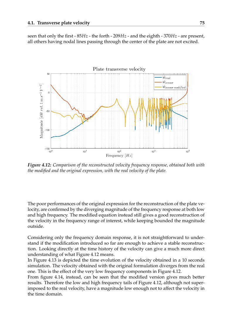
4.1. Transverse plate velocity 75
seen that only the first - 85Hz - the forth - 209Hz - and the eighth - 370Hz - are present,all others having nodal lines passing through the center of the plate are not excited.
Figure 4.12: Comparison of the reconstructed velocity frequency response, obtained both withthe modified and the original expression, with the real velocity of the plate.
The poor performances of the original expression for the reconstruction of the plate ve-locity, are confirmed by the diverging magnitude of the frequency response at both lowand high frequency. The modified equation instead still gives a good reconstruction ofthe velocity in the frequency range of interest, while keeping bounded the magnitudeoutside.
Considering only the frequency domain response, it is not straightforward to under-stand if the modification introduced so far are enough to achieve a stable reconstruc-tion. Looking directly at the time history of the velocity can give a much more directunderstanding of what Figure 4.12 means.In Figure 4.13 is depicted the time evolution of the velocity obtained in a 10 secondssimulation. The velocity obtained with the original formulation diverges from the realone. This is the effect of the very low frequency components in Figure 4.12.From figure 4.14, instead, can be seen that the modified version gives much betterresults. Therefore the low and high frequency tails of Figure 4.12, although not super-imposed to the real velocity, have a magnitude low enough not to affect the velocity inthe time domain.

76 Chapter 4. Sensor-actuator model: Numerical Testing
Figure 4.13: Comparison of the velocity reconstructed with the original expression and the realtransverse velocity of the plate at the actuator location.
Figure 4.14: Comparison of the velocity reconstructed with the modified expression and the realtransverse velocity of the plate at the actuator location.

4.2. Inertial mass velocity 77
4.2 Inertial mass velocity
In this section the reconstruction of the inertial mass velocity is briefly tested. Theexpression has been derived in Chapter 2 and is reported in Eq. 4.15 for the sake ofclarity.
z(s) =
[(R + sL) (sca + ka) + sk2
ems2makem
]i(s)−
[sca + ka
s2makem
]v(s) (4.15)
It can be modified in a similar way to what has been done for the transverse platevelocity. The poles in the origin shall be substituted with negative real part complexconjugate poles, but being Hi(s) already proper, the addition of the high frequencypole is not required.
w(s) =
(R + sL) (sca + ka) + sk2em
makem
(s2 + 2ξlωls + ω2
l
) i(s)−
sca + ka
makem
(s2 + 2ξlωls + ω2
l
) v(s) (4.16)
In Figure 4.15 and 4.16 are depicted the performances of the reconstruction expressionrespectively in frequency and time domain, compared to the real velocity of the inertialmass of the control actuator. Also in this case the reconstruction is satisfying. It can benoticed that the response is dominated by the slow mode of the actuator 30Hz, whilethe modes of the plate are present with lower amplitude.
Figure 4.15: Comparison of the reconstructed inertial mass velocity frequency response, withthe real velocity.
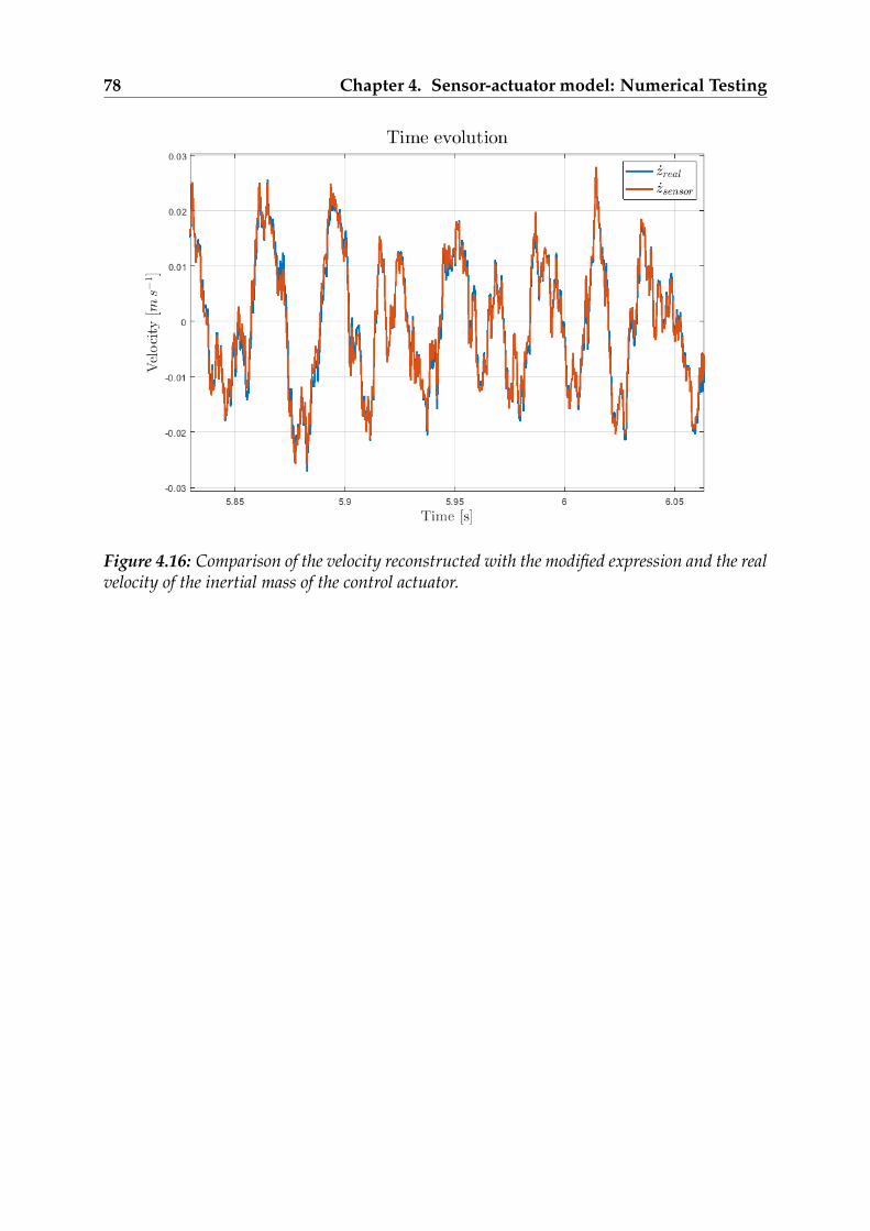
78 Chapter 4. Sensor-actuator model: Numerical Testing
Figure 4.16: Comparison of the velocity reconstructed with the modified expression and the realvelocity of the inertial mass of the control actuator.
Chapter 5
Sensor-actuator model: ExperimentalTesting
In this section the reconstruction of the velocity derived in Chapter 4 is implementedin a real-time skyhook control logic in laboratory. Filters are added and the basis forfuture developments are layed.
5.1 Control scheme
In Figure 5.1 the experimental setup is depicted. Two inertial actuators are mounted onthe thin aluminum plate, one in the center (A) used for the control, and one in a corner(B) used to introduce the disturbance. The disturbance signal generated by the desktopcomputer is a white noise filtered by an anti-aliasing filter (KEMO filter). Between thecontrol actuator and the power amplifier (LEPAI 2), the current sensor - LPRS 6-NP -and the differential scope - PICO TA043 - are placed, so that current and tension can beacquired for the reconstruction of the transverse plate velocity at the control location.Two accelerometers are also used, one glued on top of the inertial mass, and the secondon the lower face of the plate, exactly in correspondence of the actuator A. Indeed, itcan be useful to compute the velocity also by pseudo-integration of the acceleration forcomparison purposes.
Once tension and current are available, the control action is computed trough the dis-crete realization of the plate velocity equation derived in Chapter 4. Ahead of doingso, it has been necessary to filter both tension and current signals, both at low and highfrequencies.The low frequency filtering - roughly below 1Hz - is mandatory to remove acquisitionoffset from current and voltage measures.The high frequency filtering is a crucial aspect of the project, indeed the most criticalproblem and - as thoroughly explained later - still not completely solved.Both filters are realized as digital elliptic second order filters, but for sure other solutioncould be considered in future evolution of the design.
79

80 Chapter 5. Sensor-actuator model: Experimental Testing
PLATE
A
B
BNC-2110AO0
AO1
Disturbance
Control
KEMO filterIN
OUT
LEPAI 2 PICOTA043
v
LPRS 6-NP
2345
9876
OC
DV r
ef
Vou
t
GN
D+5
V
LEPAI 1
BNC-2090ACH0 ACH1 ACH2 ACH3 ACH4
DG
ND
+5V
PCADC
PCI6070
V
iDigital
BandpassFilter
Vf iltered
i f iltered
PlateVelocityReconstr.
PlateVelocity g Control DAC
PCI6713
Figure 5.1: Scheme of the experimental setup used for the testing of the skyhook control logicwith the reconstruction of the plate velocity.
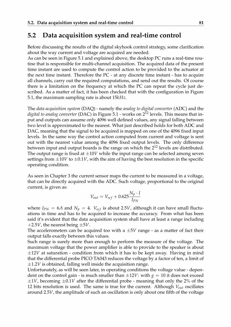
5.2. Data acquisition system and real-time control 81
5.2 Data acquisition system and real-time control
Before discussing the results of the digital skyhook control strategy, some clarificationabout the way current and voltage are acquired are needed.As can be seen in Figure 5.1 and explained above, the desktop PC runs a real-time rou-tine that is responsible for multi-channel acquisition. The acquired data of the presenttime instant are used to compute the control action to be provided to the actuator atthe next time instant. Therefore the PC - at any discrete time instant - has to acquireall channels, carry out the required computations, and send out the results. Of coursethere is a limitation on the frequency at which the PC can repeat the cycle just de-scribed. As a matter of fact, it has been checked that with the configuration in Figure5.1, the maximum sampling rate is about 15kHz.
The data acquisition system (DAQ) - namely the analog to digital converter (ADC) and thedigital to analog converter (DAC) in Figure 5.1 - works on 212 levels. This means that in-put and outputs can assume only 4096 well defined values, any signal falling betweentwo level is approximated to the nearest. What just described holds for both ADC andDAC, meaning that the signal to be acquired is mapped on one of the 4096 fixed inputlevels. In the same way the control action computed from current and voltage is sentout with the nearest value among the 4096 fixed output levels. The only differencebetween input and output boards is the range on which the 212 levels are distributed.The output range is fixed at ±10V while the input range can be selected among sevensettings from ±10V to ±0.1V, with the aim of having the best resolution in the specificoperating condition.
As seen in Chapter 3 the current sensor maps the current to be measured in a voltage,that can be directly acquired with the ADC. Such voltage, proportional to the originalcurrent, is given as:
Vout = Vre f + 0.625Np · IIPN
where IPN = 6A and Np = 4. Vre f is about 2.5V, although it can have small fluctu-ations in time and has to be acquired to increase the accuracy. From what has beensaid it’s evident that the data acquisition system shall have at least a range including+2.5V, the nearest being ±5V.The accelerometers can be acquired too with a ±5V range - as a matter of fact theiroutput falls exactly between this values.Such range is surely more than enough to perform the measure of the voltage. Themaximum voltage that the power amplifier is able to provide to the speaker is about±12V at saturation - condition from which it has to be kept away. Having in mindthat the differential probe PICO TA043 reduces the voltage by a factor of ten, a limit of±1.2V is obtained, falling well inside the acquisition range.Unfortunately, as will be seen later, in operating conditions the voltage value - depen-dent on the control gain - is much smaller than ±12V: with g = 10 it does not exceed±1V, becoming ±0.1V after the differential probe - meaning that only the 2% of the12 bits resolution is used. The same is true for the current. Although Vout oscillatesaround 2.5V, the amplitude of such an oscillation is only about one fifth of the voltage
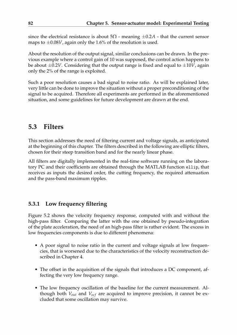
82 Chapter 5. Sensor-actuator model: Experimental Testing
since the electrical resistance is about 5Ω - meaning ±0.2A - that the current sensormaps to ±0.08V, again only the 1.6% of the resolution is used.
About the resolution of the output signal, similar conclusions can be drawn. In the pre-vious example where a control gain of 10 was supposed, the control action happens tobe about ±0.2V. Considering that the output range is fixed and equal to ±10V, againonly the 2% of the range is exploited.
Such a poor resolution causes a bad signal to noise ratio. As will be explained later,very little can be done to improve the situation without a proper preconditioning of thesignal to be acquired. Therefore all experiments are performed in the aforementionedsituation, and some guidelines for future development are drawn at the end.
5.3 Filters
This section addresses the need of filtering current and voltage signals, as anticipatedat the beginning of this chapter. The filters described in the following are elliptic filters,chosen for their steep transition band and for the nearly linear phase.
All filters are digitally implemented in the real-time software running on the labora-tory PC and their coefficients are obtained through the MATLAB function ellip, thatreceives as inputs the desired order, the cutting frequency, the required attenuationand the pass-band maximum ripples.
5.3.1 Low frequency filtering
Figure 5.2 shows the velocity frequency response, computed with and without thehigh-pass filter. Comparing the latter with the one obtained by pseudo-integrationof the plate acceleration, the need of an high-pass filter is rather evident. The excess inlow frequencies components is due to different phenomena:
• A poor signal to noise ratio in the current and voltage signals at low frequen-cies, that is worsened due to the characteristics of the velocity reconstruction de-scribed in Chapter 4.
• The offset in the acquisition of the signals that introduces a DC component, af-fecting the very low frequency range.
• The low frequency oscillation of the baseline for the current measurement. Al-though both Vout and Vre f are acquired to improve precision, it cannot be ex-cluded that some oscillation may survive.
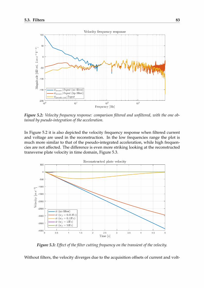
5.3. Filters 83
Figure 5.2: Velocity frequency response: comparison filtered and unfiltered, with the one ob-tained by pseudo-integration of the acceleration.
In Figure 5.2 it is also depicted the velocity frequency response when filtered currentand voltage are used in the reconstruction. In the low frequencies range the plot ismuch more similar to that of the pseudo-integrated acceleration, while high frequen-cies are not affected. The difference is even more striking looking at the reconstructedtransverse plate velocity in time domain, Figure 5.3.
Figure 5.3: Effect of the filter cutting frequency on the transient of the velocity.
Without filters, the velocity diverges due to the acquisition offsets of current and volt-

84 Chapter 5. Sensor-actuator model: Experimental Testing
age. The effect of the filter is indeed to bring to zero the offset in current and voltagesignals, in a time that depends on the cutting frequency of the filter (the higher thecutting frequency, the faster the filtering action, see Figure 5.4). During the transient ofthe filter, an offset is still present in the filtered voltage and current signals, still causingthe error to build up in the reconstructed velocity. But since the offset is now going tozero in few seconds, the filtering action built-in in the velocity reconstruction formuladiscussed in Chapter 4, is able to promptly bring the error to zero. Figure 5.2 shows thedifferent transient time for the reconstructed velocity, the higher the cutting frequencyof the filter the lesser the maximum error reached, the lesser the settling time.
Figure 5.4: Effect of the filter cutting frequency on the transient of the voltage.
The choice of the filter cutting frequency shall be a compromise between velocity of theresponse - that would require the highest possible cutting frequency - and the preser-vation of a good reconstruction of the velocity - that requires a cutting frequency lowerthan the frequency range of interest. The filter implemented in the following is de-picted in Figure 5.5 and has a cutting frequency around 5Hz.
The non infinitesimal response time of the filter would impose to wait the end of thetransient in the filtered current and voltage, before starting to compute the velocity inorder to avoid the error to build up. But thanks to the filtering action supplemented bythe negative real part poles in the velocity reconstruction transfer functions, it’s pos-sible to avoid this step, simplifying the implementation. The abovementioned polesdoes not influence the response once the transient is ended, but they simplify switch-ing on the system, avoiding having to wait for the filter’s transient to end.

5.3. Filters 85
Figure 5.5: High-pass filter for current and tension.
5.3.2 High frequency filtering
The low resolution achievable in the measures of current and voltage described aboveleads to a poor signal to noise ratio at all frequencies. This problem is particularly evi-dent in the high frequency range because - as it will be explained below - it’s worsenedby some interaction between ADC and DAC. To catch this last phenomenon, althoughthe following consideration are made about the open loop case, the system will al-ways be connected in closed loop, with a control gain equal to zero. Indeed in theorythe two conditions are equivalent, but since in the closed loop a new source of noisearises, it would be misleading to make an analysis of the pure open loop case, becausethis additional error would be missed and it would become more difficult to catch itanalyzing directly the closed loop control performances. Figure 5.6 shows the poor cor-respondence at high frequency of the transverse plate velocity obtained from currentand voltage, with that obtained by pseudo-integration of the acceleration. Both areobtained in open-loop, without a low-pass filter. Looking at Figure 5.6 can be seen thatthe approximation is good at least up to 2kHz, after that the noise in the reconstructedvelocity gets more and more evident. Moreover there are two peaks - at 3750Hz and7500Hz - quite difficult to comprehend.

86 Chapter 5. Sensor-actuator model: Experimental Testing
Figure 5.6: Comparison of the velocity frequency response for the reconstructed plate velocityand the one obtained by pseudo-integration of the acceleration.
While the noise is easily explained by the considerations made above about the lowresolution of the measures, to understand where the two peaks come from, additionaldiscussion is needed.The velocity is computed acquiring the voltage applied to the control actuator and thecurrent flowing into it. But the control action - simply a multiple of the computedvelocity - is then applied as a driving voltage to the control actuator. Both operations- acquisition and sending the control action to the actuator - are performed with thesame sampling frequency, in this case 15kHz. It will be now taken in exam a peculiarcase that makes the meaning of the peaks rather evident. Figure 5.7 reports a shorttime history of the acquired voltage, when the system has a control gain equal to zero(equivalent to open loop). In this conditions the voltage applied to the actuator is zero,and so it should be the voltage acquired. It is not so for different reasons:
• There’s an offset of about 150mV. Although it could seems huge, it has to beremembered that the voltage is acquired after his amplitude being reduced by afactor of ten with the differential probe PICO TA043. Therefore the offset rightafter acquisition is ten times smaller, 15mV. Probably, it could be reduced cali-brating the probe, but in any case it does not represent a problem thanks to thehigh-pass filter introduced in the previous section.
• The value of the voltage should be constant but it is not acquired on a fixed level.It oscillates taking at least the first two levels - and looking at longer time scalesit reaches also the forth - on both side of the mean value, introducing some highfrequency oscillations. In Figure 5.7 are highlighted two patterns that frequentlyrepeat on the whole time history, having period of two and four sampling times,meaning frequencies of 7500Hz and 3750Hz.
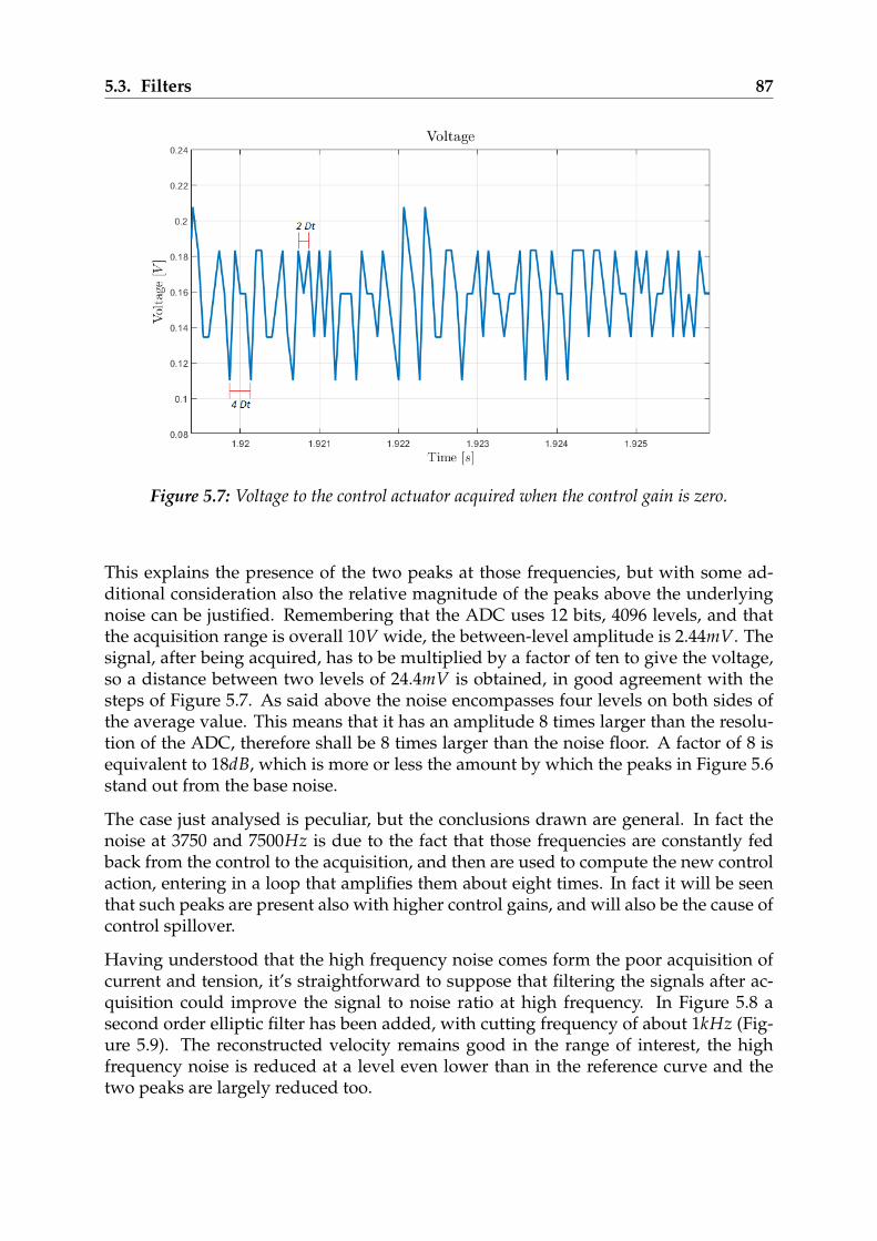
5.3. Filters 87
Figure 5.7: Voltage to the control actuator acquired when the control gain is zero.
This explains the presence of the two peaks at those frequencies, but with some ad-ditional consideration also the relative magnitude of the peaks above the underlyingnoise can be justified. Remembering that the ADC uses 12 bits, 4096 levels, and thatthe acquisition range is overall 10V wide, the between-level amplitude is 2.44mV. Thesignal, after being acquired, has to be multiplied by a factor of ten to give the voltage,so a distance between two levels of 24.4mV is obtained, in good agreement with thesteps of Figure 5.7. As said above the noise encompasses four levels on both sides ofthe average value. This means that it has an amplitude 8 times larger than the resolu-tion of the ADC, therefore shall be 8 times larger than the noise floor. A factor of 8 isequivalent to 18dB, which is more or less the amount by which the peaks in Figure 5.6stand out from the base noise.
The case just analysed is peculiar, but the conclusions drawn are general. In fact thenoise at 3750 and 7500Hz is due to the fact that those frequencies are constantly fedback from the control to the acquisition, and then are used to compute the new controlaction, entering in a loop that amplifies them about eight times. In fact it will be seenthat such peaks are present also with higher control gains, and will also be the cause ofcontrol spillover.
Having understood that the high frequency noise comes form the poor acquisition ofcurrent and tension, it’s straightforward to suppose that filtering the signals after ac-quisition could improve the signal to noise ratio at high frequency. In Figure 5.8 asecond order elliptic filter has been added, with cutting frequency of about 1kHz (Fig-ure 5.9). The reconstructed velocity remains good in the range of interest, the highfrequency noise is reduced at a level even lower than in the reference curve and thetwo peaks are largely reduced too.
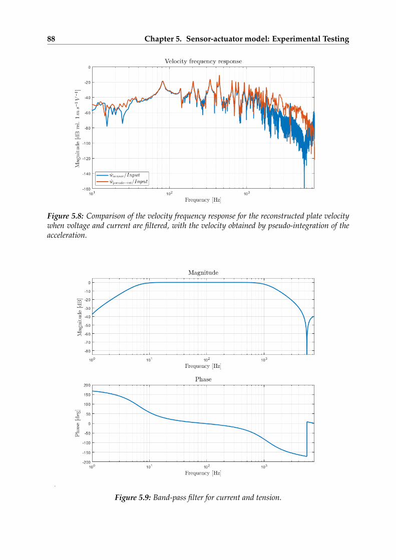
88 Chapter 5. Sensor-actuator model: Experimental Testing
Figure 5.8: Comparison of the velocity frequency response for the reconstructed plate velocitywhen voltage and current are filtered, with the velocity obtained by pseudo-integration of theacceleration.
Figure 5.9: Band-pass filter for current and tension.

5.4. Closed loop control 89
One could think to use a filter having an arbitrarily high order, but has to be kept inmind that the phase lag introduced by the filter translates in a delay of the computedvelocity with respect to the real one, therefore in a delay of the control action.
Up to now the disturbance applied to the plate has been a white noise, without anylimitation in frequency. One could be brought to think that filtering the disturbance athigh frequency could bring some improvements to the situation just described. Figure5.10 shows the effect of filtering the disturbance at 800Hz. The velocity obtained bypseudo-integration of the acceleration is indeed filtered, in fact if the disturbance hasno components at high frequency, the same should apply to the acceleration of theplate, therefore also to the velocity. On the contrary, there are no effects on the velocityobtained from current and voltage, as an additional proof that in this case the noiseis due only to the poor acquisition of the electrical quantities. Nevertheless in thefollowing the disturbance filtering will be used sometimes, to avoid high frequencymodes of the structure to be excited.
Figure 5.10: Comparison of the velocity frequency response for the reconstructed plate velocityand the pseudo-integration acceleration, when the disturbance is filtered.
5.4 Closed loop control
In this section the performances of the skyhook control, when the transverse platevelocity reconstructed from current and voltage is used, are analyzed.Figure 5.11 reports, for comparative purposes, the performances of the control system- in terms of the plate acceleration frequency response at the control point - when thefeedback action is determined from the velocity obtained by pseudo-integration of thetransverse plate acceleration.
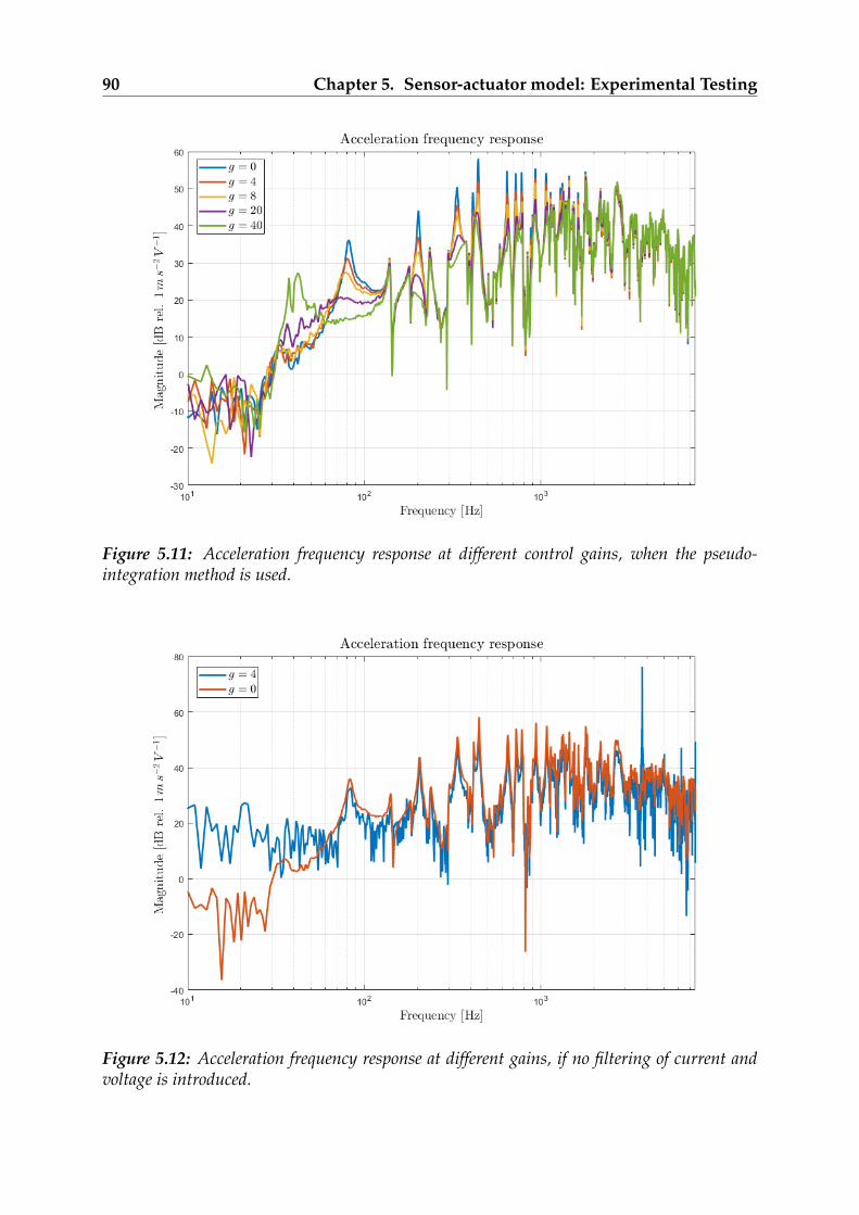
90 Chapter 5. Sensor-actuator model: Experimental Testing
Figure 5.11: Acceleration frequency response at different control gains, when the pseudo-integration method is used.
Figure 5.12: Acceleration frequency response at different gains, if no filtering of current andvoltage is introduced.
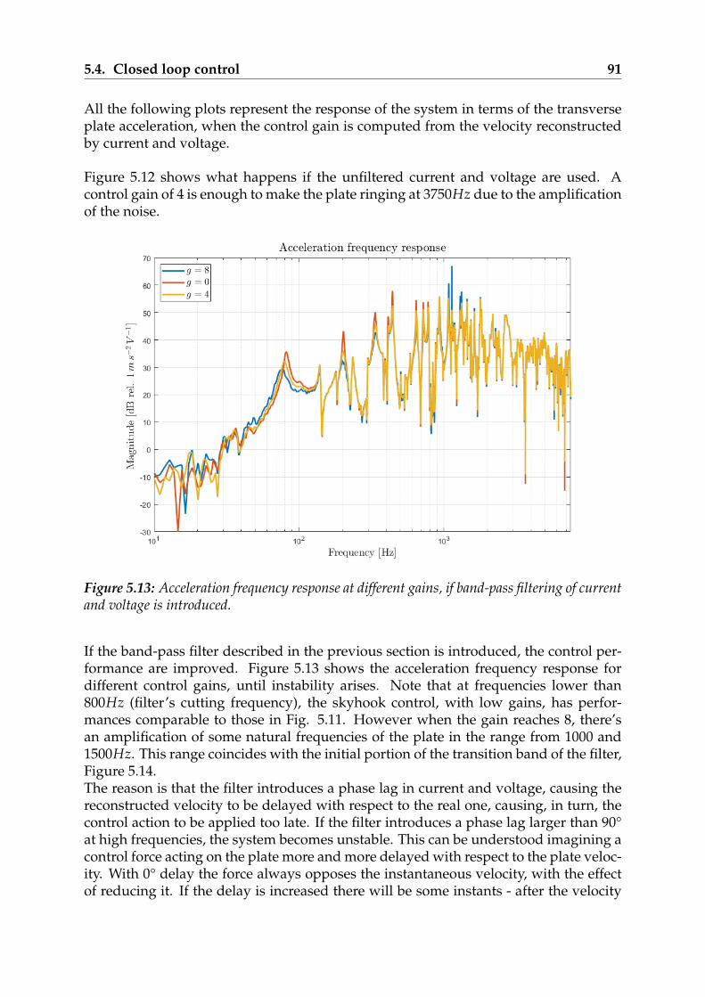
5.4. Closed loop control 91
All the following plots represent the response of the system in terms of the transverseplate acceleration, when the control gain is computed from the velocity reconstructedby current and voltage.
Figure 5.12 shows what happens if the unfiltered current and voltage are used. Acontrol gain of 4 is enough to make the plate ringing at 3750Hz due to the amplificationof the noise.
Figure 5.13: Acceleration frequency response at different gains, if band-pass filtering of currentand voltage is introduced.
If the band-pass filter described in the previous section is introduced, the control per-formance are improved. Figure 5.13 shows the acceleration frequency response fordifferent control gains, until instability arises. Note that at frequencies lower than800Hz (filter’s cutting frequency), the skyhook control, with low gains, has perfor-mances comparable to those in Fig. 5.11. However when the gain reaches 8, there’san amplification of some natural frequencies of the plate in the range from 1000 and1500Hz. This range coincides with the initial portion of the transition band of the filter,Figure 5.14.The reason is that the filter introduces a phase lag in current and voltage, causing thereconstructed velocity to be delayed with respect to the real one, causing, in turn, thecontrol action to be applied too late. If the filter introduces a phase lag larger than 90°at high frequencies, the system becomes unstable. This can be understood imagining acontrol force acting on the plate more and more delayed with respect to the plate veloc-ity. With 0° delay the force always opposes the instantaneous velocity, with the effectof reducing it. If the delay is increased there will be some instants - after the velocity
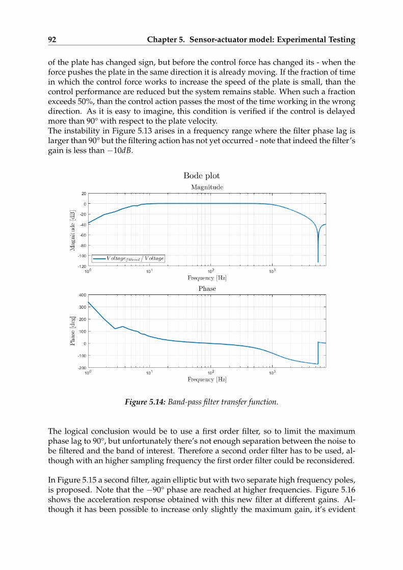
92 Chapter 5. Sensor-actuator model: Experimental Testing
of the plate has changed sign, but before the control force has changed its - when theforce pushes the plate in the same direction it is already moving. If the fraction of timein which the control force works to increase the speed of the plate is small, than thecontrol performance are reduced but the system remains stable. When such a fractionexceeds 50%, than the control action passes the most of the time working in the wrongdirection. As it is easy to imagine, this condition is verified if the control is delayedmore than 90° with respect to the plate velocity.The instability in Figure 5.13 arises in a frequency range where the filter phase lag islarger than 90° but the filtering action has not yet occurred - note that indeed the filter’sgain is less than −10dB.
Figure 5.14: Band-pass filter transfer function.
The logical conclusion would be to use a first order filter, so to limit the maximumphase lag to 90°, but unfortunately there’s not enough separation between the noise tobe filtered and the band of interest. Therefore a second order filter has to be used, al-though with an higher sampling frequency the first order filter could be reconsidered.
In Figure 5.15 a second filter, again elliptic but with two separate high frequency poles,is proposed. Note that the −90° phase are reached at higher frequencies. Figure 5.16shows the acceleration response obtained with this new filter at different gains. Al-though it has been possible to increase only slightly the maximum gain, it’s evident
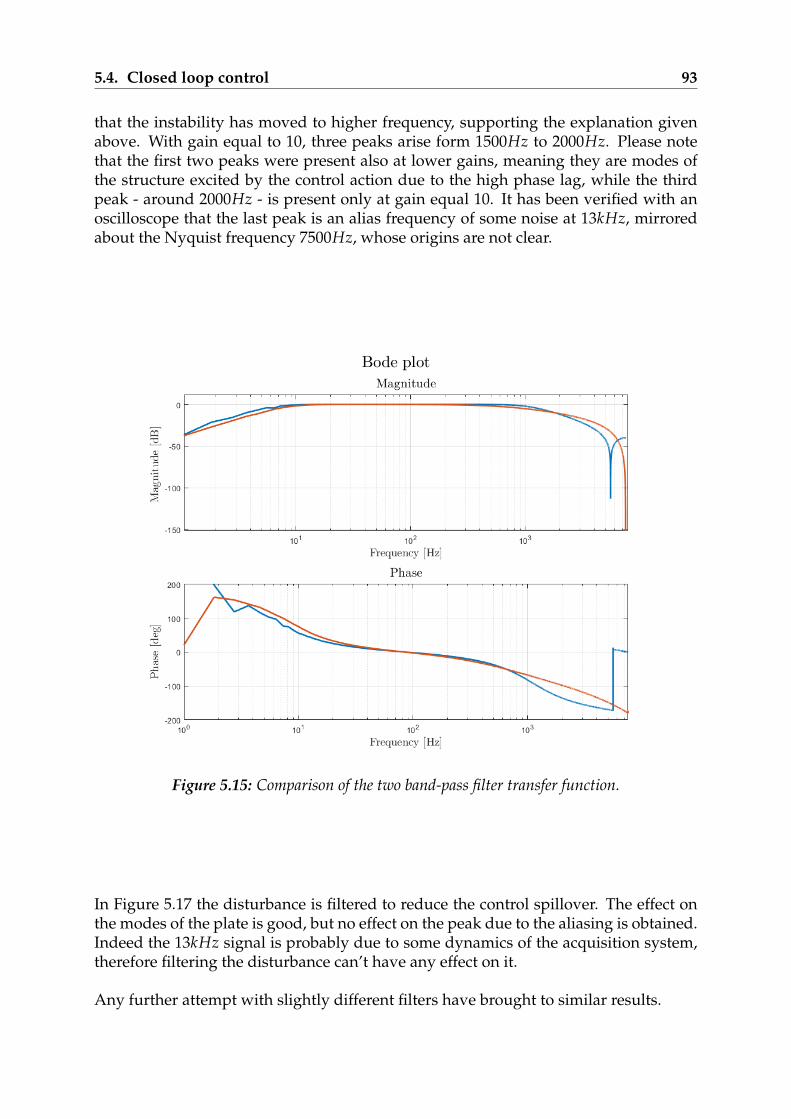
5.4. Closed loop control 93
that the instability has moved to higher frequency, supporting the explanation givenabove. With gain equal to 10, three peaks arise form 1500Hz to 2000Hz. Please notethat the first two peaks were present also at lower gains, meaning they are modes ofthe structure excited by the control action due to the high phase lag, while the thirdpeak - around 2000Hz - is present only at gain equal 10. It has been verified with anoscilloscope that the last peak is an alias frequency of some noise at 13kHz, mirroredabout the Nyquist frequency 7500Hz, whose origins are not clear.
Figure 5.15: Comparison of the two band-pass filter transfer function.
In Figure 5.17 the disturbance is filtered to reduce the control spillover. The effect onthe modes of the plate is good, but no effect on the peak due to the aliasing is obtained.Indeed the 13kHz signal is probably due to some dynamics of the acquisition system,therefore filtering the disturbance can’t have any effect on it.
Any further attempt with slightly different filters have brought to similar results.
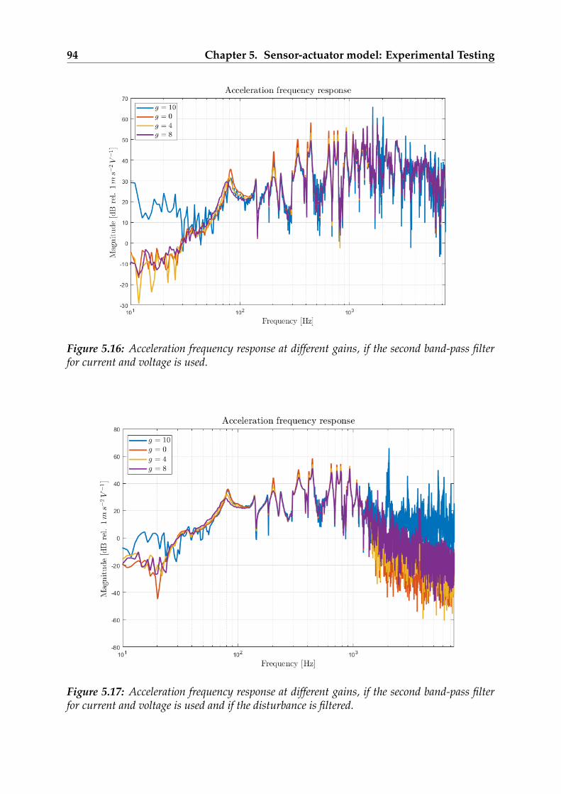
94 Chapter 5. Sensor-actuator model: Experimental Testing
Figure 5.16: Acceleration frequency response at different gains, if the second band-pass filterfor current and voltage is used.
Figure 5.17: Acceleration frequency response at different gains, if the second band-pass filterfor current and voltage is used and if the disturbance is filtered.
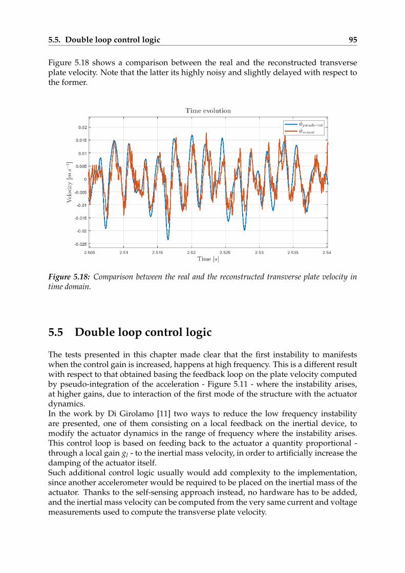
5.5. Double loop control logic 95
Figure 5.18 shows a comparison between the real and the reconstructed transverseplate velocity. Note that the latter its highly noisy and slightly delayed with respect tothe former.
Figure 5.18: Comparison between the real and the reconstructed transverse plate velocity intime domain.
5.5 Double loop control logic
The tests presented in this chapter made clear that the first instability to manifestswhen the control gain is increased, happens at high frequency. This is a different resultwith respect to that obtained basing the feedback loop on the plate velocity computedby pseudo-integration of the acceleration - Figure 5.11 - where the instability arises,at higher gains, due to interaction of the first mode of the structure with the actuatordynamics.In the work by Di Girolamo [11] two ways to reduce the low frequency instabilityare presented, one of them consisting on a local feedback on the inertial device, tomodify the actuator dynamics in the range of frequency where the instability arises.This control loop is based on feeding back to the actuator a quantity proportional -through a local gain gl - to the inertial mass velocity, in order to artificially increase thedamping of the actuator itself.Such additional control logic usually would add complexity to the implementation,since another accelerometer would be required to be placed on the inertial mass of theactuator. Thanks to the self-sensing approach instead, no hardware has to be added,and the inertial mass velocity can be computed from the very same current and voltagemeasurements used to compute the transverse plate velocity.

96 Chapter 5. Sensor-actuator model: Experimental Testing
PLATE
A
B
BNC-2110AO0
AO1
Disturbance
Control
KEMO filterIN
OUT
LEPAI 2 PICOTA043
v
LPRS 6-NP
2345
9876
OC
DV r
ef
Vou
t
GN
D+5
V
LEPAI 1
BNC-2090ACH0 ACH1 ACH2 ACH3 ACH4
DG
ND
+5V
PC
ADCPCI6070
V
i
Vacc
DigitalBandpass
Filter
Vf iltered
i f iltered
ComputePlateAcc.
AccIA
IMVelocityReconstr.
IMVelocity
Acc.PseudoIntegr.
PlateVelocity
g
gl
+
+
Control DACPCI6713
Figure 5.19: Experimental setup used to test the inertial mass velocity reconstruction.
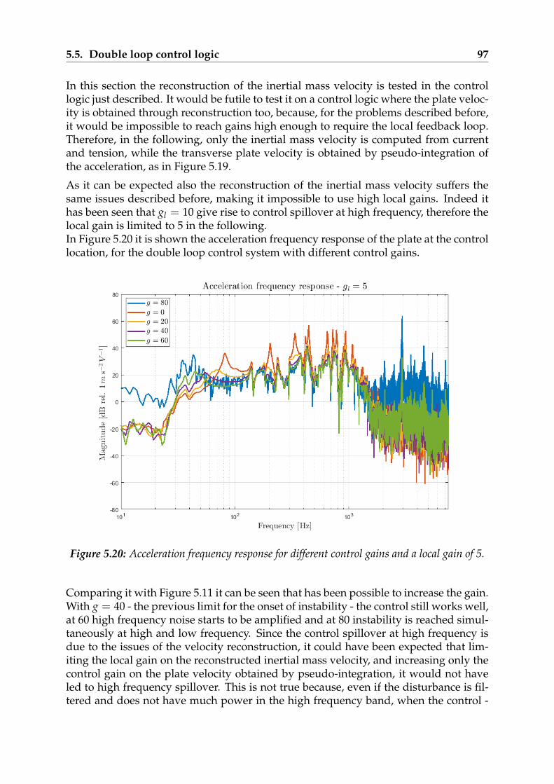
5.5. Double loop control logic 97
In this section the reconstruction of the inertial mass velocity is tested in the controllogic just described. It would be futile to test it on a control logic where the plate veloc-ity is obtained through reconstruction too, because, for the problems described before,it would be impossible to reach gains high enough to require the local feedback loop.Therefore, in the following, only the inertial mass velocity is computed from currentand tension, while the transverse plate velocity is obtained by pseudo-integration ofthe acceleration, as in Figure 5.19.
As it can be expected also the reconstruction of the inertial mass velocity suffers thesame issues described before, making it impossible to use high local gains. Indeed ithas been seen that gl = 10 give rise to control spillover at high frequency, therefore thelocal gain is limited to 5 in the following.In Figure 5.20 it is shown the acceleration frequency response of the plate at the controllocation, for the double loop control system with different control gains.
Figure 5.20: Acceleration frequency response for different control gains and a local gain of 5.
Comparing it with Figure 5.11 it can be seen that has been possible to increase the gain.With g = 40 - the previous limit for the onset of instability - the control still works well,at 60 high frequency noise starts to be amplified and at 80 instability is reached simul-taneously at high and low frequency. Since the control spillover at high frequency isdue to the issues of the velocity reconstruction, it could have been expected that lim-iting the local gain on the reconstructed inertial mass velocity, and increasing only thecontrol gain on the plate velocity obtained by pseudo-integration, it would not haveled to high frequency spillover. This is not true because, even if the disturbance is fil-tered and does not have much power in the high frequency band, when the control -
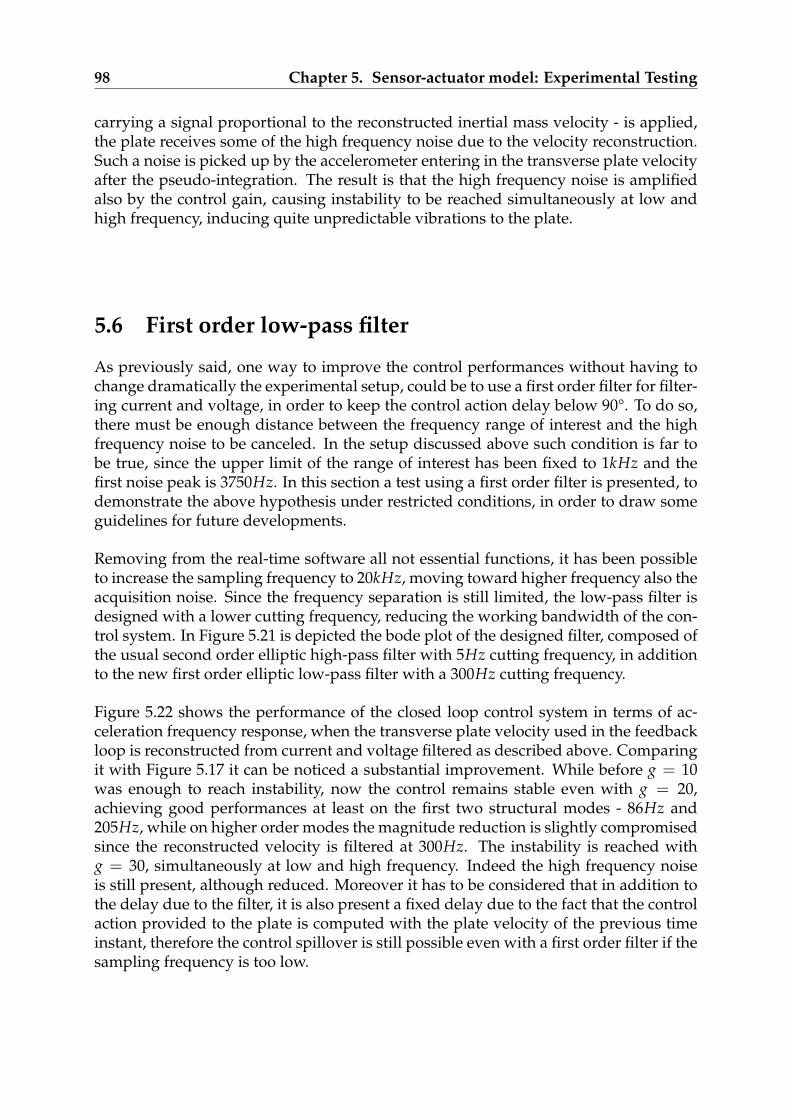
98 Chapter 5. Sensor-actuator model: Experimental Testing
carrying a signal proportional to the reconstructed inertial mass velocity - is applied,the plate receives some of the high frequency noise due to the velocity reconstruction.Such a noise is picked up by the accelerometer entering in the transverse plate velocityafter the pseudo-integration. The result is that the high frequency noise is amplifiedalso by the control gain, causing instability to be reached simultaneously at low andhigh frequency, inducing quite unpredictable vibrations to the plate.
5.6 First order low-pass filter
As previously said, one way to improve the control performances without having tochange dramatically the experimental setup, could be to use a first order filter for filter-ing current and voltage, in order to keep the control action delay below 90°. To do so,there must be enough distance between the frequency range of interest and the highfrequency noise to be canceled. In the setup discussed above such condition is far tobe true, since the upper limit of the range of interest has been fixed to 1kHz and thefirst noise peak is 3750Hz. In this section a test using a first order filter is presented, todemonstrate the above hypothesis under restricted conditions, in order to draw someguidelines for future developments.
Removing from the real-time software all not essential functions, it has been possibleto increase the sampling frequency to 20kHz, moving toward higher frequency also theacquisition noise. Since the frequency separation is still limited, the low-pass filter isdesigned with a lower cutting frequency, reducing the working bandwidth of the con-trol system. In Figure 5.21 is depicted the bode plot of the designed filter, composed ofthe usual second order elliptic high-pass filter with 5Hz cutting frequency, in additionto the new first order elliptic low-pass filter with a 300Hz cutting frequency.
Figure 5.22 shows the performance of the closed loop control system in terms of ac-celeration frequency response, when the transverse plate velocity used in the feedbackloop is reconstructed from current and voltage filtered as described above. Comparingit with Figure 5.17 it can be noticed a substantial improvement. While before g = 10was enough to reach instability, now the control remains stable even with g = 20,achieving good performances at least on the first two structural modes - 86Hz and205Hz, while on higher order modes the magnitude reduction is slightly compromisedsince the reconstructed velocity is filtered at 300Hz. The instability is reached withg = 30, simultaneously at low and high frequency. Indeed the high frequency noiseis still present, although reduced. Moreover it has to be considered that in addition tothe delay due to the filter, it is also present a fixed delay due to the fact that the controlaction provided to the plate is computed with the plate velocity of the previous timeinstant, therefore the control spillover is still possible even with a first order filter if thesampling frequency is too low.

5.6. First order low-pass filter 99
Figure 5.21: Bode plot of the band-pass filter, composed by a first order low-pass in addition toa second order high-pass.
Figure 5.22: Acceleration frequency response with a first order filtering of current and voltage.

100 Chapter 5. Sensor-actuator model: Experimental Testing
Given the awful resolution with which current and voltage are acquired, this can beconsidered a good result, and for sure gives clear indications on the direction thatfuture works should take. In this last test the frequency separation between the filter’scutting frequency and the noise frequency was little more than a decade, if the noisewere reduced by preconditioning of current and voltage it is straightforward that suchseparation could be reduced.

Chapter 6
Conclusions
The work presented in this thesis is intended as a preliminary study for the develop-ment of active devices based on the self-sensing inertial actuator concept, to be used toachieve vibroacoustic control of generic vibrating panels. The basic concept is to dampthe vibration of a generic structure installing a device providing a control action pro-portional to the transverse structural velocity, obtaining a skyhook control system. Theinnovative idea is to derive an expression to reconstruct the transverse plate velocityand the inertial mass velocity adopting electrical measures only, without any need foraccelerometers. The system is digitally implemented, looking toward future evolutionin the direction of a multi-actuator decentralized control system that would greatlybenefit from a digital implementation.The first part of this work, described in Chapters 2 and 3, concerned the developmentof a mathematical model of the experimental setup, having a dual function. Firstlyto allow the analytical derivation of an expression for the velocities, depending onlyon the voltage applied to the inertial device and on the current flowing in it, secondlyto build models of the physical components - plate, power amplifier and vibrationspeaker - to be used to numerically simulate the experimental setup. The configu-ration under analysis is composed by a rectangular thin aluminum plate and a lowcost vibration speaker used as inertial actuator, driven by a cheap power amplifier.The actuator is modelled as a simple mass-spring-damper system, whose parametershave been obtained through experiments on each device. Similarly a simple high-passfilter-like model, describing the power amplifier, has been obtained. The plate has beenmodelled at two levels of detail, firstly using a single degree of freedom model to gainsome insight into the dynamic system under analysis, keeping as simple as possiblethe numerical simulation, secondly with a complete flexible description based on theS-GUF formulation, to analyze the system behaviour reproducing the real operatingconditions.The sensor-actuator expression for the velocity is based on the lumped parametermodel of the inertial actuator, therefore suffers for any uncertainty of the model. InChapter 4 the velocity reconstruction is tested numerically and some modificationsare introduced, to solve stability related issues. The first problem is about one of thetransfer functions not being proper. A static residualization of the actuator’s electricdynamic is first proposed to reduce the order of the numerator, but this has led to even
101
102 Chapter 6. Conclusions
worst results because of the high sensitivity of the reconstruction expression to nonsymmetric modifications of the transfer functions. Therefore the expression has beenmade proper by adding a pole at high frequency to both transfer functions. The secondissue is the presence of two poles in the origin, solved moving the poles to the negativehalf of the complex plane. The final formulation gives a good reconstruction of thevelocities - both transverse plate and inertial mass - in the frequency range of interest -20Hz to 1kHz - keeping a good noise rejection outside.The last part of this work was about the experimental testing of the sensor-actuatormodel. In Chapter 5 are discussed the results obtained digitally implementing thereconstruction of the velocity on a real-time skyhook control. The main problem con-cerned the resolution of the acquisition system, since the electrical quantities to be ac-quired oscillate with small amplitude around different baselines, the acquisition rangehas to be kept wide enough to acquire both, leading to a poor signal to noise ratio. Dif-ferent filters has been introduced and tested to remove the noise at both low and highfrequency. Good performances are obtained at low frequency, while high frequencyfiltering proved to be a challenging task. If the filtering action is too weak, the noiseis not rejected and is amplified through the control gain. If it is too strong, the phaselag exceeded the phase margin, causing control spillover instability. If a first orderlow-pass filter is used, the stability of the control system is granted. Unfortunatelythe distance of the noise to be filtered from the frequency range of interest is not highenough to use a first order filter. A test has been presented where the working band ofthe control system has been limited to 300Hz, demonstrating that the first order filtergives indeed far better performances.
6.1 Future work
A lot of work has yet to be done on the self-sensing model of the actuator, beforeachieving the same performances that can be obtained with a sensor/actuator collo-cated pair. The numerical analysis demonstrated that, with the proposed modificationto the reconstruction’s transfer functions, stability can be theoretically achieved evenin non ideal conditions. However, the real-time testing performed with a partially in-adequate acquisition method showed how any segment of the control system, and notonly the reconstruction equation, is vital to achieve good performances. In particular,the signal to noise ratio in the acquired quantities plays a primary role in the goodreconstruction of the velocity. Therefore in future works more efforts shall be made inits improvement. In almost all reference works about sensor-actuators, a fully analog-ical control system was used. Of course moving to a similar architecture could greatlyimprove the signal to noise ratio, since it would remove its main source, the digitalconversion. However, for the premises on the device that is being designed, a fullyanalogical approach could introduce great hardware complexity if a multi actuator de-centralized architecture or more complex control logic were to be considered for futuredevelopments. A compromise solution could be to keep a digital implementation forthe velocity reconstruction and for the feedback loops, while introducing an analogpreconditioning of the signals to be acquired. In this way the acquisition of currentand voltage could be made with a far better resolution while keeping the hardware

6.1. Future work 103
complexity independent on the control logic adopted. An example of a precondition-ing circuit for current and voltage can be find in [33], where the current and voltagechannels are preamplified in order to better exploit the resolution of the acquisitionsystem. If a good enough signal to noise ratio were obtained, it might not even be nec-essary anymore the high frequency filtering presented in Chapter 5, or at least shouldbe enough to use a first order filter as proposed in the last test.

Bibliography
[1] R. Kim, L. Fritschi, A. Brown, D. Schewla, and S. Kephalopoulos., “Burden ofdisease from environmental noise,” in Tech. rep. World Health Organization, 2011. 1
[2] E. Kerns, E. Masterson, C. Themann, and G. M. Calvert, “Cardiovascular con-ditions, hearing difficulty, and occupational noise exposure within us indus-tries and occupations,” American Journal of Industrial Medicine 61.6, pp. 477–491,03/12/2018. 1
[3] T. Münzel, F. Schmidt, S. Steven, J. Herzog, A. Daiber, , and M. Sørensen, “Envi-ronmental noise and the cardiovascular system,” Journal of the American College ofCardiology 71.6, pp. 688–697, 2018. 1
[4] K. Genuit, “Vehicle interior noise – combination of sound, vibration and interac-tivity,” in Head acoustic GmbH, Sound and Vibrations, 2009. 1
[5] D. Mead, Passive Vibration Control. John Wiley, 1998. 1
[6] F. Fahy, Fundamentals of noise and vibration control. E FN Spon London, 1998. 1
[7] F. Fahy and JohnWalker, Advanced applications in acoustics, noise and vibration. CRCPress, 2004. 1
[8] P. Gardonio, “Review of active techniques for aerospace vibro-acoustic control,”Journal of Aircraft 39.2, pp. 206–214, 04/12/2018. 1
[9] R. Boulandet, A. Pelletier, P. Micheau, and A. Berry, “Active vibration control us-ing self-sensing actuators: an experimental comparison of piezoelectric and elec-tromagnetic technologies,” in Proc. of the ASME 2014 International Mechanical En-gineering Congress Exposition, (Montréal, Canada), November 14-20 2014. 1, 3,14
[10] R. Boulandet, M. Michau, P. Micheau, and A. Berry, “Aircraft panel with sen-sorless active sound power reduction capabilities through virtual mechanicalimpedances,” Journal of Sound and Vibration 361, pp. 2–19, 2016. 1, 3, 14
[11] D. D. Girolamo, “Active damping controllers with proof-mass electrodynamic ac-tuators: design, analysis and experiments,” Master’s thesis, Politecnico di Milano,April 2018. 2, 18, 29, 37, 46, 50, 52, 53, 54, 95
105

106 Bibliography
[12] P. Gardonio, “Smart panel with multiple decentralized units for the control ofsound transmission. part i: theoretical predictions,” Journal of Sound and Vibration274, pp. 163–192, July 2004. 2
[13] F. Fahy and J. Walker, Fundamentals of Noise and Vibration. E FN SPON, 1998. 3
[14] W. P. Engels, O. N. Baumann, S. J. Elliott, and R. Fraanje, “Centralized and decen-tralized control of structural vibration and sound radiation,” Journal of the Acous-tical Society of America 119, 2006. 3
[15] M. Baudry, P. Micheau, and A. Berry, “Decentralized harmonic active vibrationcontrol of a flexible plate using piezoelectric actuator–sensor pairs,” Journal of theAcoustical Society of America 119, 2006. 3
[16] M. J. Balas, “Direct velocity feedback control of large space structures,” Journal ofGuidance, Control, and Dynamics, 1979. 3
[17] S. J. Elliott, P. Gardonio, T. C. Sors, and M. J. Brennan, “Active vibroacoustic con-trol with multiple local feedback loops,” The Journal of the Acoustical Society ofAmerica, 2002. 3
[18] P. Gardonio, E. Bianchi, and S. Elliott, “Smart panel with multiple decentralizedunits for the control of sound transmission. part i: theoretical predictions,” Journalof sound and vibration, 2004. 3
[19] P. Gardonio, E. Bianchi, and S. Elliott, “Smart panel with multiple decentralizedunits for the control of sound transmission. part ii: design of the decentralizedcontrol units,” Journal of sound and vibration, 2004. 3
[20] P. Gardonio, E. Bianchi, and S. Elliott, “Smart panel with multiple decentralizedunits for the control of sound transmission. part iii: control system implementa-tion,” Journal of sound and vibration, 2004. 3
[21] N. W. Hagood and E. H. Anderson, “Simultaneous sensing and actuation usingpiezoelectric materials,” in Proc. SPIE 1543 Active and adaptive optical components,1991. 3
[22] J. J. Dosch, D. J. Inman, and E. Garcia, “Self-sensing piezoelectric actuator forcollocated control,” J. of Intel. Mat. Syst. and Struct., 1992. 3
[23] J. S. Vipperman and R. L. Clark, “Implementation of an adaptive piezoelectricsensoriactuator,” Am. Inst. of Aeronautics and Astronautics, 1996. 3
[24] J. S. Vipperman and R. L. Clark, “Multivariable feedback active structural acousticcontrol using adaptive piezoelectric sensoriactuators,” J. Acoust. Soc. Am., 1999. 3
[25] S. O. R. Moheimani, “A survey of recent innovations in vibration damping andcontrol using shunted piezoelectric transducers,” IEEE Trans. Control Syst. Tech.,2003. 3
[26] D. Leo and D. Limpert, “A self-sensing technique for active acoustic attenuation,”Journal Sound and Vibration, 2000. 3
Bibliography 107
[27] B. Hanson and M. Levesley, “Self-sensing applications for electromagnetic actua-tors,” Sensors and Actuators A: Physical, 2004. 3
[28] A. Pelletier, P. Micheau, and A. Berry, “Harmonic active vibration control usingpiezoelectric self-sensing actuation with complete digital compensation,” Journalof Intelligent Material Systems and Structures, November 2017. 3
[29] A. Preumont, Mechatronics - Dynamics of Electromechanical and Piezoelectric Systems.Springer, 2006. 6
[30] H. Olson, Music, Physics and Engineering. Dover Publications, 1967. 19
[31] M. D’Ottavio, L. Dozio, R. Vescovini, and O. Polit., “The ritz – sublaminate gener-alized unified formulation approach for piezoelectric composite plates,” Interna-tional Journal of Smart and Nano Materials 9.1, pp. 34–55, 2018. 19
[32] O. Faccini, “Vibroacoustic control of plates with self-tuning decentralized feed-back loops,” Master’s thesis, Politecnico di Milano, 2018. 46, 53
[33] F. Romani, “Power consumption analysis of an electromechanical inertial mass ac-tuator using a custom designed measurement board,” Master’s thesis, Universitàdi Pisa, 2017. 103