Delayed Fusion for Real-Time Vision-Aided Inertial Navigation

SPECIAL ISSUE PAPER

Delayed fusion for real-time vision-aided inertial navigation

Ehsan Asadi • Carlo L. Bottasso

Received: 13 May 2013 / Accepted: 15 October 2013

� Springer-Verlag Berlin Heidelberg 2013

Abstract In this paper, we consider the effects of delay

caused by real-time image acquisition and feature tracking

in a previously documented vision-augmented inertial

navigation system. At first, the paper illustrates how delay

caused by image processing, if not explicitly taken into

account, can lead to appreciable performance degradation

of the estimator. Next, three different existing methods of

delayed fusion and a novel combined one are considered

and compared. Simulations and Monte Carlo analyses are

used to assess the estimation errors and computational

effort of the various methods. Finally, a best performing

formulation is identified that properly handles the fusion of

delayed measurements in the estimator without increasing

the time burden of the filter.

Keywords Delayed fusion � Vision-aided inertial

navigation system � Larsen method � Delayed state

EKF � Recalculation

1 Introduction

Navigation approaches often use vision systems, since these

are among the most information-rich sensors for autonomous

positioning and mapping purposes [1]. Vision-based

navigation systems have been in use in numerous applications

such as autonomous ground vehicles (AGV) and underwater

environments [2]. Recently, they have been gaining increased

attention also in the field of unmanned aerial vehicles (UAV)

[3, 4]. Vision systems provide long range, high resolution

measurements with low power consumption and limited cost.

On the other hand, they are usually associated with rather low

sample rates, since they often require complex processing of

the acquired images, and this limits and hinders their usability

in fast and real-time applications [5].

Several attempts have already been documented in the

design and implementation of robust visual odometry

systems [6, 7]. Some authors have proposed the incorpo-

ration of inertial measurements as model inputs [8] or

states [9–11], using variants of the Kalman filtering

approach to robustly estimate the vehicle motion. Other

authors have used an entropy-like cost function or bundle

adjustment [12, 13]. The vision-aided inertial navigation

system (VA-INS) of [14] combined in a synergistic way

vision-based sensors together with classical inertial navi-

gation ones. The method made use of an extended kalman

filter (EKF), assuming that all measurements were avail-

able with no delay.

However, latency due to the extraction of information

from images in real-time applications is one of the factors

affecting accuracy and robustness of vision-based naviga-

tion systems [15, 16]. In fact, visual observations are

generated with delay, since image processing procedures

required for tracking features between stereo images and

across time steps are time consuming tasks. Because of

this, real-time performance is often achieved at the expense

of a reduced computational complexity and number of

features [5]. If delays are small or the estimation is per-

formed off-line, then the use of a classic filtering leads to

acceptable results. Otherwise, the quality of the estimates is

E. Asadi (&) � C. L. Bottasso

Department of Aerospace Science and Technology, Politecnico

di Milano, Milano, Italy

e-mail: [email protected]

C. L. Bottasso

e-mail: [email protected]

C. L. Bottasso

Wind Energy Institute, Technische Universitat Munchen,

Garching bei Munchen, Germany

123

J Real-Time Image Proc

DOI 10.1007/s11554-013-0376-8

affected by the magnitude of the delay. Consequently, it

becomes important to understand how to account for such

delay in a consistent manner, without at the same time

excessively increasing the computational burden of the

filter.

Measurement delay has been the subject of numerous

investigations in the context of systems requiring long-time

visual processing [17]. If the delay is rather small, a simple

solution is to ignore it, but this implies that the estimates

are not optimal and their quality may be affected. Another

straightforward method to handle delay is to completely

recalculate the filter during the delay period as measure-

ments arrive. Usually this method cannot be used in

practical applications because of its large storage cost and

computational burden. Other documented methods fuse

delayed measurements as they arrive through modified

Kalman filters [18, 19]. These methods are effectively

implemented in tracking and navigation systems for han-

dling delays associated with the global positioning system

(GPS). Some solutions exploit state augmentation [20, 21].

The fixed-lag smoothing method [21, 22] augments the

state vector with all previous states throughout the interval

from measurement sampling to delayed fusion; the main

drawback of this approach is a possibly high computational

load. Delayed state Kalman filtering [23], also known as

stochastic cloning [24], is an another solution based on the

augmentation of the state vector with the state at the lagged

time, when measurements are sampled. The approach has

been implemented in many applications in chemical and

biochemical processes [25, 26] and for solving localization

problems [27] to optimally incorporate the delayed mea-

surements with non-delayed ones.

The aim of this paper is to present a comprehensive

study on delayed fusion approaches in a real-time tightly

coupled VA-INS [14]. Tracked feature points are incor-

porated as delayed measurements in a multi-rate multi-

sensor data fusion process using a non-linear estimator.

More specifically, the paper:

– Analyzes the effects of delay caused by image

processing on state estimation, when such delay is not

explicitly accounted for in the estimator;

– Considers problem issues and assesses the performance

of delayed state EKF alongside two other existing

delayed fusion methods (recalculation and Larsen [19])

to incorporate delayed vision-based measurements in

the estimator;

– Considers improvements on the estimator performance

through a combination of delayed state EKF and Larsen

method, this way replacing an approximate vision-

based model by an exact one;

– Assesses the quality of the various formulations and

identifies the most promising one, in terms of

computational burden of the filter and of the quality

of its estimates, using simulation experiments and

Monte Carlo analysis.

Some preliminary results on delay analysis using recal-

culation and Larsen methods were previously presented in

[28].

2 Vision-augmented inertial navigation

Bottasso and Leonello [14] proposed a VA-INS to achieve

higher precision in the estimation of the vehicle motion.

Their implementation used low-cost small-size stereo

cameras, that can be mounted on-board small rotorcraft

unmanned aerial vehicles (RUAVs). In this approach, the

sensor readings of a standard inertial measurement unit (a

triaxial accelerometer and gyro, a triaxial magnetometer, a

GPS and a sonar altimeter) are fused within an EKF

together with the outputs of the so-called vision-based

motion sensors. The overall architecture of the system is

briefly reviewed here.

2.1 Kinematics

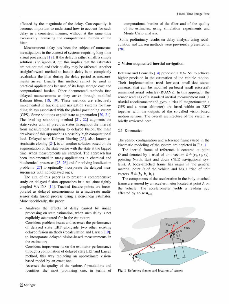
The sensor configuration and reference frames used in the

kinematic modeling of the system are depicted in Fig. 1.

The inertial frame of reference is centered at point

O and denoted by a triad of unit vectors E ¼: ðe1; e2; e3Þ;pointing North, East and down (NED navigational sys-

tem). A body-attached frame has origin in the generic

material point B of the vehicle and has a triad of unit

vectors B¼: ðb1; b2; b3Þ:The components of the acceleration in the body-attached

frame are sensed by an accelerometer located at point A on

the vehicle. The accelerometer yields a reading aacc

affected by noise nacc:

Fig. 1 Reference frames and location of sensors


123

aacc ¼ gB � aBA þ nacc: ð1Þ

In this expression, gB indicates the body-attached com-

ponents of the acceleration of gravity, where gB ¼ RT gE

with gE ¼ ð0; 0; gÞT ; while R ¼ RðqÞ are the components

of the rotation tensor that brings triad E into triad B and q

are rotation parameters.

Gyroscopes measure the body-attached components of

the angular velocity vector, yielding a reading xgyro

affected by a noise disturbance ngyro:

xgyro ¼ xB þ ngyro: ð2Þ

The kinematic equations, describing the motion of the

body-attached reference frame with respect to the inertial

one, can be written as

_vE ¼ gE � Rðaacc þ xB � xB � rBBA þ aB � rBBAÞ þ Rnacc;

ð3aÞ

_xB ¼ ahðxgyro; ngyroÞ; ð3bÞ

_rE ¼ vE ; ð3cÞ

_q ¼ TðxBÞq; ð3dÞ

where v ¼ vB is the velocity of point B;x is the angular

velocity and a the angular acceleration, while rBA is the

position vector from point B to point A and r ¼ rOB is from

point O to point B. Finally, using quaternions for the

rotation parameterization, matrix T can be written as

TðxBÞ ¼ 1

2

0 �xBT

xB �xB�

� �: ð4Þ

Gyro measurements are used in Eq. (3b) for computing

an estimate of the angular acceleration. Since this implies a

differentiation of the gyro measurements, assuming a

constant (or slowly varying) bias over the differentiation

interval, knowledge of the bias becomes unnecessary.

Hence, the angular acceleration is computed as

aB ’ ahðxgyroÞ; ð5Þ

where ah is a discrete differentiation operator. The angular

acceleration at time tk is computed according to the

following three-point stencil formula based on a parabolic

interpolation

ahðtkÞ ¼ 3xgyroðtkÞ � 4xgyroðtk�1Þ þ xgyroðtk�2Þ� �

=ð2hÞ;ð6Þ

where h = tk - tk-1 = tk-1 - tk-2. It is assumed that gyro

outputs are available with a sufficiently high rate (e.g.,

400 Hz), relative to the frequency of the inertial navigation

system (e.g., 100 Hz), to avoid feeding the estimator with

correlated measurements.

A GPS is located at point G on the vehicle (see Fig. 1).

The velocity and position vectors of point G, noted

respectively vEG and rEOG; can be expressed as

vEG ¼ vE þ RxB � rBBG; ð7aÞ

rEOG ¼ rE þ RrBBG: ð7bÞ

The GPS yields measurements of the position and

velocity of point G affected by noise, i.e.,

vgps ¼ vEG þ nvgps; ð8aÞ

rgps ¼ rEOG þ nrgps: ð8bÞ

A sonar altimeter measures the distance h along the

body-attached vector b3; between its location at point S and

point T on the terrain (assumed to be flat), with rBOS ¼ð0; 0; sÞT : In the body-attached frame B; the distance vector

between S and T has components rBST ¼ ð0; 0; hÞT ; which

are readily transformed into inertial components as rEST ¼RrBST : Hence, we get

h ¼ r3=R33 � s; ð9Þ

where r3 ¼ rE � e3 and R ¼ ½Rij�; i; j ¼ 1; 2; 3: The sonar

altimeter yields a reading hsonar affected by noise nsonar; i.e.,

hsonar ¼ hþ nsonar: ð10Þ

Furthermore, we consider a magnetometer sensing the

magnetic field m of the Earth in the body-attached system

B; so that

mB ¼ RT mE ; ð11Þ

where the inertial components mE are assumed to be known

and constant in the area of operation of the vehicle. The

magnetometer yields a measurement mmagn affected by

noise nmagn; i.e.,

mmagn ¼ mB þ nmagn: ð12Þ

Finally, considering a pair of stereo cameras located on

the vehicle (see Fig. 2), a triad of unit vectors C¼: ðc1; c2; c3Þhas origin at the optical center C of the left camera, where c1

is directed along the horizontal scanlines of the image plane,

while c3 is parallel to the optical axis, pointing towards the

scene. The right camera has its optical axis and scanlines

parallel to those of the left camera, i.e., C0 � C;where we use

the symbol ðÞ0 to indicate quantities of the right camera.

Considering that P is a fixed point, the vision-based

observation model, discretized across two time instants tk-m

and tk ¼ tk�m þ Dt; is

dðtkÞCk ¼ �DtCT�RðtkÞT vEðtkÞ

þ xBðtkÞ � ðcB þ Cdðtk�mÞCk�mÞ�þ dðtk�mÞCk�m ;

ð13Þ


123

where m is the number of time samples between two

consecutive captured images. C are the components of the

rotation tensor that bring triad B into triad C: The tracked

feature point distances are noted dC ¼ ðd1; d2; d3ÞT for

the left camera, and are obtained by stereo reconstruction

using

dC ¼ b

dpC; ð14Þ

where p ¼ ðp1; p2; f ÞT is the position vector of the feature

point on the image plane, b is the stereo baseline and d ¼p1 � p1

0 the disparity. This process yields at each time step

tk an estimate dvsn affected by noise nvsn

dvsn ¼ dðtkÞCk þ nvsn: ð15Þ

An estimate of the accuracy can be derived by considering

the influence of the disparity measure error on the

computed feature position. For example, differentiating

the third component of Eq. (14) we get

dd3 ¼ �fb

x~d2d~d; ð16Þ

where we have set d ¼ ~dw; being ~d the disparity in pixel

units and w the pixel width. From this equation, it is clear

that the accuracy of a 3D measurement is directly affected

by disparity error. Furthermore, accuracy is adversely

affected by distance, as far points are associated with lower

disparity values.

The approximate observation model of Eq. (13) uses

(average) translational and rotational velocities during the

measurement acquisition time interval; this way, mea-

surements can be expressed directly via the current state of

the vehicle. Therefore, this approximate model can be

processed within a standard EKF.

2.2 Process model and observations

The estimator is based on the following state-space model

_xðtÞ ¼ f�xðtÞ; uðtÞ; mðtÞ

�ð17aÞ

yðtkÞ ¼ h�xðtkÞ

�ð17bÞ

zðtkÞ ¼ yðtkÞ þ lðtkÞ ð17cÞ

where the state vector x is defined as

x¼: ðvET

;xBT

; rET

; qTÞT : ð18Þ

Function fð�; �; �Þ in Eq. (17a) represents in compact form

the rigid body kinematics expressed by Eq. (3). The input

vector u appearing in Eq. (17a) is defined in terms of the

measurements provided by the accelerometers and gyros,

i.e., u ¼ ðaTacc;x

TgyroÞ

T ; and m is the associated measurement

noise vector.

Similarly, Eqs. (7), (9), (11) and (13) may be gathered

together and written in compact form as an observation

model hð�Þ expressed by Eq. (17b), where the vector of

outputs y is defined as

y ¼ ðvET

G ; rET

OG; h;mBT

; . . .; dCT

; . . .ÞT : ð19Þ

The definition of model (17) is complemented by the

vector of measurements z and associated noise l vectors

z¼: ðvTgps; r

Tgps; hsonar;m

Tmagn; . . .; dT

vsn; . . .ÞT ; ð20aÞ

l¼: ðnTvgps; nT

rgps; nsonar; n

Tmagn; . . .; nT

vsn; . . .ÞT : ð20bÞ

2.3 Classic state estimation using EKF

The state estimation problem expressed by Eqs. (17),

(18), (19) and (20) was solved using the EKF approach,

initially assuming that all measurements are available

with no delay. The EKF formulation is briefly reviewed

here using the time-discrete form of Eq. (17) and

assuming m and l to be white noise processes with

covariance q and u; respectively. The prediction stage of

states and observations is performed by using the non-

linear model equations,

x�k ¼ xk�1 þ f ðxk�1; uk�1; 0Þ Dt; ð21aÞ

yk ¼ h�x�k�; ð21bÞ

whereas a linear approximation is used for estimating the

error covariance and computing the Kalman gain matrices,

P�k ¼ Ak�1 Pk�1 Ak�1T þ Gk�1 Qk�1 Gk�1

T ; ð22aÞ

Kk ¼ P�k HkT ðHk P�k Hk

T þ UkÞ�1: ð22bÞ

Matrices Ak�1;Gk�1 and Hk are computed by linearizing

the non-linear model about the current estimate,

Fig. 2 Geometry for the derivation of the discrete vision-based

motion sensor


123

Ak�1 ¼ I þ Dtof

oxjxk�1

; Gk�1 ¼ Dtof

omjxk�1

; Hk ¼oh

oxjxk

:

ð23Þ

Finally, covariance updates and state estimates are

computed as

Pk ¼ I � KkHk

� �P�k ; ð24aÞ

xk ¼ x�k þ Kk zk � h�x�k�� : ð24bÞ

As the estimator operates at a rather high rate and hence

with small time increments, the unit norm quaternion

constraint was simply realized by renormalization at each

prediction–correction step.

2.4 Image processing and tracking

The idea of VA-INS is based on tracking scene points

between stereo images and across time steps, to express the

apparent motion of the tracked points in terms of the motion

of the vehicle. The vision system is designed as a multipur-

pose element providing a rather large number of tracked

features and a dense disparity map to support several tasks

including VA-INS, 3D mapping and obstacle avoidance.

The identification and matching of feature points are

begun with the acquisition of the images; then, strong corners

are extracted from the left image with the feature extractor of

the KLT tracker [29], and a dense disparity map is obtained.

Identified feature points are encoded using the BRIEF

descriptor [30]; subsequently, matches in a transformed

image are found by computing distances between descrip-

tors. According to [30], this descriptor is competitive with

algorithms like SURF in terms of recognition rate; although

it appears to be better for small rotations than for large ones, it

is much faster in terms of generation and matching.

A real-time implementation of the system was based on

an on-board PC-104 with a 1.6 GHz CPU and 512 Mb of

volatile memory, with the purpose of analyzing the per-

formance and computational effort of the feature tracking

process. Images were captured by a Point Grey Bumblebee

XB3 stereo vision camera, and resized images with a res-

olution of 640 9 480 were used for tracking 100 points

between frames. These tests indicated the presence of a 490

ms latency between the instant animage is captured and the

time the state estimator receives the required visual infor-

mation, as shown in Table 1, which reports the worst case

encountered in all experiments.

3 Delayed fusion in VA-INS

Simulation analyses, presented later, show that the half a

second delay of the system is significant enough not to be

neglected. In other words, directly feeding this delayed

vision-based measurements to the EKF estimator will

affect the quality of the estimates. Since the magnitude of

delays associated with the tracking system is rather high in

comparison to the delays of the other sensors, these are

assumed to be delay-free in this work to simplify the

problem. It is, however, clear that the same methodology

used here for treating vision-caused delays could be used

for addressing delays generated by other components of the

system.

The outputs of the vision-based motion sensors dvsnðsÞfrom a captured image at time s will only be available at

time k = s ? N, where N is the sample delay. Delayed

outputs are labeled d�vsnðkÞ: On the other hand, measure-

ments from other sensors are not affected by such a delay,

and are available at each sampling time. For the purpose of

handling multi-rate estimation and delay, observations are

here partitioned in two groups, one collecting multi-rate

non-delayed GPS, sonar and magnetometer readings

(labeled rt, for real-time), and the other collecting delayed

vision-based observations (labeled vsn, for vision):

zrt¼: ðvTgps; r

Tgps; hsonar;m

TmagnÞ

T ; ð25aÞ

zvsn�¼: ðd�Tvsnð1Þ; d�Tvsnð2Þ; . . .; d�TvsnðnÞÞ

T : ð25bÞ

The state estimation process is based on using a proper

EKF update for each group. The recalculation, Larsen [19]

and delayed state EKF [23] methods are surveyed here for

fusing delayed tracked points in the VA-INS structure as

they arrive. All methods are briefly reviewed in the

following.

3.1 Recalculation method

A straightforward estimate can be obtained simply by

recalculating the filter throughout the delay period. As the

vision-based measurements are not available in the time

interval between s to k, one may update states and

covariance using only non-delayed measurements in this

time interval. As soon as vision measurements originally

captured at time s are received with delay at time k, the

Table 1 Time cost of image processing tasks

Process task Computing time (ms)

Image acquisition 100

Resizing, rectification 40

Dense disparity mapping 150

Feature extraction 130

Feature description 50

Feature matching 20

TOTAL 490


123

estimation procedure begins from s by repeating the update

while incorporating both non-delayed measurements and

lagged vision-based measurements.

The computational burden of this implementation of the

filter in the VA-INS is critical, because of the need of

fusing a fairly large set of measurements. Therefore the

approach, although rigorous and straightforward, is not a

good candidate for the implementation on-board small-size

aerial vehicles.

3.2 Larsen method

Within the VA-INS approach, the successive tracked

points, their uncertainty and consequently the measurement

model will be unknown until images are completely pro-

cessed. Therefore, a method is needed that does not require

information about zvsn�k until new measurements arrive.

Larsen extended Alexander [18] approach, by comput-

ing an optimal gain by extrapolating lagged measurements

to the present ones [19]:

zvsnkðintÞ ¼ zvsn�

k þHvsn�

k xk �Hvsn�

s xs: ð26Þ

This way, a correction term is calculated based on Kalman

information, accounting for measurements delay and

giving

M� ¼YN�1

i¼0

I � Krtk�iH

rtk�i

� �Ak�i�1: ð27Þ

All updates to the Kalman gain and covariance due to the

lagged measurements are delayed in Larsen method and

take place as the delayed measurements arrive to the

estimator. When lagged measurements become available,

updates are performed in a simple and fast manner as

Kvsnk ¼ M�PsH

vsn�T

s Hvsn�

s PsHvsn�T

s þ Uvsn�

k

� ��1

; ð28aÞ

dPk ¼ �Kvsnk Hvsn�

s PsMT� ; ð28bÞ

dxk ¼ M�Kvsnk zvsn�

k �Hvsn�

s xs

� �: ð28cÞ

The method can be utilized for handling either constant

or time-varying delays.

3.2.1 Flow of EKF-Larsen processing

Figure 3 shows an overview of the measurement process-

ing procedures for the standard EKF and Larsen methods.

The image processing routines are started at time

s, tracking feature points in new scenes; however, there is

no available vision-based measurement until time

k = s ? N.

Meanwhile, the multi-rate real-time measurements

zrtsþi; 1 iN are fused through the EKF Eqs. (22, 24) as

they arrive, using Hrtsþi: This will produce the Kalman gain

Krtsþi; state estimates xI

sþi and covariance PIsþi: Imple-

menting Larsen approach requires only the state vector and

covariance error at time s to be stored and the correction

term Msþi� to be calculated during the delay period as

Msþi� ¼ I � Krt

sþiHrtsþi

� �Asþi�1Msþi�1

� : ð29Þ

At time k, when the vision-based measurements become

available, Larsen equations are used to incorporate delayed

quantities zvsn�k in the estimation procedure. The Kalman

gain Kvsnk is calculated using Eq. (28a). Finally, visual

measurement corrections dPk and dxk; obtained by

Eqs. (28b, c), are added to the covariance matrix and

state vector of real-time measurement updates PIk and xI

k; to

obtain new quantities PIIk and xII

k :

3.3 Delayed state kalman filtering

An alternative formulation to this problem is presented

here by developing a specific delayed state Kalman fil-

tering. In this approach, an augmented state vector pro-

vides the vehicle state at the time stereo images are

captured, and it is used at the time delayed visual mea-

surements are incorporated into the filter. The estimator is

then based on an augmented state vector, indicated with

the notation x; which extends the vehicle states with a

copy of lagged ones. In order to prepare the cloned filter,

the augmented state vector and augmented covariance

matrix are reset right after the capture of a new pair of

stereo images. At time step s, the augmented state vector

is given by

xs ¼ ðx v T

s ; x l T

s ÞT ; ð30Þ

where

x vs ¼:

xs ¼ ðvET ðtsÞ;xB

T ðtsÞ; rET ðtsÞ; qTðtsÞÞT ; ð31aÞ

Fig. 3 Flow of sequential EKF-Larsen processing


123

x ls¼: ðvET ðtsÞ;xB

T ðtsÞ; qTðtsÞÞT ; ð31bÞ

and the augmented covariance matrix is written as

Ps ¼P v

s P v;ls

P v;l T

s P ls

� �¼ D P v

s D T ; ð32Þ

D ¼I13

I6 06�7

04�9 I4

24

35; ð33Þ

where P v;ls is the cross-correlation between the current

vehicle state x vs and the lagged one x l

s ; and D maps the

covariance matrix to the corresponding augmented one at

the same time step.

During the propagation steps, between the time of image

capture s to the time of delayed visual measurement fusion

k = s ? N, the first part of the augmented state, x vs ; is

propagated forward by using new inertial measurements

and the process model given by Eqs. (21a) and (22a),

yielding xv�k and Pv�

k : However, x ls and P l

s ; which corre-

spond to the second part of the augmented state, are kept

frozen. Note that the cross-correlation term is evolved

throughout the latency period. After N steps of propaga-

tion, the augmented covariance matrix is given by

P�

k ¼Pv�

k AsjkP v;ls

P v;l T

s ATsjk P l

s

" #; ð34Þ

where Asjk ¼QN�1

i¼0 Ak�i�1:

As the visual measurements d�vsn arrive to the estimator late,

the visual output dðtsÞCs and the visual observation model are

rewritten according to the new augmented state vector,

dðtsÞCs ¼ hðxkÞ ¼ �DtCT�RðtsÞT vEðtsÞ

þ xBðtsÞ � ðcB þ Cdðts�mÞCs�mÞ�þ dðts�mÞCs�m :

ð35Þ

By linearizing the visual observation model about the

augmented state estimate, we have

Hvsn

k ¼oh

oxk

¼ Hvsnk Hvsn

s

� ; ð36Þ

where hvsnk is equal to zero, according to Eq. (35).

The Kalman update is computed as

S ¼ Hvsn

k P�

k HvsnT

k þ Uvsn

k ; ð37aÞ

Kk ¼ P�

k HvsnT

k S�1 ¼ KT

k KTs

� T: ð37bÞ

Finally, the current state of the vehicle is updated as

xvk ¼ xv�

k þ Kk zvsn�

k �Hvsns xl

s

� �; ð38aÞ

Pvk ¼ Pv�

k � Kk S KTk : ð38bÞ

The multi-rate real-time measurements zrtsþi; 1 iN

can be readily fused during the latency period as they

arrive, using Hrt

sþi: However, they must be fused with the

current vehicle state while the lagged state remains frozen.

A simple solution can be achieved through the use of the

Schmidt-Kalman filter [31], whose gain is given as

Krt

sþi ¼ M P�

sþi HrtT

sþi Srt�1

; ð39aÞ

M ¼ I13 013�10

010�13 010�10

� �; ð39bÞ

where M indicates which states are updated.

3.4 Delayed fusion in VA-INS via an exact model

In the previous section, the motion velocity was assumed to

be constant between steps, which is a simple and effective

solution for sufficiently high image acquisition rates. An

exact model that does not require such an hypothesis is

given by the following discretization across two time

instants tk-m and tk ¼ tk�m þ Dt:

dðtkÞCk ¼ �CT�RðtkÞTðrðtkÞ � rðtk�mÞÞ

þ ðI � RðtkÞT Rðtk�mÞÞðc þ Cdðtk�mÞCk�mÞ�

þ dðtk�mÞCk�m : ð40Þ

This expression represents the position of a feature point

w.r.t. the camera at time tk in terms of the position at time

tk-m through the partial vehicle states (position and attitude)

at times tk and tk-m.

The problem of implementing this exact model

in a standard estimator arises, since the Kalman filter for-

mulation requires measurements to be independent of

previous filter states. To address this problem, while pro-

viding a robust estimation framework, a combination of

delayed state Kalman filtering and Larsen method is pro-

posed in this work and noted in the following as DS-EKF-

Larsen. This way, by utilizing an augmented state vector

that includes the current and lagged states, the exact model

can be used, whereas delayed fusion is handled by Larsen

method. Considering Eq. (40), the state vector is aug-

mented with the lagged position and the lagged quaternion

at the time the last measurements were obtained, yielding

xk�m ¼ ðx v T

k�m; xl T

k�mÞT ; ð41aÞ

x vk�m ¼ ðvE

T ðtk�mÞ;xBT ðtk�mÞ; rE

T ðtk�mÞ; qTðtk�mÞÞT ;ð41bÞ

x lk�m¼

: ðrET ðtk�mÞ; qTðtk�mÞÞT : ð41cÞ

3.5 Time complexity

The measurement-update formulation of the standard EKF

method involves the inversion of the residual covariance


123

(innovation covariance) given by Eq. (22b), with an

approximately cubic complexity of O(Nz2.37), where Nz is

the dimension of the measurement vector. The computation

also requires a matrix multiplication (see Eq. 24a) of

O(Nx2), where Nx is the dimension of the state vector xv. In

the VA-INS implementation of the filter, the most com-

putationally expensive operation is the inversion of the

residual covariance due to the fact that Nz [ Nx, because of

the incorporation of a rather large set of vision-based

measurements.

In Larsen method, the computation of the correction

term is accumulated throughout the delay period and it is

applied at each update step using Eq. (28b). This way, the

required inversion and matrix multiplication have a similar

time complexity as in the EKF case. For the delayed state

EKF within VA-INS, an increased cost in comparison to

the EKF implementation is expected for the matrix multi-

plication, due to the increased state vector dimension,

which is Nx ¼ Nxv þ Nxl :

4 Simulation experiments

A Matlab/Simulink software environment was developed,

that includes a flight mechanics model of a small rotorcraft

unmanned aerial vehicle (RUAV), models of inertial nav-

igation sensors, magnetometer, GPS and their noise mod-

els. The simulator is used in conjunction with the OGRE

graphics engine [32], for rendering a virtual environment

scene and simulating the image acquisition process. All

sensor measurements are simulated (see Table 2) as the

helicopter flies in open loop at an altitude of 2 m following

a rectangular path at a constant speed of 2 m/s within a

small village, composed of houses and several other objects

with realistic textures (see Fig. 4).

Navigation measurements are provided at a rate of

100 Hz, while stereo images at the rate of 2 Hz. The GPS,

available at a rate of 1 Hz, is turned off after 10 s in the

flight, to further highlight the effects of visual measurement

delay. State estimates are obtained by six different data

fusion processes: classic EKF with non-delayed measure-

ments, classic EKF with delayed measurements, recalcu-

lation, EKF-Larsen, delayed state EKF and DS-EKF-

Larsen method in the presence of delay.

Figure 5a shows the effects of delay on the EKF esti-

mates, presenting a comparison of positions obtained by

classic EKF, fed with delayed and non-delayed visual

measurements. Figure 5b and c presents position estimates

obtained by the two methods of EKF-Larsen and delayed

state EKF, respectively, in the presence of delayed visual

measurements, in comparison with the recalculation

method (with delay). Finally, Fig. 5d presents position

estimates obtained by processing the exact vision-based

model through the proposed DS-EKF-Larsen method, in

the presence of delayed visual measurements.

Results clearly show the negative effects of delay on the

standard EKF estimation, which are compensated with the

recalculation, the sequential filtering EKF-Larsen and also

with the delayed state EKF. Moreover, the DS-EKF-Larsen

method appears to provide for enhanced estimates, due to

the optimal incorporation of an exact model.

4.1 Monte Carlo simulation

A Monte Carlo simulation is used here for considering the

effects of random variation on the performance of the

approaches, as well as evaluating the computational time

burden of each method. The analysis consisted of 100 runs,

which is the number of simulations that were necessary in

this case to bring the statistics to convergence (in the sense

that adding additional simulations did not change the

results). For each simulation run, measurements and stereo

images are generated for the 100 s maneuver described

above, each with randomly generated errors due to noise

and random walks.

The average error in the position, velocity and attitude

estimates is shown in Figs. 6, 7 and 8, using the six

implementations of the vision-augmented data fusion pro-

cedures explained above. The ratios of the average com-

putational effort of the Kalman update by different

approaches to the standard one are depicted in Fig. 9, while

the average estimation errors for each approach are

reported in Fig. 10.

Table 2 Sensors and vibration noise parameters

Sensors Noise variance (r2)

Gyro 50 (�/s)2

Accelerometer 0.5 (m/s2)2

Magnetometer 1 9 10-4 Gauss2

Altimeter 0.5 m2

GPS 2 m2

Fig. 4 View of simulated village environment and flight trajectory


123

The EKF-Larsen and the delayed state EKF methods

show a good performance, as does the recalculation

approach. In fact, the average errors of these methods are

very close to the one obtained by the classic EKF with no

delay on the visual measurements. However, the processing

time of the filter recalculation increases twofold, as shown

Fig. 5 Comparison of position estimates in the x - y plane. a EKF

with (dark line) and without (light line) delay on visual measure-

ments; b EKF-Larsen method and recalculation in the presence of

delay; c delayed state EKF and recalculation in the presence of delay;

d DS-EKF-Larsen and EKF-Larsen in the presence of delay


123

by Fig. 9, implying a considerable additional computa-

tional burden. On the other hand, the EKF-Larsen

approach does not affect the processing time of updating

the filter, and therefore conjugates high quality estimation

and low computing effort. The processing time of the

delayed state EKF is a little bit higher than the one of the

EKF-Larsen approach, however, it is significantly less

than the one required by the recalculation method. This

additional computational burden is an expected effect of

augmenting the state vector and covariance matrix.

Finally, DS-EKF-Larsen provides better estimates, par-

ticularly for positions, in comparison to the EKF-Larsen

and delayed state EKF, but with additional complexity

and a computational cost comparable to the delayed state

EKF method. The formulations of EKF-Larsen and

delayed state EKF could be also utilized for addressing

delays generated by other sensors; however, the compu-

tational burden of the delayed state EKF method might

rise considerably due to the required additional state

augmentation at several lagged steps.

Figures 11, 12 and 13 report the average error in the

position, velocity and quaternion estimates, together with

the corresponding confidence bounds. The plots compare

EKF-Larsen and delayed state EKF in the presence of

delay with the standard EKF, fed with delayed and non-

Fig. 6 Position estimate errors in the x (thin line), y (thick line) and

z (dashed line) directions

Fig. 7 Velocity estimate errors in the x (thin line), y (thick line) and

z (dashed line) directions

Fig. 8 Attitude estimate errors; yaw error (thin line), roll error (thick

line) and pitch error (dashed line)


123

delayed visual measurements. As clearly shown in the

figures, by feeding delayed visual measurements into the

standard EKF, there is no guarantee that the errors will

remain within the filter confidence bounds. On the other

hand, the EKF-Larsen, delayed state EKF and DS-EKF-

Larsen methods perform well in the presence of delayed

visual measurements, and exhibit the same confidence

bounds obtained by using a standard EKF with non-delayed

visual measurements.

Figure 14a–c reports a comparison of the average error

among the recalculation method, which provides a refer-

ence optimal solution, and the other methods. Results show

a similar but not identical performance of the various

methods, with rather small differences.

Fig. 9 Ratios of the average time cost of different approaches to the

average time cost of the EKF-based implementation of VA-INS

Fig. 10 Average errors of velocity, position and angle estimates

Fig. 11 Position estimate error in x direction (dashed dark line) and

confidence bounds (solid line)


123

5 Conclusions

In this work, a previously documented VA-INS was

extended by implementing various approaches to handle

feature tracking delays in a multi-rate multi-sensor data

fusion process. Simulation experiments were used together

with Monte Carlo analyses to assess the estimation error

and the computational burden of the methods.

Fig. 14 Performance of EKF-Larsen and delayed state EKF in comparison to the recalculation method, assumed as an optimal reference solution

in the presence of delay and an approximate model

Fig. 12 Velocity estimate error in the x direction (dashed dark line)

and confidence bounds (solid line)

Fig. 13 Normalized quaternion estimate error (dashed dark line) and

confidence bounds (solid line)


123

The paper shows that delay caused by image processing,

if not properly handled in the state estimator, can lead to an

appreciable performance degradation. Furthermore,

sequential EKF-Larsen, delayed state EKF as well as the

recalculation method restore the estimate accuracy in the

presence of delay. On the other hand, the results of the

paper indicate that the recalculation approach implies a

significant computational burden, while Larsen method is

as expensive as the standard EKF. The delayed state EKF

has a slightly higher computational cost than Larsen

method, but a significantly lower one than the recalculation

method.

This study concluded that Larsen method, for the pres-

ent application, provides estimates that have the same

quality and computational cost of the non-delayed case.

The delayed state EKF can also be a reliable solution,

specifically if a few percent increase in computational

burden is tolerable.

Moreover, a novel combined implementation of delayed

state EKF and Larsen methods enhances the estimation

accuracy through an optimal fusion by using an exact

vision-based model in the presence of delay. DS-EKF-

Larsen provides better estimates in comparison to the EKF-

Larsen and delayed state EKF, but with additional com-

plexity and a computational cost comparable to the delayed

state EKF method.

References

1. Bonin-Fontand, F., Ortiz, A., Oliver G.: Visual navigation for

mobile robots: a survey. J. Intell. Rob. Syst. 53(3), 263–296

(2008)

2. Dalgleish, F.R., Tetlow, J.W., Allwood, R.L.: Vision-based

navigation of unmanned underwater vehicles : a survey. part 2:

Vision-based station-keeping and positioning. In: IMAREST

Proceedings, Part B: Journal of Marine Design and Operations,

vol. 8, pp. 13–19 (2005)

3. Liu, Y.C., Dai, Q.H.: Vision aided unmanned aerial vehicle

autonomy : an overview. In: Image and signal processing, 3th

International Congress on, pp. 417–421 (2010)

4. Taylor, C.N.: Enabling navigation of mavs through inertial,

vision, and air pressure sensor fusion. In: Hahn, H., Ko, H., Lee,

S. (eds.) Multisensor fusion and integration for intelligent sys-

tems, lecture notes in electrical engineering, vol. 35, pp. 143–158

(2009)

5. Chun, L., Fagen, Z., Yiwei, S., Kaichang, D., Zhaoqin, L.: Stereo-

image matching using a speeded up robust feature algorithm in an

integrated vision navigation system. J. Navig. 65, 671–692 (2012)

doi:10.1017/S0373463312000264

6. Nister, D., Naroditsky, O., Bergen, J.: Visual odometry for

ground vehicle applications. J. Field. Rob. 23(1), 3–20 (2006)

7. Goedeme, T., Nuttin, M., Tuytelaars, T., Gool, L.V.: Omnidi-

rectional vision based topological navigation. Int. J. Comput.

Vision. 74(3), 219–236 (2007)

8. Roumeliotis, S.I., Johnson, A.E., Montgomery, J.F.: Augmenting

inertial navigation with image-based motion estimation. In:

Robotics and automation, IEEE International Conference on,

pp. 4326–4333 (2002)

9. Qian, G., Chellappa, R., Zheng, Q.: Robust structure from motion

estimation using inertial data. J. Opt. Soc. Am. 18(12), 2982–2997

(2001)

10. Veth, M.J., Raquet, J.F., Pachter, M.: Stochastic constraints for

efficient image correspondence search. J. IEEE. Trans. Aerosp.

Electron. Syst. 42(3), 973–982 (2006)

11. Mourikis, A.I., Roumeliotis, S.I.: A multi-state constraint Kalman

filter for vision-aided inertial navigation. In: Robotics and automa-

tion, IEEE International Conference on, pp. 3565–3572 (2007)

12. Corato, F., Innocenti, M., Pollini, L.: Robust vision-aided inertial nav-

igation algorithm via entropy-like relative pose estimation. Gyrosco.

Navig. 4(1), 1–13 (2013). doi:10.1134/S2075108713010033

13. Tardif, J.P., George, M., Laverne, M., Kelly, A., Stentz, A.: A

new approach to vision-aided inertial navigation. In: Intelligent

robots and systems (IROS), IEEE/RSJ International Conference

on, pp. 4161–4168 (2010). doi:10.1109/IROS.2010.5651059

14. Bottasso, C.L., Leonello, D.: Vision-augmented inertial naviga-

tion by sensor fusion for an autonomous rotorcraft vehicle. In:

Unmanned Rotorcraft, AHS International Specialists Meeting on,

pp. 324–334 (2009)

15. Jones, E.S., Soatto, S.: Visual-inertial navigation, mapping and

localization: a scalable real-time causal approach. Int. J. Robot.

Res. 30(4), 407–430 (2011)

16. Ferreira, F.J., Lobo, J., Dias, J.: Bayesian real-time perception

algorithms on GPU–real-time implementation of Bayesian mod-

els for multimodal perception using CUDA. J. Real-Time. Image

Proc. 6(3), 171–186 (2011)

17. Pornsarayouth, S., Wongsaisuwan, M.: Sensor fusion of delay

and non-delay signal using Kalman filter with moving covari-

ance. In: Robotics and biomimetics, IEEE International Confer-

ence on, pp. 2045–2049 (2009)

18. Alexander, H.L.: State estimation for distributed systems with

sensing delay. pp. 103–111 (1991) SPIE . doi:10.1117/12.44843

19. Larsen, T.D., Andersen, N.A., Ravn, O., Poulsen, N.: Incorpo-

ration of time delayed measurements in a discrete-time Kalman

filter. In: Decision and Control, 37th IEEE Conference on,

pp. 3972–3977 (1998)

20. Challa, S., Legg, J.A., Wang, X.: Track-to-track fusion of out-of-

sequence tracks. In: Information Fusion, 2002. Fifth International

Conference on, vol. 2, pp. 919–926 (2002)

21. Bar-Shalom, Y., Li, X.R.: Multitarget-MultisensorTracking:

principles and Techniques. YBS Publishing (1995)

22. Challa, S., Evans, R.J., Wang, X., Legg, J.: A fixed-lag smoothing

solution to out-of-sequence information fusion problems. Com-

mun. Inform. Syst. 2(4), 325–348 (2002)

23. Van Der Merwe, R.: Sigma-point kalman filters for probabilistic

inference in dynamic state-space models. In: Ph.D Thesis, OGI

School of Science and Engineering, Oregon Health and Science

University (2004)

24. Roumeliotis, S., Burdick, J.: Stochastic cloning: a generalized

framework for processing relative state measurements. In:

Robotics and Automation, IEEE International Conference on,

vol. 2, pp. 1788–1795 (2002)

25. Gopalakrishnan, A., Kaisare, N., Narasimhan, S.: Incorporating

delayed and infrequent measurements in extended Kalman filter

based nonlinear state estimation. J. Proc. Control. 21(1),119–129

(2011)

26. Tatiraju, S., Soroush, S., Ogunnaike, B.A.: Multirate nonlinear

state estimation with application to a polymerization reactor.

AIChE J 45(4), 769–780 (1999)

27. Stanway, M.J.: Delayed-state sigma point Kalman filters for

underwater navigation. In: Autonomous Underwater Vehicles,

IEEE/OES Conference on, pp. 1–9 (2010)

28. Asadi, E., Bottasso, C.L.: Handling delayed fusion in vision-aug-

mented inertial navigation. In: Informatics in Control, Automation

and Robotics, 9th International Conference on, pp. 394–401 (2012)


123

http://dx.doi.org/10.1017/S0373463312000264

http://dx.doi.org/10.1134/S2075108713010033

http://dx.doi.org/10.1109/IROS.2010.5651059

http://dx.doi.org/10.1117/12.44843

29. Jianbo, S., Tomasi, C.: Good features to track. In: Computer

Vision and Pattern Recognition, IEEE Computer Society Con-

ference on, pp. 593–600 (1994)

30. Calonder, M., Lepetit, V., Strecha, C., Fua, P.: Brief: Binary

robust independent elementary features. In: Computer Vision,

11th European Conference on, vol. 6314(3), pp. 778–792. LNCS

Springer (2010)

31. Schmidt, S.F.: Applications of state space methods to navigation

problems, C. T. Leondes, advanced control systems edn. Aca-

demic Press, New York (1996)

32. Junker, G.: Pro OGRE 3D Programming. Springer-Verlag, New

York (2006)

Author Biographies

Ehsan Asadi received the B.Sc. degree from Kashan University,

Kashan, Iran, in 2002, and the M.Sc. degree from Yazd University,

Yazd, Iran, in 2005, both in Mechanical Engineering. Currently, he is

a Ph.D student in Aerospace Engineering at Politecnico di Milano,

Milan, Italy, where he works with POLI-Rotorcraft researchgroup.

His current research interests include sensor fusion, Kalman filter-

ing,vision-aided inertial navigation, and simultaneous localization

and mapping (SLAM).

Carlo L. Bottasso received a Ph.D degree in Aerospace Engineering

from the Politecnico di Milano, Italy, in 1993. Currently, he is the

Chair of Wind Energy at TUM, Technische Universitat Munchen,

Germany, and Professor of Flight Mechanics with the Department of

Aerospace Science and Technology, Politecnico di Milano, Italy. He

has held visiting positions at various institutions, including Rensselaer

Polytechnic Institute, Georgia Institute ofTechnology, Lawrence

Livermore National Laboratory, NASA Langley, and NREL amongo-

thers. His research interests and areas of expertise include the flight

mechanics and aeroelasticity of rotorcraft vehicles, aeroelasticity and

active control of windturbines, and flexible multibody dynamics.


123

Delayed Fusion for Real-Time Vision-Aided Inertial Navigation

Documents

Transcript of Delayed Fusion for Real-Time Vision-Aided Inertial Navigation