A novel inertial-aided visible light positioning system using ...

A novel inertial-aided visible light positioning

system using modulated LEDs and unmodulated

lights as landmarks

Qing Liang1, Member, IEEE, Yuxiang Sun2, Member, IEEE, Lujia Wang1, Member, IEEE, and Ming Liu1, Senior

Member, IEEE

Abstract—Indoor localization with high accuracy and efficiencyhas attracted much attention. Due to visible light communication(VLC), the LED lights in buildings, once modulated, hold greatpotential to be ubiquitous indoor localization infrastructure.However, this entails retrofitting the lighting system and is hencecostly in wide adoption. To alleviate this problem, we proposeto exploit modulated LEDs and existing unmodulated lights aslandmarks. On this basis, we present a novel inertial-aided visiblelight positioning (VLP) system for lightweight indoor localizationon resource-constrained platforms, such as service robots andmobile devices. With blob detection, tracking, and VLC decodingon rolling-shutter camera images, a visual frontend extractstwo types of blob features, i.e., mapped landmarks (MLs) andopportunistic features (OFs). These are tightly fused with inertialmeasurements in a stochastic cloning sliding-window extendedKalman filter (EKF) for localization. We evaluate the systemby extensive experiments. The results show that it can providelightweight, accurate, and robust global pose estimates in real-time. Compared with our previous ML-only inertial-aided VLPsolution, the proposed system has superior performance in termsof positional accuracy and robustness under challenging lightconfigurations like sparse ML/OF distribution.

Note to Practitioners—This paper is motivated by the problemthat many existing visible light positioning (VLP) systems requirehigh cost environmental modifications, i.e., replacing a large por-tion of original lights with modulated LEDs as beacons. To reducecosts in wide adoption, we seek to use fewer modulated LEDsif possible. Accordingly, we present a novel inertial-aided VLPsystem that uses both modulated LEDs and unmodulated lights aslandmarks. Like in other VLP systems, the successfully decodedLEDs provide absolute pose measurements for global localization.Unmodulated lights and the LEDs with decoding failures providerelative motion constraints, allowing the reduction of pose driftduring the outage of modulated LEDs. Owing to the tightlycoupled sensor fusion by filtering, the system can provide efficientand accurate localization when modulated LEDs are sparse. Thesystem is lightweight to run on resource-constrained platforms.For practical deployment of our system at scale, creating LEDmaps accurately and efficiently remains a problem. It is desiredto develop automated LED mapping solutions in future work.

*This work was supported by the National Natural Science Foundation ofChina, under grant No. U1713211, Zhongshan Municipal Science and Tech-nology Bureau Fund, under project ZSST21EG06, Collaborative ResearchFund by Research Grants Council Hong Kong, under Project No. C4063-18G,and Department of Science and Technology of Guangdong Province Fund,under Project No. GDST20EG54, awarded to Prof. Ming Liu (Corresponding

author: Ming Liu).1Qing Liang, Lujia Wang and Ming Liu are with the Department of

Electronic and Computer Engineering, The Hong Kong University of Scienceand Technology, Hong Kong (email: qliangah,eewanglj,[email protected]).

2Yuxiang Sun is with the Department of Mechanical Engineering, TheHong Kong Polytechnic University, Hung Hom, Hong Kong (e-mail:[email protected], [email protected]).

Index Terms—Indoor localization, sensor fusion, visible lightpositioning, visible light communication, extended Kalman filter,aided inertial navigation, service robots.

I. INTRODUCTION

LOCALIZATION is fundamental to many robot tasks (e.g.,

path-planning, navigation, and manipulation) and a wide

variety of location-based services like augmented reality and

pedestrian navigation in large venues. Platforms like service

robots and mobile devices can have low-end sensors on board

and limited processing capabilities in computation, memory,

and power. To aid long-term operation, both the localization

accuracy and efficiency count. Among established sensors,

the camera and micro-electro-mechanical inertial measurement

unit (MEMS IMU) provide rich information for metric state

estimation while being small, low-cost, and power-efficient

[1]. There are many developed visual-inertial odometry (VIO)

algorithms [2]–[7] capable of real-time accurate six-degrees-

of-freedom (DoF) pose estimation. Some are lightweight to

run on mobile devices, as revealed by ARKit [8] and ARCore

[9]. However, VIO suffers from unbounded drift over time [1].

Global pose corrections are needed for long-term operation.

When people or robots localize in frequently-visited scenes

(e.g., shopping malls), prior knowledge from prebuilt maps

or localization infrastructure like Global Positioning System

(GPS) can assist. Visual (-inertial) localization against visual

feature maps has attracted wide research interest [10]–[14],

and state-of-the-arts achieve high accuracy and efficiency. Still,

the performance could suffer from dynamic changes in the

environment [15]–[17] in the short-term (e.g., moving objects)

or long-term (e.g., appearance or lighting). Visual (-inertial)

localization in 3D light detection and ranging (LiDAR) maps

is another promising solution [18], [19]. Yet, dealing with

LiDAR maps requires high onboard computation and memory,

hindering their use on resource-constrained platforms. Com-

bined with local odometry, the absolute GPS measurements are

often effective for outdoor localization [20]–[25]. These meth-

ods can show good accuracy and efficiency. Note the GPS-like

infrastructure provides known data associations [26], quick

and reliable, by using domain-specific knowledge from radio

communications or visual coding patterns [27]. This eases the

state estimation problem, enables instant relocalization, and

promotes processing efficiency.

With the growing adoption of LED lights in buildings for

energy-efficient lighting, LEDs hold great potential to become

a kind of indoor GPS owing to visible light communication

(VLC) technologies [28]–[30]. Normally, LEDs are densely

and uniformly spaced on ceilings for illumination. As solid-

state devices, LEDs can be instantly modulated to transmit

data by visible light. The high-frequency light changes are

invisible to human eyes but are perceivable by photodiodes

or cameras. Modulated LEDs broadcast their unique identities

by VLC, allowing quick and reliable data association. They

play the dual role of lighting and localization beacons. The

LED locations are fixed and less vulnerable to environmental

changes. The LED map hence remains effective for long-term

localization after one-time registration. Modulated LEDs of

known locations enable high-accuracy 3D localization due to

the line-of-sight light propagation [31]–[33]. This is broadly

known as visible light positioning (VLP) in the literature.

Many low-cost cameras with rolling shutters can seamlessly

act as VLC receivers [33]–[35]. It is trivial to compute the

camera pose by perspective-n-point (PnP) if more than three

LED features are detected in one camera frame. Such vision-

only methods [32], [33] can suffer in reality due to insufficient

LED observations. The number of decodable LEDs in a frame

is limited by a few factors such as the geometry layout and

density of lights, the ceiling height, the camera’s field of view

(FoV), and the maximum VLC decoding distance. To tackle

this issue, some recent works [36]–[38] have adopted IMU

measurements as a complement. In our previous work [38], we

presented an integrated VLC-inertial localization system using

an extended Kalman filter (EKF). In situations in which there

is a lack of LEDs, this system can provide satisfying results

by tightly fusing LED features and inertial measurements.

As in [38], we aim to perform localization with a minimal

visual-inertial sensor suite, commonly used for monocular VIO

[7]. We focus on using ceiling lights as landmarks to develop

a lightweight localization system for indoor applications. Be

noticed that the benefits of having known data associations by

VLC require the cost of artificial modifications, e.g., upgrading

existing lights with modulated LEDs. To reduce costs for

large-scale applications, we seek to rely on as few modulated

LEDs as possible. In our case, the camera is mainly used as a

VLC receiver, which requires a very short exposure time for

operation [35]. As such, naturally occurring visual features are

hardly detectable. Meanwhile, the regular unmodulated lights

existing in buildings, despite being less rich or informative

than natural features, can be readily detected. The derived blob

features add certain visual cues for relative pose estimation,

and in this way constrain pose drift in the absence of modu-

lated LEDs. In light of this, we propose to make full use of

the blob features detectable from lights, both modulated and

unmodulated, by our underexposed camera.

In this paper, with modulated LEDs and unmodulated lights

as landmarks in buildings, we propose a novel inertial-aided

VLP system using a rolling-shutter camera for lightweight

global localization on resource-constrained platforms. From

observations of lights, we extract two types of blob features:

mapped landmarks (MLs) and opportunistic features (OFs).

The former has associated global 3D positions while the

latter does not. Specifically, MLs correspond to modulated

LEDs registered in a prior map1 and successfully decoded

during runtime. We can explicitly resolve the long-term data

associations by VLC and know from the map the associated

global positions. MLs provide absolute geometric constraints

to correct any accumulated pose errors in the long run. They

are essential to our proposed system as well as to many

other VLP systems [31]–[33]. OFs, on the other hand, come

mainly from the unmodulated lights and in part from those

modulated LEDs with decoding failures. We can resolve only

the short-term data associations by temporal feature tracking.

This way, OFs provide relative motion constraints to help

reduce pose drift during ML outages, thereby benefiting the

overall localization. OFs are sometimes optional to our system

depending on the ML outage situations. The blob features are

tightly integrated with inertial measurements by a stochastic

cloning sliding window EKF [2] for pose estimation. To the

best of our knowledge, the approach we propose is the first

inertial-aided VLP system that fully exploits modulated LEDs

and unmodulated lights as landmarks within a sliding window

filter-based framework. This gives us the flexibility to replace a

proportion of the original lights (e.g., at strategic locations like

entrances) and not all as in conventional VLP systems, while

achieving comparable localization performance with much-

reduced cost. We restrict the contributions of this work to the

context of VLP and highlight them as follows:

• A novel inertial-aided VLP system for lightweight in-

door localization that fully exploits modulated LEDs and

unmodulated lights as landmarks. The sensor measure-

ments (MLs, OFs, and inertial) are tightly fused within a

stochastic cloning sliding-window EKF framework. It is

capable of performance comparable to conventional VLP

systems at minimal infrastructure cost.

• A blob tracking-assisted decoding strategy for rolling-

shutter VLC mechanisms in VLP use case. Blob tracking

improves the decoding success during camera motion

with the introduced short-term data association.

• Design choices of using delayed ML measurements from

blob tracking and using unmodulated lights as OFs to

provide motion constraints for VLP.

• Extensive system evaluation by real-world experiments

in various scenarios showing the effectiveness and per-

formance gains of our system. It has achieved superior

positional accuracy and robustness under challenging

light conditions (e.g., very sparse ML/OF distribution)

when compared to an ML-only VLP solution [38].

The remainder of this paper is organized as follows. Section

II introduces the related work. Section III shows the overview

of the proposed system. Section IV and Section V describes

key components of the system, including an image processing

frontend and an EKF-based pose estimator. Section VI and

Section VII presents experimental results and discussions of

limitations, respectively. Section VIII concludes this paper.

The acronyms throughout this paper can be found in Table. I.

1Solving a localization problem, we assume that all modulated LEDs forMLs have been preregistered on an LED feature map before operation.

TABLE I: List of acronyms.

AGC automatic gain control OF opportunistic feature

ATE absolute trajectory error OOK on-off keying

DoF degrees of freedom PID permanent identity

EKF extended Kalman filter PnP perspective-n-point

FoV field of view RANSAC random sample consensus

GPS Global Positioning System RMSE root mean squared error

IMU inertial measurement unit ROI region of interest

LiDAR light detection and ranging SCKFstochastic cloning

Kalman filter

MEMSmicro-electro-mechanical

systemsTID temporal identity

ML mapped landmark VIO visual-inertial odometry

MOSFETmetal-oxide-semiconductor

field-effect transistorVLC

visible light

communication

MSCKFmulti-state constraint

Kalman filterVLP visible light positioning

II. RELATED WORK

There is a rich body of literature on indoor localization. For

fundamentals and comprehensive surveys, readers can refer

to [28]–[30], [39]–[46]. In this section, we only review those

closely related to our proposed system, e.g., indoor localization

using lights as landmarks in Section II-A and visual-inertial

localization with global measurements in Section II-B.

A. Indoor Localization using Lights as Landmarks

Much research effort has been put into indoor localization

using lights, including both modulated LEDs and unmodulated

light sources, as environmental features.

1) Modulated LEDs: VLP takes advantage of known data

associations conveyed by VLC. Often, VLP systems employ

modulated LEDs as location beacons, use cameras [32], [33],

[47]–[49] or photodiodes [31], [50], [51] as light sensors,

recognize each beacon using its unique identity from VLC

decoding, measure bearings or ranges to visible beacons, and

determine the sensor location from geometry measurements.

Photodiode-based VLP systems require accurate propagation

channel modeling and can be less accurate or robust than their

camera-based counterparts. For camera-based systems, vision-

only methods like PnP need three or more LED features to fix

a 6-DoF pose. Their use is limited in the case of insufficient

LEDs. In such cases, fusion of inertial measurements assists, in

loosely- [31], [36] or tightly- [37], [38] coupled ways. These

systems heavily rely on modulated LEDs for operation and

hence incur extensive modifications of lighting infrastructure.

To alleviate this issue, researchers have attempted to reuse

existing light sources without modification.

2) Unmodulated lights: Compared to modulated LEDs, the

lack of communications adds to the challenge of obtaining data

associations for unmodulated lights. These lights can relate to

certain feature descriptions for data association. LiTell [52]

is a camera-based localization system that uses unmodulated

fluorescent lights. It exploits the characteristic frequency (CF),

which is diverse among lights due to manufacturing tolerances,

from the light spectrum as a unique identifier. CF features

are extracted from high-resolution images of raw format and

matched to a built feature map for light identification. Using a

customized photodiode receiver, the follow-up Pulsar [53] can

work from LEDs whose CF features are much weaker. How-

ever, due to temperature fluctuation, grid voltage variation, and

aging, such features tend to be less reliable over time [52].

iLAMP [54] exploits the spatial radiance patterns extracted

from light images of raw format as feature descriptors, owing

to the diversity from manufacturing variations. As reported

by [52], [54], the feature extraction and matching therein

are computationally demanding, partly due to processing raw

images. This can cause high latencies in location updates (e.g.,

a few hundred ms) and differs from our goal of developing a

lightweight system for resource-constrained platforms.

Methods also exist which do not identify individual lights

explicitly. In [55], [56], lights are characterized by physical

locations without any feature description. The overhead lights

can be detected using photodiode sensors on smartphones

and by finding peaks in received light signals while people

are walking by. To handle inherent identity ambiguities, the

authors resorted to using a particle filter for solving 2D sensor

poses and the latent data association. Due to the lack of

explicit data associations, [55], [56] cannot provide instant

relocalization as other VLP systems do.

3) Both types: Our goal is to keep the benefits of modulated

LEDs for lightweight localization on resource-constrained

devices while minimizing the retrofit cost for environment

modification. This motivates us to make full use of both

modulated and unmodulated lights. In literature, the closest

work to ours in concept is [57]. The authors use an upward-

facing fisheye camera for 2D localization by observing ceiling

lights of known locations. Two modulated LEDs are added

for instant pose initialization. To obtain correspondences for

other lights, a set of light blobs are detected and matched to

the ceiling light map. Here, we focus on 6-DoF localization

with a common pinhole camera. Orthogonal to others, we

treat unmodulated lights as opportunistic features without

knowing their absolute locations. They instead provide relative

motion constraints to help reduce pose drift when modulated

LEDs are unavailable. We note the camera adopted by [57]

can sample specific pixels at high speed (with a period of

20.8 µs) while being costly. VLC is realized by analyzing

a temporal sequence of light intensities that are recorded at

specified pixels over time. By contrast, our rolling-shutter VLC

mechanism is compatible with a wide range of inexpensive

cameras on the market, such as smartphone cameras.

B. Visual-inertial Localization with Global Measurements

Map-based visual-inertial localization is an active research

topic. Many [10]–[14] exploit visual feature-based maps where

3D landmarks are associated with image feature descriptors.

The initial camera pose can be computed from 2D-3D matches

between newly detected features and mapped landmarks. Next,

accurate drift-free visual-inertial pose tracking can be done

with subsequent map constraints. For example, [10] shows

impressive efficiency and accuracy on mobile devices. How-

ever, such methods are likely to face robustness problems due

to appearance changes, e.g., from illumination and weather.

To alleviate such difficulties, recent works [18], [19] prefer

using 3D LiDAR maps, which can provide accurate and stable

representations of the environment’s geometric information.

However, they need external pose guesses as input at system

startup. In addition, real-time processing of LiDAR maps can

cause considerable computational and memory burdens [18].

Many studies resort to artificial global pose measurements.

In outdoor applications, GPS is being widely used to offer

absolute position and Doppler velocity measurements relative

to Earth. The fusion of VIO and GPS measurements can be

performed in filtering- [20], [21] or graph optimization-based

[22]–[24] frameworks. Compared to map-based solutions, such

methods can provide satisfactory positioning accuracy and

better computational efficiency. They are hence more suitable

to run on resource-constrained platforms.

In this work, instead of using visual- or LiDAR-based map

constraints, we utilize modulated LEDs as a kind of indoor

GPS infrastructure to provide absolute pose measurements in

a lightweight manner. Here VLC enables fast and reliable data

association similar to GPS ranging messages. Also, different

from traditional VLP systems, we exploit both modulated and

unmodulated lights as location landmarks, thereby minimizing

the additional infrastructure cost. We note that natural features

are unusable here since our camera is heavily underexposed.

III. SYSTEM OVERVIEW

Lighting infrastructure on building ceilings

MOSFET Driver

LED

Microcontroller

Unmodulated Lights

Modulated LEDs

ID-encoded Patterns

...

(a) Illustration of the lighting infrastructure for localization.

Blob Detection

VLC Decoding

Update

Blob Tracking

200Hz

10Hz

Augmentation

RS-Camera

IMU

Propagation

6DoF Pose

MLs OFs

LED Map

Sliding -window EKF

Image Processing

No Sync

10Hz

(b) Block diagram showing the workflow of our proposed method.

Fig. 1: Overall architecture of the proposed localization system.

The proposed system relies on ceiling lights in buildings for

localization, as illustrated in Fig. 1a. Specifically, we replace a

proportion of them with modulated LEDs as location beacons.

The modulated LEDs broadcast unique identity codes through

VLC. We adopt the exact VLC protocol as in our previous

work [38], which runs on-off keying (OOK) modulation and

Manchester coding. For experimentation, we made dozens of

modulated LEDs using commercial off-the-shelf components.

The sensor suite comprises a rolling-shutter (RS-) camera

and a MEMS IMU without hardware synchronization between

each other (see Fig. 1b). This sensor setup is common in low-

cost consumer electronics. The rolling-shutter effect can cause

motion blurs and distortions and hence contaminate regular

vision-based pose estimation. However, in our case, it renders

the camera a functional VLC receiver. We purposely exploit

such a camera for VLC and taking visual measurements.

The detailed VLC mechanism with rolling-shutter cameras

is given in our supplementary material [58]. We note that

successful decoding in the rolling-shutter VLC mechanism

often requires a sufficiently large LED image, which carries at

least a complete data packet. This causes inherent limitations

to the decoding range and the number of decodable LEDs (i.e.,

MLs) per frame. In particular, the maximum decoding range

is affected by the hardware and software configurations [38],

such as the LED’s modulation frequency and radiation surface

size, the camera’s rolling-shutter frequency and focal length,

and the data packet length in the designed VLC protocol.

As shown in Fig. 1b, the image processing frontend extracts

two types of blob features (i.e., MLs and OFs) from lights,

feeding the EKF estimator. Light blobs are detected on incom-

ing images and are tracked over frames until getting lost. We

perform VLC decoding on certain blobs of modulated LEDs. If

successfully decoded, the LED blobs can get their unique IDs

and, from the prior map, the global 3D positions. They work

as MLs to provide absolute pose measurements. Subject to

the maximum VLC decoding range, some modulated LEDs at

faraway locations are likely to suffer from decoding failures on

individual images. Assisted by the short-term data association

from blob tracking, we still have a chance to determine

their LED IDs (i.e., for long-term data associations) later as

the camera moves closer. The delayed data association leads

to delayed ML measurements, which means they must be

processed later, not immediately after their imaging times.

This is very different from [38], in which MLs are always

produced upon the arrival of a new image, and if valid, are

immediately fed into a standard EKF for updates. On the other

hand, the tracked blobs from unmodulated lights serve as OFs,

providing relative geometric constraints. We note that even

assisted by blob tracking, some modulated LEDs (e.g., too far

away) cannot be decoded until their tracking is lost. In this

case, we reuse them as OFs too. Hence, OFs can come from

both unmodulated lights and undecoded LEDs.

To process these visual features and IMU measurements, we

follow the stochastic cloning sliding window EKF framework

in MSCKF (multi-state constraint Kalman filter) VIO [2]–[5].

Note blob tracking in the visual frontend introduces excessive

delays to ML measurements, which cannot be properly han-

dled by a standard EKF as it only keeps the current evolving

state. In comparison, the stochastic cloning sliding window

EKF further maintains a few clones of the previous state (or

part thereof) in the sliding window. It can naturally incorporate

delayed measurements like MLs. To process OFs, we leverage

the multi-state constraint measurement model by MSCKF [2].

Following this, OF measurements are quickly marginalized via

nullspace projection, imposing motion constraints on multiple

cloned camera/IMU poses in the state vector. This avoids the

burden of adding OFs to the state vector and allows efficient

EKF updates. IMU measurements are used to propagate the

state vector and covariance matrix. When a new image arrives,

the filter is augmented with a clone of the current IMU pose

estimate. Once the sliding window becomes full, the oldest

IMU pose will be marginalized to keep bounded computation.

We perform EKF updates when a processed ML/OF feature

track becomes available or if the oldest IMU pose before

marginalization has associated valid ML measurements. An

overview of our algorithm flow is given in Algorithm 1.

Algorithm 1

Image registration: When a new image is recorded,

• detect and track light blobs and optionally do VLC decoding(cf. Section IV).

– produce ML measurements from modulated LEDs that areregistered a priori and successfully decoded.

– produce OF measurements from other lights, either unmod-ulated or undecoded.

• augment the state vector and covariance matrix with a clone ofthe current IMU pose estimate (cf. Section V-B).

Propagation: Propagate the state vector and covariance matrix usingIMU measurements received between two consecutive imaging times(cf. Section V-B).

EKF update: Process any MLs or OFs available (cf. Section V-D),

• when blob tracks are lost,

– if MLs exist in the lost tracks, perform a map-based updateaccording to Eq. 20 with all the associated MLs;

– perform an MSCKF-based update according to Eq. 22 withall the lost OFs that have been tracked for multiple frames.

• when the sliding window is full,

– if the oldest IMU pose is associated with MLs, perform amap-based update according to Eq. 20 with these MLs;

– remove this pose from the state vector, modify the relatedcovariance matrix, and discard any associated OFs.

IV. IMAGE PROCESSING

In this section, we detail the three modules of the image

processing frontend in the proposed system, including blob

detection in Section IV-A, blob tracking in Section IV-B, and

VLC decoding in Section IV-C. Note the blob detection and

VLC decoding methods are mostly repeated from those in our

previous work [38], while the blob tracking method is built

on well-developed techniques in the literature. These modules

per se are hence not the contribution of this work. The related

content is listed for the sake of completeness. However, our

use of blob tracking to assist VLC decoding is novel in the

VLP context, as explained in Section IV-C.

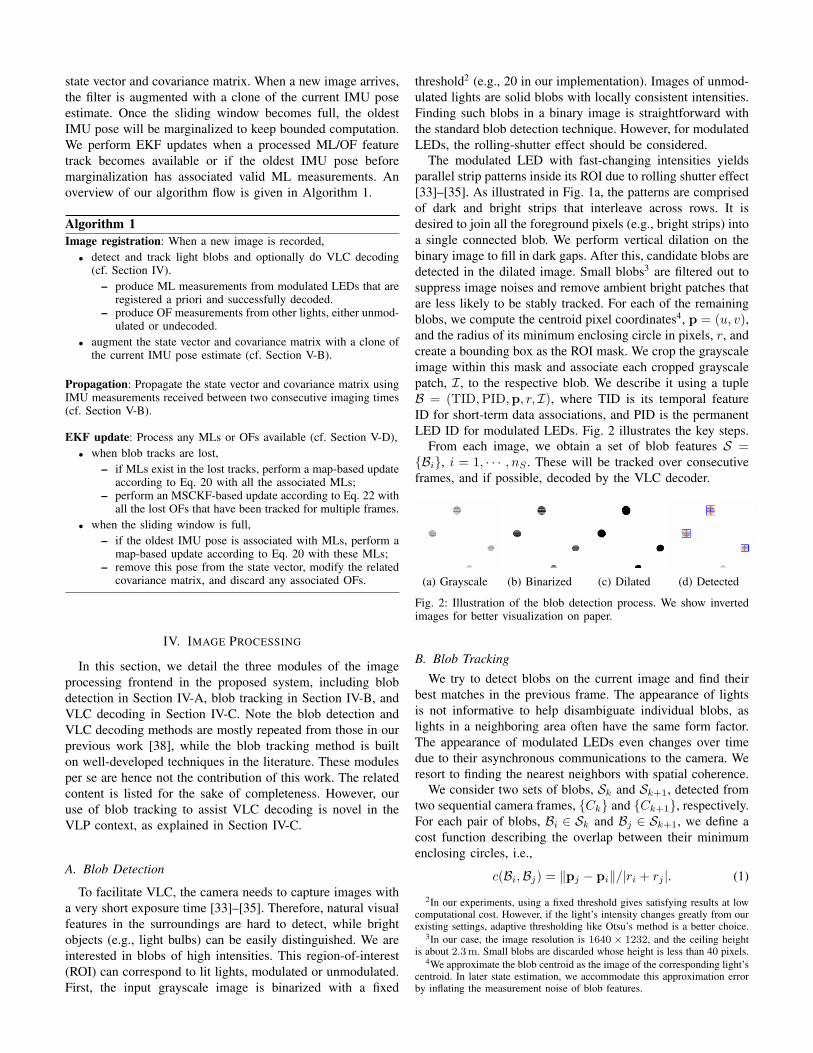
A. Blob Detection

To facilitate VLC, the camera needs to capture images with

a very short exposure time [33]–[35]. Therefore, natural visual

features in the surroundings are hard to detect, while bright

objects (e.g., light bulbs) can be easily distinguished. We are

interested in blobs of high intensities. This region-of-interest

(ROI) can correspond to lit lights, modulated or unmodulated.

First, the input grayscale image is binarized with a fixed

threshold2 (e.g., 20 in our implementation). Images of unmod-

ulated lights are solid blobs with locally consistent intensities.

Finding such blobs in a binary image is straightforward with

the standard blob detection technique. However, for modulated

LEDs, the rolling-shutter effect should be considered.

The modulated LED with fast-changing intensities yields

parallel strip patterns inside its ROI due to rolling shutter effect

[33]–[35]. As illustrated in Fig. 1a, the patterns are comprised

of dark and bright strips that interleave across rows. It is

desired to join all the foreground pixels (e.g., bright strips) into

a single connected blob. We perform vertical dilation on the

binary image to fill in dark gaps. After this, candidate blobs are

detected in the dilated image. Small blobs3 are filtered out to

suppress image noises and remove ambient bright patches that

are less likely to be stably tracked. For each of the remaining

blobs, we compute the centroid pixel coordinates4, p = (u, v),and the radius of its minimum enclosing circle in pixels, r, and

create a bounding box as the ROI mask. We crop the grayscale

image within this mask and associate each cropped grayscale

patch, I, to the respective blob. We describe it using a tuple

B = (TID,PID,p, r, I), where TID is its temporal feature

ID for short-term data associations, and PID is the permanent

LED ID for modulated LEDs. Fig. 2 illustrates the key steps.

From each image, we obtain a set of blob features S =Bi, i = 1, · · · , nS . These will be tracked over consecutive

frames, and if possible, decoded by the VLC decoder.

(a) Grayscale (b) Binarized (c) Dilated (d) Detected

Fig. 2: Illustration of the blob detection process. We show invertedimages for better visualization on paper.

B. Blob Tracking

We try to detect blobs on the current image and find their

best matches in the previous frame. The appearance of lights

is not informative to help disambiguate individual blobs, as

lights in a neighboring area often have the same form factor.

The appearance of modulated LEDs even changes over time

due to their asynchronous communications to the camera. We

resort to finding the nearest neighbors with spatial coherence.

We consider two sets of blobs, Sk and Sk+1, detected from

two sequential camera frames, Ck and Ck+1, respectively.

For each pair of blobs, Bi ∈ Sk and Bj ∈ Sk+1, we define a

cost function describing the overlap between their minimum

enclosing circles, i.e.,

c(Bi,Bj) = ‖pj − pi‖/|ri + rj |. (1)

2In our experiments, using a fixed threshold gives satisfying results at lowcomputational cost. However, if the light’s intensity changes greatly from ourexisting settings, adaptive thresholding like Otsu’s method is a better choice.

3In our case, the image resolution is 1640× 1232, and the ceiling heightis about 2.3m. Small blobs are discarded whose height is less than 40 pixels.

4We approximate the blob centroid as the image of the corresponding light’scentroid. In later state estimation, we accommodate this approximation errorby inflating the measurement noise of blob features.

We assume that the mutual distance of blobs in an image frame

is greater than the respective inter-frame pixel displacement.

In our context, the assumption works well in practice, owing

to the inherent sparsity of ceiling lights and the non-rapid

camera motion. This can be expected for pedestrians or low-

speed service robots. Rotational movements are more likely

to yield large pixel displacements between two sequential

frames, violating the above assumption. To relax this issue, we

predict the centroid location, p′i, of the blob Bi observed from

Ck in the next frame Ck+1 using IMU measurements.

The camera’s rotational change,Ck+1

CkR, can be obtained by

integrating gyroscope measurements from time step k to k+1.

Neglecting the inter-frame translation and camera distortion,

according to [59], we have the approximate relation as follows:[

p′i

1

]

= KCk+1

CkRK−1

[

pi

1

]

, (2)

where K is the known camera intrinsic matrix; and pi and p′i

are the original and predicted blob centroids in pixels, respec-

tively. In addition, we expect a small perspective distortion in

a short frame transition time and set the predicted blob radius

as r′i = ri. After this, we modify the cost function c(Bi,Bj)in Eq. 1 as c′(Bi,Bj) = ‖pj − p′

i‖/|ri + rj |, where p′i is

computed from Eq. 2. Accordingly, the cost matrix is created:

C(Sk,Sk+1) = [c′(Bi,Bj)]Bi∈Sk,Bj∈Sk+1, (3)

where the element at row i and column j represents the cost

between the previous blob Bi and the current blob Bj .

We find newly detected blobs in Sk+1 by examining the cost

matrix C. For each Bj ∈ Sk+1, if all entries in the column Cj

exceed a predefined threshold (e.g., 5 in our implementation),

we treat it as a new blob and create a new TID for it. Bj is then

removed from Sk+1. The affected column of the cost matrix

is also removed. Next, the goal is to find an assignment of

the remaining blobs in Sk+1 to the previous blobs in Sk such

that the total cost is minimal. This assignment problem can

be optimally solved by the Hungarian method in polynomial

time [60]. The TID remains unchanged for tracked blobs.

We keep track of light blobs until they are not visible

anymore. Finally, we obtain a set of blob tracks Ti, i =1, · · · , nT for nT lights. Ti is an ordered list of blobs,

〈B1, · · · , Bni〉, observed from ni consecutive frames. In par-

ticular, each track belonging to modulated LEDs will have a

valid PID upon successful VLC decoding. With the short-term

data association, blobs that are part of the track have the same

PID, thus being identifiable once any one is decodable.

C. VLC Decoding

The time-varying light signals from LEDs are perceived by

the rolling-shutter camera as spatially-varying strip patterns.

We intend to retrieve the encoded VLC messages from such

barcode-like patterns. Let us consider a set of blobs detected

from a given camera frame, S = Bi, i = 1, · · · , nS .

Blobs with barcode-like strip patterns correspond to modu-

lated LEDs. We aim to retrieve the encoded VLC information

from the induced dark and bright strips of varying widths. Note

that the VLC packet is decodable only if the blob is large

enough to contain a complete data packet [38]. Therefore,

blobs whose sizes are smaller than a given threshold (e.g.,

80 pixels in height in our implementation) will be culled in

this step. For each remaining blob Bi, we pick up grayscale

pixels in the centering column of the associated image patch

Ii. Knowing the camera’s sampling frequency, we treat these

row-indexed pixel values as a time-varying 1D signal. It is

then binarized by adaptive thresholding [61] to account for

the non-uniform illumination artifact of the light’s radiation

surface. Fig. 3 shows an example of 1D signals before and

after binarization. To recover VLC information from the binary

waveform, we use a state machine-based method for OOK

demodulation and Manchester decoding. We can then obtain

the LED’s ID from the decoding result and assign it to the

PID of the corresponding blob feature.

0 20 40 60 80 100 120 140 1600

50

100

150

Raw

0 20 40 60 80 100 120 140 160

Row index in ROI

0

1

Bin

ary PS DATA ES

Fig. 3: Example of the 1D intensity signal for VLC decoding. Theraw signal comprises the grayscale pixels in the center column of anROI. The segments of the binary signal (marked with the followingsymbols: PS, DATA, and ES) constitute a complete data packet.

Owing to the blob tracking, the PID is shared among all the

tracked blobs. As a result, LED blobs that cannot be decoded

at faraway locations still have a chance to be identified later

as the camera approaches, until their tracking gets lost. This

gives more detection instances of decoded LEDs (i.e., MLs).

In this sense, the overall decoding performance during camera

motion can be improved. Due to asynchronous LED-to-camera

communications, the received data packet may start randomly

in the ROI. For small blobs that contain a single complete

packet, it is possible that only shifted signal waveforms exist.

To mitigate this issue, we adopt a bidirectional decoding

scheme as in [35] that allows greater success in such cases.

For some larger blobs, we decode all the repeating packets

inside and crosscheck the results for consistency. Errors could

happen due to the lack of dedicated data integrity checking in

our simplified VLC protocol. Hence, the pose estimator should

be resilient to occasional communication errors.

V. ESTIMATOR DESCRIPTION

Notations: We define a fixed global reference frame, G,which is gravity aligned and with its z-axis pointing upwards

to the ceiling. We denote the IMU body frame as I and the

camera frame as C. We use the unit quaternion ABq under

JPL convention [62] to represent the rotation ABR from frame

B to A, i.e., ABR = R

(

ABq

)

. The symbol ⊗ is used to

denote quaternion multiplication. For a quantity a, we use a

for its estimate and a for the residue.

For the estimator description, we follow the conventions

and general formulations established in MSCKF [2]–[5]. In

what follows, we show in detail the EKF estimator, including

state vector in Section V-A, IMU dynamics, state propaga-

tion and augmentation in Section V-B, rolling-shutter camera

measurement model in Section V-C, and EKF update with

MLs/OFs in Section V-D. The equations of the estimator are

inherited from [2]–[5], [63] and are not the contribution of this

work. Instead, the involved technical novelties are within the

VLP context and attributed to the additional use of delayed

ML measurements and the novel use of unmodulated lights

as OFs to provide motion constraints for VLP. The benefits of

these design choices are discussed previously in Section II and

Section III, and we will further explain how to achieve this in

Section V-D. The standard parts of MSCKF are presented for

greater completeness of the system description, thus providing

the reader with a better understanding.

A. State Vector

At imaging time-step, k, the state vector, xk, maintains the

current IMU state, xI , and in the sliding window, clones of m

past IMU poses, xC , i.e., xk =[

x⊤I x⊤

C

]⊤, as in [2]–[5], [63].

The cloned poses correspond to the latest m imaging times.

The explicit forms of xI and xC are given by

xI =[

IkG q⊤ Gp⊤

IkGv⊤

Ikb⊤g b⊤

aCI q

⊤ Cp⊤I td tr

]⊤

(4)

xC =[

Ik−1

G q⊤ Gp⊤Ik−1

. . .Ik−m

G q⊤ Gp⊤Ik−m

]⊤

, (5)

where IkG q is the unit quaternion that describes the rotation,

IkG R, from the global frame to the IMU frame. GpIk and GvIk

is the respective position and velocity of the IMU expressed in

the global frame. bg and ba represents the underlying bias for

the gyroscope and accelerometer readings, respectively. CI q is

the unit quaternion describing the rotation, CI R, from the IMU

frame to the camera frame. CpI is the translation of the IMU

with respect to the camera frame. The scalar td is the time

offset between these two sensors. tr is the frame readout time

of the rolling-shutter camera. The vector xC comprises the mlatest IMU pose clones, i.e.,

Ik−i

G q and GpIk−i, i = 1, . . . ,m.

Following [4], [5], we include in the filter state the IMU-

camera spatial extrinsics, CI q,CpI. The system can hence

accommodate certain offline calibration inaccuracies. Due to

the lack of hardware synchronization in our sensor suite, we

estimate the IMU-camera time offset, td, as in [4]. Also, it

is useful to estimate the rolling-shutter frame readout time tronline, if not given by the camera’s datasheet. For td, we use

the IMU clock as the time reference and model it by a small

unknown constant [4]. The true imaging time for an image

with a camera timestamp, Ctk, is given by Itk = Ctk+ td. To

estimate tr, we follow the method proposed in [63].

The error-state vector for xI is defined as

xI =[

Gθ⊤Ik

Gp⊤Ik

Gv⊤Ik

b⊤g b⊤

aIφ⊤ C p⊤

I td tr

]⊤

, (6)

where standard additive errors apply to vector quantities (e.g.,

p = p+p) and multiplicative errors apply to quaternions, as in

[2]–[5], [63]. We follow the global quaternion error definition

[3] for the IMU orientation and have IGq ≃

IGˆq⊗

[

12Gθ⊤ 1

]⊤

,

where the 3× 1 vector Gθ is a minimal representation of the

angle errors defined in G. For CI q, as in [4], [5], we have

CI q ≃

CIˆq ⊗

[

12Iφ⊤ 1

]⊤

, where Iφ is the 3 × 1 angle-error

vector defined in I.Accordingly, the error-state vector for the full state xk is

xk =[

x⊤I |

Gθ⊤Ik−1

Gp⊤Ik−1

. . . Gθ⊤Ik−m

Gp⊤Ik−m

]⊤

. (7)

The corresponding covariance matrix, Pk|k, is partitioned as

Pk|k =

[

PIIk|kPICk|k

P⊤ICk|k

PCCk|k

]

, (8)

where PIIk|kand PCCk|k

denotes the covariance of the current

IMU state and the past IMU poses, respectively, and PICk|k

represents the cross-correlation between their estimate errors.

B. State Propagation and Augmentation

Following [3]–[5], the IMU measurements, ωm and am, are

related to the true angular velocity, Iω, and linear acceleration,Ia, in the local IMU frame by the sensor model:

ωm = Iω + bg + ng, am = Ia− IGR

Gg + ba + na, (9)

where Gg = [0, 0, −9.8m/s2] is the gravity vector expressed

in G; and ng and na are zero-mean white Gaussian noise.

Like in [3]–[5], the continuous-time process model for xI

is described by

IG˙q =

1

2Ω(

Iω)

IGq,

GpI = GvI ,GvI = I

GR⊤Ia, (10)

bg = nwg, ba = nwa,CI˙q = 0, C pI = 0, td = 0, tr = 0,

where Ω(ω) =

[

−⌊ω×⌋ ω

−ω⊤ 0

]

. The operator ⌊·×⌋ denotes the

skew-symmetric matrix. nwg and nwa are the zero-mean white

Gaussian noise processes driving the IMU biases.

With the expectation of Eq. 10, we propagate the nominal

IMU state xI by numerical integration using buffered IMU

measurements. The estimates of cloned IMU poses in the

sliding window, xC , are constant during this propagation.

To propagate the covariance, as in [2], we begin with the

linearized continuous-time IMU error-state equation:

˙xI = FI xI +GI nI , (11)

where nI =[

n⊤g n⊤

wg n⊤a n⊤

wa

]⊤is the process noise modeled

by a Gaussian process with autocorrelation E[nI(t)n⊤I (τ)] =

Qc δ(t − τ). Qc = diagσ2gI3, σ

2wgI3, σ

2aI3, σ

2waI3 is the

covariance of the continuous-time system noise that depends

on the IMU noise characteristics [1]. FI and GI are Jacobians

with respect to the IMU state error and the process noise.

The detailed expressions of FI and GI are given in the

supplementary material [58].

Given a new arriving IMU measurement at τk+1, we can

propagate the covariance for the IMU error state, PIIk|k, one

step forward from the previous IMU sampling time τk to τk+1.

To this end, we compute the discrete-time system transition

matrix, Φk+1,k, and the noise covariance, Qk, for Eq.11:

Φk+1,k ≃ exp (FI(τk)∆t) , Qk ≃ GI(τk)QcG⊤I (τk)∆t,

where we assume FI is constant over the small interval, ∆t =τk+1 − τk. The propagated covariance PIIk+1|k

is given by

PIIk+1|k= Φk+1,kPIIk|k

Φ⊤k+1,k +Qk. (12)

The covariance matrix of the cloned poses, PCCk|k, does

not change, but the cross-correlation matrix PICk|kis affected.

The covariance matrix for the full state is propagated as

Pk+1|k =

[

PIIk+1|kΦk+1,kPICk|k

P⊤ICk|k

Φ⊤k+1,k PCCk|k

]

. (13)

When a new image arrives, the state vector and covariance

will be augmented to incorporate the corresponding IMU pose

[2]–[5], [63]. Let us consider an image with timestamp t. By

our definition, its true measurement time is t+ td. Ideally, we

need to augment the state with an estimate of the current IMU

pose at time t + td. In practice, we propagate the EKF state

and the covariance up to t+ td, the best estimate we have for

the true imaging time [4], using buffered IMU measurements.

After that, a clone of the latest IMU pose estimate [IG ˆq⊤(t+td)

Gp⊤I (t + td)]

⊤ is appended to the state vector. Also, the

covariance matrix is augmented to include the covariance of

the newly cloned state, as well as its correlation with the old

state. The augmented system covariance matrix is given by

Pk+1|k ←

[

Pk+1|k Pk+1|kJ⊤a

JaPk+1|k JaPk+1|kJ⊤a

]

, (14)

with Ja =[

I6×6 06×(17+6m)

]

, where m is the number of

previously cloned poses in the sliding window.

C. Rolling-shutter Camera Model

To deal with rolling-shutter camera measurements for state

estimation properly, we follow the rolling-shutter measurement

model in [63]. Rolling shutters capture N rows on an image

sequentially at varying times. Following the convention in

[63], we treat imaging time for a rolling-shutter camera as

the time instance when the middle row is captured. Given

an image timestamped at t, the true sampling time (e.g.,

corresponding to the middle row) is t + td by the IMU

clock. The nth row away from the middle is captured at

tn = t + td + n trN

, where n ∈ (−N2 ,

N2 ] and tr is the frame

readout time. For a moving camera, individual rows on one

image may correspond to varying camera poses.

Let us consider the ith feature, fi, detected by the frontend.

Without loss of generality, we suppose the feature’s pixel

observation from the jth cloned pose, zij , lies in the nth row.

Assuming a calibrated pinhole camera model, we have

zij = h(

Cjpfi(tn))

+ nij (15)

Cjpfi(tn) =CI R

IjGR(tn)

(

Gpfi −GpIj (tn)

)

+ CpI ,

where h(·) is the perspective projection, i.e., h(

[x, y, z]⊤)

=

[x/z, y/z]⊤

. Cjpfi is the feature position in the camera frame

that relates to the jth IMU pose. nij is the normalized image

measurement noise. Gpfi is the global 3D feature position.

This can be obtained in different ways according to the feature

types. For MLs, the feature position is known directly from

the registered LED map by VLC. For OFs, the feature position

will be triangulated using the tracked feature measurements

and cloned IMU poses in the sliding window, as in [2].

The linearized residue, rij = zij − zij , at time tn is

rij ≃Hijθ (tn)

GθIj (tn) +Hijp(tn)

GpIj (tn)+

HijxI(tn)xI +H

ijf (tn)

Gpfi + nij , (16)

where GθIj (tn) and GpIj (tn) are errors in the jth IMU pose,

and Gpfi is the 3D feature position error. Hijθ (tn) and Hij

p(tn)

are Jacobians with respect to the jth IMU pose. HijxI(tn) and

Hijf (tn) is the Jacobian for the current IMU state and the

global feature position, respectively. The explicit expressions

of these Jacobians are given in the supplementary material

[58]. GθIj (tn) and GpIj (tn) depend on time tn and do not

exist in the filter’s error state. Remember that, as in [63], we

have only cloned the IMU pose at time t + td to the filter

during state augmentation. As a result, it can not be used for

EKF updates directly. By taking the Taylor expansion at t +td, we approximate these pose errors by the resulting zeroth-

order terms for computational efficiency [63]. Explicitly, we

have GθIj (tn) ≈GθIj (t+ td) and GpIj (tn) ≈

GpIj (t+ td).Accordingly, the residue is rewritten as

rij ≃Hijθ

GθIj (t+ td) +Hijp

GpIj (t+ td)+

HijxIxI +H

ijf

Gpfi + nij

=Hijxx+H

ijf

Gpfi + nij , (17)

where Hijx=

[

HijxI

02×6 · · · Hijθ Hij

p· · · 02×6

]

represents

the Jacobian with respect to the full filter state, and the time

variables in these Jacobians are omitted for brevity.

Suppose feature fi has been tracked from a set of Mi poses.

We compute the residues and Jacobians for all observations to

this feature and obtain its stacked residue form as follows:

ri ≃ Hixx+Hfi

Gpfi + ni, (18)

where ri, Hix

, Hfi and ni are block vectors or matrices. ni is

the normalized image noise vector with covariance σ2imI2Mi

.

In our implementation, we empirically set a conservative value

for σim to accommodate some approximation errors that arise

from the blob detection step (cf. Section IV-A). Eq. 18 is

not ready for EKF updates because the feature position error,Gpfi , is not in the filter error state. In what follows, we will

describe how we mitigate this issue in Section V-D.

D. EKF Update

We present the residues for two types of blob features:

1) Residue for MLs: The global feature positions of MLs,Gpfi , are known from the prior LED feature map. The affected

errors, Gpfi , are due to offline mapping and are independent

of the filter error state, x, in online estimation (cf. Eq. 18).

As in [38], we model this error as zero-mean white Gaussian

noise with covariance σ2fI3. Eq. 18 can be rewritten as

ri ≃ Hixx+ n′

i, (19)

where n′i = Hfi

Gpfi + ni denotes the inflated noise. It is

Gaussian with covariance E(

n′in

′⊤i

)

= σ2fHfiH

⊤fi+σ2

imI2Mi.

Once we have determined which MLs to process at a given

time, we compute their residues and Jacobians as per Eq. 19.

Stacking them together yields the final residue for MLs:

rML ≃ HMLx+ nML, (20)

where rML is a block vector with elements ri, HML is a block

matrix with elements Hix

, and nML is a block vector with

elements n′i. To account for false data associations, e.g., due to

errors in VLC decoding or blob tracking, only those elements

passing the Mahalanobis gating test are retained. We can now

use Eq. 20 for an EKF update with all valid MLs. We call this

step a map-based update.

2) Residue for OFs: Following the standard MSCKF [2],

the global feature positions of OFs are triangulated using the

tracked features and cloned poses in the filter. The resulting

errors, Gpfi , are correlated to the error state, x. To eliminate

this correlation, the nullspace projection technique in MSCKF

[2] is applied. Let Ui denote an unitary matrix whose columns

span the left nullspace of Hfi , i.e., U⊤i Hfi = 0. Multiplying

U⊤i to Eq. 18 yields the following residue:

roi = U⊤i ri ≃ U⊤

i Hixx+U⊤

i ni = Hi,oxx+ no

i , (21)

where the covariance of the projected noise, noi , is σ2

imI2Mi−3.

Likewise, we aggregate the residues and Jacobians for all OFs

to be processed, as computed from Eq. 21, and pass them to

a Mahalanobis gating test. The remaining elements constitute

the final residue for OFs:

rOF ≃ HOFx+ nOF, (22)

where rOF is a block vector with elements roi , HOF is a block

matrix with elements Hi,ox

, and nOF is a block vector with

elements noi . We can use Eq. 22 to perform an EKF update

with valid OFs. We call this step an MSCKF-based update.

We perform EKF updates when a processed ML/OF feature

track becomes available or if the oldest IMU pose before

marginalization has valid ML observations (cf. Algorithm 1).

Upon the arrival of a new image, we find out all blob tracks

that are newly lost. If MLs exist therein, we carry out a map-

based update according to Eq. 20 using all the associated MLs.

Rather than performing single updates with any individual

ML in each frame as in [38], we use all the involved ML

measurements that are part of a feature track to form a

single constraint, inspired by [11]. After that, OFs tracked

across multiple frames are used for an MSCKF-based update

according to Eq. 22. The past poses in the sliding window

can first get absolute corrections by MLs before we use them

to triangulate feature positions for OFs. This helps improve

the triangulation accuracy and hence benefit the MSCKF-

based updates. The strategy works reasonably well in practice.

When the sliding window is full, the oldest IMU pose gets

marginalized out of the filter to keep bounded computation.

If the pose relates to valid ML observations, we use them

to perform a map-based update before marginalization while

discarding any associated OFs. The above EKF updates can

be carried out using general EKF equations [62].

VI. EXPERIMENTAL EVALUATION

We conduct real-world experiments to study the system’s

performance in VLC decoding, localization, and odometry. We

first introduce the experiment setup for hardware preparation

and data collection in Section VI-A. We show the effectiveness

of VLC decoding assisted with blob tracking in Section VI-B.

Comparing with an EKF-based VLP baseline, we evaluate the

localization performance on different motion profiles under

various lighting conditions in Section VI-C. Moreover, we

challenge our system in adverse scenarios with severe ML

outages, and explicitly study the influence of OFs in Section

VI-D. Next, we show the performance of running odometry

with only OFs in Section VI-E. Finally, we evaluate the

algorithm efficiency with runtime analysis in Section VI-F.

A. Experiment Setup

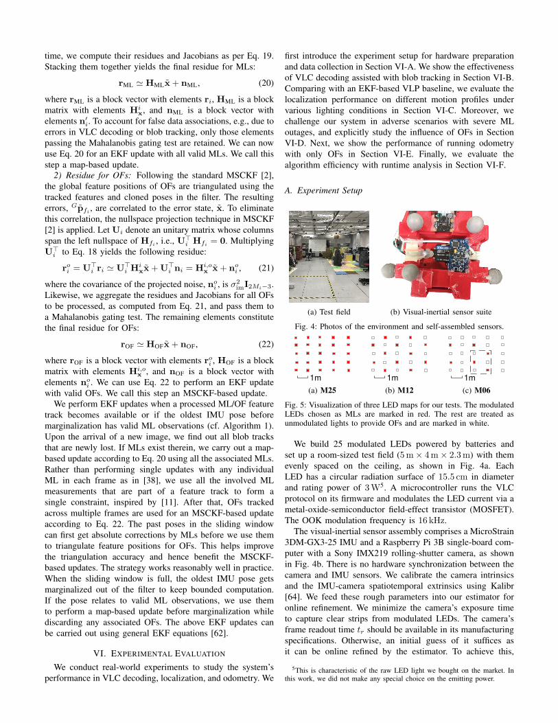
(a) Test field (b) Visual-inertial sensor suite

Fig. 4: Photos of the environment and self-assembled sensors.

1m

(a) M25

1m

(b) M12

1m

(c) M06

Fig. 5: Visualization of three LED maps for our tests. The modulatedLEDs chosen as MLs are marked in red. The rest are treated asunmodulated lights to provide OFs and are marked in white.

We build 25 modulated LEDs powered by batteries and

set up a room-sized test field (5m× 4m× 2.3m) with them

evenly spaced on the ceiling, as shown in Fig. 4a. Each

LED has a circular radiation surface of 15.5 cm in diameter

and rating power of 3W5. A microcontroller runs the VLC

protocol on its firmware and modulates the LED current via a

metal-oxide-semiconductor field-effect transistor (MOSFET).

The OOK modulation frequency is 16 kHz.

The visual-inertial sensor assembly comprises a MicroStrain

3DM-GX3-25 IMU and a Raspberry Pi 3B single-board com-

puter with a Sony IMX219 rolling-shutter camera, as shown

in Fig. 4b. There is no hardware synchronization between the

camera and IMU sensors. We calibrate the camera intrinsics

and the IMU-camera spatiotemporal extrinsics using Kalibr

[64]. We feed these rough parameters into our estimator for

online refinement. We minimize the camera’s exposure time

to capture clear strips from modulated LEDs. The camera’s

frame readout time tr should be available in its manufacturing

specifications. Otherwise, an initial guess of it suffices as

it can be online refined by the estimator. To achieve this,

5This is characteristic of the raw LED light we bought on the market. Inthis work, we did not make any special choice on the emitting power.

we first compute the row readout time τr using the formula

τr = τm/w0, where w0 represents the minimum strip width in

the strip pattern and τm is the LED’s modulation period [58].

The frame readout time is given by tr = Nτr with N as the

image height in pixels. τm and N are both known.

For existing evaluations, we assume that w0 is roughly

calibrated by hand before the operation. However, for real

applications, w0 can be inferred automatically by the software.

The rationale is as follows. The VLC data packet begins with a

4-bit preamble symbol PS = b0001 and ends with another 4-

bit symbol ES = b0111 (cf. the supplementary material [58]).

The preamble produces a LOW-logic of the maximum width

in the binary VLC signal (see Fig. 3), i.e., 3w0. We first

locate it by finding the widest LOW-logic and measure the

symbol width in pixels (denoted as l) in a programmed manner.

Then we have w0 = l/3 and tr = 3Nτm/l. We use the

obtained tr as an initial guess and feed it into the estimator for

refinement. This way, we can automate the calibration of trwithout assuming any known specifications or manual input.

The Raspberry Pi 3B (ARM Cortex-A53 [email protected],

1GB RAM) runs the sensor drivers on Ubuntu Mate 16.04

with robot operating system (ROS). The sensor data are

streamed to it and stored as ROS bags. Unless otherwise

specified, the data are ported to a desktop computer (Intel

i7-7700K [email protected], 16GB RAM) for subsequent eval-

uation. The image data are collected at 10Hz with a resolution

of 1640× 1232, and the IMU data are available at 200Hz.

An OptiTrack6 motion capture system (Mocap) provides 6-

DoF ground truth poses at 120Hz. The world frame for the

Mocap system is set up to coincide with the global frame

G. The 3D coordinates of LEDs in G are obtained by a

manual site survey with the help of Mocap and a commodity

laser ranger. We collect 14 datasets in the test field using

the handheld sensor suite with different walking profiles. The

main characteristics are summarized in Table II. During the

collection, we point the camera upwards to the ceiling. To

ease filter initialization, we put the sensor on the ground at

the start of each trial and leave it still for a few seconds.

TABLE II: Characteristics of 14 self-collected datasets.

No. Duration [s] Distance [m] Max. Vel [m/s] Name

1 48.69 40.64 1.32 circle-01

2 38.59 30.06 1.31 circle-02

3 33.99 27.88 1.35 circle-03

4 66.19 67.37 1.39 eight-01

5 45.89 43.59 1.48 eight-02

6 42.79 41.75 1.48 eight-03

7 36.80 52.41 2.59 fast-circle-01

8 32.60 36.78 1.97 fast-circle-02

9 66.99 69.05 1.47 random-01

10 46.49 45.94 1.52 random-02

11 132.68 158.83 1.65 random-03

12 39.89 34.71 1.46 square-01

13 33.89 27.53 1.31 square-02

14 40.99 43.00 1.45 square-03

Note that all lights employed here are physically modulated

LEDs, and are registered in a prior map. They are primarily

designed for MLs. For evaluation convenience, however, some

can be intentionally unregistered, acting as regular unmodu-

lated lights. With any prior knowledge discarded, these LEDs

6https://optitrack.com

seamlessly provide only OFs. This gives us the flexibility

to emulate different combinations of modulated LEDs and

unmodulated lights in the test field. As illustrated in Fig. 5,

we introduce three primary LED maps at different ML-sparsity

levels: dense, medium and sparse, that respectively have 25,

12, and 6 LEDs registered as MLs, namely M25, M12, and

M06. In each map, the unregistered LEDs act as unmodulated

lights to provide OFs. The three MLs within the dotted square

of Fig. 5c are specially used for the evaluation in Section VI-D.

B. VLC Decoding with Blob Tracking

We first test the VLC decoding performance achievable by

our hardware setup when the camera is static. For a modulated

LED, we define the decoding success rate as the ratio of the

number of images with correct decoding results to the total

number of images processed in a given time period. Table

III shows the statistics on success rates for a single LED at

varying LED-camera distances. The maximum decoding range

achieved by our system is slightly over 2.5m.

TABLE III: VLC decoding performance with a static camera.

LED-camera distance [m] 1.0 1.5 2.0 2.5 3.0

Decoding success rate [%] 98.2 88.3 72.2 16.8 0.0

0 50 100 150 200 250 300 350 400

Frame index

0

2

4

6

8

#M

Ls

per

fra

me

w/ tracking w/o tracking

Fig. 6: Evolution of the number of detected MLs over frames, withand without blob tracking, on dataset square-01 using map M25.

0.5 1 1.5 2 2.5 3

Avg. #MLs detected per frame

6

12

25

To

tal

#M

Ls

in m

ap

w/o tracking

w/ tracking

Fig. 7: Boxplot of the average number of MLs detected per frameacross the 14 datasets, with and without blob tracking, using threemaps with a different number of MLs, i.e., M06, M12, and M25.

1 2 3 4 5 6 7 8 9 10 11 12 13 14

Dataset number

1

1.5

2

2.5

3

3.5

ML

fea

ture

dep

th [

m]

w/o tracking

w/ tracking

Fig. 8: Boxplot of feature depths for all the detected MLs on eachof the 14 datasets using map M25, with and without blob tracking.

We then consider performing VLC decoding with a moving

camera as this is more general in localization scenarios. Fig.

6 shows the time-evolving number of MLs detected per frame

on dataset square-01 using map M25, with and without blob

tracking. Clearly, using blob tracking in our VLC frontend

has efficiently increased the observation number of MLs on

many frames. The boxplots in Fig. 7 summarize the average

number of MLs detected per frame on all the 14 collected

datasets, under different map configurations of M06, M12, and

M25. Comparing the results in the tracking and non-tracking

cases, we confirm the finding that, with blob tracking enabled,

the frontend can produce more valid observations of MLs per

frame for later localization. In this sense, blob tracking can

improve the decoding performance during camera motion for

the adopted rolling-shutter VLC mechanism.

To give some insights into how tracking helps in decoding,

we individually present in Fig. 8 the feature depths of detected

MLs on the 14 datasets. The feature depths are computed in

the pose estimation procedure using map M25. In particular,

the results in the tracking case are obtained by the proposed

method, while those for the non-tracking case are obtained by

our previous EKF-based solution [38]. We can observe that

the feature depths of detected MLs are way greater in the

tracking case. This is because blob tracking provides short-

term data associations for tracked lights. The modulated LEDs

that appear at faraway locations may not be decoded in time;

yet, they still have a chance to be identified later as the camera

moves closer. The median length of feature tracks obtained on

the 14 datasets ranges from 8 to 13.

C. Localization using MLs and OFs

To our knowledge, there are no open-source implementa-

tions of inertial-aided VLP systems using modulated LEDs

or unmodulated lights. In what follows, we treat our previous

work [38] as a baseline for benchmark comparison. To be

specific, we evaluate the proposed VLP system on 14 self-

collected datasets (see Table II) using three LED feature maps

of different ML-sparsity levels (see Fig. 5), i.e., M06, M12,

and M25. By design, blob tracking in the frontend can benefit

localization in two ways: 1) producing more observations of

MLs for map-based updates, and 2) enabling the optional

use of OFs for MSCKF-based updates. To study each of

their contributions, we evaluate two variants of our proposed

method. The first, named SCKF (stochastic cloning Kalman

filter), performs map-based updates with detected MLs only.

The second, named MSCKF, performs both map-based and

MSCKF-based updates with all valid observations of MLs and

OFs. We compare these two variants against [38], denoted as

EKF, that tightly fuses inertial and ML measurements by a

regular EKF without blob tracking in its VLC frontend.

The SCKF and MSCKF maintain m = 11 pose clones in

the sliding window. To initialize the global pose for all three

methods, we adopt a 2-point pose initialization method as in

[38]. All the filter parameters are kept constant when running

different methods on different trials. In particular, the process

noise and measurement noise parameters are summarized in

Table IV. We use the absolute trajectory error (ATE) [65]

to measure global position accuracy and the axis-angle error

to measure orientation accuracy. Online demonstrations are

available in the supplementary video7.

TABLE IV: Process noise and measurement noise parameters in use.

Param σg σwg σa σwa σim σf

Value 0.005 0.0001 0.05 0.002 0.03 0.03

Unit rad

s√Hz

rad

s2√Hz

m

s2√Hz

m

s3√Hz

unitless m

-1 0 1 2 3

x [m]

-1.5

-1

-0.5

0

0.5

1

1.5

y [

m]

GT EKF SCKF MSCKF

-0.4 -0.2 0 0.2-1.2

-1

-0.8

-0.6

Fig. 9: Top-view of the trajectories estimated by different methods,as well as the ground truth, on dataset square-01 using map M06.

6 12 25

Total number of MLs

0

5

10

15

Posi

tion E

rror

[cm

] EKF

SCKF

MSCKF

6 12 25

Total number of MLs

0

1

2

3

Ori

enta

tion E

rror

[deg

]Fig. 10: Error statistics by different methods on dataset square-01using three maps with different numbers of MLs.

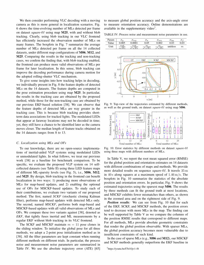
In Table V, we report the root mean squared error (RMSE)

for the global position and orientation estimates on 14 datasets

with different combinations of maps and methods. We provide

more detailed results on sequence square-01. It travels 35min 40 s along squares at a maximum speed of 1.46m/s. The

boxplots in Fig. 10 summarize the statistics of the absolute

position and orientation errors. In particular, Fig. 9 shows the

estimated trajectories using the sparsest map M06. The results

by three methods can fit the ground truth at most locations,

and MSCKF exhibits fewer mismatches than others, as shown

in the zoomed area and on the rightmost side of Fig. 9.

Position results: We can see from Fig. 10 that for each

of the EKF, SCKF, and MSCKF methods, the position errors

tend to decrease with more MLs in the map. The finding can

be well supported by Table V as we compare the columns of

the position RMSE results that correspond to different maps.

For all methods, MLs provide absolute geometric constraints

that render the global position observable. With sparser MLs,

the global position accuracy becomes more vulnerable due to

insufficient constraints of such kind.

In the case of sparse MLs (e.g., M06 and M12), our MSCKF

and SCKF methods generally outperform the EKF baseline in

7https://youtu.be/I7h1Ojv1-f8

TABLE V: Error statistics on 14 datasets using maps of M06, M12,and M25. Bold font highlights the best result in each row.

M06 Position RMSE [cm] Orientation RMSE [deg]

No. EKF SCKF MSCKF EKF SCKF MSCKF

1 2.78 2.75 2.72 1.14 1.23 1.24

2 5.11 5.46 3.33 1.33 1.32 1.34

3 4.71 3.34 3.18 1.30 1.33 1.39

4 5.35 4.91 4.07 2.06 2.05 2.06

5 5.15 4.35 4.24 1.54 1.49 1.51

6 4.82 4.09 3.33 1.65 1.60 1.63

7 8.11 6.98 4.73 1.96 2.05 2.12

8 8.10 6.50 4.62 1.39 1.47 1.51

9 7.02 7.50 4.34 1.57 1.57 1.56

10 15.23 13.38 6.13 1.83 1.89 1.90

11 12.82 9.41 4.66 1.61 1.61 1.62

12 8.40 5.77 2.92 1.33 1.27 1.28

13 5.40 4.17 2.76 1.23 1.34 1.30

14 6.25 4.26 3.65 1.84 1.75 1.75



1 2.38 2.44 2.46 1.16 1.23 1.24

2 2.70 2.63 2.54 1.32 1.31 1.33

3 4.19 3.04 2.86 1.33 1.40 1.41

4 4.04 3.91 3.01 2.01 2.04 1.60

5 4.08 3.88 3.97 1.51 1.51 1.51

6 3.90 3.37 3.21 1.58 1.61 1.63

7 3.54 3.25 3.12 2.02 2.11 2.11

8 4.20 3.40 3.10 1.49 1.58 1.56

9 3.34 3.27 3.19 1.56 1.56 1.57

10 4.96 3.57 3.00 1.80 1.82 1.84

11 3.96 3.68 3.48 1.60 1.62 1.63

12 4.15 3.19 2.70 1.27 1.27 1.28

13 4.37 3.67 2.67 1.24 1.37 1.33

14 4.89 3.23 3.08 1.85 1.80 1.80



1 2.02 2.17 2.18 1.18 1.20 1.21

2 1.99 2.29 2.28 1.32 1.28 1.29

3 2.29 2.17 2.13 1.30 1.35 1.35

4 3.24 3.30 3.31 2.01 2.02 2.02

5 2.78 2.52 2.50 1.51 1.47 1.46

6 2.33 2.43 2.42 1.53 1.53 1.53

7 2.51 2.59 2.54 2.06 2.05 2.01

8 2.47 2.39 2.36 1.62 1.60 1.60

9 2.57 2.56 2.57 1.54 1.55 1.55

10 2.73 2.54 2.54 1.77 1.78 1.78

11 3.24 3.39 3.33 1.59 1.58 1.58

12 2.82 2.56 2.52 1.28 1.28 1.28

13 2.73 2.38 2.36 1.33 1.35 1.34

14 2.54 2.45 2.47 1.82 1.66 1.66

terms of position accuracy, and the MSCKF often performs the

best. This is evident in the corresponding boxplots in Fig. 10

and is validated by most cases in the corresponding rows of

Table V. The performance gain of our MSCKF and SCKF

methods against the EKF is due in part to their inclusion

of more ML observations, produced by the visual frontend

with blob tracking, for map-based updates. Compared with the

SCKF, the MSCKF makes extra use of OFs observed from

unmodulated lights or undecoded LEDs to provide relative

motion constraints. This helps to reduce its pose drift during

ML outages and improve localization accuracy. On this point,

we provide more detailed evaluations later in Section VI-D.

With dense ML deployments (e.g., M25), however, all three

methods deliver closely high position accuracies, as shown by

Fig. 10 and the bottom rows of Table V. In this case, we

suspect the number of MLs detected per frame is no longer

the performance bottleneck as previously. All methods can be

sufficiently constrained because of rich ML occurrences. The

advantage of blob tracking for the MSCKF and SCKF is now

not as pronounced as in the sparse-ML case. Furthermore, the

performance difference between these two variants is marginal.

This is because all 25 LEDs have been registered as MLs,

and only those that fail in VLC decoding occasionally serve

OFs. The limited use of OFs renders the MSCKF almost

degenerated to the SCKF variant. Interestingly, the EKF has

achieved slightly smaller position RMS errors than ours on a

few datasets (see #1, #2, etc.). This is likely due in part to

the method of using MLs for updates. Upon the arrival of an

image input, the EKF can perform a map-based update soon

with the newly detected MLs. By contrast, the sliding window

mechanism in the MSCKF and SCKF introduces an additional

latency for each tracked ML before its use. Note that MLs

in our methods are processed when they lose tracking or the

oldest pose is marginalized out. The delayed update may have

side effects on real-time localization in the sense that absolute

pose corrections are not applied so timely as in the EKF.

To conclude, in terms of absolute position performance, our

MSCKF method has consistently achieved high accuracies of

centimeter-level RMSE on all 14 datasets using three LED

maps. It shows better robustness than others to the sparsity of

MLs within the map. We credit these advantages to making

full use of more MLs and optional OFs for localization, which

are more pronounced in scenarios with sparse MLs.

Orientation results: From Fig. 10 and Table V, we can see

that the absolute orientation errors by all three methods are

very close to each other using maps of different ML-sparsities.

The orientation RMS errors on all test cases are around 1-2

degrees. The advantage of the MSCKF method in orientation

estimation becomes less obvious than in position estimation.

We attribute this mainly to the fact that tracking orientation

accurately is much easier than tracking position using an IMU.

We see that all methods tightly fuse inertial and visual

measurements by Kalman filtering for pose estimation. The

pose is tracked with IMU double-integration and is corrected

intermittently by ML/OF measurements. The global roll and

pitch are observable owing to known gravity constraints. Their

estimates are drift-free. Yet, the global yaw and position are

observable in the presence of MLs, i.e., known 3D features that

provide absolute geometric constraints. During the outage of

MLs, the related estimates will drift but to different degrees.

The drift arises from the accumulated errors by IMU double-

integration, in which position errors grow much faster than

orientation errors. Let us consider a period between two EKF

updates. The global yaw can suffer from linear errors with time

due to uncorrected gyroscope biases. By contrast, the global

position can suffer from quadratic or even cubic errors with

time due to uncorrected IMU biases. Within a short integration

time (e.g., a few seconds), the induced yaw drift is much

smaller and easier to correct using intermittent MLs. This way,

orientation errors in three directions can be all bounded small.

To summarize, with intermittent ML corrections, the three

methods can achieve closely high performance in orientation

estimation owing to the known gravity constraint and the

inherent characteristic of slowly-growing yaw errors in ML

outages. By contrast, achieving accurate position estimates in

the long term is more difficult due to the fast-growing position

errors in IMU double-integration and the lack of observability

in 3D position during ML outages. This is a major challenge

we aim to address. As shown earlier, our MSCKF method can

effectively reduce this position drift by midway corrections

using OFs, thus improving the overall positional performance.

D. Localization under Challenging Conditions

We challenge our system under unfavorable conditions, such

as severe outages of MLs and the shortage of OFs due to

the highly sparse placement of modulated LEDs/unmodulated

lights. Through the experiments, we aim to study 1) the

influence of the sparsity of OFs on localization accuracy and 2)

the importance of OFs to the system operation. For evaluation,

we use a very sparse map, M03, with three out of 25 LEDs as

MLs, as highlighted by the dotted square in Fig. 5c. The start

and end points for data collection are within this area. This

enables the estimator to initialize its global pose by the 2-point

pose initialization [38] at startup. Using three and not two MLs

allows better initial pose guesses from more constraints. We

treat the other 22 LEDs as unmodulated lights.

The setup of 22 unmodulated lights in a 5m× 4m sized

area represents a dense deployment, comparable to the original

setup of 20 fluorescent tubes. Changing the deployment of

unmodulated lights allows us to test the system with OFs of

different sparsities. For evaluation convenience, we do not alter

the physical setup of the lights. Alternatively, we emulate a

few different sparse-deployment cases by dropping out a part

of the OF tracks produced by the frontend. This is achieved by

removing unwanted OFs as per the feature ID. We can flexibly

control the number of OFs in use by choosing a different usage

rate. In the experiments, we keep 100, 50, 25, 10, 0 percent

of the originally detected OFs. In the case of 0% OFs, the

MSCKF method degenerates to SCKF since no OFs are used

for updates. The other experiment settings remain unchanged.

We run MSCKF on the 14 datasets using map M03 and with

OF usage rates of 100, 50, 25, 10, 0 percent.

Influence of OF sparsity on localization accuracy: As

shown in Fig. 11, we present the detailed results on dataset

square-01. Fig. 11a shows the evolution of absolute position

errors over time. With three MLs, the system has experienced

the frequent absence of ML observations. This is also referred

to as ML outages (see the shaded area in Fig. 11a). We observe

that the position errors are well constrained in the presence

of MLs, regardless of how many OFs are involved. During

ML outages, however, the position errors grow more evidently

when fewer OFs are used. Given 0% OFs, the method fails

on this dataset. We believe that OFs are more important to

the system in the situation of ML outages. Fig. 11c shows the

boxplots of the absolute position and orientation errors. The

position errors grow as the OF usage rate decreases, whereas

the orientation errors do not change significantly. Fig. 11b

shows how the exact number of OFs evolves per frame as the

OF usage rate varies at 100, 50, 25, 10 percent. The number

of OFs averaged over all frames is 3.65, 1.84, 0.98, 0.41,respectively. The MSCKF can run successfully on dataset

square-01 with 0.41 OFs or more per frame on average. Given

fewer OFs, it is prone to a complete failure. It seems that the

more OFs that are used, the better the position accuracy.

The results on the 14 datasets are reported in Table VI. We

characterize the richness of OF observations by the average

0 50 100 150 200 250 300 350 400

Frame index

0

10

20

30

40

Po

siti

on

err

or

[cm

] ML outage

10% OFs

25% OFs

50% OFs

100% OFs

(a) Evolution of position errors over consecutive frames.

0 50 100 150 200 250 300 350 400

Frame index

0

2

4

6

8

10

#O

Fs

per

fra

me

100%

50%

25%

10%

(b) Evolution of the number of OFs in use per frame.

100 50 25 10

OF usage rate [%]

0

10

20

30

40

Po

siti

on

err

or

[cm

]

100 50 25 10

OF usage rate [%]

0

1

2

3

Ori

enta

tio

n e

rro

r [d

eg]

(c) Statistics of the absolute position and orientation errors.

Fig. 11: Results of the MSCKF method on dataset square-01 usingmap M03 and with OF usage rates of 100, 50, 25, 10 percent.

number of OFs over all frames. The absolute pose errors are

quantified by the position and orientation RMSE. In the last

row, we loosely summarize the results across all datasets by

averaging valid entries to provide an overall scalar metric.

As shown by the leftmost 100% column, the average number

of OFs per frame varies among datasets, ranging from 2.66to 3.71. With OF usage rates of 100, 50, 25, 10, 0 percent,

the average number of OFs per frame over all datasets is

3.27, 1.62, 0.82, 0.36, 0. Without OFs, our method fails on

8 out of 14 datasets (see 0% columns). With 10% OFs (i.e.,

0.36 per frame), it succeeds on all but one dataset (#11).

Further, with 25% OFs (i.e., 0.82 per frame) or more, the

method runs successfully on all test cases. We can see from

these successful runs in Table VI that, in our experiments

with very sparse MLs, the position errors generally increase

with fewer OFs. Nevertheless, we have reached a 3D position

accuracy of decimeters. This is close to if not better than the

best performance of many existing radio localization methods

like WiFi fingerprinting [66], [67]. When the OF usage rate

changes, the orientation errors do not differ significantly in

most cases. The reason for this is explained in Section VI-C.

To summarize, the results have reinforced our claim that

OFs help improve the position accuracy by reducing pose

drift during the ML outage. Especially, given sparse MLs, the

TABLE VI: Results of the MSCKF method on the 14 datasets using map M03 and with OF usage rates of 100, 50, 25, 10, 0 percent. The× sign indicates running failures. The last row shows the average quantity over all valid entries in each column.

No.#OFs averaged over frames Position RMSE [cm] Orientation RMSE [deg]

100% 50% 25% 10% 0% 100% 50% 25% 10% 0% 100% 50% 25% 10% 0%

1 3.54 1.78 0.86 0.58 0 4.87 6.27 6.76 7.71 22.64 0.95 0.99 0.99 1.00 1.08

2 2.83 1.56 0.68 0.34 0 5.01 9.07 13.49 21.98 × 1.01 1.01 1.02 1.03 ×3 3.01 1.54 0.79 0.51 0 4.60 4.92 5.31 6.77 9.17 1.20 1.20 1.21 1.21 1.20

4 3.68 1.89 0.99 0.42 0 4.83 6.23 6.93 16.25 × 1.14 1.22 1.23 1.39 ×5 3.71 1.96 0.87 0.38 0 4.36 5.66 6.43 14.04 15.02 1.02 1.05 1.08 1.14 1.25

6 3.36 1.60 0.85 0.27 0 4.34 4.88 6.50 12.69 13.31 0.96 0.94 0.96 0.97 1.00

7 3.21 1.51 0.70 0.47 0 8.91 9.52 10.56 26.16 × 2.27 2.27 2.14 2.25 ×8 3.35 1.50 0.83 0.22 0 6.13 9.30 10.72 12.62 42.60 1.21 1.21 1.16 1.17 1.57

9 2.89 1.45 0.73 0.28 0 7.33 10.20 11.71 25.39 × 1.03 1.03 1.06 1.07 ×10 3.33 1.69 0.93 0.31 0 8.93 9.47 9.93 19.68 × 1.35 1.31 1.28 1.32 ×11 3.12 1.56 0.81 0.31 0 8.42 11.36 27.57 × × 1.11 1.18 3.30 × ×12 3.65 1.84 0.98 0.41 0 5.84 6.24 9.50 14.74 × 1.19 1.16 1.17 1.16 ×13 3.44 1.58 0.86 0.35 0 3.81 5.46 7.54 19.39 29.45 1.03 1.10 1.09 1.18 1.32

14 2.66 1.27 0.60 0.19 0 8.35 12.6 20.70 74.13 × 1.25 1.30 1.36 1.31 ×Avg. 3.27 1.62 0.82 0.36 0 6.12 7.94 10.98 20.89 22.03 1.19 1.21 1.36 1.25 1.24

TABLE VII: Statistics of two metrics characterizing ML outages on the 14 datasets: the outage rate and the maximum outage duration.

DatasetNo. 1 2 3 4 5 6 7 8 9 10 11 12 13 14

Label c1 c2 c3 e1 e2 e3 f1 f2 r1 r2 r3 s1 s2 s3

ML outageRate [%] 45 49 45 61 58 54 63 62 69 59 77 61 50 70

Max. [s] 5.2 6.8 4.4 4.8 4.6 4.0 4.8 5.3 12.2 6.5 12.6 8.5 5.1 9.6

position performance improves with more OFs. Be noted that

the maximum number of OFs per frame is bounded in reality,

e.g., by the density of lights, ceiling height, and camera FoV.

Importance of OFs to system operation: Then we ask the

question, “At least how many OFs per frame should there be

to run the system successfully?” We see from Table VI that the

minimum number of OFs for success varies among datasets.

For instance, the system has succeeded on 6 out of 14 datasets

(e.g., #1, #3, etc.) without using OFs. Running on dataset #11,

it needs 25% OFs or more to work. As discussed earlier, we

believe that OFs are more critical to the system given ML

outages and otherwise not (see Fig. 11a). The outage is partly

due to the highly sparse deployment of MLs, e.g., using three

MLs in this evaluation. In addition, due to various motion

patterns, individual datasets could experience ML outages to

different degrees. To quantify the outage level, we propose the

below two metrics:

• ML outage rate. This is the ratio of accumulated time

of ML outages to the total time. This rate indicates how

often the outage happens and to which degree as a whole.

• Max. outage duration. This captures the most challenging

outage situation. Note that the system could fail with

severe pose drift due to a single long-term outage.

We use these together to characterize the outage situation.

The statistics of these metrics on 14 datasets are summarized

in Table VII and are visualized by the scatterplot in Fig. 12.

The labels in Fig. 12 indicate the datasets in a way described

by Table VII. The ML-outage rate is 45% or higher, with the

maximum 77% achieved on dataset #11. The maximum ML-

outage duration is between 4.0 s and 12.6 s. In Fig. 12, the

datasets on the upper right suffer from more ML outages than

those on the lower left. The system can run successfully with

no OFs on datasets indicated by squares. Running on datasets

indicated by crosses, it needs 10% OFs (i.e., 0.36 per frame)

or more. When running on the most challenging dataset #11,

it needs 25% OFs (i.e., 0.82 per frame) or more. According

to these findings, the minimum number of OFs per frame for

0.45 0.5 0.55 0.6 0.65 0.7 0.75 0.8

ML outage rate

4

6

8

10

12

Max

. M

L o

uta

ge

du

rati

on

[s]

c1

c2

c3e1e2

e3

f1f2

r1

r2

r3

s1

s2

s3

w/ 0% OFs or above

w/ 10% OFs or above

w/ 25% OFs or above

Fig. 12: Scatterplot showing the distribution of 14 datasets along twodimensions of the outage rate and maximum outage duration. Markersindicate a different number of OFs needed for success.

system operation closely depends on the ML-outage level. The

more ML outages, the more OFs are needed for success.

E. Odometry Performance using OFs only

Previously, MLs are essential to the system for localization,

while OFs can be optional. In this section, we aim to explore

the odometry performance of the VLP system using OFs only.

Here, we treat all the 25 LEDs as unmodulated lights such that

they serve as OFs. Without MLs for map-based updates, the

system degenerates to a variant of the regular MSCKF VIO

[2]. Instead of using natural point features, it works with blob

features (i.e., OFs) from ceiling lights. We initialize the filter

at rest. Unlike in the previous settings, we tune the initial

covariances of the position and orientation in the filter to

accommodate the small initial uncertainty for a VIO setup.

Other parameters remain unchanged. We aim to see if the

system can run VIO based on OFs, and to achieve this, how

many OFs there should be at least. We control the number of

OFs per frame for evaluation as in Section VI-D.

Position results: We run the system in VIO mode on 14

datasets with different OF usage rates of 100, 50, 25, 10

percent. Fig. 13 shows the boxplots of the average number

of OFs per frame and the position RMSE on all datasets. The

position errors are computed after trajectory alignment using

the posyaw method in [68]. When the OF usage rate changes

among 100, 50, 25, 10 percent, the average number of OFs

per frame on all datasets is 3.59, 1.78, 0.90, 0.36. OFs from

unmodulated lights are considerably sparser than natural point

features8. The system can run VIO successfully on all datasets

while using 25% OFs or more. But given 10% OFs, it fails to

run the complete sequence on 9 out of 14 datasets. With 25%OFs, the average number of OFs per frame is 0.90. So we

roughly say that the system can run VIO based on OFs when

supplied with around one or more OFs per frame. The position

RMSE averaged on successful runs is 0.22, 0.26, 0.34, 0.51meter. The position accuracy degrades with fewer OFs, largely

due to insufficient visual constraints.

The system has a high tolerance to the sparsity of OFs when

running odometry. We try to explain it from two aspects. First,

light blobs are good features to detect and track. Given sparse

blob features, the visual frontend can track them without using

random sample consensus (RANSAC) for outlier rejection.

Yet, this may not apply to natural features in standard VIO.

Second, the system can resolve poses recursively in a tightly

coupled way such that any individual feature measurement,

however sparse, can be adopted. On the downside, this sparsity

can also cause insufficient geometric constraints and compro-

mises the tracking performance, as shown below.

Tracking results: We assess the tracking performance in

terms of relative pose errors [68], [69]. We run the system

in VIO mode on dataset #11 (random-03) with a different

OF usage rate of 100, 50, 25 percent and present the results

in Fig. 14. Note that it fails to run with 10% OFs. Dataset

#11 is the longest among all datasets, traveling around 160min 133 s. Also included for comparison are the results of the

proposed MSCKF method using map M03.

Fig. 14a shows the estimated trajectories after alignment

using the posyaw method in [68] alongside the ground truth.

Fig. 14b shows the relative translation and yaw errors. As seen

from Fig. 14, the VIO trajectories estimated using fewer OFs

are more jittery and drift-prone; and the related translation and

yaw errors grow with the traveled distance, as expected. The

mean translation drift error computed by [68] is 1.12%, 1.39%,

and 1.63%, for the OF usage rate of 100, 50, 25 percent,

respectively. The odometry estimates suffer when fewer OFs

are used, due to insufficient constraints from OFs. Meanwhile,

with the aid of 3 MLs only, the relative pose errors become

much smaller; and the mean translation drift is reduced to

0.29%. Here, the relative pose errors do not grow with the

traveled distance due to the global localization nature.

To summarize, our system can run VIO standalone with

very sparse OFs. This supports our original idea of using OFs

to reduce pose drift during ML outages. Especially in the case

of long-term outages, even sparse OFs help to sustain the

overall system. However, the odometry performance is very

likely inferior to regular VIO due to feature sparsity. Therefore,

8The maximum number of OFs detected per frame is no more than a dozenin our tests due to the sparsity of lights. By contrast, standard VIO systemsoften work with a few tens or hundreds of point features per frame.

1 2 3 4

Average #OFs per frame

100

50

25

10

OF

usa

ge

rate

[%

]

0.2 0.4 0.6

Position RMSE [m]

Fig. 13: Results on 14 datasets when the system runs VIO withdifferent OF usage rates. Failures occur with 10% OFs in use.

−2 −1 0 1 2 3 4

x [m]

−2

−1

0

1

y[m

]

Proposed-3 MLs

VIO-100% OFs

VIO-50% OFs

VIO-25% OFs

Groundtruth

(a) Top-view of the estimated trajectories and ground truth.

16.0 32.0 48.0 64.0 81.0

0.0

0.5

1.0

1.5

Translationerror[m

]

16.0 32.0 48.0 64.0 81.0

Distance traveled [m]

0

5

10

Yaw

error[deg]

Proposed-3 MLs

VIO-100% OFs

VIO-50% OFs

VIO-25% OFs

(b) Relative translation and yaw errors evaluated by [68].

Fig. 14: Results on dataset #11 when the system runs VIO withdifferent OF usage rates. The localization results of our proposedMSCKF with 3 MLs are included for comparison.

rather than running VIO based on OFs, we would like to use

them as a beneficial supplement to MLs for global localization.

F. Runtime Analysis

To evaluate processing efficiency, we run the proposed algo-

rithms on a low-end Raspberry Pi 3B single-board computer.

We implement two threads, i.e., the VLC frontend and the

estimator. Table VIII summarizes the average time to process

an image input by each thread on dataset square-01. We can

see that the VLC thread dominates the runtime. The algorithm

efficiency can be improved by optimizing the image processing

pipeline. Due to the maintenance of a large state vector, the

proposed system with a sliding window EKF formulation

(i.e., SCKF, MSCKF) consumes more time than our previous

EKF estimator. The blob tracking module also causes a slight

increase in time (around 20%). Even so, we have achieved

real-time performance on Raspberry Pi 3B given a camera

frame rate of 10Hz. Our system remains lightweight to run

on resource-constrained computational platforms.

TABLE VIII: Timing results of the VLC frontend and estimator of ourproposed system running on a standard desktop PC and a RaspberryPi 3B for a collected dataset, compared with those of [38].

Thread VLC frontend [ms] Estimator [ms]

Platform w/o track. w/ track. EKF SCKF MSCKF

Desktop PC 3.28 3.98 0.94 2.18 2.22

Raspi 3B 40.70 50.39 10.01 28.26 29.02

VII. DISCUSSIONS

The proposed system has some limitations.

Firstly, we use circular LEDs of the same size and power

for demonstration and evaluation. This is mainly due to our

practical difficulty in preparing some homemade LEDs of

different form factors. The blob detector and tracker in the

frontend are currently designed for circular lights. However,

the system would still work with other shaped lights if the

proper blob detectors and trackers are designed for them. We

will adapt the system to more types of lights in future work.

The system’s communication and localization performance

could be affected given the use of different-powered LEDs.

The inbuilt automatic gain control (AGC) of image sensors

allows the camera to adapt to certain levels of lighting changes.

Hence, moderate changes in LED power are less likely to

affect our performance. If the LED’s intensity changes greatly

from our existing settings, we can modify the blob detection

process to accommodate this. Rather than binarizing the input

image with a fixed threshold, we prefer adaptive thresholding

like Otsu’s method [70]. Still, the impact of LED power on

system performance needs further investigation in future work.

Secondly, due to the limited LEDs at hand, the system

was only tested in a room-sized environment. However, we

argue that it is well scalable by design with the following

justifications. 1) The modulated LEDs constitute a distributed

VLC broadcasting network with one-way communication.

According to [32], the VLC function naturally scales to the

workspace scope and the concurrent number of VLC receivers

(or users). 2) The system works with a highly sparse LED map.

The required memory is almost negligible in comparison to

conventional visual or LiDAR maps. Therefore, the workspace

scope is unlikely to cause immediate limitations to our system.

However, the number of encodable LEDs can limit the scope

in use. This number is determined by the channel capacity

supported by the VLC network. Using modulated LEDs with a

larger surface than our prototypes (which are very small-sized)

or replacing our basic VLC implementation with one that is

more advanced, the channel capacity can be safely increased.

Creating an accurate map of MLs efficiently is another

problem critical to the large-scale deployment of our system

in reality. Given an up-to-date architectural floor plan with

detailed location annotations for lights, the map creation would

be straightforward. However, this knowledge can be difficult

to obtain in practice, e.g., due to privacy concerns. Manual

site-survey using professional surveying instruments like a

total station can be a valid option in practice; however, the

incurred human labor and time could be costly. An automated

LED mapping solution is more desired for real large-scale

deployment. We leave this to our future work.

Finally, the system relies on ceiling lights and an upward-

facing camera for normal operation. The orientation changes

in roll and pitch are sometimes limited during motion. The

system can accommodate large changes by inertial tracking at

the risk of losing light observations. Improving the tracking

performance with natural visual features is helpful, but is at

the cost of adding a second camera with normal exposure.

VIII. CONCLUSION

In this paper, we proposed a novel inertial-aided VLP

system using a rolling-shutter camera for lightweight indoor

localization on resource-constrained platforms. Specially, we

made full use of modulated LEDs and unmodulated lights as

landmarks within a sliding-window filter-based sensor fusion

framework, for the first time to our knowledge. We utilized a

minimal sensor suite composed of a rolling-shutter camera and

an unsynchronized IMU. The system comprised an image pro-

cessing frontend and an EKF estimator. The frontend extracted

two types of blob features (i.e., MLs, OFs) by blob detection,

tracking, and optional VLC decoding. Essential to our system,

the MLs provided absolute geometric constraints of known

data associations to help correct accumulated drift and enable

fast relocalization. Meanwhile, the OFs provided additional

visual cues for relative pose estimation, which is helpful in

reducing pose drift during ML outages. To handle delayed ML

measurements and use OFs, we followed the stochastic cloning

sliding window EKF framework of MSCKF and its multi-state

constraint measurement model. The estimator tightly fused

MLs, OFs, and inertial measurements for localization.

For system evaluation, we conducted extensive field tests

in a room-sized environment equipped with 25 ceiling LEDs.

The efficiency of the blob tracking-assisted VLC decoding

strategy was demonstrated. Compared to our previous ML-

only EKF solution, the system showed superior positional ac-

curacy and robustness under challenging light configurations,

owing to the full use of MLs and OFs. Evaluated on 14 self-

collected datasets and using maps of 6, 12, and 25 MLs, the

system consistently achieved global position accuracy of a

few centimeters and orientation accuracy of up to one or two

degrees. We explicitly showed that OFs facilitated improving

position accuracy by reducing pose drift during ML outages.

The importance of OFs to the system closely depended on the

ML-outage situation experienced. Additionally, we explored

the odometry performance of our system when supplied with

OFs only. It managed to run VIO standalone with very sparse

OFs (e.g., one OF per frame on average), despite its inferior

tracking performance. Still, the finding encourages us that even

sparsely distributed OFs can help sustain the system in the

adverse case of long-term ML outages. With runtime analysis,

finally, we demonstrated that the system is lightweight to run

on resource-constrained platforms in real-time.

In future work, we plan to generalize the system to more

types of lights, e.g., squared panels and linear tubes. For

practical deployment of our system at scale, automated LED

mapping solutions are also of necessity. With a second camera

that is normally exposed, we can further use natural features

to facilitate pose tracking and improve the overall localization.

REFERENCES

[1] G. Huang, “Visual-inertial navigation: A concise review,” in Proc. IEEE

Int. Conf. Robot. Autom. (ICRA). IEEE, 2019, pp. 9572–9582.

[2] A. I. Mourikis and S. I. Roumeliotis, “A multi-state constraint Kalmanfilter for vision-aided inertial navigation,” in Proc. IEEE Int. Conf.

Robot. Autom. (ICRA). IEEE, 2007, pp. 3565–3572.

[3] M. Li and A. I. Mourikis, “Improving the accuracy of EKF-based visual-inertial odometry,” in Proc. IEEE Int. Conf. Robot. Autom. (ICRA).IEEE, 2012, pp. 828–835.

[4] ——, “Online temporal calibration for camera–IMU systems: Theoryand algorithms,” Int. J. Rob. Res., vol. 33, no. 7, pp. 947–964, 2014.

[5] K. Sun, K. Mohta, B. Pfrommer, M. Watterson, S. Liu, Y. Mulgaonkar,C. J. Taylor, and V. Kumar, “Robust stereo visual inertial odometry forfast autonomous flight,” IEEE Rob. Autom. Lett., vol. 3, no. 2, pp. 965–972, 2018.

[6] Z. Yang and S. Shen, “Monocular visual–inertial state estimation withonline initialization and camera–IMU extrinsic calibration,” IEEE Trans.

Autom. Sci. Eng., vol. 14, no. 1, pp. 39–51, 2016.

[7] T. Qin, P. Li, and S. Shen, “VINS-Mono: A robust and versatilemonocular visual-inertial state estimator,” IEEE Trans. Rob., vol. 34,no. 4, pp. 1004–1020, 2018.

[8] Apple, “Apple ARKit,” https://developer.apple.com/augmented-reality/,accessed: 2020-05-12.

[9] Google, “Google ARCore,” https://developers.google.com/ar/, accessed:2020-05-12.

[10] T. Schneider, M. Dymczyk, M. Fehr, K. Egger, S. Lynen, I. Gilitschen-ski, and R. Siegwart, “Maplab: An open framework for research invisual-inertial mapping and localization,” IEEE Rob. Autom. Lett., vol. 3,no. 3, pp. 1418–1425, 2018.

[11] S. Lynen, T. Sattler, M. Bosse, J. A. Hesch, M. Pollefeys, andR. Siegwart, “Get out of my lab: Large-scale, real-time visual-inertiallocalization,” in Robotics: Science and Systems, vol. 1, 2015.

[12] R. C. DuToit, J. A. Hesch, E. D. Nerurkar, and S. I. Roumeliotis,“Consistent map-based 3D localization on mobile devices,” in Proc.

IEEE Int. Conf. Robot. Autom. (ICRA). IEEE, 2017, pp. 6253–6260.

[13] J. Surber, L. Teixeira, and M. Chli, “Robust visual-inertial localizationwith weak GPS priors for repetitive UAV flights,” in Proc. IEEE Int.

Conf. Robot. Autom. (ICRA). IEEE, 2017, pp. 6300–6306.

[14] A. I. Mourikis, N. Trawny, S. I. Roumeliotis, A. E. Johnson, A. Ansar,and L. Matthies, “Vision-aided inertial navigation for spacecraft entry,descent, and landing,” IEEE Trans. Robot., vol. 25, no. 2, pp. 264–280,2009.

[15] Y. Sun, M. Liu, and M. Q.-H. Meng, “Improving RGB-D SLAM indynamic environments: A motion removal approach,” Rob. Auton. Syst.,vol. 89, pp. 110–122, 2017.

[16] ——, “Motion removal for reliable RGB-D SLAM in dynamic environ-ments,” Rob. Auton. Syst., vol. 108, pp. 115 – 128, 2018.

[17] J. Cheng, H. Zhang, and M. Q.-H. Meng, “Improving visual localizationaccuracy in dynamic environments based on dynamic region removal,”IEEE Trans. Autom. Sci. Eng., 2020.

[18] X. Zuo, P. Geneva, Y. Yang, W. Ye, Y. Liu, and G. Huang, “Visual-inertial localization with prior LiDAR map constraints,” IEEE Rob.

Autom. Lett., vol. 4, no. 4, pp. 3394–3401, 2019.

[19] X. Ding, Y. Wang, D. Li, L. Tang, H. Yin, and R. Xiong, “Laser mapaided visual inertial localization in changing environment,” in Proc.

IEEE/RSJ Int. Conf. Intell. Robots Syst. (IROS). IEEE, 2018, pp. 4794–4801.

[20] S. Lynen, M. W. Achtelik, S. Weiss, M. Chli, and R. Siegwart, “A robustand modular multi-sensor fusion approach applied to MAV navigation,”in Proc. IEEE/RSJ Int. Conf. Intell. Robots Syst. (IROS). IEEE, 2013,pp. 3923–3929.

[21] S. Weiss, M. W. Achtelik, M. Chli, and R. Siegwart, “Versatile dis-tributed pose estimation and sensor self-calibration for an autonomousMAV,” in Proc. IEEE Int. Conf. Robot. Autom. (ICRA). IEEE, 2012,pp. 31–38.

[22] G. Cioffi and D. Scaramuzza, “Tightly-coupled fusion of global po-sitional measurements in optimization-based visual-inertial odometry,”arXiv preprint arXiv:2003.04159, 2020.

[23] Y. Yu, W. Gao, C. Liu, S. Shen, and M. Liu, “A GPS-aided omnidi-rectional visual-inertial state estimator in ubiquitous environments,” inProc. IEEE/RSJ Int. Conf. Intell. Robots Syst. (IROS). IEEE, 2019, pp.7750–7755.

[24] R. Mascaro, L. Teixeira, T. Hinzmann, R. Siegwart, and M. Chli,“GOMSF: Graph-optimization based multi-sensor fusion for robust UAVpose estimation,” in Proc. IEEE Int. Conf. Robot. Autom. (ICRA). IEEE,2018, pp. 1421–1428.

[25] Z. Zhang, H. Wang, and W. Chen, “A real-time visual-inertial mappingand localization method by fusing unstable GPS,” in 13th World Congr.

Int. Control Autom. (WCICA). IEEE, 2018, pp. 1397–1402.[26] T. D. Barfoot, State estimation for robotics. Cambridge University

Press, 2017.[27] A. Gadwe and H. Ren, “Real-time 6DoF pose estimation of endoscopic

instruments using printable markers,” IEEE Sens. J., vol. 19, no. 6, pp.2338–2346, 2018.

[28] Y. Zhuang, L. Hua, L. Qi, J. Yang, P. Cao, Y. Cao, Y. Wu, J. Thompson,and H. Haas, “A survey of positioning systems using visible LED lights,”IEEE Commun. Surveys Tuts., vol. 20, no. 3, pp. 1963–1988, 2018.

[29] J. Armstrong, Y. Sekercioglu, and A. Neild, “Visible light positioning:a roadmap for international standardization,” IEEE Commun. Mag.,vol. 51, no. 12, pp. 68–73, 2013.

[30] N. U. Hassan, A. Naeem, M. A. Pasha, T. Jadoon, and C. Yuen, “Indoorpositioning using visible LED lights: A survey,” ACM Computing

Surveys (CSUR), vol. 48, no. 2, pp. 1–32, 2015.[31] L. Li, P. Hu, C. Peng, G. Shen, and F. Zhao, “Epsilon: A visible light

based positioning system,” in Proc. NSDI’14, 2014, pp. 331–343.[32] A. Jovicic, “Qualcomm Lumicast: A high accuracy indoor positioning

system based on visible light communication,” 2016.[33] Y.-S. Kuo, P. Pannuto, K.-J. Hsiao, and P. Dutta, “Luxapose: Indoor

positioning with mobile phones and visible light,” in Proc. MobiCom’14.ACM, 2014, pp. 447–458.

[34] H.-Y. Lee, H.-M. Lin, Y.-L. Wei, H.-I. Wu, H.-M. Tsai, and K. C.-J. Lin,“Rollinglight: Enabling line-of-sight light-to-camera communications,”in Proc. MobiSys’15. ACM, 2015, pp. 167–180.

[35] Y. Yang, J. Hao, and J. Luo, “CeilingTalk: Lightweight indoor broadcastthrough LED-camera communication,” IEEE Trans. Mobile Comput.,vol. 16, no. 12, pp. 3308–3319, 2017.

[36] G. Simon, G. Zachar, and G. Vakulya, “Lookup: Robust and accurateindoor localization using visible light communication,” IEEE Trans.

Instrum. Meas., vol. 66, no. 9, pp. 2337–2348, 2017.[37] C. Qin and X. Zhan, “VLIP: Tightly coupled visible-light/inertial posi-

tioning system to cope with intermittent outage,” IEEE Photon. Technol.

Lett., vol. 31, no. 2, pp. 129–132, 2018.[38] Q. Liang and M. Liu, “A tightly coupled VLC-inertial localization

system by EKF,” IEEE Rob. Autom. Lett., vol. 5, no. 2, pp. 3129–3136,2020.

[39] A. Yassin, Y. Nasser, M. Awad, A. Al-Dubai, R. Liu, C. Yuen,R. Raulefs, and E. Aboutanios, “Recent advances in indoor localization:A survey on theoretical approaches and applications,” IEEE Commun.

Surveys Tuts., vol. 19, no. 2, pp. 1327–1346, 2016.[40] M. Z. Win, Y. Shen, and W. Dai, “A theoretical foundation of network

localization and navigation,” Proc. IEEE, vol. 106, no. 7, pp. 1136–1165,2018.

[41] S. Safavi, U. A. Khan, S. Kar, and J. M. Moura, “Distributed local-ization: A linear theory,” Proc. IEEE, vol. 106, no. 7, pp. 1204–1223,2018.

[42] M. Z. Win, A. Conti, S. Mazuelas, Y. Shen, W. M. Gifford, D. Dardari,and M. Chiani, “Network localization and navigation via cooperation,”IEEE Commun. Mag., vol. 49, no. 5, pp. 56–62, 2011.

[43] K. Pahlavan, X. Li, and J.-P. Makela, “Indoor geolocation science andtechnology,” IEEE Commun. Mag., vol. 40, no. 2, pp. 112–118, 2002.

[44] A. Conti, S. Mazuelas, S. Bartoletti, W. C. Lindsey, and M. Z. Win, “Softinformation for localization-of-things,” Proc. IEEE, vol. 107, no. 11, pp.2240–2264, 2019.

[45] M. F. Keskin, A. D. Sezer, and S. Gezici, “Localization via visible lightsystems,” Proc. IEEE, vol. 106, no. 6, pp. 1063–1088, 2018.

[46] A. Conti, M. Guerra, D. Dardari, N. Decarli, and M. Z. Win, “Net-work experimentation for cooperative localization,” IEEE J. Sel. Areas

Commun., vol. 30, no. 2, pp. 467–475, 2012.[47] Y. Nakazawa, H. Makino, K. Nishimori, D. Wakatsuki, and H. Koma-

gata, “Indoor positioning using a high-speed, fish-eye lens-equippedcamera in visible light communication,” in Proc. Int. Conf. Indoor

Positioning Indoor Navigat. (IPIN). IEEE, 2013, pp. 1–8.[48] Y. Li, Z. Ghassemlooy, X. Tang, B. Lin, and Y. Zhang, “A VLC

smartphone camera based indoor positioning system,” IEEE Photon.

Technol. Lett., vol. 30, no. 13, pp. 1171–1174, 2018.

[49] M. Ratosi and G. Simon, “Real-time localization and tracking usingvisible light communication,” in Proc. Int. Conf. Indoor Positioning

Indoor Navigat. (IPIN). IEEE, 2018, pp. 1–8.[50] K. Qiu, F. Zhang, and M. Liu, “Let the light guide us: VLC-based

localization,” IEEE Robot. Autom. Mag., vol. 23, no. 4, pp. 174–183,2016.

[51] Q. Liang, L. Wang, Y. Li, and M. Liu, “Plugo: a scalable visible lightcommunication system towards low-cost indoor localization,” in Proc.


[52] C. Zhang and X. Zhang, “LiTell: robust indoor localization using un-modified light fixtures,” in Proc. 22nd Annu. Int. Conf. Mobile Comput.

Netw. (MobiCom). ACM, 2016, pp. 230–242.[53] ——, “Pulsar: Towards ubiquitous visible light localization,” in Proc.

23rd Annu. Int. Conf. Mobile Comput. Netw. (MobiCom). ACM, 2017,pp. 208–221.

[54] S. Zhu and X. Zhang, “Enabling high-precision visible light localizationin today’s buildings,” in Proc. 15th Int. Conf. Mobile Syst., Appl.,

Services (MobiSys). ACM, 2017, pp. 96–108.[55] Q. Xu, R. Zheng, and S. Hranilovic, “IDyLL: Indoor localization using

inertial and light sensors on smartphones,” in Proc. Int. Joint Conf.

Pervasive Ubiquitous Comput. (UbiComp). ACM, 2015, pp. 307–318.[56] A. R. Jimenez, F. Zampella, and F. Seco, “Improving inertial pedestrian

dead-reckoning by detecting unmodified switched-on lamps in build-ings,” Sensors, vol. 14, no. 1, pp. 731–769, 2014.

[57] Y. Nakazawa, H. Makino, K. Nishimori, D. Wakatsuki, and H. Ko-magata, “LED-tracking and ID-estimation for indoor positioning usingvisible light communication,” in Proc. Int. Conf. Indoor Positioning

Indoor Navigat. (IPIN). IEEE, 2014, pp. 87–94.[58] Q. Liang, Y. Sun, and M. Liu, “Supplementary material to: A novel

inertial-aided visible light positioning system using modulated ledsand unmodulated lights as landmarks,” 2020. [Online]. Available:https://ram-lab.com/papers/2020/tase20vlc-supp.pdf

[59] A. M. Andrew, “Multiple view geometry in computer vision,” Kyber-

netes, 2001.[60] J. Munkres, “Algorithms for the assignment and transportation prob-

lems,” J. Soc. Ind. Appl. Math., vol. 5, no. 1, pp. 32–38, 1957.[61] M. Liu, K. Qiu, F. Che, S. Li, B. Hussain, L. Wu, and C. P. Yue,

“Towards indoor localization using visible light communication forconsumer electronic devices,” in Proc. IEEE/RSJ Int. Conf. Intell. Robots

Syst. (IROS). IEEE, 2014, pp. 143–148.[62] N. Trawny and S. I. Roumeliotis, “Indirect Kalman filter for 3D attitude

estimation,” University of Minnesota, Dept. of Comp. Sci. & Eng., Tech.

Rep, vol. 2, p. 2005, 2005.[63] M. Li, H. Yu, X. Zheng, and A. I. Mourikis, “High-fidelity sensor

modeling and self-calibration in vision-aided inertial navigation,” inProc. IEEE Int. Conf. Robot. Autom. (ICRA). IEEE, 2014, pp. 409–416.

[64] P. Furgale, J. Rehder, and R. Siegwart, “Unified temporal and spatialcalibration for multi-sensor systems,” in Proc. IEEE/RSJ Int. Conf. Intell.

Robots Syst. (IROS). IEEE, 2013, pp. 1280–1286.[65] J. Sturm, N. Engelhard, F. Endres, W. Burgard, and D. Cremers, “A

benchmark for the evaluation of RGB-D SLAM systems,” in Proc.


[66] Q. Liang and M. Liu, “An automatic site survey approach for indoorlocalization using a smartphone,” IEEE Trans. Autom. Sci. Eng., vol. 17,no. 1, pp. 191–206, 2019.

[67] R. Liu, S. H. Marakkalage, M. Padmal, T. Shaganan, C. Yuen, Y. L.Guan, and U.-X. Tan, “Collaborative SLAM based on Wifi fingerprintsimilarity and motion information,” IEEE Internet Things J., vol. 7,no. 3, pp. 1826–1840, 2019.

[68] Z. Zhang and D. Scaramuzza, “A tutorial on quantitative trajectoryevaluation for visual (-inertial) odometry,” in Proc. IEEE/RSJ Int. Conf.

Intell. Robots Syst. (IROS). IEEE, 2018, pp. 7244–7251.[69] A. Geiger, P. Lenz, and R. Urtasun, “Are we ready for autonomous

driving? the KITTI vision benchmark suite,” in Proc. IEEE Int. Conf.

Comput. Vis. Pattern Recog. (CVPR). IEEE, 2012, pp. 3354–3361.[70] N. Otsu, “A threshold selection method from gray-level histograms,”

IEEE Trans. Syst., Man, Cybern., vol. 9, no. 1, pp. 62–66, 1979.

Qing Liang (Member, IEEE) received his B.A. de-gree in Automation from Xi’an Jiaotong University,Xi’an, China, in 2013 and his master’s degree ininstrument science and technology from BeihangUniversity, Beijing, China, in 2016. He is currentlypursuing his Ph.D. degree with the Department ofElectronic and Computer Engineering, The HongKong University of Science and Technology, HongKong. His current research interests include sensorfusion, low-cost localization, and mobile robots.

Yuxiang Sun (Member, IEEE) received the Ph.D.degree from The Chinese University of Hong Kong,Shatin, Hong Kong, in 2017, the master’s degreefrom the University of Science and Technology ofChina, Hefei, China, in 2012, and the bachelor’sdegree from the Hefei University of Technology,Hefei, China, in 2009. He is now a research assistantprofessor at the Department of Mechanical Engi-neering, The Hong Kong Polytechnic University,Hung Hom, Hong Kong. Prior to that, he was aresearch associate at the Department of Electronic

and Computer Engineering, The Hong Kong University of Science andTechnology, Clear Water Bay, Hong Kong. He serves as an Associate Editorof IEEE Robotics and Automation Letters. Dr. Sun’s research interests includeautonomous driving, artificial intelligence, deep learning, mobile robots, etc.

Lujia Wang (Member, IEEE) received the Ph.D.degree from the Department of Electronic Engineer-ing, The Chinese University of Hong Kong, Shatin,Hong Kong, in 2015. She is now a research assis-tant professor at the Department of Electronic andComputer Engineering, The Hong Kong Universityof Science and Technology, Hong Kong. From 2016to 2021, she was an associate professor with theShenzhen Institutes of Advanced Technology, Chi-nese Academy of Sciences, Shenzhen, Guangdong.From 2015 to 2016, she was a research fellow

with the School of Electrical Electronic Engineering, Nanyang TechnologicalUniversity, Singapore. Her current research interests include Cloud Robotics,Lifelong Federated Robotic Learning, Resource/Task Allocation for RoboticSystems, and Applications on Autonomous Driving, etc.

Ming Liu (Senior Member, IEEE) received hisB.A. degree in Automation from Tongji University,Shanghai, China, in 2005 and his Ph.D. degreefrom the Department of Mechanical and ProcessEngineering, ETH Zurich, Zurich, Switzerland, in2013.

During his master’s study at Tongji University,he stayed one year in Erlangen-Nunberg Universityand Fraunhofer Institute IISB, Germany, as a mastervisiting scholar. He is currently with the Departmentof Electronic and Computer Engineering, the Depart-

ment of Computer Science and Engineering, and the Robotics Institute, TheHong Kong University of Science and Technology, Hong Kong. His researchinterests include dynamic environment modeling, deep-learning for robotics,3-D mapping, machine learning, and visual control.

Prof. Liu was a recipient of the Best Student Paper Award at the IEEEInternational Conference on Multisensor Fusion and Integration for IntelligentSystems 2012, the Best Paper in Information Award at the IEEE InternationalConference on Information and Automation 2013, the Best RoboCup Paperat the IEEE/RSJ International Conference on Intelligent Robots and Systems2013, and twice the Winning Prize of the Chunhui-Cup Innovation Contest.

A novel inertial-aided visible light positioning system using ...

Documents

Transcript of A novel inertial-aided visible light positioning system using ...