
Computer-aided Design of Electrical Machines
335
www.EngineeringEBooksPdf.com
-
Upload
khangminh22 -
Category
Documents
-
view
0 -
download
0
Transcript of Computer-aided Design of Electrical Machines

www.EngineeringEBooksPdf.com

Computer-Aided Design of Electrical Machines
K.M. Vishnu Murthy B.E; M.Tech (Elec)
(Former Sr.Dy.General Manager, BHEL, Hyderabad) Associate Professor, EEE Dept.,
G. Narayanamma Institute of Technology & Science Shaikpet, Hyderabad - 500 008, (A.P)
SSP BS Publications === 4-4-309, Giriraj Lane, Sultan Bazar,
Hyderabad - 500 095 - A. P. Phone:040-23445605,23445688
www.EngineeringEBooksPdf.com
Copyright © 2008, by Publisher
All rights reserved
No part of this book or parts thereof may be reproduced, stored in a retrieval system or transmitted in any language or by any means, electronic, mechanical, photocopying, recording or otherwise witho,ut the prior written permission of the publishers,
Published by :
BSP BS Publications
Printed at
4-4-309, Giriraj Lane, Sultan Bazar, Hyderabad - 500 095 - AP, Phone: 040 - 23445605,23445688; Fax: 23445611
e-mail: [email protected] www.bspublications.net
Adithya Art Printers Hyderabad
ISBN: 978-81-7800-146-3
www.EngineeringEBooksPdf.com

Contents
CHAPTER-1
Concept of Computer-Aided Design and Optimization
1.1 Introduction ........................................................................................................ , ........ 1
1.2 Computer-Aided Design ............................................................................................. 2
1.3 Explanation of Details of Flow Chart ......................................................................... 2
1.3.1 Input Data to be Fed into the Program .......................................................... 2
1.3.2 Applicable ConstraintslMax or Minimum Permissible Limits ........................ 4
1.3.3 Output Data to be Printed After Execution of Program ................................ 4
1.3.4 Various Objective Parameters for Optimization in an Electrical Machine .... 5
1.4 Selection of Optimal Design ........................................................................................ 5
1.5 Explanation of Lowest Cost and Significance of "Kg/KVA" ...................................... 5
Flowcharts ................................................................................................................................. 3
CHAPTER-2
Basic Concepts of Design
2.1 Introduction ............................................................................................................... 13
2.2 Specification ............................................................................................................. 13
2.3 Output Coefficient .................................................................................................. 14
2.4 Importance of Specific Loadings .............................................................................. 14
2.5 Electrical Materials .................................................................................................. 15 2.5.1 Conducting Materials ................................................................................... 15
www.EngineeringEBooksPdf.com
Conte".
2.5.2 Insulating Materials ...................................................................................... 16
2.5.3 Magnetic Materials ...................................................................................... 18
2.6 Magnetic Circuit Calculations .................................................................................. 20
2.7 General Procedure for Calculation of Amp-Turns .............. , .................................... 22
2.8 Heating & Cooling .................................................................................................... 24
2.8.1 Heatjng ......................................................................................................... 24
2.8.2 Cooling ......................................................................................................... 25
2.9 Modes of Heat Dissipation ....................................................................................... 25
2.10 Standard Rating ofElectical Machines .................................................................... 25
2.11 Ventilation Schemes ................................................................................................. 26
2.11.1 In Static Machines (Transformers) ............................................................. 26
2.11.2 In Rotating Machines ., ................................................................................ 27
2.12 Quantity of Cooling Medium .................................................................................... 30
2.13 Types of Enclosures ................................................................................................. 30
2.14 General Design Procedure ....................................................................................... 31
2.15 Steps to Get Optimal Design .................................................................................... .32
CHAPTER-3
Armature Windings
3.1 Introduction ............................................................................................................... 33
3.2 Important Terms Related to Armature Windings ..................................................... 33
3.3 Classification of Armature Windings ........................................................................ 34
3.4 Winding Pitches ........................................................................................................ 36
3.5 Armature Windings for DC Machines ..................................................................... 37
3.5.1 Rules for Design Development for Lap-Winding for Armature .................. 37
3.5.2 Examples for 4 Pole, 16 Slot DC Machine with Progressive Double Layer
Lap Winding ................................................................................................. 38
3.5.3 How to Draw the Lap Winding Diagram .................................................... 39
3.5.4 How to Represent the Position of Brushes ................................................. 39
3.5.5 Rules for Design Development of Wave-Winding ....................................... 41
3.5.6 Example for 4 Pole, 17 Slot DC Machine with Double Layer Wave Winding ....................................................................... 41
www.EngineeringEBooksPdf.com

Contents (u)
3.5.7 How to Draw the Wave Winding Diagram ................................................. 42
3.5.8 How to Represent the Position of Brushers ................................................ 44
3.5.9 Dummy or Idle Coils .................................................................................... 44
3.5.10 Criteria for Decision of Type of Winding ..................................................... 44
3.6 Armature Winding for AC Machines ....................................................................... 44
3.6.1 Similarities between DC & AC Machines ................................................... 44
3.6.2 Differences between DC & AC Machines ................................................. 45
3.6.3 How to Draw a 3-ph Single Layer Winding Diagram ................................. 45
3.6.4 How to Draw a 3-ph Double Layer Winding Diagrain ................................ 47
CHAPTER-4
DC Machines
4.1 Introduction ............................................................................................................... 57
4.2 Sequential Steps for Design of Each Part & Programming Simultaneously ............ 57
4.3 Calculation of Armature main Dimensions and flux for pole (Part-I) ..................... 58
4.3(a) Computer Program in "C" in MATLAB for Part-I ...................................... 59
4.4 Design of Armature Winding & Core (Part-2) ........................................................ 60
4.4(a) Computer Program in "C" in MATLAB for Part-2 ...................................... 63
4.5 Design of Poles & Calculation of AT (Part-3) ......................................................... 65
4.5(a) Computer Program in "e" in MATLAB for Part-3 ...................................... 68
4.6 Design of Shunt Field & Series Field Windings (Part-4) .......................................... 69
4.6(a) Computer Program in "C" in MATLAB for Part-4 ...................................... 71
4.7 Design of Commutator & Brushes (Part-5) ............................................................ 71
4.7(a) Computer Program in "C" in MATLAB for Part-5 ...................................... 72
4.8 Design ofInter-Pole/Compensating-Winding and Overall Performance (Part-6) ... 73
4.8(a) Computer Program in "C" in MATLAB for Part-6 ...................................... 75
4.9 Computer Program in "C" in MATLAB for Complete Design ................................ 76
4.10 Computer Output Results for Complete Design ...................................................... 82
4.11 Modifications to be done in the above Program to Get Optimal Design .................. 84
4.12 Computer Program in "C" in MATLAB for Optimal Design ............... : ................... 85
4.12(a) Computer Output Results for Optimal Design ............................................. 91
www.EngineeringEBooksPdf.com
(xii) Contents
CHAPTER-5
Transformers
5.1 Introduction ............................................................................................................... 93
5.2 Core Type Power Transformer ................................................................................ 93
5.2.1 Sequential Steps for Design of Each Part &
Programming Simultaneously ., ...................................................................... 93
5.2.2 Design of Magnetic Frame (Part-I) ............................................................ 94
5.2.2 (a) Computer Program in "C" in MATLAB for Part-I .................. 96
5.2.3 No-Load Current (Part-2) ............................................................................ 96
5.2.3 (a) Computer Program in "C" in MATLAB for Part-2 .................. 97
5.2.4 Design of LV Winding (Part-3) .................................................................... 98
5.2.4 (a) Computer Program in "C" in MATLAB for Part-3 .................. 99
5.2.5 DesignofHVWinding(Part-4) ....... _ ...................................................... 100
5.2.5 (a) Computer Program in "C" in MATLAB for Part-4 ................ 102
5.2.6 Performance Calculations (Part - 5) .......................................................... 102
5.2.6 (a) Computer Program in "C" in MATLAB for Part-5 ................ 103
5.2.7 Tank Design & Weights (Part-6) ............................................................... 104
5.2.7 (a) Computer Program in "C" in MATLAB for Part-6 ................ 105
5.2.8 Computer Program in "C" in MATLAB for Complete Design .................. 105
5.2.8 (a) Computer Output Results for Complete Design ...................... 110
5.2.9 Modifications to be done in the above Program to get Optimal Design ..... 112
5.2.1 0 Computer Program in "C" in MATLAB for Optimal Design ...................... 113
5.2.10 (a) Computer Output Results for Optimal Design ........................ 117
5.3 Shell Type Power Transformer ............................................................................... 118
5.3.1 Sequential Steps for Design of Each Part and
Programming Simultaneously ...................................................................... 118
5.3.2 Design of Magnetic Frame (Part-I) ........................................................... 118
5.3.2 (a) Computer Program in "C" in MATLAB for Part-I ................ 120 -
5.3.3 No-Load Current (Part-2) .......................................................................... 121
5.3.3 (a) Computer Program in "C" in MATLAB for Part-2 ................ 122
5.3.4 Design of LV Winding (Part-3) .................................................................. 123
5.3.4 (a) Computer Program in "C" in MATLAB for Part-3 ................ 124
5.3.5 Design ofHV Winding (Part-4) ................................................................. 124
5.3.5 (a) Computer Program in "C" in MATLAB for Part-4 ................ 125
www.EngineeringEBooksPdf.com

Contents (xiii)
5.3.6 Performance Calculations (Part-5) ............................................................ 126
5.3.6 (a) Computer Program in "C" in MATLAB for Part-5 ................ 127
5.3.7 Tank Design & Weights (Part-6) ............................................................... 127
5.3.7 (a) Computer Program in "C" in MATLAB for Part-6 ................ 128
5.3.8 Computer Program in "C" in MATLAB for Complete Design .................. 128
5.3.8 (a) Computer Output Results for Complete Design ..................... 133
5.3.9 Modifications to be Done in the above Program to get Optimal Design ... 135
5.3.10 Computer Program in "C" in MATLAB for Optimal Design ..................... 135
5.3.10 (a) Computer Output Results for Optimal Design ....................... 139
CHAPTER-6
Synchronous Machines
6.1 Introduction ............................................................................................................. 141
6.2 Salient Pole Type .................................................................................................... 141
6.2.1 Sequential Steps for Design of Each Part and
Programming Simultaneously..................................................................... 141
6.2.2 Calculation ofthe Stator Main Dimensions & Flux/Pole (Part-I) ............. 142
6.2.2 (a) Computer Program in "C" in MATLAB for Part-I ................ 143
6.2.3 Design of Armature Winding & Core (Part-2) .......................................... 144
6.2.3 (a) Computer Program in "C" in MATLAB for Part-2 ................ 146
6.2.4 Design of Rotor & Calculation of AT (Part-3) .......................................... 147
6.2.4 (a) Computer Program in "C" in MATLAB for Part-3 ................ 149
6.2.5 Carter Coefficients & Ampere Turns for
Various Parts of Magnetic Circuit (Part -4) ............................................. 150
6.2.5 (a) Computer Program in "C" in MATLAB for Part-4 ................ 153
6.2.6 Open Circuit Characteristic Curve (OCC) (Part - 5) ................................ 154
6.2.6 (a) Computer Program in "C" in MATLAB for Part-5 ................ 156
6.2.7 Field Current at Rated Load & PF (Part-6) .............................................. 158
6.2.7 (a) Computer Program sin "C" in MATLAB for Part-6 .............. 159
6.2.8 Field Winding Design + Losses + Efficiency (Part-7) ............................... 159
6.2.8 (a) Computer Program in "C" in MATLAB for (Part-7) ............. 161
6.2.9 Calculation of Temp-Rises & Weights (Part-8) ......................................... 162
6.2.9 (a) Computer Program in "C" in MATLAB for Part-8 ................ 163
www.EngineeringEBooksPdf.com

(xiv) Contents
6.2.l0 Computer Program in "C" in MATLAB for Complete Design .................. 164
6.2.10 (a) Computer Output Results for Complete Design ..................... 172
6.2.11 Modifications to be done in the above Program to ger Optimal Design .... 174
6.2.12 Computer Program in "C" in MATLAB for Optimal Design ..................... 174
6.2.12 (a) Computer Output Results for Optimal Design ....................... 181
6.3 Non-Salient Pole (Cylindrical Solid Rotor) Type .................................................... 182
6.3.1 Sequential Steps for Design of Each Part and
Programming Simultaneously ..................................................................... 182
6.3.2 Calculation of Stator Main Dimensions (Part-I) ........................................ 182
6.3.2 (a) Computer Program in "C" in MATLAB for Part-I ................ 184
6.3.3 Design of Armature Winding & Core (Part-2) .......................................... 185
6.3.3 (a) Computer Program in "c" in MATLAB for Part-2 ................ 189
6.3.4 Design of Rotor-Winding (Part-3) .............................................................. 190
6.3.4 (a) Computer Program in "c" in MATLAB for Part-3 ................ 192
6.3.5 Ampere Turns for Various Parts of
Magnetic Circuit at 100%V (Part-4) ......................................................... 192
6.3.5 (a) Computer Program in "c" in MATLAB for Part-4 ................ 196
6.3.6 Open Circuit Characteristic Curve (OCC) Part-5 ..................................... 197
6.3.6 (a) Computer Program in "c" in MATLAB for Part-5 ................ 199
6.3.7 Calculation ofField AT at Rated Load & PF and
Other Calculations (Part-6) ........................................................................ 201
6.3.7 (a) Computer Program in "c" in MATLAB for Part-6 ................ 202
6.3.8 Computer Program in "c" in MATLAB for Complete Design .................. 203
6.3.8 (a) Computer Output Results for Complete Design ..................... 212
6.3.9 Modifications to be done in the above Prgram to get Optimal Design ...... 215
6.3.10 Computer Program in "c" in MATLAB for Optimal Design ..................... 216
6.3.10 (a)' Computer Output Results for Optimized Design .................... 221
CHAPTER -7
Three-Phase Induction Motors 7.1 Introduction ............................................................................................................. 223
7.1.1 Squirrel Cage Motor ................................................................................... 223
7.1.2 Sequential Steps for Design of Each Part and
Programming Simultaneously ..................................................................... 223
www.EngineeringEBooksPdf.com

Contents (xv)
7.1.3 Calculation of Stator Main Dimensions & Flux (Part-I) ........................... 224
7.1.3 (a) Computer Program in "C" in MATLAB for Part-I ................ 225
7.1.4 Design of Stator Winding (Part-2) ............................................................. 226
7.1.4 (a) Computer Program in "C" in MATLAB for Part-2 ................ 229
7.1.5 Design of Squirrel Cage Rotor (Part-3) ..................................................... 230
7.1.5 (a) Computer Program in "C" in MATLAB for Part-3 ................ 231
7.1.6 Total AT & Magnetizing Current (Part-4) ..................... .' ........................... 232
7.1.6 (a) Computer Program in "C" in MATLAB for Part-4 ................ 235
7.1.7 Short-Circuit Current Calculation (Part-5) ................................................. 236
7.1.7 (a) Computer Program in "C" in MATLAB for Part-5 ................ 237
7.1.8 Performance Calculation (Part-6) .............................................................. 238
7.1.8 (a) Computer Program in "C" in MATLAB for Part-6 ................ 239
7.1.9 Computer Program in "C" in MATLAB for Complete Design .................. 239
7.1.9 (a) Computer Output Results for Complete Design ..................... 247
7.1.10 Modifications to be done in the above Program to get Optimal Design .... 250
7.1.11 Computer Program in "C" in MATLAB for Optimal Design ..................... 250
7.1.11 (a) Computer Output Results for Optimal Design ....................... 256
7.2 Slip-Ring Type Induction Motor ............................................................................. 257
7.2.1 Sequential Steps for Design of Each Part and
Programming Simultaneously ..................................................................... 257
7.2.2 Design of Slip-Ring Rotor (Part-3) ............................................................ 257
7.2.2 (a) Computer Program in "C" in MATLAB for Part-3 ............... 259
7.2.3 Computer Program in "C" in MATLAB for Complete Design ................. 260
7.2.3 (a) Computer Output Results for Complete Design ..................... 267
7.2.4 Modifications to be Done in the above Program to get Optimal Design .. , 270
7.2.5 Computer Program in "C" in MATLAB for Optimal Design .................... 271
7.2.5 (a) Computer Output Results for Optimal Design ....................... 276
CHAPTER-8
Single-Phase Induction Motors
8.1 Introduction ............................................................................................................. 277
8.2 Sequential Steps for Design of Each Part and Programming Simultaneously ....... 277
www.EngineeringEBooksPdf.com

(xvi) Contents
8.3 Calculation of Main Dimensions (Part-I) ............................................................... 278
8.3 (a) Computer Program in "c" in MATLAB for Part-I .. :.: .......................... 279
8.4 Design of Main Winding (Part-2) ........................................................................... 280
8.4 (a) Computer Program in "c" in MATLAB for Part-2 ............................... 283
8.5 Design of Rotor (Part-3) ........................................................................................ 284
8.5 (a) Computer Program in "c" in MATLAB for Part-3 ............................... 285
8.6 Amp-Turns Calculation (Part-4) ............................................................................. 285
8.6 (a) Computer Program in "c" in MATLAB for Part-4 ............................... 288
8.7 Leakage Reactance Calculation (Part-5) ............................................................... 289
8.7 (a) Computer Program in "c" in MATLAB for Part-5 ............................... 292
8.8 Design of Auxiliary Winding (Part-6) ..................................................................... 293
8.8 (a) Computer Program in "c" in MATLAB for Part-6 ............................... 296
8.9 Weights, Losses and Performance using Eq.Ckt (Part-7) ..................................... 297
8.9 (a) Computer Program in "c" in MATLAB for Part-7 ............................... 300
8.10 Computer Program in "c" in MATLAB for Complete Design .................. : ....... ~ ... 301
8.10 (a) Computer Output Results for Complete Design .................................... 309
8.11 Modifications to be done in the above Program to get Optimal Design ................. 312
8.12 Computer Program in "c" in MATLAB for Optimal Design ................................ 313
8.12 (a) Computer Output Results for Optimal Design ....................................... 318
Bibliography ......................................................................................................................... 319
Index ..................................................................................................................................... 321
www.EngineeringEBooksPdf.com

CHAPTER 1
Concept of Computer-Aided Design and Optimization
1.1 Introduction A design problem has to be fonnulated considering the various constraints, processes, availability of materials, quality aspects. cost aspects etc. Constraints can be from technical, cost or availability aspects. Technical constraints can be from calculation methods, available process systems, skilled labour, manufacturing facilities, machinery, or tools etc. Sometimes transport facilities to site also pose problems. If suitable quality
. materials are not available indigenously they may have to be imported, which effects cost and delivery time.
In designing -any system, accuracy of prediction, economy, quality and delivery period playa vital role. Basically, a design involves calculating the dimensions of various components and parts of the machine, weights, material specifications, output parameters and perfonnance in accordance with specified international standards. The calculated parameters may not tally with the final tested perfonnance. Hence, design has to be frozen keeping in view the design analysis as well as the previous operating experience of slfch machines.
The practical method in case of bigger machines is to establish a computer program for the total design incorporating the constraint parameters and running the program for various alternatives from which final design is selected.
Though the final design may meet all the required specifications, it need not be an optimal one as regards the weight and cost of the active materials, and certain perfonnance aspects like efficiency, temperature rise etc.
Various Objective Parameters/or Optimization in an Electrical Machine
(a) Higher Efficiency (b) Lower weight for given KVA output (Kg/KVA) (c) Lower Temperature-Rise (d) Lower Cost (e) Any other parameter like higher PF for induction motor, higher reactance etc.
Here we have to understand that if an optimized design is finalized keeping in view of any of the parameters mentioned above, the design may not be optimum for the above parameters. For example, if a design is selected for higher efficiency, it may not be optimum in other parameters, maybe the cost is high. Nonnally this is a case where
www.EngineeringEBooksPdf.com

2 Computer-Aided Design of Electrical Machines
compromise is to be made. This is because more costly materials like higher grade silicon steel stampings are used for armature core to reduce iron losses and hence efficiency is increased. Similar controversies will exist for other options also. One more practical example in case of bigger machines is that a constraint is imposed in weight or volume of the machine to transport it through any road bridge or tunnel to reach the site where the machine has to finally operate. Hence, it is desirable to define clearly the objective function for optimization to which the design should fulfill.
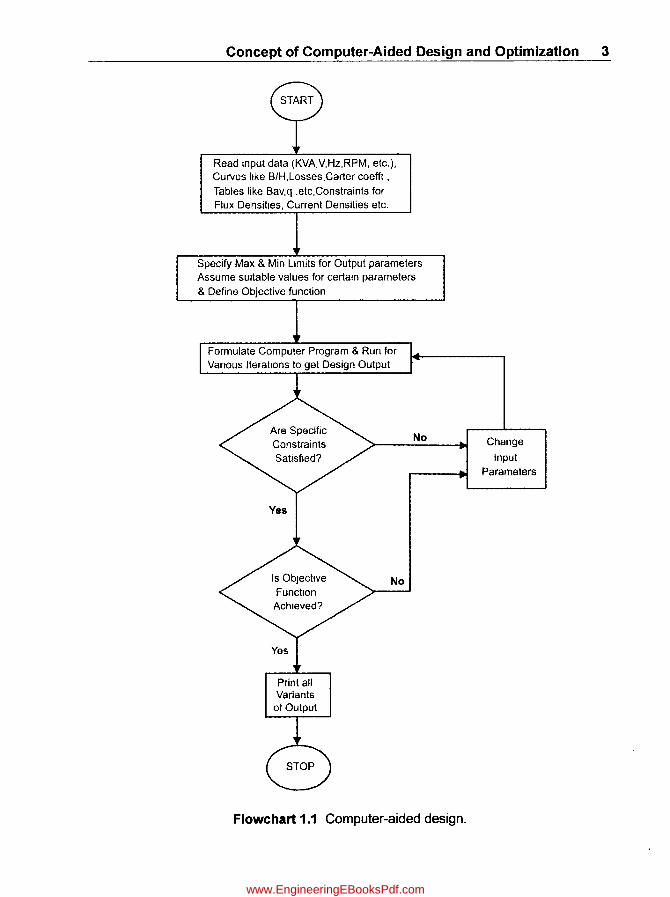
1.2 Computer-Aided Design In any practical design the number of variables is so high that hand calculations are impossible. The number of constraints is also large and for these to be satisfied by final design, a lengthy iterative approach is required. This is only possible with the help of computer programs (refer Flowchart I. J).
1.3 Explanation of Details of Flowchart
1.3.1 Input Data to be Fed into the Program
(a) Data
1. Rating of the machine (KW/KVA)
2. Rated Voltage
3. Rated Frequency (for AC only)
4. Rated Speed (RPM)
5. Type of Connection of Phases (Star/Delta) for 3 ph AC only
6. Type of Winding (Lap/Wave)
7. Number of Parallel Paths
8. Shunt/Compound in case of DC Machine
9. Squirrel Cage/Slip Ring type for 3-ph Ind.Motor
10. Rated Slip /Rotor speed for Ind.Motor
I J. Salient Pole/Round rotor type for 3-ph Alternators
J 2. Rated power factor for 3-ph Alternators
13. Core/Shell type for Transformers
J 4. Ratings of HV /L V for Transformers
(b) Applicable curves in array format like,
J. B/H for magnetic materials used for Core, Poles,
2. Loss Cuves for magnetic materials
3. Hysteresis loss vs. frequency
4. Carters coefficients for slots and vent ducts
5. Apparent Flux density
6. Leakage Coefficien~ of slots
7. HP ys. output coefficient for I-ph Ind.Motor
www.EngineeringEBooksPdf.com
Concept of Computer-Aided Design and Optimization 3
Read Input data (KVA.V.Hz,RPM, etc.), Curves like BtH,Losses.Carter coettl ,
Tables like Bav,q .etc.Constraints for Flux Densities, Current Densities etc.
Specify Max & Min Limits for Output parameters Assume sUitable values for certain parameters & Define Objective function
Formulate Computer Program & Run for VarIOus Iteralions to get Design Output
Print all Variants
of Output
No
No
Flowchart 1.1 Computer-aided design.
Change
Input Parameters
www.EngineeringEBooksPdf.com
4 Computer-Aided Design of Electrical Machines
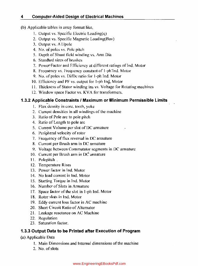
(b) Applicable tables in array format like,
I. Output vs. Specific Electric Loading(q) 2. Output vs. Specific Magnetic Loading(Bav) 3. Output vs. AT/pole 4. No. of poles vs. Pole pitch 5. Depth of Shunt field winding vs. Arm Dia 6. Standard sizes of brushes 7. Powef·-Factor and Efficiency at different ratings of Ind. Motor 8. Frequency vs. Frequency constant of I-phlnd. Motor 9. No. of poles vs. DiiDe ratio for I-ph Ind. Motor
10. Efficiency and PF vs. output for I-ph In9._ Motor II. Thickness of Stator winding ins vs. Voltage for Rotating machines 12. Window space Factor vs. K V A for transformers.
1.3.2 Applicable Constraints I Maximum or Minimum Permissible Limits I. Flux density in core, tooth, yoke 2. Curr~nt densities in all windings ofthe machine 3. RatiO' of Pole arc to pole pitch 4. Ratio of Length to pole arc 5. Current Volume per slot of DC armature 6. Peripheral velocity of rotor 7. Freq~lency of flux reversal in DC armature 8. Current per Brush arm in DC armature 9. Voltage between Commutator segments in DC armature
10. Current per Brush arm in DC· armature 11. Polepitch . 12. Temperature Rises 13. Power factor in Ind. Motor 14. No load current in Ind. Motor 15. Starting T~rque in Ind. Motor 16. Number of Slots in Armature 17. Space mctor of the slot in I-ph Ind. Motor 18. Rotor slo.ts in Ind. Motor 19. Eddy current loss factor in AC machine 20. Short Circuit Ratio of Alternator 21. Leakage reactance on AC Machine 22. Regulation 23. Saturation factor.
1.3.3 Output Data to be Printed after Execution of Program (a) Applicable Data
I. Main Dimensions and Internal dimensions of the machine 2. No. of slots
www.EngineeringEBooksPdf.com

Concept of Computer-Aided Design and Optimization 5
3. Turns in all windings 4. Copper sizes in all windings 5. Weights 6. Losses 7. Efficiency 8. Reactances 9. Full load Field current
10. Temperature rise 11. No. of cooling tubes for a transformer 12. Diameter and number of segments in Commutator 13. Full load slip oflnd. Motor.
(b) Applicable Curves
1. Open Circuit, Short Circuit and Load magnetization characteristics of Alternator
2. Slip vs. Torque curves of Ind. Motor.
1.3.4 Various Objective Parameters for Optimization in an Electrical Machine
(a) Higher Efficiency (b) Lower weight for given KVA output (Kg/KVA) (c) Lower Temperature-Rise (d) Lower Cost (e) Any other parameter like higher PF for Induction motor, higher Reactance
etc.
1.4 Selection of Optimal Design Depending upon the required objective function, the suitable design variant from the printed outputs can be picked up. We can also do it by computation by incorporating a statement to print only the best suited as per the objective.
1.5 Explanation of Lowest Cost and Significance of "Kg/KVA" Normally best objective for optimal design is the lowest cost. We will understand what is the cost?
Total cost = Material Cost + Labour cost + Over head costs Material cost = Cost of material at manufacturing works + Import duties + Sales· taxes (For imported materials cost depends on foreign exchange rates available at that time) Labour cost = Payment made to Workers Over head costs = Supervision charges + Depreciation charges on heavy machinery
We can understand from the above that it is very difficult to get all the information to arrive at total cost in the bookish design. Hence we look at more practically feasible objective from class work point of view which is nothing but minimum Kg/KV A. It means that we are able to get output of rated KVA with minimum amount of material.
Flowcharts for optimal designs of all Electrical Machines are as follows. (Flowchart 1.2 to 1.7).
www.EngineeringEBooksPdf.com

6 Computer-Aided Design of Electrical Machines
Read Input data like KW, V, Lap/Wave, No & Width of Vent. ducts, Iron factor, Ratio of length to pole arc, HV ins thk, Ht of wedge & LIp etc. Curves like B/H, Losses, Carter coefft., Tables like Bav, q etc. Desi n Constraints for Flux Densities, Current Densities etc
Formulate Computer Program In corporating Max & Min Limits for no. of flux reversals, Armature velocity, current for brush arm, Volts between commutator segments, Pole pitch, arme AT/pole, slot pitch, Current volume, width of arme cu. strip, comm. temprise, Assume suitable values for certain parameters & Define Objective function
Run for Iterations with permissible ranges of poles, speeds, Pole arc to Pole pitch ratios, Slots/pole. armature current densities, Copper strip widths, Core flux densilies,t4-_--, ralios of comm dia to armature dia to et various ossible desi noutputs
No
Go To Next Iteration
No
Flowchart 1.2 Flowchart for computer-aided optimal design of DC machine.
www.EngineeringEBooksPdf.com

Concept of Computer-Aided Design and Optimization 7
Read input data like KVA, HV & LV ratings, Hz, no. of phases, Core/Shell type, conn' Delta/Star, Iron factor, k, Curves like 8/H, Losses etc. Design Constraints for Flux DenSllles, Current Densities, No-Ld/FL current ralio
Formulate Computer Program in corporating Max & Min Limits for K, 8m, Av. Current DenSity, LID ratio, Assume sUitable values for certain parameters & Define Objective function
Run for Iterations with permissible ranges of K, Bm, Av. Current Density, LID rallo
No
No
n Vanants
Go To Next Iteration
Flowchart 1.3 Flowchart for computer-aided optimal design of transformer.
www.EngineeringEBooksPdf.com
8 Computer-Aided Design of Electrical Machines
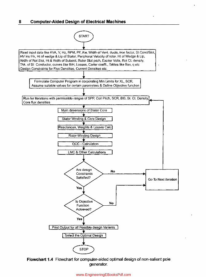
Read input data like KVA, V, Hz, RPM, PF, Kw, Width of Vent. ducts, Iron factor, St.Cond/Slot, HV ins thk, Ht of wedge & Lip of Stator, Periphoral Velocity of rotor, Ht of Wedge & Lip, Wdth of Rot Slot, Ht & Wdth of Subslot, Rotor Slot pitch, Exciter Volts, Rot Ct. density, Thk. of St Conductor, curves like B/H, Losses, Carter coefft., Tables like Bav, q etc Design Constraints for Flux Densities, Current Densities etc.
Formulate Computer Program In corporating Min Limits for XL, SCR, Assume suitable values for certain parameters & Define Objective function
Run for Iterations with permissible ranges of SPP, Coil-Pitch, SCR. BtO, St. CI. Density,I+-_---. Core flux densities
Go To Next Iteration
Flowchart 1.4 Flowchart for computer-aided optimal design of non-salient pole generator.
www.EngineeringEBooksPdf.com

Concept of Computer-Aided Design and Optimization 9
Read input data like KVA. V. RPM. Hz. PF. No & Width of Vent. ducts. Iron factor. Ratio of length to pole arc. HV ins thk. Ht of wedge&Lip .. etc Curves like BtH. Losses. Carter coefft. Tables like Bav. q etc. Design Constraints for Flux Densities. Current Densities etc
Formulate Computer Program In corporatmg Max & Min Lm11ts for Rotor perl. speed. LlPoie pitch. stator. temp-rise. Assume sUitable values for certam parameters & Define Ob ectlve function
Run for Iterations with permissible ranges of LlPP ratio. SCR .Bc. SI. Ct. DenSity ... --....
No
Go To Next Iteration
No
Flowchart 1.5 Flowchart for computer-aided optimal design of salient pole generator.
www.EngineeringEBooksPdf.com

10 Computer-Aided Design of Electrical Machines
Read input data like KW, V, Hz, PF, Sq. cage/Slip-ring, Star/Delta, No. & Width of Vent. ducts, Iron factor, HV Ins thk, Ht of wedge & Lip, Ins. Ht & Wdth wise, Curves like B/H, Losses, Carter coefft., Tables like Bav, q. pf, St. Ct. Density etc. Design Constraints for Flux Densities, Current Densities
Formulate Computer Program in corporating Max & Min limits for Rotor peri. speed, LlPoie pitch, stator Slot-pitch,Wthk ratiO, No of Rotor Slots. Assume suitable values for certain arameters & Define Ob ectlve function
Run for Iterations with permissible ranges of No. of Poles, SPP, Cond/Slot, cond thk, 1+ __ -, St. Ct. densities
No
Go To Next Iteration
No
Flowchart 1.6 Flowchart for computer-aided optimal design of 3-ph induction motor.
www.EngineeringEBooksPdf.com

Concept of Computer-Aided Design and Optimization 11
Read input data like hp, V, Hz, PF, Kt, LIDO, Iron factor, h10, h11
Curves like B/H, hZ/Kf, PICO, P VsDiIDO, Standard Wire gauge Design Constraints for Flux Densities, Current Densities
Formulate Computer Program In corporating Max & Min Limits for Current for flux densities, Space facor, Assume sUitable values for certain parameters & Define Objective function
Run for Iterations with permissible ranges of No. of Poles, slots, current densities, Bt, Bc & K1
No
No
Go To Next Iteration
Flowchart 1.7 Flowchart for computer-aided optimal design of 1-ph induction motor.
www.EngineeringEBooksPdf.com

www.EngineeringEBooksPdf.com
A
Typewritten Text
"This page is Intentionally Left Blank"

CHAPTER 2
Basic Concepts of Design
2.1 Introduction
_ Aim of design is to detennine the dimensions of each part of the machine, the material
specification, prepare the drawings and furnish to manufacturing units. Design has to be
carried out keeping in view the optimizing of the cost, volume and we~ght and at the same
time achieving the desired performance as per specification. Knowledge of latest
technological trends to supply a competitive product is a mllst. Design should conform to
stipulations specified by InternationallNational standards.
Design is the most important activity. The designer should be familiar with the following
aspects:
(a) Thorough knowledge of international/national standards.
(b) Properties of good electrical materials (like copper), magnetic materials (like
silicon steels), insulating materials (like Epoxy mica), mechanical and metallurgical
properties of all types of steel.
(c) Governing laws of electrical circuits.
(d) Laws ofheat transfer.
(e) Prices of materials used, foreign exchange rates, types of duties levied on products.
(f) Labour rates of both ski lied and unski lied labour
(g) Knowledge of competitor's products.
2.2 Specification
Basic inputs for carrying out a design of electrical machine are KVA, KW, PF, Voltage,
Speed, Frequency, No. of phases, Type of cool ing, class of insulation, permitted temperature
rise, type of winding connections, cooling medium temperature, any stipulations imposed by
customer etc. In absence of any input data, the same may be taken from relevant standards
(Table 2.1).
www.EngineeringEBooksPdf.com
14 Computer-Aided Design of Electrical Machines
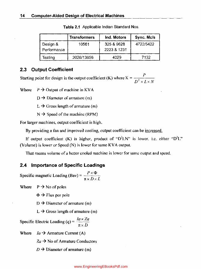
Table 2.1 Applicable Indian Standard Nos.
Transformers Ind. Motors Sync. Mc/s
Design & 10561 325 & 9628 4722/5422
Performance 2223 & 1231
. Testing 2026/13956 4029 7132
2.3 Output Coefficient
Starting point for design is the output coefficient (K) where K = ? P D- x Lx N
Where P ~ Output of machine in KV A
D ~ Diameter of armature (m)
L ~ Gross length of armature (m)
N ~ Speed of the machine (RPM)
For larger machines, output coefficient is high.
By providing a fan and improved cooling, output coefficient can be increased.
If output coefficient (K) is higher, product of "D2LN" is lower. i.e. either "D2L"
(Volume) is lower or Speed (N) is lower for same KVA output.
That means volume of a better cooled machine is lower for same output and speed.
2.4 Importance of Specific Loadings
Specific magnetic Loading (Bav) = P x <I> 1[xDxL
Where P ~ No of poles
<I> ~ Flux per pole
D ~ Diameter of armature (m)
L ~ Gross length of armature (m)
Specific Electric Loading (q) = fax Za 1[X D
Where fa ~ Armature Current (A)
Za ~ No of Armature Conductors
D ~ Diameter of armature (m)
www.EngineeringEBooksPdf.com
Basic Concepts of Design 15
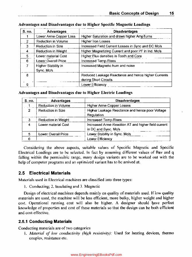
Advantages and Disadvantages due to Higher Specific Magnetic Loadings
s. no. Advantages Disadvantages
1 Lower Arme-Copper Loss Higher Saturation and draws higher AmpTurns
2 Reduction in Volume Higher Iron Losses
3 Reduction in Size Increased Field Current Losses in Sync and DC Mc/s
4 Reduction in Weight Higher Magnetizing Current and poor PF in Ind. Mcls
5 Lower material Cost Higher Flux densities in Tooth and Core
6 Lower Overall Price Increased Temp-Rises
7 Higher Stability in Increased Magnetic hum and noise Sync. Mcls
8 Reduced Leakage Reactance and hence higher Currents during Short Circuits
9 Lower Efficiency
Advantages and Disadvantages due to Higher Electric Loadings
s. no. Advantages Disadvantages
1 Reduction in Volume Higher Arme-Copper Losses
2 Reduction in Size Higtler Leakage Reactance and hence poor Voltage Regulation
3 Reduction in Weight Increased Temp-Rises
4 Lower material Cost Increased Arme-Reaction AT and higher field current in DC and Sync. Mcls
5 Lower Overall Price Lower Stability in Sync. Mcls 1--.
6 Lower Efficiency
Considering the above aspects, suitable values of Specific Magnetic and Specific Electrical Loadings are to be selected. In fact by assuming different values of Bav and q falling within the permissible range, many design variants are to be worked out with the help of computer programs and an optimized variant has to be arrived at.
2.5 Electrical Materials Materials used in Electrical machines are classified into three types:
I. Conducting; 2. Insulating and 3. Magnetic
Design of electrical machines depends mainly on quality of materials used. If low quality materials are used, the machine will be less efficient, more bulky, higher weight and higher cost. Operational running cost will also be higher. A designer should ~ave perfect knowledge of properties and cost of these materials so that the design can be both efficient and cost-effective.
2.5.1 Conducting Materials
Conducting materials are of two categories I. Material of low conductivity (high resistivity): Used for heating devices, thermo
couples, resistance etc.
www.EngineeringEBooksPdf.com

16 Computer-Aided Design of Electrical Machines
2. Material of high c()nductivity (low resistance): Used for windings of electrical machines and equipments. Material with lowest resistance should be selected so that it contributes lowest Ohmic losses to enhance efficiency and to reduce Temp-rise.
Requirements of high conductive materials:
(a) Highest Possible conductivity (least Resistance)
(b) Least possible temperature coefficient of resistance
(c) Adequate resistance to corrosion
(d) Adequate mechanical strength and high tensile strength
(e) Suitable for jointing by brazing/soldering/welding so that the joints are highly reliable contributing lowest resistance.
(f) Suitable for rollability, drawability, so that conductors of required shape (wire/strip) are easily manufactured.
Best conducing material is silver. Next best is copper and then aluminium. Propel1ies of these are compared in the following table.
S. no. Property Unit Silver Copper Aluminium 1 Conduetilvity -- 1.0 0.975 0.585
2 Resistivity IJO-em 1.46 1.777 2.826
3 Temp-Coefft % peroC 0.337 0.393 0.4
4 Cost --- Prohibitively high Medium Low
-3. Super conducting materials: Materials whose resistivity sharply decreases to practically zero value when the temperature is brought down below transition temperature are called super conductors. Due to practically zero resistance, copper losses will be almost zero. Hence, machines with these conductors can be designed with very high value of current density reducing drastically the size of the machine.
However, these machines are not in commercial use due to practical limitations.
2.5.2 Insulating Materials
Insulating materials are used to provide an electrical insulation between parts at different potenti~ls. Insulating materials are classified as per the following Table.
Required properties of good insulating materials:
(a) High Insulation Resistance
(b) High Dielectric strength
(c) Low Dielectric Losses and Low Dielectric Loss angle(tan 0)
(d) No moisture absorption
(e) Capable of withstanding without deterioration a repeated heat cycle
(f) Good heat conductivity
(g) Good mechanical strength to withstand vibrations and bending
(h) Solid material should have a high melting point
(i) Liquid materials should not evaporate or volatilize.
www.EngineeringEBooksPdf.com

Basic Concepts of Design 17
Comparison of properties of insulating materials
Dielectric Resistance
Material Strength
at 200C in Permittivity at Safe temp in Moisture
(KV/mm) at Q-cm
50 Hz DC absorption 50 Hz
Cotton 3 to 4 109 to 1013 - 90 Absorbant
Paper 6 to 10 1015 2.5 90 Absorbant
Fibre 5 109 to 1018 4 to 6 90 Absorbant if Varnish layer is cracked
Rubber 15 to 25 106 to 1015 3 to 4 40 Slightly I-
5 x 10¹³ Mica 40 to 80 5 to 8 500 No
Micanite 30 3 x 10¹³ 6 to 8 130 No
Asbestos 3 to 4.5 109 to 1015 500 Absorbant
Backalite 20 to 25 -- 5 to 6 200 No
Glass 5 to 15 1015 Room-temp No
Porcelain 10 to 20 1013 4 to 7 -do- No
Polythene 30 1016 2.3 70 No
Insulation for Conductor Covering
Copper conductors used in electrical machines are covered with some type of insulating material (usually in the form of tapes) based on thermal grading, dielectric stresses and economy.
Types of insulating materials used for conductor coverings for different temp levels are as given in the following Table.
Types of insulating materials
Ins. Max permisSible MATERIALS
class temp. limit (0C)
A 105 Cotton, silk and paper impregnated in dielectric liquid such as oil.
E 120 Cotton, silk and paper impregnated in dielectric liquid
for operating up to 120°C.
B 130 Mica, glass fibre, asbestos with suitable impregnating
materials for operating up to 130°C.
F 155 Mica, glass fibre, asbestos with suitable bonding
substances capable up to 155°C.
H 180 Silicone elastomers with mica, glass fibre, asbestos.
with silicone resins.
C 225 Silicone elastomers with mica, glass fibre, asbestos
with silicone resins.
www.EngineeringEBooksPdf.com
18 Computer-Aided Design of Electrical Machines
In electrical machines of small ratings, insulation materials of class AandE can be used
to reduce cost. But for larger machines they are not suitable since volume and weight of the
machine will be higher and efficiency lower. Techno-economical study proved that Class-B
and Class-F insulations are most appropriate for machines of medium and large ratings
respectively for commercial use.
The latest trend is to design large machines with Class-F insulation and utilize for Class
B temp-rises. Advantages of Class-F insulation is that it possesses excellent propel1ies as
indicated above and gives a reliable performance for a longer life.
Class-H and Class-C insulations are costly and hence used In compact machines
required for special applications like submarines, space craft etc., where economical aspect
is not prime criteria.
Insulating Resin and Varnish
In electrical machines, resins and varnishes are used for impregnation, coaling and adhesion.
These resins and varnishes have the following additional insulating properties.
(a) Quick drying properties
(b) Chemical stability even unde.r strong oxidizing influence
(c) Should not attack the base insulating material or the copper conductor
(d) Should set hard and good surface.
2.5.3 Magnetic Materials
Magnetic materials playa vital role in electrical machines,,.,since magnetic circuit is created
by these materials.
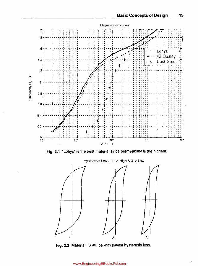
A good magnetic material should possess the following qualities (refer Figs. 2.1 and 2.2)
(a) High magnetic permeability (11) so that for required flux de!)sity it draws minimum
no. of amp turns (H = B/~L)
(b) High electrical resistivity to reduce the eddy current losses . (c) Hysteresis loop should be narrow to reduce hysteresis loss.
Silicon Steel
Magnetic properties of permeability and resistivity of steel are greatly improved by adding a
certain percentage of silicon. But, if the percentage of silicon increases 4%, steel becomes
brittle. These silicon steels are made into laminations of normal thickness of 0.35mm and
0.5 mm either by cold working or hard working.
www.EngineeringEBooksPdf.com
t E ~ II) c CIl
"'0 X ::J
u::
Basic Concepts of Design 19
Magnelizalion curves
2[-'~-----r-I"TT"-I-~- I ~ 1 "1""1-111, I I 1 IITIII .--*T I '--'(-f'-' I , • , I t I I t I" I I I '" I I • I I "1' ~.1 I I I " I I r t • Iff I' I I' I I I I I, 1, I I • I I II .,r t I I I I.,
1.8 .... - - ~ .... ~ .... ~ ~_ ~!! ~ ~ .. - _ .. ~ .... -: .... ~ .. : .. ~ ~ ~ ~; ........ ~ .... w:_ .. ~ _:_ ~ ~ " -t;..t#::- .... ~ .. ~ -~ ~ ..:~~ ~
I '" . "'" '" 1"" I I' I I' " t'" I I •• ii' f f , t "," I , I' "I' I I I ~t" f I I 'I •• , f J f , I I I It I I I I I II II I I" , I 1'1'
i I f I I I lilt I I I I I ,.1, I t~, I II • "i 1 6~-" - .. ~ ...... !- -!- -:- r iii i- ........ -: ...... :- -:- -; .. ; 111 i .......... ' -,- ;,;~ i 11 ',' I'
I •• •• t I I t I I I I I I I I I I I,· , I I I I Lohys
~I ::: : : : : : : :::: : :. , f .. ,:",·:+ : : : : : I I
I I I, I •• " •• I 'I " .. ' t I I I , It 42 Quality 14 •••••• - -' •• '- J ............. _ - .,...... •• ~~. - _ ...... -._ •• -,_... C-'d- st- c·teel . ::: : : : : : : ::: I ;..r-r I: ::: : : : : +- v 'l "" I , I f I I t 14· I • I • • +, . . . , *I.,..,---~-~ __ ~_.,J : : !!::::: : t f~t : : !::: I • I • I I I. I , • t I
12 ...... _ ... '- .. ., ...... r., ... rTT',. ........... ..,·- -,--,-,. ...... ,., +- .. ~---: ..... ~-:.;~~~;- ... -.. -: ..... -~"'~-~~..:~~
l .:!: : : : :: AI! I I' "" t:: : : : : :: I I::: :-: : I I • t I I I II I I' I : : :::.. I I I 1'1. I I ., I I I • t I I I I I ~ I I It. I • I I I I I I • I I I I I I I I I' ,
1 - - ... - ~ .... ~ ...... ~ ..: ... ~ ~ , T ;. ..... OM ~ ... w:_ -r -:- ~ ~ ~.fi ......... ~ w .. -:- ... ~ -: .. T ~ ~ ~ ~ .... - - -:- .... r .. ;. -~ ~ ~ ~ + 1
•• I I •• I I, I I , I ••• I 'I I I I •• I I I I. J I I. I
, I I I. It'll ;' I I I I , .~II 'I' I • " II • I' I It' f
~ I" It' I II .' ~ I I' IT,. I' I I " t 'I " I I I 1'1 I I , • I I I I I I • J J I I I I , • • I I It" II 1 I I •• I' I
o 8 _ •• - ~ • - ~ - • ~ ~ - ~ ~ ~ t ~ ,'" - ~ - - .: •• ~ -:- ~ 1ff ~ t - • - - ~ - • -:- - ~ -:- ~ { { t ~ - - - - -:- • -~ - ~ -~ t ~ ~ +
I , .. I I t I' I , • I I I II', 'I t I I.' I' I I. Ii •• 41 • I •• I I 1.,1 • I I 1'+,"1 • I • I I •• II .,., , I ~ I'
~ : :::: !.Y :::: I :::: ::: : ::::: :::: : : :~' o 6 r- ...... ,. ........................ to. ~ ....... '" ......... -~ ......... "'I~ .. '4 '4 .. - '" '" - ... - - -,- '" to ... - • of ..... '" ... - - -1- ... - ... - .... ~ ..... ... ! ::: : : '~':! ::::. I :::: ::: : : : : :: :::: : :: :
, • ., • I I It. 1t-' I •• I I' I I I I I I I • I I I I •• I I 'I I. II' I • I I I I I I', I I I I • I' 'I 'I t ,t I" 04 ~ .. -- .. ;--~--~ ~l't;.-~-"'-:- .. -: .. -~:-~~;~~ .. ---~ ...... :- ... ;."': .. ;~;~;"'---~: ..... -~ .. ~-~~..:~'
f
I' ., " t. • I I It' I t I I I , I I I I II I I' I I • I I
:' :::::: : :-ii:::::: I ':::::" I I"""
t , • I I II. • •• , I II I. • I I I t I I II t I I I I " I
02 ......... ~ .... I -~ ~- ~ ~! t ~ - - ... - ~- -t-:- -~ -:- ~ ~ ~ ~! - - ", .. ~ ..... -:- .. ~ .. :- ~ ~ ~ ~! ..... - - -:- .. -~ - ~ -; t ~~ • I :: ::::: ~ : 1"11, I: ::::: ; • I I. " I I I 11" j I I.' t* I I
a I ! :: : I :~Jl1L... __ l ~~illL-___ ~_i_L' f
10' 10' 10' 10' 10' AT/m-+
Fig. 2.1 "Lohys" is the best material since permeability is the highest.
Hysteresis Loss: 1 -+ High & 3~ Low
2 3
Fig. 2.2 Material 3 will be with lowest hysteresis loss.
www.EngineeringEBooksPdf.com

20 Computer-Aided Design of Electrical Machines
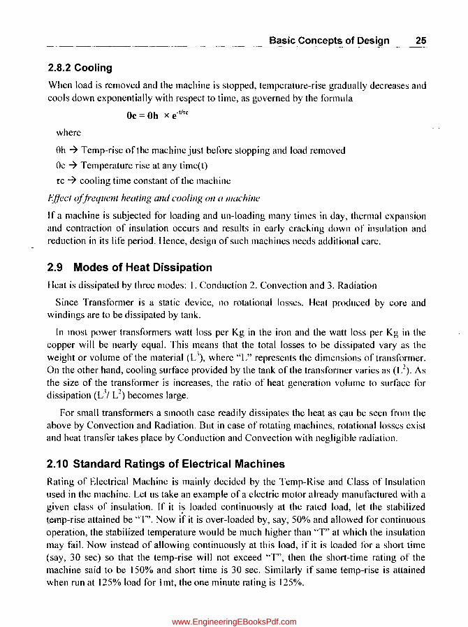
In the cold reduced process, the laminations are annealed at about II OODC to get grainoriented material. The cold rolled grain-oriented (CRGO) steels will have superior magnetic properties and can be worked at much higher flux densities. By using these in the transformers, we get the advantage of reduction in size and weight with increased efiiciency. Curves given in Fig. 2.3 indicate the loss in Watts/Kg for CRGO and NGRO (Non-grain-oriented) sheet steels.
STAMPING STEELS
OJ .;,:
4 r--i--+--f-
m 3~~-~~~-4 Q.
$: 2 ~~---j,.<'--+-:' en (/)
~ 1~~--b~+-~
1.0 1.2 1.4 1.6
Flux density, Wb/m'
(a) CRGO
OJ .;,:
40 1---4--+---.~
~ 30r--i---+~~~ & $: 201---+~~~~~ vi ~ -l
o L..---'_......1.._-1----I 08 1.2 1.6 2.0 2.4
Flux density, Wb/m'
(b) NGRO
Fig. 2.3 Core loss at 50 cIs. (a) Transformers (b) Machines
A designer should get the magnetic characteristics, loss curves of different materials from the supplier, study well and decide a suitable material for design.
2.6 Magnetic Circuit Calculations
In any Electro magnetic machine, both the magnetic and electric circuits exist. Magnetic circuit is a closed path like electric circuit. Let us understand a magnetic circuit (Fig. 2.5) by comparing an electrical circuit (Fig. 2.4).
5. no Electric-Circuit Maj:metic-Circuit
1 Resistance (R) = P x Ua Reluctance (S) = U(~ x a) = U(uO x ur x a)
2 Voltage (V) Mmf (Ampere -Turns)
3 Current (I) = VIR Flux(<l» = mmf I Reluctance
4 Voltage(V) = I x R Mmf (AT) = <l> x S
5 If there are 3 resistances in series, If there are 3 different cross-sections in
V = V1 + V2 + V3 = I x (R1 + R2 + R3) series, AT = AT1 + AT2 + AT3 = <l> x (S 1 + S2 + S3)
www.EngineeringEBooksPdf.com

__ B_a_s_ic .Concepts of Desig~ 21
~ R1 ~I R2 ~I R3
I ~--------------------~~~~--------.~~~------~
Fig. 2.4 Electncal Circuit with 3-Reslstance Elements.
~I S1 ~I S2 ·1 S3
0~ q)
III!
Fig. 2.5 Magnetic Circuit with 3 parts with different Reluctances.
. ctJZNP We take the example of a DC generator. EMF lI1duced = --- a "<1>" at rated speed·of-
60A
"NO' RPM since other parameters are constant. When the field circuit is connected to
Voltage Supply (by connecting across the armature or voltage Mains) field current is
produced. This field current passing through field turns produces mmf (AT) and the mmf
produces flux in inverse relation to total circuit reluctance (S).
Refering to above table, if the values of S I, S2 and S3 are less, then Ampere Turns (AT)
drawn by the circuit to produce rated flux "<1>" is lesser. If"AT" are lesser, field current (It)
drawn will be lesser since If = AT/T, where T = No. of field coil turns which are constant.
Then the CS (cross section) area of copper required is less and weight of copper will be less.
Since total reluctance,
LI L2 L3 (S) = S I + S2 + S3 = ---- + + -----
)10 x )11" I x a I )10 x )11"2 x a2 )10 x )11"2 x a3
It will be lesser if the permeabilities of the materials of the three parts are higher for
given lengths and CS areas. Magnetic circuit design is good if the total reluctance is reduced
and field current drawn is minimized.
Also ampere turns in any part (A Tl) = L I x 1-1 I = Ll x 8 I / (~lO x W), where "Ll" is the
length (m), "1-1 I" is AT/m and "8 I" is the flux density in that part.
In a DC machine, Path of Magnetic flux is as shown in Fig. 2.6.
www.EngineeringEBooksPdf.com

22 Computer-Aided Design of Electrical Machines
~ N-Pole Air-Gap _Jo. Arm-Tooth Arm-Core Flux
Yoke S-Pole Air-Gap Arm-Tooth
Fig. 2.6 Magnetic-Circuit in a DC machine.
2.7 General Procedure for Calculation of Amp-Turns
(a) Flux/pole (<I» value is calculated using the formula
(b) Flux density (B) in each part is calculated (B= Flux ) Area of fluxpath
(c) From the B-H characteristic of the material used for that part (ref Fig. 2.1) value of A T/m (H) is read out
(d) Length of the magnetic path (L) in meters of that pat1 is calculated
(e) AT required for that part = H x L (If the cross-section of the path is not uniform ex:- armature tooth), the path is again split into no of sub-parts, BandH values of each sub-part is estimated and average value of H is arrived at
(t) Same way AT required for each part is calculated
(g) Algebraic sum of AT required for each part gives the total AT required for the Circuit.
8.no Part Length
(L)
1 Air-Gap
2 Arm-Tooth
3 Arm-Core
4 Pole
5 Yoke
Total AT
Further Details for Calculations
1. For Air-Gap
Area of Flux
C8 (a) density (B)
Amp turns for Air-Gap (A Tg) = 0.796 x Bg x Kg x Lg x \06
AT/m (H) AT = H l( L
= ~AT
Here the additional teml "Kg" is the Total Air-Gap Coefficient, where Kg = Kgs x Kgv.
(a) The factor "Kgs" is the gap coefficient for the slot and
K SlotPitch
gs = ----------SlotPitch - Slo/Width x Cg
www.EngineeringEBooksPdf.com

Basic Concepts of Design 23
where "Cg" is the Carter Gap Coefficient and depends on ratio of slot width to Air
gap which is to be read from given curve.
(b) The factor "Kgv" is the gap coefficient for ducts and
L Kgv = where
L - IIV X hI' X Cv
L ~ Gross length of Armature
Nv ~ No of vent ducts
bv ~ Width of vent duct
Cv ~ Carter's coefft (read from given curves)
2. For Armature Tooth
(a) Flux density at one-third section from the narrow end of the tooth is calculated and
corresponding value of"H" is read and therefrom "AT" are calculated.
(b) Flux from air gap entering the armature gets divided into 2 parts: (I) majority
through tooth (2) slightly through slot. The flux density obtained with the ratio of _
total flux to the tooth cross section is the apparent FIIlX density (Bappt). To get the
value of "H", one has to use the curves drawn for apparent flux density vs. AT/m SPxGL
for various values of"Ks" where Ks = and TWx Li
SP ~ Slot pitch
GL ~ Gross length of Armature
TW ~ Tooth width at Y:J from narrow end of tooth
Li ~ Net iron length
Magnetic Circuit in a Synchronolls Machine is as shown in Fig. 2.7.
N-Pole Air-Gap Arm-Tooth Arm-Core Flux
Rot-core S-Pole .... Air-Gap Arm-Tooth
Fig. 2.7 Magnetic-Circuit in a Synchronus machine.
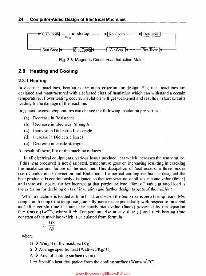
Magnetic Circuit in an Induction Motor is as shown in Fig. 2.8.
www.EngineeringEBooksPdf.com
24 Computer-Aided Design of Electrical Machines
Stat-Tooth Air-Gap .. Rot-Tooth Rot-Core Flux
Stat-Core Stat-Tooth Air-Gap Rot-Tooth
Fig.2.8 Magnetic-Circuit in an Induction Motor.
2.8 Heating and Cooling
2.8.1 Heating
In electrical machines, heating is the main criterion for design. Electrical machines are designed and manufactured with a selected class of insulation which can withstand a certain temperature. If overheating occurs, insulation will get weakened and results in short circuits leading to the damage of the machine.
In general excess temperatures can change the following insulation properties:
(a) Decrease in Resistance
(b) Decrease in Electrical Strength
(c) Increase in Dielectric Loss angle
(d) Increase in Dielectric losses
(e) Decrease in tensile strength.
As result of these, life of the machine reduces.
In all electrical equipments, various losses produce heat which increases the temperature. If this heat produced is not dissipated, temperature goes on increasing resulting in cracking the insulation and failure of the machine. This dissipation of heat occurs in three modes (i.e.) Conduction, Convection and Radiation. If a perfect cooling medium is designed the heat produced is continuously dissipated so that temperature stabilizes at some vallie (Omax) and there will not be further increase at that particular load. "8max " value at rated load is the criterion for deciding class of insulation and further design aspects of the machine.
When a machine is loaded at time t = 0, and when the temp rise is zero (Temp rise = M/c temp - amb temp), the temp-rise gradually increases exponentially with respect to time and and after certain time it attains the steady state value (8max) governed by the equation o = Omax (I_e-t/T
), where 8 -? Temperature rise at any time (t) and! -? heating time constant of the machine which is calculated from formula
GS !=-
AI..
where
G -? Weight of the machine (Kg)
S -? Average specific heat (Watt-sec/KgfOC)
A -? Area of cooling surface (sq.m)
A -? Specific heat dissipation from the cooling surface (Warts/m2/°C)
www.EngineeringEBooksPdf.com
Basic Concepts of Design 25 ----------------------------------------------------~.
2.8.2 Cooling
When load is removed and the machine is stopped, temperature-rise gradually decreases and cools down exponentially with respect to time, as governed by the formula
Be = Bh x e-1/TC
where
eh -7 Temp-rise of the machine just before stopping and load removed
Oc -7 Temperature rise at any time(t)
rc -7 cooling time constant of the machine
Effect ojji-equent healing alld cooling 011 {/ machine
If a machine is subjected for loading and un-loading many times in day, thermal expansion and contraction of insulation occurs and results in early cracking down of insulation and reduction in its life period. Hence, design of such machines needs additional care.
2.9 Modes of Heat Dissipation
Heat is dissipated by three modes: I. Conduction 2. Convection and 3. Radiation
Since Transformer is a static device, no rotational losses. Heat produced by core and windings are to be dissipated by tank.
In most power transformers watt loss per Kg in the iron and the watt loss per Kg in the copper will be nearly equal. This means that the total losses to be dissipated vary as the weight or volume of the material (L"'), where "L" represents the dimensions of transformer. On the other hand, cooling surface provided by the tank of the transformer varies as (L\ As the size of the transformer is increases, the ratio of heat generation volume to surface for dissipation (L 3/ L 2) becomes large.
For small transformers a smooth case readily dissipates the heat as can be seen from the above by Convection and Radiation. But in case of rotating machines, rotational losses exist and heat transfer takes place by Conduction and Convection with negligible radiation.
2.10 Standard Ratings of Electrical Machines
Rating of Electrical Machine is mainly decided by the Temp-Rise and Class of Insulation used in the machine. Let us take an example of a electric motor already manufactured with a given class of insulation. If it i~ loaded continuously at the rated load, let the stabilized temp-rise attained be "T". Now if it is over-loaded by, say, 50% and allowed for continuous operation, the stabilized temperature would be much higher than "T" at which the insulation may fail. Now instead of allowing continuously at this load, if it is loaded for a sh0l1 time (say, 30 sec) so that the temp-rise will not exceed "T", then the short-time rating of the machine said to be 150% and short time is 30 sec. Similarly if same temp-rise is attained when run at 125% load for I mt, the one minute rating is 125%.
www.EngineeringEBooksPdf.com

26 Computer-Aided Design of Electrical Machines
Based on this understanding, ratings are classified as follows:
(a) Continuous rating
(b) Short time rating
(c) Intermittent-periodic rating (Cyclic loading, ex: 15 mts "ON" and 30 mts "OFF"). For ~ this type of load, there will be initial temp-rise before every start.
(d) RMS horse power rating: When the load on the motor changes in cyclic order in some of the industrial applications such as rolling mills, cranes, hoists etc., in these
applications the motor may be required to deliver a particular constant load for a fixed period after which it may deliver another value of constant load for another fixed time, which may be tollowed by a no-load period. The heating of motor in such type of loadings is prop0l1ionai to HP delivered to the load. Thus for such load cycles
) ? ?
(HP.,- XII) + (HP2- x/2)+(HP,- x/3)+ ... RMS Horse Power rating =
(11+/2+/3+ .. .)
2.11 Ventilation Schemes
2.11.1 In Static Machines (Transformers)
Since transformer is a static device, no heat transfer by conduction and hence cooling is more difficult than a rotating machine and the problem of getting rid of the heat in large transformers is more difficult. This will explain the progressive design with increasing transformer size, fluted tanks, tubular construction (to increase the surface area) and finally in the largest sizes the necessity of artificial cooling.
Natural Radiation (AN): Small transformers using for metering and power are cooled by natural ventilation and convection of heat from their surfaces.
Air Blast (AB): Instead of immersing the transformer in oil the heat is dissipated by a blast of air forced through special venti lating ducts in core and between sections of wind ing.
This method of cooling requires a supply of clean air, fans, and special construction to assure its correct distribution. Its advantage lies in reduced fire and explosion risks.
Oil-Immersed, Self Cooled (ON):- The transformer is immersed in a tank filled with oil, which acts as an insulator also. Heated oil due to its lower density rises up through the circulating ducts of winding giving away its heat to the sides of the tank from which it is radiated to surrounding air. The oil becomes cold and because of its higher density flow down, thus creating a natural circulating path.
Large capacity transformers require corrugations on the surface of the tank or radiating jackets to increase the surface area.
Oil-Immersed, Forced Oil Cooled (OFN): Oil is circulated by a pump
Oil-Immersed, Forced Oil Cooled (OFB): Air is blasted by a fan
www.EngineeringEBooksPdf.com
Basic Concepts of Design 27
Oil-Immersed Water cooled (OFW): Instead of depending entirely upon the transfer of heat
from the oil to the outside surface of the tank, some of the heat can be dissipated from the
oil (circulated by a pump) in the coiled tubes in the top of the tank. Circulating water is
forced through these coils. Occasionally the oil is circulated and cooled outside the transformer.
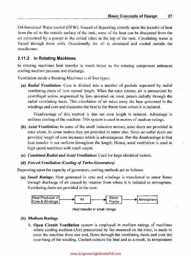
2.11.2 In Rotating Machines
In rotating machines heat transfer is much better as the rotating component enhances cooling medium pressure and discharge.
Ventilation inside a Rotating Machines is of four types:
(a) RlIt/illl Velltillltioll: Core is divided into a number of packets separated by radial
ventilating ducts of Icm normal length. When the rotor rotates, air is pressurized by centrifugal action, augmented by fans mounted on rotor, passes radially through the
radial ventilating ducts. This circulation of air takes away the heat generated in the
windings and core and dissipates the heat to the frame from where it is radiated.
Disadvantage of this method is that net core length is reduced. Advantage is
uniform cooling of thc machine. This system is used in motors of medium ratings.
(b) Axilll Ventillltion: In some of the small induction motors, axial ducts are provided in rotor alone. In somc motors they are provided in stator also. Since no radial ducts are provided length of core increases which is advantageous. But the disadvantage is that
heat transfer is not uniform throughout the length. Hence, axial ventilation is used in
high speed machines with small output.
(c) Combinet/ RlIt/illlllntl Axilll Ventillltioll: Used for large electrical motors.
(d) Forcetl- Ventillltioll (Cooling of Tllrbo-GeneTlltor!t~
Depending upon the capacity of generators, cooling methods are as follows:
(a) Smllll RlItings: Heat generated in core and windings is transferred to stator frame through discharge of air caused by rotation from where it is radiated to atmosphere.
Ventilating ducts are provided in the core.
Heat transfer in small ratings.
(b) Medium Ratings
1. Open Circuit Ventilation system is employed in medium ratings of machines where cooling medium (Air) pressurized by fan mounted on the rotor, is made to enter the machine from one end, flows through the ventilating ducts and over the over-hang of the winding. Coolant extracts the heat and as a result, its temperature
www.EngineeringEBooksPdf.com
28 Computer-Aided Design of Electrical Machines
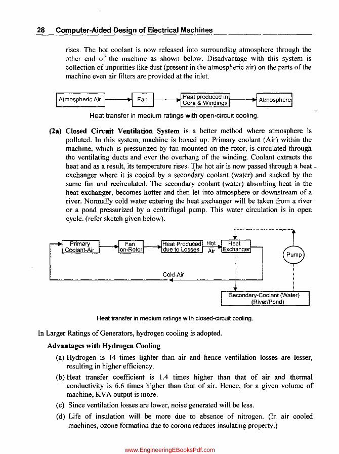
rises. The hot coolant is now released into surrounding atmosphere through the other end of the machine as shown below. Disadvantage with this system is collection of impurities like dust (present in the atmospheric air) on the parts of the machine even air filters are provided at the inlet.
Atmospheric Air I-----I~ I--__ ~ Heat produced in I-_~~ Core & Windings
Heat transfer in medium ratings with open-circuit cooling.
(2a) Closed Circuit Ventilation System is a better method where atmosphere is polluted. In this system, machine is boxed up. Primary coolant (Air) within the machine, which is pressurized by fan mounted on the rotor, is circulated through the ventilating ducts and over the overhang of the winding. Coolant extracts the heat and as a result, its temperature rises. The hot air is now passed through a heat _. exchanger where it is cooled by a secondary coolant (water) and sucked by the same fan and recirculated. The secondary coolant (water) absorbing heat in the heat exchanger, becomes hotter and then let into atmosphere or downstream of a river. Normally cold water entering the heat exchanger will be taken from a river or a pond pressurized by a centrifugal pump. This water circulation is in open cycle. (refer sketch given below).
Primary Coolant-Air
Heat Produced due to Losses I--~~
Cold-Air
r" .- ........... _. -.... .......... ""''''''-l
T Secondary-Coolant (Water)
(River/Pond)
Heat transfer in medium ratings with closed-circuit cooling.
In Larger Ratings of Generators, hydrogen cooling is adopted.
Advantages with Hydrogen Cooling
(a) Hydrogen is 14 times lighter than air and hence ventilation losses are lesser, resulting in higher efficiency.
(b) Heat transfer coefficient is 1.4 times higher than that of air and thermal conductivity is 6.6 times higher than that of air. Hence, for a given volume of machine, KVA output is more.
(c) Since ventilation losses are lower, noise generated will be less.
(d) Life of insulation will be more due to absence of nitrogen. (In air cooled machines, ozone formation due to corona reduces insulating property.)
www.EngineeringEBooksPdf.com

Basic Concepts of Design 29
(e) No fonnation of dust on machine parts like in air cooled machines.
(t) Since hydrogen is not a supporter of combustion, risk of fire within the generator is eliminated.
Disadvantages
(a) If air content in the hydrogen exceeds 22% the gas will explode. To prevent this, hydrogen cooled generators are to be sealed with seal oil system to prevent leakage of hydrogen. Frame is also to be designed against possible explosion.
(b) Hydrogen can not be directly filled into the generator as air is present. First, air has to be purged out by another inert gas (C02) which is later to be replaced by H2• Reverse process is to be followed during shutting down. These operations increase the time of starting and shutting down.
(c) These three auxiliary systems (H2, CO2 and Seal Oil) along with their control panels increase both initial and operational costs in addition to requirement of more space. Hence hydrogen cooling is not economical below certain ratings.
(d) Explosion hazard in the space surrounded by the machine exists with any leakage of hydrogen from the generator.
(2b) Hydrogen Cooled Generator is Always Closed Circuit Ventilation System. In this system, machine is boxed up tightly. Primary coolant (Hydrogen) within the machine is pressurized by fan mounted on the rotor, is circulated through the ventilating ducts and over the overhang of the winding. Coolant extracts the heat and as a result, its temperature rises. The hot hydrogen is now passed through a heat exchanger where it is cooled by a secondary coolant (water) and sucked by the same fan and recirculated. The secondary coolant (water) after absorbing heat in the heat exchanger, becomes hotter and then let into atmosphere or down stream of a river. Nonnally cold water entering the heat exchanger will be taken from a river or a pond pressurized by a centrifugal pump. This water circulation is in open cycle. (refer sketch given below).
Heat Produced ...,.,...~'--~ due to Losses
Cold-Hydrogen
l···········································r
? Secondary-Coolant (Water)
(RiverIPond)
Heat transfer in larger ratings with closed-circuit hydrogen cooling.
www.EngineeringEBooksPdf.com

30 Computer-Aided Design of Electrical Machines
3. Water Cooling
In large generators of ratings above 500 MW, water is lIsed as cooling medium as
hydrogen cooling is not sufficient. Since specific heat and thermal conductivity of water is much higher than hydrogen, water cooling is techno-economically much advantageous.
2.12 Quantity of Cooling Medium
The Quantity of cooling medium needed to dissipate the heat caused by the losses in the machine is given by the equation (II) = (Q x d) x Cp x e, where
H = Losses to be dissipated by cooling medium (KW)
Q -7 Discharge of cooling medium (m'/sec)
d -7 Density of cooling medium(Kg/mJ)
Cp -7 Specific heat (KW-sec)/Kg/°C
e -7 Temp-rise (0C)
It is to be noted that losses to be dissipated by cooling medium do not include bearing friction losses which are normally cooled by bearing oil in medium and larger generators.
In medium and larger generators two fans will be mounted on rotor on either end of generator, each fan designed to produce half the discharge (Q/2). The machine is having a ventilation system balanced on both sides with reference to axial centre of the machine.
2.13 Types of Enclosures
Electrical machine is protected by a metallic cover called enclosure against ingress of moisture, dust, atmospheric impurities and any foreign material. The degree of protection varies in different environments. If the machine is provided under a roof, it is safe from certain problems like falling of rain, snow etc. But still protection is required from air born dust etc. If the machine is not having a roof, higher degree of protection is required.
Ifhigher degree of protection is provided, cooling is lower and vice versa.
Depending upon the required degree of protection, enclosures are classified into following types:
(a) Open Type: Ends of machine are in contact with atmosphere. Cooling is better. Here it is with lowest degree of protection.
(b) Protected type: End covers are provided with holes for ventilation.
(c) Screen protected type: A wire mesh to prevent foreign bodies is additionally provided for protected type (b).
(d) Drip Proof type: In a damp environment hanging bowls are provided, so that condensed moisture does not enter the machine.
www.EngineeringEBooksPdf.com

Basic Concepts of Design 31
(e) To/ally Enclosed type: Machines of closed circuit cooling as mentioned above are
provided with this type of enclosure.
(1) Flame type: Provided for machines working 111 explosive and fire hazard
environments like coal mines etc.
2.14 General Design Procedure
Sequential steps involved in the design and manufacture of any product:
I. Customer specification as per contract, if available, should be read and salient points
of design parameters to be highlighted.
2. Latest National/International standards applicable for this design should be referred.
3. Calculation of main dimensions and subsequently dimensions of each part and
Performance parameters, using well-proven computer programs, established with
equations, scientific formulae, empirical formulae based on previous experience,
curves, tables, charts, etc.
4. Ensuring that the volume and weight of the product do not pose any problem for
either manufacture at works or transport to site or erection and commissioning at site.
Any foreseen problems should be solved before the related activity begins.
5. Preparation of the specifications of each type of materials used in the product.
6. Preparation of drawings of each part and furnishing to manufacturing shops, Purchase
department for purchase of raw materials, tools and sub-contracted items.
7. Writing of process (Sequential steps involved): How to manufacture each part, clearly
indicating the types of tools, machines, workmen, etc.
8. Writing of process: How to sequentially assemble each part/component.
9. Writing the process how to carry out tests on each component and fully assembled
machine to check the quality as specified by standards.
10. Manufacturing the components and carrying out in-process tests.
II. All components are assembled and testing has to be carried out on full machine
12. If it is a new design, additional tests (type tests) to be done over and above the normal
routine tests specified.
13. Dispatching the machine to customer site where it is erected and commissioned to
keep ready for normal operation.
14. Loading the machine at rated conditions and checking the performance.
www.EngineeringEBooksPdf.com

32 Computer-Aided Design of Electrical Machines
2.15 Steps to Get Optimal Design
(a) Input parameters like KW, Voltage, PF, Frequency, and any parameter guaranteed to customer etc., to be kept constant.
(b) Operating range (minimum and maximum values) of various input design parameters to be selected (like Flux densities, Current densities etc.)
(c) Maximum and minimum values of certain output parameters to be incorporated
(like number of stator slots, % Regulation etc.)
(d) A well proven computer program is run to print out various possible alternative designs.
(e) Optimization criteria to be identified. (like lower cost, lower weight, lower
Kg/KVA, Higher efficiency, lower temp-rise, etc.)
(t) Optimal design is selected to suit the optimization criteria.
www.EngineeringEBooksPdf.com

------ ----------------
CHAPTER 3
Armature Windings
3.1 Introduction In this chapter of armature windings, details are given how to design the scheme of winding after completion of calculations of number of poles, number of slots, conductors per slot, chording pitch etc.
3.2 Important Terms Related to Armature Windings (a) Conductor: Active length of winding wire or strip in a slot.
(b) Turn: A turn consists of two conductors placed inside separate slots on the armature periphery approximately a pole pitch apart as shown in Fig. 3.1. These conductors lie under opposite poles so that emf induced in the turn is additive.
(c) Coil: A coil may consist of one or more number of turns connected in series. If it contains two or more number of turns, it is called a multi-turn coil. Refer Fig. 3.1.
B -. -.
I
-. -.
'" '" IC I
-. -.
'" '"
I I I I I I I I I I
AB--> Conductor ABC->Single Turn Coil
Fig. 3.1
I I I I I I I I I
I I I I I I I I I
.", ~ .,.,. " .;.; '"
IQ I
PQ--> MUlti-turn Coil (3 Turns)
www.EngineeringEBooksPdf.com

34 Computer-Aided Design of Electrical Machines
) (d) Coil-side: A coil consists of two coil sides, upper or lower coil sides placed in two different slots, approximately a pole pitch apart.
(e) Over-hang: End portion of coil connecting the two conductors or coil sides is called overhang winding.
(t) Coii-Span: Distance measured in a number of slots between two coil sides of a coil placed in slots over the periphery of the armature.
(g) Full Pitch Coil: If the coil span is exactly equal to a pole pitch (=slots/pole) then it is full pitched coil.
(h) Short Pitched coil/Chorded coif: If the coil span is not equal to a pole pitch (usually less only) then it is called Short pitched coil.
3.3 Classification of Armature Windings
Armature-Windings
(a) Single-Layer: Slot contains only one conductor or one coil side
(b) Double-Layer: Slot contains two coil sides. Top/upper coil side of a slot (A) in Fig.3.2 connected to bottom/lower coil side of another slot (B) which is approximately one pole pitch away and bottom/lower side of slot (A) connected to top/upper coil side of another slot (C) which is approximately one pole pitch away.
In Fig. 3.2, A, B, C are three slots located on the armature at approximately at one pole pitch apart, having (I, 2), (3, 4) and (5, 6) as top and bottom conductors respectively. Coil side no.1 (top) of slot A is connected to Coil side.4 (bottom) of slot B and Coil side.2 of slot A(bottom) is connected to coil side 5(top) of slot C.
~ L2..J ~ ---..uJ CAB
Fig. 3.2
Each turn consists of two coil sides placed in slots separated by approximately one pole pitch apart. Each tum has to be connected with the other to complete the total winding. This connection can be done in two ways,
www.EngineeringEBooksPdf.com

Armature Windings 35
either by Lap winding or Wave winding. Finally each coil end will be connected to one commutator segment.
(c) Lap-Winding:]f both the coil sides are connected to adjacent commutator segments, say, I and 2 as shown in Fig. 3.3, and further connections are made in this manner, it is called simple Lap-winding. Here coml\lutator pitch is unity (± 1). It is to be noted that both first and second coils connected in series lie under same set of poles. For machines designed for higher currents more number of parallel paths are required. Then it is called Multiplex Lap winding. For example, if two parallel paths are provided, it is called Duplex Lap winding and commutator pitch is (±2).
North Pole
... ... ... ... ... ... ... ... ... ... ... ... ... ... I " I I I I I I
1, 2 & 3 --> Commutator Segments
Fig. 3.3 Lap-winding.
(d) Wave-Winding:]f both the coil sides are connected to commutator segments which are approximately two poles pitches apart (actually the winding pitch depends on number of poles and number of commutator segments?, say, I to X as shown in Fig. 3.4 and further connections are made in this manner, it is called simple Wave-winding.
]t is to be noted that first and second coils connected in series lie under different set of poles. For machines designed for higher currents more number of parallel paths are required. Then it is called Multiplex Wave winding. For example, if two parall~1 paths are provided, it is called Duplex Wave winding.
www.EngineeringEBooksPdf.com

36 Computer-Aided Design of Electrical Machines
.... ........ ........ ....
North Pole
.... "-I I I
I I
t. ....
1 & X --> Commutator Segments
Fig. 3.4 Wave-winding.
North Pole
(e) Progressive Winding: Back pitch (Yb) is higher than the front pitch and winding progresses in clock-wise direction when viewed from commutator end. (Fig. 3.5).
(f) Retrogressive Winding: Front pitch (Yf) is higher than back pitch and winding progresses in Anti-clockwise direction when viewed from commutator end.
(g) Full Pitched Winding: If the coil span is exactly equal to a pole pitch (=slots/pole) then it is full pitched coil.
(h) Short Pitched Winding/Chorded Winding: If the coif span is not equal to a pole pitch (usually less only), then it is called Short pitched coil.
3.4 Winding Pitches (Refer Figures 3.5 and 3.6) (a) Back pitch (Yb): Distance between two coil sides of the coil at the back of the
commutator is called Back pitch.
(b) Front pitch (Yf): Distance between finish of a coil and the starting of next coil which are connected to same commutator segment, is called Front pitch.
(c) Resnltant pitch: Distance between starting of two consecutive coils is called resultant pitch (Yr).
For Lap Winding: Yr =Yb - Yf.
For Wave Winding: Yr = Yb + Yf.
www.EngineeringEBooksPdf.com
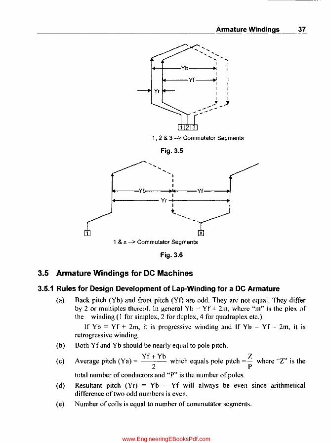
Armature Windings 37
............... ..... ..... ..... ..... ..... .....
" " I I I+--+---Yb ~I I
"
I I I+---Yf ~I I
I I
,
I I I I I I
,,'Y ~
, .......................... .....
1, 2 & 3 --> Commutator Segments
Fig. 3.5
..... ..... ..... ..... I I I
I+---:Yb ~I" Yf--~ I 1+------ Yr -1-------+1 I
t.
1 & X --> Commutator Segments
Fig. 3.6
3.5 Armature Windings for DC Machines
3.5.1 Rules for Design Development of Lap-Winding for a DC Armature
(a) Back pitch (Yb) and front pitch (Yi) are odd. They are not equal. They differ by 2 or multiples thereof. In general Yb = yf ± 2m, where "m" is the plex of the winding (1 for simplex, 2 for duplex, 4 for quadraplex etc.)
(b)
(c)
(d)
(e)
If Yb = yf + 2m, it is progressive winding and If Yb = Yf - 2m, it is retrogressive winding.
Both yf and Yb should be nearly equal to pole pitch.
A . I (Y) yf + Yb h· h I I . h Z h "Z"· h verage PltC 1 a = w IC equa s po e PltC =- were IS t e 2 P
total number of conductors and "P" is the number of poles.
Resultant pitch (Yr) = Yb - Yf will always be even since arithmetical difference of two odd numbers is even.
Number of coils is equal to number of commutator segments.
www.EngineeringEBooksPdf.com

38 Computer-Aided Design of Electrical Machines
(f)
(g)
(h)
Number of parallel paths in armature is equal to "mP", where "P" is number of poles and "m" is the plex of winding.
Commutator pitch Y c = ± 1m, "+ I" for progressive and "-I" for retrogressive windings.
Yb = Z + I and Yf = Z -I for Progressive winding p p
Z Yb= --I
P and Yf= Z +1 for Retrogressive winding.
P
3.5.2 Example for 4 Pole, 16 Slot DC Machine with Progressive Simplex Double Layer Lap Winding (Refer Fig. 3.7)
Number of Poles (P) = 4;
Total number of conductors (Z) = slots x conductors/slot = 16 x 2 = 32
- For Progressive winding, Back Pitch (Yb) = Z + I = 32 + I = 9 P 4
and Front Pitch (Yf) = Z -1 = 32 -1 = 7 P 4
In Double Layer winding, top conductors in slots are given odd numbers (I, 3, ...... .31) and bottom conductors are given even numbers (2, 4 ......... 32)
To start with top conductor in slot no. I is connected to bottom conductor of (I + Yb) = (1 + 9) = lOon one end. The other end of conductor "10" is connected to (10 - Yf) = (10 - 7) = 3 and it goes on accordingly as per the following table.
Sr. No No. of Top No. of Bottom Conductor No of Top Conductor (Zt) Conductor (Zt) (Zb) Zb = Zt + Vb Zt= Zb- Vf
1 1 1 + 9:::: 10 10 -7:::: 3
2 3 3 + 9:::: 12 12 - 7:::: 5
3 5 5 + 9:::: 14 14 -7:::: 7
4 7 7 + 9:::: 16 16 -7:::: 9
5 9 9 + 9:::: 18 18-7::::11
6 11 11 + 9:::: 20 20 -7:::: 13
7 13 13+9::::22 22 -7:::: 15
8 15 15 + 9:::: 24 24 -7:::: 17
9 17 17 + 9:::: 26 26 -7:::: 19
10 19 19 + 9:::: 28 28 - 7:::: 21
11 21 21 + 9:::: 30 30-7:::: 23
12 23 23 + 9:::: 32 32 -7:::: 25
13 25 25 + 9 :::: 34 (:::: 34 - 32 :::: 2) 34 -7:::: 27
14 27 27 + 9 :::: 36 (:::: 36 - 32:::: 4) 36-7:::: 29
15 29 29 + 9:::: 38 (:::: 38 - 32 = 6) 38 - 7 = 31
16 31 31+ 9 :::: 40 (:::: 40 - 32 = 8) 40 - 7 = 33(33 - 32 :::: 1)
www.EngineeringEBooksPdf.com
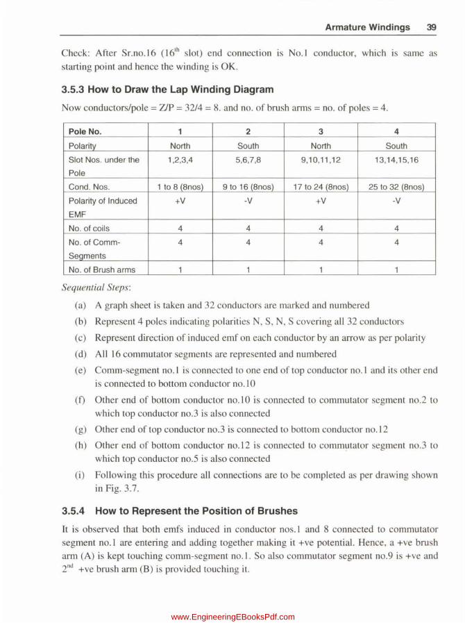
Armature Windings 39
Check: After Sr.no.16 (l6th slot) end connection is No.1 conductor, which is same as
starting point and hence the winding is OK.
3.5.3 How to Draw the Lap Winding Diagram
Now conductors/pole = 'ZiP = 32/4 = 8. and no. of brush arms = no. of poles = 4.
Pole No. 1 2 3 4
Polarity North South North South
Slot Nos. under the 1,2,3,4 5,6,7,8 9,10,11 ,12 13,14,15,16
Pole
Condo Nos. 1 to 8 (8nos) 9 to 16 (8nos) 17 to 24 (8nos) 25 to 32 (8nos)
Polarity of Induced +v -v +v -v EMF
No. of coils 4 4 4 4
No. of Comm- 4 4 4 4
Seqments
No. of Brush arms 1 1 1 1
Sequential Steps:
(a) A graph sheet is taken and 32 conductors are marked and numbered
(b) Represent 4 poles indicating polarities N, S, N, S covering all 32 conductors
(c) Represent direction of induced emf on each conductor by an arrow as per polarity
(d) All 16 commutator segments are represented and numbered
(e) Comm-segment no. 1 is connected to one end of top conductor no. 1 and its other end
is connected to bottom conductor no. 1 0
(f) Other end of bottom conductor no. 10 is connected to commutator segment no.2 to
which top conductor nO.3 is also connected
(g) Other end of top conductor no.3 is connected to bottom conductor no.12
(h) Other end of bottom conductor no.12 is connected to commutator segment no.3 to which top conductor no.5 is also connected
(i ) Following this procedure all connections are to be completed as per drawing shown in Fig. 3.7.
3.5.4 How to Represent the Position of Brushes
It is observed that both emfs induced in conductor nos. 1 and 8 connected to commutator segment no. 1 are entering and adding together making it +ve potential. Hence, a +ve brush arm (A) is kept touching comm-segment no.l . So also commutator segment no.9 is +ve and 2nd +ve brush arm (B) is provided touching it.
www.EngineeringEBooksPdf.com

(32 conductors, 16 Commutator Segments)
25
~ - - - - - - - - - - - - - - - - - - - - __ - - - - - L _ _ _ _ _ _ _ _ _ _ _ _ _ _ _____ ~ Terminal : ·ve
..... --------------------''-----_Termlnal: +ve
1) Conductors with odd numbers are "TOP" of slot & Conductors with even number are "BOTTOM" of slot
2) Direction of Arrows represent Direction of Induced EMFs
3) B+ -> Positive brush & B-ve -> Negative Brush
Fig. 3.7 Winding diagram of 4 pole, 16 slot, double layer simplex lap winding .
10
5 6
C') o 3
"tJ c::: -CD ";' l> a: CD Q,
C CD til
cC' ::::J
o -
www.EngineeringEBooksPdf.com

Armature Windings 41
Using the same logic -ve brush arms C and D are positioned touching commutator
segments 5 and 13 where emfs/currents are leaving.
Both +ve brush arms A and B are connected together making one single positive
. terminal and both -ve brush arms C and D are connected together making one single
negative terminal.
Current / Parallel Path Now number of brushes in each arm = ----------
Current density & Brush Area
3.5.5 Rules for Design Development of Wave-Winding
(a) Back pitch (Yb) and front pitch (Yf) are odd. They may be equal or differ by 2.
Both yf and Yb should be nearly equal to pole pitch.
(b) A . h(Y) Z±2 Z/2±1 No.ofCommutatorBars±1
verage Pitc a = -- = = ----------P P / 2 Pairs of Poles
(c) Resultant pitch (Yr) = Yb + yf
(d) Commutator pitch Yc = Ya
(e) No. of coils is equal to no. of commutator segments
(f) No. of parallel paths in armature is equal to "2m" where "m" is the plex of winding
3.5.6 Example for 4 Pole, 17 slot DC Machine with Double Layer Wave
Winding
No. of Poles (P) = 4;
Total no. of conductors (Z) = slots x conductors/slot = 17 x 2=34
Average Pitch (Ya) = Z ± 2 = 34 ± 2 = 8 or 9 and Resultant pitch (Yr) = 16 or 18 P 4
(Here three options are available: (1 )Yf = Yb = 9, (2)Yb = 7 and yf = 9, (3)Yb = 7 and
Yf= 9. all are OK) Now Yf= Yb = 9 option is selected.
Commutator pitch (Y c) = Ya = 9
Since this is a Double Layer winding, top conductors in slots are given odd numbers
(1,3, ...... .33) and bottom conductors are given even numbers (2,4 ......... 34).
To start with, top conductor in slot no. 1 is connected to bottom conductor of (1 + Yb) = (1 + 9) = 10 on one end. The other end of conductor "10" is connected to (10 + Yf) = (10 + 9) = 19 and it goes on accordingly as per the following Table.
www.EngineeringEBooksPdf.com

42 Computer-Aided Design of Electrical Machines
Sr. No. of Top No. of Bottom Conductor (Zb) No of Top Conductor (Zt) No Conductors (Zt) Zb = Zt+ Vb Zt = Zb + Vf 1 1 1 + 9 = 10 10+9=19 2 19 19 + 9 = 28 28 + 9 = 37(37 - 34 = 3) 3 3 3 + 9 = 12 12+9=21 4 21 21 + 9 = 30 30 + 9 = 39 (39 - 34 = 5) 5 5 5 + 9 = 14 14 + 9 = 23 6 23 23 + 9 = 32 32 + 9 = 41 (41 - 34 = 7) 7 7 7 + 9 = 16 16 + 9 = 25 8 25 25 + 9 = 34 34 + 9 = 43 (43 - 34 = 9) 9 9 9 + 9 = 18 18 + 9 = 27 10 27 27 + 9 = 36 (36 - 34 = 2) 2+9=11 11 11 11 + 9 = 20 20 + 9 = 29 12 29 29 + 9 = 38 (38 - 34 = 4) 4 + 9 = 13 13 13 13 + 9 = 22 22+9=31 14 31 31 + 9 = 40 (40 - 34 = 6) 6 + 9 = 15 15 15 15 + 9 = 24 24 + 9 = 33 16 33 33 + 9 = 42 (42 - 34 = 8) 8 + 9 = 17 17 17 17 + 9 = 26 26 + 9 = 35 (35 - 34 = 1)
Check ~ After Sr.no.17 (l7th slot) end connection is No.1 conductor which is same as starting point. It is OK.
3.5.7 How to Draw the Wave Winding Diagram
No. of comm-segments = no. of coils = 17 and no. of brush arms = no. of poles = 4
Pole No: 1 2 3 4 Polarity North South North South Polarity of Induced EMF +V -V +V -V No of Brush arms 1 1 1 1
Sequential Steps
(a) A graph sheet is taken and 34 conductors are marked and numbered. (b) Represent 4 poles indicating polarities N, S, N, S covering all 34 conductors. (c) Represent direction of induced emf on each conductor by per polarity. (d) All 17 commutator segments are represented and numbered. (e) Comm-segment no. 1 is connected to one end of top conductor no. 1 and its other end
is connected to bottom conductor no.l0. (t) The other end of bottom conductor no. 1 0 is connected to commutator segment no
(l + 9 = 10) to which top conductor no.19 is also connected. (g) The other end of top conauctor no.19 is connected to bottom conductor no.28 (h) T-he other end of bottom conductor no.28 is connected to commutator segment no:
10 + 9 = 19 (19 - 17 = 2) to which top conductor no.28 is also connected. (i) Following this procedure all connections are to be completed as per drawing shown
in Fig. 3.8.
www.EngineeringEBooksPdf.com

• • a -- - -
(34 conductors, 17 Commutator Segments)
27
I - - - - - - - - - - - - _..L ______ .. Terminal : -ve
1---------------------'---------------+ Terminal : +ve
1) Conductors with odd numbers are "TOP" of slot & Conductors with even number are "BODOM " of slot
2) Direction of Arrows represent Direction of Induced EMFs
3) B+ --> Positive brush & B-ve --> Negative Brush
Fig. 3.8 Winding diagram of 4 pole , 17 slot, double layer simplex wave winding .
l> ... 3 II) -c:: Ci1
=E :i" Q,
~ (Q til
www.EngineeringEBooksPdf.com

44 Computer-Aided Design of Electrical Machines
3.5.8 How to Represent the Position of Brushes?
On tracing the trend of emfs through the winding diagram (Fig. 3.8), it is observed that the two emfs meet at one point and separate out at another point. These are the positions of positive and negative brushes respectively. In case these points of meeting and separating the emfs are at the back of the armature, then brushes may be placed at the front (commutator) at positions opposite to these points. It is also seen that there are two parallel circuits in the winding.
3.5.9 Dummy or Idle Coils
These are used with Wave windings and resorted to when the requirements of winding are not met by the standard armature punchings available in armature winding shops. These dummy coils do not influence the electrical characteristics of the winding because they are not connected to commutator. They are only to keep the mechanical balance. They are provided similar to other coils but their ends are cut short and taped.
Example: Suppose a 4 pole, 18 slot, double layer is to be designed with wave winding,
Z = 18 x 2 = 36 and Ya = Z±2 = 36±2 = 9.5 or 8.5 with which winding is not possible. P 4
Now out of 36 conductors, if 2 conductors (l coil) is made dummy a winding with 34 conductors is possible as described above.
3.5.10 Criteria for Decision of Type of Winding
For a given number of poles and KW rating a simple wave winding gives double the voltage and half of the current, whereas simple Lap winding gives half the voltage at double the current. (refer the example given below) .
Advantage with a wave winding is that equalizer connections are not required.
Winding Type Voltage(V) Current(Amps) Power(Watts)
Wave 2xV 1/2 P = (2 x V) x (1/2) = VI
Lap V/2 2*1 P = (V/2) x (2 x I) = VI
Based on a techno-economic study with above considerations, suitable decision is to be made.
3.6 Armature Windings for AC Machines 3.6.1 Similarities between DC and AC Machines
Sr. no. Parameter DC - Machine
1 DC magnetic-Flux Exists 2 Single and Double Layers Exists 3 Lap and Wave Wound Exists 4 Progressive and Exists
Retrogressive 5 Full Pitch and Short pitch Exists
6 Wave form of Air-gap flux Non·Sinusoidal 7 Voltage induced in Armature AC (DC after Commutation)
conductors
AC - Machine(Sync)
Exists Exists
Exists Exists
Exists Non-Si n usoidal AC
www.EngineeringEBooksPdf.com
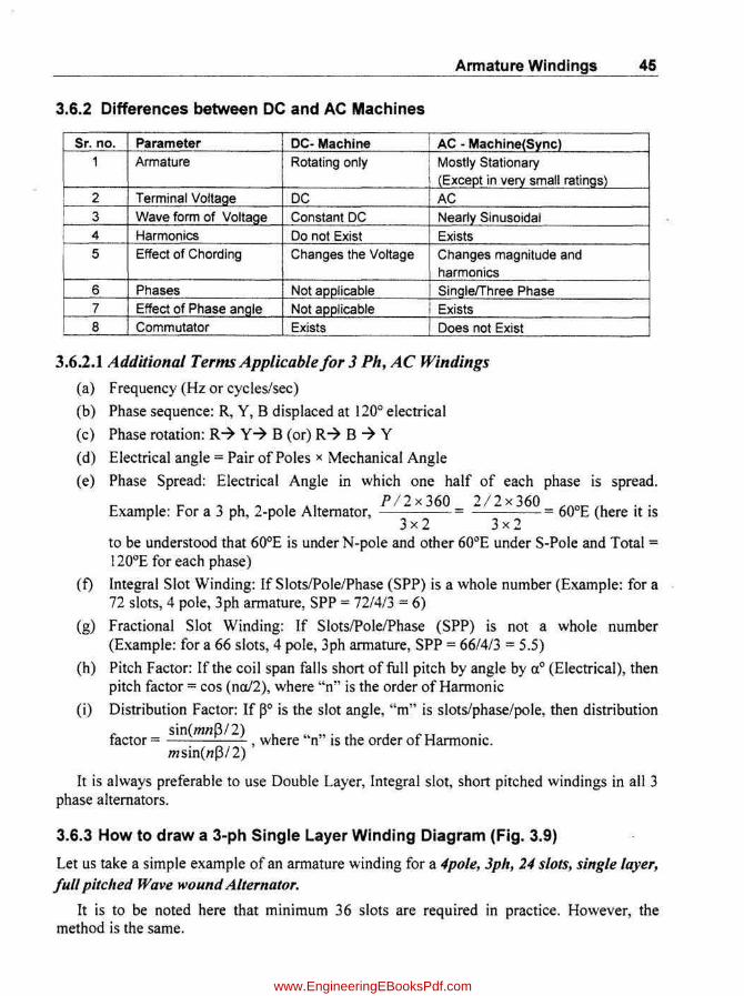
Armature Windings 45
3.6.2 Differences between DC and AC Machines
Sr. no. Parameter DC- Machine AC - Machine(Sync) 1 Armature Rotating only Mostly Stationary
(Except in very small ratings)
2 Terminal Voltage DC AC 3 Wave form of Voltage Constant DC Nearly Sinusoidal 4 Harmonics Do not Exist Exists 5 Effect of Chording Changes the Voltage Changes magnitude and
harmonics 6 Phases Not applicable SinglefThree Phase 7 Effect of Phase angle Not applicable Exists 8 Commutator Exists Does not Exist
3.6.2.1 Additional Terms Applicable for 3 Ph, AC Windings
(a) Frequency (Hz or cycles/sec)
(b) Phase sequence: R, Y, B displaced at 120° electrical
(c) Phase rotation: Ro7 Yo7 B (or) Ro7 B 7 Y
(d) Electrical angle = Pair of Poles x Mechanical Angle
(e) Phase Spread: Electrical Angle in which one half of each phase is spread. P / 2 x 360 2/2 x 360
Example: For a 3 ph, 2-pole Alternator, 600E (here it is 3x2 3x2
to be understood that 600E is under N-pole and other 600E under S-Pole and Total = 1200E for each phase)
(f) Integral Slot Winding: If Slots/Pole/Phase (SPP) is a whole number (Example: for a 72 slots, 4 pole, 3ph armature, SPP = 72/4/3 = 6)
(g) Fractional Slot Winding: If SlotslPolelPhase (SPP) is not a whole number (Example: for a 66 slots, 4 pole, 3ph armature, SPP = 66/4/3 = 5.5)
(h) Pitch Factor: If the coil span falls short of full pitch by angle by aO (Electrical), then pitch factor = cos (na/2), where "n" is the order of Harmonic
(i) Distribution Factor: If po is the slot angle, "m" is slots/phase/pole, then distribution sin(mnf3/2). .
factor = , where "n" IS the order of HarmOniC. msin(nf3/2)
It is always preferable to use Double Layer, Integral slot, short pitched windings in all 3 phase alternators.
3.6.3 How to draw a 3-ph Single Layer Winding Diagram (Fig. 3.9)
Let us take a simple example of an armature winding for a 4pole, 3ph, 24 slots, single layer, full pitched Wave wound Alternator.
It is to be noted here that minimum 36 slots are required in practice. However, the method is the same.
www.EngineeringEBooksPdf.com

46 Computer-Aided Design of Electrical Machines
Pole pitch = 24/4 = 6 slots/pole = 1800 E.
In one full revolution of rotor a conductor in any slot traverses by 360° mech (= 4/2 x
360 = 720° E). Since there are 24 slots, Slot angle = 720/24 = 30° E.
There are 3 phases R, Y and B separated by a phase angle of 120°. If "R" phase starts at 0°, Y phase at 120° later in the direction of phase rotation and B phase at 240° behind. Since slot angle is 30°, Y phase starts at 120/30 = 4 slots later and B phase starts at 4 more slots later.
In terms of slots if R phase starts at slot. 1, Y phase starts at slot no. 1 + 4 = 5 and B phase starts at slot no:5 + 4 = 9.
Since we are assuming full pitched winding, Winding pitch = Pole pitch = 6 slots.
F or a single layer winding there will be one conductor per slot and total no. of conductors will be 24* 1 = 24.
We designate conductors with numbers: 1,2,3,4,5, ................ 24.
Let us Draw the Winding Scheme for "R" Phase First
Conductor (no. 1 ) in first slot is to be connected to one end of conductor (no. 1 + 6 = 7) in slot no.7 (1 + winding pitch = 1 + 6 = 7th). The other end of this conductor (no.7) is to be connected to conductor no.7 + 6 = 13 in the 13th slot. The other end of 13th conductor is connected to conductor no.13 + 6 = 19th
, thus completing half of the "R" phase. This half connection (Rl- R2) is progressive.
The other half connection (R3-RO) is Retrogressive type, starting at conductor no.2 (TerminaI.R3), then connected to conductor numbers 2 -7 20 (2 + 24 - 6 = 20) -7 14 (20 - 6 = 14) -7 8(14 - 6 = 8) which the terminal RO.
The purpose of making one half connection progressive and other half to retrogressive is to provide proper mechanical balance of the end winding connections.
Sequential Steps for drawing the Winding Diagram
(a) A graph sheet is taken and 24 conductors are marked and numbered (However for convenience represent a few repeated conductors both sides)
(b) Represent 4 poles indicating polarities N, S, N, Scovering all 24 conductors
(c) Represent direction of induced emf on each conductor as per polarity (i for N pole and ~ for South pole)
(d) Begin with one end of top conductor (1) and name it Rl, starting of 1 st half of "R" Phase
(e) The other end of Top conductor no. 1 is connected to one end of conductor no. 7
(1) The other end of conductor no.7 is connected to one end of conductor no.13
(g) The other end of conductor no.13 is connected to one end of conductor no.19 (which is named as R2)
(h) Begin with one end of conductor (2) and name it R3, starting of 2nd halfof"R" Phase
(i) The other end of conductor no.2 is connected to one end of conductor nO.20
U) The other end of conductor nO.20 is connected to one end of conductor no.14
www.EngineeringEBooksPdf.com
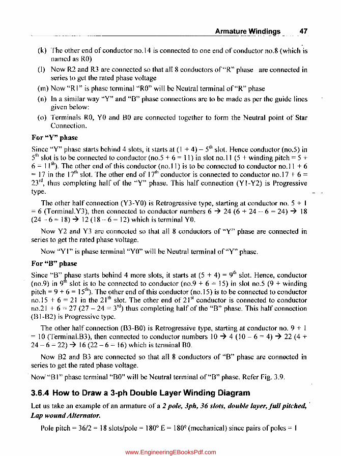
Armature Windings 47
(k) The other end of conductor no.14 is connected to one end of conductor no.8 (which is named as RO)
(I) Now R2 and R3 are connected so that all 8 conductors of"R" phase are connected in series to get the rated phase voltage
(m) Now "R 1" is phase terminal "RO" will be Neutral terminal of"R" phase
(n) In a similar way "Y" and "8" phase connections are to be made as per the guide lines given below:
(0) Terminals RO, YO and 80 are connected together to form the Neutral point of Star Connection.
For "Y" phase
Since "Y" phase starts behind 4 slots, it starts at (1 + 4) = 5th slot. Hence conductor (no.5) in 51h slot is to be connected to conductor (no.5 + 6 = 11) in slot no.11 (5 + winding pitch = 5 + 6 = 11Ih). The other end of this conductor (no.11) is to be connected to conductor no.11 + 6 = 17 in the 171h slot. The other end of 171h conductor is connected to conductor no.17 + 6 = 23 rd
, thus completing half of the "Y" phase. This half connection (Y 1-Y2) is Progressive type.
The other half connection (Y3-YO) is Retrogressive type, starting at conductor no. 5 + 1 = 6 (TerminaI.Y3), then connected to conductor numbers 6 ~ 24 (6 + 24 - 6 = 24) ~ 18 (24 - 6 = 18) ~ 12 (18 - 6 = 12) which is terminal YO.
Now Y2 and Y3 are connected so that all 8 conductors of "Y" phase are connected in series to get the rated phase voltage.
Now "Y I" is phase terminal "YO" will be Neutral terminal of"Y" phase.
For "B" phase
Since "8" ~hase starts behind 4 more slots, it starts at (5 + 4) = 9th slot. Hence, conductor (no.9) in 911 slot is to be connected to conductor (no.9 + 6 = 15) in slot no.5 (9 + winding pitch = 9 + 6 = 15Ih). The other end of this conductor (no.15) is to be connected to conductor no. 15 + 6 = 21 in the 211h slot. The other end of 21 51 conductor is connected to conductor no.21 + 6 = 27 (27 - 24 = 3rd
) thus completing half of the "8" phase. This half connection (81-82) is Progressive type.
The other half connection (83-80) is Retrogressive type, starting at conductor no. 9 + I = 10 (TerminaI.83), then connected to conductor numbers 10 ~ 4 (10 - 6 = 4) ~ 22 (4 + 24 - 6 = 22) ~ 16 (22 - 6 = 16) which is terminal 80.
Now 82 and 83 are connected so that all 8 conductors of "8" phase are connected in series to get the rated phase voltage.
- Now"81" phase terminal "80" will be Neutral terminal of"8" phase. Refer Fig. 3.9.
3.6.4 How to Draw a 3-ph Double Layer Winding Diagram
Let us take an example of an armature of a 2 pole, 3ph, 36 slots, double layer, full pitched, . Lap wound Alternator.
Pole pitch = 36/2 = 18 slots/pole = 1800 E = 180'! (mechanical) since pairs of poles = I
www.EngineeringEBooksPdf.com

48 Computer-Aided Design of Electrical Machines
In one full revolution of rotor a conductor in any slot traverses by 3600E. Since there ate 36 slots, Slot angle = 360/36 = 100E
There are 3 phases R, Y and B separated by a phase angle of 120°. If "R" phase starts at 0°, Y phase is at 120° behind and B phase at 240° behind. Since slot angle is 10°, Y phase starts at 12011 0 = 12 slots later and B phase starts 24 slots later.
In terms of slots if R phase starts at slot. I , Y phase starts at slot no. I + 12 = 13 and B phase starts at slot no.13 + 12 = 25.
Since we are assuming full pitched winding Winding pitch = Pole pitch = 18 slots.
For double layer winding there will be 2 conductors per slot and total no of conductors will be 36 x 2 = 72.
We designate top conductors with odd numbers. I, 3, 5, 7, ................ 69, '71 and bottom conductors with even numbers. 2,4,6,8 ........... 70, 72. (refer Fig. 3.10.)
Let us Draw the Winding Scheme for "R" Phase First
Top conductor (no. I) in first slot is to be connected to bottom conductor (no.38) in slot no. (1 + winding pitch) = (I + 18) = 19th slot making the back pitch = (38 - I) = 37 conductors. -The other end of this bottom conductor (no.38) is to be connected to conductor no.3 in the second slot, thus making the front pitch as (38 - 3) = 35 conductors. The average pitch = (37 + 35)/2 = 36 conductors = 18 slots. In the same way winding scheme for total "R" phase is completed as follows:
Phase Sr. No.
No of Top No. of Bottom Conductor No. of Top Conductor (Zt)
Group Conductor (Zb) (R) (Zt) Zb = Zt+ 37
Zt=Zb-35
1 1 (Beginning) 1 + 37 = 38 38 - 35 = 3 2 3 3 + 37 = 40 40-35=5 3 5 5 + 37 = 42 42 - 35 = 7
I 4 7 7 + 37 = 44 44-35=9
5 9 9 + 37 = 46 46-35=11
6 11 11 + 37 = 48 48 -7 Ending 1 37 (Ending) 37 + 37 = 74 (74 - 72 = 2) 74 - 35 = 39
2 39 39 + 37 = 76 (76 - 72 = 4) 76 - 35 = 41
3 41 41 + 37 = 78 (78 - 72 = 6) 78- 35 = 43 II 4 43 43 + 37 = 80 (80 - 72 = 8) 80 - 35 = 45
5 45 45 + 37 = 82 (82 - 72 = 10) 82-35 = 47 6 47 47 + 37 = 84 (84 - 72 = 12) 12 -7 (Beginning)
Sequential Steps for drawing the Winding Diagram
(a) A graph sheet is taken and 72 conductors are marked and numbered (However for convenience represent repeated conductors on both sides)
(b) Represent 2 poles indicating polarities N, S covering all 72 conductors
(c) Represent direction of induced emf on each conductor as per polarity (i for N pole and ~ for South pole)
www.EngineeringEBooksPdf.com

Armature Windings 49
(d) Begin with one end of top conductor (1) and name it R 1, starting of "R" Phase
(e) The other end of Top conductor no.l is connected to one end of bottom conductor no.38
(f) The other end of bottom conductor no.38 is connected to one end of top conductor. _ no.3
(g) The other end of top conductor no.3 is connected to one end of bottom conductor no.40
(h) The other end of bottom conductor no.40 is connected to one end of top conductor no.5
(i) Following this procedure all connections are to be completed for the Phase group-I and name the end of last conductor (48) as end of Phase group-I (R2)
(j) Similarly connections for Phase group-II have to be done: Here startinffi conductor will be in slot no. I + Pole Pitch = 1 + 18 = 19th. Top conductor in 19 slot is 37. Hence one end of Phase group-II is 37
(k) Using same logic used for Phase group-I, winding scheme connections for Phase group -II is to be completed as per the above table
(I) The other end of Phase group-II will emerge at conductor no.12
(m) As per the emf direction, emf will enter at 12 and leaves at 37. Hence conductor 12 (R3) is conned to R2 and conductor no.37 will be the exit end of emf for total "R" phase and is named as "RO", which will be Neutral point of Star connection
(n) Refer enclosed drawing (Fig. 3.11).
For "Y" phase Since "Y" phase starts behind 12 slots, it starts at (1 + 12) = 13th slot. Hence top conductor (no.25) in 13th slot is to be connected to bottom conductor (no.62) in slot no. (13 + winding pitch) = (13 + 18) = 31 st. In the same way winding scheme for Phase Group-I of "Y" phase is completed. Here conductor (25) is beginning and named as "Y I". Conductor "72" is the ending and named as "Y2"
Similarly connections for Phase group-II has to be done: Here starting conductor will be in slot no. 13 + Pole Pitch = 13 + 18 = 31 st. Top conductor in 31 st slot is 61. Hence one end of Phase group-II is 61 and other end emerges as 36th conductor.
Phase Sr. No No. of Top
No. of Bottom Conductor No. of Top Group (Zb) Conductor (Zt)
IV) Conductor (Zt)
Zb =Zt+ 37 Zt=Zb-35 1 25 (BeQinninQ) 25 + 37 = 62 62- 35 = 27 2 27 27 + 37 = 64 64-35=29 3 29 29 + 37 = 66 66 - 35 = 31
I 4 31 31 + 37 = 68 68-35=33 5 33 33 + 37 = 70 70- 35 = 35 6 35 35 + 37 = 72 72 -7 Endil1& 1 61 (Ending) 61 + 37 = 98 (98 - 72 = 2~ 98-35=63 2 63 63 + 37 = 1001100 -72=2~ 100-35=65 3 65 65 + 37 = 1021102 -72 = 301 102-35=67
\I 4 67 67 + 37 = 104(104-72 = 321 104-35=69 5 69 69 + 37 = 106 {106 -72 = 341 106-35=71 6 71 71 + 37 = 108 (108 - 72 =3 6) 36 -71B~nnil}9t
www.EngineeringEBooksPdf.com

50 Computer-Aided Design of Electrical Machines
As per the emf direction, emf will enter at 36 and leaves at 61 for Phase group-II. Hence conductor 36 (Y3) is conned to 72 (Y2) and conductor no:61 will be the exit end of emf for ~
tota.l "Y" phase and is named as "YO", which will be Neutral point of Star connection _ (see Fig. 3.12).
For "B" phase
Since "8" phase starts behind 12 slots to "Y" phase, it starts at (13 + 12) = 25th slot. Hence top conductor (no.49) in 25th slot is to be connected to bottom conductor (no. 14) in slot no. (25 + winding pitch) = (25 + 18) = 43 rd (43 - 36 = i h
). In the same way winding scheme for phase Group-I of "8" phase is completed. Here conductor (24) is beginning and named as "82". Conductor "49" is the ending and named as "81".
Similarly connections for Phase group-II have to be done: Here starting conductor will be in slot no. 25 + Pole Pitch = 25 + 18 = 43 rd (43 - 36 = 7th). Top conductor in 7th slot is 13. Hence one end of Phase group-II is 13 and other end emerges as 60th conductor.
Phase Sr. No
No. of Top No. of Bottom Conductor No. of Top Conductor Group Conductor (Zb) (Zt)
(8) (Zt) Zb = Zt+ 37 Zt=Zb-35
1 49(Ending) 49 + 37 = 86 (86 - 72 = 14) 86 - 35 = 51
2 51 51 + 37 = 88 (88 - 72 = 16) 88-35=53
3 53 53 + 37 = 90 (90 - 72 = 18) 90-35=55 I 4 55 55 + 37 = 92 (92 - 72 = 20) 92 -35 = 57
5 57 57 + 37 = 94 (94 - 72 = 22) 94- 35 = 59
6 59 59 + 37 = 96 (96 - 72 = 24) 24 -7 Beginning
1 13(Ending) 13 + 37 = 50 50-35=15
2 15 15 + 37 = 52 52 - 35 = 17
3 17 17 + 37 = 54 54-35= 19 II 4 19 19 + 37 = 56 56 - 35 = 21
5 21 21 + 37 = 58 58 -35 = 23
6 23 23 + 37 = 60 60 -7 (Beginning)
Here one important point to be noted is that the algebraic sum of emfs entering at Neutral Point is zero. i.e. Er + Ey + Eb = 0 and hence Er + Ey = - Eb. Hence, the direction of induced emf in "8" phase is negative. 80 is + ve and 8 I is = -ve.
As per the emf direction, emfwill enter at 13 (80) and leaves at 60 (83) for Phase groupII. Hence conductor (83) is connected to (B2). Here 13(BO) is entry point and 49 (Bl) is the Exit point of EMF. (see Fig. 3.13).
For all 3 phases
If we superimpose all the above 3 drawings on a single graph sheet, we obtain complete diagram for all 3 phase windings as shown in Fig. 3.14.
www.EngineeringEBooksPdf.com

R
N ---R1 Y1 B1
Legend:- R1-->Red
Y3
Y1
Direction of Rotation YO
Y1-->Yellow B1-->Blue N-->Neutral B1
Fig. 3.9 4-Pole, 3 phase, 24 slots, single-layer full pitched Winding of alternator. en ....
www.EngineeringEBooksPdf.com

Representation of Slots.Conductors.Phases & Poles :-
Top ~~r13fr15n17ir19fmrrm~rmrml3sCrmIJgff41l----mrl4snn'-1491lsnt531~r61lmrl6sfr67fl691l71l Bottom m tIl tIl m mJ rm ffiI llil ml mJ @1 tEl ml m1 illl @.1 [EJ mJ mJ rnl @] ffi1 ~ @I rnl @l rn1 rn1 rnl t!m @l tBI @l ~ mI @I
Sial No : 10 11 12 13 14 15 16 17 18 19 20 21 22 23 24 25 26 27 28 29 30 31 32 33 34 35 36
Phase:
Y1 Y2
Poles: NORTH·POLE SOUTH·POLE
Fig. 3.10 36 Slots, 2 pole, 3 phase double layer winding.
~
o o 3
" c: -CD ... !: c. CD c. o CD en
cO· ::l
o -m CD (') -.., n· e!. s: I» (') ::l" ::l CD en
www.EngineeringEBooksPdf.com
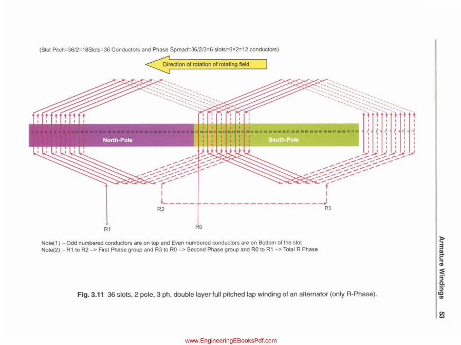
(Slot Pitch=36/2= 18Slots=36 Conductors and Phase Spread=36/2/3=6 slots=6x 2= 12 conductors)
R1
Direction of rotation of rotating field
----~ ~><~~<-~-~-~~-
I
+-----R2
--::~l\\\\\\\\\\\~l\~~~:~::l-_t I I I I I I '12i I ~ I ~ I ~ I'~ " ,~ I I I I I I
~~-~~~~.~~------------------------------~ I I I I I I
~~JJ~~JJ ----..... --------..... ------.......... _---.......... ---..... -----.......... _---.......... _---..... -----1'----I
------------------J R3
RO
Note(1) :- Odd numbered conductors are on top and Even numbered conductors are on Bottom of the slot Note(2} :- R1 to R2 -> First Phase group and R3 to RO -> Second Phase group and RO to R1 -> Total R Phase
Fig.3.11 36 slots, 2 pole, 3 ph, double layer full pitched lap winding of an alternator (only R-Phase).
www.EngineeringEBooksPdf.com

(Slot Pitch=36/2=18Slots=36 Conductors and Phase Spread=36/2/3=6 slots=6 x 2=12 conductors)
~~~~~~~~~'"
-:::~~~~~~~~~~~~~~~::-"~'''''----~
I ~-----
Y2
Y1 YO
Note(1) :- Odd numbered conductors are on top and Even numbered conductors are on Bottom of the slot
Note(2) :- Y1 to Y2 --> First Phase group and Y3 to YO --> Second Phase group and YO to Y1 --> Total Y Phase
Fig. 3.12 36 Slots, 2 pole, 3 ph, double layer full pitched lap winding of an alternator (Only V-Phase).
o o 3
"C s:: -(I) ., l> a. (I) a. C (I) en
CQ ::::s
o -m CD (") -~. (") m
www.EngineeringEBooksPdf.com

(Slot Pitch=36/2=18Slots=36 Conductors and Phase Spread=36/2/3=6 slots=6 x 2=12 conductors)
- -~ -----~ ----------:--'? -%? ~ ----
~----,,::::;::...2';::;::C'$.~;<.;; --;-~ -
I I~ ___ - -----------------~
B2 B3
B1 BO
Note(1) :- Odd numbered conductors are on top and Even numbered conductors are on Bottom of the slot Note(2) :- B1 to B2 --> First Phase group and 83 to BO --> Second Phase group and BO to 81 --> Total B Phase
Fig. 3.13 36 Slots, 2 pole, 3 ph, double layer full pitched lap winding of an alternator (Only B-Phase).
:t-., 3 Q) -c ., CD
~ ~ c. :i" cc t/)
www.EngineeringEBooksPdf.com
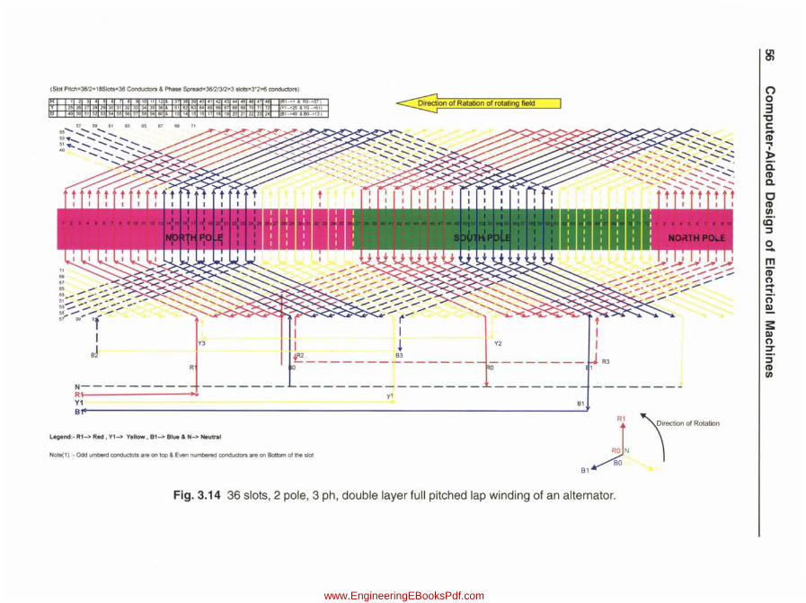
(Slot Pitch=3612=18Slots=36 Conductors & Phase Spread=36I2f3l2=3 51015=3'2=6 conductors)
~on of Ratation of rotating field .... ( ->
25 26 28 30 31 32 33 34 35 36 & 81 82 601 85 66 67 68 59 7 1 72 (Yl ->25 &Y0->61) 495051 5253 54 55 ij6 57 ij6 59 60 & 13 14 15 16 17 18 192021 2223 24 (Bl~ &00->13 )
R
N--------- -------y1
B1
Legend:- R1-> Red . V1-> Vellow. B1-> Blue & N-> Neutral
Note(1 ) :- Odd umberd conductots are on top & Even numbered conductors are on Bottom of the slot
Fig. 3.14 36 slots, 2 pole, 3 ph, double layer full pitched lap winding of an alternator.
o o 3
"C c: ... CD ... l=ei CD Q.
C CD (J)
cc' ::::s
o -
www.EngineeringEBooksPdf.com

CHAPTER 4
DC Machines
4.1 Introduction Based on winding type of annature, DC machines are categorized as lap wound and wave wound. Theory portion of design is not given in this book, but necessary fonnulae, curves and tables given in standard books are made use of. Since the machine is the same for both operations of Generator and Motor, same design is applicable for both.
Total design is split into six parts in a proper sequence. Design calculations are given for a given Rating of Generator, followed by Computer Program written in "c" language using MATLAB software for each part. Finally all the programs are added together to get the total program by running by which we get the total design. Computer output of total design is given.
This design may not be the optimum one. Now optimization objective and design Constraints are inserted into this total program. When this program is run we will get various alternative feasible designs from which the selected variant based on the Optimization Criteria can be picked up. Computer output showing the important design parameters for various feasible alternatives is given in the end of this chapter along with a logic diagram.
4.2 Sequential Steps for Design of Each Part and Programming Simultaneously (a) Calculate Output Coefficient, Main dimensions of armature (viz) D,L and
FluxIPole checking the Periphoral velocity and V olts between commutator segments
(b) Calculate no. of slots, size of slot, conductor size, checking current density, current volume, slot balance. Calculate tooth flux density, Height of core, Wt. of iron, Iron losses and Temp rise
(c) Calculate dimensions of poles, Field Coils, Yoke and Amp-Turns required
(d) Calculate Copper size, No. of turns for Shunt and series fields
(e) Detennine the diameter of Commutator and no. and size of brushes. Check for Periphoral velocity and gap between brush arms
(f) Calculate the dimensions of Interpoles and Interpole winding. Calculate total losses, efficiency, total weight and Kg/KW.
Note: By adding programs established for each part sequentially, we get the program for complete design.
57
www.EngineeringEBooksPdf.com

58 Computer-Aided Design of Electrical Machines
4.3 Calculation of Armature Main Dimensions and flux/pole (Part-1)
Specific Magnetic Loading & Dimensions & Electric Loading
KW 5 10 50 100 200 300 500 1000 1500 2000 5000 10000
Bav(T) .43 .45 .56 .6 .62 .64 .66 .68 .7 .72 .74 .76
Amp-Cond/m 15 17.5 25 28 32.5 34 36.5 41 42 44 48 51
(*1000)
Following Data is assumed.
No. of ventilating ducts (nv) = 4; Width of ventilating ducts (bv) = 10mm
Pole arc /Pole pitch (PAbPP) = 0.7; Pole Arc = Arme Core Length (L),
Slots/pole (SpP) = 14; Iron factor (k i ) = 0.9; Volage drop on FL = 3%
Values of Specific magnetic loading (Bay) = 0.66 T and Specific electric loading (q) = 36500 ac/m -7 are read from the table given above.
Calculations
FL Current (IFL) = KWxl000 = 500xl000 = 833.33 amps V 600
PxN 6x700 . Frequency (hz) = -- = = 35 (hes between 25 to 50 and hence OK)
120 120
Assuming Field and Armature copper loss = 3% of KW rating,
Pa = 1.03 x 500 = 515 KW;
Output Coefft (CO) = 0.164 x Bav x q x 10-3
= 0.164 x 0.66 x 36500 x 10-3 = 3.9508
Pa 515 DsqL = = = 0.1862 m3
COxN 3.9508x700
D = 3 DsqLxP =3 0.1862x6 =0.798 m LIPP x 1t 0.7 x 1t
= 798mm ? 800 mm (Rounded off)
Peripheral speed (vA)
= 1txDx N/60 = 1tx800x700/60
= 29.32m1s « = 30 and hence OK)
L DsqL_ 0.1862 0.291m = 291 mm? 300 mm (Rounded off) D2 (800/1000)2
Assuming vent ducts (nv = 4) of width (bv = 10mm) each and iron factor (ki = 0.9),
www.EngineeringEBooksPdf.com
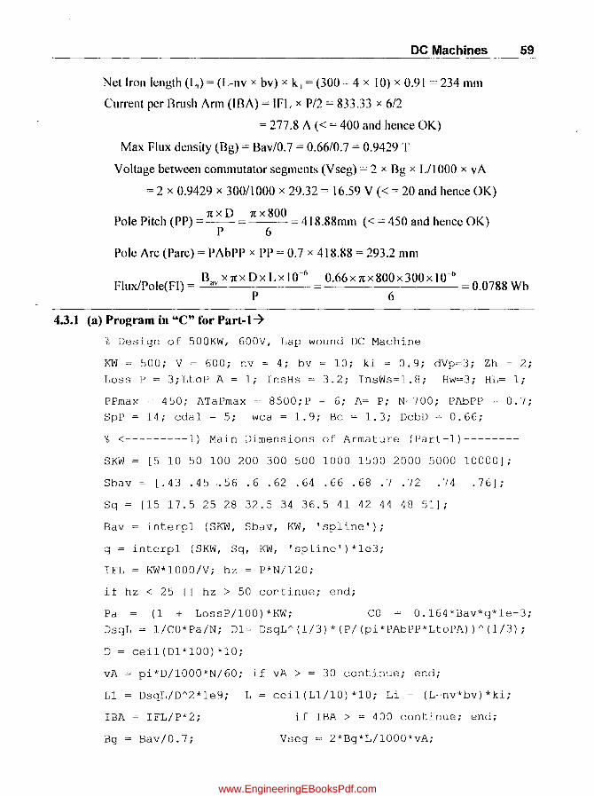
DC Machines 59
Net Iron length (L,) = (L-nv x bv) x k, = (300 -- 4 x 10) x 0.91 = 234 mm
Current per Brush Arm (IBA) = IFL x PI2 = 833.33 x 6/2
= 277.8 A « = 400 and hence OK)
Max Flux density (Bg) = Bav/0.7 = 0.66/0.7 = 0.9429 T
Voltage between commutator segments (Vseg) = 2 x Bg x LilOOO x vA
= 2 x 0.9429 x 30011000 x 29.32 = 16.59 V « = 20 and hence OK)
• 1[ x D 1[ x 800 Pole PItch (PP) =-- = = 418.88mm « = 450 and henee OK)
P 6
Pole Arc (Pare) = PAbPP x PP = 0.7 x 418.88 = 293.2 mm
FluxiPole(FI) = Bav x 1[ x D x LxI 0-6 = 0.66 x 1[ x 800 x 300 xl O-b = 0.0788 Wb
P 6
4.3.1 (a) Program in "C" for Part-l-7
% Design of 500KW, 600V, Lap wound DC Machine
KW = 500; V = 600; nv = 4; bv = 10; ki = 0.9; dVp=3; Zh = 2;
Loss P = 3;LtoP A = 1; lnsHs = 3.2; lnsWs=1.8; Hw=3; HL= 1;
PPmax = 450; ATaPmax = 8500;P = 6; A= P; N=700; PAbPP = 0.7; SpP = 14; cda1 = 5; wca = 1.9; Bc = 1.3; DcbD = 0.66;
% <---------1) Main Dimensions of Armature (Part-1)--------
SKW = [5 10 50 100 200 300 500 1000 1500 2000 5000 10000];
Sbav = [.43.45 .. 56.6.62.64.66.68.7.72 .74 .76];
Sq = [15 17.5 25 28 32.5 34 36.5 41 42 44 48 51];
Bav = interp1 (SKW, Sbav, KW, 'spline');
q = interp1 (SKW, Sq, KW, 'spline') *le3;
lFL KW*1000/V; hz = P*N/120;
if hz < 25 I I hz > 50 continue; end;
Pa (1 + LossP/100)*KW; CO 0.164*Bav*q*le-3; DsqL = l/CO*Pa/N; 01= DsqL A(1/3)*(P/(pi*PAbPPkLtoPA) )A(1/3);
o = cei1(01*100)*10;
vA pi*0/1000*N/60; if vA > = 30 continue; end;
L1 OsqL/DA2*1e9; L = ceil(L1/10)*10; Li = (L-nv*bv)*ki;
lBA = lFL/P*2;
Bg = Bav/O.7;
if lBA > = 400 continue; end;
Vseg = 2*Bg*L/1000*vA;
www.EngineeringEBooksPdf.com
60 Computer-Aided Design of Electrical Machines
if Vseg > = 20 continuejendj
PP pi*D/Pj if PP > = PPmax continuej endj
Parc = PAbPP*PPjFIl Bav*pi*D*L/P*le-6j
4.4 Design of Armature Winding and Core (Part-2)
Arme AT per Pole (ATaP) 1t x D x q x 10-3
1t X 800 x 36500 x 10-3
= 7644.5 2xP 2x6
Induced Emfon NO load(E) = (I + dVp/IOO) x V = (I + 3/100 x 600 = 618 V
For Lap wound Machine, No. of parallel paths (A) = P = 6
E x 60 x A 618 x 60 x 6 Total no. of Conductors (Z) = := := 638.7
P x FI x N 6 x 0.0788 x 700
Assuming Slots/Pole (SpP) = I4~ No of SIots(S) = SpP x P = 14 x 6 = 84
. 1t x D 1t X 800 Slot pitch (sp) = -- = = 29.92 mm
_ S 84
Conductors/Slot (Zs) = Z/S = 638.7/84 = 7.6:::: 8 mm (Rounded otl'even Integer)
Corrected no of conductors (Z) = Zs x S = 8 x 84 = 672
E x 60 x A 618 x 60 x 6 Corrected value of Flux/Pole (FI) = := = 0.0788 wb
PxZxN 6x672x700
IfL x Zs 833.33 x 8 Current Volume/slot (CV) = := := 1111 « = 1500 and hence OK)
A 6
Assuming Shunt Field Current(lsh) = 3 A,
Annature Current (Ia) = IfL + Ish = 833.33 + 3 = 836.33 A
Assuming current density (cda) = 5 A/nun2;
la 836.33 ) Cond Area ofCS (Aca) = = = 27.878 mm-
Axcda 6x5
Assuming Conductor width (wca) = 1.9mm,
Aca 27.878 Conductor ht (hca) = --= = 14.67 == 15 mm (Rounded off)
Wca -1.9
Assuming a factor of 0.98 for rounding at the conductor edges,
Revised Area of conductor (Aca) = 0.98 x hca x wca = 0.98 x 15 x 1.9 = 27.93 mm2;
Corrected current density (cds) = la = 836.33 =4.991A/mm2 A x Aca 6x 27.93
www.EngineeringEBooksPdf.com
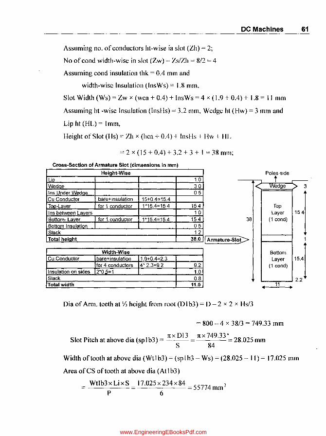
pc Machines 61
Assuming no. of conductors ht-wise ia slot (Zh) = 2;
No of cond width-wise in slot (Zw) = Zs/Zh = 8/2 = 4
Assuming cond insulation thk = 0.4 mm and
width-wise Insulation (InsWs) = 1.8 mm.
Slot Width (Ws) = Zw x (wca + 0.4) + IllsWs = 4 x (1.9 + 0.4) + 1.8 = II mm
Assuming ht -wise Insulation (InsHs) = 3.2 mm, Wedge ht (Hw) = 3 mm and
Lip ht (HL) = 1 mm,
Height of Slot (Hs) = Zh x (hca + 0.4) + IllsHs + Hw + HL
= 2 x (J 5 + 0.4) + 3.2 + 3 + 1 = 38 mm;
Cross-Section of Armature Slot (dimensions in mm)
Hei ht-Wise Poles-side 10 t 30 1< Wedge 05
bare+insulation 15+0.4=15.4 for 1 conductor 1*15.4=15 4 15 4 Top
1 0 Layer for 1. conductor 1*15.4=154 154 38 (1 cond)
05 12
L..:..::=.:..== ____________ -..L_-..;:;3.=.;8.~0 I Armature-Slo 1> Width-Wise Bottom
CU.Conductor bare+insulation 1.9+0.4=2.3 Layer for 4 conductors 4* 2.3=9.2 9.2 (1 cond)
Insulation on sides 2*0.';;=1 1.0 Slack 0.8 Total width 11.0 11
Oia of Aml. teeth at Ih height from root (0 I b3) = D - 2 x 2 x Hs/3
= 800 - 4 x 38/3 = 749.33 mm
. . 1tx013 1tx749.33* Slot PItch at above dla (sp I b3) = = = 28.025 mm
S 84
3
154
1
154! 2.2
Width of tooth at above dia (Wtl b3) = (sp I b3 - Ws) = (28.025 - II) = 17.025 mm
Area ofCS of tooth at above dia (Atlb3)
Wtlb3xLixS = 17.025x234x84 = 55774mm 1
P 6
www.EngineeringEBooksPdf.com

62 Computer-Aided Design of Electrical Machines
. . 0.0788 x 10⁶ 0.0788 x 10⁶
Flux densIty m the tooth (Btav) = = = 1.4133 T Atlb3 55744
C C f :t1 (K ) SPI b3 x L 28.025 x 300 2 11 arter oe ItS = = = . Wtlb3 xLi 17.025 x 234
. Btav 1.4133 Max tooth Flux densIty (Btm) = ::; -- = 2.019 T
PAbPP 0.7
Free Length (Overhang) of conductor (Lfr) = 140 + 1.15 x PP
= 140 + l.l5 x 418.88 = 621.72 mm
Length of Arme-Conductor (Lac) = L + Lfr = 300 + 621.72 = 921.7 mm = 0.9217 m
Anne Wdg Res (Ra) = 0.021 x Lac x Z = 0.021 x 0.9217,x 672 = 12.9363 mn AcaxA2 27.93x6-
Assuming 20% Eddy Current Losses,
Arm Copper Loss (Peua) = 1.2 x la2 x Ra = 1.2 x 836.332 x 12.9363 x 10 3 = 10858 W
Wt of Anne-Copper (Wcua) = Lae x Aea x Z x 8.911000
= 0.9217 x 27.93672 x 8.9/1000 = 153.97 Kg
Flux in core (FIc) = Fi = 0.0788 = 0.0394 Wb 2 2
Assuming Flux density in Core (Be) = 1.3 T, Area ofCS in eore (Ae)
= Fie = 0.0394 = 30318 mm2 Bc 1.3
I leight of Core (I-Ie) = Ac = 30318 = 129.56 mm L. 234
Inner diameter of Core (D j ) = D-2 x (Hs + Hc) = 800 - 2 x (38 + 129.56)
= 464.9:::: 470mm (Ronded oft)
Correeted height of Core (Hc) = (D - Di)/2 - Hs = (800 - 470)/2 - 38 =127 mm
Mean dia ofeore (Dme) = D - 2 x Hs - Hc = 800 - (2 x 38) - 127 = 597 mm
Weight of Core (We) = 7.8 x 10-6 x 1t x Dme x Ae
=7.8x lO-6 x1tx597x30318 = 443.5 Kg
Hysterisis loss in core/kg (HysPkgc) at I.3T
= (2.9/30) x hz = 2.9/30 x 35 = 3.3833 7 (Emperieal formula);
Hysterisis loss in eore (Physc) = Wc x HysPkge = 443.5 x 3.3833 = 1500.6 W
Using 0.5 mm thiek Laminations for core, Eddy current Loss in core (Peddyc)
= 0.0045 x (Bc x hz x 0.5)2 x Wc = 0.0045 x (1.3 x 35 x 0.5i x 443.5 = 1033 W
www.EngineeringEBooksPdf.com

DC Machines 63
Considcring 25% more on Loaded Condition, Iron Loss in core (Pic)
= (Physc + Peddyc) x 1.25 = (1500.6 + 1033) x 1.25 = 3167 W;
Weight of Teeth (Wt) = 7.8 x 10⁻⁶ x Wt I b3 x Li x S x Hs
= 7.8 X 10-6 x 17.025 x 234 x 84 x 38 =99.19 Kg
Hysterisis loss in Teeth/kg(l-IysPkgt) at 2.0 19T
= (8/30) x hz = 8/30 x 35 = 9.3333 ~ (Emperical fonnula);
Hysterisis loss in Teeth (Physt) = Wt x HysPkgt = 99.19 x 9.3333 = 925.8 W
For 0.5 mm thick Laminations, Eddy current Loss in teeth (Peddyt)
= 0.007 x (Rtm x hz x 0.5)1 x Wt = 0.007x (2.019 x 35x 0.5)2X 99.19 = 866.8 W
Considering 25% more on Loaded Condition, Iron Loss in tecth (Pit)
= (Physt + Peddyt) x 1.25 = (925.8 + 866.8) x 1.25 = 2240.7 W;
Total Iron Loss (Pi) = Pic + Pit =3167 + 2240.7 = 5407.7 W
Iron loss percentage (PibKW) = Pi xIOO= 5407.7 xI00=1.0815% K W x 1000 500 x 1000
Losses in Armature (Pa) = PClla + Pi = 10858 + 5407.7 = 16266 W
Over all length of Anne (Larme) = L + 70 + 0.3 x PP
= 300 + 70 + (0.3 x418.88) = 495.66 mm
Cooling Surface of Armature (SA) = 1[ x D x LarmelIOO
= 1[ x 800 x 496.66/ I 00 = 12457cm2
Loss per Sq. cm of Cooling surface (Pd) = PaiSA = 16266/12457 = 1.3057 W/ dn2;
Temp-Rise of Anne (Tra)
270x Pd I+O.09x(vA)13
270 x 1.3057 = 42.62 0C « = 50 and hence OK) 1 + 0.09 X (29.32)1.3
4.4.1 (a) Program in "C" for Part-2~
%-------2) Armature-Winding and core (part-2)-----------------
->
D = 800; q = 36500; P = 6; ATaPmax = 8500; dVp = 3; V = 600;
FI1=0.0829; N=700; SpP=14; IFL = 833.33; cda1 5; % Input Data
wca=1.9; Zh = 2; InsWs = 1.8; InsHs = 3.2; Hw 3; % Input Data
HL 1; Li = 234; L = 300; PAbPP = 0.7; PP 4 18 . 8 8 ; Be = 1. 3;
hz 35; KW = 500; vA = 29.32; % Input Data
www.EngineeringEBooksPdf.com

64 Computer-Aided Design of Electrical Machines
Ishl 3; %Assumptions
ATaP pi*0/1000*q/(2'P);if ATaP > = ATaPmax continue; end;
(1 + dVp/lOO)*Vj A = P; ZI E*60*A/(P*FIl*N); E
S SpP*P; sp = pi*O/S; if sp < 25 I I sp > j5 continue; end;
Zsl = Zl/S; Zsf=floor (Zsl/2)*2; Zse = ceil (Zsl/L)*2;
Zs = Zsf; if Zsl - Zsf > 1 Zs = Zse; end; Z S*Zs;
FI E*60*A/(P*Z*N);
CV IF'L/A*Zs; if CV < 1000 I I CV > 1500 continue; end;
la lFL + Ishl; Acal la/A/edal; heal Aeal/wcd;
hca eeil(hcal);if hea > 16 continue; end;
Aea 0.98*hea*wca; eda = Ia/A/Aea;
if cda > = 5.01 continue; end;
Zw Zs/Zh; Ws = Zw*(wea i 0.4) + InsWs;
Hs Zh*(hca t 0.4) + lnsHs + Hw i HL;
Dlb3 = 0 - 2*(2/3*Hs); splb3 = pi*01b3/S;
Wtlb3 = splb3 - Ws; Atlb3 Wtlb3*Li*S/P; Btav = FI*le6/Atlb3; Ks = splb3*L/Wtlb3/Li; if Ks > = 2.2 continue; end;
Btm Btav/PAbPPj if Btm > = 2.1 continue; end;
Lfr 140 + 1.15*PP; Lae = (L + Lfr)/le3;
Ra = 0.02l*Lae/Aea*Z/AA2; Pcua
Wcua = Lae*Aea*Z*8.ge-3; FIe = F'I/2; Ae = FIe*le6/Bc;
Hel = Ac/Li; Oil = 0-2*(Hs + Hcl); Oi eeil(Oil/lO)*lO;
Hc=(O Oi)/2 - Hs: Omc 0-2*Hs - He; We = 7.8e-6*pi*Omc*Ae;
HysPkgc = (2.9/30)*hz; % Emperial Formula
Physc We*HysPkgc; Peddyc = 0.0045*(Be*hz*0.5)A2*We;
Pie = (Physe + Peddyc) *1.25;
Wt = 7.8e-6*Wtlb3*Li*S*Hs:HysPkgt = (8/30)*hz;
Physt = Wt*HysPkgt; Peddyt = 0.007*(Btm*hz*0.5)A2*Wt:
Pit = (Physt + Peddyt)*1.25; Pi = (Pie + Pit);
PibKW
Larme
Pi/(KW*le3)*100; Pa
L .~ 70 t 0.3*PP; SA
Peua + Pi;
pi*O*Larme/.lOO; Pd
Tra = 270*Pd/(1 + O.09*(vAAl.3));
Pa/SA;
www.EngineeringEBooksPdf.com
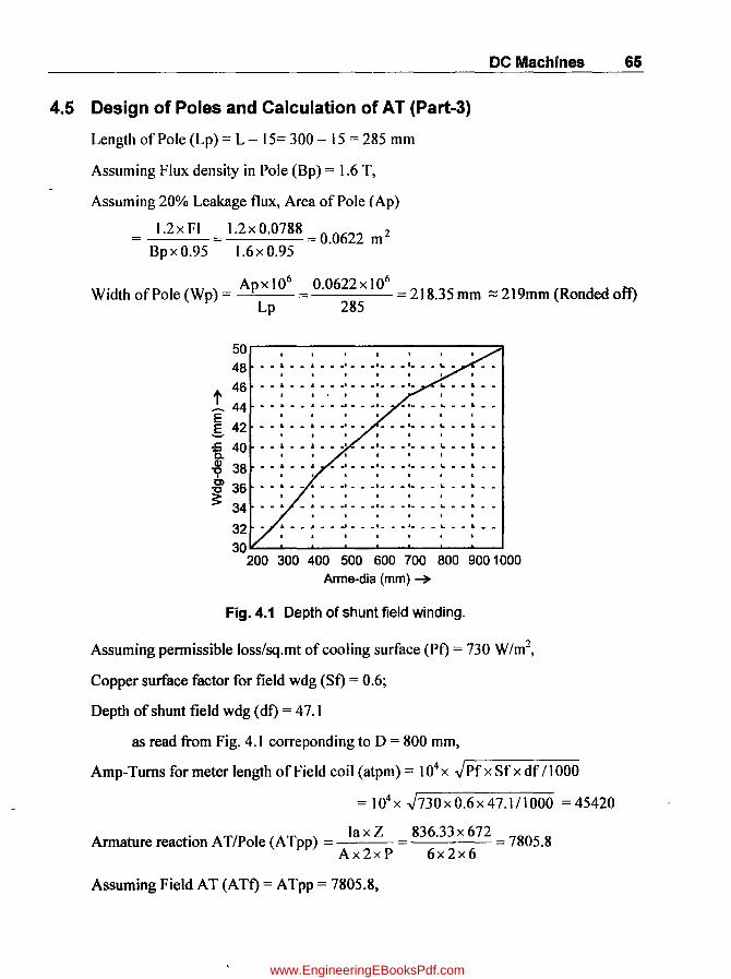
4.5 Design of Poles and Calculation of AT (Part-3)
Length of Pole (Lp) = L - 15= 300 - 15 = 285 mm
Assuming Flux density in Pole (Bp) = 1.6 T,
Assuming 20% Leakage flux, Area of Pole (Ap)
= 1.2 x FI = 1.2 x 0.0788 = 0.0622 m 2
Bp x 0.95 1.6 x 0.95
DC Machines 65
. Apxl06 0.0622x10⁶
WIdth of Pole (Wp) = = =218.35mm ::::219mm(Rondedoft) Lp 285
50~------------------------
48
t 46 ~ 44 E .s 42
'8. 40
~ 38 .g 36 3: 34
32 . • ........................ .
30~~--~~--~--~~--~~
200 300 400 500 600 700 800 900 1000 Arme-dia (mm) ~
Fig. 4.1 Depth of shunt field winding.
Assuming permissible loss/sq.mt of cooling surface (Pt) = 730 W/m2,
Copper surface factor for field wdg (St) = 0.6;
Depth of shunt field wdg (dt) = 47.1
as read from Fig. 4.1 correponding to D = 800 mm,
Amp-Turns for meter length ofField coil (atpm) = 104x .JPfx Sfx df !tOOO
= 104x .J730xO.6x47.1!t000 =45420
. la x Z 836.33 x 672 Armature reactIon AT/Pole (A Tpp) = = = 7805.8
Ax2xP 6x2x6
Assuming Field AT (ATt) = A Tpp = 7805.8,
www.EngineeringEBooksPdf.com
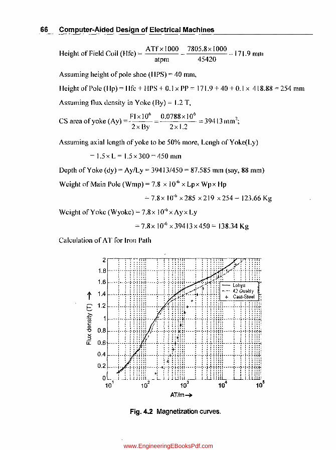
66 Computer-Aided Design of Electrical Machines
I-'°h fFOldCOI(LIl::) ATfxlOOO 780508xl000 1719 ~elg tOle 01.- IC = = = . mm
atpm 45420
Assuming height of pole shoe (UPS) = 40 mm,
Height of Pole (lIp) = Hfc + HPS + 001 x PP = 171.9 + 40 + 0.1 x 418088 = 254 mm
Assuming flux density in Yoke (By) = 1.2 T,
FI x I 06 0.0788 x 10⁶ ?
CS area of yoke (Ay) = = 39413 mm-; 2x By 2x 1.2
Assuming axial length of yoke to be 50% more, Lengh ofYoke(Ly)
= 105 x L = 105 x 300 = 450 mm
Depth of Yoke (dy) = Ay/Ly = 39413/450 = 87.585 111m (say, 88 mm)
Weight of Main Pole (Wl11p) = 708 x 10-6 X Lpx Wpx Hp
= 7.8 x 10-6 x 285 x 219 x 254 = 123.66 Kg
Weight of Yoke (Wyoke) = 708x IO-6 xAyx Ly
= 708x 10-6 x 39413 x 450 = 138034 Kg
Calculation of AT for Iron Path
Fig. 4.2 Magnetization curveso
www.EngineeringEBooksPdf.com

For Pole:
DC Machines 67
2.5 r----:----:---:--oooooooo:----:--~-___:___:7"O
2.4
2.3
t 22 • • • . • • I E ...... -; .. - .. ~ .. -~ .............. - ... - ... - ..... -- .. I ...... ..
$ .~ 2.1 ........... .. ............................ ' ........ ' ........ 1........ Ql
o >< :J u::
2 ...... .. .... y ....... "l ............... -, ...... -. ....... -, ...... ..
1 9 • • I I I • I • .. .... ~ ...... ; ....... ~ ....... -. ".- .. "," ................. I" .... ..
1.8 '-'-"'--_--'--_ ........ _~_~_~ _ ___' _ ___' o 2 4 6 8
AT/m~
10 12 14 16
x 104
Fig.4.3 Magnetization curves of teeth at Ks - 2.0
From Fig. 4.2, AT corresponding to Bp == 1.6 T, (atp) == 4400 AT/m (for 42 Quality steel) and AT for Pole (A Tp) == atp x Hpl I 000 == 4400 x 2541 I 000 == 11 17.6
For Arm-Teeth:
From Fig. 4.3, AT corresponding to Btm == 2.019 T, (atat) = 21739 AT/m
and AT for Teeth (A Tt) == atat x Hs/IOOO == 21739 x 38/1 000 == 826
For Core:
From Fig. 4.2, AT corresponding to Bc == 1.3 T,
(atac) = 39<>AT/m (for Lohys steel)
1t x Dmc 1t x 597 Length of Flux Path (Lfpc) = == == 156.29 mm
2x P 2x6
AT for Core (ATc) == atacx Lfpc/lOOO == 390x 156.29/1000 == 60.96
For Yoke:
From Fig. 4.2, AT corresponding to By == 1.2 T, (aty) == 1230 AT/m (for Cast steel)
Mean Dia (Omy) == D + 2x Hp + dy == 800 + (2x 254) + 88 == 1396;
• 1tX Dmy 1tX 1396 Length of Flux Path (Lfpy) == == == 365.5 mm and
2x P 2x 6
AT for yoke CATy) == atyx Lfpy/lOOO == 1230x 365.51l000 = 449.5
www.EngineeringEBooksPdf.com

68 Computer-Aided Design of Electrical Machines
Total AT for all parts (AIT) == ATp + ATt + ATc + ATy
==1 I 17.6 + 826 + 60.96 + 449.5 == 2454
Percentage == A IT/A Tf x 100 == 245417806 x I 00 == 3 1.44 %
AT reqd on no-load (A TO) == 0.85 x ATf== 0.85 x 7806 == 6635
Air-gap AT (ATg) == ATO- AIT == 6635 -2454 == 4181
AirGapFluxDensity(Bgm) == Bav == 0.66 == 0.9429T PAbPP 0.7
Assuming A ir Gap Coefficient (Kg) == I. 15 (Varies from 1.12 to I .18);
AT 4181 AirGapLength(Lg) == g 6 == ----------,-
0.796 x Bgm x Kg x 10 0.796x 0.9429x 1.15 * 106
== 0.0048 m== 4.85mm
Yoke outer dia (DO) == D + 2 x (Lg + Hp + dy)
== 800 + 2 x (4.85 + 254 + 88) == 1494 mm
4.5.1 (a) Program in "C" for Design of Poles and Calculation of AT-(part-3)
% ~------3) Design of Poles and Calculation of AT-(Part-3) ->
L 300; FI = 0.0788; D = 800; Ia = 836.33: A = 6: Z = 672;
P 6: PP = 418.88; % Input Data
Btrn 2.019; Hs = 38: Bc = 1.3: Drnc 597; Bav 0.66;
PAbPP = 0.7; %Input Data
Bp = 1.6: Pf = 730; Sf = 0.6; By = 1.2; Kg = 1.15; HPS = 40; %Assurnption
DA = [200 300 400 500 700 1000]; dSFW = [30 33 37 40 45 50]:
Plot (DA,dSFW); grid; xl abel ('Arrne-dia(mm)-->'); ylabel('Wdg-depth(mm)-->'):
title ('Depth of Shunt Field Winding');
Lp = L - 15: Ap = 1.2*FI/Bp/0.95;
Wp = ceil (Wpl) :
Wp1 = Ap*le6/Lp;
dfl = interp1 (DA,dSFW,D,'spline'); df = ceil (dfl*10) 110; atprn = 1e4*sqrt(Pf*Sf*df/1e3);
Atpp = Ia/A*Z/2/P; Atf = ATpp; Hfc = ATf/atprn*le3;
Hpl = Hfc + HPS + O.l*PP;
Hp = ceil (Hpl); Ay = 1.2*FI*le6/2/By; Ly = 1.5*Li
www.EngineeringEBooksPdf.com

DC Machines 69
dy1 = Ay/Ly; dy = ceil(dy1);
Wmp = 7.8e-6*Lp~Wp*Hp; Wyoke = 7.8*Ay*Ly/1e6;
SB = [. 1 . 2 . 3 . 4 . 5 . 6 . 7 . 8 . 9 1 1 . 1 1 . 2 1 . 3 1 . 4 1.5 1.6 1.7
Ha = [18 28
1.8 1.9 2.0]; % Tesla
38 48 67 80 95 120 140 180 220 295 580 1000 2200 5000 9000 16000 24000]; % for Lohys-steel
390
H = [20 30 40 50 70 90 115 140 160 200 250 320 480 1000 2200 4400 9000 16000 25000 38000]; % for 42 quality steel
Bcs = [180 270 370 440 520 590 670 '/50 820 920 1030 1230 1600 2200 3200 4800 7700 13000 22000 40000]; % for Cast-Steel
SBt = [1.8 1.9 2 2.1 2.2 2.3 2.4 2.5];
SATm = [ 9 12 20 31 51 80 1]3 155]~le3; % for Ks = 2.0
Semilogx (Ho, BB, '-', H, BB, '-.', Hcs, BB,' *'); grid;
xlabel ('AT/m-->'); ylabel ('Fluxdensity ('1')-->');
title ('Magnetization curves');
legend ('Lohys', '42 Quality', 'Cast-Steel');
alp =, interpl (BB, H, Bp, 'spline'); ATp = atp*Ilp/le3;
plot (SATm, SBl); grid; xlabel ('AT/m-->');
ylabel ('Fluxdensity ('1')-->');
title ('Magnetization curves of teeth at Ks = 2.0');
at at = interp1 (SBt, SATm, Btm, 'spline'); Att = atat*Hs/1e3;
atac = interp1 (BB, Ha, Bc, 'spline'); Atc = atac*Lfpc/1e3;
aty = interp1 (BB, Hcs, By, 'spline'); Lfpy = pi*Dmy/(2*P);
Lfpc = pi*Dmc/2/Pi
Dmy = 0 + 2*Hp + dYi
ATy = Lfpy*aty/1e3i TT = ATp + ATt + ATc + ATy;
Perc = ATT/ATf*100; ATO = 0.85*ATf; ATg = ATO - ATT;
Bgm Bav/PAbPP; Lg ATg/(0.796*Bgm*Kg*le6)*le3i DO = 0 + 2*(Lg + Hp + dy);
4.6 Design of Shunt Field and Series Field Windings (Part-4)
Assuming 15% voltage drop in Field Regulator,
Voltage across Shunt field Wdg (Vsh) = 0.85 x V = 0.85 x 600 = 510 V
Voltage across each field coil (Vc) = Vsh/P = 510/6 = 85 V
Assuming thickness of insulation on pole body (ti) = 10111m,
Mean Length of tum (Lmt) = [2 x (Wp + Lp) + 1t x (df+ 2x ti)]/JOOO
=[2x (219+285)+1t x (47.1 +2 x 10)]/1000= 1.2188111;
www.EngineeringEBooksPdf.com

70 Computer-Aided Design of Electrical Machines
CS area of Conductor (Ash) = 0.021 x Lmt x ATONc
= 0.021 x 1.2188 x 6635/85 = 1.9979 111m2
;
Assuming 80% of Field coil ht for Shunt field wdg and
balance 20% for series fld wdg,
Cooling surface ofSh. lld. coil (cssfc) = 2 x Lmt x 0.8 x Hfc/l 000
= 2 x 1.2188 x 0.8 x 171.8611 000 = 0.3351 m2;
Assuming permissible loss per sq.m of cooling surface = 730 WI m2;
Permissible Loss ofSh. rId Wdg (Psfc) = 730 x csstcx P
= 730x 0.3351 x 6 = 1467.9 W;
Sh. Fld Current (Ish) = PsfcNsh = 1467.9/510 = 2.8782 A
ATO 6635 No. ofturns/pole (Tsh) = ATO/lsh =-- = = 2305
Ish 2.8782
Selecting a conductor dia (dcu) = 1.6 mm (bare) with ins thk = 0.1 I mm,
Turns that can be wound 111 a height of 0.8 x Bfc (Tl)
- 0.8xlltc 0.8x171.86 804 80) - = = . (say, dcu + O. I I 1.6 + 0.1 I
. Tsh 2305 No. of layers to be provIded (NL) =-= -- = 28.8 (say, 29)
TI 80
Corrected no. ofturns/pole (Tsh) = TI x NL = 80 x 29 = 2320
Depth of winding (dw) = NL x (dcll + 0.11) = 29 x (1.6 + 0.11) = 49.59 mm
1txdcu 2 1tX 1.62
CS area of copper cond (Acu)= = = 2.0106 111m2 4 4
Resistance ofSh.tld winding (Rsh)
= 0.021 x Lmtx Tsh x P = 0.021 x 1.2188x 2320x 6 = 177.2 Q
Acu 2.0106
Sh. Fld. Copper Loss (Psh) = Ish2 x Rsh = 2.87822 x 177.2 = 1468 W
Wt of Sh. fld. copper (Wcsh) = Acu x Lmt x Tsh x P x 8.9 X 10-3
= 2.0 I 06 x 1.2188 x 2320 x 6 x 8.9 X 10-3 =303.6 Kg
Design of Series Field Winding
AT to be produced by Series Fld W dg on FulI Load (A Tse)
=ATf-ATO=7806-6635 = 1171
Turns IPole (Tse) = ATse/la = 1171/836.33 = 1.4 (say, 2)
Modified AT/Pole (ATse) = Tse x la = 2 x 836.33 = 1673
www.EngineeringEBooksPdf.com

Assuming current density (cdse) = 2.2 A/mm2,
. la 836.33 7 CS area of conductor (Ase) =-- = = 380.15 mm-
cdse 2.2
Copper Strip size selected: 20 X 19 mm
Resistance of Series fld winding (Rse)
DC Machines 71
= 0.021 x Lmt x Tse x P = 0.021 x 1.2188 x 2 x 6 = 0.808 mn Ase 380.15
Series Fld. Copper Loss (Pse) = la2 x Rse = 836.332 x 0.808/1000 = 565.1 W
Wt of Series. tld. copper (Wcse) = Asex Lmtx Tsex Px 8.9x 10-3
=380.15x 1.2188x2x6x8.9x 10-3 =49.48 Kg
4.6.1 (a) Program in "C" for Design of Shunt Fld and Series Fld Wdgs (Part-4)
~ ~--4) Design of Shunt Fieldand series Fld Windings -----~
ti = 10; deu = 1.6; edse = 2.2; % Assumptions
v = 600; P = 6; Wp = 219; Lp = 285; df = 47.1; ATO = 6635;
lIfe 171. 86; ATf = 7806; Ia = 836.33; % Input Data
Vsh 0.85*V; Ve = Vsh/P;
Lmt (2*(Wp + Lp) + pi*(df + 2*ti))/le3;
Ash 0.021*Lmt*ATO/Ve;essfc =2*Lmt*0.8*Hfe/le3;
Psfe = 730*essfe*P; Ish = Psfe/Vsh; Tshl = ATO/Ish;
Tla = 0.8*Hfe/(deu+0.ll); Tl = floor(Tla); NLI = Tshl/Tl;
NL eeil(NLl); Tsh = Tl*NL;
Ow NL*(deu+O.ll); Aeu = pi*deu A 2/4;
Rsh = O.021*Lmt*Tsh*P/Aeu; Psh = Ish A 2*Rsh;
Wesh = Aeu*Lmt*Tsh*P*8.9*le-3; ATsel = ATf-ATO;
Tsel = ATsel/Ia; Tse
Ase
Pse
Ia/edse;
Ia A 2*Rse;
Rse
eeil(Tsel); ATse = Tse*Ia;
0.021*Lmt*Tse*P/Ase;
Wese = Ase~Lmt*Tse*P*8.9*le-3;
4.7 Design of Commutator and Brushes (Part-5)
Assuming commutator dia is (DcbD = 66%) of Armature dia,
Comm. dia(Dc) = 0.66 x 800 = 528 mm
Periphoral speed of Commutator (vC)
= 7txDcxN/60=7tx528x700/60 = 19.35 m/s«=20 and hence OK)
No. ofComm Segments (Nc) = Zl2 = 672/2 = 336
www.EngineeringEBooksPdf.com
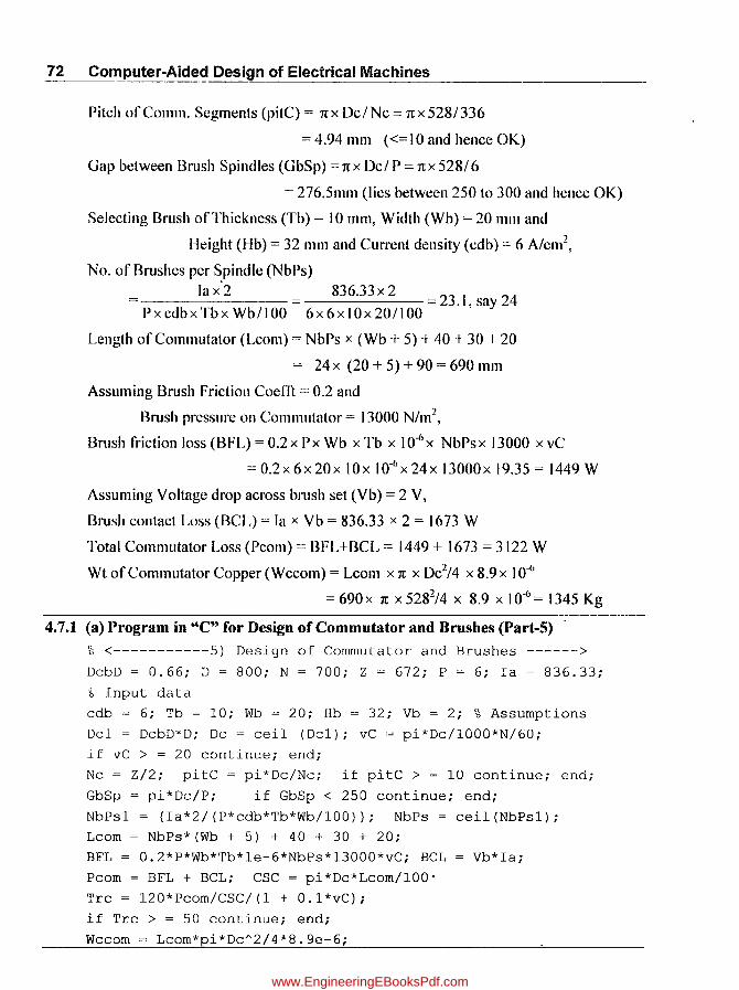
72 Computer-Aided Design of Electrical Machines
Pitch ofComm. Segments (pitC) = nx Dc/Nc = nx528/336
=4.94mm «=IOandhenccOK)
Gap between Brush Spindles (GbSp) =nx Del P = nx 528/6
= 276.5mm (lies betwecn 250 to 300 and hence OK)
Selecting Brush of Thickness (Tb) = IO mm, Width (Wb) = 20111111 and
Height (Hb) = 32 mm and Current density (cdb) = 6 A/cm2,
No. of Brushes per Spindle (NbPs)
la x 2 836.33 x 2 __ 23 I . 24 --------= . ,say Px cdbx Tbx Wb/l 00 6x 6x lOx 20/1 00
Length of Commutator (Lcom) = NbPs x (Wb + 5) + 40 + 30 + 20
= 24x (20+5)+90=690mm
Assuming Brush Frictioll Coefft = 0.2 and
Brush pressure 011 Commutator = 13000 N/m2,
Brush friction loss (BFL) = 0.2 x P x Wb x Tb x 10-6 x NbPs x 13000 x vC
= 0.2x 6x 20x lOx IO-ux 24x 13000x 19.35 = 1449 W
Assuming Voltage drop across brush set (Vb) = 2 V,
Brush contact Loss (BCL) = la x Vb = 836.33 x 2 = 1673 W
Total Commutator Loss (Pcom) = BFL+BCL = 1449 + 1673 = 3122 W
Wt of Commutator Copper (Wccom) = Lcom x 1[ x Dc2/4 x 8.9 x 10-0
=690x 1[ x 5282/4 x 8.9 x 10-6= 1345 Kg
4.7.1 (a) l)rogram in "C" for Design of Commutator and Brushes (Part-5) .
~ <-----------5) Design of Commutator and Brushes ------>
DcbD = 0.66; 0 = 800; N = 700; Z = 672; P = 6; Ia = 836.33;
'i, Input data
cdb = 6; Tb = 10; Wb = 20; Hb = 32; Vb = 2; % Assumptions
Dcl = DcbD*D; Dc = ceil (Dcl); vC = pi*Dc/lOOO*N/60;
if vC > = 20 continue; end;
Nc = Z/2; pitC = pi*Dc/Nc; if pitC > = 10 continue; end;
GbSp = pi*Dc/P; if GbSp < 250 continue; end;
NbPsl = (Ia*2/(P*cdb*Tb*Wb/lOO)); NbPs = ceil(NbPsl);
Lcom = NbPs*(Wb + 5) + 40 + 30 + 20;
BFL = 0.2*P*Wb*Tb*le-6*NbPs*13000*vC; BCL = Vb*Ia;
Pcom = BFL + BCL; CSC = pi*Dc*Lcom/lOO·
Trc = 120*Pcom/CSC/(1 + O.l*vC);
if Trc > = 50 continue; end;
Wccom = Lcom*pi*Dc A 2/4*8.ge-6;
www.EngineeringEBooksPdf.com

DC Machines 73
4.8 Design of Inter-Polel Compensating Winding and Overall Performance Assuming Interpole length (Lip) = 0.7 x L = 0.7 x 300 = 210 mm
Width ofInt. pole shoe (bip) = [{(Zs/2)-I} x pitC + Tb-0.8] x D/Dc
= [{(8/2) - I} x 4.9368 + 10 - 0.8] x 800/528 = 36.38 mm
Assuming Air gap under Inter-Pole(Lgi) = 1.5 xL = 1.5 x 4.8439 = 7.2659 mm
Ht of Interpole (Hip) = Hp-(Lgi-Lg) = 254 - (7.2659 - 4.8439)
= 251 .578 ~ 252 mm (by rounding oft)
Calculation of Flux density under the Inter-Pole (Bip):
Copper ht in Arme-slot (hcai) = 2 x (hca + 0.4) = 2 x (15 + 0.4) = 30.8 mm
Ht above slot in Armaeture (ht) = Hw + HL + InsHs/2 = 3 + 1 + (3.2/2) = 5.6 mm
Periphory of Zs/2 = 4 coils in one layer of slot (perip)
=2x [((Zs/2) x (wca+O.4)} + (hca + 0.4)]
= 2 x [{(8/2) x (1.9+0.4)} + (15+0.4)] = 49.2 mm
Leakage coefficients:
Lmdl
- 04 (hcai ht biP ) _ 0 4 (30.8 5.6 36.38) - 28612 - • X1tX --+-+ - . X1tX --+-+ - . 3xWs Ws 6xLgi 3xll 11 6x7.266
Lmd2
= Lfr x (0.23 x 10g[ Lf~ ] + 0.07] = 621.71 1 X(0.23 x IOg[62 1.71 1]+ 0.07) = 1.3541 L penp 300 49.2
Total (Lamda) = (Lmdl + Lmd2) x 10..() = (2.8612 + 1.3541) X 10..()
= 4.2 154 x 1O..() Wb/m2 ;
FI d . (B·) L 2 x la x Zs x Lamda 0 3692 T ux enslty Ip =-x = . Lip 36.379311 000
Design of Inter-Pole Winding:
Amp-turns for Inter-pole (ATip) = ATf+ (0.796x Bipx 1.1 x Lgi x 1000)
= 7806 + (0.796 x 0.3692 xl. 1 x 7.2659x 1000 = 10154
No. of turns on each Int-Pole (Tip) = ATip/Ja = 10154/836.33
= 1 2.14 ~ 13 (by rounding oft)
Modified No of AT (ATip) = Tip x la = 13 x 836.33 = J 0872
Assuming Curr~nt density (cdip) = 2.3 A/mm2,
CS area of conductor (aip) = Ia/cdip = 836.33/2.3 = 363.62 mm2,
www.EngineeringEBooksPdf.com
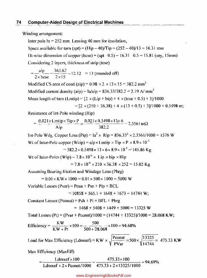
74 Computer-Aided Design of Electrical Machines
Winding arrangement:
Inter pole ht = 252 mm. Leaving 40 mm tor insulation,
Space available for turn (spt) = (I lip - 40)ffip = (252 - 40)/13 = 16.31 mm
lit-wise dimension of copper (hcse) = (spt- 0.5) = 16.31- 0.5 = 15.81 (say, 15mm)
Considering 2 layers, thickness of strip (tcse)
aip 363.62 12 12 13 ( d d t·t) ----'--- = =.::::: roun e 0 2x hcse 2x 15
Modified CS area of cond (aip) = 0.98 x 2 x 13 x 15 = 382.2 mm2
Modilied current density (aip) = la/aip = 836.33/382.2 = 2.19 A/ mm2
Mean length of turn (Lmtip) = [2 x (Lip + bip) + 4 x (tcse + 0.5) + 3]/1 000
= [2 x (210 + 36.38) + 4 x (13 + 0.5) + 3]/1000 = 0.5498 m;
Resistance of Int-Pole winding (Rip)
= 0.021 x Lmtip x Tip x P = 0.021 x 0.5498 x 13f< 6 = 2.3561 mQ Aip 382.2
Int-Pole Wdg. Copper Loss (Pip) = la2 x Rip = 836.332 x 2.356111000 = 1576 W
Wt of Inter-Pole copper (Wcip) = aipx Lmtip x Tip x P x 8.9x 10-.1
= 382.2x 0.5498x 13 x 6x 8.9x 10-3 ='145.86 Kg
Wt of Inter-Poles (Wip) = 7.8 x 10⁻⁶ x Lip x bip x Hip
=7.8x 10-6 x210 x36.38 x252= 15.02 Kg
Assuming Bcaring friction and Windage Loss (Pbrg)
= 0.01 x KWx 1000 = 0.01 x 500x 1000 = 5000 W
Variahle Losses (Pvar) = PClla + Pse + Pip + BCL
= 10858 + 565.1 + 1648 + 1673 = 14744 W;
Constant Losses (Pconst) = Psh + Pi + BFL + Pbrg
= 1468 + 5408 + 1449 + 5000 = 13325 W
Total Losses (Pt) = (Pvar + Pconst)/1000 = (14744 + 13325)/1000 = 28.068 KW;
Efticicncy = K W x 100 = 500 x 100 = 94.68% K W + Pt 500 + 28.068
Load for Max Efficiency (Ldmxef) = KW x Pconst =500x 13325 = 475.33 KW PVar 14744
Max Efficiency (MaxEff)
___ L_d_m_x_ef_x_l_O_O __ = 475.33 x 100 = 94.69% Ldmxef + 2 x Pconst/ 1 000 475.33 + 2 x 13325/1000
www.EngineeringEBooksPdf.com

DC Machines 75
Considering Insulation Wt as I %, Total Weight (WtTot)
= 1.01 x (We + Wt + Weua + Weeom + Wesh + Wese + Weip
+ Wmp + Wyoke + Wip)
= 1.01 x (443.5 + 99.2 + 154 + 1345 + 303.6 + 49.5 + 145.9 + 123.6 + 138.3 + 15)
= 2845.8 Kg
KgPkw = WtTotlKW = 2845.8/500 =5.6908
4.8.1 (a) Program for Design of Inter/Compensating-Pole-Wdg and Overall Performance (part-6)
% <---6) Design ofinter/Compensating-Pole-Wdg and Overall performance ---->
L = 300; Zs = 8; pitC = 4.9368; Tb = 10; D = 800; Dc = 528; Lg = 4.8439; Hp = 254; hea = 15; % Input data
Hw = 3; HL =1; InsHs = 3.2; wea = 1.9; Ws = II; Lfr = 621.711; la = 836.33;
ATf= 7806; P = 6; % Input data
KW = 500; Peua = 10858; Pse = 565.1; BCL = 1673; Psh = 1468; Pi = 5408;
BFL = 1449; We = 443.5; % Input data
Wt = 99.2; Weua = 154; Weeom = 1345; Wesh = 303.6; Wese = 49.5; Wmp = 123.6; Wyoke = 138.3;
edip I = 2.3; % Assumption
Lip = 0.7*L; x = Zs/2; hip = «x-I )*pitC + Tb-0.8)*DlDe; Lgi = 1.5*Lg;
Hipl = Hp-(Lgi-Lg); Hip = ceil (Hipl); heai = 2*(hea + 0.4);
ht = Hw + HL + InsHs/2; perip = 2*(Zs/2*(wea + 0.4) + (hea + 0.4»;
Lmdl = 0.4*pi*(heai/3/Ws + htlWs + hip/6/Lgi);
Lmd2 = Lfr/L *(0.23*log(Lfr/perip) + 0.07);
Lamda = (Lmdl + Lmd2)*le-6; Bip = LlLip*2*1a/6*Zs*Lamda/(bip/le3);
ATipl = ATf+ 0.796*Bip*1.1 *Lgi*le3; Tipl = ATipl/la; Tip = eei\(Tipl);
ATip = Tip*la; aip 1 = Ia/edip I; spt = (Hip-40)/Tip; hese 1 = (spt-O.S);
hese = tloor(hesel); tese1 = aipl/2/hese; tese = eeil(tesel); aip = 0.98*2*hese* tese; edip = Ia/aip; Lmtip = (2*(Lip + hip) + 4*(tese + 0.5) + 3)/le3;
Rip = 0.021 *Lmtip*Tip*P/aip; Pip = Ja"2*Rip;
Weip = aip*Lmtip*Tip*P*8.9* le-3;
Wip = 7.8e-6*Lip*hip*Hip; Pbrg = 0.01 *KW*le3; Pvar = Peua + Pse + Pip + BCL; -Peonst = Psh + Pi + BFL + Phrg; Pt = (Pvar + Peonst)/1 000;
Eff= KW/(KW + Pt)*IOO; Ldmxef= sqrt(PeonstlPvar)*KW;
MaxEff = Ldmxef/(Ldmxef + 2 *PeonstiI e3)* I 00;
WtTot = I.OI*(We + Wt + Wcua + Wccom + Wcsh +Wcse + Weip + Wmp + Wyoke + Wip);
KgPkw = WtTotlKW;
www.EngineeringEBooksPdf.com

76 Computer-Aided Design of Electrical Machines
4.9 Computer Program in "C" in MATLAB for Complete Design % Design of SOOKW, 600V, Lup wound DC Machine
KW = SOO; V = 600; nv = 4; bv = 10; ki 0.9; dVp = 3; Zh 2; LossP
LtoPA
PPmax
3; Ishl = 3;
1; InsHs = 3.2; InsWs = 1.8; Hw
4S0; ATaPmax = 8500;
3; HL = 1;
P == 6; A = P; N = 700; PabPP = 0.7; SpP = 14; cda1 = 5;
wca = 1.9; Bc = 1.3; DcbD = 0.66; cdipl = 2.3; % Assumption
f2 = fopen ('Total 500KW_Output.m','w');
% <------------1) Main Dimensions of Armature-------->
SKW = [S 10 50 100 200 300 SOO 1000 1500 2000 SOOO 10000];
Sbav = [.43 .4S .S6 .6 .62 .64.66.68.7.72 .74 .76];
Sq = [IS 17.S 25 28 32.S 34 36.S 41 42 44 48 51];
IFL == KW*1000/V; Bav = interp1 (SKW, Sbav, KW, 'spline');
q=interpl (SKW, Sq, KW, 'spljne')*le3;
hz P*N/120; if hz < 2S I I hz > SO continue; end;
Pa = (1 + LossP/100)*KW; CO = 0.164*Bav*q*le-3;
DsqL = l/CO*Pa/N;
D1 = DsqL A(1/3)*(P/(pi*PabPP*LtoPA))A(1/3);
D = ceil(D1*100)*10;
L1 = DsqL/D A2*le9; L = ceil (Ll/10)*10; vA = pi~D/1000*N/60;
if vA> = 30 continue; end;
fprintf (f2, 'Design of %3d KW,%3d V, LAP wound DC Machine\n t,
KW, V);
fprintf (f2, '<-------1) Design of Main Dimensions------>\n');
fprintf (f2, 'Rated KW = % 4.0f\n', KW);
fprintf (f2, 'RatedVolts=% 4.0f\n', V);
fprintf (f2, 'Rated Speed (RPM) = % 4.0f\n', N);
fprintf (f2, 'Rated Current (Amps) =% 4. If\n', IFL);
fprintf (f2, 'No. of Poles = % 4. Of\n', P);
fprintf (f2, 'No of ParallelPaths = % 4. Of\n', A);
fprintf (f2, 'Length/PolearcRatio = % 4. 2f\n', LtoPA);
fprintf (f2, 'AvGapFlux-dens(T) = % 4.3f\n', Bav);
fprintf (f2, 'q = Sp. ElecLoad (ac/m) = % 6. Of\n', q);
fprintf (f2, 'Frequency(c/s) = % 4.1f (Range :25toSO)\n', hz);
fprintf (f2, 'Polearc/PolePitch = % 4.2f (Range:0.67toO.70)\n', PabPP) ;
IBA = IFL/P*2; if IDA> = 400 continue; end;
www.EngineeringEBooksPdf.com

DC Machines 77
Bg = Sav/0.7; Vseg = 2*Bg*L/1000*vA; if Vseg > = 20 continue; end;
PP = pi*O/P; if PP > = PPmax continue; end;
Parc PabPP*PP; Li = (L-nv*bv)*ki; Fl1 = Bav*pi*0*L/P*le-6;
ATaP pi*0/1000*q/(2*P); if ATaP > = ATaPmax continue; end;
E (1 + dVp/100)*V; A = P; Zl = E*60*A/(P*Fl1*N);
S SpP*P; sp = pi *O/S; if sp < 25 I I sp > 35 continue; end;
Zsl = Zl/S; Zsf = f1oor(Zsl/2)*2; Zsc = ceil(Zsl/2)*2;
Zs Zsf; if Zsl-Zsf > 1 Zs = Zsc; end; Z = S*Zs;
FI E*60*A/(P*Z*N);
CV IFL/A*Zs; if CV < 1000 I I cv > 1500 continue; end;
fprintf (f2, 'Output Coefft (CO) = % 5.3 f\n',CO);
fprintf (f2,' OsqL Value = % 6.4f\n', OsqL);
fprintf (f2,' Arme dia (rom) = % 4.0 f\n', 0);
fprintf (f2,' Arme Length (rom) = % 4.0f\n', L);
fprintf (f2, 'Periphoral Vel(m/s) = % 4.2f ( < = 30 )\n', vA);
fprintf (f2, 'PeakGapFlux-dens(T) = % 4.3f\n', Bg);
fprintf (f2, 'Volts/segment % 4.1f « = 20)\n', Vseg);
fprintf (£2, 'PolePitch (rom) = % 4. 3f\n', PP);
"fprintf (f2,' Amps/Brush arm % 4.0f « = 400) \n', IBA);
fprintf (f2,' Arm. AT/Pole = % 4.0f\n', ATaP);
fprintf (f2,' Flux/Pole (Wb) = % 6.4f\n', FI);
fprintf (f2, , <-------2) Armature-Winding and core-------->\n') ;
fprintf (f2,' Tot Arm.Conductors = % 4.0 f\n', Z);
fprintf (f2,' No of Slots = % 3.0 f\n', S);
fprintf (f2,' SlotPitch (rom) = % 4.2 f (Wange:25 to 35)\n', sp) ;
fprintf (f2,' Conductors/Slot = % 4.0 f\n', Zs);
fprintf (f2,' Current (ac/Slot) = % 4.0 f « = 1500)\n', CV);
Ia = IFL + Ish1; Aca1 Ia/A/cda1; hca = ceil (Aca1/wca);
if hca > 16 continue; end;
Aca = 0.98*hca*wca; ~da = Ia/A/Aca; if cda > end;
Zw Zs/Zh;Ws = Zw*(wca + 0.4) + InsWs;
Hs Zh*(hca + 0.4) + InsHs + Hw + HL;
5.01 continue;
01b3 = D-2*(2/3*Hs); sp1b3 = pi*01b3/S; Wt1b3 = sp1b3-Ws;
At1b3 = Wt1b3*Li*S/P; Btav = FI*le6/At1b3;
Ks = sp1b3*L/Wt1b3/Li; if Ks > = 2.2 continue; end;
www.EngineeringEBooksPdf.com

78 Computer-Aided Design of Electrical Machines
Btm = Btav/PabPP; if Btm > = 2.1 continue; end;
Lfr = 140 + 1.lS*PP; Lac = (L + Lfr)/le3;
Ra = 0.021*Lac/Aca*Z/AA2; Wcua = Lac*Aca*Z*S.ge-3;
FIc = FI/2; Ac = FIc*le6/Bc; Hc1 = Ac/Li; Oil = 0-2*(Hs+Hc1); Oi = ceil(Oi1/10)*10;
He = (0-Oi)/2-Hs; Orne = 0-2*Hs-He;
fprintf (f2,' Arm-Cond (HtxW) = % 4.1fmmX % 4.1fmm\n',hea,wea);
fprintf (f2,' Arm-eond (A/mmA2) = % 4.2"f\n', eda);
fprintf (f2,' Arm-Slot (HtxW) = % 4.1 fmm X % 4.1fmm\n',Hs,Ws);
fprintf (f2,' Flux-dens: Av(1/3) % 4.3 f and Max = % 4.3 f « = 2.2T )\n', Btav, Btm);
fprintf (f2,' Arm-Res (m.ohms) % 6.2 f\n', Ra*le3);
fprintf (f2,' Wt of ArmCopper (Kg) = % 4.1 f\n',Weua);
fprintf (f2,' Core Flux-dens (T) = % 4.3 f\n', Be);
fprintf (f2, 'Ht of Core-Back (m) = % 4.1 f\n', He);
fprintf (f2,' Cor~ Inner Oia (m) = % 4.1 f\n', Oil;
Peua = 1.2*IaA2*Ra; We = 7.S e-6*pi*Dmc*Ac;
HysPkgc = (2.9/30)*hz; % Emperial Formula
Physc = Wc*HysPkgc; Peddyc = 0.004S*(Bc*h~*0.S)A2*Wc; Pi~ = (Physc + Peddyc)*1.25;
Wt = 7.Se-6*Wt1b3*Li*S*Hs; HysPkgt = (S/30)*hz;
Physt = Wt*HysPkgt; Peddyt = 0.007*(Btm*hz*0.5)A2*Wt;
Pit = (Physt+Peddyt) *1.25; Pi = (Pic+Pit);
PibKW = Pi/(KW*le3)*100; Pa Pcua + Pi;
Larme = L + 70 + 0.3*PP; SA pi*0*Larme/100;
Pd = PaiSA; Tra = 270*Pd/(1 + O.09*(vAA1.3));
Fprintf (f2,' ArmCopper Loss(W) = % 5.0 f\n', Pcua);
Fprintf (f2,' Wt of ArmCore (Kg) = % 4.0 f\n', Wc);
fprintf (f2,' Wt of ArmTeeth (Kg) = % 4.1 f\n', Wt);
fprintf (f2,' Iron Loss (W): Core + Teeth = % 4.0f + % 4.0 f = % 4.0 f\n', Pic, Pit, Pi);
fprintf (f2,' Temp-Rise of Arme (deg) = % 4.1 f\n', Tra);
fprintf (f2,' <-------3) Design of Poles and AT Calculation-------->\n');
Bp = 1.6; Pf = 730; Sf = 0.6; By = 1.2; Kg = 1.15; HPS = 40; % Assumption
DA [200 300 400 500 700 1000]; dSFW = [30 33 37 40 45 50];
~p L-15; Ap = 1.2*FI/Bp/0.95; Wp1 = Ap*le6/Lp;
www.EngineeringEBooksPdf.com
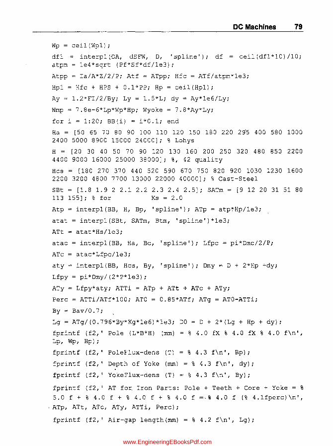
DC Machines 79
Wp = ceil (Wp1) ;
dfl = interp1('OA, dSFW, 0, 'spline'); df = cei1(dfl*10)/10; atpm 1e4*sqrt (Pf*Sf*df/1e3);
Atpp = Ia/A*Z/2/P; Atf = ATpp; Hfc = ATf/atpm*le3;
Hp1 = Hfc + HPS + O.l*PP; Hp = ceil(Hp1);
Ay = 1.2*FI/2/By; Ly = 1.5*L; dy = Ay*le6/Ly;
Wmp 7.8e-6*Lp*Wp*Hp; Wyoke = 7.8*Ay*Ly;
for i = 1:20; 88(i) = i*O.l; end
Ha = [50 65 70 80 90 100 110 120 150 180 220 2~5 400 580 1000 2400 5000 8900 15000 24000]; % Lohys
H = [20 30 40 50 70 90 120 130 160 200 250 320 480 850 2200 4400 9000 16000 25000 38000]; %, 42 quality
Hcs = [180 270 370 440 520 590 670 750 820 920 1030 1230 1600 2200 3200 4800 7700 13000 22000 40000]; % Cast-Steel
SBt = [1.8 1.9 2 2.1 2.2 2.3 2.4 2.5]; SATm = [9 12 20 31 51 80 113 155]; % for Ks = 2.0
Atp = interp1(BB, H, Bp, 'spline'); ATp = atp~Hp/1e3; atat = interp1(SBt, SATm, Btm, 'spline')*le3;
ATt = atat*Hs/1e3;
atac = interp1 (BB, Ha, Bc, 'spline'); Lfpc
ATc atac*Lfpc/1e3;
aty interp1(BB, Hcs, By, 'spline'); Omy
Lfpy = pi*Omy/(2*P*le3);
pi*Omc/2/P;
o + 2*Hp +dYi
ATy = Lfpy*aty; ATTi = ATp + ATt + ATc + ATy;
Perc = ATTi/ATf*100; ATO = 0.85*ATf; ATg = ATO-ATTi;
By Bav/0.7i
Lg ATg/(0.796*By*Kg*le6)*le3; DO = 0 + 2*(Lg + Hp + dY)i
fprintf (f2,' Pole (L*B*H) (rom) % 4.0 fX % 4.0 fX % 4.0 f\n', Lp, Wp, Hp);
fprintf (f2,' PoleFlux-dens (T) = % 4.3 f\n', Bp);
fprintf (f2,' Depth of Yoke (rom) = % 4.3 f\n', dy);
fprintf (f2,' YokeFlux-dens (T) = % 4.3 f\n', By);
fprintf (f2,' AT for Iron Parts: Pole + Teeth + Core + Yoke = %
5.0 f + % 4.0 f + % 4.0 f + % 4.0 f ~,% 4.0 f (% 4.1fperc)\n',
. ATp, ATt, ATc, ATy, ATTi, Perc);
fprintf (f2,' Air-gap length (rom) % 4.2 f\n', Lg);
www.EngineeringEBooksPdf.com

80 Computer-Aided Design of Electrical Machines
fprintf (f2,' <------4) Design of Shunt Fieldand series Fld Windings ------>\n');
ti = 10; dcu = 1.6; cdse = 2.2; % Assumptions
Vsh = 0.85*V; Vc = Vsh/P; Lmt 2*ti))/le3; Ash = 0.021*Lmt*ATO/Vc;
(2* (Wp + Lp) + pi* (df +
cssfc = 2*Lmt*0.8*Hfc/1e3; Psfc = 730*cssfc*P; Ish = Psfc/Vsh; Tsh1 = ATO/Ish;
T1a = 0.8*Hfc/(dcu + 0.11); T1
NL ceil(NL1); Tsh = T1*NL;
floor(T1a); NL1
dw NL*(dcu + 0.11); Acu = pi*dcuA 2/4;
Rsh = 0.021*Lmt*Tsh*P/Acu; Psh = Ish A 2*Rsh;
Wcsh = Acu*Lmt*Tsh*P*8.9*le-3;
Tsh1/T1;
ATse1 = ATf-ATO; Tse1 = ATse1/Ia; Tse = ceil (Tse1);
ATse = Tse*Ia; Ase = Ia/cdse; Rse = 0.021*Lmt*Tse*P/Ase;
se = Ia A 2*Rse; Wcse = Ase*Lmt*Tse*P*8.9*le-3;
fprintf (f2,' Sh.Field Wdg: Ish = % 4.2fA; Tuns/Coil = % 4.0 f; Rsh = % 5.1 fohms and Psh = % 5.1f W\n', Ish, Tsh, Rsh, Psh);
fprintf (f2,' Series-Field Wdg: Tuns/Pole = % 2.0 f; Rse = % 5.3fm. ohms and Pse = % 5.1 f W\n', Tse, Rse*le3, Pse);
fprintf (f2, '<------5) Design of Commutator and Brushes----->\n') ;
cdb 6; Tb = 10; Wb = 20; Hb = 32; Vb = 2; % Assumptions
Dc1 DcbD*D; Dc = ceil(Dc1); vC = pi*Dc/1000*N/60;
if vC > = 20 continue; end;
Nc Z/2; pitC = pi*Dc/Nc; if pitC > = 10 continue; end;
GbSp = pi*Dc/P; % if GbSp < 250 continue; end;
NbPs1= _(Ia*2/ (P*cdb*Tb*Wb/100) ); NbPs = ceil (NbPs1);
Lcom = NbPs*(Wb + 5) + 40 + 30 + 20;
BFL = 0.2*P*Wb*Tb*le-6*NbPs*13000*vc; BeL = Vb*Ia;
Pcom = BFL + BCL; CSC = pi*Dc*Lcom/100;
Trc = 120*Pcom/CSC/(1 + O.l*vC); if Trc > = 50 continue; end;
Wccom = Lcom*pi*Dc A 2/4*8.ge-6;
fprintf (f2,' Commutator: Dia = % 4.0 fmm; Per. Vel: Calc = % 4.2 f (Permissible = ZOm/s)\n', Dc, vC);
fprintf (f2,' Seg-Pitch: Calc >4mm)\n', pitC);
% 4.2 fmm (Permissible
www.EngineeringEBooksPdf.com
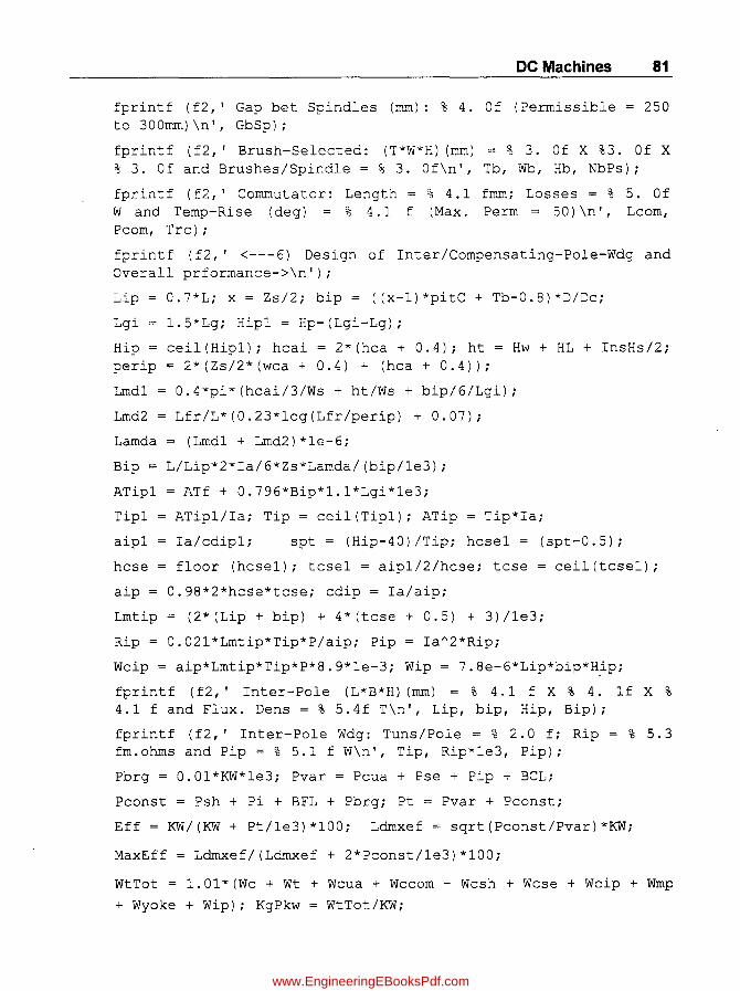
DC Machines 81
fprintf (f2,' Gap bet Spindles (mm): % 4. Of (Permissible 250 to 300mm)\n', GbSp);
fprintf (f2,' Brush-Selected: (T*W*H) (mm) = % 3. Of X %3. Of X % 3. Of and Brushes/Spindle = % 3. Of\n', Tb, Wb, Hb, NbPs);
fprin~f (f2,' Commutator: Length Wand Temp-Rise (deg) = % 4.1 f Pcom, Trc);
% 4.1 fmm; Losses = % 5. Of (Max. Perm = 50) \n', Lcom,
fprintf (f2,' <---6) Design of Inter/Compensating-Pole-Wdg and Overall prformance->\n');
Lip 0.7*L; x = Zs/2; bip = ((x-1)*pitC + Tb-0.8)*D/Dc;
Lgi 1.5*Lg; Hip1 = Hp-(Lgi-Lg);
Hip ceil(Hip1); hcai = 2*(hca + 0.4); ht = Hw + HL + InsHs/2; perip = 2*(Zs/2*(wca + 0.4) + (hca + 0.4));
Lmd1 0.4*pi*(hcai/3/Ws + ht/Ws + bip/6/Lgi);
Lmd2 Lfr/L*(0.23*log(Lfr/perip) + 0.07);
Lamda = (Lmd1 + Lmd2)*le-6;
Bip = L/Lip*2*Ia/6*Zs*Lamda/(bip/1e3);
ATipl = ATf + 0.796*Bip*1.1*Lgi*le3;
Tip1 ATipl/Ia; Tip = ceil(Tip1); ATip = Tip*Ia;
aip1 Ia/cdip1; spt = (Hip-40)/Tip; hcse1 = (spt-0.5);
hcse floor (hcse1); tcse1 = aip1/2/hcse; tcse = ceil(tcse1);
aip = 0.98*2*hcse*tcse; cdip = Ia/aip;
Lmtip = (2*(Lip + bip) + 4*(tcse + 0.5) + 3)/le3;
Rip = 0.021*Lmtip*Tip*P/aip; Pip Ia"2*Rip;
Wcip = aip*Lmtip*Tip*P*8.9*le-3; Wip = 7.8e-6*Lip*bip*H~p;
fprintf (f2,' Inter-Pole (L*B*H) (mm) = % 4.1 f X % 4. If X % 4.1 f and Flux. Dens = % 5.4f T\n', Lip, bip, Hip, Bip);
fprintf (f2,' Inter-Pole Wdg: Tuns/Pole = % 2.0 f; Rip = % 5.3 fm.ohms and Pip = % 5.1 f W\n', Tip, Rip*le3, Pip);
Pbrg = 0.01*KW*le3; Pvar = Pcua + Pse + Pip + BCL;
Pconst = Psh + Pi + BFL + Pbrg; Pt = Pvar + Pconst;
Eff = KW/(KW + Pt/1e3)*100; Ldrnxef = sqrt (Pconst/Pvar) *KW;
MaxEff = Ldrnxef/(Ldrnxef + 2*Pconst/1e3) *100;
WtTot = 1.01*(Wc + Wt + Wcua + Wccom + Wcsh + Wcse + Wcip + Wmp
+ Wyoke + Wip); KgPkw WtTot/KW;
www.EngineeringEBooksPdf.com

82 Computer-Aided Design of Electrical Machines
fprintf (f2,' Variable Losses (Pcua + Pse +Pip + BCL) := % 4.0 f + % 4.0 f + % 4.0 f + % 4.0 f = % 5.0 f W \n', Pcua, iPse, Pip, BCL, Pvar);
fprintf (f2,' Constant Losses (Psh + Pi + BFL + Pbg) = % 4.0 f . + % 4.0 f + % 4.0 f + % 4.0 f = % 5.0 f W \n', Psh, Pi, BFL,
Pbrg, Pconst);
fprintf (f2,' Toal Losses = % 5.0 f W; Efficiency = % 5.2 f perc\n', Pt, Eff);
fprintf (f2,' Load for Max. Eff % 5.0 f KW and Max. Efficiency = % 5.2 f perc\n', Ldmxef, MaxEff);
fprintf (f2,' WtTot (Kg) = Wc + Wt + Wcua + Wccorn + Wcsh + Wcse + Wcip + Wrnp + Wyoke + Wip = 'I;
fprintf (f2,' \n = % 3.0 f + % 3.0 f + % 3.0 f + % 4.0 f + % 3.0 f + % 3.0 f +', Wc, Wt, Wcua, Wccorn, Wcsh, Wcse);
fprintf (f2,' % 3. Of + % 3.0 f + % 3.0 f + % 3.0 f = % 4.0 ~f\n', Wcip, Wrnp, Wyoke, Wip, WtTot);
fprintf (f2,' Wt of Total Machine (Kg) = % 5.0 f and Kg/KW = % 5.2 f \n', WtTot, KgPkw);
fprintf (f2,' <----------------End--------------------->\n\n');
fclose (f2);
4.10 Computer Output Results for Complete Design
Design of 500 KW, 600 V, LAP wound DC Machine
<-------1) Desigfi of Main Dimensions------>
Rated KW = 500
Rated Volts = 600 I
Rated Speed (RPM) = 700
Rated Current (Amps) = 833.3
No .ofPoles = 6
No. ofParallelPaths = 6
Length/PolearcRatio = 1.00
AvGapFlux-dens (T) = 0.660
q = Sp.ElecLoad (ac/m) = 36500
Frequency (cis) = 35.0 (Range :25 to 50)
PolearclPolePitch = 0.70 (Range: 0.67 to 0.70)
www.EngineeringEBooksPdf.com

Output Coefft (CO) = 3.951
DsqL Value = 0.1862
Arme dia (mm) = 800
Arme Length (mm) = 300
Periphoral Vel (m/s)=29.32 ( <= 30)
PeakGapFlux-dens (T) = 0.943
Volts/segment = 16.6 « = 20)
PolePitch (mm) = 418.879
Amps/Brush arm = 278 « = 400 )
Arm.AT/Pole = 7645
Flux/Pole (Wb) = 0.0788
<-------2)Armature-Winding and core-------->
Tot Arm.Conductors = 672
No of Slots = 84
SlotPitch (mm) = 29.92 (Range: 25 to 35)
Conductors/Slot = 8
Current (ac/Slot) = 1111 « = 1500)
Arm-Cond (HtxW) = 15.0mm X 1.9mm
Arm-cond (A/mm"2) = 4.99
Arm-Slot (HtxW) = 38.0mm X 11.0mm
Flux-dens:Av(l/3) = 1.413 and Max = 2.019 « = 2.2T)
Arm-Res (m.ohms) = 12.94
Wt of ArmCopper (Kg) = 154.0
CoreFlux-dens (T) = 1.300
Ht of Core-Back (m) = 127.0
Core Inner Dia (m) = 470.0
ArmCopper Loss (W) = 10858
Wt of ArmCore (Kg) = 444
- Wt of ArmTeeth (Kg) = 99.2
Iron Loss(W):Core + Teeth = 3167 + 2241 = 5408
Temp-Rise of Arme (deg) = 42.6
<-------3) Design of Poles and AT Calculation--------->
Pole(L*B*H)(mm)=285 x 219 x 254
DC Machines 83
www.EngineeringEBooksPdf.com

84 C0!JIputer-Aided Design of Electrical Machines
PoleFlux-dens (T) = 1.600
Depth of Yoke (mm) = 87.585
YokeFlux-dens (T) =0.943
AT for Iron Parts: Pole + Teeth + Core + Yoke = 1118 + 826 + 63 + 449 = 2456 (31.5perc)
Air-gap length (mm) = 4.84
<------4) Design of Shunt Fieldand series Fld Windings ------>
Sh. Field Wdg: Ish = 2.88A; Tuns/Coil = 2320; Rsh = 177.2 ohms and Psh = 1468.0 W
Series-Field Wdg: TunslPole = 2; Rse = 0.808m.ohms and Pse = 565.1 W
<------5) Design of CommutatorandBrushes------>
Commutator: Dia = 528mm; Per.Vel: Calc = 19.35(Permissible =.20m/s)
Seg-Pitch: Calc = 4.94mm (Permissible >4mm)
Gap bet Spindles (mm): 276(Permissible = 250 to 300mm)
Brush-Selected: (T*W*H) (mm) = lOX 20 X 32 and Brushes/Spindle = 24
Commutator: Length = 690.0mm; Losses = 3122 Wand Temp-Rise( deg) = 11.2(Max. Perm = 50)
<---6) Design oflnter/Compensating-Pole-Wdg and Overall prformance->
Inter-Pole(L *B*HXmm) = 210.0 X 36.4 X 252.0 and Flux.dens = 0.3692 T
Inter-Pole Wdg: Tuns/Pole = 13; Rip = 2.356m. ohms and Pip = 1648.0 W
Variable Losses (Pcua + Pse + Pip + BCL) = ]0858 + 565 + 1648 + 1673 = 14744 W
Constant Losses (Psh + Pi + BFL + Pbg) = 1468 + 5408 + 1449 + 5000 = ] 3325 W
Toal Losses = 28068 W; Efficiency = 94.68 perc
Load for Max. Eff= 475 KW and Max. Efficiency = 94.69 perc
WtTot (Kg) = 1.01 *(Wc + Wt + Wcua + Wccom + Wcsh + Wcse + Wcip + Wmp + Wyoke + Wip) = 1.01 *(444 + 99 + 154 + 1345 + 304 + 49 + 146 + 124 + 138 + 15) = 2846 Wt of Total Machine(Kg) = 2846 and KglKW = 5.69
<----------------------End---------------------------->
4.11 Modifications to be done in the above Program to Get Optimal Design I. Insert "for" Loops for the following parameters to iterate the total program
between min and max permissible limits for selecting the feasible design variants:-
(a) No. of Poles
(b) No. of Speeds
www.EngineeringEBooksPdf.com

DC Machines 85
(c) Pole arc by Pole pitch ratios
(d) Slots per pole per phase
(e) Arme Wdg Current densities (0 Conductor widths
(g) Core flux density (h) Ratio of Commutator dia to Arm dia
2. Insert also mil}imum or maximum range of required objective functional values as constraint values, for example (a) Efficiency (b) Kg/KW (3) Temp-rise of Armature etc.
3. Run the program 10 get various possible design variants
Note: From the feasible design variants printed in the output, select that particular design fulfilling the objective of optimal parameter for the design
4.12 Computer Program in "C" in MATLAB for Optimal Design
% Design of 500KW, 600V, Lap wound DC Machin
% DC M/C Design 500KW, 600V, for Book
KW = 500; V = 600; nv = 4; bv = 10; ki
Loss P = 3;
LtoPA 1; InsHs = 3.2; InsWs 1.8; Ilw
PPmax 450; ATaPmax = 8500;
E2 = fopen ('Optimal 500KW_OutpuLm', 'w');
fprintf (f2, , Design of " 3d KW, % " Machine \n ' , KW, V) ;
fprintf (f2, ' Sn P N hz Z S sp
Btm Bc D L PA/PP Tra Dc/Da Dc Trc
0.9; dVp 3; Zh
3; HL 1;
3d V, LAP wound
Zs CV hcaXwca
Eff KgPkw\n' ) ;
2;
DC
cda
fprintf(f2, '===================~==~============================
================================================\n');
% <------------1) Main Dimensions of Armature-------*>
SKW = [5 10 50 100 200 300 500 1000 1500 2000 5000 10000];
S ba v = [. 4 3 . 4 5 . 5 6 . 6 . 62 . 64 . 6 6 . 68 . 7 . 72 . 7 4 . 7 6] ;
Sq = [15 17.5 25 28 32.5 34 16.5 41 42 44 48 51];
IFL = K~*1000/V; Bav = interp1 (SKW, Sbav, KW,' spline');
q = interp1 (SKW, Sq, KW,' spline')*le3;
www.EngineeringEBooksPdf.com
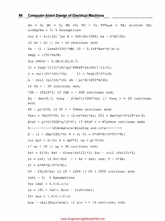
86 Computer-Aided Design of Electrical Machines
Sn = 0; M1 0; M2 =0; M3 0; EFFmax 94; minTra= 50;
minKgPkw = 7; % Assumptions
for P 4:2:10;' for N = 300:50:1000; hz P*N/120;
if hz < 25 I I hz > 50 continue; end;
Pa (1 + LossP/100)*KW; CO = O.164*Bav*q*le-3;
DsqL = l/CO*Pa/N;
for PAbPP = 0.68:0.01:0.7;
D1 = DsqL" (1/3) * (P/ (pi*PAbPP*LtoPA))" (1/3);
D ceil(D1*100)*10; L1 = DsqL/D"2*le9;
L ceil (L1/10)*10; vA = pi*D/1000*N/60;
if vA > = 30 continue; end;
IBA = IFL/P*2; if IBA > = 400 continue; end;
Bg = Bav/0.1; Vseg = 2*Bg*L/1000*vA; if Vseg >
end;
PP = pi*D/P; if PP > = PPmax continue; end;
20 continue;
Parc
ATaP
PAbPP*PP; Li = (L-nv*bv)*ki; Fl1 = Bav*pi*D*L/P*le-6;
pi*D/1000*q/(2*P); if ATaP > = ATaPmax continue; end;
%------------2)Armature-Winding and core------->
E = (1 + dVp/100)*V; A = P; Zl = E*60*A/(P*Fl1*N);
for SpP = 9:15; S = SpP*P; sp = pi*D/S;
j f sp < 25 I I sp > 35 continue; end;
Zsl = Zl/S; Zsf = floor(Zsl/2)*2; Zsc = ceil (Zsl/2)*2;
Zs Zsf; if Zsl-Zsf > 1 Zs = Zsc; end; Z = S*Zs;
FI E*60*A/(P*Z*N);
cv IFL/A*Zs; if CV < 1000 I I CV > 1500 continue; end;
Ish1 = 3; ~ Assumptions
.......-. for cdal 4.5:0.1:5;
Ia = IFL + IshI; Aca1 la/A/ cda1;
for wca = 1.6:0.1:2.2;
hca = ceil(Aca1/wca); if hca > 16 continue; end;
www.EngineeringEBooksPdf.com
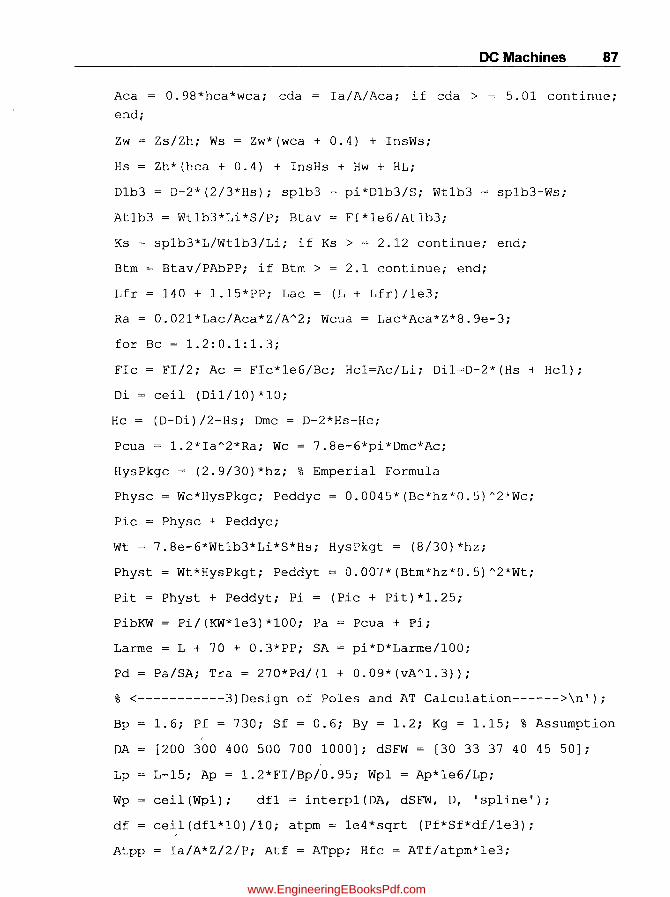
DC Machines 87
Aca = 0.98*hca*wca; cda
end,
Ia/A/Aca; if cda > = 5.01 continue;
Zw Zs/Zh; Ws = Zw*(wca + 0.4) + InsWs;
Hs Zh*(hca + 0.4) + InsHs + Hw + HL;
D1b3 = D-2*(2/3*Hs); sp1b3
At1b3 = Wt1b3*Li*S/P; Btav
pi*D1b3/S; Wtlb3
FI*le6/Atlb3;
sp1b3-Ws;
Ks = sp1b3*L/Wt1b3/Li; if Ks > = 2.12 continue; end;
Btrn
Lfr
Btav/PAbPP; if Btrn >
140 + 1.lS*PP; Lac
2.1 continue; end;
(L + Lfr) /le3;
Ra = 0.021*Lac/Aca*Z/AA2; Wcua = Lac*Aca*Z*8.ge-3;
for Bc = 1.2:0.1:1.3;
FIc = FI/2; Ac = FIc*le6/Bc; Hc1=Ac/Li; Di1=D-2*(Hs -l Hc1);
Di = ceil (Di1/10)*10;
Hc = (D-Di)/2-Hs; Drnc = D-2*Hs-Hcj
Pcua = 1.2*Ia A2*Raj Wc 7.8e-6*pi*Drnc*Ac;
HysPkgc = (2.9/30)*hz; % Ernperial Formula
Physc WC*HysPkgc; Peddyc = 0.004S*(Bc*hz*0.S)A2*Wc;
Pic = Physc -l Peddyc;
Wt = 7.8e-6*Wt1b3*Li*S*Hs; HysPkgt = (8/30)*hz;
Physt = Wt*HysPkgt; Peddyt = 0.007*(Btrn*hz*0.S)A2*Wt;
Pit = Physt + Peddyt; Pi (Pic + Pit)*1.2S;
PibKW
Larrne
Pi/(KW*le3)*100; Pa
L + 70 + 0.3*PP; SA
Pcua + Pi;
pi*D*Larrne/100;
Pd = Pa/SA; Tra = 270*Pd/(1 + 0.09*(vAA1.3));
% <-----------3)Design of Poles and AT Calculation------>\n');
Bp 1.6; Pf = 730; Sf = 0.6; By = 1.2; Kg = 1.1S; % Assumption
DA
Lp
Wp
[200 300 400 SOO 700 1000]; dSFW [30 33 37 40 45 SO];
1.2*FI/Bp/0.9S; Wp1 Ap*le6/Lp; L-1S; Ap
ceil (Wp1); df1 = interp1(DA, dSFW, 0, 'spline');
df ceil(df1*10)/10; atprn = 1e4*sqrt (Pf*Sf*df/1e3);
Atpp = Ia/A*Z/2/P; Atf = ATpp; Hfc = ATf/atprn*le3;
....
www.EngineeringEBooksPdf.com

88 Computer-Aided Design of Electrical Machines
Hp1 = Hfe + 40 + O.l*PP: Hp = eeil(Hp1):
Ay = 1.2*FI/2/By: Ly = 1.5*L: dy = Ay*le6/Ly:
Wmp 7.8e-6*Lp*Wp*Hp: Wyoke = 7.B*Ay*Ly:
for i =1:20: BB(i) = i*O.l: end
Ha = [50 65 70 80 90 100 110 120 150 180 220 295 400 580 1000
2400 5000 8900 15000 24000]: % Lohys
H = [20 30 40 50 70 90 120 130 160 200 250 320 480 850 2200
4400 9000 16000 25000 38000]: % 42 quality
Hes = [180 270 370 440 520 590 670 750 820 920 1030 1230 1600
2200 3200 4800 7700 13000 22000 40000]: % Cast-Steel
SBt = [1.8 1.9 2 2.1 2.2 2.3 2.4 2.5]:
SATm = [ 9 12 20 31 51 80 113 155]: % for Ks = 2.0
Atp = interp1(BB, H, Bp, 'spline'): ATp = atp*Hp/1e3;
Atat = interp1 JSBt, SATm, Btm, 'spline') *le3:
ATt = atat*Hs/1e3:
Lfpe = pi*Dme/2/P: ATe
atae = interp1 (BB, Ha, Be, 'spline');
atac*Lfpe/1e3:
aty = interp1(BB, Hes, By, 'spline'): Omy D + 2*Hp + dy:
pi*Dmy/ (2*P*le3): ATy = Lfpy*aty: Lfpy
ATTi ATp + ATt + ATe + ATy: Perc = ATTi/ATf*100:
ATO = 0.85*ATf; ATg = ATO-ATTi: Bgm = Bav/PAbPP:
Lg = ATg/(0.796*Bgm*Kg*le6)*le3:DO = D + 2*(Lg + Hp + dy):
% <----4)Design of Shunt Fieldand series Fld Windings ----->:
ti = 10; deu = 1.6:edse = 2:2: % Assumptions
Vsh=0.85*V: Ve=Vsh/P: Lmt = (2*(Wp + Lp) + pi*(df + 2*ti))/le3:
Ash = 0.021*Lmt*ATO/Ve: Cssfe = 2*Lmt*0.8*Hfe/1e3:
Psfe = 730*essfe*P: Ish Psfe/Vsh: Tsh1 = ATO/Ish:
T1a = 0.8*Hfe/(deu+0.11): T1 = floor(Tla): NL1 = Tsh1/T1:
NL= eeil(NL1): Tsh= T1*NL: dw= NL*(deu + 0.11):
Acu = pi *deuI\2/ 4; Rsh = O. 021*Lmt*Tsh*P/Acu: Psh IshI\2*Rsh;
Wesh= Aeu*Lmt*Tsh*P*8.9*le-3: ATsel = ATf-ATO: Tse1 = ATsel/Ia;
Tse=eeil(Tse1):ATse=Tse*Ia:Ase=Ia/cdse:Rse=
0.021*Lmt*Tse*P/Ase:Pse= I a I\2*Rse; Wcse=Ase*Lmt*Tse*P*8.9*le-3:
www.EngineeringEBooksPdf.com
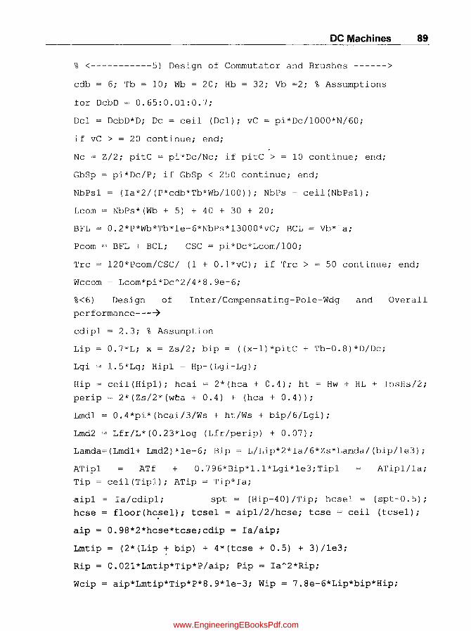
DC Machines 89
% <-----------5) Design of Commutator and Brushes ------>
edb = 6; Tb = 10; Wb = 20; Hb = 32; Vb =2; % Assumptions
for DebD = 0.65:0.01:0.7;
Dc1 DcbD*D; Dc = ceil (Del); vC pi*Dc/1000*N/60;
if vC > = 20 continue; end;
Nc Z/2; pitC = pi*Dc/Nc; if pitC > = 10 continue; end;
GbSp = pi*Dc/P; if GbSp < 250 continue; end;
NbPsl = (Ia*2/(P*cdb*Tb*Wb/100)); NbPs = ceil(NbPs1);
Lcom = NbPs*(Wb + 5) + 40 + 30 + 20;
BFL = 0.2*P*Wb*Tb*le-6*NbPs*13000~vC; BCL Vb*Ia;
Pcom = BFL ~ BCL; CSC = pi*Dc*Lcom/100;
Trc = 120*Pcom/CSC/ (1 + O.l*vC); if Trc > 50 continue; end;
Wccom = Lcom*pi*Dc A 2/4*8.ge-6;
%<6) Design of
performance---7
Inter/Compensating-Pole-Wdg
cdipl = 2.3; % Assumption
and
Lip 0.7*L; x = Zs/2; bip = ((x-1)*pitC + Tb-0.8)*D/Dc;
Lgi 1.5*Lg; Hipl = Hp-(Lgi-Lg);
Overdl1
Hip ceil(Hip1); hcai = 2*(hca + 0.4); ht = Hw + HL + InsHs/2;
perip = 2*(Zs/2*(wta + 0.4) + (hca + 0.4));
Lmdl
Lmd2
0.4*pi*(hcai/3/Ws ~ ht/Ws + bip/6/Lgi);
Lfr/L*(0.23*log (Lfr/perip) + 0.07);
Lamda=(Lmdl+ Lmd2)*le-6; Bip = L/Lip*2*Ia/6*Zs*Lamda/(bip/le3);
ATipl ATf + 0.796*Bip*1.1*Lgi*le3;Tipl ATipl/Ia;
Tip = ceil(Tip1); ATip = Tip*Ia;
-aip1
hcse
Ia/cdip1; spt = (Hip-40)/Tip; hcsel = (spt-0.5);
floor(hcsel); tcsel = aipl/2/hcse; tcse = ceil (tcse1)i
aip = 0.98*2*hcse*tcse;cdip = Ia/aip;
Lmtip = t2*(Lip ~ bip) + 4*(tcse + 0.5) + 3)/le3;
Rip = 0.021*Lmtip*Tip*P/aipi Pip
Wcip = aip*Lmtip*Tip*P*8.9*le-3; Wip = 7.8e-6*Lip*bip*Hip;
www.EngineeringEBooksPdf.com
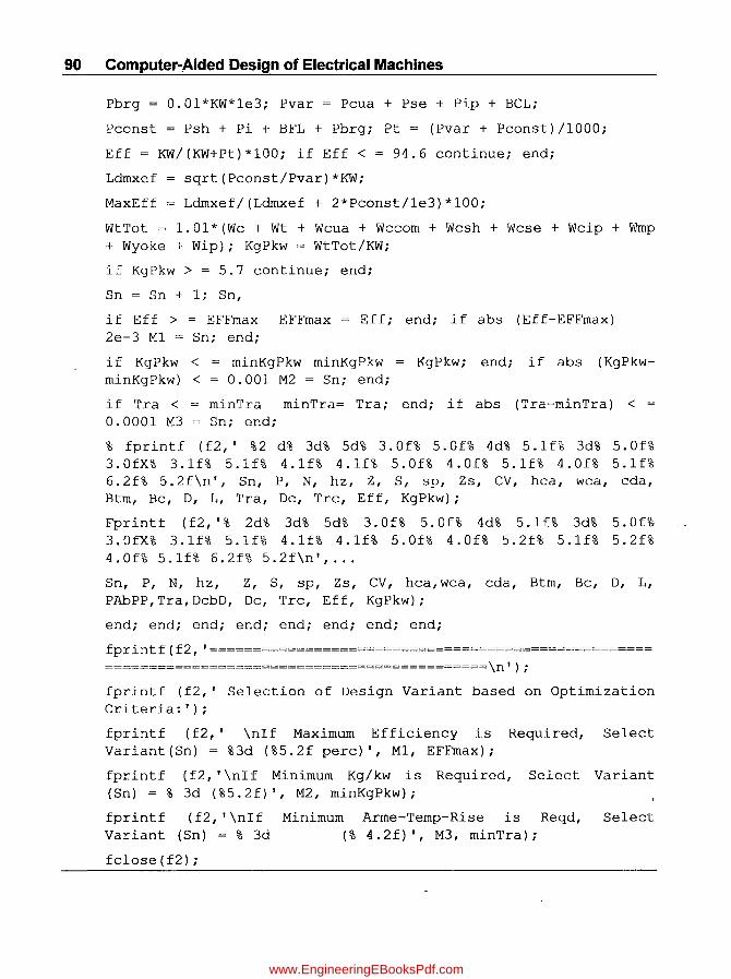
90 Computer-Aided Design of Electrical Machines
Pbrg = 0.01*KW*le3; Pvar = Pcua + Pse + Pip + BCL;
Pconst = Psh + Pi + BFL + Pbrg; Pt = (Pvar + Pconst)/1000;
Ef£ = KW/(KW+Pt) *100; if Eff < = 94.6 continue; end;
Ldrnxef
MaxEff
sqrt (Pconst/Pvar) *KW;
Ldrnxef/(Ldrnxef + 2*Pconst/1e3)*100;
WtTot = 1.01*(Wc + Wt + Wcua + Wccom + Wcsh + Wcse + Wcip + Wmp + Wyoke + Wip); KgPkw = WtTot/KW;
if KgPkw > = 5.7 continue; end;
Sn = Sn + 1; Sn,
if Eff > = EFFmax EFFmax = Eff; end; if abs (Eff-EFFmax) < = 2e-3 M1 = Sn; end;
if KgPkw < minKgPkw) <
if Tra < 0.0001 M3
minKgPkw minKgPkw = KgPkw; end; if abs (KgPkw-0.001 M2 = Sn; end;
minTra minTra= Tra; end; if abs (Tra-minTra) < = Sn; end;
% fprintf (f2,' %2 d% 3d% 5d% 3.0f% 5.0f% 4d% 5.1f% 3d% 5.0f% 3.0fX% 3.1f% 5.1f% 4.1f% 4.1f% 5.0f% 4.0f% 5.1£% 4.0f% 5.1f% 6.2f% 5.2f\n', Sn, P, N, hz, Z, S, sp, Zs, CV, hca, wca, cda, Btm, Bc, 0, L, Tra, Dc, Trc, Eff, KgPkw);
Fprintf (f2,'% 2d% 3d% 5d% 3.0f% 5.0f% 4d% 5.1f% 3d% 5.0n 3.0fX% 3.1f% 5.1f% 4.1f% 4.1f% 5.0f% 4.0f% 5.2f% 5.1f% 5.2f% 4.0f% 5.1f% 6.2f% 5.2f\n', ...
Sn, P, N, hz, Z, S, sp, Zs, CV, hca, wca, cda, Btm, Bc, 0, L, PAbPP,Tra,DcbD, Dc, Trc, Eff, KgPkw);
end; end; end; end; end; end; end; end;
fprintf(f2, '=================================================== ============================================\n');
fprintf (f2,' Selection of Design Variant based on Optimization Criteria:');
fprintf (f2,' \n1f Maximum Efficiency is Required, Select Variant (Sn) = %3d (%5.2f perc)', M1, EFFmax);
fprintf (f2,' \n1f Minimum Kg/kw is Required, Select Variant (Sn) = % 3d (%5.2f)', M2, minKgPkw);
fprintf (f2, '\n1f Variant (Sn) = % 3d
fclose(f2);
Minimum Arme-Temp-Rise is Reqd, (% 4. 2f) " M3, minTra);
Select
www.EngineeringEBooksPdf.com

4.12 (a) Computer Output Results for Optimal Design
Design of 500 KW, 600 V, LAP wound DC Machine
Sn P N hz Z S sp Zs CV hcaxwca cda Btm Bc D L PA/PP Tra Dc/Da Dc Trc Eff KgPkw ===========================================================================================================
1 6 700 35 672 84 30.3 8 1111 15 x 1.9 5.0 2.1 1.2 810 290 0.69 42.3 0.65 527 11.2 94.71 5.69 2 6 700 35 672 84 30.3 8 1111 15 x 1.9 5.0 2.1 1.3 810 290 0.69 42.3 0.65 527 11.2 94.71 5.63 3 6 700 35 672 84 30.3 8 1111 15x 1.9 5.0 2.1 1.2 810 290 0.69 42.3 0.65 527 11.2 94.71 5.69 4 6 700 35 672 84 30.3 8 1111 15 x 1.9 5.0 2.1 1.3 810 290 0.69 42.3 0.65 527 11.2 94.71 5.63 5 6 700 35 624 78 32.2 8 1111 15 x 1.9 5.0 2.1 1.3 800 300 0.70 41.5 0.65 520 11.4 94.80 5.66 6 6 700 35 624 78 32.2 8 1111 15 x 1.9 5.0 2.1 1.3 800 300 0.70 41.5 0.65 520 11.4 94.80 5.66 7 6 700 35 672 84 29.9 8 1111 15 x 1.9 5.0 2.0 1.2 800 300 0.70 42.6 0.65 520 11.4 94.69 5.67 8 6 700 35 672 84 29.9 8 1111 15 x 1.9 5.0 2.0 1.3 800 300 0.70 42.6 0.65 520 11.4 94.69 5.61 9 6 700 35 672 84 29.9 8 1111 15x 1.9 5.0 2.0 1.3 800 300 0.70 42.b 0.66 528 11.2 94.68 5.69 10 6 700 35 672 84 29.9 8 1111 15 x 1.9 5.0 2.0 1.2 800 300 0.70 42.6 0.65 520 11.4 94.69 5.67 11 6 700 35 672 84 29.9 8 1111 15 x 1.9 5.0 2.0 1.3 800 300 0.70 42.6 0.65 520 11.4 94.69 5.61 12 6 700 35 672 84 29.9 8 1111 15 x 1.9 . 5.0 2.0 1.3 800 300 0.70 42.6 0.66 528 11.2 94.68 5.69 ========~==========~=============c==========================~=============================================
Selection of Design Variant based on Optimization Criteria:
If Maximum Efficiency is Required, Select Variant (Sn) = 6 (94.80 perc)
If Minimum kg/kw is Required, Select Variant (Sn) = 11 (5.61)
If Minimum Arme-Temp-Rise if Required, Select Variant (Sn) = 6(41.53).
www.EngineeringEBooksPdf.com

www.EngineeringEBooksPdf.com
A
Typewritten Text
"This page is Intentionally Left Blank"
CHAPTER 5
Transformers
5.1 Introduction
3-ph Transformers are of mainly two types (viz) Core type and Shell type both again of two categories, Power and Distribution. Theory portion of Design is not given in this book, but the necessary formulae, curves and tables given in standard books are made use of.
5.2 Core Type Power Transformer
Total design is split into six parts in a proper sequence. Design Calculations are given for a given Rating of a Transformer, followed by Computer Program written in "C" language using MA TLAB software for each part. Finally all the Programs are added together to get the total Program by running which we get the total design. Computer output of total design is given.
This design may not be the optimum one. Now optimization objective and design constraints are inserted into this total Program. When this program is run we will get various alternative feasible designs from which the selected variant based on the Optimization Criteria can be picked up. Computer output showing the important design parameters for various feasible alternatives is given at the end of this chapter along with a logic diagram.
Problem: Design a 800 KVA, 6600/ 440 V, 50 Hz,3 Phase, Delta/Star, Core Type, ON cooled Power Transformer: (limit temp-rise to 50 deg-C).
5.2.1 Sequential Steps for Design of Each Part and Programming Simultaneously
(a) Calculate the dimensions of Magnetic frame consisting of Core, window and Yoke. Calculate Flux densities in those parts and Iron losses.
(b) Calculate Amp-Turns and No load current.
(c) Calculate No. of turns, size of Copper and final dimensions of LV winding.
(d) Calculate No. of turns, size of Copper and final dimensions ofHV winding.
(e) Check weather clearances between Magnetic frame and windings are OK.
www.EngineeringEBooksPdf.com

94 Computer-Aided Design of Electrical Machines
(f) Calculate Windings copper Losses, total losses, Efficiency, Reactances and % Regulation.
(g) Calculate Dimensions of cooling tank, number and size of cooling tubes, temperature rise, total weight and Kg/KVA.
Note: By adding programs e~tablished for each part sequentially we get the Program for complete design.
5.2.2 Design of Magnetic Frame (Part-1)
Assuming 3 stepped core with factor (k) = 0.6 and Value factor (K) = 0.6,
Volts/tum (Et) = k x ~KVA/ph = 0.6 x ..J800/3 =9.798
Assuming Max. Flux density in Core (Bm) = 1.5 T,
CS area of Core (Ai) = Et = 9.798 = 0.0294 m2; 4.44 x f x Bm 4.44 x 50 x 1.5
Core dia(d) = ..JAi/k =..J0.0294/0.6 = 0.2214;::: 0.23m (Rounded off)
Corrected (Ai) = k x d2 = 0.6 x 0.232 = 0.0317 m2;
Corrected (Et) = 4.44 x f x Bm x Ai
= 4.44 x 50 x 1.5 x 0.0317 =10.57 V Itum
Assuming Average Current density (cdav) = 2.6 Almm2;
Window Space factor (kw);::: lO
x 1.15 30+KV
;::: ___ 10 ___ x 1.15 =0.314 30+660011000
W· d Ar (A) KVAxl000 m ow ea w = ------------3.33 x fx Bm x kw x cdavx 106 x Ai
800x 1000 0.1235 m2
; 3.33 x 50 x 1.5 x 0.314 x 2.6 xl 06 x 0.0317
A . L gth fC (L) Aw 0.1235 ssummg . en 0 ore = -n---d =-0.-44---0-.2-3
= 0.5883 ;::: 0.59 m
Distance between Core centres (D) = Aw + d L
= 0.1235 + 0.23 = 0.4394;::: 0.44 m 0.59
Length of Yoke (W) = 2x D + 0.9x d = 2x 0.44 + 0.9x 0.23 = 1.1 m
Assuming Iron factor (ki) = 0.92;
CS area of core (Ac) = Ai 1 ki = 0.0317/ 0.92 = 0.0345 m2;
www.EngineeringEBooksPdf.com
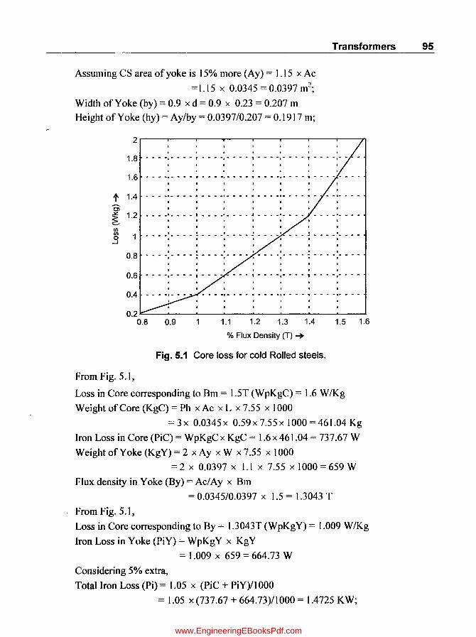
Transformers 95
Assuming CS area of yoke is 15% more (Ay) = 1.15 x Ac
= 1.15 x 0.0345 = 0.0397 m2;
Width of Yoke (by) = 0.9 x d = 0.9 x 0.23 = 0.207 m
Height of Yoke (hy) = Ay/by = 0.0397/0.207 = 0.1917 111;
I I I I • •
1.8 ...... -." ...... r ...... -," ...... , .... ... ," ...... , ......... ,.... ..
1.6 ...... -......... r ........ , ........ " ...... -," ...... ,. ........ ...... ..
t 1.4 Oi ~ 1.2 .... .... J ................... I ................ "t.. .. .... .. ...... , ...... .. ,
~ o -J
• I • • I • I .................... _ ......................................... - .. I • • • • • •
• • • , I • I 0.8 ...... -......... ; ...... -," .. .. .. I ........ I'" .... .. '; ................ ..
• 'I' I 0.6 ...... -.- ...... , ................ , .... .. -,- ...... 1 ...... "." .... ..
0.4
0.2 ~--'-----'----'--~'----~-----~----' 0.8 0.9 1.1 1.2 1.3 1.4 1.5 1.6
% Flux Density (T) ~
Fig. 5.1 Core loss for cold Rolled steels.
From Fig. 5.1,
Loss in Core corresponding to 8m = 1.5T (W pKgC) = 1.6 W IKg
Weight of Core (KgC) = Ph x Ac x L x 7.55 x 1000
= 3 x 0.0345 x 0.59 x 7.55 x 1000 = 461.04 Kg
Iron Loss in Core (PiC) = WpKgCx KgC = 1.6 x 461.04 = 737.67 W
Weight of Yoke (KgY) = 2 x Ay x W x 7.55 x 1000
= 2 x 0.0397 x 1.1 x 7.55 x 1000 = 659 W
Flux density in Yoke (8y) = AC/Ay x 8m
= 0.0345/0.0397 x 1.5 = 1.3043 T
From Fi.g: 5.1,
Loss in Core corresponding to 8y = 1.3043T (WpKgY) = 1.009 W/Kg
Iron Loss in Yoke (PiY) = WpKgY x KgY
= 1.009 x 659 = 664.73 W
Considering 5% extra,
Total Iron Loss (Pi) = 1.05 x (pjC + PiY)/1 000
= 1.05 x (737.67 + 664.73)/1000 = 1.4725 KW;
www.EngineeringEBooksPdf.com
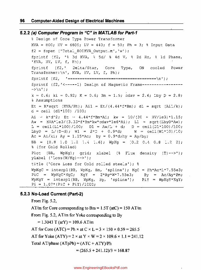
96 Computer-Aided Design of Electrical Machines
5.2.2 (a) Computer Program in "C" in MATLAB for Part-1 % Design of Core Type Power Transformer
KVA = 800; HV = 6600; LV = 440; f = SO; Ph = 3; % Input Data
f2 = fopen ('Total_800KVA_Output.m', 'w');
fprintf (f2, '% 3d KVA, % Sd/ % 4d V, % 2d Hz, % Id Phase, 'KVA, HV, LV, f, Ph);
fprintf (f2, , Delta/Star, Core Type, Transformer:\n', KVA, HV, LV, f, Ph);
ON cooled Power
,fprintf (f2, '=====================================\n');
fprintf (f2, '<-----1) Design of Magnetic Frame----------------->\n');
-k = 0.6; ki = 0.92; K = 0.6; Bm = 1.S; cdav = 2.6; Lby D = 2.8; % Assumptions
Et = K*sqrt (KVA/Ph); Ail = Et/ (4.44 *f*Bm); dl d = ceil (dl*100) /100;
sqrt (Ail/k);
Ai = k*d"2; Et = 4.44*f*Bm*Ai; kw = 10/(30 + HV/le3)*1.1S; Aw = KVA*le3/(3.33*f*Bm*kw*cdav*le6*Ai); L1 = sqrt(LbyD*Aw); L = ceil(Ll*lOO)/lOO; D1 = Aw/L-+ d; D = ceil(D1*100)/100; LbyD = L/(D-d); W1 = 2*D + 0.9*d; W = ceil(W1*10)/lO; Ac = Ai/ki; Ay = 1.lS*Ac; by = 0.9*d;hy = Ay/by;
BB = [ 0 . 8 1. 0 1. 2 1. 4 1. 6]; WpKg [ 0 . 2 0 . 4 0 . 8 1. 2 2]; % (for Cold Rolled)
Plot (BB, WpKg); grid; xlabel (% Flux density (T)-->'); ylabel ('Loss(W/Kg)-->');
title ('Core Loss for Cold rolled steels'); %
WpKgC = interp1(BB, WpKg, Bm, 'spline'); KgC PiC WpKgC*KgC; KgY 2*Ay*W*7.SSe3; WpKgY = interp1 (BB, WpKg, By, 'spline' ) ; Pi = 1.07*(PiC + PiY)/lOOOi
5.2.3 No-Load Current (Part-2)
~rom Fig. 5.2,
AT/m for Core corresponding to Bm = 1.5T (ate) = 150 AT/m
From Fig. 5.2, AT /m for Yoke corresponding to By
= 1.3043 T (atY) = 109.6 AT/m
,:AT for Core (ATC) = Ph x at C x L = 3 x 150 x 0.59 = 265.5
= Ph*Ac*L*7.SSe3; By Ac/Ay*Bmi
PiY = WpKgY*KgYi
_ AT for Yoke (A TY) = 2 x at Y x W = 2 x 109.6 x 1.1 = 241.12
Total AT/pJiase (ATpPh) = (ATC + ATY)/Ph
= (265.5 + 241.12)/3 = 168.87
www.EngineeringEBooksPdf.com

Transformers 97
2
1.9
1.B
t 1.7
~ 1.6 CI)
1.5 c: Q)
0 1.4 x
:::J u::: 1.3
1.2
1.1 1
0
... ' ......... J .... L .... ~ ... 1 ... J .. .. J .... ~ .... . . I • • • I • • • I --- ........ __ ..... - .... ----- .. .. I • • I • • • • •
.. - .......... , .. '" r""'- ...... - ........ , .. .. ,. .. ..
...... .... I .. = J .... L .... ~ .. _I .... J .. .. I .... ~ ....
.. I......, .... J .. ... .. .. .. .... .. .. '.. .. .' .... .I .. .. .. .. ..
.. I .... _I .... J .... L .... I ...... I ..... ' .... J .... ' ..... . . 100 200 300 400 500600700 BOO 9001000
AT/m~
Fig. 5.2 Core loss for cold rolled steels.
LV 440 No. ofTums in LV wdg (TI) = r;; r;; = 24.03::::: 24 (Rounded off)
,,3xEt ,,3xI0.57
. K V A x 1000 800 x 1000 Phase Current m LV Wdg (12) = r:; = 1049.7 A
,,3 x LV .Jj x 440
Wattful Current (lw) = Pi x 1000 = 1.4 725 x 1000 = 1.9322 A .Jj x LV .Jj x 440
M . . (I) 1.15 x A TpPh 1.15 x 168.87 5 7218 A agnetlzmg current m = r;; = r;; = . ,,2 x T2 ,,2 x 24
No load CUrrent (10) =Jlw2 + 1m2 =J1.93222 + 5.7218 2 = 6.0392 A
Ratio of 10/12 (lObyI2) = 10/12 x 100 = 6.039211 049.7 x 100
= 0.5753 (Lies between 0.5 to 1 and hence OK).
5.2.3 (a) Computer Program in "C" in MATLAB for Part-2 % <-----2) No-Load Current------------------>\n');
Bm = 1.5; By = 1.3043; W = 1.1; LV = 440; Et = 10.57; KVA = 800; Pi = 1.4725; % Input Data
B1 = [1 1.25 1.5 1. 75 2.0]; H1 = [70 100 150 300 1000]; % (Cold Rolled)
plot (H1,B1); grid; xlabel density(T)-->');
('AT/m-->'); ylabel
title ('Magnetization Curve for Cold rolled steels'); %
(' Flux
www.EngineeringEBooksPdf.com

98 Computer-Aided Design of Electrical Machines
atC=interp1(B1,H1,Bm, 'spline'); atY=interp1(B1,H1,By, 'spline'); ATC Ph*atC*L; ATY = 2*atY*W; ATpPh = (ATC+ATY)/Ph; T2 floor(LV/sqrt(3)/Et); 12 KVA*le3/(sqrt(3)*LV); Iw Pi*1000/ (sqrt (3) *LV); 1m 1.15* ATpPh/sqrt (2) /T2; 10 = sqrt(ImA 2 + Iw A 2); IObyI2 = 10/12*100;
% -------------------------------------------------------------
5.2.4 Design of LV Winding (Part-3)
Assume:
1. Space available for turns (AL W) = 80% length
=0.8 x L=0.8 x 0.59=0.472m=472mm
2.2 turns radially (T2r) and [T2a = TIIT2r
= 24/2 = 12] AxiallylLength-wise
3. Since 1049.7 Amps very high, 12 parallel strands (stP) in each conductor.
Since 12 turns are accommodated in a length of 472 mm,
space/turn (ALT) = 472/12 = 39.3 mm
Since we can not have a single strand of 39.3 mm, let us select 3 strands (NstA = 3) axially
No. of strands radially (NstR) = stPlNstA = 12/3 = 4
Hence width of each strand (stW) = (AL TlNstA) - 0.5
= (39.3/3) - 0.5 = 12.6::::: 12 mm (bare)
Considering 0.4 mm ins thickness for each strip,
ins Strip width= 12.4mm
Space occupied length-wise(AL Wx)
= [{(stW+O.4) x NstA} +2] xT2a+ 100
= [{(l2 + 0.4) x3} + 2] x 12 + 100
= 570.4mm (Less than 590 and hence OK)
(It is assumed 2mm as inter turn insulation and 100 mm as extra space)
Assuming 0.98 factor due to rounding of edges of each strand,
Slack in length (SlkL V ax) = Lxi 000 - AL Wx
= 0.59x 1000-570.4 = 18.6(Desirable > 7 and hence OK)
CS area of conductor (a2) = stW x stT x stP x 0.98
= 12 x 3 x 12 x 0.98 = 423.36 mm2;
Current Density (cdLV) = 12/a2 = 1049.7/423.36 = 2.48 Almm2 (lies between 2.3 to 3.5 and hence OK)
Radial Width of the winding (rwLV)
= NstR x (stT + 0.4) x T2r + 1.8 = 4 x (3 + 0.4) x 2 + 1.8 = 29 mm
www.EngineeringEBooksPdf.com
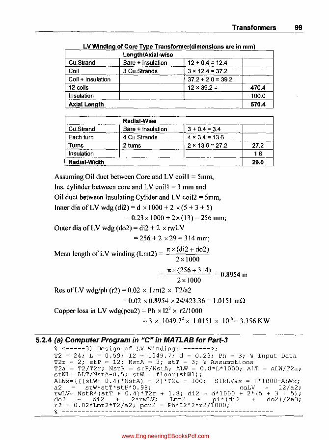
Transformers 99
LV Winding of Core Type Transformer(dimensions are in mm) Length/Axial-wise
Cu.Strand Bare + insulation 12 + 0.4 = 12.4 Coil 3 CU.Strands 3 x 12.4 = 37.2 Coil + Insulation 37.2 + 2.0 = 39.2 12 coils 12 x 39.2= Insulation Axial Length
Radial-Wise Cu.Strand Bare + insulation 3 + 0.4 = 3.4 Each tum 4 Cu.Strands 4 x 3.4 = 13.6 Turns 2 turns 2 x 13.6 = 27.2 Insulation
Radial-Width
Assuming Oil duct between Core and LV coil 1 = 5mm,
Ins. cylinder between core and LV coil I = 3 mm and
Oil duct between Insulating Cylider and LV coil2 = 5mm,
Inner dia of LV wdg (di2) = d x 1000 + 2 x (5 + 3 + 5)
= 0.23 x 1000 + 2x (13) = 256 mm;
Outer dia of LV wdg (d02) = di2 + 2 x rwLV
= 256 + 2 x 29 = 314 mm;
• • 1t x (di2 + d02) Mean length of LV wmdmg (Lmt2) = --'--------'--
2 x 1000
= 1t x (256+314) =0.8954m 2 x 1000
Res of LV wdg/ph (r2) = 0.02 x Lmt2 x T2/a2
= 0.02 x 0.8954 x 24/423.36 = 1.0 lSI mn
Copper loss in LV wdg(pcu2) = Ph x 122 x r2/1000
470.4 100.0 570.4
27.2 1.8
29.0
= 3 x 1049.72 x 1.0151 X 10-6 = 3.356 KW
5.2.4 (a) Computer Program in "C" in MA TLAB for Part-3 % <-----3) Design of LV Winding: ------->; T2 = 24; L = 0.59; 12 = 1049.7; d = 0.23; Ph = 3; % Input Data T2r = 2; stP = 12; NstA = 3; stT = 3; % Assumptions T2a = T2/T2r; NstR = stP/NstA; ALW = 0.8*L*1000; ALT = ALW/T2a; stW1= ALT/NstA-0.5; stW = floor(stW1); ALWx=(((stW+ 0.4)*NstA) + 2)*T2a + 100; SlkLVax = L*1000-ALWx; a2 stW*stT*stP*O.98; cdLV 12/a2; rwLV= NstR*(stT + O.4)*T2r + 1.8; di2 = d*1000 + 2*(5 + 3 + 5); do2 di2 + 2*rwLV; Lmt2 pi*(di2 + do2)/2e3; r2 = 0.02*Lmt2*T2/a2; pcu2 = Ph*12 A 2*r2/1000; % ------------------------------------------------------
www.EngineeringEBooksPdf.com

100 Computer-Aided Design of Electrical Machines
5.2.5 Design of HV Winding (Part-4)
No. of turns/ph (TI) = T2 x tIV/LV x 13 = 24 x 6600/440 x 13 = 623.5 = 624 (rounded oft)
. KVA x 1000 800 x 1000 Phase current 111 HV Wdg (II) = = = 40.404 A
3x BV 3x6600
Disc type winding with rectangular cross section is used
Assuming "z-2" no. of coils will have "x" no. of turns and 2 coils (both are in either end) will have "0.65 x z",
Total no. of turns (1'1) = x(z-2)+2 x 0.65 x x
fi'om which x = 1'1/(z- 2 + 1.3);
Here in the program x 1 = x and Axc = z;
Assuming total coils length-wise (AxC) = 14;
No. of turns in 12 coils (xl) = 1'1 AxC-2+ 1.3
624 ---- =46.9~48 14-2 + 1.3
Assuming each coil will have 4J= cA) strands axially
(length-wise), no. of strands in radial direction (x2)
=xl/cA=48/4= 12
No. of turns in each of the 2 end coils(x3)
= [TI- {x2xcAx (AxC-2)}]/2
= [624 - {12 x 4 x (14 -2)} ]/2 = 24
Check for Total turns (T I) = (12 x 48) + (2 x 24) = 624
Assuming 70% length is available for winding (ALW)
=0.7x Lx 1000=0.7 x590=413 mm
Space available per coil (ALPC) = ALW/A xC = 413/14 = 29.5 mm
Space for each strand (ALPC I) = ALPC/cA = 29.5/4 = 7.375 mm
Strand width (stW I) = ALPC 1- 0.4 = 7.375- 0.4 = 6.975 mm;
Select 6 mm;
Assuming current density (cdHV) = cdav + 0.2
= 2.6 + 0.2 = 2.8 A/mm2,
CS area of conductor in a turn (a I) = IIIcdHV
= 40.404/2.8 = 14.43 111m2,
Thickness of strand in a turn (stTI) = al/stWI
= 14.43/6 = 2.405, say 2.5 mm
Corrected CS area of strand in a turn (al) = stTI x stWI x 0.98
= 2.5 x 6 x 0.98= 14.7 mm2,
Current density (cdHV) = I Iial ;= 40.404/14.7 = 2.749 A/mm\
www.EngineeringEBooksPdf.com
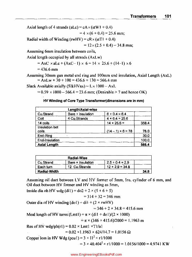
Transformers 101
Axial length of 4 strands (aLc) = cA x (stWI + 0.4)
= 4 x (6 + 0.4) = 25.6 mm;
Radial width of Winding (rwHV) = cRx (stTI + 0.4)
= 12x (2.5 + 0.4) = 34.8 mm;
Assuming 6mm insulation between coils,
Axial length occupied by all strands (AxLw) •
= AxC x aLc + (AxC- I) x 6 = 14 x 25.6 + (14-1) x 6
=436.6 mm
Assuming 30mm gun metal end ring and 100mm end insulation, Axial Length (AxL) = AxLw + 30 + 100 = 436.6 + 130 = 566.4 mm
Slack Available axially (SlkHVax) = Lx 1000 - AxL
= 0.59 x 1000 - 566.4 = 23.6 mm; (Desirable> 7 and hence OK)
HV Winding of Core Type Transfonner(dimensions are in mm)
Length/Axial-wise eu.Strand Bare + insulation 6 + 0.4 = 6.4 Coil 4 eU.Strands 4 x 6.4 = 25.6 14 coils 14 x 25.6 = 358.4 Insulation bet coils (14 -1) x 6 = 78 78.0 End-Rill!! 30.0 End-Insulation 100.0 Axial Length 566.4
Radial-Wise eu.Strand 1 Bare + insulation J 2.5 + 0.4 = 2.9 Each tum I 12 Cu. Strands I 12 x 2.9 = 34.8 Radial-Width 34.8
Assuming oil duct between LV and HV former of 5mm, Ins. cylinder of 6 mm, and Oil duct between HV former and HV winding as 5mm,
Inside dia oh HV wdg (dil) = d02 + 2 x (5 + 6 + 5)
= 314 + 32 = 346 mm
Outer dia of HV winding (do 1) = di 1 + (2 x rwHV)
= 346 + 2 x 34.8 = 415.6 mm
Meal length of HV turns '(Lmt 1) = 'It x (di 1 + do 1 )/(2 x 1000)
~ n: x (346 + 415.6)/2000 = 1.1963 m
Res ofHV wdglph(rl) = 0.02 x Lmtl xTl/al =0.02 x1.1963 x 624/14.7= 1.01560
Copper Joss in HV Wdg (pcul) = 3 x 112 x rl/1000
= 3 x 40.4042 x rl/1000 = 1.0156/1000 = 4.9741 KW
www.EngineeringEBooksPdf.com

102 Computer-Aided Design of Electrical Machines
5.2.5 (a) Computer Program in "c" in MATLAS for Part-4 % <-----------4) Design of HV Winding:-------> HV = 6600; LV = 440; cdav = 2.6; do2 = 314; T2 = 24; KVA = BOO; L = 0.59; Tla = T2*HV/LV*sqrt(3); Tl =. ceil{Tla); II = KVA*le3/{3*HV); cA 4; AxC = 14; cdHV = cdav + 0.2; %Assumptions xl Tl/{AxC-2+l.3); x2 ceil{xl/cA); x3 (Tl-(x2*cA*{AxC-2)))/2; Tlx = {AxC-2)*cA*x2 + 2*x3; cR x2; ALWI floor (0. 7*L*1000); ALPC ALWl!AxC; ALPCl = ALPC/cA; stWll = ALPCl-0.4; stWl floor (stWll); ala Il/cdHV; stTll ala/stWl; stTl = ceil (stTll*lO)/lO;al = stTl*stWl*0.9B; cdHV = Il/al; aLc = cA*(stWl + 0.4); rwHV = cR*{stTl + 0.4); AxLw = AxC*aLc + (AxC-l) *6; AxL AxLw + 30 + 100; SlkHVax L*1000-AxL; dil do2 + 10 + 12 + 10; dol = di1 + 2*rwHV; Lmtl pi*{dil + dol)/2e3; rl 0.02*Lmt1*Tl/a1; pcul = 3*Il A 2*r1/l000;
5.2.6 Performance Calculations (Part-5)
Assuming stray losses as 5%, Total Wdg Copper losses (pcuT)
= 1.05 x (pcul + pcu2) = 1.05*(4.974 + 3.356) = 8.746 KW
Total losses on Full Load (ptFL) = (pcuT + Pi)
= 8.746 + 1.473 = 10.219 KW;
Efficiency Calculation for 1 sl variant:
pf= 1.0; Ldpu = 1.0;
Pf
1.0 0.85 0.85 0.85
Total Loss (TL) = Pi + pcuT x Ldpu2
= 1.473 + (8.746 x 1.02) = 10.219 KW
Output (Opt) = LdpuxKVAxpf= 1.0 x800 x 1.0 = 800 KW
Input (lnp) = Opt + TL = 800 +10.219 = 810.219 KW
Efficiency( eft) = OptlInp x 100 = 800/810.219 xl 00 = 98.7387 %;
Load(pu) Losses(KW) Output(KW) Input(KW) Efficiency = Output/Input lC 100
1.0 10.219 800 810.219 98.7387% 1.0 10.219 680 690.219 98.5195 %
0.75 6.3924 510 516.392 98.7621 % 0.5 3.6591 340 343.659 98.9352 %
www.EngineeringEBooksPdf.com

Transformers 103
Load [or max. Efiiciency (Ldmxet) = ~ Pi xKVA pCllT
Max Efficiency (efmx) Ldmxef x 0.85
=---------(Ldmxef x 0.85) + (2 x Pi)
= 0.9895pll = 98.96 %
=~1.473 x800 = 328.25 KVA 8.746
328.25 x 0.85
(328.25 x 0.85) + (2 x 1.4 73)
Mean Turn Length (Lmt) = (Lmt 1 + Lmt2)/2
= (1.1963 + 0.8954 )/2 = 1.0458m
Length of coil (Lc) = AxLwlI 000 = 436.4/ I 000 = 0.4364 111;
AT/ph (AT) = II x TI = 40.404 x 624 = 25212
P.U.Reactance(Ex)
= 2x1txfx4x1txIO-7
xLmtxAT X[0.016+rWHv+rWLV] =0.0841 pll Lc x Et 3 x 1000
= 2x1tx50x4x1txIO-7
x 1.048 x 25212 x [0.016+ 29+34.8] =0.0841 pll 0.4364 x 10.57 3 x 1000
P.U. Resistance (Rr) = pcuT/KV A = 8.746/800 = 0.0109
P.U. Impedance (Ez) =~Er1 + Ex 2 = ~0.01092 + 0.08412 = 0.0848 pll
Regulation at 0.85pf and FL (Reg85) = Er x 0.85 + Ex x ~I - 0.85 2
= 0.0109 x 0.85 + 0.0849 x ~I- 0.85 1 = 0.0536pu (5.36%)
Regulation at UPF and FL (RegUPF) = Er = 0.0 I 09 pu (1.09%)
5.2.6 (a) Computer Program in "C" in MATLAB for Part-5 * <-----------5) Performance Calculations :------> pcu1 1.974; pcu2 3.356; Pi 1.473; AxLw II = 40.404; f ~ 50; EL = 10.57; % Input D~ta rwHV 29; rwLV 34.8; KVA 800; Lmtl Lmt2 = 0.8954; T1 ~ 624; * Input Data pcuT = 1.05*(pcu1 + pcu2); ptFL = (peuT + Pi); PF = [1 0.85 0.85 0.85]; LDPU = [1 1 0.75 0.5]; for I = ]:4;
Pi + pcuT*Ldpu A 2; + TL(i);
436.4;
1.1963;
pf = PF(i); Ldpu = LDPU(i); TL(i) Opt (i) Ldpu*KVA*pf; Inp(i) = Opt (i) eff(i) Opt(i)/Inp(i)*100;end; Ldmxef sqrt(Pi/peuT)*KVA;
www.EngineeringEBooksPdf.com

104 Computer-Aided Design of Electrical Machines
efmx = Ldrnxef*0.85/(Ldrnxef*0.85 + 2*Pi)*100i Lmt = (Lmt1 + Lmt2)/2i Lc = AxLw/lOOOi AT = Il*T1i Ex= 2*pi*f*4*pi*le-7*Lmt*AT/Lc/Et* (0.016 + (rwHV + rwLV,/3e3ii Er = pcuT /KVAi Ez = sqrt (Ex"2 + Er0 2) i --
Reg 85 = Er*0.85 + Ex*sqrt(1-0.85"2)i RegUPF = Eri
5.2.7 Tank Design and Weights (Part-6)
Assuming Length-wise clearance (~L) = 140 mm,
Length of Tank (Lt) = 2x Ox 1000 + (dol + dL)
= 2x 0.44 x 1000 + (415.6 + 140) = 1435.6 mm
Assuming Width-wise clearance (dB) = 180mm,
Width of Tank (bt) = do 1 + dB = 415.6 + 180 = 595.6 mm
Assuming Height-wise clearance (dH) = 500mm,
Height of Tank (ht) = LxI 000 + (2 x hy x 1000 + dH)
= 0.59 x 1000 + (2 x 0.1917 x 1000 + 500) = 1473.3 mm;
Volume of Tank (Vt) = Lt x bt x htl109 = 1435.6 x 595.6 x 1473.3/109 = 1.2598 m3;
. Cooling Surface area of tank (St) = 2 x (bt + Lt) x htl106 = 2 x (595.6 + 1435.6) x ]473.3/106 = 5.9853 m2
;
Temperature-rise of Tank (Tr) = ptFL x ] 000 = 10.219 x 1000 = 136.6 0C 12.5 x St ]2.5 x 5.9853 .
Since Temp-rise is to be limited to (TRP),= 50 °C, Cooling tubes are to be provided
Selecting Tube dia (Oct) of 50mm and height (Hct) Of 1000mm,
Area of each tube (At) = 1[ x Oct X Hctl106 = 1[ x 50 X ]000/106 = 0.1571 m2;
Required Tube Cooling Area (CAt) = (ptFL x 1000-12.5 x St x TRP)/(6.5 x TRP x 1.35)
= (10.219 x 1000-12.5 x 5.9853 x 50)/(6.5 x 50 x 1.35) = ]4.765 m2 ; .
No. of cooling tubes required (Nt) = 14.765/0.] 571 = 94
Wt. of Copper in HV wdg (Wcul) = 8.9 x LmtI x Tn LV wI x al/IOOO = 8.9 x 1.1963 x 624 x ]4.7/1000 = 97.665 Kg
Wt. of Copper idg(Wcu2) = 8.9 x Lmt2 x T2 x a2/1000 = 8.9 x 0.8954 x 24 x 423.36/1 000 = 80.967 Kg
Wt. of Iron (Wiron) = KgC + KgY = 46] + 659 = 1120 Kg;
Assuming 1 % Insulation Wt, Total Weight (Wtot) = 1.01 x (Wcu 1 + Wcu2 + Wiron)
= 1.01 x (97.665 + 80.967 + 1120) = 1311.6 Kg
Specific Wt (KgPkva) = WtotlKV A = 13] ] .6/800 = 1.6395
www.EngineeringEBooksPdf.com

Transformers 105
5.2.7 (a) Computer Program in "C" in MATLAB for Part-6
% <-----------6) TANK Design andWeights------->
o = 0.44; dol = 415.6; L = 0.59; hy = 0.1917; ptFL = 10.219; Lmt1 = 1.1963; T1 = 624; % Input Data Lmt2 = 0.8954; T2 = 24; a2 = 423.36; KgC = 461; KgY = 659; KVA = 800; a1 = 14.7; % Input Data dL = 140; dB = 180; dH = 500; Oct = 50; Hct 1000; TRP = 50; % Assumptions Lt 2*D*le3 + (dol + dL) ; bt (dol + dB) ; ht L*le3 + (2*hy*le3 + dH) ; Vt Lt*bt*ht/1e9; St=2*(bt+Lt)*ht/le6; Tr = ptFL*le3/12.5/St;At = pi*Dct*Hct/1e6; CAt (ptFL*le3-l2.5*St*TRP)/(6.5*TRP*1.35); Nt ceil(CAt/At); Wcu1 8.9*Lmt1*Tl*a1/1e3; Wcu2 = 8.9*le3*Lmt2*T2*a2/1e6; Wiron = KgC+KgY;
Wtot = 1.0l*(Wcu1 + Wcu2 + Wiron); KgPkva = Wtot/KVA; % -------------------------------------------------------------
5.2.8 Computer Program in "C" in MATLAB for Complete Design % Design of Core Type Power Transformer
KVA = 800; HV = 6600; LV = 440; f = 50; Ph = 3; % Input Data f2 = fopen ('Total 800KVA_Output.m', 'w"; fprintf (f2,' % 3d KVA, % 5d/ % 4d V, % 2d Hz, % 1d Phase, KVA, HV, LV, f, Ph); fprintf (f2, Delta/Star, Core Type, ON cooled Power Transformer: n', KVA, HV, LV, f, Ph); Eprintf (f2,=========~==================================== n');
fpri~tf (f2, <-----1) Design of Magnetic Frame----------->\n');
k = 0.6; ki = 0.92; K = 0.6; Bm = 1.5; cdav = 2.6; Lby 0 = 2.8; % Assumptions Et = K*sqrt (KVA/Ph); Ail = Et/(4.44*f*Bm); d1 d = ceil(d1*100)/100; Ai = k*d A 2; Et 4. 44*f*Bm*Ai; kw 10/ (30 + Aw = KVA*le3/ (3.33*f*Bm*kw*cdav*le6*Ai); L1 sqrt(LbyD*Aw); L ceil(L1*100)/lOO; o = ceil(Dl*lOO)/100; Lby 0 = L/(D-d); Wi = 2*D + 0.9*d; W = ceil (Wl*10)/10; Ac 1.15*Ac; by = O.9*d; hy = Ay/by;
sqrt (Ail/k) ;
HV/le3) *1.15;
01 Aw/L+d;
= Ai/ki; Ay =
Fprintf (f2, Assumed: For 3stepped Core factor(k) = % 4.2f, Value factor (K) = % 4.2f\n', k, K); Fprintf (f2, Assumed: Window space factor (kw) = % 5.3f, Max Core Flux Density (T) = % 3.1f\n, kw, Bm); fprintf (f2, Core dia (d) (m) % 6.3f\n, d); fprintf (f2, CS area o£ core (sq.m) % 6.4 f\n, Ai); fprintf (f2, EMF/turn % 6.2f\n, Et); fprintf (f2, Av-Current density (A/sq.mm) % 6.2f\n', cdav);
www.EngineeringEBooksPdf.com
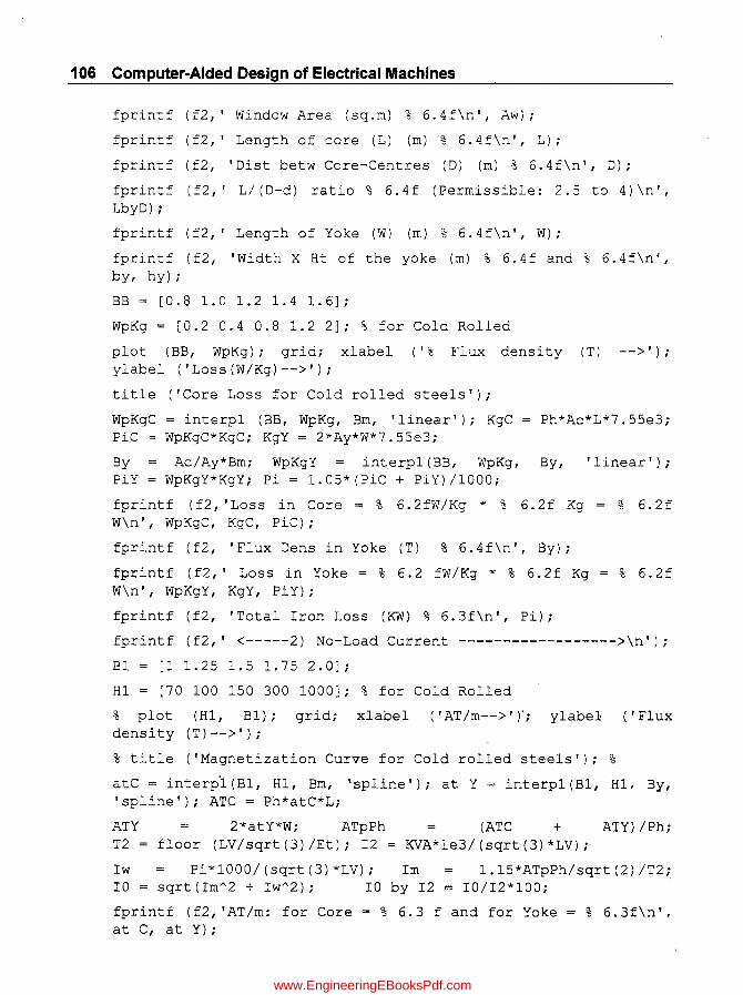
106 Computer-Aided Design of Electrical Machines
fprintf (£2,' Window Area (sq.m) % 6.4f\n', Aw);
£printf (f2,' Length of core (L) (m) % 6. 4.!:\n', L);
fprintf (f2, 'Oist betw Core-Centres (D) (m) % 6.4f\n', D);
£printf (£2,' L/(O-d) ratio % 6.4f (Permissible: 2.5 to 4)\n', LbyO) ;
fprintf (f2,' Length of Yoke (W) (m) % 6.4f\n', W);
fprintf (f2, 'Width X Ht of the yoke (m) % 6.4:: and % 6.4f\n', by, hy);
BB = [0.8 1. 0 1. 2 1. 4 1. 6] ;
WpKg = [0.2 0.4 0.8 1.2 2]; % for Cold Rolled
plot (BB, WpKg); grid; xlabel ('% Flux density (T) -->'); ylabel ('Loss(W/Kg)-->');
title ('Core Loss for Cold rolled steels');
WpKgC = interp1 (BB, WpKg, Bm, 'linear'); KgC PiC WpKgC*KgC; KgY = 2~Ay*W*7.55e3;
Ph*Ac*L*7.55e3;
By Ac/Ay*Bm; WpKgY interp1(BB, WpKg, By, 'linear'); PiY WpKgY*KgY; Pi = 1.05*(PiC + PiY)/1000;
fprintf (f2, 'Loss in Core = % 6.2fW/Kg ~ % 6.2f Kg W\n', WpKgC, KgC, PiC);
fprintf (f2, 'Flux Dens in Yoke (T) % 6.4f\n', By);
fprintf (f2,' Loss in Yoke = % 6.2 fW/Kg * % 6.2f Kg W\n', WpKgY, KgY, PiY);
fprintf (f2, 'Total Iron Loss (KW) % 6.3f\n', Pi);
% 6.2f
% 6.2£
fprintf (f2,' <-----2) No-Load Current ------------------>\n');
B1 [1 1.25 1.5 1.75 2.0];
H1 [70 100 150 300 1000]; % for Cold Rolled
% plot (H1, B1); grid; xlabel ('AT/m-->'),; ylabel ('Flux density (T)-->');
% title ('Magnetization Curve for Cold rolled steels'); %
atC = interp"l (B1, H1, Bm, 'spline'); at Y = interp1 (B1, HI, By, 'spline'); ATC = Ph*atC*L;
ATY 2*atY*W; ATpPh (ATC + ATY) /Ph; T2 floor (LV/sqrt(3)/Et); 12 = KVA*le3/(sqrt(3)*LV);
Iw Pi*1000/(sqrt(3)*LV); Im 1.15*ATpPh/sqrt(2)/T2;, IO sqrt(Im~2 + Iw~2); IO by 12 IO/I2*100;
fprintf (f2, 'AT/m: for Core = % 6.3 f and for Yoke at C, at Y);
% 6.3f\n',
www.EngineeringEBooksPdf.com

Transformers 1'07
fprintf (f2, 'Total-AT: for Core 6.3f\n', ATC, ATY);
% 6.3 £ and for Yoke
fprintf (f2, 'AT/phase: % 6.2f\n', ATpPh);
fprintf(f2, 'Turns in LV winding % 6.0f\n', T2);
=printf (f2, 'Ph-Current in LV wdg (A~p) % 6.1f\n',I2J;
fprintf (f2, 'Magnetizing-Ct (10 = Iw + jIm) % 6.3f = % 4.3£ + j % 4.3f A\n', 10, Iw, 1m);
fprintf (f2,' Ratio of IO/I2 (pe:::-c) % 6.3f (Permissible: 0.5 to l)\n', 10 by 12);
fprintf (f2, '<-----3) Design of LV Winding:------->\n');
T2r 2; stP = l2; NstA = 3; stT = 3;
T2a T2/T2r; NstR = stP/NstA; ALW = 0.8*L*1000; ALT = ALW/T2a; stW1 = ALT/NstA-0.5; stW floor(stW1);
ALWx=( ((stW+ 0.4)* NstA) + 2)*T2a + 100; SlkLVax L*lOOO-ALWx;
a2 = stW~stT*stP*0.98; cdLV = 12/a2;
rwLV = NstR*(stT+ 0.4)*T2r + 1.8; di2 = d*1000 + 2*(5 + 3 + 5);
do2 di2 + 2*rwLV; Lmt2 pi*(di2 + do2)/2e3; r2 = 0.02*Lmt2*T2/a2; pcu2 = Ph*I2A2~r2/1000;
fprintf (f2,'Turns (RadialXAxial) % 2.0f X % 2. Of \n', T2r, T2a) ;
fprintf (f2,' Conductor: % 2d Strands in Parallel of W*t (rom*rom) % 2dX % 2d\n', stP, stW, stT);
fprintf (f2, Strands (RadialXAxial) % 2.0f X % 2.0f\n', NstR, NstA) ;
fprintf (f2, CS area of Conductor (sq.rom) % 6.2f\n', a2);
fprintf (f2, Cur:::-ent density (A/sq.rom) % 6.2f (Permissible:2.3 to 3.5)\n', cdLV);
fprintf (f2, Axial Slack in LV-Wdg (mm) % 6.2f
(desirable>7)\n', SlkLVax);
fprintf (f2, Radial width of Wdg (rom) % 6.2f\n', rwLV);
fprintf (f2, Wdg-Dia (InnerXOuter) (rom) % 4.1f X % 4.1f\n', di2, do2);
fprintf (f2, Mean Length of Turn (m) % 6.2f\n', Lmt2);
fprintf (f2, Resistance/phase (m.ohm) % 6.4f\n',r2*1000);
fprintf (f2,' Cu.Loss in LV wdg (KW)'% 6.3f\n', pcu2);
fprintf (f2, '<-----------4) Design of HV Winding:------->\n');
www.EngineeringEBooksPdf.com

108 Computer-Aided Design of Electrical Machines
Tla = T2*HV/LV*sqrt(3); Tl = ceil(Tla); 11 = KVA*le3/(3*HV);
cA = 4; AxC = 14; cdHV = cdav + 0.2; % Assumptions
xl Tl/(AxC 2 + 1. 3) ; x2 ceil (xl/cA) ; x3 (Tl-(x2*cA*(AxC-2)))/2; Tlx = (AxC-2)*cA*x2 + 2*x3;
cR x2; ALWl floor (0. 7*L*1000); ALPC ALW1/AxC; ALPCl = ALPC/cA; stWll = ALPC1-0.4;
stWl floor (stW1l); ala Il/cdHV; stTll ala/stWl; stT1 = ceil(stTll*lO)/lO; al = stTl*stWl*0.98;
cdHV = II/al; aLc = cA*(stWl + 0.4); rwHV = cR*(stTl + 0.4); AxLw = AxC*aLc + (AxC-l) *6;
AxL dil
AxLw + 30 + 100; SlkHVax d02 + 10 + 12 + 10; dol = dil + 2*rwHV;
L*lOOO-AxL;
Lmtl pcul
pi* (dil + 3*I1 "2*rl/1000;
dol)/2e3; rl 0.02*Lmtl*Tl/al;
Fprintf (f2, 'Turns in HV Wdg % 6.0f\n', Tl);
Fprintf (f2, 'Ph-Current in HV wdg (Amp) % 6.2f\n',Il);
Fprintf (f2,' Wdg: % 3d coils X % 3d turns + 2 coils X % 3d turns = % 4. Of\n', AxC-2, cA*cR, x3, Tlx);
fprintf (f2,'Conductor(W*tl (mm*mm) stT-l) ;
% 4.1f X % 4.1f\n', stWl,
% fprint f (f2, Strands (RadialXAxial) % 2. 0 f NstR, NstA);
X % 2.0f\n',
fprintf (f2, 'cs area of Conductor (sq.mm) % 6.2f\n', all;
fprintf (f2, Current density (A/sq.mm) % 6.2f (Permissible:2.3 to 3.5)\n', cdHV);
fprintf (f2,' Axial Slack inHV-Wdg (mm) % 6.2f (desirable: >7)\n', SlkHVax);
fprintf (f2,' Radial width of Wdg (mml % 6.2f\n', rwHV);
fprintf (f2, Wdg-Dia (InnerXQuter) (mm) % 4.lf X % 4.1f\n', dil, dol);
fprintf (f2, Clearance bet HV Wdgs (mm) % 6. 2f (desirable: >15)\n', D*1000-dol);
fprintf (f2, Mean Length of Turn (m) % 6.2f\n', Lmtl);
fprintf (f2, 'Resistance/phase (ohm) % 6.4 f\n', rl);
fprintf (f2, Cu. Loss in LV wdg (~v) % 6.3f\n', pcul);
fprintf (f2, <-----------5) Performance Calculations:----->\n') ;
www.EngineeringEBooksPdf.com

Transformers 109
pcuT = 1.05*(pcu1 + pcu2); ptFL = (pcuT + Pi);
PF = [1 0.85 0.85 0.85]; LDPU = [1 1 0.75 0.5];
for i = 1:4;
pf = PF(i); Ldpu = LDPU(i);
TL(i Inp(i)
Pi + pcuT*~dpuA2; Opt (i) Ldpu*KVA*pf; Opt(i) + TL(i); eff(i) = Opt(i)/Inp(i)*100; end;
Ldmxef sqrt (Pi/pcuT) *KVA;
efmx = Ldmxef*0.85/(Ldmxef*0.85 + 2*Pi)*100;
Lmt = (Lmt1 + Lmt2)/2; Lc = AxLw/1000; AT I1*T1;
Ex= 2*pi*f*4*pi*le-7*Lmt*AT/Lc/Et* (0.016 + (rwHV + rwLV)/3e3); Er = pcuT/KVA;Ez = sqrt(ExA2 + Er A2);
Reg85 = Er*0.85 + Ex*sqrt(1-0.85 A2); RegUPF Er;
Fprintf (f2, 'Efficiency at UPF and Full Load: % 5.2f\n', eff(l)) ;
fprintf (f2, 0.75pu Ld: eff(4));
'Efficiency at 0.85 pf and at: %5.2f and O.Spu Ld: % 5.2f\n',
1pu Ld: eff (2),
% 5.2f, eff (3),
fprintf (£2, 'Max Efficiency = % 5.2f occuring at Load % 5.2fKVA\n', efmx, Ldmxef);
fprintf (f2, 'Mean-turn Length = % 6.4fm, Axil Length of Wdg = % 6.4fm, AT/ph = % 6.0f\n', Lmt, Lc, AT);
fprintf (f2,' Reactance % 6.4fpu, Restapce % 6.4fpu, Impedance = % 6.4fpu\n', Ex, Er, Ez);
fprintf (f2, Regulation: at FL and 0.85pf = % 5.4 fpu, at FL and UPF = % 5.4 fpu\n', Reg85, RegUPF);
fprintf (f2, '<-----------6) TANK Design andWeights------->\n');
dL = 140; dB = 180; dH = 500; Dct = 50; Hct = 1000; TRP = 50; % Assumptions;
Lt = 2*D*le3 + (dol + dL); bt = (dol + dB); ht = L*le3 + (2*hy*le3 + dH); Vt = Lt*bt*ht/1e9; St = 2*(bt + Lt)*ht/1e6;
Tr ptFL*le3/12.5/St; At pi*Dct*Hct/1e6; CAt = (ptFL*le3-12.5*St*TRP) /(6.5*TRP*1.35);Nt = ceil (CAt/At) ;
Wcu1 8.9*Lmt1*T1*a1/1e3; Wcu2 8.9*le3*Lmt2*T2*a2/1e6; Wi ron = KgC + KgY;
Wtot = 1.01* (Wcu1 + Wcu2 + Wiron); KgPkva = Wtot/KVA;
Fprintf (f2, 'Tank: Length = % 4.0from, Width = % 4.0 from, Height = % 4.0 from and Volume = % 6.3fm3\n', Lt, bt, ht, Vt);
www.EngineeringEBooksPdf.com

110 Computer-Aided Design of Electrical Machines
fprintf (f2, 'Tank : Coo~ing area = % 6.4 fsq.~ and Temp-Rise = % 4.0 f is reduced to 50 deg-C\n', St, Tr);
fprintf(f2,' Cooling Tubes: Area/Tube = % 6.4 fsq.m, RequiredArea = % 6.4fsq.m and No of Tubes = % 3.0 f\n', At, CAt, Nt);
fprintf (f2,' Weight: HV-Wdg = % 6.2f + LV-Wdg : = % 6.2£ + (Core + Yoke): = % 6.2 f and Total = % 7. If Kg\n', Wcul, Wcu2, Wiron, Wtot);
fprintf (£2,' Kg/KVA = % 6.3f\n', KgPkva);
fprintf (f2, <----------- End of Program------->\n');
fclose (f2);
5.2.8 (a) Computer Output Results for Complete Design
800 KV A, 6600/ 440 V, 50 Hz, 3 Phase, Delta/Star, Core Type, ON cooled Power Transfonner:
<-----1) Design of Magnetic Frame------------------>
Assumed: For 3stepped Core factor (k) = 0.60, Value factor (K) = 0.60
Assumed: Window space factor (kw) = 0.314, Max Core Flux Density (T) = 1.5
Core dia (d) (m) 0.230
CS area of core (sq.m) 0.0317
EMF/tum 10.57
Av-Current density (Alsq.mm) 2.60
Window Area (sq.m) 0.1235
Length of core (L) (m) 0.5900
Dist betw Core-Centres (D) (m) 0.4400
LI(D-d) ratio 2.8095 (Pennissible:2.5to4)
Length of Yoke (W) (m) 1.1000
Width X Ht of the yoke (m) 0.2070 and 0.1917
Loss in Core = 1.60WlKg x 461.04 Kg = 737.67 W
Flux Dens in Yoke (T) 1.3043
Loss in Yoke = 1.01 WlKg x 659.00 Kg = 664.73 W
Total Iron Loss (KW) 1.473
<-----2) No-Load Current------------------>
AT/m: for Core = 150.000 and for Yoke = 109.600
www.EngineeringEBooksPdf.com

Total-AT: for Core = 265.500 and for Yoke = 241.119
AT/phase: 168.87
Turns in LV winding 24
Ph-Current in LV wdg (Amp) 1049.7
Magnetizing-Ct (10 = Iw + jIm) 6.039 = 1.932 + j5.722 A
Ratio ofIO/I2 (perc) 0.575(Permissible: 0.5 to 1)
<-----3) Design of LV Winding: ------->
Turns (Radial x Axial) 2 x 12
Transformers 111
Conductor:-12 Strands in Parallel ofW x t (mm x mm) 12 x 3
Strands (Radial x Axial) 4x 3
CS area of Conductor (sq.mm) 423.36
Current density (Alsq.mm) 2.48 (Permissible: 2.3 to 3.5)
Axial Slack in LV-Wdg (mm) 19.60 (desirable>7)
Radial width ofWdg (mm) 29.00
Wdg-Dia (Inner x Outer) (mm) 256.0 x 314.0
Mean Length of Turn (m) 0.90
Resistance/phase (m.ohm) 1.0151
Cu.Loss in LV wdg (KW) 3.356
<-----------4) Design of HV Winding:------->
Turns in HV Wdg 624
Ph-Current in HV wdg (Amp) 40.40
Wdg: 12 coils x 48 turns + 2 coils x 24 turns = 624
Conductor(W x t) (mm x mm) 6.0 x 2.5
CS area of Conductor (sq.mm) 14.70
Current density (Alsq.mm) 2.75 (Permissible: 2.3 to 3.5)
Axial Slack in HV-Wdg (mm) 23.60 (desirable: >7)
Radial width ofWdg (mm) 34.80
Wdg-Dia(InnerXOuter) (mm) 346.0 x 415.6
Clearance bet HV Wdgs (mm) 24.40 (desirable: > 15)
www.EngineeringEBooksPdf.com

112 Computer-Aided Design of Electrical Machines
Mean Length of Turn (m) 1.20
Resistance/phase (ohm) 1.0156
Cu. Loss in LV wdg (KW) 4.974
<-----------5) Performance Calculations:------>
Efficiency at UPF and Full Load: 98.74
Efficiency at 0.85 pf and at: 1 pu Ld: 98.52, 0.75 pu Ld: 98.76 and 0.5pu Ld: 98.94
Max Efficiency = 98.96 occuring at Load = 328.25KV A
Mean-turn Length = 1.0458m, Axil Length ofWdg = 0.4364m, AT/ph = 25212
Reactance = 0.0841pu, Restance = 0.0109pu, Impedance = 0.0848pu
Regulation: at FL and 0.85pf= 0.0536pu, at FL and UPF = 0.0 1 09pu
<-----------6) TANK Design andWeights------->
Tank: Length = 1436mm, Width = 596 mm, Height = 1473 mm and
Volume = 1.260 m3
Tank: Cooling area = 5.9853 sq.m and Temp-Rise = 137 is reduced to 50 deg-C
Cooling Tubes: Area/Tube = 0.1571 sq.m, Required-Area = 14.7650 sq.m and No. of Tubes = 94
Weight: HV-Wdg: = 97.66 + LV-Wdg: = 80.97 + (Core + Yoke): = 1120.04 and Total = 1311.6 Kg
Kg/KV A = 1.6395
<-----------End of Program------->
5.2.9 Modifications to be done in the above Program to get Optimal Design
1. Insert "for" Loops for the following parameters to iterate the total program between min and max permissible limits for selecting the feasible design variants:
(a) No. of values of"K" (Factor of ratio of core to copper)
(b) No. of Values of "Bm", (Core flux density)
(c) No. of Average current density values
(d) No. of "LID" ratios.
2. Insert also minimum or maximum range of required objective functional values as constraint values, for example, (a) Efficiency (b) Kg/KVA (c) 10/12 ratio (d) Volume of Tank etc.
3. Run the program to get various possible design variants.
www.EngineeringEBooksPdf.com

Transformers 113
Note: From the feasible design variants printed in the output, select that particular design fulfilling the objective of optimal parameter for the design
5.2.10 Computer Program in "C" in MATLAB for Optimal Design
% Design of Core Type Power Transformer,
KVA = 800; HV = 6600; LV = 440; f = 50; Ph 3; % Input Data
f2 = fopen ('Optimal 800KVA_Output.m', 'w');
fprintf (f2,' % 3d KVA, % 5d/ % 4d V, % 2d Hz, % 1d Phase,
KVA, HV, LV, f, Ph);
fprintf (f2, Delt:a/Star, Core Type, ON cooled Power
Transformer:\n', KVA, HV, LV, f, Ph);
fprintf (f2,'
==============================================\n');
fprintf (f2,' Sn K Bm d L D W L/(D-d) cdav
cdLV CDHV 10/12 eff Kg/KVA Reg Tank Nt\n');
fprintf (f2,' --- ---- --- ---- ---- ----- -----
----\n') ;
k = 0.6; ki = 0.92; sn = 0; M1 = 0; M2 = 0; M3 = 0; M4 0;
SFFmax = 98; min 10 by 12 = 1; min KgPkva = 2; minVt 2;
'" Assumptions
kw = 10/(30 + HV/1e3)*1.15;
for K = 0.6:0.01:0.65; % K--> 0.6 to 0.65
for Bm = 1.5: 0.1: 1.6; % Bm --> 1.5 to 1.7 for CRGO and PT
for cdav = 2.5: 0.1: 3.5; % cdav --> 2.5 to 3.5
for Lby 0 = 2.6:0.2:4; % Lbyd --> 2.5 to 4
% fprintf (f2, '<-----1) Design of Magnetic Frame-----------
----->\n');
Et:
d1
Et
Aw
L1
K*sqrt (KVA/Ph) ; Ail
sqrt(Ai1/k); d = ceil(d1*100)/100; Ai
4.44*f*Bm*Ai; kw 10/(30
KVA*le3/(3.33*f*Bm*kw*cdav*le6*Ai);
sqrt(LbyD*Aw); L ceil(L1*100)/100;
+
E t / ,( 4 . 4 4 * f * Bm) ;
k*d A 2;
HV/1e3)*1.15;
01 = Aw/L + d; D ceil(D1*100)/100; LbyD1 L/(D-d);
if LbyD <= 2.5 I I LbyD > 4 continue; end;
www.EngineeringEBooksPdf.com

114 Computer-Aided Design of Electrical Machines
WI 2*0':" O.9*d; W ceil (liTl*lO; /10; .:;c
Ay = 1.lS*Ac; by = 0.9~d; hy = Ay/by;
% fprint= (=2, '<-----2) Perfor~ance of Magnetic Fra~e------
------>\n') ;
BB = [ 0 . 8 1. 0 1. 2 1. 4 1. 6]; WpKg
Cold Rolled
[0.2 0.4 0.8 1.2 2J; %
WpKgC interpl(BB,WpKg, Bm, 'linear');
KgC = Ph*Ac*L*7.S5e3; P~C = WpKgC*KgC; KgY = 2*Ay*W*7.55e3;
By = Ac/Ay*Bm; WpKgY = interpl(8B, WpKg, By, 'linear');
PiY = WpKgY*KgY; Pi = 1.05*(PiC+PiY)/1000;
% fprintf (f2, '<-----3) No-Load Current-----------------
>\n') ;
81 = [1 1.25 1.5 1.75 2.0]; HI
Cold Rolled
[70 100 150 300 1000]; %
atC interp1 (Bl, HI,
atY interpl(B1,H1,By, 'spline'); ATC
2*atY*W; ATpPh
8m,
Ph*atC*L;
(ATC +
'spline');
ATY)/Ph; ATY
T2 floor(LV/sqrt(3)/Et); 12 KVA*le3/(sqrt(3)*LV);
Iw Pi*1000/(sqrt(3)*LV); 1m 1.15*ATpPh/sqrt(2)/T2;
10 = sqrt(ImA 2 + Iw A 2); 10 by 12 = 10/12*100;
if 10 by 12 > = 0.66 continue; end;
% fprintf (f2, '<-----3) Design of LV Winding:------->\n');
T2r = 2; stP = 12; NstA = 3; stT = 3;
T2a T2/T2r; NstR stP/NstA; ALW O. 8*L*1000;
ALT = ALW/T2a; stWl = ALT/NstA-0.5; stW = floor(stWl);
ALWx=(((stW + 0.4)*NstA)+ 2)*T2a+100; SlkLVax = L*1000-ALWx;
if SlkLVax < = 7 continue; end;
a2 = stW*stT*stP*0.98; cdLV = 12/a2;
rwLV=NstR*(stT+0.4)*T2r + 1.8; di2 d*1000 + 2*(5 + 3 + 5);
do2 di2 + 2*rwLV; Lmt2 pi*(di2 + do2)/2e3;
r2 = 0.02*Lmt2*T2/a2; pcu2 = Ph*I2 A 2*r2/1000;
% fprintf (f2, '<------4) Design of HV Winding: ------->\n');
Tl = ceil (T2*HV/LV*sqrt(3)); II = KVA*le3/(3*HV);
www.EngineeringEBooksPdf.com
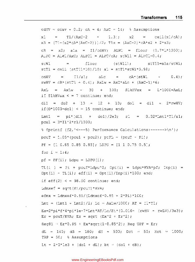
Transformers 115
cdHV = cdav ~ 0.2; cA 4; ?:<C = ~4; ;:" Assumptions
xl 1.3; ; x2 c e i 1 (x U c:A) ;
x3 ('I'1- (x2*ci\.* (AxC-2)); 12; Tlx = (AxC-2) *cA*x2 + 2 .... x3;
cR
ALPC
x2; ala I1 / c:dHV; ALW1
A~Wl/AxC; ALPCl = ALPC/cA; s~W11
floor (0.7*L*1000);
ALPC1-0.4;
s,:Wl floo~ (stWll) ; stTl1=a1al s':Wl;
stT1 ceil (st711*10)/10; al stTl*s~W1*0.98;
cdH'!
rwHV
I1/al; aLc
cR*(stT1 + 0.4); AxLw
cA*(stW1
AxC*aLc + (AxC-1) *6;
0.4) ;
AxL Ax::"'w + 30 + 100; SlkHVax L*lOOO-AxL;
if SlkHVax < 7 continue; end;
dil do2 + 10 + 12 + 10; do 1 di1 + 2*rwHV;
if(O*1000-dQ1) < 15 continue; end;
Lmt1 pi*(d:'l + do1)/2e3; r1 0.02*Lmtl*T1/a1;
% fprintf (f2, '<---5) Performance Calcula~ions:------>\~');
pcuT = 1.05*(pcul + pcu2); p~FL (pcuT + Pi);
PF = [1 0.85 0.85 0.85J; ::"'OPU = [1 1 0.75 0.5J;
for i = 1:4;
pf = PF(i); Ldpu = LOPU(i);
TL(i = Pi + pcuT*I.dpu"2; Opt (i) = Ldpu"KVA"pf; Inp(i)
Opt(i) + TL(i); eff(i) = Opt(i)/Inp(i)*100; e~d;
if eff(2) < = 9S.50 continue; end;
Ldrnxef = sqrt(Pi/pcuT)*KVA;
efmx = Ldrnxef*0.S5/(Ldrnxef*0.85 + 2*Pi)*100;
Lmt = (Lmtl + Lmt2)/2; Lc = AxLw/1000; AT = I1*T1;
Ex=2*pi*f*4*pi*le-7*Lmt*AT/Lc/Et* (0.016+ (rwHV + rwLV) /3e3);
Er = pcuT/KVA; Ez = sqrt (Ex A2 + ErA2);
Reg85 = Er*0.85 + Ex*sqr~(1-0.85A2); Reg UPF = Er;
dL 140; dB lS0; dH 500; Oct 50; Hct 1000;
TRP 50; % Assumptions
Lt = 2*O*le3 + (dol + dL); bt (dol + dB);
www.EngineeringEBooksPdf.com
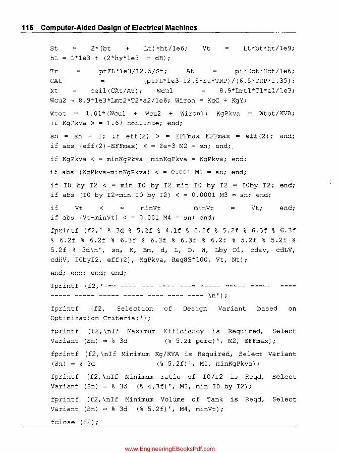
116 Computer-Aided Design of Electrical Machines
St 2*(bt + Lt)*ht/1e6; Vt Lt*bt*ht/1e9;
ht L*le3 + (2*hy*le3 + dH);
Tr ptFL*le3/12.5/St; At pi*Dct*Hct/1e6;
CAt (ptFL*le3-12.5*St*TRP)/(6.5*TRP*1.35);
Nt ceil (CAt/At); Wcu1 8. 9*Lmt1*T1*a1/1e3;
Wcu2 = 8.9*le3*Lmt2*T2*a2/1e6; Wiron = KgC + KgY;
Wtot 1.91*(Wcu1 + Wcu2 + Wiron); KgPkva Wtot/KVA;
if KgPkva > = 1.67 continue; end;
sn = sn + 1; if eff(2) > = EFFmax EFFmax
if abs (eff(2)-EFFmax) < = 2e-3 M2 sn; end;,
eff (2); end;
if KgPkva < = minKgPkva minKgPkva KgPkva; end;
if abs (KgPkva-minKgPkva) < = 0.001 M1 = sn; end;
if 10 by 12 < = min 10 by 12 min 10 by 12 = 10by 12; end;
if abs (10 by I2-min 10 by 12) < = 0.0001 ,M3 sn; end;
if Vt < if abs (Vt-minVt) <
minVt
0.001 M4
minVt Vt; end;
sn; end;
fprintf (f2, I % 3d % 5.2f % 4.1f % 5.2f % 5.2f % 6.3f % 6.3f
% 6.2f % 6.2f % 6.3f % 6.3f % 6.3f % 6.2f % 5.2f % 5.2f %
5.2f % 3d\nl, sn., K, Bm, d, L, 0, W, Lby 01, cdav, cdLV,
cdHV, 10by12, eff(2), KgPkva, Reg85*100, vt, Nt);
end; end; end; end;
fprintf (f2,1--- ---- --- ---- ---- ----- -----
----- ----- ----- ----- ---- ---- ---- \nl);
fprintf (f2, Selection of Design Variant based on
Optimization Criteria: I);
fprintf (f2,\n1f Maximum Efficiency is Required, Select
Va~iant (Sn) = % 3d (% 5.2f perc) I, M2, EFFmax);
fprintf (f2,\n1f Minimum Kg/KVA is Required, Select Variant
(Sn) = % 3d (% 5.2f) I, M1, minKgPkva);
fprintf (f2,\n1f Minimum ratio of 10/12 is Reqd, Select
Variant (Sn) = % 3d (% 4.3f) I, M3, min 10 by 12);
fprintf (f2, \nIf Minimum Volume of Tank is Reqd, Select
Variant (Sn) = % 3d (% 5.2f) I, M4, minVt);
fclose (f2);
www.EngineeringEBooksPdf.com

5.2.10 (a) Computer Output Results for Optimal Design
800 KVA, 6600/440 V, 50 liz, 3 Phase, Delta/Star, Core Type, ON cooled Power Transformer:
========================================================================================================== Sn K Bm d L I) W Ij(D-d) cdav cdLV DlIV 10/12 elf Kg/KVA Reg Tank Nt .. _ .. ____ .. _ .. _____ ... ____ ... ____ .. ____ 00 ..... - __________ .. ____ ....... _____ .. _________________ ...... ____ .. _ ... ____ .... _____ .. oO....... .. ..... ______ .... _____ .. ___________ .... ___________ ...... ____ .. ___
I 0.60 1.5 0.23 0.59 0.440 1.100 2.81 2.60 2.480 2.749 0.575 98.52 1.64 5.36 1.26 94 2 0.60 1.5 0.23 0.58 0.440 1.100 2.76 2.70 2.480 2.863 0.570 98.49 1.62 5.33 1.24 98 3 0.60 1.5 0.23 0.63 0.420 1.100 3.32 2.80 2.289 2.945 0.596 98.51 1.68 4.61 1.22 96 4 0.61 1.5 0.23 0.59 0.440 1.100 2.81 2.60 2.480 2.749 0.575 98.52 1.64 5.36 1.26 94 5 0.61 1.5 0.23 0.58 0.440 1.100 2.76 2.70 2.480 2.863 0.570 98.49 1.62 5.33 1.24 98 6 0.61 1.5 0.23 0.63 0.420 1.100 3.32 2.80 2.289 2.945 0.596 98.51 1.68 4.61 1.22 96 7 0.62 1.5 0.23 0.59 0.440 1.\ 00 2.81 2.60 2.480 2.749 0.575 98.52 1.64 5.36 1.26 94 8 0.62 1.5 0.23 0.58 0.440 1.100 2.76 2.70 2.480 2.863 0.570 98.49 1.62 5.33 1.24 98 9 0.62 1.5 0.23 0.63 0.420 1.100 3.32 2.80 2.289 2.945 0.596 98.51 1.68 4.61 1.22 96 10 0.63 1.5 0.23 0.59 0.440 1.100 2.81 2.60 2.480 2.749 0.575 98.52 1.64 5.36 1.26 94 11 0.63 1.5 0.23 0.58 0.440 1.100 2.76 2.70 2.480 2.863 0.570 98.49 1.62 5.33 1.24 98 12 0.63 1.5 0.23 0.63 0.420 1.100 3.32 2.80 2.289 2.945 0.596 98.51 1.68 4.61 1.22 96 13 0.64 1.5 0.23 0.59 0.440 1.100 2.81 2.60 2.480 2.749 0.575 98.52 1.64 5.36 1.26 94 14 0.64 1.5 0.23 0.58 0.440 1.100 2.76 2.70 2.480 2.863 0.570 98.49 1.62 5.33 1.24 98 15 0.64 1.5 0.23 0.63 0.420 1.100 3.32 2.80 2.289 2.945 0.596 98.51 1.68 4.61 1.22 96
.. - ---- --- _ .. -- ---- .. ---- .... --- ----- .. _-- --_ ..... ----- .... --- ----- .. _- .. ---- ---- ----- --_ .... -- ...... - ---- _ .... -- ........ - ----- ---- ----- - ........ ----- ----- ..... -- ---- ---- --------- ------
Selection of Design Variant based on Optimization Criteria
IfMax~mum Efficiency is Required, Select Variant (Sn) = 13 (98.52 perc)
If Minimum Kg/KVA is Required, Select Variant (Sn) = 14 (1.62)
If Minimum ratio of 10/12 is Required, Sc1.:ct Variant (Sn) = 14 (0.570)
If Minimum Volume or Tank if Required, Select Variant (Sn) = 15
www.EngineeringEBooksPdf.com

118 Computer-Aided Design of Electrical Machines
5.3 Shell Type Power Transformer
Total design is split into six parts in a proper sequence. Design calculations are given for a
given Rating of a Transfonner, followed by Computer Program written in "C" language
using MA TLAB software for each part. Finally all the Programs are added together to get the total Program by running which we get the total design. Computer Out put of total design is given.
This design may not be the optimum one. Now optimization objective and Design
Constraints are inserted into this total Program. When this program is run we will get various alternative feasible designs from which the selected variant based on the
Optimization Criteria can be picked up. Computer output showing the important design parameters for various feasible alternatives is given in the end of this chapter along with a
logic diagram.
Problem: Design a 125KVA, 33001 440 V, 50 Hz, I-Phase, Shell Type, oil cooled Power-class Transfonner: (Limitations: Temp-rise to 40 deg-C, No-load current to 1.5%,
Regulation to 4 % and Total losses to 2%).
5.3.1 Sequential Steps for Design of Each Part and Programming Simultaneously
(a) Calculate the dimensions of Magnetic frame consisting of Core, window
andY oke. Calculate Flux densities in those parts and Iron losses.
(b) Calculate Amp-Turns and No load current.
(c) Calculate No. of turns, size of Copper and final dimensions of LV winding.
(d) Calculate No. of turns, size of Copper and final dimensions ofHV winding.
(e) Check weather clearances between Magnetic frame and windings are OK.
(0 Calculate Windings copper Losses, total losses, Efficiency, Reactances and % Regulation.
(g) Calculate Dimensions of cooling tank, number and size of cooling tubes, temperature rise, total weight and KglKV A.
Note: By adding programs established for each part sequentially we get the Program for complete design.
5.3.2 Design of Magnetic Frame (Part-1)
Assuming Magnetic frame (both core and yoke) are made with Hot rolled Silicon
Steel with Rectangular Cross section and Value factor (K) = 1.1,
Volts/turn (Et) = K x .JKVA = 1.1 x .J125 = 12.2984 V/t
www.EngineeringEBooksPdf.com

Transformers 119
Assuming Ma'\.. Flux density in Core and Yoke (Bm) = 1.1 T,
Net CS area of Core (Ain) = £t 12.2984 = 0.0504 m2;
4.44 x f x Bm 4.44 x 50 x 1.1
Assuming Iron factor (ki) = 0.9,
gross CS area of Core (Aig) = Ainlki = 0.0504/0.92 = 0.056 m2;
Assuming Length 1 width of core (Rl) = 2.5,
Width of main Core (bmc) = ~Aig/RI
= -J0.056/2.5 =0.1496m::::: 150 mm(Rounded off)
Length of main core (Lmc) = Rl x bmc = 2.5 x 150 = 375 mm
Assuming Window Space factor (kw) = 0.27 and
Average Current density (cdav) = 2.5 Almm2;
Window Area (Aw) KVAx 1000
2.22 x fx Bm x kw x cdavx 106 x Ain
p5 x 1000 = 0.0301 m2; 2.22 x 50 x 1.1 x 0.27 x 2.5 x 106 x 0.0504
Assuming Height 1 width of window (R2) = 2.1,
Width of window (bw) = -JAw/R2 = -J0.030112.1
= 0.1198m::::: 120 mm (Rounded off)
Height of Window (hw) = R2 x bw = 2.1 x 120 = 252 mm
Since in a I-ph shell type Transformer, side core and yoke carry half the total flux (for same Bm)
Area of yoke (Ay) = Ainl2 = 0.0504 1 2 = 0.0252 m2;
Height of Yoke (hy) = Width of side core (bsc) = bmc/2 = 150/2 = 75 mm
Width of yoke (by) = Aylhy = 0.0252175 x 106 = 335.75 mm
Length of Yoke (Ly) = 2 x (bsc + bw) + bmc = 2 x (75 + 120) + 150 = 540 mm
Volume of central core (Vce) = Ain x hwl1000 = 0.0504 x 25211000 = 0.0127 m3;
Volume of2 side cores (V2se) = Vec = 0.0127 m3;
Total Volume of core (Ve) = Vee + V2se = 0.0127 + 0.0127 = 0.0254 m3;
\
Volume of both yokes (Vy) = 2 x Ly x Ayl1000 = 2 x 540 x 0.025211000 = 0.0272 m3;
Volume of Iron (Viron) = Vy + V c = 0.0272 + 0.0245 = 0.0526 m3;
Weight ofIron (Wiron) = Viron x 7.55 x 1000 = 0.0526 x 7.55 x 1000 = 397 Kg;
www.EngineeringEBooksPdf.com

120 Computer-Aided Design of Electrical Machines
l III III o ..J
4.5'---~--~--------~--~--~----~~
4 ...... :.-----: .. --.--:--.-- .. : ..... --.: ...... . ...... ; ... / /
· , . . . 3.5 ...... ; ...... ; ....... ; ...... -; ....... ; ..... . · , . . . · '" · '" 3 _ ..... - ~ .. _ ....... : .. --_ ... :-,_ ....... : ..... _ .... :. _ .. - -' · , . . . · , . . . · , . . . · . . . .
....... : ...... ' ....................................... .: ..... . · . .. '. 2.5 · , ., .. · . . · . . 2 - - ...... ~ ....... :- ....... :. ....... ," ...... -: .......... ," ... - - ~ ........ .. · ,. . . · " . .
I " • •
I •• • •
1.5 ....... - . ~ ... - ..... :- - .. .. .... ,"""'''' -:- .. - ... - -: - .... - - .. ~ - -- - . - ~ ..... - - .. · . .. . · . .. . , . .. . · ,. .. .
••••• _._. _., _______ • ___ •••••••• __ ............ ______ , •• __ 0-
o , • • • • • · , . . . . . . .. . 0.5 L-__ ~ __ ~ ____ .~ __ ~. ____ ~. __ ~ ____ ~. __ --'
0.8 0.9 1.1 1.2 1.3 1.4
% Flux Density (T) 7
Fig. 5.3 Core loss for hot rolled steels. \
1.5 1.6
From Fig. 5.3, Loss in Core corresponding to Bm = 1.1 T (scL) = 1.55 W/Kg
Taking 5% more for laminations, Total Iron Loss (Pi) = 397 x 1.55 x 1.05 = 646 W;
. Pi x 100 646 x 100 Percentage Iron Loss (pCPl) = 0.5168%
KVAx 1000 125 x 1000
5.3.2 (a) Computer Program in IIC" in MATLAB for Part-1
% Design of Shell Type (l-ph) Transformer KVA = 125; HV = 3300; LV = 440; f = 50; pf = 0.85; % Input Data % <-----1) Design of Magnetic Frame------------------> K = 1.1; Bm = 1.1; cdav = 2.5; kw = 0.27; ki = 0.9; Rl = 2.5; R2 = 2.1; % Assumptions Cdlv = cdav-O .1; cdhv = cdav + 0.1; Ain = Et/(4.44*f*Bm); Aig = Ain/ki;
Et = K*sqrt (KVA) ;
bmc1 = sqrt(Aig/Rl); bmc = ceil(bmcl*100) *10; Aw = KVA*le3/ (2. 22*f*Bm*kw*cdav*le6*Ain); bwl bw = ceil (bwl*100)*10;
Lmc = Rl*bmc; = sqrt (Aw/R2);
Hw = R2*bw; Ay = Ain/2; sc = bmc/2; hy = bsc; by = Ay/hy*le6; Ly 2* (bsc + bw) + bmc; Vcc = Ain*hw/l000; V2sc Vcc; Vc Vcc + V2sc; Vy 2*Ly*Ay/le3; Viron Vy + VC; Wiron = Viron*7.55e3; BB = [0.8 1.0 1.2 1.4 1.6J; WpKg = [0.8 1.2 1.9 2.9 4.2J; % (Hot Rolled) % plot (BB, WpKg); grid; xlabel ('% Flux density (T)-->'); ylabel ('Loss(W/Kg)-->');
www.EngineeringEBooksPdf.com

Transformers 121
% title ('Core Loss for Hot rolled steels'); seL = interpl (BB, WpKg, Bm, 'linear'); Pi Wiron*seL*1.05; pcPi = Pi/KVA/IO;
5.3.3 No-Load Current (Part-2)
Pi 646.06 Wattful Current (Iw) = - = = 1.4683 A
LV 440
Length of flux path in Main and side cores (Lfpc) = 2 x hwl1000
= 2 x 252/100 = 0.504 m
Length of flux path in Yoke (Lfpy) = Lyl1000 = 54011000 = 0.54 m
Total length of Flux path in magnetic frame (LfpT) = Lfpc + Lfpy
= 0.504 + 0.54 = 1.044m
2
1.9
1.8
t 1.7
E 1.6 ~ 1.5 III c Ql 1.4 c x
1.3 ::::I iI
1.2 • I I I ----_ ..... _------ .. _- .......... ---• I • I
1.1 ...... .. -.- .................... r ........ -,- ...... ..
1 0 500 1000 1500 2000 2500
AT/m~
Fig. 5.4 Magnetization curve for hot rolled steels.
From Fig. 5.4, AT/m for total frame corresponding to Bm
= LIT (atpm) = 118.8 AT/m
Total Ampere-turns (AT) = atpm x LfpT = 118.8 x 1.044 = 124.03 ; . LV 440
No of Turns m LV wdg (T2) =-= = 35.8::::: 36 (Rounded oft) Et 12.2984
M . . (I) 1.1 x AT 1.1 x 124 2 68 A agnetlZlng current m = r;:; = r;:; =. ,,2 xT2 ,,2 x36
No load Current (IO) = JIw2 + Jm2 = J1.46832 + 2.682 = 3.0556 A
www.EngineeringEBooksPdf.com

122 Computer-Aided Design of Electrical Machines
Phase Current in LV Wdg (12) = KVAx 000 = 125 x 1000 = 284.1 A LV 440
Ratio oflO1I2 (10 by 12) = 101I2*100 = 3.0556/284.1 x 100
= 1.0756 « 2 and hence OK)
Assuming average current density (cdav) = 2.5,
Current desity in LV wdg (cdlv) = cdav - 0.1 = 2.5-0.1 = 2.4 Almm2,
Current desity in HV wdg (cdhv) = cdav + 0.1 = 2.5 + 0.1 = 2.6 Almm2,
CS area of LV conductor (a2a) = ~ = 284.1 = 118.3 7mm2,
cdlv 2.4
. HV 3300 No. of Tums on HV side (TI) = - x T2 = --x 36 = 270
LV 440
Phase Current in HV Wdg (11) = KVAx 1000 = 125x 1000 = 37.879 A HV 3300
CS area ofHV conductor (ala) = ~= 37.879 = 14.57mm2,
cdhv 2.6
5.3.3 (a) Computer Program in "C" in MATLAB for Part-2
% <-----2) No-Load Current------------------>
Pi = 646.06; LV = 440; hw = 252; Ly = 540; 8m 1.1; Et = 12.2984; KVA = 125; % Input Data
cdlv = 2.4; HV = 3300; cdhv = 2.6; % Input Data
Iw Pi/LV; Lfpc= 2*hw/1000;Lfpy = Ly/1000; LfpT = Lfpc + Lfpy;
81 = [1 1. 25 1. 5 1. 75 2.0]; H1 = [100 250 650 1200 2100];
% (Hot Rolled)
% plot (H1, 81); grid; xlabel ('AT/m-->'); ylabel ('Flux
density (T) -->');
% title ('Magnetization Curve for Hot rolled steels'); %
Atpm interp1 (81, H1, Bm, , spline' ); AT atpm""LfpT;
T2a = LV/Et; T2 = ceil (T2a);
Im 1.1*AT/{sqrt(2)*T2); IO sqrt{Iw"2 + Im"2);
12 = KVA*1000/LV; IO by 12 = IO/I2*100; a2a = 12/cdlv;
T1 = T2*HV/LV; I1 = KVA*1000/HV; ala = I1/cdhv;
% -------------------------------------------------------------
www.EngineeringEBooksPdf.com
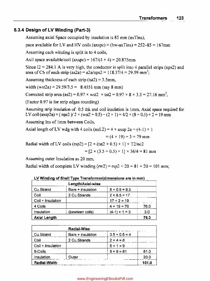
Transformers 123
5.3.4 Design of LV Winding (Part-3)
Assuming axial Space occupied by insulation is 85 mm (axTins),
pace available for LV and HV coils (axspc) = (hw-axTins) = 252-85 = 167mm
Assuming each winding is split in to 4 coils,
Axil space available/coil (axspc) = 167/(4 + 4) = 20.875mm
Since 12 = 284.1 A is very high, the conductor is split into 4 parallel strips (nps2) and area ofCS of each strip (as2a) = a2a1nps2 = 118.37/4 = 29.59 mm2
;
Assuming thickness of each strip (tst2) = 3.5mm,
width (wst2a) = 29.59/3.5 = 8.4551 mm (say 8 mm)
Corrected strip area (as2) = 0.97 x wst2 x tst2 = 0.97 x 8 x 3.5 = 27.16 mm2,
(Factor 0.97 is for strip edges rounding)
Assuming strip insulation of 0.5 thk and coil insulation is Imm, Axial space required for LV coil (axsp2a) = (nps2)/ 2 x (wst2 + 0.5) + (2 x 1) = 4/2 x (8 + 0.5) + 2 = 19 mm
Assuming Ins of 1 mm between Coils,
Axial length of LV wdg with 4 coils (axL2) = 4 x axsp 2a + (4-1) x 1
=(4x 19)+3=79mm
Radial width of LV coils (rsp2) = [2 x (tst2 + 0.5) + 1] x T2/nc2
= [2 x (3.5 + 0.5) + 1] x 36/4 = 81 mm
Assuming outer Insulation as 20 mm,
Radial width of complete LV winding (rw2) = rsp2 + 20 = 81 + 20 = 101 mm;
LV Winding of Shell Type Transformer(dimensions are in mml Length/Axial-wise
CU.Strand Bare + insulation 8 + 0.5 = 8.5
Coil 2 Cu.Strands 2x8.5=17
Coil + Insulation 17+2=19
4 Coils 4 x 19 = 76 76.0
Insulation (bewteen coils) (4-1) x 1 = 3 3.0
Axial Length 79.0
Radial-Wise
CU.Strand Bare + insulation 3.5 + 0.5 = 4
Coil 2 Cu.Strands 2x4=8
Coil + Insulation 8+1=9
9-Coils 9 x 9 = 81 81.0
Insulation Outer 20.0
Radial-Width 101.0
www.EngineeringEBooksPdf.com
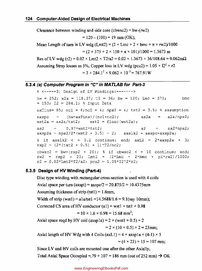
124 Computer-Aided Design of Electrical Machines
Clearance between winding and side core (cbwsc2) = bw-(rw2)
= 120 - (101) = 19 mm (OK);
Mean Length of turn in LV wdg (Lmt2) = (2 x Lmc + 2 x bmc + 1t x rw2)/1000
= (2 x 375 + 2 x 150 + 1t x 101)11000 = 1.3673 m
Res of LV wdg (r2) = 0.02 x Lmt2 x T2/a2 = 0.02 x 1.3673 x 36/108.64 = 9.062mn
Assuming Stray losses as 5%, Copper loss in LV wdg (pcu2) = 1.05 x 122 x r2
= 3 x 284.1 2 x 9.062 x 10-3 = 767.91W
5.3.4 (a) Computer Program in "C" in MATLAB for Part-3
% <-----3) Design of LV Windings:------->
hw = 252; a2a = 118.37; T2 = 36; bw = 120; Lmc = 375; bmc = 150; I2 = 284.1; % Input Data
axTins= 85; ncl = 4;nc2 = 4; nps2 = 4; tst2 = 3.5; % assumption
axspc (hw-axTins)/(ncl+nc2); as2a a2a/nps2; wst2a = as2a/tst2; wst2 = floor(wst2a);
as2 0.97*wst2*tst2; a2 as2*nps2; axsp2a = nps2/2*(wst2 + 0.5) + 2; axslk2 = axspc-axsp2a;
% ifaxslk2 < = 0.2 continue; end; axL2 rsp2 = (2*(tst2 + 0.5) + 1)*T2/nc2;
2*axsp2a + 3;
cbwsc2 = bw- (rsp2 + 20); rw2 = rsp2 + 20; Lmt2 r2 = 0.02*Lmt2*T2/a2; pcu2
% if cbwsc2 < = 10 continue; end; (2*Lmc + 2*bmc + pi*rw2)/I000;
1.05*I2"'2*r2;
5.3.5 Design of HV Winding (Part-4)
Disc type winding with rectangular cross-section is used with 4 coils
Axial space per turn (axspt) = axspc/2 = 20.875/2 = 1O.4375mm
Assuming thickness of strip (tst 1) = 1.6mm,
Width of strip (wst1) = a1a/tst1 =14.5688/1.6 = 9. 1 (say 10mm);
Corrected CS area ofHV conductor (al) = wstl x tstl x 0.98
= 10 x 1.6 x 0.98 = 15.68 mm2;
Axial space reqd by HV coil (axspla) = 2 x (wstl + 0.5) + 2
= 2 x (10 + 0.5) + 2 = 23mm;
Axial length ofHV Wdg with 4 Coils (axLl) = 4 x axspla + (4-1) x 5
= (4 x 23) + 15 = 107 mm;
Since LV and HV coils are mounted one after the other Axially,
Total Axial Space Occupied =,79 + 107 = 186 mm (out of252 mm) 7 OK
www.EngineeringEBooksPdf.com

Transformers 126
Radial turns (Trl) = Tl/8 = 270/8 = 33.75, Say 40
[Total turns = 2 (40 + 40) + 2(30 + 25) = 270] so that
max no of turns radially = 40 turns
Radial space required (rspla) = Trl x (tstl + 0.5) + 20
= 40 x (1.6 + 0.5) + 20 = 104 mm
HV Winding of Core Shell Transformer (dimensions are in mm
Length/Axial-wise
Cu.Strand Bare + insulation 10 + 0.5 = 10.5
Coil 2 CU.Strands 2 I< 10.5 = 21
Coil + Insulation 21 + 2 = 23
4 Coils 4 I< 23 = 92 92.0
Insulation (bewteen coils) (4-1)1<5=15 15.0
Axial Length 107.0
Radial-Wise
CU.Strand Bare + insulation 1.6 + 0.5 = 2.1 , 40-tums 40 I< 2.1 = 84 84.0
Insulation Outer 20.0
Radial-Width 104.0
Since LV and HV coils are mounted one after the other axially,
Total Axial Space Occupied =79 + 107 = 186 mm (out of 252mm)-->OK
Clearance between HV wdg and side core (cbwscl)
= bw-(rsp la) = 120 - (104) = 16 mm (OK);
Meal length ofHV turns (Lmtl) = Lmt2 = 1.367 m
Res ofHV wdg/ph(rl) = 0.02 x Lmtl x TlIal = 0.02 x 1.367 x 270/15.68 = 0.4709 0
Assuming Stray losses as 5%, Copper loss in HV Wdg (pcul)
= 1.05 x 112 x rl/1000 = 1.05 x 37.882 x 0.4709 = 709.4 W
5.3.5 (a) Computer Program In "c" In MATLAS for Part-4
% <-----4) Design of HV Windings:------->
axspc 20.875; ala 14.5688; T1 Lmt2 1.367; 11 = 37.88; % Input data
tst1 = 1.6; % Assumptions
270; bw 120;
www.EngineeringEBooksPdf.com
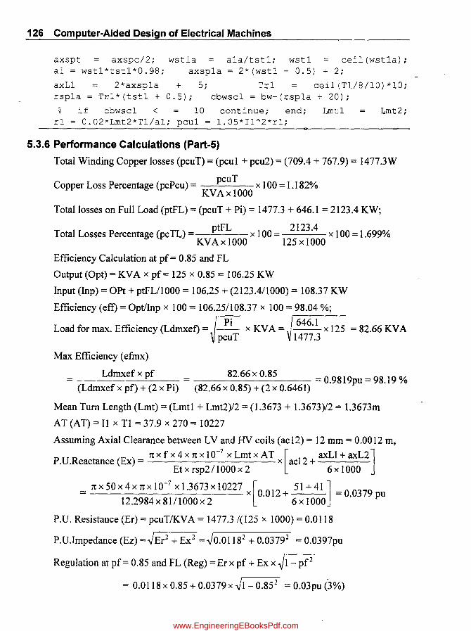
126 Computer-Aided Design of Electrical Machines
axspt axspc/2; wstla ala/tstl: wst1 ceil(wst1a): a1 = wst1*tst1*0.98: axsp1a = 2* (wstl + 0.5) + 2:
axLl 2*axsp1a + 5: Trl ceil(T1/8/10)*10: rsp1a = Tr1*(tstl + 0.5): cbwsc1 = bw-(rsp1a + 20):
~ if cbwsc1 < 10 continue: end; Lmt1 Lmt2: rl = 0.02*Lmt2*T1/a1: pcu1 = 1.05*I1A2*r1: ..
5.3.6 Performance Calculations (Part-5)
Total Winding Copper losses (pcuT) = (pcul + pcu2) = (709.4 + 767.9) = 1477.3W
pcuT Copper Loss Percentage (pcPcu) = x 100 = 1.182%
KVAx 1000
Total losses on Full Load (ptFL) = (pcuT + Pi) = 1477.3 + 646.1 = 2123.4 KW;
I ptFL 2123.4
Tota Losses Percentage (pcTL) = x 100 = x 100 = 1.699% KVAx 1000 125 x 1000
Efficiency Calculation at pf= 0.85 and FL
Output (Opt) = KVA x pf= 125 x 0.85 = 106.25 KW
Input (Inp) = OPt + ptFLllOOO = 106.25 + (2123.411000) = 108.37 KW
Efficiency (eft) = OptlInp x 100 = 106.251108.37 x 100 = 98.04 %;
Load for max. Efficiency (Ldmxef) = J Pi x KV A = 646.1 x 125 = 82.66 KV A pcuT 1477.3
Max Efficiency (efmx)
Ldrnxefxpf = 82.66 x 0.85 =0.9819pu=98.19% (Ldmxef x pf) + (2 x Pi) (82.66 x 0.85) + (2 x 0.6461)
Mean Turn Length (Lmt) = (Lmtl + Lmt2)/2 = (1.3673 + 1.3673)/2 = 1.3673m
AT (AT) = II x T1 = 37.9 x 270 = 10227
Assuming Axial Clearance between LV and HV coils (acI2) = 12 mm = 0.0012 m,
PUR (E) 1txfx4x1tx1O-7 xLmtxAT [ 1" axLl+ axL2] . . eactance x = x ac L. + ----Et x rsp211 000 x 2 6 x 1000
= 1tx50x4x1txl0-7
xlJ673xl0227 X[0.012+ 51+41] =0.0379 u 12.2984x8111000x2 6xl000 P
P.U. Resistance (Er) = pcuT/KVA = 1477.3 /(125 x 1000) = 0.0118
P.U.Impedance (Ez) =-JEr2 + Ex2 =-J0.01182 + 0.03792 = O.0397pu
Regulation at pf= 0.85 and FL (Reg) = Er x pf + Ex x ~1- pf2
= 0.0118 x 0.85 + 0.0379 x -Jl- 0.85 2 = 0.03pu (3%)
www.EngineeringEBooksPdf.com

Transformers 127
5.3.6 (a) Computer Program in "c" in MA TLAB for Part-5
% <--------5) Performance Calculations:------>
ac12 0.012; % Specification
pcu1 709.4; pcu2 = 767.9; ¥:VA = 125; Pi = 646.1; pf = 0.85; Lmt1 1.3673; Lmt2 = 1.3673; % Input Data
11 = 37.9; T1 = 270; f = 50; Et = 12.2984; rsp2 = 81; axL1 = 51; axL2 = 41; % Input Data
pcuT=pcul+ pcu2; pcPcu=pcuT/(¥:VA*1000)*100; ptFL = (pcuT + Pi); pcTL=ptFLI (¥:VA*1000) *100; Opt=¥:VA*pf; Inp= Opt + ptFL/1000; eff Opt/Inp*100; Ldmxef sqrt(Pi/pcuT) * ¥:VA; efmx Ldmxef*pf/(Ldmxef*pf + 2*Pi/1000)*100; Lmt = (Lmt1 + Lmt2)/2; AT = I1*T1;
Ex=pi*f*4*pi*le-7*Lmt*AT/(Et*rsp2/1e3*2)* (ac12+(axL1+ axL2)/6e3);
Er pcuT/(¥:VA*1000); Ez Reg = (Er*pf + Ex*sqrt(l-pf A2) )*100;
5.3.7 Tank Design and Weights (Part-6)
Assuming Length-wise clearance (dL) = 80 mm,
sqrt(ExA2
Length of Tank (Lt) = (Ly + dL) = (540 + 80) = 620 mm
Assuming Width-wise clearance (dB) = 100 mm,
+
Width of Tank (bt) = Lmc + 2 x rw2 + dB; = 375 + 2 x 101 + 100 = 677 mm
AssumingHeight -wise clearance (dH) = 450mm,
Height of Tank(ht) = hw + 2 x (hy + dH) = 252 + 2 x (75 + 450) = 852 mm ;
Volume of Tank (Vt) = Lt x bt x htl109 = 620 x 677 x 8521109 = 0.3576 m3;
ErA2);
Cooling Surface area of tank (St) = 2 x (ht + Lt) x htl106 = 2 x (677 + 620) x 852/106
= 2.2101 m2
Temperature-rise of Tank (Tr) = ptFL 12.5 x St
~2_1_2_3_.4_ = 76.86 0C 12.5 x 2.2101
Since Temp-rise is to be limited to (TRP) = 40°C, Cooling tubes are to be provided
Selecting Tube dia (Dct) of 50 mm and height (Hct) Of 550 mm,
Area of each tube (At) = 1t x Dct x Hctll 06 = 1t x 50 x 55011 06 = 0.0864 m2;
Required Tube Cooling Area (CAt)
= ptFL -12.5 x St x TRP = 2123.4 -12.5 x 2.2101 x 40 = 2.9012 m 2
6.5 x TRP x 1.35 6.5 x 40 x 1.35
www.EngineeringEBooksPdf.com
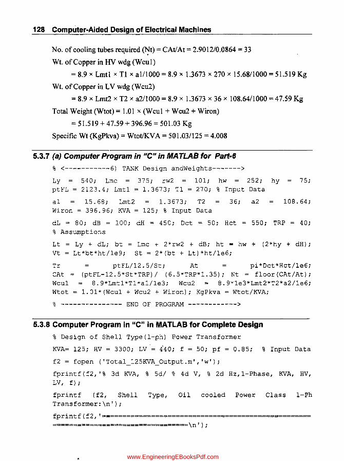
128 Computer-Aided Design of Electrical Machines
No. of cooling tubes required ~t) = CAt! At = 2.9012/0.0864 = 33
Wt. of Copper in HV wdg (W cu 1)
= 8.9 x Lmtl x T1 x al/l000 = 8.9 x 1.3673 x 270 x 15.68/1000 = 51.519 Kg
Wt. of Copper in LV wdg (W cu2)
= 8.9 x Lmt2 x T2 x a21l000 = 8.9 x 1.3673 x 36 x 108.64/1000 = 47.59 Kg
Total Weight (Wtot) = 1.01 x (Wcul + Wcu2 + Wiron)
= 51.519 + 47.59 + 396.96 = 501.03 Kg
Specific Wt (KgPkva) = WtotIKVA = 501.03/125 = 4.008
5.3.7 (a) Computer Program in "C" in MA TLAB for Part-6
% <-----------6) TANK Design andWeights------->
Ly = 540; Lmc = 375; rw2 101; hw = 252; hy = 75; ptFL = 2123.4; Lmt1 = 1.3673; T1 = 270; % Input Data
a1 15.68; Lmt2 1.3673; T2 36; a2 108.64;
Wiron = 396.96; KVA = 125; % Input Data
dL = 80; dB = 100; dH = 450; Oct = 50; Hct = 550; TRP = 40;
% Assumptions
Lt = Ly + dL; bt = Lmc + 2*rw2 + dB; ht = hw + (2*hy + dH); Vt = Lt*bt*ht/1e9; St = 2*(bt + Lt)*ht/1e6;
Tr ptFL/12. 51St; At pi*Dct*Hct/1e6; CAt = (ptFL-12.5*St*TRP) I (6.5*TRP*1.35); Nt = floor (CAt/At) ; Wcu1 8. 9*Lmt1*T1*a1/1e3i Wcu2 8. 9*le3*Lmt2*T2*a2/1e6; Wtot = 1.01*(Wcu1 + Wcu2 + Wiron); KgPkva = Wtot/KVAi
% --------------- END OF PROGRAM ------------>
5.3.8 Computer Program in "C" in MATLAB for Complete Design
% Design of Shell Type(l-ph) Power Transformer
KVA= 125; HV = 3300; LV = 4'40; f = 50; pf = 0.85; % Input Data
f2 = fopen ('Total_125KVA_Output.m', 'w');
fprintf(f2, '% 3d KVA, % 5dl % 4d V, % 2d Hz,l-Phase, KVA, HV, LV, f);
fprintf (f2, Shell Type, Oil cooled Power Class 1-Ph
Transformer:\n');
fprintf(f2, '=================================================== =================================\n');
/
www.EngineeringEBooksPdf.com

Transformers 129
fprintf (f2, '<-----1) Design of Magnetic Frame----------->\n');
K = 1.1; Bm = 1.1; cdav = 2.5f kw = 0.27; ki = 0.9; R1 = 2.5; R2 = 2.1; % Assumptions
cdlv cdav-0.1; cdhv cdav + 0.1; Et K*sqrt (KVA) ; Ain = Et/(4.44*f*Bm); Aig = Ain/ki;
bmc1 = sqrt(Aig/R1); bmc = ceil(bmc1*100)*10; Lmc = Rl*bmc;
Aw = KVA*le3/(2.22*f*Bm*kw*cdav*le6*Ain); bw1 bw ceil(bw1*100)*10;
sqrt (Aw/R2);
Hw Ly
R2*bw; Ay = Ain/2; bsc = bmc/2; hy = bsc; by 2*(bsc + bw) + bmc; Vcc = Ain*hw/1000;
V2sc = Vcc; Vc = Vcc + V2sc; Vy = 2*Ly*Ay/1e3; Viron Wiron = V~ron*7.55e3;
Ay/hy*le6;
Vy + Vc;
BB = [ 0 . 8 1. 0 1. 2 1. 4 1. 6]; WpKg % Data for Hot Rolled
[0.8 1.2 1.9 2.9 4.2];
% plot (BB, WpKg); grid; xlabel (% Flux density (T)-->'); ylabel ('Loss(W/Kg)-->');
% title (Core Loss for Hot rolled steels');
scL = interp1(BB, WpKg, Bm, linear'); Pi pc Pi = Pi/KVA/10;
Wiron*scL*1.05;
% Et, Ain, Aig, bmc1, bmc, Lmc, Aw, bw1, bw, hw, Ay, bsc, hy, by, Ly,
% Vcc, V2sc, Vc, Vy, Viron, Wiron, scL, Pi, pcPi,
fprintf (f2, Assumed: Value factor (K) % 6.2f\n', K);
fprintf (f2, 'Volts/turn % 6.2f\n', Et);
fprintf (f2, Assumed: Window space factor (kw) % 5.3f, Max Core Flux Density (T) = % 3.1 f\n', kw, Bm);
fprintf (f2, Core-CS-area (Net and Gross) (sq.m) % 6.4f and %
6.4 f\n', "Ain, Aig);
fprintf (f2, Main Core Length x Width (mm) % 6.1f x % 6.1f\n', Lmc, bmc);
fprintf (f2, Window Area (sq.m) % 6.4f\n', Aw);
fprintf (f2, Window Height x Width (rom) % 6.1f x % 6.1f\n', hw, bw) ;
fprintf (f2, 'Width x Ht of the yoke (m) % 6.0 f and % 3.0 f\n', by, hy);
fprintf (f2, Length of Yoke (Ly) (rom) % 6.0f\n', Ly);
www.EngineeringEBooksPdf.com

130 Computer-Aided Design of Electrical Machines
fprintf (f2, <-----2) No-Load Current------------------>\n');
Iw=Pi/LV; Lfpc = 2*hw/1000; Lfpy = Ly/1000; LfpT = Lfpc + Lfpy;
B1= [1 1.25 1.5 1.75 2.0];
H1 = [100 250 650 1200 2100]; % Data for Hot Rolled
% plot (H1, B1); grid; xl abel ('AT/m-->'); ylabel ('Flux density(T)-->');
% title ('Magnetization Curve for Hot rolled steels'); %
atpm T2a
interp1(B1, H1, Bm, LV/Et; T2 = ceil(T2a);
'spline'); AT atpm*LfpT;
1m 12
T1
1.1*AT/(sqrt(2)*T2); 10 sqrt(Iw"2 + Im"2); KVA*1000/LV; IObyI2 = 10/12*100; a2a = I2/cdlv;
T2*HV/LV; 11 = KVA*1000/HV; ala = I1/cdhv;
% Iw, Lfpc, Lfpy, LfpT, atpm, AT, T2a, T2, 1m, 10, 12, 10 by 12, a2a, T1, 11, ala,
fprintf (f2, 'Magnetizing-Ct(IO = Iw + jIm) % 6.3f = % 4.3f + j % 4.3f A\n', 10, Iw, 1m);
fprintf (f2, Ratio of 10/12 (perc) % 6.3f (Permissible: < 2)\n', 10 by 12);
fprintf (f2, '<-----3) Design of LV Windings:------->\n');
axTins 85; nc1 4; nc2 4; nps2 4; tst2 3.5; % assumption
axspc wst2a
(hw axTins) / (nc1 + nc2) ; as2a a2a/nps2; as2a/tst2; wst2 = floor(wst2a);
as2 axsp2a
0.97*wst2*tst2; a2 as2*nps2; nps2/2*(wst2 + 0.5) + 2; axslk2 = axspc-axsp2a;
axL2 = 2*axsp2a + 3; rsp2 (2*(tst2 + 0.5) + 1)*T2/nc2; cbwsc2 = bw - (rsp2 + 20); % if cbwsc2 < = 10 continue; end;
rw2 rsp2 + 20; Lmt2 r2 = 0.02*Lmt2*T2/a2; pcu2
(2*Lmc + 2*bmc + pi*rw2)/1000; 1.05*I2"2*r2;
% axspc, as2a, wst2a, wst2, as2, axsp2a, axslk2, axL2, rsp2, cbwsc2, rw2, Lmt2, r2, pcu2,
fprintf (f2, 'Turns in LV winding % 6.0f\n', T2);
fprintf (f2, 'Ph-Current in LV wdg (Amp) % 6.1f\n', 12);
fprintf (f2, 'Width x Thick of Cond (rnrn) % 6.1f and % 3.1 f\n', wstJ, tst2); 12,
• fprintf (f2, CS area of Conductor (sq.rnrn) % 6.3f\n', a2);
www.EngineeringEBooksPdf.com

Transformers 131
£printf (f2, Current density (A/sq.rnrn) % 6.2f (Permissible:2.3 to 3.5)\n', cdlv);
fprintf (f2, Axial Slack in LV-Wdg (rnrn) % 6.2f (desirable > O.2)\n', axslk2);
fprintf (f2, Clearance bet LV Wdg and core(rnrn) (desirable: > 10)\n', cbwsc2);
% 6. 2f
fprintf (f2, Radial width of Wdg (rnrn) % 6.2f\n', rw2);
fprin~f (f2, Mean Length of Turn (m) % 6.3f\n', Lmt2);
fprintf (f2, Resistance/phase (m.ohm) % 6.4f\n', r2*1000);
fprintf (f2, <-----4) Design of HV Windings:------->\n');
tst1 = 1.6; % Assumptions
axspt axspc/2; wst1a a1a/tst1; wst1 ceil (wst1a); a1 = wst1*tst1*0.98; axsp1a = 2*(wst1 + 0.5) + 2;
axL1 2*axsp1a + 5; Tr1 ceil (T1/8/10) *10; rsp1a = Tr1*(tst1 + 0.5); cbwsc1 = bw-(rsp1a + 20);
% if cbwsc1 < = 10 continue; end;
Lmt1 = Lmt2; r1 = 0.02*Lmt2*T1/a1; pcu1 = 1.05*I1A2*r1;
% axspt, ala, wst1a, wst1, a1, axsp1a, axL1, Tr1, rsp1a, cbwsc1, r1, pcu1,
fprintf (f2, 'Turns in HV winding % 6.0f\n', T1);
fprintf (f2, Ph-Current in HV wdg (Amp) % 6.1f\n', 11);
fprintf (f2, Width x Thick of Cond (rnrn) % 6.1f and % 3 .1f\n' , wst1, tst1);
fprintf (f2, CS area of Conductor (sq.rnrn) % 6.3f\n', a1);
fprintf (f2, Current density (A/sq.rnrn) % 6.2f (Permissible: 2.3 to 3.5)\n', cdhv);
fprintf (f2, Clearance bet HV Wdg and core (rnrn) % 6.2f (desirable: >10)\n', cbwse1);
fprintf (f2, Mean Length of Turn (m) % 6.3 f\n', Lmt1);
fprintf (f2, Resistance/phase (ohm) % 6.4f\n', r1);
fprintf (f2, <--------5) Performance Caleulations:------>\n');
ac12
peuT ptFL
0.012; % Specification
pcu1 + pcu2; pePcu pcuT/(KVA*1000) *100; (pcuT + Pi); peTL = ptFL/(KVA*1000) *100;
www.EngineeringEBooksPdf.com

132 Computer-Aided Design of Electrical Machines
Opt KVA*pf: Inp Opt + ptFL/1000: eff OptiInp*100: Ldrnxef = sqrt(Pi/pcuT)*KVA:
efmx Lmt
Ldrnxef*pf/(Ldrnxef*pf (Lmt1 + Lmt2)/2: AT = I1*T1:
+ 2*Pi/1000)*100:
Ex pi*f*4*pi*le-7*Lmt*AT/(Et*rsp2/1000*2)*(ac12 + (axL1 + axL2)/6e3):
Er .pcuT/(KVA*1000): Ez sqrt (Ex A 2 + Er A 2):
Reg = (Er*pf + Ex*sqrt(1-pf A 2))*100:
% pcuT, pcPcu, ptFL, pcTL, Opt, Inp, eff, Ldrnxef, efmx, Lmt, AT, Ex, Er, Ez, Reg,
Fprintf (f2, Cu. Losses of: HV-Wdg: = % 4.1f, LV-Wdg: = % 4.1 f and Iron Loss: = % 4.1f and Total = % 6.1 f W\n', pcu1, pcu2,
Pi, ptFL):
fprintf (f2, Percentage Loss: Iron Loss: = % 6.3f, Copper =
% 6.2 f and Total = % 6.3 f perc\n', pcPi, pcPcu, pcTL):
fprintf (f2, Efficiency at pf = % 4.2 f and Full Load = % 5.2f
perc\n', pf, eff):
fprintf (f2, Max Efficiency = % 5.2f occuring at Load KVA\n', efmx, Ldrnxef):
% 5.2 f
fprintf (f2, Mean-turn Length = % 6.4fm, AT
AT) :
% 6.0f\n', Lmt,
fprintf (f2, Reactance % 6.4 fpu, Restance % 6. 4fpu,
Impedance = % 6.4 fpu\n', Ex, Er, Ez):
fprintf (f2, Regulation: at pf = % 4.2 f and Full Load %
6.2f\n', pf, Reg):
fprintf (f2, '<-----------6) TANK Design and Weights------
>\n') :
dL = 80: dB = 100: dH Assumptions
450: Dct 50: Hct 550: TRP = 40; %
Lt = Ly + dL: bt = Lmc + 2*rw2 + dB: ht = hw + (2*hy + dH): Vt = Lt*bt*ht/1e9: St = 2*(bt + Lt)*ht/1e6;
Tr
CAt ptFL/12.5/St; At
(ptFL-12.5*St*TRP)/ (6.5*TRP*1.35); Nt pi*Dct*Hct/1e6:
floor (CAt/At) :
Wcul 8.9*Lmtl*T1*a1/1e3: Wcu2 8.9*le3*Lmt2*T2*a2/1e6; Wtot = 1.01*(Wcu1 + Wcu2 + Wiron); KgPkva = Wtot/KVA;
Lt, bt, ht, Vt, St, Tr, At, CAt, Nt, Wcul,Wcu2, Wtot, KgPkva, Lmt1, aI, a2, Tl, T2,
www.EngineeringEBooksPdf.com

Transformers 133
Fprintf (f2, 'Tank: Length = % 4. o from, Width = %4. o from, Height = % 4.0 from and Volume = % 6.3fm3\n', Lt, bt, ht, Vt);
fprintf (f2, 'Tank: Cooling area = % 6.4 fsq.m and Temp-Rise = % 4.1f is reduced to % 3d deg-C\n', St, Tr, TRP);
fprintf(f2, Cooling Tubes:Area/Tube = % 6.4 fsq.m, RequiredArea = % 6.4 fsq.m and No of Tubes = % 3.0 f\n', At, CAt, Nt);
fprintf (f2, Weight: HV-Wdg: = % 6.2f + LV-Wdg: = % 6.2f + (Core + Yoke): = % 6.2f and Total = % 7.1 f Kg\n', Wcu1,Wcu2, Wiron, Wtot);
fprintf (f2, 'Kg/KVA = % 6.3f\n', KgPkva); axL1, axL2,
fprintf (f2,<-----------End of Program------->\n');
fclose (f2);
5.3.8 (a) Computer Output Results for Complete Design
125 KV A, 3300/ 440 V, 50 Hz, I-Phase, Shell Type, Oil cooled Power Class I-Ph T ransfonner:
<-----1) Design of Magnetic Frame----------------->
Assumed: Value factor (K) 1.10
Volts/turn 12.30
Assumed: Window space factor (kw) = 0.270, Max Core Flux Density (T) = 1.1
Core-CS-area (Net and Gross) (sq.m) 0.0504 and 0.0560
Main Core Length x Width (mm) 375.0 x 150.0
Window Area (sq.m) 0.0301
Window Height x Width (mm) 252.0 x 120.0
Width x Ht of the yoke (m) 336 and 75
Length of Yoke (Ly) (mm) 540
<-----2) No-Load Current ------------------>
Magnetizing-Ct (10 = Iw + jIm) 3.056 = 1.468 + j2.680 A
Ratio of 10112 (perc) 1.076 (Pennissible: < 2)
<-----3) Design of LV Windings:------->
Turns in LV winding 36
Ph-Current in LV wdg (Amp) 284.1
Width x Thick ofCond (mm) 8.0 and 3.5
CS area of Conductor (sq.mm) 108.640
www.EngineeringEBooksPdf.com
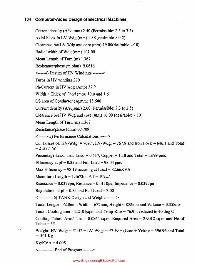
134 Computer-Aided Design of Electrical Machines
Current density (A/sq.mm) 2.40 (Pennissible: 2.3 to 3.5)
Axial Slack in LV-Wdg (mm) 1.88 (desirable> 0.2)
Clearance bet LV Wdg and core (mm) 19.00(desirable: >10)
Radial width ofWdg (mm) 101.00
Mean Length of Turn (m) 1.367
Resistance/phase (m.ohm) 9.0616
<-----4) Design ofHV Windings:------->
Turns in HV winding 270
Ph-Current in HV wdg (Amp) 37.9
Width x Thick ofCond (mm) 10.0 and 1.6
CS area of Conductor (sq.mm) 15.680
Current density (Alsq.mm) 2.60 (Pennissible: 2.3 to 3.5)
Clearance bet HV Wdg and core (mm) 16.00 (desirable: > 10)
Mean Length of Turn (m) 1.367
Resistance/phase (ohm) 0.4709
<--------5) Perfonnance Calculations:------>
Cu. Losses of: HV-Wdg: = 709.4, LV-Wdg: = 767.9 and Iron Loss: = 646.1 and Total =2123.4 W
Percentage Loss:- Iron Loss: = 0.517, Copper = 1.18 and Total = 1.699 perc
Efficiency at pf = 0.85 and Full Load = 98.04 p~rc
Max Efficiency = 98.19 occuring at Load = 82.66KV A
Mean-turn Length = 1.3673m, AT = 10227
Reactance = 0.0379pu, Restance = 0.0118pu, Impedance = 0.0397pu
Regulation: at pf= 0.85 and Full Load = 3.00
<-----------6) TANK Design and Weights------->
Tank: Length = 620mm, Width = 677mm, Height = 852mm and Volume = 0.358m3
Tank: Cooling area = 2.2101.sq.m and Temp-Rise = 76.9 is reduced to 40 deg-C
Cooling Tubes: ArealTube = 0.0864 sq.m, Required-Area = 2.9012 sq.m and No of Tubes =33
Weight: HV-Wdg: = 51.52 + LV-Wdg: = 47.59 + (Core + Yoke): = 396.96 and Total = 501 Kg
KglKV A = 4.008
<----------- End ofProgram------->
www.EngineeringEBooksPdf.com

Transformers 135
5.3.9 Modifications to be done in the above Program to get Optimal Design
I. Insert "for" Loops for the following parameters to iterate the total program between min and max permissible limits for selecting the feasible design variants:
(a) No. of values of"K" (Factor of ratio of core to copper)
(b) No. of Values of "Bm", (Core flux density)
(c) No. of Average current density values
(d) No. of "LID" ratios
(e) No. of values of"Rl" (Ratio of Length to width of main core)
(f) No. of values of"R2" (Ratio of Length to width Window).
2. Insert also minimum or maximum range of required objective functional values as constraint values, for exa,mple (a) Efficiency (b) Kg/KVA (c) !o1I2 ratio (d) Volume of Tank etc.
3. Run the program to get various possible design variants.
Note: From the feasible design variants printed in the output, select that particular design that fulfills the objective of optimal parameter for the design.
5.3.10 Computer Program in "C" in MATLAB for Optimal Design
% Design of Shell Type (l-ph) Power Transformer
KVA = 125; HV = 3300; LV = 440; f = 50; pf = 0.85; % Input
Data
f2 = fopen ('Optimal_125KVA_Output.m', 'w');
fprintf (f2, % 3d KVA, % 5d/ % 4d V, % 2d Hz, 1-Phase, KVA,
HV, LV, f);
fprintf (f2, Shell Type, Oil cooled Power Class 1-Ph Transformer:\n');
fprintf(f2,=================================================
=============================================\n');
fprintf (f2, Sn K
bw hy Ly IObyI2
K = 1.1; Bm = 1.1;
r1 = 2.5; r2 = 2;
Bm R1 R2
eff Reg
cdav Tl T2 Lmc
Vt KgPkva \r: ' )
bmc hw
cdav = 2.3; kw 0.27; ki 0.9;
scL 1. 65; atpm 150 ; cdl v 2 . 2 ;
cdhv = 2.4; % Assumptions
Sn = 0; M1 = 0; M2 = 0; M3 = 0; M4 = 0; EFFmax = 97; minIOby 12 = 2; minKgPkva = 5; min Vt = 2; % Assumptions
for k = 1:0. 1:1. 1; % (Range: 1 to 1.1)
www.EngineeringEBooksPdf.com
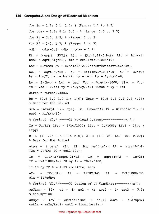
136 Computer-Aided Design of Electrical Machines
for Brn = 1.1: 0.1: 1.3; % (Range: 1.1 to 1.3)
for edav = 2.3: 0.1: 3.5 ; % (Range: 2.3 to 3.5)
for R1
for R2
2:0. 1:3; % (Range: 2 to 3)
2:0. 1:3; % (Range: 2 to 3)
edlv = edav-0.1; edhv = edav + 0.1;
Et = K*sqrt (KVA); Ain = Et/(4.44*f*Brn); Aig = Ain/ki;
brne1 = sqrt(Aig/R1); brne = eeil(brne1*100) *10;
Lrne = R1*brne; Aw = KVA*le3/(2.22*f*Brn*kw*edav*le6*Ain);
bw1 sqrt(Aw/R2); bw eeil(bw1*100)*10; hw
Ay Ain/2; bse = brne/2; hy = bse; by = Ay/hy*le6;
R2*bw;
Ly = 2* (bse + bw) + brne; Vee = Ain*hw/1000; V2se Vee;
Ve = Vee + V2se; Vy 2*Ly*Ay/1e3; Viron = Vy + Ve;
Wiron = Viron*7.55e3;
BB = [0.81.01.21.41.6]; WpKg = [0.81.21.92.94.2];
% Data for Hot Rolled
seL = interp1 (BB, WpKg, Brn, linear'): Pi
pePi = Pi/KVA/10;
Wiron*seL*1.05:
% fprintf (f2, '<-----2) No-Load Current----------->\n'):
Iw = Pi/LVi Lfpe = 2*hw/1000i Lfpy = Ly/1000i LfpT = Lfpc + Lfpy;
B1 = [1 1.25 1.5 1.75 2.0]: H1
% Data for Hot Rolled
[100 250 650 1200 2100]:
atprn inteTpl (Bl, H1, Brn, spline'): AT atprn*LfpT:
T2a LV/Et: T2 = ceil(T2a):
Irn 1.1*AT/{sqrt(2)*T2); IO sqrt{IwA 2 + IrnA 2) :
I2 = KVA*1000/LV: IO by 12 = IO/I2*100:
if IO by 12 > = 1.09 continue: end;
a2a 12/cdlv: Tl T2*HV/LV; Il KVA*1000/HV:
ala = Il/cdhv:
% fprintf (f2, '<-----3) Design of LV Windings:------->\n');
axTins = 85; ne1 = 4; nc2 = 4; nps2 = 4: tst2 3.5;
% assumption
axspe (hw axTins)/{nc1 + nc2): as2a a2a/nps2:
wst2a = as2a/tst2; wst2 = floor{wst2a):
www.EngineeringEBooksPdf.com

Transformers 137
as2
axsp2a
0.97*wst2*tst2; a2
nps2/2*(wst2 + 0.5) + 2; axslk2
as2*nps2;
axspc - axsp2a;
ifaxslk2 < = 0.2 continue; end;
axL2 = 2*axsp2a + 3; rsp2 (2*(tst2 + 0.5) + 1)*T2/nc2;
cbwsc2 = bw - (rsp2 + 20); if cbwsc2 < = 10 continue; end;
rw2 = rsp2 + 20; Lmt2 = r2 = 0.02*Lmt2*T2/a2; pcu2
tst1 1.6; % Assumptions
(2*Lmc + 2*bmc + pi*rw2) /1000; 1.05*I2"2*r2;
axspt axspc/2; wst1a a1a/tst1; wst1 ceil(wst1a);
a1 = wst1*tst1*0.9S; axsp1a = 2* (wst1 + 0.5) + 2;
axL1 2*axsp1a + 5; Tr1 ceil (T1/S/10)*10;
rsp1a = Tr1*(tst1 + 0.5);cbwsc1 = bw - (rsp1a + 20);
% if cbwsc1 < = 10 continue; end;
Lmt1 = Lmt2; r1 = 0.02*Lmt2*T1/a1; pcu1 = 1.05*I1"2*r1;
% fprintf (f2, '<--------5) Performance Calculations:-----
>\n') ;
ac12 0.012; % Specification
pcuT
ptFL
pcu1 +pcu2; pcPcu pcuT/ (KVA*1000) *100;
(pcuT+Pi); pcTL = ptFL/(KVA*1000)*100;
Opt = KVA*1000*pf; Inp = Opt + ptFL; eff if eff < = 97.95 continue; end;
Ldmxef sqrt(Pi/pcuT)*KVA;
efmx Ldmxef*pf/(Ldmxef*pf + Lmt = (Lmt1 + Lmt2)/2; AT = I1*T1;
Opt/lnp*100;
2*Pi/1000)*100;
Ex = pi*f*4*pi*le-7*Lmt*AT/ (Et*rsp2/1000*2) * (ac12 + (axL1 +
axL2)/6e3);
Er pcuT/ (KVA*1000); Ez sqrt (Ex"2 + ErA2);
Reg = (Er*p£ + Ex*sqrt(l -pfA2))*100;
% fprintf (f2,'<-------6) TANK Design and Weights-------
>\n') ;
dL = SO; dB = 100; dH
% Assumptions
450; Dct 50; Hct 550; TRP 40;
Lt Ly + dL; bt = Lmc + 2*rw2 + dB; ht = hw + (2*hy + dH);
Vt Lt*bt*nt/1e9; St = 2*(et + Lt)*ht/1e6;
www.EngineeringEBooksPdf.com
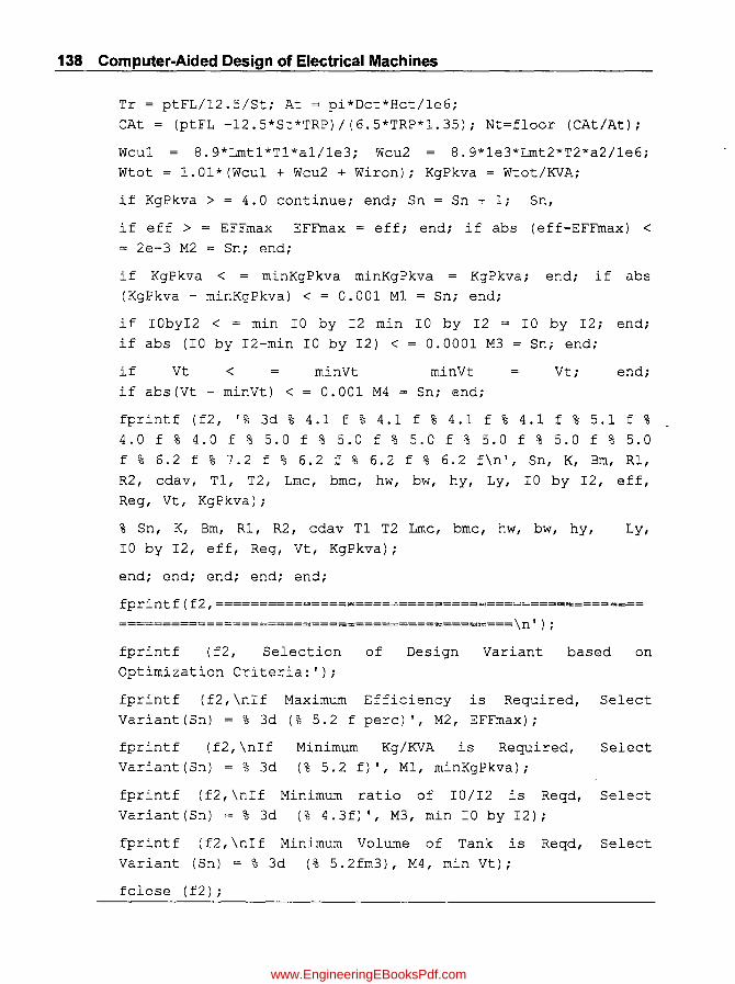
138 Computer-Aided Design of Electrical Machines
Tr = ptFL/12.5/St; At = pi*Dct*Hct/1e6;
CAt = (ptFL -12.5*St*TRP)/(6.5*TRP*1.35); Nt=floor (CAt/At);
Wcu1 8.9*Lmt1*T1*a1/1e3; Wcu2 8.9*le3*Lmt2*T2*a2/1e6;
Wtot = 1.01*(Wcu1 + Wcu2 + Wiron); KgPkva = Wtot/KVAi
if KgPkva > = 4.0 continue; end; Sn = Sn + 1; Sn,
if eff > = EFFmax EFFmax = eff; end; if abs (eff-EFFmax) <
= 2e-3 M2 = Sn; end;
if KgPkva < = minKgPkva minKgPkva = KgPkva; end; if abs
(KgPkva - minKgPkva) < = 0.001 M1 = Sn; end;
if IObyI2 < = min 10 by 12 min 10 by 12 = 10 by 12; end;
if abs (10 by I2-min 10 by 12) < = 0.0001 M3 Sn; end;
if Vt < minVt minVt Vt; end;
if abs(Vt - minVt) < = 0.001 M4 = Sn; end;
fprintf (f2, ' % 3d % 4.1 f % 4.1 f % 4.1 f % 4.1 f % 5.1 f %
4.0 f % 4.0 f % 5.0 f % 5.0 f % 5.0 f % 5.0 f % 5.0 f % 5.0
f % 6.2 f % 7.2 f % 6.2 f % 6.2 f % 6.2 f\n' , Sn, K, Bm, Rl,
R2, cdav, T1, T2, Lmc, bmc, hw, bw, hy, Ly, 10 by 12, eff,
Reg, Vt, KgPkva);
% Sn, K, Bm, R1, R2, cdav T1 T2 Lmc, bmc, hw, bw, hy, Ly,
10 by 12, eff, Reg, Vt, KgPkva);
end; end; end; end; end;
fprintf (f2, =========================================== ======
=============================================\n');
fprintf (f2, Selection of Design Variant based on
Optimization Criteria:');
fprintf (f2,\nIf Maximum Efficiency is Required, Select
Variant (Sn) = % 3d (% 5.2 f perc)', M2, EFFmax);
fprintf (f2,\nIf
Variant (Sn) = % 3d
fprintf (f2,\nIf
Variant (Sn) = % 3d
Minimum Kg/KVA is Required,
(% 5.2 f)', M1, minKgPkva);
Minimum ratio of 10/12 is Reqd,
(% 4.3f)', M3, min 10 by 12);
Select
Select
fprintf (f2, \nIf Minimum Volume of Tank is Reqd, Select
Variant (Sn) = % 3d (% 5.2fm3), M4, min Vt);
fclose (f2);
www.EngineeringEBooksPdf.com

5.3.10 (a) Computer Output Results for Optimal Design
125 K VA, 3300/440 V, 50 lIz, I-Phase, Shell Type, Oil cooled Power Class I-Ph Transformer:
================================================================================================== Sn K Bm RI R2 cdav TI T2 Lmc bmc hw bw hy Ly to by 12 eff Reg Vt KgPkva
I 1.0 1.1 2.3 2.2 2.3 300 40 345 150 286 130 75 560 1.05 98.02 3.22 0.38 4.08 2 1.0 1.1 2.6 2.0 2.3 300 40 364 140 280 140 70 560 1.04 98.01 3.27' 0.38 4.06 3 1.0 1.1 2.6 2.2 2.3 300 40 364 140 286 130 70 540 1.03 98.01 3.27 0.37 4.04 4 1.0 1.1 2.7 2.0 2.3 300 40 378 140 280 140 70 560 1.04 97.98 3.33 0.39 4.08 5 1.0 1.1 2.7 2.2 2.3 300 40 378 140 286 130 70 540 1.03 97.98 3.33 0.38 4.06 6 1.0 1.1 2.8 2.2 2.3 300 40 392 140 286 130 70 540 1.03 97.95 3.40 0.39 4.08 7 1.0 1.1 2.0 2.0 2.4 300 40 320 160 280 140 80 600 1.08 97.95 3.16 0.39 4.09 8 1.0 1.1 2.0 2.1 2.4 300 40 320 160 273 130 80 580 1.05 97.97 3.16 0.37 3.99 9 1.0 1.1 2.0 2.2 2.4 300 40 320 160 286 130 80 580 1.07 97.96 3.16 0.38 4.07 10 1.0 1.1 2.0 2.0 2.5 300 40 320 160 260 130 80 580 1.02 97.98 3.16 0.37 3.92 II 1.0 1.1 2.0 2.1 2.5 300 40 320 160 273 130 80 580 1.05 97.97 3.16 0.37 3.99 12 1.0 1.1 2.0 2.2 2.5 300 40 320 160 286 130 80 580 1.07 97.96 3.16 0.38 4.07 13 1.0 1.1 2.3 2.0 2.5 300 40 345 150 260 130 75 560 1.00 97.96 3.23 0.37 3.89 14 1.0 1.1 2.6 2.0 2.5 300 40 364 140 260 130 70 540 0.99 97.95 3.28 0.36 3.84 15 1.1 1.1 2.9 2.2 2.4 270 36 406 140 264 120 70 520 1.08 98.00 3.09 0.36 4.05 16 1.1 1.1 3.0 2.2 2.4 270 36 420 140 264 120 70 520 1.08 97.97 3.15 0.37 4.06 17 1.1 1.1 2.5 2.1 2.5 270 36 375 150 252 120 75 540 1.08 98.04 3.00 0.36 4.01 18 1.1 1.1 2.6 2.1 2.5 270 36 390 150 252 120 75 540 1.08 98.01 3.07 0.37 4.03 19 1.1 1.1 2.7 2.1 2.5 270 36 405 150 252 120 75 540 1.08 97.98 3.13 0.37 4.04 20 1.1 1.1 2.8 2.1 2.5 270 36 420 150 252 120 75 540 1.08 97.95 3.20 0.38 4.06 21 1.1 1.1 2.9 2.1 2.5 270 36 406 140 252 120 70 520 1.05 98.01 3.09 0.36 3.97 22 1.1 1.1 2.9 2.2 2.5 270 36 406 140 264 120 70 520 1.08 98.00 3.09 0.36 4.05 23 1.1 1.1 3.0 2.1 2.5 270 36 420 140 252 120 70 520 1.05 97.98 3.15 0.36 3.99 -I 24 1.1 1.1 3.0 2.2 2.5 270 36 420 140 264 120 70 520 1.08 97.97 3.15 0.37 4.06 DJ 25 1.1 1.1 2.5 2.1 2.6 270 36 375 150 252 120 75 540 1.08 97.97 3.00 0.36 3.97 :::J
UJ ================================================================================================= 0'
Selection of Design Variant based on Optim ization Critcria: 3 (I)
If Maxim um EfTiciency is Required, Selcct Variant (Sn) = 17 (98.04 perc) Ci1 If Minimum Kg/KVA is Required. Select Variant (Sn) = 14 (3.84)
If Minimum ratio of 10112 is Required, Select Variant (Sn) = 14 (0.985) ~
Co)
If Minimum Volume of Tank if Required, Select Variant (Sn) = 25 (036m3). CD
www.EngineeringEBooksPdf.com

www.EngineeringEBooksPdf.com
A
Typewritten Text
"This page is Intentionally Left Blank"
CHAPTER 6
Synchronous Machines
6.1 Introduction Synchronous machines are of two types (viz) Salient Pole type and Round Rotor type. Theory portion of Design is not given in this book, but necessary formulae, curves and tables given in standard books are made use of. Since the machine is the same for both operations of Generator and Motor, the same design is applicable for both.
6.2 Salient Pole Type
Total design is split into eight parts in a proper sequence. Design Calculations are given for a given Rating of Generator, followed by Computer Program written in "C" language using MA TLAB software for each part. Finally all the programs are added together to get the total pr.ogram by running which we get the total design. Computer output of total design is given.
This design may not be the optimum one. Now optimization objective and Design Constraints are inserted into this total program. When this program is run we will get various alternative feasible designs from which the selected variant based on the Optimization Criteria can be picked up. Computer output showing the important design
'-.. parameters for various feasible alternatives is given in the end of this chapter along with a logic diagram.
6.2.1 Sequential Steps for Design of' Each Part and Programming Simultaneously
(a) Calculate Output Coefficient, Main dimensions of Stator Core (viz) D, L and FluxjtPole, Turns/phase, No. of slots, checking the Peripheral velocity and Slot Loading
(b) Calculate size of slot, conductor size, checking current density, slot balance. Calculate tooth flux density, Depth of core, Wt. of Copper, Copper losses and Leakage reactance
(c) Calculate Air gap length, Rotor dia, Dimensions of Poles and Field Coils.
(d) Calculate Carter Coefft and Ampere-turns for Air gap, Stator tooth, core~s, rotor core and Total No-load AT
www.EngineeringEBooksPdf.com

~ided Design of Electrical Machines
(e) Calculation and plotting of Open circuit characteristic (OCC)
(f) Calculation ofField AT at rated Load and PF
(g) Calculate Copper size, No. of turns in Field winding. Calculation ofIron loss and total losses and Efficiency
(h) Calculation of Temp-rises, Total Weight and KGIKV A.
Note: By adding programs established for each part sequentially we get the Program for complete design.
Problem: Design a 2000KV A, 3300V, 375 RPM, 50 Hz, 0.85 PF, 3 ph, Star connected Salient-pole Generator.
6.2.2 Calculation of the Stator Main Dimensions and Flux/Pole (Part - I)
SPECIFIC MAGNETIC LOADING and SPECIFIC ELECTRIC LOADING
KVA 100 200 500 1000 5000 10000 20POU Bav (T) 0.52 0.54 0.56 0.58 0.61 0.63 0.65 Amp-Cond/m 20000 23000 26000 29000 3~0 37QOO 40000
Following Data is assumed:
No. of ventilating ducts (nv) = 9; Width of ventilating ducts (bv) = 10 mm
Winding factor (Kw) = 0.955; LengthlPole piteh = 2.3; Pole Arc = Core Length (L),
Slots/pole/ph (spp) = 3; Iron factor ~) = 0.9;
Values of Specific magnetic loading (Bay) = 0.6089 T and
Specific electric leacfing (q) = 33400 ac/m -7 are read from the table given above.
Calculations
No.ofPoles=p=120xf = 120x50 =16 N . 375
OUtput Coefft (K) = 11 x Bav x q x Kw x le-3
= 11 x 0.6089 x 33400 x 0.955 x le-3 = 213.6465
2xf 2x50 Speed (n) = -~ = --= 6.25rps
P 16
D2L = KV A = 2000 = 1.4978 m3 K x n 213.6465 x 6.25
D= 3 D2LxP = 3 1.4978
2Lx16 = 1.491 m= 1491mm~ 1500 mm (Roundedofi)
L/PP x 1t 2.3 x 1t
www.EngineeringEBooksPdf.com
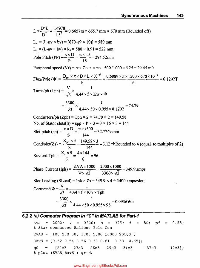
Synchronous Machines 143
D2L 1.4978 L =-1-= 2 0.6657m= 665.7 mm::::: 670 mm (Rounded off)
D- 1.5
Ls = (L-nv x by) = [670-(9 x 10)] = 580 mm
L\ = (L-nv x by) x k i = 580 x 0.91 = 522 mm
P 'I . h (P 1t x D 1t x 1.5 2 52 oePltc P)=--=--= 94. mm P 16
Peripheral speed (Vr) = 1t X D x n =1t x 15001l000x 6.25= 29.45 mls
Flux/Pole (<I»= Bav x1txDxLxl0-6 = 0.6089x1txI500x670xl0-6 =0.1202T P 16
V 1 Turns/ph (Tph) = r;; x
v3 4.44xfxKwxCl>
= 3300 x 1 = 74.79 J3 4.44 x 50 x 0.955 x O. Ii02
Conductors/ph (Zph) = Tph x 2 = 74.79 x 2 = 149.58
No. of Stator slots(S) = spp x P x 3 = 3 x 16 x 3 = 144 . 1txD 1tx1500
Slot pItch (sp)= --= = 32.7249mm S 144
Zhx3 14958x3 Condislot(Zs) = p =. = 3.12 7 Rounded to 4 (equal to multiples of 2)
S 144 . ZsxS 4x144
ReVIsed Tph = --= = 96 6 6
Ph C (I h) KV A x 1000 2000 xl 000 349 9 ase urrent p = = =. amps Vx J3 3300x Jj
Slot Loading (SLoad) = Iph x Zs = 349.9 x 4 == 1400 amp~slot; V 1 -
Corrected <I> =- x -------J3 4.44 x fx Kw x Tph
= 3300 x 1 = 0.0936Wb J3 4.44 x 50 x 0.955 x 96
6~2.2 (a) Computer Program in "C" in MATLAS for Part-1
KVA = 2000; V = 3300; N = 375; f = 50; pf 0.85; % Star connected Salient Pole Gen
KVAS [100 200 500 1000 5000 10000 20000];
BavS = [0.52 0.54 0.56 0.58 0.61 0.63 0.65];
qS [20e3 23e3 26e3 2ge3 34e3 % plot (KVAS,BavS); grid;
·37e3 40e3];
www.EngineeringEBooksPdf.com

144 Computer-Aided Design of Electrical Machines
Bav interp1 (KVAS, BavS. KVA, 'spline'); q = interp1 (KVAS, qS, KVA, 'spline'};
Kw = 0.955; 1byPP = 2.3; nv = 9; bv = 10; ki = 0.9; spp = 3; % Assumptions Pole Arc = 1;
P = 120*f/N; K = 11*Bav*q*Kw*le-3; n = 2*f/P; Osq1 ~ KVA/(K*n);
01 (Osq1*P/(1byPP*pi) )A(1/3)*1000; 0 ceil(01/10)/100; 11 = Osq1/0A2; 1 = ceil(11*100)*10; 0 = 0*1000; 1s = (1-nv*bv); 1i 1s*ki; PP pi*O/P; Vr pi*0*n/1000; flux1 = Bav*pi*0*1/P/1e6; Tphi = V/sqrt(3)/(4.44*f*Kw*flux1);
Zph = Tphi*2; S = spp*P*3; sp = pi*O/S; Zsi = Zph*3/S; Zs = ceil (~i/2) *2; Tph = Zs*S/6; Iph = KVA*le3/ (1. 7321*V); S10ad = Iph*Zs; FI = V/sqrt(3)/ (4.44*f*Kw*Tph);
6.2.3 Design of Armature Winding and Core (Part-2)
Assuming current density (cds) = 4 Almm2~
Cond Area ofCS (As) = Iph = 349.9 = 87.475mm2
cds 4
PoleArc No of teeth under pole arc (TpP) = --
SlotPitch
0.7 x 294.52 6 3 7 d d h'gh I ) = = . == (Roun e to I er nteger 32.7249
T th 'dth . (b 0) <P -_ 0.0936 --14.23 mm 00 WI at aIr gap t = BtO x Li x TpP 1.8 x 522 x 7
Slot Width (Ws) = Slot Pitch - btO = 32.72 - 14.23 = 18.49 mm
Cond Width (We) = Slot width - width of Ins = 18.49 - 6
= 12.49 m == 13 mm (Rounded off)
As 87.475 Cond Thk (Hc) = - = = 6.73 == 7mm (Rounded off)
We 13
Corrected Width of Slot (Ws) = 1 x Wc + Wins = (1 x 13) + 6 = 19 mm;
C d d · d Iph -_ 349.9 --3.9235A/mm 2 orrecte current enslty (c s) = WcxHcxO.98 13x7xO.98
(assuming a factor of 0.98 for rounding the conductor edges)
Height of Slot (Hs) = Zs x He + Zs x 2 x 0.5 + Hins + Hw + HL
= [(4 x 7) + 4 x (2 x 0.5) + 8 + 4 + 1] = 45mm (Refer Table given below)
Mean Length of Tum (Lmt) = (2 xL + 2.5 x PP + 50 x KV + 150)/1000
= (2 x 670) + (2.5 x 294.52) + (50 x 3300/1000) + 150 = 2.3913 m
www.EngineeringEBooksPdf.com
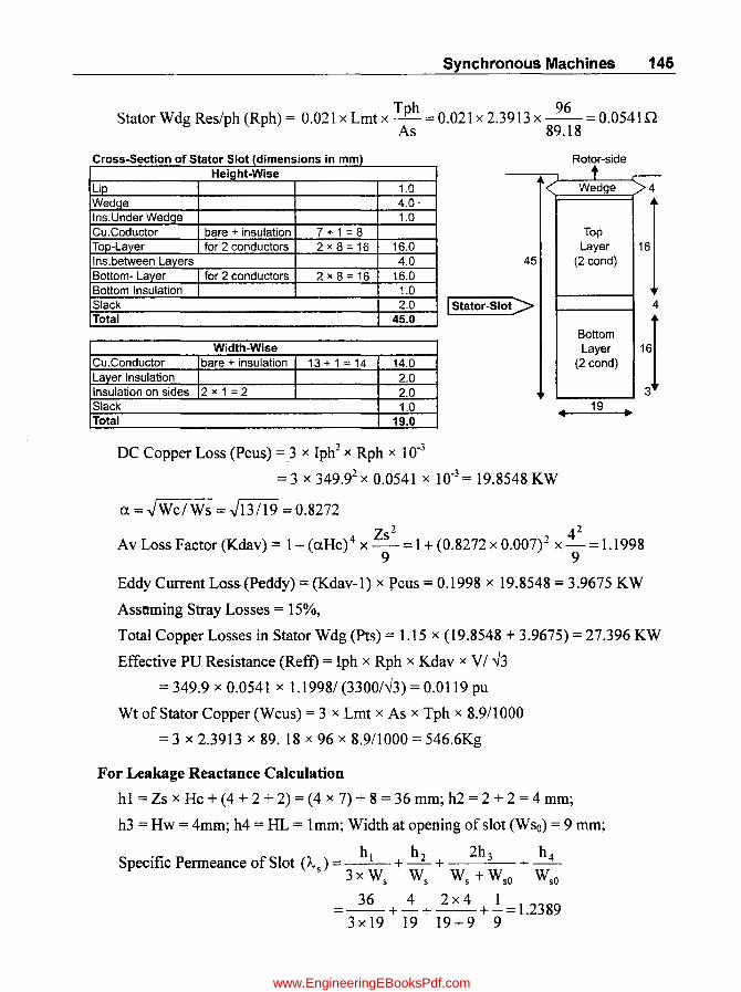
Synchronous Machines 146
Tph 96 Stator Wdg Res/ph (Rph) = 0.021 x Lmt x - = 0.021 x 2.3913 x --= 0.0541 n
~ As 89.18
Cross-Section of Stator Slot (dimensions in mm) Rotor-side Height-Wise t .--
Lip 1.0 Wedge 4 WedQe 4.0 . Ins. Under Wedge 1.0 CU.Coductor bare + insulation 7+1=8 Top Top-Layer for 2 conductors 2 x 8 = 16 16.0 Layer 16 Ins.between Layers 4.0 45 (2 cond) Bottom- Layer for 2 conductors 2 x 8 = 16 16.0 Bottom Insulation I 1.0 Slack 2.0 I Stator-Slo t> 4 Total 45.0
Bottom
1·1 Layer
(2 cond)
3
Width-Wise Cu. Conductor bare + insulation 13+1=14 14.0 Layer Insulation 2.0 Insulation on sides 2x1-2 2.0 Slack 1.0 19 Total 19.0
DC Copper Loss (Pcus) = 3 X Iph2 x Rph x 10-3
= 3 x 349.92 x 0.0541 X 10-3 = 19.8548 KW
a = .jWc/Ws = .j13119 = 0.8272
ZS2 42
Av Loss Factor (Kdav) = 1 + (aHc) 4 x - = 1 + (0.8272 X 0.007)2 x - = 1.1998 9 9
Eddy Current Loss-(Peddy) = (Kdav-l) x rcus = 0.l998 x 19.8548 = 3.9675 KW
Assaming Stray Losses = 15%,
Total Copper Losses in Stator Wdg (Pts) = 1.15 x (19.8548 + 3.9675) = 27.396 KW
Effective PU Resistance (Reft) = Iph x Rph x Kdav xVI "3
= 349.9 x 0.0541 x 1.19981 (33001"3) = 0.0119 pu
Wt of Stator Copper (Wcus) = 3 x Lmt x As x Tph x 8.911000
= 3 x 2.3913 x 89. 18 x 96 x 8.911000 = 546.6Kg
For Leakage Reactance Calculation
hI = Zs x Hc + (4 + 2 + 2) = (4 x 7) + 8 = 36 mm; h2 = 2 + 2 = 4 mm;
h3 = Hw = 4mm; h4 = HL = Imm; Width at opening of slot (Wso) = 9 mm;
Specific Permeance of Slot (I."s) = hi + ~ + 2h3 + _h_4_ 3x Ws Ws Ws + Wso Wso
36 4 2 x 4 1 = -- + - + --+ - = 1.2389
3x19 19 19+9 9
www.EngineeringEBooksPdf.com

146 Computer-Aided Design of Electrical Machines
Slot Leakage Flux (rp ) = 2 x"';2 x p.0 x Iph x Zs x Ls x As s
= 2 x "';2 x 4 x J[ X 10-7 x 349.9 x 4 x 58011000 x 1.2389 = 0.0036 Wb
K X't 2 LOAO = _s_..:...P_
1t't s
0.95
0.9
t 0.85 rn 0.8
~ 0.75
-§ 0.7 ra
LL. 0.65
0.6
0.55
· · · .. • .. ..I.. .. .. .. • .. ..... .. .. .. • .. .. ... ·
0.5 ~-'--""""'-'-'--'-----'_L..-.-L--'--'-~ 0.5 0.550.6 0.65 0.7 0.75 0.8 0.85 0.90.951
Coil SparnlPole Pitch -+
Fig. 6.1 Leakage factor.
lx(294.5211000)2 =0.8437 1tx32.725/1000
(T p 7 Pole pitch and Ts 7 Slot Pitch andKs = 1 from above graph (Fig. 6.1))
Overhang Leakage Flux (~o) = 2 x J2 x Ilo x IPb x Zs x LoAo
= 2 x J2 x 4 x J[ X 10-7 x 349.9 x 4 x 0.843/---Q..OO42
Totttl Leakage Flux = ~ L = ~ s + ~o = 0.0036 + 0.0042 = 0.0078
Leakage Rectance (XL) = ~ = 0.0078 0.0833pu ~ 0.0936
Flux in core (rpc) = 1= 0.0936 = 0.0468 Wb 2 2
Depth of Core (de) = ~e = 0.468 =81.5mm Be xLI 1.1 x 522
Outer diameter of Core (Do) = D + 2 x (Hs + de)
= 1500 + 2 x (45 + 81.5) = 1753;:::: 1760 mm (Ronded off)
Coorected Depth ofCore(dc) = (1760 -1500)/2 - 45 = 85 mm
6.2.3 (a) Computer Program in "C" in MATLAB for Part-2
% (2) Design of Stator Winding, Reactance, Core D = 1500; L = 670; FI = 0.0936; Iph = 349.9; PP ~s. = 4; Tph = 96; sp = 32.7249; % Specification
294.52;
www.EngineeringEBooksPdf.com

Synchronous Machines 147
v = 3300; Ls = 580; Li = 522; nv = 9; bv = 10; Wins 6; Hins = 8; Hw = 4; HL = 1; % Specification Ki = 0.9; cds = 4; PAtoPP = 0.7; BtO = 1.8; Bc 1.1; Ks 1; % Assumptions % Wc = 0.8; tins = 0.5; Hw = 5; HL 2; InsIL 5; Hins 6; InsM = 2; % Assumptions As Iph/cds; TpP ceil (PAtoPP*PP/sp); btO = FI*le6/(BtO*Li*TpP); Ws1 sp-btO; Wc = ceil( (Ws1)-Wins); Hc = ceil(As/Wc*2)/2; Ws = l*Wc + Wins; As=Wc*Hc*0.98; cds=Iph/As; Hs=Zs*Hc+ Zs*2*0.5+Hins+Hw+HL; rat1 = Hs/Ws; Lmt (2*L + 2.5*PP + 50*KV + 150)/1000; Rph 0.021*Lmt*Tph/As; Pcus 3*IphA2*Rph/1e3; Wcus 3*Lmt*As*Tph*8.ge-3; alfa sqrt(Wc/Ws); Kdav 1 + (alfa*Hc/10)A4*Zs A2/9; Peddy (Kdav-1)*Pcus; Pts= (Pcus + Peddy)*1.15; Reff = Iph*Rph*Kdav/(KV/sqrt(3)*le3);
<------------ Leakage Reactance ---------> h1 = Zs*Hc + 4 + 2 + 2; h2 = 2 + 2; h3 = Hw; h4 = HL; WsO = 9; Lmdas = h1/(3*Ws) + h2/Ws + 2*h3/(Ws + WsO) + h4/WsO; Fis = 2*sqrt(2)*4*pi*le-7*Iph*Ls/1000*Lmdas*Zs; CSbPP [0.5 0.6 0.7 0.8 0.9 1]; ks = [0.5 0.63 0.76 0.84 0.92 1]; plot (CSbPP, ks);grid; xlabel ('Coil Span/Pole ~itch-->');
Ylabel ('Factor KS-->'); title ('Leakage Factor'); y1 = 1; KS = interp1 (CSbPP, ks, y1, 'spline'); LOLmdO Ks*Pp A2/(pi*sp*1000); TO 2*sqrt(2)*4*pi*le-7*Iph*TO*LOLmdO; FIL FIL/FI; Flc = FI/2; dc1 = FIc*le6/ (Bc*Li); dc1); Do = ceil(Do1/10)*10; dc = (Do - D)/2
6.2.4 Design of Rotor and Calculation of AT (Part - 3)
Armature reaction:
Zs; Flo FIs + F·lo; XL
Dol = D + 2*(Hs + - Hs;
ATlPole(AT ) = 1.35 x Tph x Iph x kw = 1.35 x 96 x 349.9 x 0.955 = 5413.3 a P/2 16/2
No Load ATlPole (ATfl) = scr x Ata = 0.9 x 5413.3 = 4872
ATg = 0.75 x ATfl) = 0.75 x 4872 = 3654
AirGapFluxDensity(Bg) = Bav = 0.6089 = 0.8699T PoleArc/Polepitch 0.7
Assuming Air Gap Coefficient (Kg) = 1.17 (Varies from 1.12 to 1.18);
AT Air Gap Length (Lg) = g 6 = 0.0045 m = 4.5mm
0.796xBg xKg xl0
www.EngineeringEBooksPdf.com

148 Computer-Aided Design of Electrical Machines
Air gap 0.0045 --'--= = 0.0154 (Usual value = 0.012 to 0.016) Pole pitch 0.2928 "
Rotordia(Dr)=D-2 x Lg= 1500-2 x 4.5 = 1491mm
Axial Length of Pole (Lp) = L -15 = 670 -15 = 655 mm
Assuming Stacking factor = 0.9, Iron Length of Pole (Lpi) = 0.90 x 655 = 589.5 mm
Assuming Pole Leakage factor = 1.1,
Flux in the Pole body ( <l> p)
= 1.1 x <l> = 1.1 x 0.0936 = 0.103Wb
Assuming flux density in Pole body (Bp) = 1.5T,
Area of Pole (Ap) = <l> p / Bp = 0.103/1.5 = 0.0686 m2
Width of Pole (Wp)= Ap = 0.0686 x 106
=1l6.44mm Lpi 589.5·
W poles = Ap x Lp x P x 7800 = 0.0686 x 655 x 16 x 7.8 = 5610.9 Kg
. Depth of Field Winding (dt)
Pole-Pitch (m) 0.1 0.2 0.3 0.4 Windg-Depth (m) 0.03 0.036 0.04 0.045
0.055 r---"-""'"T""-'"T"'""--r---,.---.--...,.....---,
t 0.05 e-O; ~ 0.045 "C u: '0 0.04 .s= Q. ~ 0.035
, , , --.-~---~-.--~---~----.----~---.----• 0, • , ,
• • I' • I
- - - -.- - - • ., - - - - r - - - 1- - - - , - - - - .. - - - , - •• -· .. . ,
J. ___ ~ ___ ~ ____ ! ____ ~_._!_. __ . . . . . . I •• • I , , , , , ,
0.03 "'-----'-' - ......... -----. - ...... - .......
0.5 0.05
0.1 0.15 0.2 0:25 0.3 0.35 0.4 0.45 0.5
Pole Pitch(m)~
Flg.6.2 Field winding depth.
www.EngineeringEBooksPdf.com
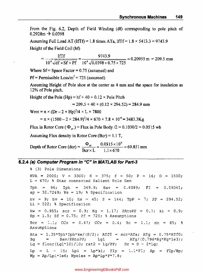
Synchronous Machines 149
From the Fig. 6.2, Depth of Field Winding (dt) corresponding to pole pitch of 0.2928m 7 0.0398
Assuming Full Load AT (Ifft) = 1.8 times ATa, Ifff= 1.8 x 5413.3 = 9743.9
Height of the Field Coil (ht)
Ifff = 9743.9 = 0.20955 m = 209.5 mm -1 0~4;-.J-;=d=f=x=S=f=x=P=f 104 .J 0.0398 x 0.75 x 725
Where Sf= Space Factor = 0.75 (assumed) and
Pf = Permissible Loss/m2 = 725 (assumed)
Assuming Height of Pole shoe at the center as 4 mm and the space for insulation as 12% of Pole pitch,
Height of the Pole (Hp) = hf + 40 + 0.12 x Pole Pitch
= 209.5 + 40 + (0.12 x 294.52) = 284.9 mm
Wrot = 1t x (Dr- 2 x Hpil4 x L x 7800
= 1t x (1500-2 x 284.9i14 x 670 x 7.8 x 10-6= 3483.3Kg
Flux in Rotor Core (<l> cr) = Flux in Pole Body 12 = 0.1030/2 = 0.0515 wb
Assuming Flux density in Rotor Core (Bcr) = 1.1 T,
Depth of Rotor Core (dcr) = <l>cr =0.0)15xl06
=69.851mm Bcrx L 1.1 x 670
6.2.4 (a) Computer Program in "c" in MATLAB for Part-3
% (3) Pole Dimensions
KIf A = 2 0 0 0 ; V = 330 0 ; N = 37 5 ; f = 5 0 ; P = 16 ; D = 15 0 0 ; L = 670; % Star connected Salient Pole Gen
Tph 96; Iph 349.9; Bav 0.6089; FI sp = 32.7249; Ws = 19; % Specification
nv = 9; bv = 10; Hs = 45; S = 144; TpP = 7; PP Li = 522; % Specification
0.09361;
294.52;
kw = 0.955; scr = 0.9; Kg 1.17; PAtoPP = 0.7; ki = 0.9; Bp = 1.5; Sf = 0.75; Pf = 725; % Assumptions
Bcr = 1.1; CCs = 0.47; CCv = 0.4; Bc = 1.1; dc = 85; % Assumptions
Ata = 1.35*Tph*Iph*kw/(P/2); ATfO = scr*ATa; ATg = 0.75*ATfO; Bg Bav/PAtoPP; Lg1 ATg/(0.796*Bg*Kg*le3); Lg = floor(Lg1*10)/10; rat2 = Lg/PP; Dr = D - 2*Lg;
Lp = L - 15; Lpi = Lp*ki; FIp Wp = Ap/Lpi*le6; Wpoles = Ap*Lp*P*7.8;
1.1*FI; Ap = FIp/Bp;
www.EngineeringEBooksPdf.com

150 Computer-Aided Design of Electrical Machines
% <--Table for Depth of Field Winding------------>
PPS = [0.1 0.2 0.3 0.4 0.5J; DF = [0.03 0.036 0.04 0.045 0.05J;
% plot (PPS I OF) ; gr id; xlabel (' Pole Pitch(m)-->'); ylabel('Depth of Fld-Wdg (m)-->');
% title ('Field Winding Depth');
df = interpl (PPS, DF, PP/le3, 'spline'); IfTf = 1. 8*ATa;
hf = IfTf/(le4*sqrt(df*Sf*Pf))*1000; Hp = hf + 40 + 0.12*PP;
dcr = Flp*le6/2/Bcr/L;Wrot = pi*(Dr - 2*Hp)A2/4*L*7.8e-6;
6.2.5 Carter Coefficients and Ampere Turns for Various Parts of Magnetic Circuit (Part-4)
t "E II)
• (3
IE II) 0 0 .... ~ III 0
0.9
0.8
0.7
0.6
0.5
0.4
0.3
0.2
0.1
0 0
· I •• • _____ J ______ ~ _____ ~ __ ___ L. ____ J _____ _ · . . . . · . · . --·--~·-·-·-r-- --~------r-----~------I • I • · . . ___ •• J ___ • ~ _____ ~ ______ ~ _____ ~ _____ •
• • I • · · -----~- ----r-·---~------r-----~------• • • • I
• I • •
----- ------~-----~------.---.-~------· . . . • • • I ___ _ J_. ____ ~ _____ J. _____ ~. ____ J _____ _
• • I • • · .. · .. - ---~-··---r-----~------p-----,------• •• I I •••
2 4 6 8 10 12
Slot Opening/Gap Length~
Fig. 6.3 Carters coefft for semi-closed slots.
SlotWidth ~ = 4.2222 Airgap 4.5
Carters Coefficient read from graph (Fig. 6.3) corresponding to 4.2222 is 0.5459
. Slot Pitch Slot CoefficIent (Kgs) = ------------
Slot Pitch - Slot width x Carter Coefft
= 32.725 =l.4641 32.725 -19 x 0.5459
DuctWidth = 10 = 2.2222 GapLength 4.5
Carters Coefficient (CCv) Read from Graph (Fig. 6.3) corresponding to 2.2222 is 0.3598
www.EngineeringEBooksPdf.com
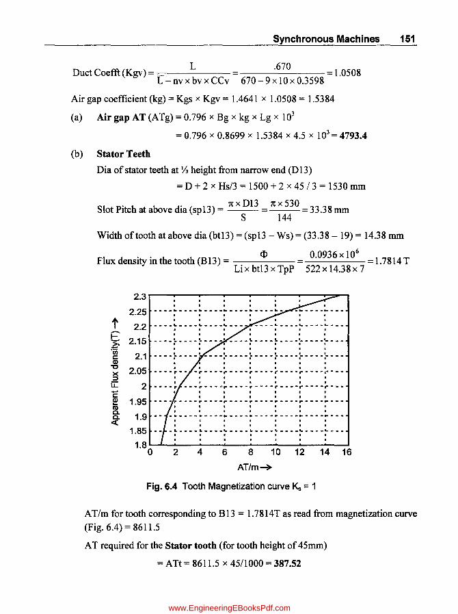
Synchronous Machines 151
Duct Coefft (Kgv) = L = .670 = 1.0508 L - nv x bv x CCv 670 - 9 x 10 x 0.3598
Air gap coefficient (kg) = Kgs x Kgv = 1.4641 x 1.0508 = 1.5384
(a) Air gap AT (ATg) = 0.796 x Bg x kg x Lg x 103
= Q.796 x 0.8699 x 1.5384 x 4.5 x 103 = 4793.4
(b) Stator Teeth
Dia of stator teeth at Y3 height from narrow end (D 13)
= D + 2 x Hs/3 = 1500 + 2 x 45 13= 1530 mm
. • 1t x D13 1t x 530 Slot PItch at above dla (sp13) = = = 33.38 mm
S 144
Width oftooth at above dia (btl 3) = (sp13 - Ws) = (33.38 - 19) = 14.38 mm
Flux density in the tooth (B13) = <l> = 0.0936 X 106
= 1.7814 T Li x btl 3 x TpP 522 x 14.38 x 7
2.3
2.25 ---- .. ---.----~----.--- .. -· . . . t 2.2
• I • • I
----~----~----~---- ---.~----~----~---· .. .. ~
2.15 ~ 'c;;
2.1 c
• •• • I
........ ~ ........ t.. ........ I ........................... ' ....... wi ..... .. · . . . . . . I • • • I • I
........ ~ ........ I ........ I .......... ~ ........ ~ ........ I .......... I ...... _ · .,... Q) · ... '0 2.05 x • •• I ----r-- .. r----~- .. --r----r----r--- .. r---::J · . .. u:: 2 · . .. --war ---r----r----r----r----r----r----c ~ 1.95
.. . . . ---·p----p----p----r----r----r----r---m • • • • • I •
a. 1.9 a. «
• I • • • • •
-~----~----~----~----~----~----~---· ..... • • I • • •
1.85 _~ ____ L ____ ~ ____ L ____ L ____ ~ ____ ~ __ _
•• I' • .. .. . 1.8
0 2 4 6 8 10 12 14 16
AT/m~
Fig. 6.4 Tooth Magnetization curve Ks = 1
AT 1m for tooth corresponding to B 13 = 1.7814 T as read from magnetization curve
(Fig. 6.4) = 8611.5
AT required for the Stator tooth (for tooth height of 45mm)
= ATt = 8611.5 x 45/1000 = 387.52
www.EngineeringEBooksPdf.com
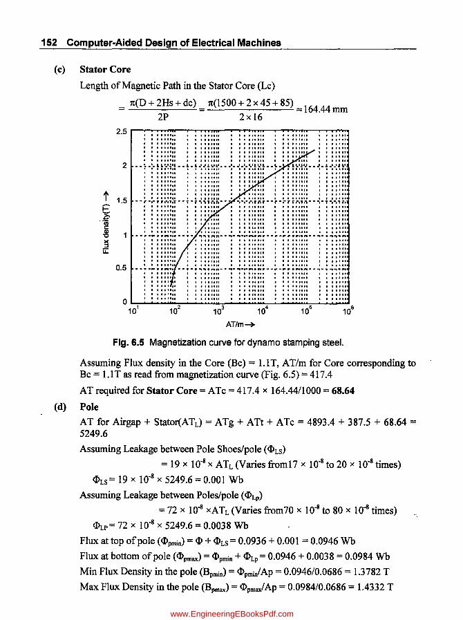
152 Computer-Aided Design of Electrical Machines
(e) Stator Core
Length of Magnetic Path in the Stator Core (Lc)
t E ,~
c Q) "0 )( ::I u::
2.5
2
1.5
0.5
n(D + 2Hs + dc) = n(1500 + 2 x 45 + 85) = 164.44 nun 2P 2x 16
...... • • II ... ..
• •• 1.1 .. I ...... ..
• • 11"" , ,
, , , , , , , ,
...... , , • •• ...... I.
III'" •• " ...... .. I, , !o,_,!., .... , .. L ...... , I!..·L· .................... .& ... , .... \, .. , '1"" •• ....... ••• •••••• • '1"" •• '1"'11 ••••••••• ...... II ....
'1"" It .... ......
"","
, , , ,
•• ""n · ...... .. · ...... .. • ••• 1 •••• · ...... .. . ....... . """ , • I •••••• • I
••• 1 .. . ....
...... .. . .. ...... .. .
._............ ... ... " ""'_ .. -.- .. -,-,.."' .......... -r r ........... -.- ........ PI
• • """ I., II II it • • •• ,... '" •••••• • •••••• • • • .".,. • •• III'" , . ,..... . ..... ,' · I I...... . I .. 1111 , , , , , , , , , , , , , , , , , ,
.1 .... """ ......
, , ,
, , , , -.- ..... "P .......... r .. P •• "" .............. PI •••••• 1 ••• •••••• I I I ••••
• I. I •••••
I •••••••• ......... , , , , I I' ".,.1
Fig. 6.5 Magnetization curve for dynamo stamping steel.
Assuming Flux density in the Core (Bc) = LIT, AT/m for Core corresponding to Bc = LIT as read from magnetization curve (Fig. 6.5) = 417.4
AT required for Stator Core = ATc = 417.4 x 164.44/1000 = 68.64
(d) Pole
AT for Airgap + Stator(ATd = ATg + ATt + ATc = 4893.4 + 387.5 + 68.64 = 5249.6
Assuming Leakage between Pole Shoes/pole ($LS)
= 19 x 10-8 x ATL (Varies from17 x 10-8 to 20 x 10-8 times)
$LS= 19 x 10-8 x 5249.6 = 0.001 Wb
Assuming Leakage between Poles/pole ($Lp)
= 72 x 10-8 xATL (Varies from70 x 10-8 to 80 x lo-B times)
$LP= 72 x 10-8 x 5249.6 = 0.0038 Wb
Flux at top of pole ($Pmin) = $ + $LS = 0.0936 + 0.001 = 0.0946 Wb
Flux at bottom of pole ($pmax) = $pmin + $Lp= 0.0946 + 0.0038 = 0.0984 Wb
Min Flux Density in the pole (Bpmin) = $pmin/Ap = 0.0946/0.0686 = 1.3782 T
Max Flux Density in the pole (Bpmax) = $pmax/ Ap = 0.0984/0.0686 = 1.4332 T
www.EngineeringEBooksPdf.com

Synchronous Machines 153
AT /m corresponding to 1.3 782 T from magnetization curve (Fig.6.5)
= atp 1 = 815.2
AT/m corresponding to 1.4332 T from magnetization curve (Fig.6.5)
= atp2 = 1172
AT for Pole = [% x atpl x HP] + [l x atp2 x HP]
= [~x 815.2 x 284.9] + [.!.. x 1172 x 284.9] = 266. 1
3 1000 3 1000
(e) Rotor Core
Length of Magnetic Path in the Rotor Core (Lcr)
= n(Dr - 2Hp - dcr) = n(1491- 2 x 284.9 - 69.85) = 83.583 rnrn 2P 2 x 16
Assuming Flux density in the Rotor Core (Bcr) = 1. IT, AT/m for Core corresponding to Bc = 1.1 T as read from magnetization curve (Fig.6.5) = 417.45
AT required for Rotor Core = ATrc = 417.45 x 83.583/1000 = 34.89
Total No-Load AT for the Magnetic Circuit at 100% rated Voltage (ATfO)
= ATg + ATt + ATc + ATp + ATrc
= 4793.4 + 387.5 + 68.64 + 266.1 + 34.89 = 5550.6
6.2.5 (a) Computer Program in "C" in MATLAB for Part-4
%-------------------Ampere-Turns at 100% V-------------------->
%<---B-H Curve for St Tooth for ks=l ---->
BtS = [1. 8 1. 9 2 2.1 2.15
attS [ge3 14e3 24e3 43e3 % ks = 1.0
2b
60e3
2.25 2.3] ;
80e3 110e3 152e3]i
% plot (attS, BtS); grid; xlabel ('AT/m-->'); ylabel ('Apparent Flux density(T)-->');
% title ('Tooth Magnetization Curve for Ks = 1');
% ---- Carters Coefft for Semi-closed slots--->
WObyLgS = [0 1 2 3 4 5 6 7 8 9 10 11 12] ; % Slot opening/Gap
CC = [0 .18 .33 .45 .53 .6 .66 .71 .75 .79 .82 .86 .89] ;
% plot (WObyLgS, CC); grid; xlabel ('Slot Opening/Gap Length->'); Ylabel ('Carter Coefficient-->');
\
% title ('Carters Coefft for Semi-closed slots');
% <---B-H Curve common for St Core, Rt core and Poles---->
www.EngineeringEBooksPdf.com

154 Computer-Aided Design of Electrical Machines
BS = [0 0.25 0.5 0.75
atS = [0 80 100 150
1.0 1.25 1.5 1.75 2.0 2.25];
300 580 2e3 8e3 3e4 16e4];
% se~ilogx (atS, BS); grid; xlabel ( 'AT /m-->' ) ; ylabel ('Flux density(T)-->');
% title ('Magnetization Curve for OynamoStamping Steel');
WsbyLg = Ws/Lg; CCg = interp1 (WObyLgS, CC~ WsbyLg, 'spline'); kgs = sp/(sp-Ws*CCg);
ObyG = bv/Lg; CCv = interp1 (WObyLgS, CC, ObyG, 'spline');
kgv = L/(L-nv*bv*CCv); kg = kgs*kgv;
%--------------------------------------------------------------
ATg = 0.796*Bg*kg*Lg*le3; 013 = 0 + 2*Hs/3; sp13 = pi*013/S; bt13 sp13-Ws; B13 FI/(Li*bt13*TpP)*le6; att interp1 (BtS, attS, B13, 'spline');
ATt att*Hs/1000; Lc = pi*(O + 2*Hs + dc)/P/2;
tc interp1(BS, atS, Bc, 'spline'); ATc atc*Lc/1000; ATL ATg + ATt + ATc; FILs = 1ge-8*ATL; FILp = 72e-8*ATL; FIpmin = FI + FILs; FIpmax = FIpmin + FILp; Bpmin = FIpmin/Ap; atp1 interp1(BS, atS, Bpmin, 'spline'); Bpmax = FIpmax/Ap;
atp2 = interp1 (BS, atS, Bpmax, 'spline');
ATp=(2/3*atp1+1/3*atp2)*Hp/1e3; Lcr = pi*(Or - 2*Hp - dcr)/P/2;
atrc interp1 (BS, atS, Bcr, 'spline');
ATrc atrc*Lcr/1000; ATfO = ATg + ATt + ATc + ATp + ATrc;
<-------------------------------------------------------
6.2.6 Open Circuit Characteristic Curve (OCC) (Part-5)
A plot of Ampere Turns on X-Axis and Various Terminal voltages (0 % to 130% of rated Voltage).
Procedure for Plotting Open Circuit Characteristic Curve (OCC)
1. Consider Terminal Voltages of 100%, 110%, 120% and 130% of rated voltage. 2. Fill up all the details pertaining to Air-Gap, Stator tooth, Stator Core, Poles and
Rotor Core calculated above under the 100% Voltage Column in the table. 3. Calculate the Flux densities in various parts at other 3 Voltages which are linearly
proportional to Voltage (Ex:-If Flux density = LIT at 100% Volts, then at 110%Volts it will be (1101100) x 1.1 = 1.2IT).
4. At these values of Flux densities measure the "AT/m" from appropriate curves as was referred for calculation for 1 00% V).
5. Calculate Values of "AT" for each part by directly multiplying the "AT/m" value with corresponding "length" of each part.
www.EngineeringEBooksPdf.com

Open Circuit Characteristic Curve (OCC) of Salient Pole Generator Length 100%( 3300 Volts) 110%( 3630 Volts) 120%(
Part m B(tssla) AT/m AT B(tesla) AT/m AT B(tesla) Air-Gap 00045 08699 47934 095689 52 27 104388 Stalor Teeth 0045 17816 8610 387 1.95976 19370 8717 213792 Stator-Core 016444 11 4174 69 121 545.2 897 132 Pole min 13782 815 151602 22782 165384
028489 266.1 7724 Polelmax1 14332 1172 1 57652 3577 171984 Rot-Core 008358 11 4174 35 121 5452 456 132 Total-AT= 5550.5 7052 Field-Amps (OCC) 58.4 74.2
3960 Volts) 130%(
AT/m AT B(tasla) 57521 113087
55650 2504 231608 6475 106 5 143
55634 179166 17481
7282 186316 6475 541 143
10165 107
4290 Volts)
AT/m AT 62_3142
168080 7564 11443 1882 89634
28235 11805
11443 956 16903 177.9
;-l 0\
~ > > g, t-3 §: <: @ <: a..c~ s:: s::-(1) ...... s:: VJ @ Dl o 0.. 0 >-+, 8' >-+, > ""I ~ ...., (1) > o Il5 -l ::s =r :: ><: <: 0 I 0 >-+, > - ~
:>< 5j == _. (JQ f"""'t-
VJ (l) =r ~ • (l)
::s "0
~ ~ 0'- VJ
~ § .... 0.. (l) (l) 0.. ""I
<: (l)
o Il5 ;:;:- =r en ~ ':f? '< (l) 0 ::::I VJ < 0 o 0 ::T ::s ;:;:- ... -< ~ 0 I ~ ::::I > n g ~. 0 In ~ 2" s: o 8 S»
(JQ .... 0 ~ 0 ::T o (JQ ::::I (") :: m (") =r • (l)
t-3 o I ...... S' en _ en
www.EngineeringEBooksPdf.com
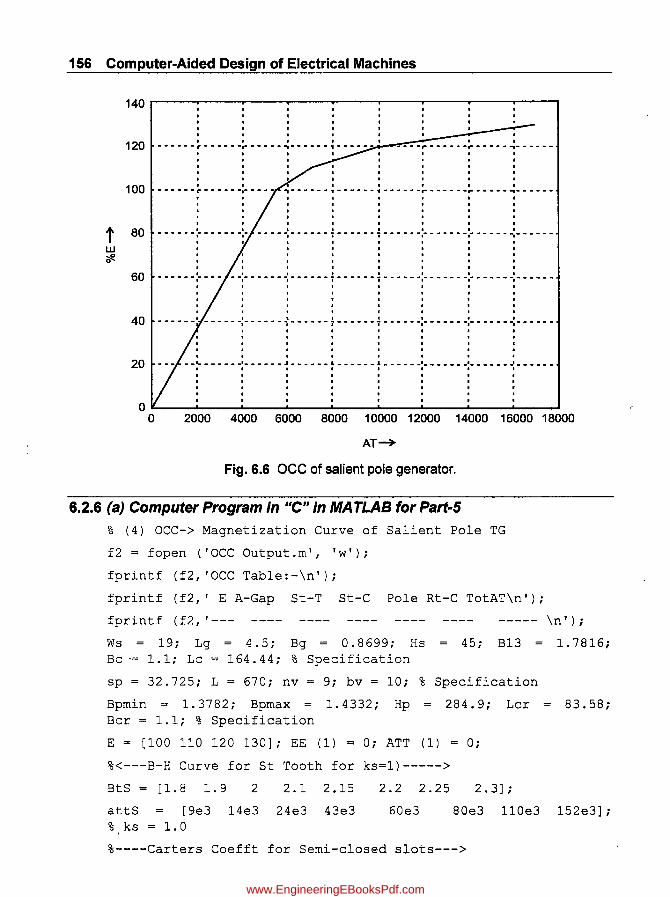
156 Computer-Aided Design of Electrical Machines
t w '#.
140~----~---------r--------~--------~----~--------~--------~----~~----~
120
100
80
60
.. . ------,------~-- .. --~ .. -----,-.-- ....
• I • • · · . -- .. ---~ .. -- .. -... -----· . · . ·
. .. ~---- .. -,---- ... , .. -.... --~---- .. -~-----~--- .. --
I •••• · ...
· ·
· · · . · . . -- .... --r------~ .. ----~------
· . . --- .. --r--- .. --r-----~----- .. · . . · . · . 40 _ ...... __ . ------:--- ... -{ ............ ;,- ........ .. · . . ........ .. -.- ......................... -.- ......... .. · . . · . . · . · . . · . · · . • • I. •
.............. .. _' ........... .I .......................... , ............ ' .............. 1_ ............ f .......... .. · . . . . . . . I • • I • • • • · . . . .
OL-----~--------~----~--------~--------~----~--------~--------~----~ o 2000 4000 6000 8000 10000 12000 14000 16000 18000
AT~
Fig. 6.6 acc of salient pole generator.
6.2.6 (a) Computer Program in "C" in MATLAS for Part-5
% (4) OCC-> Magnetization Curve of Salient Pole TG
f2 = fopen ('OCC Output.m', 'w');
fprintf (f2, 'occ Table:-\n');
fprintf (f2,' E A-Gap St-T St-C Pole Rt-C TotAT\n');
fprintf (f2, '--- ----- \n');
Ws = 19; Lg = 4.5; Bg = 0.8699; Hs = 45; B13 = 1.7816; Bc = 1.1; LC 164.44; % Specification
sp = 32.725; L = 670; nv = 9; bv = 10; % Specification
Bpmin = 1.3782; Bpmax = 1.4332; Hp = 284.9; Lcr = 83.58; Bcr = 1.1; % Specification
E = [100 110 120 130]; EE (1) = 0; ATT (1) = 0;
%<---B-H Curve for St Tooth for ks=l)----->
BtS = [1.8 1.9 2 2.1 2.15 2.2 2.25 2.3] ;
attS [ge3 14e3 24e3 43e3 60e3 80e3 110e3 152e3]; % ks = 1.0
%----Carters Coefft for Semi-closed slots--->
L _
www.EngineeringEBooksPdf.com

Synchronous Machines 157
WObyLgS = [0 1 2 3 4 5 6 7 B 9 101112]; ~ Slot opening/Gap
ee = [0. IB . 33 .45 . 53 . 6 . 66 . 71 . 75 . 79 . 62 . 86 . 89] ;
% <--- B-H Curve common for St Core, Rt core and Po1es----->
BS = [0 0.25 0.5 0.75 1.0 ~.25 1.5 1.75 2.0 2.2SJ;
atS = [0 BO 100 150 300 SSC 2e3 Be3 3e4 16e4];
Wsby~g = Ws/Lg; CCg = interpl (WO:OyLgS, CC, WsbyLg, 'spline'); kgs = sp/(sp - Ws*CCg);
ObyG = bv/Lg; CCv = interp1 (WObyLgS, ce, ObyG, 'spline'); kgv L/(L -nv*bv~CCv); kg = kgs*kgv;
for i = 1:4;
Bgx(i) = Bg*E(i)/100; ATgx(i) 0.796*Bgx(i)*kg*Lg*le3;
Bstx(i)
atST(i)
B13*£ (i) 1100;
i:lterp1(BtS, attS, Bstx(i), 'spline');
ATstx(i) = atST(i)*Hs/1000;
Bscx(i) = Bc*E(i)/100;
atSC(i)=interp1(BS,atS,Bscx(i), 'spline'); ATscx(i) = atSC(i)*Lc/1000;
Bpminx(i) = Bpmin*E(i)/100;
atP1(i) = interp1(BS, atS, Bpminx(i), 'spline');
Bpmaxx(i) = Bpmax*E(i)/100;
atP2(i)
ATpx(i)
Brcx(i)
atRC(i)
interp1(BS, atS, Bpmaxx(i), 'spline');
(2/3*atP1(i) + 1/3~atP2(i) )*Hp/1000;
Bcr*E(i)/100;
interp1(BS, atS, Brcx(i), 'spline');
ATrcx(i) = atRC(i)*Lcr/1000;
ATTx(i) = ATgx(i) + ATstx(i) + ATscx(i) + ATpx(i) + ATrcx(i); ATT(i + 1) = ATTx(i); EE(i +, 1) = E(i);
Fprintf (f2, '%3.0 f% 6.0 f% 6.0 f% 6.0 f% 6.0 f%6.0 f% B.O f\n', E(i), ATgx(i), ATstx(i), ATscx(i), ATpx(i), ATrcx(i) , ATTx(i)); end; ATTx,
Fprintf (f2, '--- ----- \n');
plot (ATT, EE) ; grid; x1abel ( 'AT-->' ) ; ylabel ( '%E-->' ) ; title ('OCC of Salient Pole Generator');
fclose (f2);
www.EngineeringEBooksPdf.com

158 Computer-Aided Design Of Electrical Machines
6.2.7 Field Current at Rated Load and PF (Part-6)
1~~~----~~~.----~~~----r-~ . 0.9 -- .. : .. -- .. :---~ .. --~-- .. : .... --:-- .. ~---~---: ....
I • • • • • I •
0.8 .... .. ~ .... ~- .... ~ ...... ~ .. .. -: ...... ~ ...... : ...... ~ .... :- ....
t ..., . I I 1
0.7 .... -:- .... -: ...... ~ ...... ~ .... -:- .... ~ ...... ~ ...... ' .... -: ...... -.::-~ .... 0.6 c: Q)
'u 0.5 IE Q)
8 0.4
I • ••
• • • • I ___
~
__ J ___ ! ___
~_
.... ' ___ J___ ..
_~
.... _. __ _ • • • I I I ••
•• •• • I I. •• . . . . • • • • I •
"--~--~---y---r- ... --'-- .. T---r .... -~ .... , . .. 1.,. • ., • I I •
0.3 .... -:- .... -:- ........... ~ .... -:- .... ~""";''''' -:- ...... :- .. .. • 'I I • •
, • I I • 0.2 ...::;;. ......... _______ '""-......... _______ '--........ --0.. ____ ..0.---1
0.5 0.55 0.6 0.65 0.70.75 0.80.850.9 0.95 1
Pole Arc/Pole Pitch ~
Fig. 6.7 Relative permeances.
From Fig. 6.7, Coefficient corresponding to Pole ArclPole Pitch = 0.7, Kr = 0.35
PFangle = $ = cos-1(0.85) = 0.5548 rad
V 3300 V ph = J3 = J3 = 1905.3 V
Vph Zpu =-=5.44510
Iph
X = Zpu X XL = 5.4451 x 0.083 = 0.45190
Eg = J(Vph x PF + Iph x Rph)2 + (Vph x sin [4>] + Iph X X)2
Eg = J (1905.3 x 0.85 + 349.9 x 0.0541)2 + (1905.3 x sin[0.5548]+ 349.9 x 0.4519)2 = 2008.5V
Egpu = Eg = 2008.5 = 1.0542pu = 105.42% Vph 1905.3
AmpereTurns corresponding to 105.42% Volts read from OCQATx)=6224 AT
ATI = ~(ATx X PF)2 + (ATxx sin[4>]+ Kr x ATa)2
ATI = ~(6~24 X 0.85)2 + (6224 x sin[0.5548]+ 0.35 x 5413.3)2 = 7400 AT
AA = sin -I (ATx x sin[nl 2 + 4>]1 AT1) = sin -1(6224 x sin[rcl 2 + 0.5548]17400) = 0.7966rad
AT2 = (1- Kr) x ATa x cos(AA) = (1- 0.35) x 5413.3 x cos(0.7966) = 2460 AT
AT at Full Load and Rated PF (ATFL) = ATl + AT2 = 7400 + 2460 = 9860 AT
www.EngineeringEBooksPdf.com
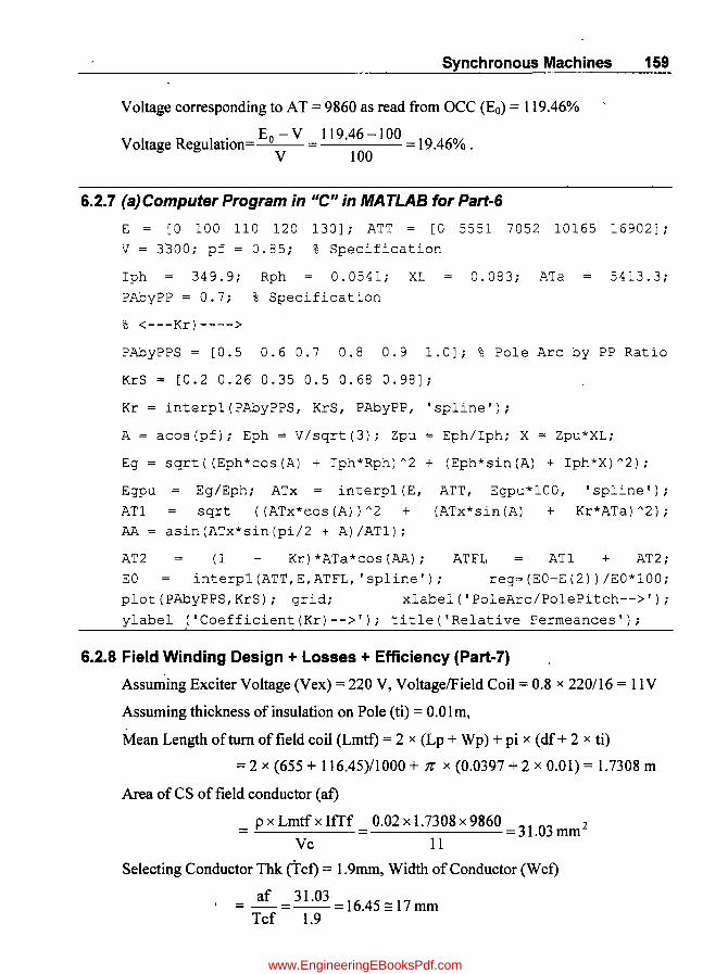
Synchronous Machines 159
Voltage corresponding to AT = 9860 as read from OCC (Eo) = 119.46%
Voltage Regulation Eo - V = 119.46 -100 = 19.46% . V 100
6.2.7 (a) Computer Program in "C" in MATLAS for Part-6
E = [0 100 llO 120 130J; ATT = [0 5551 7052 10165 16902J;
v = 3300; pf = 0.85; % Specification
Iph 349.9; Rph 0.0541; XL 0.083; ATa 5413.3;
PAbyPP = 0.7; % Specification
% <---Kr)---->
PAbyPPS = [0.5 0.6 0.7 0.8 0.9 1.0J; % Pole Arc by PP Ratio
KrS = [0.2 0.26 0.35 0.5 0.68 0.98J;
Kr = interp1(PAbyPPS, KrS, PAbyPP, 'spline');
A = acos(pf); Eph = V/sqrt(3); Zpu Eph/lph; X = Zpu*XL;
Eg = sqrt((Eph*cos(A) + Iph*Rph)A2 + (Eph*sin(A) + Iph*X)A2);
Egpu = Eg/Eph; ATx = interp1(E,
AT1 sqrt ( (ATx*cos (A) ) A2 + AA = asin(ATx*sin(pi/2 r A)/AT1);
ATT, Egpu*100, 'spline');
(ATx*sin(A) + Kr*ATa)A2);
AT2 (1 Kr)*ATa*cos(AA); ATFL AT1 + AT2;
EO interp1(ATT,E,ATFL, 'spline'); reg=(EO-E(2) )/EO*100;
plot(PAbyPPS,KrS); grid; xlabel('PoleArc/PolePitch-->');
ylabel f'Coefficient(Kr)-->'); title('Relative Permeances');
6.2.8 Field Winding Design + Losses + Efficiency (Part-7)
Assuming Exciter Voltage (Vex) = 220 V, Voltage/Field Coil = 0.8 x 220116 = 11V
Assuming thickness of insulation on Pole (ti) = 0.01 m,
Mean Length of turn of field coil (Lmtf) = 2 x (Lp + Wp) + pi x (df + 2 x ti)
= 2 x (655 + 116.45)11000 + 7r x (0.0397 + 2 x 0.01) = 1.7308 m
Area ofCS offield conductor (at)
= p x Lmtfx IfTf = 0.02 x 1.7308 x 9860 =31.03 mm 2
Vc 11
Selecting Conductor Thk (Tct) = 1.9mm, Width of Conductor (Wct)
= af = 31.03 = 16.45 =::17 mm Tcf 1.9
www.EngineeringEBooksPdf.com

160 Computer-Aided Design of Electrical Machines
Corrected Area ofCS offield conductor (at) = Wcfx Tcf x 0.98
= 17 x 1.9 x 0.98 = 31.654 mm2
(assuming a factor of 0.98 for conductor edges rounding)
Assuming current density in the field winding (cdfw) as 3.3 AI mm2
Field Current (If) = af x cdfw = 31.654 x 3.3 = 104.46 A
No. of Field Winding Turns (Tf) = Ifff = 9860 94.39 == 95 If 104.46
R . fF· Id W· d· (Rt) P x Lmtf x Tf 0.02 x 1.7308 x 95 0 1039 n eSlstance 0 Ie m mg = = =. u af 31.654
Field WindingCopperLoss(Pcuf)=Ilx Rfx P= 104.462 x 0.1039 x 16= 18137W
Brush loss at slip rings (Pbr) = Vb x If= 2 x 104.46 = 208.9 W
(assuming Voltage drop across a pair of brushes = 2 x 1 = 2 V)
Total field copper losses (pcuff) = (Pcuf+ Pbr)11000
= (18137 + 208.9)11000 = 18.346 KW
Weight of Field Copper (Wcuf) = Lmtf x af x Tf x P x 8.911 000
= 1.7308 x 31.654 x 95 x 16 x 8.911000 = 741.14 Kg
Assuming Exciter Efficiency = 98%, Input to Exciter = 18.346/0.98 = 20.85 KW
Exciter Losses (Pex) = 20.85 - 18.346 = 2.5 KW
Assuming friction and windage Loss (Pm) as 1 % of output
= 0.01 x KVA x pf= 0.01 x 2000 x 0.85 = 17 KW
Dia at centre of St tooth (D 12) = D + 2 x Hs/2 = 1500 + 45 = 1545 mm
Slot pitch at DI2(spI2) = 1t x D12/S = 1t x 15451144 = 33.707 m
With oftooth at D12 (bt12) = 33.707 - 19 = 14.707 mm
Tooth (KgT) = 7800 x S x btl2 x Li x Hs
= 7800 x 144 x 14.707 x 522 x 45 = 375.5 Kg
www.EngineeringEBooksPdf.com
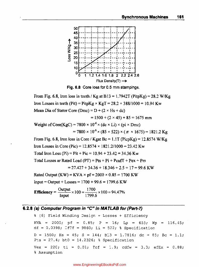
50 45
Synchronous Machines 161
. . . . .. . .... !. .... J ..... , .... I ..... !. ..... J.. _I .... 1 ... 40
t 35 , , ~ 30 • I • I • I ••
• • • • • I • • , ,
~ --r--,---,---.-_· --,---.-_ ....... ~ 25' ':' :g 20 • • • • • I I • .3 --: .. -~- .. -. --:- .... ! .. -~- .. -:- --:--
15 .. ~ .. • •. ' •.. :- .. ~ .. ~ ........ :- •
10 ,
I • I • • • • •
O~~~~~~~~~~~ o 1 1.2 1.4 1.6 1.8 2 2.2 2.42.6
Flux Density(T) -+ Fig. 6.8 Core loss for 0.5 mm stampings.
From Fig. 6.8, Iron loss in tooth 1 Kg at B 13 = 1.7942T (PitpKg) = 28.2 WlKg
Iron Losses in teeth (Pit) = PitpKg x KgT = 28.2 x 388/1000 = 10.94 Kw
Mean Dia of Stator Core (Dme) = D + (2 x Hs + de)
= 1500 + (2 x 45) + 85 = 1675 mm
Weight of Core(KgC) = 7800 x 10-6 x (de x Li) x (pi x Dme)
= 7800 x 10-6 x (85 x 522) x (n x 1675) = 1821.2 Kg
From Fig. 6.8, Iron loss in Core 1 Kgat Be = LIT (PiepKg) = 12.8574 WlKg
Iron Losses in Core (Pie) = 12.8574 x 1821.2/1000 = 23.42 Kw
Total Iron Loss (Pi) = Pit + Pie = 10.94 + 23.42 = 34.36 Kw
Total Losses ar Rated Load (PT) = Pts + Pi + PeuIT + Pex + Pm
= 27.427 + 34.36 + 18.346 + 2.5 + 17 = 99.6 KW
Rated Output (KW) = KVA x pf= 2000 x 0.85 = 1700 KW
Input = Output + Losses = 1700 + 99.6 = 1799.6 KW
. Output 1700 EffiCiency = x 100 = --xl 00 = 94.47%
Input 1799.6
&.2.8 (aJ Computer Program in "c" in MATLAB for (Part-7J
% (6) Field Winding Design + Losses + Efficiency
KVA = 2000; pf = 0.85; P = 16; Lp = 655; Wp = 116.45; df = 0.0398; IfTf = 9860; Li = 522; % Specification
D = 1500; Hs = 45; S = 144; B13 = 1.7816; dc = 85; Bc = 1.1; Pts = 27.4; btO = 14.2326; % Specification
Vex = 220; ti = 0.01; Tcf = 1.9; cdfw = 3.3; efEx = 0.88; % Assumption
www.EngineeringEBooksPdf.com

162 Computer-Aided Design of Electrical Machines
B [ 0 . 8 1 . 2 1 . 6 2 2 . 4] ; WpKg [7 15 24 34 50]; Ve 0.8*Vex/P; Lmtf = 2*{Lp + Wp)/lOOO + pi*(df + 2*ti); af 0.02*Lmtf*IfTf/Ve; Wef = ceil(af/Tef); af = Wef*Tef*0.98; If af*edfw; Tf eeil(IfTf/If); Rf 0.02*Lmtf*Tf/af; Peuf = If"'2*Rf*P; Wcuf = Lmtf*af*Tf*P*8. ge-3; Pbr = 2*1*If; PeufT (Peuf + Pbr)/le3; InpEx PeufT/efEx; Pex = InpEx - PeufT; Pm = O.Ol*KVA*pf; 012 = 0 + 2*Hs/2; sp12 = pi*012/S; bt12 = sp12-Ws;
KgT = 7.8e - 6*S*bt12*Li*Hs;
PitpKg = interpl (B, WpKg, B13, 'spline');Pit = PitpKg*KgT/le3;
Orne = 0 + 2*Hs + de; KgC = 7.8e-6*(dc*Li)*(pi*Dme);
PiepKg = interpl (B, WpKg, Be, 'spline'); Pic = PiepKg*KgC/le3; Pi = Pit + Pic; PT = Pts + Pi + PeufT + Pex + Pm; Po = KVA*pf; EFF Po/ (Po + PT) *100; plot (B, WpKg); grid; xlabel ('Flux Oensity(T)-->'); ylabel ('Loss(W/Kg)-->'); title ('Core Loss for 0.5mm Stampings');
% -------------------------------------------------------------
6.2.9 Calculation of Temp-Rises and Weights (Part-8)
Copper Losses in the slot portion (Pcust)
Ls 580 = x Pcus = x19.8548=9.6314KW
Lmt/2 2.3913/2
Total Losses dissipated by stator core surface (Pscs)
= Pcust + Pi + Peddy = 9.6314 + 34.356 + 3.9675 = 47.955KW
(a) Area of outer cylindrical surface and End Surface (AI)
= (1txDo xL)+2x 1t{D/ _D2) 4 .
= ((1tX 1760 x 670)+ 2 x 1t (17602 -1500 2 bl1()6 =5.036m 2 4
Assuming Cooling Coeftt (eel) = 0.032,
Dissipation Coefficient (WpCI)::;: AIIecl = 5.036/0.032 = 157.37 W;oC
(b) Area of inner cylindrical surface (A2)
= 1txDxLx10-6 =1tx1500x670x10-6 =3.1573m 2
0031 0.031 Cooling Coeftt (ce2) = . = = 0.0079
1 + (0.1 x Vr) 1 + (0.1 x 29.45)
Dissipation Coefficient (Wp{:2) = A2/ec2 = 3.1573/0.0079 = 401.79 W;oC
www.EngineeringEBooksPdf.com

Synchronous Machines 163
(c) Duct surface (A3)
= ~(Do2 -D2)xnvxI0-6=:(17602 -15002)x9xl0-6=5.9913m2
C I· C fit ( 0.11 0.11 0 4 00 mg oe cc3) = = =0. 37 O.lxVr 0.lx29.45
Dissipation Coefficient (WpC3) = A3/cc3 = 5.9913/0.0374 = 160.4 W/oC
Total Dissipation coefft (WpCt)
= WpCl + WpC2 + WpC3 = 157.37 + 401.79 + 160.4 = 719.57 W/oC
Stator Temp Rise (TrS) = Pscs x 1000/WpCt
= 47.955 x 10001719.57 = 66.64 °c Cooling Coeft of Field Winding (ccf)
= __ 0._1 __ = 0.1 = 0.0253 1 + (0.1)( Vr) 1 + (0.1 x 29.45)
Field Coil Surface (cs) = (2 x Lmtf x hfl1 000) + (2 x Lmtf x df)
= (2 x 1.7307 x 209.547/1000) + (2 x 1.7307 x 0.0398) = 0.8631m2
Dissipation Coefficient (WpCf) = cs/ccf = 0.8631/0.0253 = 34.05 W/oC
Field Wdg Temp Rise (Tr) = PcuflP/WpCf= 18136116/34.05 = 33.29 °c Total Weights of Acive Materials
Wt of Total Copper (Wcu) = Wcus + Wcuf= (546.62 + 741.1) = 1287.7 Kg
Wt of Active Iron (Wiron) = KgC + KgT + Wpoles + Wrot
= 1821.2 + 388 + 5611.6 + 3483.3 = 11304 Kg
Assuming 1 % weight for Insulation,
Weight of Active materials (Wtot)
= 1.01 x (Wcu + Wiron) = 1.01 x (1287.7 + 11304) = 12718 Kg
WeightIKV A (KgPkva) = WtotIKVA = 12718/2000 = 6.36 KglKVA
6.2.9 (a) Computer Program in .. c" in MATLAB for Part-8
% (7) Temp-Rise and Weights
KVA 2000; Ls 580; Lmt 2.3913; Pcus 19.8548;
Pi 34.356; Peddy = 3.9675; % Specification
Do 1760; L 670; D = 1500; % Specification
P = 16; Lmtf 1.7307; hf = 209. 547; df = 0.0398; cc1 0.032;
Vr = 29.45; nv = 9; Pcuf = 18136; % Specification
www.EngineeringEBooksPdf.com

164 Computer-Aided Design of Electrical Machines
KgT = 388; KgC = 1821.2; Wcus = 546.62; Wpoles Wcuf = 741.1; Wrot = 3483.3; % Specification
5611.6;
Pcust = Ls/1000/(Lmt/2)*Pcus; Pscs Pcust + Pi + Peddy; Al (pi*Do*L + 2*pi/4*(DoA2 DA2))/le6; WpC1 = A1/cc1; A2 = pi*D*L/1e6; cc2 = 0.031/(1 + O.l*Vr); WpC2 = A2/cc2;
A3 (pi/4*(Do A2 DA2)*nv)/le6; cc3 O.ll/(O.l*Vr); WpC3 = A3/cc3; WpCt = WpC1 + WpC2 + WpC3; TrS = Pscs*le3/WpCt; ccf = 0.1/(1 + O.l*Vr); cs = 2*Lmtf*hf/1000 + 2*Lmtf*df; WpCf = cs/ccf; TrF = Pcuf/P/WpCf;
%-----Total Weights------>
Wcu = Wcus + Wcuf; Wiron = KgC + KgT + Wpoles + Wrot; wtot 1.01*(Wcu + Wiron); KgPkva = Wtot/KVA;
%--------------------------------------------------------
6.2.10 Computer Program in "C" in MATLAB for Complete Design
% Salient Pole Alternator
KVA = 2000; V 3300; N 375; f = 50; pf % Star connected Salient Pole Gen
KVAS [ 100 200 500 1000 5000 10000 20000];
BavS [0.52 0.54 0.56 0.58 0.61 0.63 O. 65] ;
qS [20e3 23e3 26e3 2ge3 34~3
% plot (KVAS, BavS) ; grid;
Bav = interp1(KVAS, BavS, KVA, 'spline');
q = interp1 (KVAS, qS, KVA, 'spline');
37e3
0.85;
40e3];
Kw = 0.955; LbyPP = 2.3; nv = 9; bv = 10; ki = 0.9; spp 3; PAbyPP = 0.7; % Assumptions Pole Arc = L;
cds = 4; PAtoPP 0.7; BtO = 1.8; Bc = 1.1; Wins 6; Hins = 8; Hw = 4; HL = 1; Ks = 1; % Assumptions
%---------------------------------------------
KW = KVA*pf; P = 120*f/N; K = ll*Bav*q*Kw*le-3; n = 2*f/P; DsqL = KVA/(K*n); D1 = (DsqL*P/(LbyPP*pi))A(1/3)*1000; D = ceil (D1/10) /100; L1 = DsqL/DA2; L = ceil (L1*100) *10; D = D*1000; Ls = (L - nv*bv); Li = Ls*ki; PP =p i*D/P;
Vr = pi*D*n/1000; flux1 = Bav*pi*D*L/P/1e6;
Tphi=V/sqrt(3)/4.44*f*Kw*flux1); Zph = Tphi*2; S = spp*P*3;
sp= pi*D/S; Zsi = Zph*3/S; Zs = ceil(Zsi/2)*i; Tph = Z5*S/6;
www.EngineeringEBooksPdf.com

Synchronous Machines 16&
Iph = KVA*le3/ (1. 7321 *V); SLoad
FI = V/sqrt(3)/(4.44*f*Kw*Tph);
Iph*Zs;
% ----------------------------------------------------------
% (2) Design of Stator Winding, Reactance, Core-------7
As = Iph/cds; TpP = ceil(PAtoPP*PP/sp);
btO = FI*le6/(BtO*Li*TpP); Ws1 = sp-btO;
Wc ceil((Ws1)-Wins); Hc = ceil(As/Wc*2)/2;
Ws l*Wc + Wins; As = Wc*Hc*0.98; cds = Iph/As;
Hs Zs*Hc + Zs*2*0.S + Hins + Hw + HL; rat1 = Hs/Ws;
Lmt (2*L + 2.S*PP + SO*V/1000 + lS0)/1000;
Rph 0.021*Lmt*Tph/As; Pcus = 3*Iph~2*Rph/1e3;
Wcus
Kdav
3*Lmt*As*Tph*8.ge-3; alfa sqrt(Wc/Ws);
1 + (alfa*Hc/10) ~4*Zs~2/9;
Peddy = (Kdav - l)*Pcus; Pts = (Pcus + Peddy)*l.lS;
Reff = Iph*Rph*Kdav/(V/sqrt(3));
%------- Leakage Reactance --------->
h1=Zs*Hc + 4 + 2 + 2; h2 = 2 + 2; h3 Hw; h4 = HL; WsO
Lmdas = h1/(3*Ws) + h2/Ws + 2*h3/(Ws + WsO) + h4/WsO;
Fis = 2*sqrt(2)*4*pi*le-7*Iph*Ls/1000*Lmdas*Zs;
CSbPP = [O.S 0.6 0.7 0.8 0.9 1];
ks = [O.S 0.63 0.76 0.84 0.92 1];
LOLmdO = Ks*PP~2/(pi*sp*1000); TO = Zs;
Fio = 2*sqrt(2)*4*pi*le-7*Iph*TO*LOLmdO;
9;
FIL=FIs+Flo; XL=FIL/FI; Flc=FI/2; dc1 Flc*le6/(Bc*Li);
Dol 0 + 2* (Hs + dc1); Do ceil (001/10) *10;
dc = (Do - 0)/2 - Hs; Ata = 1.3S*Tph*Iph*Kw/(P/2);
% -------------------------------------------------------
f3 = fopen ('Final_Total_SPG_Output.m', 'WI);
fprintf (f3, 'Design of Salient-Pole Generator:-\n');
fprintf (f3, 'Parameter VALUES\n');
www.EngineeringEBooksPdf.com

166 Computer-Aided Design of Electrical Machines
fprintf (f3, ,--------- ------');
fprintf (f3, '\nKVA %5.0f' ,KVA);
fprintf (f3,'\nKW %5. Of' ,I('"tJ) ;
fprintf (f3, '\nVolts %5.0f',V);
fprintf (f3, '\nPF % 5 .2 f' , pf) ;
fprintf (f3, '\nHZ %5.0f',f);
fprintf (f3, '\nR.P.M %5.0f',N);
fprintf (f3, '\nNo of Poles %5.0d',P);
fprintf (f3, '\nFlux/Pole Wb % 6.5 f' , FI) ;
fprintf (f3, '\nGapFlux-den(Av) Wb/m2 %6.4f',Bav)
fprintf (f3,' \nSp.Elec Loading Ac/m %6.0f',q) ;
fprintf (f3, '\n-----------------STATOR--------------->');
fprintf (f3, '\nStator Current
fprintf (f3, '\nCORE LENGTH (tot)
fprintf (f3, '\nIron LENGTH
fprintf (f3, '\nVent Duets No X
fprintf (f3, '\nCORE 00
fprintf (f3, '\nCORE IO
fprintf (f3, '\nPOLE PITCH
fprintf (f3, '\nTURNS/Ph
fprintf (f3, '\nSTATOR SLOTS
fprintf (f3, '\nSLOT PITCH
fprintf (f3, '\nCore depth
fprintf (f3, '\nCoreFlux-den
fprintf (f3, '\nSLOT WIDTH
fprintf (f3, '\nSLOT Height (tot)
fprintf (f3, '\nHt (Lip + Wedge)
Amps %5.1f',Iph);
mm %5.0f',L);
mm %5.0f',Ls);
mm %2d X%3d',nv,bv);
mm %5.0f',00);
mm %5.0f',0) ;
mm %5.1f',PP);
mm
mm
Wb/m2
mm
mm
%5.0d',Tph);
%5.0d',S);
% 5 . 2 f' , sp) ;
% 5 . 1 f' ,de) ;
% 5. 1 f' , Be) ;
%5.1f',Ws);
%5.1f',Hs);
mm %2.0f+%2.0f',HL,Hw);
fprintf (f3, '\nFlux-den(tooth-tip) Wb/m2
fprintf (f3, '\nCondu~tors/Slot
%5.2f',BtO)
%5.0f',Zs);
www.EngineeringEBooksPdf.com

Synchronous Machines 167
fprintf (f3, '\nAmp-Conductors/Slot
fprintf (f3, '\nBare cond Wdth
fprintf (f3, '\nBare Cond Ht
fprintf (f3, '\nCurrent density
fprintf (f3, '\nAv.Loss Ratio
fprintf (f3, '\nMean-Turn Length
fprintf (f3, '\nSt Wdg Res/Ph/20a
fprintf (f3, '\nPephoral Speed
fprintf (f3, '\nArmature Reaction
fprintf (f3, '\nLeakage Reactance
rom
rom
A/rom2
m
ohm
m/s
ATiP
Perc
% (3) Rotor and AT Calc of Salient Pole TG
%5.0f' ,SLoad);
%5.1f',Wc);
%5.1f',Hc);
%5.3f',cds)
% 5 . 4 f' , Kda v) ;
%5.4f' ,Lmt);
% 5.4 f ' , Rph) ;
%5.1f',Vr) ;
%5.0f' ,ATa);
%5. 2f' , xL*100) ;
scr=0.9; Kg= 1.17; Bp 1.5; Sf = 0.75; Pf = 725; Bcr 1.1;
ATfO = scr*ATa; ATg = 0.75*ATf~; Bg = Bav/PAtoPP;
Lg1 = ATg/ (0.796*Bg*Kg*le3);Lg = floor (Lg1*10)/10;
rat2=Lg/PP; Dr=D-2*Lg; Lp = L-15; Lpi = Lp*ki; FIp = 1.1*FI;
Ap = FIp/Bp; Wp = Ap/Lpi*le6; Wpoles = Ap*Lp*P*7.8;
fprintf (f3, '\nAir-gap LENGTH rom %5.1f',Lg);
% <--Table for Depth of Field Winding------------>
PPS = [0.1 0.2 0.3 0.4 0.5};
DF = [0.03 0.036 0.04 0.045 0.05};
% ---------------------------------------~--------------
df interp1(PPS, DF, PP/1e3, 'spline'); IfTf = 1.8*ATa;
hf IfTf/(le4*sqrt(df*Sf*Pf))*1000; Hp = hf + 40 + 0.12*PP;
dcr = FIp*le6/2/Bcr/L; Wrot = pi*(Dr - 2*Hp)A2/4*L*7.8e-6;
%----------------Ampere-Turns at 100% V-------------------->
%<---B-H Curve for St Tooth for ks = 1----->
BtS = [1. 8 1. 9 2 2.1 2.15 2.2 2.25 2.3] ;
attS=[ge3 14e3 24e3 43e3 60e3 80e3 110e3 152e3];% ks 1.0
% ----Carters Coefft for Semi-closed slots---> .
www.EngineeringEBooksPdf.com

168 Computer-Aided Design of Electrical Machines
WObyLgS= [0 1 2 3 4 5 6 7 8 9 101112];
% Slot opening/Gap
CC = [ 0 . 18 . 33 . 45 . 53 . 6 . 66 . 71 . 75 . 79 . 82 . 86 . 8 9] ;
%<---B-H Curve common for St Core, Rt core and Poles---->
BS = [0 0.25 0.5 0.75 1.0 1.25 1.5 1.75 2.0 2.25];
atS = [0 80 100 150 300 580 2e3 8e3 3e4 16e4];
WsbyLg=Ws/Lg; CCg = interp1 (WObyLgS, CC, WsbyLg, 'spline');
kgs sp/(sp - Ws*CCg);ObyG = bv/Lg;
CCv interp1 (WObyLgS, CC, ObyG, 'spline');
kgv L/(L -nv*bv*CCv); kg = kgs*kgv;
%----------------------------------------------------
ATg = 0.796*Bg*kg*Lg*le3; 013 = D + 2*Hs/3; sp13 = pi*013/S;
bt13 = sp13-Ws; B13 = FI/(Li*bt13*TpP)*le6;
att = interp1 (BtS, attS, B13, 'spline'); ATt att*Hs/1000;
Lc = pi* (0 + 2*Hs + dc)/P/2;
atc = interp1 (BS, atS, Bc, 'spline'); ATc = atc*Lc/1000;
ATL = ATg + ATt + ATc; FI~s = 1ge-8*ATL; FLLp = 72e-8*ATL;
Fipmin = FI + FILs; Fipmax = Fipmin + FILp;
Bpmin= FIpmin/Ap; atp1
Bpmax= FIpmax/Ap; atp2
interp1 (BS, atS, Bpmin, 'spline');
interp1 (BS, atS, Bpmax, 'spline');
ATp=(2/3*atp1+1/3*atp2)*Hp/1e3; Lcr=pi*(Or-2*Hp-dcr)/P/2;
atrc= interp1(BS, atS, Bcr, 'spline'); ATrc = atrc*Lcr/1000;
ATfO = ATg + ATt + ATc + ATp + ATrc;
%----------------------------------------------------------
E = [100 110 120 130];
for i = 1:4;
Bgx(i) = Bg*E(i)/100; ATgx(i)
Bstx(i) B13*E(i)/100;
atST(i) interp1(BtS,
ATstx(i) = atST(i)*Hs/1000;
Bscx(i) = Bc*E(i)/100;
0.796*Bgx(i)*kg*Lg*le3;
attS, Bstx(i), 'spline');
www.EngineeringEBooksPdf.com
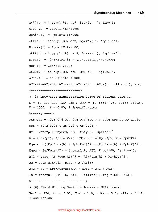
Synchronous Machines 169
atSC(i) = interp1(BS, atS, Bscx(i), 'spline');
ATscx(i) = a~SC(i)*Lc/1000;
Bpminx(i) = Bpmin*E(i)/100;
atP1(i) = interp1(BS, atS, Bpminx(i), 'spline');
Bpmaxx(i) = Bpmax*E(i)/100;
atP2(i)
ATpx(i)
Bcrx(i)
atRC(i)
interp1 (BS, atS, Bpmaxx(i), 'spline');
(2/3*atP1(i) + 1/3*atP2(i) )*Hp/1000;
Bcr*E(i)/100;
interp1(BS, atS, Bcrx(i), 'spline');
ATrcx(i) = atRC(i)*Lcr/1000;
ATTx(i)=ATgx(i)+ATstx(i)+ATscx(i) + ATpx(i) + ATrcx(i); end;
%--------------------------> % (5) LMC->Load Magnetization Curve of Salient Pole TG
E = [0 100 110 120 l30]; ATT = [0 5551 7052 10165 16902];
V = 3300; pf = 0.85; % Specification
%<---Kr ---->
PAbyPPS = [0.5 0.6 0.7 0.8 0.9 1.0]; % Pole Arc by PP Ratio
KrS = [0.2 0.26 0.35 0.5 0.68 0.98];
Kr = interp1(PAbyPPS, KrS, PAbyPP, 'spline');
A = acos(pf); Eph = V/sqrt(3); Zpu = Eph/lph; X Zpu*Xi.;
Eg= sqrt((Eph*cos(A) + Iph*Rph)A2 + (Eph*sin(A) + Iph*X)A2);
Egpu = Eg/Eph; ATx = interp1(E, ATT, Egpu*100, 'spline');
AT1 = sqrt((ATx*cos(A))A2 + (ATx*sin(A) + Kr*ATa)A2};
AA = asin(ATx*sin (pi/2 + A)/AT1);
AT2 = (1 - Ki)*ATa*cos(AA); ATFL = AT1 + AT2;
EO = interp1 (ATT, E, ATFL, 'spline'); reg = EO - E(2);
%-----------------------------> % (6) Field Winding Design + Losses + Efficiency
Vex1 = 220; ti = 0.01; Tcf = 1.9; cdfw = 3.3; efEx
% Assumption
0.88;
www.EngineeringEBooksPdf.com
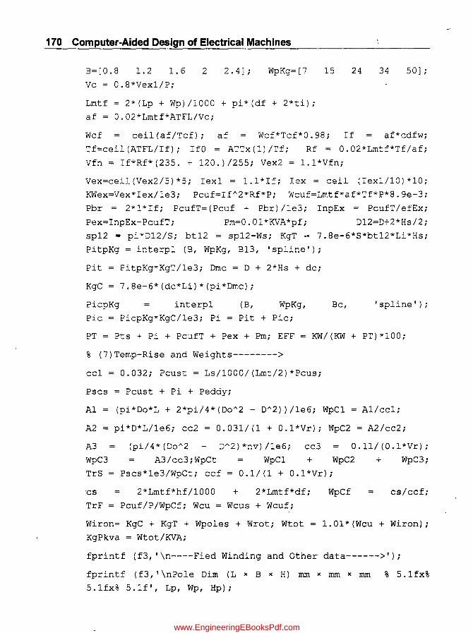
170 Computer-Aided Design of Electrical Machines
B=[0.8 1.2 1.6 2 2.4] ; WpKg= [7
Ve = 0.8*Vexl/P;
Lmtf = 2*(Lp + Wp)/1000 + pi*(df + 2*ti);
af = 0.02*Lmtf*ATFL/Ve;
15 24 34 50] ;
Wef eeil(af/Tef); af Wef*Tef*0.98; If af*cdfw;
Tf=eeil(ATFL/If); If 0 = ATTx(I)/Tf; Rf = 0.02*Lmtf*Tf/af;
Vfn = If*Rf*(235. + 120.)/255; Vex2 1.I*Vfn;
Vex=eeil (Vex2/5) *5; Iexl = 1.1*If; lex = ceil (Iexl/10) *10;
KWex=Vex*Iex/le3; Peuf=If A 2*Rf*P; Weuf=Lmtf*af*Tf*P*8.ge-3;
Pbr = 2*1*If; PeufT=(Peuf + Pbr) /le3; InpEx = PeufT/efEx;
Pex=InpEx-PeufT; Pm=O.Ol*KVA*pf; DI2=D+2*Hs/2;
sp12 = pi*DI2/S; bt12 = spI2-Ws; KgT = 7.8e-6*S*bt12*Li*Hs;
PitpKg = interpl (B, WpKg, B13, 'spline');
Pit PitpKg*KgT/le3; Dme = D + 2*Hs + de;
KgC 7.8e-6*(de*Li)*(pi*Dme);
PiepKg interp1 (B, WpKg,
Pic = PiepKg*KgC/1e3; Pi ~ Pit + Pic;
Be, 'spline');
PT = Pts + Pi + PeufT + Pex + Pm; EFF KW/(KW + PT)*100;
% (7)Temp-Rise and Weights-------->
eel = 0.032; Pcust = Ls/1000/(Lmt/2)*Peus;
Pses = Peust + Pi + Peddy;
A1 (pi*Do*L + 2*pi/4*(Do A 2 - DA 2))/le6; WpC1 = A1/ee1;
A2 pi*D*L/1e6; ee2 = 0.031/(1 + O.l*Vr); WpC2 = A2/ee2;
A3
WpC3
(pi/4*{Do A 2 DA 2)*nv)/le6;
A3/ee3;WpCt WpCl
ee3 O.II/(O.I*Vr);
+ WpC2 + WpC3;
TrS Pses*le3/WpCt; eef = 0.1/(1 + O.I*Vr);
2*Lmtf*hf/1000 + 2*Lmtf*df;
TrF = Peuf/P/WpCf; Weu = Weus + Weuf;
Wiron= KgC + KgT + Wpoles + Wrot; Wtot
KgPkva = Wtot/KVA;
WpCf es/eef;
1.01*(Weu + Wiron);
fprintf (f3, '\n----Fied Winding and Other data------>');
fprintf (f3,'\nPole Dim (L x B x H) mm x mm x mm % 5.1fx%
5.1fx% 5.1f', Lp, Wp, Hp);
www.EngineeringEBooksPdf.com

Synchronous Machines 171
fprintf (f3, '\nNo of Turns/Pole
~printf (f3, '\nDepth of core
fprintf (f3, '\nSCR
fprintf (f3, '\nNo Ld Rot Current
fprintf (f3, '\nRot Current at FL
fprintf (f3, '\nVoltage Regulation
fprintf (f3, '\nRot Volts at FL
mrn
pu
Amps
Amps
(perc)
Volts
%5.0f',Tf);
%5.1f',dcr);
%5.3f',scr);
%5.1£',1fO);
%5.1£',If);
%5.1f',reg);
%5.1f',Vfn);
fprintf (f3,' \nExciter Rating: %4.1fKW,% 4.1fV, % 4.1fA',
KWex, Vex, lex);
%-----------------------------------------------------
fprintf (f3, '\n----Weights, Losses and Efficiency:------>');
fprintf(f3, '\n VAR1ENT
fprintf (f3, '\n---------------------');
fprintf (f3, '\nWt of St.Core
fprintf (f3, '\nWt of St.Teeth
fprintf (f3, '\nWt of Poles
fprintf (f3, '\nWt of St.Copper
fprintf (f3, '\nWt of Fld-Copper
fprintf (f3, '\nTotal Wt
fprintf (f3, '\nKg/KVA
fprintf (f3, '\n---------------------');
fprintf (f3, '\nMech Losses
fprintf (f3, '\nSt- Cu Losses
fprintf (f3, '\n1ron Losses
fprintf (f3, '\nFld Copper Losses
fprintf (f3, '\nTotal Losses
fprintf (f3, '\nEfficiency
fprintf (f3, '\nTemp-Rise of St
fprintf (f3, '\nTemp-Rise of Fld
Kg
Kg
Kg
Kg
Kg
Kg
KW
KW
KW
KW
KW
Perc
VALUES');
% 6 . 0 f' , KgC) ;
% 6 . 0 f' , KgT) ;
%6.0f' ,Wpoles);
%6.0f' ,Wcus);
%6.0f' ,Wcuf);
%6. Of', Wtot);
%6.2f' , KgPkva) ;
%6.1f',Pm);
% 6. 1 f' , Pt s) ;
%6.1f',Pi);
%6.1f', PcufT);
%p.1£' , PT) ;
%6.2f' ,EFF);
Wdg(deg)%6.2f',TrS);
Wdg(deg)%6.2f',TrF);
fprintf (f3, '\n<------End of Outptit:------>'); fclose (f3);
www.EngineeringEBooksPdf.com

172 Computer-Aided Design of Electrical Machines
6.2.10 (a) Computer Output Results for Complete Design
Design of Salient-Pole Generator
Parameter VALUES
---------
KVA 2000
KW 1700
Volts 3300
PF 0.85
HZ 50
R.P.M 375
No. of Poles 16
FluxlPole Wb 0.09361
GapFlux-den(Av) Wb/m2 0.6089
Sp.Elec Loading Ac/m 33400
-----------------SlrAlr()Ft---------------»
Stator Current Amps 349.9
C()FtE LENGlrH (tot) mm 670
Iron LENGlrH mm 580
Vent Ducts No.Xmm 9 X 10
C()FtE ()D mm 1760
C()FtE ID mm 1500
P()LEPI1rCH mm 294.5
lrURNSlPh 96
Slr A lr()R SL()lrS 144
SL()lr PI1rCH mm 32.72
Core depth mm 85.0
CoreFlux-den Wb/m2 1.1
SL()lr WIDlrH mm 19.0
SL()lr Height(tot) mm 45.0
Ht (Lip+Wedge) mm 1+4
Flux-den(tooth-tip) Wb/m2 1.80
Conductors/Slot 4
www.EngineeringEBooksPdf.com

Synchronous Machines 173
Amp-Conductors/Slot 1400
Bare cond W dth mm 13.0
Bare Cond Ht mm 7.0
Current density Almm2 3.924
A v .Loss Ratio 1.1998
Mean-Tum Length m 2.3913
St W dg ResIPhl20d ohm 0.0541
Pephoral Speed mls 29.5
Armature Reaction ATIP 5413
Leakage Reactance Perc 8.30
Air-gap LENGTH mm 4.5
----Fied Winding and Other data------>
Pole Dim(LxBxH) mmXmrnXmm 655.0xI16.5x284.9
No. of TumslPole 95
Depth of core mm 69.9
SCR pu 0.900
No. Ld Rot Current Amps 58.4
Rot Current at FL Amps 104.5
Voltage Regulation (perc) 19.5
Rot Volts at FL Volts 15.1
Exciter Rating: 2.4KW, 20.0V, 120.0A
----Weights, Losses and Efficiency:------>
VARIANT VALUES
-------------
Wt. of St.Core Kg 1821
Wt. of St.Teeth Kg 388
Wt. of Poles. Kg 5612
Wt. of St.Copper Kg 547
Wt. of Fld-Copper Kg 741
Total Wt. Kg 12718
Kg/KVA 6.36
-.,.(-----------
www.EngineeringEBooksPdf.com

174 Computer-Aided Design of Electrical Machines
Mech Losses KW 17.0
St- Cu Losses KW 27.4
Iron Losses KW 34.4
Fld Copper Losses KW 18.3
Total Losses KW 99.6
Efficiency Perc 94.47
Temp-Rise of St Wdg(deg) 66.64
Temp-Rise of Fld Wdg(deg) 33.29
<-------End of Output--------->
6.2.11 Modifications to be done in the above Program to get Optimal Design
1. Insert "for" Loops for the following parameters to iterate the total program between min and max permissible limits for selecting the feasible design variants:
(a) Ratio of Length to Pole pitch
(b) Short Circuit Ratio
(c) Core flux density
(d) Arme Wdg Current densities.
2. Insert also minimum or maximum range of required objective functional values as constraint values, for example (a) Efficiency (b) Kg/KVA, (c) Temp-rise of Stator Winding
(a) Temp-rise of Rotor Winding
3. Run the program to get various possible design variants.
Note: From the feasible design variants printed in the output, select that particular design fulfilling the objective of optimal parameter for the design.
6.2.12 Computer Program in "e" in MATLAB for Optimal Design
% Salient Pole Alternator
KVA=2000; V = 3300; N = 375; f = 50; pf = 0.85; KW KVA*pf;
%'Star connected Salient Pole Gen
KVAS [ 100 200 500 1000 5000 10000 20000];
BavS [0.52 0.54 0.56 0.58 0.61 0.63 0.65] ;
qS = [20e3 23e3 26e3 2ge3 34e3 37e3 40e3J;
% plot (KVAS, BavS); grid;
Bav = interp1 (KVAS, BavS, KVA, 'spline');
www.EngineeringEBooksPdf.com

Synchronous Machines 175
q = interp1 (KVAS, qS, KVA, 'spline');
Kw = 0.955; LbyPP = 2.3; nv = 9; bv = 10; ki
PAbyPP = 0.7; % Assumptions Pole Arc = L;
0.9; spp
Cds = 4; PAtoPP 0.7; BtO
Hins = 8; Hw = 4; HL = 1; Ks
1. 8; Bc = 1. 1; Wins
1; % Assumptions
% ---------------------------------------------------
f2 = fopen ('Fina:_Optimal_SPG_Output.m', 'w');
3;
6;
fprintf (f2, 'Design of Salient-Pole Alternator of % 4d KVA,
% 5d V, % 4d RPM, % 3d hz, % 5.2f PF:-\n', KVA, V, N, f,
pf) ;
fprintf (f2,' Sn 0 L L/PP m/s S cds Zs Ac/S
St-Cond St-Slot Bc SCR EFF Kg/KVA TrS TrF\n' ) ;
fprintf (f2,' -- ----- ----- ----
-----\n') ;
sn = 0; M1 = 0; M2 = 0; M3 0; M4 0; EFFmax 90;
minKgPkva = 9; minTrS = 75; min TrF = 50; % Assumptions
for LbyPP=2.1:0.2:2.5;%(Range:0.8to3.0for Rectangular Poles)
for scr = 0.9: 0.1: 1.1; % (Range: 0.9 to 1.3
for Be = 1.1: 0.1: 1.3; % (Range: 1.1 to 1.3)
for cds = 3:0. 5:4; % Range: 3 to 5)
P=120*f/N; K = 11*Bav*q*Kw*le-3; n = 2*f/P; DsqL = KVA/K*n);
01 = (DsqL*P/(LbyPP*pi))A(1/3)*1000; 0 = ceil(D1/10)/100;
L1=DsqL/D A 2; L=ceil(L1*100)*10; 0= 0*1000; Ls = (L - nv*bv);
Li Ls*ki; PP = pi*D/P;
Vr pi*D*n/1000; if Vr > = 30.0 continue; end;
flux1= Bav*pi*D*L/P/1e6; Tphi = V/sqrt(3)/(4.44*f*Kw*fluxl);
Zph = Tphi*2; S spp*P*3; sp = pi*D/S; Zsi Zph*3/S;
Zs = ceil (Zsi/2) *2; Tph = Zs*S/6; Iph=KVA*le3/ (1. 7321*V);
SLoad = Iph*Zs; FI = V/sqrt(3)/(4.44*f*Kw*Tph);
% ----------------------------------------------------------,.. % (2) Design of Stator Winding, Reactance, Core
www.EngineeringEBooksPdf.com

176 Computer-Aided Design of Electrical Machines
As=Iph/eds; TpP=eeil(PAtoPP*PP/sp);btO=FI*le6/(BtO*Li*TpP);
Wsl = sp-btO; We = eeil((Wsl) - Wins); He = eeil(As/We*2)/2;
Ws l*We + Wins; As We*He*0.98; cds Iph/As;
Hs = Zs*He + Zs*2*0.5 + Hins + Hw + HL; rat1 = Hs/Ws;
Lmt=(2*L+2.5*PP+50*V/1000+150)/1000; Rph=0.021*Lmt*Tph/As;
Peus=3*IphA2*Rph/1e3; Weus=3*Lmt*As*Tph*8.ge-3;
alfa= sqrt(We/Ws); Kdav = 1 + (alfa*He/10) A4*ZSA2/9;
Peddy = (Kdav - l)*Peus; Pts = (Peus + Peddy)*1.15;
Reff = Iph*Rph*Kdav/(V/sqrt(3)); % Reff,
%-------Leakage Reaetanee--------->
hl=Zs*He + 4 + 2 + 2; h2 = 2 + 2; h3 Hw; h4 = HL; WsO
Lmdas h1/(3*Ws) + h2/Ws + 2*h3/(Ws + WsO) + h4/WSOi
9;
Fis 2*sqrt(2)*4*pi*le-7*Iph*Ls/1000*Lmdas*Zs;
% FIs, % Ls = 0.5835; Fis = 0.0036
CSbPP = [0.5 0.6 0.7 0.8 0.9 1];
ks = [0.5 0.63 0.76 0.84 0.92 1];
LOLmdO = Ks*Pp A2/(pi*sp*1000); TO = Zs;
Fio = 2*sqrt(2)*4*pi*le - 7*Iph*TO *LOLmdO;
FIL=FIs+FIp; XL = FIL/FI; FIe= FI/2; de1=Fle*le6/(Be*Li);
Do1=D+2*(Hs + del); Do= eeil(Dol/10)*10; dc=(Do-D)/2-Hs;
%-----------------------------------------------------
% (3) Rotor and AT Calc of Salient Pole TG
Ser=0.9; Kg=1.17; Bp = 1.5; Sf = 0.75; Pf = 725; Ber = 1.1;
Ata=1.35*Tph*Iph*Kw/(P/2); ATfO=ser*ATa; ATg = 0.75*ATfO;
Bg=Bav/PAtoPP; Lg1=ATg/(0.796*Bg *Kg*le3);
Lg
Lp
floor (Lg1*10)/10; rat2 = Lg/PP; Dr
L - 15; Lpi = Lp*ki; FIp 1.1*FI;
D
Ap FIp/Bp; Wp = Ap/Lpi*le6; Wpoles = Ap*Lp*P*7.8;
%<--Table for Depth of Field Winding------------>
2*Lg;
PPS=[O.l 0.2 0.3 0.4 0.5]; DF=[0.03 0.036 0.04 0.045 0.05];
% ------------------------------------------------------
df = interpl(PPS, DF, PP/1e3, 'spline'); IfTf = 1.8*ATa;
www.EngineeringEBooksPdf.com
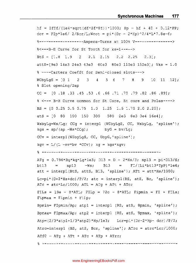
Synchronous Machines 177
hf = IfTf/(le4*sqrt(df*Sf*Pf))*1000; Hp = hf + 40 + 0.12*PP;
dcr = FIp*le6/ 2/Bcr/L;Wrot = pi*(Dr - 2*Hp)A2/4*L*7.8e-6;
%-------------------Ampere-Turns at 100% V---------------->
%<---B-H Curve for St Tooth for ks=l----->
BtS = [1. 8 1. 9 2 2.1 2.15 2.2 2.25 2.3] ;
attS=[ge3 14e3 24e3 43e3 60e3 80e3 110e3 152e3]; %ks 1.0
% ----Carters Coefft for Semi-closed slots--->
WObyLgS = [0 1 2 3 4 5 6 7 8 9 101112];
% Slot opening/Gap
CC = [ 0 . 18 . 33 . 45 . 53 . 6 . 66 . 71 . 75 . 79 . 82 . 86 . 89] ;
% <--- B-H Curve common for St Core, Rt core and Poles---->
BS = [0 0.25 0.5 0.75 1.0 1.25 1.5 1.75 2.0 2.25];
atS = [0 80 100 150 300 580 2e3 8e3 3e4 16e4];
WsbyLg=Ws/Lg; CCg = interp1 (WObyLgS, CC, WsbyLg, 'spline');
kgs sp/(sp -Ws*CCg); byG = bv/Lg;
CCv interp1(WObyLgS, CC, DbyG, 'spline');
kgv L/(L -nv*bv *CCv); kg = kgs*kgv;
% ---------------------------------------------------
ATg = 0.796*Bg*kg*Lg*le3; D13 = D + 2*Hs/3; sp13 = pi*D13/S;
bt13 sp13 -Ws; B13 FI/(Li*bt13*TpP)*le6;
att = interp1 (BtS, attS, B13, 'spline'); ATt = att*Hs/1000;
Lc=pi*(D+2*Hs+dc)/P/2; atc = interp1(BS, atS, Bc, 'spline');
ATc = atc*Lc/1000; ATL = ATg + ATt + ATc;
FILs = 1ge - 8*ATL; FILp = 72e - 8*ATL; Fipmin
Fipmax = Fipmin + FILp;
FI + FILs;
Bpmin= FIpmin/Ap; atp1
Bpmax= FIpmax/Ap; atp2
interp1 (BS, atS, Bpmin, 'spline');
interp1 (BS, atS, Bpmax, 'spline');
Atp=(2/3*atp1+1/3*atp2)*Hp/1e3; Lcr=pi*(Dr-2*Hp- dcr)/P/2;
Atrc=interp1 (BS, atS, Bcr, 'spline'); ATrc = atrc*Lcr/1000;
ATfO = ATg + ATt + ATc + ATp + ATrc;
% ----------------------------------------------------------
www.EngineeringEBooksPdf.com

178 Computer-Aided Design of Electrical Machines
E = [100 110 120 130];
for i = 1:4;
Bgx (i) = Bg*E (i) /100; ATgx (i)' 0.796*Bgx(i)*kg*Lg*le3;
Bstx (i)
atST(i)
B13*E(i)/100;
interp1 (BtS, attS, Bstx(i), 'spline');
ATstx(i) = atST(i)*Hs/1000;
Bscx(i) Bc*E(i)/100;
atSC(i) interp1 (BS, atS,'Bscx(i), 'spline');
ATscx(i) = atSC(i)*Lc/1000;
Bpminx(i) = Bpmin*E(i)/100;
atP1(i) = interp1 (BS, atS, Bpminx(i) , 'spline');
Bpmaxx(i) = Bpmax*E(i)/100;
atP2(i)
ATpx(i)
Bcrx(i)
atRC(i)
interp1 (BS, atS, Bpmaxx(i) , 'spline');
(2/3*atP1(i) + 1/3*atP2(i))*Hp/1000;
Bcr*E (i) /100;
interp1 (BS, atS, Bcrx(i), 'spline');
ATrcx(i) = atRC(i)*Lcr/1000;
ATTx(i)=ATgx(i)+ATstx(i)+ATscx(i)+ATpx(i) + ATrcx(i); end;
% -------------------------------->
% (5) LMC->Load Magnetization Curve of Salient Pole TG
E = [0 100 110 120 l30]; ATT = [0 5551 7052 10165 16902];
V = 3300; pf = 0.85; % Specification
% <---Kr---->
PAbyPPS=[0.5 0.6 0.7 0.8 0.9 1.0]; % Pole Arc by PP Ratio
KrS = [0.2 0.26 0.35 0.5 0 .. 68 0.98];
Kr = interp1 (PAbyPPS, KrS, PAbyPP, 'spline');
A = acos(pf); Eph = V/sqrt(3); Zpu = Eph/lph; X Zpu*XL;
Eg= sqrt((Eph*cos(A) + Iph*Rph)A2 + (Eph*sin(A) + Iph*X)A2);
Egpu = Eg/Eph; ATx = interp1 (E, ATT, Egpu*100, 'spline');
www.EngineeringEBooksPdf.com
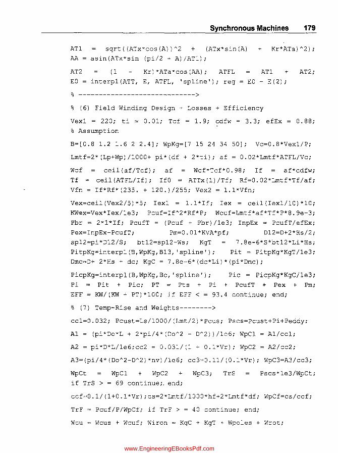
Synchronous Machines 179
AT1 sqrt ( (ATx*cos (A) ) "2 + (ATx*sin (A) + Kr * AT a) "2) ;
AA = asin(ATx*sin (pi/2 + A)/AT1);
AT2 (1 Kr)*ATa*cos(AA); ATFL ATl + AT2;
EO = interpl(ATT, E, ATFL, 'spline'); reg = EO - E(2);
% -----------------------------> % (6) Field Winding Design + Losses + Efficiency
Vexl = 220; ti = 0.01; Tcf = 1.9; cdfw = 3.3; efEx
% Assumption
0.88;
B=[0.8 1.2 1.6 2 2.4]; WpKg=[7 15 24 34 50]; Vc=0.8*Vexl/P;
Lmtf=2*(Lp+Wp)/1000+ pi*(df + 2*ti); af = 0.02*Lmtf*ATFL/Vc;
Wcf ceil(af/Tcf); af Wcf*Tcf*0.98; If af*cdfw;
Tf = ceil (ATFL/If) ; If 0 = ATTx(l)/Tf; Rf=0.02*Lmtf*Tf/af;
Vfn = If*Rf*(235. + 120.)/255; Vex2 = 1.1*Vfn;
Vex=ceil(Vex2/5) *5; Iex1 = 1.1*If; lex = ceil(Iex1/10)*10;
KWex=Vex*Iex/1e3; Pcuf=If"2*Rf*P; Wcuf=Lmtf*af*Tf*P*8.ge-3;
Pbr = 2*1*If; PcufT = (Pcuf + Pbr)/le3; InpEx = PcufT/efEx;
Pex=InpEx-PcufT; Pm=O.Ol*KVA*pf; D12=D+2*Hs/2;
7.8e-6*S*bt12*Li*Hs;
Pit = PitpKg*KgT/1e3;
sp12=pi*D12/S; bt12=sp12-Ws; KgT
PitpKg=interpl(B,WpKg,B13, 'spline');
Drnc=D+ 2*Hs + dc; KgC = 7.8e-6*(dc*Li)*(pi*Dmc);
PicpKg=interp1 (B, WpKg, Bc, 'spline') ; Pic = PicpKg*KgC/1e3;
Pi Pit + Pic; PT Pts + Pi + PeufT + Pex + Pm;
EFF = KW/(KW + PT)*lOO; if EFF < = 93.4 continue; end;
% (7) Temp-Rise and Weights-------->
ecl=0.032; Pcust=Ls/1000/(Lmt/2)*Pcus; Pscs=Peust+Pi+Peddy;
A1
A2
(pi*Do*L + 2*pi/4*(Do"2 - D"2))/le6; WpC1
pi*D*L/le6;cc2 = 0.031/(1 + O.l*Vr); WpC2
Al/cc1;
A2/cc2;
A3=(pi/4*(Do"2-D"2)*nv)/le6; cc3=0.11/(0.1*Vr); WpC3=A3/cc3;
WpCt WpC1 + WpC2 + WpC3; TrS Pscs*le3/WpCt;
if TrS > = 69 continue;. end;
cef=0.1/(1+0.l*Vr);cs=2*Lmtf/1000*hf+2*Lmtf*df; WpCf=cs/ccf;
TrF Pcuf/P/WpCf; if TrF > = 40 continue; end;
Weu Wcus + Wcuf; Wiron = KgC + KgT + Wpoles + Wrot;
www.EngineeringEBooksPdf.com
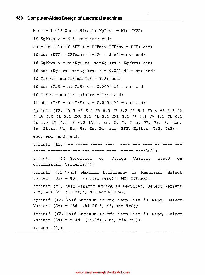
180 Computer-Aided Design of Electrical Machines
Wtot = 1.01*(Wcu + Wiron); KgPkva = Wtot/KVA;
if KgPkva > = 6.5 continue; end;
sn = sn + 1; if EFF > EFFmax EFFmax = EFF; end;
if abs (EFF - EFFmax) < = 2e - 3 M2 = sn; end;
if KgPkva < minKgPkva minKgPkva = KgPkva; end;
if abs (KgPkva -minKgPkva) < = 0.001 M1 = sn; end;
if TrS < = minTrS minTrS = TrS; end;
if abs (TrS - minTrS) < = 0.0001 M3 = sn; end;
if TrF < = minTrF minTrF = TrF; end;
if abs (TrF - minTrF) < = 0.0001 M4 = sn; end;
fprintf (f2,' % 3 d% 6.0 f% 6.0 f% 5.2 f% 6.1 f% 4 d% 5.2 f%
3 d% 5.0 f% 5.1 fX% 3.1 f% 5.1 fX% 3.1 f% 4.1 f% 4.1 f% 6.2
f% 5.2 f% 7.2 f% 6.2 f\n', sn, D, L, L by PP, Vr, S, cds,
Zs, SLoad, We, He, Ws, Hs, Be, scr, EFF, KgPkva, TrS, TrF);
end; end; end; end;
fprintf (f2,' -- ----- ----- ---- ---- --- ---- -- ---- ---
----- ----\n');
fprintf (f2, 'Selection of Design Variant based on
Optimization Criteria:');
fprintf (f2, '\nIf
Variant (Sn) = %3d
Maximum Efficiency is Required,
(% 5.2f perc),', M2, EFFmax);
Select
fprintf (f2, '\nIf Minimum Kg/KVA is Required, Select Variant
(Sn) = % 3d (%5.2f)', M1, minKgPkva);
fprintf (f2,' \nIf Minimum St-Wdg Temp-Rise is Reqd, Select
Variant (Sn) = %3d (%4.2f)', M3, min TrS);
fprintf (f2,' \nIf Minimum Rt-Wdg Temp-Rise is Reqd, Select
Variant (Sn) = % 3d (%4.2f)', M4, min TrF);
fclose (f2);
www.EngineeringEBooksPdf.com

6.2.12 (a) Computer Output Results for Optimal Design
Design of Salient-Pole Alternator of 2000 KVA, 3300 V, 375 RPM, 50 hz, 0.85 PF
Sn D L L/PP mls S cds Zs AC/S St-Cond St-Slot Bc SCR EFF Kg/KVA TrS TrF -- ----- ----- ---- ---- --- ---- -- ---- -------- --------- --- --- ----- ---- ----- --------- -- ----- ----- ---- --_ .. --- --.. - -- -_ .... _ .. ------ --------- --- --- ----- ---- -------I 1500 670 2.30 29.5 144 3.43 4 1400 13.0x8.0 19.0x49.0 1.1 0.9 94.43 6.43 68.73 33.29 2 1500 670 2.30 29.5 144 3.92 4 1400 13.0x7.0 19.0x45.0 1.1 0.9 94.47 6.36 66.64 33.29 3 1500 670 2.30 29.5 144 3.43 4 1400 13.0x8.0 19.0x49.0 I.I 0.9 94.43 6.43 68.73 33.29 4 1500 670 2.30 29.5 144 3.92 4 1400 13.0x7.0 19.0x45.0 1.1 0.9 94.47 6.36 66.64 33.29 5 1500 670 2.30 29.5 144 3.43 4 1400 13.0x8.0 19.0x49.0 1.1 0.9 94.43 6.43 68.73 33.29 6 1500 670 2.30 29.5 144 3.92 4 1400 13.0x7.0 19.0x45.0 1.1 0.9 94.47 6.36 66.64 33.29 7 1460 710 2.50 28.7 144 3.92 4 1400 13.0x7.0 19.0x45.0 1.1 0.9 94.41 6.48 67.89 33.90 8 1460 710 2.50 28.7 144 3.92 4 1400 13.0x7.0 19.0x45.0 I.I 0.9 94.41 6.48 67.89 33.90 9 1460 710 2.50 28.7 144 3.92 4 1400 13.0x7.0 19.0x45.0 I.I 0.9 94.41 6.48 67.89 33.90 -- ----- ----- .. --- ---- --- ---- -- ---- -------- --------- --- --- ----- ---- --_ .. - ---- -- ----- ----- ---- ---- --- ---- -- ---- -------- --------- --- -.. - ----- ---- ----- -_ .... ----
Selection of Design Variant based on Optimization Criteria:
If Maximum Efficiency is Required, Select Variant (Sn) = 6 (94.47 perc)
If Minimum Kg/KVA is Required, Select Variant (Sn) = 6 (6.36)
If Minimum ratio of 10/12 is Required, Select Variant (Sn) = 6 (66.64)
If Minimum Volume of Tank if Required, Select Variant (Sn) = 6 (33.29)
www.EngineeringEBooksPdf.com

182 Computer-Aided Design of Electrical Machines
6.3 Non-Salient Pole (Cylindrical Solid Rotor) Type
Total design is split into eight parts in a proper sequence. Design calculations are given for a given Rating of Generator, followed by Computer Program written in "C" language using MA TLAB software for each part. Finally all the Programs are added together to get the total Program by running which we get the total design. Computer output of total design is given.
This design may not be the optimum one. Now optimization objective and design constraints are inserted into this total Program. When this program is run we will get various alternative feasible designs from which the selected variant based on the Optimization Criteria can be picked up. Computer output showing the important design parameters for various feasible alternatives is given in the end of this chapter along with a logic diagram.
6.3.1 Sequential Steps for Design of Each Part and Programming Simultaneously
(a) Calculate Rotor dia, No. of Slots, Output Coefficient, Air gap length, Main dimensions of Stator Core (viz) D, L and FluxlPole
(b) Calculate size of slot, conductor size, bar size, checking current density, slot balance. Calculate tooth flux density, Depth of core, Wt. of Copper, Copper losses and Leakage reactance, Core losses, weights of copper and core
(c) Calculate Rotor Slots, Cond size, Concl/slot, and check slot balance. 'Calculate Field current at rated load and pf, Weight of copper, Copper and mechanical losses
(d) Calculate Carter Coefft and Ampere-turns for Air gap, Stator tooth, Stator core, Rotor tooth, Rotor core and Total No-load AT at 100%En
(e) Calculation and plotting of Open Circuit Characteristic (OCC)
(f) Calculate of Field AT at rated Load and PF and check the rotor current density. Calculate Voltage regulation, Exciter rating, Total Weight and KGIKVA, Temprise of air.
Note: By adding programs established for each part sequentially we get the Program for complete design.
Problem:
Design a 30000 KV A, 11000 V, 3000 RPM, 50 Hz, 3 ph, 0.8 pC Star connected Generator
6.3.2 Calculation of Stator Main Dimensions (Part-1)
SPECIFIC MAGNETIC LOADING and SPECIFIC ELECTRIC LOADING
KVA 100 200 500 1000 5000 10000 20000 30000
Bav (T) 0.54 0.56 0.58 0.60 0.63 0.65 0.67 0.69
Amp -Cond/m (q) 30000 33000 36000 40000 45000 48000 53000 58000
www.EngineeringEBooksPdf.com

Synchronous Machines 183
Following Data is assumed:
Width of ventilating ducts (bv) = O.Olm; Winding factor (Kw) = 0.955;
Slots/pole/ph (spp) = 9;
Iron factor (k\) = 0.92;
Values of Specific magnetic loading (Bav)
= 0.69 T and Specific electric loading (q) = 58000 aclm
(read from the Table given above).
Calculations
Ph C (I h) KVA x 1000 30000 x 1000 15745 ase urrent p = r;; = r;; = . amps
V x '\/ 3 1 1000 x '\/ 3
Rated KW output = KVA x rpf= 30000 x 0.8 = 24000 KW
No.ofPoles=p=120xf = 120x50 =2 N 3000
Speed (n) = N/60 = 3000/60 = 50 rps
Assuming Rotor Velocity (Vr) = 125 mis, Rotor diameter (Dr)
Vr 125 = --=--=0.7958m=800mm
1t x n 1t x 50
Assuming SlotslPolelPh(spp) = 9; No. of Slots (S) = spp x P x 3 = 9 x 3 x 2 = 54
Assuming Bars/Slot(Zs) = 2, No. of TumsIPh(Tph) = S x Zs/6 = 54 x 2/6 = 18
Armature Reaction AT (ATa) = 1.35 x Tph x Iph x Kw/(P/2)
= 1.35 x 18 x 1574.5 x 0.955/1 = 36540
Full pitch of Armature Wdg = SIP = 5412 = 27 slots
Slot angle (alfac) = 2 x 7Z' /S = 0.1164 rad
Assuming Armature winding is short pitched by one slot,
Pitch Factor (Kc) = cos (alfac x I) = cos(0.1164) = 0.9983
Output Coefft (K) = 11 x Bav x q x Kw x Kc x le-3
= 11 x 0.69 x 58000 x 0.955 x 0.9983 x 1 x 10-3 = 419.7
Assuming Short circuit ratio (scr) = 0.6,
AmpTums on No-Load (ATfO) = scr x ATa = 0.6 x 36540 = 21924
Airgap AmpTums (ATg)::::: 0.75 x ATfO::::: 0.75 x 21294 = 16443
Ma.x Flux density in Airgap (Bg) ::::: Bav x 1.5::::: 0.69 x 1.5 = 1.035 T
Air Gap length (Lg)
___ A_T-cg==----__ = ATg =17.36:::::18mm 0.796 x Bg x Kg x 1000 0.796 x 1.035 x 1.15 x 1000
www.EngineeringEBooksPdf.com
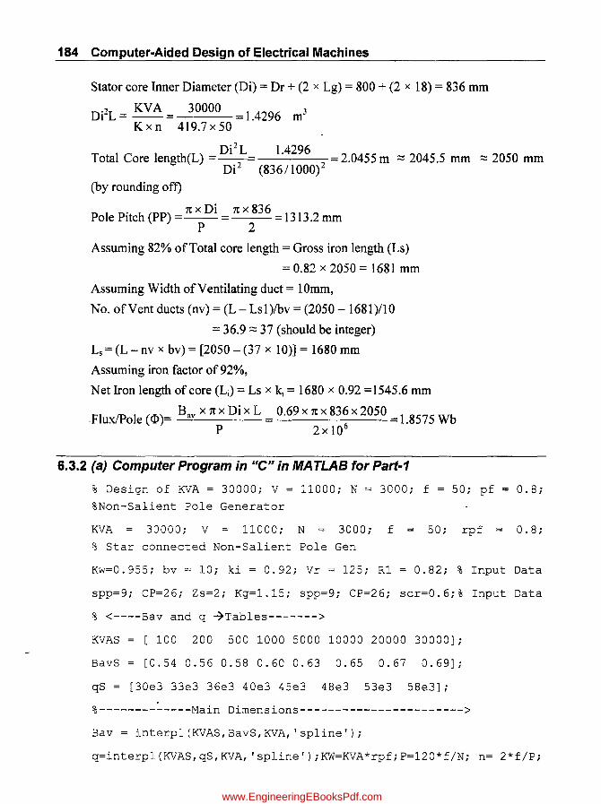
184 Computer-Aided Design of Electrical Machines
Stator core Inner Diameter (Di) = Dr + (2 x Lg) = 800 + (2 x 18) = 836 mm
Di2L = KV A = 30000 = 1.4296 m3 Kxn 419.7x50
Di2L 1.4296 Total Core length(L) = 2 2 = 2.0455 m ::::: 2045.5 mm ::::: 2050 mm
Di (836/1000) (by rounding off)
P 1 P· h(PP) 1txDi 1tx836 13132 o e Itc = --= =. mm P 2
Assuming 82% of Total core length = Gross iron length (Ls)
= 0.82 x 2050 = 1681 mm
Assuming Width of Ventilating duct = 10mm,
No. of Vent ducts (nv) = (L - Lsl)/bv = (2050 -1681)110
= 36.9::::: 37 (should be integer)
Ls=(L-nv x bv)= [2050-(37 x 10)] = 1680mm
Assuming iron factor of 92%,
Net Iron length of core (Li) = Ls x kl = 1680 x 0.92 =1545.6 mm
.FluxIPole (<1»= Bav x 1t x Di xL = 0.69 x 1t x 836 x 2050 = 1.8575 Wb p 2xl06
6.3.2 (a) Computer Program in IIC" in MATLAB for Part-1
% Design of KVA = 30000; V = 11000; N = 3000; f = 50; pf 0.8;
%Non-Salient Pole Generator
KVA = 30000; V = 11000; N = 3000; f = 50; rpf 0.8;
% Star connected Non-Salient Pole Gen
Kw=0.955; bv = 10; ki = 0.92; Vr = 125; R1 = 0.82; % Input Data
spp=9; CP=26; Zs=2; Kg=1.15; spp=9; CP=26; scr=0.6;% Input Data
% <----Bav and q 7Tables------->
KVAS [100 200 500 1000 5000 10000 20000 30000];
BavS [0.54 0.56 0.58 0.60 0.63 0.65 0.67 0.69];
qS = [30e3 33e3 36e3 40e3 45e3 48e3 53e3 58e3];
%-------------Main Dimensions----------------------->
Bav = interp1(KVAS,BavS,KVA, 'spline');
q=interp1(KVAS,qS,KVA, 'spline');KW=KVA*rpf;P=120*f/N; n= 2*f/P;
www.EngineeringEBooksPdf.com

Synchronous Machines 185
Iph=KVA*le3/(1.7321*V)i Dr1=Vr/(pi*n) i Dr= ceil(Drl*lOO)*lOi
S = sPP*P*3i Tph = S*ZS/6i Ata = 1.35*Tph*1ph*Kw/(?/2)i
alfac = P*pi/Si Kc = cos (alfac/2) i K = 11*Bav*q*Kw*Kc*le-3i ATfO=scr*ATa;ATg=O.75*ATfO;Bg=Bav*1.5;
Lgl=ATg/(O.796*Bg*Kg*le3)i Lg = ceil(Lg1)i Di = Dr + 2*Lg; DsqL = KVA/(K*n)i Ll = DsqL/(Di/1e3)"2i L = ceil(L1*lOO)*lOi PP = pi*Di/Pi Ls1= R1*Li nv1= (L - Lsl) /bVi nv = ceil (nv1) i
Ls = (L - nv*bv); Li = Ls*kii F1 = Bav*pi*Di*L*le-6/Pi
% -----------------------------------------------------
8.3.3 Design of Armature Winding and Core (Part-2)
Slot pitch (sp) = 1t x DilS = 1t x 836/54 = 48.6365 mm
<I> xl 06 1.8575 Tooth width at air gap (btO) = = = 28.1365 mm
BtO xLix SI P 1.6 x 1545.6 x 54/2
Slot width (Ws) = sp - btO = 48.6365 - 28.1365 = 20.5 mm
Assuming current density (cds 1) = 3 Almm2;
Cond Area of CS (As) = Iph = 1574.5 = 524.849 mm 2
cds 3
Assuming 2 conductors width-wise and thickness of HV insulation as 3 mm for 11 KV
Cond Width (Wc) = «Ws - 2 x HVins - 2.5)/2) = (20.5- 2 x 3 - 2.5)/2
= 6.1585:::::: 6 rom
Assuming Thickness of bare conductor as 1.8 mm,
No. of conductors !Bar height-wise (Ncv) = As = 524.849 = 24.3 :::::: 25 Hc x W c x 2 1. 8 x 6 x 2
Assuming 2% reduction due to corners rouding of conductors,
Actual copper area in a bar (As) = 0.98 x Ncv x Hc x Wc x 2
= 0.98 x 25 x 1.8 x 6 x 2 = 529.3;
. Iph 1574.5 ? Corrected current densIty (cdsl) =-=--= 2.9753 AI mm-
As 529.3
Corrected width of slot (Ws) = 2 x Wc + 2 x HVins + 2.5
= 2 x 6 + 2 x 3 + 2.5 = 20.5 mm
Assuming Insulation thickness of conductor as 0.25 mm, of Height of each Bar (Hbar) = (Ncv + 1) x (Hc + Cins) + 2 x HVins = (25 + 1) x (1.8 + 0.25) + 2 x 3
= 59.3 mm
Assuming Ht of wedge (Hw) = 9 mm, Lip ht (HL) = 25mm and
www.EngineeringEBooksPdf.com

186 Computer-Aided Design of Electrical Machines
Other Insulation in the slot (Hins) = 12 mm,
Height of Slot (Hs) = 2 x Hbar + Hins + Hw + HL = 2 x 59.3 + 12 + 9 + 25
= 164.6 mm::::: 165mm
Conductors (ht-wise) in total slot(p) = 2 x 25 = 50
a = .JWcl Ws = .J2 x 6/20.5 = 0.7651
Loss Factor of Top conductor (KdTL)
A v Loss Factor (Kdav)
=1 + (aHc)4 x (2 X NCV)2 =1+(0.7651x1.8110)4 x (2x25)2 =1.0999 9 9
Mean Length ofTuro (Lmtl) = 2 x LI10 + 2.5 x PP/I0 + 5 x KV + 15
= (2 x 2050110) + (2.5 x 1313.2/10) + (5 x 1100011000) + 15 = 808.3cm = 8.083 m
Stator Wdg Reslph (Rph) = 0.021 x Lmtx Tph = 0.021 x 8.083x~=0.0058n As 529.2
DC Copper Loss (Pc us ) = 3 x Iph2 x Rph x 10.3
= 3 x 1574.52 x 0.0058 X 10-3 = 42.9413 KW
Eddy Current Loss (Peddy) = (Kdav-l) x Pc us = 0.0999 x 42.9413 = 4.291 KW
Assuming Stray Losses = 15%,
. Total Copper Losses in Stator Wdg (Pts) = (Pcus + Peddy) x 1.15
= (42.9413 + 4.291) x 1.15 = 54.317 KW
Effective PU Resistance (Reff) = Iph x Rph x Kdav x VI ;/3 = 1574.5 x 0.0058 x 1.0999/(110001;/3) = 0.0016 pu
Tooth width at air gap (btO) = sp - Ws = 48.6365 - 20.5 = 28.1365 mm
Flux-density at Tooth tip at air gap (BtO)
<I> x 106
= 1.8575 = 1.582 T btO xLixS/P 28.1365xI545.6x54/2
Tooth width at 1/3 ht from tooth tip (btlb3) = 7t x (Di + Hs x 2/3)/S - Ws
= 7t x (836 + 165 x 2/3)/54 - 0.5 = 34.536mm
Flux-density at 1/3 ht (Btlb3)
<I> x 106
= 1.8575 = 1.2888 T b t1b3 x Li x SI P 34.356 x 1545.6 x 54/2
Flux in core(~c) = 1= 1.8575 = 0.9288 Wb 2 2
Assuming Flux density ic core (Bc) = l.lT, Depth of Core (dc)
~c 0.9288 x 106
= 546.3 mm Be X L j 1.1 x 1545.6
www.EngineeringEBooksPdf.com

Synchronous Machines 187
Outer diameter of Core (Do) = Oi + 2 x (Hs + dc) = 836 + 2 x (165 + 546.3)
= 2258.5 mm ::::: 2260 mm (Rounded off)
Revised (dc) = (2260 - 836)/2 - 165 = 547 mm
Actual Flux density in core (Bc) = ~ c
dcx LI
Cross-Section of Stator Slot dimensions in mm)
Height-Wise 250 90
1.3
CU.Coductor bare + Insulation 1 8 + 0.25 = 2.05
Top- Bar 25 + 1)*conductor 26*2.05 = 53 3
HV InsulatIon 2*3 = 6 59.3
Ins.between bars 70
Bottom- Bar 593
Bottom InsulatIon 13
Slack 28
Total 165.0
Width-Wise Cu Conductor bare + InsulatIon 6 + 0 25 = 625
Bar 2*conductor 2*6.25 = 12.5
HV InsulatIon 2'3 = 6 185
I nsulanon on SIdes 2*05 10
Slack 10
Total 20.5
Slot - Balance Ht-wise (Stsbh) =
0.9288 xl 06
= 1.0985 T 547 X 1545.6
Rotor-sIde
t LIp
< WedQe
0 Top Bar
165
tJ Bar
_ 3
I Stator-Slo(>
20.5
Hs - [Hw + HL + 7.5 + Zs x {(Ncv + 1) x (Hc + 0.25) + 7.06}]
25
9
6
5931 7
_
5931
= 165 - [9 + 25 + 7.5 + 2 x {(25 + 1) x (1.8 + 0.25) + 7.06}] = 2.78 mm -7 (OK)
Slot - Balance Width - wise (Stsbw) = Ws - [2 x (Wc + 0.25) + 2 x HVins + 1]
= 20.5 - [2 x (6 + 0.25) + 2 x 3 + I] = 1 -7 (OK)
For Leakage Reactance Calculation
hi = (Ncv+ 1) x Zs x (Hc + Cins) +ZS x 2 x HVins+6
= (25 x 1) x 2 x (1.8 + 0.25) + (2 x 2 x 3) + 6 = 124.6 mm
h2 = (Hs - hi - HL - Hw)/2 = (165 - 124.6 - 25 - 9)/2 = 3.2 mm
h3 = Hw = 9 mm; h4 = HL = 25 mm; Width at opening of slot (W so) = 20.5 mm; . hi h? 2h 3 h ~ .
SpeCIfic Permeance of Slot (As) = + -- + +--3x Ws Ws Ws + Wso Wso
= 124.6 + 3.2 + 2x9 +~=3.8407 3 X 20.5 20.5 20.5 + 20.5 20.5
Slot Leakage Flux (¢, ) = 2 x ~2 x ~O x Iph x Zs x Lsll 000 x As
= 2 x ~2 x 4 x 7r x 10-7 x 1574.5 x 4 x 1680/1000 x 3.8407 = 0.0722 Wb
www.EngineeringEBooksPdf.com
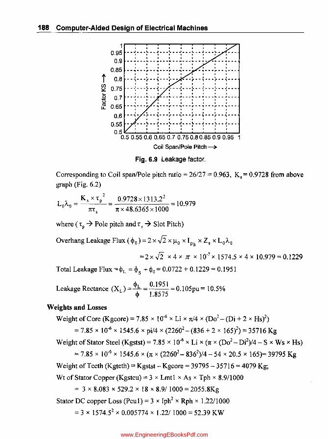
188 Computer-Aided Design of Electrical Machines
1 I • I • • • • •
0.95 .. ~ ___ ~._J. __ ~ __ J __ .~ __ J ___ ~_ · . . . . . . .
0.9 I • I • • I • __ ~ ___ ~_.~ __ •• __ ~. __ h __ ~. _h •• ~ __ _
I • • I. ••
0.85 • • • I • • I •
--~---r·-~---~--~--- -~---r--~---
t 0.8 I • • I • I • • I
• • •• •• I I --'---r--,---r-- ---r--'---r--,---(/)
0.75 ~
• • •• • I • •
--~---~--~-- :--~---~--~---~--~---... • • • • I • I • 1
~ 0.7 n:l 0.65 u.
--~---~-- ---~--~---.--.---~--~---I •• •• • · " .. . --'---r -,---~--'---r--'---r--,---
• I I • • • t •
• • I • I I • I •
0.6 --~- -r--~---~--~--·r--'---r--~---• • • • I I I • •
0.55 ____ .~._J_._~ __ J __ .~._J ___ ~._J_ ••
I • • • • • • • I
• I • I • • I • I
0.5 "'--......... --'--"'-~ .................... ---......... --'---I
0.5 0.55 0.6 0.65 0.7 0.75 0.8 0.85 0.9 0.95 1
Coil Span/Pole Pitch ~
Fig. 6.9 Leakage factor.
Corresponding to Coil spanIPole pitch ratio = 26/27 = 0.963, Ks = 0.9728 from above
graph (Fig. 6.2) ?
LoAo = Ks x 't'p - = 0.9728 x 1313.22
= 10.979 1t x 48.6365 x 1000
where ('t'p -7 Pole pitch and Ts -7 Slot Pitch)
Overhang Leakage Flux ( ~o) = 2 x .J2 x J..lo X Ipb X Zs x LoAo
=2 x.J2 x 4 x 7r x 10-7 x 1574.5 x 4 x 10.979 = 0.1229
Total Leakage Flux =~L = ~s + ~o = 0.0722 + 0.1229 = 0.1951
Leakage Rectance (XL) = 1h. = 0_1951 = 0.105pu = 10.5% ~ 1.8575
Weights and Losses
Weight of Core (Kgcore) = 7.85 x 10⁻⁶ X Li x 7tl4 x (002 - (Oi + 2 x Hs i)
= 7.85 x 10-6 x 1545.6 x pi/4 x (22602-(836+2 x 165)2)=35716Kg
Weight of Stator Steel (Kgstst) = 7.85 x 10⁻⁶ x Li x (1t x (002_ Oi2)/4 - S x Ws x Hs)
= 7.85 X 10-6 x 1545.6 x (1t x (22602- 8362)/4 - 54 x 20.5 x 165)= 39795 Kg
Weight of Teeth (Kgteth) = Kgstst - Kgcore = 39795 - 35716 = 4079 Kg;
Wt of Stator Copper (Kgstcu) = 3 x Lmtl x As x Tph x 8.911 000
= 3 x 8.083 x 529.2 x 18 x 8.9/ 1000 = 2055.8Kg
Stator DC copper Loss (Pcul) = 3 x Iph2 x Rph x 1.2211000
= 3 x 1574.52 x 0.005774 x 1.221 1000 = 52.39 KW
www.EngineeringEBooksPdf.com

Synchronous Machines 189
A d/ ( ) IphxTphx2x3 1574.5x18x6 64746
mpcon m ac = = = 1t x Di 11 000 1t x 83611 000
Addl Loss in End W dg (Padd) = 90 x Di 2 x .JL 11 000 x (ac /750)" x 10-10
=90 X 836" x -h050 11000 x (64746/750)1 X 10-10 = 67.12 Kw.
Assuming Stator Core is made with Silicon Steel Laminations of Specific Loss
(1.8 WlKg at 1 Tesla),
Iron Loss (Pi) = (1.8 x Kgteth x Bt 1 b3/\2 + 1.8 x Kgcore x Bc/\2)1l 000
=(1.8 x 4079 x 1.2888/\2 + 1.8 x 35716 x 1.0985/\2)/1000 = 89.77 KW
6.3.3 (a) Computer Program in "C" in MATLAB for Part-2
~ ----- (2art-2) Stator Winding and Core --------------------->
D':' = 836; L Rins = 12; Hw
2050; F::: = 1.8575; Iph = 1574.5; He = 1.8; 9; HL = 25; % I~put Data
Cins = 0.25; EVi"s = 3; P = 2; CP = 26; BtO = 1.6; edsl = 3; Be = 1.1; S = 54; Li = 1545.6; % Input Data
22=1313.2; V = 11000; Tph = 18; Zs = 2; Ls = 1680; ~ Input Data
sp=pi*Di/S; btO=FI~le6/(3tO*Li*S/P); Ws=sp-btO; As1 = Iph/eds1;
Wcl= ( (Ws-2*HVins-2. 5) /2); IVc=::loor (%'e1); Nev1 = Asl/ (He*We*2) ; ~ev eeil(Nevl); As O.98*Nev*He*We*2; eds1 Iph/As; Ws = 2*We + 2*HVins + 2.5;
Hbar=(Nev + l)*(He + Cins)+ 2*EVi~s; Hs1=2*Hbar+Hins + Hw + HL;
Hs eeil(Hsl) ; p 2*Nev; KdTL=1+(a~fa*He/10)A4*p~(p-1)/3;
Kdav=1+(alfa*He/10)A4*(2~Nev)A2/9;
alfa sqrt(2*We/Ws);
Lmt1 = (2*L/10 + 2.5*PP/10 + 5*V/1e3 + 15)/100;
Rph=0.021*Lmt1*Tph/As;Peus=3*Iph A2*Rph/1e3; Peddy= (Kdav -l)*Peus;
Pts = (Peus- + Peddy) *1.15; Re::f = Iph *Rph*Kdav / (V / sqrt (J) ) ;
btO=sp-Ws; BtO=FI*le6/(btO*Li*S/P); btlb3=pi*(Di+Hs*2/3)/S- Ws;
Bt1b3=FI*le6/(bt1b3*Li*S/P);FIe=FI/2; de1=Fle/(Be*Li)*le6; Dol = Di+ 2*(Hs + del); Do=eeil(Do1/10)*10; de=(Do-Di- 2*Hs)/2; Be = FIe/(de*Li)*le6;
Stsbh=Hs - (Hw T HL + 7.5 + Zs*((Nev + l)*(He + 0.25) + 7.06));
Stsbw = Ws - (2*(We + 0.25) + 2*HVins + 1);
www.EngineeringEBooksPdf.com
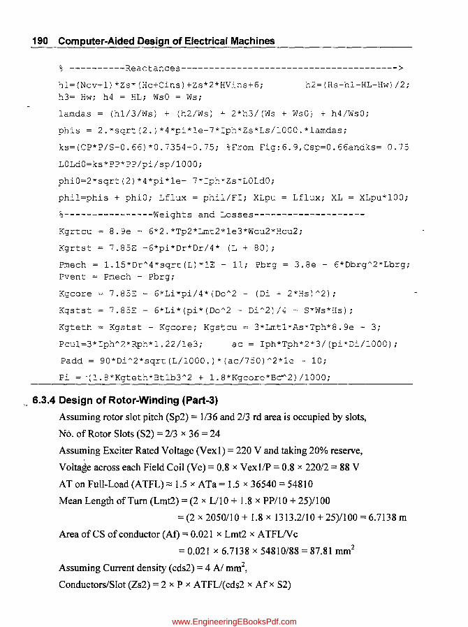
190 Computer-Aided Design of Electrical Machines
% ----------Reactances--------------------------------------->
hl=(Ncv+1)*Zs*(Hc+Cins)+Zs*2*HVins+6; h3= Hw; h4 = HL; WsO = Ws;
h2=(Hs-nl-HL-Hw)/2;
lamdas = (h1/3/Ws) + (h2/Ws) + 2*h3/(Ws + WsO) + h4/WsO;
phis = 2.~sqrt(2.)*4*pi*~e-7*Iph*Zs*Ls/1000.*lamdas;
ks=(CP*P/S-0.66)*O.7354+0.75; %From Fig:6.9,Csp=0.66andks= 0.75
LOLdO=ks*PP*PP/pi/sp/1000;
phiO=2~sqrt(2)*4*pi*le- 7*Iph*Zs*LOLdO;
phil=phis + phiO; Lflux = phil/FI; XLpu = Lflux; XL = XLpu*100;
%----------------Weights and Losses--------------------
Kgrtcu
L<grtst
8.ge - 6*2.*Tp2*Lmt2*le3*Wcu2*Hcu2;
7.85E -6*pi*Dr*Dr/4* (L + 80);
Pmech = 1.15*DrA4*sqr~(L)*lE - 11; Pbrg = 3.8e - 6*Dbrg A2*Lbrg; Pvent = Pmech - Pbrg;
7.85E Kgcore
Kgstst 7.85£ - 6*Li*(pi*(Do A2 - Di A 2)/4 - S~Ws*Hs);
Kgteth Kgstst - Kgcore; Kgstcu = 3*Lmtl*As*Tph*8.ge - 3;
Pcu1=3*IphA2*Rph*1.22/1e3; ac = Iph*Tph*2*3/(pi*Di/1000);
Padd = 90*DiA2*sqr~(L/1000.)*(ac/750)A2*le - 10;
Pi = 0(1. 8*Kgteth*Bt1b3 A2 + 1. 8*Kgcore*BC""2) /1000;
~ 6.3.4 Design of Rotor-Winding (Part-3)
Assuming rotor slot pitch (Sp2) = 1/36 and 2/3 rd area is occupied by slots,
No. of Rotor Slots (S2) = 2/3 x 36 = 24
Assuming Exciter Rated Voltage (Vex1) = 220 V and taking 20% reserve,
Voltage across each Field Coil (Vc) = 0.8 x Vex11P = 0.8 x 220/2 = 88 V
AT on Full-Load (ATFL);:::: 1.5 x ATa = 1.5 x 36540 = 54810
Mean Length of Tum (Lmt2) = (2 x Ll10 + 1.8 x PP/10 + 25)1100
= (2 x 2050/10 + 1.8 x 1313.2/10 + 25)1100 = 6.7138 m
Area ofCS of conductor (At) = 0.021 x Lmt2 x ATFLNc
= 0.021 x 6.7138 x 54810/88 = 87.81 mm2
Assuming Current density (cds2) = 4 AI mm2,
Conductors/Slot (Zs2) = 2 x P x ATFL/( cds2 x Af x S2)
www.EngineeringEBooksPdf.com

Synchronous Machines 191
= 2xpxATFL = 2x2x54810 =26.01=26mm cds2 x Af x S2 4 x 87.81 x 24
ZSJ )( S, 26 x 24 TurslPole (Tp2) = Zs2 x S2/(2 x P) = - - = = 156
2xP 2x2
Height of Copper cond (Hcu2) = ~ = 87.814 =3.1362mm ::::: 3.2 mm Wcu2 28
Revised Area ofCS of conductor (At) = Wcu2 x Hcu2 = 28 x 3.2 = 89.6 mm2
Resistance ofwindingiPole (Rfp) = 0.021 x Lmt2 x Tp2/Af
= 0.021 x 6.7138 x 156/89.6 = 0.2455 n
Field Current at Full-Load (lfFL) = Vc = 88 = 358.5 Amps Rfp 0.2455
Wound Slot ht (Hs2) = Zs2 x Hcu2 + (Zs2 - 1) x 0.4 + 14
= 26 x 3.2 + (26 - 1) x 0.4 + 14 = 107.2::::: 108 mm
Ht-wise Slot balance (Rtsbh) = Hs2 - (Zs2 x Hcu2) - (Zs2 - 1) x 0.4 - 14
= 108 - (26 x 3.2) - (26 - 1) x 0.4 - 14 = 0.8 mm ~ (OK)
Width-wise Slot balance (Rtsbw) = Ws2 - Wcu2 - 2.9
= 31 - 28 - 2.9 = 0.1 mm ~ (OK) Cross-Section of Rotor Slot (dimensions in mm) Stator-side
Height-Wise Wedqe 250
Ins under wedge 60
CU.Coductors 26' 3.2 832
Inter-tum Insulation (26 - 1)' 0.4 100
t
"')
251 / Wedge
Bottom - Insulation 80
Slack 08
Total 133.0 133 26 nos 102
of conductors Width-Wise I Rotor-Slot >
Cu. Conductor 1 • 28 28.0
Insulation on sides 2' 1.45 2.9
Slack
Total
01
31.0
:411 22 _:
: Sub-Slot: . . I .... _ ........ I
31
Wpoles = Ap x Lp x P x 7800 = 0.0686 x 0.6585 X 16 x 7800 = 5637.6 Kg
Diameter at bottom of Sub - Slot (dk) = Dr - 2 x (Hs2 + Hw2 + Hss)
= 800 -2 x (l08 + 25 + 45) = 444 mm
Wide Tooth Pitch (wtp) = (S2/4 + 1)/SP2 = (24/4 + 1)/36 = 0.1944
133
I~
www.EngineeringEBooksPdf.com
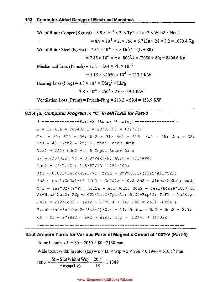
192 Computer-Aided Design of Electrical Machines
Wt. of Rotor Copper (Kgrtcu) = 8.9 x 10-3 x 2. x Tp2 x Lmt2 x· Wcu2 x Hcu2
= 8.9 x 10-3 x 2. x 156 x 6.7138 x 28 x 3.2 = 1670.4 Kg
Wt. of Rotor Steel (Kgrtst) = 7.85 x 10-6 x 1t x Dr2/4 x (L + 80)
= 7.85 X 10-6 x 1t x 8002/4 x (2050 + 80) = 8404.6 Kg
Mechanical Loss (Pmech) = 1.15 x Or4 x -..IL x 10-11
= 1.15 x -..12050 x 10-11 =213.3 KW
Bearing Loss (Pbrg) = 3.8 x 10⁻⁶ x Dbrg~ x Lbrg
= 3.8 x 10-6 x 2502 x 250 = 59.4 KW
Ventilation Loss (Pvent) = Pmech-Pbrg = 213.3 - 59.4 = 153.9 KW
6.3.4 (a) Computer Program in "C" in MA TLAB for Part-3
~ ---------------Part-3 (Ro~or Winding)---------------->.
P 2; ATa = 36540; : = 2050; PP = 1313.2;
~r2. = 60; SP2 36 ; Ws2 = 3' . -I H ') SL. = 116; Hw2 25; Wss
g:ss = 45; Wcu2 28; % Input Rotor Data
Vex1 = 220; cds2 4 % Input Ro~or Data
S2 = 2/3*SP2; Vc 0.8"'Vexl/P; ATFL = 1.5*ATai
Lmt2 = (2*L/10 + 1.8*PPIl0 + 25)/100;
Afl 0.021*Lmt2*ATFL/Vc; Zs2a = 2*P*ATFL/(cds2*Af1*S2);
22;
Zs2 ceil(Zs2a);if (Zs2 - Zs2a» = 0.5 Zs2 = floor(Zs2a); end;
Tp2 Zs2*S2/(2*P); Hcu2a = Af1/Wcu2; Hcu2 = ceil(Hcu2a*10)/10;
Af=Wcu2*Hcu2; Rfp=O.021*Lmt2*Tp2/Af; Rf20=Rfp*P; IfFL = Vc/Rfp;
Hs2a = Zs2*Hcu2 + (Zs2 - 1)*0.4 + 14; Hs2 = ceil (Hs2a);
Rtsbh=Hs2-Zs2*Hcu2-(Zs2-l)*O.4 - 14; Rtsbw = Ws2 - Wcu2 - 2.9;
dk = Dr - 2*(Hs2 + Hw2 + Hss); wtp = (S2/4. + 1)/SP2;
6.3.5 Ampere Turns for Various Parts of Magnetic Circuit at 100%V (Part-4)
Rotor Length::::: L + 80 = 2050 + 80 =2130 mm
Wide tooth width in rotor (tzi) = 1t x Oi x wtp = 1t x 836 x 0.1944 = 510.57 mm
ratio1=St-SlotWidth(Ws) = 20.5 =1.1389 Airgap(Lg) 18
www.EngineeringEBooksPdf.com

0.5
0.45
Synchronous Machines 193
. .. .. .. .! .... .... ' ........ ~ ...... ! .... .... ' ........ ' ........ ~ .... .. ,.' ..
I I • , I I I I
• 1 I • I
• I I • •
0.4 .--~ ..... ~ .. -.-:-.-~ .... ~ ... --~ ....... - ... ~- ...... : ..... -
t I. I I I I I I
035 ___ ~_ .. _"'_ ...... ," __ .. .l .. __ ....... - ... --- ......... ~ .. -- ..... - ....
• • I I • I • I •
I I I I I I I
0.3 ...... ~ ........ : ........ ~ ...... ;.... ~ ...... -: ........ ~ ...... ~ .. ...... : ........
Q5 0.25 t::
(3 0.2
I I • I I I • • I
1 1 I' I I I
0.15 .... .. .. .. .... .. ...... r .............. '" ...... -.- ................................ .. • • • • I , I , •
• • I • • • • I I
0.1 ...... ~ .... J ........ ~ ...... ! .... _ ........ _:- ...... L ....... ~_ ...... I ........
" I I I • • • I , I • •
0.05 .... ~ ...... ~ ........ :- ...... ! ...... ~ .... .. -; ...... :- ...... ~ .... .. -:- ...... • • I • I • I • I
0.5 1 1.5 2 2.5 3 3.5 4 4.5 5
Opening/Airgap ~
Fig 6.10 Carter Coefft. for open slots
Carters Coefficient (kOl) read from graph (Fig. 6.10) corresponding to 1.1389 is
0.1681
rati02 = Rt - SlotWidth(Ws2) = ~ = 1.7222 Airgap(Lg) 18
Carters Coefficient (k02) read from graph (Fig. 6.10) corresponding to 1.7222 IS
0.2387
ratiod = St - Vent - ductWidth(by) =!Q = 0.5556 Airgap(Lg) 18
Carters Coefficient (kl) read from graph (Fig. 6.10) corresponding to 0.5556 IS
0.0881
St _ SlotCoefft(ksl) = SlotPitch 48.6365 = 1.0762 SlotPitch - Slotwidth )( CarterCoefft 48.6365 - 20.5 x 0.\68\
Rt - SlotCoefft(ks2) = SlotPitch 69.8132 = 1.1185 SlotPitch - Siotwidth x CarterCoefft 69.8132 - 31 x 0.2397
by 10 Duct = Coefft(kdl) = = = 1.0966
by - kl x bv 10 - 0.0881 x 10
kgs = ks1 x kdl = 1.0762 x 1.0966 = 1.1802
kgs = (ksl + ks2 - 1.) x kdl = (1.0762 + 1.1185 - 1) x 1.0966 = 1.3102
www.EngineeringEBooksPdf.com
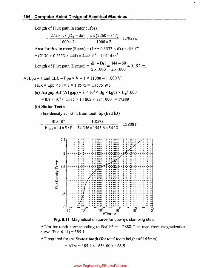
194 Computer-Aided Design of Electrical Machines
Length of Flux path in stator (Lfps)
== 2/3x7tx(Do -dc) == 7tx(2260-547) ==1.7938m 1000 x 2 1000 x 2
Area for flux in rotor (Smax) == (Lr + 0.3333 x dk) x dk/106
== (2130 + 0.3333 x 444) x 4441106 == 1.0114 m2
dk - Dri 444 60 Length of Flux path (Lsma.x) == --- == - = 0.192
~ 2 x 1000 2 x 1000
At Epu == 1 and ELL == Epu x V == 1 x 11000 == 11000 V
Flux == Epu x FI = 1 x 1.8575 == 1.8575 Wb
(a) Airgap AT (ATgap) = 8 x 10⁵ x Bg x kgus x Lg/I000
= 0.8 x 105 x 1.035 x 1.1802 x 18/1000 == 17589
(b) Stator Teeth
Flux-density at 1/3 ht from tooth tip (Bstlb3)
__ <I>_x_l_06 __ = ___ 1_.8_5_75 ___ == 1.2888T b t1b3 x Lix SIP 34.356 x 1545.6 x 54/2
m
2.5r-~-,~~~--~.~.~.p.p •• "n".--~.~.~.~.~.p .. ".~-,.-,.~~~--~~p.p .. ~.~.~.
t j::'
~ 'iii c: Q)
Cl x ~
u::
2
1.5
I ., •• 1... • •• ' .. In " .,111t I • I I •• n. • 111""'
• • I 111111
I • I ' .. 111 I • • '1'1" I'" ..... I. I .U.II • I I t.lfI. I.' 1 ••• , .. __ ........ - .... _- .... -- .... -- ..... _-- .... - .. --- ..... -- .......... I • I II.... •• "1111' • I' .... 11 I • I' 'If' • I • II II.
I' ..... .. • I ..... .. · ...... ..
. · . · .
· , I •••• CI.
I 111'1t ..
I I ,".n I I' .IIIU
• • r ...... · · .
• I 1 I r - ....... 'nt\ ..... r .... -' ... "\,..n- ... ' -t-r .... ".'1', ...... "'-,. ,,..,., • ........ II .... a ........ . • •• I'nl ••• lI.n I I ... .. ....... · ....... .
I ...... .. I I. III'" I ...... u
· ..... .. .1 ..... . .,t"lf 0.5 .............. .... .. .. ~ -......... "" ...... -.-.- .... ~ ....... - ..... _ ..................... .. · · •• tll .. · · · .... n · · · ... tll · · . ...... · · · ....... · · · .... 11 · · · · . · · .... u. · · · .... 11 · · · .. · · .. 'In. · · · ...... · · · · .I.U. · · · . .....
103
104
AT/m~
Fig. 6.11 Magnetization curve for Lowhys stamping steel.
AT/m for tooth corresponding to Bstl b3 = 1.2888 T as read from magnetization curve (Fig. 6.11) == 385.1
AT required for the Stator tooth (for total tooth height of 165mm)
= ATst== 385.1 x 165/1000==63.5
www.EngineeringEBooksPdf.com

,.
Synchronous Machines 195
(c) Stator Core
A IFI d .. (B) $xO.5x106 1.8575xO.5xl06
ctua ux enslty m core stc = =------dc X L( 547 x 1545.6
1.0985 T
AT/m for Core corresponding to Bstc = 1.0985T as read from magnetization curve
(Fig. 6.11) = 219.17
AT required for the Stator Core (ATsc) = 219.17 x 165/1 000 = 393.2
(d) Rotor Teeth
Flux-density at 113 ht from tooth tip (Brt 1 b3)
= ___ E...,!p_u_x_B.....:g=---x_tz_i_x_L_i _x_1._3_6_x_l_06 __ _ Lr x (x x (Dr - 4/3 x (Hs2 + Hw2 + Hss» x wtp)
= lx1.035x510.57x1545.6x1.36xl06 = 1.5176T
2130 x (x x (800 - 4/3 x (l08 + 25 + 45» x 0.1944)
AT 1m for Rotor tooth corresponding to 1.5176T as read from magnetization curve
(Fig. 6.11) = 1159.8
(Magnetization curve for Rotor is presumed same as that of Lowhys Steel.)
AT required for the Rotor tooth (ATrt) of (Hs2 + Hw2 + Hss)
1159.8 x (108 + 25 + 45)/1000 = 1159.8 x 178/1000 = 206.45
(e) Rotor Core
Flux density in the Rotor Core (Brtc)
= Epu x 1.05 x FIlS max = 1 x 1.05 x 1.8575/1.0114 = 1.9283 T
AT/m for Rotor Core (atrc) corresponding to 1.9283 T as read from magnetization
curve (Fig. 6.11) = 17110
(Magnetization curve for Rotor is presumed same as that of Lowhys Steel.)
AT required for the Rotor tooth (ATrc) = atrc x Lsmax = 17110 x 0.1920 = 3285.1
Total No-Load AT for the Magnetic Circuit at 100% rated Voltage (ATtot)
= ATgap + ATst + ATsc + ATrt + ATrc = 17589 + 63.5 + 393.2 + 206.45 + 3285.1
= 21538
No-Load Field Current at 100% V (Ifocc) = ATtotlTp2 = 21538/156 = 138.06 Amp
Air-Gap Field Current at 100% V (lfgap) = ATgap/Tp2 = 17589/156 = 112.75 Amp
www.EngineeringEBooksPdf.com
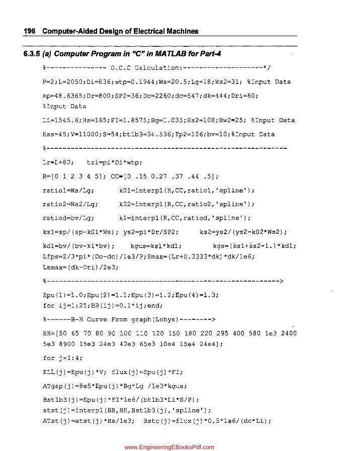
196 Computer-Aided Design of Electrical Machines
6.3.5 (a) Computer Program in "C" in MATLAB for Part-4
%--------------- o.c.c Calculation:--------------------*/
P=2;L=2050;Di=836;wtp=0.1944;Ws=20.5;Lg=18;Ws2=31; %Input Data
sp=48.6365;Dr=800;SP2=36;Do=22qO;dc=547;dk=444;Dri=60;
%Input Data
Li=1545.6;Hs=165;FI=1.8575;Bg=1.035;Hs2=108;Hw2=25; %Input Data
Hss=45;V=11000;S=54;btlb3=34.536;Tp2=156;bv=10;%Input Data
%------------------------------------------------------------Lr=L+80; tzi=pi*Di*wtp;
R=[O 1 2 3 4 5J; CC=[O .15 0.27 .37 .44 .5J;
ratiol=Ws/Lg;
ratio2=Ws2/Lg;
ratiod=bv/Lg;
kOl=interpl(R,CC,ratiol,'spline');
k02=interpl(R,CC,ratio2, 'spline');
kl=interpl(R,CC,ratiod,'spline');
ksl=sp/(sp-kOl*Ws); ys2=pi*Dr/SP2; ks2=ys2/(ys2-k02*Ws2);
kdl=bv/(bv-kl*bv); kgus=ksl*kdl; kgs=(ksl+ks2-1.)*kd1;
Lfps=2/3*pi* (Do-dc)/le3/P;Smax=(Lr+0.3333*dk) *dk/1e6;
Lsmax=(dk-Dri)/2e3;
%---------------------------------------------------------->
Epu(1)=1.0;Epu(2)=1.1;Epu(3)=1.2;Epu(4)=1.3;
for ij=1:25;BB(ij)=0.1*ij;end;
%------B-H Curve From graph(Lohys)-------->
HH=[50 65 70 80 90 100 110 120 150 180 220 295 400 580 1e3 2400
5e3 8900 15e3 24e3 40e3 65e3 10e4 15e4 24e4];
for j=1:4;
ELL(j)=Epu(j)*V; flux(j)=Epu(j)*FI;
ATgap(j)=8e5*Epu(j)*Bg*Lg /le3*kgus;
Bst1b3(j)=Epu(j)*FI*le6/(bt1b3*Li*S/P);
atst(j)=interpl(BB,HH,Bst1b3(j), 'spline');
ATst(j)=atst(j)*Hs/le3; Bstc(j)=flux(j)*0.5*le6/(dc*Li);
www.EngineeringEBooksPdf.com

Synchronous Machines 197
atsc(j)=interp1(BB,HH,Bstc(j), 'spline'); ATsc(j)=atsc(j)*Lfps;
Brt1b3(j)=Epu(j)*Bg*tzi*Li*1.36/Lr/(pi*(Dr-4./3.*(Hs2+Hw2+Hss))
*wtp) ;
atrt(j)=interp1(BB,HH,Brt1b3(j), 'spline');
ATrt(j)=atrt(j)* (Hs2+Hw2+Hss)/le3;Brtc(j)=Epu(j)*1.05*FI/Srnax;
atrc(j)=interp1(BB,HH,Brtc(j), 'spline'); ATrc(j)=atrc(j)*Lsrnax;
ATtot(j)=ATgap(j)+ATst(j)+ATsc(j)+ATrt (j)+ATrc(j);
Ifocc(j)=ATtot(j)/Tp2;Ifgap(j)=ATgap(j)/Tp2;
IFOCC(j+1)=Ifocc(j);EPU(j+1)=Epu(j);end;IFOCC(1)=0;EPU(1)=0;
plot(IFOCC,EPU);grid;xlabel('If(arnps)-->');
ylabel('Volts(PU)-->');
title('OCC of Non-Salient Pole Generator');
%-------------------------------------------------6.3.6 Open Circuit Characteristic Curve (OCC) Part-5
A plot of Ampere Turns on X-Axis and Various Tenninal voltages (0% to 130% of
rated Votage)
Proceedure for Plotting Open Circuit Characteristic Curve (OCC)
1. Consider Tenninal Voltages of 100%, 110%, 120% and 130% of rated voltage.
2. Fill up all the details pertaining to Air-Gap', Stator tooth, Stator Core, Rotor Tooth and
Rotor Core calculated above under the 100% Voltage Column in the table.
3. Calculate the Flux densities in various parts at other 3 Voltages which are linearly
proportional to Voltage (Ex: If Flux density = 1.1 T at 100% Volts, then at 110% Volts
it will be (11 0/100) x 1.1 = 1.2IT).
4. At these values of Flux densities measure the "AT/m" from Magnetization curve (as
was referred for calculation for 100%V).
5. Calculate Values of "AT" for each part by directly multiplying the "AT/m" value
with corresponding "length" of each part.
6. Add values of "AT" of all the parts under each %Voltage Colum to get the Total AT
required for each voltage.
7. Plot Values of AT on X-Axis and % Rated Voltages on Y-Axis to get OCC.
www.EngineeringEBooksPdf.com
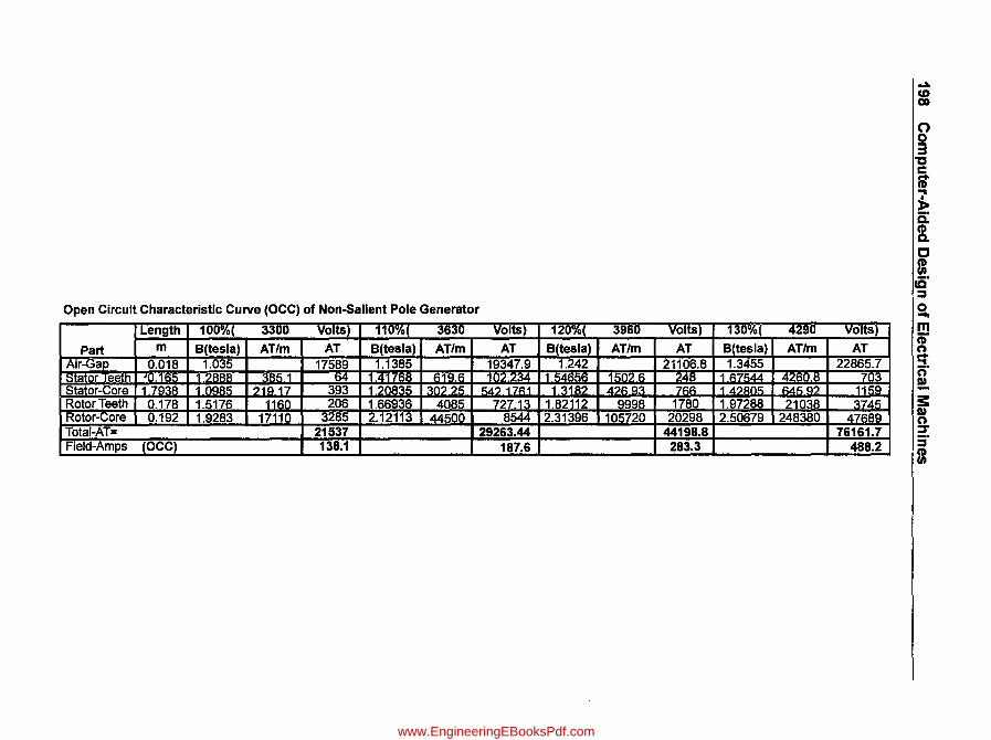
Open Circuit Characteristic Curve (OCC) of Non-Sallent Pole Generator
I Length 1~O~( 3300 Volts) 110%( 3630
Part m B(tesla) AT/m AT B(tesla) AT/m Air-Gap 0.018 1.035 17589 1.1385
• Stator Ieeth • .165 12BBB 3B5.1 I:i4 1.4176B 619.6 Stator-Core 1.7.938_ 109B5 ~1Q 17 393 120835 :10~ 25 Rotor Teeth 0.178 1.5176 t1fW_ 206 1.66936 4085 Rotor-core 0.192 1.9283 17110 3285 2.12113 44500 Total-AT= 21537 Field-Amps (OCC) 138.1
volts) 120%( 3960 Volts)
AT B(tesla) AT/m AT 19347.9 1.242 21106.8 1112.234 154656 1502.6 248
h.4? 171'l1 13182 4?693 766 727.13 1.82112 9998 1780
8544 2.31396 105720 20298 29263.44 44198.8
187.6 283.3
130%( 4290
B(tesla) AT/m 1.3455
167544 426( .8 1 .4?B05 64592 1.97288 21038 2.50679 248380
Volts)
AT 22865.7
7(13 1159 3745
4768-.a 76161.7
488.2
.... CD co
o o 3
"C C Cit ~
)-c: CD Q.
C m
cQ' ::s a m CD ~ ~
C:;' !!. s: I» n ::r 5' m
www.EngineeringEBooksPdf.com

t S-e:. ~ ~
Synchronous Machines 199
1.4r-----------------~------------------------~
· . . 1.2 .......... -:- ......... ~ .......... -:- .......... ~ ........... -:- ......... • I I • · . I' I I , •
.. .. .. .. "\'" ............ r ... .... -.- ........... , ................ - ............ , ............ r ........ ............... r ....... ... I ••• ·
0.8 ...... ...... , ..................................................................... I ..................... ... . . . . . . . 0.6 .. ~----~-----~-----~----~-----~----~-----~--- ..
• I I I I • • 1 ,.....
• . I. •• • I I I • • I
0.4 • I • • • • I • -· .. -r----~-----, .. -.. --~--- .. ' .. -- .. -r ... ----,-----r----• I • • · . . . · . . · . .
-~-----r----~-----.-----~----~-----r----~-----r- .... -
o~~=_~~~~--~~~--~--~--~--~--~ o 50 100 150 200 250 300 350 400 450 500
If (amps) ~
Fig. 6.12 acc of non-salient pole generaotor.
6.3.6 (a) Computer Program in IIC" in MATLAB for Part-5
%-------------------(OCC Calculation)------------------------->
P=2;L=2050;Di=836;wtp=0.1944;Ws=20.5;Lg=18;Ws2=31;sp=48.6365;
Dr=800;SP2=36;Do=2260;dc=547;dk=444;Dri=60;%Input Data
Li=1545.6~Hs=165;FI=1.8575;Bg=1.035;Hs2=108;Hw2=25; %Input Data
Hss=45;V=11000;S=54;bt1b3=34.536;Tp2=156;bv=10; %Input Data
%-------------------------------------------------------Lr=L+80;tzi=pi*Di*wtp;ratio1=Ws/Lg;ratio2=Ws2/Lg;ratiod=bv/Lg;
R=[O 1 2 3 4 5]; CC=[O .15 0.27 .37 .44 .5];·
k01=interp1(R,CC,ratio1, 'spline');
k02=interp1(R,CC,ratio2, 'spline');
k1=interp1(R,CC,ratiod, 'spline');
ks1=sp/(sp-k01*Ws);ys2=pi*Dr/SP2;ks2=ys2/(ys2-k02*Ws2);
kd1=bv /(bv-k1*bv); kgus=ks1*kd1;kgs=(ks1+ks2-1.)*kd1;
Lfps=2/3*pi*(Do-dc)/le3/P;
Lsmax=(dk-Dri)/2e3;
Smax=(Lr+0.3333*dk)*dk/1e6;
www.EngineeringEBooksPdf.com
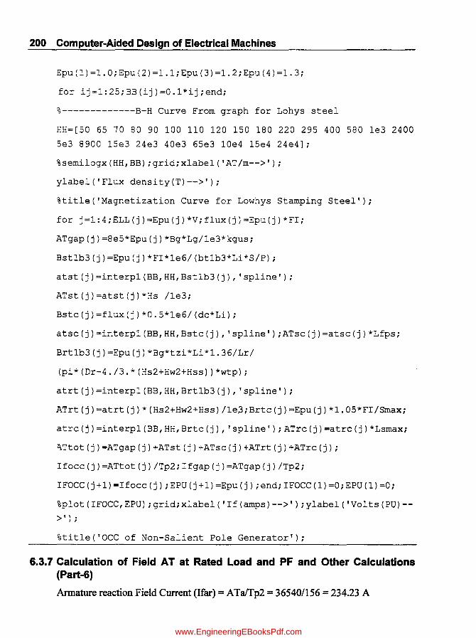
200 Computer-Aided Design of Electrical Machines
Epu(1)=1.0;Epu(2)=1.1;Epu(3)=1.2;Epu(4)=1.3;
for ij=1:25;BB(ij)=0.1*ij;end;
%-------------B-H Curve From graph for Lohys steel
HH=[50 65 70 80 90 100 110 120 150 180 220 295 400 580 1e3 2400
5e3 8900 15e3 24e3 40e3 65e3 10e4 15e4 24e4J;
%semilogx(HH,BB);grid;xlabel('AT/m-->');
ylabel('Flux density(T)-->');
%title('Magnetization Curve for Lowhys Stamping Steel');
for j=1:4;ELL(j)=Epu(j)*V;flux(j)=Epu(j)*FI;
ATgap(j)=8e5*Epu(j)*Bg*Lg/1e3*kgus;
Bst1b3(j)=Epu(j)*FI*le6/(bt1b3*Li*S/P);
atst(j)=interp1(BB,HH,Bst1b3(j),'spline');
ATst(j)=atst(j)*Hs /le3;
Bstc(j)=flux(j)*0.5*le6/(dc*Li);
atsc(j)=interp1(BB,HH,Bstc(j), 'spline');ATsc(j)=atsc(j)*Lfps;
Brt1b3(j)=Epu(j)*Bg*tzi*Li*1.36/Lr/
(pi*(Dr-4./3.*(Hs2+Hw2+Hss))*wtp);
atrt(j)=interp1(BB,HH,Brt1b3(j), 'spline');
ATrt(j)=atrt(j)*(Hs2+Hw2+Hss)/le~;Brtc(j)=Epu(j)*1.05*FI/Smax;
atrc(j)=interp1(BB,HH,Brtc(j), 'spline');ATrc(j)=atrc(j)*Lsmax;
~Ttot(j)=ATgap(j)+ATst(j)+ATsc(j)+ATrt(j)+ATrc(j);
Ifocc(j)=ATtot(j)/Tp2;Ifgap(j)=ATgap(j)/Tp2;
IFOCC(j+1)=Ifocc(j);EPU(j+1)=Epu(j);end;IFOCC(1)=0;EPU(1)=0;
%plot(IFOCC,EPU);grid;xlabel('If(amps)-->');ylabel('Volts(PU)-
>') ;
%title('OCC of Non-Salient Pole Generator');
6.3.7 Calculation of Field AT at Rated Load and PF and Other Calculations (Part-6)
Annature reaction Field Current (Ifar) = ATalTp2 = 365401156 = 234.23 A
www.EngineeringEBooksPdf.com

Synchronous Machines 201
Field Current on Short Circuit at Rated Armature current (Ifsc)
ATa + XLpu x ATgap(l) 36540 + 0.105 x 17589 = = 246.07 Amps
Tp2 156
No load Field Current (lfO) = Ifocc (1) = 138.06 A
Short Circuit Ratio (scr) = lfO/lfsc = 138.06/246.07 = 0.5611
pfr = ~1- pf2 = ~1 - 0.82 =0.6
E1=~lxpf2 +(lxpfr+XLpu)2 =~lxO.82 +(1xO.6+0.105)2 = 1.0663 pu
Field Current (Ifl) corresponding to E 1 = 1.0663pu read from OCC = 168.9 amps
Field Current at rated Load and Pf (lfFL)
= ~If/ +lfar2 -2xlfl xlfar x cos(n/2 xcos-l(pf)
=~168.92 + 234.23 2 - 2x 168.9 x 234.23 x cos(n/2 x cos-l(0.8) = 361.7 A
Open circuit voltage (EO) corresponding to IfFL
= 361.7A, read from OCC = 1.2327 pu
. E - V 1.2327 -1 Voltage RegulatIOn = 0 = = 0.23267pu = 23.267%
V 1
Rotor Current Density (cds2) = IfFLlAf= 361.7/89.6 = 4.04 Almm2
Voltage Across Rotor Wdg at Rated Ld and PF (Vfn)
= IfFL x Rf20 x (235. + 120.)/255
= 361.7 x 0.4909 x (3551255) = 247.21 Volts
Voltage rating of Exciter (Vex) =Vfn xLI =247.21 x 1.1 =271:9V(Say275V)
Current Rating of Exciter (lex) = Ifn x 1.1 = 361.7 x 1.1 = 397.9 (Say 400A)
KW rating of Exciter (KWex) = Vex x lex = 275 x 400 = 110 KW
Rotor Copper Loss· (Pcu2) = IfFL2 x Rf20 x (235. + 75.)/255 = 361.72 x 0.4909 x (3101 255)/1000 = 78.09 KW
Total Weight of Active Material (Kg T) = Kgstst + Kgstcu + Kgrtcu + Kgrtst
= 39795 + 2055.8 + 1670.4 + 8404.6 = 51926 Kg
Considering Insulation Wt asl %, Total Weight of Active Material (KgT)
= 1.01 x (Kgstst + Kgstcu + Kgrtcu + Kgrtst)
= 1.01 x (39795 + 2055.8 + 1670.4 + 8404.6) = 52445 Kg
Kgpkva = KgTIKVA = 52445/30000 = 1.748
www.EngineeringEBooksPdf.com

202 Computer-Aided Design of Electrical Machines
Total Losses (Pt) = Pcul + Padd + Pmech + Pcu2 + Pi
= 52.39 + 67.12 + 213.3 + 78.1 + 89.77 = 500.65 KW;
Efficiency at rated Ld and PF (Eft)
= KW/(KW + Pt) x 100 = 24000/(24000 + 500.65) x 100 = 97.96 %
Assuming Temp-Rise of cooling Air as 240 C, Quantity of Cooling Air (Qair)
= Pcoolx1000 = 441.3 x 1000 =16.13 (sa 17 m3/s) 1140 x 24 1140 x 24 Y
A· T R· Pcoolx 1000 441.3 x 1000 2277 0 C Ir emp Ise = = . 1140 x Qair 1140 x 17
6.3.7 (a) Computer Program in "C" in MATLAB for Part-6
%----------LMC and Other Calculations:------------------->
ATa=36540;XLpu=0.105;ATgap(1)=1 7 589;Tp2=156;
Epu=[l 1.1 1.2 1.3]; %Input Data
Ifocc=[138.0616 187.5910 283.3260 488.2209];
Ifgap(1)=112.75; %Input Data
rpf=0.8;Af=89.6;Rf20=0.4909; %Input Data
%----------------------------------------------Ifar=ATa/Tp2; Ifsc= (ATa+XLpu*ATgap (1) ) /Tp2; IfO=Ifocc(l); scr=IfO/lfsc; pf=rpf; pfr=sqrt(l-pf*pf); E1=sqrt(1.0*pf*pf+(1*pfr+XLpu)A2);
If1=interp1(Epu,Ifocc,E1, 'spline');
If FL=sqrt(If1A2+IfarA2-2*If1*Ifar*cos(pi/2+acos (pf)));
EO=interp1(Ifocc,Epu,IfFL, 'spline');reg=(EO-Epu(1))*100; cds2=IfFL/Af; Vfn=IfFL*Rf20*(235.+120.)/255; Vex1=1.1*Vfn; Vex=ceil(Vex1/5)*5; Iex1=1.1*IfFL; Iex=ceil(Iex/10) *10; KWex=Vex*Iex/1e3; Pcu2=IfFL*IfFL*Rf20* (235.+75.)/255e3;
KgT=1.01*(Kgstst+Kgstcu+Kgrtcu+Kgrtst); Kgpkva= KgT/KVA;
Pt=Pcu1+Padd+Pmech+Pcu2+Pi; Eff=KW/(KW+Pt) *100.;
Qair=ceil(Pcool*le3/1140./24.)*1.0; Tair=Pcool*le3/1140./Qair;
%--------------------------------------------------------------
6.3.8 Computer Program in "C" in MATLAB for Complete Design
www.EngineeringEBooksPdf.com

Synchronous Machines 203
%Design of KVA=30000;V=11000;N=3000;f=50;pf=0.8;Non-Salient
Pole Generator
f3=fopen('NSP_Gen_Output.m', 'w');sn=l;
KVA=30000;V=11000;N=3000;f=50;rpf=0.8;
%Star connected Non-Salient Pole Gen
Kw=0.955;bv=10;ki=0.92;Vr=125;R1=0.82;Hc=1.8;
Hins=12;Hw=9;HL=25;Cins=0.25;HVins=3;Kg=1.15;
Stsbh=2.88;Stsbw=1.14 ; Dbrg=250;Lbrg=250;Zs=2;
spp=9;CP=26;scr=0.6;BtO=1.6;cds1=3;Bc=1.1;
Dri=60;SP2=36;Ws2=31;Hw2=25;Wss=22;Hss=45;Wcu2=28;Vex1=220;
cds2=4;%Rotor Data
%<----Bav and q------->
KVAS=[ 100 200 500 1000 5000 10000 20000 30000J;
BavS=[0.54 0.56 0.58 0.60 0.63 0.65 0.67 0.69J;
qS=[30e3 33e3 36e3 40e3 45e3 48e3 53e3 58e3J;
%-------------Main Dimensions----------------------->
Bav=interp1(KVAS,BavS,KVA, 'spline');
q=interpl(KVAS,qS,KVA, 'spline');
KW=KVA*rpf; P=120*f/N;n=2*f/P; Iph=KVA*le3/(l.7321*V);
Dr=Vr/(pi*n); Dr=ceil(Dr*100)*10; Vr=pi*Dr/1000*n;
S=spp*P*3; Tph=S*Zs/6; ATa=1.35*Tph*Iph*Kw/(P/2);
Kc=sin(CP/(S/2)*pi/2); K=11*Bav*q*Kw*Kc*le-3; ATfO=scr*ATa;
ATg=0.75*ATfO; Bg=Bav*1.5; Lg=ATg/(O.796*Bg*Kg*le3);
Lg=ceil(Lg); Di=Dr+2*Lg; DsqL=KVA/(K*n); L=DsqL/(Di/1e3)A2;
L=ceil(L*100)*10; PP=pi*Di/Pi Ls=R1*Linv=(L-Ls)/bv;
FI=Bav*pi*Di*L*le-6/P; nv=ceil(nv)iLs=(L-nv*bv);
rat2=Lg/PP;
Li=Ls*ki;
%-----(Part-2) Stator Winding and Core------------------->
Di=836;L=2050;FI=1.8575;Iph=1574.5;Hc=1.8;Hins=12;Hw=9;HL=25;
Cins=0.25; HVins=3; P=2; CP=26; BtO=1.6j cds1=3; Bc=l.l; S=54;
Li=1545.6; PP=1313.2; V=11000; Tph=18;Zs=2; Ls=1680;
www.EngineeringEBooksPdf.com

204 Computer-Aided Design of Electrical Machines
sp=pi*Di/S; btO=FI*le6/(BtO*Li*S/P); Ws=sp-btO; Asl=Iph/cdsl;
Wcl=((Ws-2*HVins-2.5)/2); Wc=floor(Wcl); Ncvl=Asl/(Hc*Wc*2);
Ws=2*Wc+2*HVins+2.5; Hbar=(Ncv+l)* (Hc+Cins)+2*HVins;
Hsl=2*Hbar+Hins+Hw+HL; Hs=ceil(Hsl); p=2*Ncv;
alfa=sqrt(2*Wc/Ws); KdTL=1+(alfa*Hc/10)A4*p*(p-l)/3;
Kdav=1+(alfa*Hc/10)A4* (2*Ncv) A2/9;
Lmtl=(2*L/lO+2.5*PP/lO+5*V/le3+15)/lOO;
Rph=O.021*Lmt1*Tph/As;Pcus=3*IphA2*Rph/1e3;Peddy=(Kdav-1)*Pcus;
Pts=(Pcus+Peddy) *1.15; Reff=Iph*Rph*Kdav/(V/sqrt(3));
btO=sp-Ws; BtO=FI*le6/(btO*Li*S/P); btlb3=pi*(Di+Hs*2/3)/S-Ws;
Bt1b3=FI*le6/(btlb3*Li*S/P); Flc=FI/2;
Dol=Di+2*(Hs+dc1);
Bc=Flc/(dc*Li)*le6;
Do=ceil(Do1/10)*lO;
dc1=Flc/(Bc*Li)*le6;
dc=(Do-Di-2*Hs)/2;
Stsbh=Hs-(Hw+HL+7.5+Zs*((Ncv+l)*(Hc+O.25)+7.06));
Stsbw=Ws-(2*(Wc+O.25)+2*HVins+1);
%----------Reactances--------------------------------------->
h1=(Ncv+1) *Zs* (Hc+Cins)+Zs*2*HVins+6;h2=(Hs-hl-HL-Hw)/ 2; h3=Hw;
h4=HL;WsO=Ws; lamdas=(h1/3/Ws)+(h2/Ws)+2*h3/(Ws+WsO)+h4/WsO;
phis=2.*sqrt(2.)*4*pi*le-7*Iph*Zs*Ls/1000.*lamdas;
ks=(CP*P/S-O.66)*O.7354+0.75; LOLdO=ks*PP*PP/pi/sp/1QOO;
phiO=2*sqrt(2)*4*pi*le-7*Iph*Zs* LOLdO; ~
phil=phis+phiO; Lflux=phil/FI; XLpu=Lflux; XL=XLpu*lOO;
%---------WeightsandLosses-------------------------------------
Kgcore=7.85E-6*Li*pi/4*(Do A2-(Di+2*Hs)A2);
Kgstst=7.85E-6*Li*(pi*(DoA2-Di A2)/4-S*Ws*Hs);
Kgteth=Kgstst-Kgcore; Kgstcu=3*Lmtl*As*Tph*8.ge-3;
Pcu1=3*IphA2*Rph*1.22/1e3; ac=Iph*Tph*2*3/(pi*Di/1000);
Padd=90*Di A2*sqrt(L /lOOO.)*(ac/750)A2*le-10;
Pi=(1.8*Kgteth*Btlb3 A2+1.8*Kgcore*BcA2)/lOOO;
%*******************************************************
fprintf(f3, 'Design of Non-Salient-Pole Generator:-\n\n');
fprintf(f3, 'Parameter VALUES \n ' ) ;
www.EngineeringEBooksPdf.com

Synchronous Machines 206
fprintf(f3, ,--------
fprintf(f3, '\nKVA
fprintf(f3, '\nKW
fprintf(f3, '\nVolts
fprintf(f3, '\nPF
fprintf (f3, '\nHZ
fprintf(f3, '\nR.P.M
fprintf(f3, '\nNo of Poles
fprintf(f3, '\nFlux/Pole
fprintf(f3, '\nGapFlux-den(Av)
fprintf(f3, '\nSp.Elec Loading
Wb
Wb/m2
Ac/m
------')i
% 5 . 0 f' , KVA) i
%5.0f',KW)i
%5.0f',V)i
%5. 3f', rpf) i
%5.0f', f) i
%5.0f',N)i
%5.0d',P)i
% 5.4 f' , FI) i
%6.4f' ,Bav)
%6.0f',q) i
fprintf(f3, '\n-----------------STATOR--------------->')i
fprintf(f3, '\nStator Current Amps %5.1f',Iph)i
fprintf(f3, '\nCORE LENGTH (tot) mm %5.0f',L)i
fprintf(f3, '\nIron LENGTH
fprintf(f3, '\nVent Ducts No X
fprintf(f3, '\nCORE 00
fprintf(f3, '\nCORE 10
fprintf(f3, '\nPOLE PITCH
fprintf(f3, '\nTURNS/Ph
fprintf(f3, '\nSTATOR SLOTS
fprintf(f3, '\nChording Pitch
fprintf(f3, '\nSLOT PITCH
fprintf(f3, '\nCore depth
fprintf(f3, '\nCoreFlux-den
fprintf(f3, '\nSLOT WIDTH
mm
mm
mm
mm
mm
mm
mm
Wb/m2
mm
fprintf(f3, '\nSLOT Height (tot) mm
fprintf(f3, '\nHt(Lip+Wedge) mm
fprintf(f3, '\nFlux-den (tooth-tip) Wb/m2
fprintf(f3, '\nConductors/Slot
%5.0f' ,Ls) i
%2d X%3d',nv,bv)i
% 5 . 0 f' , Do) i
%5.0f',Di) i
%6.1f',PP);
%5. Od' "Tph) ;
%5.0d',S);
%2d/%2d',CP,S/2)i
%5.2f',sp);
% 5. 1 f' , dc) ;
%6.4f',Bc) i
%5.1f',Ws);
%5.1f',Hs);
%2.0f+%2.0f',HL,Hw);
%6.4f',BtO)
%5.0f',Zs);
www.EngineeringEBooksPdf.com
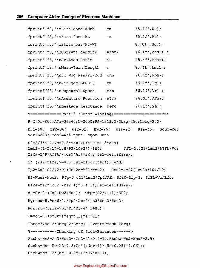
206 Computer-Aided Design of Electrical Machines
fprintf(f3, '\nBare cond Wdth
fprintf(f3, '\nBare Cond Ht
fprintf(f3, '\nStrip/bar(Ht-W)
rnrn
rnrn
A/rnrn2 fprintf(f3, '\nCurrent density
fprintf(f3, '\nAv.Loss Ratio
fprintf(f3, '\nMean-Turn Length rn
fprintf(f3, '\nSt Wdg Res/Ph/20d ohm
fprintf(f3, '\nAir-gap LENGTH rnrn
fprintf(f3, '\nPephoral Speed rn/s
fprintf(f3, '\nArrnature Reaction AT/P
fprintf(f3, '\nLeakage Reactance Perc
%5.1f',Wc);
%5.1f',Hc);
%5.0f',Ncv);
% 6 . 4 f' , cds 1 )
% 5 . 4 f' , Kda v) ;
% 5 . 4 f' , Lrnt 1) ;
% 6 . 4 f' , Rph) ;
% 5 . 1 f' , Lg) ;
%5.1f',Vr) ;
%6.Of',ATa);
% 6 . 1 f' ,XL) ;
%=============Part-3 (Rotor Winding)============~=========>
P=2iDr=800iATa=36540;L=2050;PP=1313.2;Dbrg=250;Lbrg=250;
Dri=60; SP2=36; Ws2=31; Hw2=25; Wss=22; Hss=45; Wcu2=28;
Vexl=220; cds2=4;%Input Rotor Data
S2=2/3*SP2;Vc=0.8*Vexl/P;ATFL=1.5*ATa;
Lrnt2=(2*L/10+l.8*PP/10+25)/100; Afl=0.021*Lrnt2*ATFL/Vc;
Zs2a=2*P*ATFL/(cds2*Afl*S2); Zs2=ceil(Zs2a);
if (Zs2-Zs2a»=0.5 Zs2=floor(Zs2a); end;
Tp2=Zs2*S2/(2*P);Hcu2a=Afl/Wcu2; Hcu2=ceil(Hcu2a*lO)/lO;
Af=Wcu2*Hcu2; Rfp=O.021*Lrnt2*Tp2/Af; Rf20=Rfp*P; IfFL=Vc/Rfp;
Hs2a=Zs2*Hcu2+(Zs2-1)*O.4+14;Hs2=ceil(Hs2a);
dk=Dr-2*(Hs2+Hw2+Hss); wtp=(S2/4.+1)/SP2;
Kgrtcu=8.ge-6*2.*Tp2*Lrnt2*le3*Wcu2*Hcu2;
Kgrtst=7.85E-*pi*Dr*Dr/4*(L+80);
Prnech=1.15*Dr A 4*sqrt(L)*lE-ll;
Pbrg=3.8e-6*Dbrg A 2*Lbrg; Pvent=Prnech-Pbrg;
%-----------Checking of Slot-Balances------>
Rtsbh=Hs2-Zs2*Hcu2-(Zs2-1)*0.4-14;Rtsbw=Ws2-Wcu2-2.9;
Stsbh=Hs-(Hw+HL+7.5+Zs*((Ncv+l)*(Hc+0.25)+7.06));
Stsbw=Ws-(2*(Wc+ 0.25)+2*HVins+l);
www.EngineeringEBooksPdf.com
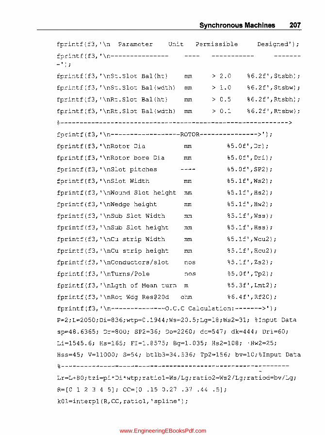
fprintf(f3, '\n Parameter
fprintf(f3, '\n--------------- , ) ;
Unit
fprintf(f3, '\nSt.Slot Bal(ht) rom
fprintf(f3, '\nSt.Slot Bal(wdth) rom
fprintf(f3, '\nRt.Slot Bal(ht) rom
fprintf(f3, '\nRt.Slot Bal(wdth) rom
Synchronous Machines 207
Permissible
> 2.0
> 1. 0
> O.S
> 0.1
Designed');
%6.2f' ,Stsbh);
%6.2f' ,Stsbw);
%6.2f' ,Rtsbh) i
%6.2f' ,Rtsbw);
%----------------------------------------------------------->
fprintf(f3, '\n------------------ROTOR--------------->');
fprintf(f3, '\nRotor Dia
fprintf(f3, '\nRotor bore Dia
fprintf(f3, '\nSlot pitches
rom
rom
fprintf(f3, '\nSlot Width rom
fprintf(f3, '\nWound Slot height rom
fprintf{f3, '\nWedge height rom
fprintf(f3, '\nSub Slot Width rom
fprintf(f3, '\nSub Slot height rom
fprintf(f3, '\nCu strip Width rom
fprintf(f3, '\nCu strip height rom
fprintf(f3, '\nConductors/slot nos
fprintf(f3, '\nTurns/Pole nos
fprintf(f3, '\nLgth of Mean turn m
fprintf(f3, '\nRot Wdg Res@20d ohm
%S.Of',Dr);
% S . 0 f' , Dr i) ;
%S.Of',SP2)i
%S.lf',Ws2);
%S.lf',Hs2);
%S.lf',Hw2);
%S.lf',Wss);
% S . 1 f' , Hs s) ;
%S.lf' ,Wcu2);
% S . 1 f' , Hcu2) ;
%S.lf',Zs2);
% S . 0 f' , Tp2) ;
%S.3f',Lmt2);
%6.4£' ,Rf20);
fprintf(f3, '\n--------------O.C.C Calculation:------->');
P=2;L=20S0;Di=836;wtp=O.1944;Ws=20.S;Lg=18;Ws2=31; %Input Data
sp=48.636S; Dr=800; SP2=36; Do=2260; dc=S47; dk=444; Dri=60;
Li=lS45.6; Hs=165; FI=1.8575; Bg=1.03S; Hs2=108; 'Hw2=2S;
Hss=45; V=11000; S=54; btlb3=34.536; Tp2=156; bv=10;%Input Data
%-----------------------------------------------------------
Lr=L+80;tzi=pi*Di*wtp;ratiol=Ws/Lg;rati02=Ws2/Lg;ratiod=bv/Lg;
R= [0 1 2 3 4 5]; CC= [ 0 . IS O. 27 . 37 . 44 . 5] ;
kOl=interpl(R,CC,ratiol, 'spline');
www.EngineeringEBooksPdf.com

208 Computer-Aided Design of Electrical Machines
k02=interp1(R,CC,ratio2, 'spline');
kl=interp1(R,CC,ratiod, 'spline');
ks1=sp/(sp-k01*Ws); ys2=pi*Dr/SP2; kd1=bv/(bv-k1*bv); kgus=ks1*kd1; Lfps=2/3*pi*(Do-dc)/le3/P;
ks2=ys2/(ys2-k02*Ws2); kgs=(ks1+ks2-1.)*kd1;
Smax=(Lr+0.3333*dk)*dk/1e6;Lsmax=(dk-Dri)/2e3;
%---------------------------------------------------------->
Epu(1)=1.0;Epu(2)=1.1;Epu(3)=1.2~Epu(4)=1.3;
for ij=1:25;BB(ij)=0.1*ij;end;
%-------------B-H Curve From graph (for Lohys material7
HH=[50 65 70 80 90 100 110 120 150 180 220 295 400 580 1000 2400 5000 8900 15e3 24e3 40e3 65e3 10e4 15e4 24e4];
%semilogx(HH,BB);grid;xlabel('AT/m-->');
%ylabel('Flux density(T)-->');
%title('Magnetization Curve for Lowhys Stamping Steel');
for j=1:4; ELL(j)=Epu(j)*V;flux(j)=Epu(j)*FI;
ATgap(j)=8e5*Epu(j)*Bg*Lg/1e3*kgus;
Bst1b3(j)=Epu(j)*FI*le6/(bt1b3*Li*S/P) ;
atst(j)=interp1(BB,HH,Bst1b3(j), 'spline');
ATst(j)=atst(j)*Hs/ 1e3;
" Bstc(j)=flux(j)*0.5*le6/(dc*Li);
atsc(j)=interp1(BB,HH,Bstc(j), 'spline') ;ATsc(j)=atsc(j)*Lfps;
Brt1b3(j)=
Epu(j)*Bg*tzi*Li*1.36/Lr/(pi*(Dr-4./3.*(Hs2+Hw2+Hss))*wtp);
atrt(j)=interp1(BB,HH,Brt1b3(j), 'spline');
ATrt(j)=atrt(j)*(Hs2+Hw2+Hss)/le3; Brtc(j)=Epu(j)*1.05*FI/Smax;
atrc(j)=interp1(BB,HH,Brtc(j), 'spline');
ATrc(j)=atrc(j)*Lsmax;
ATtot(j)=ATgap(j)+ATst(j)+ATsc(j)+ATrt(j)+ATrc(j);
Ifocc(j)=ATtot(j)/Tp2;Ifgap(j)=ATgap(j)/Tp2;
IFOCC(j+1)=Ifocc(j);EPU(j+1)=Epu(j);end;IFOCC(1)=0;EPU(1)=0;
%plot(IFOCC,EPU);grid;xlabel('If(amps)-->'); %yla~el('Volts(PU)-->');
www.EngineeringEBooksPdf.com

Synchronous Machines 209
%title('OCC of Non-Salient Pole Generator');
%-------------------------------------------------
%--------------- OCC--------------------*/
fprintf(f3, '\nE(L-L)pu %6.2f %6.2f',Epu(1),Epu(2),Epu(3),Epu(4));
fprintf(f3, '\n---------
fprintf(f3, '\nE(L-L) V %6.0f %6.0f',ELL(1),ELL(2),ELL(3), ELL(4));
fprintf(f3, '\nFlux(Wb) %6.2f %6.2f',flux(1),flux(2),flux(3),flux(4));
%6.2f
%6.0f
%6.2f
%6.2f
-----');
%6.0f
%6.2f
fprintf(f3, '\nSt.Core(Wb/m2)%6.3f%6.3f%6.3f%6.3f',Bstc(1),Bstc( 2) ,Bstc(3), Bstc(4));
fprintf(f3, '\nSt.Core-AT/Mt %6.0f %6. Of %6.0f %6.0f',atsc(1),atsc(2),atsc(3),atsc(4) );
fprintf(f3, '-> for Lohys steel');
fprintf(f3, '\nSt.Core-AT%6.0f 6.0f %6.0f %6.0f',ATsc(1),ATsc(2),ATsc(3),ATsc(4));
intf(f3, '\nSt.Tooth(Wb/m2)%6.3f%6.3f%6.3f%6.3f',Bstlb3(1),Bstlb 3(2),stlb3(3),Bstlb3(4));
printf(f3, '\nSt.Tooth-AT/Mt %6.0f %6.0f',atst(1),atst(2),atst(3),atst(4));
fprintf(f3, '-> for Lohys steels');
fprintf(f3, '\nSt.Tooth-AT%6.0f%6.0f%6.0f %6.0f',ATst(1),ATst(2),ATst(3),ATst(4) );
%6.0f %6.0f
fprintf(f3, '\nAir.GapAT%6.0f%6.0f%6.0f%6.0f',ATgap(1),ATgap(2),ATgap(3), ATgap(4));
fprintf(f3, '\nRt.WTth(Wb/m2)%6.3f%6.3f%6.3f%6.3f',Brtlb3(1),Brt Ib3(2),Brtlb3 (3),Brtlb3(4));
fprintf(f3, '\nRt.Tooth-AT/Mt %6.0f %6.0f',atrt(1),atrt(2),atrt(3),atrt(4) );
fprintf(f3, ,-> for Lohys steels');
fprintf(f3, '\nRt.Tooth-AT%6.0f%6.0f%6.0f %6.0f',ATrt(1),ATrt(2),ATrt(3),ATrt(4) );
%6.0f %6.0f
fprintf(f3, '\nRt.Core(Wb/m2)%6.3f%6.3f%6.3f%6.3f',Brtc(1),Brtc(
2),Brtc(3), Brtc(4));
www.EngineeringEBooksPdf.com

210 Computer-Aided Design of Electrical Machines
fprintf(f3, '\nRt.Core-AT/Mt%6.0f
%6.0f',atrc(l),atrc(2),atrc(3),atrc(4) );
fprintf(f3, '-> for Lohys steels');
%6.0f %6.0f
fprintf(f3, '\nRt.Core-AT%6.0f%6.0f%6.0f%6.0f',ATrc(1),ATrc(2),
ATrc(3),ATrc(4));
fprintf(f3, '\nTotal-OCC-AT%6.0f%6.0f%6.0f%6.0f',ATtot(l),
ATtot(2),ATtot(3),ATtot(4));
fprintf(f3, '\nlf-OCC-Amps%6.1f%6.1f%6.1f%6.1f',
Ifocc(l),Ifocc(2),Ifocc(3), Ifocc(4));
fprintf(f3, '\nlf-Airgap-Amps%6.1f%6.1f%6.1f%6.1f',Ifgap(l),
Ifgap(2),Ifgap(3), Ifgap(4));
fprintf(f3, '\n--------------Other Calculations:---------------
--->');
Ifar=ATa/Tp2; Ifsc=(ATa+XLpu*ATgap(l))/Tp2: IfO=Ifocc(l);
scr=IfO/lfsc; pf=rpf; pfr=sqrt(l-pf*pf);
E1=sqrt(1.0*pf*pf+(1*pfr+XLpu)A2):
If1=interp1(Epu,Ifocc,E1, 'spline');
IfFL=sqrt(If1A2+IfarA2-2*If1*Ifar*cos(pi/2+acos(pf)));
EO=interp1(Ifocc,Epu,IfFL, 'spline'); reg=(EO-Epu(l))*lOO;
cds2= IfFL/Af; Vfn=IfFL*Rf20*(235.+120.)/255; Vex1=1.1*Vfn;
Vex=ceil(Vex1/S)*S: Iex1=1.1*IfFL; Iex=ceil(Iex1/10) *10;
KWex=Vex*Iex/1e3; Pcu2=IfFL*IfFL*Rf20*(235.+75.)/255e3;
KgT=l.Ol*(Kgstst+Kgstcu+Kgrtcu+Kgrtst); Kgpkva=KgT/KVA;
Pt=Pcu1+Padd+Pmech+Pcu2+Pi;Eff=KW/(KW+Pt) *100.; Pcool=Pt-Pbrg;
Qair=ceil(Pcool*le3/1140./24.)*1.0; Tair=Pcool*le3/1140./Qair;
%--------------------------------------------------------------
fprintf(f3, '\nlf-Arm reaction Amps %5.1f',Ifar);
fprintf(f3, '\nlfscc Amps %5.1f',Ifsc);
fprintf(f3, '\nSCR pu %5.3f',scr);
fprintf(f3, '\nNo Ld Rot Current Amps % 5.lf' , If 0 ) ;
fprintf(f3, '\nRot Current at FL Amps %5.1f',IfFL);
fprintf(f3, '\nVoltage Regulation (perc) %5.1f',reg);
fprintf(f3, '\nFL-Rot-Cur-dens A/mm2 %5.2f',cds2)
www.EngineeringEBooksPdf.com
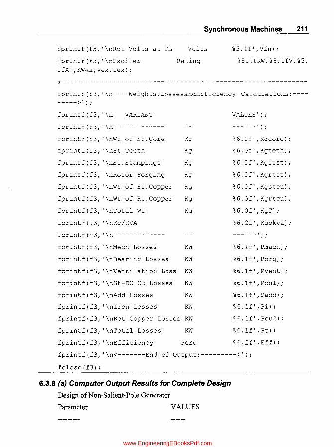
Synchronous Machines 211
rprintf(f3, '\nRot Volts at FL Volts %5.1f',Vfn);
fprintf(f3, '\nExciter Rating %5.1fKW,%5.1fV,%5.
IfA',KWex,Vex,Iex);
%--------------------------------------------------------------
fprintf(f3, '\n----Weights,LossesandEfficiency Calculations:-------->');
fprintf(f3, '\n VARIANT
fprintf(f3, '\n------------
fprintf(f3, '\nWt of St.~ore
fprintf(f3, '\nSt.Teeth
fprintf(f3, '\nSt.Stampings
fprintf(f3, '\nRotor Forging
fprintf(f3, '\nWt of St.Copper
fprintf(f3, '\nWt of Rt.Copper
fprintf(f3, '\nTotal Wt
fprintf(f3, '\nKg/KVA
fprintf(f3, '\n-------------
Kg
Kg
Kg
Kg
Kg
Kg
Kg
fprintf(f3, '\nMech Losses ~N
fprintf(f3, '\nBearing Losses KW
fprintf(f3, '\nVentilation Loss KW
fprintf(f3, '\nSt-DC Cu Losses KW
fprintf(f3, '\nAdd Losses KW
fprintf(f3, '\nIron Losses KW
fprin~f(f3, '\nRot Copper Losses KW
fprintf(f3, '\nTotal Losses
fprintf(f3, '\nEfficiency
KW
Perc
VALUES');
------') ;
% 6. 0 f' , Kgcore) i
%6.0f' ,Kgteth);
%6.0f' ,Kgstst);
%6.0f' ,Kgrtst);
%6.0f' ,Kgstcu);
%6.0f' ,Kgrtcu);
% 6 . 0 f' , KgT) ;
%6.2f' ,Kgpkva);
------');
% 6. If' , Pmech) ;
% 6. 1 f' , Pbrg) ;
%6.1f',Pvent);
%6.1f',Pcul);
%6.1f',Padd);
%6.lf' ,Pi);
%6.1f',Pcu2);
% 6 . 1 f' , Pt) ;
%6.2f' ,Eff);
fprintf(f3, '\n<-------End of Output:--------->');
fclose (f3) ;
6.3.8 (a) Computer Output Results for Complete Design
Design of Non-Salient-Pole Generator
Parameter V ALVES
www.EngineeringEBooksPdf.com

212 Computer-Aided Design of Electrical Machines
KVA 30000
KW 24000
Volts 11000
PF 0.800
HZ 50
R.P.M 3000
No. of Poles 2
FluxIPole Wb 1.8575
GapFlux-den(Av) Wb/m2 0.6900
Sp.E1ec Loading Aclm 58000
-----------------SllAll()Ft---------------»
Stator Current Amps 1574.5
C()FtE LENGllH(tot) mm 2050
Iron LENGllH mm 1680
Vent Ducts No X mm 37 X 10
C()FtE ()D mm 2260
C()FtE ID mm 836
P()LE PI1lCH mm 1313.2
1lUFtNSIPh 18
Sll A ll()Ft SL()llS 54
Chording Pitch 26/27
SL()ll PI1lCH mm 48.64
Core depth mm 547.0
CoreFlux-den Wb/m2 1.0985
SL()ll WIDllH ' mm 20.5
SL()ll Height(tot) mm 165.0
Ht (Lip+Wedge) mm 25+9
Flux-den(tooth-tip) Wb/m2 1.5820
Conductors/Slot 2
Bare cond W dth mm 6.0
Bare CondHt mm 1.8
Strip/bar(Ht-W) 25
Current density Almm2 2.9752
www.EngineeringEBooksPdf.com
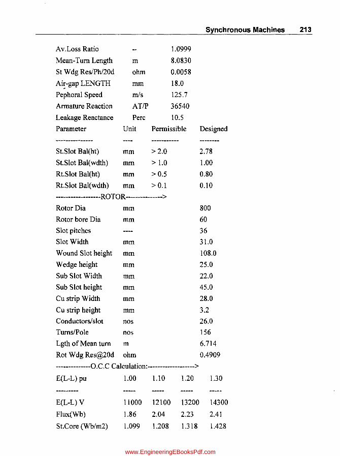
Synchronous Machines 213
A v .Loss Ratio 1.0"999
Mean-Turn Length m 8.0830
St W dg ResIPhl20d ohm 0.0058
Ai~-gap LENGTH mm 18.0
Pephoral Speed mls 125.7
Annature Reaction ATIP 36540
Leakage Reactance Perc 10.5
Parameter Unit Permissible Designed
--------------- -----------St.Slot Bal(ht) mm > 2.0 2.78
St.Slot Bal(wdth) mm > 1.0 1.00
Rt.Slot Bal(ht) mm >0.5 0.80
Rt.Slot Bal(wdth) mm > 0.1 0.10
------------------ROTO R --------------->
Rotor Dia mm 800
Rotor bore Dia mm 60
Slot pitches 36
Slot Width mm 31.0
Wound Slot height mm 108.0
Wedge height mm 25.0
Sub Slot Width mm 22.0
Sub Slot height mm 45.0
Cu strip Width mm 28.0
Cu strip height mm 3.2
Conductors/slot nos 26.0
TurnslPole nos 156
Lgth of Mean turn m 6.714
Rot Wdg Res@20d ohm 0.4909
--------------0. C. C Calculation: ------------------->
E(L-L) pu 1.00 1.10 1.20 1.30
---------E(L-L) V 11000 12100 13200 14300
Flux(Wb) 1.86 2.04 2.23 2.41
St.Core (Wb/m2) 1.099 1.208 1.318 1.428
www.EngineeringEBooksPdf.com

214 Computer-Aided Design of Electrical Machines
St.Core-A T IMt 219 302 427 646
St. C ore-AT 393 542 766 1159
St. Tooth(Wb/rn2) 1.289 1.418 1.547 1.675
St.Tooth-ATlMt 385 620 1503 4261
St.Tooth-A T 64 102 248 703
Air.Gap-AT 17589 19348 21107 22866
Rt. WTth(Wb/m2) 1.518 1.669 1.821 1.973
Rt.Tooth-ATlMt 1160 4085 9998 21038
Rt.Tooth-AT 206 727 1780 3745
Rt.Core (Wb/rn2) 1.928 2.121 2.314 2.507
Rt.Core-A T IMt 17110 44501 105719 248382
Rt.Core-AT 3285 8544 20298 47689
Total-OCC-A T 21538 29264 44199 76162
If-OCC-Amps 138.1 187.6 283.3 488.2
If-Airgap-Amps 112.8 124.0 135.3 146.6
--------------Oth er Cal culations: ------------------->
If-Arm reaction Amps 234.2
Ifscc Amps 246.1
SCR pu 0.561
No Ld Rot Current Amps 138.1
Rot Current at FL Amps 361.7
Voltage Regulation(perc) 23.3
FL-Rot-Cur-dens Almm2 4.04
Rot Volts at FL Volts 247.~
Exciter Rating 110.0KW,275.0V,400.0A
----Weights, Losses and Efficiency Calculations:--------->
VARIANT VALUES
-------------Wt. of St.Core Kg 35716
St.Teeth Kg 4079
St. Stamp ings Kg 39795
Rotor Forging Kg 8405
" ,
www.EngineeringEBooksPdf.com
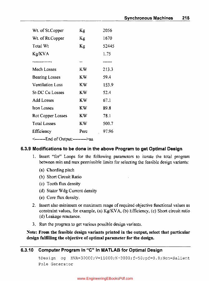
Wt. of St.Copper
Wt. of Rt.Copper
Total Wt
Kg/KVA
Mech Losses
Bearing Losses
Ventilation Loss
St-DC Cu Losses
Add Losses
Iron Losses
Rot Copper Losses
Total Losses
Efficiency
Kg
Kg
Kg
KW
KW
KW
KW
KW
KW
KW
KW
Perc
<-------End of Output: --------->aa
2056
1670
52445
1.75
213.3
59.4
153.9
52.4
67.1
89.8
78.1
500.7
97.96
Synchronous Machines 215
6.3.9 Modifications to be done in the above Program to get Optimal Design
1. Insert "for" Loops for the following parameters to iterate the total program between min and max permissible limits for selecting the feasible design variants:
(a) Chording pitch
(b) Short Circuit Ratio
(c) Tooth flux density
(d) Stator Wdg Current density
(e) Core flux density.
2. Insert also minimum or maximum range of required objective functional values as constraint values, for example, (a) KglKVA, (b) Efficiency, (c) Short circuit ratio (d) Leakage reactance.
3. Run the program to get various possible design variants.
Note: From the feasible design variants printed in the output, select that particular design fulfilling the objective of optimal parameter for the design.
6.3.10 Computer Program in "C" in MATLAB for Optimal Design
%Design og KVA=30000;V=11000;N=3000;f=50;pf=O.8;Non-Salient
Pole Generator
www.EngineeringEBooksPdf.com
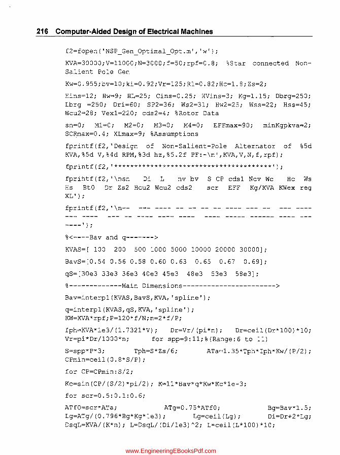
216 Computer-Aided Design of Electrical Machines
f2=fopen('NSP_Gen_Optimal_Opt.m', 'w');
KVA=30000;V=11000;N=3000;f=50;rpf=0.8; ~Star connected NonSalient Pole Gen
Kw=0.955;bv=10;ki=0.92;Vr=125;R1=0.82;Hc=1.8;Zs=2;
Hins=12; Hw=9; HL=25; Cins=0.25; HVins=3; Kg=1.15; Dbrg=250; Lbrg =250; Dri=60; SP2=36; Ws2=31; Hw2=25; Wss=22; Hss=45; Wcu2=28; Vex1=220; cds2=4; %Rotor Data
sn=O; M1=0; M2=0; M3=0; M4=0; EFFmax=90; minKgpkva=2; SC~ax=0.4; XLmax=9; %Assumptions
fprintf(f2, 'Design of Non-Salient-Pole Alternator of %5d KVA,%5d V,%4d RPM,%3d hz,%5.2f PF:-\n',KVA,V,N,f,rpf);
fprintf(f2, '***************************************');
fprihtf(f2, '\nsn Di L nv bv Hs BtO Dr Zs2 Hcu2 Wcu2 cds2 XL') ;
fprintf(f2, '\n-- --- ---- -- --
----');
%<----Bav and q------->
S CP cds1 Ncv Wc Hc Ws scr EFF Kg/KVA KWex reg
KVAS=[ 100 200 500 1000 5000 10000 20000 30000J;
BavS=[0.54 0.56 0.58 0.60 0.63 0.65 0.67 0.69J;
qS=[30e3 33e3 36e3 40e3 45e3 48e3 53e3 58e3J;
%-------------Main Dimensions----------------------->
Bav=interp1(KVAS,BavS,KVA, 'spline');
q=interp1(KVAS,qS,KVA, 'spline'); KW=KVA*rpf;P=120*f/N;n=2*f/P;
Iph=KVA*le3/(1.7321*V); Dr=Vr/(pi*n); Dr=ceil(Dr*100)*10; Vr=pi*Dr/1000*n; for spp=9:11;%(Range:6 to 11)
S=spp*P*3; Tph=S*Zs/6; ATa=1.35*Tph*Iph*Kw/(P/2); CPmin=ceil(O.8*S/P);
for CP=CPmin:S/2;
Kc=sin(CP/(S/2)*pi/2); K=11*Bav*q*Kw*Kc*le-3;
for scr=0.5:0.1:0.6;
ATfO=scr*ATa; ATg=0.75*ATfO; Bg=Bav*1.5; Lg=ATg/(O.796*Bg*Kg*le3); Lg=ceil(Lg); Di=Dr~2*Lg;
DsqL=KVA/(K*n); L=DsqL/(Di/1e3)A2; L=ceil(L*100)*10;
www.EngineeringEBooksPdf.com

Synchronous Machines 217
PP=pi*Di/P; Ls=Rl*L; nv=(L-Ls)/bv; FI=Bav*pi*Di*L*le-6/P;
nv=eeil(nv); Ls=(L-nv*bv); Li=Ls*ki;rat2=Lg/PP;
for BtO=1.6:0.l:l.9;
%-----(Part-2)Stator Winding' and Core---------------->
sp=pi*Di/S;btO=FI*le6/(BtO*Li*S/P);Ws=sp-btO;
for edsl=3:0.S:4%(Permissible Range:3 to S A/sq.mm)
Asl=Iph/edsl; Wel=((Ws-2*HVins-2.S)/2); We=floor (Wel) ; Nevl=Asl/(He*We*2); edsl=Iph/As;
Nev=eeil (Nevl) ;
Hbar=(Nev+l)* (He+Cins)+2*HVins; Hs=eeil(Hsl); p=2*Nev; KdTL=1+(alfa*He/10)A4*p*(p-l)/3;
As=0.98*Nev*Hc*Wc*2; Ws=2*We+2*HVins+2.S;
Hsl=2*Hbar+Hins+Hw+HL; alfa=sqrt(2*Wc/Ws);
Kdav=1+(alfa*He/10)A4*(2*Nev)A2/9; Lmtl=(2*L/10+2.S*PP/10+S*V/le3+1S)/ 100;
Rph=0.02l*Lmtl*Tph/As; Peus=3*IphA2*Rph/le3; Peddy=(Kdav-l)*Peus; Pts=(Pcus+Peddy)*1.1Si Reff=Iph*Rph*Kdav/(V/sqrt(3)); btO=sp-Ws; BtO=FI*le6/(btO*Li*S/P); btlb3=pi*(Di+Hs*2/3)/S-Ws;
Btlb3=FI*le6/(btlb3*~i*S/P); Fle=FI/2;for Be=1.1:0.1:1.2;
Do=eeil(Dol/10)*10; del=Fle/(Be*Li)*le6; Dol=Di+2*(Hs+del)i
de=(Do-Di-2*Hs)/2;Be=Fle/(de*Li)*le6;
Stsbh=Hs(Hw+HL+7.S+Zs*((Nev+l)*(He+0.2S)+7.06l);
Stsbw=Ws(2*(We+0.2S)+2*HVins+l);
%----------Reaetanees-------------------------------------->
hl=(Nev+l) *Zs* (He+Cins)+Zs*2*HVins+6; h3=Hw;h4= HL;WsO=Ws;
h2=(Hs-hl-HL-Hw)/2;
lamdas=(hl/3/Ws)+ (h2/Ws)+2*h3/(Ws+WsO)+h4/WsO;
phis=2.*sqrt(2.)*4*pi*le-7*Iph*Zs*Ls/1000.*lamdas;
ks=(CP*P/S-0.66)*0.73S4+0.7S; LOLdO=ks*PP*PP/pi/sp/1000; phiO=2*sqrt(2)*4*pi*le-7*Iph*Zs*LOLdO; Lflux=phil/FI; XLpu=Lflux; XL=XLpu*lOO;
phil=phis+phiO;
if XL <=10.4 eontinue;end;
%---------WeightsandLosses------------------------------
Kgcore=7.8SE-6*Li*pi/4*(Do A2-(Di+2*Hs)A2) ;
Kgstst=7.8SE-6*Li*(pi*(Do A2-Di A2)/4-S*Ws*Hs);
Kgteth=Kgstst-Kgeore; Kgstcu=3*Lmtl*As*Tph*8.ge-3;
www.EngineeringEBooksPdf.com

218 Computer-Aided Design of Electrical Machines
Pcul=3*IphA2*Rph* 1.22/le3; ac=Iph*Tph*2*3/(pi*Di/l000);
Padd=90*Di A2*sqrt (L/lOOO.)*(ac/750)A2*le-10;
Pi=(1.S*Kgteth*Btlb3 A2+l.S*Kgcore*Bc A2)/1000;
%=============Part-3 (Roto= Winding)======================>
S2=2/3*SP2; Vc=O.S*Vexl/P; ATFL=1.5*ATa;
Lmt2=(2*~/10+1.S*PP/IO+25)/100;
Zs2a=2*P*ATFL/(cds2*Afl*S2); Afl=0.02l*~mt2*ATFL/Vc;
Zs2=ceil(Zs2a);
if (Zs2-Zs2a»=0.5 Zs2=floor(Zs2a); end;
Tp2=Zs2*S2/(2*P); Hcu2a=Afl/Wcu2; Hcu2=ceil(Hcu2a*10)/10;
Af= Wcu2*Hcu2; Rfp=0.02l*Lmt2*Tp2/Af; Rf20=Rfp*P; IfFL=Vc/Rfp; Hs2a=Zs2*Hcu2+(Zs2-l)*0.4+14; Hs2=ceil(Hs2a);
dk=Dr-2*(Hs2+Hw2+Hss); wtp=(S2/4.+1)/SP2;
Kgrtcu=S.ge-6*2.*Tp2*Lmt2*le3*Wcu2*Hcu2;
Kgrtst=7.S5E-6*pi*Dr*Dr/4*(L+SO); Pmech=1.15*DrA4*sqrt(L)*lE-ll;
Pbrg=3.Se-6*DbrgA2*Lbrg; Pvent=Pmech-Pbrg;
Rtsbh=Hs2-Zs2*Hcu2-(Zs2-1) *0.4-14; Rtsbw=Ws2-Wcu2-2.9;
%--------------- O.C.C Calculation:--------------------*/
Lr=L+SO; tzi=pi*Di*wtp; ratiol=Ws/Lg; ratiod= bv/Lg;
R= [ 0 1 2 3 4 5 J; CC= [ 0 . 15 O. 27 . 37 . 44 . 5] ;
kOl=interpl(R,CC,ratiol, 'spline');
k02=interpl (R, CC, ratio2, 'spline');
kl=interpl(R,CC,ratiod, 'spline');
ratlo2=Ws2/Lg;
ksl=sp/(sp-kOl*Ws); kdl=bv/(bv-kl*bv);
ys2=pi*Dr/SP2; ks2=ys2/(ys2-k02*Ws2);
kgus=ksl*kdl;kgs=(ksl+ks2-l.)*kdl;Lfps=2/3*pi*(Do-dc)/le3/P;
Smax=(Lr+0.3333*dk)*dk/le6; Lsmax=(dk-Dri)/2e3;
%-------------------(OCC Calculation)------~--------------->
Epu(l)=l.O; Epu(2)=1.1; Epu(3)=1.2 ; Epu(4)=1.3;
for ij=1:25;BB(ij)=0.1*ij;end;
%---~---------B-H Curve From graph for Lohys material---7
HH=[50 65 70 SO 90 100 110 120 150 ISO 220 295 400 5S0 1000 2400 5000 S900 15e3 24e3 40e3 65e3 10e4 15e4 24e4];
www.EngineeringEBooksPdf.com

Synchronous Machines 219
%semilogx(HH,BB);grid;xlabel('AT/m-->') ;
%ylabel('Flux density(T)-->');
%title('Magnetization Curve for Lowhys Stamping Steel');
for j=1:4; ELL(j)=Epu(j)*V;flux(j)=Epu(j)*FI;
ATgap(j)=8e5*Epu(j)*Bg*Lg/1e3*kgus;
Bst1b3(j)=Epu(j)*FI*le6/(bt1b3*Li*S/P);
atst(j)=interp1(BB,HH,Bst1b3(j), 'spline');
ATst(j)=atst(j)* Hs/1e3; Bstc(j)=flux(j)*0.5*le6/(dc*Li);
atsc(j)=interp1(BB,HH,Bstc(j), 'spline');
ATsc(j)=atsc(j) *~fps;
Brtlb3(j)=Epu(j)*Bg*tzi*Li*1.36/Lr/(pi*(Dr4./3.*(Hs2+Hw2+Hss ) ) *wtp) ;
atrt(j)=interp1(BB,HH,Brt1b3(j), 'spline');
ATrt(j)=atrt(j)*(Hs2+Hw2+Hss)/le3; Brtc(j)=Epu(j)*1.05*FI/Smax;
atrc(j)=interp1(BB,HH,Brtc(j), 'spline');
ATrc(j)=atrc(j)*Lsmax;
ATtot(j)=ATgap(j)+ATst(j)+ATsc(j)+ATrt(j)+ATrc(j);
Ifocc(j)=ATtot(j)/Tp2; Ifgap(j)=ATgap(j)/Tp2;
IFOCC(j+1)=Ifocc(j);EPU(j+1)=Epu(j);end;
IFOCC(l)=O; EPU(l)=O;
%-------------LMC andOther Calculations:------------------->
Ifar=ATa/Tp2; Ifsc=(ATa+XLpu*ATgap(1))/Tp2; IfO=Ifocc(l);
scr2=IfO /Ifsc; if scr2 <=0.50 continue; end;
pf=rpf;pfr=sqrt(1-pf*pf);E1=sqrt(1.0*pf*pf+(1*pfr+XLpu)A2);
If1=interp1(Epu,Ifocc,E1, 'spline');
IfFL=sqrt(If1A2+IfarA2-2*If1*Ifar*cos (pi/2+acos (pf) I);
EO=interp1(Ifocc,Epu,IfFL, 'spline');reg=(EO-Epu(l) )*100; cds2= lfFL/Af; if cds2 >=4.2 continue; end; Vfn=IfFL*Rf20*(235.+120.)/255; Vex2=1.1*Vfn;
Vex=ceil (Vex2/5)*5; Iex1=1.1*IfFL; Iex=ceil(Iex1/10)*10; KWex=Vex*Iex/1e3; Pcu2=IfFL*IfFL*Rf20*(235.+75.)/255e3;
KgT=l.Ol*(Kgstst+Kgstcu+Kgrtcu+Kgrtst); Kgpkva=KgT/KVA;
if Kgpkva >=1.9 continue; end;
www.EngineeringEBooksPdf.com

220 Computer-Aided Design of Electrical Machines
Pt=Pcu1+Padd+Pmech+Pcu2+Pi; Pcool=Pt-Pbrg;
Eff=KW/(KW+Pt) *100.; if Eff <=97.5 continue; end;
Qair=ceil(Pcool*le3/1140./24.)*1.0;
Tair=Pcool*le3/1140./Qair; sn=sn+1;
if Kgpkva <=minKgpkva minKgpkva=Kgpkva;end;
if abs(Kgpkva-minKgpkva)<= 0.001 M1=sn; end;
if Eff >=EFFmax EFFmax=Eff;end;
if abs(Eff-EFFmax)<=O.Ol M2=sn; end;
if scr2 >=SCRmax SC~~ax=scr2;end;
if abs(scr2-SCRmax)<=0.001 M3=sn; end;
if XL>=XLmax XLmax=XL;end;
if abs(XL-XLmax)<=O.Ol M4=sn; end; sn,
fprintf(f2, '\n%2d%5.0f%5.0f%3d%3d%3.0f%3d%5.2f%4.0f%3.0f%5.1 f%5.1f%4.0f%5.2f',sn,Di,L,nv,bv,S,CP,cds1,Ncv,Wc~Hc,Ws,Hs,Bt 0) ;
fprintf(f2, '%5d%3d%5.1f%5.1f%5.2f%6.2f%6.2f%6.2f%5.0f%6.1f%5 .If',Dr,Zs2,Hcu2,Wcu2,cds2,scr2,Eff,Kgpkva,KWex,reg,XL);
end;end;end;end;end;end;
printf(f2, '\n-- --- ----
--' ) ;
fprintf(f2, '\nSelection Optimization Criteria:');
of Design Variant based on
fprintf(f2, '\nIf Minimum Kg/KVA is Variant (Sn)=%3d (%5.2f) ',M1,minKgpkva);
Required,
fprintf(f2, '\nIf Maximum Efficiency is Required, Variant(Sn)=%3d (%5.2f perc) ',M2,EFFmax);
fprintf (f2, '\nIf Maximum SCR is Required, Variant(Sn)=%3d (%5.2f pu) ',M3,SCRmax);
fprintf(f2, '\nIf Maximum XL is Required, Variant(Sn)=%3d (%5.1f perc) ',M4,XLmax);fclose(f2);
Select
Select
Select
Select
www.EngineeringEBooksPdf.com

6.3.10 (al Computer Output Results for Optimized Design
Design of Non-Salient-I'ole Alternator of 30000 K VA, 11000 V,3000 RPM, 50 hz, 0.801'F
Sn DI L nv bv S CI' edsl Ncv Wc lIe Ws Ib BtO Dr Zs2 lIeu2 Wcu2 cds2 scr2 1:1'1' Kg/KVA KWex reg XL -- -- ---- .. - -- .. - -- .... _- --- -- --- ---- --- ---- --- -- ---- ---- ---- ---- .. ---- ------ ---- --- ------ --- ---- -- -- -- -- ---- --- -- .. _- ---- --- ---- --- -- ---- ---- ---- ---- ----- ------ ---- --- --------
836 2050 37 10 54 26 2.98 25 6 1.8 20.5 165 158 800 26 3.2 28.0 4.04 0.56 97.96 I 75 110 23.3 105 2 836 2050 37 10 54 26 2.98 25 6 1.8 20.5 165 1.58 800 26 3.2 28.0 4.05 0.56 97Y5 1.62 110 23 I 105 3 836 2050 37 10 54 26 2.98 25 6 18 20.5 165 1.58 800 26 3.2 280 4.04 0.56 97.96 1.75 110 23.3 10.5 4 836 2050 37 10 54 26 2.98 25 6 \.8 20.5 165 1.58 800 26 3.2 28.0 4.05 0.56 9795 \.62 110 23.1 105 5 836 2050 37 10 54 27 2.98 25 6 1.8 20.5 165 1.58 800 26 3.2 280 4.04 0.56 97.96 1.75 110 23.3 10.7 6 836 2050 37 10 54 27 2.98 25 6 1.8 205 165 1.58 800 26 3.2 28.0 4.06 0.56 9795 162 110 23 I 107 7 836 2050 37 10 54 27 3.54 21 6 1.8 20.5 149 158 800 26 3.2 28.0 4.03 0.56 97.96 1.70 110 23.2 104 K 836 2050 37 10 54 27 3.54 21 6 18 205 149 1.58 800 26 3.2 28.0 405 056 9796 1.57 110 23.1 104 9 836 2050 37 10 54 27 2.98 25 6 1.8 20.5 165 1.58 800 26 3.2 28.0 4.04 056 97.96 1.75 110 233 107 10 836 2050 37 10 54 27 2.98 25 6 1.8 205 165 158 800 26 3.2 28.0 4.06 0.56 97.95 1.62 110 23 I 10.7 II 836 2050 37 10 54 27 3.54 21 6 1.8 205 149 158 800 26 3.2 28.0 4.03 056 97.96 170 110 232 104 12 836 2050 37 10 54 27 3.54 21 6 1.8 20.5 149 1.58 800 26 32 28.0 4.05 0.56 97.96 I 57 110 23.1 104 13 834 2160 39 10 60 24 298 30 5 1.8 185 186 1.59 800 25 3.6 28.0 4.11 () 51 9789 1.77 127 226 10K 14 834 2160 39 10 60 24 357 25 5 1.8 18.5 165 1.59 800 25 36 280 408 051 9789 U!4 127 226 104 15 834 2160 39 10 60 24 3.57 25 5 I 8 18.5 165 159 800 25 36 28.0 4.09 0.51 97.89 170 127 225 104 16 834 2160 39 10 60 24 2.98 30 5 18 18.5 IK6 1.59 800 25 36 211.0 411 0.51 9789 1.77 127 22.6 10K 17 834 2160 39 10 60 24 3.57 25 5 1.8 18.5 ~65 1.59 80U 25 36 28.0 408 051 97.89 184 127 22.6 104 C/J
'< 18 834 2160 39 10 60 24 3.57 25 5 1.8 18.5 165 1.59 800 25 3.6 28 () 409 0.51 9789 170 127 225 104 :s
n ___________________ .. ____________________________ ... _______________________________ .. _________ .. _ .. ____________________________________________________________________________ -_.o-;:r ...
Selection of Design Variant based on OptimizatIOn Cnteria: 0 :s
If Minimum Kg/KVA is Required, Select Variant (Sn) = 12 (1.57) 0 C
If Maximum Ellicieney is Required, Select Variant (Sn) = 12 (97.96 perc) tfj
i: If Maximum SCR is Required, Select Variant (Sn) = 12 (0.56 pu) I\)
0 IfMuximum XL is ReqUired, Select Vanant (Sn) = 16 (10.8 perc)- ::T
:s (I) tfj
N N ....
www.EngineeringEBooksPdf.com

www.EngineeringEBooksPdf.com
A
Typewritten Text
"This page is Intentionally Left Blank"

CHAPTER 7
Three-Phase Induction Motors
7.1 Introduction
Three-phase induction Motors are of two types (viz.) Squirrel Cage Rotor type and Slip-ring Rotor type. Theory portion of design is not given in this book, but necessary fonnulae-, curves and tables given in standard books are made use of.
7.1.1 Squirrel Cage Motor
Total design is split into six parts in a proper sequence. Design Calculations are given for a given Rating of an Ind motor, followed by Computer Program written in "C" language using MATLAB software for each part. Finally all the Programs are added together to get the total Program by running which we get the total design. Computer output of total design is given.
This design may not be the optimum one. Now optimization objective and design constraints are inserted into this total Program. When this program is run we will get various alternative feasible designs from which the selected variant based on the optimization criteria can be picked up. Computer output showing the important design parameters for various feasible alternatives is given in the end of this chapter along with a logic diagram.
7.1.2 Sequential Steps for Design of Each Part and Programming Simultaneously (a) Calculate Output Coefficient, Main dimensions of Stator Core (viz) D, Land
FluxIPole.
(b) Calculate Number and size of Stator slots, conductor size, by checking current density and slot balance. Calculate tooth flux density, Copper losses and Wt. of Copper, Core flux density, height of core, iron losses
(c) Calculate Air gap length, Rot dia, no. of Rotor Slots, Cond size, Copper Losses, Flux densities in tooth and Core, Weight ofrotqr copper.
(d) Calculate Carter Coefft and Ampere-turns for Air gap, Stator tooth, Stator core, Rotor tooth, ~otor core and Total No-load AT, Magnetizing current, No-Load PF.
(e) Calculation of Reactance, Short-circuit current, and ShoI1-ckt PF.
www.EngineeringEBooksPdf.com
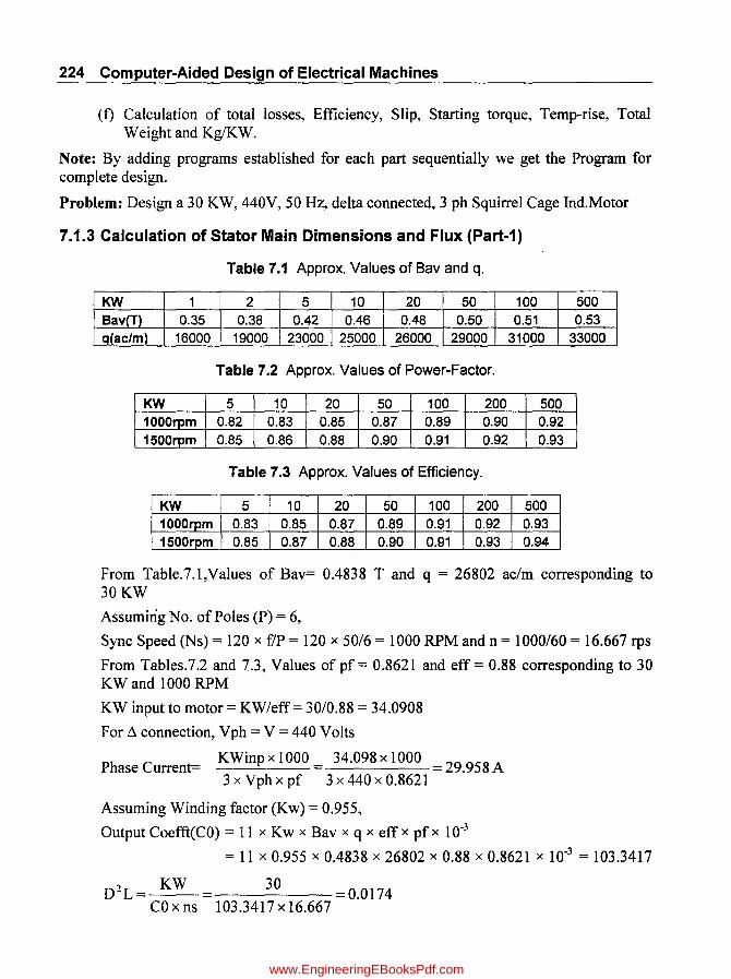
224 Computer-Aided Design of Electrical Machines
(f) Calculation of total losses, Efficiency, Slip, Starting torque, Temp-rise, Total Weight and KglKW.
Note: By adding programs established for each part sequentially we get the Program for complete design.
Problem: Design a 30 KW, 440V, 50 Hz, delta connected, 3 ph Squirrel Cage Ind.Motor
7.1.3 Calculation of Stator Main Dimensions and Flux (Part-1)
Table 7.1 Approx. Values of Bav and q.
KW 1 2 5 10 20 50 100 Bav(Tl 0.35 0.38 0.42 0.46 0.48 0.50 0.51 ~Jac/rl!t 16000 19000 23000 25000 26000 29000 31000
Table 7.2 Approx. Values of Power-Factor.
KW 5 10 20 50 100 200 500 1000lpm 0.82 0.83 0.85 0.87 0.89 0.90 0.92 1500rpm 0.85 0.86 0.88 0.90 0.91 0.92 0.93
Table 7.3 Approx. Values of Efficiency.
KW 5 10 20 50 100 200 500 1000rpm 0.83 0.85 0.87 0.89 0.91 0.92 0.93 1500rpm 0.85 0.87 0.88 0.90 0.91 0.93 0.94
500 0.53
33000
From Table.7.1,Values of Bav= 0.4838 T and q = 26802 ac/m corresponding to 30KW
Assuming No. of Poles (P) = 6,
Sync Speed (Ns) = 120 x flP = 120 x 50/6 = 1000 RPM and n = 1000/60 = 16.667 rps
From Tables.7.2 and 7.3, Values of pf = 0.8621 and eff = 0.88 corresponding to 30 KWand 1000 RPM
KW input to motor = KW/eff= 30/0.88 = 34.0908
For L1 connection, Vph = V = 440 Volts
Ph C KWinp xl 000 34.098 xl 000 29 958 A ase urrent= = = . 3xVphxpf 3x 440 x 0.8621
Assuming Winding factor (Kw) = 0.955,
Output Coefft(CO) = 11 x Kw x Bav x q x effx pfx 10.3
= 11 x 0.955 x 0.4838 x 26802 x 0.88 x 0.8621 x 10.3 = 103.3417
D2L= KW = 30 =0.0174 CO x ns 103.3417 x 16.667
www.EngineeringEBooksPdf.com

Total Core Length (L) = (0.135 X p)2
Three-Phase Induction Motors 225
0.0174
(0.135 x 6)"
= 0.1629 m = 162.9 mm::::: 160 mm (Rounded off)
Assuming Ventilating ducts (nvd) = 2, each of length (bvd) = 10 mm,
Gross iron Length (Ls) = L - nvd x bvd = 160 - 2 x 10 = 140 mm
Assuming Iron factor (ki) = 0.92, Net Iron length (Li)
= Ls x ki = 140 x 0.92 = 128.8 mm
Core inner diameter (D) = ~D2L = 0.0174 = 0.3299 m L 140/1000
= 329.9 mm::::: 330 mm (Rounded off)
. 1t x 0 1t x 330 Polepltch (PP) = --= = 172.79 mm
P 6
_L_e_n.=.gt_h_ = _14_0_ = 0.926 (::::: 1 and hence OK) Polepitch 172.79
. . 1txD 1tx330 Penphoral Veloclty(V) = --= = 17.28 m / s (::S 30 and hence OK)
ns 16.67
Flux (FI) = 1t x 0 x Lx Bav = 1t x 330 x 140 x 0.4838 = 0.0134 Wb Pxl06 6xl06
7.1.3 (a) Computer Program in IIC" in MATLAB for Part-1
% 3ph, KW = 30;V = 440; P = 6; f = 50Sq.Cage 1M
%------------Standard Curves/Tables for%Data-------------->
SKW=[125 10 20 50 100 500J;
SBav=[0.35 0.38 0.42 0.46 0.48 0.50 0.51 0.53];
Sq=[16e3 1ge3 23e3 25e3 26e3 2ge3 31e3 33e3];
SKWa=[5 10 20 50 100 200 500J;
SPF6P=[0.82 0.83 0.85 0.87 0.89 0.9 0.92]; %for 1000RPM
SEFF6P=[0.83 0.85 0.87 0.89 0.91 0.92 0.93];% for 1000R2M
SPF4P=[0.85 0.86 0.88 0.9 0.91 .92 .93J;% for 1500RPM
SEFF4P=[.85 .87 .88 .9 .91 .93 .94J;% for 1500RPM
% (l)<-----------Main Dimensions----------------------->
KW=30;V=440if=50i P=Qi %1nput Da~a------>
insW=3.4;Hw=4iHL=liinsH=6ir.vd=2;bvd=0.01;ki=O.92iBc=1.35iVph=V;
%Assumptions
www.EngineeringEBooksPdf.com
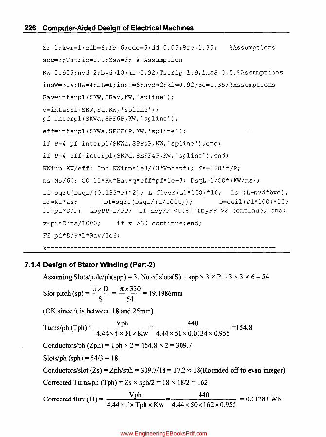
226 Computer-Aided Design of Electrical Machines
Zr=1;kwr=1;cdb=6;Tb=6;cde=6;dd=0.05;Brc=1.35; %Assump~ions
spp=3;Tstrip=1.9;Zsw=3; % Assumption
Kw=0.955;nvd=2;bvd=10;ki=0.92;Tstrip=1.9;insS=0.5;%Assumptions
insW=3.4;Hw=4;HL=1;insH=6;nvd=2;ki=0.92;Bc=1.35;%Assumptions
Bav=interp1(SKW,SBav,KW, 'spline');
q=interpl(SKW,Sq,KW, 'spline');
pf=interp1(SKWa,SPF6P,KW, 'spline');
eff=interp1(SKWa,SEFF6P,KW, 'spline');
if P=4 pf=interp1(SKWa,SPF4P,KW, 'spline') ;end;
if P=4 eff=interp1(SKWa,SEFF4P,KW, 'spline');end;
KWinp=KW/eff; Iph=KWinp*le3/(3*Vph*pf); Ns=120*f/P;
ns=Ns/60; CO=11*Kw*Bav*q*eff*pf*le-3; DsqL=l/CO*(KW/ns);
Ll=sqrt(DsqL/(0.135*P)A2); L=floor(L1*100) *10; Ls=(L-nvd*bvd);
Li=ki*Ls; D1=sqrt(DsqL/(L/1000)); D=ceil(D1*100)*10;
PP=pi*D/P; LbyPP=L/PP; if LbyPP <0.81 I LbyPP >2 continue; end;
v=pi*D*ns/1000; if v >30 continue; end;
FI=pi*D/P*L*Bav/1e6;
%-----------------------------------------------------------
7.1.4 Design of Stator Winding (Part-2)
Assuming Slots/pole/ph(spp) = 3, No ofslots(S) = spp x 3 x P = 3 x 3 x 6 = 54
• 1t x D 1t x 330 Slot pItch (sp) = -- = = 19.1986mm
. S 54
(OK since it is between 18 and 25mm)
Turns/ph (Tph)= Vph = ____ 4_40 ____ =154.8 4.44 x f x FI x Kw 4.44 x 50 x 0.0134 x 0.955
Conductors/ph (Zph) = Tph x 2 = 154.8 x 2 = 309.7
Slots/ph (sph) = 54/3 = 18
Conductors/slot (Zs) = Zph/sph = 309.7/18 = 17.2::::: 18(Rounded off to even integer)
Corrected Turns/ph (Tph) = Zs x sph/2 = 18 x 18/2 = 162
Corrected flux (FJ) = Vph 440 = 0.01281 Wb 4.44 x f x Tph x Kw 4.44 x 50 x 162 x 0.955
www.EngineeringEBooksPdf.com
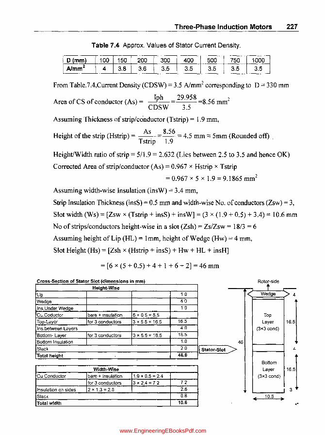
Three-Phase Induction Motors 227
Table 7.4 Approx. Values of Stator Current Density.
From Table.7.4,Current Density (CDSW) = 3.5 Almm2 corresponding to D = 330 mm
Area ofCS of conductor (As) = Iph = 29.958 =8.56 mm2
CDSW 3.5
Assuming Thickness of strip/conductor (Tstrip) = 1.9 mm,
Height of the strip (Hstrip) = ~= 8.56 = 4.5 mm::::: 5mm (Rounded oft) . Tstnp 1.9
Height/Width ratio of strip = 5/1.9 = 2.632 (Lies between 2.5 to 3.5 and hence OK)
Corrected Area of strip/conductor (As) = 0.967 x Hstrip x Tstrip
= 0.967 x 5 x 1.9 = 9.1865 mm2
Assuming width-wise Insulation (insW) = 3.4 mm,
Strip Insulation Thickness (insS) = 0.5 mm and width-wise No. of conductors (Zsw) = 3,
Slot width (Ws) = [Zsw x (Tstrip + insS) + insW] = (3 x (1.9 + 0.5) + 3.4) = 10.6 mm
No of strips/conductors height-wise in a slot (Zsh) = Zs/Zsw = 18/3 = 6
Assuming height of Lip (HL) = Imm, height of Wedge (Hw) = 4 mm,
Slot Height (Hs) = [Zsh x (Hstrip + insS) + Hw + HL + insH]
= [6 x (5 + 0.5) + 4 + 1 + 6 + 2] = 46 mm
Cross-Section of Stator Slot (dimensions in mm)
Height-Wise
Rotor-side
t lip 1 0 < Wedge >4 Wedge 40
Ins. Under Wed e 10
CU.Coductor bare + Insulation 5 + 0 5 = 5.5 Top
Top-Layer for 3 conductors 3 x 55= 16.5 16.5 Layer 16.5 40 (3x3 cond)
for 3 conductors 3x 5.5= 16.5 16.5 1.0 46 20 I Stator-Slot > 4
46.0 Total hei ht
Width-Wise
Cu Conductor bare + insulation 1.9 + 0.5 = 2.4 for 3 conductors 3 x 2.4 = 72 72
Insulation on sides 2 x 1.3 = 2.6 2.6
Bottom
Layer 16.5 (3x3 cond)
I 3 I Slack 0.8
Total width 10.6 II 10.6 ~ .-
www.EngineeringEBooksPdf.com
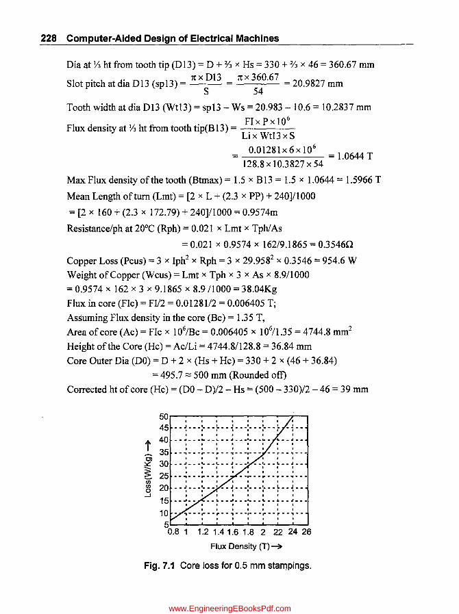
228 Computer-Aided Design of Electrical Machines
Dia at Y3 ht from tooth tip (DI3) = D + % x Hs = 330 + % x 46 = 360.67 mm •. 1t x Dl3 1t x 360.67
Slot pItch at dla Dl3 (spI3) = = = 20.9827 mm S 54
Tooth width at dia D13 (Wtl3) = spl3 - Ws = 20.983 - 10.6 = 10.2837 mm
. . FIxPxl06
Flux densIty at Y3 ht from tooth tIp(BI3) = ----Lix Wtl3xS
0.01281x6xl06
------ = 1.0644 T 128.8 xl 0.3827 x 54
Max Flux density of the tooth (Btmax) = 1.5 x Bl3 = 1.5 x 1.0644 = 1.5966 T
Mean Length of tum (Lmt) = [2 x L + (2.3 x PP) + 240]/1000
= [2 x 160 + (2.3 x 172.79) + 240]11000 = 0.9574m
Resistance/ph at 20°C (Rph) = 0.021 x Lmt x Tph/As
= 0.021 x 0.9574 x 162/9.1865 = 0.35460
Copper Loss (Pcus) = 3 x Iph2 x Rph = 3 x 29.9582 x 0.3546 = 954.6 W
Weight of Copper (Wcus) = Lmt x Tph x 3 x As x 8.911000
= 0.9574 x 162 x 3 x 9.1865 x 8.911000 = 38.04Kg
Flux in core (FIc) = FII2 = 0.0128112 = 0.006405 T;
Assuming Flux density in the core (Bc) = 1.35 T,
Area of core (Ac) = FIc x 106/Bc = 0.006405 x 10611.35 = 4744.8 mm2
Height of the Core (Hc) = AclLi = 4744.8/128.8 = 36.84 mm
Core Outer Dia (DO) = D + 2 x (Hs + Hc) = 330 + 2 x (46 + 36.84)
= 495.7 ::::: 500 mm (Rounded oft)
Corrected ht of core (Hc) = (DO - D)/2 - Hs = (500 - 330)/2 - 46 = 39 mm
• I • • • • •
45 .... ~ ... -: ... -: .... ~ ... -: .... -: .... -:-I I • •
t 40 35 .. -~ .. --~- .. ~ .. -~ ...... :--- ... -~ .... ~-. a . I • I ••• I
~ 30 .... ~ .... .. :_ .... ~ .... ~ .. .... I .... :_ .... ~ .... ~ ....
~ en CIl o -I
25 .... ~ ...... ~ .... ~ .... I .. _:_ .... ~ .... ~ .... ~ ...... , • • I • • I I
20 .... ~ .... .. :- .... ' .... { .... -:- .... :- .... ~ .... ~ .... • I • • • I • I 15 --._- __ L __ • ___ ~ __ ~ __ • __ J __ _
• • I • • I I •
10 .. ,-- .. ~ .... ~ .. -~ .... -:---~ .... ~--~--I I • • I • • •
1.2 1.4 1.6 1.8 2 22 24 26
Flux Density (T) ~
Fig. 7.1 Core 1055 for 0.5 mm stalT)pings.
www.EngineeringEBooksPdf.com
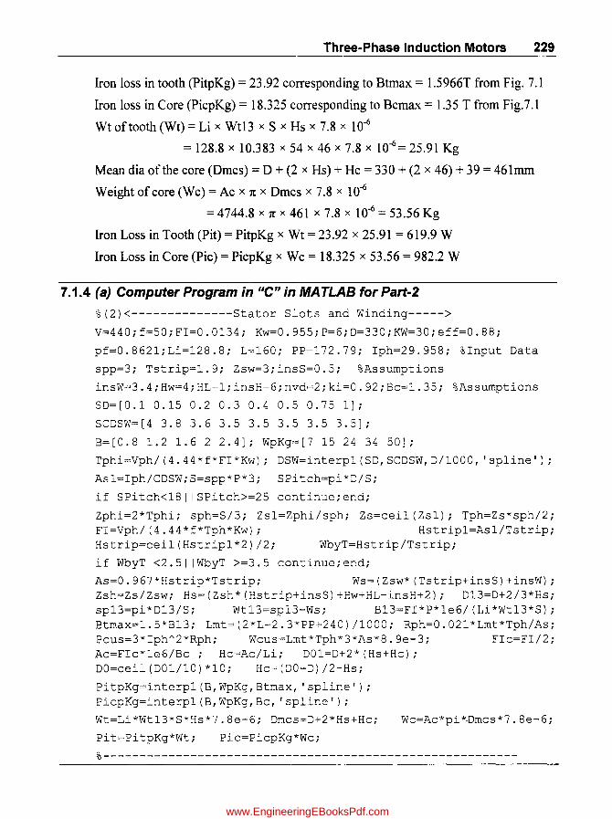
Three-Phase Induction Motors 229
Iron loss in tooth (PitpKg) = 23.92 corresponding to Btmax = 1.5 966T from Fig. 7.1
Iron loss in Core (PicpKg) = 18.3 25 corresponding to Bcmax = 1.3 5 T from Fig. 7.1
Wt of tooth (Wt) = Li x Wt13 x S x Hs x 7.8 x 10-6
= 128.8 x 10.383 x 54 x 46 x 7.8 x 10-6 = 25.91 Kg
Mean dia of the core (Dmcs) = D + (2 x Hs) + Hc = 330 + (2 x 46) + 39 = 461mm
Weight of core (Wc) = Ac x 1t x Dmcs x 7.8 x 10-6
= 4744.8 x 1t x 461 x 7.8 x 10-6 = 53.56 Kg
Iron Loss in Tooth (Pit) = PitpKg x Wt = 23.92 x 25.91 = 619.9 W
Iron Loss in Core (Pic) = PicpKg x Wc = 18.325 x 53.56 = 982.2 W
7.1.4 (a) Computer Program in "C" in MATLAB for Part-2
% (2)<--------------Stator Slots and Winding----->
V=440;f=50;FI=0.0134; Kw=0.955;P=6;0=330;KW=30;eff=0.88;
pf=0.S62l;Li=l2S.S; L=160; PP=172.79; Iph=29.95S; %Input Data
spp=3; Tstrip=1.9; Zsw=3;insS=0.5; %Assumptions
insW=3.4;Hw=4;HL=1;insH=6;nvd=2;ki=0.92;Bc=1.35; %Assumptions
SO=[O.l 0.15 0.2 0.3 0.4 0.5 0.75 1];
SCOSW=[4 3.S 3.6 3.5 3.5 3.5 3.5 3.5];
B=[O.S 1.2 1.6 2 2.4]; WpKg=[7 15 24 34 50];
Tphi=Vph/(4.44*f*FI*Kw); DSW=interpl(SD,SCDSW,D/1000, 'spline');
Asl=Iph/CDSW;S=spp*P*3; SPitch=pi*D/S;
if SPitch<lS 1 1 SPi tch>=25 continue; end;
Zphi=2*Tphi; sph=S/3; Zsl=Zphi/sph; Zs=ceil(Zsl); Tph=Zs*sph/2; FI=Vph/(4.44*f*Tph*Kw); Hstripl=Asl/Tstrip; Hstrip=ceil(Hstripl*2)/2; WbyT=Hstrip/Tstrip;
if WbyT <2.51 IWbyT >=3.5 continue;end;
As=0.967*Hstrip*Tstrip; Ws=(Zsw*(Tstrip+insS)+insW); Zsh=Zs/Zsw; Hs=(Zsh*(Hstrip+insS)+Hw+HL+insH+2); D13=D+2/3*Hs; sp13=pi*D13/S; Wt13=sp13-Ws; B13=FI*P*le6/(Li*Wt13*S); Btmax=1.5*B13; Lmt=(2*L+2.3*PP+240)/1000; Rph=0.021*Lmt*Tph/As; Pcus=3*Iph A 2*Rph; Wcus=Lmt*Tph*3*As*S.ge-3; Flc=FI/2; Ac=Flc*le6/Bc; Hc=Ac/Li; DOl=D+2*(Hs+Hc); DO=ceil(DOl/10)*10; Hc=(DO-D)/2-Hs;
PitpKg=interpl(B,WpKg,Btmax, 'spline'); PicpKg=interpl(B,WpKg,Bc, 'spline');
Wt=Li*Wt13*S*Hs*7.Se-6; Dmcs=D+2*Hs+Hc;
Pit=PitpKg*Wt; Pic=PicpKg*Wc;
Wc=Ac*pi*.Dmcs*7.8e-6;
%---------------------------------------------------------
www.EngineeringEBooksPdf.com
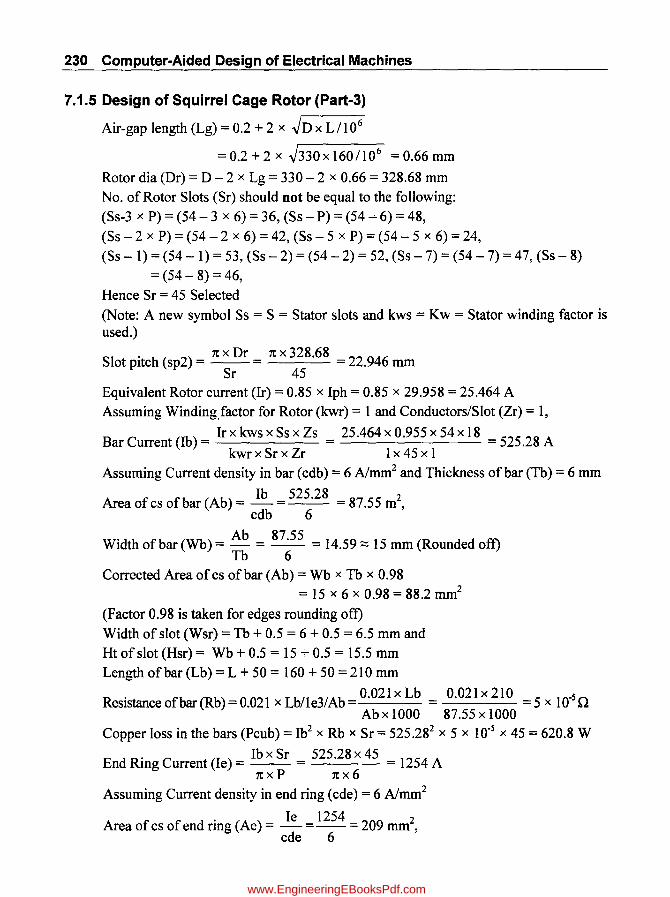
230 Computer-Aided Design of Electrical Machines
7.1.5 Design of Squirrel Cage Rotor (Part-3)
Air-gap length (Lg) = 0.2 + 2 x ~D xL / 1 06
=0.2+2x ~330x160/106 =0.66mm
Rotor dia (Dr) = D - 2 x Lg = 330 - 2 x 0.66 = 328.68 mm No. of Rotor Slots (Sr) should not be equal to the following: (Ss-3 x P) = (54 - 3 x 6) = 36, (Ss - P) = (54 -'- 6) = 48,
(Ss - 2 x P) = (54 - 2 x 6) = 42, (Ss - 5 x P) = (54 - 5 x 6) = 24, (Ss - 1) = (54 - 1) = 53, (Ss - 2) = (54 - 2) = 52, (Ss -7) = (54 -7) = 47, (Ss - 8)
= (54 - 8) = 46, Hence Sr = 45 Selected (Note: A new symbol Ss = S = Stator slots and kws = Kw = Stator winding factor is used.)
. 1t X Dr 1t x 328.68 Slot pItch (sp2) = --= = 22.946 mm
Sr 45 Equivalent Rotor current (Ir) = 0.85 x Iph = 0.85 x 29.958 = 25.464 A Assuming Winding,factor for Rotor (kwr) = 1 and Conductors/Slot (Zr) = 1,
Bar Current (Ib) = Ir x kws x Ss x Zs = 25.464 x 0.955 x 54 x 18 = 525.28 A kwr x Sr x Zr 1 x 45 x 1
Assuming Current density in bar (cdb) = 6 Almm2 and Thickness of bar (Tb) = 6 mm
Area of cs of bar (Ab) = ~ = 525.28 = 87.55 m2, cdb 6
Width of bar (Wb) = Ab = 87.55 = 14.59;:::: 15 mm (Rounded off) Tb 6
Corrected Area ofcs of bar (Ab) = Wb x Tb x 0.98 = 15 x 6 x 0.98 = 88.2 mm2
(Factor 0.98 is taken for edges rounding off) Width of slot (Wsr) = Tb + 0.5 = 6 + 0.5 = 6.5 mm and Ht of slot (Hsr) = Wb + 0.5 = 15 + 0.5 = 15.5 mm Length of bar (Lb) = L + 50 = 160 + 50 = 210 mm
Resistance ofbar(Rb) = 0.021 x Lblle3/Ab-O.021xLb = 0.021x210 =5x 1O'5g Ab x 1000 87.55 x 1000
Copper loss in the bars (Pcub) = Ib2 x Rb x Sr= 525.282 x 5 x 10,5 x 45 = 620.8 W
. Ib x Sr 525.28 x 45 End Ring Current (Ie) = -- = = 1254 A
1tXP 1tx6 Assuming Current density in end ring (cde) = 6 Almm2
. Ie 1254 2 Area of cs of end nng (Ae) = - =-- = 209 mm ,
cde 6
www.EngineeringEBooksPdf.com

Three-Phase Induction Motors 231
Mean dia of end-ring (Orne) = Dr - 50 = 328.68 - 50 = 278.68 m
R . f d' (R) 0.021xLme 0.02Ix1txDme 88 10·5r1 eSlstance 0 en rmg e = = = . x u Ae 1000 x Ae
Copperloss in the 2 End-rings (Pcue) = 2 x Ie2 x Re = 2 x 12542
x 8.8 X 10-5 = 276.7 W
Total Rotor copper loss (Pcur) = Pcub + Pcue = 620.8 + 276.7 = 897.5 W
. Pcur 897.5 EqUivalent Rot res (Rr) = --, = , 0.4614 n
3 x Ir- 3 x 25.4645-
Dia of rotor at Yltooth ht from tip (Dr 13) = Dr - 2 x 73 x Hsr
= 328.68-2 x 7j x 15.5 = 308
. 1t x Dr13 1t x 308 Rotor slot pitch at Orl3 (sprl3) = :=: = 21.50mm
Sr 45
Width of tooth at Drl3 (WtrI3) = spr13 - Wsr = 21.5 - 6.5 = 15 mm
Area of tooth at Orl3 (Atr) = Wtr13 x Li x SrlP = 15 x 128.8 x 45/6 = 14493 mm2
Flux density in tooth (Brt) = FI x 106/Atr=0.01281 x 106/14493 =0.8839T
Max Flux density in tooth (Brtmax) = Brt x 1.5
= 0.8839 x 1.5 = 1.3259 T (lies bet 1.2 to 1.4 and hence OK)
Assuming Flux density in Rotor Core (Brc) = 1.35 T,
Area of Core (Ac) = FIxl06
0.01281xl06
=4744.8m2
2 x Bre 2 x 1.35
Ac 4744.8 Depth of core (dcr) = - = = 36.84 mm
Li 128.8
Assuming Friction and Windage Loss (Pfw) 1 %
= 0.01 x KW x 1000 = 0.01 x 30 x 1000 = 300 W
Noload Loss (PnL) = Pit + Pic + Pfw = 619.9 + 982.2 + 300 = 1902.1 W
. PnL 1902.1 ActtvelWattful Component of No-load Current (lw) = -- = = 1.441 A
3 x V 3 x 440
Wt of Rotor Copper (Wcur) = Lb x Sr x Ab x 8.9 x 10-6
= 210 x 45 x 88.2 x 8.9 x 10-6 = 7.42 Kg
Wt of Rotor End-Rings (Weue) = Lme x 2 x Ae x 8.9 x 10-3
= 0.8755 x 2 x 209 x 8.9 x 10-6 = 3.29 Kg
7.1.5 (a) Computer Program in "C" in MATLAB for Part-3 % (3)<--------Squirrel Cage Rotor----------------------------->
Kw=0.955; 0=330; L=160; S=54; \P=p; Iph=29.96; Zs=18; Li=128.8;
www.EngineeringEBooksPdf.com

-232 Computer-Aided Design of Electrical Machines
FI=O.01281;KW=30;Pit=619.9;Pic=982.2;V=440; %Input data
Zr=1;kwr=1;cdb=6;Tb=6;cde=6;dd=50;Brc=1.35; %Assumptions
kws=Kw;Ss=S;Lgl=O.2 + 2*sqrt(D*L/le6); Lg=ceil(Lgl*lOO)/lOO;
Dr=D-2*Lg;
d5=Ss-1;
dl=Ss-3*P;
d6=Ss-2;
d2=Ss-P; d3=Ss-2*P;
d7=Ss-7; d8=Ss-8; Sr=Ss-9;
Ir=O.85*Iph; Ib=Ir*kws*Ss*Zs/(kwr*Sr*Zr)
d4=Ss-5*P;
sp2=pi*Dr/Sr;
Abi=Ib/cdb;
Hsr=Wb+O.5; Wb=ceil(Abi/Tb) Ab=Tb*Wb*O.98; Wsr=Tb+O.5;
Lb=L+50; Rb=O.021*Lb/le3/Ab; Pcub=Ib A 2*Rb*Sr;
Ie=Ib*Sr/P/pi;
Re=O.021*Lme/Ae;
Ae=Ie/cde;Dme=Dr-dd;Lme=pi*Dme/lOOO;
Pcue=2*Ie A 2*Re; Pcur=Pcub+Pcue;
Rr=Pcur/(3*Ir A 2) Dr13=Dr-2*2/3*Hsr;
Wtr13=spr13-Wsr; Atr=Wtr13*Li*Sr/P;
Brtmax=Brt*1.5; Ac=FI*le6/2/Brc;
dcr=Ac/Li; Pfw=O.Ol*KW*le3; PnL=Pit+Pic+Pfwi
Wcur=Lb*Sr*Ab*8.ge-6; Wcue=Lme*2*Ae*8.ge-3;
spr13=pi*Dr13/Sri
Brt=FI*le6/Atri
Iw=PnLI3/V;
%--------------------------------------------------------------
7.1.6 Total AT and Magnetizing Current (Part-4)
t E ~ ·iii c: CD Cl >< ::l
u:::
2~~~Tn~--~~~w__r~~~--~~~~
1.8
1.6
1.4
1.2
0.8
0.6
0.4
0.2
· . """ • I •••••• · ...... . • • III."
• •••• 11. • I.... • • 1'1'" .... .. :. -:-; r:-:.; i:-"" .. ! ............ o! ..... too .' .. !.!! '!.'''~ ......... .! .. 'oo ! ...... ..
I ••• ,.. • •• II.... . ...... . • ••••• 11 • I. •• I I .... ..
• • II •••• • I I .... II •••••• ,.
_.~_~_~~~YA~ .. _ .. •• '" II II
~ .. ·~J~y_ ... ~ .. ~'J&U~L_ .. ~ .. J.~,~J I • II .. II I
I • I "" I. • • I •••••
I I • I II .. • ,.1., II .. ... - ............. - ............. 1 ........... -e- .... ..
• ••• 1 •• , • • •••••• I •••••• · . "",. . . ...... . ..... . I • •••••• • •• 11.... .. I .. ,.,
.... i~ ... ~'~~ ...... r·,-i'rft'r- .. ' .. '-~l~~ · . "',., . ,."... . ..... . ... _ L _ .......... " ... " _ .... ' .. _' .. 4 .. L \".1\, .... J .. ".' .. ".' .. '
• • , •• ,. I.' •• ,... • I ' ••• 1.. • •••••• 1
• , ,. II II
" .11.,.
I , ••••••
, .1.1 ••• • I •••••
• I II. II •• - ................................ _too. 4 ......... _ .. 4 _ .. _, ... ,-••
• .1.11.. • • •••••• I I t •• I. • I ••• II •• • .... II I.' • 1 '1.1 ••• II' ,.
I.' ...... L .. L ... _I_.J .... J .............. !. J!. ""J\. .... J .. J .. '_ !,I .. ' .. " • II •• •• I I. .. •• I ,.11 II ••• II I II
AT/m~
Fig.7.2 Magnetization curve for Lohys stamping steel.
www.EngineeringEBooksPdf.com

Three-Phase Induction Motors 233
0.9 r---~-----:--",,""-~--~----::::::>I
0.8 ············!······ .. ·····i···· .. ······+···········+·· .. . . . . .
::: ::::::::::::i::::::::::::I:::: .. ·:::::·::::~:~:;j;:~~~:r~:~:~. t ...;. ~ 0.5 ........... .L. ...... ·;~·~ ... ·~l .... ·· .... ·: -se~lclosed .. o : r. : ---Open () 0.4 ............ : .... / .. ! ............ '( .......... :'--....;;.::;.;;;;..~ ~ ''':::. ~ 0.3 .. · .... · .. ,,/~ ...... ···j· .... · .. · .. ··( .......... j .. ·· ........ ·i·· .. · ...... ··
~ .. ~ ::><::C:::::::::r:::::::.J:::::::·:::r:::::::::f:::::::::: , . . . . , . . . . o : : : : :
o 2 4 6 8 10 12
Slot Opening/Airgap ~
Fig. 7.3 Carter coefft. for slots.
From Fig. 7.2, Amp-Turns/m for Stator core (at Flux density Bc = 1.35 T),
atsc = 480.8
St-Core mean dia (Dcav) = D + (2 x Hs) + Hc = 330 + (2 x 46) + 39 = 461 mm
AmpTurns for St-Core (ATSC) = 7t x Dcav x atsc = 7t x 461 x 480.8 = 38.68 P x 3 x 1000 6 x 3 x 1000
Flux density at 30° from the centre of the pole (Bt30)
= Bl3 x 1.36 = 1.0644 x 1.36 = 1.4476 T
From Fig. 7.2, Amp-Turns/m for Stator teeth (at Flux density Bt30)
= 1.4476T), atst = 706.5
AmpTurns for St-tooth (ATST) = atst x HsllOOO = 706.5 x 46/1000 = 32.5
Total AT for Stator (ATS) = ATSC + ATST = 38.68 + 32.5 = 71.18
Assuming St-Slot opening (WssO) = 4mm, WssO = _4_ = 6.06 Lg 0.66
From Fig. 7.3, Cartr coeft corresponding to 6.06 (kOl) = 0.6633
G C fft fi S Sl (k) Spitch ___ 1_9_.2 __ = 1.1604 ap oe or t- ots gs =-----=-----Spitch - WssO x kOI 19.2 - 4 x 0.6633
Assuming Rt-Slot opening (WssO) = 2mm, WssO = _2_ = 3.03 Lg 0.66
From Fig. 7.3, Carter coeft corresponding to 3.03(k02) = 0.4529
www.EngineeringEBooksPdf.com
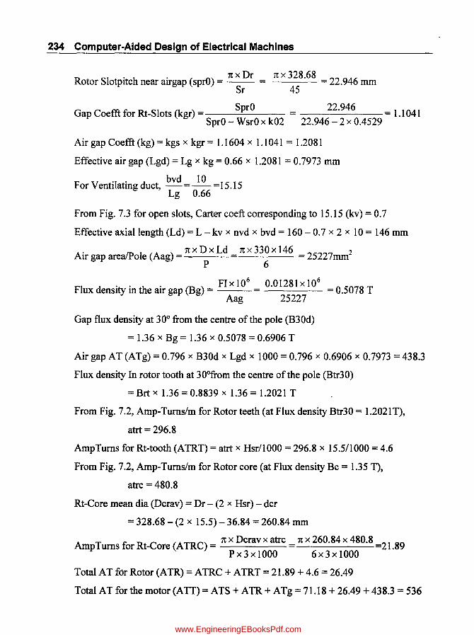
234 Computer-Aided Design of Electrical Machines
Rotor Slotpitch near airgap (sprO) = 1t x Dr = 1& x 328.68 = 22.946 mm Sr 45
SprO Gap Coefft for Rt-Slots (kgr) =-----.::.---
SprO - WsrO x k02 ___ 22_.9_4_6 __ = 1.1041 22.946 - 2 x 0.4529
Air gap Coefft (kg) = kgs x kgr = 1.1604 x 1.1041 = 1.2081
Effective air gap (Lgd) = Lg x kg = 0.66 x 1.2081 = 0.7973 mm
For Ventilating duct, bvd = ~ = 15 .15 Lg 0.66
From Fig. 7.3 for open slots, Carter coeft corresponding to 15.15 (kv) = 0.7
Effective axial length (Ld) = L - kv x nvd x bvd = 160 - 0.7 x 2 x 10 = 146 mm
. 1txDxLd 1tx330x146 , AIr gap areaIPole (Aag) = = 25227mm-
P 6
FI d . . th· (B) FI X 106
0.01281 X 106
= 0.5078 T ux ensity In e aIr gap g = = -----Aag 25227
Gap flux density at 30° from the centre of the pole (B30d)
= 1.36 x Bg = 1.36 x 0.5078 = 0.6906 T
Air gap AT (ATg) = 0.796 x B30d x Lgd x 1000 = 0.796 x 0.6906 x 0.7973 = 438.3
Flux density In rotor tooth at 30°from the centre of the pole (Btr30)
= Brt x 1.36 = 0.8839 x 1.36 = 1.2021 T
From Fig. 7.2, Amp-Turns/m for Rotor teeth (at Flux density Btr30 = 1.2021 T),
atrt = 296.8
AmpTurns for Rt-tooth (ATRT) = atrt x Hsr/1000 = 296.8 x 15.511000 = 4.6
From Fig. 7.2, Amp-Turns/m for Rotor core (at Flux density Bc = 1.35 T),
atrc = 480.8
Rt-Core mean dia (Dcrav) = Dr - (2 x Hsr) - dcr
= 328.68 - (2 x 15.5) - 36.84 = 260.84 nun
AmpTurns for Rt-Core (A TRC) = 1t x Dcrav x atrc = 1t x 260.84 x 480.8 =21.89 P x 3 x 1000 6 x 3 x 1000
Total AT for Rotor (ATR) = ATRC + ATRT = 21.89 + 4.6 = 26.49
Total AT for the motor (ATT) = ATS + ATR + ATg = 71.18 + 26.49 + 438.3 = 536
www.EngineeringEBooksPdf.com

Three-Phase Induction Motors 235
M ti agne zation AT f S -C 3 hid M t 0 )c age 'PI , n . 0 or Length Flux= 0.01281 Wb
Part M B(tesla) AT/m AT Stator-Core 0.08046 1.35 480.8 39 Stator Teeth 0.046 1.4466 706.5 32
Air-Gap 7.96E-04 0.6906 438 Rotor Teeth 1.55E-02 1.2021 296.8 5 Rotor-Core 0.04553 1.9283 480.8 22
Total-AT= 536
M . . (I ) Px ATT agnetlZmg current m = -------2 x 1.17 x K w x Tph
___ 6_x_5_3_6 __ = 8.8835 A 2 x 1.17 x 0.955 x 162
No load Phase current (10) = ~lw2 + 1m2 = ~1.4412 + 8.88352 = 9.0
Iw 1.441 No load Power Factor (pfO) =- = -- = 0.1601.
IO 9
7.1.6 (a) Computer Program in "C" in MATLAB for Part-4
% (4) <------------AmpTurns and Magnetizing-Current---------->
Bc=1.35;D=330;Hs=46;Hc=39;P=6;B13=1.0644;Lg=0.66;SPitch=19.2;
Dr=328.68;Sr=45;bvd=10;nvd=2;L=160;FI=0.01281;Brt=0.8839;
Hsr=15.5; dcr=36.8385;Brc=1.35;Kw=0.955;Tph=162;Iw=1.441;
%Input Data
WssO=4;WsrO=2; %Assumptions
%-------------BH Curve for 0.5mm,LOHYS Quality--------->
BB= [ . 1 . 2 . 3 . 4 . 5 . 6 . 7 . 8 . 9
1.7 1.8 1.9 2];
1 1.1 1.2 1.3 1.4 1.5 1.6
H= [50 65 70 80 90 100 110 120 150 180 220 295 400 580 1000
2400 5000 8900 15000 24000];
semilogx(H,BB); grid; xlabel('AT/m-->');
ylabel('Flux density(T)-->');
title('Magnetization Curve for Lohys Stamping Steel');
%-------Carters Coefft for Air Gap)--->
Ratio=[O 1 2 3 4 5 6 7 8 9 10 11 12];
cc= [0 .18 .33 .45 .53 .6 .66 .71 .75 .79 .82 .86 .89]; %Semiclosed Slots
www.EngineeringEBooksPdf.com

236 Computer-Aided Design of Electrical Machines
CC1=[O .14 .27 .37 .44 .5 .54 .58 .62 .65 .68 .69 .7J;
%Open Slots
plot(Ratio,CC,Ratio,CC1);grid;xlabel('Slot Opening/Airgap-->');
ylabel ( 'Carter Coefft-->'); title (' Carter Coefft for slots'); legend('Semiclosed', 'Open');
semilogx(HH,BB); grid; xlabel('AT/m-->');
ylabel('Flux density(T)-->');
title('Magnetization Curve for Lowhys Stamping Steel');
atsc=interp1(BB,H,Bc, 'spline'); ATSC=pi*Dcav/P/3*atsc/1e3; atst=interp1(BB,H,Bt30, 'spline');
ATS=ATSC+ATST; k01=interp1(Ratio,CC,rat1, 'spline');
kgs=SPitch/(SPitch-WssO*kOl); k02=interp1(Ratio,CC,rat2, 'spline');
Dcav=D+2*Hs+Hc; Bt30=B13*1.36;
ATST=atst*Hs/1000 ;
rat1=WssO/Lg;
rat2=WsrO/Lg;
sprO=pi*Dr/Sr; kgr=sprO/(sprO-WsrO*k02); kg=kgs*kgr; Lgd=Lg*kg; rat3=bvd/Lg; kv=interp1(Ratio,CC1,rat3, 'spline'); if rat3 >=12 kv=O.7;end;
Ld=L-kv*nvd*bvd; Aag=pi*D/P*Ld; Bg=FI*le6/Aag; B30d=1.36*Bg; ATg=O.796*B30d*Lgd*le3; Btr30=Brt*1.36; atrt=interp1(BB,H,Btr30, 'spline');
ATRT=atrt*Hsr/1e3; atrc=interp1(BB,H,Brc, 'spline');
Dcrav=Dr-2*Hsr-dcr; ATRC=pi*Dcrav/1e3/P/3*atrc; ATR=ATRC+ATRT; ATT=ATS+ATR+ATg; Im=P/2*ATT/(1.17*Kw*Tph); IO=sqrt(IwA 2+ImA 2); pfO=Iw/IO;
%-------------------------------------------------------
7.1.7 Short-Circuit Current Calculation (Part-5) \
hI = Zsh x (Hstrip + insS) = 6 x (5 + 0.5) = 33mm, h3 = Hw = 4, h4 = HL = 1,
bs = Ws = 10.6, bO = WssO = 4,
Assuming h2 = 1.6mm, Specific Permeance of Stator Slot (Lmdss)
=~+~+ 2h3 +~ = 33 +~+ 2x4 +!=1.9866 3xbs bs bs+bO bO 3xl0.6 10.6 10.6+4 4
hlr = Wb = 15, br = Wsr = 6.5, brO = WsrO = 2 and Assuming h2r = h3r = 0,
h4r = 0.5, and Ks = 1,
www.EngineeringEBooksPdf.com
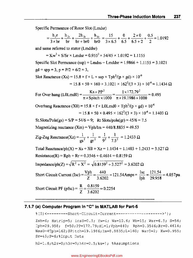
Three-Phase Induction Motors 237
Specific Permeance of Rotor Slot (Lmdsr)
=~+ h2r + 2h 3r + h4r =_1_5_+~+ 2xO +.Q2=1.0192 3 x br br br + brO brO 3 x 6.5 6.5 6.5 + 2 2
and same referred to stator (Lmddsr)
= Kw2 x S/Sr x Lmdsr = 0.9552
x 54/45 x 1.0192 = 1.1155
Specific Slot Permeance (ssp) = Lmdss + Lmddsr = 1.9866 + 1.1155 = 3.1021
gd = spp = 3, P = P/2 = 6/2 = 3,
Slot Reactance (Xs) = 15.8 x f x L x ssp x Tph2/(p x gd) x 10-9
= 15.8 x 50 x 160 x 3.1021 x 1622/(3 x 3) x 10-9 = 1.1434 n
For Over hang (LOLmdO) = Ks x pp2 1 X 172.792
= 0.495 1t x Spitch x 1000 1t x 19.1986 x 1000
Overhang Reactance (XO) = 15.8 x f x LOLmdO x Tph2/(p x gd) x 10-6
= 15.8 x 50 x 0.495 x 1622/(3 x 3) x 10-6= 1.1403 n St.SlotslPole(gs) = SIP = 54/6 = 9; Rt Siots/pole(gr) = 45/6 = 7.5
Magnetizing reactance (Xm) = VphlIm = 440/8.8835 = 49.53
. 1 1 1 1 Zig-Zag Reactance(Xz) =-+- = -+- = 1.2433 n
gs2 gr2 92 7.52
Total Reactance/ph(X) = Xs + XO + Xz = 1.1434 + 1.1403 + 1.2433 = 3.527 n Resistance(R) = Rph + Rr = 0.3546 + 0.4614 = 0.8159 n
Impedance/ph(Z) =.JR 2 + X2 = .J0.81592 + 3.5272 = 3.6202 n . . Vph 440 Isc 121.54
Short CirCUit Current (lsc) =-- = = 12 1. 54Amps = - = . =4.057pu Z 3.6202 Iph 29.958
Short Circuit PF (pfsc) = R = 0.8159 = 0.2254 Z 3.6202
7.1.7 (a) Computer Program in "c" in MATLAB for Part-5
% (5) <---------Short-Circuit-Current-------------------->');
Zsh=6; Hstrip=5; insS=O.5; Hw=4; Ws=10.6; Wb=15; Wsr=6.5; S=54;
Iph=29.958; f=50;PP=172.79;HL=1;Vph=440; Rph=O.3546;Rr=O.4614;
WssO=4Tph=162;SPitch=19.1986;Im=8.8835;L=160; WsrO=2; Kw=O.955;
Sr=45;P=6;%Input Data
h2=1.6;h2r=O;h3r=O;h4r=O.5;ks=1; %Assumptions
www.EngineeringEBooksPdf.com

238 Computer-Aided Design of Electrical Machines
hl=Zsh*(Hstrip+insS); h3=Hw; h4=HL; bs=Ws; bO=WssO;
Lmdss=hl/3/bs +h2/bs +2*h3/(bs+bO) +h4/bOi hlr=Wbi brO=WsrO; Lmdsr=hlr/3/br +h2r/br +2*h3r/ (br+brO) Lmddsr=Kw A 2*S/Sr*Lmdsr; ssp=Lmdss+Lmddsr; gd=S/P/3; Xs=15.8*f*L*ssp*Tph A2/(p*gd)*le-9; LOLmdO=ks*PP A2/pi/SPitch/lOOO; XO=15.8*f*LOLmdO*Tph A2/(p*gd)*le-6; gs=S/P; gr=Sr/Pi Xz=5/6*Xm*(l/gsA2+1/grA2); X=Xs+XO+Xz; R=Rph+Rr;
Isc=Vph/Zipfsc=R/ZiRAT=Isc/lphi
br=Wsri +h4r/brO;
p=P/2;
Xm=Vph/lm;
%----------------------------------------------------------
7.1.8 Performance Calculation (Part-6)
Total Losses (Pt) = PnL + Pcus + Pcur = 1902.1 + 954.63 + 897.4~
= 3754.2 W = 3.7542 KW
Efficiency (EFF) = KW x 100 = 30 x 100 = 88.88% KW + Pt 30 + 3.7542
Rotor Input (Rinp) = KW x 1000 + Pfw + Pcur = 30 x 1000 + 300897.49 = 31197 W
Slip at Full Load (SFL) = PcurlRinp x 100
= 897.49/31197 x 100 = 2.88% = 0.0288 pu
Starting Tq (Tst) = (lsc)2 x SFL = (121.564)2 x 0.0288 = 0.6554 pu Ir 25.4645
Pmax = 3 x Vph x (lsc - 10) = 3 x 440 x (121.564 - 9) = 60.616 KW 2(1 + pfsc) x 1000 2(1 + 0.2254) x 1000
Inner cooling area (Acooll) = [1t x D x (L x 2.5) + 2 x 1t x (D + 50) x 0.04]1106
= [1t x 330 x (160 x 2.5) + 2 x 1t x (330 + 50) x 0.04]/106 = 0.4148 m2
Acoo12 = Acooll x (1 + 0.1 x v) = Acooll x (1 + 0.1 x 17.28) = 1.1315 m2
Outer cooling area (Acoo13) = 1t x DO x LlI06 = 1t x 500 x 1601106 = 0.2513 m2
Total cooling area (AcoolT) = Acoo12 + Acoo13
1.1315 + 0.2513 = 1.3828 m2
Total Stator Loss (Pst) = Pcus + Pit + Pic = 954.63 + 619.86 + 982.2 = 2557 W
Temp rise (Tr) = 0.03 x PstlAcoolT = 0.03 x 2557/1.3828 = 55.47 °C
Area of Rotor slots (Ars) = Wsr x Hsr x Sr = 6.5 x 15:5 x 45 = 4534 m2
Rotor inner dia (Dri) = Dcrav - dcr = 260.84 - 36.84 = 224 m
Weight of Rotor (Wri) = [1t x (Dr2- Dri2)/4 - Ars] x L x 7.81106
= [1t x (328.682-2242)/4-4534] x 160 x 7.8/106= 51.05 Kg
www.EngineeringEBooksPdf.com

Three-Phase Induction Motors 239
Assuming Insulation Wt of 1 %,
Total wt (Wtot) = 1.01 x (Weus + Wt + We + Wri + Weur + Weue)
= 1.01 x (38.04 + 25.91 + 53.6 + 51.05 + 7.42 + 3.26) = 181.07 Kg
KgPKw = WtotIKW = 181.07/30 = 6.04
7.1.8 (a) Computer Program in "c" in MATLAB for Part-6
%(6)<--------------Performance-------------------->')i
PnL=1902.1iPCus=954.63iPcur=897.49iKW=30iPfw=300i1sc=121.564i 1r=25.4645iVph=440i10=8.9936ipfsc=0.2254iD=330iL=160iv=17.28i
DO=500iL=160iPic=982.2iPit=619.86iWsr=6.5iWcus=38.043iWc=53.6i
Hsr=15.5iSr=45iDcrav=260.84idcr=36.84iDr=328.68iWt=25. 91i
Wcue=3.26iWcur=7.42i %1nput Data
Pt=PnL+Pcus+Pcuri EFF=KW/(KW+Pt/1000)*100i Rinp=KW*1000+Pfw+Pcuri SFL=Pcur/Rinp*100i Tst=(1sc/1r)A2*SFL/100i Pmax=3*Vph*(1sc-10)/2/(l+pfsc)*le-3i Acool1=(pi*D*(L*2.5)+2*pi*(D+50)*0.04)/le6i Acool2=Acool1*(l+0.1*v)i
Acool3=pi*DO*L/1e6i AcoolT=Acool2+Acool3i Pst=Pcus+Pit+Pici Tr=0.03*Pst/ AcoolTi Ars=Wsr*Hsr*Sr; Dri=Dcrav-dcri Wri=(pi* (Dr A2-Dri A2)/4-Ars) *L*7.8e-6;
Wtot=1.01*(Wcus+Wt+Wc+Wri+Wcur+Wcue)i KgPKw=Wtot/KWi
%--------------------End of Program-------------------------->
7.1.9 Computer Program in "c" in MATLAB for Complete Design
%3ph,KW=30iV=440iP=6if=50Sq.Cage 1M with Sq.Cage rotor.
f2=fopen('Total_30KW_Output.m', 'w');
%------------Standard Curves/Tables for%Data-------------->
SKW=[l 2 5 10 20 50' 100 500]iSBav=[0.35 0.38 0.42 0.46 0.48 0.50 0.51 0.53]i
Sq=[16e3 1ge3 23e3 25e3 26e3 2ge3 31e3 33e3];
SKWa=[5 10 20 50 100 200 500]i
SPF6P=[0.82 0.83 0.85 0.87 0.89 0.9 0.92]i%Table for 1000RPM
SEFF6P=[0.83 0.85 0.87 0.89 0.91 0.92 0.93]i%Table for 1000RPM
SPF4P=[0.85 0.86 0.88 0.9 0.91 .92 .93]i~Table: for 1500RPM
SEFF4P=[.85 .87 .88 .9 .91 .93 .94];%Table for 1500RPM
SD=[O.l 0.15 0.2 0.3 0.4 0.5 0.75 l]i
SCDSW=[4 3.8 3.6 3.5 3.5 3.5 3.5 3.5]i
www.EngineeringEBooksPdf.com

240 Computer-Aided Design of Electrical Machines
%-------------BH Curve for--0.5mm,LOHYS Quality--------->
BB= [ . 1 . 2 . 3 . 4 . 5 . 6 . 7 . 8 . 9 1.7 1.8 1.9 2];
1 1.1 1.2 1.3 1.4 1.5 1.6
H= [50 65 70 80 90 100 110 120 150 180 220 295 400 580 1000 2400 5000 8900 .15000 24000];
%-------Carters Coefft for Air Gap--->
Ratio=[O 1 2 3 4 5 6 7 8 9 10 11 12];
CC= [ 0 . 18 . 33 .45 .53 . 6 . 66 . 71 . 75 . 79 . 82 . 86 . 89] ;
CC1= [0 .14 .27 .37 .44 .5 .54 .58 .62 .65 .68 .69 .7];
% (1) <-----------Main Dimensions----------------------->
KW=30;V=440;f=50;%P=6;Specification/lnput Data------>
insW=3.4;Hw=4;HL=1;insH=6;nvd=2;bvd=0.01;ki=0.92;Bc=1.35;Vph=V;
Zr=1;kwr=1;cdb=6;Tb=6;cde=6;dd=0.05;Brc=1.35;
Bav=interp1(SKW,SBav,KW, 'spline');
q=interp1(SKW,Sq,KW,'spline');
%Assumptions
pf=interp1(SKWa,SPF6P,KW, 'spline');
eff=interp1(SKWa,SEFF6P,KW, 'spline');
Kw=0.955;nvd=2;bvd=10;ki=0.92;Tstrip=1.9;insS=0.5;%Assumptions
insW=3.4;Hw=4;HL=1;insH=6;nvd=2;ki=0.92;Bc=1.35;%Assumptions
SD~[O.l 0.15 0.2 0.3 0.4 0.5 0.75 1];SCDSW=[4 3.8 3.6 3.5 3.5 3.5 3.5 3.5];
B=[0.8 1.2 1.6 2 2.4]; WpKg=[7 15 24 34 50];
Vph=V; KWinp=KW/eff; Iph=KWinp*le3/(3*Vph*pf);
P=6; spp=3; Tstrip=1.9; Zsw=3; % Assumption
pf=interp1(SKWa,SPF6P,KW, 'spline');
eff=interp1(SKWa,SEFF6P,KW, 'spline');
if P==4 pf=interp1(SKWa,SPF4P,KW, 'spline');end;
if P==4 eff=interp1(SKWa,SEFF4P,KW, 'spline');end;
Ns=120*f/P;ns=Ns/60;CO=11*Kw*Bav*q*eff*pf*le-3;
DsqL=l/CO*(KW/ns); L1=sqrt(DsqL/(0.135*P)A2); L=floor(L1*100)*10; Ls=(L-nvd*bvd);Li= ki*Ls;
D1=sqrt(DsqL/(L/1000));D=ceil(D1*100)*10;PP=pi*D/P;LbyPP=L/PP;
if LbyPP <0.81 I LbyPP >2 continue; end;
v=pi*D*ns/1000;if v >30 continue;end;
FI=pi*D/P*L*Bav/1e6;
www.EngineeringEBooksPdf.com

Three-Phase Induction Motors 241
% (2)<--------------Stator Slots and Winding----->
Tphi=Vph/(4.44*f*FI*Kw);CDSW=interp1(SD,SCDSW,D/1000, 'spline');
As1=Iph/CDSW;S=spp*P*3;SPitch=pi*D/S; _
if SPitch <18[ [SPitch>=25 continue; end;
Zphi=2*Tphi; sph=S/3; Zsl=Zphi/sph;Zs=ceil (Zsl); Tph=Zs*sph/2; FI=Vph/(4.44*f*Tph*Kw); Hstrip1=As1/Tstrip; Hstrip=ceil(Hstrip1*2)/2; WbyT=Hstrip/Tstrip;
if WbyT <2.5[ [WbyT >=3.5 continue; end; As=0.967*Hstrip*Tstrip;
Ws=(Zsw*(Tstrip+insS)+insW); Zsh=Zs/Zsw; Hs=(Zsh*(Hstrip+insS)+Hw+HL+insH+2);D13=D+2/3*Hs;sp13=pi*D13/S; Wt13=sp13Ws;B13=FI*P*le6/(Li*Wt13*S);Btmax=1.5*B13;
Lmt=(2*L+2.3*PP+240)/1000; Rph=0.021*Lmt*Tph/As;
Pcus=3*Iph A 2*Rph; Wcus=Lmt*Tph*3*As*8.ge3; Flc=FI/2; Ac=Flc*le6/Bc;Hc=Ac/Li; D01=D+2*(Hs+Hc); DO=ceil(D01/10)*10; Hc=(DO-D)/2-Hs;
PitpKg=interp1(B,WpKg,Btmax, 'spline');
PicpKg=interp1(B,WpKg,Bc, 'spline');
Wt=Li*Wt13*S*Hs*7.8e-6; Dmcs=D+2*Hs+Hc; Wc=Ac*pi*Dmcs*7.8e-6;
Pit=PitpKg*Wt;Pic=PicpKg*Wc;
%-----------------------ROTOR----------------------->
Zr=l; kwr=1;cdb=6;Tb=6;cde=6;dd=50;Brc=1. 35; %Assumptions
kws=Kw;Ss=S;Lg1=0.2+2*sqrt(D*L/1e6);Lg=ceil(Lg1*100)/100;
Dr=D-2*Lg;d1=Ss-3*P;d2=Ss-P;d3=Ss-2*P; d4=Ss-5*P;d5=Ss-1;
d6=Ss-2;d7=Ss-7;d8=Ss-8;Sr=Ss-9; sp2=pi*Dr/Sr; Ir=0.85*Iph; Ib=Ir*kws*Ss*Zs/(kwr*Sr*Zr);Abi=Ib/cdb; Wb=ceil(Abi/Tb); Ab=Tb*Wb*0.98;Wsr=Tb+0.5;Hsr=Wb+0.5;Lb=L+50;Rb=0.021*Lb/1e3/Ab;
Dme=Drdd; Pcub=Ib A 2*Rb*Sr; Ie=Ib*Sr/P/pi; Ae=Ie/cde;
Lme=pi*Dme/1000;Re=0.021*Lme/Ae;
Pcue=2*Ie A 2*Re;Pcur=Pcub+Pcue;Rr=Pcur/(3*Ir A 2);
Dr13=Dr2*2/3*Hsr;spr13=pi*Dr13/Sr;
Wtr13=spr13Wsr;Atr=Wtr13*Li*Sr/P;Brt=FI*le6/Atr;
Brtmax=Brt*1.5;Ac=FI*le6/2/Brc;dcr=Ac/Li;
Pfw=0.01*KW*le3;PnL=Pit+Pic+Pfw;Iw=PnL/3/V;
Wcur=Lb*Sr*Ab*8.ge-6;Wcue=Lme*2*Ae*8.ge-3;
%(4)<----AmpTurns and Magnetizing-Current----------------------
www.EngineeringEBooksPdf.com

242 Computer-Aided Design of Electrical Machines
%-------------BH Curve for--0.5mm,LOHYS Quality--------->
BB= [ . 1 . 2 . 3 . 4 . 5 . 6 . 7 . 8 . 9 1.7 1.8 1.9 2];
1 1.1 1.2 1.3 1.4 1.5 1.6
H= [50 65 70 80 90 100 110 120 150 180 220 295 400 580 1000 2400 5000 8900 15000 24000];
%-------Carters Coefft for Air Gap--->
Ratio=[O 1 2 3 4 5 6 7 8 9 10 11 12];
CC= [0 .18 .33 .45 .53 .6 .66 .71 .75 .79 .82 .86 .89 ];
CC1= [0 .14 .27 .37 .44 .5 .54 .58 .62 .65 .68 .69 .7 ];
WssO=4;WsrO=2; %Assumptionsatsc=interp1(BB,H,Bc, 'spline');
Dcav=D+2*Hs+Hc;ATSC=pi*Dcav/P/3*atsc/1e3; Bt30=B13*1.36; atst=interp1(BB,H,Bt30, 'spline');ATST=atst*Hs/1000; ATS=ATSC+ATST;rat1=WssO/Lg; k01=interp1(Ratio,CC,rat1, 'spline');
kgs=SPitch/(SPitch-WssO*k01); rat2=WsrO/Lg; k02=interp1(Ratio,CC,rat2, 'sp~ine'); sprO=pi*Dr/Sr;
kgr=sprO/(sprO-WsrO*k02); kg=kgs*kgr; Lgd=Lg*kg;
rat3=bvd/Lg; kv=interp1(Ratio,CC1,rat3, 'spline');
if rat3 >=12 kv=0.7;end;
Ld=L-kv*nvd*bvd;Aag=pi*D/P*Ld;Bg=FI*le6/Aag;B30d=1.36*Bg;
ATg= 0.796*B30d*Lgd*le3;
Btr30=Brt*1.36;atrt=interp1(BB,H,Btr30, 'spline');
ATRT=atrt*Hsr/1e3; Dcrav=Dr-2*Hsr-dcr; atrc=interp1(BB,H,Brc, 'spline');ATRC=pi*Dcrav/1e3/P/3*atrc; ATR=ATRC+ATRT; ATT=ATS+ATR+ATg; Im=P/2*ATT/(1.17*Kw*Tph); IO=sqrt(IwA 2+ImA 2); pfO=Iw/IO; IObyI=IO/Iph;
% (5) <-----------Short-Circuit-Current-------------------->');
h2=1.6;h2r=0;h3r=0;h4r=0.5;ks=1; %Assumptions
h1=Zsh*(Hstrip+insS);h3=Hw;h4=HL;bs=Ws;bO=WssO;
Lmdss=h1/3/bs +h2/bs +2*h3/(bs+bO) +h4/bO; h1r=Wb; br=Wsr; brO=WsrO; Lmdsr=h1r/3/br+h2r/br+2*h3r/(br+brO)+h4r/brO; Lmddsr=KwA 2*S/Sr*Lmdsr; ssp=Lrndss+Lrnddsr; gd=S/P/3; p=P/2; Xs=15.8*f*L*ssp*Tph A 2/(p*gd)*le9;LOLmdO=ks*PP A 2/pi/SPitch/1000;
XO=15.8*f*LOLmdO*Tph A 2/(p*gd)*le6;gs=S/P;gr=Sr/P;Xrn=Vph/Im; Xz=5/6*Xrn*(1/gs A 2+1/gr A 2); X=Xs+XO+Xz; R=Rph+Rr; Z=sqrt(RA 2+X A 2); Isc=Vph/Z; pfsc=R/Z; RAT=Isc/Iph;
%(6)<--------------Performance-------------------->');
www.EngineeringEBooksPdf.com

Three-Phase Induction Motors 243
Pt=PnL+Pcus+Pcur;EFF=KW/(KW+Pt/1000)*100;Rinp=KW*1000+Pfw+Pcur; SFL=Pcur/Rinp*100; Tst=(Isc/Ir)A2*SFL/100;
Pmax=3*Vph*(Isc-IO)/2/(1+pfsc)*le-3;
Acool1=(pi*D*(L*2.5)+2*pi*(D+50)*0.04)/le6; Acoo12=Acool1*(1+0.1*v);Acoo13=pi*DO*L/1e6;
AcoolT=Acoo12+Acoo13;Pst=Pcus+Pit+Pic; Tr=0.03*Pst/AcoolT;
Ars=Wsr*Hsr*Sr;Dri=Dcrav-dcr;
Wri=(pi*(Dr A2-Dri A2)/4-Ars)*L*7. 8e-6;
Wtot=1.01*(Wcus+Wt+Wc+Wri+Wcur+Wcue);KgPKw=Wtot/KW;
%--------------------End of Program-------------------------->
fprintf(f2, 'Design Motor\n');
of 30KW,440V,50HZ,3-Ph Sq. Cage Ind
fprintf(f2, '************************************************');
fprintf(f2, '\nInput Data:');
fprintf(f2, '\n-----------');
fprintf(f2, '\nParamter
fprintf(f2, '\n-------
fprintf(f2, '\nRating(KW)
fprintf(f2, '\nVolts
fprintf(f2, '\nPoles
fprintf(f2, '\nHz
VALUES');
------');
%5.1f',KW);
%5.0f',V);
%5.0f',P);
%5.0f',f);
fprintf(f2, '\nInterpolated values from Bav=%5.3f,q=%5.0f,eff=%5.3f,pf=%5.3f',Bav,q,pf,eff);
fprintf(f2, '\nOutput Results:');
fprintf(f2, '\n===============');
fprintf(f2, '\nParamter
fprintf(f2, '\n-------
fprintf(f2, '\nOutput Coefft(CO)
fprintf(f2, '\nSync.Speed(rps)
fprintf(f2, '\nDsqL
fprintf(f2, '\nGross Length(mm)
fprintf(f2, '\nNet iron Length(mm)
fprintf(f2, '\nStator Inner Dia(mm)
fprintf(f2, '\nPeriphoral Speed(m/s) (Max. Permissible: 30) , ,v) ;
VALUES');
------');
%6.2f' ,CO);
%5. 2f' ,ns) ;
%5.4f' ,DsqL);
%5.1f',L);
% 5.1 f ' , Li) ;
%5.1f',D);
%5.2f
curves:
www.EngineeringEBooksPdf.com
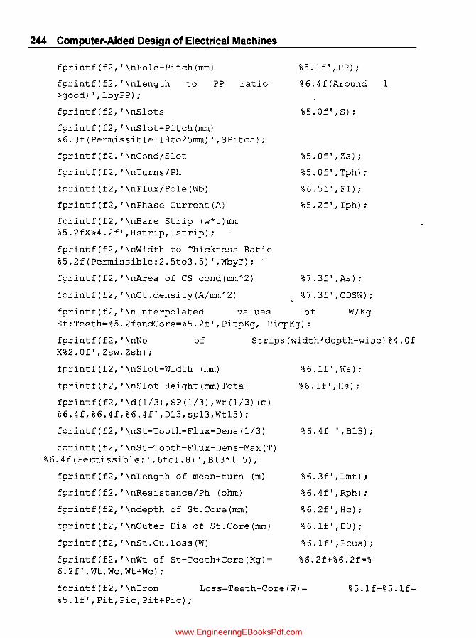
244 Computer-Aided Design of Electrical Machines
fprintf(f2, '\nPole-Pitch(mm)
fprintf(f2, '\nLength >good) , ,LbyPP) ;
fprintf(f2, '\nSlots
to PP ratio
fprintf(f2, '\nSlot-Pitch(mm) %6.3f(Permissible:18to25mm) ',SPitch);
fprintf(f2, '\nCond/Slot
fprintf(f2, '\nTurns/Ph
fprintf(f2, '\nFlux/Pole(Wb)
fprintf(f2, '\nPhase Current (A)
fprintf(f2, '\nBare Strip (w*t)mm %5.2fX%4.2f',Hstrip,Tstrip);
fprintf(f2,'\nWidth to Thickness Ratio %5.2f(Permissible:2.5to3.5) ',WbyT);
fprintf(f2, '\nArea of CS cond(mmA 2)
fprintf(f2, '\nCt.density(A/mmA 2)
%5.1f',PP);
%6. 4f (Around
%5.0f',S);
%5.0f',Zs);
%5.0f',Tph);
%6.5f',FI);
%5.2f'.,Iph);
%7 .3f' ,As);
%7 .3f' ,COSW);
fprintf(f2, '\nlnterpolated values of W/Kg St:Teeth=%5.2fandCore=%5.2f',PitpKg, PicpKg);
1
of
fprintf(f2, '\nNo X%2.0f',Zsw,Zsh);
of Strips (width*depth-wise) %4.0f
fprintf(f2, '\nSlot-Width (mm)
fprintf(f2, '\nSlot-Height(mm)Total
fprintf(f2, '\d(l13) ,SP(l13) ,Wt(l/3) (m) %6.4f,%6.4f,%6.4f',013,sp13,Wt13);
fprintf(f2, '\nSt-Tooth-Flux-Oens(1/3)
fprintf(f2, '\nSt-Tooth-Flux-Oens-Max(T) %6.4f(Permissible:1.6to1.8) ',B13*1.5);
fprintf(f2, '\nLength of mean-turn (m)
fprintf(f2, '\nResistance/Ph (ohm)
fprintf(f2, '\ndepth of St.Core(mm)
fprintf(f2, '\nOuter Oia of St.Core(mm)
fprintf(f2, '\nSt.Cu.Loss(W)
fprintf(f2, '\nWt of St-Teeth+Core(Kg)= 6.2f',Wt,Wc,Wt+Wc);
%6.1f',Ws);
% 6.1 f' , Hs) ;
%6.4f ',B13);
%6.3f' ,Lmt);
% 6. 4 f' , Rph) ;
%6.2f' ,Hc);
%6.1f' ,DO);
%6.1f',Pcus);
%6.2f+%6.2f=%
fprintf(f2, '\nlron %5.1f',Pit,Pic,Pit+Pic);
Loss=Teeth+Core(W)= %5 .1f+%5 .1f=
www.EngineeringEBooksPdf.com
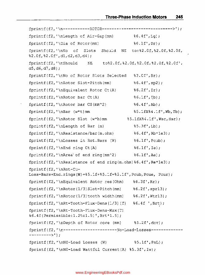
Three-Phase Induction Motors 246
fprintf(f2, '\n-----------ROTOR----------------------------->');
fprintf(f2, '\nLength of Air-Gap(mm)
fprintf(f2, '\Dia of Rotor(mm)
%6.4f' ,Lg);
% 6. 1 f' , Dr) ;
fprintf(f2, '\nNo of Slots Should NE to:%2.0f,%2.0f,%2.0f, % 2.0 f, % 2.0 f' , dl, d2, d3, d4 ) ;
fprintf(f2, '\nShould d5, d6, d7 , d8) ;
NE to%2.0f,%2.0f,%2.0f,%2.0f,%2.0f',
fprintf(f2, '\nNo of Rotor Slots Selected %3.0f',Sr);
fprintf(f2, '\nRotor Slot-Pitch(mm) %6.4f',sp2);
fprintf(f2, '\nEquivalent Rotor Ct(A) %6.2f',Ir);
fprintf(f2, '\nRotor bar Ct(A) %6.1f',lb);
fprintf(f2, '\nRotor bar CS(mmA2) %6.4f',Ab);
fprintf(f2, '\nBar (w*t)mm %5.1fX%4.1f',Wb,Tb);
fprintf(f2, '\nRotor Slot (w*h)mm %5.1fX%4.1f',Wsr,Hsr);
fprintf(f2, '\nLength of Bar (m) %5.3f',Lb);
fprintf(f2, '\nResistance/bar(m.ohm) %6.4f',Rb*le3);
fprintf(f2, '\nLosses in Rot.Bars (W) %6.lf',Pcub);
fprintf(f2, '\nEnd ring Ct(A) %6.1f',Ie);
fprintf(f2, '\nArea\ of end ring (mmA2) %6.1f',Ae);
fprintf(f2, '\nResistance of end ring(m.ohm)%6.4f',Re*le3);
fprintf(f2, '\nRot-CuLoss=Bars+End.rings(W)=%5.1f+%5.1f=%5.1f',Pcub,Pcue, Pcur);
fprintf(f2, '\nEquivalent Rotor res (Ohm)
fprintf(f2, '\nRotor(1/3)Slot-Pitch(mm)
fprintf(f2, '\nRotor(1/3)tooth width(mm)
fprintf (f2, '\nRt-Tooth-Flux-Dens (1/3) (T)
fprintf(f2, '\nRt-Tooth-Flux-Dens-Max(T) %6.4f(Permissible:1.2to1.5)' ,Brt*1.5);
fprintf(f2, '\nDepth of Rotor core (mm)
%6.3f' ,Rr);
%6.2f' ,spr13);
%6.2f' ,Wtr13);
% 6 . 4 f " Brt) ;
% 5 . 2 f' , dcr) ;
fprintf(f2, '\n----------------------No-Load-Losses--------------------->');
fprintf(f2, '\nNO-Load Losses (W) %5.1f',PnL);
fprintf(f2, '\nNO-Load Wattful Current (A) %5.3f',Iw);
www.EngineeringEBooksPdf.com

246 Computer-Aided Design of Electrical Machines
fprintf(f2, '\n-------------------Magnetizing-Current------------------->');
fprintf(f2, '\nlnterpolated values of at/m of St:Core=%5.1fandTeeth=%5.1f',atsc,atst);
fprintf(f2, '\nlnterpolated values of Caters Coeffts:k01=%5.3f,k02=%5.3f,kv= %5.3f', k01,k02,kv);
fprintf(f2, '\nStator %5.1f+%5.1f=%5.1f',ATSC,ATST,ATS);
fprintf(f2, '\nRotor AT %5.1f+%5.1f=%5.1f',ATRC,ATRT,ATR);
AT:Core+Teetn:
:Core+Teeth:
fprintf(f2, '\nTotal AT :Stator+Rotor+Airgap: %5.1f+%5.1f+%5.1f= %5.1f',ATS,ATR, ATg,ATT);
fprintf(f2, '\nNO-Load Current (A) Iw=%5.2f,Im=%5.2f and IO=%5.2f at pf=%5.3f',Iw, Im,IO,pfO);
fprintf(f2, '\nIO/lph ratio %5.3f',IObyI);
fprintf(f2, '\n-------------------Short-Circuit-Current-------------------->');
fprintf(f2, '\nSlot-Permeances: Stator=%5.3f,Rotor=%5.3f ~nd
Rotor refered to stator= %5.3f',Lmdss,Lmdsr,Lmddsr);
fprintf(f2, '\nSpecific-Slot-Permeance=%5.3f',ssp);
fprintf(f2, '\nTotalReactance(X) :Slot+Overhang+ZigZag=%5.3f+%5.3f+%5.3f=% 5.3fohms',Xs,XO,Xz,X);
fprintf(f2, '\nShort-Circuit: R=%5.2f,Z=%5.2f and Isc=%5.1f at pf=%5.3f;Isc/IFL=% 5.3f',R,Z,Isc,pfsc,RAT);
fprintf(f2, '\nTotalLosses(PnL+Pcus+Pcur)=%5.1f+%5.1f+%5.1f=%5.1 fWandEfficiency=%5.2f perc',PnL,Pcus,Pcur,Pt,EFF);
fprintf(f2, '\nSlip at FL
fprintf(f2, '\nStarting Tq
=%5.3f X Perc',SFL);
=%5.3f X FL-Tq',Tst);
fprintf(f2, '\nMax.Output(KW)=%5.1f',Pmax); v=11.75;00=0.24;L=0.09;
fprintf(f2, '\nTemp-Rise(deg-C) =%5.1f',Tr);
%0=0.15;
fprintf(f2, '\nTotalWt(Kg)=Wcus+Wt+Wc+Wri+Wcur+Wcue=%5.1f+%5.1f+ %5.1f+%5.1f+%4.1f+%4.1f=%5.1f',Wcus,Wt,Wc,Wri,Wcur,Wcue,Wtot);
fprintf(f2, '\nTotal Wt(Kg)=%5.1f and Kg/KW=%5.2f',Wtot,KgPKw);
fprintf(f2, '\n<------------End of Output-------->');
fclose (f2) ;
%-----------------------------------------------------
www.EngineeringEBooksPdf.com
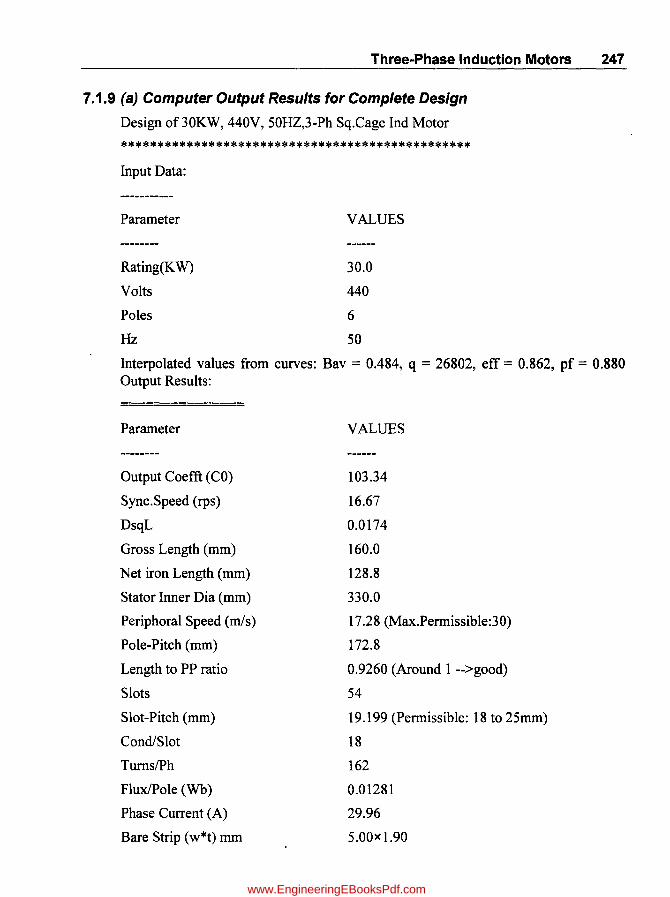
Three-Phase Induction Motors 247
7.1.9 (a) Computer Output Results for Complete Design
Design of30KW, 440V, 50HZ,3-Ph Sq.Cage Ind Motor
************************************************
Input Data:
-----------
Parameter VALUES
Rating(KW) 30.0
Volts 440
Poles 6
Hz 50
Interpolated values from curves: Bav = 0.484, q = 26802, eff = 0.862, pf = 0.880 Output Results:
Parameter
Output Coefft (CO)
Sync. Speed (rps)
DsqL
Gross Length (mm)
Net iron Length (mm)
Stator Inner Dia (mm)
Periphoral Speed (m/s)
Pole-Pitch (mm)
Length to PP ratio
Slots
Slot-Pitch (mm)
CondiSlot
TurnslPh
FluxIPole (Wb)
Phase Current (A)
Bare Strip (w*t) mm
VALUES
103.34
16.67
0.0174
160.0
128.8
330.0
17.28 (Max.Permissible:30)
172.8
0.9260 (Around 1 -->good)
54
19.199 (Permissible: 18 to 25mm)
18
162
0.01281
29.96
5.00x 1.90
www.EngineeringEBooksPdf.com

248 Computer-Aided Design of Electrical Machines
Width to Thickness Ratio
Area ofCS cond (nun"2)
Ct.density (A/nun"2)
2.63 (Pennissible: 2.5 to 3.5)
9.186
3.500
Interpolated values ofWlKg ofSt:Teeth = 23.92 and Core = 18.32
No. of Strips (width*depth - wise) 3 x 6
Slot-Width (mm) 10.6
Slot-Height (mm) Total 46.0
St-Tooth-Flux-Dens (1/3) 1.0644
St-Tooth-Flux-Dens-Max (T) 1.5966 (Pennissible: 1.6 to 1.8)
Length of mean-tum (m) 0.957
ResistancelPh (ohm) 0.3546
Depth of St.Core (mm) 39.00
Outer Dia of St. Core (mm) 500.0
St.Cu.Loss (W) 954.6
Wt. ofSt- Teeth + Core(Kg)= 25.91 + 53.60 = 79.51
Iron Loss = Teeth + Core(!V)= 619.9 + 982.2 = 1602.1
-------------------------ROTOR-----------------------------»
Length of Air-Gap (nun) 0.6600
No. of Slots Should NE to: 36, 48, 42, 24,
Should NEto 53,52,47,46,
No. of Rotor Slots Selected 45
Rotor Slot-Pitch (nun) . 22.9462
Equivalent Rotor Ct (A) 25.46
Rotor bar Ct (A) 525.3
Rotor bar CS (nun"2) 88.2000
Bar (w*t) mm 15.0 x 6.0
Rotor Slot (w*h) mm 6.5 x 15.5
Length of Bar (m) 210.000
Resistancelbar (m.ohm) 0.0500
Losses in Rot.Bars (W) 620.8
End ring Ct (A) 1254.0
Area of end ring (mm"2) 209.0
Resistance of end ring (m.ohm) 0.0880
www.EngineeringEBooksPdf.com

Three·Phase Induction Motors 249
Rot-Cu-Loss = Bars+End.rings (W) =620.8 + 276.7 = 897.5
Equivalent Rotor res (Ohm) 0.461
Rotor (1/3) Slot-Pitch (mm) 21.50
Rotor (1/3) tooth width (mm) 15.00
Rt-Tooth-Flux-Dens (1/3) (T) 0.8839
Rt-Tooth-Flux-Dens-Max (T)
Depth of Rotor core (mm)
1.3259 (Permissible: 1.2 to 1.5)
36.84
----------------------N 0-Load-Losses---------------------->
No-Load Losses (W) 1902.1
No-Load Wattful Current (A) 1.441
-------------------Magnetizing-Current -------------------->
Interpolated values ofatlm ofStCore = 480.8 and Teeth = 706.5
Interpolated values of Caters Coeffts: kOI = 0.663, k02 = 0.453, kv = 0.700
Stator AT: Core + Teeth: 38.7 + 32.5 = 71.2
Rotor AT: Core + Teeth: 21.9 + 4.6 = 26.5
Total AT: Stator + Rotor + Airgap: 71.2 + 26.5 + 438.3 = 536.0
NO-Load Current(A) Iw = 1.44, 1m = 8.88 and 10 = 9.00 at pf= 0.160
IOIIph ratio 0.300
-------------------Short -C ircuit -Current -------------------->
Slot-Permeances: Stator = 1.987, Rotor = 1.019 and Rotor referred to stator = 1.115
Specific-Slot-Permeance = 3.102
TotaIReactance(X): Slot + Overhang + Zig - Zag = 1.143 + 1.140 + 1.243 = 3.527 ohms
Short-Circuit R = 0.82, Z = 3.62 and Isc = 121.5 at pf= 0.225; IsclIFL = 4.057
Total Losses (PnL + Pcus + Pcur) = 1902.1 + 954.6 + 897.5 = 3754.2 W and Efficiency = 88.88 perc
Slip at FL = 2.877 x Perc
Starting Tq =
Max.Output (KW) =
Temp-Rise (deg-C) =
0.655 x FL - Tq
60.6
55.5
Total Wt (Kg) = Wcus + Wt + We + Wri + Wcur + Wcue = 38.0 + 25.9 + 53.6 + 51.0 + 7.4 + 3.3 = 179.3
Total Wt (Kg) = 179.3 and Kg/KW = 5.98
<------------End of Output -------->
www.EngineeringEBooksPdf.com
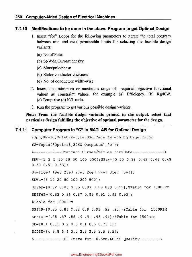
250 Computer-Aided Design of Electrical Machines
7.1.10 Modifications to be done in the above Program to get Optimal Design
1. Insert "for" Loops for the following parameters to iterate the total program between min and max permissible limits for selecting the feasible design variants:
(a) No of Poles
(b) St-Wdg Current density
(c) Slots/pole/phase
(d) Stator conductor thickness
(e) No. of conductors width-wise.
2. Insert also minimum or maximum range of required objective functional values as constraint values, for example (a) Efficiency, (b) KglKW, (c) Temp-rise (d) 1011 ratio.
3. Run the program to get various possible design variants.
Note: From the feasible design variants printed in the output, select that particular design fulfilling the objective of optimal parameter for the design.
7.1.11 Computer Program in "C" in MATLAB for Optimal Design
%3ph,KW=30;V=440;P=6;f7 50Sq.Cage IM wth Sq.Cage Rotor
f2=fopen('Optimal_30KW_Output.m', 'WI);
%--------~---Standard Curves/Tables for%Oata-------------->
SKW=[l 2 5 10 20 50 100 500];SBav=[0.35 0.38 0.42 0.46 0.48
0.50 0.51 0.53];
Sq=[16e3 1ge3 23e3 25e3 26e3 2ge3 31e3 33e3];
SKWa=[5 10 20 50 100 200 500];
SPF6P=[0.82 0.83 0.85 0.87 0.89 0.9 0.92];%Table for 1000RPM
SEFF6P=[0.83 0.85 0.87 0.89 0.91 0.92 0.93];
%Table for 1000RPM
SPF4P=[0.85 0.86 0.88 0.9 0.91 .92 .93];%Table for 1500RPM
SEFF4P=[.85 .87 .88 .9 .91 .93 .94];%Table for 1500RPM
SO=[O.l 0.15 0.2 0.3 0.4 0.5 0.75 1];
SCOSW=[4 3.8 3.6 3.5 3.5 3.5 3.5 3.5];
%-------------BH Curve for--0.5mm,LOHYS Quality--------->
www.EngineeringEBooksPdf.com
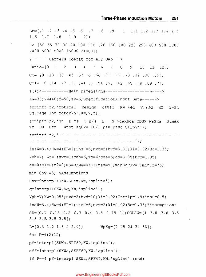
Three-Phase Induction Motors 251
BB= [ . 1 . 2 . 3 . 4 . 5 . 6 . 7 . 8 . 9
1.6 1.7 1.8 1.9 2l;
1 1.1 1.2 1.3 1.4 1.5
H= [50 65 70 80 90 100 110 120 150 180 220 295 400 580 1000
2400 5000 8900 15000 24000l;
%-------Carters Coefft for Air Gap--->
Ratio=[O 1 2 3 4 5 6 7 8 9 1011 12l;
CC= [0 .18 .33 .45 .53.6.66.71 .75 .79.82.86 .89li
CC1= [0 .14 .27 .37 .44 .5 .54 .58 .62 .65 .68 .69 .7li
% (l)<-----------Main Oimensions----------------------->
KW=30iV=440if=50i%P=6iSpecification/lnput Oata------>
fprintf(f2, 'Optimal Design of%4d KW,%4d V,%3d HZ 3-Ph
Sq.Cage Ind Motor\n',KW,V,f)i
fprintf(f2, 'Sn P Zs 0 m/s L S wcaXhca COSW WsXHs Btmax
Tr DO Eff Wtot KgPkw 10/1 pfO pfsc Slip\n') i
fprintf(f2, '-- -- -- ------ --- -- ------- ---- ------ -----
-- ---- ----- ---- ----- ---- --- ---- ----');
insW=3.4iHw=4iHL=liinsH=6invd=2ibvd=0.01iki=0.92iBc=1.35i
Vph=Vi Zr=likwr=licdb=6iTb=6icde=6idd=0.05;Brc=1.35i
sn=Oi M1=Oi M2=Oi M3=OiM4=OiEFFmax=90i minKgPkw=9iminTr=75 i
minIObyI=5i %Assumptions
Bav=interp1(SKW,SBav,KW, 'spline');
q=interp1(SKW,Sq,KW, 'spline')i
Vph=ViKw=0.955invd=2ibvd=10iki=0.92iTstri,P=1.9iinsS=0.5i
insW=3.4iHw=4iHL=liinsH=6invd=2iki=0.92iBc=1.35i%Assumptions
SO=[O.l 0.15 0.2 0.3 0.4 0.5 0.75 lliSCOSW=[4 3.8 3.63.5
3.5 3.~ 3.5 3.5li
B=[0.8 1.2 1.6 2 2.4li WpKg=[7 15 24 34 50li
for P=4:2:10i
pf=interp1(SKWa,SPF6P,KW, 'spline')i
eff=interp1(SKWa,SEFF6P,KW, 'spline')i
if P==4 pf=interp1(SKWa,SPF4P,KW, 'spline')iendi
www.EngineeringEBooksPdf.com
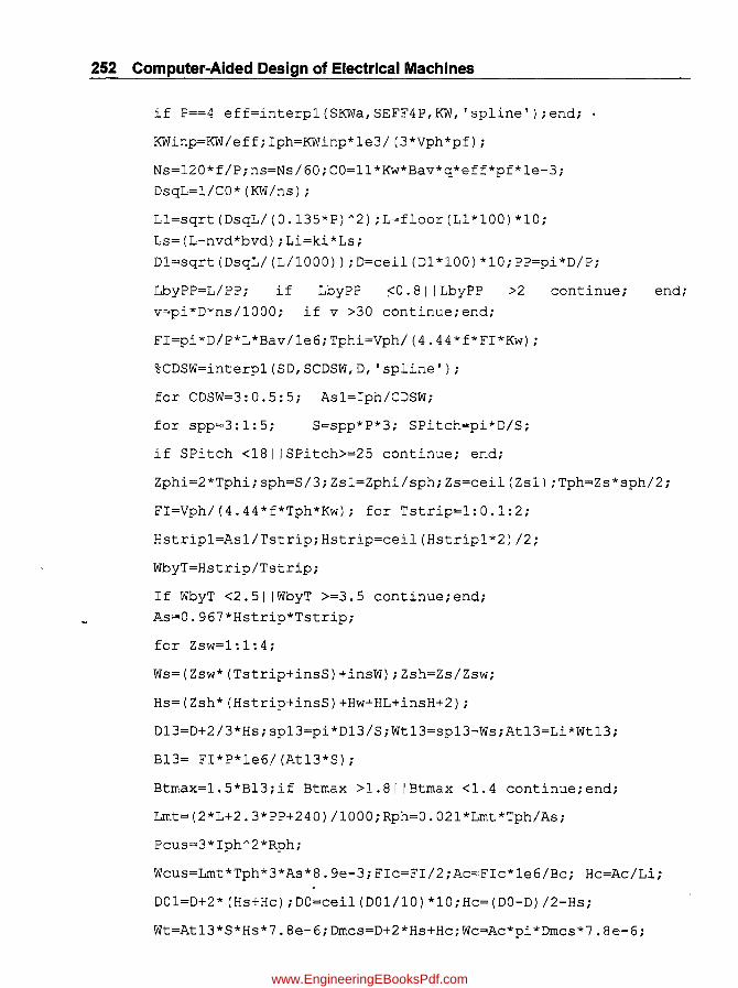
252 Computer-Aided Design of Electrical Machines
if P==4 eff=interpl(SKWa,SEFF4P,KW, 'spline');end;
KWinp=KW/eff;Iph=KWinp*le3/(3*Vph*pf);
Ns=120*f/P;ns=Ns/60;CO=11*Kw*Bav*q*eff*pf*le-3;
DsqL=l/CO*(KW/ns);
Ll=sqrt(DsqL/(0.135*P)A2) ;L=floor(Ll*lOO)*lO;
Ls=(L-nvd*bvd);Li=ki*Ls;
Dl=sqrt(DsqL/(L/lOOO));D=ceil(Dl*lOO)*lO;PP=pi*D/P;
LbyPP=L/PP; if LbyPP :<0.8 I I LbyPP >2 continue;
v=pi*D*ns/lOOO; if v >30 continue;end;
FI=pi*D/P*L*Bav/le6;Tphi=Vph/(4.44*f*FI*Kw);
%CDSW=interpl(SD,SCDSW,D, 'spline');
for CDSW=3:0.5:5; Asl=Iph/CDSW;
for spp=3:l:5; S=spp*P*3; SPitch=pi*D/S;
if SPitch <181 ISPitch>=25 continue; end;
end;
Zphi=2*TphiiSph=S/3;Zsl=Zphi/sphiZs=ceil(ZslliTph=Zs*sph/2;
FI=Vph/(4.44*f*Tph*Kw)i for Tstrip=1:0.1:2;
Hstripl=Asl/Tstrip;Hstrip=ceil(Hstripl*2)/2i
WbyT=Hstrip/Tstrip;
If WbyT <2.51 IWbyT >=3.5 continueiendi
As=0.967*Hstrip*Tstrip;
for Zsw=1:1:4;
Ws=(Zsw*(Tstrip+insS)+insW)iZsh=Zs/Zsw;
Hs=(Zsh*(Hstrip+insS)+Hw+HL+insH+2);
D13=D+2/3*Hs;sp13=pi*D13/S;Wt13=sp13-Ws;At13=Li*Wt13;
B13= FI*P*le6/(At13*S);
Btrnax=1.5*B13;if Btrnax >1.81 I Btrnax <1.4 continue;endi
Lrnt=(2*L+2.3*PP+240)/lOOOi Rph=0.02l*Lrnt*Tph/As;
Pcus=3*IphA2*Rph;
Wcus=Lrnt*Tph*3*As*8.ge-3iFIc=FI/2;Ac=FIc*le6/Bc; Hc=Ac/Lii
D01=D+2*(Hs+Hc);DO=ceil(DOl/lO)*10iHc=(DO-D)/2-Hs;
Wt=At13*S*Hs*7.8e-6;Drncs=D+2*Hs+Hc;Wc=Ac*pi*Drncs*7.8e-6;
www.EngineeringEBooksPdf.com

Three-Phase Induction Motors 263
PitpKg=interp1(B,WpKg,Btmax, 'spline');
PicpKg=interp1(B,WpKg,Bc, 'spline');
Pit=PitpKg*Wt;Pic=PicpKg*Wc;
%-----------------------ROTOR----------------------->
Zr=1;kwr=1;cdb=6;Tb=6;cde=6;dd=50;Brc=1.35; %Assumptions
kws=Kw;Ss=S;Lg1=0.2+2*sqrt(D*L/1e6);Lg=ceil(Lg1*100)/100;
Dr=D-2*Lg;d1=Ss-3*P;d2=Ss-P;d3=Ss-2*P;d4=Ss-5*P;
d5=Ss-1;d6=Ss-2;d7=Ss-7;d8=Ss-8;Sr=Ss-9;sp2=pi*Dr/Sr;
Ir=0.85*Iph;Ib=Ir*kws*Ss*Zs/(kwr*Sr*Zr); Abi=Ib/cdb;
Wb=ceil(Abi/Tb) ;Ab=Tb*Wb*0.98;Wsr=Tb+0.5;Hsr=Wb+0.5;Lb=L+50;
Rb=0.021*Lb/1e3/Ab; Pcub=Ib~2*Rb*Sr; Ie=Ib*Sr/P/pi;
Ae=Ie/cde;Dme=Dr-dd;Lme=pi* Dme/1000;Re= 0.021*Lme/Ae;
Pcue=2*Ie~2*Re;Pcur=Pcub+Pcue;Rr=Pcur/(3*Ir~2);
Dr13=Dr-2*2/3*Hsr;spr13= pi*Dr13/Sr;
Wtr13=spr13-Wsr;Atr=Wtr13*Li*Sr/P;Brt=FI*le6/Atr;Brtmax=
Brt*1.5;if Brtmax >1.5 continue;end;
Ac=FI*le6/2/Brc;dcr=Ac/Li;Pfw=0.01*KW*le3;
PnL=Pit+Pic+Pfw; Iw=PnL/3/V;
Wcur=Lb*Sr*Ab*8.ge-6; Wcue=Lme*2*Ae*8.ge-3;
% (4) <--AmpTurns and Magnetizing-Current--------------------
->
%-------------BH Curve for--0.5mm,LOHYS Quality--------->
BB= [ . 1 . 2 . 3 . 4 . 5 . 6 . 7 . 8 . 9
1.6 1.7 1.8 1.9 2];
1 1.1 1.2 1.3 1.4 1.5
H= [50 65 70 80 90 100 110 120 150 180 220 295 400 580 1000
2400 5000 8900 15000 24000];
%-------Carters Coefft for Air Gap--->
Ratio=[O 1 2 3 4 5 6 7 8 9 10 11 12 ] ;
CC= [0 .18 .33 .45 .53 .6 .66 .71 .75 .79 .82 .86 .89 ] ;
CC1= [0 .14 .27 .37 .44 .5 .54 .58 .62 .65 .68 .69 .7 ] ;
WssO=4;WsrO=2; %Assumptions
atsc=interp1(BB,H,Bc, 'spline');Dcav=D+2*Hs+Hc;
www.EngineeringEBooksPdf.com

254 Computer-Aided Design of Electrical Machines
ATSC=pi*Dcav/P/3*atsc/1e3;
Bt30=B13*1.36;atst=interp1(BB,H,Bt30, 'spline');
ATST=atst*Hs/1000;ATS=ATSC+ATST;
rat1=WssQ/Lg;k01=interp1(Ratio,CC,rat1, 'spline');
kgs=SPitch/(SPitch-WssO*k01); rat2=WsrO/Lg;
k02=interp1(Ratio,CC,rat2, 'spline');sprO=pi*Dr/Sr;
kgr=sprO/(sprO-WsrO*k02); kg=kgs*kgr; Lgd=Lg*kg;rat3=bvd/Lg;
kv=interp1(Ratio,CC1,rat3, 'spline');
if rat3 >=12 kv=0.7;end; Ld=L-kv*nvd*bvd; Aag=pi*D/P*Ld;
Bg=FI*le6/Aag; B30d=1.36*Bg; ATg=0.796 *B30d*Lgd*le3;
Btr30=Brt*1.36; atrt=interp1(BB,H,Btr30, 'spline');
ATRT=atrt*Hsr/1e3;
atrc=interp1(BB,H,Brc, 'spline');
/3*atrc; ATR=ATRC+ATRT;ATT=ATS+ATR+ATg;
Dcrav=Dr-2*Hsr-dcr;
ATRC=pi*Dcrav/le3/P
Im=P/2*ATT/(1.17*Kw*Tph);IO=sqrt(IwA2+ImA2);
pfO=Iw/IO;IObyI=IO/Iph;
% (5) <----------Short-Circuit-Current-------------------->');
h2=1.6;h2r=0;h3r=0;h4r=0.5;ks=1; %Assumptions
h1=Zsh*(Hstrip+insS);h3=Hw;h4=HL;bs=Ws;bO=WssO;
Lmdss=h1/3/bs +h2/bs +2*h3/(bs+bO) +h4/bO;
br=Wsr; brO=WsrO;
Lmdsr=h1r/3/br +h2r/br +2*h3r/(br+brO) +h4r/brO;
Lmddsr=KwA2*S/Sr*Lmdsr; ssp = Lmdss+Lmddsr;
gd=S/P/3;p=P/2;Xs=15.8*f*L*ssp*Tph A2/(p*gd)*le-9;
LOLmdO=ks*PP A2/pi/ SPitch/1000;
XO=15.8*f*LOLmdO*TphA2/(p*gd)*le-6; gs=S/P;
h1r=Wb;
gr=Sr/P;
Xm=Vph/lm; Xz=5/6 *Xm*(1/gsA2+1/grA2);X=Xs+XO+Xz; R=Rph+Rri
Z=sqrt(RA2+X A2); Isc=Vph/Z; pfsc=R/Z; RAT=Isc/lph;
%(6)<--------------Performance-------------------->');
Pt=PnL+Pcus+Pcur;EFF=KW/(KW+Pt/1000) *100;
if EFF <88.8continue; end; Rinp=KW*lOOO+Pfw+Pcur;
SFL=Pcur/Rinp*lOOi Tst=(Isc/lr)A2*SFL/100i
Pmax=3*Vph*(Isc-IO)/2/(1+pfsc)*le-3;
www.EngineeringEBooksPdf.com

Three·Phase Induction Motors 255
Acooll=(pi*D*(L*2.5)+2*pi*(D+50)*O.04)/le6i Acoo12=Acool1*(1+O.1*v)iAcoo13=pi*DO~L/le6i
AcoolT=Acoo12+Acoo13i Pst=Pcus+Pit+Pici
Tr=O.03*Pst/AcoolTi if Tr>56 continueiendi Ars=Wsr*Hsr*Sri
Dri=Dcrav-dcri Wri=(pi*(Dr A 2-Dri A 2) /4-Ars)*L*7.8e-6i
Wtot=l.Ol*(Wcus+Wt+Wc+Wri+Wcur+Wcue) iKgPkw=W~ot/KWi
if KgPkw >6.1 continueiendi
%------------------End of Program-------------------------->
sn=sn+li if EFF >=EF?max EFFmax=EFFi endi
if abs(EFF-EFFmax)<=2e-3 M2=sn; endi
if KgPkw <=minKgPkw minKgPkw=KgPkwiendi
if abs(KgPkw-minKgPkw)<=O.OOl Ml=sni endi
if endi
Tr<=minTr minTr=Triendiifabs(Tr-minTr)<=O.OOOl
if IObyI <=minIObyI minIObyI=IObyliendi
if abs(IObyI-minIObyI)<=O.OOOl M4=sni endi
M3=sni
fprintf(f2, '\n%2d%3d%3d%4.0~%3.0f%4.0f%3d%4.1fX%3.1f%4.1f',s n,P,Zs,D,v,L,S,Tstrip,Hstrip,CDSW)i
fprintf(f2, '%5.1fX%2.0f%6.3f%5.1f%4.0f%6.2f%5.0f%6.2f%5.2f%5 .2f%5.2f%4.1f',Ws,Hs,Btmax,Tr,DO,EFF,Wtot,KgPkw,IObyI,pfO,pf sc,SFL)iendiendiendiendiendi
fprintf(f2, '\n--- ----- ----- ---------- --------- --- --- ----- ---- ---- \n')i
fprintf(f2, 'Selection of Design Variant based on Optimization Criteria: ')i
fprintf(f2, '\nlf Variant (Sn)=-%3d
fprim:f(f'2, '\nlf Variant(Sn)=%3d
Maximum Efficlency is Required (%5.2f perc) ',M2,EFFmax)i
Minimum Kg /K'"tJ is Required, (%5.2f)', M1,minKgPkw) i
fprintf(f2, '\nlf Minim\L.'1\ Temp-Rise is Reqd, Variant (Sn)=%3d (%4.2f) " M3,minTr) i
Select
Select
Select
fprintf(f2, '\nI£ Variant (Sn)=%3d
Minimum ratio of IOIr is Reqd, Select (%4.2£)' ,M4,minIObyI) ifclose(f2) isn,Hs,Hc,
www.EngineeringEBooksPdf.com

7.1.11 (a) Computer Output Results for Optimal Design
Optimal Design of30 KW, 440 V, 50 HZ 3 -Ph Sq.Cage Ind Motor
Sn I} Zs D m/s L S wcaxhca CDSW Wsxlls Btmax Tr DO Eff Wtot KgPkw lOll pill pfsc Slip -- -- -- -_ .. _-- .. -.. -- ____ .. _ .. ---- ------ ----- -- _oo_ .. ___ .. ________________________________ .... ________________ ...... ___ .. _____ .... _ .. _______________________________________ ..
I 4 20 250 20 190 36 1.8x5.5 3.0 12.6x43 1.573 51.0 420 90.05 172 5.74 0.27 0.19 0.17 2.3 2 4 20 250 20 190 36 1.9x5.5 3.0 13.0x43 .628 50.4 420 90.13 173 5.78 0.27 0.18 0.17 2.3 3 4 20 250 20 190 36 2.0x5.0 3.0 13.4x41 .711 50.5 420 90.11 169 5.64 0.29 0.17 0.18 2.3 4 4 20 250 20 190 36 1.6x5.5 3.5 11.8 x43 .472 52.5 420 89.87 170 5.67 0.26 0.19 0.18 2.3 5 4 20 250 20 190 36 1.7x5.0 3.5 12.2x41 .539 52.6 420 89.86 166 5.54 0.27 0.18 0.19 2.3 6 4 20 250 20 190 36 1.8x5.0 3.5 12.6x41 .593 51.8 420 89.95 167 5.57 0.27 0.18 0.18 2.3 7 4 20 250 20 190 36 1.5x5.0 4.0 11.4x41 .443 54.6 420 89.61 164 5.48 0.26 0.18 0.19 2.3 8 4 20 250 20 190 36 1.6x4.5 4.0 11.8x38 .507 54.8 410 89.61 160 5.33 0.26 0.18 0.20 2.3 9 4 20 250 20 190 36 1.7x4.5 4.0 12.2x38 .558 53.8 410 89.74 161 5.36 0.27 0.18 0.20 2.3 10 6 18 330 17 160 54 1.9x5.5 3.0 10.6x49 .579 54.6 510 88.97 188 6.26 0.30 0.16 0.21 2.9 II 6 18 330 17 160 54 2.0x5.0 3.0 10.9x46 .644 54.6 500 88.98 182 6.08 0.31 0.16 0.22 2.9 12 6 18 330 17· 160 54 1.9x5.0 3.5 10.6x46 .597 55.5 500 88.88 181 6.04 0.30 0.16 0.23 2.9 --- ...... _- _ .... -- ---- ---- --- ....... -- ---- --_oo_--- ____ oo_ .. ___ oo ____ ....... _ .. __ .. _ .. __________ ---- .. ----- ---- ---- --- ---- -- -_oo- _ .. __ oo ____ .. _ .. _____ .. oo .... ___ oo ..... ____ .. _________________
Selection of Design Variant based on Optim ization Criteria
If Maximum Efficiency is Required, Select Variant (Sn) = 2 (99.13 perc)
If Minimum Kg/KW is Required, Select Variant (Sn) = 8 (5.33) If Minimum Temp-Rise is Required, Select Variant (Sn) = 2 (50.37) If Minimum mtio of 10/1 is Required, Select Variant (So) = 7 (0.26).
N 01 en
0 0 3 'C C S' ~ c: CD Q.
C II cO' = 0 ..... m CD n .... ::!. n !!!. 3!: AI n :::r
= II
www.EngineeringEBooksPdf.com
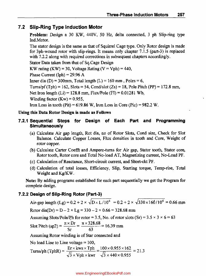
Three-Phase Induction Motors 267
7.2 Slip-Ring Type Induction Motor
Problem: Design a 30 KW, 440V, 50 Hz, delta connected, 3 ph Slip-ring type Ind.Motor.
The stator design is the same as that of Squirrel Cage type. Only Rotor design is made for 3ph-wound rotor with slip-rings. It means only chapter 7.1.5 (part-3) is replaced with 7.2.2 along with required corrections in subsequent chapters accordingly. Stator Data taken from that of Sq.Cage Design KW rating (KW) = 30, Voltage Rating (V = Vph) = 440, Phase Current (Iph) = 29.96 A Inner dia (D) = 300mm, Total length (L) = 160 mm, Poles = 6, Turns/pf (Tph) = 162, Slots = 54, Condlslot (Zs) = 18, Pole Pitch (PP) = 172.8 mm,
Net Iron length (Li) = 128.8 mm, FluxIPole (FI) = 0.01281 Wb, Winding factor (Kw) = 0.955, Iron Loss in tooth (Pit) = 619.86 W, Iron Loss in Core (Pic) = 982.2 W.
Using this Data Rotor Design is made as Follows
7.2.1 Sequential Steps for Design of Each Part and Programming Simultaneously
(a) Calculate Air gap length, Rot dia, no of Rotor Slots, Cond size, Check for Slot Balance. Calculate Copper Losses, Flux densities in tooth and Core, Weight of rotor copper.
(b) Calculate Carter Coefft and Ampere-turns for Air gap, Stator tooth, Stator core, Rotor tooth, Rotor core and Total No-load AT, Magnetizing current, No-Load PF.
(c) Calculation of Reactance, Short-circuit current, and Snort-ckt PF.
(d) Calculation of total losses, Efficiency, Slip, Starting torque, Temp-rise, Total Weight and Kg/KW.
Note: By adding programs established for each part sequentially we get the Program for complete design.
7.2.2 Design of Slip-Ring Rotor (Part-3)
Air-gap length (Lg) = 0.2 + 2 x ~D X LI106 = 0.2 + 2 x ~330x 1601106 = 0.66 mm
Rotor dia(Dr) = D - 2 x Lg = 330 - 2 x 0.66 = 328.68 mm
Assuming SlotslPole~h for rotor = 3.5, No. of rotor slots (Sr) = 3.5 x 3 x 6 = 63 • 1t x Dr 1t x 328.68
Slot Pltch (sp2) = --= 16.39 mm Sr 63
Assuming Rotor winding is of Star connected and
No load Line to Line voltage = 100,
Turns/ph (TphR) = Er x kws x Tph = 100 x 0.955 x 162 = 21.3 J3 x Vph x kwr J3 x 440 x 0.955
www.EngineeringEBooksPdf.com

258 Computer-Aided Design of Electrical Machines
C d /SI (Z) TphR x 3 x 2 21.3 x 3 x 2
on uctors ot r = ----Sr 63
= 2.02 ~ 2 (rounded off to nearest even integer) Zrx Sr 2x 63
Corrected Turns/ph (TphR) = = -- = 21 2x3 6
Equivalent Rotor Current (Ird) = 0.85 x Iph = 0.85 x 29.96 = 25.466 A
R (Ir) Ird kws x Ss x Zs 25446 0.955 x 54 x 18 19645 A otor current = x = . x = . kwr x Sr x Zr 0.955 x 63 x 2
Assuming Current density (cdr) = 5 Almm2,
CS of conductor (Acr) = Ir/cdr = 196.45/5 = 39.29 mm2,
Assuming width of conductor (wcR) = 4 mm,
Height of cond (hcR) = Acr/wcR = 39.29/4 = 9 .83~ 10 mm
Taking 0.98 factor for edges rounding off,
corrected (Acr) = 0.98 x wcR x hcR = 0.98 x 4 x 10 = 39.2 mm2,
Width of slot (Wsr) = wcR + 2.5 = 4 + 2.5 = 6.5 mm
Assuming wedge ht (HwR) = 4 mm and Lip ht (HLR) = 1 mm,
Height of slot (Hsr) = Zr x (hcR + 0.5) + 3 + HwR + HLR
= 2 x (10 + 0.5) + 3 + 4 + 1 = 29 mm Cross-Section of Rotor Slot (dimensions in mm)
Height-Wise
Lip 1.0 Wedge 4.0 Ins. Under Wedge 0.5 Cu. Conductor bare + insulation 10 + 0.5 = 10.5 Top-Layer for 1 conductor 1 x 10.5 = 10.5 10.5 Ins. between Layers 0.5 Bottom- Layer for 1 conductor 1 x 10.5 = 10.5 10.5 Bottom Insulation 0.5 29 Slack 1.5 I Rotor-Slot Total height 29.0 >
Width-Wise Cu.Conductor bare + insulation 4 + 0.5 = 4.5
for 1 conductor 1 x 4.5 = 4.5 4.5 Insulation on sides 2xO.6=1.2 1.2 Slack 0.8 Total width \ 6.5
Length of mean turn (LmtR) ;::: (2 x L + 2.3 x PP + 80)/1 000
Top
Layer
(1 cond)
Bottom
Layer
(1 cond)
6.5
=(2 x 160+2.3 x 172.8 + 80)/l000 = 0.7974 m
Resistance/ph (RphR) = 0.021 x LmtR x TphRi Acr
= 0.021 x 0.7974 x 21/39.2 = 8.9712 mn
10.5
0.5
lO'! 2.5
www.EngineeringEBooksPdf.com

· Three-Phase Induction Motors 259
Rotor Cu.Loss (Pcur) = 3 x? x RphR = 3 x 196.452 x 8.9712/1000 = 1038.7 W
Dia of rotor at ~tooth ht from tip (Dr13) = Dr-2 x % x Hsr
= 328.68 - 2 x % x 29 = 290.01
Rotor slot pitch at Dr13 (spr13) = 1t X Dr13 = 1t x 290.01 = 14.462 mm Sr 63
Width of tooth at Dr13 (Wtr13) = spr13 - Wsr = 14.4620 - 6.5 = 7.962 mm
Area of tooth at Dr13 (Atr) = Wtr13 x Li x SrlP = 7.962 x 128.8 x 63/6 = 10768 mm2
Flux density in tooth (Brt) = FI x 106/Atr = 0.01281 x 10⁶/10768 = 1.1897 T
Max Flux density in tooth (Brtmax) = Brt x 1.5 = 1.1897 x 1.5 = 1.7845 T «1.8 and hence OK)
Assuming Flux density in Rotor Core (Brc) = 1.35 T,
Ar fC (A) FI x 106
0.01281 X 10⁶
47448 1 ea 0 ore c = - =. m-2xBrc 2x1.35
Ac 4744.8 Depth of core (dcr) =- = = 36.84 mm
Li 128.8
Assuming Friction and Windage Loss (Pfw) = 1 %
= 0.01 x KW x 1000 = 0.01 x 30 x 1000 = 300 W
No load Loss (PnL) = Pit + Pic + Pfw = 619.9 + 982.2 + 300 = 1902.1 W
ActiveIWattful Component of No-load Current (Iw) = PnL = 1902.1 1.441 A 3xV 3x440
Wt. of Rotor Copper (Wcur) = LmtR x TphR x 3 x Acr x 8.9 x 10-6
= 0.7974 x 21 x 3 x 39.2 x 8.9 x 10-6 = 17.527 Kg
7.2.2 (a) Computer Program in "C" in MATLAS for Part-3
%--------------------Slip-Ring-ROTOR------------------------->
D=330;L=160;P=6;Tph=162;S=54;Kw=O.955;Vph=440;Iph=29.9 6;Zs=18;
FP=172.8;Li=128.8;FI=O.01281;KW=30;V=440;Pit=619.86;Pic=982.2;
sppR=3.5;Ss=S;kws=Kw; kwr=kws;Er=lOO;cdr=5;wcR=4;HwR=4;
HLR=l; Brc=1.35; %Assumtions
Lg1=O.2 + 2*sqrt(D*L/1e6);Lg=ceil(Lg1*lOO)/100; Dr=D-2*Lg;
Sr=sppR*3*P; sp2=pi*DrISr; TphR1=Erlsqrt(3)/Vph*~ws/kwr*Tph;
Zr1=TphR1*3*2/Sr; Zr=floor(Zr1); TphR=Zr*Sr/2/3;
Ird=O.85*Iph; Ir=Ird*(kws*Ss*Zs)/(kwr*Sr*Zr); Acr1=Ir/cdri ,hcR1=Acr1/wcR; hcR=ceil(hcR1); Acr=wcR*hcR*O.98; Wsr=wcR+2.5;
www.EngineeringEBooksPdf.com

260 Computer-Aided Design of Electrical Machines
Hsr=Zr*(hcR+0.5)+3+HwR+HLR; LmtR=(2*L+2.3*PP+80)/1000; RphR=0.021*LrntR*TphR/Acr; Pcur=3 *1rA2*RphR;
Dr13=Dr-2*2/3*Hsr; spr13=pi*Or13/Sr; Wtr13=spr13-Wsr; Atr=Wtr13*Li*Sr/P; Brt=F1*le6/Atr; Brtrnax=Brt*1.5; Ac=F1*le6/2/Brc; dcr=Ac/Li; Pfw=0.01*KW*le3; PnL=Pit+Pic+Pfw; 1w=PnL/3/V; Rr=RphR/(TphR/Tph)A2; Wcur=LmtR*TphR*3*Acr*8.ge-3;
%------------------------------------------------------Other Changes to be Made are as Follows
h1r = wcR; h2r = 1.6 ; h3r = HwR ; h4r = HLR;
br = Wsr ~ in 5th part(Short-Circuit Current)
For Short circuit Torque (Tst) = (IsclIrd)"2 x SFLl100 and
W cue = 0; ~ in 6th part{Perfonnance)
Remove Print statements whereever "bar" and "end rings" appear
Incorporating these Changes, The Modified Total Program is Given Below
7.2.3 Computer Program in "C" in MATLAB for Complete Design
%3ph,KW=30;V=440;P=6;f=50 Slip-Ring 1M
f2=fopen('Total_30KW_SR_Output.rn', 'w');
%------------Standard Curves/Tables for%Oata-------------->
SKW=[l 2 5 10 20 50 100 500];SBav=[0.35 0.38 0.42 0.46 0.48 0.50 0.51 0.53];
Sq=[16e3 1ge3 23e3 25e3 26e3 2ge3 31e3 33e3];
SKWa=[5 10 20 50 100 200 500];
SPF6P=[0.82 0.83 0.85 0.87 0.89 0.910.92];%Table for 1000RPM I
SEFF6P=[0.83 0.85 0.87 0.89 0.91 0.~2 0.93];%Table for 1000RPM
SPF4P=[0.85 0.86 0.88 0.9 0.91 .92 .93];%Table for 1500RPM
SEFF4P=[.85 .87 .88 .9 .91 .93 .94];%Table for 1500RPM
SO=[O.l 0.15 0.2 0.3 0.4 0.5 0.75 1];
SCOSW=[4 3.8 3.6 3.5 3.5 3.5 3.5 3.5];
%-------------BH Curve for--0.5rnrn,LOHYS Quality--------->
BB= [ . 1 . 2 . 3 . 4 . 5 . 6 . 7 . 8 . 9 1.7 1.8 1.9 2];
1 1.1 1.2 1.3 1.4 1.5 1.6
H= [50 65 70 80 90 100 110 120 150 180 220 295 400 580 1000 2400 5000 8900 15000 24000];
%-------Carters Coefft for Air Gap--->
Ratio=[O 1 2 3 4 5 6 7 8 9 101112];
www.EngineeringEBooksPdf.com
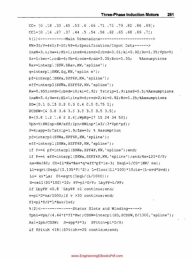
Three-Phase Induction Motors 261
CC= [ 0 . 18 . 33 . 45 . 53 . 6 . 66 . 71 . 75 . 7 9 . 82 . 8 6 . 8 9] ;
CC1=[0 .14 .27 .37 .44 .5 .54 .58 .62 .65 .68 .69 .7];
% (1) <-----------Main Dimensions----------------------->
KW=30;V=440;f=50;%P=6;Specification/lnput Data------>
insW=3.4;Hw=4;HL=1;insH=6;nvd=2;bvd=0.01;ki=0.92;Bc=1.35;Vph=V;
Zr=1;kwr=1;cdb=6;Tb=6;cde=6;dd=0.05;Brc=1.35; %Assumptions
Bav=interp1(SKW,SBav,KW, 'spline');
q=interp1(SKW,Sq,KW, 'splin e');
pf=interp1(SKWa,SPF6P,KW, 'spline');
eff=interp1(SKWa,SEFF6P,KW; 'spline');
Kw=O. 955;nvd=2;bvd=10;ki=0. 92; Tstrip=1.9;insS=0.5;%Assumptions
insW=3.4;Hw=4;HL=1;insH=6;nvd=2;ki=0.92;Bc=1.35;%Assumptions
SD=[O.l 0.15 0.2 0.3 0.4 0.5 0.75 1];
SCDSW=[4 3.8 3.6 3.5 3.5 3.5 3.5 3.5];
B=[0.8 1.2 1.6 2 2.4];WpKg=[7 15 24 34 50];
Vph=V;KWinp=KW/eff;Iph=KWinp*le3/(3*Vph*pf);
P=6;spp=3;Tstrip=1.9;Zsw=3; % Assumption
pf=interp1(SKWa,SPF6P,KW, 'spline');
eff=interp1(SKWa,SEFF6P,KW, 'spline');
if P==4 pf=interp1(SKWa,SPF4P,KW, 'spline');end;
if P==4 eff=interp1(SKWa,SEFF4P,KW, 'spline'):end:Ns=120*f/P:
ns=Ns/60: CO=11*Kw*Bav*q*eff*pf*le-3; DsqL=l/CO*(KW/ nS)i
L1=sqrt(DsqL/(0.135*P)A2)i L=floor(L1*100)*10iLs=(L-nvd*bvd)i
Li= ki*Ls: D1=sqrt(DsqL/(L/1000))i
D=ceil(D1*100)*10i PP=pi*D/Pi LbyPP=L/PPi
if LbyPP <0.81 I LbyPP >2 continueiendi
v=pi*D*ns/1000iif v >30 continue:end:
FI=pi*D/P*L*Bav/1e6:
% (2) <--------------Stator Slots and Winding----->
Tphi=Vph/(4.44*f*FI*Kw)iCDSW=interp1(SD,SCDSW,D/1000, 'spline')i
As1=Iph/CDSWi S=spp*P*3i SPitch=pi*D/Si
if SPitch <181 ISPitch>=25 continueiendi
www.EngineeringEBooksPdf.com

262 Computer-Aided Design of Electrical Machines
Zphi=2*Tphi;sph=S/3;Zsl=Zphi/sph;Zs=ceil(Zsl);Tph=Zs*sph/2; FI=Vph/(4.44*f*Tph*Kw); Hstripl=Asl/Tstrip; Hstrip=ceil(Hstripl*2)/2; WbyT=Hstrip/Tstrip;
if WbyT <2.51 IWbyT >=3.5 continue;end; As=O.967*Hstrip*Tstrip;
Ws=(Zsw*(Tstrip+insS)+insW);Zsh=Zs/Zsw;
Hs=(Zsh*(Hstrip+insS)+Hw+HL+insH+2);
D13=D+2/3*Hs;sp13=pi*D13/S;Wt13=sp13-Ws; B13=FI*P*le6/(Li*Wt13*S); Btmax=1.5*B13;
Lmt=(2*L+2.3*PP+240)/1000;Rph=O.021*Lmt*Tph/As;
Pcus=3*Iph A 2*Rph; Wcus=Lmt*Tph*3*As*8.ge-3;Flc=FI/2; Ac=Flc*le6/Bc; Hc = Ac/Li; D01=D+2*(Hs+Hc); DO=ceil(D01/10)*10; Hc=(DO-D)/2-Hs; PitpKg=interpl(B,WpKg,Btmax, 'spline'); PicpKg=interpl(B,WpKg,Bc, 'spline');
Wt=Li*Wt13*S*Hs*7.8e-6; Dmcs=D+2*Hs+Hc; WC=Ac*pi*Dmcs*7.8e-6;
Pit=PitpKg*Wt;Pic=PicpKg*Wc;
%--------------------Slip-Ring-ROTOR------------------------->
sppR=3.5;Ss=S;kws=Kw;kwr=kws;Er=100;cdr=5;wcR=4;HwR=4;HLR=l;
Brc=1.35; %Assumtions
Lgl=O.2 + 2*sqrt(D*L/le6);Lg=ceil(Lgl*100)/100;Dr=D-2*Lg;
Sr=sppR*3*P;sp2=pi*Dr/Sr;TphRl=Er/sqrt(3)/Vph*kws/kwr*Tph;
Zrl=TphRl*3*2/Sr;Zr=floor(Zrl);TphR=Zr*Sr/2/3;Er=TphR/TphRl*Er;
Ird=O.85*Iph;Ir=Ird*(kws*Ss*Zs)/(kwr*Sr*Zr);Acrl=Ir/cdr; hcRl=Acrl/wcR; hcR=ceil(hcRl); Acr=wcR*hcR*O.98; Wsr=wcR+2.5; Hsr=Zr*(hcR+O.5)+3+HwR+HLR;
LmtR=(2*L+2.3*PP+80)/1000; RphR=O.021*LmtR*TphR/Acr; Pcur=3*Ir A 2*RphR; Dr13=Dr-2*2/3*Hsr; spr13=pi*Dr13/Sr; Wtr13=spr13-Wsr; Atr=Wtr13*Li *Sr/P; Brt=FI*le6/Atr; Brtmax=Brt*1.5;Ac=FI*le6/2/Brc;dcr=Ac/Li;
Pfw=O.Ol*KW*le3; PnL=Pit+Pic+Pfw; Iw=PnL/3/V;
Rr=RphR/(TphR/ Tph)A2; Wcur=LmtR*TphR*3*Acr*8.ge-3;
%(4)<------------AmpTurns and Magnetizing-Current--------------
--------> %-------------BH Curve for--O.5mm,LOHYS Quality--------->
BB= [ . 1 . 2 . 3 . 4 . 5 . 6 . 7 . 8 . 9 1.7 1.8 1.9 2];
1 1.1 1.2 1.3 1.4 1.5 1.6
www.EngineeringEBooksPdf.com

Three-Phase Induction Motors 263
H= [50 65 70 80 90 100 110 120 150 180 220 295 400 580 1000 2400 5000 8900 15000 24000];
%-------Carters Coefft for Air Gap--->
Ratio=[O 1 2 3 4 5 6 7 8 9 10 11 12];
CC= [ 0 . 18 . 33 . 45 . 53 . 6 . 66 . 71 . 75 . 79 . 82 . 86 . 89 ];
CC1= [0 .14 .27 .37 .44 .5 .54 .58 .62 .65 .68 .69 .7 ];
WssO=4;WsrO=2; %Assumptions
atsc=interp1(BB,H,Bc, 'spline');
Dcav=D+2*Hs+Hc;ATSC=pi*Dcav/P/3*atsc/le3;
Bt30=B13*1.36;atst=interpl(BB,H,Bt30, 'spline');
ATST=atst*Hs/I000;ATS=ATSC+ATST;
ratl=WssO/Lg;kOl=interp1(Ratio,CC,ratl, 'spline');
kgs=SPitch/(SPitch-WssO*kOl);
rat2=WsrO/Lg;k02=interpl(Ratio,CC,rat2, 'spline');sprO=pi*Dr/Sr;
kgr=sprO/(sprO-WsrO*k02);kg=kgs*kgr;Lgd=Lg*kg;
rat3=bvd/Lg;kv=interp1(Ratio,CCl,rat3, 'spline');
if rat3 >=12 kv=O. 7; end; Ld=L-kv*nvd*bvd; Aag=pi *D/P*Ld; Bg=FI*le6/Aag;B30d=1.36*Bg;ATg= 0.796 *B30d*Lgd*le3;
-Btr30=Brt*1.36; atrt=interpl(BB,H,Btr30, 'spline'); ATRT=atrt*Hsr/le3; Dcrav=Dr-2*Hsr-dcr; atrc=interpl(BB,H,Brc, 'spline'); ATRC=pi *Dcrav/le3/P/3*atrc;
ATR=ATRC+ATRT; ATT=ATS+ATR+ATg; Im=P/2*ATT/(1.17*Kw*Tph);
IO=sqrt(Iw A 2+ImA 2); pfO=Iw/IO;IObyI=IO/Iph;
% (5) <-------------Short-Circuit-Current-------------------->');
h2=1. 6; h2r=1. 6; h3r=HwR; h4r=HLR; ks=l; %Assumptions
hl=Zsh*(Hstrip+insS);h3=Hw;h4=HL;bs=Ws;bO=WssO;
Lmdss=hl/3/bs +h2/bs +2*h3/ (bs+bO) +h4/bO;hlr=wcR;br=Wsr; brO= WsrO; Lmdsr=h1r/3/br +h2r/br +2*h3r/(br+brO) +h4r/brO;
Lmddsr=Kw A 2*S/Sr*Lmdsr;ssp=Lmdss+Lmddsr;
gd=S/P/3ip=P/2;Xs=15.8*f*L*ssp*TphA 2/(p*gd)*le-9;
LOLmdO= ks*PP A 2/pi/SPitch/1000;
XO=15.8*f*LOLmdO*Tph A 2/(p*gd)*le-6igs =S/P;gr=Sr/P; Xm=Vph/lm;Xz=5/6*Xm *(1/gs A 2+1/gr A 2); X=Xs+XO+XZi R=Rph+Rr;Z=sqrt(R A 2+X A 2);Isc=Vph/Z;pfsc=R/Z;RAT=Isc/lph;
%(6)<--------------Performance-------------------->');
www.EngineeringEBooksPdf.com

264 Computer-Aided Design of Electrical Machines
Pt=PnL+Pcus+Pcur;EFF=KW/(KW+Pt/1000)*100; Rinp=KW*1000+Pfw+Pcur;SFL = Pcur/Rinp*100;
Tst=(Isc/Ird) A2*SFL/100;Pmax=3*Vph* (Isc-IO)/2/(1+pfsc) *le-3;
Acool1=(pi*D*(L*2.5)+2*pi*(D+50)*0.04)/le6;
Acoo12=Acool1*(1+0.1*v);Acoo13=pi*DO*L/1e6;
AcoolT=Acoo12+Acoo13;Pst=Pcus+Pit+Pic;Tr=0.03*Pst/AcooIT;
Ars=Wsr*Hsr*Sr;Dri=Dcrav-dcr;
Wri=(pi*(DrA2-Dri A2)/4-Ars)*L*7.8e-6;
Wtot=1.01*(Wcus+Wt+Wc+Wri+Wcur);KgPKw=Wtot/KW;
%--------------------End of Program-------------------------->
fprintf(f2, 'Design of 30KW,440V,50HZ,3-Ph Slip-Ring Ind Motor\n');
fprintf(f2, '************************************************');
fprintf(f2, '\nInput Data:');
fprintf(f2, '\n-----------');
fprintf(f2, '\nParamter
fprintf(f2, '\n-------
fprintf(f2, '\nRating(KW)
fprintf(f2, '\nVolts
fprintf(f2, '\nPoles
fprintf(f2, '\nHz
VALUES');
------');
%5.1f',KW);
%5.0f',V);
%5.0f',P);
%5.0f',f);
fprintf(f2, '\nInterpolated values from curves:
Bav=%5.3f,q=%5.0f,eff=%5.3f,pf=%5.3f',Bav,q,pf,eff);
fprintf(f2, '\nOutput Results:');
fprintf(f2, '\n===============');
fprintf(f2, '\nParamter
fprintf(f2, '\n-------
fprintf(f2, '\nOutput Coefft(CO)
fprintf(f2, '\nSync.Speed(rps)
fprintf(f2, '\nDsqL
fprintf(f2, '\nGross Length(mm)
fprintf(f2, '\nNet iron Length(mm)
fprintf(f2, '\nStator Inner Dia(mm)
VALUES');
------');
%6.2f' ,CO);
% 5.2 f' , ns) ;
%5.4f' ,DsqL);
%5.1f',L);
% 5 . 1 f' , Li) ;
%5.1f',D);
www.EngineeringEBooksPdf.com

Three·Phase Induction Motors 266
fprintf(f2, '\nPeriphoral Speed(m/s) (Max. Permissible: 30) ',v);
fprintf(f2, '\nPole-Pitch(mm)
%5.2f
%5.1f',PP);
fprintf(f2, '\nLength to PP ratio %6.4f(Around 1 -->good)', LbyPP) ;
fprintf(f2, '\nSlots
fprintf(f2, '\nSlot-Pitch(mm) % 6. 3f (Permissible: 18to25mm) , ,SPi tch) ;
fprintf(f2, '\nCond/Slot
fprintf(f2, '\nTurns/Ph
fprintf(f2, '\nFlux/Pole(Wb)
fprintf(f2, '\nPhase Current (A)
fprintf(f2, '\nBare Strip (w*t)mm Hstrip, Tstrip) ;
%5.0f',S);
%5.0f',Zs);
% 5 . 0 f' , Tph) ;
% 6.5 f' , FI) ;
%5.2f',Iph);
%5.2fX%4.2f',
fprintf(f2, '\nWidth to Thickness Ratio %5.2f(Permissible: 2. 5to3 . 5) , , WbyT) ;
fprintf(f2, '\nArea of CS cond(mmA 2)
fprintf(f2, '\nCt.density(A/mmA 2)
%7.3f',As);
%7.3f',CDSW);
fprintf(f2, '\nlnterpolated values of W/Kg St:Teeth=%5.2fandCore=%5.2f',PitpKg, PicpKg);
of
fprintf(f2, '\nNo X%2.0f',Zsw,Zsh);
of Strips (width*depth-wise) %4.0f
fprintf(f2, '\nSlot-Width (mm) %6.1f',Ws);
fprintf(f2, '\~Slot-Height(mm)Total %6.1f',Hs);
fprintf(f2, '\d(1/3),SP(1/3),Wt(1/3) (m)%6.4f,%6.4f,%6.4f',D13,sp l3, Wt13);
fprintf(f2, '\nSt-Tooth-Flux-Dens(1/3)
fprintf(f2, '\nSt-Tooth-Flux-Dens-Max(T) 6to1.8)' ,B13*1.5);
fprintf(f2, '\nLength of mean-turn (m)
fprintf(f2, '\nResistance/Ph (ohm)
- fprintf(f2, '\ndepth of St.Core(mm)
fprintf(f2, '\nOuter Dia of St.Core(mm)
fprintf(f2, '\nSt.Cu.Loss(W)
%6.4f ',B13);
%64f(Permissible:1.
%6.3f',Lmt);
%6.4f' ,Rph);
%6.2f' ,He);
%6.1f',DO);
%6.1f',Pcus);
fprintf(f2,'\nWt of St-Teeth+Core(Kg)= %6.2f+%6.2f= %6.2f',Wt, Wc,Wt+Wc);
www.EngineeringEBooksPdf.com

266 Computer-Aided Design of Electrical Machines
fprintf(f2, '\nlron Loss=Teeth+Core(W)= 5.1f',Pit,Pic,Pit+Pic);
%5 .If+%5 .If=%
fprintf(f2, '\n-----------------Slip-Ring-ROTOR-------------------->');
fprintf(f2, '\nLength of Air-Gap(rnm)
fprintf(f2, '\Dia of Rotor(rnm)
fprintf(f2, '\nNo of Rotor Slots Selected
fprintf(f2, '\nRotor Slot-Pitch(rnm) •
fprintf(f2, '\nEquivalent Rotor Ct(A)
fprintf(f2, '\nRotor Cond CS(rnmA 2)
% 6 . 4 f' , Lg) ;
%6.1f',Dr);
%3.0f',Sr);
% 6 . 2 f' , sp2) ;
%6.2f',Ir);
% 6 . 4 f' , Acr) ;
fprintf(f2, '\nRot Cond (w*h)rnm %5.1fX%4.1f',wcR,hcR);
fprintf(f2, '\nRotor Slot (w*h)rnm %5.1fX%4.1f',Wsr,Hsr);
fprintf(f2, '\nRotor Cond/slot
fprintf(f2, '\nRotor Turns/Ph
fprintf(f2, '\nMean Length of rot-turn(m)
fprintf(f2, '\nResistance/phase(m.ohm)
fprintf(f2, '\nRotor Cu Loss (W)
fprintf(f2, '\nRotor res refered to St(Ohm)
fprintf(f2, '\nRotor(1/3)Slot-Pitch(rnm)
fprintf(f2, '\nRotor(1/3)tooth width(rnm)
fprintf(f2, '\nRt-Tooth-Flux-Dens(1/3T(T)
fprintf(f2, '\nRt-Tooth-Flux-Dens-Max(T) Brt*1.5);
fprintf(f2, '\nDepth of Rotor core (rnm)
%6.0f',Zr);
%6.0f' , TphR) ;
%5.3f' , LmtR) ;
%6.4f',RphR*le3) ;
%6.1f', Pcur);
%6.3f' ,Rr);
%6.2f' ,spr13);
%6.2f' ,Wtr13);
% 6 . 4 f " Brt) ;
% 6 . 4 f (Max: 1. 8 T) , ,
% 5 . 2 f' , dcr) ;
fprin~f(f2, '\n----------------------No-Load-Losses--------------->');
fprintf(f2, '\nNO-Load Losses (W)
fprintf(f2, '\nNO-Load Wattful Currerit(A)
% 5 . 1 f' , PnL) i
%5.3f',Iw);
fprintf(f2,'\n-------------------Magnetizing-Current------------->');
fprintf(f2,'\nlnterpolated values of at/m of St:Core=%5.1fandTeeth=%5.1f',atsc,atst)i
fprintf(f2, '\nlnterpolated values of Caters Coeffts:k01=%5.3f,k02=%5.3f,kv=%5.3f', k01,k02,kv);
www.EngineeringEBooksPdf.com

Three-Phase Induction Motors 267
fprintf(f2, '\nStator ATSC,ATST,ATS) ;
AT:Core+Teeth: %5.lf+%5.lf=%5.lf',
fprintf(f2, '\nRotor AT :Core+Teeth: %5.lf+%5.1f=%5.lf', ATRC,ATRT,ATR);
fprintf(f2, '\nTotal AT:Stator+Rotor+Airgap:%5.lf+%5.lf+%5.lf=%5.lf',ATS,ATR, ATg,ATT);
fprintf(f2, '\nNO-Load Current (A) 1w=%5.2f,1m=%5.2f and 10=%5.2f at pf= %5.3f', 1w,1m,10,pfO);
fprintf(f2, '\n10/1ph ratio %5.3f',10by1);
fprintf(f2, '\n----------------Short-Circuit-Current-------------->');
fprintf(f2, '\nSlot-Permeances: Stator=%5.3f,Rotor=%5.3f and Rotor refered to stator=%5.3f',Lmdss,Lmdsr,Lmddsr);
fprintf(f2, '\nSpecific-Slot-Permeance= % 5 . 3 f' , ssp) ;
fprintf(f2, '\nTotalReactance(X) :Slot+Overhang+ZigZag=%5.3f+%5.3f+%5.3f= %5.3f ohms',Xs,XO,Xz,X);
fprintf(f2, '\nShort-Circuit: R=%5.2f,Z=%5.2f and 1sc=%5.lf at pf=%5.3f;1sc/IFL= %5.3f',R,Z,Isc,pfsc,RAT);
fprintf(f2, '\nTotalLosses(PnL+Pcus+Pcur)=%5.lf+%5.lf+%5.lf=%5.1 fWandEfficiency=%5.2f perc',PnL,Pcus,Pcur,Pt,EFF);
fprintf(f2, '\nSlip at FL=
fprintf(f2, '\nStarting Tq
fprintf(f2, '\nMax.Output(KW)
fprintf(f2, '\nTemp-Rise(deg-C)
%5.3f X Perc',SFL);
%5.3f X FL-Tq',Tst);
% 5 . 1 f' , Pmax) ;
%5.lf',Tr);
fprintf(f2, '\nTotalWt(Kg)=1.01* (Wcus+Wt+Wc+Wri+Wcur)=1.01* (%5.1 f+%5.lf+%5.1f+%5.lf+%4.1f)=%5.lf',Wcus,Wt,Wc,Wri,Wcur,Wtot);
fprintf(f2, '\nTotal %5.2f',Wtot,KgPKw);
Wt(Kg)=%5.lf and
fprintf(f2, '\n<------------End of Output-------->');
fclose (f2) ;
7.2.3 (a) Computer Output Results for Complete,Design
Design of30KW, 440V, 50HZ, 3-Ph SIp-Ring Ind Motor
************************************************
Input Data
Parameter VALUES
Kg/KW=
www.EngineeringEBooksPdf.com
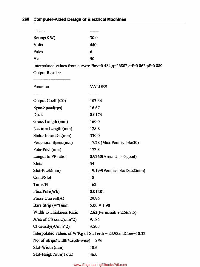
268 Computer-Aided Design of Electrical Machines
Rating(KW)
Volts
Poles
Hz
30.0
440
6
50
Interpolated values from curves: Bav=0.484,q=26802,eff=0.862,pf=0.880
Output Results:
Paramter
Output Coefft(CO)
Sync.Speed(rps)
DsqL
Gross Length (mm)
Net iron Length (mm)
Stator Inner Dia(mm)
Periphoral Speed(m/s)
Pole-Pitch(mm)
Length to PP ratio
Slots
Slot-Pitch(mm)
CondiSlot
TurnsIPh
FluxlPole(Wb )
Phase Current(A)
Bare Strip (w*t)mm
Width to Thickness Ratio
Area of CS cond(mmA2)
Ct.density(AlmmA2)
VALUES
103.34
16.67
0.0174
160.0
128.8
330.0
17.28 (Max.Permissible:30)
172.8
0.9260(Around 1 ->good)
54
19. 199(Pennissible: 18to25mm)
18
162
0.01281
29.96
5.00 x 1.90
2.63(pennissible:2.5to3.5)
9.186
3.500
Interpolated values of W /Kg of St:Teeth = 23 .92andCore= 18.32
No.ofStrips(width*depth-wise) 3x6
Slot-Width (mm) 10.6
Slot-Height(mm)Total 46.0
www.EngineeringEBooksPdf.com

St-Tooth-Flux-Dens(1I3)
St-Tooth-Flux-Dens-Max(T)
Length of mean-turn (m)
ResistancelPh (ohm)
depth ofSt.Core(mm)
Outer Dia ofSt.Core(mm)
St.Cu.Loss(W)
Wt ofSt-Teeth+Core(Kg)=
Three-Phase Induction Motors 269
1.0644
1.5966(Permissible: 1.6to 1.8)
0.957
0.3546
39.00
500.0
954.6
25.91+ 53.60= 79.51
Iron Loss=Teeth+Core(W)= 619.9+982.2=1602.1
-----------------Slip-Ring-ROTOR --------------------->
Length of Air-Gap(mm) 0.6600
No. of Rotor Slots Selected 63
Rotor Slot-Pitch(mm) 16.39
Equivalent Rotor Ct(A) 196.44
Rotor Cond CS(mm"2) 39.2000
Rot Cond (w*h)mm 4.0XIO.0
Rotor Slot (w*h)mm 6.5x29.0
Rotor Condlslot 2
Rotor TurnslPh 21
Mean Length ofrot-turn(m) 0.797
Resistance/phase(m.ohm) 8.9709
Rotor Cu Loss (W) 1038.5
Rotor res refered to St(Ohm) 0.534
Rotor(1/3)Slot-Pitch(mm) 14.46
Rotor( 113 )tooth width(mm) 7.96
Rt-Tooth-Flux-Dens(1I3)(T) 1.1898
Rt-Tooth-Flux-Dens-Max(T) 1. 7846(Max: 1: 8T)
Depth of Rotor core (mm) 36.84
----------------------N 0-Load-Losses---------------->
NO-Load Losses (W) 1902.1
NO-Load Wattful Current(A) 1.441
------------------Magnetizing-Current------------->
Interpolated values of atlm of St:Core=480.8andTeeth=706.5
www.EngineeringEBooksPdf.com

270 Computer-Aided Design of Electrical Machines
Interpolated values of Caters Coeffts: kO 1 =0.663,k02=0.453,kV=0. 700
Stator AT:Core+Teeth: 38.7+ 32.5= 71.2
Rotor AT :Core+Teeth: 19.6+ 80.7=100.3
Total AT :Stator+Rotor+Airgap: 71.2+ 100.3+445.7=617.2
N-Load Current(A) Iw= 1.44,Im=10.23 and 10=10.33 at pf=O.139
IOllph ratio 0.345
----------------Short -C ircuit -Current--------------->
Slot-Permeances: Stator=1.987, Rotor=1.892 and Rotor refered to stator=1.479
Specific-Slot-Permeance=3.466
TotaIReactance(X): Slot+Overhang+Zig-Zag=I.278+1.140+0.768=3.186 ohms
Short-Circuit: R= 0.89,Z= 3.31 and Isc=133.0 at pf=O.269;IscIIFL=4.441
Total Losses(PnL+Pcus+Pcur)=1902. 1+954.6+1 038.5=3895.2 WandEfficiency=88.51 perc
Slip atFL =
Starting Tq =
Max.Output(KW) =
3.314 X Perc
0.905 X FL-Tq
63.8
Temp-Rise(deg-C) = 55.5
Total·Wt(Kg) = 1.01 x (Wcus + Wt + Wc + Wri + Wcur)
= 1.01 x (38.0 + 25.9 + 53.6 + 53.0 + 17.5) = 190
Total Wt(Kg)=190and KglKW= 6.333 <------------End ofOutput-------->
7.2.4 Modifications to be Done in the above Program to get Optimal Design
1. Insert "for" Loops for the following parameters to iterate the total program between min and max permissible limits for selecting the feasible design variants:
(a) No 9fPoies
(b) /S{-Wdg Current density /
,(c) Slots/pole/phase
/ (d) Stator conductor thickness
(e) No. of conductors width-wise
(f) Rotor winding Current density.
2. Insert also minimum or maximum range of required objective functional values as constraint values, for example (a) Efficiency, (b) KglKW, (c) Temp-rise (d) 1011 ratio.
3. Run the program to get various possible design variants.
Note: From the feasible design variants printed in the output, select that particular design fulfilling the objective of optimal parameter for the design.
www.EngineeringEBooksPdf.com

Three-Phase Induction Motors 271
7.2.5 Computer Program in "c" in MATLAB for Optimal Design
%3ph,KW=30;V=440;P=6;f=50 Slip-Ring 1M
f2=fopen('Optimal_30KW_SR_Output.m', 'WI);
%------------Standard Curves/Tables for%Data-------------->
SKW=[125 10 20 50 100 500];
SBav=[0.35 0.38 0.42 0.46 0.48 0.50 0.51 0.53];
Sq=[16e3 1ge3 23e3 25e3 26e3 2ge3 31e3 33e3];
SKWa=[5 10 20 50 100 200 500];
SPF6P=[0.82 0.83 0.85 0.87 0.89 0.9 0.92]; Table for 1000RPM
SEFF6P=[0.83 0.85 0.87 0.89 0.91 0.92 0.93);%Table for 1000RPM
SPF4P=[0.85 0.86 0.88 0.9 0.91 .92 .93];%Table for 1500RPM
SEFF4P=[.85 .87 .88 .9 .91 .93 .94);%Table for 1500RPM
SD=[O.l 0.15 0.2 0.3 0.4 0.5 0.75 1];
SCDSW=[4 3.8 3.6 3.5 3.5 3.5 3.5 3.5);
%-------------BH Curve for--0.5mm,LOHYS Quality--------->
BB= [ . 1 . 2 . 3 . 4 . 5 . 6 . 7 . 8 . 9 1.7 1.8 1.9 2];
1 1.1 1.2 1.3 1.4 1.5 1.6
H= [50 65 70 80 90 100 110 120 150 180 220 295 400 580 1000 2400 5000 8900 15000 24000);
%-------Carters Coefft for Air Gap--->
Ratio= [0 1 2 3 4 5 6 7 8 9 10 11 12];
CC= [ 0 . 1i! . 33 . 45 . 53 . 6 . 66 . 71 . 75 . 7 9 . 82 . 8 6 . 8 9] ;
CC1= [0.14 .27 .37 .44 .5 .54 .58 .62 .65 .68 .69 .7];
% (1) <-----------Main Dimensions----------------------->
KW=30;V=440;f=50; %P=6;Specification/Input Data------>
fprintf(f2, 'Optimal Design of%4d KW,%4d V,%3d HZ 3-Ph Slip-ring Ind Motor\n',KW,V,f);
fprintf (f2, 'Sn P Zs D m/s L S wcaXhca CDSW WsXHs Btmax Tr DO Eff KgPkw 10/1 pfO pfsc Slip Zr hcR cdr Brtmx \n');
fprintf(f2, '-- -- -- ------ --- -- ------- ---- ------ ------ ---- ----- ----- ---- --- ---- ---- -- --- --- ----~');
insW=3.4;Hw=4;HL=1;insH=6;nvd=2;bvd=0.01;ki=0.92;Bc=1.35;Vph=V; %Assumptions
Zr=1;kwr=1;cdb=6;Tb=6;cde=6;dd=0.05;Brc=1.35; %Assumptions
www.EngineeringEBooksPdf.com

272 Computer-Aided Design of Electrical Machines
sn=0:M1=0:M2=0:M3=0:M4=0:EFFmax=SO:minKgPkw=9:minTr=75: minIObyI=5: %Assumptions
Bav=interp1(SKW,SBav,KW, 'spline'):
q=interp1(SKW,Sq,KW, 'spline'):
Vph=V;Kw=0.955:nvd=2;bvd=10;ki=0.92:Tstrip=1.9;insS=0.5;
insW=3. 4:Hw=4:HL=1:insH=6:nvd=2;ki=0. 92;Bc=1.35;%Assump tions
SD=[O.l 0.15 0.2 0.3 0.4 0.5 0.75 1J:
SCDSW=[4 3.S 3.6 3.5 3.5 3.5 3.5 3.5J:
B= [ 0 . S 1. 2 1. 6 2 2. 4 J : WpKg= [7 15 24 34 50 J :
for P=4:2:10:
pf=interp1(SKWa,SPF6P,KW, 'spline'):
eff=interp1(SKWa,SEFF6P,KW, 'spline'):
if P==4 pf=interp1(SKWa,SPF4P,KW, 'spline'):end:
if P==4 eff=interp1(SKWa,SEFF4P,KW, 'spline');end;
KWinp=KW/eff:lph=KWinp*le3/(3*Vph*pf);
Ns=120*f/P;ns=Ns/60;CO=11*Kw*Bav*q*eff*pf*le-3;
DsqL=l/CO*(KW/ns): L1=sqrt(DsqL/(0.135*P)A2); L=floor(L1*100) *10: Ls=(L-nvd*bvd): Li=ki*Ls; D1=sqrt(DsqL/(L/1000)):D=ceil(D1*100)*10: PP=pi*D/P;LbyPP=L/PP:
if LbyPP <O.SI I LbyPP >2 continue: end: v=pi*D*ns/1000:
if v >30 continue;end; FI=pi*D/P*L*Bav/1e6: Tphi=Vph/(4.44*f*FI*Kw): %CDSW=interp1(SD,SCDSW,D, 'spline');
for CDSW=3:0.5:5; As1=Iph/CDSW;
for spp=3:1:5;
S=spp*P*3:SPitch=pi*D/S;if SPitch <lSI ISPitch>=25 continue;end;
Zphi=2*Tphi:sph=S/3:Zs1=Zphi/sph:Zs=ceil(Zsl);Tph=Zs*sph/2; FI=Vph/(4.44*f*Tph*Kw):
for Tstrip=1:0.1:2;
Hstrip1=As1/Tstrip;Hstrip=ceil(Hstrip1*2)/2;WbyT=Hstrip/Tstrip;
if WbyT <2.51 IWbyT >=3.5 continue: end; As=0.967*Hstrip*Tstrip; for Zsw=1:1:4:
Ws=(Zsw*(Tstrip+insS)+insW); Hs=(Zsh*(Hstrip+insS)+Hw+HL+insH+2);
Zsh=Zs/Zsw;
www.EngineeringEBooksPdf.com
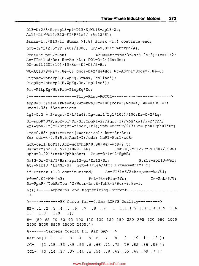
Three-Phase Induction Motors 273
D13=D+2/3*HsiSp13=pi*D13/Si Wt 13=sp13-WS i At13=Li*Wt13iB13=FI*P*le6/ (At13*S)i
Btmax=1.5*B13iif Btmax >1.81 1 Btmax <1.4 continueiendi
Lmt=(2*L+2.3*PP+240)/1000i Rph=0.021*Lmt*Tph/Asi
Pcus=3*IphA2*Rphi Wcus=Lmt*Tph*3*As*8.ge-3iFlc=FI/2i Ac=Flc*le6/Bci Hc=Ac /Lii D01=D+2*(Hs+Hc)i DO=ceil(D01/10)*10iHc=(DO-D)/2-Hsi
Wt=At13*S*Hs*7.8e-6i Dmcs=D+2*Hs+Hci WC=Ac*pi*Dmcs*7.8e-6i
PitpKg=interp1(B,WpKg,Btmax, 'spline')i PicpKg=interp1(B,WpKg,Bc, 'spline')i
Pit=PitpKg*WtiPic=PicpKg*WCi
%--------------------Slip-Ring-ROTOR------------------------->
sppR=3.5iSS=Sikws=Kwikwr=kwsiEr=100icdr=5iwcR=4iHwR=4iHLR=li Brc=1.35i %Assumtions
Lg1=0.2 + 2*sqrt(D*L/1e6)iLg=ceil(Lg1*100)/100iDr=D-2*Lgi
Sr=sppR*3*PiSp2=pi*Dr/SriTphR1=Er/sqrt(3)/Vph*kws/kwr*Tphi Zr1=TphR1*3*2/SriZr=floor(Zr1)iTphR=Zr*Sr/2/3iEr=TphR/TphR1*Er i
Ird=0.85*Iphilr=Ird*(kws*Ss*Zs)/(kwr*Sr*Zr)i for cdr=4:0.5:5.5iAcr1=Ir/cdri hcR1=Acr1/wcRi
hcR=ceil(hcR1)iAcr=wcR*hcR*0.98iWsr=wcR+2.5i Hsr=Zr*(hcR+0.5)+3+HwR+HLRi LmtR=(2*L+2.3*PP+80)/1000i RphR=0.021*LmtR*TphR/Acri Pcur=3*IrA2*RphRi
Dr13=Dr-2*2/3*Hsrispr13=pi*Dr13/Sri Wtr13=spr13-Wsri Atr=Wtr13 *Li*Sr/Pi Brt=FI*le6/Atri Brtmax=Brt*1.5i
if Brtmax >1.8 continueiendi Ac=FI*le6/2/Brcidcr=Ac/Lii
Pfw=0.01*KW*le3i PnL=Pit+Pic+Pfwi Iw=PnL/3/Vi Rr=RphR/(TphR/Tph)A2i Wcur=LmtR*TphR*3*Acr*8.ge-3i
%(4)<-----AmpTurns and Magnetizing-Current---------------------->
%-------------BH Curve for--0.5mm,LOHYS Quality--------->
BB= [ . 1 . 2 . 3 . 4 . 5 . 6 . 7 . 8 . 9 1.7 1.8 1.9 2]i
1 1.1 1.2 1.3 1.4 1.5 1.6
H= [50 65 70 80 90 100 110 120 150 180 220 295 400 580 1000 2400 5000 8900 15000 24000]i
%-------Carters Coefft for Air Gap--->
Ratio=[O 1 2 3 4 5 6 7 8 9 10 11 12] i
CC= [ 0 . 18 . 33 . 45 . 53 . 6 . 66 . 71 . 75 . 79 . 82 . 8 6 . 8 9 ] i
CC1= [0 .14 .27 .37 .44 .5 .54 .58 .62 .65 .68 .69 .7 ]i
www.EngineeringEBooksPdf.com

274 Computer-Aided Design of Electrical Machines
WSSO=4iWsrO=2i %Assumptions
atsc=interp1(BB,H,Bc, 'spline')i Dcav=D+2*Hs+Hci
ATSC=pi*Dcav/P/3*atsc/1e3i Bt30=B13*1.36i
atst=interp1(BB,H,Bt30, 'spline')i
ATST=atst*Hs/1000iATS=ATSC+ATSTi rat1=WssO/Lgi
k01=interp1(Ratio,CC,rat1, 'spline');
kgs=SPitch/(SPitch-WssO *k01)i
rat2=WsrO/Lgik02=interp1(Ratio,CC,rat2, 'spline')isprO=pi*Dr/Sri kgr=sprO/(sprO-WsrO*k02)ikg=kgs*kgriLgd=Lg*kgirat3=bvd/Lgi
kv=interp1(Ratio,CC1,rat3, 'spline'); if rat3 >=12 kv=O.7iendi
Ld=L-kv*nvd*bvdiAag=pi*D/P*LdiBg=FI*le6/AagiB30d=1.36*Bgi
ATg=O.796 *B30d*Lgd*le3i Btr30=Brt*1.36i
atrt=interp1(BB,H,Btr30, 'spline')i ATRT=atrt*Hsr/1e3i
Dcrav=Dr-2*Hsr-dcri atrc=interp1(BB,H,Brc, 'spline');
ATRC= pi*Dcrav/1e3/P/3 *atrci ATR=ATRC+ATRTi ATT=ATS+ATR+ATgi
Im=P/2*ATT/(1.17*Kw*Tph)iIO=sqrt(IwA2+ImA2)iIObyI=IO/Iphi
pfO=Iw/IOiif pfO >=0.16 continueiendi
% (5) <------------Short-Circuit-Current-------------------->')i
h2=1.6ih2r=1.6ih3r=HwRih4r=HLRiks=li %Assumptions
h1=Zsh*(Hstrip+insS)ih3=Hwih4=HLibs=WSibO=WSSOi
Lmdss=h1i3/bs +h2/bs +2*h3/ (bs+bO) +h4/bOi h1r=wcRibr=Wsri
brO=WsrOi Lmdsr=h1r/3/br +h2r/br +2*h3r/(br+brO) +h4r/brOi
Lmddsr=KwA2*S/Sr*Lmdsrissp=Lmdss+Lmddsri gd=S/P/3i p=P/2i
Xs=15.8*f*L*ssp*TphA2/(p*gd)*le- 9 i
LOLmdO=ks*PP A2/pi/SPitch/1000;
XO=15.8*f*LOLmdO*TphA2/(p*gd)*le-6i
gS=S/Pi gr=Sr/Pi Xm=Vph/lmi Xz=5/6 *Xm* (1/gsA2+1/grA2)i
X=Xs+XO+XZiR=Rph+RriZ=sqrt(RA2+XA2)iIsc=Vph/Z;pfsc=R/Z;
RAT=Isc/lphi
%(6)<--------------Performance-------------------->')i
Pt=PnL+Pcus+PcuriEFF=KW/(KW+Pt/1000)*lOOi
if EFF <88.5continuei endi
Rinp=KW*lOOO+Pfw+Pcuri SFL=Pcur/Rinp*lOOi
www.EngineeringEBooksPdf.com

Three-Phase Induction Motors 276
Tst=(Isc/Ir)A2*SFL/100; Pmax=3*Vph*(Isc-IO)/2/(1+pfsc)*le-3;
Acooll=(pi*D*(L*2.5)+2*pi*(D+50)*0.04)/le6; Acoo12=Acooll*(1+0.1*v);Acoo13=pi*DO*L/le6;
AcoolT=Acoo12+Acoo13; Pst=Pcus+Pit+Pic;
Tr=0.03*Pst/AcoolT;if Tr>55.6 continue;end;
Ars=Wsr*Hsr*Sr;Dri=Dcrav-dcr;
Wri=(pi*(DrA2-Dri A2)/4-Ars)*L*7.8e-6;
Wtot=l.Ol*(Wcus+Wt+Wc+Wri+Wcur); KgPkw=Wtot/KW;
if KgPkw >6.3 continue;end;
%--------------------End of Program-------------------------->
sn=sn+l;if EFF >=EFFmax EFFmax=EFF;end;
if abs (EFF-EFFmax) <=le-3 M2=sn; end; sn,
if KgPkw <=minKgPkw minKgPkw=KgPkw;end;
if abs(KgPkw-minKgPkw)<= 0.001 Ml=sn; end;
if Tr <=minTr minTr=Tr;end;
if abs(Tr-minTr)<=O.OOOl M3=sn; end;
if IObyI <=minIObyI minIObyI=IObyI;end;
if abs(IObyI-minIObyI)<=O.OOOl M4=sn; end;
fprintf(f2, '\n%2d%3d%3d%4.0f%3.0f%4.0f%3d%4.1fX%3.1f%4.1f',sn,P ,Zs,D,v,L,S,Tstrip,Hstrip,CDSW);
fprintf(f2, '%5.1fX%2.0f%6.3f%5.1f%4.0f%6.2f%6.2f%5.2f%5.2f%5.2f %4.1f%3.0f%4.0f%4.1f%6.2f',Ws,Hs,Btmax,Tr,DO,EFF,KgPkw,IObyI,pf O,pfsc,SFL,Zr,hcR,cdr,Brtmax);end;end;end;end;end;end; fprintf(f2, '\n-- ____________________________________ _
-- ---- ----- ----- ---- --- ---- ---- -- --- --- -----');
fprintf(f2, '\nSelection of Design Variant based on Optimization Criteria:');
fprintf(f2, '\nIf Variant (Sn)=%3d
fprintf (f2, ' \nIf Variant (Sn)=%3d
fprintf(f2, '\nIf Variant (Sn)=%3d
Maximum Efficiency is (%5.2f perc) ',M2,EFFmax);
Minimum Kg/KW is (%5.2f) ',Ml,minKgPkw);
Minimum Temp-Rise (% 4 .2 f) , ,M3, minTr) ;
Required, Select
Required, Select
is Reqd, Select
fprintf (f2, '\nIf Minimum ratio of IO/I is Reqd, Select
Variant (Sn)=%3d (%4.2f) ',M4,minIObyI);fclose(f2);
www.EngineeringEBooksPdf.com
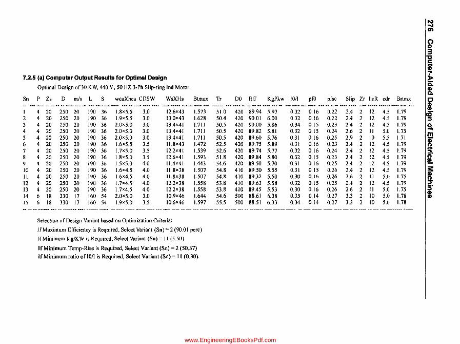
N ..., en
0 0 3
"C C If ...
7.2.5 (a) Computer Output Results for Optimal Design l> Optimal Design of 30 K W, 440 V, 50 HZ 3-Ph Slip-ring Ind Motor c:
CD Q.
Sn P Zs D mls L S wcaXhca CDSW WsXHs Btmax Tr DO EIT KgPkw 1011 pro pfsc Slip Zr hcR cdr Brtmx
~ -- --- ---.. -- -- -- -- ---.. --- -- --- ---.. _ .. - ---- ........ - .. _ .. - ---- ......... ---- ----- ............ ---- --- ------ --- --- _ .. -- -- -- ---- ............ --- ---- ......... _-- --- -- ---- ---- ---- - .. -- ----- ------ ---- --- ---
I 4 20 250 20 190 36 1.8x5.5 3.0 12.6x43 1.573 51.0 420 89.94 5.97 0.32 0.16 0.22 2.4 2 12 4.5 1.79 ii' 2 4 20 250 20 190 36 1.9x5.5 3.0 13.0x43 1.628 50.4 420 90.01 6.00 0.32 0.16 0.22 2.4 2 12 4.5 1.79 :::s 3 4 20 250 20 190 36 2.0x5.0 3.0 13.4x41 1.711 50.5 420 90.00 5.86 0.34 0.15 0.23 24 2 12 4.5 1.79 a 4 4 20 250 20 190 36 2.0x5.0 3.0 13.4x41 1.711 50.5 420 89.82 5.81 0.32 0.15 0.24 2.6 2 II 5.0 1.75 m 5 4 20 250 20 190 36 2.0x5.0 3.0 13.4x41 1.711 50.5 420 89.60 5.76 OJI 0.16 0.25 2.9 2 10 5.5 1.71 CD 6 4 20 250 20 190 36 1.6x5.5 3.5 11.8x43 1.472 52.5 420 89.75 5.89 0.31 0.16 0.23 2.4 2 12 4.5 1.79 n 7 4 20 250 20 190 36 1.7x5.0 3.5 12.2x41 1.539 52.6 420 89.74 5.77 0.32 0.16 0.24 2.4 2 12 4.5 1.79
.. ... 8 4 20 250 20 190 36 1.8x5.0 3.5 12.6x41 1.593 51.8 420 89.84 5.80 0.32 0.15 0.23 2.4 2 12 4.5 1.79 c=r 9 4 20 250 20 190 36 1.5x5.0 4.0 1I.4x41 1.443 54.6 420 89.50 5.70 0.31 0.16 0.25 2.4 2 12 4.5 1.79 !!. 10 4 20 250 20 190 36 1.6x4.5 4.0 IJ.8x38 1.507 54.8 410 89.50 5.55 0.31 0.15 0.26 2.4 2 12 4.5 1.79 s: II 4 20 250 20 190 36 1.6x4.5 4.0 11.8x38 1.507 54.8 410 89.32 5.50 0.30 0.16 0.26 2.6 2 II 5.0 1.75 I»
n 12 4 20 250 20 190 36 1.7x4.5 4.0 12.2x38 1.558 53.8 410 89.63 5.58 0.32 0.15 0.25 2.4 2 12 4.5 1.79 ::r 13 4 20 250 20 190 36 1.7x4.5 4.0 12.2x38 1.558 53.8 410 89.45 5.53 0.30 0.16 0.26 2.6 2 II 5.0 1.75 5" 14 6 18 330 17 160 54 2.0x5.0 3.0 1O.9x46 1.644 54.6 500 88.61 6.38 0.35 0.14 0.27 3.3 2 10 5.0 1.78 m 15 6 18 330 17 160 54 1.9x5.0 3.5 10.6x46 1.597 55.5 500 88.51 6.33 0.34 0.14 0.27 3.3 2 10 5.0 1.78 ___ ...... _ .. _ .. ___ .. ___ --_"_"00 ...... ______ .. _ .. _ .. _ _ _________ ....... ________ .. _____ ...... _____ ............... ________ .......... ________ ...... ______________ .. _ .. _____________ .. ____________ ........ ________ ........... ________
Selection of Design Variant based on Optimization Criteria:
If Maximum Efliciency is Required, Select Variant (Sn) = 2 (90.01 perc)
If Minimum Kg/KW is Required, Select Variant (Sn) = II (5.50)
If Minimum Temp-Rise is Required, Select Variant (Sn) = 2 (50.37)
If Minimum ratio of 1011 is Required, Select Variant (Sn) = II (0.30).
www.EngineeringEBooksPdf.com

CHAPTER 8
Single-Phase Induction Motors
8.1 Introduction Single-phase induction motors are not self-starting type. Based on type of starting they are categorized as (1) Split phase, (2) Capacitor Start, (3) Shaded Pole, and (4) Repulsion Type. Theory portion of design is not given in this book, but necessary formulae, curves and tables given in standard books are made use of.
Computer-aided design for Split-phase type is given in this book. Total design is split into six parts in a proper sequence. Design Calculations are given for a given Rating of motor, followed by Computer Program written in "C" language using MA TLAB software for each part. Finally all the Programs are added together to get the total Program by running which we get the total design. Computer output of total design is given.
This design may not be the optimum one. Now optimization objective and Design Constraints are inserted into this total Program. When this program is run we will get various alternative feasible designs from which the selected variant based on the Optimization Criteria can be picked up. Computer output showing the important design parameters for various feasible alternatives is given at the end of this chapter along with a logic diagram.
8.2 Sequential Steps for Design of Each Part and Programming Simultaneously (a) Calculate Main dimensions of stator core OD, Width of tooth, stator core depth,
Slot width and depth, Air gap length (b) Calculate for the Main Winding: No. of series turns, Turns in each coil,
conductor dia, by checking current density. Calculate mean length, Resistance, Copper losses Calculate Rot dia, no. of Rotor Slots, Cond dia, Core depth, Resistance and Copper Losses, Weight of rotor copper
(c) Calculate Carter Coefft and Ampere-turns for Air gap, Stator tooth, Stator core, Rotor tooth, Rotor core and Total No-load AT, Magnetizing current
(d) Calculate for the Auxiliary Winding: No. of series turns, Turns in each coil, conductor dia, by checking current density. Calculate mean length, Resistance, Copper losses
www.EngineeringEBooksPdf.com
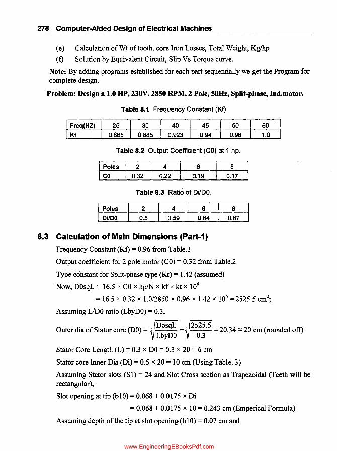
278 Computer-Aided Design of Electrical Machines
(e) Calculation ofWt of tooth, core Iron Losses, Total Weight, Kglhp
(f) Solution by Equivalent Circuit, Slip Vs Torque curve.
Note: By adding programs established for each part sequentially we get the Program for complete design.
Problem: Design a 1.0 lIP, 230V, 2850 RPM, 2 Pole, 50Hz, Split-phase, Ind.motor.
Table 8.1 Frequency Constant (Kf)
Table 8.2 Output Coefficient (CO) at 1 hp.
I ~~Ies 2
I 4
I 6
0.32 0.22 0.19
Table 8.3 Ratio of DilDO.
I Poles 2
I 4 6
0.5 0.59 0.64 DilDO
8.3 Calculation of Main Dimensions (Part-1)
Frequency Constant (Kf) = 0.96 from Table. 1
8
0.17
8
0.67
Output coefficient for 2 pole motor (CO) = 0.32 from Table.2
Type constant for Split-phase type (Kt) = 1.42 (assumed)
Now, DOsqL = 16.5 x CO x hp/N x kfx kt x 106
= 16.5 x 0.32 x 1.0/2850 x 0.96 x 1.42 x 106 = 2525.5 cm2;
Assuming LIDO ratio (LbyDO) = 0.3,
Outer dia of Stator core (DO) = 3 DosqL = V2525.5 = 20.34:::: 20 cm (rounded off) LbyDO 0.3
Stator Core Length (L) = 0.3 x DO = 0.3 x 20 = 6 cm
Stator core Inner Dia (Di) = 0.5 x 20 = 10 cm (Using Table. 3)
Assuming Stator slots (SI) = 24 and Slot Cross section as Trapezoidal (Teeth will be rectangular),
Slot opening at tip (bl0) = 0.068 + 0.0175 x Di
= 0.068 + 0.0175 x 10 = 0.243 cm (Emperical Formula)
Assuming depth of the tip at slot opening-(hl0) = 0.07 cm and
www.EngineeringEBooksPdf.com

Single-Phase Induction Motors 279
depth of the mouth (hll) = 1.3 x 0.07 = 0.091 cm,
U sing Empirical F ornlula,
W·d h f h (b 1) (1.1 + 0.032 x Di) x Di 1 t 0 toot t = -'--------'---
Sl
= (1.1 + 0.032 x 10) xl 0 = 0.5917:::::: 0.59 cm (rounded off) 24
Assuming Flux density in St. tooth (Bt) = 1.3 5 T and St.Core (Bc) = 1.15 T,
S C d h(d 1) (Bt) (SlXbtl) (1.35) (24 XO.59) 26456 t. ore ept c = - x = - x =. cm Bc 7t x P 1.15 7t x 2
Width of Slot at top section (b 11)
::::: 7t x [Di + 2 x (h10 + h11)] _ btl = 7t x [10 + 2 x (0.07 + 0.091)] _ 0.59 = 0.7611 cm SI 24
Depth of the Slot (h14) = 0.05 x (DO - Di) - (h10 + h11 + del)
= 0.05 x (20 -10) - (0.07 + 0.091 + 2.6456)::::: 2.1934 cm
Half-Slot angle (alfa)::::: 180/S1 ::::: 7S
Slot-width at the bottom (b13):::::bll +2 x h14 x tan (alfa)
::::: 0.7611 + 2 x 2.1934 x tan (7.5 x 7tf180) = 1.3387 cm
Using Empirical Formula,
Length of Air-gap (Lg)
= 0.0013 + O.OO~ Di = 0.0013 + O.OO~x 10 = 0.0427 cm
8.3 (a) Computer Program in "c" in MATLAS for Part-1 %Design of 1hp,230V,1-ph 1M
%<--------Calculation of Main Dimensions (Part-1)------->
hp=liV=230iP=2iN=2850;hz=50; %Main Data
kt=1.42;LbyDO=0.3i k i=0.93iS 1=24;%Assumptions
h10=0.07;h11=1.3*h10iBt=1.35iBc=1.15icdm1=4.5;S2=30; %Assumptions
HZ=[25 30 40 45 50 60]; KF= [ 0 . 865 . 885 . 923 . 94 . 96 1]; kf=interp1 (HZ,KF,hz, 'spline');
POLES=[2 4 6 8] ; OPTC=[0.32 CO=interp1 (POLES,OPTC, P, 'spline');
D1BYDO=[.5 .59 .64.67]; DibyDO=interp1(POLES,D1BYDO,P, 'spline');
0.22 .19 .17] ;
www.EngineeringEBooksPdf.com

280 Computer-Aided Design of Electrical Machines
DOsqL=16.5*CO*hp/N*kf*kt*le6; DO=floor(D01); L=LbyDO*DO; SP=Sl/P; if btl=floor(btla*lOO)/lOO; end;
D01=(DOsqL/LbyDO)A(1/3); Di1=DibyDO*DO; Di=ceil (Dil);
P==2 bt1a=(1.1+O.032*Di)*Di/S1;
ifP==4 btla=(1.27+0.035*Di)*Di/Sl;btl=floor(btla*100)/lOO; end;
SS=[24 36 48]; BIO=[0.068+0.0175*Di 0.038+0.0175*Di 0.0175*Di]; blO=interp1(SS,B10,Sl, 'spline');
dc1=Bt/Bc*(Sl*bt1)/(pi*P);b11=pi*(Di+2*h10+2*h11)/Sl-bt1;
h14=DibyDO*(DO-Di)-(h10+h11+dc1); alfa=180/S1;b13=bl1+2*h14*tan(alfa*pi /180);
Lg=0.013+0.0042*Di/sqrt(P);
8.4 Design of Main Winding (Part-2)
No. of Coils/pole (Ncpp) = ~ = ~ = 6 , Now using Concentric Winding, Px2 2x2
Pitch factor for Concentric Winding
Coil Slots spanned (CT) Factor(y1) Pitch Factor(Kp) = sin(y1*1T/2) No.
1 1 t013 J1~ 12113 Sin 02113 x rr/2) = 0.9927
2 2 t012 (10) 10/13 Sin (10/13 x rrl2) = 0.935
3 3 t011 (8) 8/13 Sin (8/13 x rr/2) = 0.8230
4 4 t010J6) 6/13 Sin (6/13 x rr121 = 0.6631
5 5 t09(41 4/13 Sin_(4/13 x rrl2) = 0.4647
6 6 t08 (2) 2113 Sin (2113 x rr/2) = 0.2393
rKp = 4.1179
Percentage No. ofTums in Each Coil
Coli No(nl 1 2 3 4 5 6 r %Tums(Tn) = 24.11 22.71 19.99 16.10 11.28 5.81 100 Kp(n)/4.1179 x 100
Winding factor (Kwmj =:LKp(n) x T(n)
= (0.9927 x 24.11) + (0.935 x 22.71) + (0.823 x 19.99) + (0.6631 x 16.1) + (0.4647 x 11.28) + (0.2393 x 5.81)1100 = 0.7892
Considering Iron factor (ki) = 0.93;
Net iron length in core (Li) = ki x L = 0.93 x 6 = 5.58 cm
SlotslPole (SP) = SlIP = 24/2 = 12
Area of tooth (At) = btl x Li x SP = 0.59 x 5.58 x 12 = 39.5064 cm2;
www.EngineeringEBooksPdf.com

Single-Phase Induction Motors 281
FluxlPole (FI) = 0.637 x At x Bt X 10"" = 0.637 x 39.5064 x 1.35 x 10"" = 0.0034 Wb
Considering Induced EMF (E) = 0.95 x V,
No of series turns in Main winding (Tm)
0.95 x 230 0.95 x 230 = = = 367 ~ 368 (rounded off to
4.44 x hz x FI x Kwm 4.44 x 50 x 0.0034 x 0.7892 even integer)
Total Conductors in Main winding (Nm) = 2 x Tm = 2 x 368 = 736
No. of series turns/pole in Main winding (Tppm) = TmIP = 368/2 = 184
No. of Turns in Each Coil
(Example: for 1st coil, Tcl = 24.11 x 1841100 = 44.36 ~ 44(rounded off to nearest integer)
Table 8.4 Efficiency and PF.
Output(HP) 0.05 0.1 0.25 Efficiency(pu) 0.35 0.44 0.58 PF 0.45 0.5 0.56
From Table. 8.4, efficiency (effa) = 0.7pu and
Power factor (pfa) = 0.66 corresponding to 1.0 hp
0.5 0.65 0.62
0.75 1.0 0.68 0.7 0.64 0.66
C . . d (I) hp x 746 1. 0 x 746 02 A urrent m mam w g m = = = 7. effax V x pfa 0.7 x 230 x 0.66
Assuming a current density (cdm) = 4.5 Almm2,
Area of Conductor (Arnc) = ImIcdm = 1m = 7.02 = l.5601 mm2,
cdm 4.5
. ~4 x Arnc ~4X l.5601 Diameter of conductor (dmc) = 1t = 1t = 1.4094 mm ,
Table 8.5 Standard Wire Gauge (SWG) for round Conductor as per British Standard Specification.
SWGno 5 6 7 8 9 10 11 12 13 14 15 16 17 18 19
Dia (mm) 5.38 4.88 4.47 4.06 3.66 3.25 2.95 2.64 2.31 2.03 1.83 1.63 1.42 1.22 1.02
From Table. 8.5 suitable dia of bare conductor (dmc) = l.42 mm
Considering Enamel insulation thickness as 0.075 mm,
www.EngineeringEBooksPdf.com

282 Computer-Aided Design of Electrical Machines
Dia of insulated conductor (elmcins) = 1.42 + 0.075 = 1.4975 mm;
. 1t x dmc 2 1t x 1.422 2 Area ofCS of copper m the conductor (Arnc) = = = 1.5837 mm
4 4
C d ·· . . d' (d) 1m 7.02 4433AI 2 urrent enslty m mam wm mg c m = --= . mm Arnc 1.5837
Space occupied by 44 insulated conductors in the slot (Socm)
= 44x 1txdmcins2
=44x 1tx1.4952
=0.7724cm2 4x 100 4x 100
Ares ofCS of Gross Slot (Asg) = [h11 x (b10 + b11) + h14 x (b11 + b13)]/2 = [0.091 x (0.243 + 0.7611) + 2.1934 x (0.7611 + 1.3387)]/2 = 2.3486 cm2;
Socm 0.7724 Space factor of the slot (Sfsm) = --= = 0.3289 « 0.5 and hence OK)
Asg 2.3486
Height of Stator Slot (Hs) = (h11 + h14) = (0.091 + 2.1934) = 2.2844 cm
Length of mean Tum (Lmt) in Each Coil
From Table.8.5 suitable dia of bare conductor (dmc) = 1.42 mm
Considering Enamel insulation thickness as 0.075mm,
Dia of insulated conductor (dmcins) = 1.42 + 0.075 = 1.4975 mm;
Area of CS of copper in the conductor (Arnc)
1t x dmc2 = 1t x 1.422 = 1.5837 mm2
4 4
C d ·· . . d' (elm) 1m 7.02 urrent enslty m mam wm mg c = --=--Arnc 1.5837
4.433A/mm 2
Space occupied by 44 insulated conductors in the slot (Socm)
= 44x 1txdmcins2
=44x 1tx1.4952
=0.7724cm2 4 x 100 4 x 100
Ares ofCS of Gross Slot (Asg) = [h11 x (b10 + b11) + h14 x (b11 + b13)] 12
= [0.091 x (0.243 + 0.7611) + 2.1934 x (0.7611 + 1.3387)] 12 = 2.3486 cm2;
Socm 0.7724 Space factor of the slot (Sfsm) = --= = 0.3289 « 0.5 and hence OK)
Asg 2.3486
Height of Stator Slot (Hs) = (hl1 + h14) = (0.091 + 2.1934) = 2.2844 cm
www.EngineeringEBooksPdf.com

Single-Phase Induction Motors' 283
Length of mean Tum (Lmt) in each coil
Example for Coil. 1
Lmt (1) = 8.4 x (Di + Hs)/Sl x Slots Spanned + (2 xL)
= 8.4 x (10 + 2.2844)/24 x 12 + (2 x 6) = 63.59 em
Mean Len,gth of tum of main wdg (Lmtm) = ILmt(n) x T(n)
= [(63.59 x 44) + (54 x 42) + (46.4 x 37) + (37.8 x 30) + (29.2 x 21) + (20.6 x 10)]1184 = 47.705 em
Resistance of Main wdg at 75° (Rm)
= 0.021xLmtrnxTm 0.021x 47.705 x368 =2.3280 Arne x 100 1.5837 x 100
Copper loss in main wdg (Peus) = 1m2 x Rm = 7.022 x 2.328 = 114.74 W
8.4 (a) Computer Program in "C" in MATLAB for Part-2
%<--------Design of Main Winding(Part-2)--------->
Sl=24;P=2;SP=12;ki=O.93;L=6;bt1=O.59;Bt=1.35;V=230;hz=50;hp=1; cdm1=4.5;h11=O.091;b10=O.243;b11=O.7611;h14=2.1934; b13=1.3387: Di=lO;%Input Data
Ncpp=Sl/P/2:sum1=O:sum2=O;sum3=O;sum4=O;sum5=O;
for i=l:Ncpp; y1=(SP-(i-1)*2)/(SP+1); Kp(i)=sin(y1*pi/2); sum1=sum1+Kp(i);end;
for i=l:Ncpp: PTm(i)=Kp(i)/sum1*lOO; sum2=sum2+PTm(i); end;
for i=l:Ncpp; sum3=sum3+Kp(i)*PTm(i); end; Kwm=sum3/sum2;
Li=ki*L: At=bt1*Li*SP; FI=O.637*At*Bt*le-4: Tm1=O.95*V/(4.44*hz*FI*Kwm);
Tm=ceil(Tm1/2)*2; Nm=Tm*2: Tppm=Tm/P;
for i=l:Ncpp; Tc1(i)=Tppm*PTm(i)/lOO; Tc(i)=round(Tc1(i)); sum4=sum4+Tc(i); end; corr=Tppm-sum4; Tc(Ncpp)=corr+Tc(Ncpp); sum4=sum4+corr;
HP=[.05 .1 .25 .5 .75 1]; EFF=[.35 .44 .58 .65 .68 .7]; PF=[.45 .5 .56 .62 .64 .66];
effa=interp1(HP,EFF,hp, 'spline'); pfa=interp1(HP,PF,hp, 'spline'):
Im=hp*746/(effa*V*pfa): Amc1=Im/cdm1; dmc1=sqrt(4*Amc1/pi):
www.EngineeringEBooksPdf.com

284 Computer-Aided Design of Electrical Machines
DSWG= [ 5 . 38 4. 88 4. 47 4. 06 3. 66 3. 25 2. 95 2. 64 2 . 31 2. 03 1. 83
1.63 1.42 1.22 1.02];
for i=1:15; if dmc1 >
dmcins=dmc+0.075;
DSWG(i) continue; end; dmc=DSWG(i);end;
Amc=pi*dmc A 2/4; cdm=Im/Amc;if cdm<2.8[ [cdm>4.5 continue; end;
Socm=Tc(1)*pi*dmcins A 2/4/100;
Asg=(h11*(b10+b11)+h14*(b11+b13))/2; Sfsm=Socm/Asg;
if Sfsm >0.5 continue;end; Hs=h11+h14;
for i=l:Ncpp; Lmt(i)=8.4*(Di+Hs)/Sl*(SP-(i-1)*2)+2*L;
sum5=sum5+Lmt(i)*Tc(i);end;
Lmtm=sum5/sum4;Rm=0.021*Lmtm*Tm/(Amc*100)
Wcum=Lmtm*Amc*Tm*8.ge-5;
8.5 Design of Rotor (Part-3)
Rotor outer dia (Dr) = Di - 2 x Lg = 10 - 2 x 0.0427 = 9.9146 cm
Assuming Rotor slots (S2) = 30,
Width of tooth at minimum section (bt2)
= 0.95 x SI x btl = 0.95 x 24 x 0.59 = 0.4484 cm S2 30
Assuming Slot opening (b20) = 0.075cm and depth of tip (h20) = 0.08 cm,
Radius of round slot (r21)
= 1t x (Dr - 2 x h20) - S2 x bt2 = 1t x (9.9146 - 2 x 0.08) - 30 x 0.4484 = 0.2594cm 2 x (S2 + 1t) 2 x (30 + 1t)
Dia of rotor conductor (drc) = 2 x r21- 0.038 = 2 x 0.2594 - 0.038 = 0.4808 cm
From Table. 8.5, suitable conductor is SWG:6 with dia (drc) = 4.88 mm
Area of conductor (Ab) = 1t x drc2
= 1t x 4.882
= 18.7038 mm2; 4 4
Rotor Core depth (de2) = 0.95 x dcl = 0.95 x 2.6456 = 2.5133 cm
Length of Bar leonduetor (Lb) = L + 1 = 6 + 1 = 7 em
A fCS f d · (A) NbxAb 30x18.704 89304 2 rea 0 0 en nng er = = =. mm 1tXP 1tx2
www.EngineeringEBooksPdf.com
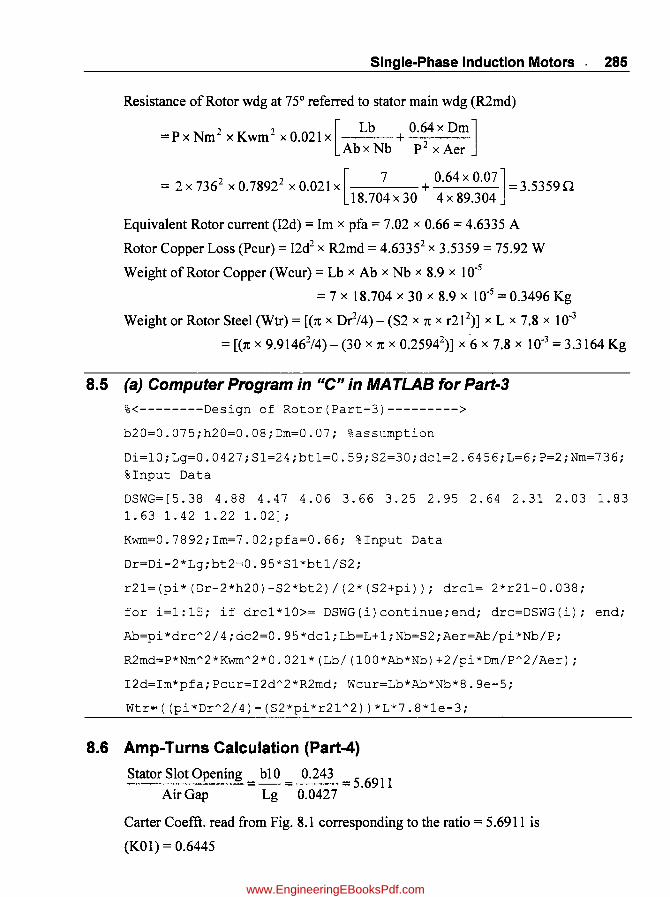
Single-Phase Induction Motors 285
Resistance of Rotor wdg at 75° referred to stator main wdg (R2md)
=PxNm 2 x Kwm 2 XO.021X[ Lb + 0.64xDm] Abx Nb p2 X Aer
= 2x736 2 X 0.78922 XO.021X[ 7 + 0.64XO.07]=3.5359n 18.704 x 30 4 x 89.304
Equivalent Rotor current (I2d) = 1m x pfa = 7.02 x 0.66 = 4.6335 A
Rotor Copper Loss (Pcur) = 12d2 x R2md = 4.63352 x 3.5359 = 75.92 W
Weight of Rotor Copper (Wcur) = Lb x Ab x Nb x 8.9 x 10-5
= 7 x 18.704 x 30 x 8.9 X 10-5 = 0.3496 Kg
Weight or Rotor Steel (Wtr) = [(1t x Dr2/4) - (S2 x 1t x r212)] x Lx 7.8 x 10-3
= [(1t x 9.91462/4) - (30 x 1t x 0.25942)] x '6 x 7.8 x 10-3 = 3.3164 Kg
8.5 (a) Computer Program in "C" in MA TLAB for Part-3 %<--------Design of Rotor(Part-3)--------->
b20=O.075;h20=0.08;Drn=0.07; %assurnption
Di=10;Lg=O.0427;Sl=24;bt1=0.59;S2=30;dc1=2.6456;L=6;P=2;Nrn=736; %Input Data
DSWG=[5.38 4.88 4.47 4.06 3.66 3.25 2.95 2.64 2.31 2.03 1.83 1.63 1.42 1.22 1.02];
Kwrn=0.7892;Irn=7.02;pfa=0.66; %Input Data
Dr=Di-2*Lg;bt2=0.95*Sl*bt1/S2;
r21=(pi*(Dr-2*h20)-S2*bt2)/(2*(S2+pi)); drc1= 2*r21-0.038;
for i=1:15; if drc1*10>= DSWG(i)continue;end; drc=DSWG(i); end;
Ab=pi*drc A 2/4;dc2=0.95*dc1;Lb=L+1;Nb=S2;Aer=Ab/pi*Nb/P;
R2rnd=P*Nrn A 2*Kwrn A 2*0.021*(Lb/(100*Ab*Nb)+2/pi*Drn/P A 2/Aer);
12d=Irn*pfa;Pcur=I2dA 2*R2rnd; Wcur=Lb*Ab*Nb*8.ge-5;
Wtr=((pi*Dr A 2/4)-(S2*pi*r21 A 2) )*L*7.8*le-3;
8.6 Amp-Turns Calculation (Part-4)
Stator Slot Opening = bl0 = 0.243 = 5.6911 Air Gap Lg 0.0427
Carter Coefft. read from Fig. 8.1 corresponding to the ratio = 5.6911 is
(KO 1) = 0.6445
www.EngineeringEBooksPdf.com

286 Computer-Aided Design of Electrical Machines
. 1t x Di 1t x 10 Slot pItch (spl) = --=-- =1.309cm
SI 24
spl 1.309 Stator Slot coefft (Kgs) = = 1.1359
sp1- blOx kOl 1.309 - 0.243 x 0.6445
0.9r---------,-' --~---,-----. , , I I I I
0.8 ---------}---------+---------~---------~-----I I 1 I , , , I I I I ,
0.7 ---------r---------+---------~--- ----1---------~--~------I I I I
t il I I I I I I I I
0.6 ---------~---------r--- -----7---------~---------~---------Ii: 1 I I I
~ : I : : :
() 0.5 ---------~------ --}---------~---------~---------~---------I I I I I e l::::
~ 0.4 ---------~- -------!---------~---------~---------~---------co ::::: U I I I I
0.3 ------- t---------+---------i---------~---------~---------I I I I I I I I I I I I I I I
0.2 ---- ----~---------t---------i---------i---------i---------I I I I I I I I I I I I I I I
0.1 - -------~---------~---------!---------~---------~---------I I I I I I I I I I I I I I I
O~-~'~-~'~-~'~-~'~-~'--~ o 2 4 6 8 10 12
Slot-Opening/Air-gap ~
Fig. 8.1 Carter coefft. for semi-closed slot.
Rotor Slot Opening = b20 = 0.075 = 1.7565 Air Gap Lg 0.0427
Carter Coefft. read from Fig. 8.1 corresponding to the ratio
= 1.7565 is (K02) = 0.3065
SI . h( 2) 1txDr 1tx9.9146 103'83 otpitc sp = --= =. cm S2 30
sp2 1.0383 Stator Slot coefft (Kgr) = = = 1.0226
sp2 - b20 x k02 1.0383 - 0.075 x 0.3065
. 1txDi 1tx10 2 Arr gap area(Aga)= --= --= 94.248 cm
PxL 2x6
Air gap coefft(Kag) = Kgs x Kgr = 1.13 59 x 1.0226 = 1.1616
Air Gap length, effective (Lgd) = Kag x Lg = 1.1616 x 0.0427 = 0.0496 cm
www.EngineeringEBooksPdf.com

Single-Phase Induction Motors
Fl d . . A' (B) Fi x 104
UX enslty In If gap ag = = 0.637 x Aga
0.0034 X 10⁴
0.637 x 94.248 = 0.5659 T
Amp Turns for the gap (ATag) = 0.796 x Bag x Kag x Lgd x 104
287
= 0.796 x 0.5659 x 1.1616 x 0.0496 x 104 = 259.5
Li x btl x Sl 5.58 x 0.59 x 24 2 Area ofStteeth per Pole (At1) = = =39.5064em;
P 2
Flux density in St tooth (Btl) = Fi xl 04
0.637 x At1
0.0034x 104
= =lJ5T 0.637 x 39.5064
E ~ III c: CD o )( :J
u:::
2~~~~~~--~-r~~~--~~~~~--~~~~ I I r II I I I I I I J I I I I r I I I I I I II I I I I I I I I I I I I I I II " I I I I I I I I I I I
I I I I I I I " r I I I I I I I I I I I I I I I I I til I I I -- - - -1---1-- ....... - ... "'", "'~---_-4 __ -C-_1- -C-~"4_"' ____ -4 __ ...j __ ""-I_~" i-o ____ -' ___ 1_ -1-_'" "''''''''''''''
I I I I I1III r I I I I II I I I I I I II I I I I1III 1.8
I I I I IIIII [I I I I II I I I I IIII I I 11111 I I I I I II I I I I I I I I I I I I I I I I I I I I 1 I I I I I I I I I I I I I I I I I I t I I I I I I I II I I I I I I , I I I I 11111 I I I I I II I I I I III II I I I IIIII ----,-- -'--r-'-T'TrTr----'--'--r'-r"J'"T - T--- - -,.- -r'- rrrTr- - --,--,--r-r'T'" 1.6 I I I I 11111 I I I I I II I I I I IIIII I I I IIIII I I I I I II I J I I I I I I I I I I I I I I I 1 I I I I I I I I I I I1II1 I I I I I r I I I IIIII I I 11111 I I I I I II I I I I I I I I I I I I I I I I I I I I I I I I I
----1--~--r-:-+·H·+~-- --,-- -:- -:--1 I 11-+----,---:--:--:-I-I-f-t:-- ---1---!--!--rt··Hi 1.4 I I I 1 I II I I I I I I I I I I I I I I I I 1 I I I I I I I I I I I I I III II I J I II I I I 1 I IIIII I I I IIIII I I I I 11111 I I I II I I I J I IIIII I I I IIIII I I I I 1IIII I I I I I II I 1 I 1 I IIIII I I I II11I ____ ~--~--~~-++~~~----4 __ --~~_~+~_. ____ 4 __ ~-_~~-~~~~~----4--~--~_~~~~~ 1.2 I I I I III II I I I I I II I I I I I III1I I I I III J I I I I I I I I I I I I I r I I I I I I I I I I " I I I I I I I I I I I I II I I I I I I I I I I I I I I I I I II I I I I I I I I I I I filii I I I I II I I I I 111111 I J IIIII I I I I I II I I I I I I I I I I I I I I I I I II I I I I I I I I
----~--;--~;-T~~r~--- ~--~--~~-~~~-~----~--,--~'-~~~r~----~--~--~-~~~~~ I I I J I II I I I I J I I I I I I I I I I I I II I I I I 1 I I I I I I I 1 II I I 1 I I I I I I I I 1 I I I 1 II I I I I I I I I I I I I I I I II ' I r I I I I I I I I I I I I I I I I I I I I I I I I I I I I I " I I I I I I I I I I I I I I I I I I I I I I I I I
0.8 --- -1---:--~ -1-t+rt~ --- -1- --:--:- -:-I-t t -+ ----i---:- -:--:-]-~ rrl- -----1---:--:- -I- tt-l-l I I I I I I I " I I I I I I I I I I I I I I I " 1 I I I J J I J I I I I I II I I I J I I I I I I I I I I " I I I I I I I I I I I I III I I I I II I I I IIIIII J I I I J 1 I I I I I I III I I I I I I II I I I I I II I II I I I IIIII
----~--~--~~-+. ~~----4--~--~~-~+~_+----4--~ __ ~~_~~~~~ ____ 4--~--~-~+~~~ I I I I I I I I I I 1 I I I I I I I I I I I I " I I I I I I I I
0.6 I I I I I I" I I I I I I I I I I I I I I I I I I I I I I I I I I 1 I I I I " I I I I I I I I I I I I I I I II I I I I I I I I I I I I I I " 1'1 I I I I I I I I I I I I I II I I I I I I I I I I I I I I " I I I I I I I I I I I I I I I I I I I J I I I J I
----~--;--r -~T~r~----~--,--~~-~T~-~----1--~-4_4-~~~r~----;--4--~-~T~1~ 0.4 I I I I J" I I I I I I I I I 1 I I I I I I I II I I I I I I I I I I I 1" I I I I I I I I I I I I I I I I I II I I I I I I I I I I I I I" II I I I I I I I 1 I I I I I I I II I I I I I I I I
0.2 I I I I 11111 I 1 I I I 11 I I I I I 11111 I I I IIIII
- - - - -t - - ,-- ~ ~- t + ~ ~:- -- --~ ---:- -:- -:-r + + -t -- - -1--l- -:--:-:-~ t- r:- ----,---:- -:- -r ++ 11 I I I I" II I I 1 I I I I I I I I I I I I II I I I I I I I I I I I I" I I I I I I I I I I I I I I I I J I I I I I I I I I I I I I" II I I I I I I I I I I I I I I I I I I I I I I I I
OL-~~ __ ~'~.'~'~'~'U'~'U'~ __ ~ __ ~'~'~'~'~'~'-U'~ __ ~' __ .'-U'~'_'~'~'.'~'~ __ ~'~~'~'-U'~'.'.'.'~ 10
1 10
2 10
3 10
4 10
5
AT/m~
Fig. 8.2 Magnetization curve for Lohys steel.
For (Btl = 1.35T), AT/m (att1) = 467.7 AT/m as read from Fig. 8.2
Length of Flux Path in St tooth (Lfpt1) = h14 + h11 + h10
= 2.1034 + 0.091 + 0.07 = 2.3544 em
Amp-Turns for St-Teeth (ATT1) = att1 x Lfptll100 = 467.7 x 2.35441100 = 11.0
Area for St.Core (Acl) = Li x del = 5.58 x 2.6456 = 14.7623 em2;
Flux density in St Core (Be 1) = Fix 104
0.637x Ae1
0.0034 X 10⁴
-----=1.1507T 0.637 x 14.7623
www.EngineeringEBooksPdf.com

288 Com ruter-Aided Design of Electrical Machines
For (Bel = 1.1507 T), AT/m (atel) = 254.9 AT/m as read from Fig. 8.2
Length of Flux Path in St Core (Lfpel)
= 1t x (DO - del) = 1t x (20 - 2.6456) = 13.63 em 2xP 2x2
Amp-Turns for St-Core (ATCl) = atel x LfpclllOO = 254.9 x 13.631100 = 34.74
Ar fR th P I (At2) Li x bt2 x S2 5.58 x 0.4484 x 30 375311 2 ea 0 or. tee per 0 e = = =. em ; P 2
Fl d .. R th(Bt2) Fixl04 0.0034 x 10⁴
--1.4211T ux enslty In otor too = = -----0.637 x At2 0.637 x 37.5311
For (Bt2 = 1.421IT), AT/m (att2) = 640.4 AT/m as read from Fig. 8.2
Length of Flux Path in Rot tooth (Lfpt2) = 2 x r2l + h20
= (2 x 0.2594) + 0.08 = 0.6 em
Amp-Turns for Rot-Teeth (A TT2) = att2 x Lfpt211 00 = 640.4 x 0.6/100 = 3.83
CS Area for Rot Core (Ae2) = Li x de2 = 5.58 x 2.5133 = 14.024 em2;
Fl d .. R C (B 2) Fixl04 0.0034 x 10⁴
--1.2112T ux enslty In ot ore e = = -----. 0.637 x Ae2 0.637 x 14.0242
For (Be2 = 1.2112 T), AT/m (ate2) = 304.15 AT/m as read from Fig. 8.2
Length of Flux Path in Rot Core (Lfpe2)
= 1t x (2 x r21 + h20 + de2) = 1t x (2 x 0.259.4 + 0.08 + 2.5133) = 2.444 em 2xP 2x2
Amp-Turns for Rot-Core (ATC2) = ate2 x Lfpe21100 = 304.15 x 2.4441100 = 7.43
Total AT required (ATT) = ATag + ATTI + ATCI + ATT2 + ATC2
= 259.5 + 11 + 34.74 + 3.83 + 7.43 = 316.5
S . c. (tf) ATT 316.5 122 aturatIon laetor sa = --= --= . ATag 259.5
8.6 (a) Computer Program in "c" in MATLAS for Part-4
%<--------Amp-Turns Calculation (Part-4)--------->
blO=0.243;Lg=0.0427;Di=10;Sl=24;b20=0.075;Dr=9.9146;S2=30;P=2;
L=6;FI=0.0034; Li=5~58;btl=0.59;h14=2.1034;hll=0.091; hl0=0.07; dcl=2.6456; DO=20;bt2=0.4484;%input Data
r21=O.2594;h20=0.08;dc2=2.5133;%input Data
SobyAgl=bl0/Lg; SOBYAG=[O 1 2 3 4 5 6 7 8 9 10 11 12];
www.EngineeringEBooksPdf.com

Single-Phase Induction Motors 289
CC=[O .19 .34.46.55.61.66.71 .75 .79 .82 .86 .89];%semiclosed-slot plot(SOBYAG,CC);grid;
xlabel('Slot-Opening/Air-gap-->');ylabel('Carters Coefft-->');
title('Carter coefft for Semi closed Slot');
K01=interp1(SOBYAG,CC, SobyAg1, 'spline'); sp1=pi*Di/S1; Kgs=sp1/(sp1-b10*K01); SobyAg2=b20/Lg; K02=interp1(SOBYAG,CC,SobyAg2, 'spline'); sp2=pi*Dr/S2; Kgr=sp2/(sp2-b20*K02);Kag=Kgs*Kgr;Lgd=Kag*Lg; Aga=pi*Di/P*L;
Bag=FI*le4/0.637/Aga; ATag=0.796*Bag*Kag*Lgd*le4;
BB= [ . 1 . 2 . 3 . 4 . 5 . 6 . 7 . 8 . 9 1 1 . 1 1 . 2 1 . 3 1 . 4 1.5 1.6 1.7 1.8 1.9 2.0 ];%Tesla
HH=[18 28 38 48 67 80 95 120 140 180 220 295 390 580 1000 2200 5000 9000 16000 24000];%for Lohys steel
semilogx(HH,BB);grid;xlabel('AT/m-->');
ylabel('Fluxdensity(T)-->');
title('Magnetization curve for Lohys steel');
At1=Li*bt1*Sl/P; Bt1=FI*le4/0.637/At1;
if Btl <1.3 I I Btl >1.7 continue; end;
att1=interp1(BB,HH,Bt1, 'spline');Lfpt1=h14+h11+h10;
ATT1=att1* Lfpt1/100; Ac1=Li*dc1; Bc1=FI*le4/2/Ac1; atc1=interp1(BB,HH,Bc1, 'spline');
Lfpc1=pi*(DO-dc1)/2/P; ATC1=atc1*Lfpc1/100;
At2=Li*bt2*S2/P;Bt2=FI*le4/0.637/At2;
att2=interp1(BB,HH,Bt2, 'spline');Lfpt2=2*r21+h20;
ATT2=att2*Lfpt2/100;Ac2=Li*dc2;Bc2=FI*le4/2/Ac2;
atc2=interp1(BB,HH,Bc2, 'spline');
Lfpc2=pi*(2*r21+h20+dc2)/2/P; ATC2=atc2*Lfpc2/100;
ATT=ATag+ATT1+ATC1+ATT2+ATC2; satf=ATT/ATag;
8.7 Leakage Reactance Calculation (Part-5) n=6
LTc2 (n) ex = ..::.n=....:.l_---:_ X 1 x _S_I_
[Tppm]2 Kwm 2 4xP
= (442+422 +372+302 +2t2 +102) x
1842 1 x~=0.9261 0.7892 4 x 2
Ratio (bllb b13) = bll = 0.7611 = 0.5686 and y b13 1.3387
Constant(A) from Fig. 8.3, (constA) = 0.558
www.EngineeringEBooksPdf.com

290 Computer-Aided Design of Electrical Machines
0.65 r----:------~--"'", -------;----, , , 0.6 --- --~-------~-------~-------~------~-------~-------~-------
0.55
0.5
t $ 0.45
~ 0.4 (;)
§ 0.35 ()
I 1 lit I I I I I I I I I I I I I I I I I I I I I I I ----- ~-------r-------r-------r------,-------,-------r-------
I I I I I I I I I I I I
I I I I I I I ______ J_ _ ____ 1. _______ L _______ 1 ________ 1 _______ .J _______ 1. ______ _ I I I I I I I I I I I I I I I I I I I I 1 I I I I I I I
------~---- --+-------~-------~------~-------~-------~-------I I I I I I I I t I I I I I I I I I I 1 I I 1 I I I ------,-------r ------r-------r------,-------,-------T-------I I I I I I I I I I I I I I I I I I I I I
------,------- t ---- -I- -- -- -- -:- --- - ---:-- -----,- --- --- t- ------I I I I I 1 I I I I I I
0.3 ------~-------t-------~-- ---~------~-------~-------t-------I I I I I I I I I I I I I
0.25 I I I I I I I
------~-------.-------~-------~-- ---~------~-------.-------I I I I I I I I I I I I I I I I I I I I
0.2 ------~-------t-------r-------~------~----- :-------t-------I I I I I I I I I I I
0.15'--_ ....... ' _---" __ ..... ' _---' __ ..... ' _---.' __ '-------' 0.4 0.6 0.8 1 1.2 1.4 1.6 1.8 2
b111b13~
Fig. 8.3 Ratio of b11/b13 vs. constant (A).
Stator Slot constant (Ks 1)
= A x h14 + h10 + 2 x hll = 0.558 x 2.1934 + 0.07 + 2 x 0.0910 = 1.3836 b13 blO b10 + bll 1.3387 0.243 0.243 + 0.7611
h20 0.08 Rotor Slot constant (Ks2) = - + 0.623 = --+ 0.623 = 1.6897
b20 0.075
Slot leakage Constant (Ks)
= Ksl x Cx + ~ x Ks2 = 1.3836 x 0.9261 + 24 x 1.6897 = 2.6331 S2 30
Factor (K.x) = 2 x 1t x hz x (Nm x Kwm)2 x 10.8
= 2 x 1t x 50 x (736 x 0.7892i x 10-8 = 1.0601
Slot Leakage Reactance (Xs)
= Kxx2.512xKsxL = 1.0601x2.512x2.6331x6 =1.7529 n Sl 24
Stator tooth face (bt10) = sp1- b10 = 1.309 - 0.243 = 1.066 cm
Rotor tooth face (bt20) = sp2 - b20 = 1.0383 - 0.075 = 0.9633 cm
Z· Z (Kzz) (btl 0 + bt20)2 (1.066 + 0.9633)2 04386 Ig ag constant = = = . 4 x (spl + sp2) 4 x (1.309 + 1.0383)
www.EngineeringEBooksPdf.com
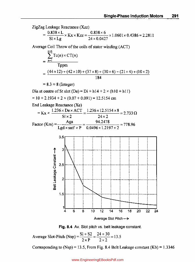
Single-Phase Induction Motors 291
ZigZag Leakage Reactance (Xzz)
= 0.838xL xKxxKzz = 0.838x6 x 1.0601 x 0.4386=2.2811 SI x Lg 24 x 0.0427
Average Coil Throw of the coils of stator winding (ACT) n=6
I Tc(n) x CT(n) = n=!
Tppm
= (44x 12) + (42 x 10) + (37 x 8) + (30x 6) + (21x 4) + (lOx 2)
184
= 8.3 ::::: 8 (Integer)
Dia at centre ofSt slot (De) = Di + h14 + 2 x (h10 + h11)
= 10 + 2.1934 + 2 x (0.07 + 0.091) = 12.5154 em
End Leakage Reactance (Xe)
= Kx x 1.236 x Dex ACT = 1.236 x 12.5154 x 8 = 2.733 n SIx 2 24x 2
Aga 94.2478 Factor (Km) = = 778.96
Lgd x satf x P 0.0496 x 1.2197 x 2
3.5 r--~-~--'----""---, -.....--....-----, I I I I I I
3 ----~- -- - -:- -- ---10-- ---~- -- ---:-- -- -~- ---- i- --- -~- ---- ~ -----I I I I I I I I
t C ::: : ttl I I I I
en ::: : § 2.5 ---- -----~-----~----~-----~-----~-----~-----~-----~-----U I I I I I I I I
I I I I I I I I I I I I I I I I I I I I I I I I I I I I J I I I I J I I
2 -----r--- -:- -----~- ---~------:-----~-----~-----~-----~-----I I I I I t I I I I I I I I I I I I I I 1 I I I I I I I I I I I I I I I t I I I I I I I I I I I I I I I J I
1.5 -----~----~-----~- -~-----~-----~-----~-----~-----~-----I I I I I I I I I I t I I I I I I I 1 I I I I I t I I I I I I
I I I
1~ ____ ~" ______ ~ __ ~~~ __ ~ __ ~ __ ~ __ ~
4 6 8 10 12 14 16 18 20 22 24
Average Slot Pitch ~
Fig. 8.4 Av. Slot pitch vs. belt leakage constant.
. SI+S2 24+30 Average Slot-Pttch (Nsp) - = = 13.5
2xP 2x2
Corresponding to (Nsp) = 13.5, From Fig. 8.4 Belt Leakage constant (Kb) = 1.3346
www.EngineeringEBooksPdf.com

292 Computer-Aided Design of Electrical Machines
Belt Leakage Reactance (Xb) = 0.000929 x Km x Kb x Kx
. = 0.000929 x 778.96 x 1.3346 x 1.0601 = 1.0237 .n
Assuming Rotor slot skew angle (skew) = 15° and factor (Kp) = 0.97,
Factor (Q) = 0.25 x (skew)2 = 0.25 X (~)2 = 0.0056 100 100
Skew Leakage reactance (Xsk) = 0.2546 x Km x Kp x Q x Kx
= 0.2546 x 778.96 x 0.97 x 0.0056 x 1.0601 = 1.1471 .n
Total Leakage Reactance of Main Wdg (XLm) = Xs + Xzz + Xe + Xb + Xsk
= 1.7529 + 2.2811 + 2.733 + 1.0237 + 1.1471 = 8.9378.n
Skew factor (Csk) = sin(skew /2 x 1t / 180) = sin(15 / 2 x 1t / 180) = 0.9971 1t x (skew /360) 1t x (15/360)
Magnetizing Reactance.(Xm) = Kx x 0.2546 x Km x Csk
= 1.0601 x 0.2546 x 778.96 x 0.9971 = 209.63 .n
Open Circuit Reactance (XO) = Xm + XLm = 209.63 + 8.9378 214.10 2 2
Magnetizing Current (lmu) =~ = 230 = 1.0743.n XO 214.1
8.7 (a) Computer Program in "C,. in MATLAB for Part-5
%<--------Leakage Reactance(Part-5)--------->
skew=15;Kp=0.97; %Assumption
Tc=[44 42 37 30 21 10]; Tppm=184;b11=0.7611; b13=1.3387; h14=2.1934; h10=0.07; b10=0.243;hl1=0.091;h20=0.08; b20=0.075; S2=30;Nm=736;sp1=1.309;sp2=1.0383; Lg=0.0427;Aga=94.2478; Lgd=0.0496; satf=1.2197;Ncpp=6;Sl=24;Kwm=0.7892;P=2;%Input Data
hz=sD;L=6;SP=12;Di=10;V=230;%Input Data
sum6=0;for i=1:Ncpp;sum6=sum6+Tc(i)A2;end;
Cx=sum6/TppmA2*Sl/(KwmA2*4*P);
B11byB13=[.5 .6 .7.8 .9 1 1.1 1.2 1.3 1.4 1.5 1.6 1.7 1.B];
CONSTANT=[0.63 .53 .46.41.36.33.3.27.25.23.21.2.18 .17] ;
plot(B11byB13,CONSTANT);grid;xlabel('b11/b13-->'); ylabel('Constant(A)-->');
title('Ratio of b11/b13 vs Constant (A) ');
b11byb13=b11/b13;
www.EngineeringEBooksPdf.com

Single-Phase Induction Motors 293
constA=interp1(B11byB13,CONSTANT,b11byb13, 'spline');
Ks1=constA*h14/b13+h10/b10+2*h11/(b10+b11);Ks2=h20/b20+0.623;
Ks=Ks1*Cx+S1/S2*Ks2; Z=Nm; Kx=2*pi*hz*(Z*Kwm)A2*le-8;
Xs=Kx*2.512*Ks*L/S1; bt10=sp1-b10;bt20=sp2-b20;
Kzz=(bt10+bt20)A2/(4*(sp1+sp2)); Xzz=Kx*Kzz*0.838 *L/(Sl*Lg);
sum7=O; for i=l:Ncpp; sum7=sum7+Tc(i)*(SP-(i-1)*2)i end;
ACT1=sum7/Tppm; ACT=floor(ACT1);De=Di+h14+2*(h10+h11);
Xe=Kx*1.236*De*ACT/S1/P;Km= Aga/(Lgd*satf~P);
AvSP=[4 8 12 16 20 24];BLC=[3.2 1.8 1.4 1.25 1.15 1.1];
plot(AvSP,BLC);grid;xlabel('Average Slot Pitch-->');
ylabel('Belt Leakage constant)-->');title('Av.Slot pitch Vs
Belt Leakage Constant');
Nsp=(Sl+S2)/2/P; Kb=interp1(AvSP,BLC,Nsp, 'spline');
Xb=0.000929*Km*Kb*Kx; Q=0.25*(skew/100)A2;
Xsk=0.2546*Km*Kp*Q*Kx; XLm=Xs+Xzz+Xe+Xb+Xsk;
Csk=sin(skew/2*pi/180)/(pi*skew/360);Xm=Kx*O.2546*Km*Csk;
XO=Xm+XLm/2; Imu=V/XO;
8.8 Design of Auxiliary Winding (Part-6) Assuming Transmission ratio (K) = 1.6,
winding factor for Auxiliary Wdg (Kwa) = 0.83, and
Using Concentric Winding, No. of Turns in Aux.wdg (Ta)
Kwm 0.7892 = Kl x Tm x -- = 1.6 x 368 x = 559.9::;:: 560 (Rounded oft)
Kwa 0.83
No. of conductors (Na) = Ta x 2 = 560 x 2 = 1120
. Ta 560 Turns per pole In Aux.wdg (Tppa) =-= - = 280
P 2
Pitch factor for Concentric Winding (connected in quadrature to main winding)
Coil No. Slots spanned Factor(y1) Pitch Factor(Kp)"= sin(y1 )( TT/2)
1 13 13/13 Sin(13/13 )( TT/2) = 1.0
2 11 11/13 Sin(11/13 )( TT/2) = 0.9709
3 9 9/13 Sin(9/13 )( TT/2) = 0.8855
4 7 7/13 Sin(7/13 x TT/2) = 0.7485
5 5 5/13 Sin(5/13 )( TT/2) = 0.5681
6 3 3/13 Sin(3/13 )( TT/2) = 0.3546
LKp =4.5276
www.EngineeringEBooksPdf.com
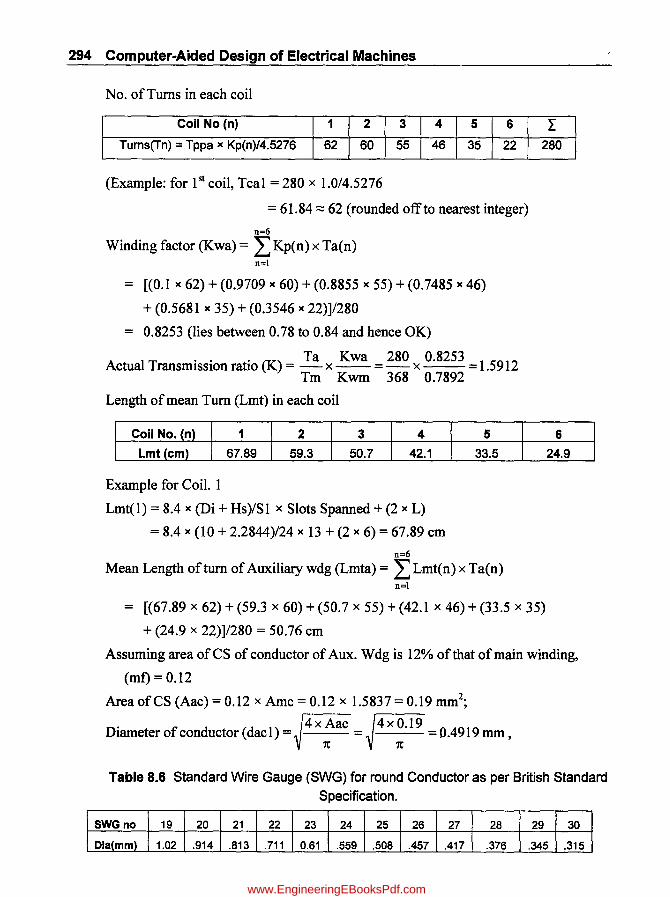
294 Computer-Aided Design of Electrical Machines
No. of Turns in each coil
Coil No (n) 1 2 3 4 5 6
Tums(Tn) = Tppa )( Kp(n)/4.5276 62 60 55 46 35 22
(Example: for 1 st coil, Tca1 = 280 x 1.0/4.5276
= 61.84;:::: 62 (rounded off to nearest integer)
n=6
Winding factor (Kwa) = L Kp(n) x Ta(n) n=!
= [(0.1)( 62) + (0.9709)( 60) + (0.8855)( 55) + (0.7485)( 46)
+ (0.5681 )( 35) + (0.3546)( 22)]/280
= 0.8253 (lies between 0.78 to 0.84 and hence OK)
A I T .. . (K) Ta Kwa 280 0.8253 5 2 ctua ransmiSSIon ratIo = - x --= - x = 1. 91 Tm Kwm 368 0.7892
Length of mean Turn (Lmt) in each coil
Coil No. (n) 1 2 3 4 5
r 280
6
Lmt (em) 67.89 59.3 50.7 42.1 33.5 24.9
Example for Coil. 1
Lmt(1) = 8.4 )( (Di + Hs)/Sl x Slots Spanned + (2)( L)
= 8.4 )( (10 + 2.2844)/24)( 13 + (2)( 6) = 67.89 cm
n=6
Mean Length of turn of Auxiliary wdg (Lmta) = L Lmt(n) x Ta(n) n=l
= [(67.89 x 62) + (59.3 x 60) + (50.7 x 55) + (42.1 x 46) + (33.5 x 35)
+ (24.9 x 22)]/280 = 50.76 cm
Assuming area ofCS of conductor of Aux. Wdg is 12% of that of main winding,
(mf) = 0.12
Area ofCS (Aac) = 0.12 x Amc = 0.12 x 1.5837 = 0.19 mm2;
. ~4xAac ~4XO.19 DIameter of conductor (dac 1) = 1t = 1t = 0.4919 mm ,
Table 8.6 Standard Wire Gauge (SWG) for round Conductor as per British Standard
Specification.
SWGno 19 20 21 22 23 24 25 26 27 28 29 30
Dla(mm) 1.02 .914 .813 .711 0.61 .559 .508 .457 .417 .376 .345 .315
www.EngineeringEBooksPdf.com
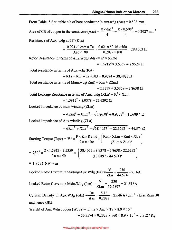
Single-Phase Induction Motors 295
From Table. 8.6 suitable dia of bare conductor in aux.wdg (dac) = 0.508 mm
. 1t x dac 2 1t x 0.5082 2 Area ofCS of copper III the conductor (Aac) = = = 0.2027 mm
4 4 Resistance of Aux. wdg at 75° (RIa)
= 0.021xLmtaxTa = 0.021x50.76x560 =29.45030 Aac xI 00 0.2027 x 100
Rotor Resistance in terms of Aux.Wdg (Rdr) = K2 x R2md
= 1.59122 x 3.5359 = 8.9524 0
Total resistance in terms of Aux.wdg (Rat)
= RIa + Rdr = 29.4503 + 8.9524 = 38.4027 0
Total resistance in terms of Main.wdg(Rmt) = Rm + R2md
= 2.3279 + 3.5359 = 5.86380
Total Leakage Reactance in terms of Aux. wdg (XLa) = K2 x XLm
= 1.59122 x 8.9378 = 22.62920
Locked Impedance of main winding (ZLm)
=JRmt2 +XLm2 =J5.86382 +8.93782 =10.6897 0
Locked Impedance of Aux winding (ZLa)
=JRat2 + XLa2 = J38.4027 2 + 22.62922 = 44.574 0
S . T (T) V2 PxKxR2md (RatxXLm-RmtxXLa] tartmg orque qst = x X 2 2x1txbz (ZLmxZLa)
= 2302 x 2 x 1.5912 x 3.5359 x (38.4027 x 8.9378 - 5.8638 x 22.6292] 2 x 1t x 50 (10.6897 X 44.574)2
= 1.7571 Nw-m
Locked Rotor Current in StartinglAux.Wdg (Isa) =~= 230 = 5.16A ZLa 44.574
Locked Rotor Current in Main. W dg (Ism) = ~ = 230 = 21.516A ZLm 10.6897
Current Density in Aux.Wdg (cda) = Isa = 5.16 =25.46A/mm 2 (Less than 30 Aac 0.2027
and hence OK)
Weight of Aux Wdg copper (Wcua) = Lmta x Aac x Ta x 8.9 x 10-5
= 50.7574 x 0.2027 x 560 x 8.9 x.1O-5 = 0.5127 Kg
www.EngineeringEBooksPdf.com

296 Computer-Aided Design of Electrical Machines
8.8 (a) Computer Program in "e" in MATLAB for Part-6
%<--------Design of Auxiliary Wdg(Part-6)--------->
K1=1.6;Kwa1=0.83;mf=0.12; %Assumptions
Tm=368;Kwm=0.7892;P=2;Ncpp=6;SP=12;Di=10;Hs=2.2844;Sl=24;L=6;
Amc=1.5837;R2md=3.5359;Rm=2.3279;XLm=8.9378;V=230;hz=50;
%Input Data
Ta1=K1*Tm*Kwm/Kwa1; Ta=ceil(Ta1/2)*2; Na=Ta*2; Tppa=Ta/P;
sum11=0; sum12=0;sum13=0;sum14=0; sum15=0;
for i=l:Ncpp; y1=(SP+1-(i-1)*2)/(SP+1); Kp(i)=sin(y1*pi/2);
sum11=sum11+Kp(i); end; sum12=0;
for i=l:Ncpp; Tca1(i)=Tppa*Kp(i)/sum11; Tca(i)=round(Tca1(i));
sum12=sum12+Tca(i); end; corr=Tppa-sum12;
Tca(Ncpp)=corr+Tca(Ncpp); sum12=sum12+corr;
for i=l:Ncpp; sum13=sum13+Kp(i)*Tca(i); end; Kwa=sum13/Tppa;
K=Ta*Kwa/ Tm/Kwm; sum15=0;
for i=l:NcPPi Lmta1(i)=8.4*(Di+Hs)/Sl*(SP+1-(i-1)*2)+2*L;
sum15=sum15+Lmta1(i)*Tca(i)i endi
Aac1=mf*Amci dac1=sqrt(4*Aac1/pi);
Lmta=sum15/Tppai
DSWG1=[1.02 .914 .813 .711 .610 .559.508.457.417.376.345
.315];
for i=1:12; if dac1 >= DSWG1(i) continueiendi
dac=DSWG1(i);endi Aac=pi*dacA2/4i R1a=0.021*Lmta*Ta/(Aac*100);
Rdr=KA2*R2md; Rat=R1a+Rdr; Rmt=Rm+R2mdi XLa=KA2*XLm; ZLm=sqrt
(Rmt A2+XLmA2) i ZLa=sqrt(RatA2+XLaA2)i
Tqst=P*K*R2md*VA2/(2*pi*hz) * (Rat*XLm-Rmt*XLa) /ZLmA2/ZLaA2;
Isa=V/ZLa; Ism=V/ZLm; Ist=Isa+Ism; cda=Isa/Aac;
if cda >30 continue;end; Wcua=Lmta*Aac*Ta*8.ge-5i
www.EngineeringEBooksPdf.com
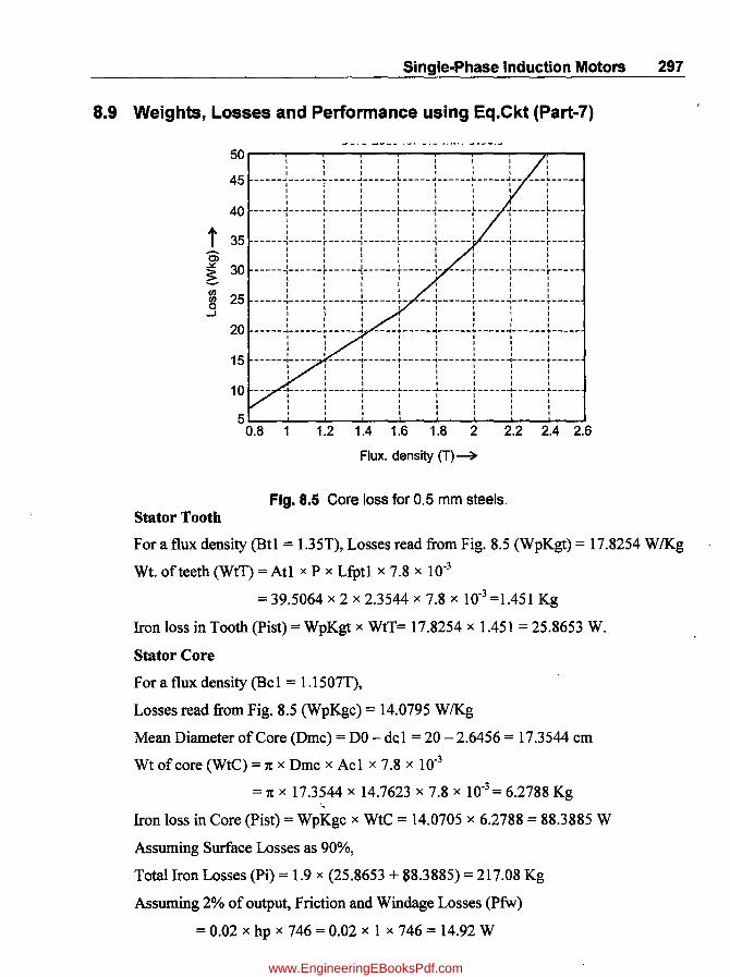
Single-Phase Induction Motors 297
8.9 Weights, Losses and Performance using Eq.Ckt (Part-7)
50~--~--~--~--~--~--~--~,~~~~ I
I 1 I I I I I I
45 -----~------r-----~------~-----i------r-----~-- ---~-----I I I I I I I I I I I I I I I I I I I I I I
40 -----1------r-----1------r-----1------r---- 1------r-----I I 1 I I I I I I t I I I I I I
t il I I I I I I
35 -----~------~-----i------~-----1------' ----i------t-----I 1 I I I I I I I I I I I I I ~
~ 30 I 1 I I I I I I -----,------r-----'------r-----'- ----r-----,------r-----
I I 1 I I I I I I I I I
~ 25 -----~------~-----~------~- --~------~-----~------~-----o 1 1 I I I I 1 I -.I I I 1 I I I I
I I I I I I I I
20 -----~------~-----~ ----~-----~-----~-----~------!-----I I I I I I I I I I I I I 1 I I I I I I I
15 -----~---- :-----~------r-----~------t-----~------f-----I I I I I I I I I I I I I I I I
I I I I I I I
~-----.-----~-----.-----~-----+-----~-----.-~---I I I I I 1 I I 10 I I I 1 I I I I I I I I I I I I
5~--~'--~'--~'--~'--~'~--~' --~'--~'--~ 0.8 1 1.2 1.4 1.6 1.8 2 2.2 2.4 2.6
Flux. density (T)---+
Fig. 8.5 Core loss for 0.5 mm steels. Stator Tooth
For a flux density (Btl = 1.35T), Losses read from Fig. 8.5 (WpKgt) = 17.8254 W/Kg
Wt. of teeth (WtT) = Atl x P x Lfptl x 7.8 x 10-3
= 39.5064 x 2 x 2.3544 x 7.8 x 10-3 =1.451 Kg
Iron loss in Tooth (Pist) = WpKgt x WtT= 17.8254 x 1.451 = 25.8653 W.
Stator Core
For a flux density (Bel = 1J507T),
Losses read from Fig. 8.5 (WpKgc) = 14.0795 W/Kg
Mean Diameter of Core (Ornc) = DO - del = 20 - 2.6456 = 17.3544 crn
Wt of core (WtC) = 1t x Drnc x Ac 1 x 7.8 X 10-3
= 1t x 17.3544 x 14.7623 x 7.8 x 10-3 = 6.2788 Kg
Iron loss in Core (Pist) = WpKgc x WtC = 14.0705 x 6.2788 = 88.3885 W
Assuming Surface Losses as 90%,
Total Iron Losses (Pi) = 1.9 x (25.8653 + 88.3885) = 217.08 Kg
Assuming 2% of output, Friction and Windage Losses (Pfw)
= 0.02 x hp x 746 = 0.02 x 1 x 746 = 14.92 W
www.EngineeringEBooksPdf.com
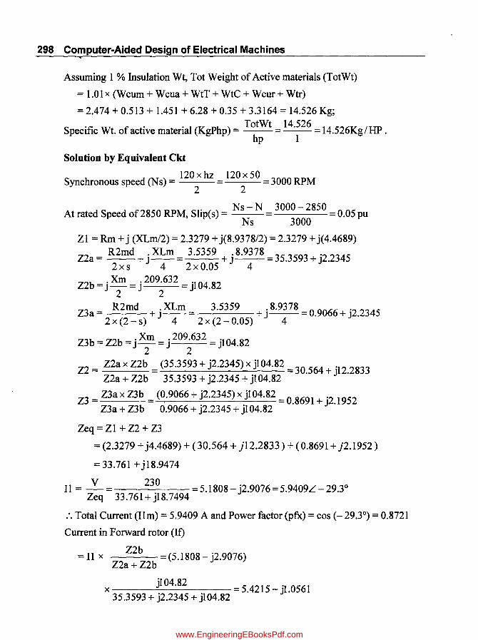
298 Computer-Aided Design of Electrical Machines
Assuming 1 % Insulation Wt, Tot Weight of Active materials (TotWt)
= 1.01x (Wcum + Wcua + WtT + WtC + Wcur+ Wtr)
= 2.474 + 0.513 + 1.451 + 6.28 + 0.35 + 3.3164 = 14.526 Kg;
Specific wt. of active material (KgPhp) = TotWt 14.526 = 14.526Kg/HP . hp 1
Solution by Equivalent Ckt
120xhz 120x50 Synchronous speed (Ns) = = =3000 RPM
2 2
. Ns-N 3000-2850 At rated Speed of 2850 RPM, Shp(s) = = = 0.05 pu
Ns 3000
Zl = Rm + j (XLml2) = 2.3279 + j(8.9378/2) = 2.3279 + j(4.4689)
Z2a = R2md + j XLm = 3.5359 + j 8.9378 = 35.3593 + j2.2345 2 x s 4 2 x 0.05 4
Z2b = j Xm = j 209.632 = j104.82 2 2
Z3a = R2md +' XLm = 3.5359 + . 8.9378 = 0.9066 + '2.2345 2x(2-s) J 4 2x(2-0.05) J 4 J
Z3b = Z2b = j Xm = j 209.632 = j104.82 2 2
Z2 = Z2a x Z2b = (35.3593 + j2.2345) x j104.82 = 30.564 + j12.2833 Z2a + Z2b 35.3593 + j2.2345 + j104.82
Z3 = Z3a x Z3b = (0.9066 + j2.2345) x j104.82 = 0.8691 + j2.1952 Z3a + Z3b 0.9066 + j2.2345 + j104.82
Zeq = ZI + Z2 + Z3
= (2.3279 + j4.4689) + (30.564 + j12.2833) + (0.8691 + j2.1952)
= 33.761 + j18.9474
II = ~= 230 =5.1808-j2.9076=5.9409L-29.30
Zeq 33.761 + j18.7494
:. Total Current (lIm) = 5.9409 A and Power factor (pfx) = cos (- 29.3°) = 0.8721
Current in Forward rotor (If)
= II x Z2b = (5.1808 - '2.9076) Z2a +Z2b J
x j104.82 '> = 5.4215 - jl.0561 35.3593 + j2.2345 + jl04.82
www.EngineeringEBooksPdf.com
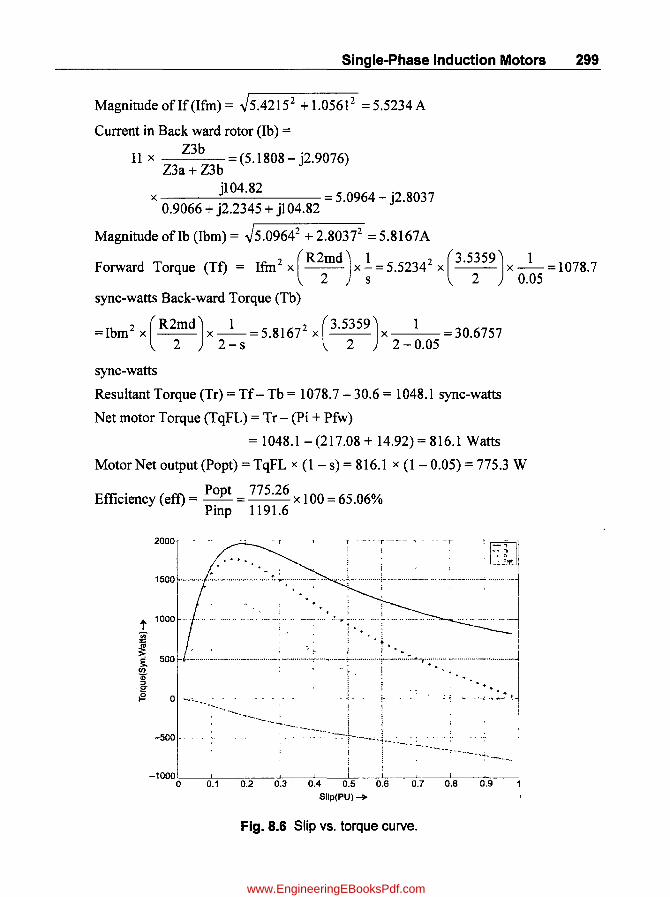
Single-Phase Induction Motors 299
Magnitude ofIf(Ifm) = ~5.42152 +1.0561 2 =5.5234A
Current in Back ward rotor (Ib) =
Ilx Z3b =(5.1808-j2.9076) Z3a+Z3b
x jl04.82 = 5.0964 - j2.8037 0.9066 + j2.2345 + jl04.82
Magnitude ofIb (Ibm) = ~5.09642 + 2.80372 = 5.8167A
Forward Torque (Tf) = Ifm2 x (R2md) x.l = 5.52342 x (3.5359) x _1_ = 1078.7 2 s 2 0.05
sync-watts Back-ward Torque (Tb)
=Ibm2 x (R2md) x _1_ = 5.81672 x (3.5359) x 1 = 30.6757 2 2 - s 2 2 - 0.05
sync-watts
Resultant Torque (Tr) = Tf - Tb = 1078.7 - 30.6 = 1048.1 sync-watts
Net motor Torque (TqFL) = Tr - (Pi + Pfw)
= 1048.1-(217.08 + 14.92)= 816.1 Watts
Motor Net output (Popt) = TqFL x (1- s) = 816.1 x (1- 0.05) = 775.3 W
Efficiency (eft) = Popt = 775.26 xl 00 = 65.06% Pinp 1191.6
2000 TEtl'1 .L1J 1500 ..... _ ..... ~ .. ~ .......... - ......... : .. !..~.~ .. : ........ - .. _. --.. ~ .............. ~ .............. ~-......... ~ ..... - ....... ~ ............ j
. . : . I
1. 1000 ............................ "'j ':.' ...: ...... !~ 1'< ..;.... ....... ..... .. .. "'''''' ....l ,!g i ... i i co t " I I "" .. : .......... _..... ······;······t--i·:~'···;:·: ;:~ ... ~:~.j ~ .:". ~"··----~~::t~l-<~:-i __ ~·_l
, "
o 0.1 0.2 0.3 0.4 0.5 0.6 0.7 0.8 0.9 Slip(PU)-+
Fig. 8.6 Slip vs. torque curve.
www.EngineeringEBooksPdf.com

300 Computer-Aided Design of Electrical Machines
8.9 (a) Computer Program in "c" in MATLAB for Part-7 %<-----Weights,Losse~andPerformance using Eq.Ckt(Part-7)------>
Btl=I.35;Atl=39.5064;P=2iLfptl=2.3544iBcl=I.1507;DO=20; dcl=2.6456; Acl=14.7623;hp=liWcum=2.474;Wcua=0.513i Wcur=0.35i Wtr=3.3164ihz=50; N=2850;Rm=2.3279;XLm=8.9378;R2md=3.5359i Xm=209.632iV=230i%Input Data
FD=[0.8 1.2 1.6 2 2.4J; WPKG=[7 15 23 34 50J; % for 0.5 mm plot(FD,WPKG);grid;xlabel('Flux.Density(T)-->')i ylabel('Loss(W/Kg)-->')ititle('Core Loss for 0.5 mm Steels')i
WpKgt=interpl(FD,WPKG,Btl, 'spline');
WtT=Atl*P*Lfptl*7.8*le-3; Pist=WpKgt* WtT;
WpKgc=interpl(FD,WPKG,Bcl, 'spline'); Dmc=DD-dcli WtC=pi*Dmc*Acl*7.8 *le-3; Pisc=WpKgc*WtC;
Pi=I.9*(Pist+Pisc)i Pfw=0.02*hp*746i
TotWt=I.01*(Wcum+Wcua+WtT+WtC+Wcur+Wtr); KgPhp=TotWt/hpi
%------Solution by Equivalent Circuit------->
Ns=120*hz/P;s=(Ns-N)/Nsi
ZI=Rm+XLm/2*j; Z2a=R2md/(2*s)+XLm/4*j; Z2b=Xm/2*j;
Z3a=R2md/(2*(2-s))+XLm/4*j;Z3b=Xm/2*jiZ2=Z2a*Z2b/(Z2a+Z2b)i Z3=Z3a*Z3b/(Z3a+Z3b); Zeq=ZI+Z2+Z3; Il=V/Zeqi ang=angle(Il)*180/pii pfx= cos(ang*pi/180)i Ilm=abs(Il)i If=Il*Z2b/(Z2a+Z2b);Ifm=abs(If)ilb=Il*Z3b/(Z3a+Z3b); Ibm=abs(Ib)i Tf=IfmA 2*R2md/(2*s); Tb=IbmA 2*R2md/(2*(2-s))i Tr=Tf-Tbi TqFL=Tr-(Pi+Pfw)i
Popt=TqFL*(I-s); Pinp=V*Ilm*pfxi eff=Popt/Pinp*lOO;
%---Extra Program for Plotting Slip vs Torque ------------->
for kk=1:49; s=kk*0.02; ZI=Rm+XLm/2*ji Z2a=R2md/(2*s)+XLm/4*j;Z2b=Xm/2*j;Z3a=R2md/(2*(2-s))+ XLm/4*j; Z3b=Xm/2*j; Z2=Z2a*Z2b/(Z2a+Z2b); Z3=Z3a*Z3b/(Z3a+Z3b)i Zeq=ZI+Z2+Z3i 1 l=V/Zeq;ang=angle(Il)*180/pi i pfx=cos(ang*pi/180)i Ilm=abs(Il); If=Il*Z2b/(Z2a+Z2b); Ifm=abs(If); Ib=Il*Z3b/(Z3a+Z3b)i Ibm=abs(Ib)i Tf=Ifm A 2*R2md/(2*s)i Tb=IbmA 2*R2md/(2*(2-s))i Tr=Tf-Tbi TqFL=Tr-(Pi+Pfw)i Popt=TqFL*(I-s);SS(kk)=Si TF(kk)=Tf; TB(kk)=-TbiTR(kk)=Tr;PO(kk)=Popt;end;
plot (SS, TF, '-' , SS, TB, '-. ' , SS, TR, '*' , SS, PO, '0' ) ; gridi legend('Tf', 'Tb', 'Tr', 'Popt');xlabel('Slip(PU)-->');
ylabel('Torque(syn.Watts)-->')ititle('Slip vs Torq~ Curve')i
%----------End of Program--------------->
www.EngineeringEBooksPdf.com
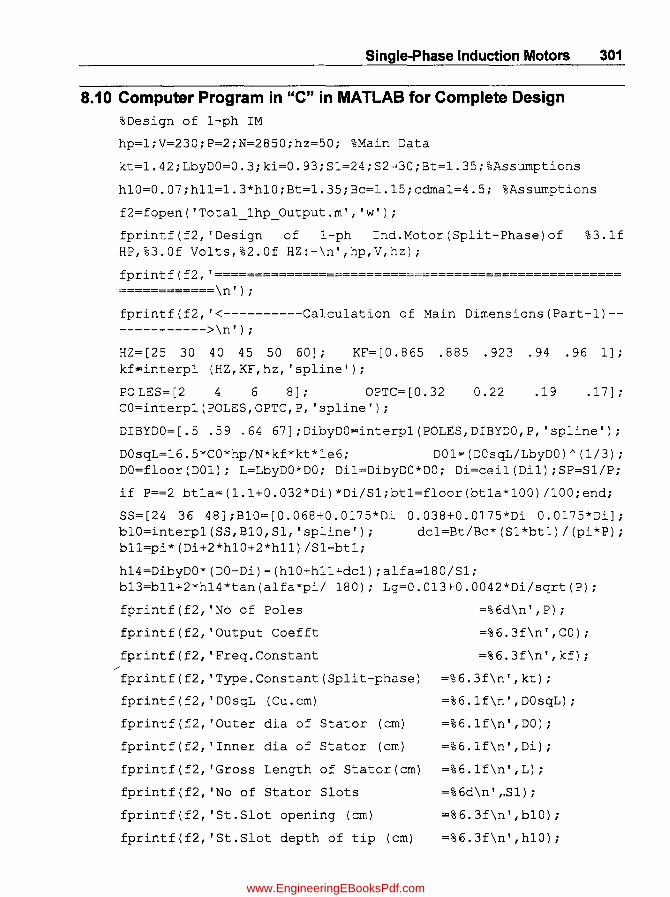
Single-Phase Induction Motors 301
8.10 Computer Program in "C" in MATLAB for Complete Design %Design of I-ph 1M
hp=1;V=230;P=2;N=2850;hz=50; %Main Data
kt=1.42;LbyDO=0.3;ki=0.93;Sl=24;S2=30;Bt=1.35;%Assumptions
hl0=0.07;hll=1.3*hl0;Bt=1.35;Be=1.15;edmal=4.5; %Assumptions
f2=fopen('Total_lhp_Output.m', 'w');
fprintf(f2, 'Design of I-ph Ind.Motor (Split-Phase) of %3.1f HP,%3.0f Volts,%2.0f HZ:-\n',hp,V,hz);
fprintf(f2, '=================================================== ============\n');
fprintf(f2, '<----------Caleulation of Main Dimensions(Part-l)------------>\n');
HZ=[25 30 40 45 50 60]; KF= [ 0 . 8 65 . 8 8 5 . 92 3 . 94 . 96 1]; kf=interpl (HZ,KF,hz, 'spline');
PO LES= [2 4 6 8] ; OPTC=[0.32 0.22 .19 .17] ; CO=interp1(POLES,OPTC,P, 'spline');
DIBYDO=[.5 .59 .64 67];DibyDO=interp1(POLES,DIBYDO,P, 'spline');
DOsqL=16.5*CO*hp/N*kf*kt*le6; D01=(DOsqL/LbyDO)A(1/3); DO=floor(D01); L=LbyDO*DO; Di1=DibyDO*DO; Di=eeil(Di1);SP=Sl/P;
if P==2 bt1a=(1.1+0.032*Di)*Di/Sl;bt1=floor(bt1a*100)/100;end;
SS=[24 36 48] ;B10=[0.068+0.0175*Di 0.038+0.0175*Di 0.0175*Di]; b10=interp1(SS,B10,Sl, 'spline'); de1=Bt/Be*(Sl*bt1)/(pi*P); b11=pi*(Di+2*h10+2*h11)/Sl-bt1;
h14=DibyDO*(DO-Di)-(h10+h11+de1);alfa=180/S1; b13=b1l+2*h14*tan(alfa*pi/ 180); Lg=0.013+0.0042*Di/sqrt(P);
fprintf(f2, 'No of Poles =%6d\n',P);
fprintf(f2, 'Output Coefft =%6.3f\n',CO);
fprintf(f2, 'Freq.Constant =%6.3f\n',kf); /
fprintf(f2, 'Type. Constant (Split-phase) =%6.3f\n',kt);
fprintf(f2, 'DOsqL (Cu.em) =%6.1f\n',DOsqL);
fprintf(f2, 'Outer dia of Stator (em) =%6.1f\n',DO);
fprintf(f2, 'Inner dia of Stator (em) =%6.1f\n',Di);
fprintf(f2, 'Gross Length of Stator (em) =%6.1f\n',L);
fprintf (f2, 'No of Stator Slots =% 6d\n' ,.SI) ;
fprintf(f2, 'St.Slot opening (em) =%6.3f\n',b10):
fprintf (f2, 'St. Slot depth of tip (em) =% 6. 3f\n' ,hl0) ;
www.EngineeringEBooksPdf.com

302 Computer-Aided Design of Electrical Machines
fprintf(f2, 'St.Slot depth of mouth(cm) =%6.3f\n',h11);
fprintf(f2, 'St.Slot tooth width (cm) =%6.3f\n',bt1);
fprintf(f2, 'St.Core depth (cm) =%6.3f\n',dc1);
fprintf(f2, 'Slot width at topandbottom(cm) =%6.3fand%6.3f\n',b11,b13);
fprintf (f2, 'St. Sl.ot depth (cm)
fprintf(f2, 'Air-gap Length (cm)
=%6.3f\n' ,h14) j
=%6.3f\n' ,Lg);
fprintf(f2, '<-----------Design of Main Winding(Part-2)------------------->\n');
Ncpp=Sl/P/2;sum1=Ojsum2=Oi s um3=OiS um4=0;sum5=0;
For i=1:Ncpp;y1=(SP-(i-1)*2)/(SP+1); Kp(i)=sin(y1*pi/2); sum1=sum1+Kp(i); end;
for i=l:NcPPi PTm(i)=Kp(i)/sum1*100i sum2=s~2+PTm(i);end;
for i=1:Ncpp;sum3=sum3+Kp(i)*PTm(i);end; Kwm=sum3/sum2j
Li=ki*L;At=bt1*Li*SP;FI=0.637*At*Bt*le-4; Tm1=0.95*V/(4.44*hz*FI*Kwm);Tm=ceil(Tml/2)*2;Nm=Tm*2; Tppm=Tm/P;
for i=1:NcPPiTc1(i)=Tppm*PTm(i)/100iTc(i)=round(Tc1(i))i
sum4=sum4+Tc(i)iend;corr=Tppm-sum4; sum4=sum4+corri
Tc(Ncpp)=corr+Tc(Ncpp);
HP=[.05 .1 .25 .5 .75 1];EFF=[.35 .44 .58 .65 .68 .7];
PF=[.45 .5 .56 .62 .64 .66];effa=interp1(HP,EFF,hp,'spline'); pfa=interp1(HP,PF,hp, 'spline'); Im=hp*746/(effa*V*pfa); Amc1=Im/cdmali dmc1=sqrt(4*Amcl/pi);
DSWG=[5.38 4.88 4.47 4.06 3.66 3.25 2.95 2.64 2.31 2.03 1.83 1.63 1.42 1.22 1.02];
for i=1:15; if dmc1 >= DSWG(i) continue; end; dmc=DSWG(i); end; dmcins=dmc+0.075i Amc=pi*dmc A 2/4; cdm=Im/Amc;
if cdm <2.8 I I cdm >4.5 continue;end;
Socm=Tc(l) *pi*dmcins A 2/4/100;Asg=(h11* (b10+b11)+h14* (bl 1+b13)) /2;
Sfsm=Socm/Asg; if Sfsm >0.5 continue;end;
Hs=h11+h14;for i=1:Ncpp;Lmt(i)=8.4*(Di+Hs)/Sl*(SP-(i-l)*2)+2*L;
sum5=sum5+Lmt(i)*Tc(i)iendiLmtm=sum5/sum4;
Rm=0.021*Lmtm*Tm/(Amc*100);Pcus=ImA 2*Rm;
Wcum=Lmtm*Amc*Tm*8.ge-5; (
www.EngineeringEBooksPdf.com

Single-Phase Induction Motors 303
fprintf(f2, 'Pitch-Factors of %2d coils:%5.3f,%5.3f,%5.3f,%5.3f,%5.3fand%5.3f\n', Ncpp,Kp);
fprintf(f2, 'Pecentage-Turns of coils:%4.1f+%4.1f+%4.1f+%4.1f+%4.1f+%4.1f= %4.0f(perc)\n',Ncpp,PTm,sum2);
%2d
fprintf(f2, 'Winding Factor
fprintf(f2, 'Flux/Pole (Wb)
%6.3f\n' ,Kwm);
% 6.4 f\n ' , FI) ;
fprintf(f2, 'No of Turns coils:%3.0f+%3.0f+%3.0f+%3.0f+%3.0f+%3.0f= %3.0f\n',Ncpp,Tc,Tppm);
fprintf(f2, 'Current in Main Wdg (A) =
in
%6.3f\n',Im);
fprintf(f2, 'Conductor: dia=%6.3fcmandCS area(total)= %5.3fsq.mm\n',dmc,Amc);
fprintf(f2, 'Current dens in Main wdg(A/sq.mm)= %6.3f(desirable:<4.5)\n',cdm);
fprintf(f2, 'Gross Slot Area(sq.cm) =%6.3f\n',Asg);
fprintf(f2, 'Space Occupied in %2.0fstrands(sq.cm)=%6.4f\n',Tc(1),Socm);
fprintf(f2, 'Space factor of the slot = desirable: < O.5)\n',Sfsm);
Coil:l
%6.3f(
%2d
by
fprintf(f2, 'Mean Turn Lengths of %2d coils (cm) :%4.1f,%4.if,%4.1f,%4.1f,%4.1fand% 4.1f\n',Ncpp,Lmt);
fprintf(f2, 'Mean Turn Lengths of Total Wdg(cm): %5.2f\n',Lmtm);
fprintf(f2, 'Resistance of Main Wdg(ohm)=
fprintf(f2, 'Copper Losses of Main Wdg(W)=
fprintf(f2, 'Wt of Main-Wdg-Copper (Kg)=
%6. 4f\n', Rm) i
%6.3f\n',Pcus);
%6.3f\n' ,Wcum);
fprintf(f2, '<---------~esign of Rotor(Part-3)--------------------------->\n');
b20=O.075ih20=O.08iDm=O.07; %assumption
Dr=Di-2*Lg;bt2=O.95*Sl*btl/S2;
r21=(pi*(Dr-2*h20)-S2*bt2)/(2*(S2+pi)); drcl=2* r21-0.038;
for i=1:15;if drcl*lO>=DSWG(i) continue; end; drc=DSWG(i); end;
Ab=pi *drc"2/ 4; dc2=O. 95*dcl; Lb=L+'l; Nb=S2; Aer=Ab/pi *Nb/P;
R2md=P*Nm"2*Kwm"2*O.021*(Lb/(lOO*Ab*Nb)+2/pi*Dm/P"2/Aer);
12d=Im*pfa;Pcur=I2d"2*R2md; Wcur=OLb*Ab*Nb*8.ge-5; Wtr=((pi*Dr"2/4)-(S2*pi*r21"2))*L*7.8*le-3;
fprintf(f2, 'Outer dia of Rotor (cm) = %6.4f\n' ,Dr);
www.EngineeringEBooksPdf.com
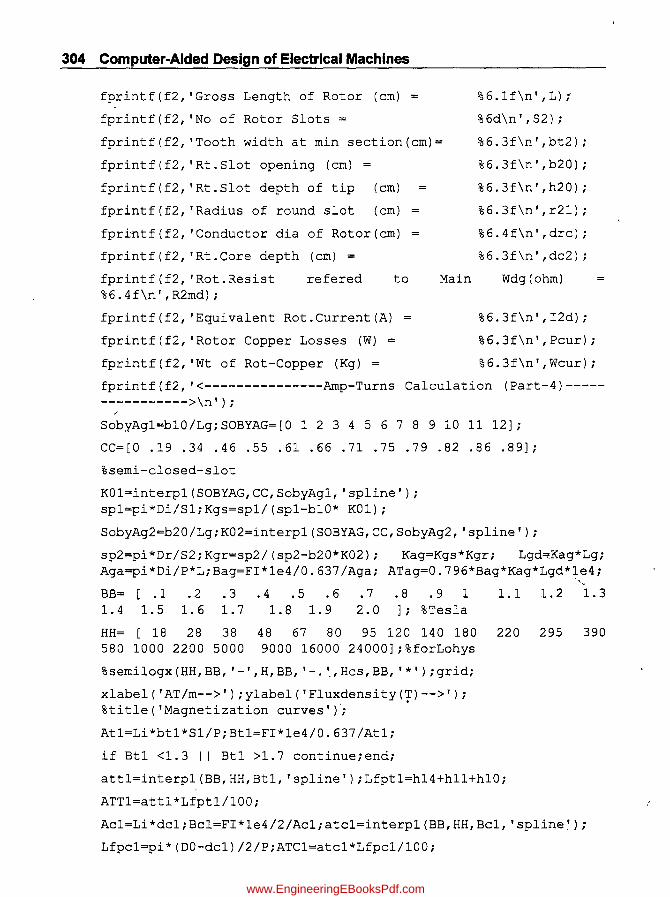
304 Computer-Aided Design of Electrical Machines
fprintf(f2, 'Gross Length of Rotor (cm) =
fprintf(f2, 'No of Rotor Slots =
fprintf(f2, 'Tooth width at min section(cm)=
fprintf(f2, 'Rt.Slot opening (cm)
fprintf(f2, 'Rt.Slot depth of tip (cm)
fprintf(f2, 'Radius of round slot (cm)
fprintf(f2, 'Conductor dia of Rotor (cm)
fprintf(f2, 'Rt.Core depth (cm) =
fprintf(f2, 'Rot.Resist %6. 4f\n' , R2md) ;
refered
fprintf(f2, 'Equivalent Rot.Current(A)
fprintf(f2, 'Rotor Copper Losses (W)
fprintf(f2, 'Wt of Rot-Copper (Kg) =
to Main
%6.1f\n',L);
%6d\n',S2);
%6.3f\n' ,bt2);
%6.3f\n' ,b20);
%6.3f\n' ,h20);
%6.3f\n' ,r2l);
%6.4f\n' ,drc);
%6.3f\n' ,dc2);
Wdg (ohm)
%6.3f\n',I2d);
%6. 3f\n' , Pcur) ;
%6.3f\n' ,Wcur);
fprintf(f2, '<---------------Amp-Turns Calculation (Part-4)--------------->\n');
/
SobyAg1=b10/Lg;SOBYAG=[0 1 2 345 6 7 8 9 10 11 12];
CC= [ 0 . 19 . 34 . 46 . 55 . 61 . 66 . 71 . 75 . 79 . 82 . 86 . 89] ;
%semi-closed-slot
K01=interpl(SOBYAG,CC,SobyAg1, 'spline'); sp1=pi*Di/S1;Kgs=sp1/(sp1-b10* KOl);
SobyAg2=b20/Lg;K02=interp1(SOBYAG,CC,SobyAg2, 'spline');
sp2=pi*Dr/S2;Kgr=sp2/(sp2-b20*K02); Kag=Kgs*Kgr; Lgd=<Kag*Lg; Aga=pi*Di/P*L;Bag=FI*le4/0.637/Aga; ATag=0.796*Bag*Kag*Lgd*~e4;
BB= [ .1 .2 .3 .4 .5 .6 .7 .8 .9 1 1.4 1.5 1.6 1.7 1.8 1.9 2.0 ] ; %Tesla
HH= [ 18 28 38 48 67 80 95 120 140 180 580 1000 2200 5000 9000 16000 24000];%forLohys
%semilogx(HH,BB, '-' ,H,BB, '-. '.,Hcs,BB, '*') ;grid;
xlabel('AT/m-->');ylabel('Fluxdensity(~)-->');
%title('Magnetization curves')j
At1=Li*bt1*Sl/P;Bt1=FI*le4/0.637/At1;
if Btl <1.3 I I Btl >1.7 continue; end;
, "
1.1 1.2 1.3
220 295 390
att1=interpl(BB,HH,Bt1, 'spline');Lfpt1=h14+hl1+hlO;
ATT1=att1*Lfpt1/100;
Ac1=Li*dc1;Bcl=FI*le4/2/Ac1;atc1=interp1(BB,HH,Bc1, 'spline');
Lfpc1=pi*(DO-dc1)/2/P;ATC1=atc1*Lfpcl/lOO;
www.EngineeringEBooksPdf.com

Single-Phase Induction Motors 305
At2=Li*bt2*S2/P;Bt2=FI*le4/0.637/At2;
att2=interp1(BB,HH,Bt2, 'spline');Lfpt2=2*r21+h20;
ATT2=att2*Lfpt2/100;
Ac2=Li*dc2;Bc2=FI*le4/2/Ac2;atc2=interp1(BB,HH,Bc2, 'spline');
Lfpc2=pi*(2*r21+h20+dc2)/2/P;ATC2=atc2*Lfpc2/100;
ATT=ATag+ATT1+ATC1+ATT2+ATC2;satf=ATT/ATag;
fprintf(f2, 'Stator Gap Coefft (Kgs) =
fprintf(f2, 'Rotor Gap Coefft (Kgr)
fprintf(f2, 'Air Gap Coefft (Kag) =
fprintf(f2, 'Air-Gap Effectivelength(cm)
% 6.4 f\n ' , Kgs) ;
%6.4f\n' ,Kgr);
%6.4f\n' ,Kag);
%6.4f\n' ,Lgd);
fprintf(f2, 'Air-Gap: Flux-density(T)=%6.4f and AmpTurns=%6.1f\n',Bag,ATag);
fprintf(f2, 'Stator tooth:Flux-density(T)=%6.4f and AmpTurns=%6.1f\n',Bt1,ATT1);
fprintf(f2, 'Stator Core AmpTurns=%6.1f\n',Bc1,ATC1);
fprintf(f2, 'Rotor tooth: AmpTurns=%6.1f\n',Bt1,ATT2);
fprintf(f2, 'Rotor Core AmpTurns=%6.1f\n',Bc1,ATC2);
fprintf(f2, 'Total AmpTurns factor=%6.3f\n',ATT,satf);
:Flux-density(T)=%6.4f and
Flux-density(T)=%6.4f and
Flux-density(T)=%6.4f and
=%6.1f and Saturation
fprintf(f2, '<-----------------Leakage Reactances(Part-5)----------------->\n');
skew=15;Kp=O.97; %Assumption
sum6=O;fori=1:Ncpp;sum6=sum6+Tc(i)A2;end;
Cx=sum6/TppmA2*Sl/(KwmA 2*4 *P);
B11byB13=[.5 .6 .7.8 .9 1 1.1 1.2 1.3 1.4 1.5 1.6 1.7 1.8];
CONSTANT=[O.63 .53 .46 .41 .36 .33 .3 .27 .25 .23 .21 .2 .18 .17]; b11byb13=b11/b13; constA=interp1(B11byB13,CONSTANT,b11byb13, 'spline');
Ks1=constA*h14/b13+h10/b10+2*h11/(b10+b11);Ks2=h20/b20+0.623; Ks=Ks1*Cx+S1/S2*Ks2i Z=Nm; Kx=2*pi*hz* (Z*Kwm) A2*le-8i Xs=Kx*2.512*Ks*L/S1; Lmd1=pi*Di/S1; Lmd2=pi*Dr/S2;
bt10=sp1-b10;bt20=sp2-b20; Kzz=(bt10+bt20)A2/(4*(Lmd1+Lmd2)); Xzz=Kx*Kzz*O.838~L/ (Sl*Lg);
www.EngineeringEBooksPdf.com
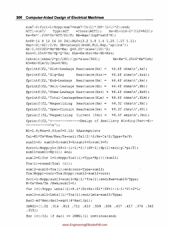
306 Computer-Aided Design of e"lectrical Machines
sum7=O;fori=1:Ncpp;sum7=sum7+Tc(i)*(SP-(i-1)*2);end; ACT1=sum7/ Tppm; ACT =f1oor (ACT1) ; De=Di+h14+2* (h10+h11) ; Xe=Kx*1.236*De*ACT/S1/P; Km=Aga/(Lgd*satf*P);
AvSP=[48 12 16 20 24];BLC=[3.2 1.8 1.4 1.25 1.15 1.1]; Nsp=(Sl+S2)/2/P; Kb=interp1(AvSP,BLC,Nsp, 'spline'); Xb=O.000929*Km*Kb*Kx; Q=O.25*(skew/100)A2; Xsk=O.2546*Km*Kp*Q*Kx; XLm=Xs+Xzz+Xe+Xb+Xsk;
Csk=sin(skew/2*pi/180)/(pi*skew/360); XO=Xm+XLm/2;Imu=V/XO;
fprintf(f2, 'Slot-Leakage Reactance (Xs)
fprintf(f2, 'Zig-Zag Reactance (Xzz)=
fprintf(f2, 'End-Leakage Reactance (Xe)
fprintf(f2, 'Belt-Leakage Reactance(Xb)
fprintf(f2, 'Skew-Leakage Reactance (Xsk)
fprintf(f2, 'Total-LeakageReactance(XLm)
fprintf(f2, 'Magnetizing Reactance (Xm)
fprintf(f2, 'Open-Circuit Reactance (Xe)
fprintf(f2, 'Magnetizing Current (Imu)
Xm=Kx*O.2546*Km*Csk;
%6.4f ohms \n ' , Xs) ;
%6.4f ohms\n' ,Xzz);
%6.4f ohms\n' ,Xe);
%6.4f ohms\n' ,Xb) ;
%6.4f ohms\n' ,Xsk);
%6.4f ohms\n' ,XLm) ;
%6.3f ohms\n' ,Xm) ;
%6.3f ohms\n', XO) ;
%6.4f amps\n' ,Imu) ;
fprintf(f2, '<--------------Design of Auxiliary Winding(Part-6)----------->\n');
K1=1.6;Kwa=O.83;mf=O.12; %Assumptions
Ta1=K1*Tm*Kwm/Kwa;Ta=ceil(Ta1/2)*2;Na=Ta*2;Tppa=Ta/P;
sum11=O; sum12=Oisum13=Oisum14=O;sum15=O;
fori=1:Ncpp;y1=(SP+1-(i-1)*2)/(SP+1);Kp(i)=sin(y1*pi/2); sum11=sum11+Kp(i); end;
sum12=O;for i=1:Ncpp;Tca1(i)=Tppa*Kp(i)/sum11;
Tca(i)=round(Tca1 (i));
sum12=sum12+Tca(i);end;corr=Tppa-sum12; Tca(Ncpp)=corr+Tca(Ncpp);sum12=sum12+corr;
fori=1:Ncpp;sum13=sum13+Kp(i)*Tca(i);end;Kwa=sum13/Tppa; K=Ta*Kwa/Tm /Kwm;sum15=O;
for i=l:Ncpp; Lmta1(i)=8.4*(Di+Hs)/Sl*(SP+1-(i-1)*2)+2*L;
sum15=sum15+Lmta1(i)*Tca(i);end;Lmta=sum15/Tppa;
Aac1=mf*Amc;dac1=sqrt(4*Aac1/pi);
DSWG 1 = [ 1 . 02 . 914 . 813 . 711 . 610 . 559 . 508 . 457 . 417 . 376 . 345 .315] ;
for i=1:12; if dac1 >= DSWG1(i) continue; end;
www.EngineeringEBooksPdf.com

Single-Phase Induction Motors 307
dac=DSWGl(i) ;end;Aac=pi*dacA2/4; Rla=0.021*Lmta*Ta/(Aac*100);
Rdr=KA2*R2md; Rat=Rla+Rdr; Rmt=Rm+R2md;XLa=KA2*XLm; ZLm=sqrt(Rmt A2+XLmA2); ZLa=sqrt(Rat A2+XLa A2); Tqst=P*K*R2md*VA2/(2*pi*hz) * (Rat*XLm-Rmt*XLa)/ ZLmA2/ZLa A2;
Isa=V/ZLa; Ism=V/ZLm; Ist=Isa+Ism; cda=Isa/Aac;if cda >30 continue; end; Wcua=Lmta*Aac*Ta*8.ge-5;
fprintf(f2, 'Pitch-Factors of %2d coils:%5.3f,%5.3f,%5.3f,%5.3f,%5.3fand%5.3f\n', Ncpp,Kp);
fprintf(f2,'No of Turns coils:%3.0f+%3.0f+%3.0f+%3.0f+%3.0f+%3.0f= Tca, Tppa) ;
in %2d %3.0f\n' , Ncpp,
fprintf(f2, 'Winding Factor %6.3f(desirable:0.78toO.84)\n',Kwa);
fprintf(f2, 'Transformation to2) \n' , K) ;
fprintf (f2, 'Mean Turn
Ratio (K)
Lengths coils (cm) :%4.1f,%4.1f,%4.1f,%4.1f,%4.1f %4.1f\n',Ncpp,Lmta1);
%6.3f(desirable:l.5
of %2d and
fprintf(f2, 'Mean Turn Lengths of Total Wdg(cm) =%5.2f\n',Lmta);
fprintf(f2, 'Conductor: of dia=%6.3fcm and CS area(total)=%6.3f sq.mm\n',dac,Aac);
fprintf(f2, 'Resistance of Aux Wdg(ohm) = %6. 4f\n', Ria);
fprintf(f2, 'Rot.Res in terms of aux wdg(ohm)= %6.4f\n',Rdr);
fprintf(f2, 'Tot.Res in terms of aux wdg(ohm) = %6.4f\n',Rat);
fprintf(f2, 'Tot.Res in terms of Main wdg(ohm)= %6.4f\n',Rmt);
fprintf(f2, 'Tot.Leak.React in terms of aux wdg(ohm) = %6.4f\n' ,XLa);
fprintf(f2, 'Locked Imped of main Wdg (ohm)
fprintf(f2, 'Locked Imped of Aux Wdg (ohm)
fprintf(f2, 'Starting Torque (N-m)
fprintf(f2, 'Locked Rot current in aux wdg(A) =
fprintf(f2, 'Locked Rot current in Main wdg(A)=
fprintf(f2, 'Total Starting Current (A)
fprintf(f2, 'Conductor Dia (mm) =
fprintf(f2, 'Current dens in Aux wdg(A/sq.mm) %6.3f(desirable:<30)\n',cda);
fprintf(f2, 'Wt of Aux-Wdg-Copper (Kg)
% 6.4 f\n ' , ZLm) ;
%6.4f\n' ,ZLa);
%6.3f\n' ,Tqst);
%6.2f\n' ,Isa);
%6.2f\n', Ism);
%6.3f\n',Ist);
%6.3f\n' ,dac);
%6.3f\n' ,Wcua);
www.EngineeringEBooksPdf.com

308 Computer-Aided Design of Electrical Machines
fprintf(f2, '<-------Weights, LossesandPerformance using Eq.Ckt(Part-7)------->\n');
FD=[O.B 1.2 1.6 2 2.4]; WPKG=[7 15 23 34 50]; % for 0.5 rom
WpKgt=interp1(FD,WPKG,Bt1, 'spline');WtT=At1*P*Lfpt1*7.B*le-3; Pist=WpKgt* WtT; WpKgc=interp1(FD,WPKG,Bc1, 'spline');
Dmc=DO-dcl;WtC=pi*Dmc*Ac1* 7.B*le-3;
Pisc=WpKgc*WtC;Pi=1.9*(PistTPisc) ;Pfw=0.02*hp*746;
TotWt=1.01*(Wcum+Wcua+WtT+WtC+Wcur+Wtr);KgPhp=TotWt/hp;
fprintf(f2, 'Stator tooth:Weight(Kg)=%6.4f and Iron Losses=%6.2f\n',WtT,Pist);
fprintf(f2, 'Stator Core: Weight (Kg)=%6.4f and Iron Losses=%6.2f\n',WtC,Pisc);
fprintf(f2, 'Total~Iron Losses(W) =
fprintf(f2, 'Friction and Windage Losses(W)
fprintf(f2, 'Total Weight(Kg)=%6.3f Wt(Kg/HP)=%6.2f\n',TotWt,KgPhp);
%6.2f\n',Pi);
%6.2f\n' ,Pfw);
and Specific
%------Solution by Equivalent Circuit------->
Ns=120*hz/PiS=(Ns-N)/Ns;
Zl=Rm+XLm/2*j;Z2a=R2md/(2*s)+XLm/4*j;Z2b=Xm/2*j;Z3a=R2md/(2*(2-s))+XLm/4*j;Z3b=Xm/2*j;
Z2=Z2a*Z2b/(Z2a+Z2b);Z3=Z3a*Z3b/(Z3a+Z3b);Zeq=Zl+Z2+Z3; Il=V/Zeq; ang=angle(I1)*lBO/pi;pfx=cos(ang*pi/1BO);I1m=abs(I1);If=I1*Z2b/ (Z2a+Z2b);Ifm=abs(If);
Ib=I1*Z3b/(Z3a+Z3b);Ibm=abs(Ib);Tf=IfmA2*R2md/(2*s);Tb=IbmA2*R2 md/(2*(2-s));
Tr=Tf-Tb;TqFL=Tr-(Pi+Pfw);Popt=TqFL*(1-s);Pinp=V*I1m*pfx; eff=Popt/Pinp*100;
fprintf(f2, 'Sync.Speed(RPM) =%4.0f %6.3f\n' ,Ns,s);
and Rated Slip(pu) =
fprintf(f2, 'Line Current (Amps)
fprintf(f2, 'Forward Torque (syn.Watts)
fprintf(f2, 'Backword Torque (syn.Watts)
fprintf(f2, 'Output at Rated Speed (Watts)
fprintf(f2, 'PF at Rated Speed
% 6 • 2 f \ n ' , I 1m) ;
%6.2f\n' ,Tf);
%6.2f\n' ,Tb);
% 6.2 f\n ' , Popt) ;
%6.3f\n' ,pfx);
fprintf(f2, 'Efficiency at Rated Speed (perc) %6.2f\n',eff);
fprintf(f2, '<-------------------------End of output------------------->\n\n');
fclose (f2) ;
www.EngineeringEBooksPdf.com

Single-Phase Induction Motors 309
8.10 (a) Computer Output Results for Complete Design
Design of I-ph Ind.Motor(Split-Phase)of 1.0 HP,230 Volts,50 HZ:
<----------Calculation of Main Dimensions(Part-l )------------->
No. of Poles 2
Output Coem.
Freq.Constant
Type.Constant(Split-phase)
DOsqL (Cu.cm)
Outer dia of Stator (cm)
Inner dia of Stator (cm)
Gross Length ofStator(cm)
No. of Stator Slots
St.Slot opening (cm)
St.Slot depth of tip (cm)
St.Slot depth ofmouth(cm)
St.Slot tooth width (cm)
St.Core depth (cm)
=
=
=
=
0.320
0.960
1.420
2525.5
20.0
10.0
6.0
24
0.243
0.070
0.091
0.590
2.646
Slot width at top and bottom(cm)
St.Slot depth (cm)
0.761and 1.339
2.193
Air-gap Length (cm) 0.043
<-----------Design of Main Winding(Part -2 )--------------------> Pitch-Factors of 6 coils: 0.993, 0.935, 0.823, 0.663, 0.465 and 0.239
Pecentage-Turns of6 coils:24.1+22.7+20.0+16.1+11.3+ 5.8= 100(perc)
Winding Factor 0.789
FluxIPole (Wb) 0.0034
No. of Turns in 6 coils: 44+ 42+ 37+ 30+ 21+ 10 184
Current in Main Wdg (A) 7.021
Conductor: dia = 1.420 cm and CS area (total)
Current dens in Main wdg(Alsq.mm)
Gross Slot Area(sq.cm)
Space Occupied in Coil: 1 by 44strands(sq.cm)
Space factor of the slot
1.584 sq.mm
4.433( desirable:<4.5)
2.349
0.7724
0.329(desirable: < 0.5)
www.EngineeringEBooksPdf.com
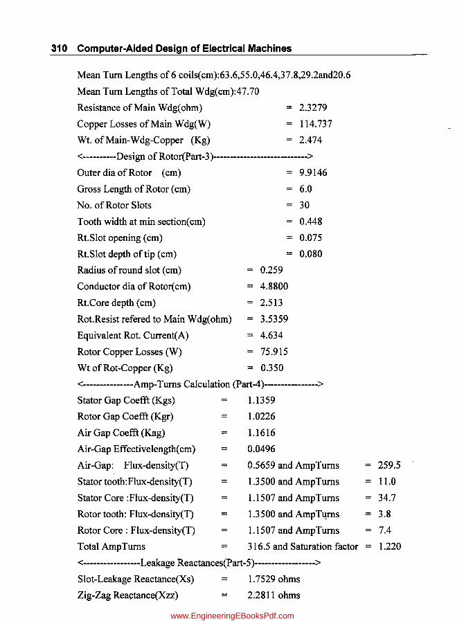
310 Computer-Aided Design of Electrical Machines
Mean Tum Lengths of 6 coils(cm):63.6,55.0,46.4,37.8,29.2and20.6
Mean Tum Lengths of Total Wdg(cm):47.70
Resistance of Main Wdg(ohm)
Copper Losses of Main W dg(W)
Wt. of Main-W dg-Copper (Kg)
= 2.3279
114.737
2.474
<----------Design of Rotor(Part -3 )----------------------------> Outer dia of Rotor (cm) 9.9146
Gross Length of Rotor (cm) 6.0
No. of Rotor Slots 30
Tooth width at min section(cm) = 0.448
Rt.Slot opening (cm) 0.075
Rt.Slot depth of tip (cm) 0.080
Radius of round slot (cm) = 0.259
Conductor dia of Rotor( cm) 4.8800
Rt.Core depth (cm) 2.513
Rot.Resist refered to Main Wdg(ohm) = 3.5359
Equivalent Rot. Current(A) 4.634
Rotor Copper Losses (W) 75.915
Wt of Rot-Copper (Kg) = 0.350
<---------------Amp-Turns Calculation (Part-4 )----------------> Stator Gap Coefft (Kgs) 1.1359
Rotor Gap Coefft (Kgr) 1.0226
Air Gap Coefft (Kag) = 1.1616
Air-Gap Effectivelength( cm) = 0.0496
Air-Gap: Flux-density(T) = 0.5659 and AmpTums
Stator tooth:Flux-density(T) = 1.3500 and AmpTurns
Stator Core :Flux-density(T) = 1.1507 and AmpTums
Rotor tooth: Flux-density(T) 1.3500 and AmpTl,Lms
Rotor Core: Flux-density(T) 1.1507 and AmpTums
Total AmpTums = 316.5 and Saturation factor
<-----------------Leakage Reactances(Part -5 )------------------> Slot-Leakage Reactance(Xs) = 1.7529 ohms
Zig-Zag Reactance(Xzz) = 2.2811 ohms
= 259.5
= 11.0
34.7
3.8
7.4
= 1.220
www.EngineeringEBooksPdf.com

Single-Phase Induction Motors 311
End-Leakage Reactance(Xe)
Be It-Leakage Reactance(Xb)
Skew-Leakage Reactance(Xsk)
T otal-LeakageReactance(XLm)
Magnetizing Reactance(Xm)
Open-Circuit Reactance(Xe)
Magnetizing Current (Imu)
2.7330 ohms
1.0237 ohms
1.1471 ohms
8.9378 ohms
209.632 ohms
214.101 ohms
1.0743 amps
<--------------Design of Auxiliary Winding(Part-6)------------>
Pitch-Factors of 6 coils: 1.000,0.971,0.885,0. 749,0.568andO.355
No of Turns in 6 coils: 62+ 60+ 55+ 46+ 35+ 22=280
Winding Factor
Transformation Ratio(K)
0.825( desirab1e:O. 78toO.84)
= 1.591 (desirable: 1.5t02)
Mean Turn Lengths of 6 coils(cm):67.9,59.3,50.7,42.1J3.5and24.9
Mean Turn Lengths of Total Wdg(cm) 50.76
Conductor: of dia= 0.508cm and CS area(tota1) = 0.203 sq.mm
Resistance of Aux Wdg(ohm) 29.4503
Rot.Res in terms of au x wdg(ohm) 8.9524
Tot.Res in terms of au x wdg(ohm) = 38.4027
Tot.Res in terms of Main wdg(ohm) = 5.8638
Tot.Leak.React in terms of au x wdg(ohm) = 22.6292
Locked Imped of main Wdg(ohm) 10.6897
Locked Imped of Aux Wdg(ohm) 44.5740
Starting Torque(N-m) 1.757
Locked Rot current in aux wdg(A) = 5.16
Locked Rot current in Main wdg(A) 21.52
Total Starting Current (A) 26.676
Conductor Dia (mm) 0.508
Current dens in Aux wdg(A/sq.mm) = 25 .458( desirab1e:<30)
Wt. of Aux-Wdg-Copper (Kg) 0.513
www.EngineeringEBooksPdf.com
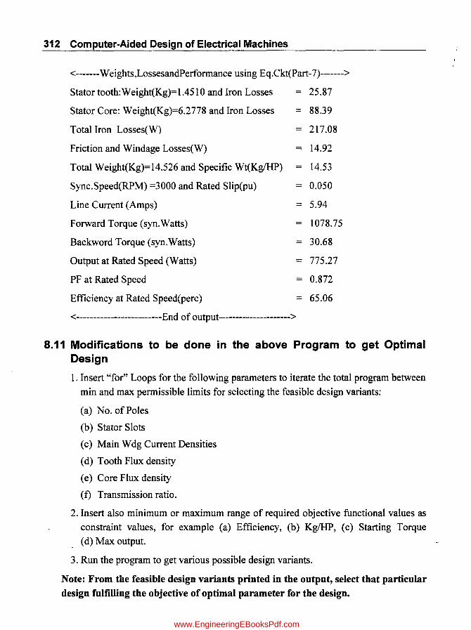
312 Computer-Aided Design of Electrical Machines
<-------Weights,LossesandPerfonnance using Eq .Ckt(Part-7)------->
Stator tooth: Weight(Kg)= 1.451 0 and Iron Losses
Stator Core: Weight(Kg)=6.2778 and Iron Losses
Total Iron Losses(W)
Friction and Windage Losses(W)
Total Weight(Kg)=14.526 and Specific Wt(KgIHP)
Sync.Speed(RPM) =3000 and Rated Slip(pu)
Line Current (Amps)
Forward Torque (syn.Watts)
Backword Torque (syn.Watts)
Output at Rated Speed (Watts)
PF at Rated Speed
Efficiency at Rated Speed(perc)
=
=
<-------------------------End of output --------------------->
25.87
88.39
217.08
14.92
14.53
0.050
5.94
1078.75
30.68
775.27
0.872
65.06
8.11 Modifications to be done in the above Program to get Optimal Design
1. Insert "for" Loops for the following parameters to iterate the total program between
min and mlLX pennissible limits for selecting the feasible design variants:
(a) No. of Poles
(b) Stator Slots
(c) Main W dg Current Densities
(d) Tooth Flux density
(e) Core Flux density
(f) Transmission ratio.
2. Insert also minimum or maximum range of required objective functional values as
constraint values, for example (a) Efficiency, (b) KgIHP, (c) Starting Torque
(d) Max output.
3. Run the program to get various possible design variants.
Note: From the feasible design variants printed in the output, select that particular design fulfilling the objective of optimal parameter for the design.
www.EngineeringEBooksPdf.com

Single-Phase Induction Motors 313
8.12 Computer Program in "C" in MATLAB for Optimal Design %Design of I-ph IM :
hp=liV=230iN=2850ihz=50i %Main Data
f2=fopen('Optimal 1hp_Output.m', 'W')i
fprintf(f2,' Design of 1-ph Ind.Motor of %3.1f HP,%4.0: Volts,%4.0f HZ:-\n',hp,V,hz)i
fprintf(f2,' Sn P DO L Di Sl Tm dmc cdm S2 Btl Bc1 K Ta dac cda Ist Tqst pfx Popt eff KgPhp\n')i
fprintf(f2, '
=======================================\n') i
%<--------Calculation of Main Dimensions (Part-1)------->
kt=1.42iLbyDO=0.3iki=0.93i %Assumptions
h10=0.07ih11=1.3*h10icdm1=4.5; %Assumptions
Sn=O i M1=0; M2=0; M3=0 i EFFmax=50; maxTqst=l. 5; minKgPhp=16; maxPopt=700; %Assumptions
for P=2:2:4i for Sl=24:12:48; for cdm1=3.5:0.1:4.5i
HZ=[25 30 40 45 50 60]iKF=[0.865 .885 .923 .94 .96 l]i kf=interp1(HZ,KF,hz, 'spline');
POLES=[2 4 6 8]; OPTC=[0.32 0.22 .19 .17] ; CO=interp1(POLES,OPTC,P, 'spline');
DIBYDO=[.5 .59.64 .67];DibyDO=interp1(POLES,DIBYDO,P, 'spline');
DOsqL=16.5*CO*hp/N*kf*kt*le6;D01=(DOsqL/LbyDO)A(l/3); DO=floor(D01);L=LbyDO*DO; Di1=DibyDO*DO;Di=ceil(Di1);SP=Sl/Pi
if P==2 bt1a=(1.1+0.032*Di)*Di/S1ibt1=floor(bt1a*100)/100;end;
if P==4 bt1a=(1.27+0.035*Di)*Di/S1ibt1=floor(bt1a*100)/100iend i
SS=[24 36 48]iB10=[0.068+0.0175*Di 0.038+0.0175*Di 0.0175*Di]i b10=interp1 (SS,B10,Sl, 'spline')i
for Bt=1.3:0.05:1.7ifor Bc=0.8:0.05:1.15; btbybc=Bt/Bci
dc1=btbybc*(Sl*bt1)/(pi*P);b11=pi*(Di+2*h10+2*h11)/Sl-btl;
h14=DibyDO*(DO-Di)-(h10+h11+dc1)i alfa=180/S1i b13=b11+2*h14*tan(alfa*pi/180);
Lg=0.013+0.0042*Di/sqrt(P)i
%<--------Design of Main Winding(Part-2)--------->
Ncpp=Sl/P/2; if ceil (Ncpp) > Ncpp continue, end; sum1=Oisum2=0;sum3=0;sum4~0; sum5=0;
for i=l :Ncpp; y1= (SP- (i-1) *2) / (SP+1) ; Kp (i),=sin (y1 *pi/2) ;
sum1= sum1+Kp(i); end;
for i=1:Ncpp;PTm(i)=Kp(i)/sum1*100;sum2=sum2+PTm(i);end;
, for i=1:Ncpp;sum3=sum3+Kp(i)*PTm(i);end;Kwm=sum3/sum2;
Li=ki*L;At=bt1*Li*SP; FI=0.637*At*Bt*le-4i
www.EngineeringEBooksPdf.com

314 Computer-Aided Design of Electrical Machines
Tm1=0.95*V/(4.44*hz*FI*Kwm); Tm=ceil(Tm1/2)*2;
Nm=Tm*2; Tppm=Tm/P;
for i=1:Ncpp;Tc1(i)=Tppm*PTm(i)/100;Tc(i)=round(Tc1(i));
sum4=sum4+Tc(i);end;corr=Tppm-sum4; Tc(Ncpp)=corr+Tc(Ncpp); sum4=sum4+ corr; HP=[.05 .1 .25 .5 .75 1];
EFF=[.35 .44 .58 .65 .68 .7]; PF=[.45.5 .56 .62 .64 .66];
effa=interp1(HP,EFF,hp, 'spline');
pfa=interp1(HP,PF,hp, 'spline');
Im=hp*746/(effa*V*pfa);Amc1=Im/cdm1;dmc1=sqrt(4*Amc1/pi);
DSWG= [ 5 . 38 4. 8 8 4. 47 4. 06 3. 66 3. 25 2. 95 2. 64 2. 31 2. 03 1. 83 1.63 1.42 1.22 1.02 .914 .813 .711 .61];
for i=1:19; if dmc1 >= DSWG(i) continue; end; dmc=DSWG(i); end;dmcins=dmc +0.075;Amc=pi*dmc A 2/4;cdm=Im/Amc; if cdm <2.8 I I cdm >4.5 continue; end; Socm=Tc(1)*pi*dmcins A2/4/100; Asg=(h11*(b10+b11)+h14*(b11+b13))/2;Sfsm=Socm/Asg;
if Sfsm >0.5 continue; end; Hs=h11+h14;
for i=l:Ncpp; Lmt(i)=8.4*(Di+Hs)/Sl*(SP-(i-1)*2)+2*L;
sum5=sum5+Lmt(i)*Tc(i);end;Lmtm=sum5/sum4; Rm=0.021*Lmtm*Tm/(Amc*100);Pcus=ImA2*Rm;
Wcum=Lmtm*Amc*Tm*8.ge-5;
%<--------Design of Rotor(Part-3)--------->
b20=0.075;h20=0.08;Dm=0.07; %assumption for S2=Sl+(ij+2)*P; Dr=Di-2*Lg;bt2=0.95*Sl*bt1/S2;
ij=1:2;
r21=(pi*(Dr-2*h20)-S2*bt2)/(2*(S2+pi));drc1=2* r21-0.038;
for i=1:19; if drc1*10 >= DSWG(i)continue;end;drc=DSWG(i); end;
Ab=pi*drcA2/4;~2=0.95*dc1;Lb=L+1;Nb=S2;Aer=Ab/pi*Nb/P;
R2md=P*Nm A 2*KwmA2*0.021*(Lb/(100*Ab*Nb)+2/pi*Dm/P A 2/Aer);
12d=Im*pfa;Pcur=I2dA 2*R2md;Wcur=Lb*Ab*Nb*8.ge-5; Wtr=((pi*DrA 2/4)-(S2*pi*r21 A 2))*L*7.8*le-3;
%<--------Amp-Turns Calculation (Part-4)--------->
SobyAg1=b10/Lg;SOBYAG=[0 1 2 3 4 5 678 9 10 11 12];
CC= [ 0 . 19 . 34 . 46 . 55 . 61 . 66 . 71 . 75 . 79 . 82 . 86 . 89] ;
%semi-closed-slot, K01=interp1(SOBYAG,CC,SobyAg1, 'spline');
sp1=pi*Di/S1;Kgs=sp1/(sp1-b10*K01);
SobyAg2=b20/Lg;K02=interp1(SOBYAG,CC,SobyAg2, 'spline');
sp2=pi*Dr/S2;Kgr=sp2/(sp2-b20*K02); Kag=Kgs*Kgr; Lgd=Kag*Lg; Aga=pi*Di/P*L;Bag=FI*le4/0.637/Aga; ATag=0.796*Bag*Kag*Lgd*le4;
www.EngineeringEBooksPdf.com

#
Single-Phase Induction Motors
BB=[ .1 .2 .3 .4 .5 r .0 .7 .8 .9 1 1.1 1.2 1.3
1.6 1.7 loS 1.9 2.0 ] i %Tesla
HH= [18 28 38 4S 67 SO 95 120 140 lS0 220 295 390 2200 5000 9000 16000 24000]i% for Lohys
At1=Li*bt1*Sl/PiBt1=FI*le4/0.637/At1i
if Btl <1.3 II Btl >1. 7 continueiendi
att1=interp1(BB,HH,Bt1, 'spline')iLfpt1=h14+h11+h10i
ATT1=att1*Lfpt1/100i Ac1=Li*dc1i Bc1=FI*le4/2/Ac1i
if Bel <O.S II Bc1 >1.2 continueiendi
BtbyBc=Bt1/Bc1iif BtbyBc >1.2 continueiendi
atc1=interp1(BB,HH,Bc1, 'spline')i
Lfpc1=pi*(DO-dc1)/2/P;ATC1=atc1*Lfpc1/100;
At2=Li*bt2*S2/PiBt2=FI*le4/0.637/At2i
att2=interp1(BB,HH,Bt2, 'spline')iLfpt2=2*r21+h20i
1.4
5S0
315
1.5
1000
ATT2=att2*Lfpt2/100i Ac2=Li*dc2i Bc2=FI*le4/2/Ac2i atc2=interp1(BB,HH,Bc2, 'spline');
Lfpc2=pi*(2*r21+h20+dc2)/2/Pi ATC2=atc2*Lfpc2/lOOi
ATT=ATag+ATT1+ATC1+ATT2+ATC2i satf=ATT/ATagi .. %<--------Leakage Reactance(Part-5)--------->
skew=15;Kp=0.97i %Assumption sum6=Oi for i=1:NcpPisum6=sum6+Tc(i)A2iendi Cx=sum6/TpprnA 2*Sl/(KwmA2*4*P);
BllbyB13= [ .5 .6 .7 .8 .9 1 1.1 1.2 1.3 1.4 1.5 1.6 1.7 1.S1i
CONSTANT=[0.63 .53.46.41.36.33 .3.27.25.23.21 .2.1S .17] i
b11byb13=b11/b13i constA=interp1(B11byB13,CONSTANT,b11byb13, 'spline')i
Ks1=constA*h14/b13+h10/b10+2*h11/(b10+b11)iKs2=h20/b20+0.623i Ks=Ks1*Cx+S1/S2*Ks2i Z=NrniKx=2*pi*hz*(Z*Kwm)A2*le-8; Xs=Kx*2.512*Ks*L/Sli Lrnd1=pi*Di/Sli Lrnd2=pi*Dr/S2;
bt10=sp1-b10ibt20=sp2-b20i Kzz=(bt10+bt20)A2/(4*(Lrnd1+Lrnd2))i Xzz=Kx*Kzz* 0.S3S*L/(Sl*Lg)i
sum7=Oifori=1:NcpPi surn7=sum7+Tc(i)*(SP-(i-1)*2)i endi ACT1=sum7/Tpprni ACT=floor(ACT1)i
De=Di+h14+2*(h10+h11)i Xe=Kx*1.236*De*ACT/Sl/Pi Km=Aga/(Lgd*satf*P)i
AvSP=[4 8 12 16 20 24]iBLC=[3.2 1.S 1.4 1.25 1.15 1.1]i
Nsp=(Sl+S2)/2/PiKb=interp1(AvSP,BLC,Nsp, 'spline'); Xb=0.000929*Krn*Kb*Kxi
Q=O.25* (skew/100) A2iXsk=O.2546*Krn*Kp*Q*KxiXLrn=Xs+Xzz+Xe +Xb+Xski
www.EngineeringEBooksPdf.com

316 Computer-Aided Design of Electrical Machines
Csk=sin(skew/2*pi/180)/(pi*skew/360);Xm=Kx*0.2546*Km*Csk; XO=Xm+XLm/2;Imu=V/XO;
%<--------Design of Auxiliary Wdg(Part-6)--------->
Kl=1.5;Kwal=0.83; %Assumption~
for Kl=1.5:0.1:2;
%for ij=1:3;mf=(0.10+ij*0.01);Aacl=mf*Amc;dacl=sqrt(4*Aacl/pi);
%DSWGl=[1.63 1.42 1.22 1.02.914.813 .711 .610.559.508.457 .417 .376 .345 .315J;
%for i=1:15; if dacl >= DSWG1(i) continue;end; dac=DSWGl(i); end;Aac pi*dac A2/4;Tal=Kl*Tm*Kwm/Kwal; Ta=ceil(Tal/2) *2; Na=Ta*2;Tppa=Ta/P; sumll=0;sum12=0;sum13=0;sum14=0;sum15=0;
fori=1:Ncpp;yl=(SP+l-(i-l)*2)/(SP+l); Kp(i)=sin(yl*pi/2);sumll=sumll+Kp(i); end;
sum12=0;for i=l:Ncpp;Tcal(i)=Tppa*Kp(i)/sumll;
Tca(i)= round(Tcal(i));sum12=sum12+Tca(i); end;
corr=Tppa-sum12;Tca(Ncpp)=corr+ Tca(Ncpp);sum12=
for l:Ncpp; sum13=sum13+Kp(i)*Tca(i); end; K=Ta*Kwa/Tm/Kwm; sum15=0; Lmtal(i)=8.4*(Di+Hs)/Sl*(SP+l-(i-l)*2)+2*L;
sum15=sum15+Lmtal(i)*Tca(i);end;Lm~a=sum15/Tppa;
sum12+corr;
Kwa=sum13/Tppa; for i=l: Ncpp;
for ij=1:3;mf=(O.10+ij*0.01);Aacl=mf*Amc;dacl=sqrt(4*Aacl/pi);
DSWG 1 = [ 1. 02 . 914 . 813 . 711 . 610 . 559 . 508 . 457 . 417 . 376 . 345 .315J;
for i=1:12; if dac1 >= DSWGl(i) continue; end;
dac=DSWGl(i);end;Aac=pi*dac A2/4; Rla=0.021*Lmta*Ta/(Aac*100);
Rdr=KA2*R2md; Rat=Rla+Rdr; Rmt=Rm+R2md;XLa=KA2*XLm; ZLm=sqrt(Rmt A 2+XLmA 2);ZLa=sqrt(Rat A2+XLa A 2); Tqst=P*K*R2md*VA2/(2*pi*hz)*(Rat*XLm-Rmt*XLa)/ ZLmA2/ZLa A 2;
if Tqst < 1.64 continue;end;Isa=V/ZLa;Ism=V/ZLm;Ist=Isa+Ism;
cda=Isa/Aac; if cda >30 continue; end; Wcua=Lmta*Aac*Ta*8.ge-5;
%<----Weights,LossesandPerformance using Eq.Ckt(Part-7)-------->
FD=[0.8 1.2 1.6 2 2.4J; WPKG=[7 15 23 34 50J; % for 0.5 mm
WpKgt=interpl(FD,WPKG,Btl, 'spline');WtT=Atl*P*Lfptl*7.8*le-3; Pist=WpKgt* WtT; WpKgc=interpl(FD,WPKG,Bcl, 'spline'); ,
Dmc=DO-dcl;WtC=pi*Dmc*Acl*7.8*le-3; Pi=1.9*(Pist+Pisc); Pfw=0.02*hp*746;
TotWt=1.01*(Wcum+Wcua+WtT+WtC+Wcur+Wtr);
KgPhp=TotWt/hp;if KgPhp >14.7 continueiend;
Pisc=WpKgc*WtCi
www.EngineeringEBooksPdf.com
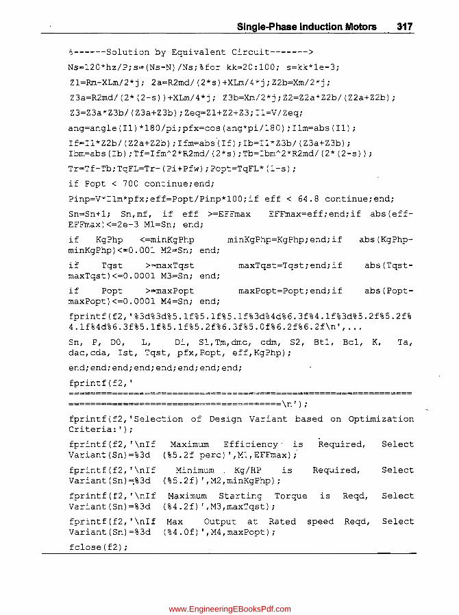
Single.Phase Induction Motors 317
%------Solution by Equivalent Circuit------->
Ns=120*hz/P;s=(Ns-N)/Ns;%for kk=20:100; s=kk*le-3;
Zl=Rm+XLm/2*j; 2a=R2md/(2*s)+XLm/4*j;Z2b=Xm/2*j;
Z3a=R2md/(2*(2-s))+XLm/4*j; Z3b=Xm/2*j;Z2=Z2a*Z2b/(Z2a+Z2b);
Z3=Z3a*Z3b/(Z3a+Z3b);Zeq=Zl+Z2+Z3;Il=V/Zeq;
ang=angle(Il)*180/pi;pfx=cos(ang*pi/lSO);Ilm=abs(Il);
I£=Il *Z2b/ (Z2a+Z2b) ; Ifm=abs'( If) ; Ib=Il * Z3b/ (Z3a+Z3b) ; Ibm=abs(Ib);Tf=IfmA 2*R2md/(2*s);Tb=IbmA 2*R2md/(2*(2-s));
Tr=Tf-Tb;TqFL=Tr-(Pi+Pfw);Popt=TqFL*(l-s);
if Popt < 700 continue;end;
Pinp=V*Ilm*pfx;eff=Popt/Pinp*lOO;if eff < 64.S continue;end;
Sn=Sn+ 1; Sn, mf, if eff >=EFFmax EFFmax=eff; end; if abs (effEFFmax)<=2e-3 Ml=Sn; end;
if KgPhp <=minKgPhp minKgPhp=KgPhp;end;if abs(KgPhp-minKgPhp)<=O.OOl M2=Sn; end;
if Tqst >=maxTqst maxTqst=Tqst;end;if abs(Tqst-maxTqst)<=O.OOOl M3~Sn; end;
if Popt >=maxPopt maxPopt=Popt;end;if abs(Popt-maxPopt)<=O.OOOl M4=Sn; end;
fprintf(f2, '%3d%3d%5.1f%5.1f%5.1f%3d%4d%6.3f%4.1f%3d%5.2f%5.2f% 4.1f%4d%6.3f%5.1f%5.1f%5.2f%6.3f%5.0f%6.2f%6.2f\n', ...
Sn, P, DO, L, Di, Sl,Tm,dmc, cdm, S2, Btl, Bel, K, Ta, dac,cda, Ist, Tqst, pfX,PDpt, eff,KgPhp);
end;end; end; end; end; end; end; end;
fprintf (f2, '
=======================================\n');
fprintf (f2, 'Selection of Design Variant based on Optimization Criteria:');
fprintf(f2, '\nIf Variant (Sn)=%3d
fprintf(f2, '\nIf Variant (Sn)=:%3d
fprintf(f2, '\nIf Variant (Sn)=%3d
fprintf(f2, '\nIf Variant (Sn)=%3d
fclose (f2) ;
Maximum Efficiency' is (%5.2f perc)' ,Ml,EFFmax);'
Required,
Minimum Kg/HP is Required, (%5.2f) ',M2,minKgPhp);
Maximum Starting Torque is (%4. 2f) , ,M3,maxTqst) ;
Max Output at Rated speed ( % 4 . 0 f) , ,M4, maxPopt) ;
Reqd,
Reqd,
Select
Select
Select
Select
www.EngineeringEBooksPdf.com
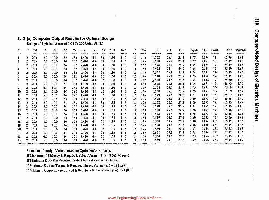
Col ~
00
0 0
8.12 (a) Computer Output Results for Optimal Design 3 ~
Design of I-ph Ind.Motor of 1.0 liP, 230 Volts, 50 liZ c .. CD,
Sn P DO L Di Sl Tm dIne edIn S2 Btl Bel K Ta dae eda Ist Tqst pfx Popt eff KgPhp ~
~ I 2 20.0 6.0 10.0 24 382 1.420 4.4 30 1.30 1.10 1.5 546 0.508 26.4 25.4 1.77 0.874 721 65.09 14.62 D.
CD 2 2 20.0 6.0 10.0 24 382 1.420 4.4 30 1.30 1.10 1.5 546 0.508 26.4 25.4 1.77 0.874 721 65.09 14.62 D.
3 2 20.0 6.0 lO.O 24 382 1.420 4.4 30 1.30 1.10 1.6 582 0.508 24.1 24.9 1.65 0.874 721 65.09 14.66 C 4 2 20.0 6.0 10.0 24 382 1.420 4.4 30 1.30 1.10 1.6 582 0.508 24.1 24.9 1.65 0.874 721 65.09 14.66 m 5 2 20.0 6.0 10.0 24 382 1.420 4.4 32 1.30 1.10 1.5 546 0.508 26.8 25.9 1.76 0.878 774 65.90 14.66 ce' 6 2 20.0 6.0 10.0 24 382 1.420 4.4 32 1.30 1.10 1.5 546 0.508 26.8 25.9 1.76 0.878 714 65.90 14.66 :s 7 2 20.0 6.0 10.0 24 382 1.420 4.4 32 1.30 1.10 1.6 582 ~508 24.5 25.5 1.64 0.878 774 65.90 14.70 0 .... 8 2 20.0 6.0 10.0 24 382 1.420 4.4 32 1.30 1.10 1.6 582 0.508 24.5 25.5 1.64 0.878 774 65.90 14.70 m 9 2 20.0 6.0 lO.O 24 382 1.420 4.4 32 1.30 1.15 1.5 546 0.508 26.7 25.9 1.76 0.875 764 65.19 14.52 CD 10 2 20.0 6.0 lO.O 24 382 1.420 4.4 32 1.30 1.15 1.5 546 0.508 26.7 25.9 1.76 0.875 764 65.19 14.52 n .. II 2 20.0 6.0 lO.O 24 382 1.420 4.4 32 1.30 1.15 1.5 546 0.559 24.5 26.5 1.71 0.875 764 65.19 14.63 ::::!. 12 2 20.0 6.0 10.0 24 368 1.420 4.4 30 1.35 1.15 1.5 526 0.508 28.0 27.2 1.89 0.872 715 65.06 14.49 n
I3 2 20.0 6.0 10.0 24 368 1.420 4.4 30 1.35 1.15 1.5 526 0.508 28.0 27.2 1.89 0.872 775 65.06 14.49 !!.
14 2 20.0 6.0 10.0 24 368 1.420 4.4 30 1.35 1.15 1.5 526 0.559 25.7 27.8 1.84 0.872 715 65.06 14.60 s: I»
15 2 20.0 6.0 lO.O 24 368 1.420 4.4 30 1.35 1.15 1.6 560 0.508 25.5 26.7 1.76 0.872 775. 65.06 14.53 n 16 2 20.0 6.0 10.0 24 368 1.420 4.4 30 1.35 1.15 1.6 560 0.508 25.5 26.7 1.76 0.872 715 65.06 14.53 :::T
:;' 17 2 20.0 6.0 10.0 24 368 1.420 4.4 30 1.35 1.15 1.6 560 0.559 23.3 27.2 1.69 0.872 715 65.06 14.63 1: 18 2 20.0 6.0 10.0 24 368 1.420 4.4 32 1.35 1.15 1.5 526 0.508 28.4 27.8 1.88 0.876 832 65.85 14.53 19 2 20.0 6.0 10.0 24' 368 1.420 4.4 32 1.35 1.15 1.5 526 0.S08 28.4 27.8 1.88 0.876 832 65.85 14.53 20 2 20.0 6.0 10.0 24 368 1.420 4.4 32 1.35 1.15 1.5 526 0.559 26.1 28.4 1.83 0.876 832 65.85 14.63 21 2 20.0 6.0 lO.O 24 368 1.420 4.4 32 1.35 1.15 1.6 560 0.508 25.9 27.3 1.75 0.876 832 65.85 14.56 22 2 20.0 6.0 10.0 24 368 1.420 4.4 32 1.35 1.15 1.6 560 0.508 25.9 27.3 1.75 0.876 832 65.85 14.56 23 2 20.0 6.0 10.0 24 368 1.420 4.4 32 1.35 1.15 1.6 560 0.559 23.7 27.8 1.69 0.876 832 65.85 14.67 ======================================~====~======~===============================================================~=========
Selection of Design Variant based on Optimization Criteria: If Maximum Efficiency is Required, Select Variant (Sn) = 8 (65.90 perc) If Minimum Kg/HP is Required, Select Variant (Sn) = 13 (14.49) If Minimum Starting Torque is Required, Select Variant (Sn) = \3 (1.89) If Minimum Output at Rated speed is Required. Select Variant (Sn) = 23 (832).
www.EngineeringEBooksPdf.com

Bibliography
P.erfonnance & Design of Alternating Current Machines by M.G. Say
Electrical Engineering Design Manual by M.G. Say
Alternating Current Machines by A.F. Puchstein, T.C. Lloyd & A.G. Conrod
Electrical Machinery by A.E. Fitzgerald, Charles Kingsley, Jr & Stephen D. Umans
Electrical Technology by B.L. Theraja & A.K. Theraja
Design of Electrical Machines by V.N. Mittie & A. Mittal
Getting Started with MA TLAB by Rudrapratap
Author's Design Experience of 29 years in BHEL
Relevant Indian Standards
www.EngineeringEBooksPdf.com

I I
www.EngineeringEBooksPdf.com
A
Typewritten Text
"This page is Intentionally Left Blank"

A
Air gap 22,148, 182, 257~ 310
Armature reaction' 65, 183, 213
Armature topth 22, 23
Armature windings 33,34,37,44
AT per pole 60
Aux winding 295
Av loss factor 145, 186
Axiallength 124,234
B Back-ward torque 299
Bar current 230
Bearing loss 192, 215
Brush contact loss 72
Brush friction 71
Brush loss 160
Brushes 39,44, 71
c Carter coefficient 150, 153
Coil throw 291
Cold rolled steels 96, 106
Commutator 4,5,44,71,72,
Commutator segment 4, 36, 59
Compensating winding 73
Cond/slot 143,269
Conducting materials 15,16
Conductor 17,34,38,60,227,270
Conductor width 60, 85
Constraints 4,93,277
Cooling 24,25,30
Cooling area 104,110,133,238
Cooling surface 24,63, 70, 127
Cooling tubes 5,94, 134
Index
Copperloss 16,74,101,124,186,231,310
Core 2,26,60,67,93,99,144, 153, 185,
195,312
Core type transformer 99, 101
Current density 16,71,100,134,182,270
Current volume 4,57,60
D DC copperloss 145,186,188
Depth of winding 70
Design of poles 65,68,
Design of rotor 147,190,284
Dissipation coefficient 162, 163
www.EngineeringEBooksPdf.com

322 Computer-Aided Design of Electrical Machines
Double layer winding 38,41,47,48
Dummy coils 44
E Eddy current loss 4, 62, 186
EffIciency 1,112,159,224,281
Electric circuit 20
Electrical materials 13, 15
EMF 21
End leakage reactance 291,306,311
End ring 230,248,260
Equivalent circuit 278
Equivalent rotor current 258,285
Exciter voltage 159
F Fieldcoil 57,65,141,163
Field regulator 69
Flux in core 62,146,186,228
Flux density 2,22,62,73, 1.10,153,186, 234,288
FluxIPole· 22,59,142,2-12
Forward rotor 298
Free length 62
Frequency constant 4,278
G Gap coefficient 22, 68, 151
Gross Iron length 184, 225
H Heat dissipation 24, 25
Heating 24, 25
Height of core 57, 62,223
HVWinding 93,100,124
Hysteresis los.s 2, 18, 19
Hysteresis loop 18
I Insulating materials 13, 16, 17
Insulation 17,123,227,298
Inter pole 72, 73, 84
Inter pole winding 73
Inter tum insulation 98
Iron factor 58,119,142,183,280
Iron length 172,225, 268, 280
Iron loss 63,95,120,142,161,229
Iron path 66
K }(gn(\TJ\ 1,5,142,215
}(gn(W 57,85,224,250,257
L LIDO ratio 278
Laminations 18, 62, 189
Lapwinding 35,37-39
Leakage flux 146, 188
Leakagereactance 4,146,187,289,311
Length of bar 230,248,284
Length of pole 65,148
Lip 73,227,258
Locked impedance 295
Locked rotor current 295
Loss factor 4,145,186
Losses 5,16,94,145,159,215,297
Lowest cost 5
L\T winding 98,99,123
M Magnetic circuit 20, 150, 192, 195
Magnetic frame 94, 118
Magnetic path 22,152,153
Magnetization curves 67,69,304
Magnetizing current 97,223,232,257,311 www.EngineeringEBooksPdf.com

Main core 119,133
Main dimensions 4,58.142,182,224,278
Main pole 66
Main winding 280,309
Maximum efficiency 90, 91, 117, 180,
276,317
Mean length of tum 69, 111, 124, 134, 186, 228,283
Mechanical loss 182, 192
Minimum section 284
N Net iron length 23,184,247,268
. Net motor torque 299
NO'load loss 249,259,269
No-load current 96, 121, 133,259
o Objective function 2,5,85, 135
Oil duct 99, 101
Open circuit characteristic 142, 154, 182, 197
Optimal design 5,32,84,85,113,135,
174,215,216,250,312
Output coefft 58, 247, 268
Overhang 28,146,267,270
p
P.O. impedance 103, 126
P.O. resistance 103, 126
Performance 73,75,102,126,238,297
Periphoral velocity 57,225
Permeance 145,237,270
Pitch 36,38,41,184,257,291
Pitch factor 45,280,307,309
Index 323
Pole arc 4, 58
Pole pitch 4,34,46,85, 174,268
R Radial width 98, 111, 125, 134
Reactances 5,311
Regulation 4,94, 118, 159,173,201,214
Resistance 16,20,70,103,112,145,160,
283,311
Rotor 2,48, 147, 182, 190,230,257,284
Rotor slots 4, 248, 310
Round slot 310
s Saturation factor 4, 288
Series field winding 69, 70
Shell type transformer 123
Short circuit current 236
Shunt field current 60
Shunt field winding 4, 69
Silicon steel 2,18,118,189
Single layer winding 45
Skew factor 292
Skew leakage reactance 292, 306, 311
Slack 101,134
Slip 2,224,25~270
Slip at full load 238
Slip rings 160,257
Slip-ring rotor 257
Slot 4,33,34,38,41,191,249,286,310
Slot balance 57,182,191,257
Slot loading 141,143
Slot opening 233,284,310
www.EngineeringEBooksPdf.com

324 Computer-Aided Design of Electrical Machines
Slot pitch 23,60, 144, 185,226,286
Siotwidth 144,185,213,248,309
Slots spanned 283.293, 294
Specific electrical loading 15
Specific magnetic loading 4, 14, 15, 142, 182, 183
Specific perrneance 145, 187,236
Spindle 72, 84
Split-phase type 277,278
. Squirrel cage 2, 223, 230
Standard ratings 25
Standards 1
Starting torque 4,224,257,295,307,311
Strand 98, 100
Stray losses 102,124,125,145,186
T Tankdesign 104,112,127,134
Temperature rise 1, 13,29, 104, 127
Total weight 75,128,163,201,311
Transmission ratio 293,294
Tube dia 104,127
Turns/ph 172, 226, 247, 268
v Ventilating ducts 26,27,58, 142,183
Ventilation loss 192,215
Ventilation schemes 26
Voltage regulation 159,173,182,201,214
Volts/turn 94, 118, 133
w Wattful current 97, 121,249,269
Wave winding 35,41,42,44
Wedge 61,212,213,227,258
Width of bar 230
Widthofpole 65,148
Winding factor 142,224,257,293,311
Windowarea 94,110,119,133
Window space factor 4,94,110,119, 129,133
y )'oke 57,67,84,95,112,133
z Zig zag reactance 237,310
'"
www.EngineeringEBooksPdf.com