Computer-Aided Design 43 (2011) 303–315

Contents lists available at ScienceDirect

Computer-Aided Design

journal homepage: www.elsevier.com/locate/cad

Teaching–learning-based optimization: A novel method for constrainedmechanical design optimization problemsR.V. Rao ∗, V.J. Savsani, D.P. VakhariaDepartment of Mechanical Engineering, S.V. National Institute of Technology, Surat-395 007, India

a r t i c l e i n f o

Article history:Received 24 November 2010Accepted 29 December 2010

Keywords:Teaching–learning-based optimizationConstrained benchmark functionsMechanical design optimization

a b s t r a c t

A new efficient optimization method, called ‘Teaching–Learning-Based Optimization (TLBO)’, is proposedin this paper for the optimization of mechanical design problems. This method works on the effect ofinfluence of a teacher on learners. Like other nature-inspired algorithms, TLBO is also a population-basedmethod and uses a population of solutions to proceed to the global solution. The population is consideredas a group of learners or a class of learners. The process of TLBO is divided into two parts: the first partconsists of the ‘Teacher Phase’ and the second part consists of the ‘Learner Phase’. ‘Teacher Phase’ meanslearning from the teacher and ‘Learner Phase’ means learning by the interaction between learners. Thebasic philosophy of the TLBO method is explained in detail. To check the effectiveness of the method it istested on five different constrained benchmark test functions with different characteristics, four differentbenchmark mechanical design problems and six mechanical design optimization problems which havereal world applications. The effectiveness of the TLBO method is compared with the other population-based optimization algorithms based on the best solution, average solution, convergence rate andcomputational effort. Results show that TLBO is more effective and efficient than the other optimizationmethods for the mechanical design optimization problems considered. This novel optimization methodcan be easily extended to other engineering design optimization problems.

© 2011 Elsevier Ltd. All rights reserved.

1. Introduction

Engineering design can be characterized as a goal-oriented,constrained, decision making process to create products thatsatisfy well-defined human needs. Design optimization consistsof certain goals (objective functions), a search space (feasiblesolutions) and a search process (optimization methods). Thefeasible solutions are the set of all designs characterized by allpossible values of the design parameters (design variables). Theoptimization method searches for the optimal design from allavailable feasible designs.

Mechanical design includes an optimization process in whichdesigners always consider certain objectives such as strength, de-flection, weight, wear, corrosion, etc. depending on the require-ments. However, design optimization for a complete mechanicalassembly leads to a complicated objective function with a largenumber of design variables. So it is good practice to apply opti-mization techniques for individual components or intermediateassemblies rather than a complete assembly. For example, in anautomobile power transmission system, the optimization of thegearbox is computationally and mathematically simpler than the

∗ Corresponding author. Tel.: +91 2612201661; fax: +91 2612201571.E-mail address: ravipudirao@gmail.com (R.V. Rao).

0010-4485/$ – see front matter© 2011 Elsevier Ltd. All rights reserved.doi:10.1016/j.cad.2010.12.015

optimization of the complete transmission system. Analytical ornumerical methods for calculating the extremes of a function havelong been applied to engineering computations. Although thesemethods perform well in many practical cases, they may fail inmore complex design situations. In real design problems the num-ber of design variables can be very large, and their influence on theobjective function to be optimized can be very complicated, witha nonlinear character. The objective function may have many localoptima, whereas the designer is interested in the global optimum.Such problems cannot be handled by classical methods (e.g. gra-dient methods) that only compute local optima. So there remainsa need for efficient and effective optimization methods for me-chanical design problems. Continuous research is being conductedin this field and nature-inspired heuristic optimization methodsare proving to be better than deterministic methods and thus arewidely used.

There are many nature-inspired optimization algorithms, suchas the Genetic Algorithm (GA), Particle Swarm Optimization(PSO), Artificial Bee Colony (ABC), Ant Colony Optimization (ACO),Harmony Search (HS), the Grenade Explosion Method (GEM), etc.,working on the principles of different natural phenomena. GA usesthe theory of Darwin based on the survival of the fittest [1,2],PSO implements the foraging behavior of a bird for searching food[3,4], ABC uses the foraging behavior of a honey bee [5–7], ACOworks on the behavior of an ant in searching for a destination from

304 R.V. Rao et al. / Computer-Aided Design 43 (2011) 303–315

Fig. 1. Distribution of marks obtained by learners taught by two different teachers.

the source [8,9], HS works on the principle of music improvisationin music players [10] and GEM works on the principle of theexplosion of a grenade [11]. These algorithms have been appliedto many engineering optimization problems and proved effectivein solving some specific kinds of problem.

The most commonly used evolutionary optimization techniqueis the genetic algorithm (GA). However, GA provides a near optimalsolution for a complex problem having large number of variablesand constraints. This is mainly due to the difficulty in determin-ing the optimum controlling parameters such as population size,crossover rate and mutation rate. A change in the algorithm pa-rameters changes the effectiveness of the algorithm. The same isthe case with PSO, which uses inertia weight, social and cognitiveparameters. Similarly, ABC requires optimum controlling parame-ters of number of bees (employed, scout, and onlookers), limit, etc.HS requires the harmonymemory consideration rate, pitch adjust-ing rate, and the number of improvisations. Therefore, the effortsmust be continued to develop a newoptimization techniquewhichis free from the algorithmparameters, i.e. no algorithmparametersare required for the working of the algorithm. This aspect is con-sidered in the present work.

The main motivation to develop a nature-based algorithm is itscapacity to solve different optimization problems effectively andefficiently. It is assumed that the behavior of nature is always opti-mum in its performance. In this paper a new optimizationmethod,Teaching–Learning-Based Optimization (TLBO), is proposed to ob-tain global solutions for continuous non-linear functions with lesscomputational effort and high consistency. The TLBO method isbased on the effect of the influence of a teacher on the output oflearners in a class. Here, output is considered in terms of results orgrades. The teacher is generally considered as a highly learned per-sonwho shares his or her knowledgewith the learners. The qualityof a teacher affects the outcome of the learners. It is obvious that agood teacher trains learners such that they can have better resultsin terms of their marks or grades.

2. Teaching–learning-based optimization

Assume two different teachers, T1 and T2, teaching a subjectwith the same content to the same merit level learners in twodifferent classes. Fig. 1 shows the distribution of marks obtainedby the learners of two different classes evaluated by the teachers.Curves 1 and 2 represent themarks obtained by the learners taughtby teacher T1 and T2 respectively. A normal distribution is assumedfor the obtainedmarks, but in actual practice it can have skewness.The normal distribution is defined as

f (X) =1

σ√2π

e−(x−µ)2

2σ2 (1)

where σ 2 is the variance,µ is themean and x is any value forwhichthe normal distribution function is required.

Fig. 2. Model for the distribution of marks obtained for a group of learners.

It is seen from Fig. 1 that curve-2 represents better results thancurve-1 and so it can be said that teacher T2 is better than teacherT1 in terms of teaching. The main difference between both theresults is their mean (M2 for Curve-2 and M1 for Curve-1), i.e. agood teacher produces a bettermean for the results of the learners.Learners also learn from interaction between themselves, whichalso helps in their results.

Based on the above teaching process, a mathematical model isprepared and implemented for the optimization of a unconstrainednon-linear continuous function, thereby developing a novel opti-mization technique called Teaching–Learning-Based Optimization(TLBO). Consider Fig. 2, which shows a model for the marks ob-tained for learners in a class with curve-A having mean MA. Theteacher is considered as the most knowledgeable person in the so-ciety, so the best learner is mimicked as a teacher, which is shownby TA in Fig. 2. The teacher tries to disseminate knowledge amonglearners, which will in turn increase the knowledge level of thewhole class and help learners to get good marks or grades. So ateacher increases the mean of the class according to his or her ca-pability. In Fig. 2, teacher TA will try tomovemeanMA towards theirown level according to his or her capability, thereby increasing thelearners’ level to a newmeanMB. Teacher TA will put maximum ef-fort into teaching his or her students, but students will gain knowl-edge according to the quality of teaching delivered by a teacher andthe quality of students present in the class. The quality of the stu-dents is judged from the mean value of the population. Teacher TAputs effort in so as to increase the quality of the students from MAto MB, at which stage the students require a new teacher, of supe-rior quality than themselves, i.e. in this case the new teacher is TB.Hence, there will be a new curve-B with new teacher TB.

Like other nature-inspired algorithms, TLBO is also a population-basedmethod that uses a population of solutions to proceed to theglobal solution. For TLBO, the population is considered as a groupof learners or a class of learners. In optimization algorithms, thepopulation consists of different design variables. In TLBO, differ-ent design variables will be analogous to different subjects offeredto learners and the learners’ result is analogous to the ‘fitness’, asin other population-based optimization techniques. The teacher isconsidered as the best solution obtained so far.

The process of TLBO is divided into two parts. The first partconsists of the ‘Teacher Phase’ and the second part consists ofthe ‘Learner Phase’. The ‘Teacher Phase’ means learning fromthe teacher and the ‘Learner Phase’ means learning through theinteraction between learners (Fig. 3).

2.1. Teacher phase

As shown in Fig. 2, the mean of a class increases fromMA to MBdepending upon a good teacher. A good teacher is one who brings

R.V. Rao et al. / Computer-Aided Design 43 (2011) 303–315 305

Fig. 3. Flow chart for Teaching–Learning-Based Optimization (TLBO).

his or her learners up to his or her level in terms of knowledge.But in practice this is not possible and a teacher can only movethe mean of a class up to some extent depending on the capabilityof the class. This follows a random process depending on manyfactors.

LetMi be themean and Ti be the teacher at any iteration i. Ti willtry to move mean Mi towards its own level, so now the new meanwill be Ti designated asMnew. The solution is updated according tothe difference between the existing and the new mean given by

Difference_Meani = ri (Mnew − TFMi) (2)

where TF is a teaching factor that decides the value of mean to bechanged, and ri is a randomnumber in the range [0, 1]. The value ofTF can be either 1 or 2, which is again a heuristic step and decidedrandomly with equal probability as TF = round[1 + rand(0, 1){2 − 1}].

This difference modifies the existing solution according to thefollowing expression

Xnew,i = Xold,i + Difference_Meani. (3)

2.2. Learner phase

Learners increase their knowledge by two different means: onethrough input from the teacher and the other through interactionbetween themselves. A learner interacts randomly with otherlearners with the help of group discussions, presentations, formalcommunications, etc. A learner learns something new if the otherlearner hasmore knowledge than him or her. Learnermodificationis expressed as

For i = 1 : PnRandomly select two learners Xi and Xj, where i = jIf f (Xi) < f (Xj)

Xnew,i = Xold,i + ri(Xi − Xj)

ElseXnew,i = Xold,i + ri(Xj − Xi)

End IfEnd ForAccept Xnew if it gives a better function value.

306 R.V. Rao et al. / Computer-Aided Design 43 (2011) 303–315

3. Implementation of TLBO for optimization

The step-wise procedure for the implementation of TLBO isgiven in this section.Step 1: Define the optimization problem and initialize theoptimization parameters.

Initialize the population size (Pn), number of generations (Gn),number of design variables (Dn), and limits of design variables(UL, LL).

Define the optimization problem as: Minimize f (X).Subject to Xi ∈ xi = 1, 2, . . . ,Dnwhere f (X) is the objective function, X is a vector for design

variables such that LL,i ≤ x,i ≤ UL,I .Step 2: Initialize the population.

Generate a random population according to the population sizeand number of design variables. For TLBO, the population sizeindicates the number of learners and the design variables indicatethe subjects (i.e. courses) offered. This population is expressed as

population =

x1,1 x1,2 · · · x1,Dx2,1 x2,2 · · · x2,D...

......

xPn,1 xPn,2 · · · xPn,D

.

Step 3: Teacher phase.Calculate the mean of the population column-wise, which will

give the mean for the particular subject asM,D = [m1,m2, . . . ,mD] . (4)

The best solution will act as a teacher for that iterationXteacher = Xf (X)=min. (5)

The teacher will try to shift themean fromM,D towards X,teacher,which will act as a new mean for the iteration. So,M_new,D = Xteacher,D. (6)The difference between two means is expressed asDifference,D = r (M_new,D −TFM,D ) . (7)

The value of TF is selected as 1 or 2. The obtained difference isadded to the current solution to update its values usingXnew,D = Xold,D + Difference,D . (8)Accept Xnew if it gives better function value.Step 4: Learner phase.

As explained above, learners increase their knowledge with thehelp of their mutual interaction. The mathematical expression isexplained in Section 2.2.Step 5: Termination criterion.

Stop if themaximumgeneration number is achieved; otherwiserepeat from Step 3.

It is seen from the above steps that no provision is made tohandle the constraints in the problem. Many types of constrainthandling technique are available in the literature, such asincorporation of static penalties, dynamic penalties, adaptivepenalties etc. Deb’s heuristic constrained handling method [12]is used in the proposed TLBO method. This method uses atournament selection operator in which two solutions are selectedand compared with each other. The following three heuristic rulesare implemented on them for the selection:• If one solution is feasible and the other infeasible, then the

feasible solution is preferred.• If both the solutions are feasible, then the solution having the

better objective function value is preferred.• If both the solutions are infeasible, then the solution having the

least constraint violation is preferred.These rules are implemented at the end of Steps 2 and 3, i.e. at theendof the teacher phase and the learner phase. Instead of acceptingsolution Xnew, if it gives better function value at the end of Steps 2and 3, Deb’s constraint handling rules [12] are used to select Xnewbased on the three heuristic rules.

4. Comparison of TLBO with other optimization techniques

Like GA, PSO, ABC, and HS, TLBO is also a population-basedtechnique which implements a group of solutions to proceedto the optimum solution. Many optimization methods requirealgorithmparameters that affect the performance of the algorithm.GA requires the crossover probability, mutation rate, and selectionmethod; PSO requires learning factors, the variation of weight,and the maximum value of velocity; ABC requires the limitvalue; and HS requires the harmony memory consideration rate,pitch adjusting rate, and number of improvisations. Unlike otheroptimization techniques TLBO does not require any algorithmparameters to be tuned, thus making the implementation of TLBOsimpler. As in PSO, TLBO uses the best solution of the iteration tochange the existing solution in the population, thereby increasingthe convergence rate. TLBO does not divide the population likeABC. As in GA, which uses selection, crossover and mutation, andABC,which uses employed, onlooker and scout bees, TLBOuses twodifferent phases, the ‘teacher phase’ and the ‘learner phase’. TLBOuses themean value of the population to update the solution. TLBOimplements greediness to accept a good solution, as in ABC.

5. Experimental studies

Different experiments have been conducted to check theeffectiveness of TLBO against other optimization techniques.Different examples are investigated based on benchmark testfunctions, mechanical design benchmark functions and othermechanical design problems from the literature.

5.1. Constrained benchmark test functions

Five different constrained benchmark functions with differentcharacteristics of objective functions and constraints (linear, non-linear, and quadratic) were experimented upon. These benchmarkfunctions are given in Appendix A. The special features of thesebenchmark functions are discussed in detail in the following sub-sections.

5.1.1. Benchmark function 1This is a quadratic minimization problem with 13 design vari-

ables and 9 linear inequality constraints. The ratio of the fea-sible search space to the entire search space is approximately0.0003% [13] and there are 6 active constraints at the opti-mum point. The optimum solution for this problem is at x∗

=

(1, 1, 1, 1, 1, 1, 1, 1, 1, 3, 3, 3, 1) with objective function valuef (x∗) = −15. This problem was solved by the different optimiza-tion methods: Multimembered Evolutionary Strategy (M-ES) [14],Particle Evolutionary Swarm Optimization (PESO) [15], CulturalDifferential Evolution (CDE) [16], Co-evolutionary Differential Evo-lution (CoDE) [17] and Artificial Bee Colony (ABC) [18]. The resultsare shown in Table 1. The parameters for TLBO are set as: popu-lation size = 50, maximum number of generations = 500. It canbe observed from Table 1 that TLBO finds the global optimum so-lution with better mean and worst solutions than PESO and CDE.Moreover TLBO requires approximately 89%, 92%, 75%, 90% and89%fewer function evaluations than M-ES, PESO, CDE, CoDE and ABCrespectively.

5.1.2. Benchmark function 2This is a nonlinear maximization problem with 10 design vari-

ables and one nonlinear equality constraint. The ratio of the fea-sible search space to the entire search space is approximately0.0000% [13] and there is 1 active constraint at the optimum point.

R.V. Rao et al. / Computer-Aided Design 43 (2011) 303–315 307

Table 1Comparison of results obtained by different optimization methods for benchmarkfunction 1.

Methods Best Mean Worst Function evaluations

M-ES −15 −15 −15 240000PESO −15 −14.710 −13 350000CDE −15 −14.999996 −14.999993 100100CoDE −15 −15 −15 248000ABC −15 −15 −15 240000TLBO −15 −15 −15 25000

Table 2Comparison of results obtained by different optimization methods for benchmarkfunction 2.

Methods Best Mean Worst Function evaluations

M-ES 1 1 1 240000PESO 0.993930 0.764813 0.464 350000CDE 0.995413 0.788635 0.639920 100100ABC 1 1 1 240000TLBO 1 1 1 100000

Table 3Comparison of results obtained by different optimization methods for benchmarkfunction 3.

Methods Best Mean Worst Function evaluations

M-ES 680.632 680.643 680.719 240000PESO 680.630 680.630 680.631 350000CDE 680.63006 680.63006 680.6301 100100CoDE 680.771 681.503 685.144 248000ABC 680.634 680.640 680.653 240000TLBO 680.630 680.633 680.638 100000

The global maximum is at x∗= (1/

√n, 1/

√n, 1/

√n, . . .) with

objective function value f (x∗) = 1. The equality constraint is con-verted into inequality constraints as |h| ≤ ε, where ε = 0.001.This problem was solved by the different optimization methods:Multimembered Evolutionary Strategy (M-ES) [14], Particle Evolu-tionary SwarmOptimization (PESO) [15], Cultural Differential Evo-lution (CDE) [16], and Artificial Bee Colony (ABC) [18]. The resultsare shown in Table 2. The parameters for TLBO are set as: popu-lation size = 50, maximum number of generations = 2000. It canbe observed from Table 2 that TLBO finds the global optimum so-lution with better best, mean and worst solutions than PESO andCDE. Moreover, the results for TLBO are same as the results forM-ES and ABC, but TLBO requires approximately 58% fewer func-tion evaluations than M-ES and ABC.

5.1.3. Benchmark function 3This is a nonlinear minimization problem with 7 design vari-

ables and 4 nonlinear inequality constraints. The ratio of the fea-sible search space to the entire search space is approximately0.5256% [13] and there are 2 active constraints at the optimumpoint. The optimum solution is at x∗

= (2.330499, 1.951372,−0.4775414, 4.365726, −0.6244870, 1.1038131, 1.594227)withobjective function value f (x∗) = 680.6300573. This problemwas solved by the different optimization methods: Multimem-bered Evolutionary Strategy (M-ES) [14], Particle EvolutionarySwarm Optimization (PESO) [15], Cultural Differential Evolution(CDE) [16], Co-evolutionary Differential Evolution (CoDE) [17] andArtificial Bee Colony (ABC) [18]. The results are shown in Table 3.The parameters for TLBO are set as: population size = 50, max-imum number of generations = 2000. It can be observed fromTable 3 that TLBO finds the global optimum solution with betterbest, mean and worst solutions than M-ES, CoDE and ABC. More-over, the results for TLBO are the same as the results for PESO andCDE, but TLBO requires approximately 71%, fewer function evalu-ations than PESO and nearly same as CDE.

Table 4Comparison of results obtained by different optimization methods for benchmarkfunction 4.

Methods Best Mean Worst Function evaluations

M-ES 7051.903 7253.047 7638.366 240000PESO 7049.38 7205.5 7894.812 350000CDE 7049.2481 7049.2483 7049.2485 100100ABC 7053.904 7224.407 7604.132 240000TLBO 7049.2481 7083.6732 7224.4968 100000

Table 5Comparison of results obtained by different optimization methods for benchmarkfunction 5.

Methods Best Mean Worst Function evaluations

M-ES 1 1 1 240000PESO 1 0.998875 0.994 350000CDE 1 1 1 100100CoDE 1 1 1 248000ABC 1 1 1 240000TLBO 1 1 1 50000

5.1.4. Benchmark function 4This is a linear minimization problem with 8 design variables

and 3 nonlinear inequality and 3 linear inequality constraints. Theratio of feasible search space to entire search space is approx-imately 0.0005% [13] and there are 3 active constraints at theoptimum point. The optimum solution is at x∗

= (579.3066,1359.9709, 5109.9707, 182.0177, 295.601, 217.982, 286.165,395.6012) with objective function value f (x∗) = 7049.248021.The equality constraint is converted into inequality constraintsas |h| ≤ ε where ε = 0.000001. This problem was solved bythe different optimizationmethods: Multimembered EvolutionaryStrategy (M-ES) [14], Particle Evolutionary Swarm Optimization(PESO) [15], Cultural Differential Evolution (CDE) [16], and Artifi-cial Bee Colony (ABC) [18]. The results are shown in Table 4. Theparameters for TLBO are set as: population size = 50, maximumnumber of generations= 2000. It can be observed fromTable 4 thatTLBO finds the global optimum solutionwith better best, mean andworst solutions than M-ES, PESO and ABC. Moreover, the resultsfrom TLBO are the same as the results from CDE for the best so-lution, but CDE shows better results than TLBO for the mean andworst solutions.

5.1.5. Benchmark function 5This is a quadratic maximization problem with 3 design vari-

ables and 93= 729 nonlinear inequality constraints. The ratio

of feasible search space to entire search space is approximately4.779% [13] and there are no active constraints at the optimumpoint. The optimum solution is at x∗

= (5, 5, 5) with objectivefunction value f (x∗) = 1. This problem was solved by the differ-ent optimization methods: Multimembered Evolutionary Strategy(M-ES) [14], Particle Evolutionary SwarmOptimization (PESO) [15],Cultural Differential Evolution (CDE) [16], and Artificial Bee Colony(ABC) [18]. The results are shown in Table 5. The parameters forTLBO are set as: population size = 50, maximum number of gen-erations = 1000. It can be observed from Table 5 that TLBO findsthe global optimum solutionwith bettermean andworst solutionsthan PESO.Moreover, the results from TLBO are the same as the re-sults ofM-ES, CDE, CoDE andABC, but TLBO requires approximately79%, 50%, 79%, and 79% fewer function evaluations thanM-ES, CDE,CoDE and ABC respectively.

5.2. Constrained benchmark mechanical design problems

Four different constrained benchmark mechanical designproblems with different characteristics of objective function andconstraints (linear and nonlinear) were experimented upon. These

308 R.V. Rao et al. / Computer-Aided Design 43 (2011) 303–315

Table 6Comparison of results obtained by different optimization methods for benchmark mechanical design problems 1–4.

Problem (µ + λ)-ES [19] UPSO [20] CPSO [21] CoDE [17] PSO-DE [13] ABC [22] TLBO

Welded Best 1.724852 1.92199 1.728 1.73346 1.72485 1.724852 1.724852Beam Mean 1.777692 2.83721 1.74883 1.76815 1.72485 1.741913 1.72844676

Evaluations 30000 100000 200000 240000 33000 30000 10000Pressure Best 6059.7016 6544.27 6061.077 6059.734 6059.714 6059.714 6059.714335Vessel Mean 6379.938 9032.55 6147.1332 6085.23 6059.714 6245.308 6059.71434

Evaluations 30000 100000 200000 240000 42100 30000 10000Tension Best 0.012689 0.01312 0.012674 0.01267 0.012665 0.012665 0.012665Compression Mean 0.013165 0.02294 0.01273 0.012703 0.012665 0.012709 0.01266576Spring Evaluations 30000 100000 200000 240000 24950 30000 10000Gear Best 2996.348 NA NA NA 2996.348 2997.058 2996.34817train Mean 2996.348 NA NA NA 2996.348 2997.058 2996.34817

Evaluations 30000 NA NA NA 54350 30000 10000

The data in bold indicate the best solution.

Table 7Variation of f (a) with a.

a ≤1.4 1.5 1.6 1.7 1.8 1.9 2 2.1 2.2 2.3 2.4 2.5 2.6 2.7 ≥2.8f (a) 1 0.85 0.77 0.71 0.66 0.63 0.6 0.58 0.56 0.55 0.53 0.52 0.51 0.51 0.5

benchmark design problems are given in Appendix B. Some of theproblems have mixed discrete-continuous design variables. Theseproblems are used by many researchers to test the performance ofdifferent algorithms. All these problems are discussed in detail inthe following sub-sections.

5.2.1. Design of a pressure vesselThe objective is to minimize the total cost of a pressure

vessel considering the cost of material, forming and welding. Thisproblem has a nonlinear objective function with 3 linear andone nonlinear inequality constraints and two discrete and twocontinuous design variables.

5.2.2. Design of tension/compression springThe objective is to minimize the weight of a tension/compre-

ssion spring subjected to one linear and three nonlinear inequalityconstraints with three continuous design variables.

5.2.3. Design of welded beamThe objective is to design a welded beam for minimum cost.

There are four continuous design variables with two linear and fivenonlinear inequality constraints.

5.2.4. Design of gear trainThe objective is to minimize the weight of a gear train with one

discrete and six continuous design variables. There are 4 linear and7 nonlinear inequality constraints. The peculiarity of this problemis that there are four active constraints at the best known feasiblesolution.

The aforementioned mechanical benchmark problems havebeen attempted by many researchers, but in this paper theeffectiveness of the results of TLBO is compared with the results ofresearch published since 2004. As PSO, DE, ES and ABC are well-known optimization algorithms, many researchers have tried toenhance the performance of the basic algorithms by modificationsbetween the years 2005 and 2010. Efforts are ongoing tomodify or hybridize these well-known algorithms to increasetheir effectiveness and efficiency. The aforementioned mechanicaldesign problemswere attempted by (µ+λ)-Evolutionary Strategy(ES) [19], Unified Particle Swarm Optimization (UPSO) [20],Co-evolutionary Particle Swarm Optimization (CPSO) [21], Co-evolutionary Differential Evolution (CoDE) [17], Hybrid PSO-DE [13] and Artificial Bee Colony (ABC) [22].

All optimization algorithms require tuning of different algo-rithm parameters for their proper functioning. It should be notedthat the selection of the algorithm parameters plays a very impor-tant role in the performance of an optimization algorithm. A smallchange in algorithm parametersmay result in a large change in theperformance of the algorithm. TLBO overcomes such difficulties astuning and selecting the proper algorithm parameters. TLBOworkssuch that it does not require any algorithm parameters. TLBO onlyrequires the population size andmaximum number of generationsand these are set as 50 and 200 respectively.

TLBO is compared with the aforementioned methods for thebest solution, mean solution and maximum number of functionevaluations required to find the optimum solution. For TLBO, 100independent runs are carried out to check the performance of thealgorithm. The results for the comparison of all the methods areshown in Table 6. It is observed form the results that TLBO give thebest solution for all the problems except for the pressure vesselproblem, for which (µ + λ)-ES has shown better performance.However, for the pressure vessel problem the average performanceof TLBO is better than (µ + λ)-ES. The average performance ofTLBO and PSO-DE is same for all the problems, except for weldedbeam problem for which PSO-DE is better. TLBO requires 66%,70% and 66% fewer function evaluations than (µ + λ)-ES, PSO-DE and ABC respectively. So it can be concluded that TLBO requirefewer function evaluations and that it also requires no algorithmparameters.

5.3. Constrained mechanical design problems from literature

Several further mechanical design problems were considered,including the Belleville spring, rolling bearing, thrust bearing,multiplate clutch disc brake, welded stiffened shells and robotgripper. All the considered problems have different natures of ob-jective functions, constraints and design variables. The multipledisc clutch brake is a minimization problem with all discrete vari-ables. The robot gripper problem has an objective function suchthat it has to select the minimum and maximum from the set ofavailable values of objective function and it varies according to theharmonic function. The step-cone pulley is a minimization prob-lem with three equality constraints and 8 inequality constraints.The hydrodynamic thrust bearing is a minimization problem witha logarithmically varying objective function and constraints. Therolling element bearing is amaximization problemwithmixed dis-crete–continuous type design variables. The Belleville spring prob-lem is a minimization problem in which one parameter existing in

R.V. Rao et al. / Computer-Aided Design 43 (2011) 303–315 309

Fig. 4. Multiple disc clutch brake [23].

the constraints is to be selected according to the design variableratios. All the problems are taken from the available literature, butthe mathematical formulation is repeated to give completeness tothis paper. The details are given in Appendix C.

5.3.1. Multiple disc clutch brakeThis problem is taken from [23]. Fig. 4 shows a multiple disc

clutch brake. The objective is to minimize the mass of the multipledisc clutch brake using five discrete variables: inner radius (ri =

60, 61, 62, . . . , 80), outer radius (ro = 90, 91, 92, . . . , 110),thickness of discs (t = 1, 1.5, 2, 2.5, 3), actuating force (F =

600, 610, 620, . . . , 1000) and number of friction surfaces (Z =

2, 3, 4, 5, 6, 7, 8, 9).

5.3.2. Robot gripperThe objective is to minimize the difference between the

maximum and minimum force applied by the gripper for therange of gripper end displacements. There are 7 continuous designvariables (a, b, c, d, e, f , δ), as shown in Fig. 5. There are sixdifferent constraints associated with the robot gripper problem.

5.3.3. Step-cone pulleyThe objective is to design a 4 step-cone pulley with minimum

weight using 5 design variables, consisting of four design variablesfor the diameters of each step, with the fifth being the width ofthe pulley. Fig. 6 shows a step-cone pulley. It is assumed in thisexample that the widths of the cone pulley and belt are the same.There are 11 constraints, out of which 3 are equality constraintsand the remainder are inequality constraints. The constraints areto assure the same belt length for all the steps, tension ratios,and power transmitted by the belt. The step pulley is designed totransmit at least 0.75 hp (0.75∗745.6998W), with an input speed

of 350 rpm and output speeds of 750, 450, 250 and 150 rpm. Theproblem is taken from [25].

5.3.4. Hydrodynamic thrust bearingThe objective is to minimize the power loss. There are four

design variables: bearing step radius (R), recess radius (Ro), oilviscosity (µ) and flow rate (Q ). Fig. 7 shows a hydrodynamicthrust bearing. Seven different constraints are associated with theproblem, based on load carrying capacity, inlet oil pressure, oiltemperature rise, oil film thickness and physical constraints.

5.3.5. Rolling element bearingThe objective is tomaximize the dynamic load carrying capacity

of a rolling element bearing. A detailed discussion of the problemis given in [27]. The design variables are ball diameter (Db), pitchdiameter (Dm), inner and outer raceway curvature coefficients (fiand fo), and number of balls (Z), as shown in Fig. 8. Moreover, thereare many parameters such as KDmin, KDmax, ε, e, and ζ that onlyappear in constraints and indirectly affect the internal geometry.Therefore, a total of 10 design variables is taken, out of which Zis the discrete design variable and the remainder are continuousdesign variables. Constraints are imposed based on kinematic andmanufacturing considerations.

5.3.6. Belleville springThe objective is to design a Belleville spring having minimum

weight and satisfying a number of constraints. The problem has4 design variables: external diameter of the spring (De), internaldiameter of the spring (Di), thickness of the spring (t), and theheight (h) of the spring, as shown in Fig. 9. Of these designvariables, t is a discrete variable and the remainder are continuousvariables. The constraints are for compressive stress, deflection,height to deflection, height to maximum height, outer diameter,inner diameter, and slope.

5.3.7. Results of mechanical design problems from literatureAll the problems are attempted in this work using TLBO and

ABC with different population sizes and the maximum numberof generations decided based on several trials. For ABC themodification rate is taken as 0.9 and the limit as ‘population size ∗

number of designvariables ∗ 5’. The results were obtained for100 independent runs. Results are compared based on the best,mean and worst solutions in a predefined number of functionevaluations, and the success rate of the algorithm. An algorithm issaid to be successful if it finds the best optimum value. Moreover,comparison is done for the convergence rate of the algorithm.Here, graphs are obtained for the function value with numberof generations. As TLBO and ABC are heuristic methods, function

Fig. 5. Robot gripper [24].

310 R.V. Rao et al. / Computer-Aided Design 43 (2011) 303–315

Table 8Comparison of results for mechanical design problems obtained using the TLBO and ABC algorithms for examples 1–6.

TLBO ABCBest Mean Worst SR Best Mean Worst SR

Multiple disc clutch brake 0.313657 0.3271662 0.392071 0.67 0.313657 0.324751 0.352864 0.54Robot gripper 4.247644 4.93770095 8.141973 0.56 4.247644 5.086611 6.784631 0.07Step-cone pulley 16.63451 24.0113577 74.022951 0.34 16.634655 36.0995 145.4705 0.06Hydrostatic thrust bearing 1625.443 1797.70798 2096.80127 0.19 1625.44276 1861.554 2144.836 0.05Rolling element bearing 81859.74 81438.987 80807.8551 0.66 81859.7416 81496 78897.81 0.69Belleville spring 1.979675 1.97968745 1.979757 0.45 1.979675 1.995475 2.104297 0.07

Fig. 6. Step-cone pulley [25].

Fig. 7. Hydrodynamic thrust bearing [26].

values to be plotted in the convergence graphs are obtainedby averaging the function values for each generation over 20independent runs.

The problemof themultiple clutch brakewas also attempted byDeb and Srinivasan [28] usingNSGA-II. The value ofminimummassreported by them is 0.4704 kg, with ri = 70 mm, ro = 90 mm, t =

1.5 mm, F = 1000 N and Z = 3. The population size and numberof generations are kept as 20 and 30 for both TLBO and ABC. Thebest value of the mass of the multiple disc clutch brake reported

Fig. 8. Rolling element bearing [27].

Fig. 9. Belleville spring [26].

by using TLBO is 0.313 kg, which is better than the previouslypublished results, with ri = 70 mm, ro = 90 mm, t = 1 mm,F = 810 N and Z = 3. It is observed from Table 8 that for themultiple disc clutch brake both ABC and TLBO give better resultsthan those available in the literature. Themean andworst solutionsobtained by both the algorithms are almost samewith ABC slightlybetter. It is also observed that the success rate of TLBO is 24.1%higher than that of ABC, whichmeans that TLBO finds the optimumsolution on more occasions than ABC. From Fig. 10 it can be seenthat the convergence rate of TLBO is faster than ABC in earliergenerations, but with an increase in the number of generations theconvergence of both algorithms becomes nearly the same.

The robot gripper problemwas attempted by Osyczka et al. [24]using GA with a population size of 400 and the number ofgenerations as 400, i.e. requiring 160000 function evaluations. Thevalue of the objective function was 5.02 N with a = 150, b =

131.1, c = 196.5, e = 12.94, f = 133.80, l = 175 and δ = 2.60.Now the same problem is attempted using TLBO and ABC witha population size of 50 and maximum number of generations as500, requiring 25000 function evaluations. The best obtained valueusing TLBO is 4.2476 N with a = 150, b = 150, c = 200, e =

0, f = 150, l = 100 and δ = 2.339539. It is observed from Table 8that the mean and worst values obtained using TLBO are betterthan ABC. Also the success rate of TLBO is approximately 700%higher than ABC. From Fig. 11 it can be seen that the convergence

R.V. Rao et al. / Computer-Aided Design 43 (2011) 303–315 311

Fig. 10. Convergence plots for the multiple disc clutch brake using the TLBO andABC algorithms (function value = weight of multiple disc clutch brake (kg)).

Fig. 11. Convergence plots for the robot gripper using the TLBO andABC algorithms(function value = gripping force (N)).

Fig. 12. Convergence plots for the step-cone pulley using the TLBO and ABCalgorithms (function value = weight of step-cone pulley (kg)).

of TLBO and ABC is almost the same in the initial generations, butas the number of generations increase the convergence of TLBO isbetter than ABC.

The step-cone pulley problem is taken from [25]. This is aninteresting problem as there are 3 equality constraints along withinequality constraints, thus imposing complexity on the problem.This problem is attempted using TLBO andABCwith the populationsize of 50 and the number of generations as 300. The best obtainedvalue of objective function using TLBO is 16.63451 kg with d1 =

40 mm, d2 = 54.7643 mm, d3 = 73.01318 mm, d4 =

88.42842 mm and w = 85.98624 mm. It is observed from Table 8that TLBO gives better results than ABC for the best, mean andworst solutions.Moreover, TLBO has an approximately 470% bettersuccess rate than ABC. From Fig. 12 it is clear that the convergencerate of TLBO is considerably better than ABC for the step-conepulley design problem.

The problem of the hydrostatic bearing was attempted byHe et al. [29] using improved PSO, by Coello [26] using newconstraint handling techniques, and by Deb and Goyal [30] usingGeneAS. The best reported results are by He et al. [29] withthe function value of 1632.2149 and Ro = 5.56868685, Ri =

5.389175395, µ = 5.40213310 and Q = 2.30154678 using

Fig. 13. Convergence plots for the hydrostatic thrust bearing using the TLBO andABC algorithms (function value = power loss (ft lb/s)).

Fig. 14. Convergence plots for the rolling element bearing using the TLBO and ABCalgorithms (function value = dynamic load carrying capacity (N)).

90000 function evaluations. This problem is attempted usingTLBO and ABC with the population size of 50 and the numberof generations as 500, requiring 25000 function evaluations.The best reported values are: function value = 1625.442764,Ro = 5.9557805026154158, Ri = 5.3890130519416788, µ =

0.0000053586972670629985,Q = 2.2696559728097379. Thisis a very interesting optimization problem because, out of 7constraints, 6 are active constraints considering an accuracy of 3decimal places, and all the design variables are highly sensitive. Theaccuracy of Ro, Ri,µ and Q is required up to 9, 9, 15 and 10 decimalplaces respectively. Considering Ro up to 8 decimal places violatesconstraints 2 and 7, Ri up to 8 decimal places violates constraint1, µ up to 14 decimal places violates constraints 2, 3 and 7, and Qup to 9 decimal places violates constraint 1. So this example canbe considered as a very good mechanical benchmark problem. Asseen from Table 8, TLBO produces better results than ABC for themean and worst solutions. Moreover, although the success rate ofTLBO is only 0.19, it is still 280% better than ABC. Convergence rateof TLBO andABC fromFig. 13 is nearly same but ability to findmeanbest solution is better for TLBO than ABC.

The problem of the rolling element bearing was presented byGupta et al. [27]. The best reported function value is 81843.3 withthe design variables x = (125.7171, 21.423, 11, 0.515, 0.515,0.4159, 0.651, 0.300043, 0.0223, 0.751). The number of functionevaluations used by Gupta et al. [27] was 225000. Here theproblem is attempted using TLBO and ABC with a population sizeof 50 and the number of generations as 200. It is observed fromTable 8 that the performance of TLBO and ABC is nearly same, withjust a 4.5% worse success rate for TLBO than for ABC. From Fig. 14it is observed that the convergence rate of ABC and TLBO is nearlysame with a slightly higher mean searching capability for TLBO.

The problem for the Belleville spring was attempted by Coello[26] using a new constraint handling technique and Deb andGoyal [30] using GeneAS. The best function value reported byCoello [26] was 2.121964, with design variables x = (0.208,0.2, 8751, 11.067). Here the same problem is attempted using

312 R.V. Rao et al. / Computer-Aided Design 43 (2011) 303–315

Table 9Values of objective functions, design variables and constraints for mechanical design problems 1–6.

Multiple disc clutch brake Robot gripper Step-cone pulley Hydrostatic thrust bearing Rolling element bearing Belleville spring

x1 70 150 40 5.95578050261541 21.42559 0.204143x2 90 150 54.7643 5.38901305194167 125.7191 0.2x3 1 200 73.01318 0.0000053586972670629 11 10.03047x4 810 0 88.42842 2.26965597280973 0.515 12.01x5 3 150 85.98624 – 0.515 –x6 – 100 – – 0.424266 –x7 – 2.339539113 – – 0.633948 –x8 – – – – 0.3 –x9 – – – – 0.068858 –x10 – – – – 0.799498 –

f (x) 0.313656611 4.247643634 16.63451 1625.4427649821 81859.74 1.979675

g1 0 28.09283911 5.14E−09 0.0001374735 0 1.77E−06g2 24 21.90716089 1E−09 0.0000010103 13.15257 7.46E−08g3 0.91942781 33.64959994 1E−10 0.0000000210 1.5252 5.8E−11g4 9830.371094 16.35040006 0.986864 0.0003243625 0.719056 1.595857g5 7894.69659 79999.998 0.99736 0.5667674507 16.49544 2.35E−09g6 0.702013203 9.8E−11 1.010154 0.0009963614 0 1.979527g7 37706.25 0.00001 1.020592 0.0000090762 0 0.198966g8 14.2979868 – 698.5773 – 2.559363 –g9 – – 475.8272 – 0 –g10 – – 209.0369 – 0 –g11 – – 1.05E−06 – – –

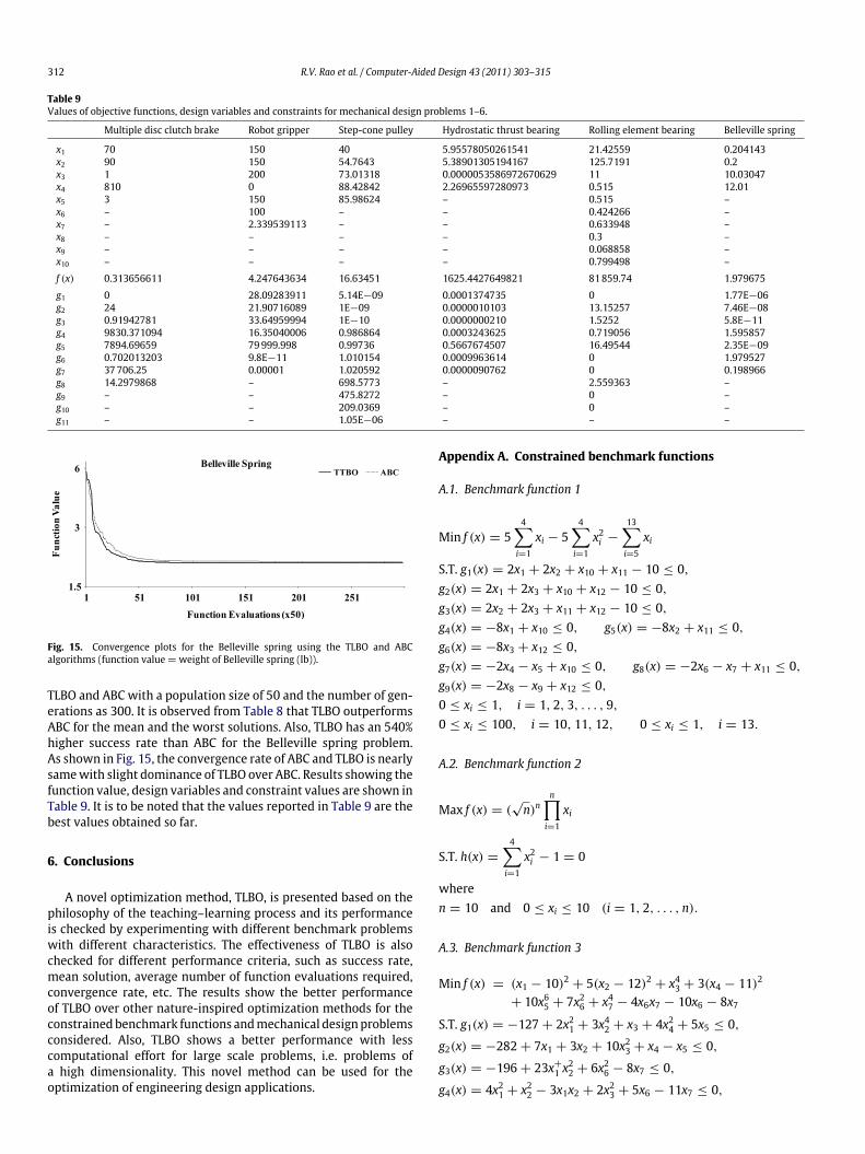
Fig. 15. Convergence plots for the Belleville spring using the TLBO and ABCalgorithms (function value = weight of Belleville spring (lb)).

TLBO and ABC with a population size of 50 and the number of gen-erations as 300. It is observed from Table 8 that TLBO outperformsABC for the mean and the worst solutions. Also, TLBO has an 540%higher success rate than ABC for the Belleville spring problem.As shown in Fig. 15, the convergence rate of ABC and TLBO is nearlysamewith slight dominance of TLBO over ABC. Results showing thefunction value, design variables and constraint values are shown inTable 9. It is to be noted that the values reported in Table 9 are thebest values obtained so far.

6. Conclusions

A novel optimization method, TLBO, is presented based on thephilosophy of the teaching–learning process and its performanceis checked by experimenting with different benchmark problemswith different characteristics. The effectiveness of TLBO is alsochecked for different performance criteria, such as success rate,mean solution, average number of function evaluations required,convergence rate, etc. The results show the better performanceof TLBO over other nature-inspired optimization methods for theconstrainedbenchmark functions andmechanical designproblemsconsidered. Also, TLBO shows a better performance with lesscomputational effort for large scale problems, i.e. problems ofa high dimensionality. This novel method can be used for theoptimization of engineering design applications.

Appendix A. Constrained benchmark functions

A.1. Benchmark function 1

Min f (x) = 54−

i=1

xi − 54−

i=1

x2i −

13−i=5

xi

S.T. g1(x) = 2x1 + 2x2 + x10 + x11 − 10 ≤ 0,g2(x) = 2x1 + 2x3 + x10 + x12 − 10 ≤ 0,g3(x) = 2x2 + 2x3 + x11 + x12 − 10 ≤ 0,g4(x) = −8x1 + x10 ≤ 0, g5(x) = −8x2 + x11 ≤ 0,g6(x) = −8x3 + x12 ≤ 0,g7(x) = −2x4 − x5 + x10 ≤ 0, g8(x) = −2x6 − x7 + x11 ≤ 0,g9(x) = −2x8 − x9 + x12 ≤ 0,0 ≤ xi ≤ 1, i = 1, 2, 3, . . . , 9,0 ≤ xi ≤ 100, i = 10, 11, 12, 0 ≤ xi ≤ 1, i = 13.

A.2. Benchmark function 2

Max f (x) = (√n)n

n∏i=1

xi

S.T. h(x) =

4−i=1

x2i − 1 = 0

wheren = 10 and 0 ≤ xi ≤ 10 (i = 1, 2, . . . , n).

A.3. Benchmark function 3

Min f (x) = (x1 − 10)2 + 5(x2 − 12)2 + x43 + 3(x4 − 11)2

+ 10x65 + 7x26 + x47 − 4x6x7 − 10x6 − 8x7S.T. g1(x) = −127 + 2x21 + 3x42 + x3 + 4x24 + 5x5 ≤ 0,

g2(x) = −282 + 7x1 + 3x2 + 10x23 + x4 − x5 ≤ 0,

g3(x) = −196 + 23x+

1 x22 + 6x26 − 8x7 ≤ 0,

g4(x) = 4x21 + x22 − 3x1x2 + 2x23 + 5x6 − 11x7 ≤ 0,

R.V. Rao et al. / Computer-Aided Design 43 (2011) 303–315 313

where−10 ≤ xi ≤ 10 (i = 1, 2, . . . , 7).

A.4. Benchmark function 4

Min f (x) = x1 + x2 + x3S.T. g1(x) = −1 + 0.0025(x4 + x6) ≤ 0,g2(x) = −1 + 0.0025(x5 + x7 − x4) ≤ 0,g3(x) = −1 + 0.01(x8 − x5) ≤ 0,g4(x) = −x1x6 + 833.33252x4 + 100x1 − 83 333.333 ≤ 0,g5(x) = −x2x7 + 1250x5 + x2x4 − 1250x4 ≤ 0,g6(x) = −x3x8 + 1250 000 + x3x5 − 2500x5 ≤ 0,where−100 ≤ x1 ≤ 10 000, −1000 ≤ xi ≤ 10 000 (i = 2, 3),−100 ≤ xi ≤ 10 000 (i = 4, 5, . . . , 8).

A.5. Benchmark function 5

Max f (x) =100 − (x1 − 5)2 − (x2 − 5)2 − (x3 − 5)2

100S.T. g(x) = (x1 − p)2 + (x2 − q)2 + (x3 − r)2 ≤ 0where0 ≤ xi ≤ 10 (i = 1, 2, 3)p, q, r = 1, 2, 3, . . . , 9.

Appendix B. Constrained benchmark mechanical design prob-lems

B.1. Design of pressure vessel

Minimize:f (x) = 0.6224x1x3x4 + 1.7781x2x23 + 3.1661x21x4 + 19.84x21x3Subject to:g1(x) = −x1 + 0.0193x3 ≤ 0,g2(x) = −x2 + 0.00954x3 ≤ 0,

g3(x) = −πx23x4 −43πx33 + 1296 000 ≤ 0,

g4(x) = x4 − 240 ≤ 0,where0 ≤ x1 ≤ 99, 0 ≤ x2 ≤ 99,10 ≤ x3 ≤ 200, 10 ≤ x4 ≤ 200.

B.2. Design of tension/compression spring

Minimize:f (x) = (N + 2)Dd2.Subject to;

g1(x) = 1 −D3N

71785d4≤ 0,

g2(x) =4D2

− dD12566(Dd3 − d4)

+1

5108d2− 1 ≤ 0,

g3(x) = 1 −140.45dD2N

≤ 0,

g4(x) =D + d1.5

− 1 ≤ 0,

where0.05 ≤ x1 ≤ 2, 0.25 ≤ x2 ≤ 1.3, 2 ≤ x3 ≤ 15.

B.3. Design of welded beam design

Minimize:

f (x) = 1.10471x21x2 + 0.04811x3x4(14.0 + x2).

Subject to:

g1(x) = τ(x) − τmax ≤ 0,g2(x) = σ(x) − σmax ≤ 0, g3(x) = x1 − x4 ≤ 0,g4(x) = 0.10471x21 + 0.04811x3x4(14.0 + x2) − 5.0 ≤ 0,g5(x) = 0.125 − x1 ≤ 0,g6(x) = δ(x) − δmax ≤ 0, g7(x) = P − Pc(x) ≤ 0,

where

τ(x) =

(τ ′)2 + 2τ ′τ ′′

x22R

+ (τ ′′)2,

τ ′=

P√2x1x2

, τ ′′=

MRJ

, M = PL +

x22

,

R =

x224

+

x1 + x3

2

2

,

J = 2

√2x1x2

x2212

+

x1 + x3

2

2

, σ (x) =6PLx4x23

,

δ(x) =4PL3

Ex33x4,

Pc(x) =4.013E

x23x

64

36

L2

1 −

x32L

E4G

,

P = 6000 lb, L = 14 in., E = 30e6 psi,G = 12e6 psi, τmax = 13 600 psi, σmax = 30 000 psi,δmax = 0.25 in.

0.1 ≤ x1 ≤ 2.0, 0.1 ≤ x2 ≤ 10.0,0.1 ≤ x3 ≤ 10.0, 0.1 ≤ x4 ≤ 2.0.

B.4. Design of gear train

Minimize:

f (x) = 0.7854x1x22(3.3333x23 + 14.9334x3 − 43.0934) − 1.508x1

× (x26 + x27) + 7.4777(x36 + x37) + 0.7854(x4x26 + x5x27)

Subject to:

g1(x) =27

x1x22x3− 1 ≤ 0, g2(x) =

397.5x1x22x

23

− 1 ≤ 0,

g3(x) =1.93x34x2x3x46

− 1 ≤ 0, g4(x) =1.93x35x2x3x47

− 1 ≤ 0,

g5(x) =

745x4x2x3

2+ 16.9e6

110x36− 1 ≤ 0,

g6(x) =

745x5x2x3

2+ 157.5e6

85x37− 1 ≤ 0,

g7(x) =x2x340

− 1 ≤ 0, g8(x) =5x2x1

− 1 ≤ 0,

g9(x) =x1

12x2− 1 ≤ 0,

314 R.V. Rao et al. / Computer-Aided Design 43 (2011) 303–315

g10(x) =1.5x6 + 1.9

x4− 1 ≤ 0,

g11(x) =1.1x7 + 1.9

x5− 1 ≤ 0,

where

2.6 ≤ x1 ≤ 3.6, 0.7 ≤ x2 ≤ 0.8, 17 ≤ x3 ≤ 28,7.3 ≤ x4 ≤ 8.3, 7.8 ≤ x5 ≤ 8.3,2.9 ≤ x6 ≤ 3.9, 5.0 ≤ x7 ≤ 5.5.

Appendix C. Constrained mechanical design problems

C.1. Multiple disc clutch brake design

Min f (x) = π(r20 − r2i )t(Z + 1)ρ

Subject to:

g1(x) = ro − ri − 1r ≥ 0,g2(x) = lmax − (Z + 1)(t + δ) ≥ 0, g3(x) = pmax − prz ≥ 0,g4(x) = pmaxvsrmax − przvsr ≥ 0,g5(x) = vsrmax − vsr ≥ 0, g6(x) = Tmax − T ≥ 0,g7(x) = Mh − sMs ≥ 0, g8(x) = T ≥ 0,

where

Mh =23µFZ

r3o − r3ir2o − r2i

, prz =F

π(r2o − r2i ),

vsr =2πn(r3o − r3i )90(r2o − r2i )

, T =Izπn

30(Mh + Mf ).

1r = 20 mm, tmax = 3 mm, tmin = 1.5 mm, lmax = 30 mm,Zmax = 10, vsrmax = 10m/s, µ = 0.5, s = 1.5,Ms = 40Nm,Mf =

3 N m, n = 250 rpm, pmax = 1 MPa, Iz = 55 kg mm2, Tmax = 15 s,Fmax = 1000 N, rimin = 55 mm, romax = 110 mm.

C.2. Robot gripper

Minimize f (x) = maxz

Fk(x, z) − minz

Fk(x, z)

Subject to:

g1(x) = Ymin − y(x, Zmax) ≥ 0,g2(x) = y(x, Zmax) ≥ 0, g3(x) = y(x, 0) − Ymax ≥ 0,g4(x) = YG − y(x, 0) ≥ 0, g5(x) = (a + b)2 − l2 − e2 ≥ 0,g6(x) = (l − Zmax)

2+ (a − e)2 − b2 ≥ 0,

g7(x) = l − Zmax ≥ 0,

where

g =

(l − z)2 + e2, α = arccos

a2 + g2

− b2

2ag

+ φ,

β = arccosb2 + g2

− a2

2bg

− φ,

φ = arctan

el − z

+ φ, Fk =

Pb sin(α + β)

2c cos(α)

,

y(x, z) = 2(e + f + c sin(β + δ)).

Ymin = 50, Ymax = 100,YG = 150, Zmax = 100, P = 100,10 ≤ a, b, f ≤ 150, 100 ≤ c ≤ 200,0 ≤ e ≤ 50, 100 ≤ l ≤ 300, 1 ≤ δ ≤ 3.14.

C.3. Step-cone pulley

Minimize f (x) = ρw

d21

1 +

N1

N

2

+ d22

1 +

N2

N

2

+ d23

1 +

N3

N

2

+ d24

1 +

N4

N

2

Subject to:

h1(x) = C1 − C2 = 0, h2(x) = C1 − C3 = 0,h3(x) = C1 − C4 = 0,g1,2,3,4(x) = Ri ≥ 2, g5,6,7,8(x) = Pi ≥ (0.75 ∗ 745.6998),

whereCi indicates the length of the belt to obtain speedNi and is given

by

Ci =πdi2

1 +

Ni

N

+

NiN − 1

24a

+ 2a i = (1, 2, 3, 4).

Ri is the tension ratio and is given by

Ri = exp[µ

π − 2 sin−1

Ni

N− 1

di2a

]i = (1, 2, 3, 4).

Pi is the power transmitted at each step

Pi = stw[1 − exp

[−µ

π − 2 sin−1

Ni

N− 1

di2a

]]πdiNi

60i = (1, 2, 3, 4).

ρ = 7200 kg/m3, a = 3 m, µ = 0.35, s = 1.75 MPa, t = 8 mm.

C.4. Hydrodynamic thrust bearing design

Minimize: f (x) =QPo0.7

+ Ef

Subject to:

g1(x) = W − Ws ≥ 0, g2(x) = Pmax − Po ≥ 0,g3(x) = 1Tmax − 1T ≥ 0, g4(x) = h − hmin ≥ 0,

g5(x) = R − Ro ≥ 0, g6(x) = 0.001 −γ

gPo

Q

2πRh

≥ 0,

g7(x) = 5000 −W

π(R2 − R2o)

≥ 0,

where

W =πPo2

R2− R2

o

ln RRo

, Po =6µQπh3

lnRRo

,

Ef = 9336Qγ C1T , 1T = 2(10P− 560)

P =log10 log10(8.122e6µ + 0.8) − C1

n,

h =

2πN60

2 2πµ

Ef

R4

4−

R4o

4

where,

γ = 0.0307, C = 0.5, n = −3.55, C1 = 10.04,Ws = 101 000, Pmax = 1000, 1Tmax = 50,hmin = 0.001, g = 386.4, N = 750.1 ≤ R, Ro,Q ≤ 16, 1e − 6 ≤ µ ≤ 16e − 6.

R.V. Rao et al. / Computer-Aided Design 43 (2011) 303–315 315

C.5. Rolling element bearing

Maximize Cd = fcZ2/3D1.8b if Db ≤ 25.4 mm

Cd = 3.647fcZ2/3D1.4b if Db > 25.4 mm

Subject to:

g1(X) =φo

2 sin−1 (Db/Dm)− Z + 1 ≥ 0,

g2(X) = 2Db − KDmin (D − d) ≥ 0,

g3(X) = KDmax (D − d) − 2Db ≥ 0,

g4(X) = ζBw − Db ≤ 0, g5(X) = Dm − 0.5 (D + d) ≥ 0,

g6(X) = (0.5 + e) (D + d) − Dm ≥ 0,

g7(X) = 0.5 (D − Dm − Db) − εDb ≥ 0,

g8(X) = fi ≥ 0.515, g9(X) = fo ≥ 0.515,

where

fc = 37.91

1 +

1.04

1 − γ

1 + γ

1.72 fi (2fo − 1)fo (2fi − 1)

0.4110/3

−0.3

,

γ =Db cosα

Dm, fi =

riDb

, fo =roDb

,

φo = 2π − 2

× cos−1

{(D − d) /2 − 3 (T/4)}2 + {D/2 − (T/4) − Db}

2− {d/2 + (T/4)}2

2 {(D − d) /2 − 3 (T/4)} {D/2 − (T/4) − Db}

,

(20)T = D − d − 2Db,

D = 160, d = 90, Bw = 30.

0.5(D + d) ≤ Dm ≤ 0.6(D + d), 0.15(D − d) ≤ Db ≤ 0.45(D −

d), 4 ≤ Z ≤ 50, 0.515 ≤ fi ≤ 0.6, 0.515 ≤ fo ≤ 0.6, 0.4 ≤

KDmin ≤ 0.5, 0.6 ≤ KDmax ≤ 0.7, 0.3 ≤ ε ≤ 0.4, 0.02 ≤ e ≤

0.1, 0.6 ≤ ζ ≤ 0.85.

C.6. Belleville spring

Minimize:

f (x) = 0.07075π(D2e − D2

i )t

Subject to:

g1(x) = S −4Eδmax

(1 − µ2)αD2e

[β

h −

δmax

2

+ γ t

]≥ 0,

g2(x) =

4Eδ

(1 − µ2)αD2e

[h −

δ

2

(h − δ)t + t3

]δ=δmax

− Pmax ≥ 0,

g3(x) = δl − δmax ≥ 0, g4(x) = H − h − t ≥ 0,

g5(x) = Dmax − De ≥ 0, g6(x) = De − Di ≥ 0,

g7(x) = 0.3 −h

De − Di≥ 0,

where

α =6

π ln K

K − 1K

2

,

β =6

π ln K

K − 1ln K

− 1

, γ =6

π ln K

K − 1

2

,

Pmax = 5400 lb, δmax = 0.2 in., S = 200 kPsi,

E = 30e6 psi, µ = 0.3, H = 2 in., Dmax = 12.01 in.,

K =De

Di, δl = f (a)a, a = h/t.

Values of f (a) vary as shown in Table 7.

References

[1] Goldberg D. Genetic algorithms in search, optimization, andmachine learning.New York: Addison-Wesley; 1989.

[2] Back T. Evolutionary algorithms in theory and practice. Oxford UniversityPress; 1996.

[3] Kennedy V, Eberhart R. Particle swarm optimization. In: Proceedings of theIEEE International Conference on Neural Networks. 1995. p. 1942–48.

[4] Clerc M. Particle swarm optimization. ISTE Publishing Company; 2006.[5] Karaboga D. An idea based on honey bee swarm for numerical optimization.

Technical report-TR06. Erciyes University, Engineering Faculty, ComputerEngineering Department. 2005.

[6] Basturk B, Karaboga D. An artificial bee colony (ABC) algorithm for numericfunction optimization. In: IEEE Swarm Intelligence Symposium. 2006.

[7] Karaboga D, Basturk B. On the performance of artificial bee colony (ABC)algorithm. Applied Soft Computing 2008;8:687–97.

[8] Dorigo M, Stutzle T. Ant colony optimization. MIT Press; 2004.[9] Blum C. Ant colony optimization: introduction and recent trends. Physics of

Life Reviews 2005;2:353–73.[10] Lee KS, Geem ZW. A newmeta-heuristic algorithm for continuous engineering

optimization: harmony search theory and practice. Computer Methods inApplied Mechanics and Engineering 2004;194:3902–33.

[11] Ahrari A, Atai AA. Grenade explosion method-a novel tool for optimization ofmultimodal functions. Applied Soft Computing 2010;10(4):1132–40.

[12] Deb K. An efficient constraint handling method for genetic algorithm.Computer Methods in Applied Mechanics and Engineering 2000;186:311–338.

[13] LiuH, Cai Z,Wang Y. Hybridizing particle swarmoptimizationwith differentialevolution for constrained numerical and engineering optimization. AppliedSoft Computing 2010;10:629–40.

[14] Mezura-Montes E, Coello CAC. A simplemulti-membered evolution strategy tosolve constrained optimization problems. IEEE Transactions on EvolutionaryComputation 2005;9(1):1–17.

[15] Zavala AEM, Aguirre AH, Diharce ERV. Constrained optimization via evolution-ary swarm optimization algorithm (PESO). In: Proceedings of the 2005 Confer-ence on Genetic and Evolutionary Computation. 2005. p. 209–16.

[16] Becerra RL, Coello CAC. Cultured differential evolution for constrainedoptimization. ComputerMethods inAppliedMechanics andEngineering 2006;195:4303–22.

[17] Huang FZ, Wang L, He Q. An effective co-evolutionary differential evolutionfor constrained optimization. Applied Mathematics and Computation 2007;186(1):340–56.

[18] Karaboga D, Basturk B. Artificial bee colony (ABC) optimization algorithm forsolving constrained optimization problems. LNAI, vol. 4529. Berlin: Springer-Verlag; 2007. p. 789–98.

[19] Mezura-Montes E, Coello CAC. Useful infeasible solutions in engineeringoptimization with evolutionary algorithms. Advances in Artificial Intelligenceof LNCS, vol. 3789. Berlin: Springer-Verlag; 2005.

[20] Parsopoulos K, Vrahatis M. Unified particle swarm optimization for solvingconstrained engineering optimization problems. In: Advances in naturalcomputation. LNCS, vol. 3612. Berlin: Springer-Verlag; 2005. p. 582–91.

[21] He Q, Wang L. An effective co-evolutionary particle swarm optimizationfor constrained engineering design problems. Engineering Applications ofArtificial Intelligence 2007;20:89–99.

[22] Akay B, Karaboga D. Artificial bee colony algorithm for large-scale problemsand engineering design optimization. Journal of Intelligent Manufacturing2010; doi:10.1007/s10845-010-0393-4.

[23] Osyczka A. Evolutionary algorithms for single and multicriteria designoptimization: studies in fuzzyness and soft computing. Heidelberg: Physica-Verlag; 2002.

[24] Osyczka A, Krenich S, Karas K. Optimum design of robot grippers using geneticalgorithms. In: Proceedings of the third World Congress of Structural andMultidisciplinary Optimization. 1999.

[25] Rao SS. Engineering optimization: theory and practice. New Delhi: New AgeInternational; 2002.

[26] Coello CAC. Treating constraints as objectives for single-objective evolutionaryoptimization. Engineering Optimization 2000;32(3):275–308.

[27] Gupta S, Tiwari R, Shivashankar BN. Multi-objective design optimization ofrolling bearings using genetic algorithm. Mechanism and Machine Theory2007;42:1418–43.

[28] Deb K, Srinivasan A. Innovization: innovative design principles throughoptimization, Kanpur genetic algorithms laboratory (KanGAL). Indian Instituteof Technology Kanpur. KanGAL report number 2005007. 2005.

[29] He S, Prempain E, Wu QH. An improved particle swarm optimizer formechanical design optimization problems. Engineering Optimization 2004;36(5):585–605.

[30] Deb K, Goyal M. Optimizing engineering designs using combined geneticsearch. In: Proceedings of seventh International Conference on GeneticAlgorithms. 1997. p. 512–28.