Hana ChocklerGeorg Weissenbacher (Eds.)

LNCS

109

82

30th International Conference, CAV 2018 Held as Part of the Federated Logic Conference, FloC 2018 Oxford, UK, July 14–17, 2018, Proceedings, Part II

Computer Aided Verification

Lecture Notes in Computer Science 10982

Commenced Publication in 1973Founding and Former Series Editors:Gerhard Goos, Juris Hartmanis, and Jan van Leeuwen

Editorial Board

David HutchisonLancaster University, Lancaster, UK

Takeo KanadeCarnegie Mellon University, Pittsburgh, PA, USA

Josef KittlerUniversity of Surrey, Guildford, UK

Jon M. KleinbergCornell University, Ithaca, NY, USA

Friedemann MatternETH Zurich, Zurich, Switzerland

John C. MitchellStanford University, Stanford, CA, USA

Moni NaorWeizmann Institute of Science, Rehovot, Israel

C. Pandu RanganIndian Institute of Technology Madras, Chennai, India

Bernhard SteffenTU Dortmund University, Dortmund, Germany

Demetri TerzopoulosUniversity of California, Los Angeles, CA, USA

Doug TygarUniversity of California, Berkeley, CA, USA

Gerhard WeikumMax Planck Institute for Informatics, Saarbrücken, Germany

More information about this series at http://www.springer.com/series/7407

Hana Chockler • Georg Weissenbacher (Eds.)

Computer AidedVerification30th International Conference, CAV 2018Held as Part of the Federated Logic Conference, FloC 2018Oxford, UK, July 14–17, 2018Proceedings, Part II

EditorsHana ChocklerKing’s CollegeLondonUK

Georg WeissenbacherTU WienViennaAustria

ISSN 0302-9743 ISSN 1611-3349 (electronic)Lecture Notes in Computer ScienceISBN 978-3-319-96141-5 ISBN 978-3-319-96142-2 (eBook)https://doi.org/10.1007/978-3-319-96142-2

Library of Congress Control Number: 2018948145

LNCS Sublibrary: SL1 – Theoretical Computer Science and General Issues

© The Editor(s) (if applicable) and The Author(s) 2018. This book is an open access publication.Open Access This book is licensed under the terms of the Creative Commons Attribution 4.0 InternationalLicense (http://creativecommons.org/licenses/by/4.0/), which permits use, sharing, adaptation, distributionand reproduction in any medium or format, as long as you give appropriate credit to the original author(s) andthe source, provide a link to the Creative Commons license and indicate if changes were made.The images or other third party material in this book are included in the book’s Creative Commons license,unless indicated otherwise in a credit line to the material. If material is not included in the book’s CreativeCommons license and your intended use is not permitted by statutory regulation or exceeds the permitted use,you will need to obtain permission directly from the copyright holder.The use of general descriptive names, registered names, trademarks, service marks, etc. in this publicationdoes not imply, even in the absence of a specific statement, that such names are exempt from the relevantprotective laws and regulations and therefore free for general use.The publisher, the authors and the editors are safe to assume that the advice and information in this book arebelieved to be true and accurate at the date of publication. Neither the publisher nor the authors or the editorsgive a warranty, express or implied, with respect to the material contained herein or for any errors oromissions that may have been made. The publisher remains neutral with regard to jurisdictional claims inpublished maps and institutional affiliations.

This Springer imprint is published by the registered company Springer Nature Switzerland AGThe registered company address is: Gewerbestrasse 11, 6330 Cham, Switzerland

Preface

It was our privilege to serve as the program chairs for CAV 2018, the 30th InternationalConference on Computer-Aided Verification. CAV is an annual conference dedicatedto the advancement of the theory and practice of computer-aided formal analysismethods for hardware and software systems. CAV 2018 was held in Oxford, UK, July14–17, 2018, with the tutorials day on July 13.

This year, CAV was held as part of the Federated Logic Conference (FLoC) eventand was collocated with many other conferences in logic. The primary focus of CAV isto spur advances in hardware and software verification while expanding to newdomains such as learning, autonomous systems, and computer security. CAV is at thecutting edge of research in formal methods, as reflected in this year’s program.

CAV 2018 covered a wide spectrum of subjects, from theoretical results to concreteapplications, including papers on application of formal methods in large-scale industrialsettings. It has always been one of the primary interests of CAV to include papers thatdescribe practical verification tools and solutions and techniques that ensure a highpractical appeal of the results. The proceedings of the conference are published inSpringer’s Lecture Notes in Computer Science series. A selection of papers wereinvited to a special issue of Formal Methods in System Design and the Journal of theACM.

This is the first year that the CAV proceedings are published under an Open Accesslicense, thus giving access to CAV proceedings to a broad audience. We hope that thisdecision will increase the scope of practical applications of formal methods and willattract even more interest from industry.

CAV received a very high number of submissions this year—215 overall—resultingin a highly competitive selection process. We accepted 13 tool papers and 52 regularpapers, which amounts to an acceptance rate of roughly 30% (for both regular papersand tool papers). The high number of excellent submissions in combination with thescheduling constraints of FLoC forced us to reduce the length of the talks to 15minutes, giving equal exposure and weight to regular papers and tool papers.

The accepted papers cover a wide range of topics and techniques, from algorithmicand logical foundations of verification to practical applications in distributed, net-worked, cyber-physical, and autonomous systems. Other notable topics are synthesis,learning, security, and concurrency in the context of formal methods. The proceedingsare organized according to the sessions in the conference.

The program featured two invited talks by Eran Yahav (Technion), on using deeplearning for programming, and by Somesh Jha (University of Wisconsin Madison) onadversarial deep learning. The invited talks this year reflect the growing interest of theCAV community in deep learning and its connection to formal methods. The tutorialday of CAV featured two invited tutorials, by Shaz Qadeer on verification of con-current programs and by Matteo Maffei on static analysis of smart contracts. Thesubjects of the tutorials reflect the increasing volume of research on verification of

concurrent software and, as of recently, the question of correctness of smart contracts.As every year, one of the winners of the CAV award also contributed a presentation.The tutorial day featured a workshop in memoriam of Mike Gordon, titled “ThreeResearch Vignettes in Memory of Mike Gordon,” organized by Tom Melham andjointly supported by CAV and ITP communities.

Moreover, we continued the tradition of organizing a LogicLounge. Initiated by thelate Helmut Veith at the Vienna Summer of Logic 2014, the LogicLounge is a series ofdiscussions on computer science topics targeting a general audience and has become aregular highlight at CAV. This year’s LogicLounge took place at the Oxford Union andwas on the topic of “Ethics and Morality of Robotics,” moderated by Judy Wajcmanand featuring a panel of experts on the topic: Luciano Floridi, Ben Kuipers, FrancescaRossi, Matthias Scheutz, Sandra Wachter, and Jeannette Wing. We thank May Chan,Katherine Fletcher, and Marta Kwiatkowska for organizing this event, and the ViennaCenter of Logic and Algorithms for their support.

In addition, CAV attendees enjoyed a number of FLoC plenary talks and eventstargeting the broad FLoC community.

In addition to the main conference, CAV hosted the Verification MentoringWorkshop for junior scientists entering the field and a high number of pre- andpost-conference technical workshops: the Workshop on Formal Reasoning in Dis-tributed Algorithms (FRIDA), the workshop on Runtime Verification for RigorousSystems Engineering (RV4RISE), the 5th Workshop on Horn Clauses for Verificationand Synthesis (HCVS), the 7th Workshop on Synthesis (SYNT), the First InternationalWorkshop on Parallel Logical Reasoning (PLR), the 10th Working Conference onVerified Software: Theories, Tools and Experiments (VSTTE), the Workshop onMachine Learning for Programming (MLP), the 11th International Workshop onNumerical Software Verification (NSV), the Workshop on Verification of EngineeredMolecular Devices and Programs (VEMDP), the Third Workshop on Fun With FormalMethods (FWFM), the Workshop on Robots, Morality, and Trust through the Verifi-cation Lens, and the IFAC Conference on Analysis and Design of Hybrid Systems(ADHS).

The Program Committee (PC) for CAV consisted of 80 members; we kept thenumber large to ensure each PC member would have a reasonable number of papers toreview and be able to provide thorough reviews. As the review process for CAV isdouble-blind, we kept the number of external reviewers to a minimum, to avoidaccidental disclosures and conflicts of interest. Altogether, the reviewers drafted over860 reviews and made an enormous effort to ensure a high-quality program. Followingthe tradition of CAV in recent years, the artifact evaluation was mandatory for toolsubmissions and optional but encouraged for regular submissions. We used an ArtifactEvaluation Committee of 25 members. Our goal for artifact evaluation was to providefriendly “beta-testing” to tool developers; we recognize that developing a stable tool ona cutting-edge research topic is certainly not easy and we hope the constructivecomments provided by the Artifact Evaluation Committee (AEC) were of help to thedevelopers. As a result of the evaluation, the AEC accepted 25 of 31 artifactsaccompanying regular papers; moreover, all 13 accepted tool papers passed the eval-uation. We are grateful to the reviewers for their outstanding efforts in making sureeach paper was fairly assessed. We would like to thank our artifact evaluation chair,

VI Preface

Igor Konnov, and the AEC for evaluating all artifacts submitted with tool papers aswell as optional artifacts submitted with regular papers.

Of course, without the tremendous effort put into the review process by our PCmembers this conference would not have been possible. We would like to thank the PCmembers for their effort and thorough reviews.

We would like to thank the FLoC chairs, Moshe Vardi, Daniel Kroening, and MartaKwiatkowska, for the support provided, Thanh Hai Tran for maintaining the CAVwebsite, and the always helpful Steering Committee members Orna Grumberg, AartiGupta, Daniel Kroening, and Kenneth McMillan. Finally, we would like to thank theteam at the University of Oxford, who took care of the administration and organizationof FLoC, thus making our jobs as CAV chairs much easier.

July 2018 Hana ChocklerGeorg Weissenbacher

Preface VII

Organization

Program Committee

Aws Albarghouthi University of Wisconsin-Madison, USAChristel Baier TU Dresden, GermanyClark Barrett Stanford University, USAEzio Bartocci TU Wien, AustriaDirk Beyer LMU Munich, GermanyPer Bjesse Synopsys Inc., USAJasmin Christian Blanchette Vrije Universiteit Amsterdam, NetherlandsRoderick Bloem Graz University of Technology, AustriaAhmed Bouajjani IRIF, University Paris Diderot, FrancePavol Cerny University of Colorado Boulder, USARohit Chadha University of Missouri, USASwarat Chaudhuri Rice University, USAWei-Ngan Chin National University of Singapore, SingaporeHana Chockler King’s College London, UKAlessandro Cimatti Fondazione Bruno Kessler, ItalyLoris D’Antoni University of Wisconsin-Madison, USAVijay D’Silva Google, USACristina David University of Cambridge, UKJyotirmoy Deshmukh University of Southern California, USAIsil Dillig The University of Texas at Austin, USACezara Dragoi Inria Paris, ENS, FranceKerstin Eder University of Bristol, UKMichael Emmi Nokia Bell Labs, USAGeorgios Fainekos Arizona State University, USADana Fisman University of Pennsylvania, USAVijay Ganesh University of Waterloo, CanadaSicun Gao University of California San Diego, USAAlberto Griggio Fondazione Bruno Kessler, ItalyOrna Grumberg Technion - Israel Institute of Technology, IsraelArie Gurfinkel University of Waterloo, CanadaWilliam Harrison Department of CS, University of Missouri, Columbia,

USAGerard Holzmann Nimble Research, USAAlan J. Hu The University of British Columbia, CanadaFranjo Ivancic Google, USAAlexander Ivrii IBM, IsraelHimanshu Jain Synopsys, USASomesh Jha University of Wisconsin-Madison, USA

Susmit Jha SRI International, USARanjit Jhala University of California San Diego, USABarbara Jobstmann EPFL and Cadence Design Systems, SwitzerlandStefan Kiefer University of Oxford, UKZachary Kincaid Princeton University, USALaura Kovacs TU Wien, AustriaViktor Kuncak Ecole Polytechnique Fédérale de Lausanne,

SwitzerlandOrna Kupferman Hebrew University, IsraelShuvendu Lahiri Microsoft, USARupak Majumdar MPI-SWS, GermanyKen McMillan Microsoft, USAAlexander Nadel Intel, IsraelMayur Naik Intel, USAKedar Namjoshi Nokia Bell Labs, USADejan Nickovic Austrian Institute of Technology AIT, AustriaCorina Pasareanu CMU/NASA Ames Research Center, USANir Piterman University of Leicester, UKPavithra Prabhakar Kansas State University, USAMitra Purandare IBM Research Laboratory Zurich, SwitzerlandShaz Qadeer Microsoft, USAArjun Radhakrishna Microsoft, USANoam Rinetzky Tel Aviv University, IsraelPhilipp Ruemmer Uppsala University, SwedenRoopsha Samanta Purdue University, USASriram Sankaranarayanan University of Colorado, Boulder, USAMartina Seidl Johannes Kepler University Linz, AustriaKoushik Sen University of California, Berkeley, USASanjit A. Seshia University of California, Berkeley, USANatasha Sharygina Università della Svizzera Italiana, Lugano, SwitzerlandSharon Shoham Tel Aviv University, IsraelAnna Slobodova Centaur Technology, USAArmando Solar-Lezama MIT, USAOfer Strichman Technion, IsraelSerdar Tasiran Amazon Web Services, USACaterina Urban ETH Zurich, SwitzerlandYakir Vizel Technion, IsraelTomas Vojnar Brno University of Technology, CzechiaThomas Wahl Northeastern University, USABow-Yaw Wang Academia Sinica, TaiwanGeorg Weissenbacher TU Wien, AustriaThomas Wies New York University, USAKaren Yorav IBM Research Laboratory Haifa, IsraelLenore Zuck University of Illinois in Chicago, USADamien Zufferey MPI-SWS, GermanyFlorian Zuleger TU Wien, Austria

X Organization

Artifact Evaluation Committee

Thibaut Balabonski Université Paris-Sud, FranceSergiy Bogomolov The Australian National University, AustraliaSimon Cruanes Aesthetic Integration, USAMatthias Dangl LMU Munich, GermanyEva Darulova Max Planck Institute for Software Systems, GermanyRamiro Demasi Universidad Nacional de Córdoba, ArgentinaGrigory Fedyukovich Princeton University, USAJohannes Hölzl Vrije Universiteit Amsterdam, The NetherlandsJochen Hoenicke University of Freiburg, GermanyAntti Hyvärinen Università della Svizzera Italiana, Lugano,

SwitzerlandSwen Jacobs Saarland University, GermanySaurabh Joshi IIT Hyderabad, IndiaDejan Jovanovic SRI International, USAAyrat Khalimov The Hebrew University, IsraelIgor Konnov (Chair) Inria Nancy (LORIA), FranceJan Kretínský Technical University of Munich, GermanyAlfons Laarman Leiden University, The NetherlandsRavichandhran Kandhadai

MadhavanEcole Polytechnique Fédérale de Lausanne,

SwitzerlandAndrea Micheli Fondazione Bruno Kessler, ItalySergio Mover University of Colorado Boulder, USAAina Niemetz Stanford University, USABurcu Kulahcioglu Ozkan MPI-SWS, GermanyMarkus N. Rabe University of California, Berkeley, USAAndrew Reynolds University of Iowa, USAMartin Suda TU Wien, AustriaMitra Tabaei TU Wien, Austria

Additional Reviewers

Alpernas, KalevAsadi, SepidehAthanasiou, KonstantinosBauer, MatthewBavishi, RohanBayless, SamBerzish, MurphyBlicha, MartinBui, Phi DiepCauderlier, RaphaëlCauli, ClaudiaCeska, Milan

Cohen, ErnieCostea, AndreeaDangl, MatthiasDoko, MarkoDrachsler Cohen, DanaDreossi, TommasoDutra, RafaelEbrahimi, MasoudEisner, CindyFedyukovich, GrigoryFremont, DanielFreund, Stephen

Friedberger, KarlheinzGhorbani, SoudehGhosh, ShromonaGoel, ShilpiGong, LiangGovind, HariGu, YijiaHabermehl, PeterHamza, JadHe, PaulHeo, KihongHolik, Lukas

Organization XI

Humenberger, AndreasHyvärinen, AnttiHölzl, JohannesIusupov, RinatJacobs, SwenJain, MiteshJaroschek, MaximilianJha, Sumit KumarKeidar-Barner, SharonKhalimov, AyratKiesl, BenjaminKoenighofer, BettinaKrstic, SrdjanLaeufer, KevinLee, WoosukLemberger, ThomasLemieux, CarolineLewis, RobertLiang, JiaLiang, JimmyLiu, PeizunLång, Magnus

Maffei, MatteoMarescotti, MatteoMathur, UmangMiné, AntoineMora, FedericoNevo, ZivOchoa, MartinOrni, AvigailOuaknine, JoelPadhye, RohanPadon, OdedPartush, NimrodPavlinovic, ZvonimirPavlogiannis, AndreasPeled, DoronPendharkar, IshanPeng, YanPetri, GustavoPolozov, OleksandrPopescu, AndreiPotomkin, KostiantynRaghothaman, Mukund

Reynolds, AndrewReynolds, ThomasRitirc, DanielaRogalewicz, AdamScott, JoeShacham, OhadSong, YahuiSosnovich, AdiSousa, MarceloSubramanian, KausikSumners, RobSwords, SolTa, Quang TrungTautschnig, MichaelTraytel, DmitriyTrivedi, AshutoshUdupa, Abhishekvan Dijk, TomWendler, PhilippZdancewic, SteveZulkoski, Ed

XII Organization

Contents – Part II

Tools

Let this Graph Be Your Witness! An Attestor for Verifying JavaPointer Programs. . . . . . . . . . . . . . . . . . . . . . . . . . . . . . . . . . . . . . . . . . . 3

Hannah Arndt, Christina Jansen, Joost-Pieter Katoen,Christoph Matheja, and Thomas Noll

MaxSMT-Based Type Inference for Python 3 . . . . . . . . . . . . . . . . . . . . . . . 12Mostafa Hassan, Caterina Urban, Marco Eilers, and Peter Müller

The JKIND Model Checker . . . . . . . . . . . . . . . . . . . . . . . . . . . . . . . . . . . . 20Andrew Gacek, John Backes, Mike Whalen, Lucas Wagner,and Elaheh Ghassabani

The DEEPSEC Prover . . . . . . . . . . . . . . . . . . . . . . . . . . . . . . . . . . . . . . . 28Vincent Cheval, Steve Kremer, and Itsaka Rakotonirina

SimpleCAR: An Efficient Bug-Finding Tool Basedon Approximate Reachability . . . . . . . . . . . . . . . . . . . . . . . . . . . . . . . . . . 37

Jianwen Li, Rohit Dureja, Geguang Pu, Kristin Yvonne Rozier,and Moshe Y. Vardi

StringFuzz: A Fuzzer for String Solvers . . . . . . . . . . . . . . . . . . . . . . . . . . . 45Dmitry Blotsky, Federico Mora, Murphy Berzish, Yunhui Zheng,Ifaz Kabir, and Vijay Ganesh

Static Analysis

Permission Inference for Array Programs . . . . . . . . . . . . . . . . . . . . . . . . . . 55Jérôme Dohrau, Alexander J. Summers, Caterina Urban,Severin Münger, and Peter Müller

Program Analysis Is Harder Than Verification:A Computability Perspective . . . . . . . . . . . . . . . . . . . . . . . . . . . . . . . . . . 75

Patrick Cousot, Roberto Giacobazzi, and Francesco Ranzato

Theory and Security

Automata vs Linear-Programming Discounted-Sum Inclusion . . . . . . . . . . . . 99Suguman Bansal, Swarat Chaudhuri, and Moshe Y. Vardi

Model Checking Indistinguishability of Randomized Security Protocols . . . . . 117Matthew S. Bauer, Rohit Chadha, A. Prasad Sistla,and Mahesh Viswanathan

Lazy Self-composition for Security Verification . . . . . . . . . . . . . . . . . . . . . 136Weikun Yang, Yakir Vizel, Pramod Subramanyan, Aarti Gupta,and Sharad Malik

SCINFER: Refinement-Based Verification of Software CountermeasuresAgainst Side-Channel Attacks. . . . . . . . . . . . . . . . . . . . . . . . . . . . . . . . . . 157

Jun Zhang, Pengfei Gao, Fu Song, and Chao Wang

Symbolic Algorithms for Graphs and Markov Decision Processeswith Fairness Objectives . . . . . . . . . . . . . . . . . . . . . . . . . . . . . . . . . . . . . 178

Krishnendu Chatterjee, Monika Henzinger, Veronika Loitzenbauer,Simin Oraee, and Viktor Toman

Attracting Tangles to Solve Parity Games . . . . . . . . . . . . . . . . . . . . . . . . . 198Tom van Dijk

SAT, SMT and Decision Procedures

Delta-Decision Procedures for Exists-Forall Problems over the Reals . . . . . . . 219Soonho Kong, Armando Solar-Lezama, and Sicun Gao

Solving Quantified Bit-Vectors Using Invertibility Conditions. . . . . . . . . . . . 236Aina Niemetz, Mathias Preiner, Andrew Reynolds, Clark Barrett,and Cesare Tinelli

Understanding and Extending Incremental Determinization for 2QBF . . . . . . 256Markus N. Rabe, Leander Tentrup, Cameron Rasmussen,and Sanjit A. Seshia

The Proof Complexity of SMT Solvers . . . . . . . . . . . . . . . . . . . . . . . . . . . 275Robert Robere, Antonina Kolokolova, and Vijay Ganesh

Model Generation for Quantified Formulas: A Taint-Based Approach . . . . . . 294Benjamin Farinier, Sébastien Bardin, Richard Bonichon,and Marie-Laure Potet

Concurrency

Partial Order Aware Concurrency Sampling . . . . . . . . . . . . . . . . . . . . . . . . 317Xinhao Yuan, Junfeng Yang, and Ronghui Gu

Reasoning About TSO Programs Using Reduction and Abstraction . . . . . . . . 336Ahmed Bouajjani, Constantin Enea, Suha Orhun Mutluergil,and Serdar Tasiran

XIV Contents – Part II

Quasi-Optimal Partial Order Reduction . . . . . . . . . . . . . . . . . . . . . . . . . . . 354Huyen T. T. Nguyen, César Rodríguez, Marcelo Sousa, Camille Coti,and Laure Petrucci

On the Completeness of Verifying Message Passing Programs UnderBounded Asynchrony . . . . . . . . . . . . . . . . . . . . . . . . . . . . . . . . . . . . . . . 372

Ahmed Bouajjani, Constantin Enea, Kailiang Ji, and Shaz Qadeer

Constrained Dynamic Partial Order Reduction . . . . . . . . . . . . . . . . . . . . . . 392Elvira Albert, Miguel Gómez-Zamalloa, Miguel Isabel, and Albert Rubio

CPS, Hardware, Industrial Applications

Formal Verification of a Vehicle-to-Vehicle (V2V) Messaging System . . . . . 413Mark Tullsen, Lee Pike, Nathan Collins, and Aaron Tomb

Continuous Formal Verification of Amazon s2n . . . . . . . . . . . . . . . . . . . . . 430Andrey Chudnov, Nathan Collins, Byron Cook, Joey Dodds,Brian Huffman, Colm MacCárthaigh, Stephen Magill, Eric Mertens,Eric Mullen, Serdar Tasiran, Aaron Tomb, and Eddy Westbrook

Symbolic Liveness Analysis of Real-World Software. . . . . . . . . . . . . . . . . . 447Daniel Schemmel, Julian Büning, Oscar Soria Dustmann, Thomas Noll,and Klaus Wehrle

Model Checking Boot Code from AWS Data Centers . . . . . . . . . . . . . . . . . 467Byron Cook, Kareem Khazem, Daniel Kroening, Serdar Tasiran,Michael Tautschnig, and Mark R. Tuttle

Android Stack Machine . . . . . . . . . . . . . . . . . . . . . . . . . . . . . . . . . . . . . . 487Taolue Chen, Jinlong He, Fu Song, Guozhen Wang, Zhilin Wu,and Jun Yan

Formally Verified Montgomery Multiplication . . . . . . . . . . . . . . . . . . . . . . 505Christoph Walther

Inner and Outer Approximating Flowpipes for Delay Differential Equations . . . 523Eric Goubault, Sylvie Putot, and Lorenz Sahlmann

Author Index . . . . . . . . . . . . . . . . . . . . . . . . . . . . . . . . . . . . . . . . . . . . 543

Contents – Part II XV

Contents – Part I

Invited Papers

Semantic Adversarial Deep Learning . . . . . . . . . . . . . . . . . . . . . . . . . . . . . 3Tommaso Dreossi, Somesh Jha, and Sanjit A. Seshia

From Programs to Interpretable Deep Models and Back. . . . . . . . . . . . . . . . 27Eran Yahav

Formal Reasoning About the Security of Amazon Web Services . . . . . . . . . . 38Byron Cook

Tutorials

Foundations and Tools for the Static Analysis of Ethereum Smart Contracts . . . 51Ilya Grishchenko, Matteo Maffei, and Clara Schneidewind

Layered Concurrent Programs. . . . . . . . . . . . . . . . . . . . . . . . . . . . . . . . . . 79Bernhard Kragl and Shaz Qadeer

Model Checking

Propositional Dynamic Logic for Higher-Order Functional Programs . . . . . . . 105Yuki Satake and Hiroshi Unno

Syntax-Guided Termination Analysis . . . . . . . . . . . . . . . . . . . . . . . . . . . . . 124Grigory Fedyukovich, Yueling Zhang, and Aarti Gupta

Model Checking Quantitative Hyperproperties . . . . . . . . . . . . . . . . . . . . . . 144Bernd Finkbeiner, Christopher Hahn, and Hazem Torfah

Exploiting Synchrony and Symmetry in Relational Verification . . . . . . . . . . 164Lauren Pick, Grigory Fedyukovich, and Aarti Gupta

JBMC: A Bounded Model Checking Tool for Verifying Java Bytecode . . . . . 183Lucas Cordeiro, Pascal Kesseli, Daniel Kroening, Peter Schrammel,and Marek Trtik

Eager Abstraction for Symbolic Model Checking . . . . . . . . . . . . . . . . . . . . 191Kenneth L. McMillan

Program Analysis Using Polyhedra

Fast Numerical Program Analysis with Reinforcement Learning . . . . . . . . . . 211Gagandeep Singh, Markus Püschel, and Martin Vechev

A Direct Encoding for NNC Polyhedra . . . . . . . . . . . . . . . . . . . . . . . . . . . 230Anna Becchi and Enea Zaffanella

Synthesis

What’s Hard About Boolean Functional Synthesis? . . . . . . . . . . . . . . . . . . . 251S. Akshay, Supratik Chakraborty, Shubham Goel, Sumith Kulal,and Shetal Shah

Counterexample Guided Inductive Synthesis Modulo Theories . . . . . . . . . . . 270Alessandro Abate, Cristina David, Pascal Kesseli, Daniel Kroening,and Elizabeth Polgreen

Synthesizing Reactive Systems from Hyperproperties . . . . . . . . . . . . . . . . . 289Bernd Finkbeiner, Christopher Hahn, Philip Lukert, Marvin Stenger,and Leander Tentrup

Reactive Control Improvisation . . . . . . . . . . . . . . . . . . . . . . . . . . . . . . . . . 307Daniel J. Fremont and Sanjit A. Seshia

Constraint-Based Synthesis of Coupling Proofs . . . . . . . . . . . . . . . . . . . . . . 327Aws Albarghouthi and Justin Hsu

Controller Synthesis Made Real: Reach-Avoid Specificationsand Linear Dynamics. . . . . . . . . . . . . . . . . . . . . . . . . . . . . . . . . . . . . . . . 347

Chuchu Fan, Umang Mathur, Sayan Mitra, and Mahesh Viswanathan

Synthesis of Asynchronous Reactive Programsfrom Temporal Specifications . . . . . . . . . . . . . . . . . . . . . . . . . . . . . . . . . . 367

Suguman Bansal, Kedar S. Namjoshi, and Yaniv Sa’ar

Syntax-Guided Synthesis with Quantitative Syntactic Objectives . . . . . . . . . . 386Qinheping Hu and Loris D’Antoni

Learning

Learning Abstractions for Program Synthesis . . . . . . . . . . . . . . . . . . . . . . . 407Xinyu Wang, Greg Anderson, Isil Dillig, and K. L. McMillan

The Learnability of Symbolic Automata. . . . . . . . . . . . . . . . . . . . . . . . . . . 427George Argyros and Loris D’Antoni

XVIII Contents – Part I

Runtime Verification, Hybrid and Timed Systems

Reachable Set Over-Approximation for Nonlinear SystemsUsing Piecewise Barrier Tubes . . . . . . . . . . . . . . . . . . . . . . . . . . . . . . . . . 449

Hui Kong, Ezio Bartocci, and Thomas A. Henzinger

Space-Time Interpolants. . . . . . . . . . . . . . . . . . . . . . . . . . . . . . . . . . . . . . 468Goran Frehse, Mirco Giacobbe, and Thomas A. Henzinger

Monitoring Weak Consistency . . . . . . . . . . . . . . . . . . . . . . . . . . . . . . . . . 487Michael Emmi and Constantin Enea

Monitoring CTMCs by Multi-clock Timed Automata. . . . . . . . . . . . . . . . . . 507Yijun Feng, Joost-Pieter Katoen, Haokun Li, Bican Xia,and Naijun Zhan

Start Pruning When Time Gets Urgent: Partial Order Reductionfor Timed Systems . . . . . . . . . . . . . . . . . . . . . . . . . . . . . . . . . . . . . . . . . 527

Frederik M. Bønneland, Peter Gjøl Jensen, Kim Guldstrand Larsen,Marco Muñiz, and Jiří Srba

A Counting Semantics for Monitoring LTL Specificationsover Finite Traces . . . . . . . . . . . . . . . . . . . . . . . . . . . . . . . . . . . . . . . . . . 547

Ezio Bartocci, Roderick Bloem, Dejan Nickovic, and Franz Roeck

Tools

Rabinizer 4: From LTL to Your Favourite Deterministic Automaton . . . . . . . 567Jan Křetínský, Tobias Meggendorfer, Salomon Sickert,and Christopher Ziegler

Strix: Explicit Reactive Synthesis Strikes Back! . . . . . . . . . . . . . . . . . . . . . 578Philipp J. Meyer, Salomon Sickert, and Michael Luttenberger

BTOR2 , BtorMC and Boolector 3.0 . . . . . . . . . . . . . . . . . . . . . . . . . . . . . . 587Aina Niemetz, Mathias Preiner, Clifford Wolf, and Armin Biere

Nagini: A Static Verifier for Python . . . . . . . . . . . . . . . . . . . . . . . . . . . . . 596Marco Eilers and Peter Müller

PEREGRINE: A Tool for the Analysis of Population Protocols . . . . . . . . . . . . . 604Michael Blondin, Javier Esparza, and Stefan Jaax

ADAC: Automated Design of Approximate Circuits . . . . . . . . . . . . . . . . . . 612Milan Češka, Jiří Matyáš, Vojtech Mrazek, Lukas Sekanina,Zdenek Vasicek, and Tomáš Vojnar

Contents – Part I XIX

Probabilistic Systems

Value Iteration for Simple Stochastic Games: Stopping Criterionand Learning Algorithm. . . . . . . . . . . . . . . . . . . . . . . . . . . . . . . . . . . . . . 623

Edon Kelmendi, Julia Krämer, Jan Křetínský,and Maximilian Weininger

Sound Value Iteration . . . . . . . . . . . . . . . . . . . . . . . . . . . . . . . . . . . . . . . 643Tim Quatmann and Joost-Pieter Katoen

Safety-Aware Apprenticeship Learning . . . . . . . . . . . . . . . . . . . . . . . . . . . 662Weichao Zhou and Wenchao Li

Deciding Probabilistic Bisimilarity Distance One for LabelledMarkov Chains . . . . . . . . . . . . . . . . . . . . . . . . . . . . . . . . . . . . . . . . . . . . 681

Qiyi Tang and Franck van Breugel

Author Index . . . . . . . . . . . . . . . . . . . . . . . . . . . . . . . . . . . . . . . . . . . . 701

XX Contents – Part I

Tools

Let this Graph Be Your Witness!

An Attestor for Verifying Java Pointer Programs

Hannah Arndt, Christina Jansen, Joost-Pieter Katoen ,Christoph Matheja(B) , and Thomas Noll

Software Modeling and Verification Group,RWTH Aachen University, Aachen, Germany

matheja@cs.rwth-aachen.de

Abstract. We present a graph-based tool for analysing Java programsoperating on dynamic data structures. It involves the generation ofan abstract state space employing a user-defined graph grammar. LTLmodel checking is then applied to this state space, supporting bothstructural and functional correctness properties. The analysis is fullyautomated, procedure-modular, and provides informative visual feedbackincluding counterexamples in the case of property violations.

1 Introduction

Pointers constitute an essential concept in modern programming languages, andare used for implementing dynamic data structures like lists, trees etc. However,many software bugs can be traced back to the erroneous use of pointers by e.g.dereferencing null pointers or accidentally pointing to wrong parts of the heap.Due to the resulting unbounded state spaces, pointer errors are hard to detect.Automated tool support for validation of pointer programs that provides mean-ingful debugging information in case of violations is therefore highly desirable.

Attestor is a verification tool that attempts to achieve both of these goals.To this aim, it first constructs an abstract state space of the input program bymeans of symbolic execution. Each state depicts both links between heap objectsand values of program variables using a graph representation. Abstraction is per-formed on state level by means of graph grammars. They specify the data struc-tures maintained by the program, and describe how to summarise substructuresof the heap in order to obtain a finite representation. After labelling each statewith propositions that provide information about structural properties such asreachability or heap shapes, the actual verification task is performed in a secondstep. To this aim, the abstract state space is checked against a user-defined LTLspecification. In case of violations, a counterexample is provided.

H. Arndt and C. Matheja—Supported by Deutsche Forschungsgemeinschaft (DFG)Grant No. 401/2-1.

c© The Author(s) 2018H. Chockler and G. Weissenbacher (Eds.): CAV 2018, LNCS 10982, pp. 3–11, 2018.https://doi.org/10.1007/978-3-319-96142-2_1

4 H. Arndt et al.

In summary, Attestor’s main features can be characterized as follows:

– It employs context-free graph grammars as a formal underpinning for definingheap abstractions. These grammars enable local heap concretisation and thusnaturally provide implicit abstract semantics.

– The full instruction set of Java Bytecode is handled. Program actions that areoutside the scope of our analysis, such as arithmetic operations or Booleantests on payload data, are handled by (safe) over-approximation.

– Specifications are given by linear-time temporal logic (LTL) formulae whichsupport a rich set of program properties, ranging from memory safety overshape, reachability or balancedness to properties such as full traversal orpreservation of the exact heap structure.

– Except for expecting a graph grammar that specifies the data structures han-dled by a program, the analysis is fully automated. In particular, no programannotations are required.

– Modular reasoning is supported in the form of contracts that summarise theeffect of executing a (recursive) procedure. These contracts can be automat-ically derived or manually specified.

– Valuable feedback is provided through a comprehensive report including (min-imal) non-spurious counterexamples in case of property violations.

– The tool’s functionality is made accessible through the command line as wellas a graphical user and an application programming interface.

Availability.Attestor’s source code, benchmarks, and documentation are avail-able online at https://moves-rwth.github.io/attestor.

2 The Attestor Tool

Attestor is implemented in Java and consists of about 20.000 LOC (excludingcomments and tests). An architectural overview is depicted in Fig. 1. It shows thetool inputs (left), its outputs (right), the Attestor backend with its processingphases (middle), the Attestor frontend (below) as well as the API connectingback- and frontend. These elements are discussed in detail below.

2.1 Input

As shown in Fig. 1 (left), a verification task is given by four inputs. First, theprogram to be analysed. Here, Java as well as Java Bytecode programs withpossibly recursive procedures are supported, where the former is translated tothe latter prior to the analysis. Second, the specification has to be given by aset of LTL formulae enriched with heap-specific propositions. See Sect. 3 for arepresentative list of exemplary specifications.

As a third input, Attestor expects the declaration of the graph grammarthat guides the abstraction. In order to obtain a finite abstract state space,this grammar is supposed to cover the data structures emerging during program

Let this Graph Be Your Witness! 5

Fig. 1. The Attestor tool

execution. The user may choose from a set of grammar definitions for standarddata structures such as singly- and doubly-linked lists and binary trees, themanual specification in a JSON-style graph format and combinations thereof.

Fourth, additional options can be given that e.g. define the initial heap config-uration(s) (in JSON-style graph format), that control the granularity of abstrac-tion and the garbage collection behaviour, or that allow to re-use results ofprevious analyses in the form of procedure contracts [11,13].

2.2 Phases

Attestor proceeds in six main phases, see Fig. 1 (middle). In the first and thirdphase, all inputs are parsed and preprocessed. The input program is read andtransformed to Bytecode (if necessary), the input graphs (initial configuration,procedure contracts, and graph grammar), LTL formulae and further optionsare read.

Depending on the provided LTL formulae, additional markings are insertedinto the initial heap (see [8] for details) in the second phase. They are used totrack identities of objects during program execution, which is later required tovalidate visit and neighbourhood properties during the fifth phase.

In the next phase the actual program analysis is conducted. To this aim,Attestor first constructs the abstract state space as described in Sect. 2.3 indetail. In the fifth phase we check whether the provided LTL specification holdson the state space resulting from the preceding step. We use an off-the-shelftableau-based LTL model checking algorithm [2].

6 H. Arndt et al.

If desired, during all phases results are forwarded to the API to make themaccessible to the frontend or the user directly. We address this output in Sect. 2.4.

2.3 Abstract State Space Generation

The core module of Attestor is the abstract state space generation. It employsan abstraction approach based on hyperedge replacement grammars, whose the-oretical underpinnings are described in [9] in detail. It is centred around a graph-based representation of the heap that contains concrete parts side by side withplaceholders representing a set of heap fragments of a certain shape. The statespace generation loop as implemented in Attestor is shown in Fig. 2.

Fig. 2. State space generation.

Initially it is provided withthe initial program state(s),that is, the program countercorresponding to the startingstatement together with the ini-tial heap configuration(s). Fromthese, Attestor picks a stateat random and applies theabstract semantics of the nextstatement: First, the heap con-figuration is locally concretisedensuring that all heap partsrequired for the statement toexecute are accessible. This isenabled by applying rules of theinput graph grammar in for-ward direction, which can entailbranching in the state space.The resulting configurations arethen manipulated according tothe concrete semantics of the statement. At this stage, Attestor automati-cally detects possible null pointer dereferencing operations as a byproduct of thestate space generation. In a subsequent rectification step, the heap configurationis cleared from e.g. dead variables and garbage (if desired). Consequently, mem-ory leaks are detected immediately. The rectified configuration is then abstractedwith respect to the data structures specified by means of the input graph gram-mar. Complementary to concretisation, this is realised by applying grammarrules in backward direction, which involves a check for embeddings of right-hand sides. A particular strength of our approach is its robustness against localviolations of data structures, as it simply leaves the corresponding heap partsconcrete. Finalising the abstract execution step, the resulting state is labelledwith the atomic propositions it satisfies. This check is efficiently implemented bymeans of heap automata (see [12,15] for details). By performing a subsumptioncheck on the state level, Attestor detects whether the newly generated stateis already covered by a more abstract one that has been visited before. If not, it

Let this Graph Be Your Witness! 7

Fig. 3. Screenshot of Attestor’s frontend for state space exploration. (Color figureonline)

adds the resulting state to the state space and starts over by picking a new state.Otherwise, it checks whether further states have to be processed or whether afixpoint in the state space generation is reached. In the latter case, this phase isterminated.

2.4 Output

As shown in Fig. 1 (right), we obtain three main outputs once the analysis iscompleted: the computed abstract state space, the derived procedure contracts,and the model checking results. For each LTL formula in the specification, resultscomprise the possible answers “formula satisfied”, “formula (definitely) not sat-isfied”, or “formula possibly not satisfied”. In case of the latter two, Attestoradditionally produces a counterexample, i.e. an abstract trace that violates theformula. If Attestor was able to verify the non-spuriousness of this counterex-ample (second case), we are additionally given a concrete initial heap that isaccountable for the violation and that can be used as a test case for debugging.

Besides the main outputs, Attestor provides general information about thecurrent analysis. These include log messages such as warnings and errors, butalso details about settings and runtimes of the analyses. The API provides theinterface to retrieve Attestor’s outputs as JSON-formatted data.

2.5 Frontend

Attestor features a graphical frontend that visualises inputs as well as resultsof all benchmark runs. The frontend communicates with Attestor’s backendvia the API only. It especially can be used to display and navigate through thegenerated abstract state space and counterexample traces.

A screenshot of the frontend for state space exploration is found in Fig. 3.The left panel is an excerpt of the state space. The right panel depicts the

8 H. Arndt et al.

currently selected state, where red boxes correspond to variables and constants,circles correspond to allocated objects/locations, and yellow boxes correspondto nonterminals of the employed graph grammar, respectively. Arrows betweentwo circles represent pointers. Further information about the selected state isprovided in the topmost panel. Graphs are rendered using cytoscape.js [6].

3 Evaluation

Tool Comparison. While there exists a plethora of tools for analysing pointerprograms, such as, amongst others, Forester [10], Groove [7], Infer [5],Hip/Sleek [17], Korat [16], Juggrnaut [9], and Tvla [3], these tools differin multiple dimensions:

– Input languages range from C code (Forester, Infer, Hip/Sleek) overJava/Java Bytecode (Juggrnaut, Korat) to assembly code (Tvla) andgraph programs (Groove).

– The degree of automation differs heavily: Tools like Forester and Inferonly require source code. Others such as Hip/Sleek and Juggrnaut addi-tionally expect general data structure specifications in the form of e.g. graphgrammars or predicate definitions to guide the abstraction. Moreover, Tvlarequires additional program-dependent instrumentation predicates.

– Verifiable properties typically cover memory safety. Korat is an exception,because it applies test case generation instead of verification. The toolsHip/Sleek, Tvla, Groove, and Juggrnaut are additionally capable ofverifying data structure invariants, so-called shape properties. Furthermore,Hip/Sleek is able to reason about shape-numeric properties, e.g. lengths oflists, if a suitable specification is provided. While these properties are notsupported by Tvla, it is possible to verify reachability properties. Moreover,Juggrnaut can reason about temporal properties such as verifying thatfinally every element of an input data structure has been accessed.

Benchmarks. Due to the above mentioned diversity there is no publicly avail-able and representative set of standardised benchmarks to compare the afore-mentioned tools [1]. We thus evaluated Attestor on a collection of challenging,pointer intensive algorithms compiled from the literature [3,4,10,14]. To assessour counterexample generation, we considered invalid specifications, e.g. that areversed list is the same list as the input list. Furthermore, we injected faultsinto our examples by swapping and deleting statements.

Properties. During state space generation, memory safety (M) is checked. More-over, we consider five classes of properties that are verified using the built-inLTL model checker:

Let this Graph Be Your Witness! 9

Table 1. The experimental results. All runtimes are in seconds. Verification timeincludes state space generation. SLL (DLL) means singly-linked (doubly-linked) list.

No. states State space gen. Verification Total runtime

Benchmark Properties Min Max Min Max Min Max Min Max

SLL.traverse M, S, R, V, N, X 13 97 0.030 0.074 0.039 0.097 0.757 0.848

SLL.reverse M, S, R, V, X 46 268 0.050 0.109 0.050 0.127 0.793 0.950

SLL.reverse (recursive) M, S, V, N, X 40 823 0.038 0.100 0.044 0.117 0.720 0.933

DLL.reverse M, S, R, V, N, X 70 1508 0.076 0.646 0.097 0.712 0.831 1.763

DLL.findLast M, C, X 44 44 0.069 0.069 0.079 0.079 0.938 0.938

SLL.findMiddle M, S, R, V, N, X 75 456 0.060 0.184 0.060 0.210 0.767 0.975

Tree.traverse (Lindstrom) M, S, V, N 229 67941 0.119 8.901 0.119 16.52 0.845 17.36

Tree.traverse (recursive) M, S 91 21738 0.075 1.714 0.074 1.765 0.849 2.894

AVLTree.binarySearch M, S 192 192 0.117 0.172 0.118 0.192 0.917 1.039

AVLTree.searchAndBack M, S, C 455 455 0.193 0.229 0.205 0.289 1.081 1.335

AVLTree.searchAndSwap M, S, C 3855 4104 0.955 1.590 1.004 1.677 1.928 2.521

AVLTree.leftMostInsert M, S 6120 6120 1.879 1.942 1.932 1.943 2.813 2.817

AVLTree.insert M, S 10388 10388 3.378 3.676 3.378 3.802 4.284 4.720

AVLTree.sllToAVLTree M, S, C 7166 7166 2.412 2.728 2.440 2.759 3.383 3.762

– The shape property (S) establishes that the heap is of a specific shape, e.g. adoubly-linked list or a balanced tree.

– The reachability property (R) checks whether some variable is reachable fromanother one via specific pointer fields.

– The visit property (V) verifies whether every element of the input is accessedby a specific variable.

– The neighbourhood property (N) checks whether the input data structure coin-cides with the output data structure upon termination.

– Finally, we consider other functional correctness properties (C), e.g. the returnvalue is not null.

Setup. For performance evaluation, we conducted experiments on an Intel Corei7-7500U CPU @ 2.70 GHz with the Java virtual machine (OpenJDK version1.8.0 151) limited to its default setting of 2 GB of RAM. All experiments were runusing the Java benchmarking harness jmh. Our experimental results are shownin Table 1. Additionally, for comparison purpose we considered Java implemen-tations of benchmarks that have been previously analysed for memory safety byForester [10], see Table 2.

10 H. Arndt et al.

Table 2. Forester benchmarks (memorysafety only). Verification times are in sec-onds.

Benchmark No. states Verification

SLL.bubblesort 287 0.134

SLL.deleteElement 152 0.096

SLLHeadPtr (traverse) 111 0.095

SLL.insertsort 369 0.147

ListOfCyclicLists 313 0.153

DLL.insert 379 0.207

DLL.insertsort1 4302 1.467

DLL.insertsort2 1332 0.514

DLL.buildAndReverse 277 0.164

CyclicDLL (traverse) 104 0.108

Tree.construct 44 0.062

Tree.constructAndDSW 1334 0.365

SkipList.insert 302 0.160

SkipList.build 330 0.173

Discussion. The results show thatboth memory safety (M) and shape(S) are efficiently processed, withregard to both state space size andruntime. This is not surprising asthese properties are directly han-dled by the state space generationengine. The most challenging tasksare the visit (V) and neighbourhood(N) properties as they require totrack objects across program execu-tions by means of markings. The lat-ter have a similar impact as pointervariables: increasing their numberimpedes abstraction as larger partsof the heap have to be kept concrete.This effect can be observed for theLindstrom tree traversal procedurewhere adding one marking (V) and three markings (N) both increase the verifi-cation effort by an order of magnitude.

References

1. Abdulla, P.A., Gadducci, F., Konig, B., Vafeiadis, V.: Verification of evolving graphstructures (Dagstuhl Seminar 15451). Dagstuhl Rep. 5(11), 1–28 (2016)

2. Bhat, G., Cleaveland, R., Grumberg, O.: Efficient on-the-fly model checking forCTL. In: LICS 1995, pp. 388–397. IEEE (1995)

3. Bogudlov, I., Lev-Ami, T., Reps, T., Sagiv, M.: Revamping TVLA: making para-metric shape analysis competitive. In: Damm, W., Hermanns, H. (eds.) CAV 2007.LNCS, vol. 4590, pp. 221–225. Springer, Heidelberg (2007). https://doi.org/10.1007/978-3-540-73368-3 25

4. Bouajjani, A., Habermehl, P., Rogalewicz, A., Vojnar, T.: Abstract regular treemodel checking of complex dynamic data structures. In: Yi, K. (ed.) SAS 2006.LNCS, vol. 4134, pp. 52–70. Springer, Heidelberg (2006). https://doi.org/10.1007/11823230 5

5. Calcagno, C., Distefano, D.: Infer: an automatic program verifier for memory safetyof C programs. In: Bobaru, M., Havelund, K., Holzmann, G.J., Joshi, R. (eds.)NFM 2011. LNCS, vol. 6617, pp. 459–465. Springer, Heidelberg (2011). https://doi.org/10.1007/978-3-642-20398-5 33

6. Cytoscape Consortium: Cytoscape: graph theory/network library for analysis andvisualisation. http://js.cytoscape.org/

7. Ghamarian, A.H., de Mol, M.J., Rensink, A., Zambon, E., Zimakova, M.V.: Mod-elling and analysis using GROOVE. Int. J. Soft. Tools Technol. Transfer 14, 15–40(2012)

8. Heinen, J.: Verifying Java programs - a graph grammar approach. Ph.D. thesis,RWTH Aachen University, Germany (2015)

9. Heinen, J., Jansen, C., Katoen, J.P., Noll, T.: Verifying pointer programs usinggraph grammars. Sci. Comput. Program. 97, 157–162 (2015)

Let this Graph Be Your Witness! 11

10. Holık, L., Lengal, O., Rogalewicz, A., Simacek, J., Vojnar, T.: Fully automatedshape analysis based on forest automata. CoRR abs/1304.5806 (2013)

11. Jansen, C.: Static analysis of pointer programs - linking graph grammars andseparation logic. Ph.D. thesis, RWTH Aachen University, Germany (2017)

12. Jansen, C., Katelaan, J., Matheja, C., Noll, T., Zuleger, F.: Unified reasoning aboutrobustness properties of symbolic-heap separation logic. In: Yang, H. (ed.) ESOP2017. LNCS, vol. 10201, pp. 611–638. Springer, Heidelberg (2017). https://doi.org/10.1007/978-3-662-54434-1 23

13. Jansen, C., Noll, T.: Generating abstract graph-based procedure summaries forpointer programs. In: Giese, H., Konig, B. (eds.) ICGT 2014. LNCS, vol. 8571, pp.49–64. Springer, Cham (2014). https://doi.org/10.1007/978-3-319-09108-2 4

14. Loginov, A., Reps, T., Sagiv, M.: Automated verification of the Deutsch-Schorr-Waite tree-traversal algorithm. In: Yi, K. (ed.) SAS 2006. LNCS, vol. 4134, pp.261–279. Springer, Heidelberg (2006). https://doi.org/10.1007/11823230 17

15. Matheja, C., Jansen, C., Noll, T.: Tree-like grammars and separation logic. In:Feng, X., Park, S. (eds.) APLAS 2015. LNCS, vol. 9458, pp. 90–108. Springer,Cham (2015). https://doi.org/10.1007/978-3-319-26529-2 6

16. Milicevic, A., Misailovic, S., Marinov, D., Khurshid, S.: Korat: a tool for generatingstructurally complex test inputs. In: Proceedings of the 29th International Confer-ence on Software Engineering, ICSE 2007, pp. 771–774. IEEE Computer Society,Washington, DC, USA (2007). https://doi.org/10.1109/ICSE.2007.48

17. Nguyen, H.H., David, C., Qin, S., Chin, W.-N.: Automated verification of shapeand size properties via separation logic. In: Cook, B., Podelski, A. (eds.) VMCAI2007. LNCS, vol. 4349, pp. 251–266. Springer, Heidelberg (2007). https://doi.org/10.1007/978-3-540-69738-1 18

Open Access This chapter is licensed under the terms of the Creative CommonsAttribution 4.0 International License (http://creativecommons.org/licenses/by/4.0/),which permits use, sharing, adaptation, distribution and reproduction in any mediumor format, as long as you give appropriate credit to the original author(s) and thesource, provide a link to the Creative Commons license and indicate if changes weremade.

The images or other third party material in this chapter are included in the chapter’sCreative Commons license, unless indicated otherwise in a credit line to the material. Ifmaterial is not included in the chapter’s Creative Commons license and your intendeduse is not permitted by statutory regulation or exceeds the permitted use, you willneed to obtain permission directly from the copyright holder.

MaxSMT-Based Type Inferencefor Python 3

Mostafa Hassan1,2, Caterina Urban2(B), Marco Eilers2 ,and Peter Muller2

1 German University in Cairo, Cairo, Egypt2 Department of Computer Science, ETH Zurich,

Zurich, Switzerlandcaterina.urban@inf.ethz.ch

Abstract. We present Typpete, a sound type inferencer that auto-matically infers Python 3 type annotations. Typpete encodes type con-straints as a MaxSMT problem and uses optional constraints and spe-cific quantifier instantiation patterns to make the constraint solving pro-cess efficient. Our experimental evaluation shows that Typpete scalesto real world Python programs and outperforms state-of-the-art tools.

1 Introduction

Dynamically-typed languages like Python have become increasingly popular inthe past five years. Dynamic typing enables rapid development and adaptationto changing requirements. On the other hand, static typing offers early errordetection, efficient execution, and machine-checked code documentation, andenables more advanced static analysis and verification approaches [15].

For these reasons, Python’s PEP484 [25] has recently introduced optionaltype annotations in the spirit of gradual typing [23]. The annotations can bechecked using MyPy [10]. In this paper, we present our tool Typpete, whichautomatically infers sound (non-gradual) type annotations and can thereforeserve as a preprocessor for other analysis or verification tools.

Typpete performs whole-program type inference, as there are no princi-pal typings in object-oriented languages like Python [1, example in Sect. 1]; theinferred types are correct in the given context but may not be as general aspossible. The type inference is constraint-based and relies on the off-the-shelfSMT solver Z3 [7] for finding a valid type assignment for the input program.We show that two main ingredients allow Typpete to scale to real programs: (1)a careful encoding of subtyping that leverages efficient quantifier instantiationtechniques [6], and (2) the use of optional type equality constraints, which con-siderably reduce the solution search space. Whenever a valid type assignment forthe input program cannot be found, Typpete encodes type error localizationas an optimization problem [19] and reports only a minimal set of unfulfilledconstraints to help the user pinpoint the cause of the error.

c© The Author(s) 2018H. Chockler and G. Weissenbacher (Eds.): CAV 2018, LNCS 10982, pp. 12–19, 2018.https://doi.org/10.1007/978-3-319-96142-2_2

MaxSMT-Based Type Inference for Python 3 13

Fig. 1. A Python implementation of the odds and evens hand game.

Typpete accepts programs written in (a large subset of) Python 3. Having astatic type system imposes a number of requirements on Python programs: (a) avariable can only have a single type through the whole program; (b) generic typeshave to be homogeneous (e.g., all elements of a set must have the same type);and (c) dynamic code generation, reflection and dynamic attribute additions anddeletions are not allowed. The supported type system includes generic classesand functions. Users must supply a file and the number of type variables for anygeneric class or function. Typpete then outputs a program with type annotations,a type error, or an error indicating use of unsupported language features.

Our experimental evaluation demonstrates the practical applicability of ourapproach. We show that Typpete performs well on a variety of real-world opensource Python programs and outperforms state-of-the-art tools.

2 Constraint Generation

Typpete encodes the type inference problem for a Python program into anSMT constraint resolution problem such that any solution of the SMT problemyields a valid type assignment for the program. The process of generating theSMT problem consists of three phases, which we describe below.

In a first pass over the input program, Typpete collects: (1) all globallydefined names (to resolve forward references), (2) all classes and their respectivesubclass relations (to define subtyping), and (3) upper bounds on the size of cer-tain types (e.g., tuples and function parameters). This pre-analysis encompassesboth the input program—including all transitively imported modules—and stubfiles, which define the types of built-in classes and functions as well as libraries.Typpete already contains stubs for the most common built-ins; users can addcustom stub files written in the format that is supported by MyPy.

In the second phase, Typpete declares an algebraic datatype Type, whosemembers correspond one-to-one to Python types. Typpete declares onedatatype constructor for every class in the input program; non-generic classes arerepresented as constants, whereas a generic class with n type parameters is rep-resented by a constructor taking n arguments of type Type. As an example, theclass Odd in Fig. 1 is represented by the constant classOdd. Typpete also declaresconstructors for tuples and functions up to the maximum size determined in thepre-analysis, and for all type variables used in generic functions and classes.

14 M. Hassan et al.

The subtype relation <: is represented by an uninterpreted function subtypewhich maps pairs of types to a boolean value. This function is delicate to definebecause of the possibility of matching loops (i.e., axioms being endlessly instanti-ated [7]) in the SMT solver. For each datatype constructor, Typpete generatesaxioms that explicitly enumerate the possible subtypes and supertypes. As anexample, for the type classOdd, Typpete generates the following axioms:

∀t. subtype(classOdd, t) = (t = classOdd ∨ t = classItem ∨ t = classobject)∀t. subtype(t, classOdd) = (t = classnone ∨ t = classOdd)

Note that the second axiom allows None to be a subtype of any other type (asin Java). As we discuss in the next section, this definition of subtype allows us toavoid matching loops by specifying specific instantiation patterns for the SMTsolver. A substitution function substitute, which substitutes type arguments fortype variables when interacting with generic types, is defined in a similar way.

In the third step, Typpete traverses the program while creating an SMTvariable for each node in its abstract syntax tree, and generating type constraintsover these variables for the constructs in the program. During the traversal, acontext maps all defined names (i.e., program variables, fields, etc.) to the corre-sponding SMT variables. The context is later used to retrieve the type assignedby the SMT solver to each name in the program. Constraints are generated forexpressions (e.g., call arguments are subtypes of the corresponding parametertypes), statements (e.g., the right-hand side of an assignment is a subtype ofthe left hand-side), and larger constructs such as methods (e.g., covariance andcontravariance constraints for method overrides). For example, the (simplified)constraint generated for the call to item1.compete(item2) at line 21 in Fig. 1contains a disjunction of cases depending on the type of the receiver:

(vitem1 = classOdd ∧ competeOdd = f 2(classOdd, arg, ret) ∧ subtype(vitem2, arg))∨ (vitem1 = classEven ∧ competeEven = f 2(classEven, arg, ret) ∧ subtype(vitem2, arg))

where f 2 is a datatype constructor for a function with two parameter types (andone return type ret), and vitem1 and vitem2 are the SMT variables correspondingto item1 and item2, respectively.

The generated constraints guarantee that any solution yields a correct typeassignment for the input program. However, there are often many different validsolutions, as the constraints only impose lower or upper bounds on the types rep-resented by the SMT variables (e.g., subtype(vitem2, arg) shown above imposesonly an upper bound on the type of vitem2). This has an impact on performance(cf. Sect. 4) as the search space for a solution remains large. Moreover, some typeassignments could be more desirable than others for a user (e.g., a user wouldmost likely prefer to assign type int rather than object to a variable initial-ized with value zero). To avoid these problems, Typpete additionally generatesoptional type equality constraints in places where the mandatory constraints onlydemand subtyping (i.e., local variable assignments, return statements, passedfunction arguments), thereby turning the SMT problem into a MaxSMT opti-mization problem. For instance, in addition to subtype(vitem2, arg) shown above,

MaxSMT-Based Type Inference for Python 3 15

Typpete generates the optional equality constraint vitem2 = arg. The optionalconstraints guide the solver to try the specified exact type first, which is oftena correct choice and therefore improves performance, and additionally leads tosolutions with more precise variable and parameter types.

3 Constraint Solving

Typpete relies on Z3 [7] and the MaxRes [18] algorithm for solving the gener-ated type constraints. We use e-matching [6] for instantiating the quantifiers usedin the axiomatization of the subtype function (cf. Sect. 2), and carefully chooseinstantiation patterns that ensure that any choice made during the search imme-diately triggers the instantiation of the relevant quantifiers. For instance, for theaxioms shown in Sect. 2, we use the instantiation patterns subtype(classOdd, t) andsubtype(t, classOdd), respectively. Our instantiation patterns ensure that as soonas one argument of an application of the subtype function is known, the quan-tifier that enumerates the possible values of the other argument is instantiated,thus ensuring that the consequences of any type choices propagate immediately.With a naıve encoding, the solver would have to guess both arguments beforebeing able to check whether the subtype relation holds. The resulting constraintsolving process is much faster than it would be when using different quantifierinstantiation techniques such as model-based quantifier instantiation [12], butstill avoids the potential unsoundness that can occur when using e-matchingwith insufficient trigger expressions.

When the MaxSMT problem is satisfiable, Typpete queries Z3 for a modelsatisfying all type constraints, retrieves the types assigned to each name in theprogram, and generates type annotated source code for the input program. Forinstance, for the program shown in Fig. 1, Typpete automatically annotates thefunction evalEven with type Even for the parameter item and a str return type.Note that Item and object would also be correct type annotations for item; thechoice of Even is guided by the optional type equality constraints.

When the MaxSMT problem is unsatisfiable, instead of reporting the unful-filled constraints in the unsatistiable core returned by Z3 (which is not guaran-teed to be minimal), Typpete creates a new relaxed MaxSMT problem whereonly the constraints defining the subtype function are enforced, while all othertype constraints are optional. Z3 is then queried for a model satisfying as manytype constraints as possible. The resulting type annotated source code for theinput program is returned along with the remaining minimal set of unfulfilledtype constraints. For instance, if we remove the abstract method compete of classItem in Fig. 1, Typpete annotates the parameters of the function match at line20 with type object and indicates the call compete at line 21 as problematic. Byobserving the mismatch between the type annotations and the method call, theuser has sufficient context to quickly identify and correct the type error.

16 M. Hassan et al.

T(SMT) T(MaxSMT) Unfulfilled T(Relaxed) Pytypeadventure 2.99s / 6.30s 3.27s / 6.76s 42 / 2 1.95s / 8.83s 0 [0]

icemu 9.45s / 6.79s 9.51s / 3.63s 4 / 2 0.08s / 21.76s 18 [2]imp 16.88s / 59.95s 16.91s / 15.87s 67 / 2 0.82s / 82.56s 3 [2]

scion 4.65s / 3.35s 4.72s / 2.97s 28 / 2 0.16s / 3.39s 0 [0]test suite 14.66s / 1.63s 14.66s / 2.17s - - 55 [34]

Fig. 2. Evaluation of Typpete on small programs and larger open source projects.

4 Experimental Evaluation

In order to demonstrate the practical applicability of our approach, we evaluatedour tool Typpete on a number of real-world open-source Python programs thatuse inheritance, operator overloading, and other features that are challenging fortype inference (but not features that make static typing impossible):

adventure [21]: An implementation of the Colossal Cave Adventure game (2modules, 399 LOC). The evaluation (and reported LOC) excludes the mod-ules game.py and prompt.py, which employ dynamic attribute additions.

icemu [8]: A library that emulates integrated circuits at the logic level (8 mod-ules, 530 LOC). We conducted the evaluation on revision 484828f.

imp [4]: A minimal interpreter for the imp toy language (7 modules, 771 LOC).The evaluation excludes the modules used for testing the project.

scion [9]: A Python implementation of a new Internet architecture (2 modules,725 LOC). For the evaluation, we used path store.py and scion addr.pyfrom revision 6f60ccc, and provided stub files for all dependencies.

We additionally ran Typpete on our test suite of manually-written programsand small programs collected from the web (47 modules and 1998 LOC).

In order to make the projects statically typeable, we had to make a num-ber of small changes that do not impact the functionality of the code, such asadding abstract superclasses and abstract methods, and (for the imp and scionprojects) introducing explicit downcasts in few places. Additionally, we made anumber of other innocuous changes to overcome the current limitations of ourtool, such as replacing keyword arguments with positional arguments, replacinggenerator expressions with list comprehensions, and replacing super calls viainlining. The complete list of changes for each project is included in our artifact.

The experiments were conducted on an 2.9 GHz Intel Core i5 processor with8GB of RAM running Mac OS High Sierra version 10.13.3 with Z3 version4.5.1. Figure 2 summarizes the result of the evaluation. The first two columnsshow the average running time (over ten runs, split into constraint generationand constraint solving) for the type inference in which the use of optional typeequality constraints (cf. Sect. 2) is disabled (SMT) and enabled (MaxSMT),respectively. We can observe that optional type equality constraints (consid-erably) reduce the search space for a solution as disabling them significantly

MaxSMT-Based Type Inference for Python 3 17

increases the running time for larger projects. We can also note that the con-straint solving time improves significantly when the type inference is run onthe test suite, which consists of many independent modules. This suggests thatsplitting the type inference problem into independent sub-problems could fur-ther improve performance. We plan to investigate this direction as part of ourfuture work.

The third column of Fig. 2 shows the evaluation of the error reporting featureof Typpete (cf. Sect. 3). For each benchmark, we manually introduced two typeerrors that could organically happen during programming and compared thesize of the unsatisfiable core (left of /) and the number of remaining unfulfilledconstraints (right of /) for the original and relaxed MaxSMT problems givento Z3, respectively. We also list the times needed to prove the first problemunsatisfiable and solve the relaxed problem. As one would expect, the numberof constraints that remain unfulfilled for the relaxed problems is considerablysmaller, which demonstrates that the error reporting feature of Typpete greatlyreduces the time that a user needs to identify the source of a type error.

Finally, the last column of Fig. 2 shows the result of the comparison of Typ-pete with the state-of-the-art type inferencer Pytype [16]. Pytype infersPEP484 [25] gradual type annotations by abstract interpretation [5] of thebytecode-compiled version of the given Python file. In Fig. 2, for the consideredbenchmarks, we report the number of variables and parameters that Pytypeleaves untyped or annotated with Any. We excluded any module on whichPytype yields an error; in square brackets we indicate the number of mod-ules that we could consider. Typpete is able to fully type all elements and thusoutperforms Pytype for static typing purposes. On the other hand, we note thatPytype additionally supports gradual typing and a larger Python subset.

5 Related and Future Work

In addition to Pytype, a number of other type inference approaches and toolshave been developed for Python. The approach of Maia et al. [17] has somefundamental limitations such as not allowing forward references or overloadedfunctions and operators. Fritz and Hage [11] as well as Starkiller [22] infer setsof concrete types that can inhabit each program variable to improve executionperformance. The former sacrifices soundness to handle more dynamic features ofPython. Additionally, deriving valid type assignments from sets of concrete typesis non-trivial. MyPy and a project by Cannon [3] can perform (incomplete) typeinference for local variables, but require type annotations for function parametersand return types. PyAnnotate [13] dynamically tracks variable types duringexecution and optionally annotates Python programs; the resulting annotationsare not guaranteed to be sound. A similar spectrum of solutions exists for otherdynamic programming languages like JavaScript [2,14] and ActionScript [20].

The idea of using SMT solvers for type inference is not new. Both F* [24] andLiquidHaskell [26] (partly) use SMT-solving in the inference for their dependenttype systems. Pavlinovic et al. [19] present an SMT encoding of the OCaml type

18 M. Hassan et al.

system. Typpete’s approach to type error reporting can be seen as a simpleinstantiation of their approach.

As part of our future work, we want to explore whether our system can beadapted to infer gradual types. We also aim to develop heuristics for inferringwhich functions and classes should be annotated with generic types based on thereported unfulfilled constraints. Finally, we plan to explore the idea of splittingthe type inference into multiple separate problems to improve performance.

Acknowledgments. We thank the anonymous reviewers for their feedback. This workwas supported by an ETH Zurich Career Seed Grant (SEED-32 16-2).

References

1. Ancona, D., Zucca, E.: Principal typings for Java-like languages. In: POPL, pp.306–317 (2004)

2. Anderson, C., Giannini, P., Drossopoulou, S.: Towards type inference for JavaScript.In: Black, A.P. (ed.) ECOOP. LNCS, vol. 3586, pp. 428–452. Springer, Heidelberg(2005). https://doi.org/10.1007/11531142 19

3. Cannon, B.: Localized type inference of atomic types in Python. Master’s thesis,California Polytechnic State University (2005)

4. Conrod, J.: IMP Interpreter. https://github.com/jayconrod/imp-interpreter5. Cousot, P., Cousot, R.: Abstract interpretation: a unified lattice model for static

analysis of programs by construction or approximation of fixpoints. In: POPL, pp.238–252 (1977)

6. de Moura, L., Bjørner, N.: Efficient E-matching for SMT solvers. In: Pfenning, F.(ed.) CADE. LNCS (LNAI), vol. 4603, pp. 183–198. Springer, Heidelberg (2007).https://doi.org/10.1007/978-3-540-73595-3 13

7. de Moura, L., Bjørner, N.: Z3: an efficient SMT Solver. In: Ramakrishnan, C.R.,Rehof, J. (eds.) TACAS 2008. LNCS, vol. 4963, pp. 337–340. Springer, Heidelberg(2008). https://doi.org/10.1007/978-3-540-78800-3 24

8. Dupras, V.: Icemu. https://github.com/hsoft/icemu9. ETH Zurich: SCION. https://github.com/scionproto/scion

10. Fisher, D., Lehtosalo, J., Price, G., van Rossum, G.: MyPy. http://mypy-lang.org/11. Fritz, L., Hage, J.: Cost versus precision for approximate typing for Python. In:

PEPM, pp. 89–98 (2017)12. Ge, Y., de Moura, L.: Complete instantiation for quantified formulas in satisfi-

abiliby modulo theories. In: Bouajjani, A., Maler, O. (eds.) CAV 2009. LNCS,vol. 5643, pp. 306–320. Springer, Heidelberg (2009). https://doi.org/10.1007/978-3-642-02658-4 25

13. Grue, T., Vorobev, S., Lehtosalo, J., van Rossum, G.: PyAnnotate. https://github.com/google/pytype

14. Hackett, B., Guo, S.: Fast and precise hybrid type inference for JavaScript. In:PLDI, pp. 239–250 (2012)

15. Jensen, S.H., Møller, A., Thiemann, P.: Type analysis for JavaScript. In: SAS, pp.238–255 (2009)

16. Kramm, M., Chen, R., Sudol, T., Demello, M., Caceres, A., Baum, D., Peters,A., Ludemann, P., Swartz, P., Batchelder, N., Kaptur, A., Lindzey, L.: Pytype.https://github.com/google/pytype

MaxSMT-Based Type Inference for Python 3 19

17. Maia, E., Moreira, N., Reis, R.: A static type inference for Python. In: DYLA(2012)

18. Narodytska, N. Bacchus, F.: Maximum satisfiability using core-guided maxsat res-olution. In: AAAI, pp. 2717–2723 (2014)

19. Pavlinovic, Z., King, T., Wies, T.: Finding minimum type error sources. In: OOP-SLA, pp. 525–542 (2014)

20. Rastogi, A., Chaudhuri, A., Hosmer, B.: The ins and outs of gradual type inference.In: POPL, pp. 481–494 (2012)

21. Rhodes, B.: Adventure. https://github.com/brandon-rhodes/python-adventure22. Salib, M.: Starkiller : a static type inferencer and compiler for Python. Master’s

thesis, Massachusetts Institute of Technology (2004)23. Siek, J., Taha, W.: Gradual typing for objects. In: Ernst, E. (ed.) ECOOP 2007.

LNCS, vol. 4609, pp. 2–27. Springer, Heidelberg (2007). https://doi.org/10.1007/978-3-540-73589-2 2

24. Swamy, N., Hritcu, C., Keller, C., Rastogi, A., Delignat-Lavaud, A., Forest, S.,Bhargavan, K., Fournet, C., Strub, P., Kohlweiss, M., Zinzindohoue, J.K., Beguelin,S.Z.: Dependent types and multi-monadic effects in F. In: POPL, pp. 256–270(2016)

25. van Rossum, G., Lehtosalo, J., Langa, L.: Type hints (2014). https://www.python.org/dev/peps/pep-0484/

26. Vazou, N., Seidel, E.L., Jhala, R.: Liquidhaskell: experience with refinement typesin the real world. In: Proceedings of the 2014 ACM SIGPLAN symposium onHaskell, Gothenburg, Sweden, 4–5 September 2014, pp. 39–51 (2014)

Open Access This chapter is licensed under the terms of the Creative CommonsAttribution 4.0 International License (http://creativecommons.org/licenses/by/4.0/),which permits use, sharing, adaptation, distribution and reproduction in any mediumor format, as long as you give appropriate credit to the original author(s) and thesource, provide a link to the Creative Commons license and indicate if changes weremade.

The images or other third party material in this chapter are included in the chapter’sCreative Commons license, unless indicated otherwise in a credit line to the material. Ifmaterial is not included in the chapter’s Creative Commons license and your intendeduse is not permitted by statutory regulation or exceeds the permitted use, you willneed to obtain permission directly from the copyright holder.

The JKIND Model Checker

Andrew Gacek1(B), John Backes1, Mike Whalen2, Lucas Wagner1,and Elaheh Ghassabani2

1 Rockwell Collins, Cedar Rapids, USAandrew.gacek@gmail.com,

john.backes@gmail.com,

lucas.wagner@rockwellcollins.com2 University of Minnesota, Minneapolis, USA

{mwwhalen,ghass013}@umn.edu

Abstract. JKind is an open-source industrial model checker developedby Rockwell Collins and the University of Minnesota. JKind uses mul-tiple parallel engines to prove or falsify safety properties of infinite statemodels. It is portable, easy to install, performance competitive with otherstate-of-the-art model checkers, and has features designed to improve theresults presented to users: inductive validity cores for proofs and coun-terexample smoothing for test-case generation. It serves as the back-endfor various industrial applications.

1 Introduction

JKind is an open-source1 industrial infinite-state inductive model checker forsafety properties. Models and properties in JKind are specified in Lustre [17],a synchronous data-flow language, using the theories of linear real and integerarithmetic. JKind uses SMT-solvers to prove and falsify multiple properties inparallel. A distinguishing characteristic of JKind is its focus on the usability ofresults. For a proven property, JKind provides traceability between the prop-erty and individual model elements. For a falsified property, JKind providesoptions for simplifying the counterexample in order to highlight the root causeof the failure. In industrial applications, we have found these additional usabilityaspects to be at least as important as the primary results. Another importantcharacteristic of JKind is that is it designed to be integrated directly into user-facing applications. Written in Java, JKind runs on all major platforms andis easily compiled into other Java applications. JKind bundles the Java-basedSMTInterpol solver and has no external dependencies. However, it can option-ally call Z3, Yices 1, Yices 2, CVC4, and MathSAT if they are available.

2 Functionality and Main Features

JKind is structured as several parallel engines that coordinate to prove prop-erties, mimicking the design of PKind and Kind 2 [8,21]. Some engines are1 https://github.com/agacek/jkind.

c© The Author(s) 2018H. Chockler and G. Weissenbacher (Eds.): CAV 2018, LNCS 10982, pp. 20–27, 2018.https://doi.org/10.1007/978-3-319-96142-2_3

The JKind Model Checker 21

Fig. 1. JKind engine architecture

directly responsible for proving properties, others aid that effort by generatinginvariants, and still others are reserved for post-processing of proof or coun-terexample results. Each engine can be enabled or disabled separately basedon the user’s needs. The architecture of JKind allows any engine to broadcastinformation to the other engines (for example, lemmas, proofs, counterexamples)allowing straightforward integration of new functionality.

The solving engines in JKind are show in Fig. 1. The Bounded ModelChecking (BMC) engine performs a standard iterative unrolling of the transi-tion relation to find counterexamples and to serve as the base case of k-induction.The BMC engine guarantees that any counterexample it finds is minimal inlength. The k-Induction engine performs the inductive step of k-induction,possibly using invariants generated by other engines. The Invariant Genera-tion engine uses a template-based invariant generation technique [22] using itsown k-induction loop. The Property Directed Reachability (PDR) engineperforms property directed reachability [11] using the implicit abstraction tech-nique [9]. Unlike BMC and k-induction, each property is handled separately by adifferent PDR sub-engine. Finally, the Advice engine produces invariants basedon previous runs of JKind as described in the next section.

Invariant sharing between the solvers (shown in Fig. 1) is an important partof the architecture. In our internal benchmarking, we have found that implicitabstraction PDR performs best when operating over a single property at a timeand without use of lemmas generated by other approaches. On the other hand,the invariants generated by PDR and template lemma generation often allowk-induction, which operates on all properties in parallel, to substantially reducethe verification time required for models with large numbers of properties.

2.1 Post Processing and Re-verification

A significant part of the research and development effort for JKind has focusedon post-processing results for presentation and repeated verification of modelsunder development.

Inductive Validity Cores (IVC). For a proven property, an inductive valid-ity core is a subset of Lustre equations from the input model for which the

22 A. Gacek et al.

property still holds [13,14]. Inductive validity cores can be used for traceabilityfrom property to model elements and determining coverage of the model by aset of properties [15]. This facility can be used to automatically generate trace-ability and adequacy information (such as traceability matrices [12] importantto the certification of safety-critical avionics systems [26]). The IVC engine usesa heuristic algorithm to efficiently produce minimal or nearly minimal cores. Ina recent experiment over a superset of the benchmark models described in theexperiment in Sect. 3, we found that our heuristic IVC computation added 31%overhead to model checking time, and yielded cores approximately 8% largerthan the guaranteed minimal core computed by a very expensive “brute force”algorithm. As a side-effect, the IVC algorithm also minimizes the set of invariantsused to prove a property and emits this reduced set to other engines (notablythe Advice engine, described below).

Smoothing. To aid in counterexample understanding and in creating structuralcoverage tests that can be more easily explained, JKind provides an optionalpost-processing step to minimize the number of changes to input variables—smoothing the counterexample. For example, applied to 129 test cases generatedfor a production avionics flight control state machine, smoothing increased run-time by 40% and removed 4 unnecessary input changes per test case on aver-age. The smoothing engine uses a MaxSat query over the original BMC-styleunrolling of the transition relation combined with weighted assertions that eachinput variable does not change on each step. The MaxSat query tries to satisfyall of these weighted assertions, but will break them if needed. This has the effectof trying to hold all inputs constant while still falsifying the original propertyand only allowing inputs to change when needed. This engine is only availablewith SMT-solvers that support MaxSat such as Yices 1 and Z3.

Advice. The advice engine saves and re-uses the invariants that were used byJKind to prove the properties of a model. Prior to analysis, JKind performsmodel slicing and flattening to generate a flat transition-relation model. Inter-nally, invariants are stored as a set of proven formulas (in the Lustre syntax)over the variables in the flattened model. An advice file is simply the emittedset of these invariant formulas. When a model is loaded, the formulas are loadedinto memory. Formulas that are no longer syntactically or type correct are dis-carded, and the remaining set of formulas are submitted as an initial set ofpossible invariants to be proved via k-induction. If they are proved, they arepassed along to other engines; if falsified, they are discarded. Names constructedbetween multiple runs of JKind are stable, so if a model is unchanged, it can beusually be re-proved quickly using the invariants and k-induction. If the model isslightly changed, it is often the case that most of the invariants can be re-proved,leading to reduced verification times.

If the IVC engine is also enabled, then advice emits a (close to) minimalset of lemmas used for proof; this often leads to faster re-verification (but moreexpensive initial verification), and can be useful for examining which of thegenerated lemmas are useful for proofs.

The JKind Model Checker 23

Fig. 2. Performance benchmarks

3 Experimental Evaluation

We evaluated the performance of JKind against Kind 2 [8], Zustre [20], Gen-eralized PDR in Z3 [19], and IC3 in nuXmv [9]. We used the default optionsfor each tool (using check invar ic3 for nuXmv). Our benchmark suite comesfrom [9] and contains 688 models over the theory of linear integer arithmetic2.All experiments were performed on a 64-bit Ubuntu 17.10 Linux machine witha 12-core Intel Xeon CPU E5-1650 v3 @ 3.50 GHz, with 32 GB of RAM and atime limit of 60 s per model.

Performance comparisons are show in Fig. 2. The key describes the numberof benchmarks solved for each tool, and the graph shows the aggregate timerequired for solving, ordered by time required per-problem, ordered indepen-dently for each tool. JKind was able to verify or falsify the most properties,although Z3 was often the fastest tool. Many of the benchmarks in this setare quickly evaluated: Z3 solves the first 400 benchmarks in just over 12 s. Dueto JKind’s use of Java, the JVM/JKind startup time for an empty model isapproximately 0.35s, which leads to poor performance on small models3. Asalways, such benchmarks should be taken with a large grain of salt. In [8], adifferent set of benchmarks slightly favored Kind 2, and in [9], nuXmv was themost capable tool. We believe that all the solvers are relatively competitive.

4 Integration and Applications

JKind is the back-end for a variety of user-facing applications. In this section,we briefly highlight a few of these applications and how they employ the featuresdiscussed previously.2 https://es.fbk.eu/people/griggio/papers/tacas14-ic3ia.tar.bz2. Note that we remo-

ved 263 duplicate benchmarks from the original set.3 Without startup time, the curve for JKind is close to the curve for Zustre.

24 A. Gacek et al.

(1) The Specification and Analysis of Requirements (SpeAR) tool is an open-source tool for prototyping and analysis of requirements [12]. Starting froma set of formalized requirements, SpeAR uses JKind to determine whetheror not the requirements meet certain properties. It uses IVCs to createa traceability matrix between requirements and properties, highlightingunused requirements, over-constrained properties, and other common prob-lems. SpeAR also uses JKind with smoothing for test-case generation usingthe Unique First Cause criteria [28].

(2) The Assume Guarantee Reasoning Environment (AGREE) tool is anopen-source compositional verification tool that proves properties ofhierarchically-composed models in the Architectural Analysis and DesignLanguage (AADL) language [3,10,23]. AGREE makes use of multipleJKind features including smoothing to present clear counterexamples, IVCto show requirements traceability, and counterexample generation to checkthe consistency of an AADL component’s contract. AGREE also usesJKind for test-case generation from component contracts.

(3) The Static IMPerative AnaLyzer (SIMPAL) tool is an open-source tool forcompositional reasoning over software [27]. SIMPAL is based on Limp, aLustre-like imperative language with extensions for control flow elements,global variables, and a syntax for specifying preconditions, postconditions,and global variable interactions of preexisting components. SIMPAL trans-lates Limp programs to an equivalent Lustre representation which is passedto JKind to perform assume-guarantee reasoning, reachability, and viabilityanalyses.

(4) JKind is also used by two proprietary tools used by product areas withinRockwell Collins. The first is a Mode Transition Table verification tool usedfor the complex state machines which manage flight modes of an aircraft.JKind is used to check properties and generate tests for mode and transi-tion coverage from Lustre models generated from the state machines. IVCsare used to establish traceability, i.e. which transitions are covered by whichproperties. The second is a Crew Alerting System MC/DC test-case gener-ation tool for a proprietary domain-specific language used for messages andalerts to airplane pilots. Smoothing is very important in this context as testcases need to be run on the actual hardware where timing is not preciselycontrollable. Thus, test cases with a minimum of changes to the inputs areideal.

5 Related Work

JKind is one of a number of similar infinite-state inductive model checkersincluding Kind 2 [8], nuXmv [9], Z3 with generalized PDR [19], and Zus-tre [20]. They operate over a transition relation described either as a Lustreprogram (Kind 2, JKind, and Zustre), an extension of the SMV language(nuXmv), or as a set of Horn clauses (Z3). Each tool uses a portfolio-based solverapproach, with nuXmv, JKind, and Kind 2 all supporting both k-induction

The JKind Model Checker 25

and a variant of PDR/IC3. nuXmv also supports guided reachability and k-liveness. Other tools such as ESBMC-DepthK [25], VVT [4] CPAchecker,[5], CPROVER [7] use similar techniques for reasoning about C programs.

We believe that the JKind IVC support is similar to proof-core supportprovided by commercial hardware model checkers: Cadence Jasper Gold andSynopsys VC Formal [1,2,18]. The proof-core provided by these tools is used forinternal coverage analysis measurements performed by the tools. Unfortunately,the algorithms used in the commercial tool support are undocumented and per-formance comparisons are prohibited by the tool licenses, so it is not possible tocompare performance on this aspect.

Previous work has been done on improving the quality of counterexamplesalong various dimensions similar to the JKind notion of smoothing, e.g. [16,24].Our work is distinguished by its focus on minimizing the number of deltas inthe input values. This metric has been driven by user needs and by our ownexperiences with test-case generation.

There are several tools that support reuse or exchange of verification results,similar to our advice feature. Recently, there has been progress on standardizedformats [6] of exchange between analysis tools. Our current advice format isoptimized for use and performance with our particular tool and designed for re-verification rather than exchange of partial verification information. However,supporting a standardized format for exchanging verification information wouldbe a useful feature for future use.

6 Conclusion

JKind is similar to a number of other solvers that each solve infinite statesequential analysis problems. Nevertheless, it has some important features thatdistinguish it. First, a focus on quality of feedback to users for both valid prop-erties (using IVCs) and invalid properties (using smoothing). Second, it is sup-ported across all major platforms and is straightforward to port due to its imple-mentation in Java. Third, it is small, modular, and well-architected, allowingstraightforward extension with new engines. Fourth, it is open-source with aliberal distribution license (BSD), so it can be adapted for various purposes, asdemonstrated by the number of tools that have incorporated it.

Acknowledgments. The work presented here was sponsored by DARPA as part ofthe HACMS program under contract FA8750-12-9-0179.

References

1. Cadence JasperGold Formal Verification Platform. https://www.cadence.com/2. Synopsys VC Formal Platform. https://www.synopsys.com3. Backes, J., Cofer, D., Miller, S., Whalen, M.W.: Requirements analysis of a quad-

redundant flight control system. In: Havelund, K., Holzmann, G., Joshi, R. (eds.)NFM 2015. LNCS, vol. 9058, pp. 82–96. Springer, Cham (2015). https://doi.org/10.1007/978-3-319-17524-9 7

26 A. Gacek et al.

4. Beyer, D., Dangl, M.: SMT-based software model checking: an experimental com-parison of four algorithms. In: Blazy, S., Chechik, M. (eds.) VSTTE 2016. LNCS,vol. 9971, pp. 181–198. Springer, Cham (2016). https://doi.org/10.1007/978-3-319-48869-1 14

5. Beyer, D., Dangl, M., Wendler, P.: Boosting k -Induction with continuously-refinedinvariants. In: Kroening, D., Pasareanu, C.S. (eds.) CAV 2015. LNCS, vol. 9206, pp.622–640. Springer, Cham (2015). https://doi.org/10.1007/978-3-319-21690-4 42

6. Beyer, D., et al.: Correctness witnesses: exchanging verification results betweenverifiers. In: FSE, pp. 326–337 (2016)

7. Brain, M., Joshi, S., Kroening, D., Schrammel, P.: Safety verification and refutationby k -invariants and k -induction. In: Blazy, S., Jensen, T. (eds.) SAS 2015. LNCS,vol. 9291, pp. 145–161. Springer, Heidelberg (2015). https://doi.org/10.1007/978-3-662-48288-9 9

8. Champion, A., Mebsout, A., Sticksel, C., Tinelli, C.: The Kind 2 model checker.In: Chaudhuri, S., Farzan, A. (eds.) CAV 2016. LNCS, vol. 9780, pp. 510–517.Springer, Cham (2016). https://doi.org/10.1007/978-3-319-41540-6 29

9. Cimatti, A., Griggio, A., Mover, S., Tonetta, S.: IC3 modulo theories via implicitpredicate abstraction. In: Abraham, E., Havelund, K. (eds.) TACAS 2014. LNCS,vol. 8413, pp. 46–61. Springer, Heidelberg (2014). https://doi.org/10.1007/978-3-642-54862-8 4

10. Cofer, D., Gacek, A., Miller, S., Whalen, M.W., LaValley, B., Sha, L.: Compo-sitional verification of architectural models. In: Goodloe, A.E., Person, S. (eds.)NFM 2012. LNCS, vol. 7226, pp. 126–140. Springer, Heidelberg (2012). https://doi.org/10.1007/978-3-642-28891-3 13

11. Een, N., et al.: Efficient implementation of property directed reachability. In:FMCAD (2011)

12. Fifarek, A.W., Wagner, L.G., Hoffman, J.A., Rodes, B.D., Aiello, M.A., Davis,J.A.: SpeAR v2.0: formalized past LTL specification and analysis of requirements.In: Barrett, C., Davies, M., Kahsai, T. (eds.) NFM 2017. LNCS, vol. 10227, pp.420–426. Springer, Cham (2017). https://doi.org/10.1007/978-3-319-57288-8 30

13. Ghassabani, E., et al.: Efficient generation of all minimal inductive validity cores.In: FMCAD (2017)

14. Ghassabani, E., et al.: Efficient generation of inductive validity cores for safetyproperties. In: FSE (2016)

15. Ghassabani, E., et al.: Proof-based coverage metrics for formal verification. In:ASE (2017)

16. Groce, A., Kroening, D.: Making the most of BMC counterexamples. Proc. BMC2004 ENTCS 119, 67–81 (2005)

17. Halbwachs, N., et al.: The synchronous dataflow programming language Lustre.IEEE (1991)

18. Hanna, Z., et al.: Formal verification coverage metrics for circuit design properties(2015). https://www.google.com/patents/US20150135150

19. Hoder, K., Bjørner, N.: Generalized property directed reachability. In: Cimatti, A.,Sebastiani, R. (eds.) SAT 2012. LNCS, vol. 7317, pp. 157–171. Springer, Heidelberg(2012). https://doi.org/10.1007/978-3-642-31612-8 13

20. Kahsai, T., Bourbouh, H.: Zustre product home page. https://github.com/coco-team/zustre

21. Kahsai, T., Tinelli, C.: PKIND: a parallel k-induction based model checker. In:PDMC (2011)

The JKind Model Checker 27

22. Kahsai, T., Garoche, P.-L., Tinelli, C., Whalen, M.: Incremental verification withmode variable invariants in state machines. In: Goodloe, A.E., Person, S. (eds.)NFM 2012. LNCS, vol. 7226, pp. 388–402. Springer, Heidelberg (2012). https://doi.org/10.1007/978-3-642-28891-3 35

23. Murugesan, A., et al.: Compositional verification of a medical device system. In:HILT (2013)

24. Ravi, K., Somenzi, F.: Minimal assignments for bounded model checking. In:Jensen, K., Podelski, A. (eds.) TACAS 2004. LNCS, vol. 2988, pp. 31–45. Springer,Heidelberg (2004). https://doi.org/10.1007/978-3-540-24730-2 3

25. Rocha, H., et al.: Model checking embedded C software using k-induction andinvariants. In: SBESC (2015)

26. RTCA DO-178C: Software Considerations in Airborne Systems and EquipmentCertification (2011)

27. Wagner, L., et al.: SIMPAL: a compositional reasoning framework for imperativeprograms. In: SPIN (2017)

28. Whalen, M.W., et al.: Coverage metrics for requirements-based testing. In: ISSTA(2006)

Open Access This chapter is licensed under the terms of the Creative CommonsAttribution 4.0 International License (http://creativecommons.org/licenses/by/4.0/),which permits use, sharing, adaptation, distribution and reproduction in any mediumor format, as long as you give appropriate credit to the original author(s) and thesource, provide a link to the Creative Commons license and indicate if changes weremade.

The images or other third party material in this chapter are included in the chapter’sCreative Commons license, unless indicated otherwise in a credit line to the material. Ifmaterial is not included in the chapter’s Creative Commons license and your intendeduse is not permitted by statutory regulation or exceeds the permitted use, you willneed to obtain permission directly from the copyright holder.

The DEEPSEC Prover

Vincent Cheval, Steve Kremer,and Itsaka Rakotonirina(B)

INRIA Nancy - Grand-Est & LORIA,Villers-les-Nancy, France

{vincent.cheval,steve.kremer,itsaka.rakotonirina}@inria.fr

Abstract. In this paper we describe the DeepSec prover, a tool forsecurity protocol analysis. It decides equivalence properties modelled astrace equivalence of two processes in a dialect of the applied pi calculus.

1 Introduction

Cryptographic protocols ensure the security of communications. They are dis-tributed programs that make use of cryptographic primitives, e.g. encryption,to ensure security properties, such as confidentiality or anonymity. Their correctdesign is quite a challenge as security is to be enforced in the presence of anarbitrary adversary that controls the communication network and may compro-mise participants. The use of symbolic verification techniques, in the line of theseminal work by Dolev and Yao [19], has proven its worth in discovering logicalvulnerabilities or proving their absence.

Nowadays mature tools exist, e.g. [7,10,24] but mostly concentrate on traceproperties, such as authentication and (weak forms of) confidentiality. Unfor-tunately many properties need to be expressed in terms of indistinguishability,modelled as behavioral equivalences in dedicated process calculi. Typically, astrong version of secrecy states that the adversary cannot distinguish the sit-uation where a value v1, respectively v2, is used in place of a secret. Privacyproperties, e.g., vote privacy, are also stated similarly [2,4,18].

In this paper we present the DeepSec prover (Deciding Equivalence Proper-ties in Security protocols). The tool decides trace equivalence for cryptographicprotocols that are specified in a dialect of the applied pi calculus [1]. DeepSecoffers several advantages over existing tools, in terms of expressiveness, preci-sion and efficiency: typically we do not restrict the use of private channels, allowelse branches, and decide trace equivalence precisely, i.e., no approximationsare applied. Cryptographic primitives are user specified by a set of subterm-convergent rewrite rules. The only restriction we make on protocol specifications

This work was supported by the ERC (agreement No. 645865-SPOOC) under theEU H2020 research and innovation program, and ANR project TECAP (ANR-17-CE39-0004-01).

c© The Author(s) 2018H. Chockler and G. Weissenbacher (Eds.): CAV 2018, LNCS 10982, pp. 28–36, 2018.https://doi.org/10.1007/978-3-319-96142-2_4

The DEEPSEC Prover 29

is that we forbid unbounded replication, i.e. we restrict the analysis to a finitenumber of protocol sessions. This restriction is similar to that of several othertools and sufficient for decidability. Note that decidability is nevertheless non-trivial as the system under study is still infinite-state due to the active, arbitraryattacker participating to the protocol.

2 Description of the Tool

2.1 Example: The Helios Voting Protocol

An input of DeepSec defines the cryptographic primitives, the protocol andthe security properties that are to be verified. Random numbers are abstractedby names (a, b, . . .), cryptographic primitives by function symbols with arity(f/n) and messages by terms viewed as modus operandi to compute bit-string. For instance, the functions aenc/3, pk/1 model randomized asymmetricencryption and public-key generation: term aenc(pk(k), r, m) models the plaintext m encrypted with public key pk(k) and randomness r. In DeepSec wewrite:

fun aenc/3. fun pk/1.

On the other hand, cryptographic destructors are specified by rewrite rules. Forexample asymmetric decryption (adec) would be defined by

reduc adec(k,aenc(pk(k),r,m)) -> m.

A plain text m can thus be retrieved from a cipher aenc(pk(k), r, m) and thecorresponding private key k. Such user-defined rewrite rules also allow us todescribe more complex primitives such as a zero-knowledge proof (ZKP) assert-ing knowledge of the plaintext and randomness of a given ciphertext:

fun zkp/3.const zpkok.reduc check(zkp(r,v,aenc(p,r,v)), aenc(p,r,v)) -> zkpok.

Although user-defined, the rewrite system is required by DeepSec to be subtermconvergent, i.e., the right hand side is a subterm of the left hand side or a groundterm in normal form. Support for tuples and projection is provided by default.

Protocol Specification. Honest participants in a protocol are modeled as pro-cesses. For instance, the process Voter(auth,id,v,pkE) describes a voter inthe Helios voting protocol. The process has four arguments: an authenticatedchannel auth, the voter’s identifier id, its vote v and the public key of the tallypkE.

30 V. Cheval et al.

let Voter(auth,id,v,pkE) =new r;let bal = aenc(pkE,r,v) inout(auth,bal);out(c, (id, bal, zkp(r,v,bal))).

let VotingSystem(v1,v2) =new k; new auth1; new auth2;out(c,pk(k)); (

Voter(auth1,id1,v1,pk(k)) |Voter(auth2,id2,v2,pk(k)) |Tally(k,auth1,auth2) ).

The voter first generates a ran-dom number r that will be usedfor encryption and ZKP. After that,she encrypts her vote and assignsit to the variable bal which is out-put on the channel auth. Finally,she outputs the ballot, id and thecorresponding ZKP on the pub-lic channel c. All in all, the pro-cess VotingSystem(v1,v2) repre-sents the complete voting scheme:two honest voters id1 and id2respectively vote for v1 and v2; the

process Tally collects the ballots, checks the ZKP and outputs the result ofthe election. The instances of the processes Voter and Tally are executed con-currently, modeled by the parallel operator |. Other operators supported byDeepSec include input on a channel (in(c,x); P), conditional (if u = v thenP else Q) and non-deterministic choice (P + Q).

Security Properties. DeepSec focuses on properties modelled as trace equiv-alence, e.g. vote privacy [18] in the Helios protocol. We express it at indistin-guishability of two instances of the protocol swapping the votes of two honestvoters:

query trace_equiv(VotingSystem(yes,no),VotingSystem(no,yes)).

DeepSec checks whether an attacker, implicitly modelled by the notion oftrace equivalence, cannot distinguish between these two instances. Note that allactions of dishonest voters can be seen as actions of this single attacker entity;thus only honest participants need to be specified in the input file.

2.2 The Underlying Theory

We give here a high-level overview of how DeepSec decides trace equivalence.Further intuition and details can be found in [14].

Symbolic Setting. Although finite-depth, even non-replicated protocols have infi-nite state space. Indeed, a simple input in(c,x) induces infinitely-many poten-tial transitions in presence of an active attacker. We therefore define a symboliccalculus that abstracts concrete inputs by symbolic variables, and constraintsthat restrict their concrete instances. Constraints typically range over deducibil-ity contraints (“the attacker is able to craft some term after spying on publicchannels”) and equations (“two terms are equal”). A symbolic semantics thenperforms symbolic inputs and collects constraints on them. Typically, executinginput in(c,x) generates a deducibility constraint on x to model the attacker

The DEEPSEC Prover 31

being able to craft the message to be input; equations are generated by condi-tionals, relying on most general unifiers modulo equational theory.

Decision Procedure. DeepSec constructs a so-called partition tree to guide deci-sion of (in)equivalence of processes P and Q. Its nodes are labelled by sets ofsymbolic processes and constraints; typically the root contains P and Q withempty constraints. The tree is constructed similarly to the (finite) tree of allsymbolic executions of P and Q, except that some nodes may be merged orsplit accordingly to a constraint-solving procedure. DeepSec thus enforces thatconcrete instances of processes of a same node are indistinguishable (statically).

The final decision criterion is that P and Q are equivalent iff all nodes of thepartition tree contain both a process originated from P and a process originatedfrom Q by symbolic execution. The DeepSec prover thus returns an attack iffit finds a node violating this property while constructing the partition tree.

2.3 Implementation

DeepSec is implemented in Ocaml (16k LOC) and the source code is licensedunder GPL 3.0 and publicly available [17]. Running DeepSec yields a terminaloutput summarising results, while a more detailed output is displayed graphicallyin an HTML interface (using the MathJax API [20]). When the query is notsatisfied, the interface interactively shows how to mount the attack.

Partial-Order Reductions. Tools verifying equivalences for bounded number ofsessions suffer from a combinatorial explosion as the number of sessions increases.We therefore implemented state-of-the-art partial-order reductions (POR) [8]that eliminate redundant interleavings, providing a significant speedup. Thisis only possible for a restricted class of processes (determinate processes) butDeepSec automatically checks whether POR can be activated.

Parallelism. DeepSec generates a partition tree (cf Sect. 2.2) to decide traceequivalence. As sibling nodes are independent, the computation on subtrees canbe parallelized. However, the partition tree is not balanced, making it hard tobalance the load. One natural solution would be to systematically add childrennodes into a queue of pending jobs, but this would yield an important commu-nication overhead. Consequently, we apply this method only until the size of thequeue is larger than a given threshold; next each idle process fetches a node andcomputes the complete corresponding subtree. Distributed computation over ncores is activated by the option -distributed n. By default, the threshold inthe initial generation of the partition tree depends on n but may be overwrittento m with the option -nb sets m.

3 Experimental Evaluation

Comparison to Other Work. When the number of sessions is unbounded, equiv-alence is undecidable. Verification tools in this setting therefore have to sacrifice

32 V. Cheval et al.

termination, and generally only verify the finer diff-equivalence [9,11,23], toofine-grained on many examples. We therefore focus on tools comparable toDeepSec, i.e. those that bound the number of sessions. SPEC [25,26] verifies asound symbolic bisimulation, but is restricted to fixed cryptographic primitives(pairing, encryption, signatures, hashes) and does not allow for else branches.APTE [13] covers the same primitives but allows else branches and decidestrace equivalence exactly. On the contrary, Akiss [12] allows for user-definedprimitives and terminates when they form a subterm-convergent rewrite sys-tem. However Akiss only decides trace equivalence without approximation fora subclass of processes (determinate processes) and may perform under- andover-approximations otherwise. Sat-Eq [15] proceeds differently by reducingthe equivalence problem to Graph Planning and SAT Solving: the tool is moreefficient than the others by several orders of magnitude, but is quite restricted inscope (it currently supports pairing, symmetric encryption, and can only analysea subclass of determinate processes). Besides, Sat-Eq may not terminate.

Authentication. Figure 1 displays a sample of our benchmarks (complete resultscan be found in [17]). DeepSec clearly outperforms Akiss, APTE, and SPEC,but Sat-Eq takes the lead as the number of sessions increase. However, theOtway-Rees protocol already illustrates the scope limit of Sat-Eq.

Besides, as previously mentioned, DeepSec includes partial-order reductions(POR). We performed experiments with and without this optimisation: for exam-ple, protocols requiring more than 12 h of computation time without POR canbe verified in less than a second. Note that Akiss and APTE also implementthe same POR techniques as DeepSec.

Fig. 1. Benchmark results on classical authentication protocols

The DEEPSEC Prover 33

Fig. 2. Benchmark results for verifying privacy type properties

Privacy. We also verified privacy properties on the private authentication pro-tocol [2], the passive-authentication and basic-access-control protocols from thee-passport [21], AKA of the 3G telephony networks [6] and the voting protocolsHelios [3] and Pret-a-Voter [22]. DeepSec is the only tool that can prove voteprivacy on the two voting protocols, and private authentication is out of thescope of Sat-Eq and SPEC. Besides, we analysed variants of the Helios vot-ing protocol, based on the work of Arapinis et al. [5] (see Fig. 2). The vanillaversion is known vulnerable to a ballot-copy attack [16], which is patched by aballot weeding (W) or a zero-knowledge proof (ZKP). DeepSec proved that,(i) when no revote is allowed, or (ii) when each honest voter only votes onceand a dishonest voter is allowed to revote, then both patches are secure. How-ever, only the ZKP variant remains secure when honest voters are allowed torevote.

Parallelism. Experiments have been carried out on a server with 40 Intel XeonE5-2687W v3 CPUs 3.10 GHz, with 50 GB RAM and 25 MB L3 Cache, using35 cores (Server 1). However the performances of parallelisation had some unex-pected behavior. For example, on the Yahalom-Lowe protocol, the use of toomany cores on a same server negatively impacts performances: e.g. on Server 1,optimal results are achieved using only 20 to 25 cores. In comparison, opti-mal results required 40–45 cores on a server with 112 Intel Xeon vE7-4850v3 CPUs 2.20 GHz, with 1.5 TB RAM and 35 MB L3 Cache (Server 2). Thisdifference may be explained by cache capacity: overloading servers with pro-cesses (sharing cache) beyond a certain threshold should indeed make the hit-miss ratio drop. This is consistent with the Server 2 having a larger cache andexploiting efficiently more cores than Server 1. Using the perf profiling tool, weconfirmed that the number of cache-references per second (CRPS) stayed rela-tively stable up to the optimal number of cores and quickly decreased beyond(Fig. 3).

DeepSec can also distribute on multiple servers, using SSH connections.Despite a communication overhead, multi-server computation may be a wayto partially avoid the server-overload issue discussed above. For example, the

34 V. Cheval et al.

5 10 20 30 40 50 60 70 800

50

100

150

200

0

10

20

Number of cores

Tim

e(m

in)

CRPS(M

/s)

Timeserv. 1serv. 2

CRPSserv. 1serv. 2

Fig. 3. Performance analysis on Yahalom-Lowe protocol with 23 roles

verification of the Helios protocol (Dishonest revote W) on 3 servers (usingresp. 10, 20 and 40 cores) resulted in a running time of 18 m 14 s, while thesame verification took 51 m 49 s on a 70-core server (also launched remotely viaSSH).

References

1. Abadi, M., Blanchet, B., Fournet, C.: The applied pi calculus: mobile values, newnames, and secure communication. J. ACM 65(1), 1–41 (2017)

2. Abadi, M., Fournet, C.: Private authentication. Theor. Comput. Sci. 322(3), 427–476 (2004)

3. Adida, B.: Helios: web-based open-audit voting. In: Proceedings of 17th USENIXSecurity Symposium, USENIX 2008, pp. 335–348. USENIX Association (2008)

4. Arapinis, M., Chothia, T., Ritter, E., Ryan, M.D.: Analysing unlinkability andanonymity using the applied pi calculus. In: Proceedings of 23rd Computer SecurityFoundations Symposium, CSF 2010, pp. 107–121. IEEE Computer Society Press(2010)

5. Arapinis, M., Cortier, V., Kremer, S.: When are three voters enough for privacyproperties? In: Askoxylakis, I., Ioannidis, S., Katsikas, S., Meadows, C. (eds.)ESORICS 2016. LNCS, vol. 9879, pp. 241–260. Springer, Cham (2016). https://doi.org/10.1007/978-3-319-45741-3 13

6. Arapinis, M., Mancini, L., Ritter, E., Ryan, M., Golde, N., Redon, K., Borgaonkar,R.: New privacy issues in mobile telephony: fix and verification. In: Proceedingsof 19th Conference on Computer and Communications Security, CCS 2012, pp.205–216. ACM Press (2012)

7. Armando, A., et al.: The AVISPA tool for the automated validation of Internetsecurity protocols and applications. In: Etessami, K., Rajamani, S.K. (eds.) CAV2005. LNCS, vol. 3576, pp. 281–285. Springer, Heidelberg (2005). https://doi.org/10.1007/11513988 27

The DEEPSEC Prover 35

8. Baelde, D., Delaune, S., Hirschi, L.: Partial order reduction for security protocols.In: Proceedings of 26th International Conference on Concurrency Theory, CON-CUR 2015. Leibniz International Proceedings in Informatics, vol. 42, pp. 497–510.Leibniz-Zentrum fur Informatik, September 2015

9. Basin, D.A., Dreier, J., Sasse, R.: Automated symbolic proofs of observationalequivalence. In: Proceedings of 22nd Conference on Computer and Communica-tions Security, CCS 2015, pp. 1144–1155. ACM Press (2015)

10. Blanchet, B.: Modeling and verifying security protocols with the applied pi calculusand proverif. Found. Trends Priv. Secur. 1(1–2), 1–135 (2016)

11. Blanchet, B., Abadi, M., Fournet, C.: Automated verification of selected equiva-lences for security protocols. In: Proceedings of Symposium on Logic in ComputerScience, LICS 2005, pp. 331–340. IEEE Computer Society Press (2005)

12. Chadha, R., Cheval, V., Ciobaca, S., Kremer, S.: Automated verification of equiva-lence properties of cryptographic protocol. ACM Trans. Comput. Log. 23(4), 1–32(2016)

13. Cheval, V.: APTE: an algorithm for proving trace equivalence. In: Abraham, E.,Havelund, K. (eds.) TACAS 2014. LNCS, vol. 8413, pp. 587–592. Springer, Heidel-berg (2014). https://doi.org/10.1007/978-3-642-54862-8 50

14. Cheval, V., Kremer, S., Rakotonirina, I.: DEEPSEC: deciding equivalence prop-erties in security protocols - theory and practice. In: Proceedings of 39th IEEESymposium on Security and Privacy, S&P 2018, pp. 525–542. IEEE ComputerSociety Press (2018)

15. Cortier, V., Delaune, S., Dallon, A.: Sat-equiv: an efficient tool for equivalenceproperties. In: Proceedings of 30th IEEE Computer Security Foundations Sympo-sium, CSF 2017, pp. 481–494. IEEE Computer Society Press (2017)

16. Cortier, V., Smyth, B.: Attacking and fixing helios: an analysis of ballot secrecy.J. Comput. Secur. 21(1), 89–148 (2013)

17. The DeepSec Prover, January 2018. https://deepsec-prover.github.io18. Delaune, S., Kremer, S., Ryan, M.D.: Verifying privacy-type properties of electronic

voting protocols. J. Comput. Secur. 17(4), 435–487 (2009)19. Dolev, D., Yao, A.: On the security of public key protocols. In: Proceedings of 22nd

Symposium on Foundations of Computer Science, FOCS 1981, pp. 350–357. IEEEComputer Society Press (1981)

20. MathJax: Beautiful Math in All Browsers. https://www.mathjax.org21. PKI Task Force: PKI for machine readable travel documents offering ICC read-only

access. Technical report, International Civil Aviation Organization (2004)22. Ryan, P.Y.A., Schneider, S.A.: Pret a voter with re-encryption mixes. In:

Gollmann, D., Meier, J., Sabelfeld, A. (eds.) ESORICS 2006. LNCS, vol. 4189,pp. 313–326. Springer, Heidelberg (2006). https://doi.org/10.1007/11863908 20

23. Santiago, S., Escobar, S., Meadows, C., Meseguer, J.: A formal definition of pro-tocol indistinguishability and its verification using Maude-NPA. In: Mauw, S.,Jensen, C.D. (eds.) STM 2014. LNCS, vol. 8743, pp. 162–177. Springer, Cham(2014). https://doi.org/10.1007/978-3-319-11851-2 11

24. Meier, S., Schmidt, B., Cremers, C., Basin, D.: The TAMARIN prover for thesymbolic analysis of security protocols. In: Sharygina, N., Veith, H. (eds.) CAV2013. LNCS, vol. 8044, pp. 696–701. Springer, Heidelberg (2013). https://doi.org/10.1007/978-3-642-39799-8 48

36 V. Cheval et al.

25. Tiu, A., Dawson, J.: Automating open bisimulation checking for the spi-calculus.In: Proceedings of 23rd Computer Security Foundations Symposium, CSF 2010,pp. 307–321. IEEE Computer Society Press (2010)

26. Tiu, A., Nguyen, N., Horne, R.: SPEC: an equivalence checker for security proto-cols. In: Igarashi, A. (ed.) APLAS 2016. LNCS, vol. 10017, pp. 87–95. Springer,Cham (2016). https://doi.org/10.1007/978-3-319-47958-3 5

Open Access This chapter is licensed under the terms of the Creative CommonsAttribution 4.0 International License (http://creativecommons.org/licenses/by/4.0/),which permits use, sharing, adaptation, distribution and reproduction in any mediumor format, as long as you give appropriate credit to the original author(s) and thesource, provide a link to the Creative Commons license and indicate if changes weremade.

The images or other third party material in this chapter are included in the chapter’sCreative Commons license, unless indicated otherwise in a credit line to the material. Ifmaterial is not included in the chapter’s Creative Commons license and your intendeduse is not permitted by statutory regulation or exceeds the permitted use, you willneed to obtain permission directly from the copyright holder.

SimpleCAR: An Efficient Bug-Finding ToolBased on Approximate Reachability

Jianwen Li1(B), Rohit Dureja1, Geguang Pu2,Kristin Yvonne Rozier1, and Moshe Y. Vardi3

1 Iowa State University, Ames, IA, USAlijwen2748@gmail.com

2 East China Normal University, Shanghai, China3 Rice University, Houston, TX, USA

Abstract. We present a new safety hardware model checker SimpleCARthat serves as a reference implementation for evaluating Complemen-tary Approximate Reachability (CAR), a new SAT-based model check-ing framework inspired by classical reachability analysis. The tool givesa “bottom-line” performance measure for comparing future extensionsto the framework. We demonstrate the performance of SimpleCAR onchallenging benchmarks from the Hardware Model Checking Competi-tion. Our experiments indicate that SimpleCAR is particularly suited forunsafety checking, or bug-finding ; it is able to solve 7 unsafe instanceswithin 1 h that are not solvable by any other state-of-the-art techniques,including BMC and IC3/PDR, within 8 h. We also identify a bug (reportssafe instead of unsafe) and 48 counterexample generation errors in thetools compared in our analysis.

1 Introduction

Model checking techniques are widely used in proving design correctness, andhave received unprecedented attention in the hardware design community [9,16].Given a system model M and a property P , model checking proves whether ornot P holds for M . A model checking algorithm exhaustively checks all behav-iors of M , and returns a counterexample as evidence if any behavior violates theproperty P . The counterexample gives the execution of the system that leads toproperty failure, i.e., a bug. Particularly, if P is a safety property, model checkingreduces to reachability analysis, and the provided counterexample has a finitelength. Popular safety checking techniques include Bounded Model Checking(BMC) [10], Interpolation Model Checking (IMC) [21], and IC3/PDR [12,14]. Itis well known that there is no “universal” algorithm in model checking; differentalgorithms perform differently on different problem instances [7]. BMC outper-forms IMC on checking unsafe instances, while IC3/PDR can solve instances thatBMC cannot and vice-versa. [19]. Therefore, BMC and IC3/PDR are the mostpopular algorithms in the portfolio for unsafety checking, or bug-finding.c© The Author(s) 2018H. Chockler and G. Weissenbacher (Eds.): CAV 2018, LNCS 10982, pp. 37–44, 2018.https://doi.org/10.1007/978-3-319-96142-2_5

38 J. Li et al.

Complementary Approximate Reachability (CAR) [19] is a SAT-based modelchecking framework for reachability analysis. Contrary to reachability analysisvia IC3/PDR, CAR maintains two sequences of over- and under- approximatereachable state-sets. The over-approximate sequence is used for safety check-ing, and the under-approximate sequence for unsafety checking. CAR does notrequire the over-approximate sequence to be monotone, unlike IC3/PDR. Bothforward (Forward-CAR) and backward (Backward-CAR) reachability analysis arepermissible in the CAR framework. Preliminary results show that Forward-CARcomplements IC3/PDR on safe instances [19].

We present, SimpleCAR, a tool specifically developed for evaluating andextending the CAR framework. The new tool is a complete rewrite of CARChecker[19] with several improvements and added capabilities. SimpleCAR has a lighterand cleaner implementation than CARChecker. Several heuristics that aidForward-CAR to complement IC3/PDR are integrated in CARChecker. Althoughuseful, these heuristics make it difficult to understand and extend the core func-tionalities of CAR. Like IC3/PDR, the performance of CAR varies significantlyby using heuristics [17]. Therefore, it is necessary to provide a basic implemen-tation of CAR (without code-bloating heuristics) that serves as a “bottom-line”performance measure for all extensions in the future. To that end, SimpleCARdiffers from CARChecker in the following aspects:

– Eliminates all heuristics integrated in CARChecker except a configurationoption to enable a IC3/PDR-like clause “propagation” heuristic.

– Uses UNSAT cores from the SAT solver directly instead of the expensiveminimal UNSAT core (MUC) computation in CARChecker.

– Poses incremental queries to the SAT solver using assumptions;– While CARChecker contributes to safety checking [19], SimpleCAR shows a

clear advantage on unsafety checking.

We apply SimpleCAR to 748 benchmarks from the Hardware Model CheckingCompetition (HWMCC) 2015 [2] and 2017 [3], and compare its performance toreachability analysis algorithms (BMC, IMC, 4× IC3/PDR, Avy [22], Quip [18]) instate-of-the-art model checking tools (ABC, nuXmv, IIMC, IC3Ref). Our extensiveexperiments reveal that Backward-CAR is particularly suited for unsafety check-ing: it can solve 8 instances within a 1-h time limit, and 7 instances within a8-h time limit not solvable by BMC and IC3/PDR. We conclude that, along withBMC and IC3/PDR, CAR is an important candidate in the portfolio of unsafetychecking algorithms, and SimpleCAR provides an easy and efficient way to evalu-ate, experiment with, and add enhancements to the CAR framework. We identify1 major bug and 48 errors in counterexample generation in our evaluated toolset; all have been reported to the tool developers.

2 Algorithms and Implementation

We present a very high-level overview of the CAR framework (refer [19] fordetails). CAR is a SAT-based framework for reachability analysis. It maintains

SimpleCAR: An Efficient Bug-Finding Tool 39

two over- and under- approximate reachable state sequences for safety andunsafety checking, respectively. CAR can be symmetrically implemented either inthe forward (Forward-CAR) or backward (Backward-CAR) mode. In the forwardmode, the F-sequence (F0, F1, . . . , Fi) is the over-approximated sequence, whilethe B-sequence (B0, B1, . . . , Bi) is under-approximated. The roles of the F- andB- sequence are reversed in the backward mode. We focus here on the backwardmode of CAR, or Backward-CAR (refer [19] for Forward-CAR)

2.1 High-Level Description of Backward-CAR

Table 1. Sequences in Backward-CAR.

F-sequence(under)

B-sequence(over)

Init F0 = I B0 = ¬P

Constraint Fi+1 ⊆ R(Fi) Bi+1 ⊇ R−1(Bi)Safety check - ∃i · Bi+1 ⊆ ⋃

0≤j≤i Bj

Unsafety check ∃i · Fi ∩ ¬P �= ∅ -

A frame Fi in the F-sequencedenotes the set of states thatare reachable from the initialstates (I) in i steps. Similarly,a frame Bi in the B-sequencedenotes the set of states thatcan reach the bad states (¬P ) in i steps. Let R(Fi) represent the set of successorstates of Fi, and R−1(Bi) represent the set of predecessor states of Bi. Table 1shows the constraints on the sequences and their usage in Backward-CAR forsafety and unsafety checking.

Alg. 1. High-level description of Backward CAR1: F0 = I, B0 = ¬P , k = 0;2: while true do3: while S(B) ∧ R(S(F )) �= ∅ do4: update F - and B- sequences.5: if ∃i · Fi ∩ ¬P �= ∅ then return unsafe;

6: perform propagation on B-sequence (optional);7: if ∃i · Bi+1 ⊆ ⋃

0≤j≤i Bj then return safe;

8: k = k + 1 and Bk = ¬P ;

Let S(F ) =⋃Fi

and S(B) =⋃Bi. Algo-

rithm 1 gives a descrip-tion of Backward-CAR.The B-sequence is exten-ded exactly once in everyiteration of the loop inlines 2–8, but the F-sequence may be extendedmultiple times in eachloop iteration in lines 3–5.As a result, CAR normally returns counterexamples with longer depth comparedto the length of the B-sequence. Due to this inherent feature of the framework,CAR is able to complement BMC and IC3/PDR on unsafety checking.

2.2 Tool Implementation

SimpleCAR is publicly available [5,6] under the GNU GPLv3 license. The toolimplementation is as follows:

– Language: C++11 compilable under gcc 4.4.7 or above.– Input: Hardware circuit models expressed as and-inverter graphs in the aiger

1.9 format [11] containing a single safety property.– Output: “1” (unsafe) to report the system violates the property, or “0” (safe)

to confirm that the system satisfies the property. A counterexample in theaiger format is generated if run with the -e configuration flag.

40 J. Li et al.

– Algorithms: Forward-CAR and Backward-CAR with and without the propa-gation heuristic (enabled using the -p configuration flag).

– External Tools: Glucose 3.0 [8] (based on MiniSAT [15]) is used as theunderlying SAT solver. Aiger tools [1] are used for parsing the input aigerfiles to extract the model and property information, and error checking.

– Differences with CARChecker [19]: The Minimal Unsat Core (MUC) andPartial Assignment (PA) techniques are not utilized in SimpleCAR, whichallows the implementation to harness the power of incremental SAT solving.

3 Experimental Analysis

3.1 Strategies

Tools. We consider five model checking tools in our evaluation: ABC 1.01 [13],IIMC 2.01, Simplic3 [17] (IC3 algorithms used by nuXmv for finite-state systems2),IC3Ref [4], CARChecker [19], and SimpleCAR. For ABC, we evaluate BMC (bmc2),IMC (int), and PDR (pdr). There are three different versions of BMC in ABC:bmc, bmc2, and bmc3. We choose bmc2 based on our preliminary analysis sinceit outperforms other versions. Simplic3 proposes different configuration optionsfor IC3. We use the three best candidate configurations for IC3 reported in [17],and the Avy algorithm [22] in Simplic3. We consider CARChecker as the originalimplementation of the CAR framework and use it as a reference implementationfor SimpleCAR. A summary of the tools and their arguments used for exper-iments is shown in Table 2. Overall, we consider four categories of algorithmsimplemented in the tools: BMC, IMC, IC3/PDR, and CAR.

Benchmarks. We evaluate all tools against 748 benchmarks in the aiger format[11] from the SINGLE safety property track of the HWMCC in 2015 and 2017.

Error Checking. We check correctness of results from the tools in two ways:

1. We use the aigsim [1] tool to check whether the counterexample generatedfor unsafe instances is a real counterexample by simulation.

2. For inconsistent results (safe and unsafe for the same benchmark by at leasttwo different tools) we attempt to simulate the unsafe counterexample, andif successful, report an error for the tool that returns safe (surprisingly, wedo not encounter cases when the simulation check fails).

Platform. Experiments were performed on Rice University’s DavinCI cluster,which comprises of 192 nodes running at 2.83 GHz, 48 GB of memory and runningRedHat 6.0. We set the memory limit to 8 GB with a wall-time limit of an hour.Each model checking run has exclusive access to a node. A time penalty of onehour is set for benchmarks that cannot be solved within the time/memory limits.

1 We use version 2.0 available at https://ryanmb.bitbucket.io/truss/ – similar to theversion available at https://github.com/mgudemann/iimc with addition of Quip [18].

2 Personal communication with Alberto Griggio.

SimpleCAR: An Efficient Bug-Finding Tool 41

Table 2. Tools and algorithms (with category) evaluated in the experiments.

Tool Algorithm Configuration Flags

ABCBMC (abc-bmc) -c ‘bmc2’

IMC (abc-int) -c ‘int’

PDR (abc-pdr) -c ‘pdr’

IIMCIC3 (iimc-ic3) -t ic3 --ic3 stats --print cex --cex aiger

Quip [18] (iimc-quip) -t quip --quip stats --print cex --cex aiger

IC3Ref IC3 (ic3-ref) -b

Simplic3

IC3 (simplic3-best1) -s minisat -m 1 -u 4 -I 0 -O 1 -c 1 -p 1 -d 2

-G 1 -P 1 -A 100

IC3 (simplic3-best2)-s minisat -m 1 -u 4 -I 1 -D 0 -g 1 -X 0 -O 1

-c 0 -p 1 -d 2 -G 1 -P 1 -A 100

IC3 (simplic3-best3) -s minisat -m 1 -u 4 -I 0 -O 1 -c 0 -p 1 -d 2

-G 1 -P 1 -A 100 -a aic3

Avy [22] (simplic3-avy) -a avy

CARCheckerForward CAR� (carchk-f) -f

Backward CAR� (carchk-b) -b

SimpleCAR

Forward CAR† (simpcar-f) -f -e

Backward CAR† (simpcar-b) -b -e

Forward CAR‡ (simpcar-fp) -f -p -e

Backward CAR‡ (simpcar-bp) -b -p -e

IC3/PDR

CAR

� with heuristics for minimal unsat core (MUC) [20], partial assignment [23], and propagation.† no heuristics‡ with heuristic for PDR-like clause propagation

3.2 Results

Error Report. We identify one bug in simplic3-best3: reports safe instead ofunsafe, and 48 errors with respect to counterexample generation in iimc-quipalgorithm (26) and all algorithms in the Simplic3 tool (22). At the time of writing,the bug report sent to the developers of Simplic3 has been confirmed. In ouranalysis, we assume the results from these tools to be correct.

BMC IMC IC3/PDR CARAlgorithm Category

0

50

100

150

Num

berof

UnsafeBenchmarks

147131 136

120

9

156

9

145

8

128

solved uniquely solved

Fig. 1. Number of benchmarks solvedby each algorithm category (run as aportfolio). Uniquely solved benchmarksare not solved by any other category.

Coarse Analysis. We focus our analysisto unsafety checking. Figure 1 shows thetotal number of unsafe benchmarks solvedby each category (assuming portfolio-runof all algorithms in a category). CARcomplements BMC and IC3/PDR bysolving 128 benchmarks of which 8are not solved by any other category.Although CAR solves the least amountof total benchmarks, the count of theuniquely solved benchmarks is compara-ble to other categories. When the wall-time limit (memory limit does not change)is increased to 8 h, BMC and IC3/PDR canonly solve one of the 8 uniquely solved

42 J. Li et al.

abc-pdr

simplic3-best1

simplic3-best2

simplic3-best3

simplic3-avy

iimc-ic3

iimc-quip

ic3-ref

0

25

50

75

100

125

Num

berof

UnsafeBenchmarks

102124 127 130

101 91 74109

6

108

6

130

6

133

4

134

4

105

4

95

6

115

solved distinctly solved

(a) Algorithms in IC3/PDR category

carchk-f

carchk-b

simpcar-f

simpcar-b

simpcar-fp

simpcar-bp

0

25

50

75

100

125

Num

berof

UnsafeBenchmarks

64 10511

11511

113

64

1

106

5

120

8

121

solved distinctly solved

(b) Algorithms in CAR category

Fig. 2. Number of benchmarks solved by every algorithm in a category. Distinctlysolved benchmarks by an algorithm are not solved by any algorithm in other categories.The set union of distinctly solved benchmarks for all algorithms in a category equalsthe count of uniquely solved for that category in Fig. 1.

benchmarks by CAR. The analysis supports our claim that CAR complementsBMC/IC3/PDR on unsafety checking.

Granular Analysis. Figure 2 shows how each algorithm in the IC3/PDR(Fig. 2a) and CAR (Fig. 2b) categories performs on the benchmarks. simpcar-bpdistinctly solves all 8 benchmarks uniquely solved by the CAR cate-gory (Fig. 1), while no single IC3/PDR algorithm distinctly solves alluniquely solved benchmarks in the IC3/PDR category. In fact, a portfo-lio including at least abc-pdr, simplic3-best1, and simplic3-best2 solves all8 instances uniquely solved by the IC3/PDR category. It is important to notethat SimpleCAR is a very basic implementation of the CAR framework comparedto the highly optimized implementations of IC3/PDR in other tools. Even thensimpcar-b outperforms four IC3/PDR implementations. Our results showthat Backward-CAR is a favorable algorithm for unsafety checking.

Analysis Conclusions. Backward-CAR presents a more promising researchdirection than Forward-CAR for unsafety checking. We conjecture that the per-formance of Forward- and Backward- CAR varies with the structure of the aigermodel. Heuristics and performance-gain present a trade-off. simpcar-bp has abetter performance compared to the heuristic-heavy carchk-b. On the otherhand, simpcar-bp solves the most unsafe benchmarks in the CAR category,however, adding the “propagation” heuristic effects its performance: there areseveral benchmarks solved by simpcar-b but not by simpcar-bp.

4 Summary

We present SimpleCAR, a safety model checker based on the CAR framework forreachability analysis. Our tool is a lightweight and extensible implementation

SimpleCAR: An Efficient Bug-Finding Tool 43

of CAR with comparable performance to other state-of-the-art tool implementa-tions of highly-optimized unsafety checking algorithms, and complements exist-ing algorithm portfolios. Our empirical evaluation reveals that adding heuristicsdoes not always improve performance. We conclude that Backward-CAR is a morepromising research direction than Forward-CAR for unsafety checking, and ourtool serves as the “bottom-line” for all future extensions to the CAR framework.

Acknowledgments. This work is supported by NSF CAREER Award CNS-1552934, NASA ECF NNX16AR57G, NSF CCF-1319459, and NSFC 61572197 and61632005 grants. Geguang Pu is also partially supported by MOST NKTSP Project2015BAG19B02 and STCSM Project No. 16DZ1100600.

References

1. AIGER Tools. http://fmv.jku.at/aiger/aiger-1.9.9.tar.gz2. HWMCC 2015. http://fmv.jku.at/hwmcc15/3. HWMCC 2017. http://fmv.jku.at/hwmcc17/4. IC3Ref. https://github.com/arbrad/IC3ref5. SimpleCAR Source. https://github.com/lijwen2748/simplecar/releases/tag/v0.16. SimpleCAR Website. http://temporallogic.org/research/CAV18/7. Amla, N., Du, X., Kuehlmann, A., Kurshan, R.P., McMillan, K.L.: An analysis of

SAT-based model checking techniques in an industrial environment. In: Borrione,D., Paul, W. (eds.) CHARME 2005. LNCS, vol. 3725, pp. 254–268. Springer, Hei-delberg (2005). https://doi.org/10.1007/11560548 20

8. Audemard, G., Simon, L.: Predicting learnt clauses quality in modern sat solvers.In: IJCAI (2009)

9. Bernardini, A., Ecker, W., Schlichtmann, U.: Where formal verification can helpin functional safety analysis. In: ICCAD (2016)

10. Biere, A., Cimatti, A., Clarke, E.M., Fujita, M., Zhu, Y.: Symbolic model checkingusing SAT procedures instead of BDDs (1999)

11. Biere, A.: AIGER Format. http://fmv.jku.at/aiger/FORMAT12. Bradley, A.R.: SAT-based model checking without unrolling. In: Jhala, R.,

Schmidt, D. (eds.) VMCAI 2011. LNCS, vol. 6538, pp. 70–87. Springer, Heidel-berg (2011). https://doi.org/10.1007/978-3-642-18275-4 7

13. Brayton, R., Mishchenko, A.: ABC: an academic industrial-strength verificationtool. In: Touili, T., Cook, B., Jackson, P. (eds.) CAV 2010. LNCS, vol. 6174, pp.24–40. Springer, Heidelberg (2010). https://doi.org/10.1007/978-3-642-14295-6 5

14. Een, N., Mishchenko, A., Brayton, R.: Efficient implementation of propertydirected reachability. In: FMCAD (2011)

15. Een, N., Sorensson, N.: An extensible SAT-solver. In: Giunchiglia, E., Tacchella,A. (eds.) SAT 2003. LNCS, vol. 2919, pp. 502–518. Springer, Heidelberg (2004).https://doi.org/10.1007/978-3-540-24605-3 37

16. Golnari, A., Vizel, Y., Malik, S.: Error-tolerant processors: formal specification andverification. In: ICCAD (2015)

17. Griggio, A., Roveri, M.: Comparing different variants of the IC3 algorithm forhardware model checking. IEEE Trans. Comput-Aided Des. Integr. Circuits Syst.35(6), 1026–1039 (2016)

18. Ivrii, A., Gurfinkel, A.: Pushing to the top. In: FMCAD (2015)

44 J. Li et al.

19. Li, J., Zhu, S., Zhang, Y., Pu, G., Vardi, M.Y.: Safety model checking with com-plementary approximations. In: ICCAD (2017)

20. Marques-Silva, J., Lynce, I.: On improving MUS extraction algorithms. In:Sakallah, K.A., Simon, L. (eds.) SAT 2011. LNCS, vol. 6695, pp. 159–173. Springer,Heidelberg (2011). https://doi.org/10.1007/978-3-642-21581-0 14

21. McMillan, K.L.: Interpolation and SAT-based model checking. In: Hunt, W.A.,Somenzi, F. (eds.) CAV 2003. LNCS, vol. 2725, pp. 1–13. Springer, Heidelberg(2003). https://doi.org/10.1007/978-3-540-45069-6 1

22. Vizel, Y., Gurfinkel, A.: Interpolating property directed reachability. In: Biere, A.,Bloem, R. (eds.) CAV 2014. LNCS, vol. 8559, pp. 260–276. Springer, Cham (2014).https://doi.org/10.1007/978-3-319-08867-9 17

23. Yu, Y., Subramanyan, P., Tsiskaridze, N., Malik, S.: All-SAT using minimal block-ing clauses. In: VLSID (2014)

Open Access This chapter is licensed under the terms of the Creative CommonsAttribution 4.0 International License (http://creativecommons.org/licenses/by/4.0/),which permits use, sharing, adaptation, distribution and reproduction in any mediumor format, as long as you give appropriate credit to the original author(s) and thesource, provide a link to the Creative Commons license and indicate if changes weremade.

The images or other third party material in this chapter are included in the chapter’sCreative Commons license, unless indicated otherwise in a credit line to the material. Ifmaterial is not included in the chapter’s Creative Commons license and your intendeduse is not permitted by statutory regulation or exceeds the permitted use, you willneed to obtain permission directly from the copyright holder.

StringFuzz: A Fuzzer for String Solvers

Dmitry Blotsky1(B), Federico Mora2, Murphy Berzish1, Yunhui Zheng3,Ifaz Kabir1, and Vijay Ganesh1

1 University of Waterloo, Waterloo, Canada{dblotsky,vganesh}@uwaterloo.ca

2 University of Toronto, Toronto, Canadafmora@cs.toronto.edu

3 IBM T.J. Watson Research Center,Yorktown Heights, USA

Abstract. In this paper, we introduce StringFuzz: a modular SMT-LIB problem instance transformer and generator for string solvers. Wesupply a repository of instances generated by StringFuzz in SMT-LIB2.0/2.5 format. We systematically compare Z3str3, CVC4, Z3str2, andNorn on groups of such instances, and identify those that are particularlychallenging for some solvers. We briefly explain our observations andshow how StringFuzz helped discover causes of performance degradationsin Z3str3.

1 Introduction

In recent years, many algorithms for solving string constraints have been devel-oped and implemented in SMT solvers such as Norn [6], CVC4 [12], and Z3(e.g., Z3str2 [13] and Z3str3 [7]). To validate and benchmark these solvers, theirdevelopers have relied on hand-crafted input suites [1,4,5] or real-world examplesfrom a limited set of industrial applications [2,11]. These test suites have helpeddevelopers identify implementation defects and develop more sophisticated solv-ing heuristics. Unfortunately, as more features are added to solvers, these bench-marks often remain stagnant, leaving increasing functionality untested. As such,there is an acute need for a more robust, inexpensive, and automatic way ofgenerating benchmarks to test the correctness and performance of SMT solvers.

Fuzzing has been used to test all kinds of software including SAT solvers[10]. Inspired by the utility of fuzzers, we introduce StringFuzz and describe itsvalue as an exploratory testing tool. We demonstrate its efficacy by present-ing limitations it helped discover in leading string solvers. To the best of ourknowledge, StringFuzz is the only tool aimed at automatic generation of stringconstraints. StringFuzz can be used to mutate or transform existing benchmarks,as well as randomly generate structured instances. These instances can be scaledwith respect to a variety of parameters, e.g., length of string constants, depth ofconcatenations (concats) and regular expressions (regexes), number of variables,number of length constraints, and many more.

c© The Author(s) 2018H. Chockler and G. Weissenbacher (Eds.): CAV 2018, LNCS 10982, pp. 45–51, 2018.https://doi.org/10.1007/978-3-319-96142-2_6

46 D. Blotsky et al.

Contributions

1. 1 The StringFuzz tool: In Sect. 2, we describe a modular fuzzer that cantransform and generate SMT-LIB 2.0/2.5 string and regex instances. Scalinginputs (e.g., long string constants, deep concatenations) are particularly use-ful in identifying asymptotic behaviors in solvers, and StringFuzz has manyoptions to generate them. We briefly document StringFuzz’s components andmodular architecture. We provide example use cases to demonstrate its utilityas an exploratory solver testing tool.

2. A repository of SMT-LIB 2.0/2.5 instances: We present a reposi-tory of SMT-LIB 2.0/2.5 string and regex instance suites that we generatedusing StringFuzz in Sect. 3. This repository consists of two categories: onewith new instances generated by StringFuzz (generated); and another withtransformed instances generated from a small suite of industrial benchmarks(transformed).

3. Experimental Results and Analysis: We compare the performance ofZ3str3, CVC4, Z3str2, and Norn on the StringFuzz suites Concats-Balanced,Concats-Big, Concats-Extracts-Small, and Different-Prefix in Sect. 4. Wehighlight these suites because they make some solvers perform poorly, butnot others. We analyze our experimental results, and pinpoint algorithmiclimitations in Z3str3 that cause poor performance.

2 StringFuzz

Implementation and Architecture. StringFuzz is implemented as a Pythonpackage, and comes with several executables to generate, transform, and analyzeSMT-LIB 2.0/2.5 string and regex instances. Its components are implemented asUNIX “filters” to enable easy integration with other tools (including themselves).For example, the outputs of generators can be piped into transformers, andtransformers can be chained to produce a stream of tuned inputs to a solver.StringFuzz is composed of the following tools:

stringfuzzgThis tool generates SMT-LIB instances. It supports several generators andoptions that specify its output. Details can be found in Table 1a.

stringfuzzxThis tool transforms SMT-LIB instances. It supports several transform-ers and options that specify its output and input, which are explained inTable 1b. Note that transformers Translate and Reverse also preserve satis-fiability under certain conditions.

stringstatsThis tool takes an SMT-LIB instance as input and outputs its properties: thenumber of variables/literals, the max/median syntactic depth of expressions,the max/median literal length, etc.

1 All source code, problem suites, and supplementary material referenced in this paperare available at the StringFuzz website [3].

StringFuzz: A Fuzzer for String Solvers 47

Table 1. StringFuzz built-in (a) generators and (b) transformers.

(a) stringfuzzg built-in generators.

Name Generates instances that have ...

Concats Long concats and optional random extracts.Lengths Many variables (and their concats) with length constraints.Overlaps An expression of the form A.X = X.B.Equality An equality among concats, each with variables or constants.Regex Regexes of varying complexity.Random-Text Totally random ASCII text.Random-AST Random string and regex constraints.

(b) stringfuzzx built-in transformers.

Name The transformer ...

Fuzz Replaces literals and operators with similar ones.Graft Randomly swaps non-leaf nodes with leaf nodes.Multiplya Multiplies integers and repeats strings by N.Nop Does nothing (can translate between SMT-LIB 2.0/2.5).Reverseb Reverses all string literals and concat arguments.Rotate Rotates compatible nodes in syntax tree.Translateb Permutes the alphabet.Unprintable Replaces characters in literals with unprintable ones.

aCan guarantee satisfiable output instances from satisfiable input instances [3].bCan guarantee input and output instances will be equisatisfiable [3].

We organized StringFuzz to be easily extended. To show this, we note thatwhile the whole project contains 3,183 lines of code, it takes an average of 45lines of code to create a transformer. StringFuzz can be installed from source,or from the Python PIP package repository.

Regex Generating Capabilities. StringFuzz can generate and transforminstances with regex constraints. For example, the command “stringfuzzgregex -r 2 -d 1 -t 1 -M 3 -X 10” produces this instance:

(set-logic QF_S)

(declare-fun var0 () String)

(assert (str.in.re var0 (re.+ (str.to.re "R5"))))

(assert (str.in.re var0 (re.+ (str.to.re "!PC"))))

(assert (<= 3 (str.len var0)))

(assert (<= (str.len var0) 10))

(check-sat)

Each instance is a set of one or more regex constraints on a single variable,with optional maximum and minimum length constraints. Each regex constraintis a concatenation (re.++ in SMT-LIB string syntax) of regex terms:

(re.++ T1 (re.++ T2 ... (re.++ Tn-1 Tn )))

48 D. Blotsky et al.

and each term Ti is recursively defined as any one of: repetition (re.*), Kleenestar (re.+), union (re.union), or a character literal. Nested operators are nestedup to a specified (using the --depth flag) depth of recursion. Terms at depth0 are regex constants. Below are 3 example regexes (in regex, not SMT-LIB,syntax) of depth 2 that can be produced this way:

((a|b)|(cc)+) ((ddd)∗) + ((ee) + |(fff)∗)

Equisatisfiable String Transformations. StringFuzz can also transformproblem instances. This is done by manipulating parsed syntax trees. By defaultmost of the built-in transformers only guarantee well-formedness, however, somecan even guarantee equisatisfiability. Table 1b lists the built-in transformers andnotes these guarantees.

Example Use Case. In Sect. 3 we use StringFuzz to generate benchmark suitesin a batch mode. We can also use StringFuzz for on-line exploratory debugging.For example, the script below repeatedly feeds random StringFuzz instances toCVC4 until the solver produces an error:

while stringfuzzg -r random-ast -m \| tee instance.smt25 | cvc4 --lang smt2.5 --tlimit=5000 --strings-exp; dosleep 0

done

3 Instance Suites

In this section, we describe the benchmark suites we generated with String-Fuzz, and on which we conducted our experimental evaluation. Table 2a listsinstances that were generated by stringfuzzg. Table 2b lists instances derivedfrom existing seed instances by iteratively applying stringfuzzx. Every trans-formed instance is named according to its seed and the transformations it under-took. For example, z3-regex-1-fuzz-graft.smt2 was transformed by applyingFuzz and then Graft to z3-regex-1.smt2.

The Amazon category contains 472 instances derived from two seeds suppliedby our industrial collaborators. The Regex category is seeded by the Z3str2 regextest suite [4], which contains 42 instances. Through cumulative transformationswe expanded the 42 seeds to 7,551 unique instances. Finally, the Sanitizer cat-egory is obtained from five industrial e-mail address and IPv4 sanitizers.

4 Experimental Results and Analysis

We generated several problem instance suites with StringFuzz that made onesolver perform poorly, but not others.2 They are Concats-Balanced, Concats-Big, Concats-Extracts-Small, and Different-Prefix . Figure 1 shows the suites that2 Only the results that made one solver perform poorly and not others are presented,but results for all StringFuzz suites are available on the StringFuzz website [3].

StringFuzz: A Fuzzer for String Solvers 49

Table 2. Repository of 10,258 SMT-LIB 2.0/2.5 instances.

(a) stringfuzzg-generated instances.

...aevahsecnatsnIemaN Quantity

Concats-{Small,Big} Right-heavy, deep tree of concats. 120Concats-Balanced Balanced, deep tree of concats. 100Concats-Extracts-{Small,Big} Single concat tree, with character extractions. 120Lengths-{Long,Short} Single, large length constraint on a variable. 200Lengths-Concats Tree of fixed-length concats of variables. 100Overlaps-{Small,Big} Formula of the form A.X = X.B. 80Regex-{Small,Big} Complex regex membership test. 120Many-Regexes Multiple random regex membership tests. 40Regex-Deep Regex membership test with many nested operators. 45Regex-Pair Test for membership in one regex, but not another. 40Regex-Lengths Regex membership test, and a length constraint. 40Different-Prefix Equality of two deep concats with different prefixes. 60

(b) stringfuzzx-generated instances.

ytitnauQdeeSemaN

Amazon Two industrial regex membership instances. 472Regex Z3str2 regular expression test suite. 7,551Sanitizer Five e-mail and IPv4 sanitiser examples. 1,170

(a) Performance on Concats-Extracts-Small (b) Performance on Different-Prefix

Fig. 1. Instances hard for CVC4

were uniquely difficult for CVC4. Figure 2 shows the suites that were uniquelydifficult for Z3str3. All experiments were conducted in series, each with a timeoutof 15 s, on an Ubuntu Linux 16.04 computer with 32 GB of RAM and an Intel R©CoreTM i7-6700 CPU (3.40 GHz).

Usefulness to Z3str3: A Case Study. StringFuzz’s ability to produce scalinginstances helped uncover several implementation issues and performance limita-tions in Z3str3. Scaling inputs can reveal issues that would normally be out ofscope for unit tests or industrial benchmarks. Three different performance and

50 D. Blotsky et al.

(a) Performance on Concats-Balanced (b) Performance on Concats-Big

Fig. 2. Instances hard for Z3str3

implementation bugs were identified and fixed in Z3str3 as a result of testingwith the StringFuzz scaling suites Lengths-Long and Concats-Big.

StringFuzz also helped identify a number of performance-related issues andopportunities for new heuristics in Z3str3. For example, by examining Z3str3’sexecution traces on the instances in the Concats-Big suite we discovered a poten-tial new heuristic. In particular, Z3str3 does not make full use of the solving con-text (e.g. some terms are empty strings) to simplify the concatenations of a longlist of string terms before trying to reason about the equivalences among sub-terms. Z3str3 therefore introduces a large number of unnecessary intermediatevariables and propagations.

5 Related Work

Many solver developers create their own test suites to validate their solvers [1,4,5]. Several popular instance suites are also publicly available for solver testingand benchmarking, such as the Kaluza [2] and Kausler [11] suites. There arelikewise several fuzzers and instance generators currently available, but none ofthem can generate or transform string and regex instances. For example, theFuzzSMT [9] tool generates SMT-LIB instances with bit-vectors and arrays,but does not support strings or regexes. The SMTpp [8] tool pre-processes andsimplifies instances, but does not generate new ones or fuzz existing ones.

References

1. CVC4 regression test suite. https://github.com/CVC4/CVC4/tree/master/test/regress

2. Kaluza benchmark suite. http://webblaze.cs.berkeley.edu/2010/kaluza/3. Stringfuzz source code, benchmark suites, and supplemental material. http://

stringfuzz.dmitryblotsky.com

StringFuzz: A Fuzzer for String Solvers 51

4. Z3str2 test suite. https://github.com/z3str/Z3-str/tree/master/tests5. Z3str3 test scripts. https://github.com/Z3Prover/z3/tree/master/src/test6. Abdulla, P.A., et al.: Norn: an SMT solver for string constraints. In: Kroening, D.,

Pasareanu, C.S. (eds.) CAV 2015. LNCS, vol. 9206, pp. 462–469. Springer, Cham(2015). https://doi.org/10.1007/978-3-319-21690-4 29

7. Berzish, M., Ganesh, V., Zheng, Y.: Z3str3: a string solver with theory-awareheuristics. In: Stewart, D., Weissenbacher, G., (eds.), 2017 Formal Methods inComputer Aided Design, FMCAD 2017, Vienna, Austria, 2–6 October 2017, pp.55–59. IEEE (2017)

8. Bonichon, R., Deharbe, D., Dobal, P., Tavares, C.: SMTpp: preprocessors andanalyzers for SMT-LIB. In: Proceedings of the 13th International Workshop onSatisfiability Modulo Theories, SMT 2015 (2015)

9. Brummayer, R., Biere, A.: Fuzzing and delta-debugging SMT solvers. In: Proceed-ings of the 7th International Workshop on Satisfiability Modulo Theories, SMT2009, pp. 1–5. ACM, New York, NY, USA (2009)

10. Brummayer, R., Lonsing, F., Biere, A.: Automated testing and debugging of SATand QBF solvers. In: Strichman, O., Szeider, S. (eds.) SAT 2010. LNCS, vol. 6175,pp. 44–57. Springer, Heidelberg (2010). https://doi.org/10.1007/978-3-642-14186-7 6

11. Kausler, S., Sherman, E.: Evaluation of string constraint solvers in the context ofsymbolic execution. In: Proceedings of the 29th ACM/IEEE International Con-ference on Automated Software Engineering, ASE 2014, pp. 259–270. ACM, NewYork, NY, USA (2014)

12. Liang, T., Reynolds, A., Tinelli, C., Barrett, C., Deters, M.: A DPLL(T ) theorysolver for a theory of strings and regular expressions. In: Biere, A., Bloem, R. (eds.)CAV 2014. LNCS, vol. 8559, pp. 646–662. Springer, Cham (2014). https://doi.org/10.1007/978-3-319-08867-9 43

13. Zheng, Y., Zhang, X., Ganesh, V.: Z3-str: a Z3-based string solver for web appli-cation analysis. In: Meyer, B., Baresi, L., Mezini, M., (eds.) Joint Meeting of theEuropean Software Engineering Conference and the ACM SIGSOFT Symposiumon the Foundations of Software Engineering, ESEC/FSE 2013, Saint Petersburg,Russian Federation, 18–26 August 2013, pp. 114–124. ACM (2013)

Open Access This chapter is licensed under the terms of the Creative CommonsAttribution 4.0 International License (http://creativecommons.org/licenses/by/4.0/),which permits use, sharing, adaptation, distribution and reproduction in any mediumor format, as long as you give appropriate credit to the original author(s) and thesource, provide a link to the Creative Commons license and indicate if changes weremade.

The images or other third party material in this chapter are included in the chapter’sCreative Commons license, unless indicated otherwise in a credit line to the material. Ifmaterial is not included in the chapter’s Creative Commons license and your intendeduse is not permitted by statutory regulation or exceeds the permitted use, you willneed to obtain permission directly from the copyright holder.

Static Analysis

Permission Inference for Array Programs

Jérôme Dohrau(B), Alexander J. Summers, Caterina Urban,Severin Münger, and Peter Müller

Department of Computer Science, ETH Zurich,Zurich, Switzerland

{jerome.dohrau,alexander.summers,

caterina.urban,peter.mueller}@inf.ethz.ch,

severin.muenger@alumni.ethz.ch

Abstract. Information about the memory locations accessed by a pro-gram is, for instance, required for program parallelisation and programverification. Existing inference techniques for this information provideonly partial solutions for the important class of array-manipulating pro-grams. In this paper, we present a static analysis that infers the memoryfootprint of an array program in terms of permission pre- and postcon-ditions as used, for example, in separation logic. This formulation allowsour analysis to handle concurrent programs and produces specificationsthat can be used by verification tools. Our analysis expresses the permis-sions required by a loop via maximum expressions over the individualloop iterations. These maximum expressions are then solved by a novelmaximum elimination algorithm, in the spirit of quantifier elimination.Our approach is sound and is implemented; an evaluation on existingbenchmarks for memory safety of array programs demonstrates accurateresults, even for programs with complex access patterns and nested loops.

1 Introduction

Information about the memory locations accessed by a program is crucial formany applications such as static data race detection [45], code optimisation[16,26,33], program parallelisation [5,17], and program verification [23,30,38,39].The problem of inferring this information statically has been addressed by avariety of static analyses, e.g., [9,42]. However, prior works provide only partialsolutions for the important class of array-manipulating programs for at leastone of the following reasons. (1) They approximate the entire array as one singlememory location [4] which leads to imprecise results; (2) they do not producespecifications, which are useful for several important applications such as humaninspection, test case generation, and especially deductive program verification;(3) they are limited to sequential programs.

In this paper, we present a novel analysis for array programs that addressesthese shortcomings. Our analysis employs the notion of access permission fromseparation logic and similar program logics [40,43]. These logics associate a per-mission with each memory location and enforce that a program part accesses ac© The Author(s) 2018H. Chockler and G. Weissenbacher (Eds.): CAV 2018, LNCS 10982, pp. 55–74, 2018.https://doi.org/10.1007/978-3-319-96142-2_7

56 J. Dohrau et al.

location only if it holds the associated permission. In this setting, determiningthe accessed locations means to infer a sufficient precondition that specifies thepermissions required by a program part.

Phrasing the problem as one of permission inference allows us to addressthe three problems mentioned above. (1) We distinguish different array elementsby tracking the permission for each element separately. (2) Our analysis inferspre- and postconditions for both methods and loops and emits them in a formthat can be used by verification tools. The inferred specifications can easily becomplemented with permission specifications for non-array data structures andwith functional specifications. (3) We support concurrency in three importantways. First, our analysis is sound for concurrent program executions becausepermissions guarantee that program executions are data race free and reducethread interactions to specific points in the program such as forking or joininga thread, or acquiring or releasing a lock. Second, we develop our analysis for aprogramming language with primitives that represent the ownership transfer thathappens at these thread interaction points. These primitives, inhale and exhale[31,38], express that a thread obtains permissions (for instance, by acquiring alock) or loses permissions (for instance, by passing them to another thread alongwith a message) and can thereby represent a wide range of thread interactionsin a uniform way [32,44]. Third, our analysis distinguishes read and write accessand, thus, ensures exclusive writes while permitting concurrent read accesses.As is standard, we employ fractional permissions [6] for this purpose; a fullpermission is required to write to a location, but any positive fraction permitsread access.

Approach. Our analysis reduces the problem of reasoning about permissions forarray elements to reasoning about numerical values for permission fractions. Toachieve this, we represent permission fractions for all array elements qa[qi] usinga single numerical expression t(qa, qi) parameterised by qa and qi. For instance,the conditional term (qa=a ∧ qi=j ? 1 : 0) represents full permission (denoted by1) for array element a[j] and no permission for all other array elements.

Our analysis employs a precise backwards analysis for loop-free code: a varia-tion on the standard notion of weakest preconditions. We apply this analysis toloop bodies to obtain a permission precondition for a single loop iteration. Perarray element, the whole loop requires the maximum fraction over all loop iter-ations, adjusted by permissions gained and lost during loop execution. Ratherthan computing permissions via a fixpoint iteration (for which a precise widen-ing operator is difficult to design), we express them as a maximum over thevariables changed by the loop execution. We then use inferred numerical invari-ants on these variables and a novel maximum elimination algorithm to infer aspecification for the entire loop. Permission postconditions are obtained analo-gously.

For the method copyEven in Fig. 1, the analysis determines that the permissionamount required by a single loop iteration is (j%2=0?(qa=a ∧ qi=j?rd:0):(qa=a ∧qi=j?1 :0)). The symbol rd represents a fractional read permission. Using a suit-able integer invariant for the loop counter j, we obtain the loop precondition

Permission Inference for Array Programs 57

Fig. 1. Program copyEven. Fig. 2. Program parCopyEven.

Fig. 3. Programming Language. n ranges over integer constants, x over integer vari-ables, a over array variables, q over non-negative fractional (permission-typed) con-stants. e stands for integer expressions, and b for boolean. Permission expressions p area separate syntactic category.

maxj|0≤j<len(a) ((j%2=0 ? (qa=a ∧ qi=j ? rd : 0) : (qa=a ∧ qi=j ? 1 : 0))). Ourmaximum elimination algorithm obtains (qa=a ∧ 0≤qi<len(a)? (qi%2=0? rd : 1) :0). By ranging over all qa and qi, this can be read as read permission for evenindices and write permission for odd indices within the array a’s bounds.

Contributions. The contributions of our paper are:

1. A novel permission inference that uses maximum expressions over parame-terised arithmetic expressions to summarise loops (Sects. 3 and 4)

2. An algorithm for eliminating maximum (and minimum) expressions over anunbounded number of cases (Sect. 5)

3. An implementation of our analysis, which will be made available as an artifact4. An evaluation on benchmark examples from existing papers and competitions,

demonstrating that we obtain sound, precise, and compact specifications, evenfor challenging array access patterns and parallel loops (Sect. 6)

5. Proof sketches for the soundness of our permission inference and correctnessof our maximum elimination algorithm (in the technical report (TR) [15])

2 Programming Language

We define our inference technique over the programming language in Fig. 3. Pro-grams operate on integers (expressions e), booleans (expressions b), and one-dimensional integer arrays (variables a); a generalisation to other forms of arrays

58 J. Dohrau et al.

is straightforward and supported by our implementation. Arrays are read andupdated via the statements x := a[e] and a[e] := x; array lookups in expressionsare not part of the surface syntax, but are used internally by our analysis. Per-mission expressions p evaluate to rational numbers; rd, min, and max are forinternal use.

A full-fledged programming language contains many statements that affectthe ownership of memory locations, expressed via permissions [32,44]. For exam-ple in a concurrent setting, a fork operation may transfer permissions to the newthread, acquiring a lock obtains permission to access certain memory locations,and messages may transfer permissions between sender and receiver. Even ina sequential setting, the concept is useful: in procedure-modular reasoning, amethod call transfers permissions from the caller to the callee, and back whenthe callee terminates. Allocation can be represented as obtaining a fresh objectand then obtaining permission to its locations.

For the purpose of our permission inference, we can reduce all of these oper-ations to two basic statements that directly manipulate the permissions cur-rently held [31,38]. An inhale(a, e, p) statement adds the amount p of per-mission for the array location a[e] to the currently held permissions. Dually,an exhale(a, e, p) statement requires that this amount of permission is alreadyheld, and then removes it. We assume that for any inhale or exhale statements,the permission expression p denotes a non-negative fraction. For simplicity, werestrict inhale and exhale statements to a single array location, but the exten-sion to unboundedly-many locations from the same array is straightforward [37].

Semantics. The operational semantics of our language is mostly standard, butis instrumented with additional state to track how much permission is held toeach heap location; a program state therefore consists of a triple of heap H(mapping pairs of array identifier and integer index to integer values), a permis-sion map P , mapping such pairs to permission amounts, and an environment σmapping variables to values (integers or array identifiers).

The execution of inhale or exhale statements causes modifications to thepermission map, and all array accesses are guarded with checks that at leastsome permission is held when reading and that full (1) permission is held whenwriting [6]. If these checks (or an exhale statement) fail, the execution terminateswith a permission failure. Permission amounts greater than 1 indicate invalidstates that cannot be reached by a program execution. We model run-time errorsother than permission failures (in particular, out-of-bounds accesses) as stuckconfigurations.

3 Permission Inference for Loop-Free Code

Our analysis infers a sufficient permission precondition and a guaranteed permis-sion postcondition for each method of a program. Both conditions are mappingsfrom array elements to permission amounts. Executing a statement s in a state

Permission Inference for Array Programs 59

Fig. 4. The backwards analysis rules for permission preconditions and relative permis-sion differences. The notation αa,e(p) is a shorthand for (qa=a ∧ qi=e ? p : 0) anddenotes p permission for the array location a[e]. Moreover, p[a′[e′] �→ e] matches allarray accesses in p and replaces them with the expression obtained from e by substi-tuting all occurrences of a′ and e′ with the matched array and index, respectively. Thecases for inhale statements are slightly simplified; the full rules are given in Fig. 6 ofthe TR [15].

whose permission map P contains at least the permissions required by a suffi-cient permission precondition for s is guaranteed to not result in a permissionfailure. A guaranteed permission postcondition expresses the permissions thatwill at least be held when s terminates (see Sect. A of the TR [15] for formaldefinitions).

In this section, we define inference rules to compute sufficient permissionpreconditions for loop-free code. For programs which do not add or remove per-missions via inhale and exhale statements, the same permissions will still beheld after executing the code; however, to infer guaranteed permission postcon-ditions in the general case, we also infer the difference in permissions betweenthe state before and after the execution. We will discuss loops in the next section.Non-recursive method calls can be handled by applying our analysis bottom-upin the call graph and using inhale and exhale statements to model the permis-sion effect of calls. Recursion can be handled similarly to loops, but is omittedhere.

We define our permission analysis to track and generate permission expres-sions parameterised by two distinguished variables qa and qi; by parameterisingour expressions in this way, we can use a single expression to represent a permis-sion amount for each pair of qa and qi values.

Preconditions. The permission precondition of a loop-free statement s and apostcondition permission p (in which qa and qi potentially occur) is denoted bypre(s, p), and is defined in Fig. 4. Most rules are straightforward adaptations of aclassical weakest-precondition computation. Array lookups require some permis-sion to the accessed array location; we use the internal expression rd to denotea non-zero permission amount; a post-processing step can later replace rd by

60 J. Dohrau et al.

a concrete rational. Since downstream code may require further permission forthis location, represented by the permission expression p, we take the maximumof both amounts. Array updates require full permission and need to take alias-ing into account. The case for inhale subtracts the inhaled permission amountfrom the permissions required by downstream code; the case for exhale adds thepermissions to be exhaled. Note that this addition may lead to a required per-mission amount exceeding the full permission. This indicates that the statementis not feasible, that is, all executions will lead to a permission failure.

To illustrate our pre definition, let s be the body of the loop in the parCopyEven

method in Fig. 2. The precondition pre(s, 0) = (qa=a ∧ qi=2∗j ? 1/2 : 0) + (qa=a

∧ qi=2∗j+1 ? 1 : 0) expresses that a loop iteration requires a half permission forthe even elements of array a and full permission for the odd elements.

Postconditions. The final state of a method execution includes the permissionsheld in the method pre-state, adjusted by the permissions that are inhaled orexhaled during the method execution. To perform this adjustment, we computethe difference in permissions before and after executing a statement. The rela-tive permission difference for a loop-free statement s and a permission expressionp (in which qa and qi potentially occur) is denoted by Δ(s, p), and is definedbackward, analogously to pre in Fig. 4. The second parameter p acts as an accu-mulator; the difference in permission is represented by evaluating Δ(s, 0).

For a statement s with precondition pre(s, 0), we obtain the postconditionpre(s, 0)+Δ(s, 0). Let s again be the loop body from parCopyEven. Since s containsexhale statements, we obtain Δ(s, 0) = 0 − (qa=a ∧ qi=2∗j ? 1/2 : 0) − (qa=a ∧qi=2∗j+1 ? 1 : 0). Thus, the postcondition pre(s, 0) + Δ(s, 0) can be simplified to0. This reflects the fact that all required permissions for a single loop iterationare lost by the end of its execution.

Since our Δ operator performs a backward analysis, our permission post-conditions are expressed in terms of the pre-state of the execution of s. Toobtain classical postconditions, any heap accesses need to refer to the pre-stateheap, which can be achieved in program logics by using old expressions or log-ical variables. Formalizing the postcondition inference as a backward analysissimplifies our treatment of loops and has technical advantages over classicalstrongest-postconditions, which introduce existential quantifiers for assignmentstatements. A limitation of our approach is that our postconditions cannot cap-ture situations in which a statement obtains permissions to locations for whichno pre-state expression exists, e.g. allocation of new arrays. Our postconditionsare sound; to make them precise for such cases, our inference needs to be com-bined with an additional forward analysis, which we leave as future work.

4 Handling Loops via Maximum ExpressionsIn this section, we first focus on obtaining a sufficient permission preconditionfor the execution of a loop in isolation (independently of the code after it) andthen combine the inference for loops with the one for loop-free code describedabove.

Permission Inference for Array Programs 61

4.1 Sufficient Permission Preconditions for Loops

A sufficient permission precondition for a loop guarantees the absence of permis-sion failures for a potentially unbounded number of executions of the loop body.This concept is different from a loop invariant: we require a precondition forall executions of a particular loop, but it need not be inductive. Our techniqueobtains such a loop precondition by projecting a permission precondition for asingle loop iteration over all possible initial states for the loop executions.

Exhale-Free Loop Bodies. We consider first the simpler (but common) caseof a loop that does not contain exhale statements, e.g., does not transfer permis-sions to a forked thread. The solution for this case is also sound for loop bodieswhere each exhale is followed by an inhale for the same array location and atleast the same permission amount, as in the encoding of most method calls.

Consider a sufficient permission precondition p for the body of a loopwhile (b) { s }. By definition, p will denote sufficient permissions to executes once; the precise locations to which p requires permission depend on the initialstate of the loop iteration. For example, the sufficient permission precondition forthe body of the copyEven method in Fig. 1, (j%2=0?(qa=a ∧ qi=j?rd :0):(qa=a ∧qi=j ? 1 : 0)), requires permissions to different array locations, depending on thevalue of j. To obtain a sufficient permission precondition for the entire loop, weleverage an over-approximating loop invariant I+ from an off-the-shelf numeri-cal analysis (e.g., [13]) to over-approximate all possible values of the numericalvariables that get assigned in the loop body, here, j. We can then express theloop precondition using the pointwise maximum maxj|I+∧b (p), over the valuesof j that satisfy the condition I+ ∧ b. (The maximum over an empty range isdefined to be 0.) For the copyEven method, given the invariant 0 ≤ j ≤ len(a),the loop precondition is maxj|0≤j<len(a) (p).

In general, a permission precondition for a loop body may also depend onarray values, e.g., if those values are used in branch conditions. To avoid theneed for an expensive array value analysis, we define both an over- and an under-approximation of permission expressions, denoted p↑ and p↓ (cf. Sect. A.1 of theTR [15]), with the guarantees that p ≤ p↑ and p↓ ≤ p. These approximationsabstract away array-dependent conditions, and have an impact on precision onlywhen array values are used to determine a location to be accessed. For exam-ple, a linear array search for a particular value accesses the array only up tothe (a-priori unknown) point at which the value is found, but our permissionprecondition conservatively requires access to the full array.

Theorem 1. Let while (b) { s } be an exhale-free loop, let x be the integervariables modified by s, and let I+ be a sound over-approximating numericalloop invariant (over the integer variables in s). Then maxx|I+∧b (pre(s, 0)↑) is asufficient permission precondition for while (b) { s }.

Loops with Exhale Statements. For loops that contain exhale statements,the approach described above does not always guarantee a sufficient permission

62 J. Dohrau et al.

precondition. For example, if a loop gives away full permission to the samearray location in every iteration, our pointwise maximum construction yields aprecondition requiring the full permission once, as opposed to the unsatisfiableprecondition (since the loop is guaranteed to cause a permission failure).

As explained above, our inference is sound if each exhale statement is fol-lowed by a corresponding inhale, which can often be checked syntactically. Inthe following, we present another decidable condition that guarantees soundnessand that can be checked efficiently by an SMT solver. If neither condition holds,we preserve soundness by inferring an unsatisfiable precondition; we did notencounter any such examples in our evaluation.

Our soundness condition checks that the maximum of the permissionsrequired by two loop iterations is not less than the permissions required by exe-cuting the two iterations in sequence. Intuitively, that is the case when neitheriteration removes permissions that are required by the other iteration.

Theorem 2 (Soundness Condition for Loop Preconditions). Given aloop while (b) { s }, let x be the integer variables modified in s and let v and v′be two fresh sets of variables, one for each of x. Then maxx|I+∧b (pre(s, 0)↑) is asufficient permission precondition for while (b) { s } if the following implicationis valid in all states:

(I+ ∧ b)[v/x] ∧ (I+ ∧ b)[v′/x] ∧ (∨

v �= v′) ⇒max(pre(s, 0)↑[v/x], pre(s, 0)↑[v′/x]) ≥ pre(s, pre(s, 0)↑[v′/x])↑[v/x]

The additional variables v and v′ are used to model two arbitrary valuations of x;we constrain these to represent two initial states allowed by I+ ∧ b and differentfrom each other for at least one program variable. We then require that the effectof analysing each loop iteration independently and taking the maximum is notsmaller than the effect of sequentially composing the two loop iterations.

The theorem requires implicitly that no two different iterations of a loopobserve exactly the same values for all integer variables. If that could be thecase, the condition

∨v �= v′ would cause us to ignore a potential pair of initial

states for two different loop iterations. To avoid this problem, we assume that allloops satisfy this requirement; it can easily be enforced by adding an additionalvariable as loop iteration counter [21].

For the parCopyEven method (Fig. 2), the soundness condition holds since,due to the v �= v′ condition, the two terms on the right of the implicationare equal for all values of qi. We can thus infer a sufficient precondition asmaxj|0≤j<len(a)/2 ((qa=a ∧ qi=2∗j ? 1/2 : 0) + (qa=a ∧ qi=2∗j+1 ? 1 : 0)).

4.2 Permission Inference for Loops

We can now extend the pre- and postcondition inference from Sect. 3 with loops.pre(while (b) { s }, p) must require permissions such that (1) the loop executeswithout permission failure and (2) at least the permissions described by p are heldwhen the loop terminates. While the former is provided by the loop precondition

Permission Inference for Array Programs 63

as defined in the previous subsection, the latter also depends on the permissionsgained or lost during the execution of the loop. To characterise these permissions,we extend the Δ operator from Sect. 3 to handle loops.

Under the soundness condition from Theorem 2, we can mimic the approachfrom the previous subsection and use over-approximating invariants to projectout the permissions lost in a single loop iteration (where Δ(s, 0) is negative)to those lost by the entire loop, using a maximum expression. This projectionconservatively assumes that the permissions lost in a single iteration are lostby all iterations whose initial state is allowed by the loop invariant and loopcondition. This approach is a sound over-approximation of the permissions lost.

However, for the permissions gained by a loop iteration (where Δ(s, 0) is pos-itive), this approach would be unsound because the over-approximation includesiterations that may not actually happen and, thus, permissions that are notactually gained. For this reason, our technique handles gained permissions viaan under-approximate1 numerical loop invariant I− (e.g., [35]) and thus projectsthe gained permissions only over iterations that will surely happen.

This approach is reflected in the definition of our Δ operator below via d,which represents the permissions possibly lost or definitely gained over all iter-ations of the loop. In the former case, we have Δ(s, 0) < 0 and, thus, the firstsummand is 0 and the computation based on the over-approximate invariantapplies (note that the negated maximum of negated values is the minimum; wetake the minimum over negative values). In the latter case (Δ(s, 0) > 0), thesecond summand is 0 and the computation based on the under-approximateinvariant applies (we take the maximum over positive values).

Δ(while (b) { s }, p) = (b ? d + p′ : p), where:d = max

x|I−∧bmax(0, Δ(s, 0))↓ − max

x|I+∧bmax(0, − Δ(s, 0))↑

p′ = maxx|I−∧¬b

max(0, p)↓ − maxx|I+∧¬b

max(0, −p)↑

x denotes again the integer variables modified in s. The role of p′ is to carry overthe permissions p that are gained or lost by the code following the loop, takinginto account any state changes performed by the loop. Intuitively, the maximumexpressions replace the variables x in p with expressions that do not dependon these variables but nonetheless reflect properties of their values right afterthe execution of the loop. For permissions gained, these properties are basedon the under-approximate loop invariant to ensure that they hold for any possi-ble loop execution. For permissions lost, we use the over-approximate invariant.For the loop in parCopyEven we use the invariant 0 ≤ j ≤ len(a)/2 to obtaind = −maxj|0≤j<len(a)/2 ((qa=a ∧ qi=2∗j ? 1/2 : 0) + (qa=a ∧ qi=2∗j+1 ? 1 : 0)).Since there are no statements following the loop, p and therefore p′ are 0.

Using the same d term, we can now define the general case of pre for loops,combining (1) the loop precondition and (2) the permissions required by the codeafter the loop, adjusted by the permissions gained or lost during loop execution:

1 An under-approximate loop invariant must be true only for states that will actuallybe encountered when executing the loop.

64 J. Dohrau et al.

pre(while (b) { s }, p) = (b ? max( maxx|I+∧b

pre(s, 0)↑, maxx|I+∧¬b

(p↑) − d) : p)

Similarly to p′ in the rule for Δ, the expression maxx|I+∧¬b (p↑) conservativelyover-approximates the permissions required to execute the code after the loop.For method parCopyEven, we obtain a sufficient precondition that is the negationof the Δ. Consequently, the postcondition is 0.

Soundness. Our pre and Δ definitions yield a sound method for computingsufficient permission preconditions and guaranteed postconditions:

Theorem 3 (Soundness of Permission Inference). For any statement s, ifevery while loop in s either is exhale-free or satisfies the condition of Theorem 2then pre(s, 0) is a sufficient permission precondition for s, and pre(s, 0)+Δ(s, 0)is a corresponding guaranteed permission postcondition.

Our inference expresses pre and postconditions using a maximum operatorover an unbounded set of values. However, this operator is not supported by SMTsolvers. To be able to use the inferred conditions for SMT-based verification, weprovide an algorithm for eliminating these operators, as we discuss next.

5 A Maximum Elimination Algorithm

We now present a new algorithm for replacing maximum expressions over anunbounded set of values (called pointwise maximum expressions in the follow-ing) with equivalent expressions containing no pointwise maximum expressions.Note that, technically our algorithm computes solutions to maxx|b∧p≥0(p) sincesome optimisations exploit the fact that the permission expressions our analysisgenerates always denote non-negative values.

5.1 Background: Quantifier Elimination

Our algorithm builds upon ideas from Cooper’s classic quantifier eliminationalgorithm [11] which, given a formula ∃x.b (where b is a quantifier-free Presburgerformula), computes an equivalent quantifier-free formula b′. Below, we give a briefsummary of Cooper’s approach.

The problem is first reduced via boolean and arithmetic manipulations to aformula ∃x.b in which x occurs at most once per literal and with no coefficient.The key idea is then to reduce ∃x.b to a disjunction of two cases: (1) thereis a smallest value of x making b true, or (2) b is true for arbitrarily smallvalues of x.

In case (1), one computes a finite set of expressions S (the bi in [11]) guar-anteed to include the smallest value of x. For each (in/dis-)equality literal con-taining x in b, one collects a boundary expression e which denotes a value for x

Permission Inference for Array Programs 65

making the literal true, while the value e − 1 would make it false. For example,for the literal y < x one generates the expression y + 1. If there are no (non-)divisibility constraints in b, by definition, S will include the smallest value of xmaking b true. To account for (non-)divisibility constraints such as x%2=0, thelowest-common-multiple δ of the divisors (and 1) is returned along with S; theguarantee is then that the smallest value of x making b true will be e + d forsome e ∈ S and d ∈ [0, δ − 1]. We use 〈〈b〉〉small(x) to denote the function handlingthis computation. Then, ∃x.b can be reduced to

∨e∈S,d∈[0,δ−1] b[e + d/x], where

(S, δ) = 〈〈b〉〉small(x).In case (2), one can observe that the (in/dis-)equality literals in b will flip

value at finitely many values of x, and so for sufficiently small values of x, each(in/dis-)equality literal in b will have a constant value (e.g., y > x will be true). Byreplacing these literals with these constant values, one obtains a new expression b′

equal to b for small enough x, and which depends on x only via (non-)divisibilityconstraints. The value of b′ will therefore actually be determined by x mod δ,where δ is the lowest-common-multiple of the (non-)divisibility constraints. Weuse 〈〈b〉〉−∞(x) to denote the function handling this computation. Then, ∃x.b canbe reduced to

∨d∈[0,δ−1] b′[d/x], where (b′, δ) = 〈〈b〉〉−∞(x).

In principle, the maximum of a function y = maxx f(x) can be defined usingtwo first-order quantifiers ∀x.f(x) ≤ y and ∃x.f(x) = y. One might thereforebe tempted to tackle our maximum elimination problem using quantifier elim-ination directly. We explored this possibility and found two serious drawbacks.First, the resulting formula does not yield a permission-typed expression thatwe can plug back into our analysis. Second, the resulting formulas are extremelylarge (e.g., for the copyEven example it yields several pages of specifications), andhard to simplify since relevant information is often spread across many terms dueto the two separate quantifiers. Our maximum elimination algorithm addressesthese drawbacks by natively working with arithmetic expression, while mim-icking the basic ideas of Cooper’s algorithm and incorporating domain-specificoptimisations.

5.2 Maximum Elimination

The first step is to reduce the problem of eliminating general maxx|b (p) terms tothose in which b and p come from a simpler restricted grammar. These simple per-mission expressions p do not contain general conditional expressions (b′ ?p1 :p2),but instead only those of the form (b′ ?r :0) (where r is a constant or rd). Further-more, simple permission expressions only contain subtractions of the form p −(b′ ?r :0). This is achieved in a precursory rewriting of the input expression by, forinstance, distributing pointwise maxima over conditional expressions and binarymaxima. For example, the pointwise maximum term (part of the copyEven exam-ple): maxj|0≤j<len(a) ((j%2=0 ? (qa=a ∧ qi=j ? rd : 0) : (qa=a ∧ qi=j ? 1 : 0))) willbe reduced to:

max( maxj|0≤j<len(a)∧j%2=0 ((qa=a ∧ qi=j ? rd : 0)),maxj|0≤j<len(a)∧j%2�=0 ((qa=a ∧ qi=j ? 1 : 0)))

66 J. Dohrau et al.

Fig. 5. Filtered boundary expression computation.

Arbitrarily-Small Values. We exploit a high-level case-split in our algorithmdesign analogous to Cooper’s: given a pointwise maximum expression maxx|b (p),either a smallest value of x exists such that p has its maximal value (and b istrue), or there are arbitrarily small values of x defining this maximal value. Tohandle the latter case, we define a completely analogous 〈〈p〉〉−∞(x) function, whichrecursively replaces all boolean expressions b′ in p with 〈〈b′〉〉−∞(x) as computed byCooper; we relegate the definition to Sect. B.3 of the TR [15]. We then use (b′ ?p′ :0), where (b′, δ1) = 〈〈b〉〉−∞(x) and (p′, δ2) = 〈〈p〉〉−∞(x), as our expression in thiscase. Note that this expression still depends on x if it contains (non-)divisibilityconstraints; Theorem 4 shows how x can be eliminated using δ1 and δ2.

Selecting Boundary Expressions for Maximum Elimination. Next, weconsider the case of selecting an appropriate set of boundary expressions, given amaxx|b (p) term. We define this first for p in isolation, and then give an extendeddefinition accounting for the b. Just as for Cooper’s algorithm, the boundaryexpressions must be a set guaranteed to include the smallest value of x definingthe maximum value in question. The set must be finite, and be as small aspossible for efficiency of our overall algorithm. We refine the notion of boundaryexpression, and compute a set of pairs (e, b′) of integer expression e and itsfilter condition b′: the filter condition represents an additional condition underwhich e must be included as a boundary expression. In particular, in contextswhere b′ is false, e can be ignored; this gives us a way to symbolically definean ultimately-smaller set of boundary expressions, particularly in the absence ofcontextual information which might later show b′ to be false. We call these pairsfiltered boundary expressions.

Definition 1 (Filtered Boundary Expressions). The filtered boundaryexpression computation for x in p, written 〈〈p〉〉smallmax(x), returns a pair of a setT of pairs (e, b′), and an integer constant δ, as defined in Fig. 5. This definition

Permission Inference for Array Programs 67

is also overloaded with a definition of filtered boundary expression computationfor (x | b) in p, written 〈〈(p, b)〉〉smallmax(x).

Just as for Cooper’s 〈〈b〉〉small(x) computation, our function 〈〈p〉〉smallmax(x) com-putes the set T of (e, b′) pairs along with a single integer constant δ, which isthe least common multiple of the divisors occurring in p; the desired smallestvalue of x may actually be some e + d where d ∈ [0, δ − 1]. There are three keypoints to Definition 1 which ultimately make our algorithm efficient:

First, the case for 〈〈(b ? p : 0)〉〉smallmax(x) only includes boundary expressionsfor making b true. The case of b being false (from the structure of the permissionexpression) is not relevant for trying to maximise the permission expression’svalue (note that this case will never apply under a subtraction operator, dueto our simplified grammar, and the case for subtraction not recursing into theright-hand operand).

Second, the case for 〈〈p1 − (b ? p : 0)〉〉smallmax(x) dually only considers bound-ary expressions for making b false (along with the boundary expressions for max-imising p1). The filter condition p1 > 0 is used to drop the boundary expressionsfor making b false; in case p1 is not strictly positive we know that the evaluationof the whole permission expression will not yield a strictly-positive value, andhence is not an interesting boundary value for a non-negative maximum.

Third, in the overloaded definition of 〈〈(p, b)〉〉smallmax(x), we combine boundaryexpressions for p with those for b. The boundary expressions for b are, however,superfluous if, in analysing p we have already determined a value for x whichmaximises p and happens to satisfy b. If all boundary expressions for p (whosefilter conditions are true) make b true, and all non-trivial (i.e. strictly positive)evaluations of 〈〈p〉〉−∞(x) used for potentially defining p’s maximum value alsosatisfy b, then we can safely discard the boundary expressions for b.

We are now ready to reduce pointwise maximum expressions to equivalentmaximum expressions over finitely-many cases:

Theorem 4 (Simple Maximum Expression Elimination). For any pair(p, b), if |= p ≥ 0, then we have:

|= maxx|b

p = max(

max(e,b′′)∈Td∈[0,δ−1]

(b′′ ∧ b[e + d/x] ? p[e + d/x] : 0)),

maxd∈[0,lcm(δ1,δ2)−1]

(b′[d/x] ? p′[d/x] : 0))

where (T, δ) = 〈〈(p, b)〉〉smallmax(x), (b′, δ1) = 〈〈b〉〉−∞(x) and (p′, δ2) = 〈〈p〉〉−∞(x).

To see how our filter conditions help to keep the set T (and therefore, thefirst iterated maximum on the right of the equality in the above theorem) small,consider the example: maxx|x≥0 ((x=i ? 1 : 0)) (so p is (x=i ? 1 : 0), while b isx ≥ 0). In this case, evaluating 〈〈(p, b)〉〉smallmax(x) yields the set T ={(i, true), (0, i < 0)} with the meaning that the boundary expression i is con-sidered in all cases, while the boundary expression 0 is only of interest if i < 0.The first iterated maximum term would be max((true∧ i≥0?(i=i?1 :0) :0), (i<0∧0≥0?(0=i?1:0):0)). We observe that the term corresponding to the boundary

68 J. Dohrau et al.

Table 1. Experimental results. For each program, we list the lines of code and the num-ber of loops (in brackets the nesting depth). We report the relative size of the inferredspecifications compared to hand-written specifications, and whether the inferred spec-ifications are precise (a star next to the tick indicates slightly more precise than hand-written specifications). Inference times are given in ms.

value 0 can be simplified to 0 since it contains the two contradictory conditionsi < 0 and 0 = i. Thus, the entire maximum can be simplified to (i≥0 ? 1 : 0).Without the filter conditions the result would instead be max((i≥0 ? 1 : 0),(0=i ? 1 : 0)). In the context of our permission analysis, the filter conditionsallow us to avoid generating boundary expressions corresponding e.g. to theinteger loop invariants, provided that the expressions generated by analysingthe permission expression in question already suffice. We employ aggressive syn-tactic simplification of the resulting expressions, in order to exploit these filterconditions to produce succinct final answers.

6 Implementation and Experimental Evaluation

We have developed a prototype implementation of our permission inference. Thetool is written in Scala and accepts programs written in the Viper language [38],which provides all the features needed for our purposes.

Permission Inference for Array Programs 69

Given a Viper program, the tool first performs a forward numerical anal-ysis to infer the over-approximate loop invariants needed for our handling ofloops. The implementation is parametric in the numerical abstract domain usedfor the analysis; we currently support the abstract domains provided by theApron library [24]. As we have yet to integrate the implementation of under-approximate invariants (e.g., [35]), we rely on user-provided invariants, or assumethem to be false if none are provided. In a second step, our tool performs theinference and maximum elimination. Finally, it annotates the input programwith the inferred specification.

We evaluated our implementation on 43 programs taken from various sources;included are all programs that do not contain strings from the array memorysafety category of SV-COMP 2017, all programs from Dillig et al. [14] (exceptthree examples involving arrays of arrays), loop parallelisation examples fromVerCors [5], and a few programs that we crafted ourselves. We manually checkedthat our soundness condition holds for all considered programs. The parallel loopexamples were encoded as two consecutive loops where the first one models theforking of one thread per loop iteration (by iteratively exhaling the permissionsrequired for all loop iterations), and the second one models the joining of allthese threads (by inhaling the permissions that are left after each loop iteration).For the numerical analysis we used the polyhedra abstract domain provided byApron. The experiments were performed on a dual core machine with a 2.60 GHzIntel Core i7-6600U CPU, running Ubuntu 16.04.

An overview of the results is given in Table 1. For each program, we comparedthe size and precision of the inferred specification with respect to hand-writtenones. The running times were measured by first running the analysis 50 timesto warm up the JVM and then computing the average time needed over thenext 100 runs. The results show that the inference is very efficient. The inferredspecifications are concise for the vast majority of the examples. In 35 out of 48cases, our inference inferred precise specifications. Most of the imprecisions aredue to the inferred numerical loop invariants. In all cases, manually strengthen-ing the invariants yields a precise specification. In one example, the source ofimprecision is our abstraction of array-dependent conditions (see Sect. 4).

7 Related Work

Much work is dedicated to the analysis of array programs, but most of it focuseson array content, whereas we infer permission specifications. The simplest app-roach consists of “smashing” all array elements into a single memory location [4].This is generally quite imprecise, as only weak updates can be performed on thesmashed array. A simple alternative is to consider array elements as distinct vari-ables [4], which is feasible only when the length of the array is statically-known.More-advanced approaches perform syntax-based [18,22,25] or semantics-based[12,34] partitions of an array into symbolic segments. These require segmentsto be contiguous (with the exception of [34]), and do not easily generalise to

70 J. Dohrau et al.

multidimensional arrays, unlike our approach. Gulwani et al. [20] propose anapproach for inferring quantified invariants for arrays by lifting quantifier-freeabstract domains. Their technique requires templates for the invariants.

Dillig et al. [14] avoid an explicit array partitioning by maintaining con-straints that over- and under-approximate the array elements being updated bya program statement. Their work employs a technique for directly generalisingthe analysis of a single loop iteration (based on quantifier elimination), whichworks well when different loop iterations write to disjoint array locations. Gedelland Hähnle [17] provide an analysis which uses a similar criterion to determinethat it is safe to parallelise a loop, and treat its heap updates as one bulk effect.The condition for our projection over loop iterations is weaker, since it allowsthe same array location to be updated in multiple loop iterations (like for exam-ple in sorting algorithms). Blom et al. [5] provide a specification technique fora variety of parallel loop constructs; our work can infer the specifications whichtheir technique requires to be provided.

Another alternative for generalising the effect of a loop iteration is to use afirst order theorem prover as proposed by Kovács and Voronkov [28]. In theirwork, however, they did not consider nested loops or multidimensional arrays.Other works rely on loop acceleration techniques [1,7]. In particular, like ours,the work of Bozga et al. [7] does not synthesise loop invariants; they directlyinfer post-conditions of loops with respect to given preconditions, while we addi-tionally infer the preconditions. The acceleration technique proposed in [1] isused for the verification of array programs in the tool Booster [2].

Monniaux and Gonnord [36] describe an approach for the verification of arrayprograms via a transformation to array-free Horn clauses. Chakraborty et al. [10]use heuristics to determine the array accesses performed by a loop iteration andsplit the verification of an array invariant accordingly. Their non-interferencecondition between loop iterations is similar to, but stronger than our soundnesscondition (cf. Sect. 4). Neither work is concerned with specification inference.

A wide range of static/shape analyses employ tailored separation logics asabstract domain (e.g., [3,9,19,29,41]); these works handle recursively-defineddata structures such as linked lists and trees, but not random-access data struc-tures such as arrays and matrices. Of these, Gulavani et al. [19] is perhapsclosest to our work: they employ an integer-indexed domain for describing recur-sive data structures. It would be interesting to combine our work with suchseparation logic shape analyses. The problems of automating biabduction andentailment checking for array-based separation logics have been recently studiedby Brotherston et al. [8] and Kimura and Tatsuta [27], but have not yet beenextended to handle loop-based or recursive programs.

8 Conclusion and Future Work

We presented a precise and efficient permission inference for array programs.Although our inferred specifications contain redundancies in some cases, they are

Permission Inference for Array Programs 71

human readable. Our approach integrates well with permission-based inferencefor other data structures and with permission-based program verification.

As future work, we plan to use SMT solving to further simplify our inferredspecifications, to support arrays of arrays, and to extend our work to an inter-procedural analysis and explore its combination with biabduction techniques.

Acknowledgements. We thank Seraiah Walter for his earlier work on this topic, andMalte Schwerhoff and the anonymous reviewers for their comments and suggestions.This work was supported by the Swiss National Science Foundation.

References

1. Alberti, F., Ghilardi, S., Sharygina, N.: Definability of accelerated relations ina theory of arrays and its applications. In: Fontaine, P., Ringeissen, C., Schmidt,R.A. (eds.) FroCoS 2013. LNCS (LNAI), vol. 8152, pp. 23–39. Springer, Heidelberg(2013). https://doi.org/10.1007/978-3-642-40885-4_3

2. Alberti, F., Ghilardi, S., Sharygina, N.: Booster: an acceleration-based verificationframework for array programs. In: Cassez, F., Raskin, J.-F. (eds.) ATVA 2014.LNCS, vol. 8837, pp. 18–23. Springer, Cham (2014). https://doi.org/10.1007/978-3-319-11936-6_2

3. Berdine, J., Calcagno, C., O’Hearn, P.W.: Smallfoot: modular automatic assertionchecking with separation logic. In: de Boer, F.S., Bonsangue, M.M., Graf, S., deRoever, W.-P. (eds.) FMCO 2005. LNCS, vol. 4111, pp. 115–137. Springer, Heidel-berg (2006). https://doi.org/10.1007/11804192_6

4. Bertrane, J., Cousot, P., Cousot, R., Feret, J., Mauborgne, L., Miné, A., Rival, X.:Static analysis and verification of aerospace software by abstract interpretation. In:AIAA (2010)

5. Blom, S., Darabi, S., Huisman, M.: Verification of loop parallelisations. In: Egyed,A., Schaefer, I. (eds.) FASE 2015. LNCS, vol. 9033, pp. 202–217. Springer, Heidel-berg (2015). https://doi.org/10.1007/978-3-662-46675-9_14

6. Boyland, J.: Checking interference with fractional permissions. In: Cousot, R. (ed.)SAS 2003. LNCS, vol. 2694, pp. 55–72. Springer, Heidelberg (2003). https://doi.org/10.1007/3-540-44898-5_4

7. Bozga, M., Habermehl, P., Iosif, R., Konečný, F., Vojnar, T.: Automatic verificationof integer array programs. In: Bouajjani, A., Maler, O. (eds.) CAV 2009. LNCS,vol. 5643, pp. 157–172. Springer, Heidelberg (2009). https://doi.org/10.1007/978-3-642-02658-4_15

8. Brotherston, J., Gorogiannis, N., Kanovich, M.: Biabduction (and related prob-lems) in array separation logic. In: de Moura, L. (ed.) CADE 2017. LNCS (LNAI),vol. 10395, pp. 472–490. Springer, Cham (2017). https://doi.org/10.1007/978-3-319-63046-5_29

9. Calcagno, C., Distefano, D., O’Hearn, P.W., Yang, H.: Compositional shape anal-ysis by means of bi-abduction. J. ACM 58(6), 26:1–26:66 (2011)

10. Chakraborty, S., Gupta, A., Unadkat, D.: Verifying array manipulating programsby tiling. In: Ranzato, F. (ed.) SAS 2017. LNCS, vol. 10422, pp. 428–449. Springer,Cham (2017). https://doi.org/10.1007/978-3-319-66706-5_21

72 J. Dohrau et al.

11. Cooper, D.C.: Theorem proving in arithmetic without multiplication. Mach. Intell.7(91–99), 300 (1972)

12. Cousot, P., Cousot, R., Logozzo, F.: A parametric segmentation functor for fullyautomatic and scalable array content analysis. In: POPL, pp. 105–118 (2011)

13. Cousot, P., Halbwachs, N.: Automatic discovery of linear restraints among variablesof a program. In: POPL, pp. 84–96 (1978)

14. Dillig, I., Dillig, T., Aiken, A.: Fluid updates: beyond strong vs. weak updates. In:Gordon, A.D. (ed.) ESOP 2010. LNCS, vol. 6012, pp. 246–266. Springer, Heidelberg(2010). https://doi.org/10.1007/978-3-642-11957-6_14

15. Dohrau, J., Summers, A.J., Urban, C., Münger, S., Müller, P.: Permission inferencefor array programs (extended version) (2018). arXiv:1804.04091

16. Ferrante, J., Ottenstein, K.J., Warren, J.D.: The program dependence graph andits use in optimization. In: Paul, M., Robinet, B. (eds.) Programming 1984. LNCS,vol. 167, pp. 125–132. Springer, Heidelberg (1984). https://doi.org/10.1007/3-540-12925-1_33

17. Gedell, T., Hähnle, R.: Automating verification of loops by parallelization. In: Her-mann, M., Voronkov, A. (eds.) LPAR 2006. LNCS (LNAI), vol. 4246, pp. 332–346.Springer, Heidelberg (2006). https://doi.org/10.1007/11916277_23

18. Gopan, D., Reps, T.W., Sagiv, S.: A framework for numeric analysis of arrayoperations. In: POPL, pp. 338–350 (2005)

19. Gulavani, B.S., Chakraborty, S., Ramalingam, G., Nori, A.V.: Bottom-up shapeanalysis. In: Palsberg, J., Su, Z. (eds.) SAS 2009. LNCS, vol. 5673, pp. 188–204.Springer, Heidelberg (2009). https://doi.org/10.1007/978-3-642-03237-0_14

20. Gulwani, S., McCloskey, B., Tiwari, A.: Lifting abstract interpreters to quantifiedlogical domains. In: POPL, pp. 235–246 (2008)

21. Gupta, A., Rybalchenko, A.: InvGen: an efficient invariant generator. In: Bouajjani,A., Maler, O. (eds.) CAV 2009. LNCS, vol. 5643, pp. 634–640. Springer, Heidelberg(2009). https://doi.org/10.1007/978-3-642-02658-4_48

22. Halbwachs, N., Péron, M.: Discovering properties about arrays in simple programs.In: PLDI, pp. 339–348 (2008)

23. Jacobs, B., Smans, J., Philippaerts, P., Vogels, F., Penninckx, W., Piessens, F.:VeriFast: a powerful, sound, predictable, fast verifier for C and Java. In: Bobaru,M., Havelund, K., Holzmann, G.J., Joshi, R. (eds.) NFM 2011. LNCS, vol. 6617,pp. 41–55. Springer, Heidelberg (2011). https://doi.org/10.1007/978-3-642-20398-5_4

24. Jeannet, B., Miné, A.: Apron: a library of numerical abstract domains for staticanalysis. In: Bouajjani, A., Maler, O. (eds.) CAV 2009. LNCS, vol. 5643, pp. 661–667. Springer, Heidelberg (2009). https://doi.org/10.1007/978-3-642-02658-4_52

25. Jhala, R., McMillan, K.L.: Array abstractions from proofs. In: Damm, W., Her-manns, H. (eds.) CAV 2007. LNCS, vol. 4590, pp. 193–206. Springer, Heidelberg(2007). https://doi.org/10.1007/978-3-540-73368-3_23

26. Johnson, N.P., Fix, J., Beard, S.R., Oh, T., Jablin, T.B., August, D.I.: A collabo-rative dependence analysis framework. In: CGO, pp. 148–159 (2017)

27. Kimura, D., Tatsuta, M.: Decision procedure for entailment of symbolic heapswith arrays. In: Chang, B.-Y.E. (ed.) APLAS 2017. LNCS, vol. 10695, pp. 169–189. Springer, Cham (2017). https://doi.org/10.1007/978-3-319-71237-6_9

28. Kovács, L., Voronkov, A.: Finding loop invariants for programs over arrays usinga theorem prover. In: Chechik, M., Wirsing, M. (eds.) FASE 2009. LNCS, vol.5503, pp. 470–485. Springer, Heidelberg (2009). https://doi.org/10.1007/978-3-642-00593-0_33

Permission Inference for Array Programs 73

29. Le, Q.L., Gherghina, C., Qin, S., Chin, W.-N.: Shape analysis via second-order bi-abduction. In: Biere, A., Bloem, R. (eds.) CAV 2014. LNCS, vol. 8559, pp. 52–68.Springer, Cham (2014). https://doi.org/10.1007/978-3-319-08867-9_4

30. Leino, K.R.M.: Dafny: an automatic program verifier for functional correctness. In:Clarke, E.M., Voronkov, A. (eds.) LPAR 2010. LNCS (LNAI), vol. 6355, pp. 348–370. Springer, Heidelberg (2010). https://doi.org/10.1007/978-3-642-17511-4_20

31. Leino, K.R.M., Müller, P.: A basis for verifying multi-threaded programs. In:Castagna, G. (ed.) ESOP 2009. LNCS, vol. 5502, pp. 378–393. Springer, Heidelberg(2009). https://doi.org/10.1007/978-3-642-00590-9_27

32. Leino, K.R.M., Müller, P., Smans, J.: Deadlock-free channels and locks. In: Gordon,A.D. (ed.) ESOP 2010. LNCS, vol. 6012, pp. 407–426. Springer, Heidelberg (2010).https://doi.org/10.1007/978-3-642-11957-6_22

33. Lerner, S., Grove, D., Chambers, C.: Composing dataflow analyses and transfor-mations. In: POPL, pp. 270–282 (2002)

34. Liu, J., Rival, X.: An array content static analysis based on non-contiguous parti-tions. Comput. Lang. Syst. Struct. 47, 104–129 (2017)

35. Miné, A.: Inferring sufficient conditions with backward polyhedral under-approximations. Electron. Not. Theor. Comput. Sci. 287, 89–100 (2012)

36. Monniaux, D., Gonnord, L.: Cell morphing: from array programs to array-freehorn clauses. In: Rival, X. (ed.) SAS 2016. LNCS, vol. 9837, pp. 361–382. Springer,Heidelberg (2016). https://doi.org/10.1007/978-3-662-53413-7_18

37. Müller, P., Schwerhoff, M., Summers, A.J.: Automatic verification of iterated sepa-rating conjunctions using symbolic execution. In: Chaudhuri, S., Farzan, A. (eds.)CAV 2016. LNCS, vol. 9779, pp. 405–425. Springer, Cham (2016). https://doi.org/10.1007/978-3-319-41528-4_22

38. Müller, P., Schwerhoff, M., Summers, A.J.: Viper: a verification infrastructure forpermission-based reasoning. In: Jobstmann, B., Leino, K.R.M. (eds.) VMCAI 2016.LNCS, vol. 9583, pp. 41–62. Springer, Heidelberg (2016). https://doi.org/10.1007/978-3-662-49122-5_2

39. Piskac, R., Wies, T., Zufferey, D.: GRASShopper – complete heap verification withmixed specifications. In: Ábrahám, E., Havelund, K. (eds.) TACAS 2014. LNCS,vol. 8413, pp. 124–139. Springer, Heidelberg (2014). https://doi.org/10.1007/978-3-642-54862-8_9

40. Reynolds, J.: Separation logic: a logic for shared mutable data structures. In: Pro-ceedings of the 17th Annual IEEE Symposium on Logic in Computer Science, LICS2002, Washington, D.C., USA, pp. 55–74. IEEE Computer Society (2002)

41. Rowe, R.N.S., Brotherston, J.: Automatic cyclic termination proofs for recursiveprocedures in separation logic. In: Proceedings of the 6th ACM SIGPLAN Con-ference on Certified Programs and Proofs, CPP 2017, New York, NY, USA, pp.53–65. ACM (2017)

42. Sălcianu, A., Rinard, M.: Purity and side effect analysis for Java programs. In:Cousot, R. (ed.) VMCAI 2005. LNCS, vol. 3385, pp. 199–215. Springer, Heidelberg(2005). https://doi.org/10.1007/978-3-540-30579-8_14

43. Smans, J., Jacobs, B., Piessens, F.: Implicit dynamic frames: combining dynamicframes and separation logic. In: Drossopoulou, S. (ed.) ECOOP 2009. LNCS, vol.5653, pp. 148–172. Springer, Heidelberg (2009). https://doi.org/10.1007/978-3-642-03013-0_8

74 J. Dohrau et al.

44. Summers, A.J., Müller, P.: Automating deductive verification for weak-memoryprograms. In: Beyer, D., Huisman, M. (eds.) TACAS 2018. LNCS, vol. 10805, pp.190–209. Springer, Cham (2018). https://doi.org/10.1007/978-3-319-89960-2_11

45. Voung, J.W., Jhala, R., Lerner, S.: RELAY: static race detection on millions oflines of code. In: European Software Engineering Conference and Foundations ofSoftware Engineering (ESEC-FSE), pp. 205–214. ACM (2007)

Open Access This chapter is licensed under the terms of the Creative CommonsAttribution 4.0 International License (http://creativecommons.org/licenses/by/4.0/),which permits use, sharing, adaptation, distribution and reproduction in any mediumor format, as long as you give appropriate credit to the original author(s) and thesource, provide a link to the Creative Commons license and indicate if changes weremade.

The images or other third party material in this chapter are included in the chapter’sCreative Commons license, unless indicated otherwise in a credit line to the material. Ifmaterial is not included in the chapter’s Creative Commons license and your intendeduse is not permitted by statutory regulation or exceeds the permitted use, you willneed to obtain permission directly from the copyright holder.

Program Analysis Is Harder ThanVerification: A Computability Perspective

Patrick Cousot1 , Roberto Giacobazzi2,3 , and Francesco Ranzato4(B)

1 New York University, New York City, USA2 University of Verona, Verona, Italy

3 IMDEA Software Institute, Madrid, Spain4 University of Padova, Padova, Italy

ranzato@math.unipd.it

Abstract. We study from a computability perspective static programanalysis, namely detecting sound program assertions, and verification,namely sound checking of program assertions. We first design a generalcomputability model for domains of program assertions and correspond-ing program analysers and verifiers. Next, we formalize and prove aninstantiation of Rice’s theorem for static program analysis and verifica-tion. Then, within this general model, we provide and show a precisestatement of the popular belief that program analysis is a harder prob-lem than program verification: we prove that for finite domains of pro-gram assertions, program analysis and verification are equivalent prob-lems, while for infinite domains, program analysis is strictly harder thanverification.

1 Introduction

It is common to assume that program analysis is harder than program verifi-cation (e.g. [1,17,22]). The intuition is that this happens because in programanalysis we need to synthesize a correct program invariant while in program ver-ification we have just to check whether a given program invariant is correct. Thedistinction between checking a proof and computing a witness for that proof canbe traced back to Leibniz [18] in his ars iudicandi and ars inveniendi , respec-tively representing the analytic and synthetic method. In Leibniz’s ars combina-toria, the ars inveniendi is defined as the art of discovering “correct” questionswhile ars iudicandi is defined as the art of discovering “correct” answers. Thesefoundational aspects of mathematical reasoning have a peculiar meaning whendealing with questions and answers concerning the behaviour of computer pro-grams as objects of our investigation.

Our main goal is to define a general and precise model for reasoning on thecomputability aspects of the notions of (sound or complete) static analyser andverifier for generic programs (viz. Turing machines). Both static analysers andverifiers assume a given domain A of abstract program assertions, that may rangefrom synctatic program properties (e.g., program sizes or LOCs) to complexity

c© The Author(s) 2018H. Chockler and G. Weissenbacher (Eds.): CAV 2018, LNCS 10982, pp. 75–95, 2018.https://doi.org/10.1007/978-3-319-96142-2_8

76 P. Cousot et al.

properties (e.g., number of execution steps in some abstract machine) and all thesemantic properties of the program behaviour (e.g., value range of program vari-ables or shape of program memories). A program analyser is defined to be anytotal computable (i.e., total recursive) function that for any program P returnsan assertion aP in A, which is sound when the concrete meaning of the assertionaP includes P . Instead, a program verifier is a (total) decision procedure whichis capable of checking whether a given program P satisfies a given assertion aranging in A, answering “true” or “don’t know”, which is sound when a positivecheck of a for P means that the concrete meaning of the assertion a includesP . Completeness, which coupled with soundness is here called precision, for aprogram analyser holds when, for any program P , it returns the strongest asser-tion in A for P , while a program verifier is called precise if it is able to proveany true assertion in A for a program P . This general and minimal model allowsus to extend to static program analysis and verification some standard resultsand methods of computability theory. We provide an instance of the well-knownRice’s Theorem [29] for generic analysers and verifiers, by proving that soundand precise analysers (resp. verifiers) exist only for trivial domains of assertions.This allows us to generalise known results about undecidability of program anal-ysis, such as the undecidability of the meet over all paths (MOP) solution formonotone dataflow analysis frameworks [15], making them independent from thestructure of the domain of assertions. Then, we define a model for comparing therelative “verification power” of program analysers and verifiers. In this model,a verifier V on a domain A of assertions is more precise than an analyser A onthe same domain A when any assertion a in A which can be proved by A for aprogram P—this means that the output of the analyser A(P ) is stronger thanthe assertion a—can be also proved by V. Conversely, A is more precise thanV when any assertion a proved by V can be also proved by A. We prove thatwhile it is always possible to constructively transform a program analyser intoan equivalent verifier (i.e., with the same verification power), the converse doesnot hold in general. In fact, we first show that for finite domains of assertions,any “reasonable” verifier can be constructively transformed into an equivalentanalyser, where reasonable means that the verifier V is: (i) nontrivial: for anyprogram, V is capable to prove some assertion, possibly a trivially true asser-tion; (ii) monotone: if V proves an assertion a and a is stronger than a′ thenV is also capable of proving a′; (iii) logically meet-closed: if V proves both a1

and a2 and the logical conjunction a1 ∧ a2 is a representable assertion then Vis also capable of proving it. Next, we prove the following impossibility result:for any infinite abstract domain of assertions A, no constructive reduction fromreasonable verifiers on A to equivalent analysers on A is possible. This provides,to the best of our knowledge, the first formalization of the common folklore thatprogram analysis is harder than program verification.

2 Background

We follow the standard terminology and notation for sets and computable func-tions in recursion theory (e.g., [12,26,30]). If X and Y are sets then X → Y

Program Analysis Is Harder Than Verification: A Computability Perspective 77

and X �→ Y denote, respectively, the set of all total and partial functions fromX to Y . If f : X �→ Y then f(x)↓ and f(x)↑ mean that f is defined/undefinedon x ∈ X. Hence dom(f) = {x ∈ X | f(x)↓ }. If S ⊆ Y then f(x) ∈ S denotesthe implification f(x)↓ ⇒ f(x) ∈ S. If f, g : X �→ Y then f = g means thatdom(f) = dom(g) and for any x ∈ dom(f) = dom(g), f(x) = g(x). The set ofall partial (total) recursive functions on natural numbers is denoted by N

r�→ N

(N r→ N). Recall that A ⊆ N is a recursively enumerable (r.e., or semidecidable)set if A = dom(f) for some f ∈ N

r�→ N, while A ⊆ N is a recursive (or decidable)set if both A and its complement A = N � A are recursively enumerable, andthis happens when there exists f ∈ N

r→ N such that f = λn. n ∈ A ? 1 : 0.Let Prog denote some deterministic programming language which is Turing

complete. More precisely, this means that for any partial recursive function f :N

r�→ N there exists a program P ∈ Prog such that �P � ∼= f , where �P � : D �→ Dis a denotational input/output semantics of P on a domain D of input/outputvalues for Prog, where: undefinedness encodes nontermination and ∼= meansequality up to some recursive encoding enc : D

r→ N and decoding dec : Nr→ D

functions, i.e., f = enc ◦�P �◦dec. We also assume a small-step transition relation⇒ ⊆ (Prog ×D) × ((Prog ×D) ∪ D) for Prog defining an operational semanticswhich is functionally equivalent to the denotational semantics: 〈P, i〉 ⇒∗ o iff�P �i = o. By an abuse of notation, we will identify the input/output semanticsof a program P with the partial recursive function computed by P , i.e., we willconsider programs P ∈ Prog whose input/output semantics is a partial recursivefunction �P � : N

r�→ N, so that, by Turing completeness, {�P � : Nr�→ N | P ∈

Prog} = Nr�→ N.

3 Abstract Domains

Static program analysis and verification are always defined with respect to agiven (denumerable) domain of program assertions, that we call here abstractdomain [7], where the meaning of assertions is formalized by a function whichinduces a logical implication relation between assertions.

Definition 3.1 (Abstract Domain). An abstract domain is a tuple 〈A, γ,≤γ〉such that:

(1) A is any denumerable set;(2) γ : A → ℘(Prog) is any function;(3) ≤γ � {(a1, a2) ∈ A × A | γ(a1) ⊆ γ(a2)} is a decidable relation.

An abstract element a ∈ A such that γ(a) = Prog is called an abstract top, whilea is called an abstract bottom when γ(a) = ∅. ��

The elements of A are called assertions or abstract values, γ is called con-cretization function (this may also be a nonrecursive function, which is typicalof abstract domains representing semantic program properties), and ≤γ is calledthe implication or approximation relation of A. Thus, in this general model,

78 P. Cousot et al.

a program assertion a ∈ A plays the role of some abstract representation of anyprogram property γ(a) ∈ ℘(Prog), while the comparison relation a1 ≤γ a2 holdswhen a1 is a stronger (or more precise) property than a2. Let us also observethat, as a limit case, Definition 3.1 allows an abstract domain to be empty, thatis, the tuple 〈∅, ∅, ∅〉 satisfies the definition of abstract domain, where ∅ denotesboth the empty set, the empty function (i.e., the unique subset of ∅ × ∅) andthe empty relation.

Example 3.2. Let us give some simple examples of abstract domains.

(1) Consider A = N with γ(n) � {P ∈ Prog | size(P ) ≤ n}, wheresize : Prog → N is some computable program size function. Here, ≤γ isclearly decidable and coincides with the partial order ≤N on numbers.

(2) Consider A = N with γ(n) � {P ∈ Prog | ∀i.∃o, k.(〈P, i〉 ⇒k o) & k ≤ n},i.e., n represents all the programs which, given any input, terminate in atmost n steps. Here again, n ≤γ m iff n ≤N m, so that ≤γ is decidable.

(3) Consider A = N with γ(n) � {P ∈ Prog | ∀i ∈ [0, n].∃o. 〈P, i〉 ⇒∗ o}, thatis, n represents all the programs which terminate for any input i ≤ n. Onceagain, n ≤γ m iff n ≤N m.

(4) Consider A = N with γ(n) � {P ∈ Prog | ∀i ∈ N. �P �(i) = o ⇒ o ≤ n},that is, n represents those programs which, in case of termination, give anoutput o bounded by n. Again, n ≤γ m iff n ≤N m.

(5) Consider A = Nr�→ N with γ(g) � {P ∈ Prog | ∀i.

(g(i)↓ ⇒ (∃o, k.〈P, i〉 ⇒k

o, k ≤ g(i))) ∧ (

(∃o, k.〈P, i〉 ⇒k o) ⇒ g(i)↓ , k ≤ g(i))}, that is, g represents

those programs whose time complexity is bounded by the function g. Here,g ≤γ g′ iff ∀i. g(i)↓ ⇒ (g′(i)↓ ∧ g(i) ≤ g′(i)). ��Definition 3.1 does not require injectivity of the concretization function γ,

thus multiple assertions could have the same meaning. Two abstract valuesa1, a2 ∈ A are called equivalent when γ(a1) = γ(a2). Let us observe that since≤γ is required to be decidable, the equivalence γ(a1) = γ(a2) is decidable as well.For example, for the well-known numerical abstract domain of convex polyhe-dra [11] represented through linear constraints between program variables, wemay well have multiple representations P1 and P2 for the same polyhedron,e.g., P1 = {x = z, z ≤ y} and P2 = {x = z, x ≤ y} both represent thesame polyhedron. Thus, in general, an abstract domain A is not required tobe partially ordered by ≤γ . On the other hand, the relation ≤γ is clearly apreorder on A. The only basic requirement is that for any pair of abstract val-ues a1, a2 ∈ A, one can decide if a1 is a more precise program assertion thana2, i.e., if γ(a1) ⊆ γ(a2) holds. In this sense we do not require that a partialorder ≤ is defined a priori on A and that γ is monotone w.r.t. ≤, since for ourpurposes it is enough to consider the preorder ≤γ induced by γ. If instead A isendowed with a partial order ≤A and A is defined in abstract interpretation [7,8]through a Galois insertion based on the concretization map γ, then it turns outthat γ(a1) ⊆ γ(a2) ⇔ a1 ≤A a2 holds, so that the decidability of the relation≤γ = {(a1, a2) ∈ A×A | γ(a1) ⊆ γ(a2)} boils down to the decidability of the par-tial order relation ≤A. As an example, it is well known that the abstract domain

Program Analysis Is Harder Than Verification: A Computability Perspective 79

of polyhedra does not admit a Galois insertion [11], nevertheless its induced pre-order relation ≤γ is decidable: for example, for polyhedra represented by linearconstraints, there exist algorithms for deciding if γ(P1) ⊆ γ(P2) for any pair ofconvex polyhedra representations P1 and P2 (see e.g. [23, Sect. 5.3]).

3.1 Abstract Domains in Abstract Interpretation

An abstract domain in standard abstract interpretation [7–9] is usually definedby a poset 〈A,≤A〉 containing a top element � ∈ A and a concretization map γA :A → ℘(Dom), where Dom denotes some concrete semantic domain (e.g., programstores or program traces), such that: (a) A is machine representable, namely theabstract elements of A are encoded by some data structures (e.g., tuples, vectors,lists, matrices, etc.), and some algorithms are available for deciding if a1 ≤A a2

holds; (b) a1 ≤A a2 ⇔ γA(a1) ⊆ γA(a2) holds (this equivalence always holdsfor Galois insertions); (c) γA(�) = Dom. Let us point out that Definition 3.1 isvery general since the concretization of an abstract value can be any programproperty, possibly a purely syntactic property or some space or time complexityproperty, as in the simple cases of Example 3.2 (1)-(2)-(5).

Let γA : A → ℘(Dom) and assume that Dom is defined by program stores,namely Dom � Var → Val, where Var is a finite set of program variables and Valis a corresponding denumerable set of values. Since Var → Val has a finite domainand a denumerable range, we can assume a recursive encoding of finite tuples ofvalues into natural numbers N, i.e. Var → Val ∼= N, and define γA : A → ℘(N).This is equivalent assuming that programs have one single variable, say x, whichmay assume tuples of values in Val. A set of numbers γA(a) ∈ ℘(N) is meant torepresent a property of the values stored in the program variable x at the endof the program execution, that is, if the program terminates its execution thenthe variable x stores a value in γA(a). Hence, as usual, the property ∅ ∈ ℘(N)means that the program does not correctly terminate its execution either by truenontermination or by some run-time error, namely, that the exit program pointis not reachable. For simplicity, we do not consider intermediate program pointsand assertions in our semantics.

For an abstract domain 〈A, γA,≤A〉 in standard abstract interpretation, thecorresponding concretization function γ : A → ℘(Prog) of Definition 3.1 isdefined as:

γ(a) � {P ∈ Prog | ∀i ∈ N. �P �(i) ∈ γA(a)}where we recall that �P �(i) ∈ γA(a) means �P �(i) = o ⇒ o ∈ γA(a). Hence, ifA contains top �A and bottom ⊥A such that γA(�A) = N and γA(⊥A) = ∅

then γ(�A) = Prog and γ(⊥A) = {P ∈ Prog | P never terminates}. Moreover,since γA is monotonic, we have that γ is monotonic as well. The fact that allthe elements in A are machine representable boils down to the requirement thatA is a recursive set, while the binary preorder relation ≤γ is decidable becausea1 ≤A a2 ⇔ γ(a1) ⊆ γ(a2) holds and ≤A is decidable. This therefore defines anabstract domain according to Definition 3.1.

80 P. Cousot et al.

In this simple view of the abstract domain A, there is no input property forthe variable x, meaning that at the beginning x may store any value. It is easyto generalize the above definition by requiring an input abstract property in Afor x, so that the abstract domain is a Cartesian product A × A together witha concretization γi/o : A × A → ℘(Prog) defined as follows:

γi/o(〈ai, ao〉) � {P ∈ Prog | ∀i ∈ N. i ∈ γA(ai) ⇒ �P �(i) ∈ γA(ao)}.

This is a generalization since, for any a ∈ A, we have that γ(a) = γi/o(〈�A, a〉).Example 3.3 (Interval Abstract Domain). Let Int be the standard intervaldomain [7] restricted to natural numbers in N, endowed with the standard subsetordering:

Int � {[a, b] | a, b ∈ N, a ≤ b} ∪ {⊥Int} ∪ {[a,+∞) | a ∈ N}with concretization γInt : Int → ℘(N), where γInt(⊥Int) = ∅, γInt([a, b]) = [a, b]and γInt([0,+∞)) = N, so that [0,+∞) is also denoted by �Int. Thus, here,for the concretization function γ : Int → ℘(Prog) we have that: γ(�Int) =Prog, γ(⊥Int) = {P ∈ Prog | ∀i. �P �(i)↑ }, γ([a,+∞)) = {P ∈ Prog | ∀i ∈N. �P �(i)↓ ⇒ �P �(i) ≥ a}. We also have the input/output concretization γi/o :Int × Int → ℘(Prog), where

γi/o(〈I, J〉) � {P ∈ Prog | ∀i ∈ N. i ∈ γInt(I) ⇒ �P �(i) ∈ γInt(J)}. ��

4 Program Analysers and Verifiers

In our model, the notions of program analyser and verifier are as general aspossible.

Definition 4.1 (Program Analyser). Given an abstract domain 〈A, γ,≤γ〉,a program analyser on A is any total recursive function A : Prog → A.The set of analysers on a given abstract domain A will be denoted by AA.An analyser A ∈ AA is sound if for any P ∈ Prog and a ∈ A,

A(P ) ≤γ a ⇒ P ∈ γ(a)

while A is precise if it is also complete, i.e., if the reverse implication also holds:

P ∈ γ(a) ⇒ A(P ) ≤γ a. ��Notice that this definition of soundness is equivalent to the standard notion

of sound static analysis, namely, for any program P , A(P ) always outputs aprogram assertion which is satisfied by P , i.e., P ∈ γ(A(P )). Let us also notethat on the empty abstract domain ∅, no analyser can be defined simply becausethere exists no function in Prog → ∅. Instead, for a singleton abstract domainA• � {•}, if A ∈ AA• is sound then γ(•) = Prog, so that • is necessarilyan abstract top. Also, if the abstract domain A contains a top abstract value

Program Analysis Is Harder Than Verification: A Computability Perspective 81

�A ∈ A then, as expected, λP.�A is a trivially sound analyser on A. Finally, weobserve that if A1 and A2 are both precise on the same abstract domain thenwe have A1 =γ A2, meaning that A1 and A2 coincide up to equivalent abstractvalues, i.e., γ◦A1 = γ◦A2. In fact, for any P ∈ Prog, we have that P ∈ γ(A2(P ))implies γ(A1(P )) ⊆ γ(A2(P )) and P ∈ γ(A1(P )) implies γ(A2(P )) ⊆ γ(A1(P )),so that A1 =γ A2.

Example 4.2. Software metrics static analysers [35] deal with nonsemantic pro-gram properties, such as the domain in Example 3.2 (1). Bounded model check-ing [4,34] handles program properties such as those encoded by the domainsof Example 3.2 (2)-(3). Complexity bound analysers such as [32,36] cope withdomains of properties such as those in Example 3.2 (4)-(5). Numerical abstractdomains used in program analysis (see [23]) include the interval abstractiondescribed in Example 3.3. ��Definition 4.3 (Program Verifier). Given an abstract domain 〈A, γ,≤γ〉, aprogram verifier on A is any total recursive function V : Prog ×A → {t, ?}.The set of verifiers on a given abstract domain A will be denoted by VA.A verifier V ∈ VA is sound if for any P ∈ Prog and a ∈ A,

V(P, a) = t ⇒ P ∈ γ(a)

while V is precise if it is also complete, i.e., if the reverse implication also holds:

P ∈ γ(a) ⇒ V(P, a) = t.

A verifier V ∈ VA is nontrivial if for any program there exists at least oneassertion which V is able to prove, i.e., for any P ∈ Prog there exists some a ∈ Asuch that V(P, a) = t. Also, a verifier is defined to be trivial when it is notnontrivial.A verifier V ∈ VA is monotone when the verification algorithm is monotone w.r.t.≤γ , i.e., (V(P, a) = t ∧ a ≤γ a′) ⇒ V(P, a′) = t. ��Remark 4.4. Let us observe some straight consequences of Definition 4.3.(1) Notice that for all nonempty abstract domains A, λ(P, a). ? is a legal andvacuously sound verifier. Also, if A = ∅ is the empty abstract domain then theempty verifier V : Prog ×∅ → {t, ?} (namely, the function with empty graph) istrivially precise.(2) Let us observe that if V is nontrivial and monotone then V is able to proveany abstract top: in fact, if � ∈ A and γ(�) = Prog then, for any P ∈ Prog,since there exists some a ∈ A such that V(P, a) = t and a ≤γ �, then, bymonotonicity, V(P,�) = t.(3) Note that if a verifier V is precise then V(P, a) = ? ⇔ P �∈ γ(a), so thatin this case an output V(P, a) = ? always means that P does not satisfy theproperty a.(4) Finally, if V1 and V2 are precise on the same abstract domain then V1(P, a) =t ⇔ P ∈ γ(a) ⇔ V2(P, a) = t, so that V1 = V2. ��

82 P. Cousot et al.

Example 4.5. Program verifiers abund in literature, e.g., [3,21,27]. For exam-ple, [13] aims at complexity verification on domains like that in Example 3.2 (5)while reachability verifiers like [33] can check numerical properties of programvariables such as those of Example 3.3. ��

5 Rice’s Theorem for Static Program Analysis andVerification

Classical Rice’s Theorem in computability theory [26,29,30] states that an exten-sional property Π ⊆ N of an effective numbering {ϕn | n ∈ N} = N

r�→ N ofpartial recursive functions is a recursive set if and only if Π = ∅ or Π = N,i.e., Π is trivial. Let us recall that Π ⊆ N is extensional when ϕn = ϕm impliesn ∈ Π ⇔ m ∈ Π. When dealing with program properties rather than indices ofpartial recursive functions, i.e., when Π ⊆ Prog, Rice’s Theorem states that anynontrivial semantic program property is undecidable (see [28] for a statementof Rice’s Theorem tailored for program properties). It is worth recalling thatRice’s Theorem has been extended by Asperti [2] through an interesting gen-eralization to so-called “complexity cliques”, namely nonextensional programproperties which may take into account the space or time complexity of pro-grams: for example, the abstract domain of Example 3.2 (5) is not extensionalbut when logically “intersected” with an extensional domain (i.e., it is a prod-uct domain A1 × A2 where the concretization function is the set intersectionλ〈a1, a2〉.γ1(a1) ∩ γ2(a2)) falls into this generalized version of Rice’s Theorem.

In the following, we provide an instantiation of Rice’s Theorem to soundstatic program analysis and verification by introducing a notion of extension-ality for abstract domains. Abstract domains commonly used in abstract inter-pretation turn out to be extensional, when they are used for approximating theinput/output behaviour of programs. For example, if a sound abstract interpreta-tion of a program P in the interval abstract domain computes as abstract outputa program assertion such as x ∈ [1, 5] and y ∈ [2,+∞) then this assertion is asound abstract output for any other program Q having the same input/outputbehaviour of P .

Definition 5.1 (Extensional Abstract Domain). An abstract domain〈A, γ,≤γ〉 is extensional when for any a ∈ A, γ(a) ⊆ Prog is an extensionalprogram property, namely, if �P � = �Q� then P ∈ γ(a) ⇔ Q ∈ γ(a). ��

As usual, the intuition is that an extensional program property dependsexclusively on the input/output program semantics �·�. As a simple example,the domains of Example 3.2 (3)-(4) are extensional while the domains of Exam-ple 3.2 (1)-(2)-(5) are not.

Definition 5.2 (Trivial Abstract Domain). An abstract domain 〈A, γ,≤γ〉is trivial when A contains abstract bottom or top elements only, i.e., for anya ∈ A, γ(a) ∈ {∅,Prog}. ��

Program Analysis Is Harder Than Verification: A Computability Perspective 83

Definition 5.2 allows 4 possible types for a trivial abstract domain A: (1)A = ∅; (2) A is nonempty and consists of bottom elements only, i.e., A �= ∅ andfor all a ∈ A, γ(a) = ∅; (3) A is nonempty and consists of top elements only,i.e., A �= ∅ and for all a ∈ A, γ(a) = Prog; (4) A satisfies (2) and (3), i.e., Acontains both bottom and top elements.

Theorem 5.3 (Rice’s Theorem for Program Analysis). Let 〈A, γ,≤γ〉 bean extensional abstract domain and let A ∈ AA be a sound analyser. Then, A isprecise iff A is trivial.

Proof. Since we assume the existence of a sound analyser A ∈ AA on the exten-sional abstract domain A, observe that necessarily A �= ∅.

Assume that A is trivial. We have to show that for any a ∈ A and P ∈ Prog,A(P ) ≤γ a ⇔ P ∈ γ(a). Assume that P ∈ γ(a) for some a ∈ A. Then, we havethat γ(a) �= ∅, so that, since A is trivial, it must necessarily be that γ(a) = Prog.By soundness of A, P ∈ γ(A(P )), so that, since A is trivial, γ(A(P )) = Prog.Hence, we have that γ(A(P )) = γ(a), thus implying A(P ) ≤γ a. On the otherhand, if A(P ) ≤γ a then γ(A(P )) ⊆ γ(a), so that, since, by soundness of A,P ∈ γ(A(P )), we also have that P ∈ γ(a).

Conversely, assume now that A is precise, namely, P ∈ γ(a) iff A(P ) ≤γ a.Thus, since A is a total recursive function and ≤γ is decidable, we have that, forany a ∈ A, P ∈? γ(a) is decidable. Since γ(a) is an extensional program property,by Rice’s Theorem, γ(a) must necessarily be trivial, i.e., γ(a) ∈ {∅,Prog}. Thismeans that the abstract domain A is trivial. ��

Rice’s Theorem for program analysis can be applied to several abstractdomains. Due to lack of space, we just mention that the well-known undecid-ability of computing the meet over all paths (MOP) solution for a monotonedataflow analysis problem, proved by Kam and Ullman [15, Sect. 6] by resortingto undecidability of Post’s Correspondence Problem, can be derived as a simpleconsequence of Theorem 5.3.

Along the same lines of Theorem 5.3, Rice’s Theorem can be instantiated toprogram verification as follows.

Theorem 5.4 (Rice’s Theorem for Program Verification). Let 〈A, γ,≤γ〉be an extensional abstract domain and let V ∈ VA be a sound, nontrivial andmonotone verifier. Then, V is precise iff A is trivial.

Proof. Let A be an extensional abstract domain and V ∈ VA be sound and non-trivial. If A = ∅ then A is trivial while the only possible verifier V : Prog ×∅ →{t, ?} is the empty verifier, which is vacuously precise but it is not nontrivial.Thus, A �= ∅ holds.

Assume that V is precise, that is, P ∈ γ(a) iff V(P, a) = t. Hence, since V is atotal recursive function, V(P, a) =? t is decidable, so that P ∈? γ(a) is decidableas well. As in the proof of Theorem5.3, since γ(a) is an extensional programproperty, by Rice’s Theorem, γ(a) ∈ {∅,Prog}. Thus, the abstract domain A istrivial.

84 P. Cousot et al.

Conversely, let A �= ∅ be a trivial abstract domain. We have to prove thatfor any a ∈ A and P ∈ Prog, V(P, a) = t ⇔ P ∈ γ(a). Consider any a ∈ A.Since A is trivial, γ(a) ∈ {∅,Prog}. If γ(a) = ∅ then, by soundness of V, forany P ∈ Prog, V(P, a) = ?, so that V(P, a) = t ⇔ P ∈ γ(a) holds. If, instead,γ(a) = Prog, i.e. a is an abstract top, then, since V is assumed to be nontrivialand monotone, by Remark 4.4 (2), V is able to prove the abstract top a for anyprogram, namely, for any P ∈ Prog, V(P, a) = t, so that V(P, a) = t ⇔ P ∈ γ(a)holds. ��

Let us remark a noteworthy difference of Theorem 5.4 w.r.t. Rice’s theoremfor static analysis. Let us consider a trivial abstract domain A � {�} withγ(�) = Prog. Here, the trivially sound analyser λP.� is also precise, in accor-dance with Theorem 5.3. Instead, the trivially sound verifier V? � λ(P, a).? isnot precise, because P ∈ γ(�) ⇔ V?(P,�) = t does not hold. The point here isthat V? lacks the property of being nontrivial, and therefore Theorem5.4 cannotbe applied. On the other hand, Vt � λ(P, a).t is nontrivial and precise, because,in this case, P ∈ γ(�) ⇔ Vt(P,�) = t holds. Similarly, if we consider the trivialabstract domain A′ � {�,�′}, with γ(�) = Prog = γ(�′), then the verifier

V ′(P, a) �{t if a = �? if a = �′

is sound and nontrivial, but still V ′ is not precise, because P ∈ γ(�′) ⇔V ′(P,�′) = t does not hold. The point here is that V ′ is not monotone, becauseV ′(P,�) = t and � ≤γ �′ but V ′(P,�′) �= t, so that Theorem 5.4 cannot beapplied.

6 Comparing Analysers and Verifiers

Let us now focus on a model for comparing the relative precision of programanalysers and verifiers w.r.t. a common abstract domain 〈A, γ,≤γ〉.Definition 6.1 (Comparison Relations). Let V,V ′ ∈ VA, A,A′ ∈ AA, andX ,Y ∈ VA ∪ AA.

(1) V � V ′ iff ∀P ∈ Prog .∀a ∈ A. V ′(P, a) = t ⇒ V(P, a) = t(2) A � A′ iff ∀P ∈ Prog . A(P ) ≤γ A′(P )(3) V � A iff ∀P ∈ Prog .∀a ∈ A. A(P ) ≤γ a ⇒ V(P, a) = t(4) A � V iff ∀P ∈ Prog .∀a ∈ A. V(P, a) = t ⇒ A(P ) ≤γ a(5) X ∼= Y when X � Y and Y � X ��

Let us comment on the previous definitions, which intuitively take intoaccount the relative “verification powers” of verifiers and analysers. The rela-tion V � V ′ holds when every assertion proved by V ′ can be also proved by V,while A � A′ means that the output assertion provided by A is more precisethan that produced by A′. Also, a verifier V is more precise than an analyser

Program Analysis Is Harder Than Verification: A Computability Perspective 85

A when the verification power of V is not less than the verification power ofA, namely, any assertion a which can be proved by A for a program P , i.e.A(P ) ≤γ a holds, can be also proved by V. Likewise, A is more precise thanV when any assertion a proved by V can be also proved by A, i.e., V(P, a) = timplies A(P ) ≤γ a.

Let us observe that 〈VA,�〉 turns out to be a poset, while 〈AA,�〉 is just apreordered set (cf. the lattice of abstract interpretations in [8]). We have that〈VA,�〉 has a greatest element V? � λ(P, a).?, which, in particular, is alwayssound although it is trivial. On the other hand, if A includes a top element �then A� � λP.� is a sound analyser which is a maximal element in 〈AA,�〉.Also, V ∼= V ′ means that V = V ′ as total functions, while A ∼= A′ means thatγ ◦ A = γ ◦ A′. Moreover, the comparison relation � is transitive even whenconsidering analysers and verifiers together: if V � A and A � V ′ then V � V ′,and if A � V and V � A′ then A � A′. Also, the relation � shifts soundnessfrom verifiers to analysers, and from analysers to verifiers as follows (due to lackof space the proof is omitted).

Lemma 6.2. Let V ∈ VA and A ∈ AA. If V is sound and V � A then A issound; if A is sound and A � V then V is sound.

As expected, any sound analyser can be used to refine a given sound verifier(cf. [19,20,24,25]) and this can be formalized and proved in our framework asfollows.

Lemma 6.3. Given A ∈ AA and V ∈ VA which are both sound, let

τA(V)(P, a) �{t if A(P ) ≤γ a

V(P, a) if A(P ) �≤γ a

Then, τA(V) ∈ VA is sound, τA(V) � V and τA(V) = V ⇔ V � A.

Proof. τA(V) ∈ VA is sound because both A and V are sound. If V(P, a) = tthen τA(V)(P, a) = t, i.e., τA(V) � V. Moreover, τA(V) = V iff A(P ) ≤γ a ⇒V(P, a) = t iff V � A. ��

6.1 Optimal and Best Analysers and Verifiers

It makes sense to define optimality by restricting to sound analysers and verifiersonly. Optimality is defined as minimality w.r.t. the precision relation �, whilebeing the best analyser/verifier means to be the most precise.

Definition 6.4 (Optimal and Best Analysers and Verifiers). A soundanalyser A ∈ AA is optimal if for any sound A′ ∈ AA, A′ � A ⇒ A′ ∼= A, whileA is a best analyser if for any sound A′ ∈ AA, A � A′.

A sound verifier V ∈ VA is optimal if for any V ′ ∈ VA, V ′ � V ⇒ V ′ ∼= V,while V is the best verifier if for any V ′ ∈ VA, V � V ′. ��

86 P. Cousot et al.

Let us first observe that if a best analyser or verifier exists then this is unique,while for analysers if A1 and A2 are two best analysers on A then A1

∼= A2 holds.Of course, the possibility of defining an optimal/best analyser or verifier dependson the abstract domain A. For example, for a variable sign domain such as{Z≤0, Z≥0, Z} just optimal analysers and verifiers could be defined, because forapproximating the set {0} two optimal sound abstract values are available ratherthan a best sound abstract value. Here, the expected but interesting propertyto remark is that the notion of precise (i.e., sound and complete) analyser turnsout to coincide with the notion of being the best analyser.

Lemma 6.5. Let A ∈ AA be sound. Then, A is precise iff A is a best analyser.

Proof. (⇒) Consider any sound A′ ∈ AA. Assume, by contradiction, thatA �� A′, namely, there exists some P ∈ Prog such that γ(A(P )) �⊆ γ(A′(P )).By soundness of A′, �P � ∈ γ(A′(P )), so that, by precision of A, γ(A(P )) ⊆γ(A′(P )), which is a contradiction. Thus, A � A′ holds. This means that A is abest analyser on A.

(⇐) We have to prove that for any P ∈ Prog and a ∈ A, �P � ∈ γ(a) ⇒γ(A(P )) ⊆ γ(a). Assume, by contradiction, that there exist Q ∈ Prog and b ∈ Asuch that �Q� ∈ γ(b) and γ(A(Q)) �⊆ γ(b). Then, we define A′ : Prog → A asfollows:

A′(P ) �{

A(P ) if P �≡ Q

b if P ≡ Q

It turns out that A′ is a total recursive function because P ≡ Q is decidable.Moreover, A′ is sound: assume that γ(A′(P )) ⊆ γ(a); if P �≡ Q then A′(P ) =A(P ) so that γ(A(P )) ⊆ γ(a), and, by soundness of A, �P � ∈ γ(a); if P ≡ Qthen A′(Q) = b so that γ(b) = γ(A′(Q)) = γ(A′(P )) ⊆ γ(a), hence, �Q� ∈ γ(b)implies �Q� ∈ γ(a). Since A is a best analyser on A, we have that A � A′, sothat γ(A(Q)) ⊆ γ(A′(Q)) = γ(b), which is a contradiction. ��

We therefore derive the following consequence of Rice’s Theorem 5.3 for staticanalysis: the best analyser on an extensional abstract domain A exists if and onlyif A is trivial. This fact formalizes in our model the common intuition that, givenany abstract domain, the best static analyser (where best means for any inputprogram) cannot be defined due to Rice’s Theorem. An analogous result can begiven for verifiers.

Lemma 6.6. Let V ∈ VA be sound. Then V is precise iff V is the best verifieron A.

Proof. Assume that V is precise and V ′ ∈ VA be sound. If V ′(P, a) = t then, bysoundness of V ′, �P � ∈ γ(a), and in turn, by completeness of V, V(P, a) = t,thus proving that V � V ′. On the other hand, assume that V is the best verifieron A. Assume, by contradiction, that V is not complete, namely that there existsome Q ∈ Prog and b ∈ A such that �Q� ∈ γ(b) and V(Q, b) = ?. We then defineV ′ : Prog ×A → {t, ?} as follows:

Program Analysis Is Harder Than Verification: A Computability Perspective 87

V ′(P, a) �{t if P ≡ Q ∧ a = b

V(P, a) otherwise

Then, V ′ is a total recursive function because P ≡ Q and a = b are decidable.Also, V ′ is sound because �Q� ∈ γ(b) and V is sound. Since V is the best verifier,we have that V � V ′, so that V ′(Q, b) = t implies V(Q, b) = t, which is acontradiction. ��

Thus, similarly to static analysis, as a consequence of Rice’s Theorem 5.4 forverification, the best nontrivial and monotone verifier on an extensional abstractdomain A exists if and only if A is trivial, which is a common belief in programverification. Let us also remark that best abstract program semantics, ratherthan program analysers, do exist for nontrivial domains (see e.g. [6]). Clearly, thisis not in contradiction with Theorem5.3 since these abstract program semanticsare not total recursive functions, i.e., they are not program analysers.

7 Reducing Verification to Analysis and Back

As usual in computability and complexity, our comparison between verificationand analysis is made through a many-one reduction, namely by reducing a ver-ification problem into an analysis problem and vice versa. The minimal require-ment is that these reduction functions are total recursive. Moreover, we requirethat the reduction function does not depend upon a fixed abstract domain. Thisallows us to be problem agnostic and to prove a reduction for all possible ver-ifiers and analysers. Program verification and analysis are therefore equivalentproblems whenever we can reduce one to the other. In the following, we provethat while it is always possible to transform a program analyser into an equiv-alent program verifier, the converse does not hold in general, but it can alwaysbe done for finite abstract domains.

7.1 Reducing Verification to Analysis

Theorem 7.1. Let 〈A, γ,≤γ〉 be any given abstract domain. There exists atransform σ : AA → VA such that:

(1) σ is a total recursive function such that for all A ∈ AA, σ(A) ∼= A;(2) if A ∈ AA is sound then σ(A) is sound;(3) σ is monotonic;(4) σ(A) ∼= σ(A′) ⇒ A ∼= A′.

Proof. Given A ∈ AA, we define σ(A) : Prog ×A → {t, ?} as follows:

σ(A)(P, a) �{t if A(P ) ≤γ a

? if A(P ) �≤γ a

(1) Since A is a total recursive function and ≤γ is decidable, we have thatσ(A) is a total recursive function, namely σ(A) ∈ VA, and σ is a total recursive

88 P. Cousot et al.

function as well. Since, by definition, σ(A)(P, a) = t ⇔ A(P ) ≤γ a, we havethat σ(A) ∼= A. (2) By Lemma 6.2, if A is sound then the equivalent verifierσ(A) is sound as well. (3) It turns out that σ is monotonic: if A � A′ thenσ(A′)(P, a) = t ⇔ A′(P ) ≤γ a ⇒ A(P ) ≤γ A′(P ) ≤γ a ⇔ σ(A)(P, a) = t, sothat σ(A) � σ(A′) holds. (4) Assume that σ(A) ∼= σ(A′), hence, for any P ∈Prog, σ(A)(P,A(P )) = σ(A′)(P,A(P )), namely, A(P ) ≤γ A(P ) ⇔ A′(P ) ≤γ

A(P ), so that A′(P ) ≤γ A(P ) holds. On the other hand, A(P ) ≤γ A′(P ) canbe dually obtained, therefore γ(A(P )) = γ(A′(P )) holds, namely A ∼= A′. ��

Intuitively, Theorem 7.1 shows that program verification on a given abstractdomain A can always and unconditionally be reduced to program analysis onA. This means that a solution to the program analysis problem on A, i.e. thedefinition of an analyser A, can constructively be transformed into a solutionto the program verification problem on the same domain A, i.e. the design of averifier σ(A) which is equivalent to A. The proof of Theorem7.1 provides thisconstructive transform σ, which is defined as expected: an analyser A on any(possibly infinite) abstract domain A can be used as a verifier for any assertiona ∈ A simply by checking whether A(P ) ≤γ a holds or not.

7.2 Reducing Analysis to Verification

It turns out that the converse of Theorem 7.1 does not hold, namely a programanalysis problem in general cannot be reduced to a verification problem. Instead,this reduction can be always done for finite abstract domains. Given a verifierV ∈ VA, for any program P ∈ Prog, let us define Vt(P ) � {a ∈ A | V(P, a) = t},namely, Vt(P ) is the set of assertions proved by V for P . Also, given an assertiona ∈ A, we define ↑a � {a′ ∈ A | a ≤γ a′} as the set of assertions weaker than a.The following result provides a useful characterization of the equivalence betweenverifiers and analysers.

Lemma 7.2. Let 〈A, γ,≤γ〉 be an abstract domain, A ∈ AA and V ∈ VA. Then,A ∼= V if and only if for any P ∈ Prog, Vt(P ) = ↑A(P ).

Proof. By Definition 6.1, it turns out that A � V iff for any P , Vt(P ) ⊆ ↑A(P ),while we have that V � A iff for any P , ↑A(P ) ⊆ Vt(P ). Thus, A ∼= V if andonly if for any P ∈ Prog, Vt(P ) = ↑A(P ). ��

A consequence of Lemma 7.2 is that, given V ∈ VA, V can be transformedinto an equivalent analyser τ(V) ∈ AA if and only if for any program P , anassertion aP ∈ A exists such that Vt(P ) = ↑aP . In this case, one can then defineτ(V)(P ) � aP .

Lemma 7.3. Let 〈A, γ,≤γ〉 be an abstract domain and V ∈ VA. If A ∈ AA issuch that A ∼= V then: (1) A �= ∅; (2) V is not trivial; (3) V is monotone.

Proof. (1) We observed just after Definition 4.1 that no analyser can be definedon the empty abstract domain. (2) If V is trivial then there exists a program

Program Analysis Is Harder Than Verification: A Computability Perspective 89

Q ∈ Prog such that for any a ∈ A, V(Q, a) = ?, so that if V ∼= A for some A ∈ AA

then, from V � A we would derive V(Q,A(Q)) = t, which is a contradiction.(3) Assume that V is not monotone. Then, there exist Q ∈ Prog and a, a′ ∈ Asuch that a ∈ Vt(Q), a ≤γ a′ but a′ �∈ Vt(Q). If V ∼= A, for some A ∈ AA,then, by Lemma 7.2, Vt(Q) = ↑A(Q), so that we would have that a ∈↑A(Q) buta′ �∈ ↑A(Q), which is a contradiction. ��

We also observe that even for a nontrivial and monotone verifier V ∈ VA on afinite abstract domain A, it is not guaranteed that an equivalent analyser exists.In fact, if an equivalent analyser A exists then, by Lemma 7.2, for any programP , Vt(P ) must contain the least element, namely for any program P it must bethe case that there exists a strongest assertion proved by V for P .

Example 7.4. Consider a sign domain such as S � {Z≤0, Z≥0, Z} whereZ≤0 ≤γ Z and Z≥0 ≤γ Z. For a program such as Q ≡ x := 0, a sound veri-fier V ∈ VS could be able to prove all the assertions in S, namely Vt(Q) = S.However, there exists no assertion aQ ∈ S such that Vt(Q) = ↑aQ. Hence, byLemma 7.2, there exists no analyser in AS which is equivalent to V. Also, ifS′ � {Z=0, Z≤0, Z≥0, Z}, so that S′ is a meet-semilattice, and V ′ ∈ VS′ is asound verifier such that V ′

t(Q) = S′� {Z=0}, still, by Lemma 7.2, there exists

no analyser in AS′ which is equivalent to V ′. ��Definition 7.5. A verifier V ∈ VA is finitely meet-closed when for any P ∈ Progand a, a1, a2 ∈ A, if V(P, a1) = t = V(P, a2) and γ(a) = γ(a1) ∩ γ(a2) thenV(P, a) = t. The following notation will be used: for any domain A,

V+A � {V ∈ VA | V is nontrivial, monotone and finitely meet-closed}. ��

Thus, finitely meet-closed verifiers can prove logical conjunctions of provableassertions.

Theorem 7.6 (Reduction for Finite Domains). Let 〈A, γ,≤γ〉 be anonempty finite abstract domain. There exists a transform τ : V

+A → AA such

that:

(1) τ is a total recursive function such that for all V ∈ V+A, τ(V) ∼= V;

(2) if V ∈ V+A is sound then τ(V) is sound;

(3) τ is monotonic;(4) τ(V) ∼= τ(V ′) ⇒ V ∼= V ′.

Proof. (1) Let A = {a1, ..., an} be any enumeration of A, with n ≥ 1. GivenV ∈ V

+A , we define τ(V) : Prog → A as follows:

τ(V)(P ) �

⎧⎪⎪⎪⎨

⎪⎪⎪⎩

r := undef;forall i ∈ 1..n do

if(ai ∈ Vt(P ) ∧ (r = undef ∨ ai ≤γ r)

)then r := ai;

output r

90 P. Cousot et al.

Then, it turns out that τ is a total recursive function. Since V is a total recursivefunction, A is finite and ≤γ is decidable, we have that τ(V) is a total recursivefunction, so that τ(V) ∈ AA. Since V is not trivial, for any P ∈ Prog, Vt(P ) �= ∅.Also, since A is finite and V is finitely meet-closed there exists some ak ∈ Vt(P )such that Vt(P ) ⊆ ↑ak, so that τ(V)(P ) outputs some value in A. Moreover,since V is monotone, ↑ak ⊆ Vt(P ), so that ↑ak = Vt(P ). Thus, the above pro-cedure defining τ(V)(P ) finds and outputs ak. Hence, for any P ∈ Prog anda ∈ A, V(P, a) = t ⇔ a ∈ Vt(P ) ⇔ a ∈ ↑ak ⇔ ak ≤γ a ⇔ τ(V)(P ) ≤γ a, thatis, τ(V) ∼= V holds.(2) By Lemma 6.2, if V is sound then the equivalent analyser τ(V) is sound aswell.(3) It turns out that τ is monotonic: if V � V ′ then, by definition, V ′

t(P ) ⊆Vt(P ), so that, since Vt(P ) = ↑ τ(V)(P ) and V ′

t(P ) = ↑ τ(V ′)(P ), we obtainτ(V)(P ) ≤γ τ(V ′)(P ), namely τ(V) � τ(V ′) holds.(4) Assume that τ(V) ∼= τ(V ′). Hence, for any P ∈ Prog, γ(τ(V)(P )) =γ(τ(V ′)(P )), so that, since Vt(P ) = ↑ τ(V)(P ) and V ′

t(P ) = ↑ τ(V ′)(P ), weobtain Vt(P ) = V ′

t(P ), namely V = V ′. ��An example of this reduction of verification to static analysis for finite

domains is dataflow analysis as model checking shown in [31] (excluding Kil-dall’s constant propagation domain [16]). Let us now focus on infinite domainsof assertions.

Lemma 7.7. There exists a denumerable infinite abstract domain 〈A, γ,≤γ〉and a verifier V ∈ V

+A such that for any analyser A ∈ AA, A �∼= V.

Proof. Let us consider the infinite domain T � N ∪ {�} together with the fol-lowing concretization function: γ(�) � Prog and, for any n ∈ N,

γ(n) � {P ∈ Prog | P on input 0 converges in n or fewer steps}where the number of steps is determined by a small-step operational semantics⇒, as recalled in Sect. 2. Thus, we have that if n,m ∈ N then n ≤γ m iff n ≤N m,while n ≤γ �. We define a function V : Prog ×T → {t, ?} as follows:

V(P, a) �

⎧⎪⎨

⎪⎩

t if a = �t if a = n and P on input 0 converges in n or fewer steps? if a = n and P on input 0 does not converge in n or fewer steps

Clearly, for any number n ∈ N, the predicate “P on input 0 converges in n orfewer steps” is decidable, where the input 0 could be replaced by any other (finiteset of) input value(s). Hence, V turns out to be a total recursive function, that is,a verifier on the abstract domain T. In particular, let us remark that V is a soundverifier. Moreover, V is nontrivial, since, for any P ∈ Prog, V(P,�) = t, andmonotone because if V(P, n) = t and n ≤γ a then either a = � and V(P,�) = tor a = m, so that n ≤N m and therefore V(P,m) = t. Clearly, V is also finitelymeet-closed, because if V(P, a1) = t = V(P, a2) and γ(a) = γ(a1) ∩ γ(a2) then

Program Analysis Is Harder Than Verification: A Computability Perspective 91

either a = a1 or a = a2, so that V(P, a) = t. Summing up, it turns out thatV ∈ V

+T . Assume now, by contradiction, that there exists an analyser A ∈ AT

such that A ∼= V. By Lemma 7.2, for any P ∈ Prog, we have that Vt(P ) = ↑A(P ).Hence, if P on input 0 diverges then Vt(P ) = {�} so that A(P ) = �, while if Pon input 0 converges in exactly n steps then Vt(P ) = {m ∈ N | m ≥ n} ∪ {�},so A(P ) = n, namely A goes as follows:

A(P ) =

{� if P on input 0 divergesn if P on input 0 converges in exactly n steps

Since A is a total recursive function, we would have defined an algorithm A fordeciding if a program P ∈ Prog on input 0 terminates or not. Since Prog isassumed to be Turing complete with respect to the operational semantics ⇒,this leads to a contradiction. ��

As a straight consequence of Lemma 7.7, the following theorem proves thatfor any infinite abstract domain A, no reduction from verifiers in V

+A to equivalent

analysers in AA is possible.

Theorem 7.8 (Impossibility of the Reduction for Infinite Domains).For any denumerable infinite abstract domain 〈A, γ,≤γ〉, there exists no functionτ : V

+A → AA such that τ is a total recursive function and for all V ∈ V

+A,

τ(V) ∼= V.

Proof. Assume, by contradiction, that τ : V+A → AA is a total recursive function

such that for all V ∈ V+A, τ(V) ∈ AA and τ(V) ∼= V. Then, for the infinite domain

A and verifier V ∈ V+A provided by Lemma 7.7, we would be able to construct an

analyser τ(V) ∈ AA such that τ(V) ∼= V, which would be in contradiction withLemma 7.7. ��

Intuitively, this result states that given any infinite abstract domain A, nogeneral algorithm exists for constructively designing out of a reasonable (i.e.,nontrivial, monotone and finitely meet-closed) verifier V on A an equivalentanalyser on the same domain A. This can be read as a precise statement provingthe folklore belief that “program analysis is harder than verification”, at leastfor infinite domains of program assertions. It is important to remark that theverifier V ∈ V

+A on the infinite domain A defined by the proof of Lemma7.7 is

sound. Thus, even if we restrict the reduction transform τ : V+,soundA → A

soundA

of Theorem 7.8 to be applied to sound verifiers—so that by Lemma6.2 the rangewould be the sound analysers in AA—the same proof of Lemma 7.7 could stillbe used for proving that such transform τ cannot exist.

A further consequence of Theorem 7.8 is the fact proved in [10] thatabstract interpretation-based program analysis with infinite domains and widen-ing/narrowing operators is strictly more powerful than with finite domains.

92 P. Cousot et al.

8 Conclusion and Future Work

We put forward a general model for studying static program analysers and veri-fiers from a computability perspective. This allowed us to state and prove, withsimple arguments borrowed from standard computability theory, that for infi-nite abstract domains of program assertions, program analysis is a harder prob-lem than program verification. This is, to the best of our knowledge, the firstformalization and proof of this popular belief, which also includes the relation-ship between type inference and type checking. We think that this foundationalmodel can be extended to study further properties of program analysers andverifiers. In particular, this opens interesting perspectives in reasoning aboutprogram analysis and verification in a more abstract way towards a theory ofcomputation that may include approximate methods, such as program analysersand verifiers, as objects of investigation, as suggested in [5,14]. For instance, theprecision of program analysis and program verification, as well as their computa-tional complexity, are intensional program properties. Intensionally different butextensionally equivalent programs may exhibit completely different behaviourswhen analysed or verified. In this perspective, new intensional versions of Rice’sTheorem can be stated for program analysis, similarly to what is known forBlum’s complexity in [2]. Also, new models for reasoning about the space andtime complexities of program analysis and verification algorithms can be stud-ied, especially for defining a notion of complexity class of program analysers andverifiers.

References

1. Alglave, J., Donaldson, A.F., Kroening, D., Tautschnig, M.: Making software veri-fication tools really work. In: Bultan, T., Hsiung, P.-A. (eds.) ATVA 2011. LNCS,vol. 6996, pp. 28–42. Springer, Heidelberg (2011). https://doi.org/10.1007/978-3-642-24372-1 3

2. Asperti, A.: The intensional content of Rice’s theorem. In: Proceedings of 35thACM Symposium on Principles of Programming Languages (POPL 2008), pp.113–119. ACM (2008)

3. Barnett, M., Chang, B.-Y.E., DeLine, R., Jacobs, B., Leino, K.R.M.: Boogie: amodular reusable verifier for object-oriented programs. In: de Boer, F.S., Bon-sangue, M.M., Graf, S., de Roever, W.-P. (eds.) FMCO 2005. LNCS, vol. 4111, pp.364–387. Springer, Heidelberg (2006). https://doi.org/10.1007/11804192 17

4. Biere, A., Cimatti, A., Clarke, E., Zhu, Y.: Symbolic model checking withoutBDDs. In: Cleaveland, W.R. (ed.) TACAS 1999. LNCS, vol. 1579, pp. 193–207.Springer, Heidelberg (1999). https://doi.org/10.1007/3-540-49059-0 14

5. Cadar, C., Donaldson, A.F.: Analysing the program analyser. In: Proceedings of38th International Conference on Software Engineering (ICSE 2016), pp. 765–768.ACM (2016)

6. Cousot, P.: Constructive design of a hierarchy of semantics of a transition systemby abstract interpretation. Theor. Comput. Sci. 277(1–2), 47–103 (2002)

Program Analysis Is Harder Than Verification: A Computability Perspective 93

7. Cousot, P., Cousot, R.: Abstract interpretation: a unified lattice model for staticanalysis of programs by construction or approximation of fixpoints. In: Proceedingsof 4th ACM Symposium on Principles of Programming Languages (POPL 1977),pp. 238–252. ACM Press (1977)

8. Cousot, P., Cousot, R.: Systematic design of program analysis frameworks. In:Proceedings of 6th ACM Symposium on Principles of Programming Languages(POPL 1979), pp. 269–282. ACM Press (1979)

9. Cousot, P., Cousot, R.: Abstract interpretation frameworks. J. Logic Comp. 2(4),511–547 (1992)

10. Cousot, P., Cousot, R.: Comparing the Galois connection and widening/narrowingapproaches to abstract interpretation. In: Bruynooghe, M., Wirsing, M. (eds.)PLILP 1992. LNCS, vol. 631, pp. 269–295. Springer, Heidelberg (1992). https://doi.org/10.1007/3-540-55844-6 142

11. Cousot, P., Halbwachs, N.: Automatic discovery of linear restraints among variablesof a program. In: Proceedings of 5th ACM Symposium on Principles of Program-ming Languages (POPL 1978), pp. 84–96. ACM Press (1978)

12. Cutland, N.: Computability: An Introduction to Recursive Function Theory. Cam-bridge University Press, Cambridge (1980)

13. Flajolet, P., Salvy, B., Zimmermann, P.: Lambda-Upsilon-Omega: an assistantalgorithms analyzer. In: Mora, T. (ed.) AAECC 1988. LNCS, vol. 357, pp. 201–212.Springer, Heidelberg (1989). https://doi.org/10.1007/3-540-51083-4 60

14. Giacobazzi, R., Logozzo, F., Ranzato, F.: Analyzing program analyses. In: Proceed-ings of 42nd ACM Symposium on Principles of Programming Languages (POPL2015), pp. 261–273. ACM Press (2015)

15. Kam, J.B., Ullman, J.D.: Monotone data flow analysis frameworks. Acta Informat-ica 7, 305–317 (1977)

16. Kildall, G.A.: A unified approach to global program optimization. In: Proceedingsof 1st ACM Symposium on Principles of Programming Languages (POPL 1973),pp. 194–206 (1973)

17. Laski, J., Stanley, W.: Software Verification and Analysis: An Integrated, Hands-on Approach. Springer, Heidelberg (2009). https://doi.org/10.1007/978-1-84882-240-5

18. Leibniz, G.: Dissertatio de arte combinatoria, Habilitation Thesis in Philosophy atLeipzig University (1666). https://en.wikipedia.org/wiki/De Arte Combinatoria

19. Leino, K.R.M., Logozzo, F.: Loop invariants on demand. In: Yi, K. (ed.) APLAS2005. LNCS, vol. 3780, pp. 119–134. Springer, Heidelberg (2005). https://doi.org/10.1007/11575467 9

20. Leino, K., Logozzo, F.: Using widenings to infer loop invariants inside an SMTsolver, or: a theorem prover as abstract domain. In: Proceedings of InternationalWorkshop on Invariant Generation (WING 2007) (2007)

21. Leino, K.R.M.: Dafny: an automatic program verifier for functional correctness.In: Clarke, E.M., Voronkov, A. (eds.) LPAR 2010. LNCS (LNAI), vol. 6355, pp.348–370. Springer, Heidelberg (2010). https://doi.org/10.1007/978-3-642-17511-4 20

22. Merz, F., Sinz, C., Falke, S.: Challenges in comparing software verification toolsfor C. In: Proceedings of 1st International Workshop on Comparative EmpiricalEvaluation of Reasoning Systems (COMPARE 2012), Manchester, UK, pp. 60–65(2012)

23. Mine, A.: Tutorial on static inference of numeric invariants by abstract interpre-tation. Found. Trends Program. Lang. 4(3–4), 120–372 (2017)

94 P. Cousot et al.

24. Moy, Y.: Sufficient preconditions for modular assertion checking. In: Logozzo,F., Peled, D.A., Zuck, L.D. (eds.) VMCAI 2008. LNCS, vol. 4905, pp. 188–202.Springer, Heidelberg (2008). https://doi.org/10.1007/978-3-540-78163-9 18

25. Moy, Y., Marche, C.: Modular inference of subprogram contracts for safety check-ing. J. Symb. Comput. 45(11), 1184–1211 (2010)

26. Odifreddi, P.: Classical Recursion Theory. Studies in Logic and the Foundations ofMathematics. Elsevier, New York City (1999)

27. O’Halloran, C.: Where is the value in a program verifier? In: Shankar, N., Wood-cock, J. (eds.) VSTTE 2008. LNCS, vol. 5295, pp. 255–262. Springer, Heidelberg(2008). https://doi.org/10.1007/978-3-540-87873-5 21

28. Reus, B.: Limits of Computation from a Programming Perspective. Springer, Hei-delberg (2016). https://doi.org/10.1007/978-3-319-27889-6

29. Rice, H.G.: Classes of recursively enumerable sets and their decision problems.Trans. Amer. Math. Soc. 74(2), 358–366 (1953)

30. Rogers, H.: Theory of Recursive Functions and Effective Computability. The MITpress, Cambridge (1992)

31. Schmidt, D.A.: Data flow analysis is model checking of abstract interpretations. In:Proceedings of 25th ACM Symposium on Principles of Programming Languages(POPL 1998), pp. 38–48. ACM (1998)

32. Sinn, M., Zuleger, F., Veith, H.: Complexity and resource bound analysis of impera-tive programs using difference constraints. J. Autom. Reasoning 59(1), 3–45 (2017)

33. Stefanescu, A., Park, D., Yuwen, S., Li, Y., Rosu, G.: Semantics-based programverifiers for all languages. In: Proceedings of ACM International Conference onObject-Oriented Programming, Systems, Languages, and Applications (OOPSLA2016), pp. 74–91. ACM (2016)

34. Shtrichman, O.: Tuning SAT checkers for bounded model checking. In: Emerson,E.A., Sistla, A.P. (eds.) CAV 2000. LNCS, vol. 1855, pp. 480–494. Springer, Hei-delberg (2000). https://doi.org/10.1007/10722167 36

35. Vogelsang, A., Fehnker, A., Huuck, R., Reif, W.: Software metrics in static programanalysis. In: Dong, J.S., Zhu, H. (eds.) ICFEM 2010. LNCS, vol. 6447, pp. 485–500.Springer, Heidelberg (2010). https://doi.org/10.1007/978-3-642-16901-4 32

36. Wilhelm, R., Engblom, J., Ermedahl, A., Holsti, N., Thesing, S., Whalley, D.,Bernat, G., Ferdinand, C., Heckmann, R., Mitra, T., Mueller, F., Puaut, I.,Puschner, P., Staschulat, J., Stenstrom, P.: The worst-case execution-time prob-lem - overview of methods and survey of tools. ACM Trans. Embed. Comput. Syst.7(3), 361–3653 (2008)

Program Analysis Is Harder Than Verification: A Computability Perspective 95

Open Access This chapter is licensed under the terms of the Creative CommonsAttribution 4.0 International License (http://creativecommons.org/licenses/by/4.0/),which permits use, sharing, adaptation, distribution and reproduction in any mediumor format, as long as you give appropriate credit to the original author(s) and thesource, provide a link to the Creative Commons license and indicate if changes weremade.

The images or other third party material in this chapter are included in the chapter’sCreative Commons license, unless indicated otherwise in a credit line to the material. Ifmaterial is not included in the chapter’s Creative Commons license and your intendeduse is not permitted by statutory regulation or exceeds the permitted use, you willneed to obtain permission directly from the copyright holder.

Theory and Security

Automata vs Linear-ProgrammingDiscounted-Sum Inclusion

Suguman Bansal(B), Swarat Chaudhuri(B), and Moshe Y. Vardi(B)

Rice University, Houston, TX 77005, USAsuguman@rice.edu

Abstract. The problem of quantitative inclusion formalizes the goal ofcomparing quantitative dimensions between systems such as worst-caseexecution time, resource consumption, and the like. Such systems aretypically represented by formalisms such as weighted logics or weightedautomata. Despite its significance in analyzing the quality of computingsystems, the study of quantitative inclusion has mostly been conductedfrom a theoretical standpoint. In this work, we conduct the first empiri-cal study of quantitative inclusion for discounted-sum weighted automata(DS-inclusion, in short).

Currently, two contrasting approaches for DS-inclusion exist: thelinear-programming based DetLP and the purely automata-theoreticBCV. Theoretical complexity of DetLP is exponential in time and spacewhile of BCV is PSPACE-complete. All practical implementations of BCV,however, are also exponential in time and space. Hence, it is not clearwhich of the two algorithms renders a superior implementation.

In this work we present the first implementations of these algorithms,and perform extensive experimentation to compare between the twoapproaches. Our empirical analysis shows how the two approaches com-plement each other. This is a nuanced picture that is much richer thanthe one obtained from the theoretical study alone.

1 Introduction

The analysis of quantitative dimensions of systems, such as worst-case executiontime, energy consumption, and the like, has been studied thoroughly in recenttimes. By and large, these investigations have tended to be purely theoretical.While some efforts in this space [12,13] do deliver prototype tools, the arealacks a thorough empirical understanding of the relative performance of differentbut related algorithmic solutions. In this paper, we further such an empiricalunderstanding for quantitative inclusion for discounted-sum weighted automata.

Weighted automata [17] are a popular choice for system models in quantita-tive analysis. The problem of quantitative language inclusion [15] formalizes thegoal of determining which of any two given systems is more efficient under sucha system model. In a discounted-sum weighted automata the value of quanti-tative dimensions are computed by aggregating the costs incurred during eachstep of a system execution with discounted-sum aggregation. The discounted-sum (DS) function relies on the intuition that costs incurred in the near futurec© The Author(s) 2018H. Chockler and G. Weissenbacher (Eds.): CAV 2018, LNCS 10982, pp. 99–116, 2018.https://doi.org/10.1007/978-3-319-96142-2_9

100 S. Bansal et al.

are more “expensive” than costs incurred later on. Naturally, it is the choice foraggregation for applications in economics and game-theory [20], Markov DecisionProcesses with discounted rewards [16], quantitative safety [13], and more.

The hardness of quantitative inclusion for nondeterministic DS-automata,or DS-inclusion, is evident from PSPACE-hardness of language-inclusion (LI)problem for nondeterministic Buchi automata [23]. Decision procedures forDS-inclusion were first investigated in [15], and subsequently through targetdiscounted-sum [11], DS-determinization [10]. A comparator-based argument [9]finally established its PSPACE-completeness. However, these theoretical advancesin DS-inclusion have not been accompanied with the development of efficientand scalable tools and algorithms. This is the focus of this paper; our goal is todevelop practical algorithms and tools for DS-inclusion.

Theoretical advances have lead to two algorithmic approaches for DS-inclusion. The first approach, referred to as DetLP, combines automata-theoreticreasoning with linear-programming (LP). This method first determinizes theDS-automata [10], and reduces the problem of DS-inclusion for determinis-tic DS-automata to LP [7,8]. Since determinization of DS-automata causes anexponential blow-up, DetLP yields an exponential time algorithm. An essen-tial feature of this approach is the separation of automata-theoretic reasoning–determinization–and numerical reasoning, performed by an LP-solver. Because ofthis separation, it does not seem easy to apply on-the-fly techniques to this app-roach and perform it using polynomial space, so this approach uses exponentialtime and space.

In contrast, the second algorithm for DS-inclusion, referred to as BCV (aftername of authors) is purely automata-theoretic [9]. The component of numericalreasoning between costs of executions is handled by a special Buchi automaton,called the comparator, that enables an on-line comparison of the discounted-sum of a pair of weight-sequences. Aided by the comparator, BCV reducesDS-inclusion to language-equivalence between Buchi automata. Since language-equivalence is in PSPACE, BCV is a polynomial-space algorithm.

While the complexity-theoretic argument may seem to suggest a clear advan-tage for the pure automata-theoretic approach of BCV, the perspective from animplementation point of view is more nuanced. BCV relies on LI-solvers as itskey algorithmic component. The polynomial-space approach for LI relies on Sav-itch’s Theorem, which proves the equivalence between deterministic and non-deterministic space complexity [21]. This theorem, however, does not yield apractical algorithm. Existing efficient LI-solvers [3,4] are based on Ramsey-basedinclusion testing [6] or rank-based approaches [18]. These tools actually use expo-nential time and space. In fact, the exponential blow-up of Ramsey-based app-roach seems to be worse than that of DS-determinization. Thus, the theoreticaladvantage BCV seems to evaporate upon close examination. Thus, it is far fromclear which algorithmic approach is superior. To resolve this issue, we provide inthis paper the first implementations for both algorithms and perform exhaustiveempirical analysis to compare their performance.

Automata vs Linear-Programming Discounted-Sum Inclusion 101

Our first tool, also called DetLP, implements its namesake algorithm as it is.We rely on existing LP-solver GLPSOL to perform numerical reasoning. Our sec-ond tool, called QuIP, starts from BCV, but improves on it. The key improvementarises from the construction of an improved comparator with fewer states. Werevisit the reduction to language inclusion in [9] accordingly. The new reductionreduces the transition-density of the inputs to the LI-solver (Transition densityis the ratio of transitions to states), improving the overall performance of QuIPsince LI-solvers are known to scale better at lower transition-density inputs [19].

Our empirical analysis reveals that theoretical complexity does not provide afull picture. Despite its poorer complexity, QuIP scales significantly better thanDetLP, although DetLP solves more benchmarks. Based on these observations, wepropose a method for DS-inclusion that leverages the complementary strengths ofthese tools to offer a scalable tool for DS-inclusion. Our evaluation also highlightsthe limitations of both approaches, and opens directions for further research inimproving tools for DS-inclusion.

2 Preliminaries

Buchi Automata. A Buchi automaton [23] is a tuple A = (S , Σ, δ, Init ,F),where S is a finite set of states, Σ is a finite input alphabet, δ ⊆ (S × Σ × S )is the transition relation, Init ⊆ S is the set of initial states, and F ⊆ S is theset of accepting states. A Buchi automaton is deterministic if for all states s andinputs a, |{s′|(s, a, s′) ∈ δ}| ≤ 1. Otherwise, it is nondeterministic. For a wordw = w0w1 . . . ∈ Σω, a run ρ of w is a sequence of states s0s1 . . . satisfying:(1) s0 ∈ Init , and (2) τi = (si, wi, si+1) ∈ δ for all i. Let inf (ρ) denote theset of states that occur infinitely often in run ρ. A run ρ is an accepting run ifinf (ρ) ∩ F �= ∅. A word w is an accepting word if it has an accepting run.

The language L(A) of Buchi automaton A is the set of all words accepted byit. Buchi automata are known to be closed under set-theoretic union, intersection,and complementation. For Buchi automata A and B, the language-equivalenceand language-inclusion are whether L(A) ≡ L(B) and L(A) ⊆ L(B), resp.

Let A = A[0], A[1], . . . be a natural-number sequence, d > 1 be a rationalnumber. The discounted-sum of A with discount-factor d is DS (A, d) = Σ∞

i=0A[i]di .

For number sequences A and B, (A,B) and (A−B) denote the sequences wherethe i-th element is (A[i], B[i]) and A[i] − B[i], respectively.

Discounted-Sum Automata. A discounted-sum automaton with discount-factor d > 1, DS-automaton in short, is a tuple A = (M, γ), where M =(S , Σ, δ, Init ,S ) is a Buchi automaton, and γ : δ → N is the weight function thatassigns a weight to each transition of automaton M. Words and runs in weightedω-automata are defined as they are in Buchi automata. Note that all states areaccepting states in this definition. The weight sequence of run ρ = s0s1 . . . ofword w = w0w1 . . . is given by wtρ = n0n1n2 . . . where ni = γ(si, wi, si+1) forall i. The weight of a run ρ is given by DS (wtρ, d). For simplicity, we denotethis by DS (ρ, d). The weight of a word in DS-automata is defined as wtA(w) =sup{DS (ρ, d)|ρ is a run of w in A}. By convention, if a word w �∈ L(A), then

102 S. Bansal et al.

OFFstart

slow ON

off, 0

on, 10

slow, 5

on,2

off, 10

slow, 5

off, 5on, 5

slow, 1

Fig. 1. System S

OFFstart ON

off, 0

on, slow, 10

on,2

off, slow, 10

Fig. 2. Specification P

wtA(w) = 0 [15]. A DS-automata is said to be complete if from every state thereis at least one transition on every alphabet. Formally, for all p ∈ S and for alla ∈ Σ, there exists q ∈ S s.t (p, a, q) ∈ δ. A run ρ ∈ P of word w ∈ L(P ) is adiminished run if there exists a run σ ∈ Q over the same word w s.t. DS (ρ, d) <DS (σ, d). We abuse notation, and use w ∈ A to mean w ∈ L(A) for Buchiautomaton or DS-automaton A. We limit ourselves to integer discount-factorsonly. Given DS-automata P and Q and discount-factor d > 1, the discounted-sum inclusion problem, denoted by P ⊆d Q, determines whether for all wordsw ∈ Σω, wtP (w) ≤ wtQ(w).

Comparator Automata. For natural number μ, integer discount-factor d > 1and inequality relation ≤, the discounted-sum comparator Aμ,d

≤ , comparator, inshort, is a Buchi automaton that accepts (infinite) words over the alphabet{0, 1 . . . , μ − 1} × {0, 1 . . . , μ − 1} such that a pair (A,B) of sequences is inL(Aμ

d ) iff DS (A, d) ≤ DS (B, d). Closure properties of Buchi automata ensurethat comparator exists for all inequality relations [9].

Motivating Example. As an example of such a problem formulation, con-sider the system and specification in Figs. 1 and 2, respectively [15]. Here, thespecification P depicts the worst-case energy-consumption model for a motor,and the system S is a candidate implementation of the motor. Transitions in Sand P are labeled by transition-action and transition-cost. The cost of an exe-cution (a sequence of actions) is given by an aggregate of the costs of transitionsalong its run (a sequence of automaton states). In non-deterministic automata,where each execution may have multiple runs, cost of the execution is the cost ofthe run with maximum cost. A critical question here is to check whether imple-mentation S is more energy-efficient than specification P . This problem can beframed as a problem of quantitative inclusion between S and P .

3 Prior Work

We discuss existing algorithms for DS-inclusion i.e. DetLP and BCV in detail.

3.1 DetLP: DS-determinization and LP-based

Boker and Henzinger studied complexity and decision-procedures for deter-minization of DS-automata in detail [10]. They proved that a DS-automata can

Automata vs Linear-Programming Discounted-Sum Inclusion 103

be determinized if it is complete, all its states are accepting states and thediscount-factor is an integer. Under all other circumstances, DS-determinizationmay not be guaranteed. DS-determinization extends subset-construction forautomata over finite words. Every state of the determinized DS-automata isrepresented by an |S|-tuple of numbers, where S = {q1, . . . q|S|} denotes the setof states of the original DS-automaton. The value stored in the i-th place in the|S|-tuple represents the “gap” or extra-cost of reaching state qi over a finite-wordw compared to its best value so far. The crux of the argument lies in provingthat when the DS-automata is complete and the discount-factor is an integer, the“gap” can take only finitely-many values, yielding finiteness of the determinizedDS-automata, albeit exponentially larger than the original.

Theorem 1 [10] [DS-determinization analysis]. Let A be a complete DS-automata with maximum weight μ over transitions and s number of states. DS-determinization of A generates a DS-automaton with at most μs states.

Chatterjee et al. reduced P ⊆d Q between non-deterministic DS-automata P anddeterministic DS-automata Q to linear-programming [7,8,15]. First, the productDS-automata P × Q is constructed so that (sP , sQ) a−→ (tP , tQ) is a transitionwith weight wP −wQ if transition sM

a−→ tM with weight wM is present in M , forM ∈ {P,Q}. P ⊆q Q is False iff the weight of any word in P × Q is greater than0. Since Q is deterministic, it is sufficient to check if the maximum weight of allinfinite paths from the initial state in P × Q is greater than 0. For discounted-sum, the maximum weight of paths from a given state can be determined bya linear-program: Each variable (one for each state) corresponds to the weightof paths originating in this state, and transitions decide the constraints whichrelate the values of variables (or states) on them. The objective is to maximizeweight of variable corresponding to the initial state.

Therefore, the DetLP method for P ⊆d Q is as follows: Determinize Q toQD via DS-determinization method from [10], and reduce P ⊆d QD to linearprogramming following [15]. Note that since determinization is possible only ifthe DS-automaton is complete, DetLP can be applied only if Q is complete.

Lemma 1. Let P and Q be non-deterministic DS-automata with sP and sQ

number of states respectively, τP states in P . Let the alphabet be Σ and maximumweight on transitions be μ. Then P ⊆d Q is reduced to linear programming withO(sP · μsQ) variables and O(τP · μsQ · |Σ|) constraints.

Anderson and Conitzer [7] proved that this system of linear equations can besolved in O(m · n2) for m constraints and n variables. Therefore,

Theorem 2 [7,15] [Complexity of DetLP]. Let P and Q be DS-automata with sP

and sQ number of states respectively, τP states in P . Let the alphabet be Σ andmaximum weight on transitions be μ. Complexity of DetLP is O(s2P ·τP ·μsQ ·|Σ|).

104 S. Bansal et al.

1: Input: Weighted automata P , Q, and discount-factor d2: Output: True if P ⊆d Q, False otherwise3: P ← AugmentWtAndLabel(P )4: Q ← AugmentWtAndLabel(Q)5: P × Q ← MakeProductSameAlpha(P , Q)6: μ ← MaxWeight(P, Q)7: Aµ,d

≤ ← MakeComparator(μ, d)

8: DimWithWitness ← Intersect(P × Q, Aµ,d≤ )

9: Dim ← FirstProject(DimWithWitness)10: return P ≡ Dim

Algorithm 1. BCV(P,Q, d), Is P ⊆d Q?

3.2 BCV: Comparator-based approach

The key idea behind BCV is that P ⊆d Q holds iff every run of P is a diminishedrun. As a result, BCV constructs an intermediate Buchi automaton Dim thatconsists of all diminished runs of P . It then checks whether Dim consists of allruns of P , by determining language-equivalence between Dim and an automa-ton P that consists of all runs of P . The comparator Aμ,d

≤ is utilized in theconstruction of Dim to compare weight of runs in P and Q.

Strictly speaking, BCV as presented in [9], is a generic algorithm for inclu-sion under a general class of aggregate functions, called ω-regular aggregatefunctions. Here, BCV (Algorithm 1) refers to its adaptation to DS. ProcedureAugmentWtAndLabel separates between runs of the same word in DS-automataby assigning a unique transition-identity to each transition. It also appends thetransition weight, to enable weight comparison afterwards. Specifically, it trans-forms DS-automaton A into Buchi automaton A, with all states as accepting, byconverting transition τ = s

a−→ t with weight wt and unique transition-identity

l to transition τ = s(a,wt,l)−−−−−→ t in A. Procedure MakeProductSameAlpha(P , Q)

takes the product of P and Q over the same word i.e., transitions sA(a,nA,lA)−−−−−−→ tA

in A, for A ∈ {P , Q}, generates transition (sP , sQ)(a,nP ,lP ,nQ,lQ)−−−−−−−−−−→ (tP , tQ)

in P × Q. The comparator Aμ,d≤ is constructed with upper-bound μ that

equals the maximum weight of transitions in P and Q, and discount-factor d.Intersect matches the alphabet of P × Q with Aμ,d

≤ , and intersects them. Theresulting automaton DimWithWitness accepts word (w,wtP , idP , wtQ, idQ) iffDS (wtP , d) ≤ DS (wtQ, d). The projection of DimWithWitness on the first threecomponents of P returns Dim which contains the word (w,wtP , idP ) iff it is adiminished run in P . Finally, language-equivalence between Dim and P returnsthe answer.

Unlike DetLP, BCV operates on incomplete DS-automata as well, and can beextended to DS-automata in which not all states are accepting.

Automata vs Linear-Programming Discounted-Sum Inclusion 105

4 QuIP: BCV-based Solver for DS-inclusion

We investigate more closely why BCV does not lend itself to a practical imple-mentation for DS-inclusion (Sect. 4.1). We identify its drawbacks, and proposean improved algorithm QuIP as is described in Sect. 4.3. QuIP improves uponBCV by means of a new optimized comparator that we describe in Sect. 4.2.

4.1 Analysis of BCV

The proof for PSPACE-complexity of BCV relies on LI to be PSPACE. In practice,though, implementations of LI apply Ramsey-based inclusion testing [6], rank-based methods [18] etc. All of these algorithms are exponential in time and spacein the worst case. Any implementation of BCV will have to rely on an LI-solver.Therefore, in practice BCV is also exponential in time and space. In fact, weshow that its worst-case complexity (in practice) is poorer than DetLP.

Another reason that prevents BCV from practical implementations is thatit does not optimize the size of intermediate automata. Specifically, we showthat the size and transition-density of Dim, which is one of the inputs to LI-solver, is very high (Transition density is the ratio of transitions to states). Bothof these parameters are known to be deterrents to the performance of existingLI-solvers [5], subsequently to BCV as well:

Lemma 2. Let sP , sQ, sd and τP , τQ, τd denote the number of states andtransitions in P , Q, and Aμ,d

≤ , respectively. Number of states and transitions inDim are O(sP sQsd) and O(τ2

P τ2Qτd|Σ|), respectively.

Proof. It is easy to see that the number of states and transitions of P Q arethe same as those of P and Q, respectively. Therefore, the number of states andtransitions in P ×Q are O(sP sQ) and O(τP τQ), respectively. The alphabet of P ×Q is of the form (a,wt1, id1, wt2, id2) for a ∈ Σ, wt1, wt2 are non-negative weightsbounded by μ and idi are unique transition-ids in P and Q respectively. Thealphabet of comparator Aμ,d

≤ is of the form (wt1, wt2). To perform intersectionof these two, the alphabet of comparator needs to be matched to that of theproduct, causing a blow-up in number of transitions in the comparator by a factorof |Σ|·τP ·τQ. Therefore, the number of states and transitions in DimWithWitnessand Dim is given by O(sP sQsd) and O(τ2

P τ2Qτd|Σ|).

The comparator is a non-deterministic Buchi automata with O(μ2) statesover an alphabet of size μ2 [9]. Since transition-density δ = |S| · |Σ| for non-deterministic Buchi automata, the transition-density of the comparator is O(μ4).Therefore,

Corollary 1. Let sP , sQ, sd denote the number of states in P , Q, Aμ,d≤ , respec-

tively, and δP , δQ and δd be their transition-densities. Number of states andtransition-density of Dim are O(sP sQμ2) and O(δP δQτP τQ · μ4 · |Σ|), respec-tively.

106 S. Bansal et al.

The corollary illustrates that the transition-density of Dim is very high even forsmall inputs. The blow-up in number of transitions of DimWithWitness (henceDim) occurs during alphabet-matching for Buchi automata intersection (Algo-rithm 1, Line 8). However, the blow-up can be avoided by performing intersection

over a substring of the alphabet of P × Q. Specifically, if s1(a,nP ,idP ,nQ,idQ)−−−−−−−−−−−−→ s2

and t1(wt1,wt2)−−−−−−→ t2 are transitions in P × Q and comparator Aμ,d

≤ respectively,

then (s1, t1, i)(a,nP ,idP ,nQ,idQ)−−−−−−−−−−−−→ (s2, t2, j) is a transition in the intersection iff

nP = wt1 and nQ = wt2, where j = (i+1) mod 2 if either s1 or t1 is an accept-ing state, and j = i otherwise. We call intersection over substring of alphabetIntersectSelectAlpha. The following is easy to prove:

Lemma 3. Let A1 = Intersect(P ×Q,Aμ,d≤ ), and A2 = IntersectSelectAlpha(P ×

Q,Aμ,d≤ ). Intersect extends alphabet of Aμ,d

≤ to match the alphabet of P × Q andIntersectSelectAlpha selects a substring of the alphabet of P × Q as defined above.Then, L(A1) ≡ L(A2).

IntersectSelectAlpha prevents the blow-up by |Σ| · τP · τQ, resulting in onlyO(τP τQτd) transitions in Dim Therefore,

Lemma 4 [Trans. Den. in BCV]. Let δP , δQ denote transition-densities of P

and Q, resp., and μ be the upper bound for comparator Aμ,d≤ . Number of states

and transition-density of Dim are O(sP sQμ2) and O(δP δQ · μ4), respectively.

Language-equivalence is performed via tools for language-inclusion. The mosteffective tool for language-inclusion RABIT [1] is based on Ramsay-based inclu-sion testing [6]. The worst-case complexity for A ⊆ B via Ramsay-based inclusiontesting is known to be 2O(n2), when B has n states. Therefore,

Theorem 3 [Practical complexity of BCV]. Let P and Q be DS-automata withsP , sQ number of states respectively, and maximum weight on transitions be μ.Worst-case complexity for BCV for integer discount-factor d > 1 when language-equivalence is performed via Ramsay-based inclusion testing is 2O(s2

P ·s2Q·μ4).

Recall that language-inclusion queries are P ⊆ Dim and Dim ⊆ P . Since Dimhas many more states than P , the complexity of P ⊆ Dim dominates.

Theorems 2 and 3 demonstrate that the complexity of BCV (in practice) isworse than DetLP.

4.2 Baseline Automata: An Optimized Comparator

The 2O(s2) dependence of BCV on the number of states s of the comparatormotivates us to construct a more compact comparator. Currently a comparatorconsists of O(μ2) number of states for upper bound μ [9]. In this section, weintroduce the related concept of baseline automata which consists of only O(μ)-many states and has transition density of O(μ2).

Automata vs Linear-Programming Discounted-Sum Inclusion 107

Definition 1 (Baseline automata). For natural number μ, integer discount-factor d > 1 and relation R, for R ∈ {≤,≥, <,>,=}, the DSbaseline automataBμ,d

R , baseline in short, is a Buchi automaton that accepts (infinite) words overthe alphabet {−(μ − 1), . . . , μ − 1} s.t. sequences V ∈ L(Bμ,d

R ) iff DS (V, d) R 0.

Semantically, a baseline automata with upper bound μ, discount-factor d andinequality relation R is the language of all integer sequences bounded by μ forwhich their discounted-sum is related to 0 by the relation R. Baseline automatacan also be said to be related to cut-point languages [14].

Since DS (A, d) ≤ DS (B, d) = DS (A − B, d) ≤ 0, Aμ,d≤ accepts (A,B) iff Bμ,d

≤accepts (A − B), regularity of baseline automata follows straight-away from theregularity of comparator. In fact, the automaton for Bμ,d

≤ can be derived fromAμ,d

≤ by transforming the alphabet from (a, b) to (a − b) along every transition.The first benefit of the modified alphabet is that its size is reduced from μ2 to2 · μ − 1. In addition, it coalesces all transitions between any two states overalphabet (a, a + v), for all a, into one single transition over v, thereby alsoreducing transitions. However, this direct transformation results in a baselinewith O(μ2) states. We provide a construction of baseline with O(μ) states only.

The key idea behind the construction of the baseline is that the discounted-sum of sequence V can be treated as a number in base d i.e. DS (V, d) =Σ∞

i=0V [i]di = (V [0].V [1]V [2] . . . )d. So, there exists a non-negative value C in base

d s.t. V + C = 0 for arithmetic operations in base d. This value C can be repre-sented by a non-negative sequence C s.t. DS (C, d) + DS (V, d) = 0. Arithmeticin base d over sequences C and V result in a sequence of carry-on X such that:

Lemma 5. Let V,C,X be the number sequences, d > 1 be a positive integersuch that following equations holds true:

1. When i = 0, V [0] + C[0] + X[0] = 02. When i ≥ 1, V [i] + C[i] + X[i] = d · X[i − 1]

Then DS (V, d) + DS (C, d) = 0.

In the construction of the comparator, it has been proven that when A andB are bounded non-negative integer sequences s.t. DS (A, d) ≤ DS (B, d), thecorresponding sequences C and X are also bounded integer-sequences [9]. Thesame argument transcends here: When V is a bounded integer sequence s.t.DS (V, d) ≤ 0, there exists a corresponding pair of bounded integer sequence Cand X. In fact, the bounds used for the comparator carry over to this case aswell. Sequence C is non-negative and is bounded by μC = μ · d

d−1 since −μC isthe minimum value of discounted-sum of V , and integer-sequence X is boundedby μX = 1+ μ

d−1 . On combining Lemma 5 with the bounds on X and C we get:

Lemma 6. Let V and be an integer-sequence bounded by μ s.t. DS (V, d) ≤ 0,and X be an integer sequence bounded by (1 + μ

d−1 ), then there exists an X s.t.

108 S. Bansal et al.

1. When i = 0, 0 ≤ −(X[0] + V [0]) ≤ μ · dd−1

2. When i ≥ 1, 0 ≤ (d · X[i − 1] − V [i] − X[i]) ≤ μ · dd−1

Equations 1–2 from Lemma 6 have been obtained by expressing C[i] in terms ofX[i], X[i−1], V [i] and d, and imposing the non-negative bound of μC = μ· d

d−1 onthe resulting expression. Therefore, Lemma 6 implicitly captures the conditionson C by expressing it only in terms of V , X and d for DS (V, d) ≤ 0 to hold.

In construction of the baseline automata, the values of V [i] is part of thealphabet, upper bound μ and discount-factor d are the input parameters. Theonly unknowns are the value of X[i]. However, we know that it can take onlyfinitely many values i.e. integer values |X[i]| ≤ μX . So, we store all possible valuesof X[i] in the states. Hence, the state-space S comprises of {(x)||x| ≤ μX} and astart state s. Transitions between these states are possible iff the correspondingx-values and alphabet v satisfy the conditions of Eqs. 1–2 from Lemma 6. There isa transition from start state s to state (x) on alphabet v if 0 ≤ −(x+v) ≤ μ· d

d−1 ,and from state (x) to state (x′) on alphabet v if 0 ≤ (d ·x−v −x′) ≤ μ · d

d−1 . All(x)-states are accepting. This completes the construction for baseline automatonBμ,d

≤ . Clearly Bμ,d≤ has only O(μ) states.

Since Buchi automata are closed under set-theoretic operations, baselineautomata is ω-regular for all other inequalities too. Moreover, baseline automatafor all other inequalities also have O(μ) states. Therefore for sake of completion,we extend Bμ,d

≤ to construct Bμ,d< . For DS (V, d) < 0, DS (C, d) > 0 (implic-

itly generated C). Since C is a non-negative sequence it is sufficient if at leastone value of C is non-zero. Therefore, all runs are diverted to non-acceptingstates (x,⊥) using the same transitions until the value of c is zero, and movesto accepting states (x) only if it witnesses a non-zero value for c. Formally,

Construction. Let μC = μ · dd−1 ≤ 2 · μ and μX = 1 + μ

d−1 . Bμ,d< =

(S , Σ, δd, Init ,F)

– S = Init ∪ F ∪ S⊥ whereInit = {s}, F = {x||x| ≤ μX}, andS⊥ = {(x,⊥)||x| ≤ μX} where ⊥ is a special character, and x ∈ Z.

– Σ = {v : |v| ≤ μ} where v is an integer.– δd ⊂ S × Σ × S is defined as follows:

1. Transitions from start state s:i. (s, v, x) for all x ∈ F s.t. 0 < −(x + v) ≤ μC

ii. (s, v, (x,⊥)) for all (x,⊥) ∈ S⊥ s.t. x + v = 02. Transitions within S⊥: ((x,⊥), v, (x′,⊥)) for all (x,⊥), (x′,⊥) ∈ S⊥, if

d · x = v + x′3. Transitions within F : (x, v, x′) for all x, x′ ∈ F if 0 ≤ d · x − v − x′ < d4. Transition between S⊥ and F : ((x,⊥), v, x′) for (x,⊥) ∈ S⊥, x′ ∈ F if

0 < d · x − v − x′ < d

Theorem 4 [Baseline]. The Buchi automaton constructed above is the baselineBμ,d

< with upper bound μ, integer discount-factor d > 1 and relation <.

The baseline automata for all inequality relations will have O(μ) states, alphabetsize of 2 · μ − 1, and transition-density of O(μ2).

Automata vs Linear-Programming Discounted-Sum Inclusion 109

1: Input: Weighted automata P , Q, and discount-factor d2: Output: True if P ⊆d Q, False otherwise3: P ← AugmentWtAndLabel(P )4: Q ← AugmentWt(Q)5: P × Q ← MakeProductSameAlpha(P , Q)6: A ← MakeBaseline(μ, d, ≤)7: DimWithWitness ← IntersectSelectAlpha(P × Q, A)8: Dim ← ProjectOutWt(DimWithWitness)9: P−wt ← ProjectOutWt(P )

10: return P−wt ⊆ Dim

Algorithm 2. QuIP(P,Q, d), Is P ⊆d Q?

4.3 QuIP: Algorithm Description

The construction of the universal leads to an implementation-friendly QuIP fromBCV. The core focus of QuIP is to ensure that the size of intermediate automata issmall and they have fewer transitions to assist the LI-solvers. Technically, QuIPdiffers from BCV by incorporating the baseline automata and an appropriateIntersectSelectAlpha function, rendering QuIP theoretical improvement over BCV.Like BCV, QuIP also determines all diminished runs of P . So, it disambiguatesP by appending weight and a unique label to each of its transitions. Since,the identity of runs of Q is not important, we do not disambiguate betweenruns of Q, we only append the weight to each transition (Algorithm 2, Line 4).The baseline automaton is constructed for discount-factor d, maximum weightμ along transitions in P and Q, and the inequality ≤. Since the alphabet of thebaseline automata are integers between −μ to μ, the alphabet of the productP × Q is adjusted accordingly. Specifically, the weight recorded along transitionsin the product is taken to be the difference of weight in P to that in Q i.e. if τP :s1

a1,wt1,l−−−−−→ s2 and τQ : t1a2,wt2−−−−→ t2 are transitions in P and Q respectively, then

τ = (s1, t1)a1,wt1−wt2,l−−−−−−−−→ (s2, t2) is a transition in P ×Q iff a1 = a2 (Algorithm 2,

Line 5). In this case, IntersectSelectAlpha intersects baseline automata A andproduct P × Q only on the weight-component of alphabet in P × Q. Specifically,

if s1(a,wt1,l)−−−−−→ s2 and t1

wt2−−→ t2 are transitions in P × Q and comparator Aμ,d≤

respectively, then (s1, t1, i)a,wt1,l−−−−→ (s2, t2, j) is a transition in the intersection

iff wt1 = wt2, where j = (i + 1) mod 2 if either s1 or t1 is an accepting state,and j = i otherwise. Automaton Dim and P−wt are obtained by project out theweight-component from the alphabet of P × Q and P respectively. The alphabetof P × Q and P are converted from (a,wt, l) to only (a, l). It is necessary toproject out the weight component since in P × Q they represent the differenceof weights and in P they represent the absolute value of weight.

Finally, the language of Dim is equated with that of P−wt which is theautomaton generated from P after discarding weights from transitions. However,it is easy to prove that Dim ⊆ P−wt. Therefore, instead of language-equivalence

110 S. Bansal et al.

between Dim and P−wt and, it is sufficient to check whether P−wt ⊆ Dim. As aresult, QuIP utilizes LI-solvers as a black-box to perform this final step.

Lemma 7 [Trans. Den. in QuIP]. Let δP , δQ denote transition-densities of P

and Q, resp., and μ be the upper bound for baseline Bμ,d≤ . Number of states and

transition-density of Dim are O(sP sQμ) and O(δP δQ · μ2), respectively.

Theorem 5 [Practical complexity of QuIP]. Let P and Q be DS-automata withsP , sQ number of states, respectively, and maximum weight on transitions be μ.Worst-case complexity for QuIP for integer discount-factor d > 1 when language-equivalence is performed via Ramsay-based inclusion testing is 2O(s2

P ·s2Q·μ2).

Theorem 5 demonstrates that while complexity of QuIP (in practice) improvesupon BCV (in practice), it is still worse than DetLP.

5 Experimental Evaluation

We provide implementations of our tools QuIP and DetLP and conduct experi-ments on a large number of synthetically-generated benchmarks to compare theirperformance. We seek to find answers to the following questions: (1). Which toolhas better performance, as measured by runtime, and number of benchmarkssolved? (2). How does change in transition-density affect performance of thetools? (3). How dependent are our tools on their underlying solvers?

5.1 Implementation Details

We implement our tools QuIP and DetLP in C++, with compiler optimizationo3 enabled. We implement our own library for all Buchi-automata and DS-automata operations, except for language-inclusion for which we use the state-of-the-art LI-solver RABIT [4] as a black-box. We enable the -fast flag in RABIT,and tune its JAVA-threads with Xss, Xms, Xmx set to 1 GB, 1 GB and 8 GBrespectively. We use the large-scale LP-solver GLPSOL provided by GLPK (GNULinear Programming Kit) [2] inside DetLP. We did not tune GLPSOL since itconsumes a very small percentage of total time in DetLP, as we see later in Fig. 4.

We also employ some implementation-level optimizations. Various steps ofQuIP and DetLP such as product, DS-determinization, baseline construction,involve the creation of new automaton states and transitions. We reduce theirsize by adding a new state only if it is reachable from the initial state, and anew transition only if it originates from such a state.

The universal automata is constructed on the restricted alphabet of onlythose weights that appear in the product P × Q to include only necessary tran-sitions. We also reduce its size with Buchi minimization tool Reduce [4].

Since all states of P × Q are accepting, we conduct the intersection so thatit avoids doubling the number of product states. This can be done, since it issufficient to keep track of whether words visit accepting states in the universal.

Automata vs Linear-Programming Discounted-Sum Inclusion 111

5.2 Benchmarks

To the best of our knowledge, there are no standardized benchmarks for DS-automata. We attempted to experimented with examples that appear in researchpapers. However, these examples are too few and too small, and do not renderan informative view of performance of the tools. Following a standard approachto performance evaluation of automata-theoretic tools [5,19,22], we experimentwith our tools on randomly generated benchmarks.

Random Weighted-Automata Generation. The parameters for our ran-dom weighted-automata generation procedure are the number of states N ,transition-density δ and upper-bound μ for weight on transitions. The states arerepresented by the set {0, 1, . . . , N −1}. All states of the weighted-automata areaccepting, and they have a unique initial state 0. The alphabet for all weighted-automata is fixed to Σ = {a, b}. Weight on transitions ranges from 0 to μ−1. Forour experiments we only generate complete weighted-automata. These weightedautomata are generated only if the number of transitions �N · δ� is greater thanN · |Σ|, since there must be at least one transition on each alphabet from everystate. We first complete the weighted-automata by creating a transition fromeach state on every alphabet. In this case the destination state and weight arechosen randomly. The remaining (N ·|Σ|−�N ·δ�)-many transitions are generatedby selecting all parameters randomly i.e. the source and destination states from{0, . . . N − 1}, the alphabet from Σ, and weight on transition from {0, μ − 1}.

5.3 Design and Setup for Experimental Evaluation

Our experiments were designed with the objective to compare DetLP and QuIP.Due to the lack of standardized benchmarks, we conduct our experiments onrandomly-generated benchmarks. Therefore, the parameters for P ⊆d Q are thenumber of states sP and sQ, transition density δ, and maximum weight wt. Weseek to find answers to the questions described at the beginning of Sect. 5.

Each instantiation of the parameter-tuple (sP , sQ, δ, wt) and a choice of toolbetween QuIP and DetLP corresponds to one experiment. In each experiment,the weighted-automata P and Q are randomly-generated with the parameters(sP , δ, wt) and (sQ, δ, wt), respectively, and language-inclusion is performed bythe chosen tool. Since all inputs are randomly-generated, each experiment isrepeated for 50 times to obtain statistically significant data. Each experiment isrun for a total of 1000 sec on for a single node of a high-performance cluster.Each node of the cluster consists of two quad-core Intel-Xeon processor runningat 2.83 GHz, with 8 GB of memory per node. The runtime of experiments that donot terminate within the given time limit is assigned a runtime of ∞. We reportthe median of the runtime-data collected from all iterations of the experiment.

These experiments are scaled-up by increasing the size of inputs. The worst-case analysis of QuIP demonstrates that it is symmetric in sP and sQ, makingthe algorithm impartial to which of the two inputs is scaled (Theorem 5). On theother hand, complexity of DetLP is dominated by sQ (Theorem 2). Therefore,we scale-up our experiments by increasing sQ only.

112 S. Bansal et al.

Since DetLP is restricted to complete automata, these experiments are con-ducted on complete weighted automata only. We collect data on total runtimeof each tool, the time consumed by the underlying solver, and the number oftimes each experiment terminates with the given resources. We experiment withsP = 10, δ ranges between 2.5–4 in increments of 0.5 (we take lower-bound of2.5 since |Σ| = 2), wt ∈ {4, 5}, and sQ ranges from 0–1500 in increments of 25,d = 3. These sets of experiments also suffice for testing scalability of both tools.

5.4 Observations

We first compare the tools based on the number of benchmarks each can solve.We also attempt to unravel the main cause of failure of each tool. Out ofthe 50 experiments for each parameter-value, DetLP consistently solves morebenchmarks than QuIP for the same parameter-values (Fig. 3a–b)1. The figuresalso reveal that both tools solve more benchmarks at lower transition-density.The most common, in fact almost always, reason for QuIP to fail before itstimeout was reported to be memory-overflow inside RABIT during language-inclusion between P−wt and Dim. On the other hand, the main cause of fail-ure of DetLP was reported to be memory overflow during DS-determinizationand preprocessing of the determinized DS-automata before GLPSOL is invoked.This occurs due to the sheer size of the determinized DS-automata, whichcan very quickly become very large. These empirical observations indicate thatthe bottleneck in QuIP and DetLP may be language-inclusion and explicit DS-determinization, respectively.

We investigate the above intuition by analyzing the runtime trends for bothtools. Figure 4a plots the runtime for both tools. The plot shows that QuIP faressignificantly better than DetLP in runtime at δ = 2.5. The plots for both the toolson logscale seem curved (Fig. 4a), suggesting a sub-exponential runtime complex-ity. These were observed at higher δ as well. However, at higher δ we observe veryfew outliers on the runtime-trend graphs of QuIP at larger inputs when just a fewmore than 50% of the runs are successful. This is expected since effectively, themedian reports the runtime of the slower runs in these cases. Figure 4b recordsthe ratio of total time spent inside RABIT and GLPSOL. The plot reveals thatQuIP spends most of its time inside RABIT. We also observe that most memoryconsumptions in QuIP occurs inside RABIT. In contrast, GLPSOL consumes anegligible amount of time and memory in DetLP. Clearly, performance of QuIPand DetLP is dominated by RABIT and explicit DS-determinization, respectively.We also determined how runtime performance of tools changes with increasingdiscount-factor d. Both tools consume lesser time as d increases.

Finally, we test for scalability of both tools. In Fig. 5a, we plot the median oftotal runtime as sQ increases at δ = 2.5, 3 (sP = 10, μ = 4) for QuIP. We attemptto best-fit the data-points for each δ with functions that are linear, quadraticand cubic in sQ using squares of residuals method. Figure 5b does the same for

1 Figures are best viewed online and in color.

Automata vs Linear-Programming Discounted-Sum Inclusion 113

Fig. 3. Number of benchmarks solved out of 50 as sQ increases with sP = 10, μ = 4.δ = 2.5 and δ = 4 in Fig. 3a and b, respectively.

Fig. 4. Time trends: Fig. 4a plots total runtime as sQ increases sP = 10,μ = 4, δ = 2.5.Figure shows median-time for each parameter-value. Figure 4b plots the ratio of timespent by tool inside its solver at the same parameter values.

DetLP. We observe that QuIP and DetLP are best fit by functions that are linearand quadratic in sQ, respectively.

Inferences and Discussion. Our empirical analysis arrives at conclusionsthat a purely theoretical exploration would not have. First of all, we observe thatdespite having a the worse theoretical complexity, the median-time complexity ofQuIP is better than DetLP by an order of n. In theory, QuIP scales exponentiallyin sQ, but only linearly in sQ in runtime. Similarly, runtime of DetLP scalesquadratically in sQ. The huge margin of complexity difference emphasizes whysolely theoretical analysis of algorithms is not sufficient.

Earlier empirical analysis of LI-solvers had made us aware of their dependenceon transition-density δ. As a result, we were able to design QuIP cognizant ofparameter δ. Therefore, its runtime dependence on δ is not surprising. How-ever, our empirical analysis reveals runtime dependence of DetLP on δ. Thisis unexpected since δ does not appear in any complexity-theoretic analysis ofDetLP (Theorem 1). We suspect this behavior occurs because the creation ofeach transition, say on alphabet a, during DS-determinization requires the pro-cedure to analyze every transition on alphabet a in the original DS-automata.

114 S. Bansal et al.

Fig. 5. Scalability of QuIP (Fig. 5a) and DetLP (Fig. 5b) at δ = 2.5, 3. Figures showmedian-time for each parameter-value.

Higher the transition-density, more the transitions in the original DS-automata,hence more expensive is the creation of transitions during DS-determinization.

We have already noted that the performance of QuIP is dominated byRABIT in space and time. Currently, RABIT is implemented in Java. AlthoughRABIT surpasses all other LI-solvers in overall performance, we believe it canbe improved significantly via a more space-efficient implementation in a moreperformance-oriented language like C++. This would, in-turn, enhance QuIP.

The current implementation of DetLP utilizes the vanilla algorithm for DS-determinization. Since DS-determinization dominates DetLP, there is certainlymerit in designing efficient algorithms for DS-determinization. However, we sus-pect this will be of limited advantage to DetLP since it will persist to incur thecomplete cost of explicit DS-determinization due to the separation of automata-theoretic and numeric reasoning.

Based on our observations, we propose to extract the complementarystrengths of both tools: First, apply QuIP with a small timeout; SinceDetLP solves more benchmarks, apply DetLP only if QuIP fails.

6 Concluding Remarks and Future Directions

This paper presents the first empirical evaluation of algorithms and tools for DS-inclusion. We present two tools DetLP and QuIP. Our first tool DetLP is basedon explicit DS-determinization and linear programming, and renders an expo-nential time and space algorithm. Our second tool QuIP improves upon a pre-viously known comparator-based automata-theoretic algorithm BCV by meansof an optimized comparator construction, called universal automata. Despite itsPSPACE-complete theoretical complexity, we note that all practical implemen-tations of QuIP are also exponential in time and space.

The focus of this work is to investigate these tools in practice. In theory,the exponential complexity of QuIP is worse than DetLP. Our empirical evalu-ation reveals the opposite: The median-time complexity of QuIP is better thanDetLP by an order of n. Specifically, QuIP scales linearly while DetLP scalesquadratically in the size of inputs. This re-asserts the gap between theory and

Automata vs Linear-Programming Discounted-Sum Inclusion 115

practice, and aserts the need of better metrics for practical algorithms. Furtheremprirical analysis by scaling the right-hand side automaton will be beneficial.

Nevertheless, DetLP consistently solves more benchmarks than QuIP. Mostof QuIP’s experiments fail due to memory-overflow within the LI-solver, indicat-ing that more space-efficient implementations of LI-solvers would boost QuIP’sperformance. We are less optimistic about DetLP though. Our evaluation high-lights the impediment of explicit DS-determinization, a cost that is unavoidablein DetLP’s separation-of-concerns approach. This motivates future research thatintegrates automata-theoretic and numerical reasoning by perhaps combiningimplicit DS-determinzation with baseline automata-like reasoning to design anon-the-fly algorithm for DS-inclusion.

Last but not the least, our empirical evaluations lead to discovering depen-dence of runtime of algorithms on parameters that had not featured in theirworst-case theoretical analysis, such as the dependence of DetLP on transition-density. Such evaluations build deeper understanding of algorithms, and willhopefully serve a guiding light for theoretical and empirical investigation in-tandem of algorithms for quantitative analysis

Acknowledgements. We thank anonymous reviewers for their comments. We thankK. S. Meel, A. A. Shrotri, L. M. Tabajara, and S. Zhu for helpful discussions. This workwas partially supported by NSF Grant No. 1704883, “Formal Analysis and Synthesisof Multiagent Systems with Incentives”.

References

1. RABIT: Ramsey-based Buchi automata inclusion testing2. GLPK. https://www.gnu.org/software/glpk/3. GOAL. http://goal.im.ntu.edu.tw/wiki/4. Rabit-Reduce. http://www.languageinclusion.org/5. Abdulla, P.A., et al.: Simulation subsumption in Ramsey-based Buchi automata

universality and inclusion testing. In: Touili, T., Cook, B., Jackson, P. (eds.) CAV2010. LNCS, vol. 6174, pp. 132–147. Springer, Heidelberg (2010). https://doi.org/10.1007/978-3-642-14295-6 14

6. Abdulla, P.A., et al.: Advanced Ramsey-based Buchi automata inclusion testing.In: Katoen, J.-P., Konig, B. (eds.) CONCUR 2011. LNCS, vol. 6901, pp. 187–202.Springer, Heidelberg (2011). https://doi.org/10.1007/978-3-642-23217-6 13

7. Andersen, G., Conitzer, V.: Fast equilibrium computation for infinitely repeatedgames. In: Proceedings of AAAI, pp. 53–59 (2013)

8. Andersson, D.: An improved algorithm for discounted payoff games. In: ESSLLIStudent Session, pp. 91–98 (2006)

9. Bansal, S., Chaudhuri, S., Vardi, M.Y.: Comparator automata in quantitative ver-ification. In: Baier, C., Dal Lago, U. (eds.) FoSSaCS 2018. LNCS, vol. 10803, pp.420–437. Springer, Cham (2018). https://doi.org/10.1007/978-3-319-89366-2 23

10. Boker, U., Henzinger, T. A.: Exact and approximate determinization of discounted-sum automata. LMCS, 10(1) (2014)

11. Boker, U., Henzinger, T.A., Otop, J.: The target discounted-sum problem. In Pro-ceedings of LICS, pp. 750–761 (2015)

116 S. Bansal et al.

12. Cerny, P., Chatterjee, K., Henzinger, T.A., Radhakrishna, A., Singh, R.: Quantita-tive synthesis for concurrent programs. In: Gopalakrishnan, G., Qadeer, S. (eds.)CAV 2011. LNCS, vol. 6806, pp. 243–259. Springer, Heidelberg (2011). https://doi.org/10.1007/978-3-642-22110-1 20

13. Cerny, P., Henzinger, T.A., Radhakrishna, A.: Quantitative abstraction refinement.ACM SIGPLAN Not. 48(1), 115–128 (2013)

14. Chatterjee, K., Doyen, L., Henzinger, T.A.: Expressiveness and closure propertiesfor quantitative languages. In: Proceedings of LICS, pp. 199–208. IEEE (2009)

15. Chatterjee, K., Doyen, L., Henzinger, T.A.: Quantitative languages. Trans. Com-put. Log. 11(4), 23 (2010)

16. Chatterjee, K., Majumdar, R., Henzinger, T.A.: Markov decision processes withmultiple objectives. In: Durand, B., Thomas, W. (eds.) STACS 2006. LNCS,vol. 3884, pp. 325–336. Springer, Heidelberg (2006). https://doi.org/10.1007/11672142 26

17. Droste, M., Kuich, W., Vogler, H.: Handbook of Weighted Automata. Springer,Heidelberg (2009). https://doi.org/10.1007/978-3-642-01492-5

18. Kupferman, O., Vardi, M.Y.: Weak alternating automata are not that weak. Trans.Comput. Log. 2(3), 408–429 (2001)

19. Mayr, R., Clemente, L.: Advanced automata minimization. ACM SIGPLAN Not.48(1), 63–74 (2013)

20. Rubinstein, A.: Finite automata play the repeated prisoner’s dilemma. J. Econ.Theory 39(1), 83–96 (1986)

21. Savitch, W.J.: Relationships between nondeterministic and deterministic tape com-plexities. J. Comput. Syst. Sci. 4(2), 177–192 (1970)

22. Tabakov, D., Vardi, M.Y.: Experimental evaluation of classical automata construc-tions. In: Sutcliffe, G., Voronkov, A. (eds.) LPAR 2005. LNCS (LNAI), vol. 3835,pp. 396–411. Springer, Heidelberg (2005). https://doi.org/10.1007/11591191 28

23. Mazala, R.: Infinite games. In: Gradel, E., Thomas, W., Wilke, T. (eds.) AutomataLogics, and Infinite Games. LNCS, vol. 2500, pp. 23–38. Springer, Heidelberg(2002). https://doi.org/10.1007/3-540-36387-4 2

Open Access This chapter is licensed under the terms of the Creative CommonsAttribution 4.0 International License (http://creativecommons.org/licenses/by/4.0/),which permits use, sharing, adaptation, distribution and reproduction in any mediumor format, as long as you give appropriate credit to the original author(s) and thesource, provide a link to the Creative Commons license and indicate if changes weremade.

The images or other third party material in this chapter are included in the chapter’sCreative Commons license, unless indicated otherwise in a credit line to the material. Ifmaterial is not included in the chapter’s Creative Commons license and your intendeduse is not permitted by statutory regulation or exceeds the permitted use, you willneed to obtain permission directly from the copyright holder.

Model Checking Indistinguishabilityof Randomized Security Protocols

Matthew S. Bauer1,4(B), Rohit Chadha2, A. Prasad Sistla3,and Mahesh Viswanathan1

1 University of Illinois at Urbana-Champaign, Champaign, USAmsbauer2@illinois.edu

2 University of Missouri, Columbia, USA3 University of Illinois at Chicago, Chicago, USA

4 Galois Inc., Arlington, USA

Abstract. The design of security protocols is extremely subtle and vul-nerable to potentially devastating flaws. As a result, many tools andtechniques for the automated verification of protocol designs have beendeveloped. Unfortunately, these tools don’t have the ability to model andreason about protocols with randomization, which are becoming increas-ingly prevalent in systems providing privacy and anonymity guarantees.The security guarantees of these systems are often formulated by meansof the indistinguishability of two protocols. In this paper, we give thefirst practical algorithms for model checking indistinguishability proper-ties of randomized security protocols against the powerful threat model ofa bounded Dolev-Yao adversary. Our techniques are implemented in theStochastic Protocol ANalayzer (Span) and evaluated on several exam-ples. As part of our evaluation, we conduct the first automated analysisof an electronic voting protocol based on the 3-ballot design.

1 Introduction

Security protocols are highly intricate and vulnerable to design flaws. Thishas led to a significant effort in the construction of tools for the auto-mated verification of protocol designs. In order to make automation feasi-ble [8,12,15,23,34,48,55], the analysis is often carried out in the Dolev-Yaothreat model [30], where the assumption of perfect cryptography is made. In theDolev-Yao model, the omnipotent adversary has the ability to read, intercept,modify and replay all messages on public channels, remember the communicationhistory as well as non-deterministically inject its own messages into the networkwhile remaining anonymous. In this model, messages are symbolic terms modulo

M. S. Bauer and M. Viswanathan—Partially supported by grant NSF CNS 1314485.R. Chadha—Partially supported by grants NSF CNS 1314338 and NSF CNS1553548.A. Prasad Sistla—Partially supported by grants NSF CNS 1314485 and CCF1564296.

c© The Author(s) 2018H. Chockler and G. Weissenbacher (Eds.): CAV 2018, LNCS 10982, pp. 117–135, 2018.https://doi.org/10.1007/978-3-319-96142-2_10

118 M. S. Bauer et al.

an equational theory (as opposed to bit-strings) and cryptographic operationsare modeled via equations in the theory.

A growing number of security protocols employ randomization to achieve pri-vacy and anonymity guarantees. Randomization is essential in protocols/systemsfor anonymous communication and web browsing such as Crowds [49], mix-networks [21], onion routers [37] and Tor [29]. It is also used in fair exchange [11,35], vote privacy in electronic voting [6,20,52,54] and denial of service preven-tion [40]. In the example below, we demonstrate how randomization is used toachieve privacy in electronic voting systems.

Example 1. Consider a simple electronic voting protocol for 2 voters Alice andBob, two candidates and an election authority. The protocol is as follows. Ini-tially, the election authority will generate two private tokens tA and tB andsend them to Alice and Bob encrypted under their respective public keys. Thesetokens will be used by the voters as proofs of their eligibility. After receivinga token, each voter sends his/her choice to the election authority along withthe proof of eligibility encrypted under the public key of the election authority.Once all votes have been collected, the election authority tosses a fair privatecoin. The order in which Alice and Bob’s votes are published depends on theresult of this coin toss. Vote privacy demands that an adversary not be able todeduce how each voter voted.

All the existing Dolev-Yao analysis tools are fundamentally limited to proto-cols that are purely non-deterministic, where non-determinism models concur-rency as well as the interaction between protocol participants and their envi-ronment. There are currently no analysis tools that can faithfully reason aboutprotocols like those in Example 1, a limitation that has long been identified bythe verification community. In the context of electronic voting protocols, [28]identifies three main classes of techniques for achieving vote privacy; blind sig-nature schemes, homomorphic encryption and randomization. There the authorsconcede that protocols based on the latter technique are “hard to address withour methods that are purely non-deterministic.” Catherine Meadows, in hersummary of the over 30 year history of formal techniques in cryptographic pro-tocol analysis [46,47], identified the development of formal analysis techniquesfor anonymous communication systems, almost exclusively built using primitiveswith randomization, as a fundamental and still largely unsolved challenge. Shewrites, “it turned out to be difficult to develop formal models and analyses oflarge-scale anonymous communication. The main stumbling block is the threatmodel”.

In this work, we take a major step towards overcoming this long-standingchallenge and introduce the first techniques for automated Dolev-Yao anal-ysis of randomized security protocols. In particular, we propose two algo-rithms for determining indistinguishability of randomized security protocols andimplemented them in the Stochastic Protocol ANalyzer (Span). Several works[7,9,28,32,41] have identified indistinguishability as the natural mechanism tomodel security guarantees such as anonymity, unlinkability, and privacy. Con-sider the protocol from Example 1, designed to preserve vote privacy. Such a

Model Checking Indistinguishability of Randomized Security Protocols 119

property holds if the executions of the protocol in which Alice votes for candidate1 and Bob votes for candidate 2 cannot be distinguished from the executions ofthe protocol in which Alice votes for candidate 2 and Bob votes for candidate 1.

Observe that in Example 1, it is crucial that the result of the election author-ity’s coin toss is not visible to the adversary. Indeed if the adversary is allowed to“observe” the results of private coin tosses, then the analysis may reveal “secu-rity flaws” in correct security protocols (see examples in [13,17,19,22,36]). Thus,many authors [10,13,17–19,22,26,36] have proposed that randomized protocolsbe analyzed with respect to adversaries that are forced to schedule the sameaction in any two protocol executions that are indistinguishable to them.

For randomized security protocols, [10,18,53] have proposed that trace equiv-alence from the applied π-calculus [5] serve as the indistinguishability relationon traces. In this framework, the protocol semantics are described by partiallyobservable Markov decision processes (POMDPs) where the adversary’s actionsare modeled non-deterministically. The adversary is required to choose its nextaction based on the partial information that it can observe about the executionthus far. This allows us to model the privacy of coin tosses. Two security pro-tocols are said to be indistinguishable [18,53] if their semantic descriptions asPOMDPs are indistinguishable. Two POMDPs M and M′ are said to be indis-tinguishable if for any adversary A and trace o, the probability of the executionsthat generate the trace o with respect to A are the same for both M and M′.

Our algorithms for indistinguishability in randomized security protocols arebuilt on top of techniques for solving indistinguishability in finite POMDPs.Our first result shows that indistinguishability of finite POMDPs is P-complete.Membership in P is established by a reduction of POMDP indistinguishabilityto equivalence in probabilistic finite automata (PFAs), which is known to be P-complete [31,45,57]. Further, we show that the hardness result continues to holdfor acyclic POMDPs. An acyclic POMDP is a POMDP that has a set of “final”absorbing states and the only cycles in the underlying graph are self-loops onthese states.

For acyclic finite POMDPs, we present another algorithm for checking indis-tinguishability based on the technique of translating a POMDP M into a fullyobservable Markov decision process (MDP), known as the belief MDP B(M) ofM. It was shown in [14] that two POMDPs are indistinguishable if and only ifthe belief MDPs they induce are bisimilar as labeled Markov decision processes.When M is acylic and finite then its belief MDP B(M) is finite and acyclic andits bisimulation relation can be checked recursively.

Protocols in Span are described by a finite set of roles (agents) that interactasynchronously by passing messages. Each role models an agent in a protocolsession and hence we only consider bounded number of sessions. An action ina role performs either a message input, or a message output or a test on mes-sages. The adversary schedules the order in which these actions are executed andgenerates input recipes comprised of public information and messages previouslyoutput by the agents. In general, there are an unbounded number of input recipesavailable at each input step, resulting in POMDPs that are infinitely branching.

120 M. S. Bauer et al.

Span, however, searches for bounded attacks by bounding the size of attackermessages. Under this assumption, protocols give rise to finite acyclic POMDPs.Even with this assumption, protocols specified in Span describe POMDPs thatare exponentially larger than their description. Nevertheless, we show that whenconsidering protocols defined over subterm convergent equational theories, indis-tinguishability of randomized security protocols is in PSPACE for boundedDolev-Yao adversaries. We further show that the problem is harder than #SATD

and hence it is both NP-hard and coNP-hard.The main engine of Span translates a randomized security protocol into

an acyclic finite POMDP by recursively unrolling all protocol executions andgrouping states according to those that are indistinguishable. We implementedtwo algorithms for checking indistinguishability in Span. The first algorithm,called the PFA algorithm, checks indistinguishability of P and P ′ by convertingthem to corresponding PFAs A and A′ as in the proof of decidability of indis-tinguishability of finite POMDPs. PFA equivalence can then be solved througha reduction to linear programming [31]. The second algorithm, called the on-the-fly (OTF) algorithm, is based on the technique of checking bisimulation ofbelief MDPs. Although asymptotically less efficient than the PFA algorithm,the recursive procedure for checking bisimulation in belief MDPs can be embed-ded into the main engine of Span with little overhead, allowing one to analyzeindistinguishability on-the-fly as the POMDP models are constructed.

In our evaluation of the indistinguishability algorithms in Span, we conductthe first automated Dolev-Yao analysis for several new classes of security pro-tocols including dinning cryptographers networks [38], mix networks [21] and a3-ballot electronic voting protocol [54]. The analysis of the 3-ballot protocol, inparticular, demonstrates that our techniques can push symbolic protocol verifi-cation to new frontiers. The protocol is a full scale, real world example, which tothe best of our knowledge, hasn’t been analyzed using any existing probabilisticmodel checker or protocol analysis tool.

Summary of Contributions. We showed that the problem of checking indis-tinguishability of POMDPs is P-complete. The indistinguishability problem forbounded instances of randomized security protocols over subterm convergentequational theories (bounded number of sessions and bounded adversarial non-determinism) is shown to be in PSPACE and #SATD-hard. We proposed andimplemented two algorithms in the Span protocol analysis tool for decidingindistinguishability in bounded instances of randomized security protocols andcompare their performance on several examples. Using Span, we conducted thefirst automated verification of a 3-ballot electronic voting protocol.

Related Work. As alluded to above, techniques for analyzing security protocolshave remained largely disjoint from techniques for analyzing systems with ran-domization. Using probabilistic model checkers such as PRISM [44], STORM[27] and APEX [42] some have attempted to verify protocols that explicitlyemploy randomization [56]. These ad-hoc techniques fail to capture powerfulthreat models, such as a Dolev-Yao adversary, and don’t provide a general ver-ification framework. Other works in the Dolev-Yao framework [28,43] simply

Model Checking Indistinguishability of Randomized Security Protocols 121

abstract away essential protocol components that utilize randomization, such asanonymous channels. The first formal framework combining Dolev-Yao analysiswith randomization appeared in [10], where the authors studied the conditionsunder which security properties of randomized protocols are preserved by pro-tocol composition. In [53], the results were extended to indistinguishability.

Complexity-theoretic results on verifying secrecy and indistinguishabil-ity properties of bounded sessions of randomized security protocols againstunbounded Dolev-Yao adverasries were studied in [18]. There the authors con-sidered protocols with a fixed equational theory1 and no negative tests (elsebranches). Both secrecy and indistinguishability were shown to be in coNEXP-TIME, with secrecy being coNEXPTIME-hard. The analogous problems forpurely non-deterministic protocols are known to be coNP-complete [25,33,51].When one fixes, a priori, the number of coin tosses, secrecy and indistinguisha-bility in randomized protocols again become coNP-complete. In our asymptoticcomplexity results and in the Span tool, we consider a general class of equationaltheories and protocols that allow negative tests.

2 Preliminaries

We assume that the reader is familiar with probability distributions. For a setX, Dist(X) shall denote the set of all discrete distributions μ on X such thatμ(x) is a rational number for each x ∈ X. For x ∈ X, δx will denote the Diracdistribution, i.e., the measure μ such that μ(x) = 1. The support of a discretedistribution μ, denoted support(μ), is the set of all elements x such that μ(x) �= 0.

Markov Decision Processes (MDPs). MDPs are used to model processesthat exhibit both probabilistic and non-deterministic behavior. An MDP Mis a tuple (Z, zs,Act,Δ) where Z is a countable set of states, zs ∈ Z is theinitial state, Act is a countable set of actions and Δ : Z × Act → Dist(Z) is theprobabilistic transition function. M is said to be finite if the sets Z and Act arefinite. An execution of an MDP is a sequence ρ = z0

α1−→ z1α2−→ · · · αm−−→ zm

such that z0 = zs and zi+1 ∈ support(Δ(zi, αi+1)) for all i ∈ {0, . . . , m−1}. Themeasure of ρ, denoted probM(ρ), is

∏m−1i=0 Δ(zi, αi+1)(zi+1). For the execution

ρ, we write last(ρ) = zm and say that the length of ρ, denoted |ρ|, is m. The setof all executions of M is denoted as Exec(M).

Partially Observable Markov Decision Processes (POMDPs). APOMDP M is a tuple (Z, zs,Act,Δ,O, obs) where M0 = (Z, zs,Act,Δ) is anMDP, O is a countable set of observations and obs : Z → O is a labeling of stateswith observations. M is said to be finite if M0 is finite. The set of executions ofM0 is taken to be the set of executions of M, i.e., we define Exec(M) as the setExec(M0). Given an execution ρ = z0

α1−→ z1α2−→ · · · αm−−→ zm of M, the trace of

1 The operations considered are pairing, hashing, encryption and decryption.

122 M. S. Bauer et al.

ρ is tr(ρ) = obs(z0)α1obs(z1)α2 · · · αmobs(zm). For a POMDP M and a sequenceo ∈ O · (Act ·O)∗, the probability of o in M, written probM(o), is the sum of themeasures of executions in Exec(M) with trace o. Given two POMDPs M0 andM1 with the same set of actions Act and the same set of observations O, we saythat M0 and M1 are distinguishable if there exists o ∈ O · (Act · O)∗ such thatprobM0

(o) �= probM1(o). If M0 and M1 cannot be distinguished, they are said

to be indistinguishable. We write M0 ≈ M1 if M0 and M1 are indistinguish-able. As is the case in [18,53], indistinguishability can also be defined through anotion of an adversary. Our formulation is equivalent, even when the adversaryis allowed to toss coins [18].

Probabilistic Finite Automata (PFAs). A PFA is like a finite-state deter-ministic automaton except that the transition function from a state on a giveninput is described as a probability distribution. Formally, a PFA A is a tuple(Q,Σ, qs,Δ, F ) where Q is a finite set of states, Σ is a finite input alphabet,qs ∈ Q is the initial state, Δ : Q × Σ → Dist(Q) is the transition relationand F ⊆ Q is the set of accepting states. A run ρ of A on an input wordu ∈ Σ∗ = a1a2 · · · am is a sequence q0q1 · · · qm ∈ Q∗ such that q0 = qs andqi ∈ support(Δ(qi−1, ai)) for each 1 ≤ i ≤ m. For the run ρ on word u, itsmeasure, denoted probA,u(ρ), is

∏mi=1 Δ(qi−1, ai)(qi). The run ρ is called accept-

ing if qm ∈ F . The probability of accepting a word u ∈ Σ, written probA(u),is the sum of the measures of the accepting runs on u. Two PFAs A0 and A1

with the same input alphabet Σ are said to be equivalent, denoted A0 ≡ A1, ifprobA0

(u) = probA1(u) for all input words u ∈ Σ∗.

3 POMDP Indistinguishability

In this section, we study the underlying semantic objects of randomized securityprotocols, POMDPs. The techniques we develop for analyzing POMDPs providethe foundation for the indistinguishability algorithms we implement in the Spanprotocol analysis tool. Our first result shows that indistinguishability of finitePOMDPs is decidable in polynomial time by a reduction to PFA equivalence,which is known to be decidable in polynomial time [31,57].

Proposition 1. Indistinguishability of finite POMDPs is in P.

Proof (sketch). Consider two POMDPs Mi = (Zi, zis,Act,Δi,O, obsi) for i ∈

{0, 1} with the same set of actions Act and the set of observations O. We shallconstruct PFAs A0 and A1 such that M0 ≈ M1 iff A0 ≡ A1 as follows. Fori ∈ {0, 1}, let “badi” be a new state and define the PFA Ai = (Qi, Σ, qi

s,Δ′i, Fi)

where Qi = Zi ∪ {badi}, Σ = Act × O, qis = zi

s, Fi = Zi and Δ′i is defined as

follows.

Δ′i(q, (α, o))(q′) =

⎧⎪⎪⎪⎨

⎪⎪⎪⎩

Δi(q, α)(q′) if q, q′ ∈ Zi and obs(q) = o

1 if q ∈ Zi, obs(q) �= o and q′ = badi

1 if q, q′ = badi

0 otherwise

.

Model Checking Indistinguishability of Randomized Security Protocols 123

Let u = (α1, o0) . . . (αk, ok−1) be a non-empty word on Σ. For the word u,let ou be the trace o0α1o1α2· · ·αk−1ok−1. The proposition follows immediatelyfrom the observation that probAi

(u) = probMi(ou). �

An MDP M = (Z, zs,Act,Δ) is said to be acyclic if there is a set of absorbingstates Zabs ⊆ Z such that for all α ∈ Act and z ∈ Zabs, Δ(z, α)(z) = 1 and for allρ = z0

α1−→ · · · αm−−→ zm ∈ Exec(M) if zi = zj for i �= j then zi ∈ Zabs. Intuitively,acyclic MDPs are MDPs that have a set of “final” absorbing states and theonly cycles in the underlying graph are self-loops on these states. A POMDPM = (Z, zs,Act,Δ,O, obs) is acyclic if the MDP M0 = (Z, zs,Act,Δ) is acyclic.We have the following result, which can be shown from the P-hardness of thePFA equivalence problem [45].

Proposition 2. Indistinguishability of finite acyclic POMDPs is P-hard. HenceIndistinguishability of finite POMDPs is P-complete.

Thanks to Proposition 1, we can check indistinguishability for finite POMDPsby reducing it to PFA equivalence. We now present a new algorithm for indis-tinguishability of finite acyclic POMDPs. A well-known POMDP analysis tech-nique is to translate a POMDP M into a fully observable belief MDP B(M)that emulates it. One can then analyze B(M) to infer properties of M. Thestates of B(M) are probability distributions over the states of M. Further,given a state b ∈ B(M), if states z1, z2 of M are such that b(z1), b(z2) arenon-zero then z1 and z2 must have the same observation. Hence, by abuse ofnotation, we can define obs(b) to be obs(z) if b(z) �= 0. Intuitively, an executionρ = b0

α1−→ b1α2−→ · · · αm−−→ bm of B(M) corresponds to the set of all executions

ρ′ of M such that tr(ρ′) = obs(b0)α1obs(b1)α2 · · · αmobs(bm). The measure ofexecution ρ in B(M) is exactly probM(obs(b0)α1obs(b1)α2 · · · αmobs(bm)).

The initial state of B(M) is the distribution that assigns 1 to the initialstate of M. Intuitively, on a given state b ∈ Dist(M) and an action α, thereis at most one successor state bα,o for each observation o. The probability oftransitioning from b to bα,o is the probability that o is observed given that thedistribution on the states of M is b and action α is performed; bα,o(z) is theconditional probability that the actual state of the POMDP is z. The formaldefinition follows.

Definition 1. Let M = (Z, zs,Act,Δ,O, obs) be a POMDP. The belief MDPof M, denoted B(M), is the tuple (Dist(Z), δzs

,Act,ΔB) where ΔB is defined asfollows. For b ∈ Dist(Z), action α ∈ Act and o ∈ O, let

pb,α,o =∑

z∈Z

b(z) ·( ∑

z′∈Z∧obs(z′)=o

Δ(z, α)(z′))

.

ΔB(b, α) is the unique distribution such that for each o ∈ O, if pb,α,o �= 0 thenΔB(b, α)(bα,o) = pb,α,o where for all z′ ∈ Z,

bα,o(z′) =

{∑z∈Z b(z)·Δ(z,α)(z′)

pb,α,oif obs(z′) = o

0 otherwise.

124 M. S. Bauer et al.

Let Mi = (Zi, zis,Act,Δi,O, obsi) for i ∈ {0, 1} be POMDPs with the same

set of actions and observations. In [14] the authors show that M0 and M1

are indistinguishable if and only if the beliefs δz0s

and δz1s

are strongly beliefbisimilar. Strong belief bisimilarity coincides with the notion of bisimilarity oflabeled MDPs: a pair of states (b0, b1) ∈ Dist(Z0)×Dist(Z1) is said to be stronglybelief bisimilar if (i) obs(b0) = obs(b1), (ii) for all α ∈ Act, o ∈ O, pb0,α,o = pb1,α,o

and (iii) the pair (bα,o0 , bα,o

1 ) is strongly belief bisimilar if pb0,α,o = pb1,α,o > 0.Observe that, in general, belief MDPs are defined over an infinite state space. Itis easy to see that, for a finite acyclic POMDP M, B(M) is acyclic and has afinite number of reachable belief states. Let M0 and M1 be as above and assumefurther that M0,M1 are finite and acyclic with absorbing states Zabs ⊆ Z0∪Z1.As a consequence of the result from [14] and the observations above, we candetermine if two states (b0, b1) ∈ Dist(Z0)×Dist(Z1) are strongly belief bisimilarusing the on-the-fly procedure from Algorithm 1.

Algorithm 1. On-the-fly bisimulation for finite acyclic POMDPs

1: function Bisimilar(beliefState b0, beliefState b1)2: if obs(b0) �= obs(b1) then return false

3: if support(b0) ∪ support(b1) ⊆ Zabs then return true

4: for α ∈ Act do5: for o ∈ O do6: if pb0,α,o �= pb1,α,o then return false

7: if pb0,α,o > 0 and !Bisimilar(bα,o0 , bα,o

1 ) then return false

8: return true

4 Randomized Security Protocols

We now present our core process calculus for modeling security protocols withcoin tosses. The calculus closely resembles the ones from [10,53]. First proposedin [39], it extends the applied π-calculus [5] by the inclusion of a new opera-tor for probabilistic choice. As in the applied π-calculus, the calculus assumesthat messages are terms in a first-order signature identified up-to an equationaltheory.

4.1 Terms, Equational Theories and Frames

A signature F contains a finite set of function symbols, each with an associatedarity. We assume F contains two special disjoint sets, Npub and Npriv, of 0-arysymbols.2 The elements of Npub are called public names and represent publicnonces that can be used by the Dolev-Yao adversary. The elements of Npriv are

2 As we assume F is finite, we allow only a fixed number of public nonces are availableto the adversary.

Model Checking Indistinguishability of Randomized Security Protocols 125

called names and represent secret nonces and secret keys. We also assume a setof variables that are partitioned into two disjoint sets X and Xw. The variablesin X are called protocol variables and are used as placeholders for messages inputby protocol participants. The variables in Xw are called frame variables and areused to point to messages received by the Dolev-Yao adversary. Terms are builtby the application of function symbols to variables and terms in the standardway. Given a signature F and Y ⊆ X ∪ Xw, we use T (F ,Y) to denote the set ofterms built over F and Y. The set of variables occurring in a term u is denotedby vars(u). A ground term is a term that contains no free variables.

A substitution σ is a partial function with a finite domain that maps vari-ables to terms. dom(σ) will denote the domain and ran(σ) will denote therange. For a substitution σ with dom(σ) = {x1, . . . , xk}, we denote σ as{x1 �→ σ(x1), . . . , xk �→ σ(xk)}. A substitution σ is said to be ground if everyterm in ran(σ) is ground and a substitution with an empty domain will bedenoted as ∅. Substitutions can be applied to terms in the usual way and wewrite uσ for the term obtained by applying the substitution σ to the term u.

Our process algebra is parameterized by an equational theory (F , E), whereE is a set of F-Equations. By an F-Equation, we mean a pair u = v whereu, v ∈ T (F \ Npriv,X ) are terms that do not contain private names. We willassume that the equations of (F , E) can be oriented to produce a convergentrewrite system. Two terms u and v are said to be equal with respect to anequational theory (F , E), denoted u =E v, if E � u = v in the first ordertheory of equality. We often identify an equational theory (F , E) by E when thesignature is clear from the context.

In the calculus, all communication is mediated through an adversary: alloutputs first go to an adversary and all inputs are provided by the adver-sary. Hence, processes are executed in an environment that consists of a frameϕ : Xw → T (F , ∅) and a ground substitution σ : X → T (F , ∅). Intuitively,ϕ represents the sequence of messages an adversary has received from protocolparticipants and σ records the binding of the protocol variables to actual inputmessages. An adversary is limited to sending only those messages that it candeduce from the messages it has received thus far. Formally, a term u ∈ T (F , ∅)is deducible from a frame ϕ with recipe r ∈ T (F \ Npriv, dom(ϕ)) in equationaltheory E, denoted ϕ �r

E u, if rϕ =E u. We will often omit r and E and writeϕ � u if they are clear from the context.

We now recall an equivalence on frames, called static equivalence [5]. Intu-itively, two frames are statically equivalent if the adversary cannot distinguishthem by performing tests. The tests consists of checking whether two recipesdeduce the same term. Formally, two frames ϕ1 and ϕ2 are said to be staticallyequivalent in equational theory E, denoted ϕ1 ≡E ϕ2, if dom(ϕ1) = dom(ϕ2)and for all r1, r2 ∈ T (F \ Npriv,Xw) we have r1ϕ1 =E r2ϕ1 iff r1ϕ2 =E r2ϕ2.

4.2 Process Syntax

Processes in our calculus are the parallel composition of roles. Intuitively, a rolemodels a single actor in a single session of the protocol. Syntactically, a role isderived from the grammar:

126 M. S. Bauer et al.

R ::= 0∣∣ in(x)�

∣∣ out(u0 · R +p u1 · R)�

∣∣ ite([c1 ∧ . . . ∧ ck], R,R)�

∣∣ (R · R)

where p is a rational number in the unit interval [0, 1], ∈ N, x ∈ X , u0, u1 ∈T (F ,X ) and ci is ui = vi with ui, vi ∈ T (F ,X ) for all i ∈ {1, . . . , k}. Theconstructs in(x)�, out(u0 · R +p u1 · R)� and ite([c1 ∧ . . . ∧ ck], R,R)� are saidto be labeled operations and ∈ N is said to be their label. The role 0 doesnothing. The role in(x)� reads a term u from the public channel and binds it tox. The role out(u0 · R +p u1 · R′)� outputs the term u0 on the public channeland becomes R with probability p and it outputs the term u1 and becomes R′

with probability 1 − p. A test [c1 ∧ . . . ∧ ck] is said to pass if for all 1 ≤ i ≤ k,the equality ci holds. The conditional role ite([c1 ∧ . . .∧ ck], R,R′)� becomes R if[c1∧ . . .∧ck] passes and otherwise it becomes R′. The role R ·R′ is the sequentialcomposition of role R followed by role R′. The set of variables of a role R is theset of variables occurring in R. The construct in(x)� · R binds variable x in R.The set of free and bound variables in a role can be defined in the standard way.We will assume that the set of free variables and bound variables of a role aredisjoint and that a bound variable is bound only once in a role. A role R is saidto be well-formed if every labeled operation occurring in R has the same label; the label is said to be the label of the well-formed role R.

A process is the parallel composition of a finite set of roles R1, . . . , Rn,denoted R1 | . . . | Rn. We will use P and Q to denote processes. A processR1 | . . . | Rn is said to be well-formed if each role is well-formed, the sets ofvariables of Ri and Rj are disjoint for i �= j, and the labels of roles Ri and Rj

are different for i �= j. For the remainder of this paper, processes are assumed tobe well-formed. The set of free (resp. bound) variables of P is the union of thesets of free (resp. bound) variables of its roles. P is said to be ground if the setof its free variables is empty. We shall omit labels when they are not relevant ina particular context.

Example 2. We model the electronic voting protocol from Example 1 in ourformalism. The protocol is built over the equational theory with signatureF = {sk/1, pk/1, aenc/3, adec/2, pair/2, fst/1, snd/1} and the equations

E = {adec(aenc(m, r, pk(k)), sk(k)) = m,

fst(pair(m1,m2)) = m1, snd(pair(m1,m2)) = m2}.

The function sk (resp. pk) is used to generate a secret (resp. public) key froma nonce. For generation of their pubic key pairs, Alice, Bob and the electionauthority hold private names kA, kB and kEA, respectively. The candidates willbe modeled using public names c0 and c1 and the tokens will be modeled usingprivate names tA and tB . Additionally, we will write yi and ri for i ∈ N to denotefresh input variables and private names, respectively. The roles of Alice, Bob andthe election authority are as follows.

Model Checking Indistinguishability of Randomized Security Protocols 127

A(cA) := in(y0) · out(aenc(pair(adec(y0, sk(kA)), cA), r0, pk(kEA)))B(cB) := in(y1) · out(aenc(pair(adec(y1, sk(kB)), cB), r1, pk(kEA)))EA := out(aenc(tA, r2, pk(kA))) · out(aenc(tB , r3, pk(kB))) · in(y3) · in(y4) ·

ite([fst(adec(y3, sk(kEA))) = tA ∧ fst(adec(y4, sk(kEA))) = tB],out(pair(snd(adec(y3, sk(kEA))), snd(adec(y4, sk(kEA)))) + 1

2

pair(snd(adec(y4, sk(kEA))), snd(adec(y3, sk(kEA))))), 0)

In roles above, we write out(u0) as shorthand for out(u0 · 0 +1 u0 · 0). Theentire protocol is evote(cA, cB) = A(cA) | B(cB) | EA.

4.3 Process Semantics

An extended process is a 3-tuple (P,ϕ, σ) where P is a process, ϕ is a frameand σ is a ground substitution whose domain contains the free variables of P .We will write E to denote the set of all extended processes. Semantically, aground process P with n roles is a POMDP [[P ]] = (Z, zs,Act,Δ,O, obs), whereZ = E ∪ {error}, zs is (P, ∅, ∅), Act = (T (F \ Npriv,Xw) ∪ {τ, } × {1, . . . , n}),Δ is a function that maps an extended process and an action to a distributionon E , O is the set of equivalence classes on frames over the static equivalencerelation ≡E and obs is as follows. Let [ϕ] denote the equivalence class of ϕ withrespect to ≡E . Define obs to be the function such that for any extended processη = (P,ϕ, σ), obs(η) = [ϕ]. We now give some additional notation needed forthe definition of Δ. Given a measure μ on E and role R we define μ · R to bethe distribution μ1 on E such that μ1(P ′, ϕ, σ) = μ(P,ϕ, σ) if μ(P,ϕ, σ) > 0and P ′ is P · R and 0 otherwise. Given a measure μ on E and a process Q, wedefine μ | Q to be the distribution μ1 on E such that μ1(P ′, ϕ, σ) = μ(P,ϕ, σ)if μ(P,ϕ, σ) > 0 and P ′ is P | Q and 0 otherwise. The distribution Q | μis defined analogously. For distributions μ1, μ2 over E and a rational numberp ∈ [0, 1], the convex combination μ1 +E

p μ2 is the distribution μ on E such thatμ(η) = p · μ1(η) + (1 − p) · μ2(η) for all η ∈ E . The definition of Δ is given inFig. 1, where we write (P,ϕ, σ) α−→ μ if Δ((P,ϕ, σ), α) = μ. If Δ((P,ϕ, σ), α) isundefined in Fig. 1 then Δ((P,ϕ, σ), α) = δerror. Note that Δ is well-defined, asroles are deterministic.

4.4 Indistinguishability in Randomized Cryptographic Protocols

Protocols P and P ′ are said to indistinguishable if [[P ]] ≈ [[P ′]]. Many interestingproperties of randomized security protocols can be specified using indistinguisha-bility. For example, consider the simple electronic voting protocol from Exam-ple 2. We say that the protocol satisfies the vote privacy property if evote(c0, c1)and evote(c1, c0) are indistinguishable.

In the remainder of this section, we study the problem of deciding whentwo protocols are indistinguishable by a bounded Dolev-Yao adversary. Werestrict our attention to indistinguishability of protocols over subterm conver-gent equational theories [4]. Before presenting our results, we give some rele-vant definitions. (F , E) is said to be subterm convergent if for every equation

128 M. S. Bauer et al.

r ∈ T (F \ Npriv, Xw) ϕ �r u x �∈ dom(σ)

(in(x)�, ϕ, σ)(r,�)−−−→ δ(0,ϕ,σ∪{x�→u})

in

i = |dom(ϕ)| + 1 ϕj = ϕ ∪ {w(i,�) �→ ujσ} for j ∈ {0, 1}(out(u0 · R0 +p u1 · R1)�, ϕ, σ)

(τ,�)−−−→ δ(R0,ϕ0,σ) +Ep δ(R1,ϕ1,σ)

out

∀i ∈ {1, . . . , k}, ci is ui = vi and uiσ =E viσ

(ite([c1 ∧ . . . ∧ ck], R, R′)�, ϕ, σ)(τ,�)−−−→ δ(R,ϕ,σ)

condIF

∃i ∈ {1, . . . , k}, ci is ui = vi and uiσ �=E viσ

(ite([c1 ∧ . . . ∧ ck], R, R′)�, ϕ, σ)(τ,�)−−−→ δ(R′,ϕ,σ)

condELSE

R �= 0 (R, ϕ, σ) α−→ μ

(R · R′, ϕ, σ) α−→ μ · R′seq

(R, ϕ, σ) α−→ μ

(0 · R, ϕ, σ) α−→ μnull

(Q, ϕ, σ) α−→ μ

(Q | Q′, ϕ, σ) α−→ μ | Q′ parl(Q′, ϕ, σ) α−→ μ

(Q | Q′, ϕ, σ) α−→ Q | μparr

Fig. 1. Process semantics

u = v ∈ E oriented as a rewrite rule u → v, either v is a proper subterm of uor v is a public name. A term u can be represented as a directed acyclic graph(dag), denoted dag(u) [4,51]. Every node in dag(u) is a function symbol, nameor a variable. Nodes labeled by names and variables have out-degree 0. A nodelabeled with a function symbol f has out-degree equal to the arity of f whereoutgoing edges of the node are labeled from 1 to the arity of f . Every nodeof dag(u) represents a unique sub-term of u. The depth of a term u, denoteddepth(u), is the length of the longest simple path from the root in dag(u). Givenan action α, depth(α) = 0 if α = (τ, j) and depth(α) = m if α = (r, j) anddepth(r) = m.

Let P be a protocol such that [[P ]] = (Z, zs,Act,Δ,O, obs). Define [[P ]]d to bethe POMDP (Z, zs,Actd,Δ,O, obs) where Actd ⊆ Act is such that every α ∈ Acthas depth(α) ≤ d. For a constant d ∈ N, we define InDist(d) to be the decisionproblem that, given a subterm convergent theory (F , E) and protocols P and P ′

over (F , E), determines if [[P ]]d and [[P ′]]d are indistinguishable. We assume thatthe arity of the function symbols in F is given in unary. We have the following.

Theorem 1. For any constant d ∈ N, InDist(d) is in PSPACE.

We now show InDist(d) is both NP-hard and coNP-hard by showing a reduc-tion from #SATD to InDist(d). #SATD is the decision problem that, given a 3CNFformula φ and a constant k ∈ N, checks if the number of satisfying assignmentsof φ is equal to k.

Model Checking Indistinguishability of Randomized Security Protocols 129

Theorem 2. There is a d0 ∈ N such that #SATD reduces to InDist(d) in logspacefor every d > d0. Thus, InDist(d) is NP-hard and coNP-hard for every d > d0.

5 Implementation and Evaluation

Using (the proof of) Proposition 1, we can solve the indistinguishability prob-lem for randomized security protocols as follows. For protocols P, P ′, translate[[P ]], [[P ′]] into PFAs A,A′ and determine if A ≡ A′ using the linear program-ming algorithm from [31]. We will henceforth refer to this approach as the PFAalgorithm and the approach from Algorithm1 as the OTF algorithm. We haveimplemented both the PFA and OTF algorithms as part of Stochastic ProtocolANalayzer (Span), which is a Java based tool for analyzing randomized securityprotocols. The tool is available for download at [1]. The main engine of Spantranslates a protocol into a POMDP, belief MDP or PFA by exploring all proto-col executions and grouping equivalent states using an engine, Kiss [4] or Akiss[16], for static equivalence. Kiss is guaranteed to terminate for subterm conver-gent theories and Akiss provides support for XOR while considering a slighlylarger class of equational theories called optimally reducing. Operations fromrewriting logic are provided by queries to Maude [24] and support for arbitraryprecision numbers is given by Apfloat [2]. Our experiments were conducted onan Intel core i7 dual quad core processor at 2.67 GHz with 12Gb of RAM. Thehost operating system was 64 bit Ubuntu 16.04.3 LTS.

Our comparison of the PFA and OTF algorithms began by examining howeach approach scaled on a variety of examples (detailed at the end of this section).The results of the analysis are given in Fig. 2. For each example, we consider afixed recipe depth and report the running times for 2 parties as well as themaximum number of parties for which one of the algorithms terminates withinthe timeout bound of 60 min. On small examples for which the protocols wereindistinguishable, we found that the OTF and PFA algorithms were roughlyequivalent. On large examples where the protocols were indistinguishable, suchas the 3 ballot protocol, the PFA algorithm did not scale as well as the OTFalgorithm. In particular, an out-of-memory exception often occurred during con-struction of the automata or the linear programming constraints. On examplesfor which the protocols were distinguishable, the OTF algorithm demonstrated asignificant advantage. This was a result of the fact that the OTF approach ana-lyzed the model as it was constructed. If at any point during model constructionthe bisimulation relation was determined not to hold, model construction washalted. By contrast, the PFA algorithm required the entire model to be con-structed and stored before any analysis could take place.

In addition to stress-testing the tool, we also examined how each algorithmperformed under various parameters of the mix-network example. The results aregiven in Fig. 3, where we examine how running times are affected by scaling thenumber of protocol participants and the recipe depth. Our results coincided withthe observations from above. One interesting observation is that the number ofbeliefs explored on the 5 party example was identical for recipe depth 4 and recipedepth 10. The reason is that, for a given protocol input step, Span generates a

130 M. S. Bauer et al.

1 2 3 4 5 6 7 8 9 10

Protocol Parties Depth Equiv Time (s) States Beliefs

PFA OTF

Kiss AKiSs Kiss Akiss

DC-net 2 10 true n/s 5.5 n/s 4 58 24

DC-net 3 10 true n/s OOM n/s 3013 n/a 286

mix-net 2 10 false TO TO .3 .4 n/a 7

mix-net 5 10 false OOM OOM 582 1586 n/a 79654

Evote 2 10 true 1 1 .5 1 34 33

Evote 8 10 true 105 105 131 124 94 93

3 Ballot 2 10 true n/s OOM n/s 1444 n/a 408

Fig. 2. Experimental Results: Columns 1 and 2 describe the example being analyzed.Column 3 gives the maximum recipe depth and column 4 indicates when the exampleprotocols were indistinguishable. Columns 5–8 give the running time (in seconds) forthe respective algorithms and static equivalence engines. We report OOM for an outof memory exception and TO for a timeout - which occurs if no solution is generatedin 60min. Column 9 gives the number of states in the protocol’s POMDP and Column10 gives the number of belief states explored in the OTF algorithm. When informationcould not be determined due to a failure of the tool to terminate, we report n/a. Forprotocols using equational theories that were not subterm convergent, we write n/s(not supported) for the Kiss engine.

minimal set of recipes. This is in the sense that if recipes r0, r1 are generated atan input step with frame ϕ, then r0ϕ �=E r1ϕ. For the given number of publicnames available to the protocol, changing the recipe depth from 4 to 10 did notalter the number of unique terms that could be constructed by the attacker. Weconclude this section by describing our benchmark examples, which are availableat [3]. Evote is the simple electronic voting protocol derived from Example 2 andthe DC-net, mix-net and 3 ballot protocols are described below.

Dinning Cryptographers Networks. In a simple DC-net protocol [38], two partiesAlice and Bob want to anonymously publish two confidential bits mA and mB ,respectively. To achieve this, Alice and Bob agree on three private random bitsb0, b1 and b2 and output a pair of messages according to the following scheme.In our modeling the protocol, the private bits are generated by a trusted thirdparty who communicates them with Alice and Bob using symmetric encryption.

If b0 = 0 Alice: MA,0 = b1 ⊕ mA, MA,1 = b2Bob: MB,0 = b1, MB,1 = b2 ⊕ mB

If b0 = 1 Alice: MA,0 = b1, MA,1 = b2 ⊕ mA

Bob: MB,0 = b1 ⊕ mB , MB,1 = b2

Model Checking Indistinguishability of Randomized Security Protocols 131

From the protocol output, the messages mA and mB can be retrieved asMA,0⊕MB,0 and MA,1⊕MB,1. The party to which the messages belong, however,remains unconditionally private, provided the exchanged secrets are not revealed.

1 2 3 4 5 6 7 8 9

Parties Depth Equiv Time (s) States Beliefs

PFA OTF

Kiss Akiss Kiss Akiss

2 1 true .3 .3 .2 .3 15 12

3 1 true 1 1.2 .4 .9 81 50

4 1 true 47 47 2 6 2075 656

5 1 true OOM OOM 34 79 n/a 4032

5 2 false OOM OOM 13 33 n/a 1382

5 3 false OOM OOM 124 354 n/a 6934

5 4 false OOM OOM 580 1578 n/a 79654

Fig. 3. Detailed Experimental Results for Mix Networks: The columns have an identicalmeaning to the ones from Fig. 2. We report OOM for an out of memory exception andwhen information could not be determined due to a failure of the tool to terminate,we report n/a.

Mix Networks. A mix-network [21], is a routing protocol used to break the linkbetween a message’s sender and the message. This is achieved by routing mes-sages through a series of proxy servers, called mixes. Each mix collects a batch ofencrypted messages, privately decrypts each message and forwards the resultingmessages in random order. More formally, consider a sender Alice (A) who wishesto send a message m to Bob (B) through Mix (M). Alice prepares a cipher-text ofthe form aenc(aenc(m,n1, pk(B)), n0, pk(M)) where aenc is asymmetric encryp-tion, n0, n1 are nonces and pk(M), pk(B) are the public keys of the Mix and Bob,respectively. Upon receiving a batch of N such cipher-texts, the Mix unwrapsthe outer layer of encryption on each message using its secret key, randomlypermutes and forwards the messages. A passive attacker, who observes all thetraffic but does not otherwise modify the network, cannot (with high probabil-ity) correlate messages entering and exiting the Mix. Unfortunately, this simpledesign, known as a threshold mix, is vulnerable to a very simple active attack.To expose Alice as the sender of the message aenc(m,n1, pk(B)), an attackersimply forwards Alice’s message along with N−1 dummy messages to the Mix.In this way, the attacker can distinguish which of the Mix’s N output messagesis not a dummy message and hence must have originated from Alice.

3-Ballot Electronic Voting. We have modeled and analyzed the 3-ballot votingsystem from [54]. To simplify the presentation of this model, we first describe

132 M. S. Bauer et al.

the major concepts behind 3-ballot voting schemes, as originally introduced by[50]. At the polling station, each voter is given 3 ballots at random. A ballot iscomprised of a list of candidates and a ballot ID. When casting a vote, a voterbegins by placing exactly one mark next to each candidate on one of the threeballots chosen a random. An additional mark is then placed next to the desiredcandidate on one of the ballots, again chosen at random. At the completion ofthe procedure, at least one mark should have been placed on each ballot and twoballots should have marks corresponding to the desired candidate. Once all ofthe votes have been cast, ballots are collected and released to a public bulletinboard. Each voter retains a copy of one of the three ballots as a receipt, whichcan be used to verify his/her vote was counted.

In the full protocol, a registration agent is responsible for authenticatingvoters and receiving ballots and ballot ids generated by a vote manager. Once avoter marks his/her set of three ballots, they are returned to the vote managerwho forwards them to one of three vote repositories. The vote repositories storethe ballots they receive in a random position. After all votes have been collectedin the repositories, they are released to a bulletin board by a vote collector.Communication between the registration agent, vote manager, vote repositoriesand vote collector is encrypted using asymmetric encryption and authenticatedusing digital signatures. In our modeling, we assume all parties behave honestly.

6 Conclusion

In this paper, we have considered the problem of model checking indistinguisha-bility in randomized security protocols that are executed with respect to a Dolev-Yao adversary. We have presented two different algorithms for the indistinguisha-bility problem assuming bounded recipe sizes. The algorithms have been imple-mented in the Span protocol analysis tool, which has been used to verify somewell known randomized security protocols. We propose the following as part offuture work: (i) extension of the current algorithms as well the tool to the case ofunbounded recipe sizes; (ii) application of the tool for checking other randomizedprotocols; (iii) giving tight upper and lower bounds for the indistinguishabilityproblem for the randomized protocols.

References

1. https://github.com/bauer-matthews/SPAN2. http://www.apfloat.org/3. https://github.com/bauer-matthews/SPAN/tree/master/src/test/resources/exam

ples/indistinguishability4. Abadi, M., Cortier, V.: Deciding knowledge in security protocols under equational

theories. Theor. Comput. Sci. 367(1–2), 2–32 (2006)5. Abadi, M., Fournet, C.: Mobile values, new names, and secure communication. In:

ACM SIGPLAN Notices, vol. 36, pp. 104–115. ACM (2001)6. Adida, B.: Helios: web-based open-audit voting. In: USENIX Security Symposium,

vol. 17, pp. 335–348 (2008)

Model Checking Indistinguishability of Randomized Security Protocols 133

7. Arapinis, M., Chothia, T., Ritter, E., Ryan, M.: Analysing unlinkability andanonymity using the applied pi calculus. In: Computer Security Foundations, pp.107–121 (2010)

8. Armando, A., Compagna, L.: SAT-based model-checking for security protocolsanalysis. Int. J. Inf. Secur. 7(1), 3–32 (2008)

9. Basin, D., Dreier, J., Sasse, R.: Automated symbolic proofs of observational equiv-alence. In: Computer and Communications Security, pp. 1144–1155 (2015)

10. Bauer, M.S., Chadha, R., Viswanathan, M.: Composing protocols with randomizedactions. In: Piessens, F., Vigano, L. (eds.) POST 2016. LNCS, vol. 9635, pp. 189–210. Springer, Heidelberg (2016). https://doi.org/10.1007/978-3-662-49635-0 10

11. Ben-Or, M., Goldreich, O., Micali, S., Rivest, R.L.: A fair protocol for signingcontracts. IEEE Trans. Inf. Theory 36(1), 40–46 (1990)

12. Blanchet, B., Abadi, M., Fournet, C.: Automated verification of selected equiva-lences for security protocols. J. Log. Algebraic Program. 75(1), 3–51 (2008)

13. Canetti, R., Cheung, L., Kaynar, D., Liskov, M., Lynch, N., Pereira, O., Segala,R.: Task-structured probabilistic I/O automata. In: Discrete Event Systems (2006)

14. Castro, P.S., Panangaden, P., Precup, D.: Equivalence relations in fully and par-tially observable Markov decision processes. In: International Joint Conference onArtificial Intelligence, vol. 9, pp. 1653–1658 (2009)

15. Chadha, R., Cheval, V., Ciobaca, S., Kremer, S.: Automated verification of equiv-alence properties of cryptographic protocol. ACM Trans. Comput. Log. 17(4), 23(2016)

16. Chadha, R., Ciobaca, S., Kremer, S.: Automated verification of equivalence proper-ties of cryptographic protocols. In: Seidl, H. (ed.) ESOP 2012. LNCS, vol. 7211, pp.108–127. Springer, Heidelberg (2012). https://doi.org/10.1007/978-3-642-28869-2 6

17. Chadha, R., Sistla, A.P., Viswanathan, M.: Model checking concurrent programswith nondeterminism and randomization. In: Foundations of Software Technologyand Theoretical Computer Science, pp. 364–375 (2010)

18. Chadha, R., Sistla, A.P., Viswanathan, M.: Verification of randomized securityprotocols. In: Logic in Computer Science, pp. 1–12. IEEE (2017)

19. Chatzikokolakis, K., Palamidessi, C.: Making random choices invisible to the sched-uler. In: Caires, L., Vasconcelos, V.T. (eds.) CONCUR 2007. LNCS, vol. 4703, pp.42–58. Springer, Heidelberg (2007). https://doi.org/10.1007/978-3-540-74407-8 4

20. Chaum, D., Ryan, P.Y.A., Schneider, S.: A practical voter-verifiable electionscheme. In: di Vimercati, S.C., Syverson, P., Gollmann, D. (eds.) ESORICS 2005.LNCS, vol. 3679, pp. 118–139. Springer, Heidelberg (2005). https://doi.org/10.1007/11555827 8

21. Chaum, D.L.: Untraceable electronic mail, return addresses, and digitalpseudonyms. Commun. ACM 24(2), 84–90 (1981)

22. Cheung, L.: Reconciling nondeterministic and probabilistic choices. Ph.D. thesis,Radboud University of Nijmegen (2006)

23. Cheval, V.: APTE: an algorithm for proving trace equivalence. In: Abraham, E.,Havelund, K. (eds.) TACAS 2014. LNCS, vol. 8413, pp. 587–592. Springer, Heidel-berg (2014). https://doi.org/10.1007/978-3-642-54862-8 50

24. Clavel, M., Duran, F., Eker, S., Lincoln, P., Martı-Oliet, N., Meseguer, J., Quesada,J.F.: Maude: specification and programming in rewriting logic. Theor. Comput. Sci.285(2), 187–243 (2002)

25. Cortier, V., Delaune, S.: A method for proving observational equivalence. In: Com-puter Security Foundations, pp. 266–276. IEEE (2009)

134 M. S. Bauer et al.

26. de Alfaro, L.: The verification of probabilistic systems under memoryless partial-information policies is hard. Technical report (1999)

27. Dehnert, C., Junges, S., Katoen, J.-P., Volk, M.: A storm is coming: a modern prob-abilistic model checker. In: Majumdar, R., Kuncak, V. (eds.) CAV 2017. LNCS,vol. 10427, pp. 592–600. Springer, Cham (2017). https://doi.org/10.1007/978-3-319-63390-9 31

28. Delaune, S., Kremer, S., Ryan, M.: Verifying privacy-type properties of electronicvoting protocols. J. Comput. Secur. 17(4), 435–487 (2009)

29. Dingledine, R., Mathewson, N., Syverson, P.: Tor: the second-generation onionrouter. Technical report, DTIC Document (2004)

30. Dolev, D., Yao, A.: On the security of public key protocols. IEEE Trans. Inf. Theory29(2), 198–208 (1983)

31. Doyen, L., Henzinger, T.A., Raskin, J.-F.: Equivalence of labeled Markov chains.Found. Comput. Sci. 19(03), 549–563 (2008)

32. Dreier, J., Dumenil, C., Kremer, S., Sasse, R.: Beyond subterm-convergent equa-tional theories in automated verification of stateful protocols. In: Maffei, M., Ryan,M. (eds.) POST 2017. LNCS, vol. 10204, pp. 117–140. Springer, Heidelberg (2017).https://doi.org/10.1007/978-3-662-54455-6 6

33. Durgin, N., Lincoln, P., Mitchell, J., Scedrov, A.: Multiset rewriting and the com-plexity of bounded security protocols. Comput. Secur. 12(2), 247–311 (2004)

34. Escobar, S., Meadows, C., Meseguer, J.: Maude-NPA: cryptographic protocolanalysis modulo equational properties. In: Aldini, A., Barthe, G., Gorrieri, R.(eds.) FOSAD 2007-2009. LNCS, vol. 5705, pp. 1–50. Springer, Heidelberg (2009).https://doi.org/10.1007/978-3-642-03829-7 1

35. Even, S., Goldreich, O., Lempel, A.: A randomized protocol for signing contracts.Commun. ACM 28(6), 637–647 (1985)

36. Garcia, F.D., Van Rossum, P., Sokolova, A.: Probabilistic anonymity and admis-sible schedulers. arXiv preprint arXiv:0706.1019 (2007)

37. Goldschlag, D.M., Reed, M.G., Syverson, P.F.: Hiding routing information. In:Anderson, R. (ed.) IH 1996. LNCS, vol. 1174, pp. 137–150. Springer, Heidelberg(1996). https://doi.org/10.1007/3-540-61996-8 37

38. Golle, P., Juels, A.: Dining cryptographers revisited. In: Cachin, C., Camenisch,J.L. (eds.) EUROCRYPT 2004. LNCS, vol. 3027, pp. 456–473. Springer, Heidelberg(2004). https://doi.org/10.1007/978-3-540-24676-3 27

39. Goubault-Larrecq, J., Palamidessi, C., Troina, A.: A probabilistic applied pi–calculus. In: Shao, Z. (ed.) APLAS 2007. LNCS, vol. 4807, pp. 175–190. Springer,Heidelberg (2007). https://doi.org/10.1007/978-3-540-76637-7 12

40. Gunter, C.A., Khanna, S., Tan, K., Venkatesh, S.S.: DoS protection for reliablyauthenticated broadcast. In: Network and Distributed System Security (2004)

41. Hirschi, L., Baelde, D., Delaune, S.: A method for verifying privacy-type properties:the unbounded case. In: Security and Privacy, pp. 564–581 (2016)

42. Kiefer, S., Murawski, A.S., Ouaknine, J., Wachter, B., Worrell, J.: APEX: an ana-lyzer for open probabilistic programs. In: Madhusudan, P., Seshia, S.A. (eds.) CAV2012. LNCS, vol. 7358, pp. 693–698. Springer, Heidelberg (2012). https://doi.org/10.1007/978-3-642-31424-7 51

43. Kremer, S., Ryan, M.: Analysis of an electronic voting protocol in the applied picalculus. In: Sagiv, M. (ed.) ESOP 2005. LNCS, vol. 3444, pp. 186–200. Springer,Heidelberg (2005). https://doi.org/10.1007/978-3-540-31987-0 14

44. Kwiatkowska, M., Norman, G., Parker, D.: PRISM 4.0: verification of probabilisticreal-time systems. In: Gopalakrishnan, G., Qadeer, S. (eds.) CAV 2011. LNCS,vol. 6806, pp. 585–591. Springer, Heidelberg (2011). https://doi.org/10.1007/978-3-642-22110-1 47

Model Checking Indistinguishability of Randomized Security Protocols 135

45. Lenhardt, R.: Probabilistic automata with parameters. Master’s thesis (2009)46. Meadows, C.: Formal methods for cryptographic protocol analysis: emerging issues

and trends. IEEE J. Sel. Areas Commun. 21(1), 44–54 (2003)47. Meadows, C.: Emerging issues and trends in formal methods in cryptographic

protocol analysis: twelve years later. In: Martı-Oliet, N., Olveczky, P.C., Talcott, C.(eds.) Logic, Rewriting, and Concurrency. LNCS, vol. 9200, pp. 475–492. Springer,Cham (2015). https://doi.org/10.1007/978-3-319-23165-5 22

48. Meier, S., Schmidt, B., Cremers, C., Basin, D.: The TAMARIN prover for thesymbolic analysis of security protocols. In: Sharygina, N., Veith, H. (eds.) CAV2013. LNCS, vol. 8044, pp. 696–701. Springer, Heidelberg (2013). https://doi.org/10.1007/978-3-642-39799-8 48

49. Reiter, M.K., Rubin, A.D.: Crowds: anonymity for web transactions. ACM Trans.Inf. Syst. Secur. 1(1), 66–92 (1998)

50. Rivest, R.L.: The threeballot voting system (2006)51. Rusinowitch, M., Turuani, M.: Protocol insecurity with finite number of sessions

is NP-complete. Ph.D. thesis, INRIA (2001)52. Ryan, P.Y.A., Bismark, D., Heather, J., Schneider, S., Xia, Z.: Pret a voter: a

voter-verifiable voting system. IEEE Trans. Inf. Forensics Secur. 4(4), 662–673(2009)

53. Bauer, M.S., Chadha, R., Viswanathan, M.: Modular verification of protocol equiv-alence in the presence of randomness. In: Foley, S.N., Gollmann, D., Snekkenes,E. (eds.) ESORICS 2017. LNCS, vol. 10492, pp. 187–205. Springer, Cham (2017).https://doi.org/10.1007/978-3-319-66402-6 12

54. Santin, A.O., Costa, R.G., Maziero, C.A.: A three-ballot-based secure electronicvoting system. Secur. Priv. 6(3), 14–21 (2008)

55. Schmidt, B., Meier, S., Cremers, C., Basin, D.: Automated analysis of Diffie-Hellman protocols and advanced security properties. In: Computer Security Foun-dations, pp. 78–94 (2012)

56. Shmatikov, V.: Probabilistic analysis of anonymity. In: Computer Security Foun-dations, pp. 119–128. IEEE (2002)

57. Tzeng, W.-G.: A polynomial-time algorithm for the equivalence of probabilisticautomata. SIAM J. Comput. 21(2), 216–227 (1992)

Open Access This chapter is licensed under the terms of the Creative CommonsAttribution 4.0 International License (http://creativecommons.org/licenses/by/4.0/),which permits use, sharing, adaptation, distribution and reproduction in any mediumor format, as long as you give appropriate credit to the original author(s) and thesource, provide a link to the Creative Commons license and indicate if changes weremade.

The images or other third party material in this chapter are included in the chapter’sCreative Commons license, unless indicated otherwise in a credit line to the material. Ifmaterial is not included in the chapter’s Creative Commons license and your intendeduse is not permitted by statutory regulation or exceeds the permitted use, you willneed to obtain permission directly from the copyright holder.

Lazy Self-composition for SecurityVerification

Weikun Yang1, Yakir Vizel1,3(B), Pramod Subramanyan2, Aarti Gupta1,and Sharad Malik1

1 Princeton University, Princeton, USA2 University of California, Berkeley, Berkeley, USA

3 The Technion, Haifa, Israelyvizel@cs.technion.ac.il

Abstract. The secure information flow problem, which checks whetherlow-security outputs of a program are influenced by high-security inputs,has many applications in verifying security properties in programs. Inthis paper we present lazy self-composition, an approach for verifyingsecure information flow. It is based on self-composition, where two copiesof a program are created on which a safety property is checked. However,rather than an eager duplication of the given program, it uses duplicationlazily to reduce the cost of verification. This lazy self-composition isguided by an interplay between symbolic taint analysis on an abstract(single copy) model and safety verification on a refined (two copy) model.We propose two verification methods based on lazy self-composition. Thefirst is a CEGAR-style procedure, where the abstract model associatedwith taint analysis is refined, on demand, by using a model generatedby lazy self-composition. The second is a method based on boundedmodel checking, where taint queries are generated dynamically duringprogram unrolling to guide lazy self-composition and to conclude anadequate bound for correctness. We have implemented these methods ontop of the SeaHorn verification platform and our evaluations show theeffectiveness of lazy self-composition.

1 Introduction

Many security properties can be cast as the problem of verifying secure informa-tion flow. A standard approach to verifying secure information flow is to reduce itto a safety verification problem on a “self-composition” of the program, i.e., two“copies” of the program are created [5] and analyzed. For example, to check forinformation leaks or non-interference [17], low-security (public) inputs are ini-tialized to identical values in the two copies of the program, while high-security(confidential) inputs are unconstrained and can take different values. The safetycheck ensures that in all executions of the two-copy program, the values of thelow-security (public) outputs are identical, i.e., there is no information leak fromconfidential inputs to public outputs. The self-composition approach is useful for

This work was supported in part by NSF Grant 1525936.

c© The Author(s) 2018H. Chockler and G. Weissenbacher (Eds.): CAV 2018, LNCS 10982, pp. 136–156, 2018.https://doi.org/10.1007/978-3-319-96142-2_11

Lazy Self-composition for Security Verification 137

checking general hyper-properties [11], and has been used in other applications,such as verifying constant-time code for security [1] and k-safety properties offunctions like injectivity and monotonicity [32].

Although the self-composition reduction is sound and complete, it is chal-lenging in practice to check safety properties on two copies of a program. Therehave been many efforts to reduce the cost of verification on self-composed pro-grams, e.g., by use of type-based analysis [33], constructing product programswith aligned fragments [4], lockstep execution of loops [32], transforming Hornclause rules [14,24], etc. The underlying theme in these efforts is to make iteasier to derive relational invariants between the two copies, e.g., by keepingcorresponding variables in the two copies near each other.

In this paper, we aim to improve the self-composition approach by making itlazier in contrast to eager duplication into two copies of a program. Specifically,we use symbolic taint analysis to track flow of information from high-securityinputs to other program variables. (This is similar to dynamic taint analysis [30],but covers all possible inputs due to static verification.) This analysis workson an abstract model of a single copy of the program and employs standardmodel checking techniques for achieving precision and path sensitivity. When thisabstraction shows a counterexample, we refine it using on-demand duplicationof relevant parts of the program. Thus, our lazy self-composition1 approach isguided by an interplay between symbolic taint analysis on an abstract (singlecopy) model and safety verification on a refined (two copy) model.

We describe two distinct verification methods based on lazy self-composition.The first is an iterative procedure for unbounded verification based on coun-terexample guided abstraction refinement (CEGAR) [9]. Here, the taint analysisprovides a sound over-approximation for secure information flow, i.e., if a low-security output is proved to be untainted, then it is guaranteed to not leak anyinformation. However, even a path-sensitive taint analysis can sometimes lead to“false alarms”, i.e., a low-security output is tainted, but its value is unaffectedby high-security inputs. For example, this can occur when a branch depends ona tainted variable, but the same (semantic, and not necessarily syntactic) valueis assigned to a low-security output on both branches. Such false alarms for secu-rity due to taint analysis are then refined by lazily duplicating relevant parts ofa program, and performing a safety check on the composed two-copy program.Furthermore, we use relational invariants derived on the latter to strengthen theabstraction within the iterative procedure.

Our second method also takes a similar abstraction-refinement view, but inthe framework of bounded model checking (BMC) [6]. Here, we dynamically gen-erate taint queries (in the abstract single copy model) during program unrolling,and use their result to simplify the duplication for self-composition (in the twocopy model). Specifically, the second copy duplicates the statements (updatelogic) only if the taint query shows that the updated variable is possibly tainted.Furthermore, we propose a specialized early termination check for the BMC-

1 This name is inspired by the lazy abstraction approach [20] for software model check-ing.

138 W. Yang et al.

based method. In many secure programs, sensitive information is propagated ina localized context, but conditions exist that squash its propagation any further.We formulate the early termination check as a taint check on all live variablesat the end of a loop body, i.e., if no live variable is tainted, then we can con-clude that the program is secure without further loop unrolling. (This is underthe standard assumption that inputs are tainted in the initial state. The earlytermination check can be suitably modified if tainted inputs are allowed to occurlater.) Since our taint analysis is precise and path-sensitive, this approach canbe beneficial in practice by unrolling the loops past the point where all taint hasbeen squashed.

We have implemented these methods in the SeaHorn verification plat-form [18], which represents programs as CHC (Constrained Horn Clause) rules.Our prototype for taint analysis is flexible, with a fully symbolic encoding of thetaint policy (i.e., rules for taint generation, propagation, and removal). It fullyleverages SMT-based model checking techniques for precise taint analysis. Ourprototypes allow rich security specifications in terms of annotations on low/high-security variables and locations in arrays, and predicates that allow informationdowngrading in specified contexts.

We present an experimental evaluation on benchmark examples. Our resultsclearly show the benefits of lazy self-composition vs. eager self-composition,where the former is much faster and allows verification to complete in largerexamples. Our initial motivation in proposing the two verification methods wasthat we would find examples where one or the other method is better. We expectthat easier proofs are likely to be found by the CEGAR-based method, and eas-ier bugs by the BMC-based method. As it turns out, most of our benchmarkexamples are easy to handle by both methods so far. We believe that our gen-eral approach of lazy self-composition would be beneficial in other verificationmethods, and both our methods show its effectiveness in practice.

To summarize, this paper makes the following contributions.

– We present lazy self-composition, an approach to verifying secure informa-tion flow that reduces verification cost by exploiting the interplay between apath-sensitive symbolic taint analysis and safety checking on a self-composedprogram.

– We present Ifc-CEGAR, a procedure for unbounded verification of secureinformation flow based on lazy self-composition using the CEGAR paradigm.Ifc-CEGAR starts with a taint analysis abstraction of information flow anditeratively refines this abstraction using self-composition. It is tailored towardproving that programs have secure information flow.

– We present Ifc-BMC, a procedure for bounded verification of secure informa-tion flow. As the program is being unrolled, Ifc-BMC uses dynamic symbolictaint checks to determine which parts of the program need to be duplicated.This method is tailored toward bug-finding.

– We develop prototype implementations of Ifc-CEGAR and Ifc-BMC andpresent an experimental evaluation of these methods on a set of benchmark-s/microbenchmarks. Our results demonstrate that Ifc-CEGAR and Ifc-

Lazy Self-composition for Security Verification 139

1 int steps = 0;

2 for (i = 0; i < N; i++) { zero[i] = product[i] = 0; }

3 for (i = 0; i < N*W; i++) {

4 int bi = bigint_extract_bit(a, i);

5 if (bi == 1) {

6 bigint_shiftleft (b, i, shifted_b , &steps);

7 bigint_add(product , shifted_b , product , &steps);

8 } else {

9 bigint_shiftleft (zero , i, shifted_zero , &steps);

10 bigint_add(product , shifted_zero , product , &steps);

11 }

12 }

Listing 1. “BigInt” Multiplication

BMC easily outperform an eager self-composition that uses the same backendverification engines.

2 Motivating Example

Listing 1 shows a snippet from a function that performs multiword multiplica-tion. The code snippet is instrumented to count the number of iterations of theinner loop that are executed in bigint shiftleft and bigint add (not shownfor brevity). These iterations are counted in the variable steps. The securityrequirement is that steps must not depend on the secret values in the array a;array b is assumed to be public.

Static analyses, including those based on security types, will conclude thatthe variable steps is “high-security.” This is because steps is assigned in aconditional branch that depends on the high-security variable bi. However, thiscode is in fact safe because steps is incremented by the same value in bothbranches of the conditional statement.

Our lazy self-composition will handle this example by first using a symbolictaint analysis to conclude that the variable steps is tainted. It will then self-compose only those parts of the program related to computation of steps, anddiscover that it is set to identical values in both copies, thus proving the programis secure.

Now consider the case when the code in Listing 1 is used to multiply two “big-ints” of differing widths, e.g., a 512b integer is multiplied with 2048b integer.If this occurs, the upper 1536 bits of a will all be zeros, and bi will not be ahigh-security variable for these iterations of the loop. Such a scenario can benefitfrom early-termination in our BMC-based method: our analysis will determinethat no tainted value flows to the low security variable steps after iteration 512and will immediately terminate the analysis.

3 Preliminaries

We consider First Order Logic modulo a theory T and denote it by FOL(T ).Given a program P , we define a safety verification problem w.r.t. P as a tran-sition system M = 〈X, Init(X),Tr(X,X ′),Bad(X)〉 where X denotes a set of

140 W. Yang et al.

(uninterpreted) constants, representing program variables; Init ,Tr and Bad are(quantifier-free) formulas in FOL(T ) representing the initial states, transitionrelation and bad states, respectively. The states of a transition system correspondto structures over a signature Σ = ΣT ∪ X. We write Tr(X,X ′) to denote thatTr is defined over the signature ΣT ∪ X ∪ X ′, where X is used to represent thepre-state of a transition, and X ′ = {a′|a ∈ X} is used to represent the post-state.

A safety verification problem is to decide whether a transition system M isSAFE or UNSAFE. We say that M is UNSAFE iff there exists a number N suchthat the following formula is satisfiable:

Init(X0) ∧(

N−1∧i=0

Tr(Xi,Xi+1)

)∧ Bad(XN ) (1)

where Xi = {ai|a ∈ X} is a copy of the program variables (uninterpreted con-stants) used to represent the state of the system after the execution of i steps.

When M is UNSAFE and sN ∈ Bad is reachable, the path from s0 ∈ Init tosN is called a counterexample (CEX).

A transition system M is SAFE iff the transition system has no counterex-ample, of any length. Equivalently, M is SAFE iff there exists a formula Inv ,called a safe inductive invariant, that satisfies: (i) Init(X) → Inv(X), (ii)Inv(X) ∧ Tr(X,X ′) → Inv(X ′), and (iii) Inv(X) → ¬Bad(X).

In SAT-based model checking (e.g., based on IC3 [7] or interpolants [23,34]), the verification procedure maintains an inductive trace of formulas[F0(X), . . . , FN (X)] that satisfy: (i) Init(X) → F0(X), (ii) Fi(X)∧Tr(X,X ′) →Fi+1(X ′) for every 0 ≤ i < N , and (iii) Fi(X) → ¬Bad(X) for every 0 ≤ i ≤ N .A trace [F0, . . . , FN ] is closed if ∃1 ≤ i ≤ N · Fi ⇒

(∨i−1j=0 Fj

). There is an

obvious relationship between existence of closed traces and safety of a transitionsystem: A transition system T is SAFE iff it admits a safe closed trace. Thus,safety verification is reduced to searching for a safe closed trace or finding aCEX.

4 Information Flow Analysis

Let P be a program over a set of program variables X. Recall that Init(X) isa formula describing the initial states and Tr(X,X ′) a transition relation. Weassume a “stuttering” transition relation, namely, Tr is reflexive and therefore itcan non-deterministically either move to the next state or stay in the same state.Let us assume that H ⊂ X is a set of high-security variables and L := X\H isa set of low-security variables.

For each x ∈ L, let Obsx(X) be a predicate over program variables X thatdetermines when variable x is adversary-observable. The precise definition ofObsx(X) depends on the threat model being considered. A simple model wouldbe that for each low variable x ∈ L, Obsx(X) holds only at program completion– this corresponds to a threat model where the adversary can run a program thatoperates on some confidential data and observe its public (low-security) outputsafter completion. A more sophisticated definition of Obsx(X) could consider, for

Lazy Self-composition for Security Verification 141

example, a concurrently executing adversary. Appropriate definitions of Obsx(X)can also model declassification [29], by setting Obsx(X) to be false in programstates where the declassification of x is allowed.

The information flow problem checks whether there exists an execution ofP such that the value of variables in H affects a variable in x ∈ L in some statewhere the predicate Obsx(X) holds. Intuitively, information flow analysis checksif low-security variables “leak” information about high-security variables.

We now describe our formulations of two standard techniques that have beenused to perform information flow analysis. The first is based on taint analy-sis [30], but we use a symbolic (rather than a dynamic) analysis that trackstaint in a path-sensitive manner over the program. The second is based on self-composition [5], where two copies of the program are created and a safety prop-erty is checked over the composed program.

4.1 Symbolic Taint Analysis

When using taint analysis for checking information flow, we mark high-securityvariables with a “taint” and check if this taint can propagate to low-securityvariables. The propagation of taint through program variables of P is determinedby both assignments and the control structure of P . In order to perform precisetaint analysis, we formulate it as a safety verification problem. For this purpose,for each program variable x ∈ X, we introduce a new “taint” variable xt. LetXt := {xt|x ∈ X} be the set of taint variables where xt ∈ Xt is of sort Boolean.Let us define a transition system Mt := 〈Y, Init t,Tr t,Bad t〉 where Y := X ∪ Xt

and

Init t(Y ) := Init(X) ∧( ∧

x∈H

xt

)∧

( ∧x∈L

¬xt

)(2)

Tr t(Y, Y ′) := Tr(X,X ′) ∧ Tr(Y,X ′t) (3)

Bad t(Y ) :=

( ∨x∈L

Obsx(X) ∧ xt

)(4)

Since taint analysis tracks information flow from high-security to low-securityvariables, variables in Ht are initialized to true while variables in Lt are initializedto false. W.l.o.g., let us denote the state update for a program variable x ∈ Xas: x′ = cond(X) ? ϕ1(X) : ϕ2(X). Let ϕ be a formula over Σ. We capture thetaint of ϕ by:

Θ(ϕ) =

⎧⎨⎩

false if ϕ ∩ X = ∅∨x∈ϕ

xt otherwise

Thus, Tr(Xt,X′t) is defined as:

∧xt∈Xt

x′t = Θ(cond)∨(cond ? Θ(ϕ1) : Θ(ϕ2))

Intuitively, taint may propagate from x1 to x2 either when x1 is assignedan expression that involves x2 or when an assignment to x1 is controlled by x2.The bad states (Bad t) are all states where a low-security variable is tainted andobservable.

142 W. Yang et al.

4.2 Self-composition

When using self-composition, information flow is tracked over an execution oftwo copies of the program, P and Pd. Let us denote Xd := {xd|x ∈ X} asthe set of program variables of Pd. Similarly, let Initd(Xd) and Trd(Xd,X

′d)

denote the initial states and transition relation of Pd. Note that Initd and Trd

are computed from Init and Tr by means of substitutions. Namely, substitutingevery occurrence of x ∈ X or x′ ∈ X ′ with xd ∈ Xd and x′

d ∈ X ′d, respectively.

Similarly to taint analysis, we formulate information flow over a self-composedprogram as a safety verification problem: Md := 〈Z, Initd,Trd,Badd〉 whereZ := X ∪ Xd and

Initd(Z) := Init(X) ∧ Init(Xd) ∧( ∧

x∈L

x = xd

)(5)

Trd(Z,Z ′) := Tr(X,X ′) ∧ Tr(Xd,X′d) (6)

Badd(Z) :=

( ∨x∈L

Obsx(X) ∧ Obsx(Xd) ∧ ¬(x = xd)

)(7)

In order to track information flow, variables in Ld are initialized to be equalto their counterpart in L, while variables in Hd remain unconstrained. A leakis captured by the bad states (i.e. Badd). More precisely, there exists a leak iffthere exists an execution of Md that results in a state where Obsx(X), Obsx(Xd)hold and x �= xd for a low-security variable x ∈ L.

5 Lazy Self-composition for Information Flow Analysis

In this section, we introduce lazy self-composition for information flow analysis.It is based on an interplay between symbolic taint analysis on a single copyand safety verification on a self-composition, which were both described in theprevious section.

Recall that taint analysis is imprecise for determining secure informationflow in the sense that it may report spurious counterexamples, namely, spuriousleaks. In contrast, self-composition is precise, but less efficient. The fact that selfcomposition requires a duplication of the program often hinders its performance.The main motivation for lazy self-composition is to target both efficiency andprecision.

Intuitively, the model for symbolic taint analysis Mt can be viewed as anabstraction of the self-composed model Md, where the Boolean variables in Mt

are predicates tracking the states where x �= xd for some x ∈ X. This intuitionis captured by the following statement: Mt over-approximatesMd.

Lazy Self-composition for Security Verification 143

Corollary 1. If there exists a path in Md from Initd to Badd then there existsa path in Mt from Init t to Bad t.

Corollary 2. If there exists no path in Mt from Init t to Bad t then there existsno path in Md from Initd to Badd.

This abstraction-based view relating symbolic taint analysis and self-composition can be exploited in different verification methods for checking secureinformation flow. In this paper, we focus on two – a CEGAR-based method(Ifc-CEGAR) and a BMC-based method (Ifc-BMC). These methods usinglazy self-composition are now described in detail.

5.1 IFC-CEGAR

We make use of the fact that Mt can be viewed as an abstraction w.r.t. to Md, andpropose an abstraction-refinement paradigm for secure information flow analysis.In this setting, Mt is used to find a possible counterexample, i.e., a path thatleaks information. Then, Md is used to check if this counterexample is spuriousor real. In case the counterexample is found to be spurious, Ifc-CEGAR usesthe proof that shows why the counterexample is not possible in Md to refine Mt.

A sketch of Ifc-CEGAR appears in Algorithm 1. Recall that we assume thatsolving a safety verification problem is done by maintaining an inductive trace.We denote the traces for Mt and Md by G = [G0, . . . , Gk] and H = [H0, . . . , Hk],respectively. Ifc-CEGAR starts by initializing Mt, Md and their respectivetraces G and H (lines 1–4). The main loop of Ifc-CEGAR (lines 5–18) startsby looking for a counterexample over Mt (line 6). In case no counterexample isfound, Ifc-CEGAR declares there are no leaks and returns SAFE.

If a counterexample π is found in Mt, Ifc-CEGAR first updates the traceof Md, i.e. H, by rewriting G (line 10). In order to check if π is spurious,Ifc-CEGAR creates a new safety verification problem Mc, a version of Md

constrained by π (line 11) and solves it (line 12). If Mc has a counterexample,Ifc-CEGAR returns UNSAFE. Otherwise, G is updated by H (line 16) andMt is refined such that π is ruled out (line 17).

The above gives a high-level overview of how Ifc-CEGAR operates. Wenow go into more detail. More specifically, we describe the functions ReWrite,Constraint and Refine. We note that these functions can be designed andimplemented in several different ways. In what follows we describe some possiblechoices.

Proof-Based Abstraction. Let us assume that when solving Mt a counterex-ample π of length k is found and an inductive trace G is computed. Following aproof-based abstraction approach, Constraint() uses the length of π to boundthe length of possible executions in Md by k. Intuitively, this is similar to bound-ing the length of the computed inductive trace over Md.

In case Mc has a counterexample, a real leak (of length k) is found. Other-wise, since Mc considers all possible executions of Md of length k, Ifc-CEGAR

144 W. Yang et al.

Algorithm 1. Ifc-CEGAR (P,H)

Input: A program P and a set of high-security variables HOutput: SAFE, UNSAFE or UNKNOWN.

1 Mt ← ConstructTaintModel(P, H)2 Md ← ConstructSCModel(P, H)3 G ← [G0 = Initt]4 H ← [H0 = Initd]5 repeat6 (G, Rtaint, π) ← MC.Solve(Mt,G)7 if Rtaint = SAFE then8 return SAFE

9 else10 H ← ReWrite(G,H)11 Mc ← Constraint(Md, π)12 (H , Rs, π) ← MC.Solve(Mc,H)13 if Rs = UNSAFE then14 return UNSAFE

15 else16 G ← ReWrite(H ,G)17 Mt ← Refine(Mt,G)

18 until ∞19 return UNKNOWN

deduces that there are no counterexamples of length k. In particular, the coun-terexample π is ruled out. Ifc-CEGAR therefore uses this fact to refine Mt

and G.

Inductive Trace Rewriting. Consider the set of program variables X, taintvariables Xt, and self compositions variables Xd. As noted above, Mt over-approximates Md. Intuitively, it may mark a variable x as tainted when x doesnot leak information. Equivalently, if a variable x is found to be untainted in Mt

then it is known to also not leak information in Md. More formally, the followingrelation holds: ¬xt → (x = xd).

This gives us a procedure for rewriting a trace over Mt to a trace over Md. LetG = [G0, . . . , Gk] be an inductive trace over Mt. Considering the definition ofMt, G can be decomposed and rewritten as: Gi(Y ) := Gi(X)∧Gt

i(Xt)∧ψ(X,Xt).Namely, Gi(X) and Gt

i(Xt) are sub-formulas of Gi over only X and Xt variables,respectively, and ψ(X,Xt) is the part connecting X and Xt.

Since G is an inductive trace Gi(Y )∧Tr t(Y, Y ′) → Gi+1(Y ′) holds. Followingthe definition of Tr t and the above decomposition of Gi, the following holds:

Gi(X) ∧ Tr(X,X ′) → Gi+1(X ′)

Lazy Self-composition for Security Verification 145

Let H = [H0, . . . , Hk] be a trace w.r.t. Md. We define the update of H byG as the trace H∗ = [H∗

0 , . . . , H∗k ], which is defined as follows:

H∗0 := Initd (8)

H∗i (Z) := Hi(Z) ∧ Gi(X) ∧ Gi(Xd) ∧

(∧{x = xd|Gi(Y ) → ¬xt}

)(9)

Intuitively, if a variable x ∈ X is known to be untainted in Mt, using Corol-lary 2 we conclude that x = xd in Md.

A similar update can be defined when updating a trace G w.r.t. Mt by a traceH w.r.t. Md. In this case, we use the following relation: ¬(x = xd) → xt. LetH = [H0(Z), . . . , Hk(Z)] be the inductive trace w.r.t. Md. H can be decomposedand written as Hi(Z) := Hi(X) ∧ Hd

i (Xd) ∧ φ(X,Xd).Due to the definition of Md and an inductive trace, the following holds:

Hi(X) ∧ Tr(X,X ′) → Hi(X ′)

Hdi (Xd) ∧ Tr(Xd,X

′d) → Hd

i (X ′d)

We can therefore update a trace G = [G0, . . . , Gk] w.r.t. Mt by defining thetrace G∗ = [G∗

0, . . . , G∗k], where:

G∗0 := Initd (10)

G∗i (Y ) := Gi(Y ) ∧ Hi(X) ∧ Hd

i (X) ∧(∧

{xt|Hi(Z) → ¬(x = xd)})

(11)

Updating G by H, and vice-versa, as described above is based on the factthat Mt over-approximates Md w.r.t. tainted variables (namely, Corollaries 1 and2). It is therefore important to note that G∗ in particular, does not “gain” moreprecision due to this process.

Lemma 1. Let G be an inductive trace w.r.t. Mt and H an inductive tracew.r.t. Md. Then, the updated H∗ and G∗ are inductive traces w.r.t. Md andMt, respectively.

Refinement. Recall that in the current scenario, a counterexample was foundin Mt, and was shown to be spurious in Md. This fact can be used to refine bothMt and G.

As a first step, we observe that if x = xd in Md, then ¬xt should hold inMt. However, since Mt is an over-approximation it may allow x to be tainted,namely, allow xt to be evaluated to true.

In order to refine Mt and G, we define a strengthening procedure for G,which resembles the updating procedure that appears in the previous section.Let H = [H0, . . . , Hk] be a trace w.r.t. Md and G = [G0, . . . , Gk] be a tracew.r.t. Mt, then the strengthening of G is denoted as Gr = [Gr

0, . . . , Grk] such

that:

146 W. Yang et al.

Gr0 :=Initd (12)

Gri (Y ) :=Gi(Y ) ∧ Hi(X) ∧ Hs

i (X) ∧(∧

{xt|Hi(Z) → ¬(x = xd)})

∧(∧{¬xt|Hi(Z) → (x = xd)}

)(13)

The above gives us a procedure for strengthening G by using H. Note thatsince Mt is an over-approximation of Md, it may allow a variable x ∈ X to betainted, while in Md (and therefore in H), x = xd. As a result, after strengthen-ing Gr is not necessarily an inductive trace w.r.t. Mt, namely, Gr

i ∧Tr t → Gri+1

′

does not necessarily hold. In order to make Gr an inductive trace, Mt must berefined.

Let us assume that Gri ∧ Tr t → Gr

i+1′ does not hold. By that, Gr

i ∧ Tr t ∧¬Gr

i+1′ is satisfiable. Considering the way Gr is strengthened, three exists x ∈ X

such that Gri ∧ Tr t ∧ x′

t is satisfiable and Gri+1 ⇒ ¬xt. The refinement step is

defined by:

x′t = Gr

i ? false : (Θ(cond) ∨ (cond ? Θ(ϕ1) : Θ(ϕ2)))

This refinement step changes the next state function of xt such that wheneverGi holds, xt is forced to be false at the next time frame.

Lemma 2. Let Gr be a strengthened trace, and let Mrt be the result of refine-

ment as defined above. Then, Gr is an inductive trace w.r.t Mrt .

Theorem 1. Let A be a sound and complete model checking algorithm w.r.t.FOL(T ) for some T , such that A maintains an inductive trace. Assuming Ifc-CEGAR uses A, then Ifc-CEGAR is both sound and complete.

Proof (Sketch). Soundness follows directly from the soundness of taint analysis.For completeness, assume Md is SAFE. Due to our assumption that A is soundand complete, A emits a closed inductive trace H. Intuitively, assuming H is ofsize k, then the next state function of every taint variable in Mt can be refined tobe a constant false after a specific number of steps. Then, H can be translated toa closed inductive trace G over Mt by following the above presented formalism.Using Lemma 2 we can show that a closed inductive trace exists for the refinedtaint model.

5.2 IFC-BMC

In this section we introduce a different method based on Bounded Model Check-ing (BMC) [6] that uses lazy self-composition for solving the information flowsecurity problem. This approach is described in Algorithm 2. In addition to theprogram P , and the specification of high-security variables H, it uses an extraparameter BND that limits the maximum number of loop unrolls performed onthe program P . (Alternatively, one can fall back to an unbounded verificationmethod after BND is reached in BMC).

Lazy Self-composition for Security Verification 147

Algorithm 2. Ifc-BMC (P,H,BND)

Input: A program P , a set of high-security variables H, max unroll boundBND

Output: SAFE, UNSAFE or UNKNOWN.1 i ← 02 repeat3 M(i) ← LoopUnroll(P, i)4 Mt(i) ← EncodeTaint(M(i))5 TR of Ms(i) ← LazySC(M(i), Mt(i))6 Bad of Ms(i) ← ∨

y∈L

¬(y = y′)

7 result ← SolveSMT(Ms(i))8 if result = counterexample then9 return UNSAFE

10 live taint ← CheckLiveTaint(Mt(i))11 if live taint = false then12 return SAFE

13 i ← i + 1

14 until i = BND15 return UNKNOWN

Algorithm 3. LazySC(Mt,M)Input: A program model M and the corresponding taint program model Mt

Output: Transition relation of the self-composed program Trs1 for each state update x ← ϕ in transition relation of M do2 add state update x ← ϕ to Trs3 tainted ← SolveSMT(query on xt in Mt)4 if tainted = false then5 add state update x′ ← x to Trs6 else7 add state update x′ ← duplicate(ϕ) to Trs

8 return Trs

In each iteration of the algorithm (line 2), loops in the program P are unrolled(line 3) to produce a loop-free program, encoded as a transition system M(i). Anew transition system Mt(i) is created (line 4) following the method describedin Sect. 4.1, to capture precise taint propagation in the unrolled program M(i).Then lazy self-composition is applied (line 5), as shown in detail in Algorithm 3,based on the interplay between the taint model Mt(i) and the transition systemM(i). In detail, for each variable x updated in M(i), where the state update isdenoted x := ϕ, we use xt in Mt(i) to encode whether x is possibly tainted. Wegenerate an SMT query to determine if xt is satisfiable. If it is unsatisfiable, i.e.,xt evaluates to False, we can conclude that high security variables cannot affectthe value of x. In this case, its duplicate variable x′ in the self-composed programMs(i) is set equal to x, eliminating the need to duplicate the computation that

148 W. Yang et al.

will produce x′. Otherwise if xt is satisfiable (or unknown), we duplicate ϕ andupdate x′ accordingly.

The self-composed program Ms(i) created by LazySC (Algorithm 3) is thenchecked by a bounded model checker, where a bad state is a state where anylow-security output y (y ∈ L, where L denotes the set of low-security vari-ables) has a different value than its duplicate variable y′ (line 6). (For ease ofexposition, a simple definition of bad states is shown here. This can be suit-ably modified to account for Obsx(X) predicates described in Sect. 4.) A coun-terexample produced by the solver indicates a leak in the original program P .We also use an early termination check for BMC encoded as an SMT-basedquery CheckLiveTaint, which essentially checks whether any live variable istainted (line 10). If none of the live variables is tainted, i.e., any initial taintfrom high-security inputs has been squashed, then Ifc-BMC can stop unrollingthe program any further. If no conclusive result is obtained, Ifc-BMC will returnUNKNOWN .

6 Implementation and Experiments

We have implemented prototypes of Ifc-CEGAR and Ifc-BMC for informa-tion flow checking. Both are implemented on top of SeaHorn [18], a softwareverification platform that encodes programs as CHC (Constrained Horn Clause)rules. It has a frontend based on LLVM [22] and backends to Z3 [15] and othersolvers. Our prototype has a few limitations. First, it does not support bit-precise reasoning and does not support complex data structures such as lists.Our implementation of symbolic taint analysis is flexible in supporting any giventaint policy (i.e., rules for taint generation, propagation, and removal). It usesan encoding that fully leverages SMT-based model checking techniques for pre-cise taint analysis. We believe this module can be independently used in otherapplications for security verification.

6.1 Implementation Details

Ifc-CEGAR Implementation. As discussed in Sect. 5.1, the Ifc-CEGAR imple-mentation uses taint analysis and self-composition synergistically and is tai-lored toward proving that programs are secure. Both taint analysis and self-composition are implemented as LLVM-passes that instrument the program.Our prototype implementation executes these two passes interchangeably as theproblem is being solved. The Ifc-CEGAR implementation uses Z3’s CHC solverengine called Spacer. Spacer, and therefore our Ifc-CEGAR implementation,does not handle the bitvector theory, limiting the set of programs that can beverified using this prototype. Extending the prototype to support this theorywill be the subject of future work.

Ifc-BMC Implementation. In the Ifc-BMC implementation, the loop unroller,taint analysis, and lazy self-composition are implemented as passes that work onCHC, to generate SMT queries that are passed to the backend Z3 solver. Since

Lazy Self-composition for Security Verification 149

the Ifc-BMC implementation uses Z3, and not Spacer, it can handle all theprograms in our evaluation, unlike the Ifc-CEGAR implementation.

Input Format. The input to our tools is a C-program with annotations indicatingwhich variables are secret and the locations at which leaks should be checked.In addition, variables can be marked as untainted at specific locations.

6.2 Evaluation Benchmarks

For experiments we used a machine running Intel Core i7-4578U with 8GB ofRAM. We tested our prototypes on several micro-benchmarks2 in addition tobenchmarks inspired by real-world programs. For comparison against eager self-composition, we used the SeaHorn backend solvers on a 2-copy version of thebenchmark. fibonacci is a micro-benchmark that computes the N-th Fibonaccinumber. There are no secrets in the micro-benchmark, and this is a sanity checktaken from [33]. list 4/8/16 are programs working with linked lists, the trailingnumber indicates the maximum number of nodes being used. Some linked listnodes contain secrets while others have public data, and the verification problemis to ensure that a particular function that operates on the linked list does notleak the secret data. modadd safe is program that performs multi-word addition;modexp safe/unsafe are variants of a program performing modular exponen-tiation; and pwdcheck safe/unsafe are variants of program that compares aninput string with a secret password. The verification problem in these examplesis to ensure that an iterator in a loop does not leak secret information, whichcould allow a timing attack. Among these benchmarks, the list 4/8/16 usestructs while modexp safe/unsafe involve bitvector operations, both of whichare not supported by Spacer, and thus not by our Ifc-CEGAR prototype.

6.3 IFC-CEGAR Results

Table 1 shows the Ifc-CEGAR results on benchmark examples with varyingparameter values. The columns show the time taken by eager self-composition(Eager SC) and Ifc-CEGAR, and the number of refinements in Ifc-CEGAR.“TO” denotes a timeout of 300 s.

We note that all examples are secure and do not leak information. Sinceour path-sensitive symbolic taint analysis is more precise than a type-basedtaint analysis, there are few counterexamples and refinements. In particular,for our first example pwdcheck safe, self-composition is not required as ourpath-sensitive taint analysis is able to prove that no taint propagates to thevariables of interest. It is important to note that type-based taint analysis cannotprove that this example is secure. For our second example, pwdcheck2 safe, ourpath-sensitive taint analysis is not enough. Namely, it finds a counterexample,due to an implicit flow where a for-loop is conditioned on a tainted value, butthere is no real leak because the loop executes a constant number of times.

2 http://www.cs.princeton.edu/∼aartig/benchmarks/ifc bench.zip.

150 W. Yang et al.

Table 1. Ifc-CEGAR results (time in seconds)

Benchmark Parameter Eager SC Ifc-CEGAR

Time (s) Time (s) #Refinements

pwdcheck safe 4 8.8 0.2 0

8 TO 0.2 0

16 TO 0.2 0

32 TO 0.2 0

pwdcheck2 safe N > 8 TO 61 1

modadd safe 2048b 180 0.2 0

4096b TO 0.3 0

Our refinement-based approach can easily handle this case, where Ifc-CEGARuses self-composition to find that the counterexample is spurious. It then refinesthe taint analysis model, and after one refinement step, it is able to prove thatpwdcheck2 safe is secure. While these examples are fairly small, they clearlyshow that Ifc-CEGAR is superior to eager self-composition.

6.4 IFC-BMC Results

The experimental results for Ifc-BMC are shown in Table 2, where we use someunsafe versions of benchmark examples as well. Results are shown for total timetaken by eager self-composition (Eager SC) and the Ifc-BMC algorithm. (Asbefore, “TO” denotes a timeout of 300 s.) Ifc-BMC is able to produce an answersignificantly faster than eager self-composition for all examples. The last twocolumns show the time spent in taint checks in Ifc-BMC, and the number oftaint checks performed.

Table 2. Ifc-BMC results (time in seconds)

Benchmark Result Eager SC Ifc-BMC Taint checks #Taint checks

Time (s) Time (s) Time (s)

fibonacci SAFE 0.55 0.1 0.07 85

list 4 SAFE 2.9 0.15 0.007 72

list 8 SAFE 3.1 0.6 0.02 144

list 16 SAFE 3.2 1.83 0.08 288

modexp safe SAFE TO 0.05 0.01 342

modexp unsafe UNSAFE TO 1.63 1.5 364

pwdcheck safe SAFE TO 0.05 0.01 1222

pwdcheck unsafe UNSAFE TO 1.63 1.5 809

Lazy Self-composition for Security Verification 151

To study the scalability of our prototype, we tested Ifc-BMC on the modularexponentiation program with different values for the maximum size of the integerarray in the program. These results are shown in Table 3. Although the Ifc-BMCruntime grows exponentially, it is reasonably fast – less than 2 min for an arrayof size 64.

7 Related Work

A rich body of literature has studied the verification of secure information flowin programs. Initial work dates back to Denning and Denning [16], who intro-duced a program analysis to ensure that confidential data does not flow tonon-confidential outputs. This notion of confidentiality relates closely to: (i)non-interference introduced by Goguen and Meseguer [17], and (ii) separabilityintroduced by Rushby [27]. Each of these study a notion of secure informationflow where confidential data is strictly not allowed to flow to any non-confidentialoutput. These definitions are often too restrictive for practical programs, wheresecret data might sometimes be allowed to flow to some non-secret output (e.g.,if the data is encrypted before output), i.e. they require declassification [29]. Ourapproach allows easy and fine-grained de-classification.

A large body of work has also studied the use of type systems that ensuresecure information flow. Due to a lack of space, we review a few exemplars andrefer the reader to Sabelfeld and Myers [28] for a detailed survey. Early work inthis area dates back to Volpano et al. [35] who introduced a type system thatmaintains secure information based on the work of Denning and Denning [16].Myers introduced the JFlow programming language (later known as Jif: Javainformation flow) [25] which extended Java with security types. Jif has beenused to build clean slate, secure implementations of complex end-to-end sys-tems, e.g. the Civitas [10] electronic voting system. More recently, Patrigiani etal. [26] introduced the Java Jr. language which extends Java with a security typesystem, automatically partitions the program into secure and non-secure partsand executes the secure parts inside so-called protected module architectures. In

Table 3. Ifc-BMC results on modexp (time in seconds)

Benchmark Parameter Time (s) #Taint checks

modexp 8 0.19 180

16 1.6 364

24 3.11 548

32 8.35 732

40 11.5 916

48 21.6 1123

56 35.6 1284

64 85.44 1468

152 W. Yang et al.

contrast to these approaches, our work can be applied to existing security-criticalcode in languages like C with the addition of only a few annotations.

A different approach to verifying secure information flow is the use of dynamictaint analysis (DTA) [3,12,13,21,30,31] which instruments a program with taintvariables and taint tracking code. Advantages of DTA are that it is scalable tovery large applications [21], can be accelerated using hardware support [13],and tracks information flow across processes, applications and even over thenetwork [12]. However, taint analysis necessarily involves imprecision and inpractice leads to both false positives and false negatives. False positives arisebecause taint analysis is an overapproximation. Somewhat surprisingly, falsenegatives are also introduced because tracking implicit flows using taint analysisleads to a deluge of false-positives [30], thus causing practical taint trackingsystems to ignore implicit flows. Our approach does not have this imprecision.

Our formulation of secure information flow is based on the self-compositionconstruction proposed by Barthe et al. [5]. A specific type of self-compositioncalled product programs was considered by Barthe et al. [4], which does not allowcontrol flow divergence between the two programs. In general this might misscertain bugs as it ignores implicit flows. However, it is useful in verifying crypto-graphic code which typically has very structured control flow. Almeida et al. [1]used the product construction to verify that certain functions in cryptographiclibraries execute in constant-time.

Terauchi and Aiken [33] generalized self-composition to consider k-safety,which uses k − 1 compositions of a program with itself. Note that self-composition is a 2-safety property. An automated verifier for k-safety propertiesof Java programs based on Cartesian Hoare Logic was proposed by Sousa andDillig [32]. A generalization of Cartesian Hoare Logic, called Quantitative Carte-sian Hoare Logic was introduced by Chen et al. [8]; the latter can also be used toreason about the execution time of cryptographic implementations. Among theseefforts, our work is mostly closely related to that of Terauchi and Aiken [33], whoused a type-based analysis as a preprocessing step to self-composition. We use asimilar idea, but our taint analysis is more precise due to being path-sensitive,and it is used within an iterative CEGAR loop. Our path-sensitive taint analysisleads to fewer counterexamples and thereby cheaper self-composition, and ourrefinement approach can easily handle examples with benign branches. In con-trast to the other efforts, our work uses lazy instead of eager self-composition,and is thus more scalable, as demonstrated in our evaluation. A recent work [2]also employs trace-based refinement in security verification, but it does not useself-composition.

Our approach has some similarities to other problems related to tainting [19].In particular, Change-Impact Analysis is the problem of determining what partsof a program are affected due to a change. Intuitively, it can be seen as a formof taint analysis, where the change is treated as taint. To solve this, Gyori etal. [19] propose a combination of an imprecise type-based approach with a pre-cise semantics-preserving approach. The latter considers the program beforeand after the change and finds relational equivalences between the two ver-

Lazy Self-composition for Security Verification 153

sions. These are then used to strengthen the type-based approach. While ourwork has some similarities, there are crucial differences as well. First, our taintanalysis is not type-based, but is path-sensitive and preserves the correctnessof the defined abstraction. Second, our lazy self-composition is a form of anabstraction-refinement framework, and allows a tighter integration between theimprecise (taint) and precise (self-composition) models.

8 Conclusions and Future Work

A well-known approach for verifying secure information flow is based on thenotion of self-composition. In this paper, we have introduced a new approachfor this verification problem based on lazy self-composition. Instead of eagerlyduplicating the program, lazy self-composition uses a synergistic combinationof symbolic taint analysis (on a single copy program) and self-composition byduplicating relevant parts of the program, depending on the result of the taintanalysis. We presented two instances of lazy self-composition: the first uses taintanalysis and self-composition in a CEGAR loop; the second uses bounded modelchecking to dynamically query taint checks and self-composition based on theresults of these dynamic checks. Our algorithms have been implemented in theSeaHorn verification platform and results show that lazy self-composition isable to verify many instances not verified by eager self-composition.

In future work, we are interested in extending lazy self-composition to sup-port learning of quantified relational invariants. These invariants are oftenrequired when reasoning about information flow in shared data structures ofunbounded size (e.g., unbounded arrays, linked lists) that contain both high-and low-security data. We are also interested in generalizing lazy self-compositionbeyond information-flow to handle other k-safety properties like injectivity, asso-ciativity and monotonicity.

References

1. Almeida, J.B., Barbosa, M., Barthe, G., Dupressoir, F., Emmi, M.: Verifyingconstant-time implementations. In: 25th USENIX Security Symposium, USENIXSecurity, pp. 53–70 (2016)

2. Antonopoulos, T., Gazzillo, P., Hicks, M., Koskinen, E., Terauchi, T., Wei, S.:Decomposition instead of self-composition for proving the absence of timing chan-nels. In: PLDI, pp. 362–375 (2017)

3. Babil, G.S., Mehani, O., Boreli, R., Kaafar, M.: On the effectiveness of dynamictaint analysis for protecting against private information leaks on Android-baseddevices. In: Proceedings of Security and Cryptography (2013)

4. Barthe, G., Crespo, J.M., Kunz, C.: Relational verification using product programs.In: Butler, M., Schulte, W. (eds.) FM 2011. LNCS, vol. 6664, pp. 200–214. Springer,Heidelberg (2011). https://doi.org/10.1007/978-3-642-21437-0 17

5. Barthe, G., D’Argenio, P.R., Rezk,T.: Secure information flow by self-composition.In: 17th IEEE Computer Security Foundations Workshop, CSFW-17, pp. 100–114(2004)

154 W. Yang et al.

6. Biere, A., Cimatti, A., Clarke, E., Zhu, Y.: Symbolic model checking withoutBDDs. In: Cleaveland, W.R. (ed.) TACAS 1999. LNCS, vol. 1579, pp. 193–207.Springer, Heidelberg (1999). https://doi.org/10.1007/3-540-49059-0 14

7. Bradley, A.R.: SAT-based model checking without unrolling. In: Jhala, R.,Schmidt, D. (eds.) VMCAI 2011. LNCS, vol. 6538, pp. 70–87. Springer, Heidel-berg (2011). https://doi.org/10.1007/978-3-642-18275-4 7

8. Chen, J., Feng, Y., Dillig, I.: Precise detection of side-channel vulnerabilities usingquantitative Cartesian Hoare logic. In: Proceedings of the 2017 ACM SIGSACConference on Computer and Communications Security, CCS 2017, pp. 875–890.ACM, New York (2017)

9. Clarke, E., Grumberg, O., Jha, S., Lu, Y., Veith, H.: Counterexample-guidedabstraction refinement. In: Emerson, E.A., Sistla, A.P. (eds.) CAV 2000. LNCS,vol. 1855, pp. 154–169. Springer, Heidelberg (2000). https://doi.org/10.1007/10722167 15

10. Clarkson, M.R., Chong, S., Myers, A.C.: Civitas: toward a secure voting system.In: Proceedings of the 2008 IEEE Symposium on Security and Privacy, SP 2008,pp. 354–368. IEEE Computer Society, Washington, DC (2008)

11. Clarkson, M.R., Schneider, F.B.: Hyperproperties. J. Comput. Secur. 18(6), 1157–1210 (2010)

12. Costa, M., Crowcroft, J., Castro, M., Rowstron, A., Zhou, L., Zhang, L., Barham,P.: Vigilante: end-to-end containment of Internet worms. In: Proceedings of theSymposium on Operating Systems Principles (2005)

13. Crandall, J.R., Chong, F.T.: Minos: control data attack prevention orthogonal tomemory model. In: Proceedings of the 37th IEEE/ACM International Symposiumon Microarchitecture (2004)

14. De Angelis, E., Fioravanti, F., Pettorossi, A., Proietti, M.: Relational verificationthrough horn clause transformation. In: Rival, X. (ed.) SAS 2016. LNCS, vol.9837, pp. 147–169. Springer, Heidelberg (2016). https://doi.org/10.1007/978-3-662-53413-7 8

15. de Moura, L., Bjørner, N.: Z3: an efficient SMT solver. In: Ramakrishnan, C.R.,Rehof, J. (eds.) TACAS 2008. LNCS, vol. 4963, pp. 337–340. Springer, Heidelberg(2008). https://doi.org/10.1007/978-3-540-78800-3 24

16. Denning, D.E., Denning, P.J.: Certification of programs for secure informationflow. Commun. ACM 20(7), 504–513 (1977)

17. Goguen, J.A., Meseguer, J.: Security policies and security models. In: 1982 IEEESymposium on Security and Privacy, Oakland, CA, USA, 26–28 April 1982, pp.11–20 (1982)

18. Gurfinkel, A., Kahsai, T., Komuravelli, A., Navas, J.A.: The SeaHorn verificationframework. In: Kroening, D., Pasareanu, C.S. (eds.) CAV 2015. LNCS, vol. 9206,pp. 343–361. Springer, Cham (2015). https://doi.org/10.1007/978-3-319-21690-4 20

19. Gyori, A., Lahiri, S.K., Partush, N.: Refining interprocedural change-impact anal-ysis using equivalence relations. In: Proceedings of the 26th ACM SIGSOFT Inter-national Symposium on Software Testing and Analysis, Santa Barbara, CA, USA,10–14 July 2017, pp. 318–328 (2017)

20. Henzinger, T.A., Jhala, R., Majumdar, R., Sutre, G.: Lazy abstraction. In: TheSIGPLAN-SIGACT Symposium on Principles of Programming Languages, pp. 58–70 (2002)

21. Kang, M.G., McCamant, S., Poosankam, P., Song, D.: DTA++: dynamic taintanalysis with targeted control-flow propagation. In: Proceedings of the Networkand Distributed System Security Symposium (2011)

Lazy Self-composition for Security Verification 155

22. Lattner, C., Adve, V.S.: LLVM: a compilation framework for lifelong programanalysis & transformation. In: 2nd IEEE/ACM International Symposium on CodeGeneration and Optimization, CGO, pp. 75–88 (2004)

23. McMillan, K.L.: Interpolation and SAT-based model checking. In: Hunt, W.A.,Somenzi, F. (eds.) CAV 2003. LNCS, vol. 2725, pp. 1–13. Springer, Heidelberg(2003). https://doi.org/10.1007/978-3-540-45069-6 1

24. Mordvinov, D., Fedyukovich, G.: Synchronizing constrained horn clauses. In: EPiCSeries in Computing, LPAR, vol. 46, pp. 338–355. EasyChair (2017)

25. Myers, A.C.: JFlow: practical mostly-static information flow control. In: Proceed-ings of the 26th Annual ACM SIGPLAN-SIGACT Symposium on Principles ofProgramming Languages. ACM (1999)

26. Patrignani, M., Agten, P., Strackx, R., Jacobs, B., Clarke, D., Piessens, F.: Securecompilation to protected module architectures. ACM Trans. Program. Lang. Syst.37(2), 6:1–6:50 (2015)

27. Rushby, J.M.: Proof of separability a verification technique for a class of secu-rity kernels. In: Dezani-Ciancaglini, M., Montanari, U. (eds.) Programming 1982.LNCS, vol. 137, pp. 352–367. Springer, Heidelberg (1982). https://doi.org/10.1007/3-540-11494-7 23

28. Sabelfeld, A., Myers, A.C.: Language-based information-flow security. IEEE J. Sel.Areas Commun. 21(1), 5–19 (2006)

29. Sabelfeld, A., Sands, D.: Declassification: dimensions and principles. J. Comput.Secur. 17(5), 517–548 (2009)

30. Schwartz, E., Avgerinos, T., Brumley, D.: All you ever wanted to know aboutdynamic taint analysis and forward symbolic execution (but might have been afraidto ask). In: Proceedings of the 2010 IEEE Symposium on Security and Privacy(2010)

31. Song, D., et al.: BitBlaze: a new approach to computer security via binary analysis.In: Sekar, R., Pujari, A.K. (eds.) ICISS 2008. LNCS, vol. 5352, pp. 1–25. Springer,Heidelberg (2008). https://doi.org/10.1007/978-3-540-89862-7 1

32. Sousa, M., Dillig, I.: Cartesian hoare logic for verifying k-safety properties. In:Proceedings of the 37th ACM SIGPLAN Conference on Programming LanguageDesign and Implementation, PLDI 2016, pp. 57–69. ACM, New York (2016)

33. Terauchi, T., Aiken, A.: Secure information flow as a safety problem. In: Hankin,C., Siveroni, I. (eds.) SAS 2005. LNCS, vol. 3672, pp. 352–367. Springer, Heidelberg(2005). https://doi.org/10.1007/11547662 24

34. Vizel, Y., Gurfinkel, A.: Interpolating property directed reachability. In: Biere, A.,Bloem, R. (eds.) CAV 2014. LNCS, vol. 8559, pp. 260–276. Springer, Cham (2014).https://doi.org/10.1007/978-3-319-08867-9 17

35. Volpano, D., Irvine, C., Smith, G.: A sound type system for secure flow analysis.J. Comput. Secur. 4(2–3), 167–187 (1996)

156 W. Yang et al.

Open Access This chapter is licensed under the terms of the Creative CommonsAttribution 4.0 International License (http://creativecommons.org/licenses/by/4.0/),which permits use, sharing, adaptation, distribution and reproduction in any mediumor format, as long as you give appropriate credit to the original author(s) and thesource, provide a link to the Creative Commons license and indicate if changes weremade.

The images or other third party material in this chapter are included in the chapter’sCreative Commons license, unless indicated otherwise in a credit line to the material. Ifmaterial is not included in the chapter’s Creative Commons license and your intendeduse is not permitted by statutory regulation or exceeds the permitted use, you willneed to obtain permission directly from the copyright holder.

SCINFER: Refinement-Based Verificationof Software Countermeasures Against

Side-Channel Attacks

Jun Zhang1, Pengfei Gao1, Fu Song1(B),and Chao Wang2

1 ShanghaiTech University, Shanghai, Chinasongfu@shanghaitech.edu.cn

2 University of Southern California,Los Angeles, CA, USA

Abstract. Power side-channel attacks, capable of deducing secret using statisti-cal analysis techniques, have become a serious threat to devices in cyber-physicalsystems and the Internet of things. Random masking is a widely used counter-measure for removing the statistical dependence between secret data and side-channel leaks. Although there are techniques for verifying whether software codehas been perfectly masked, they are limited in accuracy and scalability. To bridgethis gap, we propose a refinement-based method for verifying masking counter-measures. Our method is more accurate than prior syntactic type inference basedapproaches and more scalable than prior model-counting based approaches usingSAT or SMT solvers. Indeed, it can be viewed as a gradual refinement of a setof semantic type inference rules for reasoning about distribution types. Theserules are kept abstract initially to allow fast deduction, and then made concretewhen the abstract version is not able to resolve the verification problem. We haveimplemented our method in a tool and evaluated it on cryptographic benchmarksincluding AES and MAC-Keccak. The results show that our method significantlyoutperforms state-of-the-art techniques in terms of both accuracy and scalability.

1 Introduction

Cryptographic algorithms are widely used in embedded computing devices, includingSmartCards, to form the backbone of their security mechanisms. In general, security isestablished by assuming that the adversary has access to the input and output, but notinternals, of the implementation. Unfortunately, in practice, attackers may recover cryp-tographic keys by analyzing physical information leaked through side channels. Theseso-called side-channel attacks exploit the statistical dependence between secret dataand non-functional properties of a computing device such as the execution time [38],power consumption [39] and electromagnetic radiation [49]. Among them, differentialpower analysis (DPA) is an extremely popular and effective class of attacks [30,42].

This work was supported primarily by the National Natural Science Foundation of China(NSFC) grants 61532019 and 61761136011. Chao Wang was supported by the U.S. NationalScience Foundation (NSF) grant CNS-1617203.

c© The Author(s) 2018H. Chockler and G. Weissenbacher (Eds.): CAV 2018, LNCS 10982, pp. 157–177, 2018.https://doi.org/10.1007/978-3-319-96142-2_12

158 J. Zhang et al.

SCINFER

Typeinference approach

SMT-basedapproach

SMT SolverDDG

inputnextICR failed formula

SAT/UNSAT/Unknownproved secure

proved (not) secure

Fig. 1. Overview of SCInfer, where “ICR” denotes the intermediate computation result.

To thwart DPA attacks, masking has been proposed to break the statistical depen-dence between secret data and side-channel leaks through randomization. Althoughvarious masked implementations have been proposed, e.g., for AES or its non-linearcomponents (S-boxes) [15,37,51,52], checking if they are correct is always tediousand error-prone. Indeed, there are published implementations [51,52] later shown to beincorrect [21,22]. Therefore, formally verifying these countermeasures is important.

Previously, there are two types of verification methods for masking countermea-sures [54]: one is type inference based [10,44] and the other is model countingbased [26,27]. Type inference based methods [10,44] are fast and sound, meaning theycan quickly prove the computation is leakage free, e.g., if the result is syntactically inde-pendent of the secret data or has been masked by random variables not used elsewhere.However, syntactic type inference is not complete in that it may report false positives.In contrast, model counting based methods [26,27] are sound and complete: they checkif the computation is statistically independent of the secret [15]. However, due to theinherent complexity of model counting, they can be extremely slow in practice.

The aforementioned gap, in terms of both accuracy and scalability, has not beenbridged by more recent approaches [6,13,47]. For example, Barthe et al. [6] proposedsome inference rules to prove masking countermeasures based on the observation thatcertain operators (e.g., XOR) are invertible: in the absence of such operators, purelyalgebraic laws can be used to normalize expressions of computation results to apply therules of invertible functions. This normalization is applied to each expression once, as itis costly. Ouahma et al. [47] introduced a linear-time algorithm based on finer-grainedsyntactical inference rules. A similar idea was explored by Bisi et al. [13] for analyzinghigher-order masking: like in [6,47], however, the method is not complete, and does notconsider non-linear operators which are common in cryptographic software.

Our Contribution.We propose a refinement based approach, named SCInfer, to bridgethe gap between prior techniques which are either fast but inaccurate or accurate butslow. Figure 1 depicts the overall flow, where the input consists of the program and aset of variables marked as public, private, or random. We first transform the programto an intermediate representation: the data dependency graph (DDG). Then, we tra-verse the DDG in a topological order to infer a distribution type for each intermediatecomputation result. Next, we check if all intermediate computation results are perfectlymasked according to their types. If any of them cannot be resolved in this way, weinvoke an SMT solver based refinement procedure, which leverages either satisfiabil-ity (SAT) solving or model counting (SAT#) to prove leakage freedom. In both cases,

SCInfer: Refinement-Based Verification of Software Countermeasures 159

the result is fed back to improve the type system. Finally, based on the refined typeinference rules, we continue to analyze other intermediate computation results.

Thus, SCInfer can be viewed as a synergistic integration of a semantic rule basedapproach for inferring distribution types and an SMT solver based approach for refiningthese inference rules. Our type inference rules (Sect. 3) are inspired by Barthe et al. [6]and Ouahma et al. [47] in that they are designed to infer distribution types of interme-diate computation results. However, there is a crucial difference: their inference rulesare syntactic with fixed accuracy, i.e., relying solely on structural information of theprogram, whereas ours are semantic and the accuracy can be gradually improved withthe aid of our SMT solver based analysis. At a high level, our semantic type inferencerules subsume their syntactic type inference rules.

The main advantage of using type inference is the ability to quickly obtain soundproofs: when there is no leak in the computation, often times, the type system can pro-duce a proof quickly; furthermore, the result is always conclusive. However, if typeinference fails to produce a proof, the verification problem remains unresolved. Thus,to be complete, we propose to leverage SMT solvers to resolve these left-over verifica-tion problems. Here, solvers are used to check either the satisfiability (SAT) of a logicalformula or counting its satisfying solutions (SAT#), the later of which, although expen-sive, is powerful enough to completely decide if the computation is perfectly masked.Finally, by feeding solver results back to the type inference system, we can graduallyimprove its accuracy. Thus, overall, the method is both sound and complete.

We have implemented our method in a software tool named SCInfer and evaluatedit on publicly available benchmarks [26,27], which implement various cryptographicalgorithms such as AES and MAC-Keccak. Our experiments show SCInfer is botheffective in obtaining proofs quickly and scalable for handling realistic applications.Specifically, it can resolve most of the verification subproblems using type inferenceand, as a result, satisfiability (SAT) based analysis needs to be applied to few left-overcases. Only in rare cases, the most heavyweight analysis (SAT#) needs to be invoked.

To sum up, the main contributions of this work are as follows:

– We propose a new semantic type inference approach for verifying masking counter-measures. It is sound and efficient for obtaining proofs.

– We propose a method for gradually refining the type inference system using SMTsolver based analysis, to ensure the overall method is complete.

– We implement the proposed techniques in a tool named SCInfer and demonstrateits efficiency and effectiveness on cryptographic benchmarks.

The remainder of this paper is organized as follows. After reviewing the basics inSect. 2, we present our semantic type inference system in Sect. 3 and our refinementmethod in Sect. 4. Then, we present our experimental results in Sect. 5 and comparisonwith related work in Sect. 6. We give our conclusions in Sect. 7.

2 Preliminaries

In this section, we define the type of programs considered in this work and then reviewthe basics of side-channel attacks and masking countermeasures.

160 J. Zhang et al.

2.1 Probabilistic Boolean Programs

Following the notation used in [15,26,27], we assume that the program P implementsa cryptographic function, e.g., c ← P(p, k) where p is the plaintext, k is the secret keyand c is the ciphertext. Inside P, random variable r may be used to mask the secretkey while maintaining the input-output behavior of P. Therefore, P may be viewedas a probabilistic program. Since loops, function calls, and branches may be removedvia automated rewriting [26,27] and integer variables may be converted to bits, forverification purposes, we assume that P is a straight-line probabilistic Boolean program,where each instruction has a unique label and at most two operands.

1 bool compute (bool r1 ,bool r2 ,2 bool r3 ,bool k )3 {4 bool c1, c2, c3, c4, c5, c6 ;5 c1 = k ⊕ r2 ;6 c2 = r1 ⊕ r2 ;7 c3 = c2 ⊕ c1 ;8 c4 = c3 ⊕ c2 ;9 c5 = c4 ⊕ r1 ;

10 c6 = c5 ∧ r3 ;11 return c6 ;12 }

kr2r1r3

⊕⊕

⊕

⊕

⊕∧

c1c2

c3

c4

c5

c6

Fig. 2. An example for masking countermeasure.

Let k (resp. r) be the setof secret (resp. random) bits,p the public bits, and c thevariables storing intermediateresults. Thus, the set of vari-ables is V = k ∪ r ∪ p ∪ c.In addition, the program usesa set op of operators includingnegation (¬), and (∧), or (∨),and exclusive-or (⊕). A compu-tation of P is a sequence c1 ←i1(p, k, r); · · · ; cn ← in(p, k, r)where, for each 1 ≤ i ≤ n, the value of ii is expressed in terms of p, k and r. Eachrandom bit in r is uniformly distributed in {0, 1}; the sole purpose of using them in P isto ensure that c1, · · · cn are statistically independent of the secret k.

Data Dependency Graph (DDG). Our internal representation of P is a graph GP =

(N, E, λ), where N is the set of nodes, E is the set of edges, and λ is a labeling function.

– N = L LV , where L is the set of instructions in P and LV is the set of terminalnodes: lv ∈ LV corresponds to a variable or constant v ∈ k ∪ r ∪ p∪ {0, 1}.

– E ⊆ N × N contains edge (l, l′) if and only if l : c = x ◦ y, where either x or y isdefined by l′; or l : c = ¬x, where x is defined by l′;

– λ maps each l ∈ N to a pair (val, op): λ(l) = (c, ◦) for l : c = x ◦ y; λ(l) = (c,¬) forl : c = ¬x; and λ(l) = (v,⊥) for each terminal node lv.

We may use λ1(l) = c and λ2(l) = ◦ to denote the first and second elements of the pairλ(l) = (c, ◦), respectively. We may also use l.lft to denote the left child of l, and l.rgtto denote the right child if it exists. A subtree rooted at node l corresponds to an inter-mediate computation result. When the context is clear, we may use the following termsexchangeably: a node l, the subtree T rooted at l, and the intermediate computationresult c = λ1(l). Let |P| denote the total number of nodes in the DDG.

Figure 2 shows an example where k = {k}, r = {r1, r2, r3}, c = {c1, c2, c3, c4, c5, c6}and p = ∅. On the left is a program written in a C-like language except that ⊕ denotesXOR and ∧ denotes AND. On the right is the DDG, where

SCInfer: Refinement-Based Verification of Software Countermeasures 161

c3 = c2 ⊕ c1 = (r1 ⊕ r2) ⊕ (k ⊕ r2) = k ⊕ r1c4 = c3 ⊕ c2 = ((r1 ⊕ r2) ⊕ (k ⊕ r2)) ⊕ (r1 ⊕ r2) = k ⊕ r2c5 = c4 ⊕ r1 = (((r1 ⊕ r2) ⊕ (k ⊕ r2)) ⊕ (r1 ⊕ r2)) ⊕ r1 = k ⊕ r1 ⊕ r2c6 = c5 ∧ r3 = ((((r1 ⊕ r2) ⊕ (k ⊕ r2)) ⊕ (r1 ⊕ r2)) ⊕ r1) ∧ r3 = (k ⊕ r1 ⊕ r2) ∧ r3

Let supp : N → k ∪ r ∪ p be a function mapping each node l to its support variables.That is, supp(l) = ∅ if λ1(l) ∈ {0, 1}; supp(l) = {x} if λ1(l) = x ∈ k ∪ r ∪ p; andsupp(l) = supp(l.lft) ∪ supp(l.rgt) otherwise. Thus, the function returns a set ofvariables that λ1(l) depends upon structurally.

Given a node l whose corresponding expression e is defined in terms of variablesin V , we say that e is semantically dependent on a variable r ∈ V if and only if thereexist two assignments, π1 and π2, such that π1(r) � π2(r) and π1(x) = π2(x) for everyx ∈ V \ {r}, and the values of e differ under π1 and π2.

Let semd : N → r be a function such that semd(l) denotes the set of random vari-ables upon which the expression e of l semantically depends. Thus, semd(l) ⊆ supp(l);and for each r ∈ supp(l) \ semd(l), we know λ1(l) is semantically independent ofr. More importantly, there is often a gap between supp(l) ∩ r and semd(l), namelysemd(l) ⊆ supp(l)∩ r, which is why our gradual refinement of semantic type inferencerules can outperform methods based solely on syntactic type inference.

Consider the node lc4 in Fig. 2: we have supp(lc4 ) = {r1, r2, k}, semd(lc4 ) = {r2}, andsupp(lc4 ) ∩ r = {r1, r2}. Furthermore, if the random bits are uniformly distributed in{0, 1}, then c4 is both uniformly distributed and secret independent (Sect. 2.2).

2.2 Side-Channel Attacks and Masking

We assume the adversary has access to the public input p and output c, but not thesecret k and random variable r, of the program c ← P(p, k). However, the adversarymay have access to side-channel leaks that reveal the joint distribution of at most dintermediate computation results c1, · · · cd (e.g., via differential power analysis [39]).Under these assumptions, the goal of the adversary is to deduce information of k. Tomodel the leakage of each instruction, we consider a widely-used, value-based model,called the Hamming Weight (HW) model; other power leakage models such as thetransition-based model [5] can be used similarly [6].

Let [n] denote the set {1, · · · , n} of natural numbers where n ≥ 1. We call a set withd elements a d-set. Given values (p, k) for (p, k) and a d-set {c1, · · · , cd} of intermediatecomputation results, we use Dp,k(c1, · · · cd) to denote their joint distribution induced byinstantiating p and k with p and k, respectively. Formally, for each vector of valuesv1, · · · , vd in the probability space {0, 1}d, we have Dp,k(c1, · · · cd)(v1, · · · , vd) =

|{r ∈ {0, 1}|r| | v1 = i1(p = p, k = k, r = r), · · · , vd = id(p = p, k = k, r = r)}|2|r|

.

Definition 1. We say a d-set {c1, · · · , cd} of intermediate computation results is

– uniformly distributed if Dp,k(c1, · · · , cd) is a uniform distribution for any p and k.– secret independent if Dp,k(c1, · · · , cd) = Dp,k′ (c1, · · · , cd) for any (p, k) and (p, k′).

162 J. Zhang et al.

Note that there is a difference between them: an uniformly distributed d-set is alwayssecret independent, but a secret independent d-set is not always uniformly distributed.

Definition 2. A program P is order-d perfectly masked if every k-set {c1, · · · , ck} of Psuch that k ≤ d is secret independent. When P is (order-1) perfectly masked, we maysimply say it is perfectly masked.

To decide if P is order-d perfectly masked, it suffices to check if there exist a d-set andtwo pairs (p, k) and (p, k′) such that Dp,k(c1, · · · , cd) � Dp,k′ (c1, · · · , cd). In this context,the main challenge is computing Dp,k(c1, · · · , cd) which is essentially a model-counting(SAT#) problem. In the remainder of this paper, we focus on developing an efficientmethod for verifying (order-1) perfect masking, although our method can be extendedto higher-order masking as well.

Gap in Current State of Knowledge. Existing methods for verifying masking coun-termeasures are either fast but inaccurate, e.g., when they rely solely on syntactic typeinference (structural information provided by supp in Sect. 2.1) or accurate but slow,e.g., when they rely solely on model-counting. In contrast, our method gradually refinesa set of semantic type-inference rules (i.e., using semd instead of supp as defined inSect. 2.1) where constraint solvers (SAT and SAT#) are used on demand to resolveambiguity and improve the accuracy of type inference. As a result, it can achieve thebest of both worlds.

3 The Semantic Type Inference System

We first introduce our distribution types, which are inspired by prior work in [6,13,47],together with some auxiliary data structures; then, we present our inference rules.

3.1 The Type System

Let T = {CST, RUD, SID, NPM, UKD} be the set of distribution types for intermediate com-putation results, where �c� denotes the type of c← i(p, k, r). Specifically,

– �c� = CST means c is a constant, which implies that it is side-channel leak-free;– �c� = RUD means c is randomized to uniform distribution, and hence leak-free;– �c� = SID means c is secret independent, i.e., perfectly masked;– �c� = NPM means c is not perfectly masked and thus has leaks; and– �c� = UKD means c has an unknown distribution.

Definition 3. Let unq : N → r and dom : N → r be two functions such that (i)for each terminal node l ∈ LV, if λ1(l) ∈ r, then unq(l) = dom(l) = λ1(l); otherwiseunq(l) = dom(l) = supp(l) = ∅; and (ii) for each internal node l ∈ L, we have

– unq(l) = (unq(l.lft) ∪ unq(l.rgt)) \ (supp(l.lft) ∩ supp(l.rgt));– dom(l) = (dom(l.lft) ∪ dom(l.rgt)) ∩ unq(l) if λ2(l) = ⊕; but dom(l) = ∅ otherwise.

SCInfer: Refinement-Based Verification of Software Countermeasures 163

Fig. 3. Our semantic type-inference rules. The NPM type is not yet used here; its inference ruleswill be added in Fig. 4 since they rely on the SMT solver based analyses.

Both unq(l) and dom(l) are computable in time that is linear in |P| [47]. Following theproofs in [6,47], it is easy to reach this observation: Given an intermediate computationresult c← i(p, k, r) labeled by l, the following statements hold:

1. if |dom(l)| � ∅, then �c� = RUD;2. if �c� = RUD, then �¬c� = RUD; if �c� = SID, then �¬c� = SID.3. if r � semd(l) for a random bit r ∈ r, then �r ⊕ c� = RUD;4. for every c′ ← i′(p, k, r) labeled by l′, if semd(l) ∩ semd(l′) = ∅ and �c� = �c′� =

SID, then �c ◦ c′� = SID.

Figure 3 shows our type inference rules that concretize these observations. When mul-tiple rules could be applied to a node l ∈ N, we always choose the rules that can leadto �l� = RUD. If no rule is applicable at l, we set �l� = UKD. When the context is clear,we may use �l� and �c� exchangeably for λ1(l) = c. The correctness of these inferencerules is obvious by definition.

Theorem 1. For every intermediate computation result c← i(p, k, r) labeled by l,

– if �c� = RUD, then c is uniformly distributed, and hence perfectly masked;– if �c� = SID, then c is guaranteed to be perfectly masked.

To improve efficiency, our inference rules may be applied twice, first using the suppfunction, which extracts structural information from the program (cf. Sect. 2.1) and thenusing the semd function, which is slower to compute but also significantly more accu-rate. Since semd(l) ⊆ supp(l) for all l ∈ N, this is always sound. Moreover, type infer-ence is invoked for the second time only if, after the first time, �l� remains UKD.

Example 1. When using type inference with supp on the running example, we have

�r1� = �r2� = �r3� = �c1� = �c2� = �c3� = RUD, �k� = �c4� = �c5� = �c6� = UKD

When using type inference with semd (for the second time), we have

�r1� = �r2� = �r3� = �c1� = �c2� = �c3� = �c4� = �c5� = RUD, �k� = UKD, �c6� = SID

164 J. Zhang et al.

3.2 Checking Semantic Independence

Unlike supp(l), which only extracts structural information from the program and hencemay be computed syntactically, semd(l) is more expensive to compute. In this subsec-tion, we present a method that leverages the SMT solver to check, for any intermediatecomputation result c ← i(p, k, r) and any random bit r ∈ r, whether c is semanticallydependent of r. Specifically, we formulate it as a satisfiability (SAT) problem (formulaΦs) defined as follows:

Θr=0s (c0, p, k, r \ {r}) ∧ Θr=1

s (c1, p, k, r \ {r}) ∧ Θ�s (c0, c1),where Θr=0

s (resp. Θr=1s ) encodes the relation i(p, k, r) with r replaced by 0 (resp. 1), c0

and c1 are copies of c and Θ�s asserts that the outputs differ even under the same inputs.In logic synthesis and optimization, when r � semd(l), r will be called the don’t

care variable [36]. Therefore, it is easy to see why the following theorem holds.

Theorem 2. Φs is unsatisfiable iff the value of r does not affect the value of c, i.e., c issemantically independent of r. Moreover, the formula size of Φs is linear in |P|.

Fig. 4. Our composition rules for handling sets of intermediate computation results.

3.3 Verifying Higher-Order Masking

The type system so far targets first-order masking. We now outline how it extendsto verify higher-order masking. Generally speaking, we have to check, for any k-set{c1, · · · , ck} of intermediate computation results such that k ≤ d, the joint distribution iseither randomized to uniform distribution (RUD) or secret independent (SID).

To tackle this problem, we lift supp, semd, unq, and dom to sets of computationresults as follows: for each k-set {c1, · · · , ck},– supp(c1, · · · , ck) =

⋃i∈[k] supp(ci);

– semd(c1, · · · , ck) =⋃

i∈[k] semd(ci);– unq(c1, · · · , ck) =

(⋃i∈[k] unq(ci)

) \⋃i, j∈[k](supp(ci) ∩ supp(c j)

); and

– dom(c1, · · · , ck) =(⋃

i∈[k] dom(ci)) ∩ unq(c1, · · · , ck).

Our inference rules are extended by adding the composition rules shown in Fig. 4.

SCInfer: Refinement-Based Verification of Software Countermeasures 165

Theorem 3. For every k-set {c1, · · · , ck} of intermediate computations results,

– if �c1, · · · , ck� = RUD, then {c1, · · · , ck} is guaranteed to be uniformly distributed,and hence perfectly masked;

– if �c1, · · · , ck� = SID, then {c1, · · · , ck} is guaranteed to be perfectly masked.

We remark that the semd function in these composition rules could also be safelyreplaced by the supp function, just as before. Furthermore, to more efficiently verifythat program P is perfect masked against order-d attacks, we can incrementally applythe type inference for each k-set, where k = 1, 2, . . . , d.

4 The Gradual Refinement Approach

In this section, we present our method for gradually refining the type inference systemby leveraging SMT solver based techniques. Adding solvers to the sound type systemmakes it complete as well, thus allowing it to detect side-channel leaks whenever theyexist, in addition to proving the absence of such leaks.

4.1 SMT-Based Approach

For a given computation c← i(p, k, r), the verification of perfect masking (Definition 2)can be reduced to the satisfiability of the logical formula (Ψ ) defined as follows:

∃p.∃k.∃k′.(∑

vr∈{0,1}|r|i(p, k, vr) �

∑

vr∈{0,1}|r|i(p, k′, vr)

).

Intuitively, given values (vp, vk) of (p, k), count =∑

vr∈{0,1}|r| i(vp, vk, vr) denotes thenumber of assignments of the random variable r under which i(vp, vk, r) is evaluated tological 1. When random bits in r are uniformly distributed in the domain {0, 1}, count

2|r| isthe probability of i(vp, vk, r) being logical 1 for the given pair (vp, vk). Therefore, Ψ isunsatisfiable if and only if c is perfectly masked.

Following Eldib et al. [26,27], we encode the formula Ψ as a quantifier-free first-order logic formula to be solved by an off-the-shelf SMT solver (e.g., Z3):

(∧2|r|−1

r=0Θr

k) ∧ (∧2|r|−1

r=0Θr

k′ ) ∧ Θb2i ∧ Θ�

– Θvk (resp. Θ

vk′ ) for each r ∈ {0, · · · , 2|r|−1}: encodes a copy of the input-output relation

of i(p, k, r) (resp. i(p, k′, r)) by replacing r with concrete values r. There are 2|r|distinct copies, but share the same plaintext p.

– Θb2i: converts Boolean outputs of these copies to integers (true becomes 1 and falsebecomes 0) so that the number of assignments can be counted.

– Θ�: asserts the two summations, for k and k′, differ.

Example 2. In the running example, for instance, verifying whether node c4 is perfectlymasked requires the SMT-based analysis. For brevity, we omit the detailed logical for-mula while pointing out that, by invoking the SMT solver six times, one can get thefollowing result: �c1� = �c2� = �c3� = �c4� = �c5� = �c6� = SID.

166 J. Zhang et al.

Fig. 5. Complementary rules used during refinement of the type inference (Fig. 3).

Although the SMT formula size is linear in |P|, the number of distinct copies is expo-nential of the number of random bits used in the computation. Thus, the approach cannotbe applied to large programs. To overcome the problem, incremental algorithms [26,27]were proposed to reduce the formula size using partitioning and heuristic reduction.

Incremental SMT-Based Algorithm. Given a computation c ← i(p, k, r) that corre-sponds to a subtree T rooted at l in the DDG, we search for an internal node ls in T (acut-point) such that dom(ls) ∩ unq(l) � ∅. A cut-point is maximal if there is no othercut-point from l to ls. Let T be the simplified tree obtained from T by replacing everysubtree rooted by a maximal cut-point with a random variable from dom(ls) ∩ unq(l).Then, T is SID iff T is SID.

The main observation is that: if ls is a cut-point, there is a random variable r ∈dom(ls) ∩ unq(l), which implies λ1(ls) is RUD. Here, r ∈ unq(l) implies λ1(ls) can beseen as a fresh random variable when we evaluate l. Consider the node c3 in our runningexample: it is easy to see r1 ∈ dom(c2)∩unq(c3). Therefore, for the purpose of verifyingc3, the entire subtree rooted at c2 can be replaced by the random variable r1.

In addition to partitioning, heuristics rules [26,27] can be used to simplify SMTsolving. (1)When constructing formulaΦ of c, all random variables in supp(l)\semd(l),which are don’t cares, can be replaced by constant 1 or 0. (2) The No-Key and Sid rulesin Fig. 3 with the supp function are used to skip some checks by SMT.

Example 3. When applying incremental SMT-based approach to our running example,c1 has to be decided by SMT, but c2 is skipped due to No-Key rule.

As for c3, since r1 ∈ dom(c2)∩ unq(c3), c2 is a cut-point and the subtree rooted at c2can be replaced by r1, leading to the simplified computation r1 ⊕ (r2 ⊕ k) – subsequentlyit is skipped by the Sid rule with supp. Note that the above Sid rule is not applicable tothe original subtree, because r2 occurs in the support of both children of c3.

There is no cut-point for c4, so it is checked using the SMT solver. But since c4 issemantically independent of r1 (a don’t care variable), to reduce the SMT formula size,we replace r1 by 1 (or 0) when constructing the formula Φ.

SCInfer: Refinement-Based Verification of Software Countermeasures 167

4.2 Feeding SMT-Based Analysis Results Back to Type System

Fig. 6. Example for feeding back.

Consider a scenario where initially the type system(cf. Sect. 3) failed to resolve a node l, i.e., �l� = UKD,but the SMT-based approach resolved it as either NPMor SID. Such results should be fed back to improvethe type system, which may lead to the following twofavorable outcomes: (1) marking more nodes as per-fectly masked (RUD or SID) and (2) marking morenodes as leaky (NPM), which means we can avoidexpensive SMT calls for these nodes. More specifi-cally, if SMT-based analysis shows that l is perfectlymasked, the type of l can be refined to �l� = SID; feeding it back to the type systemallows us to infer more types for nodes that structurally depend on l.

On the other hand, if SMT-based analysis shows l is not perfectly masked, the typeof l can be refined to �l� = NPM; feeding it back allows the type system to infer thatother nodes may be NPM as well. To achieve what is outlined in the second case above,we add the NPM-related type inference rules shown in Fig. 5. When they are added tothe type system outlined in Fig. 3, more NPM type nodes will be deduced, which allowsour method to skip the (more expensive) checking of NPM using SMT.

Example 4. Consider the example DDG in Fig. 6. By applying the original type infer-ence approach with either supp or semd, we have

�c1� = �c4� = RUD, �c2� = �c3� = �c6� = SID, �c5� = �c7� = UKD.

In contrast, by applying SMT-based analysis to c5, we can deduce �c5� = SID. Feeding�c5� = SID back to the original type system, and then applying the Sid rule to c7 =c5 ⊕ c6, we are able to deduce �c7� = SID. Without refinement, this was not possible.

4.3 The Overall Algorithm

Having presented all the components, we now present the overall procedure, whichintegrates the semantic type system and SMT-based method for gradual refinement.Algorithm 1 shows the pseudo code. Given the program P, the sets of public (p), secret(k), random (r) variables and an empty map π, it invokes SCInfer(P, p, k, r, π) to tra-verse the DDG in a topological order and annotate every node l with a distributiontype from T. The subroutine TypeInfer implements the type inference rules outlined inFigs. 3 and 5, where the parameter f can be either supp or semd.

SCInfer first deduces the type of each node l ∈ N by invoking TypeInfer withf = supp. Once a node l is annotated as UKD, a simplified subtree P of the subtreerooted at l is constructed. Next, TypeInfer with f = semd is invoked to resolve the UKDnode in P. If π(l) becomes non-UKD afterward, TypeInfer with f = supp is invokedagain to quickly deduce the types of the fan-out nodes in P. But if π(l) remains UKD,SCInfer invokes the incremental SMT-based approach to decide whether l is either SIDor NPM. This is sound and complete, unless the SMT solver runs out of time/memory, inwhich case UKD is assigned to l.

168 J. Zhang et al.

Algorithm 1. Function SCInfer(P, p, k, r, π)

1 Function SCInfer(P, p, k, r, π)2 foreach l ∈ N in a topological order do3 if l is a leaf then π(l) := �l�;4 else5 TypeInfer(l, P, p, k, r, π, supp);6 if π(l) = UKD then7 let P be the simplified tree of the subtree rooted by l in P;

8 TypeInfer(l, P, p, k, r, π, semd);9 if π(l) = UKD then

10 res:=CheckBySMT(P, p, k, r);11 if res=Not-Perfectly-Masked then π(l) := NPM;12 else if res=Perfectly-Masked then π(l) := SID;13 else π(l) := UKD;

Theorem 4. For every intermediate computation result c ← i(p, k, r) labeled by l, ourmethod in SCInfer guarantees to return sound and complete results:

– π(l) = RUD iff c is uniformly distributed, and hence perfectly masked;– π(l) = SID iff c is secret independent, i.e., perfectly masked;– π(l) = NPM iff c is not perfectly masked (leaky);

If timeout or memory out is used to bound the execution of the SMT solver, it is alsopossible that π(l) = UKD, meaning c has an unknown distribution (it may or may not beperfectly masked). It is interesting to note that, if we regard UKD as potential leak and atthe same time. bound (or even disable) SMT-based analysis, Algorithm 1 degeneratesto a sound type system that is both fast and potentially accurate.

5 Experiments

We have implemented our method in a verification tool named SCInfer, which usesZ3 [23] as the underlying SMT solver. We also implemented the syntactic type infer-ence approach [47] and the incremental SMT-based approach [26,27] in the same toolfor experimental comparison purposes. We conducted experiments on publicly avail-able cryptographic software implementations, including fragments of AES and MAC-Keccak [26,27]. Our experiments were conducted on a machine with 64-bit Ubuntu12.04 LTS, Intel Xeon(R) CPU E5-2603 v4, and 32GB RAM.

Overall, results of our experiments show that (1) SCInfer is significantly more accu-rate than prior syntactic type inference method [47]; indeed, it solved tens of thousandof UKD cases reported by the prior technique; (2) SCInfer is at least twice faster thanprior SMT-based verification method [26,27] on the large programs while maintainingthe same accuracy; for example, SCInfer verified the benchmark named P12 in a fewseconds whereas the prior SMT-based method took more than an hour.

SCInfer: Refinement-Based Verification of Software Countermeasures 169

Algorithm 2. Procedure TypeInfer(l, P, p, k, r, π, f )

1 Procedure TypeInfer(l, P, p, k, r, π, f)2 if λ2(l) = ¬ then π(l) := π(l.lft) ;3 else if λ2(l) = ⊕ then4 if π(l.lft) = RUD ∧ dom(l.lft) \ f (l.rgt) � ∅ then π(l) := RUD;5 else if π(l.rgt) = RUD ∧ dom(l.rgt) \ f (l.lft) � ∅ then π(l) := RUD;6 else if π(l.rgt) = π(l.lft) = SID ∧ f (l.lft) ∩ f (l.rgt) ∩ r = ∅ then7 π(l) := SID8 else if supp(l) ∩ k = ∅ then π(l) := SID;9 else π(l) := UKD;

10 else

11 if

⎛⎜⎜⎜⎜⎜⎜⎜⎜⎜⎜⎝

((π(l.lft) = RUD ∧ π(l.rgt) � {UKD, NPM})∨(π(l.rgt) = RUD ∧ π(l.lft) � {UKD, NPM})

)

∧ f (l.lft) ∩ f (l.rgt) ∩ r = ∅

⎞⎟⎟⎟⎟⎟⎟⎟⎟⎟⎟⎠then π(l) := SID;

12 else if((dom(l.rgt) \ f (l.lft)) ∪ (dom(l.lft) \ f (l.rgt)) � ∅

∧π(l.lft) = RUD ∧ π(l.rgt) = RUD

)

then

13 π(l) := SID

14 else if

⎛⎜⎜⎜⎜⎜⎜⎜⎜⎜⎜⎝

((π(l.lft) = RUD ∧ π(l.rgt) = NPM)∨(π(l.rgt) = RUD ∧ π(l.lft) = NPM)

)

∧ f (l.lft) ∩ f (l.rgt) ∩ r = ∅

⎞⎟⎟⎟⎟⎟⎟⎟⎟⎟⎟⎠then π(l) := NPM;

15 else if((π(l.lft) = RUD ∧ π(l.rgt) = NPM ∧ dom(l.lft) \ f (l.rgt) � ∅)∨(π(l.rgt) = RUD ∧ π(l.lft) = NPM ∧ dom(l.rgt) \ f (l.lft) � ∅)

)

then

16 π(l) := NPM17 else if (π(l.lft) = π(l.rgt) = SID) ∧ f (l.lft) ∩ f (l.rgt) ∩ r = ∅ then18 π(l) := SID19 else if supp(l) ∩ k = ∅ then π(l) := SID;20 else π(l) := UKD;

5.1 Benchmarks

Table 1 shows the detailed statistics of the benchmarks, including seventeen examples(P1–P17), all of which have nonlinear operations. Columns 1 and 2 show the name ofthe program and a short description. Column 3 shows the number of instructions in theprobabilistic Boolean program. Column 4 shows the number of DDG nodes denotingintermediate computation results. The remaining columns show the number of bits inthe secret, public, and random variables, respectively. Remark that the number of ran-dom variables in each computation is far less than the one of the program. All theseprograms are transformed into Boolean programs where each instruction has at mosttwo operands. Since the statistics were collected from the transformed code, they mayhave minor differences from statistics reported in prior work [26,27].

In particular, P1–P5 are masking examples originated from [10], P6–P7 are orig-inated from [15], P8–P9 are the MAC-Keccak computation reordered examples orig-inated from [11], P10–P11 are two experimental masking schemes for the Chi func-tion in MAC-Keccak. Among the larger programs, P12–P17 are the regenerations of

170 J. Zhang et al.

Table 1. Benchmark statistics.

Name Description �Loc �Nodes |k| |p| |r|P1 CHES13 Masked Key Whitening 79 32 16 16 16

P2 CHES13 De-mask and then Mask 67 38 8 0 16

P3 CHES13 AES Shift Rows 21 6 2 0 2

P4 CHES13 Messerges Boolean to Arithmetic (bit0) 23 6 2 0 2

P5 CHES13 Goubin Boolean to Arithmetic (bit0) 27 8 1 0 2

P6 Logic Design for AES S-Box (1st implementation) 32 9 2 0 2

P7 Logic Design for AES S-Box (2nd implementation) 40 11 2 0 3

P8 Masked Chi function MAC-Keccak (1st implementation) 59 18 3 0 4

P9 Masked Chi function MAC-Keccak (2nd implementation) 60 18 3 0 4

P10 Syn. Masked Chi func MAC-Keccak (1st implementation) 66 28 3 0 4

P11 Syn. Masked Chi func MAC-Keccak (2nd implementation) 66 28 3 0 4

P12 MAC-Keccak 512b Perfect masked 426k 197k 288 288 3205

P13 MAC-Keccak 512b De-mask and then mask (compiler error) 426k 197k 288 288 3205

P14 MAC-Keccak 512b Not-perfect Masking of Chi function (v1) 426k 197k 288 288 3205

P15 MAC-Keccak 512b Not-perfect Masking of Chi function (v2) 429k 198k 288 288 3205

P16 MAC-Keccak 512b Not-perfect Masking of Chi function (v3) 426k 197k 288 288 3205

P17 MAC-Keccak 512b Unmasking of Pi function 442k 205k 288 288 3205

MAC-Keccak reference code submitted to the SHA-3 competition held by NIST, whereP13–P16 implement the masking of Chi functions using different masking schemes andP17 implements the de-masking of Pi function.

5.2 Experimental Results

We compared the performance of SCInfer, the purely syntactic type inference method(denoted Syn. Infer) and the incremental SMT-based method (denoted by SMT App).Table 2 shows the results. Column 1 shows the name of each benchmark. Column 2shows whether it is perfectly masked (ground truth). Columns 3–4 show the resultsof the purely syntactic type inference method, including the number of nodes inferredas UKD type and the time in seconds. Columns 5–7 (resp. Columns 8–10) show theresults of the incremental SMT-based method (resp. our method SCInfer), includingthe number of leaky nodes (NPM type), the number of nodes actually checked by SMT,and the time.

Compared with syntactic type inference method, our approach is significantly moreaccurate (e.g., see P4, P5 and P15). Furthermore, the time taken by both methods arecomparable on small programs. On the large programs that are not perfectly masked(i.e., P13–P17), our method is slower since SCInfer has to resolve the UKD nodesreported by syntactic inference by SMT. However, it is interesting to note that, on theperfectly masked large program (P12), our method is faster.

Moreover, the UKD type nodes in P4, reported by the purely syntactic type inferencemethod, are all proved to be perfectly masked by our semantic type inference system,

SCInfer: Refinement-Based Verification of Software Countermeasures 171

Table 2. Experimental results: comparison of three approaches.

Name Masked Syn. Infer [47] SMT App [26,27] SCInfer

UKD Time NPM By SMT Time NPM By SMT Time

P1 No 16 ≈0 s 16 16 0.39 s 16 16 0.39 s

P2 No 8 ≈0 s 8 8 0.28 s 8 8 0.57 s

P3 Yes 0 ≈0 s 0 0 ≈0 s 0 0 ≈0 sP4 Yes 3 ≈0 s 0 3 0.16 s 0 0 0.06 s

P5 Yes 3 ≈0 s 0 3 0.15 s 0 2 0.25 s

P6 No 2 ≈0 s 2 2 0.11 s 2 2 0.16 s

P7 No 2 0.01 s 1 2 0.11 s 1 1 0.26 s

P8 No 3 ≈0 s 3 3 0.15 s 3 3 0.29 s

P9 No 2 ≈0 s 2 2 0.11 s 2 2 0.23 s

P10 No 3 ≈0 s 1 2 0.15 s 1 2 0.34 s

P11 No 4 ≈0 s 1 3 0.2 s 1 3 0.5 s

P12 Yes 0 1min 5 s 0 0 92min 8 s 0 0 3.8 s

P13 No 4800 1min 11 s 4800 4800 95min 30 s 4800 4800 47min 8 s

P14 No 3200 1min 11 s 3200 3200 118min 1 s 3200 3200 53min 40 s

P15 No 3200 1min 21 s 1600 3200 127min 45 s 1600 3200 69min 6 s

P16 No 4800 1min 13 s 4800 4800 123min 54 s 4800 4800 61min 15 s

P17 No 17600 1min 14 s 17600 16000 336min 51 s 17600 12800 121min 28 s

without calling the SMT solver at all. As for the three UKD type nodes in P5, our methodproves them all by invoking the SMT solver only twice; it means that the feedback ofthe new SID types (discovered by SMT) allows our type system to improve its accuracy,which turns the third UKD node to SID.

Finally, compared with the original SMT-based approach, our method is at leasttwice faster on the large programs (e.g., P12–P17). Furthermore, the number of nodesactually checked by invoking the SMT solver is also lower than in the original SMT-based approach (e.g., P4–P5, and P17). In particular, there are 3200 UKD type nodes inP17, which are refined into NPM type by our new inference rules (cf. Fig. 5), and thusavoid the more expensive SMT calls.

To sum up, results of our experiments show that: SCInfer is fast in obtaining proofsin perfectly-masked programs, while retaining the ability to detect real leaks in not-perfectly-masked programs, and is scalable for handling realistic applications.

5.3 Detailed Statistics

Table 3 shows the more detailed statistics of our approach. Specifically, Columns 2–5show the number of nodes in each distribution type deduced by our method. Column6 shows the number of nodes actually checked by SMT, together with the time shownin Column 9. Column 7 shows the time spent on computing the semd function, whichsolves the SAT problem. Column 8 shows the time spent on computing the don’t carevariables. The last column shows the total time taken by SCInfer.

172 J. Zhang et al.

Table 3. Detailed statistics of our new method.

Name SCInfer

Nodes Time

RUD SID CST NPM SMT semd Don’t care SMT Total

P1 16 0 0 16 16 ≈0 s ≈0 s 0.39 s 0.39 s

P2 16 0 0 8 8 0.27 s 0.14 s 0.16 s 0.57 s

P3 6 0 0 0 0 ≈0 s ≈0 s ≈0 s ≈0 sP4 6 0 0 0 0 ≈0 s ≈0 s ≈0 s 0.06 s

P5 6 2 0 0 2 0.08 s 0.05 s 0.05 s 0.25 s

P6 4 3 0 2 2 0.05 s 0.07 s 0.04 s 0.16 s

P7 5 5 0 1 1 0.14 s 0.09 s 0.03 s 0.26 s

P8 11 4 0 3 3 0.14 s 0.09 s 0.06 s 0.29 s

P9 12 4 0 2 2 0.13 s 0.07 s 0.03 s 0.23 s

P10 20 6 1 1 2 0.15 s 0.14 s 0.05 s 0.34 s

P11 19 7 1 1 3 0.23 s 0.2 s 0.07 s 0.5 s

P12 190400 6400 0 0 0 ≈0 s ≈0 s ≈0 s 3.8 s

P13 185600 6400 0 4800 4800 29min 33 s 16min 5 s 1min 25 s 47min 8 s

P14 187200 6400 0 3200 3200 26min 58 s 25min 26 s 11min 53 s 53min 40 s

P15 188800 8000 0 1600 3200 33min 30 s 33min 55 s 1min 35 s 69min 6 s

P16 185600 6400 0 4800 4800 26min 41 s 32min 55 s 1min 32 s 61min 15 s

P17 185600 1600 0 17600 12800 33min 25 s 83min 59 s 3min 57 s 121min 28 s

Results in Table 3 indicate that most of the DDG nodes in these benchmark pro-grams are either RUD or SID, and almost all of them can be quickly deduced by our typesystem. It explains why our new method is more efficient than the original SMT-basedapproach. Indeed, the original SMT-based approach spent a large amount of time onthe static analysis part, which does code partitioning and applies the heuristic rules (cf.Sect. 4.1), whereas our method spent more time on computing the semd function.

Column 4 shows that, at least in these benchmark programs, Boolean constants arerare. Columns 5–6 show that, if our refined type system fails to prove perfect masking,it is usually not perfectly masked. Columns 7–9 show that, in our integrated method,most of the time is actually used to compute semd and don’t care variables (SAT), whilethe time taken by the SMT solver to conduct model counting (SAT#) is relatively small.

6 Related Work

Many masking countermeasures [15,17,34,37,41,43,46,48,50–52] have been pub-lished over the years: although they differ in adversary models, cryptographic algo-rithms and compactness, a common problem is the lack of efficient tools to formallyprove their correctness [21,22]. Our work aims to bridge the gap. It differs fromsimulation-based techniques [3,33,53] which aim to detect leaks only as opposed toprove their absence. It also differs from techniques designed for other types of side

SCInfer: Refinement-Based Verification of Software Countermeasures 173

channels such as timing [2,38], fault [12,29] and cache [24,35,40], or computing secu-rity bounds for probabilistic countermeasures against remote attacks [45].

Although some verification tools have been developed for this application [6,7,10,13,14,20,26,27,47], they are either fast but inaccurate (e.g., type-inference techniques)or accurate but slow (e.g., model-counting techniques). For example, Bayrak et al. [10]developed a leak detector that checks if a computation result is logically dependent ofthe secret and, at the same time, logically independent of any random variable. It isfast but not accurate in that many leaky nodes could be incorrectly proved [26,27]. Incontrast, the model-counting based method proposed by Eldib et al. [26–28] is accurate,but also significantly less scalable because the size of logical formulas they need tobuild are exponential in the number of random variables. Moreover, for higher-ordermasking, their method is still not complete.

Our gradual refinement of a set of semantic type inference rules were inspired byrecent work on proving probabilistic non-interference [6,47], which exploit the uniquecharacteristics of invertible operations. Similar ideas were explored in [7,14,20] aswell. However, these prior techniques differ significantly from our method becausetheir type-inference rules are syntactic and fixed, whereas ours are semantic and refinedbased on SMT solver based analysis (SAT and SAT#). In terms of accuracy, numerousunknowns occurred in the experimental results of [47] and two obviously perfect mask-ing cases were not proved in [6]. Finally, although higher-order masking were addressedby prior techniques [13], they were limited to linear operations, whereas our method canhandle both first-order and higher-order masking with non-linear operations.

An alternative way to address the model-counting problem [4,18,19,32] is to usesatisfiability modulo counting, which is a generalization of the satisfiability problem ofSMT extended with counting constraints [31]. Toward this end, Fredrikson and Jha [31]have developed an efficient decision procedure for linear integer arithmetic (LIA) basedon Barvinok’s algorithm [8] and also applied their approach to differential privacy.

Another related line of research is automatically synthesizing countermeasures [1,7,9,16,25,44,54] as opposed to verifying them. While methods in [1,7,9,44] rely oncompiler-like pattern matching, the ones in [16,25,54] use inductive program synthesisbased on the SMT approach. These emerging techniques, however, are orthogonal to ourwork reported in this paper. It would be interesting to investigate whether our approachcould aid in the synthesis of masking countermeasures.

7 Conclusions and Future Work

We have presented a refinement based method for proving that a piece of crypto-graphic software code is free of power side-channel leaks. Our method relies on a set ofsemantic inference rules to reason about distribution types of intermediate computationresults, coupled with an SMT solver based procedure for gradually refining these typesto increase accuracy. We have implemented our method and demonstrated its efficiencyand effectiveness on cryptographic benchmarks. Our results show that it outperformsstate-of-the-art techniques in terms of both efficiency and accuracy.

For future work, we plan to evaluate our type inference systems for higher-ordermasking, extend it to handle integer programs as opposed to bit-blasting them to

174 J. Zhang et al.

Boolean programs, e.g., using satisfiability modulo counting [31], and investigate thesynthesis of masking countermeasures based on our new verification method.

References

1. Agosta, G., Barenghi, A., Pelosi, G.: A code morphing methodology to automate poweranalysis countermeasures. In: ACM/IEEE Design Automation Conference, pp. 77–82 (2012)

2. Almeida, J.B., Barbosa, M., Barthe, G., Dupressoir, F., Emmi, M.: Verifying constant-timeimplementations. In: USENIX Security Symposium, pp. 53–70 (2016)

3. Arribas, V., Nikova, S., Rijmen, V.: VerMI: verification tool for masked implementations.IACR Cryptology ePrint Archive, p. 1227 (2017)

4. Aydin, A., Bang, L., Bultan, T.: Automata-based model counting for string constraints. In:Kroening, D., Pasareanu, C.S. (eds.) CAV 2015. LNCS, vol. 9206, pp. 255–272. Springer,Cham (2015). https://doi.org/10.1007/978-3-319-21690-4_15

5. Balasch, J., Gierlichs, B., Grosso, V., Reparaz, O., Standaert, F.-X.: On the cost of lazyengineering for masked software implementations. In: Joye, M., Moradi, A. (eds.) CARDIS2014. LNCS, vol. 8968, pp. 64–81. Springer, Cham (2015). https://doi.org/10.1007/978-3-319-16763-3_5

6. Barthe, G., et al.: Verified proofs of higher-order masking. In: Oswald, E., Fischlin, M. (eds.)EUROCRYPT 2015. LNCS, vol. 9056, pp. 457–485. Springer, Heidelberg (2015). https://doi.org/10.1007/978-3-662-46800-5_18

7. Barthe, G., Belaïd, S., Dupressoir, F., Fouque, P.-A., Grégoire, B., Strub, P.-Y., Zucchini, R.:Strong non-interference and type-directed higher-order masking. In: ACM Conference onComputer and Communications Security, pp. 116–129 (2016)

8. Barvinok, A.I.: A polynomial time algorithm for counting integral points in polyhedra whenthe dimension is fixed. Math. Oper. Res. 19(4), 769–779 (1994)

9. Bayrak, A.G., Regazzoni, F., Brisk, P., Standaert, F.-X., Ienne, P.: A first step towards auto-matic application of power analysis countermeasures. In: ACM/IEEE Design AutomationConference, pp. 230–235 (2011)

10. Bayrak, A.G., Regazzoni, F., Novo, D., Ienne, P.: Sleuth: automated verification of softwarepower analysis countermeasures. In: Bertoni, G., Coron, J.-S. (eds.) CHES 2013. LNCS, vol.8086, pp. 293–310. Springer, Heidelberg (2013). https://doi.org/10.1007/978-3-642-40349-1_17

11. Bertoni, G., Daemen, J., Peeters, M., Van Assche, G., Van Keer, R.: Keccak implementationoverview (2013). https://keccak.team/files/Keccak-implementation-3.2.pdf

12. Biham, E., Shamir, A.: Differential fault analysis of secret key cryptosystems. In: Kaliski,B.S. (ed.) CRYPTO 1997. LNCS, vol. 1294, pp. 513–525. Springer, Heidelberg (1997).https://doi.org/10.1007/BFb0052259

13. Bisi, E., Melzani, F., Zaccaria, V.: Symbolic analysis of higher-order side channel counter-measures. IEEE Trans. Comput. 66(6), 1099–1105 (2017)

14. Bloem, R., Gross, H., Iusupov, R., Konighofer, B., Mangard, S., Winter, J.: Formal verifi-cation of masked hardware implementations in the presence of glitches. IACR CryptologyePrint Archive, p. 897 (2017)

15. Blömer, J., Guajardo, J., Krummel, V.: Provably secure masking of AES. In: Handschuh, H.,Hasan, M.A. (eds.) SAC 2004. LNCS, vol. 3357, pp. 69–83. Springer, Heidelberg (2004).https://doi.org/10.1007/978-3-540-30564-4_5

16. Blot, A., Yamamoto, M., Terauchi, T.: Compositional synthesis of leakage resilient programs.In: Maffei, M., Ryan, M. (eds.) POST 2017. LNCS, vol. 10204, pp. 277–297. Springer,Heidelberg (2017). https://doi.org/10.1007/978-3-662-54455-6_13

SCInfer: Refinement-Based Verification of Software Countermeasures 175

17. Canright, D., Batina, L.: A very compact “Perfectly Masked” S-box for AES. In: Bellovin,S.M., Gennaro, R., Keromytis, A., Yung, M. (eds.) ACNS 2008. LNCS, vol. 5037, pp. 446–459. Springer, Heidelberg (2008). https://doi.org/10.1007/978-3-540-68914-0_27

18. Chakraborty, S., Fremont, D.J., Meel, K.S., Seshia, S.A., Vardi, M.Y.: Distribution-awaresampling and weighted model counting for SAT. In: AAAI Conference on Artificial Intelli-gence, pp. 1722–1730 (2014)

19. Chakraborty, S., Meel, K.S., Vardi, M.Y.: A scalable approximate model counter. In: Schulte,C. (ed.) CP 2013. LNCS, vol. 8124, pp. 200–216. Springer, Heidelberg (2013). https://doi.org/10.1007/978-3-642-40627-0_18

20. Coron, J.-S.: Formal verification of side-channel countermeasures via elementary circuittransformations. IACR Cryptology ePrint Archive, p. 879 (2017)

21. Coron, J.-S., Prouff, E., Rivain, M.: Side channel cryptanalysis of a higher order maskingscheme. In: Paillier, P., Verbauwhede, I. (eds.) CHES 2007. LNCS, vol. 4727, pp. 28–44.Springer, Heidelberg (2007). https://doi.org/10.1007/978-3-540-74735-2_3

22. Coron, J.-S., Prouff, E., Rivain, M., Roche, T.: Higher-order side channel security and maskrefreshing. In: Moriai, S. (ed.) FSE 2013. LNCS, vol. 8424, pp. 410–424. Springer, Heidel-berg (2014). https://doi.org/10.1007/978-3-662-43933-3_21

23. de Moura, L., Bjørner, N.: Z3: an efficient SMT solver. In: Ramakrishnan, C.R., Rehof, J.(eds.) TACAS 2008. LNCS, vol. 4963, pp. 337–340. Springer, Heidelberg (2008). https://doi.org/10.1007/978-3-540-78800-3_24

24. Doychev, G., Feld, D., Köpf, B., Mauborgne, L., Reineke, J.: CacheAudit: a tool for the staticanalysis of cache side channels. In: USENIX Security Symposium, pp. 431–446 (2013)

25. Eldib, H., Wang, C.: Synthesis of masking countermeasures against side channel attacks.In: Biere, A., Bloem, R. (eds.) CAV 2014. LNCS, vol. 8559, pp. 114–130. Springer, Cham(2014). https://doi.org/10.1007/978-3-319-08867-9_8

26. Eldib, H., Wang, C., Schaumont, P.: Formal verification of software countermeasures againstside-channel attacks. ACM Trans. Softw. Eng. Methodol. 24(2), 11 (2014)

27. Eldib, H., Wang, C., Schaumont, P.: SMT-based verification of software countermeasuresagainst side-channel attacks. In: Ábrahám, E., Havelund, K. (eds.) TACAS 2014. LNCS, vol.8413, pp. 62–77. Springer, Heidelberg (2014). https://doi.org/10.1007/978-3-642-54862-8_5

28. Eldib, H., Wang, C., Taha, M., Schaumont, P.: QMS: evaluating the side-channel resistanceof masked software from source code. In: ACM/IEEE Design Automation Conference, vol.209, pp. 1–6 (2014)

29. Eldib, H., Wu, M., Wang, C.: Synthesis of fault-attack countermeasures for cryptographiccircuits. In: Chaudhuri, S., Farzan, A. (eds.) CAV 2016. LNCS, vol. 9780, pp. 343–363.Springer, Cham (2016). https://doi.org/10.1007/978-3-319-41540-6_19

30. Clavier, C., et al.: Practical improvements of side-channel attacks on AES: feedback fromthe 2nd DPA contest. J. Cryptogr. Eng. 4(4), 259–274 (2014)

31. Fredrikson, M., Jha, S.: Satisfiability modulo counting: a new approach for analyzing pri-vacy properties. In: ACM/IEEE Symposium on Logic in Computer Science, pp. 42:1–42:10(2014)

32. Fremont, D.J., Rabe, M.N., Seshia, S.A.: Maximum model counting. In: AAAI Conferenceon Artificial Intelligence, pp. 3885–3892 (2017)

33. Goodwill, G., Jun, B., Jaffe, J., Rohatgi, P.: A testing methodology for side channel resistancevalidation. In: NIST Non-invasive Attack Testing Workshop (2011)

34. Goubin, L.: A sound method for switching between boolean and arithmetic masking. In:Koç, Ç.K., Naccache, D., Paar, C. (eds.) CHES 2001. LNCS, vol. 2162, pp. 3–15. Springer,Heidelberg (2001). https://doi.org/10.1007/3-540-44709-1_2

176 J. Zhang et al.

35. Grabher, P., Großschädl, J., Page, D.: Cryptographic side-channels from low-power cachememory. In: Galbraith, S.D. (ed.) Cryptography and Coding 2007. LNCS, vol. 4887, pp.170–184. Springer, Heidelberg (2007). https://doi.org/10.1007/978-3-540-77272-9_11

36. Hachtel, G.D., Somenzi, F.: Logic Synthesis and Verification Algorithms. Kluwer (1996)37. Ishai, Y., Sahai, A., Wagner, D.: Private circuits: securing hardware against probing attacks.

In: Boneh, D. (ed.) CRYPTO 2003. LNCS, vol. 2729, pp. 463–481. Springer, Heidelberg(2003). https://doi.org/10.1007/978-3-540-45146-4_27

38. Kocher, P.C.: Timing attacks on implementations of Diffie-Hellman, RSA, DSS, and othersystems. In: Koblitz, N. (ed.) CRYPTO 1996. LNCS, vol. 1109, pp. 104–113. Springer, Hei-delberg (1996). https://doi.org/10.1007/3-540-68697-5_9

39. Kocher, P., Jaffe, J., Jun, B.: Differential power analysis. In: Wiener, M. (ed.) CRYPTO 1999.LNCS, vol. 1666, pp. 388–397. Springer, Heidelberg (1999). https://doi.org/10.1007/3-540-48405-1_25

40. Köpf, B., Mauborgne, L., Ochoa, M.: Automatic quantification of cache side-channels. In:Madhusudan, P., Seshia, S.A. (eds.) CAV 2012. LNCS, vol. 7358, pp. 564–580. Springer,Heidelberg (2012). https://doi.org/10.1007/978-3-642-31424-7_40

41. Messerges, T.S.: Securing the AES finalists against power analysis attacks. In: Goos, G.,Hartmanis, J., van Leeuwen, J., Schneier, B. (eds.) FSE 2000. LNCS, vol. 1978, pp. 150–164. Springer, Heidelberg (2001). https://doi.org/10.1007/3-540-44706-7_11

42. Moradi, A., Barenghi, A., Kasper, T., Paar, C.: On the vulnerability of FPGA bitstreamencryption against power analysis attacks: extracting keys from xilinx Virtex-II FPGAs. In:ACM Conference on Computer and Communications Security, pp. 111–124 (2011)

43. Moradi, A., Poschmann, A., Ling, S., Paar, C., Wang, H.: Pushing the limits: a very com-pact and a threshold implementation of AES. In: Paterson, K.G. (ed.) EUROCRYPT 2011.LNCS, vol. 6632, pp. 69–88. Springer, Heidelberg (2011). https://doi.org/10.1007/978-3-642-20465-4_6

44. Moss, A., Oswald, E., Page, D., Tunstall, M.: Compiler assisted masking. In: Prouff, E.,Schaumont, P. (eds.) CHES 2012. LNCS, vol. 7428, pp. 58–75. Springer, Heidelberg (2012).https://doi.org/10.1007/978-3-642-33027-8_4

45. Ochoa, M., Banescu, S., Disenfeld, C., Barthe, G., Ganesh, V.: Reasoning about probabilisticdefense mechanisms against remote attacks. In: IEEE European Symposium on Security andPrivacy, EuroS&P, pp. 499–513 (2017)

46. Oswald, E., Mangard, S., Pramstaller, N., Rijmen, V.: A side-channel analysis resistantdescription of the AES S-Box. In: Gilbert, H., Handschuh, H. (eds.) FSE 2005. LNCS, vol.3557, pp. 413–423. Springer, Heidelberg (2005). https://doi.org/10.1007/11502760_28

47. El Ouahma, I.B., Meunier, Q., Heydemann, K., Encrenaz, E.: Symbolic approach for side-channel resistance analysis of masked assembly codes. In: Security Proofs for EmbeddedSystems (2017)

48. Prouff, E., Rivain, M.: Masking against side-channel attacks: a formal security proof. In:Johansson, T., Nguyen, P.Q. (eds.) EUROCRYPT 2013. LNCS, vol. 7881, pp. 142–159.Springer, Heidelberg (2013). https://doi.org/10.1007/978-3-642-38348-9_9

49. Quisquater, J.-J., Samyde, D.: ElectroMagnetic analysis (EMA): measures and counter-measures for smart cards. In: Attali, I., Jensen, T. (eds.) E-smart 2001. LNCS, vol. 2140,pp. 200–210. Springer, Heidelberg (2001). https://doi.org/10.1007/3-540-45418-7_17

50. Reparaz, O., Bilgin, B., Nikova, S., Gierlichs, B., Verbauwhede, I.: Consolidating maskingschemes. In: Gennaro, R., Robshaw, M. (eds.) CRYPTO 2015. LNCS, vol. 9215, pp. 764–783. Springer, Heidelberg (2015). https://doi.org/10.1007/978-3-662-47989-6_37

51. Rivain, M., Prouff, E.: Provably secure higher-order masking of AES. In: Mangard, S., Stan-daert, F.-X. (eds.) CHES 2010. LNCS, vol. 6225, pp. 413–427. Springer, Heidelberg (2010).https://doi.org/10.1007/978-3-642-15031-9_28

SCInfer: Refinement-Based Verification of Software Countermeasures 177

52. Schramm, K., Paar, C.: Higher order masking of the AES. In: Pointcheval, D. (ed.) CT-RSA2006. LNCS, vol. 3860, pp. 208–225. Springer, Heidelberg (2006). https://doi.org/10.1007/11605805_14

53. Standaert, F.-X.: How (not) to use welch’s t-test in side-channel security evaluations. IACRCryptology ePrint Archive 2017:138 (2017)

54. Wang, C., Schaumont, P.: Security by compilation: an automated approach to comprehensiveside-channel resistance. SIGLOG News 4(2), 76–89 (2017)

Open Access This chapter is licensed under the terms of the Creative Commons Attribution 4.0International License (http://creativecommons.org/licenses/by/4.0/), which permits use, sharing,adaptation, distribution and reproduction in any medium or format, as long as you give appropri-ate credit to the original author(s) and the source, provide a link to the Creative Commons licenseand indicate if changes were made.

The images or other third party material in this chapter are included in the chapter’s CreativeCommons license, unless indicated otherwise in a credit line to the material. If material is notincluded in the chapter’s Creative Commons license and your intended use is not permitted bystatutory regulation or exceeds the permitted use, you will need to obtain permission directlyfrom the copyright holder.

Symbolic Algorithms for Graphsand Markov Decision Processes

with Fairness Objectives

Krishnendu Chatterjee1(B), Monika Henzinger2, Veronika Loitzenbauer3,Simin Oraee4, and Viktor Toman1

1 IST Austria, Klosterneuburg, Austriakrish.chat@gmail.com

2 University of Vienna, Vienna, Austria3 Johannes Kepler University Linz, Linz, Austria

4 Max Planck Institute for Software Systems, Kaiserslautern, Germany

Abstract. Given a model and a specification, the fundamental model-checking problem asks for algorithmic verification of whether the modelsatisfies the specification. We consider graphs and Markov decision pro-cesses (MDPs), which are fundamental models for reactive systems. Oneof the very basic specifications that arise in verification of reactive sys-tems is the strong fairness (aka Streett) objective. Given different typesof requests and corresponding grants, the objective requires that for eachtype, if the request event happens infinitely often, then the correspondinggrant event must also happen infinitely often. All ω-regular objectivescan be expressed as Streett objectives and hence they are canonical inverification. To handle the state-space explosion, symbolic algorithms arerequired that operate on a succinct implicit representation of the systemrather than explicitly accessing the system. While explicit algorithms forgraphs and MDPs with Streett objectives have been widely studied, therehas been no improvement of the basic symbolic algorithms. The worst-case numbers of symbolic steps required for the basic symbolic algorithmsare as follows: quadratic for graphs and cubic for MDPs. In this workwe present the first sub-quadratic symbolic algorithm for graphs withStreett objectives, and our algorithm is sub-quadratic even for MDPs.Based on our algorithmic insights we present an implementation of thenew symbolic approach and show that it improves the existing approachon several academic benchmark examples.

1 Introduction

In this work we present faster symbolic algorithms for graphs and Markov deci-sion processes (MDPs) with strong fairness objectives. For the fundamentalmodel-checking problem, the input consists of a model and a specification, andthe algorithmic verification problem is to check whether the model satisfies thespecification. We first describe the specific model-checking problem we considerand then our contributions.c© The Author(s) 2018H. Chockler and G. Weissenbacher (Eds.): CAV 2018, LNCS 10982, pp. 178–197, 2018.https://doi.org/10.1007/978-3-319-96142-2_13

Symbolic Algorithms for Graphs and MDPs with Fairness Objectives 179

Models: Graphs and MDPs. Two standard models for reactive systems are graphsand Markov decision processes (MDPs). Vertices of a graph represent statesof a reactive system, edges represent transitions of the system, and infinitepaths of the graph represent non-terminating trajectories of the reactive sys-tem. MDPs extend graphs with probabilistic transitions that represent reactivesystems with uncertainty. Thus graphs and MDPs are the de-facto model of reac-tive systems with nondeterminism, and nondeterminism with stochastic aspects,respectively [3,19].

Specification: Strong Fairness (aka Streett) Objectives. A basic and fundamentalproperty in the analysis of reactive systems is the strong fairness condition,which informally requires that if events are enabled infinitely often, then theymust be executed infinitely often. More precisely, the strong fairness conditions(aka Streett objectives) consist of k types of requests and corresponding grants,and the objective requires that for each type if the request happens infinitelyoften, then the corresponding grant must also happen infinitely often. Aftersafety, reachability, and liveness, the strong fairness condition is one of the moststandard properties that arise in the analysis of reactive systems, and chaptersof standard textbooks in verification are devoted to it (e.g., [19, Chap. 3.3], [32,Chap. 3], [2, Chaps. 8, 10]). Moreover, all ω-regular objectives can be describedby Streett objectives, e.g., LTL formulas and non-deterministic ω-automata canbe translated to deterministic Streett automata [34] and efficient translation hasbeen an active research area [16,23,28]. Thus Streett objectives are a canonicalclass of objectives that arise in verification.

Satisfaction. The basic notions of satisfaction for graphs and MDPs are as follows:For graphs the notion of satisfaction requires that there is a trajectory (infinitepath) that belongs to the set of paths described by the Streett objective. ForMDPs the satisfaction requires that there is a policy to resolve the nondetermin-ism such that the Streett objective is ensured almost-surely (with probability 1).Thus the algorithmic model-checking problem of graphs and MDPs with Streettobjectives is a core problem in verification.

Explicit vs Symbolic Algorithms. The traditional algorithmic studies considerexplicit algorithms that operate on the explicit representation of the system. Incontrast, implicit or symbolic algorithms only use a set of predefined operationsand do not explicitly access the system [20]. The significance of symbolic algo-rithms in verification is as follows: to combat the state-space explosion, largesystems must be succinctly represented implicitly and then symbolic algorithmsare scalable, whereas explicit algorithms do not scale as it is computationallytoo expensive to even explicitly construct the system.

Relevance. In this work we study symbolic algorithms for graphs and MDPswith Streett objectives. Symbolic algorithms for the analysis of graphs andMDPs are at the heart of many state-of-the-art tools such as SPIN, NuSMVfor graphs [18,27] and PRISM, LiQuor, Storm for MDPs [17,22,29]. Our con-tributions are related to the algorithmic complexity of graphs and MDPs withStreett objectives for symbolic algorithms. We first present previous results andthen our contributions.

180 K. Chatterjee et al.

Previous Results. The most basic algorithm for the problem for graphs is basedon repeated SCC (strongly connected component) computation, and informallycan be described as follows: for a given SCC, (a) if for every request type thatis present in the SCC the corresponding grant type is also present in the SCC,then the SCC is identified as “good”, (b) else vertices of each request type thathas no corresponding grant type in the SCC are removed, and the algorithmrecursively proceeds on the remaining graph. Finally, reachability to good SCCsis computed. The current best-known symbolic algorithm for SCC computationrequires O(n) symbolic steps, for graphs with n vertices [25], and moreover, thealgorithm is optimal [15]. For MDPs, the SCC computation has to be replacedby MEC (maximal end-component) computation, and the current best-knownsymbolic algorithm for MEC computation requires O(n2) symbolic steps. Whilethere have been several explicit algorithms for graphs with Streett objectives [12,26], MEC computation [8–10], and MDPs with Streett objectives [7], as wellas symbolic algorithms for MDPs with Buchi objectives [11], the current best-known bounds for symbolic algorithms with Streett objectives are obtained fromthe basic algorithms, which are O(n ·min(n, k)) for graphs and O(n2 ·min(n, k))for MDPs, where k is the number of types of request-grant pairs.

Our Contributions. In this work our main contributions are as follows:

– We present a symbolic algorithm that requires O(n ·√m log n) symbolic steps,both for graphs and MDPs, where m is the number of edges. In the casek = O(n), the previous worst-case bounds are quadratic (O(n2)) for graphsand cubic (O(n3)) for MDPs. In contrast, we present the first sub-quadraticsymbolic algorithm both for graphs as well as MDPs. Moreover, in practice,since most graphs are sparse (with m = O(n)), the worst-case bounds of oursymbolic algorithm in these cases are O(n · √

n log n). Another interestingcontribution of our work is that we also present an O(n · √m) symbolic stepsalgorithm for MEC decomposition, which is relevant for our results as wellas of independent interest, as MEC decomposition is used in many otheralgorithmic problems related to MDPs. Our results are summarized in Table 1.

– While our main contribution is theoretical, based on the algorithmic insightswe also present a new symbolic algorithm implementation for graphs andMDPs with Streett objectives. We show that the new algorithm improves (byaround 30%) the basic algorithm on several academic benchmark examplesfrom the VLTS benchmark suite [21].

Technical Contributions. The two key technical contributions of our work are asfollows:

– Symbolic Lock Step Search: We search for newly emerged SCCs by a localgraph exploration around vertices that lost adjacent edges. In order to findsmall new SCCs first, all searches are conducted “in parallel”, i.e., in lock-step, and the searches stop as soon as the first one finishes successfully. Thisapproach has successfully been used to improve explicit algorithms [7,9,14,26].Our contribution is a non-trivial symbolic variant (Sect. 3) which lies at thecore of the theoretical improvements.

Symbolic Algorithms for Graphs and MDPs with Fairness Objectives 181

Table 1. Symbolic algorithms for Streett objectives and MEC decomposition.

Problem Symbolic operations

Basic algorithm Improved algorithm Reference

Graphs with Streett O(n · min(n, k)) O(n√m logn) Theorem 2

MDPs with Streett O(n2 · min(n, k)) O(n√m logn) Theorem 4

MEC decomposition O(n2) O(n√m) Theorem 3

– Symbolic Interleaved MEC Computation: For MDPs the identification of ver-tices that have to be removed can be interleaved with the computation ofMECs such that in each iteration the computation of SCCs instead of MECsis sufficient to make progress [7]. We present a symbolic variant of this inter-leaved computation. This interleaved MEC computation is the basis for apply-ing the lock-step search to MDPs.

2 Definitions

2.1 Basic Problem Definitions

Markov Decision Processes (MDPs) and Graphs. An MDP P = ((V,E), (V1, VR),δ) consists of a finite directed graph G = (V,E) with a set of n vertices V and aset of m edges E, a partition of the vertices into player 1 vertices V1 and randomvertices VR, and a probabilistic transition function δ. We call an edge (u, v) withu ∈ V1 a player 1 edge and an edge (v, w) with v ∈ VR a random edge. For v ∈ Vwe define In(v) = {w ∈ V | (w, v) ∈ E} and Out(v) = {w ∈ V | (v, w) ∈ E}. Theprobabilistic transition function is a function from VR to D(V ), where D(V ) isthe set of probability distributions over V and a random edge (v, w) ∈ E if andonly if δ(v)[w] > 0. Graphs are a special case of MDPs with VR = ∅.

Plays and Strategies. A play or infinite path in P is an infinite sequence ω =〈v0, v1, v2, . . .〉 such that (vi, vi+1) ∈ E for all i ∈ N; we denote by Ω the setof all plays. A player 1 strategy σ : V ∗ · V1 → V is a function that assignsto every finite prefix ω ∈ V ∗ · V1 of a play that ends in a player 1 vertex v asuccessor vertex σ(ω) ∈ V such that (v, σ(ω)) ∈ E; we denote by Σ the set ofall player 1 strategies. A strategy is memoryless if we have σ(ω) = σ(ω′) for anyω, ω′ ∈ V ∗ · V1 that end in the same vertex v ∈ V1.

Objectives. An objective φ is a subset of Ω said to be winning for player 1. Wesay that a play ω ∈ Ω satisfies the objective if ω ∈ φ. For a vertex set T ⊆ Vthe reachability objective is the set of infinite paths that contain a vertex of T ,i.e., Reach(T ) = {〈v0, v1, v2, . . .〉 ∈ Ω | ∃j ≥ 0 : vj ∈ T}. Let Inf(ω) for ω ∈ Ωdenote the set of vertices that occur infinitely often in ω. Given a set TP of kpairs (Li, Ui) of vertex sets Li, Ui ⊆ V with 1 ≤ i ≤ k, the Streett objective isthe set of infinite paths for which it holds for each 1 ≤ i ≤ k that whenever avertex of Li occurs infinitely often, then a vertex of Ui occurs infinitely often, i.e.,Streett(TP) = {ω ∈ Ω | Li ∩ Inf(ω) = ∅ or Ui ∩ Inf(ω) = ∅ for all 1 ≤ i ≤ k}.

182 K. Chatterjee et al.

Almost-Sure Winning Sets. For any measurable set of plays A ⊆ Ω we denoteby Prσ

v (A) the probability that a play starting at v ∈ V belongs to A whenplayer 1 plays strategy σ. A strategy σ is almost-sure (a.s.) winning from avertex v ∈ V for an objective φ if Prσ

v (φ) = 1. The almost-sure winning set〈〈1〉〉as (P, φ) of player 1 is the set of vertices for which player 1 has an almost-sure winning strategy. In graphs the existence of an almost-sure winning strategycorresponds to the existence of a play in the objective, and the set of verticesfor which player 1 has an (almost-sure) winning strategy is called the winningset 〈〈1〉〉 (P, φ) of player 1.

Symbolic Encoding of MDPs. Symbolic algorithms operate on sets of vertices,which are usually described by Binary Decision Diagrams (bdds) [1,30]. In par-ticular Ordered Binary Decision Diagrams [6] (Obdds) provide a canonical sym-bolic representation of Boolean functions. For the computation of almost-surewinning sets of MDPs it is sufficient to encode MDPs with Obdds and oneadditional bit that denotes whether a vertex is in V1 or VR.

Symbolic Steps. One symbolic step corresponds to one primitive operation assupported by standard symbolic packages like CuDD [35]. In this paper we onlyallow the same basic set-based symbolic operations as in [5,11,24,33], namely setoperations and the following one-step symbolic operations for a set of vertices Z:(a) the one-step predecessor operator Pre(Z) = {v ∈ V | Out(v)∩Z = ∅}; (b) theone-step successor operator Post(Z) = {v ∈ V | In(v) ∩ Z = ∅}; and (c) theone-step controllable predecessor operator CPreR(Z) = {v ∈ V1 | Out(v) ⊆ Z} ∪{v ∈ VR | Out(v) ∩ Z = ∅} ; i.e., the CPreR operator computes all vertices suchthat the successor belongs to Z with positive probability. This operator can bedefined using the Pre operator and basic set operations as follows: CPreR(Z) =Pre(Z)\(V1 ∩ Pre(V \Z)) . We additionally allow cardinality computation andpicking an arbitrary vertex from a set as in [11].

Symbolic Model. Informally, a symbolic algorithm does not operate on explicitrepresentation of the transition function of a graph, but instead accesses itthrough Pre and Post operations. For explicit algorithms, a Pre/Post operationon a set of vertices (resp., a single vertex) requires O(m) (resp., the order of inde-gree/outdegree of the vertex) time. In contrast, for symbolic algorithms Pre/Postoperations are considered unit-cost. Thus an interesting algorithmic question iswhether better algorithmic bounds can be obtained considering Pre/Post as unitoperations. Moreover, the basic set operations are computationally less expen-sive (as they encode the relationship between the state variables) compared tothe Pre/Post symbolic operations (as they encode the transitions and thus therelationship between the present and the next-state variables). In all presentedalgorithms, the number of set operations is asymptotically at most the numberof Pre/Post operations. Hence in the sequel we focus on the number of Pre/Postoperations of algorithms.

Algorithmic Problem. Given an MDP P (resp. a graph G) and a set ofStreett pairs TP, the problem we consider asks for a symbolic algorithm to

Symbolic Algorithms for Graphs and MDPs with Fairness Objectives 183

compute the almost-sure winning set 〈〈1〉〉as (P,Streett(TP)) (resp. the winningset 〈〈1〉〉 (G,Streett(TP))), which is also called the qualitative analysis of MDPs(resp. graphs).

2.2 Basic Concepts Related to Algorithmic Solution

Reachability. For a graph G = (V,E) and a set of vertices S ⊆ V the setGraphReach(G,S) is the set of vertices of V that can reach a vertex of Swithin G, and it can be identified with at most |GraphReach(G,S)\S| + 1many Pre operations.

Strongly Connected Components. For a set of vertices S ⊆ V we denote byG[S] = (S,E∩(S×S)) the subgraph of the graph G induced by the vertices of S.An induced subgraph G[S] is strongly connected if there exists a path in G[S]between every pair of vertices of S. A strongly connected component (SCC ) of Gis a set of vertices C ⊆ V such that the induced subgraph G[C] is stronglyconnected and C is a maximal set in V with this property. We call an SCCtrivial if it only contains a single vertex and no edges; and non-trivial otherwise.The SCCs of G partition its vertices and can be found in O(n) symbolic steps [25].A bottom SCC C in a directed graph G is an SCC with no edges from verticesof C to vertices of V \C, i.e., an SCC without outgoing edges. Analogously, atop SCC C is an SCC with no incoming edges from V \C. For more intuition forbottom and top SCCs, consider the graph in which each SCC is contracted intoa single vertex (ignoring edges within an SCC). In the resulting directed acyclicgraph the sinks represent the bottom SCCs and the sources represent the topSCCs. Note that every graph has at least one bottom and at least one top SCC.If the graph is not strongly connected, then there exist at least one top and atleast one bottom SCC that are disjoint and thus one of them contains at mosthalf of the vertices of G.

Random Attractors. In an MDP P the random attractor AttrR(P,W ) of a setof vertices W is defined as AttrR(P,W ) =

⋃j≥0 Zj where Z0 = W and Zj+1 =

Zj ∪ CPreR(Zj) for all j > 0. The attractor can be computed with at most|AttrR(P,W )\W | + 1 many CPreR operations.

Maximal End-Components. Let X be a vertex set without outgoing randomedges, i.e., with Out(v) ⊆ X for all v ∈ X ∩ VR. A sub-MDP of an MDP Pinduced by a vertex set X ⊆ V without outgoing random edges is defined asP [X] = ((X,E∩(X ×X), (V1∩X,VR ∩X), δ). Note that the requirement that Xhas no outgoing random edges is necessary in order to use the same probabilistictransition function δ. An end-component (EC) of an MDP P is a set of verticesX ⊆ V such that (a) X has no outgoing random edges, i.e., P [X] is a valid sub-MDP, (b) the induced sub-MDP P [X] is strongly connected, and (c) P [X] con-tains at least one edge. Intuitively, an end-component is a set of vertices for whichplayer 1 can ensure that the play stays within the set and almost-surely reachesall the vertices in the set (infinitely often). An end-component is a maximalend-component (MEC) if it is maximal under set inclusion. An end-componentis trivial if it consists of a single vertex (with a self-loop), otherwise it is non-trivial. The MEC decomposition of an MDP consists of all MECs of the MDP.

184 K. Chatterjee et al.

Good End-Components. All algorithms for MDPs with Streett objectives arebased on finding good end-components, defined below. Given the union of allgood end-components, the almost-sure winning set is obtained by computing thealmost-sure winning set for the reachability objective with the union of all goodend-components as the target set. The correctness of this approach is shown in[7,31] (see also [3, Chap. 10.6.3]). For Streett objectives a good end-component isdefined as follows. In the special case of graphs they are called good components.

Definition 1 (Good end-component). Given an MDP P and a set TP ={(Lj , Uj) | 1 ≤ j ≤ k} of target pairs, a good end-component is an end-component X of P such that for each 1 ≤ j ≤ k either Lj ∩X = ∅ or Uj ∩X = ∅.A maximal good end-component is a good end-component that is maximal withrespect to set inclusion.

Lemma 1 (Correctness of Computing Good End-Components [31,Corollary 2.6.5, Proposition 2.6.9]). For an MDP P and a set TP oftarget pairs, let X be the set of all maximal good end-components. Then〈〈1〉〉as

(P,Reach(

⋃X∈X X)

)is equal to 〈〈1〉〉as (P,Streett(TP)).

Iterative Vertex Removal. All the algorithms for Streett objectives maintain ver-tex sets that are candidates for good end-components. For such a vertex set Swe (a) refine the maintained sets according to the SCC decomposition of P [S]and (b) for a set of vertices W for which we know that it cannot be contained ina good end-component, we remove its random attractor from S. The followinglemma shows the correctness of these operations.

Lemma 2 (Correctness of Vertex Removal [31, Lemma 2.6.10]). Givenan MDP P = ((V,E), (V1, VR), δ), let X be an end-component with X ⊆ S forsome S ⊆ V . Then

(a) X ⊆ C for one SCC C of P [S] and(b) X ⊆ S\AttrR(P ′,W ) for each W ⊆ V \X and each sub-MDP P ′ contain-

ing X.

Let X be a good end-component. Then X is an end-component and for eachindex j, X ∩Uj = ∅ implies X ∩Lj = ∅. Hence we obtain the following corollary.

Corollary 1 ([31, Corollary 4.2.2]). Given an MDP P , let X be a good end-component with X ⊆ S for some S ⊆ V . For each i with S ∩Ui = ∅ it holds thatX ⊆ S\AttrR(P [S], Li ∩ S).

For an index j with S ∩ Uj = ∅ we call the vertices of S ∩ Lj bad vertices.The set of all bad vertices Bad(S) =

⋃1≤i≤k{v ∈ Li ∩ S | Ui ∩ S = ∅} can be

computed with 2k set operations.

3 Symbolic Divide-and-Conquer with Lock-Step Search

In this section we present a symbolic version of the lock-step search for stronglyconnected subgraphs [26]. This symbolic version is used in all subsequent results,

Symbolic Algorithms for Graphs and MDPs with Fairness Objectives 185

i.e., the sub-quadratic symbolic algorithms for graphs and MDPs with Streettobjectives, and for MEC decomposition.

Divide-and-Conquer. The common property of the algorithmic problems we con-sider in this work is that the goal is to identify subgraphs of the input graphG = (V,E) that are strongly connected and satisfy some additional proper-ties. The difference between the problems lies in the required additional proper-ties. We describe and analyze the Procedure Lock-Step-Search that we usein all our improved algorithms to efficiently implement a divide-and-conquerapproach based on the requirement of strong connectivity, that is, we dividea subgraph G[S], induced by a set of vertices S, into two parts that are notstrongly connected within G[S] or detect that G[S] is strongly connected.

Start Vertices of Searches. The input to Procedure Lock-Step-Search is aset of vertices S ⊆ V and two subsets of S denoted by HS and TS . In thealgorithms that call the procedure as a subroutine, vertices contained in HS

have lost incoming edges (i.e., they were a “head” of a lost edge) and verticescontained in TS have lost outgoing edges (i.e., they were a “tail” of a lost edge)since the last time a superset of S was identified as being strongly connected. Foreach vertex h of HS the procedure conducts a backward search (i.e., a sequenceof Pre operations) within G[S] to find the vertices of S that can reach h; andanalogously a forward search (i.e., a sequence of Post operations) from eachvertex t of TS is conducted.

Intuition for the Choice of Start Vertices. If the subgraph G[S] is not stronglyconnected, then it contains at least one top SCC and at least one bottom SCCthat are disjoint. Further, if for a superset S′ ⊃ S the subgraph G[S′] wasstrongly connected, then each top SCC of G[S] contains a vertex that had anadditional incoming edge in G[S′] compared to G[S], and analogously each bot-tom SCC of G[S] contains a vertex that had an additional outgoing edge. Thus bykeeping track of the vertices that lost incoming or outgoing edges, the followinginvariant will be maintained by all our improved algorithms.

Invariant 1 (Start Vertices Sufficient). We have HS , TS ⊆ S. Either (a)HS ∪ TS = ∅ and G[S] is strongly connected or (b) at least one vertex of eachtop SCC of G[S] is contained in HS and at least one vertex of each bottom SCCof G[S] is contained in TS.

Lock-Step Search. The searches from the vertices of HS ∪ TS are performed inlock-step, that is, (a) one step is performed in each of the searches before thenext step of any search is done and (b) all searches stop as soon as the first ofthe searches finishes. This is implemented in Procedure Lock-Step-Search asfollows. A step in the search from a vertex t ∈ TS (and analogously for h ∈ HS)corresponds to the execution of the iteration of the for-each loop for t ∈ TS . Inan iteration of a for-each loop we might discover that we do not need to considerthis search further (see the paragraph on ensuring strong connectivity below)and update the set TS (via T ′

S) for future iterations accordingly. Otherwise theset Ct is either strictly increasing in this step of the search or the search for t

186 K. Chatterjee et al.

Procedure. Lock-Step-Search(G, S, HS , TS)

/* Pre and Post defined w.r.t. to G */

1 foreach v ∈ HS ∪ TS do Cv ← {v}2 while true do3 H ′

S ← HS , T ′S ← TS

4 foreach h ∈ HS do /* search for top SCC */

5 C′h ← (Ch ∪ Pre(Ch)) ∩ S

6 if |C′h ∩ H ′

S | > 1 then H ′S ← H ′

S\{h}7 else8 if C′

h = Ch then return (Ch, H ′S , T ′

S)9 Ch ← C′

h

10 foreach t ∈ TS do /* search for bottom SCC */

11 C′t ← (Ct ∪ Post(Ct)) ∩ S

12 if |C′t ∩ T ′

S | > 1 then T ′S ← T ′

S\{t}13 else14 if C′

t = Ct then return (Ct, H ′S , T ′

S)15 Ct ← C′

t

16 HS ← H ′S , TS ← T ′

S

terminates and we return the set of vertices in G[S] that are reachable from t.So the two for-each loops over the vertices of TS and HS that are executed inan iteration of the while-loop perform one step of each of the searches and thewhile-loop stops as soon as a search stops, i.e., a return statement is executedand hence this implements properties (a) and (b) of lock-step search. Note thatthe while-loop terminates, i.e., a return statement is executed eventually becausefor all t ∈ TS (and resp. for all h ∈ HS) the sets Ct are monotonically increasingover the iterations of the while-loop, we have Ct ⊆ S, and if some set Ct doesnot increase in an iteration, then it is either removed from TS and thus notconsidered further or a return statement is executed. Note that when a searchfrom a vertex t ∈ TS stops, it has discovered a maximal set of vertices C that canbe reached from t; and analogously for h ∈ HS . Figure 1 shows a small intuitiveexample of a call to the procedure.

Comparison to Explicit Algorithm. In the explicit version of the algorithm [7,26]the search from vertex t ∈ TS performs a depth-first search that terminatesexactly when every edge reachable from t is explored. Since any search thatstarts outside of a bottom SCC but reaches the bottom SCC has to exploremore edges than the search started inside of the bottom SCC, the first searchfrom a vertex of TS that terminates has exactly explored (one of) the smallest(in the number of edges) bottom SCC(s) of G[S]. Thus on explicit graphs theexplicit lock-step search from the vertices of HS ∪ TS finds (one of) the smallest(in the number of edges) top or bottom SCC(s) of G[S] in time proportionalto the number of searches times the number of edges in the identified SCC. Insymbolically represented graphs it can happen (1) that a search started outsideof a bottom (resp. top) SCC terminates earlier than the search started within

Symbolic Algorithms for Graphs and MDPs with Fairness Objectives 187

h1

t1

t2

h1

t1

t2

h1

t2

Fig. 1. An example of symbolic lock-step search showing the first three iterations ofthe main while-loop. Note that during the second iteration, the search started from t1is disregarded since it collides with t2. In the subsequent fourth iteration, the searchstarted from t2 is returned by the procedure.

the bottom (resp. top) SCC and (2) that a search started in a larger (in thenumber of vertices) top or bottom SCC terminates before one in a smaller topor bottom SCC. We discuss next how we address these two challenges.

Ensuring Strong Connectivity. First, we would like the set returned by ProcedureLock-Step-Search to indeed be a top or bottom SCC of G[S]. For this we usethe following observation for bottom SCCs that can be applied to top SCCsanalogously. If a search starting from a vertex of t1 ∈ TS encounters anothervertex t2 ∈ TS , t1 = t2, there are two possibilities: either (1) both vertices are inthe same SSC or (2) t1 can reach t2 but not vice versa. In Case (1) the searchesfrom both vertices can explore all vertices in the SCC and thus it is sufficientto only search from one of them. In Case (2) the SCC of t1 has an outgoingedge and thus cannot be a bottom SCC. Hence in both cases we can remove thevertex t1 from the set TS while still maintaining Invariant 1. By Invariant 1 wefurther have that each search from a vertex of TS that is not in a bottom SCCencounters another vertex of TS in its search and therefore is removed from theset TS during Procedure Lock-Step-Search (if no top or bottom SCC is foundearlier). This ensures that the returned set is either a top or a bottom SCC.1

Bound on Symbolic Steps. Second, observe that we can still bound the numberof symbolic steps needed for the search that terminates first by the numberof vertices in the smallest top or bottom SCC of G[S], since this is an upperbound on the symbolic steps needed for the search started in this SCC. Thusprovided Invariant 1, we can bound the number of symbolic steps in ProcedureLock-Step-Search to identify a vertex set C � S such that C and S\C arenot strongly connected in G[S] by O((|HS | + |TS |) · min(|C|, |S\C|)). In thealgorithms that call Procedure Lock-Step-Search we charge the number ofsymbolic steps in the procedure to the vertices in the smaller set of C and S\C;this ensures that each vertex is charged at most O(log n) times over the wholealgorithm. We obtain the following result (proof in [13, Appendix A]).1 To improve the practical performance, we return the updated sets HS and TS . By

the above argument this preserves Invariant 1.

188 K. Chatterjee et al.

Theorem 1 (Lock-Step Search). Provided Invariant 1 holds, ProcedureLock-Step-Search (G, S, HS, TS) returns a top or bottom SCC C ofG[S]. It uses O((|HS | + |TS |) · min(|C|, |S\C|)) symbolic steps if C = S andO((|HS | + |TS |) · |C|) otherwise.

4 Graphs with Streett Objectives

Basic Symbolic Algorithm. Recall that for a given graph (with n vertices)and a Streett objective (with k target pairs) each non-trivial strongly connectedsubgraph without bad vertices is a good component. The basic symbolic algo-rithm for graphs with Streett objectives repeatedly removes bad vertices fromeach SCC and then recomputes the SCCs until all good components are found.The winning set then consists of the vertices that can reach a good component.We refer to this algorithm as StreettGraphBasic. For the pseudocode andmore details see [13, Appendix B].

Proposition 1. AlgorithmStreettGraphBasic correctly computes the win-ning set in graphs with Streett objectives and requires O(n · min(n, k)) symbolicsteps.

Improved Symbolic Algorithm. In our improved symbolic algorithm wereplace the recomputation of all SCCs with the search for a new top or bottomSCC with Procedure Lock-Step-Search from vertices that have lost adjacentedges whenever there are not too many such vertices. We present the improvedsymbolic algorithm for graphs with Streett objectives in more detail as it alsoconveys important intuition for the MDP case. The pseudocode is given in Algo-rithm StreettGraphImpr.

Iterative Refinement of Candidate Sets. The improved algorithm maintains aset goodC of already identified good components that is initially empty and aset X of candidates for good components that is initialized with the SCCs of theinput graph G. The difference to the basic algorithm lies in the properties of thevertex sets maintained in X and the way we identify sets that can be separatedfrom each other without destroying a good component. In each iteration onevertex set S is removed from X and, after the removal of bad vertices from theset, either identified as a good component or split into several candidate sets. ByLemma 2 and Corollary 1 the following invariant is maintained throughout thealgorithm for the sets in goodC and X .

Invariant 2 (Maintained Sets). The sets in X ∪ goodC are pairwise disjointand for every good component C of G there exists a set Y ⊇ C such that eitherY ∈ X or Y ∈ goodC.

Lost Adjacent Edges. In contrast to the basic algorithm, the subgraph inducedby a set S contained in X is not necessarily strongly connected. Instead, weremember vertices of S that have lost adjacent edges since the last time a supersetof S was determined to induce a strongly connected subgraph; vertices that lost

Symbolic Algorithms for Graphs and MDPs with Fairness Objectives 189

Algorithm. StreettGraphImpr. Improved Alg. for Graphs with StreettObj.

Input : graph G = (V, E) and Streett pairs TP = {(Li, Ui) | 1 ≤ i ≤ k}Output : 〈〈1〉〉 (G, Streett(TP))

1 X ← allSCCs(G); goodC ← ∅2 foreach C ∈ X do HC ← ∅; TC ← ∅3 while X �= ∅ do4 remove some S ∈ X from X5 B ← ⋃

1≤i≤k:Ui∩S=∅(Li ∩ S)

6 while B �= ∅ do7 S ← S\B8 HS ← (HS ∪ Post(B)) ∩ S9 TS ← (TS ∪ Pre(B)) ∩ S

10 B ← ⋃1≤i≤k:Ui∩S=∅(Li ∩ S)

11 if Post(S) ∩ S �= ∅ then /* G[S] contains at least one edge */

12 if |HS | + |TS | = 0 then goodC ← goodC ∪ {S}13 else if |HS | + |TS | ≥ √

m/ log n then14 delete HS and TS

15 C ← allSCCs(G[S])16 if |C| = 1 then goodC ← goodC ∪ {S}17 else18 foreach C ∈ C do HC ← ∅; TC ← ∅19 X ← X ∪ C20 else21 (C, HS , TS) ← Lock-Step-Search (G, S, HS , TS)22 if C = S then goodC ← goodC ∪ {S}23 else /* separate C and S\C */

24 S ← S\C25 HC ← ∅; TC ← ∅26 HS ← (HS ∪ Post(C)) ∩ S27 TS ← (TS ∪ Pre(C)) ∩ S28 X ← X ∪ {S} ∪ {C}

29 return GraphReach(G,⋃

C∈goodC C)

incoming edges are contained in HS and vertices that lost outgoing edges arecontained in TS . In this way we maintain Invariant 1 throughout the algorithm,which enables us to use Procedure Lock-Step-Search with the running timeguarantee provided by Theorem1.

Identifying SCCs. Let S be the vertex set removed from X in a fixed iteration ofAlgorithm StreettGraphImpr after the removal of bad vertices in the innerwhile-loop. First note that if S is strongly connected and contains at least oneedge, then it is a good component. If the set S was already identified as stronglyconnected in a previous iteration, i.e., HS and TS are empty, then S is identified

190 K. Chatterjee et al.

as a good component in line 12. If many vertices of S have lost adjacent edgessince the last time a super-set of S was identified as a strongly connected sub-graph, then the SCCs of G[S] are determined as in the basic algorithm. Toachieve the optimal asymptotic upper bound, we say that many vertices of Shave lost adjacent edges when we have |HS | + |TS | ≥ √

m/ log n, while lowerthresholds are used in our experimental results. Otherwise, if not too many ver-tices of S lost adjacent edges, then we start a symbolic lock-step search for topSCCs from the vertices of HS and for bottom SCCs from the vertices of TS usingProcedure Lock-Step-Search. The set returned by the procedure is either atop or a bottom SCC C of G[S] (Theorem 1). Therefore we can from now onconsider C and S\C separately, maintaining Invariants 1 and 2.

Algorithm StreettGraphImpr. A succinct description of the pseudocode is asfollows: Lines 1–2 initialize the set of candidates for good components with theSCCs of the input graph. In each iteration of the main while-loop one candidate isconsidered and the following operations are performed: (a) lines 5–10 iterativelyremove all bad vertices; if afterwards the candidate is still strongly connected(and contains at least one edge), it is identified as a good component in the nextstep; otherwise it is partitioned into new candidates in one of the following ways:(b) if many vertices lost adjacent edges, lines 13–17 partition the candidate intoits SCCs (this corresponds to an iteration of the basic algorithm); (c) otherwise,lines 20–28 use symbolic lock-step search to partition the candidate into one of itsSCCs and the remaining vertices. The while-loop terminates when no candidatesare left. Finally, vertices that can reach some good component are returned. Wehave the following result (proof in [13, Appendix B]).

Theorem 2 (Improved Algorithm for Graphs). Algorithm Streett-GraphImpr correctly computes the winning set in graphs with Streett objectivesand requires O(n · √

m log n) symbolic steps.

5 Symbolic MEC Decomposition

In this section we present a succinct description of the basic symbolic algo-rithm for MEC decomposition and then present the main ideas for the improvedalgorithm.

Basic symbolic algorithm for MEC decomposition. The basic symbolic algorithmfor MEC decomposition maintains a set of identified MECs and a set of candi-dates for MECs, initialized with the SCCs of the MDP. Whenever a candidateis considered, either (a) it is identified as a MEC or (b) it contains verticeswith outgoing random edges, which are then removed together with their ran-dom attractor from the candidate, and the SCCs of the remaining sub-MDP areadded to the set of candidates. We refer to the algorithm as MECBasic.

Proposition 2. AlgorithmMECBasic correctly computes the MEC decomposi-tion of MDPs and requires O(n2) symbolic steps.

Symbolic Algorithms for Graphs and MDPs with Fairness Objectives 191

Improved Symbolic Algorithm for MEC Decomposition. The improved symbolicalgorithm for MEC decomposition uses the ideas of symbolic lock-step searchpresented in Sect. 3. Informally, when considering a candidate that lost a fewedges from the remaining graph, we use the symbolic lock-step search to identifysome bottom SCC. We refer to the algorithm as MECImpr. Since all the impor-tant conceptual ideas regarding the symbolic lock-step search are described inSect. 3, we relegate the technical details to [13, Appendix C]. We summarize themain result (proof in [13, Appendix C]).

Theorem 3 (Improved Algorithm for MEC). AlgorithmMECImpr cor-rectly computes the MEC decomposition of MDPs and requires O(n · √

m) sym-bolic steps.

6 MDPs with Streett Objectives

Basic Symbolic Algorithm. We refer to the basic symbolic algorithm forMDPs with Streett objectives as StreettMDPbasic, which is similar to thealgorithm for graphs, with SCC computation replaced by MEC computation.The pseudocode of Algorithm StreettMDPbasic together with its detaileddescription is presented in [13, Appendix D].

Proposition 3. AlgorithmStreettMDPbasic correctly computes the almost-sure winning set in MDPs with Streett objectives and requires O(n2 · min(n, k))symbolic steps.

Remark. The above bound uses the basic symbolic MEC decomposition algo-rithm. Using our improved symbolic MEC decomposition algorithm, the abovebound could be improved to O(n · √

m · min(n, k)).

Improved Symbolic Algorithm. We refer to the improved symbolic algorithmfor MDPs with Streett objectives as StreettMDPimpr. First we present themain ideas for the improved symbolic algorithm. Then we explain the key dif-ferences compared to the improved symbolic algorithm for graphs. A thoroughdescription with the technical details and proofs is presented in [13, Appendix D].

– First, we improve the algorithm by interleaving the symbolic MEC compu-tation with the detection of bad vertices [7,31]. This allows to replace thecomputation of MECs in each iteration of the while-loop with the computa-tion of SCCs and an additional random attractor computation.

• Intuition of interleaved computation. Consider a candidate for a good end-component S after a random attractor to some bad vertices is removedfrom it. After the removal of the random attractor, the set S does not haverandom vertices with outgoing edges. Consider that further Bad(S) = ∅holds. If S is strongly connected and contains an edge, then it is a goodend-component. If S is not strongly connected, then P [S] contains at leasttwo SCCs and some of them might have random vertices with outgoingedges. Since end-components are strongly connected and do not have

192 K. Chatterjee et al.

random vertices with outgoing edges, we have that (1) every good end-component is completely contained in one of the SCCs of P [S] and (2)the random vertices of an SCC with outgoing edges and their randomattractor do not intersect with any good end-component (see Lemma 2).

• Modification from basic to improved algorithm. We use these observationsto modify the basic algorithm as follows: First, for the sets that are can-didates for good end-components, we do not maintain the property thatthey are end-components, but only that they do not have random ver-tices with outgoing edges (it still holds that every maximal good end-component is either already identified or contained in one of the candi-date sets). Second, for a candidate set S, we repeat the removal of badvertices until Bad(S) = ∅ holds before we continue with the next step ofthe algorithm. This allows us to make progress after the removal of badvertices by computing all SCCs (instead of MECs) of the remaining sub-MDP. If there is only one SCC, then this is a good end-component (if itcontains at least one edge). Otherwise (a) we remove from each SCC theset of random vertices with outgoing edges and their random attractorand (b) add the remaining vertices of each SCC as a new candidate set.

– Second, as for the improved symbolic algorithm for graphs, we use the sym-bolic lock-step search to quickly identify a top or bottom SCC every time acandidate has lost a small number of edges since the last time its supersetwas identified as being strongly connected. The symbolic lock-step search isdescribed in detail in Sect. 3.

Using interleaved MEC computation and lock-step search leads to a simi-lar algorithmic structure for Algorithm StreettMDPimpr as for our improvedsymbolic algorithm for graphs (Algorithm StreettGraphImpr). The key dif-ferences are as follows: First, the set of candidates for good end-componentsis initialized with the MECs of the input graph instead of the SCCs. Second,whenever bad vertices are removed from a candidate, also their random attrac-tor is removed. Further, whenever a candidate is partitioned into its SCCs, foreach SCC, the random attractor of the vertices with outgoing random edgesis removed. Finally, whenever a candidate S is separated into C and S\C viasymbolic lock-step search, the random attractor of the vertices with outgoingrandom edges is removed from C, and the random attractor of C is removedfrom S.

Theorem 4 (Improved Algorithm for MDPs). Algorithm StreettMDP impr correctly computes the almost-sure winning set in MDPs with Streettobjectives and requires O(n · √

m log n) symbolic steps.

7 Experiments

We present a basic prototype implementation of our algorithm and com-pare against the basic symbolic algorithm for graphs and MDPs with Streettobjectives.

Symbolic Algorithms for Graphs and MDPs with Fairness Objectives 193

Models. We consider the academic benchmarks from the VLTS benchmarksuite [21], which gives representative examples of systems with nondeterminism,and has been used in previous experimental evaluation (such as [4,11]).

Specifications. We consider random LTL formulae and use the tool Rabinizer [28]to obtain deterministic Rabin automata. Then the negations of the formulae giveus Streett automata, which we consider as the specifications.

Graphs. For the models of the academic benchmarks, we first compute SCCs,as all algorithms for Streett objectives compute SCCs as a preprocessing step.For SCCs of the model benchmarks we consider products with the specificationStreett automata, to obtain graphs with Streett objectives, which are the bench-mark examples for our experimental evaluation. The number of transitions inthe benchmarks ranges from 300K to 5Million.

MDPs. For MDPs, we consider the graphs obtained as above and consider afraction of the vertices of the graph as random vertices, which is chosen uniformlyat random. We consider 10%, 20%, and 50% of the vertices as random verticesfor different experimental evaluation.

Fig. 2. Results for graphs with Streett objectives.

Experimental Evaluation. In the experimental evaluation we compare the num-ber of symbolic steps (i.e., the number of Pre/Post operations2) executed bythe algorithms, the comparison of running time yields similar results and is pro-vided in [13, Appendix E]. As the initial preprocessing step is the same for all thealgorithms (computing all SCCs for graphs and all MECs for MDPs), the com-parison presents the number of symbolic steps executed after the preprocessing.The experimental results for graphs are shown in Fig. 2 and the experimentalresults for MDPs are shown in Fig. 3 (in each figure the two lines representequality and an order-of-magnitude improvement, respectively).

Discussion. Note that the lock-step search is the key reason for theoreticalimprovement, however, the improvement relies on a large number of Streett pairs.2 Recall that the basic set operations are cheaper to compute, and asymptotically at

most the number of Pre/Post operations in all the presented algorithms.

194 K. Chatterjee et al.

(a) 10% random vertices (b) 20% random vertices

(c) 50% random vertices

Fig. 3. Results for MDPs with Streett objectives.

In the experimental evaluation, the LTL formulae generate Streett automatawith small number of pairs, which after the product with the model accounts foran even smaller fraction of pairs as compared to the size of the state space. Thishas two effects:

– In the experiments the lock-step search is performed for a much smaller param-eter value (O(log n) instead of the theoretically optimal bound of

√m/ log n),

and leads to a small improvement.– For large graphs, since the number of pairs is small as compared to the number

of states, the improvement over the basic algorithm is minimal.

In contrast to graphs, in MDPs even with small number of pairs as comparedto the state-space, the interleaved MEC computation has a notable effect onpractical performance, and we observe performance improvement even in largeMDPs.

8 Conclusion

In this work we consider symbolic algorithms for graphs and MDPs with Streettobjectives, as well as for MEC decomposition. Our algorithmic bounds matchfor both graphs and MDPs. In contrast, while SCCs can be computed in linearly

Symbolic Algorithms for Graphs and MDPs with Fairness Objectives 195

many symbolic steps no such algorithm is known for MEC decomposition. Aninteresting direction of future work would be to explore further improved sym-bolic algorithms for MEC decomposition. Moreover, further improved symbolicalgorithms for graphs and MDPs with Streett objectives is also an interestingdirection of future work.

Acknowledgements. K. C. and M. H. are partially supported by the Vienna Sci-ence and Technology Fund (WWTF) grant ICT15-003. K. C. is partially supportedby the Austrian Science Fund (FWF): S11407-N23 (RiSE/SHiNE), and an ERC StartGrant (279307: Graph Games). V. T. is partially supported by the European Union’sHorizon 2020 research and innovation programme under the Marie Sk�lodowska-CurieGrant Agreement No. 665385. V. L. is partially supported by the Austrian ScienceFund (FWF): S11408-N23 (RiSE/SHiNE), the ISF grant #1278/16, and an ERC Con-solidator Grant (project MPM). For M. H. and V. L. the research leading to theseresults has received funding from the European Research Council under the EuropeanUnion’s Seventh Framework Programme (FP/2007-2013)/ERC Grant Agreement no.340506.

References

1. Akers, S.B.: Binary decision diagrams. IEEE Trans. Comput. C–27(6), 509–516(1978)

2. Alur, R., Henzinger, T.A.: Computer-aided verification (2004). http://www.cis.upenn.edu/group/cis673/

3. Baier, C., Katoen, J.P.: Principles of Model Checking. MIT Press, Cambridge(2008)

4. Barnat, J., Chaloupka, J., van de Pol, J.: Distributed algorithms for SCC decom-position. J. Log. Comput. 21(1), 23–44 (2011)

5. Bloem, R., Gabow, H.N., Somenzi, F.: An algorithm for strongly connected com-ponent analysis in n log n symbolic steps. Form. Methods Syst. Des. 28(1), 37–56(2006)

6. Bryant, R.E.: Symbolic manipulation of Boolean functions using a graphical rep-resentation. In: Conference on Design Automation, DAC, pp. 688–694 (1985)

7. Chatterjee, K., Dvorak, W., Henzinger, M., Loitzenbauer, V.: Model and objectiveseparation with conditional lower bounds: disjunction is harder than conjunction.In: LICS, pp. 197–206 (2016)

8. Chatterjee, K., Henzinger, M.: Faster and dynamic algorithms for maximal end-component decomposition and related graph problems in probabilistic verification.In: SODA, pp. 1318–1336 (2011)

9. Chatterjee, K., Henzinger, M.: An O(n2) time algorithm for alternating Buchigames. In: SODA, pp. 1386–1399 (2012)

10. Chatterjee, K., Henzinger, M.: Efficient and dynamic algorithms for alternatingBuchi games and maximal end-component decomposition. J. ACM 61(3), 15 (2014)

11. Chatterjee, K., Henzinger, M., Joglekar, M., Shah, N.: Symbolic algorithms for qual-itative analysis of Markov decision processes with Buchi objectives. Form. MethodsSyst. Des. 42(3), 301–327 (2013)

12. Chatterjee, K., Henzinger, M., Loitzenbauer, V.: Improved algorithms for one-pairand k-pair Streett objectives. In: LICS, pp. 269–280 (2015)

196 K. Chatterjee et al.

13. Chatterjee, K., Henzinger, M., Loitzenbauer, V., Oraee, S., Toman, V.: Sym-bolic algorithms for graphs and Markov decision processes with fairness objectives.arXiv:1804.00206 (2018)

14. Chatterjee, K., Jurdzinski, M., Henzinger, T.A.: Simple stochastic parity games.In: Baaz, M., Makowsky, J.A. (eds.) CSL 2003. LNCS, vol. 2803, pp. 100–113.Springer, Heidelberg (2003). https://doi.org/10.1007/978-3-540-45220-1 11

15. Chatterjee, K., Dvorak, W., Henzinger, M., Loitzenbauer, V.: Lower bounds forsymbolic computation on graphs: strongly connected components, liveness, safety,and diameter. In: SODA, pp. 2341–2356 (2018)

16. Chatterjee, K., Gaiser, A., Kretınsky, J.: Automata with generalized Rabin pairsfor probabilistic model checking and LTL synthesis. In: Sharygina, N., Veith,H. (eds.) CAV 2013. LNCS, vol. 8044, pp. 559–575. Springer, Heidelberg (2013).https://doi.org/10.1007/978-3-642-39799-8 37

17. Ciesinski, F., Baier, C.: LiQuor: a tool for qualitative and quantitative linear timeanalysis of reactive systems. In: QEST, pp. 131–132 (2006)

18. Cimatti, A., Clarke, E., Giunchiglia, F., Roveri, M.: NUSMV: a new symbolicmodel checker. Int. J. Softw. Tools Technol. Transf. (STTT) 2(4), 410–425 (2000)

19. Clarke Jr., E.M., Grumberg, O., Peled, D.A.: Model Checking. MIT Press, Cam-bridge (1999)

20. Clarke, E., Grumberg, O., Peled, D.: Symbolic model checking. In: Model Checking.MIT Press (1999)

21. CWI/SEN2 and INRIA/VASY: The VLTS Benchmark Suite. http://cadp.inria.fr/resources/vlts

22. Dehnert, C., Junges, S., Katoen, J.-P., Volk, M.: A Storm is coming: a modernprobabilistic model checker. In: Majumdar, R., Kuncak, V. (eds.) CAV 2017. LNCS,vol. 10427, pp. 592–600. Springer, Cham (2017). https://doi.org/10.1007/978-3-319-63390-9 31

23. Esparza, J., Kretınsky, J.: From LTL to deterministic automata: a safraless compo-sitional approach. In: Biere, A., Bloem, R. (eds.) CAV 2014. LNCS, vol. 8559, pp.192–208. Springer, Cham (2014). https://doi.org/10.1007/978-3-319-08867-9 13

24. Gentilini, R., Piazza, C., Policriti, A.: Computing strongly connected componentsin a linear number of symbolic steps. In: SODA, pp. 573–582 (2003)

25. Gentilini, R., Piazza, C., Policriti, A.: Symbolic graphs: linear solutions to connec-tivity related problems. Algorithmica 50(1), 120–158 (2008)

26. Henzinger, M.R., Telle, J.A.: Faster algorithms for the nonemptiness of Streettautomata and for communication protocol pruning. In: Karlsson, R., Lingas, A.(eds.) SWAT 1996. LNCS, vol. 1097, pp. 16–27. Springer, Heidelberg (1996).https://doi.org/10.1007/3-540-61422-2 117

27. Holzmann, G.J.: The model checker SPIN. IEEE Trans. Softw. Eng. 23(5), 279–295(1997)

28. Komarkova, Z., Kretınsky, J.: Rabinizer 3: safraless translation of LTL to smalldeterministic automata. In: Cassez, F., Raskin, J.-F. (eds.) ATVA 2014. LNCS,vol. 8837, pp. 235–241. Springer, Cham (2014). https://doi.org/10.1007/978-3-319-11936-6 17

29. Kwiatkowska, M., Norman, G., Parker, D.: PRISM 4.0: verification of probabilisticreal-time systems. In: Gopalakrishnan, G., Qadeer, S. (eds.) CAV 2011. LNCS,vol. 6806, pp. 585–591. Springer, Heidelberg (2011). https://doi.org/10.1007/978-3-642-22110-1 47

30. Lee, C.Y.: Representation of switching circuits by binary-decision programs. BellSyst. Tech. J. 38(4), 985–999 (1959)

Symbolic Algorithms for Graphs and MDPs with Fairness Objectives 197

31. Loitzenbauer, V.: Improved algorithms and conditional lower bounds for problemsin formal verification and reactive synthesis. Ph.D. thesis. University of Vienna(2016)

32. Manna, Z., Pnueli, A.: Temporal Verification of Reactive Systems: Progress (Draft)(1996)

33. Ravi, K., Bloem, R., Somenzi, F.: A comparative study of symbolic algorithmsfor the computation of fair cycles. In: Hunt, W.A., Johnson, S.D. (eds.) FMCAD2000. LNCS, vol. 1954, pp. 162–179. Springer, Heidelberg (2000). https://doi.org/10.1007/3-540-40922-X 10

34. Safra, S.: On the complexity of ω-automata. In: FOCS, pp. 319–327 (1988)35. Somenzi, F.: CUDD: CU decision diagram package release 3.0.0 (2015). http://vlsi.

colorado.edu/∼fabio/CUDD/

Open Access This chapter is licensed under the terms of the Creative CommonsAttribution 4.0 International License (http://creativecommons.org/licenses/by/4.0/),which permits use, sharing, adaptation, distribution and reproduction in any mediumor format, as long as you give appropriate credit to the original author(s) and thesource, provide a link to the Creative Commons license and indicate if changes weremade.

The images or other third party material in this chapter are included in the chapter’sCreative Commons license, unless indicated otherwise in a credit line to the material. Ifmaterial is not included in the chapter’s Creative Commons license and your intendeduse is not permitted by statutory regulation or exceeds the permitted use, you willneed to obtain permission directly from the copyright holder.

Attracting Tangles to Solve Parity Games

Tom van Dijk(B)

Formal Models and Verification,Johannes Kepler University, Linz, Austria

tom.vandijk@jku.at

Abstract. Parity games have important practical applications in formalverification and synthesis, especially to solve the model-checking problemof the modal mu-calculus. They are also interesting from the theoryperspective, because they are widely believed to admit a polynomialsolution, but so far no such algorithm is known.

We propose a new algorithm to solve parity games based on learningtangles, which are strongly connected subgraphs for which one player hasa strategy to win all cycles in the subgraph. We argue that tangles playa fundamental role in the prominent parity game solving algorithms. Weshow that tangle learning is competitive in practice and the fastest solverfor large random games.

1 Introduction

Parity games are turn-based games played on a finite graph. Two players Oddand Even play an infinite game by moving a token along the edges of the graph.Each vertex is labeled with a natural number priority and the winner of thegame is determined by the parity of the highest priority that is encounteredinfinitely often. Player Odd wins if this parity is odd; otherwise, player Evenwins.

Parity games are interesting both for their practical applications and forcomplexity theoretic reasons. Their study has been motivated by their relationto many problems in formal verification and synthesis that can be reduced to theproblem of solving parity games, as parity games capture the expressive powerof nested least and greatest fixpoint operators [11]. In particular, deciding thewinner of a parity game is polynomial-time equivalent to checking non-emptinessof non-deterministic parity tree automata [21], and to the explicit model-checkingproblem of the modal μ-calculus [9,15,20].

Parity games are interesting in complexity theory, as the problem of deter-mining the winner of a parity game is known to lie in UP ∩ co-UP [16], whichis contained in NP ∩ co-NP [9]. This problem is therefore unlikely to be NP-complete and it is widely believed that a polynomial solution exists. Despitemuch effort, such an algorithm has not been found yet.

T. van Dijk—The author is supported by the FWF, NFN Grant S11408-N23 (RiSE).

c© The Author(s) 2018H. Chockler and G. Weissenbacher (Eds.): CAV 2018, LNCS 10982, pp. 198–215, 2018.https://doi.org/10.1007/978-3-319-96142-2_14

Attracting Tangles to Solve Parity Games 199

The main contribution of this paper is based on the notion of a tangle.A tangle is a strongly connected subgraph of a parity game for which one ofthe players has a strategy to win all cycles in the subgraph. We propose thisnotion and its relation to dominions and cycles in a parity game. Tangles arerelated to snares [10] and quasi-dominions [3], with the critical difference thattangles are strongly connected, whereas snares and quasi-dominions may beunconnected as well as contain vertices that are not in any cycles. We arguethat tangles play a fundamental role in various parity game algorithms, in par-ticular in priority promotion [3,5], Zielonka’s recursive algorithm [25], strategyimprovement [10,11,24], small progress measures [17], and in the recently pro-posed quasi-polynomial time progress measures [6,12].

The core insight of this paper is that tangles can be used to attract setsof vertices at once, since the losing player is forced to escape a tangle. Thisleads to a novel algorithm to solve parity games called tangle learning, whichis based on searching for tangles along a top-down α-maximal decomposition ofthe parity game. New tangles are then attracted in the next decomposition. Thisnaturally leads to learning nested tangles and, eventually, finding dominions. Weprove that tangle learning solves parity games and present several extensions tothe core algorithm, including alternating tangle learning, where the two playerstake turns maximally searching for tangles in their regions, and on-the-fly tanglelearning, where newly learned tangles immediately refine the decomposition.

We relate the complexity of tangle learning to the number of learned tanglesbefore finding a dominion, which is related to how often the solver is distractedby paths to higher winning priorities that are not suitable strategies.

We evaluate tangle learning in a comparison based on the parity game solverOink [7], using the benchmarks of Keiren [19] as well as random parity gamesof various sizes. We compare tangle learning to priority promotion [3,5] and toZielonka’s recursive algorithm [25] as implemented in Oink.

2 Preliminaries

Parity games are two-player turn-based infinite-duration games over a finitedirected graph G = (V,E), where every vertex belongs to exactly one of twoplayers called player Even and player Odd, and where every vertex is assigned anatural number called the priority. Starting from some initial vertex, a play ofboth players is an infinite path in G where the owner of each vertex determinesthe next move. The winner of such an infinite play is determined by the parityof the highest priority that occurs infinitely often along the play.

More formally, a parity game � is a tuple (V , V ,E, pr) where V = V ∪ Vis a set of vertices partitioned into the sets V controlled by player Even and Vcontrolled by player Odd, and E ⊆ V ×V is a left-total binary relation describingall moves, i.e., every vertex has at least one successor. We also write E(u) forall successors of u and u → v for v ∈ E(u). The function pr : V → {0, 1, . . . , d}assigns to each vertex a priority, where d is the highest priority in the game.

We write pr(v) for the priority of a vertex v and pr(V ) for the highest priorityof vertices V and pr(�) for the highest priority in the game �. Furthermore, we

200 T. van Dijk

write pr−1(i) for all vertices with the priority i. A path π = v0v1 . . . is a sequenceof vertices consistent with E, i.e., vi → vi+1 for all successive vertices. A playis an infinite path. We denote with inf(π) the vertices in π that occur infinitelymany times in π. Player Even wins a play π if pr(inf(π)) is even; player Odd winsif pr(inf(π)) is odd. We write Plays(v) to denote all plays starting at vertex v.

A strategy σ : V → V is a partial function that assigns to each vertex in itsdomain a single successor in E, i.e., σ ⊆ E. We refer to a strategy of playerα to restrict the domain of σ to Vα. In the remainder, all strategies σ are of aplayer α. We write Plays(v, σ) for the set of plays from v consistent with σ, andPlays(V, σ) for {π ∈ Plays(v, σ) | v ∈ V }.

A fundamental result for parity games is that they are memoryless deter-mined [8], i.e., each vertex is either winning for player Even or for player Odd,and both players have a strategy for their winning vertices. Player α wins vertexv if they have a strategy σ such that all plays in Plays(v, σ) are winning forplayer α.

Several algorithms for solving parity games employ attractor computation.Given a set of vertices A, the attractor of A for a player α represents thosevertices from which player α can force a play to visit A. We write Attr�

α(A) toattract vertices in � to A as player α, i.e.,

μZ .A ∪ {v ∈ Vα | E(v) ∩ Z �= ∅} ∪ {v ∈ Vα | E(v) ⊆ Z}

Informally, we compute the α-attractor of A with a backward search from A,initially setting Z := A and iteratively adding α-vertices with a successor in Zand α-vertices with no successors outside Z. We also obtain a strategy σ forplayer α, starting with an empty strategy, by selecting a successor in Z when weattract vertices of player α and when the backward search finds a successor in Zfor the α-vertices in A. We call a set of vertices A α-maximal if A = Attr�

α(A).A dominion D is a set of vertices for which player α has a strategy σ such that

all plays consistent with σ stay in D and are winning for player α. We also write ap-dominion for a dominion where p is the highest priority encountered infinitelyoften in plays consistent with σ, i.e., p := max{pr(inf(π)) | π ∈ Plays(D,σ)}.

3 Tangles

Definition 1. A p-tangle is a nonempty set of vertices U ⊆ V with p = pr(U),for which player α ≡2 p has a strategy σ : Uα → U , such that the graph (U,E′),with E′ := E ∩(

σ ∪ (Uα ×U)), is strongly connected and player α wins all cycles

in (U,E′).

Informally, a tangle is a set of vertices for which player α has a strategy towin all cycles inside the tangle. Thus, player α loses all plays that stay in U andis therefore forced to escape the tangle. The highest priority by which player αwins a play in (U,E′) is p. We make several basic observations related to tangles.

Attracting Tangles to Solve Parity Games 201

1. A p-tangle from which player α cannot leave is a p-dominion.2. Every p-dominion contains one or more p-tangles.3. Tangles may contain tangles of a lower priority.

Observation 1 follows by definition. Observation 2 follows from the fact thatdominions won by player α with some strategy σ must contain strongly connectedsubgraphs where all cycles are won by player α and the highest winning priorityis p. For observation 3, consider a p-tangle for which player α has a strategythat avoids priority p while staying in the tangle. Then there is a p′-tangle withp′ < p in which player α also loses.

Fig. 1. A 5-dominion with a5-tangle and a 3-tangle

We can in fact find a hierarchy of tan-gles in any dominion D with winning strategyσ by computing the set of winning priorities{pr(inf(π)) | π ∈ Plays(D,σ)}. There is a p-tangle in D for every p in this set. Tangles arethus a natural substructure of dominions.

See for example Fig. 1. Player Odd winsthis dominion with highest priority 5 and strat-egy {d → e}. Player Even can also avoid pri-ority 5 and then loses with priority 3. The5-dominion {a,b, c,d, e} contains the 5-tangle{b, c,d, e} and the 3-tangle {c, e}.

4 Solving by Learning Tangles

Since player α must escape tangles won by player α, we can treat a tangle as anabstract vertex controlled by player α that can be attracted by player α, thusattracting all vertices of the tangle. This section proposes the tangle learningalgorithm, which searches for tangles along a top-down α-maximal decomposi-tion of the game. We extend the attractor to attract all vertices in a tangle whenplayer α is forced to play from the tangle to the attracting set. After extractingnew tangles from regions in the decomposition, we iteratively repeat the pro-cedure until a dominion is found. We show that tangle learning solves paritygames.

4.1 Attracting Tangles

Given a tangle t, we denote its vertices simply by t and its witness strategy byσT (t). We write ET (t) for the edges from α-vertices in the tangle to the rest ofthe game: ET (t) := {v | u → v ∧ u ∈ t ∩ Vα ∧ v ∈ V \ t}. We write T for alltangles where pr(t) is odd (won by player Odd) and T for all tangles where pr(t)is even. We write TAttr�,T

α (A) to attract vertices in � and vertices of tangles inT to A as player α, i.e.,

μZ .A ∪ {v ∈ Vα | E(v) ∩ Z �= ∅} ∪ {v ∈ Vα | E(v) ⊆ Z}∪ {v ∈ t | t ∈ Tα ∧ ET (t) �= ∅ ∧ ET (t) ⊆ Z}

202 T. van Dijk

1 def solve(�):2 W ← ∅, W ← ∅, σ ← ∅, σ ← ∅, T ← ∅3 while � �= ∅ :4 T, d ← search(�, T)

5 α ← pr(d) mod 2

6 D, σ ← Attr�α(d)

7 Wα ← Wα ∪ D, σα ← σα ∪ σT (d) ∪ σ8 � ← � \ D, T ← T ∩ (� \ D)

9 return W , W , σ , σ

Algorithm 1. The solve algorithm which computes the winning regions andwinning strategies for both players of a given parity game.

This approach is not the same as the subset construction. Indeed, we do notadd the tangle itself but rather add all its vertices together. Notice that thisattractor does not guarantee arrival in A, as player α can stay in the addedtangle, but then player α loses.

To compute a witness strategy σ for player α, as with Attr�

α, we select asuccessor in Z when attracting single vertices of player α and when we find asuccessor in Z for the α-vertices in A. When we attract vertices of a tangle, weupdate σ for each tangle t sequentially, by updating σ with the strategy in σT (t)of those α-vertices in the tangle for which we do not yet have a strategy in σ,i.e., {(u, v) ∈ σT (t) | u /∈ dom(σ)}. This is important since tangles can overlap.

In the following, we call a set of vertices A α-maximal if A = TAttr�,Tα (A).

Given a game � and a set of vertices U , we write �∩U for the subgame �′ whereV ′ := V ∩U and E′ := E∩(V ′×V ′). Given a set of tangles T and a set of verticesU , we write T ∩U for all tangles with all vertices in U , i.e., {t ∈ T | t ⊆ U}, andwe extend this notation to T ∩ �′ for the tangles in the game �′, i.e., T ∩ V ′.

4.2 The solve Algorithm

We solve parity games by iteratively searching and removing a dominion of thegame, as in [3,18,22]. See Algorithm 1. The search algorithm (described below)is given a game and a set of tangles and returns an updated set of tangles and atangle d that is a dominion. Since the dominion d is a tangle, we derive the winnerα from the highest priority (line 5) and use standard attractor computation tocompute a dominion D (line 6). We add the dominion to the winning regionof player α (line 7). We also update the winning strategy of player α using thewitness strategy of the tangle d plus the strategy σ obtained during attractorcomputation. To solve the remainder, we remove all solved vertices from thegame and we remove all tangles that contain solved vertices (line 8). When theentire game is solved, we return the winning regions and winning strategies ofboth players (lines 9). Reusing the (pruned) set of tangles for the next searchcall is optional; if search is always called with an empty set of tangles, the“forgotten” tangles would be found again.

Attracting Tangles to Solve Parity Games 203

1 def search(�, T):2 while true :3 r ← ∅, Y ← ∅4 while � \ r �= ∅ :5 �

′ ← � \ r, T ′ ← T ∩ (� \ r)6 p ← pr(�′), α ← pr(�′) mod 2

7 Z, σ ← TAttr�′,T ′

α

({v ∈ �′ | pr(v) = p})

8 A ← extract-tangles(Z, σ)9 if ∃ t ∈ A : ET (t) = ∅ : return T ∪ Y , t

10 r ← r ∪ (Z → p

), Y ← Y ∪ A

11 T ← T ∪ Y

Algorithm 2. The search algorithm which, given a game and a set of tangles,returns the updated set of tangles and a tangle that is a dominion.

4.3 The search Algorithm

The search algorithm is given in Algorithm 2. The algorithm iteratively com-putes a top-down decomposition of � into sets of vertices called regions suchthat each region is α-maximal for the player α who wins the highest priorityin the region. Each next region in the remaining subgame �′ is obtained bytaking all vertices with the highest priority p in �′ and computing the tangleattractor set of these vertices for the player that wins that priority, i.e., playerα ≡2 p. As every next region has a lower priority, each region is associated witha unique priority p. We record the current region of each vertex in an auxiliarypartial function r : V → {0, 1, . . . , d} called the region function. We record thenew tangles found during each decomposition in the set Y .

In each iteration of the decomposition, we first obtain the current subgame�′ (line 5) and the top priority p in �′ (line 6). We compute the next region byattracting (with tangles) to the vertices of priority p in �′ (line 7). We use theprocedure extract-tangles (described below) to obtain new tangles from thecomputed region (line 8). For each new tangle, we check if the set of outgoingedges to the full game ET (t) is empty. If ET (t) is empty, then we have a dominionand we terminate the procedure (line 9). If no dominions are found, then we addthe new tangles to Y and update r (line 10). After fully decomposing the gameinto regions, we add all new tangles to T (line 11) and restart the procedure.

4.4 Extracting Tangles from a Region

To search for tangles in a given region A of player α with strategy σ, we firstremove all vertices where player α can play to lower regions (in �′) while playerα is constrained to σ, i.e.,

νZ .A ∩ ({v ∈ Vα | E′(v) ⊆ Z} ∪ {v ∈ Vα | σ(v) ∈ Z})

This procedure can be implemented efficiently with a backward search, start-ing from all vertices of priority p that escape to lower regions. Since there can

204 T. van Dijk

be multiple vertices of priority p, the reduced region may consist of multipleunconnected tangles. We compute all nontrivial bottom SCCs of the reducedregion, restricted by the strategy σ. Every such SCC is a unique p-tangle.

4.5 Tangle Learning Solves Parity Games

We now prove properties of the proposed algorithm.

Lemma 1. All regions recorded in r in Algorithm 2 are α-maximal in theirsubgame.

Proof. This is vacuously true at the beginning of the search. Every region Z isα-maximal as Z is computed with TAttr (line 7). Therefore the lemma remainstrue when r is updated at line 10. New tangles are only added to T at line 11,after which r is reset to ∅. ��Lemma 2. All plays consistent with σ that stay in a region are won by playerα.

Proof. Based on how the attractor computes the region, we show that all cycles(consistent with σ) in the region are won by player α. Initially, Z only containsvertices with priority p; therefore, any cycles in Z are won by player α. Weconsider two cases: (a) When attracting a single vertex v, any new cycles mustinvolve vertices with priority p from the initial set A, since all other α-vertices inZ already have a strategy in Z and all other α-vertices in Z have only successorsin Z, otherwise they would not be attracted to Z. Since p is the highest priorityin the region, every new cycle is won by player α. (b) When attracting vertices ofa tangle, we set the strategy for all attracted vertices of player α to the witnessstrategy of the tangle. Any new cycles either involve vertices with priority p (asabove) or are cycles inside the tangle that are won by player α. ��Lemma 3. Player α can reach a vertex with the highest priority p from everyvertex in the region, via a path in the region that is consistent with strategy σ.

Proof. The proof is based on how the attractor computes the region. This prop-erty is trivially true for the initial set of vertices with priority p. We consideragain two cases: (a) When attracting a single vertex v, v is either an α-vertexwith a strategy to play to Z, or an α-vertex whose successors are all in Z.Therefore, the property holds for v. (b) Tangles are strongly connected w.r.t.their witness strategy. Therefore player α can reach every vertex of the tangleand since the tangle is attracted to Z, at least one α-vertex can play to Z.Therefore, the property holds for all attracted vertices of a tangle. ��Lemma 4. For each new tangle t, all successors of t are in higher α-regions.

Proof. For every bottom SCC B (computed in extract-tangles), E′(v) ⊆ Bfor all α-vertices v ∈ B, otherwise player α could leave B and B would not be abottom SCC. Recall that E′(v) is restricted to edges in the subgame �′ = � \ r.

Attracting Tangles to Solve Parity Games 205

Therefore E(v) ⊆ dom(r) ∪ B in the full game for all α-vertices v ∈ B. Recallthat ET (t) for a tangle t refers to all successors for player α that leave the tangle.Hence, ET (t) ⊆ dom(r) for every tangle t := B. Due to Lemma 1, no α-vertexin B can escape to a higher α-region. Thus ET (t) only contains vertices fromhigher α-regions when the new tangle is found by extract-tangles. ��Lemma 5. Every nontrivial bottom SCC B of the reduced region restricted bywitness strategy σ is a unique p-tangle.

Proof. All α-vertices v in B have a strategy σ(v) ∈ B, since B is a bottom SCCwhen restricted by σ. B is strongly connected by definition. Per Lemma 2, playerα wins all plays consistent with σ in the region and therefore also in B. Thus,B is a tangle. Per Lemma 3, player α can always reach a vertex of priority p,therefore any bottom SCC must include a vertex of priority p. Since p is thehighest priority in the subgame, B is a p-tangle. Furthermore, the tangle mustbe unique. If the tangle was found before, then per Lemmas 1 and 4, it wouldhave been attracted to a higher α-region. ��Lemma 6. The lowest region in the decomposition always contains a tangle.

Proof. The lowest region is always nonempty after reduction in extract-tangles, as there are no lower regions. Furthermore, this region contains non-trivial bottom SCCs, since every vertex must have a successor in the region dueto Lemma 1. ��Lemma 7. A tangle t is a dominion if and only if ET (t) = ∅Proof. If the tangle is a dominion, then player α cannot leave it, thereforeET (t) = ∅. If ET (t) = ∅, then player α cannot leave the tangle and sinceall plays consistent with σ in the tangle are won by player α, the tangle is adominion. ��Lemma 8. ET (t) = ∅ for every tangle t found in the highest region of player α.

Proof. Per Lemma 4, ET (t) ⊆ {v ∈ dom(r) | r(v) ≡2 p} when the tangle is found.There are no higher regions of player α, therefore ET (t) = ∅. ��Lemma 9. The search algorithm terminates by finding a dominion.

Proof. There is always a highest region of one of the players that is not empty.If a tangle is found in this region, then it is a dominion (Lemmas 7 and 8) andAlgorithm 2 terminates (line 9). If no tangle is found in this region, then theopponent can escape to a lower region. Thus, if no dominion is found in a highestregion, then there is a lower region that contains a tangle (Lemma 6) that mustbe unique (Lemma 5). As there are only finitely many unique tangles, eventuallya dominion must be found. ��Lemma 10. The solve algorithm solves parity games.

206 T. van Dijk

Proof. Every invocation of search returns a dominion of the game (Lemma 9).The α-attractor of a dominion won by player α is also a dominion of player α.Thus all vertices in D are won by player α. The winning strategy is derived asthe witness strategy of d with the strategy obtained by the attractor at line 6.At the end of solve every vertex of the game is either in W or W . ��

4.6 Variations of Tangle Learning

We propose three different variations of tangle learning that can be combined.The first variation is alternating tangle learning, where players take turns to

maximally learn tangles, i.e., in a turn of player Even, we only search for tanglesin regions of player Even, until no more tangles are found. Then we search onlyfor tangles in regions of player Odd, until no more tangles are found. Whenchanging players, the last decomposition can be reused.

The second variation is on-the-fly tangle learning, where new tangles immedi-ately refine the decomposition. When new tangles are found, the decompositionprocedure is reset to the highest region that attracts one of the new tangles,such that all regions in the top-down decomposition remain α-maximal. This isthe region with priority p := max{min{r(v) | v ∈ ET (t)} | t ∈ A}.

A third variation skips the reduction step in extract-tangles and onlyextracts tangles from regions where none of the vertices of priority p can escapeto lower regions. This still terminates finding a dominion, as Lemma 6 stillapplies, i.e., we always extract tangles from the lowest region. Similar variationsare also conceivable, such as only learning tangles from the lowest region.

5 Complexity

We establish a relation between the time complexity of tangle learning and thenumber of learned tangles.

Lemma 11. Computing the top-down α-maximal decomposition of a paritygame runs in time O(dm + dn|T |) given a parity game with d priorities, nvertices and m edges, and a set of tangles T .

Proof. The attractor Attr�

α runs in time O(n + m), if we record the number ofremaining outgoing edges for each vertex [23]. The attractor TAttr�,T

α runs intime O(n + m + |T | + n|T |), if implemented in a similar style. As m ≥ n, wesimplify to O(m + n|T |). Since the decomposition computes at most d regions,the decomposition runs in time O(dm + dn|T |). ��Lemma 12. Searching for tangles in the decomposition runs in time O(dm).

Proof. The extract-tangles procedure consists of a backward search, whichruns in O(n + m), and an SCC search based on Tarjan’s algorithm, which alsoruns in O(n+m). This procedure is performed at most d times (for each region).As m ≥ n, we simplify to O(dm). ��

Attracting Tangles to Solve Parity Games 207

Lemma 13. Tangle learning runs in time O(dnm|T | + dn2|T |2) for a paritygame with d priorities, n vertices, m edges, and |T | learned tangles.

Proof. Given Lemmas 11 and 12, each iteration in search runs in time O(dm +dn|T |). The number of iterations is at most |T |, since we learn at least 1 tangleper iteration. Then search runs in time O(dm|T | + dn|T |2). Since each founddominion is then removed from the game, there are at most n calls to search.Thus tangle learning runs in time O(dnm|T | + dn2|T |2). ��

Fig. 2. A parity game that requires several turns to find a dominion.

The complexity of tangle learning follows from the number of tangles thatare learned before each dominion is found. Often not all tangles in a game needto be learned to solve the game, only certain tangles. Whether this number canbe exponential in the worst case is an open question. These tangles often serveto remove distractions that prevent the other player from finding better tangles.This concept is illustrated by the example in Fig. 2, which requires multiple turnsbefore a dominion is found. The game contains 4 tangles: {c}, {g} (a dominion),{a,b, c,d} and {a, e}. The vertices {e, f,g,h} do not form a tangle, since theopponent wins the loop of vertex g. The tangle {a,b, c,d} is a dominion in theremaining game after Attr�({g}) has been removed.

The tangle {g} is not found at first, as player Odd is distracted by h, i.e.,prefers to play from g to h. Thus vertex h must first be attracted by the oppo-nent. This occurs when player Even learns the tangle {a, e}, which is thenattracted to f, which then attracts h. However, the tangle {a, e} is blocked,as player Even is distracted by b. Vertex b is attracted by player Odd whenthey learn the tangle {c}, which is attracted to d, which then attracts b. Soplayer Odd must learn tangle {c} so player Even can learn tangle {a, e}, whichplayer Even must learn so player Odd can learn tangle {g} and win the dominion{e, f,g,h}, after which player Odd also learns {a,b, c,d} and wins the entiregame.

One can also understand the algorithm as the players learning that theiropponent can now play from some vertex v via the learned tangle to a highervertex w that is won by the opponent. In the example, we first learn that bactually leads to d via the learned tangle {c}. Now b is no longer safe for player

208 T. van Dijk

Even. However, player Even can now play from both d and h via the learned0-tangle {a, e} to f, so d and h are no longer interesting for player Odd andvertex b is again safe for player Even.

6 Implementation

We implement four variations of tangle learning in the parity game solverOink [7]. Oink is a modern implementation of parity game algorithms writ-ten in C++. Oink implements priority promotion [3], Zielonka’s recursive algo-rithm [25], strategy improvement [11], small progress measures [17], and quasi-polynomial time progress measures [12]. Oink also implements self-loop solvingand winner-controlled winning cycle detection, as proposed in [23]. The imple-mentation is publicly available via https://www.github.com/trolando/oink.

We implement the following variations of tangle learning: standard tan-gle learning (tl), alternating tangle learning (atl), on-the-fly tangle learning(otftl) and on-the-fly alternating tangle learning (otfatl). The implementa-tion mainly differs from the presented algorithm in the following ways. We com-bine the solve and search algorithms in one loop. We remember the highestregion that attracts a new tangle and reset the decomposition to that regioninstead of recomputing the full decomposition. In extract-tangles, we do notcompute bottom SCCs for the highest region of a player, instead we return theentire reduced region as a single dominion (see also Lemma 8).

7 Empirical Evaluation

The goal of the empirical evaluation is to study tangle learning and its variationson real-world examples and random games. Due to space limitations, we do notreport in detail on crafted benchmark families (generated by PGSolver [13]),except that none of these games is difficult in runtime or number of tangles.

We use the parity game benchmarks from model checking and equivalencechecking proposed by Keiren [19] that are publicly available online. These are 313model checking and 216 equivalence checking games. We also consider randomgames, in part because the literature on parity games tends to favor studying thebehavior of algorithms on random games. We include two classes of self-loop-freerandom games generated by PGSolver [13] with a fixed number of vertices:

– fully random games (randomgame N N 1 N x)N ∈ {1000, 2000, 4000, 7000}

– large low out-degree random games (randomgame N N 1 2 x)N ∈ {10000, 20000, 40000, 70000, 100000, 200000, 400000, 700000, 1000000}We generate 20 games for each parameter N , in total 80 fully random games

and 180 low out-degree games. All random games have N vertices and up toN distinct priorities. We include low out-degree games, since algorithms maybehave differently on games where all vertices have few available moves, as also

Attracting Tangles to Solve Parity Games 209

suggested in [3]. In fact, as we see in the evaluation, fully random games appeartrivial to solve, whereas games with few moves per vertex are more challenging.Furthermore, the fully random games have fewer vertices but require more diskspace (40 MB per compressed file for N = 7000) than large low out-degree games(11 MB per compressed file for N = 1000000).

We compare four variations of tangle learning to the implementations ofZielonka’s recursive algorithm (optimized version of Oink) and of priority pro-motion (implemented in Oink by the authors of [3]). The motivation for thischoice is that [7] shows that these are the fastest parity game solving algorithms.

In the following, we also use cactus plots to compare the algorithms. Cac-tus plots show that an algorithm solved X input games within Y secondsindividually.

Table 1. Runtimes in sec. and number of timeouts (20 min) of the solvers Zielonka(zlk), priority promotion (pp), and tangle learning (tl, atl, otftl, otfatl).

Solver MC&EC Random Random (large)

Time Time Time Timeouts

pp 503 21 12770 6

zlk 576 21 23119 13

otfatl 808 21 2281 0

atl 817 21 2404 0

otftl 825 21 2238 0

tl 825 21 2312 0

All experimental scripts and log files are available online via https://www.github.com/trolando/tl-experiments. The experiments were performed on a clus-ter of Dell PowerEdge M610 servers with two Xeon E5520 processors and 24 GBinternal memory each. The tools were compiled with gcc 5.4.0.

7.1 Overall Results

Table 1 shows the cumulative runtimes of the six algorithms. For the runs thattimed out, we simply used the timeout value of 1200 s, but this underestimatesthe actual runtime.

7.2 Model Checking and Equivalence Checking Games

See Fig. 3 for the cactus plot of the six solvers on model checking and equivalencechecking games. This graph suggests that for most games, tangle learning is onlyslightly slower than the other algorithms. The tangle learning algorithms requireat most 2× as much time for 12 of the 529 games. There is no significant differencebetween the four variations of tangle learning.

210 T. van Dijk

Fig. 3. Cactus plots of the solvers Zielonka (zlk), priority promotion (pp) and tanglelearning (tl, atl, otftl, otfatl). The plot shows how many MC&EC games (top) orlarge random games (bottom) are (individually) solved within the given time.

The 529 games have on average 1.86 million vertices and 5.85 million edges,and at most 40.6 million vertices and 167.5 million edges. All equivalence check-ing games have 2 priorities, so every tangle is a dominion. The model checkinggames have 2 to 4 priorities. Tangle learning learns non-dominion tangles foronly 30 games, and more than 1 tangle only for the 22 games that check theinfinitely often read write property. The most extreme case is 1,572,864tangles for a game with 19,550,209 vertices. These are all 0-tangles that are thenattracted to become part of 2-dominions.

That priority promotion and Zielonka’s algorithm perform well is no surprise.See also Sect. 8.4. Solving these parity games requires few iterations for all algo-rithms, but tangle learning spends more time learning and attracting individualtangles, which the other algorithms do not do. Zielonka requires at most 27iterations, priority promotion at most 28 queries and 9 promotions. Alternatingtangle learning requires at most 2 turns. We conclude that these games are notcomplex and that their difficulty is related to their sheer size.

7.3 Random Games

Table 1 shows no differences between the algorithms for the fully random games.Tangle learning learns no tangles except dominions for any of these games. This

Attracting Tangles to Solve Parity Games 211

agrees with the intuition that the vast number of edges in these games letsattractor-based algorithms quickly attract large portions of the game.

See Fig. 3 for a cactus plot of the solvers on the larger random games. Only167 games were solved within 20 min each by Zielonka’s algorithm and only 174games by priority promotion. See Table 2 for details of the slowest 10 randomgames for alternating tangle learning. There is a clear correlation between theruntime, the number of tangles and the number of turns. One game is particularlyinteresting, as it requires significantly more time than the other games.

The presence of one game that is much more difficult is a feature of usingrandom games. It is likely that if we generated a new set of random games, wewould obtain different results. This could be ameliorated by experimenting onthousands of random games and even then it is still a game of chance whethersome of these random games are significantly more difficult than the others.

Table 2. The 10 hardest random games for the atl algorithm, with time in secondsand size in number of vertices.

Time 543 148 121 118 110 83 81 73 68 52

Tangles 4,018 1,219 737 560 939 337 493 309 229 384

Turns 91 56 23 25 30 12 18 10 10 18

Size 1M 1M 700K 1M 700K 1M 1M 1M 1M 1M

8 Tangles in Other Algorithms

We argue that tangles play a fundamental role in various other parity gamesolving algorithms. We refer to [7] for descriptions of these algorithms.

8.1 Small Progress Measures

The small progress measures algorithm [17] iteratively performs local updatesto vertices until a fixed point is reached. Each vertex is equipped with somemeasure that records a statistic of the best game either player knows that theycan play from that vertex so far. By updating measures based on the successors,they essentially play the game backwards. When they can no longer performupdates, the final measures indicate the winning player of each vertex.

The measures in small progress measures record how often each even priorityis encountered along the most optimal play (so far) until a higher priority isencountered. As argued in [7,14], player Even tries to visit vertices with evenpriorities as often as possible, while prioritizing plays with more higher evenpriorities. This often resets progress for lower priorities. Player Odd has theopposite goal, i.e., player Odd prefers to play to a lower even priority to avoida higher even priority, even if the lower priority is visited infinitely often. Whenthe measures record a play from some vertex that visits more vertices with some

212 T. van Dijk

even priority than exist in the game, this indicates that player Even can forceplayer Odd into a cycle, unless they concede and play to a higher even priority. Amechanism called cap-and-carryover [7] ensures via slowly rising measures thatthe opponent is forced to play to a higher even priority.

We argue that when small progress measures finds cycles of some priority p,this is due to the presence of a p-tangle, namely precisely those vertices whosemeasures increase beyond the number of vertices with priority p, since thesemeasures can only increase so far in the presence of cycles out of which theopponent cannot escape except by playing to vertices with a higher even priority.

One can now understand small progress measures as follows. The algorithmindirectly searches for tangles of player Even, and then searches for the bestescape for player Odd by playing to the lowest higher even priority. If no suchescape exists for a tangle, then the measures eventually rise to �, indicating thatplayer Even has a dominion. Whereas tangle learning is affected by distractions,small progress measures is driven by the dual notion of aversions, i.e., high evenvertices that player Odd initially tries to avoid. The small progress measuresalgorithm tends to find tangles repeatedly, especially when they are nested.

8.2 Quasi-polynomial Time Progress Measures

The quasi-polynomial time progress measures algorithm [12] is similar to smallprogress measures. This algorithm records the number of dominating even ver-tices along a play, i.e., such that every two such vertices are higher than allintermediate vertices. For example, in the path 1213142321563212, all verticesare dominated by each pair of underlined vertices of even priority. Higher evenvertices are preferred, even if this (partially) resets progress on lower priorities.

Tangles play a similar role as with small progress measures. The presence ofa tangle lets the value iteration procedure increase the measure up to the pointwhere the other player “escapes” the tangle via a vertex outside of the tangle.This algorithm has a similar weakness to nested tangles, but it is less severeas progress on lower priorities is often retained. In fact, the lower bound gamein [12], for which the quasi-polynomial time algorithm is slow, is precisely basedon nested tangles and is easily solved by tangle learning.

8.3 Strategy Improvement

As argued by Fearnley [10], tangles play a fundamental role in the behavior ofstrategy improvement. Fearnley writes that instead of viewing strategy improve-ment as a process that tries to increase valuations, one can view it as a processthat tries to force “consistency with snares” [10, Sect. 6], i.e., as a process thatsearches for escapes from tangles.

8.4 Priority Promotion

Priority promotion [3,5] computes a top-down α-maximal decomposition andidentifies “closed α-regions”, i.e., regions where the losing player cannot escape to

Attracting Tangles to Solve Parity Games 213

lower regions. A closed α-region is essentially a collection of possibly unconnectedtangles and vertices that are attracted to these tangles. Priority promotion thenpromotes the closed region to the lowest higher region that the losing player canplay to, i.e., the lowest region that would attract one of the tangles in the region.Promoting is different from attracting, as tangles in a region can be promotedto a priority that they are not attracted to. Furthermore, priority promotion hasno mechanism to remember tangles, so the same tangle can be discovered manytimes. This is somewhat ameliorated in extensions such as region recovery [2] anddelayed promotion [1], which aim to decrease how often regions are recomputed.

Priority promotion has a good practical performance for games where com-puting and attracting individual tangles is not necessary, e.g., when tangles areonly attracted once and all tangles in a closed region are attracted to the samehigher region, as is the case with the benchmark games of [19].

8.5 Zielonka’s Recursive Algorithm

Zielonka’s recursive algorithm [25] also computes a top-down α-maximal decom-position, but instead of attracting from lower regions to higher regions, the algo-rithm attracts from higher regions to tangles in the subgame. Essentially, thealgorithm starts with the tangles in the lowest region and attracts from higherregions to these tangles. When vertices from a higher α-region are attracted totangles of player α, progress for player α is reset. Zielonka’s algorithm also hasno mechanism to store tangles and games that are exponential for Zielonka’salgorithm, such as in [4], are trivially solved by tangle learning.

9 Conclusions

We introduced the notion of a tangle as a subgraph of the game where oneplayer knows how to win all cycles. We showed how tangles and nested tanglesplay a fundamental role in various parity game algorithms. These algorithmsare not explicitly aware of tangles and can thus repeatedly explore the sametangles. We proposed a novel algorithm called tangle learning, which identifiestangles in a parity game and then uses these tangles to attract sets of verticesat once. The key insight is that tangles can be used with the attractor to formbigger (nested) tangles and, eventually, dominions. We evaluated tangle learningin a comparison with priority promotion and Zielonka’s recursive algorithm andshowed that tangle learning is competitive for model checking and equivalencechecking games, and outperforms other solvers for large random games.

We repeat Fearnley’s assertion [10] that “a thorough and complete under-standing of how snares arise in a game is a necessary condition for devising apolynomial time algorithm for these games”. Fearnley also formulated the chal-lenge to give a clear formulation of how the structure of tangles in a given gameaffects the difficulty of solving it. We propose that a difficult game for tanglelearning must be one that causes alternating tangle learning to have many turnsbefore a dominion is found.

214 T. van Dijk

Acknowledgements. We thank the anonymous referees for their helpful comments,Jaco van de Pol for the use of the computer cluster, and Armin Biere for generouslysupporting this research.

References

1. Benerecetti, M., Dell’Erba, D., Mogavero, F.: A delayed promotion policy for paritygames. In: GandALF 2016, EPTCS, vol. 226, pp. 30–45 (2016)

2. Benerecetti, M., Dell’Erba, D., Mogavero, F.: Improving priority promotion forparity games. In: Bloem, R., Arbel, E. (eds.) HVC 2016. LNCS, vol. 10028, pp.117–133. Springer, Cham (2016). https://doi.org/10.1007/978-3-319-49052-6 8

3. Benerecetti, M., Dell’Erba, D., Mogavero, F.: Solving parity games via prioritypromotion. In: Chaudhuri, S., Farzan, A. (eds.) CAV 2016. LNCS, vol. 9780, pp.270–290. Springer, Cham (2016). https://doi.org/10.1007/978-3-319-41540-6 15

4. Benerecetti, M., Dell’Erba, D., Mogavero, F.: Robust exponential worst cases fordivide-et-impera algorithms for parity games. In: GandALF, EPTCS, vol. 256, pp.121–135 (2017)

5. Benerecetti, M., Dell’Erba, D., Mogavero, F.: Solving parity games via prioritypromotion. Formal Methods Syst. Des. 52, 193–226 (2018)

6. Calude, C.S., Jain, S., Khoussainov, B., Li, W., Stephan, F.: Deciding parity gamesin quasipolynomial time. In: STOC, pp. 252–263. ACM (2017)

7. van Dijk, T.: Oink: an implementation and evaluation of modern parity gamesolvers. In: TACAS (2018). https://arxiv.org/pdf/1801.03859

8. Emerson, E.A., Jutla, C.S.: Tree automata, mu-calculus and determinacy(extended abstract). In: FOCS, pp. 368–377. IEEE Computer Society (1991)

9. Emerson, E.A., Jutla, C.S., Sistla, A.P.: On model checking for the mu-calculusand its fragments. Theor. Comput. Sci. 258(1–2), 491–522 (2001)

10. Fearnley, J.: Non-oblivious strategy improvement. In: Clarke, E.M., Voronkov, A.(eds.) LPAR 2010. LNCS (LNAI), vol. 6355, pp. 212–230. Springer, Heidelberg(2010). https://doi.org/10.1007/978-3-642-17511-4 13

11. Fearnley, J.: Efficient parallel strategy improvement for parity games. In: Majum-dar, R., Kuncak, V. (eds.) CAV 2017. LNCS, vol. 10427, pp. 137–154. Springer,Cham (2017). https://doi.org/10.1007/978-3-319-63390-9 8

12. Fearnley, J., Jain, S., Schewe, S., Stephan, F., Wojtczak, D.: An ordered approachto solving parity games in quasi polynomial time and quasi linear space. In: SPIN,pp. 112–121. ACM (2017)

13. Friedmann, O., Lange, M.: Solving parity games in practice. In: Liu, Z., Ravn, A.P.(eds.) ATVA 2009. LNCS, vol. 5799, pp. 182–196. Springer, Heidelberg (2009).https://doi.org/10.1007/978-3-642-04761-9 15

14. Gazda, M., Willemse, T.A.C.: Improvement in small progress measures. In: Gan-dALF, EPTCS, vol. 193, pp. 158–171 (2015)

15. Mazala, R.: Infinite games. In: Gradel, E., Thomas, W., Wilke, T. (eds.) AutomataLogics, and Infinite Games. LNCS, vol. 2500, pp. 23–38. Springer, Heidelberg(2002). https://doi.org/10.1007/3-540-36387-4 2

16. Jurdzinski, M.: Deciding the winner in parity games is in UP ∩ co-UP. Inf. Process.Lett. 68(3), 119–124 (1998)

17. Jurdzinski, M.: Small progress measures for solving parity games. In: Reichel, H.,Tison, S. (eds.) STACS 2000. LNCS, vol. 1770, pp. 290–301. Springer, Heidelberg(2000). https://doi.org/10.1007/3-540-46541-3 24

Attracting Tangles to Solve Parity Games 215

18. Jurdzinski, M., Paterson, M., Zwick, U.: A deterministic subexponential algorithmfor solving parity games. SIAM J. Comput. 38(4), 1519–1532 (2008)

19. Keiren, J.J.A.: Benchmarks for parity games. In: Dastani, M., Sirjani, M. (eds.)FSEN 2015. LNCS, vol. 9392, pp. 127–142. Springer, Cham (2015). https://doi.org/10.1007/978-3-319-24644-4 9

20. Kozen, D.: Results on the propositional mu-calculus. Theor. Comput. Sci. 27, 333–354 (1983)

21. Kupferman, O., Vardi, M.Y.: Weak alternating automata and tree automata empti-ness. In: STOC, pp. 224–233. ACM (1998)

22. Schewe, S.: Solving parity games in big steps. J. Comput. Syst. Sci. 84, 243–262(2017)

23. Verver, M.: Practical improvements to parity game solving. Master’s thesis, Uni-versity of Twente (2013)

24. Voge, J., Jurdzinski, M.: A discrete strategy improvement algorithm for solvingparity games. In: Emerson, E.A., Sistla, A.P. (eds.) CAV 2000. LNCS, vol. 1855,pp. 202–215. Springer, Heidelberg (2000). https://doi.org/10.1007/10722167 18

25. Zielonka, W.: Infinite games on finitely coloured graphs with applications toautomata on infinite trees. Theor. Comput. Sci. 200(1–2), 135–183 (1998)

Open Access This chapter is licensed under the terms of the Creative CommonsAttribution 4.0 International License (http://creativecommons.org/licenses/by/4.0/),which permits use, sharing, adaptation, distribution and reproduction in any mediumor format, as long as you give appropriate credit to the original author(s) and thesource, provide a link to the Creative Commons license and indicate if changes weremade.

The images or other third party material in this chapter are included in the chapter’sCreative Commons license, unless indicated otherwise in a credit line to the material. Ifmaterial is not included in the chapter’s Creative Commons license and your intendeduse is not permitted by statutory regulation or exceeds the permitted use, you willneed to obtain permission directly from the copyright holder.

SAT, SMT and Decision Procedures

Delta-Decision Proceduresfor Exists-Forall Problems over the Reals

Soonho Kong1(B), Armando Solar-Lezama2, and Sicun Gao3

1 Toyota Research Institute, Cambridge, USAsoonho.kong@tri.global

2 Massachusetts Institute of Technology,Cambridge, USA

asolar@csail.mit.edu3 University of California, San Diego, USA

sicung@ucsd.edu

Abstract. We propose δ-complete decision procedures for solving sat-isfiability of nonlinear SMT problems over real numbers that con-tain universal quantification and a wide range of nonlinear functions.The methods combine interval constraint propagation, counterexample-guided synthesis, and numerical optimization. In particular, we showhow to handle the interleaving of numerical and symbolic computationto ensure delta-completeness in quantified reasoning. We demonstratethat the proposed algorithms can handle various challenging global opti-mization and control synthesis problems that are beyond the reach ofexisting solvers.

1 Introduction

Much progress has been made in the framework of delta-decision procedures forsolving nonlinear Satisfiability Modulo Theories (SMT) problems over real num-bers [1,2]. Delta-decision procedures allow one-sided bounded numerical errors,which is a practically useful relaxation that significantly reduces the computa-tional complexity of the problems. With such relaxation, SMT problems withhundreds of variables and highly nonlinear constraints (such as differential equa-tions) have been solved in practical applications [3]. Existing work in this direc-tion has focused on satisfiability of quantifier-free SMT problems. Going onelevel up, SMT problems with both free and universally quantified variables,which correspond to ∃∀-formulas over the reals, are much more expressive.For instance, such formulas can encode the search for robust control laws inhighly nonlinear dynamical systems, a central problem in robotics. Non-convex,multi-objective, and disjunctive optimization problems can all be encoded as∃∀-formulas, through the natural definition of “finding some x such that for allother x′, x is better than x′ with respect to certain constraints.” Many otherexamples from various areas are listed in [4].

Counterexample-Guided Inductive Synthesis (CEGIS) [5] is a framework forprogram synthesis that can be applied to solve generic exists-forall problems. Thec© The Author(s) 2018H. Chockler and G. Weissenbacher (Eds.): CAV 2018, LNCS 10982, pp. 219–235, 2018.https://doi.org/10.1007/978-3-319-96142-2_15

220 S. Kong et al.

idea is to break the process of solving ∃∀-formulas into a loop between synthe-sis and verification. The synthesis procedure finds solutions to the existentiallyquantified variables and gives the solutions to the verifier to see if they can bevalidated, or falsified by counterexamples. The counterexamples are then usedas learned constraints for the synthesis procedure to find new solutions. Thismethod has been shown effective for many challenging problems, frequently gen-erating more optimized programs than the best manual implementations [5].

A direct application of CEGIS to decision problems over real numbers, how-ever, suffers from several problems. CEGIS is complete in finite domains becauseit can explicitly enumerate solutions, which can not be done in continuousdomains. Also, CEGIS ensures progress by avoiding duplication of solutions,while due to numerical sensitivity, precise control over real numbers is difficult.In this paper we propose methods that bypass such difficulties.

We propose an integration of the CEGIS method in the branch-and-pruneframework as a generic algorithm for solving nonlinear ∃∀-formulas over realnumbers and prove that the algorithm is δ-complete. We achieve this goal byusing CEGIS-based methods for turning universally-quantified constraints intopruning operators, which is then used in the branch-and-prune framework for thesearch for solutions on the existentially-quantified variables. In doing so, we takespecial care to ensure correct handling of numerical errors in the computation,so that δ-completeness can be established for the whole procedure.

The paper is organized as follows. We first review the background, and thenpresent the details of the main algorithm in Sect. 3. We then give a rigorousproof of the δ-completeness of the procedure in Sect. 4. We demonstrated theeffectiveness of the procedures on various global optimization and Lyapunovfunction synthesis problems in Sect. 5.

Related Work. Quantified formulas in real arithmetic can be solved using sym-bolic quantifier elimination (using cylindrical decomposition [6]), which is knownto have impractically high complexity (double exponential [7]), and can not han-dle problems with transcendental functions. State-of-the-art SMT solvers suchas CVC4 [8] and Z3 [9] provide quantifier support [10–13] but they are lim-ited to decidable fragments of first-order logic. Optimization Modulo Theories(OMT) is a new field that focuses on solving a restricted form of quantifiedreasoning [14–16], focusing on linear formulas. Generic approaches to solvingexists-forall problems such as [17] are generally based on CEGIS framework,and not intended to achieve completeness. Solving quantified constraints hasbeen explored in the constraint solving community [18]. In general, existing workhas not proposed algorithms that intend to achieve any notion of completenessfor quantified problems in nonlinear theories over the reals.

2 Preliminaries

2.1 Delta-Decisions and CNF∀-Formulas

We consider first-order formulas over real numbers that can contain arbitrarynonlinear functions that can be numerically approximated, such as polynomials,

Delta-Decision Procedures for Exists-Forall Problems over the Reals 221

exponential, and trignometric functions. Theoretically, such functions are calledType-2 computable functions [19]. We write this language as LRF , formallydefined as:

Definition 1 (The LRF Language). Let F be the set of Type-2 computablefunctions. We define LRF to be the following first-order language:

t := x | f(t), where f ∈ F , possibly 0-ary (constant);ϕ := t(x) > 0 | t(x) ≥ 0 | ϕ ∧ ϕ | ϕ ∨ ϕ | ∃xiϕ | ∀xiϕ.

Remark 1. Negations are not needed as part of the base syntax, as it can bedefined through arithmetic: ¬(t > 0) is simply −t ≥ 0. Similarly, an equalityt = 0 is just t ≥ 0∧−t ≥ 0. In this way we can put the formulas in normal formsthat are easy to manipulate.

We will focus on the ∃∀-formulas in LRF in this paper. Decision problems forsuch formulas are equivalent to satisfiability of SMT with universally quantifiedvariables, whose free variables are implicitly existentially quantified.

It is clear that, when the quantifier-free part of an ∃∀ formula is in Conjunc-tive Normal Form (CNF), we can always push the universal quantifiers insideeach conjunct, since universal quantification commute with conjunctions. Thusthe decision problem for any ∃∀-formula is equivalent to the satisfiability offormulas in the following normal form:

Definition 2 (CNF∀ Formulas in LRF ). We say an LRF -formula ϕ is in theCNF∀, if it is of the form

ϕ(x) :=m∧

i=0

(∀y(

ki∨

j=0

cij(x,y)))

(1)

where cij are atomic constraints. Each universally quantified conjunct of theformula, i.e.,

∀y(ki∨

j=0

cij(x,y))

is called as a ∀-clause. Note that ∀-clauses only contain disjunctions and nonested conjunctions. If all the ∀-clauses are vacuous, we say ϕ(x) is a groundSMT formula.

The algorithms described in this paper will assume that an input formula is inCNF∀ form. We can now define the δ-satisfiability problems for CNF∀-formulas.

Definition 3 (Delta-Weakening/Strengthening). Let δ ∈ Q+ be arbitrary.

Consider an arbitrary CNF∀-formula of the form

ϕ(x) :=m∧

i=0

(∀y(

ki∨

j=0

fij(x,y) ◦ 0))

222 S. Kong et al.

where ◦ ∈ {>,≥}. We define the δ-weakening of ϕ(x) to be:

ϕ−δ(x) :=m∧

i=0

(∀y(

ki∨

j=0

fij(x,y) ≥ −δ)).

Namely, we weaken the right-hand sides of all atomic formulas from 0 to −δ.Note how the difference between strict and nonstrict inequality becomes unim-portant in the δ-weakening. We also define its dual, the δ-strengthening of ϕ(x):

ϕ+δ(x) :=m∧

i=0

(∀y(

ki∨

j=0

fij(x,y) ≥ +δ)).

Since the formulas in the normal form no longer contain negations, the relaxationon the atomic formulas is implied by the original formula (and thus weaker), aswas easily shown in [1].

Proposition 1. For any ϕ and δ ∈ Q+, ϕ−δ is logically weaker, in the sense

that ϕ → ϕ−δ is always true, but not vice versa.

Example 1. Consider the formula

∀y f(x, y) = 0.

It is equivalent to the CNF∀-formula

(∀y(−f(x, y) ≥ 0) ∧ ∀y(f(x, y) ≥ 0))

whose δ-weakening is of the form

(∀y(−f(x, y) ≥ −δ) ∧ ∀y(f(x, y) ≥ −δ))

which is logically equivalent to

∀y(‖f(x, y)‖ ≤ δ).

We see that the weakening of f(x, y) = 0 by ‖f(x, y)‖ ≤ δ defines a naturalrelaxation.

Definition 4 (Delta-Completeness). Let δ ∈ Q+ be arbitrary. We say an

algorithm is δ-complete for ∃∀-formulas in LRF , if for any input CNF∀-formulaϕ, it always terminates and returns one of the following answers correctly:

– unsat: ϕ is unsatisfiable.– δ-sat: ϕ−δ is satisfiable.

When the two cases overlap, it can return either answer.

Delta-Decision Procedures for Exists-Forall Problems over the Reals 223

Algorithm 1. Branch-and-Prune1: function Solve(f(x) = 0, Bx, δ)2: S ← {Bx}3: while S �= ∅ do4: B ← S.pop()

5: B′ ← FixedPoint(λB.B ∩ Prune(B, f(x) = 0), B

)

6: if B′ �= ∅ then7: if ‖f(B′)‖ > δ then8: {B1, B2} ← Branch(B′)9: S.push({B1, B2})

10: else11: return δ-sat12: end if13: end if14: end while15: return unsat16: end function

2.2 The Branch-and-Prune Framework

A practical algorithm that has been shown to be δ-complete for ground SMTformulas is the branch-and-prune method developed for interval constraint prop-agation [20]. A description of the algorithm in the simple case of an equalityconstraint is in Algorithm 1.

The procedure combines pruning and branching operations. Let B be the setof all boxes (each variable assigned to an interval), and C a set of constraints inthe language. FixedPoint(g, B) is a procedure computing a fixedpoint of a functiong : B → B with an initial input B. A pruning operation Prune : B ×C → B takesa box B ∈ B and a constraint as input, and returns an ideally smaller box B′ ∈ B(Line 5) that is guaranteed to still keep all solutions for all constraints if there isany. When such pruning operations do not make progress, the Branch procedurepicks a variable, divides its interval by halves, and creates two sub-problems B1

and B2 (Line 8). The procedure terminates if either all boxes have been prunedto be empty (Line 15), or if a small box whose maximum width is smaller thana given threshold δ has been found (Line 11). In [2], it has been proved thatAlgorithm 1 is δ-complete iff the pruning operators satisfy certain conditions forbeing well-defined (Definition 5).

3 Algorithm

The core idea of our algorithm for solving CNF∀-formulas is as follows. Weview the universally quantified constraints as a special type of pruning opera-tors, which can be used to reduce possible values for the free variables basedon their consistency with the universally-quantified variables. We then use thesespecial ∀-pruning operators in an overall branch-and-prune framework to solve

224 S. Kong et al.

the full formula in a δ-complete way. A special technical difficulty for ensuringδ-completeness is to control numerical errors in the recursive search for coun-terexamples, which we solve using double-sided error control. We also improvequality of counterexamples using local-optimization algorithms in the ∀-pruningoperations, which we call locally-optimized counterexamples.

In the following sections we describe these steps in detail. For notationalsimplicity we will omit vector symbols and assume all variable names can directlyrefer to vectors of variables.

3.1 ∀-Clauses as Pruning Operators

Consider an arbitrary CNF∀-formula1

ϕ(x) :=m∧

i=0

(∀y(

ki∨

j=0

fij(x, y) ≥ 0)).

It is a conjunction of ∀-clauses as defined in Definition 2. Consequently, weonly need to define pruning operators for ∀-clauses so that they can be used ina standard branch-and-prune framework. The full algorithm for such pruningoperation is described in Algorithm 2.

Algorithm 2. ∀-Clause Pruning

1: function Prune(Bx, By, ∀y∨k

i=0 fi(x, y) ≥ 0, δ′, ε, δ)2: repeat3: Bprev

x ← Bx

4: ψ ← ∧i fi(x, y) < 0

5: ψ+ε ← Strengthen(ψ, ε)6: b ← Solve(y, ψ+ε, δ′) � 0 < δ′ < ε < δ should hold.7: if b = ∅ then8: return Bx � No counterexample found, stop pruning.9: end if

10: for i ∈ {0, ..., k} do

11: Bi ← Bx ∩ Prune(Bx, fi(x, b) ≥ 0

)

12: end for13: Bx ← ⊔k

i=0 Bi

14: until Bx �= Bprevx

15: return Bx

16: end function

In Algorithm 2, the basic idea is to use special y values that witness thenegation of the original constraint to prune the box assignment on x. The twocore steps are as follows.1 Note that without loss of generality we only use nonstrict inequality here, since in

the context of δ-decisions the distinction between strict and nonstrict inequalities asnot important, as explained in Definition 3.

Delta-Decision Procedures for Exists-Forall Problems over the Reals 225

1. Counterexample generation (Line 4 to 9). The query for a counterexample ψis defined as the negation of the quantifier-free part of the constraint (Line 4).The method Solve(y, ψ, δ) means to obtain a solution for the variables yδ-satisfying the logic formula ψ. When such a solution is found, we havea counterexample that can falsify the ∀-clause on some choice of x. Then weuse this counterexample to prune on the domain of x, which is currently Bx.The strengthening operation on ψ (Line 5), as well as the choices of ε and δ′,will be explained in the next subsection.

2. Pruning on x (Line 10 to 13). In the counterexample generation step, we haveobtained a counterexample b. The pruning operation then uses this value toprune on the current box domain Bx. Here we need to be careful about thelogical operations. For each constraint, we need to take the intersection of thepruned results on the counterexample point (Line 11). Then since the originalclause contains the disjunction of all constraints, we need to take the box-hull(⊔

) of the pruned results (Line 13).

We can now put the pruning operators defined for all ∀-clauses in the overallbranch-and-prune framework shown in Algorithm 1.

The pruning algorithms are inspired by the CEGIS loop, but are differentin multiple ways. First, we never explicitly compute any candidate solution forthe free variables. Instead, we only prune on their domain boxes. This ensuresthat the size of domain box decreases (together with branching operations), andthe algorithm terminates. Secondly, we do not explicitly maintain a collectionof constraints. Each time the pruning operation works on previous box – i.e.,the learning is done on the model level instead of constraint level. On the otherhand, being unable to maintain arbitrary Boolean combinations of constraintsrequires us to be more sensitive to the type of Boolean operations needed in thepruning results, which is different from the CEGIS approach that treats solversas black boxes.

3.2 Double-Sided Error Control

To ensure the correctness of Algorithm 2, it is necessary to avoid spurious coun-terexamples which do not satisfy the negation of the quantified part in a ∀-clause.We illustrate this condition by consider a wrong derivation of Algorithm 2 wherewe do not have the strengthening operation on Line 5 and try to find a coun-terexample by directly executing b ← Solve(y, ψ =

∧ki=0 fi(x, y) < 0, δ). Note

that the counterexample query ψ can be highly nonlinear in general and notincluded in a decidable fragment. As a result, it must employ a delta-decisionprocedure (i.e. Solve with δ′ ∈ Q

+) to find a counterexample. A consequence ofrelying on a delta-decision procedure in the counterexample generation step isthat we may obtain a spurious counterexample b such that for some x = a:

k∧

i=0

fi(a, b) ≤ δ instead ofk∧

i=0

fi(a, b) < 0.

226 S. Kong et al.

Consequently the following pruning operations fail to reduce their input boxesbecause a spurious counterexample does not witness any inconsistencies betweenx and y. As a result, the fixedpoint loop in this ∀-Clause pruning algorithmwill be terminated immediately after the first iteration. This makes the outer-most branch-and-prune framework (Algorithm 1), which employs this pruningalgorithm, solely rely on branching operations. It can claim that the problemis δ-satisfiable while providing an arbitrary box B as a model which is smallenough (‖B‖ ≤ δ) but does not include a δ-solution.

To avoid spurious counterexamples, we directly strengthen the counterexam-ple query with ε ∈ Q

+ to have

ψ+ε :=k∧

i=0

fi(a, b) ≤ −ε.

Then we choose a weakening parameter δ′ ∈ Q in solving the strengthened for-mula. By analyzing the two possible outcomes of this counterexample search, weshow the constraints on δ′, ε, and δ which guarantee the correctness of Algo-rithm 2:

– δ′-sat case: We have a and b such that∧k

i=0 fi(a, b) ≤ −ε + δ′. For y = b tobe a valid counterexample, we need −ε + δ′ < 0. That is, we have

δ′ < ε. (2)

In other words, the strengthening factor ε should be greater than the weak-ening parameter δ′ in the counterexample search step.

– unsat case: By checking the absence of counterexamples, it proved that∀y

∨ki=0 fi(x, y) ≥ −ε for all x ∈ Bx. Recall that we want to show that

∀y∨k

i=0 fi(x, y) ≥ −δ holds for some x = a when Algorithm 1 uses thispruning algorithm and returns δ-sat. To ensure this property, we need thefollowing constraint on ε and δ:

ε < δ. (3)

3.3 Locally-Optimized Counterexamples

The performance of the pruning algorithm for CNF∀-formulas depends on thequality of the counterexamples found during the search.

Figure 1a illustrates this point by visualizing a pruning process for an uncon-strained minimization problem, ∃x ∈ X0∀y ∈ X0f(x) ≤ f(y). As it finds a seriesof counterexamples CE1, CE2, CE3, and CE4, the pruning algorithms uses thosecounterexamples to contract the interval assignment on X from X0 to X1, X2,X3, and X4 in sequence. In the search for a counterexample (Line 6 of Algo-rithm 2), it solves the strengthened query, f(x) > f(y) + δ. Note that the queryonly requires a counterexample y = b to be δ-away from a candidate x whileit is clear that the further a counterexample is away from candidates, the moreeffective the pruning algorithm is.

Delta-Decision Procedures for Exists-Forall Problems over the Reals 227

X4

Global Minimum

X3

X2

X1

X0

CE1

CE2

CE3

CE4

X2

Global Minimum

X1

X0

CE1

CE2CE1

Local

Optimization

Local

OptimizationCE2

Fig. 1. Illustrations of the pruning algorithm for CNF∀-formula with and without usinglocal optimization.

Based on this observation, we present a way to improve the performanceof the pruning algorithm for CNF∀-formulas. After we obtain a counterexam-ple b, we locally-optimize it with the counterexample query ψ so that it “fur-ther violates” the constraints. Figure 1b illustrates this idea. The algorithm firstfinds a counterexample CE1 then refines it to CE′

1 by using a local-optimizationalgorithm (similarly, CE2 → CE′

2). Clearly, this refined counterexample gives astronger pruning power than the original one. This refinement process can alsohelp the performance of the algorithm by reducing the number of total iterationsin the fixedpoint loop.

The suggested method is based on the assumption that local-optimizationtechniques are cheaper than finding a global counterexample using interval prop-agation techniques. In our experiments, we observed that this assumption holdspractically. We will report the details in Sect. 5.

4 δ-Completeness

We now prove that the proposed algorithm is δ-complete for arbitrary CNF∀

formulas in LRF . In the work of [2], δ-completeness has been proved for branch-and-prune for ground SMT problems, under the assumption that the pruningoperators are well-defined. Thus, the key for our proof here is to show that the∀-pruning operators satisfy the conditions of well-definedness.

The notion of a well-defined pruning operator is defined in [2] as follows.

Definition 5. Let φ be a constraint, and B be the set of all boxes in Rn. A

pruning operator is a function Prune : B × C → B. We say such a pruningoperator is well-defined, if for any B ∈ B, the following conditions are true:

1. Prune(B,φ) ⊆ B.2. B ∩ {a ∈ R

n : φ(a) is true.} ⊆ Prune(B,φ).3. Write Prune(B,φ) = B′. There exists a constant c ∈ Q

+, such that, if B′ �= ∅and ‖B′‖ < ε for some ε ∈ Q

+, then for all a ∈ B′, φ−cε(a) is true.

228 S. Kong et al.

We will explain the intuition behind these requirements in the next proof, whichaims to establish that Algorithm 2 defines a well-defined pruning operator.

Lemma 1 (Well-Definedness of ∀-Pruning). Consider an arbitrary ∀-clause in the generic form

c(x) := ∀y(f1(x, y) ≥ 0 ∨ ... ∨ fk(x, y) ≥ 0

).

Suppose the pruning operators for f1 ≥ 0, ..., fk ≥ 0 are well-defined, then the∀-pruning operation for c(x) as described in Algorithm 2 is well-defined.

Proof. We prove that the pruning operator defined by Algorithm 2 satisfies thethree conditions in Definition 5. Let B0, ..., Bk be a sequence of boxes, where B0

is the input box Bx and Bk is the returned box B, which is possibly empty.The first condition requires that the pruning operation for c(x) is reductive.

That is, we want to show that Bx ⊆ Bprevx holds in Algorithm 2. If it does not

find a counterexample (Line 8), we have Bx = Bprevx . So the condition holds

trivially. Consider the case where it finds a counterexample b. The pruned boxBx is obtained through box-hull of all the Bi boxes (Line 13), which are resultsof pruning on Bprev

x using ordinary constraints of the form fi(x, b) ≥ 0 (Line 11),for a counterexample b. Following the assumption that the pruning operators arewell-defined for each ordinary constraint fi used in the algorithm, we know thatBi ⊆ Bprev

x holds as a loop invariant for the loop from Line 10 to Line 12. Thus,taking the box-hull of all the Bi, we obtain Bx that is still a subset of Bprev

x .The second condition requires that the pruning operation does not eliminate

real solutions. Again, by the assumption that the pruning operation on Line 11does not lose any valid assignment on x that makes the ∀-clause true. In fact,since y is universally quantified, any choice of assignment y = b will preservesolution on x as long as the ordinary pruning operator is well-defined. Thus, thiscondition is easily satisfied.

The third condition is the most nontrivial to establish. It ensures that whenthe pruning operator does not prune a box to the empty set, then the box shouldnot be “way off”, and in fact, should contain points that satisfy an appropriaterelaxation of the constraint. We can say this is a notion of “faithfulness” ofthe pruning operator. For constraints defined by simple continuous functions,this can be typically guaranteed by the modulus of continuity of the function(Lipschitz constants as a special case). Now, in the case of ∀-clause pruning, weneed to prove that the faithfulness of the ordinary pruning operators that areused translates to the faithfulness of the ∀-clause pruning results. First of all, thiscondition would not hold, if we do not have the strengthening operation whensearching for counterexamples (Line 5). As is shown in Example 1, because ofthe weakening that δ-decisions introduce when searching for a counterexample,we may obtain a spurious counterexample that does not have pruning power. Inother words, if we keep using a wrong counterexample that already satisfies thecondition, then we are not able to rule out wrong assignments on x. Now, sincewe have introduced ε-strengthening at the counterexample search, we know thatb obtained on Line 6 is a true counterexample. Thus, for some x = a, fi(a, b) < 0

Delta-Decision Procedures for Exists-Forall Problems over the Reals 229

for every i. By assumption, the ordinary pruning operation using b on Line 11guarantees faithfulness. That is, suppose the pruned result Bi is not empty and‖Bi‖ ≤ ε, then there exists constant ci such that fi(x, b) ≥ −ciε is true. Thus,we can take the c = mini ci as the constant for the pruning operator defined bythe full clause, and conclude that the disjunction

∨ki=0 fi(x, y) < −cε holds for

‖Bx‖ ≤ ε.

Using the lemma, we follow the results in [2], and conclude that the branch-and-prune method in Algorithm 1 is delta-complete:

Theorem 1 (δ-Completeness). For any δ ∈ Q+, using the proposed ∀-

pruning operators defined in Algorithm 2 in the branch-and-prune frameworkdescribed in Algorithm 1 is δ-complete for the class of CNF∀-formulas in LRF ,assuming that the pruning operators for all the base functions are well-defined.

Proof. Following Theorem 4.2 (δ-Completeness of ICPε) in [2], a branch-and-prune algorithm is δ-complete iff the pruning operators in the algorithm areall well-defined. Following Lemma 1, Algorithm 2 always defines well-definedpruning operators, assuming the pruning operators for the base functions arewell-defined. Consequently, Algorithms 2 and 1 together define a delta-completedecision procedure for CNF∀-problems in LRF .

5 Evaluation

Implementation. We implemented the algorithms on top of dReal [21], an open-source delta-SMT framework. We used IBEX-lib [22] for interval constraintspruning and CLP [23] for linear programming. For local optimization, we usedNLopt [24]. In particular, we used SLSQP (Sequential Least-Squares QuadraticProgramming) local-optimization algorithm [25] for differentiable constraintsand COBYLA (Constrained Optimization BY Linear Approximations) local-optimization algorithm [26] for non-differentiable constraints. The prototypesolver is able to handle ∃∀-formulas that involve most standard elementaryfunctions, including power, exp, log,

√·, trigonometric functions (sin, cos, tan),inverse trigonometric functions (arcsin, arccos, arctan), hyperbolic functions(sinh, cosh, tanh), etc.

Experiment environment. All experiments were ran on a 2017 Macbook Prowith 2.9 GHz Intel Core i7 and 16 GB RAM running MacOS 10.13.4. All codeand benchmarks are available at https://github.com/dreal/CAV18.

Parameters. In the experiments, we chose the strengthening parameter ε =0.99δ and the weakening parameter in the counterexample search δ′ = 0.98δ. Ineach call to NLopt, we used 1e–6 for both of absolute and relative toleranceson function value, 1e–3 s for a timeout, and 100 for the maximum number ofevaluations. These values are used as stopping criteria in NLopt.

230 S. Kong et al.

Table 1. Experimental results for nonlinear global optimization problems: The first19 problems (Ackley 2D – Zettl) are unconstrained optimization problems and the lastfive problems (Rosenbrock Cubic – Simionescu) are constrained optimization problems.We ran our prototype solver over those instances with and without local-optimizationoption (“L-Opt.” and “No L-Opt.” columns) and compared the results. We chose δ =0.0001 for all instances.

Name Solution Time (sec)

Global No L-Opt. L-Opt. No L-Opt. L-Opt. Speed up

Ackley 2D 0.00000 0.00000 0.00000 0.0579 0.0047 12.32

Ackley 4D 0.00000 0.00005 0.00000 8.2256 0.1930 42.62

Aluffi Pentini −0.35230 −0.35231 −0.35239 0.0321 0.1868 0.17

Beale 0.00000 0.00003 0.00000 0.0317 0.0615 0.52

Bohachevsky1 0.00000 0.00006 0.00000 0.0094 0.0020 4.70

Booth 0.00000 0.00006 0.00000 0.5035 0.0020 251.75

Brent 0.00000 0.00006 0.00000 0.0095 0.0017 5.59

Bukin6 0.00000 0.00003 0.00003 0.0093 0.0083 1.12

Cross in tray −2.06261 −2.06254 −2.06260 0.5669 0.1623 3.49

Easom −1.00000 −1.00000 −1.00000 0.0061 0.0030 2.03

EggHolder −959.64070 −959.64030 −959.64031 0.0446 0.0211 2.11

Holder Table 2 −19.20850 −19.20846 −19.20845 52.9152 41.7004 1.27

Levi N13 0.00000 0.00000 0.00000 0.1383 0.0034 40.68

Ripple 1 −2.20000 −2.20000 −2.20000 0.0059 0.0065 0.91

Schaffer F6 0.00000 0.00004 0.00000 0.0531 0.0056 9.48

Testtube holder −10.87230 −10.87227 −10.87230 0.0636 0.0035 18.17

Trefethen −3.30687 −3.30681 −3.30685 3.0689 1.4916 2.06

W Wavy 0.00000 0.00000 0.00000 0.1234 0.0138 8.94

Zettl −0.00379 −0.00375 −0.00379 0.0070 0.0069 1.01

Rosenbrock Cubic 0.00000 0.00005 0.00002 0.0045 0.0036 1.25

Rosenbrock Disk 0.00000 0.00002 0.00000 0.0036 0.0028 1.29

Mishra Bird −106.76454 −106.76449 −106.76451 1.8496 0.9122 2.03

Townsend −2.02399 −2.02385 −2.02390 2.6216 0.5817 4.51

Simionescu −0.07262 −0.07199 −0.07200 0.0064 0.0048 1.33

5.1 Nonlinear Global Optimization

We encoded a range of highly nonlinear ∃∀-problems from constrained andunconstrained optimization literature [27,28]. Note that the standard optimiza-tion problem

min f(x) s.t. ϕ(x), x ∈ Rn,

can be encoded as the logic formula:

ϕ(x) ∧ ∀y(ϕ(y) → f(x) ≤ f(y)

).

Delta-Decision Procedures for Exists-Forall Problems over the Reals 231

Fig. 2. Nonlinear global optimization examples.

As plotted in Fig. 2, these optimization problems are non-trivial: they arehighly non-convex problems that are designed to test global optimization orgenetic programming algorithms. Many such functions have a large number oflocal minima. For example, Ripple 1 Function [27].

f(x1, x2) =2∑

i=1

−e−2(log 2)( x1−0.10.8 )2(sin6(5πxi) + 0.1 cos2(500πxi))

defined in xi ∈ [0, 1] has 252004 local minima with the global minimaf(0.1, 0.1) = −2.2. As a result, local-optimization algorithms such as gradient-descent would not work for these problems for itself. By encoding them as ∃∀-problems, we can perform guaranteed global optimization on these problems.

232 S. Kong et al.

Table 1 provides a summary of the experiment results. First, it shows that wecan find minimum values which are close to the known global solutions. Second,it shows that enabling the local-optimization technique speeds up the solvingprocess significantly for 20 instances out of 23 instances.

5.2 Synthesizing Lyapunov Function for Dynamical System

We show that the proposed algorithm is able to synthesize Lyapunov functionsfor nonlinear dynamic systems described by a set of ODEs:

x (t) = fi(x (t)), ∀x (t) ∈ Xi.

Our approach is different from a recent related-work [29] where they useddReal only to verify a candidate function which was found by a simulation-guided algorithm. In contrast, we want to do both of search and verify steps bysolving a single ∃∀-formula. Note that to verify a Lyapunov candidate functionv : X → R

+, v satisfies the following conditions:

∀x ∈ X \ 0 v(x )(0) = 0

∀x ∈ X ∇v(x (t))T · fi(x (t)) ≤ 0.

We assume that a Lyapunov function is a polynomial of some fixed degreesover x , that is, v(x ) = zTPz where z is a vector of monomials over x andP is a symmetric matrix. Then, we can encode this synthesis problem into the∃∀-formula:

∃P [(v(x ) = (zTPz ))∧(∀x ∈ X \ 0 v(x )(0) = 0)∧(∀x ∈ X ∇v(x (t))T · fi(x (t)) ≤ 0)]

In the following sections, we show that we can handle two examples in [29].

Normalized Pendulum. Given a standard pendulum system with normalizedparameters [

x1

x2

]=

[x2

− sin(x1) − x2

]

and a quadratic template for a Lyapunov function v(x ) = xTPx = c1x1x2 +c2x

21 +c3x

22, we can encode this synthesis problem into the following ∃∀-formula:

∃c1c2c3 ∀x1x2 [((50c3x1x2 + 50x21c1 + 50x2

2c2 > 0.5)∧(100c1x1x2 + 50x2c3 + (−x2 − sin(x1)(50x1c3 + 100x2c2)) < −0.5))∨¬((0.01 ≤ x2

1 + x22) ∧ (x2

1 + x22 ≤ 1))]

Our prototype solver takes 44.184 s to synthesize the following function as asolution to the problem for the bound ‖x‖ ∈ [0.1, 1.0] and ci ∈ [0.1, 100] usingδ = 0.05:

v = 40.6843x1x2 + 35.6870x21 + 84.3906x2

2.

Delta-Decision Procedures for Exists-Forall Problems over the Reals 233

Damped Mathieu System. Mathieu dynamics are time-varying and definedby the following ODEs:

[x1

x2

]=

[x2

−x2 − (2 + sin(t))x1

].

Using a quadratic template for a Lyapunov function v(x ) = xTPx =c1x1x2 + c2x

21 + c3x

22, we can encode this synthesis problem into the following

∃∀-formula:

∃c1c2c3 ∀x1x2t [(50x1x2c2 + 50x21c1 + 50x2

2c3 > 0)∧(100c1x1x2 + 50x2c2 + (−x2 − x1(2 + sin(t)))(50x1c2 + 100x2c3) < 0)

∨ ¬((0.01 ≤ x21 + x2

2) ∧ (0.1 ≤ t) ∧ (t ≤ 1) ∧ (x21 + x2

2 ≤ 1))]

Our prototype solver takes 26.533 s to synthesize the following function as asolution to the problem for the bound ‖x‖ ∈ [0.1, 1.0], t ∈ [0.1, 1.0], and ci ∈[45, 98] using δ = 0.05:

V = 54.6950x1x2 + 90.2849x21 + 50.5376x2

2.

6 Conclusion

We have described delta-decision procedures for solving exists-forall formulasin the first-order theory over the reals with computable real functions. Theseformulas can encode a wide range of hard practical problems such as generalconstrained optimization and nonlinear control synthesis. We use a branch-and-prune framework, and design special pruning operators for universally-quantifiedconstraints such that the procedures can be proved to be delta-complete, wheresuitable control of numerical errors is crucial. We demonstrated the effective-ness of the procedures on various global optimization and Lyapunov functionsynthesis problems.

References

1. Gao, S., Avigad, J., Clarke, E.M.: Delta-decidability over the reals. In: LICS, pp.305–314 (2012)

2. Gao, S., Avigad, J., Clarke, E.M.: δ-complete decision procedures for satisfiabilityover the reals. In: Gramlich, B., Miller, D., Sattler, U. (eds.) IJCAR 2012. LNCS(LNAI), vol. 7364, pp. 286–300. Springer, Heidelberg (2012). https://doi.org/10.1007/978-3-642-31365-3 23

3. Kong, S., Gao, S., Chen, W., Clarke, E.: dReach: δ-reachability analysis for hybridsystems. In: Baier, C., Tinelli, C. (eds.) TACAS 2015. LNCS, vol. 9035, pp. 200–205. Springer, Heidelberg (2015). https://doi.org/10.1007/978-3-662-46681-0 15

4. Ratschan, S.: Applications of quantified constraint solving over the reals-bibliography. arXiv preprint arXiv:1205.5571 (2012)

234 S. Kong et al.

5. Solar-Lezama, A.: Program Synthesis by Sketching. University of California, Berke-ley (2008)

6. Collins, G.E.: Hauptvortrag: quantifier elimination for real closed fields by cylin-drical algebraic decomposition. In: Automata Theory and Formal Languages, pp.134–183 (1975)

7. Brown, C.W., Davenport, J.H.: The complexity of quantifier elimination and cylin-drical algebraic decomposition. In: ISSAC-2007 (2007)

8. Barrett, C., et al.: CVC4. In: Gopalakrishnan, G., Qadeer, S. (eds.) CAV 2011.LNCS, vol. 6806, pp. 171–177. Springer, Heidelberg (2011). https://doi.org/10.1007/978-3-642-22110-1 14

9. de Moura, L., Bjørner, N.: Z3: an efficient SMT solver. In: Ramakrishnan, C.R.,Rehof, J. (eds.) TACAS 2008. LNCS, vol. 4963, pp. 337–340. Springer, Heidelberg(2008). https://doi.org/10.1007/978-3-540-78800-3 24

10. de Moura, L., Bjørner, N.: Efficient e-matching for SMT solvers. In: Pfenning, F.(ed.) CADE 2007. LNCS (LNAI), vol. 4603, pp. 183–198. Springer, Heidelberg(2007). https://doi.org/10.1007/978-3-540-73595-3 13

11. Bjørner, N., Phan, A.-D., Fleckenstein, L.: νZ - an optimizing SMT solver. In:Baier, C., Tinelli, C. (eds.) TACAS 2015. LNCS, vol. 9035, pp. 194–199. Springer,Heidelberg (2015). https://doi.org/10.1007/978-3-662-46681-0 14

12. Ge, Y., Barrett, C., Tinelli, C.: Solving quantified verification conditions usingsatisfiability modulo theories. In: Pfenning, F. (ed.) CADE 2007. LNCS (LNAI),vol. 4603, pp. 167–182. Springer, Heidelberg (2007). https://doi.org/10.1007/978-3-540-73595-3 12

13. Reynolds, A., Deters, M., Kuncak, V., Tinelli, C., Barrett, C.: Counterexample-guided quantifier instantiation for synthesis in SMT. In: Kroening, D., Pasareanu,C.S. (eds.) CAV 2015. LNCS, vol. 9207, pp. 198–216. Springer, Cham (2015).https://doi.org/10.1007/978-3-319-21668-3 12

14. Nieuwenhuis, R., Oliveras, A.: On SAT modulo theories and optimization problems.In: Biere, A., Gomes, C.P. (eds.) SAT 2006. LNCS, vol. 4121, pp. 156–169. Springer,Heidelberg (2006). https://doi.org/10.1007/11814948 18

15. Cimatti, A., Franzen, A., Griggio, A., Sebastiani, R., Stenico, C.: Satisfiabilitymodulo the theory of costs: foundations and applications. In: Esparza, J., Majum-dar, R. (eds.) TACAS 2010. LNCS, vol. 6015, pp. 99–113. Springer, Heidelberg(2010). https://doi.org/10.1007/978-3-642-12002-2 8

16. Sebastiani, R., Tomasi, S.: Optimization in SMT with LA(Q) Cost Functions.In: Gramlich, B., Miller, D., Sattler, U. (eds.) IJCAR 2012. LNCS (LNAI), vol.7364, pp. 484–498. Springer, Heidelberg (2012). https://doi.org/10.1007/978-3-642-31365-3 38

17. Dutertre, B.: Solving exists/forall problems with yices. In: Workshop on Satisfia-bility Modulo Theories (2015)

18. Nightingale, P.: Consistency for quantified constraint satisfaction problems. In: vanBeek, P. (ed.) CP 2005. LNCS, vol. 3709, pp. 792–796. Springer, Heidelberg (2005).https://doi.org/10.1007/11564751 66

19. Weihrauch, K.: Computable Analysis: An Introduction. Springer, New York (2000).https://doi.org/10.1007/978-3-642-56999-9

20. Benhamou, F., Granvilliers, L.: Continuous and interval constraints. In: Rossi, F.,van Beek, P., Walsh, T. (eds.) Handbook of Constraint Programming. Elsevier(2006)

21. Gao, S., Kong, S., Clarke, E.M.: dReal: an SMT solver for nonlinear theories overthe reals. In: CADE, pp. 208–214 (2013)

Delta-Decision Procedures for Exists-Forall Problems over the Reals 235

22. Trombettoni, G., Araya, I., Neveu, B., Chabert, G.: Inner regions and intervallinearizations for global optimization. In: Burgard, W., Roth, D. (eds.) Proceedingsof the Twenty-Fifth AAAI Conference on Artificial Intelligence, AAAI 2011, SanFrancisco, California, USA, 7–11 August 2011. AAAI Press (2011)

23. Lougee-Heimer, R.: The common optimization interface for operations research:promoting open-source software in the operations research community. IBM J.Res. Dev. 47(1), 57–66 (2003)

24. Johnson, S.G.: The NLopt nonlinear-optimization package (2011)25. Kraft, D.: Algorithm 733: Tomp-Fortran modules for optimal control calculations.

ACM Trans. Math. Softw. 20(3), 262–281 (1994)26. Powell, M.: Direct search algorithms for optimization calculations. Acta Numerica

7, 287–336 (1998)27. Jamil, M., Yang, X.S.: A literature survey of benchmark functions for global opti-

misation problems. Int. J. Math. Model. Numer. Optimisation 4(2), 150–194 (2013)28. Wikipedia contributors: Test functions for optimization – Wikipedia. The Free

Encyclopedia (2017)29. Kapinski, J., Deshmukh, J.V., Sankaranarayanan, S., Arechiga, N.: Simulation-

guided lyapunov analysis for hybrid dynamical systems. In: HSCC 2014, Berlin,Germany, 15–17 April 2014, pp. 133–142 (2014)

Open Access This chapter is licensed under the terms of the Creative CommonsAttribution 4.0 International License (http://creativecommons.org/licenses/by/4.0/),which permits use, sharing, adaptation, distribution and reproduction in any mediumor format, as long as you give appropriate credit to the original author(s) and thesource, provide a link to the Creative Commons license and indicate if changes weremade.

The images or other third party material in this chapter are included in the chapter’sCreative Commons license, unless indicated otherwise in a credit line to the material. Ifmaterial is not included in the chapter’s Creative Commons license and your intendeduse is not permitted by statutory regulation or exceeds the permitted use, you willneed to obtain permission directly from the copyright holder.

Solving Quantified Bit-Vectors UsingInvertibility Conditions

Aina Niemetz1(B) , Mathias Preiner1 ,Andrew Reynolds2 , Clark Barrett1 ,

and Cesare Tinelli2

1 Stanford University, Stanford, USAniemetz@cs.stanford.edu

2 The University of Iowa, Iowa City, USA

Abstract. We present a novel approach for solving quantified bit-vectorformulas in Satisfiability Modulo Theories (SMT) based on computingsymbolic inverses of bit-vector operators. We derive conditions that pre-cisely characterize when bit-vector constraints are invertible for a rep-resentative set of bit-vector operators commonly supported by SMTsolvers. We utilize syntax-guided synthesis techniques to aid in estab-lishing these conditions and verify them independently by using severalSMT solvers. We show that invertibility conditions can be embedded intoquantifier instantiations using Hilbert choice expressions, and give exper-imental evidence that a counterexample-guided approach for quantifierinstantiation utilizing these techniques leads to performance improve-ments with respect to state-of-the-art solvers for quantified bit-vectorconstraints.

1 Introduction

Many applications in hardware and software verification rely on SatisfiabilityModulo Theories (SMT) solvers for bit-precise reasoning. In recent years, thequantifier-free fragment of the theory of fixed-size bit-vectors has received a lotof interest, as witnessed by the number of applications that generate problemsin that fragment and by the high, and increasing, number of solvers that par-ticipate in the corresponding division of the annual SMT competition. Modelingproperties of programs and circuits, e.g., universal safety properties and pro-gram invariants, however, often requires the use of quantified bit-vector formulas.Despite a multitude of applications, reasoning efficiently about such formulas isstill a challenge in the automated reasoning community.

The majority of solvers that support quantified bit-vector logics employinstantiation-based techniques [8,21,22,25], which aim to find conflicting groundinstances of quantified formulas. For that, it is crucial to select good instantia-tions for the universal variables, or else the solver may be overwhelmed by the

This work was partially supported by DARPA under award No. FA8750-15-C-0113and the National Science Foundation under award No. 1656926.

c© The Author(s) 2018H. Chockler and G. Weissenbacher (Eds.): CAV 2018, LNCS 10982, pp. 236–255, 2018.https://doi.org/10.1007/978-3-319-96142-2_16

Solving Quantified Bit-Vectors Using Invertibility Conditions 237

number of ground instances generated. For example, consider a quantified for-mula ψ = ∀x. (x + s �≈ t) where x, s and t denote bit-vectors of size 32. Toprove that ψ is unsatisfiable we can instantiate x with all 232 possible bit-vectorvalues. However, ideally, we would like to find a proof that requires much fewerinstantiations. In this example, if we instantiate x with the symbolic term t − s(the inverse of x + s ≈ t when solved for x), we can immediately conclude thatψ is unsatisfiable since (t − s) + s �≈ t simplifies to false.

Operators in the theory of bit-vectors are not always invertible. However, weobserve it is possible to identify quantifier-free conditions that precisely char-acterize when they are. We do that for a representative set of operators in thestandard theory of bit-vectors supported by SMT solvers. For example, we haveproven that the constraint x ·s ≈ t is solvable for x if and only if (−s | s) & t ≈ tis satisfiable. Using this observation, we develop a novel approach for solvingquantified bit-vector formulas that utilizes invertibility conditions to generatesymbolic instantiations. We show that invertibility conditions can be embeddedinto quantifier instantiations using Hilbert choice functions in a sound manner.This approach has compelling advantages with respect to previous approaches,which we demonstrate in our experiments.

More specifically, this paper makes the following contributions.

– We derive and present invertibility conditions for a representative set of bit-vector operators that allow us to model all bit-vector constraints in SMT-LIB [3].

– We provide details on how invertibility conditions can be automatically syn-thesized using syntax-guided synthesis (SyGuS) [1] techniques, and make pub-lic 162 available challenge problems for SyGuS solvers that are encodings ofthis task.

– We prove that our approach can efficiently reduce a class of quantified for-mulas, which we call unit linear invertible, to quantifier-free constraints.

– Leveraging invertibility conditions, we implement a novel quantifier instan-tiation scheme as an extension of the SMT solver CVC4 [2], which showsimprovements with respect to state-of-the-art solvers for quantified bit-vectorconstraints.

Related Work. Quantified bit-vector logics are currently supported by the SMTsolvers Boolector [16], CVC4 [2], Yices [7], and Z3 [6] and a Binary Decision Dia-gram (BDD)-based tool called Q3B [14]. Out of these, only CVC4 and Z3 providesupport for combining quantified bit-vectors with other theories, e.g., the theoriesof arrays or real arithmetic. Arbitrarily nested quantifiers are handled by all butYices, which only supports bit-vector formulas of the form ∃x∀y. Q[x,y] [8]. Forquantified bit-vectors, CVC4 employs counterexample-guided quantifier instan-tiation (CEGQI) [22], where concrete models of a set of ground instances and thenegation of the input formula (the counterexamples) serve as instantiations forthe universal variables. In Z3, model-based quantifier instantiation (MBQI) [10]is combined with a template-based model finding procedure [25]. In contrast toCVC4, Z3 not only relies on concrete counterexamples as candidates for quan-tifier instantiation but generalizes these counterexamples to generate symbolic

238 A. Niemetz et al.

instantiations by selecting ground terms with the same model value. Boolec-tor employs a syntax-guided synthesis approach to synthesize interpretations forSkolem functions based on a set of ground instances of the formula, and uses acounterexample refinement loop similar to MBQI [21]. Other counterexample-guided approaches for quantified formulas in SMT solvers have been consideredby Bjørner and Janota [4] and by Reynolds et al. [23], but they have mostlytargeted quantified linear arithmetic and do not specifically address bit-vectors.Quantifier elimination for a fragment of bit-vectors that covers modular lineararithmetic has been recently addressed by John and Chakraborty [13], althoughwe do not explore that direction in this paper.

2 Preliminaries

We assume the usual notions and terminology of many-sorted first-order logicwith equality (denoted by ≈). Let S be a set of sort symbols, and for everysort σ ∈ S let Xσ be an infinite set of variables of sort σ. We assume that setsXσ are pairwise disjoint and define X as the union of sets Xσ. Let Σ be asignature consisting of a set Σs ⊆ S of sort symbols and a set Σf of interpreted(and sorted) function symbols fσ1···σnσ with arity n ≥ 0 and σ1, ..., σn, σ ∈ Σs.We assume that a signature Σ includes a Boolean sort Bool and the Booleanconstants (true) and ⊥ (false). Let I be a Σ -interpretation that maps: eachσ ∈ Σs to a non-empty set σI (the domain of I), with BoolI = {,⊥}; eachx ∈ Xσ to an element xI ∈ σI ; and each fσ1···σnσ ∈ Σf to a total functionfI : σI

1 × ... × σIn → σI if n > 0, and to an element in σI if n = 0. If x ∈ Xσ

and v ∈ σI , we denote by I[x �→ v] the interpretation that maps x to v and isotherwise identical to I. We use the usual inductive definition of a satisfiabilityrelation |= between Σ-interpretations and Σ-formulas.

We assume the usual definition of well-sorted terms, literals, and formulasas Bool terms with variables in X and symbols in Σ, and refer to them as Σ-terms, Σ-atoms, and so on. A ground term/formula is a Σ-term/formula withoutvariables. We define x = (x1, ..., xn) as a tuple of variables and write Qxϕ withQ ∈ {∀,∃} for a quantified formula Qx1 · · · Qxnϕ. We use Lit(ϕ) to denote theset of Σ-literals of Σ-formula ϕ. For a Σ-term or Σ-formula e, we denote thefree variables of e (defined as usual) as FV(e) and use e[x] to denote that thevariables in x occur free in e. For a tuple of Σ-terms t = (t1, ..., tn), we writee[t] for the term or formula obtained from e by simultaneously replacing eachoccurrence of xi in e by ti. Given a Σ-formula ϕ[x] with x ∈ Xσ, we use Hilbert’schoice operator ε [12] to describe properties of x. We define a choice functionεx. ϕ[x] as a term where x is bound by ε. In every interpretation I, εx. ϕ[x]denotes some value v ∈ σI such that I[x �→ v] satisfies ϕ[x] if such values exist,and denotes an arbitrary element of σI otherwise. This means that the formula∃x. ϕ[x] ⇔ ϕ[εx. ϕ[x]] is satisfied by every interpretation.

A theory T is a pair (Σ, I), where Σ is a signature and I is a non-empty classof Σ-interpretations (the models of T ) that is closed under variable reassignment,i.e., every Σ-interpretation that only differs from an I ∈ I in how it interprets

Solving Quantified Bit-Vectors Using Invertibility Conditions 239

Table 1. Set of considered bit-vector operators with corresponding SMT-LIB 2 syntax.

Symbol SMT-LIB syntax Sort

≈, <u, >u, <s, >s =, bvult, bvugt, bvslt, bvsgt σ[n] × σ[n] → Bool

∼ , − bvnot, bvneg σ[n] → σ[n]

&, |, <<, >>, >>a bvand, bvor, bvshl, bvlshr, bvashr σ[n] × σ[n] → σ[n]

+, ·, mod, ÷ bvadd, bvmul, bvurem, bvudiv σ[n] × σ[n] → σ[n]

◦ concat σ[n] × σ[m] → σ[n+m]

[u : l] extract σ[n] → σ[u−l+1], 0 ≤ l ≤ u < n

variables is also in I. A Σ-formula ϕ is T -satisfiable (resp. T -unsatisfiable) if itis satisfied by some (resp. no) interpretation in I; it is T -valid if it is satisfied byall interpretations in I. A choice function εx. ϕ[x] is (T -)valid if ∃x. ϕ[x] is (T -)valid. We refer to a term t as ε -(T -)valid if all occurrences of choice functions int are (T -)valid. We will sometimes omit T when the theory is understood fromcontext.

We will focus on the theory TBV = (ΣBV , IBV ) of fixed-size bit-vectors asdefined by the SMT-LIB 2 standard [3]. The signature ΣBV includes a uniquesort for each positive bit-vector width n, denoted here as σ[n]. Similarly, X[n] isthe set of bit-vector variables of sort σ[n], and XBV is the union of all sets X[n].We assume that ΣBV includes all bit-vector constants of sort σ[n] for each n,represented as bit-strings. However, to simplify the notation we will sometimesdenote them by the corresponding natural number in {0, . . . , 2n−1}. All inter-pretations I ∈ IBV are identical except for the value they assign to variables.They interpret sort and function symbols as specified in SMT-LIB 2. All functionsymbols in Σf

BV are overloaded for every σ[n] ∈ ΣsBV . We denote a ΣBV -term

(or bit-vector term) t of width n as t[n] when we want to specify its bit-widthexplicitly. We use maxs[n] or mins[n] for the maximum or minimum signed valueof width n, e.g., maxs[4] = 0111 and mins[4] = 1000. The width of a bit-vectorsort or term is given by the function κ, e.g., κ(σ[n]) = n and κ(t[n]) = n.

Without loss of generality, we consider a restricted set of bit-vector functionsymbols (or bit-vector operators) Σf

BV as listed in Table 1. The selection of oper-ators in this set is arbitrary but complete in the sense that it suffices to expressall bit-vector operators defined in SMT-LIB 2.

3 Invertibility Conditions for Bit-Vector Constraints

This section formally introduces the concept of an invertibility condition andshows that such conditions can be used to construct symbolic solutions for aclass of quantifier-free bit-vector constraints that have a linear shape.

Consider a bit-vector literal x + s ≈ t and assume that we want to solve forx. If the literal is linear in x, that is, has only one occurrence of x, a generalsolution for x is given by the inverse of bit-vector addition over equality: x = t−s.Computing the inverse of a bit-vector operation, however, is not always possible.

240 A. Niemetz et al.

For example, for x · s ≈ t, an inverse always exists only if s always evaluatesto an odd bit-vector. Otherwise, there are values for s and t where no suchinverse exists, e.g., x · 2 ≈ 3. However, even if there is no unconditional inversefor the general case, we can identify the condition under which a bit-vectoroperation is invertible. For the bit-vector multiplication constraint x · s ≈ t withx /∈ FV(s) ∪ FV(t), the invertibility condition for x can be expressed by theformula (−s | s) & t ≈ t.

Definition 1 (Invertibility Condition). Let �[x] be a ΣBV -literal. A quantifier-free ΣBV -formula φc is an invertibility condition for x in �[x] if x �∈ FV(φc)and φc ⇔ ∃x. �[x] is TBV -valid.

An invertibility condition for a literal �[x] provides the exact conditions underwhich �[x] is solvable for x. We call it an “invertibility” condition because we canuse Hilbert choice functions to express all such conditional solutions with a singlesymbolic term, that is, a term whose possible values are exactly the solutionsfor x in �[x]. Recall that a choice function εy. ϕ[y] represents a solution for aformula ϕ[x] if there exists one, and represents an arbitrary value otherwise.We may use a choice function to describe inverse solutions for a literal �[x]with invertibility condition φc as εy. (φc ⇒ �[y]). For example, for the generalcase of bit-vector multiplication over equality the choice function is defined asεy. ((−s | s) & t ≈ t ⇒ y · s ≈ t).

Lemma 2. If φc is an invertibility condition for an ε-valid ΣBV -literal �[x] andr is the term εy. (φc ⇒ �[y]), then r is ε-valid and �[r] ⇔ ∃x. �[x] is TBV -valid.1

Intuitively, the lemma states that when �[x] is satisfiable (under conditionφc), any value returned by the choice function εy. (φc ⇒ �[y]) is a solution of �[x](and thus ∃x. �[x] holds). Conversely, if there exists a value v for x that makes�[x] true, then there is a model of TBV that interprets εy. (φc ⇒ �[y]) as v.

Now, suppose that ΣBV -literal � is again linear in x but that x occurs arbi-trarily deep in �. Consider, for example, a literal s1 ·(s2+x) ≈ t where x does notoccur in s1, s2 or t. We can solve this literal for x by recursively computing the(possibly conditional) inverses of all bit-vector operations that involve x. Thatis, first we solve s1 · x′ ≈ t for x′, where x′ is a fresh variable abstracting s2 + x,which yields the choice function x′ = εy. ((−s1 | s1) & t ≈ t ⇒ s1 · y ≈ t). Then,we solve s2 + x ≈ x′ for x, which yields the solution x = x′ − s2 = εy. ((−s1 |s1) & t ≈ t ⇒ s1 · y ≈ t) − s2.

Figure 1 describes in pseudo code the procedure to solve for x in an arbitraryliteral �[x] = e[x] � t that is linear in x. We assume that e[x] is built over theset of bit-vector operators listed in Table 1. Function solve recursively constructsa symbolic solution by computing (conditional) inverses as follows. Let functiongetInverse(x, �[x]) return a term t′ that is the inverse of x in �[x], i.e., such that�[x] ⇔ x ≈ t′. Furthermore, let function getIC(x, �[x]) return the invertibilitycondition φc for x in �[x]. If e[x] has the form �(e1, . . . , en) with n > 0, x must

1 All proofs can be found in an extended version of this paper [19].

Solving Quantified Bit-Vectors Using Invertibility Conditions 241

solve(x, e[x] �� t):

If e = x

If �� ∈ {≈} then return telse return εy. (getIC(x, x �� t) ⇒ y �� t).

else e = �(e1, . . . , ei[x], . . . , en) with n > 0 and x �∈ FV(ej) for all j �= i.

Let d[x′] = �(e1, . . . , ei−1, x′, ei+1, . . . , en) where x′ is a fresh variable.

If �� ∈ {≈, }≈� and � ∈ {∼ , −,+}then let t′ = getInverse(x′, d[x′] ≈ t) and return solve(x, ei �� t′)else let φc = getIC(x′, d[x′] �� t) and return solve(x, ei ≈ εy. (φc ⇒ d[y] �� t)).

Fig. 1. Function solve for constructing a symbolic solution for x given a linear literale[x] �� t.

occur in exactly one of the subterms e1, . . . , en given that e is linear in x. Letd be the term obtained from e by replacing ei (the subterm containing x) witha fresh variable x′. We solve for subterm ei[x] (treating it as a variable x′)and compute an inverse getInverse(x′, d[x′] ≈ t), if it exists. Note that for adisequality e[x] �≈ t, it suffices to compute the inverse over equality and propagatethe disequality down. (For example, for ei[x] + s �≈ t, we compute the inverset′ = getInverse(x′, x′ + s ≈ t) = t − s and recurse on ei[x] �≈ t′.) If no inversefor e[x] � t exists, we first determine the invertibility condition φc for d[x′] viagetIC(x′, d[x′] � t), construct the choice function εy. (φc ⇒ d[y] � t), and set itequal to ei[x], before recursively solving for x. If e[x] = x and the given literalis an equality, we have reached the base case and return t as the solution for x.Note that in Fig. 1, for simplicity we omitted one case for which an inverse canbe determined, namely x · c ≈ t where c is an odd constant.

Theorem 3. Let �[x] be an ε-valid ΣBV -literal linear in x, and let r =solve(x, �[x]). Then r is ε-valid, FV(r) ⊆ FV(�) \ {x} and �[r] ⇔ ∃x. �[x] isTBV -valid.

Tables 2 and 3 list the invertibility conditions for bit-vector operators {·, mod, ÷, &, |, >>, >>a, <<, ◦} over relations {≈, �≈, <u, >u}. Due to space restrictionswe omit the conditions for signed inequalities since they can be expressed interms of unsigned inequality. We omit the invertibility conditions over {≤u,≥u} since they can generally be constructed by combining the correspondingconditions for equality and inequality—although there might be more succinctequivalent conditions. Finally, we omit the invertibility conditions for operators{∼ , −, +} and literals x � t over inequality since they are basic bounds checks,e.g., for x <s t we have t �≈ min. The invertibility condition for x �≈ t and forthe extract operator is .2

2 All the omitted invertibility conditions can be found in the extended version of thispaper [19].

242 A. Niemetz et al.

The idea of computing the inverse of bit-vector operators has been usedsuccessfully in a recent local search approach for solving quantifier-free bit-vectorconstraints by Niemetz et al. [17]. There, target values are propagated via inversevalue computation. In contrast, our approach does not determine single inversevalues based on concrete assignments but aims at finding symbolic solutionsthrough the generation of conditional inverses. In an extended version of thatwork [18], the same authors present rules for inverse value computation overequality but they provide no proof of correctness for them. We define invertibilityconditions not only over equality but also disequality and (un)signed inequality,and verify their correctness up to a certain bit-width.

3.1 Synthesizing Invertibility Conditions

We have defined invertibility conditions for all bit-vector operators in ΣBV whereno general inverse exists (162 in total). A noteworthy aspect of this work is thatwe were able to leverage syntax-guided synthesis (SyGuS) technology [1] to helpidentify these conditions. The problem of finding invertibility conditions for aliteral of the form x � s � t (or, dually, s � x � t) linear in x can be recastas a SyGuS problem by asking whether there exists a binary Boolean functionC such that the (second-order) formula ∃C∀s∀t. ((∃x. x � s � t) ⇔ C(s, t)) issatisfiable. If a SyGuS solver is able to synthesize the function C, then C can beused as the invertibility condition for x � s � t. To simplify the SyGuS problemwe chose a bit-width of 4 for x, s, and t and eliminated the quantification overx in the formula above by expanding it to

∃C∀s∀t. (15∨

i=0

i � s � t) ⇔ C(s, t)

Since the search space for SyGuS solvers heavily depends on the input gram-mar (which defines the solution space for C), we decided to use two gram-mars with the same set of Boolean connectives but different sets of bit-vectoroperators:

Or = {¬,∧,≈, <u, <s, 0,mins,maxs, s, t,∼ ,−,&, |}Og = {¬,∧,∨,≈, <u, <s,≥u,≥s, 0,mins,maxs, s, t,∼ ,+,−,&, |, >>,<<}The selection of constants in the grammar turned out to be crucial for finding

solutions, e.g., by adding mins and maxs we were able to synthesize substantiallymore invertibility conditions for signed inequalities. For each of the two sets ofoperators, we generated 140 SyGuS problems3, one for each combination of bit-vector operator � ∈ {·, mod, ÷, &, |, >>, >>a, <<} over relation � ∈ {≈, �≈,<u, ≤u, >u, ≥u, <s, ≤s, >s, ≥s}, and used the SyGuS extension of the CVC4solver [22] to solve these problems.

Using operators Or (Og) we were able to synthesize 98 (116) out of 140invertibility conditions, with 118 unique solutions overall. When we found more3 Available at https://cvc4.cs.stanford.edu/papers/CAV2018-QBV/.

Solving Quantified Bit-Vectors Using Invertibility Conditions 243

Table 2. Conditions for the invertibility of bit-vector operators over (dis)equality.Those for ·, & and | are given modulo commutativity of those operators.

�[x] ≈ �≈x · s �� t (−s | s) & t ≈ t s �≈ 0 ∨ t �≈ 0

x mod s �� t ∼(−s) ≥u t s �≈ 1 ∨ t �≈ 0

s mod x �� t (t + t − s) & s ≥u t s �≈ 0 ∨ t �≈ 0

x ÷ s �� t (s · t) ÷ s ≈ t s �≈ 0 ∨ t �≈ ∼0

s ÷ x �� t s ÷ (s ÷ t) ≈ t

{s & t ≈ 0 for κ(s) = 1

� otherwise

x & s �� t t & s ≈ t s �≈ 0 ∨ t �≈ 0

x | s �� t t | s ≈ t s �≈ ∼0 ∨ t �≈ ∼0

x >> s �� t (t << s) >> s ≈ t t �≈ 0 ∨ s <u κ(s)

s >> x �� tκ(s)∨i=0

s >> i ≈ t s �≈ 0 ∨ t �≈ 0

x >>a s �� t(s <u κ(s) ⇒ (t << s) >>a s ≈ t) ∧(s ≥u κ(s) ⇒ (t ≈ ∼0 ∨ t ≈ 0))

�

s >>a x �� tκ(s)∨i=0

s >>a i ≈ t(t �≈ 0 ∨ s �≈ 0) ∧(t �≈ ∼0 ∨ s �≈ ∼0)

x << s �� t (t >> s) << s ≈ t t �≈ 0 ∨ s <u κ(s)

s << x �� tκ(s)∨i=0

s << i ≈ t s �≈ 0 ∨ t �≈ 0

x ◦ s �� t s ≈ t[κ(s) − 1 : 0] �s ◦ x �� t s ≈ t[κ(t) − 1 : κ(t) − κ(s)] �

than one solution for a condition (either with operators Or and Og, or manually)we chose the one that involved the smallest number of bit-vector operators. Thus,we ended up using 79 out of 118 synthesized conditions and 83 manually craftedconditions.

In some cases, the SyGuS approach was able to synthesize invertibility con-ditions that were smaller than those we had manually crafted. For example, wemanually defined the invertibility condition for x · s ≈ t as (t ≈ 0) ∨ ((t &−t) ≥u (s & −s) ∧ (s �≈ 0)). With SyGuS we obtained ((−s | s) & t) ≈ t.For some other cases, however, the synthesized solution involved more bit-vectoroperators than needed. For example, for x mod s �≈ t we manually defined theinvertibility condition (s �≈ 1) ∨ (t �≈ 0), whereas SyGuS produced the solution∼(−s) | t �≈ 0. For the majority of invertibility conditions, finding a solutiondid not require more than one hour of CPU time on an Intel Xeon E5-2637with 3.5 GHz. Interestingly, the most time-consuming synthesis task (over 107 hof CPU time) was finding condition ((t + t) − s) & s ≥u t for s mod x ≈ t.A small number of synthesized solutions were only correct for a bit-width of 4,e.g., solution (∼s << s)<< s <s t for x ÷ s <s t. In total, we found 6 width-dependent synthesized solutions, all of them for bit-vector operators ÷ andmod. For those, we used the manually crafted invertibility conditions instead.

244 A. Niemetz et al.

Table 3. Conditions for the invertibility of bit-vector operators over unsigned inequal-ity. Those for ·, & and | are given modulo commutativity of those operators.

�[x] <u >u

x · s �� t t �≈ 0 t <u −s | s

x mod s �� t t �≈ 0 t <u ∼(−s)

s mod x �� t t �≈ 0 t <u s

x ÷ s �� t 0 <u s ∧ 0 <u t ∼0 ÷ s >u t

s ÷ x �� t 0 <u ∼(−t & s) ∧ 0 <u t t <u ∼0

x & s �� t t �≈ 0 t <u s

x | s �� t s <u t t <u ∼0

x >> s �� t t �≈ 0 t <u ∼s >> s

s >> x �� t t �≈ 0 t <u s

x >>a s �� t t �≈ 0 t <u ∼0

s >>a x �� t (s <u t ∨ s ≥s 0) ∧ t �≈ 0 s <s (s >>∼t) ∨ t <u s

x << s �� t t �≈ 0 t <u ∼0 << s

s << x �� t t �≈ 0κ(s)∨i=0

(s << i) >u t

x ◦ s �� t tx ≈ 0 ⇒ s <u ts tx ≈ ∼0 ⇒ s >u ts

where tx = t[κ(t) − 1 : κ(t) − κ(x)], ts = t[κ(s) − 1 : 0]

s ◦ x �� t s ≤u ts ∧ (s ≈ ts ⇒ tx �≈ 0) s ≥u ts ∧ s ≈ ts ⇒ tx �≈ ∼0

where tx = t[κ(x) − 1 : 0], ts = t[κ(t) − 1 : κ(t) − κ(s)]

3.2 Verifying Invertibility Conditions

We verified the correctness of all 162 invertibility conditions for bit-widths from 1to 65 by checking for each bit-width the TBV -unsatisfiability of the formula¬(φc ⇔ ∃x. �[x]) where � ranges over the literals in Tables 2 and 3 with s and treplaced by fresh constants, and φc is the corresponding invertibility condition.

In total, we generated 12,980 verification problems and used all participatingsolvers of the quantified bit-vector division of SMT-competition 2017 to verifythem. For each solver/benchmark pair we used a CPU time limit of one hourand a memory limit of 8 GB on the same machines as those mentioned in theprevious section. We consider an invertibility condition to be verified for a certainbit-width if at least one of the solvers was able to report unsatisfiable for thecorresponding formula within the given time limit. Out of the 12,980 instances,we were able to verify 12,277 (94.6%).

Overall, all verification tasks (including timeouts) required a total of 275 daysof CPU time. The success rate of each individual solver was 91.4% for Boolector,85.0% for CVC4, 50.8% for Q3B, and 92% for Z3. We observed that on 30.6% ofthe problems, Q3B exited with a Python exception without returning any result.For bit-vector operators {∼ , −, +, &, |, >>, >>a, <<, ◦}, over all relations, andfor operators {·, ÷, mod} over relations {�≈,≤u,≤s}, we were able to verify

Solving Quantified Bit-Vectors Using Invertibility Conditions 245

all invertibility conditions for all bit-widths in the range 1–65. Interestingly, nosolver was able to verify the invertibility conditions for x mod s <s t with abit-width of 54 and s mod x <u t with bit-widths 35–37 within the allottedtime. We attribute this to the underlying heuristics used by the SAT solversin these systems. All other conditions for <s and <u were verified for all bit-vector operators up to bit-width 65. The remaining conditions for operators {·,÷, mod} over relations {≈, >u, ≥u, >s, ≥s} were verified up to at least a bit-width of 14. We discovered 3 conditions for s ÷ x � t with � ∈ {�≈, >s,≥s}that were not correct for a bit-width of 1. For each of these cases, we added anadditional invertibility condition that correctly handles that case.

We leave to future work the task of formally proving that our invertibilityconditions are correct for all bit-widths. Since this will most likely require thedevelopment of an interactive proof, we could leverage some recent work by Ekiciet al. [9] that includes a formalization in the Coq proof assistant of the SMT-LIBtheory of bit-vectors.

4 Counterexample-Guided Instantiation for Bit-Vectors

In this section, we leverage techniques from the previous section for constructingsymbolic solutions to bit-vector constraints to define a novel instantiation-basedtechnique for quantified bit-vector formulas. We first briefly present the overalltheory-independent procedure we use for quantifier instantiation and then showhow it can be specialized to quantified bit-vectors using invertibility conditions.

We use a counterexample-guided approach for quantifier instantiation, asgiven by procedure CEGQIS in Fig. 2. To simplify the exposition here, we focuson input problems expressed as a single formula in prenex normal form and withup to one quantifier alternation. We stress, though, that the approach appliesin general to arbitrary sets of quantified formulas in some Σ-theory T with adecidable quantifier-free fragment. The procedure checks via instantiation theT -satisfiability of a quantified input formula ϕ of the form ∃y∀x. ψ[x,y] whereψ is quantifier-free and x and y are possibly empty sequences of variables. Itmaintains an evolving set Γ , initially empty, of quantifier-free instances of theinput formula. During each iteration of the procedure’s loop, there are three pos-sible cases: (1) if Γ is T -unsatisfiable, the input formula ϕ is also T -unsatisfiableand “unsat” is returned; (2) if Γ is T -satisfiable but not together with ¬ψ[y,x],the negated body of ϕ, then Γ entails ϕ in T , hence ϕ is T -satisfiable and “sat”is returned. (3) If neither of previous cases holds, the procedure adds to Γ aninstance of ψ obtained by replacing the variables x with some terms t, andcontinues. The procedure CEGQI is parametrized by a selection function S thatgenerates the terms t.

Definition 4 (Selection Function). A selection function takes as input a tupleof variables x, a model I of T , a quantifier-free Σ-formula ψ[x], and a set Γ ofΣ-formulas such that x �∈ FV(Γ ) and I |= Γ ∪{¬ψ}. It returns a tuple of ε-validterms t of the same type as x such that FV(t) ⊆ FV(ψ) \ x.

246 A. Niemetz et al.

CEGQIS(∃y∀x. ψ[y,x])

Γ := ∅Repeat:1. If Γ is T -unsatisfiable, then return “unsat”.2. Otherwise, if Γ ′ = Γ ∪ {¬ψ[y,x]} is T -unsatisfiable, then return “sat”.3. Otherwise, let I be a model of T and Γ ′ and t = S(x, ψ, I, Γ ). Γ := Γ ∪{ψ[y, t]}.

Fig. 2. A counterexample-guided quantifier instantiation procedure CEGQIS , parame-terized by a selection function S, for determining the T -satisfiability of ∃y∀x. ψ[y,x]with ψ quantifier-free and FV(ψ) = y ∪ x.

Definition 5. Let ψ[x] be a quantifier-free Σ-formula. A selection function is:

1. Finite for x and ψ if there is a finite set S∗ such that S(x, ψ, I, Γ ) ∈ S∗ forall legal inputs I and Γ .

2. Monotonic for x and ψ if for all legal inputs I and Γ , S(x, ψ, I, Γ ) = t onlyif ψ[t] �∈ Γ .

Procedure CEGQIS is refutation-sound and model-sound for any selectionfunction S, and terminating for selection functions that are finite and monotonic.

Theorem 6 (Correctness of CEGQIS). Let S be a selection function and letϕ = ∃y∀x. ψ[y,x] be a legal input for CEGQIS . Then the following hold.

1. If CEGQIS(ϕ) returns “unsat”, then ϕ is T -unsatisfiable.2. If CEGQIS(ϕ) returns “sat” for some final Γ , then ϕ is T -equivalent to

∃y.∧

γ∈Γ γ.3. If S is finite and monotonic for x and ψ, then CEGQIS(ϕ) terminates.

Thanks to this theorem, to define a T -satisfiability procedure for quantifiedΣ-formulas, it suffices to define a selection function satisfying the criteria ofDefinition 4. We do that in the following section for TBV .

4.1 Selection Functions for Bit-Vectors

In Fig. 3, we define a (class of) selection functions SBVc for quantifier-free bit-

vector formulas, which is parameterized by a configuration c, a value of theenumeration type {m, k, s, b}. The selection function collects in the set Mall the literals occurring in Γ ′ that are satisfied by I. Then, it collects in theset N a projected form of each literal in M . This form is computed by thefunction projectc parameterized by configuration c. That function transforms itsinput literal into a form suitable for function solve from Fig. 1. We discuss theintuition for projection operations in more detail below.

After constructing set N , the selection function computes a term ti for eachvariable xi in tuple x, which we call the solved form of xi. To do that, it first

Solving Quantified Bit-Vectors Using Invertibility Conditions 247

SBVc (x, ψ, I, Γ ) where c ∈ {m,k, s,b}Let M = {� | I |= �, � ∈ Lit(ψ)}, N = {projectc(I, �) | � ∈ M}.For i = 1, . . . , n where x = (x1, . . . , xn):

Let Ni =⋃

�[x1,...,xi−1]∈N linearize(xi, I, �[t1, . . . , ti−1]).

Let ti =

{solve(xi, choose(Ni)) if Ni is non-empty

xIi otherwise

tj := tj{xi �→ ti} for each j < i.Return (t1, . . . , tn).

projectm(I, s �� t) : return � projects(I, s �� t) : return s ≈ t + (s − t)I

projectk(I, s �� t) : return s �� t projectb(I, s �� t) : return

⎧⎪⎨

⎪⎩

s ≈ t if sI = tI

s ≈ t + 1 if sI > tI

s ≈ t − 1 if sI < tI

Fig. 3. Selection functions SBVc for quantifier-free bit-vector formulas. The procedure

is parameterized by a configuration c, one of either m (model value), k (keep), s (slack),or b (boundary).

constructs a set of literals Ni all linear in xi. It considers literals � from N andreplaces all previously solved variables x1, . . . , xi−1 by their respective solvedforms to obtain the literal �′ = �[t1, . . . , ti−1]. It then calls function linearize onliteral �′ which returns a set of literals, each obtained by replacing all but oneoccurrence of xi in � with the value of xi in I.4

Example 7. Consider an interpretation I where xI = 1, and ΣBV -terms a and bwith x �∈ FV(a) ∪ FV(b). We have that linearize(x, I, x · (x + a) ≈ b) returns theset {1 · (x + a) ≈ b, x · (1 + a) ≈ b}; linearize(x, I, x ≥u a) returns the singletonset {x ≥u a}; linearize(x, I, a �≈ b) returns the empty set. �If the set Ni is non-empty, the selection function heuristically chooses a literalfrom Ni (indicated in Fig. 3 with choose(Ni)). It then computes a solved form tifor xi by solving the chosen literal for xi with the function solve described in theprevious section. If Ni is empty, we let ti is simply the value of xi in the givenmodel I. After that, xi is eliminated from all the previous terms t1, . . . , ti−1 byreplacing it with ti. After processing all n variables of x, the tuple (t1, . . . , tn)is returned.

The configurations of selection function SBVc determine how literals in M

are modified by the projectc function prior to computing solved forms, basedon the current model I. With the model value configuration m, the selectionfunction effective ignores the structure of all literals in M and (because theset Ni is empty) ends up choosing the value xI

i as the solved form variable

4 This is a simple heuristic to generate literals that can be solved for xi. More elaborateheuristics could be used in practice.

248 A. Niemetz et al.

xi, for each i. On the other end of the spectrum, the configuration k keeps allliterals in M unchanged. The remaining two configurations have an effect onhow disequalities and inequalities are handled by projectc. With configuration sprojectc normalizes any kind of literal (equality, inequality or disequality) s � tto an equality by adding the slack value (s − t)I to t. With configuration b itmaps equalities to themselves and inequalities and disequalities to an equalitycorresponding to a boundary point of the relation between s and t based onthe current model. Specifically, it adds one to t if s is greater than t in I, itsubtracts one if s is smaller than t, and returns s ≈ t if their value is the same.These two configurations are inspired by quantifier elimination techniques forlinear arithmetic [5,15]. In the following, we provide an end-to-end example ofour technique for quantifier instantiation that makes use of selection functionSBV

c .

Example 8. Consider formula ϕ = ∃y.∀x1. (x1 ·a ≤u b) where a and b are termswith no free occurrences of x1. To determine the satisfiability of ϕ, we invokeCEGQISBV

con ϕ for some configuration c. Say that in the first iteration of the

loop, we find that Γ ′ = Γ ∪ {x1 · a >u b} is satisfied by some model I of TBV

such that xI1 = 1, aI = 1, and bI = 0. We invoke SBV

c ((x1), I, Γ ′) and firstcompute M = {x1 · a >u b}, the set of literals of Γ ′ that are satisfied by I.The table below summarizes the values of the internal variables of SBV

c for thevarious configurations:

Config N1 t1

m ∅ 1

k {x1 · a >u b} εz. (a <u −b | b) ⇒ z · a >u b

s, b {x1 · a ≈ b + 1} εz. ((−a | a) & b + 1 ≈ b + 1) ⇒ z · a ≈ b + 1

In each case, SBVc returns the tuple (t1), and we add the instance t1 · a ≤u b

to Γ . Consider configuration k where t1 is the choice expression εz. ((a <u −b |b) ⇒ z · a >u b). Since t1 is ε-valid, due to the semantics of ε, this instance isequivalent to:

((a <u −b | b) ⇒ k · a >u b) ∧ k · a ≤u b (1)

for fresh variable k. This formula is TBV -satisfiable if and only if ¬(a <u −b | b) isTBV -satisfiable. In the second iteration of the loop in CEGQISBV

c, set Γ contains

formula (1) above. We have two possible outcomes:

(i) ¬(a <u −b | b) is TBV -unsatisfiable. Then (1) and hence Γ are TBV -unsatisfiable, and the procedure terminates with “unsat”.

(ii) ¬(a <u −b | b) is satisfied by some model J of TBV . Then ∃z.z · a ≤u b isfalse in J since the invertibility condition of z · a ≤u b is false in J . Hence,Γ ′ = Γ ∪ {x1 · a >u b} is unsatisfiable, and the algorithm terminates with“sat”.

Solving Quantified Bit-Vectors Using Invertibility Conditions 249

In fact, we argue later that quantified bit-vector formulas like ϕ above, whichcontain only one occurrence of a universal variable, require at most one instanti-ation before CEGQISBV

kterminates. The same guarantee does not hold with the

other configurations. In particular, configuration m generates the instantiationwhere t1 is 1, which simplifies to a ≤u b. This may not be sufficient to showthat Γ or Γ ′ is unsatisfiable in the second iteration of the loop and the algo-rithm may resort to enumerating a repeating pattern of instantiations, such asx1 �→ 1, 2, 3, . . . and so on. This obviously does not scale for problems with largebit-widths. �More generally, we note that CEGQISBV

kterminates with at most one instance

for input formulas whose body has just one literal and a single occurrence of eachuniversal variable. The same guarantee does not hold for instance for quantifiedformulas whose body has multiple disjuncts. For some intuition, consider extend-ing the second conjunct of (1) with an additional disjunct, i.e. (k ·a ≤u b∨ �[k]).A model can be found for this formula in which the invertibility condition(a <u −b | b) is still satisfied, and hence we are not guaranteed to terminateon the second iteration of the loop. Similarly, if the literals of the input formulahave multiple occurrences of x1, then multiple instances may be returned by theselection function since the literals returned by linearize in Fig. 3 depend on themodel value of x1, and hence more than one possible instance may be consideredin loop in Fig. 2.

The following theorem summarizes the properties of our selection functions.In the following, we say a quantified formula is unit linear invertible if it is ofthe form ∀x.�[x] where � is linear in x and has an invertibility condition for x.We say a selection function is n-finite for a quantified formula ψ if the numberof possible instantiations it returns is at most n for some positive integer n.

Theorem 9. Let ψ[x] be a quantifier-free formula in the signature of TBV .

1. SBVc is a finite selection function for x and ψ for all c ∈ {m,k, s,b}.

2. SBVm is monotonic.

3. SBVk is 1-finite if ψ is unit linear invertible.

4. SBVk is monotonic if ψ is unit linear invertible.

This theorem implies that counterexample-guided instantiation using configura-tion SBV

m is a decision procedure for quantified bit-vectors. However, in practicethe worst-case number of instances considered by this configuration for a variablex[n] is proportional to the number of its possible values (2n), which is practi-cally infeasible for sufficiently large n. More interestingly, counterexample-guidedinstantiation using SBV

k is a decision procedure for quantified formulas that areunit linear invertible, and moreover has the guarantee that at most one instan-tiation is returned by this selection function. Hence, formulas in this fragmentcan be effectively reduced to quantifier-free bit-vector constraints in at most twoiterations of the loop of procedure CEGQIS in Fig. 2.

250 A. Niemetz et al.

4.2 Implementation

We implemented the new instantiation techniques described in this section as anextension of CVC4, which is a DPLL(T )-based SMT solver [20] that supportsquantifier-free bit-vector constraints, (arbitrarily nested) quantified formulas,and support for choice expressions. For the latter, all choice expressions εx. ϕ[x]are eliminated from assertions by replacing them with a fresh variable k of thesame type and adding ϕ[k] as a new assertion, which notice is sound since allchoice expressions we consider are ε-valid. In the remainder of the paper, wewill refer to our extension of the solver as cegqi. In the following, we discussimportant implementation details of the extension.

Handling Duplicate Instantiations. The selection functions SBVs and SBV

b arenot guaranteed to be monotonic, neither is SBV

k for quantified formulas thatcontain more than one occurrence of universal variables. Hence, when applyingthese strategies to arbitrary quantified formulas, we use a two-tiered strategythat invokes SBV

m as a second resort if the instance for the terms returned by aselection function already exists in Γ .

Linearizing Rewrites. Our selection function in Fig. 3 uses the function linearizeto compute literals that are linear in the variable xi to solve for. The way wepresently implement linearize makes those literals dependent on the value of xi

in the current model I, with the risk of overfitting to that model. To addressthis limitation, we use a set of equivalence-preserving rewrite rules whose goalis to reduce the number of occurrences of xi to one when possible, by applyingbasic algebraic manipulations. As a trivial example, a literal like xi + xi ≈ ais rewritten first to 2 · xi ≈ a which is linear in xi if a does not contain xi. Inthat case, this literal, and so the original one, has an invertibility condition asdiscussed in Sect. 3.

Variable Elimination. We use procedure solve from Sect. 3 not only for selectingquantifier instantiations, but also for eliminating variables from quantified for-mulas. In particular, for a quantified formula of the form ∀xy. � ⇒ ϕ[x,y], if � islinear in x and solve(x, �) returns a term s containing no ε-expressions, we canreplace this formula by ∀y. ϕ[s,y]. When � is an equality, this is sometimes calleddestructive equality resolution (DER) and is an important implementation-leveloptimization in state-of-the-art bit-vector solvers [25]. As shown in Fig. 1, we usethe getInverse function to increase the likelihood that solve returns a term thatcontains no ε-expressions.

Handling Extract. Consider formula ∀x[32]. (x[31 : 16] �≈ a[16] ∨ x[15 : 0] �≈b[16]). Since all invertibility conditions for the extract operator are , ratherthan producing choice expressions we have found it more effective to eliminateextracts via rewriting. As a consequence, we independently solve constraintsfor regions of quantified variables when they appear underneath applications ofextract operations. In this example, we let the solved form of x be y[16] ◦ z[16]where y and z are fresh variables, and subsequently solve for these variables iny ≈ a and z ≈ b. Hence, we may instantiate x with a ◦ b, a term that we wouldnot have found by considering the two literals independently in the negated bodyof the formula above.

Solving Quantified Bit-Vectors Using Invertibility Conditions 251

5 Evaluation

We implemented our techniques in the solver cegqi and considered four configu-rations cegqic, where c is one of {m, k, s, b}, corresponding to the four selectionfunction configurations described in Sect. 4. Out of these four configurations,cegqim is the only one that does not employ our new techniques but uses onlymodel values for instantiation. It can thus be considered our base configuration.All configurations enable the optimizations described in Sect. 4.2 when applica-ble. We compared them against all entrants of the quantified bit-vector divisionof the 2017 SMT competition SMT-COMP: Boolector [16], CVC4 [2], Q3B [14]and Z3 [6]. With the exception of Q3B, all solvers are related to our approachsince they are instantiation-based. However, none of these solvers utilizes invert-ibility conditions when constructing instantiations. We ran all experiments onthe StarExec logic solving service [24] with a 300 s CPU and wall clock timelimit and 100 GB memory limit.

We evaluated our approach on all 5,151 benchmarks from the quantified bit-vector logic (BV) of SMT-LIB [3]. The results are summarized in Table 4. Config-uration cegqib solves the highest number of unsatisfiable benchmarks (4, 399),which is 30 more than the next best configuration cegqis and 37 more than

Table 4. Results on satisfiable and unsatisfiable benchmarks with a 300 s timeout.

unsat Boolector CVC4 Q3B Z3 cegqim cegqik cegqis cegqib

h-uauto 14 12 93 24 10 103 105 106

keymaera 3917 3790 3781 3923 3803 3798 3888 3918

psyco 62 62 49 62 62 39 62 61

scholl 57 36 13 67 36 27 36 35

tptp 55 52 56 56 56 56 56 56

uauto 137 72 131 137 72 72 135 137

ws-fixpoint 74 71 75 74 75 74 75 75

ws-ranking 16 8 18 19 15 11 12 11

Total unsat 4332 4103 4216 4362 4129 4180 4369 4399

sat Boolector CVC4 Q3B Z3 cegqim cegqik cegqis cegqib

h-uauto 15 10 17 13 16 17 16 17

keymaera 108 21 24 108 20 13 36 75

psyco 131 132 50 131 132 60 132 129

scholl 232 160 201 204 203 188 208 211

tptp 17 17 17 17 17 17 17 17

uauto 14 14 15 16 14 14 14 14

ws-fixpoint 45 49 54 36 45 51 49 50

ws-ranking 19 15 37 33 33 31 31 32

Total sat 581 418 415 558 480 391 503 545

Total (5151) 4913 4521 4631 4920 4609 4571 4872 4944

252 A. Niemetz et al.

the next best external solver, Z3. Compared to the instantiation-based solversBoolector, CVC4 and Z3, the performance of cegqib is particularly strong on theh-uauto family, which are verification conditions from the Ultimate Automizertool [11]. For satisfiable benchmarks, Boolector solves the most (581), which is36 more than our best configuration cegqib.

Overall, our best configuration cegqib solved 335 more benchmarks thanour base configuration cegqim. A more detailed runtime comparison betweenthe two is provided by the scatter plot in Fig. 4. Moreover, cegqib solved 24more benchmarks than the best external solver, Z3. In terms of uniquely solvedinstances, cegqib was able to solve 139 benchmarks that were not solved byZ3, whereas Z3 solved 115 benchmarks that cegqib did not. Overall, cegqibwas able to solve 21 of the 79 benchmarks (26.6%) not solved by any of theother solvers. For 18 of these 21 benchmarks, it terminated after consideringno more than 4 instantiations. These cases indicate that using symbolic termsfor instantiation solves problems for which other techniques, such as those thatenumerate instantiations based on model values, do not scale.

Interestingly, configuration cegqik, despite having the strong guaranteesgiven by Theorem 9, performed relatively poorly on this set (with 4, 571 solvedinstances overall). We attribute this to the fact that most of the quantified for-mulas in this set are not unit linear invertible. In total, we found that only 25.6%of the formulas considered during solving were unit linear invertible. However,only a handful of benchmarks were such that all quantified formulas in the prob-lem were unit linear invertible. This might explain the superior performance ofcegqis and cegqib which use invertibility conditions but in a less monolithic way.

cegqi_m Runtime [s]

cegq

i_b

Run

time

[s]

0.01 0.1 1 10 100

0.01

0.1

1

10

100

10x faster (61) 100x faster (245) 1000x faster (51)

Fig. 4. Configuration cegqim vs. cegqib.

For some intuition on this, consider theproblem ∀x. (x > a ∨ x < b) wherea and b are such that a > b is TBV -valid. Intuitively, to show that this for-mula is unsatisfiable requires the solverto find an x between b and a. Thisis apparent when considering the dualproblem ∃x. (x ≤ a ∧ x ≥ b). Con-figuration cegqib is capable of findingsuch an x, for instance, by consider-ing the instantiation x �→ a when solv-ing for the boundary point of the firstdisjunct. Configuration cegqik, on theother hand, would instead consider theinstantiation of x for two terms thatwitness ε-expressions: some k1 that isnever smaller than a, and some k2 that is never greater that b. Neither of theseterms necessarily resides in between a and b since the solver may subsequentlyconsider models where k1 > b and k2 < a. This points to a potential use forinvertibility conditions that solve multiple literals simultaneously, something weare currently investigating.

Solving Quantified Bit-Vectors Using Invertibility Conditions 253

6 Conclusion

We have presented a new class of strategies for solving quantified bit-vector for-mulas based on invertibility conditions. We have derived invertibility conditionsfor the majority of operators in a standard theory of fixed-width bit-vectors. Animplementation based on this approach solves over 25% of previously unsolvedverification benchmarks from SMT LIB, and outperforms all other state-of-the-art bit-vector solvers overall.

In future work, we plan to develop a framework in which the correctness ofinvertibility conditions can be formally established independently of bit-width.We are working on deriving invertibility conditions that are optimal for linearconstraints, in the sense of admitting the simplest propositional encoding. Wealso are investigating conditions that cover additional bit-vector operators, somecases of non-linear literals, as well as those that cover multiple constraints. Whilethis is a challenging task, we believe efficient syntax-guided synthesis solvers cancontinue to help push progress in this direction. Finally, we plan to investigatethe use of invertibility conditions for performing quantifier elimination on bit-vector constraints. This will require a procedure for deriving concrete witnessesfrom choice expressions.

References

1. Alur, R., Bodık, R., Juniwal, G., Martin, M.M.K., Raghothaman, M., Seshia, S.A.,Singh, R., Solar-Lezama, A., Torlak, E., Udupa, A.: Syntax-guided synthesis. In:Formal Methods in Computer-Aided Design, FMCAD 2013, Portland, OR, USA,20–23 October 2013, pp. 1–8 (2013)

2. Barrett, C., et al.: CVC4. In: Gopalakrishnan, G., Qadeer, S. (eds.) CAV 2011.LNCS, vol. 6806, pp. 171–177. Springer, Heidelberg (2011). https://doi.org/10.1007/978-3-642-22110-1 14. http://dl.acm.org/citation.cfm?id=2032305.2032319

3. Barrett, C., Stump, A., Tinelli, C.: The SMT-LIB standard: version 2.0. In: Gupta,A., Kroening, D. (eds.) Proceedings of the 8th International Workshop on Satisfi-ability Modulo Theories, Edinburgh, UK (2010)

4. Bjørner, N., Janota, M.: Playing with quantified satisfaction. In: 20th InternationalConferences on Logic for Programming, Artificial Intelligence and Reasoning -Short Presentations, LPAR 2015, Suva, Fiji, 24–28 November 2015, pp. 15–27(2015)

5. Cooper, D.C.: Theorem proving in arithmetic without multiplication. In: Meltzer,B., Michie, D. (eds.) Machine Intelligence, vol. 7, pp. 91–100. Edinburgh UniversityPress (1972)

6. de Moura, L., Bjørner, N.: Z3: an efficient SMT solver. In: Ramakrish-nan, C.R., Rehof, J. (eds.) TACAS 2008. LNCS, vol. 4963, pp. 337–340. Springer, Heidelberg (2008). https://doi.org/10.1007/978-3-540-78800-3 24.http://dl.acm.org/citation.cfm?id=1792734.1792766

7. Dutertre, B.: Yices 2.2. In: Biere, A., Bloem, R. (eds.) CAV 2014. LNCS, vol. 8559,pp. 737–744. Springer, Cham (2014). https://doi.org/10.1007/978-3-319-08867-9 49

254 A. Niemetz et al.

8. Dutertre, B.: Solving exists/forall problems in yices. In: Workshop on SatisfiabilityModulo Theories (2015)

9. Ekici, B., et al.: SMTCoq: a plug-in for integrating SMT solvers into Coq. In:Majumdar, R., Kuncak, V. (eds.) CAV 2017. LNCS, vol. 10427, pp. 126–133.Springer, Cham (2017). https://doi.org/10.1007/978-3-319-63390-9 7

10. Ge, Y., de Moura, L.: Complete instantiation for quantified formulas in satisfi-abiliby modulo theories. In: Bouajjani, A., Maler, O. (eds.) CAV 2009. LNCS,vol. 5643, pp. 306–320. Springer, Heidelberg (2009). https://doi.org/10.1007/978-3-642-02658-4 25

11. Heizmann, M., et al.: Ultimate automizer with an on-demand construction ofFloyd-Hoare automata. In: Legay, A., Margaria, T. (eds.) TACAS 2017. LNCS,vol. 10206, pp. 394–398. Springer, Heidelberg (2017). https://doi.org/10.1007/978-3-662-54580-5 30

12. Hilbert, D., Bernays, P.: Grundlagen der Mathematik. Die Grundlehren der math-ematischen Wissenschaften. Verlag von Julius Springer, Berlin (1934)

13. John, A.K., Chakraborty, S.: A layered algorithm for quantifier elimination fromlinear modular constraints. Formal Methods Syst. Des. 49(3), 272–323 (2016).https://doi.org/10.1007/s10703-016-0260-9

14. Jonas, M., Strejcek, J.: Solving quantified bit-vector formulas using binary decisiondiagrams. In: Creignou, N., Le Berre, D. (eds.) SAT 2016. LNCS, vol. 9710, pp.267–283. Springer, Cham (2016). https://doi.org/10.1007/978-3-319-40970-2 17

15. Loos, R., Weispfenning, V.: Applying linear quantifier elimination (1993)16. Niemetz, A., Preiner, M., Biere, A.: Boolector 2.0 system description. J. Satisfia-

bility Boolean Model. Comput. 9, 53–58 (2014). (published 2015)17. Niemetz, A., Preiner, M., Biere, A.: Precise and complete propagation based local

search for satisfiability modulo theories. In: Chaudhuri, S., Farzan, A. (eds.) CAV2016. LNCS, vol. 9779, pp. 199–217. Springer, Cham (2016). https://doi.org/10.1007/978-3-319-41528-4 11

18. Niemetz, A., Preiner, M., Biere, A.: Propagation based local search for bit-precisereasoning. Formal Methods Syst. Des. 51(3), 608–636 (2017). https://doi.org/10.1007/s10703-017-0295-6

19. Niemetz, A., Preiner, M., Reynolds, A., Barrett, C., Tinelli, C.: On solvingquantified bit-vectors using invertibility conditions. eprint arXiv:cs.LO/1804.05025(2018)

20. Nieuwenhuis, R., Oliveras, A., Tinelli, C.: Solving SAT and SAT modulo theories:from an abstract Davis-Putnam-Logemann-Loveland Procedure to DPLL(T). J.ACM 53(6), 937–977 (2006)

21. Preiner, M., Niemetz, A., Biere, A.: Counterexample-guided model synthesis. In:Tools and Algorithms for the Construction and Analysis of Systems - 23rd Interna-tional Conference, TACAS 2017, Held as Part of the European Joint Conferenceson Theory and Practice of Software, ETAPS 2017, Uppsala, Sweden, 22–29 April2017, Proceedings, Part I, pp. 264–280 (2017)

22. Reynolds, A., Deters, M., Kuncak, V., Tinelli, C., Barrett, C.: Counterexample-guided quantifier instantiation for synthesis in SMT. In: Kroening, D., Pasareanu,C.S. (eds.) CAV 2015. LNCS, vol. 9207, pp. 198–216. Springer, Cham (2015).https://doi.org/10.1007/978-3-319-21668-3 12

23. Reynolds, A., King, T., Kuncak, V.: Solving quantified linear arithmetic bycounterexample-guided instantiation. Formal Methods Syst. Des. 51(3), 500–532(2017). https://doi.org/10.1007/s10703-017-0290-y

Solving Quantified Bit-Vectors Using Invertibility Conditions 255

24. Stump, A., Sutcliffe, G., Tinelli, C.: StarExec: a cross-community infrastructurefor logic solving. In: Demri, S., Kapur, D., Weidenbach, C. (eds.) IJCAR 2014.LNCS (LNAI), vol. 8562, pp. 367–373. Springer, Cham (2014). https://doi.org/10.1007/978-3-319-08587-6 28

25. Wintersteiger, C.M., Hamadi, Y., de Moura, L.M.: Efficiently solving quantifiedbit-vector formulas. Formal Methods Syst. Des. 42(1), 3–23 (2013)

Open Access This chapter is licensed under the terms of the Creative CommonsAttribution 4.0 International License (http://creativecommons.org/licenses/by/4.0/),which permits use, sharing, adaptation, distribution and reproduction in any mediumor format, as long as you give appropriate credit to the original author(s) and thesource, provide a link to the Creative Commons license and indicate if changes weremade.

The images or other third party material in this chapter are included in the chapter’sCreative Commons license, unless indicated otherwise in a credit line to the material. Ifmaterial is not included in the chapter’s Creative Commons license and your intendeduse is not permitted by statutory regulation or exceeds the permitted use, you willneed to obtain permission directly from the copyright holder.

Understanding and ExtendingIncremental Determinization for 2QBF

Markus N. Rabe1(B), Leander Tentrup2, Cameron Rasmussen1,and Sanjit A. Seshia1

1 University of California, Berkeley,Berkeley, USA

rabe@berkeley.edu2 Saarland University, Saarbrucken, Germany

Abstract. Incremental determinization is a recently proposed algorithmfor solving quantified Boolean formulas with one quantifier alterna-tion. In this paper, we formalize incremental determinization as a setof inference rules to help understand the design space of similar algo-rithms. We then present additional inference rules that extend incre-mental determinization in two ways. The first extension integrates thepopular CEGAR principle and the second extension allows us to analyzedifferent cases in isolation. The experimental evaluation demonstratesthat the extensions significantly improve the performance.

1 Introduction

Solving quantified Boolean formulas (QBFs) is one of the core challenges inautomated reasoning and is particularly important for applications in verificationand synthesis. For example, program synthesis with syntax guidance [1,2] andthe synthesis of reactive controllers from LTL specifications has been encodedin QBF [3,4]. Many of these problems require only formulas with one quantifieralternation (2QBF), which are the focus of this paper.

Algorithms for QBF and program synthesis largely rely on thecounterexample-guided inductive synthesis principle (CEGIS) [5], originatingin abstraction refinement (CEGAR) [6,7]. For example, for program synthe-sis, CEGIS-style algorithms alternate between generating candidate programsand checking them for counter-examples, which allows us to lift arbitrary veri-fication approaches to synthesis algorithms. Unfortunately, this approach oftendegenerates into a plain guess-and-check loop when counter-examples cannotbe generalized effectively. This carries over to the simpler setting of 2QBF. Forexample, even for a simple formula such as ∀x.∃y. x = y, where x and y are 32-bitnumbers, most QBF algorithms simply enumerate all 232 pairs of assignments. Infact, even the modern QBF solvers diverge on this formula when preprocessingis deactivated.

Recently, Incremental Determinization (ID) has been suggested to overcomethis problem [8]. ID represents a departure from the CEGIS approach in that itc© The Author(s) 2018H. Chockler and G. Weissenbacher (Eds.): CAV 2018, LNCS 10982, pp. 256–274, 2018.https://doi.org/10.1007/978-3-319-96142-2_17

Understanding and Extending Incremental Determinization for 2QBF 257

is structured around identifying which variables have unique Skolem functions.(To prove the truth of a 2QBF ∀x.∃y. ϕ we have to find Skolem functions fmapping x to y such that ϕ[f/y] is valid.) After assigning Skolem functions toa few of the existential variables, the propagation procedure determines Skolemfunctions for other variables that are uniquely implied by that assignment. Whenthe assignment of Skolem functions turns out to be incorrect, ID analyzes theconflict, derives a conflict clause, and backtracks some of the assignments. Inother words, ID lifts CDCL to the space of Skolem functions.

ID can solve the simple example given above and shows good performance onvarious application benchmarks. Yet, the QBF competitions have shown that therelative performance of ID and CEGIS still varies a lot between benchmarks [9].A third family of QBF solvers, based on the expansion of universal variables [10–12], shows yet again different performance characteristics and outperforms bothID and CEGIS on some (few) benchmarks. This variety of performance char-acteristics of different approaches indicates that current QBF solvers could besignificantly improved by integrating the different reasoning principles.

In this paper, we first formalize and generalize ID [8] (Sect. 3). This helps usto disentangle the working principles of the algorithm from implementation-leveldesign choices. Thereby our analysis of ID enables a systematic and principledsearch for better algorithms for quantified reasoning. To demonstrate the valueand flexibility of the formalization, we present two extensions of ID that integrateCEGIS-style inductive reasoning (Sect. 4) and expansion (Sect. 5). In the exper-imental evaluation we demonstrate that both extensions significantly improvethe performance compared to plain ID (Sect. 6).

Related Work. This work is written in the tradition of works such as the ModelEvolution Calculus [13], AbstractDPLL [14], MCSAT [15], and recent calculi forQBF [16], which present search algorithms as inference rules to enable the studyand extension of these algorithms. ID and the inference rules presented in thispaper can be seen as an instantiation of the more general frameworks, such asMCSAT [15] or Abstract Conflict Driven Learning [17].

Like ID, quantified conflict-driven clause learning (QCDCL) lifts CDCL toQBF [18,19]. The approaches differ in that QCDCL does not reason about func-tions, but only about values of variables. Fazekas et al. have formalized QCDCLas inference rules [16].

2QBF solvers based on CEGAR/CEGIS search for universal assignmentsand matching existential assignments using two SAT solvers [5,20,21]. There areseveral generalizations of this approach to QBF with more than one quantifieralternation [22–26].

2 Preliminaries

Quantified Boolean formulas over a finite set of variables x ∈ X with domainB = {0,1} are generated by the following grammar:

ϕ := 0 | 1 | x | ¬ϕ | (ϕ) | ϕ ∨ ϕ | ϕ ∧ ϕ | ∃x. ϕ | ∀x. ϕ

258 M. N. Rabe et al.

We consider all other logical operations, including implication, XOR, andequality as syntactic sugar with the usual definitions. We abbreviate multiplequantifications Qx1.Qx2. . . . Qxn.ϕ using the same quantifier Q ∈ {∀,∃} by thequantification over the set of variables X = {x1, . . . , xn}, denoted as QX.ϕ.

An assignment x to a set of variables X is a function x : X → B that mapseach variable x ∈ X to either 1 or 0. Given a propositional formula ϕ overvariables X and an assignment x ′ to X ′ ⊆ X, we define ϕ(x ′) to be the formulaobtained by replacing the variables X ′ by their truth value in x ′. By ϕ(x ′,x ′′)we denote the replacement by multiple assignments for disjoint sets X ′,X ′′ ⊆ X.

A quantifier Qx.ϕ for Q ∈ {∃,∀} binds the variable x in its subformulaϕ and we assume w.l.o.g. that every variable is bound at most once in anyformula. A closed QBF is a formula in which all variables are bound. We definethe dependency set of an existentially quantified variable y in a formula ϕ as theset dep(y) of universally quantified variables x such that ϕ’s subformula ∃y. ψ isa subformula of ϕ’s subformula ∀x.ψ′. A Skolem function fy maps assignmentsto dep(y) to a truth value. We define the truth of a QBF ϕ as the existence ofSkolem functions fY = {fy1 , . . . , fyn

} for the existentially quantified variablesY = {y1, . . . , yn}, such that ϕ(x , fY (x )) holds for every x , where fY (x ) is theassignment to Y that the Skolem functions fY provide for x .

A formula is in prenex normal form, if the formula is closed and starts witha sequence of quantifiers followed by a propositional subformula. A formula ϕ isin the kQBF fragment for k ∈ N

+ if it is closed, in prenex normal form, and hasexactly k − 1 alternations between ∃ and ∀ quantifiers.

A literal l is either a variable x ∈ X, or its negation ¬x. Given a set ofliterals {l1, . . . , ln}, their disjunction (l1 ∨ . . . ∨ ln) is called a clause and theirconjunction (l1 ∧ . . . ∧ ln) is called a cube. We use l to denote the literal that isthe logical negation of l. We denote the variable of a literal by var(l) and liftthe notion to clauses var(l1 ∨ · · · ∨ ln) = {var(l1), . . . , var(ln)}.

A propositional formula is in conjunctive normal form (CNF), if it is a con-junction of clauses. A prenex QBF is in prenex conjunctive normal form (PCNF)if its propositional subformula is in CNF. Every QBF ϕ can be transformed intoan equivalent PCNF with size O(|ϕ|) [27].

Resolution is a well-known proof rule that allows us to merge two clauses asfollows. Given two clauses C1 ∨ v and C2 ∨ ¬v, we call C1 ⊗v C2 = C1 ∨ C2 theirresolvent with pivot v. The resolution rule states that C1 ∨ v and C2 ∨ ¬v implytheir resolvent. Resolution is refutationally complete for propositional Booleanformulas, i.e. for every propositional Boolean formula that is equivalent to falsewe can derive the empty clause.

For quantified Boolean formulas, however, we need additional proof rules.The two most prominent ways to make resolution complete for QBF are to addeither universal reduction or universal expansion, leading to the proof systemsQ-resolution [28] and ∀Exp-Res [10,29], respectively.

Universal expansion eliminates a single universal variable by creating two copiesof the subformulas of its quantifier. Let Q1.∀x.Q2. ϕ be a QBF in PCNF, where

Understanding and Extending Incremental Determinization for 2QBF 259

Q1 and Q2 each are a sequence of quantifiers, and let Q2 quantify over variablesX. Universal expansion yields the equivalent formula Q1.Q2.Q

′2. ϕ[1/x,X ′/X]∧

ϕ[0/x], where Q′2 is a copy of Q2 but quantifying over a fresh set of variables X ′

instead of X. The term ϕ[1/x, X ′/X] denotes the ϕ where x is replaced by 1and the variables X are replaced by their counterparts in X ′.

Universal reduction allows us to drop universal variables from clauses when noneof the existential variables in that clause may depend on them. Let C a clauseof a QBF and let l be a literal of a universally quantified variable in C. Let usfurther assume that l does not occur in C. If all existential variables v in C wehave var(l) /∈ dep(v), universal reduction allows us to remove l from C. Theresulting formula is equivalent to the original formula.

Stack. For convenience, we use a stack data structure to describe the algorithm.Formally, a stack is a finite sequence. Given a stack S, we use S(i) to denotethe i-th element of the stack, starting with index 0, and we use S.S′ to denoteconcatenation. We use S[0, i] to denote the prefix up to element i of S. All stackswe consider are stacks of sets. In a slight abuse of notation, we also use stacks asthe union of their elements when it is clear from the context. We also introducean operation specific to stacks of sets S: We define add(S, i, x) to be the stackthat results from extending the set on level i by element x.

2.1 Unique Skolem Functions

Incremental determinization builds on the notion of unique Skolem functions.Let ∀X.∃Y. ϕ be a 2QBF in PCNF and let χ be a formula over X characterizingthe domain of the Skolem functions we are currently interested in. We say that avariable v ∈ Y has a unique Skolem function for domain χ, if for each assignmentx with χ(x ) there is a unique assignment v to v such that ϕ(x , v) is satisfiable.In particular, a unique Skolem function is a Skolem function:

Lemma 1. If all existential variables have a unique Skolem function for the fulldomain χ = 1, the formula is true.

The semantic characterization of unique Skolem functions above does nothelp us with the computation of Skolem functions directly. We now introduce alocal approximation of unique Skolem functions and show how it can be used asa propagation procedure.

We consider a set of variables D ⊆ X ∪ Y with D ⊇ X and focus on thesubset ϕ|D of clauses that only contain variables in D. We further assume thatthe existential variables in D already have unique Skolem functions for χ in theformula ϕ|D. We now define how to extend D by an existential variable v /∈ D.To define a Skolem function for v we only consider the clauses with uniqueconsequence v, denoted Uv, that contain a literal of v and otherwise only literalsof variables in D. (Note that ϕ|D ∪ Uv = ϕ|D∪{v}). We define that variable vhas a unique Skolem function relative to D for χ, if for all assignments to Dsatisfying χ and ϕ there is a unique assignment to v satisfying Uv.

260 M. N. Rabe et al.

In order to determine unique Skolem functions relative to a set D in practice,we split the definition into the two statements deterministic and unconflicted.Each statement can be checked by a SAT solver and together they imply thatvariable v has a unique Skolem function relative to D.

Given a clause C with unique consequence v, let us call ¬(C \ {v,¬v}) theantecedent of C. Further, let Al =

∨C∈Uv,l∈C ¬(C \ {v,¬v}) be the disjunction

of antecedents for the unique consequences containing the literal l of v. It is clearthat whenever Av is satisfied, v needs to be true, and whenever A¬v is satisfied,v need to be false. We define:

deterministic(v, ϕ, χ,D) := ∀D. ϕ|D ∧ χ ⇒ Av ∨ A¬v

unconflicted(v, ϕ, χ,D) := ∀D. ϕ|D ∧ χ ⇒ ¬( Av ∧ A¬v )

deterministic states that v needs to be assigned either true or false for everyassignment to D in the domain χ that is consistent with the existing Skolemfunction definitions ϕ|D. Accordingly, unconflicted states that v does not have tobe true and false at the same time (which would indicate a conflict) for any suchassignment. Unique Skolem functions relative to a set D approximate uniqueSkolem functions as follows:

Lemma 2. Let the existential variables in D have unique Skolem functionsfor domain χ and let v ∈ Y have a unique Skolem function relative to D fordomain χ. Then v has a unique Skolem function for domain χ.

3 Inference Rules for Incremental Determinization

In this section, we develop a nondeterministic algorithm that formalizes andgeneralizes ID. We describe the algorithm in terms of inference rules that specifyhow the state of the algorithm can be developed. The state of the algorithmconsists of the following elements:

– The solver status S ∈ {Ready,Conflict(L,x ),SAT,UNSAT}. The conflict sta-tus has two parameters: a clause L that is used to compute the learnt clauseand the assignment x to the universals witnessing the conflict.

– A stack C of sets of clauses. C(0) contains the original and the learnt clauses.C(i) for i > 0 contain temporary clauses introduced by decisions.

– A stack D of sets of variables. The union of all levels in the stack represent theset of variables that currently have unique Skolem functions and the clausesin C|D represent these Skolem functions. D(0) contains the universals andthe existentials whose Skolem functions do not depend on decisions.

– A formula χ over D(0) characterizing the set of assignments to the universalsfor which we still need to find a Skolem function.

– A formula α over variables D(0) representing a temporary restriction on thedomain of the Skolem functions.

We assume that we are given a 2QBF in PCNF ∀X.∃Y. ϕ and that all clausesin ϕ contain an existential variable. (If ϕ contains a non-tautological clause

Understanding and Extending Incremental Determinization for 2QBF 261

Propagate

(Ready, C, D, χ, α) v /∈ Ddeterministic(v, C, χ ∧ α, D) unconflicted(v, C, χ ∧ α, D)

(Ready, C, add(D, |D| − 1, v), χ, α)

Decide(Ready, C, D, χ, α) v /∈ D all c ∈ δ have unique consequence v

(Ready, C.δ, D.∅, χ, α)

Sat(Ready, C, D, χ,1) D = X ∪ Y

(SAT, C, D, χ,1)

Fig. 1. Inference rules needed to prove true QBF

without existential variables, the formula is trivially false by universal reduction.)We define (Ready, ϕ,X,1,1) to be the initial state of the algorithm. That is, theclause stack C initially has height 1 and contains the clauses of the formula ϕ.We initialize D as the stack of height 1 containing the universals.

Before we dive into the inference rules, we want to point out that some of therules in this calculus are not computable in polynomial time. The judgementsdeterministic and unconflicted require us to solve a SAT problem and are, ingeneral, NP-complete. This is still easier than the 2QBF problem itself (unlessNP includes ΠP

2 ) and in practice they can be discharged quickly by SAT solvers.

3.1 True QBF

We continue with describing the basic version of ID, consisting of the rules inFigs. 1 and 2, and first focus on the rules in Fig. 1, which suffice to prove true2QBFs. Propagate allows us to add a variable to D, if it has a unique Skolemfunction relative to D. (The notation add(D, |D| − 1, v) means that we add v tothe last level of the stack.) The judgements deterministic and unconflicted involvethe current set of clauses C (i.e. the union of all sets of clauses in the sequenceC). These checks are restricted to the domain χ ∧ α. Both χ and α are truethroughout this section; we discuss their use in Sects. 4 and 5.

Invariant 1. All existential variables in D have a unique Skolem function forthe domain χ ∧ α in the formula ∀X.∃Y. C|D, where C|D are the clauses in Cthat contain only variables in D.

If Propagate identifies all variables to have unique Skolem functions relativeto the growing set D, we know that they also have unique Skolem functions(Lemma 2). We can then apply Sat to reach the SAT state, representing thatthe formula has been proven true (Lemma 1).

Lemma 3. ID cannot reach the SAT state for false QBF.

262 M. N. Rabe et al.

Proof. Let us assume we reached the SAT state for a false 2QBF and prove thestatement by way of contradiction. The SAT state can only be reached by therule Sat and requires D = X ∪ Y . By Invariant 1 all variables have a Skolemfunction in ∀X.∃Y. C. Since C includes ϕ, this Skolem function does not violateany clause in ϕ, which means it is indeed a proof. �

When Propagate is unable to determine the existence of a unique Skolemfunction (i.e. for variables where the judgement deterministic does not hold) wecan use the rule Decide to introduce additional clauses such that deterministicholds and propagation can continue. Note that additional clauses make it easierto satisfy deterministic and adding the clause v (i.e. a unit clause) even ensuresthat deterministic holds for v.

Assuming we consider a true 2QBF, we can pick a Skolem function fy for eachexistential variable y and encode it using Decide. We can simply consider thetruth table of fy in terms of the universal variables and define δ to be the set ofclauses {¬x ∨v | fy(x )}∪{¬x ∨¬v | ¬fy(x )}. (Here we interpret the assignmentx as a conjunction of literals.) These clauses have unique consequence v and theyguarantee that v is deterministic. Further, they guarantee that v is unconflicted,as otherwise fy would not be a Skolem function, so we can apply Propagateto add v to D. Repeating this process for every variable let us reach the pointwhere Y ⊆ D and we can apply Sat to reach the SAT state.

Lemma 4. ID can reach the SAT state for true QBF.

Note that proving the truth of a QBF in this way requires guessing correctSkolem functions for all existentials. In Subsect. 3.4 we discuss how terminationis guaranteed with a simpler type of decisions.

Conflict(Ready, C, D, χ, α) refutes unconflicted(v, C, χ ∧ α, D)

(Conflict({v, ¬v}, ), C, D, χ, α)

Analyze(Conflict(L, ), C, D, χ, α) c ∈ C(0) l ∈ L l ∈ c

(Conflict(L ⊗var(l) c, ), C, D, χ, α)

Learn(Conflict(L, ), C, D, χ, α) var(L) �⊆ D

(Ready, add(C, 0, L), D, χ, α)

Unsat(Conflict(L, ), C, D, χ, α) var(L) ⊆ D(0) �|= L

(UNSAT, C, D, χ, α)

Backtrack(S, C, D, χ, α) 0 < dlvl ≤ |C|(S, C[0, dlvl ], D[0, dlvl ], χ, α)

Fig. 2. Additional inference rules needed to disprove false QBF

Understanding and Extending Incremental Determinization for 2QBF 263

3.2 False QBF

To disprove false 2QBFs, i.e. formulas that do not have a Skolem function, weneed the rules in Fig. 2 in addition to Propagate and Decide from Fig. 1.The conflict state can only be reached via the rule Conflict, which requiresthat a variable v is conflicted, i.e. unconflicted fails. The Conflict rule storesthe assignment x to D that proves the conflict and it creates the nucleus ofthe learnt clause {v,¬v}. Via Analyze we can then resolve that nucleus withclauses in C(0), which consists of the original clauses and the clauses learnt sofar. We are allowed to add the learnt clause back to C(0) by applying Learn.

Invariant 2. C(0) is equivalent to ϕ.

Note that C(0) and ϕ are propositional formulas over X ∪ Y . Their equiv-alence means that they have the same set of satisfying assignments. We proveInvariant 2 together with the next invariant.

Invariant 3. Clause L in conflict state Conflict(L,x ) is implied by ϕ.

Proof. C(0) contains ϕ initially and is only ever changed by adding clausesthrough the Learn rule, so C(0) ⇒ ϕ holds throughout the computation.

We prove the other direction of Invariants 2 and 3 by mutual induction. Ini-tially, C(0) consists exactly of the clauses ϕ, satisfying Invariant 2. The nucleusof the learnt clause v ∨¬v is trivially true, so it is implied by any formula, whichgives us the base case of Invariant 3. Analyze is the only rule modifying L,and hence soundness of resolution together with Invariant 2 already gives us theinduction step for Invariant 3 [30]. Since Learn is the only rule changing C(0),Invariant 3 implies the induction step of Invariant 2. �

When adding the learnt clause to C(0) we have to make sure that Invariant 1is preserved. Learn hence requires that we have backtracked far enough withBacktrack, such that at least one of the variables in L is not in D anymore.In this way, L may become part of future Skolem function definitions, but willfirst have to be checked for causing conflicts by Propagate.

If all variables in L are in D(0) and the assignment x from the conflict violatesL, we can conclude the formula to be false using Unsat. The soundness of thisstep follows from the fact that x includes an assignment satisfying C(0)|D(0)

(i.e. the clauses defining the Skolem functions for D(0)), Invariants 1 and 3.

Lemma 5. ID cannot reach the UNSAT state for true QBF.

We will now show that we can disprove any false QBF. The main difficultyin this proof is to show that from any Ready state we can learn a new clause, i.e.a clause that is semantically different to any clause in C(0), and then return tothe Ready state. Since there are only finitely many semantically different clausesover variables X ∪Y , and we cannot terminate in any other way (Lemma 5), weeventually have to find a clause L with var(L) ⊆ D(0), which enables us to goto the UNSAT state.

264 M. N. Rabe et al.

From the Ready state, we can always add more variables to D with Decideand Propagate, until we reach a conflict. (Otherwise we would reach a statewhere D = Y we were able to prove SAT, contradicting Lemma 5.) We only entera Conflict state for a variable v, if there are two clauses (c1∨v) and (c2∨¬v) withunique consequence v such that x |= ¬c1 ∧ ¬c2 (see definition of unconflicted).

In order to apply Analyze, we need to make sure that (c1 ∨ v) and (c2 ∨¬v)are in C(0). We can guarantee this by restricting Decide as follows: We saya decision for a variable v′ is consistent with the unique consequences in state(Ready, C,D, χ, α), if unconflicted(v, C.δ, χ∧α,D). We can construct such a deci-sion easily by applying Decide only on variables that are not conflicted already(i.e. unconflicted(v, C, χ∧α,D)) and by defining δ to be the CNF representationof ¬Av ⇒ ¬v (i.e. require v to be false, unless a unique consequence containingliteral v applies). It is clear that for this δ no new conflict for v is introducedand hence unconflicted(v, C.δ, χ ∧ α,D).

Assuming that all decisions are taken consistent with the unique conse-quences, we know that when we encounter a conflict for variable v, we did notapply Decide for v, and hence the clauses (c1∨v) and (c2∨¬v) causing the con-flict must be in C(0). We can hence apply Analyze twice with clauses (c1 ∨ v)and (c2 ∨ ¬v) and obtain the learnt clause L = c1 ∨ c2. Since x |= ¬c1 ∧ ¬c2,the learnt clause is violated by x . As x refutes unconflicted(v, C, χ ∧ α,D) byconstruction, it must satisfy the clauses C|D and learnt clause L hence cannotbe in C|D. Further, L only contains variables that are in D, as (c1 ∨ v) and(c2 ∨ ¬v) were clauses with unique consequence v. So, L would have been inC|D, if it existed in C already, and hence L is new. We can either add the newclause to C(0) after backtracking, or we can conclude UNSAT.

Lemma 6. ID can reach the UNSAT state for false QBF.

The clause learning process considered here only applies one actual resolu-tion step per conflict (L1 ⊗v L2). In practice, we probably want to apply multi-ple resolution steps before applying Learn. It is possible to use the conflictingassignment x to (implicitly) construct an implication graph and mimic the clauselearning of SAT solvers [8,31].

3.3 Example

We now discuss the application of the inference rules along the following formula:

∀x1, x2. ∃y1, . . . , y4. (x1 ∨ ¬y1) ∧ (x2 ∨ ¬y1) ∧ (¬x1 ∨ ¬x2 ∨ y1) ∧ (1)(¬x2 ∨ y2) ∧ (¬y1 ∨ y2) ∧ (x2 ∨ y1 ∨ ¬y2) ∧ (2)(y1 ∨ ¬y3) ∧ (y2 ∨ ¬y3) ∧ (3)(¬y1 ∨ y4) ∧ (¬y3 ∨ ¬y4) (4)

Initially, the state of the algorithm is the tuple (Ready, ϕ,X,1,1). The rulePropagate can be applied to y1 in the initial state, as we are in the Readystate, y1 /∈ X, and because y1 satisfies the checks deterministic and unconflicted:

Understanding and Extending Incremental Determinization for 2QBF 265

The antecedents of y1 are Ay1 = x1 ∧ x2 and A¬y1 = ¬x1 ∨ ¬x2 (see clausesin line (1)). It is easy to check that both Ay1 ∨ A¬y1 nor ¬(Ay1 ∧ A¬y1) holdfor all assignments to x1 and x2. The state resulting from the application ofPropagate is (Ready, ϕ,X ∪{y1},1,1). (Alternatively, we could apply Decidein the initial state, but deriving unique Skolem functions is generally preferable.)

While Propagate was not applicable to y2 before, it now is, as the increasedset D made y2 deterministic (see clauses in line (2)). We can thus derive the state(Ready, ϕ,X ∪ {y1, y2},1,1).

Now, we ran out of variables to propagate and the only applicable ruleis Decide. We arbitrarily choose y3 as our decision variable and arbitrar-ily introduce a single clause δ = {(¬y1 ∨ ¬y2 ∨ y3)}, arriving in the state(Ready, ϕ.δ,X∪{y1, y2},1,1). In this step we can immediately apply Propagate(consider δ and the clauses in line (3)) to add the decision variable to the set Dand arrive at (Ready, ϕ.δ,X ∪ {y1, y2, y3},1,1).

We can now apply Backtrack to undo the last decision, but this would notbe productive. Instead identify y4 to be conflicted and we enter a conflict statewith Conflict: (Conflict({y4,¬y4}, x1∧x2), ϕ.δ,X∪{y1, y2, y3},1,1). To resolvethe conflict we apply Analyze twice - once with each of the clauses in line (4)- bringing us into state (Conflict({¬y1,¬y3}, x1 ∧ x2), ϕ.δ,X ∪ {y1, y2, y3},1,1).We can backtrack one level such that D = X ∪ {y1, y2} and then apply Learnto enter state (Ready, ϕ ∪ {(¬y1 ∨ ¬y3)},X ∪ {y1, y2},1,1).

The rest is simple: we apply Propagate on y3 and take a decision for y4. Asno other variable can depend on y4 we can take an arbitrary decision for y4 thatmakes y4 deterministic, as long as this does not make y4 conflicted. Finally, wecan propagate y4 and then apply SAT to conclude that we have found Skolemfunctions for all existential variables.

3.4 Termination

So far, we have described sound and nondeterministic algorithms that allow usto prove or disprove any 2QBF. We can easily turn the algorithm in the proofof Lemma 6 into a deterministic algorithm that terminates for both true andfalse QBF by introducing an arbitrary ordering of variables and assignments:Whenever there is nondeterminism in the application of one of the rules asdescribed in Lemma 6, pick the smallest variable for which one of the rules isapplicable. When multiple rules are applicable for that variable, pick them inthe order they appear in the figures. When the inference rule allows multipleassignments, pick the smallest. In particular, this guarantees that the existentialvariables are added to D in the arbitrarily picked order, as for any existentialnot in D we can either apply Propagate, Decide, or Conflict.

Restricting Decide to decisions that are consistent with the unique con-sequences may be unintuitive for true QBF, where we try to find a Skolemfunction. However, whenever we make the 2QBF false by introducing clauseswith Decide, we will eventually go to a conflict state and learn a new clause.Deriving the learnt clause for conflicted variable v from two clauses with uniqueconsequence v (as described for Lemma 6) means that we push the constraints

266 M. N. Rabe et al.

SAT ∃Y. ϕ 2QBF ∀X. ∃Y. ϕ

State Partial assignment of values Partial assignment of functionsPropagation unit propagation unique Skolem function w.r.t. DDecision unit clause clause with unique consequenceConflict unit clauses y and ¬y ∃X that implies y and ¬yLearning clause clause

Fig. 3. Concepts in ID and their counterparts in CDCL

towards smaller variables in the variable ordering. The learnt clause will thusimprove the Skolem function for a smaller variable or cause another conflict fora smaller variable. In the extreme case, we will eventually learn clauses that looklike function table entries, as used in Lemma 4, i.e. clauses containing exactlyone existential variable. At some point, even with our restriction for Decide, wecannot make a “wrong” decision: The cases for which a variable does not havea clause with unique consequence are either irrelevant for the satisfaction of the2QBF or our restricted decisions happen to make the right assignment.

In cases where no static ordering of variables is used - as it will be the case inany practical approach - the termination for true QBF is less obvious but followsthe same argument: Given enough learnt clauses, the relationships between thevariables are dense enough such that even naive decisions suffice.

3.5 Pure Literals

The original paper on ID introduces the notion of pure literals for QBF thatallows us to propagate a variable v even if it is not deterministic, if for a literal lof v, all clauses c that l occurs in are either satisfied or l is the unique consequenceof c. The formalization presented in this section allows us to conclude that pureliterals are a special case of Decide: We can introduce clauses defining v to beof polarity l whenever all clauses containing l are satisfied by another literal.

That is, we can precisely characterize the minimal set of cases in which v hasto be of polarity l and the decision is guaranteed to never introduce unnecessaryconflicts. The same definition cannot be made when l occurs in clauses where itis not a unique consequence, as then the clause contains another variable thatis not deterministic yet.

3.6 Relation of ID and CDCL

There are some obvious similarities between ID and conflict-driven clause learn-ing (CDCL) for SAT. Both algorithms modify their partial assignments by propa-gation, decisions, clause learning, and backtracking. The main difference betweenthe algorithms is that, while CDCL solvers maintain a partial assignment ofBoolean values to variables, ID maintains a partial assignment of functions tovariables (which is represented by the clauses C|D). We summarized our obser-vations in Fig. 3.

Understanding and Extending Incremental Determinization for 2QBF 267

InductiveRefinement(Conflict(L, ), C, D, χ, α) ϕ( |X , )

(Conflict(L, ), C, D, χ ∧ ¬ϕ( ), α)

Failed(Conflict(L, ), C, D, χ, α) ϕ( |X) is unsatisfiable

(UNSAT, C, D, χ, α)

Fig. 4. Inference rules adding inductive reasoning to ID

4 Inductive Reasoning

The CEGIS approach to solving a 2QBF ∀X. ∃Y. ϕ is to iterate over X assign-ments x and check if there is an assignment y such that ϕ(x ,y) is valid. Uponevery successful iteration we exclude all assignments to X for which y is amatching assignment. If the space of X assignments is exhausted we concludethe formula is true, and if we find an assignment to X for which there is nomatching Y assignment, the formula is false [21].

While this approach shows poor performance on some problems, as discussedin the introduction, it is widely popular and has been successfully applied inmany cases. In this section we present a way how it can be integrated in IDin an elegant way. The simplicity of the CEGIS approach carries over to ourextension of ID - we only need the two additional inference rules in Fig. 4.

We exploit the fact that ID already generates assignments x to X in itsconflict check. Whenever ID is in a conflict state, the rules in Fig. 4 allow us tocheck if there is an assignment y to Y that together with |X , which is the partof x defining variables in X, satisfies ϕ. If there is such an assignment y , we canlet the Skolem functions output y for the input x . But the output y may workfor other assignments to X, too. The set of all assignments to X for which yworks as an output, is easily characterized by ϕ(y).1 InductiveRefinementallows us to exclude the assignments ϕ(0) from χ, which represents the domain(i.e. assignments to X) for which we still need to find a Skolem function.

This gives rise to a new invariant, stating that ¬χ only includes assignmentsto X for which we know that there is an assignment to Y satisfying ϕ. With thisinvariant it is clear that Lemma 3 also holds for arbitrary χ.

Invariant 4. ∀X.∃Y. ¬χ ⇒ ϕ

It is easy to check that Propagate preserves Invariant 1 also if χ and α arenot 1. Invariants 2 and 3 are unaffected by the rules in this section. To makesure that Lemma 5 is preserved as well, we thus only have to inspect Failed,which is trivially sound.

1 We can actually exploit the Skolem functions that do not depend on decisions andexclude C(0)(yD(0)) from χ instead, i.e. the set of assignments to D(0) to which the

part of y that is not in D(0) is a solution.

268 M. N. Rabe et al.

Assume(Ready, C, D, χ, α) var(l) ∈ D(0)

(Ready, C, D, χ, α ∧ l)

Close(Ready, C, D, χ, α) D = X ∪ Y

(Ready, C(0), D(0), χ ∧ ¬α,1)

Fig. 5. Inference rules adding case distinctions to ID

A Portfolio Approach? In principle, we could generate assignments x inde-pendently from the conflict check of ID. The result would be a portfolio app-roach that simply executes ID and CEGIS in parallel and takes the result fromwhichever method terminates first. The idea behind our extension is that con-flict assignments are more selective and may thus increase the probability thatwe hit a refuting assignment to X. Also ID may profit from excluding groupsof assignments for which frequently cause conflicts. We revisit this question inSect. 6.

Example. We extend the example from Subsect. 3.3 from the point where weentered the conflict state (Conflict({y4,¬y4}, x1 ∧ x2), ϕ.δ,X ∪ {y1, y2, y3},1,1).We can apply InductiveRefinement, checking that there is indeed a solutionto ϕ for the assignment x1, x2 to the universals (e.g. y1, y2,¬y3, y4). Instead ofdoing the standard conflict analysis as in our previous example, we can applyLearn to add the (useless) clause y4 ∨ ¬y4 to C(0) without any backtracking.That is, we effectively ignore the conflict and go to state (Ready, ϕ ∪ {(y4 ∨¬y4)}.δ,X ∪ {y1, y2, y3},¬x1 ∨ ¬x2,1).

There is no assignment to X that provokes a conflict for y4, other than theone we excluded through InductiveRefinement. We can thus take an arbitrarydecision for y4 that is consistent with the unique consequences (see Subsect. 3.2),Propagate y4, and then conclude the formula to be true.

5 Expansion

Universal expansion (defined in Sect. 2) is another fundamental proof rule thatdeals with universal variables. It has been used in early QBF solvers [10] andhas later been integrated in CEGAR-style QBF solvers [26,32].

One way to look at the expansion of a universal variable x is that it introducesa case distinction over the possible values of x in the Skolem functions. However,instead of creating a copy of the formula explicitly, which often caused a blowupin required memory, we can reason about the two cases sequentially. The rulesin Fig. 5 extend ID by universal expansion in this spirit.

Using Assume we can, at any point, assume that a variable v in D(0), i.e.a variable that has a unique Skolem function without any decisions, has a par-ticular value. This is represented by extending α by the corresponding literal

Understanding and Extending Incremental Determinization for 2QBF 269

of v, which restricts the domain of the Skolem function that we try to constructfor subsequent deterministic and unconflicted checks. Invariant 1 and Lemma 5already accommodate the case that α is not 1.

When we reach a point where D contains all variables, we cannot apply Sat,as that requires α to be true. In this case, Invariant 1 only guarantees us that thefunction we constructed is correct on the domain χ ∧ α. We can hence restrictthe domain for which we still need to find a Skolem function and strengthenχ by ¬α. In particular, Close maintains Invariant 4. When χ ends up beingequivalent to 0, Invariant 4 guarantees that the original formula is true. (In thiscase we can reach the SAT state easily, as we know that from now on everyapplication of Propagate must succeed.2)

Note that Assume does not restrict us to assumptions on single variables.Together with Decide and Propagate it is possible to introduce variables witharbitrary definitions, add them to D(0), and then assume an outcome with therule Assume.

Example. Again, we consider the formula from Subsect. 3.3. Instead of the rea-soning steps described in Subsect. 3.3, we start using Assume with literal x2.Whenever checking deterministic or unconflicted in the following, we will thusrestrict ourselves to universal assignments that set x2 to true. It is easy to checkthat this allows us to propagate not only y1 and y2, but also y3. A decision (e.g.δ′ = {(y4)}) for y4 allows us to also propagate y4 (this time without potentialfor conflicts), arriving in state (Ready, ϕ.δ′,X ∪ {y1, y2, y3, y4},1, x2).

We can Close this case concluding that under the assumption x2 we havefound a Skolem function. We enter the state (Ready, ϕ,X,¬x2,1) which indicatesthat in the future we only have to consider universal assignments with ¬x2. Alsofor the case ¬x2, we cannot encounter conflicts for this formula. Expansion henceallows us to prove this formula without any conflicts.

6 Experimental Evaluation

We extended the QBF solver CADET [8] by the extensions described in Sects. 4and 5. We use the CADET-IR and CADET-E to denote the extensions ofCADET by inductive reasoning (Sect. 4) and universal expansion (Sect. 5),respectively. We also combined both extensions and refer to this version asCADET-IR-E. The experiments in this section evaluate these extensions againstthe basic version of CADET and against other successful QBF solvers of therecent years, in particular GhostQ [33], RAReQS [32], Qesto [23], DepQBF [19]in version 6, and CAQE [24,26]. For every solver except CADET and GhostQ,we use Bloqqer [34] in version 031 as preprocessor. For our experiments, we useda machine with a 3.6GHz quad-core Intel Xeon processor and 32GB of mem-ory. The timeout and memout were set to 600 s and 8GB. We evaluated the2 Technically, we could replace Sat by a rule that allows us to enter the SAT state

whenever χ is 0, which arguably would be more elegant. But that would require usto introduce the Close rule already for the basic ID inference system.

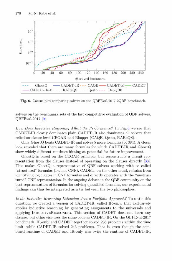
270 M. N. Rabe et al.

0 20 40 60 80 100 120 140 160 180 200 220 240

10−1

100

101

102

# solved instances

time(sec.)

GhostQ CADET-IR CAQE CADET-E CADETCADET-IR-E RAReQS Qesto DepQBF

Fig. 6. Cactus plot comparing solvers on the QBFEval-2017 2QBF benchmark.

solvers on the benchmark sets of the last competitive evaluation of QBF solvers,QBFEval-2017 [9].

How Does Inductive Reasoning Affect the Performance? In Fig. 6 we see thatCADET-IR clearly dominates plain CADET. It also dominates all solvers thatrelied on clause-level CEGAR and Bloqqer (CAQE, Qesto, RAReQS).

Only GhostQ beats CADET-IR and solves 5 more formulas (of 384). A closerlook revealed that there are many formulas for which CADET-IR and GhostQshow widely different runtimes hinting at potential for future improvement.

GhostQ is based on the CEGAR principle, but reconstructs a circuit rep-resentation from the clauses instead of operating on the clauses directly [33].This makes GhostQ a representative of QBF solvers working with so called“structured” formulas (i.e. not CNF). CADET, on the other hand, refrains fromidentifying logic gates in CNF formulas and directly operates with the “unstruc-tured” CNF representation. In the ongoing debate in the QBF community on thebest representation of formulas for solving quantified formulas, our experimentalfindings can thus be interpreted as a tie between the two philosophies.

Is the Inductive Reasoning Extension Just a Portfolio-Approach? To settle thisquestion, we created a version of CADET-IR, called IR-only, that exclusivelyapplies inductive reasoning by generating assignments to the universals andapplying InductiveReasoning. This version of CADET does not learn anyclauses, but otherwise uses the same code as CADET-IR. On the QBFEval-2017benchmark, IR-only and CADET together solved 235 problems within the timelimit, while CADET-IR solved 243 problems. That is, even though the com-bined runtime of CADET and IR-only was twice the runtime of CADET-IR,

Understanding and Extending Incremental Determinization for 2QBF 271

0 20 40 60 80 100 12010−2

10−1

100

101

102

# solved instances

time(sec.)

CADET-IRE CADET-IR RAReQS DepQBF GhostQCADET-E CADET Qesto CAQE

Fig. 7. Cactus plot comparing solver performance on the Hardware Fixpoint formulas.Some but not all of these formulas are part of QBFEval-2017. The formulas encodediameter problems that are known to be hard for classical QBF search algorithms [35].

they solved fewer problems. CADET-IR also uniquely solved 22 problems. Thisindicates that CADET-IR improves over the portfolio approach.

How Does Universal Expansion Affect the Performance? CADET-E clearly dom-inates plain CADET on QBFEval-2017, but compared to CADET-IR and someof the other QBF solvers, CADET-E shows mediocre performance overall. How-ever, for some subsets of formulas, such as the Hardware Fixpoint formulas shownin Fig. 7, CADET-E dominated CADET, CADET-IR, and all other solvers. Wealso combined the two extensions of CADET to obtain CADET-IR-E. While thishelped to improve the performance on the Hardware Fixpoint formulas even fur-ther, it did not change the overall picture on QBFEval-2017.

7 Conclusion

Reasoning in quantified logics is one of the major challenges in computer-aidedverification. Incremental Determinization (ID) introduced a new algorithmicprinciple for reasoning in 2QBF and delivered first promising results [8]. In thiswork, we formalized and generalized ID to improve the understanding of thealgorithm and to enable future research on the topic. The presentation of thealgorithm as a set of inference rules has allowed us to disentangle the designchoices from the principles of the algorithm (Sect. 3). Additionally, we haveexplored two extensions of ID that both significantly improve the performance:The first one integrates the popular CEGAR-style algorithms and IncrementalDeterminization (Sect. 4). The second extension integrates a different type ofreasoning termed universal expansion (Sect. 5).

272 M. N. Rabe et al.

Acknowledgements. We want to thank Martina Seidl, who brought up the idea toformalize ID as inference rules, and Vijay D’Silva, who helped with disentangling thedifferent perspectives on the algorithm. This work was supported in part by NSF grants1139138, 1528108, 1739816, SRC contract 2638.001, the Intel ADEPT center, and theEuropean Research Council (ERC) Grant OSARES (No. 683300).

References

1. Solar-Lezama, A., Rabbah, R.M., Bodık, R., Ebcioglu, K.: Programming by sketch-ing for bit-streaming programs. In: Proceedings of PLDI, pp. 281–294 (2005)

2. Alur, R., Bodik, R., Juniwal, G., Martin, M.M., Raghothaman, M., Seshia, S.A.,Singh, R., Solar-Lezama, A., Torlak, E., Udupa, A.: Syntax-guided synthesis.Depend. Softw. Syst. Eng. 40, 1–25 (2015)

3. Faymonville, P., Finkbeiner, B., Rabe, M.N., Tentrup, L.: Encodings of boundedsynthesis. In: Legay, A., Margaria, T. (eds.) TACAS 2017. LNCS, vol. 10205, pp.354–370. Springer, Heidelberg (2017). https://doi.org/10.1007/978-3-662-54577-5 20

4. Bloem, R., Konighofer, R., Seidl, M.: SAT-based synthesis methods for safety specs.In: McMillan, K.L., Rival, X. (eds.) VMCAI 2014. LNCS, vol. 8318, pp. 1–20.Springer, Heidelberg (2014). https://doi.org/10.1007/978-3-642-54013-4 1

5. Solar-Lezama, A., Tancau, L., Bodık, R., Seshia, S.A., Saraswat, V.A.: Combi-natorial sketching for finite programs. In: Proceedings of the 12th InternationalConference on Architectural Support for Programming Languages and OperatingSystems (ASPLOS), pp. 404–415. ACM Press, October 2006

6. Clarke, E., Grumberg, O., Jha, S., Lu, Y., Veith, H.: Counterexample-guidedabstraction refinement. In: Emerson, E.A., Sistla, A.P. (eds.) CAV 2000. LNCS,vol. 1855, pp. 154–169. Springer, Heidelberg (2000). https://doi.org/10.1007/10722167 15

7. Jha, S., Seshia, S.A.: A theory of formal synthesis via inductive learning. Acta Inf.54(7), 693–726 (2017)

8. Rabe, M.N., Seshia, S.A.: Incremental determinization. In: Creignou, N., Le Berre,D. (eds.) SAT 2016. LNCS, vol. 9710, pp. 375–392. Springer, Cham (2016). https://doi.org/10.1007/978-3-319-40970-2 23

9. Pulina, L.: The ninth QBF solvers evaluation - preliminary report. In: Proceedingsof QBF@SAT. CEUR Workshop Proceedings, vol. 1719, pp. 1–13. CEUR-WS.org(2016)

10. Biere, A.: Resolve and expand. In: Hoos, H.H., Mitchell, D.G. (eds.) SAT 2004.LNCS, vol. 3542, pp. 59–70. Springer, Heidelberg (2005). https://doi.org/10.1007/11527695 5

11. Pigorsch, F., Scholl, C.: An AIG-based QBF-solver using SAT for preprocessing.In: Proceedings of DAC, pp. 170–175. IEEE (2010)

12. Charwat, G., Woltran, S.: Dynamic programming-based QBF solving. In: Lonsing,F., Seidl, M. (eds.) Proceedings of Quantified Boolean Formulas. CEUR WorkshopProceedings, vol. 1719, pp. 27–40 (2016)

13. Baumgartner, P., Tinelli, C.: The model evolution calculus. In: Baader, F. (ed.)CADE 2003. LNCS (LNAI), vol. 2741, pp. 350–364. Springer, Heidelberg (2003).https://doi.org/10.1007/978-3-540-45085-6 32

14. Nieuwenhuis, R., Oliveras, A., Tinelli, C.: Abstract DPLL and abstract DPLLmodulo theories. In: Baader, F., Voronkov, A. (eds.) LPAR 2005. LNCS (LNAI),vol. 3452, pp. 36–50. Springer, Heidelberg (2005). https://doi.org/10.1007/978-3-540-32275-7 3

Understanding and Extending Incremental Determinization for 2QBF 273

15. de Moura, L., Jovanovic, D.: A model-constructing satisfiability calculus. In: Gia-cobazzi, R., Berdine, J., Mastroeni, I. (eds.) VMCAI 2013. LNCS, vol. 7737, pp.1–12. Springer, Heidelberg (2013). https://doi.org/10.1007/978-3-642-35873-9 1

16. Fazekas, K., Seidl, M., Biere, A.: A duality-aware calculus for quantified Booleanformulas. In: Proceedings of SYNASC, pp. 181–186. IEEE Computer Society (2016)

17. D’Silva, V., Haller, L., Kroening, D.: Abstract conflict driven learning. In: Pro-ceedings POPL, pp. 143–154. ACM (2013)

18. Giunchiglia, E., Narizzano, M., Tacchella, A.: QuBE: a system for deciding quan-tified Boolean formulas satisfiability. In: Gore, R., Leitsch, A., Nipkow, T. (eds.)IJCAR 2001. LNCS, vol. 2083, pp. 364–369. Springer, Heidelberg (2001). https://doi.org/10.1007/3-540-45744-5 27

19. Lonsing, F., Biere, A.: DepQBF: a dependency-aware QBF solver. JSAT 7(2–3),71–76 (2010)

20. Ranjan, D., Tang, D., Malik, S.: A comparative study of 2QBF algorithms. In:Proceedings of SAT. ACM (2004)

21. Janota, M., Marques-Silva, J.: Abstraction-based algorithm for 2QBF. In: Sakallah,K.A., Simon, L. (eds.) SAT 2011. LNCS, vol. 6695, pp. 230–244. Springer, Heidel-berg (2011). https://doi.org/10.1007/978-3-642-21581-0 19

22. Janota, M., Klieber, W., Marques-Silva, J., Clarke, E.: Solving QBF with coun-terexample guided refinement. In: Cimatti, A., Sebastiani, R. (eds.) SAT 2012.LNCS, vol. 7317, pp. 114–128. Springer, Heidelberg (2012). https://doi.org/10.1007/978-3-642-31612-8 10

23. Janota, M., Marques-Silva, J.: Solving QBF by clause selection. In: Proceedings ofIJCAI, pp. 325–331. AAAI Press (2015)

24. Rabe, M.N., Tentrup, L.: CAQE: a certifying QBF solver. In: Proceedings ofFMCAD, pp. 136–143 (2015)

25. Bloem, R., Braud-Santoni, N., Hadzic, V.: QBF solving by counterexample-guidedexpansion. CoRR, vol. abs/1611.01553 (2016.). http://arxiv.org/abs/1611.01553

26. Tentrup, L.: On expansion and resolution in CEGAR based QBF solving. In:Majumdar, R., Kuncak, V. (eds.) CAV 2017. LNCS, vol. 10427, pp. 475–494.Springer, Cham (2017). https://doi.org/10.1007/978-3-319-63390-9 25

27. Tseitin, G.S.: On the complexity of derivation in propositional calculus. In: Studiesin Constructive Mathematics and Mathematical Logic, Reprinted in [36], vol. 2,no. 115–125, pp. 10–13 (1968)

28. Buning, H., Karpinski, M., Flogel, A.: Resolution for quantified Boolean formulas.Inf. Comput. 117(1), 12–18 (1995)

29. Janota, M., Marques-Silva, J.: Expansion-based QBF solving versus Q-resolution.Theoret. Comput. Sci. 577, 25–42 (2015)

30. Robinson, J.A.: A machine-oriented logic based on the resolution principle. J. ACM12(1), 23–41 (1965)

31. Marques-Silva, J.P., Sakallah, K.A.: GRASP - a new search algorithm for satisfia-bility. In: Proceedings of CAD, pp. 220–227. IEEE (1997)

32. Janota, M., Klieber, W., Marques-Silva, J., Clarke, E.M.: Solving QBF with coun-terexample guided refinement. Artif. Intell. 234, 1–25 (2016)

33. Klieber, W., Sapra, S., Gao, S., Clarke, E.: A non-prenex, non-clausal QBF solverwith game-state learning. In: Strichman, O., Szeider, S. (eds.) SAT 2010. LNCS,vol. 6175, pp. 128–142. Springer, Heidelberg (2010). https://doi.org/10.1007/978-3-642-14186-7 12

274 M. N. Rabe et al.

34. Biere, A., Lonsing, F., Seidl, M.: Blocked clause elimination for QBF. In: Bjørner,N., Sofronie-Stokkermans, V. (eds.) CADE 2011. LNCS (LNAI), vol. 6803, pp.101–115. Springer, Heidelberg (2011). https://doi.org/10.1007/978-3-642-22438-6 10

35. Tang, D., Yu, Y., Ranjan, D., Malik, S.: Analysis of search based algorithms forsatisfiability of propositional and quantified Boolean formulas arising from circuitstate space diameter problems. In: Hoos, H.H., Mitchell, D.G. (eds.) SAT 2004.LNCS, vol. 3542, pp. 292–305. Springer, Heidelberg (2005). https://doi.org/10.1007/11527695 23

36. Siekmann, J., Wrightson, G.: Automation of Reasoning: 2: Classical Papers onComputational Logic 1967–1970. Springer, Heidelberg (1983)

Open Access This chapter is licensed under the terms of the Creative CommonsAttribution 4.0 International License (http://creativecommons.org/licenses/by/4.0/),which permits use, sharing, adaptation, distribution and reproduction in any mediumor format, as long as you give appropriate credit to the original author(s) and thesource, provide a link to the Creative Commons license and indicate if changes weremade.

The images or other third party material in this chapter are included in the chapter’sCreative Commons license, unless indicated otherwise in a credit line to the material. Ifmaterial is not included in the chapter’s Creative Commons license and your intendeduse is not permitted by statutory regulation or exceeds the permitted use, you willneed to obtain permission directly from the copyright holder.

The Proof Complexity of SMT Solvers

Robert Robere1(B), Antonina Kolokolova2, and Vijay Ganesh3

1 University of Toronto, Toronto, Canadarobere@cs.toronto.edu

2 Memorial University of Newfoundland, St. John’s, Canadakol@mun.ca

3 University of Waterloo, Waterloo, Canadavijay.ganesh@uwaterloo.ca

Abstract. The resolution proof system has been enormously helpful indeepening our understanding of conflict-driven clause-learning (CDCL)SAT solvers. In the interest of providing a similar proof complexity-theoretic analysis of satisfiability modulo theories (SMT) solvers, weintroduce a generalization of resolution called Res(T). We show thatmany of the known results comparing resolution and CDCL solvers liftto the SMT setting, such as the result of Pipatsrisawat and Darwicheshowing that CDCL solvers with “perfect” non-deterministic branchingand an asserting clause-learning scheme can polynomially simulate gen-eral resolution. We also describe a stronger version of Res(T), Res∗(T),capturing SMT solvers allowing introduction of new literals. We analyzethe theory EUF of equality with uninterpreted functions, and show thatthe Res∗(EUF) system is able to simulate an earlier calculus introducedby Bjørner and de Moura for the purpose of analyzing DPLL(EUF). Fur-ther, we show that Res∗(EUF) (and thus SMT algorithms with clauselearning over EUF, new literal introduction rules and perfect branching)can simulate the Frege proof system, which is well-known to be far morepowerful than resolution. Finally, we prove under the Exponential TimeHypothesis (ETH) that any reduction from EUF to SAT (such as theAckermann reduction) must, in the worst case, produce an instance ofsize Ω(n log n) from an instance of size n.

1 Introduction

It is common practice in formal verification literature to view SAT/SMT solveralgorithms as proof systems and study their properties, such as soundness, com-pleteness and termination, using proof-theoretic tools [GHN+04,ORC09,Tin12].However, much work remains in applying the powerful lens of proof complexitytheory in understanding the relative power of these solvers. All too often, thepower of SAT and SMT (satisfiability modulo theories) solving algorithms isdetermined by how they perform at the annual SAT or SMTCOMP competi-tions [BHJ17,smt]. While such competitions are an extremely useful practicaltest of the power of solving methods, they do not address fundamental questions

c© The Author(s) 2018H. Chockler and G. Weissenbacher (Eds.): CAV 2018, LNCS 10982, pp. 275–293, 2018.https://doi.org/10.1007/978-3-319-96142-2_18

276 R. Robere et al.

such as which heuristics are truly responsible for the power of these solvers orwhat are the lower bounds for these methods when viewed as proof systems.

Solvers, by their very nature, are a tangled jumble of heuristics that interactwith each other in complicated ways. Many SMT solvers run into hundreds ofthousands of lines of code, making them very hard to analyze. It is often difficultto discern which sets of heuristics are universally useful, which sets are tailoredto a class of instances, and how their interactions actually help solver perfor-mance. A purely empirical approach, while necessary, is far from sufficient indeepening our understanding of solver algorithms. What is needed is an appro-priate combination of empirical and theoretical approaches to understanding thepower of solvers. Fortunately, proof complexity theory provides a powerful lensthrough which to mathematically analyze solver algorithms as proof systems andto understand their relative power via lower bounds. The value of using proofcomplexity theory to better understand solving algorithms as proof systems isthree-fold: first, it allows us to identify key ingredients of a solving algorithm andprove lower bounds to non-deterministic combinations of such ingredients. Thatis, we can analyze the countably many variants of a solving algorithm in a unifiedmanner via a single analysis, rather than analyzing different configurations ofthe same set of proof-theoretic ingredients; second, proof complexity-theoretictools allow us to recognize the relative power of two proof systems, via appro-priate lower bounds, even if both have worst-case exponential time complexity;finally, proof complexity theory brings with it a rich literature and connectionsto other sub-fields of complexity theory (e.g., circuit complexity) that we may beable to leverage in analyzing solver algorithms. Many proof complexity theoristsand logicians have long recognized this, and there is rich literature on the anal-ysis of SAT solving algorithms such as DPLL and conflict-driven clause-learning(CDCL) solvers [PD11,BKS04,BBJ14,AFT11]. In this paper, we lift some ofthese results to the setting of SMT solvers, following the work of Bjørner and deMoura [BM14].

Our focus is primarily the proof complexity-theoretic analysis of the“DPLL(T ) method”1, the prime engine behind many modern SMT solvers[GHN+04,Tin12]. (While other approaches to solving first-order formulas havebeen studied, DPLL(T) remains a fundamental and dominant approach.) ADPLL(T)-based SMT solver takes as input a Boolean combination of first-ordertheory T atoms or their negation (aka, theory literals), and decides whethersuch an input is satisfiable. Informally, a typical DPLL(T)-based SMT solver S

1 Prior to mid 2000’s, SAT researchers and complexity theorists confusingly used theterm DPLL to refer to both the original algorithm proposed by Davis, Putnam,Loveland, and Loeggemann in 1960, as well as the newer algorithm by Joao Marques-Silva and Karem Sakallah that added clause learning to DPLL (proposed in 1996),even though they are vastly different in power as proof systems. We will follow theliterature and use DPLL(T ) to indicate a “modern” SMT solver with clause learningand restarts, but, we urge SMT solver researchers to use the more appropriate termCDCL(T ) rather than DPLL(T ) to refer to the lazy approach to SMT.

The Proof Complexity of SMT Solvers 277

is essentially a CDCL Boolean SAT solver that calls out a theory solver Ts dur-ing its search to perform theory propagations and theory conflict-clause learning.The typical theory solver Ts is designed to accept only quantifier-free conjunc-tion of theory T literals (the T in the term DPLL(T)), while the SAT solver“handles” the Boolean structure of input formulas. Roughly speaking, the SMTsolver S works as follows: First, it constructs a Boolean abstraction BF of theinput formula F , by replacing theory literals by Boolean variables. If BF isUNSAT, S returns UNSAT. Otherwise, satisfying assignments to the Booleanabstraction BF are found, which in turn correspond to conjunctions of theoryliterals. Such conjunctions are then input to the theory solver Ts, which maydeduce new implied formulas (via theory propagation and conflict clause learn-ing) that are then used to help prune the search space of assignments to F . Thesolver S returns SAT upon finding a satisfying theory assignment to the input F ,and UNSAT otherwise. (For further details, we refer the reader to the excellentexposition on this topic by Tinelli [Tin12].)

A Brief Description of the Res(T ) Proof System: To abstractly model aDPLL(T)-based SMT solver S, we define a proof system Res(T ) below for a givenfirst-order theory T . The Res in Res(T ) refers to the general resolution proofsystem for Boolean logic. Without loss of generality, we assume that Res(T )accepts theory formulas in conjunctive normal form (CNF). Let F denote aCNF with propositional variables representing atoms from an underlying theoryT , and for any clause C in FF let vars(F ) denote the set of propositional atomsoccurring in F . The proof rules of Res(T ) augment the resolution proof rule asfollows: A proof in Res(T ) is a general resolution refutation of F , where at anystep the theory T -solver can add to the set of clauses an arbitrary clause Csuch that T � C and every propositional atom in vars(C) occurs in the originalformula. That is, each line of a Res(T ) proof is deduced by one of the followingrules:

Resolution. C ∨ �,D ∨ � � C ∨ D, for previously derived clauses C and D.Theory Derivation. � C for any clause C such that T � C and for which every

theory literal in C occurs in the input formula.

For example, a theory of linear arithmetic may introduce a clause (x ≥ 5∨y ≥7 ∨ x + y < 12), which can then be used in the subsequent steps of a resolutionproof, provided each of those literals occurred in the original CNF formula F .The filter on the theory rule of Res(T ) models the fact that in many modernSMT solvers, the “theory solver” is only allowed to reason about literals whichalready occur in the formula. Recent solvers such as Z3, Yices [Z3,Yic] break thisrule and allow the theory solver to introduce new propositional atoms; to modelthis we introduce the stronger variant Res∗(T ) with a strengthened theory rule:

Strong Theory Derivation: � C for any clause C such that T � C.

278 R. Robere et al.

1.1 Our Contributions

We prove the following results about the two systems Res(T ), Res∗(T ) and thecomplexity of SMT solving.

1. We show that DPLL(T ) with an arbitrary asserting clause learning schemeand non-deterministic branching and theory propagation is equivalent (as aproof system) to Res(T ) for any theory T . More precisely: if the theory solverin DPLL(T ) can only reason about literals in the input, then it is equivalentto Res(T ); if it can reason about arbitrary literals then it is equivalent toRes∗(T ). (See Sect. 3)

2. When the theory T is E, the theory of pure equalities, Res∗(E) is equivalentto the SP (E) system of Bjørner et al. [BDdM08], which seems to have noefficient proofs of the PHP. (See Sect. 5.1)

3. When the theory T is EUF (equality with uninterpreted function symbols),the proof system Res∗(EUF) can simulate E-Res, a different generalization ofresolution introduced by Bjorner and de Moura [BM14] for the purpose of sim-ulating standard implementations of DPLL(EUF). Furthermore, Res∗(EUF)can simulate the powerful Frege proof system. (See Sect. 5.2)

4. When T is LA, a theory of linear arithmetic over a set of numbers contain-ing integers, Res(LA) can polynomially simulate the system R(lin) of Raz andTzameret [RT08], and thus has polynomial size proofs of several hard tautolo-gies such as the pigeonhole principle and Tseitin tautologies. (See Sect. 5.3)

5. Finally, we prove under the Exponential Time Hypothesis (ETH) that anyreduction from EUF to SAT (such as the Ackermann reduction) must, in theworst case, produce an instance of size Ω(n log n) from an instance of size n.(See Sect. 6)

These results seem to suggest that our generalization is the “right” proof sys-tem corresponding to DPLL(T ), as it characterizes proofs produced by DPLL(T )and it can simulate other proof systems introduced in the literature to captureDPLL(T ) for particular theories T .

1.2 Previous Work

Among the previous proof systems combining resolution with non-propositionalreasoning are R(CP) proof system of [Kra98], where propositional variables arereplaced with linear inequalities, and R(lin) introduced by Raz and Tzameret[RT08], which reasons with linear equalities, modifying the resolution rule. R(lin)polynomially simulates R(CP) when all coefficients in an R(CP) proof are polyno-mially bounded. In the SMT community, Bjørner et al. [BDdM08,BM14] intro-duced calculi capturing the power of resolution over the theory of equality andequality with uninterpreted functions. They show that these systems capturethe power of resolution over the corresponding theories, extended with rules forintroducing new atoms. Our results supersede previous work since our simula-tions hold for any first-order theory T .

The Proof Complexity of SMT Solvers 279

2 Preliminaries

2.1 Propositional Proof Systems

In this paper, all proof systems are defined by a set of “allowed lines” equippedwith a list of deduction rules that allow us to deduce new lines from old ones. Wefirst recall the resolution system, which is a refutation system for propositionalformulas in CNF (product of sums) form. The lines of a resolution proof aredisjunctions of boolean literals called clauses, and these lines are equipped witha single deduction rule called the resolution rule: given two clauses of the formC ∨ �, D ∨ � we deduce the clause C ∨ D. If φ = C1 ∧ C2 ∧ · · · ∧ Cm is anunsatisfiable CNF formula then a resolution refutation of φ is a sequence ofclauses C1, C2, . . . , Cm, Cm+1, . . . , Ct where Ct is the empty clause and all clausesCi with i > m are deduced from earlier clauses by applying the resolution rule.

Observe that clauses satisfy a subsumption principle: if C, D are clausessuch that C ⊆ D then every assignment satisfying C also satisfies D. Thisimplies that we can safely add a weakening rule to resolution which, from aclause C, derives the clause C ∨ x for any literal x not already occurring in C.The subsumption principle implies that this weakening rule does not change thepower of resolution, as any use of a clause D ⊇ C can be eliminated or replacedwith C.

We also consider the Frege proof system, which captures standard “textbook-style” proofs. The lines of a Frege system are given by arbitrary boolean formulas,and from two boolean formulas we can deduce any new boolean formula whichfollows under typical boolean reasoning (e.g. deducing the conjunction of two for-mulas, the disjunction of their negation, and so on). Crucially, Frege proofs allowapplying a generalized “resolution rule” to arbitrary polynomial-size formulas.

The power of different propositional proof systems are compared using thenotion of an polynomial simulation (p-simulation). Proof system A polynomi-ally simulates (or p-simulates) proof system B if, for every unsatisfiable formulaF , the shortest refutation proof of F in A is at most polynomially longer thanthe shortest refutation proof of a formula F in B. For example, the Frege proofsystem p-simulates the Resolution proof system, but the converse is widely con-jectured not to hold.

2.2 First-Order Theories

In this paper we study proof systems for first-order theories. For the sake of com-pleteness we recall some relevant definitions from first-order logic, but remarkthat this is essentially standard fare.

Let L be a first-order signature (a list of constant symbols, function symbols,and predicate symbols). Given a set of L-sentences A and an L-sentence B wewrite A � B if every model of A is also a model of B. A first order theory (orsimply a theory) is a set of L-sentences that is consistent (that is, it has a model)and is closed under �. The decision problem for a theory T is the following: givena set S of literals over L, decide if there is a model M of T such that M � S.

280 R. Robere et al.

The satisfiability problem for T , also denoted T -SAT, is the following: given aquantifier-free formula F in T in conjunctive normal form (CNF), decide if thereis a model M of T such that M � F .

A simple example of a theory is E, the conjunctive theory of equality. Thesignature of E contains a single predicate symbol = and an infinite list of con-stant symbols. It is axiomatized by the standard axioms of equality (reflexivity,symmetry, and transitivity), and a sample sentence in E would be the formulaa �= b ∨ b �= c ∨ a = c, which encodes the transitivity of equality between theconstant symbols a, b, and c. Following the SMT literature, we will call termsfrom the theory (such as a and b) theory variables, and the atoms derived fromthese terms (such as a �= b or a = c) will be called theory literals or just literals.We note that the decision problem for E can be decided very efficiently [DST80];in contrast, the satisfiability problem for E is easily seen to be NP-complete.

3 Res(T ): Resolution Modulo Theories

We now define a generalization of resolution which captures the type of reasoningmodulo a first-order theory that is common in SMT solvers. We give two variants:the first, denoted Res(T ), allows the deduction of any clause C of theory literalssuch that T � C and for which every literal in C already occurs in the inputformula. This is intended to model “standard” lazy SMT solvers [NOT06] whichonly reason about literals in the input formula.

The second, more powerful variant is denoted Res∗(T ), and allows the deduc-tion of any clause of literals C such that T � C, even if the new clause containsliterals which do not occur in the input formula. We introduce this to explorethe power of lazy SMT solvers that are allowed to introduce new literals fromthe theory, and note that there are well-known examples in the SMT literaturewhich show that introducing new literals can drastically decrease the length ofrefutations (e.g. the diamond equalities [BDdM08]). Indeed, in Sect. 5.2 we showthat this power can drastically increase the proof theoretic strength of SMTsolvers.

Definition 1 (Res(T ),Res∗(T )). Let T be a theory and let F be an quantifier-free CNF formula over T . The lines of a Res(T ) (Res∗(T )) proof are quantifier-free clauses of theory literals deduced from F and T by the following derivationrules.

Resolution. C ∨ �,D ∨ � � C ∨ D.

Weakening. C � C ∨ � for any theory literal � occurring in the input formula.

Theory Derivation (Res(T )). � C for any clause C satisfying T � C and forwhich every literal in C occurs in the input formula.

Strong Theory Derivation (Res∗(T )). � C for any clause C satisfying T � C.A refutation of F is a proof in which the final line is the empty clause.

The Proof Complexity of SMT Solvers 281

It is easy to see that both Res(T ) and Res∗(T ) are sound since all rules aresound, and completeness follows from a straightforward modification of the usualproof of resolution completeness (see, e.g. Jukna [Juk12]).

Technically speaking, Res(T ) is not a (formal) propositional proof system asdefined by Cook and Reckhow [CR79] since the proofs may not be efficientlyverifiable if deductions from the theory T are computationally difficult to verify.However, all theories considered in this paper (cf. Sect. 5) are very efficientlydecidable, and thus the corresponding Res(T ) proofs are efficiently verifiable.

Note that the clauses introduced by the theory derivations are arbitrary the-orems of T ; this means there is no direct information exchange between theresolution proof and the theory. It is enough to derive clauses in the theoryderivation rules rather than arbitrary formulas since every axiom can be writtenin CNF form, and introduced as a sequence of clauses. The strong theory deriva-tion rule can introduce new theory literals which might not have been present inthe initial formula—we emphasize that the new theory literals can even containtheory variables (i.e. first-order terms) that did not occur in the original formula.We will see that this ability to introduce new literals seems to give Res∗(T ) extrapower over general resolution.

4 Lazy SMT Solvers and Res(T )

In this section we show that lazy SMT solvers and resolution modulo theoriesare polynomially-equivalent as proof systems, provided that the SMT solvers aregiven a set of branching and restart decisions a priori.

We model SMT solvers by the algorithm schema2 DPLL(T ), which is givenin Algorithm 1. Using this schema we prove two results: first, if the theorysolver in DPLL(T ) can only reason about literals occurring in its input formula,then DPLL(T ) is polynomially equivalent to Res(T ). Second, if the theory solveris strengthened so that it is allowed to introduce new literals then the result-ing solver can polynomially simulate Res∗(T ). The proofs of these results usetechniques developed for comparing Boolean CDCL solvers and resolution byPipatsrisawat and Darwiche [PD11].

2 In the literature, SMT solvers are typically defined as abstract state-transition sys-tems (see, for instance, [GHN+04,BM14]); we have chosen to define it instead as analgorithm schema (cf. Algorithm 1) inspired by the abstract definition of a CDCLsolver by Pipatsrisawat and Darwiche [PD11].

282 R. Robere et al.

Algorithm 1. DPLL(T )

Input: CNF formula F over T -literals;Output: SAT or UNSATLet σ = ∅ be an initially empty partial assignment of T -literals;Let Γ be an initially empty collection of learned clauses;while true do

if F ∧ Γ ∧ σ �1 ∅ thenif σ = ∅ then

return UNSAT;Apply the clause learning scheme to learn a conflict clause C,add it to Γ ;Backjump σ to the second highest decision level in C;

else if σ �T ∅ thenApply the T -conflict scheme to learn a conflict clause C, add itto Γ ;Backjump σ to the second highest decision level in C;

elseif σ satisfies F then

return SAT;Apply the restart scheme to decide whether or not to restart;if restart then

Set σ = ∅;Restart loop;

Apply the T -propagate scheme;Unit propagate literals to completion and update σ accordingly;Apply the branching scheme to choose a decision literal �, setσ = σ ∪ {�};

If T is a theory and A,B are formulas over T then we write A �T B as ashorthand for T ∪ {A} � B (i.e. every model of the theory T that satisfies Aalso satisfies B). We also define unit resolution, which describes the action ofthe unit propagator.

Definition 2 (Unit Resolution). Let F be a collection of clauses over anarbitrary theory T . A clause C is derivable from F by unit resolution if thereexists a resolution proof from F of C such that in each application of the reso-lution rule, one of the clauses is a unit clause. If C is derivable from F by unitresolution then we write F �1 C. If F �1 ∅ then we say F is unit refutable,otherwise it is unit consistent.

A DPLL(T ) algorithm is defined by specifying algorithms for each of thebolded “schemes” in Algorithm 1:

Clause Learning Scheme. When a clause in the database is falsified by thecurrent partial assignment, the Clause Learning Scheme is applied to learna new clause C which is added to the database of stored clauses.

The Proof Complexity of SMT Solvers 283

Restart Scheme. The solver applies the Restart Scheme to decide whetheror not to restart its search, discarding the current partial assignment σ andsaving the list of learned clauses.

Branching Scheme. The Branching Scheme is applied to choose an unas-signed variable from the formula F or from the learned clauses Γ and assign thevariable a Boolean value.

T -Propagate Scheme. During search, the DPLL(T ) solver can hand the theorysolver the current partial assignment σ and ask whether or not it should unit-propagate a literal; if a unit propagation is possible the theory solver will returna clause C from the theory witnessing this unit propagation.

T -Conflict Scheme. When the theory solver detects that the current partialassignment σ contradicts the theory, the T -Conflict Scheme is applied to learna new clause of literals C, ¬C ⊆ σ, which is added to the clause database.

We pay particular interest to the specification of the T -propagate scheme.The next definition describes two types of propagation schemes: a weak propa-gation scheme is only allowed to return clauses which propagate literals in theformula, while the more powerful strong propagation scheme returns a clause ofliterals from the theory that may contain new literals.

Definition 3. A weak T -propagate scheme is an algorithm which takes as inputa conjunction of theory literals σ over T and returns (if possible) a clause C =¬σ ∨ � where T � C and the literal � occurs in the input formula of the DPLL(T )algorithm.

A strong T -propagate scheme is an algorithm which takes as input a con-junction of literals σ over T , and if possible returns a clause C of literals from Tsuch that T � C and ¬σ ⊆ C. An algorithm equipped with a strong T -propagatescheme will be called a DPLL∗(T ) solver.

A DPLL(T ) algorithm equipped with a weak T -propagation scheme is equiv-alent to the basic theory propagation rules found in SMT solvers (see, forexample, [BM14,NOT06]). For technical convenience we assume that the weakT -propagate scheme adds a clause to the database “certifying” the unit prop-agation, while in actual implementations the clause would likely not be addedand the literal would simply be propagated. Recent SMT solvers [Yic,Z3] havestrengthened the interaction between the SAT solver and the theory solver, allow-ing the theory solver to return constraints over new variables; this is modelledvery generally by strong T -propagate schemes.

4.1 DPLL(T ) and Res(T )

We now prove the main result of this section, after introducing some preliminariesfrom [PD11] that are suitably modified for our setting. Fix a theory T . Anassignment trail is a sequence of pairs σ = {(�i, di)}ti=1 where each literal �i isa literal from the theory and each di ∈ {d, p}, indicating that the literal wasset by a decision or a unit propagation. The decision level of a literal �i in σ

284 R. Robere et al.

is the number of decision literals occurring in σ up to and including �i. Givenan assignment trail σ and a clause C we say that C is asserting if it containsexactly one literal occurring in σ at the highest decision level. A clause learningscheme is asserting if all conflict clauses produced by the scheme are assertingwith respect to the assignment trail at the time of conflict.

An extended branching sequence is an ordered sequence B = {β1, β2, . . . , βt}where each βi is either (1) a literal from the theory, (2) a symbol x ∈ {R,NR},to denote a restart or no-restart, respectively, or (3) a clause C such that T � C.Intuitively, extended branching sequences are used to provide a DPLL(T ) solverwith a list of instructions for how to proceed in its execution. For instance,whenever the solver calls the Branching Scheme, we consume the next βi fromthe sequence, and if it is a literal from the theory then the solver assigns thatliteral. Similarly, when the DPLL(T ) solver calls the Restart Scheme it uses thebranching sequence to dictate whether or not to restart, and when the solvercalls the T -propagate scheme it uses the sequence to dictate which clause tolearn. If the symbol does not correctly match the current scheme being calledthen the solver halts in error, and if the branching sequence is empty, then thealgorithm proceeds using the heuristics defined by the algorithm.

We now introduce absorbed clauses (and their duals, empowering clauses),which were originally defined by Pipatsrisawat and Darwiche [PD11] and inde-pendently by Atserias et al. [AFT11]. One should think of the absorbed clausesas being learned “implicitly”—they may not necessarily appear in F , but, if weassign all but one of the literals in the clause to false then unit propagation inDPLL(T ) will set the final literal to true.

Definition 4 (Empowering Clauses). Let F be a collection of clauses overan arbitrary theory T and let A be a DPLL(T ) solver. Let α be a conjunctionof literals, and let C = (¬α ⇒ �) be a clause. We say that C is empoweringwith respect to F at � if the following holds: (1) F ∪ T � C, (2) F ∧ α is unitconsistent, and (3) any execution of A on F that satisfies α without setting �does not unit-propagate �. The literal � is said to be empowering. If item (1), (2)are satisfied but (3) is false then we say that the solver A and F absorbs C at�; if A and F absorbs C at at every literal then the clause is simply absorbed.

For an example, consider the set of clauses (x ∨ y ∨ z), (¬z ∨ a), (¬a ∨ b).The clause (x ∨ y ∨ b) is absorbed by this set of clauses as, for instance, if wefalsify x and y then the unit-propagator will force b to be set to true. Thus inthe DPLL(T ) algorithm the unit propagator will behave as though this clause islearned even though it is not (if we remove the final clause ¬a∨b, then (x∨y∨b)is empowering but not absorbed).

The next lemma shows that for any theory clause C, there is an extendedbranching sequence which can be applied to absorb that clause.

Lemma 5. Let F be an unsatisfiable CNF over a theory T and let Π be anyRes(T ) proof from F . Let ΠT ⊆ Π be the set of clauses in Π derived usingthe theory rule. For any DPLL(T ) algorithm A there is an extended branchingsequence B such that after applying B to the solver A every clause in ΠT willbe absorbed.

The Proof Complexity of SMT Solvers 285

Proof. Order ΠT arbitrarily as C1, C2, . . . , Ct and remove any clause that isabsorbed or already in F , as these are clearly already absorbed. We constructB directly: add the negations of literals in C1 to B until one literal remains,and then add the clause C1 to the extended branching sequence. By definitionthe weak T -propagator will be called and will return C1, adding it to the clausedatabase. Restart and continue to the next theory clause in order.

Our proof of mutual simulations between Res(T ) and DPLL(T ) crucially relieson the following technical lemma (which is a modified version of a lemma from[PD11]).

Lemma 6. Let F be an unsatisfiable, unit-consistent CNF over literals from atheory T and let Π be any Res(T ) proof from F . Let ΠT be the set of clauses inΠ derived using the theory rule. Then there exists a clause C in Π that is bothempowering and unit-refutable with respect to F ∪ ΠT .

Proof. Let Π denote a Res(T )-refutation of F and assume without loss of gen-erality (by applying Lemma 5) that the first derived clauses in Π are in ΠT .If every clause in Π is unit-refutable from F , then the empty clause is unit-refutable and thus F is not unit-consistent, which is a contradiction. So, assumethat there exists a clause Ci which is the first clause in Π by this ordering suchthat it is not unit-refutable. Since Π is a Res(T )-proof, Ci is one of three types:either it is a clause in F , it is a clause derived from the theory rule, or Ci wasderived by applying the resolution rule to two clauses Cj , Ck. If Ci ∈ F thenit is clearly unit-refutable, which is a contradiction. If Ci was derived from thetheory rule then it is unit-refutable with respect to ΠT , which is again a con-tradiction. Finally, suppose that Ci was derived by applying the resolution ruleto clauses Cj and Ck, and write Cj = (α ⇒ �), Ck = (β ⇒ �) where � is theresolved literal and j, k < i in the ordering of clauses in Π. Since Cj and Ck

are both unit-refutable, assume by way of contradiction that neither Cj nor Ck

are empowering. It follows by definition that both clauses are absorbed at everyliteral. Thus, if we consider F ∧α∧β, it follows by the absorption property thatF ∧ α ∧ β �1 �,F ∧ α ∧ β �1 ¬� which implies that F ∧ α ∧ β �T

1 ∅. However,Ci = α ∧ β, and thus we have concluded Ci is unit-refutable, which is a contra-diction! Thus at least one of Cj or Ck is both empowering and unit-refutable.

The gist of the Lemma 6 is simple: if clauses C∨� and D∨� are both absorbedby a collection of clauses C, then asserting C ∧ D in the DPLL solver will hit aconflict since it will unit-imply both � and �. In the main theorem, proved next,we show that empowering and unit-refutable clauses will be absorbed by thesolver after sufficiently many restarts.

Theorem 7. The DPLL(T ) system with an asserting clause learning scheme,non-deterministic branching and T -propagation polynomially simulates Res(T ).Equivalently: for any unsatisfiable CNF F over a theory T , and any Res(T ) refu-tation Π of F there exists an extended branching sequence B such that runninga DPLL(T ) algorithm on input F using B will refute F in time polynomial inthe length of |Π|.

286 R. Robere et al.

Proof. Let F be an unsatisfiable CNF over the theory T , and let Π be a Res(T )refutation of F . Let ΠT ⊆ Π be the set of clauses in Π derived using thetheory rule, and write Π = C1, C2, . . . , Cm. As a first step, apply Lemma 5 andconstruct an extended branching sequence B′ which leads to the absorbtion ofall clauses in ΠT . We prove the following claim, from which the theorem directlyfollows.

Claim. Let C be any unit-refutable and empowering clause with respect to F .Then there exists an extended branching sequence B of polynomial size suchthat after applying B the clause C will be absorbed.

Let � be any empowering literal of C, and write C = (α ⇒ �). Let B beany extended branching sequence in which all literals in α are assigned. SinceC is empowering, it follows that F ∧ α is unit-consistent. Extending B with thedecision literal ¬� will therefore cause a conflict since C is unit-refutable. LetC ′ be the asserting clause obtained by applying the clause learning scheme toB∪{¬�}. If F ∧C ′ absorbs C at �, then we are done and we continue to the nextempowering literal. Otherwise, we resolve whatever conflicts the solver needs toresolve (possibly adding more learned clauses along the way) until the branchingsequence is unit-consistent.

Observe that after this process we must have that F ∧ C ′ �1 �′ where �′

is some literal at the same decision level as �, since the clause learning schemeis asserting. Thus the number of literals at the maximum decision level hasreduced by one. At this point, we restart and do exactly the same sequence ofbranchings—each time, as argued above, we reduce the number of literals at themaximum decision level by 1. Since � is a literal at the maximum decision level,it implies that after at most O(n) restarts (and O(n2) learned clauses) we willhave absorbed the clause C at �. Repeating this process at most n times foreach empowering literal in C we can absorb C, and it is clear that the numberof learned clauses is polynomial from the analysis.

We are now ready to finish the proof. Apply the claim repeatedly to the firstempowering and unit-refutable clause in Π to absorb that clause—by Lemma 6,such a clause will exist as long as the CNF F is not unit-refutable; a DPLL(T )solver can obtain an arbitrary theory clause by setting relevant literals in thebranching sequence and using theory propagation. Since the length of the proofΠ is finite (length m), it follows that this process must terminate after at most miterations. At this point, there can not be such an empowering and unit-refutableclause, and so by Lemma 6 it follows that F (with its learned clauses) is nowunit-refutable, and so the DPLL(T ) algorithm halts and outputs UNSAT.

The reverse direction of the theorem is straightforward, and thus we havethe following corollary:

Corollary 8. The DPLL(T ) system with an asserting clause learning scheme,non-deterministic branching and T -propagation is polynomially equivalent toRes(T ).

A key point of the above simulation is that it does not depend on whetheror not the T -propagation scheme is weak or strong—since the clauses learned

The Proof Complexity of SMT Solvers 287

by the scheme are specified in advance by the extended branching sequence thesame proof will apply if we began with a Res∗(T ) proof instead. Of course, if webegin with a Res∗(T ) proof instead of a Res(T ) proof we may use the full powerof the theory derivation rule, requiring that we use a DPLL∗(T ) algorithm witha strong T -propagation scheme instead. We record this observation as a secondtheorem.

Theorem 9. The DPLL∗(T ) system with an asserting clause learning scheme,non-deterministic branching and T -propagation is polynomially equivalent toRes∗(T ).

5 Case Studies: Resolution Modulo Common Theories

In this section, we study the power of Res(T ) over theories that are common inthe SMT context—namely, we focus on the theory of equality E, the theory ofuninterpreted function symbols EUF, and the theory of linear arithmetic LA.

5.1 Resolution over E: A Theory of Equality

We first consider E, the theory of equality. Bjørner et al. [BDdM08] introduced aproof-theoretic calculus called SP(E) for reasoning over the theory of equality—in a prototype of our main result, they showed that proofs in SP(E) exactlycharacterized proofs produced by a simple model SMT solver. In this sectionwe show that the theory Res∗(E) is polynomially-equivalent to SP(E), which isevidence that our general framework is the correct way of capturing the powerof SMT solvers.

Let us first reproduce the rules of SP(E) from [BDdM08]: Cut. C∨�, D∨¬� �C ∨ D, E-Dis. C ∨ a �= a � C, E-Eqs. C ∨ a = b ∨ a = c � C ∨ a = b ∨ b �= c,Sup. C ∨ a = b, D[a] � C ∨ D[b]. Observe that the Sup rule allows replacingsome occurrences of a term a in atoms of a clause D with b (not necessarily forall occurrences of a). Both the Sup rule and the E-Eqs rule can introduce literalsthat did not occur in the initial formula.

Proposition 10. Res∗(E) and SP(E) are polynomially equivalent.

Proof (Sketch). Bjørner et al. show that SP(E) exactly characterizes the proofsproduced by a simple theoretical model of an SMT solver, which we will denoteby DPLL(e + Δ) [BDdM08, Theorem 4.1]. Examining the solver DPLL(e + Δ)from [BDdM08], it is not hard to see it is equivalent to the algorithm DPLL∗(E)(that is, DPLL(T ) with a strong T -propagation rule). The equivalence betweenRes∗(E) and DPLL∗(E) follows by the Corollary of Theorem 9.

In the conclusion of [BDdM08] it is stated that there are no short SP(E)proofs of the following encoding of the pigeonhole principle (PHP): there areclauses of the form (di = r1 ∨ . . . di = rn), for i ∈ [1, n + 1], enforcing thatthe ith pigeon must travel to some hole, and clauses of the form (di �= dj) for

288 R. Robere et al.

i, j ∈ [1, n + 1] which, when combined with the first family of clauses and thetransitivity axioms of E, imply that no two pigeons can travel to the same hole.Since their SP(E) system is equivalent to Res∗(E) it follows that the lower boundson SP(E) carry over:

Corollary 11. If SP(E) does not have polynomial-size refutations of the pigeon-hole principle, then neither does Res∗(E).

5.2 Resolution over EUF: Equality with Uninterpreted Functions

Next, we study the theory EUF, which is an extension of the theory of equalityto contain uninterpreted function symbols. The signature of EUF consists ofan unlimited set of uninterpreted function symbols and constant symbols; aterm in the theory is thus inductively defined as either a constant symbol or anapplication of a function symbol to a sequence of terms: f(t1, . . . , tk). There isone relational symbol = interpreted as equality between terms, so theory literalsof EUF are of the form t = t′ for terms t, t′.

The axioms of EUF state that = is an equivalence relation, together witha family of congruence axioms for the function symbols stating, for any k-ary function symbol f and any sequences of terms t1, t2, . . . , tk, t′1, t

′2, . . . , t

′k,

if t1 = t′1, . . . , tk = t′k, then f(t1, . . . , tk) = f(t′1, . . . , t′k). The decision problem

for EUF can be decided in time O(n log n) by the Downey-Sethi-Tarjan congru-ence closure algorithm [DST80].

Using EUF as a central example, Bjorner and de Moura [BM14] observed thatDPLL(T ) suffers some serious limitations in terms of access to the underlyingtheory. To resolve this, they modified DPLL(EUF) with a set of non-deterministicrules that allowed it to dynamically introduce clauses corresponding to the con-gruence and transitivity axioms. To characterize the strength of this new algo-rithm, they introduced a variant of resolution called E-Res, extending SP(E)from [BDdM08] to reasoning over uninterpreted functions. We show that theRes∗(EUF) proof system can polynomially-simulate the E-Res system, whichagain suggests that we have the “correct” proof system for capturing SMT rea-soning. Due to space considerations, we leave the proof to the full version of thepaper.

Theorem 12. The system E-Res is polynomially simulated by Res∗(EUF).

However, unlike the case of SP(E) the converse direction is not so clear. Thetheory rule in Res∗(EUF) is fundamentally semantic: it allows one to derive anyclause which follows from the theory EUF semantically; this is in contrast tothe E-Res system which is fundamentally syntactic. Thus, to show that E-Respolynomially simulates EUF, one would need to show that any use of the theoryrule in a Res∗(EUF) proof could be somehow replaced with a short proof inE-Res. We leave this as an open problem.

Next, we show that Res∗(EUF) and E-Res can efficiently simulate the Fregeproof system, which is a very powerful propositional proof system studied inproof complexity. We note that the simulation crucially relies on the introduction

The Proof Complexity of SMT Solvers 289

of new theory literals; this suggests that an SMT solver which can intelligentlyintroduce new theory literals has the potential to be extremely powerful.

Theorem 13. Res∗(EUF) (and, in fact, E-Res) can efficiently simulate theFrege proof system.

Proof Sketch. We show the stronger statement that E-Res simulates Frege. Theidea of the proof is to introduce constants e0 �= e1 corresponding to False andTrue; every positive literal x in the original formula is replaced by x = e1, andnegative literal ¬x by x = e0. Then introduce uninterpreted function symbolsN,O,A, together with constraints that make N,O,A behave as NOT, OR andAND, respectively (such as N(e0) = e1 ∧ N(e1) = e0). So formulas in the Fregerefutation are iteratively transformed into expressions of the form tF = e0 ortF = e1, where tF is a term obtained by replacing Boolean connectives in aformula F by N,O,A. As the Frege proof ends with an empty sequent, thecorresponding E-Res proof ends with an empty clause. See the full version fordetails.

5.3 Resolution over LA: A Theory of Linear Arithmetic

Finally, we study the theory of linear arithmetic LA. A formula in the theory LAover a domain D is a conjunction of expressions of the form Σn

i=1aixi ◦ b, where◦ ∈ {=,≤, <, �=,≥, >}, and ai, xi ∈ D — usually, D is integers or reals3. Weshow that Res(LA) polynomially simulates the proof system R(lin) introducedby Raz and Tzameret [RT08]. This is interesting, as R(lin) has polynomial-sizeproofs of several difficult tautologies considered in proof complexity, such as thepigeonhole principle, Tseitin tautologies and the clique-colouring principle.

In the proof system R(lin) propositional variables are linear equations overintegers. The input formula is a CNF over such equations, together with∧n

i=1(xi = 0 ∨ xi = 1) clauses ensuring 0/1 assignment. The rules of infer-ence consist of a modified resolution rule, together with two structural rules,weakening and simplification:

R(lin)-cut. Let (A ∨ L1), (B ∨ L2) be two clauses containing linear equalitiesL1 and L2, respectively. From these two clauses, derive a clause (A ∨ B ∨(L1 − L2)).

Weakening. From a (possibly empty) clause A derive (A∨L) for any equation L.Simplification. From (A ∨ k = 0), where k �= 0 is a constant, derive A.

Proposition 14. Res(LA) polynomially simulates R(lin).

3 Some definitions of linear arithmetic do not include disequalities; however, as dise-qualities and strict inequalities occur naturally in SMT context, SMT-oriented lineararithmetic solvers do incorporate mechanisms for dealing with them.

290 R. Robere et al.

Proof. We show how to simulate rules of R(lin) in Res(LA). We can assume,without loss of generality, that Res(LA) has a weakening rule which simulatesweakening of R(lin) directly. For the simplification rule, note that LA � k �= 0for any k �= 0; one application of the resolution rule on (k �= 0) and (A ∨ k = 0)results in A.

Finally, let L1 be Σni=1aixi = b and L2 be Σn

i=1cixi = d. From (A ∨ L1),(B ∨ L2) we want to derive (A ∨ B ∨ L1 − L2). First derive in LA a clauseC = (Σn

i=1aixi �= b∨Σni=1cixi �= d∨Σn

i=1(ai − ci)xi = b−d). Resolving (A∨L1)with C, and then resolving the resulting clause with (B ∨ L2) gives the desired(A ∨ B ∨ (L1 − L2)).

Note that we didn’t need to specify whether LA is over the integers, rationalsor reals, and hence the proof works for any of them. Also, in order to establishour simulations it is sufficient to consider a fragment of LA with only equalitiesand inequalities, and produce only unit clauses and width-3 clauses of a fixedform.

Corollary 15. Res(LA) has polynomial-size proofs of the pigeonhole principle,Tseitin tautologies and a clique-colouring principle for k =

√(n) size clique and

k′ = (log n)2/8 log log n size colouring.

6 Lazy vs. Eager Reductions and the Exponential TimeHypothesis

Throughout this paper we have primarily discussed the Lazy approach to SMT.In this section, we consider the Eager approach, in which an input formula Fover a theory T is reduced to an equisatisfiable propositional formula G, whichis then solved using a suitable (Boolean) solver.

The Eager approach is still used in several modern SMT solvers such as theSTP solver for bit-vectors and arrays [GD07]. A common eager reduction usedwhen solving equations over the theory of equality, E (or its generalization touninterpreted function symbols EUF), is the Ackermann reduction. Let us firstdescribe a simple version of the Ackermann reduction over the theory E.

Let F denote a CNF over literals from the theory E—so, each literal is ofthe form a = b for constant terms a, b—which we will ultimately transform intoa Boolean SAT instance. Let n denote the number of constant terms occurringin F , let m denote the number of distinct literals occurring in F , and considerthe literal a = b and the literal b = a to be the same. For each literal a = bintroduce a Boolean variable xa=b, and for each clause of literals

∨i ai = bi create

a clause∨

i xai=bi . To encode the transitivity of equality, for each triple of terms(a, b, c) occurring in the initial CNF F introduce a clause of the form ¬xa=b ∨¬xb=c ∨ xa=c. Note that the final formula will have O(n2) Boolean variablescorresponding to each possible term a = b—a potential quadratic blow-up—which is unavoidable using this encoding due to the transitivity axioms. Observethat this blow-up only occurs in the eager approach—in the lazy approach tosolving we only need to consider the literals a = b which occur in the original

The Proof Complexity of SMT Solvers 291

formula F . It is therefore natural to wonder if this blow-up in the number ofinput variables can somehow be avoided.

In fact, one can construct a more clever Eager reduction from E-SAT to SATwhich only introduces O(n log n) boolean variables; however, this more cleverencoding does not represent the literals a = b as Boolean variables xa=b andinstead uses a more complicated pointer construction. This improved reductionturns out to be the best possible under the well-known (and widely believed)Exponential Time Hypothesis, which is a strengthening of P �= NP.

Exponential Time Hypothesis (ETH). There is no deterministic or ran-domized algorithm for SAT running in time 2o(n), where n is the number ofinput variables.

Theorem 16. Let F be an instance of E-SAT with n distinct terms. For anypolynomial-time reduction R from E-SAT to SAT, the boolean formula R(F)must have Ω(n log n) variables unless ETH fails.

Proof. By way of contradiction, suppose that ETH holds and let R be a reductionfrom E-SAT to SAT which introduces o(n log n) variables. Let 2-CSP denote aconstraint satisfaction problem with two variables per constraint. The theoremfollows almost immediately from the following result of Traxler [Tra08].

Theorem 17 (Theorem 1 in [Tra08], Rephrased). Consider any 2-CSP C1∧C2 ∧ · · · ∧ Cm over an alphabet Σ of size d, where each constraint is of the formx �= a ∨ y �= b for variables x, y and constants a, b ∈ Σ. Unless ETH fails, everyalgorithm for this problem requires time dcn for some universal constant c > 0.

There is a simple reduction from the restriction of 2-CSP described in theabove theorem to E-SAT. Introduce terms e1, e2, . . . , ed, each intended to rep-resent a symbol from the universe Σ, and also terms x1, x2, . . . , xn for eachvariable x occurring in the original CSP instance. Now, for each i �= j introduceunit clauses ei �= ej , and similarly for each i ∈ [n] add a clause of the formxi = e1 ∨ xi = e2 ∨ · · · ∨ xi = ed. Finally, for each constraint in the 2-CSP ofthe form xi �= a ∨ xj �= b introduce a clause xi �= ea ∨ xj �= eb, where ea, ebare the terms corresponding to the symbols a, b. Let F ′ denote the final E-SATinstance, and it is clear that F ′ is satisfiable if and only if the original 2-CSP issatisfiable, and also that F ′ has n + d constant terms.

Now, apply the Ackermann reduction R to F ′, obtaining a SAT instanceR(F ′). By assumption the final SAT instance has o((n+d) log(n+d)) variables;running the standard brute-force algorithm for SAT gives an algorithm runningin 2o((n+d) log(n+d)) time for the 2-CSP variant described above. However, by theabove theorem, every algorithm for this 2-CSP variant requires time at leastdcn = 2cn log d, which violates ETH if d ≈ n.

7 Conclusion

In this paper, we studied SMT solvers through the lens of proof complexity,introducing a generalization of the resolution proof system and arguing that it

292 R. Robere et al.

correctly models the “lazy” SMT framework DPLL(T ) [NOT06]. We further pre-sented and analyzed a stronger version Res∗(T ) that allows for the introductionof new literals, and showed that it models DPLL∗(T ), which is a modificationof an SMT solver that can introduce new theory literals; this captures the newliteral introduction in solvers such as Yices and Z3 [Z3,Yic].

There are many natural directions to pursue. First, although we have not con-sidered it here, it is natural to introduce an intermediate proof system betweenRes(T ) and Res∗(T ) which is allowed to introduce new theory literals but notnew theory variables. For instance, if we have the formula a = f(b) ∧ a = cin EUF, then this intermediate proof system could introduce the theory literalc = f(b) but not the theory literal f(c) = f(a), whereas both are allowed tobe introduced by Res∗(T ). It is not clear to us if this intermediate system cansimulate Frege, and we suggest studying it in its own right.

A second direction that we believe is quite interesting is extending our resultson EUF to capture the extended Frege system, which is the most powerful proofsystem typically studied in proposition proof complexity. Intuitively, it seemsthat EUF by itself is not strong enough to capture extended Frege; we considerfinding a new theory T which can capture it an interesting open problem.

References

[AFT11] Atserias, A., Fichte, J.K., Thurley, M.: Clause-learning algorithms withmany restarts and bounded-width resolution. J. Artif. Intell. Res. 40,353–373 (2011)

[BBJ14] Bonet, M.L., Buss, S., Johannsen, J.: Improved separations of regularresolution from clause learning proof systems. J. Artif. Intell. Res. 49,669–703 (2014)

[BDdM08] Bjørner, N., Dutertre, B., de Moura, L.: Accelerating lemma learningusing joins - DPLL(Join). In: 15th International Conference on Logic forProgramming Artificial Intelligence and Reasoning, LPAR 2008 (2008)

[BHJ17] Balyo, T., Heule, M.J.H., Jarvisalo, M.: SAT competition 2016: recentdevelopments. In: Singh, S.P., Markovitch, S. (eds.) Proceedings of theThirty-First AAAI Conference on Artificial Intelligence, 4–9 February2017, San Francisco, California, USA, pp. 5061–5063. AAAI Press (2017)

[BKS04] Beame, P., Kautz, H.A., Sabharwal, A.: Towards understanding and har-nessing the potential of clause learning. J. Artif. Intell. Res. 22, 319–351(2004)

[BM14] Bjørner, N., de Moura, L.: Tractability and modern SMT solvers. In: Bor-deaux, L., Hamadi, Y., Kohli, P. (eds.) Tractability: Practical Approachesto Hard Problems, pp. 350–377. Cambridge University Press (2014)

[CR79] Cook, S.A., Reckhow, R.A.: The relative efficiency of propositional proofsystems. J. Symb. Log. 44(1), 36–50 (1979)

[DST80] Downey, P.J., Sethi, R., Tarjan, R.E.: Variations on the common subex-pression problem. J. ACM (JACM) 27(4), 758–771 (1980)

[GD07] Ganesh, V., Dill, D.L.: A Decision procedure for bit-vectors and arrays. In:Damm, W., Hermanns, H. (eds.) CAV 2007. LNCS, vol. 4590, pp. 519–531.Springer, Heidelberg (2007). https://doi.org/10.1007/978-3-540-73368-3 52

The Proof Complexity of SMT Solvers 293

[GHN+04] Ganzinger, H., Hagen, G., Nieuwenhuis, R., Oliveras, A., Tinelli, C.:DPLL(T ): fast decision procedures. In: Alur, R., Peled, D.A. (eds.) CAV2004. LNCS, vol. 3114, pp. 175–188. Springer, Heidelberg (2004). https://doi.org/10.1007/978-3-540-27813-9 14

[Juk12] Jukna, S.: Boolean Function Complexity: Advances and Frontiers.Springer, Heidelberg (2012). https://doi.org/10.1007/978-3-642-24508-4

[Kra98] Krajıcek, J.: Discretely ordered modules as a first-order extension of thecutting planes proof system. J. Symb. Log. 63(04), 1582–1596 (1998)

[NOT06] Nieuwenhuis, R., Oliveras, A., Tinelli, C.: Solving SAT and SAT modulotheories. J. ACM 53(6), 937–977 (2006)

[ORC09] Oliveras, A., Rodr1guez-Carbonell, E.: Combining decision procedures:the Nelson-Oppen approach. Techniques (2009)

[PD11] Pipatsrisawat, K., Darwiche, A.: On the power of clause-learning SATsolvers as resolution engines. Artif. Intell. 175(2), 512–525 (2011)

[RT08] Raz, R., Tzameret, I.: Resolution over linear equations and multilinearproofs. Annals Pure Appl. Log. 155(3), 194–224 (2008)

[smt] The Annual SMTCOMP Competition Website. http://www.smtcomp.org[Tin12] Tinelli, C.: Foundations of Lazy SMT and DPLL(T) (2012)[Tra08] Traxler, P.: The time complexity of constraint satisfaction. In: Grohe,

M., Niedermeier, R. (eds.) IWPEC 2008. LNCS, vol. 5018, pp. 190–201.Springer, Heidelberg (2008). https://doi.org/10.1007/978-3-540-79723-4 18

[Yic] The Yices SMT Solver. http://yices.csl.sri.com/[Z3] The Z3 Theorem Prover. https://github.com/Z3Prover

Open Access This chapter is licensed under the terms of the Creative CommonsAttribution 4.0 International License (http://creativecommons.org/licenses/by/4.0/),which permits use, sharing, adaptation, distribution and reproduction in any mediumor format, as long as you give appropriate credit to the original author(s) and thesource, provide a link to the Creative Commons license and indicate if changes weremade.

The images or other third party material in this chapter are included in the chapter’sCreative Commons license, unless indicated otherwise in a credit line to the material. Ifmaterial is not included in the chapter’s Creative Commons license and your intendeduse is not permitted by statutory regulation or exceeds the permitted use, you willneed to obtain permission directly from the copyright holder.

Model Generation for QuantifiedFormulas: A Taint-Based Approach

Benjamin Farinier1,2(B), Sebastien Bardin1, Richard Bonichon1,and Marie-Laure Potet2

1 CEA, LIST, Software Safety and Security Lab,Universite Paris-Saclay, Gif-sur-Yvette, France

{benjamin.farinier,sebastien.bardin,richard.bonichon}@cea.fr

2 Univ. Grenoble Alpes, Verimag,Grenoble, France

{benjamin.farinier,marie-laure.potet}@univ-grenoble-alpes.fr

Abstract. We focus in this paper on generating models of quantifiedfirst-order formulas over built-in theories, which is paramount in softwareverification and bug finding. While standard methods are either gearedtoward proving the absence of a solution or targeted to specific theories,we propose a generic and radically new approach based on a reduction tothe quantifier-free case. Our technique thus allows to reuse all the efficientmachinery developed for that context. Experiments show a substantialimprovement over state-of-the-art methods.

1 Introduction

Context. Software verification methods have come to rely increasingly on rea-soning over logical formulas modulo theory. In particular, the ability to generatemodels (i.e., find solutions) of a formula is of utmost importance, typically in thecontext of bug finding or intensive testing—symbolic execution [21] or boundedmodel checking [7]. Since quantifier-free first-order formulas on well-suited theo-ries are sufficient to represent many reachability properties of interest, the Satis-fiability Modulo Theory (SMT) [6,25] community has primarily dedicated itselfto designing solvers able to efficiently handle such problems.

Yet, universal quantifiers are sometimes needed, typically when consider-ing preconditions or code abstraction. Unfortunately, most theories handled bySMT-solvers are undecidable in the presence of universal quantifiers. There existdedicated methods for a few decidable quantified theories, such as Presburgerarithmetic [9] or the array property fragment [8], but there is no general andeffective enough approach for the model generation problem over universallyquantified formulas. Indeed, generic solutions for quantified formulas involving

c© The Author(s) 2018H. Chockler and G. Weissenbacher (Eds.): CAV 2018, LNCS 10982, pp. 294–313, 2018.https://doi.org/10.1007/978-3-319-96142-2_19

Model Generation for Quantified Formulas: A Taint-Based Approach 295

heuristic instantiation and refutation are best geared to proving the unsatis-fiability of a formula (i.e., absence of solution) [13,20], while recent proposalssuch as local theory extensions [2], finite instantiation [31,32] or model-basedinstantiation [20,29] either are too narrow in scope, or handle quantifiers on freesorts only, or restrict themselves to finite models, or may get stuck in infiniterefinement loops.

Goal and Challenge. Our goal is to propose a generic and efficient approach tothe model generation problem over arbitrary quantified formulas with supportfor theories commonly found in software verification. Due to the huge effortmade by the community to produce state-of-the-art solvers for quantifier-freetheories (QF-solvers), it is highly desirable for this solution to be compatiblewith current leading decision procedures, namely SMT approaches.

Proposal. Our approach turns a quantified formula into a quantifier-free for-mula with the guarantee that any model of the latter contains a model of theformer. The benefits are threefold: the transformed formula is easier to solve,it can be sent to standard QF-solvers, and a model for the initial formula isdeducible from a model of the transformed one. The idea is to ignore quanti-fiers but strengthen the quantifier-free part of the formula with an independencecondition constraining models to be independent from the (initially) quantifiedvariables.

Contributions. This paper makes the following contributions:

We propose a novel and generic framework for model generation of quantifiedformula (Sect. 5, Algorithm 1) relying on the inference of sufficient indepen-dence condition (Sect. 4). We prove its correctness (Theorem 1, mechanized inCoq) and its efficiency under reasonable assumptions (Propositions 4 and 5).Especially our approach implies only a linear overhead in the formula size.We also briefly study its completeness, related to the notion of weakest inde-pendence condition.

We define a taint-based procedure for the inference of independence conditions(Sect. 5.2), composed of a theory-independent core (Algorithm2) togetherwith theory-dependent refinements. We propose such refinements for a largeclass of operators (Sect. 6.2), encompassing notably arrays and bitvectors.

Finally, we present a concrete implementation of our method specialized onarrays and bitvectors (Sect. 7). Experiments on SMT-LIB benchmarks andsoftware verification problems notably demonstrate that we are able not onlyto very effectively lift quantifier-free decision procedures to the quantifiedcase, but also to supplement recent advances, such as finite or model-basedquantifier instantiation [20,29,31,32]. Indeed, we concretely supply SMTsolvers with the ability to efficiently address an extended set of software ver-ification questions.

Discussions. Our approach supplements state-of-the-art model generation onquantified formulas by providing a more generic handling of satisfiable problems.

296 B. Farinier et al.

We can deal with quantifiers on any sort and we are not restricted to finite mod-els. Moreover, this is a lightweight preprocessing approach requiring a single callto the underlying quantifier-free solver. The method also extends to partial elim-ination of universal quantifiers, or reduction to quantified-but-decidable formulas(Sect. 5.4).

While techniques a la E-matching allow to lift quantifier-free solvers to theunsatisfiability checking of quantified formulas, this works provides a mechanismto lift them to the satisfiability checking and model generation of quantifiedformulas, yielding a more symmetric handling of quantified formulas in SMT.This new approach paves the way to future developments such as the definition ofmore precise inference mechanisms of independence conditions, the identificationof interesting subclasses for which inferring weakest independence conditions isfeasible, and the combination with other quantifier instantiation techniques.

2 Motivation

Let us take the code sample in Fig. 1 and suppose we want to reach functionanalyze me. For this purpose, we need a model (a.k.a., solution) of the reachabil-ity condition φ � ax + b > 0, where a, b and x are symbolic variables associatedto the program variables a, b and x. However, while the values of a and b areuser-controlled, the value of x is not. Therefore if we want to reach analyze me ina reproducible manner, we actually need a model of φ∀ � ∀x.ax + b > 0, whichinvolves universal quantification. While this specific formula is simple, modelgeneration for quantified formulas is notoriously difficult: PSPACE-complete forbooleans, undecidable for uninterpreted functions or arrays.

Fig. 1. Motivating example

Reduction to the Quantifier-Free Case Through Independence. We pro-pose to ignore the universal quantification over x, but restrict models to those

Model Generation for Quantified Formulas: A Taint-Based Approach 297

which do not depend on x. For example, model {a = 1, x = 1, b = 0} does dependon x, as taking x = 0 invalidates the formula, while model {a = 0, x = 1, b = 1}is independent of x. We call constraint ψ � (a = 0) an independence condition:any interpretation of φ satisfying ψ will be independent of x, and therefore amodel of φ ∧ ψ will give us a model of φ∀.

Inference of Independence Conditions Through Tainting. Figure 1details in its right part a way to infer such independence conditions. Given aquantified reachability condition (1), we first associate to every variable v a(boolean) taint variable v• indicating whether the solution may depend on v(value �) or not (value ⊥). Here, x• is set to ⊥, a• and b• are set to � (2).An independence condition (3)—a formula modulo theory—is then constructedusing both initial and taint variables. We extend taint constraints to terms, t•

indicating here whether t may depend on x or not, and we require the top-levelterm (i.e., the formula) to be tainted to � (i.e., to be indep. from x). Condition(3) reads as follows: in order to enforce that (ax + b > 0)• holds, we enforcethat (ax)• and b• hold, and for (ax)• we require that either a• and x• hold, ora• holds and a = 0 (absorbing the value of x), or the symmetric case. We seethat ·• is defined recursively and combines a systematic part (if t• holds thenf(t)• holds, for any f) with a theory-dependent part (here, based on ×). Aftersimplifications (4), we obtain a = 0 as an independence condition (5) which isadjoined to the reachability condition freed of its universal quantification (6).A QF-solver provides a model of (6) (e.g., {a = 0, b = 1, x = 5}), lifted into amodel of (1) by discarding the valuation of x (e.g., {a = 0, b = 1}).

In this specific example the inferred independence condition (5) is the mostgeneric one and (1) and (6) are equisatisfiable. Yet, in general it may be anunder-approximation, constraining the variables more than needed and yieldinga correct but incomplete decision method: a model of (6) can still be turned intoa model of (1), but (6) might not have a model while (1) has.

3 Notations

We consider the framework of many-sorted first-order logic with equality, andwe assume standard definitions of sorts, signatures and terms. Given a tuple ofvariables x � (x1, . . . , xn) and a quantifier Q (∀ or ∃), we shorten Qx1 . . . Qxn.Φas Qx.Φ. A formula is in prenex normal form if it is written as Q1x1 . . . Qnxn.Φwith Φ a quantifier-free formula. A formula is in Skolem normal form if it is inprenex normal form with only universal quantifiers. We write Φ (x) to denotethat the free variables of Φ are in x. Let t � (t1, . . . , tn) be a term tuple, wewrite Φ (t) for the formula obtained from Φ by replacing each occurrence of xi

in Φ by ti. An interpretation I associates a domain to each sort of a signatureand a value to each symbol of a formula, and �Δ�I denotes the evaluation ofterm Δ over I. A satisfiability relation |= between interpretations and formulasis defined inductively as usual. A model of Φ is an interpretation I satisfyingI |= Φ. We sometimes refer to models as “solutions”. Formula Ψ entails formulaΦ, written Ψ |= Φ, if every interpretation satisfying Ψ satisfies Φ as well. Two

298 B. Farinier et al.

formulas are equivalent, denoted Ψ ≡ Φ, if they have the same models. A theoryT � (Σ,I) restricts symbols in Σ to be interpreted in I. The quantifier-freefragment of T is denoted QF-T .

Convention. Letters a, b, c . . . denote uninterpreted symbols and variables. Let-ters x, y, z . . . denote quantified variables. a, b, c denote sets of uninterpretedsymbols. x,y,z . . . denote sets of quantified variables. Finally, a, b, c . . . denotevaluations of associated (sets of) symbols.

In the rest of this paper, we assume w.l.o.g. that all formulas are in Skolemnormal form. Recall that any formula φ in classical logic can be normalized intoa formula ψ in Skolem normal form such that any model of φ can be liftedinto a model of ψ, and vice versa. This strong relation, much closer to formulaequivalence than to formula equisatisfiability, ensures that our correctness andcompleteness results all along the paper hold for arbitrarily quantified formula.

Companion Technical Report. Additional technical details (proofs, experi-ments, etc.) are available online at http://benjamin.farinier.org/cav2018/.

4 Musing with Independence

4.1 Independent Interpretations, Terms and Formulas

A solution (x, a) of Φ does not depend on x if Φ(x,a) is always true or alwaysfalse, for all possible valuations of x as long as a is set to a. More formally, wedefine the independence of an interpretation of Φ w.r.t. x as follows:

Definition 1 (Independent interpretation)

– Let Φ (x,a) a formula with free variables x and a. Then an interpretation Iof Φ (x,a) is independent of x if for all interpretations J equal to I excepton x, I |= Φ if and only if J |= Φ.

– Let Δ (x,a) a term with free variables x and a. Then an interpretation I ofΔ (x,a) is independent of x if for all interpretations J equal to I except onx, �Δ (x,a)�I = �Δ (x,a)�J .

Regarding formula ax + b > 0 from Fig. 1, {a = 0, b = 1, x = 1} is indepen-dent of x while {a = 1, b = 0, x = 1} is not. Considering term (t [a ← b]) [c], witht an array written at index a then read at index c, {a = 0, b = 42, c = 0, t = [. . . ]}is independent of t (evaluates to 42) while {a = 0, b = 1, c = 2, t = [. . . ]} is not(evaluates to t [2]). We now define independence for formulas and terms.

Definition 2 (Independent formula and term)

– Let Φ (x,a) a formula with free variables x and a. Then Φ (x,a) is indepen-dent of x if ∀x.∀y. (Φ (x,a) ⇔ Φ (y,a)) is true for any value of a.

– Let Δ (x,a) a term with free variables x and a. Then Δ (x,a) is independentof x if ∀x.∀y. (Δ (x,a) = Δ (y,a)) is true for any value of a.

Model Generation for Quantified Formulas: A Taint-Based Approach 299

Definition 2 of formula and term independence is far stronger than Defini-tion 1 of interpretation independence. Indeed, it can easily be checked that if aformula Φ (resp. a term Δ) is independent of x, then any interpretation of Φ(resp. Δ) is independent of x. However, the converse is false as formula ax+b > 0is not independent of x, but has an interpretation {a = 0, b = 1, x = 1} which is.

4.2 Independence Conditions

Since it is rarely the case that a formula (resp. term) is independent from a setof variables x, we are interested in Sufficient Independence Conditions. Theseconditions are additional constraints that can be added to a formula (resp. term)in such a way that they make the formula (resp. term) independent of x.

Definition 3 (Sufficient Independence Condition (SIC))

– A Sufficient Independence Condition for a formula Φ (x,a) with regard to xis a formula Ψ (a) such that Ψ (a) |= (∀x.∀y.Φ (x,a) ⇔ Φ (y,a)).

– A Sufficient Independence Condition for a term Δ (x,a) with regard to x, isa formula Ψ (a) such that Ψ (a) |= (∀x.∀y.Δ (x,a) = Δ (y,a)).

We denote by sicΦ,x (resp. sicΔ,x) a Sufficient Independence Condition fora formula Φ (x,a) (resp. for a term Δ (x,a)) with regard to x. For example,a = 0 is a sicΦ,x for formula Φ � ax + b > 0, and a = c is a sicΔ,t for termΔ � (t [a ← b]) [c]. Note that ⊥ is always a sic, and that sic are closed under ∧and ∨. Proposition 1 clarifies the interest of sic for model generation.

Proposition 1 (Model generalization). Let Φ (x,a) a formula and Ψ asicΦ,x . If there exists an interpretation {x, a} such that {x, a} |= Ψ (a)∧Φ (x,a),then {a} |= ∀x.Φ (x,a).

Proof (sketch of). Appendix C.1 of the companion technical report.

For the sake of completeness, we introduce now the notion of WeakestIndependence Condition for a formula Φ (x,a) with regard to x (resp. a termΔ (x,a)). We will denote such conditions wicΦ,x (resp. wicΔ,x).

Definition 4 (Weakest Independence Condition (WIC))

– A Weakest Independence Condition for a formula Φ (x,a) with regard to x isa sicΦ,x Π such that, for any other sicΦ,x Ψ , Ψ |= Π.

– A Weakest Independence Condition for a term Δ (x,a) with regard to x is asicΔ,x Π such that, for any other sicΔ,x Ψ , Ψ |= Π.

Note that Ω � ∀x.∀y. (Φ (x,a) ⇔ Φ (y,a)) is always a wicΦ,x , and any for-mula Π is a wicΦ,x if and only if Π ≡ Ω. Therefore all syntactically differentwic have the same semantics. As an example, both sic a = 0 and a = c pre-sented earlier are wic. Proposition 2 emphasizes the interest of wic for modelgeneration.

300 B. Farinier et al.

Proposition 2 (Model specialization). Let Φ (x,a) a formula and Π(a) awicΦ,x . If there exists an interpretation {a} such that {a} |= ∀x.Φ (x,a), then{x, a} |= Π (a) ∧ Φ (x,a) for any valuation x of x.

Proof (sketch of). Appendix C.2 of the companion technical report.

From now on, our goal is to infer from a formula ∀x.Φ (x,a) a sicΦ,x Ψ (a),find a model for Ψ (a) ∧ Φ (x,a) and generalize it. This sicΦ,x should be asweak—in the sense “less coercive”—as possible, as otherwise ⊥ could always beused, which would not be very interesting for our overall purpose.

For the sake of simplicity, previous definitions omit to mention the theoryto which the sic belongs. If the theory T of the quantified formula is decidablewe can always choose ∀x.∀y. (Φ (x,a) ⇔ Φ (y,a)) as a sic, but it is simpler todirectly use a T -solver. The challenge is, for formulas in an undecidable theoryT , to find a non-trivial sic in its quantifier-free fragment QF-T .

Under this constraint, we cannot expect a systematic construction of wic,as it would allow to decide the satisfiability of any quantified theory with adecidable quantifier-free fragment. Yet informally, the closer a sic is to be awic, the closer our approach is to completeness. Therefore this notion might beseen as a fair gauge of the quality of a sic. Having said that, we leave a deeperstudy on the inference of wic as future work.

5 Generic Framework for SIC-Based Model Generation

We describe now our overall approach. Algorithm1 presents our sic-basedgeneric framework for model generation (Sect. 5.1). Then, Algorithm 2 proposes ataint-based approach for sic inference (Sect. 5.2). Finally, we discuss complexityand efficiency issues (Sect. 5.3) and detail extensions (Sect. 5.4), such as partialelimination.

From now on, we do not distinguish anymore between terms and formulas,their treatment being symmetric, and we call targeted variables the variables wewant to be independent of.

5.1 SIC-Based Model Generation

Our model generation technique is described in Algorithm1. Function solveQtakes as input a formula ∀x.Φ (x,a) over a theory T . It first calculates a sicΦ,x

Ψ (a) in QF-T . Then it solves Φ (x,a) ∧ Ψ (a). Finally, depending on the resultand whether Ψ (a) is a wicΦ,x or not, it answers sat, unsat or unknown.solveQ is parametrized by two functions solveQF and inferSIC:

solveQF is a decision procedure (typically a SMT solver) for QF-T . solveQF issaid to be correct if each time it answers sat (resp. unsat) the formula issatisfiable (resp. unsatisfiable); it is said to be complete if it always answerssat or unsat, never unknown.

Model Generation for Quantified Formulas: A Taint-Based Approach 301

Algorithm 1. SIC-based model generation for quantified formulasParameter: solveQF

Input: Φ(v) a formula in QF-TOutput: sat (v) with v |= Φ, unsat or unknown

Parameter: inferSICInput: Φ a formula in QF-T , and x a set of targeted variablesOutput: Ψ a sicΦ,x in QF-T

Function solveQ:Input: ∀x.Φ (x,a) a universally quantified formula over theory TOutput: sat (a) with a |= ∀x.Φ (x,a), unsat or unknown

Let Ψ (a) � inferSIC (Φ (x,a) ,x)match solveQF (Φ (x,a) ∧ Ψ (a))

with sat (x, a) return sat (a)with unsat

if Ψ is a wicΦ,x then return unsatelse return unknown

with unknown return unknown

inferSIC takes as input a formula Φ in QF-T and a set of targeted variables x,and produces a sicΦ,x in QF-T . It is said to be correct if it always returns asic, and complete if all the sic it returns are wic. A possible implementationof inferSIC is described in Algorithm 2 (Sect. 5.2).

Function solveQ enjoys the two following properties, where correctness and com-pleteness are defined as for solveQF.

Theorem 1 (Correctness and completeness)

– If solveQF and inferSIC are correct, then solveQ is correct.– If solveQF and inferSIC are complete, then solveQ is complete.

Proof (sketch of). Follow directly from Propositions 1 and 2 (Sect. 4.2).

5.2 Taint-Based SIC Inference

Algorithm 2 presents a taint-based implementation of function inferSIC. It con-sists of a (syntactic) core calculus described here, refined by a (semantic) theory-dependent calculus theorySIC described in Sect. 6. From formula Φ (x,a) andtargeted variables x, inferSIC is defined recursively as follow.

If Φ is a constant it returns � as constants are independent of any variable. IfΦ is a variable v, it returns � if we may depend on v (i.e., v �∈ x), ⊥ otherwise. IfΦ is a function f (φ1, . . . , φn), it first recursively computes for every sub-term φi

a sicφi,x ψi. Then these results are sent with Φ to theorySIC which computes asicΦ,x Ψ . The procedure returns the disjunction between Ψ and the conjunctionof the ψi’s. Note that theorySIC default value ⊥ is absorbed by the disjunction.

302 B. Farinier et al.

Algorithm 2. Taint-based sic inferenceParameter: theorySIC

Input: f a function symbol, its parameters φi, x a set of targeted variablesand ψi their associated sicφi,x

Output: Ψ a sicf(φi),x

Default: Return ⊥Function inferSIC(Φ,x):

Input: Φ a formula and x a set of targeted variablesOutput: Ψ a sicΦ,x

either Φ is a constant return �either Φ is a variable v return v /∈ xeither Φ is a function f (φ1, . , φn)

Let ψi � inferSIC (φi,x) for all i ∈ {1, . , n}Let Ψ � theorySIC (f, (φ1,., φn) , (ψ1,., ψn) ,x)return Ψ ∨

∧i ψi

The intuition is that if the φi’s are independent of x, then f (φ1, . . . , φn) is.Therefore Algorithm 2 is said to be taint-based as, when theorySIC is left to itsdefault value, it acts as a form of taint tracking [15,27] inside the formula.

Proposition 3 (Correctness). Given a formula Φ (x,a) and assuming thattheorySIC is correct, then inferSIC (Φ,x) indeed computes a sicΦ,x .

Proof (sketch of). This proof has been mechanized in Coq1.

Note that on the other hand, completeness does not hold: in general inferSICdoes not compute a wic, cf. discussion in Sect. 5.4.

5.3 Complexity and Efficiency

We now evaluate the overhead induced by Algorithm 1 in terms of formula sizeand complexity of the resolution—the running time of Algorithm1 itself beingexpected to be negligible (preprocessing).

Definition 5. The size of a term is inductively defined as size (x) � 1 for xa variable, and size (f (t1, . . . , tn)) � 1 + Σi size (ti) otherwise. We say thattheorySIC is bounded in size if there exists K such that, for all terms Δ,size (theorySIC (Δ, ·)) ≤ K.

Proposition 4 (Size bound). Let N be the maximal arity of symbols definedby theory T . If theorySIC is bounded in size by K, then for all formula Φ in T ,size (inferSIC (Φ, ·)) ≤ (K + N) · size (Φ).

1 http://benjamin.farinier.org/cav2018/.

Model Generation for Quantified Formulas: A Taint-Based Approach 303

Proposition 5 (Complexity bound). Let us suppose theorySIC bounded insize, and let Φ be a formula belonging to a theory T with polynomial-time check-able solutions. If Ψ is a sicΦ,· produced by inferSIC, then a solution for Φ ∧ Ψis checkable in time polynomial in size of Φ.

Proof (sketch of). Appendices C.3 and C.4 of the companion technical report.

These propositions demonstrate that, for formula landing in complex enoughtheories, our method lifts QF-solvers to the quantified case (in an approximatedway) without any significant overhead, as long as theorySIC is bounded in size.This latter constraint can be achieved by systematically binding sub-terms to(constant-size) fresh names and having theorySIC manipulates these binders.

5.4 Discussions

Extension. Let us remark that our framework encompasses partial quantifierelimination as long as the remaining quantifiers are handled by solveQF. Forexample, we may want to remove quantifications over arrays but keep those onbitvectors. In this setting, inferSIC can also allow some level of quantification,providing that solveQF handles them.

About WIC. As already stated, inferSIC does not propagate wic in general.For example, considering formulas t1 � (x < 0) and t2 � (x ≥ 0), then wict1,x =⊥ and wict2,x = ⊥. Hence inferSIC returns ⊥ as sic for t1 ∨ t2, while actuallywict1∨t2,x = �.

Nevertheless, we can already highlight a few cases where wic can be com-puted. (1) inferSIC does propagate wic on one-to-one uninterpreted functions.(2) If no variable of x appears in any sub-term of f(t, t′), then the associatedwic is �. While a priori naive, this case becomes interesting when combinedwith simplifications (Sect. 7.1) that may eliminate x. (3) If a sub-term falls ina sub-theory admitting quantifier elimination, then the associated wic is com-puted by eliminating quantifiers in (∀.x.y.Φ(x,a) ⇔ Φ(y,a)). (4) We may alsothink of dedicated patterns: regarding bitvectors, the wic for x ≤ a ⇒ x ≤ x+kis a ≤ Max − k. Identifying under which condition wic propagation holds is astrong direction for future work.

6 Theory-Dependent SIC Refinements

We now present theory-dependent sic refinements for theories relevant to pro-gram analysis: booleans, fixed-size bitvectors and arrays—recall that uninter-preted functions are already handled by Algorithm2. We then propose a gener-alization of these refinements together with a correctness proof for a larger classof operators.

304 B. Farinier et al.

6.1 Refinement on Theories

We recall theorySIC takes four parameters: a function symbol f , its arguments(t1, . . . , tn), their associated sic (t•1, . . . , t

•n), and targeted variables x. theorySIC

pattern-matches the function symbol and returns the associated sic according torules in Fig. 2. If a function symbol is not supported, we return the default value⊥. Constants and variables are handled by inferSIC. For the sake of simplicity,rules in Fig. 2 are defined recursively, but can easily fit the interface required fortheorySIC in Algorithm 2 by turning recursive calls into parameters.

Booleans and Ite. Rules for the boolean theory (Fig. 2a) handles ⇒, ∧, ∨and ite (if-then-else). For binary operators, the sic is the conjunction of thesic associated to one of the two sub-terms and a constraint on this sub-termthat forces the result of the operator to be constant—e.g., to be equal to ⊥(resp. �) for the antecedent (resp. consequent) of an implication. These equalityconstraints are based on absorbing elements of operators.

Inference for the ite operator is more subtle. Intuitively, if its condition isindependent of some x, we use it to select the sicx of the sub-term that will beselected by the ite operator. If the condition is dependent of x, then we cannotuse it anymore to select a sicx . In this case, we return the conjunction of thesicx of both sub-terms and the constraint that the two sub-terms are equal.

Fig. 2. Examples of refinements for theorySIC

Bitvectors and Arrays. Rules for bitvectors (Fig. 2b) follow similar ideas, withconstant � (resp. ⊥) substituted by 1n (resp. 0n), the bitvector of size n full ofones (resp. zeros). Rules for arrays (Fig. 2c) are derived from the theory axioms.The definition is recursive: rules need be applied until reaching either a store atthe position where the select occurs, or the initial array variable.

As a rule of thumb, good sic can be derived from function axioms in the formof rewriting rules, as done for arrays. Similar constructions can be obtained forexample for stacks or queues.

6.2 R-Absorbing Functions

We propose a generalization of the previous theory-dependent sic refinementsto a larger class of functions, and prove its correctness.

Model Generation for Quantified Formulas: A Taint-Based Approach 305

Intuitively, if a function has an absorbing element, constraining one of itsoperands to be equal to this element will ensure that the result of the functionis independent of the other operands. However, it is not enough when a relationbetween some elements is needed, such as with (t[a ← b]) [c] where constrainta = c ensures the independence with regards to t. We thus generalize the notionof absorption to R-absorption, where R is a relation between function arguments.

Definition 6. Let f : τ1 × · · · × τn → τ a function. f is R-absorbing if thereexists IR ⊂ {1, · · · , n} and R a relation between αi : τi, i ∈ IR such that, for allb � (b1, . . . , bn) and c � (c1, . . . , cn) ∈ τ1 × · · · × τn, if R(b|IR) and b|IR = c|IRwhere ·|IR is the projection on IR, then f(b) = f(c).

IR is called the support of the relation of absorption R.

For example, (a, b) �→ a ∨ b has two pairs 〈R, IR〉 coinciding with the usualnotion of absorption, 〈a=�, {1a}〉 and 〈b=�, {2b}〉. Function (x, y, z) �→ xy + zhas among others the pair 〈x=0, {1x, 3z}〉, while (a, b, c, t) �→ (t[a ← b]) [c] hasthe pair 〈a=c, {1a, 3c}〉. We can now state the following proposition:

Proposition 6. Let f (t1, . . . , tn) be a R-absorbing function of support IR, andlet t•i be a sicti,x for some x. Then R (ti∈IR)

∧i∈IR t•i is a sicf,x .

Proof (sketch of). Appendix C.5 of the companion technical report.

Previous examples (Sect. 6.1) can be recast in term of R-absorbing function,proving their correctness (cf. companion technical report). Note that regardingour end-goal, we should accept only R-absorbing functions in QF-T .

7 Experimental Evaluation

This section describes the implementation of our method (Sect. 7.1) for bitvectorsand arrays (ABV), together with experimental evaluation (Sect. 7.2).

7.1 Implementation

Our prototype Tfml (Taint engine for ForMuLa)2 comprises 7 klocs of OCaml.Given an input formula in the SMT-LIB format [5] (ABV theory), Tfml per-forms several normalizations before adding taint information following Algo-rithm1. The process ends with simplifications as taint usually introduces manyconstant values, and a new SMT-LIB formula is output.

Sharing with Let-Binding. This stage is crucial as it allows to avoid termduplication in theorySIC (Algorithm 2, Sect. 5.3, and Proposition 4). We intro-duce new names for relevant sub-terms in order to easily share them.

Simplifications. We perform constant propagation and rewriting (standardrules, e.g. x − x �→ 0 or x × 1 �→ x) on both initial and transformed formulas –equality is soundly approximated by syntactic equality.2 http://benjamin.farinier.org/cav2018/.

306 B. Farinier et al.

Shadow Arrays. We encode taint constraints over arrays through shadowarrays. For each array declared in the formula, we declare a (taint) shadowarray. The default value for all cells of the shadow array is the taint of theoriginal array, and for each value stored (resp. read) in the original array, westore (resp. read) the taint of the value in the shadow array. As logical arraysare infinite, we cannot constrain all the values contained in the initial shadowarray. Instead, we rely on a common trick in array theory: we constrain onlycells corresponding to a relevant read index in the formula.

Iterative Skolemization. While we have supposed along the paper to work onskolemized formulas, we have to be more careful in practice. Indeed, skolemiza-tion introduce dependencies between a skolemized variable and all its precedinguniversally quantified variables, blurring our analysis and likely resulting in con-sidering the whole formula as dependent. Instead, we follow an iterative process:1. Skolemize the first block of existentially quantified variables; 2. Compute theindependence condition for any targeted variable in the first block of universalquantifiers and remove these quantifiers; 3. Repeat. This results in full Skolemiza-tion together with the construction of an independence condition, while avoidingmany unnecessary dependencies.

7.2 Evaluation

Objective. We experimentally evaluate the following research questions: RQ1How does our approach perform with regard to state-of-the-art approaches formodel generation of quantified formulas? RQ2 How effective is it at liftingquantifier-free solvers into (sat-only) quantified solvers? RQ3 How efficient isit in terms of preprocessing time and formula size overhead? We evaluate ourmethod on a set of formulas combining arrays and bitvectors (paramount insoftware verification), against state-of-the-art solvers for these theories.

Protocol. The experimental setup below runs on an Intel(R) Xeon(R) E5-2660v3 @ 2.60 GHz, 4 GB RAM per process, and a timeout of 1000 s per formula.

Table 1. Answers and resolution time (in seconds, include timeout)

Boolector• CVC4 CVC4• CVC4E CVC4E• Z3 Z3• Z3E Z3E•SMT-LIB # sat 399 84 242 84 242 261 366 87 366

unsat N/A 0 N/A 0 N/A 165 N/A 0 N/A

unknown 870 1185 1027 1185 1027 843 903 1182 903

Total time 349 165 194 667 165 196 934 270 150 36 480 192 41 935

Binsec # sat 1042 951 954 951 954 953 1042 953 1042

unsat N/A 62 N/A 62 N/A 319 N/A 62 N/A

unknown 379 408 467 408 467 149 379 406 379

Total time 1152 64 761 76 811 64 772 77 009 30 235 11 415 135 11 604

Solver•: solver enhanced with our method. Z3E , CVC4E : essentially E-matching

Model Generation for Quantified Formulas: A Taint-Based Approach 307

Metrics. For RQ1 we compare the number of sat and unknown answersbetween solvers supporting quantification, with and without our approach.For RQ2, we compare the number of sat and unknown answers betweenquantifier-free solvers enhanced by our approach and solvers supporting quan-tification. For RQ3, we measure preprocessing time and formulas size over-head.

Benchmarks. We consider two sets of ABV formulas. First, a set of 1421 for-mulas from (a modified version of) the symbolic execution tool Binsec [12]representing quantified reachability queries (cf. Sect. 2) over Binsec bench-mark programs (security challenges, e.g. crackme or vulnerability finding).The initial (array) memory is quantified so that models depend only on userinput. Second, a set of 1269 ABV formulas generated from formulas of theQF-ABV category of SMT-LIB [5] – sub-categories brummayerbiere, dwpformulas and klee selected. The generation process consists in universallyquantifying some of the initial array variables, mimicking quantified reacha-bility problems.

Competitors. For RQ1, we compete against the two state-of-the-art SMTsolvers for quantified formulas CVC4 [4] (finite model instantiation [31]) andZ3 [14] (model-based instantiation [20]). We also consider degraded versionsCVC4E and Z3E that roughly represent standard E-matching [16]. For RQ2we use Boolector [10], one of the very best QF-ABV solvers.

Table 2. Complementarity of our approach with existing solvers (sat instances)

CVC4• Z3• Boolector•SMT-LIB CVC4 −10 +168 [252] −10 +325 [409]

Z3 −119 +224 [485] −86 +224 [485]

Binsec CVC4 −25 +28 [979] −25 +116 [1067]

Z3 −25 +114 [1067] −25 +114 [1067]

Results. Tables 1 and 2 and Fig. 3 sum up our experimental results, which haveall been cross-checked for consistency. Table 1 reports the number of successes(sat or unsat) and failures (unknown), plus total solving times. The • signindicates formulas preprocessed with our approach. In that case it is impossibleto correctly answer unsat (no wic checking), the unsat line is thus N/A. SinceBoolector does not support quantified ABV formulas, we only give results withour approach enabled. Table 1 reads as follow: of the 1269 SMT-LIB formulas,standalone Z3 solves 426 formulas (261 sat, 165 unsat), and 366 (all sat) ifpreprocessed. Interestingly, our approach always improves the underlying solverin terms of solved (sat) instances, either in a significant way (SMT-LIB) or ina modest way (Binsec). Yet, recall that in a software verification setting everywin matters (possibly new bug found or new assertion proved). For Z3•, it alsostrongly reduces computation time. Last but not least, Boolector• (a pure QF-solver) turns out to have the best performance on sat-instances, beating state-of-the-art approaches both in terms of solved instances and computation time.

308 B. Farinier et al.

Fig. 3. Overhead in formula size

Table 2 substantiates the comple-mentarity of the different methods,and reads as follow: for SMT-LIB,Boolector• solves 224 (sat) formu-las missed by Z3, while Z3 solves 86(sat) formulas missed by Boolector•,and 485 (sat) formulas are solved byeither one of them.

Figure 3 shows formula size aver-aging a 9-fold increase (min 3, max12): yet they are easier to solvebecause they are more constrained.Regarding performance and overheadof the tainting process, taint time isalmost always less than 1s in ourexperiments (not shown here), 4 minfor worst case, clearly dominated byresolution time. The worst case is dueto a pass of linearithmic complexity which can be optimized to be logarithmic.

Pearls. We show hereafter two particular applications of our method. Table 3reports results of another symbolic execution experiment, on the grub example.

Table 3. GRUB example

Boolector• Z3

# sat 540 1

unsat N/A 42

unknown 355 852

Total time 16 732 159 765

On this example, Boolector• completely out-performs existing approaches. As a secondapplication, while the main drawback of ourmethod is that it precludes proving unsat,this is easily mitigated by complementingthe approach with another one geared (orable) to proving unsat, yielding efficientsolvers for quantified formulas, as shown inTable 4.

Table 4. Best approaches

Former New

Z3 B• B• � Z3

SMT-LIB sat 261 399 485

unsat 165 N/A 165

unknown 843 870 619

Time 270 150 350 94 610

Binsec sat 953 1042 1067

unsat 319 N/A 319

unknown 149 379 35

Time 64 761 1 152 1 169

Conclusion. Experiments demonstrate therelevance of our taint-based technique formodel generation. (RQ1) Results in Table 1shows that our approach greatly facilitatesthe resolution process. On these examples,our method performs better than state-of-the-art solvers but also strongly complementsthem (Table 2). (RQ2) Moreover, Table 1demonstrates that our technique is highlyeffective at lifting quantifier-free solvers toquantified formulas, in both number of satanswers and computation time. Indeed, oncelifted, Boolector performs better (for sat-only) than Z3 or CVC4 with full quan-tifier support. Finally (RQ3) our tainting method itself is very efficient both intime and space, making it perfect either for a preprocessing step or for a deeper

Model Generation for Quantified Formulas: A Taint-Based Approach 309

integration into a solver. In our current prototype implementation, we considerthe cost to be low. The companion technical report contains a few additionalexperiments on bitvectors and integer arithmetic, including the example fromFig. 1.

8 Related Work

Traditional approaches to solving quantified formulas essentially involve eithergeneric methods geared to proving unsatisfiability and validity [16], or completebut dedicated approaches for particular theories [8,36]. Besides, some recentmethods [20,22,31] aim to be correct and complete for larger classes of theories.

Generic Method for Unsatisfiability. Broadly speaking, these methodsiteratively instantiate axioms until a contradiction is found. They are genericw.r.t. the underlying theory and allow to reuse standard theory solvers, buttermination is not guaranteed. Also, they are more suited to prove unsatisfia-bility than to find models. In this family, E-matching [13,16] shows reasonablecost when combined with conflict-based instantiation [30] or semantic triggers[17,18]. In pure first-order logic (without theories), quantifiers are mainly han-dled through resolution and superposition [1,26] as done in Vampire [24,33] andE [34].

Complete Methods for Specific Theories. Much work has been done ondesigning complete decision procedures for quantified theories of interest, notablyarray properties [8], quantified theory of bitvectors [23,36], Presburger arithmeticor Real Linear Arithmetic [9,19]. Yet, they usually come at a high cost.

Generic Methods for Model Generation. Some recent works detailattempts at more general approaches to model generation.

Local theory extensions [2,22] provide means to extend some decidable theo-ries with free symbols and quantifications, retaining decidability. The approachidentifies specific forms of formulas and quantifications (bounded), such thatthese theory extensions can be solved using finite instantiation of quantifierstogether with a decision procedure for the original theory. The main drawbackis that the formula size can increase a lot.

Model-based quantifier instantiation is an active area of research notablydeveloped in Z3 and CVC4. The basic line is to consider the partial model underconstruction in order to find the right quantifier instantiations, typically in a try-and-refine manner. Depending on the variants, these methods favors either sat-isfiability or unsatisfiability. They build on the underlying quantifier-free solverand can be mixed with E-matching techniques, yet each refinement yields asolver call and the refinement process may not terminate. Ge and de Moura [20]study decidable fragments of first-order logic modulo theories for which model-based quantifier instantiation yields soundness and refutational completeness.Reynolds et al. [30], Barbosa [3] and Preiner et al. [28] use models to guide theinstantiation process towards instances refuting the current model. Finite modelquantifier instantiation [31,32] reduces the search to finite models, and is indeed

310 B. Farinier et al.

geared toward model generation rather than unsatisfiability. Similar techniqueshave been used in program synthesis [29].

We drop support for the unsatisfiable case but get more flexibility: we dealwith quantifiers on any sort, the approach terminates and is lightweight, in thesense that it requires a single call to the underlying quantifier-free solver.

Other. Our method can be seen as taking inspiration from program taint anal-ysis [15,27] developed for checking the non-interference [35] of public and secreteinput in security-sensitive programs. As far as the analogy goes, our approachshould not be seen as checking non-interference, but rather as inferring precon-ditions of non-interference. Moreover, our formula-tainting technique is closerto dynamic program-tainting than to static program-tainting, in the sense thatprecise dependency conditions are statically inserted at preprocess-time, thenprecisely explored at solving-time.

Finally, Darvas et al. [11] presents a bottom-up formula strengtheningmethod. Their goal differ from ours, as they are interested in formula well-definedness (rather than independence) and validity (rather than model genera-tion).

9 Conclusion

This paper addresses the problem of generating models of quantified first-orderformulas over built-in theories. We propose a correct and generic approach basedon a reduction to the quantifier-free case through the inference of independenceconditions. The technique is applicable to any theory with a decidable quantifier-free case and allows to reuse all the work done on quantifier-free solvers. Themethod significantly enhances the performances of state-of-the-art SMT solversfor the quantified case, and supplements the latest advances in the field.

Future developments aim to tackle the definition of more precise inferencemechanisms of independence conditions, the identification of interesting sub-classes for which inferring weakest independence conditions is feasible, and thecombination with other quantifier instantiation techniques.

References

1. Bachmair, L., Ganzinger, H.: Rewrite-based equational theorem proving with selec-tion and simplification. J. Log. Comput. 4(3), 217–247 (1994)

2. Bansal, K., Reynolds, A., King, T., Barrett, C.W., Wies, T.: Deciding local theoryextensions via e-matching. In: Kroening, D., Pasareanu, C.S. (eds.) CAV 2015.LNCS, vol. 9207, pp. 87–105. Springer, Cham (2015). https://doi.org/10.1007/978-3-319-21668-3 6

3. Barbosa, H.: Efficient instantiation techniques in SMT (work in progress). In:Proceedings of the 5th Workshop on Practical Aspects of Automated Reasoning,Co-located with International Joint Conference on Automated Reasoning (IJCAR2016), Coimbra, Portugal, 2 July 2016, pp. 1–10 (2016)

Model Generation for Quantified Formulas: A Taint-Based Approach 311

4. Barrett, C., et al.: CVC4. In: Gopalakrishnan, G., Qadeer, S. (eds.) CAV 2011.LNCS, vol. 6806, pp. 171–177. Springer, Heidelberg (2011). https://doi.org/10.1007/978-3-642-22110-1 14

5. Barrett, C., Stump, A., Tinelli, C.: The SMT-LIB standard: version 2.0. In: Gupta,A., Kroening, D. (eds.) Proceedings of the 8th International Workshop on Satisfi-ability Modulo Theories (Edinburgh, UK) (2010)

6. Barrett, C.W., Sebastiani, R., Seshia, S.A., Tinelli, C.: Satisfiability modulo theo-ries. In: Handbook of Satisfiability, pp. 825–885 (2009)

7. Biere, A.: Bounded model checking. In: Handbook of Satisfiability, pp. 457–481(2009)

8. Bradley, A.R., Manna, Z., Sipma, H.B.: What’s decidable about arrays? In: Emer-son, E.A., Namjoshi, K.S. (eds.) VMCAI 2006. LNCS, vol. 3855, pp. 427–442.Springer, Heidelberg (2005). https://doi.org/10.1007/11609773 28

9. Brillout, A., Kroening, D., Rummer, P., Wahl, T.: Beyond quantifier-free inter-polation in extensions of presburger arithmetic. In: Jhala, R., Schmidt, D. (eds.)VMCAI 2011. LNCS, vol. 6538, pp. 88–102. Springer, Heidelberg (2011). https://doi.org/10.1007/978-3-642-18275-4 8

10. Brummayer, R., Biere, A.: Boolector: an efficient smt solver for bit-vectors andarrays. In: Kowalewski, S., Philippou, A. (eds.) TACAS 2009. LNCS, vol. 5505, pp.174–177. Springer, Heidelberg (2009). https://doi.org/10.1007/978-3-642-00768-2 16

11. Darvas, A., Mehta, F., Rudich, A.: Efficient well-definedness checking. In:Armando, A., Baumgartner, P., Dowek, G. (eds.) IJCAR 2008. LNCS (LNAI),vol. 5195, pp. 100–115. Springer, Heidelberg (2008). https://doi.org/10.1007/978-3-540-71070-7 8

12. David, R., Bardin, S., Ta, T.D., Mounier, L., Feist, J., Potet, M., Marion, J.: BIN-SEC/SE: a dynamic symbolic execution toolkit for binary-level analysis. In: IEEE23rd International Conference on Software Analysis, Evolution, and Reengineering,SANER 2016, Osaka, Japan, 14–18 March 2016, vol. 1, pp. 653–656 (2016)

13. de Moura, L.M., Bjørner, N.: Efficient e-matching for SMT solvers. In: Pfenning,F. (ed.) CADE 2007. LNCS (LNAI), vol. 4603, pp. 183–198. Springer, Heidelberg(2007). https://doi.org/10.1007/978-3-540-73595-3 13

14. de Moura, L.M., Bjørner, N.: Z3: an efficient SMT solver. In: Ramakrishnan, C.R.,Rehof, J. (eds.) TACAS 2008. LNCS, vol. 4963, pp. 337–340. Springer, Heidelberg(2008). https://doi.org/10.1007/978-3-540-78800-3 24

15. Denning, D.E., Denning, P.J.: Certification of programs for secure informationflow. Commun. ACM 20(7), 504–513 (1977)

16. Detlefs, D., Nelson, G., Saxe, J.B.: Simplify: a theorem prover for program check-ing. J. ACM 52(3), 365–473 (2005)

17. Dross, C., Conchon, S., Kanig, J., Paskevich, A.: Reasoning with triggers. In: 10thInternational Workshop on Satisfiability Modulo Theories, SMT 2012, Manchester,UK, 30 June–1 July 2012, pp. 22–31 (2012)

18. Dross, C., Conchon, S., Kanig, J., Paskevich, A.: Adding decision procedures toSMT solvers using axioms with triggers. J. Autom. Reason. 56(4), 387–457 (2016)

19. Farzan, A., Kincaid, Z.: Linear arithmetic satisfiability via strategy improvement.In: Proceedings of the Twenty-Fifth International Joint Conference on ArtificialIntelligence, IJCAI 2016, New York, NY, USA, 9–15 July 2016, pp. 735–743 (2016)

20. Ge, Y., de Moura, L.M.: Complete instantiation for quantified formulas in satis-fiabiliby modulo theories. In: Bouajjani, A., Maler, O. (eds.) CAV 2009. LNCS,vol. 5643, pp. 306–320. Springer, Heidelberg (2009). https://doi.org/10.1007/978-3-642-02658-4 25

312 B. Farinier et al.

21. Godefroid, P., Levin, M.Y., Molnar, D.A.: SAGE: whitebox fuzzing for securitytesting. ACM Queue 10(1), 20 (2012)

22. Ihlemann, C., Jacobs, S., Sofronie-Stokkermans, V.: On local reasoning in verifica-tion. In: Ramakrishnan, C.R., Rehof, J. (eds.) TACAS 2008. LNCS, vol. 4963, pp.265–281. Springer, Heidelberg (2008). https://doi.org/10.1007/978-3-540-78800-3 19

23. Jonas, M., Strejcek, J.: Solving quantified bit-vector formulas using binary decisiondiagrams. In: Creignou, N., Le Berre, D. (eds.) SAT 2016. LNCS, vol. 9710, pp.267–283. Springer, Cham (2016). https://doi.org/10.1007/978-3-319-40970-2 17

24. Kovacs, L., Voronkov, A.: First-order theorem proving and Vampire. In: Shary-gina, N., Veith, H. (eds.) CAV 2013. LNCS, vol. 8044, pp. 1–35. Springer, Heidel-berg (2013). https://doi.org/10.1007/978-3-642-39799-8 1

25. Kroening, D., Strichman, O.: Decision Procedures - An Algorithmic Point of View.Texts in Theoretical Computer Science. An EATCS Series. Springer, Heidelberg(2008). https://doi.org/10.1007/978-3-662-50497-0

26. Nieuwenhuis, R., Rubio, A.: Paramodulation-based theorem proving. In: Handbookof Automated Reasoning, vol. 2, pp. 371–443 (2001)

27. Ørbæk, P.: Can you trust your data? In: Mosses, P.D., Nielsen, M., Schwartzbach,M.I. (eds.) CAAP 1995. LNCS, vol. 915, pp. 575–589. Springer, Heidelberg (1995).https://doi.org/10.1007/3-540-59293-8 221

28. Preiner, M., Niemetz, A., Biere, A.: Counterexample-guided model synthesis. In:Legay, A., Margaria, T. (eds.) TACAS 2017. LNCS, vol. 10205, pp. 264–280.Springer, Heidelberg (2017). https://doi.org/10.1007/978-3-662-54577-5 15

29. Reynolds, A., Deters, M., Kuncak, V., Tinelli, C., Barrett, C.: Counterexample-guided quantifier instantiation for synthesis in SMT. In: Kroening, D., Pasareanu,C.S. (eds.) CAV 2015. LNCS, vol. 9207, pp. 198–216. Springer, Cham (2015).https://doi.org/10.1007/978-3-319-21668-3 12

30. Reynolds, A., Tinelli, C., de Moura, L.M.: Finding conflicting instances of quan-tified formulas in SMT. In: Formal Methods in Computer-Aided Design, FMCAD2014, Lausanne, Switzerland, 21–24 October 2014, pp. 195–202 (2014)

31. Reynolds, A., Tinelli, C., Goel, A., Krstic, S.: Finite model finding in SMT. In:Sharygina, N., Veith, H. (eds.) CAV 2013. LNCS, vol. 8044, pp. 640–655. Springer,Heidelberg (2013). https://doi.org/10.1007/978-3-642-39799-8 42

32. Reynolds, A., et al.: Quantifier instantiation techniques for finite model finding inSMT. In: Bonacina, M.P. (ed.) CADE 2013. LNCS (LNAI), vol. 7898, pp. 377–391.Springer, Heidelberg (2013). https://doi.org/10.1007/978-3-642-38574-2 26

33. Riazanov, A., Voronkov, A.: The design and implementation of VAMPIRE. AICommun. 15(2–3), 91–110 (2002)

34. Schulz, S.: E - a brainiac theorem prover. AI Commun. 15(2–3), 111–126 (2002)35. Smith, G.: Principles of secure information flow analysis. In: Christodorescu, M.,

Jha, S., Maughan, D., Song, D., Wang, C. (eds.) Malware Detection. ADIS, vol. 27,pp. 291–307. Springer, Boston (2007). https://doi.org/10.1007/978-0-387-44599-1 13

36. Wintersteiger, C.M., Hamadi, Y., de Moura, L.M.: Efficiently solving quantifiedbit-vector formulas. In: Proceedings of 10th International Conference on FormalMethods in Computer-Aided Design, FMCAD 2010, Lugano, Switzerland, 20–23October, pp. 239–246 (2010)

Model Generation for Quantified Formulas: A Taint-Based Approach 313

Open Access This chapter is licensed under the terms of the Creative CommonsAttribution 4.0 International License (http://creativecommons.org/licenses/by/4.0/),which permits use, sharing, adaptation, distribution and reproduction in any mediumor format, as long as you give appropriate credit to the original author(s) and thesource, provide a link to the Creative Commons license and indicate if changes weremade.

The images or other third party material in this chapter are included in the chapter’sCreative Commons license, unless indicated otherwise in a credit line to the material. Ifmaterial is not included in the chapter’s Creative Commons license and your intendeduse is not permitted by statutory regulation or exceeds the permitted use, you willneed to obtain permission directly from the copyright holder.

Concurrency

Partial Order Aware ConcurrencySampling

Xinhao Yuan(B), Junfeng Yang(B), and Ronghui Gu

Columbia University, New York, USA{xinhaoyuan,junfeng,rgu}@cs.columbia.edu

Abstract. We present POS, a concurrency testing approach that sam-ples the partial order of concurrent programs. POS uses a novel priority-based scheduling algorithm that dynamically reassigns priorities regard-ing the partial order information and formally ensures that each par-tial order will be explored with significant probability. POS is simpleto implement and provides a probabilistic guarantee of error detectionbetter than state-of-the-art sampling approaches. Evaluations show thatPOS is effective in covering the partial-order space of micro-benchmarksand finding concurrency bugs in real-world programs, such as Firefox’sJavaScript engine SpiderMonkey.

1 Introduction

Concurrent programs are notoriously difficult to test. Executions of differentthreads can interleave arbitrarily, and any such interleaving may trigger unex-pected errors and lead to serious production failures [13]. Traditional testing overconcurrent programs relies on the system scheduler to interleave executions (orevents) and is limited to detect bugs because some interleavings are repeatedlytested while missing many others.

Systematic testing [9,16,18,28–30], instead of relying on the system sched-uler, utilizes formal methods to systematically schedule concurrent events andattempt to cover all possible interleavings. However, the interleaving space ofconcurrent programs is exponential to the execution length and often far exceedsthe testing budget, leading to the so-called state-space explosion problem. Tech-niques such as partial order reduction (POR) [1,2,8,10] and dynamic interfacereduction [11] have been introduced to reduce the interleaving space. But, in mostcases, the reduced space of a complex concurrent program is still too large totest exhaustively. Moreover, systematic testing often uses a deterministic searchalgorithm (e.g., the depth-first search) that only slightly adjusts the interleavingat each iteration, e.g., flip the order of two events. Such a search may very wellget stuck in a homogeneous interleaving subspace and waste the testing budgetby exploring mostly equivalent interleavings.

To mitigate the state-space explosion problem, randomized scheduling algo-rithms are proposed to sample, rather than enumerating, the interleaving spacec© The Author(s) 2018H. Chockler and G. Weissenbacher (Eds.): CAV 2018, LNCS 10982, pp. 317–335, 2018.https://doi.org/10.1007/978-3-319-96142-2_20

318 X. Yuan et al.

Fig. 1. (a) An example illustrating random walk’s weakness in probabilistic guaranteeof error detection, where variable x is initially 0; (b) An example illustrating PCT’sredundancy in exploring the partial order.

while still keeping the diversity of the interleavings explored [28]. The moststraightforward sampling algorithm is random walk : at each step, randomly pickan enabled event to execute. Previous work showed that even such a samplingoutperformed the exhaustive search at finding errors in real-world concurrentprograms [24]. This can be explained by applying the small-scope hypothesis [12,Sect. 5.1.3] to the domain of concurrency error detection [17]: errors in real-worldconcurrent programs are non-adversarial and can often be triggered if a smallnumber of events happen in the right order, which sampling has a good proba-bility to achieve.

Random walk, however, has a unsurprisingly poor probabilistic guaranteeof error detection. Consider the program in Fig. 1a. The assertion of thread Afails if, and only if, the statement “x = 1” of thread B is executed before thisassertion. Without knowing which order (between the assertion and “x = 1”)triggers this failure as a priori, we should sample both orders uniformly becausethe probabilistic guarantee of detecting this error is the minimum samplingprobability of these two orders. Unfortunately, random walk may yield extremelynon-uniform sampling probabilities for different orders when only a small numberof events matter. In this example, to trigger the failure, the assertion of threadA has to be delayed (or not picked) by m times in random walk, making itsprobabilistic guarantee as low as 1/2m.

To sample different orders more uniformly, Probabilistic Concurrency Testing(PCT) [4] depends on a user-provided parameter d, the number of events todelay, to randomly pick d events within the execution, and inserts a preemptionbefore each of the d events. Since the events are picked randomly by PCT, thecorresponding interleaving space is sampled more uniformly, resulting in a muchstronger probabilistic guarantee than random walk. Consider the program inFig. 1a again. To trigger the failure, there is no event needed to be delayed, otherthan having the right thread (i.e. thread B) to run first. Thus, the probabilitytrigger (or avoid) the failure is 1/2, which is much higher than 1/2m.

However, PCT does not consider the partial order of events entailed by a con-current program, such that the explored interleavings are still quite redundant.Consider the example in Fig. 1b. Both A1 and B1 are executed before the barrierand do not race with any statement. Statements A2 and B2 form a race, and so

Partial Order Aware Concurrency Sampling 319

do statements A3 and B3. Depending on how each race is resolved, the programevents have total four different partial orders. However, without considering theeffects of barriers, PCT will attempt to delay A1 or B1 in vain. Furthermore,without considering the race condition, PCT may first test an interleaving A2 →A3 → B2 → B3 (by delaying A3 and B2), and then test a partial-order equivalentand thus completely redundant interleaving A2 → B2 → A3 → B3 (by delayingA3 and B3). Such redundancies in PCT waste testing resources and weaken theprobabilistic guarantee.

Towards addressing the above challenges, this paper makes three main con-tributions. First, we present a concurrency testing approach, named partial ordersampling (POS), that samples the concurrent program execution based on thepartial orders and provides strong probabilistic guarantees of error detection. Incontrast to the sophisticated algorithms and heavy bookkeeping used in priorPOR work, the core algorithm of POS is much more straightforward. In POS,each event is assigned with a random priority and, at each step, the event withthe highest priority is executed. After each execution, all events that race withthe executed event will be reassigned with a fresh random priority. Since eachevent has its own priority, POS (1) samples the orders of a group of dependentevents uniformly and (2) uses one execution to sample independent event groupsin parallel, both benefiting its probabilistic guarantee. The priority reassignmentis also critical. Consider racing events e1 and e2, and an initial priority assign-ment that runs e1 first. Without the priority reassignment, e2 may very well bedelayed again when a new racing event e3 occurs because e2’s priority is morelikely to be small (the reason that e2 is delayed after e1 at the first place). Suchpriority reassignments ensure that POS samples the two orders of e2 and e3uniformly.

Secondly, the probabilistic guarantee of POS has been formally analyzed andshown to be exponentially stronger than random walk and PCT for general pro-grams. The probability for POS to execute any partial order can be calculatedby modeling the ordering constraints as a bipartite graph and computing theprobability that these constraints can be satisfied by a random priority assign-ment. Although prior POR work typically have soundness proofs of the spacereduction [1,8], those proofs depend on an exhaustive searching strategy and itis unclear how they can be adapted to randomized algorithms. Some random-ized algorithms leverage POR to heuristically avoid redundant exploration, butno formal analysis of their probabilistic guarantee is given [22,28]. To the bestof our knowledge, POS is the first work to sample partial orders with formalprobabilistic guarantee of error detection.

Lastly, POS has been implemented and evaluated using both randomly gen-erated programs and real-world concurrent software such as Firefox’s JavaScriptengine SpiderMonkey in SCTBench [24]. Our POS implementation supportsshared-memory multithreaded programs using Pthreads. The evaluation resultsshow that POS provided 134.1× stronger overall guarantees than random walkand PCT on randomly generated programs, and the error detection is 2.6× fasterthan random walk and PCT on SCTBench. POS managed to find the six most

320 X. Yuan et al.

difficult bugs in SCTBench with the highest probability among all algorithmsevaluated and performed the best among 20 of the total 32 non-trivial bugs inour evaluation.

Related Work. There is a rich literature of concurrency testing. Systematictesting [9,14,18,28] exhaustively enumerates all possible schedules of a program,which suffers from the state-space explosion problem. Partial order reductiontechniques [1,2,8,10] alleviate this problem by avoiding exploring schedules thatare redundant under partial order equivalence but rely on bookkeeping the mas-sive exploration history to identify redundancy and it is unclear how they canbe applied to the sampling methods.

PCT [4] explores schedules containing orderings of small sets of events andguarantees probabilistic coverage of finding bugs involving rare orders of a smallnumber of events. PCT, however, does not take partial orders into account andbecomes ineffective when dealing with a large number of ordering events. Also,the need of user-provided parameters diminishes the coverage guarantee, as theparameters are often provided imprecisely. Chistikov et al. [5] introduced hit-ting families to cover all admissible total orders of a set of events. However, thisapproach may cover redundant total orders that correspond to the same partialorder. RAPOS [22] leverages the ideas from the partial order reduction, resem-bling our work in its goal, but does not provide a formal proof for its probabilisticguarantee. Our micro-benchmarks show that POS has a 5.0× overall advantageover RAPOS (see Sect. 6.1).

Coverage-driven concurrency testing [26,32] leverages relaxed coverage met-rics to discover rarely explored interleavings. Directed testing [21,23] focuses onexploring specific types of interleavings, such as data races and atomicity viola-tions, to reveal bugs. There is a large body of other work showing how to detectconcurrency bugs using static analysis [19,25] or dynamic analysis [7,15,20]. Butnone of them can be effectively applied to real-world software systems, while stillhave formal probabilistic guarantees.

2 Running Example

Figure 2 shows the running example of this paper. In this example, we assumethat memory accesses are sequentially consistent and all shared variables (e.g.,x, w, etc.) are initialized to be 0. The program consists of two threads, i.e., A andB. Thread B will be blocked at B4 by wait(w) until w > 0. Thread A will set wto be 1 at A3 via signal(w) and unblock thread B. The assertion at A4 will failif, and only if, the program is executed in the following total order:

B1 → A1 → B2 → B3 → A2 → A3 → B4 → B5 → B6 → A4

To detect this bug, random walk has to make the correct choice at every step.Among all ten steps, three of them only have a single option: A2 and A3 mustbe executed first to enable B4, and A4 is the only statement left at the last step.Thus, the probability of reaching the bug is 1/27 = 1/128. As for PCT, we have

Partial Order Aware Concurrency Sampling 321

Fig. 2. The running example involving two threads.

to insert two preemption points just before statements B2 and A2 among tenstatements, thus the probability for PCT is 1/10 × 1/10 × 1/2 = 1/200, wherethis 1/2 comes from the requirement that thread B has to be executed first.

In POS, this bug can be detected with a substantial probability of 1/48,much higher than other approaches. Indeed, our formal guarantees ensure thatany behavior of this program can be covered with a probability of at least 1/60.

3 Preliminary

Concurrent Machine Model. Our concurrent abstract machine models afinite set of processes and a set of shared objects. The machine state is denotedas s, which consists of the local state of each process and the state of sharedobjects. The abstract machine assumes the sequential consistency and allowsthe arbitrary interleaving among all processes. At each step, starting from s,any running process can be randomly selected to make a move to update thestate to s′ and generate an event e, denoted as s

e−→ s′.An event e is a tuple e := (pid, intr, obj, ind), where pid is the process ID,

intr is the statement (or instruction) pointer, obj is the shared object accessedby this step (we assume each statement only access at most a single sharedobject), and ind indicates how many times this intr has been executed and isused to distinguish different runs of the same instruction. For example, the exe-cution of the statement “A2: y++” in Fig. 2 will generate the event (A, A2, y, 0).Such an event captures the information of the corresponding step and can beused to replay the execution. In other words, given the starting state s and theevent e, the resulting state s′ of a step “ e−→” is determined.

A trace t is a list of events generated by a sequence of program transitions(or steps) starting from the initial machine state (denoted as s0). For example,the following program execution:

s0e0−→ s1

e1−→ · · · en−→ sn+1

generates the trace t := e0 • e1 • · · · • en, where the symbol “ • ” means“cons-ing”an event to the trace. Trace events can be accessed by index (e.g., t[1] = e1).

322 X. Yuan et al.

A trace can be used to replay a sequence of executions. In other words, giventhe initial machine state s0 and the trace t, the resulting state of running t(denoted as “State(t)”) is determined.

We write En(s) := {e | ∃s′, s e−→ s′} as the set of events enabled (or allowed tobe executed) at state s. Take the program in Fig. 2 as an example. Initially, bothA1 and B1 can be executed, and the corresponding two events form the enabledset En(s0). The blocking wait at B4, however, can be enabled only after beingsignaled at A3. A state s is called a terminating state if, and only if, En(s) = ∅.We assume that any disabled event will eventually become enabled and everyprocess must end with either a terminating state or an error state. This indicatesthat all traces are finite. For readability, we often abbreviate En(State(t)), i.e.,the enabled event set after executing trace t, as En(t).

Partial Order of Traces. Two events e0 and e1 are called independent events(denoted as e0⊥e1) if, and only if, they neither belong to the same process noraccess the same object:

e0⊥e1 := (e0.pid �= e1.pid) ∧ (e0.obj �= e1.obj)

The execution order of independent events does not affect the resulting state. If atrace t can be generated by swapping adjacent and independent events of anothertrace t′, then these two traces t and t′ are partial order equivalent. Intuitively,partial order equivalent traces are guaranteed to lead the program to the samestate. The partial order of a trace is characterized by the orders between alldependent events plus their transitive closure. Given a trace t, its partial orderrelation “�t” is defined as the minimal relation over its events that satisfies:

(1) ∀i j, i < j ∧ t[i] �⊥ t[j] =⇒ t[i] �t t[j](2) ∀i j k, t[i] �t t[j] ∧ t[j] �t t[k] =⇒ t[i] �t t[k]

Two traces with the same partial order relation and the same event set must bepartial order equivalent.

Given an event order E and its order relation �E , we say a trace t follows Eand write “t E” if, and only if,

∀e0 e1, e0 �t e1 =⇒ e0 �E e1

We write “t |= E” to denote that E is exactly the partial order of trace t:

t |= E := ∀e0 e1, e0 �t e1 ⇐⇒ e0 �E e1

Probabilistic Error-Detection Guarantees. Each partial order of a concur-rent program may lead to a different and potentially incorrect outcome. There-fore, any possible partial order has to be explored. The minimum probabilityof these explorations are called the probabilistic error-detection guarantee of arandomized scheduler.

Algorithm 1 presents a framework to formally reason about this guarantee. Asampling procedure Sample samples a terminating trace t of a program. It starts

Partial Order Aware Concurrency Sampling 323

Algorithm 1. Sample a trace using scheduler Sch and random variable R

1: procedure Sample(Sch, R)2: t ← [ ]3: while En(t) �= ∅ do4: e ← Sch(En(t), R)5: t ← t • e6: end while7: return t8: end procedure

with the empty trace and repeatedly invokes a randomized scheduler (denotedas Sch) to append an event to the trace until the program terminates. The ran-domized scheduler Sch selects an enabled event from En(t) and the randomnesscomes from the random variable parameter, i.e., R.

A naive scheduler can be purely random without any strategy. A sophisti-cated scheduler may utilize additional information, such as the properties of thecurrent trace and the enabled event set.

Given the randomized scheduler Sch on R and any partial order E of a pro-gram, we write “P (Sample(Sch, R) |= E)” to denote the probability of coveringE , i.e., generating a trace whose partial order is exactly E using Algorithm 1. Theprobabilistic error-detection guarantee of the scheduler Sch on R is then definedas the minimum probability of covering the partial order E of any terminatingtrace of the program:

minE

P (Sample(Sch, R) |= E)

4 POS - Algorithm and Analysis

In this section, we first present BasicPOS, a priority-based scheduler and ana-lyze its probability of covering a given partial order (see Sect. 4.1). Based on theanalysis of BasicPOS, we then show that such a priority-based algorithm canbe dramatically improved by introducing the priority reassignment, resulting inour POS algorithm (see Sect. 4.2). Finally, we present how to calculate the prob-abilistic error-detection guarantee of POS on general programs (see Sect. 4.3).

4.1 BasicPOS

In BasicPOS, each event is associated with a random and immutable priority,and, at each step, the enabled event with the highest priority will be picked toexecute. We use Pri to denote the map from events to priorities and describeBasicPOS in Algorithm 2, which instantiates the random variable R in Algo-rithm1 with Pri. The priority Pri(e) of every event e is independent with eachother and follows the uniform distribution U(0, 1).

We now consider in what condition would BasicPOS sample a trace thatfollows a given partial order E of a program. It means that the generated trace t,

324 X. Yuan et al.

Algorithm 2. Sample a trace with BasicPOS under the priority map Pri

1: procedure SampleBasicPOS(Pri) � Pri ∼ U(0, 1)2: t ← [ ]3: while En(t) �= ∅ do4: e∗ ← arg maxe∈En(t) Pri(e)5: t ← t • e∗

6: end while7: return t8: end procedure

at the end of each loop iteration (line 5 in Algorithm2), must satisfy the invariant“t E”. Thus, the event priorities have to be properly ordered such that, givena trace t satisfies “t E”, the enabled event e∗ with the highest priority mustsatisfies “t • e∗ E”. In other words, given “t E”, for any e ∈ En(t) and“t • e � E”, there must be some e′ ∈ En(t) satisfying “t • e′ E” and a properpriority map where e′ has a higher priority, i.e., Pri(e′) > Pri(e). Thus, e willnot be selected as the event e∗ at line 4 in Algorithm 2. The following Lemma 1indicates that such an event e′ always exists:

Lemma 1

∀t e, t E ∧ e ∈ En(t) ∧ t • e � E=⇒ ∃e′, e′ ∈ En(t) ∧ t • e′ E ∧ e′ �E e

Proof. We can prove it by contradiction. Since traces are finite, we assume thatsome traces are counterexamples to the lemma and t is the longest such trace.In other words, we have t E and there exists e ∈ En(t) ∧ t • e � E such that:

∀e′, e′ ∈ En(t) ∧ t • e′ E =⇒ ¬(e′ �E e) (1)

Since E is the partial order of a terminating trace and the traces t has notterminated yet, we know that there must exist an event e′ ∈ En(t) such thatt • e′ E . Let t′ := t • e′, by (1), we have that ¬(e′ �E e) and

e ∈ En(t′)∧ t′ • e � E∧ ∀e′′, e′′ ∈ En(t′) ∧ t′ • e′′ E =⇒ ¬(e′′ �E e)

First two statements are intuitive. The third one also holds, otherwise, e′ �E ecan be implied by the transitivity of partial orders using e′′. Thus, t′ is a coun-terexample that is longer than t, contradicting to our assumption. �

Thanks to Lemma 1, we then only need to construct a priority map such thatthis e′ has a higher priority. Let “e ��E e′ := ∃t, t E ∧ {e, e′} ⊆ En(t)” denotethat e and e′ can be simultaneously enabled under E . We write

PSE(e) := {e′ | e′ �E e ∧ e ��E e′}

Partial Order Aware Concurrency Sampling 325

as the set of events that can be simultaneously enabled with but have to beselected prior to e in order to follow E . We have that any e′ specified by Lemma 1must belong to PSE(e). Let VE be the event set ordered by E . The priority mapPri can be constructed as below:

∧

e∈VE , e′∈PSE(e)

Pri(e) < Pri(e′) (Cond-BasicPOS)

The traces sampled by BasicPOS using this Pri will always follow E .Although (Cond-BasicPOS) is not the necessary condition to sample a trace

following a desired partial order, from our observation, it gives a good estimationfor the worst cases. This leads us to locate the major weakness of BasicPOS:the constraint propagation of priorities. An event e with a large PSE(e) set mayhave a relatively low priority since its priority has to be lower than all the eventsin PSE(e). Thus, for any simultaneously enabled event e′ that has to be delayedafter e, Pri(e′) must be even smaller than Pri(e), which is unnecessarily hard tosatisfy for a random Pri(e′). Due to this constraints propagation, the probabilitythat a priority map Pri satisfies (Cond-BasicPOS) can be as low as 1/|VE |!.

Here, we explain how BasicPOS samples the following trace that triggersthe bug described in Sect. 2:

tbug := (B, B1, x, 0) • (A, A1, x, 0) • (B, B2, x, 0) • (B, B3, y, 0) • (A, A2, y, 0)• (A, A3, w, 0) • (B, B4, w, 0) • (B, B5, y, 0) • (B, B6, z, 0) • (A, A4, z, 0)

To sample trace tbug , according to (Cond-BasicPOS), the priority map hasto satisfy the following constraints:

Pri(tbug [0] = (B, B1, x, 0)) > Pri(tbug [1] = (A, A1, x, 0))Pri(tbug [1]) > Pri(tbug [2] = (B, B2, x, 0))Pri(tbug [2]) > Pri(tbug [4] = (A, A2, y, 0))Pri(tbug [3] = (B, B3, y, 0)) > Pri(tbug [4])Pri(tbug [6] = (B, B4, w, 0)) > Pri(tbug [9] = (A, A4, z, 0))Pri(tbug [7] = (B, B5, y, 0)) > Pri(tbug [9])Pri(tbug [8] = (B, B6, z, 0)) > Pri(tbug [9])

Note that these are also the necessary constraints for BasicPOS to followthe partial order of tbug . The probability that a random Pri satisfies theconstraints is 1/120. The propagation of the constraints can be illustratedby the first three steps:

Pri(tbug [0]) > Pri(tbug [1]) > Pri(tbug [2]) > Pri(tbug [4])

that happens in the probability of 1/24. However, on the other hand, ran-dom walk can sample these three steps in the probability of 1/8.

326 X. Yuan et al.

4.2 POS

We will now show how to improve BasicPOS by eliminating the propagation ofpriority constraints. Consider the situation when an event e (delayed at sometrace t) becomes eligible to schedule right after scheduling some e′, i.e.,

t E ∧ {e, e′} ⊆ En(t) ∧ t • e � E ∧ t • e′ • e EIf we reset the priority of e right after scheduling e′, all the constraints causingthe delay of e will not be propagated to the event e′′ such that e ∈ PSE(e′′).However, there is no way for us to know which e should be reset after e′ duringthe sampling, since E is unknown and not provided. Notice that

t E ∧ {e, e′} ⊆ En(t) ∧ t • e � E ∧ t • e′ • e E =⇒ e.obj = e′.obj

If we reset the priority of all the events that access the same object with e′, thepropagation of priority constraints will also be eliminated.

To analyze how POS works to follow E under the reassignment scheme, wehave to model how many priorities need to be reset at each step. Note thatblindly reassigning priorities of all delayed events at each step would be sub-optimal, which degenerates the algorithm to random walk. To give a formal andmore precise analysis, we introduce the object index functions for trace t andpartial order E :

I(t, e) := | {e′ | e′ ∈ t ∧ e.obj = e′.obj} |IE(e) := | {e′ | e′ �E e ∧ e.obj = e′.obj} |

Intuitively, when e ∈ En(t), scheduling e on t will operate e.obj after I(t, e)previous events. A trace t follows E if every step (indicated by t[i]) operates theobject t[i].obj after IE(t[i]) previous events in the trace.

We then index (or version) the priority of event e using the index functionas Pri(e, I(t, e)) and introduce POS shown in Algorithm3. By proving that

∀e′, I(t, e) ≤ I(t • e′, e) ∧ (I(t, e) = I(t • e′, e) ⇐⇒ e.obj �= e′.obj)

we have that scheduling an event e will increase the priority version of all theevents accessing e.obj, resulting in the priority reassignment.

We can then prove that the following statements hold:

∀t e, t E ∧ e ∈ En(t) =⇒ (t • e E ⇐⇒ I(t, e) = IE(e))∀t e, t E ∧ e ∈ En(t) ∧ t • e � E =⇒ I(t, e) < IE(e)

To ensure that the selection of e∗ on trace t follows E at the line 4 of Algorithm 3,any e satisfying I(t, e) < IE(e) has to have a smaller priority than some e′

satisfying I(t, e′) = IE(e) and such e′ must exist by Lemma 1. In this way, thepriority constraints for POS to sample E are as below:

∧Pri(e, i) < Pri(e′, IE(e′)) for some i < IE(e)

which is bipartite and the propagation of priority constraints is eliminated. Theeffectiveness of POS is guaranteed by Theorem 1.

Partial Order Aware Concurrency Sampling 327

Algorithm 3. Sample a trace with POS under versioned priority map Pri

1: procedure SamplePOS(Pri) � Pri ∼ U(0, 1)2: t ← [ ]3: while En(t) �= ∅ do4: e∗ ← arg maxe∈En(t) Pri(e, I(t, e))5: t ← t.e∗

6: end while7: return t8: end procedure

Theorem 1. Given any partial order E of a program with P > 1 processes. Let

DE := | {(e, e′) | e �E e′ ∧ e �⊥ e′ ∧ e ��E e′} |be the number of races in E, we have that

1. DE ≤ |VE | × (P − 1), and2. POS has at least the following probability to sample a trace t E:

(1P

)|VE |RU

where R = P × |VE |/(|VE | + DE) ≥ 1 and U = (|VE | − �DE/(P − 1)�)/2 ≥ 0

Please refer to the technical report [33] for the detailed proof and the constructionof priority constraints.

Here, we show how POS improves BasicPOS over the example in Sect. 2.The priority constraints for POS to sample the partial order of tbug are asbelow:

Pri(tbug [0] , 0) > Pri(tbug [1] , 0)Pri(tbug [1] , 1) > Pri(tbug [2] , 1)Pri(tbug [2] , 2) > Pri(tbug [4] , 0)Pri(tbug [3] , 0) > Pri(tbug [4] , 0)Pri(tbug [6] , 1) > Pri(tbug [9] , 0)Pri(tbug [7] , 2) > Pri(tbug [9] , 0)Pri(tbug [8] , 0) > Pri(tbug [9] , 0)

Since each Pri(e, i) is independently random following U(0, 1), the proba-bility of Pri satisfying the constraints is 1/2 × 1/2 × 1/3 × 1/4 = 1/48.

4.3 Probability Guarantee of POS on General Programs

We now analyze how POS performs on general programs compared to randomwalk and PCT. Consider a program with P processes and N total events. It isgenerally common for a program have substantial non-racing events, for exam-ple, accessing shared variables protected by locks, semaphores, and condition

328 X. Yuan et al.

variables, etc. We assume that there exists a ratio 0 ≤ α ≤ 1 such that in anypartial order there are at least αN non-racing events.

Under this assumption, for random walk, we can construct an adversaryprogram with the worst case probability as 1/PN for almost any α [33]. ForPCT, since only the order of the (1 − α)N events may affect the partial order,the number of preemptions needed for a partial order in the worst case becomes(1 − α)N , and thus the worst case probability bound is 1/N (1−α)N . For POS,the number of races DE is reduced to (1 − α)N × (P − 1) in the worst case,Theorem 1 guarantees the probability lower bound as

1PN

(1

1 − (1 − 1/P )α

)αN/2

Thus, POS advantages random walk when α > 0 and degenerates to randomwalk when α = 0. Also, POS advantages PCT if N > P (when α = 0) orN 1/α−1 > P1/α

√1 + α/P − α (when 0 < α < 1). For example, when P = 2

and α = 1/2, POS advantages PCT if N > 2√

3. In other words, in this case,POS is better than PCT if there are at least four total events.

5 Implementation

The algorithm of POS requires a pre-determined priority map, while the imple-mentation could decide the event priority on demand when new events appear.The implementation of POS is shown in Algorithm4, where lines 14–18 are forthe priority reassignment. Variable s represents the current program state withthe following interfaces:

– s.Enabled() returns the current set of enabled events.– s.Execute(e) returns the resulting state after executing e in the state of s.– s.IsRacing(e, e′) returns if there is a race between e and e′.

In the algorithm, if a race is detected during the scheduling, the priority of thedelayed event in the race will be removed and then be reassigned at lines 6–9.

Relaxation for Read-Only Events. The abstract interface s.IsRacing(. . .) allowsus to relax our model for read-only events. When both e and e′ are read-onlyevents, s.IsRacing(e, e′) returns false even if they are accessing the same object.Our evaluations show that this relaxation improves the execution time of POS.

Fairness Workaround. POS is probabilistically fair. For an enabled event e withpriority p > 0, the cumulative probability for e to delay by k → ∞ steps withoutracing is at most (1−pP)k → 0. However, it is possible that POS delays events forprolonged time, slowing down the test. To alleviate this, the current implemen-tation resets all event priorities for every 103 voluntary context switch events,e.g., sched yield() calls. This is only useful for speeding up few benchmarkprograms that have busy loops (sched yield() calls were added by SCTBenchcreators) and has minimal impact on the probability of hitting bugs.

Partial Order Aware Concurrency Sampling 329

Algorithm 4. Testing a program with POS1: procedure POS(s) � s: the initial state of the program2: pri ← [ε �→ −∞] � Initially, no priority is assigned except the special symbol ε3: while s.Enabled() �= ∅ do4: e∗ ← ε � Assume ε /∈ s.Enabled()5: for each e ∈ s.Enabled() do6: if e /∈ pri then7: newPriority ← U(0, 1)8: pri ← pri[e �→ newPriority]9: end if

10: if pri(e∗) < pri(e) then11: e∗ ← e12: end if13: end for14: for each e ∈ s.Enabled() do � Update priorities15: if e �= e∗ ∧ s.IsRacing(e, e∗) then16: pri ← pri \ {e} � The priority will be reassigned in the next step17: end if18: end for19: s ← s.Execute(e∗)20: end while21: return s22: end procedure

6 Evaluation

To understand the performance of POS and compare with other sampling meth-ods, we conducted experiments on both micro benchmarks (automatically gen-erated) and macro benchmarks (including real-world programs).

6.1 Micro Benchmark

We generated programs with a small number of static events as the micro bench-marks. We assumed multi-threaded programs with t threads and each threadexecutes m events accessing o objects. To make the program space tractable,we chose t = m = o = 4, resulting 16 total events. To simulate different objectaccess patterns in real programs, we chose to randomly distribute events access-ing different objects with the following configurations:

– Each object has respectively {4,4,4,4} accessing events. (Uniform)– Each object has respectively {2,2,6,6} accessing events. (Skewed)

The results are shown in Table 1. The benchmark columns show the char-acteristics of each generated program, including (1) the configuration used forgenerating the program; (2) the number of distinct partial orders in the program;(3) the maximum number of preemptions needed for covering all partial orders;and (4) the maximum number of races in any partial order. We measured the

330 X. Yuan et al.

Table 1. Coverage on the micro benchmark programs. Columns under “benchmark”are program characteristics explained in Sect. 6.1. “0(x)” represents incomplete cover-age.

Benchmark Coverage

Conf. PO.count

Maxprempt.

Maxraces

RW PCT RAPOS BasicPOS POS

Uniform 4478 6 19 2.65e−08 0(4390) 1.84e−06 0(4475) 7.94e−06

7413 6 20 3.97e−08 0(7257) 3.00e−07 2.00e−08 5.62e−06

1554 5 19 8.37e−08 0(1540) 1.78e−06 4.00e−08 8.54e−06

6289 6 20 1.99e−08 0(6077) 1.34e−06 0(6288) 6.62e−06

1416 6 21 1.88e−07 0(1364) 1.99e−05 1.80e−07 4.21e−05

Skewed 39078 7 27 5.89e−09 0(33074) 0(39044) 0(38857) 1.20e−07

19706 7 24 4.97e−09 0(18570) 0(19703) 0(19634) 5.00e−07

19512 6 27 2.35e−08 0(16749) 1.00e−07 0(19502) 1.36e−06

8820 6 23 6.62e−09 0(8208) 1.00e−07 0(8816) 1.20e−06

7548 7 25 1.32e−08 0(7438) 1.30e−06 2.00e−08 3.68e−06

Geo-mean* 2.14e−08 2.00e−08 4.11e−07 2.67e−08 2.87e−06

Table 2. Coverage on the micro benchmark programs - 50% read

Benchmark Coverage

Conf. PO.

count

Max

prempt.

Max

races

RW PCT RAPOS BasicPOS POS POS∗

Uniform 896 6 16 7.06e−08 0(883) 9.42e−06 2.00e−08 9.32e−06 1.41e−05

1215 6 18 3.53e−08 0(1204) 8.70e−06 6.00e−08 1.22e−05 1.51e−05

1571 7 17 8.83e−09 0(1523) 4.22e−06 0(1566) 7.66e−06 1.09e−05

3079 6 15 1.99e−08 0(3064) 8.20e−07 1.20e−07 7.08e−06 7.68e−06

1041 4 18 2.51e−07 0(1032) 3.05e−05 2.20e−06 3.32e−05 4.85e−05

Skewed 3867 6 19 6.62e−09 0(3733) 1.24e−06 8.00e−08 4.04e−06 4.24e−06

1057 6 20 2.12e−07 0(1055) 4.68e−06 2.08e−06 2.79e−05 2.80e−05

1919 6 20 2.09e−07 0(1917) 2.02e−06 3.80e−07 1.48e−05 1.48e−05

11148 7 21 4.71e−08 0(10748) 4.00e−08 0(11128) 1.58e−06 3.02e−06

4800 7 19 3.97e−08 0(4421) 5.00e−07 0(4778) 1.58e−06 4.80e−06

Geo-mean* 4.77e−08 2.00e−08 2.14e−06 1.05e−07 7.82e−06 1.08e−05

coverage of each sampling method on each program by the minimum hit ratio onany partial order of the program. On every program, we ran each sampling meth-ods for 5×107 times (except for random walk, for which we calculated the exactprobabilities). If a program was not fully covered by an algorithm within the sam-ple limit, the coverage is denoted as “0(x)”, where x is the number of coveredpartial orders. We let PCT sample the exact number of the preemptions needed

Partial Order Aware Concurrency Sampling 331

for each case. We tweaked PCT to improve its coverage by adding a dummyevent at the beginning of each thread, as otherwise PCT cannot preempt theactual first event of each thread. The results show that POS performed the bestamong all algorithms. For each algorithm, we calculated the overall performanceas the geometric mean of the coverage.1 POS overall performed ∼7.0× bettercompared to other algorithms (∼134.1× excluding RAPOS and BasicPOS).

To understand our relaxation of read-only events, we generated another set ofprograms with the same configurations, but with half of the events read-only. Theresults are shown in Table 2, where the relaxed algorithm is denoted as POS∗.Overall, POS∗ performed roughly ∼1.4× as good as POS and ∼5.0× bettercompared to other algorithms (∼226.4× excluding RAPOS and BasicPOS).

6.2 Macro Benchmark

We used SCTBench [24], a collection of concurrency bugs on multi-threadedprograms, to evaluate POS on practical programs. SCTBench collected 49 con-currency bugs from previous parallel workloads [3,27] and concurrency test-ing/verification work [4,6,18,21,31]. SCTBench comes with a concurrency test-ing tool, Maple [32], which intercepts pthread primitives and shared memoryaccesses, as well as controls their interleaving. When a bug is triggered, it will becaught by Maple and reported back. We implemented POS with the relaxationof read-only events in Maple. Each sampling method was evaluated in SCTBenchby the ratio of tries and hits of the bug in each case. For each case, we ran eachsampling method on it until the number of tries reaches 104. We recorded thebug hit count h and the total runs count t, and calculated the ratio as h/t.

Two cases in SCTBench are not adopted: parsec-2.0-streamcluster2 andradbench-bug1. Because neither of the algorithms can hit their bugs once, whichconflicts with previous results. We strengthened the case safestack-bug1 byinternally repeating the case for 104 times (and shrunk the run limit to 500). Thisamortizes the per-run overhead of Maple, which could take up to a few seconds.We modified PCT to reset for every internal loop. We evaluated variants of PCTalgorithms of PCT-d, representing PCT with d−1 preemption points, to reducethe disadvantage of a sub-optimal d. The results are shown in Table 3. We ignorecases in which all algorithms can hit the bugs with more than half of their tries.The cases are sorted based on the minimum hit ratio across algorithms. Theperformance of each algorithm is aggregated by calculating the geometric meanof hit ratios2 on every case. The best hit ratio for each case is marked as blue.

The results of macro benchmark experiments can be highlighted as below:

– Overall, POS performed the best in hitting bugs in SCTBench. The geometricmean of POS is ∼2.6× better than PCT and ∼4.7× better than random walk.Because the buggy interleavings in each case are not necessarily the most

1 For each case that an algorithm does not have the full coverage, we conservativelyaccount the coverage as 1

5×107into the geometric mean.

2 For each case that an algorithm cannot hit once within the limit, we conservativelyaccount the hit ratio as 1/t in the calculation of the geometric mean.

332 X. Yuan et al.

difficult ones to sample, POS may not perform overwhelmingly better thanothers, as in micro benchmarks.

– Among all 32 cases shown in the table, POS performed the best among allalgorithms in 20 cases, while PCT variants were the best in 10 cases andrandom walk was the best in three cases.

– POS is able to hit all bugs in SCTBench, while all PCT variants missed onecase within the limit (and one case with hit ratio of 0.0002), and random walkmissed three cases (and one case with hit ratio of 0.0003).

Table 3. Bug hit ratios on macro benchmark programs

Partial Order Aware Concurrency Sampling 333

7 Conclusion

We have presented POS, a concurrency testing approach to sample the partialorder of concurrent programs. POS’s core algorithm is simple and lightweight:(1) assign a random priority to each event in a program; (2) repeatedly executethe event with the highest priority; and (3) after executing an event, reassignits racing events with random priorities. We have formally shown that POS hasan exponentially stronger probabilistic error-detection guarantee than existingrandomized scheduling algorithms. Evaluations have shown that POS is effectivein covering the partial-order space of micro-benchmarks and finding concurrencybugs in real-world programs such as Firefox’s JavaScript engine SpiderMonkey.

Acknowledgements. We thank the anonymous reviewers for their helpful feedbacksthat greatly improved this paper. We thank Madan Musuvathi for insightful discus-sions. This research was supported in part by NSF CNS-1564055, ONR N00014-16-1-2263, and ONR N00014-17-1-2788 grants.

References

1. Abdulla, P., Aronis, S., Jonsson, B., Sagonas, K.: Optimal dynamic partial orderreduction. In: Proceedings of the 41st ACM SIGPLAN-SIGACT Symposium onPrinciples of Programming Languages, POPL 2014, pp. 373–384. ACM, San Diego(2014)

2. Albert, E., Arenas, P., de la Banda, M.G., Gomez-Zamalloa, M., Stuckey, P.J.:Context-sensitive dynamic partial order reduction. In: Majumdar, R., Kuncak, V.(eds.) CAV 2017. LNCS, vol. 10426, pp. 526–543. Springer, Cham (2017). https://doi.org/10.1007/978-3-319-63387-9 26

3. Bienia, C.: Benchmarking Modern Multiprocessors. Princeton University, Prince-ton (2011)

4. Burckhardt, S., Kothari, P., Musuvathi, M., Nagarakatte, S.: A randomized sched-uler with probabilistic guarantees of finding bugs. In: Proceedings of the FifteenthEdition of ASPLOS on Architectural Support for Programming Languages andOperating Systems, ASPLOS XV, pp. 167–178. ACM, Pittsburgh (2010)

5. Chistikov, D., Majumdar, R., Niksic, F.: Hitting families of schedules for asyn-chronous programs. In: Chaudhuri, S., Farzan, A. (eds.) CAV 2016. LNCS, vol.9780, pp. 157–176. Springer, Cham (2016). https://doi.org/10.1007/978-3-319-41540-6 9

6. Cordeiro, L., Fischer, B.: Verifying multi-threaded software using SMT-basedcontext-bounded model checking. In: Proceedings of the 33rd International Con-ference on Software Engineering, ICSE 2011, pp. 331–340. ACM, Waikiki (2011)

7. Flanagan, C., Freund, S.N.: FastTrack: efficient and precise dynamic race detection.In: Proceedings of the 30th ACM SIGPLAN Conference on Programming LanguageDesign and Implementation, PLDI 2009, pp. 121–133. ACM, Dublin (2009)

8. Flanagan, C., Godefroid, P.: Dynamic partial-order reduction for model check-ing software. In: Proceedings of the 32nd ACM SIGPLAN-SIGACT Symposiumon Principles of Programming Languages, POPL 2005, pp. 110–121. ACM, LongBeach (2005)

334 X. Yuan et al.

9. Godefroid, P.: Model checking for programming languages using VeriSoft. In: Pro-ceedings of the 24th ACM SIGPLAN-SIGACT Symposium on Principles of Pro-gramming Languages, POPL 1997, pp. 174–186. ACM, Paris (1997)

10. Godefroid, P.: Partial-Order Methods for the Verification of Concurrent Systems:An Approach to the State-Explosion Problem. Springer, New York (1996). https://doi.org/10.1007/3-540-60761-7

11. Guo, H., Wu, M., Zhou, L., Hu, G., Yang, J., Zhang, L.: Practical software modelchecking via dynamic interface reduction. In: Proceedings of the Twenty-ThirdACM Symposium on Operating Systems Principles, SOSP 2011, pp. 265–278.ACM, Cascais (2011)

12. Jackson, D.: Software Abstractions: Logic, Language, and Analysis. The MITPress, Cambridge (2006)

13. Jackson, J.: Nasdaq’s Facebook Glitch Came From Race Conditions. http://www.cio.com/article/706796/

14. Leesatapornwongsa, T., Hao, M., Joshi, P., Lukman, J.F., Gunawi, H.S.: SAMC:semantic-aware model checking for fast discovery of deep bugs in cloud systems.In: Proceedings of the 11th USENIX Conference on Operating Systems Designand Implementation, OSDI 2014, pp. 399–414. USENIX Association, Broomfield(2014)

15. Lu, S., Tucek, J., Qin, F., Zhou, Y.: AVIO: detecting atomicity violations viaaccess interleaving invariants. In: Proceedings of the 12th International Conferenceon Architectural Support for Programming Languages and Operating Systems,ASPLOS XII, pp. 37–48. ACM, San Jose (2006)

16. Musuvathi, M., Park, D.Y.W., Chou, A., Engler, D.R., Dill, D.L.: CMC: a prag-matic approach to model checking real code. In: Proceedings of the 5th Symposiumon Operating Systems Design and implementation, OSDI 2002, pp. 75–88. USENIXAssociation, Boston (2002)

17. Musuvathi, M., Qadeer, S.: Iterative context bounding for systematic testing ofmultithreaded programs. In: Proceedings of the 28th ACM SIGPLAN Conferenceon Programming Language Design and Implementation, PLDI 2007, pp. 446–455.ACM, San Diego (2007)

18. Musuvathi, M., Qadeer, S., Ball, T., Basler, G., Nainar, P.A., Neamtiu, I.: Findingand reproducing Heisenbugs in concurrent programs. In: Proceedings of the 8thUSENIX Conference on Operating Systems Design and Implementation, OSDI2008, pp. 267–280. USENIX Association, San Diego (2008)

19. Naik, M., Aiken, A., Whaley, J.: Effective static race detection for Java. In:Proceedings of the 27th ACM SIGPLAN Conference on Programming LanguageDesign and Implementation, PLDI 2006, pp. 308–319. ACM, Ottawa (2006)

20. O’Callahan, R., Choi, J.-D.: Hybrid dynamic data race detection. In: Proceedingsof the Ninth ACM SIGPLAN Symposium on Principles and Practice of ParallelProgramming, PPoPP 2003, pp. 167–178. ACM, San Diego (2003)

21. Park, S., Lu, S., Zhou, Y.: CTrigger: exposing atomicity violation bugs from theirhiding places. In: Proceedings of the 14th International Conference on ArchitecturalSupport for Programming Languages and Operating Systems, ASPLOS XIV, pp.25–36. ACM, Washington, D.C. (2009)

22. Sen, K.: Effective random testing of concurrent programs. In: Proceedings ofthe Twenty-Second IEEE/ACM International Conference on Automated SoftwareEngineering, ASE 2007, pp. 323–332. ACM, Atlanta (2007)

23. Sen, K.: Race directed random testing of concurrent programs. In: Proceedingsof the 29th ACM SIGPLAN Conference on Programming Language Design andImplementation, PLDI 2008, pp. 11–21. ACM, Tucson (2008)

Partial Order Aware Concurrency Sampling 335

24. Thomson, P., Donaldson, A.F., Betts, A.: Concurrency testing using controlledschedulers: an empirical study. ACM Trans. Parallel Comput. 2(4), 23:1–23:37(2016)

25. Voung, J.W., Jhala, R., Lerner, S.: RELAY: static race detection on millions oflines of code. In: Proceedings of the the 6th Joint Meeting of the European SoftwareEngineering Conference and the ACM SIGSOFT Symposium on the Foundationsof Software Engineering, ESEC-FSE 2007, pp. 205–214. ACM, Dubrovnik (2007)

26. Wang, C., Said, M., Gupta, A.: Coverage guided systematic concurrency testing.In: Proceedings of the 33rd International Conference on Software Engineering,ICSE 2011, pp. 221–230. ACM, Waikiki (2011)

27. Woo, S.C., Ohara, M., Torrie, E., Singh, J.P., Gupta, A.: The SPLASH-2 programs:characterization and methodological considerations. In: Proceedings of the 22ndAnnual International Symposium on Computer Architecture, ISCA 1995, pp. 24–36. ACM, S. Margherita Ligure (1995)

28. Yang, J., Chen, T., Wu, M., Xu, Z., Liu, X., Lin, H., Yang, M., Long, F., Zhang, L.,Zhou, L.: MODIST: transparent model checking of unmodified distributed systems.In: Proceedings of the 6th USENIX Symposium on Networked Systems Design andImplementation, NSDI 2009, pp. 213–228. USENIX Association, Boston (2009)

29. Yang, J., Sar, C., Engler, D.: EXPLODE: a lightweight, general system for findingserious storage system errors. In: Proceedings of the 7th USENIX Symposium onOperating Systems Design and Implementation - Volume 7, OSDI 2006, p. 10.USENIX Association, Seattle (2006)

30. Yang, J., Twohey, P., Engler, D., Musuvathi, M.: Using model checking to findserious file system errors. In: Proceedings of the 6th Conference on Symposiumon Operating Systems Design & Implementation - Volume 6, OSDI 2004, p. 19.USENIX Association, San Francisco (2004)

31. Yang, Y., Chen, X., Gopalakrishnan, G.: Inspect: a runtime model checker formultithreaded C programs. Technical report UUCS-08-004, University of Utah,Salt Lake City, UT, USA (2008)

32. Yu, J., Narayanasamy, S., Pereira, C., Pokam, G.: Maple: a coverage-driven testingtool for multithreaded programs. In: Proceedings of the ACM International Con-ference on Object Oriented Programming Systems Languages and Applications,OOPSLA 2012, pp. 485–502. ACM, Tucson (2012)

33. Yuan, X., Yang, J., Gu, R.: Partial order aware concurrency sampling (extendedversion). Technical report, Columbia University, New York, NY, USA (2018)

Open Access This chapter is licensed under the terms of the Creative CommonsAttribution 4.0 International License (http://creativecommons.org/licenses/by/4.0/),which permits use, sharing, adaptation, distribution and reproduction in any mediumor format, as long as you give appropriate credit to the original author(s) and thesource, provide a link to the Creative Commons license and indicate if changes weremade.

The images or other third party material in this chapter are included in the chapter’sCreative Commons license, unless indicated otherwise in a credit line to the material. Ifmaterial is not included in the chapter’s Creative Commons license and your intendeduse is not permitted by statutory regulation or exceeds the permitted use, you willneed to obtain permission directly from the copyright holder.

Reasoning About TSO Programs UsingReduction and Abstraction

Ahmed Bouajjani1, Constantin Enea1, Suha Orhun Mutluergil2(B),and Serdar Tasiran3

1 IRIF, University Paris Diderot and CNRS, Paris, France{abou,cenea}@irif.fr

2 Koc University, Istanbul, Turkeysmutluergil@ku.edu.tr

3 Amazon Web Services, New York, USAtasirans@amazon.com

Abstract. We present a method for proving that a program runningunder the Total Store Ordering (TSO) memory model is robust, i.e., allits TSO computations are equivalent to computations under the Sequen-tial Consistency (SC) semantics. This method is inspired by Lipton’sreduction theory for proving atomicity of concurrent programs. For pro-grams which are not robust, we introduce an abstraction mechanismthat allows to construct robust programs over-approximating their TSOsemantics. This enables the use of proof methods designed for the SCsemantics in proving invariants that hold on the TSO semantics of anon-robust program. These techniques have been evaluated on a largeset of benchmarks using the infrastructure provided by CIVL, a generictool for reasoning about concurrent programs under the SC semantics.

1 Introduction

A classical memory model for shared-memory concurrency is Sequential Con-sistency (SC) [16], where the actions of different threads are interleaved whilethe program order between actions of each thread is preserved. For performancereasons, modern multiprocessors implement weaker memory models, e.g., TotalStore Ordering (TSO) [19] in x86 machines, which relax the program order. Forinstance, the main feature of TSO is the write-to-read relaxation, which allowsreads to overtake writes. This relaxation reflects the fact that writes are bufferedbefore being flushed non-deterministically to the main memory.

Nevertheless, most programmers usually assume that memory accesses hap-pen instantaneously and atomically like in the SC memory model. This assump-tion is safe for data-race free programs [3]. However, many programs employinglock-free synchronization are not data-race free, e.g., programs implementingsynchronization operations and libraries implementing concurrent objects. In

This work is supported in part by the European Research Council (ERC) under theEuropean Union’s Horizon 2020 research and innovation programme (grant agree-ment No. 678177).

c© The Author(s) 2018H. Chockler and G. Weissenbacher (Eds.): CAV 2018, LNCS 10982, pp. 336–353, 2018.https://doi.org/10.1007/978-3-319-96142-2_21

Reasoning About TSO Programs Using Reduction and Abstraction 337

most cases, these programs are designed to be robust against relaxations, i.e.,they admit the same behaviors as if they were run under SC. Memory fencesmust be included appropriately in programs in order to prevent non-SC behav-iors. Getting such programs right is a notoriously difficult and error-prone task.Robustness can also be used as a proof method, that allows to reuse the existingSC verification technology. Invariants of a robust program running under SC arealso valid for the TSO executions. Therefore, the problem of checking robustnessof a program against relaxations of a memory model is important.

In this paper, we address the problem of checking robustness in the caseof TSO. We present a methodology for proving robustness which uses the con-cepts of left/right mover in Lipton’s reduction theory [17]. Intuitively, a programstatement is a left (resp., right) mover if it commutes to the left (resp., right)with respect to the statements in the other threads. These concepts have beenused by Lipton [17] to define a program rewriting technique which enlarges theatomic blocks in a given program while preserving the same set of behaviors. Inessence, robustness can also be seen as an atomicity problem: every write state-ment corresponds to two events, inserting the write into the buffer and flushingthe write from the buffer to the main memory, which must be proved to happenatomically, one after the other. However, differently from Lipton’s reduction the-ory, the events that must be proved atomic do not correspond syntactically todifferent statements in the program. This leads to different uses of these conceptswhich cannot be seen as a direct instantiation of this theory.

In case programs are not robust, or they cannot be proven robust using ourmethod, we define a program abstraction technique that roughly, makes readsnon-deterministic (this follows the idea of combining reduction and abstractionintroduced in [12]). The non-determinism added by this abstraction can lead toprograms which can be proven robust using our method. Then, any invariant(safety property) of the abstraction, which is valid under the SC semantics, isalso valid for the TSO semantics of the original program. As shown in our exper-iments, this abstraction leads in some cases to programs which reach exactly thesame set of configurations as the original program (but these configurations canbe reached in different orders), which implies no loss of precision.

We tested the applicability of the proposed reduction and abstraction basedtechniques on an exhaustive benchmark suite containing 34 challenging programs(from [2,7]). These techniques were precise enough for proving robustness of 32of these programs. One program (presented in Fig. 3) is not robust, and requiredabstraction in order to derive a robust over-approximation. There is only oneprogram which cannot be proved robust using our techniques (although it isrobust). We believe however that an extension of our abstraction mechanism toatomic read-write instructions will be able to deal with this case. We leave thisquestion for future work.

An extended version of this paper with missing proofs can be found at [8].

2 Overview

The TSO memory model allows strictly more behaviors than the clas-sic SC memory model: writes are first stored in a thread-local buffer and

338 A. Bouajjani et al.

Fig. 1. An example message passing program and a sample trace. Edges of the traceshows the happens before order of global accesses and they are simplified by applyingtransitive reduction.

non-deterministically flushed into the shared memory at a later time (also, thewrite buffers are accessed first when reading a shared variable). However, in prac-tice, many programs are robust, i.e., they have exactly the same behaviors underTSO and SC. Robustness implies for instance, that any invariant proved underthe SC semantics is also an invariant under the TSO semantics. We describein the following a sound methodology for checking that a program is robust,which avoids modeling and verifying TSO behaviors. Moreover, for non-robustprograms, we show an abstraction mechanism that allows to obtain robust pro-grams over-approximating the behaviors of the original program.

As a first example, consider the simple “message passing” program in Fig. 1.The send method sets the value of the “communication” variable y to somepredefined value from register r1. Then, it raises a flag by setting the variablex to 1. Another thread executes the method recv which waits until the flag isset and then, it reads y (and stores the value to register r2). This program isrobust, TSO doesn’t enable new behaviors although the writes may be delayed.For instance, consider the following TSO execution (we assume that r1 = 42):

(t1, isu) (t1, isu)(t1, com, y, 42) (t1, com, x, 1)

(t2, rd, x, 0) (t2, rd, x, 0) (t2, rd, x, 1)(t2, rd, y, 42)

The actions of each thread (t1 or t2) are aligned horizontally, they are either issueactions (isu) for writes being inserted into the local buffer (e.g., the first (t1, isu)represents the write of y being inserted to the buffer), commit actions (com) forwrites being flushed to the main memory (e.g., (t1, com, y, 42) represents thewrite y := 42 being flushed and executed on the shared memory), and readactions for reading values of shared variables. Every assignment generates twoactions, an issue and a commit. The issue action is “local”, it doesn’t enable ordisable actions of other threads.

The above execution can be “mimicked” by an SC execution. If we had notperformed the isu actions of t1 that early but delayed them until just beforetheir corresponding com actions, we would obtain a valid SC execution of thesame program with no need to use store buffers:

Reasoning About TSO Programs Using Reduction and Abstraction 339

(t1, wr, y, 42) (t1, wr, x, 1)

(t2, rd, x, 0) (t2, rd, x, 0) (t2, rd, x, 1)(t2, rd, y, 42)

Above, consecutive isu and com actions are combined into a single write action(wr). This intuition corresponds to an equivalence relation between TSO exe-cutions and SC executions: if both executions contain the same actions on theshared variables (performing the same accesses on the same variables with thesame values) and the order of actions on the same variable are the same forboth executions, we say that these executions have the same trace [20], or thatthey are trace-equivalent. For instance, both the SC and TSO executions givenabove have the same trace given in Fig. 1. The notion of trace is used to formal-ize robustness for programs running under TSO [7]: a program is called robustwhen every TSO execution has the same trace as an SC execution.

Our method for showing robustness is based on proving that every TSO exe-cution can be permuted to a trace-equivalent SC execution (where issue actionsare immediately followed by the corresponding commit actions). We say that anaction α moves right until another action β in an execution if we can swap αwith every later action until β while preserving the feasibility of the execution(e.g., not invalidating reads and keeping the actions enabled). We observe thatif α moves right until β then the execution obtained by moving α just beforeβ has the same trace with the initial execution. We also have the dual notionof moves-left with a similar property. As a corollary, if every issue action movesright until the corresponding commit action or every commit action moves leftuntil the corresponding issue action, we can find an equivalent SC execution. Forour execution above, the issue actions of the first thread move right until theircorresponding com actions. Note that there is a commit action which doesn’tmove left: moving (t1, com, x, 1) to the left of (t2, rd, x, 0) is not possible since itwould disable this read.

In general, issue actions and other thread local actions (e.g. statements usinglocal registers only) move right of other threads’ actions. Moreover, issue actions(t, isu) move right of commit actions of the same thread that correspond to writesissued before (t, isu). For the message passing program, the issue actions moveright until their corresponding commits in all TSO executions since commitscannot be delayed beyond actions of the same thread (for instance reads). Hence,we can safely deduce that the message passing program is robust. However, thisreasoning may fail when an assignment is followed by a read of a shared variablein the same thread.

Fig. 2. An example store buffering program.

Consider the “store-buffering”like program in Fig. 2. This pro-gram is also robust. However, theissue action generated by x := 1might not always move right untilthe corresponding commit. Considerthe following execution (we assumethat initially, z = 5):

340 A. Bouajjani et al.

(t1, isu) (t1, rd, z, 5) (t1, com, x, 1) . . .

(t2, isu) (t2, com, y, 1)(t2, τ)(t2, rd, x, 0) . . .

Here, we assumed that t1 executes foo and t2 executes bar. The fence instruc-tion generates an action τ . The first issue action of t1 cannot be moved to theright until the corresponding commit action since this would violate the programorder. Moreover, the corresponding commit action does not move left due to theread action of t2 on x (which would become infeasible).

The key point here is that a later read action by the same thread, (t1, rd, z, 5),doesn’t allow to move the issue action to the right (until the commit). However,this read action moves to the right of other threads actions. So, we can constructan equivalent SC execution by first moving the read action right after the commit(t1, com, x, 1) and then move the issue action right until the commit action.

In general, we say that an issue (t, isu) of a thread t moves right until thecorresponding commit if each read action of t after (t, isu) can move right untilthe next action of t that follows both the read and the commit. Actually, thisproperty is not required for all such reads. The read actions that follow a fencecannot happen between the issue and the corresponding commit actions. Forinstance, the last read action of foo cannot happen between the first issue offoo and its corresponding commit action. Such reads that follow a fence are notrequired to move right. In addition, we can omit the right-moves check for readactions that read from the thread local buffer (see Sect. 3 for more details).

In brief, our method for checking robustness does the following for every writeinstruction (assignment to a shared variable): either the commit action of thiswrite moves left or the actions of later read instructions that come before a fencemove right in all executions. This semantic condition can be checked using theconcept of movers [17] as follows: every write instruction is either a left-moveror all the read instructions that come before a fence and can be executed laterthan the write (in an SC execution) are right-movers. Note that this requires nomodeling and verification of TSO executions.

For non-robust programs that might reach different configurations underTSO than under SC, we define an abstraction mechanism that replaces readinstructions with “non-deterministic” reads that can read more values than theoriginal instructions. The abstracted program has more behaviors than the orig-inal one (under both SC and TSO), but it may turn to be robust. When it isrobust, we get that any property of its SC semantics holds also for the TSOsemantics of the original program.

Consider the work stealing queue implementation in Fig. 3. A queue is rep-resented with an array items. Its head and tail indices are stored in the sharedvariables H and T, respectively. There are three procedures that can operate onthis queue: any number of threads may execute the steal method and removean element from the head of the queue, and a single unique thread may executeput or take methods nondeterministically. The put method inserts an elementat the tail index and the take method removes an element from the tail index.

Reasoning About TSO Programs Using Reduction and Abstraction 341

Fig. 3. Work stealing queue.

This program is not robust. If there is a single element in the queue and thetake method takes it by delaying its writes after some concurrent steals, oneof the concurrent steals might also remove this last element. Popping the sameelement twice is not possible under SC, but it is possible under TSO semantics.However, we can still prove some properties of this program under TSO. Ourrobustness check fails on this program because the writes of the worker thread(executing the put and take methods) are not left movers and the read fromthe variable H in the take method is not a right mover. This read is not a rightmover w.r.t. successful CAS actions of the steal procedure that increment H.

We apply an abstraction on the instruction of the take method that readsfrom H such that instead of reading the exact value of H, it can read any valueless than or equal to the value of H. We write this instruction as havoc(h, h ≤ H)(it assigns to h a nondeterministic value satisfying the constraint h ≤ H). Notethat this abstraction is sound in the sense that it reaches more states underSC/TSO than the original program.

The resulting program is robust. The statement havoc(h, h ≤ H) is a rightmover w.r.t. successful CAS actions of the stealer threads. Hence, for all thewrite instructions, the reachable read instructions become right movers and ourcheck succeeds. The abstract program satisfies the specification of an idempotentwork stealing queue (elements can be dequeued multiple times) which impliesthat the original program satisfies this specification as well.

3 TSO Robustness

We present the syntax and the semantics of a simple programming languageused to state our results. We define both the TSO and the SC semantics, an

342 A. Bouajjani et al.

Fig. 4. Syntax of the programs. The star (∗) indicates zero or more occurrences ofthe preceding element. 〈pid〉, 〈tid〉, 〈var〉, 〈reg〉 and 〈label〉 are elements of their givendomains representing the program identifiers, thread identifiers, shared variables, regis-ters and instruction labels, respectively. 〈expr〉 is an arithmetic expression over 〈reg〉∗.Similarly, 〈bexpr〉 is a boolean expression over 〈reg〉∗.

abstraction of executions called trace [20] that intuitively, captures the happens-before relation between actions in an execution, and the notion of robustness.

Syntax. We consider a simple programming language which is defined in Fig. 4.Each program P has a finite number of shared variables −→x and a finite num-ber of threads (

−→t ). Also, each thread ti has a finite set of local registers (−→ri )

and a start label l0i . Bodies of the threads are defined as finite sequences oflabelled instructions. Each instruction is followed by a goto statement whichdefines the evolution of the program counter. Note that multiple instructionscan be assigned to the same label which allows us to write non-deterministicprograms and multiple goto statements can direct the control to the same labelwhich allows us to mimic imperative constructs like loops and conditionals. Anassignment to a shared variable 〈var〉 := 〈expr〉 is called a write instruction.Also, an instruction of the form 〈reg〉 := 〈var〉 is called a read instruction.

Instructions can read from or write to shared variables or registers. Eachinstruction accesses at most one shared variable. We assume that the programP comes with a domain D of values that are stored in variables and registers,and a set of functions F used to calculate arithmetic and boolean expressions.

The fence statement empties the buffer of the executing thread. The cas(compare-and-swap) instruction checks whether the value of its input variableis equal to its second argument. If so, it writes sets third argument as the valueof the variable and returns true. Otherwise, it returns false. In either case, casempties the buffer immediately after it executes. The assume statement allowsus to check conditions. If the boolean expression it contains holds at that state,it behaves like a skip. Otherwise, the execution blocks. Formal description ofthe instructions are given in Fig. 5.

Reasoning About TSO Programs Using Reduction and Abstraction 343

Fig. 5. The TSO transition relation. The function ins takes a label l and returns the setof instructions labelled by l. We always assume that x ∈ −→x , r ∈ −→rt and pc′ = pc[t → l′]where pc(t) : inst goto l′; is a labelled instruction of t and inst is the instructiondescribed at the beginning of the rule. The evaluation function eval calculates thevalue of an arithmetic or boolean expression based on mem (ae stands for arithmeticexpression). Sequence concatenation is denoted by ◦. The function varsOfBuf takesa sequence of pairs and returns the set consisting of the first fields of these pairs.

TSO Semantics. Under the TSO memory model, each thread maintains a localqueue to buffer write instructions. A state s of the program is a triple of theform (pc,mem, buf). Let L be the set of available labels in the program P.Then, pc :

−→t → L shows the next instruction to be executed for each thread,

mem :⋃

ti∈−→t

−→ri ∪ −→x → D represents the current values in shared variables and

registers and buf :−→t → (−→x × D)∗ represents the contents of the buffers.

There is a special initial state s0 = (pc0,mem0, buf0). At the beginning, eachthread ti points to its initial label l0i i.e., pc0(ti) = l0i . We assume that there is aspecial default value 0 ∈ D. All the shared variables and registers are initiated as0 i.e., mem0(x) = 0 for all x ∈ ⋃

ti∈−→t

−→ri ∪ −→x . Lastly, all the buffers are initially

empty i.e., buf0(ti) = ε for all ti ∈ −→t .

344 A. Bouajjani et al.

The transition relation →TSO between program states is defined in Fig. 5.Transitions are labelled by actions. Each action is an element from

−→t ×({τ, isu}∪

({com, rd}×−→x ×D)). Actions keep the information about the thread performingthe transition and the actual parameters of the reads and the writes to sharedvariables. We are only interested in accesses to shared variables, therefore, othertransitions are labelled with τ as thread local actions.

A TSO execution of a program P is a sequence of actions π = π1, π2, . . . , πn

such that there exists a sequence of states σ = σ0, σ1, . . . , σn, σ0 = s0 is theinitial state of P and σi−1

πi−→ σi is a valid transition for any i ∈ {1, . . . , n}. Weassume that buffers are empty at the end of the execution.

SC Semantics. Under SC, a program state is a pair of the form (pc,mem)where pc and mem are defined as above. Shared variables are read directlyfrom the memory mem and every write updates directly the memory mem.To make the relationship between SC and TSO executions more obvious, everywrite instruction generates isu and com actions which follow one another in theexecution (each isu is immediately followed by the corresponding com). Sincethere are no write buffers, fence instructions have no effect under SC.

Traces and TSO Robustness. Consider a (TSO or SC) execution π of P. Thetrace of π is a graph, denoted by Tr(π): Nodes of Tr(π) are actions of π exceptthe τ actions. In addition, isu and com actions are unified in a single node.The isu action that puts an element into the buffer and the corresponding comaction that drains that element from the buffer correspond to the same nodein the trace. Edges of Tr(π) represent the happens before order (hb) betweenthese actions. The hb is union of four relations. The program order po keeps theorder of actions performed by the same thread excluding the com actions. Thestore order so keeps the order of com actions on the same variable that writedifferent values1. The read-from relation, denoted by rf , relates a com action toa rd action that reads its value. Lastly, the from-reads relation fr relates a rdaction to a com action that overwrites the value read by rd; it is defined as thecomposition of rf and so.

We say that the program P is TSO robust if for any TSO execution π of P,there exists an SC execution π′ such that Tr(π) = Tr(π′). It has been proventhat robustness implies that the program reaches the same valuations of theshared memory under both TSO and SC [7].

4 A Reduction Theory for Checking Robustness

We present a methodology for checking robustness which builds on conceptsintroduced in Lipton’s reduction theory [17]. This theory allows to rewrite a1 Our definition of store order deviates slightly from the standard definition which

relates any two writes writing on the same variable, independently of values. Thenotion of TSO trace robustness induced by this change is slightly weaker than theoriginal definition, but still implies preservation of any safety property from the SCsemantics to the TSO semantics. The results concerning TSO robustness used inthis paper (Lemma 1) are also not affected by this change. See [8] for more details.

Reasoning About TSO Programs Using Reduction and Abstraction 345

given concurrent program (running under SC) into an equivalent one that haslarger atomic blocks. Proving robustness is similar in spirit in the sense thatone has to prove that issue and commit actions can happen together atomically.However, differently from the original theory, these actions do not correspondto different statements in the program (they are generated by the same writeinstruction). Nevertheless, we show that the concepts of left/right movers canbe also used to prove robustness.

Movers. Let π = π1, . . . , πn be an SC execution. We say that the action πi movesright (resp., left) in π if the sequence π1, . . . , πi−1, πi+1, πi, πi+2, . . . , πn (resp.,π1, . . . , πi−2, πi, πi−1, πi+1 . . . , πn) is also a valid execution of P, the thread of πi

is different than the thread of πi+1 (resp., πi−1), and both executions reach tothe same end state σn. Since every issue action is followed immediately by thecorresponding commit action, an issue action moves right, resp., left, when thecommit action also moves right, resp., left, and vice-versa.

Let instOfπ be a function, depending on an execution π, which given anaction πi ∈ π, gives the labelled instruction that generated πi. Then, a labelledinstruction � is a right (resp., left) mover if for all SC executions π of P and forall actions πi of π such that instOf(πi) = �, πi moves right (resp., left) in π.

A labelled instruction is a non-mover if it is neither left nor right mover, andit is a both mover if it is both left and right mover.

Reachability Between Instructions. An instruction �′ is reachable from theinstruction � if � and �′ both belong to the same thread and there exists anSC execution π and indices 1 ≤ i < j ≤ |π| such that instOfπ(πi) = � andinstOfπ(πj) = �′. We say that �′ is reachable from � before a fence if πk is not anaction generated by a fence instruction in the same thread as �, for all i < k < j.When � is a write instruction and �′ a read instruction, we say that �′ is buffer-free reachable from � if πk is not an action generated by a fence instruction inthe same thread as � or a write action on the same variable that �′ reads-from,for all i < k < j.

Definition 1. We say that a write instruction �w is atomic if it is a left moveror every read instruction �r buffer-free reachable from �w is a right mover. Wesay that P is write atomic if every write instruction �w in P is atomic.

Note that all of the notions used to define write atomicity (movers andinstruction reachability) are based on SC executions of the programs. The fol-lowing result shows that write atomicity implies robustness.

Theorem 1 (Soundness). If P is write atomic, then it is robust.

We will prove the contrapositive of the statement. For the proof, we needthe notion of minimal violation defined in [7]. A minimal violation is a TSOexecution in which the sum of the number of same thread actions between isuand corresponding com actions for all writes is minimal. A minimal violationis of the form π = π1, (t, isu), π2, (t, rd, y, ∗), π3, (t, com, x, ∗), π4 such that π1

is an SC execution, only t can delay com actions, the first delayed action is

346 A. Bouajjani et al.

the (t, com, x, ∗) action after π3 and it corresponds to (t, isu) after π1, π2 doesnot contain any com or fence actions by t (writes of t are delayed until after(t, rd, y, ∗)), (t, rd, y, ∗) →hb+ act for all act ∈ π3 ◦ {(t, com, x, ∗)} (isu and comactions of other threads are counted as one action for this case), π3 doesn’tcontain any action of t, π4 contains only and all of the com actions of t that aredelayed in (t, isu) ◦ π2 and no com action in (t, com, x, ∗) ◦ π4 touches y.

Minimal violations are important for us because of the following property:

Lemma 1 (Completeness of Minimal Violations [7]). The program P isrobust iff it does not have a minimal violation.

Before going into the proof of Theorem1, we define some notations. Let πbe a sequence representing an execution or a fragment of it. Let Q be a set ofthread identifiers. Then, π|Q is the projection of π on actions from the threadsin Q. Similarly, π|n is the projection of π on first n elements for some numbern. sz(π) gives the length of the sequence π. We also define a product operator⊗. Let π and ρ be some execution fragments. Then, π ⊗ ρ is same as π exceptthat if the ith isu action of π is not immediately followed by a com action bythe same thread, then ith com action of ρ is inserted after this isu. The productoperator helps us to fill unfinished writes in one execution fragment by insertingcommit actions from another fragment immediately after the issue actions.

Proof (Theorem 1). Assume P is not robust. Then, there exists a minimal vio-lation π = π1, α, π2, θ, π3, β, π4 satisfying the conditions described before, whereα = (t, isu), θ = (t, rd, y, ∗) and β = (t, com, x, ∗). Below, we show that thewrite instruction w = instOf(α) is not atomic.

1. w is not a left mover.1.1. ρ = π1, π2|−→t \{t}, π3|−→t \{t}|sz(π3|−→

t \{t})−1, γ, (α, β) is an SC execution of Pwhere γ is the last action of π3. γ is a read or write action on x performedby a thread t′ other than t and value of γ is different from what is writtenby β.

1.1.1. ρ is an SC execution because t never changes value of a shared variablein π2 and π3. So, even we remove actions of t in those parts, actionsof other threads are still enabled. Since other threads perform onlySC operations in π, π1, π2|−→t \{t}, π3|−→t \{t} is an SC execution. Fromπ, we also know that the first enabled action of t is α if we delay theactions of t in π2 and π3.

1.1.2. The last action of π3 is γ. By definition of a minimal violation, weknow that θ →hb+ α and π3 does not contain any action of t. So,there must exist an action γ ∈ π3 such that either γ reads from xand γ →fr β in π or γ writes to x and γ →st β in π. Moreover, γis the last action of π3 because if there are other actions after γ, wecan delete them and can obtain another minimal violation which isshorter than π and hence contradict the minimality of π.

1.2. ρ′ = π1, π2|−→t \{t}, π3|−→t \{t}|sz(π3|−→t \{t})−1, (α, β), γ is an SC execution with

a different end state than ρ defined in 1.1 has or it is not an SC execution,where instOf(γ′) = instOf(γ).

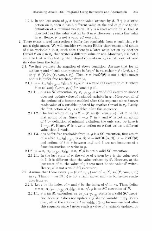
Reasoning About TSO Programs Using Reduction and Abstraction 347

1.2.1. In the last state of ρ, x has the value written by β. If γ is a writeaction on x, then x has a different value at the end of ρ′ due to thedefinition of a minimal violation. If γ is a read action on x, then itdoes not read the value written by β in ρ. However, γ reads this valuein ρ′. Hence, ρ′ is not a valid SC execution.

2. There exists a read instruction r buffer-free reachable from w such that r isnot a right mover. We will consider two cases: Either there exists a rd actionof t on variable z in π2 such that there is a later write action by anotherthread t′ on z in π2 that writes a different value or not. Moreover, z is not avariable that is touched by the delayed commits in π4 i.e., it does not readits value from the buffer.

2.1. We first evaluate the negation of above condition. Assume that for allactions γ and γ′ such that γ occurs before γ′ in π2, either γ �= (t, rd, z, vz)or γ′ �= (t′, isu)(t′, com, z, v′

z). Then, r = instOf(θ) is not a right moverand it is buffer-free reachable from w.

2.1.1. ρ = π1, π2|−→t \{t}, π2|{t} ⊗ π4, θ, θ′ is a valid SC execution of P where

θ′ = (t′, isu)(t′, com, y, ∗) for some t �= t′.2.1.1.1. ρ is an SC execution. π1, π2|−→t \{t} is a valid SC execution since t

does not update value of a shared variable in π2. Moreover, all ofthe actions of t become enabled after this sequence since t neverreads value of a variable updated by another thread in π2. Lastly,the first action of π3 is enabled after this sequence.

2.1.1.2. The first action of π3 is θ′ = (t′, isu)(t′, com, y, ∗). Let θ′ be thefirst action of π3. Since θ →hb θ′ in π and θ′ is not an actionof t by definition of minimal violation, the only case we have isθ →fr θ′. Hence, θ′ is a write action on y that writes a differentvalue than θ reads.

2.1.1.3. r is buffer-free reachable from w. ρ is a SC execution, first actionof ρ after π1, π2|−→t \{t} is α, β; w = instOf((α, β)), r = instOf(θ)and actions of t in ρ between α, β and θ are not instances of afence instruction or write to y.

2.1.2. ρ′ = π1, π2|−→t \{t}, π2|{t} ⊗ π4, θ′, θ is not a valid SC execution.

2.1.2.1. In the last state of ρ, the value of y seen by t is the value readin θ. It is different than the value written by θ′. However, at thelast state of ρ′, the value of y t sees must be the value θ′ writes.Hence, ρ′ is not a valid SC execution.

2.2. Assume that there exists γ = (t, rd, z, vz) and γ′ = (t′, isu)(t′, com, z, v′z)

in π2. Then, r = instOf(γ) is not a right mover and r is buffer-free reach-able from w.

2.2.1. Let i be the index of γ and j be the index of γ′ in π2. Then, defineρ = π1, π2|j−1|−→t \{t}, π2|i|{t} ⊗ π4, γ

′. ρ is an SC execution of P.2.2.1.1. ρ is an SC execution. π1, π2|j−1|−→t \{t} prefix is a valid SC execu-

tion because t does not update any shared variable in π2. More-over, all of the actions of t in π2|i|{t} ⊗ π4 become enabled afterthis sequence since t never reads a value of a variable updated by

348 A. Bouajjani et al.

another thread in π2 and γ′ is the next enabled in π2 after thissequence since it is a write action.

2.2.2. Let i and j be indices of γ and γ′ in π2 respectively. Define ρ′ =π1, π2|j−1|−→t \{t}, π2|i−1|{t} ⊗ π4, γ

′, γ. Then, ρ′ is not a valid SC exe-cution.

2.2.2.1. In the last state of ρ, value of z seen by t is vz. It is different thanthe v′

z, value written by γ′. However, in the last state of ρ′, thevalue of z t sees must be v′

z. Hence, ρ′ is not a valid SC execution.2.2.3. r is buffer-free reachable from w because ρ defined in 2.2.1 is

an SC execution, first action after π1, π2|j−1|−→t \{t} is α, β, w =instOf((α, β)), r = instOf(γ) and actions of t in ρ between α, β and θare not instances of a fence instruction or a write to z by t.

5 Abstractions and Verifying Non-robust Programs

In this section, we introduce program abstractions which are useful for verifyingnon-robust TSO programs (or even robust programs – see an example at the endof this section). In general, a program P ′ abstracts another program P for somesemantic model M ∈ {SC,TSO} if every shared variable valuation σ reachablefrom the initial state in an M execution of P is also reachable in an M executionof P ′. We denote this abstraction relation as P �M P ′.

In particular, we are interested in read instruction abstractions, which replaceinstructions that read from a shared variable with more “liberal” read instruc-tions that can read more values (this way, the program may reach more sharedvariable valuations). We extend the program syntax in Sect. 3 with havoc instruc-tions of the form havoc(〈reg〉, 〈varbexpr〉), where 〈varbexpr〉 is a boolean expres-sion over a set of registers and a single shared variable 〈var〉. The meaningof this instruction is that the register reg is assigned with any value thatsatisfies varbexpr (where the other registers and the variable var are inter-preted with their current values). The program abstraction we consider willreplace read instructions of the form 〈reg〉 := 〈var〉 with havoc instructionshavoc(〈reg〉, 〈varbexpr〉).

While replacing read instructions with havoc instructions, we must guaranteethat the new program reaches at least the same set of shared variable valuationsafter executing the havoc as the original program after the read. Hence, weallow such a rewriting only when the boolean expression varbexpr is weaker (ina logical sense) than the equality reg = var (hence, there exists an execution ofthe havoc instruction where reg = var).

Lemma 2. Let P be a program and P ′ be obtained from P by replacing aninstruction l1 : x := r; goto l2 of a thread t with l1 : havoc(r, φ(x,−→r )); goto l2such that ∀x, r. x = r =⇒ φ(x,−→r ) is valid. Then, P �SC P ′ and P �TSO P ′.

The notion of trace extends to programs that contain havoc instructions asfollows. Assume that (t, hvc, x, φ(x)) is the action generated by an instructionhavoc(r, φ(x,−→r )), where x is a shared variable and −→r a set of registers (the

Reasoning About TSO Programs Using Reduction and Abstraction 349

Fig. 6. An example program that needs a read abstraction to pass our robustnesschecks. The havoc statement in comments reads as follows: if value of x is not 0 thenr1 gets either the value of x or 0. Otherwise, it is 0.

action stores the constraint φ where the values of the registers are instantiatedwith their current values – the shared variable x is the only free variable in φ(x)).Roughly, the hvc actions are special cases of rd actions. Consider an executionπ where an action α = (t, hvc, x, φ(x)) is generated by reading the value of awrite action β = (com, x, v) (i.e., the value v was the current value of x when thehavoc instruction was executed). Then, the trace of π contains a read-from edgeβ →rf α as for regular read actions. However, fr edges are created differently. Ifα was a rd action we would say that we have α →fr γ if β →rf α and β →st γ.For the havoc case, the situation is a little bit different. Let γ = (com, x, v′) bean action. We have α →fr γ if and only if either β →rf α, β →st γ and φ(v′)is false or α →fr γ′ and γ′ →st γ where γ′ is an action. Intuitively, there is afrom-read dependency from an havoc action to a commit action, only when thecommit action invalidates the constraint φ(x) of the havoc (or if it follows sucha commit in store order).

The notion of write-atomicity (Definition 1) extends to programs with havocinstructions by interpreting havoc instructions havoc(r, φ(x,−→r )) as regular readinstructions r := x. Theorem 1 which states that write-atomicity implies robust-ness can also be easily extended to this case.

Read abstractions are useful in two ways. First, they allow us to prove prop-erties of non-robust program as the work stealing queue example in Fig. 3. Wecan apply appropriate read abstractions to relax the original program so that itbecomes robust in the end. Then, we can use SC reasoning tools on the robustprogram to prove invariants of the program.

Second, read abstractions could be helpful for proving robustness directly.The method based on write-atomicity we propose for verifying robustness issound but not complete. Some incompleteness scenarios can be avoided usingread abstractions. If we can abstract read instructions such that the new programreaches exactly the same states (in terms of shared variables) as the original one,it may help to avoid executions that violate mover checks.

Consider the program in Fig. 6. The write statement x := 1 in procedurefoo is not atomic. It is not a left mover due to the read of x in the do-while loopof bar. Moreover, the later read from y is buffer-free reachable from this writeand it is not a right mover because of the write to y in bar. To make it atomic, weapply read abstraction to the read instruction of bar that reads from x. In the

350 A. Bouajjani et al.

new relaxed read, r1 can read 0 along with the value of x when x is not zero asshown in the comments below the instruction. With this abstraction, the writeto x becomes a left mover because reads from x after the write can now read theold value which was 0. Thus, the program becomes write-atomic. If we think ofTSO traces of the abstract program and replace hvc nodes with rd nodes, weget exactly the TSO traces of the original program. However, the abstractionadds more SC traces to the program and the program becomes robust.

6 Experimental Evaluation

To test the practical value of our method, we have considered the benchmarkfor checking TSO robustness described in [2], which consists of 34 programs.This benchmark is quite exhaustive, it includes examples introduced in previousworks on this subject. Many of the programs in this benchmark are easy to provebeing write-atomic. Every write is followed by no buffer-free read instructionwhich makes them trivially atomic (like the message passing program in Fig. 1).This holds for 20 out of the 34 programs. Out of the remaining programs, 13required mover checks and 4 required read abstractions to show robustness (ourmethod didn’t succeed on one of the programs in the benchmark, explained atthe end of this section). Except Chase-Lev, the initial versions of all the 12examples are trace robust2. Besides Chase-Lev, read-abstractions are equivalentto the original programs in terms of reachable shared variable configurations.Detailed information for these examples can be found in Table 1.

To check whether writes/reads are left/right movers and the soundness ofabstractions, we have used the tool Civl [13]. This tool allows to prove asser-tions about concurrent programs (Owicki-Gries annotations) and also to checkwhether an instruction is a left/right mover. The buffer-free read instructionsreachable from a write before a fence were obtained using a trivial analysis of thecontrol-flow graph (CFG) of the program. This method is a sound approximationof the definition in Sect. 4 but it was sufficient for all the examples.

Our method was not precise enough to prove robustness for only one example,named as nbw-w-lr-rl in [7]. This program contains a method with explicit callsto the lock and unlock methods of a spinlock. The instruction that writes tothe lock variable inside the unlock method is not atomic, because of the readsfrom the lock variable and the calls to the getAndSet primitive inside the lockmethod. Abstracting the reads from the lock variable is not sufficient in thiscase due to the conflicts with getAndSet actions. However, we believe that readabstractions could be extended to getAndSet instructions (which both read andwrite to a shared variable atomically) in order to deal with this example.

2 If we consider the standard notion of so (that relates any two writes on the samevariable independent of their values), all examples except MCSLock and dc-locking

become non trace robust.

Reasoning About TSO Programs Using Reduction and Abstraction 351

Table 1. Benchmark results. The second column (RB) stands for the robustness statusof the original program according to our extended hb definition. RA column shows thenumber of read abstractions performed. RM column represents the number of readinstructions that are checked to be right movers and the LM column represents thewrite instructions that are shown to be left movers. PO shows the total number ofproof obligations generated and VT stands for the total verification time in seconds.

Name RB RA RM LM PO VT

Chase-Lev − 1 2 - 149 0.332

FIFO-iWSQ + - 2 - 124 0.323

LIFO-iWSQ + - 1 - 109 0.305

Anchor-iWSQ + - 1 - 109 0.309

MCSLock + 2 2 - 233 0.499

r+detour + - 1 - 53 0.266

r+detours + - 1 - 64 0.273

sb+detours+coh + - 2 - 108 0.322

sb+detours + - 1 1 125 0.316

write+r+coh + - 1 - 78 0.289

write+r + - 1 - 48 0.261

dc-locking + 1 4 1 52 0.284

inline pgsql + 2 2 - 90 0.286

7 Related Work

The weakest correctness criterion that enables SC reasoning for proving invari-ants of programs running under TSO is state-robustness i.e., the reachable setof states is the same under both SC and TSO. However, this problem has highcomplexity (non-primitive recursive for programs with a finite number of threadsand a finite data domain [6]). Therefore, it is difficult to come up with an effi-cient and precise solution. A symbolic decision procedure is presented in [1] andover-approximate analyses are proposed in [14,15].

Due to the high complexity of state-robustness, stronger correctness crite-ria with lower complexity have been proposed. Trace-robustness (that we callsimply robustness in our paper) is one of the most studied criteria in the litera-ture. Bouajjani et al. [9] have proved that deciding trace-robustness is PSpace-complete, resp., EXPSpace-complete, for a finite, resp., unbounded, number ofthreads and a finite data domain.

There are various tools for checking trace-robustness. Trencher [7] appliesto bounded-thread programs with finite data. In theory, the approach in Trenchercan be applied to infinite-state programs, but implementing it is not obviousbecause it requires solving non-trivial reachability queries in such programs. Incomparison, our approach (and our implementation based on Civl) applies toinfinite state programs. All our examples consider infinite data domains, while

352 A. Bouajjani et al.

Chase-Lev, FIFO-iWSQ, LIFO-iWSQ, Anchor-iWSQ, MCSLock, dc-locking andinline pgsql have an unbounded number of threads. Musketeer [4] provides anapproximate solution by checking existence of critical cycles on the control-flowgraph. While Musketeer can deal with infinite data (since data is abstractedaway), it is restricted to bounded-thread programs. Thus, it cannot deal with theunbounded thread examples mentioned above. Furthermore, Musketeer cannotprove robust even some examples with finitely many threads, e.g., nbw w wr,write+r, r+detours, sb+detours+coh. Other tools for approximate robustnesschecking, to which we compare in similar ways, have been proposed in [5,10,11].

Besides trace-robustness, there are other correctness criteria like triangularrace freedom (Trf) and persistence that are stronger than state-robustness.Persistence [2] is incomparable to trace-robustness, and Trf [18] is strongerthan both trace-robustness and persistence. Our method can verify examplesthat are state-robust but neither persistent nor Trf.

Reduction and abstraction techniques were used for reasoning on SC pro-grams. Qed [12] is a tool that supports statement transformations as a way ofabstracting programs combined with a mover analysis. Also, Civl [13] allowsproving location assertions in the context of the Owicki-Gries logic which isenhanced with Lipton’s reduction theory [17]. Our work enables the use of suchtools for reasoning about the TSO semantics of a program.

References

1. Abdulla, P.A., Atig, M.F., Chen, Y.-F., Leonardsson, C., Rezine, A.: Counter-example guided fence insertion under TSO. In: Flanagan, C., Konig, B. (eds.)TACAS 2012. LNCS, vol. 7214, pp. 204–219. Springer, Heidelberg (2012). https://doi.org/10.1007/978-3-642-28756-5 15

2. Abdulla, P.A., Atig, M.F., Ngo, T.-P.: The best of both worlds: trading efficiencyand optimality in fence insertion for TSO. In: Vitek, J. (ed.) ESOP 2015. LNCS,vol. 9032, pp. 308–332. Springer, Heidelberg (2015). https://doi.org/10.1007/978-3-662-46669-8 13

3. Adve, S.V., Hill, M.D.: A unified formalization of four shared-memory models.IEEE Trans. Parallel Distrib. Syst. 4(6), 613–624 (1993)

4. Alglave, J., Kroening, D., Nimal, V., Poetzl, D.: Don’t sit on the fence. In: Biere,A., Bloem, R. (eds.) CAV 2014. LNCS, vol. 8559, pp. 508–524. Springer, Cham(2014). https://doi.org/10.1007/978-3-319-08867-9 33

5. Alglave, J., Maranget, L.: Stability in weak memory models. In: Gopalakrishnan,G., Qadeer, S. (eds.) CAV 2011. LNCS, vol. 6806, pp. 50–66. Springer, Heidelberg(2011). https://doi.org/10.1007/978-3-642-22110-1 6

6. Atig, M.F., Bouajjani, A., Burckhardt, S., Musuvathi, M.: On the verificationproblem for weak memory models. ACM Sigplan Not. 45(1), 7–18 (2010)

7. Bouajjani, A., Derevenetc, E., Meyer, R.: Checking and enforcing robustnessagainst TSO. In: Felleisen, M., Gardner, P. (eds.) ESOP 2013. LNCS, vol. 7792, pp.533–553. Springer, Heidelberg (2013). https://doi.org/10.1007/978-3-642-37036-6 29

8. Bouajjani, A., Enea, C., Mutluergil, S.O., Tasiran, S.: Reasoning about TSO pro-grams using reduction and abstraction. CoRR, abs/1804.05196 (2018)

Reasoning About TSO Programs Using Reduction and Abstraction 353

9. Bouajjani, A., Meyer, R., Mohlmann, E.: Deciding robustness against total storeordering. In: Aceto, L., Henzinger, M., Sgall, J. (eds.) ICALP 2011. LNCS, vol.6756, pp. 428–440. Springer, Heidelberg (2011). https://doi.org/10.1007/978-3-642-22012-8 34

10. Burckhardt, S., Musuvathi, M.: Effective program verification for relaxed memorymodels. In: Gupta, A., Malik, S. (eds.) CAV 2008. LNCS, vol. 5123, pp. 107–120.Springer, Heidelberg (2008). https://doi.org/10.1007/978-3-540-70545-1 12

11. Burnim, J., Sen, K., Stergiou, C.: Sound and complete monitoring of sequentialconsistency for relaxed memory models. In: Abdulla, P.A., Leino, K.R.M. (eds.)TACAS 2011. LNCS, vol. 6605, pp. 11–25. Springer, Heidelberg (2011). https://doi.org/10.1007/978-3-642-19835-9 3

12. Elmas, T., Qadeer, S., Tasiran, S.: A calculus of atomic actions. In: ACM Sympo-sium on Principles of Programming Languages, p. 14. Association for ComputingMachinery Inc., January 2009

13. Hawblitzel, C., Qadeer, S., Tasiran, S.: Automated and modular refinement rea-soning for concurrent programs. In: Computer Aided Verification (2015)

14. Kuperstein, M., Vechev, M., Yahav, E.: Partial-coherence abstractions for relaxedmemory models. In: ACM SIGPLAN Notices, vol. 46, pp. 187–198. ACM (2011)

15. Kuperstein, M., Vechev, M., Yahav, E.: Automatic inference of memory fences.ACM SIGACT News 43(2), 108–123 (2012)

16. Lamport, L.: How to make a multiprocessor computer that correctly executes mul-tiprocess programs. IEEE Trans. Comput. 100(9), 690–691 (1979)

17. Lipton, R.J.: Reduction: a method of proving properties of parallel programs. Com-mun. ACM 18(12), 717–721 (1975)

18. Owens, S.: Reasoning about the implementation of concurrency abstractions onx86-TSO. In: D’Hondt, T. (ed.) ECOOP 2010. LNCS, vol. 6183, pp. 478–503.Springer, Heidelberg (2010). https://doi.org/10.1007/978-3-642-14107-2 23

19. Sewell, P., Sarkar, S., Owens, S., Nardelli, F.Z., Myreen, M.O.: x86-TSO: a rigorousand usable programmer’s model for x86 multiprocessors. Commun. ACM 53(7),89–97 (2010)

20. Shasha, D., Snir, M.: Efficient and correct execution of parallel programs that sharememory. ACM Trans. Program. Lang. Syst. (TOPLAS) 10(2), 282–312 (1988)

Open Access This chapter is licensed under the terms of the Creative CommonsAttribution 4.0 International License (http://creativecommons.org/licenses/by/4.0/),which permits use, sharing, adaptation, distribution and reproduction in any mediumor format, as long as you give appropriate credit to the original author(s) and thesource, provide a link to the Creative Commons license and indicate if changes weremade.

The images or other third party material in this chapter are included in the chapter’sCreative Commons license, unless indicated otherwise in a credit line to the material. Ifmaterial is not included in the chapter’s Creative Commons license and your intendeduse is not permitted by statutory regulation or exceeds the permitted use, you willneed to obtain permission directly from the copyright holder.

Quasi-Optimal Partial Order Reduction

Huyen T. T. Nguyen1 , Cesar Rodrıguez1,3, Marcelo Sousa2, Camille Coti1 ,and Laure Petrucci1(B)

1 LIPN, CNRS UMR 7030, Universite Paris 13,Sorbonne Paris Cite, Villetaneuse, France{tnguyen,cesar.rodriguez}@lipn.fr,

{camille.coti,laure.petrucci}@lipn.univ-paris13.fr2 University of Oxford, Oxford, UK

marcelo.sousa@cs.ox.ac.uk3 Diffblue Ltd., Oxford, UK

Abstract. A dynamic partial order reduction (DPOR) algorithmis optimal when it always explores at most one representative perMazurkiewicz trace. Existing literature suggests that the reductionobtained by the non-optimal, state-of-the-art Source-DPOR (SDPOR)algorithm is comparable to optimal DPOR. We show the first programwith O(n) Mazurkiewicz traces where SDPOR explores O(2n) redundantschedules (as this paper was under review, we were made aware of therecent publication of another paper [3] which contains an independently-discovered example program with the same characteristics). We further-more identify the cause of this blow-up as an NP-hard problem. Ourmain contribution is a new approach, called Quasi-Optimal POR, thatcan arbitrarily approximate an optimal exploration using a provided con-stant k. We present an implementation of our method in a new toolcalled Dpu using specialised data structures. Experiments with Dpu,including Debian packages, show that optimality is achieved with lowvalues of k, outperforming state-of-the-art tools.

1 Introduction

Dynamic partial-order reduction (DPOR) [1,10,19] is a mature approach tomitigate the state explosion problem in stateless model checking of multi-threaded programs. DPORs are based on Mazurkiewicz trace theory [13], a true-concurrency semantics where the set of executions of the program is partitionedinto equivalence classes known as Mazurkiewicz traces (M-traces). In a DPOR,this partitioning is defined by an independence relation over concurrent actionsthat is computed dynamically and the method explores executions which are rep-resentatives of M-traces. The exploration is sound when it explores all M-traces,and it is considered optimal [1] when it explores each M-trace only once.

Since two independent actions might have to be explored from the samestate in order to explore all M-traces, a DPOR algorithm uses independence tocompute a provably-sufficient subset of the enabled transitions to explore for eachstate encountered. Typically this involves the combination of forward reasoningc© The Author(s) 2018H. Chockler and G. Weissenbacher (Eds.): CAV 2018, LNCS 10982, pp. 354–371, 2018.https://doi.org/10.1007/978-3-319-96142-2_22

Quasi-Optimal Partial Order Reduction 355

Fig. 1. (a) Programs; (b) partially-ordered executions;

(persistent sets [11] or source sets [1,4]) with backward reasoning (sleep sets [11])to obtain a more efficient exploration. However, in order to obtain optimality, aDPOR needs to compute sequences of transitions (as opposed to sets of enabledtransitions) that avoid visiting a previously visited M-trace. These sequences arestored in a data structure called wakeup trees in [1] and known as alternativesin [19]. Computing these sequences thus amounts to deciding whether the DPORneeds to visit yet another M-trace (or all have already been seen).

In this paper, we prove that computing alternatives in an optimal DPORis an NP-complete problem. To the best our knowledge this is the first formalcomplexity result on this important subproblem that optimal and non-optimalDPORs need to solve. The program shown in Fig. 1(a) illustrates a practical con-sequence of this result: the non-optimal, state-of-the-art SDPOR algorithm [1]can explore here O(2n) interleavings but the program has only O(n) M-traces.

The program contains n := 3 writer threads w0, w1, w2, each writing to adifferent variable. The thread count increments n − 1 times a zero-initializedcounter c. Thread master reads c into variable i and writes to xi.

The statements x0 = 7 and x1 = 8 are independent because they produce thesame state regardless of their execution order. Statements i = c and any state-ment in the count thread are dependent or interfering : their execution ordersresult in different states. Similarly, xi = 0 interferes with exactly one writerthread, depending on the value of i.

Using this independence relation, the set of executions of this program canbe partitioned into six M-traces, corresponding to the six partial orders shownin Fig. 1(b). Thus, an optimal DPOR explores six executions (2n-executions for nwriters). We now show why SDPOR explores O(2n) in the general case. Concep-tually, SDPOR is a loop that (1) runs the program, (2) identifies two dependentstatements that can be swapped, and (3) reverses them and re-executes theprogram. It terminates when no more dependent statements can be swapped.

Consider the interference on the counter variable c between the master andthe count thread. Their execution order determines which writer thread inter-feres with the master statement xi = 0. If c = 1 is executed just before i = c,then xi = 0 interferes with w1. However, if i = c is executed before, then xi = 0interferes with w0. Since SDPOR does not track relations between dependentstatements, it will naively try to reverse the race between xi = 0 and all writerthreads, which results in exploring O(2n) executions. In this program, exploring

356 H. T. T. Nguyen et al.

only six traces requires understanding the entanglement between both interfer-ences as the order in which the first is reversed determines the second.

As a trade-off solution between solving this NP-complete problem and poten-tially explore an exponential number of redundant schedules, we propose a hybridapproach called Quasi-Optimal POR (QPOR) which can turn a non-optimalDPOR into an optimal one. In particular, we provide a polynomial algorithmto compute alternative executions that can arbitrarily approximate the optimalsolution based on a user specified constant k. The key concept is a new notionof k-partial alternative, which can intuitively be seen as a “good enough” alter-native: they revert two interfering statements while remembering the resolutionof the last k − 1 interferences.

The major differences between QPOR and the DPORs of [1] are that: (1)QPOR is based on prime event structures [17], a partial-order semantics thathas been recently applied to programs [19,21], instead of a sequential view tothread interleaving, and (2) it computes k-partial alternatives with an O(nk)algorithm while optimal DPOR corresponds to computing ∞-partial alternativeswith an O(2n) algorithm. For the program shown in Fig. 1(a), QPOR achievesoptimality with k = 2 because races are coupled with (at most) another race.As expected, the cost of computing k-partial alternatives and the reductionsobtained by the method increase with higher values of k.

Finding k-partial alternatives requires decision procedures for traversing thecausality and conflict relations in event structures. Our main algorithmic contri-bution is to represent these relations as a set of trees where events are encoded asone or two nodes in two different trees. We show that checking causality/conflictbetween events amounts to an efficient traversal in one of these trees.

In summary, our main contributions are:

– Proof that computing alternatives for optimal DPOR is NP-complete(Sect. 4).

– Efficient data structures and algorithms for (1) computing k-partialalternatives in polynomial time, and (2) represent and traverse partialorders (Sect. 5).

– Implementation of QPOR in a new tool called Dpu and experimental evalu-ations against SDPOR in Nidhugg and the testing tool Maple (Sect. 6).

– Benchmarks with O(n) M-traces where SDPOR explores O(2n) executions(Sect. 6).

Furthermore, in Sect. 6 we show that: (1) low values of k often achieve opti-mality; (2) even with non-optimal explorations Dpu greatly outperforms Nid-hugg; (3) Dpu copes with production code in Debian packages and achievesmuch higher state space coverage and efficiency than Maple.

Proofs for all our formal results are available in the unabridged version [15].

2 Preliminaries

In this section we provide the formal background used throughout the paper.

Quasi-Optimal Partial Order Reduction 357

Concurrent Programs. We consider deterministic concurrent programs composedof a fixed number of threads that communicate via shared memory and synchro-nize using mutexes (Fig. 1(a) can be trivially modified to satisfy this). We alsoassume that local statements can only modify shared memory within a mutexblock. Therefore, it suffices to only consider races of mutex accesses.

Formally, a concurrent program is a structure P := 〈M,L, T,m0, l0〉, whereM is the set of memory states (valuations of program variables, includinginstruction pointers), L is the set of mutexes, m0 is the initial memory state,l0 is the initial mutexes state and T is the set of thread statements. A threadstatement t := 〈i, f〉 is a pair where i ∈ N is the thread identifier associated withthe statement and f : M → (M×Λ) is a partial function that models the trans-formation of the memory as well as the effect Λ := {loc}∪({acq, rel}×L) of thestatement with respect to thread synchronization. Statements of loc effect modellocal thread code. Statements associated with 〈acq, x〉 or 〈rel, x〉 model lockand unlock operations on a mutex x. Finally, we assume that (1) functions f arePTIME-decidable; (2) acq/rel statements do not modify the memory; and (3)loc statements modify thread-shared memory only within lock/unlock blocks.When (3) is violated, then P has a datarace (undefined behavior in almost alllanguages), and our technique can be used to find such statements, see Sect. 6.

We use labelled transition systems (LTS) semantics for our programs. Weassociate a program P with the LTS MP := 〈S,→, A, s0〉. The set S := M ×(L → {0, 1}) are the states of MP , i.e., pairs of the form 〈m, v〉 where m is thestate of the memory and v indicates when a mutex is locked (1) or unlocked (0).The actions in A ⊆ N × Λ are pairs 〈i, b〉 where i is the identifier of the threadthat executes some statement and b is the effect of the statement. We use thefunction p : A → N to retrieve the thread identifier. The transition relation → ⊆S × A × S contains a triple 〈m, v〉 〈i,b〉−−−→ 〈m′, v′〉 exactly when there is somethread statement 〈i, f〉 ∈ T such that f(m) = 〈m′, b〉 and either (1) b = loc andv′ = v, or (2) b = 〈acq, x〉 and v(x) = 0 and v′ = v|x�→1, or (3) b = 〈rel, x〉 andv′ = v|x�→0. Notation fx�→y denotes a function that behaves like f for all inputsexcept for x, where f(x) = y. The initial state is s0 := 〈m0, l0〉.

Furthermore, if s a−→ s′ is a transition, the action a is enabled at s. Let enabl(s)denote the set of actions enabled at s. A sequence σ := a1 . . . an ∈ A∗ is arun when there are states s1, . . . , sn satisfying s0

a1−→ s1 . . . an−−→ sn. We definestate(σ) := sn. We let runs(MP ) denote the set of all runs and reach(MP ) :={state(σ) ∈ S : σ ∈ runs(MP )} the set of all reachable states.

Independence. Dynamic partial-order reduction methods use a notion calledindependence to avoid exploring concurrent interleavings that lead to the samestate. We recall the standard notion of independence for actions in [11]. Twoactions a, a′ ∈ A commute at a state s ∈ S iff

– if a ∈ enabl(s) and s a−→ s′, then a′ ∈ enabl(s) iff a′ ∈ enabl(s′); and– if a, a′ ∈ enabl(s), then there is a state s′ such that s a.a′

−−→ s′ and s a′.a−−→ s′.

358 H. T. T. Nguyen et al.

Independence between actions is an under-approximation of commutativity.A binary relation ♦ ⊆ A × A is an independence on MP if it is symmetric,irreflexive, and every pair 〈a, a′〉 in ♦ commutes at every state in reach(MP ).

In general MP has multiple independence relations, clearly ∅ is always oneof them. We define relation ♦P ⊆ A × A as the smallest irreflexive, symmetricrelation where 〈i, b〉 ♦P 〈i′, b′〉 holds if i �= i′ and either b = loc or b = acq xand b′ �∈ {acq x, rel x}. By construction ♦P is always an independence.

Labelled Prime Event Structures. Prime event structures (pes) are well-knownnon-interleaving, partial-order semantics [7,8,16]. Let X be a set of actions.A pes over X is a structure E := 〈E,<,#, h〉 where E is a set of events, < ⊆E×E is a strict partial order called causality relation, # ⊆ E×E is a symmetric,irreflexive conflict relation, and h : E → X is a labelling function. Causalityrepresents the happens-before relation between events, and conflict between twoevents expresses that any execution includes at most one of them. Figure 2(b)shows a pes over N×Λ where causality is depicted by arrows, conflicts by dottedlines, and the labelling h is shown next to the events, e.g., 1 < 5, 8 < 12, 2 # 8,and h(1) = 〈0, loc〉. The history of an event e, �e := {e′ ∈ E : e′ < e}, is theleast set of events that need to happen before e.

The notion of concurrent execution in a pes is captured by the conceptof configuration. A configuration is a (partially ordered) execution of the system,i.e., a set C ⊆ E of events that is causally closed (if e ∈ C, then �e ⊆ C)and conflict-free (if e, e′ ∈ C, then ¬(e # e′)). In Fig. 2(b), the set {8, 9, 15}is a configuration, but {3} or {1, 2, 8} are not. We let conf (E) denote the setof all configurations of E , and [e] := �e ∪ {e} the local configuration of e. InFig. 2(b), [11] = {1, 8, 9, 10, 11}. A configuration represents a set of interleavingsover X. An interleaving is a sequence in X∗ that labels any topological sortingof the events in C. In Fig. 2(b), inter({1, 8}) = {ab, ba} with a := 〈0, loc〉 andb := 〈1, acq m〉.

The extensions of C are the events not in C whose histories are included in C:ex (C) := {e ∈ E : e /∈ C ∧ �e ⊆ C}. The enabled events of C are the extensionsthat can form a larger configuration: en(C) := {e ∈ ex (C) : C ∪ {e} ∈ conf (E)}.Finally, the conflicting extensions of C are the extensions that are not enabled:cex (C) := ex (C) \ en(C). In Fig. 2(b), ex ({1, 8}) = {2, 9, 15}, en({1, 8}) ={9, 15}, and cex ({1, 8}) = {2}. See [20] for more information on pes concepts.

Parametric Unfolding Semantics. We recall the program pes semantics of [19,20](modulo notation differences). For a program P and any independence ♦ on MP

we define a pes UP,♦ that represents the behavior of P , i.e., such that theinterleavings of its set of configurations equals runs(MP ).

Each event in UP,♦ is defined by a canonical name of the form e := 〈a,H〉,where a ∈ A is an action of MP and H is a configuration of UP,♦. Intuitively, erepresents the action a after the history (or the causes) H. Figure 2(b) shows anexample. Event 11 is 〈〈0, acq m〉, {1, 8, 9, 10}〉 and event 1 is 〈〈0, loc〉, ∅〉. Notethe inductive nature of the name, and how it allows to uniquely identify eachevent. We define the state of a configuration as the state reached by any of itsinterleavings. Formally, for C ∈ conf (UP,♦) we define state(C) as s0 if C = ∅

Quasi-Optimal Partial Order Reduction 359

Fig. 2. (a) A program P ; (b) its unfolding semantics UP,♦P .

and as state(σ) for some σ ∈ inter(C) if C �= ∅. Despite its appearance state(C)is well-defined because all sequences in inter(C) reach the same state, see [20]for a proof.

Definition 1 (Unfolding). Given a program P and some independence rela-tion ♦ on MP := 〈S,→, A, s0〉, the unfolding of P under ♦, denoted UP,♦, isthe pes over A constructed by the following fixpoint rules:

1. Start with a pes E := 〈E,<,#, h〉 equal to 〈∅, ∅, ∅, ∅〉.2. Add a new event e := 〈a,C〉 to E for any configuration C ∈ conf (E) and any

action a ∈ A if a is enabled at state(C) and ¬(a ♦ h(e′)) holds for every<-maximal event e′ in C.

3. For any new e in E, update <, #, and h as follows: for every e′ ∈ C, sete′ < e; for any e′ ∈ E \C, set e′ # e if e �= e′ and ¬(a ♦ h(e′)); set h(e) := a.

4. Repeat steps 2 and 3 until no new event can be added to E; return E.

Step 1 creates an empty pes with only one (empty) configuration. Step 2 insertsa new event 〈a,C〉 by finding a configuration C that enables an action a which isdependent with all causality-maximal events in C. In Fig. 2, this initially createsevents 1, 8, and 15. For event 1 := 〈〈0, loc〉, ∅〉, this is because action 〈0, loc〉is enabled at state(∅) = s0 and there is no <-maximal event in ∅ to consider.Similarly, the state of C1 := {1, 8, 9, 10} enables action a1 := 〈0, acq m〉, andboth h(1) and h(10) are dependent with a1 in ♦P . As a result 〈a1, C1〉 is anevent (number 11). Furthermore, while a2 := 〈0, loc〉 is enabled at state(C2),with C2 := {8, 9, 10}, a2 is independent of h(10) and 〈a2, C2〉 is not an event.

After inserting an event e := 〈a,C〉, Definition 1 declares all events in Ccausal predecessors of e. For any event e′ in E but not in [e] such that h(e′)is dependent with a, the order of execution of e and e′ yields different states.We thus set them in conflict. In Fig. 2, we set 2 # 8 because h(2) is dependentwith h(8) and 2 /∈ [8] and 8 /∈ [2].

3 Unfolding-Based DPOR

This section presents an algorithm that exhaustively explores all deadlock statesof a given program (a deadlock is a state where no thread is enabled).

360 H. T. T. Nguyen et al.

Algorithm 1. Unfolding-based POR exploration. See text for definitions.

1 Initially, set U := ∅,2 and call Explore(∅, ∅, ∅).3 Procedure Explore(C,D,A)

4 Add ex (C) to U5 if en(C) ⊆ D return6 if A = ∅7 Choose e from en(C) \ D8 else9 Choose e from A ∩ en(C)

10 Explore(C ∪ {e}, D,A \ {e})11 if ∃J ∈ Alt(C,D ∪ {e})12 Explore(C,D ∪ {e}, J \ C)

13 U := U ∩ QC,D

14 Function cexp(C)

15 R := ∅16 foreach event e ∈ C of type acq

17 et := pt(e)18 em := pm(e)19 while ¬(em ≤ et) do20 em := pm(em)21 if (em < et) break22 em := pm(em)23 e := 〈h(e), [et] ∪ [em]〉24 Add e to R

25 return R

For the rest of the paper, unless otherwise stated, we let P be a terminatingprogram (i.e., runs(MP ) is a finite set of finite sequences) and ♦ an independenceon MP . Consequently, UP,♦ has finitely many events and configurations.

Our POR algorithm (Algorithm1) analyzes P by exploring the configurationsof UP,♦. It visits all ⊆-maximal configurations of UP,♦, which correspond to thedeadlock states in reach(MP ), and organizes the exploration as a binary tree.

Explore(C,D,A) has a global set U that stores all events of UP,♦ discoveredso far. The three arguments are: C, the configuration to be explored; D (fordisabled), a set of events that shall never be visited (included in C) again; andA (for add), used to direct the exploration towards a configuration that conflictswith D. A call to Explore(C,D,A) visits all maximal configurations of UP,♦which contain C and do not contain D, and the first one explored contains C∪A.

The algorithm first adds ex (C) to U . If C is a maximal configuration (i.e.,there is no enabled event) then line 5 returns. If C is not maximal but en(C) ⊆ D,then all possible events that could be added to C have already been exploredand this call was redundant work. In this case the algorithm also returns andwe say that it has explored a sleep-set blocked (SSB) execution [1]. Algorithm 1next selects an event enabled at C, if possible from A (line 7 and 9) and makes arecursive call (left subtree) that explores all configurations that contain all eventsin C ∪{e} and no event from D. Since that call visits all maximal configurationscontaining C and e, it remains to visit those containing C but not e. At line11 we determine if any such configuration exists. Function Alt returns a set ofconfigurations, so-called clues. A clue is a witness that a ⊆-maximal configurationexists in UP,♦ which contains C and not D ∪ {e}.

Definition 2 (Clue). Let D and U be sets of events, and C a configurationsuch that C ∩ D = ∅. A clue to D after C in U is a configuration J ⊆ U suchthat C ∪ J is a configuration and D ∩ J = ∅.

Quasi-Optimal Partial Order Reduction 361

Definition 3 (Alt function). Function Alt denotes any function such thatAlt(B,F) returns a set of clues to F after B in U , and the set is non-empty ifUP,♦ has at least one maximal configuration C where B ⊆ C and C ∩ F = ∅.

When Alt returns a clue J , the clue is passed in the second recursive call(line 12) to “mark the way” (using set A) in the subsequent recursive calls atline 10, and guide the exploration towards the maximal configuration that Jwitnesses. Definition 3 does not identify a concrete implementation of Alt. Itrather indicates how to implement Alt so that Algorithm 1 terminates and iscomplete (see below). Different PORs in the literature can be reframed in termsof Algorithm 1. SDPOR [1] uses clues that mark the way with only one eventahead (|J \ C| = 1) and can hit SSBs. Optimal DPORs [1,19] use size-varyingclues that guide the exploration provably guaranteeing that any SSB will beavoided.

Algorithm 1 is optimal when it does not explore a SSB. To make Algorithm 1optimal Alt needs to return clues that are alternatives [19], which satisfy strongerconstraints. When that happens, Algorithm1 is equivalent to the DPOR in [19]and becomes optimal (see [20] for a proof).

Definition 4 (Alternative [19]). Let D and U be sets of events and C aconfiguration such that C ∩D = ∅. An alternative to D after C in U is a clue Jto D after C in U such that ∀e ∈ D : ∃e′ ∈ J , e # e′.

Line 13 removes from U events that will not be necessary for Alt to findclues in the future. The events preserved, QC,D := C ∪ D ∪ #(C ∪ D), includeall events in C ∪ D as well as every event in U that is in conflict with someevent in C ∪ D. The preserved events will suffice to compute alternatives [19],but other non-optimal implementations of Alt could allow for more aggressivepruning.

The ⊆-maximal configurations of Fig. 2(b) are [7] ∪ [17], [14], and [19]. Ouralgorithm starts at configuration C = ∅. After 10 recursive calls it visits C =[7]∪[17]. Then it backtracks to C = {1}, calls Alt({1}, {2}), which provides, e.g.,J = {1, 8}, and visits C = {1, 8} with D = {2}. After 6 more recursive calls itvisits C = [14], backtracks to C = [12], calls Alt([12], {2, 13}]), which provides,e.g., J = {15}, and after two more recursive calls it visits C = [12] ∪ {15}with D = {2, 13}. Finally, after 4 more recursive calls it visits C = [19].

Finally, we focus on the correctness of Algorithm1, and prove terminationand soundness of the algorithm:

Theorem 1 (Termination). Regardless of its input, Algorithm1 always stops.

Theorem 2 (Completeness). Let C be a ⊆-maximal configuration of UP,♦.Then Algorithm1 calls Explore(C,D,A) at least once with C = C.

4 Complexity

This section presents complexity results about the only non-trival steps in Algo-rithm1: computing ex (C) and the call to Alt(·, ·). An implementation of

362 H. T. T. Nguyen et al.

Alt(B,F) that systematically returns B would satisfy Definition 3, but wouldalso render Algorithm 1 unusable (equivalent to a DFS in MP ). On the otherhand the algorithm becomes optimal when Alt returns alternatives. Optimalitycomes at a cost:

Theorem 3. Given a finite pes E, some configuration C ∈ conf (E), and aset D ⊆ ex (C), deciding if an alternative to D after C exists in E is NP-complete.

Theorem 3 assumes that E is an arbitrary pes. Assuming that E is the unfold-ing of a program P under ♦P does not reduce this complexity:

Theorem 4. Let P be a program and U a causally-closed set of events fromUP,♦P

. For any configuration C ⊆ U and any D ⊆ ex (C), deciding if an alter-native to D after C exists in U is NP-complete.

These complexity results lead us to consider (in next section) new approachesthat avoid the NP-hardness of computing alternatives while still retaining theircapacity to prune the search.

Finally, we focus on the complexity of computing ex (C), which essentiallyreduces to computing cex (C), as computing en(C) is trivial. Assuming that Eis given, computing cex (C) for some C ∈ conf (E) is a linear problem. However,for any realistic implementation of Algorithm 1, E is not available (the verygoal of Algorithm 1 is to find all of its events). So a useful complexity resultabout cex (C) necessarily refers to the orignal system under analysis. When E isthe unfolding of a Petri net [14], computing cex (C) is NP-complete:

Theorem 5. Let N be a Petri net, t a transition of N , E the unfolding of Nand C a configuration of E. Deciding if h−1(t) ∩ cex (C) = ∅ is NP-complete.

Fortunately, computing cex (C) for programs is a much simpler task. Func-tion cexp(C), shown in Algorithm1, computes and returns cex (C) when Eis the unfolding of some program. We explain cexp(C) in detail in Sect. 5.3.But assuming that functions pt and pm can be computed in constant time,and relation < decided in O(log |C|), as we will show, clearly cexp works intime O(n2 log n), where n := |C|, as both loops are bounded by the size of C.

5 New Algorithm for Computing Alternatives

This section introduces a new class of clues, called k-partial alternatives. Thesecan arbitrarily reduce the number of redundant explorations (SSBs) performedby Algorithm 1 and can be computed in polynomial time. Specialized data struc-tures and algorithms for k-partial alternatives are also presented.

Definition 5 (k-partial alternative). Let U be a set of events, C ⊆ U aconfiguration, D ⊆ U a set of events, and k ∈ N a number. A configuration J isa k-partial alternative to D after C if there is some D ⊆ D such that |D| = kand J is an alternative to D after C.

Quasi-Optimal Partial Order Reduction 363

A k-partial alternative needs to conflict with only k (instead of all) eventsin D. An alternative is thus an ∞-partial alternative. If we reframe SDPOR interms of Algorithm 1, it becomes an algorithm using singleton 1-partial alter-natives. While k-partial alternatives are a very simple concept, most of theirsimplicity stems from the fact that they are expressed within the elegant frame-work of pes semantics. Defining the same concept on top of sequential semantics(often used in the POR literature [1,2,9–11,23]), would have required much morecomplex device.

We compute k-partial alternatives using a comb data structure:

Definition 6 (Comb). Let A be a set. An A-comb c of size n ∈ N is anordered collection of spikes 〈s1, . . . , sn〉, where each spike si ∈ A∗ is a sequenceof elements over A. Furthermore, a combination over c is any tuple 〈a1, . . . , an〉where ai ∈ si is an element of the spike.

It is possible to compute k-partial alternatives (and by extension optimalalternatives) to D after C in U using a comb, as follows:

1. Select k (or |D|, whichever is smaller) arbitrary events e1, . . . , ek from D.2. Build a U -comb 〈s1, . . . , sk〉 of size k, where spike si contains all events in U

in conflict with ei.3. Remove from si any event e such that either [e] ∪ C is not a configuration or

[e] ∩ D �= ∅.4. Find combinations 〈e′

1, . . . , e′k〉 in the comb satisfying ¬(e′

i # e′j) for i �= j.

5. For any such combination the set J := [e′1]∪. . .∪[e′

k] is a k-partial alternative.

Step 3 guarantees that J is a clue. Steps 1 and 2 guarantee that it will conflictwith at least k events from D. It is straightforward to prove that the procedurewill find a k-partial alternative to D after C in U when an ∞-partial alternativeto D after C exists in U . It can thus be used to implement Definition 3.

Steps 2, 3, and 4 require to decide whether a given pair of events is in conflict.Similarly, step 3 requires to decide if two events are causally related. Efficientlycomputing k-partial alternatives thus reduces to efficiently computing causalityand conflict between events.

5.1 Computing Causality and Conflict for PES Events

In this section we introduce an efficient data structure for deciding whether twoevents in the unfolding of a program are causally related or in conflict.

As in Sect. 3, let P be a program, MP its LTS semantics, and ♦P its inde-pendence relation (defined in Sect. 2). Additionally, let E denote the pes UP,♦P

of P extended with a new event ⊥ that causally precedes every event in UP,♦P.

The unfolding E represents the dependency of actions in MP through thecausality and conflict relations between events. By definition of ♦P we knowthat for any two events e, e′ ∈ E :

– If e and e′ are events from the same thread, then they are either causallyrelated or in conflict.

364 H. T. T. Nguyen et al.

– If e and e′ are lock/unlock operations on the same variable, then similarlythey are either causally related or in conflict.

This means that the causality/conflict relations between all events of onethread can be tracked using a tree. For every thread of the program we defineand maintain a so-called thread tree. Each event of the thread has a correspondingnode in the tree. A tree node n is the parent of another tree node n′ iff the eventassociated with n is the immediate causal predecessor of the event associatedwith n′. That is, the ancestor relation of the tree encodes the causality relationsof events in the thread, and the branching of the tree represents conflict. Giventwo events e, e′ of the same thread we have that e < e′ iff ¬(e # e′) iff the treenode of e is an ancestor of the tree node of e′.

We apply the same idea to track causality/conflict between acq and relevents. For every lock l ∈ L we maintain a separate lock tree, containing anode for each event labelled by either 〈acq, l〉 or 〈rel, l〉. As before, the ancestorrelation in a lock tree encodes the causality relations of all events represented inthat tree. Events of type acq/rel have tree nodes in both their lock and threadtrees. Events for loc actions are associated to only one node in the thread tree.

This idea gives a procedure to decide a causality/conflict query for two eventswhen they belong to the same thread or modify the same lock. But we still needto decide causality and conflict for other events, e.g., loc events of differentthreads. Again by construction of ♦P , the only source of conflict/causality forevents are the causality/conflict relations between the causal predecessors ofthe two. These relations can be summarized by keeping two mappings for eachevent:

Definition 7. Let e ∈ E be an event of E. We define the thread mappingtmax : E × N → E as the only function that maps every pair 〈e, i〉 to the unique<-maximal event from thread i in [e], or ⊥ if [e] contains no event from thread i.Similarly, the lock mapping lmax : E × L → E maps every pair 〈e, l〉 to theunique <-maximal event e′ ∈ [e] such that h(e′) is an action of the form 〈acq, l〉or 〈rel, l〉, or ⊥ if no such event exists in [e].

The information stored by the thread and lock mappings enables us to decidecausality and conflict queries for arbitrary pairs of events:

Theorem 6. Let e, e′ ∈ E be two arbitrary events from resp. threads i and i′,with i �= i′. Then e < e′ holds iff e � tmax (e′, i). And e # e′ holds iff there issome l ∈ L such that lmax (e, l) # lmax (e′, l).

As a consequence of Theorem 6, deciding whether two events are related bycausality or conflict reduces to deciding whether two nodes from the same lockor thread tree are ancestors.

5.2 Computing Causality and Conflict for Tree Nodes

This section presents an efficient algorithm to decide if two nodes of a tree areancestors. The algorithm is similar to a search in a skip list [18].

Quasi-Optimal Partial Order Reduction 365

Let 〈N, �, r〉 denote a tree, where N is a set of nodes, � ⊆ N × N is theparent relation, and r ∈ N is the root. Let d(n) be the depth of each node inthe tree, with d(r) = 0. A node n is an ancestor of n′ if it belongs to the onlypath from r to n′. Finally, for a node n ∈ N and some integer g ∈ N such thatg ≤ d(n) let q(n, g) denote the unique ancestor n′ of n such that d(n′) = g.

Given two distinct nodes n, n′ ∈ N , we need to efficiently decide whether n isan ancestor of n′. The key idea is that if d(n) = d(n′), then the answer is clearlynegative; and if the depths are different and w.l.o.g. d(n) < d(n′), then we havethat n is an ancestor of n′ iff nodes n and n′′ := q(n′, d(n)) are the same node.

To find n′′ from n′, a linear traversal of the branch starting from n′ wouldbe expensive for deep trees. Instead, we propose to use a data structure similarto a skip list. Each node stores a pointer to the parent node and also a numberof pointers to ancestor nodes at distances s1, s2, s3, . . ., where s ∈ N is a user-defined step. The number of pointers stored at a node n is equal to the number oftrailing zeros in the s-ary representation of d(n). For instance, for s := 2 a nodeat depth 4 stores 2 pointers (apart from the pointer to the parent) pointing tothe nodes at depth 4−s1 = 2 and depth 4−s2 = 0. Similarly a node at depth 12stores a pointer to the ancestor (at depth 11) and pointers to the ancestorsat depths 10 and 8. With this algorithm computing q(n, g) requires traversinglog(d(n) − g) nodes of the tree.

5.3 Computing Conflicting Extensions

We now explain how function cexp(C) in Algorithm 1 works. A call to cexp(C)constructs and returns all events in cex (C). The function works only when thepes being explored is the unfolding of a program P under the independence ♦P .

Owing to the properties of UP,♦P, all events in cex (C) are labelled by acq

actions. Broadly speaking, this is because only the actions from different threadsthat are co-enabled and are dependent create conflicts in UP,♦P

. And this isonly possible for acq statements. For the same reason, an event labelled bya := 〈i, 〈acq, l〉〉 exists in cex (C) iff there is some event e ∈ C such that h(e) = a.

Function cexp exploits these facts and the lock tree introduced in Sect. 5.1to compute cex (C). Intuitively, it finds every event e labelled by an 〈acq, l〉statement and tries to “execute” it before the 〈rel, l〉 that happened before e(if there is one). If it can, it creates a new event e with the same label as e.

Function pt(e) returns the only immediate causal predecessor of event e inits own thread. For an acq/rel event e, function pm(e) returns the parent nodeof event e in its lock tree (or ⊥ if e is the root). So for an acq event it returnsa rel event, and for a rel event it returns an acq event.

6 Experimental Evaluation

We implemented QPOR in a new tool called Dpu (Dynamic Program Unfolder,available at https://github.com/cesaro/dpu/releases/tag/v0.5.2). Dpu is astateless model checker for C programs with POSIX threading. It uses the

366 H. T. T. Nguyen et al.

LLVM infrastructure to parse, instrument, and JIT-compile the program, whichis assumed to be data-deterministic. It implements k-partial alternatives (k isan input), optimal POR, and context-switch bounding [6].

Dpu does not use data-races as a source of thread interference for POR.It will not explore two execution orders for the two instructions that exhibit adata-race. However, it can be instructed to detect and report data races foundduring the POR exploration. When requested, this detection happens for a user-provided percentage of the executions explored by POR.

6.1 Comparison to SDPOR

In this section we investigate the following experimental questions: (a) Howdoes QPOR compare against SDPOR? (b) For which values of k do k-partialalternatives yield optimal exploration?

We use realistic programs that expose complex thread synchronization pat-terns including a job dispatcher, a multiple-producer multiple-consumer scheme,parallel computation of π, and a thread pool. Complex synchronizations pat-terns are frequent in these examples, including nested and intertwined criticalsections or conditional interactions between threads based on the processed data,and provide means to highlight the differences between POR approaches anddrive improvement. Each program contains between 2 and 8 assertions, oftenensuring invariants of the used data structures. All programs are safe and havebetween 90 and 200 lines of code. We also considered the SV-COMP’17 bench-marks, but almost all of them contain very simple synchronization patterns, notrepresentative of more complex concurrent algorithms. On these benchmarksQPOR and SDPOR perform an almost identical exploration, both timeout onexactly the same instances, and both find exactly the same bugs.

In Table 1, we present a comparison between Dpu and Nidhugg [2], anefficient implementation of SDPOR for multithreaded C programs. We run k-partial alternatives with k ∈ {1, 2, 3} and optimal alternatives. The number ofSSB executions dramatically decreases as k increases. With k = 3 almost noinstance produces SSBs (except MPC(4,5)) and optimality is achieved withk = 4. Programs with simple synchronization patterns, e.g., the Pi benchmark,are explored optimally both with k = 1 and by SDPOR, while more complexsynchronization patterns require k > 1.

Overall, if the benchmark exhibits many SSBs, the run time reduces as kincreases, and optimal exploration is the fastest option. However, when thebenchmark contains few SSBs (cf., Mpat, Pi, Poke), k-partial alternatives canbe slightly faster than optimal POR, an observation inline with previous lit-erature [1]. Code profiling revealed that when the comb is large and containsmany solutions, both optimal and non-optimal POR will easily find them, butoptimal POR spends additional time constructing a larger comb. This suggeststhat optimal POR would profit from a lazy comb construction algorithm.

Dpu is faster than Nidhugg in the majority of the benchmarks because itcan greatly reduce the number of SSBs. In the cases where both tools explore the

Quasi-Optimal Partial Order Reduction 367

Table 1. Comparing QPOR and SDPOR. Machine: Linux, Intel Xeon 2.4 GHz. TO:timeout after 8min. Columns are: Th: nr. of threads; Confs: maximal configurations;Time in seconds, Memory in MB; SSB: Sleep-set blocked executions. N/A: analysiswith lower k yielded 0 SSBs.

Benchmark Dpu (k=1) Dpu (k=2) Dpu (k=3) Dpu (optimal) Nidhugg

Name Th Confs Time SSB Time SSB Time SSB Time Mem Time Mem SSB

Disp(5,2) 8 137 0.8 1K 0.4 43 0.4 0 0.4 37 1.2 33 2KDisp(5,3) 9 2K 5.4 11K 1.3 595 1.0 1 1.0 37 10.8 33 13KDisp(5,4) 10 15K 58.5 105K 16.4 6K 10.3 213 10.3 87 109 33 115KDisp(5,5) 11 151K TO - 476 53K 280 2K 257 729 TO 33 -Disp(5,6) 12 ? TO - TO - TO - TO 1131 TO 33 -

Mpat(4) 9 384 0.5 0 N/A N/A 0.5 37 0.6 33 0Mpat(5) 11 4K 2.4 0 N/A N/A 2.7 37 1.8 33 0Mpat(6) 13 46K 50.6 0 N/A N/A 73.2 214 21.5 33 0Mpat(7) 15 645K TO - TO - TO - TO 660 359 33 0Mpat(8) 17 ? TO - TO - TO - TO 689 TO 33 -

MPC(2,5) 8 60 0.6 560 0.4 0 0.4 38 2.0 34 3KMPC(3,5) 9 3K 26.5 50K 3.0 3K 1.7 0 1.7 38 70.7 34 90KMPC(4,5) 10 314K TO - TO - 391 30K 296 239 TO 33 -MPC(5,5) 11 ? TO - TO - TO - TO 834 TO 34 -

Pi(5) 6 120 0.4 0 N/A N/A 0.5 39 19.6 35 0Pi(6) 7 720 0.7 0 N/A N/A 0.7 39 123 35 0Pi(7) 8 5K 3.5 0 N/A N/A 4.0 45 TO 34 -Pi(8) 9 40K 48.1 0 N/A N/A 42.9 246 TO 34 -

Pol(7,3) 14 3K 48.5 72K 2.9 1K 1.9 6 1.9 39 74.1 33 90KPol(8,3) 15 4K 153 214K 5.5 3K 3.0 10 3.0 52 251 33 274KPol(9,3) 16 5K 464 592K 9.5 5K 4.8 15 4.8 73 TO 33 -Pol(10,3) 17 7K TO - 17.2 9K 6.8 21 7.1 99 TO 33 -Pol(11,3) 18 10K TO - 27.2 12K 9.7 28 10.6 138 TO 33 -Pol(12,3) 19 12K TO - 46.3 20K 13.5 36 16.4 184 TO 33 -

same set of executions, Dpu is in general faster than Nidhugg because it JIT-compiles the program, while Nidhugg interprets it. All the benchmark in Table 1are data-race free, but Nidhugg cannot be instructed to ignore data-races andwill attempt to revert them. Dpu was run with data-race detection disabled.Enabling it will incur in approximatively 10% overhead. In contrast with previousobservations [1,2], the results in Table 1 show that SSBs can dramatically slowdown the execution of SDPOR.

6.2 Evaluation of the Tree-Based Algorithms

We now evaluate the efficiency of our tree-based algorithms from Sect. 5 answer-ing: (a) What are the average/maximal depths of the thread/lock sequentialtrees? (b) What is the average depth difference on causality/conflict queries? (c)What is the best step for branch skip lists? We do not compare our algorithmsagainst others because to the best of our knowledge none is available (other thana naive implementation of the mathematical definition of causality/conflict).

We run Dpu with an optimal exploration over 15 selected programsfrom Table 1, with 380 to 204K maximal configurations in the unfolding. Intotal, the 15 unfoldings contain 246 trees (150 thread trees and 96 lock trees)with 5.2M nodes. Figure 3 shows the average depth of the nodes in each tree(subfigure a) and the maximum depth of the trees (subfigure b), for each of the246 trees.

368 H. T. T. Nguyen et al.

Fig. 3. (a), (b) Depths of trees; (c), (d) frequency of depth distances

While the average depth of a node is 22.7, as much as 80% of the trees have amaximum depth of less than 8 nodes, and 90% of them less than 16 nodes. Theaverage of 22.7 is however larger because deeper trees contain proportionallymore nodes. The depth of the deepest node of every tree was between 3 and 77.

We next evaluate depth differences in the causality and conflict queries overthese trees. Figure 3(a) and (b) respectively show the frequency of various depthdistances associated to causality and conflict queries made by optimal POR.

Surprisingly, depth differences are very small for both causality and conflictqueries. When deciding causality between events, as much as 92% of the querieswere for tree nodes separated by a distance between 1 and 4, and 70% had adifference of 1 or 2 nodes. This means that optimal POR, and specifically theprocedure that adds ex (C) to the unfolding (which is the main source of causalityqueries), systematically performs causality queries which are trivial with theproposed data structures. The situation is similar for checking conflicts: 82% ofthe queries are about tree nodes whose depth difference is between 1 and 4.

These experiments show that most queries on the causality trees require veryshort walks, which strongly drives to use the data structure proposed in Sect. 5.Finally, we chose a (rather arbitrary) skip step of 4. We observed that othervalues do not significantly impact the run time/memory consumption for mostbenchmarks, since the depth difference on causality/conflict requests is very low.

6.3 Evaluation Against the State-of-the-Art on System Code

We now evaluate the scalability and applicability of Dpu on five multithreadedprograms in two Debian packages: blktrace [5], a block layer I/O tracing mech-anism, and mafft [12], a tool for multiple alignment of amino acid or nucleotide

Quasi-Optimal Partial Order Reduction 369

sequences. The code size of these utilities ranges from 2K to 40K LOC, and mafftis parametric in the number of threads.

Table 2. Comparing DPU with Maple (samemachine). LOC: lines of code; Execs: nr. of exe-cutions; R: safe or unsafe. Other columns asbefore. Timeout: 8min.

Benchmark Dpu Maple

Name LOC Th Time Ex R Time Ex R

Add(2) 40K 3 24.3 2 U 2.7 2 SAdd(4) 40K 5 25.5 24 U 34.5 24 UAdd(6) 40K 7 48.1 720 U TO 316 UAdd(8) 40K 9 TO 14K U TO 329 UAdd(10) 40K 11 TO 14K U TO 295 U

Blk(5) 2K 2 0.9 1 S 4.6 1 SBlk(15) 2K 2 0.9 5 S 23.3 5 SBlk(18) 2K 2 1.0 180 S TO 105 SBlk(20) 2K 2 1.5 1147 S TO 106 SBlk(22) 2K 2 2.6 5424 S TO 108 SBlk(24) 2K 2 10.0 20K S TO 105 S

Dnd(2,4) 16K 3 11.1 80 U 122 80 UDnd(4,2) 16K 5 11.8 96 S 151 96 SDnd(4,4) 16K 5 TO 13K U TO 360 UDnd(6,2) 16K 7 149.3 4320 S TO 388 S

Mdl(1,4) 38K 7 26.1 1 U 1.4 1 UMdl(2,2) 38K 5 29.2 9 U 13.3 9 UMdl(2,3) 38K 5 46.2 576 U TO 304 UMdl(3,2) 38K 7 31.1 256 U 402 256 UMdl(4,3) 38K 9 TO 14K U TO 329 U

Pla(1,5) 41K 2 22.8 1 U 1.7 1 UPla(2,4) 41K 3 37.2 80 U 142.4 80 UPla(4,3) 41K 5 160.5 1368 U TO 266 UPla(6,3) 41K 7 TO 4580 U TO 269 U

We compared Dpu againstMaple [24], a state-of-the-arttesting tool for multithreadedprograms, as the top ranked veri-fication tools from SV-COMP’17are still unable to cope withsuch large and complex multi-threaded code. Unfortunately wecould not compare against Nid-hugg because it cannot deal withthe (abundant) C-library calls inthese programs.

Table 2 presents our exper-imental results. We use Dpuwith optimal exploration and themodified version of Maple usedin [22]. To test the effectivenessof both approaches in state spacecoverage and bug finding, weintroduce bugs in 4 of the bench-marks (Add,Dnd,Mdl,pla). Forthe safe benchmark Blk, weperform exhaustive state-spaceexploration using Maple’s DFSmode. On this benchmark, Dpu outperfors Maple by several orders of mag-nitude: Dpu explores up to 20K executions covering the entire state space in10 s, while Maple only explores up to 108 executions in 8 min.

For the remaining benchmarks, we use the random scheduler of Maple, con-sidered to be the best baseline for bug finding [22]. First, we run Dpu to retrievea bound on the number of random executions to answer whether both tools areable to find the bug within the same number of executions. Maple found bugsin all buggy programs (except for one variant in Add) even though Dpu greatlyoutperforms and is able to achieve much more state space coverage.

6.4 Profiling a Stateless POR

In order to understand the cost of each component of the algorithm, we pro-file Dpu on a selection of 7 programs from Table 1. Dpu spends between 30%and 90% of the run time executing the program (65% in average). The remainingtime is spent computing alternatives, distributed as follows: adding events to theevent structure (15% to 30%), building the spikes of a new comb (1% to 50%),searching for solutions in the comb (less than 5%), and computing conflictingextensions (less than 5%). Counterintuitively, building the comb is more expen-sive than exploring it, even in the optimal case. Filling the spikes seems to bemore memory-intensive than exploring the comb, which exploits data locality.

370 H. T. T. Nguyen et al.

7 Conclusion

We have shown that computing alternatives in an optimal DPOR exploration isNP-complete. To mitigate this problem, we introduced a new approach to com-pute alternatives in polynomial time, approximating the optimal explorationwith a user-defined constant. Experiments conducted on benchmarks includingDebian packages show that our implementation outperforms current verificationtools and uses appropriate data structures. Our profiling results show that run-ning the program is often more expensive than computing alternatives. Hence,efforts in reducing the number of redundant executions, even if significantlycostly, are likely to reduce the overall execution time.

References

1. Abdulla, P., Aronis, S., Jonsson, B., Sagonas, K.: Optimal dynamic partial orderreduction. In: The 41st Annual ACM SIGPLAN-SIGACT Symposium on Princi-ples of Programming Languages (POPL 2014). ACM (2014)

2. Abdulla, P.A., et al.: Stateless model checking for TSO and PSO. In: Baier, C.,Tinelli, C. (eds.) TACAS 2015. LNCS, vol. 9035, pp. 353–367. Springer, Heidelberg(2015). https://doi.org/10.1007/978-3-662-46681-0 28

3. Abdulla, P.A., Aronis, S., Jonsson, B., Sagonas, K.: Source sets: a foundationfor optimal dynamic partial order reduction. J. ACM 64(4), 25:1–25:49 (2017).https://doi.org/10.1145/3073408

4. Abdulla, P., Aronis, S., Jonsson, B., Sagonas, K.: Comparing source sets and persis-tent sets for partial order reduction. In: Aceto, L., et al. (eds.) Models, Algorithms,Logics and Tools. LNCS, vol. 10460, pp. 516–536. Springer, Cham (2017). https://doi.org/10.1007/978-3-319-63121-9 26

5. blktrace. http://brick.kernel.dk/snaps/6. Coons, K.E., Musuvathi, M., McKinley, K.S.: Bounded partial-order reduction. In:

OOPSLA, pp. 833–848 (2013)7. Esparza, J.: A false history of true concurrency: from Petri to tools. In: van de

Pol, J., Weber, M. (eds.) SPIN 2010. LNCS, vol. 6349, pp. 180–186. Springer,Heidelberg (2010). https://doi.org/10.1007/978-3-642-16164-3 13

8. Esparza, J., Heljanko, K.: Unfoldings – A Partial-Order Approach to Model Check-ing. EATCS Monographs in Theoretical Computer Science. Springer, Heidelberg(2008). https://doi.org/10.1007/978-3-540-77426-6

9. Farzan, A., Holzer, A., Razavi, N., Veith, H.: Con2colic testing. In: Proceedings ofthe 2013 9th Joint Meeting on Foundations of Software Engineering, ESEC/FSE2013, pp. 37–47. ACM, New York (2013)

10. Flanagan, C., Godefroid, P.: Dynamic partial-order reduction for model checkingsoftware. In: Principles of Programming Languages (POPL), pp. 110–121. ACM(2005). https://doi.org/10.1145/1040305.1040315

11. Godefroid, P. (ed.): Partial-Order Methods for the Verification of Concurrent Sys-tems - An Approach to the State-Explosion Problem. LNCS, vol. 1032. Springer,Heidelberg (1996). https://doi.org/10.1007/3-540-60761-7

12. MAFFT. http://mafft.cbrc.jp/alignment/software/13. Mazurkiewicz, A.: Trace theory. In: Brauer, W., Reisig, W., Rozenberg, G. (eds.)

ACPN 1986. LNCS, vol. 255, pp. 278–324. Springer, Heidelberg (1987). https://doi.org/10.1007/3-540-17906-2 30

Quasi-Optimal Partial Order Reduction 371

14. McMillan, K.L.: Using unfoldings to avoid the state explosion problem in the veri-fication of asynchronous circuits. In: von Bochmann, G., Probst, D.K. (eds.) CAV1992. LNCS, vol. 663, pp. 164–177. Springer, Heidelberg (1993). https://doi.org/10.1007/3-540-56496-9 14

15. Nguyen, H.T.T., Rodrıguez, C., Sousa, M., Coti, C., Petrucci, L.: Quasi-optimalpartial order reduction. CoRR abs/1802.03950 (2018). http://arxiv.org/abs/1802.03950

16. Nielsen, M., Plotkin, G., Winskel, G.: Petri nets, event structures and domains,part I. Theor. Comput. Sci. 13(1), 85–108 (1981)

17. Nielsen, M., Plotkin, G., Winskel, G.: Petri nets, event structures and domains. In:Kahn, G. (ed.) Semantics of Concurrent Computation. LNCS, vol. 70, pp. 266–284.Springer, Heidelberg (1979). https://doi.org/10.1007/BFb0022474

18. Pugh, W.: Skip lists: a probabilistic alternative to balanced trees. In: Dehne, F.,Sack, J.-R., Santoro, N. (eds.) WADS 1989. LNCS, vol. 382, pp. 437–449. Springer,Heidelberg (1989). https://doi.org/10.1007/3-540-51542-9 36

19. Rodrıguez, C., Sousa, M., Sharma, S., Kroening, D.: Unfolding-based partial orderreduction. In: Proceedings of the CONCUR, pp. 456–469 (2015)

20. Rodrıguez, C., Sousa, M., Sharma, S., Kroening, D.: Unfolding-based partial orderreduction. CoRR abs/1507.00980 (2015). http://arxiv.org/abs/1507.00980

21. Sousa, M., Rodrıguez, C., D’Silva, V., Kroening, D.: Abstract interpretation withunfoldings. CoRR abs/1705.00595 (2017). https://arxiv.org/abs/1705.00595

22. Thomson, P., Donaldson, A.F., Betts, A.: Concurrency testing using controlledschedulers: an empirical study. TOPC 2(4), 23:1–23:37 (2016)

23. Yang, Y., Chen, X., Gopalakrishnan, G., Kirby, R.M.: Efficient stateful dynamicpartial order reduction. In: Havelund, K., Majumdar, R., Palsberg, J. (eds.) SPIN2008. LNCS, vol. 5156, pp. 288–305. Springer, Heidelberg (2008). https://doi.org/10.1007/978-3-540-85114-1 20

24. Yu, J., Narayanasamy, S., Pereira, C., Pokam, G.: Maple: a coverage-driven testingtool for multithreaded programs. In: OOPSLA, pp. 485–502 (2012)

Open Access This chapter is licensed under the terms of the Creative CommonsAttribution 4.0 International License (http://creativecommons.org/licenses/by/4.0/),which permits use, sharing, adaptation, distribution and reproduction in any mediumor format, as long as you give appropriate credit to the original author(s) and thesource, provide a link to the Creative Commons license and indicate if changes weremade.

The images or other third party material in this chapter are included in the chapter’sCreative Commons license, unless indicated otherwise in a credit line to the material. Ifmaterial is not included in the chapter’s Creative Commons license and your intendeduse is not permitted by statutory regulation or exceeds the permitted use, you willneed to obtain permission directly from the copyright holder.

On the Completeness of VerifyingMessage Passing Programs Under

Bounded Asynchrony

Ahmed Bouajjani1, Constantin Enea1(B), Kailiang Ji1, and Shaz Qadeer2

1 IRIF, University Paris Diderot and CNRS, Paris, France{abou,cenea,jkl}@irif.fr

2 Microsoft Research, Redmond, USAqadeer@microsoft.com

Abstract. We address the problem of verifying message passing pro-grams, defined as a set of processes communicating through unboundedFIFO buffers. We introduce a bounded analysis that explores a spe-cial type of computations, called k-synchronous. These computations canbe viewed as (unbounded) sequences of interaction phases, each phaseallowing at most k send actions (by different processes), followed by asequence of receives corresponding to sends in the same phase. We givea procedure for deciding k-synchronizability of a program, i.e., whetherevery computation is equivalent (has the same happens-before relation)to one of its k-synchronous computations. We show that reachability overk-synchronous computations and checking k-synchronizability are bothPSPACE-complete.

1 Introduction

Communication with asynchronous message passing is widely used in concurrentand distributed programs implementing various types of systems such as cachecoherence protocols, communication protocols, protocols for distributed agree-ment, device drivers, etc. An asynchronous message passing program is built asa collection of processes running in parallel, communicating asynchronously bysending messages to each other via channels or message buffers. Messages sentto a given process are stored in its entry buffer, waiting for the moment theywill be received by the process. Sending messages is not blocking for the senderprocess, which means that the message buffers are supposed to be of unboundedsize.

Such programs are hard to get right. Asynchrony introduces a tremendousamount of new possible interleavings between actions of parallel processes, andmakes it very hard to apprehend the effect of all of their computations. Due

This work is supported in part by the European Research Council (ERC) under theEuropean Union’s Horizon 2020 research and innovation programme (grant agree-ment No. 678177).

c© The Author(s) 2018H. Chockler and G. Weissenbacher (Eds.): CAV 2018, LNCS 10982, pp. 372–391, 2018.https://doi.org/10.1007/978-3-319-96142-2_23

On the Completeness of Verifying Message Passing Programs 373

to this complexity, verifying properties (invariants) of such systems is hard. Inparticular, when buffers are ordered (FIFO buffers), the verification of invariants(or dually of reachability queries) is undecidable even when each process is finite-state [10].

Therefore, an important issue is the design of verification approaches thatavoid considering the full set of computations to draw useful conclusions aboutthe correctness of the considered programs. Several such approaches have beenproposed including partial-order techniques, bounded analysis techniques, etc.,e.g., [4,6,13,16,23]. Due to the hardness of the problem and its undecidability,these techniques have different limitations: either applicable only when buffersare bounded (e.g., partial-order techniques), or limited in scope, or do not provideany guarantees of termination or insight about the completeness of the analysis.

In this paper, we propose a new approach for the analysis and verification ofasynchronous message-passing programs with unbounded FIFO buffers, whichprovides a decision procedure for checking state reachability for a wide class ofprograms, and which is also applicable for bounded-analysis in the general case.

We first define a bounding concept for prioritizing the enumeration of pro-gram behaviors. This concept is guided by our conviction that the behaviors ofwell designed programs can be seen as successions of bounded interaction phases,each of them being a sequence of send actions (by different processes), followedby a sequence of receive actions (again by different processes) corresponding tosend actions belonging to the same interaction phase. For instance, interactionphases corresponding to rendezvous communications are formed of a single sendaction followed immediately by its corresponding receive. More complex inter-actions are the result of exchanges of messages between processes. For instancetwo processes can send messages to each other, and therefore their interactionstarts with two send actions (in any order), followed by the two correspondingreceive actions (again in any order). This exchange schema can be generalizedto any number of processes. We say that an interaction phase is k-bounded, for agiven k > 0, if its number of send actions is less than or equal to k. For instancerendezvous interactions are precisely 1-bounded phases. In general, we call k-exchange any k-bounded interaction phase. Given k > 0, we consider that acomputation is k-synchronous if it is a succession of k-exchanges. It can be seenthat, in k-synchronous computations the sum of the sizes of all messages buffersis bounded by k. However, as it will be explained later, boundedness of the mes-sages buffers does not guarantee that there is a k such that all computations arek-synchronous.

Then, we introduce a new bounded analysis which for a given k, consid-ers only computations that are equivalent to k-synchronous computations. Theequivalence relation on computations is based on a notion of trace correspondingto a happens-before relation capturing the program order (the order of actions inthe code of a process) and the precedence order between sends and their corre-sponding receives. Two computations are equivalent if they have the same trace,i.e., they differ only in the order of causally independent actions. We show thatthis analysis is PSPACE-complete when processes have a finite number of states.

374 A. Bouajjani et al.

An important feature of our bounding concept is that it is possible todecide its completeness for systems composed of finite-state processes, but withunbounded message buffers: For any given k, it is possible to decide whetherevery computation of the program (under the asynchronous semantics) is equiv-alent to (i.e., has the same trace as) a k-synchronous computation of that pro-gram. When this holds, we say that the program is k-synchronizable1. Knowingthat a program is k-synchronizable allows to conclude that an invariant holdsfor all computations of the program if no invariant violations have been foundby its k-bounded exchange analysis. Notice that k-synchronizability of a pro-gram does not imply that all its behaviours use bounded buffers. Consider forinstance a program with two processes, a producer that consists of a loop ofsends, and a consumer that consists of a loop of receives. Although there arecomputations where the entry buffer of the consumer is arbitrarily large, theprogram is 1-synchronizable because all its computations are equivalent to com-putations where each message sent by the producer is immediately received bythe consumer.

Importantly, we show that checking k-synchronizability of a program, withpossibly infinite-state processes, can be reduced in linear time to checking statereachability under the k-synchronous semantics (i.e., without considering allthe program computations). Therefore, for finite-state processes, checking k-synchronizability is PSPACE and it is possible to decide invariant propertieswithout dealing with unbounded message buffers when the programs are k-synchronizable (the overall complexity being PSPACE).

Then, a method for verifying asynchronous message passing programs canbe defined, based on iterating k-bounded analyses with increasing value of k,starting from k = 1. If for some k, a violation (i.e., reachability of an error state)is detected, then the iteration stops and the conclusion is that the programis not correct. On the other hand, if for some k, the program is shown to bek-synchronizable and no violations have been found, then again the iterationterminates and the conclusion is that the program is correct.

However, it is possible that the program is not k-synchronizable for any k. Inthis case, if the program is correct then the iteration above will not terminate.Thus, an important issue is to determine whether a program is synchronizable,i.e., there exists a k such that the program is k-synchronizable. This problem ishard, and we believe that it is undecidable, but we do not have a formal proof.

We have applied our theory to a set of nontrivial examples, two of thembeing presented in Sect. 2. All the examples are synchronizable, which confirmsour conviction that non-synchronizability should correspond to an ill-designedsystem (and therefore it should be reported as an anomaly).

An extended version of this paper with missing proofs can be found at [9].

1 A different notion of synchronizability has been defined in [4] (see Sect. 8).

On the Completeness of Verifying Message Passing Programs 375

2 Motivating Examples

We provide in this section examples illustrating the relevance and the appli-cability of our approach. Figure 1 shows a commit protocol allowing a client toupdate a memory that is replicated in two processes, called nodes. The access tothe nodes is controlled by a manager. Figure 2 shows an execution of this pro-tocol. This system is 1-synchronizable, i.e., every execution is equivalent to onewhere only rendezvous communication is used. Intuitively, this holds becausemutually interacting components are never in the situation where messages sentfrom one to the other are crossing messages sent in the other direction (i.e., thecomponents are “talking” to each other at the same time). For instance, theexecution in Fig. 2 is 1-synchronizable because its conflict graph (shown in thesame figure) is acyclic. Nodes in the conflict graph are matching send-receivepairs (numbered from 1 to 6 in the figure), and edges correspond to the programorder between actions in these pairs. The label of an edge records whether theactions related by program order are sends or receives, e.g., the edge from 1 to2 labeled by RS represents the fact that the receive of the send-receive pair 1

Fig. 1. A distributed commit protocol. Each process is defined as a labeled transitionsystem. Transitions are labeled by send and receive actions, e.g., send(c,m, update) isa send from the client c to the manager m with payload update. Similarly, rec(c,OK)denotes process c receiving a message OK.

Fig. 2. An execution of the distributed commit protocol and its conflict graph.

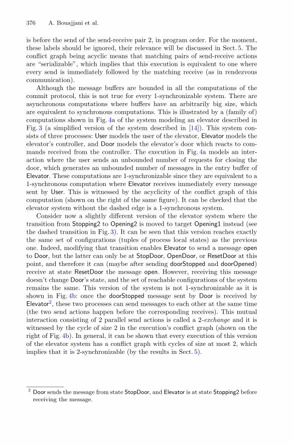
376 A. Bouajjani et al.

is before the send of the send-receive pair 2, in program order. For the moment,these labels should be ignored, their relevance will be discussed in Sect. 5. Theconflict graph being acyclic means that matching pairs of send-receive actionsare “serializable”, which implies that this execution is equivalent to one whereevery send is immediately followed by the matching receive (as in rendezvouscommunication).

Although the message buffers are bounded in all the computations of thecommit protocol, this is not true for every 1-synchronizable system. There areasynchronous computations where buffers have an arbitrarily big size, whichare equivalent to synchronous computations. This is illustrated by a (family of)computations shown in Fig. 4a of the system modeling an elevator described inFig. 3 (a simplified version of the system described in [14]). This system con-sists of three processes: User models the user of the elevator, Elevator models theelevator’s controller, and Door models the elevator’s door which reacts to com-mands received from the controller. The execution in Fig. 4a models an inter-action where the user sends an unbounded number of requests for closing thedoor, which generates an unbounded number of messages in the entry buffer ofElevator. These computations are 1-synchronizable since they are equivalent to a1-synchronous computation where Elevator receives immediately every messagesent by User. This is witnessed by the acyclicity of the conflict graph of thiscomputation (shown on the right of the same figure). It can be checked that theelevator system without the dashed edge is a 1-synchronous system.

Consider now a slightly different version of the elevator system where thetransition from Stopping2 to Opening2 is moved to target Opening1 instead (seethe dashed transition in Fig. 3). It can be seen that this version reaches exactlythe same set of configurations (tuples of process local states) as the previousone. Indeed, modifying that transition enables Elevator to send a message opento Door, but the latter can only be at StopDoor, OpenDoor, or ResetDoor at thispoint, and therefore it can (maybe after sending doorStopped and doorOpened)receive at state ResetDoor the message open. However, receiving this messagedoesn’t change Door’s state, and the set of reachable configurations of the systemremains the same. This version of the system is not 1-synchronizable as it isshown in Fig. 4b: once the doorStopped message sent by Door is received byElevator2, these two processes can send messages to each other at the same time(the two send actions happen before the corresponding receives). This mutualinteraction consisting of 2 parallel send actions is called a 2-exchange and it iswitnessed by the cycle of size 2 in the execution’s conflict graph (shown on theright of Fig. 4b). In general, it can be shown that every execution of this versionof the elevator system has a conflict graph with cycles of size at most 2, whichimplies that it is 2-synchronizable (by the results in Sect. 5).

2 Door sends the message from state StopDoor, and Elevator is at state Stopping2 beforereceiving the message.

On the Completeness of Verifying Message Passing Programs 377

3 Message Passing Systems

We define a message passing system as the composition of a set of processes thatexchange messages, which can be stored in FIFO buffers before being received(we assume one buffer per process, storing incoming messages from all the otherprocesses). Each process is described as a state machine that evolves by execut-ing send or receive actions. An execution of such a system can be representedabstractly using a partially-ordered set of events, called a trace. The partial orderin a trace represents the causal relation between events. We show that thesesystems satisfy causal delivery, i.e., the order in which messages are receivedby a process is consistent with the causal relation between the correspondingsendings.

Fig. 3. A system modeling an elevator.

We fix sets P and V of process ids and message payloads, and sets S ={send(p, q, v) : p, q ∈ P, v ∈ V} and R = {rec(q, v) : q ∈ P, v ∈ V} of send actionsand receive actions. Each send send(p, q, v) combines two process ids p, q denotingthe sender and the receiver of the message, respectively, and a message payloadv. Receive actions specify the process q receiving the message, and the messagepayload v. The process executing an action a ∈ S ∪ R is denoted proc(a), i.e.,proc(a) = p for all a = send(p, q, v) or a = rec(p, v), and the destination q ofa send s = send(p, q, v) ∈ S is denoted dest(s). The set of send, resp., receive,actions a of process p, i.e., with proc(a) = p, is denoted by Sp, resp., Rp.

A message passing system is a tuple S = ((Lp, δp, l0p) | p ∈ P) where Lp is the

set of local states of process p, δp ⊆ L × (Sp ∪ Rp) × L is a transition relation

378 A. Bouajjani et al.

describing the evolution of process p, and l0p is the initial state of process p.Examples of message passing systems can be found in Figs. 1 and 3.

We fix a set M of message identifiers, and the sets Sid = {si : s ∈ S, i ∈ M}and Rid = {ri : r ∈ R, i ∈ M} of indexed actions. Message identifiers are usedto pair send and receive actions. We denote the message id of an indexedsend/receive action a by msg(a). Indexed send and receive actions s ∈ Sid andr ∈ Rid are matching, written s �−� r, when msg(s) = msg(r).

A configuration c = 〈l, b〉 is a vector l of local states along with a vector b ofmessage buffers (sequences of message payloads tagged with message identifiers).The transition relation a−→ (with label a ∈ Sid ∪ Rid) between configurations isdefined as expected. Every send action enqueues the message into the destina-tion’s buffer, and every receive dequeues a message from the buffer. An executionof a system S under the asynchronous semantics is a sequence of indexed actionswhich corresponds to applying a sequence of transitions from the initial configu-ration (where processes are in their initial states and the buffers are empty). LetasEx(S) denote the set of these executions. Given an execution e, a send actions in e is called an unmatched send when e contains no receive action r such thats �−� r. An execution e is called matched when it contains no unmatched send.

Traces. Executions are represented using traces which are sets of indexed actionstogether with a program order relating every two actions of the same processand a source relation relating a send with the matching receive (if any).

Fig. 4. Executions of the elevator.

Formally, a trace is a tuple t = (A, po, src) where A ⊆ Sid ∪ Rid, po ⊆ A2

defines a total order between actions of the same process, and src ⊆ Sid ×Rid isa relation s.t. src(a, a′) iff a �− �a′. The trace tr(e) of an execution e is (A, po, src)where A is the set of all actions in e, po(a, a′) iff proc(a) = proc(a′) and a occursbefore a′ in e, and src(a, a′) iff a �−�a′. Examples of traces can be found in Figs. 2

On the Completeness of Verifying Message Passing Programs 379

and 4. The union of po and src is acyclic. Let asTr(S) = {tr(e) : e ∈ asEx(S)}be the set of traces of S under the asynchronous semantics.

Traces abstract away the order of non-causally related actions, e.g., two sendsof different processes that could be executed in any order. Two executions havethe same trace when they only differ in the order between such actions. Formally,given an execution e = e1 ·a ·a′ ·e2 with tr(e) = (A, po, src), where e1, e2 ∈ (Sid∪Rid)∗ and a, a′ ∈ Sid∪Rid, we say that e′ = e1 ·a′ ·a·e2 is derived from e by a validswap iff (a, a′) ∈ po∪src. A permutation e′ of an execution e is conflict-preservingwhen e′ can be derived from e through a sequence of valid swaps. For simplicity,whenever we use the term permutation we mean conflict-preserving permutation.For instance, a permutation of send1(p1, q, ) send2(p2, q, ) rec1(q, ) rec2(q, )is send1(p1, q, ) rec1(q, ) send2(p2, q, ) rec2(q, ) and a permutation of theexecution send1(p1, q1, ) send2(p2, q2, ) rec2(q2, ) rec1(q1, ) is send1(p1, q1, )rec1(q1, ) send2(p2, q2, ) rec2(q2, ).

Note that the set of executions having the same trace are permutations of oneanother. Also, a system S cannot distinguish between permutations of executionsor equivalently, executions having the same trace.

Causal Delivery. The asynchronous semantics ensures a property known ascausal delivery, which intuitively, says that the order in which messages arereceived by a process q is consistent with the “causal” relation between them.Two messages are causally related if for instance, they were sent by the sameprocess p or one of the messages was sent by a process p after the other one wasreceived by the same process p. This property is ensured by the fact that themessage buffers have a FIFO semantics and a sent message is instantaneouslyenqueued in the destination’s buffer. For instance, the trace (execution) on theleft of Fig. 5 satisfies causal delivery. In particular, the messages v1 and v3 arecausally related, and they are received in the same order by q2. On the right ofFig. 5, we give a trace where the messages v1 and v3 are causally related, butreceived in a different order by q2, thus violating causal delivery. This trace isnot valid because the message v1 would be enqueued in the buffer of q2 beforesend(p, q1, v2) is executed and thus, before send(q1, q2, v3) as well.

Fig. 5. A trace satisfying causal delivery (on the left) and a trace violating causaldelivery (on the right).

380 A. Bouajjani et al.

Fig. 6. An execution of the 1-synchronous semantics.

Formally, for a trace t = (A, po, src), the transitive closure of po∪src, denotedby �t, is called the causal relation of t. For instance, for the trace t on the left ofFig. 5, we have that send(p, q2, v1) �t send(q1, q2, v3). A trace t satisfies causaldelivery if for every two send actions s1 and s2 in A,

(s1 �t s2 ∧ dest(s1) = dest(s2)) =⇒ ( ∃r2 ∈ A. s2 �−� r2)∨(∃r1, r2 ∈ A. s1 �−� r1 ∧ s2 �−� r2 ∧ (r2, r1) ∈ po)

It can be easily proved that every trace t ∈ asTr(S) satisfies causal delivery.

4 Synchronizability

We define a property of message passing systems called k-synchronizability asthe equality between the set of traces generated by the asynchronous semanticsand the set of traces generated by a particular semantics called k-synchronous.

The k-synchronous semantics uses an extended version of the standardrendez-vous primitive where more than one process is allowed to send a mes-sage and a process can send multiple messages, but all these messages must bereceived before being allowed to send more messages. This primitive is calledk-exchange if the number of sent messages is at most k. For instance, the exe-cution send1(p1, p2, ) send2(p2, p1, ) rec1(p2, ) rec2(p1, ) is an instance of a2-exchange. To ensure that the k-synchronous semantics is prefix-closed (if itadmits an execution, then it admits all its prefixes), we allow messages to bedropped during a k-exchange transition. For instance, the prefix of the previousexecution without the last receive (rec2(p1, )) is also an instance of a 2-exchange.The presence of unmatched send actions must be constrained in order to ensurethat the set of executions admitted by the k-synchronous semantics satisfiescausal delivery. Consider for instance, the sequence of 1-exchanges in Fig. 6, a1-exchange with one unmatched send, followed by two 1-exchanges with match-ing pairs of send/receives. The receive action (rec(q2, v3)) pictured as an emptybox needs to be disabled in order to exclude violations of causal delivery. Tothis, the semantics tracks for each process p a set of processes B(p) from whichit is forbidden to receive messages. For the sequence of 1-exchanges in Fig. 6,the unmatched send(p, q2, v1) disables any receive by q2 of a message sent byp (otherwise, it will be even a violation of the FIFO semantics of q2’s buffer).Therefore, the first 1-exchange results in B(q2) = {p}. The second 1-exchange

On the Completeness of Verifying Message Passing Programs 381

(the message from p to q1) forbids q2 to receive any message from q1. Otherwise,this message will be necessarily causally related to v1, and receiving it will leadto a violation of causal delivery. Therefore, when reaching send(q1, q2, v3) thereceive rec(q2, v3) is disabled because q1 ∈ B(q2).

Fig. 7. The synchronous semantics. Above, ε is a vector where all the components areε, and

e−→ is the transition relation of the asynchronous semantics.

Formally, a configuration c′ = (l, B) in the synchronous semantics is a vectorl of local states together with a function B : P → 2P. The transition relation⇒k is defined in Fig. 7. A k-exchange transition corresponds to a sequenceof transitions of the asynchronous semantics starting from a configuration withempty buffers. The sequence of transitions is constrained to be a sequence ofat most k sends followed by a sequence of receives. The receives are enableddepending on previous unmatched sends as explained above, using the functionB. The semantics defined by ⇒k is called the k-synchronous semantics.

Executions and traces are defined as in the case of the asynchronous seman-tics, using ⇒k for some fixed k instead of →. The set of executions, resp., traces,of S under the k-synchronous semantics is denoted by sExk(S), resp., sTrk(S).The executions in sExk(S) and the traces in sTrk(S) are called k-synchronous.

An execution e such that tr(e) is k-synchronous is called k-synchronizable.We omit k when it is not important. The set of executions generated by a systemS under the k-synchronous semantics is prefix-closed. Therefore, the set of itsk-synchronizable executions is prefix-closed as well. Also, k-synchronizable andk-synchronous executions are undistinguishable up to permutations.

Definition 1. A message passing system S is called k-synchronizable whenasTr(S) = sTrk(S).

It can be easily proved that k-synchronizable systems reach exactly thesame set of local state vectors under the asynchronous and the k-synchronoussemantics. Therefore, any assertion checking or invariant checking problem fora k-synchronizable system S can be solved by considering the k-synchronoussemantics instead of the asynchronous one. This holds even for the problem ofdetecting deadlocks. Therefore, all these problems become decidable for finite-state k-synchronizable systems, whereas they are undecidable in the general case(because of the FIFO message buffers).

382 A. Bouajjani et al.

5 Characterizing Synchronous Traces

Fig. 8. A trace and itsconflict graph.

We give a characterization of the traces generated by thek-synchronous semantics that uses a notion of conflict-graph similar to the one used in conflict serializability [27].The nodes of the conflict graph correspond to pairs ofmatching actions (a send and a receive) or to unmatchedsends, and the edges represent the program order relationbetween the actions represented by these nodes.

For instance, an execution with an acyclic conflictgraph, e.g., the execution in Fig. 2, is “equivalent” to anexecution where every receive immediately follows thematching send. Therefore, it is an execution of the 1-synchronous semantics. For arbitrary values of k, the con-flict graph may contain cycles, but of a particular form.For instance, traces of the 2-synchronous semantics may

contain a cycle of size 2 like the one in Fig. 4(b). More generally, we show thatthe conflict graph of a k-synchronous trace cannot contain cycles of size strictlybigger than k. However, this class of cycles is not sufficient to precisely charac-terize the k-synchronous traces. Consider for instance the trace on top of Fig. 8.Its conflict-graph contains a cycle of size 4 (shown on the bottom), but the traceis not 4-synchronous. The reason is that the messages tagged by 1 and 4 mustbe sent during the same exchange transition, but receiving message 4 needs thatthe message 3 is sent after 2 is received. Therefore, it is not possible to scheduleall the send actions before all the receives. Such scenarios correspond to cycles inthe conflict graph where at least one receive is before a send in the program order(witnessed by the edge labeled by RS). We show that excluding such cycles, inaddition to cycles of size strictly bigger than k, is a precise characterization ofk-synchronous traces.

The conflict-graph of a trace t = (A, po, src) is the labeled directed graphCGt = 〈V,E, �E〉 where: (1) the set of nodes V includes one node for each pair ofmatching send and receive actions, and each unmatched send action in t, and (2)the set of edges E is defined by: (v, v′) ∈ E′ iff there exist actions a ∈ act(v) anda′ ∈ act(v′) such that (a, a′) ∈ po (where act(v) is the set of actions of trace tcorresponding to the graph node v). The label of the edge (v, v′) records whethera and a′ are send or receive actions, i.e., for all X,Y ∈ {S,R}, XY ∈ �(v, v′) iffa ∈ Xid and a′ ∈ Yid.

A direct consequence of previous results on conflict serializability [27] is that atrace is 1-synchronous whenever its conflict-graph is acyclic. A cycle of a conflictgraph CGt is called bad when it contains an edge labeled by RS. Otherwise, itis called good. The following result is a characterization of k-synchronous traces.

Theorem 1. A trace t satisfying causal delivery is k-synchronous iff every cyclein its conflict-graph is good and of size at most k.

Theorem 1 can be used to define a runtime monitoring algorithm for k-synchronizability checking. The monitor records the conflict-graph of the trace

On the Completeness of Verifying Message Passing Programs 383

produced by the system and checks whether it contains some bad cycle, or a cycleof size bigger than k. While this approach requires dealing with unbounded mes-sage buffers, the next section shows that this is not necessary. Synchronizabilityviolations, if any, can be exposed by executing the system under the synchronoussemantics.

6 Checking Synchronizability

We show that checking k-synchronizability can be reduced to a reachability prob-lem under the k-synchronous semantics (where message buffers are bounded).This reduction holds for arbitrary, possibly infinite-state, systems. More pre-cisely, since the set of (asynchronous) executions of a system is prefix-closed,if a system S admits a synchronizability violation, then it also admits a bor-derline violation, for which every strict prefix is synchronizable. We show thatevery borderline violation can be “simulated”3 by the synchronous semanticsof an instrumentation of S where the receipt of exactly one message is delayed(during every execution). We describe a monitor that observes executions of theinstrumentation (under the synchronous semantics) and identifies synchroniz-ability violations (there exists a run of this monitor that goes to an error statewhenever such a violation exists).

6.1 Borderline Synchronizability Violations

For a system S, a violation e to k-synchronizability is called borderline whenevery strict prefix of e is k-synchronizable. Figure 9(a) gives an example of a bor-derline violation to 1-synchronizability (it is the same execution as in Fig. 4(b)).

We show that every borderline violation e ends with a receive action and thisaction is included in every cycle of CGtr(e) that is bad or exceeds the bound k.Given a cycle c = v, v1, . . . , vn, v of a conflict graph CGt, the node v is called acritical node of c when (v, v1) is an SX edge with X ∈ {S,R} and (vn, v) is anY R edge with Y ∈ {S,R}.

Lemma 1. Let e be a borderline violation to k-synchronizability of a system S.Then, e = e′ · r for some e′ ∈ (Sid ∪ Rid)∗ and r ∈ Rid. Moreover, the node v ofCGtr(e) representing r (and the corresponding send) is a critical node of everycycle of CGtr(e) which is bad or of size bigger than k.

6.2 Simulating Borderline Violations on the Synchronous Semantics

Let S ′ be a system obtained from S by “delaying” the reception of exactly onenondeterministically chosen message: S ′ contains an additional process π andexactly one message sent by a process in S is non-deterministically redirected

3 We refer to the standard notion of (stuttering) simulation where one system mimicsthe transitions of the other system.

384 A. Bouajjani et al.

Fig. 9. A borderline violation to 1-synchronizability.

to π4, which sends it to the original destination at a later time5. We show thatthe synchronous semantics of S ′ “simulates” a permutation of every borderlineviolation of S. Figure 9(b) shows the synchronous execution of S ′ that corre-sponds to the borderline violation in Fig. 9(a). It is essentially the same exceptfor delaying the reception of doorOpened by sending it to π who relays it to theelevator at a later time.

The following result shows that the k-synchronous semantics of S ′ “simu-lates” all the borderline violations of S, modulo permutations.

Lemma 2. Let e = e1 · sendi(p, q, v) · e2 · reci(q, v) be a borderline violation tok-synchronizability of S. Then, sExk(S ′) contains an execution e′ of the form:

e′ = e′1 · sendi(p, π, (q, v)) · reci(π, (q, v)) · e′

2 · sendj(π, q, v) · recj(q, v)

such that e′1 · sendi(p, q, v) · e′

2 is a permutation of e1 · sendi(p, q, v) · e2.

Checking k-synchronizability for S on the system S ′ would require thatevery (synchronous) execution of S ′ can be transformed to an execution of Sby applying an homomorphism σ where the send/receive pair with destinationπ is replaced with the original send action and the send/receive pair initiatedby π is replaced with the original receive action (all the other actions are leftunchanged). However, this is not true in general. For instance, S ′ may admit anexecution sendi(p, π, (q, v))·reci(π, (q, v))·sendj(p, q, v′)·recj(q, v′)·sendi′(π, q, v)·reci′(q, v) where a message sent after the one redirected to π is received earlier,and the two messages were sent by the same process p. This execution is possibleunder the 1-synchronous semantics of S ′. Applying the homomorphism σ, we getthe execution sendi(p, q, v) · sendj(p, q, v′) · recj(q, v′) · reci(q, v) which violatescausal delivery and therefore, it is not admitted by the asynchronous semantics

4 Meaning that every transition labeled by a send action send(p, q, v) is doubled bya transition labeled by send(p, π, (q, v)), and such a send to π is enabled only oncethroughout the entire execution.

5 The process π stores the message (q, v) it receives in its state and has one transitionwhere it can send v to the original destination q.

On the Completeness of Verifying Message Passing Programs 385

of S. Our solution to this problem is to define a monitor Mcausal , i.e., a processwhich reads every transition label in the execution and advances its local state,which excludes such executions of S ′ when run under the synchronous semantics,i.e., it blocks the system S ′ whenever applying some transition would lead to anexecution which, modulo the homomorphism σ, is a violation of causal delivery.This monitor is based on the same principles that we used to exclude violationsof causal delivery in the synchronous semantics in the presence of unmatchedsends (the component B from a synchronous configuration).

6.3 Detecting Synchronizability Violations

We complete the reduction of checking k-synchronizability to a reachability prob-lem under the k-synchronous semantics by describing a monitor Mviol (k), whichobserves executions in the k-synchronous semantics of S ′ ||Mcausal and checkswhether they represent violations to k-synchronizability; Mviol (k) goes to anerror state whenever such a violation exists.

Essentially, Mviol(k) observes the sequence of k-exchanges in an execu-tion and tracks a conflict graph cycle, if any, interpreting sendi(p, π, (q, v)) ·reci(π, (q, v)) as in the original system S, i.e., as sendi(p, q, v), and sendi(π, q, v) ·reci(q, v) as reci(q, v). By Lemma 2, every cycle that is a witness for non k-synchronizability includes the node representing the pair sendi(p, q, v), reci(q, v).Moreover, the successor of this node in the cycle represents an action that is exe-cuted by p and the predecessor an action executed by q. Therefore, the monitorsearches for a conflict-graph path from a node representing an action of p to anode representing an action of q. Whenever it finds such a path it goes to anerror state.

Figure 10 lists the definition of Mviol (k) as an abstract state machine. Bythe construction of S ′, we assume w.l.o.g., that both the send to π and the sendfrom π are executed in isolation as an instance of 1-exchange. When observingthe send to π, the monitor updates the variable conflict, which in generalstores the process executing the last action in the cycle, to p. Also, a variablecount, which becomes 0 when the cycle has strictly more than k nodes, is ini-tialized to k. Then, for every k-exchange transition in the execution, Mviol(k)non-deterministically picks pairs of matching send/receive or unmatched sendsto continue the conflict-graph path, knowing that the last node represents anaction of the process stored in conflict. The rules for choosing pairs of match-ing send/receive to advance the conflict-graph path are pictured on the rightof Fig. 10 (advancing the conflict-graph path with an unmatched send doesn’tmodify the value of conflict, it just decrements the value of count). There aretwo cases depending on whether the last node in the path conflicts with the sendor the receive of the considered pair. One of the two processes involved in thispair of send/receive equals the current value of conflict. Therefore, conflictcan either remain unchanged or change to the value of the other process. Thevariable lastIsRec records whether the current conflict-graph path ends in aconflict due to a receive action. If it is the case, and the next conflict is between

386 A. Bouajjani et al.

Fig. 10. The monitor Mviol(k). B is the set of Booleans and N is the set of naturalnumbers. Initially, conflict is ⊥, while lastIsRec and sawRS are false.

this receive and a send, then sawRS is set to true to record the fact that thepath contains an RS labeled edge (leading to a potential bad cycle).

When π sends its message to q, the monitor checks whether the conflict-graphpath it discovered ends in a node representing an action of q. If this is the case,this path together with the node representing the delayed send forms a cycle.Then, if sawRS is true, then the cycle is bad and if count reached the value 0,then the cycle contains more than k nodes. In both cases, the current executionis a violation to k-synchronizability.

The set of executions in the k-synchronous semantics of S ′ composed withMcausal and Mviol (k), in which the latter goes to an error state, is denoted byS ′k ||Mcausal || ¬Mviol (k).

Theorem 2. For a given k, a system S is k-synchronizable iff the set of execu-tions S ′

k ||Mcausal || ¬Mviol (k) is empty.

Given a system S, an integer k, and a local state l, the reachability problemunder the k-synchronous semantics asks whether there exists a k-synchronousexecution of S reaching a configuration (l, B) with l = lp for some p ∈ P. Theo-rem 2 shows that checking k-synchronizability can be reduced to a reachabilityproblem under the k-synchronous semantics. This reduction holds for arbitrary(infinite-state) systems, which implies that k-synchronizability can be checkedusing the existing assertion checking technology. Moreover, for finite-state sys-tems, where each process has a finite number of local states (message buffers canstill be unbounded), it implies that checking this property is PSPACE-complete.

On the Completeness of Verifying Message Passing Programs 387

Theorem 3. For a finite-state system S, the reachability problem under the k-synchronous semantics and the problem of checking k-synchronizability of S aredecidable and PSPACE-complete.

7 Experimental Evaluation

Fig. 11. Experimental results.

As a proof of concept, we have applied ourprocedure for checking k-synchronizabilityto a set of examples extracted from thedistribution of the P language6. Two-phasecommit and Elevator are presented inSect. 2, German is a model of the cache-coherence protocol with the same name,OSR is a model of a device driver, and

Replication Storage is a model of a protocol ensuring eventual consistency of areplicated register. These examples cover common message communication pat-terns that occur in different domains: distributed systems (Two-phase commit,Replication storage), device drivers (Elevator, OSR), cache-coherence protocols(German). We have rewritten these examples in the Promela language and usedthe Spin model checker7 for discharging the reachability queries. For a givenprogram, its k-synchronous semantics and the monitors defined in Sect. 6 areimplemented as ghost code. Finding a conflict-graph cycle which witnesses nonk-synchronizability corresponds to violating an assertion.

The experimental data is listed in Fig. 11: Proc, resp., Loc, is the number ofprocesses, resp., the number of lines of code (loc) of the original program, k isthe minimal integer for which the program is k-synchronizable, and Time givesthe number of minutes needed for this check. The ghost code required to checkk-synchronizability takes 250 lines of code in average.

8 Related Work

Automatic verification of asynchronous message passing systems is undecidablein general [10]. A number of decidable subclasses has been proposed. The classof systems, called synchronizable as well, in [4], requires that a system gener-ates the same sequence of send actions when executed under the asynchronoussemantics as when executed under a synchronous semantics based on rendezvouscommunication. These systems are all 1-synchronizable, but the inclusion isstrict (the 1-synchronous semantics allows unmatched sends). The techniquesproposed in [4] to check that a system is synchronizable according to their defi-nition cannot be extended to k-synchronizable systems. Other classes of systemsthat are 1-synchronizable have been proposed in the context of session types,

6 Available at https://github.com/p-org.7 Available at http://spinroot.com.

388 A. Bouajjani et al.

e.g., [12,20,21,26]. A sound but incomplete proof method for distributed algo-rithms that is based on a similar idea of avoiding reasoning about all programcomputations is introduced in [3]. Our class of synchronizable systems differs alsofrom classes of communicating systems that restrict the type of communication,e.g., lossy-communication [2], half-duplex communication [11], or the topology ofthe interaction, e.g., tree-based communication in concurrent pushdowns [19,23].

The question of deciding if all computations of a communicating systemare equivalent (in the language theoretic sense) to computations with boundedbuffers has been studied in, e.g., [17], where this problem is proved to be unde-cidable. The link between that problem and our synchronizability problem is not(yet) clear, mainly because non synchronizable computations may use boundedbuffers.

Our work proposes a solution to the question of defining adequate (in termsof coverage and complexity) parametrized bounded analyses for message pass-ing programs, providing the analogous of concepts such as context-boundingor delay-bounding defined for shared-memory concurrent programs. Boundedanalyses for concurrent systems was initiated by the work on bounded-contextswitch analysis [25,28,29]. For shared-memory programs, this work has beenextended to unbounded threads or larger classes of behaviors, e.g., [8,15,22,24].Few bounded analyses incomparable to ours have been proposed for messagepassing systems, e.g., [6,23]. Contrary to our work, these works on boundedanalyses in general do not propose decision procedures for checking if the anal-ysis is complete (covers all reachable states). The only exception is [24], whichconcerns shared-memory.

Partial-order reduction techniques, e.g., [1,16], allow to define equivalenceclasses on behaviors, based on notions of action independence and explore (ide-ally) only one representative of each class. This has lead to efficient algorithmictechniques for enhanced model-checking of concurrent shared-memory programsthat consider only a subset of relevant action interleavings. In the worst case,these techniques will still need to explore all of the interleavings. Moreover, thesetechniques are not guaranteed to terminate when the buffers are unbounded.

The work in [13] defines a particular class of schedulers, that roughly, pri-oritize receive actions over send actions, which is complete in the sense that itallows to construct the whole set of reachable states. Defining an analysis basedon this class of schedulers has the same drawback as partial-order reductions,in the worst case, it needs to explore all interleavings, and termination is notguaranteed.

The approach in this work is related to robustness checking [5,7]. The gen-eral paradigm is to decide that a program has the same behaviors under twosemantics, one being weaker than the other, by showing a polynomial reductionto a state reachability problem under the stronger semantics. For instance, inour case, the class of message passing programs with unbounded FIFO channelsis Turing powerful, but still, surprisingly, k-synchronizability of these programsis decidable and PSPACE-complete. The results in [5,7] cannot be applied in

On the Completeness of Verifying Message Passing Programs 389

our context: the class of programs and their semantics are different, and the cor-responding robustness checking algorithms are based on distinct concepts andtechniques.

References

1. Abdulla, P.A., Aronis, S., Jonsson, B., Sagonas, K.F.: Optimal dynamic partialorder reduction. In: Jagannathan, S., Sewell, P. (eds.) The 41st Annual ACMSIGPLAN-SIGACT Symposium on Principles of Programming Languages, POPL2014, San Diego, CA, USA, 20-21 January 2014, pp. 373–384. ACM (2014). https://doi.org/10.1145/2535838.2535845

2. Abdulla, P.A., Jonsson, B.: Verifying programs with unreliable channels. Inf. Com-put. 127(2), 91–101 (1996). https://doi.org/10.1006/inco.1996.0053

3. Bakst, A., von Gleissenthall, K., Kici, R.G., Jhala, R.: Verifying distributedprograms via canonical sequentialization. PACMPL 1(OOPSLA), 110:1–110:27(2017). https://doi.org/10.1145/3133934

4. Basu, S., Bultan, T.: On deciding synchronizability for asynchronously communi-cating systems. Theor. Comput. Sci. 656, 60–75 (2016). https://doi.org/10.1016/j.tcs.2016.09.023

5. Bouajjani, A., Derevenetc, E., Meyer, R.: Robustness against relaxed memorymodels. In: Hasselbring, W., Ehmke, N.C. (eds.) Software Engineering 2014, Kiel,Deutschland. LNI, vol. 227, pp. 85–86. GI (2014). http://eprints.uni-kiel.de/23752/

6. Bouajjani, A., Emmi, M.: Bounded phase analysis of message-passing programs.In: Flanagan, C., Konig, B. (eds.) TACAS 2012. LNCS, vol. 7214, pp. 451–465.Springer, Heidelberg (2012). https://doi.org/10.1007/978-3-642-28756-5 31

7. Bouajjani, A., Emmi, M., Enea, C., Ozkan, B.K., Tasiran, S.: Verifying robustnessof event-driven asynchronous programs against concurrency. In: Yang, H. (ed.)ESOP 2017. LNCS, vol. 10201, pp. 170–200. Springer, Heidelberg (2017). https://doi.org/10.1007/978-3-662-54434-1 7

8. Bouajjani, A., Emmi, M., Parlato, G.: On sequentializing concurrent programs.In: Yahav, E. (ed.) SAS 2011. LNCS, vol. 6887, pp. 129–145. Springer, Heidelberg(2011). https://doi.org/10.1007/978-3-642-23702-7 13

9. Bouajjani, A., Enea, C., Ji, K., Qadeer, S.: On the completeness of verifying mes-sage passing programs under bounded asynchrony. arXiv:1804.06612 [cs.PL]

10. Brand, D., Zafiropulo, P.: On communicating finite-state machines. J. ACM 30(2),323–342 (1983). https://doi.org/10.1145/322374.322380

11. Cece, G., Finkel, A.: Verification of programs with half-duplex communication. Inf.Comput. 202(2), 166–190 (2005). https://doi.org/10.1016/j.ic.2005.05.006

12. Denielou, P.-M., Yoshida, N.: Multiparty session types meet communicatingautomata. In: Seidl, H. (ed.) ESOP 2012. LNCS, vol. 7211, pp. 194–213. Springer,Heidelberg (2012). https://doi.org/10.1007/978-3-642-28869-2 10

13. Desai, A., Garg, P., Madhusudan, P.: Natural proofs for asynchronous programsusing almost-synchronous reductions. In: Black, A.P., Millstein, T.D. (eds.) Pro-ceedings of the 2014 ACM International Conference on Object Oriented Program-ming Systems Languages & Applications, OOPSLA 2014, part of SPLASH 2014,Portland, OR, USA, 20–24 October 2014, pp. 709–725. ACM (2014). https://doi.org/10.1145/2660193.2660211

390 A. Bouajjani et al.

14. Desai, A., Gupta, V., Jackson, E.K., Qadeer, S., Rajamani, S.K., Zufferey, D.: P:safe asynchronous event-driven programming. In: Boehm, H., Flanagan, C. (eds.)ACM SIGPLAN Conference on Programming Language Design and Implementa-tion, PLDI 2013, Seattle, WA, USA, 16–19 June 2013, pp. 321–332. ACM (2013).https://doi.org/10.1145/2462156.2462184

15. Emmi, M., Qadeer, S., Rakamaric, Z.: Delay-bounded scheduling. In: Ball, T.,Sagiv, M. (eds.) Proceedings of the 38th ACM SIGPLAN-SIGACT Symposium onPrinciples of Programming Languages, POPL 2011, Austin, TX, USA, 26–28 Jan-uary 2011, pp. 411–422. ACM (2011). https://doi.org/10.1145/1926385.1926432

16. Flanagan, C., Godefroid, P.: Dynamic partial-order reduction for model check-ing software. In: Palsberg, J., Abadi, M. (eds.) Proceedings of the 32nd ACMSIGPLAN-SIGACT Symposium on Principles of Programming Languages, POPL2005, Long Beach, California, USA, 12–14 January 2005, pp. 110–121. ACM (2005).https://doi.org/10.1145/1040305.1040315

17. Genest, B., Kuske, D., Muscholl, A.: On communicating automata with boundedchannels. Fundam. Inform. 80(1–3), 147–167 (2007). http://content.iospress.com/articles/fundamenta-informaticae/fi80-1-3-09

18. Gupta, A., Malik, S. (eds.): CAV 2008. LNCS, vol. 5123. Springer, Heidelberg(2008). https://doi.org/10.1007/978-3-540-70545-1

19. Heußner, A., Leroux, J., Muscholl, A., Sutre, G.: Reachability analysis of commu-nicating pushdown systems. Logical Methods Comput. Sci. 8(3) (2012). https://doi.org/10.2168/LMCS-8(3:23)2012

20. Honda, K., Vasconcelos, V.T., Kubo, M.: Language primitives and type disciplinefor structured communication-based programming. In: Hankin, C. (ed.) ESOP1998. LNCS, vol. 1381, pp. 122–138. Springer, Heidelberg (1998). https://doi.org/10.1007/BFb0053567

21. Honda, K., Yoshida, N., Carbone, M.: Multiparty asynchronous session types. J.ACM 63(1), 9:1–9:67 (2016). https://doi.org/10.1145/2827695

22. Kidd, N., Jagannathan, S., Vitek, J.: One stack to run them all. In: van de Pol, J.,Weber, M. (eds.) SPIN 2010. LNCS, vol. 6349, pp. 245–261. Springer, Heidelberg(2010). https://doi.org/10.1007/978-3-642-16164-3 18

23. La Torre, S., Madhusudan, P., Parlato, G.: Context-bounded analysis of concurrentqueue systems. In: Ramakrishnan, C.R., Rehof, J. (eds.) TACAS 2008. LNCS,vol. 4963, pp. 299–314. Springer, Heidelberg (2008). https://doi.org/10.1007/978-3-540-78800-3 21

24. La Torre, S., Madhusudan, P., Parlato, G.: Model-checking parameterized concur-rent programs using linear interfaces. In: Touili, T., Cook, B., Jackson, P. (eds.)CAV 2010. LNCS, vol. 6174, pp. 629–644. Springer, Heidelberg (2010). https://doi.org/10.1007/978-3-642-14295-6 54

25. Lal, A., Reps, T.W.: Reducing concurrent analysis under a context bound tosequential analysis. In: Gupta and Malik [18], pp. 37–51. https://doi.org/10.1007/978-3-540-70545-1 7

26. Lange, J., Tuosto, E., Yoshida, N.: From communicating machines to graphicalchoreographies. In: Rajamani, S.K., Walker, D. (eds.) Proceedings of the 42ndAnnual ACM SIGPLAN-SIGACT Symposium on Principles of Programming Lan-guages, POPL 2015, Mumbai, India, 15–17 January 2015, pp. 221–232. ACM(2015). https://doi.org/10.1145/2676726.2676964

27. Papadimitriou, C.H.: The serializability of concurrent database updates. J. ACM26(4), 631–653 (1979)

On the Completeness of Verifying Message Passing Programs 391

28. Qadeer, S., Rehof, J.: Context-bounded model checking of concurrent software.In: Halbwachs, N., Zuck, L.D. (eds.) TACAS 2005. LNCS, vol. 3440, pp. 93–107.Springer, Heidelberg (2005). https://doi.org/10.1007/978-3-540-31980-1 7

29. Qadeer, S., Wu, D.: KISS: keep it simple and sequential. In: Pugh, W., Chambers,C. (eds.) Proceedings of the ACM SIGPLAN 2004 Conference on ProgrammingLanguage Design and Implementation 2004, Washington, DC, USA, 9–11 June2004, pp. 14–24. ACM (2004). https://doi.org/10.1145/996841.996845

Open Access This chapter is licensed under the terms of the Creative CommonsAttribution 4.0 International License (http://creativecommons.org/licenses/by/4.0/),which permits use, sharing, adaptation, distribution and reproduction in any mediumor format, as long as you give appropriate credit to the original author(s) and thesource, provide a link to the Creative Commons license and indicate if changes weremade.

The images or other third party material in this chapter are included in the chapter’sCreative Commons license, unless indicated otherwise in a credit line to the material. Ifmaterial is not included in the chapter’s Creative Commons license and your intendeduse is not permitted by statutory regulation or exceeds the permitted use, you willneed to obtain permission directly from the copyright holder.

Constrained Dynamic Partial OrderReduction

Elvira Albert1 , Miguel Gomez-Zamalloa1(B) , Miguel Isabel1 ,and Albert Rubio2

1 Complutense University of Madrid,Madrid, Spain

mzamalloa@fdi.ucm.es2 Universitat Politecnica de Catalunya,

Barcelona, Spain

Abstract. The cornerstone of dynamic partial order reduction (DPOR)is the notion of independence that is used to decide whether each pairof concurrent events p and t are in a race and thus both p · t and t · pmust be explored. We present constrained dynamic partial order reduc-tion (CDPOR), an extension of the DPOR framework which is able toavoid redundant explorations based on the notion of conditional inde-pendence—the execution of p and t commutes only when certain inde-pendence constraints (ICs) are satisfied. ICs can be declared by the pro-grammer, but importantly, we present a novel SMT-based approach toautomatically synthesize ICs in a static pre-analysis. A unique featureof our approach is that we have succeeded to exploit ICs within thestate-of-the-art DPOR algorithm, achieving exponential reductions overexisting implementations.

1 Introduction

Partial Order Reduction (POR) is based on the idea that two interleavings canbe considered equivalent if one can be obtained from the other by swappingadjacent, non-conflicting independent execution steps. Such equivalence class iscalled a Mazurkiewicz trace, and POR guarantees that it is sufficient to exploreone interleaving per equivalence class. Early POR algorithms [8,10,20] reliedon static over-approximations to detect possible future conflicts. The Dynamic-POR (DPOR) algorithm, introduced by Godefroid [9] in 2005, was a break-through in the area because it does not need to look at the future. It keepstrack of the independence races witnessed along its execution and uses them todecide the required exploration dynamically, without the need of static approx-imation. DPOR is nowadays considered one of the most scalable techniques for

This work was funded partially by the Spanish MECD Salvador de MadariagaMobility Grants PRX17/00297 and PRX17/00303, the Spanish MINECO projectsTIN2015-69175-C4-2-R and TIN2015-69175-C4-3-R, and by the CM projectS2013/ICE-3006.

c© The Author(s) 2018H. Chockler and G. Weissenbacher (Eds.): CAV 2018, LNCS 10982, pp. 392–410, 2018.https://doi.org/10.1007/978-3-319-96142-2_24

Constrained Dynamic Partial Order Reduction 393

software verification. The key of DPOR algorithms is in the dynamic construc-tion of two types of sets at each scheduling point: the sleep set that containsprocesses whose exploration has been proved to be redundant (and hence shouldnot be selected), and the backtrack set that contains the processes that havenot been proved independent with previously explored steps (and hence need tobe explored). Source-DPOR (SDPOR) [1,2] improves the precision to computebacktrack sets (named source sets), proving optimality of the resulting algorithmfor any number of processes w.r.t. an unconditional independence relation.

Challenge. When considering (S)DPOR with unconditional independence, if apair of events is not independent in all possible executions, they are treated aspotentially dependent and their interleavings explored. Unnecessary explorationcan be avoided using conditional independence. E.g., two processes executingrespectively the atomic instructions if(z≥ 0) z = x; and x = x + 1; would beconsidered dependent even if z≤ −1—this is indeed an independence constraint(IC) for these two instructions. Conditional independence was early introducedin the context of POR [11,15]. The first algorithm that has used notions of con-ditional independence within the state-of-the-art DPOR algorithm is Context-Sensitive DPOR (CSDPOR) [3]. However, CSDPOR does not use ICs (it ratherchecks state equivalence dynamically during the exploration) and exploits con-ditional (context-sensitive) independence only partially to extend the sleep sets.Our challenge is twofold: (i) extend the DPOR framework to exploit ICs dur-ing the exploration in order to both reduce the backtrack sets and expand thesleep sets as much as possible, (ii) statically synthesize ICs in an automaticpre-analysis.

Contributions. The main contributions of this work can be summarized as:

1. We introduce sufficient conditions –that can be checked dynamically– tosoundly exploit ICs within the DPOR framework.

2. We extend the state-of-the-art DPOR algorithm with new forms of pruning(by means of expanding sleep sets and reducing backtrack sets).

3. We present an SMT-based approach to automatically synthesize ICs foratomic blocks, whose applicability goes beyond the DPOR context.

4. We experimentally show the exponential gains achieved by CDPOR on sometypical concurrency benchmarks used in the DPOR literature before.

2 Background

In this section we introduce some notations, the basic notions on the POR theoryand the state-of-the-art DPOR algorithm that we will extend in Sect. 3.

Our work is formalized for a general model of concurrent systems, in whicha program is composed of atomic blocks of code. An atomic block can containjust one (global) statement that affects the global state, a sequence of localstatements (that only read and write the local state of the process) followed bya global statement, or a block of code with possibly several global statements

394 E. Albert et al.

but whose execution cannot interleave with other processes because it has beenimplemented as atomic (e.g., using locks, semaphores, etc.). Each atomic blockin the program is given a unique block identifier. We use spawn(P [ini ]) to createa new process. Depending on the programming language, P can be the name ofa method and [ini] initial values for the parameters, or P can be the identifier ofthe initial block to execute and [ini] the initialization instructions, etc., in everycase with mechanisms to continue the execution from one block to the followingone. Notice that the use of atomic blocks in our formalization generalizes theparticular case of considering atomicity at the level of single instructions.

As previous work on DPOR [1–3], we assume the state space does not containcycles, executions have finite unbounded length and processes are deterministic(i.e., at a given time there is at most one event a process can execute). Let Σbe the set of states of the system. There is a unique initial state s0 ∈ Σ. Theexecution of a process p is represented as a partial function executep : Σ �→ Σthat moves the system from one state to a subsequent state. Each applicationof the function executep represents the execution of an atomic block of the codethat p is running, denoted as event (or execution step) of process p. An executionsequence E (also called derivation) of a system is a finite sequence of events ofits processes starting from s0, and it is uniquely characterized by the sequenceof processes that perform steps of E. For instance, p · q · q denotes the executionsequence that first performs one step in p, followed by two steps in q. We useε to denote the empty sequence. The state of the system after E is denoted bys[E]. The set of processes enabled in state s (i.e., that can perform an executionstep from s) is denoted by enabled(s).

2.1 Basics of Partial Order Reduction

An event e of the form (p, i) denotes the i-th occurrence of process p in anexecution sequence, and e denotes the process p of event e, which is extended tosequences of events in the natural way. We write e to refer to the identifier ofthe atomic block of code the event e is executing. The set of events in executionsequence E is denoted by dom(E). We use e <E e′ to denote that event e occursbefore event e′ in E, s.t. <E establishes a total order between events in E, andE ≤ E′ to denote that sequence E is a prefix of sequence E′. Let dom[E](w)denote the set of events in execution sequence E.w that are in sequence w, i.e.,dom(E.w)\dom(E). If w is a single process p, we use next[E](p) to denote thesingle event in dom[E](p). If P is a set of processes, next[E](P ) denotes the set ofnext[E](p) for all p ∈ P . The core concept in POR is that of the happens-beforepartial order among the events in execution sequence E, denoted by →E . Thisrelation defines a subset of the <E total order, such that any two sequences withthe same happens-before order are equivalent. Any linearization E′ of →E ondom(E) is an execution sequence with exactly the same happens-before relation→E′ as →E . Thus, →E induces a set of equivalent execution sequences, all withthe same happens-before relation. We use E � E′ to denote that E and E′ arelinearizations of the same happens-before relation. The happens-before partialorder has traditionally been defined in terms of a dependency relation between

Constrained Dynamic Partial Order Reduction 395

Algorithm 1. (Source+Context-sensitive)+Constrained DPOR algorithm1: procedure explore(E)2: if (∃p ∈ (enabled(s[E])\sleep(E))) then3: back(E) := {p};4: while (∃p ∈ (back(E)\sleep(E))) do5: let n = next[E](p);6: for all (e ∈ dom(E) such that e �E.p n) do7: let E′ = pre(E, e);8: let u = dep(E, e, n);9: if (¬(U⇒(Ie,n, e, n, s[E′.u])) then10: updateBack(E,E′, e, p);11: if C(s[E′.u]) for some C ∈ Ie,n then12: add u.p.e to sleep(E′);13: else14: updateSleepCS(E,E′, e, p);

15: sleep(E.p) := {x | x ∈ sleep(E), E |= p � x}16: ∪ {x | p.x ∈ sleep(E)}17: ∪ {x | x ∈ sleep(E), |x| = 1, m = next[E](x), U⇒(In,m, n,m, s[E]))};18: explore(E.p);19: sleep(E) := sleep(E) ∪ {p};

the execution steps associated to those events [10]. Intuitively, two steps p andq are dependent if there is at least one execution sequence E for which theydo not commute, either because (i) one enables the other (i.e., the executionof p leads to introducing q, or viceversa), or because (ii) s[E.p.q] �= s[E.q.p]. Wedefine dep(E, e, n) as the subsequence containing all events e′ in E that occurafter e and happen-before n in E.p (i.e., e<Ee′ and e′→E.pn). The unconditionaldependency relation is used for defining the concept of a race between two events.Event e is said to be in race with event e′ in execution E, if the events belong todifferent processes, e happens-before e′ in E (e →E e′), and the two events are“concurrent”, i.e. there exists an equivalent execution sequence E′ � E wherethe two events are adjacent. We write e �E e′ to denote that e is in race withe′ and that the race can be reversed (i.e., the events can be executed in reverseorder). POR algorithms use this relation to reduce the number of equivalentexecution sequences explored, with SDPOR ensuring that only one executionsequence in each equivalence class is explored.

2.2 State-of-the-Art DPOR with Unconditional Independence

Algorithm 1 shows the state-of-the-art DPOR algorithm –based on the SDPORalgorithm of [1,2],1 which in turn is based on the original DPOR algorithmof [9]. We refer to this algorithm as DPOR in what follows. The context-sensitiveextension of CSDPOR [3] (lines 14 and 16) and our extension highlighted in blue

1 The extension to support wake-up trees [2] is deliberately not included to simplifythe presentation.

396 E. Albert et al.

(lines 8–10, 11–13 and 17) should be ignored by now and will be described inSect. 3.

The algorithm carries out a depth-first exploration of the execution treeusing POR receiving as parameter a derivation E (initially empty). Essentially,it dynamically finds reversible races and is able to backtrack at the appropriatescheduling points to reverse them. For this purpose, it keeps two sets at everyprefix E′ of E: back(E′) with the set of processes that must be explored from E′,and, sleep(E′) with the set of sequences of processes that previous executionshave determined do not need to be explored from E′. Note that in the originalDPOR the sleep set contained only single processes, but in later improvementssequences of processes are added, so our description considers this general case.The algorithm starts by selecting any process p that is enabled by the statereached after executing E and is not already in sleep(E). If it does not findany such process p, it stops. Otherwise, after setting back(E) = {p} to startthe search, it explores every element in back(E) that is not in sleep(E). Thebacktrack set of E might grow as the loop progresses (due to later executions ofline 10). For each such p, DPOR performs two phases: race detection (lines 6, 7and 10) and state exploration (lines 15, 18 and 19). The race detection starts byfinding all events e in dom(E) such that e �E.p n, where n is the event beingselected (see line 5). For each such e, it sets E′ to pre(E, e), i.e., to be the pre-fix of E up to, but not including e. Procedure updateBack modifies back(E′)in order to ensure that the race between e and n is reversed. The source-setextension of [1,2] detects cases where there is no need to modify back(E′) –thisis done within procedure updateBack whose code is not shown because it isnot affected by our extension. After this, the algorithm continues with the stateexploration phase for E.p, by retaining in its sleep set any element x in sleep(E)whose events in E.p are independent of the next event of p in E (denoted asE |= px), i.e., any x such that next[E](p) would not happen-before any event indom(E.p.x)\dom(E.p). Then, the algorithm explores E.p, and finally it adds p tosleep(E) to ensure that, when backtracking on E, p is not selected until a depen-dent event with it is selected. All versions of the DPOR algorithm (except [3]) relyon the unconditional (or context-insensitive) dependency relation. This relationhas to be over-approximated, usually by requiring that global variables accessedby one execution step are not modified by the other.

Example 1. Consider the example in Fig. 1 with 3 processes p, q, r containing asingle atomic block. Since all processes have a single event, by abuse of notation,we refer to events by their process name throughout all examples in the paper.Relying on the usual over-approximation of dependency all three pairs of eventsare dependent. Therefore, starting with one instance per process, the algorithmhas to explore 6 execution sequences, each with a different happens-before rela-tion. The tree, including the dotted and dashed fragments, shows the explorationfrom the initial state z = −2, x = −2. The value of variable z is shown in brack-ets at each state. Essentially, in all states of the form E.e, the algorithm alwaysfinds a reversible race between the next event of the current selected process(p, q or r) and e, and adds it to back(E). Also, when backtracking on E, none

Constrained Dynamic Partial Order Reduction 397

of the elements in sleep(E) is propagated down, since all events are considereddependent. In the best case, considering an exact (yet unconditional) depen-dency relation which realizes that events p and r are independent, the algorithmwill make the following reductions. In state 6, p and r will not be in race andhence p will not be added to back(q). This avoids exploring the sequence p.rfrom 5. When backtracking on state 0 with r, where sleep(ε) = {p, q}, p will bepropagated down to sleep(r) since ε |= r p, hence avoiding the exploration ofp.q from 8. Thus, the algorithm will explore 4 sequences.

Fig. 1. Left: code of working example (up) and ICs (down). Right: execution treestarting from z = −2, x = −2. Full tree computed by SDPOR, dotted fragment notcomputed by CSDPOR, and, dashed+dotted fragment not computed by CDPOR.

3 DPOR with Conditional Independence

Our aim in CDPOR is twofold: (1) provide techniques to both infer and soundlycheck conditional independence, and (2) be able to exploit them at all pointsof the DPOR algorithm where dependencies are used. Section 3.1 reviews thenotions of conditional independence and ICs, and introduces a first type of checkwhere ICs can be directly used in the DPOR algorithm. Section 3.2 illustrateswhy ICs cannot be used at the remaining independence check points in thealgorithm, and introduces sufficient conditions to soundly exploit them at thosepoints. Finally, Sect. 3.3 presents the CDPOR algorithm that includes all typesof checks.

3.1 Using Precomputed ICs Directly Within DPOR

Conditional independence consists in checking independence at the given state.

Definition 1 (conditional independence). Two events α and β are inde-pendent in state S, written indep(α, β, S) if (i1) none of them enables the other

from S; and, (i2) if they are both enabled in S, then Sα·β−→ S′ and S

β·α−→ S′.

398 E. Albert et al.

The use of conditional independence in the POR theory was firstly studied in [15],and it has been partially applied within the DPOR algorithm in CSDPOR [3].Function updateSleepCS at line 14 and the modification of sleep at 16 encapsulatethis partial application of CSDPOR (the code of updateSleepCS is not shownbecause it is not affected by our extension). Intuitively, updateSleepCS works asfollows: when a reversible race is found in the current sequence being explored,it builds an alternative sequence which corresponds to the reverse race, and thenchecks whether the states reached after running the two sequences are the same.If they are, it adds the alternative sequence to the corresponding sleep set sothat this sequence is not fully explored when backtracking. Therefore, sleep setscan contain sequences of events which can be propagated down via the rule ofline 16 (i.e., if the event being explored is the head of a sequence in the sleepset, then the tail of the sequence is propagated down). In essence, the techniqueto check (i2) in Definition 1 in CSDPOR consists in checking state equivalencewith an alternative sequence in the current state (hence it is conditional) and, ifthe check succeeds, it is exploited in the sleep set only (and not in the backtrackset).

Example 2. Let us explain the intuition behind the reductions that CSDPORis able to achieve w.r.t. unconditional independence-based DPOR on the exam-ple. In state 1, when the algorithm selects q and detects the reversible racebetween q and p, it computes the alternative sequence q.p and realizes thats[p.q] = s[q.p], and hence adds p.q to sleep(ε). Similarly, in state 2, it computesp.r.q and realizes that s[p.q.r] = s[p.r.q] adding r.q to sleep(p). Besides thesetwo alternative sequences, it computes two more. Overall, CSDPOR explores 2complete sequences (p.q.r and q.r.p) and 13 states (the 9 states shown, plus 4additional states to compute the alternative sequences).

Instead of computing state equivalence to check (i2) as in [3], our approachassumes precomputed independence constraints (ICs) for all pairs of atomicblocks in the program. ICs will be evaluated at the appropriate state to deter-mine the independence between pairs of concurrent events executing such atomicblocks.

Definition 2 (ICs). Consider two events α and β that execute, respectively, theatomic blocks α and β. The independence constraints Iα,β are a set of booleanexpressions (constraints) on the variables accessed by α and β (including localand global variables) s.t., if some constraint C in Iα,β holds in state S, writtenC(S), then condition (i2) of indep(α, β, S) holds.

Our first contribution is in lines 11–13 where ICs are used within DPOR asfollows. Before executing updateSleepCS at line 14, we check if some constraintin Ie,n holds in the state s[E′.u], by building the sequence E′.u, where u =dep(E, e, n). Only if our check fails we proceed to execute updateSleepCS. Theadvantages of our check w.r.t. updateSleepCS are: (1) the alternative executionsequence built by updateSleepCS is strictly longer than ours and hence morestates will be explored, and (2) updateSleepCS must check state equivalence

Constrained Dynamic Partial Order Reduction 399

while we evaluate boolean expressions. Yet, because our IC is an approximation,if we fail to prove independence we can still use updateSleepCS.

Example 3. Consider the ICs in Fig. 1 (down left), which provide the constraintsensuring the independence of each pair of atomic blocks, and whose synthesisis explained in Sect. 4.1. In the exploration of the example, when the algorithmdetects the reversible race between q and p in state 1, instead of computingq.p and then comparing s[p.q] = s[q.p] as in CSDPOR, we would just check theconstraint in Ip,q at state ε, i.e., in z = −2 (line 11), and since it succeeds, q.p isadded to sleep(ε). The same happens at states 2, again at 1 (when backtrackingwith r), and 5. This way we avoid the exploration of the additional 4 states dueto the computation of the alternative sequences in Example 2 (namely q.p, r.pand r.q from state 0, and r.q from 1). The algorithm is however still exploringmany redundant derivations, namely states 4, 5, 6, 7 and 8.

3.2 Transitive Uniformity: How to Further Exploit ICs WithinDPOR

The challenge now is to use ICs, and therefore conditional independence, atthe remaining dependency checks performed by the DPOR algorithm, and mostimportantly, for the race detection (line 6). In the example, that would avoidthe addition of q and r to back(ε) and r to back(p), and hence would make thealgorithm only explore the sequence p.q.r. Although that can be done in ourexample, it is unsound in general as the following counter-example illustrates.

Example 4. Consider the same example but starting from the initial state z =−1, x = −2. During the exploration of the first sequence p.q.r, the algorithmwill not find any race since p and q are independent in z = −1, q and r areindependent in z = x = −1, and, p and r are always independent. Therefore,no more sequences than p.q.r with final result z = 0 will be explored. There ishowever a non-equivalent sequence, r.q.p, which leads to a different final statez = −1.

The problem of using conditional independence within the POR theory wasalready identified by Katz and Peled [15]. Essentially, the main idea of PORis that the different linearizations of a partial order yield equivalent executionsthat can be obtained by swapping adjacent independent events. However, thisis no longer true with conditional dependency. In Example 4, using conditionalindependence, the partial order of the explored derivation p.q.r would be empty,which means there would be 6 possible linearizations. However r.q.p is not equiv-alent to p.q.r since q and p are dependent in s[r], i.e., when z = 0. An extracondition, called uniformity, is proposed in [15] to allow using conditional inde-pendence within the POR theory. Intuitively, uniform independence adds a con-dition to Definition 1 to ensure that independence holds at all successor statesfor those events that are enabled and are uniformly independent with the twoevents whose independence is being proved. While this notion can be checkeda posteriori in a given exploration, it is unclear how it could be applied in a

400 E. Albert et al.

dynamic setting where decisions are made a priori. Here we propose a weakernotion of uniformity, called transitive uniformity, for which we have been ableto prove that the dynamic-POR framework is sound. The difference with [15] isthat our extra condition ensures that independence holds at all successor statesfor all events that are enabled, which is thus a superset of the events consideredin [15]. We notice that the general happens-before definition of [1,2] does notcapture our transitive uniform conditional independence below (namely prop-erty seven of [1,2] does not hold), hence CDPOR cannot be seen as an instanceof SDPOR but rather as an extension.

Definition 3. The transitive uniform conditional independence relation, writ-ten unif(α, β, S), fulfills (i1) and (i2) and, (i3) unif(α, β, Sγ) holds for allγ /∈ {α, β} enabled in S, where Sγ is defined by S

γ−→ Sγ .

During the exploration of the sequence p.q.r in Example 4, the algorithm will nowfind a reversible race between p and q, since the independence is not transitivelyuniform in z = −1, x = −2. Namely, (i3) does not hold since r is enabled andwe have x = −1 and z = 0 in s[r], which implies ¬unif(p, q, s[r]) ((i2) does nothold).

We now introduce sufficient conditions for transitive uniformity that canbe precomputed statically, and efficiently checked, in our dynamic algorithm.Condition (i1) is computed dynamically as usual during the exploration sim-ply storing enabling dependencies. Condition (i2) is provided by the ICs. Oursufficient conditions to ensure (i3) are as follows. For each atomic block b, weprecompute statically (before executing DPOR) the set W (b) of the global vari-ables that can be modified by the full execution of b, i.e., by an instruction in bor by any other block called from, or enabled by, b (transitively). To this end, wedo a simple analysis which consists in: (1) First we build the call graph for theprogram to establish the calling relationships between the blocks in the program.Note that when we find a process creation instruction spawn(P [ini]) we have acalling relationship between the block in which the spawn instruction appearsand P . (2) We obtain (by a fixed point computation) the largest relation ful-filling that g belongs to W (b) if either g is modified by an instruction in b or gbelongs to W (c) for some block c called from b. This computation can be donewith different levels of precision, and it is well-studied in the static analysis field[18]. We let G(C) be the set of global variables evaluated on constraint C in I.

Definition 4 (sufficient condition for transitive uniformity, U⇒). Let Ebe a sequence, I a set of constraints, α and β be two events enabled in s[E],and T = next[E](enabled(s[E])) \ {α, β}, we define U⇒(I, α, β, s[E]) ≡ ∃C ∈ I :C(s[E]) ∧ ((G(C) ∩ ⋃

t∈T W (t)) = ∅).

Intuitively, our sufficient condition ensures transitive uniformity by checking thatthe global variables involved in the constraint C of the IC used to ensure theuniformity condition are not modified by other enabled events in the state.

Theorem 1. Given a sequence E and two events α and β enabled in s[E], wehave that U⇒(Iα,β , α, β, s[E]) ⇒ unif(α, β, s[E]).

Constrained Dynamic Partial Order Reduction 401

3.3 The Constrained DPOR Algorithm

The code highlighted in blue in Algorithm1 provides the extension to applyconditional independence within DPOR. In addition to the pruning explained inSect. 3.1, it achieves two further types of pruning:

1. Back-set reduction. The race detection is strengthened with an extra condition(line 9) so that e and n (the next event of p) are in race only if they arenot conditionally independent in state s[E′.u] (using our sufficient conditionabove). Here u is the sub-sequence of events of E that occur after e and“happen-before” n. This way the conditional independence is evaluated inthe state after the shortest subsequence so that the events are adjacent in anequivalent execution sequence.

2. Sleep-set extension. An extra condition to propagate down elements in thesleep set is added (line 17) s.t. a sequence x, with just one process, is propa-gated if its corresponding event is conditionally independent of n in s[E].

It is important to note also that the inferred conditional independencies arerecorded in the happens-before relation to be later re-used for subsequent com-putations of the � and dep definitions.

Example 5. Let us describe the exploration for the example in Fig. 1 usingour CDPOR. At state 1, the algorithm checks whether p and q are in race.U⇒(Ip,q, p, q, S) does not hold in z = −2 since, although (z ≤ −1) ∈ Ip,q holds,we have that G(z ≤ −1)∩W (r) = {z} �= ∅. Process q is hence added to back(ε).On the other hand, since (z ≤ −1) ∈ Ip,q holds in z = −2 (line 11), q.p is addedto sleep(ε) (line 12). At state 2 the algorithm checks the possible race betweenq and r after executing p. This time the transitive uniformity of the indepen-dence of q and r holds since (z ≤ −2) ∈ Iq,r holds, and there are no enabledevents out of {q, r}. Our algorithm therefore avoids the addition of r to back(p)(pruning 1 above). The algorithm also checks the possible race between p and rin z = −2. Again, true ∈ Ip,r holds and is uniform since G(true) = ∅ (pruning1). The algorithm finishes the exploration of sequence p.q.r and then backtrackswith q at state 0. At state 5 the algorithm selects process r (p is in the sleepset of 5 since it is propagated down from the q.p in sleep(ε)). It then checksthe possible race between q and r, which is again discarded (pruning 1), sincetransitive uniformity of the independence of q and r can be proved: we have that(z ≤ −2) ∈ Iq,r holds in z = −2 and W (p) ∩ G(z ≤ −2) = ∅, where p is the onlyenabled event out of {q, r} and W (p) = {x}. This avoids adding r to back(ε).Finally, at state 5, p is propagated down in the new sleep set (pruning 2), sinceas before true ∈ Ip,r ensures transitive uniformity. The exploration thereforefinishes at state 6.

Overall, on our working example, CDPOR has been able to explore only onecomplete sequence p.q.r and the partial sequence q.r (a total of 6 states). Thelatter one could be avoided if a more precise sufficient condition for uniformityis provided which, in particular, is able to detect that the independence of p andq in ε is transitive uniform, i.e., it still holds after r (even if r writes variable z).

402 E. Albert et al.

Theorem 2 (soundness). For each Mazurkiewicz trace T defined by the hap-pens before relation, Explore(ε, ∅) in Algorithm1 explores a complete executionsequence T ′ that reaches the same final state as T .

4 Automatic Generation of ICs Using SMT

Generating ICs amounts to proving (conditional) program equivalence w.r.t. theglobal memory. While the problem is very hard in general, proving equivalenceof smaller blocks of code becomes more tractable. This section introduces anovel SMT-based approach to synthesize ICs between pairs of atomic blocks ofcode. Our ICs can be used within any transformation or analysis tool –beyondDPOR– which can gain accuracy or efficiency by knowing that fragments ofcode (conditionally) commute. Section 4.1 first describes the inference for basicblocks; Sect. 4.2 extends it to handle process creation and Sect. 4.3 outlines otherextensions, like loops, method invocations and data structures.

4.1 The Basic Inference

In this section we consider blocks of code containing conditional statements andassignments using linear integer arithmetic (LIA) expressions. The first step tocarry out the inference is to transform q and r into two respective deterministicTransition Systems (TSs), Tq and Tr (note that q and r are assumed to bedeterministic), and compose them in both reverse orders Tq·r and Tr·q. Considerr and q in Fig. 1 whose associated TSs are (primed variables represent the finalvalue of the variables):

Tq : z ≥ 0 → z′ = x; Tr : true → x′ = x + 1, z′ = z + 1;z < 0 → z′ = z;

The code to be analyzed is the composition of Tq and Tr in both orders:

Tq·r: z ≥ 0 → x′ = x+ 1, z′ = x+ 1; Tr·q: z ≥ −1 → x′ = x+ 1, z′ = x+ 1;z < 0 → x′ = x+ 1, z′ = z + 1; z < −1 → x′ = x+ 1, z′ = z + 1;

In what follows we denote by Ta·b the deterministic TS obtained from the con-catenation of the blocks a and b, such that all variables are assigned in oneinstruction using parallel assignment. We let A |G be the restriction to the globalmemory of the assignments in A (i.e., ignoring the effect on local variables). Thefollowing definition provides an SMT formula over LIA (a boolean formula wherethe atoms are equalities and inequalities over linear integer arithmetic expres-sions) which encodes the independence between the two blocks.

Definition 5 (IC generation). Let us consider two atomic blocks q and r anda global memory G and let Ci → Ai (resp. C ′

j → A′j) be the transitions in Tq·r

(resp. Tr·q). We obtain Fq,r as the SMT formula:∨

i,j(Ci ∧ C ′j ∧ Ai |G= A′

j |G).

Constrained Dynamic Partial Order Reduction 403

Intuitively, the SMT encoding in the above definition has as solutions all thosestates where both a condition Ci of a transition in Tq·r and C ′

j of a transition inTr·q hold (and hence are compatible) and the final global state after executingall instructions in the two transitions (denoted Ai and A′

j) remains the same.Next, we generate the constraints of the independence condition Iq,r by

obtaining a compact representation of all models over linear arithmetic atoms(computed by an allSAT SMT solver) satisfying Fq,r. In particular, we add aconstraint in Iq,r for every obtained model.

Example 6. In the example, we have the TS with conditions and assignments:

Tq·r: C1:z ≥ 0 A1:x′ = x+ 1, z′ = x+ 1 Tr·q: C′

1:z ≥ −1 A′1:x

′ = x+ 1, z′ = x+ 1C2:z < 0 A2:x

′ = x+ 1, z′ = z + 1 C′2:z < −1 A′

2:x′ = x+ 1, z′ = z + 1

and we obtain a set with three constraints Iq,r = {(z ≥ 0), (z = x), (z < −1)}by computing all models satisfying the following resulting formula:

(z ≥ 0 ∧ z ≥ −1 ∧ x + 1 = x + 1 ∧ x + 1 = x + 1) ∨(z ≥ 0 ∧ z < −1 ∧ x + 1 = x + 1 ∧ x + 1 = z + 1) ∨(z < 0 ∧ z ≥ −1 ∧ x + 1 = x + 1 ∧ z + 1 = x + 1) ∨(z < 0 ∧ z < −1 ∧ x + 1 = x + 1 ∧ z + 1 = z + 1)

The second conjunction is unsatisfiable since there is no model with both C1 andC ′

2. On the other hand, the equalities of the first and the last conjunctions alwayshold, which give us the constraints z ≥ 0 and z ≤ −2. Finally, all equalities holdwhen x = z, which give us the third constraint as a result for our SMT encoding.

Note that, as in this case Fq,r describes not only a sufficient but also a necessarycondition for independence, the obtained constraints IC are also a sufficientand necessary conditions for independence. This allows removing line 14 in thealgorithm, since the context-sensitive check will fail if line 11 does. However, thenext extensions do not ensure that the generated ICs are necessary conditions.

4.2 IC for Blocks with Process Creation

Consider the following two methods whose body constitutes an atomic block(e.g., the lock is taken at the method start and released at the return). Theyare inspired by a highly concurrent computation for the Fibonacci used in theexperiments. Variables nr and r are global to all processes:

fib(int v) {if (v≤1) {spawn(res(v));}else {spawn(fib(v-1));

spawn(fib(v-2));}}

res(int v) {if (nr>0) {nr=0; r=v; }else {spawn(res(r+v));

r=0;nr=1;}}

We now want to infer Ifib(v),fib(v1), Ifib(v),res(v1), Ires(v),res(v1). The first step is toobtain, for each block r, a TS with uninterpreted functions, denoted TSu

r , inwhich transitions are of the form C → (A,S) where A are the parallel assign-ments as in Sect. 4.1, and S is a multiset containing calls to fresh uninterpretedfunctions associated to the processes spawned within the transition (i.e., a pro-cess creation spawn(P ) is associated to an uninterpreted function spawn P ).

404 E. Albert et al.

Tufib: v ≤ 1 → (skip, {spawn res(v)})

v > 1 → (skip, {spawn fib(v − 1), spawn fib(v − 2)}Tures: nr ≥ 0 → (nr′ = 0, r′ = v, {})

nr < 0 → (nr′ = 1, r′ = 0, {spawn res(r + v)}The following definition extends Definition 5 to handle process creation. Intu-itively, it associates a fresh variable to each different element in the multisets(mapping P ′ below) and enforces equality among the multisets.

Definition 6 (IC generation with process creation). Let us consider TSur·q

and TSuq·r. We define P = {∪s | s ∈ S, with C → (A,S) ∈ TSu

r·q ∪ TSuq·r}.

Let P ′ be a mapping from the elements in P to fresh variables, and P ′(S) bethe replacement of the elements in the multiset S applying the mapping P ′. LetCi → (Ai, Si) (resp. C ′

j → (A′j , S

′j)) be the transitions in TSu

q·r (resp. TSur·q). We

obtain Fq,r as the SMT formula:∨

i,j(Ci ∧C ′j ∧Ai |G= A′

j |G ∧P ′(Si) ≡ P ′(S′j)).

For simplicity and efficiency, we consider that ≡ corresponds to the syntacticequality of the multisets. However, in order to improve the precision of the encod-ing we apply P ′ to Si and Sj replacing two process creations by the same variableif they are equal modulo associativity and commutativity (AC) of arithmeticoperators and after substituting the equalities already imposed by Ai |G= A′

j

(see example below). A more precise treatment can be achieved by using equalitywith uninterpreted functions (EUF) to compare the multisets of processes.

Example 7. Let us show how we apply the above definition to infer Ires(v),res(v1).We first build Tres(v)·res(v1) from Tres(v) by composing it with itself:

nr ≤ 0 → (nr′ = 0, r′ = v1, {spawn res(r+v)})nr > 0 → (nr′ = 1, r′ = 0, {spawn res(v+v1)})

and Tres(v1)·res(v) which is like the one above but exchanging v and v1. Next, wedefine P ′ = {spawn res(r + v) �→ x1, spawn res(v + v1) �→ x2, spawn res(r +v1) �→ x3, spawn res(v1+v) �→ x4} and apply it with the improvement describedabove

(nr ≤ 0 ∧ nr ≤ 0 ∧ 0 = 0 ∧ v = v1 ∧ {x1} = {x1}) ∨(nr ≤ 0 ∧ nr > 0 ∧ 0 = 1 ∧ v1 = 0 ∧ {x1} = {x4}) ∨(nr > 0 ∧ nr ≤ 0 ∧ 1 = 0 ∧ 0 = v ∧ {x2} = {x3}) ∨(nr > 0 ∧ nr > 0 ∧ 1 = 1 ∧ 0 = 0 ∧ {x2} = {x2})

Note that the second and the third conjunction are unfeasible and hence canbe removed from the formula. In the first one spawn res(r + v1) is replaced byx1 (instead of x3) since we can substitute v1 by v as v = v1 is imposed in theconjunction and in the fourth one spawn res(v1 + v) is replaced by x2 (insteadof x4) since it is equal modulo AC to spawn res(v + v1). Then we finally have

(nr ≤ 0 ∧ nr ≤ 0 ∧ 0 = 0 ∧ v = v1) ∨ (nr > 0 ∧ nr > 0 ∧ 1 = 1 ∧ 0 = 0)

As before, Ires(v),res(v1) = {(nr > 0), (v = v1)} is then obtained by computing allsatisfying models. In the same way we obtain Ifib(v),res(v1) = Ifib(v),fib(v1) = {true}.

Constrained Dynamic Partial Order Reduction 405

The following theorem states the soundness of the inference of ICs, that holdsby construction of the SMT formula.

Theorem 3 (soundness of independence conditions). Given the assump-tions in Definition 6, if ∃C ∈ Ir,q s.t. C(S) holds, then S

r·q−→ S′ and Sq·r−→ S′.

We will also get a necessary condition in those instances where the use of syn-tactic equality modulo AC on the multisets of created processes (as describedabove) is not loosing precision. This can be checked when building the encoding.

4.3 Other Extensions

We abstract loops from the code of the blocks so that we can handle themas uninterpreted functions similarly to Definition 6. Basically, for each loop, wegenerate as many uninterpreted functions as variables it modifies (excludinglocal variables of the loop) plus one to express all processes created inside theloop. The functions have as arguments the variables accessed by the loop (againexcluding local variables). This transformation allows us to represent that eachvariable might be affected by the execution of the loop over some parameters,and then check in the reverse trace whether we get to the loop over the sameparameters.

Definition 7 (loop extraction for IC generation). Let us consider a loopL that accesses x1, . . . , xn variables and modifies y1, . . . , ym variables (excludinglocal loop variables) and let l1, . . . , lm+1 be fresh function symbol names. Wereplace L by the following code:

x′1 = x1; . . . ; x′

n = xn; y1 = l1(x′1, ..., x

′n); . . . ; ym = lm(x′

1, ..., x′n);

spawn(fm+1(x′1, ..., x

′n)); (only if there are spawn operations inside the loop)

Existing dependency analysis can be used to infer the subset of x1, . . . , xn thataffects each yi, achieving more precision with a small pre-computation overhead.

The treatment of method invocations (or function calls) to be executed atom-ically within the considered blocks can be done analogously to loops by intro-ducing one fresh function for every (non-local) variable that is modified withinthe method call and one more for the result. The parameters of these new func-tions are the original ones plus one for each accessed (non-local) variable. Afterthe transformations for both loops and calls described above, we have TSs withfunction calls that are treated as uninterpreted functions in a similar way toDefinition 6. However these functions can now occur in the conditions and theassignments of the TS. To handle them, we use again a mapping P ′′ to removeall function calls from the TS and replace them by fresh integer variables. Afterthat the encoding is like in Definition 6, and we obtain an SMT formula overLIA, which is again sent to the allSAT SMT solver. Once we have obtainedthe models we replace back the introduced fresh variables by the function callsusing the mapping P ′′. Several simplifications on equalities involving functioncalls can be done before and after invoking the solver to improve the result. As a

406 E. Albert et al.

final remark, data structures like lists or maps have been handled by expressingtheir uses as function calls, hence obtaining constraints that include conditionson them.

5 Experiments

In this section we report on experimental results that compare the performance ofthree DPOR algorithms: SDPOR [1,2], CSDPOR [3] and our proposal CDPOR.We have implemented and experimentally evaluated our method within theSYCO tool [3], a systematic testing tool for message-passing concurrent pro-grams. SYCO can be used online through its web interface available at http://costa.fdi.ucm.es/syco. To generate the ICs, SYCO calls a new feature of theVeryMax program analyzer [6] which uses Barcelogic [5] as SMT solver. Asbenchmarks, we have borrowed the examples from [3] (available online from theprevious url) that were used to compare SDPOR with CSDPOR. They are clas-sical concurrent applications: several concurrent sorting algorithms (QS, MS,PS), concurrent Fibonacci Fib, distributed workers Pi, a concurrent registrationsystem Reg and database DBP, and a consumer producer interaction BB. Thesebenchmarks feature the typical concurrent programming methodology in whichcomputations are split into smaller atomic subcomputations which concurrentlyinterleave their executions, and which work on the same shared data. There-fore, the concurrent processes are highly interfering, and both inferring ICs andapplying DPOR algorithms on them becomes challenging.

We have executed each benchmark with size increasing input parameters. Atimeout of 60 s is used and, when reached, we write >X to indicate that for thecorresponding measure we encountered X units up to that point (i.e., it is at leastX). Table 1 shows the results of the executions for 6 different inputs. ColumnTr shows the number of traces, S the number of states that the algorithmsexplore, and T the time in sec it takes to compute them. For CDPOR, we alsoshow the time T smt of inferring the ICs (since the inference is performed oncefor all executions, it is only shown in the first row). Times are obtained onan Intel(R) Core(TM) i7 CPU at 2.5 GHz with 8 GB of RAM (Linux Kernel5.4.0). Columns Gs and Gcs show the time speedup of CDPOR over SDPORand CSDPOR, respectively, computed by dividing each respective T by the timeT of CDPOR. Column Gsmt shows the time speedup over CSDPOR includingT smt in the time of CDPOR. We can see from the speedups that the gains ofCDPOR increase exponentially in all examples with the size of the input. Whencompared with CSDPOR, we achieve reductions up to 4 orders of magnitude forthe largest inputs on which CSDPOR terminates (e.g., Pi, QS). It is importantto highlight that the number of non-unitary sequences stored in sleep sets is 0in every benchmark except in BB for which it remains quite low (namely forBB(11) the peak is 22).

W.r.t. SDPOR, we achieve reductions of 4 orders of magnitude even forsmaller inputs for which SDPOR terminates (e.g., PS). Note that since mostexamples reach the timeout, the gains are at least the ones we show, thus the

Constrained Dynamic Partial Order Reduction 407

Table 1. Experimental evaluation

concrete numbers shown should not be taken into account. In some examples(e.g., BB, MS), though the gains are linear for the small inputs, when the sizeof the problem increases both SDPOR and CSDPOR time out, while CDPORcan still handle them efficiently.

Similar reductions are obtained for number of states explored. In this case,the system times out when it has memory problems, and the computation stopsprogressing (hence the number of explored states does not increase with the inputany more). As regards the time to infer the annotations T smt, we observe that inmost cases it is negligible compared to the exploration time of the other methods.QS is the only example that needs some seconds to be solved and this is due tothe presence of several nested conditional statements combined with the use of

408 E. Albert et al.

built-in functions for lists, which makes the generated SMT encoding harder forthe solver and the subsequent simplification step. Note that the inference is apre-process which does not add complexity to the actual DPOR algorithm.

6 Related Work and Conclusions

The notion of conditional independence in the context of POR was first intro-duced in [11,15]. Also [12] provides a similar strengthened dependency definition.CSDPOR was the first approach to exploit this notion within the state-of-the-artDPOR algorithm. We advance this line of research by fully integrating condi-tional independence within the DPOR framework by using independence con-straints (ICs) together with the notion of transitive uniform conditional indepen-dence –which ensures the ICs hold along the whole execution sequence. Both ICsand transitive uniformity can be approximated statically and checked dynam-ically, making them effectively applicable within the dynamic framework. Thework in [14,21] generated for the first time ICs for processes with a single instruc-tion following some predefined patterns. This is a problem strictly simpler thanour inference of ICs both in the type of IC generated (restricted to the patterns)and on the single-instruction blocks they consider. Furthermore, our approachusing an AllSAT SMT solver is different from the CEGAR approach in [4]. TheICs are used in [14,21] for SMT-based bounded model checking, an approachto model checking fundamentally different from our stateless model checkingsetting. As a consequence ICs are used in a different way, in our case with nobounds on number of processes, nor derivation lengths, but requiring a unifor-mity condition on independence in order to ensure soundness. Maximal causalityreduction [13] is technically quite different from CDPOR as it integrates SMTsolving within the dynamic algorithm.

Finally, data-centric DPOR (DCDPOR) [7] presents a new DPOR algorithmbased on a different notion of dependency according to which the equivalenceclasses of derivations are based on the pairs read-write of variables. Consider thefollowing three simple processes {p, q, r} and the initial state x = 0:

p: write(x = 5), q: write(x = 5), r: read(x). In DCDPOR, we have onlythree different observation functions: (r, x) (reading the initial value), (r, p)(reading the value that p writes), (r, q) (reading the value that q writes). There-fore, this notion of relational independence is finer grained than the traditionalone in DPOR. However, DCDPOR does not consider conditional dependency,i.e., it does not realize that (r, p) and (r, q) are equivalent, and hence only twoexplorations are required (and explored by CDPOR). The example in conclusion,our approach and DCDPOR can complement each other: our approach wouldbenefit from using a dependency based on the read-write pairs as proposed inDCDPOR, and DCDPOR would benefit from using conditional independenceas proposed in our work. It remains as future work to study this integration.Related to DCDPOR, [16] extends optimal DPOR with observers. For the pre-vious example, [16] needs to explore five executions: r.p.q and r.q.p, are equivalentbecause p and q do not have any observer. Another improvement orthogonal toours is to inspect dependencies over chains of events, as in [17,19].

Constrained Dynamic Partial Order Reduction 409

References

1. Abdulla, P.A., Aronis, S., Jonsson, B., Sagonas, K.: Source sets: a foundation foroptimal dynamic partial order reduction. J. ACM 64(4), 25:1–25:49 (2017)

2. Abdulla, P.A., Aronis, S., Jonsson, B., Sagonas, K.F.: Optimal dynamic partialorder reduction. In: POPL, pp. 373–384 (2014)

3. Albert, E., Arenas, P., de la Banda, M.G., Gomez-Zamalloa, M., Stuckey, P.J.:Context-sensitive dynamic partial order reduction. In: Majumdar, R., Kuncak, V.(eds.) CAV 2017. LNCS, vol. 10426, pp. 526–543. Springer, Cham (2017). https://doi.org/10.1007/978-3-319-63387-9 26

4. Bansal, K., Koskinen, E., Tripp, O.: Commutativity condition refinement (2015)5. Bofill, M., Nieuwenhuis, R., Oliveras, A., Rodrıguez-Carbonell, E., Rubio, A.: The

barcelogic SMT solver. In: Gupta, A., Malik, S. (eds.) CAV 2008. LNCS, vol.5123, pp. 294–298. Springer, Heidelberg (2008). https://doi.org/10.1007/978-3-540-70545-1 27

6. Borralleras, C., Larraz, D., Oliveras, A., Rivero, J.M., Rodrıguez-Carbonell, E.,Rubio, A.: VeryMax: tool description for termCOMP 2016. In: WST (2016)

7. Chalupa, M., Chatterjee, K., Pavlogiannis, A., Vaidya, K., Sinha, N.: Data-centricdynamic partial order reduction. In: POPL 2018 (2018)

8. Clarke, E.M., Grumberg, O., Minea, M., Peled, D.A.: State space reduction usingpartial order techniques. STTT 2(3), 279–287 (1999)

9. Flanagan, C., Godefroid, P.: Dynamic partial-order reduction for model checkingsoftware. In: POPL, pp. 110–121 (2005)

10. Godefroid, P. (ed.): Partial-Order Methods for the Verification of Concurrent Sys-tems. LNCS, vol. 1032. Springer, Heidelberg (1996). https://doi.org/10.1007/3-540-60761-7

11. Godefroid, P., Pirottin, D.: Refining dependencies improves partial-order verifica-tion methods (extended abstract). In: Courcoubetis, C. (ed.) CAV 1993. LNCS,vol. 697, pp. 438–449. Springer, Heidelberg (1993). https://doi.org/10.1007/3-540-56922-7 36

12. Gunther, H., Laarman, A., Sokolova, A., Weissenbacher, G.: Dynamic reductionsfor model checking concurrent software. In: Bouajjani, A., Monniaux, D. (eds.)VMCAI 2017. LNCS, vol. 10145, pp. 246–265. Springer, Cham (2017). https://doi.org/10.1007/978-3-319-52234-0 14

13. Huang, S., Huang, J.: Speeding up maximal causality reduction with static depen-dency analysis. In: ECOOP, pp. 16:1–16:22 (2017)

14. Kahlon, V., Wang, C., Gupta, A.: Monotonic partial order reduction: an optimalsymbolic partial order reduction technique. In: Bouajjani, A., Maler, O. (eds.) CAV2009. LNCS, vol. 5643, pp. 398–413. Springer, Heidelberg (2009). https://doi.org/10.1007/978-3-642-02658-4 31

15. Katz, S., Peled, D.A.: Defining conditional independence using collapses. TCS101(2), 337–359 (1992)

16. Aronis, S., Jonsson, B., Lang, M., Sagonas, K.: Optimal dynamic partial orderreduction with observers. In: Beyer, D., Huisman, M. (eds.) TACAS 2018. LNCS,vol. 10806, pp. 229–248. Springer, Cham (2018). https://doi.org/10.1007/978-3-319-89963-3 14

17. Nguyen, H.T.T., Rodrıguez, C., Sousa, M., Coti, C., Petrucci, L.: Quasi-optimalpartial order reduction. CoRR, abs/1802.03950 (2018)

18. Nielson, F., Nielson, H.R., Hankin, C.: Principles of Program Analysis. Springer,Heidelberg (1999). https://doi.org/10.1007/978-3-662-03811-6

410 E. Albert et al.

19. Rodrıguez, C., Sousa, M., Sharma, S., Kroening, D.: Unfolding-based partial orderreduction. In: CONCUR, pp. 456–469 (2015)

20. Valmari, A.: Stubborn sets for reduced state space generation. In: Rozenberg, G.(ed.) ICATPN 1989. LNCS, vol. 483, pp. 491–515. Springer, Heidelberg (1991).https://doi.org/10.1007/3-540-53863-1 36

21. Wang, C., Yang, Z., Kahlon, V., Gupta, A.: Peephole partial order reduction. In:Ramakrishnan, C.R., Rehof, J. (eds.) TACAS 2008. LNCS, vol. 4963, pp. 382–396.Springer, Heidelberg (2008). https://doi.org/10.1007/978-3-540-78800-3 29

Open Access This chapter is licensed under the terms of the Creative CommonsAttribution 4.0 International License (http://creativecommons.org/licenses/by/4.0/),which permits use, sharing, adaptation, distribution and reproduction in any mediumor format, as long as you give appropriate credit to the original author(s) and thesource, provide a link to the Creative Commons license and indicate if changes weremade.

The images or other third party material in this chapter are included in the chapter’sCreative Commons license, unless indicated otherwise in a credit line to the material. Ifmaterial is not included in the chapter’s Creative Commons license and your intendeduse is not permitted by statutory regulation or exceeds the permitted use, you willneed to obtain permission directly from the copyright holder.

CPS, Hardware, Industrial Applications

Formal Verification of a Vehicle-to-Vehicle(V2V) Messaging System

Mark Tullsen1(B), Lee Pike2, Nathan Collins1, and Aaron Tomb1

1 Galois, Inc., Portland, OR, USA{tullsen,conathan,atomb}@galois.com

2 Groq, Inc., Palo Alto, USAleepike@gmail.com

Abstract. Vehicle-to-Vehicle (V2V) communications is a “connectedvehicles” standard that will likely be mandated in the U.S. within thecoming decade. V2V, in which automobiles broadcast to one another,promises improved safety by providing collision warnings, but it alsoposes a security risk. At the heart of V2V is the communication messag-ing system, specified in SAE J2735 using the Abstract Syntax NotationOne (ASN.1) data-description language. Motivated by numerous previ-ous ASN.1 related vulnerabilities, we present the formal verification ofan ASN.1 encode/decode pair. We describe how we generate the imple-mentation in C using our ASN.1 compiler. We define self-consistency forencode/decode pairs that approximates functional correctness withoutrequiring a formal specification of ASN.1. We then verify self-consistencyand memory safety using symbolic simulation via the Software AnalysisWorkbench.

Keywords: Automated verification · ASN.1 · Vehicle-to-VehicleLLVM · Symbolic execution · SMT solver

1 Introduction

At one time, automobiles were mostly mechanical systems. Today, a modernautomobile is a complex distributed computing system. A luxury car might con-tain tens of millions of lines of code executing on 50–70 microcontrollers, alsoknown as electronic control units (ECUs). A midrange vehicle might contain atleast 25 ECUs, and that number continues to grow. In addition, various radiossuch as Bluetooth, Wifi, and cellular provide remote interfaces to an automobile.

With all that code and remotely-accessible interfaces, it is no surprise thatsoftware vulnerabilities can be exploited to gain unauthorized access to a vehi-cle. Indeed, in a study by Checkoway et al. on a typical midrange vehicle, forevery remote interface, they found some software vulnerability that provided anattacker access to the vehicle’s internal systems [4]. Furthermore, in each case,

This work was performed while Dr. Pike was at Galois, Inc.

c© The Author(s) 2018H. Chockler and G. Weissenbacher (Eds.): CAV 2018, LNCS 10982, pp. 413–429, 2018.https://doi.org/10.1007/978-3-319-96142-2_25

414 M. Tullsen et al.

once the interface is exploited, the attackers could parlay the exploit to makearbitrary modifications to other ECUs in the vehicle. Such modifications couldinclude disabling lane assist, locking/unlocking doors, and disabling the brakes.Regardless of the interface exploited, full control can be gained.

Meanwhile, the U.S. Government is proposing a new automotive standard forvehicle-to-vehicle (V2V) communications. The idea is for automobiles to havededicated short-range radios that broadcast a Basic Safety Message (BSM)—e.g., vehicle velocity, trajectory, brake status, etc.—to other nearby vehicles(within approximately 300 m). V2V is a crash prevention technology that canbe used to warn drivers of unsafe situations—such as a stopped vehicle in theroadway. Other potential warning scenarios include left-turn warnings when line-of-sight is blocked, blind spot/lane change warnings, and do-not-pass warnings.In addition to warning drivers, such messages could have even more impact forautonomous or vehicle-assisted driving. The U.S. Government estimates that ifapplied to the full national fleet, approximately one-half million crashes and 1,000deaths could be prevented annually [15]. We provide a more detailed overviewof V2V in Sect. 2.

While V2V communications promise to make vehicles safer, they also providean additional security threat vector by introducing an additional radio and moresoftware on the vehicle.

This paper presents initial steps in ensuring that V2V communications areimplemented securely. We mean “secure” in the sense of having no flaws thatcould be a vulnerability; confidentiality and authentication are provided in othersoftware layers and are not in scope here. Specifically, we focus on the securityof encoding and decoding the BSM. The BSM is defined using ASN.1, a datadescription language in widespread use. It is not an exaggeration to say thatASN.1 is the backbone of digital communications; ASN.1 is used to specifyeverything from the X.400 email protocol to voice over IP (VoIP) to cellulartelephony. While ASN.1 is pervasive, it is a complex language that has beenamended substantially over the past few decades. Over 100 security vulnera-bilities have been reported for ASN.1 implementations in MITRE’s CommonVulnerability Enumeration (CVE) [14]. We introduce ASN.1 and its securityvulnerabilities in Sect. 3.

This paper presents the first work in formally verifying a subsystem of V2V.Moreover, despite the pervasiveness and security-critical nature of ASN.1, it isthe first work we are aware of in which any ASN.1 encoder (that translate ASN.1messages into a byte stream) and decoder (that recovers an ASN.1 message froma byte stream) has been formally verified. The only previous work in this direc-tion is by Barlas et al., who developed a translator from ASN.1 into CafeOBJ,an algebraic specification and verification system [1]. Their motivation was toallow reasoning about broader network properties, of which an ASN.1 specifica-tion may be one part, their work does not address ASN.1 encoding or decodingand appears to be preliminary.

The encode/decode pair is first generated by Galois’ ASN.1 compiler, part ofthe High-Assurance ASN.1 Workbench (HAAW). The resulting encode/decode

Formal Verification of a Vehicle-to-Vehicle (V2V) Messaging System 415

pair is verified using Galois’ open source Software Analysis Workbench (SAW),a state-of-the-art symbolic analysis engine [6]. Both tools are further describedin Sect. 4.

In Sect. 5 we state the properties verified: we introduce the notion of self-consistency for encode/decode verification, which approximates functional cor-rectness without requiring a formal specification of ASN.1 itself. Then wedescribe our approach to verifying the self consistency and memory safety ofthe C implementation of the encode/decode pair in Sect. 6 using compositionalsymbolic simulation as implemented in SAW. In Sect. 7 we put our results intocontext.

2 Vehicle-to-Vehicle Communications

As noted in the introduction, V2V is a short-range broadcast technology withthe purpose of making driving safer by providing early warnings. In the V2Vsystem, the BSM is the key message broadcasted, up to a frequency of 10 Hz (itcan be perhaps lower due to congestion control). The BSM must be compatiblebetween all vehicles, so it is standardized under SAE J2735 [7].

The BSM is divided into Part I and Part II, and both are defined with ASN.1.Part I is called the BSM Core Data and is part of every message broadcast. Part Iincludes positional data (latitude, longitude, and elevation), speed, heading, andacceleration. Additionally it includes various vehicle state information includingtransmission status (e.g., neutral, park, forward, reverse), the steering wheelangle, braking system status (e.g., Are the brakes applied? Are anti-lock brakesavailable/engaged?, etc.), and vehicle size. Our verification, described in Sect. 6,is over Part I.

Part II is optional and extensible. Part II could include, for example,regionally-relevant data. It can also include additional vehicle safety data, includ-ing, for example, which of the vehicle’s exterior lights are on. It may includeinformation about whether a vehicle is a special vehicle or performing a criticalmission, such as a police car in an active pursuit or an ambulance with a criticalpatient. It can include weather data, and obstacle detection.

3 ASN.1

Abstract Syntax Notation One (ASN.1) is a standardized data description lan-guage in widespread usage. Our focus in this section is to give a sense of whatASN.1 is as well as its complexity. We particularly focus on aspects that haveled to security vulnerabilities.

3.1 The ASN.1 Data Description Language and Encoding Schemes

ASN.1 was first standardized in 1984, with many revisions since. ASN.1 is a datadescription language for specifying messages; although it can express relations

416 M. Tullsen et al.

between request and response messages, it was not designed to specify statefulprotocols. While ASN.1 is “just” a data description language, it is quite largeand complex. Indeed, merely parsing ASN.1 specifications is difficult. Dubuis-son notes that the grammar of ASN.1 (1997 standard) results in nearly 400shift/reduce errors and over 1,300 reduce/reduce errors in a LALR(1) parsergenerator, while a LL(k) parser generator results in over 200 production rulesbeginning with the same lexical token [8]. There is a by-hand transformation ofthe grammar into an LL(1)-compliant grammar, albeit no formal proof of theirequivalence [9].

Not only is the syntax of ASN.1 complex, but so is its semantics. ASN.1contains a rich datatype language. There are at least 26 base types, includingarbitrary integers, arbitrary-precision reals, and 13 kinds of string types. Com-pound datatypes include sum types (e.g., CHOICE and SET), records with subtyp-ing (e.g., SEQUENCE), and recursive types. There is a complex constraint system(ranges, unions, intersections, etc.) on the types. Subsequent ASN.1 revisionssupport open types (providing a sort of dynamic typing), versioning to supportforward/backward compatibility, user-defined constraints, parameterized speci-fications, and so-called information objects which provide an expressive way todescribe relations between types.

So far, we have only highlighted the data description language itself. A setof encoding rules specify how the ASN.1 messages are serialized for transmissionon the wire. Encoder and decoder pairs are always with respect to a specificschema and encoding rule. There are at least nine standardized ASN.1 encodingrules. Most rules describe 8-bit byte (octet) encodings, but three rule sets arededicated to XML encoding. Common encoding rules include the Basic EncodingRules (BER), Distinguished Encoding Rules (DER), and Packed Encoding Rules(PER). The encoding rules do not specify the transport layer protocol to use (orany lower-level protocols, such as the link or physical layer).

3.2 Example ASN.1 Specification

To get a concrete flavor of ASN.1, we present an example data schema. Let usassume we are defining messages that are sent (TX) and received (RX) in aquery-response protocol.

MsgTx ::= SEQUENCE {txID INTEGER(1..5),

txTag UTF8STRING

}MsgRx ::= SEQUENCE {

rxID INTEGER(1..7),

rxTag SEQUENCE(SIZE(0..10)) OF INTEGER

}

We have defined two top-level types, each a SEQUENCE type. A SEQUENCE is annamed tuple of fields (like a C struct). The MsgTx sequence contains two fields:txID and txTag. These are typed with built-in ASN.1 types. In the definition

Formal Verification of a Vehicle-to-Vehicle (V2V) Messaging System 417

of MsgRx, the second field, rxTag, is the SEQUENCE OF structured type; it isequivalent to an array of integers that can have a length between 0 and 10,inclusively. Note that the txID and rxID fields are constrained integers that fallinto the given ranges.

ASN.1 allows us to write values of defined types. The following is a value oftype MsgTx:

msgTx MsgTx ::= {txID 1,

txTag "Some msg"

}

3.3 ASN.1 Security

There are currently over 100 vulnerabilities associated with ASN.1 in the MITRECommon Vulnerability Enumeration (CVE) database [14]. These vulnerabilitiescover many vendor implementations as well as encoders and decoders embeddedin other software libraries (e.g., OpenSSL, Firefox, Chrome, OS X, etc.). Thevulnerabilities are often manifested as low-level programming vulnerabilities.A typical class of vulnerabilities are unallowed memory reads/writes, such asbuffer overflows and over-reads and NULL-pointer dereferences. While generallyarcane, ASN.1 was recently featured in the popular press when an ASN.1 venderflaw was found in telecom systems, ranging from cell tower radios to cellphonebaseband chips [11]; an exploit could conceivably take down an entire mobilephone network.

Multiple aspects of ASN.1 combine to make ASN.1 implementations a richsource for security vulnerabilities. One reason is that many encode/decodepairs are hand-written and ad-hoc. There are a few reasons for using ad-hocencoders/decoders. While ASN.1 compilers exist that can generate encoders anddecoders (we describe one in Sect. 4.1), many tools ignore portions of the ASN.1specification or do not support all encoding standards, given the complexity andbreadth of the language. A particular protocol may depend on ASN.1 languagefeatures or encodings unsupported by most existing tools. Tools that supportthe full language are generally proprietary and expensive. Finally, generatedencoders/decoders might be too large or incompatible with the larger system(e.g., a web browser), due to licensing or interface incompatibilities.

Even if an ASN.1 compiler is used, the compiler will include significant hand-written libraries that deal with, e.g., serializing or deserializing base types andmemory allocation. For example, the unaligned packed encoding rules (UPER)require tedious bit operations to encode types into a compact bit-vector repre-sentation. Indeed, the recent vulnerability discovered in telecom systems is notin protocol-specific generated code, but in the associated libraries [11].

Finally, because ASN.1 is regularly used in embedded and performance-critical systems, encoders/decoders are regularly written in unsafe languages,like C. As noted above, many of the critical security vulnerabilities in ASN.1encoders/decoders are memory safety vulnerabilities in C.

418 M. Tullsen et al.

4 Our Tools for Generating and Verifying ASN.1 Code

We briefly introduce the two tools used in this work. First we introduce ourASN.1 compiler for generating the encode/decode pair, then we introduce thesymbolic analysis engine used in the verification.

4.1 High-Assurance ASN.1 Workbench (HAAW)

Our High-Assurance ASN.1 Workbench (HAAW) is a suite of tools developedby Galois that supports each stage of the ASN.1 protocol development lifecycle:specification, design, development, and evaluation. It is composed of an inter-preter, compiler, and validator, albeit with varying levels of maturity. HAAW isimplemented in Haskell.

The HAAW compiler is built using semi-formal design techniques and is thor-oughly tested to help ensure correctness. The implementation of the HAAW com-piler is structured to be as manifestly correct as feasible. It effectively imports a(separately tested) ASN.1 interpreter which is then “partially-evaluated” on thefly to generate code. The passes are as follows: An input ASN.1 specification is“massaged” to a specification-like form which can be interpreted by a built-inASN.1 interpreter. This specification-like form is combined with the interpretercode and is converted into a lambda-calculus representation; to this representa-tion we apply multiple optimization rules; we finally “sequentialize” to a monadiclambda-calculus (where we are left with the lambda calculus, sequencing oper-ators, and encoding/decoding primitives), this last representation is then trans-formed into C code. The generated code is linked with a library that encodesand decodes the basic ASN.1 types.

Moreover, while the HAAW compiler improves the quality of the code gen-erated, we verify the generated code and libraries directly, so HAAW is not partof the trusted code-base.

4.2 The Software Analysis Workbench (SAW)

The Software Analysis Workbench (SAW)1 is Galois’ open-source, state-of-the-art symbolic analysis engine for multiple programming languages. Here we brieflyintroduce SAW, see Dockins et al. [6] for more details.

An essential goal of SAW is to generate semantic models of programs inde-pendent of a particular analysis task and to interface with existing automatedreasoning tools. SAW is intended to be mostly automated but supports user-guidance to improve scalability.

The high-level architecture of SAW is shown in Fig. 1. At the heart of SAWis SAWCore. SAWCore is SAW’s intermediate representation (IR) of programs.SAWCore is a dependently-typed functional language, providing a functional rep-resentation of the semantics of a variety of imperative and functional languages.

1 saw.galois.com.

Formal Verification of a Vehicle-to-Vehicle (V2V) Messaging System 419

Fig. 1. SAW architecture, reproduced from [6].

SAWCore includes common built-in rewrite rules. Additionally, users can pro-vide domain-specific rewrite rules, and because SAWCore is a dependently-typedlanguage, rewrite rules can be given expressive types to prove their correctness.

SAW currently supports automated translation of both low-level virtualmachine (LLVM) and Java virtual machine (JVM) into SAWCore. Thus, pro-gramming languages that can be compiled to these two targets are supportedby SAW. Indeed, SAW can be used to prove the equivalence between programswritten in C and Java.

SAWCore can also be generated from Cryptol. Cryptol is an open-sourcelanguage2 for the specification and formal verification of bit-precise algorithms[10], and we use it to specify portions of our code, as we describe in Sect. 6.

A particularly interesting feature of Cryptol is that it is a typed functionallanguage, similar to Haskell, but includes a size-polymorphic type system thatincludes linear integer constraints. To give a feeling for the language, the con-catenate operator (#) in Cryptol has the following type:

(#) : fst, snd, a (fin fst)

=> [fst]a -> [snd]a -> [fst + snd]a

It concatenates two sequences containing elements of type a, the first of lengthfst—which is constrained to be of finite (fin) length (infinite sequences areexpressible in Cryptol)—and the second of length snd. The return type is asequence of a’s of length fst + snd. Cryptol relies on satisfiability modulo the-ories (SMT) solving for type-checking.

SAWCore is typically exported to various formats supported by externalthird-party solvers. This includes SAT solver representations (and invertergraphs (AIG), conjunctive normal form (CNF), and ABC’s format [3]), as wellas SMT-Lib2 [2], supported by a range of SMT solvers.

2 https://cryptol.net/.

420 M. Tullsen et al.

SAW allows bit-precise reasoning of programs, and has been used to proveoptimized cryptographic software is correct [6]. SAW’s bit-level reasoning is alsouseful for encode/decode verification, and in particular, ASN.1’s UPER encodingincludes substantial bit-level operations.

Finally, SAW includes SAWScript, a scripting language that drives SAW andconnects specifications with code.

5 Properties: Encode/Decode Self Consistency

Ideally, we would prove full functional correctness for the encode/decode pair:that they correctly implement the ASN.1 UPER encoding/decoding rules forthe ASN.1 types defined in SAE J2735. However, to develop a specificationthat would formalize all the required ASN.1 constructs, their semantics, and theproper UPER encoding rules would be an extremely large and tedious undertak-ing (decades of “man-years”?). Moreover, it is not clear how one would ensurethe correctness of such a specification.

Instead of proving full functional correctness, we prove a weaker propertyby proving consistency between the encoder and decoder implementations. Wecall our internal consistency property self-consistency, which we define as theconjunction of two properties, round-trip and rejection. We show that self-consistency implies that decode is the inverse of encode, which is an intuitiveproperty we want for an encode/decode pair.

The round-trip property states that a valid message that is encoded and thendecoded results in the original message. This is a completeness property insofaras the decoder can decode all valid messages.

A less obvious property is the rejection property. The rejection property infor-mally states that any invalid byte stream is rejected by the decoder. This is asoundness property insofar as the decoder only decodes valid messages.

In the context of general ASN.1 encoders/decoders, let us fix a schema S andan encoding rule. Let MS be the set of all ASN.1 abstract messages that satisfythe schema. Let B the set of all finite byte streams. Let encs : Ms → B be anencoder, a total function on Ms. Let error be a fixed constant such that error �∈Ms. Let the total function decs : B → (Ms ∪ {error}) be its correspondingdecoder.

The round-trip and rejection properties can respectively be stated as follows:

Definition 1 (Round-trip)

∀m ∈ Ms.decs(encs(m)) = m.

Definition 2 (Rejection)

∀b ∈ B.decs(b) = error ∨ encs(decs(b)) = b.

The two properties are independent: a decoder could properly decode validbyte streams while mapping invalid byte streams to valid messages. Such a

Formal Verification of a Vehicle-to-Vehicle (V2V) Messaging System 421

decoder would be allowed by Round-trip but not by Rejection. An encode/decodepair that fails the Rejection property could mean that dec does not terminatenormally on some inputs (note that error is a valid return value of dec). Clearly,undefined behavior in the decoder is a security risk.

Definition 3 (Self-consistency). An encode/decode pair encS and decS isself-consistent if and only if it satisfies the round-trip and rejection properties.

Self-consistency does not require any reference to a specification of ASN.1encoding rules, simplifying the verification. Indeed, they are applicable to anyencode/decode pair of functions.

However, as noted at the outset, self-consistency does not imply ful func-tional correctness. For example, for an encoder encS and decoder decS pair,suppose the messages MS = {m0, m1} and the byte streams B includes{b0, b1} ⊆ B. Suppose that according to the specification, it should be thecase that encS(m0) = b0, encS(m1) = b1, decs(b0) = m0 and dec(b1) = m1, andfor all b ∈ B such that b �= b0 and b �= b1, decS(b) = error . However, supposethat in fact encS(m0) = b1, encS(m1) = b0, decS(b0) = m1 and decS(b1) = m0,and for all other b ∈ B, dec(b) = error . Then encS and decS satisfy both theround-trip and rejection properties, while being incorrect.

That said, if self-consistency holds, then correctness reduces to showing thateither encoder or decoder matches its specification, but showing both hold isunnecessary.

In our work, we formally verify self-consistency and memory safety. We alsogive further, informal, evidence of correctness by both writing individual testvectors and by comparing our test vectors to that produced by other ASN.1compilers.

6 Verification

Figure 2 summarizes the overall approach to generating and verifying theencode/decode pair, which we reference throughout this section.

6.1 First Steps

The given SAE J2735 ASN.1 specification (J2735.asn) is given as input to HAAWto generate C code for the encoder and decoder. A HAAW standard libraryis emitted (the dotted line from HAAW to libHAAW.c in Fig. 2 denotes thatthe standard library is not specific to the SAE-J2735 specification and is notcompiled from HAAW).

We wrote the round-trip and rejection properties (Sect. 5) as two C functions.For example, the round-trip property is encoded, approximately, as follows:

bool round_trip(BSM *msg_in) {unsigned char str[BUF_SIZE];

enc(msg_in, str);

422 M. Tullsen et al.

Fig. 2. Code generation and verification flow.

BSM *msg_out;

dec(msg_out, str);

return equal_msg(msg_in, msg_out);

}

The actual round trip property is slightly longer as we need to deal with Clevel setup, allocation, etc. This is why we chose to implement this property inC (rather than in SAWScript).

Now all we need to do is verify, in SAWScript, that the C function round tripreturns 1 for all inputs. At this point, it would be nice to say the power of ourautomated tools was sufficient to prove round trip without further programmerintervention. This, unsurprisingly, was not the case. Most of the applications ofSAW have been to cryptographic algorithms where code typically has loops withstatically known bounds. In our encoder/coder code we have a number of loopswith unbounded iterations: given such code we need to provide some guidanceto SAW.

In the following sections we present how we were able to use SAW, as wellas our knowledge of our specific code, to change an intractable verification taskinto one that could be done (by automated tools) in less than 5 h. An importantnote: the rest of this section describes SAW techniques that allow us to achievetractability, they do not change the soundness of our results.

Formal Verification of a Vehicle-to-Vehicle (V2V) Messaging System 423

6.2 Compositional Verification with SAW Overrides

SAW supports compositional verification. A function (e.g., compiled from Java orC) could be specified in Cryptol and verified against its specification. That Cryp-tol specification can then be used in analyzing the remainder of the program,such that in a symbolic simulation, the function is replaced with its specification.We call this replacement an override. Overrides can be used recursively and candramatically improve the scalability of a symbolic simulation. SAW’s scriptinglanguage ensures by construction that an override has itself been verified.

Overrides are like lemmas, we prove them once, separately, and can re-usethem (without re-proof). The lemma that an override provides is an equivalencebetween a C function and a declarative specification provided by the user (inCryptol). The effort to write a specification and add an override is often requiredto manage intractability of the automated solvers used.

6.3 Overriding “copy bits” in SAW

There are two critical libHAAW functions that we found to be intractable to verifyusing symbolic simulation naively. Here we describe generating overrides for oneof them:

copy_bits

( unsigned char * dst

, uint32_t *dst_i

, unsigned char const * src

, uint32_t *src_i

, uint32_t const length)

{uint32_t src_i_bound = *src_i + length;

while (*src_i < src_i_bound) {copy_overlapping_bits (dst, dst_i, src, src_i, src_i_bound);

}return 0;

}

The above function copies length bits from the src array to the dst array,starting at the bit indexed by src i in src and index dst i in dst; src i anddst i are incremented by the number of bits copied; copy overlapping bits isa tedious but loop-free function with bit-level computations to convert to/froma bit-field and byte array. This library function is called by both the encoderand decoder.

One difficulty with symbolically executing copy bits with SAW is that SAWunrolls loops. Without a priori knowledge of the size of length and src i, thereis no upper bound on the number of iterations of the loop. Indeed, memorysafety is dependent on an invariant holding between the indices, the number ofbits to copy, and the length of the destination array: the length of the destinationarray is not passed to the function, so there is no explicit check to ensure nowrite-beyond-array in the destination array.

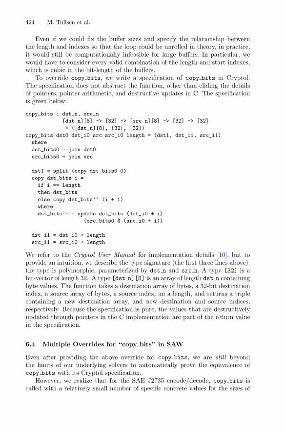
424 M. Tullsen et al.

Even if we could fix the buffer sizes and specify the relationship betweenthe length and indexes so that the loop could be unrolled in theory, in practice,it would still be computationally infeasible for large buffers. In particular, wewould have to consider every valid combination of the length and start indexes,which is cubic in the bit-length of the buffers.

To override copy bits, we write a specification of copy bits in Cryptol.The specification does not abstract the function, other than eliding the detailsof pointers, pointer arithmetic, and destructive updates in C. The specificationis given below:

copy_bits : dst_n, src_n

[dst_n][8] -> [32] -> [src_n][8] -> [32] -> [32]

-> ([dst_n][8], [32], [32])

copy_bits dst0 dst_i0 src src_i0 length = (dst1, dst_i1, src_i1)

where

dst_bits0 = join dst0

src_bits0 = join src

dst1 = split (copy dst_bits0 0)

copy dst_bits i =

if i == length

then dst_bits

else copy dst_bits’’ (i + 1)

where

dst_bits’’ = update dst_bits (dst_i0 + i)

(src_bits0 @ (src_i0 + i))

dst_i1 = dst_i0 + length

src_i1 = src_i0 + length

We refer to the Cryptol User Manual for implementation details [10], but toprovide an intuition, we describe the type signature (the first three lines above):the type is polymorphic, parameterized by dst n and src n. A type [32] is abit-vector of length 32. A type [dst n][8] is an array of length dst n containingbyte values. The function takes a destination array of bytes, a 32-bit destinationindex, a source array of bytes, a source index, an a length, and returns a triplecontaining a new destination array, and new destination and source indices,respectively. Because the specification is pure, the values that are destructivelyupdated through pointers in the C implementation are part of the return valuein the specification.

6.4 Multiple Overrides for “copy bits” in SAW

Even after providing the above override for copy bits, we are still beyondthe limits of our underlying solvers to automatically prove the equivalence ofcopy bits with its Cryptol specification.

However, we realize that for the SAE J2735 encode/decode, copy bits iscalled with a relatively small number of specific concrete values for the sizes of

Formal Verification of a Vehicle-to-Vehicle (V2V) Messaging System 425

the dst and src arrays, the indexes dst i and src i, and the length of bits tocopy length. The only values that we need to leave symbolic are the bit valueswithin the dst and src arrays. Therefore, rather than creating a single overridefor an arbitrary call to copy bits, we generate separate overrides for each uniqueset of “specializable” arguments, i.e., dst i, src i, and length.

Thus we note another feature of SAW: SAW allows us to specify a set of con-crete function arguments for an override; for each of these, SAW will specializethe override. (I.e., it will prove each specialization of the override.) In our casethis turns one intractable override into 56 tractable ones. The 56 specializations(which corresponds to the number of SEQUENCE fields in the BSM specifi-cation) were not determined by trial and error but by running instrumentedcode.

It is important to note that the consequence of a missing overrride special-ization cannot change the soundness of SAW’s result: Overrides in SAW cannotchange the proof results, they only change the efficiency of proof finding. If wehad a missing override specialization for copy bits we would only be back wherewe started: a property that takes “forever” to verify.

This approach works well for the simple BSM Part I. However, once webegin to verify encoders/decoders for more complex ASN.1 specifications (e.g.,containing CHOICE and OPTIONAL constructs), this method will need to be gen-eralized.

6.5 Results

A SAW script (script.saw) ties everything together and drives the symbolicexecution in SAW and lifts LLVM variables and functions into a dependent logicto state pre- and post-conditions and provide Cryptol specifications as needed.Finally, SAW then generates a SMT problem; Z3 [5] is the default solver we use.

Just under 3100 lines of C code were verified, not counting blank or commentlines. The verification required writing just under 100 lines of Cryptol specifi-cation. There are 1200 lines of SAW script auto-generated by the test harnessin generating the override specifications. Another 400 lines of SAW script ishand-written for the remaining overrides and to drive the overall verification.

Executed on a modern laptop with an Intel Core i7-6700HQ 2.6 GHz proces-sor and 32 GB of memory, the verification takes 20 min to prove the round-tripproperty and 275 min to prove the rejection property. The round-trip propertyis less expensive to verify because symbolic simulation is sensitive to branching,and for the round-trip property, we assert the data is valid to start, which in turnensures that all of the decodings succeed. In rejection, on the other hand, we havea branch at each primitive decode, and we need to consider both possibilities(success and failure).

426 M. Tullsen et al.

7 Discussion

7.1 LLVM and Definedness

Note that our verification has been with respect to the LLVM semantics not theC source of our code. SAW does not model C semantics, but inputs LLVM as theprogram’s semantics (we use clang to generate LLVM from the C). By verifyingLLVM, SAW is made simpler (it need only model LLVM semantics rather thanC) and we can do inter-program verification more easily. The process of provingthat a program satisfies a given specification within SAW guarantees definednessof the program (and therefore memory safety) as a side effect. That is, thetranslation from LLVM into SAWCore provides a well-defined semantics for theprogram, and this process can only succeed if the program is well-defined. Insome cases, this well-definedness is assumed during translation and then provedin the course of the specification verification. For instance, when analyzing amemory load, SAW generates a semantic model of what the program does ifthe load was within the bounds of the object it refers to, and generates a sidecondition that the load was indeed in bounds.

Verifying LLVM rather than the source program is a double-edged sword. Onthe one hand, the compiler front-end that generates LLVM is removed from thetrusted computing base. On the other hand, the verification may not be soundwith respect to the program’s source semantics. In particular, C’s undefinedbehaviors are a superset of LLVM’s undefined behaviors; a compiler can soundlyremove undefined behaviors but not introduce them. For example, a flaw in theGCC compiler allowed the potential for an integer overflow when multiplyingthe size of a storage element by the number of elements. The result could beinsufficient memory being allocated, leading to a subsequent buffer overflow.clang, however, introduces an implicit trap on overflow [12].

Moreover, the LLVM language reference does not rigorously specify well-definedness, and it is possible that our formalization of LLVM diverges from aparticular compiler’s [13].

7.2 Other Assumptions

We made some memory safety assumptions about how the encode/decode rou-tines are invoked. First, we assume that the input and output buffers providedto the encoder and decoder, respectively, do not alias. We also assume that eachbuffer is 37 bytes long (sufficient to hold a BSM with Part I only). A metaargument shows that buffers of at least 37 bytes are safe: we verify that for all37-byte buffers, we never read or write past their ends. So, if the buffers werelonger, we would never read the bytes above the 37th element.

For more complex data schemas (and when we extend to BSM Part II) whosemessages require a varying octet size, we would need to ensure the buffers aresufficiently large for all message sizes.

Formal Verification of a Vehicle-to-Vehicle (V2V) Messaging System 427

7.3 Proof Robustness

By “proof robustness” we mean how much effort is required to verify anotherprotocol or changes to the protocol. We hypothesize that for other protocolsthat use UPER and a similar set of ASN.1 constructs, the verification effortwould be small. Most of our manual effort focused on the libHAAW libraries,which is independent of the particular ASN.1 protocol verified. That said, verylarge protocol specifications may require additional proof effort to make themcompositional.

In future work, we plan to remove the need to generate overrides as a separatestep (as described in Sect. 6.2) by modifying HAAW to generate overrides as itgenerates the C code.

8 Conclusion

Hopefully we have motivated the security threat to V2V and the need for elimi-nating vulnerabilities in ASN.1 code. We have presented a successful applicationof automated formal methods to real C code for a real-world application domain.

There are some lessons to be learned from this work:

(1) Fully automated proofs of correctness properties are possible, but not trivial.The encoding of properties into C and SAWScript and getting the proofsto go through took one engineer approximately 3 months, this engineer hadsome experience with SAW; we were also able to get support and bug-fixesfrom the SAW developers. (It also helped that the code was bug-free so no“verification” time was spent on finding counter-examples and fixing code.)

(2) The straightforward structure of the C used in the encode/decode routinesmade them more amenable to automated analysis (see Sect. 6). It certainlyhelped that the code verified was compiler-generated and was by designintended to be, to some degree, manifestly correct. The lesson is not “chooselow-hanging fruit” but “look, low-hanging fruit in safety critical code” orpossibly even “create low-hanging fruit!” (by using simpler C).

(3) For non-trivial software, the likelihood of having a correct specification athand, or having the resources to create it, is quite slim! For instance, tofully specify correct UPER encoding/decoding for arbitrary ASN.1 specifi-cations would be a Herculean task. But in our case, we formulated two sim-ple properties—Round-Trip and Rejection—and by proving them we havealso shown memory safety and some strong (not complete, see Sect. 5) guar-antees of functional correctness. This technique could be applied to anyencode/decode pair.

There are many ways we hope to extend this work:

(1) We plan to extend our verification to the full BSM. This now gets us to morechallenging ASN.1 constructs (e.g., CHOICE) that involve a more complicatedcontrol-flow in the encoders/decoders. We do not expect a proof to be foundautomatically, but our plan is to generate lemmas with the generated C codethat will allow proofs to go through automatically.

428 M. Tullsen et al.

(2) Once we can automatically verify the full BSM, we expect to be able toperform a similar fully-automatic verification on many ASN.1 specifications(most do not use the full power of ASN.1). We would like to explore whatproperties of a given ASN.1 specification might guarantee the ability toperform such a fully-automatic verification.

(3) By necessity, parts of our SAWScript and the verification properties havea dependence on the particular API of the HAAW compiler (how abstractvalues are encoded, details of the encoding/decoding functions, memory-management design choices, etc.). Currently the authors are working on gen-eralizing this so that one can abstract over ASN.1-tool-specific API issues.The goal is to be able to extend our results to other encode/decode pairs(generated by hand or by other ASN.1 compilers).

(4) Note that the self-consistency property is generic (and has no reference toASN.1). As a result, we believe our work can be extended to encode/decodepairs on non-ASN.1 data.

Acknowledgments. This work was performed under subcontract to Battelle Memo-rial Institute for the National Highway Safety Transportation Administration(NHTSA). We thank Arthur Carter at NHTSA and Thomas Bergman of Battelle fortheir discussions and guidance. Our findings and opinions do not necessarily representthose of Battelle or the United States Government.

References

1. Barlas, K., Koletsos, G., Stefaneas, P.S., Ouranos, I.: Towards a correct translationfrom ASN.1 into CafeOBJ. IJRIS 2(3/4), 300–309 (2010)

2. Barrett, C., Fontaine, P., Tinelli, C.: The SMT-LIB Standard: Version 2.5. Tech-nical report, Department of Computer Science, The University of Iowa (2015).www.SMT-LIB.org

3. Brayton, R., Mishchenko, A.: ABC: an academic industrial-strength verificationtool. In: Touili, T., Cook, B., Jackson, P. (eds.) CAV 2010. LNCS, vol. 6174, pp.24–40. Springer, Heidelberg (2010). https://doi.org/10.1007/978-3-642-14295-6 5

4. Checkoway, S., McCoy, D., Kantor, B., Anderson, D., Shacham, H., Savage, S.,Koscher, K., Czeskis, A., Roesner, F., Kohno, T.: Comprehensive experimentalanalyses of automotive attack surfaces. In: USENIX Security (2011)

5. de Moura, L., Bjørner, N.: Z3: an efficient smt solver. In: Ramakrishnan, C.R.,Rehof, J. (eds.) TACAS 2008. LNCS, vol. 4963, pp. 337–340. Springer, Heidelberg(2008). https://doi.org/10.1007/978-3-540-78800-3 24

6. Dockins, R., Foltzer, A., Hendrix, J., Huffman, B., McNamee, D., Tomb, A.: Con-structing semantic models of programs with the software analysis workbench. In:Blazy, S., Chechik, M. (eds.) VSTTE 2016. LNCS, vol. 9971, pp. 56–72. Springer,Cham (2016). https://doi.org/10.1007/978-3-319-48869-1 5

7. DSRC Technical Committee: Dedicated Short Range Communications (DSRC)message set dictionary (j2735 20103). Technical report, SAE International (20016)

8. Dubuisson, O.: ASN.1 Communication between heterogeneous Systems. Elsevier-Morgan Kaufmann, Burlington (2000)

9. Fouquart, P., Dubuisson, O., Duwez, F.: Une analyse syntaxique d’ASN.1:1994.Technical report, Internal Report RP/LAA/EIA/83, France Telecom R&D, March1996

Formal Verification of a Vehicle-to-Vehicle (V2V) Messaging System 429

10. Galois Inc.: Cryptol: the language of cryptography. Galois, Inc., portland (2016).http://www.cryptol.net/files/ProgrammingCryptol.pdf

11. Goodin, D.: Software flaw puts mobile phones and networks at risk of completetakeover. Ars Technica (2016)

12. Lattner, C.: What every C programmer should know about undefined behav-ior #3/3. Online blog, May 2011. http://blog.llvm.org/2011/05/what-every-c-programmer-should-know 21.html

13. Lee, J., Youngju Song, Y.K., Hur, C.K., Das, S., Majnemer, D., Regehr, J., Lopes,N.P.: Taming undefined behavior in LLVM. In: Proceedings of 38th Conference onProgramming Language Design and Implementation (PLDI) (2017)

14. MITRE: Common vulnerabilities and exposures for ASN.1, February 2017. https://cve.mitre.org/cgi-bin/cvekey.cgi?keyword=ASN.1

15. U.S. Dept. of Transportation: Fact sheet: Improving safety and mobilitythrough vehicle-to-vehicle communications technology (2016). https://icsw.nhtsa.gov/safercar/v2v/pdf/V2V NPRM Fact Sheet 121316 v1.pdf

Open Access This chapter is licensed under the terms of the Creative CommonsAttribution 4.0 International License (http://creativecommons.org/licenses/by/4.0/),which permits use, sharing, adaptation, distribution and reproduction in any mediumor format, as long as you give appropriate credit to the original author(s) and thesource, provide a link to the Creative Commons license and indicate if changes weremade.

The images or other third party material in this chapter are included in the chapter’sCreative Commons license, unless indicated otherwise in a credit line to the material. Ifmaterial is not included in the chapter’s Creative Commons license and your intendeduse is not permitted by statutory regulation or exceeds the permitted use, you willneed to obtain permission directly from the copyright holder.

Continuous Formal Verificationof Amazon s2n

Andrey Chudnov1, Nathan Collins1, Byron Cook3,4, Joey Dodds1,Brian Huffman1, Colm MacCarthaigh3, Stephen Magill1(B), Eric Mertens1,

Eric Mullen2, Serdar Tasiran3, Aaron Tomb1, and Eddy Westbrook1

1 Galois, Inc., Portland, USAstephen@galois.com

2 University of Washington, Seattle, USA3 Amazon Web Services, Seattle, USA

4 University College London, London, UK

Abstract. We describe formal verification of s2n, the open source TLSimplementation used in numerous Amazon services. A key aspect of thisproof infrastructure is continuous checking, to ensure that propertiesremain proven during the lifetime of the software. At each change to thecode, proofs are automatically re-established with little to no interac-tion from the developers. We describe the proof itself and the technicaldecisions that enabled integration into development.

1 Introduction

The Transport Layer Security (TLS) protocol is responsible for much of theprivacy and authentication we enjoy on the Internet today. It secures our phonecalls, our web browsing, and connections between resources in the cloud madeon our behalf. In this paper we describe an effort to prove the correctness ofs2n [3], the open source TLS implementation used by many Amazon and AmazonWeb Services (AWS) products (e.g. Amazon S3 [2]). Formal verification playsan important role for s2n. First, many security-focused customers (e.g. financialservices, government, pharmaceutical) are moving workloads from their own datacenters to AWS. Formal verification provides customers from these industrieswith concrete information about how security is established in Amazon WebServices. Secondly, automatic and continuous formal verification facilitates rapidand cost-efficient development by a distributed team of developers.

In order to realize the second goal, verification must continue to work withlow effort as developers change the code. While fundamental advances have beenmade in recent years in the tractability of full verification, these techniquesgenerally either: (1) target a fixed version of the software, requiring significant re-proof effort whenever the software changes or, (2) are designed around synthesisof correct code from specifications. Neither of these approaches would work forAmazon as s2n is under continuous development, and new versions of the codewould not automatically inherit correctness from proofs of previous versions.

c© The Author(s) 2018H. Chockler and G. Weissenbacher (Eds.): CAV 2018, LNCS 10982, pp. 430–446, 2018.https://doi.org/10.1007/978-3-319-96142-2_26

Continuous Formal Verification of Amazon s2n 431

To address the challenge of program proving in such a development environ-ment, we built a proof and associated infrastructure for s2n’s implementationsof DRBG, HMAC, and the TLS handshake. The proof targets an existing imple-mentation and is updated either automatically or with low effort as the codechanges. Furthermore, the proof connects with existing proofs of security prop-erties, providing a high level of assurance.

Our proof is now deployed in the continuous integration environment fors2n, and provides a distributed team of developers with repeated proofs of thecorrectness of s2n even as they continue to modify the code. In this paper, wedescribe how we structured the proof and its supporting infrastructure, so thatthe lessons we learned will be useful to others who address similar challenges.

Figure 1 gives an overview of our proof for s2n’s implementation of the HMACalgorithm and the tooling involved. At the left is the ultimate security propertyof interest, which for HMAC is that if the key is not known, then HMAC is indis-tinguishable from a random function (given some assumptions on the underlyinghash functions). This is a fixed security property for HMAC and almost neverchanges (a change would correspond to some new way of thinking about securityin the cryptographic research community). The HMAC specification is also fairlystatic, having been updated only once since its publication in 20021. Beringeret al. [6] have published a mechanized formal proof that the high-level HMACspecification establishes the cryptographic security property of interest.

As we move to the right through Fig. 1, we find increasingly low-level arti-facts and the rate of change of these artifacts increases. The low-level HMACspecification includes details of the API exposed by the implementation, andthe implementation itself includes details such as memory management and per-formance optimizations. This paper focuses on verifying these components in amanner that uses proof automation to decrease the manual effort required forongoing maintenance of these verification artifacts. At the same time, we ensurethat the automated proof occurring on the right-hand side of the figure is linkedto the stable, foundational security results present at the left.

In this way, we realize the assurance benefit of the foundational securitywork of Beringer et al. while producing a proof that can be integrated into thedevelopment workflow. The proof is applied as part of the continuous integrationsystem for s2n (which uses Travis CI) and runs every time a code change ispushed or a pull request is issued. In one year of code changes only three manualupdates to the proof were required.

The s2n source code, proof scripts, and access to the underlying proof toolscan all be found in the s2n GitHub [3] repository. The collection of proof runsis logged and appears on the s2n Travis CI page [4].

In addition to the HMAC proof, we also reused the approach shown inthe right-hand side of Fig. 1 to verify the deterministic random big generator(DRBG) algorithm and the TLS Handshake protocol. In these cases we didn’tlink to foundational cryptographic security proofs, but nonetheless had specifi-cations that provided important benefits to developers by allowing them to (1)

1 And this update did not change the functional behavior specified in the standard.

432 A. Chudnov et al.

check their code against an independent specification and (2) check that theircode continues to adhere to this specification as it changes. Our TLS Handshakeproof revealed a bug (which was promptly fixed) in the s2n implementation [10],providing evidence for the first point. All of our proofs have continued to be usedin development since their introduction, supporting the second point.

This PaperWork of Beringer et al.

Indistinguishability from random

Security Property

Coq HMAC

High-Level

Changes Infrequently

Monolithic API

High-Level

s2n C code

Implementation

Changes FrequentlyIncreasing Automation

Proved In Coq Proved In Coq Combination of Coq (Manual)and Cryptol (Automatic)

Proved with SAW(mostly automatic)

Incremental API

Low-Level

Fig. 1. An overview of the structure of our HMAC proof.

Related Work. Projects such as Everest [8,12], Cao [5], and Jasmin [1], gener-ate verified cryptographic implementations from higher level specifications, e.g.F* models. While progress in this space continues to be promising—HACL* hasrecently achieved performance on primitives that surpasses handwritten C [25]—we have found in our experiments that the generated TLS code does not yet meetthe performance, power, and space constraints required by the broad range ofAWS products that use s2n.

Static analysis for hand-written cryptographic implementations has been pre-viously reported in the context of Frama-C/PolarSSL [23], focusing on scalingmemory safety verification to a large body of code. Additionally, unsound buteffective bug hunting techniques such as fuzzing have been applied to TLS imple-mentations in the past [11,18]. The work we report on goes further by provingbehavioral correctness properties of the implementation that are beyond thecapabilities of these techniques. In this we were helped because the implemen-tation of s2n is small (less than 10k LOC), and most iteration is bounded.

The goal of our work is to verify deep properties of an existing and activelydeveloped open source TLS implementation that has been developed for bothhigh performance and low power as required by a diverse range of AWS prod-ucts. Our approach was guided by lessons learned in several previous attemptsto prove the correctness of s2n that either (1) required too much developerinteraction during the modification of the code [17], or (2) where pushbuttonsymbolic model checking tools did not scale. Similarly, proofs developed usingtools from the Verified Software Toolchain (VST) [6] are valuable for establishingthe correctness and security of specifications, but are not sufficiently resilient tocode changes, making them challenging to integrate into an ongoing develop-ment process. Their use of a layered proof structure, however, provided us witha specification that we could use to leverage their security proof in our work.

Continuous Formal Verification of Amazon s2n 433

O’Hearn details the industry impact of continuous reasoning about codein [19], and describes additional instances of integration of formal methods withdeveloper workflows.

2 Proof of HMAC

In this section, we walk through our HMAC proof in detail, highlighting howthe proof is decomposed, the guarantees provided, the tools used, and how thisapproach supports integration of verification into the development work-flow.While HMAC serves as an example, we have also performed a similar proof ofthe DRBG and TLS Handshake implementations. We do not discuss DRBGfurther, as there are no proof details that differ significantly from HMAC. Wedescribe our TLS verification in Sect. 3.

2.1 High-Level HMAC Specification

The keyed-Hash Message Authentication Code algorithm (HMAC) is used forauthenticated integrity in TLS 1.2. Authenticated integrity guarantees that thedata originated from the sender and was not changed or duplicated in transit.HMAC is used as the foundation of the TLS Pseudorandom Function (PRF),from which the data transmission and data authentication shared keys arederived. This ensures that both the sender and recipient have exchanged thecorrect secrets before a TLS connection can proceed to the data transmissionphase.

HMAC is also used by some TLS cipher suites to authenticate the integrityof TLS records in the data transmission phase. This ensures, for example, thata third party watching the TLS connection between a user and a webmail clientis unable to change or repeat the contents of an email body during transmission.It is also used by the HMAC-based Extract-and-Expand Key Derivation Func-tion (HKDF) which is implemented within s2n as a utility function for generalpurpose key derivation and is central to the design of the TLS1.3 PRF.

FIPS 198-1 [24] defines the HMAC algorithm as

HMAC(K,message) = H((K ⊕ opad)‖H((K ⊕ ipad)‖message))

where H is any hash function, ⊕ is bitwise xor, and ‖ is concatenation. opad andipad are constants defined by the specification. We will refer to this definitionas the monolithic specification.

Following Fig. 1, we use the Cryptol specification language [14] to expressHMAC in a form suitable for mechanized verification, first in a monolithic form,and then in an incremental form. We prove high-level properties with Coq [22]and tie these to the code using the Software Analysis Workbench (SAW) [16].We first describe the proof of high-level properties before going into specificsregarding the tools in Sect. 2.4.

434 A. Chudnov et al.

2.2 Security Properties of HMAC

The Cryptol version of the Monolithic HMAC specification follows.

hmac k message = H((k ^ opad) # H((k ^ ipad) # message))

where H is any hash function, ^ is bitwise xor, and # is concatenation.The high-level Cryptol specification and the FIPS document look nearly iden-

tical, but what assurance do we have that either description of the algorithmis cryptographically secure? We can provide this assurance by showing that theCryptol specification establishes one of the security properties that HMAC isintended to provide—namely, that HMAC is indistinguishable from a functionreturning random bits.

Indistinguishability from random is a property of cryptographic output thatsays that there is no effective strategy by which an attacker that is viewing theoutput of the cryptographic function and a true random output can distinguishthe two, where an “effective” strategy is one that has a non-negligible chanceof success given bounded computing resources. If the output of a cryptographicfunction is indistinguishable from random, that implies that no information canbe learned about the inputs of that function by examining the outputs.

We prove that our Cryptol HMAC specification has this indistinguishabilityproperty using an operational semantics of Cryptol we developed in Coq. Thesemantics enable us to reuse portions of the proof by Beringer et. al [6], whichuses the Coq Foundational Cryptography Framework (FCF) library [20] to estab-lish the security of the HMAC construction. We construct a Coq proof showingthat our Cryptol specification is equivalent (when interpreted using the formaloperational semantics) to the specification considered in the Beringer et. al work.The Cryptol specification is a stepping stone to automated verification of thes2n implementations, so when combined with the verification work we describesubsequently, we eventually establish that the implementation of HMAC in s2nalso has the desired security property. The Coq code directly relating to HMACis all on the s2n GitHub page. These proofs are not run as part of continuousintegration, rather, they are only rerun in the unlikely event that the monolithicspecification changes.

2.3 Low-Level Specification

The formal specification of HMAC presented in the FIPS standard operates ona single complete message. However, network communication often requires theincremental processing of messages. Thus all modern implementations of HMACprovide an incremental interface with the following abstract types:

init : Key -> Stateupdate : Message -> State -> Statedigest : State -> MAC

The init function creates a state from a key, the update function updatesthat state incrementally with chunks of the message, and the digest functionfinalizes the state, producing the MAC.

Continuous Formal Verification of Amazon s2n 435

The one-line monolithic specification is related to these incremental functionsas follows. If we can partition a message m into m = m1‖m2‖ . . . ‖mn then (inpseudo code/logic notation)

HMAC(k,m) = digest(update(mn(. . . (update m1(init k)))) (1)

In other words, any MAC generated by partitioning a message and incrementallysending it in order through these functions should be equal to a MAC generatedby the complete message HMAC interface used in the specification.

We prove that the incremental interface to HMAC is equivalent to the non-incremental version using a combination of manual proof in Coq and auto-mated proof in Cryptol. Note that this equivalence property can be stated inan implementation-independent manner and proved outside of a program veri-fication context. This is the approach we take—independently proving that theincremental and monolithic message interfaces compute the same HMAC, andthen separately showing that s2n correctly implements the incremental interface.

Our Coq proof proceeds via induction over the number of partitions withthe following lemmas establishing the relationship between the monolithic anditerative implementations. These lemmas are introduced as axioms in the Coqproof, but subsequently checked using SAW.

update_empty : forall s, HMAC_update empty_string s = s.

equiv_one : forall m k,HMAC_digest (HMAC_update m (HMAC_init k)) = HMAC k m.

update_concat : forall m1 m2 s,HMAC_update (concat m1 m2) s = HMAC_update m2 (HMAC_update m1 s).

The first lemma states that processing an empty message does not changethe state. The second lemma states that applying the incremental interface to asingle message is equivalent to applying the monolithic interface. These lemmasconstitute the base cases for an inductive proof of equation (1) above. The lastlemma states that calling update twice (first with m1 and then with m2) resultsin the same state as calling update once with m1 concatenated with m2. Thisconstitutes the inductive step in the proof of (1).

The update_empty lemma can be proved by analyzing the code with symbolicvalues provided for the state s, as the state is of fixed size. The equiv_one andupdate_concat lemmas require reasoning about unbounded data. SAW has lim-ited support for such proofs. In particular, it has support for equational rewritingof terms in its intermediate language, but not for induction. In the case of theupdate_concat lemma, a few simple builtin rewrite rules are sufficient to estab-lish the statement for all message sizes. For equiv_one , a proof of the statementfor all message sizes would require induction. Since SAW does not support induc-tion, we prove that this statement holds for a finite number of key and messagesizes. In theory we could still obtain a complete proof by checking all messagesizes up to 16k bytes (the maximum size message permitted by the TLS stan-dard). This may be tractable in a one-off proof, but for our continuously-applied

436 A. Chudnov et al.

proofs we instead consider a smaller set of samples, chosen to cover all branchesin the code. This yields a result that is short of full proof, but still provides muchhigher state space coverage than testing methods.

Given the three lemmas above, we then use Coq to prove the following the-orem by induction on the list of partitions, ms.

HMAC key (fold_right concat empty_string ms) =HMAC_digest (fold_left (fun (st: state) msg =>

HMAC_update msg st)ms

(HMAC_init key)).

The theorem establishes the equivalence of the incremental and monolithicinterfaces for any decomposition of a message into any number of fragments ofany size.

2.4 Implementation Verification

The incremental Cryptol specification is low-level enough that we were able toconnect it to the s2n HMAC implementation using automated proof techniques.As this is the aspect of the verification effort that is critical for integration intoan active development environment, we go into some detail, first discussing thetools that were used and then describing the structure of the proof.

Tools. We use the Software Analysis Workbench (SAW) to orchestrate this stepof the proof. SAW is effective both for manipulating the kinds of functional termsthat arise from Cryptol, and for constructing functional models from imperativeprograms. It can be used to show equivalence of distinct software implemen-tations (e.g. an implementation in C and one in Java) or equivalence of animplementation and an executable specification.

SAW uses bounded symbolic execution to translate Cryptol, Java, and C pro-grams into logical expressions, and proves properties about the logical expres-sions using a combination of rewriting, SAT, and SMT. The result of the boundedsymbolic execution of the input programs is a pure functional term representingthe function’s entire semantics. These extracted semantics are then related tothe Cryptol specifications by way of precondition and postcondition assertionson the program state.

The top-level theorems we prove have some variables that are universallyquantified (e.g. the key used in HMAC) and others that are parameters weinstantiate to a constant (e.g. the size of the key). We achieve coverage forthe latter by running the proof for several parameter instantiations. In somecases this is sufficient to cover all cases (e.g. the standard allows only a smallfinite number of key sizes). In others, the space of possible instantiations islarge enough that fully covering it would yield runtimes too long to fit into thedeveloper workflow (for example, messages can be up to 16k long). In such cases,we consider a smaller set of samples, chosen to cover all branches in the code.

Continuous Formal Verification of Amazon s2n 437

This yields a result that is short of full proof, but still provides much higherstate space coverage than testing methods.

Internally SAW reasons about C programs by first translating them to LLVM.For the remainder of the paper we will talk about the C code, although froma soundness perspective the C code must be compiled through LLVM for theproofs to apply to the compiled code.

Proof Structure. The functions in the low-level Cryptol specification describedabove share the incremental format of the C program, and also consume argu-ments and operate on state that matches the usage of arguments and state in theC code. However, the Cryptol specification does not capture the layout of statein memory. This separates concerns and allows us to reason about equivalence ofthe monolithic and incremental interfaces in a more tractable purely functionalsetting, while performing the implementation proof in a context in which thespecification and implementation are already structurally quite similar.

As an example of this structural similarity, the C function has type:

int s2n_hmac_update(struct s2n_hmac_state *state,const void *in, uint32_t size);

We define a corresponding Cryptol specification with type:

hmac_update : {Size} (32 >= width Size) =>HMAC_state -> [Size][8] -> HMAC_state

These type signatures look a bit different, but they represent the same thing.In Cryptol, we list Size first, because it is a type, not a value. This meansthat we do not need to independently check that the input buffer (in Cryptolrepresented by the type [Size][8]) matches the size input—the Cryptol typesystem guarantees it. The type system also sets the constraint that the sizedoesn’t exceed 232, a constraint set by the C type of Size.

We use SAW’s SAWScript language to describe the expected memory layoutof the C program, and to map the inputs and outputs of the Cryptol functionto the inputs and outputs of the C program. The following code presents theSAWScript for the hmac_update_spec function.

1 let hmac_update_spec msg_size cfg = do {2 (msg_val, msg_pointer) <- ptr_to_fresh_array msg_size i8;3 (initial_state, state_pointer) <- setup_hmac_state cfg4 hmac_invariants initial_state cfg;5

6 execute_func [state_pointer, message_pointer, msg_size];7

8 let final_state =9 {{ hmac_update_c_state initial_state msg_val }};

10 check_hmac_state state_pointer final_state;11 hmac_invariants final_state cfg;12 check_return zero;13 };

438 A. Chudnov et al.

This SAWScript code represents a Hoare triple, with the precondition andpost condition separated by the body (the execute_func command), which per-forms the symbolic execution of the LLVM code using the provided arguments.Lines 2 and 3 are effectively universal quantification over the triple, setting upthe values and pointers that match the type needed by the C function. Thevalues msg_val and initial_state are referenced in both the C code and theCryptol specification, whereas the pointers exist only on the C side.

Lines 8–10 capture that the final state resulting from executing the C functionshould be equivalent to the state produced by evaluating the Cryptol specifica-tion. Specifically, Lines 8 and 9 capture the output of the Cryptol specification(double curly braces denote Cryptol expressions within SAWScript) and Line 10asserts that this state matches the C state present in memory at state_pointer.This is what ultimately establishes equivalence of the implementation and spec-ification.

The proof is aided by maintaining a collection of state invariants, which areassumed to hold in Line 4 and are re-established in Line 11. These are manualinvariants, but they occur as function specifications rather than appearing inter-nal to loops. They only require modification in the event that the meaning ofthe HMAC state changes.

The msg_size parameter indicates how large of a message this particularproof should cover. Because SAW performs a bounded unrolling of the programunder analysis, each proof must cover one fixed size for each unbounded datastructure or iterative construct. However, by parameterizing the proof, it caneasily be repeated for multiple sizes. Furthermore, as described in Sect. 2.3, wealso prove in Coq that calling update twice with messages m1 and m2 is equiv-alent to calling it once with m1 concatenated with m2. As a consequence, thefixed size proofs we perform of update can be composed to guarantee that theupdate function is correct even over longer messages.

The cfg parameter contains configuration values for each of the six hashesthat can be used with HMAC. The configuration values of interest to HMACare the input and output sizes of the hash block function.

Given the specification of the C function above, we can now verify that theimplementation satisfies the specification:

verify m "s2n_hmac_update"hash_ovs true (hmac_update_spec msg_size cfg) yices_hash_unint;

The "s2n_hmac_update" argument specifies the C function that we are veri-fying. hash_ovs is a list, defined elsewhere, that contains all of the overrides thatthe verification will use. An override is a specification that will be used in placeof a particular implementation function and corresponds to what other tools callstubs or models. In this case, we’ve overridden all of the C hash functions, stat-ing assumptions regarding their use of memory and their equivalence to Cryptolimplementations of the same hash functions. When the verifier comes across acall to one of these hash functions in the C code, it will instead use the providedspecification. The result is that our proof assumes correct implementation of thehash functions.

Continuous Formal Verification of Amazon s2n 439

The fact that the structure of the low-level Cryptol specification matchesthe structure of the C code, coupled with SAW’s use of SMT as the primarymechanism for discharging verification conditions, enables a proof that contin-ues to work through a variety of code changes. In particular, changes to thecode in function bodies often requires no corresponding specification or proofscript change. Similarly, changes that add fields or change aspects of in-memorydata structures that are not referenced by the specification do not require proofupdates. Changes in the API (e.g. function arguments) do require proof scriptchanges, but these are typically minor. Fixing a broken proof typically involvesadding a new state field to the SAW script, updating the Cryptol specification touse that field correctly, and then passing the value of that field into the Cryptolprogram in the post-condition. If the Cryptol specification is incorrect, SAW willgenerate counterexamples that can be used to trace through the code and thespec together in order to discover the mismatch.

2.5 Integrating the Proof into Development

Integration with the s2n CI system mostly took place within the Travis config-uration file for s2n. At the time of integration, targets for the build, integrationtesting, and fuzzing on both Linux and OSX already existed. We updated theTravis system with Bash scripts that automatically download and install theappropriate builds of SAW, Z3, and Yices into the Travis system. These files arein the s2n repository and can be reused by anyone under the Apache 2.0 license.

A Travis CI build can occur on any number of virtual machines, and eachvirtual machine is given an hour to complete. We run our HMAC proofs onconfigurations for six different hashes. For each of these configurations we checkat three key-sizes in order to test the relevant cases in the implementation (smallkeys get padded, exact keys remain unchanged, and large keys are hashed). Foreach of those key-sizes we check six different message sizes. These proofs run inan average of ten minutes. We discovered that it’s best to stay well clear of the60 min limit imposed by Travis in order to avoid false-negatives due to variationsin execution time.

The proof runs alongside the tests that are present in the s2n repository onevery build, and if the proof fails a flag is raised just as if a test case were to fail.

3 Proof of TLS Handshake

In addition to the HMAC and DRBG proofs, we have proved correctness of theTLS state machine implemented in s2n. Specifically, we have proved that (1) itimplements a subset of TLS 1.2 as defined in IETF RFCs 5246 [21], 5077 [15] and6066 [13] and (2) the socket corking API, which optimizes how data is split intopackets, is used correctly. Formally, we proved that the implementation refinesa specification (conversely, the specification simulates the implementation). Weobtained this Cryptol specification, called the RFC specification by examiningthe RFCs and hand-compiling them into a Cryptol file complete with relevant

440 A. Chudnov et al.

excerpts from the RFCs. We assume that the TLS handshake as specified in theRFCs is secure, and do not formalize nor verify any cryptographic propertiesof the specification. In the future, we would like to take a similar approach tothat described in Sect. 2.2 to link our refinement proof with a specification-levelsecurity proof for TLS, such as that from miTLS [9].

The s2n state machine is designed to ensure correctness and security, pre-venting join-of-state-machines vulnerabilities like SMACK [7]. In addition, s2nallows increased throughput via the use of TCP socket corking, which combinesseveral TLS records into one TCP frame where appropriate.

The states and transitions of the s2n state machine are encoded explicitlyas linearized arrays, as opposed to being intertwined with message parsing andother logic. This is an elegant decomposition of the problem that makes most ofthe assumptions explicit and enables the use of common logic for message anderror handling as well as protocol tracking.

Even with the carefully designed state machine implementation, formal spec-ification and verification helped uncover a bug [10].

Structure of the TLS Handshake State Machine Correctness Proof.The automated proof of correctness of the TLS state machine has two parts(Fig. 2). First we establish an equivalence between the two functions2 that drivethe TLS handshake state machine in s2n and their respective specifications inCryptol. Again we utilize low-level specifications that closely mirror the shapeof the C functions. Our end goal, however, is correctness with respect to thestandards, encoded in the RFC specification in Cryptol. The library implementsonly a subset of the standards, thus we can only prove a simulation relation andnot equivalence. Namely, we show that every sequence of messages generated bythe low-level specification starting from a valid initial state can be generated bythe RFC specification starting from a related state. The dashed line in Fig. 2shows at which points the states match at the implementation and specificationlevels.

CLIENT HELLO SERVER HELLO APPLICATION DATA

RFC spec

Low-lvl spec

C Code

handshakeTransition

advance message

conn set handshake type

s2n advance message

s2n conn set handshake type

Fig. 2. Structure of the TLS handshake correctness proof

2 s2n conn set handshake type and s2n advance message.

Continuous Formal Verification of Amazon s2n 441

RFC-Based Specification of the TLS Handshake. The high-level hand-shake protocol specification that captures the TLS state machine is implementedin Cryptol and accounts for the protocol, message type and direction, as wellas conditions for branching in terms of abstract connection parameters, but notmessage contents.

We represent the set of states as unsigned 5-bit integers (Listing 1). The statetransition relation is represented by a Cryptol function handshakeTransition(Listing 2) which, given abstract connection parameters (Listing 3) and thecurrent state returns the next state. If there is no valid next state, the statemachine stutters. The parameters determine the transition to take in each stateand represent configurations of the end-points as well as contents of the HELLOmessage sent by the other party. We kept the latter separate from the messagespecifications in order to avoid reasoning about message structure and parsing.We can still relate the abstract parameters to the implementation because theyare captured in the connection state. Finally, the message function (Listing 4)gives the message type, protocol and direction for every state.

type State = [5]

(helloRequestSent : State) = 0

(clientHelloSent : State) = 1

(serverHelloSent : State) = 2

// ...

(serverCertificateStatusSent : State) = 23

Listing 1: Specification of TLS handshake protocol states

handshakeTransition : Parameters -> State -> State

handshakeTransition params old =

snd (find fst (True, old) [ (old == from /\ p, to)

| (from, p, to) <- valid_transitions]) where

valid_transitions =

[(helloRequestSent, True, clientHelloSent)

,(clientHelloSent, True, serverHelloSent)

,(serverHelloSent, params.keyExchange != DH_anon

/\ ~params.sessionTicket, serverCertificateSent)

// ...

,(serverCertificateStatusSent, ~(keyExchangeNonEphemeral params)

, serverKeyExchangeSent)

]

Listing 2: Specification of the TLS handshake state transition function. Validtransitions are encoded as triples (start, transition condition, end).

442 A. Chudnov et al.

type KeyExchange = [3]

(DH_anon : KeyExchange) = 0

// ...

(DH_RSA : KeyExchange) = 5

type Parameters =

{keyExchange : KeyExchange // Negotiated key exchange algorithm

,sessionTicket : Bit // The client had a session ticket

,renewSessionTicket : Bit // Server decides to renew a session ticket

,sendCertificateStatus : Bit // Server decides to send the certificate

// status message

,requestClientCert : Bit // Server requests a cert from the client

,includeSessionTicket : Bit} // Server includes a session ticket

// extension in SERVER_HELLO

Listing 3: Abstract connection parameters

message : State -> Message

message = lookupDefault messages (mkMessage noSender data error)

where messages =

[(helloRequestSent, mkMessage server handshake helloRequest)

,(clientHelloSent, mkMessage client handshake clientHello)

,(serverHelloSent, mkMessage server handshake serverHello)

// ...

,(serverChangeCipherSpecSent,

mkMessage server changeCipherSpec changeCipherSpecMessage)

,(serverFinishedSent, mkMessage server handshake finished)

,(applicationDataTransmission, mkMessage both data applicationData)

]

Listing 4: Expected message sent/received in each handshake state

Socket Corking. Socket corking is a mechanism for reducing packet fragmenta-tion and increasing throughput by making sure full TCP frames are sent when-ever possible. It is implemented in Linux and FreeBSD using the TCP CORK andTCP NOPUSH flags respectively. When the flag is set, the socket is consideredcorked, and the operating system will only send complete (filled up to the bufferlength) TCP frames. When the flag is unset, the current buffer, as well as allfuture writes, are sent immediately.

Writing to an uncorked socket is possible, but undesirable as it might resultin partial packets being sent, potentially reducing throughput. On the otherhand, forgetting to uncork a socket after the last write can have more seriousconsequences. According to the documentation, Linux limits the duration ofcorking to 200 ms, while FreeBSD has no limit. Hence, leaving a socket corked inFreeBSD might result in the data not being sent. We have verified that socketsare not corked or uncorked twice in a row. In addition, the structure of themessage handling implementation in s2n helps us informally establish a strongercorking safety property. Because explicit handshake message sequences include

Continuous Formal Verification of Amazon s2n 443

the direction the message is sent, we can establish that the socket is (un)corkedappropriately when the message direction changes. In future work we plan toexpand the scope of our proof to allow us to formally establish full corkingsafety.

4 Operationalizing the Proof

We have integrated the checking of our proof into the build system of s2n, aswell as the Continuous Integration (CI) system used to check the validity of codeas it is added to the s2n repository on GitHub. For the green “build passed”badge displayed on the s2n GitHub page to appear, all code updates now mustsuccessfully verify with our proof scripts. Not only do the these checks run oncommitted code, they are also automatically run on all pull requests to theproject. This allows the maintainers of s2n to quickly determine the correctnessof submitted changes when they touch the code that we have proved. In thissection we discuss aspects of our tooling that were important enablers of thisintegration.

Proof Robustness. For this integration to work, our proofs must be robust in theface of code change. Evolving projects like s2n should not be slowed down bythe need to update proofs every time the code changes. Too many proof updatescan lead to significantly slowed development or, in the extreme case, to proofsbeing disabled or ignored in the CI environment. The automated nature of ourproofs mean that they generally need to be changed only in the event of interfacemodifications—either to function declarations or state definitions.

Of these two, state changes are the most common, and can be quite complexconsidering that there are usually large possibly nested C structs involved (forexample, the s2n_connection struct has around 50 fields, some of which arestructs themselves). To avoid the developer pain that would arise if such structupdates caused the proof the break, we have structured the verification so thatproof scripts do not require updates when the modified portions of the state donot affect the computation being proved. Recall that our proofs are focused onfunctional correctness. Thus in order to affect the proof, a new or modified fieldmust influence the computation. Many struct changes target non-security-criticalportions of the code (e.g. to track additional data for logging) and so do not meetthis criterion. For such fields we prove that they are handled in a memory safemanner and that they do not affect the computation being performed by thecode the proof script targets.

In the future, we intend to add the option to perform a “strict” version ofthis state handling logic to SAW, which would ensure that newly added fields arenot modified at all by the portion of the code being proved. Such a check wouldensure that the computation being analyzed computes the specified function andnothing else and would highlight cases in which new fields introduce undesirabledata flows (e.g. incorrectly storing sensitive data). However even such an optionwould not replace whole program data flow analysis, which we recommend incases where there is concern about potential incorrect data handling.

444 A. Chudnov et al.

Negative Test Cases. Each of our proofs also includes a series of negative testcases as evidence that the tools are functioning properly. These test cases patchthe code with a variety of mistakes that might actually occur and then run thesame proof scripts using the same build tools to check that the tool detects theintroduced error.

Examples of the negative test cases we use include an incorrect modificationto a side-channel mitigation, running our TLS proofs on a version of the codewith an extra call to cork and uncork, a version modified to allow early CCS, aswell as a version with the incomplete handshake bug that we discovered in theprocess of developing the proof. Such tests are critical, both to display the valueof the proofs, by providing them with realistic bugs to catch, and as a defenseagainst possible bugs in the tool that may be introduced as it is updated.

Proof Metrics. We also report real-time proof metrics. Our proof scripts printout JSON encoded statistics into the Travis logs. From there, we have developedan in-browser tool that scrapes the Travis logs for the project, compiling therelevant statistics into easily consumable charts and tables. The primary metricswe track are: (1) the number of lines of code that are analyzed by the proof (whichincreases as we develop proofs for more components of s2n), and (2) the numberof times the verified code has been changed and re-analyzed (which tracks theongoing value of the proof). This allows developers to easily track the impact ofthe proofs over time.

Since deployment of the proof to the CI system in November of 2016 ourproofs have been re-played 956 times. This number does not account for proof re-plays performed in forks of the repository. We have had to update the proof threetimes. In all cases the proof update was complete before the code review processfinished. Not all of these runs involved modification to the code that our proofswere about, however each of the runs increased the confidence of the maintainersin the relevant code changes, and each run reestablishes the correctness of thecode to the public, who may not be aware of what code changed at each commit.

HMAC and DRBG each took roughly 3 months of engineering effort. TheTLS handshake verification took longer at 8 months, though some of that timeinvolved developing tool extensions to support reasoning about protocols. Atthe start of each project, the proof-writers were familiar with the proof tools butnot with the algorithms or the s2n implementations of them. The effort amountslisted above include understanding the C code, writing the specifications in Cryp-tol, developing the code-spec proofs using SAW, the CI implementation work,and the process of merging the proof artifacts into the upstream code-base.

5 Conclusion

In this case study we have described the development and operation in practice ofa continuously checked proof ensuring key properties of the TLS implementationused by many Amazon and AWS services. Based on several previous attemptsto prove the correctness of s2n that either required too much developer inter-action during modifications or where symbolic reasoning tools did not scale, we

Continuous Formal Verification of Amazon s2n 445

developed a proof structure that nearly eliminates the need for developers tounderstand or modify the proof following modifications to the code.

References

1. Almeida, J.B., Barbosa, M., Barthe, G., Blot, A., Gregoire, B., Laporte, V.,Oliveira, T., Pacheco, H., Schmidt, B., Strub, P.: Jasmin: high-assurance and high-speed cryptography. In: Thuraisingham, B.M., Evans, D., Malkin, T., Xu, D. (eds.),Proceedings of the 2017 ACM SIGSAC Conference on Computer and Communi-cations Security, CCS 2017, Dallas, TX, USA, 30 October– 03 November 2017, pp.1807–1823. ACM (2017)

2. Amazon.com, Inc., Amazon Simple Storage Service (s3). https://aws.amazon.com/s3/

3. Amazon.com, Inc. s2n. https://github.com/awslabs/s2n. Accessed Dec 20174. awslabs/s2n - Travis CI. https://travis-ci.org/awslabs/s2n5. Barbosa, M., Castro, D., Silva, P.F.: Compiling CAO: from cryptographic specifi-

cations to C implementations. In: Abadi, M., Kremer, S. (eds.) POST 2014. LNCS,vol. 8414, pp. 240–244. Springer, Heidelberg (2014). https://doi.org/10.1007/978-3-642-54792-8 13

6. Beringer, L., Petcher, A., Katherine, Q.Y., Appel, A.W.: Verified correctness andsecurity of OpenSSL HMAC. In: USENIX Security Symposium, pp. 207–221 (2015)

7. Beurdouche, B., Bhargavan, K., Delignat-Lavaud, A., Fournet, C., Kohlweiss, M.,Pironti, A., Strub, P.-Y., Zinzindohoue, J.K.: A messy state of the union: tamingthe composite state machines of TLS. In: 2015 IEEE Symposium on Security andPrivacy (SP), pp. 535–552. IEEE (2015)

8. Bhargavan, K., Fournet, C., Kohlweiss, M., Pironti, A., Strub, P.: ImplementingTLS with verified cryptographic security, pp. 445–459. IEEE, May 2013

9. Bhargavan, K., Fournet, C., Kohlweiss, M., Pironti, A., Strub, P.-Y., Zanella-Beguelin, S.: Proving the TLS handshake secure (as it is). Cryptology ePrintArchive, Report 2014/182 (2014). https://eprint.iacr.org/2014/182

10. Chudnov, A.: Missing branches in the handshake state machine, July 2017. https://github.com/awslabs/s2n/pull/551

11. de Ruiter, J., Poll, E.: Protocol state fuzzing of TLS implementations. In: 24thUSENIX Security Symposium (USENIX Security 15), pp. 193–206. USENIX Asso-ciation, Washington, D.C. (2015)

12. Delignat-Lavaud, A., Fournet, C., Kohlweiss, M., Protzenko, J., Rastogi, A.,Swamy, N., Zanella-Beguelin, S., Bhargavan, K., Pan, J., Zinzindohoue, J.K.:Implementing and proving the TLS 1.3 record layer. In: 2017 IEEE Symposium onSecurity and Privacy (SP), pp. 463–482. IEEE (2017)

13. Eastlake III, D.: Transport Layer Security (TLS) Extensions: Extension Defini-tions. RFC 6066, January 2011

14. Erkok, L., Matthews, J.: Pragmatic equivalence and safety checking in Cryptol, p.73. ACM Press (2008)

15. Eronen, P., Tschofenig, H., Zhou, H., Salowey, J.A.: Transport Layer Security(TLS) Session Resumption without Server-Side State. RFC 5077, January 2008

16. Galois, Inc.: The software analysis workbench. https://saw.galois.com/index.html17. Gorelli, M.: Deductive verification of the s2n HMAC code. Master’s thesis, Uni-

verstity of Oxford (2016)

446 A. Chudnov et al.

18. Kaloper-Mersinjak, D., Mehnert, H., Madhavapeddy, A., Sewell, P.: Not-quite-so-broken TLS: lessons in re-engineering a security protocol specification and imple-mentation. In: 24th USENIX Security Symposium (USENIX Security 2015), pp.223–238. USENIX Association, Washington, D.C. (2015)

19. O’Hearn, P.: Continuous reasoning: scaling the impact of formal methods. In: Logicin Computer Science (LICS). (2018)

20. Petcher, A., Morrisett, G.: The foundational cryptography framework.arXiv:1410.3735 [cs], October 2014. arXiv:1410.3735

21. Rescorla, E., Dierks, T.: The Transport Layer Security (TLS) Protocol Version 1.2.RFC 5246, August 2008

22. The Coq Development Team. The Coq proof assistant, version 8.7.1, December2017

23. Trustinsoft. PolarSSL verification kit. https://trust-in-soft.com/polarssl-verification-kit/

24. Turner, J.M.: The keyed-Hash Message Authentication Code (HMAC). FederalInformation Processing Standards Publication (2008)

25. Zinzindohoue, J.-K., Bhargavan, K., Protzenko, J., Beurdouche, B.: HACL*: a ver-ified modern cryptographic library. In: ACM Conference on Computer and Com-munications Security (CCS) (2017)

Open Access This chapter is licensed under the terms of the Creative CommonsAttribution 4.0 International License (http://creativecommons.org/licenses/by/4.0/),which permits use, sharing, adaptation, distribution and reproduction in any mediumor format, as long as you give appropriate credit to the original author(s) and thesource, provide a link to the Creative Commons license and indicate if changes weremade.

The images or other third party material in this chapter are included in the chapter’sCreative Commons license, unless indicated otherwise in a credit line to the material. Ifmaterial is not included in the chapter’s Creative Commons license and your intendeduse is not permitted by statutory regulation or exceeds the permitted use, you willneed to obtain permission directly from the copyright holder.

Symbolic Liveness Analysisof Real-World Software

Daniel Schemmel1(B), Julian Buning1, Oscar Soria Dustmann1, Thomas Noll2,and Klaus Wehrle1

1 Communication and Distributed Systems,RWTH Aachen University, Aachen, Germany

{schemmel,buening,soriadustmann,wehrle}@comsys.rwth-aachen.de

2 Software Modeling and Verification,RWTH Aachen University, Aachen, Germany

noll@cs.rwth-aachen.de

Abstract. Liveness violation bugs are notoriously hard to detect, espe-cially due to the difficulty inherent in applying formal methods to real-world programs. We present a generic and practically useful livenessproperty which defines a program as being live as long as it will eventu-ally either consume more input or terminate. We show that this propertynaturally maps to many different kinds of real-world programs.

To demonstrate the usefulness of our liveness property, we also presentan algorithm that can be efficiently implemented to dynamically find las-sos in the target program’s state space during Symbolic Execution. Thisextends Symbolic Execution, a well known dynamic testing technique,to find a new class of program defects, namely liveness violations, whileonly incurring a small runtime and memory overhead, as evidenced byour evaluation. The implementation of our method found a total of fivepreviously undiscovered software defects in BusyBox and the GNU Core-utils. All five defects have been confirmed and fixed by the respectivemaintainers after shipping for years, most of them well over a decade.

Keywords: Liveness analysis · Symbolic Execution · Software testingNon-termination bugs

1 Introduction

Advances in formal testing and verification methods, such as Symbolic Execution[10–12,22–24,42,49] and Model Checking [5,6,13,17,21,27,29,30,43,50], haveenabled the practical analysis of real-world software. Many of these approachesare based on the formal specification of temporal system properties using sets ofinfinite sequences of states [1], which can be classified as either safety, liveness, orproperties that are neither [31]. (However, every linear-time property can be rep-resented as the conjunction of a safety and a liveness property.) This distinctionis motivated by the different techniques employed for proving or disproving such

c© The Author(s) 2018H. Chockler and G. Weissenbacher (Eds.): CAV 2018, LNCS 10982, pp. 447–466, 2018.https://doi.org/10.1007/978-3-319-96142-2_27

448 D. Schemmel et al.

properties. In practical applications, safety properties are prevalent. They con-strain the finite behavior of a system, ensuring that “nothing bad” happens, andcan therefore be checked by reachability analysis. Hence, efficient algorithmsand tools have been devised for checking such properties that return a finitecounterexample in case of a violation [34].

Liveness properties, on the other hand, do not rule out any finite behaviorbut constrain infinite behavior to eventually do “something good” [2]. Theirchecking generally requires more sophisticated algorithms since they must beable to generate (finite representations of) infinite counterexamples. Moreover,common finite-state abstractions that are often employed for checking safety dogenerally not preserve liveness properties.

While it may be easy to create a domain-specific liveness property (e.g., “aGET/HTTP/1.1 must eventually be answered with an HTTP/1.1 {status}”), itis much harder to formulate general liveness properties. We tackle this challengeby proposing a liveness property based on the notion of programs as implemen-tations of algorithms that transform input into output:

Definition 1. A program is live if and only if it always eventually consumesinput or terminates.

By relying on input instead of output as the measure of progress, we circumnavi-gate difficulties caused by many common programming patterns such as printingstatus messages or logging the current state.

Detection. We present an algorithm to detect violations of this liveness propertybased on a straightforward idea: Execute the program and check after eachinstruction if the whole program state has been encountered before (identicalcontents of all registers and addressable memory). If a repetition is found thatdoes not consume input, it is deterministic and will keep recurring ad infinitum.To facilitate checking real-world programs, we perform the search for such lassosin the program’s state space while executing it symbolically.

Examples. Some examples that show the generality of this liveness propertyare: 1. Programs that operate on input from files and streams, such as cat,sha256sum or tail. This kind of program is intended to continue running aslong as input is available. In some cases this input may be infinite (e.g., cat -).2. Reactive programs, such as calc.exe or nginx wait for events to occur. Oncean event occurs, a burst of activity computes an answer, before the softwaregoes back to waiting for the next event. Often, an event can be sent to signal atermination request. Such events are input just as much as the contents of a fileread by the program are input.

In rare cases, a program can intuitively be considered live without satisfyingour liveness property. Most prominent is the yes utility, which will loop forever,only printing output. According to our experience the set of useful programsthat intentionally allow for an infinite trace consuming only finite input is verysmall and the violation of our liveness property can, in such cases, easily berecognized as intentional. Our evaluation supports this claim (cf. Sect. 6).

Symbolic Liveness Analysis of Real-World Software 449

Bugs and Violations. The implementation of our algorithm detected a total offive unintended and previously unknown liveness violations in the GNU Coreutilsand BusyBox, all of which have been in the respective codebases for at least7 to 19 years. All five bugs have been confirmed and fixed within days. Thethree implementations of yes we tested as part of our evaluation, were correctlydetected to not be live. We also automatically generated liveness violating inputprograms for all sed interpreters.

1.1 Key Contributions

This paper presents four key contributions:

1. The definition of a generic liveness property for real-world software.2. An algorithm to detect its violations.3. An open-source implementation of the algorithm, available on GitHub1,

implemented as an extension to the Symbolic Execution engine KLEE [10].4. An evaluation of the above implementation on a total of 354 tools from the

GNU Coreutils, BusyBox and toybox, which so far detects five previouslyunknown defects in widely deployed real-world software.

1.2 Structure

We discuss related work (Sect. 2), before formally defining our liveness property(Sect. 3). Then, we describe the lasso detection algorithm (Sect. 4), demonstratethe practical applicability by implementing the algorithm for the SymEx engineKLEE (Sect. 5) and evaluate it on three real-world software suites (Sect. 6). Wefinally discuss the practical limitations (Sect. 7) and conclude (Sect. 8).

2 Related Work

General liveness properties [2] can be verified by proof-based methods [40], whichgenerally require heavy user support. Contrarily, our work is based upon thestate-exploration approach to verification. Another prominent approach to verifythe correctness of a system with respect to its specification is automatic ModelChecking using automata or tableau based methods [5].

In order to combat state-space explosion, many optimization techniques havebeen developed. Most of these, however, are only applicable to safety properties.For example, Bounded Model Checking (BMC) of software is a well-establishedmethod for detecting bugs and runtime errors [7,18,19] that is implemented bya number of tools [16,38]. These tools investigate finite paths in programs bybounding the number of loop iterations and the depth of function calls, which isnot necessarily suited to detect the sort of liveness violations we aim to discover.There is work trying to establish completeness thresholds of BMC for (safetyand) liveness properties [33], but these are useful only for comparatively small1 https://github.com/COMSYS/SymbolicLivenessAnalysis.

450 D. Schemmel et al.

systems. Moreover, most BMC techniques are based on boolean SAT, instead ofSMT, as required for dealing with the intricacies of real-world software.

Termination is closely related to liveness in our sense, and has been inten-sively studied. It boils down to showing the well-foundedness of the program’stransition relation by identifying an appropriate ranking function. In recentworks, this is accomplished by first synthesizing conditional termination proofsfor program fragments such as loops, and then combining sub-proofs using atransformation that isolates program states for which termination has not beenproven yet [8]. A common assumption in this setting is that program variablesare mathematical integers, which eases reasoning but is generally unsound. Anotable exception is AProVE [28], an automated tool for termination and com-plexity analysis that takes (amongst others) LLVM intermediate code and buildsa SymEx graph that combines SymEx and state-space abstraction, covering bothbyte-accurate pointer arithmetic and bit-precise modeling of integers. However,advanced liveness properties, floating point values, complex data structures andrecursive procedures are unsupported. While a termination proof is a witness forour liveness property, an infinite program execution constitutes neither witnessnor violation. Therefore, non-termination proof generators, such as TNT [26],while still related, are not relevant to our liveness property.

The authors of Bolt [32] present an entirely different approach, by proposingan in-vivo analysis and correction method. Bolt does not aim to prove that asystem terminates or not, but rather provides a means to force already runningbinaries out of a long-running or infinite loop. To this end, Bolt can attach to anunprepared, running program and will detect loops through memory snapshot-ting, comparing snapshots to a list of previous snapshots. A user may then chooseto forcefully break the loop by applying one of two strategies as a last-resortoption. Previous research into in-vivo analysis of hanging systems attempts toprove that a given process has run into an infinite loop [9]. Similarly to Bolt,Looper also attaches to a binary but then uses Concolic Execution (ConEx) togain insight into the remaining, possible memory changes for the process. Thisallows for a diagnosis of whether the process is still making progress and willeventually terminate. Both approaches are primarily aimed at understanding orhandling an apparent hang, not for proactively searching for unknown defects.

In [35], the authors argue that non-termination has been researched signifi-cantly less than termination. Similar to [14,25], they employ static analysis tofind every Strongly Connected SubGraph (SCSG) in the Control Flow Graph(CFG) of a given program. Here, a Max-SMT solver is used to synthesize a for-mulaic representation of each node, which is both a quasi-invariant (i.e., alwaysholding after it held once) and edge-closing (i.e., not allowing a transition thatleaves the node’s SCSG to be taken). If the solver succeeds for each node in areachable SCSG, a non-terminating path has been found.

In summary, the applicability of efficient methods for checking liveness inour setting is hampered by restrictions arising from the programming model, thesupported properties (e.g., only termination), scalability issues, missing supportfor non-terminating behavior or false positives due to over-approximation. In thefollowing, we present our own solution to liveness checking of real-world software.

Symbolic Liveness Analysis of Real-World Software 451

3 Liveness

We begin by formally defining our liveness property following the approach byAlpern and Schneider [1–3], which relies on the view that liveness properties donot constrain the finite behaviors but introduce conditions on infinite behaviors.Here, possible behaviors are given by (edge-labeled) transition systems.

Definition 2 (Transition System). A transition system T is a 4-tuple(S ,Act ,−→, I ):

– S is a finite set of states,– Act is a finite set of actions,– −→ ⊆ S × Act × S is a transition relation (written s

α−→ s′), and– I ⊆ S is the set of initial states.

For s ∈ S, the sets of outgoing actions is denoted by Out(s) = {α ∈ Act |s

α−→ s′ for some s′ ∈ S}. Moreover, we require T to be deadlock free, i.e.,Out(s) �= ∅ for each s ∈ S. A terminal state is indicated by a self-loop involvingthe distinguished action ↓ ∈ Act: if ↓ ∈ Out(s), then Out(s) = {↓}.

The self-loops ensure that all executions of a program are infinite, which isnecessary as terminal states indicate successful completion in our setting.

Definition 3 (Executions and Traces). An (infinite) execution is a sequenceof the form s0α1s1α2s2 . . . such that s0 ∈ I and si

αi+1−−−→ si+1 for every i ∈ N.Its trace is given by α1α2 . . . ∈ Actω.

Definition 4 (Liveness Properties)

– A linear-time property over Act is a subset of Actω.– Let Π ⊆ Act be a set of productive actions such that ↓ ∈ Π. The Π-liveness

property is given by {α1α2 . . . ∈ Actω | αi ∈ Π for infinitely many i ∈ N}.A liveness property is generally characterized by the requirement that each

finite trace prefix can be extended to an infinite trace that satisfies this property.In our setting, this means that in each state of a given program it is guaranteedthat eventually a productive action will be performed. That is, infinitely manyproductive actions will occur during each execution. As ↓ is considered produc-tive, terminating computations are live. This differs from the classical settingwhere terminal states are usually considered as deadlocks that violate liveness.

We assume that the target machine is deterministic w.r.t. its computationsand model the consumption of input as the only source of non-determinism. Thismeans that if the execution is in a state in which the program will execute a non-input instruction, only a single outgoing (unproductive) transition exists. If theprogram is to consume input on the other hand, a (productive) transition existsfor every possible value of input. We only consider functions that provide at leastone bit of input as input functions, which makes ↓ the only productive actionthat is also deterministic, that is, the only productive transition which must be

452 D. Schemmel et al.

taken once the state it originates from is reached. More formally, |Out(s)| >1 ⇔ Out(s) ⊆ Π \ {↓}. Thus if a (sub-)execution siαi+1si+1 . . . contains noproductive transitions beyond ↓, it is fully specified by its first state si, as therewill only ever be a single transition to be taken.

Similarly, we assume that the target machine has finite memory. This impliesthat the number of possible states is finite: |S | ∈ N. Although we model eachpossible input with its own transition, input words are finite too, therefore Actis finite and hence Out(s) for each s ∈ S .

4 Finding Lassos

Any trace t that violates a liveness property must necessarily consist of a finiteprefix p that leads to some state s ∈ S , after which no further productive transi-tions are taken. Therefore, t can be written as t = pq, where p is finite and maycontain productive actions, while q is infinite and does not contain productiveactions. Since S is a finite set and every state from s onward will only havea single outgoing transition and successor, q must contain a cycle that repeatsitself infinitely often. Therefore, q in turn can be written as q = fcω where f isfinite and c non-empty. Due to its shape, we call this a lasso with pf the stemand c the loop.

Due to the infeasible computational complexity of checking our liveness prop-erty statically (in the absence of input functions, it becomes the finite-spacehalting problem), we leverage a dynamic analysis that is capable of finding anyviolation in bounded time and works incrementally to report violations as theyare encountered. We do so by searching the state space for a lasso, whose loopdoes not contain any productive transitions. This is naıvely achieved in thedynamic analysis by checking whether any other state visited since the last pro-ductive transition is equal to the current one. In this case the current statedeterministically transitions to itself, i.e., is part of the loop.

To implement this idea without prohibitively expensive resource usage, twomain challenges must be overcome: 1. Exhaustive exploration of all possibleinputs is infeasible for nontrivial cases. 2. Comparing states requires up to 264

byte comparisons on a 64 bit computer. In the rest of this section, we discuss howto leverage SymEx to tackle the first problem (Sect. 4.1) and how to cheapenstate comparisons with specially composed hash-based fingerprints (Sect. 4.2).

4.1 Symbolic Execution

Symbolic Execution (SymEx) has become a popular dynamic analysis techniquewhose primary domain is automated test case generation and bug detection[10–12,15,22,41,42,49]. The primary intent behind SymEx is to improve uponexhaustive testing by symbolically constraining inputs instead of iterating overall possible values, which makes it a natural fit.

Background. The example in Fig. 1 tests whether the variable x is in the rangefrom 5 to 99 by performing two tests before returning the result. As x is the

Symbolic Liveness Analysis of Real-World Software 453

Fig. 1. SymEx tree showing the execution of a snippet with two ifs. The variable x issymbolic and one state is unreachable, as its Path Constraint is unsatisfiable.

input to this snippet, it is initially assigned an unconstrained symbolic value.Upon branching on x < 5 in line 2, the SymEx engine needs to consider twocases: One in which x is now constrained to be smaller than 5 and another onein which it is constrained to not be smaller than 5. On the path on which x < 5held, ok is then assigned false, while the other path does not execute thatinstruction. Afterwards, both paths encounter the branch if(x > = 100) in line4. Since the constraint set {x < 5, x ≥ 100} is unsatisfiable, the leftmost of thefour resulting possibilities is unreachable and therefore not explored. The threeremaining paths reach the return statement in line 6. We call the set of currentlyactive constraints the Path Constraint (PC). The PC is usually constructed insuch a way, as to contain constraints in the combined theories of quantifier-freebit-vectors, finite arrays and floating point numbers2.

Symbolic Execution of the Abstract Transition System. By using sym-bolic values, a single SymEx state can represent a large number of states in thetransition system. We require that the SymEx engine, as is commonly done,never assigns a symbolic value (with more than one satisfying model) to theinstruction pointer. Since the productive transitions of the transition system arederived from instructions in the program code, this means that each instructionthat the SymEx engine performs either corresponds to a number of productive,input-consuming transitions, or a number of unproductive, not input-consumingtransitions. Therefore, any lasso in the SymEx of the program is also a lasso inthe transition system (the ↓ transition requires trivial special treatment).

To ensure that the opposite is also true, a simple and common optimizationmust be implemented in the SymEx engine: Only add branch conditions to thePC that are not already implied by it. This is the case iff exactly one of thetwo branching possibilities is satisfiable, which the SymEx engine (or rather itsSMT solver) needs to check in any case. Thereby it is guaranteed that if theSymEx state is part of a loop in the transition system, not just the concrete

2 While current SymEx engines and SMT solvers still struggle with the floating pointtheory in practice [37], the SMT problem is decidable for this combination of theories.Bitblasting [20] gives a polynomial-time reduction to the boolean SAT problem.

454 D. Schemmel et al.

values, but also the symbolic values will eventually converge towards a steadystate. Again excluding trivial special treatment for program termination, a lassoin the transition system thus entails a lasso in the SymEx of the program.

4.2 Fingerprinting

To reduce the cost of each individual comparison between two states, we takean idea from hash maps by computing a fingerprint ρ for each state and com-paring those. A further significant improvement is possible by using a strongcryptographic hash algorithm to compute the fingerprint: Being able to rely(with very high probability) on the fingerprint comparison reduces the memoryrequirements, as it becomes unnecessary to store a list of full predecessor states.Instead, only the fingerprints of the predecessors need to be kept.

Recomputing the fingerprint after each instruction would still require a fullscan over the whole state at each instruction however. Instead, we enable effi-cient, incremental computation of the fingerprint by not hashing everything, butrather hashing many small fragments, and then composing the resulting hashesusing bitwise xor. Then, if an instruction attempts to modify a fragment f , it iseasy to compute the old and new fragment hashes. The new fingerprint ρnew canthen be computed as ρnew := ρold ⊕ hash(fold) ⊕ hash(fnew). Changing a singlefragment therefore requires only two computations and bitwise xors on constantsize bit strings—one to remove the old fragment from the composite and one toinsert the new one. Each incremental fingerprint update only modifies a smallnumber of fragments statically bounded by the types used in the program.

4.3 Algorithm Overview

The proposed algorithm explores as much of the input state as is possible withina specified amount of time, using SymEx to cover large portions of the inputspace simultaneously. Every SymEx state is efficiently checked against all itspredecessors by comparing their fingerprints.

5 Efficient Implementation of the Algorithm

To develop the algorithm presented in the previous section into a practicallyuseful program, we decided to build upon the KLEE SymEx engine [10], withwhich many safety bugs in real-world programs have been previously found[10,15,41]. As KLEE in turn builds upon the LLVM compiler infrastructure[36], this section begins with a short introduction to LLVM Intermediate Rep-resentation (IR) (Sect. 5.1), before explaining how the fragments whose hashesmake up the fingerprint can be implemented (Sect. 5.2) and how to track finger-prints (Sect. 5.3). Finally, we detail a technique to avoid as many comparisonsas possible (Sect. 5.4).

Symbolic Liveness Analysis of Real-World Software 455

5.1 LLVM Intermediate Representation

LLVM Intermediate Representation (IR) was designed as a typed, low-level lan-guage independent from both (high-level) source language and any specific tar-get architecture, to facilitate compiler optimizations. It operates on an unlim-ited number of typed registers of arbitrary size, as well as addressable memory.Instructions in IR operate in Static Single Assignment (SSA) form, i.e., registersare only ever assigned once and never modified. The language also has functions,which have a return type and an arbitrary number of typed parameters. Apartfrom global scope, there is only function scope, but IR features no block scope.

Addressable objects are either global variables, or explicitly allocated, e.g.,using malloc (cleaned up with free) or alloca (cleaned up on return fromfunction).

Fig. 2. Six kinds of fragments suffice to denote all possible variants. Symbolic valuesare written as serialized symbolic expressions consisting of all relevant constraints. Allother fields only ever contain concrete values, which are simply used verbatim. Fieldsof dynamic size are denoted by a ragged right edge.

5.2 Fragments

When determining what is to become a fragment, i.e., an atomic portion of afingerprint, two major design goals should be taken into consideration:

1. Collisions between hashed fragments should not occur, as they would expungeone another from the fingerprint. This goal can be decomposed further:(a) The hashing algorithm should be chosen in a manner that makes collisions

so unlikely, as to be non-existent in practice.(b) The fragments themselves need to be generated in a way that ensures that

no two different fragments have the same representation, as that wouldof course cause their hashes to be equal as well.

2. Fragment sizes should be as close as possible to what will be modified by theprogram in one step. Longer fragments are more expensive to compute andhash, and shorter fragments become invalidated more frequently.

Avoiding Collisions. In order to minimize the risk of accidental collisions,which would reduce the efficacy of our methodology, we chose the cryptographi-cally secure checksum algorithm BLAKE2b [4] to generate 256 bit hashes, provid-ing 128 bit collision resistance. To the best of our knowledge, there are currently

456 D. Schemmel et al.

Fig. 3. Incremental computation of a new fingerprint. Fingerprints are stored in a callstack, with each stack frame containing a partial fingerprint of all addressable memoryallocated locally in that function, another partial fingerprint of all registers used in thefunction and a list of previously encountered fingerprints. A partial fingerprint of alldynamic and global variables is stored independently.

no relevant structural attacks on BLAKE2b, which allows us to assume that thecollision resistance is given. For comparison: The revision control system GITcurrently uses 160 bit SHA-1 hashes to create unique identifiers for its objects,with plans underway to migrate to a stronger 256 bit hash algorithm3.

To ensure that the fragments themselves are generated in a collision-freemanner, we structure them with three fields each, as can be seen in Fig. 2.The first field contains a tag that lets us distinguish between different types offragments, the middle field contains an address appropriate for that type, and thelast field is the value that the fragment represents. We distinguish between threedifferent address spaces: 1. main memory, 2. LLVM registers, which similarlyto actual processors hold values that do not have a main memory address, and3. function arguments, which behave similarly to ordinary LLVM registers, butrequire a certain amount of special handling in our implementation. For example,the fragment (0x01, 0xFF3780, 0xFF) means that the memory address 0xFF3780holds the concrete byte 0xFF. This fragment hashes to ea58...f677.

If the fragment represents a concrete value, its size is statically bounded bythe kind of write being done. For example, a write to main memory requires1 byte + 8 byte + 1 byte = 10 byte and modifying a 64 bit register requires1 byte + 8 byte + 64 bit

8 bit/byte = 17 byte. In the case of fragments representingsymbolic values on the other hand, such a guarantee cannot effectively be made,as the symbolic expression may become arbitrarily large. Consider, for example,a symbolic expression of the form λ = input1 + input2 + . . . + inputn, whoseresult is directly influenced by an arbitrary amount of n input words.

In summary, fragments are created in a way that precludes structural weak-nesses as long as the hash algorithm used (in our case 256 bit BLAKE2b) remainsunbroken and collisions are significantly less probable than transient failures ofthe computer performing the analysis.

3 https://www.kernel.org/pub/software/scm/git/docs/technical/hash-function-transition.html (Retrieved Jan. 2018).

Symbolic Liveness Analysis of Real-World Software 457

5.3 Fingerprint Tracking

When using the KLEE SymEx engine, the call stack is not explicitly mappedinto the program’s address space, but rather directly managed by KLEE itself.This enables us to further extend the practical usefulness of our analysis by onlyconsidering fragments that are directly addressable from each point of the exe-cution, which in turn enables the detection of certain non-terminating recursivefunction calls. It also goes well together with the implicit cleanup of all functionvariables when a function returns to its caller.

To incrementally construct the current fingerprint we utilize a stack thatfollows the current call stack, as is shown exemplary in Fig. 3. Each entry consistsof three different parts: 1. A (partial) fingerprint over all local registers, i.e.,objects that are not globally addressable, 2. A (partial) fingerprint over all locallyallocated objects in main memory and 3. A list of pairs of instruction IDs andfingerprints, that denote the states that were encountered previously.

Modifying Objects. Any instruction modifying an object without readinginput, such as an addition, is dealt with as explained previously: First, recom-pute the hash of the old fragment(s) before the instruction is performed andremove it from the current fingerprint. Then, perform the instruction, computethe hash of the new fragment(s) and add it to the current fingerprint.

Similarly modify the appropriate partial fingerprint, e.g., for a load the fin-gerprint of all local registers of the current function. Note that this requires eachmemory object to be mappable to where it was allocated from.

Function Calls. To perform a function call, push a new entry onto the stackwith the register fingerprint initialized to the xor of the hashes of the argumentfragments and the main memory fingerprint set to the neutral element, zero.Update the current fingerprint by removing the caller’s register fingerprint andadding the callee’s register fingerprint. Add the pair of entry point and currentfingerprint to the list of previously seen fingerprints.

Function Returns. When returning from a function, first remove both thefingerprint of the local registers, as well as the fingerprint of local, globallyaddressable objects from the current fingerprint, as all of these will be implicitlydestroyed by the returning function. Then pop the topmost entry from the stackand re-enable the fingerprint of the local registers of the caller.

Reading Input. Upon reading input all previously encountered fingerprintsmust be disregarded by clearing all fingerprint lists of the current SymEx state.

5.4 Avoiding Comparisons

While it would be sufficient to simply check all previous fingerprints for a repeti-tion every time the current fingerprint is modified, it would be rather inefficientto do so. To gain as much performance as possible, our implementation attemptsto perform as few comparisons as possible.

458 D. Schemmel et al.

We reduce the number of fingerprints that need to be considered at any pointby exploiting the structure of the call stack: To find any non-recursive infiniteloop, it suffices to search the list of the current stack frame, while recursiveinfinite loops can be identified using only the first fingerprint of each stack frame.

We also exploit static control flow information by only storing and testingfingerprints for Basic Blocks (BBs), which are sequences of instructions withlinear control flow4. If any one instruction of a BB is executed infinitely often,all of them are. Thus, a BB is either fully in the infinite cycle, or no part of it is.

It is not even necessary to consider every single BB, as we are looking for atrace with a finite prefix leading into a cycle. As the abstract transition system isan unfolding of the CFG, any cycle in the transition system must unfold from acycle in the CFG. Any reachable cycle in the CFG must contain a BB with morethan one predecessor, as at least one BB must be reachable from both outsideand inside the cycle. Therefore, it is sufficient to only check BBs with multiplepredecessors. As IR only provides intraprocedural CFGs, we additionally performa check for infinite recursion at the beginning of each function.

6 Evaluation

In this section we demonstrate the effectiveness and performance of our app-roach on well tested and widely used real-world software. We focus on threedifferent groups of programs: 1. The GNU Coreutils and GNU sed (Sect. 6.1),2. BusyBox (Sect. 6.2) and 3. Toybox (Sect. 6.3) and evaluate the performanceof our liveness analysis in comparison with baseline KLEE in the following met-rics: 1. instructions per second and 2. peak resident set size. Additionally, weanalyze the impact of the time limit on the overhead (Sect. 6.4). We summarizeour findings in Sect. 6.5.

Setup. We used revision aa01f835 of our software, which is based on KLEErevision 37f554d6. Both versions are invoked as suggested by the KLEE authorsand maintainers [10,47] in order to maximize reproducability and ensure realis-tic results. However, we choose the Z3 [39] solver over STP [20] as the formerprovides a native timeout feature, enabling more reliable measurements. Thesolver timeout is 30 s and the memory limit is 10 000 MiB.

We run each configuration 20 times in order to gain statistical confidence inthe results. From every single run, we extract both the instructions, allowing usto compute the instructions per second, and the peak resident set size of the pro-cess, i.e., the maximal amount of memory used. We additionally reproduced thedetected liveness violations with 30 runs each with a time limit of 24 h, recordingthe total time required for our implementation to find the first violation. For allresults we give a 99% confidence interval.

4 In IR there is an exemption for function calls, namely they do not break up BBs.5 https://github.com/COMSYS/SymbolicLivenessAnalysis/tree/aa01f83.6 https://github.com/klee/klee/tree/37f554d.

Symbolic Liveness Analysis of Real-World Software 459

6.1 GNU Utilities

We combine the GNU tools from the Coreutils 8.25 [45] with GNU sed 4.4 [46],as the other tool suites also contain an implementation of the sed utility. Weexcluded 4 tools from the experiment as their execution is not captured byKLEE’s system model. Thereby, the experiment contains a total of 103 tools.

Violations. The expected liveness violation in yes occurred after 2.51 s ± 0.26 s.In 26 out of 30 runs, we were also able to detect a violation in GNU sed aftera mean computation time of 8.06 h ± 3.21 h (KLEE’s timeout was set to 24 h).With the symbolic arguments restricted to one argument of four symbolic charac-ters, reproduction completed in all 30 runs with a mean of 5.19 min ± 0.17 min.

Fig. 4. GNU Coreutils and GNU sed, 60 min time limit. Relative change of instructionsper second (top) and peak resident set (bottom) versus the KLEE baseline. Note thelogarithmic scale and the black 99% confidence intervals.

Fig. 5. BusyBox, 60 min time limit. Relative change of instructions per second (top)and peak resident set (bottom) versus the KLEE baseline. Note the logarithmic scaleand the black 99% confidence intervals.

We detected multiple violations in tail stemming from two previouslyunknown bugs, that we reported. Both bugs were originally detected andreported in version 8.257 and fixed in version 8.26. Both bugs were in the code-base for over 16 years. Reproducing the detection was successful in 30 of 30attempts with a mean time of 1.59 h ± 0.66 h until the first detected violation.

We detected another previously unknown bug in ptx. Although we originallyidentified the bug in version 8.27, we reported it after the release of 8.288, leading7 GNU tail report 1: http://bugs.gnu.org/24495.

GNU tail report 2: http://bugs.gnu.org/24903.8 GNU ptx report: http://bugs.gnu.org/28417.

460 D. Schemmel et al.

to a fix in version 8.29. This bug is not easily detected: Only 9 of 30 runscompleted within the time limit of 24 h. For these, mean time to first detectionwas 17.15 h ± 3.74 h.

Performance. Figure 4 shows the relative changes in instructions per secondand peak resident set. As can be seen, performance is only reduced slightlybelow the KLEE baseline and the memory overhead is even less significant. Theleftmost tool, make-prime-list, shows the by far most significant change fromthe KLEE baseline. This is because make-prime-list only reads very littleinput, followed by a very complex computation in the course of which no furtherinput is read.

6.2 BusyBox

For this experiment we used BusyBox version 1.27.2 [44]. As BusyBox containsa large number of network tools and daemons, we had to exclude 232 tools fromthe evaluation, leaving us with 151 tools.

Violations. Compared with Coreutils’ yes, detecting the expected liveness vio-lation in the BusyBox implementation of yes took comparatively long with27.68 s ± 0.33 s. We were unable to detect any violations in BusyBox sed with-out restricting the size of the symbolic arguments. When restricting them to oneargument with four symbolic characters, we found the first violation in all 30runs within 1.44 h ± 0.08 h. Our evaluation uncovered two previously unknownbugs in BusyBox hush9. We first detected both bugs in version 1.27.2. In all 30runs, a violation was detected after 71.73 s ± 5.00 s.

Performance. As shown in Fig. 5, BusyBox has a higher slowdown on averagethan the GNU Coreutils (c.f. Fig. 4). Several tools show a decrease in memoryconsumption that we attribute to the drop in retired instructions. yes shows theleast throughput, as baseline KLEE very efficiently evaluates the infinite loop.

Fig. 6. Toybox, 60 min time limit. Relative change of instructions per second (top)and peak resident set (bottom) versus the KLEE baseline. Note the logarithmic scaleand the black 99% confidence intervals.

9 BusyBox hush report 1: https://bugs.busybox.net/10421.BusyBox hush report 2: https://bugs.busybox.net/10686.

Symbolic Liveness Analysis of Real-World Software 461

6.3 Toybox

The third and final experiment with real-world software consists of 100 toolsfrom toybox 0.7.5 [48]. We excluded 76 of the total of 176 tools, which rely onoperating system features not reasonably modeled by KLEE.

Violations. For yes we encounter the first violation after 6.34 s ± 0.24 s, whichputs it in between the times for GNU yes and BusyBox yes. This violation isalso triggered from env by way of toybox’s internal path lookup. As with theother sed implementations, toybox sed often fails to complete when run withthe default parameter set. With only one symbolic argument of four symboliccharacters, however, we encountered a violation in all 30 runs within 4.99 min ±0.25 min.

Performance. Overall as well, our approach shows a performance for toybox inbetween those for the GNU Coreutils and BusyBox, as can be seen in Fig. 6. Bothmemory and velocity overhead are limited. For most toybox tools, the overheadis small enough to warrant always enabling our changes when running KLEE.

Fig. 7. Changes in instructions per second, peak res-ident set and branch coverage over multiple KLEEtimeouts. Note the logarithmic scale and the black99% confidence intervals.

Fig. 8. Heap usage of a 30 minBusyBox hush run. The 186vertical lines show detectedliveness violations.

6.4 Scaling with the Time Limit

To ascertain whether the performance penalty incurred by our implementationscales with the KLEE time limit, we have repeated each experiment with timelimits 15 min, 30 min and 60 min. The results shown in Fig. 7 indicate that, atleast at this scale, baseline KLEE and our implementation scale equally well.This is true for almost all relevant metrics: retired instructions per second, peakresident set and covered branches. The prominent exception is BusyBox’s mem-ory usage, which is shown exemplary in Fig. 8 for a 30 min run of BusyBox hush.As can be seen, the overhead introduced by the liveness analysis is mostly stableat about a quarter of the total heap usage.

462 D. Schemmel et al.

6.5 Summary

All evaluated tool suites show a low average performance and memory penaltywhen comparing our approach to baseline KLEE. While the slowdown is signif-icant for some tools in each suite, it is consistent as long as time and memorylimits are not chosen too tightly. In fact, for these kinds of programs, it is rea-sonable to accept a limited slowdown in exchange for opening up a whole newcategory of defects that can be detected. In direct comparison, performancevaries in between suites, but remains reasonable in each case.

7 Limitations

Our approach does not distinguish between interpreters and interpreted pro-grams. While this enables the automatic derivation of input programs for suchinterpreters as sed, it also makes it hard to recognize meaningful error cases. Thiscauses the analysis of all three implementations of sed used in the evaluation(Sect. 6) to return liveness violations.

In its current form, our implementation struggles with runaway counters, as a64 bit counter cannot be practically enumerated on current hardware. Combiningstatic analyses, such as those done by optimizing compilers may significantlyreduce the impact of this problem in the future.

A different pattern that may confound our implementation is related torepeated allocations. If memory is requested again after releasing it, the newlyacquired memory may not be at the same position, which causes any pointersto it to have different values. While this is fully correct, it may cause the imple-mentation to not recognize cycles in a reasonable time frame. This could bemitigated by analyzing whether the value of the pointer ever actually matters.For example, in the C programming language, it is fairly uncommon to inspectthe numerical value of a pointer beyond comparing it to NULL or other pointers.A valid solution would however require strengthening KLEE’s memory model,which currently does not model pointer inspection very well.

Another potential problem is how the PC is serialized when using symbolicexpressions as the value of a fragment (c.f. Sect. 5.2). We currently reuse KLEE’sserialization routines, which are not exactly tuned for performance. Also, eachsymbolic value that is generated by KLEE is assigned a unique name, that isthen displayed by the serialization, which discounts potential equivalence.

Finally, by building upon SymEx, we inherit not only its strengths, but alsoits weaknesses, such as a certain predilection for state explosion and a relianceon repeated SMT solving [12]. Also, actual SymEx implementations are limitedfurther than that. For example, KLEE returns a concrete pointer from allocationroutines instead of a symbolic value representing all possible addresses.

8 Conclusion and Outlook

It is our strong belief that the testing and verification of liveness propertiesneeds to become more attractive to developers of real-world programs. Our work

Symbolic Liveness Analysis of Real-World Software 463

provides a step in that direction with the formulation of a liveness property thatis general and practically useful, thereby enabling even developers uncomfortablewith interacting with formal testing and verification methods to at least checktheir software for liveness violation bugs.

We demonstrated the usefulness of our liveness property by implementing itas an extension to the Symbolic Execution engine KLEE, thereby enabling it todiscover a class of software defects it could not previously detect, and analyzingseveral large and well-tested programs. Our implementation caused the discoveryand eventual correction of a total of five previously unknown defects, three inthe GNU Coreutils, arguably one of the most well-tested code bases in existence,and two in BusyBox. Each of these bugs had been in released software for over 7years—four of them even for over 16 years, which goes to show that this class ofbugs has so far proven elusive. Our implementation did not cause a single falsepositive: all reported violations are indeed accompanied by concrete test casesthat reproduce a violation of our liveness property.

The evaluation in Sect. 6 also showed that the performance impact, in mattersof throughput as well as in matters of memory consumption, remains significantlybelow 2× on average, while allowing the analysis to detect a completely newrange of software defects. We demonstrated that this overhead remains stableover a range of different analysis durations.

In future work, we will explore the opportunities for same-state merging thatour approach enables by implementing efficient equality testing of SymEx statesvia our fingerprinting scheme. We expect that this will further improve the per-formance of our approach and maybe even exceed KLEE’s baseline performanceby reducing the amount of duplicate work done.

Acknowledgements. This research is supported by the European Research Council(ERC) under the European Union’s Horizon 2020 Research and Innovation Programme(grant agreement №. 647295 (SYMBIOSYS)).

References

1. Alpern, B., Schneider, F.B.: Verifying temporal properties without temporal logic.ACM Trans. Program. Lang. Syst. 11(1), 147–167 (1989)

2. Alpern, B., Schneider, F.B.: Defining liveness. Inf. Process. Lett. 21(4), 181–185(1985)

3. Alpern, B., Schneider, F.B.: Recognizing safety and liveness. Distrib. Comput.2(3), 117–126 (1987)

4. Aumasson, J.P., Neves, S., Wilcox-O’Hearn, Z., Winnerlein, C.: BLAKE2: simpler,smaller, fast as MD5. In: Proceedings of the 11th International Conference onApplied Cryptography and Network Security (ACNS 2013), pp. 119–135, June2013

5. Baier, C., Katoen, J.P.: Principles of Model Checking. The MIT Press, Cambridge(2008)

6. Ball, T., Podelski, A., Rajamani, S.K.: Boolean and cartesian abstraction for modelchecking C programs. Int. J. Softw. Tools Technol. Transf. 5(1), 49–58 (2003)

464 D. Schemmel et al.

7. Biere, A., Cimatti, A., Clarke, E., Zhu, Y.: Symbolic model checking withoutBDDs. In: Cleaveland, W.R. (ed.) TACAS 1999. LNCS, vol. 1579, pp. 193–207.Springer, Heidelberg (1999). https://doi.org/10.1007/3-540-49059-0 14

8. Borralleras, C., Brockschmidt, M., Larraz, D., Oliveras, A., Rodrıguez-Carbonell,E., Rubio, A.: Proving termination through conditional termination. In: Legay,A., Margaria, T. (eds.) TACAS 2017. LNCS, vol. 10205, pp. 99–117. Springer,Heidelberg (2017). https://doi.org/10.1007/978-3-662-54577-5 6

9. Burnim, J., Jalbert, N., Stergiou, C., Sen, K.: Looper: lightweight detection ofinfinite loops at runtime. In: Proceedings of the 24th IEEE/ACM InternationalConference on Automated Software Engineering (ASE 2009), November 2009

10. Cadar, C., Dunbar, D., Engler, D.: KLEE: unassisted and automatic generationof high-coverage tests for complex systems programs. In: Proceedings of the 8thUSENIX Symposium on Operating Systems Design and Implementation (OSDI2008), December 2008

11. Cadar, C., Ganesh, V., Pawlowski, P.M., Dill, D.L., Engler, D.R.: EXE: automat-ically generating inputs of death. ACM Trans. Inf. Syst. Secur. 12(2), 10 (2008)

12. Cadar, C., Sen, K.: Symbolic execution for software testing: three decades later.Commun. ACM 56(2), 82–90 (2013)

13. Chan, W., Anderson, R.J., Beame, P., Burns, S., Modugno, F., Notkin, D., Reese,J.D.: Model checking large software specifications. IEEE Trans. Softw. Eng. 24(7),498–520 (1998)

14. Chen, H.Y., Cook, B., Fuhs, C., Nimkar, K., O’Hearn, P.W.: Proving nontermina-tion via safety. In: Proceedings of the 20th International Conference on Tools andAlgorithms for the Construction and Analysis of Systems (TACAS 2014), April2014

15. Chipounov, V., Kuznetsov, V., Candea, G.: S2E: a platform for in vivo multi-pathanalysis of software systems. In: Proceedings of the 16th International Confer-ence on Architectural Support for Programming Languages and Operating Systems(ASPLOS 2011), March 2011

16. Clarke, E., Kroening, D., Lerda, F.: A tool for checking ANSI-C programs. In:Jensen, K., Podelski, A. (eds.) TACAS 2004. LNCS, vol. 2988, pp. 168–176.Springer, Heidelberg (2004). https://doi.org/10.1007/978-3-540-24730-2 15

17. Clarke, E.M., Grumberg, O., Hiraishi, H., Jha, S., Long, D.E., McMillan, K.L.,Ness, L.A.: Verification of the Futurebus+ cache coherence protocol. Formal Meth-ods Syst. Des. 6(2), 217–232 (1995)

18. Cordeiro, L., Fischer, B., Marques-Silva, J.: SMT-based bounded model checkingfor embedded ANSI-C software. IEEE Trans. Softw. Eng. 38(4), 957–974 (2012)

19. Falke, S., Merz, F., Sinz, C.: The bounded model checker LLBMC. In: ASE 2013,pp. 706–709 (2013)

20. Ganesh, V., Dill, D.L.: A Decision procedure for bit-vectors and arrays. In: Proceed-ings of the 19th International Conference on Computer-Aided Verification (CAV2007), pp. 519–531, July 2007

21. Godefroid, P.: Model checking for programming languages using VeriSoft. In:POPL 1997, pp. 174–186. ACM (1997)

22. Godefroid, P., Klarlund, N., Sen, K.: DART: directed automated random testing.In: Proceedings of the Conference on Programming Language Design and Imple-mentation (PLDI 2005), vol. 40, pp. 213–223, June 2005

23. Godefroid, P., Levin, M.Y., Molnar, D.: SAGE: whitebox fuzzing for security test-ing. ACM Queue 10(1), 20 (2012)

Symbolic Liveness Analysis of Real-World Software 465

24. Godefroid, P., Levin, M.Y., Molnar, D.A.: Automated whitebox fuzz testing. In:Proceedings of the 15th Network and Distributed System Security Symposium(NDSS 2008), vol. 8, pp. 151–166, February 2008

25. Gulwani, S., Srivastava, S., Venkatesan, R.: Program analysis as constraint solving.In: Proceedings of the Conference on Programming Language Design and Imple-mentation (PLDI 2008), June 2008

26. Gupta, A., Henzinger, T.A., Majumdar, R., Rybalchenko, A., Xu, R.G.: Provingnon-termination. In: POPL 2008, pp. 147–158. ACM (2008)

27. Havelund, K., Pressburger, T.: Model checking Java programs using JavaPathFinder. Int. J. Softw. Tools Technol. Transf. 2(4), 366–381 (2000)

28. Hensel, J., Giesl, J., Frohn, F., Stroder, T.: Proving termination of programs withbitvector arithmetic by symbolic execution. In: De Nicola, R., Kuhn, E. (eds.)SEFM 2016. LNCS, vol. 9763, pp. 234–252. Springer, Cham (2016). https://doi.org/10.1007/978-3-319-41591-8 16

29. Holzmann, G., Najm, E., Serhrouchni, A.: Spin model checking: an introduction.Int. J. Softw. Tools Technol. Transf. 2(4), 321–327 (2000)

30. Holzmann, G.J.: Design and validation of protocols: a tutorial. Comput. Netw.ISDN Syst. 25(9), 981–1017 (1993)

31. Kindler, E.: Safety and liveness properties: a survey. Bull. Eur. Assoc. Theor.Comput. Sci. 53, 268–272 (1994)

32. Kling, M., Misailovic, S., Carbin, M., Rinard, M.: Bolt: on-demand infinite loopescape in unmodified binaries. In: Proceedings of the 27th Annual Conference onObject-Oriented Programming Systems, Languages and Applications (OOPSLA2012), October 2012

33. Kroening, D., Ouaknine, J., Strichman, O., Wahl, T., Worrell, J.: Linear com-pleteness thresholds for bounded model checking. In: Gopalakrishnan, G., Qadeer,S. (eds.) CAV 2011. LNCS, vol. 6806, pp. 557–572. Springer, Heidelberg (2011).https://doi.org/10.1007/978-3-642-22110-1 44

34. Kupferman, O., Vardi, M.Y.: Model checking of safety properties. Formal MethodsSyst. Des. 19(3), 291–314 (2001)

35. Larraz, D., Nimkar, K., Oliveras, A., Rodrıguez-Carbonell, E., Rubio, A.: Prov-ing non-termination using Max-SMT. In: Proceedings of the 26th InternationalConference on Computer-Aided Verification (CAV 2014), July 2014

36. Lattner, C., Adve, V.: LLVM: a compilation framework for lifelong program analy-sis & transformation. In: Proceedings of the 2nd International Symposium on CodeGeneration and Optimization (CGO 2004), San Jose, CA, USA, pp. 75–88, March2004

37. Liew, D., Schemmel, D., Cadar, C., Donaldson, A.F., Zahl, R., Wehrle, K.:Floating-point symbolic execution: a case study in N-version programming. In: Pro-ceedings of the 32nd IEEE/ACM International Conference on Automated SoftwareEngineering (ASE 2017), pp. 601–612, October–November 2017

38. Merz, F., Falke, S., Sinz, C.: LLBMC: bounded model checking of C and C++programs using a compiler IR. In: Joshi, R., Muller, P., Podelski, A. (eds.) VSTTE2012. LNCS, vol. 7152, pp. 146–161. Springer, Heidelberg (2012). https://doi.org/10.1007/978-3-642-27705-4 12

39. de Moura, L., Bjørner, N.: Z3: an efficient SMT solver. In: Proceedings of the14th International Conference on Tools and Algorithms for the Construction andAnalysis of Systems (TACAS 2008), pp. 337–340, March–April 2008

40. Owicki, S., Lamport, L.: Proving liveness properties of concurrent programs.TOPLAS 4(3), 455–495 (1982)

466 D. Schemmel et al.

41. Sasnauskas, R., Landsiedel, O., Alizai, M.H., Weise, C., Kowalewski, S., Wehrle, K.:KleeNet: discovering insidious interaction bugs in wireless sensor networks beforedeployment. In: Proceedings of the 9th ACM/IEEE International Conference onInformation Processing in Sensor Networks (IPSN 2010), April 2010

42. Sen, K., Marinov, D., Agha, G.: CUTE: a concolic unit testing engine for C. In:Proceedings of the Conference on Programming Language Design and Implemen-tation (PLDI 2005), vol. 30, pp. 263–272, June 2005

43. Straunstrup, J., Andersen, H.R., Hulgaard, H., Lind-Nielsen, J., Behrmann, G.,Kristoffersen, K., Skou, A., Leerberg, H., Theilgaard, N.B.: Practical verificationof embedded software. Computer 33(5), 68–75 (2000)

44. The BusyBox Developers: BusyBox: The Swiss Army Knife of Embedded Linux,August 2017, version 1.27.2. https://busybox.net

45. The GNU Project: GNU Coreutils, January 2016, version 8.25. https://www.gnu.org/software/coreutils

46. The GNU Project: GNU sed, February 2017, version 4.4. https://www.gnu.org/software/sed

47. The KLEE Team: OSDI 2008 Coreutils Experiments. http://klee.github.io/docs/coreutils-experiments/. Section 07

48. The toybox Developers: toybox, October 2017, version 0.7.5. http://landley.net/toybox

49. Tillmann, N., De Halleux, J.: Pex-white box test generation for .NET. In: Pro-ceedings of the 2nd International Conference on Tests and Proofs (TAP 2008), pp.134–153, April 2008

50. Tretmans, J., Wijbrans, K., Chaudron, M.: Software engineering with formal meth-ods: the development of a storm surge barrier control system revisiting seven mythsof formal methods. Formal Methods Syst. Des. 19(2), 195–215 (2001)

Open Access This chapter is licensed under the terms of the Creative CommonsAttribution 4.0 International License (http://creativecommons.org/licenses/by/4.0/),which permits use, sharing, adaptation, distribution and reproduction in any mediumor format, as long as you give appropriate credit to the original author(s) and thesource, provide a link to the Creative Commons license and indicate if changes weremade.

The images or other third party material in this chapter are included in the chapter’sCreative Commons license, unless indicated otherwise in a credit line to the material. Ifmaterial is not included in the chapter’s Creative Commons license and your intendeduse is not permitted by statutory regulation or exceeds the permitted use, you willneed to obtain permission directly from the copyright holder.

Model Checking Boot Code from AWSData Centers

Byron Cook1,2, Kareem Khazem1,2, Daniel Kroening3, Serdar Tasiran1,Michael Tautschnig1,4(B), and Mark R. Tuttle1

1 Amazon Web Services, Seattle, USAtautschn@amazon.com

2 University College London, London, UK3 University of Oxford, Oxford, UK

4 Queen Mary University of London, London, UK

Abstract. This paper describes our experience with symbolic modelchecking in an industrial setting. We have proved that the initial bootcode running in data centers at Amazon Web Services is memory safe,an essential step in establishing the security of any data center. Standardstatic analysis tools cannot be easily used on boot code without modifica-tion owing to issues not commonly found in higher-level code, includingmemory-mapped device interfaces, byte-level memory access, and linkerscripts. This paper describes automated solutions to these issues andtheir implementation in the C Bounded Model Checker (CBMC). CBMCis now the first source-level static analysis tool to extract the memorylayout described in a linker script for use in its analysis.

1 Introduction

Boot code is the first code to run in a data center; thus, the security of a datacenter depends on the security of the boot code. It is hard to demonstrate bootcode security using standard techniques, as boot code is difficult to test anddebug, and boot code must run without the support of common security miti-gations available to the operating system and user applications. This industrialexperience report describes work to prove the memory safety of initial boot coderunning in data centers at Amazon Web Services (AWS).

We describe the challenges we faced analyzing AWS boot code, some of whichrender existing approaches to software verification unsound or imprecise. Thesechallenges include

1. memory-mapped input/output (MMIO) for accessing devices,2. device behavior behind these MMIO regions,3. byte-level memory access as the dominant form of memory access, and4. linker scripts used during the build process.

Not handling MMIO or linker scripts results in imprecision (false positives), andnot modeling device behavior is unsound (false negatives).

We describe the solutions to these challenges that we developed. We imple-mented our solutions in the C Bounded Model Checker (CBMC) [20]. We achievec© The Author(s) 2018H. Chockler and G. Weissenbacher (Eds.): CAV 2018, LNCS 10982, pp. 467–486, 2018.https://doi.org/10.1007/978-3-319-96142-2_28

468 B. Cook et al.

soundness with CBMC by fully unrolling loops in the boot code. Our solutionsautomate boot code verification and require no changes to the code being ana-lyzed. This makes our work particularly well-suited for deployment in a continu-ous validation environment to ensure that memory safety issues do not reappearin the code as it evolves during development. We use CBMC, but any otherbit-precise, sound, automated static analysis tool could be used.

2 Related Work

There are many approaches to finding memory safety errors in low-level code,from fuzzing [2] to static analysis [24,30,39,52] to deductive verification [21,34].

A key aspect of our work is soundness and precision in the presence of verylow-level details. Furthermore, full automation is essential in our setting to oper-ate in a continuous validation environment. This makes some form of modelchecking most appealing.

CBMC is a bounded model checker for C, C++, and Java programs, availableon GitHub [13]. It features bit-precise reasoning, and it verifies array bounds(buffer overflows), pointer safety, arithmetic exceptions, and assertions in thecode. A user can bound the model checking done by CBMC by specifying for aloop a maximum number of iterations of the loop. CBMC can check that it isimpossible for the loop to iterate more than the specified number of times bychecking a loop-unwinding assertion. CBMC is sound when all loop-unwindingassertions hold. Loops in boot code typically iterate over arrays of known sizes,making it possible to choose loop unwinding limits such that all loop-unwindingassertions hold (see Sect. 5.7). BLITZ [16] or F-Soft [36] could be used in placeof CBMC. SATABS [19], Ufo [3], Cascade [55], Blast [9], CPAchecker [10], Cor-ral [33,43,44], and others [18,47] might even enable unbounded verification. Ourwork applies to any sound, bit-precise, automated tool.

Note that boot code makes heavy use of pointers, bit vectors, and arrays,but not the heap. Thus, memory safety proof techniques based on three-valuedlogic [45] or separation logic as in [8] or other techniques [1,22] that focus on theheap are less appropriate since boot code mostly uses simple arrays.

KLEE [12] is a symbolic execution engine for C that has been used to findbugs in firmware. Davidson et al. [25] built the tool FIE on top of KLEE fordetecting bugs in firmware programs for the MSP430 family of microcontrollersfor low-power platforms, and applied the tool to nearly a hundred open sourcefirmware programs for nearly a dozen versions of the microcontroller to find bugslike buffer overflow and writing to read-only memory. Corin and Manzano [23]used KLEE to do taint analysis and prove confidentiality and integrity proper-ties. KLEE and other tools like SMACK [49] based on the LLVM intermediaterepresentation do not currently support the linker scripts that are a crucial partof building boot code (see Sect. 4.5). They support partial linking by concatenat-ing object files and resolving symbols, but fail to make available to their analysisthe addresses and constants assigned to symbols in linker scripts, resulting in animprecise analysis of the code.

Model Checking Boot Code from AWS Data Centers 469

S2E [15] is a symbolic execution engine for x86 binaries built on top of theQEMU [7] virtual machine and KLEE. S2E has been used on firmware. Parvezet al. [48] use symbolic execution to generate inputs targeting a potentially buggystatement for debugging. Kuznetsov et al. [42] used a prototype of S2E to findbugs in Microsoft device drivers. Zaddach et al. [56] built the tool Avatar ontop of S2E to check security of embedded firmware. They test firmware runningon top of actual hardware, moving device state between the concrete device andthe symbolic execution. Bazhaniuk et al. [6,28] used S2E to search for securityvulnerabilities in interrupt handlers for System Management Mode on Intel plat-forms. Experts can use S2E on firmware. One can model device behavior (seeSect. 4.2) by adding a device model to QEMU or using the signaling mechanismused by S2E during symbolic execution. One can declare an MMIO region (seeSect. 4.1) by inserting it into the QEMU memory hierarchy. Both require under-standing either QEMU or S2E implementations. Our goal is to make it as easyas possible to use our work, primarily by way of automation.

Ferreira et al. [29] verify a task scheduler for an operating system, but thatis high in the software stack. Klein et al. [38] prove the correctness of the seL4kernel, but that code was written with the goal of proof. Dillig et al. [26] syn-thesize guards ensuring memory safety in low-level code, but our code is writtenby hand. Rakamaric and Hu [50] developed a conservative, scalable approach tomemory safety in low-level code, but the models there are not tailored to our codethat routinely accesses memory by an explicit integer-valued memory address.Redini et al. [51] built a tool called BootStomp on top of angr [54], a frame-work for symbolic execution of binaries based on a symbolic execution enginefor the VEX intermediate representation for the Valgrind project, resulting in apowerful testing tool for boot code, but it is not sound.

3 Boot Code

We define boot code to be the code in a cloud data center that runs from themoment the power is turned on until the BIOS starts. It runs before the operatingsystem’s boot loader that most people are familiar with. A key component toensuring high confidence in data center security is establishing confidence in bootcode security. Enhancing confidence in boot code security is a challenge becauseof unique properties of boot code not found in higher-level software. We nowdiscuss these properties of boot code, and a path to greater confidence in bootcode security.

3.1 Boot Code Implementation

Boot code starts a sequenced boot flow [4] in which each stage locates, loads,and launches the next stage. The boot flow in a modern data center proceeds asfollows: (1) When the power is turned on, before a single instruction is executed,the hardware interrogates banks of fuses and hardware registers for configurationinformation that is distributed to various parts of the platform. (2) Boot code

470 B. Cook et al.

starts up to boot a set of microcontrollers that orchestrate bringing up therest of the platform. In a cloud data center, some of these microcontrollers arefeature-rich cores with their own devices used to support virtualization. (3) TheBIOS familiar to most people starts up to boot the cores and their devices.(4) A boot loader for the hypervisor launches the hypervisor to virtualize thosecores. (5) A boot loader for the operating system launches the operating systemitself. The security of each stage, including operating system launched for thecustomer, depends on the integrity of all prior stages [27].

Ensuring boot code security using traditional techniques is hard. Visibilityinto code execution can only be achieved via debug ports, with almost no abil-ity to single-step the code for debugging. UEFI (Unified Extensible FirmwareInterface) [53] provides an elaborate infrastructure for debugging BIOS, but notfor the boot code below BIOS in the software stack. Instrumenting boot codemay be impossible because it can break the build process: the increased sizeof instrumented code can be larger than the size of the ROM targeted by thebuild process. Extracting the data collected by instrumentation may be difficultbecause the code has no access to a file system to record the data, and memoryavailable for storing the data may be limited.

Static analysis is a relatively new approach to enhancing confidence in bootcode security. As discussed in Sect. 2, most work applying static analysis to bootcode applies technology like symbolic execution to binary code, either becausethe work strips the boot code from ROMs on shipping products for analysisand reverse engineering [42,51], or because code like UEFI-based implementa-tions of BIOS loads modules with a form of dynamic linking that makes sourcecode analysis of any significant functionality impossible [6,28]. But with accessto the source code—source code without the complexity of dynamic linking—meaningful static analysis at the source code level is possible.

3.2 Boot Code Security

Boot code is a foundational component of data center security: it controls whatcode is run on the server. Attacking boot code is a path to booting your owncode, installing a persistent root kit, or making the server unbootable. Boot codealso initializes devices and interfaces directly with them. Attacking boot codecan also lead to controlling or monitoring peripherals like storage devices.

The input to boot code is primarily configuration information. The run-time behavior of boot code is determined by configuration information in fuses,hardware straps, one-time programmable memories, and ROMs.

From a security perspective, boot code is susceptible to a variety of eventsthat could set the configuration to an undesirable state. To keep any maliciousadversary from modifying this configuration information, the configuration isusually locked or otherwise write-protected. Nonetheless, it is routine to dis-cover during hardware vetting before placing hardware on a data center floorthat some BIOS added by a supplier accidentally leaves a configuration registerunlocked after setting it. In fact, configuration information can be intentionallyunlocked for the purpose of patching and then be locked again. Any bug in a

Model Checking Boot Code from AWS Data Centers 471

patch or in a patching mechanism has the potential to leave a server in a vulner-able configuration. Perhaps more likely than anything is a simple configurationmistake at installation. We want to know that no matter how a configurationmay have been corrupted, the boot code will operate as intended and withoutlatent exposures for potential adversaries.

The attack surface we focus on in this paper is memory safety, meaningthere are no buffer overflows, no dereferencing of null pointers, and no pointerspointing into unallocated regions of memory. Code written in C is known tobe at risk for memory safety, and boot code is almost always written in C, inpart because of the direct connection between boot code and the hardware, andsometimes because of space limitations in the ROMs used to store the code.

There are many techniques for protecting against memory safety errors andmitigating their consequences at the higher levels of the software stack. Lan-guages other than C are less prone to memory safety errors. Safe libraries can dobounds checking for standard library functions. Compiler extensions to compil-ers like gcc and clang can help detect buffer overflow when it happens (which isdifferent from keeping it from happening). Address space layout randomizationmakes it harder for the adversary to make reliable use of a vulnerability. None ofthese mitigations, however, apply to firmware. Firmware is typically built usingthe tool chain that is provided by the manufacturer of the microcontroller, andfirmware typically runs before the operating system starts, without the benefit ofoperating system support like a virtual machine or randomized memory layout.

4 Boot Code Verification Challenges

Boot code poses challenges to the precision, soundness, and performance of anyanalysis tool. The C standard [35] says, “A volatile declaration may be used todescribe an object corresponding to an MMIO port” and “what constitutes anaccess to an object that has volatile-qualified type is implementation-defined.”Any tool that seeks to verify boot code must provide means to model what theC standard calls implementation-defined behavior. Of all such behavior, MMIOand device behavior are most relevant to boot code. In this section, we discussthese issues and the solutions we have implemented in CBMC.

4.1 Memory-Mapped I/O

Boot code accesses a device through memory-mapped input/output (MMIO).Registers of the device are mapped to specific locations in memory. Boot codereads or writes a register in the device by reading or writing a specific location inmemory. If boot code wants to set the second bit in a configuration register, and ifthat configuration register is mapped to the byte at location 0x1000 in memory,then the boot code sets the second bit of the byte at 0x1000. The problemposed by MMIO is that there is no declaration or allocation in the source codespecifying this location 0x1000 as a valid region of memory. Nevertheless accesseswithin this region are valid memory accesses, and should not be flagged as an

472 B. Cook et al.

out-of-bounds memory reference. This is an example of implementation-definedbehavior that must be modeled to avoid reporting false positives.

To facilitate analysis of low-level code, we have added to CBMC a built-infunction

__CPROVER_allocated_memory(address , size)

to mark ranges of memory as valid. Accesses within this region are exemptfrom the out-of-bounds assertion checking that CBMC would normally do. Thefunction declares the half-open interval [address, address+size) as valid memorythat can be read and written. This function can be used anywhere in the sourcecode, but is most commonly used in the test harness. (CBMC, like most programanalysis approaches, uses a test harness to drive the analysis.)

4.2 Device Behavior

An MMIO region is an interface to a device. It is unsound to assume that thevalues returned by reading and writing this region of memory follow the seman-tics of ordinary read-write memory. Imagine a device that can generate uniqueids. If the register returning the unique id is mapped to the byte at location0x1000, then reading location 0x1000 will return a different value every time,even without intervening writes. These side effects have to be modeled. Oneeasy approach is to ‘havoc’ the device, meaning that writes are ignored andreads return nondeterministic values. This is sound, but may lead to too manyfalse positives. We can model the device semantics more precisely, using one ofthe options described below.

If the device has an API, we havoc the device by making use of a more generalfunctionality we have added to CBMC. We have added a command-line option

--remove -function -body device_access

to CBMC’s goto-instrument tool. When used, this will drop the implemen-tation of the function device access from compiled object code. If there isno other definition of device access, CBMC will model each invocation ofdevice access as returning an unconstrained value of the appropriate returntype. Now, to havoc a device with an API that includes a read and write method,we can use this command-line option to remove their function bodies, and CBMCwill model each invocation of read as returning an unconstrained value.

At link time, if another object file, such as the test harness, provides a seconddefinition of device access, CBMC will use this definition in its place. Thus, tomodel device semantics more precisely, we can provide a device model in the testharness by providing implementations of (or approximations for) the methodsin the API.

If the device has no API, meaning that the code refers directly to the addressin the MMIO region for the device without reference to accessor functions, wehave another method. We have added two function symbols

__CPROVER_mm_io_r(address , size)

__CPROVER_mm_io_w(address , size , value)

Model Checking Boot Code from AWS Data Centers 473

to CBMC to model the reading or writing of an address at a fixed integer address.If the test harness provides implementations of these functions, CBMC will usethese functions to model every read or write of memory. For example, defining

char __CPROVER_mm_io_r(void *a, unsigned s) {

if(a == 0x1000) return 2;

}

will return the value 2 upon any access at address 0x1000, and return a non-deterministic value in all other cases.

In both cases—with or without an API—we can thus establish sound and, ifneeded, precise analysis about an aspect of implementation-defined behavior.

4.3 Byte-Level Memory Access

It is common for boot code to access memory a byte at a time, and to access abyte that is not part of any variable or data structure declared in the programtext. Accessing a byte in an MMIO region is the most common example. Bootcode typically accesses this byte in memory by computing the address of thebyte as an integer value, coercing this integer to a pointer, and dereferencingthis pointer to access that byte. Boot code references memory by this kind ofexplicit address far more frequently than it references memory via some explicitlyallocated variable or data structure. Any tool analyzing boot code must have amethod for reasoning efficiently about accessing an arbitrary byte of memory.

The natural model for memory is as an array of bytes, and CBMC doesthe same. Any decision procedure that has a well-engineered implementationof a theory of arrays is likely to do a good job of modeling byte-level memoryaccess. We improved CBMC’s decision procedure for arrays to follow the state-of-the-art algorithm [17,40]. The key data structure is a weak equivalence graphwhose vertices correspond to array terms. Given an equality a = b between twoarray terms a and b, add an unlabeled edge between a and b. Given an updatea{i ← v} of an array term a, add an edge labeled i between a and a{i ← v}.Two array terms a and b are weakly equivalent if there is a path from a to bin the graph, and they are equal at all indices except those updated along thepath. This graph is used to encode constraints on array terms for the solver. Forsimplicity, our implementation generates these constraints eagerly.

4.4 Memory Copying

One of the main jobs of any stage of the boot flow is to copy the next stageinto memory, usually using some variant of memcpy. Any tool analyzing bootcode must have an efficient model of memcpy. Modeling memcpy as a loop iteratingthrough a thousand bytes of memory leads to performance problems duringprogram analysis. We added to CBMC an improved model of the memset andmemcpy library functions.

Boot code has no access to a C library. In our case, the boot code shippedan iterative implementation of memset and memcpy. CBMC’s model of the C

474 B. Cook et al.

library previously also used an iterative model. We replaced this iterativemodel of memset and memcpy with a single array operation that can be han-dled efficiently by the decision procedure at the back end. We instructed CBMCto replace the boot code implementations with the CBMC model using the--remove-function-body command-line option described in Sect. 4.2.

4.5 Linker Scripts

Linking is the final stage in the process of transforming source code into anexecutable program. Compilation transforms source files into object files, whichconsist of several sections of related object code. A typical object file containssections for executable code, read-only and read-write program data, debuggingsymbols, and other information. The linker combines several object files into asingle executable object file, merging similar sections from each of the input filesinto single sections in the output executable. The linker combines and arrangesthe sections according to the directives in a linker script. Linker scripts arewritten in a declarative language [14].

The functionality of most programs is not sensitive to the exact layout of theexecutable file; therefore, by default, the linker uses a generic linker script1 thedirectives of which are suited to laying out high-level programs. On the otherhand, low-level code (like boot loaders, kernels, and firmware) must often behard-coded to address particular memory locations, which necessitates the useof a custom linker script.

One use for a linker script is to place selected code into a specialized memoryregion like a tightly-coupled memory unit [5], which is a fast cache into whichdevelopers can place hot code. Another is device access via memory-mapped I/Oas discussed in Sects. 4.1 and 4.2. Low-level programs address these hard devicesby having a variable whose address in memory corresponds to the address thatthe hardware exposes. However, no programming language offers the ability toset a variable’s address from the program; the variable must instead be laid outat the right place in the object file, using linker script directives.

While linker scripts are essential to implement the functionality of low-levelcode, their use in higher-level programs is uncommon. Thus, we know of nowork that considers the role of linker scripts in static program analysis; a recentformal treatment of linkers [37] explicitly skips linker scripts. Ensuring thatstatic analysis results remain correct in the presence of linker scripts is vitalto verifying and finding bugs in low-level code; we next describe problems thatlinker scripts can create for static analyses.

Linker Script Challenges. All variables used in C programs must be definedexactly once. Static analyses make use of the values of these variables to decideprogram correctness, provided that the source code of the program and librariesused is available. However, linker scripts also define symbols that can be accessedas variables from C source code. Since C code never defines these symbols, and

1 On Linux and macOS, running ld --verbose displays the default linker script.

Model Checking Boot Code from AWS Data Centers 475

linker scripts are not written in C, the values of these symbols are unknown toa static analyzer that is oblivious to linker scripts. If the correctness of codedepends on the values of these symbols, it cannot be verified. To make thisdiscussion concrete, consider the code in Fig. 1.

/* main.c */

#include <string.h>

extern char text_start;

extern char text_size;

extern char scratch_start;

int main() {

memcpy (&text_start ,

&scratch_start ,

(size_t )& text_size );

}

/* link.ld */

SECTIONS {

.text : {

text_start =.;

*(. text)

}

text_size=SIZEOF (.text);

.scratch : {

scratch_start =.;

.=.+0 x1000;

scratch_end =.;

}

}

Fig. 1. A C program using variables whose addresses are defined in a linker script.

This example, adapted from the GNU linker manual [14], shows the commonpattern of copying an entire region of program code from one part of memory toanother. The linker writes an executable file in accordance with the linker scripton the right; the expression “.” (period) indicates the current byte offset intothe executable file. The script directs the linker to generate a code section called.text and write the contents of the .text sections from each input file into thatsection; and to create an empty 4 KiB long section called .scratch. The symbolstext_start and scratch_start are created at the address of the beginning ofthe associated section. Similarly, the symbol text_size is created at the addressequal to the code size of the .text section. Since these symbols are defined inthe linker script, they can be freely used from the C program on the left (whichmust declare the symbols as extern, but not define them). While the data at thesymbols’ locations is likely garbage, the symbols’ addresses are meaningful; inthe program, the addresses are used to copy data from one section to another.

Contemporary static analysis tools fail to correctly model the behavior of thisprogram because they model symbols defined in C code but not in linker scripts.Tools like SeaHorn [32] and KLEE [12] do support linking of the intermediaterepresentation (IR) compiled from each of the source files with an IR linker. Byusing build wrappers like wllvm [46], they can even invoke the native systemlinker, which itself runs the linker script on the machine code sections of theobject files. The actions of the native linker, however, are not propagated back tothe IR linker, so the linked IR used for static analysis contains only informationderived from C source, and not from linker scripts. As a result, these analyzers

476 B. Cook et al.

lack the required precision to prove that a safe program is safe: they generatefalse positives because they have no way of knowing (for example) that a memcpy

is walking over a valid region of memory defined in the linker script.

Information Required for Precise Modeling. As we noted earlier in thissection, linker scripts provide definitions to variables that may only be declaredin C code, and whose addresses may be used in the program. In addition, linkerscripts define the layout of code sections; the C program may copy data to andfrom these sections using variables defined in the linker script to demarcate validregions inside the sections. Our aim is to allow the static analyzer to decide thememory safety of operations that use linker script definitions (if indeed theyare safe, i.e., don’t access memory regions outside those defined in the linkerscript). To do this, the analyzer must know (referencing our example in Fig. 1but without loss of generality):

1. that we are copying &text_size bytes starting from &text_start;2. that there exists a code section (i.e., a valid region of memory) whose starting

address equals &text_start and whose size equals &text_size;3. the concrete values of that code section’s size and starting address.

Fact 1 is derived from the source code; Fact 2—from parsing the linker script;and Fact 3—from disassembling the fully-linked executable, which will have hadthe sections and symbols laid out at their final addresses by the linker.

Extending CBMC. CBMC compiles source files with a front-end that emu-lates the native compiler (gcc), but which adds an additional section to the endof the output binary [41]; this section contains the program encoded in CBMC’sanalysis-friendly intermediate representation (IR). In particular, CBMC’s front-end takes the linker script as a command-line argument, just like gcc, and del-egates the final link to the system’s native linker. CBMC thus has access to thelinker script and the final binary, which contains both native executable codeand CBMC IR. We send linker script information to CBMC as follows:

1. use CBMC’s front end to compile the code, producing a fully-linked binary,2. parse the linker script and disassemble the binary to get the required data,3. augment the IR with the definitions from the linker script and binary, and4. analyze the augmented intermediate representation.

Our extensions are Steps 2 and 3, which we describe in more detail below. Theyare applicable to tools (like SeaHorn and KLEE) that use an IR linker (likellvm-link) before analyzing the IR.

Extracting Linker Script Symbols. Our extension to CBMC reads a linkerscript and extracts the information that we need. For each code section, itextracts the symbols whose addresses mark the start and end of the section,if any; and the symbol whose address indicates the section size, if any. Thesections key of Fig. 2 shows the information extracted from the linker script inFig. 1.

Model Checking Boot Code from AWS Data Centers 477

Extracting Linker Script Symbol Addresses. To remain architecture inde-pendent, our extension uses the objdump program (part of the GNU Binutils [31])to extract the addresses of all symbols in an object file (shown in the addresses

key of Fig. 2). In this way, it obtains the concrete addresses of symbols definedin the linker script.

"sections" : {

".text": {

"start": "text_start",

"size": "text_size"

},

".scratch" : {

"start": "scratch_start",

"end": "scratch_end"

}

},

"addresses" : {

"text_start": "0x0200",

"text_size": "0x0600",

"scratch_start": "0x1000",

"scratch_end": "0x2000",

}

Fig. 2. Output from our linker script parser when run on the linker script in Fig. 1, ona binary with a 1 KiB .text section and 4 KiB .scratch section.

Augmenting the Intermediate Representation. CBMC maintains a sym-bol table of all the variables used in the program. Variables that are declaredextern in C code and never defined have no initial value in the symbol table.CBMC can still analyze code that contains undefined symbols, but as noted ear-lier in this section, this can lead to incorrect verification results. Our extensionto CBMC extracts information described in the previous section and integratesit into the target program’s IR. For example, given the source code in Fig. 1,CBMC will replace it with the code given in Fig. 3.

In more detail, CBMC

1. converts the types of linker symbols in the IR and symbol table to char *,2. updates all expressions involving linker script symbols to be consistent with

this type change,3. creates the IR representation of C-language definitions of the linker script

symbols, initializing them before the entry point of main(), and4. uses the __CPROVER_allocated_memory API described in Sect. 4.1 to mark code

sections demarcated by linker script symbols as allocated.

The first two steps are necessary because C will not let us set the address ofa variable, but will let us store the address in a variable. CBMC thus changesthe IR type of text_start to char *; sets the value of text_start to the addressof text_start in the binary; and rewrites all occurrences of “&text_start” to“text_start”. This preserves the original semantics while allowing CBMC tomodel the program. The semantics of Step 4 is impossible to express in C,justifying the use of CBMC rather than a simple source-to-source transformation.

478 B. Cook et al.

#include <string.h>

extern char text_start;

extern char text_size;

extern char scratch_start;

int main() {

memcpy (&text_start ,

&scratch_start ,

(size_t )& text_size );

}

#include <string.h>

char *text_start = 0x0200;

char *text_size = 0x0600;

char *scratch_start = 0x1000;

int main() {

__CPROVER_allocated_memory(

0x0200 , 0x0600);

__CPROVER_allocated_memory(

0x1000 , 0x1000);

memcpy(text_start ,

scratch_start ,

(size_t)text_size );

}

Fig. 3. Transformation performed by CBMC for linker-script-defined symbols.

5 Industrial Boot Code Verification

In this section, we describe our experience proving memory safety of boot coderunning in an AWS data center. We give an exact statement of what we proved,we point out examples of the verification challenges mentioned in Sect. 4 and oursolutions, and we go over the test harness and the results of running CBMC.

Boot sourcesBoot configuration

NAND8

UART

SNOR

Stage 2

Any binary

Any

source

Straps OTP

Stage 1

Device configuration

Any boot configuration

Any device configuration

No memorysafety errors

Fig. 4. Boot code is free of memory safety errors.

We use CBMC to prove that 783 lines of AWS boot code are memory safe.Soundness of this proof by bounded model checking is achieved by having CBMCcheck its loop unwinding assertions (that loops have been sufficiently unwound).This boot code proceeds in two stages, as illustrated in Fig. 4. The first stageprepares the machine, loads the second stage from a boot source, and launches

Model Checking Boot Code from AWS Data Centers 479

the second stage. The behavior of the first stage is controlled by configurationinformation in hardware straps and one-time-programmable memory (OTP),and by device configuration. We show that no configuration will induce a memorysafety error in the stage 1 boot code.

More precisely, we prove:

Assuming– a buffer for stage 2 code and a temporary buffer are both 1024 bytes,– the cryptographic, CRC computation, and printf methods have no side

effects and can return unconstrained values,– the CBMC model of memcpy and memset, and– ignoring a loop that flashes the console lights when boot fails;

then– for every boot configuration,– for every device configuration,– for each of the three boot sources, and– for every stage 2 binary,

the stage 1 boot code will not exhibit any memory safety errors.

Due to the second and third assumptions, we may be missing memory safetyerrors in these simple procedures. Memory safety of these procedures can beestablished in isolation. We find all memory safety errors in the remainder of thecode, however, because making buffers smaller increases the chances they willoverflow, and allowing methods to return unconstrained values increases the setof program behaviors considered.

The code we present in this section is representative of the code we ana-lyzed, but the actual code is proprietary and not public. The open-source projectrBoot [11] is 700 lines of boot code available to the public that exhibits most ofthe challenges we now discuss.

5.1 Memory-Mapped I/O

MMIO regions are not explicitly allocated in the code, but the addresses ofthese regions appear in the header files. For example, an MMIO region for thehardware straps is given with

#define REG_BASE (0x1000)

#define REG_BOOT_STRAP (REG_BASE + 0x110)

#define REG_BOOT_CONF (REG_BASE + 0x124)

Each of the last two macros denotes the start of a different MMIO region, leav-ing 0x14 bytes for the region named REG_BOOT_STRAP. Using the builtin functionadded to CBMC (Sect. 4.1), we declare this region in the test harness with

__CPROVER_allocated_memory(REG_BOOT_STRAP , 0x14);

480 B. Cook et al.

5.2 Device Behavior

All of the devices accessed by the boot code are accessed via an API. For example,the API for the UART is given by

int UartInit(UART_PORT port , unsigned int baudRate );

void UartWriteByte(UART_PORT port , uint8_t byte);

uint8_t UartReadByte(UART_PORT port);

In this work, we havoc all of the devices to make our result as strong aspossible. In other words, our device model allows a device read to return anyvalue of the appropriate type, and still we can prove that (even in the contextof a misbehaving device) the boot code does not exhibit a memory safety error.Because all devices have an API, we can havoc the devices using the commandline option added to CBMC (Sect. 4.2), and invoke CBMC with

--remove -function -body UartInit

--remove -function -body UartReadByte

--remove -function -body UartWriteByte

5.3 Byte-Level Memory Access

All devices are accessed at the byte level by computing an integer-valued addressand coercing it to a pointer. For example, the following code snippets fromBootOptionsParse show how reading the hardware straps from the MMIO regiondiscussed above translates into a byte-level memory access.

#define REG_READ(addr) (*( volatile uint32_t *)( addr))

regVal = REG_READ(REG_BOOT_STRAP );

In CBMC, this translates into an access into an array modeling memory at loca-tion 0x1000 + 0x110. Our optimized encoding of the theory of arrays (Sect. 4.3)enables CBMC to reason more efficiently about this kind of construct.

5.4 Memory Copying

The memset and memcpy procedures are heavily used in boot code. For example,the function used to copy the stage 2 boot code from flash memory amounts toa single, large memcpy.

int SNOR_Read(unsigned int address ,

uint8_t* buff ,

unsigned int numBytes) {

...

memcpy(buff ,

(void *)( address + REG_SNOR_BASE_ADDRESS),

numBytes );

...

}

CBMC reasons more efficiently about this kind of code due to our loop-freemodel of memset and memcpy procedures as array operations (Sect. 4.4).

Model Checking Boot Code from AWS Data Centers 481

5.5 Linker Scripts

Linker scripts allocate regions of memory and pass the addresses of these regionsand other constants to the code through the symbol table. For example, the linkerscript defines a region to hold the stage 2 binary and passes the address and sizeof the region as the addresses of the symbols stage2_start and stage2_size.

.stage2 (NOLOAD) : {

stage2_start = .;

. = . + STAGE2_SIZE;

stage2_end = .;

} > RAM2

stage2_size = SIZEOF (. stage2 );

The code declares the symbols as externally defined, and uses a pair of macrosto convert the addresses of the symbols to an address and a constant before use.

extern char stage2_start [];

extern char stage2_size [];

#define STAGE2_ADDRESS (( uint8_t *)(& stage2_start ))

#define STAGE2_SIZE (( unsigned )(& stage2_size ))

CBMC’s new approach to handling linker scripts modifies the CBMC interme-diate representation of this code as described in Sect. 4.5.

5.6 Test Harness

The main procedure for the boot code begins by clearing the BSS section, copyinga small amount of data from a ROM, printing some debugging information, andinvoking three functions

SecuritySettingsOtp ();

BootOptionsParse ();

Stage2LoadAndExecute ();

that read security settings from some one-time programmable memory, read theboot options from some hardware straps, and load and launch the stage 2 code.

The test harness for the boot code is 76 lines of code that looks similar to

void environment_model () {

__CPROVER_allocated_memory(REG_BOOT_STRAP , 0x14);

__CPROVER_allocated_memory(REG_UART_UART_BASE ,

UART_REG_OFFSET_LSR +

sizeof(uint32_t ));

__CPROVER_allocated_memory(REG_NAND_CONFIG_REG ,

sizeof(uint32_t ));

}

void harness () {

environment_model ();

482 B. Cook et al.

SecuritySettingsOtp ();

BootOptionsParse ();

Stage2LoadAndExecute ();

}

The environment_model procedure defines the environment of the software undertest not declared in the boot code itself. This environment includes more than30 MMIO regions for hardware like some hardware straps, a UART, and someNAND memory. The fragment of the environment model reproduced above usesthe __CPROVER_allocated_memory built-in function added to CBMC for this workto declare these MMIO regions and assign them unconstrained values (model-ing unconstrained configuration information). The harness procedure is the testharness itself. It builds the environment model and calls the three proceduresinvoked by the boot code.

5.7 Running CBMC

Building the boot code and test harness for CBMC takes 8.2 s compared tobuilding the boot code with gcc in 2.2 s.

Running CBMC on the test harness above as a job under AWS Batch, itfinished successfully in 10:02 min. It ran on a 16-core server with 122 GiB ofmemory running Ubuntu 14.04, and consumed one core at 100% using 5 GiB ofmemory. The new encoding of arrays improved this time by 45 s.

The boot code consists of 783 lines of statically reachable code, meaning thenumber of lines of code in the functions that are reachable from the test harnessin the function call graph. CBMC achieves complete code coverage, in the sensethat every line of code CBMC fails to exercise is dead code. An example of deadcode found in the boot code is the default case of a switch statement whose casesenumerate all possible values of an expression.

The boot code consists of 98 loops that fall into two classes. First are for-loops with constant-valued expressions for the upper and lower bounds. Secondare loops of the form while (num) {...; num--} and code inspection yields abound on num. Thus, it is possible to choose loop bounds that cause all loop-unwinding assertions to hold, making CBMC’s results sound for boot code.

6 Conclusion

This paper describes industrial experience with model checking production code.We extended CBMC to address issues that arise in boot code, and we proved thatinitial boot code running in data centers at Amazon Web Services is memory safe,a significant application of model checking in the industry. Our most significantextension to CBMC was parsing linker scripts to extract the memory layoutdescribed there for use in model checking, making CBMC the first static analysistool to do so. With this and our other extensions to CBMC supporting devicesand byte-level access, CBMC can now be used in a continuous validation flow tocheck for memory safety during code development. All of these extensions are inthe public domain and freely available for immediate use.

Model Checking Boot Code from AWS Data Centers 483

References

1. Abdulla, P.A., Bouajjani, A., Cederberg, J., Haziza, F., Rezine, A.: Monotonicabstraction for programs with dynamic memory heaps. In: Gupta, A., Malik,S. (eds.) CAV 2008. LNCS, vol. 5123, pp. 341–354. Springer, Heidelberg (2008).https://doi.org/10.1007/978-3-540-70545-1 33

2. AFL: American fuzzy lop. http://lcamtuf.coredump.cx/afl3. Albarghouthi, A., Li, Y., Gurfinkel, A., Chechik, M.: Ufo: a framework for

abstraction- and interpolation-based software verification. In: Madhusudan, P.,Seshia, S.A. (eds.) CAV 2012. LNCS, vol. 7358, pp. 672–678. Springer, Heidelberg(2012). https://doi.org/10.1007/978-3-642-31424-7 48

4. Arbaugh, W.A., Farber, D.J., Smith, J.M.: A secure and reliable bootstrap archi-tecture. In: 1997 IEEE Symposium on Security and Privacy, 4–7 May 1997, Oak-land, CA, USA, pp. 65–71. IEEE Computer Society (1997). https://doi.org/10.1109/SECPRI.1997.601317

5. Arm Holdings: ARM1136JF-S and ARM1136J-S Technical Reference Manual(2006). https://developer.arm.com/docs/ddi0211/latest/

6. Bazhaniuk, O., Loucaides, J., Rosenbaum, L., Tuttle, M.R., Zimmer, V.: Symbolicexecution for BIOS security. In: 9th USENIX Workshop on Offensive Technologies(WOOT 15). USENIX Association, Washington, D.C. (2015)

7. Bellard, F.: QEMU, a fast and portable dynamic translator. In: Proceedings of theAnnual Conference on USENIX Annual Technical Conference, ATEC 2005, p. 41.USENIX Association, Berkeley (2005)

8. Berdine, J., et al.: Shape analysis for composite data structures. In: Damm, W.,Hermanns, H. (eds.) CAV 2007. LNCS, vol. 4590, pp. 178–192. Springer, Heidelberg(2007). https://doi.org/10.1007/978-3-540-73368-3 22

9. Beyer, D., Henzinger, T.A., Jhala, R., Majumdar, R.: Checking memory safetywith Blast. In: Cerioli, M. (ed.) FASE 2005. LNCS, vol. 3442, pp. 2–18. Springer,Heidelberg (2005). https://doi.org/10.1007/978-3-540-31984-9 2

10. Beyer, D., Keremoglu, M.E.: CPAchecker: a tool for configurable software verifi-cation. In: Gopalakrishnan, G., Qadeer, S. (eds.) CAV 2011. LNCS, vol. 6806, pp.184–190. Springer, Heidelberg (2011). https://doi.org/10.1007/978-3-642-22110-1 16

11. Burton, R.A.: rBoot: an open source boot loader for the ESP8266 (2017). https://github.com/raburton/rboot

12. Cadar, C., Dunbar, D., Engler, D.R.: KLEE: unassisted and automatic generationof high-coverage tests for complex systems programs. In: Draves, R., van Renesse,R. (eds.) 8th USENIX Symposium on Operating Systems Design and Implementa-tion, OSDI 2008, 8–10 December 2008, San Diego, California, USA, Proceedings,pp. 209–224. USENIX Association (2008). http://www.usenix.org/events/osdi08/tech/full papers/cadar/cadar.pdf

13. C bounded model checker GitHub repository. https://github.com/diffblue/cbmc14. Chamberlain, S., Taylor, I.L.: The GNU linker. Red Hat, Inc. (2018). https://

sourceware.org/binutils/docs/ld/15. Chipounov, V., Kuznetsov, V., Candea, G.: The S2E platform: design, implemen-

tation, and applications. ACM Trans. Comput. Syst. 30(1), 2:1–2:49 (2012)16. Cho, C.Y., D’Silva, V., Song, D.: BLITZ: compositional bounded model checking

for real-world programs. In: 2013 28th IEEE/ACM International Conference onAutomated Software Engineering (ASE), pp. 136–146, November 2013

484 B. Cook et al.

17. Christ, J., Hoenicke, J.: Weakly equivalent arrays. In: Lutz, C., Ranise, S. (eds.)FroCoS 2015. LNCS (LNAI), vol. 9322, pp. 119–134. Springer, Cham (2015).https://doi.org/10.1007/978-3-319-24246-0 8

18. Cimatti, A., Griggio, A.: Software model checking via IC3. In: Madhusudan, P.,Seshia, S.A. (eds.) CAV 2012. LNCS, vol. 7358, pp. 277–293. Springer, Heidelberg(2012). https://doi.org/10.1007/978-3-642-31424-7 23

19. Clarke, E., Kroening, D., Sharygina, N., Yorav, K.: SATABS: SAT-based predicateabstraction for ANSI-C. In: Halbwachs, N., Zuck, L.D. (eds.) TACAS 2005. LNCS,vol. 3440, pp. 570–574. Springer, Heidelberg (2005). https://doi.org/10.1007/978-3-540-31980-1 40

20. Clarke, E., Kroening, D., Lerda, F.: A tool for checking ANSI-C programs. In:Jensen, K., Podelski, A. (eds.) TACAS 2004. LNCS, vol. 2988, pp. 168–176.Springer, Heidelberg (2004). https://doi.org/10.1007/978-3-540-24730-2 15

21. Cohen, E., et al.: VCC: a practical system for verifying concurrent C. In: Berghofer,S., Nipkow, T., Urban, C., Wenzel, M. (eds.) TPHOLs 2009. LNCS, vol. 5674, pp.23–42. Springer, Heidelberg (2009). https://doi.org/10.1007/978-3-642-03359-9 2

22. Condit, J., Hackett, B., Lahiri, S.K., Qadeer, S.: Unifying type checking andproperty checking for low-level code. In: Proceedings of the 36th Annual ACMSIGPLAN-SIGACT Symposium on Principles of Programming Languages, POPL2009, pp. 302–314. ACM, New York (2009)

23. Corin, R., Manzano, F.A.: Taint analysis of security code in the KLEE sym-bolic execution engine. In: Chim, T.W., Yuen, T.H. (eds.) ICICS 2012. LNCS,vol. 7618, pp. 264–275. Springer, Heidelberg (2012). https://doi.org/10.1007/978-3-642-34129-8 23

24. Synopsys static analysis (Coverity). http://coverity.com25. Davidson, D., Moench, B., Ristenpart, T., Jha, S.: FIE on firmware: finding vul-

nerabilities in embedded systems using symbolic execution. In: Presented as partof the 22nd USENIX Security Symposium (USENIX Security 2013), pp. 463–478.USENIX, Washington, D.C. (2013)

26. Dillig, T., Dillig, I., Chaudhuri, S.: Optimal guard synthesis for memory safety. In:Biere, A., Bloem, R. (eds.) CAV 2014. LNCS, vol. 8559, pp. 491–507. Springer,Cham (2014). https://doi.org/10.1007/978-3-319-08867-9 32

27. Dodge, C., Irvine, C., Nguyen, T.: A study of initialization in Linux and OpenBSD.SIGOPS Oper. Syst. Rev. 39(2), 79–93 (2005). https://doi.org/10.1145/1055218.1055226

28. Engblom, J.: Finding BIOS vulnerabilities with symbolic execution and vir-tual platforms, June 2016. https://software.intel.com/en-us/blogs/2017/06/06/finding-bios-vulnerabilities-with-excite

29. Ferreira, J.F., Gherghina, C., He, G., Qin, S., Chin, W.N.: Automated verificationof the FreeRTOS scheduler in HIP/SLEEK. Int. J. Softw. Tools Technol. Transf.16(4), 381–397 (2014)

30. Fortify static code analyzer. https://software.microfocus.com/en-us/products/static-code-analysis-sast/overview

31. Free Software Foundation: Documentation for Binutils 2.29 (2017). https://sourceware.org/binutils/docs-2.29/

32. Gurfinkel, A., Kahsai, T., Komuravelli, A., Navas, J.A.: The SeaHorn verificationframework. In: Kroening, D., Pasareanu, C.S. (eds.) CAV 2015. LNCS, vol. 9206,pp. 343–361. Springer, Cham (2015). https://doi.org/10.1007/978-3-319-21690-4 20

Model Checking Boot Code from AWS Data Centers 485

33. Haran, A., et al.: SMACK+Corral: a modular verifier. In: Baier, C., Tinelli, C.(eds.) TACAS 2015. LNCS, vol. 9035, pp. 451–454. Springer, Heidelberg (2015).https://doi.org/10.1007/978-3-662-46681-0 42

34. Harrison, J.: HOL Light theorem prover. http://www.cl.cam.ac.uk/∼jrh13/hol-light

35. ISO/IEC 9899:2011(E): Information technology - Programming languages - C.Standard, International Organization for Standardization, Geneva, CH, Decem-ber 2011

36. Ivancic, F., Yang, Z., Ganai, M.K., Gupta, A., Ashar, P.: Efficient SAT-basedbounded model checking for software verification. Theoret. Comput. Sci. 404(3),256–274 (2008)

37. Kell, S., Mulligan, D.P., Sewell, P.: The missing link: explaining ELF static linking,semantically. In: Visser, E., Smaragdakis, Y. (eds.) Proceedings of the 2016 ACMSIGPLAN International Conference on Object-Oriented Programming, Systems,Languages, and Applications, OOPSLA 2016, Part of SPLASH 2016, Amsterdam,The Netherlands, 30 October–4 November 2016, pp. 607–623. ACM (2016)

38. Klein, G., Elphinstone, K., Heiser, G., Andronick, J., Cock, D., Derrin, P., Elka-duwe, D., Engelhardt, K., Kolanski, R., Norrish, M., Sewell, T., Tuch, H., Win-wood, S.: seL4: formal verification of an OS kernel. In: Proceedings of the ACMSIGOPS 22nd Symposium on Operating Systems Principles, SOSP 2009, pp. 207–220. ACM, New York (2009)

39. Klocwork static code analyzer. https://www.klocwork.com/40. Kroening, D., Strichman, O.: Decision Procedures - An Algorithmic Point of View.

Texts in Theoretical Computer Science. An EATCS Series, 2nd edn. Springer,Heidelberg (2016). https://doi.org/10.1007/978-3-662-50497-0

41. Kroening, D., Tautschnig, M.: Automating software analysis at large scale. In:Hlineny, P., et al. (eds.) MEMICS 2014. LNCS, vol. 8934, pp. 30–39. Springer,Cham (2014). https://doi.org/10.1007/978-3-319-14896-0 3

42. Kuznetsov, V., Chipounov, V., Candea, G.: Testing closed-source binary devicedrivers with DDT. In: Proceedings of the 2010 USENIX Conference on USENIXAnnual Technical Conference, USENIXATC 2010, p. 12. USENIX Association,Berkeley (2010)

43. Lal, A., Qadeer, S.: Powering the static driver verifier using Corral. In: Proceedingsof the 22nd ACM SIGSOFT International Symposium on Foundations of SoftwareEngineering, FSE 2014, pp. 202–212. ACM, New York (2014)

44. Lal, A., Qadeer, S., Lahiri, S.K.: A solver for reachability modulo theories. In:Madhusudan, P., Seshia, S.A. (eds.) CAV 2012. LNCS, vol. 7358, pp. 427–443.Springer, Heidelberg (2012). https://doi.org/10.1007/978-3-642-31424-7 32

45. Lev-Ami, T., Manevich, R., Sagiv, M.: TVLA: a system for generating abstractinterpreters. In: Jacquart, R. (ed.) Building the Information Society. IIFIP, vol.156, pp. 367–375. Springer, Boston (2004). https://doi.org/10.1007/978-1-4020-8157-6 28

46. Mason, I.A.: Whole program LLVM (2017). https://github.com/SRI-CSL/whole-program-llvm/tree/master/wllvm

47. McMillan, K.L.: Lazy abstraction with interpolants. In: Ball, T., Jones, R.B. (eds.)CAV 2006. LNCS, vol. 4144, pp. 123–136. Springer, Heidelberg (2006). https://doi.org/10.1007/11817963 14

48. Parvez, R., Ward, P.A.S., Ganesh, V.: Combining static analysis and targetedsymbolic execution for scalable bug-finding in application binaries. In: Proceedingsof the 26th Annual International Conference on Computer Science and SoftwareEngineering, CASCON 2016, pp. 116–127. IBM Corporation, Riverton (2016)

486 B. Cook et al.

49. Rakamaric, Z., Emmi, M.: SMACK: decoupling source language details from veri-fier implementations. In: Biere, A., Bloem, R. (eds.) CAV 2014. LNCS, vol. 8559,pp. 106–113. Springer, Cham (2014). https://doi.org/10.1007/978-3-319-08867-9 7

50. Rakamaric, Z., Hu, A.J.: A scalable memory model for low-level code. In: Jones,N.D., Muller-Olm, M. (eds.) VMCAI 2009. LNCS, vol. 5403, pp. 290–304. Springer,Heidelberg (2008). https://doi.org/10.1007/978-3-540-93900-9 24

51. Redini, N., Machiry, A., Das, D., Fratantonio, Y., Bianchi, A., Gustafson, E.,Shoshitaishvili, Y., Kruegel, C., Vigna, G.: BootStomp: on the security of bootload-ers in mobile devices. In: Kirda, E., Ristenpart, T. (eds.) 26th USENIX SecuritySymposium, USENIX Security 2017, Vancouver, BC, Canada, 16–18 August 2017,pp. 781–798. USENIX Association (2017). https://www.usenix.org/conference/usenixsecurity17/technical-sessions/presentation/redini

52. Sen, K.: Automated test generation using concolic testing. In: Proceedings of the8th India Software Engineering Conference, ISEC 2015, p. 9. ACM, New York(2015)

53. Unified extensible firmware interface forum. http://www.uefi.org/54. Wang, F., Shoshitaishvili, Y.: Angr - the next generation of binary analysis. In:

2017 IEEE Cybersecurity Development (SecDev), pp. 8–9, September 201755. Wang, W., Barrett, C., Wies, T.: Cascade 2.0. In: McMillan, K.L., Rival, X. (eds.)

VMCAI 2014. LNCS, vol. 8318, pp. 142–160. Springer, Heidelberg (2014). https://doi.org/10.1007/978-3-642-54013-4 9

56. Zaddach, J., Bruno, L., Francillon, A., Balzarotti, D.: AVATAR: a framework tosupport dynamic security analysis of embedded systems’ firmwares. In: 21st Net-work and Distributed System Security Symposium (NDSS), February 2014

Open Access This chapter is licensed under the terms of the Creative CommonsAttribution 4.0 International License (http://creativecommons.org/licenses/by/4.0/),which permits use, sharing, adaptation, distribution and reproduction in any mediumor format, as long as you give appropriate credit to the original author(s) and thesource, provide a link to the Creative Commons license and indicate if changes weremade.

The images or other third party material in this chapter are included in the chapter’sCreative Commons license, unless indicated otherwise in a credit line to the material. Ifmaterial is not included in the chapter’s Creative Commons license and your intendeduse is not permitted by statutory regulation or exceeds the permitted use, you willneed to obtain permission directly from the copyright holder.

Android Stack Machine

Taolue Chen1,6, Jinlong He2,5, Fu Song3, Guozhen Wang4, Zhilin Wu2(B),and Jun Yan2,5

1 Birkbeck, University of London, London, UK2 State Key Laboratory of Computer Science, Institute of Software,

Chinese Academy of Sciences, Beijing, Chinawuzl@ios.ac.cn

3 ShanghaiTech University, Shanghai, China4 Beijing University of Technology, Beijing, China

5 University of Chinese Academy of Sciences, Beijing, China6 State Key Laboratory of Novel Software Technology,

Nanjing University, Nanjing, China

Abstract. In this paper, we propose Android Stack Machine (ASM), aformal model to capture key mechanisms of Android multi-tasking suchas activities, back stacks, launch modes, as well as task affinities. Themodel is based on pushdown systems with multiple stacks, and focuseson the evolution of the back stack of the Android system when interact-ing with activities carrying specific launch modes and task affinities. Forformal analysis, we study the reachability problem of ASM. While thegeneral problem is shown to be undecidable, we identify expressive frag-ments for which various verification techniques for pushdown systems ortheir extensions are harnessed to show decidability of the problem.

1 Introduction

Multi-tasking plays a central role in the Android platform. Its unique design, viaactivities and back stacks, greatly facilitates organizing user sessions throughtasks, and provides rich features such as handy application switching, back-ground app state maintenance, smooth task history navigation (using the “back”button), etc [16]. We refer the readers to Sect. 2 for an overview.

Android task management mechanism has substantially enhanced user expe-riences of the Android system and promoted personalized features in app design.However, the mechanism is also notoriously difficult to understand. As a witness,it constantly baffles app developers and has become a common topic of question-and-answer websites (for instance, [2]). Surprisingly, the Android multi-tasking

This work was partially supported by UK EPSRC grant (EP/P00430X/1),ARC grants (DP160101652, DP180100691), NSFC grants (61532019, 61761136011,61662035, 61672505, 61472474, 61572478) and the National Key Basic Research (973)Program of China (2014CB340701), the INRIA-CAS joint research project “Verifi-cation, Interaction, and Proofs”, and Key Research Program of Frontier Sciences,CAS, Grant No. QYZDJ-SSW-JSC036.

c© The Author(s) 2018H. Chockler and G. Weissenbacher (Eds.): CAV 2018, LNCS 10982, pp. 487–504, 2018.https://doi.org/10.1007/978-3-319-96142-2_29

488 T. Chen et al.

mechanism, despite its importance, has not been thoroughly studied before, letalong a formal treatment. This has impeded further developments of computer-aided (static) analysis and verification for Android apps, which are indispensablefor vulnerability analysis (for example, detection of task hijacking [16]) and appperformance enhancement (for example, estimation of energy consumption [8]).

This paper provides a formal model, i.e., Android Stack Machine (ASM),aiming to capture the key features of Android multi-tasking. ASM addresses thebehavior of Android back stacks, a key component of the multi-tasking machin-ery, and their interplay with attributes of the activity. In this paper, for theseattributes we consider four basic launch modes, i.e., standard ( STD), singleTop(STP), singleTask (STK), singleInstance (SIT), and task affinities. (For simplic-ity more complicated activity attributes such as allowTaskReparenting will notbe addressed in the present paper.) We believe that the semantics of ASM, spec-ified as a transition system, captures faithfully the actual mechanism of Androidsystems. For each case of the semantics, we have created “diagnosis” apps withcorresponding launch modes and task affinities, and carried out extensive exper-iments using these apps, ascertaining its conformance to the Android platform.(Details will be provided in Sect. 3.)

For Android, technically ASM can be viewed as the counterpart of push-down systems with multiple stacks, which are the de facto model for (multi-threaded) concurrent programs. Being rigours, this model opens a door towardsa formal account of Android’s multi-tasking mechanism, which would greatlyfacilitate developers’ understanding, freeing them from lengthy, ambiguous, elu-sive Android documentations. We remark that it is known that the evolutionof Android back stacks could also be affected by the intent flags of the activi-ties. ASM does not address intent flags explicitly. However, the effects of mostintent flags (e.g., FLAG ACTIVITY NEW TASK, FLAG ACTIVITY CLEAR TOP) canbe simulated by launch modes, so this is not a real limitation of ASM.

Based on ASM, we also make the first step towards a formal analysis ofAndroid multi-tasking apps by investigating the reachability problem which isfundamental to all such analysis. ASM is akin to pushdown systems with multiplestacks, so it is perhaps not surprising that the problem is undecidable in general;in fact, we show undecidability for most interesting fragments even with just twolaunch modes. In the interest of seeking more expressive, practice-relevant decid-able fragments, we identify a fragment STK-dominating ASM which assumesSTK activities have different task affinities and which further restricts the useof SIT activities. This fragment covers a majority of open-source Android apps(e.g., from Github) we have found so far. One of our technical contributionsis to give a decision procedure for the reachability problem of STK-dominatingASM, which combines a range of techniques from simulations by pushdown sys-tems with transductions [19] to abstraction methods for multi-stacks. The work,apart from independent interests in the study of multi-stack pushdown systems,lays a solid foundation for further (static) analysis and verification of Androidapps related to multi-tasking, enabling model checking of Android apps, secu-rity analysis (such as discovering task hijacking), or typical tasks in softwareengineering such as automatic debugging, model-based testing, etc.

Android Stack Machine 489

We summarize the main contributions as follows: (1) We propose—to the bestof our knowledge—the first comprehensive formal model, Android stack machine,for Android back stacks, which is also validated by extensive experiments. (2) Westudy the reachability problem for Android stack machine. Apart from strongestpossible undecidablity results in the general case, we provide a decision procedurefor a practically relevant fragment.

2 Android Stack Machine: An Informal Overview

In Android, an application, usually referred to as an app, is regarded as a collec-tion of activities. An activity is a type of app components, an instance of whichprovides a graphical user interface on screen and serves the entry point for inter-acting with the user [1]. An app typically has many activities for different userinteractions (e.g., dialling phone numbers, reading contact lists, etc). A distin-guished activity is the main activity, which is started when the app is launched.A task is a collection of activities that users interact with when performing acertain job. The activities in a task are arranged in a stack in the order in whicheach activity is opened. For example, an email app might have one activity toshow a list of latest messages. When the user selects a message, a new activityopens to view that message. This new activity is pushed to the stack. If the userpresses the “Back” button, an activity is finished and is popped off the stack.[In practice, the onBackPressed() method can be overloaded and triggered whenthe “Back” button is clicked. Here we assume—as a model abstraction—thatthe onBackPressed() method is not overloaded.] Furthermore, multiple tasksmay run concurrently in the Android platform and the back stack stores all thetasks as a stack as well. In other words, it has a nested structure being a stackof stacks (tasks). We remark that in android, activities from different apps canstay in the same task, and activities from the same app can enter different tasks.

Typically, the evolution of the back stack is dependent mainly on twoattributes of activities: launch modes and task affinities. All the activities of anapp, as well as their attributes, including the launch modes and task affinities,are defined in the manifest file of the app. The launch mode of an activity decidesthe corresponding operation of the back stack when the activity is launched. Asmentioned in Sect. 1, there are four basic launch modes in Android: “standard”,“singleTop”, “singleTask” and “singleInstance”. The task affinity of an activityindicates to which task the activity prefers to belong. By default, all the activ-ities from the same app have the same affinity (i.e., all activities in the sameapp prefer to be in the same task). However, one can modify the default affinityof the activity. Activities defined in different apps can share a task affinity, oractivities defined in the same app can be assigned with different task affinities.Below we will use a simple app to demonstrate the evolution of the back stack.

Example 1. In Fig. 1, an app ActivitiesLaunchDemo1 is illustrated. The appcontains four activities of the launch modes STD, STP, STK and SIT, depicted1 Adapted from an open-source app https://github.com/wauoen/LaunchModeDemo.

490 T. Chen et al.

by green, blue, yellow and red, respectively. We will use the colours to name theactivities. The green, blue and red activities have the same task affinity, whilethe yellow activity has a distinct one. The main activity of the app is the greenactivity. Each activity contains four buttons, i.e., the green, blue, yellow and redbutton. When a button is clicked, an instance of the activity with the colourstarts. Moreover, the identifiers of all the tasks of the back stack, as well astheir contents, are shown in the white zones of the window. We use the followingexecution trace to demonstrate how the back stack evolves according to thelaunch modes and the task affinities of the activities: The user clicks the buttonsin the order of green, blue, blue, yellow, red, and green.1. [Launch the app] When the app is launched, an instance of the main activity

starts, and the back stack contains exactly one task, which contains exactlyone green activity (see Fig. 1(a)). For convenience, this task is called the greentask (with id: 23963).

2. [Start an STD activity] When the green button is clicked, since the launchmode of the green activity is STD, a new instance of the green activity startsand is pushed into the green task (see Fig. 1(b)).

3. [Start an STP activity] When the blue button is clicked, since the top activityof the green task is not the blue activity, a new instance of the blue activityis pushed into the green task (see Fig. 1(c)). On the other hand, if the bluebutton is clicked again, because the launch mode of the blue activity is STPand the top activity of the green task is already the blue one, a new instanceof the blue activity will not be pushed into the green task and its content iskept unchanged.

4. [Start an STK activity] Suppose now that the yellow button is clicked, sincethe launch mode of the yellow activity is STK, and the task affinity of theyellow activity is different from that of the bottom activity of the green task,a new task is created and an instance of the yellow activity is pushed intothe new task (called the yellow task, with id: 23964, see Fig. 1(d), where theleftmost task is the top task of the back stack).

5. [Start an SIT activity] Next, suppose that the red button is clicked, becausethe launch mode of the red activity is SIT, a new task is created and aninstance of the red activity is pushed into the new task (called the red task,with id: 23965, see Fig. 1(e)). Moreover, at any future moment, the red activityis the only activity of the red task. Note that here a new task is created inspite of the affinity of the red activity.

6. [Start an STD activity from an SIT activity] Finally, suppose the green buttonis clicked again. Since the top task is the red task, which is supposed to containonly one activity (i.e., the red activity), the green task is then moved to thetop of the back stack and a new instance of the green activity is pushed intothe green task (see Fig. 1(f)).

3 Android Stack Machine

For k ∈ N, let [k] = {1, · · · , k}. For a function f : X → Y , let dom(f) and rng(f)denote the domain (X) and range (Y ) of f respectively.

Android Stack Machine 491

Fig. 1. ActivitiesLaunchDemo: the running example (Color figure online)

Definition 1 (Android stack machine). An Android stack machine (ASM)is a tuple A = (Q,Sig, q0,Δ), where

– Q is a finite set of control states, and q0 ∈ Q is the initial state,– Sig = (Act, Lmd,Aft, A0) is the activity signature, where

• Act is a finite set of activities,• Lmd : Act → {STD,STP,STK,SIT} is the launch-mode function,• Aft : Act → [m] is the task-affinity function, where m = |Act|,• A0 ∈ Act is the main activity,

– Δ ⊆ Q × (Act ∪ {�}) × Inst × Q is the transition relation, where Inst ={�, back} ∪ {start(A) | A ∈ Act}, such that (1) for each transition(q,A, α, q′) ∈ Δ, it holds that q′ �= q0, and (2) for each transition (q, �, α, q′) ∈Δ, it holds that q = q0, α = start(A0), and q′ �= q0.

For convenience, we usually write a transition (q,A, α, q′) ∈ Δ as qA,α−−→ q′,

and (q, �, α, q′) ∈ Δ as q�,α−−→ q′. Intuitively, � denotes an empty back stack, �

denotes there is no change over the back stack, back denotes the pop action, andstart(A) denotes the activity A being started. We assume that, if the back stackis empty, the Android stack system terminates (i.e., no further continuation ispossible) unless it is in the initial state q0, We use Act� to denote {B ∈ Act |Lmd(B) = �} for � ∈ {STD,STP,STK,SIT}.

Semantics. Let A = (Q,Sig, q0,Δ) be an ASM with Sig = (Act, Lmd,Aft, A0).A task of A is encoded as a word S = [A1, · · · , An] ∈ Act+ which denotes

the content of the stack, with A1 (resp. An) as the top (resp. bottom) symbol,denoted by top(S) (resp. btm(S)). We also call the bottom activity of anon-empty task S as the root activity of the task. (Intuitively, this is thefirst activity of the task.) For � ∈ {STD,STP,STK,SIT}, a task S is called a�-task if Lmd(btm(S)) = �. We define the affinity of a task S, denoted by Aft(S),to be Aft(btm(S)). For S1 ∈ Act∗ and S2 ∈ Act∗, we use S1 · S2 to denote theconcatenation of S1 and S2, and ε is used to denote the empty word in Act∗.

As mentioned in Sect. 2, the (running) tasks on Android are organized asthe back stack, which is the main modelling object of ASM. Typically we writea back stack ρ as a sequence of non-empty tasks, i.e., ρ = (S1, · · · , Sn), where

492 T. Chen et al.

S1 and Sn are called the top and the bottom task respectively. (Intuitively, S1

is the currently active task.) ε is used to denote the empty back stack. For anon-empty back stack ρ = (S1, · · · , Sn), we overload top by using top(ρ) to referto the task S1, and thus top2(ρ) the top activity of S1.

Definition 2 (Configurations). A configuration of A is a pair (q, ρ) where q ∈Q and ρ is a back stack. Assume that ρ = (S1, · · · , Sn) with Si = [Ai,1, · · · , Ai,mi

]for each i ∈ [n]. We require ρ to satisfy the following constraints:

1. For each A ∈ ActSTK or A ∈ ActSIT, A occurs in at most one task. Moreover,if A occurs in a task, then A occurs at most once in that task. [At most oneinstance for each STK/SIT-activity]

2. For each i ∈ [n] and j ∈ [mi − 1] such that Ai,j ∈ ActSTP, Ai,j �= Ai,j+1.[Non-stuttering forSTP- activities]

3. For each i ∈ [n] and j ∈ [mi] such that Ai,j ∈ ActSTK, Aft(Ai,j) = Aft(Si).[Affinities of STK- activities agree to the host task]

4. For each i ∈ [n] and j ∈ [mi] such that Ai,j ∈ ActSIT, mi = 1. [SIT-activitiesmonopolize a task]

5. For i �= j ∈ [n] such that btm(Si) �∈ ActSIT and btm(Sj) �∈ ActSIT, Aft(Si) �=Aft(Sj). [Affinities of tasks are mutually distinct, except for thoserooted at SIT- activities]

By Definition 2(5), each back stack ρ contains at most |ActSIT| + |rng(Aft)|(more precisely, |ActSIT| + |{Aft(A) | A ∈ Act \ ActSIT}|) tasks. Moreover, byDefinition 2(1–5), all the root activities in a configuration are pairwise distinct,which allows to refer to a task whose root activity is A as the A-task.

Let ConfA denote the set of configurations of A. The initial configuration ofA is (q0, ε). To formalize the semantics of A concisely, we introduce the followingshorthand stack operations and one auxiliary function. Here ρ = (S1, · · · , Sn) isa non-empty back stack.

Noaction(ρ) ≡ ρ Push(ρ,B) ≡ (([B] · S1), S2, · · · , Sn)NewTask(B) ≡ ([B]) NewTask(ρ,B) ≡ ([B], S1, · · · , Sn)

Pop(ρ) ≡

⎧⎨

⎩

ε, if n = 1 and S1 = [A];(S2, · · · , Sn), if n > 1 and S1 = [A];(S′

1, S2, · · · , Sn), if S1 = [A] · S′1 with S′

1 ∈ Act+;PopUntil(ρ,B) ≡ (S′′

1 , S2, · · · , Sn), whereS1 = S′

1 · S′′1 with S′

1 ∈ (Act \ {B})∗ and top(S′′1 ) = B;

Move2Top(ρ, i) ≡ (Si, S1, · · · , Si−1, Si+1, · · · , Sn)

GetNonSITTaskByAft(ρ, k) ≡{

Si, if Aft(Si) = k and Lmd(btm(Si)) �= SIT;Undef, otherwise.

Intuitively, GetNonSITTaskByAft(ρ, k) returns a non-SIT task whose affinityis k if it exists, otherwise returns Undef.

In the sequel, we define the transition relation (q, ρ) A−→ (q′, ρ′) on ConfA toformalize the semantics of A. We start with the transitions out of the initialstate q0 and those with � or back action.

Android Stack Machine 493

– For each transition q0�,start(A0)−−−−−−→ q, (q0, ε)

A−→ (q,NewTask(A0)).– For each transition q

A,�−−→ q′ and (q, ρ) ∈ ConfA such that top2(ρ) = A,(q, ρ) A−→ (q′,Noaction(ρ)).

– For each transition qA,back−−−−→ q′ and (q, ρ) ∈ ConfA such that top2(ρ) = A,

(q, ρ) A−→ (q′,Pop(ρ)).

The most interesting case is, however, the transitions of the form qA,start(B)−−−−−−→

q′. We shall make case distinctions based on the launch mode of B. For each

transition qA,start(B)−−−−−−→ q′ and (q, ρ) ∈ ConfA such that top2(ρ) = A, (q, ρ) A−→

(q′, ρ′) if one of the following cases holds. Assume ρ = (S1, · · · , Sn).Case Lmd(B) = STD

– Lmd(A) �= SIT, then ρ′ = Push(ρ,B);– Lmd(A) = SIT2, then

• if GetNonSITTaskByAft(ρ,Aft(B)) = Si3, then ρ′ =Push(Move2Top(ρ, i), B),

• if GetNonSITTaskByAft(ρ,Aft(B)) =Undef, then ρ′ = NewTask(ρ,B);

Case Lmd(B) = STP

– Lmd(A) �= SIT and A �= B, then ρ′ = Push(ρ,B);– Lmd(A) �= SIT and A = B, then ρ′ = Noaction(ρ);– Lmd(A) = SIT (see footnote 2),

• if GetNonSITTaskByAft(ρ,Aft(B)) = Si (see footnote 3), then

* if top(Si) �= B, ρ′ = Push(Move2Top(ρ, i), B),* if top(Si) = B, ρ′ = Move2Top(ρ, i);

• if GetNonSITTaskByAft(ρ,Aft(B)) = Undef, then ρ′ = NewTask(ρ,B);

Case Lmd(B) = SIT

– A = B (see footnote 2), then ρ′ = Noaction(ρ);– A �= B and Si = [B] for some i ∈ [n]4, then ρ′ = Move2Top(ρ, i);– A �= B and Si �= [B] for each i ∈ [n], then ρ′ = NewTask(ρ,B);

Case Lmd(B) = STK

– Lmd(A) �= SIT and Aft(B) = Aft(S1), then

• if B does not occur in S15, then ρ′ = Push(ρ,B);

• if B occurs in S16, then ρ′ = PopUntil(ρ,B);

– Lmd(A) �= SIT =⇒ Aft(B) �= Aft(S1), then

2 By Definition 2(4), S1 = [A].3 If i exists, it must be unique by Definition 2(5). Moreover, i > 1, as Lmd(A) = SIT.4 If i exists, it must be unique by Definition 2(1). Moreover, i > 1, as A �= B.5 B does not occur in ρ at all by Definition 2(3–5).6 Note that B occurs at most once in S1 by Definition 2(1).

494 T. Chen et al.

• if GetNonSITTaskByAft(ρ,Aft(B)) = Si7,

* if B does not occur in Si (see footnote 5), then ρ′ =Push(Move2Top(ρ, i), B);* if B occurs in Si

8, then ρ′ = PopUntil(Move2Top(ρ, i), B),

• if GetNonSITTaskByAft(ρ,Aft(B)) = Undef, then ρ′ = NewTask(ρ,B);

This concludes the definition of the transition definition of A−→. As usual, weuse A⇒ to denote the reflexive and transitive closure of A−→.

Example 2. The ASM for the ActivitiesLaunchDemo app in Example 1 is A =(Q,Sig, q0,Δ), where Q = {q0, q1}, Sig = (Act, Lmd,Aft, Ag) with

– Act = {Ag, Ab, Ay, Ar}, corresponding to the green, blue, yellow and redactivity respectively in the ActivitiesLaunchDemo app,

– Lmd(Ag) = STD, Lmd(Ab) = STP, Lmd(Ay) = STK, Lmd(Ar) = SIT,– Aft(Ag) = Aft(Ab) = Aft(Ar) = 1, Aft(Ay) = 2,

and Δ comprises the transitions illustrated in Fig. 2. Below is a path in the graphA−→ corresponding to the sequence of user actions clicking the green, blue, blue,yellow, red, blue button (cf. Example 1),

(q0, ε)�,start(Ag)−−−−−−−→ (q1, ([Ag]))

Ag,start(Ab)−−−−−−−−→ (q1, ([Ab, Ag]))Ab,start(Ab)−−−−−−−→

(q1, ([Ab, Ag]))Ab,start(Ay)−−−−−−−−→ (q1, ([Ay], [Ab, Ag]))

Ay,start(Ar)−−−−−−−−→(q1, ([Ar], [Ay], [Ab, Ag]))

Ar,start(Ag)−−−−−−−−→ (q1, ([Ag, Ab, Ag], [Ar], [Ay])).

q0 q1

Ac, start(Ac′) :c, c′ ∈ {g, b, y, r}

�, start(Ag)back

Fig. 2. ASM corresponding tothe ActivitiesLaunchDemo app

Proposition 1 reassures that A−→ is indeed arelation on ConfA as per Definition 2.

Proposition 1. Let A be an ASM. For each(q, ρ) ∈ ConfA and (q, ρ) A−→ (q′, ρ′), (q′, ρ′) ∈ConfA, namely, (q′, ρ′) satisfies the five con-straints in Definition 2.

Remark 1. A single app can clearly be modeledby an ASM. However, ASM can also be usedto model multiple apps which may share tasks/activities. (In this case, thesemultiple apps can be composed into a single app, where a new main activityis added.) This is especially useful when analysing, for instance, task hijacking[16]. We sometimes do not specify the main activity explicit for convenience.The translation from app source code to ASM is not trivial, but follows standardroutines. In particular, in ASM, the symbols stored into the back stack are just7 If i exists, it must be unique by Definition 2(5). Moreover, i > 1, as Lmd(A) �=SIT =⇒ Aft(B) �= Aft(S1).

8 Note that B occurs at most once in Si by Definition 2(1).

Android Stack Machine 495

names of activities. Android apps typically need to, similar to function callsof programs, store additional local state information. This can be dealt withby introducing an extend activity alphabet such that each symbol is of theform A(b), where A ∈ Act and b represents local information. When we presentexamples, we also adopt this general syntax.

Model validation. We validate the ASM model by designing “diagnosis” Androidapps with extensive experiments. For each case in the semantics of ASM, wedesign an app which contains activities with the corresponding launch modes andtask affinities. To simulate the transition rules of the ASM, each activity containssome buttons, which, when clicked, will launch other activities. For instance, inthe case of Lmd(B) = STD, Lmd(A) = SIT, GetNonSITTaskByAft(ρ,Aft(B)) =Undef, the app contains two activities A and B of launch modes SIT and STDrespectively, where A is the main activity. When the app is launched, an instanceof A is started. A contains a button, which, when clicked, starts an instance ofB. We carry out the experiment by clicking the button, monitoring the contentof the back stack, and checking whether the content of the back stack conformsto the definition of the semantics. Specifically, we check that there are exactlytwo tasks in the back stack, one task comprising a single instance of A andanother task comprising a single instance of B, with the latter task on the top.Our experiments are done in a Redmi-4A mobile phone with Android version6.0.1. The details of the experiments can be found at https://sites.google.com/site/assconformancetesting/.

4 Reachability of ASM

Towards formal (static) analysis and verification of Android apps, we studythe fundamental reachability problem of ASM. Fix an ASM A = (Q,Sig, q0,Δ)with Sig = (Act, Lmd,Aft, A0) and a target state q ∈ Q. There are usually twovariants: the state reachability problem asks whether (q0, ε)

A−→ (q, ρ) for someback stack ρ, and the configuration reachability problem asks whether (q0, ε)

A−→(q, ρ) when ρ is also given. We show they are interchangeable as far as decidabilityis concerned.

Proposition 2. The configuration reachability problem and the state reachabil-ity problem of ASM are interreducible in exponential time.

Proposition 2 allows to focus on the state reachability problem in the rest ofthis paper. Observe that, when the activities in an ASM are of the same launchmode, the problem degenerates to that of standard pushdown systems or evenfinite-state systems. These systems are well-understood, and we refer to [6] forexplanations. To proceed, we deal with the cases where there are exactly twolaunch modes, for which we have

(42

)= 6 possibilities. The classification is given

in Theorems 1 and 2. Clearly, they entail that the reachability for general ASM(with at least two launch modes) is undecidable. To show the undecidablity, wereduce from Minsky’s two-counter machines [14], which, albeit standard, reveals

496 T. Chen et al.

the expressibility of ASM. We remark that the capability of swapping the orderof two distinct non-SIT-tasks in the back stack—without resetting the content ofany of them—is the main source of undecidability.

Theorem 1. The reachability problem of ASM is undecidable, even when theASM contains only (1) STD and STK activities, or (2) STD and SIT activities,or (3) STK and STP activities, or (4) SIT and STP activities.

In contrast, we have some relatively straightforward positive results:

Theorem 2. The state reachability problem of ASM is decidable in polynomialtime when the ASM contains STD and STP activities only, and in polynomialspace when the ASM contains STK and SIT activities only.

As mentioned in Sect. 1, we aim to identify expressive fragments of ASM withdecidable reachability problems. To this end, we introduce a fragment calledSTK-dominating ASM, which accommodates all four launch modes.

Definition 3 (STK-dominating ASM). An ASM is said to be STK-dominating if the following two constraints are satisfied:

(1) the task affinities of the STK activities are mutually distinct,

(2) for each transition qA,start(B)−−−−−−→ q′ ∈ Δ such that A ∈ ActSIT, it holds that

either B ∈ ActSIT ∪ ActSTK, or B ∈ ActSTD ∪ ActSTP and Aft(B) = Aft(A0).

The following result explains the name “STK-dominating”.

Proposition 3. Let A = (Q,Sig, q0,Δ) be an STK-dominating ASM withSig = (Act, Lmd,Aft, A0). Then each configuration (q, ρ) that is reachable fromthe initial configuration (q0, ε) in A satisfies the following constraints: (1) foreach STK activity A ∈ Act with Aft(A) �= Aft(A0), A can only occur at the bot-tom of some task in ρ, (2) ρ contains at most one STD/STP-task, which, whenit exists, has the same affinity as A0.

It is not difficult to verify that the ASM given in Example 2 is STK-dominating.

Theorem 3. The state reachability of STK-dominating ASM is in 2-EXPTIME.

The proof of Theorem3 is technically the most challenging part of this paper.We shall give a sketch in Sect. 5 with the full details in [6].

5 STK-dominating ASM

For simplicity, we assume that A contains STD and STK activities only9. Totackle the (state) reachability problem for STK-dominating ASM, we considertwo cases, i.e., Lmd(A0) = STK and Lmd(A0) �= STK. The former case is simpler

9 The more general case that A also contains STP and SIT activities is slightly moreinvolved and requires more space to present, which can be found in [6].

Android Stack Machine 497

because, by Proposition 3, all tasks will be rooted at STK activities. For thelatter, more general case, the back stack may contain, apart from several tasksrooted at STK activities, one single task rooted at A0. Sections 5.1 and 5.2 willhandle these two cases respectively.

We will, however, first introduce some standard, but necessary, backgroundson pushdown systems. We assume familiarity with standard finite-state automata(NFA) and finite-state transducers (FST). We emphasize that, in this paper,FST refers to a special class of finite-state transducers, namely, letter-to-letterfinite-state transducers where the input and output alphabets are the same.

Preliminaries of Pushdown systems. A pushdown system (PDS) is a tuple P =(Q,Γ,Δ), where Q is a finite set of control states, Γ is a finite stack alphabet,and Δ ⊆ Q×Γ ×Γ ∗ ×Q is a finite set of transition rules. The size of P, denotedby |P|, is defined as |Δ|.

Let P = (Q,Γ,Δ) be a PDS. A configuration of P is a pair (q, w) ∈ Q × Γ ∗,where w denotes the content of the stack (with the leftmost symbol being thetop of the stack). Let ConfP denote the set of configurations of P. We definea binary relation P−→ over ConfP as follows: (q, w) P−→ (q′, w′) iff w = γw1 andthere exists w′′ ∈ Γ ∗ such that (q, γ, w′′, q′) ∈ Δ and w′ = w′′w1. We use P⇒ todenote the reflexive and transitive closure of P−→.

A configuration (q′, w′) is reachable from (q, w) if (q, w) P⇒(q′, w′). For C ⊆ConfP , pre∗(C) (resp. post∗(C)) denotes the set of predecessor (resp. successor)reachable configurations {(q′, w′) | ∃(q, w) ∈ C, (q′, w′) P⇒(q, w)} (resp. {(q′, w′) |∃(q, w) ∈ C, (q, w) P⇒(q′, w′)}). For q ∈ Q, we define Cq = {q} × Γ ∗ and writepre∗(q) and post∗(q) as shorthand of pre∗(Cq) and post∗(Cq) respectively.

As a standard machinery to solve reachability for PDS, a P-multi-automaton(P-MA) is an NFA A = (Q′, Γ, δ, I, F ) such that I ⊆ Q ⊆ Q′ [4]. Evidently,multi-automata are a special class of NFA. Let A = (Q′, Γ, δ, I, F ) be a P-MAand (q, w) ∈ ConfP , (q, w) is accepted by A if q ∈ I and there is an acceptingrun q0q1 · · · qn of A on w with q0 = q. Let ConfA denote the set of configurationsaccepted by A. Moreover, let L(A) denote the set of words w such that (q, w) ∈ConfA for some q ∈ I. For brevity, we usually write MA instead of P-MA whenP is clear from the context. Moreover, for an MA A = (Q′, Γ, δ, I, F ) and q′ ∈ Q,we use A(q′) to denote the MA obtained from A by replacing I with {q′}. A setof configurations C ⊆ ConfP is regular if there is an MA A such that ConfA = C.

Theorem 4 ([4]). Given a PDS P and a set of configurations accepted by anMA A, we can compute, in polynomial time in |P| + |A|, two MAs Apre∗ andApost∗ that recognise pre∗(ConfA) and post∗(ConfA) respectively.

The connection between ASM and PDS is rather obvious. In a nutshell,ASM can be considered as a PDS with multiple stacks, which is well-known tobe undecidable in general. Our overall strategy to attack the state reachabilityproblem for the fragments of ASM is to simulate them (in particular, the multiplestacks) via—in some cases, decidable extensions of—PDS.

498 T. Chen et al.

5.1 Case Lmd(A0) = STK

Our approach to tackle this case is to simulate A by an extension of PDS, i.e.,pushdown systems with transductions (TrPDS), proposed in [19]. In TrPDS, eachtransition is associated with an FST defining how the stack content is modified.Formally, a TrPDS is a tuple P = (Q,Γ,T ,Δ), where Q and Γ are preciselythe same as those of PDS, T is a finite set of FSTs over the alphabet Γ , andΔ ⊆ Q×Γ ×Γ ∗ ×T ×Q is a finite set of transition rules. Let R(T ) denote theset of transductions defined by FSTs from T and �R(T )� denote the closureof R(T ) under composition and left-quotient. A TrPDS P is said to be finite if�R(T )� is finite.

The configurations of P are defined similarly as in PDS. We define a binaryrelation P−→ on ConfP as follows: (q, w) P−→ (q′, w′) if there are γ ∈ Γ , thewords w1, u, w2, and T ∈ T such that w = γw1, (q, γ, u, T , q′) ∈ Δ, w1

T−→w2, and w′ = uw2. Let P⇒ denote the reflexive and transitive closure of P−→.Similarly to PDS, we can define pre∗(·) and post∗(·) respectively. Regular setsof configurations of TrPDS can be represented by MA, in line with PDS. Moreprecisely, given a finite TrPDS P = (Q,Γ,T ,Δ) and an MA A for P, one cancompute, in time polynomial in |P|+ |�R(T )�|+ |A|, two MAs Apre∗ and Apost∗

that recognize the sets pre∗(ConfA) and post∗(ConfA) respectively [17–19].To simulate A via a finite TrPDS P, the back stack ρ = (S1, · · · , Sn) of A

is encoded by a word S1� · · · �Sn�⊥ (where � is a delimiter and ⊥ is the bottomsymbol of the stack), which is stored in the stack of P. Recall that, in thiscase, each task Si is rooted at an STK-activity which sits on the bottom of Si.Suppose top(S1) = A. When a transition (q,A, start(B), q′) with B ∈ ActSTK isfired, according to the semantics of A, the B-task of ρ, say Si, is switched tothe top of ρ and changed into [B] (i.e., all the activities in the B-task, except Bitself, are popped). To simulate this in P, we replace every stack symbol in theplace of Si with a dummy symbol † and keep the other symbols unchanged. Onthe other hand, to simulate a back action of A, P continues popping until thenext non-dummy and non-delimiter symbol is seen.

Proposition 4. Let A = (Q,Sig, q0,Δ) be an STK-dominating ASM withSig = (Act, Lmd,Aft, A0) and Lmd(A0) = STK. Then a finite TrPDS P =(Q′, Γ,T ,Δ′) with Q ⊆ Q′ can be constructed in time polynomial in |A| suchthat, for each q ∈ Q, q is reachable from (q0, ε) in A iff q is reachable from(q0,⊥) in P.

For a state q ∈ Q, pre∗P(q) can be effectively computed as an MA Bq, and

the reachability of q in A is reduced to checking whether (q0,⊥) ∈ ConfBq.

5.2 Case Lmd(A0) �= STK

We then turn to the more general case Lmd(A0) �= STK which is significantlymore involved. For exposition purpose, we consider an ASM A where there areexactly two STK activities A1, A2, and the task affinity of A2 is the same as

Android Stack Machine 499

that of the main task A0 (and thus the task affinity of A1 is different from thatof A0). We also assume that all the activities in A are “standard” except A1, A2.Namely Act = ActSTD∪{A1, A2} and A0 ∈ ActSTD in particular. Neither of thesetwo assumptions is fundamental and their generalization is given in [6].

By Proposition 3, there are at most two tasks in the back stack of A. Thetwo tasks are either an A0-task and an A1-task, or an A2-task and an A1-task.An A2-task can only surface when the original A0-task is popped empty. Ifthis happens, no A0-task will be recreated again, and thus, according to thearguments in Sect. 5.1, we can simulate the ASM by TrPDS directly and we aredone. The challenging case is that we have both an A0-task and an A1-task.To solve the state reachability problem, the main technical difficulty is thatthe order of the A0-task and the A1-task may be switched for arbitrarily manytimes before reaching the target state q. Readers may be wondering why theycannot simply simulate two-counter machines. The reason is that the two tasksare asymmetric in the sense that, each time when the A1-task is switched fromthe bottom to the top (by starting the activity A1), the content of the A1-task isreset into [A1]. But this is not the case for A0-task: when the A0-task is switchedfrom the bottom to the top (by starting the activity A2), if it does not containA2, then A2 will be pushed into the A0-task; otherwise all the activities aboveA2 will be popped and A2 becomes the top activity of the A0-task. Our decisionprocedure below utilises the asymmetry of the two tasks.

Intuition of construction. The crux of reachability analysis is to construct afinite abstraction for the A1-task and incorporate it into the control states ofA, so we can reduce the state reachability of A into that of a pushdown systemPA (with a single stack). Observe that a run of A can be seen as a sequenceof task switching. In particular, an A0;A1;A0 switching denotes a path in A−→where the A0-task is on the top in the first and the last configuration, while theA1-task is on the top in all the intermediate configurations. The main idea ofthe reduction is to simulate the A0;A1;A0 switching by a “macro”-transition ofPA. Note that the A0-task regains the top task in the last configuration eitherby starting the activity A2 or by emptying the A1-task. Suppose that, for anA0;A1;A0 switching, in the first (resp. last) configuration, q (resp. q′) is thecontrol state and α (resp. β) is the finite abstraction of the A1-task. Then forthe “macro”-transition of PA, the control state will be updated from (q, α) to(q′, β), and the stack content of PA is updated accordingly:

– If the A0-task regains the top task by starting A2, then the stack content isupdated as follows: if the stack does not contain A2, then A2 will be pushedinto the stack; otherwise all the symbols above A2 will be popped.

– On the other hand, if the A0-task regains the top task by emptying the A1-task, then the stack content is not changed.

Roughly speaking, the abstraction of the A1-task must carry the informationthat, when A0-task and A1-task are the top resp. bottom task of the back stackand A0-task is emptied, whether the target state q can be reached from theconfiguration at that time. As a result, we define the abstraction of the A1-task

500 T. Chen et al.

whose content is encoded by a word w ∈ Act∗, denoted by α(w), as the set of allstates q′′ ∈ Q such that the target state q can be reached from (q′′, (w)) in A.[Note that during the process that q is reached from (q′′, (w)) in A, the A0-taskdoes not exist anymore, but a (new) A2-task, may be formed.] Let AbsA1 = 2Q.

To facilitate the construction of the PDS PA, we also need to record how theabstraction “evolves”. For each (q′, A, α) ∈ Q×(Act\{A1})×AbsA1 , we computethe set Reach(q′, A, α) consisting of pairs (q′′, β) satisfying: there is an A0;A1;A0

switching such that in the first configuration, A is the top symbol of the A0-task,q′ (resp. q′′) is the control state of the first (resp. last) configuration, and α (resp.β) is the abstraction for the A1-task in the first (resp. last) configuration.10

Computing Reach(q′, A, α). Let (q′, A, α) ∈ Q × (Act \ {A1}) × AbsA1 . We firstsimulate relevant parts of A as follows:

– Following Sect. 5.1, we construct a TrPDS PA0 = (QA0 , ΓA0 ,TA0 ,ΔA0 )to simulate the A1-task and A2-task of A after the A0-task is emptied, whereQA0 = Q ∪ Q × Q and ΓA0 = Act ∪ {�, †,⊥}. Note that A0 may still—asa “standard” activity—occur in PA0 though the A0-task disappears.In addition, we construct an MA Bq = (Qq, ΓA0 , δq, Iq, Fq) to representpre∗

PA0(q), where Iq ⊆ QA0 . Then given a stack content w ∈ Act∗STDA1

of the A1-task, the abstraction α(w) of w, is the set of q′′ ∈ Iq ∩ Q such that(q′′, w�⊥) ∈ ConfBq

.– We construct a PDS PA0, A2 = (QA0, A2 , ΓA0, A2 ,TA0, A2 ,ΔA0, A2 ) to sim-

ulate the A1-task of A, where ΓA0, A2 = (Act \ {A2}) ∪ {⊥}. In addi-tion, to compute Reach(q′, A, α) later, we construct an MA M(q′,A,α) =(Q(q′,A,α), ΓA0, A2 , δ(q′,A,α), I(q′,A,α), F(q′,A,α)) to represent

post∗PA0, A2({(q1, A1⊥) | (q′, A, start(A1), q1) ∈ Δ}).

Definition 4. Reach(q′, A, α) comprises

– the pairs (q′′, β) ∈ Q × AbsA1 satisfying that (1) (q′, A, start(A1), q1) ∈ Δ,

(2) (q1, A1⊥)PA0, A2=====⇒ (q2, Bw⊥), (3) (q2, B, start(A2), q′′) ∈ Δ, and (4) β

is the abstraction of Bw, for some B ∈ Act \ {A2}, w ∈ (Act \ {A2})∗ andq1, q2 ∈ Q,

– the pairs (q′′,⊥) such that (q′, A, start(A1), q1) ∈ Δ and (q1, A1⊥)PA0, A2=====⇒

(q′′,⊥) for some q1 ∈ Q.

Importantly, conditions in Definition 4 can be characterized algorithmically.

Lemma 1. For (q′, A, α) ∈ Q × (Act \ {A1}) × AbsA1 , Reach(q′, A, α) is theunion of

– {(q′′,⊥) | (q′′,⊥) ∈ ConfM(q′,A,α)} and

10 As we can see later, Reach(q′, A, α) does not depend on α for the two-task specialcase considered here. We choose to keep α in view of readability.

Android Stack Machine 501

– the set of pairs (q′′, β) ∈ Q × AbsA1 such that there exist q2 ∈ Q and B ∈Act \ {A2} satisfying that (q2, B, start(A2), q′′), and(B(Act \ {A2})∗�⊥) ∩ (Act∗STDA1�⊥) ∩ (L(M(q′,A,α)(q2))〈⊥〉−1)�⊥ ∩ Lβ �= ∅,where L(M(q′,A,α)(q2))〈⊥〉−1 is the set of words w such that w⊥ belongs toL(M(q′,A,α)(q2)), and Lβ =

⋂

q′′′∈β

L(Bq(q′′′)) ∩⋂

q′′′∈Q\β

L(Bq(q′′′)), with L

representing the complement language of L.

Construction of PA. We first construct a PDS PA0 = (QA0 , ΓA0 ,ΔA0), tosimulate the A0-task of A. Here QA0 = (Q × {0, 1}) ∪ (Q × {1} × {pop}),ΓA0 = ActSTD ∪ {A2,⊥}, and ΔA0 comprises the transitions. Here 1 (resp. 0)marks that the activity A2 is in the stack (resp. is not in the stack) and the tagpop marks that the PDS is in the process of popping until A2. The constructionof PA0 is relatively straightforward, the details of which can be found in [6].

We then define the PDS PA = (QA, ΓA0 ,ΔA), where QA = (AbsA1 ×QA0)∪{q}, and ΔA comprises the following transitions,

– for each (p, γ, w, p′) ∈ ΔA0 and α ∈ AbsA1 , we have ((α, p), γ, w, (α, p′)) ∈ ΔA(here p, p′ ∈ QA0 , that is, of the form (q′, b) or (q′, b, pop)), [behaviour ofthe A0-task]

– for each (q′, A, α) ∈ Q × (Act \ {A1}) × AbsA1 and b ∈ {0, 1} such thatM(q′,A,α)(q) �= ∅, we have ((α, (q′, b)), A,A, q) ∈ ΔA, [switch to the A1-task and reach q before switching back]

– for each (q′, A, α) ∈ Q × (Act \ {A1}) × AbsA1 and (q′′, β) ∈ Reach(q′, A, α)such that β �= ⊥,

• if A �= A2, then we have ((α, (q′, 0)), A,A2A, (β, (q′′, 1))) ∈ ΔA and((α, (q′, 1)), A, ε, (β, (q′′, 1, pop))) ∈ ΔA,

• if A = A2, then we have ((α, (q′, 1)), A2, A2, (β, (q′′, 1))) ∈ ΔA,[switch to the A1-task and switch back to the A0-task later bylaunching A2]

– for each (q′, A, α) ∈ Q × (Act \ {A1}) × AbsA1 , (q′′,⊥) ∈ Reach(q′, A, α) andb ∈ {0, 1}, we have ((α, (q′, b)), A,A, (∅, (q′′, b))) ∈ ΔA,[switch to the A1-task and switch back to the A0-task later whenthe A1-task becomes empty]

– for each α ∈ AbsA1 , b ∈ {0, 1} and A ∈ ActSTD ∪ {A2}, ((α, (q, b)), A,A, q) ∈ΔA, [q is reached when the A0-task is the top task]

– for each q′ ∈ Q and α ∈ AbsA1 with q′ ∈ α, ((α, (q′, 0)),⊥,⊥, q) ∈ ΔA.[q is reached after the A0-task becomes empty and the A1-taskbecomes the top task]

Proposition 5. Let A be an STK-dominating ASM where there are exactly twoSTK-activities A1, A2 and Aft(A2) = Aft(A0). Then q is reachable from theinitial configuration (q0, ε) in A iff q is reachable from the initial configuration((∅, (q0, 0)),⊥) in PA.

502 T. Chen et al.

6 Related Work

We first discuss pushdown systems with multiple stacks (MPDSs) which are themost relevant to ASM. (For space reasons we will skip results on general push-down systems though.) A multitude of classes of MPDSs have been considered,mostly as a model for concurrent recursive programs. In general, an ASM can beencoded as an MPDS. However, this view is hardly profitable as general MPDSsare obviously Turing-complete, leaving the reachability problem undecidable.

To regain decidability at least for reachability, several subclasses of MPDSswere proposed in literature: (1) bounding the number of context-switches [15],or more generally, phases [10], scopes [11], or budgets [3]; (2) imposing a linearordering on stacks and pop operations being reserved to the first non-emptystack [5]; (3) restricting control states (e.g., weak MPDSs [7]). However, ourdecidable subclasses of ASM admit none of the above bounded conditions. Aunified and generalized criterion [12] based on MSO over graphs of boundedtree-width was proposed to show the decidability of the emptiness problem forseveral restricted classes of automata with auxiliary storage, including MPDSs,automata with queues, or a mix of them. Since ASMs work in a way fairlydifferent from multi-stack models in the literature, it is unclear—literally forus—to obtain the decidability by using bounded tree-width approach. Moreover,[12] only provides decidability proofs, but without complexity upper bounds. Ourdecision procedure is based on symbolic approaches for pushdown systems, whichprovides complexity upper bounds and which is amenable to implementation.

Higher-order pushdown systems represent another type of generalization ofpushdown systems through higher-order stacks, i.e., a nested “stack of stack”structure [13], with decidable reachability problems [9]. Despite apparent resem-blance, the back stack of ASM can not be simulated by an order-2 pushdownsystem. The reason is that the order between tasks in a back stack may bedynamically changed, which is not supported by order-2 pushdown systems.

On a different line, there are some models which have addressed, for instance,GUI activities of Android apps. Window transition graphs were proposed forrepresenting the possible GUI activity (window) sequences and their associatedevents and callbacks, which can capture how the events and callbacks modifythe back stack [21]. However, the key mechanisms of back stacks (launch modesand task affinities) were not covered in this model. Moreover, the reachabilityproblem for this model was not investigated. A similar model, labeled transitiongraph with stack and widget (LATTE [20]) considered the effects of launch modeson the back stacks, but not task affinities. LATTE is essentially a finite-stateabstraction of the back stack. However, to faithfully capture the launch modesand task affinities, one needs an infinite-state system, as we have studied here.

7 Conclusion

In this paper, we have introduced Android stack machine to formalize the backstack system of the Android platform. We have also investigated the decidability

Android Stack Machine 503

of the reachability problem of ASM. While the reachability problem of ASM isundecidable in general, we have identified a fragment, i.e., STK-dominating ASM,which is expressive and admits decision procedures for reachability.

The implementation of the decision procedures is in progress. We also plan toconsider other features of Android back stack systems, e.g., the “allowTaskRepar-enting” attribute of activities. A long-term program is to develop an efficient andscalable formal analysis and verification framework for Android apps, towardswhich the work reported in this paper is the first cornerstone.

References

1. Android documentation. https://developer.android.com/guide/components/activities/tasks-and-back-stack.html

2. Stackoverflow entry: Android singletask or singleinstance launch mode? https://stackoverflow.com/questions/3219726/

3. Abdulla, P.A., Atig, M.F., Rezine, O., Stenman, J.: Multi-pushdown systems withbudgets. In: Formal Methods in Computer-Aided Design (FMCAD), pp. 24–33(2012)

4. Bouajjani, A., Esparza, J., Maler, O.: Reachability analysis of pushdown automata:application to model-checking. In: Mazurkiewicz, A., Winkowski, J. (eds.) CON-CUR 1997. LNCS, vol. 1243, pp. 135–150. Springer, Heidelberg (1997). https://doi.org/10.1007/3-540-63141-0 10

5. Breveglieri, L., Cherubini, A., Citrini, C., Crespi-Reghizzi, S.: Multi-push-downlanguages and grammars. Int. J. Found. Comput. Sci. 7(3), 253–292 (1996)

6. Chen, T., He, J., Song, F., Wang, G., Wu, Z., Yan, J.: Android stack machine (fullversion) (2018). http://www.dcs.bbk.ac.uk/∼taolue/pub-papers/ASM-full.pdf

7. Czerwinski, W., Hofman, P., Lasota, S.: Reachability problem for weak multi-pushdown automata. In: Proceedings of the 23rd International Conference on(CONCUR), pp. 53–68 (2012)

8. Hao, S., Li, D., Halfond, W.G.J., Govindan, R.: Estimating mobile applicationenergy consumption using program analysis. In: Proceedings of the 35th Interna-tional Conference on Software Engineering (ICSE), pp. 92–101 (2013)

9. Knapik, T., Niwinski, D., Urzyczyn, P.: Higher-order pushdown trees are easy.In: Proceedings of the 5th International Conference on Foundations of SoftwareScience and Computation Structures (FOSSACS), pp. 205–222 (2002)

10. La Torre, S., Madhusudan, P., Parlato, G.: A robust class of context-sensitivelanguages. In: Proceedings of the 22nd IEEE Symposium on Logic in ComputerScience (LICS), pp. 161–170 (2007)

11. La Torre, S., Napoli, M.: Reachability of multistack pushdown systems with scope-bounded matching relations. In: Proceedings of the 22nd International Conferenceon Concurrency Theory (CONCUR), pp. 203–218 (2011)

12. Madhusudan, P., Parlato, G.: The tree width of auxiliary storage. In: Proceedingsof the 38th ACM SIGPLAN-SIGACT Symposium on Principles of ProgrammingLanguages (POPL), pp. 283–294 (2011)

13. Maslov, A.N.: Multilevel stack automata. Probl. Inf. Transm. 15, 1170–1174 (1976)14. Minsky, M.: Computation: Finite and Infinite Machines. Prentice Hall Int., Upper

Saddle River (1967)

504 T. Chen et al.

15. Qadeer, S., Rehof, J.: Context-bounded model checking of concurrent software. In:Proceedings of the 11th International Conference on Tools and Algorithms for theConstruction and Analysis of Systems (TACAS), pp. 93–107 (2005)

16. Ren, C., Zhang, Y., Xue, H., Wei, T., Liu, P.: Towards discovering and under-standing task hijacking in android. In: Proceedings of the 24th USENIX SecuritySymposium (USENIX Security), pp. 945–959 (2015)

17. Song, F.: Analyzing pushdown systems with stack manipulation. Inf. Comput.259(1), 41–71 (2018)

18. Song, F., Miao, W., Pu, G., Zhang, M.: On reachability analysis of pushdown sys-tems with transductions: application to Boolean programs with call-by-reference.In: Proceedings of the 26th International Conference on Concurrency Theory(CONCUR), pp. 383–397 (2015)

19. Uezato, Y., Minamide, Y.: Pushdown systems with stack manipulation. In: Pro-ceedings of the 11th International Symposium on Automated Technology for Ver-ification and Analysis (ATVA), pp. 412–426 (2013)

20. Yan, J., Wu, T., Yan, J., Zhang, J.: Widget-sensitive and back-stack-aware GUIexploration for testing android apps. In: Proceedings of the 2017 IEEE Interna-tional Conference on Software Quality, Reliability and Security (QRS), pp. 42–53(2017)

21. Yang, S., Zhang, H., Wu, H., Wang, Y., Yan, D., Rountev, A.: Static windowtransition graphs for android. In: Proceedings of the 30th IEEE/ACM InternationalConference on Automated Software Engineering (ASE), pp. 658–668 (2015)

Open Access This chapter is licensed under the terms of the Creative CommonsAttribution 4.0 International License (http://creativecommons.org/licenses/by/4.0/),which permits use, sharing, adaptation, distribution and reproduction in any mediumor format, as long as you give appropriate credit to the original author(s) and thesource, provide a link to the Creative Commons license and indicate if changes weremade.

The images or other third party material in this chapter are included in the chapter’sCreative Commons license, unless indicated otherwise in a credit line to the material. Ifmaterial is not included in the chapter’s Creative Commons license and your intendeduse is not permitted by statutory regulation or exceeds the permitted use, you willneed to obtain permission directly from the copyright holder.

Formally VerifiedMontgomery Multiplication

Christoph Walther(B)

Technische Universitat Darmstadt,Darmstadt, Germany

Chr.Walther@informatik.tu-darmstadt.de

Abstract. We report on a machine assisted verification of an efficientimplementation of Montgomery Multiplication which is a widely usedmethod in cryptography for efficient computation of modular exponenti-ation. We shortly describe the method, give a brief survey of the VeriFun

system used for verification, present the formal proofs and report on theeffort for creating them. Our work uncovered a serious fault in a pub-lished algorithm for computing multiplicative inverses based on Newton-Raphson iteration, thus providing further evidence for the benefit ofcomputer-aided verification.

Keywords: Modular arithmetic · Multiplicative inversesMontgomery Multiplication · Program verificationTheorem proving by induction

1 Introduction

Montgomery Multiplication [6] is a method for efficient computation of residuesaj mod n which are widely used in cryptography, e.g. for RSA, Diffie-Hellman,ElGamal, DSA, ECC etc. [4,5]. The computation of these residues can beseen as an iterative calculation in the commutative ring with identity Rn =(Nn,⊕, in,�, 0, 1 mod n) where n ≥ 1, Nn = {0, . . . , n − 1}, addition defined bya ⊕ b = a + b mod n, inverse operator defined by in(a) = a · (n − 1) mod n,multiplication defined by a � b = a · b mod n, neutral element 0 and identity1 mod n.

For any m ∈ N relatively prime to n, some m-1n ∈ Nn exists such that

m � m-1n = 1 mod n. m-1

n is called the multiplicative inverse of m in Rn and isused to define a further commutative ring with identity Rm

n = (Nn,⊕, in,⊗, 0,m mod n) where multiplication is defined by a ⊗ b = a � b � m-1

n and identitygiven as m mod n. The multiplication ⊗ of Rm

n is called Montgomery Multipli-cation.

The rings Rn and Rmn are isomorphic by the isomorphism h : Rn → Rm

n

defined by h(a) = a � m and h−1 : Rmn → Rn given by h−1(a) = a � m-1

n .Consequently a · b mod n can be calculated in ring Rm

n as well because

a · b mod n = a � b = h−1(h(a � b)) = h−1(h(a) ⊗ h(b)). (∗)c© The Author(s) 2018H. Chockler and G. Weissenbacher (Eds.): CAV 2018, LNCS 10982, pp. 505–522, 2018.https://doi.org/10.1007/978-3-319-96142-2_30

506 C. Walther

function redc(x, z,m, n:N):N <=if m �= 0then let q := (x+ n · (x · z mod m))/m in

if n > q then q else q − n end ifend let

end if

function redc∗(x, z,m, n, j:N):N <=if m �= 0then if n �= 0

then if j = 0then m mod nelse redc(x · redc∗(x, z,m, n,-(j)), z,m, n)end if

end ifend if

Fig. 1. Procedures redc and redc∗ implementing the Montgomery Reduction

The required operations h,⊗ and h−1 can be implemented by the so-calledMontgomery Reduction redc [6] (displayed in Fig. 1) as stated by Theorem 1:

Theorem 1. Let a, b, n,m ∈ N with m > n > a, n > b and n,m relativelyprime, let I = im(n-1

m) and let M = m2 mod n. Then I is called the MontgomeryInverse and (1) h(a) = redc(a · M, I, m, n), (2) a ⊗ b = redc(a · b, I,m, n), and(3) h−1(a) = redc(a, I,m, n).

By (∗) and Theorem 1, a · b mod n can be computed by procedure redc andconsequently aj mod n can be computed by iterated calls of redc (implementedby procedure redc∗ of Fig. 1) as stated by Theorem 2:

Theorem 2. Let a, n,m, I and M like in Theorem1. Then for all j ∈ N:1

aj mod n = redc(redc∗(redc(a · M, I,m, n), I,m, n, j), I,m, n).

By Theorem 2, j + 2 calls of redc are required for computing aj mod n, viz.one call to map a to h(a), j calls for the Montgomery Multiplications and onecall for mapping the result back with h−1. This approach allows for an efficientcomputation of aj mod n in Rm

n (for sufficient large j), if m is chosen as a powerof 2 and some odd number for n, because x mod m then can be computed withconstant time and x/m only needs an effort proportional to log m in procedureredc, thus saving the expensive mod n operations in Rn.

1 Exponentiation is defined here with 00 = 1 so that redc(redc∗(redc(0 ·M, I,m, n), I,m, n, 0), I,m, n) = 1 mod n holds in particular.

Formally Verified Montgomery Multiplication 507

2 About �eriFunThe truth of Theorems 1 and 2 is not obvious at all, and some number theory withmodular arithmetic is needed for proving them. Formal proofs are worthwhilebecause correctness of cryptographic methods is based on these theorems.

structure bool <= true, falsestructure N <= 0,+(−:N)structure signs <= ‘+’, ‘−’structure Z <= [outfix] 〈 : 〉(sign:signs, [outfix]| :N)structure triple[@T1,@T2,@T3] <= [outfix] � : � ( [postfix]1:@T1,

[postfix]2:@T2, [postfix]3:@T3 )

lemma z �= 0 → [x · (y mod z) ≡ x · y] mod z <= ∀ x, y, z:N

if{¬ z = 0, (x · (y mod z) mod z) = (x · y mod z), true}

Fig. 2. Data structures and lemmas in �eriFun

Proof assistants like Isabelle/HOL, HOL Light, Coq, ACL2 and others havebeen shown successful for developing formal proofs in Number Theory (see e.g.[14]). Here we use the �eriFun system2 [7,10] to verify correctness of Mont-gomery Multiplication by proving Theorems 1 and 2. The system’s object lan-guage consists of universal first-order formulas plus parametric polymorphism.Type variables may be instantiated with polymorphic types. Higher-order func-tions are not supported. The language provides principles for defining data struc-tures, procedures operating on them, and for statements (called “lemmas”) aboutthe data structures and procedures. Unicode symbols may be used and functionsymbols can be written in out-, in-, pre- and postfix notation so that readabilityis increased by use of the familiar mathematical notation. Figure 2 displays someexamples. The data structure bool and the data structure N for natural numbersbuilt with the constructors 0 and +(. . .) for the successor function are the onlypredefined data structures in the system. -(. . .) is the selector of +(. . .) thusrepresenting the predecessor function. Subsequently we need integers Z as wellwhich we define in Fig. 2 as signed natural numbers. For instance, the expression〈‘−’, 42〉 is a data object of type Z, selector sign yields the sign of an integer (like‘−’ in the example), and selector |. . .| gives the absolute value of an integer (like42 in the example). Identifiers preceded by @ denote type variables, and thereforepolymorphic triples are defined in Fig. 2. The expression �42, 〈‘+’, 47〉, 〈‘−’, 5〉�is an example of a data object of type triple[N, Z, Z]. The ith component of atriple is obtained by selector (. . .)i.

Procedures are defined by if - and case-conditionals, functional compositionand recursion like displayed in Fig. 1. Procedure calls are evaluated eagerly,2 An acronym for “A Verifier for Functional Programs”.

508 C. Walther

i.e. call-by-value. The use of incomplete conditionals like for redc and redc∗

results in incompletely defined procedures [12]. Such a feature is required whenworking with polymorphic data structures but is useful for monomorphic datastructures too as it avoids the need for stipulating artificial results, e.g. forn/0. Predicates are defined by procedures with result type bool. Procedurefunction[infix] > (x, y:N):bool <= . . . for deciding the greater-than relation isthe only predefined procedure in the system. Upon the definition of a procedure,�eriFun’ s automated termination analysis (based on the method of Argument-Bounded Functions [8,11]) is invoked for generating termination hypotheseswhich are sufficient for the procedure’s termination and proved like lemmas.Afterwards induction axioms are computed from the terminating procedures’recursion structure to be on stock for future use.

Lemmas are defined with conditionals if : bool × bool × bool → bool as themain connective, but negation ¬ and case-conditionals may be used as well.Only universal quantification is allowed for the variables of a lemma. Figure 2displays a lemma about (the elsewhere defined) procedure mod (computing theremainder function) which is frequently used in subsequent proofs. The stringin the headline (between “lemma” and “<=”) is just an identifier assigning aname to the lemma for reference and must not be confused with the statementof the lemma given as a boolean term in the lemma body. Some basic lemmasabout equality and >, e.g. stating transitivity of = and >, are predefined in thesystem. Predefined lemmas are frequently used in almost every case study sothat work is eased by having them always available instead of importing themfrom some proof library.

Lemmas are proved with the HPL-calculus (abbreviating Hypotheses, Pro-grams and Lemmas) [10]. The most relevant proof rules of this calculus areInduction, Use Lemma, Apply Equation, Unfold Procedure, Case Analysis andSimplification. Formulas are given as sequents of form H, IH � goal, where His a finite set of hypotheses given as literals, i.e. negated or unnegated predicatecalls and equations, IH is a finite set of induction hypotheses given as partiallyquantified boolean terms and goal is a boolean term, called the goalterm of thesequent. A deduction in the HPL -calculus is represented by a tree whose nodesare given by sequents. A lemma � with body ∀ . . . goal is verified iff (i) the goal-term of each sequent at a leaf of the proof tree rooted in {}, {} � goal equals trueand (ii) each lemma applied by Use Lemma or Apply Equation when buildingthe proof tree is verified. The base of this recursive definition is given by lemmasbeing proved without using other lemmas. Induction hypotheses are treated likeverified lemmas, however being available only in the sequent they belong to.

The Induction rule creates the base and step cases for a lemma from an induc-tion axiom. By choosing Simplification, the system’s first-order theorem prover,called the Symbolic Evaluator, is started for rewriting a sequent’s goaltermusing the hypotheses and induction hypotheses of the sequent, the definitionsof the data structures and procedures as well as the lemmas already verified.This reasoner is guided by heuristics, e.g. for deciding whether to use a pro-cedure definition, for speeding up proof search by filtering out useless lemmas,

Formally Verified Montgomery Multiplication 509

etc. Equality reasoning is implemented by conditional term rewriting with AC -matching, where the orientation of equations is heuristically established [13].The Symbolic Evaluator is a fully automatic tool over which the user has nocontrol, thus leaving the HPL-proof rules as the only means to guide the systemto a proof.

Also the HPL-calculus is controlled by heuristics. When applying the Verifycommand to a lemma, the system starts to compute a proof tree by choosingappropriate HPL-proof rules heuristically. If a proof attempt gets stuck, the usermust step in by applying a proof rule to some leaf of the proof tree (sometimesafter pruning some unwanted branch of the tree), and the system then takes overcontrol again. Also it may happen that a further lemma must be formulated bythe user before the proof under consideration can be completed. All interactionsare menu driven so that typing in proof scripts is avoided (see [7,10]).

�eriFun is implemented in Java and installers for running the system underWindows, Unix/Linux or Mac are available from the web [7]. When workingwith the system, we use proof libraries which had been set up over the yearsby extending them with definitions and lemmas being of general interest. Whenimporting a definition or a lemma from a library into a case study, all programelements and proofs the imported item depends on are imported as well. Thecorrectness proofs for Montgomery Multiplication depend on 9 procedures and 96lemmas from our arithmetic proof library, which ranges from simple statementslike associativity and commutativity of addition up to more ambitious theoremsabout primes and modular arithmetic. In the sequel we will only list the lemmaswhich are essential to understand the proofs and refer to [7] for a completeaccount of all used lemmas and their proofs.

3 Multiplicative Inverses

We start our development by stipulating how multiplicative inverses are com-puted. To this effect we have to define some procedure I : N × N → N satisfying3

∀x, y:N y = 0 ∧ gcd(x, y) = 1 → [x · I(x, y) ≡ 1]mod y (1)

∀x, y, z:N y = 0 ∧ gcd(x, y) = 1 → [z · x · I(x, y) ≡ z]mod y (2)

∀n, x, y, z:N y = 0 ∧ gcd(x, y) = 1 → [n + z · x · I(x, y) ≡ n + z]mod y. (3)

Lemma 2 is proved with Lemma 1 and library lemma

∀n,m, x, y:N gcd(n,m) = 1 ∧ [m · x ≡ m · y]modn → [x ≡ y]modn (4)

after instructing the system to use library lemma

∀x, y, z:N z = 0 → [x · (y mod z) ≡ x · y]mod z (5)3 If x, y, z ∈ Z and n ∈ N, then n|z abbreviates z mod n = 0, where z mod n = −(|z|mod n) if z < 0, and [x ≡ y] mod n stands for n|x − y. x mod n = y mod n issufficient for [x ≡ y] mod n but only necessary, if x and y have same polarity.

510 C. Walther

and �eriFun proves Lemma 3 automatically using Lemma 2 as well as librarylemma

∀n, x, y, z:N z = 0 ∧ [x ≡ y]mod z → [x + n ≡ y + n]mod z. (6)

Multiplicative inverses can be computed straightforwardly with Euler’s φ-function, where Lemma 1 then is proved with Euler’s Theorem [7,14]. But thisapproach is very costly and therefore unsuitable for an implementation of Mont-gomery Multiplication.

function euclid(x, y:N):triple[N, Z, Z] <=if y = 0then � x, 〈‘+’, 1〉, 〈‘+’, 0〉 �

else let e := euclid(y, (x mod y)), g := (e)1, s := (e)2, t := (e)3 incase sign(s) of‘+’ : � g, 〈‘ – ’, | t |〉, 〈‘+’, | s |+ (x/y) · | t |〉 �,‘ – ’: � g, 〈‘+’, | t |〉, 〈‘ – ’, | s |+ (x/y) · | t |〉 �

end caseend let

end if

function IB(x, y:N):N <=if y �= 0then let s := (euclid(x, y))2 in

case sign(s) of ‘+’ : (| s | mod y), ‘ – ’ : y − (| s | mod y) end caseend let

end if

Fig. 3. Computation of multiplicative inverses by the extended Euclidean algorithm

3.1 Bezout’s Lemma

A more efficient implementation of procedure I is based on Bezout’s Lemmastating that the greatest common divisor can be represented as a linear combi-nation of its arguments:

Bezout’s LemmaFor all x, y ∈ N some s, t ∈ Z exist such that gcd(x, y) = x · s + y · t.

If y = 0, IB(x, y) := s mod y is defined and gcd(x, y) = 1 holds, then byBezout’s Lemma [x ·IB(x, y) = x · (s mod y) ≡ x · s ≡ x · s+ y · t = 1] mod y. Toimplement this approach, the integer s need to be computed which can be per-formed by the extended Euclidean algorithm displayed in Fig. 3. This approachis more efficient because a call of euclid(x, y) (and in turn of IB(x, y) given asin Fig. 3) can be computed in time proportional to (log y)2 if x < y, whereasthe use of Euler’s φ-function needs time proportional to 2log y in the context ofMontgomery Multiplication (as φ(2k+1) = 2k).

However, s ∈ Z might be negative so that y + (s mod y) ∈ N instead ofs mod y then must be used as the multiplicative inverse of x because the carriers

Formally Verified Montgomery Multiplication 511

lemma Bezout’s Lemma #1 <= ∀ x, y : N

let e := euclid(x, y), g := (e)1, s := (e)2, t := (e)3 incase sign(s) of ‘+’ : x · | s | = y · | t |+ g, ‘–’ : x · | s |+ g =y · | t | end caseend let

(7)

lemma Bezout’s Lemma #2 <= ∀ x, y : N (euclid(x, y))1 = gcd(x, y) . (8)

Fig. 4. Bezout’s Lemma

of the rings Rn and Rmn are subsets of N. We therefore define IB as shown in

Fig. 3 which complicates the proof of Lemma 1 (with I replaced by IB) as thisdefinition necessitates a proof of [x · y + x · (s mod y) ≡ 1] mod y if s < 0.

Bezout’s Lemma is formulated in our system’s notation by the pair of lemmasdisplayed in Fig. 4. When prompted to prove Lemma 7, the system starts a Peanoinduction upon x but gets stuck in the step case. We therefore command to useinduction corresponding to the recursion structure of procedure euclid. �eriFunresponds by proving the base case and simplifying the induction conclusion incase sign(s) = ‘+’ to

y = 0 → x · |t|+g = (x mod y) · |t|+g + |t| · (y −1) · (x/y)+ |t| · (x/y) (i)

(where e abbreviates euclid(y, (x mod y)), g := (e)1, s := (e)2 and t := (e)3)using the induction hypothesis

∀x′ : N let{e := euclid(x′, (x mod y)), g := (e)1, s := (e)2, t := (e)3;case{sign(s);

‘+’ : x′ · | s | = (x mod y) · | t | + g,

‘−’ : x′ · | s | + g = (x mod y) · | t |}}

and some basic arithmetic properties. We then instruct the system to use thequotient-remainder theorem for replacing x at the left-hand side of the equationin (i) by (x/y)·y+(x mod y) causing �eriFun to complete the proof. The systemcomputes a similar proof obligation for case sign(s) = ‘−’ which is proved in thesame way.

By “basic arithmetic properties” we mean well known facts like associativity,commutativity, distributivity, cancellation properties etc. of +,−, ·, /, gcd , . . .which are defined and proved in our arithmetic proof library. These facts areused almost everywhere by the Symbolic Evaluator so that we will not mentiontheir use explicitly in the sequel.

When called to prove Lemma 8 by induction corresponding to the recursionstructure of procedure euclid, �eriFun responds by proving the base case andrewrites the step case with the induction hypothesis to

y = 0 → gcd(x, y) = gcd(y, (x mod y)). (ii)

512 C. Walther

It then automatically continues with proving (ii) by induction correspondingto the recursion structure of procedure gcd where it succeeds for the base andthe step case. Lemma 8 is useful because it relates procedure euclid to proceduregcd of our arithmetic proof library so that all lemmas about gcd can be utilizedfor the current proofs.

For proving the inverse property

∀x, y:N y = 0 ∧ gcd(x, y) = 1 → [x · IB(x, y) ≡ 1] mod y (9)

of procedure IB, we call the system to unfold procedure call IB(x, y). �eriFunresponds by proving the statement for case sign(s) = ‘+’ using Bezout’s Lemma 7and 8 and the library lemmas

∀x, y, z:N z = 0 ∧ z | x → [x + y ≡ y]mod z (10)

∀x, y:N y = 0 → y | x · y (11)

as well as (5), but gets stuck in the remaining case with proof obligation

y = 0 ∧ sign(s) = ‘−’ ∧ g = 1 → [x · y − x · (|s| mod y) ≡ 1] mod y (iii)

where g abbreviates (euclid(x, y))1 and s stands for (euclid(x, y))2. Proof obli-gation (iii) represents the unpleasant case of the proof development and necessi-tates the invention of an auxiliary lemma for completing the proof. After someunsuccessful attempts, we eventually came up with lemma

∀x, y, z, u:N y �= 0 ∧ y | (x · z + u) ∧ x ≥ u → [x · y − x · (z mod y) ≡ u]mod y. (12)

For proving (iii), we command to use Lemma12 for replacing the left-hand sideof the congruence in (iii) by g, and �eriFun computes

y = 0 ∧ sign(s) = ‘−’ ∧ g = 1 →(x ≥ g → y | (x · |s| + g)) ∧(x < g → [x · y − x · (|s| mod y) ≡ 1] mod y. (iv)

Now we can call the system to use Bezout’s Lemma 7 for replacing x · |s| + g

in (iv) by y · |t| causing �eriFun to complete the proof with Bezout’s Lemma 8and library lemma (11) in case of x ≥ g and otherwise showing that x < g = 1entails x = 0 and 1 = g = gcd(0, y) = y in turn, so that x · y − x · (|s| mod y)simplifies to 0 and [0 ≡ 1] mod y rewrites to true.

It remains to prove auxiliary lemma (12) for completing the proof of Lemma 9:After being called to use library lemma4

∀x, y, z:N z = 0 ∧ z | (x − y) ∧ z | (y − x) → [x ≡ y ] mod z (13)

4 At least one of z|(x − y) or z|(y − x) holds trivially because subtraction is definedsuch that a − b = 0 iff a ≤ b.

Formally Verified Montgomery Multiplication 513

for replacing the left-hand side of the congruence in (12) by u, �eriFun computes

y = 0 ∧ y | (x · z + u) ∧ x ≥ u → y | (u − (x · y − x · (z mod y))) (v)

with the library lemmas (11) and

∀x, y, z:N z = 0 ∧ [x ≡ y] mod z → z | (x − y) (14)

∀x, y, z, n:N n = 0 → [x + y · (z mod n) ≡ x + y · z ] mod n. (15)

We then command to use library lemma ∀x, y, z:N z = 0 ∧ x ≤ y → x ≤ y · z(with u substituted for x, x for y and y − (z mod y) for z) after x factoring out,causing �eriFun to prove (v) with the synthesized lemma5

∀x, y:N y = 0 → y > (x mod y). (16)

function IN′(x, k:N):N <=if 2 > kthen kelse let h := �k/2; r := IN′((x mod 2 ↑ h), h); y := 2 ↑ k in

(2 · r + ((r · r mod y) · x mod y) mod y)end let

end if

function IN (x, y:N):N <= if y �= 0 then y − IN′(x, log2(y)) end if

Fig. 5. Computation of multiplicative inverses by Newton-Raphson iteration

3.2 Newton’s Method

Newton-Raphson iteration is a major tool in arbitrary-precision arithmetic andefficient algorithms for computing multiplicative inverses are developed in combi-nation with Hensel Lifting [2]. Figure 5 displays an implementation by procedureIN for odd numbers x and powers y of 2 (where ↑ computes exponentiationsatisfying 0 ↑ 0 = 1). Procedure IN is defined via procedure IN ′ which isobtained from [3], viz. Algorithm 2′ Recursive Hensel, where however ‘−’ insteadof ‘+’ is used in the result term. Algorithm 2′ was developed to compute a mul-tiplicative inverse of x modulo pk for any x not dividable by a prime p andreturns a negative integer in most cases. By replacing ‘−’ with ‘+’, all calcula-tions can be kept within N so that integer arithmetic is avoided. As procedureIN ′ computes the absolute value of a negative integer computed by Algorithm2′, one additional subtraction is needed to obtain a multiplicative inverse whichis implemented by procedure IN . The computation of IN (x, 2k) only requireslog k steps (compared to k2 steps for IB(x, 2k)), and therefore IN is the methodof choice for computing a Montgomery Inverse.5 Synthesized lemmas are a spin-off of the system’s termination analysis.

514 C. Walther

However, Algorithm 2′ is flawed so that we wasted some time with ourverification attempts: The four mod-calls in the algorithm are not needed forcorrectness, but care for efficiency as they keep the intermediate numbers small.Now instead of using modulus 2k for both inner mod-calls, Algorithm 2′ calcu-lates mod 2�k/2� thus spoiling correctness. As the flawed algorithm cares for evensmaller numbers, the use of mod 2�k/2� could be beneficial indeed, and there-fore it was not obvious to us whether we failed in the verification only becausesome mathematical argumentation was missing. But this consideration put us onthe wrong track. Becoming eventually frustrated by the unsuccessful verificationattempts, we started �eriFun’s Disprover [1] which—to our surprise—came upwith the counter example x = 3, k = 2 for Lemma 17 in less than a second.6 Wethen repaired the algorithm as displayed in Fig. 5 and subsequently verified it(cf. Lemma 20). Later we learned that the fault in Algorithm 2′ has not beenrecognized so far and that one cannot do better to patch it as we did.7

For proving the inverse property (20) of procedure IN , we first have to verifythe correctness statement

∀x, k:N 2 � x → (x · IN ′(x, k) mod 2k) = 2k − 1 (17)

for procedure IN ′ : We call the system to use induction corresponding to therecursion structure of procedure IN ′ which provides the induction hypothesis

∀x′:N k ≥ 2 ∧ 2 � x′ → (x′ · IN ′(x′, �k/2�) mod 2�k/2�) = 2�k/2� − 1. (18)

�eriFun proves the base case, but gets stuck in the step case with

k ≥ 2 ∧ 2 � x →(x · (2A + (x · (A2 mod 2k) mod 2k) mod 2k)mod 2k) = 2k − 1 (i)

where A stands for IN ′((x mod 2�k/2�), �k/2�). By prompting the system to useLemma 5, proof obligation (i) is simplified to

k ≥ 2 ∧ 2 � x → (2B + B2 mod 2k) = 2k − 1 (ii)

(where B abbreviates x · A) thus eliminating the formal clutter resulting fromthe mod-calls in procedure IN ′ . Next we replace 2B + B2 by (B + 1)2 − 1 andthen call the system to replace B by (B/C) · C + R where C = 2�k/2� and R =((x mod C) · A mod C), which is justified by the quotient-remainder theorem asR rewrites to (B mod C) by library lemma (5). This results in proof obligation

k ≥ 2 ∧ 2 � x → (((B/C) · C + R + 1)2 − 1 mod 2k) = 2k − 1 (iii)6 The Disprover is based on two heuristically controlled disproving calculi, and its

implementation provides four selectable execution modes (Fast Search, ExtendedSearch, Simple Terms and Structure Expansion). For difficult problems, the usermay support the search for counter examples by presetting some of the universallyquantified variables with general terms or concrete values.

7 Personal communication with Jean-Guillaume Dumas.

Formally Verified Montgomery Multiplication 515

and we command to use the induction hypothesis (18) for replacing R in (iii) byC − 1. �eriFun then responds by computing

k ≥ 2 ∧ 2 � x → (((B/C) · C + C)2 − 1 mod 2k) = 2k − 1 (iv)

using library lemmas ∀x, y, z:N y = 0∧z = 0∧z | y → [(x mod y) ≡ x] mod z and(5) to prove 2 � (x mod 2�k/2�) for justifying the use of the induction hypothesis.

When instructed to factor out C in (iv), the system computes

k ≥ 2 ∧ 2 � x → ((2�k/2�)2 · (B/C + 1)2 − 1 mod 2k) = 2k − 1. (v)

We command to use library lemma

∀x, y, z:N z = 0 ∧ z � x ∧ z | y ∧ y ≥ x → (y − xmod z) = z − (xmod z) (19)

for replacing the left-hand side of the equation in (v) yielding

k ≥ 2 ∧ 2 � x → 2k − (1 mod 2k) = 2k − 1 (vi)

justified by proof obligation

k ≥ 2 ∧ 2 � x →2k = 0 ∧ 2k � 1 ∧ 2k | (2�k/2�)2 · (B/C + 1)2 ∧ (2�k/2�)2 · (B/C + 1)2 ≥ 1

which �eriFun simplifies to

k ≥ 2 ∧ 2 � x → 2k | (2�k/2�)2 · (B/C + 1)2 (vii)

in a first step. It then uses auxiliary lemma ∀x:N x ≤ 2 · �x/2� and the librarylemmas (11) and ∀x, y, z:N x = 0 ∧ z ≤ y → xz | xy for rewriting (vii) subse-quently to true. Finally the system simplifies (vi) to true as well by unfoldingthe call of procedure mod, and Lemma 17 is proved.

When called to verify the inverse property

∀x, y:N 2 � x ∧ 2?(y) → [x · IN (x, y) ≡ 1] mod y (20)

of procedure IN (where 2?(y) decides whether y is a power of 2), �eriFun unfoldsthe call of procedure IN and returns

y ≥ 2 ∧ 2 � x ∧ 2?(y) → (x · y − x · IN ′(x, log2(y)) mod y) = 1. (viii)

Now we instruct the system to use library lemma (19) for replacing the left-handside of the equation in (viii), and �eriFun computes

y ≥ 2 ∧ 2 � x ∧ 2?(y) →(x · IN ′(x, log2(y)) mod y) = 0 ∧ y − (x · IN ′(x, log2(y)) mod y) = 1 (ix)

using auxiliary lemma ∀x, y:N 2?(y) → y > IN ′(x, log2(y)) and the library lem-mas (11), (14) and

∀x, y, z:N x · y > x · z → y > z. (21)

Finally we let the system use library lemma ∀x:N 2?(x) → 2log2(x) = x to replaceboth moduli y in (ix) by 2log2(y) causing �eriFun to rewrite both occurrencesof (x · IN ′(x, log2(y)) mod y) with Lemma 17 to y − 1 and proof obligation (ix)to true in turn, thus completing the proof of (20).

516 C. Walther

function i(x, y:N):N <= if y �= 0 then (x · -(y) mod y) end if

function h(x,m, n:N):N <= if n �= 0 then (x ·m mod n) end if

function ⊗(x, y,m, n:N):N <= if n �= 0 then (x · y · I(m, n) mod n) end if

function h−1(x,m, n:N):N <= if n �= 0 then (x · I(m, n) mod n) end if

function I(x, y:N):N <= if 2?(y) then IN (x, y) else IB(x, y) end if

Fig. 6. Procedures for verifying Montgomery Multiplication

4 Correctness of Montgomery Multiplication

We continue by defining procedures for computing the functions i, h,⊗ and h−1

as displayed in Fig. 6, where we write i(x, y) instead of iy(x) in the proceduresand lemmas. As we aim to prove correctness of Montgomery Multiplicationusing procedure IN for computing the Montgomery Inverse with minimal costs,2 � n ∧ 2?(m) instead of gcd(n,m) = 1 must be demanded to enable the useof Lemma 20 when proving the statements of Theorems 1 and 2. However, themultiplicative inverses n-1

m and m-1n both are needed in the proofs (whereas only

n-1m is used in applications of redc and redc∗). Consequently procedure IN can-

not be used in the proofs as it obviously fails in computing m-1n (except for

case n = m = 1, of course). This problem does not arise if procedure IB isused instead, where gcd(n,m) = 1 is demanded, because IB(n,m) = n-1

m andIB(m,n) = m-1

n for any coprimes n and m by Lemma 9. The replacement of IBby IN when computing the Montgomery Inverse then must be justified after-wards by additionally proving

∀x, y:N 2 � x ∧ 2?(y) → IB(x, y) = IN (x, y). (22)

However, proving (22) would be a complicated and difficult enterprise becausethe recursion structures of procedures euclid and IN ′ differ significantly. But wecan overcome this obstacle by a simple workaround: We use procedure I of Fig. 6instead of IB in the proofs and let the system verify the inverse property

∀x, y:N y = 0 ∧ gcd(x, y) = 1 → [x · I(x, y) ≡ 1] mod y (i)

of procedure I before: �eriFun easily succeeds with library lemma (4) and theinverse property (9) of procedure IB after being instructed to use library lemma∀x, y, n:N n ≥ 2 ∧ n | y ∧ gcd(x, y) = 1 → n � x and the inverse property (20) ofprocedure IN . Consequently I(n,m) = n-1

m and I(m,n) = m-1n for any coprimes

n and m, and therefore I can be used in the proofs. The use of IN instead of Iwhen computing the Montgomery Inverse is justified afterwards with lemma

∀x, y:N 2?(y) → I(x, y) = IN (x, y)

having an obviously trivial (and automatic) proof.

Formally Verified Montgomery Multiplication 517

Central for the proofs of Theorems 1 and 2 is the key property

∀m,n, x:N m > n ∧ n · m > x ∧ gcd(n,m) = 1 →redc(x, i(I(n,m),m),m, n) = (x · I(m,n) mod n) (23)

of procedure redc: For proving Theorem 1.1

∀m,n, a:N m > n > a ∧ gcd(n,m) = 1 →h(a,m, n) = redc(a · (m · m mod n), i(I(n,m),m),m, n) (Thm 1.1)

we command to use (23) for replacing the right-hand side of the equation by(a · (m · m mod n) · I(m,n) mod n). The system then replaces the left-hand sideof the equation with a · m mod n by unfolding procedure call h(a,m, n) andsimplifies the resulting equation to true with Lemma 2, the synthesized lemma(16) and the library lemmas (5) and

∀x, y, u, v:N x > y ∧ u > v → x · u > y · v. (24)

Theorems 1.2 and 1.3, viz.

∀m,n, a, b:N m > n > a ∧ n > b ∧ gcd(n,m) = 1→ ⊗(a, b,m, n) = redc(a · b, i(I(n,m),m),m, n) (Thm 1.2)

∀m,n, a:N m > n > a ∧ gcd(n,m) = 1

→ h−1(a,m, n) = redc(a, i(I(n,m),m),m, n) (Thm 1.3)

are (automatically) proved in the same way.Having proved Theorem 1, it remains to verify the key property (23) for

procedure redc (before we consider Theorem 2 subsequently). We start by provingthat division by m in Rn can be expressed by I: We call the system to prove

∀m,n, x:N n = 0 ∧ m | x ∧ gcd(n,m) = 1 → [x/m ≡ x · I(m,n)] mod n (25)

and �eriFun automatically succeeds with Lemma 2 and the library lemmas (4)and ∀x, y, z:Ny = 0 ∧ y | x → (x/y) · y = x.

As a consequence of Lemma 25, the quotient q in procedure redc can beexpressed in Rn by I in particular (if redc is called with the Montgomery Inverseas actual parameter for the formal parameter z), which is stated by lemma

∀m,n, x:N n = 0 ∧ gcd(n,m) = 1→ [(x + n · (x · i(I(n,m),m) mod m))/m ≡ x · I(m,n)] mod n. (26)

For obtaining a proof, we command to use Lemma 25 for replacing the left-handside of the congruence in (26) by (x + n · (x · i(I(n,m),m) mod m)) · I(m,n)

518 C. Walther

causing �eriFun to complete the proof using Lemma 3 as well as the librarylemmas (5), (10), (11), (15) and ∀x, y:N y = 0 → y | (x + (y − 1) · x).

An obvious correctness demand for the method is that each call of redc (underthe given requirements) computes some element of the residue class mod n. Thisis guaranteed by the conditional subtraction of n from the quotient q in the bodyof procedure redc. However, at most one subtraction of n from q results in thedesired property only if n + n > q holds, which is formulated by lemma

∀m,n, x:N m · n > x → n + n > (x + n · (x · i(I(n,m),m) mod m))/m. (27)

We prompt the system to use a case analysis upon m · (n + n) > x + n · (x ·i(I(n,m),m) mod m) causing �eriFun to prove the statement in the positivecase with the library lemmas (5) and ∀x, y, z:N x ·z > y → x > y/z and to verifyit in the negative case with the synthesized lemma (16) and the library lemmas(5), (21) and ∀x, y, u, v:N x > y ∧ u ≥ v → x + u > y + v.

Now the mod n property of procedure redc can be verified by proving lemma

∀m,n, x:N m > n ∧ n · m > x ∧ gcd(n,m) = 1 →redc(x, i(I(n,m),m),m, n) = (redc(x, i(I(n,m),m),m, n) mod n). (28)

We let the system unfold the call of procedure mod in (28) causing �eriFun touse the synthesized lemma (16) for computing the simplified proof obligation

m > n ∧ n · m > x ∧ gcd(n,m) = 1 → n > redc(x, i(I(n,m),m),m, n). (i)

Then we command to unfold the call of procedure redc which simplifies to

m > n ∧ n · m > x ∧ gcd(n,m) = 1∧(x + n · (x · i(I(n,m),m) mod m))/m ≥ n

→ n > (x + n · (x · i(I(n,m),m) mod m))/m − n. (ii)

Finally we let the system use library lemma ∀x, y, z:N x > y ∧ y ≥ z → x − z >y − z resulting in proof obligation

m > n ∧ n · m > x ∧ gcd(n,m) = 1∧ (x + n · (x · i(I(n,m),m) mod m))/m ≥ n

[ n + n > (x + n · (x · i(I(n,m),m) mod m))/m∧∧ (x + n · (x · i(I(n,m),m) mod m))/m ≥ n

→ (n + n) − n > (x + n · (x · i(I(n,m),m) mod m))/m − n ]→ n > (x + n · (x · i(I(n,m),m) mod m))/m − n (iii)

which simplifies to

m > n ∧ n · m > x ∧ gcd(n,m) = 1∧ (x + n · (x · i(I(n,m),m) mod m))/m ≥ n

∧ (n + n) − n > (x + n · (x · i(I(n,m),m) mod m))/m − n

→ n > (x + n · (x · i(I(n,m),m) mod m))/m − n (iv)

by Lemma 27 and to true in turn using the plus-minus cancellation.

Formally Verified Montgomery Multiplication 519

Now all lemmas for proving the key lemma (23) are available: We demandto use Lemma 28 for replacing the left-hand side of the equation in (23) by(redc(x, i(I(n,m),m),m, n) mod n) and to apply lemma (26) for replacing theright-hand side by ((x+n · (x · i(I(n,m),m) mod m))/m mod n) resulting in thesimplified proof obligation

m > n ∧ n · m > x ∧ gcd(n,m) = 1 →[redc(x, i(I(n,m),m),m, n) ≡ (x + n · (x · i(I(n,m),m) mod m))/m]mod n.

(v)

Then we unfold the call of procedure redc causing the system to prove (v) withlibrary lemma (5).

Having proved the key lemma (23), the proof of Theorem 2

∀m,n, a, j:N m > n > a ∧ gcd(n,m) = 1 →(aj mod n) = redc(redc∗(redc(a · M, I,m, n), I,m, n, j), I,m, n) (Thm 2)

(where M = ((m·m) mod n) and I = i(I(n,m),m)) is easily obtained by supportof a further lemma, viz.

∀m,n, a, j:N m > n > a ∧ gcd(n,m) = 1 →(m · aj mod n) = redc∗(redc(a · M, I,m, n), I,m, n, j). (29)

When called to use Peano induction upon j for proving (29), �eriFun provesthe base case and rewrites the step case with the induction hypothesis to

m > n > a ∧ gcd(n,m) = 1 ∧ j �= 0 →(m · aj−1 · a mod n) = redc(redc(a · M, I,m, n) · (m · aj−1 mod n), I,m, n). (vi)

Then we command to replace both calls of redc with the key lemma (23) causing�eriFun to succeed with the lemmas (2), (5), (16) and (24).

Finally the system proves (Thm 2) using lemmas (2), (5), (16), (29) andlibrary lemma ∀x, y, z:N x = 0 ∧ y > z → x · y > z after being prompted to use(Thm 1.3) for replacing the right-hand side of the equation in (Thm 2).

5 Discussion and Conclusion

We presented machine assisted proofs verifying an efficient implementation ofMontgomery Multiplication, where we developed the proofs ourselves as we arenot aware of respective proofs published elsewhere. Our work also uncovereda serious fault in a published algorithm for computing multiplicative inversesbased on Newton-Raphson Iteration [3], which could have dangerous conse-quences (particularly when used in cryptographic applications) if remainedundetected.

520 C. Walther

Proc. Lem. Rules User System % Steps mm:ss

IB(n,m) = n-1m 8 (7) 49 (3) 241 (39) 36 (3) 205 (36) 85, 1 (92, 3) 3171 0:19

IN (n,m) = n-1m 10 (9) 76 (3) 368 (59) 59 (3) 309 (56) 84, 0 (94, 9) 6692 1:32

Theorems 1 & 2 20 (12) 116 (3) 547 (78) 96 (6) 451 (72) 82, 4 (92, 3) 9739 2:19

Fig. 7. Proof statistics

Figure 7 displays the effort for obtaining the proofs (including all proceduresand lemmas which had been imported from our arithmetic proof library). Co-lumn Proc. counts the number of user defined procedures (the recursively definedones given in parentheses), Lem. is the number of user defined lemmas (thenumber of synthesized lemmas given in parentheses), and Rules counts the totalnumber of HPL-proof rule applications, separated into user invoked (User) andsystem initiated (System) ones (with the number of uses of Induction given inparentheses). Column % gives the automation degree, i.e. the ratio between Sys-tem and Rules, Steps lists the number of first-order proof steps performed by theSymbolic Evaluator and Time displays the runtime of the Symbolic Evaluator.8

The first two rows show the effort for proving Lemmas 9 and 20 as illustratedin Sect. 3. As it can be observed from the numbers, verifying the computation ofmultiplicative inverses by Newton-Raphson Iteration is much more challengingfor the system and for the user than the method based on Bezout’s Lemma.Row Theorems 1 and 2 below displays the effort for proving Theorems 1 and2 as illustrated in Sect. 4 (with the effort for the proofs of Lemmas 9 and 20included).

The numbers in Fig. 7 almost coincide with the statistics obtained for othercase studies in Number Theory performed with the system (see e.g. [14] and also[7] for more examples), viz. an automation degree of ∼85% and a success rateof ∼95% for the induction heuristic. All termination proofs (hence all requiredinduction axioms in turn) had been obtained without user support, where 6 ofthe 12 recursively defined procedures, viz. mod, /, gcd, log2, euclid and IN ′ , donot terminate by structural recursion.9 While an automation degree up to 100%can be achieved in mathematically simple domains, e.g. when sorting lists [7,9],values of 85% and below are not that satisfying when concerned with automatedreasoning. The cause is that quite often elaborate ideas for developing a proof areneeded in Number Theory which are beyond the ability of the system’s heuristicsguiding the proof search.10 We also are not aware of other reasoning systemsoffering more machine support for obtaining proofs in this difficult domain.

8 Time refers to running �eriFun 3.5 under Windows 7 Enterprise with an INTELCore i7-2640M 2.80 GHz CPU using Java 1.8.0 45.

9 Procedure 2?(. . .) is not user defined, but synthesized as the domain procedure [12]of the incompletely defined procedure log2.

10 Examples are the use of the quotient-remainder theorem for proving (i) in Sect. 3.1and (iii) in Sect. 3.2 which are the essential proof steps there although more complexproof obligations result.

Formally Verified Montgomery Multiplication 521

From the user’s perspective, this case study necessitated more work thanexpected, and it was a novel experience for us to spend some effort for verifying avery small and non-recursively defined procedure. The reason is that correctnessof procedure redc depends on some non-obvious and tricky number theoreticprinciples which made it difficult to spot the required lemmas. In fact, almostall effort was spend for the invention of the auxiliary lemmas in Sect. 4 andof Lemma 12 in Sect. 3.1. Once the “right” lemma for verifying a given proofobligation eventually was found, its proof turned out to be a routine task. Theproof of Lemma17 is an exception as it required some thoughts to create it andsome effort as well to lead the system (thus spoiling the proof statistics). Proofdevelopment was significantly supported by the system’s Disprover [1] which(besides detecting the fault in Algorithm 2′) often helped not to waste time withtrying to prove a false conjecture, where the computed counterexamples provideduseful hints how to debug a lemma draft.

References

1. Aderhold, M., Walther, C., Szallies, D., Schlosser, A.: A fast disprover for �eriFun.

In: Ahrendt, W., Baumgartner, P., de Nivelle, H. (eds.) Proc. Workshop on Non-Theorems, Non-Validity, Non-Provability, DISPROVING 2006, Seattle, WA, pp.59–69 (2006). http://verifun.de/documents

2. Brent, R., Zimmermann, P.: Modern Computer Arithmetic. Cambridge UniversityPress, New York (2010)

3. Dumas, J.: On Newton-Raphson iteration for multiplicative inverses modulo primepowers. IEEE Trans. Comput. 63(8), 2106–2109 (2014). https://doi.org/10.1109/TC.2013.94

4. Hankerson, D., Menezes, A.J., Vanstone, S.: Guide to Elliptic Curve Cryptography.Springer, Secaucus (2003). https://doi.org/10.1007/b97644

5. Menezes, A.J., Oorschot, P.C.V., Vanstone, S.A., Rivest, R.L.: Handbook ofApplied Cryptography. CRC Press Inc., Boca Raton (2001)

6. Montgomery, P.L.: Modular multiplication without trial division. Math. Comput.44(170), 519–521 (1985). https://doi.org/10.1090/S0025-5718-1985-0777282-X

7. VeriFun. http://www.verifun.de8. Walther, C.: On proving the termination of algorithms by machine. Artif. Intell.

71(1), 101–157 (1994). https://doi.org/10.1016/0004-3702(94)90063-99. Walther, C.: A largely automated verification of GHC’s natural mergesort. Tech-

nical report VFR 17/01, FB Informatik, Techn. Universitat Darmstadt (2017)10. Walther, C., Schweitzer, S.: Verification in the classroom. J. Autom. Reason. 32(1),

35–73 (2004). https://doi.org/10.1023/B:JARS.0000021872.64036.4111. Walther, C., Schweitzer, S.: Automated termination analysis for incompletely

defined programs. In: Baader, F., Voronkov, A. (eds.) LPAR-11. LNCS, vol.3452, pp. 332–346. Springer, Heidelberg (2005). https://doi.org/10.1007/978-3-540-32275-7 22

12. Walther, C., Schweitzer, S.: Reasoning about incompletely defined programs. In:Sutcliffe, G., Voronkov, A. (eds.) LPAR-12. LNCS, vol. 3835, pp. 427–442. Springer,Heidelberg (2005). https://doi.org/10.1007/11591191 30

522 C. Walther

13. Walther, C., Schweitzer, S.: A pragmatic approach to equality reasoning. Techni-cal report VFR 06/02, FB Informatik, Technische Universitat Darmstadt (2006).http://verifun.de/documents

14. Walther, C., Wasser, N.: Fermat, Euler, Wilson - Three case studies in numbertheory. J. Autom. Reason. 59(2), 267–286 (2017). https://doi.org/10.1007/s10817-016-9387-z

Open Access This chapter is licensed under the terms of the Creative CommonsAttribution 4.0 International License (http://creativecommons.org/licenses/by/4.0/),which permits use, sharing, adaptation, distribution and reproduction in any mediumor format, as long as you give appropriate credit to the original author(s) and thesource, provide a link to the Creative Commons license and indicate if changes weremade.

The images or other third party material in this chapter are included in the chapter’sCreative Commons license, unless indicated otherwise in a credit line to the material. Ifmaterial is not included in the chapter’s Creative Commons license and your intendeduse is not permitted by statutory regulation or exceeds the permitted use, you willneed to obtain permission directly from the copyright holder.

Inner and Outer ApproximatingFlowpipes for Delay Differential

Equations

Eric Goubault, Sylvie Putot(B), and Lorenz Sahlmann

LIX, CNRS and Ecole Polytechnique,Palaiseau, France

putot@lix.polytechnique.fr

Abstract. Delay differential equations are fundamental for modelingnetworked control systems where the underlying network induces delayfor retrieving values from sensors or delivering orders to actuators. Theyare notoriously difficult to integrate as these are actually functional equa-tions, the initial state being a function. We propose a scheme to computeinner and outer-approximating flowpipes for such equations with uncer-tain initial states and parameters. Inner-approximating flowpipes areguaranteed to contain only reachable states, while outer-approximatingflowpipes enclose all reachable states. We also introduce a notion ofrobust inner-approximation, which we believe opens promising perspec-tives for verification, beyond property falsification. The efficiency of ourapproach relies on the combination of Taylor models in time, with anabstraction or parameterization in space based on affine forms, or zono-topes. It also relies on an extension of the mean-value theorem, whichallows us to deduce inner-approximating flowpipes, from flowpipes outer-approximating the solution of the DDE and its Jacobian with respect toconstant but uncertain parameters and initial conditions. We presentsome experimental results obtained with our C++ implementation.

1 Introduction

Nowadays, many systems are composed of networks of control systems. Thesesystems are highly critical, and formal verification is an essential element fortheir social acceptability. When the components of the system to model aredistributed, delays are naturally introduced in the feedback loop. They maysignificantly alter the dynamics, and impact safety properties that we want toensure for the system. The natural model for dynamical systems with such delaysis Delay Differential Equations (DDE), in which time derivatives not only dependon the current state, but also on past states. Reachability analysis, which involvescomputing the set of states reached by the dynamics, is a fundamental tool for theverification of such systems. As the reachable sets are not exactly computable,approximations are used. In particular, outer (also called over)-approximatingc© The Author(s) 2018H. Chockler and G. Weissenbacher (Eds.): CAV 2018, LNCS 10982, pp. 523–541, 2018.https://doi.org/10.1007/978-3-319-96142-2_31

524 E. Goubault et al.

flowpipes are used to prove that error states will never be reached, whereasinner (also called under)-approximating flowpipes are used to prove that desiredstates will actually be reached, or to falsify properties. We propose in this articlea method to compute both outer- and inner-approximating flowpipes for DDEs.

We concentrate on systems that can be modeled as parametric fixed-delaysystems of DDEs, where both the initial condition and right-hand side of thesystem depend on uncertain parameters, but with a unique constant and exactlyknown delay: {

z(t) = f(z(t), z(t − τ), β) if t ∈ [t0 + τ, T ]z(t) = z0(t, β) if t ∈ [t0, t0 + τ ]

(1)

where the continuous vector of variables z belongs to a state-space domain D ⊆R

n, the (constant) vector of parameters β belongs to the domain B ⊆ Rm, and

f : D × D × B → D is C∞ and such that Eq. (1) admits a unique solution1

on the time interval [t0, T ]. The initial condition is defined on t ∈ [t0, t0 + τ ]by a function z0 : R+ × B → D. The method introduced here also applies inthe case when the set of initial states is given as the solution of an uncertainsystem of ODEs instead of being defined by a function. Only the initialization ofthe algorithm will differ. When several constant delays occur in the system, thedescription of the method is more complicated, but the same method applies.

Example 1. We will exemplify our method throughout the paper on the system{x(t) = −x(t) · x(t − τ) =: f (x(t), x(t − τ), β) t ∈ [0, T ]x(t) = x0(t, β) = (1 + βt)2 t ∈ [−τ, 0]

We take β ∈ [13 , 1

], which defines a family of initial functions, and we fix τ = 1.

This system is a simple but not completely trivial example, for which wehave an analytical solution on the first time steps, as detailed in Example 4.

Contributions and Outline. In this work, we extend the method introduced byGoubault and Putot [16] for ODEs, to the computation of inner and outer flow-pipes of systems of DDEs. We claim, and experimentally demonstrate with ourprototype implementation, that the method we propose here for DDEs is bothsimple and efficient. Relying on outer-approximations and generalized intervalcomputations, all computations can be safely rounded, so that the results areguaranteed to be sound. Finally, we can compute inner-approximating flowpipescombining existentially and universally quantified parameters, which offers somestrong potential for property verification, beyond falsification.

In Sect. 2, we first define the notions of inner and outer-approximating flow-pipes, as well as robust inner-approximations, and state some preliminaries ongeneralized interval computations, which are instrumental in our inner flowpipescomputations. We then present in Sect. 3 our method for outer-approximating

1 We refer the reader to [12,27] for the conditions on f .

Inner and Outer Approximating Flowpipes for Delay Differential Equations 525

solutions to DDEs. It is based on the combination of Taylor models in timewith a space abstraction relying on zonotopes. Section 4 relies on this approachto compute outer-approximations of the Jacobian of the solution of the DDEwith respect to the uncertain parameters, using variational equations. Inner-approximating tubes are obtained from these using a generalized mean-valuetheorem introduced in Sect. 2. We finally demonstrate our method in Sect. 5,using our C++ prototype implementation, and show its superiority in terms ofaccuracy and efficiency compared to the state of the art.

Related Work. Reachability analysis for systems described by ordinary differ-ential equations, and their extension to hybrid systems, has been an activetopic of research in the last decades. Outer-approximations have been dealtwith ellipsoidal [20], sub-polyhedral techniques, such as zonotopes or sup-port functions, and Taylor model based methods, for both linear and non-linear systems [2,4–6,10,14,17,26]. A number of corresponding implementationsexist [1,3,7,13,22,25,29]. Much less methods have been proposed, that answerthe more difficult problem of inner-approximation. The existing approaches useellipsoids [21] or non-linear approximations [8,16,19,31], but they are often com-putationally costly and imprecise. Recently, an interval-based method [24] wasintroduced for bracketing the positive invariant set of a system without rely-ing on integration. However, it relies on space discretization and has only beenapplied successfully, as far as we know, to low dimensional systems.

Taylor methods for outer-approximating reachable sets of DDEs have beenused only recently, in [28,32]. We will demonstrate that our approach improvesthe efficiency and accuracy over these interval-based Taylor methods.

The only previous work we know of for computing inner-approximations ofsolutions to DDEs, is the method of Xue et al. [30], extending the approachproposed for ODEs in [31]. Their method is based on a topological condition anda careful inspection of what happens at the boundary of the initial condition.We provide in the section dedicated to experiments a comparison to the fewexperimental results given in [30].

2 Preliminaries on Outer and Inner Approximations

Notations and Definitions. Let us introduce some notations that we willuse throughout the paper. Set valued quantities, scalar or vector valued, corre-sponding to uncertain inputs or parameters, are noted with bold letters, e.g x.When an approximation is introduced by computation, we add brackets: outer-approximating enclosures are noted in bold and enclosed within inward fac-ing brackets, e.g. [x], and inner-approximations are noted in bold and enclosedwithin outward facing brackets, e.g. ]x[.

An outer-approximating extension of a function f : Rm → R

n is a func-tion [f ] : P(Rm) → P(Rn), such that for all x in P(Rm), range(f,x) ={f(x), x ∈ x} ⊆ [f ](x). Dually, inner-approximations determine a set of val-ues proved to belong to the range of the function over some input set. An

526 E. Goubault et al.

inner-approximating extension of f is a function ]f [: P(Rm) → P(Rn), suchthat for all x in P(Rm), ]f [(x) ⊆ range(f,x). Inner and outer approxima-tions can be interpreted as quantified propositions: range(f,x) ⊆ [z] can bewritten (∀x ∈ x) (∃z ∈ [z]) (f(x) = z), while ]z[⊆ range(f,x) can be written(∀z ∈ ]z[) (∃x ∈ x) (f(x) = z).

Let ϕ(t, β) for time t ≥ t0 denote the time trajectory of the dynamical system(1) for a parameter value β, and z(t,β) = {ϕ(t, β), β ∈ β} the set of statesreachable at time t for the set of parameter values β. We extend the notion ofouter and inner-approximations to the case where the function is the solutionϕ(t, β) of system (1) over the set β. An outer-approximating flowpipe is given byan outer-approximation of the set of reachable states, for all t in a time interval:

Definition 1 (Outer-approximation). Given a vector of uncertain (con-stant) parameters or inputs β ∈ β, an outer-approximation at time t ofthe reachable set of states, is [z](t,β) ⊇ z(t,β), such that (∀β ∈ β) (∃z ∈[z](t,β)) (ϕ(t, β) = z).

Definition 2 (Inner-approximation). Given a vector of uncertain (con-stant) parameters or inputs β ∈ β, an inner-approximation at time t of the reach-able set, is ]z[(t,β) ⊆ z(t,β) such that (∀z ∈]z[(t,β)) (∃β ∈ β) (ϕ(t, β) = z).

In words, any point of the inner flowpipe is the solution at time t of system (1),for some value of β ∈ β. If the outer and inner approximations are computedaccurately, they approximate with arbitrary precision the exact reachable set.

Our method will also solve the more general robust inner-approximationproblem of finding an inner-approximation of the reachable set, robust to uncer-tainty on an uncontrollable subset βA of the vector of parameters β:

Definition 3 (Robust inner-approximation). Given a vector of uncertain(constant) parameters or inputs β = (βA, βE) ∈ β, an inner-approximation of thereachable set z(t,β) at time t, robust with respect to βA, is a set ]z[A(t,βA,βE)such that (∀z ∈]z[A(t,βA,βE)) (∀βA ∈ βA) (∃βE ∈ βE) (ϕ(t, βA, βE) = z).

Outer and Inner Interval Approximations. Classical intervals are used inmany situations to rigorously compute with interval domains instead of reals,usually leading to outer-approximations of function ranges over boxes. We denotethe set of classical intervals by IR = {[x, x], x ∈ R, x ∈ R, x ≤ x}. Intervals arenon-relational abstractions, in the sense that they rigorously approximate inde-pendently each component of a vector function f . We thus consider in this sectiona function f : R

m → R. The natural interval extension consists in replacingreal operations by their interval counterparts in the expression of the function.A generally more accurate extension relies on a linearization by the mean-valuetheorem. Suppose f is differentiable over the interval x. Then, the mean-valuetheorem implies that (∀x0 ∈ x) (∀x ∈ x) (∃c ∈ x) (f(x) = f(x0)+f ′(c)(x−x0)).If we can bound the range of the gradient of f over x, by [f ′](x), then we canderive the following interval enclosure, usually called the mean-value extension:for any x0 ∈ x, range(f,x) ⊆ f(x0) + [f ′](x)(x − x0).

Inner and Outer Approximating Flowpipes for Delay Differential Equations 527

Example 2. Consider f(x) = x2−x, its range over x = [2, 3] is [2, 6]. The naturalinterval extension of f , evaluated on [2, 3], is [f ]([2, 3]) = [2, 3]2 − [2, 3] = [1, 7].The mean-value extension gives f(2.5)+ [f ′]([2, 3])([2, 3] − 2.5) = [1.25, 6.25],using x0 = 2.5 and [f ′](x) = 2x − 1.

Modal Intervals and Kaucher Arithmetic. The results introduced in thissection are mostly based on the work of Goldsztejn et al. [15] on modal intervals.Let us first introduce generalized intervals, i.e., intervals whose bounds are notordered, and the Kaucher arithmetic [18] on these intervals.

The set of generalized intervals is denoted by IK = {x = [x, x], x ∈ R, x ∈R}. Given two real numbers x and x, with x ≤ x, one can consider two general-ized intervals, [x, x], which is called proper, and [x, x], which is called improper.We define dual([a, b]) = [b, a] and pro ([a, b]) = [min(a, b), max(a, b)].

Definition 4 ([15]). Let f : Rm → R be a continuous function and x ∈ IKm,

which we can decompose in xA ∈ IRp and xE ∈ (dual IR)q with p + q = m. A

generalized interval z ∈ IK is (f,x)-interpretable if

(∀xA ∈ xA) (Qzz ∈ pro z) (∃xE ∈ pro xE) (f(x) = z) (2)

where Qz = ∃ if (z) is proper, and Qz = ∀ otherwise.

When all intervals in (2) are proper, we retrieve the interpretation of classi-cal interval computation, which gives an outer-approximation of range(f,x), or(∀x ∈ x) (∃z ∈ [z]) (f(x) = z). When all intervals are improper, (2) yields aninner-approximation of range(f,x), or (∀z ∈ ]pro z[) (∃x ∈ pro x) (f(x) = z).

Kaucher arithmetic [18] provides a computation on generalized intervals thatreturns intervals that are interpretable as inner-approximations in some simplecases. Kaucher addition extends addition on classical intervals by x + y = [x +y, x + y] and x − y = [x − y, x − y]. For multiplication, let us decompose IK inP = {x = [x, x], x � 0 ∧ x � 0}, −P = {x = [x, x], x � 0 ∧ x � 0}, Z = {x =[x, x], x � 0 � x}, and dual Z = {x = [x, x], x � 0 � x}. When restricted toproper intervals, the Kaucher multiplication coincides with the classical intervalmultiplication. Kaucher multiplication xy extends the classical multiplication toall possible combinations of x and y belonging to these sets. We refer to [18] formore details.

Kaucher arithmetic defines a generalized interval natural extension (see [15]):

Proposition 1. Let f : Rm → R be a function, given by an arithmetic

expression where each variable appears syntactically only once (and with degree1). Then for x ∈ IK

m, f(x), computed using Kaucher arithmetic, is (f,x)-interpretable.

In some cases, Kaucher arithmetic can thus be used to compute an inner-approximation of range(f,x). But the restriction to functions f with singleoccurrences of variables, that is with no dependency, prevents a wide use. Ageneralized interval mean-value extension allows us to overcome this limitation:

528 E. Goubault et al.

Theorem 1. Let f : Rm → R be differentiable, and x ∈ IK

m which we candecompose in xA ∈ IR

p and xE ∈ (dual IR)q with p + q = m. Suppose that foreach i ∈ {1, . . . , m}, we can compute [Δi] ∈ IR such that{

∂f

∂xi(x), x ∈ pro x

}⊆ [Δi]. (3)

Then, for any x ∈ pro x, the following interval, evaluated with Kaucherarithmetic, is (f,x)-interpretable:

f(x) = f(x) +n∑

i=1

[Δi](xi − xi). (4)

When using (4) for inner-approximation, we can only get the following sub-set of all possible cases in the Kaucher multiplication table: (x ∈ P) × (y ∈dual Z) = [xy, xy], (x ∈ −P) × (y ∈ dual Z) = [xy, xy], and (x ∈ Z) × (y ∈dual Z) = 0. Indeed, for an improper x, and x ∈ pro x, it holds that (x − x)is in dual Z. The outer-approximation [Δi] of the Jacobian is a proper interval,thus in P, −P or Z, and we can deduce from the multiplication rules that theinner-approximation is non empty only if [Δi] does not contain 0.

Example 3. Let f be defined by f(x) = x2 − x, for which we want to computean inner-approximation of the range over x = [2, 3]. Due to the two occurrencesof x, f(dual x), computed with Kaucher arithmetic, is not (f,x)-interpretable.The interval f(x) = f(2.5) + f ′([2, 3])(x − 2.5) = 3.75 + [3, 5](x − 2.5) givenby its mean-value extension, computed with Kaucher arithmetic, is (f,x)-interpretable. For x = [2, 3], using the multiplication rule for P ×dual Z, we getf(x) = 3.75 + [3, 5]([2, 3] − 2.5) = 3.75 + [3, 5][0.5,−0.5] = 3.75 + [1.5,−1.5] =[5.25, 2.25], that can be interpreted as: (∀z ∈ [2.25, 5.25]) (∃x ∈ [2, 3]) (z = f(x)).Thus, [2.25, 5.25] is an inner-approximation of range(f, [2, 3]).

In Sect. 4, we will use Theorem 1 with f being each component (for a n-dimensional system) of the solution of the uncertain dynamical system (1): weneed an outer enclosure of the solution of the system, and of its Jacobian withrespect to the uncertain parameters. This is the objective of the next sections.

3 Taylor Method for Outer Flowpipes of DDEs

We now introduce a Taylor method to compute outer enclosures of the solutionof system (1). The principle is to extend a Taylor method for the solution ofODEs to the case of DDEs, in a similar spirit to the existing work [28,32]. Thiscan be done by building a Taylor model version of the method of steps [27], atechnique for solving DDEs that reduces these to a sequence of ODEs.

Inner and Outer Approximating Flowpipes for Delay Differential Equations 529

3.1 The Method of Steps for Solving DDEs

The principle of the method of steps is that on each time interval [t0+iτ, t0+(i+1)τ ], for i ≥ 1, the function z(t−τ) is a known history function, already computedas the solution of the DDE on the previous time interval [t0 + (i − 1)τ, t0 + iτ ].Plugging the solution of the previous ODE into the DDE yields a new ODE onthe next tile interval: we thus have an initial value problem for an ODE withz(t0 + iτ) defined by the previous ODE. This process is initialized with z0(t) onthe first time interval [t0, t0 + τ ]. The solution of the DDE can thus be obtainedby solving a sequence of IVPs for ODEs. Generally, there is a discontinuity inthe first derivative of the solution at t0 + τ . If this is the case, then because ofthe term z(t − τ) in the DDE, a discontinuity will also appear at each t0 + iτ .

Example 4. Consider the DDE defined in Example 1. On t ∈ [0, τ ] the solutionof the DDE is solution of the ODE

x(t) = f(x(t), x0(t − τ, β)) = −x(t)(1 + β(t − τ))2, t ∈ [0, τ ]

with initial value x(0) = x0(0, β) = 1. It admits the analytical solution

x(t) = exp(

− 13β

((1 + (t − 1)β)3 − (1 − β)3

)), t ∈ [0, τ ] (5)

The solution of the DDE on the time interval [τ, 2τ ] is the solution of the ODE

x(t) = −x(t) exp(

− 13β

((1 + (t − τ − 1)β)3 − (1 − β)3

)), t ∈ [τ, 2τ ]

with initial value x(τ) given by (5). An analytical solution can be computed,using the transcendantal lower γ function.

3.2 Finite Representation of Functions as Taylor Models

A sufficiently smooth function g (e.g. C∞), can be represented on a time interval[t0, t0 + h] by a Taylor expansion

g(t) =k∑

i=0

(t − t0)ig[i](t0) + (t − t0)k+1g[k+1](ξ), (6)

with ξ ∈ [t0, t0 + h], and using the notation g[i](t) := g(i)(t)i! . We will use such

Taylor expansions to represent the solution z(t) of the DDE on each time interval[t0 + iτ, t0 + (i + 1)τ ], starting with the initial condition z0(t, β) on [t0, t0 + τ ].For more accuracy, we actually define these expansions piecewise on a finer timegrid of fixed time step h. The function z0(t, β) on time interval [t0, t0 + τ ] is thusrepresented by p = τ/h Taylor expansions. The lth such Taylor expansion, validon the time interval [t0 + lh, t0 + (l + 1)h] with l ∈ {0, . . . , p − 1}, is

z0(t, β) =k∑

i=0

(t − t0)iz[i](t0 + lh, β) + (t − t0)k+1z[k+1](ξl, β), (7)

for a ξl ∈ [t0 + lh, t0 + (l + 1)h].

530 E. Goubault et al.

3.3 An Abstract Taylor Model Representation

In a rigorous version of the expansion (7), the z[i](t0+lh, β) as well as g[k+1](ξl, β)are set-valued, as the vector of parameters β is set valued. The simplest wayto account for these uncertainties is to use intervals. However, this approachsuffers heavily from the wrapping effect, as these uncertainties accumulate withintegration time. A more accurate alternative is to use a Taylor form in theparameters β for each z[i](t0 + lh, β). This is however very costly. We choose inthis work to use a sub-polyhedric abstraction to parameterize Taylor coefficients,expressing some sensitivity of the model to the uncertain parameters: we rely onaffine forms [9]. The result can be seen as Taylor models of arbitrary order intime, and order close to 1 in the parameters space.

The vector of uncertain parameters or inputs β ∈ β is thus defined as a vectorof affine forms over m symbolic variables εi ∈ [−1, 1]: β = α0+

∑mj

i=1 αiεi, wherethe coefficients αi are vectors of real numbers. This abstraction describes the setof values of the parameters as given within a zonotope. In the sequel, we will usefor zonotopes the same bold letter notation as for intervals, that account for setvalued quantities.

Example 5. In Example 1, β = [13 , 1] can be represented by the centered formβ = 2

3 + 13ε1. The set of initial conditions x0(t,β) is abstracted as a func-

tion of the noise symbol ε1. For example, at t = −1, x0(−1,β) = (1 − β)2 =(1 − 2

3 − 13ε1)2 = 1

9 (1 − ε1)2. The abstraction of affine arithmetic operators iscomputed componentwise on the noise symbols εi, and does not introduce anyover-approximation. The abstraction of non affine operations is conservative: anaffine approximation of the result is computed, and a new noise term is added,that accounts for the approximation error. Here, using ε21 ∈ [0, 1], affine arith-metic [9] will yield [x0](−1,β) = 1

9 (1 − 2ε1 + [0, 1]) = 19 (1.5 − 2ε1 + 0.5ε2), with

ε2 ∈ [−1, 1]. We are now using notation [x0], denoting an outer-approximation.Indeed, the abstraction is conservative: [x0](−1,β) takes its values in 1

9 [−1, 4],while the exact range of x0(−1, β) for β ∈ [13 , 1] is 1

9 [0, 4].

Now, we can represent the initial solution for t ∈ [t0, t0 + τ ] of the DDE (1)as a Taylor model in time with zonotopic coefficients, by evaluating in affinearithmetic the coefficients of its Taylor model (7). Noting r0j = [t0 + jh, t0 +(j + 1)h], we write, for all j = 0, . . . , p − 1,

[z](t) =k−1∑l=0

(t − t0)l[z0j ][l] + (t − t0)k[z0j ][k], t ∈ r0j (8)

where the Taylor coefficients

[z0j ][l] :=[z0](l)(t0 + jh,β)

l!, [z0j ][l] :=

[z0](l)(r0j ,β)l!

(9)

can be computed by differentiating the initial solution with respect to t ([z0](l)

denotes the l-th time derivative), and evaluating the result in affine arithmetic.

Inner and Outer Approximating Flowpipes for Delay Differential Equations 531

Example 6. Suppose we want to build a Taylor model of order k = 2 for theinitial condition in Example 1 on a grid of step size h = 1/3. Consider theTaylor model for the first step [t0, t0 + h] = [−1,−2/3]: we need to evaluate[x00][0] = [x0](−1,β), which was done Example 5.

We also need [x00][1] and [x00][2]. We compute [x00][1] = [x0](−1,β) = 2β(1−β) and [x00][2] = [x0](2)(rl)/2 = [x0](rl)/2 = β2, with β = 2

3 + 13ε1. We evaluate

these coefficients with affine arithmetic, similarly to Example 5.

3.4 Constructing Flowpipes

The abstract Taylor models (8) introduced in Sect. 3.3, define piecewise outer-approximating flowpipes of the solution on [t0, t0+τ ]. Using the method of steps,and plugging into (1) the solution computed on [t0+(i−1)τ, t0+iτ ], the solutionof (1) can be computed by solving the sequence of ODEs

z(t) = f(z(t), z(t − τ), β), for t ∈ [t0 + iτ, t0 + (i + 1)τ ] (10)

where the initial condition z(t0 + iτ), and z(t − τ) for t in [t0 + iτ, t0 + (i + 1)τ ],are fully defined by (8) when i = 1, and by the solution of (10) at previous stepwhen i is greater than 1.

Let the set of the solutions of (10) at time t and for the initial conditionsz(t′) ∈ z′ at some initial time t′ ≥ t0 be denoted by z(t, t′,z′). Using a Taylormethod for ODEs, we can compute flowpipes that are guaranteed to contain thereachable set of the solutions z(t, t0 + τ, [z](t0 + τ)) of (10), for all times t in[t0 + τ, t0 +2τ ], with [z](t0 + τ) given by the evaluation of the Taylor model (8).This can be iterated for further steps of length τ , solving (10) for i = 1, . . . , T/τ ,with an initial condition given by the evaluation of the Taylor model for (10) atthe previous step.

We now detail the algorithm that results from this principle. Flowpipes arebuilt using two levels of grids. At each step on the coarser grid with step sizeτ , we define a new ODE. We build the Taylor models for the solution of thisODE on the finer grid of integration step size h = τ/p. We note ti = t0 + iτ thepoints of the coarser grid, and tij = t0 + iτ + jh the points of the finer grid. Inorder to compute the flowpipes in a piecewise manner on this grid, the Taylormethod relies on Algorithm 1. All Taylor coefficients, as well as Taylor expansionevaluations, are computed in affine arithmetic.

Step 1: Computing an a Priori Enclosure. We need an a priori enclosure[zij ] of the solution z(t), valid on the time interval [tij , ti(j+1)]. This is done by astraightforward extension of the classical approach [26] for ODEs relying on theinterval Picard-Lindelof method, applied to Eq. (10) on [tij , ti(j+1)] with initialcondition [zij ]. If [f ] is Lipschitz, the natural interval extension [F ] of the Picard-Lindelof operator defined by [F ](z) = [zij ]+[tij , ti(j+1)][f ](z, [zi(j−1)],β), wherethe enclosure of the solution over ri(j−1) = [ti(j−1), tij ] has already be computedas [zi(j−1)], admits a unique fixpoint. A simple Jacobi-like iteration, z0 = [zij ],zl+1 = F (zl) for all l ∈ N, suffices to reach the fixpoint of this iteration which

532 E. Goubault et al.

Build by (9) the [z0j ][l], j ∈ {0, . . . , p − 1} that define the Taylor model on

[t0, t0 + τ ], and Initialize next flowpipe: [z10] = [z0](t10, β) at t10 = t0 + τFor all i = 0, . . . , T/τ do

For all j = 0, . . . , p − 1 doStep 1: compute an a priori enclosure [zij ] of z(t) valid on [tij , ti(j+1)]Step 2: build by (12), (14), a Taylor model valid on [tij , ti(j+1)]Using (11), initialize next flowpipe: [zi(j+1)] = [z](ti(j+1), tij , [zij ]) if

j < p − 1, [z(i+1)0] = [z](t(i+1)0, tij , [zij ]) if j = p − 1

Algorithm 1. Sketch of the computation of outer reachable sets for a DDE

yields [zij)], and ensures the existence and uniqueness of a solution to (10) on[tij , ti(j+1)]. However, it may be necessary to reduce the step size.

Step 2: Building the Taylor Model. A Taylor expansion of order k of thesolution at tij which is valid on the time interval [tij , ti(j+1)], for i ≥ 1, is

[z](t, tij , [zij ]) = [zij ] +k−1∑l=1

(t − tij)l[f ij ][l] + (t − tij)k[f ij ]

[k], (11)

The Taylor coefficients are defined inductively, and can be computed by auto-matic differentiation, as follows:[

f ij

][1] = [f ]([zij ], [z(i−1)j ],β

)(12)

[f1j

][l+1] =1

l + 1

([∂f [l]

∂z

] [f1j

][1] + [z0j ][f0j

][1]) (13)

[f ij

][l+1] =1

l + 1

([∂f [l]

∂z

] [f ij

][1] +[

∂f [l]

∂zτ

] [f (i−1)j

][1])if i ≥ 2 (14)

The Taylor coefficients for the remainder term are computed in a similar way,evaluating [f ] over the a priori enclosure of the solution on rij = [tij , ti(j+1)].For instance, [f ij ][1] = [f ]([zij ], [z(i−1)j ]). The derivatives can be discontinuousat ti0: the [f i0]

[l] coefficients correspond to the right-handed limit, at time t+i0.Let us detail the computation of the coefficients (12), (13) and (14). Let z(t)

be the solution of (10). By definition, dzdt (t) = f(z(t), z(t−τ), β) = f [1](z(t), z(t−

τ), β) from which we deduce the set valued version (12). We can prove (14) byinduction on l. Let us denote ∂z the partial derivative with respect to z(t), and∂zτ with respect to the delayed function z(t − τ). We have

f [l+1](z(t), z(t − τ), β) = 1(l+1)!

d(l+1)zdt(l+1) (t) = 1

l+1ddt

(f [l](z(t), z(t − τ), β)

)= 1

l+1

(z(t)∂f [l]

∂z + z(t − τ)∂f [l]

∂zτ

)= 1

l+1

(f(z(t), z(t − τ), β)∂f [l]

∂z +

f(z(t − τ), z(t − 2τ), β)∂f [l]

∂zτ

)

Inner and Outer Approximating Flowpipes for Delay Differential Equations 533

from which we deduce the set valued version (14). For t ∈ [t0 + τ, t0 + 2τ ], theonly difference is that z(t − τ) is obtained by differentiating the initial solutionof the DDE on [t0, t0 + τ ], which yields (13).

Example 7. As in Example 6, we build the first step of the Taylor model of orderk = 2 on the system of Example 1. We consider t ∈ [t0 + τ, t0 + 2τ ], on a grid ofstep size h = 1/3. Let us build the Taylor model on [t0 + τ, t0 + τ +h] = [0, 1/3]:we need to evaluate[x10], [f10][1] and [f10][2] in affine arithmetic.

Following Algorithm 1, [x10] = [x0](t10,β) = [x0](t0 +τ,β) = [x0](0,β) = 1.Using (12) and the computation of [x00] of Example 5, [f10][1] =[f ]([x10], [x00]) = [f ](1, 1

9 (1.5 − 2ε1 + 0.5ε2)) = − 19 (1.5 − 2ε1 + 0.5ε2). Finally,

using (13), [f10][2] = 0.5f(r10, r00), where ri0 for i = 0, 1 (with r00 = r10 − τ) isthe time interval of width h equal to [ti0, ti1] = [−1+ i,−1+ i+1/3], and f(t, t−τ) = x(t)x(t− τ)+x(t)x(t− τ) = f(t, t− τ)x(t− τ)+x(t)x0(t− τ) = −x(t)x(t−τ)2+2x(t)β(1+βt). Thus, [f10][2] = −0.5[x(r10)][x(r00)]2+[x(r10)]β(1+βr10).We need enclosures for x(r00) and x(r10), to compute this expression. Enclosure[x(r00)] is directly obtained as [x0](r00) = (1+βr00)2, evaluated in affine arith-metic. Evaluating [x(r10)] requires to compute an a priori enclosure of the solu-tion on interval r10, following the approach described as Step 1 in Algorithm 1.The Picard-Lindelof operator is [F ](x) = [x10] + [0, 1

3 ][f ](x, [x(r00)],β) =1 + [0, 1

3 ](1 + βr00)2x. We evaluate it in interval rather than affine arith-metic for simplicity: [F ](x) = 1 + [0, 1

3 ](1 + [13 , 1][−1,− 2

3 ])2

x = 1 + [0, 72

35 ]x.Starting with x0 = [x10] = 1, we compute x1 = [F ](1) = [1, 1 + 72

35 ],x2 = [F ](x1) = [1, 1 + 72

35 + (72

35 )2], etc. This is a geometric progression, thatconverges to a finite enclosure.

Remark. A fixed step size yields a simpler algorithm. However it is possible touse a variable step size, with an additional interpolation of the Taylor models.

4 Inner-Approximating Flowpipes

We will now use Theorem 1 in order to compute inner-approximating flowpipesfrom outer-approximating flowpipes, extending the work [16] for ODEs to thecase of DDEs. The main idea is to instantiate in this theorem the function f asthe solution z(t, β) of our uncertain system (1) for all t, and x as the range β ofthe uncertain parameters. For this, we need to compute an outer-approximationof z(t, β) for some β ∈ β, and of its Jacobian matrix with respect to β at anytime t and over the range β. We follow the approach described in Sect. 3.4.

Outer-Approximation of the Jacobian Matrix Coefficients. For the DDE(1) in arbitrary dimension n ∈ N and with parameter dimension m ∈ N, theJacobian matrix of the solution z = (z1, . . . , zn) of this system with respect tothe parameters β = (β1, . . . , βm) is

Jij(t) =∂zi

∂βj(t)

534 E. Goubault et al.

for i between 1 and n, j between 1 and m. Differentiating (1), we obtain thatthe coefficients of the Jacobian matrix of the flow satisfy

Jij(t) =p∑

k=1

∂fi

∂zk(t)Jkj(t) +

p∑k=1

∂fi

∂zτk

(t)Jkj(t − τ) +∂fi

∂βj(t) (15)

with initial condition Jij(t) = (Jij)0(t, β) = ∂(zi)0∂βj

(t, β) for t ∈ [t0, t0 + τ ].

Example 8. The Jacobian matrix for Example 1 is a scalar since the DDE isreal-valued and the parameter is scalar. We easily get J11(t) = −x(t−τ)J11(t)−x(t)J11(t − τ) with initial condition (J11)0(t, β) = 2t(1 + βt).

Equation (15) is a DDE of the same form as (1). We can thus use the methodintroduced in Sect. 3.4, and use Taylor models to compute outer-approximatingflowpipes for the coefficients of the Jacobian matrix.

Computing Inner-Approximating Flowpipes. Similarly as for ODEs [16],the algorithm that computes inner-approximating flowpipes, first uses Algo-rithm 1 to compute outer-approximations, on each time interval [tij , ti(j+1)],of

1. the solution z(t, β) of the system starting from the initialization functionz0(t, β) defined by a given β ∈ β

2. the Jacobian J(t, β) of the solution, for all β ∈ β

Then, we can deduce inner-approximating flowpipes by using Theorem1. Letas in Definition 3 β = (βA, βE) and note JA the matrix obtained by extractingthe columns of the Jacobian corresponding to the partial derivatives with respectto βA. Denote by JE the remaining columns. If the quantity defined by Eq. (16)for t in [tij , ti(j+1)] is an improper interval

]z[A(t, tij ,βA,βE) = [z](t, tij , [zij ]) + [J ]A(t, tij , [J ij ])(βA − βA)

+[J ]E(t, tij , [J ij ])(dual βE − βE) (16)

then the interval (pro ]z[A(t, tij ,βA,βE)) is an inner-approximation of the reach-able set z(t,β) valid on the time interval [tij , ti(j+1)], which is robust withrespect to the parameters βA, in the sense of Definition 3. Otherwise the inner-approximation is empty. If all parameters are existentially quantified, that is ifthe subset βA is empty, we obtain the classical inner-approximation of Defini-tion 2. Note that a unique computation of the center solution [z] and the Jacobianmatrix [J ] can be used to infer different interpretations as inner-approximationsor robust inner-approximations. With this computation, the robust inner flow-pipes will always be included in the classical inner flowpipes.

The computation of the inner-approximations fully relies on the outer-approximations at each time step. A consequence is that we can soundly imple-ment most of our approach using classical interval-based methods: outward

Inner and Outer Approximating Flowpipes for Delay Differential Equations 535

rounding should be used for the outer approximations of flows and Jacobians.Only the final computation by Kaucher arithmetic of improper intervals shouldbe done with inward rounding in order to get a sound computation of the inner-approximation.

Also, the wider the outer-approximation in Taylor models for the center andthe Jacobian, the tighter and thus the less accurate is the inner-approximation.This can lead to an empty inner-approximation if the result of Eq. (16) inKaucher arithmetic is not an improper interval. This can occur in two way.Firstly, the Kaucher multiplication [J ]E(dual βE − βE) in (16), yields a non-zero improper interval only if the Jacobian coefficients do not contain 0. Sec-ondly, suppose that the Kaucher multiplication yields an improper interval. Itis added to the proper interval [z](t, tij , [zij ]) + [J ]A ∗ (βA − βA). The centersolution [z](t, tij , [zij ]) can be tightly estimated, but the term [J ]A(βA − βA)that measures robustness with respect to the βA parameters can lead to a wideenclosure. If this sum is wider than the improper interval resulting from theKaucher multiplication, then the resulting Kaucher sum will be proper and theinner-approximation empty.

5 Implementation and Experiments

We have implemented our method using the FILIB++ C++ library [23] for inter-val computations, the FADBAD++2 package for automatic differentiation, and (aslightly modified version of) the aaflib3 library for affine arithmetic.

Let us first consider the running example, with order 2 Taylor models, andan integration step size of 0.05. Figure 1 left presents the results until t = 2(obtained in 0.03 s) compared to the analytical solution (dashed lines): the solidexternal lines represent the outer-approximating flowpipe, the filled region rep-resents the inner-approximating flowpipe. Until time t = 0, the DDE is in itsinitialization phase, and the conservativeness of the outer-approximation is dueto the abstraction in affine arithmetic of the set of initialization functions. Usinghigher-order Taylor models, or refining the time step improves the accuracy.However, for the inner-approximation, there is a specific difficulty: the Jacobiancontains 0 at t = −1, so that the inner-approximation is reduced to a point.This case corresponds to the parameter value β = 1. To address this problem,we split the initial parameter set in two sub-intervals of equal width, computeindependently the inner and outer flowpipes for these two parameters ranges,and then join the results to obtain Fig. 1 center. It is somehow counter intuitivethat we can get this way a larger, thus better quality, inner-approximating set,as the inner-approximation corresponds to the property that there exist a valueof β in the parameter set such that a point of the tube is definitely reached. Tak-ing a larger β parameter set would intuitively lead to a larger such inner tube.However, this is in particular due to the fact that we avoid here the zero in the

2 http://www.fadbad.com.3 http://aaflib.sourceforge.net.

536 E. Goubault et al.

Jacobian. More generally, such a subdivision yields a tighter outer-approximationof the Jacobian, and thus better accuracy when using the mean-value theorem.

Fig. 1. Running example (Taylor model order 2, step size 0.05)

In order to obtain an inner-approximation without holes, we can use a subdi-vision of the parameters with some covering. This is the case for instance using 10subdivisions, with 10% of covering. Results are now much tighter: Fig. 1 right rep-resents a measure γ(x, t) of the quality of the approximations (computed in 45 s)for a time horizon T = 15, with Taylor Model of order 3, a step size of 0.02. Thisaccuracy measure γ(x, t) is defined by γ(x, t) = γu(x)

γo(x)where γu(x) and γo(x) mea-

sure respectively the width of the inner-approximation and outer-approximation,for state variable x. Intuitively, the larger the ratio (bounded by 1),the better the approximation. Here, γ(x, t) almost stabilizes after some time,to a high accuracy of 0.975. We noted that in this example, the order of the Tay-lor model, the step size and the number of initial subdivisions all have a notableimpact on the stabilized value of γ, that can here be decreased arbitrarily.

Example 9. Consider a basic PD-controller for a self-driving car, controlling thecar’s position x and velocity v by adjusting its acceleration depending on thecurrent distance to a reference position pr, chosen here as pr = 1. We consider adelay τ to transfer the input data to the controller, due to sensing, computationor transmission times. This leads, for t ≥ 0, to:{

x′(t) = v(t)v′(t) = −Kp

(x(t − τ) − pr

) − Kd v(t − τ)

Choosing Kp = 2 and Kd = 3 guarantees the asymptotic stability of the con-trolled system when there is no delay. The system is initialized to a constantfunction (x, v) ∈ [−0.1, 0.1] × [0, 0.1] on the time interval [−τ, 0].

This example demonstrates that even small delays can have a huge impacton the dynamics. We represent in the left subplot of Fig. 2 the inner and outer

Inner and Outer Approximating Flowpipes for Delay Differential Equations 537

Fig. 2. Left and center: velocity and position of controlled car (left τ = 0.35, centerτ = 0.2); Right: vehicles position in the platoon example

approximating flowpipes for the velocity and position, with delay τ = 0.35, untiltime T = 10. They are obtained in 0.32 s, using Taylor models of order 3 and atime step of 0.03. The parameters were chosen such that the inner-approximationalways remains non-empty. We now study the robustness of the behavior of thesystem to the parameters: Kp and Kd are time invariant, but now uncertainand known to be bounded by (Kp,Kd) ∈ [1.95, 2.05]× [2.95, 3.05]. The Jacobianmatrix is now of dimension 2 × 4. We choose a delay τ = 0.2, sufficiently smallto not induce oscillations. Thanks to the outer-approximation, we prove thatthe velocity never becomes negative, in contrast to the case of τ = 0.35 whereit is proved to oscillate. In Fig. 2 center, we represent, along with the over-approximation, the inner-approximation and a robust inner-approximation. Theinner-approximation, in the sense of Definition 2, contains only states for whichit is proved that there exists an initialization of the state variables x and v in[−0.1, 0.1] × [0, 0.1] and a value of Kp and Kd in [1.95, 2.05] × [2.95, 3.05], suchthat these states are solutions of the DDE. The inner-approximation which isrobust with respect to the uncertainty in Kp and Kd, in the sense of Defini-tion 3, contains only states for which it is proved that, whatever the values ofKp and Kd in [1.95, 2.05] × [2.95, 3.05], there exist an initialization of x and v in[−0.1, 0.1]×[0, 0.1], such that these states are solutions of the DDE. These resultsare obtained in 0.24 s, with order 3 Taylor models and a time step of 0.04. Therobust inner-approximation is naturally included in the inner-approximation.

We now demonstrate the efficiency of our approach and its good scalingbehavior with respect to the dimension of the state space, by comparing ourresults with the results of [30] on their seven-dimensional Example 3:

Example 10. Let x(t) = f(x(t), x(t − τ)), t ∈ [τ = 0.01, T ], where f(x(t),x(t − τ) = (1.4x3(t) − 0.9x1(t − τ), 2.5x5(t) − 1.5x2(t), 0.6x7(t) −0.8x3(t)x2(t), 2−1.3x4(t)x3(t), 0.7x1(t)−x4(t)x5(t), 0.3x1(t)−3.1x6(t), 1.8x6(t)−1.5x7(t)x2(t)), and the initial function is constant on [−τ, 0] with values ina box4 [1.0, 1.2] × [0.95, 1.15] × [1.4, 1.6] × [2.3, 2.5] × [0.9, 1.1] × [0.0, 0.2] ×[0.35, 0.55]. We compute outer and inner approximations of the reachablesets of the DDE until time t = 0.1, and compare the quality measure

4 The first component is different from that given in [30], but is the correct initialcondition, after discussion with the authors.

538 E. Goubault et al.

γ(x1), . . . , γ(x7) for the projection of the approximations over each variablex1 to x7, of our method with respect to [30]. We obtain for our workthe measures 0.998, 0.996, 0.978, 0.964, 0.97, 0.9997, 0.961, to be compared to0.575, 0.525, 0.527, 0.543, 0.477, 0.366, 0.523 for [30]. The results, computed withorder 2 Taylor models, are obtained in 0.13 s with our method, and 505 s with[30]. Our implementation is thus both much faster and much more accurate.However, this comparison should only be taken as a rough indication, as it isunfair to [30] to compare their inner boxes to our projections on each component.

Example 11. Consider now the model, adapted from [11], of a platoon of nautonomous vehicles. Vehicle Ci+1 is just after Ci, for i = 1 to n − 1. Vehi-cle C1 is the leading vehicle. Sensors of Ci+1 measure its current speed vi+1 aswell as the speed vi of the vehicle just in front of it. There respective positionsare xi+1 and xi. We take a simple model where each vehicle Ci+1 accelerates sothat to catch up with Ci if it measures that vi > vi+1 and acts on its brakesif vi < vi+1. Because of communication, accelerations are delayed by some timeconstant τ :

xi(t) = vi(t) i = 2, · · · , nvi+1(t) = α(vi(t − τ) − vi+1(t − τ)) i = 2, · · · , n − 1

We add an equation defining the way the leading car drives. We suppose it adaptsits speed between 1 and 3, following a polynomial curve. This needs to adaptthe acceleration of vehicle C2:

x1(t) = 2 + (x1(t)/5 − 1)(x1(t)/5 − 2)(x1(t)/5 − 3)/6v2(t) = α(2 + (x1(t)/5 − 1)(x1(t)/5 − 2)(x1(t)/5 − 3)/6 − v2(t − τ))

We choose τ = 0.3 and α = 2.5. The initial position before time 0 of car Ci isslightly uncertain, taken to −(i − 1) + [−0.2, 0.2], and its speed is in [1.99,2.01].We represent in the right subplot of Fig. 2 the inner and outer approximationsof the position of the vehicles in a 5 vehicles platoon (9-dimensional system)until time T = 10, with a time step of 0.1, and order 3 Taylor models, computedin 2.13 s. As the inner-approximations of different vehicles intersect, there aresome unsafe initial conditions, such that the vehicules will collide. This exampleallows us to demonstrate the good scaling of our method: for 10 vehicles (19-dimsystem) and with the same parameters, results are obtained in 6.5 s.

6 Conclusion

We have shown how to compute, efficiently and accurately, outer and inner flow-pipes for DDEs with constant delay, using Taylor models combined with anefficient space abstraction. We have also introduced a notion of robust inner-approximation, that can be computed by the same method. We would like toextend this work for fully general DDEs, including variable delay, as well as studyfurther the use of such computations for property verification on networked con-trol systems. Indeed, while testing is a weaker alternative to inner-approximation

Inner and Outer Approximating Flowpipes for Delay Differential Equations 539

for property falsification, we believe that robust inner-approximation providesnew tools towards robust property verification or control synthesis.

Acknowledgments. The authors were supported by ANR project MALTHY, ANR-13-INSE-0003, DGA project “Complex Robotics Systems Safety” and the aca-demic chair “Complex Systems Engineering” of Ecole Polytechnique-ENSTA-Telecom-Thales-Dassault-DCNS-DGA-FX-FDO-Fondation ParisTech.

References

1. Sandretto, J.A.D., Chapoutot, A.: DynIBEX: a differential constraint library forstudying dynamical systems. In: HSCC, April 2016. Poster

2. Althoff, M.: Reachability analysis of nonlinear systems using conservative polyno-mialization and non-convex sets. In: HSCC 2013, pp. 173–182. ACM (2013)

3. Althoff, M.: An introduction to CORA 2015. In: ARCH 2014 and ARCH 2015, pp.120–151 (2015)

4. Althoff, M., Stursberg, O., Buss, M.: Reachability analysis of nonlinear systemswith uncertain parameters using conservative linearization. In: Proceedings ofCDC, pp. 4042–4048 (2008)

5. Bouissou, O., Chapoutot, A., Djoudi, A.: Enclosing temporal evolution of dynam-ical systems using numerical methods. In: Brat, G., Rungta, N., Venet, A. (eds.)NFM 2013. LNCS, vol. 7871, pp. 108–123. Springer, Heidelberg (2013). https://doi.org/10.1007/978-3-642-38088-4 8

6. Chen, X., Abraham, E., Sankaranarayanan, S.: Taylor model flowpipe constructionfor non-linear hybrid systems. In: RTSS, pp. 183–192 (2012)

7. Chen, X., Abraham, E., Sankaranarayanan, S.: Flow*: an analyzer for non-linearhybrid systems. In: Sharygina, N., Veith, H. (eds.) CAV 2013. LNCS, vol. 8044, pp.258–263. Springer, Heidelberg (2013). https://doi.org/10.1007/978-3-642-39799-8 18

8. Chen, X., Sankaranarayanan, S., Abraham, E.: Under-approximate flowpipes fornon-linear continuous systems. In: FMCAD, pp. 59–66. IEEE/ACM (2014)

9. Comba, J., Stolfi, J.: Affine arithmetic and its applications to computer graphics.In: SIBGRAPI (1993)

10. Dang, T., Testylier, R.: Reachability analysis for polynomial dynamical systemsusing the Bernstein expansion. Reliab. Comput. 17, 128–152 (2012)

11. Erneux, T.: Applied Delay Differential Equations. Surveys and Tutorials in theApplied Mathematical Sciences. Springer, New York (2009). https://doi.org/10.1007/978-0-387-74372-1

12. Falbo, C.E.: Some elementary methods for solving functional Differential equations(2004)

13. Frehse, G., et al.: SpaceEx: scalable verification of hybrid systems. In: Gopalakr-ishnan, G., Qadeer, S. (eds.) CAV 2011. LNCS, vol. 6806, pp. 379–395. Springer,Heidelberg (2011). https://doi.org/10.1007/978-3-642-22110-1 30

14. Girard, A.: Reachability of uncertain linear systems using zonotopes. In: Morari,M., Thiele, L. (eds.) HSCC 2005. LNCS, vol. 3414, pp. 291–305. Springer, Heidel-berg (2005). https://doi.org/10.1007/978-3-540-31954-2 19

15. Goldsztejn, A., Daney, D., Rueher, M., Taillibert, P.: Modal intervals revisited: amean-value extension to generalized intervals. In: QCP 2005 (2005)

540 E. Goubault et al.

16. Goubault, E., Putot, S.: Forward inner-approximated reachability of non-linearcontinuous systems. In: HSCC, pp. 1–10. ACM (2017)

17. Le Guernic, C., Girard, A.: Reachability analysis of hybrid systems using supportfunctions. In: Bouajjani, A., Maler, O. (eds.) CAV 2009. LNCS, vol. 5643, pp.540–554. Springer, Heidelberg (2009). https://doi.org/10.1007/978-3-642-02658-4 40

18. Kaucher, E.W.: Interval analysis in the extended interval space IR. In: Alefeld,G., Grigorieff, R.D. (eds.) Fundamentals of Numerical Computation. ComputingSupplementum, vol. 2, pp. 33–49. Springer, Vienna (1980). https://doi.org/10.1007/978-3-7091-8577-3 3

19. Korda, M., Henrion, D., Jones, C.N.: Inner approximations of the region of attrac-tion for polynomial dynamical systems. In: NOLCOS (2013)

20. Kurzhanski, A.B., Varaiya, P.: Ellipsoidal techniques for reachability analysis. In:Lynch, N., Krogh, B.H. (eds.) HSCC 2000. LNCS, vol. 1790, pp. 202–214. Springer,Heidelberg (2000). https://doi.org/10.1007/3-540-46430-1 19

21. Kurzhanski, A.B., Varaiya, P.: Ellipsoidal techniques for reachability analysis:internal approximation. Syst. Control Lett. 41, 201–211 (2000)

22. Kurzhanski, A.B., Varaiya, P.: Ellipsoidal toolbox. Technical report, EECS, Berke-ley, May 2006

23. Lerch, M., Tischler, G., von Gudenberg, J.W., Hofschuster, W., Kramer, W.:FILIB++, a fast interval library supporting containment computations. ACMTrans. Math. Softw. 32, 299–324 (2006)

24. Le Mezo, T., Jaulin, L., Zerr, B.: Bracketing the solutions of an ordinary Differentialequation with uncertain initial conditions. Appl. Math. Comput. 318, 70–79 (2017)

25. Nedialkov, N.S.: VNODE-LP—a validated solver for initial value problems in ordi-nary differential equations. Technical report CAS-06-06-NN (2006)

26. Nedialkov, N.S., Jackson, K., Corliss, G.: Validated solutions of initial value prob-lems for ordinary Differential equations. Appl. Math. Comput. 105, 21–68 (1999)

27. Shampine, L.F., Thompson, S.: Numerical solution of delay Differential equations.In: Gilsinn, D.E., Kalmar-Nagy, T., Balachandran, B. (eds.) Delay DifferentialEquations, pp. 1–27. Springer, Boston (2009). https://doi.org/10.1007/978-0-387-85595-0 9

28. Szczelina, R.: Rigorous integration of delay differential equations. Ph.D. thesis,Faculty of Mathematics and Computer Science, Jagiellonian University, Krakow(2014)

29. Testylier, R., Dang, T.: NLTOOLBOX: a library for reachability computation ofnonlinear dynamical systems. In: Van Hung, D., Ogawa, M. (eds.) ATVA 2013.LNCS, vol. 8172, pp. 469–473. Springer, Cham (2013). https://doi.org/10.1007/978-3-319-02444-8 37

30. Xue, B., et al.: Safe over- and under-approximation of reachable sets for delayDifferential equations. In: Abate, A., Geeraerts, G. (eds.) FORMATS 2017. LNCS,vol. 10419, pp. 281–299. Springer, Cham (2017). https://doi.org/10.1007/978-3-319-65765-3 16

31. Xue, B., She, Z., Easwaran, A.: Under-approximating backward reachable sets bypolytopes. In: Chaudhuri, S., Farzan, A. (eds.) CAV 2016. LNCS, vol. 9779, pp.457–476. Springer, Cham (2016). https://doi.org/10.1007/978-3-319-41528-4 25

32. Zou, L., Franzle, M., Zhan, N., Mosaad, P.N.: Automatic verification of stabilityand safety for delay Differential equations. In: Kroening, D., Pasareanu, C.S. (eds.)CAV 2015. LNCS, vol. 9207, pp. 338–355. Springer, Cham (2015). https://doi.org/10.1007/978-3-319-21668-3 20

Inner and Outer Approximating Flowpipes for Delay Differential Equations 541

Open Access This chapter is licensed under the terms of the Creative CommonsAttribution 4.0 International License (http://creativecommons.org/licenses/by/4.0/),which permits use, sharing, adaptation, distribution and reproduction in any mediumor format, as long as you give appropriate credit to the original author(s) and thesource, provide a link to the Creative Commons license and indicate if changes weremade.

The images or other third party material in this chapter are included in the chapter’sCreative Commons license, unless indicated otherwise in a credit line to the material. Ifmaterial is not included in the chapter’s Creative Commons license and your intendeduse is not permitted by statutory regulation or exceeds the permitted use, you willneed to obtain permission directly from the copyright holder.

Author Index

Abate, Alessandro I-270Akshay, S. I-251Albarghouthi, Aws I-327Albert, Elvira II-392Anderson, Greg I-407Argyros, George I-427Arndt, Hannah II-3

Backes, John II-20Bansal, Suguman I-367, II-99Bardin, Sébastien II-294Barrett, Clark II-236Bartocci, Ezio I-449, I-547Bauer, Matthew S. II-117Becchi, Anna I-230Berzish, Murphy II-45Biere, Armin I-587Bloem, Roderick I-547Blondin, Michael I-604Blotsky, Dmitry II-45Bonichon, Richard II-294Bønneland, Frederik M. I-527Bouajjani, Ahmed II-336, II-372Büning, Julian II-447

Češka, Milan I-612Chadha, Rohit II-117Chakraborty, Supratik I-251Chatterjee, Krishnendu II-178Chaudhuri, Swarat II-99Chen, Taolue II-487Cheval, Vincent II-28Chudnov, Andrey II-430Collins, Nathan II-413, II-430Cook, Byron I-38, II-430, II-467Cordeiro, Lucas I-183Coti, Camille II-354Cousot, Patrick II-75

D’Antoni, Loris I-386, I-427David, Cristina I-270Dillig, Isil I-407Dodds, Joey II-430Dohrau, Jérôme II-55

Dreossi, Tommaso I-3Dureja, Rohit II-37

Eilers, Marco I-596, II-12Emmi, Michael I-487Enea, Constantin I-487, II-336, II-372Esparza, Javier I-604

Fan, Chuchu I-347Farinier, Benjamin II-294Fedyukovich, Grigory I-124, I-164Feng, Yijun I-507Finkbeiner, Bernd I-144, I-289Frehse, Goran I-468Fremont, Daniel J. I-307

Gacek, Andrew II-20Ganesh, Vijay II-45, II-275Gao, Pengfei II-157Gao, Sicun II-219Ghassabani, Elaheh II-20Giacobazzi, Roberto II-75Giacobbe, Mirco I-468Goel, Shubham I-251Gómez-Zamalloa, Miguel II-392Goubault, Eric II-523Grishchenko, Ilya I-51Gu, Ronghui II-317Gupta, Aarti I-124, I-164, II-136

Hahn, Christopher I-144, I-289Hassan, Mostafa II-12He, Jinlong II-487Henzinger, Monika II-178Henzinger, Thomas A. I-449, I-468Hsu, Justin I-327Hu, Qinheping I-386Huffman, Brian II-430

Isabel, Miguel II-392

Jaax, Stefan I-604Jansen, Christina II-3Jensen, Peter Gjøl I-527

Jha, Somesh I-3Ji, Kailiang II-372

Kabir, Ifaz II-45Katoen, Joost-Pieter I-507, I-643, II-3Kelmendi, Edon I-623Kesseli, Pascal I-183, I-270Khazem, Kareem II-467Kolokolova, Antonina II-275Kong, Hui I-449Kong, Soonho II-219Kragl, Bernhard I-79Krämer, Julia I-623Kremer, Steve II-28Křetínský, Jan I-567, I-623Kroening, Daniel I-183, I-270, II-467Kulal, Sumith I-251

Larsen, Kim Guldstrand I-527Li, Haokun I-507Li, Jianwen II-37Li, Wenchao I-662Loitzenbauer, Veronika II-178Lukert, Philip I-289Luttenberger, Michael I-578

MacCárthaigh, Colm II-430Maffei, Matteo I-51Magill, Stephen II-430Malik, Sharad II-136Matheja, Christoph II-3Mathur, Umang I-347Matyáš, Jiří I-612McMillan, Kenneth L. I-191, I-407Meggendorfer, Tobias I-567Mertens, Eric II-430Meyer, Philipp J. I-578Mitra, Sayan I-347Mora, Federico II-45Mrazek, Vojtech I-612Mullen, Eric II-430Müller, Peter I-596, II-12, II-55Münger, Severin II-55Muñiz, Marco I-527Mutluergil, Suha Orhun II-336

Namjoshi, Kedar S. I-367Nguyen, Huyen T. T. II-354Nickovic, Dejan I-547

Niemetz, Aina I-587, II-236Noll, Thomas II-3, II-447

Oraee, Simin II-178

Petrucci, Laure II-354Pick, Lauren I-164Pike, Lee II-413Polgreen, Elizabeth I-270Potet, Marie-Laure II-294Prasad Sistla, A. II-117Preiner, Mathias I-587, II-236Pu, Geguang II-37Püschel, Markus I-211Putot, Sylvie II-523

Qadeer, Shaz I-79, II-372Quatmann, Tim I-643

Rabe, Markus N. II-256Rakotonirina, Itsaka II-28Ranzato, Francesco II-75Rasmussen, Cameron II-256Reynolds, Andrew II-236Robere, Robert II-275Rodríguez, César II-354Roeck, Franz I-547Rozier, Kristin Yvonne II-37Rubio, Albert II-392

Sa’ar, Yaniv I-367Sahlmann, Lorenz II-523Satake, Yuki I-105Schemmel, Daniel II-447Schneidewind, Clara I-51Schrammel, Peter I-183Sekanina, Lukas I-612Seshia, Sanjit A. I-3, I-307, II-256Shah, Shetal I-251Sickert, Salomon I-567, I-578Singh, Gagandeep I-211Solar-Lezama, Armando II-219Song, Fu II-157, II-487Soria Dustmann, Oscar II-447Sousa, Marcelo II-354Srba, Jiří I-527Stenger, Marvin I-289Subramanyan, Pramod II-136Summers, Alexander J. II-55

544 Author Index

Tang, Qiyi I-681Tasiran, Serdar II-336, II-430, II-467Tautschnig, Michael II-467Tentrup, Leander I-289, II-256Tinelli, Cesare II-236Toman, Viktor II-178Tomb, Aaron II-413, II-430Torfah, Hazem I-144Trtik, Marek I-183Tullsen, Mark II-413Tuttle, Mark R. II-467

Unno, Hiroshi I-105Urban, Caterina II-12, II-55

van Breugel, Franck I-681van Dijk, Tom II-198Vardi, Moshe Y. II-37, II-99Vasicek, Zdenek I-612Vechev, Martin I-211Viswanathan, Mahesh I-347, II-117Vizel, Yakir II-136Vojnar, Tomáš I-612

Wagner, Lucas II-20Walther, Christoph II-505

Wang, Chao II-157Wang, Guozhen II-487Wang, Xinyu I-407Wehrle, Klaus II-447Weininger, Maximilian I-623Westbrook, Eddy II-430Whalen, Mike II-20Wolf, Clifford I-587Wu, Zhilin II-487

Xia, Bican I-507

Yahav, Eran I-27Yan, Jun II-487Yang, Junfeng II-317Yang, Weikun II-136Yuan, Xinhao II-317

Zaffanella, Enea I-230Zhan, Naijun I-507Zhang, Jun II-157Zhang, Yueling I-124Zheng, Yunhui II-45Zhou, Weichao I-662Ziegler, Christopher I-567

Author Index 545