Cooling of the End-Windings in Electrical Traction Machines
153
Dissertation Cooling of the End-Windings in Electrical Traction Machines Dipl.-Ing. Martin Hettegger Institut für Grundlagen und Theorie der Elektrotechnik Technische Universität Graz Graz University of Technology Betreuer: Univ.-Prof. Dipl.-Ing. Dr. techn. Oszkár Bíró Graz, im Oktober 2012
-
Upload
khangminh22 -
Category
Documents
-
view
0 -
download
0
Transcript of Cooling of the End-Windings in Electrical Traction Machines

Dissertation
Cooling of the End-Windingsin Electrical Traction Machines
Dipl.-Ing. Martin Hettegger
Institut für Grundlagen und Theorie der ElektrotechnikTechnische Universität Graz
Graz University of Technology
Betreuer: Univ.-Prof. Dipl.-Ing. Dr. techn. Oszkár Bíró
Graz, im Oktober 2012


PrefaceMany people have been encouraging me in the work leading to my PhD thesis. I wouldlike to appreciate everyone for their contributions during my time as a PhD student.
First and foremost, I would like to express my sincere gratitude to my supervisor,Univ.-Prof. Dipl.-Ing. Dr. Oszkár Bíró for the valuable guidance. The advice andsupport received from him was vital for the success of this thesis.
Deepest gratitude goes also to Dipl.-Ing. Dr. Bernhard Streibl who was an inspiringcounterpart at my industrial partner, the Traktionssysteme Austria GmbH. I verymuch appreciate his contributions during the measurements and his encouragementand collaboration in writing the publications.
I am very grateful to the staff of the Traktionssysteme Austria GmbH for supportingmy work and for providing the measuring facility. Special thanks also to the head ofthe product development and design team Dipl.-Ing. Dr.phil. Dr.techn. habil. HaraldNeudorfer, who gave the permission to present the measured results in this thesis.
I would also like to express my gratitude to Dipl.-Ing. Dr. Georg Ofner and Univ.-Doz. Dipl.-Ing. Dr. Bernhard Brandstätter from ELIN Motoren GmbH for theirsupport.
I sincerely appreciate the Christian Doppler Association for providing the produc-tive working environment of the Christian Doppler Laboratory.
Finally, I would like to express my deep gratitude to my family and friends forbeing there for me and, whenever it was necessary, taking my mind off the subject.
Martin Hettegger


AbstractSimulation of the heat transfer at the end-windings of an electric machine is oftenrestricted by the quality of the coefficients used in the simulation model. This thesispresents a method of obtaining correlations between the convective wall heat transfercoefficient and parameters of the end-region of an electrical machine and its opera-tional conditions. The data have been evaluated by computational fluid dynamics andvalidated by measurements. Dimensionless numbers for the convective wall heat trans-fer coefficients have been correlated to the operating conditions by the Gauss-Newtonmethod. This characterization provides a way of calculating values for the convectivewall heat transfer coefficient depending on the rotational speed and the end-shieldgeometry. Due to the used dimension analysis, the result is adaptable on scaled ge-ometries. It is not an exact method for calculating the convective convective wall heattransfer coefficient, but provides a tool with sufficient accuracy for most engineeringpurposes.
KurzfassungDie Genauigkeit der Wärmefluss-Simulation am Wickelkopf einer elektrischen Mas-chine wird von der Qualität der verwendeten Koeffizienten im Simulationsmodell bes-timmt. Diese Arbeit stellt eine Methode vor, die zur Gewinnung von Korrelatio-nen zwischen den konvektiven Wärmeübergangskoeffizient und geometrischen Param-eter der Endzone einer elektrischen Maschine, sowie deren Betriebsbedingungen di-ent. Die Daten zur Korrelation wurden mithilfe von Computational Fluid Dynamicserzeugt und mit Messungen validiert. Dimensionslose Kennzahlen für den konvek-tive Wärmeübergangskoeffizienten wurden mit den Betriebsbedingungen anhand desGauss-Newton-Verfahren korreliert. Diese Charakterisierung bietet die Möglichkeitdie konvektiven Wärmeübergangskoeffizienten in Abhängigkeit von der Drehzahl undLagerschild-Geometrie zu approximieren. Aufgrund der verwendeten dimensionslosenKennzahlen ist die Approximation auch für skalierte Geometrien anwendbar. Eshandelt sich hierbei nicht um eine exakte Methode zur Berechnung des konvektivenWärmeübergangskoeffizient, sondern bietet ein Werkzeug welches Wärmeübergangsko-effizienten des Wickelkopfes sehr schnell und für die meisten technischen Zwecke mithinreichender Genauigkeit ermittelt.


Statutory Declaration
I declare that I have authored this thesis independently, that I have not used otherthan the declared sources / resources and that I have explicitly marked all materialwhich has been quoted either literally or by content from the used sources.
Eidesstattliche Erklärung
Ich erkläre an Eides statt, dass ich die vorliegende Arbeit selbstständig verfasst, andereals die angegebenen Quellen/Hilfsmittel nicht benutzt und die den benutzten Quellenwörtlich und inhaltlich entnommenen Stellen als solche kenntlich gemacht habe.
Ort Datum Unterschrift


Contents
Nomenclature . . . . . . . . . . . . . . . . . . . . . . . . . . . . . . . . . . . XIII
1 Introduction 11.1 Motivation . . . . . . . . . . . . . . . . . . . . . . . . . . . . . . . . . . 11.2 Literature review . . . . . . . . . . . . . . . . . . . . . . . . . . . . . . 31.3 Current practice . . . . . . . . . . . . . . . . . . . . . . . . . . . . . . . 51.4 Approach in this thesis . . . . . . . . . . . . . . . . . . . . . . . . . . . 61.5 Structure of the thesis . . . . . . . . . . . . . . . . . . . . . . . . . . . 71.6 Employed commercial software packages . . . . . . . . . . . . . . . . . 7
2 Fundamentals 82.1 Heating and cooling of electrical machines . . . . . . . . . . . . . . . . 8
2.1.1 Heating process . . . . . . . . . . . . . . . . . . . . . . . . . . . 82.1.2 Balance of energy . . . . . . . . . . . . . . . . . . . . . . . . . . 92.1.3 Heat sources . . . . . . . . . . . . . . . . . . . . . . . . . . . . . 112.1.4 Cooling methods . . . . . . . . . . . . . . . . . . . . . . . . . . 12
2.2 Heat transfer . . . . . . . . . . . . . . . . . . . . . . . . . . . . . . . . 152.2.1 Conductive heat transfer . . . . . . . . . . . . . . . . . . . . . . 152.2.2 Convective heat transfer . . . . . . . . . . . . . . . . . . . . . . 162.2.3 Heat transfer by radiation . . . . . . . . . . . . . . . . . . . . . 172.2.4 The wall heat transfer coefficient . . . . . . . . . . . . . . . . . 19
2.3 Fluid dynamics . . . . . . . . . . . . . . . . . . . . . . . . . . . . . . . 212.3.1 Fluid and viscosity . . . . . . . . . . . . . . . . . . . . . . . . . 212.3.2 Conservation of mass . . . . . . . . . . . . . . . . . . . . . . . . 222.3.3 Conservation of momentum . . . . . . . . . . . . . . . . . . . . 222.3.4 Conservation of energy . . . . . . . . . . . . . . . . . . . . . . . 242.3.5 Navier-Stokes equations . . . . . . . . . . . . . . . . . . . . . . 242.3.6 Variables of the turbulent flow . . . . . . . . . . . . . . . . . . . 252.3.7 Reynolds Averaged Navier-Stokes (RANS) equations . . . . . . 272.3.8 The boundary layer . . . . . . . . . . . . . . . . . . . . . . . . . 282.3.9 Dimensionless numbers in fluid dynamics . . . . . . . . . . . . . 292.3.10 Turbulent flow in wall-proximity . . . . . . . . . . . . . . . . . . 31
2.4 Computational Fluid Dynamics . . . . . . . . . . . . . . . . . . . . . . 342.4.1 Discretization . . . . . . . . . . . . . . . . . . . . . . . . . . . . 35
IX

2.4.2 Modeling turbulent flow . . . . . . . . . . . . . . . . . . . . . . 422.4.3 Direct numerical simulation . . . . . . . . . . . . . . . . . . . . 432.4.4 RANS models . . . . . . . . . . . . . . . . . . . . . . . . . . . . 432.4.5 Boundary conditions . . . . . . . . . . . . . . . . . . . . . . . . 482.4.6 Mesh requirements . . . . . . . . . . . . . . . . . . . . . . . . . 52
3 Validation of the simulation setup 553.1 Cylinder in a cross flow . . . . . . . . . . . . . . . . . . . . . . . . . . . 55
3.1.1 Empirical results . . . . . . . . . . . . . . . . . . . . . . . . . . 563.2 Fluid properties of the coolant . . . . . . . . . . . . . . . . . . . . . . . 603.3 Simulation setup of the cylinder in cross flow . . . . . . . . . . . . . . . 623.4 Comparison of simulation results with empirical results . . . . . . . . . 653.5 Global-local domain decomposition method . . . . . . . . . . . . . . . . 70
4 Measurements at the end-region 734.1 Investigated motor . . . . . . . . . . . . . . . . . . . . . . . . . . . . . 734.2 Determining the air mass flow in the machine . . . . . . . . . . . . . . 74
4.2.1 Determining the duct roughness . . . . . . . . . . . . . . . . . . 754.2.2 Air mass flow in the inner cooling cycle . . . . . . . . . . . . . . 77
4.3 Heat flux measurement . . . . . . . . . . . . . . . . . . . . . . . . . . . 794.3.1 Heat flux sensor . . . . . . . . . . . . . . . . . . . . . . . . . . . 804.3.2 Power supply . . . . . . . . . . . . . . . . . . . . . . . . . . . . 814.3.3 Thermal resistance of the sensor . . . . . . . . . . . . . . . . . . 824.3.4 Sensor positions . . . . . . . . . . . . . . . . . . . . . . . . . . . 834.3.5 Measured heat flux . . . . . . . . . . . . . . . . . . . . . . . . . 84
5 Simulated heat transfer of the end region 895.1 Domain decomposition global model . . . . . . . . . . . . . . . . . . . 90
5.1.1 Global model geometry and mesh . . . . . . . . . . . . . . . . . 905.1.2 Global model simulation setup . . . . . . . . . . . . . . . . . . . 92
5.2 Domain decomposition local model . . . . . . . . . . . . . . . . . . . . 945.2.1 Local model geometry and mesh . . . . . . . . . . . . . . . . . . 945.2.2 Local model simulation setup . . . . . . . . . . . . . . . . . . . 95
5.3 Results of the global local domain decomposition model . . . . . . . . . 97
6 Characterizing the heat transfer 1026.1 Dimension analysis and Pi-Theorem . . . . . . . . . . . . . . . . . . . . 1036.2 Simulation . . . . . . . . . . . . . . . . . . . . . . . . . . . . . . . . . . 104
6.2.1 Geometry . . . . . . . . . . . . . . . . . . . . . . . . . . . . . . 1056.2.2 Variations . . . . . . . . . . . . . . . . . . . . . . . . . . . . . . 1066.2.3 Boundary conditions . . . . . . . . . . . . . . . . . . . . . . . . 1076.2.4 Simulation results . . . . . . . . . . . . . . . . . . . . . . . . . . 108
6.3 Characterization of the wall heat transfer coefficient . . . . . . . . . . . 109

6.3.1 Non-dimensional approach . . . . . . . . . . . . . . . . . . . . . 1096.3.2 Method . . . . . . . . . . . . . . . . . . . . . . . . . . . . . . . 1116.3.3 Approximation . . . . . . . . . . . . . . . . . . . . . . . . . . . 1136.3.4 Application . . . . . . . . . . . . . . . . . . . . . . . . . . . . . 1146.3.5 Discussion . . . . . . . . . . . . . . . . . . . . . . . . . . . . . . 114
7 Results and Conclusion 1207.1 New scientific results . . . . . . . . . . . . . . . . . . . . . . . . . . . . 1207.2 Conclusion . . . . . . . . . . . . . . . . . . . . . . . . . . . . . . . . . . 121
Bibliography 123
Appendix 132
A Fundamentals 132A.1 Wall heat transfer coefficient classification . . . . . . . . . . . . . . . . 132
A.1.1 Models of cooling of thermal systems . . . . . . . . . . . . . . . 132A.2 IEC-60034-6 Tables . . . . . . . . . . . . . . . . . . . . . . . . . . . . . 133
B Fundamentals CFD 134B.1 Vector-variable form of the Navier Stokes equations . . . . . . . . . . . 134B.2 k-ε model . . . . . . . . . . . . . . . . . . . . . . . . . . . . . . . . . . 135B.3 k-ω model . . . . . . . . . . . . . . . . . . . . . . . . . . . . . . . . . . 135B.4 Baseline and Shear Stress Transport Model . . . . . . . . . . . . . . . . 136
B.4.1 Original BSL and SST equations: . . . . . . . . . . . . . . . . . 136B.5 Scale Adaptive Simulation (SAS) Transport model . . . . . . . . . . . . 137B.6 Gamma-Theta transition model . . . . . . . . . . . . . . . . . . . . . . 138
C Measurement 139C.1 Measurements of heat flux . . . . . . . . . . . . . . . . . . . . . . . . . 139


XIII
NomenclatureLatin symbols:
A area in m2
a radiation absorption coefficienta1 SST turbulence model constantai Pi-Theorem variableat specific technical work in J/kgAt technical work in JAh wetted crossectional area in m2
B constant valueC constant valuecp specific heat capacity in J/kgKd diameter in mdh hydraulic diameter in mDor outer rotor diameter in meo specific outer energy in J/kgEo outer energy in JE absolute errorENu absolute error of Nusselt numbereNu relative error of Nusselt numbere relative error in %f frequency in HzF force in NF1,F2 SST turbulence model
blending functionsF force vector in NfB specific force per
unit volume in N/m3
f specific force vector perunit volume in N/m3
f (.), F(.)function of (.)g(.) function of (.)g acceleration vector in m/s2
h specific enthalpy in J/kgKhy height in mH enthalpy in JI current in AI identity tensorIt turbulence intensityk turbulence kinetic energy per
unit mass in m2/s2
ks surface roughness in mKHFS sensitivity of heat flux sensor
in µV/(W/m2)L characteristic length in mLx, Ly finite-differences for
Cartesian coordinatesl mixing length in mlx geometry length in mlh length in m
m mass in kgn rotational speed in rev/minn surface normalnλ, nµ Sutherland exponentsO(.) order of (.)P power in WPk production of turbulence
kinetic energy in kg/ms3
p pressure in Paq1. . . q4 characterization parametersQ heat energy in JQ heat flux in Wq heat flux density in W/m2
qw convection heat flux density in W/m2
qr radiation heat flux density in W/m2
q heat flux density vector in W/m2
Qo outer heat energy in Jqo specific outer heat energy in J/kgrth specific thermal resistance in Km2/WR electrical resistance in ΩRs specific gas constant in J/kgKRth thermal resistance in K/Wsf geometry scaling factorS magnitude of strain rate in 1/sSλ,Sµ Sutherland constant in KT temperature in KTe environmental temperature in KTw wall temperature in KT∞ fluid temperature beyond the wall in Kt time in sU inner energy in JUB electrical potential at the brushes in VUh wetted cross-sectional
circumference in mUi inner energy in Jui specific inner energy in J/kguτ friction velocity in m/su+ dimensionless velocityu, v,w velocity in m/sv velocity vector in m/sV volume in m3
V Euclidean norm of velocity vector in m/sWm test function of weighted residual methodx Cartesian direction in mx direction vector in my Cartesian direction in my distance to the wall in my0 initial finite volume cell height

XIV
next to the wall in my+ dimensionless distance to the wall
z Cartesian direction in m
Greek symbols:
α heat transfer coefficient in W/m2KαS heat transfer coefficient by radiation
in W/m2Kβ volumetric thermal expansion coefficient
in 1/Kε radiation emission-coefficientε turbulence eddy dissipation in m2/s3
η Kolmogorov microscale in mΦ angle in °∆T temperature difference in Kδ thickness of velocity boundary layer mδij Kronecker deltaδt thickness of thermal boundary layer mΓt eddy diffusivity Paκ von Kármán constantλ thermal conductivity of air W/mKλ anisotropic thermal conductivity W/mKλf Darcy friction factorλt turbulence thermal conductivity W/mK
µ molecular viscosity in m2/sµt turbulent viscosity in m2/sν kinematic viscosity in m2/sνt turbulence eddy viscosity in m2/sω turbulence frequency in 1/sΠi Pi-Theorem dimensionless valuesπ constant valueρ density in kg/m3
σ stress tensor in Paσ Stefan-Boltzmann constant in W/m2K4
σii principal stress in PaΘ+ dimensionless near wall temperature profileτij shear stress in Paτt turbulent wall shear stress in Paτw wall shear stress in Paτ total shear stress in Paτ viscose stress tensor in Pa
Dimensionless numbers:
Bi Biot numberEc Eckert numberEu Euler number
Gr Grashof numberNu Nusselt numberPr Prandtl number
Re Reynolds number
Subscripts:
a ambientab absorptionavg averageaprx approximationD diameter as char. lengthDE drive ende environmentem emissionf fluidfc forced convection
i, j, k alternating Cartesiancoordinates in indexnotation
log logarithmic layermax maximummin minimummon monitornc natural convectionNDE non drive endr radiation
s surfacetot totalvis viscose sublayerw wallref referencex, y, z Cartesian coordinates∞ beyond the wall
Superscripts:
(i, j, k) iteration stepB body forceS surface force
+, ∗ dimensionlesslog logarithmic layervis viscose sublayer

Chapter 1
Introduction
1.1 Motivation
Electric traction motors are steadily gaining importance in the drive-train as means oftransportation. Especially, public transport already uses electric traction motors to alarge extent. Due to the long operating times of the electric motor in such applications,even a small improvement has evident consequences on operating costs.
Higher efficiency can be reached by customized machines exactly fitting the re-quirements of the customer. The consequence is lower production numbers of thesame motor type and less capability for expensive prototypes. On the other hand,there is an advantage in less weight and less energy consumption saving resources interms of copper, iron and hence weight and money.
Self ventilated traction motors have the problem of worse cooling at low revolutionspeeds. Especially for start/stop scenarios, it is necessary for the motor to store (buffer)the heat energy caused by the electric and iron losses within the machine, due to thehigh torque and high current at low or zero velocity.
Electric traction motors are being used in both directions of rotation and in a widerange of rotational speed. Therefore it does not make sense to optimize them for onecertain revolution speed or direction, which complicates the optimization of the motoras regards efficiency.
To investigate this problem, it is necessary to simulate one operational cycle of thevehicle. This involves a transient analysis with the energy balance of supplied, buffered,converted and transported energy considered. No matter whether the calculation iscarried out by numerical simulation, derived by empirical formulas or a thermal circuitmethod [30], a good description of the boundary conditions is mandatory to predictthe temperatures inside the motor with sufficient accuracy.
Since the thermal conductivity is generally constant, the conductive heat transportwithin solids can be derived reliably. The problem becomes more complicated at thesurface where the convective and radiation heat transfer transports the heat energyfrom the solid material into the surrounding space.
1

2 CHAPTER 1. INTRODUCTION
A reliable prediction of the temperature distribution in an electrical machine duringthe design process depends basically on the used boundary conditions, heat sourcesand heat sinks. The convective wall heat transfer coefficient appears in a boundarycondition of high importance for any type of thermal simulation of electrical machines.It is a fundamental value which directly influences the calculated energy transport overthe system boundary, and thus defines the level of the inner temperature field. It is nota constant value but depends on temperature-dependent fluid properties and factorswhich are affected by the flow conditions of the surrounding fluid (air). These factorscan be geometry of the end-windings, geometry of the end-shield, ventilation flowrate and revolution speed. Therefore, it is obligatory to adjust the wall heat transfercoefficient for each time step in a transient simulation.
The magnitude of the wall heat transfer coefficient α in an environment with airand forced convection ranges between 30 and about 300 W/m2K [48]. This wide rangeentails the risk of non-negligible errors if transient calculations are carried out with aconstant wall heat transfer coefficient.
With analytical investigations known from the established literature, many machineparameters have been predictable for years, but there are still parameters like theconvective wall heat transfer coefficients at the end-windings, which depend highly onthe complex geometry and cannot be calculated analytically [42].
An exact, analytical derivation of the wall heat transfer coefficient is possible forvery simple geometric setups under certain flow conditions, but due to the convolutedshape it is not feasible for the end-windings of an electric machine. The value ofthe local wall heat transfer coefficient αx has a linear dependence on the differenceof wall and fluid temperature ∆T = TW − Tf , only in the case of forced convectionwith constant wall temperature or radiation with a vanishing temperature difference∆T. For any other case of convection, condensation or radiation the dependence ismuch more sophisticated [33]. On this account, only the average value of the wall heattransfer coefficient over a certain area makes sense for the use in boundary conditionsin thermal field calculations. Nevertheless, the derivation of the local wall heat transfercoefficient by computational fluid dynamics (CFD) is necessary, in order to validate thesimulations with measurements. Therefore, it has been necessary to obtain convectivewall heat transfer coefficients by measurements until other approaches become reliable[42].
As sketched in Fig. 1.1 the convective wall heat transfer coefficient α can eitherbe calculated by empirical formulas, measured on existing machines or obtained byCFD. Measurements demand the actual geometry and application of sensors, whichcan be time consuming and requires operational resources. With CFD simulationsit is possible to investigate any kind of shape but it can become very tedious witha rising level of detail. Empirical formulas on the other hand are easy to use andfast in calculation. They can even be used in transient simulations of traction motordrive cycles, with changing rotational velocities and thus changing convective wallheat transfer coefficient inside the electrical machine in each time step. Therefore it isbeneficial to have empirical formulas for the examined geometry, which are available

1.2. LITERATURE REVIEW 3
Nu=Π(πiqi)
Measurement CFD
α
Validation
App
roxi
mat
ion
Approxim
ation
Figure 1.1: Approaches of deriving the heat transfer
in literature for typical geometries [88] but not for sophisticated shapes like the end-windings of electrical machines.
On the one hand, the data from measurements can be used to validate the CFDsimulations (and vice versa), on the other hand the data can be taken to approxi-mate the convective wall heat transfer coefficient with empirical formulas by meansof dimensional analysis and similitude theory as explained in [15] and [96]. In thepresent investigation all data for the convective wall heat transfer coefficients havebeen obtained by CFD and validated by measurements.
1.2 Literature reviewDue to their elementary geometric shape an analytical description of the wall heattransfer coefficient for cooling ducts and cooling fins has already done by [72]. Text-books as [62, 78] and [29] introduce the conductive and the convective heat transportbut do not discuss the cooling characteristics of the end-windings or end-region. Sincethe results of the temperature field analysis in an electric motor depend on the accu-racy of the convective wall heat transfer coefficient, as explained in [50], the predictionof such values is an essential part of the design process. Several researches on the issueabout heat transfer on end-windings of electric machines have been carried out in thelast decades. Recent publications concerning convective air cooled electrical machinesare mainly focused on smaller machines in a power class of a few kVA and with simplecooling strategies.
A calculation of the convective wall heat transfer coefficients of totally enclosed fancooled (TEFC) motors has been established in [8], based on measured temperaturesat the end-windings and the end-shield, as well as calculated thermal resistances.Detailed information about temperature measurements at the end-region of two typesof induction machines has been shown in [8], and hence a method for calculating theconvective wall heat transfer coefficient of the end-windings. This method has been

4 CHAPTER 1. INTRODUCTION
tested on different motor-power classes in [9] and compared to a commercial thermalanalysis software in [11]. Since the convective wall heat transfer at the end-windingsdepends highly on the geometry of the end-region and on the angular velocity of therotor, the values for the convective wall heat transfer coefficient can be distributed overa wide range, depending on the type of machine, as outlined on a set of TEFC motorsin [81]. A summary of end-region convection correlations have been prepared in [82],in addition to other heat transfer problems in electric machines. Different formulas forthe determination of the convective wall heat transfer coefficient of the end-windingshave been compared in [28] for a motor similar to the TEFC type. A scalability withdimensionless numbers would be beneficial to the calculation of the convective wallheat transfer coefficient of similar geometries.
Measured convective wall heat transfer coefficients at the end-region and coolingducts of through-ventilated induction motors have been published in [69] and [70].These publications also investigate the differences of the end-windings’ heat transferbetween lap wound and concentric wound induction motors by using heat flux sensorsto determine local convective wall heat transfer coefficients and pitot-static tubes tomeasure the velocity of the coolant. Since these measurements have been carried outon specific locations at the end-windings an averaged heat transfer coefficient cannotbe determined accurately, which would be beneficial to a thermal network model.
An early numerical approach to solve the temperature distribution inside the statorcore with FEM has been published in [5]. Results of research about thermal manage-ment in turbo or hydro generators have been published in [16,32,84,85,90–92]. The keytopics in these publications are the temperature fields inside specific parts of the statorand rotor, dependence of the wall heat transfer coefficient on environmental pressure,air mass flow and distribution of pressure but do not deal with the derivation of thewall heat transfer coefficient on the end-windings itself.
A possible way of obtaining the convective wall heat transfer coefficients of com-plex geometries is by numerical simulation of fluid flow with software for computationalfluid dynamics (CFD). The investigations in [65] and [64] have applied this methodto a TEFC type motor and have also identified some limits of this approach. CFDsimulations have been compared to measurements with heat flux sensors applied to anexperimental test rig in [61]. In [81], CFD has been introduced as a tool for the flowvisualizations. An optimization of the air mass flow inside an TEFC motor has beeninvestigated in [68] by comparing CFD simulations with differently modeled ventila-tors. A comparison of the flow conditions in the end-region of a TEFC motor betweenthe original complex end-windings and simplified end-windings has been illustratedin [60]. The cooling effects in radially ventilated stator ducts in an air cooled turbogenerator have been investigated in [52,53], using CFD for the calculation of the heattransfer but without any details about the used simulation setup. A very comprehen-sive and detailed investigation about CFD for rotating electrical machinery has beenpublished in [21]. This work contains measurements and CFD simulations of heat fluxand pressure loss on the example of the ventilation system of a salient pole generator,including dimensionless correlations.

1.3. CURRENT PRACTICE 5
Progress in the fields of computational power and numerical calculation of fluidflow in the last decades offers the possibility to obtain certain motor parameters bya numerical approach. Especially recent improvements of turbulence models [56, 57]and transition models [49,55] are of great value to the accuracy of the convective wallheat transfer coefficient, predicted by CFD. Even though a CFD simulation of theconvective wall heat transfer of a whole machine is hardly possible with reasonablecomputational effort [87], it is still possible to solve sub-problems of the fluid flow withthe known boundary conditions.
Due to the different size and different winding types, the heat transfer values for theinvestigated double air cooled system (DACS) induction motor cannot be compareddirectly to the investigated TEFC motors presented in [11] and [82]. Basic differencesin the power class and the cooling system prevent a reasonable comparison with theresults obtained in this thesis.
1.3 Current practicePrototypes are mostly uneconomic in the design process of a machine, if productionnumbers of a certain machine type are small. Designing electrical motors by priornumerical simulations is a state of the art method in industry. A survey of presentapproaches for thermal analysis as well as a comprehensive list of references can befound in [10].
Due to the high computational effort, CFD simulations of whole electrical ma-chines are more the topic of academic research than the daily business in machinedevelopment. With today’s computational power, the simulation of subproblems ismore common in industry. Most manufacturers of electric machines have a historywhich goes back several decades. Their methods of machine development have grownover years, improved step-by-step by some generations of engineers. The core-principleof the thermal calculation is a thermal network model [31] as it has been used since theearly beginnings of electrical machine development. The early employment of comput-ers has been very useful in accelerating the calculations with sometimes higher level ofdetail and thus higher accuracy, but the method itself did not change much. Due tosimple calibration with measurements of manufactured machines within decades of de-velopment these thermal network models satisfy the requested accuracy and savor theconfidence of manufacturers. Furthermore, these models are cheap and with today’scomputational power, able to solve transient problems, e.g. for vehicle drive cycles.This grown method works well as long as the manufactured machines are within knownpower classes, have similar shapes and known cooling methods. For any other machinewith an ’out of line’ cooling strategy, these individually calibrated thermal networkmodels might fail.
For novel concepts of electrical machines, a more flexible approach is requiredfor thermal calculation and for the calibration of thermal network models. Today’smodels in CFD can predict the convective wall heat transfer coefficient with acceptable

6 CHAPTER 1. INTRODUCTION
accuracy, allowing a calibration of thermal and fluid flow network models. A derivationof the thermal management by a thermal network model coupled with a fluid flownetwork model has been presented by Traxler-Samek et. al [86]. In this paper theauthors examine the cooling process as an interaction of convective and conductiveheat transfer, as it appears in reality. A state of the art method for the design ofhydro generator ventilation has been introduced in [20], combining the benefits of thesimulation techniques CFD and fluid flow network.
1.4 Approach in this thesisModern electrical machines have to satisfy many requirements regarding the electrical,mechanical and thermal behavior. Sometimes the improvement on one requirementhas to be carried out at the cost of another requirement and the determination ofthe application-oriented ideal configuration becomes a challenging task. The designof a new machine is often based on values for similar machines but marginal changesof geometry. Even small changes in the geometry can have noticeable consequencesin the thermal behavior of a machine. Therefore a method is required, which allowsan interpolation between similar machine types or an extrapolation within a specificrange.
The aim of the present thesis is the prediction of the convective wall heat transfercoefficient at the end-windings inside an electrical machine depending on known oper-ating conditions and geometric dimensions of the end-shield and end-windings. Due tothe large number of different cooling methods for electrical machines, one specific cool-ing type has been chosen for the investigations. Nevertheless, the presented methodof characterization can be used for any type of machine by combining and enhancingthe investigations in [35–42].
In [37–39,41,42], a proper configuration setup for CFD simulations has been inves-tigated to achieve accurate values for the convective wall heat transfer coefficients andhave been validated by measurements. The flow conditions next to the end-windingsdepend primarily on the rotational speed of the machines rotor and the ventilationcharacteristics of the fan. Both have been considered in the characterization of theend-windings’ heat transfer in [36] by means of dimensional analysis and theory ofsimilitude. Another important factor to the flow conditions next to the end-windingsis the shape of the inner side of the end-shield. By varying basic geometric dimensionsof the end-shield in two dimensional models, the end-windings’ heat transfer has beenchanged and correlated to the geometric variations in [40]. This work has been com-bined with [36] additionally to a set of scaled geometries on three dimensional modelsin [35], allowing the characterization of the end-windings’ convective wall heat trans-fer coefficient depending on the rotational speed, the fan characteristics, some basicgeometric dimensions and a geometry scale factor.
The investigations in this work have been carried out under steady state condi-tions for specific operating points. Based on the results for these operating points, a

1.5. STRUCTURE OF THE THESIS 7
characteristic function for the transient behavior has been obtained by approximation.
1.5 Structure of the thesisThe following Chapter 2 presents physical basics and tools which appear in or havebeen used in this thesis. The accuracy of CFD calculations depends on the rightconfiguration of the fluid flow calculation. Different turbulence models have beentested regarding the quality of the derived convective wall heat transfer coefficient.Their configuration has been validated with empirical values of the heat transfer oncylinders in a cross flow as explained in Chapter 3. In the same chapter the global-localdomain decomposition method has been introduced allowing the prediction of localwall heat transfer coefficients of larger models with reasonable computational effort.Chapter 4 presents measurements on an induction motor’s cooling system which havebeen used for the validation and for the identification of operational conditions. Theseoperational conditions and the simulation setup of Chapter 3 have been employed forthe simulation of the heat transfer at end-windings in Chapter 5. With this validatedconfiguration setup, an analysis has been carried out in Chapter 6 which characterizesthe convective wall heat transfer coefficient in correlation to geometric variations andchanging operational conditions. The operational conditions used for the simulationsetup in Chapters 5 and 6 have been measured on a particular motor, introduced inChapter 4. This chapter also includes measurements of temperatures and heat fluxes,which are compared to the simulated results followed by the conclusion and commentson the scientific value in Chapter 7.
1.6 Employed commercial software packagesAll CFD calculations which are presented in this work or have been accomplished withthe CFD software CFX from the software package ANSYS Academic Research v12.1and v13.0. The meshes used for the CFD calculations have been created with theANSYS Mechanical 13.0 software and with ANSYS ICEM CFD 13.0. Calculationsand diagrams have been created with MATLAB R 2009b.

Chapter 2
Fundamentals
2.1 Heating and cooling of electrical machines
2.1.1 Heating processConversion of electrical into mechanical power (and vice versa) inside an electricalmachine is always linked to a conversion into heat to some extent. Heat is usuallynot the intended purpose of the conversion process and is therefore denoted as powerloss, causing a rise in temperature inside the machine. At the beginning, all parts ofthe machine have uniform temperature. The heating of different parts of the machinedepends on the local loss density and heat capacity of the material. With differentlyrising temperatures in different parts of the machine, the arising temperature gradientcauses heat flux between the machine parts. Heat always follows the negative temper-ature gradient and finally reaches a cooling medium which discharges the heat energyto the environment. Temperatures and heat fluxes are rising inside the machine untilthe discharged heat equals the generated heat caused by the loss density in every partof the machine. Once the discharged and generated heat are balanced, the machine asa whole discharges the same amount of power as the losses occurring inside are andno more heat is stored inside the machine. Consequently, the temperatures inside themachine remain at a steady state value, if the operating conditions stay constant.
The temperature difference between the coolant at the beginning of the coolingcycle and a specific location in the machine is known as the over-temperature of thislocation. The maximal over-temperature in an electrical machine is primarily lim-ited by the thermal stability of the windings’ insulation material, which is classifiedinto insulation classes regarding thermal stability. The average over-temperature ofthe windings is usually determined by measuring their electrical resistance, a proce-dure known as resistance-method. Depending on the winding-type, an additional 5to 15K [63] are added to the average over-temperature, in order to get the maximumover-temperature of the winding. If the winding temperature is measured by a ther-mometer (thermometer-method) different values have to be added, in order to get themaximum over-temperature. The maximal allowable over-temperatures for specific
8

2.1. HEATING AND COOLING OF ELECTRICAL MACHINES 9
parts of the machine are known as over-temperature limits and are listed in the IEC60034-1 standard, as shown in Tab. 2.1.
Insulation class 130 (R) 155 (P) 180 (H)Over-temperature limits (in K) 80 105 125
Table 2.1: Over-temperature limits of the windings of a rotating electrical machine in a power classof less than 200 kVA and more than 600 VA cooled by air, evaluated by the resistance method (IEC60034-1) [63]
The steady state can be achieved with a long operation time. Due to the heat capac-ity of materials, the machine can be overloaded for short periods of time. Respectingthe required relaxing periods for cooling, the over-temperature limit of the windingswill not be exceeded. Since such operating conditions exist on a regular basis, the tenideal operation-modes from S1 (continuous running duty) to S10 (duty with discreteconstant loads) have been standardized in IEC 60034-1 [45]. This standard definesoperation modes with cyclic periods of load, non-load or down time conditions. [63].
2.1.2 Balance of energyThe cooling process of an electrical machine should also be considered from a thermo-dynamic point of view. The energy state of an electrical machine at a specific point oftime can be explained by the first law of thermodynamics for a closed system
dQ + dAt = dEo + dUi , (2.1)
with the supplied external energy on the left-hand side and the stored energy at theright-hand side [71]. In equation (2.1) Q and At stand for variables of the energytransport and Eo and Ui stand for variables of the energy state and d denotes thedifferential change. Considering the electrical machine as one system within a systemboundary, the transport variables dQ and dAt denote the energy transport across thesystem boundary and the state variables dEo and dUi stand for the differential changeof energy change inside the system.
The types of externally supplied energy are heat Q and work At, which both haveto be positive when added to, or negative when taken away from the system. Sincereversible heat cannot be stored in an electrical machine, all the heat energy Q isusually taken away from the system via the cooling process and is therefore negativein (2.1). Any outer thermal energy Qo which is transferred across system boundariesto the machine needs to be added (i.e. radiation, sunlight). The work At which istransported across the system boundary can be split into mechanical work Atm andelectrical work Ate. Assuming the machine is in motor operation mode, the electricalwork has to be positive and the mechanical work, which is taken away from the system,has to be negative. In generator operation mode of the machine, the mechanical workhas to be positive and the electrical work has to be negative in (2.1).

10 CHAPTER 2. FUNDAMENTALS
Energy stored inside the system is separated into outer energy dEo and inner en-ergy dUi. Since there are no relevant chemical processes which can store energy on amolecular level, the stored heat energy is the only existing inner energy Ui.
Outer energy can be stored as kinetic energy dEo kin, potential energy dEo pot, elec-trical energy dEo el or magnetic energy dEo mag. The magnetic energy is high in com-parison to the electrical energy and would be the only outer energy in the case of atransformer, but in the case of a rotating electrical machine the kinetic energy is thedominating outer energy. The potential energy is usually not relevant. Electrical en-ergy can be stored in a battery, which is usually not present inside the machine, or inan electrical field. Capacitors inside the electrical machine are able to store electricalenergy, but its value is usually much smaller than the values of kinetic or magneticenergy and can also be neglected. Nevertheless, the electrical energy and the magneticenergy can become relevant for the outer energy at zero speed of rotation.
In the cooling process of an electrical machine, the transported energy is morerelevant than the stored energy, hence the system can be described in more detail withthe first law of thermodynamics for an open system [71]:
dAt + dQo +∑
dmi(hi + eoi) = dUi + dEo (2.2)
with the transported energy at the left- and the stored energy at the right-hand side.Since the derivative of the stored energy with respect to time is zero in steady state,the energy balance can be expressed as:
dAte + dAtm + dQo +∑
dmi(hi + eoi) = 0 , (2.3)
with specific enthalpy hi, specific energy eoi and mass mi for the i’th transport across thesystem boundary. Considering a single coolant only with one transport into (h1 + eo1)and one transport out of (−h2 − eo2) the system, the steady state flow process
at = h2 − h1 + eo2 − eo1 − qo (2.4)
covers all variables relevant to cooling, which is, in most cases, sufficient to describethe process. All variables in (2.4) are given as specific energy per unit mass: technicalwork at = At
m , enthalpy hi = Him , outer energy eoi = Eoi
m and heat energy qo = Qom . The
enthalpy H includes the inner energy U and the energy stored in the pressure p for thevolume V, and can be expressed as:
H = Ui + pV , (2.5)
or, for specific values, with the density ρ:
h = ui + p
ρ. (2.6)
2.1. HEATING AND COOLING OF ELECTRICAL MACHINES 11
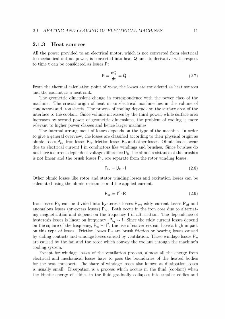
2.1.3 Heat sourcesAll the power provided to an electrical motor, which is not converted from electricalto mechanical output power, is converted into heat Q and its derivative with respectto time t can be considered as losses P:
P = dQ
dt= Q . (2.7)
From the thermal calculation point of view, the losses are considered as heat sourcesand the coolant as a heat sink.
The geometric dimensions change in correspondence with the power class of themachine. The crucial origin of heat in an electrical machine lies in the volume ofconductors and iron sheets. The process of cooling depends on the surface area of theinterface to the coolant. Since volume increases by the third power, while surface areaincreases by second power of geometric dimensions, the problem of cooling is morerelevant to higher power classes and hence larger machines.
The internal arrangement of losses depends on the type of the machine. In orderto give a general overview, the losses are classified according to their physical origin asohmic losses Pcu, iron losses Pfe, friction losses Pfr and other losses. Ohmic losses occurdue to electrical current I in conductors like windings and brushes. Since brushes donot have a current dependent voltage difference UB, the ohmic resistance of the brushesis not linear and the brush losses Pbr are separate from the rotor winding losses.
Pbr = UB · I (2.8)
Other ohmic losses like rotor and stator winding losses and excitation losses can becalculated using the ohmic resistance and the applied current.
Pcu = I2 · R (2.9)
Iron losses Pfe can be divided into hysteresis losses Phy, eddy current losses Ped andanomalous losses (or excess losses) Pex. Both occur in the iron core due to alternat-ing magnetization and depend on the frequency f of alternation. The dependence ofhysteresis losses is linear on frequency: Phy ∼ f. Since the eddy current losses dependon the square of the frequency, Ped ∼ f2, the use of converters can have a high impacton this type of losses. Friction losses Pfr are brush friction or bearing losses causedby sliding contacts and windage losses caused by ventilation. These windage losses Pware caused by the fan and the rotor which convey the coolant through the machine’scooling system.
Except for windage losses of the ventilation process, almost all the energy fromelectrical and mechanical losses have to pass the boundaries of the heated bodiesfor the heat transport. The share of windage losses also known as dissipation lossesis usually small. Dissipation is a process which occurs in the fluid (coolant) whenthe kinetic energy of eddies in the fluid gradually collapses into smaller eddies and

12 CHAPTER 2. FUNDAMENTALS
finally turns into heat energy due to the internal friction and viscosity of the fluid.Since dissipation losses are generated directly in the cooling fluid, there is no need totransport these losses across the boundary.
The diagram in Fig. 2.1 shows a classification of losses in an induction motoraccording to the sequence of the power flow. The windings in the stator, which areconnected to the electrical network, cause losses due to the ohmic resistance of theconducting material. Since in most cases this material is copper, these ohmic lossesare also known as copper losses Pcus. Due to the alternating current in the stator
Motor input Pin Input to rotor PinrMechanical power development Pm
Motor output PoutStator copper
loss Pcus
Rotor copper loss Pcur
Friction loss Pfr
Stator iron loss Pfe Windage loss Pw
Figure 2.1: Power flow diagram of an induction motor including the sequence of appearance in theenergy flow.
windings and to the rotating magnetic field of the rotor, the alternating and rotatingmagnetic field in the stator causes eddy current losses, hysteresis losses and anomalouslosses Pfe. The power from the stator is transmitted to the rotor over the air gap bymagnetic excitation of stator and rotor iron, similarly to the process occurring in atransformer. This converted power is denoted as Pinr in Fig. 2.1 and can be interpretedas the input power the rotor receives from the stator. Since the rotor revolves withalmost the same speed as the rotating magnetic field of the stator, the frequency in therotor conductors is only a few Hz at steady state operation, after the speed-up phase.Due to the low frequency in the rotor, the eddy current losses can be neglected andthe ohmic losses Pcur dominate. The rest of the power is transformed to mechanicalpower Pm which has to be reduced by the friction losses Pfr and windage losses Pw inorder to obtain the mechanical output power of the motor Pout.
2.1.4 Cooling methodsThe heat energy of an electrical machine is discharged to the environment either di-rectly by a coolant or indirectly through a heat exchanger. The over-temperature ina machine can be controlled by the cooling method, the type of coolant, the coolantstreaming velocity, the distance and material between the heat source and the heatsink.

2.1. HEATING AND COOLING OF ELECTRICAL MACHINES 13
Numerous methods of cooling are available, which can be categorized by the num-ber of cooling circuits arranged together, the type of coolant, the design of coolingcircuit and the conveying method of the coolant. When two cooling circuits arrangedin series, they are denoted as a primary and a secondary cooling cycle with a primarycoolant which passes the heat energy to the secondary coolant with the aid of a heatexchanger. An open cooling cycle takes the coolant from direct or close environment(e.g. ambient air or nearby water reservoir) and discharges the heated coolant to thesame environment. The primary cooling cycle is usually separated from the environ-ment and therefore has to be a closed cooling cycle. Machines without any coolingpipes or cooling ducts for air inlet and outlet can either take and discharge the coolantfrom a direct environment in a free cooling circuit, or use the direct contact with theenvironment for surface cooling.
Figure 2.2: Ventilation methods for small and medium size machines: (a) closed machine with surfacecooling and outer radial flow fan L (cooling method IC 4A1A1 or IC 411), (b) machine with opencooling cycle, axial cooling ducts and one radial flow fan L (cooling method IC 0A1 or IC 01); (c)machine with open cooling cycles, two radial flow fans L, axial and radial ducts in the stator (coolingmethod IC 0A1 or IC 01) [63]
Depending on the type of coolant, cooling methods can be separated into gas-cooled and liquid-cooled methods. For gaseous coolants, the conveying process canbe carried out by a shaft mounted fan or an externally driven fan. Liquids require apump usually driven externally. In small and medium sized machines the gas-cooledmethods with surface cooling are more frequently used. In order to protect machinesfrom contaminating dust or moisture, large-scaled machines are often built with aclosed primary cooling cycle. Machines which have a high circumferential velocity usehydrogen (or sometimes helium) as coolant in a closed and pressure-resistant primarycooling circuit. Beside the benefit of lower dissipation losses, the wall heat transfercoefficient in hydrogen cooled machines is about 50% higher [63] than in air cooledmachines and they can operate in a protective atmosphere reducing oxidation. Thesecondary coolant for such an assembly is usually water.
Water is the prevailing medium for liquid-cooled methods due to its high specificheat capacity. This permits good cooling properties with small amounts (volumes) ofcoolant, small cooling duct cross sections and low coolant flow velocities. In the caseof directly cooled conductors where the coolant flows directly inside hollow conductorsor in pipes next to the conductors, a liquid coolants such as water have a great benefit.
A standard for designation of cooling methods has been defined in IEC 60034-6 [46]. The standard describes the cooling arrangement and the types of coolants

14 CHAPTER 2. FUNDAMENTALS
using specific codes:
IC 5 A 1 A 1 ,
with IC for International Coding and subsequent code letters and numbers. In thisexample 5, denotes the cooling arrangement of an integrated heat exchanger betweenthe primary and secondary cooling circuit with air (A) as coolant for both coolingcycles. Self ventilation depending on the speed of rotation of the machine (1) has beenchosen for the movement (conveying) type of the primary and secondary coolant. Thecodes for cooling arrangement, type of coolant and conveying type are listed and brieflyexplained in the appendix (Tab. A.1, A.2 and A.3). A more detailed description ofthe nomenclature can be found in the IEC 60034-6 standard. The following Fig. 2.3demonstrates the explained cooling method.
Figure 2.3: Ventilation of a machine with a closed primary and an open secondary cooling circuit(cooling method IC 5A1A1 or IC 511) [63]
The different constructions of the drive-train of vehicles require different typesof traction-motors. The weight of the vehicle and the number of wheels which aredriven directly by the traction-motors have an influence on the cooling-type. Otherinfluencing factors are the properties of the gear-box, the vehicles’ maximum speed andthe maximum traction torque, especially at zero speed. Depending on these properties,various types of cooling systems have been developed to meet the desired requirementsof the vehicle manufacturer.
A common practice for describing the cooling method of an electrical motor is theacronym of the cooling system itself, as shown in the first column in Tab. 2.2. Someacronyms fit to IEC standards listed in the third column. Although this is a commonlyused nomenclature, it is not part of a recognized standard. Due to the large number ofdifferent cooling strategies, only a few types are randomly listed in Tab. 2.2, withoutany preference on technical properties. Some of them are considered in this work.
Due to limited space and weight, air is usually used as a coolant in electricaltraction motors. Optimizing the cooling process means optimizing the pressure drivenair flow through the machine. Efficient ventilators which provide this pressure can beconveniently designed for one single speed of rotation and a specified rotating direction.Due to the changing operational conditions, the ventilation of an electrical tractionmotor is more challenging compared to motors with fixed operational conditions [63].

2.2. HEAT TRANSFER 15
Acronym Explanation IEC 60034-6 standardTEFC Totally Enclosed Fan Cooled IC 4A1A1, IC 4A1A6TESC Totally Enclosed Self CooledDACS Double Air Cooled System
TEAOM Totally Enclosed Air Over MotorTETV Tube Ventilated IC 5A1A1, IC 5A1A6SPDP Open Air type IC 0A1, IC 0A6CACW Water Cooled IC 8A1W7CACA Air Cooled IC 6A1A1, IC 6A1A6, IC 6A6A6DPFC Drip Proof Fan CooledTENV Totally Enclosed Non-Ventilated
Table 2.2: Acronyms of cooling methods and the corresponding IEC standards
2.2 Heat transferAs shown in [7], the transport of heat energy can rely on different physical effects suchas diffusion in materials, spatial movement of materials or electromagnetic radiationbetween materials. Depending on the effect, three different means of heat transferare distinguished: conductive heat transfer, heat transfer by convection and radiation.The descriptions of the following subsections are mainly abstracted from [7].
2.2.1 Conductive heat transferConductive heat transfer is the transport of heat energy by the vector heat flux densityq as a function of the direction vector x and time t [7]:
q = q(x, t) . (2.10)
The heat flux direction is perpendicular to the isothermal lines, from higher to lowermagnitude of temperature. This direction coincides with that of the negative gradientof temperature describing the fundamental law of heat conduction discovered by Jean-Baptiste-Joseph Fourier:
q = −λ · ∇T , (2.11)
where the temperature T and the thermal conductivity λ especially for fluids, dependon local temperature and pressure. The thermal conductivity describes the amount ofheat per unit surface area which can be transported through a specific material. Forsolid materials and for small changes in temperature and pressure the thermal con-ductivity can be assumed as constant. The thermal conductivities of some selected,technically relevant or exceptional materials are listed in Tab. 2.3. The thermal con-ductivity is usually an isotropic material property with equal values in each direction.For composite or laminated materials which consist of two or more materials withdifferent thermal conductivities, a homogenization of the thermal conductivity doesmake sense, in order to simplify calculation. Such homogenization of materials can

16 CHAPTER 2. FUNDAMENTALS
Material λ in W/mK Material λ in W/mKNanotubes ≈ 8000 Casted iron 41 . . . 55Silver 427 Steel 13 . . . 48Copper 399 Water 0.598Aluminum 99.2% 209 Air 0.0257
Table 2.3: Thermal conductivity of some materials at a temperature of 20°C [6,48]
lead to an anisotropic thermal conductivity:
λ =
λxλyλz
. (2.12)
According to the second law of thermodynamics, the conductive heat flux describesa non-reversible process flowing from the higher to the lower temperature against thetemperature gradient and has, for that reason, a negative sign. For a flat plate withthickness b, surface area A and different temperatures Tw1 and Tw2 on the two surfaces,the heat flux is
Q = λ A
b(Tw1 − Tw2) . (2.13)
2.2.2 Convective heat transferIn contrast to solid bodies, the transport of heat inside a fluid is not restricted toconductive heat transport. On the account of macroscopic fluid movements relativeto the heat source, heat energy is also transported by local fluid exchange. Hence theconvective heat transport depends not only on the fluid properties but also on thelocal flow conditions next to the energy source.
Since a fluid typically adheres to the surface (y = 0) of a solid body, as sketchedin Fig. 2.8 on page 29, the velocity of the fluid relative to the surface is zero, whichis known as the non-slip-condition. The heat transport from the solid material to thefluid starts with conductive heat transport and consequently Fourier’s fundamentallaw of heat conduction is valid at the boundary from solid to fluid material. Henceconvective heat transport depends on the value of the fluid’s thermal conductivity λand the heat flux density qw directly at the surface can be expressed as:
qw = −λ(∂T
∂y
)y=0
. (2.14)
The heat flux density depends on the difference between the surface temperature Twand the temperature of the fluid T∞
qw = α(Tw − T∞) , (2.15)
where the wall heat transfer coefficient α can be calculated analytically for very simplegeometries under certain flow conditions. An analytical way of calculation for convo-luted surfaces and/or turbulent flow conditions does not exist. Therefore α has to be

2.2. HEAT TRANSFER 17
found empirically or by numerical methods. Using the equality of (2.14) and (2.15)leads to:
α = −λ
(∂T∂y
)w
Tw − T∞. (2.16)
The ratio λ/α is illustrated in Figure 2.4 as the slope of the temperature profile nextto the surface [6].
wal
l
Tf
0 y
λ/α
T
Tf
Tw
Figure 2.4: Temperature profile of the fluid for convective heat transport from the solid surface tothe fluid
The wall heat transfer coefficient depends basically on the fluid properties andon the flow conditions. Some examples for the magnitude of the wall heat transfercoefficient are shown in Tab. 2.4. The wall heat transfer coefficient α is usually used
Fluid Flow condition α in W/m2KAir free convection 6 - 30Superheated steam or air forced convection 30 - 300Oil forced convection 60 - 1.800Water forced convection 300 - 18.000Water boiling 3.000 - 60.000Steam condensing 6.000 - 120.000
Table 2.4: Order of magnitude of convection heat transfer coefficients [48]
as a mean value for a specific surface. If the coefficient is used as a value for a specificlocation at the surface it is very often designated as local wall heat transfer coefficientαx.
2.2.3 Heat transfer by radiationBesides convective heat transfer and heat transfer by conduction, every surface cantransfer heat energy by radiation of electromagnetic waves in and close to the infrared

18 CHAPTER 2. FUNDAMENTALS
spectrum of light. The heat flux density qr which is caused by radiation can beexpressed as
qr = σT4 , (2.17)rising with the fourth power of the surface temperature T and σ = 5.671 · 10−8 W/m2K4
for an ideally absorbed radiation. This correlation was first discovered by Josef Stefanand Ludwig Boltzmann hence σ is called the Stefan-Boltzmann constant. Since mostbodies do not ideally emit or absorb radiation, the material property of the surfacehas to be considered with the inclusion of the emission-coefficient ε
qr em = ε(T)σT4 (2.18)
for emitted radiation and the absorption-coefficient a
qr ab = aσT4 , (2.19)
for absorbed radiation, respectively. The total emitted or absorbed power can beexpressed with the surface area A as Qem = AεσT4 and as Qab = AaσT4
e. Since theprocess of emission and absorption appear simultaneously in most technical applica-tions, the total balance of exchanged power is of interest. For an emitting body withtemperature T in an environment with temperature Te the resulting balance of poweris:
Q = Qem − Qab = Aσ(εT4 − aT4e) . (2.20)
The use of a so called gray body in a black environment is sufficient in many technicalcalculations. For such conditions, the absorption coefficient a can be assumed to theequal to the emission coefficient ε:
Q = Qem − Qab = Aσε(T4 − T4e) . (2.21)
In contrast to conduction and convection, radiation is also possible in vacuum. If theheated body is surrounded by a fluid, convective heat transfer occurs simultaneouslywith radiation and has to be considered in the overall heat flux density. Thereforeq = qc + qr and
q = α(T− T∞) + εσ(T4 − T4e) = (α + αr)(T− Te) , (2.22)
with the temperature of environmental surfaces Te and the temperature of air T∞,which can be assumed to be equal in many cases. This leads to a mathematicaldescription of the heat transfer coefficient by radiation:
αr = εσT4 − T4
e
T− Te. (2.23)
One important property of heat radiation becomes evident from this equation.Since the radiation heat flux depends on the fourth power of the temperature difference,it has to be considered if the surface temperature is very high or if the simultaneouslyexisting heat flux by convection is very small, e.g. free buoyant convection [6].

2.2. HEAT TRANSFER 19
2.2.4 The wall heat transfer coefficientThe majority of English textbooks dealing with the topic of heat transfer denote (2.15)as Newton’s law of cooling. According to [1], this is a widespread misconception. Inthe year of 1701, Newton commented the cooling process of red glowing hot ironas follows: Therefore if the Times of cooling are taken equal, the Heats will be inGeometrical Ratio, and therefore are easily found by a Table of Logarithms [66]. Aspointed out in [1], Newton’s paper was originally written in Latin and he used theword ’calor’, which was translated to the word ’heat’ in the 18th century, since theword ’temperature’ had not yet been established. He explained the change in thetemperature of a hot body over time in the form of:
d∆T
dt∼ −∆T, (2.24)
which describes a cooling curve. Newton was dealing with the process of cooling butdid not define a coefficient as we do today. Furthermore, he assumed that the wholebody had a uniform temperature and did not consider the surface of the body orheat flux. Since the influence of area is crucial to the convective wall heat transfercoefficient, it is questionable that Newton was the creator of this coefficient. Theconcept of the wall heat transfer coefficient was most likely developed a whole centurylater by Fourier. In 1822 he published an awarded earlier version of Analytical Theoryof Heat [26], which seems to be the first profound evidence of the wall heat transfercoefficient [1].
The textbook interpretation of Newton’s law of cooling (2.15) adopts a very sim-ple approach which meets the requirements in many cases. On the other hand, thisapproach can fail on a quite simple example, as shown in [33] :
0 L/2 L
Tw(L)
Tf
Tw(0)
Tw
(L)
≤ T f ≤
Tw
(0)
T
w
Tf
0 L/2 Lq(L)
0
q(L)
≤ q
(x)
≤ q(
0)
0 ≤ x ≤ L
(a) Wall temperature Tw, fluid temperatureT∞and resulting heat flux q
0 L/2 L
0
−∞ ≤
α ≤
∞
0 ≤ x ≤ L
(b) Local wall heat transfer coefficient α
Figure 2.5: Example of a heat transfer scenario with non-physical behavior of the convective wallheat transfer coefficient as described in [33] and calculated by CFD
Assume a flat plate with the length L and a linearly declining surface temperatureTw(x) > Tf from the leading edge at x = 0, with Tw(x) = Tf at x = L/2 to Tw(x) < Tf
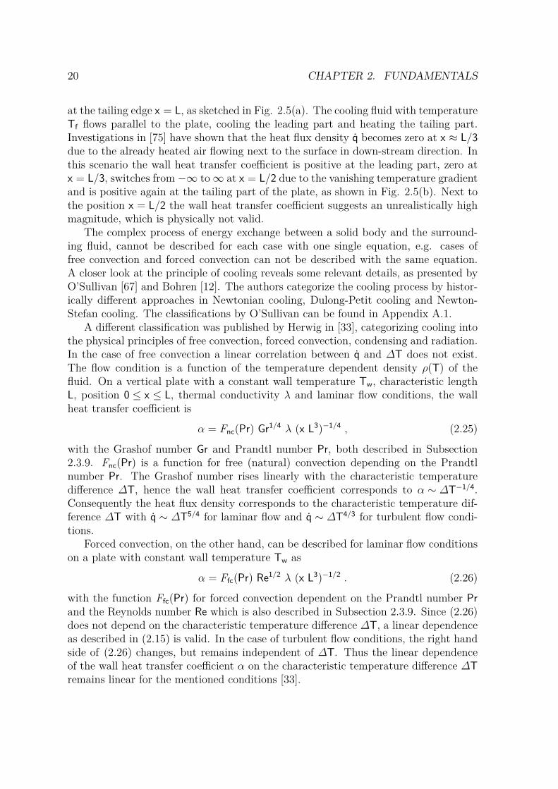
20 CHAPTER 2. FUNDAMENTALS
at the tailing edge x = L, as sketched in Fig. 2.5(a). The cooling fluid with temperatureTf flows parallel to the plate, cooling the leading part and heating the tailing part.Investigations in [75] have shown that the heat flux density q becomes zero at x ≈ L/3due to the already heated air flowing next to the surface in down-stream direction. Inthis scenario the wall heat transfer coefficient is positive at the leading part, zero atx = L/3, switches from −∞ to∞ at x = L/2 due to the vanishing temperature gradientand is positive again at the tailing part of the plate, as shown in Fig. 2.5(b). Next tothe position x = L/2 the wall heat transfer coefficient suggests an unrealistically highmagnitude, which is physically not valid.
The complex process of energy exchange between a solid body and the surround-ing fluid, cannot be described for each case with one single equation, e.g. cases offree convection and forced convection can not be described with the same equation.A closer look at the principle of cooling reveals some relevant details, as presented byO’Sullivan [67] and Bohren [12]. The authors categorize the cooling process by histor-ically different approaches in Newtonian cooling, Dulong-Petit cooling and Newton-Stefan cooling. The classifications by O’Sullivan can be found in Appendix A.1.
A different classification was published by Herwig in [33], categorizing cooling intothe physical principles of free convection, forced convection, condensing and radiation.In the case of free convection a linear correlation between q and ∆T does not exist.The flow condition is a function of the temperature dependent density ρ(T) of thefluid. On a vertical plate with a constant wall temperature Tw, characteristic lengthL, position 0 ≤ x ≤ L, thermal conductivity λ and laminar flow conditions, the wallheat transfer coefficient is
α = Fnc(Pr) Gr1/4 λ (x L3)−1/4 , (2.25)
with the Grashof number Gr and Prandtl number Pr, both described in Subsection2.3.9. Fnc(Pr) is a function for free (natural) convection depending on the Prandtlnumber Pr. The Grashof number rises linearly with the characteristic temperaturedifference ∆T, hence the wall heat transfer coefficient corresponds to α ∼ ∆T−1/4.Consequently the heat flux density corresponds to the characteristic temperature dif-ference ∆T with q ∼ ∆T5/4 for laminar flow and q ∼ ∆T4/3 for turbulent flow condi-tions.
Forced convection, on the other hand, can be described for laminar flow conditionson a plate with constant wall temperature Tw as
α = Ffc(Pr) Re1/2 λ (x L3)−1/2 . (2.26)
with the function Ffc(Pr) for forced convection dependent on the Prandtl number Prand the Reynolds number Re which is also described in Subsection 2.3.9. Since (2.26)does not depend on the characteristic temperature difference ∆T, a linear dependenceas described in (2.15) is valid. In the case of turbulent flow conditions, the right handside of (2.26) changes, but remains independent of ∆T. Thus the linear dependenceof the wall heat transfer coefficient α on the characteristic temperature difference ∆Tremains linear for the mentioned conditions [33].

2.3. FLUID DYNAMICS 21
2.3 Fluid dynamics
The heat transport by convection depends on the properties of the fluid and the stateof fluid flow. In order to express the quantity of the convective heat transfer, it isessential to know what the flow conditions are. With regard to the flow simulation,some fundamental basics of fluid dynamics are described in this section.
2.3.1 Fluid and viscosity
Matter which cannot sustain shear stress under resting conditions but is deformingits shape is referred to as fluid [14]. A fluid is considered as a continuum and can beeither liquid or gaseous.
y τ
Figure 2.6: Shear of fluid between two horizontal plates with profiles of velocity u(y) and shear stressτ
Consider a fluid between two parallel flat plates with constant distance y = hy, assketched in Fig. 2.6. On one plate, a force F is acting in parallel direction to the platesand the other plate is fixed. Due to the constant force, the plate moves with constantvelocity u in the same direction and causes a shear stress τ in the fluid. Since no otherforces are acting on the fluid or the plates, the shear stress in the fluid is constantin every plane parallel to the plates from y = 0 to h. Experiments on technicallyimportant fluids (e.g. air and water) show that shear stress and velocity gradient areproportional:
τ = µdu
dy, (2.27)
with the dynamic viscosity µ as a property of the relevant material. This also impliesthat the fluid cannot sustain shear stress at rest. All fluids which meet this conditionare Newtonian Fluids [34].

22 CHAPTER 2. FUNDAMENTALS
2.3.2 Conservation of massThe theory of fluid dynamics assumes that mass cannot be produced or destroyed.This axiom leads to the equation of conservation of mass [80]:
∂ρ
∂t+∇ · (ρv) = 0 (2.28)
with velocity vector v = v(u, v,w) and density ρ. The conservation of mass in (2.28)is written in the conservative form or divergence form. In the conservative form,the exactly same amount of mass flows into a certain volume as it flows out on theother side, if the volume is free of any sources or sinks. On the other hand the non-conservative form or quasi-linear form of (2.28) is
∂ρ
∂t+ (v · ∇)ρ+ (ρ∇ · v) = 0 . (2.29)
Without taking the density into account properly, the mass-flux through the bound-aries of adjacent cells will not be canceled. Hence the conservative form of the conser-vation equations is important to keep the total mass constant in numerical calculations.In many applications, the density can be assumed as incompressible, which means thatit does not change during transport between locations x = x(x, y, z) or in time t. Onthis account, the equation of continuity can be reduced to the conservative form forincompressible fluids
∇ · (ρv) = 0 (2.30)and to the divergence free condition for the velocity
∇ · v = 0 , (2.31)
respectively [22,43].
2.3.3 Conservation of momentumThe axiom of momentum from classical mechanics can be applied to liquid or gaseousfluids [34]:
d
dt(∆mv) =
∑i
Fi . (2.32)
This derivative on the left hand side is vd∆mdt +∆m dv
dt . Due to the conservation ofmass (2.32), d∆m
dt becomes zero and (2.32) can be expressed by
∆mdvdt
=∑
i
Fi . (2.33)
With the expression of mass per unit volume ∆m∆V = ρ and force per unit volume Fi
∆V = fi,(2.32) can be written as
ρdvdt
=∑
i
fi . (2.34)

2.3. FLUID DYNAMICS 23
The forces applied to a fluid are separated into mass or body forces and contactor surface forces. Body forces fB
i occur due to centrifugal forces, Lorenz forces orgravitational force
fBi = ρg , (2.35)
with the acceleration gx, gy and gz in the direction of x, y and z, respectively.The surface forces fS
i on a cubic control volume ∆V = ∆x∆y∆z occur in the formof tension forces. Considering that fluids can not accommodate shear stress at restand are able to accommodate compressive stress but not tension stress, the surfaceforces in direction x can be written as(
∂σxx
∂x∆x
)∆y∆z ,
(∂τyx
∂x∆y
)∆x∆z and
(∂τzx
∂x∆z
)∆x∆y , (2.36)
which, expressed per unit volume, become ∂σxx∂x , ∂τyx
∂x and ∂τzx∂x . The principal stress σxx
is defined perpendicularly to the control volumes face in the yz plane and the shearstresses τyx and τzx in the yx plane and zx plane, respectively. All tensions occurringon the cubic control volume are usually written in the stress tensor
σ =
σxx τyx τzxτxy σyy τzyτxz τyz σzz
. (2.37)
If the fluid is in rest with v = 0, then the shear stress is zero and the principal stressremains at the value of the hydrostatic pressure p, which can be separated from theprincipal stresses σxx, σyy, σzz in the stress tensor σ and the viscose stress tensor τremains
τ = σ − pI =
σxx τyx τzxτxy σyy τzyτxz τyz σzz
− p 0 0
0 p 00 0 p
=
τxx τyx τzxτxy τyy τzyτxz τyz τzz
, (2.38)
where I denotes the identity tensor. Combining (2.34), (2.35) and (2.38) as
fSi = τ∇ = σ∇−∇p (2.39)
the conservation of momentum can be written in vector notation
ρdvdt
= −∇p + σ∇+ fB , (2.40)
or in the coordinate-wise form [2]
∂(ρu)∂t
+ (∇ · ρuv) = −∂p
∂x+ ∂τxx
∂x+ ∂τyx
∂y+ ∂τzx
∂z+ fB
x
∂(ρv)∂t
+ (∇ · ρvv) = −∂p
∂y+ ∂τxy
∂x+ ∂τyy
∂y+ ∂τzy
∂z+ fB
y
∂(ρw)∂t
+ (∇ · ρwv) = −∂p
∂z+ ∂τxz
∂x+ ∂τyz
∂y+ ∂τzz
∂z+ fB
z (2.41)

24 CHAPTER 2. FUNDAMENTALS
with mass acceleration ∂(ρu)∂t +∇ · ρuv, pressure force−∂p
∂x , viscose forces∂τxx∂x + ∂τyx
∂y + ∂τzx∂z
and body forces fBx , each per unit volume [17].
2.3.4 Conservation of energySimilarly to the conservation of mass, the energy in a system cannot be created ordestroyed. The temporal change of a body’s energy equals the sum of the power of allapplied forces plus all the supplied energy per unit of time [80]. This can be expressedmathematically as:
∂
∂t
[ρ
(e + V2
2
)]+[∇ · ρ
(e + V2
2
)v]
= ρfB · v− (∇pv)
+ ∂
∂x(uτxx + vτxy + wτxz) + ∂
∂y(uτyx + vτyy + wτyz) + ∂
∂z(uτzx + vτzy + wτzz)
− (∇ · q) + qQ , (2.42)
with the total energy per unit volume
Et = ρ
(e + V2
2
)(2.43)
containing the inner energy ρe, the kinetic energy ρV2
2 and the Euclidean norm of thevelocity vector V = ||v||2 on the left-hand side [2]. The right-hand side of the equationincludes the power of the body forces ρfB · v, the surface forces −∇pv + ∂
∂x (.) + ∂∂y(.)
+ ∂∂z(.), all heat energy transported over the system boundaries ∇ · q and the inner
energy sources qQ.
2.3.5 Navier-Stokes equationsThe flow conditions cannot be calculated with the equations on conservation of momen-tum (2.41) and mass of incompressible fluids (2.31), because the number of unknowns ishigher than the number of equations. For constant density ρ, the momentum equationfor direction x can be written as
∂(ρu)∂t
+ (∇ · ρuv) = −∂p
∂x+ ∂τxx
∂x+ ∂τyx
∂y+ ∂τzx
∂z+ fB
x (2.44)
By introducing Stokes’ law for frictional force
τxx = 2µ
(∂u
∂x
), τyx = µ
(∂v
∂x+ ∂u
∂y
)and τzx = µ
(∂w
∂x+ ∂u
∂y
), (2.45)
the tensions in (2.44) can be replaced by derivatives of velocities:
∂(ρu)∂t
+ (∇ · ρuv) = −∂p
∂x+ µ
(∂2u
∂x2+ ∂2u
∂y2+ ∂2u
∂z2
)+ fB
x (2.46)

2.3. FLUID DYNAMICS 25
where µ is the dynamic viscosity of the fluid. Hence:
∂(ρu)∂t
+ (∇ · ρuv) = −∂p
∂x+ µ∆u + fB
x
∂(ρv)∂t
+ (∇ · ρvv) = −∂p
∂y+ µ∆v + fB
y
∂(ρw)∂t
+ (∇ · ρwv) = −∂p
∂z+ µ∆w + fB
z , (2.47)
The equations for continuity of momentum are along with the continuity of mass andcontinuity of energy called the Navier-Stokes equations. With the help of the Navier-Stokes equations, an exact solution can be achieved for specific cases of laminar fluidflow and constant density.
2.3.6 Variables of the turbulent flowTurbulent flow can be a desired flow condition, since convectional processes such as heator mass transport are more pronounced in comparison with laminar flow conditions.Although the Navier-Stokes equations can be used to calculate laminar flow undervarious conditions, they fail when the fluid flow is turbulent. On the other hand, aturbulent flow always requires additional power to sustain the permanent fluctuationof the fluid. Under turbulent flow conditions, the velocity v can be split into a timeaverage value v and a fluctuating value v′ in the form of v = v + v′. The average
Figure 2.7: Time averaged values for (left) steady state flow and (right) transient flow conditions [22]
and fluctuating components of the velocity vector v exist for each component u, v andw in the appropriate directions x, y and z. As sketched in Fig. 2.7, only the u partis shown in the direction x from the vector v if this behavior affects all dimensionsindependently:
u(x, t) = u(x, t) + u′(x, t) . (2.48)Due to turbulence, stochastic oscillating lateral and longitudinal movements relative tothe mean flow of fluid particles require mechanical energy for permanent acceleration

26 CHAPTER 2. FUNDAMENTALS
and deceleration. The exchange of momentum and recurrent partial elastic deforma-tion of fluid particles in a streaming fluid cause a transformation from kinetic intothermal energy called dissipation. The isotropic dissipation rate with the unit m2/s3
is defined in [76] by:
ε = ν∂u′i∂xk
∂u′i∂xk
, (2.49)
with index notation which is equivalent to
ε = µ
ρ
(∂u′
∂x
)2
+(∂v′
∂x
)2
+(∂w′
∂x
)2
+(∂u′
∂y
)2
+(∂v′
∂y
)2
+(∂w′
∂y
)2
+(∂u′
∂z
)2
+(∂v′
∂z
)2
+(∂w′
∂z
)2 . (2.50)
With the resulting additional flow resistance, the fluid seems to have a higher shearstress and hence a higher viscosity than under laminar flow conditions. According to(2.27), this additional turbulent wall shear stress τt can be expressed for the fluid flowwith velocity u in direction x as:
τt = µt ·∂u
∂y(2.51)
where µt is the turbulent viscosity and y the direction perpendicular to the flow di-rection and the wall surface. The turbulent viscosity µt depends on the local flowconditions and is therefore a parameter of momentum exchange and not of fluid prop-erties. The eddy viscosity which is widely used for numerical calculations is definedby:
νt = µt
ρ. (2.52)
Due to the dependence on turbulence, a universally valid expression of eddy viscosityis not available [79]. As shown in Subsection 2.4.4, basic turbulence models use theeddy viscosity to define the Reynolds stress tensor for the calculation of turbulentflow. The permanent acceleration of fluid particles is a form of energy, which can beexpressed per unit mass by the turbulence kinetic energy k:
k = u′2 + v′2 + w′2
2(2.53)
with the averaged fluctuating velocities for each Cartesian direction. Consequently, theunit of the turbulence kinetic energy is m2/s2. For fluid boundary conditions (e.g. inletand outlet) a frequently used expression is the turbulence intensity It with isotropicturbulence u′ = v′ = w′:
It = u′
u, (2.54)

2.3. FLUID DYNAMICS 27
which is calculated for the flow in direction x by the isotropic fluctuating part and themean velocity u [4]:
u′ =√
2
3k . (2.55)
An intensity above 10% can be considered as high and, if it is below 1%, as lowturbulence intensity. For the flow conditions in a cooling duct, the intensity in thecore of the flow can be described with the Reynolds number ReDh for the hydraulicdiameter Dh as [25]:
It = 0.16 (ReDh)−1/8 (2.56)
2.3.7 Reynolds Averaged Navier-Stokes (RANS) equationsThe velocities for laminar flow in the Navier-Stokes equations in (2.47) can be replacedby the time-averaged and fluctuating velocities as shown in (2.48). Assuming thatthe time-average of the fluctuating value a′ = 0 is zero, the rules for calculating withaveraged values are:
a + b = a + b a = a ab = ab∂a
∂s= ∂a
∂s
As seen in (2.47), the Navier-Stokes equation for the x direction is
∂(ρu)∂t
+ (∇ · ρuv) = −∂p
∂x+ µ∆u + fB
x . (2.57)
Resolving (∇ · ρuv), the left hand side of this equation is:
∂(ρu)∂t
+ ∂(ρu2)∂x
+ ∂(ρuv)∂y
+ ∂(ρuw)∂z
= . . . (2.58)
and replacing the velocities by the mean and the fluctuating part as shown in (2.48)leads to:
∂(ρ(u + u′))∂t
+ ∂(ρ(u + u′)2)∂x
+ ∂(ρ(u + u′)(v + v′))∂y
+ ∂(ρ(u + u′)(w + w′))∂z
= . . . .
(2.59)The whole equation can be averaged by averaging the single terms according to therule a + b = a + b after resolving the products in the derivatives in (2.59):
∂(ρu)∂t
+ ∂(ρu′)∂t
+ ∂(ρu2)∂x
+ 2∂(ρuu′)∂x
+ ∂(ρu′2)∂x
+ ∂(ρuv)∂y
+ ∂(ρuv′)∂y
+ ∂(ρu′v)∂y
+ ∂(ρu′v′)∂y
+ ∂(ρuw)∂z
+ ∂(ρuw′)∂z
+ ∂(ρu′w)∂z
+ ∂(ρu′w′)∂z
= . . . . (2.60)

28 CHAPTER 2. FUNDAMENTALS
Applying the rules a′ = 0 and ∂a∂s = ∂a
∂s , the equation can be reduced to:
∂(ρu)∂t
+ ∂(ρu2)∂x
+ ∂(ρuv)∂y
+ ∂(ρuw)∂z
+ ∂(ρu′2)∂x
+ ∂(ρu′v′)∂y
+ ∂(ρu′w′)∂z
= −∂p
∂x+ µ∆u + fB
x , (2.61)
which can be abbreviated in index notation for the Cartesian coordinates:
∂(ρui)∂t
+ ∂
∂xj
(ρuiuj + ρu′iu
′j
)= − ∂p
∂xi+ µ
∂2ui
∂x2j
+ fBi . (2.62)
For all three coordinates of the Cartesian coordinate system the Reynolds AveragedNavier-Stokes can be written as:
∂u
∂t+ u
∂u
∂x+ v
∂u
∂y+ w
∂u
∂z= −1
ρ
∂p
∂x+ ν∆u− ∂u′2
∂x− ∂v′u′
∂y− ∂w′u′
∂z+ gx
∂v
∂t+ u
∂v
∂x+ v
∂v
∂y+ w
∂v
∂z= −1
ρ
∂p
∂y+ ν∆v − ∂u′v′
∂x− ∂v′2
∂y− ∂w′v′
∂z+ gy
∂w
∂t+ u
∂w
∂x+ v
∂w
∂y+ w
∂w
∂z= −1
ρ
∂p
∂z+ ν∆w − ∂u′w′
∂x− ∂v′w′
∂y− ∂w′2
∂z+ gz(2.63)
with the kinematic viscosity ν = µ/ρ. A detailed derivation of the RANS equationscan be found e.g. in [34,79]. These equations represent the basis of most fluid dynamicsimulation tools designed for engineering purposes. Due to the consideration of fluc-tuating flow conditions, additional strains also known as Reynolds stress are includedon the right-hand side of the equation (2.63). Since the determination of the Reynoldsstress is computationally time-consuming, these additional strains are usually replacedby special models in CFD simulations [25,80].
2.3.8 The boundary layerAssume an impermeable surface (wall) parallel to the mean flow direction x of a fluid(as shown in Figure 2.8). The fluid flow is considered laminar and in steady state.Since the non-slip-condition is valid at the boundary, the relative velocity of the fluidto the surface is zero directly at the surface (y → 0).
Examining the flow field next to the surface, it is evident that the velocity u(y) riseswith the increase of the distance y to the surface, until it reaches the velocity u∞ . Inthe outer fluid flow, at a fictitious infinite distance perpendicular to the consideredsurface, flow conditions are assumed to be not influenced by the examined surface.The margin of the velocity boundary layer δ(x) is defined by the position where thevelocity profile u(y) reaches the value of the outer flow u∞ .
The thermal boundary layer δt(x) is defined in a similar manner. The fluid temper-ature Tf at the surface equals the surface temperature T(y→ 0) = Tw. As shown in
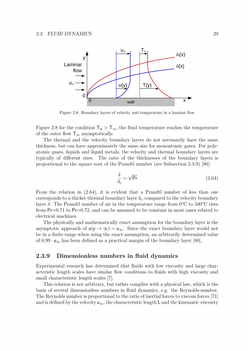
2.3. FLUID DYNAMICS 29
wall
u∞
u(y)
T∞
T(y)
0 x
y
u∞
Laminar flow
0
δt(x)
δ(x)
Figure 2.8: Boundary layers of velocity and temperature in a laminar flow
Figure 2.8 for the condition Tw > T∞, the fluid temperature reaches the temperatureof the outer flow T∞ asymptotically.
The thermal and the velocity boundary layers do not necessarily have the samethickness, but can have approximately the same size for monoatomic gases. For poly-atomic gases, liquids and liquid metals, the velocity and thermal boundary layers aretypically of different sizes. The ratio of the thicknesses of the boundary layers isproportional to the square root of the Prandtl number (see Subsection 2.3.9) [80]:
δ
δt∼√
Pr (2.64)
From the relation in (2.64), it is evident that a Prandtl number of less than onecorresponds to a thicker thermal boundary layer δt, compared to the velocity boundarylayer δ. The Prandtl number of air in the temperature range from 0°C to 500°C risesfrom Pr=0.71 to Pr=0.72, and can be assumed to be constant in most cases related toelectrical machines.
The physically and mathematically exact assumption for the boundary layer is theasymptotic approach of u(y→∞) = u∞. Since the exact boundary layer would notbe in a finite range when using the exact assumption, an arbitrarily determined valueof 0.99 · u∞ has been defined as a practical margin of the boundary layer [80].
2.3.9 Dimensionless numbers in fluid dynamicsExperimental research has determined that fluids with low viscosity and large char-acteristic length scales have similar flow conditions to fluids with high viscosity andsmall characteristic length scales [7].
This relation is not arbitrary, but rather complies with a physical law, which is thebasis of several dimensionless numbers in fluid dynamics, e.g. the Reynolds-number.The Reynolds number is proportional to the ratio of inertial forces to viscous forces [71]and is defined by the velocity u∞, the characteristic length L and the kinematic viscosity

30 CHAPTER 2. FUNDAMENTALS
of the fluid ν.Re = u∞ ρ L
µ= u∞ L
ν. (2.65)
It indicates whether the flow condition is turbulent or laminar, e.g. in the case of apipe flow a Reynolds number Re < 2300 indicates a laminar pipe flow [79].
The Prandtl number defines the relation between flow field and temperature field [7]and is defined as:
Pr = µ cp
λ= ν
a, (2.66)
with specific heat capacity cp and thermal conductivity λ.The Eckert number Ec is a ratio describing the temperature field, e.g. for su-
personic flows or flow conditions with noteworthy internal friction (dissipation), withtemperature difference ∆T between the surface and the environment.
Ec = u2∞
cp ∆T(2.67)
In contrast to the Eckert number, the Grashof number Gr gains importance for slowand buoyant flows driven by acceleration of gravity g and local change of density, whichcan be characterized by the volumetric thermal expansion coefficient β:
Gr = g β L3 ∆T
ν2(2.68)
On the other hand, the Grashof number is usually negligible for mechanically generatedflows.
A very important number for problems of heat transfer is the Nusselt number Nu,which characterizes the ratio between the existing heat flux density and the theoreticalheat flux density caused by simple conductive heat transfer [13]. In general the Nusseltnumber depends on the four numbers mentioned above:
Nu = F(Re,Pr,Ec,Gr) = α L
λ, (2.69)
where Nu and α are the surface averaged values of the local Nusselt number Nux and ofthe local wall heat transfer coefficient αx, respectively. Replacing the wall heat transfercoefficient with the wall heat flux and temperature difference leads to the frequentlyused expression
Nu = qw L
λ ∆T. (2.70)
Due to the reasons mentioned above, the Eckert number and, in most cases, theGrashof number can be neglected in the investigations of the present work. The Prandtlnumber for air can be assumed to be constant in the considered range of temperature.The only influencing factor in this investigation is the Reynolds number.
In problems related to conductive heat transfer and sometimes also convectiveheat transfer, the Biot number can give useful information about the temperature

2.3. FLUID DYNAMICS 31
field inside solid material. Like the Nusselt number, the Biot number is defined by theheat transfer coefficient α, the characteristic length L and the thermal conductivity λ:
Bi = α L
λ. (2.71)
In contrast to the Nusselt number, the thermal conductivity of the solid material isused for the Biot number. If the value of the Biot number in a specific problem isbelow 2, an almost homogeneous temperature field inside the solid material can beassumed [7].
The ratio between compressive force (pressure) and inertial force is known as theEuler number Eu [79], determined by pressure p, density ρ and velocity u∞:
Eu = p
ρu2∞. (2.72)
2.3.10 Turbulent flow in wall-proximityThis subsection is based on derivations of turbulent flow in [80]. In technical applica-tions for convective cooling, the flow conditions are usually turbulent and laminar flowsare exceptions. The laminar behavior of fluid flow parallel to the wall can be explainedby the Navier-Stokes equation (2.47) with the conditions u = f(y) and v = w = 0 by
0 = µd2u
dy2. (2.73)
The vanishing second derivative of velocity indicates a constant shear stress τyx and alinear dependence of velocity u on the distance to the wall y. For the same conditions,the turbulent behavior of fluid flow parallel to the wall can be described by introducingthe Reynolds equation
ρv∂u
∂y= ∂τyx
∂y. (2.74)
Since v = 0, it reduces to ∂τyx∂y = 0, with the total shear stress τyx containing the viscose
shear stress τyx and the Reynolds stress ρu′v′:
τyx = τyx − ρu′v′ . (2.75)
Combining (2.73) and (2.75), the wall shear stress can be derived by integration as
τw = µ∂u
∂y− ρu′v′ or τw
ρ= ν
∂u
∂y− u′v′ (2.76)
respectively. The unit of the ratio τw/ρ is the square of velocity and therefore itssquare root is known as friction velocity
uτ =√τw
ρ, (2.77)

32 CHAPTER 2. FUNDAMENTALS
which quantifies the fluctuating velocity of the turbulent flow. By re-arranging (2.76)to
1 = d(u/uτ )d(y uτ/ν) −
u′v′
u2τ
(2.78)
the dependenceu
uτ= f
(y
uτν
)(2.79)
andu′v′
u2τ
= g(
yuτν
)(2.80)
can be identified. This universal law of the wall in (2.79) and (2.80) was discovered byLudwig Prandtl (1925) and is valid for all turbulent flow conditions next to the wallwhich satisfy the above mentioned assumptions. Since the Reynolds stress disappearsnext to the wall the function f can be derived by a Taylor series expansion from (2.79)
u(y+)uτ
= y+ d(u/uτ )dy+
∣∣∣∣∣y=0
+ (y+)2 1
2
d2(u/uτ )(dy+)2
∣∣∣∣∣y=0
+ (y+)3 1
6
d3(u/uτ )(dy+)3
∣∣∣∣∣y=0
+ . . . , (2.81)
with u(0) = 0 due to the non-slip condition. Here, y+ is the dimensionless wall distancedefined as
y+ = yuτν. (2.82)
Due to the vanishing fluctuation at the wall u′v′|y=0 = 0, using (2.78), the first termon the right hand side in (2.81) can be written as:
d(u/uτ )dy+
∣∣∣∣∣y=0
= 1 . (2.83)
Building the first and second derivatives of (2.78), the second and third terms in (2.81)become
d2(u/uτ )(dy+)2
∣∣∣∣∣y=0
= 1
u2τ
d(u′v′)dy
dy
dy+ = 1
u2τ
ν
uτ
[∂u′
∂yv′ + ∂v′
∂yu′]
y=0
= 0 (2.84)
andd3(u/uτ )(dy+)3
∣∣∣∣∣y=0
= 1
u2τ
(ν
uτ
)2[∂2u′
∂y2v′ + 2
∂u′
∂y
∂v′
∂y+ ∂2v′
∂y2u′]
y=0
= 0 . (2.85)
These terms also disappear due to the vanishing fluctuating velocity perpendicular tothe wall, hence
u(y+)uτ
= y+ + O(y+)4 . (2.86)
The influence of fluctuation on the velocity profile depends on the order of the fourthpower of the dimensionless wall distance O(y+)4. In a thin layer next to the wall, thefluctuations do not disappear but the mean velocity is dominated by the viscose shear

2.3. FLUID DYNAMICS 33
stress. Therefore this thin layer is called viscose sublayer. Between the viscose sublayerand the zone with rising influence of the Reynolds stress the transition is smooth.
With a rising distance to the wall, the influence of the viscose stress decreasesand the Reynolds stress dominates the velocity profile. For this region, (2.76) can bereduced to
τw = τt = −ρ(u′v′) . (2.87)
One approach for describing these fluctuations mathematically is provided by the for-mulation of Boussinesq
τt = −ρ(u′v′) = νt∂u
∂y, (2.88)
with the eddy viscosity νt which e.g. can be set to a constant value. Since the Reynoldsstress disappears next to a solid surface, this approach is inappropriate in cases withthe influence of walls but can be used for flow conditions without the wall influence.
Another approach is provided by the Mixing Length Model developed by LudwigPrandtl which considers the turbulent (wall) shear stress τt to be:
τt = −ρ(u′v′) = ρl2
(du
dy
)2
or τt = ρl2
∣∣∣∣∣du
dy
∣∣∣∣∣ du
dy(2.89)
respectively. With the mixing length l, the eddy viscosity νt = ρl2∣∣∣du
dy
∣∣∣ is defined de-pending on the velocity gradient next to the wall. Although this approach is notan exact solution, the mixing length model produces good results for many practicalproblems. Since the Reynolds stress has to disappear directly at the wall, the mixinglength is chosen to be linear depending on the wall distance with
l = κy . (2.90)
For a constant wall shear stress with τw = ρu2τ , the mixing length model (2.89) can be
written asuτ = κy
du
dy. (2.91)
By the integration of (2.91) the velocity profile of the logarithmic law of the walloutside the viscose sublayer is obtained:
u
uτ= 1
κln(y) + C (2.92)
where κ and C are empirical constants. A conversion using C = B + (1/κ)ln(uτ/ν)results in the non-dimensional equation:
u
uτ= 1
κln(
yuτν
)+ B . (2.93)
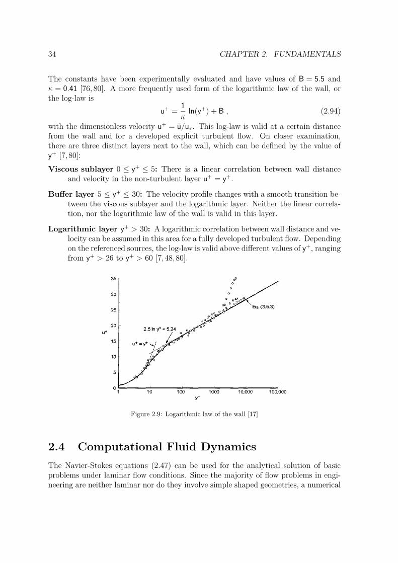
34 CHAPTER 2. FUNDAMENTALS
The constants have been experimentally evaluated and have values of B = 5.5 andκ = 0.41 [76, 80]. A more frequently used form of the logarithmic law of the wall, orthe log-law is
u+ = 1
κln(y+) + B , (2.94)
with the dimensionless velocity u+ = u/uτ . This log-law is valid at a certain distancefrom the wall and for a developed explicit turbulent flow. On closer examination,there are three distinct layers next to the wall, which can be defined by the value ofy+ [7, 80]:Viscous sublayer 0 ≤ y+ ≤ 5: There is a linear correlation between wall distance
and velocity in the non-turbulent layer u+ = y+.
Buffer layer 5 ≤ y+ ≤ 30: The velocity profile changes with a smooth transition be-tween the viscous sublayer and the logarithmic layer. Neither the linear correla-tion, nor the logarithmic law of the wall is valid in this layer.
Logarithmic layer y+ > 30: A logarithmic correlation between wall distance and ve-locity can be assumed in this area for a fully developed turbulent flow. Dependingon the referenced sources, the log-law is valid above different values of y+, rangingfrom y+ > 26 to y+ > 60 [7, 48,80].
Figure 2.9: Logarithmic law of the wall [17]
2.4 Computational Fluid DynamicsThe Navier-Stokes equations (2.47) can be used for the analytical solution of basicproblems under laminar flow conditions. Since the majority of flow problems in engi-neering are neither laminar nor do they involve simple shaped geometries, a numerical

2.4. COMPUTATIONAL FLUID DYNAMICS 35
approach is required. Computational fluid dynamics (CFD) is a general term for nu-merical calculations of fluid flow problems by dividing the calculation domain intosmall parts of finite size and basic geometry. With this discretization the conservationequations can be applied to the single finite volumes, which can be solved by differentmethods. Common methods for the numerical calculation are: the finite difference(FD) method and the finite volume (FV) method.
2.4.1 DiscretizationThe solution domain is discretized by a mesh whose nodes are used for the calculationand is thereby divided into a finite number of non overlapping control volumes.
The FDmethod solves the differential form of conservation equations with the node-values of the calculation mesh. This method is easy and effective to implement forstructured meshes, and especially with methods of higher order. A major drawback ofthe FD method is its restriction to structured meshes and therefore to basic geometries.Since FD methods have not been used in this work, they are not described in detail.
Different implementations of the FV method use different strategies for defining thecontrol volume center and hence the valid location of the calculated values. Using the
Figure 2.10: Two-dimensional structured finite volume mesh in the xy-plane [17]
mass center of the control volume, as shown in Fig. 2.10, is one way of implementationwhich is beneficial to the accuracy of the averaged volume values. Values for the faces ofcontrol volumes are interpolated between the mass centers of adjacent control volumes.Another implementation of the FV method is the median dual approach which definesthe mesh nodes as centers of the control volumes. By using the edge centers and meshvolume centers as corners, an apparent control volume is built around the calculationnode. Since the control volume faces are located on the edge center between the mesh

36 CHAPTER 2. FUNDAMENTALS
nodes, the interpolated values for faces are more accurate than the ones obtainedwith the mass center method [4, 22]. The following description, based on derivationsin [2,17,23,24], is used for a structured mesh in a two-dimensional xy-plane with controlvolumes identified by the sequential numbers i and j for the position in the x and ydirections, as shown in Fig. 2.10.
Basic CFD methods use the RANS equations introduced in Subsection 2.3.7 to cal-culate the fluxes of mass, momentum and energy. Due to the fluctuating and thereforetime dependent flow parameters and the fine mesh resolution, the calculation of theReynolds stresses with direct numerical simulation (DNS) is very time consuming, asbriefly outlined in Subsection 2.4.3 on page 43. Since the results of time-averaged flowparameters are usually sufficient, it is more feasible to approximate the fluctuationsby turbulence models and calculate the flow conditions by the Navier-Stokes equationsreplacing the molecular viscosity µ by the effective viscosity
µeff = µ+ µt . (2.95)
The turbulent viscosity µt, on the other hand, can be calculated e.g. by the turbulencemodels described in Subsection 2.4.4 starting on page 43. With the modelled fluctua-tions, the calculation mesh for solving the Navier-Stokes equations can be much coarserthan for a calculation with DNS reducing the computational effort for the solution.
For the following example, the external heat sources and the body forces fB havebeen neglected, since buoyant or gravity forces have not been assumed. Therefore, theequations for the conservation of momentum (2.41) for two spatial dimensions can besimplified to
∂(ρu)∂t
+ ∂(ρu2)∂x
+ ∂(ρuv)∂y
= −∂p
∂x+ ∂τxx
∂x+ ∂τyx
∂y
∂(ρv)∂t
+ ∂(ρvu)∂x
+ ∂(ρv2)∂y
= −∂p
∂y+ ∂τxy
∂x+ ∂τyy
∂y. (2.96)
For the same conditions, the conservation of mass in (2.28) can be written as
∂ρ
∂t+ ∂(ρu)
∂x+ ∂(ρv)
∂y= 0 . (2.97)
The conservation of energy in (2.42) without the body forces and the energy transportover the system boundaries can be written for two spatial dimensions as
∂Et
∂t+ ∂(uEt)
∂x+ ∂(vEt)
∂y= −∂(pu)
∂x− ∂(pv)
∂y+ ∂
∂x(uτxx + vτxy) + ∂
∂y(uτyx + vτyy) + qQ .
(2.98)The heat flux in (2.98) written in index notation is generally defined as
qQ = −λ∂T
∂xi+ cpρT′u′i , (2.99)

2.4. COMPUTATIONAL FLUID DYNAMICS 37
and
−cpρT′u′i = λt∂T
∂xi(2.100)
with the turbulent conductivity λt. The turbulent conductivity is defined with theturbulent Prandtl number Prt = 0.9 as
λt = cpµt
Prt. (2.101)
For two dimensional flow, the vector components of qQ are defined as
qQx = −(λ+ cpµt
Prt
)∂T
∂x
qQy = −(λ+ cpµt
Prt
)∂T
∂y. (2.102)
The shear stresses in (2.96) written in index notation are generally defined as
τij = µ
(∂ui
∂xj+ ∂uj
∂xi− 2
3δij + ∂uk
∂xk
)− ρ(u′′i u′′j ) (2.103)
and
−ρ(u′′i u′′j ) = µt
(∂ui
∂xj+ ∂uj
∂xi− 2
3δij + ∂uk
∂xk
)− 2
3δijk , (2.104)
with the turbulent kinetic energy k as defined in (2.53). Hence, for the flow calculationin two dimensional domain the shear stresses are defined as
τxx = µeff∂u
∂x− µeff
2
3
(∂u
∂x+ ∂v
∂y
)− 2
3ρk
τyy = µeff∂v
∂y− µeff
2
3
(∂u
∂x+ ∂v
∂y
)− 2
3ρk
τxy = µeff
(∂u
∂y+ ∂v
∂x
). (2.105)
Since the equations (2.96), (2.97) and (2.98) have an identical structure, they can be

38 CHAPTER 2. FUNDAMENTALS
written in vector notation with the flux vectors:
Q =
ρρuρvEt
,
E =
ρu
ρu2 + p− τxx
ρuv − τxy
(Et + p− τxx)u− τxyv + qQx
,
F =
ρv
ρuv − τxy
ρv2 + p− τyy
(Et + p− τyy)v − τxyu + qQy
, (2.106)
with the velocities u and v, the total energy Et and the hydrostatic pressure
p = (γ − 1)[Et − 0.5ρ(u2 + v2)] . (2.107)
Hence, the Navier-Stokes equations in the two dimensional Cartesian coordinate sys-tem without external heat or the body forces are in vector notation:
∂Q∂t
+ ∂E∂x
+ ∂F∂y
= 0 . (2.108)
The finite volume method is based on the subdomain method, a special weightedresidual method [23]. For three spatial dimensions, the general formulation of theweighted residual methods is∫∫∫
Wm(x, y, z) RWRM dx dy dz = 0 (2.109)
where Wm is a test function and RWRM the residual. In the subdomain method, thetest function is defined as Wm = 1 inside the subdomain and Wm = 0 outside thesubdomain. For equations like the continuity equation (2.97) with first derivativesonly, the subdomain method can be written for two spatial dimensions as
∫∫ABCD
1
(∂ρ
∂t+ ∂(ρu)
∂x+ ∂(ρv)
∂y
)dx dy = 0 . (2.110)
By applying Green’s theorem, the double integral over the subdomain can be replacedby line integrals:
∂
∂t
∫ρ dV +
∫ B
A(ρu)dy −
∫ D
C(ρu)dy +
∫ C
B(ρv)dx−
∫ A
D(ρu)dy = 0 . (2.111)

2.4. COMPUTATIONAL FLUID DYNAMICS 39
As illustrated in Fig. 2.10, the line integrals in (2.111) can be replaced by the sum ofthe specific mass fluxes over the elements boundaries, with h = yB − yA = yC − yD andk = xA − xD = xB − xC [23]:
∂
∂t(hk ρij) +
DA∑AB
[(ρu)h− (ρv)k] = 0 . (2.112)
Since the volume hk is independent of time, (2.112) can be divided by hk and thediscretized conservation of mass can be written as
∂ρij
∂t+ (ρu)AB − (ρu)CD
k + (ρv)BC − (ρv)DA
h = 0 , (2.113)
with the flux components (ρu)AB, (ρv)BC, (ρu)CD and (ρv)DA. Different finite volumemethods can be distinguished by the way of evaluation of the flux terms. An overviewof different finite volume methods and methods of flux term calculation can be foundi.a. [43] or [44]. One basic method of evaluation is by averaging the fluxes as
(ρu)AB = 1
2[(ρu)i+1,j + (ρu)i,j] and (ρu)CD = 1
2[(ρu)i,j + (ρu)i−1,j] (2.114)
in x direction and
(ρu)BC = 1
2[(ρv)i,j+1 + (ρv)i,j] and (ρu)DA = 1
2[(ρv)i,j + (ρv)i,j−1] (2.115)
in y direction. Applying the average fluxes to (2.113), the discretized form of theconservation of mass is
∂ρij
∂t+ (ρu)i+1,j − (ρu)i−1,j
2k + (ρv)i,j+1 − (ρv)i,j−1
2h = 0 . (2.116)
The system of equations (2.108) can be solved e.g. implicitly with the Beam andWarming scheme. To implement this scheme to the compressible viscose Navier-Stokesequations, (2.108) changes to
∂Q∂t
= RHS , (2.117)
with the spatial derivatives at the right hand side
RHS = −∂E∂x− ∂F∂y
= − ∂
∂x
(Ei − Ev
1(Q,Qx)− Ev2(Q,Qy)
)− ∂
∂y
(Fi − Fv
1(Q,Qx)− Fv2(Q,Qy)
). (2.118)
The flux terms in (2.118) are separated into the inviscid fluxes Ei and Fi and the viscosetherms Ev
1, Fv1, Ev
2 and Fv2 by applying (2.105) and (2.102) to (2.106). Therefore, the

40 CHAPTER 2. FUNDAMENTALS
flux vectors in (2.106) can be written as
Q =
ρρuρvEt
, E(Q) =
ρu
ρu2 + pρuv
(Et + p)u
, F(Q) =
ρvρuv
ρv2 + p(Et + p)v
,
Ev1 + Ev
2 =
0
23µeff(2ux − vy)µeff(uy + vx)
µeffv(uy + vx) + 23µeffu(2ux − vy) + λtTx
,
Fv1 + Fv
2 =
0
µeff(uy + vx)23µeff(2vy − ux)
µeffu(uy + vx) + 23µeffv(2vy − ux) + λtTy
(2.119)
where the subscripts x, y next to the velocities u, v and the temperature T indicate aderivative with respect to x or y, respectively [83]. The derivatives with respect to thedirection x are grouped in Ev
1 and Fv1 and the derivatives with respect to the direction
y are grouped in Ev2 and Fv
2, respectively [24]. For transient problems, the Beam-Warming scheme uses the following general difference formula for the calculation ofthe time steps
(1 + Θ2)∆Qn −Θ2∆Qn = ∆t(Θ1RHSn+1 + (1−Θ1)RHSn) , (2.120)
with ∆Qn+1 = Qn+1 −Qn and ∆Qn = Qn −Qn−1 at the time-step n. With the pa-rameters Θ1 and Θ2, the stability and accuracy of the difference scheme can be mod-ified [24]. Using the values Θ1 = 1 and Θ2 = 0, the compressible Navier-Stokes equa-tions are solved with the Euler implicit scheme, first-order accurate in time. A three-point backward implicit scheme can be applied with Θ1 = 1 and Θ2 = 0.5 which issecond-order accurate in time [83]. One time-step increment of the right hand side is
RHSn+1 = RHSn − ∂
∂x(A∆Qn+1 −P∆Qn+1 −R∆Qn+1
x −∆Ev,n+12 )
− ∂
∂y(B∆Qn+1 −T∆Qn+1 − S∆Qn+1
y −∆Fv,n+12 ) ,(2.121)
with the inviscid Jacobian matrices A and B and the derivatives
P = ∂Ev1
∂Q, T = ∂Fv
2
∂Q, R = ∂Ev
1
∂Qx, S = ∂Fv
2
∂Qy. (2.122)
The right hand side (2.118) can be simplified by introducing
R∆Qn+1x = (R∆Qn+1)x −Rx∆Qn+1
S∆Qn+1y = (S∆Qn+1)y − Sy∆Qn+1 . (2.123)

2.4. COMPUTATIONAL FLUID DYNAMICS 41
The cross-derivatives
∆Ev,n+12 = ∆Ev,n
2 + O(∆t2) and ∆Fv,n+11 = ∆Fv,n
1 + O(∆t2) (2.124)
can be replaced by the values from the previous time-step with second order accuracy[24]. By introducing (2.121) and (2.124) in (2.120), the system of equations can bewritten as
∆Qn+1 =[
I + Θ1∆t
1 + Θ2
(∂
∂x(A−P + Rx)n − ∂2
∂x2Rn
)
+ Θ1∆t
1 + Θ2
(∂
∂y(B−T + Sy)n − ∂2
∂y2Sn
)]∆Qn+1
= ∆t RHSn
1 + Θ2+ 1 + Θ2
Θ2∆Qn + Θ′1∆t
1 + Θ2
(∂
∂x∆Ev,n
2 + ∂
∂y∆Fv,n
1
)= ∆Qm , (2.125)
with the identity matrix I. For transient problems the constant Θ′1 is equal to Θ1.Finally, the algorithm of the Beam-Warming scheme is
I + Θ1∆t
1 + Θ2
(Lx(A−P + Rx)n − L2
x(R)n)
∆Q∗ = ∆Qm , (2.126)
with I + Θ1∆t
1 + Θ2
(Ly(B−T + Sy)n − L2
y(S)n)
∆Qn+1 = ∆Q∗ . (2.127)
In (2.126) and (2.127) . . .L2x(R)n)∆Q∗ implies . . .L2
x(R∆Q∗) and Lx, L2x, Ly and L2
yare the first and second order three point central differences for the directions x andy, respectively [24].
Due to the central difference discretization, oscillations may occur at locations withdiscontinuities which can be avoided with an additional dissipation term (damping) tothe Beam-Warming scheme:
I + Θ1∆t
1 + Θ2
(Lx(A−P + Rx)n − L2
x(R)n − εiL2x
)∆Q∗ = ∆Qm − εe(L4
x + L4y)Qn
(2.128)I + Θ1∆t
1 + Θ2
(Ly(B−T + Sy)n − L2
y(S)n − εiL2y
)∆Qn+1 = ∆Q∗ , (2.129)
with0 ≤ εe ≤
1 + 2Θ2
8(1 + Θ2) and εe
εi= 2 . (2.130)
A steady-state solution can be achieved with the pseudo-transient method. The ideaof the pseudo-transient method is the solution of an equivalent transient problem,solved until the solution reaches a steady-state and the time-steps can be considered

42 CHAPTER 2. FUNDAMENTALS
as iteration steps. For the steady-state, the terms −P + Rx and −T + Sy can beignored, since the influence of µ and λ on Q can be neglected. Additionally to thissimplification, the solution of the pseudo-transient formulation with the first orderaccurate Euler implicit scheme is more efficient [24,83].
Due to the conservative formulation of the FV method, numerical problems areavoided at discontinuous positions e.g. at shock waves. Therefore, the FV method isbeneficial for the calculation of problems in fluid dynamics [17,22]. Since the structureof the momentum equations (2.96) is similar to the structure of the transport equationof turbulence, as shown in (2.137) and (2.142) on page 45, its discretization can beapplied in the same way.
2.4.2 Modeling turbulent flowMost technically relevant flow conditions are turbulent. Since turbulent flow cannotbe treated like laminar or inviscid flow, different methods of calculation are required.
A turbulent flow is characterized by a clearly transient behavior of the fluid inmicroscopic length scales. The chaotic fluctuation of fluid occurs in all three spatialdimensions. Only a mean flow can be represented in two dimension for particularcases. Fluid flow requires permanent charge of power to maintain the movement ofthe fluids. This automatically causes turbulence under all flow conditions except forlaminar flows. The energy type of moving fluid particles is kinetic energy which isconverted irreversibly into heat energy by dissipation. Turbulence can be regarded asa permanent process of producing and collapsing eddies in a wide-band length scalewhich has to be calculated for accurate simulation of fluid flow. [22]
A variety of turbulence models are available today, each having strengths for specificapplications. Tab. 2.5 shows some of the commonly available models grouped by themethod of modeling turbulence. In this work, only the models which have been used
RANS Eddy-viscosity RANS Reynolds-Stress Eddy Simulation ModelsModels Models (transient)
- Zero Equation model - LRR Reynolds Stress - Large Eddy Simulation- Standard k-ε model - QI Reynolds Stress (LES)- RNG k-ε model - Special, Sarkar and Gatski - Detached Eddy Simulation- Standard k-ω model Reynolds Stress (DES)- Baseline (BSL) zonal - SMC-ω model - Scale Adaptive Simulationk-ω model - Baseline (BSL) Reynolds’ SST (SAS)
- SST zonal k-ω model Stress model- k-ε model
Table 2.5: Commonly used turbulence models [4]
during the simulations are explained in detail. The relevant turbulence model is theSST models. This model is based on the popular k-ε and k-ω turbulence models, whichalso deserve an explanation.

2.4. COMPUTATIONAL FLUID DYNAMICS 43
2.4.3 Direct numerical simulationAs outlined in Tab. 2.5, the turbulence models can be categorized in accordance withtheir ways of resolving turbulent effects. The direct numerical simulation (DNS) is notmentioned in this context. Since this method does not model but resolve turbulence,it is the most expensive simulation method. DNS performs direct calculation withoutmodels or averaging and therefore it is numerically the simplest method. The wholeflow domain is discretized by a very fine mesh, resolving eddies until they collapsedue to shear stress caused by molecular viscosity. The simulation domain must be atleast the size of the physical domain or the size of the largest occurring eddy. Dueto the absence of a turbulence model, this method must calculate the dissipation ofkinetic energy of particle fluctuation. The mesh resolution where dynamic (molecular)viscosity is dominating is defined by the Kolmogorov length scale η, which can beexpressed by:
η =(ν3
ε
)1/4
, (2.131)
with kinematic viscosity ν and turbulent dissipation rate ε. In the case of air in atechnically relevant flow condition, a finite volume size of some micrometers wouldbe required to adequately discretize the flow domain. Even for simple problems, thenumber of finite volumes and therefore the number of numerical operations wouldrise dramatically. With a smaller length scale, the time scale would also decrease,requiring a higher number of time steps. These requirements demand high calculationpower over a long period of time making DNS uneconomical for engineering purposes.The implementation of steady state methods or two-dimensional simulation is notpossible in DNS. Nevertheless, this simulation method is the most accurate methodof numeric simulation and is therefore used for solving academic problems. Due tothe improvements in computational technology, in the future this method might alsobecome relevant for engineering purposes [22].
2.4.4 RANS modelsSurface averaged values are sufficient for most engineering purposes. Detailed infor-mation about the flow regime is not necessary if the target values are of acceptableaccuracy. In order to reduce calculation costs, the application of turbulence modelsdoes make sense. Many popular turbulence models are based on the Reynolds Aver-aged Navier-Stokes equations, as introduced in Subsection 2.3.7. RANS eddy viscositymodels use the idea of Osborne Reynolds by separating flow into an average flow com-ponent and a fluctuating component, as shown in (2.48). All unsteady parts can beremoved by modeling the fluctuating components, including other transient aspectsof the fluid flow. Hence, a steady state simulation is possible if the type of flow isphysically in a steady state.
For an incompressible fluid, the conservation of mass (2.30) can be expressed by

44 CHAPTER 2. FUNDAMENTALS
the index notation as:∂(ρui)∂xi
= 0 (2.132)
and the momentum in (2.62) with neglected body forces as
∂(ρui)∂t
+ ∂
∂xj
(ρuiuj + ρu′iu
′j
)= − ∂p
∂xi+ ∂τ ij
∂xj, (2.133)
for Cartesian coordinates with the shear stress tensor τ ij = µ(∂ui∂xj
+ ∂uj∂xi
), shown in
(2.27) and (2.38), respectively. A mean scalar value φ can be calculated for the flowregime by
∂(ρφ)∂t
+ ∂
∂xj
(ρujφ+ ρu′jφ
′)
= ∂
∂xj
(Γ∂φ
∂xj
), (2.134)
with the diffusivity Γ. Since these equations contain the Reynolds shear stress ρu′iu′j,the system of equations still has too many unknowns for a solution, which is alsoknown as the closure problem of RANS equations. This closure problem can either besolved by approximation with empirical parameters, or by calculating the Reynoldsstress tensor with correlation of higher order, again using approximation models. Sinceit seems impossible to find an exact solution of this closure problem, the introductionof turbulence models is unavoidable. Commonly applied turbulence models use theeddy viscosity νt (or turbulent viscosity µt respectively) for deriving the Reynoldsstress tensor, as shown in (2.52). It is assumed that the turbulent transport of mass,momentum and energy is controlled by the turbulent viscosity µt in the same way aslaminar flow is controlled by the dynamic viscosity µ in the Navier-Stokes equations(2.47). Due to this assumption the Reynolds stress can be written as
−ρu′iu′j = µt
(∂ui
∂xj+ ∂uj
∂xi
)− 2
3ρδijk . (2.135)
with the turbulent viscosity µt, the Kronecker symbol δij and the turbulence kineticenergy k as shown in (2.53). The scalar values φ are derived likewise with the Reynoldsflux
−ρu′iφ′ = Γt
∂φ
∂xj. (2.136)
with eddy diffusivity Γt = µt/Prt which is defined by the turbulent viscosity and theturbulent Prandtl number Prt [4, 22].
k-ε turbulence model
A basic definition of turbulence requires at least two dimensions for its characterization,namely the turbulence kinetic energy k (or dimension of velocity) and a dimension oflength L. These parameters are related to each other via the dimensionless constant

2.4. COMPUTATIONAL FLUID DYNAMICS 45
Cµ. In most turbulence models, the dimension of velocity is defined by the turbulencekinetic energy k which can be derived from the momentum equation:
∂(ρk)∂t
+ ∂(ρujk)∂xj
= ∂
∂xj
(µ∂k
∂xj
)− ∂
∂xj
(ρ
2u′ju′iu′i + p′u′j
)− ρu′iu
′j
∂(ui)∂xj− µ∂u′i
∂xk
∂u′i∂xk
.
(2.137)The terms on the left-hand side and the first term on the right-hand side can becalculated directly. Turbulent diffusion is the second term on the right hand-side anddescribes the transport of turbulence kinetic energy. It has to be modeled and in mostcases this is accomplished by gradient induced diffusion:
−(ρ
2u′ju′iu′i + p′u′j
)≈ µt
σk
∂k
∂xj, (2.138)
with the turbulent viscosity µt and the turbulent Prandtl number σk of the k-ε modelwhich is a model constant. The third term on the right-hand side in (2.137) is theproduction rate of turbulent kinetic energy. If the approach of eddy viscosity (2.135)is used for calculating the Reynolds stress tensor, the production term can be approx-imated by:
Pk = −ρu′iu′j
∂(ui)∂xj
≈ µt
(ui
∂xj+ uj
∂xi
)ui
∂xj(2.139)
which can be calculated without any further approximations. The last term in (2.137)represents the isotropic dissipation rate ε, as shown in (2.49), which finally leads tothe frequently implemented form of the k equation:
∂(ρk)∂t
+∇ (ρujk) = ∇[(µ+ µt
σk
)∇k]
+ Pk − ρε . (2.140)
As mentioned previously, a dimension of length is required for definition of turbu-lence. The idea of a turbulent equilibrium of production and dissipation and the factthat dissipation participates in the energy equation lead to the following widespreadapproach of the length scale L:
ε ≈ k3/2
L. (2.141)
The turbulence dissipation rate can be obtained from the Navier-Stokes equationsby modeling the whole right-hand side, but it is more useful to consider the wholeequation as a model, which is defined for most k-ε models with:
∂(ρε)∂t
+ ∂(ρujε)∂xj
= Cε1Pkε
k− ρCε2
ε2
k+ ∂
∂xj
(µt
σε
∂ε
∂xj
). (2.142)
The turbulent viscosity is defined in this model as:
µt = ρCµ√
kL = ρCµk2
ε. (2.143)

46 CHAPTER 2. FUNDAMENTALS
The constant values in the equations above are:
Cµ = 0.09 , Cε1 = 1.44 , Cε1 = 1.92 , σk = 1 , σε = 1.3 . (2.144)
The whole system of equations can be solved by replacing the dynamic viscosity µwith the effective viscosity µeff = µ+ µt in the RANS equations [22].
Based on equations (2.137) and (2.146) this turbulence model is denoted as thek-ε model. It is used in a wide band of applications and may be adjusted with minorchanges, such as the addition of a term for consideration of the buoyant forces Pkb andPεb
k-ω turbulence model
The k-ω model introduces a second transport equation in addition to the k equation,which includes the turbulence frequency ω. The calculation of the kinetic energy isappropriate to the k equation in the k-ε model above with:
∂ρk
∂t+∇ (ρvk) = ∇
[(µ+ µt
σk
)∇k]
+ Pk − β∗ρk . (2.145)
Instead of dissipation, the k-ω model uses the transport of turbulent frequency ω:
∂ρω
∂t+∇ (ρvω) = ∇
[(µ+ µt
σω
)∇ω
]+ α
ω
kPk − βρω2 , (2.146)
with the turbulent viscosity defined by:
µt = ρk
ω, (2.147)
the turbulence eddy dissipation rate:
ε = β∗ωk , (2.148)
and the constant values:
α = 0.09, β = 1.44, β∗ = 1.92, σ∗k = σ∗ω = 2 . (2.149)
[22]Numerically, the k-ω model is very similar to the k-ε model. It shows its strength in
calculations regarding the viscose and logarithmic sublayer of the boundary layer closeto solid surfaces. In contrast to other models, it is relatively simple and numericallystable, but still it is not able to accurately calculate the asymptotic behavior of theturbulence in the free fluid flow. Another drawback is the inaccurate distribution ofthe k and ε values in comparison to results from DNS calculations [56].

2.4. COMPUTATIONAL FLUID DYNAMICS 47
Shear Stress Transport (SST) model
In the free stream region, the k-ω model has a deficit, which on the other hand is aclear advantage of the k-ε model, compared to DNS results. The combination of thetwo models with the aid of a blending function F1 results in a model called baseline(BSL) model. The blending function is designed to be one in the boundary layer nextto the wall, where the original k-ω model prevails. In the free stream, the blendingfunction gradually declines to zero and the fluid flow is calculated with the transformedk-ε model. The modification with respect to the transport of the principal turbulentshear stress and the definition of eddy viscosity by
νt = a1 k
max(a1 ω, S F2) (2.150)
with constant value a1, magnitude of the strain rate S and a second blending functionF2, in addition to the implementation of the baseline model, leads to the shear-stresstransport (SST) model [4].
The original and implemented BSL and SST equations for turbulence transportand blending function can be found in the Appendix (B.4).
Scale-adaptive simulation (SAS) model
The SAS turbulence model is based on the k-kL model [73,74] which includes an exacttransport equation for the turbulent length scale. The approach for the length scalein [73] has strong theoretical foundations and provides a quantity which is proportionalto the size of the resolved eddies. Since the k-kL model has deficiencies in combinationwith the logarithmic law of the wall, it did not succeed in commercial applications.One fundamental difference to the SAS turbulence model is the calculation of thelength scale with the derivative of the velocity field. By keeping the second derivativeof velocity instead of the third derivative, the SAS turbulence model does function incombination with the log-law and the length scale is proportional to the von Kármánlength scale [54]. For a two dimensional flow, the von Kármán length scale in x-direction is defined as
LvK = κ
∣∣∣∣∣ ∂u/∂y
∂2u/∂y2
∣∣∣∣∣ (2.151)
with the von Kármán constant κ. In standard turbulence models, the length scaleis proportional to the thickness of the shear layer adjusting the local flow topologyincorrectly and therefore calculates with a higher diffusion [54, 58]. Since the SASturbulence model can only be used for transient simulations and not for steady state,it requires a higher computational effort if averaged values are required. The transportequations and model constants for the SAS turbulence model can be found in AppendixB.5.

48 CHAPTER 2. FUNDAMENTALS
Gamma-Theta transition model
The change from a laminar to a turbulent fluid flow is not a sudden transition butrather a process which depends on various factors. Transition starts above a specificcritical Reynolds number which considers the prevailing velocity and the viscosity ofthe fluid. The influence of other factors like the surface roughness or the upstreamturbulence intensity cannot be easily quantified. Since the whole transition processhas not yet been completely investigated, it is a current topic in the research of fluiddynamics [34]. Similarly to the transition from laminar to turbulent flow, the reverseprocess of relaminarization from turbulent to laminar flow is also not fully explainableyet. The transition process can occur anywhere in the fluid flow domain where the re-quired flow conditions are met. Due to its direct connection to attached and separatedflow conditions at surfaces and, therefore, to heat transfer problems, the transition inboundary layers is of special interest [55].
In [59] the authors first introduced the Gamma-Theta model as an empirical ap-proach to the simulation of transition. The same transition model has been imple-mented with a few changes, as presented in [4, 49], in the commercial CFD softwarepackage used in this work. It is based on two transport equations which use local infor-mation of the calculation domain only. One of the primary variables is the strain-rate(or vorticity) Reynolds number which is defined as
ReS = ρy2
µ
∂u
∂y= ρy2
µS (2.152)
with the wall distance y, the density ρ, the viscosity µ and the absolute value of strainrate S. Physically, y2S is responsible for the disturbance in the boundary layer andν = µ/ρ is responsible for damping the turbulence. The first transport equation forthe intermittency γ is used to locally initiate transition and to enable the produc-tion term of the turbulent kinetic energy. The basis of this operation is the ratio ofthe transition momentum-thickness Reynolds number and the strain-rate Reynoldsnumber. The second transport equation for the transition onset momentum-thicknessReynolds number ReΘ considers the influence of the non-local turbulent intensity closeto the wall in the boundary layer. The Gamma-Theta transition (γ − ReΘ) model canbe used in connection with the BSL, SST and SAS turbulence models. A detaileddescription of the Gamma-Theta model can be found in [49] and [55]. The definitionof the transport equations for γ and ReΘ can be found in Appendix B.6.
2.4.5 Boundary conditionsWall function model
The boundary conditions of the turbulence equations are treated similarly to theboundary conditions of scalar values. Such problems can be avoided by the use ofwall-functions which employ the idealized logarithmic-law of the wall (as shown in

2.4. COMPUTATIONAL FLUID DYNAMICS 49
Subsection 2.3.10) to approximate the near wall effects. With the assumption of bal-anced production and dissipation of turbulence, friction velocity can be expressed as:
uτ = C1/4µ
√k , (2.153)
and the wall shear stress can be derived by:
τw = ρu2τ = ρC1/4
µ κ√
ku
ln(y+eκB) , (2.154)
with the dimensionless distance of the wall y+, as shown in (2.82), derived by thenode-wall distance y0 and the kinematic viscosity ν = µ/ρ:
y+ = ρy0uτµ
. (2.155)
Tangential forces on the control volume faces can be calculated using the wall shearstress (2.154), which is required for the boundary conditions of the momentum equa-tions. Since the derivative of velocity parallel to the wall with respect to the perpen-dicular direction y→ 0 cannot be calculated from values of the nodes next to the wall,this approximation is unavoidable. When using the wall-function model, the diffu-sive flux at the wall is set to zero in the k transport equation in order to obtain theboundary conditions for the momentum equations. This means that the derivative ofk with respect to the perpendicular direction of the wall is zero, which is equivalent toa Neumann boundary condition. The turbulence kinetic energy k is zero at the surfacebut can assume a high value in nodes next to the surface. Hence the production ratein the control volume next to the wall also requires a modification:
Pk ≈ −ρu′v′∂(u)∂y≈ τw
u
∂y. (2.156)
This modification is valid due to the nearly constant wall shear stress close to the wall,but again requires a differentiation of the wall-parallel velocity. Since this velocitygradient is not linear, a derivative with respect to the wall distance (∂u/∂y)n in themesh-node next to the wall would be wrong, as shown in Fig. 2.11. In this case aderivative of the logarithmic-law of the wall with the values from the control volumenext to the wall can be used:
∂u
∂y= uτκy
=C1/4µ
√k
κy, (2.157)
which is equivalent to the re-arranged equation (2.91) before integration to the log-law.By knowing this velocity derivative, the wall shear stress and production rate can becalculated [22].
Dissipation rate is derived by the assumption of balanced production and dissi-pation of turbulence. In control volumes next to the wall, only the turbulent kinetic

50 CHAPTER 2. FUNDAMENTALS
Figure 2.11: Velocity profile u(y) and mesh-nodes n next to the wall with the initial wall-node distancey0, the velocity gradient at the wall (∂u/∂y)n and the velocity gradient in the mesh-node next to thewall (∂u/∂y)w
energy is solved by the turbulence model and the dissipation rate is set proportionalto the turbulence kinetic energy:
ε =C3/4µ k3/2
κy. (2.158)
A major drawback of the wall-model approach is its strong connection to the ide-alized velocity profile of the log-law.
Since the velocity profile at the wall does not always fit the logarithmic profile,e.g. at points of flow separation, the log law does not describe correctly the derivativeof velocity. In situations of clearly attached flow conditions, e.g. pipe flow, the wall-model can calculate well approximated values. When using the wall-model approach insituations with much flow separation, the calculation eventually prove to be incorrect.
Resolved near wall region
Close to the wall, the k-ε model, as shown in the last section, can encounter prob-lems due to the numerical oscillation of k and ε which occasionally assume negativevalues. Since both parameters are physically always positive, this can lead to conver-gence problems in the solution. These problems can be reduced by refining the mesh,especially in the direction perpendicular to the considered wall. Turbulence kineticenergy at the surface must be zero k|y→0 = 0 due to the non-slip-condition, while theturbulence dissipation rate ε, can be approximated by:
ε = ν
(∂2k
∂n2
)wall
or ε = 2ν
(∂k1/2
∂n
)2
wall
. (2.159)
Since turbulence becomes non-isotropic close to the wall, modified k-ε models arerequired when resolving the near wall region with a finer mesh. These are denoted asLow-Reynolds turbulence models [22].
2.4. COMPUTATIONAL FLUID DYNAMICS 51
Automatic near-wall treatment
A great benefit of the k-ω turbulence model is the availability of an exact solutionof the ω value in the viscose sublayer next to a wall. As in the wall function model,the diffusive flux in the k equation is set to zero. The diffusive flux in the momentumequation Fu is derived by:
Fu = −ρuτu∗ , (2.160)
with
u∗ = 4
√√√√√√√√√µ
ρ
∣∣∣∣∣u0
y0
∣∣∣∣∣4
+(√
a1k)4
(2.161)
and the friction velocityuτ = 4
√(uvisτ )4 + (ulog
τ )4 , (2.162)
which contains the friction velocity for the viscose sublayer
uvisτ =
√√√√µ
ρ
∣∣∣∣∣u0
y0
∣∣∣∣∣ (2.163)
and the friction velocity for the logarithmic layer
ulogτ = u
1/κ log(y+) + B, (2.164)
with the von Kármán constant κ and the log-law constant B. In order to correctlyapproximate the near-wall effects at locations with a coarse mesh y+ > 11.06, theautomatic near-wall treatment works with a blending function between the logarithmicand the sublayer region. As presented in [57], the blending between these dissipationrates is accomplished by
ω =√ω2
log(y+) + ω2vis(y+) . (2.165)
The dissipation rate in the logarithmic region is defined by:
ωlog = uτ0.3κy
(2.166)
and the dissipation rate for the sublayer region is:
ωvis = 6ν
0.075y2, (2.167)
with the non-dimensional wall distance y+ = y uτ/ν.

52 CHAPTER 2. FUNDAMENTALS
Calculation of heat flux
In [47], the dimensionless near wall temperature profile Θ+ was evaluated from empiri-cal data for different types of fluids with different Prandtl numbers. The dimensionlessnear wall temperature profile is defined as
Θ+ = Tw − T∞Tτ
, (2.168)
withTτ = qw
ρ cp uτ. (2.169)
Based on this near wall temperature profile, the automatic wall treatment calculatesthe heat transfer in the boundary layer.
Θ+ = Pr y+e−Γw +(
2.12 ln(1 + y+) + βPr
)e−1/Γw , (2.170)
with the functions
βPr = (3.85 Pr1/3 − 1.3)2 + 2.12 ln(Pr) and Γw = 0.01(Pr · y+)4
1 + 5 Pr3 · y+ , (2.171)
the Prandtl number Pr, as defined in Subsection 2.3.9. The automatic wall treatmentuses the distance to the first calculation node next to the wall with y0 = n0. Dueto historic and stability reasons the standard and scalable wall treatment use only aquarter of the distance with y0 = n0/4. This temperature profile is valid for the viscoseand the logarithmic sublayer. The definition of the wall heat flux qw is:
qw = ρ cp u∗
Θ+ (Tw − T∞) , (2.172)
with wall temperature Tw and fluid temperature T∞ [4]. An example for the temper-ature profile Θ+(y+) is shown in Fig. 2.12 as published in [47] for air with a Prandtlnumber of Pr = 0.7 and y∗ = y+.
2.4.6 Mesh requirementsA mesh used for CFD simulations has to meet certain requirements. Especially ifthe goal is to predict near-wall effects such as wall shear stress or convective heattransfer, the elements next to the wall require a specific wall to mesh-node distance y0depending on the Reynolds number and thus on the local fluid velocity and properties.The approach of the wall function model assumes the validity of the logarithmic lawof the wall at solid surfaces, as shown in Fig. 2.11. The log-law itself is not an exactdescription of the wall effects, but is rather a model. It describes the similarity of fluidflow and turbulence next to a surface between two parallel plates or pipes with circularcross sections and assumes a mean flow parallel to the wall, as shown in Subsection2.3.10.

2.4. COMPUTATIONAL FLUID DYNAMICS 53
Figure 2.12: Temperature profile Θ+ over the dimensionless wall distance y+ in a turbulent flow ofair on a plate based on experimental data [47].
The theory of the boundary layer assumes a thin boundary layer with thickness δcompared to the characteristic length L as well as high Reynolds number.
1√Re∼ δ
L= εb 1 (2.173)
Due to the high Reynolds number, the inertial forces prevail over the viscous forcesand potential flow1 can be assumed outside the boundary layer. The viscous forcesare relevant directly next to the wall inside the boundary layer. This works as longas the mean flow goes in the direction of a negative pressure gradient along the wall.A problem occurs when the mean flow goes against a positive pressure gradient nextto the wall. Compared to the turbulent zone, the viscous layer stores less energy andtends to follow the pressure gradient from higher to lower level of pressure against thedirection of the mean flow.
ν∂2u
∂y2= 1
ρ
∂p
∂x< 0 (2.174)
In this situation, eddies caused by the return flow expand the boundary layer to athickness where (2.173) becomes questionable or even invalid and consequently influ-ences all models which are based on this theory [76].
The validity of the simulated heat transfer coefficient with the wall function modeldepends basically on the logarithmic law of the wall and thus the theory of the bound-ary layer [37]. Hence the boundary layer of surface areas which are supposed to adjoinseparated flow conditions and are relevant for heat transfer results should be resolvedwith mesh-layers of thin prisms during the meshing procedure [89]. A resolved bound-ary layer requires a specific height of the first cell next to the surface for the calculationof accurate values for the near wall effects. The use of prismatic cells next to the wallis an established way of resolving the boundary layer, with an initial cell height ofy+ ≈ 1 for the first prism-layer. The following prism layers have a layer height growth
1Potential flow is an idealized frictionless and non-vortical flow [14,79]

54 CHAPTER 2. FUNDAMENTALS
factor of 1.2 times the height of the layer beneath. For a proper resolution of theboundary layer at least ten prism-layers are required. For basic geometries, the valuefor the height of the first element can be calculated using the Reynolds number Re,the characteristic length L and the desired value for y+ [4]:
y0 = Ly+√
74Re−13/14 . (2.175)
Due to the small values of y0, the number of elements rises rapidly when the heat fluxof larger areas is investigated.
Depending on the model of near-wall treatment, the approximation of near-walleffects in CFD simulations fits best to empirical data for values of about y+ ≈ 1 fora resolved boundary layer or y+ ≈ 30 for a log-law wall model. As shown in [89], thevalue of y+ = 11.06 represents the most unsuitable case and thus the model probablydescribes the near wall effects with a higher error than above or below this value [42].
Chapter 3
Validation of the simulation setup
Simulating heat transfer by CFD is a time-consuming process due to the high numberof finite volume cells requiring a long computation time. The accuracy of the simula-tion results depends essentially on the models and on the computation mesh used forthe simulation. The choice of a turbulence model depends on its accuracy regardingconvective wall heat transfer. In order to analyze the end-windings’ numerical modelwith an adequate configuration, the parameters of the numerical simulations have beentested on simple three-dimensional models. To ensure good agreement between theCFD results and the real wall heat flux distribution, numerical models of a cylinderin a cross flow have been investigated with configurations for different Reynolds num-bers [42]. Several measurements of this setup have been published in the last decadesoffering a high reliability of the results. The comparison of the measured and thesimulated results provides a good overview of the methods’ accuracy.
3.1 Cylinder in a cross flowCircular cylinders are popular objects in fluid dynamic investigations. Despite theirsimple geometry, the flow conditions around a circular cylinder vary greatly dependingon the circumferential position. It has an attached flow at the forward stagnation point,flow separation at about 80° from the forward stagnation point as sketched in Fig. 3.1,and separated turbulent flow in the downstream wake space. The downstream zone ofa cylinder has an unsteady but periodical behavior, which is known as the von Kármánvortex street. The pressure and velocity are changing periodically at Reynolds numbersas low as Re > 90 [76] creating an alternating force perpendicular to the mean flow andperiodical changes in heat transfer with respect to time. Beside its basic shape and thediverse flow conditions, the circular cylinder is important in solving industrial problemsconnected to structural analysis or heat transfer (e.g. tube bundle heat exchanger).A sketch of the used setup is shown in Fig. 3.1. The Reynolds number Re of thissetup can be calculated with (2.65) using the diameter D as characteristic length, aswell as the free stream velocity u∞ and the temperature dependent kinematic viscosity
55

56 CHAPTER 3. VALIDATION OF THE SIMULATION SETUP
u∞ Φ
T∞
Tw
αΦ
D0° 180°
Figure 3.1: Sketch of a cylinder in cross flow with diameter D, local convective heat transfer coefficientαΦ, wall temperature Tw, fluid temperature T∞, free stream velocity u∞ and angle Φ = 0 at theforward stagnation point
ν. This geometry has been extensively investigated and is therefore used in this workfor the validation of the numerical models in CFD. In the following subsections, theempirical approaches are briefly described and compared to the numerical results.
The information about the average heat transfer from a cylinder (pipe) is sufficientfor many engineering purposes. Such cases have been investigated by [93, 94] and[97] and give accurate results for a wide range of Reynolds numbers. For the modelvalidation, it is preferable to use local values of the wall heat transfer coefficient at aspecific circumferential location. These data can be found in the investigations of [27]dealing with Reynolds numbers from Re = 70 800 to 219 000. Investigations of thecircumferential variation of the local Nusselt number NuΦ at lower Reynolds numbers,starting from Re = 8 290, are available in [77].
The use of the Nusselt number is an established way to specify the heat transferfor a more general expression of wall heat transfer. The local Nusselt number NuΦcan be derived by (2.69) using the local heat transfer coefficient αΦ, the characteristiclength D and the thermal conductivity of air λ [42].
3.1.1 Empirical resultsWhite
The wall heat transfer for a wide range of Prandtl numbers 0.7 ≤ Pr ≤ 300 and Reynoldsnumbers 10 ≤ Re ≤ 105 can be calculated with
NuD = 0.3 + 0.62 Re1/2 Pr1/3
[1 + (0.4/Pr)2/3]1/4
1 +(
Re
280 000
)5/84/5
, (3.1)
where NuD denotes the average Nusselt number with the diameter D as characteristiclength [94]. The Reynolds number (2.65) and Prandtl number (2.66) are both definedin Subsection 2.3.9.
Whitaker
Considering the different values of the dynamic viscosity for bulk-temperature (’mixingcup temperature’) µb and for wall temperature µ0, (3.2) shows a reasonable agreement

3.1. CYLINDER IN A CROSS FLOW 57
with measurements at high-temperature gradients with a dynamic viscosity ratio of0.25 ≤ µb/µ0 ≤ 5.2, for the range of Reynolds number 44 ≤ Re ≤ 105 and Prandtlnumber 0.67 ≤ Pr ≤ 300:
NuD =(
0.4 Re1/2 + 0.06 Re2/3)
Pr0.4
(µb
µ0
)1/4
. (3.2)
Zukauskas
Another empirical formula which gives an average Nusselt number NuD for a cylinderin a cross flow is available in [97]. It can be used for a wider range of Reynolds numbers1 ≤ Re ≤ 106 in comparison to (3.1) and (3.2) and is defined as:
NuD = C Rem Prn
(Pr
Prs
), (3.3)
where n = 0.37 for Pr < 10, n = 0.36 for Pr > 10 and the values of the constants C andm depend on the used Reynolds number, as shown in Tab. 3.1. All fluid parameters
Table 3.1: Coefficients for (3.3)
Re C m1 – 40 0.75 0.440 – 1 · 103 0.51 0.5
1 · 103 – 2 · 105 0.26 0.62 · 105 – 1 · 106 0.076 0.7
are defined for the free stream temperature T∞, except the Prandtl number Prs, whichis defined for the surface temperature Tw.
Giedt
The aim of the investigation in [27] has been to identify the wall heat transfer coefficientof a circular cylinder made of acrylic glass with an outer diameter of 101.6 mm and atotal length of 1016 mm. Different velocities and angles of attack of the free air streamhave resulted in different heat transfer coefficients at different angular positions on thecylinder and thus different surface temperatures. A thin metal tape with a total lengthof 1651 mm, thickness of 50.8 µm and width of 25.4 mm has been wrapped helicallyaround the cylinder for five full turns. The metal tape was made of nickel-chromealloy has an electric resistance of 0.86 Ω/m measured at T = 21°C. By applying anelectric current I to the metal tape, a uniform heat flux density q has been achieved onthe surface of the cylinder. With a constant heat flux density at the surface, the onlydegree of freedom has been the temperature difference∆T measured by thermocouples.The heat transfer coefficient has hence been obtained as
α = q
∆T∝ I2 R
∆T. (3.4)

58 CHAPTER 3. VALIDATION OF THE SIMULATION SETUP
The prepared cylinder has been exposed to the air flow of a wind tunnel with a 0.9144 mwide nozzle opening. Iron-constantan thermocouples have been applied on one half ofthe circumference at distances of 12.7 mm to measure the temperature variations. Apressure sensor has been applied to the cylinder and the circumferential static pressureshave been measured by revolving the cylinder and placing the sensor at the desiredcircumferential positions. The ambient temperature Tref has been measured using ashielded iron-constantan thermocouple. The heat flux caused by radiation has beenconsidered analytically with an emission coefficient of ε = 0.2 for the nickel-chrometape. The Nusselt number has been evaluated with a thermal conductivity λ at anaverage film temperature of:
Tavg = Tref + Tmax − Tmin
2, (3.5)
with the maximum surface temperature Tmax and the minimum surface temperatureTmin.
The numerical reconstruction of the setup requires an appropriate ambient temper-ature for the calculation of the material properties of air in order to obtain accurate airvelocities for the Reynolds numbers given in the publication. The ambient temperatureis not given but can be estimated by the material properties. Regarding the calculationof the wall heat transfer coefficient from the Nusselt number, a constant value is men-tioned in the paper with α = 0.044 · Nu, which equals the ratio between the thermalconductivity and the diameter of the cylinder1 λ/D = 0.25 W/m2K. For a diameterof D = 0.1016 m, the thermal conductivity is λref = 0.25 · D = 0.02537 W/mK. With athermal conductivity of air λ10 = 0.02512 W/mK at T = 10°C and λ20 = 0.02587 W/mKat T = 20°C [88], the average film temperature is approximately Tavg = 13.3°C. Dueto the vague factor of λ/D, the film temperatures can only be estimated with an accu-racy of ±3.8°C. This uncertainty has not be considered in the subsequent calculations.The difference between the maximal and the minimal temperature at the surface isshown in the diagram in Fig. 3.2(b) with ∆T = Tmax − Tmin = 4.9°F = 2.7°C. Ac-cording to (3.5), the reference temperature is Tref = Tavg −∆T/2 = 12°C. The exper-iment has been carried out for different velocities of air and hence different Reynoldsnumbers from 70 800 to 219 000. The values for the velocities are missing in thepublication and they have been re-calculated for the purposes of the present inves-tigation by rearrangement of (2.65). The adequate kinematic viscosity has beenlinearly interpolated between ν10 = 1.44 · 10−5m2/s and ν20 = 1.532 · 10−5m2/s withν12 = 1.457 · 10−5m2/s. The resulting velocities according to the Reynolds numbersfor a diameter D = 0.1016 m of the cylinder can be found in Tab. 3.2 on page 65.
Schmidt
The experimental setup in [77] has had the aim of measuring the wall heat transfercoefficient along the circumference of a circular cylinder but using a different method
1Converted from λ/D = 0.044 Btu/(h ft2 F) with 1 Btu/(h ft2 F) = 5.6745 W/m2K

3.1. CYLINDER IN A CROSS FLOW 59
(a) Wall heat transfer (b) Temperature distribution
Figure 3.2: Distribution of (a) the wall heat transfer and (b) temperature distribution at the surfacewith respect to the angle from the forward stagnation point [27]
than the one previously described. In order to investigate low and high Reynoldsnumbers with the same setup, cylinders with three different diameters D = 50 mm,100 mm and 250 mm have been used.
By constantly feeding the brass cylinder with steam, the surface has been kept ata constant and uniform temperature of 100°C. An electrically heated and thermallyinsulated copper bar has been embedded into the surface of the cylinder assuring asmooth transition of the surface. By keeping the copper bar at the same temperatureas the rest of the cylinder, the wall heat transfer can be calculated using the surfacetemperature and the supplied electrical power. Conductive heat transport between thecopper bar and the brass cylinder has been neglected due to the uniform temperatureand the resulting vanishing temperature gradient. Heat flux by radiation has beenconsidered with an emission coefficient of ε = 0.1 for the polished surface of the copperbar.
The investigations have been carried out at an ambient temperature of Ta = 20°C

60 CHAPTER 3. VALIDATION OF THE SIMULATION SETUP
(a) (b)
Figure 3.3: Wall heat transfer on two different cylinders with diameters of (a) 50 mm and (b) 100 mmand hence different ranges of Reynolds numbers [77]
to 26°C kept constant within a range of 0.1°C for each test run. For the calculation ofthe Reynolds and Nusselt numbers, the material properties for thermal conductivityλ = 0.0241 W/mK and kinematic viscosity ν = 1.94 · 10−5 m2/s have been used. Thecylinders have been placed behind a 600 mm wide and 250 mm high nozzle connectingtwo chambers with sizes 6× 5× 3 m and 6× 4× 3 m. The chambers have also beenconnected with a fan, so the pressure in both of them has changed assuring a steadypressure driven flow through the nozzle. The velocity in the nozzle has been measuredusing a Prandtl pitot tube and the difference of pressures in the two chambers.
3.2 Fluid properties of the coolantIn order to consider the temperature dependence of the streaming fluid, the materialproperties of air have been adjusted by calculating the parameters as listed in [88]with a Gauss Newton method. The heat capacity cp has been approximated by the socalled zero pressure polynomial [3]
cp
Rs= t1 + t2 T + t3 T2 + t4 T3 + t5 T4 , (3.6)

3.2. FLUID PROPERTIES OF THE COOLANT 61
300 400 500 600
3.5
3.55
3.6
3.65
3.7
3.75c p/R
in m
ol/k
g
300 400 500 6001.5
2
2.5
3
3.5
µ in
10−
5 Pas
300 400 500 600
3
4
5
T in K
λ in
10−
2 W/m
K
300 400 500 6000.5
1
1.5
T in K
ρ in
kg/
m3
Figure 3.4: Properties of dry air at a pressure of p = 1 bar from [88] (dots) including approximation(line)
with the gas constant for air Rs = 287.12 JkgK , the temperature T in Kelvin and the
following coefficients:
t1 = 3.574 t2 = 4.269 10−4 K−1
t3 = −4.185 10−8 K−2 t4 = 3.099 10−9 K−3
t5 = −2.385 10−12 K−4 .
The values for the dynamic viscosity µ have been approximated by the Sutherlandformula
µ
µref= Tref + Sµ
T + Sµ·(
TTref
)nµ, (3.7)
as well as the thermal conductivity λ
λ
λref= Tref + Sλ
T + Sλ·(
TTref
)nλ. (3.8)
In these formulae, Sµ and Sλ stand for the Sutherland constant while nµ and nλ repre-sent the appropriate exponents. Values for the reference viscosity µref and the referencethermal conductivity λref have been chosen from a material property table in [88] at thereference temperature Tref = 325 K which is close to the mean operating temperatureof air in an electrical machine
Sµ = 77.8 K µref = 1.97 10−5 Pa s nµ = 1.57Sλ = 60.7 K λref = 2.82 10−2 W/mK nλ = 1.68 .
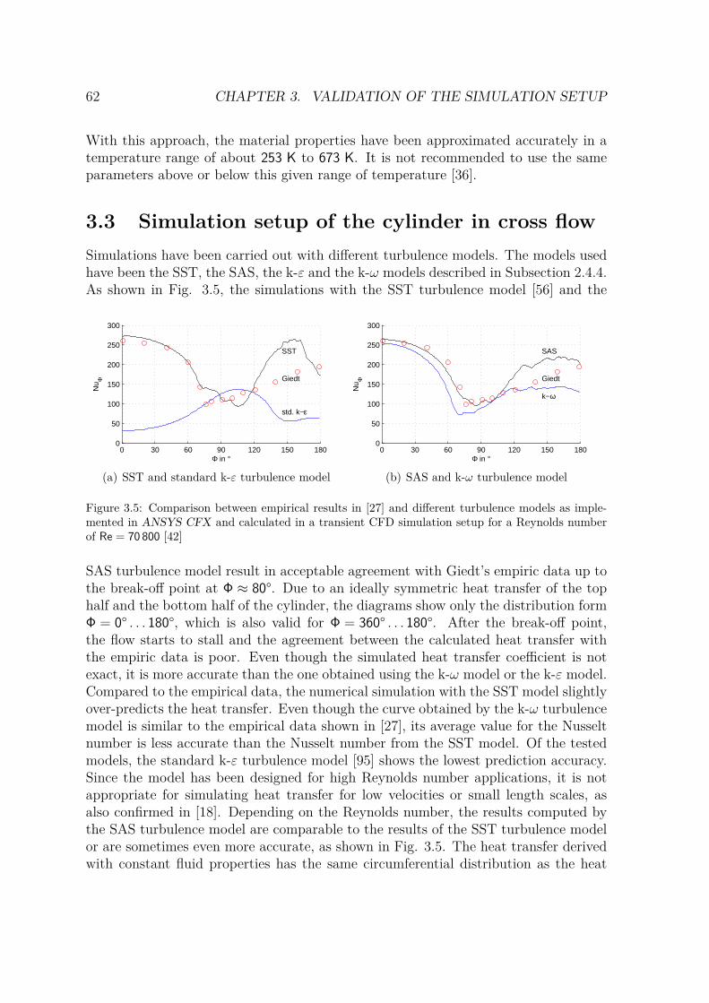
62 CHAPTER 3. VALIDATION OF THE SIMULATION SETUP
With this approach, the material properties have been approximated accurately in atemperature range of about 253 K to 673 K. It is not recommended to use the sameparameters above or below this given range of temperature [36].
3.3 Simulation setup of the cylinder in cross flowSimulations have been carried out with different turbulence models. The models usedhave been the SST, the SAS, the k-ε and the k-ω models described in Subsection 2.4.4.As shown in Fig. 3.5, the simulations with the SST turbulence model [56] and the
0 30 60 90 120 150 1800
50
100
150
200
250
300
SST
std. k−ε
Giedt
Φ in °
Nu Φ
(a) SST and standard k-ε turbulence model
0 30 60 90 120 150 1800
50
100
150
200
250
300
Φ in °
Nu Φ
k−ω
SAS
Giedt
(b) SAS and k-ω turbulence model
Figure 3.5: Comparison between empirical results in [27] and different turbulence models as imple-mented in ANSYS CFX and calculated in a transient CFD simulation setup for a Reynolds numberof Re = 70 800 [42]
SAS turbulence model result in acceptable agreement with Giedt’s empiric data up tothe break-off point at Φ ≈ 80°. Due to an ideally symmetric heat transfer of the tophalf and the bottom half of the cylinder, the diagrams show only the distribution formΦ = 0° . . . 180°, which is also valid for Φ = 360° . . . 180°. After the break-off point,the flow starts to stall and the agreement between the calculated heat transfer withthe empiric data is poor. Even though the simulated heat transfer coefficient is notexact, it is more accurate than the one obtained using the k-ω model or the k-ε model.Compared to the empirical data, the numerical simulation with the SST model slightlyover-predicts the heat transfer. Even though the curve obtained by the k-ω turbulencemodel is similar to the empirical data shown in [27], its average value for the Nusseltnumber is less accurate than the Nusselt number from the SST model. Of the testedmodels, the standard k-ε turbulence model [95] shows the lowest prediction accuracy.Since the model has been designed for high Reynolds number applications, it is notappropriate for simulating heat transfer for low velocities or small length scales, asalso confirmed in [18]. Depending on the Reynolds number, the results computed bythe SAS turbulence model are comparable to the results of the SST turbulence modelor are sometimes even more accurate, as shown in Fig. 3.5. The heat transfer derivedwith constant fluid properties has the same circumferential distribution as the heat

3.3. SIMULATION SETUP OF THE CYLINDER IN CROSS FLOW 63
transfer derived with temperature-dependent fluid properties. However, the absolutevalues do not match the empirical data [42]. Since the SAS turbulence model can onlybe solved in transient simulations, the computational effort is much higher than forthe SST turbulence model, which can be used in steady state simulations. Therefore,the SST turbulence model and steady state simulation setup have been chosen for thefollowing investigations.
In order to test the configuration parameters for different Reynolds numbers, moretest cases have been examined. The calculated and the simulated results including theused operating parameters of the different test cases are presented in Tab. 3.2. In thesame table, the average values for NuD1, NuD2 and NuD3 which have been calculatedwith (3.1), (3.2) and (3.3), are compared to the average Nusselt numbers of the datain Fig. 3.2 and Fig. 3.3.
The validation of the simulation setup in the present work has been carried outon three different geometries. The measurement setups described in Subsection 3.1.1have been modeled using CFD for cylinders with diameters D = 102 mm as used by [27]and D = 50 mm as well as D = 100 mm as used by [77]. The wire-frame of one usedgeometry is shown in Fig. 3.6, including the streamlines from the model inlet to themodel outlet.
ab
c
d
d
ee
Figure 3.6: Geometry wire-frame and streamlines with (a) the model inlet, (b) the cylinder, (c) themodel outlet, (d) the model outflow region and (e) the periodical sectional planes.
The mesh next to the surface of the cylinder has been created with specific prop-erties to achieve a dimensionless wall distance of y+ ≈ 1 (see (2.155)) for the highestReynolds number used with this model. The value of y+ must be considered duringthe meshing procedure and defines the initial height y0 of the cells next to the wallcalculated with (2.175). These initial cells have been modeled as a prism layer followedby at least 20 further prism layers with a cell height growth rate of 20% [38]. This
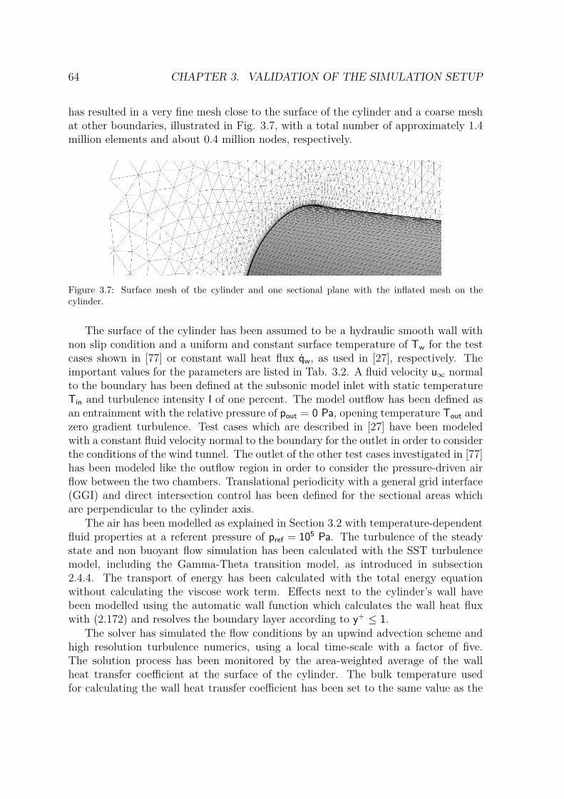
64 CHAPTER 3. VALIDATION OF THE SIMULATION SETUP
has resulted in a very fine mesh close to the surface of the cylinder and a coarse meshat other boundaries, illustrated in Fig. 3.7, with a total number of approximately 1.4million elements and about 0.4 million nodes, respectively.
Figure 3.7: Surface mesh of the cylinder and one sectional plane with the inflated mesh on thecylinder.
The surface of the cylinder has been assumed to be a hydraulic smooth wall withnon slip condition and a uniform and constant surface temperature of Tw for the testcases shown in [77] or constant wall heat flux qw, as used in [27], respectively. Theimportant values for the parameters are listed in Tab. 3.2. A fluid velocity u∞ normalto the boundary has been defined at the subsonic model inlet with static temperatureTin and turbulence intensity I of one percent. The model outflow has been defined asan entrainment with the relative pressure of pout = 0 Pa, opening temperature Tout andzero gradient turbulence. Test cases which are described in [27] have been modeledwith a constant fluid velocity normal to the boundary for the outlet in order to considerthe conditions of the wind tunnel. The outlet of the other test cases investigated in [77]has been modeled like the outflow region in order to consider the pressure-driven airflow between the two chambers. Translational periodicity with a general grid interface(GGI) and direct intersection control has been defined for the sectional areas whichare perpendicular to the cylinder axis.
The air has been modelled as explained in Section 3.2 with temperature-dependentfluid properties at a referent pressure of pref = 105 Pa. The turbulence of the steadystate and non buoyant flow simulation has been calculated with the SST turbulencemodel, including the Gamma-Theta transition model, as introduced in subsection2.4.4. The transport of energy has been calculated with the total energy equationwithout calculating the viscose work term. Effects next to the cylinder’s wall havebeen modelled using the automatic wall function which calculates the wall heat fluxwith (2.172) and resolves the boundary layer according to y+ ≤ 1.
The solver has simulated the flow conditions by an upwind advection scheme andhigh resolution turbulence numerics, using a local time-scale with a factor of five.The solution process has been monitored by the area-weighted average of the wallheat transfer coefficient at the surface of the cylinder. The bulk temperature usedfor calculating the wall heat transfer coefficient has been set to the same value as the

3.4. COMPARISON OF SIMULATION RESULTS WITH EMPIRICAL RESULTS65
D Re Nuavg αavg Tin Tw qw u∞ NuD1 NuD2 NuD3 NuCFDmm W
m2K °C °C Wm2
ms (3.1) (3.2) (3.3)
102 70800 179.3 44.78 12 211 10.15 171.6 181.9 186.1 205.7102 101300 236.6 59.08 12 211 14.53 217.4 224.1 230.8 268.1102 140000 360.4 90.00 12 211 20.08 280.2 340.5102 170000 442.8 110.57 12 211 24.38 314.8 393.8102 186000 479.6 119.76 12 211 26.67 332.3 422.4102 219000 515.0 128.59 12 211 31.41 366.4 479.9050 8290 51.4 24.79 24 100 3.22 48.3 50.9 51.5 61.6050 21200 93.1 44.85 24 100 8.23 82.0 86.9 90.4 124.2050 33920 123.9 59.72 24 100 13.16 108.3 113.8 119.9 168.7050 52800 171.5 82.64 24 100 20.49 142.2 147.0 156.3 225.5100 15550 74.8 18.03 24 100 3.02 68.6 72.7 75.1 94.9100 39800 140.7 33.91 24 100 7.72 119.3 124.8 132.0 190.1100 64450 192.4 46.38 24 100 12.50 161.4 165.1 176.2 261.4100 101300 265.3 63.94 24 100 19.65 217.2 214.8 231.1 353.3100 170000 377.3 90.94 24 100 32.98 315.3 498.0250 39200 119.7 11.54 24 100 3.04 118.2 123.8 130.8250 102000 233.5 22.51 24 100 7.92 218.2 215.7 232.1250 257600 471.8 45.49 24 100 19.99 411.1250 426000 717.9 69.21 24 100 33.06 584.7
Table 3.2: Parameters according to the investigated Reynolds numbers in [27] and [77] compared tothe results of empirical equations of [93,94] and [97]
ambient temperature T∞.
3.4 Comparison of simulation results with empiri-cal results
The values of the empirical results discussed in Section 3.1 depend on various pa-rameters of the investigation setup. As described in [27] and [77], the actual setupconditions have been compared to the different approaches of (3.1), (3.2) and (3.3), asshown in Fig. 3.8.
In [27], a wind tunnel brings the fluid in motion and the cylinder is heated elec-trically, assuring a constant heat flux qw and varying wall temperature Tw at thecylinder’s surface. The investigation of [77], on the other hand, uses a pressure drivenfluid flow and a constant wall temperature Tw of the cylinder with a varying heat fluxqw. The fluid properties of air required for the calculation of the air velocities from theReynolds numbers and for the definition of the Nusselt numbers are available in [77],but they match only partially the fluid properties used in [88]. Compared to [88],the kinematic viscosity of ν = 1.94 · 10−5 corresponds to an average film tempera-ture of T = 61.7°C which is the arithmetic average of fluid and wall temperature, butthe thermal conductivity of λ = 0.0241 W/m2K would correspond to a temperature ofT = −3.4°C. An accurate value for thermal conductivity is required for the calculation
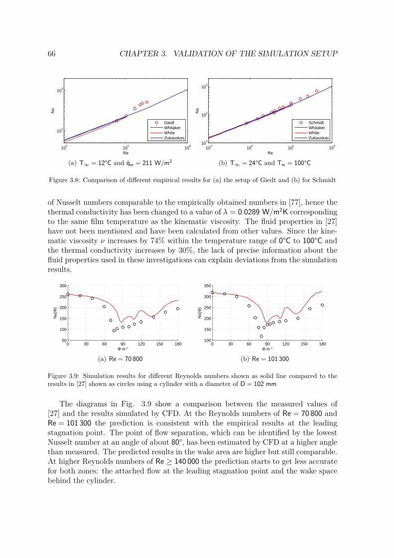
66 CHAPTER 3. VALIDATION OF THE SIMULATION SETUP
104
105
106
102
103
Re
Nu
GiedtWhitakerWhiteZukauskas
(a) T∞ = 12°C and qw = 211 W/m2
103
104
105
106
101
102
103
Re
Nu
SchmidtWhitakerWhiteZukauskas
(b) T∞ = 24°C and Tw = 100°C
Figure 3.8: Comparison of different empirical results for (a) the setup of Giedt and (b) for Schmidt
of Nusselt numbers comparable to the empirically obtained numbers in [77], hence thethermal conductivity has been changed to a value of λ = 0.0289 W/m2K correspondingto the same film temperature as the kinematic viscosity. The fluid properties in [27]have not been mentioned and have been calculated from other values. Since the kine-matic viscosity ν increases by 74% within the temperature range of 0°C to 100°C andthe thermal conductivity increases by 30%, the lack of precise information about thefluid properties used in these investigations can explain deviations from the simulationresults.
0 30 60 90 120 150 18050
100
150
200
250
300
Φ in °
Nu(
Φ)
(a) Re = 70 800
0 30 60 90 120 150 180100
150
200
250
300
350
Φ in °
Nu(
Φ)
(b) Re = 101 300
Figure 3.9: Simulation results for different Reynolds numbers shown as solid line compared to theresults in [27] shown as circles using a cylinder with a diameter of D = 102 mm
The diagrams in Fig. 3.9 show a comparison between the measured values of[27] and the results simulated by CFD. At the Reynolds numbers of Re = 70 800 andRe = 101 300 the prediction is consistent with the empirical results at the leadingstagnation point. The point of flow separation, which can be identified by the lowestNusselt number at an angle of about 80°, has been estimated by CFD at a higher anglethan measured. The predicted results in the wake area are higher but still comparable.At higher Reynolds numbers of Re ≥ 140 000 the prediction starts to get less accuratefor both zones: the attached flow at the leading stagnation point and the wake spacebehind the cylinder.

3.4. COMPARISON OF SIMULATION RESULTS WITH EMPIRICAL RESULTS67
0 30 60 90 120 150 180200
250
300
350
400
450
Φ in °
Nu(
Φ)
(a) Re = 140 000
0 30 60 90 120 150 180200
300
400
500
600
700
Φ in °
Nu(
Φ)
(b) Re = 170 000
Figure 3.10: Simulation results for different Reynolds numbers shown as solid line compared to theresults in [27] shown as circles using a cylinder with a diameter of D = 102 mm
0 30 60 90 120 150 180200
300
400
500
600
700
Φ in °
Nu(
Φ)
(a) Re = 186 000
0 30 60 90 120 150 180300
400
500
600
700
800
Φ in °
Nu(
Φ)
(b) Re = 219 000
Figure 3.11: Simulation results for different Reynolds numbers shown as solid line compared to theresults in [27] shown as circles using a cylinder with a diameter of D = 102 mm
Compared to the investigations of [77], the prediction with CFD shows good agree-ment at very low Reynolds numbers as shown in Fig. 3.12. The difference between themeasured and the simulated results at the leading stagnation point can be explainedwith incomplete or incorrect information about the used fluid parameters in [77]. Eventhe angle where flow separation occurs matches the measured results and the Nusseltnumber is predicted with an accurate magnitude. In the wake area, the values becomeless consistent with the empirical data with an over-prediction of magnitude.
At higher Reynolds numbers, the consistency between simulated and measured val-ues of the point of flow separation deteriorates. The simulation tends to estimate theseparation point about 10° behind the measured point but the magnitude of heat trans-fer at this point is estimated with good accuracy even for higher Reynolds numbers.Regarding the mean heat transfer in the downstream area of fluid flow, the relativeerror of simulated and measured results is smaller for higher Reynolds numbers asshown in Fig. 3.13 than it is for lower Reynolds numbers as shown in 3.12.
Since the characteristic length is not as obvious for the end-windings of an electricalmachine as it is for a cylinder, a single Reynolds number for a certain rotational speedcan hardly be specified. Basically, two different flow conditions can be identified atthe end-windings of the investigated type of motor, where a Reynolds number can be

68 CHAPTER 3. VALIDATION OF THE SIMULATION SETUP
0 30 60 90 120 150 1800
20
40
60
80
100
Φ in °
Nu(
Φ)
(a) Re = 8 290
0 30 60 90 120 150 1800
50
100
150
200
Φ in °
Nu(
Φ)
(b) Re = 21 200
Figure 3.12: Simulation results for different Reynolds numbers shown as solid line compared to theresults in [77] shown as circles using a cylinder with a diameter of D = 50 mm
0 30 60 90 120 150 1800
50
100
150
200
250
Φ in °
Nu(
Φ)
(a) Re = 33 900
0 30 60 90 120 150 18050
100
150
200
250
300
350
Φ in °
Nu(
Φ)
(b) Re = 52 800
Figure 3.13: Simulation results for different Reynolds numbers shown as solid line compared to theresults in [77] shown as circles using a cylinder with a diameter of D = 50 mm
defined theoretically by comparing the flow conditions with a flow parallel to a plate.On the one hand, the angular speed of the rotor is causing a high velocity of air nextto the end-windings. In this azimuthal direction, the width of the conductors can bechosen as characteristic length. On the other hand, the air coming from the coolingducts flows in axial direction over the end-windings. In this case, the overhang of theend-windings is a proper characteristic length. Considering these two flow conditionsindependently, the maximum Reynolds number will not exceed the value of Re = 105.

3.4. COMPARISON OF SIMULATION RESULTS WITH EMPIRICAL RESULTS69
0 30 60 90 120 150 18020
40
60
80
100
120
140
Φ in °
Nu(
Φ)
(a) Re = 15 550
0 30 60 90 120 150 18050
100
150
200
250
300
Φ in °
Nu(
Φ)
(b) Re = 39 800
Figure 3.14: Simulation results for different Reynolds numbers shown as solid line compared to theresults in [77] shown as circles using a cylinder with a diameter of D = 100 mm
0 30 60 90 120 150 1800
100
200
300
400
Φ in °
Nu(
Φ)
(a) Re = 64 450
0 30 60 90 120 150 180100
200
300
400
500
600
Φ in °
Nu(
Φ)
(b) Re = 101 300
0 30 60 90 120 150 1800
200
400
600
800
Φ in °
Nu(
Φ)
(c) Re = 170 000
Figure 3.15: Simulation results for different Reynolds numbers shown as solid line compared to theresults in [77] shown as circles using a cylinder with a diameter of D = 100 mm

70 CHAPTER 3. VALIDATION OF THE SIMULATION SETUP
3.5 Global-local domain decomposition methodAs shown in the previous section, the calculation of the wall heat transfer requiresa very fine resolution of the mesh close to the surface. Due to the large surfacearea, a properly resolved mesh of the whole end region of the investigated inductionmotor would contain about 12 million finite volume cells which might exceed thecomputational possibilities. In order to adopt the convective heat transfer problem tothe computational resources, a method is required which can simulate the heat transferproblem piece by piece. This leads to the idea of the global-local domain decompositionmethod, allowing simulation of fluid flow on a coarse mesh and simulation of the wallheat transfer coefficient on a fine mesh but only at specific locations. In order to testits validity, the heat transfer coefficient of the same cylindrical geometry has beencalculated as in Section 3.3 by using the global-local domain decomposition method.Both the global and the local models are shown in Fig. 3.16. The global model on the
(a) Global model with boundary mesh of local model (b) Local model
Figure 3.16: (a) Streamline, cylinder and boundary area from local model in the global model and(b) cylinder in the local model
left hand side shows streamlines starting from the model inlet (left), the surface meshof the back sectional plane, the cylinder and the location of the boundary mesh fromthe local model. On the right hand side of Fig. 3.16, the local model is shown withthe shaded boundary interface and the surface meshes of the back sectional plane andthe cylinder.
The boundary conditions for the fine local mesh are taken from the flow simulationon the coarse global mesh by transferring the velocity components for all Cartesiancoordinates u, v,w, the temperature T, the turbulence kinetic energy k and the tur-bulence eddy dissipation ε from the coarse mesh to the boundary of the fine mesh.Once a solution for the coarse mesh is available, the boundary node coordinates of thefine mesh can be used for a user defined area to export the velocity, temperature andturbulence variables to boundary condition profiles, as shown in Fig. 3.17.

3.5. GLOBAL-LOCAL DOMAIN DECOMPOSITION METHOD 71
(a) Velocities u, v,w (b) Temperature T
(c) Turbulence kinetic energy k (d) Turbulence eddy dissipation ε
Figure 3.17: Boundary conditions transfer from the global to the local model for a Reynolds numberof Re = 15 550
The local model has been solved with the configuration described in Section 3.3.Due to the fine mesh resolution but small total size of the local mesh, the convectivewall heat transfer coefficient can be simulated with acceptable accuracy in a reasonableperiod of time. The results of simulated wall heat transfer coefficients are shown inFig. 3.18 and Fig. 3.19, respectively.
The diagrams shown in Fig. 3.19 compare the results of the domain decompositionmethod with the results from the simulation in 3.4 and the empirical results. Anoticeable detail is the higher wall heat transfer coefficient between the angles ofΦ = 20° and Φ = 70°. Nevertheless, the results of the domain decomposition methodin the wake area reproduce the empirical results with higher accuracy than withoutdomain decomposition. Especially at low Reynolds numbers, this method generatesgood results with small errors, as shown in Fig. 3.19 (a).

72 CHAPTER 3. VALIDATION OF THE SIMULATION SETUP
Figure 3.18: Simulated wall heat transfer coefficient at the cylindric surface of the local model withReynolds number of Re = 15 550
0 30 60 90 120 150 1800
50
100
150
Φ in °
Nu(
Φ)
(a) Re = 15 550
0 30 60 90 120 150 1800
50
100
150
200
250
300
Φ in °
Nu(
Φ)
(b) Re = 38 900
0 30 60 90 120 150 1800
100
200
300
400
Φ in °
Nu(
Φ)
(c) Re = 64 450
0 30 60 90 120 150 1800
100
200
300
400
500
600
Φ in °
Nu(
Φ)
(d) Re = 101 300
Figure 3.19: Results of global-local domain decomposition calculation for different values of theReynolds number (solid lines), results calculated without domain decomposition (dashed lines) andempirical results as published in [77] (circles)

Chapter 4
Measurements at the end-region
Despite the opportunities presented in the previous chapters, a totally reliable modelfor predicting the convective heat transfer coefficient is not available yet. It is stillnecessary to validate the derived values under certain operating conditions by mea-surements. On the one hand, the results of this chapter are required for specifyingaccurate operation parameters for the simulations. On the other hand, the measuredheat transfer values are necessary for the validation of numerical results. Since theinvestigated fluid flow is inside the closed cooling cycle of an induction machine, theoperation parameters for the simulation such as mass flow or temperature cannot beobtained easily. By measuring the static pressure inside one cooling duct of the induc-tion machine, the air velocity inside this cooling duct has been identified for differentrotational speeds of the motor. For these different operational conditions, the wallheat fluxes at several positions on the end-windings have been measured to obtainpoints of comparison for the simulations presented in Chapter 5.
4.1 Investigated motorThe measurements have been carried out on an induction motor designed to be used asa traction motor in a tramway, as sketched in Fig. 4.1. The motor with a rated powerof 120 kW at a rated speed of 2290 rpm has been designed to work in the whole rangeof rotational speeds up to 4230 rpm in both rotational directions. The cooling type ofthe machine is a so called double air cooled system (DACS) or IC 5A1A1, respectively,as presented in Subsection 2.1.4. The cooling of the machine under investigation isbased on an inner air-circuit consisting of cooling ducts which pass through the rotoras well as the stator and driven by an axis-mounted fan. This is a closed circuit andthus protects the rotor and the stator end-region from contaminating dust. By meansof this circuit, the rotor losses and the losses in the end-winding region of the machineare transferred to the stator yoke. Another axis-mounted fan discharges air through aset of cooling ducts which are located radially outward of the inner-circuit ducts. Theair flow of this path is loaded with the iron losses and copper losses of the stator and
73

74 CHAPTER 4. MEASUREMENTS AT THE END-REGION
a
bd
ef
g j
l
m
DE NDE
c
h
ki
n
f
n
l
i
ab
A
A
j
Figure 4.1: Longitudinal section (A-A) and cross section of the investigated DACS motor with (a)stator iron, (b) rotor iron, (c) path of inner cooling circuit, (d) fan of the inner cooling circuit, (e)end-windings of the motors drive end, (f) cooling ducts of the inner cooling circuit in the stator, (g,h)end-windings of the motors non drive end, (i) cooling ducts of the inner cooling circuit in the rotor,(j) waste grease drain, (k) fan of the outer cooling circuit, (l) stator cooling ducts of outer coolingcircuit in the stator, (m) path of outer cooling circuit and (n) separation between inner and outercooling circuit
the losses handed over from the inner circuit. This is an open cooling circuit whichreleases the heated air to the environment. In this investigation, only the inner coolingcircuit on the non drive end side (NDE) has been examined. The separation betweenthe inner and the outer cooling cycle is indicated by a dashed line on the right handside of Fig. 4.1. Due to the asymmetric shape of the end-shield, differences in theheat flux of different conductors can be expected. The heat flux has been measured oneight different conductors of the end-windings with four pairs of heat flux sensors, eachpair mounted at identical positions on different conductors. Two of these positions arelabeled (g) and (h) in Fig. 4.1. The waste grease drain which causes the asymmetryof the end-shield is labeled (i) [36,41,42].
4.2 Determining the air mass flow in the machine
It is necessary to know the air mass flow m in the cooling duct, in order to use itas operation parameters in the simulation of the heat transfer values, presented inChapter 5. By measuring the loss of static pressure in the cooling ducts, the velocityand hence the air mass flow can be calculated. Since the cooling ducts of the presentmachine are parts of the laminated stator and rotor iron, a specific roughness exists attheir surfaces. Therefore the ducts cannot be considered as hydraulically smooth andtheir roughness has to be taken into account in the calculation of the air mass flow m.

4.2. DETERMINING THE AIR MASS FLOW IN THE MACHINE 75
4.2.1 Determining the duct roughnessDue to the lamination of the stator sheets, the surfaces of the inner and outer coolingducts have the same absolute roughness ks in m [88]. The roughness has been deter-mined by measuring the pressure loss along one outer cooling duct and the total airmass flow mto of the outer cooling circuit. Uniform flow conditions in all cooling ductsof the same size of the outer cooling circuit have been assumed and manufacturing tol-erances have been neglected. The used measuring setup is shown in Fig. 4.2. It allowsthe measurement of the total air mass flow of the outer cooling circuit. The ambient
Figure 4.2: Setup for measuring the total air mass flow mo of the outer cooling circuit with (a) theair inlet, (b) four pressure probes at the narrowest position of the cone, connected by a ring-likepipe, (c) the air inlet, (e) the investigated traction motor and (d) the pressure transducer, whichhas been connected to an analog digital converter. The measurements have been carried out atTraktionssysteme Austria GmbH
temperature and ambient pressure have remained constant during the measurementsat values of Ta = 28°C and pa = 95 600 Pa respecitvely. Using the ideal gas law
ρ = p
Rs · T, (4.1)
the density ρ = 1.106 kg/m3 has been calculated with the ideal gas constant for air Rs =287.12 J/kgK and the prevailing temperature. The kinematic viscosity ν = 1.608 · 10−5
m2/s has been obtained for the specific temperature by interpolating listed values fordry air in [88].
The outer cooling circuit consists of two different types of cooling ducts with di-ameters doA and doB, total numbers noA and noB and cross sectional areas AoA andAoB, respectively1. Since the measurements have been taken at a cooling duct with
1Since most calculation steps have to be accomplished for both types of ducts, the index of thevariables has been changed to ox for these steps, to represent oA or oB.

76 CHAPTER 4. MEASUREMENTS AT THE END-REGION
diameter doA, the iterative calculation of the roughness is based on cooling ducts oftype A. The initial value for the air mass flow mox and hence the velocity vox in thecooling ducts have been determined by the total air mass flow mto, density ρ and thetotal sum of cross sectional areas of all cooling ducts.
v(0)ox = mto
ρ(noAAoA + noBAoB) . (4.2)
The iterative solution of the roughness starts with the calculation of the Reynoldsnumbers Re(i)
ox for both types of cooling ducts with (2.65) for all rotational speedsusing the hydraulic diameters dox and velocities vox as parameters. Since the pressurelosses have been measured between positions along the cooling duct, the pressure losscoefficients for the inlet and the outlet can be disregarded. Without these additionallosses at the inlet and the outlet the pressure losses in these cooling ducts can bedescribed by the Darcy-Weissbach equation [14]
∆po = λfol
do
ρ
2v2
o , (4.3)
with the pipe length l between the considered positions for the pressure difference∆po and the Darcy friction factor of the pipe-flow λfox. The friction factor has beencalculated by re-arranging (4.3):
λ(i)fox = 2 ∆po dox
l ρ(
v(i)ox
)2 (4.4)
and hence the roughness ks has been solved by the re-arranged Colebrook and Whiteequation [88] with the values for the cooling circuit of type A
k(i)s = doA
2
10γ − 18.574
Re(i)oA
√λ
(i)foA
with γ = 0.5
1.7384− 1√λ
(i)foA
. (4.5)
Since the roughness and the friction factor of a cooling duct do not change with theoperational conditions, the mean values for the various operational conditions k(i)
s andλ
(i)foA have been used for iteratively re-calculating the friction factor with the Colebrook
and White equation:
1√λ
(j+1)fox
= 1.7384− 2 log
2 k(i)s
dox+ 18.574
Re(i)ox
√λ
(j)fox
. (4.6)
The new velocity for the type B cooling ducts has been calculated by
v(i)oB =
√√√√2 ∆po doB
l ρ λ(i)foB
, (4.7)

4.2. DETERMINING THE AIR MASS FLOW IN THE MACHINE 77
and the velocity of the type A cooling ducts by subtracting the air mass flow in thetype B ducts from the total air mass flow mto
v(i)oA = mto/ρ− noB AoB v
(i)oB
noA AoA. (4.8)
Using these new velocities, the next iteration step can be derived by re-starting withthe calculation of the Reynolds numbers and the friction factor in (4.4).
The roughness has been calculated using the pressure probe values between the firstand the fourth, the second and the fourth and the first and third positions. Accordingto the positions, the values of the lengths have been changed to l = 0.112 m (for II-IVand I-III) and l = 0.168 m (for I-IV), respectively. The obtained average value of the
I-IV II-IV I-IIIf voB voA ReoA ∆p λfoA ks ∆p λfoA ks ∆p λfoA ksHz m/s m/s Pa 10−2 mm Pa 10−2 mm Pa 10−2 mm mm50 13.5 15.6 25357 37 4.32 0.333 21 3.68 0.188 25 4.38 0.34760 16.4 19.1 31176 54 4.17 0.305 30 3.48 0.159 35 4.06 0.27870 19.4 22.6 36903 75 4.14 0.302 44 3.64 0.196 49 4.05 0.28380 21.7 25.8 42121 94 3.98 0.271 52 3.30 0.139 62 3.94 0.26290 24.5 29.0 47251 119 4.00 0.279 68 3.43 0.165 79 3.99 0.275100 27.3 32.0 52084 147 4.07 0.297 83 3.45 0.170 97 4.03 0.287110 30.2 34.4 56151 180 4.29 0.349 102 3.64 0.209 122 4.36 0.367ks in mm 0.305 0.175 0.300 0.260
Table 4.1: Calculation of the average roughness of cooling ducts
cooling duct roughness ks is the arithmetic mean value of all derived values in Tab.4.1. Since, for the calculation of the air mass flow, the inner and the outer coolingducts have been assumed to be uniform, the average roughness can be used for thecooling ducts of the inner and the outer cooling cycle [42].
4.2.2 Air mass flow in the inner cooling cycleThe parts of the inner cooling circuit are encapsulated by the end-shields and cannot beaccessed during the operation of the machine. A particular construction is necessaryin order to obtain values which characterize the air mass flow in the inner coolingcircuit. This construction is sketched in Fig. 4.3.
Four holes have been drilled at equidistant positions along one cooling duct labeled(f) in Fig. 4.1. Other cooling ducts of the inner cooling cycle and the same type, atdifferent circumferential positions, are not accessible during operation of the machine.Beside the holes offering access to the cooling duct, two holes have been drilled ineach end-shield. Pressure probe pipes have been placed in these drill holes, in orderto measure the static pressure in the positions shown in Fig. 4.3. The pressures havebeen measured at certain rotational speeds of the motor, with a fully signal-conditionedpressure transducer measuring in the range of ±500 Pa with non-linear properties and

78 CHAPTER 4. MEASUREMENTS AT THE END-REGION
p1 p4p3p2pDE pNDE
NDEDEm.
Figure 4.3: Longitudinal section of a cooling duct with attached pressure probes. The air mass flowm inside the duct can be derived by the measured pressure loss ∆p = p1 − p4
hysteresis of 0.1%. By electronically collecting more than 100 pressure values withina time period of about 10 seconds, a mean value of the relative pressure betweenthe pressure probes shown in Tab. 4.2 has been estimated for further calculations.As shown in Fig. 4.4, the loss of static pressure inside the cooling ducts changeslinearily in relation to the position along the length of the ducts even for turbulentflow conditions, allowing extrapolation of the static pressure at the inlet of the coolingduct.
0 0.05 0.1 0.15 0.2 0.25 0.3 0.35−5
0
5
10
15
20
25
30
35
40
pin
=8.141 Pa
f=50 Hz
pin
=15.89 Pa
f=70 Hz
pin
=24.26 Pa
f=90 Hz
pin
=35.66 Pa
f=110 Hz
l in m
p stat
in P
a
Measured pressuresApproximationExtrapolated pressures
Figure 4.4: Loss of static pressure along the cooling ducts for different frequencies f of supply currentand corresponding rotational speeds.
For the calculation of the air mass flow in the inner circuit, it is necessary to deter-mine the pressure loss ∆pi = pi1 − pi4 inside the cooling duct, as well as the diameterdi of the cooling duct, the distance l between the pressure probes of pi1 and pi4, thekinematic viscosity ν of air at fluid temperature Tf and the roughness ks of the innersurface of the cooling duct. With an initial estimation of the velocity v(0)
i in the coolingduct, the air mass flow has been calculated by an iterative refinement of the velocity

4.3. HEAT FLUX MEASUREMENT 79
v(k)i . One iteration step k consists of the calculation of the Darcy friction factor
λ(k)fi = 2 ∆pi dki
lρ(
v(k)i
)2 , (4.9)
the Reynolds number
Re(k)i = v
(k)i dki
ν, (4.10)
the Darcy friction factor λ(k+1)fi by the Colebrook-White equation
1
λ(k+1)fi
=1.7384− 2 log
2 ks
dki+ 18.574
Re(k)i
√λ
(k)fi
2
(4.11)
and the velocity inside the cooling ducts with
v(k+1)i =
√√√√ 2 ∆pi dki
λ(k+1)fi l ρ
. (4.12)
Once the change of the friction factor between two consecutive iterations is below atolerance (this usually occurs in less than ten iterations), the air mass flow in onecooling duct of the inner cooling cycle mi can be calculated by
mi = vi ρ Ai , (4.13)
where ρ is the density of air at a certain temperature and A is the cross-sectional areaof the cooling duct [42]. The results for air velocity and air mass flow in one coolingduct is listed in correspondence with the measured pressures in Tab. 4.2.
static pressure probes calculatedf Ta Tm pa pi1 pi2 pi3 pi4 pDE ρ Re v miHz °C °C hPa Pa Pa Pa Pa Pa kg/m3 m/s g/s50 29.0 76.3 945 1.35 2.72 4.57 6.10 24.27 0.942 3 159 4.13 0.78270 25.1 75.1 944 3.32 6.27 9.39 12.07 48.11 0.944 4 417 5.74 1.08990 28.1 70.5 956 5.75 9.63 14.55 18.69 80.00 0.969 5 503 6.98 1.360110 28.1 67.0 956 8.60 14.67 21.70 27.41 118.00 0.979 6 796 8.47 1.667
Table 4.2: Relative static pressure at different positions of the inner cooling cycles cooling ductcompared to the static pressure pNDE in the end-shield of the non drive end side including flowproperties at average temperature Tm = (Tf + Tw)/2.
4.3 Heat flux measurementThe heat flux density q from the end-windings to the surrounding air has been mea-sured using thermopiles as heat flux sensors at specific positions of eight end-windingconductors at the non drive end side of the motor.

80 CHAPTER 4. MEASUREMENTS AT THE END-REGION
Due to the size of the investigated motor, the end-windings offer some areas whereheat flux sensors can be applied. Depending on the type of sensor, it is either permittedto only slightly bend the sensor for application or it is recommended not to bend it atall. Therefore, the application surface has to offer a planar area where the sensor can beapplied which, in this case, has dimensions of 10× 30 mm or 5× 60 mm, respectively.A smaller sensor would be desirable, but due to the measuring principle, a certainsensor area is necessary to achieve a gaugeable signal. The heat flux sensors havebeen fixed to the surface with a special type of glue which withstands operationaltemperatures of up to 150°C [51].
Due to the asymmetry of the end-shield, the two heat flux sensors in each pairhave been placed at identical positions on different conductors as sketched in Fig. 4.1where measuring point HFS-5 is labeled (g) and measuring point HFS-6 is labeled (h).For an accurate calculation of the heat transfer coefficient α, the fluid temperatures Tf
Heat flux sensor
Pt100Pt100
Heat flux sensor
Figure 4.5: Measuring points HFS-5 and HFS-6 at opposite conductors of the end-windings
have been measured by Pt100 temperature sensors next to the surface of the heat fluxsensors. The wall temperatures Tw have been measured by separate thermocouplesinside the heat flux sensors shown in Fig. 4.5. Based on these measured values, theconvective heat transfer coefficient α can be derived as
α = q
Tw − Tf, (4.14)
if forced convection and homogeneous wall and fluid temperature can be assumed [33].
4.3.1 Heat flux sensorThe used heat flux sensors consist of a polymeric plate as a substrate with knownthickness h and thermal resistance Rth. As shown in Fig. 4.6, the top and bottomsides of this plate are covered by thermocouples individually connected through thesubstrate to a thermopile. The heat flux sensors shown in Fig. 4.5 and used in thisinvestigation utilize Type-T thermocouples for measurement. The sensitivity of theheat flux sensor depends on the number of thermocouples in the thermopile and thus

4.3. HEAT FLUX MEASUREMENT 81
∞
w
HFS
(a) Temperature profile (b) HFS principle
Figure 4.6: Schematic sketch of a heat flux sensor in cross-sectional view with free stream velocity u,free stream temperature T∞ (= Tf), wall temperature Tw, thermal resistance Rth, sensor thickness h,sensor output voltage U and heat flux q
the sensor area. In this investigation, sensors with areas of 100 mm2 and 250 mm2 andsensitivities of about KHFS = 0.6µV/(W/m2) and KHFS = 1.5µV/(W/m2), respectively,have been used. One separate Type-T thermocouple inside the heat flux sensors,which is not connected to the thermopile, is used to measure the surface temperatureTw. This value is necessary for the calculation of the convective wall heat transfercoefficient α from the measured heat flux q as in (4.14) [37].
4.3.2 Power supplyThe measurements have been completed for several different rotational velocities ofthe rotor, operated in no-load conditions. In order to achieve higher temperatures inthe end-region, the motor has been overexcited.
Since the used heat flux sensors generate a signal in the range of some millivoltsand are connected to the measuring amplifier by a two-wire circuit, they are sensitiveto induced interference voltages. In order to avoid such interferences, the operationhas been accomplished without an inverter for the power supply. As shown in Fig. 4.7,the operation power has been generated by a machine unit with Ward Leonard SpeedControl System, which is capable of generating three-phase sinusoidal voltage of up toUm = 630 V and a frequency up to f = 100 Hz. The induction motor on the left handside of Fig. 4.7 is connected to the public electric network. It mechanically drives aDC generator which, in turn, supplies a DC motor. A synchronous generator createsthe electric power for the investigated motor shown on the right hand side of Fig. 4.7.The frequency f has been changed by regulating the excitation of the DC motor, whilethe voltage Um has been controlled with the excitation of the synchronous generator.
Using a 30 channel data acquisition system, all signals for temperature and heatflux have been simultaneously measured, digitally converted and stored including atime stamp for each time step of 4 s. In order to collect approximately one hundred

82 CHAPTER 4. MEASUREMENTS AT THE END-REGION
M1n n M2 m
Figure 4.7: Schematic diagram of the power converting machine unit with Ward Leonard SpeedControl System
sets of data for each operating point of the machine, the voltage and frequency havebeen held constant for several minutes.
4.3.3 Thermal resistance of the sensor
As generally known, any sensor affects the measured physical value. In the presentcase, the heat flux density is measured by the temperature difference between thetop and bottom surface of the heat flux sensor, which means that the measured walltemperature deviates from the real wall temperature. This difference is necessary tomeasure the heat flux through the sensor, but it leads to an error in the calculation ofthe heat transfer coefficient.
The thermal resistance from the conductors surface to the environmental air con-sists of the thermal resistance of the insulation Rth I and the thermal resistance of theconvective heat transfer Rth C. Assuming that the used glue has approximately the samethermal conductivity as the conductors’ insulation (resin), the thermal resistance ofthe heat flux sensor Rth H will additionally affect a small portion of the conductors’ sur-face where the heat flux sensor is mounted. Therefore the overall thermal resistance ofthe conductor is Rth1 = Rth I + Rth C, and Rth2 = Rth I + Rth H + Rth C for the sensor area,respectively. As the heat transfer coefficient α increases, the thermal resistance ofconvection decreases. However, due to the rising heat flux density q, the influence ofthe thermal resistance of the heat flux sensor Rth H becomes ascending, resulting ingreater errors for higher heat transfer coefficients.
The surface area not covered by the heat flux sensor has been assumed to be fivetimes higher than the area of the heat flux sensor. A relative thermal resistance of theheat flux sensor has been specified by the manufacturer with rthH = 4 · 10−4 Km2/W.Assuming the thermal conductivity of the insulation is λI = 0.25 W/mK and its thick-ness is lI = 1 mm, one can calculate the total thermal resistance Rth wH with the heatflux sensor and Rth woH without the heat flux sensor with:
Rth = rth
A= l
A λ= 1
A α= ∆T
Pth(4.15)
The higher the value of the convective heat transfer coefficient α, the greater therelative error of the thermal resistance ERth = (RthwH − RthwoH)/RthwoH, as shown inTab. 4.3.

4.3. HEAT FLUX MEASUREMENT 83
α Rth C1 Rth C2 Rth wH Rth woH ERthW/m2K K/W K/W K/W K/W %
10 200 1000 173.44 173.33 0.064200 10 50 15.11 15.00 0.714
Table 4.3: Example of the relative error of thermal resistance at high and low values of the heattransfer coefficient
4.3.4 Sensor positions
Duct No1
Duct No4
Duct No28Duct No30
No58 & 59No2
No8
Figure 4.8: Front view at the end-windings with numbering order of cooling ducts and conductors
In order to identify the positions of the sensors, the conductors have been numberedfrom No1 to No60 and the cooling ducts from No1 to No30, respecively. Looking axiallyat the end-windings, the numbering of the cooling ducts starts next to the top positioncounting clockwise, as shown in Fig. 4.8. The conductors are numbered in the sameway as the cooling ducts and according to the stator slots starting next to the statorslot at the top position.
Four pairs of heat flux sensors have been applied to the end-windings. The twoheat flux sensors in each pair have been fixed at identical positions on two differentconductors as shown in Fig. 4.9 to Fig. 4.12. Each of these figures show one pair ofheat flux sensors applied to identical positions for all four positions HFS-A to HFS-D, as shown in the next chapter in Fig. 5.5. In order to obtain reliable informationabout the air-temperatures next to the sensors, they have been measured by Pt100sensors positioned next to the heat flux sensors as shown in 4.5. The sensors HFS-5and HFS-6 have been applied to the tips of the end-windings by adapter plates madeof copper to accomplish a more homogeneous distribution of wall temperature and toprovide flat surfaces for sensor application. Measurements at the opposite side of theend-windings’ tips have been taken by the sensors HFS-9 and HFS-10 directly gluedto the conductors’ insulation. At the position on the end-windings conductors close tothe rotors end-ring, high values of heat transfer have been expected. In this positionthe sensors HFS-11 and HFS-12 have been glued to the conductors with thermallyconducting tape. Measurements at the position of the conductors which are close tothe outlets of the cooling ducts have been taken by the sensors HFS-13 and HFS-14. The temperature of the fluid entering the end-region has been measured by two

84 CHAPTER 4. MEASUREMENTS AT THE END-REGION
(a) HFS-5 at conductor No58 (b) HFS-6 at conductor No27
Figure 4.9: Heat flux sensors applied at position HFS-A on the end-windings
(a) HFS-9 at conductor No59 (b) HFS-10 at conductor No45
Figure 4.10: Heat flux sensors applied at position HFS-B on the end-windings
separate Pt100 sensors at the outlets of cooling ducts No4 and No28, as shown inFig. 4.13. A complete wiring list of the used measurement amplifier can be found inAppendix C.1.
4.3.5 Measured heat fluxIn Fig. 4.14 to Fig. 4.17, the values measured by all heat flux sensors are shown asboxplots, depending on the frequency of the power supply and the respective rotational

4.3. HEAT FLUX MEASUREMENT 85
(a) HFS-11 at conductor No22 (b) HFS-12 at conductor No11
Figure 4.11: Heat flux sensors applied at position HFS-C on the end-windings
(a) HFS-13 at conductor No2 (b) HFS-14 at conductor No8
Figure 4.12: Heat flux sensors applied at position HFS-D on the end-windings
speed. The upper and lower levels of the boxes are calculated with the upper and lowerquartile of the measured values. One quartile contains a quarter of measured valuesabove or below the median for one specific operation point. The horizontal line inthe box is the value of the median from the data recorded at the specific operationpoint. The whiskers above and below the box show the value range of the rest of thedata with the maximum range of the inter-quartile length. Outliners which are outsidethe inter-quartile range above or below the box are shown as crosses. The ordinatesof the diagrams have been limited to a minimum wall heat transfer coefficient ofαmin = 0 W/m2K and a maximum value of αmax = 450 W/m2K, since negative valuesor coefficients above this range are assumed to be non-physical.
As shown in the figures, the values measured are wide spread at many operation

86 CHAPTER 4. MEASUREMENTS AT THE END-REGION
(a) Duct No28 (b) Duct No4
Figure 4.13: Pt100 sensors measuring the air-temperature at the outlets of two cooling ducts of theinner cooling cycle
points. This measuring error can be explained with the following reasons. As men-tioned above, the heat flux sensors gain a signal caused by the heat flux in the rangeof some millivolts and are glued directly to the conductor, separated only by a thinlayer of insulation. Each heat flux sensor and temperature sensor is connected to themeasuring equipment by an unshielded two-wire circuit. The temperature gradient be-tween conductor and fluid is small, especially at higher revolution speeds with higherair mass flow and hence better cooling of the conductors. This small gradient causes asmall signal of the heat flux sensor and increases the relative error of the temperaturedifference measurements, since the values of wall and fluid temperature are close. Inthis case, effects mentioned in Subsection 2.2.4 cause an unphysical behavior of thewall heat transfer coefficient. Due to the asymmetric (non rotation-symmetric) shapeof the end-shield, as well as to the difference in the number of stator ducts and slots,the measured values of the pairs of heat flux sensors at identical measuring pointsdiffer from each other, as shown in some diagrams in Fig. 4.14 to Fig. 4.17.

4.3. HEAT FLUX MEASUREMENT 87
0
10
20
30
40
50
60
70
10 20 30 40 50 60 70 80 90 100f in Hz
α in
W/m
2 K
(a) HFS-5
0
5
10
15
20
25
30
35
10 20 30 40 50 60 70 80 90 100f in Hz
α in
W/m
2 K
(b) HFS-6
Figure 4.14: Measured wall heat transfer coefficient at different frequencies of supply power
0
5
10
15
20
25
30
35
40
10 20 30 40 50 60 70 80 90 100f in Hz
α in
W/m
2 K
(a) HFS-9
0
10
20
30
40
50
60
70
80
10 20 30 40 50 60 70 80 90 100f in Hz
α in
W/m
2 K
(b) HFS-10
Figure 4.15: Measured wall heat transfer coefficient at different frequencies of supply power

88 CHAPTER 4. MEASUREMENTS AT THE END-REGION
0
50
100
150
200
250
10 20 30 40 50 60 70 80 90 100f in Hz
α in
W/m
2 K
(a) HFS-11
0
50
100
150
200
250
300
350
400
450
10 20 30 40 50 60 70 80 90 100f in Hz
α in
W/m
2 K
(b) HFS-12
Figure 4.16: Measured wall heat transfer coefficient at different frequencies of supply power
0
20
40
60
80
10 20 30 40 50 60 70 80 90 100f in Hz
α in
W/m
2 K
(a) HFS-13
0
50
100
150
200
250
300
350
400
450
10 20 30 40 50 60 70 80 90 100f in Hz
α in
W/m
2 K
(b) HFS-14
Figure 4.17: Measured wall heat transfer coefficient at different frequencies of supply power

Chapter 5
Simulated heat transfer of the endregion
The geometry of the induction machine on which the measurements in Chapter 4 havebeen carried out has been used for the present simulations. As shown in Fig. 4.1, thistype of machine consists of two separate cooling circuits with a separate fan for eachcircuit. To obtain detailed information about the heat transfer at the end-windingsinside the closed inner cooling circuit, measurements alone are not sufficient but arerequired for validation. For further use in heat transfer calculations, the averagevalues of the heat transfer coefficients are required, rather than coefficients at certainpositions with small areas of heat flux sensors, as collected in Chapter 4. In orderto obtain reliable coefficients for a heat transfer characterization (see Chapter 6), thesimulation of wall heat transfer coefficients has been validated in the present chapter.The measured heat transfer values at the end-windings can only be compared to areasin the simulation setup which correspond to the positions where the heat flux sensorsof the actual measurements have been placed. Due to its non-symmetric shape, theend region cannot be split into periodic regions as a whole, but as explained in themeshing procedure in Subsection 5.1.1, a separation into a periodic and a non-periodicvolume is possible. As presented in Subsection 2.4.6, the mesh at the surface has toresolve the boundary layer to accurately simulate the wall heat transfer. Since thenumber of finite volumes would be too high with a resolved boundary layer at thewhole end-windings surface, the simulation in this chapter has been carried out withthe global-local domain decomposition method, as explained in Section 3.5.
The investigation presented in this chapter has been accomplished in connectionto previous research published in [37–39] and [41,42].
89

90 CHAPTER 5. SIMULATED HEAT TRANSFER OF THE END REGION
1 2
34
5
(a) Side view
6 7
(b) Front view
Figure 5.1: Global model of the NDE end region with (1) the model air inlets, (2) cooling ducts of theinner cooling circuit in the stator, (3) the end-windings, (4) the end-shield, (5) the model air outlets,(6) cooling ducts inside the rotor iron and (7) the end-ring.
5.1 Domain decomposition global model
5.1.1 Global model geometry and mesh
Like the measurements, the CFD simulation is focused on the end region of the non-drive-end (NDE) side of the same induction machine’s inner cooling circuit, as de-scribed in Section 4.1. As shown in Fig. 5.1(a), the stator domain of the modelcontains the surfaces of the end-windings, the end-shield and the half length of theinner cooling circuits ducts of the stator iron. The rotor domain contains the surfacesof the half length of the cooling ducts inside the rotor iron, the end-ring and the shaft.Since the air gap between the rotor iron and the stator iron is 1-2 millimeters wide, ithas been assumed that it is not relevant to the flow conditions around the end-windingsand it has not been modeled or meshed in the present model.
Some details of the end-shield are shown in Fig. 5.2 as e.g. the waste greasedrain which renders a segmentation of the end-shield into equal parts of rotationalperiodicity impossible. The end region contains four bracings reaching deeper into theend region than the cooling fins. As shown in the results, these bracings influence theflow conditions and, consequently, the heat transfer.
The end-windings shown in Fig. 5.1(a) obviously have a periodic structure whichcan simplify the simulation model. Since the end-shield shown in Fig. 5.2 cannotbe simplified with the same periodicity as the end-windings, the stator domain hasbeen split into a periodic part with the end-winding and a non-periodic part with theend-shield and stator cooling ducts.

5.1. DOMAIN DECOMPOSITION GLOBAL MODEL 91
a
b b
c c
Figure 5.2: Perspective view of the air volume shaped by the inner surface of the end-shield with (a)the waist grease drain (b) two of a total of four bracings and (c) cooling fins
The stator and rotor dimensions have been taken from the original engineeringdrawings. One conductor of the end-windings has been modeled with the softwarepackage CATIA V5 and has been imported into ANSYS Workbench. All other end-windings have been copied from the single imported end-winding. Due to the manu-facturing process of the stator windings, the tolerance of the end-winding dimensionsis in the range of several millimeters and does not fit exactly to the used model. Thisimprecision may lead to a difference between the measured and the simulated heattransfer values. Since the whole circumference of the end-shield has been modeledwithout simplification, realistic flow conditions in the end region can be expected.
In order to compare the results of different conductors independent of changingmesh quality, an identical mesh for each conductor is required. Since a free-mesh-algorithm would create different surface meshes on different conductors and conse-quently a different volume mesh, a periodical mesh sector has been created for theangle of one single conductor, as shown in 5.3(a). As visible in the same figure, thesurface of the end-windings has been meshed by four layers of prismatic cells to assureat least nine mesh elements between adjacent conductors.
(a) Periodical mesh of the end-winding (b) End-windingmesh
(c) Total stator mesh
Figure 5.3: Periodical sector and assembled mesh of the end-windings and mesh of the whole stator

92 CHAPTER 5. SIMULATED HEAT TRANSFER OF THE END REGION
This periodical mesh has been copied for each further conductor in azimuthal di-rection to create the total mesh of the end-windings, as shown in 5.3(b). Based on theend-windings’ surface mesh in 5.3(b), the rest of the volume inside the end-shield hasbeen created using a tetrahedral free mesh, shown in Fig. 5.3(c)
The rotor of the induction machine has been created in a similar way. As shownin Fig. 5.4(a), the periodical shape of the rotor has been used to create the mesh ofone quarter of the circumference of the rotor. By copying and rotating this mesh threetimes, the whole rotor domain has been created, as shown in 5.4(b)
(a) Periodical mesh sector of the rotor mesh (b) Total rotor mesh
Figure 5.4: Periodical sector and assembled mesh of the rotor
The cooling ducts of the stator and the rotor have been created by sweeping thesurface mesh of the cooling ducts’ cross-sectional area into the axial direction of themachine. After copying the periodical mesh parts in both domains, covering meshnodes have been merged to obtain a consistent mesh for the stator domain and therotor domain.
5.1.2 Global model simulation setupFor the simulation setup, the stator domain shown in Fig. 5.3(c) and the rotor domainshown in Fig. 5.4(b) have been connected by a frozen rotor general grid interface(GGI) linking the stationary to the rotating domain. The simulation has been startedfor the same rotational speeds n which have also been used during the measurements.All ventilation ducts in Fig. 5.3(c), which are connected to the stator, represent themodel air inlets. The inlets in the stator domain have been configured with an openingpressure of pin = 0 Pa and inlet fluid temperatures Tin for different rotational velocitiesn, in accordance with the measured results, as listed in Tab. 5.1. In addition to theinlet fluid temperature Tin, the wall temperature Tw of the end-windings has also beenadjusted for the different simulations with different rotational speeds, also listed inTab. 5.1. All other surfaces of the stator and the rotor domains have been assumedto be adiabatic walls. The measurements of the air mass flow have been taken at one

5.1. DOMAIN DECOMPOSITION GLOBAL MODEL 93
f n Tin Tw mtot/mmonHz min−1 K K50 1503 346 353 30.5460 1800 346 353 30.5870 2104 345 352 30.6380 2400 343 349 30.6790 2700 341 346 30.71100 3007 338 342 30.76
Table 5.1: Variated operating parameters
single cooling duct, as presented in Subsection 4.2.2. Due to the non-symmetric end-shield, the flow conditions in the end region are changing with the azimuthal angle.Consequently the air mass flow in the single stator cooling duct is varying dependingon its angular position. To consider this, the air mass flow of the same cooling ductexamined during the measurements has been monitored and adjusted during the CFDsimulations. The total air mass flow has been set to the model air outlets which areparts of the rotor domain shown in Fig. 5.4. The ratio between the total air massflow mtot and the air mass flow of the monitored cooling ducts mmon is listed in Tab.5.1 for all used rotational speeds. Due to the linear correlation between the air massflow in the cooling ducts and the rotational speed of the machine, the air mass flow ofthe monitored (and measured) cooling duct has been calculated by linear interpolationbetween zero and maximal air mass flow at maximum speed
mmon = mmax · nnmax
. (5.1)
The surfaces of the cooling ducts and the end-windings have been set to rough wallwith a sand grain roughness height of ks duct = 0.26 mm for the cooling ducts whichhas been determined by measurements as described in Section 4.2. The environmentalpressure of p0 = 956 hPa has not changed during the measurements. Therefore, areference pressure of pref = p0 has been set for all simulations [42].
The transport of enthalpy has been solved with the total energy equation whichincludes the kinetic energy effects. Compared to sonic speed, the velocities of airaround the end-windings are relatively low, hence a rise of air temperature due todissipation has not been assumed. Dissipation is viscose work and is a part of theconservation of energy in the Navier-Stokes equations. Since the influence of dissipationis negligible, it has been disabled for the solution. Due to the relatively high rotationalvelocity of the rotor compared to velocities, which can be caused by free convection,buoyant forces caused by gravity have been neglected during the numerical calculation.Compared to the convective heat transfer inside the end-shield and the low temperaturedifference between walls, the heat transfer by radiation is relatively low and has beenneglected as well.
The configuration of turbulence models has been set in accordance with the vali-dation setup for the global local domain decomposition method presented in Section3.5.

94 CHAPTER 5. SIMULATED HEAT TRANSFER OF THE END REGION
5.2 Domain decomposition local model
5.2.1 Local model geometry and meshThe local model has been used to calculate the flow around the single conductors on arefined mesh, using boundary conditions calculated in the global model. Fig. 5.5 showsone conductor as it has been examined with the positions HFS-A to HFS-D where heatflux sensors have been applied to some conductors. As shown in the measurements,
HFS-C
HFS-D
HFS-A
(a) Left side view (b) Front view
HFS-B
(c) Right side view
Figure 5.5: Conductor of local domain with the different positions of heat-flux sensors HFS-A toHFS-D
four pairs of heat flux sensors have been applied on eight different conductors. Eachpair of sensors has been fixed at an identical position HFS-A to HFS-D. In order toobtain identical calculation meshes for all conductors, one single conductor has beenmeshed and the mesh of all other conductors has been obtained by transformation ofthe mesh coordinates with an angle of six degrees for the remaining 59 conductors.Consequently, each of the four sensor positions is available on all 60 conductors butonly 24 of them have been used for comparison with the measurements presented inChapter 4.
The mesh for the local model has been created by first building an envelope areaaround the conductor as sketched in Fig. 5.6. This envelope area must not touch or
a
b
c
Figure 5.6: Local model of the conductor with (a) the cord, (b) the resin-impregnated support and(c) the envelope area
cross any surfaces of adjacent conductors or the end-shield. The volume between theconductor’s surface and the envelope area has been filled with a block-structured mesh
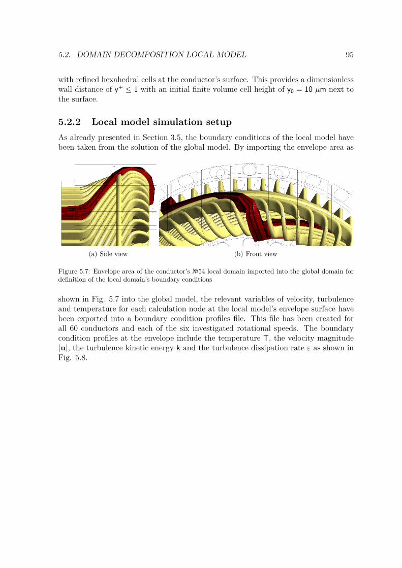
5.2. DOMAIN DECOMPOSITION LOCAL MODEL 95
with refined hexahedral cells at the conductor’s surface. This provides a dimensionlesswall distance of y+ ≤ 1 with an initial finite volume cell height of y0 = 10 µm next tothe surface.
5.2.2 Local model simulation setupAs already presented in Section 3.5, the boundary conditions of the local model havebeen taken from the solution of the global model. By importing the envelope area as
(a) Side view (b) Front view
Figure 5.7: Envelope area of the conductor’s 54 local domain imported into the global domain fordefinition of the local domain’s boundary conditions
shown in Fig. 5.7 into the global model, the relevant variables of velocity, turbulenceand temperature for each calculation node at the local model’s envelope surface havebeen exported into a boundary condition profiles file. This file has been created forall 60 conductors and each of the six investigated rotational speeds. The boundarycondition profiles at the envelope include the temperature T, the velocity magnitude|u|, the turbulence kinetic energy k and the turbulence dissipation rate ε as shown inFig. 5.8.

96 CHAPTER 5. SIMULATED HEAT TRANSFER OF THE END REGION
(a) Temperature (b) Velocity magnitude
(c) Turbulence kinetic energy (d) Turbulence eddy dissipation
Figure 5.8: Boundary conditions for the envelope area of the local domain at a rotational speed ofn = 3007 min−1

5.3. RESULTS OF THE GLOBAL LOCAL DOMAIN DECOMPOSITION MODEL97
5.3 Results of the global local domain decomposi-tion model
As seen in the example presented in Chapter 3, a reliable heat transfer coefficient canonly be obtained if the condition y+ ≤ 1 is satisfied (see Section 3.5). This cannotbe achieved with acceptable computational demand in a global model, therefore, aglobal local decomposition has been applied. The simulation of the global model hasbeen executed with the solution of the total energy equation (2.42) included in orderto obtain valid temperature values for the local domains boundary conditions. Sincethe energy equation also includes the solution of the heat flux, an analysis of thewall heat transfer coefficient can easily be performed, even though it has been derivedwith the logarithmic law of the wall. The absolute quantity of the wall heat transfercoefficient may not be accurate, nevertheless, a qualitative illustration is informative.The contour plot in Fig. 5.9 shows the local wall heat transfer coefficient α, wherethe blue areas designate its lowest values and the red areas the highest. The cooling
Figure 5.9: Convective wall heat transfer coefficient at the end-windings with the end-shield sketchedas a wire-frame obtained from the global model
ducts of the stator generate a jet flow condition after the ducts’ outlet which causesa locally higher heat transfer coefficient at the end-windings. This locally increasedheat transfer is shown in Fig. 5.9 as yellow contours, recurring azimutally with thesame periodicity as the cooling ducts. The averaged values of the wall heat transfercoefficients at the global meshes, as shown in Fig. 5.9 are listed in Tab. 5.2, includingminimum, average and maximum values of the dimensionless wall distance y+.
In creating the local models, care has been taken to get values of y+ ≤ 1 next tothe conductors surfaces. In order to obtain comparable results, identical meshes of all

98 CHAPTER 5. SIMULATED HEAT TRANSFER OF THE END REGION
n α y+avg y+
min y+max
min−1 W/m−2K1503 13.40 1.63 0.06 5.941800 14.86 1.87 0.07 6.992104 16.59 2.07 0.06 7.572400 18.86 2.35 0.09 8.002700 20.76 2.60 0.08 8.813007 22.55 2.90 0.14 10.10
Table 5.2: Simulated wall heat transfer coefficient obtained from the global model
conductors have been developed. The only difference between the separate conductorsis the transformed coordinate system and the individual boundary conditions for eachconductor obtained from the global mesh, as shown in Fig. 5.8. Each of the 60conductors has been simulated for six different rotational speeds using the respectiveboundary conditions profile obtained from the global models. One example of thesimulation on the local model is illustrated in Fig. 5.10 and shows the wall heattransfer coefficient on conductor 54 for a rotational velocity of n = 3007 min−1.
(a) Left view (b) Front view (c) Right view
Figure 5.10: Local wall heat transfer coefficient on the surface of conductor 54 for a rotationalvelocity of n = 3007 min−1
The values of the average wall heat transfer coefficients for each conductor and eachrotational speed are shown in the diagrams in Fig. 5.11. The results for each conductorare shown as circles. Also, the wall heat transfer coefficients of all conductors havebeen averaged for each rotational speed and are presented in the right bottom cornerof the diagrams. These are average values of the whole end-windings calculated in thelocal meshes and thus can be compared with the results from the global mesh, shownin Tab. 5.2. It is evident that the results of the global and local mesh match witha relative error of less than 2%. This shows that for this particular problem, the y+
values used in the global model shown in Tab. 5.2 are also sufficient. This can beexplained as follows.
Obviously, the heat transfer at the end-windings is caused by an attached flowparallel to the wall, rather than by a highly turbulent separated flow next to the wall.Therefore, the logarithmic law of the wall is valid at most locations of the end-windingsand the wall heat transfer can be calculated with good accuracy with the log-law. A

5.3. RESULTS OF THE GLOBAL LOCAL DOMAIN DECOMPOSITION MODEL99
comparison between adjacent conductors for the different rotational velocities showsan alternating behavior from one conductor to the next. As shown in Fig. 5.9, the jetflow of the cooling ducts causes a higher heat transfer at specific locations. Since thenumber of conductors of this machine is two times greater than the number of coolingducts, it is obvious that the heat transfers of every second conductor are comparableand thus altering from one to the next conductor.
The diagrams in Fig. 5.12 show a comparison of the simulated values, shownas circles, to the values measured in Chapter 4, shown as squares. These valueshave been examined on the conductors equipped with heat flux sensors during themeasurements and at identical positions on the adjacent conductors, shown as trianglesin the diagrams. The heat flux at identical positions is spread widely between someneighboring conductors, e.g. as shown in Figs. 5.12(a), 5.12(c) or 5.12(g). On the onehand, this is caused by the unequal number of cooling ducts and conductors. On theother hand, the air flow inside the end-shield is disturbed by the waste grease drainand the bracings shown in Fig. 5.2.
In some diagrams in Fig. 5.12, poor congruence between simulated and measuredresults can be observed. Beside errors caused by CFD, the measurements also exhibita certain error. The manufacturer of the used Pt100 temperature sensors ensures anaccuracy of DIN class A between −90°C and 300°C in the DIN EN 60751 standard [19].For a measured temperature of 80°C this error class guarantees an absolute temperatureaccuracy of 0.31°C. Although all sensors have been calibrated at the environmentaltemperature, an absolute error of less than 0.1°C cannot be guaranteed. Since thedifference between fluid and wall temperature is below 8°C for all rotational speeds,the measuring error can have high influence on the wall heat transfer coefficient, as alsodiscussed in Subsection 2.2.4. As shown at the end of Chapter 4, the measured resultspresented here are average values of sometimes widely spreading measuring data ofthe same sensor. The wider the measuring samples spread, the more samples wouldbe necessary to get statistically significant values. For some operation points of themachine, the number of collected samples is too small. Nevertheless, the average valuesfit into the general trend of steadily rising heat transfer with increasing rotationalspeed.
Another source of error is the accuracy of the conductors’ manufacture. The realend-windings do not satisfy an exact periodicity due to manufacturing tolerances whichcan cause e.g. an azimutal offset of the heat flux sensors’ position of some degrees. Inthe model, on the other hand, the conductors have been rotated and copied by an angleof exacly six degrees. As already mentioned, the heat flux at identical positions onadjacent conductors can differ widely, hence a misplaced conductor in the real machinecan have a different heat flux compared to the simulated conductor.

100 CHAPTER 5. SIMULATED HEAT TRANSFER OF THE END REGION
10 20 30 40 50 600
2
4
6
8
10
12
14
16
Conductor No.
α in
W/m
2 K
αavg
=13.7 W/m2K
(a) n = 1503 min−1
10 20 30 40 50 600
2
4
6
8
10
12
14
16
18
Conductor No.α
in W
/m2 K
αavg
=15.0 W/m2K
(b) n = 2104 min−1
10 20 30 40 50 600
5
10
15
20
Conductor No.
α in
W/m
2 K
αavg
=16.6 W/m2K
(c) n = 2104 min−1
10 20 30 40 50 600
5
10
15
20
Conductor No.
α in
W/m
2 K
αavg
=18.9 W/m2K
(d) n = 2400 min−1
10 20 30 40 50 600
5
10
15
20
25
Conductor No.
α in
W/m
2 K
αavg
=21.2 W/m2K
(e) n = 2700 min−1
10 20 30 40 50 600
5
10
15
20
25
Conductor No.
α in
W/m
2 K
αavg
=22.9 W/m2K
(f) n = 3007 min−1
Figure 5.11: Averaged values of the wall heat transfer coefficient for all conductors at different rota-tional speeds

5.3. RESULTS OF THE GLOBAL LOCAL DOMAIN DECOMPOSITION MODEL101
1500 2000 2500 30000
10
20
30
40
50
60
70
n in min−1
α in
W/m
2 K
(a) HFS-05 at position HFS-A
1500 2000 2500 30000
10
20
30
40
50
n in min−1
α in
W/m
2 K
(b) HFS-06 at position HFS-A
1500 2000 2500 30000
5
10
15
20
25
30
35
n in min−1
α in
W/m
2 K
(c) HFS-09 at position HFS-B
1500 2000 2500 30000
10
20
30
40
50
60
70
n in min−1
α in
W/m
2 K
(d) HFS-10 at position HFS-B
1500 2000 2500 30000
50
100
150
200
n in min−1
α in
W/m
2 K
(e) HFS-11 at position HFS-D
1500 2000 2500 30000
50
100
150
n in min−1
α in
W/m
2 K
(f) HFS-12 at position HFS-D
1500 2000 2500 30000
20
40
60
80
100
n in min−1
α in
W/m
2 K
(g) HFS-13 at position HFS-C
1500 2000 2500 30000
50
100
150
200
n in min−1
α in
W/m
2 K
(h) HFS-14 at location HFS-C
Figure 5.12: Simulated results of the local wall heat transfer coefficients (circles) compared to themeasured results (squares) and at identical positions on two neighboring conductors (triangles)

Chapter 6
Characterizing the heat transfer
Predicting the thermal behavior of complex geometric shapes by calculating the ther-mal field inside solid materials depends on the availability of proper values of the wallheat transfer coefficient. Simulation of the heat transfer at the end-windings of an elec-tric machine is often restricted by the quality of the coefficients used in the simulationmodel.
Since this coefficient depends basically on the usually turbulent fluid flow, there ispractically no way of calculating it exactly in any case. Earlier investigations on heattransfer problems used experimental setups to obtain non-dimensional correlationsfrom the measured heat transfer values, as outlined in [93]. The correlations of suchpublications have been defined for simple geometries like flat plates or pipes and havebeen listed in works of reference, e.g. in [88]. Since the geometry of the end-windingsdepends on a range of parameters, a large number of geometry-variations are necessaryand thus measurements on varied geometries would be very costly. Hence measurementbased correlations can hardly be found in literature for such geometries.
A correlation between tangential velocity and the wall heat transfer coefficient hasbeen found for totally enclosed fan cooled motors, as shown in [8]. Since electricalmachines of a higher power class have typically other cooling systems, different corre-lations are necessary. In [70], an electrical machine has been investigated extensivelywhich has a comparable cooling system to the machine investigated in this work.Since the measurements have been taken on a single geometry, only a correlation tothe rotational speed would be possible. The investigation in this chapter has beenaccomplished in addition to former research published in [36] and [40].
The non-dimensional descriptions of correlations have the benefit of scalability de-pending on specific characteristic lengths. A characteristic length can be the diameterof a pipe in the case of a pipe-flow or the length of a plate in the case of a fluid flowparallel to a flat plate. In case of a more complex shape, as that of the end-windingsof an electric machine, the characteristic length is not obvious.
The data for correlations of the wall heat transfer coefficient had been collected bymeasurements in the past. Today the progress in computer and simulation technologyprovides tools for replacing the majority of measurements on experimental setups. By
102

6.1. DIMENSION ANALYSIS AND PI-THEOREM 103
using CFD, it has become possible to simulate the fluid flow including the relevanteffects, like the convective wall heat transfer. This technology cannot be consideredan exact method, since it is based on non-exact models to some extent. Nevertheless,it provides sufficient accuracy for most engineering applications.
The following chapter gives an outline of obtaining correlations between the con-vective wall heat transfer coefficient of the end-windings and geometrical as well asoperational conditions. The heat transfer values of a variety of geometries have beencomputed by CFD before correlating them to the known conditions with the Gauss-Newton method.
The result is a set of characterization parameters which allows the calculation of thewall heat transfer coefficient by a simple formula which can be applied e.g. to a thermalnetwork model for drive cycle simulations of traction motors. This characterizationprovides a way of calculating values for the convective wall heat transfer coefficientdepending on specific degrees of freedom for the rotational speed of the rotor and thegeometry of the end-shield. Due to the conversion into dimensionless numbers, theresult is also applicable on scaled geometries.
6.1 Dimension analysis and Pi-TheoremA physical magnitude has three attributes: value, unit and dimension. Dimension isan agreement with the purpose of quantifying a natural principle with a value. This isa convention about the principle and not a result of the principle. The dimensions of aspecific system are categorized as fundamental dimensions and derived dimensions. Forexample, in a dynamic system, the fundamental dimensions are length, time and mass.The derived dimensions for this system can be force, velocity and acceleration, whichare products of powers of fundamental dimensions. The choice of the fundamentaldimensions is a matter of agreement but still has to satisfy the following two criteria:
• No fundamental dimension can be derived from other fundamental dimensions.
• Each derived dimension of the considered problem can be obtained from thefundamental dimensions.
Units are classified as fundamental or derived units, according to their dimensions [34].The Pi-Theorem [34] can be used to calculate a common solution for any correlationas a function of a specific number of dimensionless values. For the correlation of nvariables ai with m fundamental dimensions with
f(a1, a2, . . . , an) = 0 , (6.1)
the solution of the correlation has the common form
F(Π1,Π2, . . .Πn−m) = 0 . (6.2)

104 CHAPTER 6. CHARACTERIZING THE HEAT TRANSFER
The Πi values in (6.2) represent a set of (n−m) independent and dimensionless values.Depending on the actual problem, a specific set of fundamental dimensions is required.A system of the three fundamental dimensions length (L), time (Z) and mass (M) turnsout to be reasonable for finding solutions to dynamic problems. Since this system isnot able to define a value of heat energy, an additional dimension for the temperatureis required. Hence heat transfer problems can be defined from the thermodynamicpoint of view by the dimensions of length (L), time (Z), mass (M) and temperature(T).
The main task in the dimension analysis is the definition of relevant values and atarget value which are specific to the problem. A list of relevance separates the valuesinto five categories, from R1 to R5, and each value has to be controlled depending onits influence on the target value. If the change of a value might change the target valueit should be included in the list of relevance, as shown in Tab. 6.1.
R1 Target value Value to be determinedR2 Geometric values Characteristic geometrical valuesR3 Process values Characteristic values for the intensity of the processR4 Material properties Material properties which can be relevant for the processR5 Constants Constant values of physical relations
Table 6.1: List of relevance
6.2 SimulationThe focus of this investigation has been on the end-windings of the non drive-end sideof various variations of the induction motor examined in Chapter 4, as shown in theoutlined detail A in Fig. 6.1. The analyzed motor type in this chapter is the same
Figure 6.1: Longitudinal section of the investigated induction motor with the outlined detail A [40]

6.2. SIMULATION 105
type as the analyzed motor used for the measurements in Chapter 4 and simulationsin Chapter 5 and is described in detail in Section 4.1. This motor type is used as atraction motor and operates in the whole velocity range up to the maximal rotationalspeed. Since the values of convective heat transfer are changing with the rotationalspeed, these speed dependent values of the cooling cycle are of interest.
6.2.1 Geometry
The analysis of the convective heat transfer with CFD programs requires a very finemesh at the surface of the end-windings. Hence the number of degrees of freedomincreases dramatically and it becomes necessary to focus the simulation on just onecertain part of the machine. Since a principle solution of this problem is required,not the whole circumference of the end-region containing the stator and the rotor hasbeen modeled. In contrast to the motor presented in Chapters 4 and 5, a rotationalperiodicity has been assumed. The number of stator slots is an integer multiple of thenumber of the cooling ducts which are equally spaced over the whole circumference.On this account, a sector has been considered for the investigations by CFD whichcovers only one cooling duct and two conductors. The rotor of this machine featuresan equal number of cooling ducts on two different pitch circles. Like the stator, therotor has been simplified by a section containing one pair of cooling ducts, one ductfrom the outer pitch circle and one duct from the inner pitch circle. One drawback ofthis simplification is the inaccurate modelling of the end-shield. In the real machineit does not have the same rotational periodicity as the end-windings or stator coolingducts. The geometry which has been used for the CFD investigations is shown in Fig.6.2, which also explains the parts of this model. Starting at the model’s air inlet, the
Figure 6.2: Used sectors for the CFD simulation with the stator-volume containing (a) model airinlet, (b) cooling duct of the stator, (c) stator duct outlet, (d) end-windings and (e) end-shield. Therotor-volume contains the, (f) short circuit ring, (g) shaft, (h) rotor duct inlets, (i) rotor cooling ductsand (j) model air outlet.

106 CHAPTER 6. CHARACTERIZING THE HEAT TRANSFER
coolant flows through the stator cooling duct, passes the end-windings, the end-shieldand the short circuit ring and flows through the rotor cooling ducts to the model’s airoutlet.
6.2.2 VariationsModifications of the end-shield geometry lead to a change of the local fluid velocityaround the end-windings. Due to this change of velocity, the value of the convectiveheat transfer at the end-windings’ surface is affected. In order to investigate thecorrelations of geometric variations to the heat transfer, the geometry of the end-region has been modified. The three geometric dimensions end-shield hight lV, end-shield diameter lH and overhang of the end-windings lA, as shown in Fig. 6.3, have beenchanged and 16 different geometries and calculation meshes, respectively, have beencreated. All other dimensions have been kept constant for all geometric variations, buthave been used for the correlations. In order to consider the heat transfer on the scaled
lA
lH
l Vl E
l D
l B
lT
lF
or
Figure 6.3: Geometric dimensions which have been used for this investigation. The dimensions lV, lEand lK represent radii measured from the rotational axis of the machine.
end-regions, the 16 different geometries have been converted to larger geometries scaledby 20%. The scaled geometries have been re-meshed with the same mesh propertiesas the original geometries. With four different rotational speeds of the rotor and twodifferent values for the air mass flow in the stator cooling ducts each, a total numberof 256 CFD simulations on 32 different meshes have been accomplished to obtain thecalculation of the correlation.
In order to achieve a proper wall treatment at the surface of the end-windings byCFD, thin inflated mesh layers have been created at the the end-windings’ surface-mesh. With ten layers of prismatic cells, a growth factor of 1.2 and a total thickness

6.2. SIMULATION 107
of 1 mm for all layers, a dimensionless cell height of y+ < 1 has been achieved, evenfor the highest rotational velocity of the rotor.
6.2.3 Boundary conditionsThe wall heat transfer coefficients have been identified by CFD simulations with dif-ferent boundary conditions determined by varying revolution speeds n of the rotor andair mass flows min through the stator cooling ducts at a constant air temperature. Atthe rotor’s circumference, the revolution speed causes a maximum angular velocityw which can be calculated from the revolution speed n expressed in revolutions perminute and the outer diameter Dor of the rotor iron or end-ring, respectively:
w = Dor π n60 . (6.3)
Each model has been analyzed with four different rotational velocities to achieve acorrelation with the heat transfer.
A certain mean velocity v in the stator cooling ducts is caused by the air mass flowat the inlet min which can be obtained as
v = min
ρ A(6.4)
where ρ is the density of air at atmospheric conditions and A denotes the cross sectionalarea of the stator cooling ducts [36].
In the real machine, the air mass flow min is a function of rotational speed n andis affected by the pressure to mass flow characteristics of the fan of the inner coolingcycle. For a general description of the machine it should be independent of the fan toprovide more freedom in the design process. To achieve this, the functional relationshipbetween air mass flow min and rotational speed n is split and the two variables are givenas separate and independent parameters. Since the air mass flow through the coolingducts m depends linearly on the rotational speed n, the ratio m/n of these values isa constant value for a specific fan. In order to make the correlations dependent onthe fan characteristics two different ratios of air mass flow to rotational speed m/nhave been investigated. Their used values including the resulting values of wall heattransfer coefficient can be found in Tab. 6.2 for the non scaled geometry and in Tab.6.3 for the scaled geometries, respectively.
Since the heat transfer of the scaled geometries should be comparable to the resultsof the original geometries, the rotational speed and the velocity in the stator coolingducts has to be adjusted to achieve equal Reynolds numbers inside the machine. Forthe same Reynolds numbers of scaled and original geometry the velocity w and hencethe rotational speed n has to be adjusted by the same factor of sf = 1.2 as the ge-ometry, since the kinematic viscosity ν can be assumed to be constant. Decreasingthe circumferential velocity by the scaling factor requires a reduction of the rotational

108 CHAPTER 6. CHARACTERIZING THE HEAT TRANSFER
speed by the square of the scaling factor with
nscaled = noriginal
s2f
(6.5)
The air mass flow of a fan rises with the third power of the diameter and thus with thescaling factor at equal rotational speed. Since the rotational speed is reduced by thesquare of the scaling factor and the cross section rises with the square of the scalingfactor, the resulting velocity in the cooling ducts decreases linearly achieving equalReynolds numbers in the cooling ducts for the original and scaled geometry:
vscaled = voriginal
sf(6.6)
The temperature of air at the model’s air inlet, labeled (a) in Fig. 6.2, has been setto Tin = 350 K. The air has been modeled with temperature dependent fluid propertiesand with a constant density of
ρ = p0
Rs Tin, (6.7)
with the reference pressure p0, the ideal gas constant for air Rs = 287.12 J/kgK andthe temperature at the model’s air inlet Tin in K. The heat capacity cp has beenapproximated by a so called zero pressure polynomial and the thermal conductivity λand dynamic viscosity µ have been modeled by the Sutherland formula, as describedin Section 3.2. The wall temperature has been defined as Tew = 360 K for the end-windings and Tes = 330 K for the end-shield. All other walls of the simulation modelhas been assumed to be adiabatic. The model’s air outlets, labeled as (j) in Fig. 6.2,have been set to a subsonic entrainment with 0 Pa relative pressure.
As mentioned above, the model has been simplified to a small sector, in orderto reduce the computational effort. Due to this simplification, sectional areas evolvefor the stator and the rotor, which have been defined as interfaces with rotationalperiodicity. Since the number of cooling ducts in the stator and the rotor is not equal,the sector-angle of the rotor-volume is different from the sector-angle of the stator-volume. For this reason, the volumes of stator and rotor have been connected by afrozen rotor interface, which supports this pitch change.
Thermal radiation is a phenomenon in which the heat flux rises with the fourthpower of temperature difference. Since this temperature difference between surfaceand environment has been expected to be not higher than 10 K the total amountof transported heat energy by radiation has been assumed to be small and thereforeneglected in this investigation.
6.2.4 Simulation resultsIn order to achieve acceptable results for the convective wall heat transfer coefficient,a CFD simulation setup with the Shear-Stress-Transport (SST) turbulence model fora steady state simulation has been chosen, as described in [37]. The configuration of

6.3. CHARACTERIZATION OF THE WALL HEAT TRANSFER COEFFICIENT109
the models have been set according to the validation setup, as described in Section3.3. After solving the CFD simulation of all model variations, the convective wall heattransfer coefficients α have been obtained by calculating the area weighted averageof the heat transfer coefficient over all surfaces of the end-windings. The results havebeen listed in Tab. 6.2 and 6.3, respectively. Knowing the wall heat transfer coefficientα, one can easily calculate the corresponding Nusselt number with (2.69), as shown inSection 6.3.
n in min−1 1000 2000 3000 4000 1000 2000 3000 4000m in 10−3 kg/s 0.260 0.521 0.781 1.041 0.545 1.090 1.635 2.180lV lH lA α αmm mm mm W/m2K W/m2K175 80 90 9.4 16.0 21.5 26.7 15.5 25.5 34.8 43.1175 90 100 9.6 16.3 22.2 27.6 15.1 24.7 32.7 39.8175 95 90 6.9 13.5 18.2 24.3 11.4 20.0 26.8 33.1175 95 95 8.6 15.4 20.9 26.4 12.8 21.8 29.4 36.0175 95 100 8.4 15.0 21.1 26.3 13.3 22.6 30.2 37.1175 125 90 6.9 11.4 14.8 18.3 11.1 19.1 25.6 31.7175 125 100 6.6 10.9 16.6 19.8 11.0 19.3 26.1 32.4180 95 90 7.6 13.9 19.9 25.6 11.3 20.0 27.4 34.0180 95 95 7.8 14.9 20.8 26.8 12.3 21.6 29.6 36.5180 95 100 7.9 14.6 20.4 25.6 13.0 22.8 31.0 38.1185 80 90 9.1 15.9 20.9 26.5 15.0 25.2 33.9 41.5185 90 100 8.9 15.7 22.1 27.1 14.9 25.1 33.3 40.6185 95 90 6.8 12.7 17.1 23.3 10.7 19.4 26.3 32.8185 95 100 7.5 14.1 20.2 25.2 12.4 21.8 29.5 36.2185 125 90 5.3 11.5 12.8 16.0 9.9 18.0 24.5 30.8185 125 100 4.9 11.1 12.4 15.9 9.6 17.6 24.1 30.2
Table 6.2: Area weighted average of the convective wall heat transfer coefficient α at the end-windingsdepending on rotational velocity of the rotor for the variations of the original geometry.
6.3 Characterization of the wall heat transfer coef-ficient
Since an analytical calculation of the convective wall heat transfer coefficient fails in thecase of the convoluted shape of the end-windings, an alternative approach is required.
6.3.1 Non-dimensional approachAn alternative solution has been found in the dimension analysis by correlating varia-tions of boundary conditions and geometric modifications to the convective heat trans-fer coefficient on the end-windings. In fluid dynamics, the use of dimension analysisis a common method, as shown on the example of the Reynolds number (2.65). By

110 CHAPTER 6. CHARACTERIZING THE HEAT TRANSFER
n in min−1 694 1389 2083 2778 694 1389 2083 2778m in 10−3 kg/s 0.312 0.625 0.937 1.250 0.654 1.308 1.962 2.616lV lH lA α αmm mm mm W/m2K W/m2K210 96 108 8.2 13.5 17.9 22.3 12.6 20.4 26.9 32.6210 108 120 8.4 13.9 18.6 23.3 13.0 20.9 27.5 33.4210 114 108 6.9 11.9 16.3 21.2 9.9 17.0 23.0 28.3210 114 114 7.2 12.4 17.2 21.7 10.6 18.0 24.2 29.7210 114 120 7.7 13.1 17.6 22.4 11.7 19.3 25.7 31.4210 150 108 6.5 10.9 14.7 18.1 9.6 16.4 22.2 27.4210 150 120 6.6 11.2 15.1 19.0 9.8 16.8 22.6 27.8216 114 108 6.2 12.0 16.9 21.6 9.5 16.9 23.2 28.8216 114 114 6.5 12.3 17.1 21.8 10.1 17.9 24.4 30.1216 114 120 7.0 13.1 17.9 22.6 11.3 19.4 26.2 32.2222 96 108 8.1 14.6 19.3 23.7 13.3 21.4 28.4 34.6222 108 120 8.1 14.1 19.1 23.8 13.1 21.7 28.7 34.9222 114 108 6.3 12.3 17.2 22.0 9.7 17.1 23.4 29.0222 114 120 7.2 12.9 18.3 23.1 11.6 19.8 26.6 32.6222 150 108 4.7 9.2 12.8 19.2 9.0 15.8 21.8 27.1222 150 120 5.1 10.4 14.4 20.4 8.9 16.0 22.2 27.6
Table 6.3: Area weighted average of the convective heat transfer coefficient α at the end-windingsdepending on rotational velocity of the rotor for the scaled geometry.
relating the velocity and length to the viscosity, the quotient becomes a criterion aboutthe extent of turbulence.
Like the Reynolds number the Nusselt number (2.69) describes a physical phe-nomenon by making the convective wall heat transfer coefficient α dimensionless.
As shown in [48], there is also a correlation between the Nusselt number and otherdimensionless numbers, as for instance:
Nu = F(Re,Pr,Ec,Gr) . (6.8)
In the case of air as coolant and the common temperature range inside an electricmachine, the Prandtl number (see (2.66)) remains almost constant at about Pr = 0.7and can be included in a constant factor. The Eckert number Ec becomes relevantfor supersonic fluid flow, which does not occur in the investigated electric motor. Ifthe fluid flow is caused by buoyant forces, the Grashof number Gr dominates, whichcan be assumed at zero rotational velocity. Buoyant forces cannot be used with thesimplified model, since the direction of gravity has no rotational periodicity. Since theEckert number can be neglected in subsonic problems and the Grashof number due tothe forced flow conditions, the correlation between Nusselt and Reynolds numbers canbe simplified to:
Nu = F(Re) = C · Ren (6.9)

6.3. CHARACTERIZATION OF THE WALL HEAT TRANSFER COEFFICIENT111
6.3.2 MethodThe aim of this work is finding a correlation between the Nusselt number, whichdescribes the convective wall heat transfer and the flow conditions around the end-windings. In this particular case it is assumed that the heat transfer depends on theflow conditions of air only, since the fluid properties remain almost constant but arestill temperature dependent. According to (6.1) the relevant variables of the heattransfer problem can be identified as
α = f(v,w, lV, lH, lA, lF, ν, λ) , (6.10)
with wall heat transfer coefficient α, the velocities v and w, the geometric dimensionslV, lH, lA and lF the kinematic viscosity ν and the thermal conductivity λ. The con-ductor width lF is a geometric dimension which only depend on the geometry scalingfactor sf . A list of relevance is shown in Tab. 6.4 with h = 9 relevant variables. The
Relevance Derived dimension Unit SI unitR1: α Wm−2K−1 kgs−3K−1
R2: lV, lH, lA, lF m mR3: v, w ms−1 ms−1
R4: ν m2s−1 m2s−1
R5: λ Wm−1K−1 kgms−3K−1
Table 6.4: List of relevant variables
transfer problem requires m = 4 fundamental dimensions length (in m), time (in s),mass (in kg) and temperature (in K) for a suitable characterization. For the set ofn−m = 5 independent variables, the characterization must satisfy (6.2). Since di-mensionless numbers for turbulence and heat transfer are available with the Reynoldsnumber and the Nusselt number, the procedure in the dimension analysis of makingthe variables dimensionless is obsolete. The correlation according to (6.9) is sufficientbut a description of C, Re and q is required in accordance with
Π5 = F(Π1,Π2,Π3,Π4) . (6.11)
The flow conditions and velocities next to the end-windings depend on the angularvelocity wi of the short circuit ring or the rotor and the velocity vi in the stator coolingducts, respectively. The angular velocity can be derived by the rotational speed ni andthe diameter of the short circuit ring Dor with (6.3). By using the air mass flow mand cross-sectional area of the stator cooling ducts A, the velocity in the cooling ductscan be calculated with (6.4). These velocities have been considered by the Reynoldsnumber at the end-windings close to the stator cooling ducts outlets
Π1i = vi Lvi
ν= Re(v) , (6.12)

112 CHAPTER 6. CHARACTERIZING THE HEAT TRANSFER
with the characteristic length Lvi and the Reynolds number at the end-windings closeto the short circuit ring by
Π2i = wi Lwi
ν, (6.13)
with the characteristic length Lwi. The characteristic length Lvi is the overhang of theend-windings, labeled lAi in Fig. 6.3 and the characteristic length Lwi is the width of aconductor, labeled lFi in Fig. 6.3. The index i denotes one of the 256 CFD simulations.
On the other, hand the fluid flow around the end-windings is influenced by sectionalareas in the flow path which has to be passed by the coolant. In the present caseespecially those sectional areas are of interest which represent a bottleneck in the flowpath and constrain the air to a higher velocity. Such possible constricted cross-sectionalareas can be found on two locations around the end-windings, one in radial and onein axial direction between end-windings and end-shield, as shown in Fig. 6.4. The
a
b
Figure 6.4: Bottlenecks in the air flow path between end-windings and end-shield (a) in radial directionand (b) in axial direction
hydraulic diameter dh is an established parameter in fluid dynamics, which describesthe influence of the cross-sectional area to the flow conditions. It is defined as
dh = 4 · Ah
Uh(6.14)
which is a ratio of four times the wetted area Ah and the wetted circumference Uh ofthe cross-sectional area. By calculating these hydraulic diameters of the bottleneckswith
Lzi = 2(lHi + lTi − lAi) (6.15)and
Lri = 4(lVi − lEi) , (6.16)and taking them as the characteristic length in the calculation of the Reynolds number,the third and the fourth dimensionless factors can be calculated as
Π3i = v Lzi
ν(6.17)

6.3. CHARACTERIZATION OF THE WALL HEAT TRANSFER COEFFICIENT113
andΠ4i = v Lri
ν. (6.18)
The fifth dimensionless factor is the Nusselt number which can be calculated with(2.69) using the wall heat transfer coefficient α from the CFD simulation and thecharacteristic length Lui. During the investigation, a characteristic length Lui for theend-windings of
Lui = lAi + lDi π
2(6.19)
has proved to be reasonable.By combining the values Π1i to Π4i, the most important parameters are expected
to be covered in order to calculate the Nusselt number:
Nuaprx i = Πq11i · Π
q22i · Π
q33i · Π
q44i · q5 . (6.20)
6.3.3 ApproximationBy using the Gauss-Newton method, the coefficients q1 . . . q5 have been adjusted tominimize the error between (6.20) and the values simulated with CFD, shown in Tab.6.2 and 6.3, respectively. The resulting characterization parameters for the approxi-mation of the wall heat transfer coefficient at the end-windings are presented in Tab.6.5. The results of this approximation have been plotted in Fig. 6.5 to 6.8 as functions
Table 6.5: Characterization parameters
q1 q2 q3 q4 q50.6764 0.2161 -0.1307 -0.0034 0.0638
of the Reynolds numbers of the cooling ducts Re(v) which have been calculated withthe CFD simulations. Compared to the computed values of the wall heat transfercoefficient by CFD, the average relative error of the approximation can be specified forthis data set with eNu = 5.4% and the maximum relative error with max(eNu) = 53%.
Revising the results of the approximation, one has to be careful concerning thephysical validity of the values q1 to q5, since the Gauss-Newton method might findsolutions which are mathematically optimal but physically invalid. The Nusselt num-ber on a flat plate rises with the length and with the Reynolds number of the plate.Since the flow conditions along the overhang lAi of the end-windings can be comparedto the conditions of a flat plate the Nusselt number must rise with a rising overhanglAi and the factor q1 has to be positive. The Nusselt number should rise with risingrotational speed, hence the factor q2 must have positive values. For a preset air massflow, the fluid velocity should rise if the cross-sectional area and hydraulic diameter in(6.15) and (6.16) becomes smaller, hence it is more likely that the factors q3 and q4have negative values. Since the Reynolds and the Nusselt numbers are positive, thefactor q5 has to be positive as well.

114 CHAPTER 6. CHARACTERIZING THE HEAT TRANSFER
6.3.4 ApplicationWith the availability of the end-windings’ heat transfer characterization, the wall heattransfer coefficient α can be obtained easily for similar geometries analyzed in thiswork. Once the geometry and operational parameters are available for a specific mo-tor the Pi-values can be calculated with (6.12), (6.13), (6.17) and (6.18). By knowingthe Pi-values the Nusselt number of a specific operation point can be calculated by(6.20) including the characterization parameters in Tab. 6.5. Rearranging (2.69), thewall heat transfer coefficient α can the be obtained with the characteristic length Luas calculated in (6.19) and the thermal conductivity of air λ for the prevailing tem-perature. Applying this characterization to the geometry investigated in chapters 4and 5 the approximated heat transfer coefficients αaprx can be calculated, as shownin Tab. 6.6. The approximated wall heat transfer coefficients have been comparedwith the simulated values from the global model αglob in Tab. 5.2 and the results ofthe local model αloc in Section 5.3, also shown in Tab. 6.6. Since this characteriza-
n w m v Π3 Π4 Nu αaprx αglob αlocmin−1 m/s kg/s m/s – – – W/m2K1503 18.1 7.6E-04 4.00 2915 4127 61.4 13.8 13.4 13.71800 21.7 9.2E-04 4.79 3492 4943 70.4 15.9 14.9 15.02104 25.3 1.1E-03 5.59 4081 5778 79.3 17.9 16.6 16.62400 28.9 1.2E-03 6.38 4655 6591 87.6 19.7 18.9 18.92700 32.5 1.4E-03 7.18 5237 7414 95.8 21.6 20.8 21.23007 36.2 1.5E-03 7.99 5833 8258 103.9 23.4 22.6 22.9
Table 6.6: Application of characterization to the geometry investigated in the chapters 4 and 5including a comparison of the results
tion is based on a specific range of geometric dimensions and operational conditions,the interpolation inside these ranges is safe. Heat transfer coefficients calculated forgeometries or operational conditions which were extrapolated outside these ranges,might be calculated with a much higher error than estimated in here.
6.3.5 DiscussionWith the aid of dimension analysis it has been possible to extract a set of parameterswhich allow the characterization of the average convective wall heat transfer coefficienton the end-windings of a traction motor. The characterization with a non-dimensionalcorrelation has the benefit of scalability depending on specific characteristic lengths.
In the present chapter the procedure of obtaining correlations of the convectivewall heat transfer coefficient of the end-windings and geometrical plus operationalconditions has been outlined. The employment of CFD allows the simulation of thefluid flow including the according effects, like the convective wall heat transfer. Inthe present case 32 different geometries with two different values for the air massflow in the stator cooling ducts and each with four different rotational speeds of the

6.3. CHARACTERIZATION OF THE WALL HEAT TRANSFER COEFFICIENT115
rotor have been investigated. Out of these 256 CFD simulation cases the data forthe correlation of heat transfer and operational conditions have been extracted. Thecomputed heat transfer values of the varied geometries have been correlated to theknown boundary conditions and geometric dimensions with the Gauss-Newton method.Interpreting the obtained characterization parameters in Tab. 6.5, one can see thatthe Reynolds numbers affect the heat transfer to a higher extent than the geometricratios. Especially the fluid flow from the stator cooling ducts has a large influenceto the overall heat transfer. In Fig. 6.5 to Fig. 6.8, the simulated results have beencompared to the approximations. Each diagram contains the average heat transfer asNusselt number obtained from eight different CFD simulations with two different ratiosof rotational speed n to stator cooling duct mass flow m. The two different ratios m1/nand m2/n have been approximated with the obtained characterization parameters ofthis chapter, shown as solid lines in the diagrams. Additionally to these results, therelative errors between the simulated and approximated Nusselt numbers have beenplotted together with the corresponding simulation results. Each pair of the left andright hand side diagrams refer to a non-scaled and a scaled pair of geometries. Since theCFD simulations of one pair of non-scaled and scaled geometry has been accomplishedwith boundary conditions for theoretically equal Reynolds numbers, the correspondingNusselt numbers in the diagrams in Fig. 6.5 to 6.8 should match each other. In allthese pairs of diagrams the results differ more or less. Especially the results of thediagram-pairs in Fig. 6.8(e) to Fig. 6.8(h) stray widely up to a maximum error of53%. Since these are comparisons of equal simulation setups, this difference can beidentified as an error of the CFD simulation. Therefore this difference can be identifiedpartially as an error of the CFD simulation, which was also experienced during theCFD simulations by non properly converging residuals. The average error on the otherhand remains mostly below 10% which is sufficient for most engineering purposes.
The benefit of this parameter set is a more flexible way of calculating the wall heattransfer coefficients. Compared to other approaches, this method allows more degreesof freedom regarding the basic end-shield dimensions and a scalability of the geometryas a whole.
Additional results of models with more variations of geometry and additional di-mensionless ratios can be appended to the existing data, in order to make the presentedmethod more flexible to other geometries.

116 CHAPTER 6. CHARACTERIZING THE HEAT TRANSFER
0 1 2 3 4 5
x 104
0
50
100
150
200
250
Re(v)
Nu
6.2%3.3%
4.0%
2.5%
4.1%
4.2%
3.7%
4.2%
NuCFD
Nuaprx
(a) lV = 175 mm, lH = 80 mm, lA = 90 mm
0 1 2 3 4 5
x 104
0
50
100
150
200
Re(v)
Nu
5.4%1.4%
0.4%
2.0%
3.5%
4.2%
5.8%
16.0%
NuCFD
Nuaprx
(b) lV = 210 mm, lH = 96 mm, lA = 108 mm
0 1 2 3 4 5
x 104
0
50
100
150
200
250
Re(v)
Nu
3.0%2.8%
0.2%
2.0%
3.2%
1.9%
5.3%
2.0%
NuCFD
Nuaprx
(c) lV = 175 mm, lH = 90 mm, lA = 100 mm
0 1 2 3 4 5
x 104
0
50
100
150
200
250
Re(v)
Nu
6.0%3.0%
1.3%
0.5%
2.2%
1.5%
4.6%
1.2%
NuCFD
Nuaprx
(d) lV = 210 mm, lH = 108 mm, lA = 120 mm
0 1 2 3 4 5
x 104
0
50
100
150
200
Re(v)
Nu
6.4%17.5%
2.1%1.9%
3.7%
2.4%
4.7%
4.5%
NuCFD
Nuaprx
(e) lV = 175 mm, lH = 95 mm, lA = 90 mm
0 1 2 3 4 5
x 104
0
50
100
150
200
Re(v)
Nu
1.5%1.9%
0.4%3.9%
0.9%
4.8%
1.7%
6.5%
NuCFD
Nuaprx
(f) lV = 210 mm, lH = 114 mm, lA = 108 mm
0 1 2 3 4 5
x 104
0
50
100
150
200
Re(v)
Nu
0.9%1.0%
1.5%6.9%
0.9%
6.8%
0.7%
8.2%
NuCFD
Nuaprx
(g) lV = 175 mm, lH = 95 mm, lA = 95 mm
0 1 2 3 4 5
x 104
0
50
100
150
200
Re(v)
Nu
1.2%2.2%
1.2%3.7%
0.0%
4.1%
1.4%
6.2%
NuCFD
Nuaprx
(h) lV = 210 mm, lH = 114 mm, lA = 114 mm
Figure 6.5: Simulated results and approximation of the Nusselt number for variations of geometryincluding the relative error in percent

6.3. CHARACTERIZATION OF THE WALL HEAT TRANSFER COEFFICIENT117
0 1 2 3 4 5
x 104
0
50
100
150
200
Re(v)
Nu
0.5%6.3%
0.3%
1.4%
1.9%
2.1%
3.3%
2.2%
NuCFD
Nuaprx
(a) lV = 175 mm, lH = 95 mm, lA = 100 mm
0 1 2 3 4 5
x 104
0
50
100
150
200
Re(v)
Nu
4.4%3.2%
2.2%
3.4%
0.1%
2.7%
1.7%
4.1%
NuCFD
Nuaprx
(b) lV = 210 mm, lH = 114 mm, lA = 120 mm
0 1 2 3 4 5
x 104
0
50
100
150
Re(v)
Nu
3.1%3.5%
4.9%
6.8%
3.5%
11.9%
3.1%
12.7%
NuCFD
Nuaprx
(c) lV = 175 mm, lH = 125 mm, lA = 90 mm
0 1 2 3 4 5
x 104
0
50
100
150
Re(v)
Nu
7.2%7.0%
7.7%
1.7%
7.3%
0.5%
6.8%
4.2%
NuCFD
Nuaprx
(d) lV = 210 mm, lH = 150 mm, lA = 108 mm
0 1 2 3 4 5
x 104
0
50
100
150
200
Re(v)
Nu
1.4%13.8%
2.1%
16.0%
1.5%
3.5%
1.3%
7.9%
NuCFD
Nuaprx
(e) lV = 175 mm, lH = 125 mm, lA = 100 mm
0 1 2 3 4 5
x 104
0
50
100
150
200
Re(v)
Nu
5.7%4.3%
6.0%
4.6%
5.1%
3.9%
4.2%
6.0%
NuCFD
Nuaprx
(f) lV = 210 mm, lH = 150 mm, lA = 120 mm
0 1 2 3 4 5
x 104
0
50
100
150
200
Re(v)
Nu
7.3%7.1%
2.5%1.1%
1.5%
6.5%
1.8%
9.4%
NuCFD
Nuaprx
(g) lV = 180 mm, lH = 95 mm, lA = 90 mm
0 1 2 3 4 5
x 104
0
50
100
150
200
Re(v)
Nu
6.2%12.1%
1.0%5.8%
0.4%
7.6%
0.1%
11.4%
NuCFD
Nuaprx
(h) lV = 216 mm, lH = 114 mm, lA = 108 mm
Figure 6.6: Simulated results and approximation of the Nusselt number for variations of geometryincluding the relative error in percent

118 CHAPTER 6. CHARACTERIZING THE HEAT TRANSFER
0 1 2 3 4 5
x 104
0
50
100
150
200
Re(v)
Nu
3.2%9.2%
0.9%3.7%
1.5%
6.3%
0.8%
9.3%
NuCFD
Nuaprx
(a) lV = 180 mm, lH = 95 mm, lA = 95 mm
0 1 2 3 4 5
x 104
0
50
100
150
200
Re(v)
Nu
3.6%9.5%
0.2%1.6%
0.9%
6.3%
0.2%
9.0%
NuCFD
Nuaprx
(b) lV = 216 mm, lH = 114 mm, lA = 114 mm
0 1 2 3 4 5
x 104
0
50
100
150
200
Re(v)
Nu
3.0%13.4%
0.6%
4.2%
0.6%
1.2%
0.6%
0.3%
NuCFD
Nuaprx
(c) lV = 180 mm, lH = 95 mm, lA = 100 mm
0 1 2 3 4 5
x 104
0
50
100
150
200
Re(v)
Nu
1.4%6.1%
2.7%
1.4%
2.2%
4.9%
0.9%
6.8%
NuCFD
Nuaprx
(d) lV = 216 mm, lH = 114 mm, lA = 120 mm
0 1 2 3 4 5
x 104
0
50
100
150
200
Re(v)
Nu
3.6%6.6%
2.9%
3.0%
1.8%
6.7%
0.3%
4.7%
NuCFD
Nuaprx
(e) lV = 185 mm, lH = 80 mm, lA = 90 mm
0 1 2 3 4 5
x 104
0
50
100
150
200
Re(v)
Nu
9.0%0.7%
4.9%18.3%
2.5%
3.7%
0.4%
2.2%
NuCFD
Nuaprx
(f) lV = 222 mm, lH = 96 mm, lA = 108 mm
0 1 2 3 4 5
x 104
0
50
100
150
200
250
Re(v)
Nu
1.9%9.9%
1.5%
5.3%
0.9%
2.1%
3.0%
3.2%
NuCFD
Nuaprx
(g) lV = 185 mm, lH = 90 mm, lA = 100 mm
0 1 2 3 4 5
x 104
0
50
100
150
200
250
Re(v)
Nu
7.0%0.7%
4.9%12.0%
2.4%
3.0%
0.1%
2.8%
NuCFD
Nuaprx
(h) lV = 222 mm, lH = 108 mm, lA = 120 mm
Figure 6.7: Simulated results and approximation of the Nusselt number for variations of geometryincluding the relative error in percent

6.3. CHARACTERIZATION OF THE WALL HEAT TRANSFER COEFFICIENT119
0 1 2 3 4 5
x 104
0
50
100
150
200
Re(v)
Nu
12.2%19.1%
5.1%
7.2%
5.3%
8.5%
5.1%
0.9%
NuCFD
Nuaprx
(a) lV = 185 mm, lH = 95 mm, lA = 90 mm
0 1 2 3 4 5
x 104
0
50
100
150
200
Re(v)
Nu
3.9%10.9%
0.2%10.5%
1.1%
9.0%
0.7%
11.7%
NuCFD
Nuaprx
(b) lV = 222 mm, lH = 114 mm, lA = 108 mm
0 1 2 3 4 5
x 104
0
50
100
150
200
Re(v)
Nu
7.4%18.7%
3.5%
7.6%
4.1%
2.0%
5.4%
1.5%
NuCFD
Nuaprx
(c) lV = 185 mm, lH = 95 mm, lA = 100 mm
0 1 2 3 4 5
x 104
0
50
100
150
200
Re(v)
Nu
4.1%4.2%
4.9%
3.4%
3.8%
6.0%
2.1%
7.2%
NuCFD
Nuaprx
(d) lV = 222 mm, lH = 114 mm, lA = 120 mm
0 1 2 3 4 5
x 104
0
50
100
150
Re(v)
Nu
8.0%34.0%
0.3%
6.5%
0.6%
29.2%
0.6%
28.5%
NuCFD
Nuaprx
(e) lV = 185 mm, lH = 125 mm, lA = 90 mm
0 1 2 3 4 5
x 104
0
50
100
150
Re(v)
Nu
0.8%16.4%
4.0%
7.7%
5.7%
6.4%
5.8%
4.8%
NuCFD
Nuaprx
(f) lV = 222 mm, lH = 150 mm, lA = 108 mm
0 1 2 3 4 5
x 104
0
50
100
150
Re(v)
Nu
15.6%53.0%
7.2%
14.5%
6.6%
17.8%
5.7%
34.4%
NuCFD
Nuaprx
(g) lV = 185 mm, lH = 125 mm, lA = 100 mm
0 1 2 3 4 5
x 104
0
50
100
150
200
Re(v)
Nu
3.9%25.2%
1.1%
26.6%
3.5%
8.7%
3.8%
12.3%
NuCFD
Nuaprx
(h) lV = 222 mm, lH = 150 mm, lA = 120 mm
Figure 6.8: Simulated results and approximation of the Nusselt number for variations of geometryincluding the relative error in percent

Chapter 7
Results and Conclusion
7.1 New scientific results
Investigations known from the literature are focused, with some exceptions, on TEFCmotors. Due to a different cooling strategy of traction motors with DACS, empiricalmodels for the convective wall heat transfer coefficient of the end-windings of TEFCmotors cannot be used for DACS motors. The recent advances in CFD, e.g. [49, 56],allow the numerical calculation of the convective wall heat transfer coefficient withacceptable accuracy. Hence, the approach of this thesis is based on CFD and onmeasurements for validation.
The capability of CFD for predicting the convective wall heat transfer coefficienthas been identified on a cylinder in a cross-flow. It has been shown that the predictionof the convective wall heat transfer coefficient with the SST turbulence model is not ex-act but correlates with the empirical results with acceptable accuracy. The simulationhas been accomplished with different velocities showing that the agreement is betterfor low Reynolds numbers which are more likely in the end-region of the investigatedmachine.
Due to the non-periodical shape of the end-region of the measured motor, the CFDsimulations have taken into account the whole circumference of the end-region. Inorder to obtain accurate values of the wall heat transfer coefficient, the simulationshave been carried out with a resolved boundary layer mesh using the global-localdomain decomposition method. The results have shown that the local models haveled to no significant improvements in this particular case. The simulated values of thewall heat transfer coefficient have been validated by locally measured values.
A transient thermal network for calculating the thermal management of a tractionmotor requires a fast way of calculating the convective wall heat transfer coefficient.The implementation of a rough approximation is more useful in this case than thecomputationally costly CFD method. Therefore, a characterization of the convectivewall heat transfer coefficient has been created in this thesis which allows the variationof rotational speed, cooling duct air mass flow, end-windings overhang, end-shield
120

7.2. CONCLUSION 121
diameter and end-shield height, as well as a variation by a total scaling of the geometry.
7.2 ConclusionIn order to efficiently deploy the available resources in the manufacturing process ofelectrical machines, a comprehensive understanding of the utilization of each single partof the machine is valuable. By visualizing various physical mechanisms, simulationssupport this understanding to a large extent.
For the simulation of the thermal management of an electrical machine, boundaryconditions like the convective wall heat transfer coefficient are required. The accuracyof the thermal management simulation depends highly upon the accuracy of theseboundary conditions. The quantity of transferred heat depends on the coolant (fluid)and on the flow conditions next to the heated surface. In the case of a self ventilatedmotor, the flow conditions depend exclusively on its rotational speed. Traction motorshave to operate in the full range of rotational speed, from zero at start conditions to thehighest rotational speed at the vehicle’s maximum velocity. Since the flow conditionsdepend on the rotational speed and thus on the operation cycle of the traction motor,an accurate transient simulation of the heat management requires convective wall heattransfer coefficients depending on the rotational speed.
The heat transfer inside the cooling ducts is comparable to a pipe flow, which hasbeen investigated satisfactorily in the past and the results are available in referencebooks as [88] for a large number of different flow conditions and fluids. These flowconditions can often be reduced to 2-D problems and some of them can even be solvedanalytically. Due to the convoluted shape of the end-windings, the prediction of theconvective wall heat transfer coefficient on their surfaces requires a more sophisticatedapproach. Regarding traction motors, a variety of different cooling methods withdifferent shapes of end-windings and end-shields are feasible. Therefore it is unlikelyto find a common solution for all types of end-windings, hence this work is focusing onone specific type of traction motor. The method used in this work, on the other hand,is applicable to any type of cooling method and shape of end-region, respectively.
The investigation of the convective wall heat transfer has been carried out usingcomputational fluid dynamics (CFD), briefly described in Section 2.4. The velocity ofair and its turbulence next to a wall is a major factor for its convective heat transfercoefficient. With the method of CFD it is possible to gather velocity information aboutfluid conditions which were hardly gaugeable in the past. The underlying models ofCFD are able to calculate accurate results within certain limits but may yield wrongresults, if the limits of one model are disregarded. To ensure proper use of these CFDmodels, the simulation setup has been validated on a circular cylinder by comparing thesimulation results to previously published measurements. In Chapter 3 this validationhas been carried out in accordance with established investigations.
One type of end-windings has been investigated with measurements at specificpositions. Due to the shape of the end-windings and the size of the used heat flux

122 CHAPTER 7. RESULTS AND CONCLUSION
sensors, local values of the convective wall heat transfer coefficient have been measuredrather than values averaged over the whole end-windings’ surfaces. Heat flux sensorswith a larger sensing area would gain a more averaged result and would hence bebeneficial to such investigations. Since it is not possible to bend the used type ofheat flux sensors, the application of larger sensors to the convoluted surface of theend-windings is impossible.
The end-windings of the investigated traction motor are cooled by a closed coolingcircuit, which are not accessible during operation without modifications of the motor.In order to obtain values of the air mass flow inside the cooling ducts, the loss of staticpressure along the cooling ducts has been measured. The air mass flow depends notonly on the static pressure but also on the roughness of the surface inside the coolingducts. This roughness has also been evaluated by measuring the static pressure insidethe cooling ducts of the outer cooling circuit. Since this is an open cooling circuit,values of the total air mass flow have been available during the operation. By measuringthe total air mass flow of the machine, the air mass flow inside the single cooling ductsof the outer cooling cycle have been available. These measurements including thecorresponding calculations are presented in Chapter 4.
On the one hand, CFD is very helpful to get a survey of the heat transfer over thewhole surface. On the other hand, measurements can be performed at certain spotsonly, but are indispensable to validate the simulation results [42]. The end-regionof a real induction machine has no strict rotational periodicity. Some non-periodicshapes as waste grease drain, bracings and fins whose numbers are not equal to thenumber of the end-windings can cause different flow conditions on different end-windingconductors. Hence, the convective wall heat transfer coefficient varies azimuthally atthe conductors. Obviously a more accurate comparison between measurements andsimulation can be achieved by modeling the whole circumference of the machines end-region, rather than a single sector. Since CFD simulations of convective heat transferproblems require a very fine calculation mesh, a computable limit on contemporarycomputers can be reached very fast.
Despite the permanent improvement of commercial CFD software, the prediction ofconvective heat transfer coefficients is still a demanding subject. Especially for coolingpurposes, the examined geometry is rarely optimized for fluid flow and thus causesflow separation and re-attachment, which can not always be simulated accurately byCFD, the choice of the turbulence model is essential, as presented in [42]. In Chapter5 the measured results of the local convective wall heat transfer coefficients have beencompared to the simulated results. These simulations have been carried out for thewhole circumference of the end-windings with the global-local domain decompositionmethod to appropriately consider the shape of the end-region.
With this validated simulation setup, a characterization of the end-windings’ con-vective wall heat transfer coefficient has been carried out. By the use of CFD, a numberof different end-winding geometries and different operational conditions have been in-vestigated to find the different values of the convective wall heat transfer coefficient atthe end-windings.

7.2. CONCLUSION 123
With the aid of the Pi-Theorem, a correlation between the convective wall heattransfer coefficient and the operational conditions, as well as the geometrical changesof the end-shield has been found. The result is a flexible approximation of the Nusseltnumber dependent on operational conditions. The Nusselt number is, as customary, afunction of the Reynolds number but adapted by additional parameters, as shown inChapter 6. It is not only a function of the rotational speed and the mass flow throughthe cooling vents but also a function of some basic geometric values [35]. With thedimensionless Reynolds numbers and Nusselt numbers the result is also applicable toscaled geometries with similar shapes. The attained characterization of the convectivewall heat transfer coefficient provides an easy and fast way to forecast the heat fluxfrom the end-windings and is, therefore, well suitable for transient simulations withthermal network models. Describing the air mass flow through the cooling vents withthe rotational speed of the rotor, the performance of the ventilator can be considered.This also provides an improvement for optimizing the properties of the ventilator [36].
The surface of the real end-windings is partially smooth and partially rough, dueto resin impregnated bandages wrapped around the conductors. These investigationshave been made on hydraulically smooth surfaces, since measurements have been car-ried out with heat flux sensors with smooth surfaces. The conditions at the end-windings’ surface depend on the manufacturing processes to a high extent and aretherefore subject to statistical distribution of smooth and rough regions on the sur-face. Therefore a number of identical motors would be required to find a statisticallysignificant result.

Bibliography
[1] Eugene F. Adiutori. Origins of the heat transfer coefficient. In Mechanical Engi-neering, pages 46–50. West Chester, Ohio, 1990.
[2] John D. Anderson. Computational Fluid Dynamics - The Basics with Applica-tions. McGraw-Hill, New York, 1995.
[3] AnsysWB. Release 11.0 Documentation for ANSYS Workbench. Ansys, Inc.,Southpointe 275 Technology Drive Canonsburg, PA 15317, 2007.
[4] AnsysWB. Release 13.0 Documentation for ANSYS Workbench. SAS IP, Inc.,Southpointe 275 Technology Drive Canonsburg, PA 15317, 2010.
[5] A.F. Armor and M.V.K. Chari. Heat flow in the stator core of large turbine-generators, by the method of three-dimensional finite elements part II: Tempera-ture distribution in the stator iron. IEEE Transactions on Power Apparatus andSystems, 95(5):1657 – 1668, 1976.
[6] Hans Dieter Baehr and Stephan Kabelac. Thermodynamik - Grundlagen undtechnische Anwendungen. Springer, Berlin Heidelberg, 14th edition, 2009.
[7] Hans Dieter Baehr and Karl Stephan. Wärme- und Stoffübertragung. Springer,Heidelberg London New York, 6th edition, 2008.
[8] A. Boglietti and A. Cavagnino. Analysis of the endwinding cooling effects in TEFCinduction motors. IEEE Transactions on Industry Applications, 43(5):1214–1222,2007.
[9] A. Boglietti, A. Cavagnino, and D. Staton. Determination of critical parameters inelectrical machine thermal models. IEEE Transactions on Industry Applications,44(4):1150–1159, 2008.
[10] A. Boglietti, A. Cavagnino, D. Staton, M. Shanel, M. Mueller, and C. Mejuto.Evolution and modern approaches for thermal analysis of electrical machines.IEEE Transactions on Industrial Electronics, 56(3):871–882, 2009.
124

BIBLIOGRAPHY 125
[11] A. Boglietti, A. Cavagnino, D.A. Staton, M. Popescu, C. Cossar, and M.I. McGilp.End space heat transfer coefficient determination for different induction motor en-closure types. IEEE Transactions on Industry Applications, 45(3):929–937, 2009.
[12] Craig F. Bohren. Comment on “Newton’s law of cooling—A critical assessment,”by Colm T. O’Sullivan. American Journal of Physics, 59:1044, 1991. Depart-ment of Meteorology, Pennsylvania State University, University Park, Pennsylva-nia 16802.
[13] Günther Brenn. Strömungslehre und Wärmeübertragung I. TU Graz, 2004.
[14] Leopold Böswirth. Technische Strömungslehre. Vieweg, Wiesbaden, 2007.
[15] Edgar Buckingham. The principle of similitude. Nature, 96(2406):396–397, 1915.
[16] N.J. Carew. Experimental determination of heat transfer co-efficients of salientpole rotors. In IEE Colloquium on Thermal Aspects of Machines, pages 8/1 –8/8,London, UK, October 27 1992.
[17] Tuncer Cebeci, Jian Shao, Fassi Kafyeke, and Eric Laurendeau. ComputationalFluid Dynamics for Engineers From Panel to Navier-Stokes Methods with Com-puter Programs. Springer, Berlin Heidelberg, 2005.
[18] K. Dhinsa, C. Bailey, and K. Pericleous. Investigation into the performance ofturbulence models for fluid flow and heat transfer phenomena in electronic applica-tions. IEEE Transactions on Components and Packaging Technologies, 28(4):686– 699, 2005.
[19] DIN-EN-60751. Industrial platinum resistance thermometers and platinum tem-perature sensors (iec 60751:2008), 2009.
[20] E. Farnleitner and G. Kastner. Moderne Methoden der Ventilationsauslegung vonPumpspeichergeneratoren. E&I Elektrotechnik und Informationstechnik, 127:24–29, 2010.
[21] Ernst Farnleitner. Computational Fluid Dynamics Analysis for Rotating ElectricalMachinery. PhD thesis, University of Leoben, Austria, 1999.
[22] Joel H. Ferziger and Milovan Peric. Numerische Strömungsmechanik. Springer,Berlin Heidelberg, 2008.
[23] C.A.J. Fletcher. Computational Techniques for Fluid Dynamics, volume 1.Springer, Berlin Heidelberg New York, 2nd edition, 2006.
[24] C.A.J. Fletcher. Computational Techniques for Fluid Dynamics, volume 2.Springer, Berlin Heidelberg New York, 2nd edition, 2006.

126 BIBLIOGRAPHY
[25] Fluent. FLUENT 6.0 User’s Guide. Fluent Inc., Centerra Resource park, 10Cavendish Court, Lebanon, NH 03766, 2001.
[26] Jean Baptiste Joseph Fourier. The Analytical Theory of Heat. Cambridge Uni-versity Press, 1878.
[27] W. H. Giedt. Investigation of Variation of Point Unit-Heat-Transfer Coefficientaround a Cylinder Normal to an Air Stream, volume 71. Trans.ASME, 1949.
[28] G. Gilson, S.J. Pickering, D.B. Hann, and C. Gerada. Analysis of the end wind-ing heat transfer variation with altitude in electric motors. In IECON ’09. 35thAnnual Conference of IEEE Industrial Electronics, pages 2545 –2550, Porto, Por-tugal, November 3-5 2009.
[29] Gottfried Gotter. Erwärmung und Kühlung elektrischer Maschinen. Springer-Verlag, Berlin Göttingen Heidelberg, 1954.
[30] J. Hak. Der Luftspalt-Wärmewiderstand einer elektrischen Maschine. ElectricalEngineering (Archiv für Elektrotechnik), 42(5):257–272, 1956.
[31] J. Hak. Lösung eines Wärmequellen-Netzes mit Berücksichtigung der Kühlströme.Electrical Engineering (Archiv fur Elektrotechnik), 42(3):137–154, 1956.
[32] K. Hattori, K. Ide, K. Takahashi, K. Kobashi, H. Okabe, and T. Watanabe.Performance assessment study of a 250 MVA air-cooled turbo-generator. InIEMDC’03. IEEE International Electric Machines and Drives Conference, 2003.,volume 1, pages 124 – 128, Madison, Wisconsin, June 1-4 2003.
[33] Heinz Herwig. Kritische Anmerkungen zu einem weitverbreiteten Konzept: derWärmeübergangskoeffizient α. Forschung im Ingenieurwesen, 63:13–17, 1997.
[34] Heinz Herwig. Strömungsmechanik - Eine Einführung in die Physik und die math-ematische Modellierung von Strömungen. Springer, Berlin Heidelberg, 2nd edi-tion, 2006.
[35] Martin Hettegger, Alice Reinbacher-Köstinger, and Oszkár Bíró. Characteriz-ing the convective wall heat transfer on convoluted shapes in the end-region ofan induction machine. In XX International Conference on Electrical Machines(ICEM), 2012, pages 1–8, Marseille, France, September 2–5 2012.
[36] Martin Hettegger, Bernhard Streibl, Oszkár Bíró, and Harald Neudorfer. Char-acterizing the heat transfer on the end-windings of an electrical machine for tran-sient simulations. InMELECON 2010 - 15th IEEE Mediterranean ElectrotechnicalConference, pages 581–586, Valetta, Malta, April 26–28 2010.

BIBLIOGRAPHY 127
[37] Martin Hettegger, Bernhard Streibl, Oszkár Bíró, and Harald Neudorfer. Identi-fying the heat transfer coefficients on the end-windings of an electrical machineby measurements and simulations. In XIX International Conference on ElectricalMachines (ICEM), pages 1–5, Rome, Italy, September 6–8 2010.
[38] Martin Hettegger, Bernhard Streibl, Oszkár Bíró, and Harald Neudorfer. Mea-surements and simulations of the heat transfer on end windings of an inductionmachine. In 14th International IGTE Symposium, pages 97–100, Graz, Austria,September 19–22 2010.
[39] Martin Hettegger, Bernhard Streibl, Oszkár Bíró, and Harald Neudorfer. Mea-surements and simulations of the heat transfer on end windings of an inductionmachine. In Sixth International PhD & DLA Symposium, page C:116, Pécs, Hun-gary, October 25–26 2010.
[40] Martin Hettegger, Bernhard Streibl, Oszkár Bíró, and Harald Neudorfer. Charac-terizing the heat transfer on the end-windings in an electrical machine dependingon geometrical properties of the end-region. In ISEF 2011 - XV InternationalSymposium on Electromagnetic Fields in Mechatronics, Electrical and ElectronicEngineering, pages 1–8, Funchal, Portugal, September 1–3 2011.
[41] Martin Hettegger, Bernhard Streibl, Oszkár Bíró, and Harald Neudorfer. Mea-surements and simulations of the heat transfer on end windings of an inductionmachine. COMPEL, 30(6):1727–1736, 2011.
[42] Martin Hettegger, Bernhard Streibl, Oszkár Bíró, and Harald Neudorfer. Mea-surements and simulations of the convective heat transfer coefficients on the end-windings of an electrical machine. IEEE Transactions on Industrial Electronics,59(5):2299–2308, 2012.
[43] Charles Hirsch. Numerical Computation of Internal and External Flows Funda-mentals of Computational Fluid Dynamics. Elsevier Science & Technology Books,Burlington, 2nd edition, 2007.
[44] Klaus A. Hoffmann and Steve T. Chiang. Computational Fluid Dynamics, vol-ume 2. Engineering Education System, Wichita, Kansas, 4th edition, 2000.
[45] IEC60034-1. Rotating electrical machines - part 1: Rating and performance, 2004.
[46] IEC60034-6. Rotating electrical machines - part 6: Methods of cooling, 1991.
[47] B.A. Kader. Temperature and concentration profiles in fully turbulent boundarylayers. International Journal of Heat and Mass Transfer, 24(9):1541 – 1544, 1981.
[48] Frank Kreith and Mark S. Bohn. Principles of Heat Transfer. Thomson, 6thedition, 2001.
128 BIBLIOGRAPHY
[49] R.B. Langtry and F.R. Menter. Transition modeling for general CFD applicationsin aeronautics. Technical report, ANSYS Germany GmbH, 2005.
[50] Weili Li, Junci Cao, and Xiaochen Zhang. Electrothermal analysis of inductionmotor with compound cage rotor used for PHEV. IEEE Transactions on Indus-trial Electronics, 57(2):660 –668, 2010.
[51] Loctite. Technical Data Sheet - Loctite 603. Henkel Technologies, 2004.
[52] Yiping Lu, Wenhao Yin, Pengfei Chen, and Weili Li. Mechanism research on airmass flow rate distribution in rotor radial ducts of turbo generator with sub-slotventilation. In WAC 2008. World Automation Congress, pages 1–5, Waikoloa,Hawaii, September 28 - October 2 2008.
[53] Yiping Lu, Wenhao Yin, Jiade Han, Weili Li, and Pengfei Chen. Effect of insula-tion property and distribution of turbo generator rotor on temperature field. InWAC 2008. World Automation Congress, pages 1–5, Waikoloa, Hawaii, September28 - October 2 2008.
[54] F. Menter and Y. Egorov. The scale-adaptive simulation method for unsteady tur-bulent flow predictions. part 1: Theory and model description. Flow, Turbulenceand Combustion, 85:113–138, 2010.
[55] F. Menter, R. Langtry, and S. Völker. Transition modelling for general purposeCFD codes. Flow, Turbulence and Combustion, 77:277–303, 2006.
[56] F. R. Menter. Two-equation eddy-viscosity turbulence models for engineeringapplications. AIAA Journal, 32:1598–1605, 1994.
[57] Florian Menter, Jorge Carregal Ferreira, Thomas Esch, and Brad Konno. TheSST turbulence model with improvedwall treatment for heat transfer predictionsin gas turbines. In Proceedings of the International Gas Turbine Congress, pages1–7, Tokyo, Japan, November 2-7 2003.
[58] F.R. Menter and Y. Egorov. A scale adaptive simulation model using two-equationmodels. In 43rd AIAA Aerospace Sciences Meeting and Exhibit, AIAA-2005-1095,Reno, NV, January 10–13 2005.
[59] F.R. Menter, R.B. Langtry, S.R. Likki, Y.B. Suzen, P.G. Huang, and S. Völker. Acorrelation based transition model using local variables part 1 - model formulation.In ASME-GT2004-53452, ASME TURBO EXPO 2004, Vienna, Austria, June14–17 2004.
[60] C. Micallef, S.J. Pickering, K. Simmons, and K. Bradley. Improvements in airflow in the end region of a large totally enclosed fan cooled induction motor. InIEEE International Conference on Electric Machines and Drives, pages 579–584,San Antonio, Texas, May 15-18 2005.

BIBLIOGRAPHY 129
[61] C. Micallef, S.J. Pickering, K.A. Simmons, and K.J. Bradley. Improved coolingin the end region of a strip-wound totally enclosed fan-cooled induction electricmachine. IEEE Transactions on Industrial Electronics, 55(10):3517 –3524, 2008.
[62] Germar Müller. Grundlagen elektrischer Maschinen. VCH-Verl.-Ges., Weinheim,1994.
[63] Germar Müller and Bernd Ponick. Allgemeine Betrachtungen über rotierendeelektrische Maschinen, pages 203–281. Wiley-VCH Verlag GmbH & Co. KGaA,Weinheim, 2006.
[64] J. Mugglestone, S.J. Pickering, and D. Lampard. Effect of geometric changeson the flow and heat transfer in the end region of a TEFC induction motor. InNinth International Conference on Electrical Machines and Drives, pages 40–44,Canterbury Christ Church College, UK, September 1-3 1999.
[65] J. Mugglestone, S.J. Pickering, and D. Lampard. Prediction of the heat transferfrom the end winding of a TEFC strip-wound induction motor. In Ninth Interna-tional Conference on Electrical Machines and Drives, pages 484–486, CanterburyChrist Church College, UK, September 1-3 1999.
[66] Isaac Newton. A scale of the degrees of heat. Proceedings of the Royal Society ofLondon, 22:1–4, 1701.
[67] Colm T. O’Sullivan. Newton’s law of cooling-a critical assessment. AmericanJournal of Physics, 58(10):pp. 956–960, 1990.
[68] S. Pickering, F. Thovex, P. Wheeler, and K. Bradley. Thermal design of an inte-grated motor drive. In 32nd Annual Conference of the IEEE Industrial Electronics,pages 4794–4799, Paris, France, November 7-10 2006.
[69] S.J. Pickering, D. Lampard, N. Hay, and T.F. Roylance. Heat transfer fromthe stator end-windings of a low voltage concentric-wound induction motor. InSeventh International Conference on Electrical Machines and Drives, pages 477–481, Southampton, UK, September 11-13 1995.
[70] S.J. Pickering, D. Lampard, N. Hay, and T.F. Roylance. Heat transfer in athrough-ventilated induction motor. IEE Proceedings on Electric Power Applica-tions, 145(5):429–433, 1998.
[71] Rudolf Pischinger, Manfred Klell, and Theodor Sams. Thermodynamik der Ver-brennungskraftmaschine. Springer, Vienna, 2009.
[72] Rudolf Richter. Elektrische Maschinen. Springer, Berlin, 1967.
[73] Julius C. Rotta. Über eine Methode zur Berechnung turbulenter Scherströmungen.Technical Report Rep. 69 A14, Aerodynamische Versuchsanstalt, Göttingen, 1968.
130 BIBLIOGRAPHY
[74] Julius C. Rotta. Turbulente Strömungen - Eine Einführung in die Theorie undihre Anwendung. Teubner, Stuttgart, 1972.
[75] H. Schlichting. Wärmeübergang an einer längsangeströmten ebenen Platte mitveränderlicher Wandtemperatur. Forschung auf dem Gebiete des Ingenieurwe-sens, 17:1–8, 1951.
[76] Hermann Schlichting and Klaus Gersten. Grenzschicht-Theorie. Springer, BerlinHeidelberg, 2006.
[77] Ernst Schmidt and Karl Wenner. Heat transfer over the circumference of a heatedcylinder in transverse flow. Forschung auf dem Gebiete des Ingenieurwesens,12(2):65–73, 1943.
[78] Wladimir Schuisky. Berechnung elektrischer Maschinen. Springer, Wien, 1960.
[79] Herbert Sigloch. Technische Fluidmechanik. Springer, Berlin Heidelberg, 2012.
[80] Joseph H. Spurk and Nuri Aksel. Strömungslehre Einführung in die Theorie derStrömungen. Springer, Berlin Heidelberg, 8th edition, 2010.
[81] D. Staton, A. Boglietti, and A. Cavagnino. Solving the more difficult aspectsof electric motor thermal analysis. In IEMDC’03. IEEE International ElectricMachines and Drives Conference, volume 2, pages 747–755, Madison, Wisconsin,June 1-4 2003.
[82] D. Staton, A. Boglietti, and A. Cavagnino. Solving the more difficult aspectsof electric motor thermal analysis in small and medium size industrial inductionmotors. IEEE Transactions on Energy Conversion, 20(3):620–628, 2005.
[83] John C. Tannehill, Dale A. Anderson, and Richard H. Pletcher. ComputationalFluid Mechanics and Heat Transfer. Taylor & Francis, Philadelphia, 2nd edition,1997.
[84] M. Tari, K. Yoshida, S. Sekito, J. Allison, R. Brutsch, A. Lutz, and N. Frost.A high voltage insulating system with increased thermal conductivity for turbogenerators. In Electrical Insulation Conference and Electrical Manufacturing CoilWinding Technology Conference, pages 613 – 617, Brigham, UT, September 23-252003.
[85] M. Tari, L. Yoshida, S. Sekito, R. Brutsch, J. Allison, and A. Lutz. HTC insulationtechnology drives rapid progress of indirect-cooled turbo generator unit capacity.In IEEE Power Engineering Society Summer Meeting, volume 3, pages 1427 –1432, Vancouver, Canada, July 15-19 2001.

BIBLIOGRAPHY 131
[86] G. Traxler-Samek, B. Jordan, and A. Schwery. Kühlung von luftgekühltenWasserkraftgeneratoren bei verschiedenen Betriebszuständen. E&I Elektrotech-nik und Informationstechnik, 128:181–187, 2011.
[87] G. Traxler-Samek, R. Zickermann, and A. Schwery. Cooling airflow, losses, andtemperatures in large air-cooled synchronous machines. IEEE Transactions onIndustrial Electronics, 57(1):172 –180, 2010.
[88] VDI, editor. VDI Heat Atlas. Springer, Berlin Heidelberg, 10th edition, 2006.
[89] W. Vieser, T. Esch, and F. Menter. Heat transfer predictions using advancedtwo-equation turbulence models. Technical report, AEA Technology, 2002.
[90] H.Y. Wang, P.S. Su, and X.H. Wang. Calculation on the thermal field of the watercooling stator of three-gorge hydro-generator. In ICEMS 2005. Proceedings of theEighth International Conference on Electrical Machines and Systems, volume 3,pages 2231 –2235, Nanjing, China, September 27-29 2005.
[91] Li Weili, Chai Feng, and Zhao Fen. Study on eddy current loss and heat-transfercharacter of stator windings in synchronous generator. In ICEMS 2008. Interna-tional Conference on Electrical Machines and Systems, pages 479 –484, Wuhan,China, October 17-20 2008.
[92] Li Weili, Zhou Feng, and Chi Liming. Calculation of rotor ventilation and heat forturbo-generator radial and tangential air-cooling system. In POWERCON ’98.Proceedings of International Conference on Power System Technology, volume 2,pages 1030 –1033, Beijing, China, August 18-21 1998.
[93] Stephen Whitaker. Forced convection heat transfer correlations for flow in pipes,past flat plates, single cylinders, single spheres, and for flow in packed beds andtube bundles. AIChE Journal, 18(2):361–371, 1972.
[94] Frank M. White. Heat and mass transfer. Addison-Wesley series in mechanicalengineering. Addison-Wesley, 1988.
[95] David C Wilcox. Turbulence modeling for CFD : Solutions manual. DCW Indus-tries, La Canada, CA, 1994.
[96] Jürgen Zierep. Ähnlichkeitsgesetze und Modellregeln der Strömungslehre. G.Braun, Karlsruhe, 1972.
[97] A. A. Zukauskas. Heat Transfer from Tubes in Cross Flow, volume 8. AcademicPress, 1972.

Appendix A
Fundamentals
A.1 Wall heat transfer coefficient classification
A.1.1 Models of cooling of thermal systemsIn [67] the author arranges the different models chronologically and named it by theirinventors.
Newtonian cooling
It is the first known approach describing the principle of cooling of a solid body.1
A
dQ
dt= q = α(Tw − T∞) (A.1)
Under certain circumstances the so called Newton’s law of cooling is valid if the fol-lowing conditions are satisfied:
• The ratio α/cp of the wall heat transfer coefficient α and the specific heat forconstant pressure cp remains constant.
• The surface of the observed solid has a uniform temperature Tw.
• The ambient temperature T∞ of the fluid remains constant during the consideredperiod of time.
• No internal sources of heat generation inside the solid body.
Dulong-Petit cooling
Under circumstances of mixed cooling principles, the linearized approach in (A.1) ispotentially insufficient. For a combination of cooling by radiation, conduction andconvection with low velocity, the following power-law relationship is applicable:
q = g(Tw − T∞)n (A.2)The factors g and n can be identified by fitting (A.2) to empirical results.
132
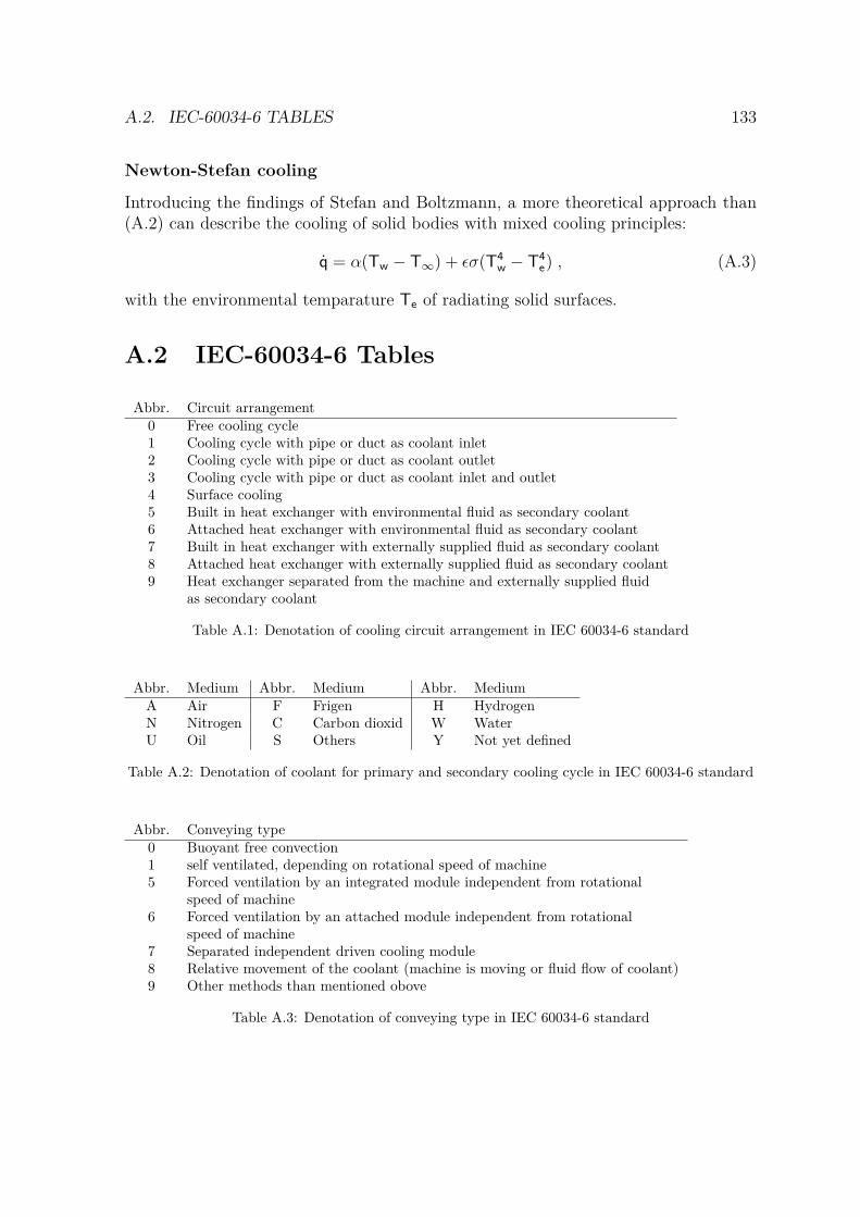
A.2. IEC-60034-6 TABLES 133
Newton-Stefan cooling
Introducing the findings of Stefan and Boltzmann, a more theoretical approach than(A.2) can describe the cooling of solid bodies with mixed cooling principles:
q = α(Tw − T∞) + εσ(T4w − T4
e) , (A.3)
with the environmental temparature Te of radiating solid surfaces.
A.2 IEC-60034-6 Tables
Abbr. Circuit arrangement0 Free cooling cycle1 Cooling cycle with pipe or duct as coolant inlet2 Cooling cycle with pipe or duct as coolant outlet3 Cooling cycle with pipe or duct as coolant inlet and outlet4 Surface cooling5 Built in heat exchanger with environmental fluid as secondary coolant6 Attached heat exchanger with environmental fluid as secondary coolant7 Built in heat exchanger with externally supplied fluid as secondary coolant8 Attached heat exchanger with externally supplied fluid as secondary coolant9 Heat exchanger separated from the machine and externally supplied fluid
as secondary coolant
Table A.1: Denotation of cooling circuit arrangement in IEC 60034-6 standard
Abbr. Medium Abbr. Medium Abbr. MediumA Air F Frigen H HydrogenN Nitrogen C Carbon dioxid W WaterU Oil S Others Y Not yet defined
Table A.2: Denotation of coolant for primary and secondary cooling cycle in IEC 60034-6 standard
Abbr. Conveying type0 Buoyant free convection1 self ventilated, depending on rotational speed of machine5 Forced ventilation by an integrated module independent from rotational
speed of machine6 Forced ventilation by an attached module independent from rotational
speed of machine7 Separated independent driven cooling module8 Relative movement of the coolant (machine is moving or fluid flow of coolant)9 Other methods than mentioned obove
Table A.3: Denotation of conveying type in IEC 60034-6 standard

Appendix B
Fundamentals CFD
B.1 Vector-variable form of the Navier Stokes equa-tions
∂Q∂t
+ ∂E∂x
+ ∂F∂y
+ ∂G∂z
= S (B.1)
Q =
ρρuρvρw
ρ(e + V2
2 )
S =
0ρgx
ρgy
ρgz
ρ(ugx + vgy + wgz) + ρq
(B.2)
E =
ρu
ρu2 + p− τxx
ρuv − τxy
ρuw − τxz
ρ(e + V2
2 ) + pu− uτxx − vτxy − wτxz + qx
(B.3)
F =
ρv
ρuv − τxy
ρv2 + p− τyy
ρvw − τyz
ρ(e + V2
2 ) + pv − uτxy − vτyy − wτyz + qy
(B.4)
G =
ρw
ρuw − τxz
ρvw − τyz
ρw2 + p− τzz
ρ(e + V2
2 ) + pw − uτxz − vτyz − wτzz + qz
(B.5)
134
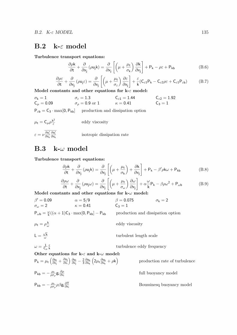
B.2. K-ε MODEL 135
B.2 k-ε modelTurbulence transport equations:
∂ρk
∂t+ ∂
∂xj(ρujk) = ∂
∂xj
[(µ+ µt
σk
)∂k
∂xj
]+ Pk − ρε+ Pkb (B.6)
∂ρε
∂t+ ∂
∂xj(ρujε) = ∂
∂xj
[(µ+ µt
σε
)∂ε
∂xj
]+ ε
k(Cε1Pk − Cε2ρε+ Cε1Pεb) (B.7)
Model constants and other equations for k-ε model:σk = 1 σε = 1.3 Cε1 = 1.44 Cε2 = 1.92Cµ = 0.09 σρ = 0.9 or 1 κ = 0.41 C3 = 1Pεb = C3 ·max[0,Pkb] production and dissipation option
µt = Cµρk2
ε eddy viscosity
ε = ν∂u′
i∂xk
∂u′i
∂xkisotropic dissipation rate
B.3 k-ω modelTurbulence transport equations:
∂ρk
∂t+ ∂
∂xj(ρujk) = ∂
∂xj
[(µ+ µt
σk
)+ ∂k
∂xj
]+ Pk − β′ρkω + Pkb (B.8)
∂ρω
∂t+ ∂
∂xj(ρujω) = ∂
∂xj
[(µ+ µt
σω
)∂ω
∂xj
]+ α
ω
kPk − βρω2 + Pωb (B.9)
Model constants and other equations for k-ω model:β′ = 0.09 α = 5/9 β = 0.075 σk = 2σω = 2 κ = 0.41 C3 = 1Pωb = ω
k ((α+ 1)C3 ·max[0,Pkb]− Pkb production and dissipation option
µt = ρ kω eddy viscosity
L =√
kω turbulent length scale
ω = 1Cµ
εk turbulence eddy frequency
Other equations for k-ε and k-ω model:Pk = µt
(∂ui∂xj
+ ∂uj∂xi
)∂ui∂xj− 2
3∂uk∂xk
(2µt
∂uk∂xk
+ ρk)
production rate of turbulence
Pkb = − µtρσρ
gi∂ρ∂xi
full buoyancy model
Pkb = − µtρσρ
ρβgi∂T∂xi
Boussinesq buoyancy model

136 APPENDIX B. FUNDAMENTALS CFD
B.4 Baseline and Shear Stress Transport ModelB.4.1 Original BSL and SST equations:Model equations as published in [56]
Original k-ω model:
dρk
dt= τij
∂ui
∂xj− β∗ρωk + ∂
∂xj
[(µ+ σk1µt)
∂k
∂xj
](B.10)
dρω
dt= γ1
νtτij∂ui
∂xj− β1ρω
2 + ∂
∂xj
[(µ+ σω1µt)
∂ω
∂xj
](B.11)
Transformed k-ε model:dρk
dt= τij
∂ui
∂xj− β∗ρωk + ∂
∂xj
[(µ+ σk2µt)
∂k
∂xj
](B.12)
dρω
dt= γ2
νtτij∂ui
∂xj− β2ρω
2 + ∂
∂xj
[(µ+ σω2µt)
∂ω
∂xj
]+ 2ρσω2
1
ω
∂k
∂xj
∂ω
∂xj(B.13)
Blending function F1:F1 = tanh(arg4
1) (B.14)
arg1 = min
(max
( √k
β′ωy; 500ν
y2ω
); 4ρk
CDkwσω2y2
)(B.15)
CDkw = max
(2ρ
1
σω2ω
∂k
∂xj
∂ω
∂xj; 1.0 · 10−10
)(B.16)
Blending function F2:F2 = tanh(arg2
2) (B.17)
arg2 = max
( √k
β′ωy; 500ν
y2ω
)(B.18)
Blending the model constants:φ1 = (σk1, . . . ), φ2 = (σk2, . . . ) and φ = (σk, . . . ):
φ = F1φ1 + (1− F1)φ2 (B.19)
BSL and SST k transport equation:
dρk
dt= τij
∂ui
∂xj− β∗ρωk + ∂
∂xj
[(µ+ σkµt)
∂k
∂xj
](B.20)
BSL and SST ω transport equation:
dρω
dt= γ
νtτij∂ui
∂xj− βρω2 + ∂
∂xj
[(µ+ σωµt)
∂ω
∂xj
]+ 2ρσω2
1
ω
∂k
∂xj
∂ω
∂xj(B.21)
Model constants and other equations for BSL and SST model:Constant values for (B.10) and (B.11):

B.5. SCALE ADAPTIVE SIMULATION (SAS) TRANSPORT MODEL 137
σk1 = 0.5 σω1 = 0.5 β1 = 0.075 β∗ = 0.09 κ = 0.41
γ1 = β1/β∗ − σω1κ
2/√β∗
Constant values for (B.12) and (B.13):
σk2 = 1 σω2 = 0.856 β2 = 0.0828 β∗ = 0.09 κ = 0.41
γ2 = β2/β∗ − σω2κ
2/√β∗
BSL and SST transport equations as implemented in ANSYS CFX v13 [4]
∂(ρk)∂t
+ ∂(ρujk)∂xj
= ∂
∂xj
[(µ+ µt
σk
)∂k
∂xj
]+ Pk − β∗ρωk + Pkb (B.22)
∂(ρω)∂t
+ ∂(ρujω)∂xj
= ∂
∂xj
[(µ+ µt
σω
)∂ω
∂xj
]+ (1− F1) 2ρ
σω2ω
∂k
∂xj
∂ω
∂xj+ α
ω
kPk − βρω2 + Pωb
(B.23)
B.5 Scale Adaptive Simulation (SAS) Transport modelTurbulence transport equations as implemented in ANSYS CFX v13 [4]:
∂ρk
∂t+ ∂(ρujk)
∂xj= ∂
∂xj
[(µ+ µt
σk
)∂k
∂xj
]+ Pk − ρCµkω (B.24)
∂ρω
∂t+ ∂(ρujω)
∂xj= ∂
∂xj
[(µ+ µt
σω
)∂ω
∂xj
]+ (1− F1) 2ρ
σω2ω
∂k
∂xj
∂ω
∂xj+ α
ω
kPk − ρβω2 + QSAS
(B.25)Model constants
ζ2 = 3.51 σΦ = 2/3 C = 2 CS = 0.11
Other equationsSAS source term:
QSAS = max[ρζ2κS2
(L
LvK
)2
− C2ρk
σΦmax
(1
ω2
∂ω
∂xj
∂ω
∂xj,
1
k2
∂k
∂xj
∂k
∂xj
), 0
](B.26)
Pk = µtS2 production term
Pk = min(Pk,Climρε) limiting production term with clip factor Clim
Sij = 12
[∂ui∂xj
+ ∂uj∂xi
]strain rate tensor
S =√
2SijSij magnitude of strain rate

138 APPENDIX B. FUNDAMENTALS CFD
L =√
kc1/4µ ·ω
length scale of modeled turbulence
LvK = κSu′′ the von Kármán length scale
|u′′| =√
∂2ui∂x2
k
∂2ui∂x2
jsecond derivative of velocity
B.6 Gamma-Theta transition modelThe formulation of the γ − ReΘ transition model as presented in [49]:Transport equation for intermittency γ:
∂(ργ)∂t
+ ∂(ρujγ)∂xj
= Pγ1 − Eγ1 + Pγ2 − Eγ2 + ∂
∂xj
[(µ+ µt
σγ
)∂γ
∂xj
], (B.27)
Transition sources:
Pγ1 = Flengthca1ρS(γFonset)cα and Eγ1 = ce1Pγ1γ (B.28)
Destruction or relaminarization sources:
Pγ2 = ca2ρΩγFturb and Eγ2 = ce2Pγ2γ (B.29)
Transport equation for transition momentum-thickness Reynolds number ReΘ:
∂(ρReΘ)∂t
+ ∂(ρujReΘ)∂xj
= PΘt + ∂
∂xj
[σΘt(µ+ µt)
∂ReΘ
∂xj
](B.30)
Model constants for γ − ReΘ model:
ce1 = 1.0 ca1 = 2.0 cα = 0.5 ce2 = 50 ca2 = 0.06 σγ = 1.0
S strain rate magnitude
Flength empirical correlation controlling the length of the transition region
Ω vorticity magnitude
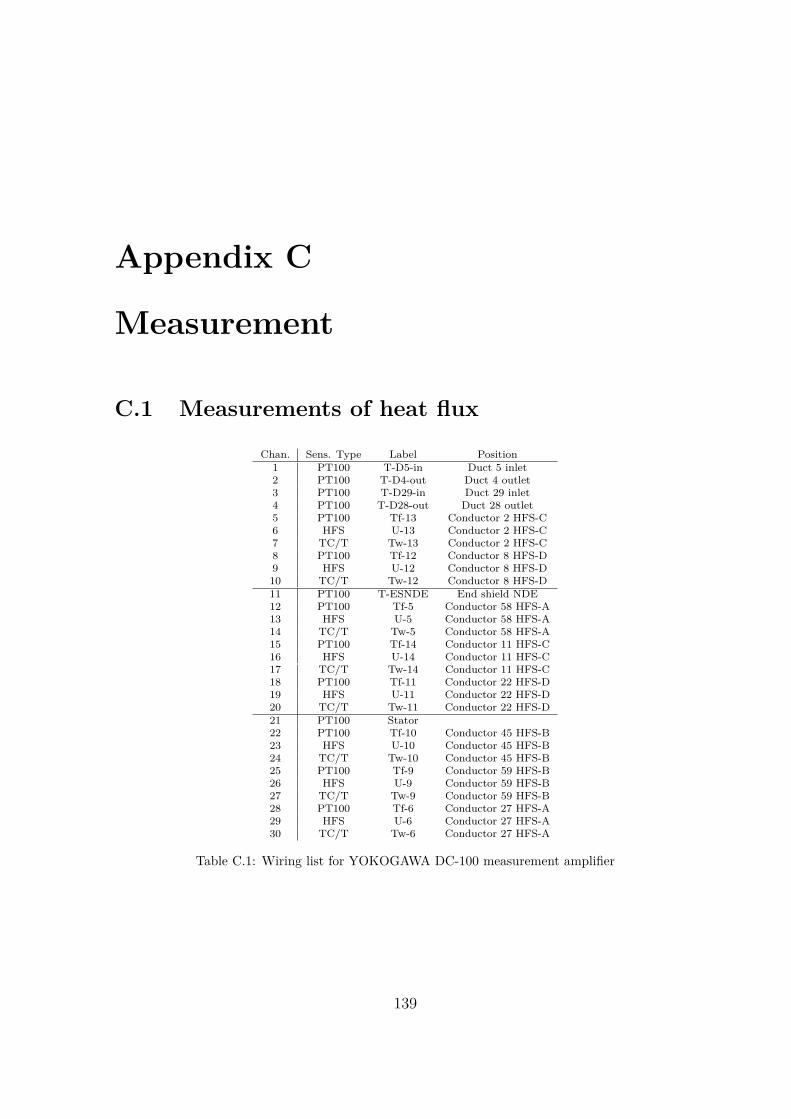
Appendix C
Measurement
C.1 Measurements of heat flux
Chan. Sens. Type Label Position1 PT100 T-D5-in Duct 5 inlet2 PT100 T-D4-out Duct 4 outlet3 PT100 T-D29-in Duct 29 inlet4 PT100 T-D28-out Duct 28 outlet5 PT100 Tf-13 Conductor 2 HFS-C6 HFS U-13 Conductor 2 HFS-C7 TC/T Tw-13 Conductor 2 HFS-C8 PT100 Tf-12 Conductor 8 HFS-D9 HFS U-12 Conductor 8 HFS-D10 TC/T Tw-12 Conductor 8 HFS-D11 PT100 T-ESNDE End shield NDE12 PT100 Tf-5 Conductor 58 HFS-A13 HFS U-5 Conductor 58 HFS-A14 TC/T Tw-5 Conductor 58 HFS-A15 PT100 Tf-14 Conductor 11 HFS-C16 HFS U-14 Conductor 11 HFS-C17 TC/T Tw-14 Conductor 11 HFS-C18 PT100 Tf-11 Conductor 22 HFS-D19 HFS U-11 Conductor 22 HFS-D20 TC/T Tw-11 Conductor 22 HFS-D21 PT100 Stator22 PT100 Tf-10 Conductor 45 HFS-B23 HFS U-10 Conductor 45 HFS-B24 TC/T Tw-10 Conductor 45 HFS-B25 PT100 Tf-9 Conductor 59 HFS-B26 HFS U-9 Conductor 59 HFS-B27 TC/T Tw-9 Conductor 59 HFS-B28 PT100 Tf-6 Conductor 27 HFS-A29 HFS U-6 Conductor 27 HFS-A30 TC/T Tw-6 Conductor 27 HFS-A
Table C.1: Wiring list for YOKOGAWA DC-100 measurement amplifier
139