Rubber friction, tread deformation and tire traction

This article appeared in a journal published by Elsevier. The attachedcopy is furnished to the author for internal non-commercial researchand education use, including for instruction at the authors institution

and sharing with colleagues.

Other uses, including reproduction and distribution, or selling orlicensing copies, or posting to personal, institutional or third party

websites are prohibited.

In most cases authors are permitted to post their version of thearticle (e.g. in Word or Tex form) to their personal website orinstitutional repository. Authors requiring further information

regarding Elsevier’s archiving and manuscript policies areencouraged to visit:

http://www.elsevier.com/copyright

http://www.elsevier.com/copyright

Author's personal copy

Wear 265 (2008) 1052–1060

Contents lists available at ScienceDirect

Wear

journa l homepage: www.e lsev ier .com/ locate /wear

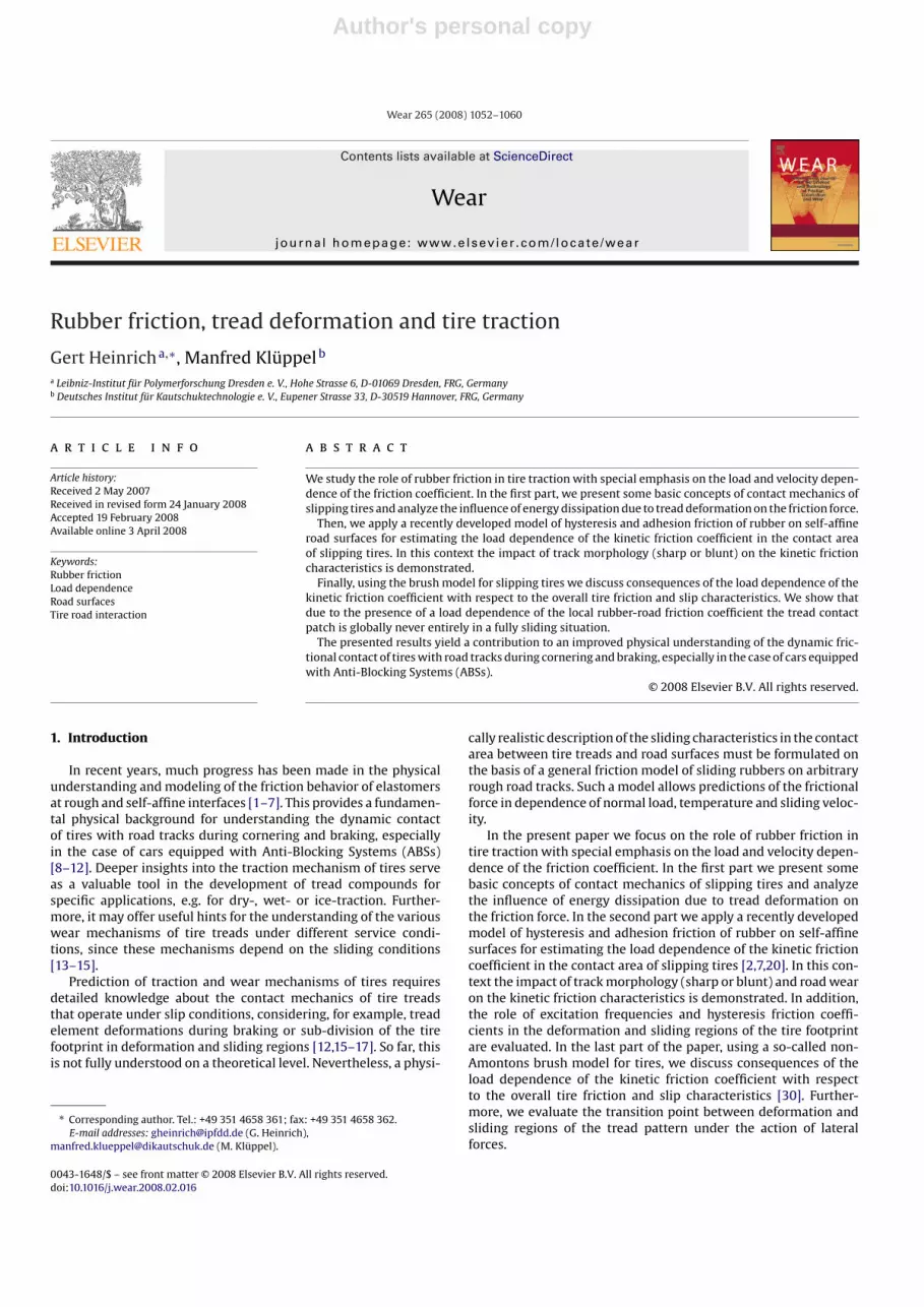
Rubber friction, tread deformation and tire traction

Gert Heinricha,∗, Manfred Kluppelb

a Leibniz-Institut fur Polymerforschung Dresden e. V., Hohe Strasse 6, D-01069 Dresden, FRG, Germanyb Deutsches Institut fur Kautschuktechnologie e. V., Eupener Strasse 33, D-30519 Hannover, FRG, Germany

a r t i c l e i n f o

Article history:Received 2 May 2007Received in revised form 24 January 2008Accepted 19 February 2008Available online 3 April 2008

Keywords:Rubber frictionLoad dependenceRoad surfacesTire road interaction

a b s t r a c t

We study the role of rubber friction in tire traction with special emphasis on the load and velocity depen-dence of the friction coefficient. In the first part, we present some basic concepts of contact mechanics ofslipping tires and analyze the influence of energy dissipation due to tread deformation on the friction force.

Then, we apply a recently developed model of hysteresis and adhesion friction of rubber on self-affineroad surfaces for estimating the load dependence of the kinetic friction coefficient in the contact areaof slipping tires. In this context the impact of track morphology (sharp or blunt) on the kinetic frictioncharacteristics is demonstrated.

Finally, using the brush model for slipping tires we discuss consequences of the load dependence of thekinetic friction coefficient with respect to the overall tire friction and slip characteristics. We show thatdue to the presence of a load dependence of the local rubber-road friction coefficient the tread contactpatch is globally never entirely in a fully sliding situation.

The presented results yield a contribution to an improved physical understanding of the dynamic fric-tional contact of tires with road tracks during cornering and braking, especially in the case of cars equippedwith Anti-Blocking Systems (ABSs).

© 2008 Elsevier B.V. All rights reserved.

1. Introduction

In recent years, much progress has been made in the physicalunderstanding and modeling of the friction behavior of elastomersat rough and self-affine interfaces [1–7]. This provides a fundamen-tal physical background for understanding the dynamic contactof tires with road tracks during cornering and braking, especiallyin the case of cars equipped with Anti-Blocking Systems (ABSs)[8–12]. Deeper insights into the traction mechanism of tires serveas a valuable tool in the development of tread compounds forspecific applications, e.g. for dry-, wet- or ice-traction. Further-more, it may offer useful hints for the understanding of the variouswear mechanisms of tire treads under different service condi-tions, since these mechanisms depend on the sliding conditions[13–15].

Prediction of traction and wear mechanisms of tires requiresdetailed knowledge about the contact mechanics of tire treadsthat operate under slip conditions, considering, for example, treadelement deformations during braking or sub-division of the tirefootprint in deformation and sliding regions [12,15–17]. So far, thisis not fully understood on a theoretical level. Nevertheless, a physi-

∗ Corresponding author. Tel.: +49 351 4658 361; fax: +49 351 4658 362.E-mail addresses: [email protected] (G. Heinrich),

[email protected] (M. Kluppel).

cally realistic description of the sliding characteristics in the contactarea between tire treads and road surfaces must be formulated onthe basis of a general friction model of sliding rubbers on arbitraryrough road tracks. Such a model allows predictions of the frictionalforce in dependence of normal load, temperature and sliding veloc-ity.

In the present paper we focus on the role of rubber friction intire traction with special emphasis on the load and velocity depen-dence of the friction coefficient. In the first part we present somebasic concepts of contact mechanics of slipping tires and analyzethe influence of energy dissipation due to tread deformation onthe friction force. In the second part we apply a recently developedmodel of hysteresis and adhesion friction of rubber on self-affinesurfaces for estimating the load dependence of the kinetic frictioncoefficient in the contact area of slipping tires [2,7,20]. In this con-text the impact of track morphology (sharp or blunt) and road wearon the kinetic friction characteristics is demonstrated. In addition,the role of excitation frequencies and hysteresis friction coeffi-cients in the deformation and sliding regions of the tire footprintare evaluated. In the last part of the paper, using a so-called non-Amontons brush model for tires, we discuss consequences of theload dependence of the kinetic friction coefficient with respectto the overall tire friction and slip characteristics [30]. Further-more, we evaluate the transition point between deformation andsliding regions of the tread pattern under the action of lateralforces.

0043-1648/$ – see front matter © 2008 Elsevier B.V. All rights reserved.doi:10.1016/j.wear.2008.02.016


G. Heinrich, M. Kluppel / Wear 265 (2008) 1052–1060 1053

Fig. 1. Schematic view of tread deformation during ABS-braking.

2. Contact mechanics and friction of slipping tires

Investigations of tread element deformation and sliding veloc-ity distribution during cornering or ABS-braking of slipping tires,e.g. experimentally by electronic sensor techniques or, theoreti-cally, by Finite Element (FE)-simulations, have demonstrated thatthe relative slip between tires and road tracks can be split into twomain contributions: (i) a so called tread deformation regime in thefront part of the contact patch, where the sliding velocity is almostzero, and (ii) a tread sliding regime in the rear part of the con-tact patch where the sliding velocity is almost equal to the slipvelocity [15–19]. The slip is generally defined as S ≡ (vx − vc)/vx,where vx is the vehicle velocity, corresponding to the track or drumspeed in a co-moving frame of the tire axis (indoor drum test),and vc is the tread base velocity in the same co-moving axis sys-tem. Accordingly, the slip velocity v = vx − vc can be divided into amean tread deformation velocity vd and a mean sliding velocity vs

(v = vd + vs). Both of these velocities are averaged over the contactlength l ≡ L + d, where L is the footprint length and d the horizontaltread deformation length (Fig. 1).

A fundamental characteristic of tire–road contact mechanicsis the braking or side force coefficient, usually in tire technologydenoted as �–slip curve, describing the behavior of slipping tiresunder cornering or ABS-conditions. It is well known that for smallslip values (S < 0.05) the �–slip curves of tires depend only on thetread stiffness but not on the vehicle velocity or the morphologicaldetails of the track affecting the traction behavior. This has clearlybeen shown by various indoor tests applying different tire typesand surface morphologies under dry and wet conditions [15–17].The role of vehicle speed and tread stiffness in �–slip curves isdepicted schematically in Fig. 2.

The independence of the initial slope of longitudinal �–slipcurves on vehicle speed can be used for an estimation of the slidingvelocity in the tread deformation regime. The mean deformation

Fig. 2. Characteristic shape of �–slip curves of tires, indicating the influence of treadstiffness and vehicle speed, respectively.

velocity vd = d/t∗ is given by the ratio between tread deformation dand contact time of the tread elements t∗ = l/vc = (L + d)/(vx − v).This implies for the slip:

S ≡ v

vx= vs

vx+ d/L

1 + (d/L)

(1 − v

vx

)(1)

Generally, the relation (d/L) < 10−1 is fulfilled, and for small slipvalues it holds v � vx, implying for the slip S ≈ (vs/vx) + (d/L). Thisexpression becomes independent of vehicle speed only if (vs/vx) �(d/L) < 10−1. It means that for small slip values the mean slidingvelocity vs is at least two or three orders of magnitude smaller thanthe vehicle velocity vx. Accordingly, the initial slope of the longi-tudinal �–slip curves simply reflects the stiffness Fx/d of the treadelements, where Fx is the horizontal force acting on the tread ele-ments. Note, we do not discuss cornering where Fx would play therole of lateral force.

The frictional force acting on a slipping tire can be evaluatedby adding the different contributions of energy dissipation in thetire, which transmits force between car and road track. First weconsider the energy dissipation resulting from energy dissipationmechanisms in the contact area. We anticipate that this mechanismwill be identified as the dominant one. However, an additional con-tribution comes from the hysteresis of the deformed tread materialwhich has not been discussed so far in the literature. This contri-bution results from the fact that the energy stored in the deformedtread elements is not fully recovered when the elements relax afterdetachment from the track. Accordingly, the mechanically effectivefriction coefficient can be split into two contributions:

� ≡ Fx

FN= �C + �D (2)

where �C comes from energy dissipation mechanisms in the con-tact area (compare Section 4) and �D considers the viscoelasticenergy dissipation �Ediss due to tread element deformation:

�D = �Ediss

FNl= �G′′(�0, ω, T)�2

0 A0h

FNl(3)

Here, �Ediss/l is a longitudinal friction force over the contact lengthdue to the dynamical tread element deformation. Fx is the total hor-izontal force acting on the tread elements, FN is the normal load,G′′ is the loss part of the complex shear modulus G*, ω is frequency,T is temperature, h is the (excited) tread height, �0 is the maxi-mum shear strain of the tread elements, A0 is the apparent footprint area and l = L + d is the characteristic length scale, at which thedeformation induced energy dissipation takes place. For slip valuesS � 1, as normally realized during cornering or ABS-braking, it canbe identified with the footprint length L (l = L/(1 − S) ≈ L). Since

�0 = �C�0

|G∗(�0, ω, T)| (4)

one obtains with the apparent normal pressure �0 = FN/A0:

� ≈ �C

(1 + ��0h�C

LJ′′(�0, ω, T)

)(5)

with the stress-, frequency- and temperature-dependent loss partof the shear compliance:

J′′(�0, ω, T) = G′′(�0, ω, T)|G∗(�0, ω, T)|2 (6)

With this consideration the frictional contribution of tread defor-mation �D to the effective horizontal force acting on the vehicle canbe estimated. For passenger cars the pressure in the footprint area isapproximately �0 ≈ 0.3 MPa; and the loss part of the shear compli-ance of a typical tread compound measured at constant stress �0,frequency ω ≈ 10 Hz, corresponding to a vehicle velocity of about


1054 G. Heinrich, M. Kluppel / Wear 265 (2008) 1052–1060

80 km/h, and operation temperature T ≈ 60–70 ◦C is found in therange of J” ≈ 3 × 10−7 Pa−1. With a friction coefficient on dry roadtracks �C ≈ 1 and L ≈ 10 h one obtains from Eq. (5) � ≈ 1.03 �C, i.e.the effective friction coefficient is about 3% larger than the frictioncoefficient due to energy dissipation in the contact area. For thetraction of tires on wet roads, snow or ice the contribution of energydissipation due to tread deformation is even smaller. This makesit clear that tread deformation of slipping tires provides no directadvantage concerning safety during cornering or ABS-braking byincreasing the effective friction coefficient, significantly. Instead,secondary effects, which are related to the small sliding velocity inthe front part of the contact patch (deformation region) supportingadhesion, dewetting or hydroplaning may play a more importantrole. Therefore, in the following we will ignore the contribution �Dthat takes into account the viscoelastic energy dissipation due totread deformation and we use � = �C.

3. Kinetic rubber friction coefficient on rough road surfaces

It is well known that the kinetic friction coefficient of rubbersliding on rough surfaces depends on sliding velocity, tempera-ture and normal load [15–24]. The velocity, temperature and loaddependence results directly from the viscoelastic response of theelastomeric material, reflecting the viscoelastic origin of rubberfriction. The load dependence of the friction coefficient includesthe effect of the rubber modulus. Furthermore, the load depen-dence can be referred to the surface and rubber specific formationof contact spots and may differ significantly for various road sur-face profiles [20,21]. A secondary source of load dependence canbe the friction induced thermal heating in the contact area leadingto a reduction of the friction coefficient with increasing load [22].In the following we will consider the predictions of friction the-ory and contact mechanics of elastomers on self-affine surfaces toget a deeper insight into the impact of load on the kinetic frictioncoefficient.

It is now well established that the concept of self-affinity canbe applied to characterize the texture of many rough (includingroad) surfaces [1–8,10–12,20]. Self-affine surfaces exhibit an invari-ant behavior under anisotropic dilation in vertical and horizontaldirections. This is represented by the surface fractal dimension D(2 ≤ D ≤ 3), constituting a quantitative measure of the surface irreg-ularities for length scales smaller than the two correlation lengths�⊥ and �||. For an estimation of these three surface descriptors onecan refer to the height-difference correlation function Cz(), rep-resenting the mean square height fluctuations with respect to thehorizontal length scale [2,3]:

Cz(l) = 〈(z(x + l) − z(x))2〉 (7)

Here, the average 〈. . .〉 is taken over the (statistical) realizationsof the surface profile z(x). In the case of self-affine surfaces oneobserves a power law dependence for the height-difference cor-relation function with an exponent determined by the fractaldimension D:

Cz() = �2⊥

(

�||

)6−2D

for l < �|| (8)

For ≥ �|| a plateau value �2⊥ is reached that corresponds to the

variance �2 = (1/2) �2⊥ of the roughness profile [2]. Both length

scales �⊥ and �|| describe the maximum roughness parallel and per-pendicular to the profile, below which self-affinity is fulfilled. Theevaluation of the three surface descriptors of self-affine surfaces,the fractal dimension D and the two cut-off lengths �⊥ and �||, isillustrated in Fig. 3 for the profile of a low-� blunt asphalt track ascharacterized by laser measurements.

Fig. 3. Example of a laser measurement of the profile (a) and corresponding heightdifference correlation function averaged over a large number of profiles (b) of a low-� blunt asphalt track. The fractal descriptors D = 2.35, �⊥ = 1.18 mm, �|| = 4.2 mm areindicated.

The spectral power density S(f) equals the Fourier transform ofthe auto-correlation function and represents a second indepen-dent method of fractal surface analysis [2]. Here, f = (1/) beingthe spatial frequency. The spectral power density S(f), required forthe estimation of the hysteresis friction coefficient, is analyticallyderived in a similar manner as a function of the surface descriptorsD, �⊥ and �||. In the case of small spatial frequencies f < fmin, S(f) isconstant while for large spatial frequencies one finds for self-affinesurfaces the scaling form [2]:

S(f ) = k(

f

fmin

)2D−7

for f > fmin (9)

Here, fmin = �−1|| corresponds to the horizontal cut-off length.

The pre-factor k = (3 − D) �2⊥ �|| is also termed “topothesy”. It was

recently demonstrated for different elastomer composites that thekinetic friction coefficient on various dry and wet road tracks canassumed to be dominated by two main contributions, the hysteresisand adhesion contribution [32]:

�k = �Hys + �Adh (10)

This approach appears reasonable as long as the vehicle speed onwet roads is not too large and the abrasion of rubber particles issmall, i.e. the contributions of viscous dissipation in the lubricantand cohesive friction can be neglected. Accordingly, the load depen-dence of the kinetic friction coefficient is affected by hysteresis andadhesion effects. The rubber hysteresis is described by an integralover the interval of mechanical excitation frequencies [ωmin, ωmax].Its amount is determined by the load, velocity and temperaturedependent length interval of contact [�||, min] [2,3,5,7,20]:

�Hys ≡ FHys

FN= 1

2(2�)2

〈ı〉�ovs

∫ ωmax

ωmin

dω ω G′′(ω) S(ω) (11)

Here, G′′(ω) is the loss modulus of the rubber material, S(ω) isthe spectral power density of the road roughness spectra in thefrequency domain, vs is the sliding velocity, �0 is the normal pres-sure and 〈ı〉 is the mean thickness of the excitation rubber layer.The minimum angular frequency ωmin = 2� vs/�|| is determined



by the horizontal cut-off length of the roughness spectra �|| andthe maximum angular frequency ωmax = 2� vs/min depends onthe minimum coupling length min, which is strongly affected bythe load (see below). We point out that for non-linear, filled rub-ber materials the amplitude of the deformation cycles of G′′(ω) inEq. (11) has to be adjusted to the conditions of hysteresis frictionexcitation, e.g. the applied load.

For typical contact pressures �0 = 0.3 MPa in the footprint ofa passenger tire the frequency interval of contact extends overabout three decades. In this range of applications the influence ofload on the integral value of Eq. (11) is small and the load depen-dence of the hysteresis friction coefficient is governed by that ofthe front factor 〈ı〉/�0 [20]. Both of these quantities depend onthe Greenwood–Williamson functions Fn(t), describing the con-tact mechanics of rubber materials with rough surfaces via theheight distribution function of the track [31]. A generalization ofthe Greenwood–Williamson theory to viscoelastic contact of elas-tomers at self-affine interfaces leads to the following expressions[2,20]:

〈ı〉 ∼ 〈zp〉 = �F1

(d

�

)(12)

�0 ≈ 0.53�⊥|G∗(ωmin)|�s3/2�||

F3/2

(ds

�s

)(13)

with the Greenwood–Williamson functions Fn(t) defined as follows[31]:

Fn(t) =∫ ∞

t

(z − t)n(z) dz with n = 0, 1,32

(14)

Here, d is the load-dependent mean gap distance between therubber and the mean height of the road track, (z) is the heightdistribution of the track, � is the variance of the height distribution,〈zp〉 is the mean penetration depth of the rubber, |G*(ωmin)| is thenorm of the complex modulus at minimum excitation frequencyand �⊥ is the vertical cut-off length of the roughness spectra. Theindex s for ds, s(z) and �s indicates a transition to the height distri-bution of the track summits on the largest roughness scale, whichcan be obtained by applying an affine transformation with an affinescaling factor s [20]. The consideration of this modified distributions(z) for the calculation of the normal pressure by Eq. (13) is nec-essary to insure that adjacent asperities act widely independenton the rubber. This is fulfilled due to the restriction to the contactor pressure ranges formed by the largest asperities, which can beconsidered to be sufficiently separated from each other. This is anecessary condition for applying the Greenwood–Williamson con-cept by calculating the total normal pressure as a sum of individual,non-intersecting stress fields of the rubber [20].

Fig. 4 shows examples of height distributions of two differentasphalt tracks, a high-� sharp track and a low-� blunt track, asobtained from laser measurements on a large number of differentspatial locations of the tracks. As usual, the mean height of the dis-tributions are chosen as zero profile height. We point out that bothdistributions differ significantly from a Gaussian distribution andshow quite different characteristics: First, the variance of the sharptrack is smaller than that of the blunt track, indicating that the lateris made of coarse asphalt. Furthermore, the high-� track is quitesymmetric and the low-� track more asymmetric. This asymmetryreflects the fact that the low-� blunt track is a worn asphalt track,which is already strongly abraded by the traffic. This is indicated bythe steep increase of the distribution function on the right hand sidereferring to the top side of the track. The different shape of the twodistribution functions has consequences on the load dependenceof the hysteresis friction coefficient Eq. (11), since the front fac-tor (〈ı〉/�0) ∼ (F1/F3/2) behaves differently. This is demonstrated in

Fig. 4. Height distribution of two asphalt road tracks as found from laser triangula-tion measurements.

Fig. 5, where the ratio of Greenwood–Williamson functions F1/F3/2is plotted against the normalized gap distance t. The simulationsfor the two asphalt tracks were obtained in range of pressure values�0 = 0.1–0.6 MPa. The simulations for the two corundum tracks, acoarse one (EKW 60) and a fine one (EKW 180), also shown in Fig. 5,were obtained in the pressure range �0 = 20–200 kPa. Note that forthe low-� track the normalized gap distance t = d/� changes muchless as compared to the high-� track or the corundum tracks dueto the larger value of the normalization factor � (variance) of thelow-� track.

Fig. 5 demonstrates that the front factor (〈ı〉/�0) ∼ (F1/F3/2) ofthe hysteresis friction coefficient decreases with increasing load(decreasing surface distance) in the case of the high-� asphaltsharp track, when the generalized Greenwood–Williamson the-ory of elastic contact at self-affine interfaces is applied. A similarbehavior is observed for the two depicted sharp corundum tracks.However, the low-� blunt asphalt track shows the opposite behav-ior, i.e. a slightly increasing front factor of the hysteresis frictioncoefficient with increasing load. This behavior is traced back to theasymmetric shape of the height distribution function of the wornblunt track. Experimental evidence for the predicted opposite char-acteristics of sharp and blunt tracks has been already reported by

Fig. 5. Dependence of the front factor (〈ı〉/�0) ∼ (F1/F3/2) of the hysteresis frictioncoefficient Eq. (11) on the normalized gap distance t = d/� for the two asphalt roadtracks of Fig. 4 and two corundum tracks EKW 60 and EKW 180, respectively.



Grosch who measured the load dependence of the friction coeffi-cient of different tread compounds on sharp and blunt corundumsurfaces and on blunt glass surfaces using the so-called Grosch-Wheel-Tester [21].

As indicated before, the influence of load on the integral valueof the hysteresis friction coefficient Eq. (11) is small for largepressures. Then, the load dependence of the hysteresis friction coef-ficient is governed by that of the front factor 〈ı〉/�0 depicted in Fig. 5.However, in the low pressure range the influence of load on theintegral value of Eq. (11) cannot be neglected and impacts the loaddependence of the hysteresis friction coefficient, as well. In partic-ular, this leads to a less moderate increase of the hysteresis frictioncoefficient with decreasing load as compared to that predicted bythe front factors for the two corundum tracks. In the framework ofour generalized Greenwood–Williamson theory of viscoelastic con-tact at self-affine interfaces one obtains for the minimum couplinglength min the following expression [2,20]:

min

�||=

(0.09�s3/2�⊥(2D − 4)|G∗(min)|F0(d/�)

�||(2D − 2)|G∗(�||)|F3/2(ds/�s)

)1/(3D−6)

(15)

where we used the notation |G*(min)| = |G*(ωmax)| with ωmax = 2�vs/min and |G*(�||)| = |G*(ωmin)| with ωmin = 2� vs/�||. According toEq. (15), the load dependence of the minimum coupling lengthis given by the ratio of the Greenwood–Williamson functionsmin ∼ (F0/F3/2)1/(3D−6), implying that the load dependence of minbecomes weaker with increasing fractal dimension D. For almostflat surfaces when the fractal dimension approaches the limitingvalue D = 2, min becomes very sensitive for load variations. Theexplicit behavior, e.g. a decreasing or increasing characteristic ofthe load dependence of min, is again affected by the shape of theheight distribution of the track under consideration.

In this paper we will not focus on these track specific effectson min, but apply the predictions of Eq. (15) more generally to thecontact mechanics of slipping tires. Typically, at normal pressure�0 ≈ 0.3 MPa and sliding velocity vs ≈ 1 m/s, as realized in thesliding regime of the tire footprint, the length interval of contact[�||, min] as well as the interval of excitation angular frequencies[ωmin, ωmax] extends approximately about four decades. Further-more, in the case of sharp tracks it decreases by about one decadeif the normal load is reduced by a factor of 10. In the followingwe assume that the sliding velocity in the deformation regime ofthe tire footprint can be approximated by vs ≈ 0.01 m/s, i.e. twoorders of magnitude smaller than in the sliding regime. This isin agreement with the result obtained in Section 2, stating thatthe sliding velocity vs in the deformation regime is at least twoto three orders of magnitude smaller than the vehicle velocityvx ≈ 10 m/s. Then, one obtains an interval of excitation angularfrequencies [ωmin, ωmax] that extends over about five decades witha maximum frequency ωmax shifted to lower frequencies by aboutone decade compared to the sliding regime.

The two intervals of excitation frequencies in the deformationand sliding regions of a passenger car tire footprint are indicatedin Fig. 6 where viscoelastic master curves of the dynamic mod-uli |G*(ω)| and G′′(ω) of an E-SBR sample with 60 phr carbon black(N339) are displayed. The master curves in Fig. 6 have been obtainedfrom dynamic-mechanical measurements with strip samples at1 Hz and 3% strain (Rheometrics RDA II) by applying a horizontalas well as vertical shifting procedure. This shifting procedure forfilled elastomers is considered more closely in Ref. [7] where thevertical shifting is shown to be related to a thermal activation ofthe filler network. The evaluated contact intervals via Eq. (15) areindicated by the two rectangles in Fig. 6, reflecting the dependenceon the dynamical stiffness ratio, i.e. ratio of amount of complexmoduli |G*(min)|/|G*(�||)|. With these intervals of contact the hys-

Fig. 6. Viscoelastic master curves of E-SBR rubber samples with 60 phr carbon black(N339) and the corresponding calculated frequency regimes of dynamic-mechanicalexcitation (Eq. (15)) in the deformation and sliding regions of a passenger tire foot-print.

teresis friction coefficients Eq. (11) in the deformation and slidingregions of the tire footprint can be calculated by integrating overthe corresponding frequency regimes of the loss modulus G′′. Fortypical tread compounds sliding over a sharp or blunt road trackthis procedure yields characteristic values for the hysteresis fric-tion coefficients that differ, approximately, by a factor of 3. Thesignificant lower friction values in the deformation region, whichare found for the maximum possible sliding velocity vs ≈ 0.01 m/s,may lead to the conclusion that hysteresis friction does not playa dominant role in the front part of the tire footprint where treaddeformation governs the tire slip. Nevertheless, the deformationregion is important for controlling the car during braking and steer-ing maneuvers especially on wet tracks, since the water is squeezedout of the contact area during the relatively long contact time inthis region. Furthermore, for the larger sliding velocities realized inthe sliding region (vs ≈ 1 m/s), hysteresis induced thermal heatingimplies a decrease of the friction coefficient, which is not consid-ered in the above evaluation using the isothermal approach Eq. (11).

It is widely accepted that hysteresis friction is the main factorof tire grip on wet road tracks, where adhesion plays a minor role.However, on dry tracks adhesion gives an additional significant con-tribution to tire traction that scales with the load-dependent realarea of contact Ac [7,32]:

�Adh = FAdh

FN= �s

�0

Ac

A0(16)

Here, �s is the true shear stress in the real contact area that resultsfrom molecular energy dissipation mechanisms of the rubber inthe contact patches. A discussion of possible dissipation mecha-nisms is given in [7] and [32], where experimental friction dataof rubbers on dry and lubricated tracks measured for low slidingvelocities are shown to be in fair agreement with the friction modelunder consideration. The load dependence of the real contact areais again determined by the Greenwood–Williamson Functions Fn(t)[2,7,20]:

Ac(min) = A0

((2D − 4)2�||F2

o (d/�)F3/2(ds/�s)|G∗(�||)|808�s3/2(2D − 2)2�⊥|G∗(min)|

)1/3

(17)

According to Eqs. (13), (16) and (17) the load dependence ofthe adhesion friction coefficient scales with the ratio of theGreenwood–Williamson Functions �Adh ∼ (F0/F3/2)2/3. This is quitesimilar to the scaling behavior of min, implying that for sharptracks the adhesion friction coefficient decreases with increasingload. However, the behavior of the function F0/F3/2 is again affected



by the shape of the height distribution of the track. Accordingly, theload dependence of blunt tracks can show just the opposite behav-ior. Note that the scaling exponents of �Adh and min are equal in thespecial case of a Brownian surface with fractal dimension D = 2.5.For more realistic values of the fractal dimension D ≈ 2.1–2.3 theexponents of �Adh is significantly smaller than that of min, indi-cating that the load dependence of �Adh is less pronounced thanthat of min.

4. The non-Amontons brush model of tire traction

In this section we discuss some essential consequences of theload dependence of the friction coefficient with respect to tire char-acteristics. We restrict our discussion to the longitudinal force–slipcharacteristics. Within the brush model two main assumptions aremade: (i) each element of the tire can deflect independently and (ii)the magnitude of the deflection is proportional to the force actingon it (see, for example [23,24]).

We further assume a parabolic pressure distribution in the cir-cumference direction over the contact patch within the footprintarea (Fig. 7):

p(�) = 4pm�

l

(1 − �

l

)(18)

where the �-axis represents the longitudinal displacement of a tire,l is the contact length of the tire tread, and pm is the maximum valueof the contact pressure distribution occurring at � = (l/2). We areaware that it is more realistic to use an elliptical pressure distribu-tion [23] instead of a parabolic one. Basically, this can be consideredin the following model. However, this will complicate a physicaldiscussion with numerical solutions because no final transparentanalytical solutions can be found in this case.

The tire-surface slip S during braking is introduced in Eq. (1)where vx is the vehicle speed (the drum speed) and vc is the speedof the tire tread base.

We can calculate a shear deformation, a shear force and a slidingforce. When a braking force is applied, an adhesion region and asliding region occur on the contact patch, where a is the adhesionlength on the contact patch (Fig. 7).

Fig. 7. Visualization of the parabolic pressure distribution in the circumferentialdirection over the contact patch in the footprint area. The breakaway point � = acharacterizes the point at which the longitudinal stresses of the deformation andsliding regions become equal.

Within the deformation region (0 ≤ � ≤ a) we have the simpleexpression for the longitudinal shear stress [23]:

�(A)�

= kx �� = kx Sa � (19)

where kx is a longitudinal stiffness rate per unit area of tread rub-ber (=modulus per length in N/m3). Within the model, kx has thephysical meaning of a spring constant per unit area.

In Eq. (19) we have introduced the adhesional slip factor

Sa ≡ S

1 − S= vx − vc

vc(20)

We give an argument for the deformation (adhesional) slip factorwhich focuses on the time development. Let vx be the velocity of thevehicle and let vc be the rolling velocity which is the speed of tiretread base within our model. Then the slip velocity is v = vx − vc.Now, consider a rubber block. Assume that it comes in contactwith the road at time t = 0. The block will be in contact with theroad for a time t* determined by the rolling velocity: vc t = l, wherel is the length (in the rolling direction) of the tire–road contactarea. Thus t∗ = l/vc. At time t the top surface of the rubber blockwill be at � = vc t (so that � = 0 at t = 0 and � = l at t = t*). The dis-placement of the top surface of the rubber block in the contactarea relative to the road is given by v t. Thus, in the deforma-tion region (no slip at the block–road interface) the shear stressbeing:

� = kxv t = kxv�

vc= kx

v

vc� = kx

[vx − vc

vc

]�

= kx

[vx − vc

vx

](vx

vc

)� = kx

S

1 − S�

since (vx/vc) = 1/(1 − S). This is again the result of Eq. (19) (see alsoremarks in Ref. [25]).

The stick area extends between 0 ≤ � ≤ a, where a is determinedby the static shear stress:

�(A)�

= kx Sa a = �s p(a) (21a)

where �S is the static friction coefficient and p(�) is the pressureprofile in the contact region.

In the sliding region (a < � ≤ l) the longitudinal frictional stressacts, i.e.

�(S)�

= �k p(�) (21b)

where �k is the kinetic friction coefficient.In the case of Amontons and Coulombian friction the kinetic

friction coefficient �k is a constant value �0. However, consid-ering the pressure dependence of the rubber friction coefficient(non-Amontons case [30]) leads – in a simple phenomenologicalapproach – to [26]:

�k ≡ �k(p(�)) = �0

(p(�)pm

)−n

(22)

where �0 is the reference value. For n = 0 we have againthe simple case of Amontons-friction. A model which assumesthat the rubber slides over equally spaced- and sized hemi-spheres, using Hertz’s equation of pressure distribution, yieldsn = +1/3 [27]. Several specific and different situations of pres-sure dependence of the friction coefficient are discussed in Ref.[28].

Combining Eqs. (21b) and (22) yields the longitudinal frictionalstress:

�(S)�

= �0 pm

(p(�)pm

)1−n

(23)



The maximum value of the contact pressure, pm, is related to thevertical (normal) load FN as follows:

FN = w

∫ l

0

p(�) d� = 23

wpml (24)

which gives

pm = 3FN

2wl(25)

where w being the width of the contact patch.The braking force Fx can be estimated as follows:

Fx = w

∫ a

0

�(A)�

d� + w

∫ l

a

�(S)�

d� (26)

which gives

Fx = kxSaa2

2+ 41−n�0pml

∫ 1

˛a=(a/l)

(x(1 − x))1−n dx (27)

where x = (�/l). The quantity ˛a = (a/l) is called adhesion ratio whichis related to the sliding ratio of the contact patch, ˛s, as follows:˛s = (1 − ˛a).

To find the breakaway point (� = a), we locate the point at whichthe longitudinal stresses of the deformation and sliding regionsbecome equal, i.e. �(a)

�= �(S)

�. Putting � = a and substituting above

Eqs. (21)–(23) gives:

�sFzl

2

[4

a

l

(1 − a

l

)]1−n

= CsSaa (28)

where

Cs = 12

wl2kx (29)

Now we can discuss the relationship between the adhesional slipfactor (Sa), respectively slip (S), and the sliding ratio (˛s). For thetrivial case n = 0 we immediately obtain:

˛s ≡ 1 − a

l= SaCs

3�sFz= Sa

S∗a,C

(30)

where

S∗a,C ≡ 3�sFz

Cs(31)

denotes the critical adhesional slip factor in the Amontons-casen = 0. Physically, it follows immediately from the boundary condi-tions when a small rubber block within the contact area comes intocontact with the road:

lim�→0

d�(a)�

d�= lim

�→0

d�(s)�

d�

For Sa equal to the critical adhesional slip factor S∗a,C we find a sliding

ratio ˛s = 1, i.e. an adhesion ratio ˛a = 0. When the length a becomes0, the tread contact patch is entirely in a sliding condition. Thecorresponding critical slip, S∗

C, is then given as S∗C ≡ S∗

a,C/(1 + S∗a,C).

Note, that for small slip values the difference between the criticalslip S∗

C and the critical adhesional slip factor S∗a,C is small. However,

in the literature these physically important differences are oftennot considered [25].

In the special non-Amontons case of a Hertzian road sur-face we have a pressure dependence of the friction coefficientin Eq. (22) with an exponent n = (1/3). One obtains fromEq. (28):

�sFz

[4

a

l

(1 − a

l

)]2/3= CsSa

a

l(32)

and, with ˛a = (a/l) and the abbreviation r ≡ 41/3Sa/S∗a,C, a quadratic

equation for the adhesion ratio:

˛2a − (r3 + 2)˛a + 1 = 0 (33)

For the ideal free rolling case S = Sa = 0 we have r = 0 and find, asexpected, the trivial solution ˛a = 1, i.e. a = l, i.e. the adhesion regionis equal to the contact length of the tire tread and we have zerosliding region. The final solution of Eq. (33) for ˛a < 1 is

˛a = 12

(r3 + 2)

(1 −

√1 − 4

(r3 + 2)2

)(34)

which expresses the adhesion ratio as a function of the slip S (or,with Eq. (20) as a function of the adhesional slip factor Sa). Eq.(34) shows immediately that the adhesion ratio becomes zero forSa → ∞, i.e. for S = 1 (see Eq. (20)). In the vicinity of the blockingcase (S → 1) the adhesion ratio behaves like ˛a ∼ r−3. Physically, thisresult means that in the presence of a pressure dependence of thefriction coefficient the tread contact patch is (as a whole) neverentirely in a sliding condition. Such a situation can be reached onlyfor the fully blocked sliding case S = 1. As a consequence, we haveno critical slip < 1. Obviously, this result holds for all non-Amontonssituations n �= 0 and not only for the analytically studied and exactlysolvable special case n = (1/3).

The braking force, Eq. (27), divided by the normal force yieldswith Eq. (30) in the case n = 0 the simple result for the overall (tire)friction as function of sliding ratio:

� ≡ Fx

Fz= �0 f1(˛s)

f1(˛s) = 3�{˛s − (2 − 1/�)˛2s + (1 − 2/3�)˛3

s }(35)

where � ≡ (�s/�0) is the ratio between static and (constant) kineticfriction coefficient.

We easily find �(˛s = 0) = 0 and �(˛s = 1) = �0. The state ˛s = 1is reached for the slip:

S = S∗C ≡

S∗a,C

1 + S∗a,C

(36)

We further find the limiting values of the derivatives of the overallfriction coefficient:

lim˛s→0

d�

d˛s= 3�s

lim˛s→1

d�

d˛s= 0

From Eq. (35) follows the circumferential stiffness of the tire treadprofile:

Cs ≡ dFx

dS

∣∣∣S=0

= Kxl (37)

where Kx = (1/2)w kx l being the profile shear stiffness in N/m.The maximum in the friction � occurs at the sliding ratio:

˛s = ˛maxs = �

3� − 2(38)

which is smaller than one for � > 1. As expected, the maximumoccurs for � = 1 at ˛max

s = 1.The corresponding slip S of the �-maximum is then given by

S = Smax = S∗a,c

�3�−2

1 + S∗a,c · �

3�−2(39)

At the maximum the tire friction equals

�max

�0= 4� − 3

(3 − 2/�)2(40)



Fig. 8. Longitudinal tire friction coefficient as function of sliding ratio ˛s ≡ x (Eq.(41)).

In the general case (n �= 0) we obtain from Eq. (27) (using Eq. (30)):

� ≡ Fx

Fz= �0 f2(˛s; n)

f2(˛s; n) = 3�

⎛⎝ ˛s(1 − ˛s)2+

41−n

2�

[B(2 − n, 2 − n) − (1 − ˛s)2−n

2 − n 2F1(n − 1, 2 − n; 3 − n; (1 − ˛s))

]⎞⎠ (41)

where B(2 − n, 2 − n) = � (2 − n)� (2 − n)/� (4 − n) denotes the Beta-function and 2F1 is the hypergeometric function. � (x) is theGamma-function.

It is easily shown that

f2(˛s; n = 0) = f1(˛s) and f2(˛s = 0; n arbitrary) = 0

The special case n = (1/3) yields with ˛s ≡ x (0 ≤ x ≤ 1):

f2

(x;

13

)= 3�

(x(1 − x)2 + 42/3

2�

[B(

53

,53

)− 3(1 − x)5/3

5 2F1

(−2

3,

53

;83

; (1 − x))])

(42)

Fig. 8 shows, as an example, the longitudinal tire friction coefficientas a function of the sliding ratio ˛s. Graph 1 corresponds to the(arbitrary chosen) case � = 1 (i.e., equal static and kinetic frictioncoefficient) and n = 0.5 (i.e., load dependence of the kinetic frictioncoefficient). Graph 2 corresponds to � = 1.8 and n = 0 (i.e., frictionwithout load dependence).

We point to the interesting finding within our model that inthe simple Amontons case (graph 2) the limiting sliding ratio ˛s = 1corresponds to the critical slip S = S∗

c . However, for graph 1 the slid-ing ratio ˛s = 1 corresponds to the slip S = 1, i.e. we have no global

Fig. 9. Longitudinal tire friction coefficient as function of sliding ratio ˛s ≡ x andpressure exponent of friction coefficient (n); see Eqs. (41)–(42).

critical slip which is smaller 1. As already noted, this result meansphysically that due to the presence of a load dependence of the localrubber-road friction coefficient the tread contact patch is globallynever entirely in a fully sliding situation. Such a situation is reachedonly for the fully blocked sliding case S = 1.

Fig. 9 visualizes Eq. (41) together with Eq. (42). It can be easilyshown that in the Hertz case n = (1/3) the maximum value of thefunction f2 is approximately 12% larger in comparison to the casen = 0, i.e. f2(x = 1; 1/3)/f2(x = 1; 0) ≈ 1.12.

5. Conclusions

We have analyzed the load dependence of the hysteresis frictioncoefficient of sliding rubbers over rough and self-affine surfaces. Wedemonstrated how the influence of height distributions of differ-ent road tracks can be considered within the corresponding frictionmodel. Special attention is devoted to contact situations that corre-spond to slipping tires and tread deformations during ABS-braking.We note here that, from a point of view of fundamental research, therelationship between the area of real contact, the external appliedload and the surface morphology is still an question of intensive

research. A great deal of theoretical work has been devotedto the comprehension of this very complicated phenomenon[1–6,33,34].

We analyzed the role of contributions to the effective frictioncoefficient coming from viscoelastic energy dissipation due to treadelement deformation. As conclusion, viscoelastic energy dissipa-tion due to tread deformation of slipping tires provides no direct

advantage concerning safety during cornering or ABS-braking byincreasing the effective friction coefficient, significantly. Instead,secondary effects, which are related to the small sliding velocity inthe front part of the contact patch (deformation region) supportingadhesion, dewetting or hydroplaning may play an important role.

Consequences of load influences on sliding friction are discussedin a simple physical brush model of tire traction. We found thatdue to the presence of a load dependence of the local rubber-roadfriction coefficient the tread contact patch is – as a whole – neverentirely in a completely sliding situation.

The presented results yield an improved basic physical under-standing of the dynamic frictional contact of tires with roadtracks during cornering and braking, especially in the case of carsequipped with Anti-Blocking Systems (ABSs). Moreover, a detailedunderstanding of rubber friction and tire traction affords specificimprovements in tire development and tire testing (for example,see Ref. [29]). The model can certainly also be used for the descrip-tion of the braking (and side force) slip characteristics of slippingrubber wheels as used in laboratory experiments. But we are awareof the still missing experimental comparison with predicted tireresults. In the moment we were unable to refer any suitable exper-imental tire data. However, a big progress has been made in caseof laboratory friction experiments with rubber samples on well-characterized pieces of road tracks using the above-introducedsurface descriptors [7,8,32]. There is evidence, both as far as thesurface descriptors go, as well as for the influence of the pre-



dicted load and complex modulus dependence of the tire treadcompounds.

Acknowledgements

The authors thank Dr. B.N.J. Persson (FZ Julich, Germany) forvaluable discussions and remarks. Discussions with Dr. J. Schramm,N. Kendziorra (Continental AG, Hannover, Germany) and A. Muller,A. Le Gal (DIK Hannover, Germany) are gratefully appreciated.

References

[1] G. Heinrich, Rubber Chem. Technol. 70 (1997) 1.[2] M. Kluppel, G. Heinrich, Paper No. 43, ACS Rubber Division Meeting, Chicago,

May 13–16, 1999, Rubber Chem. Technol. 73 (2000) 578.[3] G. Heinrich, M. Kluppel, T.A. Vilgis, Comp. Theor. Polym. Sci. 10 (2000) 53.[4] B.N.J. Persson, Sliding Friction: Physical Principles and Applications, Springer-

Verlag, Berlin, Heidelberg, NY, 1998.[5] B.N.J. Persson, Paper No. 24, ACS Rubber Division Meeting, Cleveland, Ohio,

October16–19, 2001, J. Chem. Phys. 115 (2001) 3840, Phys. Rev. Lett. 87 (11)(2001) 6101.

[6] B.N.J. Persson, E. Tosatti, J. Chem. Phys. 112 (2000) 2021.[7] A. Le Gal, X. Yang, M. Kluppel, J. Chem. Phys. 123 (2005) 014704.[8] S. Westermann, F. Petry, R. Boes, G. Thielen, Kautsch. Gummi Kunstst. 57 (2004)

645.[9] G. Heinrich, L. Grave, M. Stanzel, VDI-Report (Germany) No. 1188 49 (1995).

[10] A. Muller, J. Schramm, M. Kluppel, Kautsch. Gummi Kunstst. 55 (2002)432.

[11] J. Schramm, PhD Thesis, University of Regensburg (G) (2002).[12] G. Heinrich, J. Schramm, A. Muller, M. Kluppel, N. Kendziorra, S. Kelbch, Road

Surface Influences on Braking Behavior of PC-Tires during ABS-Wet and DryBraking (in German language), Fortschritt-Berichte VDI, Reihe 12, No. 511(2002) 69–86, Proceedings 4, Darmstadter Reifenkolloquium, Darmstadt (G),17, Okt (2002).

[13] K.A. Grosch, Rubber Chem. Technol. 65 (1992) 78.[14] A.G. Veith, Polymer Testing 7 (1987) 177;

A.G. Veith, Rubber Chem. Technol. 65 (1992) 601.[15] K.A. Grosch, Proc. Royal Soc. Lond. A274 (1993) 1.[16] J. Roth, PhD Thesis, University (TH) of Darmstadt (G), VDI-Report No. 195

(1993).[17] U. Eichhorn, PhD Thesis, University (TH) of Darmstadt (G), VDI-Report No. 222

(1993).[18] H.W. Kummer, W.E. Meyer, J. Mater. 1 (No. 3) (1966) 667.[19] D.F. Moore, The Friction and Lubrication of Elastomers, Pergamon Press, Oxford,

1972.

[20] M. Kluppel, A. Muller, A. Le Gal, G. Heinrich, Dynamic contact of tires with roadtracks, Paper No. 49, ACS Rubber Division Meeting, San Francisco (C), April28–30, 2003.

[21] K.A. Grosch, Kautsch. Gummi Kunstst. 49 (1996) 432.[22] B.N.J. Persson, J. Phys.: Condens. Matter 18 (2006) 7789.[23] S.K. Clark (Ed.), Mechanics of Pneumatic Tires, US Dept. of Transportation,

National Highway Traffic Safety Administration, Washington, DC, 1981.[24] A.N. Gent, J.D. Walter, The Pneumatic Tire, CD published by NHTSA, Washington,

DC, 2005.[25] In literature sometimes the longitudinal shear stress in the sticky area is

assumed to be proportional to the slip S instead of Sa. In the case of Amontonsfriction – where the sliding friction coefficient does not depend on normal load– the difference between the numerical values is small because the critical slip(breakaway point from sticky to sliding region) is always much smaller thanS = 1. However, in the case of a load dependence of the friction values and corre-sponding pressure distributions in the footprint area the critical slip approachesS = 1 corresponding to the fully blocked case. This is physically clear becausepressure distribution of friction coefficient guarantees the presence of stickyareas in all states of tire slip. The use of S instead of Sa in Eq. (19) leads to the(unphysical) result of an infinite critical slip. This is shown in Section 4.

[26] F.P. Bowden, D. Tabor, The Friction and Lubrication of Solids, Clarendon Press,Oxford, 1986.

[27] A. Schallamach, Proc. Phys. Soc. Lond. Sec. B 65 (1952) 657.[28] K.A. Grosch, Rubber Chem. Technol. 69 (1996) 495.[29] S. Yamazaki, M. Yamaguchi, E. Hiroki, T. Suzuki, Tire Sci. Technol. 28 (2000) 58.[30] To the pioneers in friction research and tribology one counts beside

Leonardo da Vinci and others [see, for example http://depts.wahington.edu/nanolab/ChemE554/Summaries%20C: Introduction to Tribology, Fric-tion] also Guillaume Amontons (1663–1705) and Charles-Augustin Coulomb(1736–1806). Some of their findings are usually summarized in the followingtree laws: (1) the force of friction is directly proportional to the applied load(Amontons 1st law); (2) the force of friction is independent of the apparent areaof contact (Amontons 2st law); (3) kinetic friction is independent of the slidingvelocity (Coulomb’s law). According Amontons 1st law the friction coefficientdoes not depend on normal load. Therefore, we call deviations from this law, i.e.a certain dependence of the friction coefficient on the load, as non-Amontonsfriction behavior. Accordingly, any dependence of the kinetic friction on slidingvelocity is called non-Coulombian behavior. Schallamach considered the loaddependence of the friction of highly elastic materials and published an investi-gation and an explanation based on the Hertz contact deformation model [27].Bowden and Tabor (1954) used a simplified single asperity model of contactbased on the Hertz elastic theory and investigated friction from the perspec-tive of a purely elastic sliding process. They found a non-linear friction loaddependence of the frictional force Fx∼F2/3

N .[31] J.A. Greenwood, J.B. Williamson, Proc. Royal Soc. Lond. A 295 (1966) 300.[32] A. Le Gal, M. Kluppel, J. Phys.: Condens. Matter 20 (2008) 015007.[33] B.N.J. Persson, Eur. Phys. J. E8 (2002) 385.[34] B.N.J. Persson, Phys. Rev. Lett. 89 (2002) 245502.

Rubber friction, tread deformation and tire traction

Documents

Transcript of Rubber friction, tread deformation and tire traction