Induction Machines Handbook
457
-
Upload
khangminh22 -
Category
Documents
-
view
1 -
download
0
Transcript of Induction Machines Handbook


Induction Machines Handbook

Electric Power Engineering SeriesSeries Editor:
Leonard L. Grigsby
Electromechanical Systems, Electric Machines, and Applied MechatronicsSergey E. Lyshevski
Power QualityC. Sankaran
Power System Operations and Electricity MarketsFred I. Denny and David E. Dismukes
Electric MachinesCharles A. Gross
Electric Energy SystemsAnalysis and Operation
Antonio Gomez-Exposito, Antonio J. Conejo, and Claudio Canizares
The Induction Machines Design Handbook, Second EditionIon Boldea and Syed A. Nasar
Linear Synchronous MotorsTransportation and Automation Systems, Second Edition
Jacek F. Gieras, Zbigniew J. Piech, and Bronislaw Tomczuk
Electric Power Generation, Transmission, and Distribution, Third EditionLeonard L. Grigsby
Computational Methods for Electric Power Systems, Third EditionMariesa L. Crow
Electric Energy SystemsAnalysis and Operation, Second Edition
Antonio Gomez-Exposito, Antonio J. Conejo, and Claudio Canizares
For more information about this series, please visit: https://www.crcpress.com/Electric-Power-Engineering-Series/book-series/CRCELEPOWENG
Induction Machines Handbook, Third Edition (Two-Volume Set)Ion Boldea
Induction Machines Handbook, Third EditionSteady State Modeling and Performance
Ion Boldea
Induction Machines Handbook, Third EditionTransients, Control Principles, Design and Testing
Ion Boldea
Induction Machines HandbookTransients, Control Principles,
Design and Testing
Third Edition
Ion Boldea

MATLAB® and Simulink® are trademarks of The MathWorks, Inc. and are used with permission. The MathWorks does not warrant the accuracy of the text or exercises in this book. This book’s use or discussion of MATLAB® and Simulink® software or related products does not constitute endorsement or sponsorship by The MathWorks of a particular pedagogical approach or particular use of the MATLAB® and Simulink® software.
Third edition published 2020by CRC Press6000 Broken Sound Parkway NW, Suite 300, Boca Raton, FL 33487-2742
and by CRC Press2 Park Square, Milton Park, Abingdon, Oxon, OX14 4RN
© 2020 Taylor & Francis Group, LLC
First edition published by CRC Press 2001Second edition published by CRC Press 2009
CRC Press is an imprint of Taylor & Francis Group, LLC
Reasonable efforts have been made to publish reliable data and information, but the author and publisher cannot assume responsibility for the validity of all materials or the consequences of their use. The authors and pu blishers have attempted to trace the copyright holders of all material reproduced in this publication and apologize to copyright holders if permission to publish in this form has not been obtained. If any copyright material has not been acknowledged please write and let us know so we may rectify in any future reprint.
Except as permitted under U.S. Copyright Law, no part of this book may be reprinted, reproduced, transmitted, or utilized in any form by any electronic, mechanical, or other means, now known or hereafter invented, including photocopying, microfilming, and recording, or in any information storage or retrieval system, without written permission from the publishers.
For permission to photocopy or use material electronically from this work, access www.copyright.com or contact the Copyright Clearance Center, Inc. (CCC), 222 Rosewood Drive, Danvers, MA 01923, 978-750-8400. For works that are not available on CCC please contact [email protected]
Trademark notice: Product or corporate names may be trademarks or registered trademarks, and are used only for identification and explanation without intent to infringe.
Library of Congress Cataloging‑in‑Publication DataNames: Boldea, I., author. Title: Induction machines handbook: steady state modeling and performance / Ion Boldea. Description: Third edition. | Boca Raton: CRC Press, 2020. | Series: Electric power engineering | Includes bibliographical references and index. | Contents: v. 1. Induction machines handbook: steady stat — v. 2. Induction machines handbook: transients Identifiers: LCCN 2020000304 (print) | LCCN 2020000305 (ebook) | ISBN 9780367466121 (v. 1 ; hbk) | ISBN 9780367466183 (v. 2 ; hbk) | ISBN 9781003033417 (v. 1 ; ebk) | ISBN 9781003033424 (v. 2 ; ebk) Subjects: LCSH: Electric machinery, Induction—Handbooks, manuals, etc. Classification: LCC TK2711 .B65 2020 (print) | LCC TK2711 (ebook) | DDC 621.34—dc23 LC record available at https://lccn.loc.gov/2020000304LC ebook record available at https://lccn.loc.gov/2020000305
ISBN: 978-0-367-46618-3 (hbk)ISBN: 978-1-003-03342-4 (ebk)
Typeset in Timesby codeMantra

A humble, late, tribute to:
Nikola Tesla
Galileo Ferraris
Dolivo-Dobrovolski

vii
ContentsPreface xv..............................................................................................................................................Author xxi.............................................................................................................................................
Chapter 1 Induction Machine Transients 1......................................................................................
1.1 Introduction 1 .......................................................................................................1.2 The Phase-Coordinate Model 1............................................................................1.3 The Complex Variable Model 4 ...........................................................................1.4 Steady State by the Complex Variable Model 7...................................................1.5 Equivalent Circuits for Drives 9...........................................................................1.6 Electrical Transients with Flux Linkages as Variables 12...................................1.7 Including Magnetic Saturation in the Space-Phasor Model 14............................1.8 Saturation and Core Loss Inclusion into the State-Space Model 16....................1.9 Reduced-Order Models 21 ...................................................................................
1.9.1 Neglecting Stator Transients 22..............................................................1.9.2 Considering Leakage Saturation 23........................................................1.9.3 Large Machines: Torsional Torque 25.....................................................
1.10 The Sudden Short Circuit at Terminals 28...........................................................1.11 Most Severe Transients (So Far) 31......................................................................1.12 The abc–d-q Model for PWM Inverter-Fed IMs 34.............................................
1.12.1 Fault Conditions 36 .................................................................................1.13 First-Order Models of IMs for Steady-State Stability in Power Systems 39.......1.14 Multimachine Transients 43 .................................................................................1.15 Subsynchronous Resonance (SSR) 44..................................................................1.16 The M/Nr Actual Winding Modelling for Transients 47 ......................................1.17 Multiphase Induction Machines Models for Transients 54..................................
1.17.1 The Six-Phase Machine 54......................................................................1.17.2 The Five-Phase Machine 56....................................................................
1.18 Doubly Fed Induction Machine Models for Transients 57...................................1.19 Cage-Rotor Synchronized Reluctance Motors 61................................................1.20 Cage Rotor PM Synchronous Motors 64..............................................................1.21 Summary 65 .........................................................................................................References 68..................................................................................................................
Chapter 2 Single-Phase IM Transients 71........................................................................................
2.1 Introduction 71 .....................................................................................................2.2 The d-q Model Performance in Stator Coordinates 71........................................2.3 Starting Transients 75 ...........................................................................................2.4 The Multiple-Reference Model for Transients 76................................................2.5 Including the Space Harmonics 76.......................................................................2.6 Summary 77 .........................................................................................................References 78 ..................................................................................................................
Chapter 3 Super-High-Frequency Models and Behaviour of IMs 79 ..............................................
3.1 Introduction 79 .....................................................................................................3.2 Three High-Frequency Operation Impedances 80...............................................

viii Contents
3.3 The Differential Impedance 82............................................................................3.4 Neutral and Common Mode Impedance Models 84 ............................................3.5 The Super-High-Frequency Distributed Equivalent Circuit 87............................3.6 Bearing Currents Caused by PWM Inverters 91..................................................3.7 Ways to Reduce PWM Inverter Bearing Currents 94..........................................3.8 Summary 95 .........................................................................................................References 96..................................................................................................................
Chapter 4 Motor Specifications and Design Principles 99..............................................................
4.1 Introduction 99 .....................................................................................................4.2 Typical Load Shaft Torque/Speed Envelopes 99..................................................4.3 Derating due to Voltage Time Harmonics 102.....................................................4.4 Voltage and Frequency Variation 103..................................................................4.5 Specifying Induction Motors for Constant V and f 103.......................................4.6 Matching IMs to Variable Speed/Torque Loads 105...........................................4.7 Design Factors 108 ...............................................................................................
4.7.1 Costs 108 .................................................................................................4.7.2 Material Limitations 110 .........................................................................4.7.3 Standard Specifications 110 ....................................................................4.7.4 Special Factors 110 .................................................................................
4.8 Design Features 110 .............................................................................................4.9 The Output Coefficient Design Concept 111.......................................................4.10 The Rotor Tangential Stress Design Concept 117................................................4.11 Summary 120 .......................................................................................................References 122................................................................................................................
Chapter 5 IM Design below 100 KW and Constant V and f (Size Your Own IM) 123..................
5.1 Introduction 123 ...................................................................................................5.2 Design Specifications by Example 123 ................................................................5.3 The Algorithm 124 ...............................................................................................5.4 Main Dimensions of Stator Core 125...................................................................5.5 The Stator Winding 127.......................................................................................5.6 Stator Slot Sizing 129 ...........................................................................................5.7 Rotor Slots 133 .....................................................................................................5.8 The Magnetization Current 137...........................................................................5.9 Resistances and Inductances 138.........................................................................
5.9.1 Skewing Effect on Reactances 143.........................................................5.10 Losses and Efficiency 144 ....................................................................................5.11 Operation Characteristics 146 ..............................................................................5.12 Temperature Rise 147 ...........................................................................................5.13 Summary 149 .......................................................................................................References 150................................................................................................................
Chapter 6 Induction Motor Design above 100 KW and Constant V and f (Size Your Own IM) 151.................................................................................................
6.1 Introduction 151 ...................................................................................................6.2 Medium-Voltage Stator Design 153 .....................................................................
6.2.1 Main Stator Dimensions 153...................................................................

ixContents
6.2.2 Stator Main Dimensions 155...................................................................6.2.3 Core Construction 155 ............................................................................6.2.4 The Stator Winding 157..........................................................................
6.3 Low-Voltage Stator Design 159............................................................................6.4 Deep Bar Cage Rotor Design 160........................................................................
6.4.1 Stator Leakage Reactance Xsl 160 ..........................................................6.4.2 The Rotor Leakage Inductance Lrl 163 ...................................................
6.5 Double-Cage Rotor Design 166...........................................................................6.5.1 Working Cage Sizing 168.......................................................................
6.6 Wound Rotor Design 172.....................................................................................6.6.1 The Rotor Back Iron Height 174.............................................................
6.7 IM with Wound Rotor-Performance Computation 175........................................6.7.1 Magnetization mmfs 175 ........................................................................6.7.2 The Airgap Fg 175...................................................................................6.7.3 The Stator Teeth mmf 176......................................................................6.7.4 Rotor Tooth mmf (Ftr) Computation 177.................................................6.7.5 Rotor Back Iron mmf Fcr (as for the Stator) 178.....................................6.7.6 The Rotor Winding Parameters 179.......................................................6.7.7 The Rotor Slot Leakage Geometrical Permeance Coefficient λsr 179 ....6.7.8 Losses and Efficiency 181.......................................................................6.7.9 The Machine Rated Efficiency ηn 184 ....................................................6.7.10 The Rated Slip Sn (with Short-Circuited Slip Rings) 184.......................6.7.11 The Breakdown Torque 184....................................................................
6.8 Summary 185 .......................................................................................................References 186 ................................................................................................................
Chapter 7 Induction Machine Design for Variable Speed 187 ........................................................
7.1 Introduction 187 ...................................................................................................7.2 Power and Voltage Derating 189..........................................................................7.3 Reducing the Skin Effect in Windings 190..........................................................
7.3.1 Rotor Bar Skin Effect Reduction 190 .....................................................7.4 Torque Pulsations Reduction 192.........................................................................7.5 Increasing Efficiency 193 .....................................................................................7.6 Increasing the Breakdown Torque 194 .................................................................7.7 Wide Constant Power Speed Range via Voltage Management 197.....................7.8 Design for High- and Super-High-Speed Applications 202.................................
7.8.1 Electromagnetic Limitations 202 ............................................................7.8.2 Rotor Cooling Limitations 202 ...............................................................7.8.3 Rotor Mechanical Strength 203 ..............................................................7.8.4 The Solid Iron Rotor 203........................................................................7.8.5 21 kW, 47,000 rpm, 94% Efficiency with Laminated Rotor 206 .............
7.9 Sample Design Approach for Wide Constant Power Speed Range 207...............7.9.1 Solution Characterization 207 .................................................................
7.10 Summary 208 .......................................................................................................References 210 ................................................................................................................
Chapter 8 Optimization Design Issues 211.....................................................................................
8.1 Introduction 211 ...................................................................................................8.2 Essential Optimization Design Methods 213.......................................................

x Contents
8.3 The Augmented Lagrangian Multiplier Method (ALMM) 214...........................8.4 Sequential Unconstrained Minimization 215 ......................................................8.5 Modified Hooke–Jeeves Method 216...................................................................8.6 Genetic Algorithms 217 .......................................................................................
8.6.1 Reproduction (Evolution and Selection) 218 ...........................................8.6.2 Crossover 220 ..........................................................................................8.6.3 Mutation 220 ...........................................................................................8.6.4 GA Performance Indices 222 ..................................................................
8.7 Summary 223 .......................................................................................................References 224................................................................................................................
Chapter 9 Single-Phase IM Design 227...........................................................................................
9.1 Introduction 227 ...................................................................................................9.2 Sizing the Stator Magnetic Circuit 227 ................................................................9.3 Sizing the Rotor Magnetic Circuit 231.................................................................9.4 Sizing the Stator Windings 232............................................................................9.5 Resistances and Leakage Reactances 236............................................................9.6 The Magnetization Reactance xmm 239................................................................9.7 The Starting Torque and Current 240 ..................................................................9.8 Steady-State Performance around Rated Power 241............................................9.9 Guidelines for a Good Design 243.......................................................................9.10 Optimization Design Issues 243...........................................................................9.11 Two-Speed PM Split-Phase Capacitor Induction/Synchronous Motor 246 .........
9.11.1 Pole-Changing and Using Permanent Magnets 246...............................9.11.2 The Chosen Geometry 247.....................................................................9.11.3 Experimental Results 248 .......................................................................9.11.4 Theoretical Characterization: Steady-State Model and
Optimal Design 250................................................................................9.11.5 Steady-State Model 251 ..........................................................................9.11.6 Optimal Design 251 ................................................................................9.11.7 2D FEM Investigations 254....................................................................9.11.8 Proposed Circuit Model for Transients and Simulation Results 254......9.11.9 Conclusion 257 ........................................................................................
9.12 Summary 258 .......................................................................................................References 259................................................................................................................
Chapter 10 Three-Phase Induction Generators 261...........................................................................
10.1 Introduction 261 ...................................................................................................10.2 Self-Excited Induction Generator (SEIG) Modelling 264....................................10.3 Steady-State Performance of SEIG 265...............................................................10.4 The Second-Order Slip Equation Model for Steady State 266 ............................10.5 Steady-State Characteristics of SEIG for Given Speed and Capacitor 273.........10.6 Parameter Sensitivity in SEIG Analysis 273 ........................................................10.7 Pole Changing SEIGs 274....................................................................................10.8 Unbalanced Steady-State Operation of SEIG 275................................................
10.8.1 The Delta-Connected SEIG 275.............................................................10.8.2 Star-Connected SEIG 277.......................................................................10.8.3 Two Phases Open 278.............................................................................

xiContents
10.9 Transient Operation of SEIG 281 .......................................................................10.10 SEIG Transients with Induction Motor Load 282 ..............................................10.11 Parallel Operation of SEIGs 284........................................................................10.12 The Doubly Fed IG (DFIG) Connected to the Grid 285....................................
10.12.1 Basic Equations 285 ............................................................................10.12.2 Steady-State Operation 287.................................................................
10.13 DFIG Space-Phasor Modelling for Transients and Control 290........................10.14 Reactive-Active Power Capability of DFIG 292................................................10.15 Stand-alone DFIGs 293......................................................................................10.16 DSW Cage and Nested-Cage Rotor Induction Generators 297..........................10.17 DFIG with Diode-Rectified Output 301.............................................................10.18 Summary 303.....................................................................................................References 305................................................................................................................
Chapter 11 Single-Phase Induction Generators 307..........................................................................
11.1 Introduction 307 .................................................................................................11.2 Steady-State Model and Performance 308 .........................................................11.3 The d-q Model for Transients 313......................................................................11.4 Expanding the Operation Range with Power Electronics 314...........................11.5 Summary 315 .....................................................................................................References 315................................................................................................................
Chapter 12 Linear Induction Motors 317 ..........................................................................................
12.1 Introduction 317 .................................................................................................12.2 Classifications and Basic Topologies 319...........................................................12.3 Primary Windings 321.......................................................................................12.4 Transverse Edge Effect in Double-Sided LIM 323............................................
12.4.1 The Transverse Edge Effect Correction Coefficients 327...................12.5 Transverse Edge Effect in Single-Sided LIM 329..............................................12.6 A Technical Theory of LIM Longitudinal End Effects 331..............................12.7 Longitudinal End-Effect Waves and Consequences 333....................................12.8 Secondary Power Factor and Efficiency 337......................................................12.9 The Optimum Goodness Factor 338..................................................................12.10 Linear Flat Induction Actuators (No Longitudinal End Effect) 338..................
12.10.1 The Equivalent Circuit 339.................................................................12.10.2 Performance Computation 340...........................................................12.10.3 Normal Force in Single-Sided Configurations 341.............................12.10.4 A Numerical Example 342 ..................................................................12.10.5 Design Methodology by Example 342 ................................................12.10.6 The Ladder Secondary 346.................................................................
12.11 Tubular LIAs 348 ...............................................................................................12.11.1 A Numerical Example 350..................................................................
12.12 Short-Secondary Double-Sided LIAs. 352.........................................................12.13 Linear Induction Motors for Urban Transportation 353....................................
12.13.1 Specifications 353...............................................................................12.13.2 Data from Past Experience 354...........................................................12.13.3 Objective Functions . 354.....................................................................12.13.4 Typical Constraints 354.......................................................................

xii Contents
12.13.5 Typical Variables 354..........................................................................12.13.6 The Analysis Model 355.....................................................................12.13.7 Discussion of Numerical Results 355.................................................
12.14 Transients and Control of LIMs 357..................................................................12.15 LIM Control with Dynamic Longitudinal End Effect 359................................12.16 Electromagnetic Induction Launchers 360.........................................................12.17 Summary 362.....................................................................................................References 364................................................................................................................
Chapter 13 Testing of Three-Phase IMs 367.....................................................................................
13.1 Loss Segregation Tests 367................................................................................13.1.1 The No-Load Motor Test 368..............................................................13.1.2 Stray Losses from No-Load Overvoltage Test 370.............................13.1.3 Stray Load Losses from the Reverse Rotation Test 370......................13.1.4 The Stall Rotor Test 371......................................................................13.1.5 No-Load and Stall Rotor Tests with PWM Converter Supply 372 .....13.1.6 Loss Measurement by Calorimetric Methods 374 ..............................
13.2 Efficiency Measurements 376 ............................................................................13.2.1 IEEE Standard 112–1996 377.............................................................13.2.2 IEC Standard 34–2 377.......................................................................13.2.3 Efficiency Test Comparisons 378........................................................13.2.4 The Motor/Generator Slip Efficiency Method 378.............................13.2.5 The PWM Mixed-Frequency Temperature Rise and
Efficiency Tests (Artificial Loading) 381............................................13.2.5.1 The Accelerating–Decelerating Method 381.......................13.2.5.2 The PWM Dual Frequency Test 384...................................
13.3 The Temperature-Rise Test via Forward Short-circuit (FSC) Method 386.......13.4 Parameter Estimation Tests 389.........................................................................
13.4.1 Parameter Calculation from No-Load and Standstill Tests 391.........13.4.2 The Two-Frequency Standstill Test 393..............................................13.4.3 Parameters from Catalogue Data 393.................................................13.4.4 Standstill Frequency Response Method 395.......................................13.4.5 The General Regression Method for Parameters Estimation 399 .......13.4.6 Large IM Inertia and Parameters from Direct Starting
Acceleration and Deceleration Data 404.............................................13.5 Noise and Vibration Measurements: From No Load to Load 409.....................
13.5.1 When On-Load Noise Tests Are Necessary? 409...............................13.5.2 How to Measure the Noise On-Load 409............................................
13.6 Recent Trends in IM Testing 411.......................................................................13.7 Cage-PM Rotor Line-Start IM Testing 411.......................................................13.8 Linear Induction Motor (LIM) Testing 412 .......................................................13.9 Summary 413 .....................................................................................................References 416 ................................................................................................................
Chapter 14 Single-Phase IM Testing 419 ..........................................................................................
14.1 Introduction 419 .................................................................................................14.2 Loss Segregation in Split-Phase and Capacitor-Start IMs 420..........................14.3 The Case of Closed Rotor Slots 425...................................................................14.4 Loss Segregation in Permanent Capacitor IMs 426...........................................

xiiiContents
14.5 Speed (Slip) Measurements 426.........................................................................14.6 Load Testing 426 ................................................................................................14.7 Complete Torque–Speed Curve Measurements 427 ..........................................14.8 Summary 429 .....................................................................................................References 430................................................................................................................
Index 431 ..............................................................................................................................................

xv
PrefaceMOTIVATION
The 2010–2020 decade has seen notable progress in induction machine (IM) technology such as
• Extension of analytical and finite element modelling (FEM) for better precision and performance
• Advanced FEM-assisted optimal design methodologies with multi-physics character• Introduction of upgraded premium efficiency IM international standards• Development and fabrication of copper cage rotor IMs drives for traction on electric
vehicles• Extension of wound rotor induction generators (WRIGs) or doubly fed induction genera-
tors (DFIGs) with partial ratings A.C.–D.C.–A.C. converters in wind energy conversion and to pump storage reversible power plants (up to 400 MVA/unit)
• Extension of cage-rotor induction generators with full-power PWM converters for wind energy conversion (up to 5 MVA/unit)
• Development of cage (or nested cage)-rotor dual stator winding induction generators/motors with partial ratings power electronics for wind energy and vehicular technologies (autonomous operation)
• Development of line-start premium efficiency IMs with cage rotor, provided with PMs and (or) magnetic saliency for self-synchronization and operation at synchronism (three phase and single phase), for residential applications, etc.
• Introduction of multiphase (m > 3) IMs for higher torque density and more fault-tolerant electric drives.
All the above, reflected in a strong increase of line-start IMs and variable-speed IM motor and generator drives markets, have prompted us to prepare a new (third) edition of this book.
Short DeScription
As a way to mediate between not discomforting the readers/users of second edition, but still bring/add, wherever thought, proper, recent/representative knowledge, the titles of chapters from the second edition in this volume have been kept almost the same but reordered/corrected/improved and enhanced also with recent “knowledge pills” as new sections such as
Chapter 1/1.17 Multiphase induction machines models for transientsChapter 1/1.18 Doubly fed induction machine models for transientsChapter 1/1.19 Cage-rotor synchronized reluctance motorsChapter 1/1.20 Cage-rotor-PM synchronous motorsChapter 9/9.11 Two-speed PM split-phase capacitor induction/synchronous motorChapter 10/10.9 Transient operation of SEIGChapter 10/10.13 DFIG space-phasor modelling for transients and controlChapter 10/10.14 Reactive-active power capability of DFIGChapter 10/10.15 Dual stator winding cage and nested cage-rotor induction generatorsChapter 10/10.16 DFIGs with diode-rectified outputChapter 12/12.15 LIM control with dynamic longitudinal end effectChapter 13/13.6 Recent trends in IM testingChapter 13/13.7 Cage PM-rotor line start IM testingChapter 13/13.8 Linear induction motor (LIM) testing

xvi Preface
Although efforts have been made to make all chapters rather self-sufficient within volume II, there is still a notable quantity of knowledge – expressions of parameters especially – from volume I, to reduce the text length.
Finally, the large number of numerical examples and representative graphic results from litera-ture, processed and quoted exhaustively, should offer the reader solid understanding of phenomena with quantitative back-up as well as inspiration for follow-up work.
contentS
Chapter 1: “Three and Multiphase Induction Machine Transients”/70 pagesTo investigate IM transients or their control system design, rotor – position – independent
machine inductance models are required, to simplify the mathematics. This is how the d-q for two phase and three phase – orthogonal space phasor – models have been developed 100 years ago from the phase –coordinate models, whose stator – rotor coupling inductances do depend on rotor posi-tion (to secure non-zero average torque production).
A zero sequence component is added for full power and loss equivalence. For five, six, nine phases multiple orthogonal (d-q) models with multiple zero sequence components are required.
The chapter derives the d-q model of three phase IMs from the phase coordinate model by the so called Park transformation directly in space phasor (complex variable) form in general coordinates (the airgap is ideally constant) if the slot openings are neglected or considered globally (as an airgap increase, by the Carter coefficient Kc > 1).
The steady state equivalent circuit and space phasor diagram are derived first and illustrated via a numerical example.
Then a fairly general structural diagram with stator and rotor flux linkage and space phasors as variables, valid at given speed (slip) is derived and proven to yield analytical solutions for transients in the form of complex eigen values. Magnetic saturation was introduced also in the d-q (space pha-sor) model together with core loss via a numerical example of transients which shed more light on the first milliseconds after a transient initiation behaviour of IM, with further decoupling of d-q axis needed for field oriented control (FOC).
Finally, recent models for transients of multiphase IMs, IMs with dual stator windings and regu-lar or nested cage rotor and for PM assisted cage rotor IMs (for premium efficiency), are given in new Sections 1.17–1.20 to hopefully inspire the diligent reader to further self-study and application.
Chapter 2: “Single-Phase Source-Fed IM Transients”/8 pagesThe d-q model as applied to starting and load transients for the single phase source (split – phase
capacitor) IM via a MATLAB program is unfolded here in a dedicated specialized small chapter to facilitate the interested reader in this subject a quick introduction orientation. Multiple reference (+−, f-b) modelling for transients and the inclusion of space harmonics is added to serve in advanced studies.
In general the possible asymmetry of stator windings of split-phase capacitor IM with cage (or cage +PM) rotor leads to the use of stator coordinates in pertinent orthogonal models.
Chapter 3: “Super-High Frequency Models and Behaviour of IMs/21 pagesFast electric (voltage) transients (in the microseconds range), typical to atmospheric discharges and to voltage steep repetitive pulses of PWM static power converters with long power cables in variable speed motor/generator drives, require totally different models to describe properly the response of IMs to them.
A 2–3 p.u. voltage amplification was measured in long cable PWM-converter fed IM variable speed drives; also, specific bearings stray currents and shaft voltages with detrimental effects have been met in variable speed drives. The chapter treats these aspects discerning line (Zm), -differential -, neutral (Zon) ground (common made, Zog) impedances for high (converter switching) frequency range, via circuit models and frequency responses. The distributed equivalent circuit for high frequency is

xviiPreface
described with FEM calculations. Finally, the bearing currents caused by PWM converter and ways to reduce them, are presented.
Chapter 4: “Motor Specifications and Design Principles”/24 pagesTypical specifications (in numbers) are basis for any design (dimensioning) of IM. Typical load
speed/torque profiles are given also; derating due voltage time harmonics, voltage and frequency variations, specifications for constant voltage and frequency (V and f), matching the IM with the given variable speed load, design factors, design features and the output coefficient and rotor tan-gential stress design concepts are treated in detail.
Coefficients, with numerical examples, are introduced to create a solid basis for IM dimensioning.Chapter 5: “IM Design below 100 kW and Constant V1&f1”/28 pagesAn analytical nonlinear circuit model – based IM dimensioning rather complete sequence, with
included starting current, torque, peak torque (in p.u.) and rated power factor and efficiency with limited winding over temperature for given equivalent heat transmission (convection) coefficient defined for the outer area of stator laminations (stack) is followed step by step through a case study in order to grasp the fundamentals of electromagnetic IM design.
The design methodology introduced in this chapter may serve as preliminary design in industry and/or as an initial design in developing optimal design methodologies (codes).
Chapter 6: “Induction Motor Design above 100 kW and Constant V1&f1”/38 pagesInduction machines above 100 kW are built at low (up to 690 Vline-RMS) and medium (up to or
even more than 6 kVline-RMS) voltage, with cage or wound rotor.The present chapter develops an IM electromagnetic design sequence for 736 kW, V1n = 4 kV(s),
f1 = 60 Hz, 2p1 = 4 pole, m = 3 phases in quite a few rotor variants: deep bar rotor, dual cage rotor, and, respectively, wound rotor (V2l = 644 V, star connection), including performance calculation for the latter case yielding an efficiency of 0.946 for a rather slip sn = 1.57%. In general, when used for variable speed, the WRIG is expected to a much higher maximum slip.
So, if the maximum rotor voltage equals the stator rated voltage at Smax, then the rotor number of turns /coil and the conductor cross – section (and current) are modified accordingly for around 0.3 p.u. rotor power capability.
The presented methodology avoids iterations and thus may constitute a solid preliminary design tool that requires a small computation time, while being fully intuitional and thus very useful to the young reader/designer in the field.
Chapter 7: “Induction Machine Design Principles for Variable Speed”/26 pagesThe complex process of designing a variable speed IM to meet performance/cost and torque/
speed envelops per given D.C. input voltage (current) to the inverter is treated in this chapter by introducing key principles for electromagnetic design such as: general drives, constant power speed range (CPSR), power and voltage derating (due to the PWM converter supply), reducing skin effect in windings – especially in the rotor bars, torque pulsation reduction methods, increasing efficiency and breakdown torque, voltage management for wide constant power range (CPSR) design for high and super – high speed (a 21 kW, 47 krpm, 94% efficiency IM sample design, for wide CPSR is included).
Chapter 8: “Optimization Design Issues”/15 pagesAgain, the “optimization design”, an art of itself, has been “reduced” here to a solid intro-
duction of key issues related to specifications, single multi-dimensional objective function and the constraint function, variable vector and its range for the case in point, the machine model and the mathematical search method for finding of the global optimum geometry of IM. Four essential opti-mization methods (algorithms) are selected for orientative presentation here: augmented Lagrangian multiplier method, sequential unconstraint minimization, modified Hooke – Jeeves method and genetic algorithms. For the last two methods and IM, dedicated chapters with MATLAB computer programs on-line are available in [24]; more information on FEM based optimization design of IMs may be found in [25–27].

xviii Preface
Chapter 9: “Single-Phase IM Design”/36 pagesGiven the single (split) phase capacitor IM peculiarities and low power applications, this chapter
is dedicated to the young reader designer centred on this subject.A general/preliminary electromagnetic design (dimensioning) of a split phase capacitor induc-
tion motor is offered via a case study at 186. 5 W, 115 V, 60 Hz, 2p1 = 4 poles, dealing with: sizing the stator and rotor magnetic circuits, sizing of stator windings (for quasi – sinusoidal mmf), resis-tances and leakage reactances, steady state performance around rated power, optimization design issues via a case study.
Finally, the design of a PM assisted cage rotor split phase capacitor IM is presented in some detail as it is credited for premium efficiency but with conflicting starting performance require-ments (new).
Chapter 10: “Three-Phase Induction Generators”/49 pagesThis chapter concentrates mainly on self (capacitor) excited cage rotor induction generator cred-
ited with good performance in small and medium power applications.Issues such as IG classification, self-excited IG (SEIG) modelling, SEIG steady state perfor-
mance, second order slip equation model for SEIG with numerical example, SEIG performance for constant speed and capacitors, unbalanced steady state operation of SEIG, SEIG transients with IM motor load, parallel operation of SEIGs are all treated in this chapter.
Also, the WRIG (or DFIG) with slip rings and brushes to connect a partial (smax) p.u. PWM D.C.–D.C.–A.C. converter to the rotor is characterized.
Finally, in notable length new Sections 10.13–10.15 dual stator winding cage and nested – cage rotor IGs are treated together with DFIG with variable stator frequency and diode rectified output, credited with high potential in wind energy (with H(M)VDC interfacing) and for D.C. power bus vehicular(aircraft, marine vessel etc.) power systems.
Chapter 11: “Single-Phase Induction Generators”/10 pagesThis short chapter, intended for the selective reader, deals with: Single phase SEIGs topologies, steady state modelling performance, the d-q model via a case study
and a battery fed inverter excited single phase IG with parallel output A.C. capacitor for variable speed bidirectional inverter power flow, to increase the power – speed range and reduce voltage regulation.
The rather complete model for steady state, with asymmetric stator orthogonal windings, empha-sizing the role of magnetic saturation and the V-I characteristics with capacitors in both windings offer solid ground for application oriented industrial designs.
Chapter 12: “Linear Induction Motors (LIMs)”/51 pagesThis is an extended review on steady state and transients modelling and performance of three
phase LIMs with flat and tubular topologies, considering the transverse edge and dynamic lon-gitudinal effects (including their coefficients in control: in a new Section 12.15 with numerical examples and data all over the place, to enforce quick assimilation of knowledge (more on LIMs, for transportation, especially).
Chapter 13: “Testing of Three Phase IMs”/56 pagesThis rather comprehensive chapter follows in good part the international standards in use and
adds nuances to virtual load testing and free acceleration – deceleration testing to offer a rounded view on a dynamic technology in full swing.
Loss segregation tests, stray load losses from no load overvoltage test and from reverse rotation test, no load and stall rotor tests with PWM converter (variable frequency and voltage) supply, calo-rimetric loss measurement, efficiency measurement, standard IEEE 1/2 – 1996, IEC – standard 34-2, efficiency test comparisons, motor/generator slip efficiency method, mixed frequency artificial (vir-tual) load testing with PWM converter supply, the slow free acceleration and deceleration testing – for parameters and efficiency measurement in medium/high power IMs, parameter (Ri, Li) estimation from no-load and standstill, two frequency, catalogue data, standstill frequency testing and by general regression methods, noise measurements, are all treated in this rather comprehensive chapter.

xixPreface
To bring some very recent knowledge, new Sections 13.6 and 13.7 refer to very recent innovative IM testing sequences.
Chapter 14: “Single-Phase IM Testing”/12 pagesThis short chapter deals with single phase IM testing as it is quite different from the three phase
IM testing and has been given far less attention by Academia and Industry. The main issue treated hereby is the loss segregation tests of single phase IM based on a method developed by the now legendary C. G. Veinott in 1935 and unsurpassed until today (in our opinion). Reference is made to [5] where the method is extended /adopted for the cage – PM rotor IM of premium efficiency.
Timisoara, 2019
MATLAB® is a registered trademark of The MathWorks, Inc. For product information, please contact:
The MathWorks, Inc.3 Apple Hill DriveNatick, MA 01760-2098 USATel: 508-647-7000Fax: 508-647-7001E-mail: [email protected]: www.mathworks.com

xxi
Author
Ion Boldea, IEEE Life Fellow and Professor Emeritus at University Politehnica Timisoara, Romania, has taught, did research, and published extensively papers and books (monographs and textbooks) over more than 45 years, related to rotary and linear electric motor/generator variable speed drives, and maglevs. He was a visiting professor in the USA and UK for more than 5 years since 1973 to present.
He was granted four IEEE Best Paper Awards, has been a member of IEEE IAS, IE MEC, and IDC since 1992, was the guest editor of numerous special sections in IEEE Trans, vol. IE, IA, deliv-ered keynote addresses at quite a few IEEE-sponsored International Conferences, participated in IEEE Conference tutorials, and is an IEEE IAS distinguished lecturer since 2008 (with lecture in the USA, Brasil, South Korea, Denmark, Italy, etc.). He held periodic intensive graduate courses for Academia and Industry in the USA and Denmark in the last 20 years.
He was a general chair of ten biannual IEEE-sponsored OPTIM International Conferences (www.info-optim.ro) and is the founding and current chief editor, since 2000, of the Internet-only Journal of Electrical Engineering, “www.jee.ro”.
As a full member of Romanian Academy, he received the IEEE-2015 “Nikola Tesla Award” for his contributions to the development of rotary and linear electric motor/generator drives and maglevs modelling, design, testing, and control in industrial applications.
1
1 Induction Machine Transients
1.1 INTRODUCTION
Induction machines (IMs) undergo transients when voltage, current, and/or speed undergo changes. Turning on or off the power grid leads to transients in induction motors.
Reconnecting an IM after a short-lived power fault (zero current) is yet another transient. Bus switching for high-power IMs feeding urgent loads also qualifies as large deviation transients.
Sudden short circuits, at the terminals of large induction motors, lead to very large peak transient currents and torques. On the other hand, more and more induction motors are used in variable speed drives with fast electromagnetic and mechanical transients.
So, modelling transients is required for power-grid-fed (constant voltage and frequency) and pulse width modulation (PWM) converter-fed IM drives control.
Modelling the transients of IMs may be carried out through circuit models or through coupled field/circuit models (through finite element modelling or FEM). We will deal first with phase- coordinate abc model with inductance matrix exhibiting terms dependent on rotor position.
Subsequently, the space-phasor (d–q) model is derived. Both single- and double-rotor circuit models are dealt with. Saturation is included also in the space-phasor (d–q) model. The abc–d-q model is then derived and applied, as it is adequate for nonsymmetrical voltage supplies and for PWM converter-fed IMs.
Reduced-order d–q models are used to simplify the study of transients for low- and high-power motors, respectively.
Modelling transients with the computation of cage bar and end-ring currents is required when cage and/or end-ring faults occur. Finally, the FEM-coupled field circuit approach is dealt with.
Autonomous generator transients are left out as they are treated in Chapter 10 dedicated to induc-tion generators (IGs) (in Volume 2).
1.2 THE PHASE-COORDINATE MODEL
The IM may be viewed as a system of electric and magnetic circuits which are coupled magnetically and/or electrically.
An assembly of resistances, self-inductances and mutual inductances is thus obtained. Let us first deal with the inductance matrix.
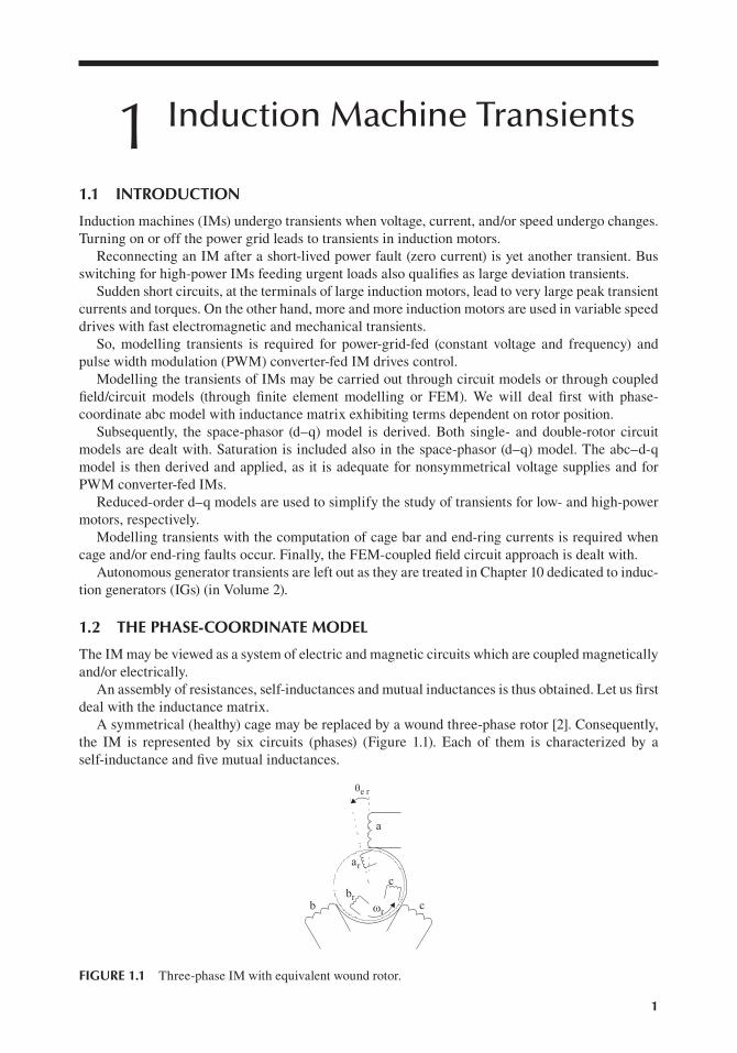
A symmetrical (healthy) cage may be replaced by a wound three-phase rotor [2]. Consequently, the IM is represented by six circuits (phases) (Figure 1.1). Each of them is characterized by a self-inductance and five mutual inductances.
ωr
a
cb
ar
c
br
θe r
FIGURE 1.1 Three-phase IM with equivalent wound rotor.

2 Induction Machines Handbook
The stator- and rotor-phase self-inductances do not depend on rotor position if slot openings are neglected. Also, mutual inductances between stator phases and rotor phases do not depend on rotor position. A sinusoidal distribution of windings is assumed. Finally, stator/rotor-phase mutual inductances depend on rotor position (θer = p1θr).
The induction matrix, Labcarbrcr er( )θ is
Labcarbrcr er
Laa Lab Lac LaarLabr
LacrLab Lbb Lbc Lbar
LbbrLbcr
Lac Lbc Lcc LcarLcbr
LccrLaar
LbarLcar
LararLarbr
LarcrLabr
LbbrLcbr
LarbrLbrbr
LbrcrLacr
LbcrLccr
LarcrLbrcr
Lcrcr
( )θ[[|
]]|
=
[
[
|||||||||||
]
]
|||||||||||
(1.1)
with
Laa Lbb Lcc Lls Lms; Lab Lac Lbc Lsm 2;
LaarLbbr
LccrLsrmcos er; Larar
LbrbrLcrcr
Llrr Lrm
r ;
Lcra Larb Lbrc Lsrmcos er23
; LarbrLarcr
LbrcrLrm
r 2;
Lcrb Lbra Larc Lsrmcos er23
= = = + = = = −
= = = θ = = = +
= = = θ − π)(|
))| = = = −
= = = θ + π)(|
))|
(1.2)
Assuming a sinusoidal distribution of windings, it may be easily shown that
Lsrm Lsm Lrmr= ⋅ (1.3)
Reducing the rotor to stator is useful especially for cage-rotor IMs, as no access to rotor variables is available.
In this case, the mutual inductance becomes equal to self-inductance Lsrm Lsm→ and the rotor rLrm → Lsmself-inductance equal to the stator self-inductance .
To conserve the fluxes and losses, with stator-reduced variables,
iariarr
ibribrr
icricrr
LsrmLsm
Krs= = = = (1.4)
VarVar
r =VbrVbr
r =VcrVcr
r =iarr
iar=
ibrr
ibr=
icrr
icr
1Krs
= (1.5)
RR
=LL
1K
r
rr
lr
lrr
rs2= (1.6)
3Induction Machine Transients
The
exp
ress
ions
of r
otor
resi
stan
ce R
r and
leak
age
indu
ctan
ce L
lr, b
oth
redu
ced
to th
e st
ator
for b
oth
cage
and
wou
nd ro
tors
, are
giv
en in
Cha
pter
6, V
ol. 1
.T
he s
ame
is tr
ue fo
r R
s and
Lls. T
he m
agne
tiza
tion
self
-ind
ucta
nce
Lsm
has
bee
n ca
lcul
ated
in C
hapt
er 5
, Vol
. 1.
Now
, the
mat
rix
form
of
phas
e-co
ordi
nate
(var
iabl
e) m
odel
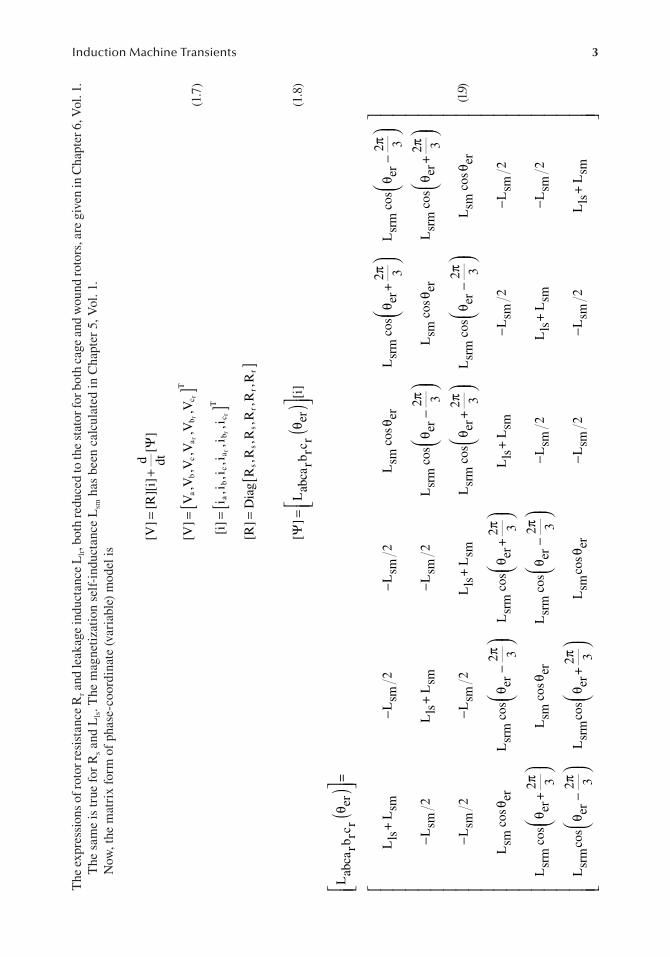
is
[V]
[R][
i]d dt
[]
=+
Ψ
[V]
V,V
,V,V
,V,V
ab
ca
bc
T
rr
r[
]=
(1
.7)
[i]
i,i
,i,i
,i,i
ab
ca
bc
T
rr
r[
=
[R]
Dia
gR
,R,R
,R,R
,Rs
ss
rr
r[
]=
]
[
]L
abca
rbrc
rer
[i]
()
Ψ=
θ
(1.8
)
Lab
carb
rcr
er=
Lls
+L
smL
sm2
Lsm
2L
smco
ser
Lsr
mco
ser
+2 3
Lsr
mco
ser
2 3
Lsm
2L
ls+
Lsm
Lsm
2L
srm
cos
er2 3
Lsm
cos
erL
srm
cos
er+
2 3
Lsm
2L
sm2
Lls
+L
smL
srm
cos
er+
2 3L
srm
cos
er2 3
Lsm
cos
er
Lsm
cos
erL
srm
cos
er2 3
Lsr
mco
ser
+2 3
Lls
+L
smL
sm2
Lsm
2
Lsr
mco
ser
+2 3
Lsm
cos
erL
srm
cos
er2 3
Lsm
2L
ls+
Lsm
Lsm
2
Lsr
mco
ser
2 3L
srm
cos
er+
2 3L
smco
ser
Lsm
2L
sm2
Lls
+L
sm
()
θ
−−
θθ
π
θ
−π
−−
θ−
π
θ
π
−−
θπ
θ−
π
θ
θθ
−π
θπ
−−
θπ
θθ
−π
−
θ−
π
θ
π
θ
−−
(1
.9)
θ
−

4 Induction Machines Handbook
with (1.8), (1.7) becomes
[V] [R][i] [L]Li
[i]d[i]dt
d[L]d
[i]ddter
er= + + ∂∂
+θ
θ (1.10)
Multiplying (1.10) by [i]T, we get
[i] [V] [i] R[i]ddt
12
[L][i][i]12
[i]d
d[L][i]T T T T
err= +
+
θω (1.11)
where the first term represents the winding losses, the second, the stored magnetic energy variation, and the third, the electromagnetic power, Pe.
P Tp
12
[i]d[L]d
[i]e er
1
T
err= ω =
θω (1.12)
The electromagnetic torque Te is
T12
p [i]d[L]d
[i]e 1T
er
=θ
(1.13)
The motion equation is
Jp
ddt
T T ;ddt1
re load
err
ω = − θ = ω (1.14)
An eight-order nonlinear model with time-variable coefficients (inductances) has been obtained, even with core loss neglected.
Numerical methods are required to solve it, but the computation time is prohibitive. Consequently, the phase-coordinate model is to be used only for special cases as the inductance and resistance matrices may be assigned any amplitude and rotor position dependencies.
The complex or space vector variable model is now introduced to get rid of rotor position depen-dence of parameters.
1.3 THE COMPLEX VARIABLE MODEL
Let us use the following notations:
a e ; cos23
= Re[a]; cos43
Re a
cos23
Re ae ; cos +43
Re a e
j23 2
erj
er2 jer er
= π π =
θ + π
= θ π
=
π
θ θ
(1.15)
Based on the inductance matrix, expression (1.9), the stator phase a and rotor-phase ar flux linkages, Ψa and Ψar, are
L i L Re i ai a i L Re i ai a i ea ls a sm a b2
c sm a b2
cj
r r rer( )Ψ = + + + + + +
θ (1.16)
L i L Re i ai a i L Re i ai a i ea lr a sm a b2
c sm a b2
cj
r r r r rer( )Ψ = + + + + + +
− θ (1.17)

5Induction Machine Transients
We may now introduce the following complex variables as space phasors [1]:
i23
i ai a iss
a b2
c( )= + + (1.18)
i23
i ai a irr
a b2
cr r r( )= + + (1.19)
Also,
Re i i13
i i iss
a a b c( ) ( )= − + + (1.20)
Re i i13
i i irr
a a b cr r r r( ) ( )= − + + (1.21)
In symmetric steady-state and transient regimes (or for star connection of phases),
i i i i i i 0a b c a b cr r r+ + = + + = (1.22)
With the above definitions, Ψa and Ψar become
L Re i L Re i i e ; L32
La ls ss
m ss
rr j
m smer( ) ( )Ψ = + + =θ (1.23)
L Re i L Re i i ea lr rr
m rr
ss j
rer( ) ( )Ψ = + + − θ (1.24)
Similar expressions may be derived for phases br and cr. After adding them together, using the complex variable definitions (1.18) and (1.19) for flux linkages and voltages, we also obtain
V R iddt
; L i L i e
V R iddt
; L i L i e
ss
s ss s
s
ss
s ss
m rr j
rr
r rr r
r
rr
r rr
m ss j
er
er
= + Ψ Ψ = +
= + Ψ Ψ = +
θ
− θ
(1.25)
where
L L L ; L L Ls sl m r rl m= + = + (1.26)
V23
V aV a V ; V23
V aV a Vss
a b2
c rr
a b2
cr r r( ) ( )= + + = + + (1.27)
In the above equations, stator variables are still given in stator coordinates and rotor variables in rotor coordinates.
Making use of a rotation of complex variables by the general angle θb in the stator and θb − θer in the rotor, we obtain all variables in a unique reference rotating at electrical speed ωb
ddt
bbω = θ (1.28)

6 Induction Machines Handbook
e ; i i e ; V V es
ssb j
ss
sb j
ss
sb jb b bΨ = Ψ = =θ θ θ
e ; 1 i i e ; V V err
rb j
rr
rb j
rr
rbb er b er j b erΨ = Ψ = =( ) ( ) ( )θ −θ θ −θ θ −θ
(1.29)
With these new variables, Equations (1.25) become
V R iddt
j ; L i L is s ss
b s s s s m r= + Ψ + ω Ψ Ψ = +
V R iddt
j ; L i L ir r rr
b r r r r r m s( )= + Ψ + ω − ω Ψ Ψ = +
(1.30)
For convenience, the superscript b was dropped in (1.30). The electromagnetic torque is related to motion-induced voltage in (1.30).
T32
p Re j i32
p Re j ie 1 s s*
1 r r*( ) ( )= ⋅ ⋅ ⋅ψ ⋅ = − ⋅ ⋅ ⋅ψ ⋅ (1.31)
Adding the equations of motion, the complete complex variable (space-phasor) model of IM is obtained.
Jp
ddt
T T ;ddt1
re load
err
ω = − θ = ω (1.32)
The complex variables may be decomposed in a plane along two orthogonal d and q axes rotating at speed ωb to obtain the d–q (Park) model [2].
V V j V ; i i j i ;s d q s d q s d q= + ⋅ = + ⋅ Ψ = Ψ + ⋅Ψj
V V j V ; i i j i ; jr dr qr r dr qr r dr qr= + ⋅ = + ⋅ Ψ = Ψ + ⋅Ψ (1.33)
With (1.33), the voltage equations (1.30) become
ddt
V R idd s d b q
Ψ = − ⋅ + ω ⋅Ψ
ddt
V R iqq s q b d
Ψ = − ⋅ − ω ⋅Ψ
ddt
R idrdr r dr b r qrV ( )Ψ = − ⋅ + ω − ω ⋅Ψ (1.34)
ddt
V R iqrqr r qr b r dr( )Ψ = − ⋅ − ω − ω ⋅Ψ
T32
P i i32
P L i i i ie 1 d q q d 1 m q dr d qr( ) ( )= Ψ − Ψ = −
Also from (1.27) with (1.19), the Park transformation for stator P(θb) is derived.
V
V
V
P
V
V
V
d
q
0
b
a
b
c
( )
= θ ⋅
(1.35)

7Induction Machine Transients
P23
cos cos23
cos23
sin sin23
sin23
12
12
12
b
b b b
b b b( )
( )
( )θ = ⋅
−θ −θ + π
−θ − π
−θ −θ + π
−θ − π
(1.36)
The inverse Park transformation is
P32
Pb1
bT( ) ( )θ = ⋅ θ
− (1.37)
A similar transformation is valid for the rotor but with θb − θer instead of θb.It may be easily proved that the homopolar (real) variables V0, i0, V0r, i0r, Ψ0 and Ψ0r do not
interface in energy conversion:
ddt
V R i ; L i
ddt
V R i ; L i
00 s 0 0 0s 0
0r0r r 0r 0r 0r 0
Ψ = − ⋅ Ψ ≈ ⋅
Ψ = − ⋅ Ψ ≈ ⋅ (1.38)
L0s and L0r are the homopolar inductances of stator and rotor, respectively. Their values are equal or lower (for chorded coil windings) to the respective leakage inductances Lls and Llr.
A few remarks on the complex variable (space-phasor) and d–q models are in order.
• Both models include, in the form presented here, only the space fundamental of mmfs and airgap flux distributions.
• Both models exhibit inductances independent of rotor position.• The complex variable (space-phasor) model is credited with a reduction in the number of
equations with respect to the d–q model, but it operates with complex variables.• When solving the state-space equations, only the d–q model, with real variables, benefits
from existing commercial software (Mathematica, MATLAB®–Simulink®, Spice, etc.).• Both models are very practical in treating the transients and control of symmetrical IMs
fed from symmetrical voltage power grids or from PWM converters.• Easy incorporation of magnetic saturation and rotor skin effect are yet two additional
assets of complex variable and d–q models. The airgap flux density retains a sinusoidal distribution along the circumferential direction.
• Besides the widespread usage of complex variable, other models (variable transformations) that deal especially with asymmetric supply or asymmetric machine cases have also been introduced (for a summary, see Refs. [3,4]).
1.4 S TEADY STATE BY THE COMPLEX VARIABLE MODEL
Constant speed and load are expressed by IM steady state. For a machine fed from a sinusoidal voltage symmetrical power grid, the phase voltages at IM terminals are
V V 2 cos t (i 1)23
; i 1,2,3a,b,c 1= ⋅ ω − − ⋅ π
= (1.39)
8 Induction Machines Handbook
The voltage space-phasor Vbs in random coordinates (from (1.27)) is
V23
V (t) aV (t) a V (t) esb
a b2
cj b( )= + + − θ (1.40)
From (1.39) and (1.40),
V =V 2 cos t jsin tsb
1 b 1 b( ) ( )ω − θ + ω − θ (1.41)
Only for steady state,
tb b 0θ = ω + θ (1.42)
Consequently,
V V 2esb j t1 b 0= [ ]( )ω −ω +θ (1.43)
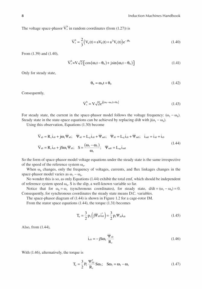
For steady state, the current in the space-phasor model follows the voltage frequency: (ω1 − ωb). Steady state in the state-space equations can be achieved by replacing d/dt with j(ω1 − ωb).
Using this observation, Equations (1.30) become
V R i j ; L i ; L i ; i i i
V R i jS ; S ; L i
s0 s s0 1 s0 s0 sl s0 m0 r0 rl r0 m0 m0 s0 r0
r0 r r0 1 r01 r
rm0 m m0
( )
= + ω Ψ Ψ = + Ψ Ψ = + Ψ = +
= + ω Ψ = ω − ωω
Ψ = (1.44)
So the form of space-phasor model voltage equations under the steady state is the same irrespective of the speed of the reference system ωb.
When ωb changes, only the frequency of voltages, currents, and flux linkages changes in the space-phasor model varies as ω1 − ωb.
No wonder this is so, as only Equations (1.44) exhibit the total emf, which should be independent of reference system speed ωb. S is the slip, a well-known variable so far.
Notice that for b 1ω = ω (synchronous coordinates), for steady state, d/dt ( 1 b) 0= ω − ω = . Consequently, for synchronous coordinates the steady state means D.C. variables.
The space-phasor diagram of (1.44) is shown in Figure 1.2 for a cage-rotor IM.From the stator space equations (1.44), the torque (1.31) becomes
T32
p j i32
p ie 1 r0 r0*
1 r0 r0( )= Ψ = Ψ (1.45)
Also, from (1.44),
i jSR
r0 1r0
r
= − ω Ψ (1.46)
With (1.46), alternatively, the torque is
T32
PR
S ; Se 1r02
r1 1 1 r= Ψ ω ω = ω − ω (1.47)

9Induction Machine Transients
Solving for Ψr0 in Equations (1.44) leads to the standard torque formula:
T3p V
RS
R CRS
L C L
; C 1LL
e1
1
s2 r
s 1r
2
12
ls 1 lr2
1ls
m( )≈
ω+
+ ω +
= + (1.48)
Expression (1.47) shows that, for constant rotor flux space-phasor amplitude, the torque varies lin-early with speed ω r as it does in a separately excited D.C. motor. So all steady-state performance may be calculated using the space-phasor model as well.
1.5 EQUIVALENT CIRCUITS FOR DRIVES
Equations (1.30) lead to a general equivalent circuit good for transients, especially in variable speed drives (Figure 1.3).
V R i p j L i p j
V R i p j L i p j
s s s b sl s b m
r r r b r rl r b r m( ) ( )( ) ( )
( ) ( )
= + + ω + + ω Ψ
= + + ω − ω + + ω − ω Ψ (1.49)
Is Ir
Im
Vs
(p+j )Ls1ωb
(p+j )Lω mb
(p+j( )Lω −ω ) rlb r
Rr
–j L Iω r m m
Rs(a)
(b)
Is Ir
Im
Vs
j Lω sl1
Rr
Rs j Lω rl1
j Lω m1
ωω −ω
1
1 r
Vrω
ω −ω1
1 r
jω Ψ1 s jω Ψ1 r
FIGURE 1.3 The general equivalent circuit with Vs = 0 (a) and for steady state, Vr ≠ 0 (b).
Ir0−
L1r Ir0−
FIGURE 1.2 Space-phasor diagram for steady state.

10 Induction Machines Handbook
The reference system speed ωb may be random, but three particular values have met with rather wide acceptance.
• Stator coordinates: ωb = 0; for steady state: p → jω1
• Rotor coordinates: ωb = ωr; for steady state: p → jSω1
• Synchronous coordinates: ωb = ω1; for steady state: p → 0.
Also, for steady state in variable speed drives, the steady-state circuit (the same for all values of ωb) with p → j(ω1 − ωb) is shown in Figure 1.3a and b.
Figure 1.3b shows, in fact, the standard T equivalent circuit of IM for steady state, but in space phasors and not in phase phasors.
A general method to “arrange” the leakage inductances Lsl and Lrl in various positions in the equivalent circuit consists of a change of variables.
i i a ; aL i ira
r ma m s ra( )= Ψ = + (1.50)
Making use of this change of variables in (1.49) yields
V R i p j L aL i j
aV a R i p j a aL L i p j
s s s b s m s b ma
r2
r ra
b r rl m ra
b r ma
p( )( ) ( )
( )( )
( ) ( )( )
= + + ω − + + ω Ψ
= + + ω − ω − + + ω − ω Ψ (1.51)
An equivalent circuit may be developed based on (1.51), as shown in Figure 1.4.The generalized equivalent circuit shown in Figure 1.4 warrants the following comments:
• For a = 1, the general equivalent circuit that is shown in Figure 1.3 is reobtained and aΨ =a
m Ψm: the main flux.• For a = Lm/Lr < 1, the inductance term in the “rotor section” “disappears”, being moved to
the primary section:
aLL
L i iLL
LL
ma m
rm s r
r
m
m
rrΨ = +
= Ψ (1.52)
• For a = Ls/Lm > 1, the leakage inductance term is lumped into the “rotor section”:
aLL
L i iLL
ma s
mm s r
m
ssΨ = +
= Ψ (1.53)
Is I /ar
Im
Vs
(p+j )(L -aL )ω mb
(p+j )aLω mb
(p+j( )(aL -L )ω −ω )b r
R ar
-j aL Iω r m m
Rs mrs a
aVr
2
a
a
( )( )b s mp jω L aL+ − ( )( ) ( )b r r ma p j ω ω aL L+ − −
amr mjω aL I−
FIGURE 1.4 Generalized equivalent circuit.

11Induction Machine Transients
• This latter type of equivalent circuit is adequate for stator flux orientation control.• For D.C. braking, the stator is fed with D.C. The method is used for variable speed drives.
The model for this regime is obtained by a D.C. current source (ω1 = 0), ωb = 0 (stator coor-dinates, Vr = 0, a = Lm/Lr.), which is shown in Figure 1.4.
The result is shown in Figure 1.5.For steady state, the equivalent circuits for ar = Lm/Lr and ar = Ls/Lm and Vr = 0 are shown in
Figure 1.6.
Example 1.1 The Constant Rotor Flux Torque/Speed Curve
Let us consider an induction motor with a single rotor cage and constant parameters: Rs = Rr = 1 Ω, Lsl = Lrl = 5 mH, Lm = 200 mH, Ψr0 = 1 Wb, S = 0.2, ω1 = 2π6 rad/s, p1 = 2, Vr = 0. Find the torque, rotor current, stator current, stator and main flux and voltage for this situation. Draw the corre-sponding space-phasor diagram.
Solution
We are going to use the equivalent circuit shown in Figure 1.6a and the rotor current and torque expressions (1.46 and 1.47):
T32
pR
S32
211
0.2 2 6 22.608 Nme 1r02
r1
2
= Ψ ω = ⋅ π =
I SR
0.2 2 611
7.536 Ar0 1r0
r
= − ω Ψ = − ⋅ π = −
Isdc
Isdc
Imr
p LL
m2
r -ω LL
m2
rImr
R LL
mr
r
2a
b c
+
-
Idc IdcIsdc=
r
–
2m
mrrr
Lω I
L−
FIGURE 1.5 Equivalent circuit for D.C. braking.
Is0 Ir
I0r0
Vs0
j L -L /L )ω ( s1
R S
r
Rs
jω 1jω Ψ1 r
LL
m
rLL
m
r
2
m2
r LLm
r
LL
m
r
2
2
( )21 s m rjω L L L−
(a)
Is0
Ir0
Vs0
jω 1
Sr
Rs
jω 1
LL
s
mm
r
LLs
m
LL
s
m
2
2Lsjω Ψ1 r
L L L
s
m-L
s s r1 m
m m
L L Ljω L
L L−
(b)
jω Ψ1 sR
FIGURE 1.6 Steady-state equivalent circuits: (a) rotor flux oriented and (b) stator flux oriented.

12 Induction Machines Handbook
If the rotor current is placed along real axis in the negative direction, the rotor flux magnetization current Ir0 (Figure 1.6a) is
I jI
RS
LL
LL
jI R
S Lj
( 7.536) 10.2 2 6 0.2
j5A0r0
r0r m
r
1m2
r
r0 r
1 m
( ) ( )= −−
ω= −
−ω
= − + ⋅⋅ π ⋅
−
The stator current is
I ILL
I 7.5360.2050.2
j5 7.7244 j5.0 As0 r0r
m0r0= − + = − = −
The stator flux Ψs is
L I L I 0.205(7.7244 j5.0) 0.2( 7.536) 0.076 j1.025s0 s s0 m r0Ψ = + = − + − = −
The airgap flux Ψm is
L I I 0.2(7.7244 j5.0 7.536) 0.03768 j1.0m0 m s0 r0( )Ψ = + = − − = −
The rotor flux is
L I 0.03768 j1.0 0.005( 7.536) j1.0 (as expected)r0 m0 rl r0Ψ = Ψ + = − + − = −
The voltage Vso is
V j R I j2 6(0.076 j1.025) 1(7.7244 j5.0) 46.346 j2.136so 1 so s so= ω Ψ + = π − + − = −
The corresponding space-phasor diagram is shown in Figure 1.7.
1.6 ELECTRICAL TRANSIENTS WITH FLUX LINKAGES AS VARIABLES
Equations (1.30) may be transformed by changing the variables through the elimination of currents:
iL
LL L
; 1L
L L
iL
LL L
s1 s
sr
m
s r
m2
s r
r1 r
rs
m
s r
= σ Ψ − Ψ
σ = −
= σ Ψ − Ψ
−
−
(1.54)
I0r0
Ir0
Is0
Ir0
-
Vs0
Is0Ψs0 Rs
jω1
Ψs0Ψr0
LL
rm
ϕ1
rr0m
LI L−
FIGURE 1.7 The space-phasor diagram.

13Induction Machine Transients
ddt
1 j V K
ddt
1 j V K
ss
b s s s s r r
rr
b r r r r r s s( )
( )
( )
′τ Ψ + + ⋅ω ⋅ ′τ ⋅Ψ = ′τ + Ψ
′τ Ψ + + ⋅ ω − ω ⋅ ′τ ⋅Ψ = ′τ + Ψ
(1.55)
with
L LK m
s = =; K m
Lr
s Lr
Lr
;Lr
ss
sr
r
r
τ = τ =
;s s r r′τ = τ ⋅σ ′τ = τ ⋅σ (1.56)
By electrical transients, we mean constant speed transients. So both ωb and ωr are considered known. The inputs are the two voltage space phasors Vs and Vr, and the outputs are the two flux linkage space phasors Ψs and Ψr.
The structural diagram of Equations (1.55) is shown in Figure 1.8.The transient behaviour of stator and rotor flux linkages as complex variables, at constant speeds
ωb and ωr, for standard step or sinusoidal voltages Vs and Vr signals has analytical solutions. Finally, the torque transients have also analytical solutions as
T32
p Re j ie 1 s s*( )= Ψ (1.57)
The two complex eigenvalues of (1.55) are obtained from
p 1 j K
K p 1 j0
s b s r
s r b r r( )′τ + + ω ′τ −
− ′τ + + ω − ω ′τ= (1.58)
As expected, the eigenvalues p1,2 depend on the speed of the motor and on the speed of the reference system ωb.
Equation (1.58) may be put in the form
( )( )
( ) ( )
( )
′τ ′τ + ′τ + ′τ + ′τ ′τ ω − ω −
+ + ⋅ω ⋅ ′τ + ⋅ ω − ω ⋅ ′τ =
p p j 2 K K
1 j 1 j 0
2s r s r s r b r s r
b s b r r
(1.58’)
τ 's τ 's
jτ 'X
–
stator
ωb
ωb
referencesystemspeed
Kr
Vs Ks
τ 'r
τ 'r
rX
-
ωb ωr-ωr rotor
speed
Vbr
–
rotor
–
b rω ω–
jτ 's
FIGURE 1.8 IM space-phasor diagram for constant speed.

14 Induction Machines Handbook
In essence, in-rush current and torque (at zero speed), for example, have a rather straightforward solution through the knowledge of eigenvalues, with ωr = 0 = ωb.
p p K K 1 02s r s r s r( )′τ ′τ + ′τ + ′τ − + =
p± 4 K K 1
21,2 0
s r s r2
s r s r
s rr b
( ) ( ) ( ) ( )=
− ′τ + ′τ ′τ + ′τ − ′τ ′τ − +′τ ′τω = ω =
(1.59)
The same capability of yielding analytical solutions for electrical transients is claimed by the spiral vector theory [5].
For constant amplitude stator or rotor flux conditions,
ddt
j orddt
j ; Stator frequencys
1 b sr
1 b r 1( ) ( )Ψ = ω − ω Ψ Ψ = ω − ω Ψ ω −
Equations (1.55) are left with only one complex eigenvalue. Even a simpler analytical solution for electrical transients is feasible for constant stator or rotor flux conditions, so typical in fast response modern vector control drives.
Also, at least at zero speed, the eigenvalue with voltage type supply is about the same for stator or for rotor supply.
The same equations may be expressed with is and Ψr as variables, by simply putting a = Lm/Lr and by eliminating ir from (1.51) with (1.50).
1.7 INCLUDING MAGNETIC SATURATION IN THE SPACE-PHASOR MODEL
To incorporate magnetic saturation easily into the space-phasor model (1.49), we separate the leak-age saturation from main flux path saturation with pertinent functions obtained a priori from tests or from field solutions (FEM).
L L i , L L i ; L i isl sl s lr lr r m m m m( ) ( ) ( )= = Ψ = (1.60)
i i im s r= + (1.61)
Let us consider the reference system oriented along the main flux Ψm, that is Ψm = Ψm, and eliminate the rotor current, maintaining Ψm and is as variables.
V R p j L i i p j
V R p j L i i i i p j
s s b sl s s b m
r r b r lr m s m s b r m
( )( ) ( )( ) ( )
( ) ( )
( ) ( )
= + + ω
⋅ + + ω ⋅Ψ
= + + ω − ω −
⋅ − + + ω − ω ⋅Ψ
(1.62)
iL i
mm
m m( )= Ψ (1.63)
We may add the equation of motion,
Jp
p32
p Real j i Tr
11 m s
*load( )ω = Ψ − (1.64)

15Induction Machine Transients
Provided the magnetization curves Lsl(is) and Llr(ir) are known, Equations (1.62)–(1.64) may be solved only by numerical methods after splitting Equations (1.62) along d and q axes.
For steady state, however, it suffices that in the equivalent circuits, Lm is made a function of im, Lsl of is0 and Llr of (iro) (Figure 1.9). This is only in synchronous coordinates where steady state means D.C. variables.
In reality, in both the stator and the rotor, the magnetic fields are A.C. at frequency ω1 and Sω1. So, in fact, for transformer-induced voltages given in Equations (1.62), transient (A.C.) inductances should be used.
L i L iLi
i L ilst
s ls sls
ss ls s( ) ( ) ( )= + ∂
∂<
L i L iLi
i L ilrt
r lr rlr
rr lr r( ) ( ) ( )= + ∂
∂< (1.65)
L i L iLi
i L imt
m m mm
mm m m( ) ( ) ( )= + ∂
∂<
Typical curves are shown in Figure 1.10.As the transient (A.C.) inductances are even smaller than the normal (D.C.) inductances, the
machine behaviour at high currents is expected to show further increased currents.Furthermore, as shown in Chapter 6, Vol. 1, the leakage flux circumferential flux lines at high
currents influence the main (radial) flux and contribute to the resultant flux in the machine core. The saturation in the stator is given by the stator flux Ψs and in the rotor by the rotor flux for high levels of currents.
So, for large currents, it seems more appropriate to use the equivalent circuit with stator and rotor fluxes shown (Figure 1.11). However, two new variable inductances, Lsi and Lri, are added. Lg refers to the airgap only. Finally, the stator and rotor leakage inductances are related only to end connec-tions and slot volume: L e
ls , L elr [6].
Is Ir
Im
Vs
j L (I )ω sl1
R S
r
Rs j L (I )ω rl1
j L (I )ω m1 m
s r
FIGURE 1.9 Standard equivalent circuit for steady-state leakage and main flux path saturation.
Lls
Llst
Lls
Llst
Is
Lm
Lmt
Lm
Lmt
Im
FIGURE 1.10 Leakage and main flux normal and transient inductances versus current.

16 Induction Machines Handbook
As expected, the functions Ψ es(isi) = Lsiisi and Ψr(iri) = Lriiri have to be known together with Lls ,
L elr , Rs, Rr and Lg which are hereby considered constant.
In the presence of skin effect, L elr and Rr are functions of slip frequency ωsr = ω1 – ωr.
Furthermore, we should notice that it is not easy to measure all parameters in the equivalent circuit shown in Figure 1.11. It is, however, possible to calculate them either by sophisticated analytical or through FEM models. Depending on the machine design and load, the relative importance of the two variable inductances Lsi and Lri may be notable or negligible.
Consequently, the equivalent circuit may be simplified. For example, for heavy loads the rotor saturation may be ignored, and thus, only Lsi remains. Then, Lsi and Lg in parallel may be lumped into an equivalent variable inductance Lms and Le
ls and Lelr into the total constant leakage inductance
of the machine Ll. Then, the equivalent circuit shown in Figure 1.10 degenerates into the one shown in Figure 1.12.
When high currents occur, during transients in electric drives, the equivalent circuit of Figure 1.11 indicates severe saturation while the conventional circuit (Figure 1.9) indicates moderate saturation of the main path flux and some saturation of the stator leakage path.
So when high current (torque) transients occur, the real machine, due to the Lsm reduction, produces torque performance quite different from the predictions by the conventional equivalent circuit (Figure 1.9). Up to 2–2.5 p.u. current, however, the differences between the two models are negligible.
In IMs designed for extreme saturation conditions (minimum weight), models like those shown in Figure 1.11 have to be used, unless FEM is applied.
1.8 SATURATION AND CORE LOSS INCLUSION INTO THE STATE-SPACE MODEL
To include the core loss into the space-phasor model of IMs, we assume here that the core losses occur, both in the stator and in the rotor, into equivalent orthogonal windings: cd – cq, cdr – cqr (Figure 1.13) [7].
Alternatively, when rotor core loss is neglected (cage-rotor IMs), the cdr – cqr windings account for the skin effect (the double-cage equivalence principle).
Is Ir
Img
Vs
ls RrRs pLe
Isi
pΨs pLsipΨg pLg
j ω Ψr r
Iri
pΨr pLri
lrpLe
FIGURE 1.11 Space-phasor equivalent circuit with stator and rotor core saturation included (stator coordinates). (After Ref. [6].)
Is
Vs
RrRs
Ims
pΨs pLms
j ω Ψr rpΨr
lpL
For steady state p=jω1
FIGURE 1.12 Space-phasor equivalent circuit with stator saturation included (stator coordinates).

17Induction Machine Transients
Let us consider also that the core loss windings are coupled to the other windings only by the main flux path.
The space-phasor equations are thus straightforward (by addition).
R i Vddt
j ; L is s ss
b s s m ls s− = − Ψ − ω Ψ Ψ = Ψ +
R id
dtj ; L i
R i Vddt
j ; L i
cs cscs
b cs cs m lcs cs
r r rr
b r r r m lr r( )
= − Ψ − ω Ψ Ψ = Ψ +
− = − Ψ − ω − ω Ψ Ψ = Ψ +
(1.66)
R id
dtj ; L icr cr
crb r cr cr m lcr cr( )= − Ψ − ω − ω Ψ Ψ = Ψ +
i i i i i ; L i im s cs r cr m m m m( ) ( )= + + + Ψ = (1.67)
The airgap torque now contains two components: one given by the stator current and the other one (braking) given by the stator core losses.
T32
p Re j i i32
p Re j i ie 1 s s*
cs cs*
1 m s*
cs*( ) ( )= Ψ + Ψ
= Ψ +
(1.68)
Equations (1.66) and (1.67) lead to a fairly general equivalent circuit when we introduce the transient magnetization inductance Lmt (1.65) and consider separately main flux and leakage paths saturation (Figure 1.14).
The apparently involved equivalent circuit shown in Figure 1.14 is fairly general and may be applied for many practical cases such as
• The reference system may be attached to the stator, ωb = 0 (for cage rotor and large transients), to the rotor (for the doubly fed IM) or to stator frequency ωb = ω1 for electric drives transients.
cdr dr
id
icdii
ωb
d
Vd
ωr
ωb
jq
Vq
iq
icq
qri
cqri
FIGURE 1.13 d–q model with stator and core loss windings.

18 Induction Machines Handbook
• To easily simplify Equations (1.66–1.67), the reference system may be attached to the main flux space phasor: Ψm = Ψm m( )i and eventually using im, ics, icr, ir, and ωr as variables with is as a dummy variable [7,8]. As expected, d–q decomposition is required.
• For a cage rotor with skin effect (medium- and high-power motors fed from the power grid directly), we should simply make Vr = 0 and consider the rotor core loss winding (with its equations) as the second (fictitious) rotor cage.
Example 1.2 Saturation and Core Losses
Simulation results are presented in what follows. The motor constant parameters are Rs = 3.41 Ω, Rr = 1.89 Ω, L −2
sl = 1.14 · 10 H, L −2rl = 0.9076 · 10 H, J = 6.25 · 10−3 Kgm2. The magnetization
curve Ψm(im) together with core loss in the stator at 50 Hz is shown in Figure 1.15.The stator core loss resistance Rcs is
R32 P
32
2 50 2
5001183.15cs
12
m2
iron
2 2( )= ω Ψ ≈π ⋅
= Ω
Considering that Llcs · ω1 = Rcs; Llcs = 1183.15/(2π50) = 3.768 H.
Is Ir
Vs
ls
Rr
j ω Ψr m
RspL +j Lω
Ics
j ω Ψb m
(p+j )Lω lcsb
Rcs
Im Icr
b ls lrpL +j( Lω −ω )b lrrtt
pLmt
(p+j( ))Lω −ω b r lcr
Rcr
Ir
Vr
+
-
for steady state: p=j( )ω − ω b1
–
FIGURE 1.14 Space-phasor T equivalent circuit with saturation and rotor core loss (or rotor skin effect).
2
1
piron500Wcore
loss
Ψ (Wb)m
10
i (A)m
FIGURE 1.15 Magnetization curve and stator core loss.

19Induction Machine Transients
For steady-state and synchronous coordinates (d/dt = 0), Equations (1.66) become
R i V j ; V 380 2es s0 s0 1 s0 s0j 0− = − ω Ψ = δ
R i j ; i i i ics cs0 1 cs0 m0 s0 cs0 r0= − ω Ψ = + + (1.69)
R i jSr r0 1 r0= − ω Ψ
For given values of slip S, the values of stator current is0 2 (RMS/phase) and the electromagnetic torque are calculated for steady state using (1.69) and the flux–current relationship using (1.66) and (1.67) and Figure 1.15. The results are given in Figure 1.16a and b [7]. There are notable differences in stator current due to saturation. The differences in torque are rather small. Efficiency–power factor product and the magnetization current versus slip are shown in Figure 1.17a and b.
Again, saturation and core loss play an important role in reducing the efficiency–power factor although core loss itself tends to increase the power factor while it tends to reduce the efficiency.The reduction of magnetization current im with slip is small but still worth considering.
Two transients have been investigated by solving (1.66) and (1.67) and the motion equations through the Runge–Kutta–Gill method.
1. Sudden 40% reduction of supply voltage from 380 V per phase (RMS), steady-state con-stant load corresponding to S = 0.03.
2. Disconnection of the loaded motor at S = 0.03 for 10 ms and reconnection (at δ0 = 0, though any phasing could be used). The load is constant again.
The transients for transient 1 are shown in Figure 1.18a–c.Some influence of saturation and core loss occurs in the early stages of the transients, but
in general, the influence of them is moderate because at reduced voltage, saturation influence diminishes considerably.
The second transient, occurring at high voltage (and saturation level), causes more important influences of saturation (and core loss) as shown in Figure 1.19a–c.The saturation and core loss lead to higher current peaks, but apparently for low but faster torque and speed transients.
In high-performance variable speed drives, high levels of saturation may be inflicted to increase the torque transient capabilities of IM. Vector control detuning occurs, and it has to be corrected. Also, in very precise torque control drives, such second-order phenomena are to be considered. Skin effect also influences the transients of IMs and the model shown in Figure 1.13 can handle it for cage-rotor IMs directly, as shown earlier in this paragraph.
FIGURE 1.16 Steady-state phase current and torque versus slip (i) saturation and core loss consid-ered, (ii) saturation considered, core loss neglected, and (iii) no saturation, no core loss. (After Ref. [7].)

20 Induction Machines Handbook
FIGURE 1.17 Efficiency–power factor product and magnetization current versus slip. (After Ref. [7].)
FIGURE 1.18 Sudden 40% voltage reduction at S = 0.03 constant load: (a) stator phase current and (b) torque (After Ref. [7]) and (c) speed.
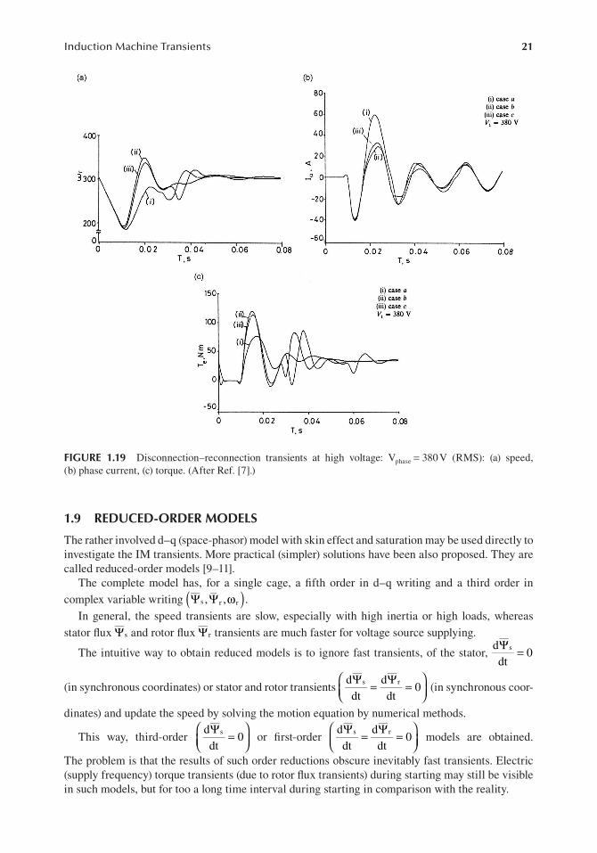
21Induction Machine Transients
1.9 REDUCED-ORDER MODELS
The rather involved d–q (space-phasor) model with skin effect and saturation may be used directly to investigate the IM transients. More practical (simpler) solutions have been also proposed. They are called reduced-order models [9–11].
The complete model has, for a single cage, a fifth order in d–q writing and a third order in
complex variable writing (Ψ Ψs , ,r ω )r .
In general, the speed transients are slow, especially with high inertia or high loads, whereas
stator flux Ψs and rotor flux Ψr transients are much faster for voltage source supplying.
dΨs = 0 dt
The intuitive way to obtain reduced models is to ignore fast transients, of the stator,
dΨ dΨ s = = 0 dt dt (in synchronous coordinates) or stator and rotor transients
r (in synchronous coor-
dinates) and update the speed by solving the motion equation by numerical methods. dΨs
= 0 dt dΨ dΨs r= = 0 dt dt
This way, third-order or first-order models are obtained.
The problem is that the results of such order reductions obscure inevitably fast transients. Electric (supply frequency) torque transients (due to rotor flux transients) during starting may still be visible in such models, but for too a long time interval during starting in comparison with the reality.
FIGURE 1.19 Disconnection–reconnection transients at high voltage: Vphase = 380 V (RMS): (a) speed, (b) phase current, (c) torque. (After Ref. [7].)

22 Induction Machines Handbook
So there are two questions with model order reduction:
• What kind of transients are to be investigated?• What torque transients have to be preserved?
In addition to this, low- and high-power IMs seem to require different reduced-order models to produce practical results in simulating a group of IMs when the computation time is critical.
1.9.1 neglecting Stator tranSientS
In this case, in synchronous coordinates, the stator flux derivative is considered zero (Equations (1.55)).
0 1 j V K1 s s s s r r( )+ + ω ′τ Ψ = ′τ + Ψ
ddt
1 j V K
T32
p Re j i ; iL
LL L
rr
1 r r r r s s
e 1 r r*
r* 1 r
rs
m
s r( )
( )( )′τ Ψ + + ω − ω Ψ = ′τ + Ψ
= − Ψ = σ Ψ − Ψ
− (1.70)
Jp
ddt
T T1
re load
ω = −
With two algebraic equations, there are three differential ones (in real d–q variables).For cage-rotor IMs,
V K1 j
ss s r r
1 s
Ψ = ′τ + Ψ+ ω ′τ
(1.71)
ddt
1 jK K
1 jV K
1 jr
1 rs r
1 s
r
r
s
1 s r
s s( ) ( )( )Ψ = − + ω − ω ++ ω ′τ
Ψ′τ
+ ′τ ⋅ ⋅+ ω ′τ ′τ
(1.72)
T32
p ImL
L L32
pL
L LIm
V K1 j
e 11
r s* m
s r1
1m
s rr
s s r r
1 s
= σ Ψ Ψ
= σ Ψ ′τ + Ψ− ω ′τ
−
(1.73)ddt
pJ
T Tr 1e load( )ω = −
* * −
Fast (at stator frequency) transient torque pulsations are absent in this third-order model (Figure 1.20b).
The complete model and third-order model for a motor with Ls = 0.05 H, Lr = 0.05 H, Lm = 0.0474 H, Rs = 0.29 Ω, Rr = 0.38 Ω, ω1 = 100π rad/s, Vs = 220 2 V, p1 = 2, J = 0.5 Kgm2 yields, for no-load, starting transient results as shown in Figure 1.20 [11].
It is to be noted that steady-state torque at high slips (Figure 1.20a) falls into the middle of torque pulsations, which explains why calculating no-load starting time with steady-state torque produces good results.
A second-order system may be obtained by considering only the amplitude transients of Ψr in (1.73) [11], but the results are not good enough in the sense that the torque fast (grid frequency) transients are present during start-up at higher speed than for the full model.

23Induction Machine Transients
Modified second-order models have been proposed to improve the precision of torque results [11] (Figure 1.20), but the results are highly dependent on motor parameters and load during starting. So, in fact, for starting transients when the torque pulsations (peaks) are required with precision, model reduction may be exercised with extreme care.
The presence of leakage saturation makes the above results mostly of academic interest.
1.9.2 conSiDering leakage Saturation
As shown in Chapter 9, Vol. 1, the leakage inductance (Lsc = Lsl + Lrl = Ll) decreases with current. This reduction is accentuated when the rotor has closed slots and more moderate when both, stator and rotor, have semiclosed slots (Figure 1.21).
The calculated (or measured) curves of Figure 1.21 may be fitted with analytical expressions of RMS rotor current such as [12]
X L K KI2
for curve 1l 1 l 1 2r
K
= ω = +
−
(1.74)
X L K K tanh K I K K cos K I for curve 2l 1 l 3 4 3 r3
6 7 8 r( ) ( )= ω = − − + (1.75)
FIGURE 1.20 Starting transients: (a) fifth-order model, (b) third-order model, and (c) modified second-order model. (After Ref. [11].)

24 Induction Machines Handbook
During starting on no-load, the stator current envelope Isp(t) varies approximately as [12]
IQ I
3 1t
tt
t
sp1 rK
K0 K0
2≈
+ +
(1.76)
Q1 reflects the effect of point on wave connection when nonsymmetrical switching of supply is considered to reduce torque transients (peaks) [13]
Q 2X SR R
cos sin ( )1l K
s r
2 2( )( )≈ ++
⋅ α + α + β (1.77)
α – point on wave connection of first phase-to-phase (b-c) voltage.β – delay angle in connecting the third phase.It has been shown that minimum current (and torque) transients are obtained for α = π/2 and
β = π/2 [14].As the steady-state torque gives approximately the same starting time as the transient one, we
may use it in the motion equation (for no-load).
Jp
ddt
3 V R p 1
RRS
S L S
T1
r ph2
r 1
1s
r2
12
l2
eω =
⋅ ⋅ ⋅ω
⋅+
+ ω
= (1.78)
We may analytically integrate this equation with respect to time up to the breakdown point: SK slip, dω dSr = −ω1dt dt
noting that .
tJ
3V R p12
R L S 1 SK012
ph2
r2
12 s
21 l K0
2K02( )( )( )( )= ω + ω −
2R R 1 S R ln1
Ss r K0 r
2
K0
( )+ − +
(1.79)
with SR
R L SK0
r
s2
1 l K02( )( )
=+ ω
(1.80)
i (p.u.)s
0.05
0.1
2 4 6 8
semiclosed rotor slots 2
closed rotor slots 1
l =lsc l(p.u.)
FIGURE 1.21 Typical leakage inductance versus stator current for semiclosed and closed stator slots.

25Induction Machine Transients
On the other hand, the base current IrK is calculated at standstill.
IV
R R L (1)rK
ph
s r2
l2( )( )
=+ + ω
(1.81)
Introducing Ll as function of Ir from (1.74) or (1.75) into (1.81), we may solve it numerically to find IrK.Now, we may calculate the time variation of Isp (the current envelope) versus time during
no-load starting. The current envelope compares favourably with complete model results and with test results [12].
As the current envelope varies with time, so does the leakage inductance Ll(Isp), and finally, the torque value in (1.78) is calculated as a function of time through its peak values, since from Equation (1.78) we may calculate slip (S) versus time.
Sample results shown in Figure 1.22 [12] show that the approximation above is really practical and that neglecting the leakage saturation leads to an underestimation of torque peaks by more than 40%!
1.9.3 large MachineS: torSional torque
Starting of large IMs causes not only heavy starting currents but also high torsional torque due to the large masses of the motor and load which may exhibit a natural torsional frequency in the range of electric torque oscillatory components.
Sudden voltage switching (through a transformer or star/delta switch), low leakage time con-stants τs′ and τ′r or a long starting interval causes further problems in starting large inertia loads in large IMs. The layout of such a system is shown in Figure 1.23.
FIGURE 1.22 Torque transients during no-load starting. (After [12].)

26 Induction Machines Handbook
The mechanical equations of the rotating masses in Figure 1.23, with elastic couplings, are straightforward [15].
=
D +D2H
K2H
D2H
K2H
1 0 0 0D2H
K2H
D +D2H
K2H
0 0 1 0
•
m
•
m
•
L
•
L
M ML
M
S 0
M
ML
M
S 0
M
ML
M
S 0
L
L HL
L
S 0
L
m
m
L
L
( )
( )
ω
θ
ω
θ
− − ω ω
− ω − − ω
⋅
ωθωθ
(1.82)
ω0 – base speed, HM, HL – inertia in seconds, DHL, DML, DM in p.u./rad/s, Ks in p.u./rad.The rotor d–q model equation (1.34), with single rotor cage, in p.u. (relative units) is, after a few
manipulations,
⋅ω
=
− − ωω
− ωω
ωω
− ωω
− − −−
+
x 0 x 0
0 x 0 x
x 0 x 0
0 x 0 x
1 ddt
i
i
i
i
rx
0x
xr
x0
0 Sx r Sx
Sx 0 Sx r
i
i
i
i
1 00 10 00 0
V
V
00
s m
s m
m r
m r
0
q
d
qr
dr
sm s
0
m m
0
m s
0s
m m
0
m r r
m r r
q
d
qr
dr
q
d (1.83)
where rs, rr, xs, xr, and xm are the p.u. values of stator (rotor) resistances and stator, rotor and magnetization reactances
r =RX
; x =L
X; X =
V
Is
s
ns
0 s
nn
nph
nph
ω (1.84)
H
Jp
S(seconds)
0
1
2
n
=
ω
(1.85)
HM
DML
DM DL
HL
θ L
ω L
θ r
ω r
KS
FIGURE 1.23 Large IM with inertia load.

27Induction Machine Transients
FIGURE 1.24 Starting transients of a large motor with elastic coupling of inertial load (After Ref. [15]). (a) Electromagnetic torque, (b) shaft torque, and (c) motor speed.

28 Induction Machines Handbook
V jV23
V V e V e ed q a b
j23
c
j23 j t0+ = + +
π − π− ω (1.86)
The torque is t x i i i ie m dr q qr d( )= − (1.87)
Equations (1.82) and (1.83) may be solved by numerical methods such as the Runge–Kutta–Gill method. For the data [15] rs = 0.0453 p.u., xs = 2.1195 p.u., rr = 0.0272 p.u., xr = 2.0742 p.u., xm = 2.042 p.u., HM = 0.3 s, HL = 0.74 s, DL = DM = 0, DML = 0.002 p.u./(rad/s), KS = 30 p.u./rad, TL = 0.0, ω0 = 377 rad/s, the electromagnetic torque (te), the shaft torque (tsh) and the speed ωr are shown in Figure 1.24 [15].
The current transients include a stator frequency current component in the rotor, a slip frequency current in the rotor, and D.C. decaying components both in the stator and in the rotor. As expected, their interaction produces four torque components: unidirectional torque (by the rotating field components), supply frequency ω0, slip frequency Sω0, and speed frequency ωm.
The three A.C. components may interact with the mechanical part whose natural frequency fm is [15]:
f1
2K H +H
2H H26Hzm
S M L
M L
( )=π
= (1.88)
The torsional (shaft) torque shown in Figure 1.24b (much higher than the electromagnetic torque) may be attributed to the interaction of the slip frequency component of electromagnetic torque, which starts at 60 Hz (S = 1) and reaches 26 Hz as the speed increases (S · 60 Hz = 26 Hz, ωm = (1 − S)ω0 = 215 rad/s). The speed frequency component (ωm) of electromagnetic torque is active when ωm = 162 rad/s (ωm = 2πfm), but it turns out to be small.
A good start would imply the avoidance of torsional torques to prevent shaft damage.For example, in the star/delta connection starting, the switching from star to delta may be delayed
until the speed reaches 80% of rated speed to avoid the torsional torques occurring at 215 rad/s and reducing the current and torque peaks below it.
The total starting time with star/delta is larger than for direct (full voltage) starting, but shaft damage is prevented.
Using an autotransformer with 40%, 60%, 75%, and 100% voltage steps reduces further the shaft torque but at the price of even larger starting time.
Also, care must be exercised to avoid switching voltage steps near ωm = 215 rad/s (in our case).
1.10 THE SUDDEN SHORT CIRCUIT AT TERMINALS
Sudden short circuit at the terminals of large induction motors produces severe problems in the corresponding local power grid [16].
Large IMs with cage rotors are skin-effect-influenced, so the double-cage representation is required. Substituting Vr = 0 in (1.66), the space-phasor model for double-cage IMs is obtained, and eliminating the stator core loss and the rotor core loss, the second rotor cage equation can be obtained. In rotor coordinates,
V R i s j ; L i ; L is s s s r s s m sl s m m m= + Ψ + ω Ψ Ψ = Ψ + ⋅ Ψ = ⋅
0 R i s ; i i i i ; L ir1 r1 r1 m s r1 r2 r1 m rl1 r1= ⋅ + Ψ = + + Ψ = Ψ + ⋅ (1.89)
0 R i s ; L ir2 r2 r2 r2 m rl2 r2= ⋅ + Ψ Ψ = Ψ + ⋅
To simplify the solution, we may consider that the speed remains constant (eventually with initial slip S0 = 0).

29Induction Machine Transients
Eliminating ir1 and ir2 from (1.89) yields
(p) L(p)i (p)s sΨ = (1.90)
The operational inductance L(p) is
L(p) L1+T p 1+T p
1+T p 1+T ps
0 0
( ) ( )( ) ( )=
′ ′′′ ′′
(1.91)
The transient and subtransient inductances Ls′ and Ls′′ for synchronous machines are given as follows:
L lim(L(p)) = LTT
< Lsp
T T 0 s0
s0′ = ′′→∞
′′= ′′= (1.92)
L = lim L(p)ss®0
L lim L(s) LT TT T
Lss
s0 0
s′′ = = ′ ′′′ ′′→∞
(1.93)
Using Laplace transformation (for ωr = ω1 = ct) makes the solution much easier to obtain. First, the initial (D.C.) stator current at no-load in rotor (synchronous) coordinates (ωr = ω1), i
0s (t), is
iV ej L
; V V 2;R 0s0 s
j
1 ss s=
ω= ≈
γ
(1.94)
V V 2 cos t (i 1)23
a,b,c 1= ω + γ − − π
(1.95)
To short-circuit the machine model, −V ejγs must be applied to the terminals, and thus, substituting
Equation (1.89) in (1.90) yield (in Laplace form)
V e
pR p j L(p) i (p)s
j
s 1 s( )− = + + ω γ
(1.96)
DenotingR
L(p)RL
cts s
s
α = ≈′′
= (1.97)
the current is(p) becomes
i (s)V e
pL(p) p js
sj
1( )= −+ ω + α
γ
(1.98)
with L(p) of (1.91) written in the form
1
L(p)1L
1L
1L
p
1T
p
1L
1L
p
1T
ps
s s s s= + ′−
′+
+ ′′−
′
′′+
(1.99)
is(p) may be put into an easy form to solve.

30 Induction Machines Handbook
Finally, is(t) is
( )= −ω
− +′
−
−
( ) ( )γ − α+ ω −′ − α+ ωi (t)
Vj
e1L
1 e1L
1L
e ess
1
j
s
j t
s s
tT j t1 1
+′′
−′
−
( )−′′ − α+ ω1
L1L
e es s
tT j t1
(1.100)
Now, the current in phase a, ia(t), is
i (t) Re i (t) i (t) e
= V 21L
e sin1L
1L
e1L
1L
e sin t
a s s0 j t
1 s
t
1 s 1 s
tT
1 s 1 s
tT
1
1( )
( )
= +
ω ′′γ −
ω ′−
ω
+ω ′′
−ω ′
ω + γ
ω
−α −′
−′′
(1.101)
A few remarks are in order.
• The subtransient component, related to α, T″, Ls′′ reflects the decay of the leakage flux towards the rotor surface (upper cage).
• The transient component, related to T′ and Ls′, reflects the decay of leakage flux pertaining to the lower cage.
• The final value of short-circuit current is zero.• The torque expression requires first the stator flux solution.
T32
P ie 1 s s*( )= Ψ (1.102)
The initial value of stator flux (Rs ≈ 0) is
V ej
L is0 s
j
1s s
0Ψ =ω
=γ
(1.103)
with i0s from (1.94).
After short circuit,
(p)V e
p p jL(p)i (p)s
sj
1s[ ]Ψ = −
+ ω + α=
γ
(1.104)
with is(p) from (1.98).
So, (t)V e
j1 es
sj
1
j t1( )Ψ = −α + ω
− ( )γ
− α+ ω (1.105)
We neglect α and add Ψs (t) with Ψ0s to obtain Ψst (t).
(t)V ej
ests
j
1
( j )t1Ψ =ω
γ− α+ ω (1.106)
Now, from (1.100), (1.105) and (1.102), the torque is
T 3VP 1
L1L
e1L
1L
e sin te2 1
1 1 s 1 s
tT
1 s 1 s
tT
1( )=ω ω ′
−ω
+ω ′′
−ω ′
ω
−′
−′′ (1.107)

31Induction Machine Transients
Neglecting the damping components in (1.107), the peak torque is
T3P V 1
Lepeak
12
1 1 s
≈ −ω ω ′′
(1.108)
This result is analogous to that of peak torque at start-up.Typical parameters for a 30 kW motors are [17,18]T′ = 50.70 ms, T″ = 3.222 ms, T0′ = 590 ms, T0′′= 5.244 ms T0″ = 5.244 ms, 1/α = 20.35 ms,
Lm = 30.65 mH, Lsl = 1 mH (Ls = 31.65 mH), Rs = 0.0868 Ω.Analysing, after acquisition, the sudden short-circuit current, the time constants (T0′, T0′′, T′, T″)
may be determined by curve-fitting methods.Using power electronics, the IM may be separated very quickly from the power grid and then
short-circuited at various initial voltages and frequency [17]. Such tests may be an alternative to standstill frequency response tests in determining the machine parameters.
Finally, we should note that the torque and current peaks at sudden short circuit are not (in general) larger than those for direct connection to the grid at any speed. It should be stressed that when direct connection to the grid is applied at various initial speeds, the torque and current peaks are about the same.
Reconnection, after a short turn-off period before the speed and the rotor current have decreased, produces larger transients if the residual voltage at stator terminals is in phase opposition with the supply voltage at the reconnection instant.
The question arises: which is the most severe transient? So far apparently there is no definite answer to this question, but the most severe transient up to now is apparently reported in [18].
1.11 M OST SEVERE TRANSIENTS (SO FAR)
We inferred above that reconnection, after a short supply interruption, could produce current and torque peaks which are higher than those for direct starting or sudden short circuit.
Whatever cause would prolong the existence of D.C. decaying currents in the stator (rotor) at high levels would also produce severe current and torque oscillations due to interaction between the A.C. source frequency current component caused by supply reconnection and the large D.C. decay-ing currents already in existence before reconnection.
One more reason for severe torque peaks would be the phasing between the residual volt-ages at machine terminals at the moment of supply reconnection. If the two add up, higher tran-sients occur.
The case may be [13] when an IM, supplied through a power transformer whose primary is on turned off after starting the motor, at time td with the secondary connected to the motor, is left for an interval Δt, before supply reconnection takes place (Figure 1.25).
During the transformer primary turn-off, the total (no-load) impedance of the transformer (rts, xt0s), as seen from the secondary side, is connected in series with the IM stator resistance rs and leakage reactance xls, given in relative (or absolute) units.
To investigate the above transients, we simply use the d–q model in p.u. in (1.83) with the simple motion equation:
Hddt
t tre L
ω = − (1.109)
During the Δt interval, the model is changed only in the sense of replacing rs with rs + rts and xls with xls + xtos. When the transformer primary is reconnected, rts and xtos are eliminated.
Digital simulations have been run for a 7.5 HP and a 500 HP IM.The parameters of the two motors are [18] shown in Table 1.1.

32 Induction Machines Handbook
In Figure 1.26a,b,c, results shown have been obtained for the 7.5 HP machine. Figure 1.27 shows only 12 p.u. peak torque for the 500 HP machine, whereas 26 p.u. peak torque is noticeable for the 7.5 HP machine.
The influence of turn-off moment td (after starting) and of the transformer primary turn-off period Δt on peak torque is shown in Figure 1.28 for the 7.5 HP machines.
Figure 1.28 shows very high torque peaks. They depend on the turn-off time after starting td. There is a period difference between td values for curves a and c, and their behaviour is similar. This shows that the residual voltage phasing at the reconnection instant is important. If it adds to the supply volt-age, the torque peaks increase. When it subtracts, the peak torques decrease. The periodic behaviour with Δt is a proof of this aspect.
Also, up to a point, when the perturbation time Δt increases, the D.C. (nonperiodic) current components are high as the combined stator and secondary transformer (subtransient) and IM time constant is large.
This explains the larger value of peak torque with Δt increasing. Finally, the speed shows oscilla-tions (even to negative values, for low inertia (power)) and the machine total starting time is notably increased.
Unusually, high peak torques and currents are expected with this kind of transients for a rather long time, especially for low-power machines, whereas, even for high-power IMs, they are at least 20% higher than those for sudden short circuit.
ON
1 2
power transformer
IM
switch 1
td∆t
ton toff ton
FIGURE 1.25 Arrangement for most severe transients.
TABLE 1.1Machine Parameters
Size (HP) VL line rpm Tn (Nm) In (A) Rs (Ω) Xls (Ω) Xm (Ω) Rr (Ω) Xlr (Ω) J (Kgm2) f1 (Hz)
7.5 440 1440 37.2 9.53 0.974 2.463 68.7 1.213 2.463 0.042 50
500 2300 1773 1980 93.6 0.262 1.206 54.04 0.187 1.206 11.06 60

33Induction Machine Transients
FIGURE 1.26 Transformer primary turn-off and reconnection transients (7.5 HP): (a) torque, (b) current, (c) speed, versus time. (After Ref. [13].)

34 Induction Machines Handbook
1.12 THE abc–d-q MODEL FOR PWM INVERTER-FED IMS
Time-domain modelling of PWM inverter-fed IMs, for both steady state and transients, symmetri-cal and fault conditions, may be approached through the so-called abc–d-q model (Figure 1.29).
FIGURE 1.27 Transformer primary turn-off and reconnection transients (500 HP). (After Ref. [13].)
FIGURE 1.28 Peak torque versus perturbation duration (7.5 HP machine). (After Ref. [13].)

35Induction Machine Transients
The derivation of the abc–d-q model in stator coordinates may be obtained starting again from, abc–arbrcr model with Park transformation of only rotor variables:
P[1] [0]
[0] Pabcdq0
3 3 b er( )=θ − θ ×
(1.110)
For stator coordinates, b = 0.θInstead of phase voltages, the line voltages may be used:Vab, Vbc, Vca instead of Va, Vb, Vc,
V V V ; V V V ; V V Vab a b bc b c ca c a= − = − = − (1.111)
Using the 6 × 6 inductance matrix Labcar rb cr (θer ) from (1.1), the abc–d-q model equations become
[V] [R][I] G[I] Lddt
[I]r= + ω + (1.112)
[R] Diag R ,R ,R ,R ,R ,Rs s s r r r[ ]=
[V] V ,V ,V ,0,0ab bc ca[ ]= (1.113)
[I] i , i , i , i , ia b c dr qr=
[G]
0 0 0 0 00 0 0 0 00 0 0 0 0
0L
2L
20 L
23
LL
6L
6L 0
m mr
mm m
r
=
−
− −
(1.114)
b
a
c
q
dr
r
θer
FIGURE 1.29 The abc–d-q model.

36 Induction Machines Handbook
[L] =
LL3
L3
L23
0
L3
LL3
L6
L2
L3
L3
LL
6L
2
23
LL
6L
6L 0
0L
2L
20 L
sm m
m
ms
m m m
m ms
m m
mm m
r
m mr
− −
− − −
− − −
− −
−
(1.115)
The parameters Ls, Lr and Lm refer to phase inductances:
L L L ; L L Ls m ls r m lr= + = + (1.116)
The torque equation becomes
T p [I] [G][I]e 1T= (1.117)
Finally, the motion equation is
JP
ddt
T T B1
re load r
ω = − − ω (1.118)
For PWM excitation and mechanical steady state (ωr = const.) based on Vab(t), Vbc(t) and Vca(t) functions, as imposed by the corresponding PWM strategy, the currents may be found from (1.112) under the form:
I [L] [R] [G] [I] [L] [V]1r
1[ ][ ] = − + ω +•
− − (1.119)
Initial values of currents are to be given for steady-state sinusoidal supply and the same fundamental.Although a computer program is required, the computation time is rather low as the coefficients
in (1.119) are constant.Results obtained for an IM with Rs = 0.2 Ω, Rr = 0.3 Ω, Xm = 16 Ω, Xr = Xs = 16.55 Ω, fed with
a fundamental frequency fn = 60 Hz, at a switching frequency fc = 1260 Hz (Fnc = 21) and sinusoidal PWM, are shown in Figure 1.30 [19].
When the speed varies, the PWM switching patterns may change and thus produce current and torque transients. A smooth transition is to be performed for good performance. The abc–d-q model, including the motion equation, also serves this purpose (e.g. switching from harmonic elimination PWM (N = 5) to square wave, as shown in Figure 1.31 [19]).
The current waveform changes to the classic six-pulse voltage response after notable current and torque transients.
1.12.1 Fault conDitionS
Open line conditions or single phasing due to loss of gating signals of a pair of inverter switches are typical faults. Let us consider delta connection when line a is opened (Figure 1.32a). The relationships between the system currents [iab, ibc, ica, id, iq] and the “fault” currents ibac, ibc, id, iq are (Figure 1.32a)

37Induction Machine Transients
FIGURE 1.30 Computed waveforms for sinusoidal PWM scheme (Fnc = 21), f = 60 Hz: (a) line-to-line voltage Vab, (b) line current ia, and (c) developed torque. (After Ref. [19].)
FIGURE 1.31 Computed transient response for a change from harmonic (N = 5) elimination PWM to square wave excitation at 60 Hz: (a) voltage, (b) current, and (c) torque. (After Ref. [19].)

38 Induction Machines Handbook
i
i
i
i
i
i
i
i
i
; I [C] i
ab
bc
ca
d
q
bac
bc
d
q
n 0[ ][ ]= =C (1.120)
[C]
1 0 0 00 1 0 01 0 0 0
0 0 1 00 0 0 1
=
−
− (1.121)
The voltage relationship is straightforward as power has to be conserved:
V
V
V
V
[C]
V
V
V
V
V
; V = [C] V
bac
bc
d
q
T
ab
bc
ca
d
q
nT
0[ ][ ]
=
(1.122)
Now, we may replace the voltage matrix in (1.112) to obtain
V [C] [R][C] I [C] [G][C] I [C] [L][C]d I
dtn
Tn
Tr n
T n[ ] [ ] [ ] [ ]= + ω + (1.123)
b
a
c
ibac
ibac
ibc
ia
ic
ib
(a)
(b)
(c)
(d)
FIGURE 1.32 Computed transient response for a single phasing fault on line “a” at 60 Hz (a) open line con-dition, (b) instant when single phasing occurs, (c) D.C. link current, and (d) line current is. (After Ref. [19].)

39Induction Machine Transients
All we need, to be able to solve Equation (1.123), is the initial conditions.In reality, (Figure 1.32a) at time t = 0, the currents iba and ica are forced to be equal to Ibac when open
line occurs. To avoid a discontinuity in the stored energy, the flux conservation law is applied to (1.112).We impose iab = ica = −ibac and the conservation of flux will give the variation of rotor current to
comply with flux conservation. Typical results for such a transient [19] are shown in Figure 1.32b–d. Severe D.C. line pulsations and line b current transients are visible.
Other fault conditions may be treated in a similar way.The soft-starter-fed IM (Figure 1.33) may be investigated with the same ab, bc, ca, dr, and qr models.The soft starter modifies the voltage amplitude while keeping the frequency constant. At small
frequency (below 33%) by asymmetric control, a kind of frequency change can be accomplished and thus the starting torque is increased below 33% of rated speed. Also, by adequate current shape control, the torque pulsations during IM starting are reduced [20].
Typical results are shown in Figure 1.34.It is clear that the torque pulsations may be reduced during starting by adequate control.
1.13 FIRST-ORDER MODELS OF IMS FOR STEADY-STATE STABILITY IN POWER SYSTEMS
The quasi-static (first order) or slip model of IMs with neglected stator and rotor transients may be
dΨ dΨs = = 0dt dt
obtained from the general model (1.70) with r
in synchronous coordinates.
1 j V +K1 s s ss s r r( )+ ω ′τ Ψ = ′τ Ψ
1 j K1 r r s s( )( )+ ω − ω Ψ = Ψ
T32
P Re j i ; iL
LL L
e 1 r r*
r1 r
rs
m
s r( )= − Ψ = σ Ψ − Ψ
− (1.124)
JP
ddt
T T1
re load
ω = −
It has been noted that this overly simplified speed model becomes erroneous for large IMs.In near-rated conditions, the structural dynamics of low- and high-power IMs differ. The domi-
nant behaviour of low-power IMs is a first-order speed model, whereas the high-power IMs is char-acterized by a first-order voltage model [21,22].
Starting again with the third-order model of (1.70), we may write the rotor flux space phasor as
er rjΨ = Ψ δ (1.125)
FIGURE 1.33 The soft-starter-fed IM.

40 Induction Machines Handbook
This way, we may separate the real and imaginary part of rotor equation of (1.70) as
Kddt
Kxx'
K +x x
xV cos ; K K =
LL
=LL
r
r
rr r r r s
m
s
m
r
′τ Ψ = Ψ − ′′
δ ≈
ddt
x xx
KV sin
Kr 1 r
r r r
δ = ω − ω − − ′′
δ′τ Ψ
(1.125’)
Hddt
Vx
K sin tr rr load′ ω = − Ψ
′δ −
where V – voltage, Ψr – rotor flux amplitude, x – no-load reactance, x’ – short-circuit (transient) reactance in relative units (p.u.), and τ′r, ω1 and ωr in absolute units and H’ in seconds. The stator resistance is neglected.
In relative units, ΨrKr may be replaced by the concept of the voltage behind the transient reac-tance x’, E’.
FIGURE 1.34 Starting performance (after Ref. [20]) (Ch. 4 – torque, Ch. 3 – current, Ch. 2 – speed). (a) Simultaneous switching, (b) all phases switched at α = 72°C, and (c) with current shape control.
41Induction Machine Transients
KdEdt
xx
Ex x
xV cosr
r
′τ ′ =′
′ + − ′′
δ
ddt
x xx
KV sin
Er 1 r
rr
δ = ω − ω − − ′′
δ′τ ′
(1.126)
Hddt
VEx
sin trload′ ω = − ′
′δ −
• The concept of E’ is derived from the synchronous motor similar concept.• The angle δ is the rotor flux vector angle with respect to the synchronous reference system.• The steady-state torque is obtained from (1.126) with d/dt = 0.
Ex xx
V cos′ = − + ′′
δ (1.127)
x x
xK
V sinE
0 for motoringr 1 rrr
ω − ω − − ′′
δ′τ ′
< (1.128)
t VEx
sin1x
1x
V2
sin 2 0 for motoringe
2
= − ′′
δ = −′
−
δ > (1.129)
for positive torque. δ < 0 and for peak torque. δK = π/4 as in a fictitious reluctance synchronous motor with xd = x (no-load reactance) and xq = x’ (transient reactance).
For low-power IMs, E’ and δ are the fast variables and ωr − ω1, the slow variable.Consequently, we may replace δ and E’ from the steady-state Equations (1.127) and (1.128) in the
motion Equation (1.126).
x Hd
dtV
x xx
T
1 + Tx t ; T
Kr 1 2 r 1
r 12 load
r
r
( ) ( )( )
′ ′ ω − ω = − − ′′
ω − ω ′′ ω − ω
− ′ ′ = ′τ (1.130)
Also, from (1.127) and (1.128),
Ex x V
x 1 T; tan T
2r 1
2
1r 1
( )( )
( )′ = − ′+ ′ ω − ω
δ ≈ ′ ω − ω− (1.131)
In contrast, for high-power IMs, the slow variable is E’ and the fast variables are δ and ωr − ω1. With dωr/dt = 0 and dδ/dt = 0 in (1.126),
sinx tVE
; 01 loadr 1( )δ = − ′
′
ω − ω =− (1.132)
It is evident that ωr = ω1 ≠ 0.A nontrivial first-order approximation of ωr − ω1 is [22]
x t
T (VE ) x tr 1
load
2load
2( )ω − ω ≈ ′
′ ′ − ′ (1.133)

42 Induction Machines Handbook
Substituting δ from (1.132) in (1.126) yields
TdEdt
xx
Ex x
xV 1
x tVE
load2
′ ′ = −′
′ + − ′′
− ′′
(1.134)
Equations (1.132–1.134) represent the modified first-order model for high-power IMs. Good results with these first-order models are reported in [21] for 50 and 500 HP, respectively, in comparison with the third-order model (Figure 1.35).
Still better results for large IMs are claimed in [22] with a heuristic first-order voltage model based on sensitivity studies.
FIGURE 1.35 Third- and first-order model transients: (a) 50 HP IM and (b) 500 HP IM. (After Ref. [21].)

43Induction Machine Transients
1.14 MULTIMACHINE TRANSIENTS
A good part of industrial loads is represented by induction motors. The power range of induction motors in industry spans from a few kW to more than 10 MW per unit. A local (industrial) transformer feeds through pertinent switchgears a group of induction motors which may undergo randomly load perturbations, direct turn-on starting or turn-off. Alternatively, bus transfer schemes are providing for energy-critical duty loads in processes such as thermal nuclear power plants.
During the time interval between turn-off from one power grid until the turn-on to the emergency power grid, the group of induction motors, with a series reactance common feeder or with a paral-lel capacitor bank (used for power factor correction), exhibits a residual voltage, which slowly dies down until reconnection takes place (Figure 1.36). During this period, the residual rotor c urrents in the various IMs of the group are producing stator emfs, and, depending on their relative phasing and amplitude (speed or inertia), some of them will act as generators and some as motors until their mechanical and magnetic energy dry out.
The obvious choice to deal with multimachine transients is to use the complete space-phasor model with flux linkages Ψs and Ψr and ωr as variables (1.54–1.56 and 1.64).
Adding up to the fifth-order model of all n IMs (5n equations), the equations related to the terminal capacitor (and the initial conditions before the transient is initiated) seem the natural way to solve any multimachine transient. A unique synchronous reference system may be chosen to speed up the solution.
Furthermore, to set the initial conditions, say, when the group is turned off, we may write that total stator current ist (0+ =) 0. With a capacitor at the terminal, the total current is zero.
i 0 i 0;dVdt
iC
sj
j 1
n
cs c∑ ( )+ + = =
=
(1.135)
with is from (1.54),
iL
L
L Lsj
j 1
n
j1 sj
sj
rj mj
mj rjj 1
n
∑ ∑= σ Ψ −Ψ
=
−
=
(1.136)
Differentiating Equations (1.135) with (1.136) with respect to time will produce an equation contain-ing a relationship between the stator and rotor flux time derivatives. This way, the flux conservation law is met.
We take the expressions of these derivatives from the space-phasor model of each machine and find the only unknown, (Vs ) t 0= +, as the values of all variables Ψsj, Ψrj and ωrj, before the transient is initiated, are known.
M1 M2 M3 M4
CXc
FIGURE 1.36 A group of induction motors.

44 Induction Machines Handbook
Now, if we neglect the stator transients and make use of the third-order model, we may use the stator equations of any machine in the group to calculate the residual voltage Vs (t) as long as (1.135) with (1.136) is fulfilled.
This way no iteration is required and only solving the third model of each motor is, in fact, done [23,24]. Unfortunately, although the third-order model forecasts the residual voltage Vs(t) almost as well as the full (fifth-order) model, the test results show a sudden drop in this voltage in time. This sharply contrasts with the experimental results.
A possible explanation for this is the influence of magnetic saturation which maintains the “self-excitation” process of some of the machines with larger inertia for some time, after which a fast deexcitation of them by the others, which act as motors, occurs.
Apparently magnetic saturation has to be accounted for to get any meaningful results related to residual voltage transient with or without terminal capacitors.
Simpler first-order models have been introduced earlier in this chapter. They have been used to study load variation transients once the flux in the machine is close to its rated value [25,26].
Furthermore, multimachine transients (such as limited-time bus fault) with unbalanced power grid voltages have also been treated, based on the d-q (space-phasor) model – complete or reduced. However, in all these cases, no strong experimental validation has been brought up so far.
So we feel that model reduction, or even saturation and skin effect modelling, has to be pursued with extreme care when various multimachine transients are investigated.
1.15 SUBSYNCHRONOUS RESONANCE (SSR)
Subsynchronous series resonance [27,28] may occur when the induction motors are fed from a power source which shows a series capacitance (Figure 1.37). It may lead to severe oscillations in speed, torque, and current. It appears, in general, during machine starting or after a power supply fault.
In Figure 1.37, fb is the base frequency, f1 is the current frequency, and n is the rotor speed. The reactances are written at base frequency.
It is self-evident that the space-phasor model may be used directly to solve this problem com-pletely, provided a new variable (capacitor voltage Vc) is introduced.
dVdt
1C
ics= (1.137)
The total solution contains a forced solution and a free solution. The complete mathematical model is complex when magnetic saturation is considered. It simplifies greatly if the magnetization reactance
Xc
F2Rs
F Xsl Xrl
XmXg
Rg
F
Eg
RF − ν
r
F= ff
1b
ν=npfb
n - speed(rps)f - base frequencyb
1
power source induction motor
FIGURE 1.37 Equivalent circuit with power source parameters, Rg, Xg, and Xc in series.

45Induction Machine Transients
Xm is considered constant (though at a saturated value). In contrast to the induction capacitor-excited generator, the free solution here produces conditions that lead to machine heavy saturation.
In such conditions, we may treat separately the resonance conditions for the free solution.To do so, we lump the power source impedance Rg and Xg into stator parameters to get
R R R ; X X Xe s g e g sl= + = + (1.138)
and eliminate the generator (power source) emf Eg (Figure 1.38).To simplify the analysis, let us use a graphical solution. The internal impedance locus is, as
R e ,a [29] F known, a circle with the centre 0 at 0 .
a XX
2 X Xe
e2
e m( )≈ ++
(1.139)
and the radius r
rX
2 X Xe2
e m( )≈+
(1.140)
On the other hand, the external (the capacitor, in fact) impedance is represented by the imaginary axis (Figure 1.39). The intersection of the circle with the imaginary axis, for a given capacitor, takes place in two points F1 and F2 which correspond to reference conditions. F1 corresponds to the lower slip and is the usual self-excitation point of IGs.
Xc
F2
e
F Xe Xrl
Xm
RF − ν
r
Zext Z int
R
FIGURE 1.38 Equivalent circuit for free solution.
F1
F2
MotorGenerator
Im
Re
a
r0Re
F
FIGURE 1.39 Impedance locus.

46 Induction Machines Handbook
The p.u. values of frequencies F1 and F2, for a given series capacitor Xc, resistor Re, and reactance Xe, are
FX X
X
FX
X XX XX
1e m
c
2
em rl
m rl
c
≈ +
≈+
+
(1.141)
Alternatively, for a given resonance frequency and capacitor, we may obtain the resistance Re to cause SSR. With F = F1 given, we may use the impedance locus to obtain Re.
XF
a rRF
c
12
2 e
1
2
= + −
(1.142)
Also, from the internal impedance at Re(Zint) = 0 equal to X F2c 1 , the value of speed (slip: F − ν)
may be obtained.
slip FR X X
XF
X XXF
X X X X X1
r m ec
12
m rlc
12 e m rl m rl( ) ( )
= − ν ≈ ±− −
+ −
+ −
(1.143)
In general, we may use Equation (1.143) with both ± to calculate the frequencies for which reso-nance occurs.
F a r F R 2aX X 04 2 2 2e2
c c2( ) ( )− + − + = (1.144)
The maximum value of Re, which still produces resonance, is obtained when the discriminant of (1.144) becomes zero.
R 2X a r a KXe max c2 2
c( )= − + = (1.145)
The corresponding frequency is
F R2X
2aX Re max
c2
c e max2( ) =
− (1.146)
This way the range of possible source impedance that may produce SSR has been defined.Preventing SSR may be done either by increasing Re above Remax (which means notable losses)
or by connecting a resistor Rad in parallel with the capacitor (Figure 1.40), which means less losses.A graphical solution is at hand as Zint locus is already known (the circle). The impedance locus of
the Rad||Xc circuit is a half circle with the diameter Rad/F and the centre along the horizontal nega-tive axis (Figure 1.41).
The SSR is eliminated if the two circles, at same frequency, do not intersect each other. Analytically, it is possible to solve the equation:
Z Z 0ext int+ = (1.146’)

47Induction Machine Transients
again, with Rad||Xc as Zext.A sixth-order polynomial equation is obtained. The situation with a double real root and four
complex roots corresponds to the two circles being tangent. Only one SSR frequency occurs. This case defines the critical value of Rad for SSR.
In general, Rad (critical) increases with Xc and so does the corresponding SSR frequency [28,29].Using a series capacitor for starting medium power IMs to reduce temporary supply voltage sags
and starting time is a typical situation when the prevention of SSR is necessary.
1.16 THE M/NR ACTUAL WINDING MODELLING FOR TRANSIENTS
By m/Nr winding model, we mean the induction motor with m stator windings and Nr actual (rotor loop) windings [30].
In the general case, the stator windings may exhibit faults such as local short circuits, or some open coils, when the self and mutual inductances of stator windings have special expressions that may be defined using the winding function method [31–33].
While such a complex methodology may be justifiable in large machine preventive fault diagnos-tics, for a symmetrical stator the definition of inductances is simpler.
The rotor cage is modelled through all its Nr loops (bars). One more equation for the end ring is added. So the machine model is characterized by (m + Nr + 1 + 1) equations (the last one is the motion equation). Rotor bar and end-ring faults, so common in IMs, may thus be modelled through the m/Nr actual winding model.
The trouble is that it is not easy to measure all inductances and resistances entering the model. In fact, relying on analysis (or field) computation is the preferred choice.
The stator phase equations (in stator coordinates) are
Xc
F2
Re Xe Xrl
Xm
RF − ν
r
Zext Z int
R F
ad
FIGURE 1.40 Additional resistance Rad for preventing SSR.
Im
Re
a
r0Re
F
Zint
R ||Xad cZ =ext
RadF
FIGURE 1.41 Impedances locus for SSR prevention.

48 Induction Machines Handbook
V R iddt
a s aa= + Ψ
V R iddt
b s bb= + Ψ (1.147)
V R iddt
c s cc= + Ψ
The rotor cage structure and unknowns are shown in Figure 1.42.The Kth
r rotor loop equation (in rotor coordinates) is
0 2 RRN
id
dtR i ib
e
rkr
krb (k 1)r (k+1)r( )= +
+ Ψ − +− (1.148)
Also, for one of the end rings,
0 R i Ldidt
RN
i Ldidt
e e ee e
rkr e
kr
1
Nr
∑= + − +
(1.149)
As expected, for a healthy cage, the end-ring loop cage current ie = 0.The relationships between the bar-loop and end-ring currents ib and ie are given by Kirchhoff’s
law:
i i i ; i i ibk kr (k 1)r ek kr e= − = −+ (1.150)
This explains why only Nr + 1-independent rotor current variables remain.The self and mutual stator phase inductances are given through their standard expressions
(see Chapter 5, Vol. 1):
L L L12
Lab bc ca sm= = = − (1.151)
L4 W K L
K p g 1+Ksm
0 1 w12
2c 1 s
( )( )= µ τ
π
L L L L Laa bb cc ls sm= = = =
i1r
i2r
i3r
Nr
ib1
ib2
ib3
Kr
(K+1)r
ie1
ie2
ie
iek
(k+1)ri
FIGURE 1.42 Rotor cage with rotor loop currents.

49Induction Machine Transients
The saturation coefficient Ks is considered constant. Lls – leakage inductance, τ – pole pitch, L – stack length, p1 – pole pairs, g – airgap, W1 – turns/phase, and Kw1 – winding factor.
The self-inductance of the rotor loop is calculated on the base of rotor loop area,
L2 N 1 p LN K g 1 K
K ,K0 r 1
r2
c sr r ( )
( )= µ − τ+
(1.152)
The mutual inductance between rotor loops is
L2 P L
N K g 1 KK , K j0 1
r2
c sr r ( )= − µ τ
+( )+ (1.153)
This is a kind of average small value, as in reality, the coupling between various rotor loops varies notably with the distance between them.
The mutual inductances LaKr, LbKr and LcKr of stator–rotor loops are
L L cos K 123
bK r sr er rr ( ) ( )θ = θ + − α − π
(1.154)
L L cos K 123
cK r sr er rr ( ) ( )θ = θ + − α + π
L L cos K 1aK r sr er rr [ ]( ) ( )θ = θ + − α
P2N
; p ; p pole pairs1r
er 1 r 1α = π θ = θ − (1.155)
LW K L
2gK 1 Ksin
2sr
1 w1 0
c s
( )( )= − µ τ
+α
(1.156)
The m + Nr + 1 electrical equations may be written in matrix form as
[V] [R][i] Ldidt
+ [G][i]er( )= + ′ θ
(1.157)
[V] V ,V ,V ,0,0, 0
[I] i , i , i , i , i , i , i
a b cT
a b c 1r 2r N eT
r[ ][ ]=
=
(1.158)

50 Induction Machines Handbook
L =
L L L 0
L L L 0
L L L 0LN
L L LLN
L L LLN
0 0 0LN
LN
LN
LN
LN
+L
er
aa er ab er aN er
ab er bb er bN er
ac er bc er cN er
e
r
a3r er b3r er 3rN ere
r
aN er bN er N N ere
r
e
r
e
r
e
r
e
r
e
re
r
r
r
r
r r r r
( )
( ) ( ) ( )( ) ( ) ( )( ) ( ) ( )
( ) ( ) ( )
( ) ( ) ( )
′ θ
θ θ θθ θ θθ θ θ
−
θ θ θ −
θ θ θ −
− − − − −
(1.159)
G =
a b c 1r N
adL
ddL
d0
b 0c 01r 02r 03r 0
NdL
ddL
d0
0 0 0 0 0 0 0 0 0
r
aa er
er
aN er
er
raN er
er
N N er
er
r
r r r
[ ]
( ) ( )
( ) ( )
θθ
θθ
θθ
θθ
(1.160)
R =
R 0 0 0 0 0 00 R 0 0 00 0 R 0 0
0 0 0 2 R +RN
R 0 0 RRN
0 0 0 R 2 R +RN
R 0RN
0 RRN
R
0 0 0 0 0 0 R 2 R +RN
RN
0 0 0RN
RN
RN
RN
RN
R
s
s
s
be
rb b
e
r
b be
rb
e
r
be
r
b
b be
r
e
r
e
r
e
r
e
r
e
r
e
re
[ ]
− − −
−
− −
− −
−
−
−
− − − − −
(1.161)

51Induction Machine Transients
The motion equations are
ddt
PJ
T T ;ddt
r 1e load
err( )ω = − θ = ω (1.162)
The torque Te is
T P [I]L
d[I]e 1
T er
er
( )=
∂ θ θ
(1.163)
Finally,
T p L i12
i12
i i sin K 1e 1 sr a b c Kr er r
1
Nr
∑ [ ]( )= − −
θ + − α
32
i i i sin K 1b c Kr er r
1
Nr
∑ [ ]( ) ( )+ − θ + − α
(1.164)
A few remarks are in order:
• The (3 + Nr + 2)-order system has quite a few coefficients (inductances) depending on rotor position θer.
• When solving such a system using the Runge–Kutta–Gill or the like method, a matrix inversion is required for each integration step.
• The case of healthy cage can be handled by a generalized space vector (phasor) approach when the coefficients’ dependence on rotor position is eliminated.
• The case of faulty bars is handled by increasing the resistance of that (those) bar (Rb) to a few orders of magnitude.
• When an end-ring segment is broken, the corresponding Re/Nr term in the resistance matrix is increased to a few orders in magnitude (both along the diagonal and along its vertical and horizontal direction in the last row and column, respectively).
In Ref. [34], a motor with the following data was investigated:Rs = 10 Ω, Rb = Re = 155 μΩ, Lls = 0.035 mH, Lms = 378 mH, W1 = 340 turns/phase, Kw1 = 1,
Nr = 30 rotor slots, p1 = 2 pole pairs, Le = Lb = 0.1 μH, Lsr = 0.873 mH, τ = 62.8 mm (pole pitch), L = 66 mm (stack length), g = 0.375 mm, Kc = 1, Ks = 0, J = 5.4 10−3 Kgm2, f = 50 Hz, VL = 380 V, Pn = 736 W, I0 = 2.1 A.
Numerical results for bar 2 broken (Rb2 = 200Rb) with the machine under load TL = 3.5 Nm are shown in Figure 1.43.
For the ring segment 3 broken (Re3 = 103 Re/Nr), the speed and torque are given in Figure 1.44 [34].
• Small pulsations in speed and torque are caused by a single bar or end-ring segment faults.• A few broken bars would produce notable torque and speed pulsations. Also, a 2Sf1
frequency component will show up, as expected, in the stator phase currents.
The assumption that the interbar resistance is infinitely large (no interbar currents or insulated bars) is hardly true in reality. In presence of interbar currents, the effect of one to two broken bars tends to be diminished [35].
The transients of IM have also been approached by FEM, specifically by time stepping coupled FEM circuit (or state space) models [36,37]. The computation time is still large, but the results are getting better and better as new contributions are made. The main advantage of such method is the

52 Induction Machines Handbook
FIGURE 1.43 Bar 2 broken at steady state (TL = 3.5 Nm): (a) speed, (b) torque (after Ref. [34]), and (c) broken bar current (after Ref. [34]).

53Induction Machine Transients
FIGURE 1.44 End-ring 3 broken at steady state: (a) speed (after Ref. [34]) and (b) torque (after Ref. [34]).

54 Induction Machines Handbook
possibility to account for most detailed topological aspects and for nonlinear material properties. Moreover, coupling the electromagnetic to thermal and mechanical modelling seems feasible in the near future.
Quite a few more analytical models with FEM backup to handle broken bar effects have been introduced recently [38–40].
1.17 MULTIPHASE INDUCTION MACHINES MODELS FOR TRANSIENTS
For multiphase IMs, i.e. IMs with more than three phases, five, six, and seven phases would be typical choices. They have recently been investigated in order to provide more freedom in inverter control for variable speed, more fault tolerance and more torque density. In terms of efficiency, however, they have not been proven yet are superior to typical three-phase distributed winding IMs.
The windings of an m-phase machine may be symmetrical or asymmetrical as the spatial electri-cal angle of adjoint phases is αes = 2π/m or α′es = π /m.
Odd number of phase windings (m = 5, 7, …) may be only symmetric, whereas even number of phase windings may be both symmetric and asymmetric. For example, the six-phase IM may be built symmetric (αes = 2π/6) with one single neutral point or of two three-phase windings (α′es = π /6) when two independent neutral points are available but not mandatory.
In general for IM, sinusoidal current and rather sinusoidal mmf (distributed windings) contain additional space/time harmonics effects.
However, to increase torque density essentially by reducing the magnetic saturation in the machine, a third harmonics may be injected in the reference current.
1.17.1 the Six-phaSe Machine
Let us first consider a typical six-phase (dual three-phase) IM with a single neutral point (Figure 1.45).
Extending the orthogonal (α-β or d-q or space vector) model theory from three phase to m > 3 cases, the six-phase phase-coordinate model, whose mutual stator/rotor inductance depends on rotor position, is transformed for the case in point (Figure 1.45), for stator coordinates, into three orthogo-nal batches of variables: α-β, x-y, O1-O2. The transformation matrix is
FIGURE 1.45 Dual three-phase (six-phase) IM.

55Induction Machine Transients
V
V
V
V
V
V
13
112
12
32
32
0
03
23
212
12
1
112
12
32
32
0
03
23
212
12
1
1 1 1 0 0 00 0 0 1 1 1
V
V
V
V
V
V
s
s
sx
sy
so1
so2
sa
sa
sb
sb
sc
sc
1
2
1
2
1
2
= ⋅
− − −
− −
− − −
− −
α
β
(1.165)
Now as magnetic saturation and space harmonics have been neglected, the three sets of orthogonal pairs of equations are (similar to three-phase IMs)
V
V
V
V
R 0 0 0
0 R 0 0
0 M R L
M 0 L R
L 0 M 0
0 L 0 M
M 0 L 0
0 M 0 L
ddt
i
i
i
i
i
i
i
i
s
s
r
r
s
s
er r r er
er r er r
s
s
r
r
s
s
r
r
s
s
r
r
=θ θ
− θ − θ
+⋅ ⋅
α
β
α
β
α
β
α
β
α
β
α
β
(1.166)
where Ls, Lr, Rs and Rr are stator and rotor cyclical-phase inductances and resistances, θ er = ω r is electrical rotor speed and M is the cyclical coupling inductance between stator and rotor (magneti-zation inductance).
Approximately, the xy and O1O2 component equations are related only to leakage flux and losses and are driven to zero by control:
V R i Lddt
i ; V R i Lddt
isx s sx ls sx sy s sy ls sy≈ + ≈ +
V R i Lddt
i ; V R i Lddt
iso1 s so1 ls so1 so2 s so2 ls so2≈ + ≈ + (1.167)
V R i Lddt
iro r ro lr ro≈ +
with Lls and Llr as stator and rotor leakage inductances. Consequently, the torque is produced by the α-β sequence, which then may be transformed into d-q synchronous coordinates for conve-nient FOC:
T p M i i i ie 1 s r s r= −( )β α α β (1.168)
As the three new sets of variables are well decoupled, the FOC is straightforward.It is however feasible to connect the six-phase machine neutral to the inverter’s D.C. bus neutral
point (by a divided capacitor filter or an additional leg), and an additional zero sequence is ulti-mately generated to produce a third harmonic flux, which limits the peak flux in the machine and thus produces more torque [41,42].

56 Induction Machines Handbook
1.17.2 the Five-phaSe Machine
A typical five-phase IM may have 2 poles with 20 stator slots and 30 rotor slots (Figure 1.46) [43].Here again the third harmonic injection principle is used to flatten the flux pattern and produce
additional torque. The extended Park transformation P5(θer) now in d-q coordinates of synchronous speeds ωe1 and 3ωe1 leads to
V R i p ; 0 Rr i pd1s s d1se d1se e1 q1se 1 d1re d1re e1 r q1re( )= + Ψ − ω Ψ = + Ψ − ω − ω Ψ
Vq R i p ; 0 R i p1s s q1se q1se e1 d1se r1 q1re q1re e1 r d1re( )= + Ψ + ω Ψ = + Ψ + ω − ω Ψ
(1.169)
V R i p 3d3se s d3se d3se e3 q3se= + Ψ − ω Ψ
V R i p 3
0 R i p 3
q3se s q3se q3se e3 d3se
r3 d3re d3re e3 r q3re( )
= + Ψ + ω Ψ
= + Ψ − ω − ω Ψ (1.170)
0 R i p 3r3 q3re q3re e3 r d3re( )= + Ψ + ω − ω Ψ
i i
i i
j L L ji L ji
j L L ji L ji
d3se q3se d3se q3re d3se q3re
d3re q3re d3re q3re d3se q3se
ls3 m3 m3
lr3 m3 m3
Ψ Ψ
Ψ Ψ
( ) ( )( ) ( )
( )
( )
+ = + + + +
+ = + + + + (1.171)
with
T p L i i i i 3L i i i ie 1 m1 q1se d1re d1se q1re m3 q3se d3re d3se q3re( ) ( )= − + − (1.172)
FIGURE 1.46 Five-phase IM. (After Ref. [43].)

57Induction Machine Transients
VV
VV
V
cos cos cos cos cos
sin sin sin sin sin
cos cos cos cos cos
sin sin sin sin sin
VVVVV
2
5
2 3 4
2 3 4
3 3 3 3 4 3 3
3 3 3 3 4 3 2
1
2
1
2
1
2
1
2
1
2
d1se
q1se
d3se
q3se
Ose
as
bs
cs
ds
es
er1 er1 er1 er1 er1
er1 er1 er1 er1 er1
er3 er3 er3 er3 er3
er3 er3 er3 er3 er3
( ) ( ) ( ) ( )( ) ( ) ( ) ( )
( ) ( ) ( ) ( )( ) ( ) ( ) ( )
=
θ− θ − − − −
θ− θ − − − −
⋅
θ − α θ − α θ − α θ − α
θ − α θ − α θ − α θ − α
θ − α θ − α θ − α θ − α
θ − α θ − α θ − α θ − α
(1.173)
The machine may be run on the fundamental only, or on the third space harmonic only (the speed is three times smaller than that for the fundamental) or with both, to increase the torque density (α = 2π/5).
We have to notice however that the machine parameters for the first and third space harmonics of the machine are quite different [44].
L52
l N ; L52
l N ; N4
N cos20
m1 0 r s12
m3 0 r s32
s1 s= µ π = µ π =π
π
R52
Nn sin / 2
R 1 cos R ; N4 N
3cos
320
r1
2s12
bar2
erb er e ring s3
s
( ) ( )= π
α
− α + =π
π
L52
Nn sin / 2
L 1 cos Llr1
2s12
bar2
erb er e ring( ) ( )= π
α
− α + (1.174)
R45
2N
n sin 3 / 2R 1 cos3 Rr3
2s32
bar2
erb er e ring( ) ( )= π ⋅
α− α +
L45
2N
n sin 3 / 2L 1 cos3 Llr3
2s32
bar2
erb er e ring( ) ( )= π ⋅
α− α +
where l – stack length; r – rotor radius;, Ns – conductor slot;, αer = 2πp1/nbar; nbar – bars in the rotor; Rb, Lb – rotor bar resistance and leakage inductance; and Rering, Lering – end ring sector resistance and inductance. Magnetic saturation is still neglected in the above expressions.
A method to estimate on line these machines parameters is available in [45].Due to the reshaped (trapezoidal) flux pattern on account of third space harmonics component,
the inverter pole voltage tends to be rectangular, which allows wider torque-speed envelope for given D.C. link voltage in the inverter. Also it has been demonstrated [43] that more torque for given RMS current is feasible with their improved flux pattern, at high load levels.
For a comprehensive up-to-date review of multiple-phase machine drives, see [46].
1.18 DOUBLY FED INDUCTION MACHINE MODELS FOR TRANSIENTS
Dual-stator winding induction machines (DSWIMs) with cage (or nested cage) rotor may be considered a peculiar case of multiphase IMs which have received strong R&D attention espe-cially for stand-alone or grid-connected generators with D.C. or A.C. output-limited kVA ratings converter (feeding the control winding) for limited variable speed range mainly because they are brushless in contrast to standard doubly fed induction machines (DFIMs) with wound rotor which

58 Induction Machines Handbook
require, in general, brushes to feed by partial kVA rating converter (RSC) connected to the rotor winding.
First, let us describe the model of the regular doubly fed induction generator (DFIG) in stand-alone mode with A.C. and D.C. outputs [47] (Figure 1.47).
The main problem is the nonlinearities, primarily the magnetic saturation in Lm(im) which is required for self-excitation when the system is started.
As a mere example the space-phasor equations of the six-phase/three-phase dual-stator (p and c) winding IG (Figure 1.48) are straightforward in stator coordinates:
FIGURE 1.47 Stand-alone DFIG: (a) with nonlinear and unbalanced A.C. loads [47] and (b) BDFIG with D.C. loads [48].

59Induction Machine Transients
V R id
dt; L L i L i L i L ip1 p1 p1
p1p1 p1l m p1 lmp12 p2 lmcp1 c m r( )= +
ΨΨ = + + + +
V R id
dt; L i L +L i L i L i
V R iddt
; L i L i L L i L i
p2 p2 p2p2
p2 lmp12 p1 p2l m p2 lmcp2 c m r
c c cc
c lmcp1 M lmcp2 p2 cl m c m r
( )
( )
= +Ψ
Ψ = + + +
= + Ψ Ψ = + + + +
(1.175)
0 R i jddt
; L i i i i L ir r r rr
r m p1 p2 c r re r( )= − ω Ψ + Ψ Ψ = + + + +
The power winding (p) contains 2 three-phase windings (1, 2) which are coupled only by the mutual leakage inductance Llmp12. The 3 + 3-phase power winding is chosen to reduce the machine current harmonics in the presence of a diode rectifier (Figure 1.47b); c refers to the three-phase control sta-tor winding connected through an active rectifier/inverter to a D.C. link which needs a low-voltage battery for safe starting self-excitation. The excitation capacitor equations have to be added together with load equations. The equivalent circuit of this machine resembles that of the standard cage-rotor three-phase IM, but the fact is that it shows three inputs (Figure 1.48).
Note that the control winding fed at variable frequency, shown in Figure 1.48, as a current source, may have a number of pole pairs different from the power winding (which may be three phase if A.C. loads only are accommodated). But then, it is usual to make the rotor with a bar-loop cage with (pp + pc) – poles when the so-called brushless DFIG (BDFIG) is obtained [49,50]. In yet another version of BDFIG, the cascade BDFIG reintroduced [51] this time has been fed (controlled) by PWM converters in both stators (Figure 1.49) when a wide constant power speed range (CPSR) is obtained.
As shown in Figure 1.49, the windings of the two twin rotors are connected in counter series; also there are in fact two IMs here with wound rotors and p1 and p2 pole pairs fed at ω1 and ω2 stator frequencies. The model in stator coordinates for transients (in field-oriented or spiral vector-phase variables) looks the same [51]:
i s iV R s L32
M32
M1 s1 1 rls1 s1r s1r= + +
+
iV s j p p32
M R s j p p L32
Mr s22*
1 2 r s2r 1 2 r ls2 s2r 2*( )( ) ( )− = − + Ω − + − + Ω +
i
i i0 s jp32
M s jp32
M R s jp L32
M M i1 r1 r s1r 1 r s2r 2*
1 r lr s1r s2r r( ) ( ) ( ) ( )= − Ω − − Ω + + − Ω + +
(1.176)
FIGURE 1.48 Six three-phase dual-stator winding IG space-phasor circuit in stator coordinates.

60 Induction Machines Handbook
Ωr – mechanical angular speed; s – Laplace operator (d/dt).The electromagnetic torque Te is
T 94
p M Imag i i p M Imag i ie 1 s1r 1 r*
1 s2r 2*
r*= ( )( ) ( ) ( )+ − ⋅ − (1.177)
3All parameters are referred to as the power winding (1) and are phase values (this is why Ns1r and
23
Ns2r occur). In space-phasor form, V1, V2, i1, i2, and ir as space vectors are to be used, whereas in 2spiral vector form, they are simply phase variables [52].
Finally, the space vector model of the brushless doubly fed induction machine (BDFIM) with pp, pc stator pole pair windings and p1 + p2 rotor pole loop cage [53] is straightforward:
= ⋅ −
ddt
i
i
i
L 0 M
0 L M
M M L
-R 0 0
0 R 0
0 0 R
s1
s2
r
s1 s1r
2 s2r
s1r s2r r
1
s1
s2
r
[ ]+ ω
θ
θ
θ θ
+ × = θ
θ
0 0dMd
0 0dMd
dMd
dMd
0
i
i
i
V
V
0
T i i
dMd
dMd
ir
s1r
r
s2r
r
s1r
r
s2r
r
s1
s2
r
s1
s2 e s1T
s1T
s1r
r
s2r
r
r
(1.178)
FIGURE 1.49 The cascaded BDFIM.

61Induction Machine Transients
It goes without saying that mutual inductances Ms1r and Ms2r between the stator windings and the rotor loop cage depend on rotor position in (1.178).
Also the synchronous speed Ωr is
p p
r1 2
1 2ω ω ω= +
+ (1.179)
For starting as a motor, the control winding will be short-circuited (asynchronous starting) and then connected to its PWM converter for self-synchronization. Alternatively, the control winding, with main winding open, will be fed from PWM converter for slow starting (the converter kVAs are limited), and then, the stator is connected as for regular DFIGs.
1.19 CAGE-ROTOR SYNCHRONIZED RELUCTANCE MOTORS
In line-start applications, to secure good starting and better efficiency the cage rotor may be provided with magnetic saliency. A now historical such configuration is shown in Figure 1.50 [54].
More than one flux barrier may be stamped below uniform slots in the rotor to secure higher magnetic saliency. In a two-pole cage rotor with only shaft ends (Figure 1.51), the saliency may be improved to the point of providing 0.8+ power factor in a two-pole 15 kW induction motor stator.
In essence, the machine starts as an induction motor, and then self-synchronizes and operates as a reluctance synchronous machine.
If the saliency ratio (Ld/Lq) is high enough, the machine self-synchronizes under sizeable load torque with a rather large resistance rotor cage that provides good starting performance.
Arguably, the better efficiency in synchronous operation, even with a smaller power factor, justifies the practical utilization of such machines, especially when the speed should not vary with load.
FIGURE 1.50 Single flux barrier four-pole cage rotor.

62 Induction Machines Handbook
The d-q model of cage rotor Relsyn (reluctance synchronous) motor is shown in Figure 1.52, which leads to the following equations:
( )Ψ = − + ω Ψ Ψ = +ddt
V R i ; L i L i +idd s d r q d sl d dm d dr
( )Ψ= − − ω Ψ Ψ = + +
d
dtV R i ; L i L i iq
q s q r d q sl q qm q qr (1.180)
Ψ = − Ψ =ddt
V R i ; L i00 s 0 0 sl 0
( )Ψ = − Ψ = + +ddt
R i ; L i L i idrdr dr dr drl dr dm d dr
( )Ψ= − Ψ = + +
d
dtR i r; L i L i iqr
qr q qr qrl qr qm q qr (1.181)
( )( )ω = − = Ψ − Ψddt
pJ
T T ; T32
p i ir 1e load e 1 d q q d
FIGURE 1.52 The d–q model of cage rotor Relsyn motor.
FIGURE 1.51 Two-pole “shaftless” cage variable reluctance rotor.

63Induction Machine Transients
ddt
; P2
3
cos cos2
3cos
2
3
sin sin2
3sin
2
3
1
2
1
2
1
2
err er
er er er
er er er
( ) ( )( ) ( )( )
( )
( )θ = ω θ =
−θ −θ +π
−θ −π
−θ −θ +π
−θ −π
(1.182)
P ;ii
i
P ; pV
V
V
V
V
V
i
i
ier
d
q
0
er r 1 r
d
q
0
a
b
c
a
b
c
= θ = θ ω =( ) ( )⋅ ⋅ Ω (1.183)
Note that if permanent magnets are added in axis d, in the rotor, then Ψd and Ψdr contain one more term: ΨPMd. In that case, however, in general (but not mandatory), Ldm < Lqm (inversed saliency).
Defining α = Lq/Ld, β = Rs/ω1Ld finally the torque (Te0) expression, for steady state (in rotor coor-dinates: d/dt = 0),
T 3pV2
L(1 )
sin2 2 (1 )sin 2e0 112
d2 2
2 2
( ) ( )=ω
⋅ − αα + β
⋅ α − β δ − β − α δ + αβ (1.184)
πθ0 = + δ: δ2
The space angle between the stator voltage vector Vso and the q axis is is the power angle, and V is the phase voltage RMS value.
The max torque is obtained at the power angle δm:
( )
12
tan1 4
m1
2
=δ α − ββ + α
≤ π− (1.185)
In small machines, β may not be considered zero and thus δm < π/4. For large machines, β(Rs) may be neglected and δmi ≈ π/4. The machine currents during steady state are
( )
( )
=ω δ − δ
+ ω
=ω δ + δ
+ ω= +
iV 2 L cos R sin
R L L
iV 2 L sin R cos
R L L; i i i
d01 q s
s2
1 d q
q01 d s
s2
1 d qs02
d02
q02
(1.186)
The iron losses may be considered as
P3 V 2
2
2R; V V 2cos t i 1
23
ironiron
abc r( ) ( )= = ω − − π
(1.187)
So the synchronous operation efficiency (η) and power factor (cos φ) may be calculated:
ωT 1
e − pp
mec
η = 1 (1.188)
ω V 2e
( )2
3T 1 + +2 3
R isps0
1 2 2 Riron

64 Induction Machines Handbook
Again, when neglecting the losses in the machine, the maximum/ideal power factor is
cos11
iϕ = − α+ α
(1.189)
and is obtained for δi = αtan ;−1 i id0i q0i = α .
The higher the saliency (1/α), the higher the maximum power factor.An equivalent steady-state (synchronous operation) circuit in space vector may be obtained by
considering (Figure 1.53).
ii i
2; i
i i2j
; i i e2j
d0s0 s0
*
q0s0 s0
*
s0*
s01( )= + = − = δ − ϕ (1.190)
V i Re , R j X , X ; X Ls0 s0 1 s e 1 se se 1 sl( )( )( ) ( )= δ ϕ + + δ ϕ + = ω (1.191)
Xe ,2
L L L L cos 2
Re ,1
L L sin 2 ; cosR
X R
11
dm qm dm qm 1
11
dm qm 1 1e
e2
e2
( )
( ) ( )( ) ( )
( ) ( )
δ ϕ = ω + − − ϕ − δ
δ ϕ =ω
− ϕ − δ ϕ =+
(1.192)
Re ,( )δ ϕ1 should be negative for generating (δ < 0, also).For a standard but thorough self-synchronization and stability study when such a motor with low
saliency (Ld/Lq < 2.5) is started on line, see Ref. [54].When saliencies Ld/Lq > 4–5 are reached, with multiple flux barriers behind the rotor slots (or
with an axial lamination anisotropic rotor with aluminium sheets instead of insulation layers) the Relsyn motor with cage rotor offers higher efficiency at only slightly lower power factor than the corresponding IM with the same stator.
1.20 CAGE ROTOR PM SYNCHRONOUS MOTORS
In yet another effort to improve efficiency in line-start A.C. motors, PMs are added under the cage rotor. The PMs may be mounted on rotor surface (above the cage) when the equivalent airgap is large and IM power factor is low, but the PM utilization is very good; alternatively, the PMs may be planted in 1(2) flux barriers per pole-hub below the cage (Figure 1.54 [55]).
FIGURE 1.53 Equivalent circuit for synchronous operation.

65Induction Machine Transients
Quite a few winding configurations (Δ/parallel, star/parallel, Δ/series, star/Δ, star/series) which provided adequate switches are available and have been proposed to yield good efficiency and power factor (even leading) for various input voltage levels and loads [48].
1.21 SUMMARY
• IMs undergo transients when the amplitude and frequency of electric variables and (or) the speed vary in time.
• Direct starting, after turn-off, sudden mechanical loading, sudden short circuit, reconnec-tion after a short supply fault, behaviour during short intervals of supply voltage reduction, performance when PWM converter-fed are all typical examples of IM transients.
• The investigation of transients may be approached directly by circuit models or by coupled FEM circuit models of different degrees of complexity.
• The phase-coordinate model is the “natural” circuit model, but its stator–rotor mutual inductances depend on rotor position. The order of the model is 8 for a single three-phase winding in the rotor. The symmetrical rotor cage may be replaced by one-, two-, and, three-phase windings to cater for skin (frequency) effects.
• Solving such a model for transients requires a notable computation effort on a contem-porary PC. Dedicated numerical software (such as MATLAB) has quite a few numerical methods to solve such systems of nonlinear equations.
• To eliminate the parameter (inductance) dependence on rotor position, the space-phasor (complex variable) or d–q model is used. The order of the system (in d–q, real, variables) is not reduced, but its solution is much easier to obtain through numerical methods.
• In complex variables, with zero homopolar components, only two electrical and one mechanical equations remain for a single cage rotor.
• With stator and rotor flux space phasors Ψs and Ψr as variables and constant speed, the machine model exhibits only two complex eigenvalues. Their expressions depend on the speed of the reference system.
• As expected, below breakdown torque–speed, the real part of the complex eigenvalues tends to be positive suggesting unstable operation.
FIGURE 1.54 Line-start permanent magnet synchronous motor (PMSM) with single rotor flux barrier and PM per pole.

66 Induction Machines Handbook
• The model has two transient electrical time constants τs′ and τ′r: one of the stator and one of the rotor. So, for voltage supply, the stator and rotor flux transients are similar. Not so for current supply (only the rotor equation is used) when the rotor flux transients are slow (marked by the rotor time constant τr = Lr/Rr).
• Including magnetic saturation in the complex variable model is easy for main flux path if the reference system is oriented to main flux space phasor Ψm = Ψm, as Ψm = Lm(im)im.
• The leakage saturation may be accounted for separately by considering the leakage induc-tance dependence on the respective (stator or rotor) current.
• The standard equivalent circuit may be amended to reflect the leakage and main induc-tances, Lsl, Lrl, and Lm, dependence on respective currents, is, ir, and im. However, as both the stator and rotor cores experience A.C. fields, the transient values of these inductances should be used to get better results.
• For large stator (and rotor) currents such as in high-performance drives, the main and leak-age fluxes contribute to the saturation of teeth tops. In such cases, the airgap inductance Lg is separated as constant, and total core inductances Lsi and Lri of one stator and one rotor, variables with respective currents, are responsible for the magnetic saturation influence in the machine.
• Further on, the core loss may be added to the complex variable model by orthogonal short-circuited windings in the stator (and rotor). The ones in the rotor may be alternatively used as a second rotor cage.
• Core losses influence slightly the efficiency torque and power factor during steady state. Only in the first few milliseconds, the core loss “leakage” time constant influences the behaviour of IM transients. The slight detuning in field orientation controlled drives, due to core loss, is to be considered mainly when precise (sub 1% error) torque control is required.
• Reduced-order models of IMs are used in the study of power system steady state or tran-sients, as the number of motors is large.
• Neglecting the stator transients (stator leakage time constant τ′r) is the obvious choice in obtaining a third-order model (with Ψr and ωr as state variables). It has to be used only in synchronous coordinates (where steady-state means D.C.). However, as the sup-ply frequency torque oscillations are eliminated, such a simplification is not to be used in calculating starting transients.
• The supply frequency oscillations in torque during starting are such that the average tran-sient torque is close to the steady-state torque. This is why calculating the starting time of a motor via the steady-state circuit produces reasonable results.
• Considering leakage saturation in investigating starting transients is paramount in calcu-lating correctly the peak torque and current values.
• Large IMs are coupled to plants through a kind of elastic couplings which, together with the inertia of motor and load, may lead to torsional frequencies which are equal to those of transient torque components. Large torsional torques occur at the load shaft in such cases. Avoiding such situations is the practical choice.
• The sudden short circuit at the terminals of high-power IMs represents an important liabil-ity for not-so-strong local power grids. The torque peaks are not, however, severely larger than those occurring during starting. The sudden short-circuit test may be used to deter-mine the IM parameters in real saturation and frequency effect conditions.
• More severe transients than direct starting, reconnection on residual voltage or sudden short circuit have been found. The most severe case so far occurs apparently when the pri-mary of transformer feeding an IM is turned off for a short interval (tens of milliseconds), very soon after direct starting. The secondary of the transformer (now with primary on no-load) introduces a large stator time constant which keeps alive the D.C. decaying stator

67Induction Machine Transients
current components. This way, very large torque peaks occur. They vary from 26 to 40 p.u. in a 7.5 HP to 12 to 14 p.u. in a 500 HP machine.
• To treat unsymmetrical stator voltages (connections) so typical with PWM converter-fed drives, the abc–d-q model seems the right choice. Fault conditions may be treated rather easily as the line voltages are the inputs to the system (stator coordinates).
• For steady-state stability in power systems, first-order models are recommended. The obvi-ous choice of neglecting both stator and rotor electrical transients in synchronous coor-dinates is not necessarily the best one. For low-power IMs, the first-order system thus obtained produces acceptably good results in predicting the mechanical (speed) transients. The subtransient voltage (rotor flux) E’ and its angle δ represent the fast variables.
• For high-power motors, a modified first-order model is better. This new model reflects the subtransient voltage E’ (rotor flux, in fact) transients, with speed ωr and angle δ as the fast transients calculated from algebraic equations.
• In industry, a number of IMs of various power levels are connected to a local power grid through a power bus which contains a series reactance and a parallel capacitor (to increase power factor).
• Connection and disconnection transients are very important in designing the local power grid. Complete d–q models, with saturation included, proved to be necessary to simulate residual voltage (turn-off) of a few IMs when some of them act as motors and some as generators until the mechanical energy and magnetic energy in the system die down rather abruptly. The parallel capacitor delays the residual voltage attenuation, as expected.
• Series capacitors are used in some power grids to reduce the voltage sags during large motor starting. In such cases, SSR conditions might occur.
• In such a situation, high current and torque peaks occur at a certain speed. The maximum value of power bus plus stator resistance Re for which SSR occurs shows how to avoid SSR. A better solution (in terms of losses) to avoid SSR is to put a resistance in parallel with the series capacitor. In general, the critical resistance Rad (in parallel) for which SSR might occur increases with the series capacitance and so does the SSR frequency.
• Rotor bar and end-ring segment faults occur frequently. To investigate them, a detailed modelling of the rotor cage loops is required. Detailed circuit models to this end are avail-able. In general, such fault introduces mild torque and speed pulsations and (1–2S)f1 pulsa-tions in the stator current. Information like this may be instrumental in IM diagnosis and monitoring. Interbar currents tend to attenuate the occurring asymmetry.
• Even more complete circuit models that handle both rotor bar currents and also the mixed eccentricity have been recently developed, based on the winding function method [56].
• Finite element-coupled circuit models have been developed in the last 10 years to deal with the IM transients. Still when skin and saturation effects, skewing and the rotor motion, and the IM structural details are all considered, the computation time is still prohibitive but feasible [57]. Worldwide aggressive R&D FEM efforts should render in the near future such complete (3D) models feasible (at least for prototype design refinements with thermal and mechanical models linked together).
• New circuit models for better converter/IM modelling software have recently been intro-duced [58].
• Multiphase IMs for variable speed drives for better fault tolerance have been proposed recently.
• Dual-stator winding IMs with cage rotor and a fractional kVA converter have been intro-duced for variable speed generators, and they are expected to be applied in both stand-alone and grid applications [59,60].
• PM-assisted cage-rotor IMs with no or notable magnetic rotor saliency are now promoted for superpremium efficiency line-start applications.

68 Induction Machines Handbook
• The bar-to-bar circuit modelling of cage-rotor IM is useful to detect broken bars in “counter-current” braking tests [61].
• Very recent refinements on saturation and core loss modelling for transients in [7] are available in [62], as the subject is very important.
• A recent study treats analytically the broken bar and stator inter-turn faults together with promising results [61,63].
REFERENCES
1. K. P. Kovacs, I. Racz, Transient Regimes of AC Machines, Springer Verlag, Berlin, Heidelberg, 1985 (original edition in German, 1959).
3. I. Boldea, S. A. Nasar, Dynamics of Electric Machines, Macmillan Publishers, New York, 1986.4. C. V. Jones, The Unified Theory of Electric Machines, Butterworth, London, 1979.5. S. Yamamura, AC Motors for High Performance Applications, Marcel Dekker, New York, 1986.6. G. R. Slemon, Modelling of induction machines for electric drives, IEEE Transactions on Industry
Applications, Vol. 25, No. 6, 1989, pp. 1126–1131.7. I. Boldea, S. A. Nasar, Unified treatment of core losses and saturation in the orthogonal axis model of
electric machines, Proceedings of IEEE, Vol. 134, Part B. No. 6, 1987, pp. 355–363.8. P. Vas, Simulation of saturated double: Cage induction machines, EMPS Journal, Vol. 25, No. 3, 1997,
pp. 271–285.9. P. C. Krause, F. Nazari, T. L. Skvarenina, D. W. Olive, The theory of neglecting stator transients, IEEE
Transactions on Power Apparatus and Systems, Vol. 98, No. 1, 1979, pp. 141–148.10. G. G. Richards, O. T. Tan, Simplified models for induction machine under balanced and unbalanced
conditions, IEEE Transactions on Industry Applications, Vol. 17, No. 1, 1981, pp. 15–21.11. N. Derbel, B. A. Kamon, M. Poloujadoff, On the order reduction of induction machine during start up,
IEEE Transactions on Energy Conversion, Vol. 10, No. 4, 1995, pp. 655–660.12. M. Akbaba, Incorporating the saturated leakage reactance of induction motors into transients computa-
tions, Record of ICEM – 1990, MIT, Cambridge, MA, Vol. 3, 1990, pp. 994–999.13. R. D. Slater, W. S. Wood, Constant speed solution applied to the evaluation of induction motor torque
peaks, Proceedings of IEEE, Vol. 114, No. 10, 1967, pp. 1429–1435.14. I. Bendl, L. Schreier, Torque and constant stress of a three phase induction motor due to nonsimultane-
ous switch on, EMPS Journal, Vol. 21, No. 5, 1993, pp. 591–603.15. A. A. Shaltout, Analysis of torsional torques in starting of large squirrel cage induction machines, IEEE
Transactions on Energy Conversion, Vol. 9, No. 1, 1994, pp. 135–141.16. S. A. Nasar, I. Boldea, Electric Machines: Dynamics and Control, CRC Press, Boca Raton, FL,
1993.17. N. Retiere, M. Ivanes, D. Diallo, P. J. Chrozan, Modelling and study of 3 phase short – circuits of a
double – cage induction machine, EMPS Journal, Vol. 27, No. 4, 1999, pp. 343–362.18. M. Akbaba, A phenomenon that causes most severe transients in three-phase induction motors, EMPS
Journal, Vol. 18, No. 2, 1990, pp. 149–162.19. P. N. Enjeti, J. F. Lindsay, Steady state and transient behaviour of PWM inverter fed induction motors,
EMPS Journal, Vol. 16, No. 1, 1989, pp. 1–13.20. G. Zenginobuz, I. Çadırcı, M. Ermis, C. Burlak, Soft starting of large IMs at constant current with mini-
mized starting torque pulsations, IEEE Transactions on Industry Applications, Vol. 37, No. 5, 2001, pp. 1334–1347.
21. S. Ahmed-Zaid, M. Taleb, Structural modelling of small and large induction machines using integral manifolds, IEEE Transactions on Energy Conversion, Vol. 6, 1991, pp. 529–533.
22. M. Taleb, S. Ahmed-Zaid, W. W. Price, Induction machine models near voltage collapse, EMPS Journal, Vol. 25, No. 1, 1997, pp. 15–28.
23. S. C. Srivastava, K. N. Srivastava, G. H. Murty, Transient residual voltage analysis during isolated operation of a group of induction motor loads, EMPS Journal, Vol. 22, No. 2, 1994, pp. 289–309.
24. I. A. M. Abdel-Halim, M. A. Al-Ahmar, M. Z. El-Sherif, Transient performance of a group of induc-tion motors with terminal capacitors following supply disconnection, IBID, Vol. 26, No. 3, 1998, pp. 235–247.
2. R. H. Park, Two reaction theory of synchronous machines: Generalised method analysis, Transactions of The American Institute of Electrical Engineers, Vol. 48, 1929, pp. 716–730.

69Induction Machine Transients
25. S. Srihoran, L. H. Tan, H. M. Ting, Reduced transient model of a group of induction motors, IEEE Transactions on Energy Conversion, Vol. 8, No. 4, 1993, pp. 769–777.
26. R. G. Harley, J. M. E. Correia, G. D. Jennings, E. B. Makram, Induction motor model for the study of transient stability in both balanced and unbalanced multimachine networks, IEEE Transactions on Energy Conversion, Vol. 7, No. 1, 1992, pp. 209–215.
27. D. J. N. Limebeer, R. G. Harley, Subsynchronous resonance of single: Cage induction motors, Proceedings of IEEE, Vol. 128B, No. 1, 1981, pp. 33–42.
28. D. J. N. Limebeer, R. G. Harley, Subsynchronous resonance of deep bar induction motors, Proceedings of IEEE, Vol. 128B, No. 1, 1981, pp. 43–51.
29. P. G. Casielles, L. Zaranza, J. Sanz, Subsynchronous resonance in self: Excited induction machines – analysis and evaluation, Record of ICEM 1990, MIT, Cambridge, MA, Vol. 3, 1990, pp. 971–975.
30. S. A. Nasar, Electromechanical energy conversion in nm: Winding double cylindrical structures in pres-ence of space harmonics, IEEE Transactions on Power Apparatus and Systems, Vol. 87, No. 4, 1968, pp. 1099–1106.
31. H. A. Tolyat, T. A. Lipo, Feasibility study of a converter optimised induction motor, Electric Power Research Institute, EPRI Final Report 2624-02, January 1989.
32. H. A. Tolyat, T. A. Lipo, Transient analysis of cage induction machines under stator, rotor, bar and end ring faults, IEEE Transactions on Energy Conversion, Vol. 10, No. 2, 1995, pp. 241–247.
33. H. A. Tolyat, M. S. Arefeen, A. G. Parlos, A method for dynamic simulation of airgap eccen-tricity in induction machines, IEEE Transactions on Industry Applications, Vol. 32, No. 4, 1996, pp. 910–918.
34. St. Manolas, J. A. Tegopoulos, Analysis of squirrel cage induction motors with broken bars and endrings, Record of IEEE - IEMDC-1997, 1997, pp. TD2-1.1–1.3.
35. I. Kerszenbaum, C. F. Landy, The existence of large interbar current in three-phase cage motors with rotor bar and/or end ring faults, IEEE Transactions on Power Apparatus and Systems, Vol. 103, 1984, pp. 1854–1861.
36. S. L. Ho, W. N. Fu, Review and future application of finite element methods in induction machines, EMPS Journal, Vol. 26, No. 1, 1998, pp. 111–125.
37. J. F. Bangura, H. A. Demerdash, Performance characterisation of torque ripple reduction in induc-tion motor adjustable speed drives using time stepping coupled F.E. state space techniques, Part 1 + 2, Record of IEEE-IAS 1998, Annual Meeting, St. Louis, MI, Vol. 1, 1998, pp. 218–236.
38. C. C. M. Cunha, R. O. C. Lyra, B. C. Filhom, Simulation and analysis of IMs with rotor asymmetries, IEEE Transactions on Industry Applications, Vol. 41, No. 1, 2005, pp. 18–24.
39. F. Cupertino, E. de Vanna, L. Salvatore, S. Stasi, Analysis techniques for detection of IM broken rotor bars after supply disconnection, IEEE Transactions on Industry Applications, Vol. 40, No. 2, 2004, pp. 526–533.
40. B. Mirafzal, N. A. O. Demerdash, Induction machine broken-bar fault diagnosis using the rotor mag-netic field space-vector orientation, IEEE Transactions on Industry Applications, Vol. 40, No. 2, 2004, pp. 534–542.
41. D.C. White, H. H. Woodson, Electromechanical Energy Conversion, Wiley, New York, 1959.42. R. Lyra, T.A. Lipo, Torque density improvement in a six phase IM with third harmonic injection, IEEE
Transactions on Industry Applications, Vol. 38, No. 5, 2002, pp. 1351–1360.43. L. Zheng, J.E. Fletcher, B.W. Williams, X. He, Dual plane vector control of a five: Phase IM for improved
flux pattern, IEEE Transactions on Industrial Electronics, Vol. 55, No. 5, 2008, pp. 1996–2005.44. A.R. Munoz, T.A. Lipo, Complex vector model of squirrel cage induction machine including instan-
taneous rotor bar currents, IEEE Transactions on Industry Applications, Vol. 35, No. 6, 1999, pp. 1332–1340.
45. M. Mengoni, S. C. Agarlita, L. Zarri, D. Casadei, On line estimation of stator resistance and mutual inductance of multiphase induction machines, Record of OPTIM - 2012 (IEEEXplore), 2012, pp. 471–423.
46. E. Levi, Multiphase electric machines for variable speed drives, IEEE Transactions on Industrial Electronics, Vol. 55, No. 5, 2008, pp. 1893–1909.
47. M. Szypulski, G. Iwanski, Sensorless control of stand-alone DFIG supplying nonlinear and unbalanced loads, IEEE Transactions on Energy Conversion, Vol. 31, No. 4, 2016, pp. 1530–1538.
48. F. Bu, W. Huang, Y. Hu, K. Shi, An excitation – capacitor – optimized dual stator – winding induction generator with the static excitation controller for wind power application, IEEE Transactions on Energy Conversion, Vol. 26, No. 1, 2011, pp. 122–131.
70 Induction Machines Handbook
49. A. R. W. Broadway, L. Burbridge, Self-cascaded machine: A low-speed motor or high-frequency brush-less alternator, IEEE Proceedings of the Institution of Electrical Engineers, Vol. 117, No. 7, 1970, pp. 1277–1290.
50. A. Oraee, E. Abdi, S. Abdi, R. McMahon, P. J. Tavner, Effects of rotor winding structure on the BDFM equivalent circuit parameters, IEEE Transactions on Energy Conversion, Vol. 30, No. 4, 2005, pp. 1660–1669.
51. P. Han, M. Cheng, Z. Chen, Dual electrical part control of cascaded doubly fed IM for EV/HEV applica-tions, IEEE Transactions on Industry Applications, Vol. 35, No. 6, 1999, pp. 1332–1340.
52. S. Yamamura, Spiral Vector Theory of AC Circuits and Machine, Oxford University Press, Oxford, UK, 1992.
53. S. Shao, E. Abdi, R. McMahon, Low cost variable speed drive based on a brushless doubly fed motor and a fractional unidirectional converter, IEEE Transactions on Industrial Electronics, Vol. 59, No. 1, 2012, pp. 317–325.
54. I. Boldea, Reluctance Synchronous Machines and Drives, Oxford University Press, Oxford, UK, 1996.55. F. J. T. E. Ferreira, G. Baoming, A. T. de Almeida, Stator winding connection-mode management
in line-start PM motors to improve their efficiency and power factor, IEEE Transactions on Energy Conversion, Vol. 28, No. 3, 2013, pp. 523–534.
56. J. Faiz, I. T. Ardekanei, H. A. Toliyat, An evaluation of inductances of a squirrel cage IM under mixed eccentric conditions, IEEE Transactions on Energy Conversion, Vol. 18, No. 2, 2003, pp. 252–258.
57. Z. K. Papazacharopoulos, K. V. Tatis, A. G. Kladas, S. N. Manias, Dynamic model for harmonic induc-tion motor analysis determined by finite elements, IEEE Transactions on Energy Conversion, Vol. 19, No. 1, 2004, pp. 102–108.
58. L. Wang, J. Jatskevich, S. D. Pekarek, Modelling of induction machines using a voltage-behind- reactance formulation, IEEE Transactions on Energy Conversion, Vol. 23, No. 2, 2008, pp. 382–392.
59. A. Rolán, F. C. López, S. Bogarra, L. Monjo, J. Pedra, Reduced order models for squirrel cage induction generators for fixed: Speed wind turbines under unbalanced conditions, IEEE Transactions on Energy Conversion, Vol. 31, No. 2, 2016, pp. 566–577.
60. U. Shipurkar, T. D. Strous, H. Polinder, J. A. Ferreira, A. Veltman, Achieving sensorless control of the brushless doubly: Fed induction machine, IEEE Transactions on Energy Conversion, Vol. 32, No. 4, 2017, pp. 1611–1619.
61. D. G. Jerkan, D. D. Reljić, D. P. Marčetić, Broken rotor bar fault detection of IM based on the counter current braking method, IEEE Transactions on Energy Conversion, Vol. 32, No. 4, 2017, pp. 1356–1366.
62. M. Pucci, State space: Vector model of the induction motor including magnetic saturation and iron losses, IEEE Transactions on Industry Applications, Vol. 55, No. 4, 2019, pp. 3453–3468.
63. M. Ojaghi, M. Sabouri, J. Faiz, Performance analysis of squirrel-cage induction motors under bro-ken rotor bar and stator inter-turn fault conditions using analytical modeling, IEEE Transactions on Magnetic, Vol. 54, No. 11, 2018, 8203705.

71
2 Single-Phase IM Transients
2.1 INTRODUCTION
Single-phase induction motors undergo transients during starting, load perturbation or voltage sags, etc. When inverter fed, in variable speed drives, transients occur even for mechanical steady state, during commutation mode.
To investigate the transients, for orthogonal stator windings, the cross-field (or d-q) model in sta-tor coordinates is traditionally used [1].
In the absence of magnetic saturation, the motor parameters are constant. Skin effect may be considered through a fictitious double cage on the rotor.
The presence of magnetic saturation may be included in the d-q model through saturation curves and flux linkages as variables. Even for sinusoidal input voltage, the currents may not be sinusoidal. The d-q model is capable of handling it. The magnetization curves may be obtained either through special flux decay standstill tests in the d-q (m.a) axes (one at a time) or from finite element model-ling (FEM) – in D.C. with zero rotor currents. The same d-q model can handle nonsinusoidal input voltages such as those produced by a static power converter or by power grid polluted with harmon-ics by other nearby loads.
In the case of nonorthogonal windings on stator, a simplified equivalence with a d-q (orthogonal) winding system is worked out. Alternatively, a multiple-reference system + − model is used [2].
The d-q model uses stator coordinates, which imply A.C. steady-state quantities, whereas the multiple-reference model uses + − synchronous reference systems which imply D.C. steady-state quantities. Consequently, for the investigation of stability, the frequency response approach is typi-cal to the d-q model, whereas small deviation linearization approach is typical to the multiple-reference + − model.
Finally, to consider the number of stator and rotor slots, that is space flux harmonics, the winding function approach is preferred [3]. This way, the torque/speed deep around 33% of no-load ideal speed, the effect of the relative numbers of stator and rotor slots, broken bars, and rotor skewing may be considered. Still saturation remains a problem as long as superposition is used.
A complete theory of single-phase induction machine (IM), valid for both steady state and transients, may be approached only by a FEM-circuit-coupled model, yet to be developed in an elegant computation-time competitive software. The abovementioned models will be described in detail next.
2.2 THE d-q MODEL PERFORMANCE IN STATOR COORDINATES
As in general the two windings are orthogonal but not identical, only stator coordinates may be used directly in the d-q (cross-field) model of the single-phase IMs (Figure 2.1).
It is the fact that when one phase is open, any coordinates will do it, but this works only in the case of the split-phase IM after starting [4].
First, all the d-q model variables are reduced to the main winding:
V V (t) V (t) a
I I
qs s c
ds m
( )= −
= (2.1)
V V (t)ds s=
I I aqs a= ⋅

72 Induction Machines Handbook
where a is the auxiliary winding-to-main winding ratio of the equivalent turns.Also
dVdt
1C
I
ac qs= (2.2)
The d-q model equations, in stator coordinates, are now straightforward:
ddt
V (t) R Idss sm ds
ψ = −
d
dtV (t) V (t) a
Ra
I
ddt
I R
qss c
sa2 qs
drdr rm r qr
( )ψ= − −
ψ = − ω ψ (2.3)
d
dtI Rqr
qr rm r drψ
= + ω ψ
The flux–current relationships are given by the following equations:
La
I ; L I I L Iqssa2 qs qm qm m qs qr m qm( )Ψ = + Ψ Ψ = + =
(2.4)
L Idr rm dr dmΨ = + Ψ
L I ; L I I L Ids sm ds dm dm m ds dr m dm( )Ψ = + Ψ Ψ = + =
L Iqr rm qr qmΨ = + Ψ
The magnetization inductance Lm depends on both Idm and Iqm when saturation is accounted for because of cross-coupling saturation effects. As the magnetic circuit is nonisotropic even with slot-ting neglected, the total flux vector Ψm is a function of total magnetization current Im:
L I I
I I I ;
m m m m
m dm2
qm2
m dm2
qm2
( )ψ =
= + ψ = ψ + ψ (2.5)
Once Lm(Im) is known, it may be used in the computation process with its previous computation step value, provided the sampling time is small enough.
q auxVa
V
C
V = V
mainI
s m
C
qr
dr
qs
ds
s
I
I
jq
q V
dd
Vds
dsI
qsI
s d
FIGURE 2.1 The d-q model.

73Single-Phase IM Transients
We have to add the motion equation:
Jp
ddt
T T ,1
re load er r( )ω = − θ ω
ddt
perr 1
θ = ω (2.6)
T I I pe ds qs qs ds 1( )= Ψ − Ψ
Equations (2.2)–(2.6) constitute a nonlinear seventh-order system with Vc, Ids, Iqs, Idr, Iqr, ωr, and θer as variables. The inputs are the source voltage Vs(t) and the load torque Tload.
The load torque may vary with speed (for pumps, fans) and also with rotor position (for compressors).
In most applications, θer does not intervene as the load torque depends only on speed, so the order of the system becomes six.
When the two stator windings do not occupy the same number of slots, there may be slight dif-ferences between the magnetization curves along the two axes, but they are in many cases small enough to be neglected in the treatment of transients.
A good approximation of the magnetization curve may be obtained through FEM, at zero speed, with D.C. excitation along one axis and contribution from the second axis. Direct current decay tests at standstill in one axis, with D.C. injection in the second axis, should provide similar results. After many “data points” shown in Figure 2.2 are calculated, curve fitting may be used to yield a unique correspondence between Ψm and Im.
As expected, if enough digital simulation time for transients is allowed for, steady-state behav-iour may be reached.
For sinusoidal power source voltage, when the magnetic saturation is not considered, the line current is sinusoidal for no-load and under-load conditions, whereas when the magnetic saturation is considered, the line current is nonsinusoidal for no-load and load conditions (Figure 2.3) [5].
The influence of saturation is visible. It is even more visible in the main winding current RMS computation versus output power experiments (Figure 2.4) [5].
The differences are smaller in the auxiliary winding for the case in point: Pn = 1.1 kW, Un = 220 V, In = 6.8 A, C = 25 μF, fn = 50 Hz, a = 1.52, Rsm = 2.6 Ω, Rsa = 6.4 Ω, Rrm = 3.11 Ω, Lsm = Lrm = 7.5 mH, J = 1.1 × 10⁻³ Kgm2 and Lsa = 17.3 mH. The magnetization curve is shown in Figure 2.2. The motor power factor, calculated for the fundamental, at low loads, is much less than that predicted by the nonsaturated d-q model. On the other hand, it is similar to the saturated d-q model that produces results, for a wide range of loads, which are very close to the experimental ones.
Ψ [Wb]
I [A]
0.5
1.0
5
m
m
FIGURE 2.2 The magnetization curve.

74 Induction Machines Handbook
This may be due to the fact that the saturation curve has been obtained through tests and thus the saturation level is tracked for each instantaneous value of magnetization current (flux).
The RMS current correct prediction by the saturated d-q model for steady state represents nota-ble progress in assessing more correctly the losses in the machine.
Still, the core losses – fundamental and additional – and additional losses in the rotor cage (including the interbar currents) are not yet included in the model. Space harmonics though apparently somehow included in the Ψm(Im) curve are not thoroughly treated in the saturated d-q model.
FIGURE 2.4 RMS of main winding current versus output power. Curve 1 – saturated model, curve 2 – unsaturated model, and . – test results.
FIGURE 2.3 Steady state by the d-q model with saturation included. (a,b) No load, (c,d) on load, (a,c) test results, and (b,d) digital simulation.

75Single-Phase IM Transients
2.3 STARTING TRANSIENTS
It is a known fact that during severe starting transients, the main flux path saturation does not play a crucial role. However, it is embedded in the model and may be used if needed.
For a single-phase IM with the data, Vs = 220 V, f1n = 50 Hz, Rsm = Rsa = 1 Ω, a = 1, Lm = 1.9 H, Lsm = Lsa = 0.2 H, Rrm = 35 Ω, Lrm = 0.1 H, J = 10−3 Kgm2, Ca = 5 μF, ζ = 90°, the starting transients calculated via the d-q model are presented in Figure 2.5. The load torque is zero from start to t = 0.4 s, when a 0.4 Nm load torque is suddenly applied.
The average torque is negative because of the choice of signs.The torque pulsations are large which are shown in Figure 2.5b, while the average torque is
0.4 Nm, equal to the load torque. The large torque pulsations reflect the departure from symmetry conditions. The capacitor voltage goes up to a peak value of 600 V, which indicates that a larger capacitor might be needed.
The hodograph of stator current vector is shown in Figure 2.6.
I I jIs d q= + (2.7)
FIGURE 2.5 Starting transients. (a) Speed versus time, (b) torque versus time, (c) input current versus time, and (d) capacitor voltage versus time.
FIGURE 2.6 Current hodograph during starting.

76 Induction Machines Handbook
The hodograph should be a circle for symmetry, but in Figure 2.6, there is no such circle.To study the influence of capacitance on the starting process, the capacitance of the starting
capacitor is set to Cs = 30 μF. At t = 0.4 s, the capacitance is reduced suddenly, i.e. Ca = 5 μF (Figure 2.7).
The torque and current transients are too large when Cs = 30 μF, which indicates that the capaci-tor is now too large.
2.4 THE MULTIPLE-REFERENCE MODEL FOR TRANSIENTS
The d-q model has to use stator coordinates as long as the two windings are not identical. However, if the d-q model is applied separately for the instantaneous + and − (f, b) components, then, for syn-chronous coordinates, +ω1 (for the + (f) component) and −ω1 (for the − (b) component), the steady state means D.C. variables [2].
Consequently, the dynamic (stability) analysis may be performed via the system linearization (small deviation theory).
Stability to sinusoidal load torque pulsation such as in compressor loads can thus be handled. The superposition principle precludes the inclusion of magnetic saturation in the model [2].
2.5 INCLUDING THE SPACE HARMONICS
The existence of space harmonics causes torque pulsations, cogging, and crawling.The space harmonics have three origins, as mentioned in Chapter 13, Vol. 1.
• Stator mmf space harmonics• Slot opening permeance pulsations• Main flux path saturation.
A general method to deal with space harmonics of all these three origins is presented based on the multiple magnetic circuit approach in References [6,7]. The rotor is considered bar by bar.
Toliyat and Sargolzaei [3] show that space harmonics are produced by the stator mmf, and can be dealt with the effect of skewing. Based on winding function approach, the latter method [3] also considers m windings in the stator and Nr bars in the rotor. Magnetic saturation is neglected.
The deep(s) in the torque/speed curve may be predicted by this procedure. Also the influence of the ratio of slot numbers Ns/Nr of stator and rotor and of cogging (parasitic, asynchronous) torques is clearly evident. For example, Figure 2.8 illustrates [3] the starting transients of a single-phase capacitor motor with the same number of slots per stator and rotor, without skewing. As expected, the motor is not able to start due to the strong parasitic synchronous torque at stall (Figure 2.8a).
With skewing of one slot pitch, even with Ns = Nr slots, the motor can start (Figure 2.8b).
FIGURE 2.7 Starting transients for Cs = 30 μF at start and Ca = 5 μF from t = 0.4 s on (a) speed and (b) torque.

77Single-Phase IM Transients
2.6 SUMMARY
• Transients occur during starting or load torque perturbation operation modes.• Also, power source voltage (and frequency) variation causes transients in the single-phase
IM.• When power converter (variable voltage, variable frequency)-fed, the single-phase IM
experiences time harmonics also.• The standard way to handle the single-phase IM is using the cross-field (d-q) model when
magnetic saturation, time harmonics and skin effect may be considered simultaneously.• Due to magnetic saturation, the main winding and total stator currents depart from sinusoi-
dal waveforms, at both no-load and under-load conditions. The magnetic saturation level depends on the load, machine parameters and capacitance value. It seems that neglecting saturation leads to notable discrepancy between the main and total currents measured and calculated RMS values. This is the only reason why losses are not predicted correctly with sinusoidal currents, especially for low powers.
• Switching the starting capacitor off produces important speed, current, and torque transients.
• The d-q model has a straightforward numerical solution for transients, but, due to the stator winding asymmetry, it has to make use of stator coordinates to yield rotor position-independent inductances. Steady state means A.C. variables at power source frequency. Consequently, small deviation theory, to study stability, may not be used, except for the case when the auxiliary winding is open.
• The multiple-reference system theory, using + − (f, b) models in their synchronous coordi-nates (+ω1 and −ω1), may be used to investigate stability after linearization.
• Finally, besides FEM-circuit-coupled model, the winding function approach or the mul-tiple equivalent magnetic circuit method simulates each rotor bar, and thus, asynchronous and synchronous parasitic torques may be detected.
• A FEM-circuit-coupled model (software), which is easy to handle, and computation-time competitive, for single-phase IM, is apparently not available as of this writing.
• Line-start 1 phase source split-phase capacitor self-synchronizing IMs with cage-PM-reluctance rotor have been studied recently to increase efficiency at moderate extra cost in home-like appliances [8].
FIGURE 2.8 Starting speed transients for Ns = Nr (a) without skewing and (b) with skewing. (After Ref. [3].)

78 Induction Machines Handbook
REFERENCES
1. I. Boldea, S. A. Nasar, Electrical Machine Dynamics, Macmillan Publishing Company, New York, 1986.
2. T. A. Walls, S. D. Sudhoff, Analysis of a single-phase induction machine with a shifted auxiliary wind-ing, IEEE Transactions on Energy Conversion, Vol. 11, No. 4, 1996, pp. 681–686.
3. H. A. Toliyat, N. Sargolzaei, Comprehensive method for transient modelling of single phase induction motors including the space harmonics, EMPS Journal, Vol. 26, No. 3, 1998, pp. 221–234.
4. S. S. Shokralla, N. Yasin, A. M. Kinawy, Perturbation analysis of a split phase induction motor in time and frequency domains, EMPS Journal, Vol. 25, No. 2, 1997, pp. 107–120.
5. K. Arfa, S. Meziani, S. Hadji, B. Medjahed, Modelization of single phase capacitor run motor account-ing for saturation, Record of ICEM-1998, Istanbul, Turkey,Vol. 1, 1998, pp. 113–118.
6. V. Ostovic, Dynamics of Saturated Electric Machines, Springer Verlag, New York, 1985.7. L. Vandevelle, C. B. Rasmussen, J. A. A. Melkebeek, Radial forces and torque ripples in split-phase
induction motors, Record of ICEM-2006, Chania, Vol. 1, 2006, pp. 584–588.8. L. N. Tutelea, T. Staudt, A. A. Popa, W. Hoffmann, I. Boldea, Line start 1 phase–source split phase
capacitor cage–PM rotor-RelSyn motor: Modeling, performance and optimal design with experiments, IEEE Transactions on Industrial Electronics, Vol. 65, No. 2, 2018, pp. 1772–1780.

79
3 Super-High-Frequency Models and Behaviour of IMs
3.1 INTRODUCTION
Voltage strikes and restrikes produced during on/off switching operations of induction motors fed from standard power grid may cause severe dielectric voltage stresses on the stator induction machine (IM) windings, leading, eventually, to failure.
In industrial installations, high dielectric stresses may occur during second- and third-pole cir-cuit breaker closure. The second- and the third-pole closure in electromagnetic power circuit break-ers has been shown to occur within 0–700 μs [1].
For such situations, electrical machine modelling in the frequency range of a few KHz is required. Steep-fronted voltage waves with magnitudes up to 5 p.u. may occur at the machine terminals under certain circuit breaker operating conditions.
On the other hand, PWM voltage source inverters produce steep voltage pulses which are applied repeatedly to induction motor terminals in modern electric drives.
In insulated gate bipolar transistor (IGBT) inverters, the voltage switching rise times of 0.05–2 μs, in presence of long cables, have been shown to produce strong winding insulation stresses and pre-mature motor bearing failures.
With short rise time IGBTs and power cables longer than a critical length lc, repetitive voltage pulse reflection may occur at motor terminals.
The reflection process depends on the parameters of the feeding cable between motor and inverter, the IGBT voltage pulse time tr, and the motor parameters.
The peak line-to-line terminal overvoltage (VpK) at the receiving end of an initially uncharged transmission line (power cable) subjected to a single PWM pulse with rise time tr [2] is
V 1 V
Z ZZ Z
pK l l m dc
mm 0
m 0
c( ) ( )= + Γ
Γ = −+
≥
(3.1)
where the critical cable length lc corresponds to the situation when the reflected wave is fully devel-oped; Vdc is the D.C. link voltage in the voltage source inverter, and Γm is the reflection coefficient (0 < Γm < 1).
Z0 is the power cable and Zm the induction motor surge impedance. The distributed nature of a long-cable L–C parameters favours voltage pulse reflection, besides inverter short rising time. Full reflection occurs along the power cable if the voltage pulses take longer than one-third of the voltage rising time to travel from converter to motor at speed u* ≈ 150–200 m/μs.
The voltage is then doubled, and critical length is reached [2] (Figure 3.1).The receiving (motor) end may get 3Vdc for cable lengths greater than lc when the transmission
line (power cable) has initial trapped charges due to multiple PWM voltage pulses.Inverter rise times of 0.1–0.2 μs lead to equivalent frequency in the MHz range.Consequently, Super-high-frequency modelling of IMs involves frequencies in the range of
1 kHz to 10 MHz.

80 Induction Machines Handbook
The effects of such fast voltage pulses on the machine windings include
• In nonuniform voltage distribution along the windings, most of the voltage drop occurs at the first 1–2 coils (connected to the terminals). Especially with random coils, the inter-turn voltage between the first and, say, the last turn, which may be located nearby, may become high enough to produce premature insulation ageing.
• The common mode voltage PWM inverter pulses, on the other hand, produce parasitic capacitive currents between stator windings and motor frame and, in parallel, through air-gap parasitic capacitance and through bearings, to motor frame. The common mode circuit is closed through the cable capacitances to ground.
• Common mode current may unwarrantly trip the null protection of the motor and damage the bearing by lubricant electrostatic breakdown.
The super-high frequency or surge impedance of the IM may be approached globally either when it is to be identified through direct tests or as a complex distributed parameter (capacitor, inductance, resistance) system, when identification from tests at the motor terminals is in fact not possible.
In such a case, either special tests are performed on a motor with added measurement points inside its electric (magnetic) circuit, or analytical or FEM methods are used to calculate the distrib-uted parameters of the IM.
IM modelling for surge voltages may then be used to conceive methods to attenuate reflected waves and change their distribution within the motor so as to reduce insulation stress and bearing failures.
We will start with global (lumped) equivalent circuits and their estimation, and continue with distributed parameter equivalent circuits.
3.2 T HREE HIGH-FREQUENCY OPERATION IMPEDANCES
When PWM inverter-fed, the IM terminals experience three pulse voltage components.
• Line-to-line voltages (e.g. phase A in series with phases B and C in parallel): Vab, Vbc, and Vca
• Line (phase)-to-neutral voltages: Van, Vbn, and Vcn
• Common mode voltage V0in (Figure 3.2)
VV V V
30in
a b c= + + (3.2)
Assume that the zero sequence impedance of IM is Z0.
t ( s)µ
l (m)
r
c
60 120 180 240 300
1
2
3
4
5
FIGURE 3.1 Critical power cable length lc.

81Super-High-Frequency Models and Behaviour of IMs
The zero sequence voltage and current are then
VV V V V V V
3V V V
3V0
a n b n c n a b cn
( ) ( ) ( )= − + − + − = + + − (3.3)
Also, by definition,
II I I
3I3
0a b c n= + + =
V Z In n n=
V Z I0 0 0= (3.4)
Eliminating Vn and V0 from (3.3) with (3.4) yields
I3
Z 3ZV V V
3n
0 n
a b c( )=+
⋅ + + (3.5)
and again from (3.3),
V
V V V3
Z I V
V 3Z I Z I
0ina b c
0 0 n
n n 0 n n
= + + = +
= = (3.6)
This is how the equivalent lumped impedance (Figure 3.2) for the common voltage evolved.It should be noted that for the differential voltage mode, the currents flow between phases and
thus no interference between the differential and common modes occurs.To measure the lumped IM parameters for the three modes, terminal connections as shown in
Figure 3.3 are made.
ia ib ic
va v vb c
Z m
Z n
0
E
+
n
3Zn
Z 0
FIGURE 3.2 PWM inverter with zero sequence impedance of the load (insulated neutral point).
a
b
c
n
g
Z m Z 0n
a
b
cn
g
Z 0g
a
b
cn
g
FIGURE 3.3 Line (Zm) neutral (Zon) and ground (common mode Zog).

82 Induction Machines Handbook
Impedances shown in Figure 3.3, referred here as differential (Zm), zero sequence – neutral – (Zon), and common mode (Zog), can be measured directly by applying single-phase A.C. voltage of various frequencies. Both the amplitude and the phase angle are of interest.
3.3 THE DIFFERENTIAL IMPEDANCE
Typical frequency responses for the differential impedance Zm are shown in Figure 3.4 [3].
FIGURE 3.4 Differential mode impedance (Zm). (After Ref. [3].)

83Super-High-Frequency Models and Behaviour of IMs
Zm has been determined by measuring the line voltage Vac during the PWM sequence with phase a, b together and c switched from the + A.C. bus to the − D.C. bus. The value of Δe is the transient peak voltage Vac above D.C. bus magnitude during trise, and ΔI is phase c peak transient phase current.
ZeI
m = ∆∆
(3.7)
As shown in Figure 3.4, Zm decreases with increasing IM power. Also it has been found out that Zm varies from manufacturer to manufacturer, for given power, as much as 5 times. When using an RLC analyser (with phases a and b in parallel, connected in series with phase c), the same imped-ance has been measured by a frequency response test (Figure 3.5) [3].
The phase angle of the differential impedance Zm approaches a positive maximum between 2 and 3 kHz (Figure 3.5b). This is due to lamination skin effect which reduces the iron core A.C. inductance.
At critical core frequency firon, the field penetration depth equals the lamination thickness dlam.
d =1
flam
iron iron rel 0π σ µ µ (3.8)
The relative iron permeability μrel is essentially determined by the fundamental magnetization cur-rent in the IM. Above firon eddy current shielding becomes important, and the iron core inductance starts to decrease until it approaches the wire self-inductance and stator air core leakage inductance at the resonance frequency fr = 25 kHz (for the 1 HP motor) and 55 kHz for the 100 HP motor.
Beyond fr, turn-to-turn and turn-to-ground capacitances of wire perimeter as well as coil-to-coil (and phase-to-phase) capacitances prevail such that the phase angle approaches now − 90° (pure capacitance) around 1 MHz.
So, as expected, with increasing frequency the motor differential impedance switches character from inductive to capacitive (Figure 3.5b). Zm is important in the computation of reflected wave volt-age at motor terminals with the motor fed from a PWM inverter through a power (feeding) cable. Many simplified lumped equivalent circuits have been tried to model the experimentally obtained wide-band frequency response [4,5].
As very high-frequency phenomena are confined to the stator slots, due to the screening effect of rotor currents – and to stator end connection conductors, a rather simple line-to-line circuit motor model may be adopted to predict the line motor voltage surge currents.
The model in [3] is basically a resonant circuit to handle the wide range of frequencies involved (Figure 3.6).
FIGURE 3.5 Differential impedance Zm versus frequency (a) amplitude and (b) phase angle. (After Ref. [3].)

84 Induction Machines Handbook
Chf and Rhf determine the model at high frequencies (above 10 kHz in general), whereas Llf and Rlf are responsible for lower frequency modelling. The identification of the model in Figure 3.6 from frequency response may be done through optimization (regression) methods.
Typical values of Chf, Rhf, Llf, and Rlf are given in Table 3.1 after Ref. [3].A rather linear increase of Chf and a rather linear decrease of Rhf, Rlf, and Llf both with increasing
power are shown in Table 3.1.The high-frequency resistance Rhf is much smaller than the low-frequency resistance Rlf.
3.4 NEUTRAL AND COMMON MODE IMPEDANCE MODELS
Again we start our study from some frequency response tests for the connections shown in Figure 3.3b (for Zon) and Figure 3.3c (for Zog) [6]. Sample results are shown in Figure 3.7a and b.
Many lumped parameter circuits to fit results such as those shown in Figure 3.7 may be tried on.Such a simplified phase circuit is shown in Figure 3.8a [6].Harmonics copper losses are represented by Rsw, μLsl – stator first turn leakage inductance, Csw –
inter-turn equivalent capacitor, Cft – total capacitance to ground, and Rframe – stator initial frame to ground damping resistance, which are all computable by regression methods from frequency response.
The impedances Zon and Zog (with the three phases in parallel) shown in Figure 3.8a are
ZpL
3 1 pLR
p LC
2
; R R 0ond
d
e
2d
ge
1skin
1=+ +
= =− − (3.9)
Z1 p
LR
p L C
6pC 1 pLR
p LC
2
; R 0og
d
e
2d g
gd
e
2d
gskin
1=+ +
+ +
=− (3.10)
ZL
R
Chf
lf
R
m
hf
lf
FIGURE 3.6 Simplified differential mode IM equivalent circuit.
TABLE 3.1Differential Mode IM Model Parameters
1 kW 10 kW 100 kW
Chf 250 pF 800 pF 8.5 nF
Rhf 18 Ω 1.3 Ω 0.13 ΩRlf 150 Ω 300 Ω 75 ΩLlf 190 mH 80 mH 3.15 μH

85Super-High-Frequency Models and Behaviour of IMs
The poles and zeros are
f Z ,Z1
22
L Cp on og
d g( ) =
π (3.11)
f Z f Z ,Z 2z og p on og( ) ( )= (3.12)
FIGURE 3.7 Frequency dependence of (a) Zon and (b) Zog. (After Ref. [6].)

86 Induction Machines Handbook
At low frequency (1–10 kHz), Zog is almost purely capacitive:
C1
6 2 f Zg
og f( )=
⋅ π (3.13)
Taking f = 1 kHz and Zog (1 kHz) from the graph shown in Figure 3.7b, the capacitance Cg is determined.
With the pole frequency fp (Zon, Zog), corresponding to peak Zon value, the resistance Re is
R 3 Ze on fp( )= (3.14)
Finally, Ld is obtained from (3.11) with fp known from the graph shown in Figure 3.7 and Cg calcu-lated from (3.13).
This is a high-frequency inductance.It is thus expected that at low frequency (1–10 kHz), fitting of Zon and Zog with the model will not
be so good.Typical values for a 1.1 kW four-pole, 50 Hz, 220/380 V motor are Cg = 0.25 nF, Ld(hf) = 28 mH,
and Re = 17.5 kΩ.For 55 kW, Cg = 2.17 nF, Ld(hf) = 0.186 mH, and Re = 0.295 kΩ.On a logarithmic scale, the variation of Cg and Ld(hf) with motor power in kW is approximated
[6] to
C 0.009 0.53ln P (kW) ,[nF]g n( )= + (3.15)
ln L h 2.36 0.1P (kW),[mH]d f n( )( ) = − (3.16)
eR
gC
frameR
gC
dL
g
abc n
skinRskinL(a)
Phase slηL sR
sR
sftCFrame Ground
swRswC
slL
rlL
Neutral
r SR
(b)
FIGURE 3.8 (a) Simplified high-frequency phase circuit and (b) universal (low- and high-frequency) circuit per phase.

87Super-High-Frequency Models and Behaviour of IMs
for 220/380 V, 50 Hz, 1–55 kW IMs.To improve the low-frequency (between 1 and 10 kHz) fitting between the equivalent circuit and
the measured frequency response, an additional low-frequency Re, Le branch may be added in paral-lel to Ld shown in Figure 3.8.
The addition of an eddy current resistance representing the motor frame Rframe (Figure 3.8) may also improve the equivalent circuit precision.
Test results with triangular voltage pulses and with a PWM converter and short cable have proven that the rather simple high-frequency phase equivalent circuit shown in Figure 3.8 is reliable.
More elaborated equivalent circuits for both differential and common voltage modes may be adopted for better precision [5]. For their identification however, regression methods have to be used, when the skin effect branch shown in Figure 3.8 is to be considered at least when Zog is identi-fied. Both amplitude and phase of frequency response up to 1 MHz are used for identification by regression methods [7].
Alternatively, the d-q model is placed in parallel, and thus, a general equivalent circuit accept-able for digital simulations at any frequency is obtained. This way, a universal low, wide frequency IM model is obtained (Figure 3.8b) [8].
The lumped equivalent circuits for high frequency presented here are to be identified from fre-quency response tests. Their configuration retains a large degree of approximation. They serve only to assess the impact of differential and common mode voltage surges at the induction motor terminals.
The voltage surge and its distribution within the IM will be addressed next.
3.5 THE SUPER-HIGH-FREQUENCY DISTRIBUTED EQUIVALENT CIRCUIT
When power grid is connected, IMs undergo surge-connection or atmospherical surge voltage pulses. When PWM voltage is surge-fed, IMs get trains of steep front voltage pulses. Their distribu-tion, in the first few microseconds, along the winding coils, is not uniform.
Higher voltage stresses in the first 1–2 terminal coils and their first turns occur.This nonuniform initial voltage distribution is due to the presence of stray capacitors between
turns (coils) and the stator frame.The complete distributed circuit parameters should contain individual turn-to-turn and turn-to-
ground capacitances, self-turn, turn-to-turn and coil-to-coil inductances and self-turn, and eddy current resistances.
Some of these parameters may be measured through frequency response tests only if the machine is tapped adequately for the purpose. This operation may be practical for a special prototype to check design computed values of such distributed parameters.
The computation process is extremely complex, even rather impossible, in terms of turn-to-turn parameters in random wound coil windings.
Even via 3D-FEM, the complete set of distributed circuit parameters valid from 1 kHz to 1 MHz is not yet feasible.
However, at high frequencies (in the MHz range), corresponding to switching times in the order of tens of a microsecond, the magnetic core acts as a flux screen and thus most of the magnetic flux will be contained in air, as leakage flux.
The high-frequency eddy currents induced in the rotor core will confine the flux within the sta-tor. In fact, the magnetic flux will be nonzero in the stator slot and in the stator coil end connections zone.
Let us suppose that the end connection resistances, inductances and capacitances between vari-ous turns and to the frame can be calculated separately. The skin effect is less important in this zone, and the capacitances between the end turns and the frame may be neglected, as their distance to the frame is notably larger in comparison with conductors in slots which are much closer to the slot walls.

88 Induction Machines Handbook
So, in fact, the FEM may be applied within a single stator slot, conductor by conductor (Figure 3.9).The magnetic and electrostatic field is zero outside the stator slot perimeter Γ and nonzero inside it.The turn in the middle of the slot has a lower turn-to-ground capacitance than turns situated
closer to the slot wall.The conductors around a conductor in the middle of the slot act as an eddy current screen between
turn and ground (slot wall).In a random wound coil, positions of the first and of the last turns (nc) are not known and thus
may differ in different slots.Computation of the inductance and resistance slot matrixes is performed separately within an
eddy current FEM package [9].The first turn current is set to 1 A at a given high frequency, whereas the current is zero in all
other conductors. The mutual inductances between the active turn and the others are also calculated.The computation process is repeated for each of the slot conductors as active.With I = 1 A (peak value), the self-inductance L and resistance R of the conductor are
L2W
I
2
; RP
I
2
mag
peak2
peak2=
=
(3.17)
The output of the eddy current FE analysis per slot is an nc × nc impedance matrix.
FIGURE 3.9 Flux distribution in a slot for eddy current FE analysis.

89Super-High-Frequency Models and Behaviour of IMs
The magnetic flux lines for nc 55 turns/coil (slot), f 1≈ trise , from 1 to 10 MHz, with one central active conductor (Ipeak = 1 A) (Figure 3.9, [9]) show that the flux lines are indeed contained within the slot volume.
The eddy current field solver calculates A and Φ in the field equation:
=
1
A j j Ar
r( ) ( )( )∇µω
∇ = σ + ωε − ω − ∆Φ (3.18)
whereA(x,y) – the magnetic potential (Wb/m)Φ(x,y) – the electric scalar potential (V)μr – the magnetic permeabilityω – the angular frequencyσ – the electric conductivityεr – the dielectric permittivity.
The capacitance matrix may be calculated by an electrostatic FEM package.This time, each conductor is set to 1 V (D.C.) source, whereas the others are set to 0 V. The slot
walls are defined as a zero potential boundary. The electrostatic field simulator solves now for the electric potential Φ(x,y).
(x, y) (x,y)r 0( )∇ ε ε ∇Φ = −ρ (3.19)
where ρ(x,y) is the electric charge density.The result is an nc × nc capacitance matrix per slot which contains the turn-to-turn and turn-to-
slot wall capacitance of all conductors in slot. The computation process is done nc times with always a different single conductor as the 1 V (D.C.) source.
The matrix terms Cij are
C 2Wij elij= (3.20)
where Welij is the electric field energy associated with the electric flux lines that connect charges on conductor “i” (active) and “j” (passive).
As electrostatic analysis is performed, the dependence of capacitance on frequency is neglected.A complete analysis of a motor with 24, 36, 48, … stator slots with each slot represented by
nc × nc (e.g. 55 × 55) matrixes would be hardly practical.A typical line-end coil simulation circuit, with the first 5 individual turns visualized, is shown
in Figure 3.10 [9].To consider extreme possibilities, the line-end coil and the last five turns of the first coil are also
simulated turn-by-turn. The rest of the turns are simulated by lumped parameters. All the other coils per phase are simulated by lumped parameters. Only the diagonal terms in the impedance
FIGURE 3.10 Equivalent circuit of the line-end coil.

90 Induction Machines Handbook
and capacitance matrixes are nonzero. Saber-simulated voltage drops across the line-end coil and in its first three turns are shown in Figure 3.11a and b for a 750 V voltage pulse with trise = 1 μs [9].
The voltage drop along the line-end coil was 280 V for trise = 0.2 μs and only 80 V for trise = 1 μs. Notice that there are six coils per phase. Feeder cable tends to lead to 1.2–1.6 kV voltage amplitude by wave reflection and thus dangerously high electric stress may occur within the line-end coil of each phase, especially for IGBTs with trise < 0.5 μs, and random wound machines.
Thorough frequency response measurements with a tapped winding IM have been performed to measure turn–turn and turn-to-ground distributed parameters [10].
Further on, the response of windings to PWM input voltages (rise time: 0.24 μs) with short and long cables have been obtained directly and calculated through the distributed electric circuit with measured parameters. Rather satisfactory but not very good agreement has been obtained [10].
It was found that the line-end coil (or coil 01) takes up 52% and the next one (coil 02) takes also a good part of input peak voltage (42%) [10]. This is in contrast to FE analysis results which tend to predict a lower stress on the second coil [9].
FIGURE 3.11 Voltage drop versus time for trise = 1 μs: (a) line-end coil (after Ref. [9]). (b) Turns 1–3 of line-end coil (after Ref. [9]).

91Super-High-Frequency Models and Behaviour of IMs
As expected, long power cables tend to produce higher voltage surges at motor terminals. Consequently, the voltage drop peaks along the line-end coil and its first turn are up to two to three times higher. The voltage distribution of PWM voltage surges along the winding coils, especially along its line-end first 2 coils and the line-end first 3 turns thus obtained, is useful to winding insu-lation design.
Also preformed coils seem more adequate than random coils.It is recommended that in power grid-fed IMs, the timing between the first-, second-, and third-
pole power switch closure be from 0 to 700 μs. Consequently, even if the commutation voltage surge reaches 5 p.u. [11], in contrast to 2–3 p.u. for PWM inverters, the voltage drops along the first two coils and their first turns are not necessarily higher because the trise of commutation voltage surges is much larger than 0.2–1 μs. As we already mentioned, the second main effect of voltage surges on the IM is the bearing early failures with PWM inverters. Explaining this phenomenon requires, however, special lumped parameter circuits.
3.6 B EARING CURRENTS CAUSED BY PWM INVERTERS
Rotor eccentricity, homopolar flux effects, or electrostatic discharge are known causes of bearing (shaft) A.C. currents in power grid-fed IMs [12,13]. The high-frequency common mode large volt-age pulse at IM terminals, when fed from PWM inverters, has been suspected to further increase bearing failure. Examination of bearing failures in PWM inverter-fed IM drives indicates fluting, induced by electrical discharge machining (EDM). Fluting is characterized by pits or transverse grooves in the bearing race which lead to premature bearing wear.
When riding the rotor, the lubricant in the bearing behaves as a capacitance. The common mode voltage may charge the shaft to a voltage that exceeds the lubricant’s dielectric field rigidity believed to be around 15 Vpeak/μm. With an average oil film thickness of 0.2–2 μm, a threshold shaft voltage of 3–30 Vpeak is sufficient to trigger EDM.
As described in Section 3.1, a PWM inverter produces zero sequence besides positive and nega-tive sequence voltages.
These voltages reach the motor terminals through power cables, online reactors, or common mode chokes [2]. These impedances include common mode components as well.
The behaviour of the PWM inverter IM system in the common voltage mode is suggested by the three-phase schemata shown in Figure 3.12 [14].
stator rotor
bearingequivalent
circuit
induction motor
zerosequence
source
PWM inverter+ cable, etc
C
C C
C
R
Z
sf rf
sr
b
lb
FIGURE 3.12 Three-phase PWM inverter plus IM model for bearing currents.

92 Induction Machines Handbook
The common mode voltage, originating from the zero sequence PWM inverter source, is distrib-uted between stator and rotor neutral and ground (frame):
Csf – the stator winding-frame stray capacitor,Csr – stator–rotor winding stray capacitor (through airgap mainly)Crf – rotor winding to motor frame stray capacitorRb – bearing resistanceCb – bearing capacitanceZl – nonlinear lubricant impedance which produces intermittent shorting of capacitor Cb
through bearing film breakdown or contact point.
With the feeding cable represented by a series/parallel impedance Zs, Zp, the common mode voltage equivalent circuit may be extracted from Figure 3.12, as shown in Figure 3.13. R0 and L0 are the zero sequence impedances of IM to the inverter voltages. Calculating Csf, Csr, Crf, Rb, Cb, and Zl is still a formidable task.
Consequently, experimental investigation has been performed to somehow segregate the various couplings performed by Csf, Csr, and Crf.
The physical construction to the scope implies adding an insulated bearing support sleeve to the stator for both bearings. Also brushes are mounted on the shaft to measure Vrg.
Grounding straps are required to short outer bearing races to the frame to simulate normal (unin-sulated) bearing operation (Figure 3.14) [14].
In region A in Figure 3.15, the shaft voltage Vrg charges to about 20 Vpk. At the end of region A, Vsng jumps to a higher level causing a pulse in Vrg. In that moment, the oil film breaks down at 35 Vpk and a 3 Apk bearing current pulse is produced. At high temperatures, when oil film thickness is fur-ther reduced, the breakdown voltage (Vrg) pulse may be as low as 6–10 V.
Region B is without bearing current. Here, the bearing is charged and discharged without current.
Region C shows the rotor and bearing (Vrg and Vsng) charging to a lower voltage level. No EDM occurs this time. Vrg = 0 with Vsng high means that contact asperities are shorting Cb.
The shaft voltage Vrg, measured between the rotor brush and the ground, is a strong indicator of EDM potentiality. Test results in Figure 3.15 [2] show the shaft voltage Vrg, the bearing current Ib, and the stator neutral to ground voltage Vsng.
An indicator of shaft voltage is the bearing voltage ratio (BVR):
BVRV
VC
C C Crg
sng
sr
sr b rf
= =+ +
(3.21)
With insulated bearings, neglecting the bearing current (if the rotor brush circuits are open and the ground of the motor is connected to the inverter frame), the ground current IG refers to stator
s
0g
0 0sr
sng
sf rf
b
lb
V
Ground
R L C
C C
VI.M.
R
ZC
Z
pZ
FIGURE 3.13 Common mode lumped equivalent circuit.

93Super-High-Frequency Models and Behaviour of IMs
winding to stator frame capacitance Csf (Figure 3.16a). With an insulated bearing, but with both rotor brushes connected to the inverter frame, the measured current IAB is related to stator winding to rotor coupling (Csr) (Figure 3.16b).
In contrast, short-circuiting the bearing insulation sleeve (G’) allows the measurement of initial (uninsulated) bearing current Ib (Figure 3.16c).
Csr, Csf, Crf, Rb, and Cb can be identified through the experiments shown in Figure 3.16 [15].
FIGURE 3.14 The test motor.
FIGURE 3.15 Bearing breakdown parameters. (After Ref. [2].)

94 Induction Machines Handbook
3.7 WAYS TO REDUCE PWM INVERTER BEARING CURRENTS
Reducing the shaft voltage Vrg to <1 to 1.5 Vpk is apparently enough to avoid EDM and thus elimi-nate bearing premature failure.
To do so, bearing currents should be reduced or their path be bypassed by larger capacitance path, that is, increasing Csf or decreasing Csr.
Three main practical procedures have evolved [14] so far:
• Properly insulated bearings (Cb decrease)• Conducting tape on the stator in the airgap (to reduce Csr)• Copper slot stick covers (or paint) and end windings shielded with nomex rings and cov-
ered with copper tape and all connected to ground (to reduce Csr) (Figure 3.17).
copper platedstator slot sticks
dielectriclayer
rotor
copper shield toground
FIGURE 3.17 Conductive shields to bypass bearing currents (Csr is reduced).
inverterGi
IG
a b c
G
(a)
inverterGi
a b c
G
ABI
(b)
inverterGi
a b cG'
GIbI
(c)
FIGURE 3.16 Capacitive coupling modes: (a) stator winding to stator, (b) stator winding to rotor, and (c) uninsulated bearing current Ib. (After Ref. [3].)
95Super-High-Frequency Models and Behaviour of IMs
Various degrees of shaft voltage attenuation rates (from 50% to 100%) have been achieved with such methods depending on the relative area of the shields. Shaft voltages close to NEMA (National Electrical Manufacturers Association) specifications have been obtained.
The conductive shields do not affect notably the machine temperatures.Besides the EDM discharge bearing current, a kind of circulating bearing current that flows axi-
ally through the stator frame has been identified [16]. Essentially, a net high-frequency axial flux is produced by the difference in stator coil end currents due to capacitance current leaks along the stack length between conductors in slots and the magnetic core. However, the relative value of this circulating current component proves to be small in comparison with EDM discharge current.
3.8 SUMMARY
• Super-high-frequency models for IMs are required to assess the voltage surge effects due to switching operations or PWM inverter-fed operation modes.
• The PWM inverter produces 0.2–2 μs rise time voltage pulses in both differential of com-mon modes. These two modes seem independent of each other and, due to multiple reflec-tion with long feeder cables, may reach up to 3 p.u. D.C. voltage levels.
• The distribution of voltage surges within the IM-repetitive in case of PWM inverters along the stator windings is not uniform. Most of the voltage drops along the first two line-end coils and particularly along their first 1–3 turns.
• The common mode voltage pulses seem to produce also premature bearing failure through EDM. They also produce most of electromagnetic interference effects.
• To describe the global response of IM to voltage surges, the differential impedance Zm, the neutral impedance Zng, and the common voltage (or ground) impedance Zog are defined through pertinent stator winding connections (Figure 3.3) in order to be easily estimated through direct measurements.
• The frequency response tests performed with RLC analysers suggest simplified lumped parameter equivalent circuits.
• For the differential impedance Zm, a resonant parallel circuit with high-frequency capac-itance Chf and eddy current resistance Rhf in series is produced. The second Rlf, Llf branch refers to lower frequency modelling (1–50 kHz or so). Such parameters are shown to vary almost linearly with motor power (Table 3.1). Care must be exercised, however, as there may be notable differences between Zm(p) from different manufacturers, for given power.
• The neutral (Zng) and ground (common voltage) Zog impedances stem from the phase lumped equivalent circuit for high frequencies (Figure 3.8). Its components are derived from frequency responses through some approximations.
• The phase circuit boils down to two ground capacitors (Cg) with a high-frequency induc-tance in between, Ld. Cd and Ld are shown to vary simply with motor power ((3.15)–(3.16)). Skin effects components may be added.
• To model the voltage surge distribution along the stator windings, a distributed high- frequency equivalent circuit is necessary. Such a circuit should visualize turn-to-turn and turn-to-ground capacitances, turn-to-turn inductances, and eddy current resistances. The computation of such distributed parameters has been attempted by FEM, for super-high frequencies (1 MHz or so). The electromagnetic and electrostatic field is nonzero only in the stator slots and in and around stator coil end connections.
• FEM-derived distributed equivalent circuits have been used to predict voltage surge dis-tribution for voltage surges within 0–2 μs rising time. The first coil takes most of the voltage surge. Its first 1–3 turns particularly so. The percentage of voltage drop on the line-end coil decreases from 70% for 0.1 μs rising time voltage pulses to 30% for 1 μs rising time [17].

96 Induction Machines Handbook
• Detailed tests with thoroughly tapped windings have shown that as the rising time trise increases, not only the first but also the second coil takes a sizeable portion of voltage surge [8]. Improved discharge resistance (by adding oxides) insulation of magnetic wires [1] together with voltage surge reduction is the main avenues to long insulation life in IMs.
• Bearing currents, due to common mode voltage surges, are deemed responsible for occasional bearing failures in PWM inverter-fed IMs, especially when fed through long power cables.
• The so-called shaft voltage Vrg is a good indicator of bearing-failure propensity. In general, Vrg values of 15 Vpk at room temperature and 6–10 Vpk in hot motors are enough to trigger the EDM which produces bearing fluting. In essence, the high voltage pulses reduce the lubricant nonlinear impedance and thus a large bearing current pulse occurs, which further advances the fluting process towards bearing failure.
• Insulated bearings or Faraday shields (in the airgap or on slot taps, covering also the end connections) are practical solutions to avoid large bearing EDM currents. They increase the bearings life [18].
• A diverting capacitor for bearing currents has been introduced recently [19].• Given the complexity and practical importance of super-high-frequency behaviour of IMs,
much progress is expected in the near future [20], including pertinent international test standards.
• Reference [21] presents another universal high-frequency circuit model, valid for both star- and delta-phase connections and for common mode and differential mode effects with ample details and experimental proof.
REFERENCES
1. K. J. Cormick, T. R. Thompson, Steep fronted switching voltage transients and their distribution in motor windings, part 1, Proceedings of the IEEE, Vol. 129, 1982, pp. 45–55.
2. I. Boldea, S. A. Nasar, Electric Drives, CRC Press, Boca Raton, FL, 1998, Chapter 13, pp. 359–370.3. G. Skibinski, R. Kerman, D. Leggate, J. Pankan, D. Schleger, Reflected wave modelling techniques
for PWM AC motor drives, Record of IEEE IAS-1998 Annual Meeting, St. Louis, MO, Vol. 2, 1998, pp. 1021–1029.
4. G. Grandi, D. Casadei, A. Massarini, High frequency lumped parameter model for AC motor windings, European Conference on Power Electronics and Applications (EPE), Brussels, 1997, pp. 2578–2583.
5. I. Dolezel, J. Skramlik, V. Valough, Parasitic currents in PWM voltage inverter-fed asynchronous motor drives, European Power Electronic Conference EPE’99, Lausanne, 1999, pp. 1–10.
6. A. Boglietti, E. Carpaneto, An accurate induction motor high frequency model for electromagnetic compatibility analysis, Electric Power Components and Systems, Vol. 29, 2001, pp. 191–209.
7. A. Boglietti, A. Cavagnino, M. Lazzari, Experimental high-frequency parameter identification of A.C. electrical motors, IEEE Transactions on Industry Applications, Vol. 43, No. 1, 2007, pp. 23–29.
8. B. Mirafzal, G. Skibinski, R. Tallam, D. Schlegel, R. Lukaszewski, Universal induction motor model with low-to-high frequency response characteristics, Record of IEEE-IAS, Vol. 1, 2006, pp. 423–433.
9. G. Suresh, H. A. Toliyat, D. A. Rendussara, P. N. Enjeti, Predicting the transient effects of PWM voltage waveform on the stator windings of random wound induction motors, Record of IEEE-IAS – Annual Meeting, New Orleans, LA, Vol. 1, 1997, pp. 135–141.
10. F. H. Al-Ghubari, A. von Jouanne, A. K. Wallace, The effects of PWM Inverters on the winding voltage distribution in induction motors, Electric Power Components and Systems, Vol. 29, 2001.
11. J. Guardado, K. J. Cornick, Calculation of machine winding parameters at high frequencies for switch-ing transients study, IEEE Transactions on Energy Conversion, Vol. 11, No. 1, 1996, pp. 33–40.
12. F. Punga, W. Hess, Bearing currents, Electrotechnick und Maschinenbau, Vol. 25, 1907, pp. 615–618 (in German).
13. M. J. Costello, Shaft voltage and rotating machinery, IEEE Transactions on Industry Applications, Vol. 29, No. 2, 1993, pp. 419–426.
14. D. Busse, J. Erdman, R. J. Kerkman, D. Schlegel, G. Skibinski, An evaluation of the electrostatic shielded induction motor: A solution to rotor shaft voltage buildup and bearing current, Record of IEEE-IAS-1996, Annual Meeting, San Diego, CA, Vol. 1, 1996, pp. 610–617.

97Super-High-Frequency Models and Behaviour of IMs
15. S. Chen, T. A. Lipo, D. Fitzgerald, Source of induction motors bearing caused by PWM inverters, IEEE Transactions on Energy Conversion, Vol. 11, No. 1, 1996, pp. 25–32.
16. S. Chen, T. A. Lipo, D. W. Novotny, Circulating type motor bearing current in inverter drives, Record of IEEE-IAS-1996, Annual Meeting, San Diego, CA, Vol. 1, 1996, pp. 162–167.
17. G. Stone, S. Campbell, S. Tetreault, Inverter-fed drives: Which motor stators are at Risk? IEEE-IA Magazine, Vol. 6, No. 5, 2000, pp. 17–22.
18. A. Muetze, A. Binder, Calculation of motor capacitances for prediction of the voltage across the bear-ings in machines of inverter-based drive systems, IEEE Transactions on Industry Applications, Vol. 43, No. 3, 2007, pp. 665–672.
19. A. Muetze, H. W. Oh, Application of static charge dissipation to mitigate electric discharge bearing cur-rents, IEEE Transactions on Industry Applications, Vol. 44, No. 1, 2008, pp. 135–143.
20. J. L. Guardado, J. A. Flores, V. Venegas, J. L. Naredo, F. A. Uribe, A machine winding model for switch-ing transient studies using network synthesis, IEEE Transactions on Energy Conversion, Vol. 20, No. 2, 2005, pp. 322–328.
21. G. Vidmar, D. Miljavec, A universal high-frequency three-phase electric-motor model suitable for the delta- and star- winding connections, IEEE Transactions on Power Electronics, Vol. 30, No. 8, 2015, pp. 4365–4376.

99
4 Motor Specifications and Design Principles
4.1 INTRODUCTION
Induction motors are used to drive loads in various industries for powers from <100 W to 10 MW and more per unit. Speeds encountered go up to tens of thousands of rpm.
There are two distinct ways to supply an induction motor to drive a load:
• Constant voltage and frequency (constant V and f) – power grid connection• Variable voltage and frequency – PWM static converter connection.
The load is represented by its shaft torque–speed curve (envelope).There are a few basic types of loads. Some require only constant speed (constant V and f supply),
and others request variable speed (variable V and f supply).In principle, the design specifications of the induction motor for constant and variable speeds are
different from each other. Also, an existing motor, which was designed for constant V and f supply, may at some point in time be supplied from variable V and f supply for variable speed.
It is thus necessary to lay out the specifications for constant and variable V and f supply and check if the existing motor is the right choice for variable speed. Selecting an induction motor for the two cases requires special care.
Design principles are common to both constant and variable speeds. However, for the latter case, different specifications with machine special design constraints or geometrical aspects (rotor slot geometry, for example) lead to different final configurations. That is, induction motors designed for PWM static converter supplies are different.
It seems that in the near future, more and more IMs will be designed and fabricated for variable speed applications.
4.2 TYPICAL LOAD SHAFT TORQUE/SPEED ENVELOPES
Load shaft torque/speed envelopes may be placed in the first quadrant or in the second to the fourth quadrants (Figure 4.1a and b).
B
A1
TT
LLn
ΩΩ
rn
ΩΩ
rmaxb
Ωbr1
TT
eeb
low duty cyclerated duty cycle
1
(b)(a)
x
xΩ
FIGURE 4.1 Single (a) and multiquadrant (b) load speed/torque envelopes.

100 Induction Machines Handbook
Constant V- and f-fed induction motors may be used only for single-quadrant load torque/speed curves.
In modern applications (high-performance machine tools, robots, elevators, electric vehicles), multiquadrant operation is required. In such cases, only variable V and f (PWM static converter)-fed IMs are adequate.
Even in single-quadrant applications, variable speed may be required (from point A to point B in Figure 4.1a) in order to reduce energy consumption for lower speeds, by supplying the induction machine (IM) through a PWM static converter at variable V and f (Figure 4.2).
The load torque/speed curves may be classified into three main categories:• Squared torque (centrifugal pumps, fans, mixers, etc.):
= ΩΩ
T TL Ln
r
n
2
(4.1)
• Constant torque (conveyors, rollertables, elevators, extruders, cement kilns, etc.):
T T ConstantL Ln= = (4.2)
• Constant power (electric vehicles, etc.)
T T for
T T for
Lb r b
Lbb
rr b
= Ω ≤ Ω
= ΩΩ
Ω > Ω (4.3)
A generic view of the torque/speed envelopes for the three basic loads is shown in Figure 4.3.The load torque/speed curves of Figure 4.3 show a marked diversity, and, especially, the power/
speed curves indicate that the induction motor capability to meet them depends on the motor torque/speed envelope and on the temperature rise for the rated load duty cycle.
There are two main limitations concerning the torque/speed envelope deliverable by the induc-tion motor. The first one is the mechanical characteristic of the IM itself, and the second is the temperature rise.
For a general-purpose design induction motor, when used with variable V and f supply, the torque/speed envelope for continuous duty cycle for self-ventilation (ventilator on shaft) and sepa-rate ventilator (constant speed ventilator), respectively, is shown in Figure 4.4.
Sustained operation at large torque levels and low speed is admitted only with separate (constant speed) ventilator cooling. The decrease of torque with speed reduction is caused by temperature constraints.
B
A1
TT
L
Ln
ΩΩ
r
n
1
fan load
V /fn nV<Vf<f
nn
x
x
V/f
FIGURE 4.2 Variable V/f for variable speed in single-quadrant operation.

101Motor Specifications and Design Principles
As shown in Figure 4.4, the quadratic torque load (pumps, ventilators torque/speed curve) falls below the motor torque/speed envelope under rated speed (torque). For such applications only self-ventilated IM design is required.
Not so for servodrives (e.g. machine tools) where sustained operation at low speed and rated torque is necessary.
A standard motor capable of producing the extended speed/torque of Figure 4.4 has to be fed through a variable V and f source (a PWM static converter) whose voltage and frequency have to vary with speed as shown in Figure 4.5.
The voltage ceiling of the inverter is reached at base speed Ωb. Above Ωb, constant voltage is applied for increasing frequency. How to manage the IM flux linkage (rotor flux) to yield the maxi-mum speed/torque envelope is a key point in designing an IM for variable speed.
1
1
power
torque
T
Ωr
load
fans,pumps
1
1
power
T
Ωr
coilwinders
3 torque
1
1
power
T
Ωr
loadelectrictransportation
2.5
1
1
power
T
Ωr
load
load
spindles,electric carpropulsion
4torque torque
0.5
1
1
power
T
Ωr
load
excavatorstorque
1
1
power
T
Ωr
load
elevatorstorque
lowspeed
highspeed
FIGURE 4.3 Typical load speed/torque curves (first quadrant shown).
f increases
1
separate ventilator
100%90%80%70%60%50%40%
TT
een
ΩΩ
rb1.0 2.0
pump load
relative speed
self-ventilator
voltage
FIGURE 4.4 Standard induction motor torque/speed envelope for variable V and f supply.

102 Induction Machines Handbook
4.3 D ERATING DUE TO VOLTAGE TIME HARMONICS
Derating is required when an induction motor designed for sinusoidal voltage and constant frequency is supplied from a power grid which has a notable voltage harmonic content due to increasing use of PWM static converters for other motors or due to its supply from similar static power converters. In both cases, the time harmonic content of motor input voltages is the cause of additional winding and core losses (as shown in Chapter 11, Vol. 1). Such additional losses for rated power (and speed) would mean higher than rated temperature rise of windings and frame. To maintain the rated design temperature rise, the motor rating has to be reduced.
The increase in switching frequency in recent years for PWM static power converters for low- and medium-power IMs has led to a significant reduction in voltage time harmonic content at motor terminals. Consequently, the derating has been reduced. NEMA 30.01.2 suggests derating the induction motor as a function of harmonic voltage factor (HVF) (Figure 4.6).
Reducing the HVF via power filters (active or passive) becomes thus a priority as the variable speed drives extension becomes more and more important.
In a similar way, when IMs designed for sinewave power source are fed from IGBT PWM volt-age source inverters, typical for induction motors now up to 5 MW or more (as of today), a certain derating is required as additional winding and core losses due to voltage harmonics occur.
This derating is not yet firmly standardized, but it should be more important when power increases as the switching frequency decreases. A value of up to 10% derating for such a situation is now common practice.
VVn
ΩΩ
r
b1.0 2.0
frequency
voltage
torque1
FIGURE 4.5 Voltage and frequency versus speed.
derating factor
(HVF)
1.0
0.9
0.8
0.7
0.60 0.02 0.04 0.06 0.08 0.1 0.12
Harmonic voltage factor
FIGURE 4.6 Derating for harmonic content of standard motors operating on sinewave power with harmonic content.

103Motor Specifications and Design Principles
When using an IM fed from a sinewave power source with line voltage VL through a PWM con-verter, the motor terminal voltage is somewhat reduced with respect to VL due to various voltage drops in the rectifier and inverter power switches, etc.
The reduction factor is 5%–10% depending on the PWM strategy in the converter.
4.4 VOLTAGE AND FREQUENCY VARIATION
When matching an induction motor to a load, a certain supply voltage reduction has to be allowed for which the motor is still capable to produce rated power for a small temperature rise over rated value. A value of voltage variation of ±10% of rated value at rated frequency is considered appropri-ate (NEMA 12.44).
Also, a ±5% frequency variation at rated voltage is considered acceptable. A combined 10% sum of absolute values, with a frequency variation of <5%, has to be also handled successfully. As expected in such conditions, the motor rated speed, efficiency, and power factor, for rated power, will be slightly different from rated label values.
Through their negative sequence, unbalanced voltages may produce additional winding stator and rotor losses. In general, a 1% unbalance in voltages would produce a 6%–10% unbalance in phase currents.
The additional winding losses occurring this way would cause notable temperature increases unless the IM is derated (NEMA, Figure 4.7). A limit of about 1% in voltage unbalance is recom-mended for medium- and high-power motors.
4.5 S PECIFYING INDUCTION MOTORS FOR CONSTANT V AND f
Key information pertaining to motor performance, construction, and operating conditions is pro-vided for end users’ consideration when specifying induction motors.
National (NEMA in the USA [1]) and international (IEC in Europe) standards deal with such issues, to provide harmonization between manufacturers and users worldwide.
Table 4.1 summarizes most important headings and the corresponding NEMA section.Among these numerous specifications, which show the complexity of IM design, nameplate
markings are of utmost importance.
FIGURE 4.7 Derating due to voltage unbalance in %.
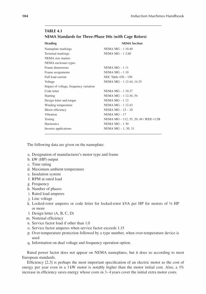
104 Induction Machines Handbook
The following data are given on the nameplate:
a. Designation of manufacturer’s motor type and frameb. kW (HP) outputc. Time ratingd. Maximum ambient temperaturee. Insulation systemf. RPM at rated loadg. Frequencyh. Number of phasesi. Rated load amperesj. Line voltagek. Locked-rotor amperes or code letter for locked-rotor kVA per HP for motors of ½ HP
or morel. Design letter (A, B, C, D)
m. Nominal efficiencyn. Service factor load if other than 1.0o. Service factor amperes when service factor exceeds 1.15p. Over-temperature protection followed by a type number, when over-temperature device is
usedq. Information on dual voltage and frequency operation option.
Rated power factor does not appear on NEMA nameplates, but it does so according to most European standards.
Efficiency [2,3] is perhaps the most important specification of an electric motor as the cost of energy per year even in a 1 kW motor is notably higher than the motor initial cost. Also, a 1% increase in efficiency saves energy whose costs in 3–4 years cover the initial extra motor costs.
TABLE 4.1 NEMA Standards for Three-Phase IMs (with Cage Rotors)
Heading NEMA Section
Nameplate markings
Terminal markings
NEMA size starters
NEMA MG – 1 10.40
NEMA MG – 1 2.60
NEMA enclosure types
Frame dimensions NEMA MG – 1 11
Frame assignments
Full load current
NEMA MG – 1 10
NEC Table 430 – 150
Voltage
Impact of voltage, frequency variation
Code letter
NEMA MG – 1 12.44, 14.35
NEMA MG – 1 10.37
Starting
Design letter and torque
Winding temperature
Motor efficiency
Vibration
NEMA MG – 1 12.44, 54
NEMA MG – 1 12
NEMA MG – 1 12.43
NEMA MG – 12 – 10
NEMA MG – 17
Testing
Harmonics
NEMA MG – 112, 55, 20, 49 / IEEE-112B
NEMA MG – 1 30
Inverter applications NEMA MG – 1, 30, 31

105Motor Specifications and Design Principles
Standard and high-efficiency IM classes have been defined and standardized by now world-wide. As expected, high-efficiency (class E) induction motors have higher efficiency than standard motors, but their size, initial cost, and locked-rotor current are higher. This latter aspect places an additional burden on the local power grid when feeding the motor upon direct starting. If soft-starting or inverter operation is used, the higher starting current does not have any effect on the local power grid rating. NEMA defines specific efficiency levels for Design B IMs (Table 4.3).
On the other hand, EU established three classes EFF1, EFF2, and EFF3 of efficiencies, giving the manufacturers an incentive to qualify for the higher classes (Table 4.2).
The torque/speed curves reveal, for constant V-/f-fed IMs, additional specifications such as start-ing torque, pull-up, and breaking torque for the four classes (letters: A, B, C, and D designs) of induction motors (Figure 4.8).
The performance characteristics of the B, C, and D designs from NEMA Table 2.1 with their typical applications are summarized in Table 4.3.
EFF4 class of premium efficiency was defined by IEC, but so far, only R&D IM prototypes with PM assistance apparently qualified.
4.6 MATCHING IMS TO VARIABLE SPEED/TORQUE LOADS
As IMs are, in general, designed for 60(50) Hz, when used for variable speed, with variable V and f supply, they operate at variable frequency. Below the rated frequency, the machine is capable of full flux linkage, whereas above that, flux weakening occurs.
For given load speed and load torque, with variable V and f supply we may use IMs with 2p1 = 2, 4, 6. Each of them, however, works at a different (distinct) frequency.
Figures 4.9 shows the case of quadratic torque (pump) load with the speed range of 0–2000 rpm, load of 150 kW at 2000 rpm, 400 V, 50 Hz (network). Two different motors are used: one of two poles and one of four poles.
At 2000 rpm, the two-pole IM works at 33.33 Hz – with full flux, whereas the four-pole IM operates at 66.66 Hz in the flux-weakening zone. Which of the two motors is used is decided by the motor costs and losses. Note, however, that the absolute torque (in Nm) of the motor has to be the same in both cases.
For a constant torque load (extruder) with the speed range of 300–1100 rpm, 50 kW at 1200 rpm (network: 400 V, 50 Hz), two motors compete. One, of four poles, will work at 40 Hz and the other, of six poles, at 60 Hz (Figure 4.10).
Again, both motors can satisfy the specifications for the entire speed range as the load torque is below the available motor torque. Again the torque in Nm is the same for both motors, and the choice between the two motors is given by motor costs and total losses.
While starting torque and current are severe design constraints for IMs designed for constant V and f supply, they are not for variable V and f supply.
Skin effect is important for constant V and f supply as it reduces the starting current and increases the starting torque. In contrast to this, for variable V and f supply, skin effect is to be reduced, espe-cially for high-performance speed control systems.
Breakdown torque may become a much more important design factor for variable V and f supply, when a large speed zone for constant power is required. A spindle drive or an electric car drive may require more than three to one constant power speed range (Figure 4.11).
The peak torque of IM is approximately
T 3V2 f
ff
p2L
Tff
ekphn
1n
21n
1
21
scekf
1n
1
2
1n≈π
=
(4.4)
The peak torque for constant (rated) voltage is inversely proportional to frequency squared. To pro-duce a 4/1 constant power speed range, the peak torque has to be four times the rated torque. Only in this case, the motor may produce at f1max = 4f1n, 25% of rated torque.

106 Induction Machines Handbook
TAB
LE 4
.2
460
V, F
our-
Pole
, Ope
n-Fr
ame
Des
ign
B P
erfo
rman
ce a
nd N
EMA
-Defi
ned
Perf
orm
ance
Full
Load
A
mpe
res
(FU
) pe
r N
EC T
able
43
0–15
0
Max
imum
Loc
ked-
Rot
or A
mpe
res
(IR
A)
per
NEM
A M
G 1
, Ta
bles
12.
35 a
nd
12.3
5 A
Nom
inal
Ful
l Loa
d Ef
fici
enci
es (
%)
per
NEM
A M
G 1
, Tab
les
12.1
0 an
d 12
.11
(Ope
n Fo
ur P
ole)
Min
imum
Loc
ked-
Rot
or
Torq
ue (
%)
per
NEM
A
MG
1, T
able
s 12
.2 a
nd
12.3
8.4
Min
imum
Bre
akdo
wn
Torq
ue (
%)
per
NEM
A M
G 1
Tab
les
12.3
9.1
and
12.3
9.3
Min
imum
Pul
l-up
To
rque
(%
) pe
r N
EMA
MG
1 T
able
s 12
.40.
1 an
d 12
.40.
3R
atio
: LR
A/F
LAEf
fici
ency
R
atio
: D
esig
ns
B a
nd E
Des
ign
BD
esig
nE
Des
ign
BD
esig
nE
Des
ign
Ba
Des
ign
ED
esig
n E/
Des
ign
BD
esig
nB
D
esig
nE
Des
ign
BD
esig
nE
Des
ign
BD
esig
nE
HP
34.
832
376.
77.
786
.589
.51.
0421
518
025
020
015
012
0
57.
646
616.
180
87.5
90.2
1.03
185
170
225
200
130
120
7½11
6492
5.8
8.4
88.5
911.
0317
516
021
520
012
011
0
1014
8111
35.
88.
189
.591
.71.
0316
516
020
020
011
511
0
1521
116
169
5.5
891
92.4
102
160
150
200
200
110
110
2027
145
225
5.4
8.3
9193
1.02
150
150
200
200
105
110
2534
183
281
5.4
8.3
91.7
93.6
1.09
150
140
200
190
105
100
3040
218
337
5.5
8.4
92.4
94.1
1.02
150
140
200
190
105
100
4052
290
412
567.
993
94.5
1.02
140
130
200
190
100
100
5065
363
515
568
9395
.41.
0314
013
020
019
010
010
0
6077
435
618
5.6
7.5
93.6
95.4
1.02
140
120
200
180
100
90
7596
543
723
5.7
7.6
94.1
95.4
1.01
140
120
200
180
100
90
100
124
725
937
5.8
7.5
94.1
95.4
1.01
125
110
200
180
100
80
125
156
908
1171
5.8
7.8
94.5
95.4
1.01
110
110
200
180
100
80
150
180
1085
1405
67.
895
95.8
1.01
110
100
200
170
100
80
200
240
1450
1873
67.
895
95.8
1.01
100
100
200
170
9080
250
302
1825
2344
67.
895
.496
.21.
0180
9017
517
075
70
300
361
2200
2809
617.
895
.496
.21.
0180
9017
517
075
70
350
414
2550
3277
6.2
7.9
95.4
96.5
1.01
8075
175
160
7560
400
477
2900
3745
6.1
7.9
95.4
96.5
1.01
8075
175
160
7560
450
515
3250
4214
6.3
8.2
95.8
96.8
1.01
8075
175
160
7560
500
590
3625
4682
6.1
7.9
95.8
968
1.01
8075
175
160
7560
a A
pplie
s to
indu
ctio
n m
otor
s la
belle
d “P
rem
ium
Effi
cien
cy”
or “
Ene
rgy
Effi
cien
t”; D
esig
n e
was
aba
ndon
ed m
200
0, b
ut th
e co
mpa
riso
n ho
lds.

107Motor Specifications and Design Principles
Consequently, if the load maximum torque is equal to the rated torque, then at 4f1n, the rated power is still produced.
In reality, a breakdown torque of 400% is hardly practical. However, efforts to reduce the short-circuit leakage inductance (Lsc) have led up to 300% breakdown torque.
So there are two solutions to provide the required load torque/speed envelope: increasing the motor rating (size) and costs and increasing the flux (voltage) level in the machine by switching from star to delta connection (or by reducing the number of turns per phase by switching off part of stator coils).
The above rationale was intended to suggest some basic factors that guide the IM design.Relating the specifications to a dedicated machine geometry is the object of design (or dimen-
sioning). This enterprise might also be called sizing the IM.Because there are many geometrical parameters and their relationships to specifications (perfor-
mance) are in general nonlinear, the design process is so complicated that it is still a combination of art and science, based solidly on existing experience (motors) with tested (proven) performance. In the process of designing an induction motor, we will define hereby a few design factors, features, and sizing principles.
FIGURE 4.8 (a) NEMA designs A, B, C, and D (b) torque/speed curves.

108 Induction Machines Handbook
4.7 DESIGN FACTORS
Factors that influence notably the IM design are as follows.
4.7.1 coStS
Costs in most cases is the overriding consideration in IM design. But how we define costs? It may be the costs of active materials with or without the fabrication costs. Fabrication costs depend on machine size, materials available or not in stock, manufacturing technologies, and manpower costs.
TABLE 4.3 Motor Designs after NEMA and EU
Locked-Rotor Torque
(% Rated Load Torque)
Breakdown Torque (% Rated Load
Torque)
Locked-Rotor Current (% Rated Load
Current)Slip %Classification Typical Applications Rel. η
Design BNormal locked-
rotor torque and normal locked-rotor current
70–275a 175–300a 600–700 0.5–5 Fans, blowers, centrifugal pumps and compressors, motor–generator sets, etc., where starting torque requirements are relatively low
Medium or high
Design CHigh locked-rotor
torque and normal locked-rotor current
200–250a 190–225a 600–700 1–5 Conveyors, crushers, stirring machines, agitators, reciprocating pumps and compressors, etc., where starting under load is required
Medium
Design DHigh locked-rotor torque and high slip
275 275 600–700 High peak loads with or without fly wheels, such as punch presses, shears, elevators, extractors, winches, hoists, oil well pumping and wire drawing machines
Medium
Note: Design A motor performance characteristics are similar to those for Design B except that the locked-rotor starting current is higher than the values shown in the table.
a Higher values are for motors having lower horsepower ratings.
Others Similar Local
Regulations, for Example, in Countries Like
IEC60034-30EuP Directive2005/32/EC
Europe (50 Hz)CEMEP
Voluntary AgreementUS (60 Hz)
EPAct
IE1 Standard efficiency Comparable to EFF2 Below standard efficiency AS in Australia
IE2 High efficiency Comparable to EFF1 Identical to NEMA Energy efficiency/EPACT
NBR in BrazilGB/T in China
IE3 Premium efficiency Extrapolated IE2 with 10%–15% lower losses
Identical to NEMA Premium efficiency
IS in IndiaJIS in JapanMEPS in Korea

109Motor Specifications and Design Principles
The costs of capitalized losses per entire motor active life surpass quite a few times the initial motor costs. So loss reduction (through higher efficiency or via variable V and f supply) pays off generously. This explains the rapid expansion of variable speed drives with IMs worldwide.
Finally, maintenance costs are also important but not predominant. We may now define the global costs of an IM as
Global costs Material costs Fabrication and selling costs
Losses capitalized costs Maintenance costs
= +
+ + (4.5)
Global costs are also a fundamental issue when we have to choose between repairing an old motor or replacing it with a new motor (with higher efficiency and corresponding (higher) initial costs).
torque
100%
f(Hz)33.33 66.66
2p =21
2p =41
FIGURE 4.9 Torque versus motor frequency (and speed) pump load.
100%
f(Hz)40 60
torque
4 poles6 poles
FIGURE 4.10 Torque versus motor frequency (and speed): constant torque load.
en
1n
r
1 2 3 4
1
2
3
4
0.25
TT
f
4
0.54/9
0.25
load
Ω
FIGURE 4.11 Induction motor torque/speed curves for various values of frequency and a 4/1 constant power speed range.

110 Induction Machines Handbook
4.7.2 Material liMitationS
The main materials used in IM fabrication are magnetic-steel laminations, copper and aluminium for windings, and insulation materials for windings in slots.
Their costs are commensurate with performance. Progress in magnetic and insulation materials has been continuous. Such new improved materials drastically affect the IM design (geometry), performance (efficiency), and costs.
Flux density, B(T), losses (W/kg) in magnetic materials, current density J (A/mm2) in conduc-tors, and dielectric rigidity E (V/m) and thermal conductivity of insulation materials are key factors in IM design.
4.7.3 S tanDarD SpeciFicationS
IM materials (lamination thickness, conductor diameter), performance indexes (efficiency, power factor, starting torque, starting current, breakdown torque), temperature by insulation class, frame sizes, shaft height, cooling types, service classes, protection classes, etc. are specified in national (or international) standards (NEMA, IEEE, IEC, EU, etc.) to facilitate globalization in using induction motors for various applications. They limit, to some extent, the designer’s options but provide solu-tions that are widely accepted and economically sound.
4.7.4 Special FactorS
In special applications, special specifications such as minimum weight and maximum reliability in aircraft applications become the main concern. Transportation applications require ease of main-taining, high reliability, and good efficiency. Circulating water home pumps requires low noise, highly reliable induction motors.
Large compressors have large inertia rotors, and thus, motor heating during frequent starts is severe. Consequently, maximum starting torque/current becomes the objective function.
4.8 DESIGN FEATURES
The major issues in designing an IM may be divided into five areas: electrical, dielectric, magnetic, thermal and mechanical.
• Electrical designTo supply the IM, the supply voltage, frequency, and number of phases are specified.
From these data, the minimum power factor, and a target efficiency, the phase connection (start or delta), winding type, number of poles, slot numbers, and winding factors are cal-culated. Current densities (or current sheets) are imposed.
• Magnetic designBased on output coefficients, power, speed, number of poles, and type of cooling, the
rotor diameter is calculated. Then, based on a specific current loading (in A/m) and airgap flux density, the stack length is determined.
Fixing the flux densities in various parts of the magnetic circuit with given current den-sities and slot mmfs, the slot sizing, core height, and external stator diameter Dout are all calculated. After choosing Dout, which is standardized, the stack length is modified until the initial current density in slot is secured.
It is evident that sizing the stator and rotor core is carried out in many ways based on various criteria.
• Insulation designInsulation material and its thickness, be it slot/core insulation, conductor insulation, end
connection insulation, or terminal leads insulation, depend on machine voltage insulation class and on the environment in which the motor operates.
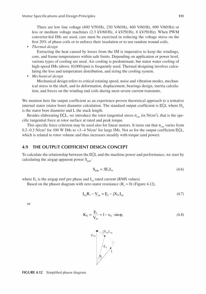
111Motor Specifications and Design Principles
There are low line voltage (400 V/50 Hz, 230 V/60 Hz, 460 V/60 Hz, 690 V/60 Hz) or less or medium voltage machines (2.3 kV/60 Hz, 4 kV/50 Hz, 6 kV/50 Hz). When PWM converter-fed IMs are used, care must be exercised in reducing the voltage stress on the first 20% of phase coils or to enforce their insulation or to use random wound coils.
• Thermal designExtracting the heat caused by losses from the IM is imperative to keep the windings,
core, and frame temperatures within safe limits. Depending on application or power level, various types of cooling are used. Air cooling is predominant, but stator water cooling of high-speed IMs (above 10,000 rpm) is frequently used. Thermal designing involves calcu-lating the loss and temperature distribution, and sizing the cooling system.
• Mechanical designMechanical design refers to critical rotating speed, noise and vibration modes, mechan-
ical stress in the shaft, and its deformation, displacement, bearings design, inertia calcula-tion, and forces on the winding end coils during most severe current transients.
We mention here the output coefficient as an experience-proven theoretical approach to a tentative internal stator (stator bore) diameter calculation. The standard output coefficient is D2
isL where Dis is the stator bore diameter and L the stack length.
Besides elaborating D2isL, we introduce the rotor tangential stress σtan (in N/cm2), that is the spe-
cific tangential force at rotor surface at rated and peak torque.This specific force criterion may be used also for linear motors. It turns out that σtan varies from
0.2–0.3 N/cm2 for 100 W IMs to <3–4 N/cm2 for large IMs. Not so for the output coefficient D2isL,
which is related to rotor volume and thus increases steadily with torque (and power).
4.9 T HE OUTPUT COEFFICIENT DESIGN CONCEPT
To calculate the relationship between the D2isL and the machine power and performance, we start by
calculating the airgap apparent power Sgap:
S 3E Igap 1 1n= (4.6)
where E1 is the airgap emf per phase and I1n rated current (RMS values).Based on the phasor diagram with zero stator resistance (Rs = 0) (Figure 4.12),
I R V E jX I1n s 1n 1 ls 1n− = − (4.7)
or
KEV
1 x sinE1
1nls 1= ≈ − ⋅ ϕ (4.8)
V1n
jX I1nls
E1
I-
1ϕ
FIGURE 4.12 Simplified phasor diagram.

112 Induction Machines Handbook
with
xX IV
esls 1n
1n
= (4.9)
The p.u. value of stator leakage reactance increases with pole pairs p1 and so does sin φ1 (power factor decreases when p1 increases).
K 0.98 0.005pE 1≈ − (4.10)
Also, the input apparent power S1n is
S 3V IP
cos1n 1n 1n
n
n 1n
= =η ϕ
(4.11)
where Pn is the rated output power, and ηn and cos φ1n are the assigned values of rated efficiency and power factor based on past experience.
Typical values of efficiency for Design B (NEMA) are given in Table 4.3. Each manufacturer has its own set of data.
Efficiency increases with power and decreases with the number of poles. Efficiency of wound rotor IMs is slightly larger than that of cage-rotor IMs of the same power and speed because the rotor windings are made of copper and the total additional load (stray) losses are lower.
As efficiency is defined with stray losses pstray of 0.5(1.0)% of rated power in Europe (still!) and with the latter (pstray) measured in direct load tests in USA, differences in actual losses (in IMs of the same power and nameplate efficiency) of even more than 20% may be encountered when motors fabricated in Europe are compared with those made in the USA. Recently, IEC adopted the stray load loss estimation from load tests very similar to IEEE standard.
Anyways, the assigned value of efficiency is only a starting point for design as iterations are performed until the best performance is obtained.
The power factor also increases with power and decreases with the number of pole pairs with values slightly smaller than corresponding efficiency for existing motors. More data on initial effi-ciency and power factor data will be given in subsequent chapters on design methodologies.
The emf E1 is written as a function of airgap pole flux φ:
E 4f K W K1 1 f 1 w1= φ (4.12)
where f1 is frequency, 1.11 > Kf > 1.02 form factor (dependent on teeth saturation) (Figure 4.13), W1 is turns per phase, Kw1 is the winding factor, and ϕ is the pole flux.
LBi gφ = α τ (4.13)
where αi is the flux density shape factor dependent on the magnetic saturation coefficient of teeth (Figure 4.13), and Bg is the flux density in the airgap. The pole pitch τ is
D
2p; n
fp
is
11
1
1
τ = π = (4.14)
Finally, Sgap is
S K K D Ln60
A Bgap f i w12
is2 1
1 g= α π (4.15)

113Motor Specifications and Design Principles
The specific stator current load A1 (A/m) is
A6W I
D1
1 1n
is
=π
(4.16)
We separate the volume utilization factor C0 (Esson’s constant) as
C K K A B60S
D Ln; n in rpm0 f i w1
21 g
gap
is2
11= α π = (4.17)
C0 is not in fact a constant as both the values of A1(A/m) and airgap flux density (Bg) increase with machine power and with the number of pole pairs.
The D2isL output coefficient may be calculated from (4.17) with Sgap from (4.6) and (4.11):
D L1
C60n
K Pcos
is2
0 1
E n
n 1n
=η ϕ
(4.18)
Typical values of C0 as a function Sgap with pole pairs p1 as parameter for low-power IMs is given in Figure 4.14, with KE from (4.10).
2The DisL (internal) output constant (proportional to rotor core volume) is, in fact, almost propor-tional to machine rated shaft torque. Torque production requires apparently less volume as the pole pair number p1 increases, and C0 increases with increasing p1 (Figure 4.14).
It is standard to assign also a value λ to the stack length-to-pole pitch ratio:
L 2LP
D; 0.6 3.01
is
λ =τ
=π
< λ < (4.19)
The stator bore diameter may now be calculated from (4.18) with (4.19).
FIGURE 4.13 Form factor Kf and flux density shape factor αi versus teeth saturation.

114 Induction Machines Handbook
D2p 1
Cpf
K Pcos
is1
0
1
1
E n
n 1n
3=πλ η ϕ
(4.20)
This is a standard design formula. However, it does not say enough on the machine total volume (weight). Moreover, in many designs, the stator external (frame internal) diameters are standardized.
A similar (external) output coefficient D2outL may be derived if we first adopt a design current
density Jcon(A/m2) and consider the slot fill factor (with conductors), Kfill = 0.4–0.6, given together with the tooth and stator back iron flux densities Bts and Bcs.
With the known airgap flux density Bg and tooth flux density Bts, the stator slot height hs is approximately
h6W I
B
Bj K
1D
AB
Bj K
s1 n
g
tscon fill
is
1
g
tscon fill
=π
= (4.21)
Now the core (yoke) radial height hcs is
h2LB 2
D2P
B
Bcs
cs
i is
1
g
cs
= φ = α π
(4.22)
The outer stator diameter Dout is
D D 2 h hout is s cs( )= + + (4.23)
We replace Dis from (4.23) in D2isL with hs and hcs from (4.21) and (4.22):
D L D L f Dis2
out2
0 is( )= ⋅ (4.24)
FIGURE 4.14 Esson’s “constant” C0 versus Sgap (airgap apparent power).

115Motor Specifications and Design Principles
f D1
12 h h
D
0 is
s cs
is
2( )( )
=+ +
(4.25)
And, finally,
f D1
12A B
j K B D 2 p
B
B
0 is
1 ts
con fill g is
i
1
g
cs
2( ) =
+ + α π
(4.26)
From (4.24),
D LD L
f D1
C f DPf
K Pcos
out2 is
2
0 is 0 0 is
1
1
E n
n 1n( ) ( )= =η ϕ
(4.27)
As LD
2Pis
1
= λ π (4.28)
D2pC f
K Pcos
1D f D
out12
0 1
E n
n 1n is 0 is( )=πλ η ϕ
(4.29)
Although (4.29) through the function D fis 0 i( )D1
s −
suggests that a minimum Dout may be obtained for given λ, Bg/Bco, Bg/Bt, jcon, and A1, it seems more practical to use (4.29) to find the outer sta-tor diameter Dout after the stator bore diameter was obtained from (4.20). Now if this value is not a standard one and a standard frame is a must, the aspect ratio λ is modified until Dout matches a standardized value.
The specific current loading A1 depends on pole pitch τ and number of poles on Dis, once a cer-tain cooling system (current density) is adopted.
In general, A increases with D from values of <103 1 is A/m for Dis = 4 · 10−2 m to 45,000 A/m for
Dis = 0.4 m and 2p1 = 2 poles. Smaller values are common for larger number of poles and same sta-tor bore diameter.
On the other hand, the design current density jcon varies in the interval j = (3.5–8.0)106 A/m2con for
axial or axial-radial air cooling. Higher values are designated to high-speed IMs (lower pole pair numbers p1) or for liquid cooling. While A1 varies along such a large span and the slot height hs-to-slot width bs ratio is limited to Kaspect = 3–6, to limit the slot leakage inductance, using A1 is avoided by calculating slot height hs as
h K b KDN
1b
KDN
1B
Bs aspect s aspect
is taspect
is g= = π −
= π −
(4.30)s slot s tsτ
Higher values of aspect ratios are typical to larger motors.This way, D2
outL is
D L1
CPf
K Pcos
12K
N1
B
B 2 P
B
Bout2
0
1
1
E n
n 1n
aspect
s
g
ts
i
1
g
cs
2
=η ϕ
+π
−
+ α π
(4.31)

116 Induction Machines Handbook
Also,
DD
12K
N1
B
B 2 p
B
Bout
is
aspect
s
g
ts
i
1
g
cs
≈ +π
−
+ α π (4.32)
To start, we may calculate Dis/Dout as a function of only pole pairs p1 if Bg/Bts = ct and Bg/Bcs = ct, with Kaspect s and N (slots/stator) also assigned corresponding values (Table 4.4).
The stack aspect ratio λ is assigned an initial value in a rather large interval: 0.6–3.In general, longer stacks, allowing for a smaller stator bore diameter (for given torque), lead to
shorter stator winding end connections, lower winding losses, and lower inertia, but the temperature rise along the stack length may become important. An optimal value of λ is highly dependent on IM design specifications and the design objective function taken into consideration. There are applica-tions with space shape constraints that prevent the using of a long motor.
Example 4.1 Output Coefficient
Let us consider a 55 kW, 50 Hz, 400 V, 2p1 = 4 induction motor whose assigned (initial) rated effi-ciency and power factor are ηn = 0.92, cos φn = 0.92.
Let us determine the stator internal and external diameters Dout and Dis for λ = L/τ = 1.5.
Solution
The emf coefficient KE (4.10) is KE = 0.98 − 0.005 · 2 = 0.97The airgap apparent power Sgap (4.3) is
= =ϕ η
= ⋅ ⋅⋅
= ⋅S 3K V I KP
cos0.97 55 10
0.92 0.9263.03 10 VAgap E 1 1n E
n
n n
33
Esson’s constant C0 is obtained from Figure 4.14 for p1 = 2 and Sgap = 63.03 · 103 VA: C0 = 222 · 103 J/m3.
For an airgap flux density Bg = 0.8 T, Kw1 = 0.955, αi = 0.74, Kf = 1.08 (teeth saturation coefficient 1 + Kst = 1.5, Figure 4.13). The specific current loading A1 is (4.17)
3
=α π
= ⋅⋅ ⋅ ⋅ π
= ⋅AC
K K B222 10
1.08 0.74 0.955 0.836.876 10 A/m1
0
f i w12
g2
3
with λ = 1.5 from (4.20), the stator internal diameter Dis is obtained.
= ⋅⋅
⋅⋅
⋅ ⋅ ⋅ =D2 2
2 1.51
222 102
5063.03 10 0.2477mis 3
33
The stator stack length L (4.19) is
= λ π = ⋅ π ⋅⋅
=LD
2p1.5 0.2477
2 20.2917mis
1
TABLE 4.4 Outer Stator Diameter-to-Inner Stator Diameter Ratios
Dout
Dis
2p1 2 4 6 8 ≥10
1.65–1.69 1.46–1.49 1.37–1.40 1.27–1.30 1.24–1.26

117Motor Specifications and Design Principles
with jcon = 6 · 106 A/m, Kfill = 0.5, Bts = Bcs = 1.6 T, the stator slot height hs is (4.21).
= ⋅
⋅ ⋅ ⋅= ⋅ −h
36.876 100.81.6
6 10 0.524.584 10 ms
3
6
3
The stator back iron height hcs (4.22) is
= α π = ⋅ π ⋅⋅ ⋅
⋅ ≈ ⋅ −h2
D2p
B
B0.74 0.2477
2 2 20.81.6
36 10 mcsi is
1
g
cs
3
The external stator diameter Dout becomes
( ) ( )= + + = + + =D D 2 h h 0.2477 2 0.024584 0.036 0.3688mout is cs s
With Ns = 48 slots/stator and a slot aspect ratio Kaspect = 3.03, the value of slot height hs (4.30) is
h KDN
1B
B3.03
0.247748
10.81.6
0.0246ms aspectis
s
g
ts
= π −
= π −
=
About the same value of hs as above has been obtained. It is interesting to calculate the approxi-mate value of the specific tangential force σtan.
P
DD2
L
p2 f
55 10
20.2917 0.2477
22 50
tann
isis
1
1
3
2σ ≈
π
π= ⋅
π ⋅ ⋅⋅
π
1.246 10 N/m 1.246 N/cm4 2 2= ⋅ =
This is not a high value, and the moderate-low slot aspect ratio Kaspect = hs/bs = 3.03 is a clear indication of this situation.
Apparently, the machine stator internal diameter may be reduced by increasing A1 (in fact, C0 Esson’s constant). For the same λ, the stack length will be reduced, while the stator external diam-eter will also be slightly reduced (the back iron height hcs decreases, and the slot height increases).
Given the simplicity of the above analytical approach further speculations on better (eventually optimized) designs are considered inappropriate here.
4.10 THE ROTOR TANGENTIAL STRESS DESIGN CONCEPT
The rotor tangential stress σ (N/m2tan ) may be calculated from the motor torque Te.
T 2
D L DN/mtan
en
is is
2( )( )σ = ⋅π ⋅
(4.33)
The electromagnetic torque Ten is approximately
Tp P 1
pP
2 f 1 Sen
1 nmec
n
1 n( )≈+
π − (4.34)
Pn is rated motor power; Sn = rated slip.The rated slip is <2%–3% for most induction motors, and the mechanical losses are in general
around 1% of rated power.

118 Induction Machines Handbook
Tp P 1.012 f 0.98
0.1641 Ppf
en1 n
1n
1
1
≈ ⋅π
= ⋅ (4.35)
Choosing σtan in the interval 0.2–5 N/cm2 or 2,000–50,000 N/m2, we use (4.33) directly, with λ = 2p1 iL Dπ s, to determine the internal stator diameter.
D4p
0.1641 Ppf
is1
2tan
n1
1
3=π λσ
⋅ ⋅
(4.36)
No apparent need occurs to adopt at this stage efficiency and power factor values for rated load.We can now use the no-load value of airgap flux density Bg0:
B3 2W K I
p K g 1 Kg0
0 1 w1 0
1 c s( )= µπ +
(4.37)
where the no-load current I0 and the number of turns/phase W1 are unknown and the airgap g, Carter’s coefficient Kc, and saturation factor Ks are assigned pertinent values.
g 0.1 0.02 P 10 [m]; for P 1
g 0.1 0.012 P 10 [m]; for P 2
n3 3
1
n3 3
1
( )( )
≈ + ⋅ =
≈ + ⋅ ≥
−
− (4.38)
Typical values of airgap are 0.35, 0.4, 0.45, 0.5, 0.55 … mm, etc. Also, Kc ≈ (1.15–1.35) for semi-closed slots and Kc = 1.5–1.7 for open stator slots (high-power induction motors). The saturation factor is typically Ks = 0.3–0.5 for p1 ≥ 2 and larger for 2p1 = 2.
The airgap flux density Bg is
= − =B (0.5 0.7)T for 2p 2g 1
= − =
= − =
B (0.65 0.75)T for 2p 4
B (0.7 0.8)T for 2p 6
g 1
g 1
(4.39)
= − =B (0.75 0.85)T for 2p 8g 1
The larger values correspond to larger motors.The product, W1I0, is thus obtained from (4.37). The number of turns W1 may be calculated from
the emf E1 (4.12) and (4.13).
WE
4f K KE 2p
4f K K D LB1
1
1 f w1
1 1
1 f w1 i is g
=φ
=α π
(4.40)
with W1I0 and W1 known, the no-load (magnetization) current I0 may be obtained. The airgap active power Pgap is
P T2 fp
3K V Igap en1
1E 1 T= π = (4.41)
where IT is the stator current torque component (in phase with E1). With IT determined from (4.41), we now calculate the stator rated current I1n:
I I I1n 02
T2≈ + (4.42)

119Motor Specifications and Design Principles
The rotor bar current (for a cage rotor) Ib is
I2mW K I
Nb
1 w1 T
r
≈ (4.43)
Nr – number of rotor slots, m – number of stator phases.We now check the product ηn cos φ1n:
cosP
3V I1n n
n
1 1n
η ϕ = < (4.44)
The linear current loading A1 is also checked:
A2mW I
D1
1 1n
is
=π
(4.45)
and eventually compare with data from existing similar motors.With all these data available, the sizing of stator and rotor slots and their windings is feasi-
ble. Then, the machine reactances and resistances and the steady-state performance are calcu-lated. Knowing the motor geometry and the loss breakdown, the thermal aspects (design) may be approached. Finally, if the temperature rise or other performance is not satisfactory, the design process is repeated.
Given the complexity of such an enterprise, some coherent methodologies are in order. They will be explained in subsequent chapters.
Example 4.2 Tangential Stress
Let us consider the motor data from Example 4.1, assume σtan = 1.5 · 104 N/m2, and determine the values of Dis, L, W1, I0, I1n, and ηn cos φn.
Solution
With p1 = 2, Pn = 55 kW, f1 = 50 Hz, λ= 1.5, from (4.36),
= ⋅ ⋅ ⋅ ⋅ ⋅π ⋅ ⋅ ⋅
=D4 2 0.1641 55 10 2
1.5 1.5 10 500.2352mis
3
2 43
The stack length L is
= λ π = π ⋅⋅
=LD
2p1.5
0.23522 2
0.277mis
1
with Bg = 0.8 T, Kf = 1.08, αi = 0.74, Kw1 = 0.955, KE = 0.97, and from (4.40), the number of turns per phase W1 is
W0.97
4003
2 2
4 50 1.08 0.955 0.74 0.2352 0.277 0.836 turns/phase1 =
⋅
⋅ ⋅
⋅ ⋅ ⋅ ⋅ ⋅ π ⋅ ⋅ ⋅=
The rated electromagnetic torque Ten (4.35) is
= ⋅ = ⋅ ⋅ ⋅ =T 0.1641 Ppf
0.1641 55 102
50361.02 Nmen n
1
1
3

120 Induction Machines Handbook
Now, from (4.41), the torque current component IT is
= ⋅ π = ⋅ π
⋅ ⋅ ⋅=I
T 2 f3K V p
361.02 2 50
3 0.97400
32
84.24 ATen 1
E 1 1
The magnetization current I0 is obtained from (4.37):
( )=π +
µ= ⋅ π ⋅ ⋅ ⋅ ⋅ + ⋅
⋅ ⋅ ⋅ ⋅=
−
−IB P K g 1 K
3 2W K0.8 2 1.25 0.55 (1 0.5) 10
1.256 10 36 0.955 3 228.36 A0
g0 1 c s
0 1 w1
3
6
The airgap g (4.38) is
( )= + ⋅ = ⋅− −g 0.1 0.012 55,000 10 0.55 10 m3 3 3
The stator rated current I1n is
= + = + =I I I 28.36 84.24 88.887 A1n 02
T2 2 2
3
η ϕ = = ⋅
⋅ ⋅=cos
P3V I
55 10
3400
388.887
0.894n 1nn
1 1n
This corresponds to a rather high (say) ηn = cos φ1n = 0.9455.Note that these values appear at design starting, before all the losses in the machine have been
assessed. They provide a design start without Esson’s (output) constant which increased continu-ously over the last decades as material quality and cooling systems improved steadily.
4.11 SUMMARY
• Mechanical loads are characterized by torque/speed curves.• Single-quadrant and multiquadrant load torque/speed curves are typical.• Constant V and f supply IMs are suitable only for constant speed single-quadrant loads.• For single and multiquadrant variable speed loads, variable V and f supply IMs are
required. They result in energy savings commensurable with speed control range.• Three load torque/speed curves are typical: quadratic torque/speed (pumps), constant
torque (elevators), and constant power (machine tool, spindles, traction, etc.).• The standard IM design torque/speed envelope, to match the load, includes two regions:
below and above base speed Ωb. For base speed full voltage, full torque is delivered at rated service cycle and rated temperature rise.
• With self-ventilation, the machine over-temperature restriction leads to torque reduction with speed reduction. For constant torque below base speed, separate (constant speed) ventilation is required.
• Above base speed, with constant voltage and increasing frequency, the torque available decreases and so does the flux linkage in the machine.
• A 2/1 constant power speed range (from Ωb to 2Ωb) is typical with standard IM designs at constant voltage.
• When an induction motor designed for sine wave power is faced with a notable har-monic content in the power grid due to the presence of power electronic equipment nearby, it has to be derated. In general, a HVF of less than 3% is considered harmless (Figure 4.6).

121Motor Specifications and Design Principles
• A standard sine wave IM, when fed from a PWM voltage source inverter, due to the addi-tional (time harmonics) core and winding losses, has to be derated. A derating of up to 10% is considered acceptable with today’s IGBT converters.
• Further on, the presence of a static power converter leads to a 5% voltage reduction at motor terminals with respect to the power grid voltage.
• Finally, an additional derating occurs due to unbalanced power grid voltage. The derating is significant for voltage unbalance above 2% (Figure 4.7).
• Induction motor specifications for constant V and f motors are lined up in perti-nent standards. Nameplate markings refer to a myriad of specifications for the user’s convenience.
• Efficiency is the most important nameplate marking as the cost of losses per year is about (or more than) 30%–40% of initial motor costs.
• Standard and high-efficiency motors are now available. EU regulations refer to high-efficiency thresholds (Table 4.3).
• Designs A, B, C, and D reveal through their torque–speed curves, the starting, pull-up, and breakdown torques which are important factors in most constant V and f supply IMs.
• Matching a constant V and f IM to a load refers to equality of load and motor torque at rated speed and lower load torque below rated speed.
• For variable speed drives, two different pole pairs count motors at two different frequen-cies: one below base speed (full flux zone) and one above base speed (flux-weakening, constant voltage zone) may be used.
• For constant power large speed ranges Ωmax/Ωb > 3, very large breakdown torque designs are required (above 300%). Alternatively, the voltage per phase is increased above base speed by star/delta connection or a larger torque (larger size) IM is chosen.
• Designing of an IM involves sizing the motor for given specifications of power, supply parameters, and load torque/speed envelope.
• Main design factors are costs of active materials, fabrication and selling, losses capital-ized costs, maintenance costs, material limitations (magnetic, electric, dielectric, thermal, mechanical), and special application specifications.
• The IM design features five issues:• Electric design• Dielectric design• Magnetic design• Thermal design• Mechanical design.
• IM sizing is both a science and an art based on prior experience.• D2
isL output coefficient design concept has gained widespread acceptance due to Esson’s output constant, and with efficiency and power factor known, the stator bore diameter Dis, may be calculated for given power, speed, and stack length L per pitch τ ratio λ given.
• Further on, with given stator winding current density, airgap, stator teeth, and back core flux densities Bg, Bts, Bcs, the outer stator diameter is obtained. Based on these data, the stator/rotor slot sizing, wire gauge, machine parameters, performance, losses, and tem-peratures may be determined. Such a complex enterprise requires coherent methodologies, to be developed in subsequent chapters.
• The rotor tangential (shear) stress, σtan = (0.2–4) N/cm2, is defined as a more general design concept valid for both rotary and linear induction motors (LIM). This way, there is no need to assign initial values to efficiency and power factor to perform the complete design (sizing) process.
• More on design principles in References [4–9].

122 Induction Machines Handbook
REFERENCES
1. A. H. Bonett, G. C. Soukup, NEMA Motor – Generator Standards for Three-Phase Induction Motors, IEE – IAS Magazine, May–June 1999, pp. 49–63.
2. B. De Vault, D. Heckenkamp, T. King, Selection of Short Circuit Protection and Control for Design E Motors, IBID, pp. 26–37.
3. J. C. Andreas, Energy: Efficient Electric Motors, Marcel Dekker Inc., New York, 1982.4. E. Levi, Polyphase Motors: A Direct Approach to Their Design, Wiley Interscience, Hoboken, NJ, 1985.5. B. J. Chalmers, A. Williamson, A.C. Machines: Electromagnetics and Design, Research Studies Press
LTD, John Wiley & Sons Inc., Hoboken, NJ, 1991.6. E. S. Hamdi, Design of Small Electrical Machines, John Wiley & Sons Ltd, Chichester, England, 1993.7. A. Boglietti, A. Cavagnino, M. Lazzari, Geometrical approach to induction motor design, IECON 2007,
33rd Annual Conference of the IEEE Industrial Electronics Society, Taipei, Taiwan, 2007, pp. 149–156.
9. J. Pyrhonen, T. Jokinen, V. Hrabovcova, Design of Rotating Electrical Machines, Wiley, Chichester, UK, 2009.
8. T. A. Lipo, Introduction to AC Machine Design, University of Wisconsin Press, Madison, WI, 2007.

123
5 IM Design below 100 KW and Constant V and f (Size Your Own IM)
5.1 INTRODUCTION
The power of 100 kW is traditionally considered the border between small- and medium-power induction machines (IMs). In general, sub-100 kW motors use a single stator and rotor stack (no radial cooling channels) and a finned frame washed by air from an externally mounted at shaft end ventilator (Figure 5.1). It has an aluminum cast-cage rotor and, in general, random wound sta-tor coils made of round magnetic wire with one to six elementary conductors (diameter ≤ 2.5 mm) in parallel and one to three current paths in parallel, depending on the number of pole pairs. The number of pole pairs p1 = 1, 2, 3, … 6.
Induction motors with power below 100 kW constitute a sizeable portion of electric motor world markets. Their design for standard or high efficiency is by now a mature mixture of art and science, at least in the preoptimization stage. Design optimization will be dealt with separately in a dedicated chapter.
For most part, IM design methodologies are proprietary.Here, we present a sample of such methodologies next. For further reference, see also [1].
5.2 D ESIGN SPECIFICATIONS BY EXAMPLE
Standard design specifications are
• Rated power: Pn[W] = 5.5 kW• Synchronous speed: n1[rpm] = 1800• Line supply voltage: V1[V] = 460 V• Supply frequency: f1[Hz] = 60• Number of phases m = 3• Phase connections: star
FIGURE 5.1 Low-power three-phase IM with cage rotor.
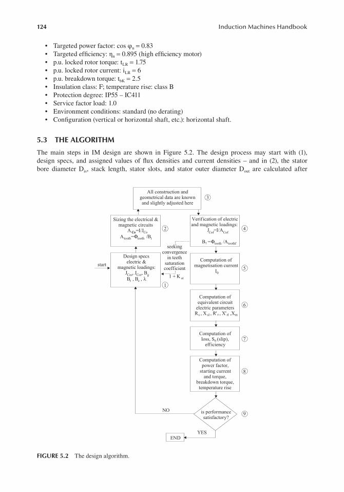
124 Induction Machines Handbook
• Targeted power factor: cos φn = 0.83• Targeted efficiency: ηn = 0.895 (high efficiency motor)• p.u. locked rotor torque: tLR = 1.75• p.u. locked rotor current: iLR = 6• p.u. breakdown torque: tbK = 2.5• Insulation class: F; temperature rise: class B• Protection degree: IP55 – IC411• Service factor load: 1.0• Environment conditions: standard (no derating)• Configuration (vertical or horizontal shaft, etc.): horizontal shaft.
5.3 THE ALGORITHM
The main steps in IM design are shown in Figure 5.2. The design process may start with (1), design specs, and assigned values of flux densities and current densities – and in (2), the stator bore diameter Dis, stack length, stator slots, and stator outer diameter Dout are calculated after
All construction andgeometrical data are known and slightly adjusted here
Sizing the electrical & magnetic circuits
A =I/JA = /BΦ
Co Co
tooth tooth t
Verification of electric and magnetic loadings:
J =I/A
B = /AΦtooth toothft
Cof Cof
Design specselectric &
magnetic loadings:J , J , BB , B , λCos Cor g
t c
start
1 + K st
1
2 4
3
Computation ofmagnetisation current
I05
Computation ofequivalent circuit
electric parametersR , X , R' , X' ,X
6
Co
s sl r rl m
Computation ofloss, S (slip),
efficiency7n
Computation ofpower factor,
starting currentand torque,
breakdown torque, temperature rise
8
is performance satisfactory?
9NO
YESEND
seekingconvergence
in teethsaturationcoefficient
FIGURE 5.2 The design algorithm.

125IM Design below 100 KW and Constant V
stator and rotor currents are determined. The rotor slots, back iron height, and cage sizing are also determined in (2).
All dimensions are adjusted in (3) to standardized values (stator outer diameter, stator winding wire gauge, etc.). Then in (4), the actual magnetic and electric loadings (current and flux densities) are verified.
If the magnetic saturation coefficients (1 + Kst) of stator and rotor tooth are not equal to assigned values, the design restarts (1) with adjusted values of tooth flux densities until sufficient convergence is obtained in 1 + Kst.
Once this loop is surpassed, the stages (5) to (8) are traveled by computing the magnetization current I0 (5); equivalent circuit parameters are calculated in (6); losses, rated slip Sn, and efficiency are determined in (7); and then, power factor, locked rotor current and torque, breakdown torque, and temperature rise are assessed in (8).
In (9), all this performance is checked and, if found unsatisfactory, the whole process is restarted in (1) with new values of flux densities and/or current densities and stack aspect ratio λ = L/τ (τ – pole pitch).
The decision in (9) may be made based on an optimization method which might result in going back to (1) or directly to (3) when the chosen construction and geometrical data are altered a ccording to an optimization method (deterministic or evolutionary) as shown in Chapter 8, Vol. 2.
So, IM design is basically an iterative procedure [2] whose output – the resultant machine to be built – depends on the objective function(s) to be minimized and on the corroborating constraints related to temperature rise, starting current (torque), breakdown torque, etc.
The objective function may be weight or costs or (efficiency)−1 or global costs of active materials or a weighted combination of them.
But before treating the optimization stage in Chapter 8, Vol. 2, let us perform here a practical design.
5.4 MAIN DIMENSIONS OF STATOR CORE
We are going to use the widely accepted D2isL output constant concept unfolded in the previous
chapter. For completely new designs, the rotor tangential stress concept can be used.Based on this, the stator bore diameter Dis (4.15) is
=πλ
= − =D2p p
f
S
C; K 0.98 0.005p 0.97is
1 1
1
gap
0
3 E 1 (5.1)
=η ϕ
λ =π
=τ
SK Pcos
; L2pD
Lgap
E n
n 1n
1
is
(5.2)with
From past experience, λ is given in Table 5.1.From (5.2), the apparent airgap power Sgap is
= ⋅ ⋅⋅
=S0.97 5.5 100.895 0.83
7181.8VAgap
3
TABLE 5.1 Stack Aspect Ratio λ2p1 2 4 6 8
λ 0.6–1.0 1.2–1.8 1.6–2.2 2–3

126 Induction Machines Handbook
C0 is extracted from Figure 4.14 for Sgap = 7181.8 VA, C0 = 147 · 103 J/m3 and λ = 1.5, f1 = 60 Hz, p1 = 2. So Dis from (5.1) is
= ⋅ ⋅π ⋅ ⋅
⋅⋅
=D2 2 215 60
7181.8147 10
0.1116mis 33
The stack length L (from 5.2) is
= π ⋅⋅
=L1.5 0.1116
2 20.1315m
The pole pitch
τ = π ⋅⋅
=0.11162 2
0.0876m
The number of stator slots per pole 3q may be 3 · 2 = 6 or 3 · 3 = 9. For q = 3, the slot pitch τs will be around
τ = τ =⋅
= ⋅ −
3q0.0876
3 39.734 10 ms
3 (5.3)
In general, the larger q gives better performance (space field harmonics and losses are smaller).The slot width at airgap is to be around 5–5.3 mm with a tooth of 4.7–4.4 mm, which is mechani-
cally feasible.From past experience (or from optimal lamination concept, introduced later in this chapter), the
ratio of the internal to external stator diameter Dis/Dout, below 100 kW for standard motors, is given in Table 5.2.
With 2p1 = 4, Dout can be determined by substituting the value of KD = 0.62 in the following equation:
= = =DDK
0.11160.62
0.18moutis
D
(5.4)
Let us suppose that this value is standardized. The airgap value has been introduced also in Chapter 4, Vol. 1, as
( )( )
= + ⋅ ⋅ =
= + ⋅ ⋅ ≥
−
−
g 0.1 0.02 P 10 m for 2p 2
g 0.1 0.012 P 10 m for 2p 2
n3 3
1
n3 3
1
(5.5)
TABLE 5.2 Inner/Outer Stator Diameter Ratio
Dis
Dout
2p1 2 4 6 8
0.54–0.58 0.61–0.63 0.68–0.71 0.72–0.74

127IM Design below 100 KW and Constant V
In our case,
( )= + ⋅ ⋅ = ⋅ ≈ ⋅− − −g 0.1 0.012 5500 10 0.3111 10 0.35 10 m3 3 3 3
As known, a very small airgap would produce large space airgap field harmonics and additional losses, whereas a very large one would reduce the power factor and efficiency.
5.5 THE STATOR WINDING
Induction motor windings are presented in Chapter 4, Vol. 1. Based on such knowledge, we choose the number of stator slots Ns:
= = ⋅ ⋅ ⋅ =N 2p qm 2 2 3 3 36s 1 (5.6)
A two-layer winding with chorded coils: y/τ = 7/9 is chosen as 7/9 = 0.777 which is close to 0.8, which would reduce the first (fifth-order) stator mmf space harmonic.
The electrical angle between emfs in neighboring slots αec is
α = π = π = π2 pN
2 236 9
ec1
s
(5.7)
The largest common divisor of Ns and p1 (36, 2) is t = p1 = 2, and thus, the number of distinct stator slot emfs Ns/t = 36/2 = 18. The star of emf phasors has 18 arrows (Figure 5.3A), and the distribution of phases in slots is shown in Figure 5.3B.
The zone factor Kq1 is
=
π
π
= π
=Ksin
6
qsin6q
0.5
3sin18
0.9598q1 (5.8)
1,1
9
18,3
617,3
5
16,34
15,33
14,32
13,31
12,3
0
11,2
9
10,2
89,2
7
8,2
6
7,25
6,24
5,23
4,22
3,2
12,2
0
A
B’
C
A’
B
C’
A A A C’C’C’B B B A’ A’ A’ C C C B’B’B’A A A
1 2 3 4 5 6 7 8 9 10
11
12
13
14
15
16
17
18
19
20
21
22
23
24
25
26
27
28
29
30
31
32
33
34
35
36
C’ C’C’B B B A’ A’ A’ C C C B’ B’B’
A C’C’ C’B B B A’ A’ A’ C C C B’B’ B’A A A C’C’C’ B B B A’ A’ A’ C C C B’B’B’ A A
FIGURE 5.3 A 36 slots, 2p1 = 4 poles, 2 layer, chorded coils (y/τ = 7/9) three-phase winding.

128 Induction Machines Handbook
The chording factor Ky1 is
= πτ
= π =K sin2
ysin
279
0.9397y1 (5.9)
So, the stator winding factor Kw1 becomes
= = ⋅ =K K K 0.9598 0.9397 0.9019w1 q1 y1
The number of turns per phase is based on the pole flux ϕ:
φ = α τLBi g (5.10)
The airgap flux density is recommended in the intervals:
( )= − =B 0.5 0.75 T for 2p 2g 1
( )
( )
= − =
= − =
B 0.65 0.78 T for 2p 4
B 0.7 0.82 T for 2p 6
g 1
g 1
(5.11)
( )= − =B 0.75 0.85 T for 2p 8g 1
The pole spanning coefficient αi (Figure 4.13) depends on the tooth saturation factor 1 + Kst.Let us consider 1 + Kst = 1.4, with αi = 0.729, Kf = 1.085. Now from (5.10) with Bg = 0.7 T,
φ = ⋅ ⋅ ⋅ = ⋅ −0.729 0.0876 0.1315 0.7 5.878 10 Wb3
The number of turns per phase W1 (from Chapter 4, Vol. 1, (4.9)) is
=φ
=⋅
⋅ ⋅ ⋅ ⋅ ⋅=−W
K V
4K K f
0.97460
34 1.085 0.902 60 5.878 10
186.8 turns/phase1E 1ph
f w1 13 (5.12)
The number of conductors per slot ns is
=na Wp q
s1 1
1
(5.13)
where a1 is the number of current paths in parallel.In our case, a1 = 1 and
= ⋅⋅
=n1 186.8
2 331.33s (5.14)
It should be an even number as there are two distinct coils per slot in a double-layer winding, ns = 30. Consequently, W1 = p1qns = 2 · 3 · 30 = 180.
Going back to (5.12), we have to recalculate the actual airgap flux density Bg:
= ⋅ =B 0.7186.8180
0.726Tg (5.15)

129IM Design below 100 KW and Constant V
The rated current I1n is
=η ϕ
=⋅ ⋅ ⋅
=IP
cos 3V5500
0.895 0.83 1.73 4609.303A1n
n
n n 1
(5.16)
As high efficiency is required, and in general, at this power level and speed, winding losses are predominant, from the recommended current densities:
( )
( )
= =
= =
J 4 7 A/mm for 2p 2,4,
J 5 8 A/mm for 2p 6,8
cos2
1
cos2
1
(5.17)
we choose J 4.5 A/mm2.cos =The magnetic wire cross section ACo is
= =⋅
=AI
J a9.3034.5 1
2.06733mmCo1n
cos 1
2 (5.18)
With the wire gauge diameter dCo
=π
= ⋅π
=d4A 4 2.06733
1.622mmCoCo (5.19)
In general, if dCo > 1.3 mm, in low-power IMs, we may use a few conductors in parallel ap.
′ =π
= ⋅π ⋅
=d4A
a4 2.06733
21.15mmCo
Co
p
(5.20)
Now, we have to choose a standardized bare wire diameter from Table 5.3.The value of 1.15 mm is standardized, so each coil is made of 15 turns and each turn contains 2
elementary conductors in parallel (diameter d′Co = 1.15mm).If the number of conductors in parallel ap > 4, the number of current paths in parallel has to be
increased. If, even in this case, a solution is not found, rectangular cross-sectional magnetic wire is used.
5.6 S TATOR SLOT SIZING
As we know by now the number of turns per slot ns and the number of conductors in parallel ap with the wire diameter d′Co, we can calculate the useful slot area Asu provided we use a slot fill factor Kfill. For round wire, Kfill ≈ 0.35–0.4 below 10 kW and 0.4 to 0.44 above 10 kW.
Ad a n
4K1.15 2 304 0.40
155.7mmsuCo2
p s
fill
22=
π ′= π ⋅ ⋅ ⋅
⋅= (5.21)
For the case in point, trapezoidal or rounded semiclosed stator slot shape is recommended. (Figure 5.4).
For such slot shapes, the stator tooth is rectangular (Figure 5.5). The variables bos, hos, and hw are assigned values from past experience: bos = 2 to 3 mm ≤ 6g, hos = 0.5–1.0 mm, and wedge height hw = 1–4 mm.
The stator slot pitch τs (from 5.3) is τs = 9.734 mm.

130 Induction Machines Handbook
TABLE 5.3 Standardized Magnetic Wire Diameters
Rated Diameter (mm) Insulated Diameter (mm)
0.3 0.327
0.32 0.348
0.33 0.359
0.35 0.3795
0.38 0.4105
0.40 0.4315
0.42 0.4625
0.45 0.4835
0.48 0.515
0.50 0.536
0.53 0.567
0.55 0.5875
0.58 0.6185
0.60 0.639
0.63 0.6705
0.65 0.691
0.67 0.7145
0.70 0.742
0.71 0.7525
0.75 0.749
0.80 0.8455
0.85 0.897
0.90 0.948
0.95 1.0
1.0 1.051
1.05 1.102
1.10 1.153
1.12 1.173
1.15 1.2035
1.18 1.2345
1.20 1.305
1.25 1.305
1.30 1.356
1.32 1.3765
1.35 1.407
1.40 1.4575
1.45 1.508
1.5 1.559
FIGURE 5.4 Recommended stator slot shapes.

131IM Design below 100 KW and Constant V
Assuming that all the airgap flux passes through the stator teeth:
τ ≈B L B b LKg s ts ts Fe (5.22)
KFe ≈ 0.96 for 0.5 mm thick lamination considers the influence of lamination insulation thickness.With Bts = 1.5–1.65 T, (Bts = 1.55 T), from (5.22) the tooth width bts can be determined:
0.726 ⋅ ⋅9.734 10−3
b = = ⋅4.75 10−3ts m
1.55 ⋅0.96
From technological limitations, the tooth width should not be under 3.5 · 10−3 m.With bos = 2.2 · 10−3 m, hos = 1 · 10−3 m, and h −3
w = 1.5 · 10 m, the slot lower width bs1 is
π +( )D 2h 2+ hb = is os w
s1 − bN
tss
π +( )111.6 2 1⋅ + 2 ⋅ ⋅1.5 10−3
= − ⋅4.75 10− −3 3= ⋅5.42 10 m (5.23)36
The useful area of slot Asu can be expressed as
( )b b+A hsu = s1 s2
s (5.24)2
Also,
≈ + πb bs2 s1 2hs tan (5.25)
Ns
From these two equations, the unknowns bs2 and hs can be determined as follows:
πb b2 2
s2 − =s1 4Asu tan (5.26)Ns
π πb 4s2 = A tsu an + =b 12 30 4− ⋅155.72 tan + ≈5.422 3⋅10 m
Ns1 9.16 (5.27)
s 36−
FIGURE 5.5 Stator slot geometry.

132 Induction Machines Handbook
Using (5.24), the slot useful height hs can be determined as
2A 2 ⋅155.72h = su = ⋅ =10−3
s 21.36 ⋅10 m (5.28)b bs1 + s2 5.42 + 9.16
−3
Now, we proceed in calculating the teeth saturation factor 1 + Kst by assuming that stator and rotor tooth produce same effects in this respect:
+ = + F F+1 Kst 1 mts mtr (5.29)
Fmg
The airgap mmf Fmg, with Kc = 1.2, is
BF ≈ ⋅1.2 g ⋅ g = ⋅1.2 0.35 ⋅ ⋅10−3 0.726
mg −6 = 242.77 Aturns (5.29’)µ0 1.256 ⋅10
with Bts = 1.55 T, from the magnetization curve table (Table 5.4), Hts = 1760 A/m. Consequently, the stator tooth mmf Fmts is
F = +H h( )h h+ = 1760(21.36 + +1 1.5) 1⋅ =0−3mts ts s os w 41.99 Aturns (5.30)
From (5.29), we may calculate the value of rotor tooth mmf Fmtr which corresponds to 1 + Kst = 1.4.
F = −K (5 3stF . 1)mtr mg Fmts = ⋅0.4 242.77 − =41.99 55.11 Aturns
As this value is only slightly larger than that of stator tooth, we may go on with the design process.
TABLE 5.4Lamination Magnetization Curve Bm(Hm)
B (T) H (A/m) B (T) H (A/m)
0.05 22.8 1.05 237
0.1 35 1.1 273
0.15 45 1.15 310
0.2 49 1.2 356
0.25 57 1.25 417
0.3 65 1.3 482
0.35 70 1.35 585
0.4 76 1.4 760
0.45 83 1.45 1050
0.5 90 1.5 1340
0.55 98 1.55 1760
0.6 106 1.6 2460
0.65 115 1.65 3460
0.7 124 1.7 4800
0.75 135 1.75 6160
0.8 148 1.8 8270
0.85 162 1.85 11,170
0.9 177 1.9 15,220
0.95 198 1.95 22,000
1.0 220 2.0 34,000

133IM Design below 100 KW and Constant V
However, if Fmtr ≪ Fmts (or negative) in (5.31), it would mean that for given 1 + Kst, a smaller value of flux density Bg is required.
Consequently, the whole design procedure has to be brought back to Equation (5.10). The itera-tive procedure is closed for now when Fmtr ≈ Fmts.
As the outer diameter of stator has been calculated in (5.4) at Dout = 0.18 m, the stator back iron height hcs becomes
(
( )
(
( )
=−
=− + + +
=
hD D +2 h +h +h
2
180 111.6 2 21.36 1.5 1
210.34 mm
csout is os w s
(5.32)
))
The back core flux density Bcs has to be verified here, with ϕ = 5.878 · 10−3 Wb (from 5.10).
= φ = ⋅⋅ ⋅ ⋅
=−
−B2Lh
5.878 102 0.1315 10.34 10
2.16T!!cscs
3
3 (5.33)
Evidently Bcs is too large. There are three main ways to solve this problem. One is to simply increase the stator outer diameter until Bcs ≈ 1.4–1.7 T. The second solution is going back to the design start (Equation 5.1) and introducing a larger stack aspect ratio λ which eventually would result in a smaller Dis, and, finally, a larger back iron height bcs and thus a lower Bcs. The third solution is to increase current density and thus reduce slot height hs. However, if high efficiency is the target, such a solution is to be used cautiously.
Here, we decide to modify the stator outer diameter to D′out = 0.190 m and thus obtain
=+ − = ⋅ ⋅
+ ⋅=
−
−B 2.16b
b0.190 0.180
2
2.16 10.34 10(10.34 5) 10
1.456 Tcscs
cs
3
3
This is considered here a reasonable value.From now on, the outer stator diameter will be D′out = 0.190 m.
5.7 ROTOR SLOTS
For cage rotors, as shown in Chapters 10 and 11, Vol. 1, care must be exercised in choosing the correspondence between the stator and rotor numbers of slots to reduce parasitic torque, additional losses, radial forces, noise, and vibration. Based on past experience (Chapters 10 and 11, Vol. 1, back this up by pertinent explanations), the most adequate number of stator and rotor slot combinations is given in Table 5.5.
For our case, let us choose Ns ≠ Nr: Nr = 28.As the starting current is rather large – high efficiency is targeted – the skin effect is not very
pronounced. Also, as the locked rotor torque is large, the leakage inductance is not to be large. Consequently, from the six typical slot shapes shown in Figure 5.6, that shown in Figure 5.6c is used for the rotor.
First, we need the value of rated rotor bar current Ib:
=I K2mW K
NIb I
1 w1
r1n (5.34)

134 Induction Machines Handbook
with KI 1, the rotor and stator mmf would have equal magnitudes. In reality, the stator mmf is slightly larger:
=
≈ ⋅ ϕ + = ⋅ + =K 0.8 cos 0.2 0.8 0.83 0.2 0.864I 1n (5.35)
From (5.34), the bar current Ib is
= ⋅ ⋅ ⋅ ⋅ ⋅ =I0.864 2 3 180 0.9019 9.303
28279.6 Ab
For high efficiency, the current density in the rotor bar jb = 3.42 A/mm2. The rotor slot area Ab is
= =⋅
= ⋅ −AIJ
279.63.42 10
81.65 10 mbb
b6
6 2 (5.36)
The end-ring current Ier is
= π = π
=II
2sinp
N
279.6
2sin228
628.255 Aerb
1
r
(5.37)
TABLE 5.5 Stator/Rotor Slot Numbers
2p1 Ns Nr – Skewed Rotor Slots
2 24 18, 20, 22, 28, 30,33,34
36 25, 27, 28, 29, 30, 43
48 30, 37, 39, 40, 41
4 24 16, 18, 20, 30, 33, 34, 35, 36
36 28, 30, 32, 34, 45, 48
48 36, 40, 44, 57, 59
72 42, 48, 54, 56, 60, 61, 62, 68, 76
6 36 20, 22, 28, 44, 47, 49
54 34, 36, 38, 40, 44, 46
72 44, 46, 50, 60, 61, 62, 82, 83
8 48 26, 30, 34, 35, 36, 38, 58
72 42, 46, 48, 50, 52, 56, 60
12 72 69, 75, 80
90 86, 87, 93, 94
(a) (b) (c) (d) (e) (f )
FIGURE 5.6 Typical rotor cage slots.

135IM Design below 100 KW and Constant V
The current density in the end ring Jer = (0.75–0.8)Jb. The higher values correspond to end rings attached to the rotor stack, as part of heat is transferred directly to rotor core.
With Jer = 0.75 · Jb = 0.75 · 342 · 106 = 2.55 · 106 A/m2, the end-ring cross section, Aer, is
IA = =er 628.255 = ⋅ −6 2
er 6 245 10 m (5.38)Jer 2.565 ⋅10
We may proceed now to rotor slot sizing based on the variables defined in Figure 5.7.The rotor slot pitch τr is
π −( )D 2g π −( )111.6 0.7 ⋅10−3
τ = is = = ⋅12.436 10−3r m (5.39)
N 28r
With the rotor tooth flux density Btr = 1.60 T, the tooth width btr is
B 0.726b ≈ ⋅g τ = ⋅ ⋅12.436 10−3
tr = ⋅5.88 10 m 5.40)K B
r (Fe tr 0.96 ⋅1.6
−3
The diameter d1 is obtained from
π −D 2re h dor − 1 = d b1 tr (5.41)Nr
+( )
π −( )D 2 − bd = re h Nor r tr
1 π + Nr
π −( )111.6 0.7 − −1 28 ⋅ ⋅5.88 10−3
= = ⋅5.70 10−3 m; h = 0 3 mπ + or
28⋅0.5 1 (5.42)−
To define completely the rotor slot geometry, we use the slot area equations:
π 2 d d+= ( ) ( )hA d d+ +2 1 2 r
b 1 2 (5.43)8 2
− = πd d1 2 2hr tan (5.44)
Nr
d1
d2
btr
τr b
or
hor
hr
Dre
Dshaft
h =0.5x10 m-3
or
b =1.5x10 m-3
or
or
or
h 0.5 x 10 m
b 1.5 x 10 m
−3
−3
==
FIGURE 5.7 Rotor slot geometry.

136 Induction Machines Handbook
Solving (5.43) and (5.44), we obtain d2 and hr (with d1 = 5.70 · 10−3 m, Ab = 81.65 · 10−6 m2) as d2 = 1.2 · 10−3 m and h = 20 · 10−3
r m.Now, we have to verify the rotor teeth mmf Fmtr for Btr = 1.6 T, Htr = 2460 A/m (Table 5.4).
( )
( )
= + + +
= + + +
⋅
=
−
F H h hd d
2
2460 20 0.51.2 5.70
210
60.134 Aturns
mtr tr r or1 2
3
(5.45)
This is rather close to the value of Fmtr = 55.11 Aturns of (5.31). So the design is acceptable so far.If Fmtr had been too large, we might have reduced the flux density and thus increase tooth width
btr and the bar current density. Increasing the slot height is not practical as already d −32 = 1.2 · 10 m.
This bar current density increase could reduce the efficiency below the target value. We may alter-natively increase 1 + Kst and redo the design from (5.10).
When the power factor constraint is not too tight, this is a good solution. To maintain the same efficiency, the stator bore diameter has to be increased. So the design should restart from Equation (5.1). The process ends when Fmtr is within bounds.
When Fmtr is too small, we may increase Btr and return to (5.40) until sufficient convergence is obtained. The required rotor back core may be calculated after allowing for a given flux density Bcr = 1.4–1.7 T. With Bcr = 1.65 T, the rotor back core height hcr is
= φ⋅
= ⋅⋅ ⋅
= ⋅−
−h2
1L B
5.878 102 0.1315 1.65
13.55 10 mcrcr
33 (5.46)
The maximum diameter of the shaft Dshaft is
( ) ≤ − − + + + +
= − ⋅ − + + + +
⋅ ≈ ⋅− −
D D 2g 2 hd d
2h h
111.6 2 0.35 2 1.5(1.2 5.69)
220 13.55 10 35 10 m
shaft max is or1 2
r cr
3 3 (5.47)
The shaft diameter corresponds to the rated torque and is given in tables based on mechanical design and past experience. The rated torque is approximately
( ) ( )
=π −
≈ ⋅
π −=
−
TP
2fp
1 S
5.5 10
2602
1 0.0233.56 Nmen
n
1
1n
3
(5.48)
For the case in point, the 35 · 10−3 m left for the shaft diameter suffices.The end-ring cross section is shown in Figure 5.8.In general, Dre–Der = (3–4)10−3 m.Also,
( )= − + + +
b (1.0 1.2) h hb b
2r or
1 2 (5.49)

137IM Design below 100 KW and Constant V
For
= ⋅ + + +
= ⋅ −b 1.0 1 20
(5.69 1.2)2
24.445 10 m3 (5.50)
the value of a is
= = ⋅⋅
= ⋅−
−−a
Ab
245 1024.445 10
10.02 10 mer6
33 (5.51)
5.8 T HE MAGNETIZATION CURRENT
The total magnetization mmf F1m is
=µ
+ + + +
F 2 K gB
F F F F1m cg
0mts mtr mcs mcr (5.52)
So far we have considered Kc = 1.2 in Fmg (5.29). We do know now all variables to calculate Carter’s coefficient Kc:
γ =+
= ⋅⋅ +
= ⋅−
−b5g b
2.2 105 0.35 2.2
1.2253 10 m1os2
os
2 33 (5.53)
γ =+
= ⋅⋅ +
= ⋅−
−b5g b
1.5 105 0.35 1.5
0.692 10 m2or2
or
2 33 (5.54)
= ττ − γ
=−
=K9.734
9.734 1.22531.144c1
s
s 1
(5.55)
= ττ − γ
=−
=K12.436
12.436 0.6921.059c2
r
r 2
(5.56)
The total Carter coefficient Kc is
= = ⋅ =K K K 1.144 1.059 1.2115c c1 c2 (5.57)
This is very close to the assigned value of 1.2, so it holds. With Fmts = 42 Aturns (5.30) and Fmtr = 60.134 Aturns (5.41) as definitive values (for (1 + Kst) = 1.4), we still have to calculate the back core mmfs Fmcs and Fmcr.
( ) ( )= π −
F CD h
2pH Bmcs cs
out cs
1cs cs (5.58)
Der
Dreb
ah +h +(b +b )/2or s 1 2
FIGURE 5.8 End-ring cross section.

138 Induction Machines Handbook
( ) ( )= π +
F CD h
2pH Bmcr cr
shaft cr
1cr cr (5.59)
Ccs and Ccr are subunitary empirical coefficients that define an average length of flux path in the back core. They can be calculated by using analytical iterative model (AIM), Chapter 5, Vol. 1.
≈ ⋅ −C 0.88 ecs,r0.4Bcs,r
2
(5.60)
with Bcs = 1.456 T and Bcr = 1.6 T from Table 5.4 Hcs = 1050 A/m, Hcr = 2460 A/m. From (5.58) and (5.59),
= ⋅ π( − )⋅⋅
=− ⋅−
F 0.88 e190 15.34 10
2 21050 54.22 Aturnsmcs
0.4 1.4563
2
( )= ⋅ π + ⋅
⋅=− ⋅
−
F 0.88 e36 13.55 10
2 22460 23.04 Aturnsmcr
0.4 1.63
2
Finally, from (5.52) and (5.29),
= ⋅ + + + + =F 2 (242.77 42 60.134 54.22 23.04) 844.3281m
The total saturation factor Ks comes from
= − =⋅
− =KF
2F1
844.3282 242.77
1 1.739s1m
mg
(5.61)
The magnetization current Iμ is
( )= π = π ⋅ ⋅
⋅ ⋅=µI
p F / 23 2W K
2 844.3286 2 180 0.9019
3.86 A1 1m
1 w1
(5.62)
The relative (p.u.) value of Iμ is
= = = =µµi
I
I3.869.303
0.415 41.5%1n
(5.62’)
5.9 RESISTANCES AND INDUCTANCES
The resistances and inductances refer to the equivalent circuit (Figure 5.9).The stator phase resistance is
Rl WA a
s Coc 1
co 1
= ρ (5.63)
The coil length ls includes the active part 2L and the end connection part 2lend
( )= +l 2 L lc end (5.64)
The end connection length depends on the coil span y, number of poles, shape of coils, and number of layers in the winding.

139IM Design below 100 KW and Constant V
In general, manufacturing companies developed empirical formulas such as
= − =
= − =
= π +
= − =
l 2y 0.04 m for 2p 2
l 2y 0.02 m for 2p 4
l2
y 0.018 m for 2p 6
l 2.2y 0.012 m for 2p 8
end
end
end
end
(5.65)=
1
1
1
1
y = β with β the chording factor. In general,τ
≤ β ≤23
1 (5.66)
y 7In our case for = , we do have
τ 9
= τ = ⋅ =y79
79
0.0876 0.06813m (5.67)
And from (5.65) for 2p1 = 4,
= − = ⋅ − =l 2y 0.02 2 0.06813 0.02 0.11626mend (5.68)
The copper resistivity at 20°C and 115°C is (ρ =Co) 1.78 10 8 m20°C
⋅ Ω− and (ρ =Co) (1.37 Co115° °Cρ )20 C
We do not know yet the rated stator temperature, but the high-efficiency target indicates that thewinding temperature should not be too large even if the insulation class is F. We use here (ρCo ) .
80°C
.
11
273(80 20) 2.1712 10 mCo 80 C Co 20 C
8( ) ( )ρ = ρ + −
= ⋅ Ω° °
− (5.69)
From (5.63):
= ⋅ ⋅ + ⋅⋅
= Ω−−R 2.1712 10
2(0.1315 0.11626) 1802.06733 10
0.93675s8
6
Is
Vs
Rs j Lω1 sl j Lω1 rl
RS
r
j Lω1 m
Ir
I =Ior µ
FIGURE 5.9 The T equivalent circuit (core losses not evident).

140 Induction Machines Handbook
The rotor bar/end-ring segment equivalent resistance Rbe is
= ρ +π
RL
AK
l
2A sinP
N
be Alb
Rer
er2 1
r
(5.70)
The cast aluminum resistivity at 20°C (ρ =) 3.1⋅ Ω10−8Al m, and the end-ring segment length l
20°C er is
( )= π − = π( − ⋅ − − )⋅ = ⋅
−−l
D bN
111.6 2 0.35 6 24.445 1028
9.022 10 merer
r
33 (5.71)
Kr, the skin effect resistance coefficient for the bar (Chapter 9, Vol. 1, Equation 9.1), is approxi-mately (as for a rectangular bar)
( )( )= ξ
ξ + ξξ − ξ
≈ ξKsinh 2 sin 2
cosh 2 cos 2R (5.72)
ξ = β β = ω µρ
= π ⋅ ⋅⋅ ⋅
=−
−−h S;
22 60 1.25 10
2 3.1 1087(m)s r s
1 0
Al
6
81 (5.73)
For hr = 20 · 10−3 m and S = 1, ξ = 87 · 20 · 10−3 · 1 = 1.74; Kr ≈ 1.74. From (5.70), the value of Rbe is
= ⋅ + −
⋅⋅
+ ⋅
⋅ ⋅ π
= ⋅ Ω
°= −
−
−
−
−
R 3.1 10 11
273(80 20)
0.1315 1.7381.65 10
9.022 10
2 245 10 sin228
1.194 10
be 80S 1 8
6
3
6 2
4
The rotor cage resistance reduced to the stator R′r is
( ) ( )′ = = ⋅ ⋅ ⋅ ⋅ = Ω= °−R
4mN
W K R4 328
(180 0.9019) 1.194 10 1.1295r S 11
r1 w1
2be 80
2 4 (5.74)
The stator phase leakage reactance Xsl is
( )= µ ω λ + λ + λ β =τ
X 2 LWp q
;y
sl 0 112
1s ds ec (5.75)
λs, λds, and λec are the slot, differential, and end-ring connection coefficients:
( )
( ) ( )
( ) ( )
λ =+
++
+
+ β
=+
+ ⋅+
+
+
=
23
hb b
2hb b
hb
1 34
23
21.365.42 9.16
2 1.52.2 5.42
12.2
1 3 7 9
41.523
ss
s1 2
w
os s1
os
os
(5.76)

141IM Design below 100 KW and Constant V
The expression of λds has been developed in Chapter 9, Vol. 1, Equation (9.85). An alternative approximation is given here:
( )λ ≈ τ γ0.9 q K CK g 1+K
dss
2w12
s ds
c st
(5.77)
= −τ
C 1 0.033bg
sos2
s
( )( )( )( )( )
( )
γ = ϕ + ⋅
γ = ϕ + ⋅
γ = ϕ + ⋅
γ = ϕ + ⋅
γ = ϕ + ⋅
γ = ⋅ − =
ϕ = π β −
−
−
−
−
−
1
ds 0.11sin 0.28 10 ; fo
ds 0.11sin 0.41 10 ; fo
ds 0.14sin 0.76 10 ; fo
ds 0.18sin 1.24 10 ; fo
ds 0.25sin 2.6 10 ; for 2
ds 9.5 10 2; for q 1
6 5.5
12
12
12
12
12
(5.78)
=
=
=
=
=
r q 8
r q 6
r q 4
r q 3
q
For β = 7/9 and q = 3, γds (from (5.78)) is
γ = π ⋅ −
+
⋅ = ⋅− −0.18sin
6 79
5.5 1.24 10 1.15 10ds2 2
= −⋅
=C 1 0.0332.2
0.35 9.7340.953s
2
From Equation (5.77),
λ = ⋅ ⋅ ⋅ ⋅ ⋅ ⋅ ⋅⋅ ⋅ +
=− −
−0.9 9.734 10 3 0.9019 0.953 1.15 10
1.21 0.35 10 (1 0.4)1.18ds
3 2 2 2
3
For two-layer windings, the end connection-specific geometric permeance coefficient λec is
( )λ = − ⋅β ⋅τ
= ⋅ − ⋅ ⋅
=
0.34qL
l 0.64
0.343
0.13150.11626 0.64
79
0.0876 0.5274
ec end
(5.79)
From Equation (5.75), the stator phase reactance Xsl is
= ⋅ ⋅ ⋅ π ⋅ ⋅⋅
+ + = Ω−X 2 1.126 10 2 60 0.13151802 3
(1.523 0.18 0.5274) 2.17sl6
2
(5.80)

142 Induction Machines Handbook
The equivalent rotor bar leakage reactance Xbe is
( )= π µ λ + λ + λX 2 f L Kbe 1 0 r X dr er (5.80’)
where λr are the rotor slot, differential, and end-ring permeance coefficient. For the rounded slot shown in Figure 5.7 (see Chapter 6, Vol. 1),
( ) ( )λ ≈ ++
+ = + ⋅+
+ =0.662h
3 d dhb
0.662 20
3 5.7 1.20.51.5
2.922rr
1 2
or
or
(5.81)
The value of λdr is (Chapter 6, Vol. 1)
λ = τ γ
γ =
−0.9K g
N6p
; 96pN
10drr dr
c
r
1
2
dr1
r
22 (5.82)
γ = ⋅
= ⋅− −9
6 228
10 1.653 10dr
22 2
λ = ⋅⋅
⋅ ⋅⋅
=−0.9 12.436
1.21 0.351.653 10
286 2
2.378dr2
2
( ) ( )λ = −
⋅ ⋅ π
⋅ −+
= ⋅
⋅ ⋅ π ⋅
⋅+
=
2.3 D b
N L 4sinP
N
log4 7 D b
b 2a
2.3 80.455
28 131.5 4sin2
28
log4.7 80.45524.445 20
0.2255
erer
r2 1
r
er
2
(5.83)
The skin effect coefficient for the leakage reactance Kx is, for ξ = 1.74,
( )( )≈
ξξ − ξξ − ξ
≈ξ
=K3
2
sinh (2 ) sin (2 )
cosh (2 ) cos(2 )
32
0.862x (5.84)
From (5.80), Xbe is
( ) == π ⋅ ⋅ ⋅ ⋅ + + = ⋅ Ω− −Xbe S 1
2 60 1.256 10 0.1315(2.922 0.862 2.378 0.2255) 3.1877 106 4
The rotor leakage reactance Xrl becomes
( )( ) = ⋅ ⋅ ⋅ = Ω−X 4mW K
NX =12
(180 0.9019)28
3.1387 10 3.6506rl S=11 w1
2
rbe
24 (5.85)
For zero speed (S = 1), both stator and rotor leakage reactances are reduced due to leakage flux path saturation. This aspect has been treated in detail in Chapter 9, Vol. 1. For the power levels of interest here, with semiclosed stator and rotor slots:
( )
( )
= − ≈ ⋅ = Ω
= − ≈ ⋅ = Ω
=
=
X X (0.7 0.8) 2.17 0.75 1.625
X X (0.6 0.7) 3.938 0.65 2.56
sl satS 1
sl
rl satS 1
rl
(5.86)
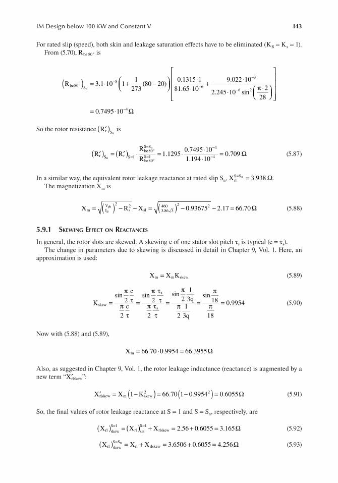
143IM Design below 100 KW and Constant V
For rated slip (speed), both skin and leakage saturation effects have to be eliminated (KR = Kx = 1).From (5.70), Rbe 80° is
( ) = ⋅ + −
⋅⋅
+ ⋅
⋅ π ⋅
= ⋅ Ω
°−
−
−
−
−
R 3.1 10 11
273(80 20)
0.1315 181.65 10
9.022 10
2.245 10 sin2
28
0.7495 10
be80S
86
3
6 2
4
n
So the rotor resistance (R′r )S is
n
( ) ( )′ = ′ ⋅ = ⋅ ⋅⋅
= Ω=°
=
−
−R RR
R1.1295
0.7495 101.194 10
0.709r S r S 1
be80S=S
be80S 1
4
4n
n
(5.87)°
In a similar way, the equivalent rotor leakage reactance at rated slip S , XS S= nn rl = Ω3.938 .
The magnetization Xm is
( ) ( )= − − = − − = ΩµX R X 0.93675 2.17 66.70m IV 2
s2
sl 3.86 3460 2 2ph (5.88)
5.9.1 Skewing eFFect on reactanceS
In general, the rotor slots are skewed. A skewing c of one stator slot pitch τs is typical (c = τs).The change in parameters due to skewing is discussed in detail in Chapter 9, Vol. 1. Here, an
approximation is used:
=X X Km m skew (5.89)
=
πτ
πτ
=
π ττ
π ττ
=
π
π =
π
π =Ksin
2c
2c
sin2
2
sin2
13q
21
3q
sin18
18
0.9954skew
s
s (5.90)
Now with (5.88) and (5.89),
= ⋅ = ΩX 66.70 0.9954 66.3955m
Also, as suggested in Chapter 9, Vol. 1, the rotor leakage inductance (reactance) is augmented by a new term “X′rlskew”:
( ) ( )′ = − = − = ΩX X 1 K 66.70 1 0.9954 0.6055rlskew m skew2 2 (5.91)
So, the final values of rotor leakage reactance at S = 1 and S = Sn, respectively, are
( ) ( )= + = + = Ω=X X X 2.56 0.6055 3.165rl skewS=1
rl satS 1
rlskew (5.92)
( ) = + = + = Ω=X X X 3.6506 0.6055 4.256rl skewS S
rl rlskewn (5.93)

144 Induction Machines Handbook
5.10 L OSSES AND EFFICIENCY
The efficiency is defined in general as output per input power:
∑
η = =+
PP
P
P losses
out
in
out
in
(5.94)
The loss components are
∑ = + + + +losses p p p p pCo Al iron mv stray (5.95)
pCo, the stator winding loss component, is
= = ⋅ ⋅ =p 3R I 3 0.93675 9.303 243.215WCo s 1n2 2 (5.96)
pAl, rotor cage loss component (at S = Sn), is
( )= =p 3 R I 3R K IAl r S rn2
r I2
1n2
n (5.97)
With (5.87) and (5.35), we get
= ⋅ ⋅ ⋅ =p 3 0.709 0.864 9.303 137.417 WAl2 2
The mechanical/ventilation losses are considered here pmv = 0.03Pn for p1 = 1, 0.012Pn for p1 = 2, and 0.008Pn for p1 = 3, 4.
The stray losses pstray are explained in detail in Chapter 11, Vol. 1. Here, their standard value pstray = 0.01Pn is considered.
The core loss piron is made of fundamental p1iron and additional (harmonics) ph
iron iron loss.The fundamental core losses occur only in the teeth and back iron (pt1, py1) of the stator as the
rotor (slip) frequency is low (f2 < 3–4 Hz).The stator teeth fundamental losses (see Chapter 11, Vol. 1) are
≈
p K p
f50
B Gt1 t 101
1.3
ts1.7
t1 (5.98)
where p10 is the specific losses in W/Kg at 1.0 T and 50 Hz (p10 = 2–3 W/Kg; it is a catalogue data for the lamination manufacturer). Kt = 1.6–1.8 accounts for core loss augmentation due to mechanical machining (Kt value depends on the quality of the material, sharpening of the cutting tools, etc.).
Gt1, the stator tooth weight, is
( )= γ ⋅ ⋅ ⋅ + + ⋅ ⋅
= ⋅ ⋅ ⋅ ⋅ + + ⋅ ⋅ ⋅ =− −
G N b h h h L K
7800 36 4.75 10 (21.36 1.5 1) 10 0.1315 0.95 3.975Kg
t1 iron s ts s w os Fe
3 3
(5.99)
With Bts = 1.55 T and f1 = 60 Hz, from (5.98), pt1 is
= ⋅ ⋅ ⋅ ⋅ =p 1.7 2
6050
1.55 3.975 36.08 Wt1
1.31.7
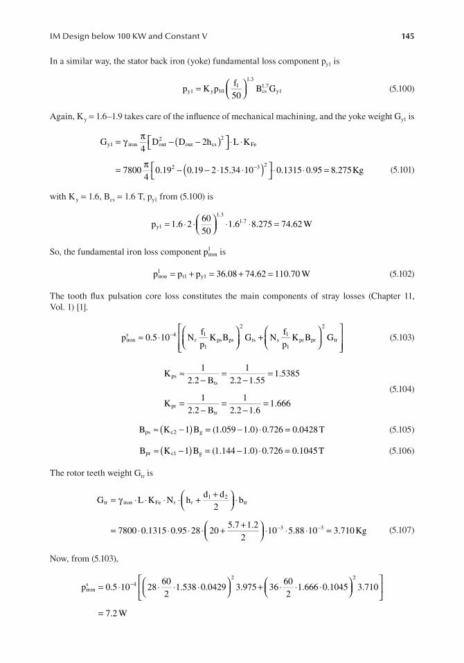
145IM Design below 100 KW and Constant V
In a similar way, the stator back iron (yoke) fundamental loss component py1 is
=
p K p
f50
B Gy1 y 101
1.3
cs1.7
y1 (5.100)
Again, K y = 1.6–1.9 takes care of the influence of mechanical machining, and the yoke weight Gy1 is
( )
( )= γ π − − ⋅ ⋅
= π − − ⋅ ⋅
⋅ ⋅ =−
G4
D D 2h L K
78004
0.19 0.19 2 15.34 10 0.1315 0.95 8.275Kg
y1 iron out2
out cs2
Fe
2 3 2(5.101)
with K y = 1.6, Bcs = 1.6 T, py1 from (5.100) is
= ⋅ ⋅ ⋅ ⋅ =p 1.6 2
6050
1.6 8.275 74.62 Wy1
1.31.7
So, the fundamental iron loss component p1iron is
= + = + =p p p 36.08 74.62 110.70 Wiron1
t1 y1 (5.102)
The tooth flux pulsation core loss constitutes the main components of stray losses (Chapter 11, Vol. 1) [1].
≈ ⋅
+
−p 0.5 10 Nfp
K B G Nfp
K B Girons 4
r1
1ps ps
2
ts s1
1pr pr
2
tr (5.103)
≈−
=−
=
=−
=−
=
K1
2.2 B1
2.2 1.551.5385
K1
2.2 B1
2.2 1.61.666
psts
prtr
(5.104)
( )≈ − = − ⋅ =B K 1 B (1.059 1.0) 0.726 0.0428Tps c2 g (5.105)
( )≈ − = − ⋅ =B K 1 B (1.144 1.0) 0.726 0.1045T (5.106)pr c1 g
The rotor teeth weight Gtr is
= γ ⋅ ⋅ ⋅ ⋅ + +
⋅
= ⋅ ⋅ ⋅ ⋅ + +
⋅ ⋅ ⋅ =− −
G L K N hd d
2b
7800 0.1315 0.95 28 205.7 1.2
210 5.88 10 3.710Kg
tr iron Fe r r1 2
tr
3 3 (5.107)
Now, from (5.103),
= ⋅ ⋅ ⋅ ⋅
+ ⋅ ⋅ ⋅
=
−p 0.5 10 28602
1.538 0.0429 3.975 36602
1.666 0.1045 3.710
7.2 W
irons 4
2 2

146 Induction Machines Handbook
The total core loss piron is
= + = + =p p p 110.70 7.2 117.90 Wiron iron1
irons (5.108)
Total losses (5.95) is
∑ = + + + ⋅ ⋅ =−losses 243.215 137.417 117.90 2.2 10 5500 609.6 W2
The efficiency ηn (from 5.87) becomes
η =+
=55005500 609.6
0.9002!n
The targeted efficiency was 0.895, so the design holds. If the efficiency had been smaller than the target value, the design should have returned to square one by adopting a larger stator bore diam-eter Dis, then smaller current densities, etc. A larger size machine would have been obtained, in general.
5.11 OPERATION CHARACTERISTICS
The operation characteristics are defined here as active no-load current I0a, rated slip Sn, rated torque Tn, breakdown slip and torque Sk, Tbk, current Is and power factor versus slip, starting current, and torque ILR, TLR.
The no-load active current is given by the no-load losses:
( )=+ + ⋅ ⋅
= + + ⋅ ⋅ =µIp p 3 I R
3V117.9 56.1 3 3.86 0.936
3 460 30.271A0a
iron mv2
s
ph
2
(5.109)
The rated slip Sn is
=+ + +
=+ + +
=Sp
P p p p137.417
5500 137.417 56.1 27.50.024!n
Al
N Al mv stray
(5.110)
The rated shaft torque Tn is
( )
=π −
=π −
=TP
2fp
1 S
5500
2602
(1 0.024)29.91Nmn
n
1
1n
(5.111)
The approximate expressions of torque versus slip (Chapter 7, Vol. 1) are
( )=
ω+
+ +
T3p V
RS
R CRS
X C Xe
1
1
ph2 r
s mr
2
sl m rl2
(5.112)
≈ + = + =with C 1XX
12.1766.4
1.0327msl
m
(5.113)
From (5.112), the breakdown torque Tbk for motoring is

147IM Design below 100 KW and Constant V
( )
( )=
ω + + +
= ⋅⋅ π + + +
=
T3p2
V
R R X C X
3 22 2 60
460 3
0.936 0.936 (2.17 4.256)75.48 Nm
bk1
1
ph2
s s2
sl 1 rl2
2
2 2(5.114)
The starting current ILR is
( ) ( )
( ) ( )
=+ + +
=+ + +
=
= = =I
V
R R X X
460 3
0.936 1.1295 1.6275 3.16554.44 A
LRph
s rS 1 2
slS 1
rlS 1 2
2 2(5.115)
The starting torque TLR may now be computed as
=ω
= ⋅ ⋅ ⋅π
==
T3R I
P3 1.1295 54.44 2
2 6053.305NmLR
rS 1
LR2
11
2
(5.116)
In the specifications, the rated power factor cos φ1n, Tbk/Ten, TLR/Ten, and ILR/I1n are given. So we have to check the final design values of these constraints:
ϕη ⋅
= <cos =P
3V I=
5500
3460
39.303 0.90
0.825 0.831nn
ph 1n n
(5.117)
= = = ≈tTT
75.4829.91
2.523 2.5bkbk
en
(5.118)
= = = ≈tTT
53.30529.91
1.7828 1.75LRLR
en
(5.119)
i =II
=54.449.303
=5.85<6.0LRLR
1n
(5.120)
Apparently, the design does not need any iterations. This is pure coincidence “combined” with standard specifications and designer’s experience! Higher breakdown or starting torque ratios tbk, tLR would, for example, need lower rotor leakage inductance and higher rotor resistance as influenced by skin effect. A larger stator bore diameter is again required. In general, it is not easy to make a few simple changes to get the desired operation characteristics. Here, the optimization design methods come into play.
5.12 TEMPERATURE RISE
Any electromagnetic design has to be thermally valid (Chapter 12, Vol. 1). Only a coarse verifica-tion of temperature rise is given here.
First, the temperature differential Δθco between the conductors in slots and the slot wall is calculated:
∆θ ≈α
PA
coco
cond ls
(5.121)

148 Induction Machines Handbook
Then, the frame temperature rise Δθframe with respect to ambient air is determined:
∑∆θ =α
losses
Aframe
conv frame
(5.122)
For IMs with self-ventilators placed outside the motor (below 100 kW),
W m K
60; for 2p 2;
50; for 2p 4;
40; for 2p 6;
32; for 2p 8;
conv2
1
1
1
1
( )α =
=
=
=
=
(5.123)
More precise values are given in Chapter 12, Vol. 1.The slot insulation conductivity plus its thickness are lumped into αcond:
α = λ =⋅
=−h0.25
0.3 10833W/m Kcond
ins
ins3
2 (5.124)
λins is the insulation thermal conductivity in (W/m K) and hins the total insulation thickness from the slot middle to teeth wall.
The stator slot lateral area Als is
A 2≈ +( )h b ⋅ ⋅L N = ⋅(2 21.36 + ⋅9.16) 10−3 2ls s s2 s ⋅ ⋅0.1315 36 = 0.2456m (5.125)
The frame area Sframe (including the Finns area) is
= π + τ ⋅ = π ⋅ + ⋅ =A D (L ) K 190(0.1315 0.0876) 3.0 0.392mframe out fin2 (5.126)
Now, from (5.121)
∆θ =⋅
= °234.215833 0.2456
1.18 Cco
and from (5.122),
∆θ =⋅
= °609.650 0.392
31.10 Cframe
Suppose that the ambient temperature is θamb = 40°C.In this case, the winding temperature is
θ = θ + ∆θ + ∆θ = + + = ° < °40 1.18 31.10 72.28 C 80 CCo amb Co frame (5.127)
For this particular design, the Kfin = 3.0, which represents the frame area multiplication by fins, provided to increase heat transfer, may be somewhat reduced, especially if the ambient temperature would be 20°C as usual.

149IM Design below 100 KW and Constant V
5.13 SUMMARY
• 100 kW is, in general, considered the border between low- and medium-power IMs.• Low-power IMs use a single stator and rotor stack and a finned frame cooled by an external
ventilator mounted on the motor shaft.• Low-power IMs use a rotor cage made of cast aluminum and a random wound coil stator
winding made of round (in general) magnetic wire with 1–4(6) elementary conductors in parallel and 1–3 current paths in parallel.
• The number of poles is 2p1 = 2, 4, 6, 8, 10, in general.• In designing an IM, we understand sizing of the IM; the breakdown torque, starting torque,
and current are essential among design specifications.• The design algorithm contains nine main stages: design specs; sizing the electric and mag-
netic circuits; adjustment of sizing data; verification of electric and magnetic loading (with eventual return to step one); computation of magnetization current, of equivalent circuit parameters, of losses, rated slip, and efficiency, of power factor; temperature rise; and perfor-mance check with eventual returns to step one, with adjusted electric and magnetic loadings.
• With assigned values to efficiency and power factor, based on past experience (Esson’s out-put coefficient), the stator bore diameter Dis is calculated after assigning a value (dependent on and increasing with the number of poles) for λ = stack length/pole pitch = 0.6–3.
• The airgap should be small to increase power factor, but not too small to avoid too high stray losses.
• Double-layer, chorded coils stator windings are used in most cases.• The essence of slot design is the design current density, which depends on the IM design
letters A, B, C, and D, type of cooling, power level, and number of poles. Values in the range of 4–8 A/mm2 are typical below 100 kW.
• Semiclosed trapezoidal (rounded) stator and rotor slots with rectangular teeth are most adequate below 100 kW.
• A key factor in the design is the teeth saturation factor 1 + Kst which is assigned an initial value which has to be met after a few design iterations.
• There are special stator/rotor slot number combinations to avoid synchronous parasitic torques, radial forces, noise, and vibration. They are given in Table 5.5.
• An essential design variable is the ratio KD = outer/inner stator diameter. Its recommended value intervals decrease with the number of poles, based on past experience.
• When the lamination cross section is designed such that to produce the maximum airgap flux density for a given rated current density in the stator via optimal lamination algorithm (OLA) [3], the ratio KD is
Using values around these would most probably yield practical designs.• Care must be exercised to correct the rotor resistance and leakage reactances for skin effect
and leakage magnetic saturation at zero speed (S = 1). Otherwise, both starting torque and starting current calculations will contain notable errors.
• No electromagnetic design is practical unless the temperature rise corresponds to the winding insulation class. Detailed thermal design methodologies are presented in Chapter 12, Vol. 1.
• For more on IM design basics, see [4–6].• Design optimization methods will be introduced in Chapter 8, Vol. 2.
2p1 2 4 6 8
KD 0.58 0.65 0.69 0.72

150 Induction Machines Handbook
REFERENCES
1. K. Vogt, Electrical Machines: Design of Rotary Electric Machines, Fourth edition (in German), Chapter 16, VEB Verlag Technik, Berlin, 1988.
2. G. Madescu, I. Boldea, T. J. E. Miller, An Analytical Iterative Model (AIM) for induction motor design, Record of IEEE – IAS – 1996, Annual Meeting, San Diego, CA, Vol. 1, 1996, pp. 566–573.
3. G. Madescu, I. Boldea, T. J. E. Miller, The Optimal Lamination Approach (OLA) for induction motor design, IEEE Transactions on Industry Applications, Vol. 34, No. 2, 1998, pp. 1–8.
4. J. Cathey, Electric Machines: Analysis and Design with MATLAB, Chapter 6, McGraw-Hill Higher Education, New York, 2001.
5. I. Boldea, L. N. Tutelea, Electric Machines: Steady State, Transients and Design with MATLAB, Chapters 11–16, CRC Press, Boca Raton, FL, Taylor and Francis Group, New York, 2010.
6. J. Pyrhonen, T. Jokinen, V. Hrabovcova, Design of Rotating Electrical Machines, Wiley, Chichester, UK, 2009.

151
6 Induction Motor Design above 100 KW and Constant V and f (Size Your Own IM)
6.1 INTRODUCTION
Induction motors above 100 kW are built for low voltage (480 V/50 Hz, 460 V/60 Hz, 690 V/50 Hz) or medium voltages, 2.4–6 kV and 12 kV in special cases.
The advent of power electronic converters, especially those using insulated gate bipolar transistors (IGBTs), caused the rise of power/unit limit for low-voltage induction machines (IMs), 400 V/50 Hz to 690 V/60 Hz, to more than 2 MW. Although we are interested here in constant V- and f-fed IMs, this trend has to be observed.
Higher voltage, for given power, means lower cross section easier to wind stator windings. It also means lower cross-sectional feeding cables. However, it means thicker insulation in slots, etc. and thus a low slot-fill factor, and a slightly larger size machine. Also, a higher voltage power switch tends to be costly. Insulated coils are used. Radial–axial cooling is typical, so radial ventilation channels are provided. In contrast, low-voltage IMs above 100 kW are easy to build, especially with round conductor coils (a few conductors in parallel with copper diameter below 3.0 mm) and, as power goes up, with more than one current path, a1 > 1. This is feasible when the number of poles increases with power: for 2p1 = 6, 8, 10, 12. If 2p1 = 2, 4 as power goes up, the current goes up and preformed coils made of stranded rectangular conductors, eventually with one to two turns/coil only, are required. Rigid coils are used, and slot insulation is provided.
Axial cooling, finned-frame, unistack configuration low-voltage IMs have been recently intro-duced up to 2.2 MW for low voltages (690 V/60 Hz and less).
Most IMs are built with cage rotors, but, for heavy starting, or limited speed-control applica-tions, wound rotors are used.
To cover most of these practical cases, we will unfold a design methodology treating the case of the same machine with medium-voltage stator and a low-voltage stator, and deep bar cage rotor, double-cage rotor, and wound rotor.
The electromagnetic design algorithm is similar to that applied below 100 kW. However, the slot shape and stator coil shape, insulation arrangements, and parameters expressions accounting for saturation and skin effects are slightly, or more, different with the three types of rotors.
Knowledge in Chapters 9 and 11, Vol. 1, on skin and saturation effects, respectively, and for stray losses is directly applied throughout the design algorithm.
The deep bar and double-cage rotors will be designed based on fulfilment of breakdown torque and starting torque and current, to reduce drastically the number of iterations required. Even when optimization design is completed, the latter will be much less time-consuming, as the “initial” design is meeting approximately the main constraints. Unusually, high breakdown/rated torque ratios (tbe = Tbk/Ten > 2.5) are to be approached with open stator slots and larger li/τ ratios to obtain low stator leakage inductance values.
T3p2
V 1L
; L L Lbk1 ph
1
2
scsc sl rl≈
ω
= + (6.1)

152 Induction Machines Handbook
where Lsl is the stator leakage, and Lrl is the rotor leakage inductance at breakdown torque. It may be argued that, in reality, the current at breakdown torque is rather large (Ik/I1n ≥ Tbk/Ten) and thus both leakage flux paths saturate notably and, consequently, both leakage inductances are somewhat reduced by 10%–15%. While this is true, it only means that ignoring the phenomenon in (6.1) will yield conservative (safe) results.
The starting torque TLR and current ILR are
T3 R K I p
LRr S 1 istart
2LR2
1
1
( )≈
ω= (6.2)
IV
R R L LLR
1ph
s r S 1
212
sl S 1 rl S 1
2( )( ) ( )( ) ( )≈
+ + ω += = =
(6.3)
In general, Kistart = 0.9–0.975 for powers above 100 kW. Once the stator design, based on rated performance requirements, is done, with Rs and Lsl known, Equations (6.1) through (6.3) yield unique values for (Rr )S 1= , (L )sat
rl S 1= and (Lrl )S S= . For a targeted efficiency and with the stator n
design done and core loss calculated, the rotor resistance at rated power (slip) can be calculated approximately:
RP
3R I p p p1
3 K Ir S S
n
ns 1n
2iron stray mec
i 1n2n
( )( )
=η
− − − −
= (6.4)
withKI
I0.8cos 0.2; I
P3V cos
ir S S
1n1n 1n
n
1n 1n n
n( )
= ≈ ϕ + =ϕ η
= (6.5)
We may assume that rotor bar resistance and leakage inductance at S = 1 represent 0.80–0.95 of their values calculated from (6.1) through (6.4).
R (0.85 0.95)R
K; K
4m W KN
be S 1
r S 1
bsbs
1 W12
r
( ) ( )( )= − ==
= (6.6)
L (0.75 0.80)L
Kbe S 1
rl S 1sat
bs
( ) ( )= −=
= (6.7)
Their values for rated slip are
R (0.7 0.85)R
Kbe S S
r S S
bsn
n( ) ( )= −=
= (6.8)
L (0.8 0.85)L
Kbe S S
rl S S
bsn
n( ) ( )= −=
= (6.9)
With rectangular semiclosed rotor slots, the skin effect KR and Kx coefficients are
KR
Rh ;
fR
be S 1
be S S
Skin r Skin1 0
Aln
( )( )= ≈ ξ = β β = π µ
ρ=
=
(6.10)

153IM Design above 100 KW and Constant V and f
L
L
h3b
Khb
h3b
hb
be S 1unsat
be S S
r
rx
or
or
r
r
or
or
n
( )( ) ≈
+
+=
=
(6.11)
where hor – rotor slot neck height, bor – rotor slot openinghr – active rotor slot height, br – rotor slot width.
Apparently, by assigning a value for hor/bor, Equation (6.11) allows us to calculate br because
K3
2 hx
skin r
≈β
(6.12)
Now, the bar cross section for given rotor current density jAL, (Ab = hr · br) is
AIj
K IK j
; K2m W K
Nb
b
Al
i 1n
bi ALbi
1 1 w1
r
= = = (6.13)
If Ab from (6.13) is too far away from hr · br, a more complex than rectangular slot shape is to be looked for to satisfy the values of KR and KX calculated from 6.10 and 6.11.
It should be noted that the rotor leakage inductance has also a differential component which has not been considered in (6.9) and (6.11).
Consequently, the above rationale is merely a basis for a closer-to-target rotor design start from the point of view of breakdown and starting torques, and starting current.
A similar approach may be taken for the double-cage rotor, but to separate the effects of the two cages, the starting and rated power conditions are taken to design the starting and working cage, respectively.
6.2 MEDIUM-VOLTAGE STATOR DESIGN
To save space, the design methodology will be unfolded simultaneously with a numerical example of an IM with the following specifications:
• Pn = 736 kW (1000 HP)• Targeted efficiency: 0.96• V1n = 4 kV (Δ)• f1 60 Hz, 2p1 4 poles, m 3 phases;= = =
Service: Si1 continuous, insulation class F, temperature rise for class B (maximum 80 K).The rotor will be designed separately for three cases: deep bar cage, double-cage, and wound
rotor configurations.
6.2.1 Main Stator DiMenSionS
As we are going to use again Esson’s constant (Chapter 4, Vol. 1), we need the apparent airgap power Sgap.
S 3EI 3K V Igap 1n E 1ph 1n= = (6.14)
with K 0.98 0.005 p 0.98 0.005 2 0.97.E 1= − ⋅ = − ⋅ = (6.15)

154 Induction Machines Handbook
The rated current I1n is
IP
3V cos1n
n
1n n n
=ϕ η
(6.16)
To find I1n, we need to assign target values to rated efficiency ηn and power factor cos φn, based on past experience and design objectives.
Although the design literature uses graphs of n, cos n versus power and number of pole pairs p1, continuous progress in materials and technologies makes the ηn graphs quickly obsolete. However, the power factor data tend to be less dependent on material properties and more dependent on air-gap/pole-pitch ratio and on the leakage/magnetization inductance ratio (Lsc/Lm) as
η φ
( )φ ≈−
+
++
cos1
LL L
1L
L L
maxzero loss
sc
m sl
sc
m sl
(6.17)
Because Lsc/Lm ratio increases with the number of poles, the power factor decreases with the num-ber of poles increasing. Also, as the power goes up, the ratio Lsc/Lm goes down, for given 2p1, and thus, cos φn increases with power.
Furthermore, for high breakdown torque, Lsc has to be small and thus the maximum power factor increases. Adopting a rated power factor is not easy. Data shown in Figure 6.1 are to be taken as purely orientative.
Corroborating (6.1) with (6.17), for given breakdown torque, the maximum ideal power factor (cos φ)max can be obtained.
For our case, cos n 0.92–0.93.φ =Rated efficiency may be purely assigned a desired, though realistic, value. Higher values are
typical for high-efficiency motors. However, for 2p1 < 8, and Pn > 100 kW the efficiency is above 0.9 and goes up to more than 0.95 for Pn > 2000 kW. For high-efficiency motors, efficiency at 2000 kW goes as high as 0.97 with recent designs.
With ηn = 0.96 and cos φn = 0.92, the rated phase current I1nf (6.16) is
I736 10
3 4 10 0.92 0.96120.42
3A1nf
3
3= ⋅⋅ ⋅ ⋅ ⋅
=−
FIGURE 6.1 Typical power factor of cage-rotor IMs.

155IM Design above 100 KW and Constant V and f
From (6.14), the airgap apparent power Sgap becomes
S 3 0.97 4000 120.42 808.307 10 VAgap3= ⋅ ⋅ ⋅ = ⋅
6.2.2 Stator Main DiMenSionS
The stator bore diameter Dis can be determined using Esson’s constant from Equation (5.1):
D2p p
f
S
Cis
1
1
1
1
gap
0
3=πλ
(6.18)
From Figure 4.14, C0 = 265 · 103 J/m3, λ = 1.1 = stack length/pole pitch (Table 5.1, Chapter 5) with (6.18), Dis is
D2 2
1.12
60808.307 10
265 100.49mis
3
33= ⋅
π ⋅⋅
⋅=
The airgap is chosen at g = 1.5 · 10−3 m as a compromise between mechanical constraints and limita-tion of surface and tooth flux pulsation core losses.
The stack length li is
lD
2p1.1
0.492 2
0.423miis
1
= λτ = λ ⋅ π = π ⋅⋅
= (6.19)
6.2.3 core conStruction
Traditionally, the core is divided between a few elementary ones with radial ventilation channels in between. Such a configuration is typical for radial–axial cooling (Figure 6.2) [1].
Recently, the unistack core concept, rather standard for low power (below 100 kW), has been extended up to more than 2000 kW both for medium- and low-voltage stator IMs. In this case, axial air cooling of the finned motor frame is provided by a ventilator on motor shaft, outside bearings (Figure 6.3) [2].
As both concepts are in use and as, in Chapter 5, the unistack case has been considered, the divided stack configuration will be considered here for high-voltage stator case.
The inner/outer stator diameter ratio intervals have been recommended in Table 5.2. For 2p1 = 4, let us consider KD = 0.63.
FIGURE 6.2 Divided core with radial–axial air cooling. (Source: ABB.)

156 Induction Machines Handbook
Consequently, the outer stator diameter Dout is
DDK
0.50.63
0.78m 780mmoutis
D
= = = = (6.20)
The airgap flux density is taken as Bg = 0.7 T. From Equation (4.14), C0 is
C K K A B 2p0 B i w1 1 g 1= α π (6.21)
Assuming a tooth saturation factor (1 + Kst) = 1.25, from Figure 4.13, KB = 1.1, αi = 0.65. The wind-ing factor is given a value Kw1 ≈ 0.925. With Bg = 0.7 T, 2p1 = 4 and C 3
0 = 265 · 103 J/m , the stator rated current sheet A1 is
A265 10
1.1 0.69 0.925 0.7 442.93 10 Aturns/m1
33= ⋅
⋅ ⋅ ⋅π ⋅ ⋅= ⋅
This is a moderate value.The pole flux ϕ is
l B ;D
2pi i g
is
1
φ = α τ τ = π (6.22)
0.5
2 20.3925m; 0.65 0.3925 0.423 0.7 0.0755Wbτ = π ⋅
⋅= φ = ⋅ ⋅ ⋅ =
The number of turns per phase W1 (a1 = 1 current paths) is
WK V
4K f K0.97 4000
4 1.1 60 0.925 0.07552101
E ph
B 1 w1
=φ
= ⋅⋅ ⋅ ⋅ ⋅
= (6.23)
The number of conductors per slot ns is written as
n2m a W
Ns
1 1 1
s
= (6.24)
FIGURE 6.3 Unistack with axial air cooling. (Source: ABB.)

157IM Design above 100 KW and Constant V and f
The number of stator slots, Ns, for 2p1 = 4 and q = 6, becomes
N 2p q m 2 2 6 3 72s 1 1 1= = ⋅ ⋅ ⋅ = (6.25)
So n2 3 1 210
7217.50s = ⋅ ⋅ ⋅ =
We choose ns = 18 conductors/slot, but we have to decrease the ideal stack length li to
l l17.50
180.423
17.5018
0.411mi i= ⋅ = ⋅ ≈
18The flux per pole φ ≈ φ⋅ = 0.07765Wb
17.50The airgap flux density remains unchanged (Bg = 0.7 T).As the ideal stack length li is final (provided the teeth saturation factor Kst is confirmed later on),
the former may be divided into a few parts.Let us consider nch = 6 radial channels each 10−2 m wide (bch = 10−2 m). Due to axial flux fringing,
its equivalent width b′ch ≈ =0.75bch 7.5 ⋅ =10−3 m g( )1.5mm . So the total geometrical length Lgeo is
L l n b 0.411 6 0.0075 0.456mgeo i ch ch= + ′ = + ⋅ = (6.26)
On the other hand, the length of each elementary stack is
lL n b
n 10.456 6 0.01
6 10.05667ms
geo ch ch
ch
=−
+= − ⋅
+≈ (6.27)
As laminations are 0.5 mm thick, the number of laminations required to make ls is easy to match. So there are seven stacks each 56 mm long (axially).
6.2.4 the Stator winDing
For medium-voltage IMs, the winding is made of form-wound (rigid) coils. The slots are open in the stator so that the coils may be introduced in slots after prefabrication (Figure 6.4). The number of slots per pole/phase q1 is to be chosen rather large as the slots are open and the airgap is only g = 1.5 · 10−3 m.
FIGURE 6.4 Open stator slot for high-voltage winding with form-wound (rigid) coils. (Source: ABB.)

158 Induction Machines Handbook
The stator slot pitch τs is
DN
0.4972
0.02137msis
s
τ = π = π ⋅ = (6.28)
The coil throw is taken as y/τ = 15/18 = 5/6 (q1 = 6). There are 18 slots per pole to reduce drastically the fifth mmf space harmonic.
The winding factor Kw1 is
Ksin
6
6 sin6 6
sin2
56
0.9235w1 =
π
⋅ π⋅
π =
The winding is fully symmetric with Ns/m1a1 = 24 (integer), 2p1/a1 = 4/1 (integer). Also t = g.c.d(Ns,p1) = p1 = 2, and Ns/m1t = 72/(3 · 2) = 12 (integer).
The conductor cross section ACo is (delta connection)
AI
; a 1, J 6.3 A/mm ; I 69.36 ACo1nf
1 Co2
1nf= = = (6.29)a J1 Co
=
A120.42
1 6.3 311.048mm a bCo
2c c=
⋅= = ⋅
A rectangular cross-sectional conductor will be used. The rectangular slot width bs is
b (0.36 0.5) 0.021375 (0.36 0.5) 7.7 10.7mms s= τ ⋅ ÷ = ⋅ ÷ = ÷ (6.30)
Before choosing the slot width, it is useful to discuss the various insulation layers (Table 6.1).The available conductor width in slot ac is
a b b 10.0 4.4 5.6mmc s ins= − = − = (6.31)
This is a standardized value, and it was considered when adopting bs = 10 mm (6.30). From (6.19), the conductor height bc becomes
bAa
11.0485.6
2mmcCo
c
= = ≈ (6.32)
So the conductor size is 2 × 5.6 mm2.
TABLE 6.1Stator Slot Insulation at 4 kV
Thickness (mm)
Figure 6.4 Denomination Tangential Radial
1 Conductor insulation (both sides) 1 · 04 = 0.4 18 · 0.4 = 7.2
2 Epoxy mica coil and slot insulation 4 4 · 2 = 8.0
3 Interlayer insulation - 2 · 1 = 2
4 Wedge - 1 · 4 = 4
Total bins = 4.4 hins = 21.2

159IM Design above 100 KW and Constant V and f
The slot height hs is written as
h h n b 21.2 18 2 57.2mms ins s c= + = + ⋅ = (6.33)
Now the back iron radial thickness hcs is
hD D
2h
780 4902
57.2 87.8mmcsout is
s= − − = − − = (6.34)
The back iron flux density Bcs is
B2l h
0.07552 0.411 0.0878
1.00 Tcsi cs
= φ =⋅ ⋅
≈ (6.35)
This value is too small, so we may reduce the outer diameter to a lower value: Dout = 730 mm; the back core flux density will be now close to 1.4 T.
The maximum tooth flux density Btmax is
BB 21.37 0.7
1.315Ttmaxs g=
τ= ⋅ = (6.36)
b 21.37 10s sτ − −
This is acceptable although even higher values (up to 1.8 T) are used as the tooth gets wider with radius and the average tooth flux density will be notably lower than Btmax.
The stator design is now complete, but it is not definitive. After the rotor is designed, perfor-mance is computed. Design iterations may be required, at least to converge Kst (teeth saturation factor), if not for observing various constraints (related to performance or temperature rise).
6.3 LOW-VOLTAGE STATOR DESIGN
Traditionally, low-voltage stator IMs above 100 kW have been built with round conductors (a few in parallel) in cases where the number of poles is large so that many current paths in parallel are feasible (a1 = p1).
Recently, extension of variable speed IM drives tends to lead to the conclusion that low-voltage IMs up to 2000 kW and more at 690 V/60 Hz (660 V, 50 Hz) or at (460 V/50 Hz, 400 V/50 Hz) are to be designed for constant V and f, but having in view the possibility of being used in general-purpose variable speed drives with voltage source PWM IGBT converter supplies. To this end, the machine insulation is enforced by using almost exclusively form-wound coils and open stator slots as for medium-voltage IMs. Also, insulated bearings are used to reduce bearing stray currents from PWM converters (at switching frequency).
Low-voltage PWM converters have a cost advantage. Also, a single stator stack is used (Figure 6.5).
The form-wound (rigid) coils (Figure 6.5) have a small number of turns (conductors) and a kind of crude transposition occurs in the end-connections zone to reduce the skin effect. For high-powers and 2p1 = 2, 4, even 2–3 elementary conductors in parallel and a1 = 2, 4 current paths may be used to keep the elementary conductors within a size with limited skin effect (Chapter 9, Vol. 1).
In any case, skin effect calculations are required as the power goes up and the conductor cross section follows path. For a few elementary conductors or current paths in parallel, additional (circu-lating current) losses occur as detailed in Sections 9.2–9.3, Vol. 1.
Aside from these small differences, the stator design follows the same path as for medium-voltage stators.
This is why it will not be further treated here.

160 Induction Machines Handbook
6.4 DEEP BAR CAGE ROTOR DESIGN
We will now resume here the design methodology in Section 6.2 with the deep bar cage-rotor design. More design specifications are needed for the deep bar cage.
Breakdown torque
Rated torqueTT
2.7bk
en
= =
Startingcurrent
Rated currentII
6.1LR
n
= ≤
Starting torque
Rated torqueTT
1.2LR
en
= =
The above data are merely an example.As shown in Section 6.1, in order to size the deep bar cage, the stator leakage reactance Xsl is
required. As the stator design is done, Xsl can be calculated.
6.4.1 Stator leakage reactance xSl
As documented in Chapter 9, Vol. 1, the stator leakage reactance Xsl can be written as
X 15.8f
100W100
lp q
sl1 1
2i
1 1is∑=
λ (6.37)
FIGURE 6.5 Open slot, low-voltage, single-stack stator winding (axial cooling). (Source: ABB.)

161IM Design above 100 KW and Constant V and f
where ∑λ is is the sum of the leakage slot (λss), differential (λds), and end-connection (λfs) geo-
metrical permeance coefficients.
h h3b
Khb
Kh4b
K1 3
4;
y 56
sss1 s3
s
s2
s
s3
s
( )λ = − + +
= + β β =τ
=
β β
β
(6.38)
In our case, (see Figure 6.6).
h n b n 0.4 2 2 1 18 2 18 0.4 2 2 1 48.2mms1 s c s= ⋅ + ⋅ + ⋅ + = ⋅ + ⋅ + ⋅ + = (6.39)
Also, hs3 = 2 · 2 + 1 = 5 mm, hs2 = 1 · 2 + 4 = 6 mm. From (6.37),
48.2 5
3 106
10
1 356
45
4 101.91ssλ = −
⋅+
+
+⋅
=
The differential geometrical permeance coefficient λds is calculated as in Chapter 6, Vol. 1:
0.9 q K K
K gds
s 1 w12
01 d1
c
( )λ =⋅ τ σ
(6.40)
with K 1 0.033bg
1 0.03310
1.5 21.370.897501
s2
s
2
≈ −τ
= −⋅
= (6.41)
σd1 is the ratio between the differential leakage and the main inductance, which is a function of coil chording (in slot pitch units) and qs (slot/pole/phase) (Figure 6.7): σd1 = 0.3 · 10−2.
The Carter coefficient Kc (as in Chapter 5, Vol. 1, Equations (5.53)–(5.56)) is
K K Kc c1 c2= (6.42)
Kc2 is not known yet but, as the rotor slots are semiclosed, Kc2 < 1.1 with Kc1 ≫ Kc2 due to the fact that the stator has open slots:
b
5g b10
5 1.5 105.714; K
21.3721.37 5.71
1.3651s2
s
2
c1s
s 1
γ =+
=⋅ +
= = ττ − γ
=−
= (6.43)
Consequently, Kc ≈ 1.365 · 1.1 = 1.50.
bs
hs1
hs2
hs3
FIGURE 6.6 Stator slot geometry.

162 Induction Machines Handbook
From (6.40),
0.9 21.37(6 0.923) 0.895 0.3 10
1.5 1.50.6335ds
2 2
λ = ⋅ ⋅ ⋅ ⋅⋅
=−
The end-connection permeance coefficient λfs is
0.34ql
l 0.64fs1
ifs( )λ = − βτ (6.44)
lfs is the end-connection length (per one side of stator) and can be calculated based on the end-connection geometry in Figure 6.8.
l 2 l l 2 lsin
h
2 0.01556
12
0.314sin 40
0.0562 0.548m
fs 1 1 1 1 s( )≈ + ′ + πγ = + βτα
+ π
= +°
+ π ⋅ = (6.45)
So, from (6.44),
l '1
αl 1
h =56.2mms
γ =h1 s
FIGURE 6.8 Stator end-connection coil geometry.
FIGURE 6.7 Differential leakage coefficient.

163IM Design above 100 KW and Constant V and f
0.346
0.4060.548 0.64
56
0.314 1.912tsλ = −
=
Finally, from (6.37), the stator leakage reactance Xls (unaffected by leakage saturation) is
X 15.860
1002 6 18
1000.4062 6
(1.91 0.6335 1.912) 6.667ls
2
=
⋅ ⋅
⋅
+ + = Ω
As the stator slots are open, leakage flux saturation does not occur even for S = 1 (standstill), at rated voltage. The leakage inductance of the field in the radial channels has been neglected.
The stator resistance Rs is
R KW 2A
L l
1 1.8 10 180 20
27212 18
2 (0.451 0.548)11.048 10
0.8576
s R Co801
Cogeo fs
36
( )= ρ +
= ⋅ ⋅ + −
⋅ ⋅ ⋅ ⋅ +
⋅= Ω
°
−−
(6.46)
Although the rotor resistance at rated slip may be approximated from (6.4), it is easier to compare it to stator resistance:
R (0.7 0.8)R 0.8 0.8576 0.686r S S sn( ) = ÷ = ⋅ = Ω= (6.47)
for aluminium bar cage rotors and high-efficiency motors. The ratio of 0.7–0.8 in (6.47) is only orientative to produce a practical design start. Copper bars may be used when very high efficiency is targeted for single-stack axially-ventilated configurations.
6.4.2 the rotor leakage inDuctance lrl
The rotor leakage inductance Lrl can be computed from the breakdown torque’s expression (6.1):
L3p
2T
VL ; L
X 6.6672 60
0.0177Hrl1
LR
1ph
1
2
sl slsl
1
=ω
− =ω
=π
= (6.48)
with
T t T tP
pLR LR en LRn
11= =
ω (6.49)
Now, Lrl is
L3p V
2t PL
3 40002 2.7 736 10 2 60
0.0177 0.01435 Hrl1 1ph
2
LR n 1sl
2
3=ω
− = ⋅⋅ ⋅ ⋅ ⋅ π
− = (6.50)
From starting current and torque expressions (6.2) and (6.3),
R
t Pp
3p K I1.2 736 10
3 0.975 5.6120
3
2.0538r S 1
1 LR n1
1
1
1 istart LRphase2
3
22( ) =
ω ω
= ⋅ ⋅
⋅ ⋅
= Ω=
−
(6.51)

164 Induction Machines Handbook
L1 V
IR R L
12 60
4000
5.6120
3
(1.083 2.0537) 6.667 8.436 10 H
rl S 11
1ph
LRphase
2
s r S 1
2sl S 1
2
2 3
( ) ( )( ) ( )=ω
− + −
=π
− + −
= ⋅
= = =
− (6.52)
Note that due to skin effect (Rr )S 1 2.914 R= = ( )s S S and due to both leakage saturation and skin = n
effect, the rotor leakage inductance at stall is (Lrl ) (S 1
Using (6.8) and (6.10), the skin effect resistance ratio KR is= 0.5878 L= =rl )S S .
n
KR
R0.950.8
2.9990.950.8
3.449Rr S 1
r S Sn
( )( )= ⋅ = ⋅ ==
=
(6.53)
The deep rotor bars are typically rectangular, but other shapes are also feasible. A modern alumin-ium rectangular bar insulated from core by a resin layer is shown in Figure 6.9. For a rectangular bar, the expression of KR (when skin effect is notable) is (6.10):
K hR skin r≈ β (6.54)
withf 60 1.256 10
3.1 1087mskin
1 0
Al
6
81β = π µ
ρ= π ⋅ ⋅ ⋅
⋅=
−
−− (6.55)
The rotor bar height hr is
h3.449
873.964 10 mr
2= = ⋅ −
From (6.11),
L
L0.750.85
h3b
Khb
h3b
hb
0.58780.750.85
0.51864rl S 1
rl S S
r
rx
or
or
r
r
or
or
n
( )( ) =
+′
+= ⋅ ==
=
(6.56)
K3
2 h3
2 87 3.977 100.43x
skin r2≈
β=
⋅ ⋅ ⋅=− (6.57)
Γ
hrbr
or
horHtr
resinlayer
aluminiumbar
b
FIGURE 6.9 Insulated aluminium bar.

165IM Design above 100 KW and Constant V and f
We have to choose the rotor slot neck hor = 1.0 · 10−3 m from mechanical reasons. A value of bor has to be chosen, say, bor = 2 · 10−3 m. Now we have to check the saturation of the slot neck at start which modifies bor into bor′ in (6.56). We use the approximate approach developed in Section 9.8, Vol. 1.
First, the bar current at start is
I III
0.95 Kbstart nstart
nbs=
⋅ ⋅ (6.58)
with N 64 and straight rotor slots.r =Kbs is the ratio between the reduced-to-stator and actual bar current.
K2mW K
N2 3(12 18)0.923
6418.69075bs
1 w1
r
= = ⋅ ⋅ = (6.59)
I 5.6 0.95120
318.69 6896.9Abstart = ⋅ ⋅ ⋅ = (6.60)
Using Ampere’s law in the Γ contour shown in Figure 6.9 yields
B
b b H I 2tr
rel 0r or os rel tr bstart( )
µ µτ − + µ = (6.61)
Iteratively, using the lamination magnetization curve (Table 5.4), with the rotor slot pitch τr,
D 2g
N
0.49 2 1.5 10
6423.893 10 mr
is
r
33( )( )τ =
π −=
π − ⋅ ⋅= ⋅
−− (6.62)
the solution of (6.61) is Btr = 2.29 T and μrel = 12!The new value of slot opening bor′ , to account for tooth top saturation at S = 1, is
b bb
2 10(23.893 2) 10
123.8244 10 mor or
r or
rel
33
3′ = + τ −µ
= ⋅ + − ⋅ = ⋅−−
− (6.63)
Now, with Nr = 64 slots, the minimum rotor slot pitch (at slot bottom) is
D 2g 2h
N49 2 1.5 2 39.64 10
6420 10 mrmin
is r
r
33( )τ =
π − −= π( − ⋅ − ⋅ ) ⋅ = ⋅
−− (6.64)
With the maximum rotor tooth flux density Btmax = 1.45 T, the maximum slot width brmax is
bB
B20 10 1
0.71.45
10.58mmrmax rg
tmaxr
3= τ − τ = ⋅ −
=− (6.65)
The rated bar current density jAl is
jI
h bK I K
h b0.936 120 18.69
39.64 10 33.061A/mmAl
b
r r
i n bs
r r
2= = = ⋅ ⋅⋅
= (6.66)
with K 0.8cos 0.2 0.8 0.92 0.2 0.936i n= ϕ + = ⋅ + = (6.67)
We may now verify (6.56).

166 Induction Machines Handbook
0.518643
39.6410
0.431
3.82439.643 10
112
0.8291.821
0.455!≥⋅ ⋅ +
⋅⋅ +
= =
The fact that approximately the large cage dimensions of hr = 39.64 m and br = 10 mm with bor = 2 mm, hor = 1 mm fulfilled the starting current, and starting and breakdown torques, for a rotor bar rated cur-rent density of only 3.06 A/mm2, means that the design leaves room for further reduction of slot width.
We may now proceed, based on the rated bar current Ib = 1213.38 A (6.66), to the detailed design of the rotor slot (bar), end ring, rotor back iron.
Then, the teeth saturation coefficient Kst is calculated. If notably different from the initial value, the stator design may be redone from the beginning until acceptable convergence is obtained. Further on, the magnetization current equivalent circuit parameters, losses, rated efficiency and power fac-tor, rated slip, torque, breakdown torque, starting torque, and starting current are all calculated.
Most of these calculations are to be done with the same expressions as in Chapter 5 which is why we do not repeat them here.
6.5 DOUBLE-CAGE ROTOR DESIGN
When a higher starting torque for lower starting current and good efficiency are all required, the double-cage rotor comes into play. However, the breakdown torque and the power factor tend to be slightly lower as the rotor cage leakage inductance at load is larger.
The main constraints are
TT
t 2.0bk
enek= >
I5.35LR <
I1n
TT
t 1.5LR
enLR= ≥
Typical geometries of double-cage rotors are shown in Figure 6.10.The upper cage is the starting cage as most of rotor current flows through it at start, mainly
because the working cage leakage reactance is high, so its current at primary (f1) frequency is small.In contrast, at rated slip (S < 1.5 · 10−2), most of the rotor current flows through the working
(lower) cage as its resistance is smaller and its reactance (at slip frequency) is smaller than for the starting cage resistance.
In principle, it is fair to say that there is always current in both cages, but, at high rotor frequency (f2 = f1), the upper cage is more important, whereas at rated rotor frequency (f2 = Snf1), the lower cage takes more current.
S
W
S
W
S
W
W
FIGURE 6.10 Typical rotor slot geometries for double-cage rotors.

167IM Design above 100 KW and Constant V and f
The end ring may be common to both cages, but, when frequent starts are considered, separate end rings are preferred because of different thermal expansion (Figure 6.11). It is also possible to make the upper cage of brass and the lower cage of copper.
The equivalent circuit for the double cage has been introduced in Chapter 9 (Section 9.7), Vol. 1, and is inserted here only for easy reference (Figure 6.12).
For the common end-ring case, Rring = Rring' (ring equivalent resistance, reduced-to-bar resis-tance), and Rbs and Rbw are the upper and lower bar resistances.
For separate end rings, Rring = 0, but the rings resistances Rbs → Rbs + Rrings, Rbw → Rbw + Rringw. Lrl contains the differential leakage inductance only for common end ring.
Also,
L l lhb
; L lhb
bs 0 geo srs
rse 0 geo
or
or( )≈ µ + = µ (6.68)
L l lh
3bha
hb
bw 0 geo wrw
rw
n
n
rs
rs( )≈ µ + + +
The mutual leakage inductance Lml is
L lh
2bml 0 geo
rs
rs
≈ µ (6.69)
l /2s
a r1
a rs
lower cageend ring
upper cageend ring
brs
Derl Ders
l /2w
FIGURE 6.11 Separate end rings.
R ringjS (L +L ( ))ω φ1 ring e e
Z =R (S )+jSX ( )ω Sω be be be 11
Rbs
Rbw
jS Lω1 bs
jS Lω1 bw
jS Lω1 ml
Xel
(a)
ars
brw
horhrs
h
hrw
a
φe
φw
bor
n n
(b)
FIGURE 6.12 Equivalent circuit of Figure 6.11 double-cage (a) and slot geometrical parameters (b).

168 Induction Machines Handbook
In reality, instead of lgeo, we should use li, but in this case, the leakage inductance of the rotor bar field in the radial channels is to be considered. The two phenomena are lumped into lgeo (the geo-metrical stack length).
The lengths of bars outside the stack are ls and lw, respectively.First, we approach the starting cage, made of brass (in our case) with a resistivity
ρbrass = 4ρCo = 4 · 2.19 · 10−8 = 8.76 · 10−8 (Ωm). We do this based on the fact that, at start, only the starting (upper) cage works.
T t T tP
p 3p
R 0.95ILR LR en LRn
11
1
1r S 1 LR
2( )= ≈ω
=ω = (6.70)
I 5.35I 5.35120
3371.1ALR 1n= = = (6.71)
From (6.70), the rotor resistance (( )Rr S 1= ) is
Rt P
3 0.95 I1.5 736 10
3 0.95 371.12.8128r S 1
LR n
LR2
3
2( ) =⋅ ⋅
= ⋅ ⋅⋅ ⋅
= Ω= (6.72)
From the equivalent circuit at start, the rotor leakage inductance at S = 1, (Lrl )S 1= , is
LV
IR R L
1
4000371.1
(0.8576 2.8128) 6.6671
2 1209.174 10 H
rl S 1ph
LR
2
s r S 1
2ls
1
22 3
( )( ) ( )=
− + −
ω
=
− + −
⋅
π= ⋅
= =
− (6.73)
If it were not for the rotor working cage large leakage in parallel with the starting cage, (Rr )S 1= and (Lrl )S 1= would simply refer to the starting cage whose design would then have been straightforward.
To produce realistic results, we first have to design the working cage.To do so, we again assume that the copper working cage (made of copper) resistance, referred to
the stator, is
R 0.8R 0.8 0.8576 0.6861r S S sn( ) = = ⋅ = Ω= (6.74)
This is the same as for the aluminium deep bar cage, although it is copper this time. The reason is to limit the slot area and depth in the rotor.
6.5.1 working cage Sizing
The working cage bar approximate resistance Rbe is
R (0.7 0.8)R
K0.75 0.6861
7452.670.6905 10be
r S=S
bs
4n( )
≈ ÷ = ⋅ = ⋅ Ω− (6.75)
From (6.6), Kbs is
K4m W K
N4 3 (12 18 0.923)
647452.67bs
1 w12
r
2( )= = ⋅ ⋅ ⋅ ⋅ = (6.76)

169IM Design above 100 KW and Constant V and f
The working cage cross section Abw is
Al l
R2.2 10
0.451 0.010.6905 10
1.468 10 mbwCo geo w
bw
84
4 2( )=
ρ += ⋅ +
⋅= ⋅−
−− (6.77)
The rated bar current Ib (already calculated from (6.66)) is Ib = 1213.38 A, and thus, the rated current density in the copper bar jCob is
jI
A1213.38
1.468 108.26 10 A/mCob
b
bw4
6 2= =⋅
= ⋅− (6.78)
This is a value close to the maximum value acceptable for radial–axial air cooling.A profiled bar 1 · 10−2 m wide and 1.5 · 10−2 m high is used: brw = 1 · 10−2 m, hrw = 1.5 · 10−2 m.The current density in the end ring has to be smaller than in the bar (about 0.7–0.8), and thus, the
working (copper) end-ring cross section Arw is
AA
0.75 2sinp
N
1.468 10
1.5sin2
64
9.9864 10 mrwbw
1
r
44 2=
⋅ π = ⋅π ⋅ = ⋅
−− (6.79)
So (from Figure 6.11),
a b 9.9846 10 mrl rl4 2= ⋅ − (6.80)
We may choose a = 2 · 10−2 rl m and brl = 5.0 · 10−2 m.
The slot neck dimensions will be considered as (Figure 6.12b) bor = 2.5 · 10−3 m, hor = 3.2 · 10−3 m (larger than in the former case) as we can afford a large slot neck permeance coefficient hor/bor because the working cage slot leakage permeance coefficient is already large.
Even for the deep cage, we could afford a larger hor and bor to stand the large mechanical centrifu-gal stresses occurring during full operation speed.
We go on to calculate the rotor differential geometrical permeance coefficient for the working cage (Chapter 5, Vol. 1, Equation (5.82)).
0.9
K gN6p
; 96pN
10drr dr
c
r
1
2
dr1
r
22λ = ⋅τ γ
γ =
⋅ − (6.81)
96 264
10 0.3164 10dr
22 2γ = ⋅
⋅ = ⋅− −
0.9 23.893
1.5 1.50.3164 10
6412
0.86dr2
2
λ = ⋅⋅
⋅ ⋅ ⋅ =−
The saturated value of λdrl takes into account the influence of tooth saturation coefficient Kst assumed to be Kst = 0.25.
1 K
0.961.25
0.688drsdrl
st
λ = λ+
= = (6.82)

170 Induction Machines Handbook
The working end-ring-specific geometric permeance λerl is (Chapter 5, Vol. 1, Equation (5.83)):
2.3 D b
N l 4sinp
N
log4.7 D b
b 2a
2.3 0.49 3 10 4 10 5 10
64 0.451 4sin2
64
log397 10
(50 2 20) 100.530
erlerl rl
r geo2 1
r
erl rl
rl rl
3 2 2
2
3
3
( )
( ) ( )λ = ⋅ −π
⋅ −+
≈⋅ − ⋅ − ⋅ − ⋅
⋅ ⋅ π ⋅
⋅+ ⋅ ⋅
=− − − −
−
(6.83)
The working end-ring leakage reactance Xrlel (Chapter 5, Vol. 1, Equation 5.85) is
X 2 f l 10 7.85 60 0.451 10 0.530 1.1258 10rlel 0 1 geo8
erl6 4≈ µ π ⋅ λ = ⋅ ⋅ ⋅ ⋅ = ⋅ Ω− − − (6.84)
The common (mutual) reactance (Figure 6.12) is made of the differential and slot neck components, unsaturated, for rated conditions and saturated at S = 1:
X 2 f lhb
el S 1 1 geo 0 drsor
or
( ) = π µ λ +′
=
X 2 f lhb
el S S 1 geo 0 dror
orn
( ) = π µ λ +
=
(6.85)
The influence of tooth top saturation at start is considered as before (in 6.60–6.63).With bor′ = 1.4bor, we obtain
X 2 60 0.451 0.862.53.2
1.256 10 3.503 10el S S6 4
n( ) = π ⋅ ⋅ +
⋅ ⋅ = ⋅ Ω=
− −
X 2 60 0.451 0.6882.5
3.5 1.41.256 10 2.6595 10el S 1
6 4( ) = π ⋅ ⋅ ++
⋅ ⋅ = ⋅ Ω=
− −
Now, we can calculate the approximate values of starting cage resistance from the value of the equivalent resistance at start Rstart.
RR
K2.81287452.67
3.7742 10startr S 1
bs
4( )= = = ⋅ Ω= − (6.86)
From Figure 6.12a, the starting cage resistance Rbes is
RR X
R
3.7742 10 2.6595 10
3.7742 105.648 10bes
start2
el2
start
4 2 4 2
44( ) ( )
≈ + =⋅ + ⋅
⋅= ⋅ Ω
− −
−− (6.87)( )
For the working cage reactance Xrlw, we also have
XR X
X
3.7742 10 2.6595 10
2.6595 108.0156 10rlw
start2
el2
el
4 2 4 2
44( ) ( )
= + =⋅ + ⋅
⋅= ⋅ Ω
− −
−− (6.88)
The presence of common leakage Xel makes starting cage resistance Rbes larger than the equivalent starting resistance Rstart. The difference is notable and affects the sizing of the starting cage.

171IM Design above 100 KW and Constant V and f
The value of Rbes includes the influence of starting end ring. The starting cage bar resistance Rb is approximately
≈ ÷ = ⋅ ⋅ = ⋅ Ω− −R R (0.9 0.95) 0.9 5.648 10 5.083 10bs bes4 4 (6.89)
The cross section of the starting bar Abs is
= ρ+
= ⋅ ⋅ +⋅
= ⋅−−
−Al l
R4 2.2 10
0.451 0.055.083 10
0.8673 10 mbs brassgeo s
bs
84
4 2 (6.90)
The utilization of brass has reduced drastically the starting cage bar cross section. The length of starting cage bar was prolonged by ls = 5 · 10−2 m (Figure 6.11) as only the working end-ring axial length is arl = 2 · 10−2 m on each side of the stack.
We may adopt a rectangular bar again (Figure 6.12b) with b = 1 · 10−2 −2rs m and hrs = 0.86 · 10 m.
The end-ring cross section Ars (as in 6.79) is
=⋅ ⋅ π = ⋅
⋅ π ⋅ = ⋅−
−AA
0.75 2 sinp
N
0.8673 10
1.5 sin2
64
5.898 10 mrsbs
1
r
44 2 (6.91)
The dimensions of the starting cage ring are chosen to be the following: ars · brs (Figure 6.11) = 2 · 10−2 · 3 · 10−2 m2.
Now, we calculate more precisely the starting cage bar equivalent resistance, Rbes, and that of the working cage, Rbew,
R RR
2sinp
N
; RlA
bew bwrw
2 1
r
rw Corw
rw
= +π
= ρ
R RR
2sinp
N
; RlA
bes bsrs
2 1
r
rs brassrs
rs
= +π
= ρ
(6.92)
The size of end rings is shown in Figure 6.13.It is now straightforward to calculate Rbes and Rbew based on lrs and lrw, the end-ring segments
length shown in Figure 6.13.The only unknowns are (Figure 6.13) the stator middle neck dimensions an and hn.From the value of the working cage reactance (Xrlw (6.88)), if we subtract the working end-ring
reactance (Xrlel, (6.84)), we are left with the working cage slot reactance in rotor terms.
20mm
9mm
15mm
25mm 20mm
50mm
30mm
brass
copper
φ 488mm
3.2mm
2.5mm
9mm
5.5mm
15mm
10mm
2mm
10mm
FIGURE 6.13 Double-cage design geometry.

172 Induction Machines Handbook
X X X
X 8.0156 10 1.1258 10 6.8898 10
rlslot rlw rlel
rlslot4 4 4
= −
= ⋅ − ⋅ = ⋅ Ω− − − (6.93)
The slot geometrical permeance coefficient for the working cage λrl is
X
2 f l6.8898 10
2 60 1.256 10 0.4513.243!rl
rlslot
1 o geo
4
6λ =π µ
= ⋅π ⋅ ⋅ ⋅
=−
− (6.94)
Let us remember that λrl refers only to working cage body and the middle neck interval,
h
3bha
rlrw
rw
n
n
λ = + (6.95)
Finally,
ha
3.24315
3 102.7435n
n
= −⋅
=
with a 2 10 m; h 5.5 10 mn3
n3= ⋅ = ⋅− −
As for the deep bar cage rotor, we were able to determine all working and starting cage dimen-sions so that they meet (approximately) the starting torque, current, and rated efficiency and power factor.
Again, all the parameters and performance may now be calculated as for the design in Chapter 5.Such an approach would drastically reduce the number of design iterations until satisfactory
performance is obtained with all constraints observed. Also, having a workable initial sizing helps to approach the optimization design stage if so desired.
6.6 W OUND ROTOR DESIGN
For the stator as in previous paragraphs, we approach here the wound rotor design methodology. The rotor winding has diametrical coils and is placed in two layers. As the stator slots are open, to limit the airgap flux pulsations (and consequently, the tooth flux pulsation additional core losses), the rotor slots are to be at least half-closed (Figure 6.13). This leads to the solution with wave-shaped half-preformed coils made of a single bar with one or more (2) conductors in parallel.
The half-shaped uniform coils are introduced frontally in the slots, and then, the coil unfinished terminals are bent as required to form wave coils which suppose less material to connect the coils into phases.
The number of rotor slots Nr is now chosen to yield an integer q2 (slots/pole/pitch) which is smaller than q1 = 6. Choosing q2 = 5, the value of Nr is
N 2p mq 2 2 3 5 60r 1 2= = ⋅ ⋅ ⋅ = (6.96)
A smaller number of rotor than stator slots lead to low tooth flux pulsation core losses (Chapter 11, Vol. 1).
The winding factor is now the distribution factor.
Ksin
6
q sin6q
0.5
5sin6.5
0.9566w2
22
=
π
π = π
= (6.97)

173IM Design above 100 KW and Constant V and f
The rotor tooth pitch isτr
D 2g
N(490 2 1.5) 10
6025.486 10 mr
is
r
33( )τ =
π −= π − ⋅ ⋅ = ⋅
−− (6.98)
As we decided to use wave coils, there will be one conductor (turn) per coil and thus nr = 2 conductor/slot.
The number of turns per phase, with a2 current path in parallel, W2, is (a2 = 1):
WN n
2m a60 22 3 1
20 turns/phase2r r
1 2
= = ⋅⋅ ⋅
= (6.99)
It is now straightforward to calculate the emf E2 in the rotor phase based on E1 = KEVph in the stator.
E EW KW K
0.97 4000 20 0.956612 18 0.923
372.33 V2 12 w2
1 w1
= = ⋅ ⋅ ⋅⋅ ⋅
= (6.100)
Usually, star connection is used and the inter-slip-ring (line) rotor voltage V2l is
V E 3 372.33 1.73 644 V2l 2= = ⋅ = (6.101)
We know by now the rated stator current and the ratio Ki = 0.936 (for cos φn = 0.92) between rotor and stator current (6.67). Consequently, the rotor phase rated current is
I KW KW K
I 0.93612 18 0.92320 0.9566
1203
676.56 A2n i1 w1
2 w2n= = ⋅ ⋅ ⋅
⋅⋅ = (6.102)
The conductor area may be calculated after adopting the rated current density: jCor > jCo = 6.3 A/mm2, by (5–15)%. We choose here jCor = 7 A/mm2.
AIj
676.567 10
96.65 10 mCor2n
Cor6
6 2= =⋅
= ⋅ − (6.103)
As the voltage is rather low, the conductor insulation is only 0.5 mm thick/side, also 0.5 mm foil slot insulation per side and an interlayer foil insulation of 0.5 mm suffice.
The slot width br is
b 1B
B28.486 10 1
0.71.3
13.14 10 mr rg
tr min
3 3< τ −
= ⋅ −
= ⋅− − (6.104)
Let us choose br = 10.5 · 10−3 mConsidering the insulation system width (both side) of 2 · 10−3 m, the conductor allowable width
acond ≈ 8.5 · 10−3 m. We choose two vertical conductors, so each has ac = 4 · 10−3 m. The conductor height bc is
bA2a
96.652 4.0
12 10 mcCor
c
3= =⋅
≈ ⋅ − (6.105)
Rectangular conductor cross sections are standardized, so the sizes found in (6.105) may have to be slightly corrected.
Now the final slot size (with 1.5 · 10−3 m total insulation height (radially)) is shown in Figure 6.14.

174 Induction Machines Handbook
The maximum rotor tooth flux density Btrmax is
B D 2g 2h N b D 2g B
490 3 0.8490 3 2 35.5 60 10.5
1.582T
trmax is rt r r
1
is g( )( )
[ ]
( ) ( )
( )( )
= π − − − π −
= π − ⋅π − − ⋅ − ⋅
=
−
(6.106)
This is still an acceptable value.The key aspects of wound rotor designs are by now solved. However, this time we will pursue the
whole design methodology to prove the performance.For the wound rotor, the efficiency, power factor (cos φn = 0.92), and the breakdown p.u. torque
tbk = 2.5 (in our case) are the key performance parameters.The starting performance is not so important as such a machine is to use either power electronics
or a variable resistance for limited range speed control and for starting, respectively.
6.6.1 the rotor Back iron height
The rotor back iron has to flow half the pole flux, for a given maximum flux density Bcr = (1.4–1.6) T. The rotor back core height hcr is
hB
B1
K0.71.4
0.39250.98
0.0638mcrg
cr Fe
= τπ
=π ⋅
= (6.107)
2. slot insulation
4. interlayerinsulation
1. conductor insulation
3. slot bottom insulation
6. wedge5. top slot insulatio n
h4
bc
h2
ac
(b)
(a)
b =2.5mmor
h 2.5mmor
h 4mmw
b =10mmr
h
=35.
5mm
rt
4mm
12mm
29mm
FIGURE 6.14 (a) Wound rotor slot and (b) half-preformed wave coils.
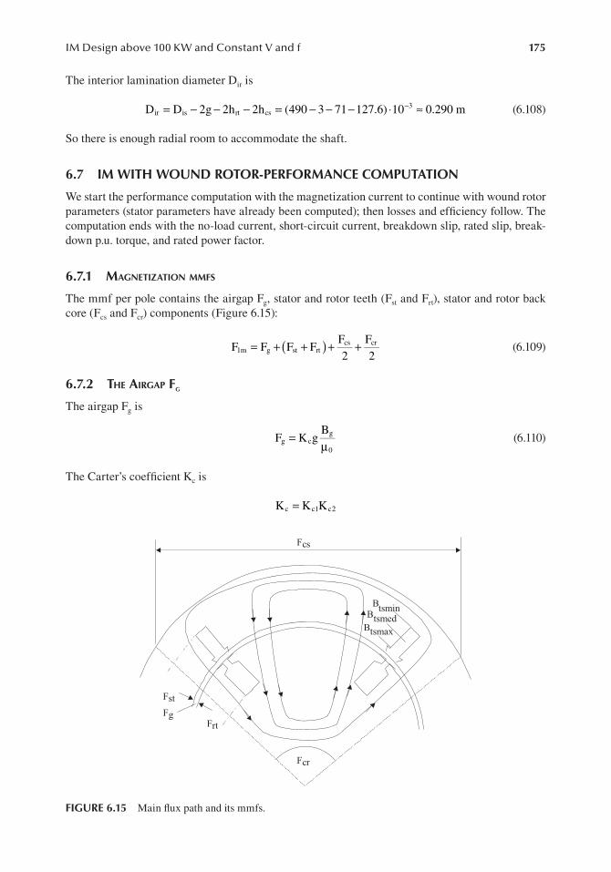
175IM Design above 100 KW and Constant V and f
The interior lamination diameter Dir is
D D 2g 2h 2h (490 3 71 127.6) 10 0.290 mir is rt cs3= − − − = − − − ⋅ ≈− (6.108)
So there is enough radial room to accommodate the shaft.
6.7 I M WITH WOUND ROTOR-PERFORMANCE COMPUTATION
We start the performance computation with the magnetization current to continue with wound rotor parameters (stator parameters have already been computed); then losses and efficiency follow. The computation ends with the no-load current, short-circuit current, breakdown slip, rated slip, break-down p.u. torque, and rated power factor.
6.7.1 Magnetization MMFS
The mmf per pole contains the airgap Fg, stator and rotor teeth (Fst and Frt), stator and rotor back core (Fcs and Fcr) components (Figure 6.15):
F F F FF2
F2
1m g st rtcs cr( )= + + + + (6.109)
6.7.2 the airgap Fg
The airgap Fg is
F K gB
g cg
0
=µ
(6.110)
The Carter’s coefficient Kc is
K K Kc c1 c2=
Fst
Frt
Fg
Fcs
Fcr
B
B
Btsmax
tsmed
tsmin
FIGURE 6.15 Main flux path and its mmfs.

176 Induction Machines Handbook
Kg
;
bg
5b
g
c1,2s,r
s,r s,rs,r
os,r2
os,r= τ
τ − γγ =
+(6.111)with
Kc1 has been already calculated in (6.43): Kc1 = 1.365. With bor = 5 · 10−3 m, g = 1.5 · 10−3 m and τr = 25.486 · 10−3 m, γr is
51.5
55
1.5
1.333; K25.486
25.486 1.5 1.3331.0852r
2
c2γ =
+= =
− ⋅=
Finally, Kc = 1.365 · 1.0852 = 1.4812 < 1.5 (as assigned from start).From (6.110), Fg is
F 1.4812 1.5 100.7
1.256 101188 Aturnsg
36= ⋅ ⋅
⋅=−
−
6.7.3 the Stator teeth MMF
With the maximum stator tooth flux density Btmax = 1.5 T, the minimum value Btsmin occurs at slot bottom diameter:
B D 2h N b B D
490 2 57.2 72 10 490 0.7 0.914 T
tsmin is st s s1
g is
1
( )
( )
( )
( )
= π + − π
= π + ⋅ − ⋅ π ⋅ ⋅ =
−
− (6.112)
The average value Btsmed is
BD B
D h N b490 0.7
490 57.2 72 101.0788Ttsmed
is g
is st s s( ) ( )=π
π + −= π ⋅ ⋅
π + − ⋅= (6.113)
For the three flux densities, the lamination magnetization curve (Chapter 5, Vol. 1, Table 5.4) yields:
H 1123A/m, H 335A/m, H 192 A/mtsmax tsmed tsmin= = =
The average value of Hts is
H16
H 4H H
16
(1123 4 345 192) 442.5A/m
ts tsmax tsmed tsmin( )= + +
= + ⋅ + =
(6.114)
The stator tooth mmf Fts becomes
F h H 57.2 10 442.5 25.31Aturnsts st ts3= = ⋅ ⋅ =− (6.115)

177IM Design above 100 KW and Constant V and f
6.7.4 rotor tooth MMF (Ftr) coMputation
It is done as for the stator. The average tooth flux density Btrmed is
BD B
D h N b490 0.7
490 35.52 60 10.51.351Ttrmed
is g
is rt r r
=π
= π ⋅ ⋅ = (6.116)( ) ( )π − − π − − ⋅
The corresponding iron magnetic fields for Btrmin = 1.3 T, Btrmed = 1.351 T, and Btrmax = 1.582 T are
H 9000 A/m, H 1750 A/m, H 760 A/mtrmax trmed trmin= = =
The average Htr is
H16
H 4H H 2793.33 A/mtr trmax trmed trmin( )= + + = (6.117)
The rotor tooth mmf Ftr is
F h H 35.5 10 2793.33 99.163Aturnstr rt tr3= = ⋅ ⋅ =− (6.118)
We are now in position to check the teeth saturation coefficient 1 + Kst (adopted as (1.25)):
1 K 1F F
F1
30.22 99.1631418
1.0912 1.25stts tr
g
+ = + + = + + = < (6.119)
The value of 1 + Kst is a bit too small, indicating that the stator teeth are weakly saturated. Slightly wider stator slots would have been feasible. In case the stator winding losses are much larger than stator core loss, increasing the slot width by 10% could lead to higher conductor loss reduction. Another way to take advantage of this situation is illustrated in [3], Figure 6.16, where axial cool-ing is used, and the rotor diameter is reduced due to better cooling. For a two-pole 1.9 MW, 6600 V machine, the reduction of mechanical loss led to 1% efficiency rise (from 0.96 to 0.97) [3].
The stator back core mmf Fcs is
F l Hcs cs cs= (6.120)
As both Bcs and lcs vary within a pole-pitch span, a correct value of Fcs would warrant finite element modelling (FEM) calculations.
FIGURE 6.16 Tooth axial ventilation design (high-voltage stator).

178 Induction Machines Handbook
We take here Bcsmax as reference:
BB
h0.7 0.3925
0.730 0.60442
1.358Tcsmaxg
cs
=τ
π= ⋅
π −
= (6.121)
Hcsmax = 600 A/mThe mean length lcs is
lD h
2PK
0.730 628 10
2 20.4 0.2095mcs
out cs
1cs
3( )( )= π − =π − ⋅
⋅=
−
(6.122)
Kcs is an amplification factor which essentially depends on the flux density level in the back iron.Again Bc1max is a bit too small. Consequently, if the temperature rise allows, the outer stator
diameter may be reduced, perhaps to 0.700 m (from 0.73 m).
F l H 0.2095 600 125Aturnscs cs c1max= = ⋅ =
6.7.5 rotor Back iron MMF Fcr (aS For the Stator)
F H l 760 0.1118 84.95Aturnscr cr cr= = ⋅ = (6.123)
H B H (1.4) 760 A/mcr cr cr( ) = =
lD h
2PK
0.296 0.062 2
0.4 0.1118mcrir cr
1cr
( ) ( )= π + = π −⋅
= (6.124)
From (6.109), the total mmf per pole F1m is
F 1188 25.31 99.163125 84.95
21417.45 Aturns1m = + + + + =
The mmf per pole F1m is
F3 2I W K
p1m
1 w1
1
=π
µ (6.125)
So the magnetization current Iμ is
IF p
3 2W K1417.45 2
3 2 12 18 0.92310.555A1m 1
1 w1
= π = ⋅ ⋅π⋅ ⋅ ⋅
=µ (6.126)
The ratio between the magnetization and rated phase current Iμ/I1n is
I
I10.55
120 30.152
1n
= =µ
Even at this power level and 2p1 = 4, because the ratio τ/g = 392/1.5 = 261.33 (pole pitch/airgap) is rather large and the saturation level is low, the magnetization current is lower than 20% of rated current. The machine has slightly more iron than needed, or the airgap may be increased from 1.5 · 10−3 m to (1.8–2)10−3 m. As a bonus, the additional surface and tooth flux pulsation core losses will be reduced. We may simply reduce the outer diameter such that to saturate notably the stator back iron. The gain will be less volume and weight.

179IM Design above 100 KW and Constant V and f
6.7.6 the rotor winDing paraMeterS
As the stator phase resistance Rs and leakage reactance (Xsl) have been already computed (Rs = 0.8576 Ω, Xsl = 6.667 Ω), only the rotor winding parameters Rr and Xlr have to be calculated.
The computation of Rr, Xrl requires the calculation of rotor coil end-connection length based on its geometry (Figure 6.17).
The end-connection length lfr per rotor side is
ly
cosh3
h 2
0.314 35.5 104
0.70743
2 35.5 10 0.5m
frr
rtrt
3
3
=α
+ +
⋅
=− ⋅ ⋅ π
+ ⋅ ⋅ ⋅ =
−
− (6.127)
So the phase resistance Rrr (before reduction to stator) is
R K2 l l W
A1.0 2.2 10
2(0.5 0.451) 2096 10
0.87 10rr
R Co80fr geo 2
cor
86
2( )= ρ
+= ⋅ ⋅ + ⋅
⋅= ⋅ Ω°
−−
− (6.128)
6.7.7 the rotor Slot leakage geoMetrical perMeance coeFFicient λSr
The rotor slot leakage geometrical permeance coefficient λsr is (Figure 6.14)
2b3b
h4b
hb
hb
2hb b
2 123 10.5
1.24 10.5
1.810.5
2.55
2 45 10.5
1.978
s,rc
r
4
r
2
s
or
or
w
or r( )λ ≈ + + + ++
= ⋅⋅
+⋅
+ + + ⋅+
= (6.129)
The rotor differential leakage permeance coefficient λdr is (as in [4])
0.9 q K K
K gdr
r 2 w22
or dr
c
( )λ =⋅τ σ
(6.130)
K 1.0 0.033bg
1.0 0.0335
1.5 24.860.9778or
or2
r
2
= −τ
= −⋅
= (6.131)
where σdr is the differential leakage coefficient as defined in Figure 6.3, Section 6.3, Vol. 1. For q2 = 5 and diametrical coils σdr = 0.64 · 10−2,
αh /3 ct
welded
r
y= -h τ r
=hrt
FIGURE 6.17 Rotor half-formed coil winding.

180 Induction Machines Handbook
0.924.86
1.8 1.5(5 0.9566) 0.9778 0.64 10 1.4428dr
2 2λ =⋅
⋅ ⋅ ⋅ ⋅ =−
The end-connection permeance coefficient λfr (defined as for the stator) is
0.34ql
l 0.64 0.345
0.4060.5 0.64 0.314 1.252fr
2
irfr( ) ( )λ = − τ = − ⋅ = (6.132)
The rotor phase leakage reactance Xlr (before reduction to stator) is
X 4 f Wl
P q
4 3.14 60 1.256 10 200.4062 5
(1.978 1.4428 1.252) 7.1828 10
rlr
1 0 22 i
1 2ri
6 2 2
∑= π µ λ
= ⋅ ⋅ ⋅ ⋅ ⋅⋅
+ + = ⋅ Ω (6.133)− −
After reduction to stator, the rotor resistance and leakage reactances Rr rr , Xrl become Rr and Xrl.
R RW KW K
0.87 1012 18 0.92320 0.9566
0.94
X XW KW K
7.1828 10 108.6 7.8
r rr 1 w1
2 w2
22
2
rl rlr 1 w1
2 w2
22
=
= ⋅ ⋅ ⋅ ⋅⋅
= Ω
=
= ⋅ ⋅ = Ω
−
−
(6.134)
The magnetization reactance Xm is
XV I X
I(4000 10.55 6.667)
10.55372.48m
ph sl( )≈
−= − ⋅ = Ωµ
µ (6.135)
The p.u. parameters are
XV
I4000120 57.66n
ph
1n
= = = Ω
rRX
0.875657.66
0.01487 p.u.ss
n
= = =
rRX
0.9457.66
0.0163 p.u.rr
n
= = = (6.136)
xXX
6.66757.66
0.1156 p.u.lsls
n
= = =
xX 57.66
0.1352 p.u.lrlr
n
= = =X 7.8
xXX
372.4857.66
6.45 p.u. 3.2 4 p.u.mm
n
( )= = = > −
3
Again, xm is visibly higher than usual but, as explained earlier, this may be the starting point for machine size further reduction. A simple reduction of the outer stator diameter to saturate the sta-tor back iron would bring xm into the standard interval of (3.5–4)p.u. for four-pole IMs of 700 kW

181IM Design above 100 KW and Constant V and f
power range with wound rotors. An increase in airgap will produce similar effects, with additional core loss reduction.
We leave here xm as it is in (6.136) as a reminder that the IM design is an iterative procedure.
6.7.8 loSSeS anD eFFiciency
The losses in IMs may be classified as
• Conductor (winding or electric) losses• Core losses• Mechanical/ventilation losses
The stator winding rated losses pcos are
P 3R I 3 0.8576 69.36 12.378 10 Wcos s 1n2 2 3= = ⋅ ⋅ = ⋅ (6.137)
For the rotor winding:
p 3R I 3R K I 3 0.94 0.936 69.36 11.885 10 Wcor r 1n2
r i2
1n2 2 3( )= = = ⋅ ⋅ ⋅ = ⋅ (6.138)
Considering a voltage drop, Vss = 0.75 V, in the slip ring and brushes, the slip-ring brush losses psr (with I2n from (6.102)) is
P 3V I 3 0.75 676.56 1.522 10 Wsr sr 2n3= = ⋅ ⋅ = ⋅
Additional winding losses due to skin and proximity effects (Chapter 11, Vol. 1) may be neglected for this case due to proper conductor sizing.
The core losses have three components (Chapter 11, Vol. 1):
• Fundamental core losses• Additional no-load core losses• Additional load (stray) core losses.
The fundamental core losses are calculated by empirical formulas (FEM may also be used) as in Chapter 5, Vol. 1.
The stator teeth fundamental core losses Piront is (5.98)
p K pf50
B Giront t 1050
11.3
ts1.7
ts=
(6.139)
Kt = 1.6–1.8, takes into account the mechanical machining influence on core losses; p10 (1 T, 50 Hz) = (2–3) W/Kg for 0.5 mm thick laminations.
The value of Bt varies along the tooth height so the average value Bts (Hts), Equation (6.114), is Bts (528 A/m) = 1.32 T.
The stator teeth weight Gts is
G4
D 2h D h b N l
40.490 2 56.2 10 0.490 56.2 10 10 10 72 0.406 7800
175.87Kg
ts is st2
is2
ts s s i iron
3 2 2 3 3( )( )
( )
( )= π + − −
γ
= π + ⋅ ⋅ − − ⋅ ⋅ ⋅ ⋅
⋅ ⋅
=
− − −
(6.140)

182 Induction Machines Handbook
From (6.139),
P 1.8 2.46050
1.32 175.87 1.543 10 Wiront
1.31.7 3= ⋅
⋅ = ⋅
Similarly, the stator back iron (yoke) fundamental losses Pyiron are
P K pf50
B Girony
y 1050
11.3
cs1.7
ys=
(6.141)
Ky = 1.2–1.4 takes care of the influence of mechanical machining on yoke losses (for lower power machines this coefficient is larger).
The stator yoke weight Gys is
G
D D 2h
4l
40.93 (0.49 2 0.0562) 0.406 7800 422.6Kg
ys
out2
is st2
i iron
2 2(
( )=
π − +γ
= π − + ⋅ ⋅ ⋅ = (6.142)
( )
)
p 1.35 2.46050
1.274 422.6 2.619 10 Wirony
1.71.7= ⋅ ⋅
⋅ ⋅ = ⋅ 3
Stator and rotor surface core losses, due to slot openings (Chapter 11, Vol. 1), are approximately:
P 2pb
l K psirons
1s os
si Fe siron
s( )= τ τ −τ
(6.143)
with the specific surface stator core losses (in W/m2) pssiron as
p 5 10 B KN 60f
P 10,000sirons 5
os2
r2
0r 1
1
1.5
≈ ⋅ τ⋅
(6.144)
Bos is the airgap flux pulsation due to rotor slot openings
B K B 0.23 1.48 0.7 0.2368Tos s c g= β = ⋅ ⋅ = (6.145)
βs can be taken from Figure 5.4 (Chapter 5, Vol. 1). With bor/g = 5/1.5, βs ≈ 0.23. K0 again depends on mechanical factors: K0 = 1.5, in general.
p 5 10 0.2368 0.02486 1.560 60 602 10,000
922.49 W/msirons 5 2 2
1.52= ⋅ ⋅ ⋅ ⋅ ⋅ ⋅ ⋅
⋅
=
From (6.143):
p 2 2 0.314(21.37 10)
21.370.406 0.95 922.49 0.237 10 Wsiron
s 3= ⋅ ⋅ − ⋅ ⋅ ⋅ = ⋅
As the rotor slot opening bor per gap g ratio is only 5/1.5, the stator surface core losses are expected to be small.

183IM Design above 100 KW and Constant V and f
The rotor surface core losses prsiron are
p 2Pb
l K psironr
1r or
si Fe siron
r( )= τ −τ
τ (6.146)
with p 5 10 B KN 60f
P 10,000; B K Bsiron
r 5or2
s2
0r 1
1
1.5
or r c g= ⋅ τ⋅
= β
The coefficient βr for bos/g = 10/1.5 is, Figure 5.4, Chapter 5, Vol. 1, βr = 0.41.Consequently,
B 0.41 1.48 0.7 0.426Tor = ⋅ ⋅ =
p 5 10 0.426 0.0214 2.072 60 602 10,000
3877 W/msironr 5 2 2
1.52= ⋅ ⋅ ⋅ ⋅ ⋅ ⋅ ⋅
⋅
=
K0 = 2.0 as the rotor is machined to the rated airgap.
P 2 2(24.86 5)
24.860.314 0.406 0.95 3877 1.5 10 Wsiron
r 3= ⋅ − ⋅ ⋅ ⋅ ⋅ = ⋅
The tooth flux pulsation core losses are still to be determined.
P P P K 0.5 10 Nfp
G Nfp
Gpuls pulss
pulsr
04
r1
1ps
2
ts s1
1pr
2
tr= + ≈ ′ ⋅ β
+ β
− (6.147)
K 1 B (1.085 1) 0.7 0.060 Tps c2 g( )β ≈ − = − ⋅ =
K 1 B (1.36 1) 0.7 0.252Tpr c1 g( )β ≈ − = − ⋅ =
K′0 > 1 is a technological factor to account for pulsation loss increases due to saturation and type of lamination manufacturing technology (cold or hot stripping). We take here K′0 = 2.0.
The rotor teeth weight Gtr is
GD 2g D 2g 2h
4N h b ltr
is2
is rt2
r rt r i iron
(( ) ( )=
π − − − −−
γ
0.49 3 10 (0.487 20.0355)
460 0.0355 105 10 0.406 7800 88.55Kg
3 2 2
2( )( )
=π − ⋅ − −
− ⋅ ⋅ ⋅
⋅ ⋅ =−
−
(6.148)
)
From (6.147),
P 2 0.5 10 60
602
0.060 175.87 72602
0.252 88.55
2.828 10 W
puls4
2 2
3
= ⋅ ⋅ ⋅ ⋅
⋅ + ⋅ ⋅
⋅
= ⋅
−

184 Induction Machines Handbook
The mechanical losses due to friction (brush-slip-ring friction and ventilator on-shaft mechanical input) depend essentially on the type of cooling machine system design.
We take them all here as being Pmec = 0.01Pn. For two-pole or high-speed machines, Pmec > 0.01Pn and should be, in general, calculated as precisely as feasible in a thorough mechano-thermal design.
6.7.9 the Machine rateD eFFiciency ηn
The machine rated efficiency ηn is
PP p P P P P P P P P
nn
n cos cor sr iront
irony
sirons
sironr
puls mec
η =+ + + + + + + + +
736 1010 736 12.378 11.885 1.522 1.543 2.619 0.237 1.5 2.828 7.36
0.946
3
3 (= ⋅+ + + + + + + + +
= (6.149)
)
As the efficiency is notably below the target value (0.96), efforts to improve the design are in order. Additional losses are to be reduced. Here is where optimization comes into play.
6.7.10 the rateD Slip Sn (with Short-circuiteD Slip ringS)
The rated slip Sn (with short-circuited slip rings) can be calculated as
SR K IK V
0.94 0.936 69.360.97 4000
0.0157nr i 1n
e ph
≈ = ⋅ ⋅⋅
= (6.150)
Alternatively, accounting for all additional core losses in the stator,
Sp
P p p11.885 10
10 (736 11.885 7.36)0.015736n
cor
n cor mec
3
3=+ +
= ⋅⋅ + +
= (6.151)
The rather large value of rated slip is an indication of not so high efficiency. A reduction of current density in both the stator and rotor windings seems appropriate to further increase efficiency.
The rather low teeth flux densities allow for slot area increases to cause winding loss reductions.
6.7.11 the BreakDown torque
The approximate formula for breakdown torque is
T3p2
V
X X3 2
2 2 604000
(6.67 7.8)8.8035 10 Nmbk
1
1
ph2
ls lr
23≈
ω += ⋅
⋅ π ⋅ += ⋅ (6.152)
The rated torque Ten is
Tp P1 S
2 736 102 60 (1 0.015)
3.966 10 Nmen1 n
1 n
33
( )=ω −
= ⋅ ⋅π ⋅ ⋅ −
= ⋅ (6.153)
The breakdown torque ratio tek is
tTT
8.80353.966
2.2ekbk
en
= = ≈ (6.154)
This is an acceptable value.

185IM Design above 100 KW and Constant V and f
6.8 SUMMARY
• Above 100 kW, induction motors are built for low voltage (≤690 V) and for medium voltage (between 1 and 12 KV).
• Low-voltage IMs are designed and built lately up to more than 2 MW power per unit, in the eventuality of their use with PWM converter supplies.
• For constant voltage and frequency supply, besides efficiency and initial costs, the starting torque and current and the peak torque are important design factors.
• The stator design is based on targeted efficiency and power factor, whereas rotor design is based on the starting performance and breakdown torque.
• Deep bar cage rotors are used when moderate p.u. starting torque is required (tLR < 1.2). The bar depth and width are determined based on breakdown torque, starting torque, and starting current constraints. This methodology reduces the number of design iterations drastically.
• The stator design is dependent on the cooling system: axial cooling (unistack core con-figuration) and radial–axial cooling (multistack core with radial ventilation channels, respectively).
• For medium-voltage stator design, open rectangular slots with form-wound chorded (rigid) coils, built into two-layer windings, are used. Practically only rectangular cross-sectional conductors are used [5,6].
• The rather large insulation total thickness makes the stator slot fill in high-voltage wind-ings rather low, with slot aspect ratios hst/bs > 5. Large slot leakage reactance values are expected.
• In low-voltage stator designs, above 100 kW, semiclosed-slot, round-wire coils are used only up to 200–250 kW for 2p1 = 2, 4; also, for larger powers and large numbers of poles (2p1 = 8, 10), quite a few current paths in parallel (a1 = p1) may be used.
• For low-voltage stator designs, prepared also for PWM converter use, only rectangular shape conductors in form-wound coils are used, to secure good insulation as required for PWM converter supplies. To reduce skin effect, the conductors are divided into a few elementary conductors in parallel. Stranding is performed twice, at the end-connection zone (Chapter 9, Vol. 1).
• Deep bar design handles large breakdown torques, tbk ≈ 2.5–2.7 and more, with moder-ate starting torques tLR < 1.2 and starting currents iLR < 6.1. Based on breakdown torque, starting torque, and current values, with stator already designed (and thus stator resis-tance and leakage reactance values known), the rotor resistance and leakage reactance values (with and without skin effect and leakage saturation consideration) are calculated. This leads directly to the adequate rectangular deep bar geometry. If other bar geometries are used, the skin effect coefficients are calculated by the refined multilayer approach (Chapter 9, Vol. 1).
• Double-cage rotor designs lead to lower starting currents iLR < 5.5, larger starting torque tLR > (1.4–1.5) and good efficiency but moderate power factor.
• A similar methodology, based on starting and rated power performance leads to the start-ing and working cage sizing, respectively. Thus, a first solution meeting the main con-straints is obtained. Refinements should follow, eventually through design optimization methods.
• For limited variable speed range, or for heavy and frequent starting (up to breakdown torque at start), wound rotor designs are used.
• The two-layer wound rotor windings are, in general, low-voltage type, with half-formed diametrical wave uniform coils in semiclosed or semiopen slots (to reduce surface and tooth flux pulsation core loss). A few elementary conductors in parallel may be needed to handle the large rotor currents as the power goes up.

186 Induction Machines Handbook
• The wound rotor design is similar to stator design, being based only on rated targeted effi-ciency (and power factor) and on the assigned rotor current density.
• This chapter presents design methodologies using a single motor (low- and medium- voltage stator 736 kW (1000 HP) design with deep bar cage, double-cage and wound rotor). Only for the wound rotor, all parameters (losses, efficiency, rated slip, breakdown torque, and rated power factor) are calculated. Its design for large slip and converter-fed in the rotor can be found (as doubly fed induction generator or DFIG) in [7].
• Ways to improve the resultant performance are indicated. Temperature rise calculations may be performed as in Chapter 5, Vol. 2, but with more complex mathematics. If tem-perature rise is not met (insulation class F and temperature rise class B) and it is too high, a new design with a larger geometry or lower current densities or (and) flux densities has to be tried.
• Chapters 4–6, laid out the machine models (analysis) and a way to size the machine for given performance and constraints (preliminary synthesis).
• The mathematics in these chapters may be included in a design optimization software. Design optimization will be treated in a separate chapter. FEM is to be used for refinements.
• The above methodologies are by no means unique to the scope, as IM design is both a sci-ence and an art [8–10].
REFERENCES
1. ABB Industry Oy, Machines, Product Information, AMA Machines, PIF 2b000-999/364. 2. ABB Industry Oy, Machines, Product Information, HXR Machines, PIF 2a000-999/364. 3. C. M. Glew, G. D. LeFlem, J. D. Walker, The customer is always right – improved performance of
high speed induction motors, record of “electrical machines and drives”, IEE Conference Publication No. 412, London, 11–13 September 1995, pp. 37–40.
4. P. L. Alger, Induction Machines: Their Behaviour and Uses, Second edition, Godon & Breach Publishers, London, 1995.
5. A. Demenkco, K. Oberretl, Calculation of additional slot leakage permeance in electrical machines due to radial ventilation ducts, COMPEL: The Journal for Computation and Mathematics in EEE, Vol. 11, No. 1,1982, pp. 93–96.
6. E. Levi, Polyphase Motors: A Direct Approach to Their Design, Wiley Interscience, Hoboken, NJ, 1985. 7. I. Boldea, Variable Speed Generators, Second edition, Chapter 3, CRC Press: Boca Raton, FL, 2016. 8. P. L. Cochran, Polyphase Induction Motors, Marcel Dekker, Inc., New York, 1989. 9. J. Pyrhonen, T. Jokinen, V. Hrabovcova, Design of Rotating Electrical Machines, Wiley, Chichester,
UK, 2009. 10. I. Boldea, L. Tutelea, I. Torac, F. Marignetti, 10 MW, 10 rpm, 10 Hz, directly driven cage rotor induc-
tion generator (CRIG): Preliminary design and key FEM validations, Record of IEEE-ACEMP-OPTIM Conference, Istambul, Turkey, 2019.

187
7 Induction Machine Design for Variable Speed
7.1 INTRODUCTION
Variable speed drives with induction motors are by now a mature technology with strong and dynamic markets for applications in all industries. Based on the load torque/speed envelope, three main types of applications are distinguished:
• Servodrives: no constant power speed range (CPSR)• General drives: moderate CPSR (ωmax/ωb ≤ 2)• Constant power drives: large CPSR (ωmax/ωb ≥ 2).
Servodrives for robots, machine tools, are characterized, in general, by constant torque versus speed up to base speed ωb. The base speed ωb is the speed for which the motor can produce (for continuous service) for rated voltage and rated temperature rise, the rated (base) power Pb, and rated torque Teb.
Servodrives are characterized by fast torque and speed response, and thus for short time, during transients, the motor has to provide a much higher torque Tek than Teb. The higher the torque, the better the speed response. Also servodrives are characterized by sustained very low-speed and up to rated (base) torque operation, for speed or position control. In such conditions, low torque pulsations and limited temperature rise are imperative.
Temperature rise has to be limited to avoid both winding insulation failure and mechanical deformation of the shaft which would introduce errors in position control.
In general, servodrives have a constant speed (separate shaft) power, grid fed, ventilator attached to the induction machine (IM) at the non-driving end. The finned stator frame is thus axially cooled through the ventilator’s action. Alternatively, liquid cooling of the stator may be provided.
Even from such a brief introduction, it becomes clear that the design performance indexes of IMs for servodrives need special treatment. However, fast torque and speed response and low torque pulsations are paramount. Efficiency and power factor are second-order performance indexes as the inverter KVA rating is designed for the low duration peak torque (speed) transients requirements.
General drives, which cover the bulk of variable speed applications, are represented by fans, pumps, compressors, etc.
General drives are characterized by a limited speed control range, in general, from 0.1ωb to 2ωb. Above base speed ωb, constant power is provided. A limited CPSR ωmax/ωb = 2.0 is sufficient for most cases. Above base speed, the voltage stays constant.
Based on the stator voltage circuit equation at steady state,
V I R js s s 1 s= + ω Ψ (7.1)
with Rs ≈ 0
V
ss
1
Ψ ≈ω
(7.2)

188 Induction Machines Handbook
Above base speed (ωb), the frequency ω1 increases for constant voltage. Consequently, the stator flux level Ψs decreases. Flux weakening occurs. We might say that general drives have a 2/1-flux weakening speed range.
As expected, there is some torque reserve for fast acceleration and braking at any speed. About 150%–200%, overloading is typical.
General drives use IMs with on-the-shaft ventilators. More sophisticated radial–axial cooling systems with a second cooling agent in the stator may be used.
General drives may use high-efficiency IM designs as in this case efficiency is important.Made with class F insulated preformed coils and insulated bearings for powers above 100 kW
and up to 2000 kW, and at low voltage (maximum 690 V), such motors are used in both constant and variable speed applications. While designing IMs on purpose for general variable speed drives is possible, it may seem more practical to have a single design for both constant and variable speed: the high-efficiency induction motor.
In constant power variable-speed applications such as spindles or hybrid (or electric) car pro-pulsion and generator systems, the main objective is a large flux weakening speed range ωmax/ωb > 2, in general more than 3–4, and even 6–7 in special cases. Designing an IM for a wide CPSR is very challenging because the breakdown torque Tbk is in p.u. limited: tbk < 3 in general.
T3p2
V 1L
eK1 ph
1
2
sc
≈ω
⋅ (7.3)
Increasing the breakdown torque as the base speed (frequency) increases could be done by
• Increasing the pole number 2p1.• Increasing the phase voltage.• Decreasing the leakage inductance Lsc (by increased motor size, winding tapping, phase
connection changing, special slot (winding) designs to reduce Lsc). Each of these solutions has impact on both IM and static power converter costs. The global cost of the drive and the capitalized cost of its losses are solid criteria for appropriate designs. Such applications are most challenging. Yet another category of variable speed applications is represented by super-high-speed drives.
• For fast machine tools, vacuum pumps etc., speeds which imply fundamental frequencies above 300 Hz (say above 18,000 rpm) are considered here for up to 100 kW powers and above 150 Hz (9000 rpm) for higher powers.
As the peripheral speed goes up, above (60–80) m/s, the mechanical constraints become predomi-nant and thus novel rotor configurations become necessary. Solid rotors with copper bars are among the solutions considered in such applications. Also, as the size of IM increases with torque, high-speed machines tend to be small (in volume/power) and thus heat removal becomes a problem. In many cases, forced liquid cooling of the stator is mandatory.
Despite worldwide efforts in the last decade, the design of IMs for variable speed, by analytical and numerical methods, did not crystallize in widely accepted methodologies.
What follows should be considered a small step towards such a daring goal.As basically the design expressions and algorithms developed for constant V/f (speed) are
applicable to variable speed design, we will concentrate only on what distinguishes this latter enterprise.
• In the end, a rather detailed design case study is presented. Among the main issues in IM design for variable speed, we treat here
• Power and voltage derating• Reducing skin effect

189Induction Machine Design for Variable Speed
• Reducing torque pulsations• Increasing efficiency• Approaches to leakage inductance reduction• Design for wide constant power wide speed range• Design for variable very high speed.
7.2 P OWER AND VOLTAGE DERATING
An induction motor is only a part of a variable speed drive assembly (Figure 7.1).As such, the IM is fed from the power electronics converter (PEC) directly, but indirectly, in
most cases, from the industrial power grid.There are a few cases where the PEC is fed from a D.C. source (battery).The PEC inflicts on the motor voltage harmonics (in a voltage source type) or current harmonics
(in a current source type). In this case, voltage and current harmonics, whose frequency and ampli-tude are dependent on the PWM (control) strategy and power level, are imposed on the induction motor.
Additionally, high-frequency common voltage mode currents may occur in the stator phases in high-frequency PWM voltage source converter IM drives. All modern PECs have incorporated filtering methods to reduce the additional current and voltage (flux) harmonics in the IMs, as they produce additional losses.
Analytical and even finite element methods have been proposed to cater to these time harmon-ics losses (see Chapter 11, Vol. 1). Still, these additional time harmonics core and winding losses depend not only on machine geometry and materials, but also on PWM, switching frequency, and load level [1,2].
On top of this, for given power grid voltage, the maximum fundamental voltage at motor termi-nals depends on the type of PEC (single or double stage, type of power electronics switches (PES)) and PWM (control) strategy.
Though each type of PEC has its own harmonics and voltage drop signature, the general rule is that lately both these indexes have decreased. The matrix converter is a notable exception in the sense that its voltage derating (drop) is larger (up to 20%) in general.
Voltage derating – <10%, in general 5% – means that the motor design is performed at a rated voltage Vm which is smaller than the ac power grid voltage Vg:
V V 1 v ;v 0.1m g derat der( )= − < (7.4)
Power derating comes into play in the design when we choose the value of Esson’s constant C0 (W/m3), as defined by past experience for sinusoidal power supply, and reduce it to C′0 for variable V/f supply:
C C 1 p ; p (0.08 0.12)0 0 derat derat( )′ = − ≈ − (7.5)
It may be argued that this way of handling the PEC-supplied IM design is quite empirical. True, but this is done only to initiate the design (sizing) process. After the sizing is finished, the voltage drops in the PEC and the time harmonics core and winding losses may be calculated (see Chapter 11, Vol. 1).
3 ~
50 (60) HzIM
Power electronics conveter (PEC)
Load machine
FIGURE 7.1 IM in a variable speed drive system.
190 Induction Machines Handbook
Design refinements are then done. Alternatively, if prototyping is feasible, test results are used to validate (or correct) the loss computation methodologies.
There are two main cases: one when the motor exists, as designed for sinusoidal power supply, and the other when a new motor is to be designed for the scope.
The derating concepts deal with both these cases the same way.However, the power derating concept is of little use where no solid past experience exists, such as in
wide CPSR drives or in super-high-speed drives. In such cases, the tangential specific force (N/cm2), Chapter 4, Vol. 2, with limited current sheet (or current density) and flux densities, seems to be the right guidelines for practical solutions. Finally, the temperature rise and performance (constraints) checks may lead to design iterations. As already mentioned in Chapter 4, the rated (base) tangential specific force (σt) for sinusoidal power supply is
(0.3 4.0) N/cmtsin 2σ ≈ − (7.6)
Derating may now be applied to σsint , to get σPEC
t
1 ptPEC
tsin
derat( )σ = σ − (7.7)
for the same rated (base) torque and speed.The value of σPEC
t increases with rated (base) torque and decreases with base speed.
7.3 REDUCING THE SKIN EFFECT IN WINDINGS
In variable speed drives, variables V and f are used. Starting torque and current constraints are not anymore relevant in designing the IM. However, for fast torque (speed) response during variable frequency and voltage starting or loading or for constant power wide speed range applications, the breakdown torque has to be large.
Unfortunately, increasing the breakdown torque without enlarging the machine geometry is not an easy task.
On the other hand, the rotor skin effect that limits the starting current and produces larger start-ing torque, based on a larger rotor resistance, is no longer necessary.
Reducing skin effect is thus now mandatory to reduce additional time harmonics winding losses.Skin effect in winding losses depends on frequency, conductor size, and position in slots. First,
the rotor and stator skin effect at fundamental frequency is to be reduced. Second, the rotor and sta-tor skin effect has to be checked and limited at PEC switching frequency. The amplitude of currents is larger for the fundamental than for time harmonics. Still, the time harmonics conductor losses at large switching frequencies are notable. In super-high-speed IMs, the fundamental frequency is already large, (300–3(5)000) Hz. In this case, the fundamental frequency skin effects are to be severely checked and kept under control for any practical design as the slip frequency may reach tenth of Hz (up to 50–60 Hz).
As the skin effect tends to be larger in the rotor cage, we will start with this problem.
7.3.1 rotor Bar Skin eFFect reDuction
The skin effect is a direct function of the parameter:
hS
21 cor 0ζ = ω σ µ
(7.8)
The slot shape also counts. But if the slot is rectangular or circular, only the slot diameter and the slot height count.

191Induction Machine Design for Variable Speed
Rounded trapezoidal slots may also be used to secure constant tooth flux density and further reduce the skin effects (Figure 7.2).
For given rotor slot (bar) area Ab (Figure 7.2a–c), we have
Ad4
h2d3
h2
b d
h23
d5
36d
br2
rr r1
or r
r 1 r2
(
= π
= ⋅ + +
= + π
(7.9)
)
For the rectangular slot, the skin effect coefficients KR and KX have the standard formulas:
Ksinh 2 sin 2cosh 2 cos 2
K32
sinh 2 sin 2cosh 2 cos 2
R
X
= ζ ζ + ζζ − ζ
=ζ
ζ − ζζ − ζ
(7.10)
In contrast, for round or trapezoidal-round slots, the multiple-layer approach, discussed in Chapter 9, Vol. 1, has to be used.
A few remarks are in order:
• As expected, for given geometry and slip frequency, skin effects are more important in copper than in aluminium bars
• For given rotor slot area, the round bar has limited skin effect• As the bar area (bar current or motor torque) increases, the maximum slip frequency
fsr = Sf1 for which KR < 1.1 diminishes• Peak slip frequency fsrk varies from 2 to 10 Hz• The smaller values correspond to larger (MW) machines and larger values to sub-KW
machines designed for base frequencies of 50 (60) Hz. For fsrK, KR < 1.1 has to be fulfilled if rotor additional losses are to be limited. Consequently, the maximum slot depth depends heavily on motor peak torque requirements
• For super-high-speed machines, fsrk may reach even 50 (60) Hz, so extreme care in designing the rotor bars is to be exercised (in the sense of severe limitation of slot depth, if possible).
• Maintaining reduced skin effect at fsrK means, apparently, less deep slots and thus, for given stator bore diameter, longer lamination stacks. As shown in the next paragraph, this leads to slightly lower leakage inductances and thus to larger breakdown torque. That is, a beneficial effect.
dr
b
h
hb
b /3
α ∼ 30
h
d = d
d = d /3
d2
1r
1 r
2 1
r
r
r
r1
or
d
0
b = dr r
(a) (b) (c)
FIGURE 7.2 Rotor bar slots with low skin effect: (a) round shape, (b) rectangular, and (c) pair shape.
192 Induction Machines Handbook
• When the rotor skin effect for fsrK may not be limited by reducing the slot depth, we have to go so far as to suggest the usage of a wound rotor with short-circuited phases and mechani-cally enforced end connections against centrifugal forces
• To reduce the skin effect in the end rings, they should not be placed very close to the laminated stack, although their heat transmission and mechanical resilience are a bit compromised
• Using copper instead of aluminium leads to a notable reduction of rotor bar resistance for the same bar cross section although the skin effect is larger. A smaller copper bar cross section is allowed, for the same resistance as aluminium, but for less deep slots and thus smaller slot leakage inductance. Again, larger breakdown torque may be obtained. The extra cost of copper may prove well worthwhile due to lower losses in the machine.
• As the skin effect is maintained low, the slot-body geometrical specific permeance λsr for the three cases mentioned earlier (Figure 7.2) is
0.666
h3b
23 3
b d
h2d
0.4
srround
srrect r
r
r r
srtrap r
r
λ ≈
λ ≈ +
=
λ ≈ +
(7.11)
Equations (7.11) suggest that, in order to provide for identical slot geometrical specific permeance λsr, hr/br ≤ 1.5 for the rectangular slot and hr/dr < 0.5 for the trapezoidal slot. As the round part of slot area is not negligible, this might be feasible (hr r
Also for the rectangular slot with br = dr, hr = (π/4) dr ≪1.5, so the rectangular slot may produce:/d ≈ π/8 < 0.5), especially for low torque machines.
( /4) /12 2/3 3 0.67strect
srroundλ π = π + = ≈ λ
In reality, as the rated torque gets larger, the round bar is difficult to adopt as it would lead to a very small number of rotor slots or a very larger rotor diameter. In general, a slot aspect ratio hr/br ≤ 3 may be considered acceptable for many practical cases.
• The skin effect in the stator windings, at least for fundamental frequencies less than 100(120) Hz, is negligible in well-designed IMs for all power levels. For high-powers, elementary rectangular cross-sectional conductors in parallel are used. They are eventu-ally stranded in the end-connection zone. The skin effect and circulating current additional losses have to be limited in large motors
• In super-high-speed IMs, for fundamental frequencies above 300 Hz (up to 3 kHz or more), stator skin effect has to be carefully investigated and suppressed by additional methods such as Litz wire or even by using thin wall pipe conductors with direct liquid cooling when needed
• Skin effect stator and rotor winding losses at PWM inverter carrier frequency are to be calculated as shown in Chapter 11, Vol. 1.
7.4 TORQUE PULSATIONS REDUCTION
Torque pulsations are produced both by airgap magnetic permeance space harmonics in interaction with stator (rotor) mmf space harmonics and by voltage (current) time harmonics produced by the PEC which supplies the IM to produce variable speed.

193Induction Machine Design for Variable Speed
As torque time harmonics pulsations depend mainly on the PEC type and power level, we will not treat them here. The space harmonic torque pulsations are produced by the so-called parasitic torques (see Chapter 10, Vol. 1). They are of two categories, asynchronous and synchronous, and depend on the number of rotor and stator slots, slot opening/airgap ratios and airgap/pole pitch ratio, and the degree of saturation of stator (rotor) core. They all however occur at rather large values of slip: S > 0.7 in general.
This fact seems to suggest that for pump-/fan-type applications, where the minimum speed hardly goes below 30% base speed, the parasitic torques occur only during starting.
Even so, they should be considered, and the same rules apply, in choosing stator/rotor slot num-ber combinations, as for constant V and f design (Chapter 5, Table 5.5).
• As shown in Chapter 5, slot openings tend to amplify the parasitic synchronous torques for Nr > Ns (Nr – rotor slot count and Ns – stator slot count). Consequently, Nr < Ns appears to be a general design rule for variables V and f, even without rotor slot skewing (for series-connected stator windings).
• Adequate stator coil throw chording (5/6) will reduce drastically asynchronous parasitic torque.
• Carefully chosen slot openings to mitigate between low parasitic torques and acceptable slot leakage inductances are also essential.
• Parasitic torque reduction is all the more important in servodrives applications with sus-tained low (even very low)-speed operation. In such cases, additional measures such as skewed resin insulated rotor bars and eventually closed rotor slots and semiclosed stator slots are necessary. Finite element modelling (FEM) investigation of parasitic torques may become necessary to secure sound results.
7.5 INCREASING EFFICIENCY
Increasing efficiency is related to loss reduction. There are fundamental core and winding losses and additional ones due to space and time harmonics.
Lower values of current and flux densities lead to a larger but more efficient motor. This is why high-efficiency motors are considered suitable for variables V and f.
Additional core losses and winding losses are discussed in detail in Chapter 11, Vol. 1.Here, we only point out that the rules to reduce additional losses, presented in Chapter 11, Vol. 1,
still hold. They are reproduced here and extended for convenience and further discussion.
• Large number of slots/pole/phase in order to increase the order of the first slot space harmonic.• Insulated or uninsulated high bar-slot wall contact resistance rotor bars in long stack
skewed rotors, to reduce inter-bar current losses.• Skewing is not adequate for low bar-slot wall contact resistance as it does not reduce the
harmonics (stray) cage losses while it does increase inter-bar current losses.• 0.8Ns < Nr < Ns – to reduce the differential leakage coefficient of the first slot harmonics
(Ns ± p1) and thus reduce the inter-bar current losses.• For Nr < Ns, skewing may be altogether eliminated after parasitic torque levels are checked.
For q = 1,2 skewing seems mandatory, though.• Usage of thin special laminations (0.1–0.2 mm) above f1n = 300 Hz is recommended to
reduce core loss in super-high-speed IM drives.• Chorded coils (y/τ ≈ 5/6) reduce the asynchronous parasitic torque produced by the first
phase belt harmonic (υ = 5).• With delta connection of stator phases: (Ns − Nr) ≠ 2p1, 4p1, 8p1.• With parallel paths stator windings, the stator interpath circulating currents produced by
rotor bar current mmf harmonics have to be avoided by observing a certain symmetry of stator winding paths.

194 Induction Machines Handbook
• Small stator (rotor) slot openings lead to smaller surface and tooth flux pulsation additional core losses, but they tend to increase the leakage inductances and thus reduce the break-down torque
• Carefully increase the airgap to reduce additional core and cage losses without compro-mising too much the power factor and efficiency.
• Use sharp tools and annealed laminations to reduce surface core losses.• Return rotor surface to prevent rotor lamination short circuits which would lead to increased
rotor surface core losses.• Use only recommended Ns and Nr combinations and check for parasitic torque and stray
load levels, and avoid large radial local forces.• To reduce the time and space harmonics losses in the rotor cage, U-shaped bridge rotor
slots have been proposed (Figure 7.3) [3].
In essence in conventional rotor slots, the airgap flux density harmonics induce voltages which produce eddy currents in the aluminium situated in the slot necks. By providing a slit in the rotor laminations (Figure 7.3b and c), the rotor conductor is moved further away from the airgap and thus, the additional cage losses are reduced.
However, this advantage comes with three secondary effects.First, the eddy currents in the aluminium cage close to airgap damp the airgap flux density varia-
tion on the rotor surface and in the rotor tooth. This, in turn, limits the rotor core surface and tooth flux pulsation core losses.
In our new situation, this no longer occurs. Skewed rotor slots seem appropriate to keep the rotor surface and tooth flux pulsation core losses under control.
Second, the iron bridge height hb above the slot, even when saturated, leads to a notable addi-tional slot leakage geometrical permeance coefficient: λb.
Consequently, the value of Lsc is slightly increased leading to a breakdown torque reduction.Third, the mechanical resilience of the rotor structure is somewhat reduced which might prevent
the usage of this solution to super-high-speed IMs.
7.6 INCREASING THE BREAKDOWN TORQUE
As already inferred, a large breakdown torque is desirable either for high transient torque reserve or for widening the CPSR. Increasing the breakdown torque boils down to leakage inductance decreasing, when the base speed and stator voltage are given (7.3).
The total leakage inductance of the IM contains a few terms as shown in Chapter 6, Vol. 1.The stator and rotor leakage inductances are (Chapter 6, Vol. 1).
L 2 L n p qsl 0 i s2
1 1 ss zs ds end( )= µ ⋅ λ + λ + λ + λ (7.12)
Al(copper)
Al(copper)
h
iron bridge
b
(a) (b) (c)
FIGURE 7.3 Rotor slot designs: (a) conventional, (b) straight bridge closed slot, (c) u-bridge close slot, and (d) asymmetric slot.

195Induction Machine Design for Variable Speed
ns – conductors slot
L 4mW K
N2 Lrl 1
1 W12
r0 i b er zr dr skew( )( )= ⋅ µ λ + λ + λ + λ + λ (7.13)
m1 – number of phasesLi – stack lengthq1 – slots/pole/phaseλss – stator slot permeance coefficientλzs – stator zig-zag permeance coefficientλds – stator differential permeance coefficientλend – stator end-coil permeance coefficientλb – rotor slot permeance coefficientλer – end ring permeance coefficientλzr – rotor zig-zag permeance coefficientλdr – rotor differential permeance coefficientλskew – rotor skew leakage coefficient.
The two general expressions are valid for open and semiclosed slots. For closed rotor slots λb has the slot iron bridge term as rotor current dependent.
With so many terms, out of which very few may be neglected in any realistic analysis, it becomes clear that an in-depth sensitivity analysis of Lsl and Lrl to various machine geometrical variables is not easy to wage.
The main geometrical variables which influence Lsc = Lsl + Lrl are
• Pole number: 2p1
• Stack length/pole pitch ratio: Li/τ• Slot/tooth width ratio: bs1r/bts1r
• Stator bore diameter• Stator slots/pole/phase q1
• Rotor slots/pole pair Nr/p1
• Stator (rotor) slot aspect ratio hss1r/bs1r
• Airgap flux density level Bg
• Stator (rotor) base torque (design) current density.
Simplified sensitivity analysis [4] of jcos, jAl to tsc (or tbk – breakdown torque in p.u.) has revealed that two, four, and six poles are the main pole counts to consider except for very low direct speed drives – c onveyor drives – where even 2p1 = 12 is to be considered, only to eliminate the mechanical transmission.
Globally, when efficiency, breakdown torque, and motor volume are all considered, the four-pole motor seems most desirable.
Reducing the number of poles to 2p1 = 2, for given speed n1 = f1/p1 (rps), means lower frequency, but, for the same stator bore diameter, it means larger pole pitch and longer end connections and thus larger λend in (7.12).
Now with q1 larger, for 2p1 = 2, the differential leakage coefficient λds is reduced. So, unless the stack length is not small at design start (pancake shape), the stator leakage inductance (7.12) decreases by a ratio between 1 and 2 when the pole count increases from two to four poles, for the same current and flux density. Considering the two rotors identical, with the same stack length, Lrl in (7.13) would not be much different. This leads us to the peak torque formula (7.3).
T3p2 2L
;V
ek1 sph
2
scsph
ph
1
( )≈
ΨΨ =
ω (7.14)

196 Induction Machines Handbook
For the same number of stator slots for 2p1 = 2 and 4, conductors per slot ns, same airgap flux den-sity, and same stator bore diameter, the phase flux linkage ratio in the two cases is
21
sph 2p 2
sph 2p 4
1
1
( )( )Ψ
Ψ==
=
(7.15)
as the frequency is doubled for 2p1 = 4, in comparison with 2p1 = 2, for the same no-load speed (f1/p1).
Consequently,
L
L1.5 1.8
sc 2p 2
sc 2p 4
1
1
( )( ) = −=
=
(7.16)
Thus, for the same bore diameter, stack length, and slot geometry,
T
T2
1.5 1.8
ek 2p 2
ek 2p 4
1
1
( )( ) ≈
−=
=
(7.17)
From this simplified analysis, we may draw the conclusion that the 2p1 = 2 pole motor is better. If we consider the power factor and efficiency, we might end up with a notably better solution.
For super-high-speed motors, 2p1 = 2 seems a good choice (f1n > 300 Hz).For given total stator slot area (same current density and turns/phase) and the same stator bore
diameter, increasing q1 (number of slot/pole/phase) does not essentially influence Lsl (7.12) – the sta-tor slot leakage and end-connection leakage inductance components – as nsp1q1 = W1 = ct and slot depth remains constant, whereas the slot width decreases to the extent q1 increases, and so does λend:
0.34L
l 0.64 y qendi
end 1( )λ ≈ − ⋅ ⋅ (7.18)
where lend – end-connection length, y – coil throw, and Li – stack length.However, λds decreases and apparently so does λzs. In general, with larger q1, the total stator
leakage inductance will decrease slightly. In addition, the stray losses have been proved to decrease with q1 increasing.
A similar rationale is valid for the rotor leakage inductance Lrl (7.13) where the number of rotor slots increases. It is well understood that the condition 0.8Ns < Nr < Ns is to be observed.
A safe way to reduce the leakage reactance is to reduce the slot aspect ratio hss,r/bss,r < 3.0–3.5. For given current density, this would lead to lower q1 (or Ns) for a larger bore diameter, that is, a larger machine volume.
However, if the design current density is allowed to increase (sacrificing to some extent the effi-ciency) with a better cooling system, the slot aspect ratio could be kept low to reduce the leakage inductance Lsc.
• A low leakage (transient) inductance Lsc is also required for current source inverter IM drives [4].
So far, we have considered the same current and flux densities, stator bore diameter, stack length, but the stator and yoke radial height for 2p1 = 2 is doubled with respect to the four-pole machine.
h
h(1.5 2)
1
cs,r 2p 2
cs,r 2p 4
1
1
( )( ) ≈ −=
=
(7.19)

197Induction Machine Design for Variable Speed
Even if we oversaturated the stator and rotor yokes, more so for the two-pole machine, the outer stator diameter will still be larger in the latter case. It is true that this leads to a larger heat exchange area with the environment, but still the machine size is larger.
So, when the machine size is crucial, 2p1 4 [5] even 2p1 6 is chosen (urban transportation traction motors).
= =
Whether to use long or short stack motors is another choice to make in the pursuit of smaller leakage inductance Lsc. Long stator stacks may allow smaller stator bore diameters, smaller pole pitches, and thus smaller stator end connections.
Slightly smaller Lsc values are expected. However, a lower stator (rotor) diameter does imply deeper slots for the same current density. An increase in slot leakage occurs.
Finally, increasing the stack length leads to limited breakdown torque increase.When low inertia is needed, the stack length is increased, whereas the stator bore diameter is reduced.
The efficiency will vary little, but the power factor will likely decrease. Consequently, the PEC KVA rating has to be slightly increased. The kVA ratings for two-pole machines with the same external stator diameter and stack length, torque, and speed, is smaller than those for a four-pole machine because of higher power factor. So when the inverter KVA is to be limited, the two-pole machine might prevail.
A further way to decrease the stator leakage inductance may be to use four layers (instead of two) and chorded coils to produce some cancelling of mutual leakage fluxes between them. The techno-logical complication seems to render such approaches as less practical.
7.7 WIDE CONSTANT POWER SPEED RANGE VIA VOLTAGE MANAGEMENT
CPSR varies for many applications from 2 to 1 to 5(6) to 1 or more.The obvious way to handle such requirements is to use an IM capable to produce, at base speed
ωb, a breakdown torque Tbk:
TT
Cbk
en
max
b
= ωω
= ω (7.20)
• A larger motor
In general, IMs may not develop a peak to rated torque higher than 2.5 (3) to 1 (Figure 7.4a).In the case when a large CPSR Cω is required, it is only intuitive to use a larger IM (Figure 7.4b).
3
2
1
T
T = Ten eb
ek
T > T ek enωω
maxb
T > T bk ebωω
max
b
T < Teb en
T < Teneb
ωmax
ωmaxωb
Ten
TbkTe
ωb
T en( )ωω
maxb
T eb( )ωω
maxb
Te
Ten
max
b
ω(a) full size motor: 3.0
ω<
max
b
ω(b) larger motor: 3.0
ω>
FIGURE 7.4 Torque–speed envelope for constant power: (a) full size motor and (b) larger motor.

198 Induction Machines Handbook
Adopting a larger motor, to have enough torque reserve up to maximum speed for constant power may be done with either an IM with 2p1 = 2, 4 of higher rating or a larger number of pole motor with the same power. While such a solution is obvious for wide CPSR (Cω > 2.0–3.0), it is not always acceptable as the machine size is notably increased.
• Higher voltage/phase
The typical torque/speed, voltage/speed, and current/speed envelopes for moderate CPSR are shown in Figure 7.5.
The voltage is considered constant above base speed. The slip frequency fsr is rather constant up to base speed and then increases up to maximum speed. Its maximum value fsrmax should be less or equal to the critical value (that corresponding to breakdown torque):
f fR
2 Lsr sr max
r
sc
≤ =π
(7.21)
T32
pV 1
LTbk max 1
ph
r max
2
sceb
b
max
( ) =ω
⋅ ≥ ⋅ ωωω (7.22)
If
T Tbk max ebb
max
( ) < ωωω , (7.23)
it means that the motor has to be oversized to produce enough torque at maximum speed.If a torque (power reserve) is to be secured for fast transients, a larger torque motor is required.Alternatively, the phase voltage may be increased during the entire constant power range (Figure 7.6).To provide a certain constant overloading over the entire speed range, the phase voltage has to
increase over the entire CPSR. This means that for base speed ωb, the motor will be designed for lower voltage and thus larger current. The inverter current loading (and costs) will be increased.
Let us calculate the torque Te, and stator current Is from the basic equivalent circuit.
T3p V R /s
R CRs
L
;
L L C L ;C 1LL
1.02 1.08
e1
1
ph2
r
s 1r
2
12
sc2
sc sl 1 rl 1sl
m
≈ω
⋅⋅
+
+ ω ′
′ = + = + ≈ −
(7.24)
ωmaxωb
ωω
max
b
voltage
torque
power
current
voltagecurrenttorquepower
f = S f fsr 1
~~ (2.0 - 3)max
b
ωω
≈ (2.0−3)
srmax
FIGURE 7.5 Torque, voltage, current versus frequency.

199Induction Machine Design for Variable Speed
I V1L
1
R CRs
Ls ph
1 m
2
s 1r
2
12 2
sc
≈ω
++
+ ω ′
(7.25)
At maximum speed, the machine has to develop the peak torque TMp at maximum voltage VM.Now if for both Tbp and TMp, the breakdown torque conditions are met
T3p2
V 12L
T3p2
V 12L
,
bP1 b
b
2
sc
Mp1 M
max
2
sc
=ω
⋅
=ω
⋅
(7.26)
the voltage ratio VM/Vb is (as in [6])
VV
T
T
T
TT
T
CCC
M
b
2max
b
2Mp
bp
max
b
Mp
M
bp
b
Mt
bt
= ωω
= ωω
⋅
= ω (7.27)
For ωmax/ωb = 4, CMt = 1.5, Cbt = 2.5, we find from (7.17) that VM/Vb = 1.55. So the current rating of the inverter (motor) has to be increased by 55%.
Such a solution looks extravagant in terms of converter extra costs, but it does not suppose IM overrating (in terms of power). Only a special design for lower voltage Vb at base speed ωb is required. Moreover, 55% overvoltage design in the PEC is rather usual.
For
S SC R
R LK,b,m
1 r
s2
b,M2
sc2
= =+ ω ′
(7.28)
and ω1 = ωb and, respectively, ω1 = ωM from (7.25), the corresponding base and peak currents values Ib and IM may be obtained.
These currents are to be used in the motor (Ib) and converter I 2M design.( )
ωω
maxb
peak torque
rated torquevoltage V
T
ωmaxω bωC =
V
T
T
T
T
= C
~~ωω
maxb
=
ebp
b
b
M
Mp
M
TbpTb
bt
TMTb
Cω
=TMp
TMMtC
FIGURE 7.6 Raising voltage for the CPSR.

200 Induction Machines Handbook
Now, based on the above rationale, the various cases, from constant overloading CMT = Cbt to zero overloading at maximum speed CMT = 1, may be treated in terms of finding VM/Vb and IM/Ib ratios and thus prepare for motor and converter design (or selection) [6].
As already mentioned, reducing the slot leakage inductance components through lower slot aspect ratios may help to increase the peak torque by as much as (50%–60%) in some cases, when forced air cooling with a constant speed fan is used [6].
• High CPSR: ωmax/ωb > 4
For a large CPSR, the above methods are not generally sufficient. Changing the phase voltage by switching motor phase connection from star to delta (Y to Δ) leads to a sudden increase in phase voltage by 3. A notably larger CPSR is obtained this way (Figure 7.7).
The Y to Δ connection switching has to be done through a magnetic switch with the PEC control temporarily inhibited and then so smoothly reconnected that no notable torque transients occurred. This voltage change is thus done “on the fly”.
An even larger CPSR extension may be obtained by using a winding tap (Figure 7.8) to switch from a large to a small number of turns per phase (from W1 to W1′, W W1 1′ = >C 1W1 ).
A double single-throw magnetic switch suffices to switch from high (W1) to low number of turns (W1/CW1) for high speed.
Once the winding is designed with the same current density for both winding sections, the switching from W1 to W1/CW1 turns leads to stator and rotor resistance reduction by CW1 > 1 times and a total leakage inductance Lsc reduction by C2
W1.In terms of peak (breakdown torque), it means a strong increase by C2
W1. The CPSR is extended by
Cmax H
max LW2
1
ωω
= (7.29)
Y to connection ∆power
speed
ωmax∆ωb maxYω
ωmax∆
maxYω = ( 3 ) = 32
FIGURE 7.7 Extended CPSR by Υ to Δ stator connection switching.
A
A
B
B C
C
L
H
L
H
H
L
1 w
1
W /C
W
low speedterminal
high speedterminal
FIGURE 7.8 Tapped stator winding.

201Induction Machine Design for Variable Speed
The result is similar to that obtained with Y to Δ connection switching, but this time, CW1 may be made larger than 3 and thus a larger extension of CPSR is obtained without oversizing the motor. The price to be paid is the magnetic (or thyristor-soft) switch. The current ratios for the two winding situations for the peak torque are
II
Cs max H
s max LW1≈ (7.30)
The leakage inductance Lsc decreases with C2W, whereas the frequency increases CW times.
Consequently, the impedance decreases, at peak torque conditions, CW times. This is why the maxi-mum current increases CW1 times at peak speed ωmaxH with respect to its value at ωmaxL. Again, the inverter rating has to be increased accordingly while the motor cooling has to be adequate for these high demands in winding losses. The core losses are much smaller, but they are generally smaller than copper losses unless super-high speed (or high-power) is considered. As for how to build the stator winding, to remain symmetric in the high-speed connection, it seems feasible to use two unequal coils per layer and make two windings, with W C1 W1 and W 11 W( )− C−1
1 turns per phase, respectively, and connect them in series. The slot filling factor will be slightly reduced but, with the lower turns coil on top of each slot layer, a further reduction of slot leakage inductance for high-speed connection is obtained as a bonus.
• Inverter pole count switching
It is basically possible to reduce the number of poles in the ratio of 2 to 1 using two twin half-rating inverters and thus increase the CPSR by a factor of two [7].
No important oversizing of the converter seems needed. In applications when PEC redundancy for better feasibility is a must, such a solution may prove adequate.
It is also possible to use a single PEC and two simple three-phase soft switches (with thyristors) to connect it to the 2 three-phase terminals corresponding to two different pole count windings (Figure 7.9).
Such windings with good winding factors are presented in Chapter 4, Vol. 1.As can be seen from Figure 7.9, the current remains rather constant over the extended CPSR, as
does the converter rating. Apart from the two magnetic (or static) switches, only a modest additional motor overcost due to dual pole count winding is to be considered the price to pay for speed range extension at constant power. For cost-sensitive applications, this solution might be practical.
ωb ωmaxL ωmaxN
current
extension
dual polenumber
winding IM
2p - poles
2p' - poles
staticswitch
abclow
speed
PEC3 ~
staticswitchABChigh
speed
2p > 2p'
1
1 1
1
A
B
C
Power
Sf Sfslip frequency
11
2p1 2p'<2p1 1
FIGURE 7.9 Dual static switch for dual pole count winding IM.

202 Induction Machines Handbook
7.8 DESIGN FOR HIGH- AND SUPER-HIGH-SPEED APPLICATIONS
As we already mentioned, super-high-speed range start at about 18 krpm (300 Hz in two-pole IMs). Between 3 krpm (50 Hz) and 18 krpm (300 Hz), the interval of high speeds is located (Figure 7.10).
Below 300 Hz, where standard PWM-PEC is available, up to tens of kW (recently up to MW/unit) but above 50 Hz, the design is very much similar to that for speeds below 50 Hz. Two-pole motors are favoured, with lower flux densities to limit core losses, forced stator cooling, and carefully lim-ited mechanical losses. Laminations and conductors are of the standard type with close watch on skin effect containment.
Above 300 Hz, in the super-high-speed applications, the increase in mechanical stresses, mechanical and core loss, and skin effects has triggered specialized worldwide research efforts. We will characterize the most representative of them next.
7.8.1 electroMagnetic liMitationS
The Esson’s constant C0 still holds (Chapter 4):
C2
K A B0
2
W 1 g1≈ π (7.31)
The linear current density A1 (Aturns/m) is limited to (5–20)103 A/m for most super-high-speed IMs and in general increases with stator bore diameter Dis.
The stator bore diameter Dis is related to motor power Pn as (Chapter 4).
DK Pcos
pf
1C
1L
;K 0.98 p 5 10isE n 1
1 0E 1
3=η ϕ
⋅ ⋅ ⋅ ≈ − ⋅ ⋅ − (7.32)
where f1 – frequency, p1 – pole pairs, L – stack length, η – efficiency, and KE – emf coefficient.As the no-load speed n1 f1/p is large, for given stack length L, the stator bore diameter Dis may
be obtained for given C0, from (7.32).=
For super-high-speed motors, even with thin laminations (0.1 mm thick), the airgap flux den-sity is lowered to Bg < (0.5–0.6) T to reduce the core losses which tend to be large as frequency increases. Longer motors (L – larger) tend to require, as expected, low stator bore diameters Dis.
7.8.2 rotor cooling liMitationS
Due to the unistack rotor construction, made either from solid iron or from laminations, the heat due to rotor losses – total conductor, core, and air friction losses – has to be transferred to the cool-ing agent almost entirely through the rotor surface. Thus, the rotor diameter Der ≈ Dis is limited by
frequency
super - highspeed range
high speedinterval
f [Hz]
speed [krpm]183
50
300
1
super - high speed range
FIGURE 7.10 High- and super-high-speed division.

203Induction Machine Design for Variable Speed
DRotor _ losses
Lis
ra
≥π ⋅α∆θ
(7.33)
where α – heat transfer factor W/m20K and Δθra – rotor to internal air temperature differential.Among rotor losses, besides fundamental cage and core losses, space and time harmonics losses
in the core and rotor cage are notable.
7.8.3 rotor Mechanical Strength
The centrifugal stress on the rotor increases with speed squared. At the laminated rotor bore Der ≈ Dis, the critical stress σK(N/m2) should not be surpassed [6].
D16
(3 )(1 )3
DisK
r2 int
2< σγω + µ
− − µ+ µ
⋅ (7.34)
where γ – rotor material density (kg/m3), ωr – rotor angular speed (rad/s), μ – Poisson’s ratio, and Dint(m) – interior diameter of rotor laminations (Dint = 0 for solid rotor).
For 100 kW IMs with L/D = 3 (long stack motors) and C = 60 · 103 J/m3is 0 , the limiting curves
given by (7.32)–(7.34) are shown in Figure 7.12 [8].Results in Figure 7.11 lead to remarks such that
• To increase the speed, improved (eventually liquid) rotor cooling may be required.• When speed and the Esson’s constant increase, the rotor losses per rotor volume increase
and thus thermal limitations become the main problem.• The centrifugal stress in the laminated rotor restricts the speed range (for 100 kW).
7.8.4 the SoliD iron rotor
As the laminated rotor shows marked limitations, extending the speed range for given power leads, inevitably, to the solid rotor configuration. The absence of the central hole and the solid structure produce a more rugged configuration.
The solid iron rotor is also better in terms of heat transmission, as it allows for good axial heat exchange by thermal conductivity.
FIGURE 7.11 Stator bore diameter limiting curves for 100 kW machines at very high speed. (After Ref. [8].)

204 Induction Machines Handbook
Unfortunately, the smooth solid iron rotor is characterized by a large equivalent resistance Rr and a rather limited magnetization inductance. This is so because the depth of field penetration in the rotor δiron is [9]
Re1
( / ) j2 f SK
i2
1iron
T0 rel
δ ≈π τ + π σ ⋅µ ⋅µ
(7.35)
where τ – pole pitch, μrel – relative iron permeability, and KT – conductivity correction factor to be explained later in this section:
b 2 f S
K1
iron
T0 rel= π σ ⋅µ µ
(7.36)
a ( / )2= π τ
a a b
2 a bi
2 2
2 2( )δ = + +
+ (7.37)
For τ = 0.1 m, μrel = 18, Sf −11 = 5 Hz, σiron = 10 σco = 5 · 106 (Ωm)−1, from (7.36) to (7.37),
δi = 1.316 · 10−2 m.To provide reasonable airgap flux density Bg 0.5–0.6 T, the field penetration depth in iron i for
a highly saturated iron, with say μrel = 36 (for Sf1 = 5 Hz) and Biron = 2.3 T (Hiron = 101733.6 A/m), must be
≈ δ
B /
B0.55
2.37.6 10 [m]iron
g
iron
2δ ≥⋅τ π
=π ⋅
⋅ τ = ⋅ ⋅ τ− (7.38)
For δiron = 0.01316 m, the pole pitch τ should be τ < 0.173 m. As the pole pitch was supposed to be = 0.1 m, the iron permeability may be higher.τ
For a 2p1 = 2 pole machine, typical for super-high-speed IMs, the stator bore diameter Dis
D2p 2 1 0.173
0.110 m!is1< τ
π= ⋅ ⋅
π= (7.39)
This is a severe limitation in terms of stator bore diameter (see Figure 7.11). For higher diameters Dis, smaller relative permeabilities have to be allowed for. The consequence of the heavily saturated rotor iron is a large magnetization mmf contribution which in relative values to airgap mmf is
F
F
13
H
B 2g
13
0.1 101,733 1.256 10
0.55 2 1.0 103.872!iron
airgap
iron 0
g
6
3
′ ≈τ ⋅ ⋅µ
⋅≈
⋅ ⋅ ⋅
⋅ ⋅ ⋅=
−
− (7.40)
A rather low power factor is expected. The rotor leakage reactance to resistance ratio may be approximately considered as 1.0 (for constant, even low permeability)
L
R11 rl
r
ω ≈ (7.41)

205Induction Machine Design for Variable Speed
From [8], the rotor resistance reduced to the stator is
R6L K
pK Wr
T
i 1 ironW 1
21( )= ⋅
δ τ σ⋅ (7.42)
In (7.42), the rotor length was considered equal to stator stack length, and KT is a transverse edge coefficient which accounts for the fact that the rotor current paths have a circumferential component (Figure 7.12):
From [8],
K1
1tanh( L / 2 n)
( L / 2 K)
1T ≈− π τ ⋅
π τ ⋅
> (7.43)
The longer the stack length/pole pitch ratio L/τ, the smaller the coefficient.Here, n = 1. While KT reduces the equivalent apparent conductivity of iron, it does increase the
rotor resistance as KT , lowering the torque for given slip frequency Sf1.This is why the rotor structure may be slitted with the rotor longer than the stack to get
lower transverse edge effect coefficient KT. With copper end rings, we may consider KT = 1 in (7.43) and in (7.35), (since the end rings resistance is much smaller than the rotor iron resistance (Figure 7.13)).
How deep the rotor slits should be is a matter of optimal design as the main flux paths have to close below their bottom. So definitely hslit > δi. Notably larger output has been demonstrated for given stator with slitted rotor and copper end rings [10].
The radial slots may be made wider and filled with copper bars (Figure 7.14a); copper end rings are added. As expected, still larger output for better efficiency and power factor has been obtained [10].
Another solution would be closed rotor slots with copper bars and circumferential deep slits in the rotor (Figure 7.14b).
end rings
l
l
l
rotor slit
hslit
1
r
1
FIGURE 7.13 Radially slitted rotor with end rings.
FIGURE 7.12 Smooth solid rotor induced current paths.

206 Induction Machines Handbook
This time, before the copper bars are inserted in slots, the rotor is provided with thin and deep circumferential slits such that to increase the transverse edge effect coefficient KT (7.43) where n is the number of stack axial sections produced by slits.
This time they serve to destroy the solid iron eddy currents as the copper bars produce more efficiently torque, that is, for lower rotor resistance. The value of n may be determined such that KT is so large that depth of penetration δiron ≥ 2dco (dco – copper bar diameter). Three to six such circumferential slits generally suffice.
The closed rotor slots serve to keep the copper bar tight, while the slitted iron serves as a rugged rotor and better core while the space harmonics losses in the rotor iron are kept reasonably small.
A thorough analysis of the solid rotor with or without copper cage with and without radial or cir-cumferential slits may require a full-fledged 3D FEM approach. This is time-consuming, and thus, full-scale careful testing may not be avoided.
7.8.5 21 kw, 47,000 rpM, 94% eFFiciency with laMinateD rotor
As shown in Figure 7.11, at 50,000 rpm, a stator bore diameter Dis of up to 80 mm is acceptable from the rotor material strength point of view [11].
Reference [11] reports a good performance 21 kW, 47,000 rpm (f1 = 800 Hz) IM with a laminated rotor which is very carefully designed and tested for mechanical and thermal compliance.
High resistivity silicon 3.1% laminations (0.36 mm thick) were specially thermally treated to reduce core loss at 800 Hz to less than 30 W/kg at 1 T, and to avoid brittleness, while still holding an yield strength above 500 MPa. Closed rotor slots are used, and the rotor lamination stress in the slot bridge zone was carefully investigated by FEM.
Al 25 (85% copper conductivity) was used for the rotor bars, whereas the more rugged Al 60 (75% copper conductivity) was used to make the end rings. The airgap was g = 1.27 mm for a rotor diameter of 51 mm, a stack length L = 102 mm, and 2p1 = 2 poles. The stator/rotor slot numbers are Ns/Nr = 24/17, rated voltage 420 V, and current 40 A. A rather thick shaft is provided (30 mm in diameter) for mechanical reasons. However, in this case part of it is used as rotor yoke for the main flux. As the rated slip frequency Sf1 = 5 Hz, the flux penetrates enough in the shaft to make the lat-ter a good part of the rotor yoke. The motor is used as a direct drive for a high-speed centrifugal compressor system. Shaft balancing is essential. Cooling of the motor is carried out in the stator by using a liquid cold refrigerant. The refrigerant also flows through the end connections and through the airgap zone in the gaseous form. To reduce the pressure drop, a rather large airgap (g = 1.27 mm) was adopted. The motor is fed from an IGBT voltage source PWM converter switched at 15 kHz.
The solution proves to be the least expensive by a notable margin when compared with PM-brushless and switched reluctance motor drives of equivalent performance.
This is a clear example of how, by carefully pushing forward existing technologies, new bound-aries are reached [11,12]
copper bars
solid ironrotor
(a) (b)
copperend ring
circumferential thin and deep slits
FIGURE 7.14 Solid iron rotor with copper bars: (a) copper bars in radial open slots (slits) and (b) copper bars in closed slots.

207Induction Machine Design for Variable Speed
7.9 S AMPLE DESIGN APPROACH FOR WIDE CONSTANT POWER SPEED RANGE
Design specifications are
Base power: Pn = 7.5 kWBase speed: nb = 500 rpmMaximum speed nmax = 6000 rpmCPSR: 500–6000 rpmPower supply line voltage: 400 V, 50 Hz, 3 phase
7.9.1 S olution characterization
The design specifications indicate an unusually large CPSR nmax/nb = 12:1. Among the solutions for this case, it seems that a combination of winding connection switching from Y to Δ and high peak torque design with lower than rated voltage at base speed might do it.
The Y to Δ connection produces an increase of constant power speed zone by
nn
V
V31
max
max Y
ph
ph Y
2( )( )=
=∆ ∆ (7.44)
It remains a 4/1 ratio CPSR for the Y (low-speed) connection of windings.As the peak/rated torque seldom goes above 2.5–2.7, the voltage at base speed has to be reduced
notably.To leave some torque reserve up to maximum speed, even in the Δ (high-speed) connection, a
voltage reserve has to be left.First, from (7.27), we may calculate the VMY/Δ/Vrated from the high-speed zone,
VV
CC
MY/
rated
2max
max Y
Mt
bt
= ωω
⋅∆−
∆ (7.45)
CMT is the overload capacity at maximum speed. Let us consider (CMT) = 1 for ωmaxΔ (6000 rpm). CbT is the ratio between peak torque and base torque, a matter of motor design. Let us take CbT = 2.7. In this case from (7.45) (point B),
VV
2.73 1
0.95MY/
rated
=⋅
=∆ (7.46)
Now for point A in Figure 7.15, we may apply the same formula:
V
VVV
CC
b
rated
2mY/
rated
2max Y
b
Mt
bt
=
⋅ ωω
⋅−
∆−
(7.46’)
As for point A V < Vrated, there is a torque reserve, so we may consider again CMt = 1.0:
V
V0.95
14
2.71.0
0.78b
rated
= ⋅ = (7.47)
Admitting a voltage derating of 5% (Vderat = 0.05) due to the PEC, the base line voltage at motor terminals, which should produce rated power at nb = 500 rpm, is

208 Induction Machines Handbook
V VV
V1 V 400 0.78(1 0.05) 296Vb line line
bderat( ) ( )= ⋅ ⋅ − = ⋅ − = (7.48)
rated
For constant power factor and efficiency, reducing the voltage for a motor does increase the current in proportion:
II
VV
400296
1.35b
b
rated
b
′ ≈ = = (7.49)
As this overloading is not needed during steady state, it follows that the PEC does not need to be overrated as it allows 50% current overload for short duration by design.
Now the largest torque Tb is needed at base speed (500 rpm), with the lowest voltage Vbline = 296 V.
TP
2n60
7500 602 500
143.3Nmbb
b=
π ⋅= ⋅
π ⋅= (7.50)
The needed peak (breakdown) torque Tbk is
T C T 2.7 143.3 387 NmbK bT b= ⋅ = ⋅ = (7.51)
The electromagnetic design has to be done for base power, base speed, and base voltage with the peak torque ratio constraint.
The thermal analysis has to consider the operation times at different speeds. Also the core (fun-damental and additional) and mechanical losses increase with speed, while the winding losses also slightly increase due to power factor decreasing with speed and due to additional winding loss increase with frequency.
Basically, from now on the electromagnetic design is similar to that with constant V/f (Chapters 5 and 6, Vol. 2). However, care must be exercised to additional losses due to skin effects, space and time harmonics, and their influence on temperature rise and efficiency.
7.10 SUMMARY
• Variable speed drives with induction motors may be classified by the speed range for con-stant output power.
• Servodrives lack in general any CPSR, and the base torque is available for fast acceleration and deceleration provided the inverter is oversized to handle the higher currents typical for breakdown torque conditions.
1
VV
AB
C
0.780.95
Y to ∆
high speed∆
loadspeed
∆ ωmaxY
n (rpm)500 2000 6000ωmaxY ωmax∆ωb
MN∆
rated
Vrated
V
Vrated
Vb
FIGURE 7.15 Line voltage envelope versus speed.

209Induction Machine Design for Variable Speed
• General drives have a moderate CPSR of ωmax/ωb < 2, for constant (ceiling) voltage from the PEC. Increases in the ratio ωmax/ωb are obtainable basically only by reducing the total leakage inductance of the machine. Various parameters such as stack length, bore diam-eter, or slot aspect ratio may be used to increase the “natural” CPSR up to ωmax/ωb ≤ Tbk/Tb < (2.2–2.7). No overrating of the PEC or of the IM is required.
• Constant power drives are characterized by ωmax/ωb > TbK/Tb. There are quite a few ways to go around this challenging task. Among them are designing the motor at base speed for a lower voltage and allowing the voltage to increase steadily and reach its peak value at maximum speed.
• The constant power speed zone may be extended notably this way but at the price of higher rated (base) current in the motor and PEC. While the motor does not have to be oversized, the PEC does. This method has to be used with caution.
• Using a winding tap, and some static (or magnetic) switch, is another very efficient approach to extend the constant power speed zone because the leakage inductance is reduced by the number of turns reduction ratio for high speeds. A much higher peak torque is obtained. This explains the widening of CPSR. The current raise is proportional to the turns reduction ratio. So PEC oversizing is inevitable. Also, only a part of the winding is used at high speeds.
• Winding connection switching from Y to Δ is capable of increasing the speed range at constant power by as much as three times without overrating the motor or the converter. A dedicated magnetic (or static) switch with PEC short time shutdown is required during the connection switching. Using a Z-PWM converter to increase phase voltage might also be feasible.
• Pole count changing from higher to lower values also extends the constant power speed zone by p1 1p′ times. For p1 1p 2′ = /1, a twin half rated power PEC may be used to do the switching of pole count. Again, no oversizing of motor or total converter power is required. Alternatively, a single full-power PEC may be used to supply a motor with dual pole count winding terminals by using two conventional static (or magnetic) three-phase power switches.
• The design for variable speed has to reduce the skin effect which has a strong impact on rotor cage sizing.
• The starting torque and current constraints typical for constant V/f design no longer exist.• High-efficiency IMs with insulated bearings designed for constant V/f may be (in general)
safely supplied by PEC to produce variable speed drives.• Super-high-speed drives (centrifugal compressors, vacuum pumps, spindles) are consid-
ered here for speeds above 18,000 rpm (or 300 Hz fundamental frequency). This classifica-tion reflects the actual standard PWM-PEC performance limitations.
• For super-high speeds, the torque and size are reduced and thus the rotor thermal and mechanical limitations become even more evident. Centrifugal force-produced mechan-ical stress might impose, at certain peripheral rotor speed, the usage of a solid iron rotor.
• While careful design of laminated rotor IMs has reached 21 kW at 47,000 rpm (800 Hz), for larger powers and equivalent or higher peripheral speed, apparently, solid iron rotors may be mandatory.
• To reduce iron equivalent conductivity and thus increase field penetration depth, the solid iron rotor with circumferential deep (and thin) slits and copper bars in slots seems a practi-cal solution.
• The most challenging design requirements occur for wide CPSR applications (ωmax/ωb > peak_torque/base_torque). The electromagnetic design is performed for base speed and base power for lower than maximum PEC voltage Vsmax. The thermal design has to consider the loss evolution with increasing speed.
• Once the design specifications and the most demanding performance are identified, the design (sizing) of IM for variable speed may follow a similar path as for constant V and f operation (Chapters 4–6, Vol. 2).

210 Induction Machines Handbook
• Still new rotor slot shaping was recently proved to reduce rotor cage harmonics losses to boost efficiency by 1% in a 1 MW variable speed traction IM [13], signalling the use of surrogate FEM IM model (only in optimal design attempts of the future) regularly.
• Using FEM allowed the reduction of torque pulsations notably in IMs (from 44% to 33% for square wave voltages and down to 10% for sinusoidal currents); those remaining are mainly due to voltage time harmonics currents [14].
• New attempts in better cage rotor design and manufacturing for super-high-speed applica-tions (4 kW, 120 rpm), with promising results, keep surfacing [15].
REFERENCES
1. J. Singh, Harmonic analysis and loss comparison of microcomputer based PWM strategies for induction motor drive, EMPS, Vol. 27, No. 10, 1999, pp. 1129–1139.
2. A. Boglietti, P. Ferraris, M. Lazzari, M. Pastorelli, Change in iron losses with the switching frequency in soft magnetic materials supplied by PWM inverter, IEEE Transactions on Magnetics, Vol. 31, No. 6, 1995, pp. 4250–4255.
3. H. P. Nee, Rotor slot design of inverter: Fed induction motors. Record of 1995 EMD International Conference, IEEE Conference Publications, No. 412, 1995, pp. 52–56.
4. K. N. Pavithran, R. Pavimelalagan, G. Sridhara, J. Holtz, Optimum design of an induction motor for operation with current source inverters, Proceedings of IEEE, Vol. 134, Pt. B, No. 1, 1987, pp. 1–7.
5. J. L. Oldenkamp, S. C. Peak, Selection and design of an inverter driven induction motor for a traction drive application, IEEE Transactions on Industry Applications, Vol. 21, No. 1, 1985, pp. 285–295.
6. A. Bogllietti, P. Ferraris, M. Lazzari, F. Profumo, A new design criterion for spindle drive induction motors controlled by field oriented technique, EMPS, Vol. 21, No. 2, 1993, pp. 171–182.
7. M. Osama, T. A. Lipo, A new inverter control scheme for induction motor drives requiring wide speed range, Record of IEEE – IAS – 1995 – Annual Meeting, Orlando, FL, Vol. 1, 1995, pp. 350–355.
8. G. Pasquarella, K. Reichert, Development of solid rotors for a high speed induction machine with mag-netic bearings, Record of ICEM – 1990, MIT, Boston, Vol. 2, 1990, pp. 464–469.
9. I. Boldea, S. A. Nasar, Linear Motion Electromagnetic Systems, John Wiley, Hoboken, NJ, 1985, pp. 88–91.
10. J. Huppunen, J. Pirhönen, Choosing the main dimensions of a medium speed (<30000 rpm) solid rotor induction motor, Record of ICEM – 1998, Istanbul, Turkey, Vol. 1, 1998, pp. 296–301.
11. W. L. Soong, G. B. Kliman, R. N. Johnson, R. White, J. Miller, Novel high speed induction motor for a commercial centrifugal compressor, Record of ICEM – 1998, Istanbul, Turkey, Vol. 1, 1998, pp. 296–301.
12. A. Boglietti, P. Ferraris, M. Lazzari, F. Profumo, About the design of very high frequency induction motors for spindle applications, EMPS, Vol. 25, No. 4, 1997, pp. 387–409.
13. N. Kunihiro, K. Nishihama, M. Iizuka, K. Sugimoto, M. Sawahata, Investigation into loss reduced rotor slot structure by analyzing local behaviours of harmonic magnetic fluxes in inverter fed induction motor, IEEE Transactions on Industry Applications, Vol. 53, No. 2, 2017, pp. 1070–1097.
14. A. K. Mishra, B. S. Rajpurohit, R. Kumar, Induction machine drive design for enhanced torque profile, IEEE Transactions on Industry Applications, Vol. 54, No. 2, 2018, pp. 1283–1291.
15. J. Barta, N. Uzhegov, P. Losak, C. Ondrusek, M. Mach, J. Pyrhönen, Squirrel cage cage rotor design and manufacturing for high speed applications, IEEE Transactions on Industrial Electronics, Vol. 66, No. 9, 2019, pp. 6768–6778.

211
8 Optimization Design Issues
8.1 INTRODUCTION
As we have seen in previous chapters, the design of an induction motor means determining the induction machine (IM) geometry and all data required for manufacturing so as to satisfy a vector of performance variables, together with a set of constraints.
As IMs are now a mature technology, there is a wealth of practical knowledge, validated in industry, on the relationship between performance constraints and the physical aspects of the IM itself.
Also, mathematical modelling of IMs by circuit, field, or hybrid models provides formulas of performance and constraint variables as functions of design variables.
The path from given design variables to performance and constraints, is called analysis, whereas the reverse path is called synthesis.
Optimization design refers to ways of doing efficiently synthesis by repeated analysis such that some single (or multiple) objective (performance) function is maximized (minimized) while all constraints (or part of them) are fulfilled (Figure 8.1).
Typical single objective (optimization) functions for IMs are
• Efficiency, η• Cost of active materials, cam
• Motor weight, Wm
• Global cost (Cam + cost of manufacturing and selling + loss capitalized cost + maintenance cost).
While single objective function optimization is rather common, multiobjective optimization methods have been recently introduced [1].
The IM is a rather complex artefact, and thus, there are many design variables that describe it rather completely. A typical design variable set (vector) of limited length is given here.
Analysis orFormulas for
and constraintvariables
Synthesis oroptimisation
methodDesign
variablesPerformance and
constraint functions
Interface- specifications;
- constraints;- stop conditions
– specifications; – optimization objective functions;
– constraints; – stop conditions.
method optimisation
performance
FIGURE 8.1 Optimization design process.

212 Induction Machines Handbook
• Number of conductors per stator slot• Stator wire gauge• Stator core (stack) length• Stator bore diameter• Stator outer diameter• Stator slot height• Airgap length• Rotor slot height• Rotor slot width• Rotor cage end-ring width.
The number of design variables may be increased or reduced depending on the number of adopted constraint functions. Typical constraint functions are
• Starting/rated current• Starting/rated torque• Breakdown/rated torque• Rated power factor• Rated stator temperature• Stator slot filling factor• Rated stator current density• Rated rotor current density• Stator and rotor tooth flux density• Stator and rotor back iron flux density.
The performance and constraint functions may change attributes in the sense that any of them may switch roles. With efficiency as the only objective function, the other possible objective functions may become constraints.
Also, breakdown torque may become an objective function, for some special applications, such as variable speed drives. It may be even possible to turn one (or more) design variables into a constraint. For example, the stator outer diameter or even the entire stator slotted lamination cross section may be fixed in order to reduce manufacturing costs of the newly designed IM.
The constraints may be equalities or inequalities. Equality constraints are easy to handle when their assigned value is used directly in the analysis and thus the number of design variables is reduced.
Not so with an equality constraint such as starting torque/rated torque, or starting current/rated current as they are calculated making use, in general, of all design variables.
Inequality constraints are somewhat easier to handle as they are not so tight restrictions.The optimization design’s main issue is the computation time (effort) until convergence towards
a global optimum is reached.The problem is that, with such a complex nonlinear model with lots of restrictions (constraints),
the optimization design method may, in some cases, converge too slowly or not converge at all.Another implicit problem with convergence is that the objective function may have multiple
maximal (minimal) and the optimization method gets trapped in a local rather than the global optimum (Figure 8.2).
It is only intuitive that, in order to reduce the computation time and increase the probability of reaching a global optimum, the search in the subspace of design variables has to be thorough.
This process gets simplified if the number of design variables is reduced. This may be done by intelligently using the constraints in the process. In other words, the analysis model has to be wisely manipulated to reduce the number of variables.

213Optimization Design Issues
It is also possible to start the optimization design with a few different sets of design variable vectors, within their existing domain. If the final objective function value is the same for the same final design variables and constraint violation rate, then the optimization method was able to find the global optimum.
But there is no guarantee that such a successful ending will take place for other IM with different specifications, investigated with the same optimization method.
These challenges have led to numerous optimization method proposals for the design of electri-cal machines, IMs in particular.
8.2 ESSENTIAL OPTIMIZATION DESIGN METHODS
Most optimization design techniques employ nonlinear programming (NLP) methods. A typical form for a uni-objective NLP problem can be expressed in the form:
Minimize F(x) (8.1)
= =Subject to: g (x) 0; j 1, ,mj e (8.2)
≥ = +g (x) 0; j m 1, ,mj e (8.3)
≤ ≤X X Xlow high (8.4)
where
=X x ,x , ,x1 1 n (8.5)
is the design variable vector, F(x) is the objective function, and gj(x) are the equality and inequality constraints. The design variable vector X is bounded by lower (Xlow) and upper (Xhigh) limits.
The NLP problems may be solved by direct methods (DMs) and indirect methods (IDMs). The DM converts the constrained problem into a simpler, unconstrained problem by integrating the constraints into an augmented objective function.
Among the DMs, the complex method [2] stands out as an extension of the simplex method [3]. It is basically a stochastic approach. From the numerous IDMs, we mention here first the sequential quadratic programming (SQP) [4,5]. In essence, the optimum is sought by successively solving quadratic programming (QP) subproblems which are produced by quadratic approximations of the Lagrangian function.
The QP is used to find the search direction as part of line search procedure. Under the name of “augmented Lagrangian multiplies method” (ALMM) [6], it has been adopted for inequality constraints. The objective function and constraints gradients must be calculated.
global optimum
local optimal
FIGURE 8.2 Multiple maxima objective function for two design variables.

214 Induction Machines Handbook
The Hooke–Jeeves [7,8] direct search method may be applied in conjunction with sequential unconstrained minimization technique (SUMT) [8] or without it. No gradients are required. Given a large number of design variables and the problem nonlinearity, the multitude of constraints has ruled out many other general optimization techniques such as grid search, mapping linearization, and simulated annealing, when optimization design of the IM is concerned.
Among the stochastic (evolutionary) practical methods for IM optimization design, the genetic algorithm (GA) method [9] and the Monte Carlo approach [10] have gained most attention.
Finally, a fuzzy artificial experience-based approach to optimization design of double-cage IM is mentioned here [11].
Evolutionary methods start with a few vectors of design variables (initial population) and use genetics inspired operations such as selection (reproduction) crossover and mutation to approach the highest fitness chromosomes by the survival of the fittest principle.
Such optimization approaches tend to find the global optimum but for a larger computation time (slower convergence). They do not need the computation of the gradients of the fitness function and constraints. Nor do they require an already good initial design variable set as most nongradient deterministic methods do.
No single optimization method has gained absolute dominance so far and stochastic and deter-ministic methods have complimentary merits. So it seems that the combination of the two is the way of the future. First, the GA is used to yield in a few generations a rough global optimization. After that, ALMM or Hooke–Jeeves methods may be used to secure faster convergence and larger precision in constraints meeting.
The DM called the complex (random search) method is also claimed to produce good results [12]. A feasible initial set of design variables is necessary, but no penalty (wall) functions are required as the stochastic search principle is used. The method is less probable to land on a local optimum due to the random search approach applied.
8.3 THE AUGMENTED LAGRANGIAN MULTIPLIER METHOD (ALMM)
To account for constraints, in ALMM, the augmented objective function L(x,r,h) takes the form
∑= + + =
L(X,r,h) F(X) r min 0,g (X) h ri (i)2
i 1
m
(8.6)
where X is the design variable vector, gi(s) is the constraint vector (8.2)–(8.3), h(i) is the multiplier vector having components for all m constraints, and r is the penalty factor with an adjustable value along the optimization cycle.
An initial value of design variables set (vector X0) and that of penalty factor r are required. The initial values of the multiplier vector h0 components are all considered as zero.
As the process advances, r is increased.
= ⋅ = ÷+r C r ; C 2 4k 1 k (8.7)
Also a large initial value of the maximum constraint error is set. With these initial settings, based on an optimization method, a new vector of design variables Xk which minimizes L(X,r,h) is found. A maximum constraint error δk is found for the most negative constraint function gi(X).
[ ]( )δ =≤ ≤max min 0,g Xk1 i m
i k (8.8)
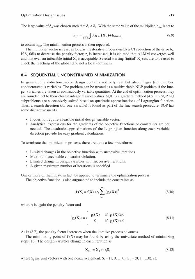
215Optimization Design Issues
The large value of δ0 was chosen such that δ1 < δ0. With the same value of the multiplier, h(i)k is set to
[ ]( )= +≤ ≤
−h min 0, r g X h(i)k1 i m
k i k (i)k 1 (8.9)
to obtain hi(1). The minimization process is then repeated.The multiplier vector is reset as long as the iterative process yields a 4/1 reduction of the error δk.
If δk fails to decrease the penalty factor, rk is increased. It is claimed that ALMM converges well and that even an infeasible initial X0 is acceptable. Several starting (initial) X0 sets are to be used to check the reaching of the global (and not a local) optimum.
8.4 SEQUENTIAL UNCONSTRAINED MINIMIZATION
In general, the induction motor design contains not only real but also integer (slot number, conductors/coil) variables. The problem can be treated as a multivariable NLP problem if the inte-ger variables are taken as continuously variable quantities. At the end of optimization process, they are rounded off to their closest integer feasible values. SQP is a gradient method [4,5]. In SQP, SQ subproblems are successively solved based on quadratic approximations of Lagrangian function. Thus, a search direction (for one variable) is found as part of the line search procedure. SQP has some distinctive merits.
• It does not require a feasible initial design variable vector.• Analytical expressions for the gradients of the objective functions or constraints are not
needed. The quadratic approximations of the Lagrangian function along each variable direction provide for easy gradient calculations.
To terminate the optimization process, there are quite a few procedures:
• Limited changes in the objective function with successive iterations.• Maximum acceptable constraint violation.• Limited change in design variables with successive iterations.• A given maximum number of iterations is specified.
One or more of them may, in fact, be applied to terminate the optimization process.The objective function is also augmented to include the constraints as
∑′ = + γ=
f (X) f(X) g (X)i2
i 1
m
(8.10)
where γ is again the penalty factor and
=≥<
g (X)
g (X) if g (X) 0
0 if g (X) 0i
i i
i (8.11)
As in (8.7), the penalty factor increases when the iterative process advances.The minimizing point of f’(X) may be found by using the univariate method of minimizing
steps [13]. The design variables change in each iteration as
= + α+X X Sj 1 j j j (8.12)
where Sj are unit vectors with one nonzero element. S1 = (1, 0, …,0); S2 = (0, 1, …,0), etc.

216 Induction Machines Handbook
The coefficient αj is chosen such that
( ) ( )′ <+f X f Xj 1 j (8.13)
To find the best , we may use a quadratic equation in each point.α
f (X ) H( ) a b c 2′ + α = α = + α + α (8.14)
H(α) is calculated for three values of α:
α = α = α =0, d, 2d, (d isarbitrary)1 2 3
= =
= = + +
= = + +
H(0) t a
H(d) t a bd cd
H(2d) t a 2bd 4cd
1
22
32
(8.15)
From (8.15), a, b, and c are calculated. But from
∂∂α
= α = −H0;
b2c
opt (8.16)
4t 3t t
4t 3t 2tdopt
2 1 3
2 3 1
α = − −− −
(8.17)
To be sure that the extreme is a minimum,
∂∂α
= > + >Hc 0; t t 2d
2
2 3 1 (8.18)
These simple calculations have to be done for each iteration and along each design variable direction.
8.5 MODIFIED HOOKE–JEEVES METHOD
A direct search method may be used in conjunction with the pattern search of Hooke–Jeeves [7]. Pattern search relies on evaluating the objective function for a sequence of points (within the fea-sible region). By comparisons, the optimum value is chosen. A point in a pattern search is accepted as a new point if the objective function has a better value than in the previous point.
Let us denote
X P(k−1) − revious base point
X C(k) − urrent base exploratory point
X P(k+1) − attern point (after the pattern move)
The process includes exploratory and pattern moves. In an exploratory move, for a given step size (which may vary during the search), the exploration starts from X(k − 1) along each coordinate (variable) direction.
Both positive and negative directions are explored. From these three points, the best X(k) is c hosen. When all n variables (coordinates) are explored, the exploratory move is completed. The resulting point is called the current base point X(k).

217Optimization Design Issues
A pattern move refers to a move along the direction from the previous to the current base point. A new pattern point is calculated:
( )= + −+ −X X a X X(k 1) (k) (k) (k 1) (8.19)
where a is an accelerating factor.A second pattern move is initiated.
( )= + −+ + +X X a X X(k 2) (k 1) (k 1) (k) (8.20)
The success of this second pattern move X(k + 2) is checked. If the result of this pattern move is better than that of point X(k + 1), then X(k + 2) is accepted as the new base point. If not, then X(k + 1) constitutes the new current base point.
A new exploratory-pattern cycle begins but with a smaller step search and the process stops when the step size becomes sufficiently small.
The search algorithm may be summarized as
Step 1: Define the starting point X(k − 1) in the feasible region and start with a large step size.Step 2: Perform exploratory moves in all coordinates to find the current base point X(k).Step 3: Perform a pattern move: X X(k+ −1) = +(k) (a X( )k) − X(k 1) with a < 1.Step 4: Set X(k − 1) = X(k).Step 5: Perform tests to check if an improvement took place. Is X(k + 1) a better point?
If “YES” set X(k) = X(k + 1) and go to step 3.If “NO” continue.
Step 6: Is the current step size the smallest?If “YES”, stop with X(k) as the optimal vector of variables.If “NO” reduce the step size and go to step 2.
To account for the constraints, the augmented objective function f’(X), (8.10)–(8.11), is used. This way, the optimization problem becomes an unconstraint one. In all nonevolutionary methods presented so far, it is necessary to do a few runs for different initial variable vectors to make pretty sure that a global optimum is obtained. It is necessary to have a feasible initial variable vector. This requires some experience from the designer. Comparisons between the above meth-ods reveal that the sequential unconstrained minimization method (Han and Powell) is a very powerful but time-consuming tool, whereas the modified Hooke–Jeeves method is much less time-consuming [14–16].
8.6 GENETIC ALGORITHMS
GAs are computational models which emulate biological evolutionary theories to solve optimi-zation problems. The design variables are grouped in finite length strings called chromosomes. GA maps the problem to a set of strings (chromosomes) called population. An initial population is adopted by way of a number of chromosomes. Each string (chromosome) may constitute a potential solution to the optimization problem.
The string (chromosome) can be constituted with an orderly alignment of binary or real coded variables of the system. The chromosome – the set of design variables – is composed of genes which may take a number of values called alleles. The choice of the coding type, binary or real, depends on the number and type of variables (real or integer) and the required precision. Each design vari-able (gene) is allowed a range of feasible values called search space. In GA, the objective function is called fitness value. Each string (chromosome) of population of generation i is characterized by a fitness value.

218 Induction Machines Handbook
The GA manipulates upon the population of strings in each generation to help the fittest survive and thus, in a limited number of generations, obtain the optimal solution (string or set of design vari-ables). This genetic manipulation involves copying the fittest string (elitism) and swapping genes in some other strings of variables (genes).
Simplicity of operation and the power of effect are the essential merits of GA. On top of that, they do not need any calculation of gradients (of fitness function) and provide more probably the global rather than a local optimum.
They do so because they start with a random population – a number of strings of variables – and not only with a single set of variables as nonevolutionary methods do.
However, their convergence tends to be slow, and their precision is moderate. Handling the constraints may be done as for nonevolutionary methods through an augmented fitness function.
Finally, multiobjective optimization may be handled mainly by defining a comprehensive fitness function incorporating as linear combinations, for example, the individual fitness functions.
Although the original GAs make use of binary coding of variables, real coded variables seem more practical for induction motor optimization as most variables are continuous. Also, in a hybrid optimization method, mixing GAs with a nonevolutionary method for better convergence, preci-sion, and less computation time requires real coded variables.
For simplicity, we will refer here to binary coding of variables. That is, we describe first a basic GA algorithm.
A simple GA uses three genetic operations:
• Reproduction (evolution and selection)• Crossover• Mutation.
8.6.1 reproDuction (evolution anD Selection)
Reproduction is a process in which individual strings (chromosomes) are copied into a new genera-tion according to their fitness (or scaled fitness) value. Again, the fitness function is the objective function (value).
Strings with higher fitness value have a higher probability of contributing one or more offsprings in the new generation. As expected, the reproduction rate of strings may be established in many ways.
A typical method emulates the biased roulette wheel where each string has a roulette slot size proportional to its fitness value.
Let us consider as an example 4 five-digit binary numbers whose fitness value is the decimal number value (Table 8.1).
The percentage given in Table 8.1 may be used to draw the corresponding biased roulette wheel (Figure 8.3).
TABLE 8.1Fitness Values
String Number String Fitness Value % of Total Fitness Value
1 01000 64 5.5
2 01101 469 14.4
3 10011 361 30.9
4 11000 576 49.2
Total 1170 100

219Optimization Design Issues
Each time a new offspring is required, a simple spin of the biased roulette produces the repro-duction candidate. Once a string has been selected for reproduction, an exact replica is made and introduced into the mating pool for the purpose of creating a new population (generation) of strings with better performance.
The biased roulette rule of reproduction might not be fair enough in reproducing strings with very high fitness value. This is why other methods of selection may be used. The selection by the arrangement method, for example, takes into consideration the diversity of individuals (strings) in a population (generation). First, the m individuals are arranged in the decreasing order of their fitness in m rows.
Then, the probability of selection ρi as offspring of one individual situated in row i is [1]
r 1 2 2 m 1
mi
i ( )( ) ( )ρ =
φ − − φ − − (8.21)
ϕ – pressure of selection ϕ = (1–2)m – population size (number of strings)ri – row of ith individual (there are m rows)ρi – probability of selection of ith row (individual).
Figure 8.4 shows the average number of offsprings versus the row of individuals. The pressure of selection ϕ is the average number of offspring of best individual. For the worst, it will be 2 − ϕ. As expected, an integer number of offspring is adopted.
By the pressure of selection ϕ value, the survival chance of best individuals may be increased as desired.
30.9%
14.4%
5.5%
49.2%
FIGURE 8.3 The biased roulette wheel.
1 2 3 m-1 m
2-φ
1
φ
ρ
FIGURE 8.4 Selection by arrangement.

220 Induction Machines Handbook
8.6.2 croSSover
After the reproduction process is done, crossover may proceed. A simple crossover contains two steps:
• Choosing randomly two individuals (strings) for mating• Mating by selection of a crossover point K along the chromosome length l. Two new strings
are created by swapping all characters in positions K + 1 to l (Figure 8.5).
Besides simple (random) crossover, at the other end of scale, completely continued crossover may be used. Let us consider two individuals of the tth generation A(t) and B(t), whose genes are real variables a1, …, an and b1, …, bn,
[ ]=A(t) a ,a ,...,a1 2 n (8.22)
[ ]=B(t) b ,b ,..., b1 2 n (8.23)
The two new offspring A(t + 1), B(t + 1) may be produced by linear combination of parents A(t) and B(t).
A(t 1) a 1 b ,..., a 1 b1 1 n n1 1 n n( ) ( )+ = ρ + − ρ ρ + − ρ (8.24)
B(t 1) b 1 a ,..., b 1 a1 1 n n n n1 1( ) ( )+ = ρ + − ρ ρ + − ρ (8.25)
where ρ1, …, ρn ∈ [0,1] are random values (uniform probability distribution).
8.6.3 Mutation
Mutation is required because reproduction and crossover tend to become overzealous and thus loose some potentially good “genetic material”.
In simple GAs, mutation is a low probability (occasional) random alteration of one or more genes in one or more offspring chromosomes. In binary coding GAs, a zero is changed to a 1. The mutation plays a secondary role, and its frequency is really low.
Table 8.2 gives a summary of simple GAs.In real coded Gas, the mutation changes the parameters of selected individuals by a random
change in predefined zones. If A(t) is an individual of tth generation, subject to mutation, each gene will undergo important changes in first generations. Gradually, the rate of change diminishes. For the tth generation, let us define two numbers (p) and (r) which are randomly used with equal probabilities:
crossover point
011
0
1
11
0
0
0
Two oldchromosomes
crossover
0
1
1
0
0
no1'1
1
0
0
1
no2'
Two newchromosomes
no1 no2
FIGURE 8.5 Simple crossover operation.

221Optimization Design Issues
= + −p 1 Positivealteration
= − −p 1 Negativealteration (8.26)
∈ −r [0,1] Uniform distribution
The factor r selected for uniform distribution determines the amplitude of change. The mutated (Kth) parameter (gene) is given by [17]
( )′ = + − −
= +−
a a a a 1 r ; for p 1k k kmax k
1tT
5
( )′ = − − −
= −−
a a a a 1 r ; for p 1k k k kmin
1tT
5(8.27)
where akmax and akmin are the maximum and minimum feasible values of ak parameter (gene).T is the generation index when mutation is cancelled. Figure 8.6 shows the mutation relative
amplitude for various generations (t/T varies) as a function of the random number r, based on (8.27).
TABLE 8.2GA Stages
Stage Chromosomes Fitness Value
Initial population: size 3, with 8 genes and its fitness values
P1: 11010110 F(P1) = 6%P2: 10010111 F(P2) = 60%P3: 01001001 F(P3) = 30%
Reproduction: based on fitness value a number of chromosomes survive. There will be two P2 and one P3
P2: 10010111 No need to recalculate fitness as P2: 10010111 P2 and P3 will mate←|→P3: 01001001
Crossover: some portion of P2 and P3 will be swapped
P2: 10010111 No need of it hereP2′: 10010001P3′: 01001111
Mutation: some binary genes of some chromosomes are inverted
P2: 10010111 A new generation of individuals P2′′: 10011001 has been formed; a new cycle P3′: 01001111 starts
1
0.5
0.5 1
t/T=0
t/T=0.25
t/T=0.5
random r
(1-r )(1-t/T)
5
FIGURE 8.6 Mutation amplitude for various generations (t/T).

222 Induction Machines Handbook
8.6.4 ga perForMance inDiceS
As expected, GAs are supposed to produce a global optimum with a limited number (%) of all fea-sible chromosomes (variable sets) searched. It is not easy to assess the minimum number of genera-tions (T) or the population size (m) required to secure a sound optimal selection. The problem is still open, but a few attempts to solve it have been made.
A schema, as defined by Holland, is a similarity template describing a subset of strings with similarities at certain string positions.
If to a binary alphabet 0,1 we add a new symbol * which may be indifferent, a ternary alphabet is created 1,0,*.
A subset of 4 members of a schema like *111* is shown in (8.28):
11111,11110,01111,01110 (8.28)
The length of the string n1 = 5, and thus, the number of possible schemata is 35. In general, if the ordinality of the alphabet is K (K = 2 in our case), there are (K + 1)n schemata.
The exact number of unique schemata in a given population is not countable because we do not know all the strings in this particular population. But a bound for this is feasible.
A particular binary string contains 2n1 schemata as each position may take its value; thus, a population of size m contains between 2n1 and m ⋅2n1 schemata. How many of them are usefully processed in a GA? To answer this question, let us introduce two concepts:
• The order o of a schema H (δ(H)): the number of fixed positions in the template. For 011**1**, the order o(H) is 4.
• The length of a schema H, (δ(H)): the distance between the first and the last specified string position. In 011**1**, δ(H) = 6 − 1 = 5.
The key issue now is to estimate the effect of reproduction, crossover, and mutation on the number of schemata processed in a simple GA.
It has been shown [9] that short, low-order, above-average fitness schemata receive exponen-tially increasing chances of survival in subsequent generations. This is the fundamental theorem of GAs.
Despite the disruption of long, high-order schemata by crossover and mutation, the GA implicitly process a large number of schemata (%n 3
1 ),whereas in fact explicitly they process a relatively small number of strings (m in each population). So, despite the processing of n1 structures, each genera-tion GAs process approximately n 3
1 schemata in parallel with no memory of bookkeeping. This property is called implicit parallelism of computation power in GAs.
To be efficient, GAs must find solutions by exploring only a few combinations in the variable search space. Those solutions must be found with a better probability of success than with random search algorithms. The traditional performance criterion of GA is the evolution of average fitness of the population through subsequent generations.
It is almost evident that such a criterion is not complete as it may concentrate the point around a local, rather than global optimum.
A more complete performance criterion could be the ratio between the number of success runs per total given number of runs (1000, for example, [18], Pag (A)):
=P (A)Number of success runs
1000ag (8.29)
For a pure random search algorithm, it may be proved that the theoretical probability to find p optima in a searching space of M possible combinations, after making A% calls of the objective functions, is [18]

223Optimization Design Issues
∑= −
= ⋅
−
=
P (A)pM
1pM
; AKM
1000rand
i 1
i 1
K
(8.30)
The initial population size M in GA is generally M > 50.We should note that when the searching space is discretized, the number of optima may be dif-
ferent from the case of continuous searching space.In general, the crossover probability Pc = 0.7 and the mutation probability Pm ≤ 0.005 in practical
GAs. For a good GA algorithm, searching less than A = 10% of the total searching space should produce a probability of success Pag(A) > Prand(A) with Pag(A) > 0.8 for A = 10% and Pag(A) > 0.98 for A = 20%.
Special selection mechanisms, different from the biased roulette wheel selection, are required. Stochastic remainder techniques [19] assign offsprings to strings based on the integer part of the expected number of offspring. Even such solutions are not capable to produce performance as stated above.
However if the elitist strategy is used to make sure that the best strings (chromosomes) survive intact in the next generation, together with selection by stochastic remainder technique and real coding, the probability of success may be drastically increased [18,20].
Surrogate FEM model-based optimal IM design codes are still due to appear. However, most of optimal design code of electric machines are proprietary, and even if not, they require extended space for a usable presentation. Consequently, we suggest you Ref. [21], Chapter 15, and its compan-ion computer codes (one by Hooke–Jeeves and the other by G.A.) for two IM optimal design source codes, presented with case studies.
Recently, the GAs and some deterministic optimization methods have been compared in IM design [22–24]. Mixed conclusions have resulted.
8.7 SUMMARY
• GAs offer some advantages over deterministic methods.• GAs reduce the risk of being trapped in local optima.• GAs do not need a good starting point as they start with a population of possible solutions.
However, a good initial population reduces the computation time.• GAs are more time-consuming although using real coding, elitist strategy, and stochastic
remainder selection techniques increases the probability of success to more than 90% with only 10% of searching space investigated.
• GAs do not need to calculate the gradient of the fitness function; the constraints may be introduced in an augmented fitness function as penalty functions as done with determinis-tic methods. Many deterministic methods do not require computation of gradients.
• GAs show in general lower precision and slower convergence than deterministic methods.• Other refinements such as scaling the fitness function might help in the selection process
of GAs and thus reduce the computation time for convergence.• It seems that hybrid approaches, which start with GAs (with real coding), to avoid trap-
ping in local optima, and continue with deterministic (even gradient) methods for fast and accurate convergence, might become the way of the future.
• If a good initial design is available, optimization methods produce only incremental improvements; however, for new designs (high-speed IMs, for example), they may prove indispensable.
• Once optimization design is performed based on nonlinear analytical IM models, with frequency effects approximately considered, the final solution (design) performance may be calculated more precisely by FEM as explained in previous chapters.
• For IM with involved rotor slot configurations – deep bars, closed slots, and double-cage – it is also possible to leave the stator unchanged after optimization and change only the

224 Induction Machines Handbook
main rotor slot dimensions (variables) and explore by FEM their effect on performance and constraints (starting torque and starting current) until a practical optimum is reached.
• Any optimization approach may be suited to match the FEM. In [14], a successful attempt with Fuzzy Logic optimizer and FEM assistance is presented for a double-cage IM. Only a few tens of 2DFEM runs are used, and thus, the computation time remains practical.
• Notable advances in matching FEM with optimization IM design methods are still expected as the processing power of PCs is increasing continuously. The FEM-based optimal design codes developed recently for permanent magnet synchronous motors (PMSMs) [25] may be a way to go for IMs too.
• A cost pattern value method for local search algorithm has been applied recently to optimal FEA-based design of IMs for high torque density [22,26,27] with a case study at 260 kW.
REFERENCES
1. U. Sinha, A Design and Optimisation Assistant for Induction Motors and Generators, PhD Thesis, MIT, June 1998.
2. M. Box, A new method of constrained optimisation and a comparison with other methods, Computer Journal, Vol. 8, 1965, pp. 42–52.
3. J. Helder, R. Mead, A simplex method for function minimisation, Computer Journal, Vol. 7, 1964, pp. 308–313.
4. S. P. Han, A globally convergent method for nonlinear programming, Journal of Optimisation Theory and Applications, Vo. l22, 1977, pp. 297–309.
5. M. J. D. Powell, A fast algorithm for nonlinearly constrained optimisation calculation, In: Numerical Analysis, Lecture Notes in Mathematics, Editor: D. A. Watson, Springer Verlag, Berlin, Germany, Vol. 630, 1978, pp. 144–157.
6. R. Rockefeller, Augmented lagrange multiplier functions and duality in convex programming, SIAM Journal on Control and Optimization, Vol. 12, 1994, pp. 268–285.
7. R. Hooke, T. A. Jeeves, Direct search solution of numerical and statistical problem, Journal of ACM, Vol. 8, 1961, pp. 212.
8. R. Ramarathnam, B. G. Desa, V. S. Rao, A comparative study of minimisation techniques for optimisation of IM design, IEEE Transactions on Power Apparatus and Systems, Vol. 92, 1973, pp. 1448–1454.
9. D. E. Goldberg, Genetic Algorithms in Search Optimisation and Machine Learning, Addison Wesley Longman Inc., Boston, MA, 1989.
10. U. Sinha, A Design Assistant for Induction Motors, S. M. Thesis, Department of Mechanical Engineering, MIT, August 1993.
11. N. Bianchi, S. Bolognani, M. Zigliotto, Optimised design of a double cage induction motor by fuzzy artificial experience and finite element analysis, Record of ICEM – 1998, Istanbul, Turkey, Vol. 1/3, 1998.
12. Q. Changtoo, W. Yaguang, Optimisation design of electrical machines by random search approach, Record of ICEM – 1994, Paris, session D16, 1994, pp. 225–229.
13. A. V. Fiacco, G. P. McCormick, Nonlinear Programming Sequential Unconstrained Minimisation Techniques, John Wiley, Hoboken, NJ, 1969.
14. J. Appelbaum, E. F. Fuchs, J. C. White, I. A. Kahn, Optimisation of three phase induction motor design, Part I + II, IEEE Transactions on Energy Conversion, Vol. 2, No. 3, 1987, pp. 407–422.
15. Ch. Li, A. Rahman, Three–phase induction motor design optimisation using the modified Hooke–Jeeves method, EMPS, Vol. 18, No. 1, 1990, pp. 1–12.
16. C. Singh, D. Sarkas, Practical considerations in the optimisation of induction motor design, Proceedings of IEE-B, Vol. 149, No. 4, 1992, pp. 365–373.
17. C. Z. Janikov, Z. Michaleewiez, An experimental comparison of binary and floating point representa-tion in genetic algorithms, Proceedings of Fourth International Conference on Genetic Algorithms, San Diego, CA, 1991, pp. 31–36.
18. F. Wurtz, M. Richomme, J. Bigeon, J. C. Sabonnadiere, A few results for using genetic algorithms in the design of electrical machines, IEEE Transactions on Magnetics, Vol. 33, No. 2, 1997, pp. 1892–1895.
19. J. E. Baker, Adaptive selection methods of genetic algorithms, Proceedings of the first International Conference on Genetic Algorithms, 1998, pp. 101–111.

225Optimization Design Issues
20. M. Srinivas, L. M. Patniak, Genetic algorithms: a survey, Computer, IEEE Review, Vol. 27, 1994, pp. 17–26.
21. I. Boldea, L. N. Tutelea, Electric Machines: Steady State Transients and Design with MATLAB, CRC Press, Boca Raton, FL, Taylor and Francis Group, New York, 2010.
22. S. Hamarat, K. Leblebicioglu, H. B. Ertan, Comparison of deterministic and nondeterministic optimisation algorithms for design optimisation of electrical machines, Record of ICEM – 1998, Istanbul, Turkey, 1998, pp. 1477–1481.
23. Ö. Göl, J. P. Wieczorek, A comparison of deterministic and stochastic optimisation methods in induction motor design, Record of ICEM-1998, Istanbul, 1998, pp. 1472–1476.
24. S. H. Shahalami, S. Saadate, Genetic algorithm approach in the identification of squirrel cage induction motor’s parameters, Record of ICEM – 1998, Istanbul, Turkey, 1998, pp. 908–913.
25. A. Fatemi, D. M. Ionel, O. Demerdash, T. W. Nehl, Fast multi-objective CMODE: Type optimization of PM machines using multicore desktop computers, IEEE Transactions on Industry Applications, Vol. 52, No. 4, 2016, pp. 2941–2950.
26. D. Lee, H.-Ch. Jung, Cost pattern value method for local search algorithms applied to optimal FEA: Based design of induction motors, IEEE Transactions on Magnetics, Vol. 54, No. 4, 2018, pp. 8202408.
27. A. K. Mishra, B. S. Rajpurohit, R. Kumar, Induction machine drive design for enhanced torque profile, IEEE Transactions on Industry Applications, Vol. 54, No. 2, 2018, pp. 1283–1291.

227
9 Single-Phase IM Design
9.1 INTRODUCTION
Designing involves “dimensioning”, that is the finding of a suitable geometry and manufacturing data and performance indexes for given specifications. Designing, then, involves first dimensioning (or syn-thesis), sizing, and then assessing the performance (analysis). Finally, if the specifications are not met, the process is repeated according to an adopted strategy until satisfactory performance is obtained.
On top of this, optimization is performed according to one (or more) objective functions, as detailed in Chapter 8, in relation to three-phase induction machines (IMs). Typical specifications (with a case study) are
• Rated power Pn = 186.5 W (1/4 HP)• Rated voltage V 115 Vsn =• Rated frequency f1n = 60 Hz; 4 poles• Rated power factor cos φn = 0.98 lagging; service: continuous or short duty• Breakdown p.u. torque 1.3–2.5• Starting p.u. torque 0.5–3.5• Starting p.u. current 5–6.5• Capacitor p.u. maximum voltage: 0.6–1.6.
The breakdown torque p.u. may go as high as 4.0 for the dual capacitor configuration and special-service motors.
Also, starting torques above 1.5 p.u. are obtained only with a starting capacitor.The split-phase IM is also capable of high starting and breakdown torques in p.u. as during start-
ing, both windings are active, at the expense of rather high resistance, both in the rotor and in the auxiliary stator windings.
For two (three)-speed operation, the 2 (3) speed levels in % of ideal synchronous speed have to be specified. They are to be obtained with tapped windings. In such a case, it has to be verified that for each speed, there is some torque reserve up to the breaking torque of that tapping.
Also, for multispeed motors, the locked rotor torque on low-speed mode has to be less than the load torque at the desired low speed. For a fan load, at 50% as the low speed, the torque is 25% and thus the locked rotor torque has to be <25%.
We start with the sizing of the magnetic circuit, move on to the selection of stator windings, and continue with rotor slotting and cage sizing. The starting and (or) permanent capacitors are defined. Further on, the parameter expressions are given, and steady-state performance is calculated. When optimization design is performed, objective (penalty) functions are calculated and constraints are verified. If their demands are not met, the whole process is repeated, according to a deterministic or stochastic optimization mathematical method, until sufficient convergence is reached.
9.2 SIZING THE STATOR MAGNETIC CIRCUIT
As already discussed in Chapter 4, when dealing with design principles of three-phase IMs, there are basically two design initiation constants, based on past experience:
• The machine utilization factor Cu:D2oL
• The rotor tangential stress ft in N/cm2 or N/m2.

228 Induction Machines Handbook
Do is here the outer stator diameter and L the stator stack length.As design optimization methods advance and better materials are produced, Cu and ft tend to
increase slowly. Also, low service duty allows for larger Cu and ft.However, in general, better efficiency requires larger Cu and lower ft.Figure 9.1 [1] presents standard data on Cu in cubic inches (1 inch = 25.4 mm):
C D Lu o2= (9.1)
for the three-phase small-power IMs.Concerning the rated tangential stress, there is not yet a history of its use, but it is known that
it increases with the stator interior (bore) diameter Di, with values of around ft = 0.20 N/cm2 for Di = 30 mm to ft = 1 N/cm2 for Di = 70 mm or so, and more.
In general, any motor company could calculate ft (Di) for the two, four, six, eight single-phase IMs fabricated so far and then produce its own ft database.
The rather small range of ft variation may be exploited best, in our era of computers, for optimi-zation design.
The ratio between stator interior (bore) diameter Di and the external diameter Do depends on the number of poles, on Do, and on magnetic (flux densities) and electric (current density) loadings.
Figure 9.2 presents standard data [1] from three sources: T. C. Lloyd, P. M. Trickey, and Ref. [2]. In Ref. [2], the ratio Di/Do is obtained for maximum airgap flux density in the airgap per given stator magnetization mmf in three-phase IMs (Di/Do = 0.58 for 2p1 = 2, 0.65 for 2p1 = 4, 0.69 for 2p1 = 6, 0.72 for 2p1 = 8).
The Di/Do values of Ref. [2] are slightly larger than those of P. M. Trickey, as they are obtained from a contemporary optimization design method for three-phase IMs.
In our case study, from Figure 9.1, for 186.5 W (1/4 HP), 2p1 = 4 poles, we choose
C D L 3.5615 10 mu o2 3 3= = ⋅ − (9.2)
with L/Do = 0.380, Do = 0.137 m, L = 0.053 m.The outer stator punching diameter Do might not be free to choose, as the frames for single-phase
IMs come into standardized sizes [3].
FIGURE 9.1 Machine utilization factor C D2u o= L (cubic inches) for fractional/horsepower three-phase IMs.

229Single-Phase IM Design
For four poles, we choose from Figure 9.2 a kind of average value of the three sets of data: D /D = 0.60. Consequently, the stator bore diameter D = 0.6 · 0.137 = 82.8 · 10−3 m.i o i
The airgap g = 0.3 mm and thus the rotor external diameter Dor = Di − 2g = (82.8 – 2 · 0.3)10−3 = 82.2 · 10−3 m.
The number of slots of stator Ns is chosen as for three-phase IMs (the rules for most adequate combinations Ns and Nr established for three-phase IMs hold in general also for single-phase IMs see Chapter 10, Vol. 1). Let us consider Ns r
The theoretical peak airgap flux density Bg = 0.6–0.75 T. Let us consider Bg = 0.705 T. Due to saturation, it will be somewhat lower (flattened). Consequently, the flux per pole in the main wind-ing Φm is
= 36 and N = 30.
2
K B Lm dis gΦ ≈π
⋅ ⋅ ⋅ τ ⋅ (9.3)
The pole pitch
D2p 4
82.2 10 64.57 10 mi
1
3 3τ = π ⋅ = π ⋅ ⋅ ≈ ⋅− − (9.4a)
With Kdis = 0.9
FIGURE 9.2 Interior/outer diameter ratio Di/Do versus Do.

230 Induction Machines Handbook
2
0.9 0.705 64.57 10 0.053 1.382 10 Wbm3 3Φ =
π⋅ ⋅ ⋅ ⋅ ≈ ⋅− −
Once we choose the design stator back iron flux density Bcs = 1.3–1.7 T, the back iron height hcs can be calculated as
h2 B L
1.382 102 1.5 0.053
8.69 10 9 10 mcsm
cs
33 3= Φ
⋅ ⋅= ⋅
⋅ ⋅= ⋅ ≈ ⋅
−− − (9.4b)
The stator slot geometry is shown in Figure 9.3.The number of slots per pole is Ns/2p1 = 36/(2 · 2) = 9. So the tooth width bts is
b2p
N B Lts
m 1
s ts
= Φ ⋅⋅ ⋅
(9.5)
With the tooth flux density Bts ≅ (0.8–1.0) Bcs
b1.382 10 436 1.3 0.053
2.55 10 mts
33= ⋅ ⋅
⋅ ⋅≈ ⋅
−− (9.6)
This value is close to the lowest limit in terms of punching capabilities.Let us consider hos = 1 · 10−3 m, wos = 6g = 6 · 0.3 · 10−3 = 1.8 · 10−3 m.Now the lower and upper slot width w1s and w2s are
W
D 2 h h
Nb
82.8 2(1 1)
362.55 10
5.00 10 m
1si os ws
sts
3
3
( ) ( )( )=
π + +− = π + + −
≈ ⋅
−
− (9.7)
WD 2h
Nb
137 2 936
2.5 10 8.00 10 m2so cs
sts
3 3( )= π − − = π( − × ) −
≈ ⋅− − (9.8)
The useful slot height
h =18ts
W =1.8os
ss
h =9cs
W =82s
bts
1s
h =1os
D =1370
D = 82.8i
h =16
=2.5
W =5
wsh =1
FIGURE 9.3 Stator slot geometry in millimetre.

231Single-Phase IM Design
h
D2
h h hD2
1372
9 282.8
210
16.0 10 m
tso
cs ws osi 3
3
= − − − − = − − −
≈ ⋅
−
− (9.9a)
So the “active” stator slot area As is
AW W
2h
(5.00 8.00)2
16 10 104 10 ms1s 2s
ss6 6 2( )= + = + ⋅ = ⋅− − (9.9b)
For slots which host both windings or in split-phase IMs, some slots may be larger than others.
9.3 SIZING THE ROTOR MAGNETIC CIRCUIT
The rotor slots for single-phase IMs are either round or trapezoidal or in between (Figure 9.4).With 30 rotor slots, the rotor slot pitch τsr is
D
N82.2 10 4
308.6 10 msr
r
r
33τ = π ⋅ = π ⋅ ⋅ ⋅ = ⋅
−− (9.10)
With a rotor tooth width btr = 2.6 · 10−3 m, the tooth flux density Btr is
B2p
N b L1.388 10 4
30 2.6 10 0.0531.343 Ttr
1
r tr
3
3= Φ⋅⋅ ⋅
= ⋅ ⋅⋅ ⋅ ⋅
=−
− (9.11)
The rotor slots useful area is in many cases (35%–60%) of that of the stator slot
A 0.38A N
N0.38 104 10
3630
47.42 10 mrs s
r
6 6 2= ⋅ = ⋅ ⋅ ⋅ = ⋅− − (9.12)
The trapezoidal rotor slot (Figure 9.4), with
h W 1 10 m
has W b (8.6 2.6)10 6 10 m
or or3
1r sr tr3 3
= = ⋅
≈ τ − = − = ⋅
−
− − (9.13)
Adopting a slot height h2 = 10 · 10−3 m, we can calculate the rotor slot bottom width W2r:
W2Ah
W2 47.40 10
10 106 10 3.48 10 m2r
r
21s
3
33 3= − = ⋅ ⋅
⋅− ⋅ = ⋅
−
−− − (9.14)
r
r
1
2
h2
hor
W ~1or
W =3.52r
orW ~1or
h =1or
hor
r
h =102
W =6
W ~1
1r
FIGURE 9.4 Typical rotor slot geometries.

232 Induction Machines Handbook
A “geometrical” verification is now required.
WD h h h 2
Nb
82.2 2(1 1 10) 10
302.6 10 3.49 10 m
2rr or or1 2
rtr
33 3[ ]
( )=
π − + + ⋅ −
= π − + + − ⋅ = ⋅−
− − (9.15)
As (9.14) and (9.15) produce about the same value of slot bottom width, the slot height h2 has been chosen correctly. Otherwise, h2 should have been changed until the two values of W2r converged.
To avoid such an iterative computation, (9.14) and (9.15) could be combined into a second-order equation with h2 as the unknown after the elimination of W2r.
A round slot with a diameter dr = W2r = 6 · 10−3 m would have produced an area:
A4
6 10 28.26 10 m .r3 2 6 2( )= π ⋅ = ⋅− −
This would have been a very small value unless copper bars are used instead of aluminium bars. The end-ring area Aring is
A A1
2sinp
N
47.42 101
2sin2
30
114 10 mring r1
r
6 6 2≈ π ⋅ = ⋅ π ⋅ = ⋅− − (9.16)
AWith a radial height br = 15 · 10−3 m, the ring axial length is a ring
r = = 7.6 ⋅10−3 m.br
9.4 SIZING THE STATOR WINDINGS
By now, the number of slots in the stator is known: Ns = 36. As we do have a permanent capacitor motor, the auxiliary winding is always operational. It thus seems naturally to allocate both windings about the same number of slots in fact 20/16. In general, single-layer windings with concentrated coils are used. (Figure 9.5)
With 5(4) coils (slots) per pole and phase, the winding factors for the two phases (Chapter 4, Vol. 1) are
Ksin q
2
q sin2
sin 536
5sin36
0.9698wm
ms
ms
=
α
α =⋅ π
π =
Ksin q
2
q sin2
sin 436
4sin36
0.9810wa
as
as
=
α
α =⋅ π
π = (9.17)
m m m m m m m m m m m m m m m m m m m ma a a a a a a a a a a a a a a a
1 2 3 4 5 6 7 8 9 10 11 12 13 14 15 16 17 18 19 20 21 22 23 24 25 26 27 28 29 30 31 32 33 34 35 36
FIGURE 9.5 Stator winding: m – main phase, a – auxiliary phase, four poles.

233Single-Phase IM Design
In case the number of turns/phase in various slots is not the same, the winding factor is calculated in (9.20).
As detailed in Chapter 4, Vol. 1, two types of sinusoidal windings can be built (Figure 9.6).When the total number of slots per pole per phase is an odd number, concentrated coils with slot
axis symmetry seem adequate. In contrast, for even number of slots/pole/phase, concentrated coils with tooth axis symmetry are recommended.
Should we have used such windings for our case with qm = 5 and qa = 4, slot axis symmetry would have applied to the main winding and tooth axis symmetry to the auxiliary winding. A typical coil group is shown in Figure 9.7.
From Figure 9.7, the angle between the axis a-a (Figures 9.6 and 9.7) and the kth slot, kν (for the νth harmonic), is
β
N
(k 1)2N
ks s
β = γ π ν + − πνν (9.18)
The effective number of conductors per half a pole Z′ν is [4]
Z Z cosk k
k 1
n
∑′ = βν ν
= (9.19)
N 4p Z1= ⋅ ′ν ν
Nν is the effective number of conductors per phase.The winding factor Kwν is simply
Z1
Z2
Z3
Z1
Z2
Z3
Z1
Z2
Z3
Z1
Z2
Z3
slot axis tooth axis
a a
a a
r = 1 r = 1
(a) (b)
FIGURE 9.6 Sinusoidal windings: (a) with slot axis symmetry and (b) with tooth axis symmetry.
a a
β1
β2
β3
a
D
pole
De i
lec
L
Z
Z
Z
Z
Z
Z
1
2
3
1
2
3lengthLec
FIGURE 9.7 Typical “overlapping” winding.

234 Induction Machines Handbook
KZ
Z
Z cos
Z
w
k
k 1
n
k k
k 1
n
k
k 1
n
∑∑
∑= ′ =
β
νν
=
ν
=
=
(9.20)
The length of the conductors per half a pole group of coil, lcn, is [3]
l Z L ( 2)L D2p
cn k ec e1
k1
k 1
n
∑≈ + π − + π − β
=
(9.21)
So the resistance per phase Rphase is
R4p lA
phase Co1 cn
con
= ρ (9.22)
Acon is the conductor (magnet wire) cross-sectional area. Acon depends on the total number of con-ductors per phase, slot area, and design current density.
The problem is that although the supply current at rated load may be calculated as
IP
V cos186.5
0.7 115 0.982.36 A,s
n
n s
=η ϕ
=⋅ ⋅
= (9.23)
with an assigned value for the rated efficiency, ηn, still the rated current for the main and auxiliary currents Im and Ia is not known at this stage.
Im and Ia should be almost 90° phase-shifted for rated load and
I I Is m a= + (9.24)
= =I NNow as the ratio a m a , for symmetry, we may assume that
Ia Nm
II
11a
ms
2≈
+
(9.25)
With the turn ratio in the interval a = 1.0–2, in general I Im s= ⋅(0.700 − 0.90).The number of turns of the main winding Nm is to be determined by observing that the emf in
the main winding Em s= −(0.96 0.98) V⋅ and thus with (9.3)
E 2 N k fm m m wm 1n= π Φ (9.26)
Finally
N =0.97 115
2 1.382 10 0.9698 60313 turnsm 3
⋅π ⋅ ⋅ ⋅ ⋅
=−
In our case, the main winding has 10 (p1qm = 2 · 5 = 10) identical coils. So the number of turns per slot nsm is

235Single-Phase IM Design
nN
q p3135 2
31turns/coilsmm
m 1
= =⋅
= (9.27)
Assuming the turn ratio is a = 1.5, the number of turns per coil in the auxiliary winding is
nN a kq p k
310 1.5 0.96984 2 0.9810
57 turns/coilsam wm
a 1 wa
= ⋅ ⋅⋅ ⋅
= ⋅ ⋅⋅ ⋅
≈ (9.28)
As the slots are identical and their useful area is (from 9.9b) As = 104 · 10−6 m2, the diameters of the magnetic wire used in two windings are
=π
⋅ = ⋅ ⋅ ≈ ⋅− −d4 A K
n10
43.14
104 0.431
1.3 10 mms fill
sm
3 3
(9.29)
=π
⋅ = ⋅ ⋅ ≈ ⋅− −d4 A K
n10
43.14
104 0.457
1.0 10 mas fill
sa
3 3
The filling factor was considered rather large: Kfill = 0.4.The predicted current density in the two windings would be
=π
=
+
⋅π ⋅ ⋅
= ⋅−
jI
d 42.36
11
1.51.3
410
1.4847 10 A/mComm
m2 2 2
6
6 2
=⋅π ⋅
=⋅π ⋅ ⋅
= ⋅−jI
a d 41.9696
1.5 1 104
1.6726 10 A/mCoam
a2 2 6
6 2
(9.30)
The forecasted current densities, for rated power, are rather small so good efficiency (for the low power considered here) is expected.
An initial value for the permanent capacitor has to be chosen.I 1.96
Let us assume complete symmetry for rated load, with I mnan = = = 1.3 A.
a 1.5Further on
V V a 115 1.5 172Van mn= ⋅ = ⋅ = (9.31)
The capacitor voltage Vc is
V V V 115 1 1.5 207.3Vc s2
an2 2= + = + = (9.32)
Finally, the permanent capacitor C is
CIV
1.32 60 207.3
16 Fa
1 C
=ω
=⋅π ⋅ ⋅
≈ µ (9.33)
We may choose a higher value of C than 16 μF (say 25 μF) to increase somewhat the breakdown and the starting torque.

236 Induction Machines Handbook
9.5 RESISTANCES AND LEAKAGE REACTANCES
The main and auxiliary winding resistances, Rsm and Rsa, respectively, (9.22) are
R 4 2ld 4
sm Cocnm
m2= ρ ⋅ ⋅
π (9.34)
R 4 2ld 4
sa Cocna
a2= ρ ⋅ ⋅
π
The length of the coils/half a pole for main and auxiliary windings lcnm (9.21) is
l n 212
L 3( 2)L D32p
236
436
31 212
0.053 3( 2) 0.025 0.1434
236
436
9.805m
cnm cm ec e1
≈ +
+ π − + π − π − π
= ⋅ +
⋅ + π − ⋅ + π − π − π
= (9.35)
l n 2L 3( 2)L D22p
236
436
57 2 0.053 3( 2) 0.025 0.1424 18 9
11.38 m
cna ca ec e1
≈ + π − + π − π − π
= ⋅ ⋅ + π − ⋅ + π − π − π
= (9.36)
Finally,
R2.1 10 4 2 9.805
41.3 10
1.2417sm
8
2 6= ⋅ ⋅ ⋅ ⋅
π ⋅ ⋅= Ω
−
−
R2.1 10 4 2 11.38
41 10
2.435sa
8
2 6= ⋅ ⋅ ⋅ ⋅
π ⋅ ⋅= Ω
−
−
The main winding leakage reactance Xsm is
X X X X Xsm ss se sd skew= + + + (9.37)
whereXss – the stator slot leakage reactanceXse – the stator end-connection leakage reactanceXsd – the stator differential leakageXskew – skewing reactance.
X X 2W L
p qse ss 0 1
12
ss se( )+ = µ ω ⋅⋅
λ + λ (9.38)
with (Chapter 6, Vol. 1, and Figure 9.3)
2h
3 W W2h
W WhW
2 163(5 8)
2 15 8
11.8
1.53ssss
1s 2s
ws
1s 2s
os
os( )λ =+
++
+ = ⋅+
+ ⋅+
+ = (9.39)

237Single-Phase IM Design
Also (Chapter 6, Vol. 1, Equation (6.28))
0.67
q2
Ll 0.64se
m
ec( )λ =⋅
− ⋅τ (9.40)
It is qm/2, as the q coils/pole are divided into two sections whose end connections go into opposite directions (Figure 9.5).
The end-connection average length lec is
ll 2
q nLec
m cn
m cm
= ⋅ − (9.41)
With lcn from (9.21)
l9.805 2
5 310.053 0.0735mec
m = ⋅⋅
− =
0.67
52
0.053(0.0735 0.64 0.065) 1.008seλ =
⋅− ⋅ =
The differential leakage reactance Xsd (Chapter 6, Vol. 1, Equations (6.2) and (6.9) and (Figures 6.2–6.5)) is
XX
2.6 10 0.92 2.392 10sd
mmds d
2 2= σ ⋅ ∆ = ⋅ ⋅ = ⋅− − (9.42)
for qm = 5, Ns = 36, Nr = 30, one slot pitch skewing of rotor.Xmm is the nonsaturated magnetization reactance of the main winding (Chapter 5, Vol. 1,
Equation (5.115))
X4
W KL
p g K
2 604 4 10
(10 31 0.9698)0.053 0.065
2 0.3 10 1.372.085
mm 10
2 m wm12
1 C
7
22
3
( )= ω µπ
⋅ ⋅ τ⋅ ⋅
= π ⋅ ⋅ π ⋅π
⋅ ⋅ ⋅⋅ ⋅ ⋅
= Ω−
−
where KC is the Carter coefficient and g the airgap.
XX
1 K 1sin
2 1sin
18
18
9.108 10skew
mmskew2
2 skew
skew2
2
23( ) ( )
= − = −
α
α= −
π
π
= ⋅ − (9.43)
Finally, the main winding leakage reactance Xsm is
X 2 4 10
2 60 310 0.053 (1.53 1.008)2 5
72.085 (23.92 9.108) 10 4.253
sm7
2
3
= ⋅ π ⋅ π ⋅ ⋅ ⋅ ⋅ +⋅
+ ⋅ + ⋅ = Ω
−
−
The auxiliary winding is placed in identical slots, and thus, the computation process is similar. A simplified expression for Xsa in this case is

238 Induction Machines Handbook
X XWW
4.25357 831 10
9.204sa sma
m
2 2
≈
= ⋅ ⋅⋅
= Ω (9.44)
The rotor leakage reactance, after its reduction to the main winding (Chapter 6, Vol. 1 Equations (6.86)–(6.87)), is
X X X L Lrm rmd bem 1 rmd bem( )= + ′ = ω + ′ (9.45)
The rotor-skewing component has been “attached” to the stator and the zig-zag component is lumped into differential one Xrmd.
From Equation (6.16) (Chapter 6, Vol. 1),
X X 2.8 10 Xrmd dr0 mm2
mm= σ = × − (9.46)
With Nr/p1 = 30/2 = 15 and one slot pitch skewing (from Figure 6.4 in Vol. 1)
2.8 10dr02σ = ⋅ −
The equivalent bar–end-ring leakage inductance L′ben is (Equation 6.86 in Vol. 1):
L L12 K W
Nbem bem
wm2
m2
r
′ = ⋅ (9.47)
From (6.91)–(6.92), Vol. 1,
L l 2 2DN
ben 0 b b 0 eiir
r
= µ λ + µ λ ⋅ π ⋅ (9.48)
The rotor bar (slot) and end-ring permeance coefficients, λb and λei, respectively, (from (6.18) and (6.46) in Vol. 1 and Figure 9.5), are
hW
2hW W
2h3 W W
11
1 21 6
2 103(6 3.5)
1.987bor
or
or1
o1 o2
2
1r 2r( ) ( )λ = ++
++
= + ⋅+
+ ⋅+
= (9.49)
2.3 D
4 N L sinp
N
log4.7 D
a 2 bei
ir
r2 1
r
ir
r r
λ = ⋅
⋅ ⋅ ⋅ π
⋅+ ⋅
(9.50)
with D D≈ − b (= −82.8 15) 1⋅ =0− −3 367.8 ⋅ =10 m a 7.6 ⋅ =10− −3ir r r m and b 1r 5 1⋅ 0 m3 from (9.16)
2.3 67.8 10
4 30 0.053 sin15
log4.7 67.8
2 15 7.60.579ei
3
2λ = ⋅ ⋅
⋅ ⋅ ⋅ π
⋅⋅ +
=
−
so from (9.48)
L 1.256 10 0.053 1.987 0.5792 67.8 10
300.1425 10 Hben
63
6= ⋅ ⋅ + π ⋅ ⋅
= ⋅−−
−

239Single-Phase IM Design
Now from (9.45),
X 2.8 10 X L12K W
N
2.8 10 72.085 2 60 0.1425 1012 0.9698 310
30
3.961
rm2
mm 1 benwm2
m2
r
2 62 2
= ⋅ + ω
= ⋅ ⋅ + π ⋅ ⋅ ⋅ ⋅ ⋅
= Ω
−
− −
(9.51)
The rotor cage resistance is
R R12K W
Nrm be
wm2
m2
r
= (9.52)
With Rbe (Equation (6.63) in Vol. 1),
R RR
2 sinp
N
be bring
2 1
r
= +⋅ π ⋅
(9.53)
RlA
3 100.065
47.42 104.112 10
Rl
A3 10
2 67.8 101.14 10 30
3.735 10
b Cob
r
86
5
ring bring
ring
83
46
= ρ = ⋅⋅
= ⋅ Ω
= ρ = ⋅ π ⋅ ⋅⋅ ⋅
= ⋅ Ω
−−
−
−−
−−
(9.54)
Finally,
R 4.112 103.735 10
2 sin2
30
120.9698 310
303.048rm
56
2
2 2
= ⋅ + ⋅
⋅ π ⋅
⋅ ⋅ ⋅ = Ω−−
Note that the rotor resistance and leakage reactance calculated above are not affected by the skin effects.
9.6 THE MAGNETIZATION REACTANCE Xmm
The magnetization reactance Xmm is affected by magnetic saturation which is dependent on the resultant magnetization current Im.
Due to the symmetry of the magnetization circuit, it is sufficient to calculate the functional Xm (Im) for the case with current in the main winding (Ia = 0, bare rotor slots).
The computation of Xm(Im) may be performed analytically (see Chapter 6 or Ref. [4]) or by finite element modelling (FEM). For the present case, to avoid lengthy calculations, let us consider Xmm constant for a moderate saturation level (1 + Ks) = 1.5
X X1
1 K72.085
1.548.065mm mm unsat
s
( )=+
= = Ω (9.55)

240 Induction Machines Handbook
9.7 THE STARTING TORQUE AND CURRENT
The theory behind the computation of starting torque and current is presented in Chapter 14, Vol. 1, Section 14.5:
I I 1ta
C Z a sin
costa
s S 1 sces sc
2sc
sc
2
es2
2
( )( ) = +ω ⋅ − ϕ
ϕ
+= (9.56)
tT
2pI R
K sin
a 1 K 2K coses
es
1
1sc2
r S 1
a sc
a2
a sc( )( )=
ω
= ⋅ ϕ+ + ϕ
+ =
K1
C a Z; I
V2 Z
a 2sc
scs
sc
=ω ⋅ ⋅ ⋅
=⋅
Z R R X X
(1.2417 3.048) (4.235 3.96) 9.26
sc sm rm2
sm rm2
2 2
( ) ( )= + + +
= + + + = Ω (9.57)
cos 0.463scϕ =
sin 0.887scϕ =
K1
2 60 25 10 1.5 9.265.095a 6 2=
π ⋅ ⋅ ⋅ ⋅ ⋅=−
I115
2 9.266.2095 A; R R 3.048sc r S 1 rm( )=
⋅= = = Ω+ =
T2 2
2 606.2095 3.048 2.495Nmsc
2= ⋅π ⋅
⋅ ⋅ =
The relative value of starting torque tes is
t5.095 0.887
1.5 1 5.095 2 5.095 0.4630.095es 2( )= ⋅
+ + ⋅ ⋅=
T t T 0.095 2.495 0.237 Nmes es sc= = ⋅ =
The rated torque Ten, for an alleged rated slip Sn = 0.06, would be
TP p1 S
186.5 22 60 1 0.06
1.053 Nmenn 1
1 n( ) ( )≈ω ⋅ −
= ⋅π ⋅ ⋅ −
= (9.58)
So the starting torque is rather small as the permanent capacitance Ca = 25 · 10−6 F is too small.

241Single-Phase IM Design
The starting current (9.56) is
I 6.2095 10.0951.5
15.095
0.887
0.4630.0951.5
5.636 As S 1
2
2
( ) = +−
+
≈=
The starting current is not large (the presumed rated source current Isn = 2.36 A, (Equation 9.23)), but the starting torque is small.
The result is typical for the permanent (single) capacitor IM.
9.8 STEADY-STATE PERFORMANCE AROUND RATED POWER
Although the core losses and the stray load losses have not been calculated, the computation of torque and stator currents for various slips for S = 0.04–0.20 may be performed as developed in Chapter 14, Vol. 1, Section 14.3.
To shorten the presentation, we will illustrate this point by calculating the currents and torque for S = 0.06.
First, the impedances Z ,m mZ and Zm+ − a ((14.11)–(14.14) in Chapter 14, Vol. 1) are calculated
Z R j X jX jX
RS
RS
j X X
1.2417 j 4.253j 48.056 j 3.96
3.0480.06
3.0480.06
j 48.056 3.9623.43 j 29.583
sm sm
mm rmrm
rmmm rm( )
( )
= + ⋅ ++
+ +
= + ⋅ +⋅ ⋅ +
+ ⋅ += + ⋅
+
(9.59)
Z R j X jX j X
R(2 S)
R(2 S)
j X X
1.2417 j 4.253 j48.056 j 3.96
3.048(2 0.06)
3.048(2 0.06)
j (48.056 3.96)2.7 j 7.912
sm sm
mm rmrm
rmmm rm( )
= + ⋅ + ⋅⋅ +
−
−+ ⋅ +
≈ + ⋅ + ⋅⋅ ⋅ +
−
−+ ⋅ +
≈ + ⋅
−
(9.60)
Z12
Ra
R j12
Xa
X j1
2 a C
12
2.4351.5
1.2417 0j
2 1.5 2 60 25 10
0.08 j 23.6 j 23.6
am sa
2 smsa2 sm 2
2 2 6
= −
+ ⋅ −
− ⋅
⋅ ⋅ω ⋅
= −
+ −
⋅ ⋅ π ⋅ ⋅ ⋅
= − − ⋅ ≈ − ⋅
−
(9.61)
The current components Im+ and Im− ((14.16) and (14.17) Chapter 14, Vol. 1) are

242 Induction Machines Handbook
IV2
1ja
Z 2Z
Z Z Z Z Z1.808 j 2.414m
sam
am ( )= ⋅
−
+
⋅ + += − ⋅+
−
+ − + − (9.62)
IV2
1ja
Z 2Z
Z Z Z Z Z0.304 j 8.197 10m
sam
am
3
( )= ⋅+
+
⋅ + += − ⋅ ⋅−
+
+ − + −
− (9.63)
Now, the torque components T+ and T− are calculated from (14.18) to (14.19) (Chapter 14, Vol. 1):
T2p
I R Z Re+1
1m+2
e sm( )=ω
− + (9.64)
T2p
I R Z Re1
1m2
e sm( )= −ω
− − − − (9.65)
T T Te e e= ++ −
The source current Is is
I I I I I jI I
a3.721 j 1.422s m a m m
m m( )= + = + + ⋅−
= − ⋅+ −+ − (9.66)
The source power factor becomes
cosR I
I0.9341
e s
s
( )ϕ = = (9.67)
T2 2
2 609.096 [23.43 1.2417] 2.1425Nme = ⋅ ⋅ ⋅ − =+
T2 2
2 600.09248 [2.7 1.2417] 0.967 10 Nme
3= − ⋅π ⋅
⋅ ⋅ − = − ⋅−−
π ⋅
Note that the current is about 60% higher than the presumed rated current (2.36 A), while the torque is twice the rated torque Ten ≈ 1 Nm.
It seems that when the slip is reduced gradually, perhaps around 4% (S = 0.04), the current goes down and so does the torque, coming close to the rated value, which corresponds to the rated power Pn (9.58).
On the other hand, if the slip is gradually increased, the breakdown torque region is reached.To complete the design, Core, stray load, and mechanical losses need to be calculated. Although
the computation of losses is traditionally performed as for the three-phase IMs, the elliptic trav-elling field of single-phase IM leads to larger losses [5]. We will not follow this aspect here in further detail.
We may now consider the preliminary electromagnetic design done. Thermal model may then be developed as for the three-phase IM (Chapter 12, Vol. 1).

243Single-Phase IM Design
Design trials may now start to meet all design specifications. The complexity of the nonlinear model of the single-phase IM makes the task of finding easy ways to meet, say, the starting torque and current, breakdown torque and providing for good efficiency, rather difficult.
This is where the design optimization techniques come into play.However, to cut short the computation time of optimization design, a good preliminary design is
useful and so are a few design guidelines based on experience (see Ref. [1]).
9.9 GUIDELINES FOR A GOOD DESIGN
• In general, a good value for the turn ratio a lies in the interval between 1.5 and 2.0, except for reversible motion when a = 1 (identical stator windings).
• The starting and breakdown torques may be considered proportional to the number of turns of main winding squared.
• The maximum starting torque increases with the turn ratio a.• The flux densities in various parts of the magnetic circuit are inversely proportional to the
number of turns in the main winding, for given source voltage.• The breakdown torque is almost inversely proportional to the sum Rsm + Rrm + Xsm + Xrm.• When changing gradually the number of turns in the main winding, the rated slip varies
with W2m.
• The starting torque may be increased, up to a point, in proportion to rotor resistance Rrm increase.
• For a given motor, there is a large capacitor CST which could provide maximum starting torque and another one CSA to provide, again at start, maximum torque/current. A value between CST and CSA is recommended for best starting performance. For running condi-tions, a smaller capacitor Ca is needed. In permanent capacitor IMs, a value Ca′ closer to Ca (C Ca a′ > ) is in general used.
• The torque varies with the square root of stack length. If stack length variation ratio K is accompanied by the number of turns variation by 1 K , the torque remains almost unchanged.
9.10 OPTIMIZATION DESIGN ISSUES
Optimization design implies:
• A machine model for analysis (as the one described in previous sections).• Single or multiple objective functions and constraints.• A vector of initial independent variables (from a preliminary design) is required in nonevo-
lutionary optimization methods.• A method of optimization (search of new variable vectors until the best objective function
value is obtained).
Typical single objective functions F are
F1 – maximum efficiency without excessive material costF2 – minimum material (iron, copper, aluminium, capacitor) cost for an efficiency above a
threshold valueF3 – maximum starting torqueF4 – minimum global costs (materials plus loss capitalized costs for given duty cycle over the
entire life of the motor).

244 Induction Machines Handbook
A combination of the above objectives functions could also be used in the optimization process.A typical variable vector X might contain
1. Outer rotor diameter Dr
2. Stator slot depth hst
3. Stator yoke height hcs
4. Stator tooth width bts
5. Stack length L 6. Airgap length g 7. Airgap flux density Bg
8. Rotor slot depth hrt
9. Rotor tooth width btr
10. Main winding wire size dm
11. Auxiliary winding wire size da
12. Capacitance Ca
13. Effective turn ratio a.
Variables 10–12 vary in steps while the others are continuous.Typical constraints are
• Starting torque Tes
• Starting current (Is)S=1
• Breakdown torque Teb
• Rated power factor cos φn
• Stator winding temperature rise ΔTm
• Rated slip Sn
• Slot fullness kfill
• Capacitor voltage VC
• Rotor cage maximum temperature Trmax.
Chapter 8 of this book presented in brief quite a few optimization methods (for more information, see Ref. [6]).
According to most of them, the objective function F (x) is augmented with the SUMT [7]:
P X ,r F X r1
G Xk k k k
j kj 1
m
∑( ) ( ) ( )= +=
(9.68)
where the penalty factor rk is gradually decreased as the optimization search counter k increases.There are many search engines which can change the initial variable vector towards a global
optimum for P (Xk, rk) (Chapter 8).Hooke–Jeeves modified method is a good success example for rather moderate computation time
efforts.Ref. [8] presents such an optimization design attempt for a two-pole, 150 W, 220 V, 50 Hz motor
with constraints as shown in Table 9.1.Efficiency (F1) and material cost (F2) evolution during the optimization process is shown in
Figure 9.8a [8]. Stack length evolution during F1 and F2 optimization process shown in Figure 9.8b shows an increase before decreasing towards the optimum value.
Also, it is interesting to note that criteria F1 (max. efficiency) and F2 (minimum material costs) lead to quite different wire sizes in both the main and auxiliary windings (Figure 9.9a and b) [8].
A 3.4% efficiency increase has been obtained in this particular case. This means about 3.4% less energy input for the same mechanical work.

245Single-Phase IM Design
It has to be noted that reducing the core losses by using better core material and thermal treat-ments (and various methods of stray load loss reduction) could lead to further increases in efficiency.
Although the power/unit of single-phase IMs is not large, their number is.Consequently, increases in efficiency of 3% or more have a major impact on both the world’s
energy consumption and the environment (lower temperature motors, less power from the power plants, and thus less pollution).
FIGURE 9.8 Evolution of the optimization process (after Ref. [8]): (a) efficiency and material costs: F1 and F2 and (b) stack length for F1 and F2.
TABLE 9.1Design Constraints
Constraint Limit Standard F1 F2 F3
Power factor >0.92 0.96 0.96 0.95 0.94
Main winding temperature (°C) <90 86.2 82.2 86.0 (+) 84.8
Max. torque (Nm) >1.27 1.29 1.27 (+) 1.28 (+) 1.49
Start torque (Nm) 0.84 0.878 0.876 0.84 (+) 1.06
Start current (A) <11.5 10.5 10.9 11.5 (+) 11.5 (+)
4 2Slot fullness kfill (tod )π<0.8 0.78 0.8 (+) 0.66 0.8 (+)
Capacitor voltage (V) <280 263 264 246 261
Efficiency >0.826 0.826 0.859 0.828 (+) 0.836

246 Induction Machines Handbook
9.11 TWO-SPEED PM SPLIT-PHASE CAPACITOR INDUCTION/SYNCHRONOUS MOTOR
To illustrate the optimal design virtues further hereby a pole-changing (four and two poles) split-phase capacitor IM is rather thoroughly optimally designed and characterized (for steady state and transients) [9].
The machine is destined to start and work most of the time in low-speed (four poles 50(60) Hz)operation mode and a short duty cycle in two-pole operation mode.
As an example, let us consider the following specifications:For four-pole operation,
V1 = 115 Vf1n = 60 Hz, efficiency ≥0.84Pn4p = 50 WPn2p 100 W for two-pole operation, efficiency 0.62.= ≥
Based on a thorough literature list [10–31] and the mathematical models in previous chapters, the following optimal design methodology was put in place [9].
9.11.1 pole-changing anD uSing perManent MagnetS
Although the use of 2/1 pole-changing method in split-phase capacitor phase induction motors is, in principle, a good old idea for most cases where speed variation is necessary, its use is not always economically viable for small fractional horsepower single-phase motors used in compressors for
FIGURE 9.9 (a) Main winding wire sizes evolution during the optimization process. (After Ref. [8].) (b) Auxiliary winding wire sizes evolution during the optimization process.

247Single-Phase IM Design
household refrigeration. The main problem is the lower efficiency at lower speed, exactly at the condition where high efficiency is required for usual refrigerator drives. One of the reasons for that is the magnetization current, which is significantly higher at a higher number of poles.
Figure 9.10 shows a theoretical comparison graph of two existing 100 W single-phase run capaci-tor induction motors, designed to work at two and four poles. The amount of active material was kept the same for both configurations to generate a fair comparison. The maximum efficiency reached by the two-pole configuration was considerably higher than for the four-pole machine.
For the motor shown in Figure 9.10, the advantages of using a two-speed motor are lost by the low efficiency produced at four-pole condition where the motor runs 90% of the time. To reduce or even overcome this problem, a way to increase the efficiency for four-pole operation has to be found, taking into account that the motor must have enough torque at two and four poles and also have a minimum guaranteed efficiency for two-pole operation and sufficient torque to pass through eventual overloads.
Starting from the example shown in Figure 9.10, a four-pole magnet and cage-rotor configuration in the rotor should notably increase the efficiency at low speed, but it may ruin the performance at high speed (two poles), due to PM-produced core loss and core saturation. There is no doubt that the magnets should form four poles in the rotor, since this is the condition where the efficiency should be maximized, but the difficult task is how to avoid the loss of performance (or at least minimize the loss) for two-pole operation. There are a few rules we found useful to follow when PMs are used for the four-pole operation mode:
• The magnets should not generate two-pole large saliency (Ld/Lq should be near unity).• There must be enough space between the magnets to avoid flux concentration in two-pole
operation, which may greatly increase the core losses.• The magnets should generate enough flux for four-pole operation.• The magnets flux should however not be too high, to avoid deterioration of the starting
curve for four-pole operation, by a very high drag torque by PMs.• The position and thickness of the magnets must be dimensioned to avoid PM demagnetiza-
tion for both two- and four-pole operation.
9.11.2 the choSen geoMetry
The geometry shown in Figure 9.11 is proposed here to reach the minimum requirements which are necessary to generate high efficiency and good starting for four-pole operation (low speed), and acceptable efficiency and high breakdown torque for two-pole operation.
To be sure that the proposed geometry will not generate two-pole saliency, it is necessary to check the reluctance torque (Br = 0 in PMs). This can be done using a FEA static analysis and a script language to shift the rotor step by step along 90°. Additionally, the FEA analysis helps to
FIGURE 9.10 Comparison graph of existing 100 W IM, two- and four-pole capacitor run induction motors.

248 Induction Machines Handbook
identify possible flux bottlenecks of the lamination, which can cause efficiency problems for two-pole operation. Figure 9.11 shows the output of the first step of the simulation, where it is possible to see the machine cross section and the flux density map.
Figure 9.12 shows the reluctance (zero Br in PMs) torque curve (obtained by 2D FEM), where it is possible to note that the average value is zero. This way, the rotor will not generate too a significant oscillatory torque for two-pole operation; an increase in efficiency and a reduction the motor vibra-tion are obtained this way.
The motor windings should be arranged to generate both two and four poles, and this can be done several ways. Some configurations can be used to save copper and others to improve manufacturing ability.
The prototype has been constructed with windings configurations as shown in Figure 9.13 (to use only two switches (Figure 9.20: dual switch four pole and simple switch two pole) in order to simplify the switching required for pole count changing), for a compressor that requires 50 and 100 W of shaft power, for four-pole and two-pole operation, respectively.
Consequent pole (one pole wound and one not) four-pole windings (Figure 9.13b and c) are used to reduce copper weight.
9.11.3 experiMental reSultS
Only the main winding is provided for two-pole operation, because the starting is performed in four-pole operation.
FIGURE 9.11 Proposed geometry for a two- to four-pole motor (a) and flux density map for two-pole operation, 1.3 A – peak current (b).
FIGURE 9.12 Reluctance torque (two poles).

249Single-Phase IM Design
For the prototype in (Figure 9.13), the measured torques versus speed, and calculated and mea-sured efficiency versus load are shown in Figure 9.14. To illustrate the contradictory performance in four- and two-pole operation, Figure 9.15 shows the experimental results with 13 mm and 14.3 mm long PMs per pole, respectively.
FIGURE 9.13 Two- and four-pole windings: (a) two-pole main winding, (b) four-pole main winding, and (c) four-pole auxiliary winding.
FIGURE 9.14 Prototype (a), asynchronous torque (b), and efficiencies versus load torque (c).

250 Induction Machines Handbook
The prototype (Figure 9.14a) was tested in an active dynamometer environment at two poles with only main winding. At four poles, it was tested with both windings plus both capacitors (start and run).
Note that the curves in Figures 9.14b,c and 9.15 represent average values, since the real curves show torque ripple due to the magnet flux torque pulsations, slot-opening, etc.
The efficiency targets are almost met (84% tested of the desired 85% for four-pole operation), but refinements might rise the efficiency further by 1%–2% for both operation modes.
9.11.4 theoretical characterization: SteaDy-State MoDel anD optiMal DeSign
So far we presented the essentials of the rationale behind the proposed two- to four-pole motor configuration and some field experimental results that validate it rather satisfactorily for industrial applications.
As expected, a thorough theoretical investigation effort was put forward also. This part will be exposed in some detail here. In essence, four main items have been followed:
• Developing a nonlinear analytical circuit model for two- and four-pole operation modes for steady state, to be used for general design
• Developing an optimal design methodology and a dedicated MATLAB code (see espe-cially the proposed optimization function)
FIGURE 9.15 Measured efficiency torque curves for 2p = 4 (a) and 2p = 2 operation motors (b), and 13 mm M2 and, respectively, 14.3 mms, M1, of PM per pole.

251Single-Phase IM Design
• Two-dimensional FEM investigation of PM flux density in the airgap and of torque pulsa-tions for four-pole mode operation, for given stator currents
• Developing a machine circuit model with MATLAB code for the investigation of starting and load-perturbation transients embedding magnetic saturation, with transient passage from four- to two-pole operation.
9.11.5 SteaDy-State MoDel
The magnetic equivalent circuit for four-pole operation in d axis, shown in Figure 9.16, allows to compute the permanent magnet emf, where Rmsy and Rmst are stator yoke and teeth magnetic reluctances, respectively; Rmrt, Rmrb, Rmry, and Rmpm are the magnetic reluctances per pole of rotor cage teeth, rotor PM bridge, rotor yoke, and PM, respectively; and VPM is the pole mmf of PM. This magnetic circuit represents a pole section and accounts iteratively for magnetic saturation at zero stator and rotor currents. Then, for steady-state operation, the magnetic saturation at no load “is frozen” when calculating constant circuit parameters for the machine model. It may be argued that stator currents in synchronous four-pole operation influence the saturation level; this aspect was checked by 2D FEM investigations and found acceptably small (Figure 9.11b) to allow con-stant circuit parameters of the machine, to be used in the forthcoming optimal analytical design methodology.
The equivalent circuit parameters expressions are rather standard [11], but amended by magnetic saturation coefficients derived from no-load operation (PM only contribution). The interior PM has been considered to produce a virtual airgap saliency; this way, the main inductances Ld4 and Lq4, for four- and two-pole inductance Lm2, have been calculated with rather novel expressions not given here for lack of space. A MATLAB computer program was first developed to calculate, for given geometrical and winding data, the steady-state synchronous (for four-pole operation) and asyn-chronous steady state (for four- and two-pole operation). Skipping the strenuous analytical details, sample results are given in Figure 9.17.
It may be observed that the peak efficiency for both 2p = 4 and 2p = 2, Figure 9.17, closely match the experimental values (Figure 9.14). Also, for asynchronous four-pole operation, the machine seems capable to produce enough torque for quick-enough starting.
9.11.6 optiMal DeSign
Based on this, further on, an optimal design methodology based on Hooke–Jeeves algorithm [20] has been developed. The variables vector in the optimal design is presented in Table 9.2.
The hereby proposed intricate optimization multiple objective function is
c c c c ct i e pdpm pt= + + + (9.69)
c c c c c c ci c l PM ri rc w= + + + + + (9.70)
cP
1000p
10.5p
1h n ee
n2p
2p
2p4p
4p
4ppy y pr=
− ηη
+− ηη
(9.71)
FIGURE 9.16 Magnetic circuit per pole – four-pole operation.

252 Induction Machines Handbook
c max 0,k H 0.9H
Hk cpt
sdPM pm1d c
ccdpm i=
−
(9.72)
c max 0,k H 0.9H
Hk cpdpm
sdPM pm1d c
ccdpm i=
−
(9.73)
where ct is the total cost (objective function), ci the initial cost, cc the stator copper cost (USD), cl the stator lamination cost (USD), cPM the PM cost (USD), cri the rotor iron cost (USD), crc the rotor cage cost (USD), cw the weight penalty cost (USD), ce the energy cost (USD), Pn the rated power in W, P2p and P4p the probability of two- and four-pole operation, respectively, η2p and η4p the efficiency at two- and four-pole operation, respectively, hpy the number of operation hours per year, ny the number of years, epr the energy price, cpt the penalty over temperature cost (USD/C degree), Tw the winding
FIGURE 9.17 Steady-state efficiency (simulation results): (a) 2p = 4 (synchronous mode – efficiency and power factor), (b) 2p = 4 – asynchronous mode, torque components (Td – direct torque, Ti – inverse torque, Ta – asynchronous torque, Tb – PM breaking torque, T – total torque), and (c) 2p = 2 (asynchronous mode – efficiency and power factor). (After Ref. [9].)

253Single-Phase IM Design
temperature (C degree), Twmax the winding maximum allowed temperature, kpt the temperature pen-alty cost gain, cpdPM the PM demagnetization penalty cost (USD), ksdPM the demagnetization safety factor, Hpm1d the PM field strength at the maxim stator current (A/m), and kcdpm the PM demagnetiza-tion penalty gain.
The price of main active materials considered in the optimal design are 10 USD/kg for cooper, 5 USD/kg for laminations, 5 USD/kg for aluminium, and 50 USD/kg for PMs.
It is evident by the key optimization results in Table 9.3 that the optimization design is needed, but the progress it produces is moderate (4% increase efficiency), because the initial values of vari-ables were chosen based on solid industrial experience.
Also, the optimal design time of 14.7 s (Table 9.3) is considered reasonable (the optimal design prototype has not been fabricated yet).
The 4% increase in efficiency for four-pole operation obtained with 1 USD increase of active material cost (Table 9.3) may be translated in 2 Wh gain (per hour) which, for 0.1 USD/kWh and 5000 h (33% duty cycle), would need a recovery time of about 2 years, which is satisfactory as the fabrication of the optimal configuration does not bring notable additional costs.
TABLE 9.3Optimal Design Key Results
Table Column Subhead Initial Optimized
Outer diameter (mm) 63.04 66.74
Stack length (mm) 40 41.6
Efficiency (%) (4p/2p) 81.3/56.3 87.97/60.35
Power factor (4p/2p) 0.878/0.703 0.988/0.744
Active material cost (USD) 25.6 26.6
PM weight (g)/cost (USD) 24.64/1.23 21.4/1.07
Active material weight (kg) 3.98 4.13
Computation time (s) 0.59 14.7
TABLE 9.2Optimal Design Variables
Variables Initial Final Legend
Dsi (mm) 63.4 67.4 Stator inner diameter
Lstack (mm) 40 41.6 Core stack length
Wst pu 0.45 0.46 Stator tooth width in pu
Wrt pu 0.45 0.45 Rotor tooth width in pu
arb (mm2) 14.7 17.8 Rotor bar area
wpm pu 0.8 0.95 Width of PM relative to the field barrier
hpm (mm) 1.5 1 PM height
Knm2c 1 1 Multiplication factor for main coil turns
Knm4c 1 1 Multiplication factor for main coil turns
Kna4c 1 1.21 Multiplication factor for auxiliary coil turns
wmbs 4 4 Width of magnetic barrier in slots number
dm2w i 13 13 Wire index two-pole windinga
dm4w i 12 12 Wire index four-pole main windinga
da4w i 8 9 Wire index four-pole auxiliary windinga
a Index in a wire diameter table.

254 Induction Machines Handbook
9.11.7 2D FeM inveStigationS
In order to check the analytical design model and optimal design results, 2D FEM analysis was performed for four-pole synchronous mode and given values of currents in the main and auxiliary windings and power angle. But first the PM airgap flux density is verified as shown in Figure 9.18. Its fundamental component is rather close to the one considered in the analytical (magnetic circuit based) model (0.3568 T (analytically) versus 0.3556 T (by FEM) initial dimensions from Table 9.2).
Figure 9.19a and b shows that the stator current in the two pole only (main) winding influences notably the airgap flux density distribution, but its peak value is not unusually high at 0.85 T; mag-netic saturation for two-pole operation varies with speed and, in a more refined future analytical model, this aspect may be considered in the future.
Sample, 2D FEM results shown in Figure 9.19c indicate clearly that there is a notable magnetic saliency in the four-pole operation mode (Lm4, La4) but the saliency is mild in Lm2, for two-pole operation (end-connection leakage inductances are not included).
Again, the average value of inductance L2 (for two poles), which includes the airgap (Lm2), sta-tor slot leakage, and differential leakage components, is close to the analytical model value (L2 is around 0.41 H by 2D FEM, Figure 9.19c, and 0.43 H in the analytical model) and shows small saliency, as desired. The same acceptable agreement of analytical and FEM calculated d and q (minimum and maximum) inductances of main (Lm4) and auxiliary (La4) windings for four-pole operation was observed.
9.11.8 propoSeD circuit MoDel For tranSientS anD SiMulation reSultS
The circuit model for transients, developed here, integrates the d-q models for four- and two-pole windings in a single, dedicated MATLAB computer program that has to be capable of simulating the machine acceleration from zero speed to the steady-state speed of four-pole operation and then onward into two-pole steady-state operation speed. In addition, it has to handle torque perturba-tions at any speed. The schematic circuit model for transients is depicted in Figure 9.20, whereas the blocks “Model_4p” and “Model_2p” are described below in equation terms, for better clarity.
The four-pole model:
V R i s ; V R i sgrid m4 m4 sm4 a4 a4 a4 am4= + ψ ′ = ′ ′ + ψ (9.74)
iL
; iL
m4sm4 mm4
m 4a4
am4 sa4
a 4
= ψ − ψ ′ = ψ − ψ′σ σ
(9.75)
FIGURE 9.18 No-load operation: PM airgap flux density distribution for one pole (PM pole angle to vertical is 45°).

255Single-Phase IM Design
i
i
cos( ) sin( )
sin( ) cos( )
i
i
d4
q4
m4
a4
=
θ θ− θ θ
⋅
′
(9.76)
LsL RsL R
id4 dmr 4 r4
rd4 r4d4 PMψ = +
++ ψσ (9.77)
FIGURE 9.19 Airgap flux density for two-pole operation under load (Im2 = 1.3 A – peak value) for (a) (vertical) PM pole angle, (b) 45° PM pole angle, and two pole (Lm2) and (c) four-pole synchronous inductances (Lm4, La4).

256 Induction Machines Handbook
LsL RsL R
iq4 qmr 4 r4
rq4 r4q4ψ = +
+σ (9.78)
ψ
ψ
=
θ − θθ θ
⋅
ψ
ψ
cos( ) sin( )
sin( ) cos( )
mm4
am4
d4
q4
(9.79)
T 2 i iem4p mm a am m( )= ψ ′ − ψ (9.80)
VVk
iik
a4a4
a4a4
a4
a4
′ = − = − ′(9.81)
RRk
LLk
a4a4
a42 a 4
a 4
a42′ = ′ =σσ (9.82)
V V1s
1C
ia grid a4= − ⋅ ⋅ (9.83)
where Vgrid, Va′, Rm(14 Ω), R_a(26.5 Ω), Lm L′σ (39 mH), and aσ (20 mH) are main and auxiliary wind-ing voltages, resistances, and leakage inductances, reduced to the main winding, respectively; Va is the auxiliary winding voltage; Im, Ia′ , Ψsm, and Ψam are the main and auxiliary winding currents and total flux linkages reduced to the main winding, respectively; Ldm(285 mH), Lqm(472 mH), Lrd, Lrq, and Lrσ (22 mH) the d-q magnetization, total rotor inductances, and rotor leakage inductance, respectively, all reduced to the main winding; ΨPM(0.337 Wb) is the PM flux linkage in d axis; θ the rotor angle; ka(0.819) the turn ratio factor for auxiliary to main winding; and C the capacity in series with auxiliary winding (15 μF at start – before 0.8 s, 5 μF running capacitor).
After notably processing the standard equations of split-phase IM [11], now with flux linkages as variables, the two-pole IM machine model is
s
RL
R1
L0
R1
LRL
0RL
V
0
0
sm2
rm2
ra2
s2
ss2
m2
r2m2
r2
r2
r
r
sm2
rm2
ra2
2pψ
ψ
ψ
=
−σ
− σσ
− σσ
−σ
−ω
ω −
⋅
ψ
ψ
ψ
+
(9.84)
FIGURE 9.20 Dynamics model – general block diagram.
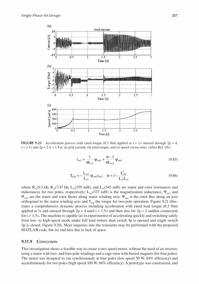
257Single-Phase IM Design
i1L
1L
m2s2
sm2m2
rm2=σ
ψ + σ −σ
ψ (9.85)
TLL
i ; 1L
L Le2p
m2
r2rm2 m2
m22
s2 r2
= − ψ σ = − (9.86)
where Rs2(9.3 Ω), Rr2(7.47 Ω), Ls2(359 mH), and Lr2(343 mH) are stator and rotor resistances and inductances for two poles, respectively; Lm2(337 mH) is the magnetization inductance; Ψsm2 and Ψrm2 are the stator and rotor fluxes along stator winding axis; Ψrma is the rotor flux along an axis orthogonal to the stator winding axis and Te2p the torque for two-pole operation. Figure 9.21 illus-trates a comprehensive dynamic process including acceleration with rated load torque (0.3 Nm) applied at 1s and onward through 2p = 4 until t = 1.5 s and then also for 2p = 2 sudden connection for t > 1.5 s. The machine is capable (as in experiments) of accelerating quickly and switching safely from low- to high-speed mode under full load (where dual switch 4p is opened and single switch 2p is closed, Figure 9.20). More inquiries into the transients may be performed with the proposed MATLAB code, but we end here due to lack of space.
9.11.9 concluSion
This investigation shows a feasible way to create a two-speed motor, without the need of an inverter, using a stator with two- and four-pole windings and a cage rotor with buried magnets (for four poles). The motor was designed to run synchronously at four poles (low speed 50 W, 84% efficiency) and asynchronously for two poles (high speed 100 W, 60% efficiency). A prototype was constructed, and
FIGURE 9.21 Acceleration process with rated torque (0.3 Nm) applied at t = 1 s onward through 2p = 4, t < 1.5 s and 2p = 2 (t > 1.5 s): (a) grid current, (b) total torque, and (c) speed versus time. (After Ref. [9].)

258 Induction Machines Handbook
dynamometer tests were performed to confirm the theoretical simulations. Moreover, rather compre-hensive models for steady state and transients accounting for various losses and for magnetic satura-tion have been developed to optimally design the machine according to specifications. Four percent efficiency rise by optimal design methodology for low-speed operation in comparison with the expe-rienced standard analytical design was obtained and considered satisfactory. The theoretical effort was satisfactorily verified in part by 2D FEM inquiries and in full-scale industrial experiments.
Separate four-pole consequent split-phase windings (to save copper weight) and a two-pole main-only winding have been used to reduce the switching of the pole count to only a dual switch 4p and simple switch 2p. Although this motor can be a good option for the applications where the 2/1 ratio speed variation can generate benefits, the attractiveness of this solution can vary with the cost of the materials (mainly magnets and starting devices) and must be ultimately evaluated, case by case, by the motor designer.
9.12 SUMMARY
• The design of single-phase IM tends to be more involved as the magnet field is rather ellip-tical, in contrast to being circular, as for three-phase IMs.
• The machine utilization factor Cu and the tangential force density (stress) ft tend to be higher and smaller, respectively, than for three-phase IMs. They also depend on the type of single-phase IM split-phase, dual capacitor, permanent capacitor, or split-phase capacitor.
• For new specifications, the tangential force density ft (0.1–1.5) N/cm2 is recommended to initiate the design process. For designs in given standardized frames, the machine utiliza-tion factor Cu seems more practical as an initiation constant.
• The number of stator Ns and rotor slots Nr selection goes as for three-phase IMs in terms of parasitic torque reduction. The larger the number of slots, the better the performance.
• The stator bore-to-stator outer diameter ratio Di/Do may be chosen as variable in small intervals, increasing with the number of poles above 0.58 for 2p1 = 2, 0.65 for 2p1 = 4, 0.69 for 2p1 = 6 and 0.72 for 2p1 = 8. These values correspond to laminations which provide maximum no-load airgap flux density for given stator mmf in three-phase IMs [2].
• By choosing the airgap, stator, rotor tooth, and core flux densities, the sizing of stator and rotor slotting becomes straightforward.
• The main winding effective number of turns is then calculated by assuming the emf Em/Vs ≈ 0.95–0.97.
• The main and auxiliary windings can be made with identical coils or with graded turn coils (sinusoidal windings). The effective number of turns (or the winding factor) for sinu-soidal windings is computed by a special formula. In such a case, the geometry of various slots may differ. More so for the split-phase IMs where the auxiliary winding occupies only 33% of stator periphery and is active only during starting.
• The rotor cage cross-sectional total area may be chosen for start as 35%–60% of the area of stator slots.
• The turn ratio between auxiliary and main winding is a = 1.5–2.0, in general. It is equal to unity (a = 1) for reversible motors which have identical stator windings.
• The capacitance initial value is chosen for symmetry conditions at an assigned value of rated slip and efficiency (for rated power).
• Once the preliminary sizing is done, the resistance and leakage reactances may be cal-culated. Then, either by refined analytical methods or by FEM (with bare (cage-free) rotor and zero auxiliary winding current), the magnetization curve Ψm(Imm) or reactance Xmm(Imm) is obtained.
• To estimate the starting and steady-state running performance and constraints such as starting torque and current, rated slip, current, efficiency, power factor, and breakdown torque, revolving field or cross-field models are used.

259Single-Phase IM Design
• The above completes a preliminary electromagnetic design. A thermal model is used then to estimate stator and rotor temperatures.
• Based on such an analysis model, an optimization design process may be started. A good initial (preliminary) design is useful in most nonevolutionary optimization methods [5].
• The optimization design (Chapter 8) is a constrained nonlinear programming problem. The constraints may be lumped into an augmented objective function by procedures such as SUMT [7]. Better procedures for safe global optimization are currently proposed [32].
• Increases in efficiencies of a few percent may be obtained by optimization design [9]. Given the immense number of single-phase IMs, despite the low-power/unit, their total power is significant. Consequently, any improvement of efficiency of more than 1%–2% is relevant in both energy costs and environmental effects.
• Reduction of space harmonics in the design stage is yet another important issue [33].• Winding reconfiguration with solid-state switches is presented in Ref. [34].• The single-phase IM preliminary design case study and then the optimal design meth-
odology and code developed in this chapter for a two-speed PM-assisted IM [9] are mere example of the complexity facing IM designers of today and tomorrow.
REFERENCES
1. C. G. Veinott, Small electric motors, Chapter 6. In: Handbook of Electric Machines, Editor S. A. Nasar, McGraw-Hill Company, New York, 1987.
2. G. Madescu, I. Boldea, T. J. E. Miller, The Optimal Lamination Approach (OLA) to induction machine design global optimization, Record of IEEE-IAS-1996, San Diego, CA, Vol. 2, 1996, pp. 574–580.
3. E. S. Hamdi, Design of Small Electrical Machines, John Wiley & Sons, Hoboken, NJ, 1994, pp. 140. 4. J. Stepina, Single Phase Induction Motors, Springer Verlag, New York, Chapter 5, 1981 (in German). 5. C. B. Rasmussen, T. J. E. Miller, Revolving field polygon technique for performance prediction of single
phase induction motors, Record of ICEM-2000, Helsinki, 2000. 6. H. Huang, E. F. Fuchs, Z. Zak, Optimization of single phase induction motor design, part I + II, IEEE
Transactions on Energy Conversion, Vol. 3, 1988, pp. 349–366. 7. G. I. Hang, S. S. Shapiro, Statistical Models in Engineering, John Wiley & Sons, Hoboken, NJ, 1967. 8. F. Parasiliti, M. Villani, Design procedure for single phase capacitor motors performance improvement,
Record of ICEM-1994, Paris, France, pp. 193–197. 9. F. J. H. Kalluf, L. N. Tutelea, I. Boldea, A. Espindola, 2/4 pole split-phase capacitor motor for small
compressors: A comprehensive motor characterization, IEEE Transactions on Industry Applications, Vol. 50, No. 1, 2014, pp. 356–363.
10. W. J. Morril, The revolving: Field theory of the capacitor motor, Transactions of the American Institute of Electrical Engineers, Vol. 48, No. 2, 1929, pp. 614–629.
11. I. Boldea, S. A. Nasar, Induction Machines Design Handbook, Second edition, CRC Press, Boca Raton, FL, 2010.
12. C. B. Rasmussen, T. J. E. Miller, Revolving field polygon technique for performance prediction of single phase induction motors, IEEE Transactions on Industry Applications, Vol. 39, No. 5, 2003, pp. 1300–1306.
13. I. Boldea, T. Dumitrescu, S. A. Nasar, Unified analysis of 1-phase AC motors having capacitors in the auxiliary winding, IEEE Transaction on Energy Conversion, Vol. 14, No. 3, 1999, pp. 577–582.
14. M. Popescu, C. Rasmussen, T. J. E. Miller, M. McGilp, Effect of MMF harmonics on a single-phase induction motor performance: A unified approach, Conference Record of the 2007 IEEE Industry Applications Conference 42nd Annual Meeting, 2007, New Orleans, LA, pp. 1164–1170.
15. P. S. Andersen, D. G. Dorell, N. C. Weihrouch, P. K. Hansen, Synchronous torques in split phase induc-tion motors, IEEE Transactions on Industry Applications, Vol. 46, No. 1, 2010, pp. 222–231.
16. N. Bianchi, S. Bolognani, and F. Tonel, Thermal analysis of a run capacitor single-phase induction motor, IEEE Transactions on Industry Applications, Vol. 39, No. 2, 2003, pp. 457–465.
17. K. Kurihara, M. A. Rahman, High-efficiency line-start interior permanent-magnet synchronous motors, IEEE Transactions on Industry Applications, Vol. 40, No. 3, 2004, pp. 789–796.
18. M. A. Rahman, A. M. Osheiba, K. Kurihara, M. A. Jabbar, H. W. Ping, K. Wang, H. M. Zubayer, Advances on single-phase line-start high efficiency interior permanent magnet motors, IEEE Transactions on Industrial Electronics, Vol. 59, No. 3, 2012, pp. 1333–1345.

260 Induction Machines Handbook
19. K. Kurihara, T. Kubota, M. Hori, Steady-state and transient performance analysis for a single-phase capacitor-run permanent-magnet motor with skewed rotor slots, IEEE Transactions on Industrial Electronics, Vol. 57, No. 1, 2010, pp. 44–51.
20. M. Popescu, T. J. E. Miller, Mc. Gilp, F. J. Kallut, C. da Silva, L. von Dokonal, Effect of winding harmonics on the asynchronous torque of a single phase line start PM motor, IEEE Transactions on Industry Applications, Vol. 42, No. 4, 2006, pp. 1014–1023.
21. F. J. H. Kalluf, C. Pompermaier, M. V. Ferreira da Luz, N. Sadowski, Braking torque analysis of the single phase line-start permanent magnet synchronous motor, Proceedings of ICEM, Rome, Italy, 2010, pp. 1–5.
22. E. Peralta-Sanchez, A. C. Smith, Line-start permanent-magnet machines using a canned rotor, IEEE Transactions on Industry Applications, Vol. 45, No. 3, 2009, pp. 903–910.
23. L. Fang, B. H. Lee, J.-P. Hong, H. Nam, Rotor saliency improved structural design for cost reduction in single-phase line-start permanent magnet motor, Proceedings of IEEE ECCE, San Jose, CA, 2009, pp. 139–146.
24. W. H. Kim, K. C. Kim, S. Joo Kim, D. W. Kang, S.-C. Go, M. Woo Lee, Y.-D. Chun, J. Lee, A steady on the optimal rotor design of LSPM Considering the starting torque, IEEE Transactions on Magnetics, Vol. 45, No. 3, 2009, pp. 1808–1811.
25. S.-W. Baek, B.-T. Kim, B.-I. Kwon, Practical optimum design based on magnetic balance for a single phase line start PM motor, IEEE Transactions on Magnetics, Vol. 47, No. 11, 2011, pp. 3008–3011.
26. A. D. Aliabad, M. Mirsalim, N. F. Ershad, Line-start permanent magnet motors: Significant improve-ments in starting torque, synchronization, and steady-state performance, IEEE Transactions on Magnetics, Vol. 46, No. 12, 2010, pp. 4066–4072.
27. Z. Wu, J. Wang, J. Ying, J. Zeng, Sensorless brushless DC motor drive for air-conditioner compressor, Proceeding of IEEE ICEMS, Vol. 2, 2001, pp. 968–971.
28. M. Popescu, T. J. E. Miller, M. I. McGilp, G. Strappazzon, N. Trivillin, R. Santarossa, Torque behavior of one-phase permanent-magnet AC motor, IEEE Transactions on Energy Conversion, Vol. 21, No. 1, 2006, pp. 19–26.
29. S. Williamson, A. C. Smith, A unified approach to the analysis of single-phase induction motors, IEEE Transactions on Industry Applications, Vol. 35, No. 4, 1999, pp. 837–843.
30. V. V. Sastry, P. S. Rao, P. V. Rao, Improved tow-speed single-winding single-phase induction motors, IEEE Transactions on Pattern Analysis and Machine, Vol. 90, No. 3, 1971, pp. 1355–1366.
31. L. N. Tutelea, I. Boldea, Induction motor electromagnetic design optimization: Hooke Jeeves method versus genetic algorithms, Proceedings of OPTIM, 2010, Romania, pp. 485–492.
32. X. Liu, W. Xu, Global optimization of electrical machines with the filled function methods, EMPS, Vol. 29, 2001.
33. J. P. Bacher, Reduction of harmonics of single phase induction motors with a small power range by specified design steps, Record of ICEM-2006, 2006, Greece, pp. 631–635.
34. J. Schraud, E. F. Fuchs, H. A. Fuchs, Experimental verification of critical-speed increase of single-phase induction machines via winding reconfiguration with solid-state switches, IEEE Transactions on Energy Conversion, Vol. 23, No. 2, 2008, pp. 460–465.

261
10 Three-Phase Induction Generators
10.1 INTRODUCTION
In Chapter 7, Vol. 1, we alluded to the induction generator mode both in stand-alone (capacitor excited) and grid-connected situations. In essence for the cage-rotor generator mode, the slip S is negative (S < 0). As the induction machine (IM) with a cage rotor is not capable of producing reac-tive power, the energy for the machine magnetization has to be provided from an external means, either from the power grid or from constant (or electronically controlled) capacitors [1–24].
The generator mode is currently used for braking advanced PWM converter-fed drives for indus-trial (elevator) and traction purposes. Induction generators – grid connected or isolated-capacitor excited – are used for constant or variable speed and constant or variable voltage/frequency, in small hydropower plants, wind energy systems, emergency power supplies, etc. [1]. Both cage and wound rotor configurations are in use. For a summary of these possibilities, see Table 10.1. Cogeneration of electric power in industry at the grid (constant voltage and frequency) for small range variable speed and motor/generator operation in pump-back hydropower plants or in wind energy conversion are all typical applications for wound rotor IMs.
In what follows, we will discuss the main performance issues of IGs first in stand-alone con-figurations and then at power grid. Although changes in performance owing to variable speed are a key issue here, we will not deal with power electronics or control issues. We choose to do so as IG systems now constitute a mature technology whose in-depth (useful) treatment could be the subject matter of an entire book [25,26].
Typical configurations of IGs are shown in Figures 10.1–10.4.Figure 10.1 portrays a WRIG whose rotor is connected through a bi-directional power flow
converter and transformer (optional) to the power grid which has constant voltage and frequency.For limited prime mover speed variation (X%), the power converter rating is limited to X% of IG
rated power. Consequently, reasonably lower costs are encountered.Figure 10.2 shows an isolated cage-rotor IG (CRIG) with variable frequency but constant voltage
for variable prime mover speed. The power electronics converter shown in Figure 10.2 has limited ratings and simplified control as it acts as a Variac to control (reduce) the capacitance reactive power flow into the IG for constant voltage control.
The A.C.–A.C. power electronics converter (PEC) in Figure 10.3 makes the transition from the variable voltage Vg and frequency fg of the generator to the constant voltage and frequency of the
TABLE 10.1IG Configurations
IG Type
Speed
Constant VariableGrid
Connected Isolated
Stator Frequency
Constant Variable
Voltage
Constant Variable
Wound rotor - * * * * * * *Cage rotor * * * * * * * *
- Impractical.* Practical.
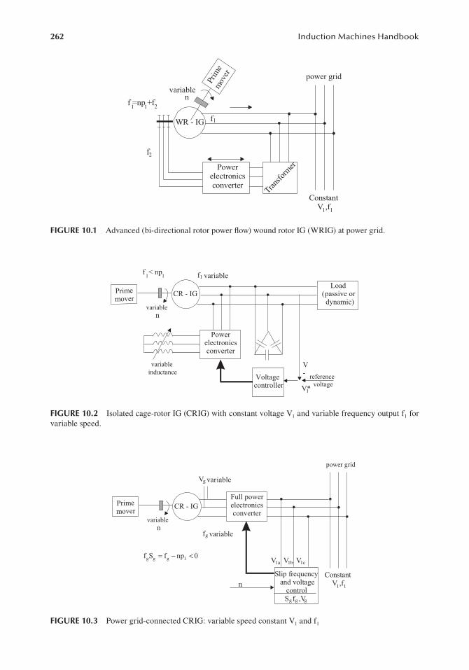
262 Induction Machines Handbook
WR - IG
Powerelectronicsconverter
Transfo
rmer
Prim
emov
er
nf =np +f1 1 2
f1
f2
ConstantV ,f
variablepower grid
1 1
FIGURE 10.1 Advanced (bi-directional rotor power flow) wound rotor IG (WRIG) at power grid.
CR - IG
Powerelectronicsconverter
Primemover
n
f < np 1 1 f1 variable
Voltagecontroller
Load(passive ordynamic)
V- reference
voltageV*1
variable
variable inductance
reference voltage
FIGURE 10.2 Isolated cage-rotor IG (CRIG) with constant voltage V1 and variable frequency output f1 for variable speed.
CR - IGPrimemover
variablen
f S =f -np <0 g 1
fg variable
Slip frequencyand voltage
controlS f ,V
g g
Vg variable
Full powerelectronicsconverter
g g g
n
V1a V1b V1c
ConstantV ,f1 1
variable
power grid
g g g 1f S f np 0= − <
FIGURE 10.3 Power grid-connected CRIG: variable speed constant V1 and f1

263Three-Phase Induction Generators
power grid. In the process, the same PEC transfers reactive power from the power grid to provide the magnetization of the cage-rotor induction generator (CRIG), or reactive power is “delivered” to the grid even when the CRIG is idle.
The PEC is rated at full power and thus adds to the total costs of the equipment, while the CR-IG is rugged and costs less.
Handling limited variable speed prime movers (wind or constant head small hydraulic turbines) to extract most of the available primary energy may be done by simpler methods such as pole chang-ing windings for CR-IG (Figure 10.4a) or even a parallel connected Rad/Lad circuit in the rotor of the WRIG for grid-connected IGs (Figure 10.4b).
On the other hand, for less frequency-sensitive loads voltage regulation for variable speed vari-able frequency but constant voltage, long-shunt capacitor connections or saturable load interfacing transformers may be used in conjunction with CR-IGs.
Solutions like those shown in Figure 10.4 are characterized by low costs. But the power flow control and voltage regulation (for isolated systems) are only moderate. For low-/medium-power applications with limited prime mover speed variation, they may be adequate.
The system configurations presented in Figures 10.1–10.4 are meant to show the multitude of solutions that are feasible and have been proposed. Some of them are extensively used in wind power and small hydropower systems.
In the following, we will focus on IG behaviour in such schemes rather than on the systems themselves. First, we will investigate in depth the self-excitation and load performance under steady state and transients of CR-IG with capacitors for isolated systems.
Then, the WRIG with bi-directional power capability PEC in the rotor for grid-connected systems will be discussed in detail in terms of stability limits and performance.
Finally, DSW cage (or loop-cage) rotor IGs and the cascaded IG, which recently have a rich literature and strong R&D efforts, are discussed in their fundamentals.
CR - IGPrimemover
variablen
Full powerstatic
switch
with polechangingwinding
Limitedpowerswitch
with pole changing winding
variable
power grid
(a)
CR - IGPrimemover
variablen
Power
switch
R ||Lad ad
WR - IG
variable
power grid
(b)
FIGURE 10.4 Simplified IG systems: (a) CRIG with pole changing winding and two static power switches for grid connection and (b) WRIG with parallel Rad || Lad in the rotor for grid connection system.

264 Induction Machines Handbook
10.2 SELF-EXCITED INDUCTION GENERATOR (SEIG) MODELLING
We describe a cage-rotor IG with capacitor excitation using SEIG (Figure 10.5a). The standard equivalent circuit of SEIG on a per phase bases is shown in Figure 10.5b.
First, with the switch S open, the machine is driven by the prime mover. As the SEIG picks up speed slowly, the no-load terminal voltage increases and settles at a certain value. This is the self-excitation process, which has been known since the 1930s [2].
In essence, first the residual magnetism in the rotor laminated core (from previous IG operation) produces by motion an emf in the stator windings. Its frequency is f10 = n0p1. This emf is applied to the machine terminals and produces in the RLC circuit of each phase a magnetization current which produces an airgap field. This field adds to the remnant field of the rotor to produce a higher emf. The process goes on until an equilibrium is reached for a given speed n0 and a given capacitance C at a voltage level V0. However, this process is stable as long as the machine is saturated and thus Xm(Im) is a nonlinear function (as shown already in Chapter 7, Vol. 1).
In a very simplified form, with X1l, X2l, R1, and R2 neglected, the equivalent circuit for no load degenerates to Xm in parallel with a capacitor and a small emf determined by the remnant rotor field (Figure 10.6a).
CR - IGPrimemover
n
f1 variableR
R
R
SXc
Resistiveload
(balanced)
excitation capacitors
(a)
R XcjIc
Xmj
X1lj X2ljRI1 I2
Im
1
RS
2S<0for generator mode
excitation capacitors
load
(b)
FIGURE 10.5 SEIG with resistive load: (a) general scheme and (b) standard equivalent circuit.
Xcj
Im
X (I )mj m
Erem
E1
f =np ; =2 fω π
X = Lωm m
10 10 101
10
E1
V10E1 =
I C10
E1=I L (I )ω m10 10 10
Erem I10
( )1 m 10 m mE =I ω L I
mI
mI
(b)(a)
ω10
FIGURE 10.6 Oversimplified circuit for explaining self-excitation: (a) the circuit and (b) the characteristics.
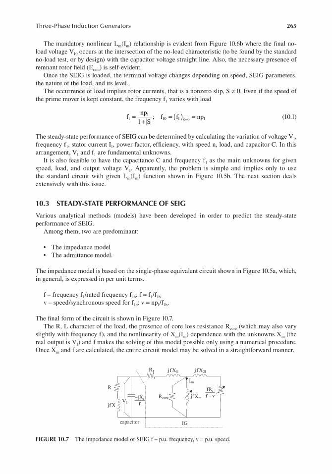
265Three-Phase Induction Generators
The mandatory nonlinear Lm(Im) relationship is evident from Figure 10.6b where the final no-load voltage V10 occurs at the intersection of the no-load characteristic (to be found by the standard no-load test, or by design) with the capacitor voltage straight line. Also, the necessary presence of remnant rotor field (Erem) is self-evident.
Once the SEIG is loaded, the terminal voltage changes depending on speed, SEIG parameters, the nature of the load, and its level.
The occurrence of load implies rotor currents, that is a nonzero slip, S ≠ 0. Even if the speed of the prime mover is kept constant, the frequency f1 varies with load
fnp
1 S; f f np1
110 1 S 0 1( )=
+= == (10.1)
The steady-state performance of SEIG can be determined by calculating the variation of voltage V1, frequency f1, stator current I1, power factor, efficiency, with speed n, load, and capacitor C. In this arrangement, V1 and f1 are fundamental unknowns.
It is also feasible to have the capacitance C and frequency f1 as the main unknowns for given speed, load, and output voltage V1. Apparently, the problem is simple and implies only to use the standard circuit with given Lm(Im) function shown in Figure 10.5b. The next section deals extensively with this issue.
10.3 STEADY-STATE PERFORMANCE OF SEIG
Various analytical methods (models) have been developed in order to predict the steady-state performance of SEIG.
Among them, two are predominant:
• The impedance model• The admittance model.
The impedance model is based on the single-phase equivalent circuit shown in Figure 10.5a, which, in general, is expressed in per unit terms.
f – frequency f1/rated frequency f1b: f = f1/f1b
v – speed/synchronous speed for f1b: v = np1/f1b.
The final form of the circuit is shown in Figure 10.7.The R, L character of the load, the presence of core loss resistance Rcore (which may also vary
slightly with frequency f), and the nonlinearity of Xm(Im) dependence with the unknowns Xm (the real output is V1) and f makes the solving of this model possible only using a numerical procedure. Once Xm and f are calculated, the entire circuit model may be solved in a straightforward manner.
R
X f
c-j fXmj
fX1lj f X2ljR
Im
1
fRf-v
2
jf XV1
capacitor IG
Rcore
capacitor
cjXf
−2f R
f v−
FIGURE 10.7 The impedance model of SEIG f – p.u. frequency, v = p.u. speed.

266 Induction Machines Handbook
Fifth- or fourth-order polynomial equations in f or Xm are obtained from the conditions that the real and imaginary parts of the equivalent impedance are zero. A wealth of literature on this subject is available [3–5]. Rather recently a fairly general solution of the impedance model, based on the optimization approach, has been introduced [6].
However, the high order of system nonlinearity prevents an easy understanding of performance sensitivity to various parameters. In search of a simpler solution, the admittance model has been proposed [7].
While the Xm equation is simple, calculating f involves a complex procedure. In [8,9], admittance models, that lead to quadratic equations for the unknowns, are obtained for balanced resistive load, without additional simplifying assumptions.
10.4 THE SECOND-ORDER SLIP EQUATION MODEL FOR STEADY STATE
The second-order equation model may be obtained from the standard circuit shown in Figure 10.8.The slip is negative for generator mode:
S(f v)
f= −
(10.2)
The airgap voltage Ea for frequency f (in p.u.):
E fE IRS
jXa 1 22
2l= = +
(10.3)
where E1 is the airgap voltage at rated frequency.For simplicity, the core loss resistance is neglected, while the load is purely resistive. The parallel
capacitor-load resistance circuit may be transformed into a series one:
R jXR j
Xf
R jXf
R
1R X
f
jXf
1X
f R
L L
C
C2
C2
2
C
C2
2 2
− =−
−=
+−
+(10.4)
Now, we may lump R1 and RL into R1L = R1 + RL and fX1l and XL into X1L = fX1l − XL to obtain the simplified equivalent circuit shown in Figure 10.9.
Notice that frequency f will be given and the new unknowns are S and Xm while E1(Im) or Xm(E1) comes from the no-load curve of IG. Also the load resistance R, the capacitance C, and the values of R2, X2l, R1, and X1l are given. Consequently, with f known and S calculated, the speed v can be computed as
v f 1 S( )= − (10.5)
Xf
c-jf Xmj
fX2lj f X1ljR /S
Im
2
V1
IG
A R 1I2 I1
RE =fEA 1a 1E =f E
FIGURE 10.8 Equivalent circuit of SEIG with slip S and frequency f (p.u.) shown.

267Three-Phase Induction Generators
If the speed is known, a simpler iterative procedure is required to change f until the desired v is obtained.
We should mention that, with given f, the presence of any type of load does not complicate the problem rather than the expressions of RL and XL in (10.4). An induction motor load is such a typical dynamic load.
For self-excitation, the summation of currents in node A (Figure 10.9) must be zero (implicitly E1 ≠ 0):
0 I I I ;2 1 m= − + + (10.6)
fE1
jfX1
R jXS
R jSfX01
m 1L 1L 2 2l
++
++
= (10.7)
The same result is obtained in [9] after introducing a voltage source in the rotor.The real and imaginary parts of (10.7) have to be zero:
R
R XSR
R S f X01L
1L2
1L2
2
22 2 2
2l2+
++
= (10.8)
1
fXX
R XSfX
R S f X0
m
1L
1L2
1L2
2l
22 2 2
2l2−
++
+= (10.9)
For a given f, load, and IG parameters, (10.8) has the slip S as the only unknown:
aS bS c 02 + + = (10.10)
with a f X R ; b R R X ; c R R22l2
1L 2 1L2
1L2
1L 22( )= = + + = (10.11)
Equation (10.10) has two solutions, but only the smaller one (S1) refers to a real generator mode. The larger one refers to a braking regime (all the power is consumed in the machine losses).
Sb b 4ac
2a01,2
2
= − ± − < (10.12)
Complex solutions S1,2 imply that self-excitation cannot take place.Once S1 is known, the corresponding speed v, for a given frequency f, capacitance, and load, is
calculated from (10.5). When the speed is given, f is changed until the desired speed v is obtained.Now, with S, f, etc. known, the only unknown in (10.9) is Xm, which is given by
XR R X
SfX R R X f; S 0m
2 1L2
1L2
2L 1L 2 1L
( )( )=
+− +
< (10.13)
RS
fXmj
Im
jfX
R
jX
2
S<0
2l
fE1
1L
1L
2 1AI I
FIGURE 10.9 A simple nodal form of SEIG equivalent circuit.
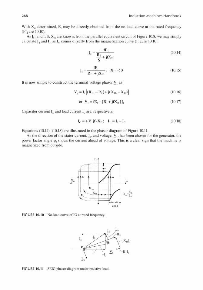
268 Induction Machines Handbook
With Xm determined, E1 may be directly obtained from the no-load curve at the rated frequency (Figure 10.10).
As E1 and f, S, Xm are known, from the parallel equivalent circuit of Figure 10.8, we may simply calculate I2 and I1, as Im comes directly from the magnetization curve (Figure 10.10):
IfE
RS
jfX2
1
22l
= −
+(10.14)
IfE
R jX; X 01
1
1L 1L1L=
+< (10.15)
It is now simple to construct the terminal voltage phasor V1 as
V I R R j X X1 1 1L 1 1L 1l[ ]( ) ( )= − + − (10.16)
V fE R jfX I1 1 1 1l 1( )= − + (10.17)or
Capacitor current IL and load current IC are, respectively,
I V jf X ; I I IC 1 C L 1 C= + = − (10.18)
Equations (10.14)–(10.18) are illustrated in the phasor diagram of Figure 10.11.As the direction of the stator current, I1, and voltage, V1, has been chosen for the generator, the
power factor angle φ1 shows the current ahead of voltage. This is a clear sign that the machine is magnetized from outside.
E1
Xm
Xm Im
X =EImm
1
zone saturation
FIGURE 10.10 No-load curve of IG at rated frequency.
cI
cI
1I
2-I
mI
mI
1V 11R I
11ljX I1fE
LI2I−
FIGURE 10.11 SEIG phasor diagram under resistive load.

269Three-Phase Induction Generators
As expected, for a resistive load, the terminal voltage V1 and the load current IL end up in phase (Figure 10.11). We may approximately calculate the core losses, pcore, as
p3 fE
Rcore
12
core
( )= (10.19)
with Rcore determined from no-load tests at the rated frequency. In reality, Rcore varies slightly with frequency, and a no-load test for different frequencies would give the Rcore(f) functional.
The SEIG efficiency ηg is
3V I cos
3V I cos 3R I 3R I p pg
1 L L
1 L L 1 12
2 22
core mec
η = ϕϕ + + + +
(10.20)
Mechanical losses are determined separately from the standard no-load tests at variable voltage and, eventually, frequency.
As we can see, the direct steady-state problem with f1 and capacitance load, machine parameters and no-load characteristic given, and S and Xm as unknowns may be solved in a straightforward manner. In the case when the speed v, instead of f, is fixed, the problem may be solved the same way through a few iterations by changing f in (10.10) until the value of S < 0 will produce the required speed v = f(1 − S).
The solution to (10.10) leads to a few solution existence conditions:
fX X ; XX f
1X
f R
1l L LC
C2
2 2
< =+
(10.21)
where XL refers to the capacitor in parallel with the load impedance.Without capacitive predominance, the voltage collapses. With given XC (capacitor), (10.21)
reduces to a load resistance R condition given by
R XX
X f XC
1l
C2
1l
≥−
(10.22)
The load resistance R has to be a real number in (10.22):
X f XC2
1l≥ (10.23)
Thus, (10.22) sets the value of the minimum load resistance Rmin for a given capacitance, frequency f, and stator leakage reactance X1l. The smaller the X1l, the lower the Rmin, that is the larger the maxi-mum load.
Also the slip Equation (10.10) solutions have to be real such that
b 4ac R R X 4f X R R 0222
1L2
1L2 2 2
2l2
1L2
22( )− = + − > (10.24)
2fXR X
R2l
1L2
1L2
1L
( )≤
+(10.25)or
A low rotor leakage reactance X2l seems beneficial from this point of view.The maximum possible value of the slip Smax corresponds to b2−4ac = 0, and from (10.12) with
(10.25), it becomes
Sb
2aR
fXmax
2
2l
= − = − (10.26)

270 Induction Machines Handbook
For this limiting value of the slip, (10.21) is not satisfied any more. So the composite capacitor-load reactance is not capacitive any more. Consequently, the voltage collapses at Smax. However, the ele-gant expression (10.26), which corresponds essentially to an ideal maximum load power, represents a design constraint condition. We may remember that Smax of (10.26) corresponds to the peak torque slip of constant airgap flux vector-controlled IM [10].
Example 10.1 The Slip S and Xm Problem Solution
Let us consider an IM with the following data: Pn = 7.36 kW, f1b = 60 Hz, 2p1 = 2 poles, star con-nection, V1n = 300 V, stator resistance R1 = 0.148 Ω, rotor resistance R2 = 0.144 Ω, stator leakage reactance (at 60 Hz) X1l = 0.42 Ω, and the rotor leakage reactance X2l = 0.25 Ω. The no-load curve E(Xm) at 60 Hz (Figure 10.10) may be broken into a few straight-line segments [9].
=
≥ Ω− ≤ ≤
− ≤ ≤− <
E
0; X 24.0
304.1 7.67X ; 19 X 24
220 3.16X ; 16 X 19
206 2.17X ; X 16
1
m
m m
m m
m m
(10.27)
Let us determine the voltage and speed for fg = 43.33 Hz and for fg = 58.33 Hz and zero load (R = ∞), for C = 180 μF.
Solution
We start with a given frequency for no load R = ∞ in (10.4), with f ≈ 43.33/60 ≈ 0.722, RL = 0, XL = XC/f, R1L = R1 + RL = R1 = 0.148 Ω.
= − = ⋅ −π ⋅ ⋅ ⋅
≈ − Ω−X fXXf
0.722 0.421
2 60 0.722 180 1020.111L 1l
c6
Now from (10.11), a, b, and c are
( ) ( )= + = ⋅ + =b R R X 0.144 0.148 33.42 160.8332 1L2
1L2 2 2
= = ⋅ ⋅ = ⋅ −a f X R 0.722 0.25 0.148 4.821 1022l2
1L2 2 2
= = ⋅ = ⋅ −c R R 0.148 0.144 3.069 101L 22 2 3
From (10.12)
= − + −S
b b 4ac2a
1
2
For 4ac ≪ b, we can approximate S1 by
= − = ⋅⋅
≈ ⋅ ≈−
−Scb
3.069 102 160.33
1 10 01
35
This small value was expected.From (10.13), the magnetization reactance is
( )
=+
−≈ − = = > ΩX
R R X
R X fXf
20.110.722
27.864 24.0m2 1L
21L2
2 1L
1L
with zero rotor current, Xm is expected to be fully compensated by the capacitance reactance minus the stator leakage reactance. The emf value E1, for Xm = 27.864 > 24 in (10.27), is E1 = 0; that

271Three-Phase Induction Generators
is, at a low frequency (speed), with a capacitance C = 180 μF (per phase), the machine does not self-excite even on no load!
For fg = 58.33Hz (f = 0.9722), however, and R = ∞, X1L becomes
= − = ⋅ −π ⋅ ⋅ ⋅
= − Ω−X fXXf
0.9722 0.421
2 60 0.9722 180 1014.751L 1l
C6
In this case,
= − = − = ΩXX
f14.750.9722
15.179m1L
Now, from (10.27),
E 206 2.27 15.179 171.54 V1 = − ⋅ =
The phase current I1 (equal, in this case, to capacitor current) is (from (10.15))
=+
= ⋅−
= ⋅ +−IfE
R jX0.9722 171.540.148 j14.75
1.13 10 j11.30611
1L 1L
2
The terminal voltage V1 from (10.17) is
( )( )= − +
= ⋅ − + ⋅ ⋅ +
= −
−
V fE R jfX I
0.9722 171.54 (0.148 j0.9722 0.42) 1.13 10 j11.306
171.422 j1.67
1 1 1 1l 1
2
Due to capacitor current, V1 > fE1 as expected. Note also that with S = 0, I 0′2 = .When the machine is loaded (R = 40 Ω), as expected, at f = 43.33 Hz and same capacitor, the
machine again will not self-excite (it did not under no load).However, for f = 58.33 Hz, it may self-excite.
With R = 40 Ω and =π ⋅ ⋅
= Ω−X1
2 60 180 1014.744C 6 from (10.4),
=+
=+ ⋅
= ΩRR
1R fX
40
140 0.9722
14.744
5.027L 2 2
C2
2 2
2
=+
=+
⋅
= ΩX
Xf
1X
R f
14.7440.9722
114.744
0.9722 40
13.26L
C
C2
2 2
2
2 2
So
= + = + = ΩR R R 0.148 5.027 5.1751L 1 l
= − = ⋅ − = − ΩX fX X 0.9722 0.42 13.26 12.8511L 1l L
The coefficients a–c are obtained again from (10.11):
( ) ( )= + = + =b R R jX 0.144 5.475 12.551 27.63772 1L2
1L2 2 2
= = ⋅ ⋅ =a f X R 0.9722 0.25 5.175 0.305722l2
1L2 2
= = ⋅ =c R R 5.175 0.25 0.3231L 22 2

272 Induction Machines Handbook
Still b2 ≫ 4ac, so S1 is
= − = − = − ⋅ −Sc
b0.323
27.63771.17 101
2
Now, the speed n is
( )( )= − = ⋅ + ⋅ = =−n f 1 S 58.33 1 1.17 10 59.126rps 3540.75rpmg 12
The magnetizing reactance Xm is (10.13)
((=
+− +
XR R X
SfX R R X fm
2 1L2
1L2
2l 1L 2 1L
( )( )=
+− − ⋅ ⋅ ⋅ ⋅ + ⋅ − ⋅
= Ω−
0.144 5.175 12.851
1.17 10 0.9722 0.25 5.175 0.144 ( 12.851) 0.972215.241
2 2
2
))
The emf E1 is thus (10.27)
= − ⋅ =E 206 2.27 15.241 171.40 V1
The stator current I1 (10.15) can be written as
=+
= ⋅−
= +IfE
R jX0.9722 171.545.175 j12.851
4.493 j11.15711
1L 1L
The terminal phase voltage V1 (10.16) is
( )= − +
= ⋅ − + ⋅ +
= − =
V fE R jfX I
0.9722 171.40 (0.148 j0.9722 0.148)(4.493 j11.157)
166.729 j2.29; V 166.74 V
1 1 1 1l 1
1
Notice that the terminal voltage decreased from no load to R = 40 Ω load, from 171.54 to 166.74 V, while the speed required for the same frequency fg = 58.33 Hz had to be increased from 3500 to 3540.75rpm.
The load is still rather small as the output power P2 is
( )= = ⋅ ⋅ + =P 3R I 3 5.027 4.493 11.157 2.181kW 7.36 kW2 L l2 2 2
If the speed v is given, the computation of slip from (10.12) is done starting with a few frequencies lower than the speed until the required speed is obtained.
Once computerized, the rather straightforward computation procedure presented here allows for all performance computation, for given frequency f (or speed), capacitance, load, and machine parameters. Any load can be handled directly putting it in form of a series impedance.
The slip and capacitor problem occurs when the voltage V1, speed, and load are given. To retain simplicity in the computation process, the same algorithm as above may be used repeatedly for a few values of frequency and then for capacitance (above the no-load value at same voltage) until the required voltage and speed are obtained.
The iterative procedure converges rapidly as voltage in general increases with capacitance C.

273Three-Phase Induction Generators
10.5 STEADY-STATE CHARACTERISTICS OF SEIG FOR GIVEN SPEED AND CAPACITOR
The main steady-state characteristics of SEIGs are to be obtained at constant (given) speed though a prime mover, such as a constant speed small hydroturbine, does not have constant speed if unregulated.
They are
• Voltage versus current characteristic for given speed and load power factor• Voltage versus power for given speed and load power factor• Frequency (slip) versus load power for given speed and power factor.
All these curves may be obtained by using the second-order slip equation model.Such qualitative characteristics are shown in Figure 10.12a–c.The slight increase and then decrease in output voltage with power (and current) for leading
power factor is expected. For lagging power factor, the voltage drops rapidly, and thus, the critical slip is achieved at lower power levels. The frequency is influenced only a little by the power factor for given load. On the other hand, for low value of slips, S1, from (10.12), becomes
Sc
bR R
R X1
1L 2
1L2
1L2= − = −
+(10.28)
The larger the X1L, the smaller the S1. Note that X1L includes the self-excitation capacitance in parallel with the load.
The characteristics notably change if the prime mover speed is not regulated. The same methodology as above may be used, with the speed versus power curve as given, to obtain results as shown in [1].
For constant head hydroturbines, the speed decreases with power, and thus, the voltage regula-tion is even more pronounced. Variable capacitance is needed to limit the voltage regulation.
10.6 PARAMETER SENSITIVITY IN SEIG ANALYSIS
The influence of IG resistances R1 and R2 and reactances X1l, X2l, and Xm and of parallel or series–parallel excitation capacitor on performance is described using parameter sensitivity studies.
v 1 0.8 lead1.0
0.8 lag
1
II
1
1n
v 1 0.8 lead1.0
0.8 lag
1
PP
2
n
f0.8 lead
1.00.8 lag
1
PP
2
n
111
(a) (b) (c)
FIGURE 10.12 Steady-state curves for given speed, capacitor, and load power factor: (a) voltage/current, (b) voltage/power, and (c) frequency/power.

274 Induction Machines Handbook
Parameter sensitivity studies of SEIG may be performed for unregulated (variable speed) [1] or regulated (constant speed) prime movers [6]. The main conclusions of such studies are as follows:
For constant speed:• The no-load voltage increases with capacitance.• The terminal voltage and maximum output power increase notably with capacitance.• For constant voltage, the needed excitation capacitance increases with power.• At no load, the magnetization reactance decreases with the supply voltage increase.• In the stable load area, voltage increases with IG leakage reactance and decreases with
rotor resistance.For variable speed (constant head hydroturbine),
• Along a rather large (40%) load resistance variation range, the output power varies only a little.
• Within the range of rather constant power, the voltage drops sharply with load, more so with inductive-resistive loads.
• Up to peak load power, the frequency and speed decrease with power. They tend to increase after that, which is to be translated into stable operation from this point of view.
• The maximum power depends approximately on C2.2 [3] and the corresponding voltage on C0.5 [11].
• For no load, the minimum capacitance requirement is inversely proportional to speed squared.
• As expected, under load the minimum required capacitance depends on load imped-ance, load power factor, and speed.
• When the capacitance is too small, it produces negligible capacitive current for magne-tization and thus the SEIG cuts off. At the other end, with too large a capacitance, the rotor impedance of the generator causes de-excitation and the voltage collapses again. In between, there should be an optimal value of capacitance C for which both output power and efficiency are high.
• When feeding an IM load, the SEIG’s power rating should be two to three times higher than that of the IM and about twice the capacitance needed for a 0.8 lag power fac-tor passive load. These requirements are mainly imposed by the IM transients during starting [12].
• The long-shunt connection decreases the voltage regulation and increases the maxi-mum load accordingly. Avoiding low-frequency oscillations makes subsynchronous resonance important [13].
• Saturable reactances (or transformers) have been proposed also to reduce voltage regu-lation at low costs [14].
10.7 POLE CHANGING SEIGS
Pole changing winding stator SEIGs have been proposed for isolated generator systems with vari-able speed operation when an up to two-to-one speed ratio is required. To keep the flux density in the airgap about the same for both pole numbers, the numbers of poles have to be carefully chosen.
Adequate numbers are 4/6, 6/8, 8/10, etc. The connection of phases for the two pole numbers is also important for the same airgap flux density. Parallel star and series star for 4/6 pole combination was found adequate for the scope [8].
The pole switching should occur near (but before) the drop-out speed for the low pole number.The voltage drop (for single capacitor) with load, for both numbers of poles, is about the same.
Operating at lower number of poles (higher speed), the power is doubled with respect to the case of lower number of poles. Also the efficiency is higher, as expected, at higher speed.

275Three-Phase Induction Generators
For constant voltage, when the speed is doubled, the capacitance and voltage amps reactive (VAR), demands in both six- and four-pole configurations drop to 1/7th and 1/3rd. When the load increases, the capacitance and VAR demands increase almost twofold [5].
High winding factor pole changing windings with simple (2 three-phase ends) pole switch-ing power switch configurations are required (see Chapter 4, Vol. 1). SEIGs with dual windings (of different power ratings) are commercially available.
10.8 UNBALANCED STEADY-STATE OPERATION OF SEIG
Failure of one capacitor or unbalanced load impedances in a three-phase SEIG lead to unbalanced operation.
A general approach to unbalanced operation is provided here by using the symmetrical compo-nent method [15]. Both the SEIG and the load may be either delta- or star-connected.
The equivalent circuit of IG for the positive and negative sequence, with frequency f and speed v in p.u. (as in Section 10.3 (Figure 10.7)) is shown in Figure 10.13.
For the negative sequence, the slip changes from S+ = f/(f – v) to S− = f/(f + v).Also, as the slip frequency is different for the two sequences, f =+ −
s S f+ ⋅ ⋅ f ;1b f =s 1S f− ⋅ ⋅ f b, the skin effect in the rotor will in reality change R2 in the negative sequence circuit accordingly. To the first approximation, this aspect may be neglected. The superposition of effects in the (+,−) method implies that Xm is the same also, though still influenced by magnetic saturation.
Core loss is neglected for simplicity.
10.8.1 the Delta-connecteD Seig
Let us consider a delta-connected IG tied to a delta-connected admittance network Yab, Yac, and Ybc (Figure 10.14).
The expression of load and excitation capacitive admittance is
Y1
Zj
fX
abab C
= + (10.29)
f Xmj
fX1lj fX2ljR
Im
1
f Rf-v
2
I2I1++
+
V1+ YG
+
(a)
f Xmj
f X1lj fX2ljR
Im
1
f Rf+v
2
I2I1--
-
V1- YG
-
(b)
FIGURE 10.13 +/− sequence equivalent circuits of SEIG.

276 Induction Machines Handbook
The total load capacitor supposedly unbalanced admittances are first decomposed into the sequence components as
= ⋅−
Y
Y
Y
1
3
1 1 1
1 a a
1 a a
Y
Y
Y
0
+ 2
2
ab
bc
ca
(10.30)
The total load-capacitor phase currents ILab, IL
bc, and ILca can also be transformed into their sequence
components as
I
I
I
Y Y Y
Y Y Y
Y Y Y
V
V
V
abL0
abL+
abL
0 +
+ 0
+ 0
ab0
ab+
ab
= ⋅−
−
−
− −
(10.31)
In the delta connection, there is no zero sequence voltage V0ab = 0. Consequently, the line currents
Ia components I+a and I−
a are
I I I (1 a)I (1 a) Y V Y V
I I I 1 a I 1 a Y V Y V
a abL
caL
abL 0
ab ab
a abL
caL 2
abL 2
ab0
ab( ) ( )( )
( )= − = − = − +
= − = − = − +
+ + + + + − −
− − − − + + −(10.32)
From Figure 10.13, the generator phase current components I+1 and I−
1 are
I Y V ; I Y V1 G 1 1 G 1= =+ + + − − − (10.33)
Similar to (10.32), we may write the line current Ia components based on generator phase current components as
I (1 a)I (1 a)V Y
I (1 a)I 1 a V Y
a abG
ab G
a abG 2
ab G( )= − = − −
= − = − −
+ + + +
− − − −(10.34)
Iab
Vab Vca
Vbc
G I caG
IbcG
aIab
L IcaL
IbcL
b c
a
b cL
L
L
Yab Yca
YbcIb
Ic
Ia
Yab Z ab-jX f
CcjXf
−
FIGURE 10.14 SEIG with delta-connected unbalanced load and excitation capacitors.
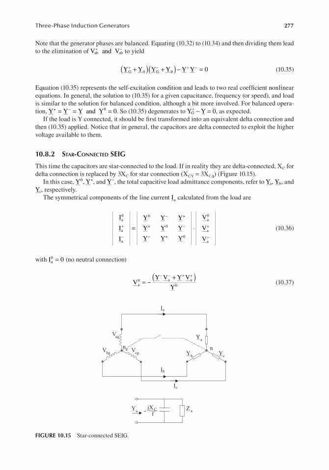
277Three-Phase Induction Generators
Note that the generator phases are balanced. Equating (10.32) to (10.34) and then dividing them lead to the elimination of V+ −
ab and Vab to yield
Y Y Y Y Y Y 0G 0 G 0( )( )+ + − =+ − + − (10.35)
Equation (10.35) represents the self-excitation condition and leads to two real coefficient nonlinear equations. In general, the solution to (10.35) for a given capacitance, frequency (or speed), and load is similar to the solution for balanced condition, although a bit more involved. For balanced opera-tion, Y Y+ = =− Y and Y 00 = . So (10.35) degenerates to Y Y+
G − = 0, as expected.If the load is Y connected, it should be first transformed into an equivalent delta connection and
then (10.35) applied. Notice that in general, the capacitors are delta connected to exploit the higher voltage available to them.
10.8.2 Star-connecteD Seig
This time the capacitors are star-connected to the load. If in reality they are delta-connected, X C for delta connection is replaced by 3X C for star connection (X CY = 3X CΔ) (Figure 10.15).
In this case, Y0, Y+, and Y−, the total capacitive load admittance components, refer to Ya, Yb, and Yc, respectively.
The symmetrical components of the line current Ia calculated from the load are
I
I
I
Y Y Y
Y Y Y
Y Y Y
V
V
V
a0
a
a
0 +
+ 0
+ 0
a0
a
a
= ⋅+
−
−
−
−
+
−
(10.36)
with I 00a = (no neutral connection)
VY V Y V
Ya0 a a
0
( )= −
+− − + +
(10.37)
Vag
VcgVbg
Ya
YcYb
Ib
Ic
Ia
Ya Z ajX f
C
n
-
ng
FIGURE 10.15 Star-connected SEIG.

278 Induction Machines Handbook
Making use of V0a in the star two equations of (10.36), we obtain
I YY Y
YV Y
Y YY
V
I YY Y
YV Y
Y YY
V
a0
0 a 0 a
a 0 a0
0 a
= −
+ −
= −
+ −
++ −
+ −+ +
−
− +− −
++ −
−
(10.38)
The same line current components, calculated from the generator side, are simply
I Y V ; I Y Va G ag a G ag= − =+ + + − − − (10.39)
As the generator and the load line voltages have their sum equal to zero, even with unbalanced load, it may be shown that
V 1 a V 1 a V
V (1 a)V (1 a)V
ab2
a2
ag
ab a ag
( ) ( )= − = −
= − = −
+ + +
− − −(10.40)
Consequently, V V and V Va ag a ag= =+ + − − (10.41)
From (10.38) to (10.39), with (10.41), we obtain the self-excitation equation:
Y YY Y
YY Y
Y YY
YY Y
YY
Y YY
0G0
0 G0
0 0 0+ −
+ −
− −
−
=++ −
−+ −
+− −
−+ +
(10.42)
Note that if the SEIG is star-connected and the capacitor-load combination is delta-connected with original +−0 sequence admittances as Y0, Y+, Y−, then a self-excitation equation similar to (10.35) is obtained
13
Y Y13
Y Y Y Y 0G0
G0+
+
− =+ − + − (10.43)
Also when ng and n are connected, the zero sequence current I 0a is not zero, generally. However
there is no zero sequence generator voltage V0a = =V 00
ag .Consequently, the situation is in this case similar to that of delta/delta connection, but the total
load admittances Y0, Y+, and Y− correspond to the star-connected load admittances Ya, Yb, and Yc, respectively.
Whereas the above treatment is fairly standard and general, a few examples are in order.
10.8.3 t wo phaSeS open
Let us consider the case of delta/delta connection (Figure 10.16) with a single capacitor between aL and bL and a single load
Y Y12
; Y Y 0ab bc ca= = = = (10.44)
For this case
Y Y YY3
0 = = =+ − (10.45)

279Three-Phase Induction Generators
With (10.45), the self-excitation equation (10.35) becomes
3Y Y Y Y Y 0G G G G( )+ + =+ − + − (10.46)
3Y
1Y
1Y
0G G
+ + =+ − (10.47)or
3Equation (10.47) illustrates the series connection of + and − generator sequence circuits to = 3Z
Y(Figure 10.16).Other unbalanced conditions may occur. For example, if phase C opens for some reason, while
the load Z is balanced, the SEIG performs as with a single capacitor and load impedance but with new load admittance Yab = 1.5 Y and Ybc = Yca = 0 [15].
For a short circuit across phase, a Δ/Δ connection Yab = ∞ and thus Y Y0 += = Y− = ∞. Consequently (10.35) becomes (Figure 10.16a).
Y Y 0G G+ =+ − (10.48)
As the capacitor is short-circuited, there will be no self-excitation. The same is true for a three-phase short circuit.
In essence, the computation of steady-state performance under unbalanced conditions includes solving first the self-excitation nonlinear Equations (10.35) or (10.42) or (10.43), (10.47) for given speed (frequency), load, and capacitance, to find the frequency (speed) and the magnetization reac-tance Xm. Then, as for the balanced conditions, equivalent circuits are solved, provided the magne-tization curve E1(Xm) is known. It was proved in Ref. [15] that the positive sequence magnetization curves obtained for balanced no load and one-line-open load differ from each other in the saturation zone (Figure 10.17).
It turns out that, whenever a zero line current occurs, the one-line-open characteristic in Figure 10.17 should be applied [15].
I.G.Primemover
Z L-jX f
Cba
c
(a)
f X1lj
fXmjR1
R1-v/f
r
fX2lj
3ZL-3jX
fC
f X1lj
fXmjR1
R1+v/f
r
f X2lj
f E1
Z Z L-jX f
C
(b)
FIGURE 10.16 Unbalanced SEIG with Δ/Δ connection: single capacitor and single load.

280 Induction Machines Handbook
Sometimes, the range of self-excitation capacitance is needed. Specifying the maximum mag-netization reactance Xmax, the speed (frequency), machine parameters, and load, the solution of self-excitation equations developed in this section produces the required frequency (speed) and capacitances.
There are two solutions for the capacitances, Cmax and Cmin, and they depend strongly on load and speed. For maximum load, the two values become equal to each other. Beyond that point, the voltage collapses.
Sample results obtained for Cmax and Cmin on no load under balanced and unbalanced (one capaci-tor only) conditions for r1 = 0.09175 p.u., r2 = 0.06354 p.u., p1 = 2, f1b = 60 Hz, x1l = x2l = 0.2112 p.u., xmax = 2.0 p.u. are shown in Figure 10.18 [15].
Meticulous investigation of various load and capacitor unbalances on load has proved [15] that the theory of symmetrical components works well.
1
2
0.5 1.0
fX (
p.u)
m
V (p.u.)c1
balanced caseone line open
0
balanced caseone line open
FIGURE 10.17 Positive sequence magnetizing characteristics. (After Ref. [15].)
10
0.4 0.8
C
&
C
(F)µ
max
V (p.u.)0
min
1.2
210
310
410
Measured C & CCalculated CCalculated C
max minmax
min
10
0.4 0.8
C
&
C
(F)µ
max
V (p.u.)0
min
1.2
210
310
410
Measured C & CCalculated CCalculated C
maxmax
min∆
Y
min
(b)
(a)
FIGURE 10.18 Min-max capacitors on no load (continued): (a) balanced capacitor (after Ref. [15]) and (b) one capacitor only.

281Three-Phase Induction Generators
The range of Cmin to Cmax for delta connection is three times smaller than for the star connection. In terms of parameter sensitivity analysis, the trends for unbalanced load are similar to those for balanced load. However, the efficiency is notably reduced and stays low with load variation.
10.9 TRANSIENT OPERATION OF SEIG
SEIGs work alone or in parallel on variable loads. Load and speed perturbations, voltage build-up on no load, and excitation capacitance changes during load operation are all causes for transients. To investigate the transients, the d-q model is in generally preferred. Also stator coordinates are used to deal easily with eventual parallel operation or active loads (A.C. motors).
The d-q model (in stator coordinates) for the SEIG alone, including cross-coupling saturation [16,17], is given as
V R i L p i G iG G G G G rG G G[ ] [ ][ ] [ ] [ ] [ ][ ]= − − − ω (10.49)
with V V ,V ,0,0G d q[ ] = (10.50)
i i , i , i , iG d q dr qr[ ] = (10.51)
The torque
T32
P L i i i ieG 1G m q dr d qr( )= − (10.52)
J
Pd
dtT T
1G
rGPM eG
ω = − (10.53)
pV1C
i ; pV1C
id dc q qc= = (10.54)
i i i ; i i idc d dL qc q qL= + = + (10.55)
idc, iqc, idL, and iqL are d, q components of capacitor and load currents, respectively.The association of signs in (10.49) corresponds to generator mode.Now, the parameter matrices RG, LG, and GG are
R Diag R ,R ,R ,RG 1 1 2 2[ ]=
L =
L L L L
L L L L
L L L L
L L L L
G
1d dq md dq
dq 1q dq mq
md dq 2d dq
dq mq dq 2q
(10.56)
G
0 0 0 00 0 0 00 L 0 L
L 0 L 0
Gm 2
m 2
=
− −
(10.57)
where Lm is the magnetization inductance and im the magnetization current.
i i i ; i i i ; i i imd d dr mq q qr m md2
mq2= + = + = + (10.58)

282 Induction Machines Handbook
The cross-coupling transient inductance Ldq [16,17] is
Li i
idLdi
dqmd mq
m
m
m
= (10.59)
Also the transient magnetization inductances along the two axes Lmd and Lmq [16,17] are
L Lii
dLdi
md mmd2
m
m
m
= + (10.60)
L Li
idLdi
mq mmq2
m
m
m
= + (10.61)
Also
L L L ; L L L
L L L ; L L L
1d 1l md 1q 1l mq
2d 2l md 2q 2l mq
= + = +
= + = + (10.62)
The SEIG equations for constant speed ωr on no load may be written also in the form (cross- coupling saturation is neglected here):
0 [Z][I] V0[ ]= + (10.63)
with
Z
R pL 1/sC 0 pL 0
0 R pL 1/sC 0 pL
pL L R pL L
L pL L R pL
s s m
s s m
m r m r r r r
r m m r r r r
=
+ ++ +−ω + −ω
ω ω + (10.64)
[I] i i i i ; V V V V Vqs ds qr dr 0 cq0 cd0 remq remd[ ]=
=
where Vremq and Vremd are the remnant flux density emfs (small values), Vcq0 and Vcd0 are the no-load 2
terminal d-q voltages ,and p is the Laplace operator; Lm is a function of im s= +( )i i 2d rd + +( )i isq rq .
For self-excitation at no load, Det[Z] = 0 and all the roots in “p” should have negative real parts. An eight-order polynomial equation in “s” is to be solved [18]. All machine parameters, capacitor C, and speed influence the self-excitation process, but especially the magnetic saturation expressed by Lm(im) function and the remnant (initial) no-load voltages Vremq and Vremq.
Finally also, in practice, the machine acceleration (am = dωt/dt) when too large may impede on self-excitation as active current components (q components) occur in the stator and they may hamper self-excitation.
10.10 SEIG TRANSIENTS WITH INDUCTION MOTOR LOAD
There are practical situations, in remote areas, when the SEIG is supplying an induction motor which in turns drives a pump or a similar load.
A pump load is characterized by increasing torque with speed such that
T T Kload L0 L rM2≈ + ω (10.65)

283Three-Phase Induction Generators
The most severe design problem of such a system is the starting (transient) process. The rather low impedance of IM at low speeds translates into high transient currents from the SEIG. On the other hand, a large excitation capacitor is needed for rated voltage with the motor on load. When the motor is turned off, this large capacitor produces large voltage transients. Part of it must be discon-nected, or an automatic capacitance reduction to control the voltage is required. An obvious way out of this difficulty would be to have a smaller (basic) capacitance (CG) connected to the generator and one (CM) to the motor (Figure 10.19).
First, the SEIG is accelerated by the prime mover until it establishes a certain speed with a cer-tain output voltage. Then, the IM is connected. Under rather notable voltage and current transients, the motor accelerates and settles at a speed corresponding to the case when the motor torque equals the pump torque.
To provide safe starting, the generator rated power should be notably in excess of the motor rated power. In general, even an 1/0.6 ratio marginally suffices.
Typical such transients for a 3.7 kW SEIG and a 2.2 kW motor with CG = 18 μF, CM = 16 μF, are shown in Figure 10.20 [19].
Voltage and current transients are evident, but the motor accelerates and settles on no load smoothly. Starting on pump load is similar but slightly slower.
On the other hand, the voltage build-up in the SEIG takes about 1–2 s. Sudden load changes are handled safely up to a certain level which depends on the ratio of power ratings of the motor and SEIG.
SEIGPrimemover
rGω
PumploadIM
CG CM
rMω
FIGURE 10.19 SEIG with IM load and split excitation capacitor.
FIGURE 10.20 Motor load starting transients for a SEIG, CG = 18 μF, Cm = 16 μF. (After Ref. [19].)

284 Induction Machines Handbook
For the present case, a 0%–40% motor step load is handled safely, but an additional 60% step load is not sustainable [19]. Very low overloading is acceptable unless the SEIG to motor power rat-ing is larger than 3 ÷ 4.
In case of overloading, an overcurrent relay set at 1.2–1.3 p.u. for 300–400 ms can be used to trip the circuit.
During a short circuit at generator terminals, surges of 2 p.u. in voltage and 5 p.u. in current occur for a short time (up to some 20 ms) before the voltage collapses.
Although the split capacitor method (Figure 10.19) is very practical, for motors rated <20% of SEIG rating a single capacitor will do.
10.11 PARALLEL OPERATION OF SEIGS
An isolated power system made of a few SEIGs is a practical solution for upgrading the generating power rating upon demand. Such a stand-alone power system may have a single excitation capaci-tor, but most probably, it has to be variable, to match the load variations which occur inevitably. Capacitor change may be done in steps through a few power switches or continuously through power electronics control of a paralleled inductor current (Figure 10.21).
The operation of such a power grid on steady state is to be approached as done for the sin-gle SEIG. However, the magnetization curves and parameters of all SEIGs are required. Finally, the self-excitation condition will be under the form of an admittance summation equal to zero. Neglecting the “de-excitation” inductance Lex, the terminal voltage equation is
V1
Rj
fXjf
XIs
L L Csi
i 1
N
∑− +
==
(10.66)
The SEIG’s equations (Section 10.3 and Figure 10.7) may be expressed as
I I IfE
R
1vf
jfXmi si 2i
1i
2i
i2li
+ = = −
−+
(10.67)
SEIG 1
Primemover
Primemover
Primemover
1
Is1
3~Vs
SEIG 2
Is2
SEIG n
Isn
2
n
C
StaticVARIAC
Lex
LLRL
load
FIGURE 10.21 Isolated power grid with paralleled SEIGs.

285Three-Phase Induction Generators
vi is the p.u. speed of the ith generator. Xmi(E1i) represents the magnetization curve of the ith machine. All these curves have to be known. Again, for a given excitation capacitance C, motor parameters and speeds of various SEIGs and load, the voltage, frequency, SEIG currents, capacitor currents, and load currents and load powers (active and reactive) could be iteratively determined from (10.66) to (10.67). A starting value of f is in general adopted to initiate the iterative computation. For sample results, see Ref. [20].
The SEIGs speeds in p.u. have to be close to each other to avoid that some of them switch to motoring mode. Transient operation may be approached by using the d-q models of all SEIGs with the summation of the stator phase currents equal to the capacitor plus load current. So the solution of transients is similar to that for a single SEIG, as presented earlier in this chapter, but the number of equations is larger. Only numerical methods such as Runge–Kutta–Gill, etc. may succeed in solving such stiff nonlinear systems.
10.12 THE DOUBLY FED IG (DFIG) CONNECTED TO THE GRID
As shown in Figure 10.1, a wound-rotor induction generator (dubbed as doubly fed) may deliver power not only through the stator but also through the rotor provided a bi-directional power flow converter is used in the rotor circuit. The main merit of a doubly fed IG is its capability to deliver constant voltage and frequency output for ±(20–40)% speed variation around conventional synchro-nous speed. If the speed variation range is (20–40)% so is the rating of static power converter and transformer in the rotor circuit (Figure 10.1). For bi-directional power flow in the rotor circuit, single stage converters (cycloconverters or matrix converters) or dual-stage back-to-back voltage source PWM inverters have to be used.
Independent reactive and active power flow control – with harmonics elimination – may be achieved this way for both super and subsynchronous speed operation. Less costly solutions use a unidirectional power flow converter in the rotor when only super or subsynchronous operation as generator is possible.
Here, we are interested mainly in the IG behaviour when doubly fed. So we will consider sinusoidal variables with rotor voltage amplitude, frequency, and phase open to free change through an ideal bi-directional power electronics voltage-source converter.
10.12.1 B aSic equationS
To investigate the DFIG, the d-q (space-phasor) model as presented in Chapter 1, Vol. 2, on transients is used.
In synchronous coordinates,
V R1 = +( )1 1( )p j+ ω L i1 1 + +( )p jω1 mL i2
(10.68)V2 = +( )p jS Lω +1 m i R1 ( )2 1+ +( )p jS Lω 2 i2
with
V V jV V V jV
i i ji i i ji
L L L L L L
T32
p L Imag i iJp
T T
1 d q dr qr
d q dr qr
1 1 m
e m* p r
1
PM e
m
++ ;; ++
;; ++
;;
;;
= =
= + =
= + = +
=
ω = −
22
11 22
11 11 22 22
11 11 22

286 Induction Machines Handbook
We should add the Park transformation:
2π 2π cos cθ −V 1,2 1os θ +,2 cos −θ1,2 − V
2 3 3a
d = VV 3
b (10.69)q
sin s( ) 2π 2π −θ1,2 1in −θ ,2 + sin −θ 2 − V 1, 3 3 c
The transformation in synchronous coordinates, valid for stator and rotor, is
θ =1 1∫ω =t tω −1 for constant frequencystator
θ2 1= ω∫ ∫( )− ω r 1t d= θ − ω r t f− or the rotor with variable speed
dθSo, 2 = ω1 r− ω = ωS 1 (10.70)
dt
For constant speed (ωr = constant),
θ2 1= ωS t + δ (10.71)
Also, for an infinite power bus
2π V V1abc = ω1 12 cos t (− −i 1) 3 (10.72)
2π V2abc = ωV 22 1cos t − δ − −(i 1) 3
In (10.72), the rotor phase voltages V2abc are expressed in stator coordinates. This explains the same frequency in V1abc and V2abc (θ1 = 0, θ2 = −ωrt). Using (10.72) and (10.71) in (10.69), we obtain
V1d = =2V1 1; V q 0 (10.73)
For constant speed,
V2d = δ2V2 2cos ; V 2q 2= − V sinδ
As shown in (10.73), in synchronous coordinates, the DFIG voltages in the stator are D.C. quantities. Under steady-state constant δ, the rotor voltages are also D.C. quantities, as expected. The angle δ may be considered as the power angle and thus DFIG operates as a synchronous machine. The rotor voltage 2V2 and its phase δ with respect to stator voltage in same coordinates (synchronous in our case) and slip S are thus the key factors which determine the machine operation mode (motor or generator) and performance.
The proper relationship between V2 and δ for various speeds (slips) represents the fundamental question for DFIG operation.
The various phase displacements in (10.71)–(10.72) are shown in Figure 10.22.The d-q model equations serve to solve most transients in the time domain by numerical meth-
ods with V1 and V2 and prime mover torque TPM as inputs and the various currents and speed as variables.
However to get an insight into the DFIG behaviour, we here investigate steady-state operation and its stability limits.

287Three-Phase Induction Generators
V 21 1= −R Id0 ω ψ1 q0 q; Lψ =0 mI Lqr0 1+ Iq0
0 R= +1 qI ;0 1ω ψd0 ψ =d0 L Im dr0 − L I1 d0
(10.74)V 22 2cos Rδ = I Sdr0 0− ω1 qψ ψr0; Lqr0 2= +I Lqr0 mIq0
−V 22 2sin Rδ = I Sqr0 0+ ω1 dψ ψr0; Ldr0 2= +I Ldr0 mId0
3
Te0 = −p L1 m ( )I Iq0 dr0 dI I0 qr0 (10.75)2
( nT 3) V V si δ L
R =e0 1 2R =0 = P 2
1 1
m
; Lsc = L( )L L21 2 − m L1 (10.76)
S 00 ≠ ω1 Sω1 1 ω Lsc L1
( ) p V1 1 2V L T 3e0 1 =
mR 0= cosδ (10.77)S 00 = ω1 R2 L1
V1q
q axis
d axis
V2q
i1q
i 2q
δ
V2
V=V
2
1
1V2d
V1d
i2d
i 1d rotor phase a
stator phase a
V2ai2a
V1a
i1aω t1
ω t1
(1-S)
FIGURE 10.22 The d-q axis model and the voltage vectors V1 and V2 in synchronous coordinates.
10.12.2 S teaDy-State operation
The steady-state performance can be calculated with S = S0 and δ = δ0 and V1, V2 from (10.73):
with the torque Te0 given by
The main characteristic is Te0(δ) for the rotor voltage amplitude V2 as a parameter. The frequency of rotor voltage system is in the real machine Sω1, while its phase shift with respect to the stator voltages at time zero is δ.
Although an analytical solution at Te0(δ) is obtainable from (10.74) to (10.75) as they are, for R1 = R2 = 0 a much simpler solution is obtained. Such a solution is acceptable for high-power and slip values:
Positive torque means motoring. Positive δ means V2 lagging V1. It is now evident that the behaviour of DFIG resembles that of a synchronous machine. As long as the ratio V2/S0ω1 is constant, the maximum torque value remains the same. But this is to say that when the rotor flux is constant, the maximum torque is the same and thus the stability boundaries remain large.
As R1 = R2 = 0 assumption does not work at zero slip (S0 = 0), we may derive this case separately from (10.74) with R1 = 0, R2 ≠ 0, but with S0 = 0. Hence,
The two approximations of the torque, one valid at rather large slips and the other valid at zero slip (conventional synchronism), are shown in Figure 10.23, for positive, negative, and zero slip.

288 Induction Machines Handbook
V LR c2 0osδ + S Lω δ1 sc sin − 1 R S m
p V V L V2 0
( ) 2 LT 3= 1 1 2
m
e0 R 0 1 (10.78)
1= ω1 L1 R S2 + ω L 2 2 ( )0 1 sc
L
m V1 − S 0
( ) 3p1 1V V 1 V2 T 2 L
e0 δ =0 0 = ( 0 9)R 0= 1 R S2
2 + ω 2 1 .71 ω ( )0 1Lsc
AM
V2
decreases
Te0
δ0
+π
S >00
Motor
AG
−π
Generator
Te0
δ0
AM
AG
Generator
MotorMotor
−π
+π
+2π
V2
decreasesS <0
0
AM
V2
decreases
Te0
δ0
+π
Motor
AG
−π
Generator
(a) (b)
(c)
FIGURE 10.23 Ideal torque-angle curves (a) and (b) at nonzero (rather large slips |S| > 0.1), R1 = R2 = 0 and (c) at zero slip (R1 = 0, R2 ≠ 0).
The statically stable operation zones occur between points AM and AG.For S0 ≠ 0 motor and generator operation is in principle feasible for both super and subsyn-
chronous speeds (S0 < 0 and S0 > 0). However, the complete expression of torque for S0 ≠ 0, which includes the resistances, will alter the simple expression of torque shown in (10.76). A better approx-imation would be obtained for R2 ≠ 0 with R1 = 0. For low values of slip S0, the rotor resistance is important even for high-power IMs.
After some manipulations, (10.74) and (10.75) yield
As expected, when R2 = 0, expression (10.76) is reobtained, and when S0 = 0, expression (10.77) follows from (10.78).
Expression (10.78) does not collapse either for V2 = 0 or for S0 = 0. It only neglects the stator resistances, for simplicity, (Figure 10.24).
For δ0 = 0, the torque is

289Three-Phase Induction Generators
V2 L S<> 1 0 ; T( ) .V
e0 0L 0 0δ =0
<> (1 80)1 m
∂Te0 = −0; R s2 Kinδ + S L0 1ω δcos 0= (10.81)∂δ sc K
0
S L0 1ω
tanδ = scKG,M (10.82)
R2
im d= +i i2 2m qm ; idm = +i id dr q; i m q= +i iqr.
3 ( ) 3
S1 = +V id d0 qV iq0 + −j ( )V id q0 q− V id0 (10.83)2 2
AM
V
V2
Te0
δ0
+π
S >00
Motor
A'G
−πGenerator
+π/2−π/2
AG
A'M
δ <π/2k
>
1
L
L1
m
S0
V
V2 <
1
L
L1
m
S0
Te0
δ
S <00
AM
AG
Motor
+π/2 +3π/2+π +2π
δ >π/2k
Generator
(a) (b)
FIGURE 10.24 Realistic torque-angle curves (R2 ≠ 0, R1 = 0) (a) S0 > 0 and (b) S0 < 0.
So (Te0 ) 0 may be either positive or negativeδ =0
For S0 negative, the situation in (10.80) is reversed. As shown in Figure 10.24, the stability zones of motoring and generating modes are no longer equally large due to rotor resistance R2 and also due to the ratio V2/V1 and the sign of slip S0 <> 0.
The extension of the stability zone AG–AM in terms of δKG to δ0KM may be simply found by s olving the equation:
The lower the value of the rotor resistance, the larger the value of δKG,M and thus the larger the total stability angle zone travel (AG − AM).
Slightly larger stability zones for generating occur for negative slips (S0 < 0). As the slip decreases, the band of the stability zones also decreases (see (10.82)).
The static stability problem may be approached through the eigenvalues method [20] of the linearized system only to obtain similar results even with nonzero stator resistance.
The complete performance of DFIG may be calculated by directly solving the system (10.74) for currents. Saturation may be accounted for by noting that L1 = L1l + Lm, L2 = L2l + Lm and Lm(im) – magnetization curve – is given, with
The core losses may be added also, in both the stator and rotor as slip frequency is not necessarily small.
The stator and rotor power equations are

290 Induction Machines Handbook
S32
V i V i j32
V i V i2 dr dr0 qr qr0 dr qr0 qr dr0( ) ( )= + + − − (10.84)
In principle, the active and reactive power in the stator or rotor may be positive or negative depend-ing on the capabilities of the PEC connected in the rotor circuit. Absorbed active and reactive power are positive in (10.83) and (10.84) as the d-q model is written for motoring association of signs.
Advanced vector control methods with decoupled active and reactive power control of DFIG have been proposed recently ([22], Chapter 4, Vol. 2].
Slip recovery systems, which use unidirectional power flow power electronics converters in the rotor, lead to limited performance in terms of power factor, voltage and current harmonics, and control flexibility. Also, they tend to have equivalent characteristics different from those discussed here and are well documented in the literature [23]. Special doubly fed IMs – with DSWs (p1 and p2 pole pairs) and nested-cage rotor with p1 + p2 poles – have been rather recently proposed [24]. Also DSWs with p1 and p2 pole pairs and a regular cage-rotor may be practical. The lower power winding is inverter fed. With the wind energy systems on the rise and low-power hydropower plants gaining popularity, the IG systems with variable speed are expected to have a dynamic future in the 1–5 MVA range with cage rotors and up to tens and hundreds of MVA with wound rotors [25,26].
10.13 DFIG SPACE-PHASOR MODELLING FOR TRANSIENTS AND CONTROL
The space-phasor equations (10.68) can be written in terms of stator and rotor flux linkages is and ir:
∂ΨΨ + ΨL i ; L= +i i ; L ms m= Ψ sl s m m s( )r mf =
∂Lm
Ψr m= Ψ + =L irl r m; i i is r+ =; is 1i , i ir 2= (10.85)
V Vs 1= =, Vr 2V ; R Rs 1= =,Rr 2R ; L L1 s= +l mL ; L L2 r= +l mL
where s = p = Laplace operator.Consequently, equations (10.68) become
(R ps b+ +( )j Lω +sl ) i Vs s = −L pmt ( )i is r+ − j Lωιb m ( )i is r+ (10.86)
(R pr b+ + j L( )ω − ω +r rl r) i Vr m= −L pt s( )i i+ −r bj L( )ω − ω +r m ( )i is r
By using (10.85) in (10.86) to eliminate the currents, we end up with two space-phasor equations with Ψs and Ψr as state variables:
dΨτ ss′ + +( )1 jω τ Ψ′ = −τ +′V ks rΨ
dtb s s s r
dΨτ′ rr + +1 j( )ω − ω τ Ψ′ = −τ +′V k Ψ (10.87)
dt( )b r r r r r s s
Ls L L2 L Lτ′s = σ; τ =′ r mr σ σ; 1= − m
; k ; kRs R
s = = m
r L Ls r Lr
s Lr
ks and kr vary in general in the 0.91–0.96 interval.The structural diagram shown in Figure 10.25 illustrate Equations (10.87).

291Three-Phase Induction Generators
dΨi R V+ = d
d s d − ;dt (10.88)
iq sR V+ =q r−ω Ψd
3 3 L iP m qr
s d= +3 V( )i Vd qiq q= =V iq 1ω Ψd ;2 2 Ls
(10.90)
Q 3s d= −( ) 3 3 ΨV iq qV id 1= ω Ψ =i d L i
2d d ω
2 L1 ( )Ψ −d m dr
s
ωV r
dr0 r= +R idr L Ssc ω =1 qi ;r S 1−ω1
(10.91) Lm
Vqr0 r= −R iqr − ωS 1 Ψ + L
d sL ic dr s
FIGURE 10.25 DFIG structural diagram with Ψs and Ψ r as space-phasor state variables.
The structural diagram reveals two small time constants τ′s and τ′r: one related to stator and the other to rotor.
As expected, by keeping one of the flux linkage amplitudes constant, the number of time constants is reduced by one; this is the key of field-oriented control (FOC).
Decomposing the space-phasor equations (10.86) in d-q components and assuming Ψs s= Ψ = Ψd; dΨ
Ψ qq = 0 and = 0 (stator flux orientation), the stator equation becomes
dt
dΨNow, with the stator flux considered constant (for grid normal operation), d = 0 and with R = 0,
dt s
Vd q≈ ≈0, V −ω r dΨ (10.89)
Consequently, the active and reactive stator powers Ps and Qs, in d-q variables are
Using the rotor equation in (10.86) yields, for steady state,
Equations 10.90 express the essence of FOC in the sense that the stator active power Ps is controlled by the q axis rotor current Iqr, whereas stator reactive power Qs is controlled by the d axis rotor current idr.

292 Induction Machines Handbook
10.14 REACTIVE-ACTIVE POWER CAPABILITY OF DFIG
As well known, D.C.-excited synchronous generators are capable to “produce” and “consume” notable reactive power in order to provide for voltage amplitude regulation in A.C. power grids. Once DFIGs are connected to the power grid (Figure 10.26), their reactive power capabilities are important too [27].
The currently installed WT-DFIGs range from 1.5 to 6 MW, 1000–2000 rpm (four-pole DFIGs), and 650–1350 rpm (six pole DFIGs) with a slip range of −0.35 to 0.35 p.u., nominal slip: −0.15 to −0.2 p.u., voltage range of 0.9–1.1 p.u., and power factor 0.9 leading/lagging.
The rotor side converter (RSC) and line side converter (LSC) (Figure 10.25) may share the reac-tive current (power) contribution, both “extracting” the reactive power from the properly sized D.C. link capacitor.
While the LSC “produces/consumes” reactive power at grid frequency ω1 (constant so far), the RSC “produces” reactive power to magnetize the DFIG, and more, at slip frequency ω2, which is then “magnified” in the DFIG stator at stator frequency ω ω1 2 . But then, the LSC acts directly on power grid and RSC through DFIG with its losses.
Due to limited RSC ratings, the rotor current of DFIG is limited. But so is the LSC current. The two may have different kVA ratings.
FIGURE 10.26 Wind turbine (WT) driven DFIG connected to the power grid (a) and WT active power versus speed in p.u. values (b).

293Three-Phase Induction Generators
FIGURE 10.27 Typical DFIG reactive-active current capability. (After Ref. [27].)
Figure 10.27 [27] shows the DFIG reactive-active current capability for rated stator current, without considering the machine losses, but a rated active stator current of 0.8 p.u.
The LSC has to supply the slip active power first (iLsc active) to the RSC and then eventually to “produce/consume” some reactive power (iLsc reactive) for a rated value iLsc rated.
In general, the maximum Lsc current is around 0.2 p.u. while Lsc active current increases and the maximum Lsc reactive current decreases with stator active current.
Finally, the combined reactive-active currents and powers are summarized in Figure 10.28a–c [27].In the dynamic speed range, lower reactive power may allow increased active power
(Figure 10.28b and c); however, the DFIG with its two converters RSC and LSC may regulate independently the active and reactive power. When the WT has to run in lower noise mode (around DFIG synchronism), the thermal limitation on static power switches in RSC implies a current (power) reduction.
Also, low grid frequency implies large slip and thus large rotor voltage which may not always be realized by the D.C. link voltage limitation.
Moreover, the operation of DFIG at variable stator frequency (ω1) – proposed to reduce the max slip (Smax) and thus reduce the RSC and LSC ratings to as low values as 0.05 p.u. – leads to a voltage “deficit” that has to be corrected by additional power electronics means or DFIG measures. Stand-alone DFIG with diode rectifiers for D.C. output faces this problem.
Finally, the use of direct ac–ac PWM static converters to DFIG rotor circuit (or to the stator of CRIG) such as matrix converters demand a special treatment in terms of their reactive power capability.
10.15 STAND-ALONE DFIGS
DFIGs have been rather early proposed for Diesel engine-driven autonomous generators with con-stant frequency and voltage for a limited speed range due to its RSC + LSC converters reduced kVA, despite the problems of mechanical brushes used to transmit the slip power to the rotor [29–31] (Figure 10.29a–c).

294 Induction Machines Handbook
FIGURE 10.28 Combined (DFIG + Lsc) reactive/active currents and powers of DFIG: (a) currents and powers with optimal PWM but without (b) and (c) thermal limitations in RSC around synchronism. (After Ref. [27].)

295Three-Phase Induction Generators
FIGURE 10.29 Stand-alone DFIG: (a) with A.C. output (after Ref. [30]) and (b) with D.C. output (after Ref. [32]).
The two basic schemes for stand-alone DFIG may be characterized by
• Both schemes based on DFIG self-excitation remnant emf and machine saturation (Lm(im)) are required, together with limited rotor acceleration at start.
• Both schemes are designed in general to operate with constant stator frequency ω*1
and variable (with speed ωr) slip (rotor) frequency ω2; however, in both by special con-trol ω*
1 may be modified but observing the requirement for constant output A.C. or D.C. voltage.
• Both schemes are suitable for small- and medium-power wind parks and for avionics and ship generator systems at variable speed but constant output voltage.
• For the D.C. output scheme (Figure 10.29b), a full-power diode rectifier is used, which on one side reduces the costs but on other side introduces notable stator current harmonics and requests a unity power factor in the stator. A 6 phase stator winding with a dual 3 phase diode rectifier might be considered for the situation.
• Allowing for variable frequency ω1 in the stator will limit the kVA ratings of the PWM converters in the schemes allowing for larger speed range (2.5 to 1 as needed in avionics) and constant voltage control.
Results shown in Figure 10.30, both with sensorless control, from [30,32] illustrate the stand-alone DFIG remarkable dynamic capabilities.

296 Induction Machines Handbook
FIGURE 10.30 Stand-alone DFIG transients: (a) step load with nonlinear load (after Ref. [30]) and (b) step stator frequency transients (after Ref. [32]).

297Three-Phase Induction Generators
10.16 DSW CAGE AND NESTED-CAGE ROTOR INDUCTION GENERATORS
There are quite a few configurations for DSW, all intended to eliminate the rotor mechanical brushes (Figure 10.31).
The two main configurations in Figure 10.31 are
• DSW (p1 = or ≠ p2) cage-rotor IGs [33–37]: DSW-CRIG• DSW (p1 ≠ p2) loop-cage p1 + p2 pole rotor IG: so-called brushless BDFIG (M) [38–40].
In general, the DSW-CRIG [35–37, 45] relies – when p1 = p2 – on the main field interaction, and thus, the control winding may be used fully but the speed of the rotor is close to ω1/p1 and the slip frequency is small.
In contrast, the brushless doubly fed induction machine (BDFIM) with p1 ≠ p2 pole pairs of stator windings and p1 + p2 loop-cage poles rotor couples the two stator winding through a harmonic
FIGURE 10.31 DSW cage (loop-cage) IMs: (a) with standard cage rotor and A.C. output and D.C. output (battery storage) and A.C. or D.C. main power output (p1 = or ≠ p2), (b) with p1 ≠ p2 DSW and p1 + p2 pole rotor with loop cage.

298 Induction Machines Handbook
(whose maximum winding factor in the winding is around 0.5) which results in smaller torque density. However, the synchronous (operation) speed ωr = (ω1 + ω2)/(p1 + p2) is reduced notably and thus the machine is usable in low speed drives, primarily.
To illustrate the performance of such machines in generator mode, Figure 10.32 shows the output power (P1, P2, Ptotal), stator currents and generator efficiency versus machine speed for a DSW-CRIG
FIGURE 10.32 DSW-CRIG with “diode rectifier” main winding and 50% sizing of each winding: (a) powers, (b) currents, (c) efficiency versus rotor speed in rps. (After Ref. [37].)

299Three-Phase Induction Generators
with diode rectifier after the main winding and 50% rating of the control winding PWM con-verter capable to maintain rather constant D.C. output voltage (eight poles: turns ratio: R21 = 24/31). For f1 = 23–27.5 Hz and f2 < 3 Hz, the D.C. voltage and power winding current vary little [37].
As the speed may not vary more than 15% to secure reasonable efficiency, the DSW-CRIG may be practical mostly with diesel engine power generation where such a speed range is enough to reduce fuel consumption (or pollution).
On the other hand, the BDFIG may handle large speed variations while reducing the speed (by its topology: p1, p2, p1 + p2) (Figure 10.33) [40].
FIGURE 10.33 BDFIG transients: (a) PW voltage for rotor speed changes, (b) load multiple step increase (unity power factor), and (c) transients for 5 kW induction motor load. (After Ref. [40].)
3
600
(a)
(b)
(c)
–600
0
50
–50
0
50.5
49.5
50.0
850
650
750
600
–600
0
50
–50
0
50.5
49.5
50.0
5
–15
–5
600
–600
0
50
–50
0
50.5
49.550.0
5
–15
–5
4 5 6 7
3 4
is2d*
is2q*
is2d*
is2q*
5 6 7
3 4 5Time (s)
Sp
ee
dfr
eq.
curr
en
tvo
ltag
efr
eq.
curr
en
tvo
ltag
eD
Qcu
rren
tfr
eq.
curr
en
tvo
ltag
eD
Qcu
rren
t
6 7

300 Induction Machines Handbook
FIGURE 10.34 BDFIG FOC for stand-alone operation. (After Ref. [40].)
A few remarks are in order
• The speed ramping in Figure 10.33a goes through synchronism (ω2 = 0) when the sequence of control winding current (from under-synchronous to over-synchronous operation).
• The voltage and frequency f1 of PW are maintained rather constant during the speed ramping (the prototype has p1 = 1, p2 = 3).
• The control winding (CW) frequency ω2(f2) is to be considered negative for under-
sync on e ation Ω = ω +hr ous op r 1 2ω
r and positive for over-synchronous operation; this is p p1 2+
in contrast with DFIG because the CW is now placed in the stator.• Consequently, the CW power is added to PW power under synchronism (ω2 = 0) and
subtracted from the latter for over synchronism; this tends to improve efficiency somewhat at lower speeds but reduce it somewhat at higher speeds.
• The machine efficiency is smaller than that of a conventional IM of same size and so are its ratings (the IM in same frame size D250 is rated at 25 kW, not 10 kW, for example).
• The basic FOC scheme is illustrated in Figure 10.34.• As shown in Figure 10.34, the reference CW d-q angle θ*
s2 is
θ*s2 = ω∫ ∫* + θ ( )+ θ*
s1 dt m 1p p2 s; d*1 = ωs1 t (10.92)
where ω*s1 – PW reference (output) frequency and θm – rotor mechanical position (measured
or estimated).• The d-q reference currents of CW i*
q nd i*s2 a s2d are obtained, respectively, from measured
d-q PW current is1q and from a combination of the output of the Vs1 regulator plus a f eedforward contribution of is1d multiplied by a gain P.

301Three-Phase Induction Generators
10.17 DFIG WITH DIODE-RECTIFIED OUTPUT
DFIGs may be used in stand-alone applications with a diode-rectified constant (regulated) D.C. output voltage for variable speed in a minimal PEC cost scheme [42] (Figure 10.35).
In essence, in this case the stator frequency varies with speed to maintain small enough slip frequency (in the rotor) and constant D.C. output voltage by adequate control, without increas-ing the pulse width modulation voltage source converter (PWM VSC) ratings above 20%–30% for a 2.5 to 1 speed range for a 2 to 1 stator frequency variation range.
Typical results for such a system control case study at 2 kW output power (Figure 10.36) show such capability with <20% kVA ratings of the rotor connected voltage source converter (VSC) [43].
Also the control may improve the efficiency by selecting an optimal stator frequency for given speed and load power (Figure 10.37) [43], again for limited kVA rating of the converter.
Variable stator frequency DFIG control was also proposed in large-power wind generators A.C. connected in parallel and then through a voltage boost transformer to a full-power VSC (rectifier) as the sending end of a M(H) VDC transmission system [44]. The DFIG-PWM A.C.–D.C.–D.C. con-verter rating was reduced to 5%, but the deficit of D.C. stator output voltage at low speeds remained to be compensated by the full-power VSC rectifier planted as interface to M(H) VDC transmission system.
A further simplified scheme for M(H) VDC transmission with a <30% rating A.C.–D.C.–A.C. PWM converter of DFIG, but with a voltage boosting transformer and a full-power diode rectifier, may provide direct M(H) VDC interface with controlled constant D.C. output voltage. This way, the cost of power electronics seems to be reduced drastically (Figure 10.38).
All controls are exercised through the partial rating (<30%) A.C.–D.C.–D.C. PWM converter, while A.C. paralleling of DFIGs in a wind park is eliminated.
FIGURE 10.35 Stand-alone DFIG with diode-rectified output and single PWM VSC connected to the rotor.

302 Induction Machines Handbook
FIGURE 10.36 DC link voltage control at 2 kW, from 900–1400 rpm; D.C. output voltage, rotor speed, stator voltage, and current. (After Ref. [43].)
FIGURE 10.37 DFIG efficiency versus stator frequency at 1600–2000 rpm for 2 kW D.C. output power. (After Ref. [43].)

303Three-Phase Induction Generators
FIGURE 10.38 DFIG with variable stator frequency control and voltage boosting transformer plus full-power diode rectifier as sending end of M(H) VDC power transmission systems.
Behind the obvious simplicity and cost reduction may hide demerits in the control that need to be carefully examined (“the devil is in the details”).
10.18 SUMMARY
• Three-phase IMs are used as generators both in wound rotor (doubly fed) and in cage-rotor configurations.
• IGs may work in isolation or grid-connected.• IGs may be used in constant or variable speed, constant or variable frequency, and constant
or variable output voltage systems [28].• As a rule, less frequency-sensitive isolated systems use cage-rotor IGs with self-excitation
(SEIG).• Grid-connected systems use both cage-rotor IGs (CRIGs) or doubly fed (wound rotor) IGs
(DFIGs).• SEIGs use parallel capacitors at the terminals. For a given speed IG and a given no-load
voltage, there is a specific value of the capacitor that can produce it. Magnetic saturation is a must in SEIGs.
• When SEIGs with constant speed prime mover are loaded, the frequency and voltage decrease with load. The slip (negative) increases with load.
• The basic problem for steady-state operation of SEIG starts with a given frequency, load, IG parameters, and self-excitation capacitance to find the speed (slip), voltage, currents, power, efficiency, etc.
• Impedance and admittance methods are used to study SEIG steady state. While the impedance methods lead to 4(5)th-order equations in S (or Xm), an admittance method

304 Induction Machines Handbook
that leads to a second-order equation in slip is presented. This greatly simplifies the computational process as Xm (the magnetization reactance) is obtained from a first-order equation.
• There is a minimum load resistance which still allows SEIG self-excitation which is inversely proportional to the self-excitation capacitance C (10.22).
• The ideal maximum power slip is Smax = −R2/(fX2l), with rotor resistance R2 and leakage reactance X21 at rated frequency and stator frequency f in p.u. This expression is typical for constant airgap flux conditions in vector-controlled IM drives.
• The SEIG steady-state curves are voltage/current, voltage/power, and frequency/power for given speed and self-excitation capacitance.
• SEIG parameter sensitivity studies show that voltage and maximum output power increase with capacitance.
• For no load, the minimum capacitor that can provide self-excitation is inversely propor-tional to speed squared.
• When feeding an IM from a SEIG, in general the rating of SEIG should be two to three times the motor rating though, for pump-load starting, even 1.6 times overrating will do. To avoid high overvoltages when the IM load is disconnected, the excitation capacitor may be split between the IM and the SEIG.
• Pole changing stator SEIGs are used for wide speed range harnessing of SEIG’s prime mover energy more completely (wind turbines, for example).
• Pole changing winding design has to maintain large enough airgap flux densities that saturate the cores to secure self-excitation over the entire design speed range.
• Unbalanced operation of SEIGs may be analysed through the method of symmetrical com-ponents and is basically similar to that of balanced load, but efficiency is notably lower and the phase voltages may differ from each other notably. When one line current is zero, the single capacitor no-load curve of IG should be considered.
• Transients of SEIG occur for voltage build-up or load perturbation. They may be inves-tigated by the d-q model. At short circuit, for example, with IM load, the SEIG receives for a few periods 2 p.u. voltage and up to 5 p.u. current transients before the voltage collapses.
• Parallel operation of SEIGs in isolated systems makes use of a single but variable capacitor to control the voltage for variable load.
• The slip of all SEIGs in parallel has to be negative to avoid motoring. So the speeds (in p.u.) have to be very close to each other.
• Full usage of DFIG occurs when it allows bi-directional power flow in the rotor circuit.• Generating is thus feasible to both sub- and overconventional synchronous speed. Separate
active and reactive power control may be commanded.• The study of DFIG requires the d-q model which allows for an elegant treatment of steady
state with rotor voltage V2 and voltage power angle δ (angle between V1 and V2 in syn-chronous coordinates) as variables and no-load slip S0 as parameter. The DFIG works as a synchronous machine with constant stator voltage V1 and frequency. The rotor voltage A.C. system has the slip frequency. Thus, variable speed is handled implicitly.
• The stability angle δK extension increases with slip and leakage reactance and decreases with rotor resistance. Also V2/V1 (voltage ratio) plays a crucial role in stability. Constant (V2/Sω1) ratio – constant rotor flux – tends to hold the peak torque less variable with slip and thus enhances stability margins.
• Eigenvalues of the linearized d-q model may serve well to investigate the DFIG stability boundaries. Vector control with separate active and reactive rotor power control change the behaviour of the DFIG for the better in terms of both steady state and transients ([25], Chapter 4, Vol. 2).

305Three-Phase Induction Generators
• New topologies such as dual pole stator winding (p1, p2 pole pairs) with p1 + p2 rotor cage nests [23] and conventional cage rotors [24] have been proposed. The IG subject seems far from exhausted.
• New control schemes of 1 phase SEIGs in stand-alone applications are proposed to reduce costs but preserve performance [41] – no speed governor but controlled ballast load for constant frequency and some voltage regulation with load.
REFERENCES
1. P. K. S. Khan, J. K. Chatterjee, Three-phase induction generators, a discussion on performance, EMPS, Vol. 27, No. 8, 1999, pp. 813–832.
2. E. D. Basset, F. M. Potter, Capacitive excitation of induction generators, Electrical Engineering, Vol. 54, 1935, pp. 540–545.
3. S. S. Murthy, O. P. Malik, A. K. Tandon, Analysis of self-excited induction generators, IEE Proceedings C, Vol. 129, No. 6, 1982, pp. 260–265.
4. L. Shridhar, B. Singh, C. S. Jha, A step toward improvements in the characteristics of self-excited induc-tion generators, IEEE Transactions on Energy Conversion, Vol. 8, 1993, pp. 40–46.
5. S. P. Singh, B. Singh, B. P. Jain, Steady state analysis of self-excited pole-changing induction generator, The Institution of Engineering (India), Journal-EL, Vol. 73, 1992, pp. 137–144.
6. S. P. Singh, B. Singh, M. P. Jain, A new technique for the analysis of self-excited induction generator, EMPS, Vol. 23, No. 6, 1995, pp. 647–656.
7. L. Quazene, G. Mcpherson Jr, Analysis of isolated induction generators, Transactions on Power Application System, Vol. 102, No. 8, 1983, pp. 2793–2798.
8. N. Ammasaigounden, M. Subbiah, M. R. Krishnamurthy, Wind driven self-excited pole-changing induction generators, IEE Proceedings B, Vol. 133, No. 5, 1986, pp. 315–321.
9. K. S. Sandhu, S. K. Jain, Operational aspects of self-excited induction generator using a new model, EMPS, Vol. 27, No. 2, 1999, pp. 169–180.
10. I. Boldea, S. A. Nasar, Vector Control of A.C. Drives, CRC Press, Boca Raton, FL, 1992.11. N. N. Malik, A. A. Mazi, Capacitance requirements for isolated self-excited induction generators, IEEE
Transactions on Energy Conversion, Vol. 2, No. 1, 1987, pp. 62–68.
13. E. Bim, J. Szajner, Y. Burian, Voltage compensation of an induction generator with long shunt connec-tion, IBID, Vol. 4, No. 3, 1989, pp. 506–513.
14. S. M. Alghumainen, Steady state analysis of an induction generator self-excited by a capacitor in paral-lel with a saturable reactor, EMPS, Vol. 26, No. 6, 1998, pp. 617–625.
15. A. H. Al-Bahrani, Analysis of self-excited induction generators under unbalanced conditions, EMPS, Vol. 24, No. 2, 1996, pp. 117–129.
16. I. Boldea, S. A. Nasar, Unified treatment of core losses and saturation in the orthogonal-axis model of electric machines, IEE Proceedings B, Vol. 134, No. 6, 1987, pp. 355–363.
17. K. E. Hallenius, P. Vas, J. E. Brown, The analysis of saturated self-excited asynchronous generator, IEEE Transactions on Energy Conversion, Vol. 6, No. 2, 1991, pp. 336–345.
18. J. N. Baie, Y.-E. Kim, Ch.-H. Yoo, Torque control topologies of a selfexcited induction generator as an electric retarder, IEEE Transactions on Energy Conversion, Vol. 31, No. 2, 2016, pp. 557–565.
19. B. Singh, L. Shridhar, C. B. Iha, Transient analysis of self-excited induction generator supplying dynamic load, EMPS, Vol. 27, No. 9, 1999, pp. 941–954.
20. Ch. Chakraborty, S. N. Bhadra, A. K. Chattopadhyay, Analysis of parallel-operated self-excited induc-tion generators, IEEE Transactions on Energy Conversion, Vol. 14, No. 2, 1999, pp. 209–216.
21. A. Masmoudi, A. Tuomi, M. B. A. Kamoun, M. Poloujadoff, Power flow analysis and efficiency optimi-sation of a double fed synchronous machine, EMPS, Vol. 21, No. 4, 1993, pp. 473–491.
22. I. Boldea, S. A. Nasar, Electric Drives, CRC Press, Boca Raton, FL, First edition, 1998, Second edition, 2005, Third edition 2017.
23. M. M. Eskander, T. El-Hagri, Optimal performance of double output induction generators WECS, EMPS, Vol. 25, No. 10, 1997, pp. 1035–1046.
24. A. Wallace, P. Rochelle, R. Spée, Rotor modelling development for brushless double-fed machines, EMPS, Vol. 23, No. 6, 1995, pp. 703–715.
12. A. Kh. Al-Jabri, A. I. Alolah, Limits on the performance of the three-phase self-excited induction generators, IEEE Transactions on Energy Conversion, Vol. 5, No. 2, 1990, pp. 350–356.

306 Induction Machines Handbook
25. I. Boldea, Electric Generators Handbook, Second edition, Vol. 1 + 2, CRC Press, Boca Raton, FL, Taylor and Francis Group, New York, 2016.
26. M. G. Simoes, F. A. Farret, Renewable Energy Systems: Design and Analysis with Induction Generators, Second edition, CRC Press, Boca Raton, FL, 2007.
27. S. Engelhardt, I. Erlich, C. Feltes, J. Kretschmann, F. Shewarega, Reactive power capability of wind turbines based on DFIG, IEEE Transactions on Energy Conversion, Vol. 26, No. 1, 2011, pp. 364–372.
28. R. Cardenas, R. Pena, J. C. Clare, P. Wheeler, Analytical and experimental evaluation of a WECS based on a cage induction generator fed by a matrix converter, IEEE Transactions on Energy Conversion, Vol. 26, No. 1, 2011, pp. 204–215.
29. G. Iwanski, W. Koczara, Sensorless direct voltage control of the stand-alone slip-ring induction genera-tor, IEEE Transactions on Industrial Electronics, Vol. 54, No. 2, 2007, pp. 1237–1239.
30. M. Szypulski, G. Iwanski, Sensorless state control of stand-alone doubly fed induction generator supplying nonlinear and unbalanced loads, IEEE Transactions on Energy Conversion, Vol. 31, No. 4, 2016, pp. 1530–1538.
31. G. Abad, J. Lopez, M. A. Rodriguez, L. Marroyo, G. Iwanski, Doubly Fed Induction Machine: Modelling and Control for Wind Energy Conversion, Wiley, Hoboken, NJ, 2011.
32. G. D. Marques, D. M. Sousa, M. F. Iacchetti, Air-gap power based sensorless control in a DFIG connected to a DC link, IEEE Transactions on Energy Conversion, Vol. 30, No. 1, 2015, pp. 367–375.
33. O. Ojo, Z. Wu, Modeling of dual – stator – winding induction machine including the effect of main flux linkage magnetic saturation, IEEE Transactions on Industry Applications, Vol. 44, No. 4, 2008, pp. 1099–1107.
34. O. Ojo, I. E. Davidson, PWM-VSI inverter-assisted stand-alone dual stator winding induction generator, IEEE Transactions on Industry Applications, Vol. 36, No. 6, 2000, pp. 1604–1610.
35. F. Bu, Sh. Zhuang, W. Huang, N. Su, Y. Hu, Asymmetric operation analysis of dual stator winding induc-tion generator variable frequency AC generating system with unbalanced loads, IEEE Transactions on Energy Conversion, Vol. 64, No. 1, 2017, pp. 52–59.
36. L. N. Tutelea, S. I. Deaconu, N. Budisan, I. Boldea, Double stator winding induction generator for wind and hydro applications: 2D FEM analysis and optimal design, Record of 15th European Conference on Power Electronics and Applications (EPE), Lille, France, 2013.
37. L. N. Tutelea, I. Boldea, N. Muntean, S. I. Deaconu, Modeling and performance of novel scheme dual winding cage rotor variable speed induction generator with DC link power delivery, Record of IEEE-ECCE, Pittsburgh, PA, 2014.
38. A. K. Wallace, R. Spee, G. C. Alexander, The brushless doubly-fed motor as a limited – speed – range pump drive, Record of IEEE-ISIE, Hungary, 1993, pp.33–37.
39. H. Gorginpour, H. Oraee, R. A. McMahon, Electromagnetic-thermal design optimization of the brush-less doubly fed induction generator, IEEE Transactions on Industrial Electronics, Vol. 61, No. 4, 2014, pp. 1710–1721.
40. X. Chen, X. Wang, Operation and control of stand-alone brushless doubly fed induction generator using control winding side converters, EPCS, Vol. 44, No, 9, 2016, pp. 1051–1062.
41. U. K. Kalla, B. Singh, S. S. Murthy, Modified electronic load controller for constant frequency opera-tion with voltage regulation of small hydro-driven single-phase SEIG, IEEE Transactions on Industry Applications, Vol. 52, No. 4, 2016, pp. 2789–2800.
42. G. D. Marques, M. F. Iacchetti, Stator frequency regulation in a field oriented controlled DFIG con-nected to a DC link, IEEE Transactions on Industrial Electronics, Vol. 61, No. 11, 2014, pp. 5930–5939.
43. M. Niraula, L. Maharjan, B. Fahimi, M. Kiani, I. Boldea, Variable stator frequency control of stand-alone DFIG with diode rectifier output, Record of IEEE – EFEA Symposium, Rome, Italy, 2018.
44. V. Gevorgian, M. Singh, E. Muljadi, Variable frequency operation of HVDC-VSC interconnected type 1 offshore wind power plant, 2012 IEEE Power and Energy Society General Meeting, San Diego, CA, 2012.
45. P. Han, M. Cheng, X. Wei, Y. Jiang, Steady-state characteristics of the dual-stator brushless doubly fed induction generator, IEEE Transactions on Industrial Electronics, Vol. 65, No. 1, 2018, pp. 200–210.

307
11 Single-Phase Induction Generators
11.1 INTRODUCTION
Small, portable or fixed, single-phase generators are built for up to 10–20 kW.Traditionally, they use a synchronous single-phase generator with rotating diodes.Self-excited, self-regulated single-phase induction generators (IGs) provide, in principle, good
voltage regulation, more power output/weight, and more sinusoidal output voltage.In some applications, where tight voltage control is required, power electronics may be intro-
duced to vary the capacitors “used” by the induction machine (IM). Among the many possible con-figurations [1,2], we investigate here only one, which holds a high degree of generality in its analysis and seems very practical in the same time (Figure 11.1).
The auxiliary winding is connected over a self-excitation capacitor Cea and constitutes the excita-tion winding.
The main winding has a series connected capacitor Csm for voltage self-regulation and delivers output power to a given load.
With the power (main) winding open, the IG is rotated to the desired speed. Through self-excitation (in the presence of magnetic saturation), it produces a certain no-load voltage at main terminals. To adjust the no-load voltage, the self-excitation capacitor Cea may be changed accordingly, for a given IG.
After that, the load is connected, and the main winding delivers power to the load.The load voltage/current curve depends on the load impedance and its power factor, speed, IG
parameters, and the two capacitors Cea and Csm. Varying Csm, the voltage regulation may be reduced to desired values.
In general, increasing Csm tends to increase the voltage at rated load, with a maximum voltage in between. This peak voltage for intermediate load may be limited by a parallel saturable reactor.
To investigate the steady-state performance of single-phase IGs, the revolving theory seems to be appropriated. Saturation has to be considered as no self-excitation occurs without it. On the other hand, to study the transients, the d-q model, with saturation included, as shown in Chapter 2, Vol. 2, may be used.
Let us deal with the steady-state performance first.
Prime
mover
(gas -
engine)
main
aux
excitation
winding
Z
Cea
Csm
L
ω r
Prime
mover
(gas -
engine)
FIGURE 11.1 Self-excited self-regulated single-phase induction generator.
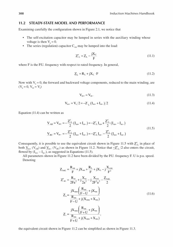
308 Induction Machines Handbook
11.2 STEADY-STATE MODEL AND PERFORMANCE
Examining carefully the configuration shown in Figure 2.1, we notice that
• The self-excitation capacitor may be lumped in series with the auxiliary winding whose voltage is then Va = 0.
• The series (regulation) capacitor Csm may be lumped into the load:
Z Z′ = − jXCL L (11.1)
F
where F is the P.U. frequency with respect to rated frequency. In general,
Z RL = +L LjX ⋅ F (11.2)
Now with Va = 0, the forward and backward voltage components, reduced to the main winding, are (Va = 0, Vm = Vs)
Vm m+ −= V (11.3)
Vm s+ += =V 2 − +Z IL ( )m mI 2− (11.4)
Equation (11.4) can be written as
Z′ ′V L Z L
AB = =Vm+ − ( )I Im+ + =m L− −−Z I′ m+ + ( )I I−2 2 m+ m
(11.5)Z′ Z′
VBC = =V − − L ( )I I+ = Lm
2 m+ m L− −−Z I′ m − ( )I I −2 m+ + m
Consequently, it is possible to use the equivalent circuit shown in Figure 11.5 with Z′L in place of both Vm+ (VAB) and Vm− (VBC) as shown in Figure 11.2. Notice that −Z 2′L also enters the circuit, flowed by (Im+ – Im−), as suggested in Equations (11.5).
All parameters shown in Figure 11.2 have been divided by the P.U. frequency F. U is p.u. speed.Denoting
Z = +Rsm1mL jXsm + +RL jX csm
L − Xj
F F F2
R X X ZZ′ = +sa sa cea 1mL
aL 2 j 2 − −j2Fa 2a 2F2 2a 2
R jXmm rm + jX
F U− rm (11.6)Z =+ Rrm + +j X( )− mm Xrm
F U
R jXmm rm + jX
+ rmF U Z =− ,Rrm + +j X( )
+ mm XrmF U
the equivalent circuit shown in Figure 11.2 can be simplified as shown in Figure 11.3.

309Single-Phase Induction Generators
The self-excitation condition implies that the sum of the currents in node 0 (Figure 11.3) is zero:
1 1= + 1
(11.7)Z Z1mL ++ +Z Z1mL a− Z′ L
Two conditions are provided in (11.7) to solve for two unknowns. We may choose F and Xmm as unknowns provided the magnetization curve: Vg+(Xmm) is known from measurements or from finite element modelling (FEM) calculations.
In reality, Xmm is a known function of the magnetization current: Imm: Xmm(Imm) (Figure 11.4).To simplify the computation process, we may consider that Z− is
Z− ≈ Rrm + jXF U+ rm (11.8)
As, except for Xmm, all other parameters are considered constant, we can express Z+ from (11.7) as
( )Z Z1m + ⋅ ZZ − ′
+ = aL − ZZ Z1mL a+ +− Z′ 1mL (11.9)
L
F - P.U. frequencyU - P.U. speed
A
B
C
0
+
RF - U
jX
F + UjXR
F
I
Z'
I
2F
smsm
m-
L
jXmm
-
Rrm
rm
jXrm
rmmm
jXmm
Z'L2- Xsa
a2 - Xsmj2( )
- jXcea
a22Rsaa2 - R sm
12F( )
Z'L
I m+
RF
smjXsm
FIGURE 11.2 Self-excited self-regulated single-phase IG (Figure 11.1): equivalent circuit for steady state.
0
Z +
Z-
Z 1mL
Z'aL
Z 1mL
I m+
I m-
Zg+Zg+
F
FIGURE 11.3 Simplified equivalent circuit of single-phase generator.
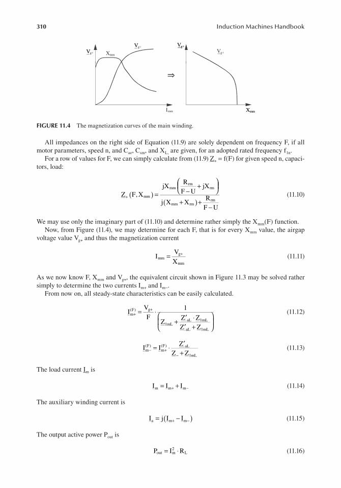
310 Induction Machines Handbook
R jXmm rm + jX
rm F U− Z F+ ( ),Xmm = (11.10)R
j X( )mm + +X rmrm
F U−
I = Vg+mm (11.11)
Xmm
(F) gm = ⋅V + 1
I + (11.12)F Z Z′ ⋅
Z + aL 1mL
1mL Z Z′aL + 1mL
(F) Z′I Im− += ⋅(F) aL
m (11.13)Z Z− + 1mL
I Im m= ++ −Im (11.14)
I ja m= −( )I I+ −m (11.15)
⇒
Xmm
V
I
g+
mm
Vg+
Xmm
Xmm
Vg+VVg+VVg+
FIGURE 11.4 The magnetization curves of the main winding.
All impedances on the right side of Equation (11.9) are solely dependent on frequency F, if all motor parameters, speed n, and Cae, Csm, and XL, are given, for an adopted rated frequency f1n.
For a row of values for F, we can simply calculate from (11.9) Z+ = f(F) for given speed n, capaci-tors, load:
We may use only the imaginary part of (11.10) and determine rather simply the Xmm(F) function.Now, from Figure (11.4), we may determine for each F, that is for every Xmm value, the airgap
voltage value Vg+ and thus the magnetization current
As we now know F, Xmm and Vg+, the equivalent circuit shown in Figure 11.3 may be solved rather simply to determine the two currents Im+ and Im−.
From now on, all steady-state characteristics can be easily calculated.
The load current Im is
The auxiliary winding current is
The output active power Pout is
P 2out = ⋅I Rm L (11.16)

311Single-Phase Induction Generators
The rotor + current component Ir+ becomes
I I= − ⋅ jXmmr m+ + (11.17)Rrm + +j X( )X
F U− rm mm
The total input active power from the shaft Pinput is
≈ ⋅ R U⋅P 2I2 rm
m+ −− ⋅ R Uinput 2I2 rm
F U− m (11.18)F U+
For a realistic efficiency formula, the additional core and mechanical losses piron + pstray + pmec have to be added to the ideal input of (11.18).
η = Pout (11.19)P pinput + +iron p pstray m+ ec
As the speed is given, we change the slip by varying F. We might change the load resistance with frequency (slip) to yield realistic results from the beginning.
As Xmm(Vg+) may be given as a table, the values of Xmm(F) function may be looked up simply into another table. If no Xmm is found from the given data, it means that either the load impedance or the capacitors, for that particular frequency and speed, are not within the existence domain.
So either the load is modified or the capacitor is changed to re-enter the existence domain.The above algorithm may be synthesized as shown in Figure 11.5.
FIGURE 11.5 Performance computation algorithm.
2
ppp,X,R,a,X
R,X,RParameters
++
( )=+ FZ)8.26(Equation
=mmX)9.26(Equation
mmX+gV
mmX+gV
)16.26(EquationI)14.26(EquationI)13.26(EquationI)12.26(EquationI)11.26(EquationI
r
a
m
m
m
=====
+
−
+
mLm
input
out
IZV)18.26(Equation
)17.26(EquationP)15.26(EquationP
⋅==η
==
( )( )( )
( )( )F
FIFPFV
FI:Plot
a
m
m
η
smea C,C
Uspeed
mecstrayiron
rmrm2
sa
sasmsm
ppp,X,R,a,X
R,X,R
++
( )=+ FZ)8.26(Equation
=mmX)9.26(Equation
mmX+gV
mmX+gV
)16.26(EquationI)14.26(EquationI)13.26(EquationI)12.26(EquationI)11.26(EquationI
r
a
m
m
m
=====
+
−
+
mLm
input
out
IZV)18.26(Equation
)17.26(EquationP)15.26(EquationP
⋅==η
==
( )( )(
( )( )F
FIFPFV
FI:Plot
a
out
m
m
η
smea C,C
U
input variables
input variables F
Equation (11.9)
Equation (11.10)
Im+ = Equation (11.11) Im- = Equation (11.12) Im = Equation (11.14) Ia = Equation (11.15) Ir+ = Equation (11.17)
Pout = Equation (11.16) Pinput = Equation (11.18) η = Equation (11.19) Vm = ZL · Im
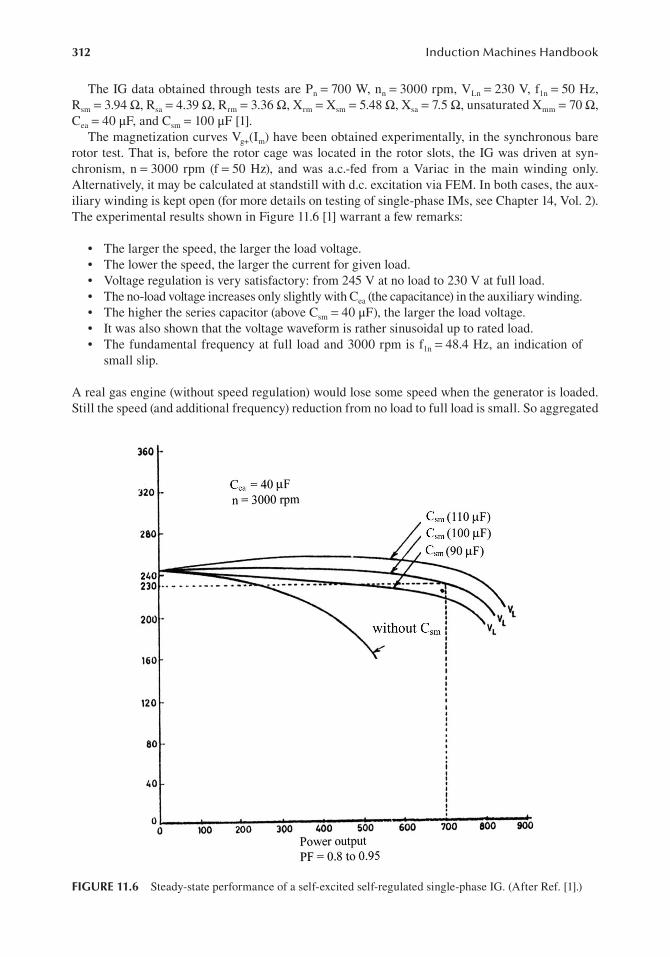
312 Induction Machines Handbook
The IG data obtained through tests are Pn = 700 W, nn = 3000 rpm, VLn = 230 V, f1n = 50 Hz, Rsm = 3.94 Ω, Rsa = 4.39 Ω, Rrm = 3.36 Ω, Xrm = Xsm = 5.48 Ω, Xsa = 7.5 Ω, unsaturated Xmm = 70 Ω, Cea = 40 μF, and Csm = 100 μF [1].
The magnetization curves Vg+(Im) have been obtained experimentally, in the synchronous bare rotor test. That is, before the rotor cage was located in the rotor slots, the IG was driven at syn-chronism, n = 3000 rpm (f = 50 Hz), and was a.c.-fed from a Variac in the main winding only. Alternatively, it may be calculated at standstill with d.c. excitation via FEM. In both cases, the aux-iliary winding is kept open (for more details on testing of single-phase IMs, see Chapter 14, Vol. 2). The experimental results shown in Figure 11.6 [1] warrant a few remarks:
• The larger the speed, the larger the load voltage.• The lower the speed, the larger the current for given load.• Voltage regulation is very satisfactory: from 245 V at no load to 230 V at full load.• The no-load voltage increases only slightly with Cea (the capacitance) in the auxiliary winding.• The higher the series capacitor (above Csm = 40 μF), the larger the load voltage.• It was also shown that the voltage waveform is rather sinusoidal up to rated load.• The fundamental frequency at full load and 3000 rpm is f1n = 48.4 Hz, an indication of
small slip.
A real gas engine (without speed regulation) would lose some speed when the generator is loaded. Still the speed (and additional frequency) reduction from no load to full load is small. So aggregated
FIGURE 11.6 Steady-state performance of a self-excited self-regulated single-phase IG. (After Ref. [1].)

313Single-Phase Induction Generators
voltage regulation is, in these conditions, at full load, slightly larger but still below 8%, with a speed drop from 3000 to 2920 rpm [1].
11.3 THE d-q MODEL FOR TRANSIENTS
The transients may be treated directly via d-q model in stator coordinates with saturation included (as done for motoring).
dIVds = −V Rcsm L− −I L ds
ds L (11.20)dt
dVCsm 1= I ;ds I =ds Im (11.21)
dt Csm
Vq C= −V ea (11.22)
dVCea 1 W K= = a Wa (11.23)dt a C2 I ;qs I Iqs a ⋅ =a; a
ea W Km Wm
The d-q model in Section 11.2 is
dΨds = −V (ds t) R Ism dsdt
dΨqs R= −V − sacea Iqs
dt a2
(11.24)dΨdr = −I Rdr rm ω Ψr qr
dt
dΨqr = +I Rqr rm ω Ψr drdt
ψds = +L Ism ds Ψ Ψdm; Ldm = mmIdm
ψ =dr L Irm dr + Ψqm; LΨ =qm mmIqm
Lψ saqs = +
a2 I ;qs Ψ =qm I Idm ds + Idr (11.25)
ψ =qr L Irm qr + Ψqm; Iqm = +I Iqs qr
and : ψ =m mL Im m( )⋅ =I ; 2m mI Idm + I2
qm
To complete the model, the motion equation is added
J dωr = +T Tpmover ep1 dt (11.26)
T pe 1= ψ( )dsI Iqs − Ψqs ds < 0
The prime mover torque Tpmover may be dependent on speed or/and on the rotor position also. The equations of the prime mover speed governor (if any) may be added.

314 Induction Machines Handbook
Equation (11.20) shows that when the load contains an inductance LL (e.g. a single-phase IM), Ids has to be a variable and thus the whole d-q model (Equation 11.24) has to be rearranged to accom-modate this situation in the presence of magnetic saturation.
However, with resistive load (RL) − LL = 0 – the solution is straightforward with Vcsm, Vcea, Ψds, Ψqs, Vqs, Ψdr, Ψqr, and ωr as variables.
If the speed ωr is a given function of time, the motion Equation (11.26) is simply ignored. The self-excitation under no load, during prime mover start-up, load sudden variations, load dumping, or sudden short circuit are typical transients to be handled via the d-q model.
11.4 EXPANDING THE OPERATION RANGE WITH POWER ELECTRONICS
Power electronics can provide more freedom to the operation of single-phase IMs in terms of load voltage and frequency control [3]. An example is shown in Figure 11.7 [4].
The auxiliary winding is now a.c.-fed at the load frequency f1, through a single-phase inverter, from a battery.
To filter out the double-frequency current produced by the converter, the Lf, Cf filter is used. Ca filters the d.c. voltage of the battery.
The main winding reactive power requirement may be reduced by the parallel capacitor Cm with or without a short- or a long-shunt series capacitor.
By adequate control in the inverter, it is possible to regulate the load frequency and voltage when the prime mover speed varies.
The inverter may provide more or less reactive power.It is also possible that, when the load is large, the active power is contributed by the battery. On
the other hand, when the load is low, the auxiliary winding can pump back active power to recharge the battery.
This potential infusion of active power from the battery to load may lead to the idea that, in principle, it is possible to operate as a generator even if the speed of the rotor ωr is not greater than ω1 = 2πf1. However, as expected, more efficient operation occurs when ωr > ω1.
The auxiliary winding is 90° (electrical) ahead of the main winding, and thus, no pulsation-type interaction with the main winding exists. The interaction through the motion emfs is severely fil-tered for harmonics by the rotor currents. So the load voltage is practically sinusoidal. The investi-gation of this system may be performed through the d-q model, as presented in the previous section (for more details on this subject in [5,6], see Ref. [4]).
A series connected capacitor in the short shunt for the output winding has been proved to reduce drastically voltage regulation [7], even when the IG is self-excited [8].
FIGURE 11.7 Single-phase IG with battery inverter-fed auxiliary winding.
Cm
main
load
single phase IMsinglephaseinvertor
d.c.voltagefilter
filter2f
battery
VL
Caux
f
cc
a
f
1
C
single phase IM single-phase inverter

315Single-Phase Induction Generators
11.5 SUMMARY
• The two winding IM may be used for low-power autonomous single-phase generators.• Among many possible connections, it seems that one of the best connects the auxiliary
winding upon an excitation capacitor Cea, while the main winding (provided with a self-regulation series capacitors Csm) supplies the load.
• The steady-state modelling may be done with the revolving theory (+, − or f, b) model.• The saturation plays a key role in this self-excited self-regulated configuration.• The magnetic saturation is related, in the model, to the direct (+) forward component.• A rather simple computer program can provide the steady-state characteristics: output volt-
age, current, frequency versus output power for given speed, machine parameters, and magnetization curve.
• Good voltage regulation (<8%) has been reported.• The sudden short circuit apparently does not threaten the IG integrity.• The transients may be handled through the d-q model in stator coordinates via some addi-
tional terminal voltage relationships.• More freedom in the operation of single-phase IG is brought by the use of a fractional
rating battery-fed inverter to supply the auxiliary winding. Voltage and frequency control may be provided this way. Also, bi-directional power flow between inverter and battery can be performed. So the battery may be recharged when the IG load is low.
• A three-phase IM operating as single-phase IG with promising performance is described in Ref. [9].
• In the power range of 10–20 kW, the single-phase IG represents a strong potential competi-tor to existing gensets using synchronous generators.
• Using three-phase IGs with inverter excitation at load winding terminals to yield single-phase a.c. power generation may also produce a strong competitor to small-power synchro-nous generators [10].
REFERENCES
1. S. S. Murthy, A novel self-excited self-regulated single phase induction generator, part I + II, IEEE Transactions on Energy Conversion, Vol. 8, No. 3, 1993, pp. 377–388.
2. O. Ojo, Performance of self-excited single-phase induction generators with short shunt and long shunt connections, IEEE Transactions on Energy Conversion, Vol. 11, No. 3, 1996, pp. 477–482.
3. D. W. Novotny, D. J. Gritter, G. H. Studmann, Self-excitation in inverter driven induction machines, IEEE Transactions on Power Apparatus and Systems, Vol. 96, No. 4, 1977, pp. 1117–1125.
4. O. Ojo, O. Omozusi, A. A. Jimoh, Expanding the operating range of a single-phase induction generator with a PWM inverter, Record of IEEE-IAS-1998, St. Louis, MI, 1998, Vol. 1, pp. 205–212.
5. W. Jazdzynski, Optimum designed induction motors with die-cast aluminum and cooper cages: A com-parative study, Record of ICEM-2006, Greece, 2006, pp. 464–468.
6. A. Kuperman, V. Spitsa, R. Rabinovici, E. Zeev, G. Weiss, Design of a robust controller for an induction generator in an autonomous power system, Record of ICEM-2006, Greece, 2006, pp. 539–543.
7. D. Lamabadu, S. Rajakaruna, Dynamic analysis of novel single-phase induction generator using an improved machine model, IEEE Transactions on Energy Conversion, Vol. 32, No. 1, 2017, pp. 1–11.
8. S. S. Murthy, B. Singh, V. Sandeep, A novel and comprehensive performance analysis of a single-phase two-winding self-excited induction generator, IEEE Transactions on Energy Conversion, Vol. 27, No. 1, 2012, pp. 117–127.
9. S. N. Mahato, S. P. Singh, M. P. Sharma, Capacitors required for maximum power of a self-excited single-phase induction generator using a three-phase machine, IEEE Transactions on Energy Conversion, Vol. 23, No. 2, 2008, pp. 372–381.
10. B. Singh, S. Sharma, Stand-alone single-phase power generation employing a three-phase isolated asyn-chronous generator, IEEE Transactions on Industry Applications, Vol. 48, No. 6, 2012, pp. 2414–2423.

317
12 Linear Induction Motors
12.1 INTRODUCTION
For virtually every rotary electric machine, there is a linear motion counterpart. So is the case with induction machines. They are called linear induction machines.
Linear induction motors (LIMs) develop directly an electromagnetic force, called thrust, along the direction of the travelling field motion in the airgap.
The imaginary process of “cutting” and “unrolling” rotary counterpart is illustrated in Figure 12.1.
The primary contains in general a three-phase winding in the uniform slots of the laminated core.
The secondary is made of either a laminated core with a ladder cage in the slots or an aluminium (copper) sheet with (or without) a solid iron back core.
Apparently, the LIM operates as its rotary counterpart does, with thrust instead of torque and linear speed instead of angular speed, based on the principle of travelling field in the airgap.
In reality, there are quite a few differences between linear and rotary IMs such as the following [1–8]:
• The magnetic circuit is open at the two longitudinal ends (along the travelling field direc-tion). As the flux law has to be observed, the airgap field will contain additional waves whose negative influence on performance with LIM in motion is called dynamic longitu-dinal end effect (Figure 12.2a).
• In short primaries (with two, four poles), there are current asymmetries between phases due to the fact that one phase has a position to the core longitudinal ends which is different from those of the other two. This is called static longitudinal effect (Figure 12.2b).
• Due to same limited primary core length, the back iron flux density tends to include an additional nontravelling (ac) component which should be considered when sizing the back iron of LIMs (Figure 12.2c).
• In the LIM shown in Figure 12.1 (called single sided, as there is only one primary along one side of secondary), there is a strong normal force (of attraction or repulsion type) between the primary and secondary. This normal force may be put to use to compensate for part of the weight of the moving primary and thus reduce the wheel wearing and noise level (Figure 12.2d).
• For secondaries with aluminium (copper) sheet with (without) solid back iron, the induced currents (in general at slip frequency Sf1) have part of their closed paths contained in the active (primary core) zone (Figure 12.2e). They have additional – longitudinal (along OX axis) – components which produce additional losses in the secondary and a distortion in the airgap flux density along the transverse direction (OY). This is called the transverse edge effect.
FIGURE 12.1 Imaginary process of obtaining a LIM from its rotary counterpart.

318 Induction Machines Handbook
secondarycurrent density paths
at zero slip
primary
a.) dynamic longitudinal effect
12001200
i
i
i
a
b
c
x
τ τ
0
airgapflux lines
S=1
c.) back core flux density distribution
iron
Alsecondary
currentdensity
x
repulsion normal force (F )nr
attraction normal force (F )na
z
y
primarycurrent
primary
F =F -Fnrnan
d.) nonzero normal force Fn
Jy
Jx
zero secondary currents
nonzero secondary currents
y
Bz
0e.) transverse edge effect
x x
∆primary
ejection lateral force (F )le
y
realigning lateral force (F )lra
F =F -Flralee
0
f.) nonzero lateral force Fe
(a) dynamic longitudinal effect
120°120°
(c) back core f lux density distribution
(d) nonzero normal force Fn
(e) transverse edge effect
(f ) nonzero lateral force Fe
(b) static longitudinal effect
FIGURE 12.2 Panoramic view of main differences between LIMs and rotary IMs.
• When the primary is placed off centre along OY, the longitudinal components of the cur-rent density in the active zone produce an ejection-type lateral force. At the same time, the secondary back core tends to realign the primary along OY. So the resultant lateral force may be either decentralizing or centralizing in character (Figure 12.2f).
All these differences between linear and rotary IMs warrant a specialized investigation of field distribution and performance in order to limit the adverse effects (longitudinal end effects and back iron flux distortion, etc.) and exploit the desirable ones (normal and lateral forces, or transverse edge effects).
The same differences suggest the main merits and demerits of LIMs:Merits
• Direct electromagnetic thrust propulsion (no mechanical transmission or wheel adhesion limitation for propulsion)
• Ruggedness; very low maintenance costs

319Linear Induction Motors
• Easy topological adaptation to direct linear motion applications• Precision linear positioning (no play (backlash) as with any mechanical transmission)• Separate cooling of primary and secondary• All advanced drive technologies for rotary IMs may be applied without notable changes
to LIMs.
Demerits
• Due to large airgap-to-pole pitch (g/τ) ratios – g/τ > 1/250 – the power factor and efficiency tend to be lower than with rotary IMs. However, the efficiency is to be compared with the combined efficiency of rotary motor + mechanical transmission counterpart. Larger mechanical clearance is required for speeds above 3 m/s. The aluminium sheet (if any) in the secondary contributes an additional (magnetic) airgap.
• Efficiency and power factor are further reduced by longitudinal end effects. Fortunately, these effects are notable only in high-speed low-pole count LIMs, and they may be some-what limited by pertinent design measures.
• Additional noise and vibration due to uncompensated normal force, unless the latter is put to use to suspend the mover (partially or totally) by adequate close loop control.
As sample LIM applications have been presented in Chapter 1, Vol. 1, we may now pro-ceed with the investigation of LIMs, starting with classifications and practical construction aspects.
12.2 CLASSIFICATIONS AND BASIC TOPOLOGIES
LIMs may be built single sided (Figure 12.1) or double sided (Figure 12.3a), with moving (short) primary (Figure 12.1) or moving (short) secondary (Figure 12.3b).
As single-sided LIMs are more rugged, they have been used in more applications. Figure 12.3b shows a double-sided practical short-moving secondary LIM for low-speed short-travel applications.
LIMs shown in Figures 12.1–12.3 are flat. For flat single-sided LIMs, the secondaries may be made of aluminium (copper) sheets on back solid iron (for low costs), ladder conductor in slots of laminated core (for better performance), and a pure conducting layer in electromagnetic metal stir-rers (Figure 12.4a–c).
In double-sided LIMs, the secondary is made of an aluminium sheet (or structure) or from a liquid metal (sodium) as in flat LIM pumps.
Besides flat LIMs, tubular configurations may be obtained by rerolling the flat structures along the transverse (OY) direction (Figure 12.5). Tubular LIMs or tubular LIM pumps are in general single sided and have short fix primaries and moving limited length secondaries (except for liquid metal pumps).
FIGURE 12.3 Double-sided flat LIMs (a) double-sided short (moving) primary LIM and (b) double-sided short (moving) secondary LIM for conveyors.
long (fix) secondary
aluminum sheet
short (moving)primaries
short (moving) secondary element
double-sided long (fix) primary
(b)(a)

320 Induction Machines Handbook
conductingsheet
solidback iron
conductingladder
laminatedsecondary core
with slots
fixedprimary
liquid metal
(a)
(c)
(b)
FIGURE 12.4 Flat single-sided secondaries (a) sheet on iron, (b) ladder conductor in slots, (c) liquid metal.
conductor sheet
secondary back iron
primary circularcoils
2pτprimarystacks
(a)
moving secondary
disk shapelaminations
ring shapesecondary
conductors in slots
primarythermal
insulation
liquidsodiumchannel
stainlesssteel shell
secondaryback iron (yoke)
center return pipe (if any)
A C’ B A’ C B’ circular coils
(b)
(c)
FIGURE 12.5 Tubular LIMs: (a) with longitudinal primary lamination stacks, (b) with disk-shaped lamina-tions, and (c) liquid metal tubular LIM pump: the secondary.

321Linear Induction Motors
The primary core may be made of a few straight stacks (Figure 12.5a) with laminations machined to circular stator bore shape. The secondary is typical aluminium (copper) sheet on iron. The stator coils have a ring shape.
While transverse edge effect is absent and coils appear to lack end connections, building a well-centred primary is not easy.
An easier-to-build solution is obtained with only two-size disk-shaped laminations on both pri-mary and secondary (Figure 12.5b). The secondary ring-shaped conductors are thus placed also in slots.
Better performance is expected though the fact that, in the back cores, the magnetic field goes perpendicular to laminations, which tends to produce additional core losses. The interlamina-tion insulation leads to an increased magnetization mmf and thus takes back part of this notable improvement.
The same rationale is valid for tubular LIM liquid metal pumps (Figure 12.5c) in terms of pri-mary manufacturing process. Pumps allow for notably higher speeds (u = 15 m/s or more) when the fixed primaries may be longer and have more poles (2p1 = 8 or more). The liquid metal (sodium) low electrical conductivity leads to a smaller dynamic longitudinal effect which at least has to be checked to see whether it is negligible.
12.3 PRIMARY WINDINGS
In general, three-phase windings are used as three-phase PWM converters are widely available for rotary induction motor drives. Special applications which require only 2p1 = 2 pole might ben-efit from two-phase windings as two-phase windings are both placed in the same position with respect to the magnetic core ends. Consequently, the phase currents are fully symmetric at very low speeds.
LIM windings are similar to those used for rotary IMs, and ideally, they produce a pure travel-ling mmf. However, as the magnetic circuit is open along the direction of motion, there are some particular aspects of LIM windings.
Among the possible winding configurations, we illustrate here a few:
• Single-layer full-pitch (y = τ) windings with even number of poles 2p1 (Figure 12.6): three phase and two phase.
• Triple-layer chorded-coil (y/τ = 2/3) winding with even number of poles 2p1 (Figure 12.7).• Double-layer chorded-coil (2/3 < y/τ < 1) coil winding with odd number of poles 2p1 + 1
(the two end poles have half-filled slots) (Figure 12.8).• Fractionary winding for miniature LIMs (Figure 12.9).
A few remarks are in order
• The single-layer winding with an even number of poles makes better usage of primary magnetic core, but it shows rather large coil end connections. It is recommended for 2p1 = 2, 4.
• The triple-layer chorded-coil winding is easy to manufacture automatically; it has low end connections and also has a rather low winding (chording) factor Ky = 0.867.
• The double-layer chorded-coil winding with an odd total number of poles (Figure 12.8) has shorter end connections and is easier to build, but it makes a poorer use of primary magnetic core as the two end poles are half-wound. As the number of poles increases above seven, nine, the end poles influence becomes small. It is recommended thus for low-, medium-, and high-speed LIMs (2p1 + 1 > 5).
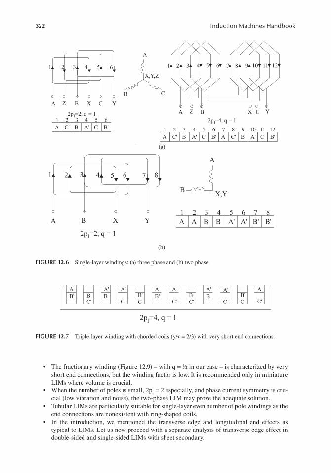
322 Induction Machines Handbook
A
B' B
C'
A'
B
A'
C
B'
C
A
B'
A
C'
B
C'
A'
B
A'
C
B'
C
A
C'
2p =4, q = 11
FIGURE 12.7 Triple-layer winding with chorded coils (y/τ = 2/3) with very short end connections.
• The fractionary winding (Figure 12.9) – with q = ½ in our case – is characterized by very short end connections, but the winding factor is low. It is recommended only in miniature LIMs where volume is crucial.
• When the number of poles is small, 2p1 = 2 especially, and phase current symmetry is cru-cial (low vibration and noise), the two-phase LIM may prove the adequate solution.
• Tubular LIMs are particularly suitable for single-layer even number of pole windings as the end connections are nonexistent with ring-shaped coils.
• In the introduction, we mentioned the transverse edge and longitudinal end effects as typical to LIMs. Let us now proceed with a separate analysis of transverse edge effect in double-sided and single-sided LIMs with sheet secondary.
1 42 53 6
A Z B X C Y
2p =2; q = 11
A
1
C'
2
B
3
A'
4
C
5
B'
6
A
B C
X,Y,Z
1 42 53 6 7 108 119 12
A Z B X C Y
A
1
C'
2
B
3
A'
4
C
5
B'
6
2p =4; q = 11
A
7
C'
8
B
9
A'
10
C
11
B'
12
a.)
(a)
1 62 53 84 7
A B X Y
2p =2; q = 11
A
BX,Y
A
1
A
2
B
3
B
4
A'
5
A'
6
B'
7
B'
8
(b)
FIGURE 12.6 Single-layer windings: (a) three phase and (b) two phase.

323Linear Induction Motors
12.4 TRANSVERSE EDGE EFFECT IN DOUBLE-SIDED LIM
A simplified single-dimensional theory of transverse edge effect is presented here.The main assumptions are
• The stator slotting is considered only through Carter coefficient Kc:
g 2
1 bK os
c = ; γ = (12.1)1 g− γ /τ g
s 5 + γbos
• The primary winding in slots is replaced by an infinitely thin current sheet travelling wave J1 (x, t)
A C B X Z Y
A
1
C'
2
B
3
A'
4
C
5
B'
6
A
7
C'
8
B
9
A'
10
C
11
B'
12
A' C B' A C' B A' C B' A C' B
13 14
2p +1 = 5; q = 1, y/ = 2/3τ1
2p +1 = 7; q = 2, y/ = 5/6τ1
FIGURE 12.8 Double-layer chorded-coil windings with 2p1 + 1 poles.
1 2 3 4 5 6
A C B X Z Y
2p =2, q = 1/2, m = 3phases1
A B X Y
2p =2, q = 1/2, m = 2phases1
(a) (b)
FIGURE 12.9 Fractionary single-layer winding (low end connections) (a) three phase and (b) two phase.

324 Induction Machines Handbook
π j S ω −1t x 3 2W K
J (x, t) = =J e τ ; J 1 w1 1I1 m m in Aturns/m (12.2)
p1τ
where S – slip, 2p1 – pole number, W1 – turns/phase, Kw1 – winding factor, τ – pole pitch, and I1 – phase current (RMS). Coordinates are attached to secondary.
• The skin effect in the secondary conductor sheet is neglected or considered through the standard correction coefficient:
d d sinh + sin d d
K s s d skin ≈ ≥ 1 (12.3)
2ds d d cosh − cos ds s d
1 µ ω0 1Sσ≈ Al (12.4)ds 2
For single-sided LIMs, d/ds will replace 2d/ds in (12.3); ds – skin depth in the aluminium (copper) sheet layer. Consequently, the aluminium conductivity is corrected by 1/Kskin:
σ = σAlAls (12.5)
Kskin
• For a large airgap between the two primaries, there is a kind of flux leakage which makes the airgap look larger gl [1].
g gl c= K Kleakage
g sinh 2τ Kleakage = > 1 (12.6)g
2τ
• Only for large g/τ ratio, Kleakage is notably different from unity. The airgap flux den-sity distribution in the absence of secondary shows the transverse fringing effect (Figure 12.10).
FIGURE 12.10 Fringing and end-connection flux considerations.
g
a
ae
a
ae

325Linear Induction Motors
The transverse fringing effect can be calculated by introducing a larger (equivalent) stack width 2ae instead of 2a:
2ae = +2a (1.2 ÷ 2.0)g (12.7)
For large airgap in low-thrust LIMs this effect is notable.As expected, the above approximations may be eliminated provided a 3D finite element
modelling (FEM) was used. The amount of computation effort for a 3D-FEM model is so large that it is feasible mainly for special cases rather than for preliminary or optimization design.
• Finally, the longitudinal effects are neglected for the time being, and space variations along thrust direction and time variations are assumed to be sinusoidal.
In the active region (|z| ≤ ae), Ampere’s law along contour 1 (Figure 12.11) yields
∂H π j t g y ω − x
e = = 1
J d; J J e τ
∂z 2x 1 m (12.8)
Figure 12.11b shows the active and overhang regions with current density along motion direction.The same law applied along contour 2 (Figure 12.11b) in the longitudinal plane gives
∂−ge H H+ = J Jm + d (12.9)∂x
( )x 0 2z
Faraday’s law also yields
∂J2z ∂J− 2x = − j Sµ ω∂ 0 1σ +Als
x( )H H
∂z y 0 (12.10)
Equations (12.8)–(12.10) are all in complex terms as sinusoidal time variation was assumed.H0 is the airgap field in the absence of secondary:
jJH m
0 = (12.11)πg
τ e
The three equations above combine to yield
∂2 Hy ∂2 H d d2 + y − µj Sω σ H j= µ Sω σ H (12.12)
∂x ∂z2 0 1 Alsg y 0 1 Als
e g 0e
FIGURE 12.11 Transverse cross section of a double-sided LIM (a) and longitudinal view (b).
ae ae
y
1
over-
hang
regionb c
z
J2x
J (x,t)1
y
x
2
J
(a) (b)
xx
2zover-
hang
region
active region

326 Induction Machines Handbook
The solution of (12.12) becomes
jH SGH 0 e
y = − + αA cosh z + αBsinh z (12.13)1 j+ SGe
with
τ ω2
G = 1 0µ σAls di π2 (12.14)
ge
2 π 2
α = ( )1 j+ SGτ e (12.15)
Gi is called the rather ideal goodness factor of LIM, a performance index we will return to fre-quently next.
In the overhang region (|z| > ae), we assume that the total field is zero; that is, J2z and J2x satisfy Laplace’s equation:
∂J2z ∂J− 2x = 0 (12.16)∂x ∂z
Consequently,
πJ C2zr = sinh (c − <z) a z ≤
τ e c
(12.17)π
J j2xr = C cosh (c z− )τ
πJ D2zl = sinh (b + −z) b z< < −a
τ e
(12.18)π
J j2xl = D cosh (b z+ )τ
where r and l refer to right and left, respectively.From the continuity boundary conditions at z = ±ae, we find
H jSGi ( )C C1 2 cosh a 2e e0+ α( ) + αsinh ( )a
A = (12.19)1 j+ SGi ( )1 C+ α1 2C sinh 2( )a Ce + +( )1 2C cosh 2( )αae
A C( )C sinh aB ( )
2 1− α( )= e
C C1 2+ αcosh ( )a 2e e+ αsinh ( ) a
C t1 = ατ πanh c( )− = ατ π
a ;e C t2 anh b( )− ae (12.20)π τ π τ
− αjgC = e
A sinh aα + 1π ( )e eBcosh a( )α ( 2.21)d cosh c − a
τ( )e
− αjgD = e − αA sinh a( )e e+ αBcosh a( ) (12.22)π
d cosh b − aτ
( )e

327Linear Induction Motors
a
Fza = µ0 1d pτ Re ∫e
( )J H∗2x y dz (12.23)
−ae
6µ ω0 1 ( )W K 2 ( )
X = 1 w1 τ 2aem 2 (12.24)
π p g1 1
FIGURE 12.12 Transverse distribution of flux and secondary current densities. (After Ref. [5].)
Sample computation results of flux and current densities distributions for a rather high-speed LIM with the data – τ = 0.35 m, f1 = 173.3 Hz, S = 0.08, d = 6.25 mm, g = 37.5 mm, Jm = 2.25 · 105 A/m – are shown in Figure 12.12 [5].
The transverse edge effect produces a “deep” in the airgap flux density transverse (along OZ) distribution. Also, if the secondary is placed off centre, along OZ, the distribution of both secondary current density components is nonsymmetric along OZ.
The main consequences of transverse edge effect are an apparent increase in the secondary equivalent resistance R′2 and a decrease in the magnetization inductance (reactance Xm). Besides, when the secondary is off centre in the transverse (lateral) direction, a lateral decentralizing force Fza is produced:
Again sample results for the same LIM as above are given in Figure 12.13.The lateral force Fz decreases as ae/τ decreases or the overhangs c-ae, b-ae > τ/π. In fact, there
is no use to extend the overhangs of secondary beyond τ/π as there are hardly any currents for |z| > |τ/π + ae|.
12.4.1 t he tranSverSe eDge eFFect correction coeFFicientS
In the absence of transverse edge effect, the magnetization reactance Xm has the conventional expression (for rotary induction machines):

328 Induction Machines Handbook
X 12( )W K 2 a
R′ m 1 w1 e2 = = (12.25)
Gi σ τAls 1p d
K2 1 S+ 2
X G K2 2 2
K = i R KX
t 2 2 ≥ 1 (12.26)KR 1 S+ Gl
K K
K R tm = ≤ 1 (12.27)
KX
λKR i= −1 Re 1( )− SG tanh ( ) αae (12.28)
αae
K = +1 Re j( ) SG+ SG i λX i ( )tanh αa (12.29)
αae
e
1λ = (12.30)π
1 1+ +( )jSG t1/2
i anh a( )α ⋅e etanh −τ
( )c a
1
Kt ≈ (12.31)πtanh a
τ e π π −1
1− +1 tanh a ⋅ ( )− e etanh c aπ a τ τ
τ e
0.1 0.2La
tera
l dec
entra
lizin
gfo
rce
(N)
0.2 105
0.1 105
2p =12poles1
b-c (m)b – c (m)
FIGURE 12.13 Decentralizing lateral force Fz.
The secondary resistance reduced to the primary R′2 is
Because of the transverse edge effect, the secondary resistance is increased by Kt > 1 times and the magnetization inductance (reactance) is decreased by Km < 1 times:
For b = c [9],
For LIMs with narrow primaries (2ae/τ < 0.3) and at low slips, Km ≈ 1 and
Transverse edge effect correction coefficients depend on the goodness factor Gi, slip, S, and the geometrical type factors ae/τ, (c − ae)/τ.

329Linear Induction Motors
u 2= τ ωs 1f = τ 1 (12.32)
π
K
G G me i= < G (12.33)
Ki
t
K K
g g c leake = > g (12.34)
Km
σ = σAle < σAl (12.35)
K Kskin t
larger area overhang
primary
secondary
FIGURE 12.14 Reduced transverse edge effect secondary.
For b ≠ c, the correction coefficients have slightly different expressions, but they may be eventu-ally developed based on the flux and secondary current densities transverse distribution.
The transverse edge effect may be exploited for developing large thrusts with lower currents or may be reduced by large overhangs (up to τ/π) and an optimum ae/τ ratio.
On the other hand, the transverse edge effect may be reduced, when needed, by making the over-hangs of a larger cross section or of copper (Figure 12.14).
In general, the larger the value of SGi, the larger the transverse edge effect for given ae/τ and c/τ. In low-thrust (speed) LIMs, the pole pitch τ is small, so is the synchronous speed us
Consequently, the goodness factor Gi is rather small, below, or slightly over unity.Now, we may define an equivalent – realistic – goodness factor Ge as
where the transverse edge effect is also considered.Alternatively, the combined airgap leakage (Kleak), skin effect (Kskin), and transverse edge effect
(Km, Kt) may be considered as correction coefficients for an equivalent airgap ge and secondary conductivity σe:
We notice that all these effects contribute to a reduction in the realistic goodness factor Gi.
12.5 TRANSVERSE EDGE EFFECT IN SINGLE-SIDED LIM
For the single-sided LIM with conductor sheet on iron secondary (Figure 12.15), a similar simpli-fied theory has been developed where both the aluminium and saturated solid back iron contribu-tions are considered [5,7].

330 Induction Machines Handbook
1
Kti = (12.36)π itan
τ a1− e
π iτ ae
σ = σ ironti (12.37)
Kti
π 2
− δ 1 σi = Real + ωjS iron
1 iµ ron (12.38) τ K ti
τ B
B gxi = K ;pf 1 K≤ <pf 2 (12.39)
π δi
σ 1 σ δ K σ = Al
e + iron i skinal (12.40)
Kskinal Kta σAlK dti
d
y
z
primary
Al sheet
y
x
ironδ i
3 thick laminationback core
x Al
FIGURE 12.15 Single-side LIM with three thick lamination secondary back core.
The division of solid secondary back iron into, say, three (i = 3) pieces along transverse direction leads to a reduction of eddy currents. This is due to an increase in the “transverse edge effect” in the solid back iron.
As there are no overhangs for secondary back iron (c-ae = 0), the transverse edge effect coef-ficient Kti of (12.31) becomes
Now, an equivalent iron conductivity σti may be defined as
The depth of field penetration in the secondary back iron δi is thus
The iron permeability μiron depends mainly on the tangential (along OX) flux density Bxi, in fact, on its average over the penetration depth δi
where Bg is the given value of airgap flux density, and Kpf accounts for the increase in back-core maximum flux density in LIMs due to its open magnetic circuit along axis x [2,7]; Kpf = 1 for rotary IMs.
Now we may define an equivalent conductivity σe of the aluminium to account for the secondary back iron contribution
where Kskinal is the skin effect coefficient for aluminium (12.3), and Kta the transverse edge effect coefficient for aluminium.
In a similar way, an equivalent airgap may be defined which accounts for the magnetic path in the secondary by a coefficient Kp:

331Linear Induction Motors
= +( ) K Kg 1e pK g c leak (12.41)
Kma
τ2 µK = 0
p π2 (12.42)2gKc iδ µiron
Kp may not be neglected even if the secondary back iron is not heavily saturated.Now the equivalent goodness factor Ge may be written as
µ ω τ σ2
G = 0 1 ede π2 (12.43)
ge
The problem is that Ge depends on ω1, S, and μiron, for given machine geometry.An iterative procedure is required to account for magnetic saturation in the back iron of sec-
ondary (μiron). The value of the resultant airgap flux density Bg = μ0(H + H0) can be obtained from (12.13) and (12.11) by neglecting the Z-dependent terms:
µ τ JB m 3 2I W kW≈ 0 1
g ( ) , J 1 1m ≈ (12.44)
π +ge 1 jSGe pτ
For a given value of Bg, S, W1, Kt, Kma, and Kti are directly calculated. Then, from (12.38) to (12.39) and the iron magnetization curve, μiron (and Bxi, and δi) is iteratively calculated.
Then, σe and ge are calculated from (12.40) to (12.42). Finally, Ge is determined. The primary phase current I1 is computed from (12.44).
All above data are used to calculate the LIM thrust and other performance indices to be dis-cussed in the next section using a technical longitudinal effect theory of LIMs.
12.6 A TECHNICAL THEORY OF LIM LONGITUDINAL END EFFECTS
Although we will consider the double-sided LIM, the results to be obtained here are also valid for single-sided LIMs with the same equivalent airgap ge and secondary conductivity σe.
The technical theory as introduced here relies on a quasi-one-dimensional model attached to the short (moving) primary. Also, for simplicity, the primary core is considered infinitely long, but the primary winding is of finite length (Figure 12.16). All effects discussed in the previous section enter the values of σe, ge and Ge, and the primary mmf is replaced by the travelling current sheet J1 (12.2). Complex variables are used as sinusoidal time variations are considered.
In the active zone (0 ≤ x ≤ 2p1τ), Ampere’s law along abcd (Figure 12.16) yields
∂H π j t ω −1 xg t = +J e τ
e ∂ 1 J d2 (12.45)x
where Ht is the resultant magnetic field in airgap. It varies only along OX axis. Also the secondary current density J2 has only one component (along OZ).
FIGURE 12.16 Double-sided LIM with infinitely long primary core.
y
xz a b
cd
J2
J1
active zone
2pτenoztixeenozyrtne
g d
x

332 Induction Machines Handbook
Faraday’s law is applied to moving bodies:
∂Bcurl E = − + ⋅u B; J = σeE (12.46)
∂t
yields
∂J2 ∂H= ωj H t1 0µ σe t + µ0 euσ (12.47)
∂x ∂x
where u is the relative speed between primary and secondary.Equations (12.45) and (12.47) can be combined into
∂2 H H π π
− µj xt ∂ −
2 0 euσ′ t − ωj H1 0µ σ =′e t − j J e τ 2∂x ∂x g
m (1 .48)τ e
dσ =′e eσ (12.49)ge
The characteristic equation of (12.48) becomes
γ −2 µ0 eσ γ′u j− ω1 0µ σ =′e 0 (12.50)
Its roots are
a b 1+ b 1γ = ± 1 1 ± +1 j 1 −
1,2 = γ ± γj (12.51)2 2 2
1,2r i
with
a1 0= µ σ = π′e eu G (1− S) (12.52)τ
24
b 11 = + (12.53) G (e 1 S− )2
The complete solution of Ht within active zone is
π−H (x) = +
j xA eγ γ1 2x x
ta t B et + B e τn (12.54)
with
j Jτ u u−Bn = m ; S = s (12.55)
π +g 1e e( )SG us
The coefficient e j tω1 is to be added.In the entry (x < 0) and exit (x > 2p1τ) zones, there are no primary currents. Consequently,
H Centry = ≤ee ;γ1x x 0 (12.56)
H Dexit = >2xee ;γ x 2p1τ (12.57)
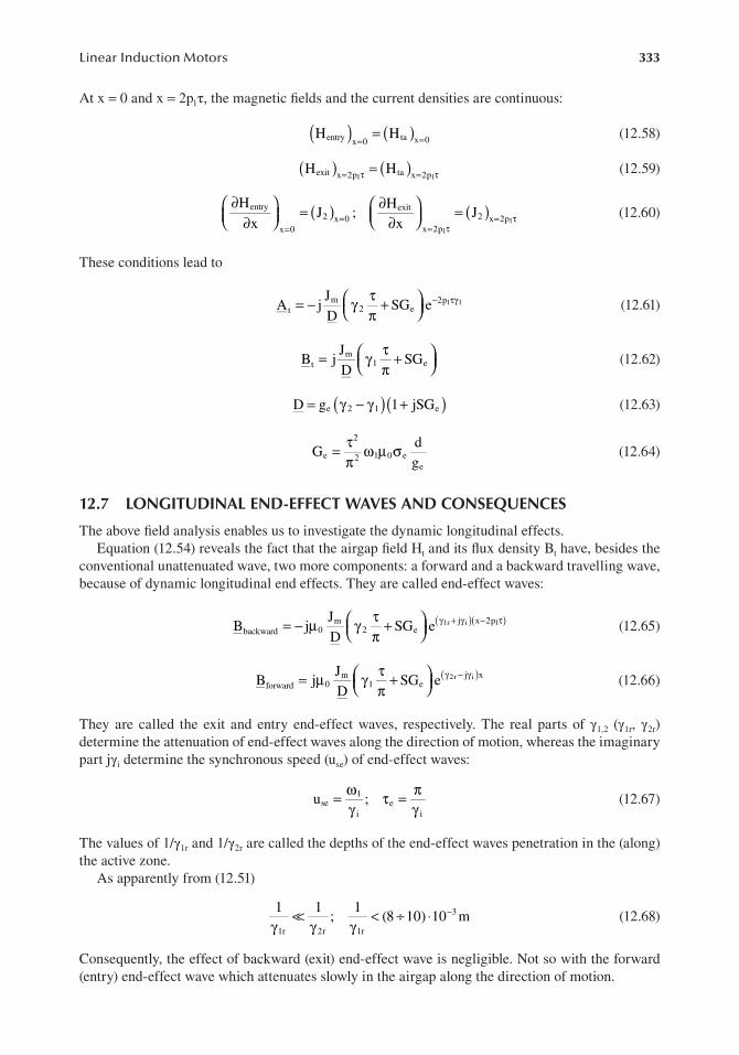
333Linear Induction Motors
At x = 0 and x = 2p1τ, the magnetic fields and the current densities are continuous:
(H Hexit ) ( tax 2p = )x 2p (12.59)= τ1 1= τ
∂Hentry ∂H = ( )J ;2 x 0
exit = ( )J
∂x = ∂ 2
x 0 x x 2p (12.60)1
= = τx 2= τp1
(H Hentry ) = ( )ta x 0 (12.58)x 0= =
These conditions lead to
Jm τ A jt = − γ + SG e 2p1 12 e − τγ (12.61)
D π
JB j m τ
t = γ SGD
1 e+ (12.62) π
D = γg 1e 2( )− γ1 e( )+ jSG (12.63)
τ2 dGe = ω µ σ (12.64)
π2 1 0 ege
12.7 LONGITUDINAL END-EFFECT WAVES AND CONSEQUENCES
The above field analysis enables us to investigate the dynamic longitudinal effects.Equation (12.54) reveals the fact that the airgap field Ht and its flux density Bt have, besides the
conventional unattenuated wave, two more components: a forward and a backward travelling wave, because of dynamic longitudinal end effects. They are called end-effect waves:
J ( )B j m τ backward = − µ γ0 2 e+ ( ) SG e γ +1r j xγ −i 12p τ (12.65)
D π
J τ ( )B j m γ −2r j xγ iforward = µ0 γ1 e+ SG e (12.66)
D π
They are called the exit and entry end-effect waves, respectively. The real parts of γ1,2 (γ1r, γ2r) determine the attenuation of end-effect waves along the direction of motion, whereas the imaginary part jγi determine the synchronous speed (use) of end-effect waves:
ωu ;1
se = τ = πγ e (12.67)
i γ i
The values of 1/γ1r and 1/γ2r are called the depths of the end-effect waves penetration in the (along) the active zone.
As apparently from (12.51)
1 1 1 ; < ÷(8 10) 1⋅ 0 m−3 (12.68)
γ γ1r 2r γ1r
Consequently, the effect of backward (exit) end-effect wave is negligible. Not so with the forward (entry) end-effect wave which attenuates slowly in the airgap along the direction of motion.
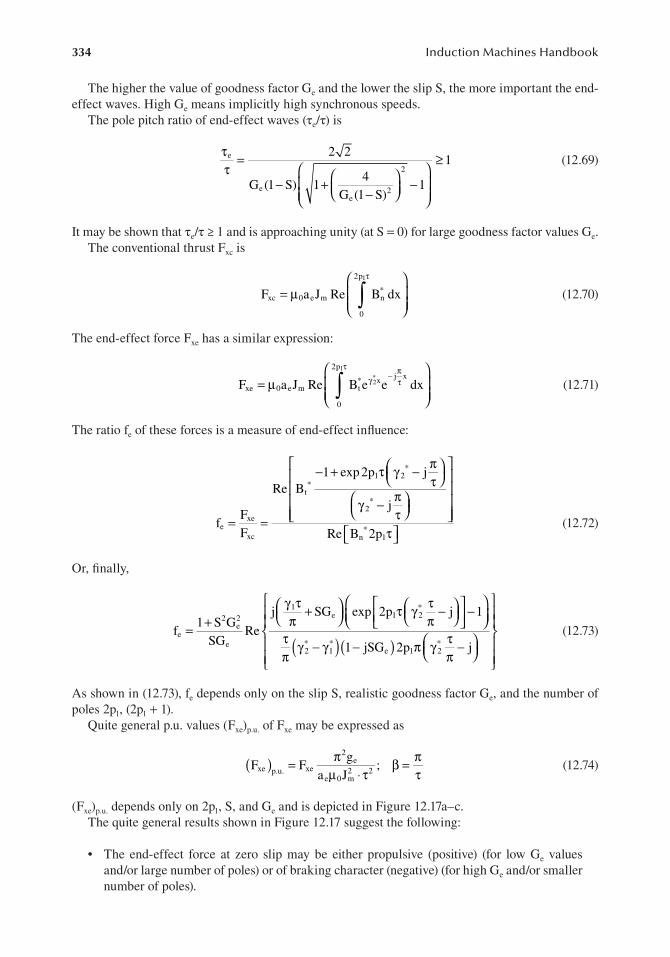
334 Induction Machines Handbook
The higher the value of goodness factor Ge and the lower the slip S, the more important the end-effect waves. High Ge means implicitly high synchronous speeds.
The pole pitch ratio of end-effect waves (τe/τ) is
τe 2 2= ≥ 1 (12.69)τ 2 4
G (e 1 S− +) 1 −1 G ( 2 e 1 S− )
It may be shown that τe/τ ≥ 1 and is approaching unity (at S = 0) for large goodness factor values Ge.The conventional thrust Fxc is
2p1τ Fxc = µ0 ea J *
m nRe ∫ B dx (12.70) 0
The end-effect force Fxe has a similar expression:
2p1τ π− j x F a J γ
xe = µ * x*2 τ
0 e m tRe e dx ∫ B e (12.71)
0
The ratio fe of these forces is a measure of end-effect influence:
* π − +1 exp2p1 2τ γ − j Re B * τ
t γ −* π
2 j F
f xe τ e = = (12.72)
F Re B 2*xc n p1τ
Or, finally,
γ τ j S1 τ
G ee 1 xp 2p2 + τ γ * − − j 1 1 S+
2 G2
e π π fe = Re (12.73)
SGe τ γ −* γ −*
π ( ) * τ 2 1 ( )1 jSGe 12p π γ 2 − j π
As shown in (12.73), fe depends only on the slip S, realistic goodness factor Ge, and the number of poles 2p1, (2p1 + 1).
Quite general p.u. values (Fxe)p.u. of Fxe may be expressed as
( gF Fxe ) π2 π= e
xep.u. β =µ ⋅2 2 ; (12.74)
a Je 0 m τ τ
(Fxe)p.u. depends only on 2p1, S, and Ge and is depicted in Figure 12.17a–c.The quite general results shown in Figure 12.17 suggest the following:
• The end-effect force at zero slip may be either propulsive (positive) (for low Ge values and/or large number of poles) or of braking character (negative) (for high Ge and/or smaller number of poles).

335Linear Induction Motors
FIGURE 12.17 End-effect force Fxe in p.u.: (a) at zero slip (after Ref. [5]), (b) at small slips, and (c) versus normalized speed.

336 Induction Machines Handbook
• For a given number of poles and zero slip, there is a certain value of the realistic goodness factor Geo, for which the end-effect force is zero. This value of Ge is called here the opti-mum goodness factor [3].
• For large values of Ge, the end-effect force changes sign more than once as the slip varies from one to zero.
• The existence of the end-effect force at zero slip is a distinct manifestation of dynamic longitudinal end effect.
Further on, the airgap flux density Bg = μoHta (see (12.54)) has a nonuniform distribution along OX that accentuates if S is low, goodness factor Ge is high and the number of poles is low.
Typical qualitative distributions are shown in Figure 12.18.This phenomenon produces nonuniform attraction forces between the two primaries along OX
and nonuniformities in the back-core flux density Bcore distribution:
x1
Bcore = ∫ B dh
g x (12.75)core
0
where hcore is the primary core height.The problem is similar in single-sided LIMs, but there the saturation of secondary solid iron requires iterative computation procedures.
A nonuniform distribution shows also the secondary current density J2:
π− j x g τ
J = γe A eγ γ1 2x B e x jSG Je me 2 + γ − (12.76)
d t t1 2 g 1e e( )+ jSG
Higher current density values are expected at the entry end (x = 0) and/or at the exit end at low val-ues of slip for high goodness factor Ge and low number of poles 2p1 [5, p. 271].
Consequently, the secondary plate losses are distributed nonuniformly along the direction of motion in the airgap [5, p. 231].
Also, the propulsion force is not distributed uniformly along the core length. In the presence of large longitudinal end effects, the thrust at entry end goes down to zero, even to negative values [5, p. 232].
Similar aspects occur in relation to normal forces in double-sided and single-sided LIMs [5, p. 232].
FIGURE 12.18 Airgap flux density distribution along OX.
0 2p τ
S=1
S=0.1S=0.12p =6G = 15
1
1
e
|B |g
x
infinite core lengthfinite core length

337Linear Induction Motors
12.8 SECONDARY POWER FACTOR AND EFFICIENCY
Based on the secondary current density J2 distribution (12.76), the power losses in the secondary P2 are
∞a d2
P e2 = ∫ ( )J J*
2 2 dx (12.77)σe eg
−∞
Similarly, the reactive power Q2 in the airgap is
Q a2 e= ω1 0µ g He
−∞∫∞
( )*ta H dta x (12.78)
The secondary efficiency η2 is
η = uFx2 ; Fx x= +F Fc xe (12.79)
uFx 2+ P
The secondary power factor cos φ2 is
( )uF Pcosϕ = x 2+
2 (12.80)( )uFx 2+ +P Q2 2
2
Longitudinal end effects deteriorate both the secondary efficiency and power factor. Typical numer-ical results for a super-high-speed LIM are shown in Figure 12.19.
So far, we considered the primary core as infinitely long. In reality, this is not the case. Consequently, the field in the exit zone decreases more rapidly (Figure 12.18), and thus, the total secondary power losses are in fact smaller than calculated above.
However, due to the same reason, at exit end there will be an additional reluctance small force [3, pp. 74–79].
FIGURE 12.19 LIM secondary efficiency η2 and power factor cos φ2. (After Refs. [5,10].)

338 Induction Machines Handbook
Numerical methods such as FEM would be suitable for a precise estimation of field distribution in the active, entry, and exit zones. However, to account for transverse edge effect also, 3D-FEM is mandatory.
Alternatively, 3D multilayer analytical methods have been applied successfully to single-sided LIMs with solid saturated and conducting secondary back iron [11–13] for reasonable computation time.
12.9 THE OPTIMUM GOODNESS FACTOR
As we already noticed, the forward end-effect wave has a longitudinal penetration depth of δend = 1/γ2r. We may assume that if
( )δend S 0= ≤ 0.1 (12.81)2p1τ
the longitudinal end-effect consequences are negligible for 2p1 ≥ 4. Condition (12.81) involves only the realistic goodness factor, Go, and the number of poles.
Indirectly condition (12.81) is related to frequency, pole pitch (synchronous speed), secondary sheet thickness, conductivity, total airgap, etc.
Consequently, two LIMs of quite different speeds and powers may have the same longitudinal effect relative consequences if Ge and 2p1 and slip S are the same [14].
End-effect compensation schemes have been introduced earlier [2,3] and recently [15], but they did not prove to be better in terms of overall (global) advantages compared to well-designed LIMs.
By well-designed LIMs for high speed, we mean here those designed for zero longitudinal end-effect force at zero slip, that is designs at optimum goodness factor Geo [5, p. 238] which is solely dependent on the number of poles 2p1 (Figure 12.20).
Geo is a rather intuitive compromise as higher Ge leads to both conventional performance enhancement and increase in the longitudinal effect adverse influence on performance.
LIMs where the dynamic longitudinal end effect may be neglected are called low-speed LIMs or linear induction actuators, whereas the rest of them are called high-speed LIMs.
High-speed LIMs are used for transportation – urban and interurban. In urban (suburban) trans-portation, the speed hardly goes above 20(30) m/s, but this is enough to make the longitudinal end effects worth considering, at least by global thrust correction coefficients [16].
12.10 LINEAR FLAT INDUCTION ACTUATORS (NO LONGITUDINAL END EFFECT)
Again, we mean by linear induction actuators (LIAs) low-speed short travel, linear induction motor drives for which the dynamic longitudinal end effect may be neglected (12.81).
FIGURE 12.20 The optimum goodness factor.
4 6 8 10 12 14 16
10
20
30
40
Ge0
2p1
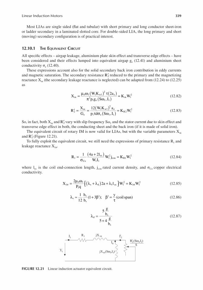
339Linear Induction Motors
Most LIAs are single sided (flat and tubular) with short primary and long conductor sheet-iron or ladder secondary in a laminated slotted core. For double-sided LIA, the long primary and short (moving) secondary configuration is of practical interest.
12.10.1 the equivalent circuit
All specific effects – airgap leakage, aluminium plate skin effect and transverse edge effects – have been considered and their effects lumped into equivalent airgap ge (12.41) and aluminium sheet conductivity σe (12.40).
These expressions account also for the solid secondary back iron contribution in eddy currents and magnetic saturation. The secondary resistance R′2 reduced to the primary and the magnetizing reactance Xm (the secondary leakage reactance is neglected) can be adapted from (12.24) to (12.25) as
µ ω0 1 ( )W K 2 τ 2aX 1 w ( )
K W2m = 1 e
2 = m 1 (12.82)π ωp g1 e ( )S ,1 1I
X 12( )W K 2
R 1 w a′ = =m 1 e2 = K W2
G p d1 e ( )S ,1 1IR2 1 (12.83)
e τ σ ω
So, in fact, both Xm and R′2 vary with slip frequency Sω1 and the stator current due to skin effect and transverse edge effect in both, the conducting sheet and the back iron (if it is made of solid iron).
The equivalent circuit of rotary IM is now valid for LIAs, but with the variable parameters Xm and R′2 (Figure 12.21).
To fully exploit the equivalent circuit, we still need the expressions of primary resistance R1 and leakage reactance X1σ.
1 ( )4a + 2lR ec
1 = W j2 = K W2 (12.84)σ W I
1 con R1 1Co 1 1
where lec is the coil end-connection length, jcon rated current density, and σCo copper electrical conductivity.
2µ ωX 0 1
1σ σ= ( )λ + λ +2a λ l W =2 K W2 (12.85)
P qs d f ec 1 1 1
1
1 h yλ ≈ ss (1+ 3 )β′ ; β =′ (coil span) (12.86)
12 bs τ
g5
bλ = sd (12.87)g
5 4+bs
FIGURE 12.21 Linear induction actuator equivalent circuit.
V1
I1R1 jX1σ I'2
I0
jX (S ,I )ωm 1 1
R' (S ,I )ωS
2 1 1

340 Induction Machines Handbook
where bs and hs are open slot width and height, respectively.
λ ≈f e0.3q(3 1β − ); l Kc f≈ τ; Kf = ÷1.3 1.6 (12.88)
where λs, λd, and λf are slot, differential, and end connection-specific geometrical permeances.The primary phase mmf W1I1 (RMS) is
τ 2h
W I 2 s1 1 = jcon K
3qd K
bfill (12.89)
s
3qbwhere K s
d = , the open slot width/slot pitch, is 0.5–0.7 for LIAs; hs/bs is the slot aspect ratio τ
and varies between 3 and 6(7) for LIAs; and Kfill is the slot fill factor and varies in the interval Kfill = 0.35−0.45 for round wire random wound coils and is 0.6–0.7 for preformed rectangular wire coils.
12.10.2 perForMance coMputation
Making use of the equivalent circuit (Figure 12.21), with all parameters already calculated, we can simply determine the thrust Fx as
3I′ ′2R 3I2R′Fx = 2 2 = 1 2 (12.90)
S 2⋅ τf 21 1
S 2⋅ τf1 +1 SGe
The efficiency η1 and power factor cos φ1 are
2 fτ −1 S Fη1 = 1 x( )2 fτ +F 3I R2 (12.91)
1 x 1 1
2 fτ +1 xF 3I R2
cosϕ = 1 11 (12.92)
3V1f I1
As expected, the realistic goodness factor Ge plays an important role in thrust production (for given stator current I1) and in performance (Figure 12.22).
FIGURE 12.22 Thrust versus slip.
I =constant
I decreases
1
1
Fx
Generator
Motor
Sk=1/Ge
S
1
-1 -Sk

341Linear Induction Motors
The peak thrust for given stator current follows from (12.90) with
∂Fx ±3I2R G′= →0 Sk eG 1= ± ; Fxk = 1 2 e (12.93)∂S 2 fτ ⋅1 2
Evidently (12.93) is valid only if R′2, Xm, and Ge are constant.In many low-speed applications, the realistic goodness is around unity. If peak thrust/current is
needed at standstill, then Sk = 1 and thus the design goodness factor at start is
d τ2
Ge 1= ω σ µe 0 2 = =1 for S 1k (12.94)ge π
Here, ω1 = 2πf1 is the primary frequency at start. If a variable frequency converter is used, the start-ing frequency is reduced.
The thrust/secondary losses is, from (12.90),
Fx F= x 1= (12.95)P2 3I′ ′2
2 R2 12 fτ ⋅S
For S = 1 the smaller the frequency f1 at start, for given τ, the larger the thrust/secondary conductor losses.
However as the value of τ decreases, to reduce the back-core height, for given airgap flux density, the starting frequency does not fall below (5–6) Hz for practical cases.
12.10.3 norMal Force in Single-SiDeD conFigurationS
The normal force between single-sided LIAs primary and secondary has two components:
• An attraction force Fna between the primary core and the secondary back iron produced by the normal airgap flux density component.
• A repulsion force Fnr between the primary and secondary current mmfs.
As the longitudinal end effect is absent, Fna is
22ae B 2g p1τ
Fna = (12.96)2µ0
Substituting Bg from (12.44) in (12.96), Fna becomes
a J2 2 2pFna ≈ e 0µ τ1m 1τ (12.97)
π +2g 12 2e ( )S G2
e
To calculate the repulsive force Fnr, the tangential component (along OX) of airgap magnetic field Hx is needed. The value of Hx along the primary surface is
H Jx m= =; Bx 0µ Jm (12.98)
aFnr = τ4 e p d1 0µ Re J J*
2 2 m (12.99)
But J2 = ωS B1 eσ πg (12.100)
τ

342 Induction Machines Handbook
Finally,
τ2 ( )µ J S2
GFnr ≈ −2ae 1τ ωS ae 1dp 0 m e
2 ( ) (12.101)π g 1+ S G2 2
e e
The net normal force Fn is
µ τJ2 20 m g π
F e 22 2
n n= +F Fa nr e= τ2a p1 ( ) 1− S Ge (12.102)π +2g 12 2S G2
e e τ
From (12.102), the net normal force becomes repulsive if
τSGe > (12.103)
geπ
which is not the case in most low-speed LIMs (LIAs) even at zero speed (S = 1).Core losses in the primary core have been so far neglected, but they may be added as in rotary
IMs. Anyway, they tend to be relatively smaller as the airgap flux density is only Bgn = (0.2–0.45) T, because of the rather large magnetic airgap (air-plus-conductor sheet thickness).
12.10.4 a nuMerical exaMple
Let us consider a sheet on iron secondary (single-sided) LIA. The initial data are pole pitch τ = 0.084 m, 2ae = 0.08 m, the number of secondary back iron “solid” laminations is i = 3, number of poles 2p1 = 6, q = 2, W1 = 480 turns/phase, g = 0.012 m (out of which dAl = 0.006 m), aluminium plate width 2c = 0.12 m, σAl = 3.5 · 107 (Ωm)−1, σiron = 3.55 · 106 (Ωm)−1, slot depth hs = 0.045 m, slot width bs = 0.009 m, and β’ = y/τ = 5/6 (coil span ratio).
The equivalent conductivity and airgap ratios versus frequency at start (S = 1) and the thrust and goodness factor for given (constant) stator current I1 = 3 A (RMS) are shown in Figure 12.23 [5].
Figure 12.23 shows the influence of skin effect, saturation, and eddy currents in the secondary back iron.
As the frequency increases, Ge slowly deteriorates (decreases) because the skin depth δi in iron decreases and so the back iron contribution to the equivalent airgap increases.
The airgap ratio shows a minimum. It is the σe/ge ratio that counts in the goodness factor. For our case, approaching f1 = 10 Hz at start seems a good choice.
12.10.5 D eSign MethoDology By exaMple
In a single-sided LIA, the back iron in the secondary is necessary to provide a low magnetic reluc-tance path for the magnetic flux which crosses the airgap. Usage of a solid back iron is imposed by economic reasons. If a laminated secondary core is to be used to step-up performance, then a ladder secondary in slots seems the adequate choice. This case will be investigated in a separate section.
For the time being, we consider the case of secondary solid back iron. Due to larger equivalent airgap per pole pitch ratio (ge/τ) both, the efficiency and power factor, are not particularly high; they do not seem the best design criteria to start with.
We also need some data from past experience: mechanical gap g-d = 1–4 mm, airgap flux density Bg = 0.15 to 0.35 T, aluminium sheet thickness d = 2–4 mm, slot depth/slot width, Kslot = hs/bs = 3–6.
The number of poles should be 2p1 = 4, 6, 8. The case of 2p1 = 2 should be used only in very small thrust applications. The secondary overhangs (c-a) should not surpass τ/π. Let us consider c-a = τ/π.

343Linear Induction Motors
FIGURE 12.23 Equivalent airgap (ge/g) and secondary conductivity (σe/σAl) thrust Fx and goodness factor Ge versus frequency at standstill. (After Ref. [5].)
The basic design criterion is chosen as maximum thrust/given stator current (12.93) which yields
S Gk e = 1 (12.104)
This case corresponds approximately to maximum thrust per conductor losses.
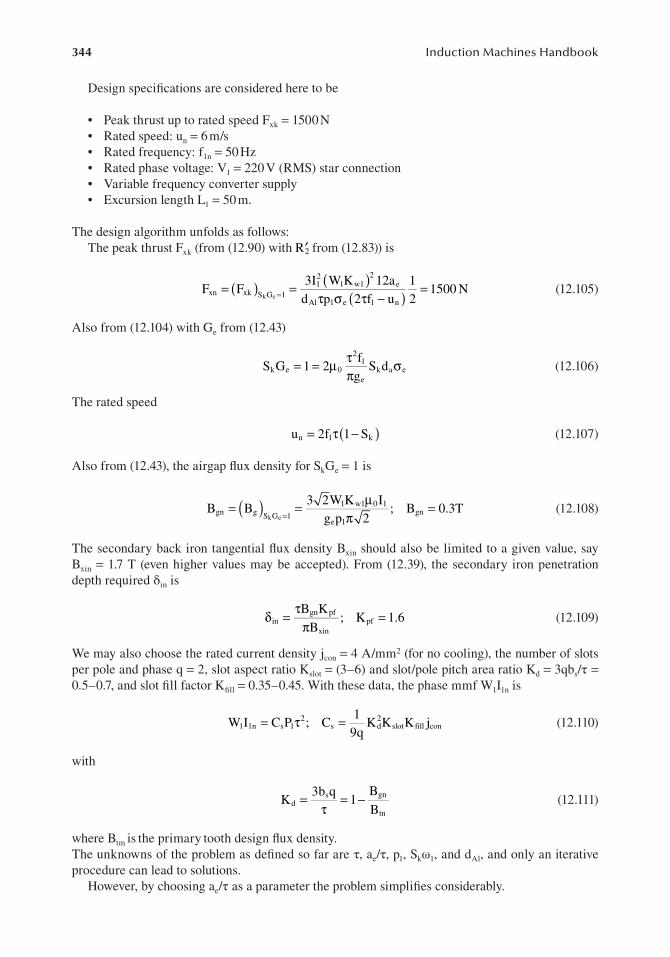
344 Induction Machines Handbook
Design specifications are considered here to be
• Peak thrust up to rated speed Fxk = 1500 N• Rated speed: un = 6 m/s• Rated frequency: f1n = 50 Hz• Rated phase voltage: V1 = 220 V (RMS) star connection• Variable frequency converter supply• Excursion length L1 = 50 m.
The design algorithm unfolds as follows:The peak thrust Fxk (from (12.90) with R′2 from (12.83)) is
3I2 ( )W K 2
F ( ) 12a 1xn = =F 1 1 w1 e
xk S G =1 = 1500 N (12.105)k e d pAlτ σ1 e ( )2 fτ −1 nu 2
Also from (12.104) with Ge from (12.43)
τ2fS Gk e = =1 2µ 1
0 S d σ (12.106)πg
k a ee
The rated speed
u 2n 1= τf 1( )− Sk (12.107)
Also from (12.43), the airgap flux density for SkGe = 1 is
( ) 3 2W K1 w1 0µ IB B 1
gn = =g ; B 0.3T )S G 1 g p 2
gn = (12.108k e =
e 1π
The secondary back iron tangential flux density Bxin should also be limited to a given value, say Bxin = 1.7 T (even higher values may be accepted). From (12.39), the secondary iron penetration depth required δin is
τB Kδin = gn pf ; Kpf = 1.6 (12.109)
πBxin
We may also choose the rated current density jcon = 4 A/mm2 (for no cooling), the number of slots per pole and phase q = 2, slot aspect ratio Kslot = (3–6) and slot/pole pitch area ratio Kd = 3qbs/τ = 0.5–0.7, and slot fill factor Kfill = 0.35–0.45. With these data, the phase mmf W1I1n is
1W I1 1n s= τC P 2
1 ; Cs d= K K2slotK jfill con (12.110)
9q
with
3b q BK s
d = = −1 gn (12.111)τ Btn
where Btm is the primary tooth design flux density.The unknowns of the problem as defined so far are τ, ae/τ, p1, Skω1, and dAl, and only an iterative procedure can lead to solutions.
However, by choosing ae/τ as a parameter the problem simplifies considerably.

345Linear Induction Motors
From (12.109) and (12.38), we get
K Btiπ22 4
τ S ω = xink 1 − = 4 c
µ σ0 i B gn
τ (12.112)
The thrust Fxk, from (12.105) with (12.108) and (12.106), is
a Fxn = τ6C B K p 3 es gn w1 1 (12.113) τ
As the primary frequency f1 is given, we may choose also the number of poles as a parameter 2p1 = 4, 6 … In this case from (12.113), the pole pitch τ can be calculated as
Fτ = xn (12.114)3 a
6c B K P e s gn w1 1 τ
Now, Skω1 is
S 2k 1ω = π − πf u1 n (12.115)
τ
Alternatively, we may have used (12.112) to find Skω1 in which case even f1 from (12.115) could have been calculated. This would be the case with f1n not specified. Anyways, (12.112) is to be checked.
Now, from (12.105) to (12.108)
3cσ =e Ad sτπl (12.116)
S Bk 1ω gn
From (12.40), the value σAlskinda is
3Csτπ σ δσ = i i AlskindAl − K
S B ta (12.117)k 1ω g Kti
As Kta comes from Equations (12.14), (12.26) to (12.30), where Ge (which contains σAlskinda) is included, the computation of σAlskindAl may be done only iteratively from these equations.
With σAlskindAl known, again, iteratively, dAl may be determined (the skin effect depends on dAl). A valid solution is found if dAl < ge.
With the above procedure, the equivalent parameters entering the equivalent circuit, Xm, R′2, R1, and X1σ from (12.92) to (12.88), for rated speed un and thrust Fxn, can be calculated. The only unknown is now the number of turns per phase W1
VW = 1
1 (12.118) 2 2
K′W I K R2 m
1 1n R 1 ( ) K+ + +
( )K
x1σ +
2k k 1 S 2
S 1+ 1 S Ge k eG ( ) ( )
with W1I1n from (12.110), (12.118) provides a unique value for W1.

346 Induction Machines Handbook
To choose the adequate ae/τ ratio, which will lead to the best design, the cost Ct of both primary (Cp) and secondary (Csec) is evaluated:
C Ct p= + Csec (12.119)
6W I K C 1 1n
p = +( )2a K C1 Cτ γ o Co 1+ τ2P ( ) τ 1 K− ⋅d s2aK d
lot + δ3 2i 1P 2τ ⋅ a C γ i ii (12.120)Jcon 3q
where γCo, γi, CCo, and Cii are the specific weights and specific prices of copper and core, respectively.Csec is given as
2τ C 2sec A= + d Cl Aγ +l Al i3 2δ γ a a Ci i L1 (12.121)
π
where γAl and CAl are aluminium specific weight and specific cost, respectively, and L1 is the total LIA secondary length (excursion length + primary length).
When L1 ≫ 2p1τ the secondary cost becomes an important cost factor. Thus, a high ae/τ ratio leads to a smaller length primary but also to a wider (large cost) secondary. The final choice is left to the designer. The apparent power S1 may be used as an indicator of converter costs.
For our numerical case, the results in Figure 12.24 are obtained. The total cost/iron specific cost (Ct/Cii) has a minimum for ae/τ = 0.7, but this corresponds to a rather high S1 (KVA). A high S1 means a higher cost frequency converter. A good compromise would be ae/τ = 0.9, Skω1 = 93 rad/s, τ = 0.085 m, dAl = 1.8 · 10−3 m, W1 = 384 turns/phase, I1n = 32.757 A, S1 = 21.92 KVA.
Now that the LIA dimensions are all known, the performance may be calculated iteratively for every (V1, f1) pair and speed U.
For a double-sided LIA with aluminium sheet secondary, the same design procedure may be used, after its drastic simplification due to the absence of solid iron in the secondary. Also the two-sided windings may be lumped into an equivalent one.
12.10.6 the laDDer SeconDary
Lowering the airgap to g = 1 mm or even less in special applications with LIAs may be feasible. In such cases, the primary slots should be semiclosed to reduce Carter’s coefficient value and addi-tional losses. The secondary may then be built from a laminated core with, again, semiclosed slots, for same reasons as above (Figure 12.25).
To calculate the performance, the conventional equivalent circuit is used. The secondary param-eter expressions are identical to those derived for the rotary IM. The adequate number of combina-tions of primary/secondary slots (per primary length) is the same as for rotary IM. In fact, the whole design process is the same as for the rotary IM.
The only difference is that the electromagnetic power is
3R′ ′I 2
Pelm x= τF 2 f 2 21 = (12.122)
S
instead of
ω 3R IPelm eT 1 ′ ′2
= = 2 2 (12.123)p1 S
for rotary IMs.For short excursion (less than a few metres) and g ≈ 1 mm, quite good performance may be
obtained with ladder secondary.

347Linear Induction Motors
FIGURE 12.24 Design numerical results: (a) Skω1, (b) iron penetration depth δI aluminium thickness dAl, (c) cost versus ae/τ, and (d) S1 (KVA), specific thrust fx(N/cm2). (Adapted from Ref. [10].)
short (moving)primary
long (fix)secondary
FIGURE 12.25 LIA with ladder secondary.

348 Induction Machines Handbook
12.11 TUBULAR LIAS
There are two main tubular LIA configurations: one with longitudinal primary laminations stack and the other with ring-shaped laminations and secondary ring-shaped conductors in slots (Figure 12.26).
Due to manufacturing advantages, we consider here – except for liquid pump applications – disk-shaped laminations (Figure 12.26).
The main problem of this configuration is that it has open slots on both sides of the airgap.To limit the airgap flux harmonics (with all their consequences in “parasitic” losses and forces),
for an airgap g (g ≈ 1 mm) the primary slot width bs should not be larger than (4–6) g. Fortunately, this suffices for many practical cases.
The secondary ring width br should not be larger than (3–4)g. Another secondary effect origi-nates in the fact that the back-core flux path goes perpendicular to laminations.
Consequently, the total airgap is increased at least by the insulation total thickness along say ≈ τ/3. Fortunately, this increase by gad is not very large:
1gad = τ0.03 ≈ τ0.01 (12.124)
3
For a pole pitch, τ = 30 mm, gad = 0.3–0.4 mm, which is acceptable. A very good stacking factor of 0.97 has been assumed in (12.124). Also eddy current core losses will be increased notably in the back iron due to the perpendicular field (Figure 12.27).
Performing slits in the back-core disk-shaped laminations during stamping leads to a notable reduction of eddy current losses. Finally, the secondary is to be coated with mechanically resilient, nonconducting, nonmagnetic material for allowing the use of linear bearings.
FIGURE 12.26 Tubular LIA with secondary conductor rings.
FIGURE 12.27 Tubular LIA back-core disk-shaped lamination (a) and its slitting (b) to reduce eddy current losses.
back core f luxeddy current
paths
back core zone
slit
(a) (b)
bs
g
DiDav1 Dav2br
x
primary laminations
hs
secondary laminations
secondary copper (Al)rings
primary ring shape coils

349Linear Induction Motors
Once these peculiarities are taken care of, the tubular LIM performance computation runs smoothly. The absence of end connections, in both the primary and secondary coils, is a definite advantage of tubular configurations.
So no transverse edge effect occurs in the secondary. The primary back iron is not likely to satu-rate, but the secondary back iron may do so as its area for the half-pole flux is much smaller than in the primary.
The equivalent circuit parameters are
1 Dπ JR av1 con
1t = W2 (12.125)σCo W I
11 1n
DX 2 av1
1t = µ0 1ω π ( )λ + 2
p qs1 λd1 W1 (12.126)
1
We have just “marked” in (12.125) and (12.126) that the primary coil average length is πDav1. For the secondary with copper rings,
( )W K 2
X 2′ 1 w12r = µ0 1ω πD 1av2 ⋅ λ2 ( )+ λ (12.127)
Ns2 d2
s2
1 Dπ W K 2
R av2 ( )′2r = ⋅12 1 w1 (12.128)σCo Aring Ns2
where λs and λd are defined in (12.86) and (12.87), Ns2 is the number of secondary slots along pri-mary length, and Aring is the copper ring cross section.
The magnetization reactance Xm is
6µ ω π τX 0 1
m 2 ( )W K 2 D= i
π 1 w1 (12.129) g
p gK 1 ad 1 c + + 2 K
gsat
where Ksat, iron saturation coefficient, should be kept (in general) below 0.4–0.5.For an aluminium sheet secondary on laminated core,
6 Dπ −( )2g − d W K 2
R′ = i Al 1( )w12 ; X′ = 0
p d2 (12.130)
1 Aτ σl Al
The equivalent circuit (Figure 12.28) now contains also the secondary leakage reactance which is however small as the slots are open and not very deep.
Based on the equivalent circuit, all performance may be obtained at ease.The tubular LIA is used for short stroke applications which implicitly leads to maximum speeds
below 2–3 m/s. Consequently, the design of tubular LIAs, in terms of energy conversion, should aim to produce the maximum thrust at standstill per unit of apparent power, if possible.
FIGURE 12.28 Equivalent circuit of tubular LIA with secondary copper rings in slots.
V1
I1R1 jX1 I'2
I0
jX m
R'S
2
jX'2

350 Induction Machines Handbook
The primary frequency may be varied (and controlled) through a static power converter.In terms of costs, both the LIA and power converter costs are to be considered. Hereby, however,
we illustrate the criterion of maximum thrust at standstill.The electromagnetic power Pelm is
Pelm x= τF 2 f 3 21 e= R I1 (12.131)
R′2 X2
Sm
Re = (12.132) R′ 2
2
+ +( )X X′ 2
S m 2
or with
Xm R′Ge = , R = 2 )
R′ e (12.1332 2
1 ′ 2X
S + +1 2 SG e Xm
Now, the maximum thrust is obtained for
( 1S Gk e )opt = (12.134)X′
1+ 2
Xm
For standstill, Sk = 1. When initiating the design process, the ratio X X′2 m is not known and can only be assigned a value to be adjusted iteratively later on. A good start would be X X′2 m = 0.2.
From now on, the design methodology developed for the flat LIA may be used here.
12.11.1 a nuMerical exaMple
Let us consider a tubular LIA with copper ring secondary and the data primary bore diameter Di = 0.15 m, primary external diameter De = 0.27 m, pole pitch τ = 0.06 m, q = 1 slots/pole/phase, primary slot depth hs = 0.04 m, primary slot width bs = 0.0125 m, number of poles 2p1 = 8, the second-ary slot pitch τs2 = 10−2 m, secondary slot width bs2 = 6 · 10−3 m, secondary slot depth h = 4 · 10−3
s2 m, airgap g = 2 · 10−3 m, current density jcon = 3 · 106 A/m2, and slot fill factor Kfill = 0.6.
Let us determine the frequency f2 for maximum thrust at standstill and the corresponding thrust, apparent power, and conductor losses.
First, with the available data, we may calculate from (12.127) the secondary leakage reactance as a function of f1W1Kw1:
12X 4′ D 2 2 6− 2 2
2 0= µ π ⋅av2 ( )λ +N
s2 λ =d2 f W1 1 Kw1 1.97 ⋅10 f W1 1 Kw1 (12.135)s2
with
5g 5 3⋅hs2 4 bλ = = λ0.33; = s2 = 6
s2 = d2 = 0.57 (12.136)3b 3 6 4g 4 3⋅
5 + 0s2 ⋅ 5 +bs2 6
The secondary resistance (12.128) is

351Linear Induction Motors
1 Dπ
R′ = av2 12 W K 22 ⋅ =( )1 w1 0.876 ⋅10−4 ( )W K 2
σCo h b1 w1 (12.137)
s2 s2
The magnetic reactance Xm (12.129) becomes
6µ ω0 1 DX = ( ) π τ
W K 2 i 10− f W( )K 2m 2 1 w1 = 5
1 1 w1 (12.138)π g
P g1 1+ +ad K g
sat
gad + =K 0.5g
sat .Let us assign
Now, the optimum goodness factor is (from (12.134))
X 1G m 1
0 = = =0.114fR′ 1s = (12.139)
2 X′2 1+ ⋅+ 2.24 10−2 f1 1s
R′2
From (12.139), the primary frequency at standstill f1s is f1s ≈ 7.5 Hz. The primary phase mmf W1I1n is
W I1 1n s= =pqn I p1n 1 sq h( )b Ks fillJ 4con = ⋅4 1⋅ ⋅0− −2 21.2 ⋅ ⋅10 0.6 ⋅ ⋅3 10−6 = 3456 Aturns (12.140)
Hence, the primary phase resistance and leakage reactance R1t, X1t are (12.125) and (12.126)
1 Dπ JR av1 con
1t = W2 51 = ⋅1.035 10− W2
σ W I1 (12.141)
Co 1 1n
with Dav1 = Di + hs = 0.15 + 0.04 = 0.19 m.
DX 2= µ ω π av1 ( )λ + λ =W2 5⋅ 2
1t 0 1 2.483 10− W (12.142)p q
s1 d1 1 11
The number of turns W1 may be determined once the rated current I1n is assigned a value. For I1n = 20 A, from (12.140), W1 = 3456/20 ≈ 172 turns/phase.
The apparent power S1 does not depend on voltage (or on W1) and is
jX R j′ XS 31 S 1 = +I R2 +( ) 1 1t jX m 2( )′2
= 1t +j X( ) (12.143)
m 2+ X R′ + ′2
With W1I2
1n and R1t, X1t, Xm, R′2, X′2 proportional to W1 and with Kw1 = 1.00 (q = 1), we obtain
S1 1≈ ϕ3000 VA; cos ≈ 0.52 (12.144)
The corresponding phase voltage at start is
S 3000V 1
1 = = = 50.00 V(RMS) (12.145)3I1n 3 2⋅ 0
The rated input power P1 = S1cos φ1 = 3000 · 0.52 = 1560 W.The primary conductor loss pcos is
pcos 1= =3R I 32 41n ⋅ ⋅0.135 10− (3456)2 = 370.86 W (12.146)

352 Induction Machines Handbook
The electromagnetic power Pelm can be expressed as
Pelm 1= −P pcos = −1560 370.86 = 1189 W (12.147)
The thrust at standstill Fxk is
P 1189F elm
xk = = = 1321.26 N (12.147’)2 fτ 1 2 ⋅ ⋅0.06 7.5
Thus, the peak thrust at standstill per watt is
Ff xk 1321.26
xW = = = 0.847 N/W (12.148)P1 1560
Also
Fxk 1321.26fxVA = = = 0.44 N/VA (12.149)
S1 3000
Such specific thrust values are typical for tubular LIAs.
12.12 SHORT-SECONDARY DOUBLE-SIDED LIAS
In some industrial applications such as special conveyors, the vehicle is provided with an aluminium (light-weight) sheet which travels guided between two-layer primaries (Figure 12.29).
The primary units may be switched on and off as required by the presence of a vehicle in the nearby unit.
The fact that we deal with a secondary which is shorter than the primary leads to a redistribution of secondary current density along the direction of motion. Let us consider the simplified case of a single short vehicle inside a single longer primary.
FIGURE 12.29 Short-secondary double-sided LIA: (a) cross section, (b) multiple vehicle system, and (c) single vehicle.
VEHICLE
primaryunit
primaryunit
vehicle 2 vehicle 1
b.)
c.)
x1 Ly
2pτ
xz
x
J2
(a)
(b)
(c)

353Linear Induction Motors
The second current density paths (Figure 12.29c) reveal the transverse edge effect which may be accounted for as in the previous section. Also, the skin effect may be considered as done before in the chapter.
The dynamic longitudinal end effect is considered negligible. So the secondary current density in the secondary is simply having the conventional travelling component and a constant one which provides for the condition
L
∫v
( )J d2z x 0= (12.150)0
J2z (from (12.76) with At = Bt = 0) is
π−−
j xjSG J e τ
J = e m2z +( ) A (12.151)
d 1Al + jSGe
From (12.150) to (12.151), A is
πj L
1 e−v
τ − jSG J τ A = e m
( ) (12.152)d 1Al + jSG je π Lv
In fact, A represents an alternative current density which produces additional losses and a pulsation in thrust. Its frequency is the slip frequency Sf1, of the entire J2z.
As expected when Lv = 2Kτ, A = 0.Care must be exercised when defining the equivalent parameters of the equivalent circuit, as
part of the primary “works” on empty airgap while only the part facing the vehicle is active. Three-dimensional FEM approaches seem most adequate to solve this case.
Linear induction pumps are also complex systems characterized by various phenomena (for details, see Reference [5], Chapter 5).
12.13 LINEAR INDUCTION MOTORS FOR URBAN TRANSPORTATION
LIMs when longitudinal effects have to be considered are typically applied to people movers on airports (Chicago, Dallas–Fortwoth, Tokyo), in metropolitan areas (Toronto, Vancouver, Detroit), or even for interurban transportation (S. Korea, China). Only single-sided configurations have been applied so far.
As in the previous section, we did analyse all special effects in LIMs, including the opti-mal goodness factor definition corresponding to zero longitudinal end-effect force at zero slip (Figure 12.20), we will restrict ourselves here to discuss only some design aspects through a rather practical numerical example. More elaborated optimization design methods including some based on FEM are reported in [17–19]. However, they seem to ignore the transverse edge effect and satu-ration and eddy currents in the secondary solid back iron.
12.13.1 SpeciFicationS
• Peak thrust at standstill, Fxk = 12.0 kN• Rated speed, Un = 34 m/s• Rated thrust, at Un Fxn = 3.0 kN;• Pole pitch, τ = 0.25 m (from 0.2 to 0.3 m)• Mechanical gap, gm = 10−2 m• Starting primary current, IK = 400–500 A.

354 Induction Machines Handbook
12.13.2 Data FroM paSt experience
• The average airgap flux density Bgn = 0.25–0.40 T for conductor sheet on solid iron second-ary and Bgn = 0.35–0.45 T for ladder-type secondary.
• The primary current sheet fundamental J 5 mk = 1.5–2.5 · 10 A/m.
• The effective thickness of aluminium (copper) sheet of the secondary dAl = (4–6)10−3 m.• The pole pitch τ = 0.2–0.3 m to limit the secondary back iron depth and reduce end con-
nections of coils in the primary winding.• The frequency at standstill and peak thrust should be larger than f1sc = 4–5 Hz to avoid
large vibration and noise during starting.• The primary stack width/pole pitch: 2a/τ = 0.75–1. The lower limit is required to reduce
the too large influence of end-connection losses and the upper to secure reasonable second-ary costs.
12.13.3 oBjective FunctionS
Typical objective functions to minimize are
• Inverse efficiency F1 = 1/η• Secondary costs F2 = Csec
• Minimum primary weight F3 = G1
• Primary KVA F4 = S1k
• Capitalized cost of losses Fc = (Ploss)av.
A combination of these objectives may be used to obtain a reasonable compromise between energy conversion performance and investment and loss costs [17].
12.13.4 typical conStraintS
• Primary temperature T1 < 120° (with forced cooling)• Secondary temperature in stations during peak traffic hours T2
• Core flux densities < (1.7–1.9) T• Mechanical gap gm ≥ 10−2 m.
Some of the unused objective functions may be taken as constraints.
12.13.5 typical variaBleS
Integer variables• Number of poles 2p1
• Sots per pole per phase q• Number of turns per coils nc (W1 = 2p1qnc).
Real variables• Pole pitch τ• Airgap gm
• Aluminium thickness dAl
• Stack width 2a• Primary slot height hs
• Primary teeth flux density Bt1
• Back iron tangential flux density Bxin
• Rated frequency f1.

355Linear Induction Motors
12.13.6 the analySiS MoDel
The analysis model has to make the connection between the variables, the objective functions, and the constraints. So far in this chapter, we have developed a rather complete analytical model which accounts for all specific phenomena in LIMs such as transverse edge effect, saturation and eddy currents in the secondary back iron, airgap leakage, and skin effect in the aluminium sheet of sec-ondary and longitudinal end effect.
So, from this point of view, it would seem reasonable to start with a feasible variable-vector and then calculate the objective function(s) and constraints and use a direct search method to change the variables until sufficient convergence of the objective function is obtained (see the Hooke–Jeeves method presented in Chapter 8).
To avoid the risk of being trapped in a local minimum, a few different starting variable-vectors should be tried and the best design is chosen. Finding a good starting variable-vector is a key factor in such approaches.
On the other hand, genetic algorithms are known for being able to reach global optima as they start with a population of variable-vectors (chromosomes); FEM approaches have been presented in [18]).
To find a good initial design, the methodologies developed for rotary IM still hold, but the thrust expression includes an additional term to account for longitudinal effect.
Following the analysis model developed in this chapter, the following results have been obtained for the above initial data τ = 0.25 m, 2p1 = 10, W1 = 90, I1sc = 420 A (for peak thrust), f1sc = 6 Hz, 2a = 0.27 m, V1sc = 220 V (at start), phase voltage at 20 m/s and rated thrust is V1n = 200 V, efficiency at rated speed and thrust η1 = 0.8, rated power factor cos φ1 = 0.55. Performance characteristics are shown in Figures 12.30–12.32.
12.13.7 DiScuSSion oF nuMerical reSultS
• Above 80% of rated speed (34 m/s), the efficiency is quite high: 0.8.• The power factor remains around 0.5 above 50% of rated speed.• The thrust versus speed curves satisfy typical urban traction requirements.• Regenerative braking, provided the energy retrieval is accepted through the static con-
verter, is quite good down to 25% of maximum speed. More regenerative power can be produced at high speeds by adequate control (full flux in the machine) but at higher volt-ages in the D.C. link.
• Though not shown, a substantial net attraction force is developed (two to three times or more than the thrust) which may produce noise and vibration if not kept under control.
• These results may be treated as an educated starting point in the optimization design. Minimum cost of secondary objective function would lead to a not so wide stack
FIGURE 12.30 Imposed current and speed dependence of frequency.
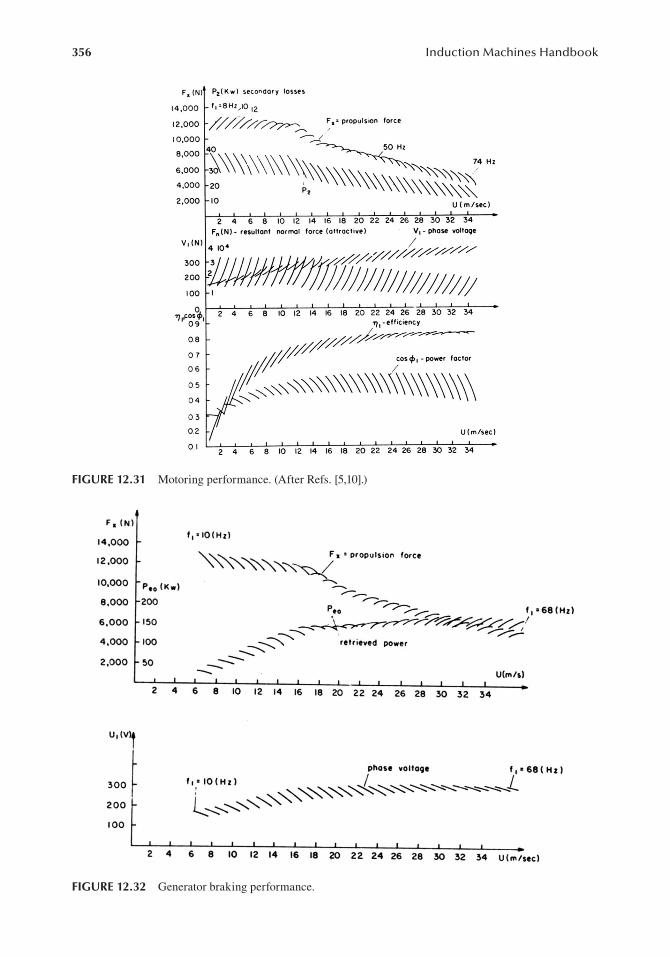
356 Induction Machines Handbook
FIGURE 12.31 Motoring performance. (After Refs. [5,10].)
FIGURE 12.32 Generator braking performance.

357Linear Induction Motors
(2a < 0.27 m) with a lower efficiency in the motor. The motor tends to be larger. The pole pitch may be slightly smaller [17].
• The thermal design of secondary, especially around the stop stations, during heavy traffic, is a particular constraint which needs a special treatment [5, pp. 248–250].
12.14 TRANSIENTS AND CONTROL OF LIMS
The modelling for transients, as for steady state, given the complex influences of magnetic satura-tion and skin effects for essentially 3D configurations, should be approached through 3D-FEM or 3D analytical models.
However, for control system design purposes, a circuit model is needed. The methods of LIM control follow the path for rotary induction motors, but constant (or controlled) slip frequency con-trol and stator current control have gained practical acclaim for urban transportation systems.
Such a generic system is shown in Figure 12.33.The slip frequency (Sf )*
1 versus speed U is imposed a priori. The speed regulator (a robust one: sliding mode type, for example) produces the reference thrust. Now, with speed U, (Sf1)* and F*
x known, we need to calculate the reference current I*
S. If FEM extended data are available, it is pos-sible to produce, by optimization, both (Sf )* and I*
1 S for given F*x and speed U, based on, say, max
thrust per losses or per stator current.Adopting for optimization initialization a given constant slip frequency value, constant, or
slightly increasing with speed (positive for motoring and negative for regenerative braking) is a practical solution.
However, if these data are not available, it would be practical to have an analytical tool model to calculate the stator current for given thrust, slip frequency, and speed from an equivalent circuit that accounts for, mainly, longitudinal effect.
As shown in Ref. [3] the longitudinal effect deteriorates the thrust, increases the losses in the secondary and deteriorates the power factor.
Starting from the equivalent circuit of rotary IMs, good for linear induction actuators (when longitudinal and effect is negligible) a rather complete parameter equivalent circuit has been intro-duced for LIMs (Figure 12.34).
The single-sided LIM with aluminium on solid or on secondary is characterized by a sizeable leakage inductance Lrl besides resistor Rr.
Based on power balance (calculated by technical field theories or FEM) or by equivalent cir-cuit fitting for a few representative measured speeds U, slip frequencies, and current values, the
FIGURE 12.33 Generic slip frequency (Sf1) control of LIM for propulsion only.
Speedregulator−
*U( )*
1Sf
U
( )( )**S x 1i f F , Sf ,U=
( )
* *a S S* *b S S
* * *c a b
i i cosθ2πi i cos θ3
i i i
=
= −
= − +
πτ
−
U
( )*
1Sf 2πU Sθ
−
−
+
A.C.current
regulator
−
+ PWMinverter
LIM
++
ai bi
*xF
*SI

358 Induction Machines Handbook
mLrlL
rR
200km hU
1Sf 12Hz≈
10
20
30
aendR Ω
rR
mLrlL
FIGURE 12.34 Complete variable equivalent circuit for LIMs; magnetic saturation is neglected.
magnetizing inductance Lm decreases with increasing speed, the secondary resistance Rr increases with speed, while the secondary leakage inductance remains rather constant, for a 200 km/h urban LIM system as shown in Figure 12.35.
An additional resistance Radend is required to fit both the secondary losses and thrust up to the largest speed when longitudinal end effect is most important.
The main problem to sort out with this equivalent circuit is the design of Radend when the end effect thrust at zero slip, S, changes sign from braking (for large longitudinal effect LIMs, Radend > 0) to perhaps a negative value of Radend when the end-effect thrust at zero slip is motoring (for lower longitudinal effect LIMs).
Finally, for LIMs designed for optimal goodness factor (Figure 12.20) when (Fx end)S = 0 = 0, apparently Radend should be perhaps discarded.
If combined propulsion and suspension control is pursued, then the stator current control may be used for suspension control, while slip frequency may be used for propulsion control (Figure 12.36). Low limitations on slip frequency have to be eliminated in this case. Alternatively, direct thrust and suspension control may be used as for rotary IMs [20,21].
The control in Figure 12.36 is basically of feedforward A.C. current vector type.Again, either the equivalent circuit or the FE method may be used to find a reasonable slip fre-
quency reference (Sf1)*.Motion sensorless control may be approached as for rotary IMs but with extreme care in urban
transportation system applications when notable longitudinal end effect occurs.Finally, robust control [22] with self-commissioning and online parameter detuning elimination,
when magnetic saturation, skin effect, temperatures of stator and mover, and the airgap vary, is still due as urban (and suburban) people movers keep spreading around megacities of the future.
In the absence of longitudinal end effects, the theory of transients as developed for rotary induc-tion motors may be used. The influence of transverse edge effect and secondary eddy currents may
FIGURE 12.35 Parameters’ variation with speed at constant slip frequency for a typical urban LIM system.

359Linear Induction Motors
( )1 K− e 2(U) R′
Re = (12.153)K (e U)
Ψm m= −L 1( )K (e mU) i (12.155)
FIGURE 12.36 Combined generic suspension and propulsion LIM control.
be modelled by an equivalent double cage (Chapter 1). The ladder secondary with broken bars may need a bar-to-bar simulation as done for rotary IMs (Chapter 1).
A fictitious ladder [23] (or d-q pole by pole [24]) model of transients may be used to account for longitudinal end effects.
Also FEM-circuit-coupled models have been introduced for the scope [19]. The control of LIMs by static power converters is very similar to that presented in Chapter 8, Vol. 1, for rotary IMs. Early control systems in use today apply slip frequency control in PWM-voltage source inverters such as in the UTDC2 system [25].
Flux control may be used to tame the normal force while still providing for adequate flux and thrust combinations for good efficiency over the entire speed range [26].
Advanced vector control techniques – such as direct torque and flux control (DTFC) – have been proposed for combined levitation–propulsion of a small vehicle for indoor transport in a clean room [20].
12.15 LIM CONTROL WITH DYNAMIC LONGITUDINAL END EFFECT
The rather complete equivalent circuit shown in Figure 12.34 cannot be used in a practical control strategy for high-speed (large dynamic longitudinal end effect) LIMs.
For such purposes, a simplified equivalent circuit [10,17] has been proposed where the dynamic end effect is represented by an additional secondary resistance Re (in parallel to the main flux branch), flowed by a current ie:
where R′2 is the secondary equivalent resistance, and Ke(U) takes into account the dynamic longi-tudinal end effect:
Ke 1(U) K≈ +U K U22 (12.154)
The coefficients K1 and K2 may be obtained by detailed analytical or 3D-FEM calculations. Ke(U) increases monotonically with speed.
In the same time, the airgap flux Ψm is

360 Induction Machines Handbook
The stator flux vector Ψ1 is
Ψ1 1= ⋅L il 1 + Ψm (12.156)
The dynamic longitudinal end effect is represented by Re through a fictitious winding:
Ψ1 1= ⋅L il 1 + Ψm (12.157)
The thrust F
x is thus
3 πFx 1= Im ag ( )Ψ ⋅ i i*
1 − Ψ( )⋅ *m e (12.158)
2 τ
The secondary circuit in stator coordinates is
0 R= ′ ′2 2i p2 2+ Ψ + π′ j UΨ′τ 2 (12.159)
with
Ψ′2 2= L i′ ′l 2 + Ψm e; i + =i im 1 + i2′ (12.160)
Based on this model, the stator flux Ψ1 can be estimated from a voltage model:
Ψ = −∫ ( ) TV R* i dt ≈ e ( )V R*
1 1 1 11 T
1 − 1 1i (12.161)+ ⋅e p
where Te is a control design time constant to reduce integral’s error above say, 1 Hz.In (12.161) V*
1 is the reference voltage vector. Then, from (12.156) the airgap flux Ψm is estimated. Finally, the current ie of dynamic longitudinal end effect is calculated:
πR i′2 1( )− Ψm mL j− UΨm
i τe = (12.162)
R R1 e′ +
Now from (12.158), the thrust Fx is estimated. Based on this model, a DTFC strategy has been developed (Figure 12.37).
A typical result of such a DTFC for a LIM is shown in Figure 12.38 [10].Note. Similar dynamic longitudinal correction coefficients as in [10] may be adopted without Re
concept but with Lm = Lm0(1 − f(Q)); R′2 2= R f′0 ⋅ =(Q); f(Q) 1 e− −Q Q; Q l= ⋅primary U L′ ′2 2R .( ) ( )
12.16 ELECTROMAGNETIC INDUCTION LAUNCHERS
The principle of electromagnetic induction may be used to launch by repulsion an electrically con-ducting armature at a high speed by quickly injecting current in a primary coil placed in its vicinity (Figure 12.39).
A multicoil arrangement is also feasible for launching a large weight vehicle.The principle is rather simple. The “air core” stator coil gets a fast injection of current i1 from a
high-voltage capacitor through a very fast high-voltage switch. The time varying field thus created produces an emf and thus a current i2 in the secondary (mover) coil(s). The current in the mover coil i2 decreases slowly enough in time to produce a high repulsion force on the mover coil. That is to launch it.

361Linear Induction Motors
FIGURE 12.37 Direct thrust and flux control of LIMs with dynamic longitudinal end effect.
FIGURE 12.38 Step thrust response in the DTFC of an urban LIM without and with dynamic end-effect consideration. (After Ref. [10].)
i1
i2
x
statorcoil
movercoil
Fx
charged highvoltage capacitor
ultrafast switch
r2r1
FIGURE 12.39 Coaxial filamentary coil structure.
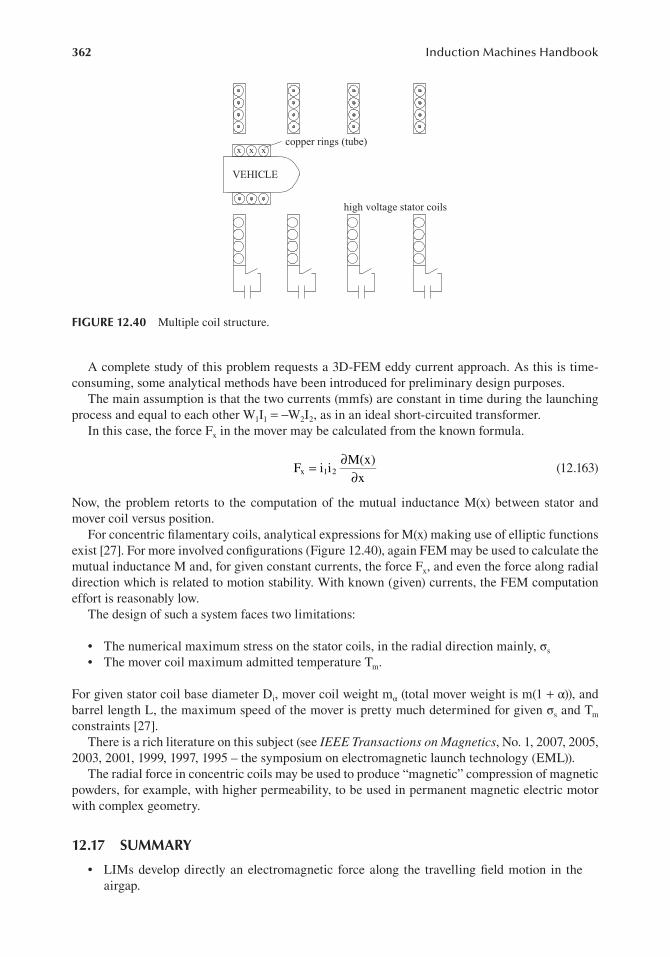
362 Induction Machines Handbook
∂M(x)
Fx 1= i i2 (12.163)∂x
x x xcopper rings (tube)
high voltage stator coils
VEHICLE
FIGURE 12.40 Multiple coil structure.
A complete study of this problem requests a 3D-FEM eddy current approach. As this is time-consuming, some analytical methods have been introduced for preliminary design purposes.
The main assumption is that the two currents (mmfs) are constant in time during the launching process and equal to each other W1I1 = −W2I2, as in an ideal short-circuited transformer.
In this case, the force Fx in the mover may be calculated from the known formula.
Now, the problem retorts to the computation of the mutual inductance M(x) between stator and mover coil versus position.
For concentric filamentary coils, analytical expressions for M(x) making use of elliptic functions exist [27]. For more involved configurations (Figure 12.40), again FEM may be used to calculate the mutual inductance M and, for given constant currents, the force Fx, and even the force along radial direction which is related to motion stability. With known (given) currents, the FEM computation effort is reasonably low.
The design of such a system faces two limitations:
• The numerical maximum stress on the stator coils, in the radial direction mainly, σs
• The mover coil maximum admitted temperature Tm.
For given stator coil base diameter Di, mover coil weight mα (total mover weight is m(1 + α)), and barrel length L, the maximum speed of the mover is pretty much determined for given σs and Tm constraints [27].
There is a rich literature on this subject (see IEEE Transactions on Magnetics, No. 1, 2007, 2005, 2003, 2001, 1999, 1997, 1995 – the symposium on electromagnetic launch technology (EML)).
The radial force in concentric coils may be used to produce “magnetic” compression of magnetic powders, for example, with higher permeability, to be used in permanent magnetic electric motor with complex geometry.
12.17 SUMMARY
• LIMs develop directly an electromagnetic force along the travelling field motion in the airgap.

363Linear Induction Motors
• Cutting and unrolling a rotary IM leads to a single-sided LIM with now a ladder-type secondary.
• A three-phase winding produces basically a travelling field in the airgap at the speed Us = 2τf1 (τ – pole pitch and f1 – primary frequency).
• Due to the open character of the magnetic circuit along the travelling field direction, addi-tional currents are induced at entry and exit ends.
• They die out along the active part of LIM producing additional secondary losses, thrust, power factor, and efficiency deterioration. All these are known as dynamic longitudinal end effects.
• The longitudinal end effects may be neglected in the so-called low-speed LIMs called linear induction actuators.
• When the secondary ladder is replaced by a conducting sheet on solid iron, a lower cost secondary is obtained. This time, the secondary current density has longitudinal compo-nents under the stack zone. This is called transverse edge effect which leads to an equiva-lent reduction of conductivity and an apparent increase in the airgap. Also the transverse airgap flux density is nonuniform, with a minimum around the middle position.
• The ratio between the magnetization reactance Xm and secondary equivalent resistance R′2 is called the goodness factor G Xe m= R′2 . Airgap leakage, skin effect, and transverse edge effects are accounted for in Ge.
• The longitudinal end effect is proven to depend only on Ge, number of poles 2p1, and the value of slip S.
• The longitudinal effect introduces a backward and a forward travelling field attenuated wave in the airgap. Only the forward wave dies out slowly and, when this happens along a distance shorter than 10% of primary length, the longitudinal end effect may be neglected.
• Compensation windings to destroy longitudinal effect have not proved yet practical. Instead, designing the LIM with an optimum goodness factor G0 produces good results. G0 has been defined such as the longitudinal end-effect force at zero slip be zero. G0 increases rather linearly with the number of poles.
• In designing LIAs for speed short travel applications, a good design criterion is to produce maximum thrust per conductor losses (N/W) at zero speed. This condition leads to (Ge)S = 1, and it may be met with a rather low primary frequency f1sc = 6–15 Hz for most applications.
• In designing LIA systems, the costs of primary + secondary + power converter tend to be a more pressing criterion than energy conversion ratings which are rather low generally for very low speeds (η1cos φ1 < 0.45).
• The ladder secondary leads to magnetic airgaps of 1 mm or so, for short travels (in the metre range) and thus better energy conversion performance is to be expected (η1cos φ1 up to 0.55).
• Tubular LIMs with disk shape laminations and secondary copper rings in slots are easy to build and produce satisfactory energy conversion (η1cos φ1 up to 0.5) for short travels (below 1 m long) at rather good thrust densities (up to 1 N/W and 1.5 N/cm2).
• LIMs for urban transportation have been in operation for more than two decades. Their design specifications are similar to a constant torque + constant power torque speed enve-lope rotary IM drive. The peak thrust at standstill is obtained at Ge = 1 for a frequency in general larger than (5–6) Hz to avoid large vibrational noise during starting.
• For base speed (continuous thrust at full voltage) and up to a maximum speed (at constant power), energy conversion (η, KVA) or minimum costs of primary and secondary or pri-mary weight objective functions are combined for optimization design. All deterministic and stochastic optimization methods presented in Chapter 8, for rotary IMs, are also suit-able for LIMs.
• Electromagnetic induction launchers based on the principle of repulsion force between opposite sign currents in special single and multistator ring-shaped stator coils fed from

364 Induction Machines Handbook
precharged high-voltage capacitors and concentric copper rings may have numerous prac-tical applications. They may be considered as peculiar configurations of air core linear induction actuators [27,28]. Also they may be used to produce huge compression stresses for various applications.
• New aspects of LIMs design and control have been given special attention in the recent years [10,15,21,22,29–34], as dynamic longitudinal end effect has to be considered in urban and interurban transport by LIM propulsion control [26,35].
REFERENCES
1. E. R. Laithwaite, Induction Machines for Special Purposes, Chemical Publishing Company, New York, 1966.
2. S. Yamamura, Theory of Linear Induction Motors, Wiley Interscience, Hoboken, NJ, 1972.3. S. A. Nasar, I. Boldea, Linear Motion Electric Machines, Wiley Interscience, Hoboken, NJ, 1976.4. M. Poloujadoff, Theory of Linear Induction Machines, Oxford University Press, Oxford, 1980.5. I. Boldea, S. A. Nasar, Linear Motion Electromagnetic Systems, Wiley, Hoboken, NJ, 1985.6. S. A. Nasar, I. Boldea, Linear Electric Motors, Prentice Hall, Upper Saddle River, NJ, 1987.7. I. Boldea, S. A. Nasar, Linear Electric Actuators and Generators, Cambridge University Press,
Cambridge, 1997.8. I. Boldea, S. A. Nasar, Linear Motion Electromagnetic Devices, Gordon & Breach, London, UK, 2001.9. H. Bolton, Transverse edge effect in sheet rotor induction motors, Proceedings of IEE, Vol. 116, 1969,
pp. 725–739.10. I. Boldea, Linear Electric Machines, Drives and MAGLEVs Handbook, Chapter 4, CRC Press,
Boca Raton, FL, Taylor and Francis Group, New York, 2016.11. K. Oberretl, Three dimensional analysis of the linear motor taking into account edge effects and the
distribution of the windings, Achiv für Electrotechnik, Vol. 55, 1973, pp. 181–190.12. I. Boldea, M. Babescu, Multilayer approach to the analysis of single-sided linear induction motors,
Proceedings of IEE, Vol. 125, No. 4, 1978, pp. 283–287.13. I. Boldea, M. Babescu, Multilayer theory of DC linear brakes with solid iron secondary, IBID, Vol. 123,
No. 3, 1976, pp. 220–222.14. I. Boldea, S. A. Nasar, Simulation of high speed linear induction motor end effects in low speed tests,
Proceedings of IEE, Vol. 121, No. 9, 1974, pp. 961–964.15. T. Koseki, R. Mano, T. Mizuma, Flux synthesis of a linear induction motor for compensating end-effect
based on insight of a control engineer, LDIA, 2003, pp. 359–362.16. J. F. Gieras, Linear Induction Drives, O.U.P. Clarendon Press, Oxford, 1994.17. T. Higuchi, K. Himeno, S. Nonaka, Multiobjective optimisation of single-sided linear induction motor
for urban transit, Record of LDIA-95, Nagasaki, 1995, pp. 45–48.18. D. Ho Im, S.-Ch. Park, Il. Ho Lee, Inverse design of linear induction motor for subway using NN and
FEM, IBID, pp. 61–64.19. D. Ho Im, S.-Ch. Park, Ki-Bo Jang, Dynamic characteristic prediction of linear motor car by NN and
FEM, IBID, pp. 65–68.20. I. Takahashi, Y. Ide, Decoupling control of thrust and attractive force of a LIA-using space vector con-
trolled inverter, Record of IEE-IAS, Annual Meeting, 1990.21. T. Morizane, N. Kimura, K. Taniguchi, Simultaneous control of propulsion and levitation of linear
induction motor in a novel MAGLEV system, EPE-PEMC, 2000, pp. 55–57.22. K.-Y. Lian, C.-Y. Hung, C.-S. Chin, L.-C. Fu, Robust adaptive control of LIMs with unknown end effect
and secondary resistance, IEEE Transactions on Energy Conversion, Vol. 23, No. 2, 2008, pp. 412–422.23. K. Oberretl, Single-sided linear motor with ladder secondary (in German), Archiv für Electrotechnik,
Vol. 56, 1976, pp. 305–319.24. T. A. Lipo, T. A. Nondahl, Pole by pole d-q model of a LIM, IEEE-PES Winter Meeting, New York,
1978.25. A. K. Wallace, J. M. Parker, G. E. Dawson, Slip control for LIM propelled transit vehicle, IEEE
Transactions on Magnetics, Vol. 16, No. 5, 1980, pp. 710–712.26. D. Hu, W. Xu, R. Dian, Y. Liu, Loss minimization control strategy for LIM in urban transit considering
normal force, IEEE Transactions on Industry Applications, Vol. 55, No. 2, 2019, pp. 1536–1549.

365Linear Induction Motors
27. S. Williamson, A. Smith, Pulsed coilgun limits, IEEE Transactions on Magnetics, Vol. 33, No. 1, 1997, pp. 201–207.
28. A. Musolino, M. Raugi, B. Tellini, 3D field analysis in tubular induction launchers with armature trans-verse motion, IBID, Vol. 35, No. 1, 1999, pp. 154–159.
29. K. Oberretl, General harmonic field theory for a three phase LIM with ladder secondary accounting for multiple secondary reaction and slot openings (in German), Archiv für Electrotechnik, Vol. 76, 1993, part I-II, pp. 111–120 and 201–212.
30. C. M. Cabral, Analysis of linear induction motors using new longitudinal end effect factors, LDIA, 2003, pp. 291–294.
31. G. G. Santolo Meo, A. Ometto, Optimal control of linear induction machines taking into account end-effects, LDIA, 2003, pp. 335–338.
32. N. Fujii, Characteristics of linear induction motor with onboard long armature core for transit, LDIA, 2003, pp. 231–234.
33. N. Fujii, T. Hoshi, Y. Tanabe, Characteristics of two types of end effect compensators for linear induc-tion motor, LDIA, 2003, pp. 73–76.
34. F. Alonge, M. Cirrincione, F. D’Ippolito, M. Pucci, A. Sferlazza, Parameter identification of LIM model in extended range of operation by means of input – output data, IEEE Transactions on Industry Applications, Vol. 50, No. 2, 2014, pp. 959–972.
35. A. Accetta, M. C. Di Piazza, M. Luna, M. Pucci, Electrical loss minimization of LIMs considering the dynamic end effects, IEEE Transactions on Industry Applications, Vol. 55, No. 2, 2019, pp.1561–1573.

367
13 Testing of Three-Phase IMs
Experimental investigation or testing of induction machines (IMs) at the manufacturer’s and user’s site may be considered an engineering art in itself.
It is also an indispensable tool in research and development of newly fabricated and new IMs in terms of new materials, sizing, topologies, control, or power supply and application requirements.
There are national and international standards on the testing of IMs of low and high-power with cage or wound rotor, fed from sinusoidal or PWM converter, and working in various environments.
We mention here the International Electrotechnical Committee (IEC) and the National Electrical Manufacturers Association (NEMA) with their standards on IMs (IEC–34 series and NEMA MG1–1993 for large IMs).
Temperature, losses and efficiency, starting, unbalanced operation, overload, dielectric limits, cooling, noise, surge capabilities, and electromagnetic compatibility tests are all standardized.
A description of standard tests is not considered here as the reader may study the standards for himself; the space required would be too large and the diversity of different standards prescriptions is so pronounced that it may create confusion for a newcomer in the field.
Instead, we decided to present here the most widely accepted tests and a few nonstandardized ones which have been promoted recently, with strong international vigour.
They refer to
• Loss segregation/power- and temperature-based methods• Load testing/direct and indirect approaches• Machine parameters estimation methods• Noise testing methodologies.
13.1 LOSS SEGREGATION TESTS
Let us first recall here the loss breakdown (Figure 13.1) in the IM as presented in detail in Chapter 11, Vol. 1.
For sinusoidal (power grid) supply, the time harmonics are neglected. Their additional losses in the stator and rotor windings and cores are considered zero.
FIGURE 13.1 Loss breakdown in IMs.
Input electricpower
Output MechanicalPower
mechanicallosses
harmonic &fundam.
harmonicfundam. &harmonic
fundam. & timeharmonicstator winding
lossesstator core
lossesrotor core
losses rotor windinglosses
additional losses
stray load losses
time harmoniclosses
space harmoniclosses

368 Induction Machines Handbook
However, besides the fundamental stator core and stator and rotor winding losses, additional losses occur. There are additional core losses (rotor and stator surface and tooth pulsation losses) due to slotting, slot openings for different stator and rotor number of slots. Saturation adds new losses. Also, there are space harmonics produced time harmonic rotor current losses which tend to be smaller in skewed rotors where surface iron additional losses are larger. The lack of insulation between the rotor cage bars and the rotor core allows for inter-bar currents and additional losses which are not negligible for high-frequency rotor current harmonics.
All this non-fundamental losses are called either additional or stray load losses.In fact, the correct term would be “additional” or “non-fundamental” as they exist, to some
extent, even under no mechanical load. They accentuate with load and are, in general, considered proportional with current (or torque) squared.
On top of that, time harmonics additional losses (Figure 13.1), in both copper and iron, occur with nonsinusoidal voltage (current) power supplies such as PWM power electronics converters.
As a rather detailed analysis of such a complex loss composition has been carried out in Chapter 11, Vol. 1, here we present only one sequence of testing for loss segregation, believed to be coherent and practical. A few additional methods are merely suggested. This line of testing contains only the standard no-load test at variable voltage, but extended well above rated voltage, and the stall rotor test.
The no-load and short-circuit (stall rotor) variable voltage tests are known to allow for the segre-gation of mechanical losses, pmec, the no-load core losses, and the fundamental copper losses.
The extension of no-load test well above rated voltage (as suggested in [1]) is used as basis to derive an expression for the stray load losses considered proportional to current squared. The same tests are recommended for the PWM power electronics converter IM drives when the inverter is used in all tests.
13.1.1 the no-loaD Motor teSt
A variable-voltage transformer, with symmetric phase voltages, supplies an induction motor whose rotor is free at shaft. A data acquisition system acquires three currents and three voltages and, if avail-able, a power analyser, measures the power per each phase.
The method of 2 Wm leads to larger errors as the power factor on no load is low and the total power is obtained by subtracting two large numbers.
It is generally accepted that at no-load motoring, up to rated voltage, the loss composition is approximately
P0 1= +3R I p210 iron + pmec (13.1)
If hysteresis losses are neglected or measured as the jump in input power when the motor on no load is driven through the synchronous speed, the iron losses may be assimilated with eddy current losses which are known to be proportional to flux and frequency squared. This is to say that piron is proportional to voltage squared (Figure 13.2):
p 2iron = K Viron 1 (13.2)
When reducing the voltage down to 25%–30% of rated value, the speed decreases very little so the mechanical losses are independent of voltage V1. The voltage reduction is stopped when the stator current starts rising.
Consequently,
P − =3R I K2 V p20 1 10 iron 1 + mec (13.3)
The stator resistance may be measured through a D.C. voltage test with two phases in series.

369Testing of Three-Phase IMs
Alternatively, when all six terminals are available, the A.C. test with all phases in series is preferable as the airgap field is very low, so the core loss is negligible (Figure 13.3).
With voltage, current, and power measured, the stator resistance Rs and homopolar reactance X0 (lower or equal to stator leakage reactance) are
R = V~1~ (13.4)
3I~
2V
X X0 l≤ =1 ~
− R2
3I~ 1 (13.5)
With full pitch coil windings X0 = Xl1. However, X0 < Xl1 for chorded windings. Low voltage is required to avoid overcurrents in this test.
For large machines with skin effect in the stator, even at fundamental frequency, R1~ is required.The same is valid with IMs fed from PWM power converters. In the latter case, the Variac is
replaced by the PWM converter, triggered for two power switches only, with a low modulation index.
The graphical representation of (13.3) is shown in Figure 13.4.The intercept of the graph on the vertical axis is the mechanical losses.The fundamental iron losses p1
iron for various values of voltage are graphically represented in Figure 13.4.
FIGURE 13.3 AC resistance measurement when six terminals are available.
Variablevoltagetransformer
or PWM V/fconverter
PowerAnalyzer
IM
PC
Variable voltage transformer
power analyser Power
Analyzer
FIGURE 13.2 No-load motor test arrangement.
~V ~I ~P ~
Power
Variablevoltage
transformer
a
cb
x
z
y
power analyser
Variable voltage
transformer Power Analyzer

370 Induction Machines Handbook
P
K straystray = 2 (13.6)
3I10
0.1
1
1
1.2
P - 3R Is0s02
pstray
piron1
mecpVV
1
1n
2)(
VV
1
1n
II10n
10
1
FIGURE 13.4 No-load input (less stator copper loss) versus voltage squared.
We may infer that in most IMs, the stator impedance voltage drop is small so the fundamental core loss determined at no load is valid as well for on-load conditions.
In reality, under load conditions the value of p1iron slightly decreases as the emf does the same.
13.1.2 Stray loSSeS FroM no-loaD overvoltage teSt
When increasing the voltage over its rated (design) value, Equation (13.3) deviates from a straight line (Figure 13.4), at least for low-power IMs [1].
Apparently in this case, the iron saturates so the third flux harmonic, due to saturation, causes more losses. This is not so in most IMs as explained in Section 5.4.4, (Vol. 1). However, the stator current increases notably above rated no-load current. Space harmonics-induced currents in the rotor will also increase. Not so for the fundamental rotor current. So the stator core surface and tooth pulsation losses are not notable. Fortunately, they are not large even under load conditions.
All in all, we can use this extension of no-load test to find the stray loss coefficient as
With the voltage values <115%–120%, the difference in power shown in Figure 13.4 is calculated, together with the respective current I10 measured. A few readings are taken, and an average value for the stray load coefficient Kstray is obtained.
Test results on three low-power IMs (250 W, 550 W, and 4.2 kW) have resulted in stray losses at a rated current of 2%, 0.9%, and 2.5% [1]. It is recognized that for stray load losses, generalizations have to be made with extreme caution.
On-load tests are required to verify the practicality of this rather simple method for wide power ranges. It is today recognized that stray load losses are much larger than 0.5% or 1% as stipulated in some national and still in IEC standards [2], although standard changes are underway. Their computation from on-load tests, as in IEEE–112B standard, seems a more realistic approach. As the on-load testing is rather costly, other simpler methods are considered.
Historically, the reverse rotation test at low voltage and rated current has been considered as an acceptable way of segregating stray load losses [3].
13.1.3 Stray loaD loSSeS FroM the reverSe rotation teSt
Basically, the IM is rotated in the opposite direction of its stator travelling field (Figure 13.5). The stator is fed at low voltage through a Variac.
With the speed n = −f1/p, the value of slip S = 1 − np1/f1 = 2, and thus, the frequency of rotor currents is 2f1.

371Testing of Three-Phase IMs
I R2 3I2R
P1 m− =P 3R I2 2 2 2 21 1 + +P 3iron + −Pstray − Pmec (13.7)
2 2
V 2
p ≈ ⋅ 1iron P(iron )rated (13.8)
V1n
3 ~Drivemotor
Poweranalyzer
LowvoltageVariac
PP 1mn f
p1
11 =
n fp1
1
=
nDrive Motor
power analyser
Low voltage Variac
Power analyzer
FIGURE 13.5 Reverse rotation test.
The mechanical input will cover the mechanical losses pmec, the rotor stray losses plus the term due to 3I2
2R (2 1 S− ) S. For S = 2, this term becomes −3I22R 22 . Consequently, the difference between
the stator electric input P1 and the mechanical input Pm is
The rotor winding loss terms gets cancelled in (13.7).The fundamental iron losses in Piron are different from those for rated power motoring as they
tend to be proportional to voltage squared. Also Piron contains the stator flux pulsation losses, which again may be considered to depend on voltage squared.
So,
The method has additional precision problems, as detailed in [4], besides the need for a drive with measurable shaft torque (power).
By comparison, the extension of no-load test above rated voltage is much more practical. But is it a satisfactory method? Only time will tell as many other attempts to segregate the stray load losses did not yet get either universal acceptance.
13.1.4 the Stall rotor teSt
Traditionally, the stall rotor (short-circuit) test is carried out with a three-phase supply and mechani-cal blockage to stall the rotor. With single-phase supply, however, the torque is zero and thus the rotor remains at standstill by itself (Figure 13.6a and b).
FIGURE 13.6 Stall rotor tests (a) three-phase supply and (b) single-phase supply.
3 ~
rotor blocking required
IMPower
analyzer3 ~
3 ~low
voltageVariac
poweranalyser
3 ~
Power analyzer
(a)
1 ~
∆Y
Poweranalyzer
1 ~
1 ~low
voltageVariac
poweranalyser
1 ~
Power analyzer
(b)

372 Induction Machines Handbook
The tests are carried out for low voltages until the current reaches its rated value. If the test is car-ried out at rated frequency f1n, the skin effect in the rotor is pronounced and thus the rotor resistance is notably larger than that in load operation when the slip frequency Sf1n ≪ f1n. Only for low-power IMs (in the kW range), of general design (moderate starting torque), the assumption of low rotor skin effect is true.
It is true also for all wound rotor IMs.With voltage, current, and power measured, the stall rotor (short-circuit) resistance Rsc and reac-
tance Xsc are determined as follows:
PR R1 2+ =s Rs sc3
sc = 2 ;3Isc3
V 2
Xssc =
sc3 − =R X2 s X ,s resp
Isc l1 + l2 ectively:
sc3 (13.9)
Rs s s Psc11 + =R R2 sc = 2 2 ;
3Isc1
2s 2 V
X = sc1 sc − =R X2 s Xs
Isc +
3 sc1 l1 l2
We use the superscript “s” to emphasize that these values have been obtained at stall. The values of Rs
sc and Xssc are less practical than they seem for load conditions. Skin effect and leakage saturation,
at high values of stall currents, for rated voltage, lead to different values of Rssc, X
ssc at stall.
The short-circuit test is supposed to provide also for fundamental winding losses computation at rated current:
PCo = +P Pco1n co2n = ⋅3Rssc I2
1n (13.10)
that is, to segregate the winding losses for rated currents. It manages to do so correctly only for IMs with no skin effect at rated frequency in the rotor (Sf1 = f1) and in wound rotor IMs.
However, if a low-frequency low-voltage power source is available (even 5% of rated frequency will do), the test will provide correct data of rated copper losses (and R1 + R2, Xl1 + Xl2) to be used in fundamental winding losses for efficiency calculation attempts.
13.1.5 no-loaD anD Stall rotor teStS with pwM converter Supply
The availability of PWM converters for IM drives raises the question if their use in no-load and stall tests as variable voltage and frequency power sources is not the way of the future.
It is evident that for IMs destined for variable-speed applications, with PWM converter sup-plies, the no-load and stall tests are to be performed with PWM converter rather than with Variac (transformer) supplies.
As the voltage supplied to the motor has time harmonics, the stator and rotor currents have time harmonics. So, in the first place, even if S ≈ 0, the time harmonics produced rotor currents are non-zero as their slip is Sυ ≈ 1. The space harmonics produced rotor harmonics currents, existing also with sinusoidal voltage supply, are augmented by the presence of stator voltage time harmonics. They are, however, load independent (Sυ ≈ 1).
So the loss breakdown with PWM converter supply at no load is
P0 1′ = 3R′ ′I 3210 + R I′ ′2
2 20 + p p′iron + mec (13.11)

373Testing of Three-Phase IMs
It has been shown that despite the fact that the stator and rotor no-load currents show time harmonics due to PWM converters, the airgap emf is quasi-sinusoidal [5]. And so is the magnetization current Im.
So, performing the no-load test for same fundamental voltage and frequency, once with sinusoi-dal power source and once with PWM converter, the current relationships are
I I2 210 = m
(13.12)I I10′2 ≈ ′2 + 2
20 Im
Thus, the rotor current under no-load I′20 for PWM converter supply is
I I′ 220 = 10′ − I2
10 (13.12’)
The stator and rotor resistances R1′ and R′2 valid for the given current harmonics spectrum are not known.
However, with the rotor absent, a slightly overestimated value of R1′ may be obtained. From a stall rotor test at low fundamental frequency (5%), R1 2′ + R′ may be found.
From Equation (13.11), we may represent graphically p′iron + pmec as a function of fundamental volt-age squared for various fundamental frequencies. Finally, we obtain Piron(f1,(V1/V1n)2) and pmec(f1).
In general, for PWM converter supply, both the no-load losses and the stall rotor losses are larger than those for sinusoidal supply with same fundamental voltage and frequency.
With high switching frequency PWM converters, the time harmonics content of voltage and current is less important and thus smaller no-load and stall rotor additional losses occur [5] (Figures 13.7 and 13.8). For the cage rotor IM stall tests, the difference in losses is negligible, although the current (RMS) is larger (Figure 13.8).
It may be argued that for given A.C. power grid parameters, in general, PWM converters cannot produce the rated voltage fundamental to the motor.
A 3%–5% voltage fundamental reduction due to converter limits is accepted. So either correction of all losses, proportional to voltage ratio squared, is applied to PWM converter tests or the power grid is set to provide 5% more than rated voltage fundamental.
As for the extension of the voltage beyond rated voltage by 10%–15%, for the no-load test, to calculate the stray load loss coefficient mentioned in a previous section, a voltage up/down trans-former is required. Alternatively, the ratio V1n/f1 may be increased by decreasing the frequency.
All these being said, it appears that the no-load and stall rotor tests for loss segregation may be extended to PWM converter supplied induction motors.
Pertinent data acquisition and processing systems are required with nonsinusoidal voltages and currents to calculate fundamentals and losses.
In parallel with the electrical methods to segregate the losses in IM, presented so far, temperature/time and calorimetric methods have also been developed to determine the various losses in the IM.
Temperature-time methods require numerous temperature sensors to be planted in key points within the IM. If the loss distribution is known and the IM is disconnected from the source and kept at constant speed, the temperature/time derivative, at the time of disappearance of the loss source, is
dT 1= − ⋅Q (13.13)dt C
where C is the thermal capacity of the body volume considered and Q the respective whole losses in that region.
The tests is carried out on both load and no load [6,7]. The intrusive character of the method and the requirement of knowing the thermal capacity of various parts of IM body seem to limit the use of this method to prototyping.

374 Induction Machines Handbook
FIGURE 13.7 No-load testing (after Ref. [5]) (a) current and (b) losses.
13.1.6 loSS MeaSureMent By caloriMetric MethoDS
The calorimetric method [8] is based on the principle that the temperature rise in a wall-insulated chamber is proportional to the losses dissipated inside.
For steady state (thermal equilibrium), the rate of heat transfer by the air coolant, Q, which in fact represents the IM losses, is
Q M= ∆C Tp (13.14)
where M(kg/s) is the mass flow rate of coolant, Cp(J/KgK) the specific heat of the air, and ΔT the temperature rise (K) of coolant at exit with respect to entrance. For better precision, the dual cham-ber calorimetric approach has been introduced [9] (Figure 13.9).

375Testing of Three-Phase IMs
∑ ∆Tp P 1
IM = heater (13.15)∆T2
FIGURE 13.8 Stall rotor test (after Ref. [5]) (a) current and (b) losses.
In the first chamber, the IM is placed. In the second chamber, a known power heater is located. This way, the motor losses ΣpIM are

376 Induction Machines Handbook
Output power Overall losses
η = = 1− (13.16)Input power Input power
FIGURE 13.9 The dual chamber calorimeter method.
The air properties, not easy to find with variable temperature, are not required. Also the errors of temperature sensors tend to cancel each other, as we need only ΔT1/ΔT2.
There is some heat leakage from the calorimeter. This loss may be determined with a precision of ±0.5 W [9]. Also, as an order of magnitudes, 60–100 L/s of air is required for loss measurements of 0.2–1 kW. A proper temperature rise per chamber should be around 10°C.
The overall uncertainty of this method is about ±15 W. The friction losses due to stuffing the motor shaft through the chamber walls have to be considered too.
For IMs with losses above 150 W, an error in the loss measurements <10% is expected. The method works for any load levels and with any kind of IM supply. However, it takes time – until thermal steady state is reached – and implies notable costs. For prototyping, however, it seems appropriate.
13.2 EFFICIENCY MEASUREMENTS
Due to its impact on energy costs, efficiency is the single most important parameter index in electric machines.
As induction motors are fabricated and used worldwide, national and international standards for efficiency measurements have been introduced. We mention here some of them which are deemed to be highly representative
• IEEE Standard 112–1996 [10]• IEC–34–2 and IEC–34–2A [11]• JEC 37.
NEMA MG1–1993 and the Canadian standard C390 correspond to IEEE–112, whereas most European countries abide by IEC standard. JEC holds in Japan, mainly.
The definition of efficiency η is basically unique
However, the main difference between the above standards involves how the stray load losses are defined and treated as part of overall losses.
Direct measurement of stray losses is obtained from
Pstray i= −P P 2nput ( )+ +p 3R I + +3R 2
output iron 1 1 2 2I pmec (13.17)

377Testing of Three-Phase IMs
with: I I2 1≈ −2 I2m
where Im, the magnetization current, is equal to the no-load current at the respective voltage.The various losses in (13.17) are obtained through the loss segregation methods. The input and
output powers are measured directly.Let us now summarize how the efficiency and stray load losses are handled in the IEEE–112 and
IEC–34–2 standards.
13.2.1 ieee StanDarD 112–1996
This rather complete standard consists of five methods to determine efficiency. They are called methods A, B, C, E, and F.
Method A is, in fact, a direct method where the input and output powers are measured directly.Method B measures directly the stray load losses.Linear regression is used to reduce measurement errors. The stray load losses are considered
proportional to torque squared.
(P A 2stray ) = Tshaft (13.18)
corrected
The correlation coefficient of linear regression has to be larger than 0.9 to secure good measurements.Method C introduces a back-to-back (motor/generator) test. The stray load losses are obtained
by loss segregation (13.17), but the measured power is, in fact, the difference between the input and output of the two identical machines. So the total losses in the two machines are measured. Consequently, better precision is expected. The total stray load losses thus segregated are divided between the motor and generator considering that they are proportional to current squared.
Methods E and E1 are indirect methods. So the output power is not measured directly.In fact, in method E, the stray load losses are measured via the reverse rotation test (see Section 13.1.3).
In method E1, the stray load losses are simply assumed to have a certain value (Table 13.1).Methods F and F1 make use of the equivalent circuit with stray losses directly measured (F) or
assigned a certain value (F1).
13.2.2 iec StanDarD 34–2
The efficiency is estimated by determining all loss components of the IM.The losses are to be determined by the loss segregation methods or from the measurement of
overall losses:
• Direct load test with torque measurement• Calibrated torque load machine• Mechanical back-to-back test (as for IEEE–112 C)• Electrical back-to-back test.
TABLE 13.1 Assumed Stray Load Losses/Rated Output/IEEE–112 Method E1
Rated Power (kW) Stray Load Losses (%)
0.75–90 1.8
91–375 1.5
376–1800 1.2
≥1800 0.9

378 Induction Machines Handbook
The preferred method in the standard is however the segregation of losses with stray load losses having a fixed value of 0.5% of rated power. The Japanese standard JEC still apparently neglects the stray load losses altogether.
Stray load losses in Table 13.1 (IEEE–112E1) are notably higher than the 0.5% in IEC–34–2 stan-dard and the zero value in JEC standard. Consequently, the same induction motor would be labelled with the highest efficiency in the JEC standard and then in the IEC–34–2, and finally the lowest, and most realistic, in the IEEE–112E1 standard. IEC prepared recently a new efficiency standard close to IEEE–112E1 standard.
13.2.3 eFFiciency teSt coMpariSonS
Typical tests according to the three standards run on the same induction motor of 75 kW are shown in Table 13.2 [12].
A few remarks are in order
• The first test, the direct method, involves direct measurement of input electrical power, shaft torque, and speed with a total possible error in efficiency of maximum 1%.
• IEEE–112B tests imply that linear regression is used on the measured stray losses, consid-ered proportional to torque squared.
• For IEC–34–2, the stray load losses are considered 0.5% of rated output and proportional to torque squared.
The main conclusion is that differences in efficiency, with respect to direct measurements of more than 2%, may be encountered with the IEC–34–2 and JEC, whereas IEEE–112B is much closer to reality.
The evident suggestion then is to use the IEEE–112B method as often as possible whenever the direct method is feasible. The problem is that the direct method requires almost one day testing time per motor, notable man power, and energy.
Providing and mounting a brushless torque-meter with integrated speed sensor of both high pre-cision (<1%) and 1rpm speed error, is not an easy task as torque (power) increases. Also the power grid rating increases with the power of the tested IM.
13.2.4 the Motor/generator Slip eFFiciency MethoD
Difficulties related to the torque-meter acquisition, mounting and frequent calibration, and exces-sive energy consumption may be tamed by eliminating the torque-meter and loading the IM with another IM fed from the now available bidirectional PWM voltage-source converter supply used for high-performance variable-speed drives (Figure 13.10). This method may be seen as an extension of IEEE–112C back-to-back method. A very precise speed sensor or a slip frequency measuring device is still required [13].
In principle, the IM is tested for ±0.25, ±0.5, ±0.75, ±1.0, ±1.25, and ±1.5 times rated slip speeds as a motor and as a generator with the voltages, currents, and input power measured via a power analyser.
It is admitted that the power level is proportional to slip so the 25%, 50%, 75%, 100%, 125%, and 150% loads are approximately obtained. Alternatively, the slip is adjusted to the required power. The power balance equations for the motor and generator modes and equal (or known) slip values are
I2
Pin/m = +3R 21 1I pm iron/m s+ ⋅K I2
tray 1m + 3R 2m2 (13.19)
Sm
R I2
P = −2 2out /g 3 g K I2
Sstray 1 − −p 3R I2
g iron/g 1 1g (13.20)g

379Testing of Three-Phase IMs
For the 25%–150% load range, the rotor circuit is highly resistive and thus
I I22m = −2
1m I2m (13.21)
I I22g = −2
1g I2m (13.22)
With Im equal to the no-load current at rated voltage, the rotor currents for motor and generator modes, I2m and I2g, are obtained.
TABLE 13.2 Efficiency Testing of a 75 kW Standard IM according to Direct Measurements: IEEE–112B, IEC–34–2, and JEC [12]
Load 25% 50% 75% 100%
Uaverage (V) 407.8 404.7 400.2 391.3
Iaverage (A) 71.4 91.2 118.1 149.6
Pel (W) 22270 41820 61850 81360
Power factor (-) 0.44 0.65 0.76 0.80
T (Nm) 182.2 364.0 548.3 723.3
n (rpm) 997 995 994 991
Pshaft (W) 19021 37924 57078 75064
Slip (%) 0.3 0.5 0.6 0.9
Ploss measured directly (W) 3249 3896 4772 62962PR1 ,1 (W) 354 578 968 1553
Pcore (W) 1774 1728 1660 15272PR1 ,2 (W) 60.4 198 355 705
Pw,fr (W) 910 910 910 910
Pstray (W) 151 482 879 1601
Pshaft/Prated (%) 25.4 50.6 76.1 100.1
Efficiency Direct (%) 85.4 90.7 92.3 92.3
Efficiency Using IEEE–112
Linear Regression Coefficient. Slope: 2.802 10−3 Correlation: 0.99
Pstray corr. (W) 93 371 843 1466
Ploss core (W) 3191 3785 4736 6161
Pshaft core (W) 19079 38035 57114 75199
Pshaft/Prated (%) 25.4 50.7 76.2 100.3
Efficiency IEEE–112 (%) 85.7 90.9 92.3 92.4
Efficiency Using IEC–34–2
Pstray (W) 93 151 253 407
Ploss (W) 31.91 3565 4146 5102
Pshaft (W) 19079 38255 57704 76258
Pshaft/Prated (%) 25.4 51.0 76.9 101.7
Efficiency IEC–34–2 (%) 85.7 91.5 93.3 93.7
Efficiency Using JEC
Pstray (W) 0 0 0 0
Ploss (W) 3098 3414 3893 4695
Pshaft (W) 19172 38406 57957 76665
Pshaft/Prated (%) 25.6 51.2 77.3 102.2
Efficiency JEC (%) 86.1 91.8 93.7 94.2
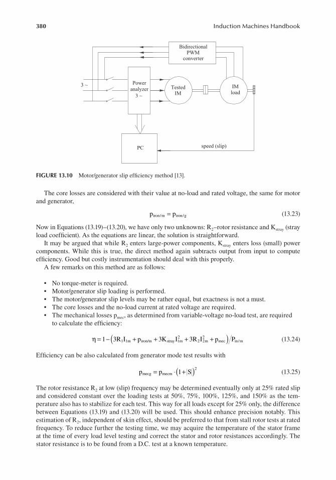
380 Induction Machines Handbook
η = −1 3( R I + +p 3K I21 1 + +3R 2
m iron/m stray 1m 2 2I pm mec iPn/m (13.24))
pmecg = ⋅p 1mecm ( )+ S2 (13.25)
3 ~ Poweranalyzer
3 ~Tested
IMIMload
speed (slip)PC
BidirectionalPWM
converter
Power analyser
3 ~
Power analyzer
FIGURE 13.10 Motor/generator slip efficiency method [13].
The core losses are considered with their value at no-load and rated voltage, the same for motor and generator,
piron/m = piron/g (13.23)
Now in Equations (13.19)–(13.20), we have only two unknowns: R2–rotor resistance and Kstray (stray load coefficient). As the equations are linear, the solution is straightforward.
It may be argued that while R2 enters large-power components, Kstray enters loss (small) power components. While this is true, the direct method again subtracts output from input to compute efficiency. Good but costly instrumentation should deal with this properly.
A few remarks on this method are as follows:
• No torque-meter is required.• Motor/generator slip loading is performed.• The motor/generator slip levels may be rather equal, but exactness is not a must.• The core losses and the no-load current at rated voltage are required.• The mechanical losses pmec, as determined from variable-voltage no-load test, are required
to calculate the efficiency:
Efficiency can be also calculated from generator mode test results with
The rotor resistance R2 at low (slip) frequency may be determined eventually only at 25% rated slip and considered constant over the loading tests at 50%, 75%, 100%, 125%, and 150% as the tem-perature also has to stabilize for each test. This way for all loads except for 25% only, the difference between Equations (13.19) and (13.20) will be used. This should enhance precision notably. This estimation of R2, independent of skin effect, should be preferred to that from stall rotor tests at rated frequency. To reduce further the testing time, we may acquire the temperature of the stator frame at the time of every load level testing and correct the stator and rotor resistances accordingly. The stator resistance is to be found from a D.C. test at a known temperature.

381Testing of Three-Phase IMs
If time permits, the machine may be stopped quickly, by fast braking it with the load machine which is supplied by a bi-directional power flow converter, for the stator resistance to be D.C. (by milliohmmeter) measured.
Test results in [13] proved satisfactory when compared with IEEE–112B tests.Still, the coupling of a loading machine at the IM shaft is required. For vertical shaft IMs as well
as large-power IMs, this may be incurring too high costs.Recently, the MF method, stemming from the classical two-frequency method [14], has been
revived by using a static power converter to supply the IM [15,16]. The key problem in this artificial loading test is the equivalence of losses with those of direct load testing.
13.2.5 the pwM MixeD-Frequency teMperature riSe anD eFFiciency teStS (artiFicial loaDing)
The two-frequency test relies on the principle of supplying the IM with voltages V1 and V2 of two different frequencies f1 and f2:
V(t) V= ω1 1cos t + ωV c2 2os t (13.26)
The rated frequency f1 differs from f2 such that the IM speed oscillates very little. Consequently, the IM works as a motor for f1 and as a generator for f2. The RMS value of stator current depends on the amplitude and frequency of second voltage: V2 and f2.
Traditionally, the test uses a synchronous generator of frequency f2 ≈ (0.8–0.85)f1 and V2 < V1, connected in series with the power grid voltage V1(f1), to supply the IM. V2 and f2 are modified until the RMS value of stator current has the desired value (around or equal to rated value in general).
The test has been traditionally used to determine the temperature rise transients and steady-state value, to replicate direct load loss conditions. The exceptional advantage is that no loading machine is attached to the shaft. Consequently, the testing costs and time are drastically reduced, especially for vertical shaft IMs.
However, due to the lack of correct loss equivalence such tests were reported to yield, in general, higher temperature (6°C–10°C) than direct load tests for the same RMS current.
This is one reason why the MF traditional tests did not get yet enough acceptance.The availability of PWM converters should change the picture to the point that such tests could
be applied, at least for IMs destined for variable speed drives, to determine the efficiency. There are quite a few ways to control the PWM converter to obtain artificial loading.
Among them, we mention here
• The accelerating–decelerating method [15]• Fast primary frequency oscillation method [15]• PWM dual frequency method. [16]
13.2.5.1 The Accelerating–Decelerating MethodThe IM is supplied from an off-the-shelf PWM converter – even one with unidirectional power flow will do. The reference speed is ramped up and down linearly or sinusoidally around the rated frequency synchronous speed so that the IM with free shaft can follow path.
The speed variation range nmin–nmax and its time variation
dn n n−≈ max min (13.27)dt T
are used as parameters to try to provide loss equivalence with the direct load test.

382 Induction Machines Handbook
Common sense indicates that for equivalent stator copper loss, the same RMS current as in direct load testing is required.
As the speed has to go above rated (base) speed, the inverter voltage ceiling is causing constant voltage to be applied above rated speed with only frequency as a variable.
As (nmax–nmin)/nrated ≈ 0.2–0.4, the mechanical losses vary. As they are, in general, proportional to speed squared, the process of making it equivalent should not be very difficult.
nmax
−( 2 1 3 3
P K minmec ) 2 n nmax
m n m mrated = =n ( ) ∫ K n dn = ⋅K (13.28)n nmax − min 3 nmax − nmin
nmin( )
Consequently,
n2max + ⋅n nmax min + =n 32
min n2n
As the frequency varies, all core losses are considered proportional to voltage squared, and the torque is also proportional with voltage squared (constant slip during the tests), the average core loss is slightly smaller than for direct load tests. In general, nmax and nmin are rather symmetric with respect to rated speed.
Consequently nmax and nmin are found easily.Now the pace of acceleration is left to be adjusted such that to produce the equivalent RMS stator
current over the speed oscillation cycle.An RMS current estimator based on current acquisition over a few periods can be used as current
feedback signal. The reference RMS current will be input to a slow current close loop that outputs the reference speed oscillation frequency between nmin and nmax.
The voltages Va and Vb and the currents Ia and Ib are acquired and transformed to synchronous coordinates:
πcos cV I ( ) 2π 2
( ) −θ os −θ s a aes es + co −θ es − V I( )d d
2 3 3
= ⋅ ( )V Iq q( ) V I ;
3 ( ) 2π π b b2 sin −θes −θes + sin −θ V I3
es − 3 c c( ) (13.29)
V Vc a= − − V ;b
I Ic a= − − I ;b
θ =es ∫ω1 dt;
The frequency f1 varies with time as the machine accelerates and decelerates.The input power
3P1 d= +
2( )V Id qV Iq (13.30)
is in fact the instantaneous active power.If the reference frame axis d falls along phase a axis at time zero, then Vq = 0 and thus only one
term appears in (13.30).The reactive input power Q1 is
3Q1 d= −V Iq q+ V Id (13.30’)
2( )
and retains also one term only. Notice that the current has both components.

383Testing of Three-Phase IMs
The main advantage of this variable transformation – to be done offline through a PC – is that it provides “instantaneous” power values without requiring averaging over a few integral electrical periods [15].
Consequently, while the machine travels from nmin to nmax and back, the active and (reactive) instantaneous powers travel a circle when shown as a function of speed (Figure 13.11) [15]. Basically, the machine works as a motor during acceleration from nmin to nmax and as a generator from nmax to nmin, and thus the, input instantaneous active power is at times positive or negative.
The average power per cycle represents the average total losses in the IM per cycle Ploss. By the same token, the average of positive values yields the average input power Pin1m. So the efficiency η is
η = −1 Ploss Pin1m (13.31)
FIGURE 13.11 Speed oscillation and instantaneous active power variation (Pn = 7.5 kW). (After Ref. [15].)

384 Induction Machines Handbook
Reference [15] reports <1% difference in efficiency between this method and the direct loading method.
The main demerit of the method is the speed continuous dynamics which gives rise to additional noise and vibration losses in the IM.
If the frequency is changed up and down quickly, the IM speed cannot follow it and thus speed dynamics is avoided. Care must be exercised in this case not to go beyond the D.C. line capacitor threshold voltage during inevitable fast switching from motor to generator mode.
13.2.5.2 The PWM Dual Frequency TestAn inverter with an open control architecture is prepared to produce, through PWM, the V(t) shown in (13.26) which contains two distinct frequencies [16].
This may be chosen around the rated synchronous speed of the IM:
f f1 1= +n ∆f (13.32)
f f2 1= −n ∆f
Now Δf is the output of a slow RMS current close-loop controller, which will result in the required current load.
Again, Δf is so large that the IM speed oscillates very little somewhere below the average of the two frequencies. The switching from motoring to generating is now carried out, by the electromag-netic field, with a frequency equal to the difference between f1 and f2.
To provide for the same core losses, they are considered proportional to voltage squared and superposition is applied.
Consequently,
V21n = +V V2 2
1 2 (13.33)
Still, to determine V1 and V2 from (13.33) one of them should be adopted. Alternatively, the ampli-tude of the magnetic flux may be conserved to provide about the same saturation level:
V 2 2 2
1n V V
= 1 +
2 (13.34)
f1n f1 f2
with Δf = 5 · 10−2 f1n from (13.33) and (13.34), V2 = 0.5383V1n and V1 = 0.8427V1n. A rather com-plete block diagram of the entire system is shown in Figure 13.12. As evident in Figure 13.12, the whole testing process is “mechanized”. This includes starting the IM with a single frequency voltage, which is ramped slowly until the rated frequency is reached. Then, gradually, the dual frequency voltage PWM enters into action and produces the recalculated voltage amplitudes and frequencies. It should be noted that as the load is varied, through the RMS current, not only Δf var-ies but, also, the voltage amplitudes V1 and V2 vary according to (13.33) and (13.34). Typical test results are shown in Figure 13.13 [16].
As expected, the voltage, flux, and current are modulated. Also the capacitor voltage in the D.C. link varies. When it increases, generating mode is encountered.
The instantaneous active power may be calculated as in the previous method, in synchronous coordinates. This time, a few electrical cycles may be averaged, but in essence, the average of instantaneous active power represents the total losses of the machine. The average of the positive values yields the average input power Pin1m. So the efficiency may be calculated again as in (13.32) for various reference stator RMS currents. Ultimately, the efficiency can be plotted against output power, which is the difference between input power and losses.
Also temperature measurements may be added either to check the validity of the loss equiva-lence or, for given temperature, to calibrate the reference RMS current value.

385Testing of Three-Phase IMs
FIGURE 13.12 PWM dual frequency test system: the block diagram. (After Ref. [16].)
FIGURE 13.13 Sample test results with the PWM dual frequency method. Left side: voltages, speed, c urrent, and torque during acceleration to speed; Right side: steady-state waveforms – flux linkage, stator current, speed, torque, with their hodographs. (After Ref. [16].)
Temperature measurements [16] seem to confirm the method although verifications on many motors are required for full validation.
It should be emphasized that the IM current has been raised up to 150% and thus the complete efficiency test up to 150% load may be replicated by the PWM dual frequency test.
Notice that the slip frequency is around the rated value and thus the skin effect is not different from the case of direct load testing.
The MF methods may be used also for the temperature rise tests.One more indirect method for temperature rise testing, used extensively by a leading manufac-
turer for the last 40 years for powers up to 20 MW, is discussed next [17].
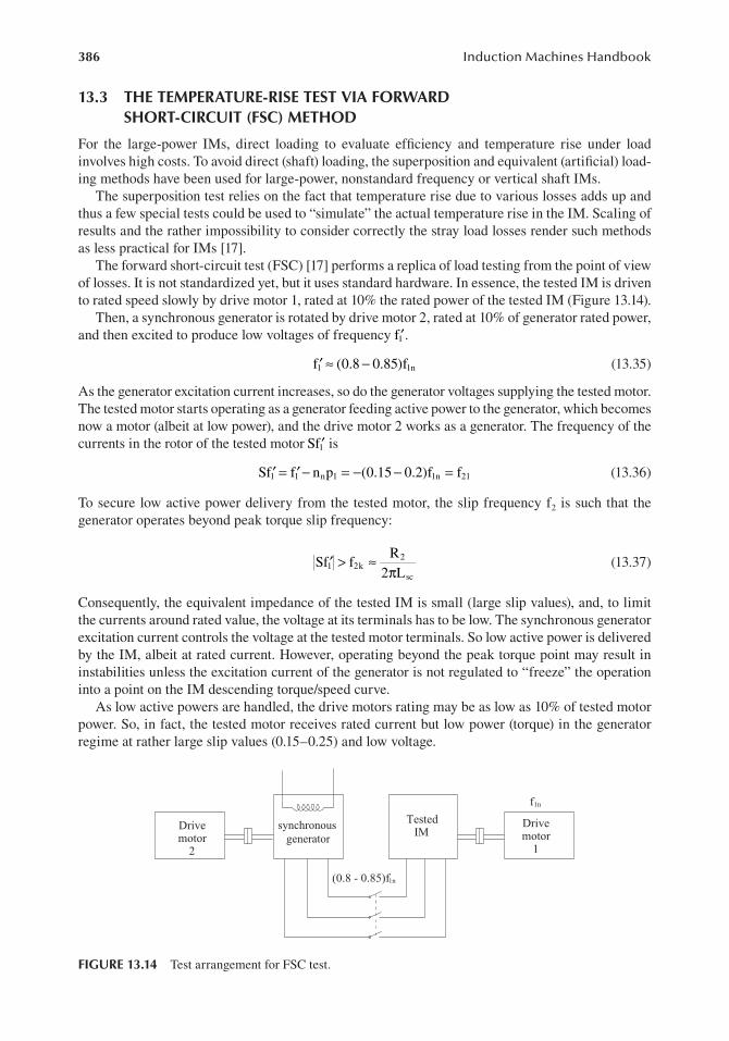
386 Induction Machines Handbook
13.3 THE TEMPERATURE-RISE TEST VIA FORWARD SHORT-CIRCUIT (FSC) METHOD
For the large-power IMs, direct loading to evaluate efficiency and temperature rise under load involves high costs. To avoid direct (shaft) loading, the superposition and equivalent (artificial) load-ing methods have been used for large-power, nonstandard frequency or vertical shaft IMs.
The superposition test relies on the fact that temperature rise due to various losses adds up and thus a few special tests could be used to “simulate” the actual temperature rise in the IM. Scaling of results and the rather impossibility to consider correctly the stray load losses render such methods as less practical for IMs [17].
The forward short-circuit test (FSC) [17] performs a replica of load testing from the point of view of losses. It is not standardized yet, but it uses standard hardware. In essence, the tested IM is driven to rated speed slowly by drive motor 1, rated at 10% the rated power of the tested IM (Figure 13.14).
Then, a synchronous generator is rotated by drive motor 2, rated at 10% of generator rated power, and then excited to produce low voltages of frequency f1′.
f (1 1′ ≈ −0.8 0.85)f n (13.35)
As the generator excitation current increases, so do the generator voltages supplying the tested motor. The tested motor starts operating as a generator feeding active power to the generator, which becomes now a motor (albeit at low power), and the drive motor 2 works as a generator. The frequency of the currents in the rotor of the tested motor Sf1′ is
Sf1 1′ = f n′ − =n 1p (− −0.15 0.2)f1n = f21 (13.36)
To secure low active power delivery from the tested motor, the slip frequency f2 is such that the generator operates beyond peak torque slip frequency:
RSf1 2′ > ≈f 2
k (13.37)2 Lπ sc
Consequently, the equivalent impedance of the tested IM is small (large slip values), and, to limit the currents around rated value, the voltage at its terminals has to be low. The synchronous generator excitation current controls the voltage at the tested motor terminals. So low active power is delivered by the IM, albeit at rated current. However, operating beyond the peak torque point may result in instabilities unless the excitation current of the generator is not regulated to “freeze” the operation into a point on the IM descending torque/speed curve.
As low active powers are handled, the drive motors rating may be as low as 10% of tested motor power. So, in fact, the tested motor receives rated current but low power (torque) in the generator regime at rather large slip values (0.15–0.25) and low voltage.
FIGURE 13.14 Test arrangement for FSC test.
Drivemotor
2
Syncronousgenerator
TestedIM
Drivemotor
1
(0.8 - 0.85)f1n
1nf
synchronousgenerator

387Testing of Three-Phase IMs
The fundamental problem in using this method, intended to replicate temperature rise for rated loading, is, again, equivalence of losses.
But before that, choosing the generator frequency f1′ is crucial.When the test f1′ frequency decreases, the copper losses in the tested motor tend to increase (slip
increases) and the required rating of drive motor 1 decreases.In general, as the slip is rather large, the rotor current, for given stator current, is higher than
that for rated load conditions (low slip). The difference is generated by the no-load (magnetization) current, as the rotor current tends to get closer to stator current with increasing slip.
For low no-load current IMs (low number of poles and/or high power), the increase in rotor current in the test with respect to rated power conditions is rather small. Not so for large number of poles and/or low-power IMs.
For f 41′ = 0 Hz and f1n = 50 Hz, the slip frequency (Sf1) = 10 Hz, and thus, at least for medium and large-power cage rotor IMs, the skin effect is notable in contrast to rated power conditions.
This is an inherent limitation of the method. Let us now discuss the status of various loss components in the FSC test:
• The stator copper lossesAs the current is kept at rated value only, the lower skin effect, due to lower frequency
f1′ (f f1 1′ < n), will lead to slightly lower copper losses than in rated load conditions in high-power IMs. If the design data are known, with f1′ given, the skin effect resistance coef-ficient may be calculated for f1n and f1′ (Chapter 9, Vol. 1). Corrections then may be added.
• The fundamental iron losses are definitely lower than those for rated conditions as f1′ is lower than that for rated conditions and so is the voltage, even the flux.
To the first approximation, the fundamental core losses are proportional to voltage squared (irrespective of frequency). Also, there are some fundamental core losses in the rotor as Sf1′ is (0.15–0.25) f1.
The no-load iron losses at rated voltage and frequency conditions may be compared with the low iron losses estimated for the FSC test with the difference added by increasing stator current to compensate for the difference in the loss balance.
• Rotor cage fundamental lossesAs indicated earlier, the rotor cage losses are larger and dependent on the generator
frequency f1′, but, to calculate their difference, would require the magnetization reactance and the rotor resistance R2 and leakage reactance Xl2 at the rather large frequency Sf1′ (with skin effect considered).
• Stray load lossesA good part of stray load losses occurs in the rotor bars. The frequency S fν 1′ of the rotor
bar harmonics currents due to stator mmf space harmonics is
S fν 1 1′ = −[ ]1 (υ −1 S) f ′ (13.38)
For phase belt harmonics,
ν = ±6K +1 (13.39)
with n 5= − , 7+ −, 11,13,… (13.40)
If for FST f 41′ = 0 Hz and S = −0.2375, for rated load conditions f1n = 50 Hz and Sn = 0.01, the rotor current harmonics frequency S fν 1′ is very close in the two cases (287.5/297.5, 306.5/296.5, 584.5/594.5, 603.5/593.5).
So, from this point of view, the two cases are rather equivalent. That is, the FST method is consistent with the direct load method. However, the rotor current harmonics are also influenced by

388 Induction Machines Handbook
slot permeance harmonics, which are voltage dependent. So in general, the stator mmf-caused rotor bar stray losses are smaller for the FST than those for rated conditions.
On the other hand, tooth flux pulsation core losses have to be considered. As the saturation is not present (low voltage; lower main flux level), the flux pulsation in the tooth, for given currents, tends to be larger in the FST, than for rated load conditions.
The rotor slot harmonic pole pairs pμ is
pµ = ±KNr 1p (13.41)
where Nr – number of rotor slots, p1 – IM pole pairs.The frequency fμ of the eddy currents induced in the stator tooth is
f pµ µ′ = − (1 S) + S f 1′ (13.42)
It suffices to consider K = 1,2.For the same example as above (f 41′ = 0 Hz, S = −0.2375 and f1 = 50 Hz, Sn = 0.01) and K = 1,2,
again frequencies fμ very close to each other are obtained for the two situations.So the stator harmonics core losses are equivalent.Still, we have to remember that the rotor cage fundamental losses tend to be somewhat
larger (because of much larger slip and skin effect), whereas the fundamental core losses are much lower.
The degree to which these two effects neutralize each other is an issue to be tackled for every machine separately.
Final results related to temperature rise for three tests – FSC, IEEE-112F and the two frequency methods (MF) – for a 1960 kW four poles, 50 Hz, 6600 V IM [17] are shown in Figure 13.15. The FSC and direct loading tests produce very close results, whereas the MF method overestimates the temperature by 5°C–7°C.
The standard MF method overestimation of temperature rise (Figure 13.15) is due to lower speed, speed oscillations, and due to higher core losses as the supply frequency voltage V1 comes in with 100% with V2 added to it. It appears that the PWM dual frequency test is free from such limitations and would produce reliable results in temperature rise as well as in efficiency tests. Returning to
FIGURE 13.15 Steady-state temperature rises with three tests. (After Ref. [17].)

389Testing of Three-Phase IMs
FSC, we notice that if the core losses are neglected (the voltage is reduced), the difference between the generated power PG and the shaft input power Pshaft for the tested motor is
P aft G− =P 3I R2
1 1 2+ +3I2 V2
sh R p2 stray + +p pmec iron (13.43) V1n
The mechanical losses pmec are considered to be known, whereas Pshaft, Pg, and I1 have to be mea-sured. When a D.C. machine is used as drive motor 1, its calibration is easy and thus Pshaft may be estimated without a torque-meter. The iron losses at rated voltage are piron.
Now if we consider the stray losses located in the stator, then the electromagnetic power concept yields
3I22R V 2
2 = +P 3G 1R I21 + +p pstray iron (13.44)
S V1n
Eliminating I22R2 from (13.43) to (13.44) yields
( )P p− V 2
p = shaft mec − −P 3 −1 S+ G 1R I2
stray 1 piron (13.45) V1n
As all powers involved are rather small, the error of calculating pstray is not expected to be large. With pstray calculated, from (13.45), the rotor fundamental cage losses 3R2 2I2 are determined. To the first approximation, with I I2 1≈ −2 I2
m (Im – the no-load current at low voltage levels, that is under unsaturated conditions), the rotor resistance R2 at Sf1′ frequency may be determined as a bonus. Comparing results on parameter calculation from FSC and IEEE–112F shows acceptable correla-tion for the 1960 kW IM investigated in Ref. [17].
The level of voltage at IM terminals during FSC is around 20% rated voltage. A few remarks on FSC are in order
• The loss distribution is changed with more losses in the rotor and less in the stator.• The skin effect is rather notable in the rotor.• It is possible, in principle, to replace the drive motor 2 and the A.C. generator by a bi-directional
power PWM converter sized around 20% the rated power of the tested IM (Figure 13.16).
The control options, for adequate loss equivalence and stable operation, are improved by the pres-ence and the capabilities of the PWM converter.
13.4 PARAMETER ESTIMATION TESTS
By IM parameters, we mean the resistances and inductances in the adopted circuit model and the inertia.
There are many ways we may develop a circuit model which duplicates better or worse the per-formance of IM in different operation modes. Magnetic saturation, skin effect, and the space and
FIGURE 13.16 The FSC test with PWM converter.
3 ~ TestedIM
Bidirectional power f low converter
(20% voltage and kVA rating)
Drive motor
10% rating

390 Induction Machines Handbook
time mmf harmonics make the problem of parameter estimation very difficult. Traditionally, the no-load and stalled rotor tests at rated frequency are used to estimate the parameters of the single-cage circuit model, with skin effect neglected.
On the other hand, for IM with deep rotor bars, or double-cage rotors, short-circuit tests at rated frequency produce too a high value for the rotor resistance for the IM running at load and rated frequency.
Standstill frequency response (SSFR) tests are recommended for such cases.Still, the large values of currents during IM direct starting at the power grid produce saturation
in the leakage path of both stator and rotor magnetic fields. Consequently, the leakage inductances are notably reduced. This effect adds to the rotor leakage inductance reduction due to skin effect.
The closed rotor cage slot leakage field, on the other hand, saturates the upper iron bridge for rotor currents above 10% of rated current.
This means that for such a case, the rotor leakage inductance does not vary essentially at currents above 10% rated current, that is during starting or on-load conditions.
For variable-speed IM operation, the level of the airgap flux varies notably. Consequently, the magnetization inductance varies also. The apparent way out of these difficulties may seem to use the traditional single-rotor circuit model with all parameters as variables (Figure 13.17) with primary (f1), rotor slip frequency Sf1, and stator, rotor, and magnetization currents (I1, I2, and Im) as measured variables. The trouble is that most parameters depend on more than one variable and thus such an equivalent circuit is hardly practical (Figure 13.17). Also, if space and time harmonics are to be considered, the general equivalent circuit becomes all but manageable.
For the space harmonics, the slip S changes to Sν, whereas for time harmonics, both fK and SK vary with the harmonics order K (see Chapter 10, Vol. 1, on time harmonics). We should remember that, while spinning the rotor, slip frequency Sf1 is different from stator frequency f1 and thus only tests performed in such conditions match the performance. Also, Finite element modelling (FEM) is now useful enough in the computation of all parameters in any conditions of operation.
Finally, for IM control for drives, a rather simplified equivalent circuit (model) with some param-eter variation would be practical. This is how simplified solutions for IM parameter estimation offline and on line evolved.
Among them, in fact, only the no-load and short-circuit single frequency test-derived param-eter estimation method is standardized worldwide. The two frequency and the frequency response standstill tests have gained some momentum lately. Modified regression methods to estimate double-cage model parameters based on acquiring data over a direct slow starting period or directly from transients during a fast start have been developed recently. Finally, for variable-speed drives commissioning and their adaptive control, offline and online simplified methods to determine some parameter detuning are currently used. A rough synthesis of these trends is presented next.
FIGURE 13.17 Fundamental single-cage rotor equivalent circuit with variable parameters.
I1
l2
coreR (f ,I ,S)
j L (I ,Sf )ω1R (f )s
1lj L (I ,f )ω1 1 1
I
IC
V1
1 mmj L (I )ω1 m
21
m
1
R (Sf )S
2 1
I2
S=1- /ω ωr 1

391Testing of Three-Phase IMs
13.4.1 paraMeter calculation FroM no-loaD anD StanDStill teStS
The no-load motor test – Section 13.1.1 – is hereby used to calculate the electric parameters appear-ing in the equivalent circuit for zero rotor currents (Figure 13.18).
With voltage V1, current I10, and power P0 measured, we may calculate two parameters:
( )P p−R R1 c+ = 0 mec
s3I2
10
(13.46)1 V 2
L 1 21l + =Lm − +( )R R
ω I 1 cs1 10
The stator phase resistances may be D.C. measured or, if possible, in A.C. without the rotor in place. In this case, if a small three-phase voltage is applied, the machine will show a very small Rcs (core losses are very small). The calculated phase inductance slightly overestimates the stator leakage inductance.
The overestimation is related to the magnetic energy in the air left by the missing rotor.The equivalent inductance Lg of the “air” inside stator is, in fact, corresponding to the magnetiza-
tion inductance of an equivalent airgap of τ/π (τ the pole pitch):
gL = ⋅( ) π
g mL unsat (13.47)τ
Suppose we do these measurements (without the rotor) and obtain from power, voltage, and current measurements,
= PR 3~
1~3I2
10~
(13.48)1 V 2
L + =L 1~
l1 g − R2
ω1 I10~ 1~
From the no-load test at low voltage, the unsaturated value of Lm is obtained. Then from (13.47), Lg is easily calculated, provided the airgap is known. Finally from (13.48), Ll1 is found with Lg already calculated.
In general, however, the stator leakage inductance is not considered separable from the no-load and short-circuit tests.
The short-circuit (standstill or stall) tests, on the other hand, are performed at low voltage with three-phase or single-phase supply (Section 13.1.4), and Rsc and Xsc = ω1Lsc are calculated from
FIGURE 13.18 Fundamental no-load equivalent circuit.
I10 11 1l
1l m
10
1
1 m1
cs
Rj Lω
R
j Lω
L +Lrated
voltage
I
V
V
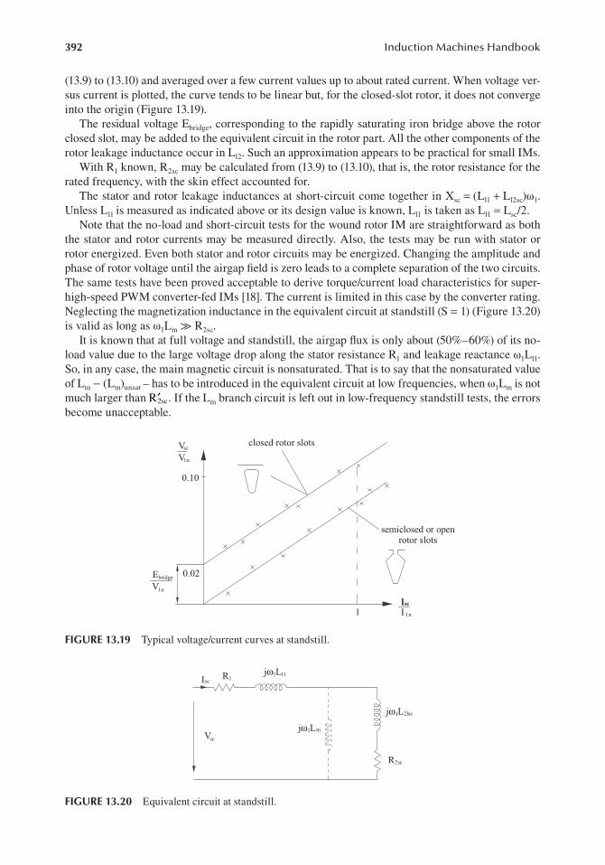
392 Induction Machines Handbook
(13.9) to (13.10) and averaged over a few current values up to about rated current. When voltage ver-sus current is plotted, the curve tends to be linear but, for the closed-slot rotor, it does not converge into the origin (Figure 13.19).
The residual voltage Ebridge, corresponding to the rapidly saturating iron bridge above the rotor closed slot, may be added to the equivalent circuit in the rotor part. All the other components of the rotor leakage inductance occur in Ll2. Such an approximation appears to be practical for small IMs.
With R1 known, R2sc may be calculated from (13.9) to (13.10), that is, the rotor resistance for the rated frequency, with the skin effect accounted for.
The stator and rotor leakage inductances at short-circuit come together in Xsc = (Ll1 + Ll2sc)ω1. Unless L1l is measured as indicated above or its design value is known, Ll1 is taken as Ll1 ≈ Lsc/2.
Note that the no-load and short-circuit tests for the wound rotor IM are straightforward as both the stator and rotor currents may be measured directly. Also, the tests may be run with stator or rotor energized. Even both stator and rotor circuits may be energized. Changing the amplitude and phase of rotor voltage until the airgap field is zero leads to a complete separation of the two circuits. The same tests have been proved acceptable to derive torque/current load characteristics for super-high-speed PWM converter-fed IMs [18]. The current is limited in this case by the converter rating. Neglecting the magnetization inductance in the equivalent circuit at standstill (S = 1) (Figure 13.20) is valid as long as ω1Lm ≫ R2sc.
It is known that at full voltage and standstill, the airgap flux is only about (50%–60%) of its no-load value due to the large voltage drop along the stator resistance R1 and leakage reactance ω1Ll1. So, in any case, the main magnetic circuit is nonsaturated. That is to say that the nonsaturated value of Lm − (Lm)unsat – has to be introduced in the equivalent circuit at low frequencies, when ω1Lm is not much larger than R′2sc. If the Lm branch circuit is left out in low-frequency standstill tests, the errors become unacceptable.
FIGURE 13.19 Typical voltage/current curves at standstill.
FIGURE 13.20 Equivalent circuit at standstill.
0.10
closed rotor slots
semiclosed or openrotor slots
II
VV
EV
1n
sc
sc
1n
bridge
1n
0.02
1Isc
Isc1 1lj Lω
j Lω 2lsc1
1 msc
1
V
R
R
j Lω
2sc
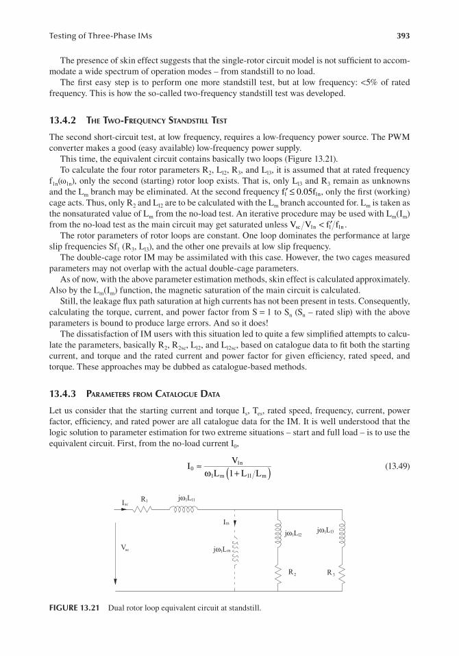
393Testing of Three-Phase IMs
The presence of skin effect suggests that the single-rotor circuit model is not sufficient to accom-modate a wide spectrum of operation modes – from standstill to no load.
The first easy step is to perform one more standstill test, but at low frequency: <5% of rated frequency. This is how the so-called two-frequency standstill test was developed.
13.4.2 the two-Frequency StanDStill teSt
The second short-circuit test, at low frequency, requires a low-frequency power source. The PWM converter makes a good (easy available) low-frequency power supply.
This time, the equivalent circuit contains basically two loops (Figure 13.21).To calculate the four rotor parameters R2, Ll2, R3, and Ll3, it is assumed that at rated frequency
f1n(ω1n), only the second (starting) rotor loop exists. That is, only Ll3 and R3 remain as unknowns and the Lm branch may be eliminated. At the second frequency f1 1′ ≤ 0.05f n, only the first (working) cage acts. Thus, only R2 and Ll2 are to be calculated with the Lm branch accounted for. Lm is taken as the nonsaturated value of Lm from the no-load test. An iterative procedure may be used with Lm(Im) from the no-load test as the main circuit may get saturated unless Vsc V f1n < 1 1′ f n .
The rotor parameters of rotor loops are constant. One loop dominates the performance at large slip frequencies Sf1 (R3, Ll3), and the other one prevails at low slip frequency.
The double-cage rotor IM may be assimilated with this case. However, the two cages measured parameters may not overlap with the actual double-cage parameters.
As of now, with the above parameter estimation methods, skin effect is calculated approximately. Also by the Lm(Im) function, the magnetic saturation of the main circuit is calculated.
Still, the leakage flux path saturation at high currents has not been present in tests. Consequently, calculating the torque, current, and power factor from S = 1 to Sn (Sn – rated slip) with the above parameters is bound to produce large errors. And so it does!
The dissatisfaction of IM users with this situation led to quite a few simplified attempts to calcu-late the parameters, basically R2, R2sc, Ll2, and Ll2sc, based on catalogue data to fit both the starting current, and torque and the rated current and power factor for given efficiency, rated speed, and torque. These approaches may be dubbed as catalogue-based methods.
13.4.3 paraMeterS FroM catalogue Data
Let us consider that the starting current and torque Is, Tes, rated speed, frequency, current, power factor, efficiency, and rated power are all catalogue data for the IM. It is well understood that the logic solution to parameter estimation for two extreme situations – start and full load – is to use the equivalent circuit. First, from the no-load current I0,
VI 1n
0 ≈ω +1 mL 1( ) (13.49)
L L1l m
FIGURE 13.21 Dual rotor loop equivalent circuit at standstill.
j Lω l31
1 l1j Lω 1RIsc
scV
R
Im
1 mj Lω
1 l2j Lω
2 3R

394 Induction Machines Handbook
we obtain an approximate value of Lm. For start L1l/Lm = 0.02–0.05. At the end of the estimation process, Ll1 is obtained.
Then, we may return with a corrected value of Ll1/Lm to (13.49) and perform the whole process again until sufficient convergence is reached.
This saturated value is valid for rated load calculations.For the starting torque, Tes at starting stator current Is
3R ⋅ ⋅I p2
Tes = 2sc 2s 1
ω1 (13.50)
I I2s ≈ −2s I2
0
From (13.50), R2sc may be determined. The equivalent circuit at start yields
( + =) (1 V1n 2
L L 2l1sc l2sc − +R R )
ω1 Is 1 2sc (13.51)
The stator resistance R1 may be D.C. measured, and thus, (Ll1sc + Ll2sc), as influenced by skin effect and leakage saturation, is determined.
On full load, the mechanical losses are assigned an initial value pmec = 0.01Pn.Thus, the electromagnetic torque is equal to the shaft torque plus the mechanical loss torque.
p 2
T = +p 1mec P 3R I
n
en 1 = 2 2n p Pn 2 fπ −1 n( )1 S Sn 1ω 1
(13.52)
I I2 ≈ −2 22n 1n I0
With R2 determined easily from (13.52), we write the balance of powers at rated slip:
Q 3= V I1n nϕ =1n 3 Lω +2 2 21 1n si 1 l1 1I 3n ω +1 lL I2 2n 3Lm 1ω ⋅ I0 (13.53)
R I2
P1 1= ϕ3V I c 2 2 2n 1n 1os n 1= +3R I p1n iron + +p 3 n
stray (13.54)Sn
1 Pn 11− = +3R I p2 + +p 3R I2 + p (13.55)
η 1 iron stray 2 2n mec
There are five unknowns – Ll1, Ll2, piron, pstray, and pmec – in Equations (13.53)–(13.55).However from (13.54), piron + pstray can be calculated directly. They are introduced in (13.55) to
calculate mechanical loss pmec. If they differ from the initial value of 1% of rated power Pn, their value is corrected in (13.52) and pcore + pstray and pmec are recalculated again until sufficient conver-gence in pmec is obtained.
In Equation (13.53), we do have two unknowns remaining: the stator and rotor leakage induc-tances. They may not be separated, and thus, we consider them equal to each other: Ll1 = Ll2.
This way
( )3V I sinϕ − ω= =
1n m 1n 13 Lm 0I2
Ll1 Ll2 )3 2ω −1 1( ) (13.56
I I2 2n 0

395Testing of Three-Phase IMs
Now going back to (13.51), if the IM has open stator slots, there will be no leakage flux path satura-tion in the stator, and thus, Ll1sc = Ll1 = Ll2. Consequently, from (13.51), Ll2sc is found. With semi-closed stator slots, both stator and rotor leakage flux paths may saturate. So, we might consider Ll1sc = Ll2sc as well. Again, Ll2sc = Ll1sc is found from (13.51).
Attention has to be paid to (13.56) as computation precision is important because most of the reactive power is “spent” in the airgap, in Lm. In general, 2L1l > Ll1sc + Ll2sc. If 2L1l ≤ Ll1sc + Ll2sc is obtained, the skin and saturation effects are mild and the short-circuit values hold as good for all slip values.
An approximate dependence of rotor resistance and leakage inductances with slip, between S = 1 and S = Sn, is
( )S S−R (S) R ( ) n
2 2= + R R2sc 2− ; S ≥ S1 S− n (13.57)
n
S S−Ll2(S) L= − n
l2 ( )L Ll2 − l2sc ; S ≥ Sn (13.58)1 S−
S S−L = − ( ) n
l1(S) Ll1 L Ll1 − l1sc ; S ≥ Sn (13.59)1 S− n
This way, the parameter dependence on slip is known, so torque, current, power factor versus slip are calculated. Alternatively, we may consider that the rotor parameters at standstill R2sc and Ll2sc represent the starting cage and R2l, Ll2, the working cage. Such an attitude may prove practical for the investigation of IM transients and control.
It should be emphasized that catalogue data methods provide for complete agreement between the circuit model and the actual machine performance only at standstill and at full load. There is no guarantee that the rotor parameters vary linearly or as in (13.57) with slip for all rotor (stator) slot geometries.
In other words, the agreement of, say, the torque and current versus slip curves for all slips is not guaranteed to any definable error.
From the need to secure good agreement between the circuit model and the real machine, for ever wider operation modes, more sophisticated methods have been proposed.
We introduce here two of the most representative ones: the SSFR method and the step-wise regression general method.
13.4.4 StanDStill Frequency reSponSe MethoD
Standstill tests, especially when a single-phase A.C. supply is used (zero torque), require less man power, equipment, and electrical energy to perform than running tests. To replicate the machine performance with different rotor slip frequency Sf1, tests at standstill with a variable voltage and frequency supply have been proposed [19,20]. Dubbed as SSFR, such tests have been first used for synchronous generator parameter estimation.
In essence, the IM is fed with variable voltage and frequency from a PWM converter supply.Single-phase supply is preferred as the torque is zero, and thus, no mechanical fixture to stall the
rotor is required. However, as three-phase PWM converters are available up to high powers and the tests are performed at low currents (less than 10% of rated current), three-phase testing seems more practical (Figure 13.22).
The test provides for the consideration of skin effect, which is frequency dependent. However, as the current is low, to avoid IM overheating, the SSFR test methods should not be expected to pro-duce good agreement with the real machine in the torque/slip or current/slip curves at rated voltage.
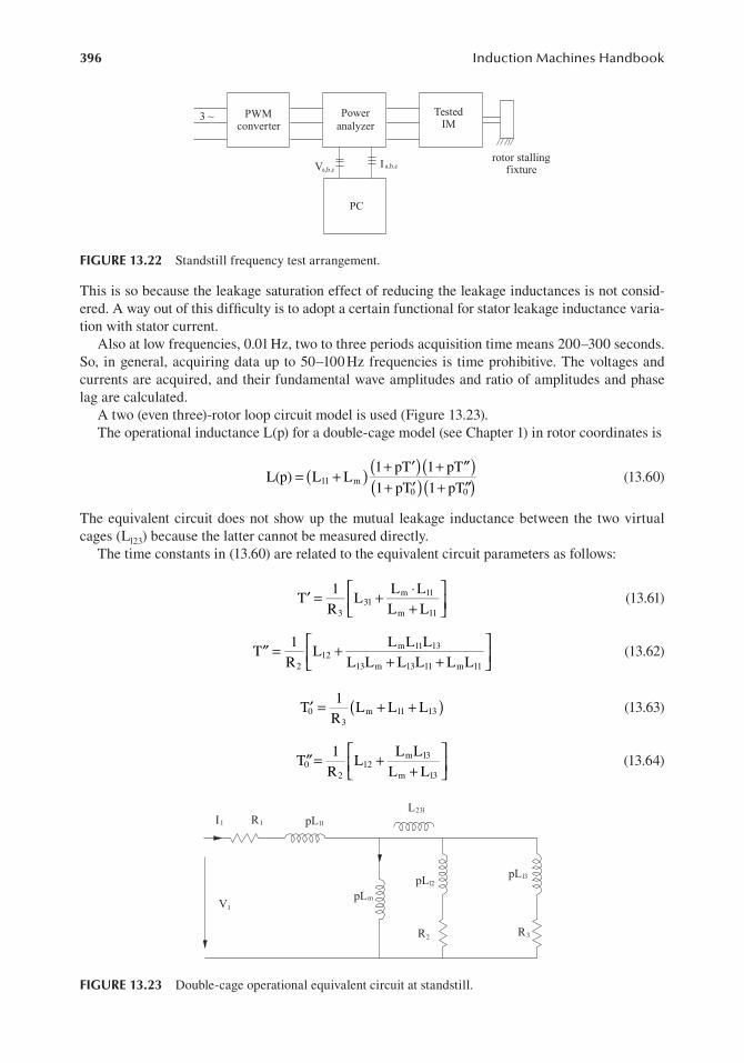
396 Induction Machines Handbook
( )+ ′ ( )+ ′′
L(p) L= +( ) 1 pT 1 pTl1 Lm ( ) (13.60)
1 p+ T 10 0′ ( )+ pT′′
1 L L⋅′ = + m l1
T L (13.61)R 3l
3 L L m l+ 1
1 L L L
T L m l1 l3 ′′ = +l2 (13.62)R2 L Ll3 m l+ +L L3 l1 mL Ll1
1
T0′ = +( )L Lm l1 l+ L 3 (13.63)R3
1 L L
T′′= +L m l30 l2 (13.64)
R2 L Lm l+ 3
3 ~ PWMconverter
TestedIM
PC
V Ia,b,c a,b,crotor stalling
fixture
Power analyzer
FIGURE 13.22 Standstill frequency test arrangement.
This is so because the leakage saturation effect of reducing the leakage inductances is not consid-ered. A way out of this difficulty is to adopt a certain functional for stator leakage inductance varia-tion with stator current.
Also at low frequencies, 0.01 Hz, two to three periods acquisition time means 200–300 seconds. So, in general, acquiring data up to 50–100 Hz frequencies is time prohibitive. The voltages and currents are acquired, and their fundamental wave amplitudes and ratio of amplitudes and phase lag are calculated.
A two (even three)-rotor loop circuit model is used (Figure 13.23).The operational inductance L(p) for a double-cage model (see Chapter 1) in rotor coordinates is
The equivalent circuit does not show up the mutual leakage inductance between the two virtual cages (Ll23) because the latter cannot be measured directly.
The time constants in (13.60) are related to the equivalent circuit parameters as follows:
FIGURE 13.23 Double-cage operational equivalent circuit at standstill.
L
pLpL
R3
pLl3l2
23l
m
pLl1R1
R2
V1
I1

397Testing of Three-Phase IMs
The unsaturated value of the no-load inductance Ls = Ll1 + Lm has to be determined separately from the no-load test at lower than rated voltage.
Also the stator leakage inductance value has to be known from design or is being assigned a “reasonable” value of 2%–5% of no-load inductance Ls.
The measurements will result in impedance estimation for every frequency the test is performed.
VZ (ω =) sc
sc = ωR ( .I
sc ) j+ ωX (sc ) (13 65)sc
When the IM is single-phase supply fed between two phases, a factor of two occurs in the denomi-nator of (13.65).
We now calculate L(jω) from (13.65):
( )Z R−L( jω =) sc 1 = ωRe( ) + ωj Im( ) (13.66)
jω1
Equating the real and imaginary parts in (13.60) and (13.66), we obtain
Re(ω =) Lω +s 0ω ωIm( )( )T T′ + 0′′ − ω3L Ts ′ ′T R′ + ω2 e(ω ⋅) T0 0′ ⋅T′′ (13.67)
Im( )ω = ω2L Ts 0( )′ + T R′′ − ω e(ω) T( )′ + T I0′′ − ω2 m(ω)T0 0′ ⋅T′′ (13.68)
A new set of unknowns, instead of T′, T″, T0′, T0′′, is now defined [21].
X L1 s=
X T2 0= ′ + T0′′
X L3 s= T T′ ′′ (13.69)
X T4 0= ′ ′T0′
X L5 s= ( )T T′ + ′′
Ls may be discarded by introducing the known value of the nonsaturated no-load inductance.A linear system is obtained.In matrix form,
Z Hi i= =X ; i 1,2,....,m (13.70)
with
Z Ri = ωe( ), Im( )ω T
I (13.71)
X X= 1,X2 3 4,X ,X ,X5, (13.72)
ω ω Im( )ω −ω ω3 2 Re( )ω 0Hi = (13.73)
0 R−ω e(ω ω) 0 2 2Im( )ω ω

398 Induction Machines Handbook
The measurements are taken for m ≥ 5 distinct frequencies.As the number of equations is larger than the number of unknowns, various approximation
methods may be used to solve the problem.The solution of (13.70) in the least squared error method sense is
= ⋅ −1
X [H]T [H] [ ⋅ ⋅H]T [Z] (13.74)
Once the variable vector |X| is known, the actual unknowns Ls, T′, T″, T0′, T0′′ are
L Xs 1=
1T′ ′,T ′ = ±
2X1( ) (13.75)X X2
5 5 − 4X3 1X
1T0 0′ ′,T ′= ±( )X X2
2 2 − 4X4 (13.76)2
The least squared error method has been successfully applied to a 1288 kW IM in [21].Typical direct impedance results are shown in Figure 13.24 [21].Comparative results [20,21] of parameter values estimated with Bode diagram and, respectively,
by the least squared method, for same machine, are given in Table 13.3 [21].Good agreement between the two methods of solution is evident.
FIGURE 13.24 SSFR of a 1288 kW IM. (After Ref. [21].)

399Testing of Three-Phase IMs
However, as [20] shows, when applying these parameters to the torque/slip or current/slip curves at rated load, the discrepancies in torque and current at high values of slip are inadmissible. This may be explained by the neglect of leakage saturation, which in the real machine with high starting torque and current is notable.
As always in such cases, an empirical expression of the stator leakage inductance, which decreases with stator current, may be introduced to improve the model performance at high currents.
Still, there seem to be some notable discrepancies in the breaking torque region, which hold in there even after correcting the stator leakage inductance for leakage saturation. A three-circuit cage seems necessary in this particular case.
This raises the question of when the SSFR parameter estimation may be used with guaran-teed success. It appears only for small periodic load perturbations around rated speed or for esti-mating the machine behaviour with respect to high-frequency time harmonics so typical in PWM converter-fed IMs.
Step response methods to different levels of voltage and current peak values may be the response to the leakage saturation at high currents inclusion into the IM models.
Short voltage pulses may be injected in the IM at standstill between two phases until the current peaks to a threshold, predetermined value. A pair of positive and negative voltage pulses may be applied to eliminate the influence of hysteresis.
The current and voltage are acquired and processed using the same operational inductance (13.60).
v p( ) = ⋅2 i(p) R[ ]1 + pL(p) (13.77)
The two cage model may be used, with its parameters determined to fit the current/time transient experimental curve via an approximation method (least squared method, etc.)
The voltage signals will stop, via a fast static power switch, at values of current up to the peak starting current to explore fully the leakage saturation phenomenon. The pulses are so short that the motor does not get warm after 10–15 threshold current level tests. Also, the testing will last only 1–2 minutes in all and requires simplified power electronics equipment. It may be argued that the step voltage is too a fast signal and thus the rotor leakage inductances and resistances are too much influenced by the skin effect. Only extensive tests hold the answer to this serious question.
The method to estimate the parameters from this test is somehow included in the general regression method that follows.
13.4.5 the general regreSSion MethoD For paraMeterS eStiMation
As variable parameters, with current and/or rotor slip frequency, are difficult to handle, constant parameters are preferred. By using a two-rotor cage circuit model, the variable parameters of a single cage with slip frequency are calculated. Not so for magnetic saturation effects.
The deterministic way of defining variable parameters for the complete spectrum of frequency and current has to be apparently abandoned for constant parameter models which, for a given
TABLE 13.3 Comparative Parameter Estimates for an 1288 kW IM
Parameter Bode Diagram [20] Least Squared Method [21]
ls p.u.
T′ s5.3
88 · 10−3
5.299
87.99 · 10−3
T″ s 3.6 · 10−3 3.6 · 10−3
T0′ s
T′′0 s
2.0
4.55 · 10−3
2.00
4.55

400 Induction Machines Handbook
spectrum of operation modes, give general satisfaction according to an optimization criterion, such as the least squared error over the investigated operation mode spectrum.
For transient modes, the transient model has to be used, whereas for steady-state modes, the steady-state equations are applied.
The d.q. model of double-cage IM in synchronous coordinates in space phasor quantities is (Chapter 1)
dΨV1 1= +R I 1
1 + ωj ;1 1Ψ Ψ1 m= Ψ + L Il1 1 (13.78)dt
dΨ0 R= +2 2I
2 + ωjS 1 2Ψ Ψ; L2 m= Ψ + l2 I2 (13.79)dt
dΨ0 R= +3 3I 3 + ωjS 1 3Ψ Ψ; L3 m= Ψ + l3 I3 (13.80)
dt
Ψm = +L Im ( )1 2I I+ =3 2; I I jd2 + =I ;q2 I I3 d3 + jIq3 (13.81)
J dω r 3= −T Te load e; T = ⋅p L1 m Imag I I1 2⋅ +( )*I
*3 (13.82)
p1 dt 2
For sinusoidal voltages,
V1 = γV 2 cos j− γV 2 sin ; I I1 = +d1 jIq1 (13.83)
Equations (13.78)–(13.82) represent a seven-order system with seven variables (Id1, Iq1, Id2, Iq2, Id3, Iq3, and ωr).
For steady-state, d/dt = 0 in Equations (13.78)–(13.80) – synchronous coordinates.When the IM is fed from a nonsinusoidal voltage source, Vs has to be calculated according to
Park transformation:
2 2π 2π− V = +
j j
V ( 3 − θj 1s a t) V (b t)e V3 + c (t)e e (13.84)
3
dθ1 = ω1 (13.85)dt
Equation (13.85) represents the case when the fundamental frequency varies during the parameter estimation testing process.
For steady state, (13.79)–(13.81) are solved for torque Te, stator current, I1, and input power P1 [22].
T (S) 3= ⋅ p Re V2 1 ⋅ r (13.86)
ω1 S A( )2 2+ B
C D2 2+I (1 S) = V 2 2 (13.87)
A B+
AC − BDP(S) 3= V2
A B2 2 (13.88)+

401Testing of Three-Phase IMs
R R 2 3+ +
=2 3 ( )R R ( )R X2
2 l3 + R X2 23 l2 S
Rr 2 (13.89)( )R R2 3+ + ( )X Xl2 + 2 S2
l3
( )X Xl2 l3 ( )X Xl2 + +l3 S R2 2X R+ 2XXrl =
2 l3 3 l2
2 2 (13.90)( )R R2 3+ + ( )X Xl2 + l3
C 1= + X Xrl m r; D = =R S( )X ;m lE 1+ X X1 m (13.91)
RA R= +1C
r E; B X= +l1 X Erl ⋅ − R D1 (13.92)S
X Li 1= ω i (13.93)
The steady-state and transient models have the phase voltage RMS value V, its phase angle γ, p1 pole pairs, and frequency ω1 as inputs.
For steady state, the slip value is also a given. The stator resistance R1, stator leakage Ll1, and magnetization inductances Lm are to be known a priori.
The stator current or torque or power under steady state is measured.Using torque, or current or input power measured functions of slip (from S1 to S2), the rotor double-
cage parameters that match the measured curve have to be found. This is only an example for steady state. In a similar way, the observation vector may be changed for transients into stator currents d–q components versus time: Id1(t), Iq1(t). For a number of time steps t1, …, tn, the two currents are cal-culated from the measured stator current after transformation through Park transformation (13.84).
To summarize, the parameters vector |X| can be estimated from a row |Y| of test data at steady state or transients:
X R= T2 3,R ,Ll2 ,Ll3 (13.94)
Y Y= [ ]( )S ,1 2Y S( ), , Y S( )n (13.95)
Y S( )K e= T S( )K 1or I S( )K 1or P S( )K (13.96)
where S1, …, Sn are the n values of slip considered for steady state. For transients, the test data Id1(t) and Iq1(t) are acquired at n time instants t1, …, tn. The stator current d–q components in synchronous coordinates constitute now the observation vector:
[Y] Y= [ ]( )t ,1 2Y t( ), , Y t( )n (13.97)
Y t( )K d= I t1 K( ) or I tq1 ( )K (13.98)
In general, the problem to solve may be written as
Y f= ζ( )K K,X ; 1ξ = , , n (13.99)
with ζ = SK for steady-state estimation and ζ = tK for transients estimation. The parameter ξK is the error for the Kth value of SK (or tK).
There are many ways to solve such a problem iteratively. Gauss–Newton method, when used after linearization, tends to run into almost singularity matrix situations. On the contrary, the step-wise

402 Induction Machines Handbook
regression method, based on Gauss–Jordan pivot concept [21], seems to produce safely good results across the board. For details on the computation algorithm, see Ref. [22]. The method’s convergence should not depend on the width of change limits of parameters or on their assigned start values.
Typical results obtained in [22] for steady-state and dynamic (direct starting) operation modes are given in Table 13.4.
Sample results on convergence progress for Te(S) observation vector show fast convergence rates in Figure 13.25 [22].
The corresponding torque/slip curve fitting is, as expected, very good (Figure 13.26).Similarly good agreement for the torque–time curve during starting transients is shown in
Figure 13.27 when the Te(t) function is observed.A few remarks are
• The curve fitting of the observed vectors over the entire explored zone is very good, and therate of convergence is safe and rather independent of the extension of parameter existencerange.
• The estimated parameter vectors (Table 13.4) have only up to 3% variations depending onthe observation vector: torque or current. This is a strong indication that if the torque/slipis observed, the current/slip curve will also fit rather well.
FIGURE 13.25 Convergence progress in rotor resistance estimation from Te(S). (After Ref. [22].)
TABLE 13.4 Estimated Parameters for Various Observation Vectors
Estimated Parameters [Ω]
R2 R3 Xl2 Xl3 Xl1
Values used to calculate the input (theoretical) characteristics and runs 3.1144 0.2717 3.0187 4.6098 3.1316
Values obtained after estimation from Te = f(S) 3.1225 0.2717 3.032 4.6145 3.1261
Values obtained after estimation from Is = f(S) 3.0221 0.2722 2.868 4.5552 3.1946
Values obtained after estimation from ia = f(S) 3.0842 0.2718 2.9706 4.5931 3.1513
Values obtained after estimation from |is| = f(t) 3.0525 0.2721 2.9099 4.5671 3.1762
Values obtained after estimation from Te = f(t) 3.1114 0.2664 3.0693 4.5831 3.093
Source: After Ref. [22].

403Testing of Three-Phase IMs
• The phase current measurement is straightforward, but the torque measurement is not so.We may however calculate the torque offline from measured voltages and currents Va, Vb,Ia, and Ib:
( )= Ψ − Ψα β β αTe32
p I I1 (13.100)
=αV Va
( )
( )
= +
=
= +
β
α
β
V13
V 2V
I I
I13
I 2I
a b
a
a b
(13.101)
FIGURE 13.26 The static characteristic of electromagnetic torque Te = f (S): (after Ref. [22]) solid line (___), the theoretical characteristic of Te = f (S); dotted line (……), the characteristic calculated for starting values of parameters; dashed line (------), the characteristic calculated for final values of estimated parameters.
FIGURE 13.27 Runs of the electromagnetic torque Te during the start-up: (after Ref. [22]) solid line (____), the theoretical run of Te = f (t); dotted line (……), the run calculated for starting values of parameters; dashed line (------), the run calculated for final values of estimated parameters.

404 Induction Machines Handbook
∫∫ ( )
( )= −
= −
α α α
β β β
V V R I dt
V V R I dt
1
1
The precision of torque estimates by (13.100) is good at rated frequency but smaller at low fre-quencies f1. The integrator should be implemented as a filter to cancel the offset. In (13.100), the reduction of the electromagnetic torque due to core loss, which is smaller than 1% of rated torque in general, is neglected. If core loss pcore is known from the no-load test, the torque of (13.100) can be reduced by ΔTecore:
∆ =ω
T pp
ecore core1
1
(13.102)
• The direct start is easy to perform, as only two voltages and two currents are to be acquiredand the data are processed offline. It shows that this test may be the best way to estimatethe IM parameters for a large spectrum of operation modes. Such a way is especially prac-tical for medium–large-power IMs.
• Very large-power machines direct starting is rather slow as the relative inertia is large andthe power grid voltage drops notably during the process. In such a case, the method ofparameter estimation data may be simplified as shown in the following section where alsothe inertia is estimated.
13.4.6 large iM inertia anD paraMeterS FroM Direct Starting acceleration anD Deceleration Data
Testing large-power IMs takes time and requires notably human effort. Any attempt to reduce it while preserving the quality of the results should be considered.
Direct connection to the power grid, even if through a transformer at lower than rated voltage in a limited power manufacturer’s laboratory, seems a practical way to do it. The essence of such a test consists of the fact that the acceleration would be slow enough to validate steady-state operation mode approximation all throughout the process. In large-power IMs, reducing the supply voltage to 60% would do it, in general. We assume that the core loss is proportional to voltage squared. By performing no-load tests at decreasing voltages, we can separate first the mechanical from iron losses by the standard loss segregation method. The mechanical losses vary with speed. To begin, we may suppose a linear dependence:
p pn
f /p
p pVV
mec mec01
2
iron iron00
2
≈ ⋅
= ⋅
(13.103)
During the no-load acceleration test, the voltage and current of two phases are acquired together with the speed measurement. Based on this, the average power is calculated. To simplify the process of active power calculation, synchronous coordinates can be used:
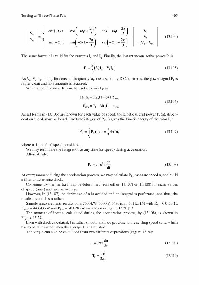
405Testing of Three-Phase IMs
V
V23
cos t cos t23
cos t23
sin t sin t23
sin t23
V
V
V V
d
q
1 1 1
1 1 1
a
b
a b( )
( )
( )=
−ω −ω + π
−ω − π
−ω −ω + π
−ω − π
⋅− +
(13.104)
The same formula is valid for the currents Id and Iq. Finally, the instantaneous active power P1 is
( )= +P32
V I V I1 d d q q (13.105)
As Vd, Vq, Id, and Iq, for constant frequency ω1, are essentially D.C. variables, the power signal P1 israther clean and no averaging is required.
We might define now the kinetic useful power PK as
= − +
= − −
P (n) P (1 S) p
P P 3R I p
K elm mec
elm 1 s 12
iron
(13.106)
As all terms in (13.106) are known for each value of speed, the kinetic useful power PK(n), depen-dent on speed, may be found. The time integral of PK(n) gives the kinetic energy of the rotor Ec:
∫= = πE P (n)dtJ2
4 nc K
0
t
2f2 (13.107)
where nf is the final speed considered.We may terminate the integration at any time (or speed) during acceleration.Alternatively,
= πP J4 ndndt
K2 (13.108)
At every moment during the acceleration process, we may calculate PK, measure speed n, and build a filter to determine dn/dt.
Consequently, the inertia J may be determined from either (13.107) or (13.108) for many values of speed (time) and take an average.
However, in (13.107) the derivative of n is avoided and an integral is performed, and thus, the results are much smoother.
Sample measurements results on a 7500 kW, 6000 V, 1490 rpm, 50 Hz, IM with R1 = 0.0173 Ω,Pmec0 = 44.643 kW and Piron = 78.628 kW are shown in Figure 13.28 [23].
The moment of inertia, calculated during the acceleration process, by (13.108), is shown in Figure 13.29.
Even with dn/dt calculated, J is rather smooth until we get close to the settling speed zone, which has to be eliminated when the average J is calculated.
The torque can also be calculated from two different expressions (Figure 13.30):
= πT 2 Jdndt
(13.109)
=π
TP
2 ne
K (13.110)

406 Induction Machines Handbook
dnpmec (n) J= − 4π2 n (13.111)
dt
FIGURE 13.28 Current, phase, voltage, power and speed during direct starting of a 7500 kW IM. (After Ref. [23].)
FIGURE 13.29 Inertia calculated during the acceleration process using the speed derivative (13.108). (After Ref. [23].)
Again, Equation (13.110), with PK(n) from (13.106) which avoids dn/dt, produces a smoother torque/time curve.
The torque may be represented as a function of speed also, as speed has been acquired.The torque shown in Figure 13.30 is scaled up to 6 kV line voltage (star connection), assuming
that the torque is proportional to voltage squared.The testing may add a free deceleration test from which, with inertia known from the above
p rocedure, the more exact mechanical loss dependence on speed pmec(n) can be determined:
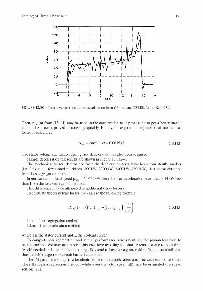
407Testing of Three-Phase IMs
2
Pstray m(I) P= −( )ec l.s.m. ( ) IPmec f.d.m.
⋅ (13.113) I0
FIGURE 13.30 Torque versus time during acceleration from (13.109) and (13.110). (After Ref. [23].)
Then, pmec(n) from (13.111) may be used in the acceleration tests processing to get a better inertia value. The process proved to converge quickly. Finally, an exponential regression of mechanical losses is calculated:
p = α 2.4mec n ; α = 0.001533 (13.112)
The stator voltage attenuation during free deceleration has also been acquired.Sample deceleration test results are shown in Figure 13.31a–c.The mechanical losses, determined from the deceleration tests, have been consistently smaller
(i.e. for quite a few tested machines: 800 kW, 2200 kW, 2800 kW, 7500 kW) than those obtained from loss segregation method.
In our case at no-load speed pmec = 64.631 kW from the free deceleration tests, that is 14 kW less than from the loss segregation method.
This difference may be attributed to additional (stray losses).To calculate the stray load losses, we can use the following formula:
l.s.m. – loss segregation methodf.d.m. – free deceleration method
where I is the stator current and I0 the no-load current.To complete loss segregation and secure performance assessment, all IM parameters have to
be determined. We may accomplish this goal here avoiding the short-circuit test due to both time (work) needed and also the fact that large IMs tend to have strong rotor skin effect at standstill and thus a double-cage rotor circuit has to be adopted.
The IM parameters may also be identified from the acceleration and free deceleration test data alone through a regression method, while even the rotor speed n(t) may be estimated (no speed sensor) [23].

408 Induction Machines Handbook
FIGURE 13.31 Free deceleration tests [23]: (a) speed versus time, (b) stator voltage amplitude versus time, and (c) mechanical losses versus speed.

409Testing of Three-Phase IMs
13.5 NOISE AND VIBRATION MEASUREMENTS: FROM NO LOAD TO LOAD
Noise in IM has electromagnetic and mechanical origins. The noise level accepted depends on the environment in which the IM works. At the present time, standards (ISO1680) prescribe noise limits for IMs, based on sound power levels measured at no-load conditions, if the noise level does not vary with load. It is not yet clear how to set the sufficient conditions for no-load noise tests.
The load machine produces additional noise, and thus, it is simpler to retort to IM no-load noise tests only.
If the electromagnetic noise is relatively large, it is very likely that under load, it will increase further [22]. Also, when PWM converter fed, the IM noise will change from no-load to load condi-tions. Skipping the basics of sound theory [24] in electrical machines, we will synthesize here ways to measure the noise under load in IMs.
13.5.1 when on-loaD noiSe teStS are neceSSary?
Noise tests with the machine on no load (free at shaft) are much easier to perform, eventually in an acoustic chamber (anechoic room for free field or reverberant room for diffuse field). So it is natural to take the pains and perform noise measurements on-load only when the difference in noise level between the two situations is likely to be notable.
An answer to this question may be that the on-load noise measurements are required when the electromagnetic noise at no load is relatively important. Under load, space harmonics fields accen-tuate and are likely to produce increased noise, aside from the noise related to torque pulsations (parasitic torques) and uncompensated radial forces.
To separate the no-load electromagnetic noise sound power level LW,em, three tests on no load are required [25,26]:
a. The no-load sound power Lwo is measured according to standards.b. After taking off the ventilator, the sound power level LWf is measured. Subtracting LWf from
LWo, we determine the ventilator system sound power level LW,vent:
LW,vent = −10 log 1( )0 10.1LWo 00.1LWf (13.114)
c. Without the ventilator, the no-load noise measurements are carried out at ever smallervoltage level before the speed decreases. By extrapolating for zero voltage, the mechanicalsound power level LW,mec is obtained. Consequently, the electromagnetic sound level at noload LW,em is
LW,em = −10 log 1( )0 10.1LWo 00.1LWmec (13.115)
Now if the electromagnetic sound levels LW,em are more than 8 dB smaller than the total mechanical sound power, the noise measurements on-load are not necessary.
LW,em < −8dB + +10log( )100.1LW,mec W100.1L ,vent (13.116)
13.5.2 how to MeaSure the noiSe on-loaD
There are a few conditions to meet for noise tests:
• The sound pressure has to be measured by microphones placed in the acoustic far field(about 1m from the motor).

410 Induction Machines Handbook
• The background sound pressure level radiated by any sound source has to be 10dB lowerthan the sound pressure generated by the motor itself.
• Every structure-based vibration has to be eliminated.
Acoustical chambers fulfil these conditions, but large machine shops, especially in the after hours, are also suitable for noise measurements.
Under on-load conditions, the loading machine and the mechanical transmission (clutch) produce additional noise. As the latter is located close to the IM, its contribution to the resultant noise power level is not easy to segregate.
Separation of the loading machine noise may be performed through putting it outside the acous-tic chamber which contains the tested motor.
Also, an acoustic capsule may be built around the coupling plus the load machine with the tested motor placed in the machine shop.
Both solutions are costly and hardly practical unless a special “silent” motor is to be tested thoroughly.
Thus, in situ noise measurements, in large machine shops, after hours, appear as the practical solution for noise measurements on-load.
The sound pressure or power is measured in the far field 1m from the motor, in general. To reduce the influence of the loading machine noise, the measurements are taken at near field 0.2 m from the motor.
However, in this case, near-field errors occur mainly due to motor vibration modes.To eliminate the near-field errors, comparative measurements in the same points are made.For example, in a near-field point (0.2 m from the motor), the sound pressure is measured on no-load
and with the load coupled to obtain LW,on and LW,n. The difference between the two represents the load contribution to noise and is not affected by the near field error:
∆ =L Ln W,n − LW,on (13.117)
This method of near-field measurements is most adequate for tests at the working place of the IMs.Noise, in the far or near field, may be measured directly by sound pressure microphones
(Figure 13.32) or calculated based on vibration speed measurements.The microphone method measures sound pressure and produces very good results if the
microphone placement avoids the aggregation of load machine noise contributions. Its place-ment in zone 2 (Figure 13.32) at d = 1 m from motor, though the best available solution, may still lead to about 3 dB increase in noise as loading machine contribution. This may be considered a systematic error at worst.
The artificial loading by PWM dual frequency methods avoids the presence of the load machine, and it may constitute a viable method to verify IM noise measurements under load.
The noise level may be also calculated from vibration mode speeds measurement. Measurements of IM frame vibration mode speeds are made on its frame. This is the traditional method and is described in detail in the literature [24,25,27–29].
Experimental results reported in [25] lead to conclusions such as
• The sound power level may be determined directly by sound intensity (pressure) measure-ment in the far field (1 m away from IM) through microphones (Figure 13.32).
• The sound power level of the IM under load may be determined indirectly via measure-ments by microphones, on no-load and on-load, made in the near field (0.2 m) of the IM(Equations (13.115)–(13.116)).
• Finally, the sound power may be calculated from noise or vibration measurements depend-ing on which the mechanical or electromagnetic noise dominates.

411Testing of Three-Phase IMs
dSound
processorunit
IM loadmachine
Zone 1Zone 2
measuring envelope
FIGURE 13.32 Sound intensity measurement arrangements.
• All these procedures seem worth further consideration, as their results are close. In [25],the far-field microphone method departured from the other two by 0.80 dB (from 78.32 to79.12 dB on-load).
• A ΔLn of 6.84 dB increase due to load was measured for a 5 kW IM in [25].
For details on noise and vibration essentials, see Ref. [29].In the power electronics era, IM noise theory, testing and reduction are expected to prompt new
R&D efforts.
13.6 RE CENT TRENDS IN IM TESTING
In view of recent developments in IM optimal design, their use fed by PWM converter for variable speed drives, supply voltage asymmetries or time harmonics in line-start applications, new model-ling methods, a few trends in IM testing may be deciphered:
• Direct loading tests of PWM converter-fed IM to determine motor losses and their com-parison with laborious FEA [30].
• In situ efficiency estimation of IM under unbalanced voltages [31].• Space vector versus FEM models to identify torsional vibration of cage IMs [32] and IM
acoustic spectra.• Parameter estimation of multiphase IMs [33].• Offline identification of IM parameters (with core loss estimation) from stator current
locus [34].• Self-commissioning cycle to estimate IM parameters in PWM inverter-fed variable speed
sensorless drives [35].• Parameter and performance, estimation in doubly fed induction motor/generators
(DFIM/G) for limited speed variable/speed applications.• Dual stator winding cage (or loop cage) brushless DFIM(G) testing for parameters and
performance in limited variable speed applications [36].• Internal and external fault-detection measurement methods for IMs beyond stator current
signature analysis [36–38].• The list may go on, and we end up with a section on the testing of cage-PM rotor line-start
induction motors as they tend to be used on superpremium efficiency applications and onlinear induction motor (LIM) testing.
13.7 CAGE-PM ROTOR LINE-START IM TESTING
The cage-PM rotor IMs are now considered to be used in superpremium efficiency line-start appli-cations for energy savings.
In addition, the PM-assisted cage rotor IM starts as a regular induction motor, but then, at a c ertain speed (slip Ss), it self-synchronizes and then operates as a PM synchronous motor, with nota-bly increased efficiency (by as much as up to 4%–6%) in comparison with an IM in the same frame.

412 Induction Machines Handbook
Also the power factor is improved (especially for 2p ≥ 4 poles). However, these merits come accompanied by a few challenges:
• The starting/rated current ratio Istart/Irated ≈ 6.3–6.8 (p.u.).• High enough starting torque to overcome the additional braking torque of PM motion
induced currents in the stator during asynchronous operation.• Enough torque at slip Ss to secure successful self-synchronization which implies strong
magnets unless a large magnetic anisotropy in the rotor (multiple flux barriers) produces alarge enough reluctance synchronous torque.
• PM demagnetization during starting due to not enough shielding from the rotor cage cur-rents and during synchronous operation at overloads.
• Additional notable initial costs when high energy PMs are used; the payback time for theseextra costs has to be <2.5–3 years to justify the effort; applications with more than 8 hours/day full load operation may qualify. Also, lower speed (2p > 4) applications seem adequateas IMs perform poorly in such topologies.
In view of the above, the testing of such motors becomes a critical issue. Basically, a combination of IM tests with some tests from inverter-fed PMSM tests is used for the implementation.
So far a coherent set of tests to characterize such machines fully is still yet due, not to mention a dedicated standard.
Consequently, we end up here by a few mere educated guesses on tests to fully characterize cage-PM rotor IMs:
• Slowly free accelerating test followed by free deceleration test.• Artificial loading (as presented for IMs) with special PWM converter to oscillate the phase
of the output voltage vector in order to swap quickly from motoring to generating [39]: todetermine efficiency and perform the heating test.
• Back-to-back loading of twin machines: one connected to the grid and motoring and theother operating as a generator supplying a resistive load, to validate efficiency and theheating-cooling; the no-load voltage as generator will illustrate the PM flux linkage wave-form and the state of the magnets before and after critical conditions (during starting andunder heavy overload (if needed by the application)).
13.8 LINEAR INDUCTION MOTOR (LIM) TESTING
LIM testing is constraint by the fact that no mechanical transmission is placed between it and the linear motion load. Also the primary (inductor) and secondary have different lengths; in general, the secondary (a conductor sheet on iron or cage type) is longer than the primary. Finally, in most applications, PWM converter variable speed (position) control is required. Attempts to develop rec-ommendations for a standard for testing of LIMs have been made starting in 1990, but it seems that no widely accepted version is available yet.
In view of this situation here, a few suggestions on coherent LIM testing and performance are made:
• Stall testing at quite a few frequencies (f1 = f2 slip frequency) with one phase in series withthe other two phases in parallel up to rated current to calculate the LIM circuit parametersRsc and Lsc:
Rsc = +R R1 2′ ( )f ;2 sL Lc 1≈ +l 2L f′ l 2( ) (13.118)
• To estimate R1 and L1l approximately, the phases are connected in series and fed in A.C. ata few frequencies with the homopolar impedance measured: R0(f1), L10(f1); approximatelyL10 ≈ L1l.

413Testing of Three-Phase IMs
• The main problem is the estimation of magnetization inductance Lm. Same stall tests at lowfrequencies provide enough information to calculate Lm(im) with R′2 2( )f , L1l ( )f2 alreadydetermined above.
• Finally, the dynamic longitudinal effects influence on R′2 and Lm can be estimated onlyduring running tests (Chapter 12).
• Running tests may be performed with the actual LIM in a back-to-back configurationwith two twin LIMs; one will operate as a motor and the other – with parallel terminalcapacitor – will work in the generator mode on a resistive loading. From such a test, thedynamic longitudinal end effects on the circuit model (on R′2 and Lm) as a function ofspeed (slip) and current level as well as efficiency may be obtained.
• However, to reduce the costs, when a new LIM prototype is design, a dual arch stator (primary) rotary rotor may be used as a surrogate back-to-back test rig. The two arch stator may be placed diametrically to cancel radial forces on the rotor, and there should be large free air between thetwo tangentially such that the dynamic longitudinal end effect rotor (secondary) currents dieout from the exit of one stator arch to the entrance under the next one.
Again, one stator winding will be fed as motor and the other as generator (with capaci-tor plus resistive load or through an inverter drive).
With the second stator winding having various capacitors at terminals and no resistiveload as generator, the variation of magnetization inductance can be calculated as the no-load voltage V0:
V ≈ ω ( )L L+ ≈m 0( ) ii 0
0 1 l1 (13.119)ω1C
• Artificial loading may be exercised on the arch–stator–rotor counterpart of LIM as for therotary IM. In this case, only one stator arch is required, but there is an uncompensatedradial force on the stator (rotor). However, this uncompensated radial force if measured(on the arch stator) will give an approximate value of the normal force of LIM for variousvalues of stator current, slip frequency (Sf1), and speed U.
13.9 SUMMARY
• IM testing refers essentially to loss segregation, direct and indirect load testing, parameterestimation, and noise and vibration measurements.
• Loss segregation is performed to verify design calculations and avoid full load testing forefficiency calculation.
• The no-load and standstill tests are standard in segregating the mechanical losses, funda-mental core losses, and winding losses.
• The key absence in loss segregation is however the so-called stray load losses.• Stray load losses may be defined by identifying their origins: rotor and stator surface and
teeth flux pulsation space harmonics core losses, the rotor cage non-fundamental losses.The latter are caused by stator mmf space harmonics, augmented by airgap permeanceharmonics, and/or inter-bar rotor core losses. Separating these components in measure-ments is hardly practical.
• In face of such a complex problem, the stray load losses have been defined as the differencebetween the total losses calculated from load tests and the ones obtained from no-load andstandstill (loss segregation) tests.
• Although many tests to measure directly the stray load losses have been proposed, so faronly two seem to hold.
• In reverse motion test, the IM fed at low voltage is driven at rated speed but in reversedirection to the stator voltage system. The slip S ≈ 2. Although the loss equivalence with

414 Induction Machines Handbook
the rated load operation is far from complete, the elimination of rotor cage fundamental loss from calculations “makes” the method acceptable in industry.
• In the no-load test extension over rated voltage – performed so far only on small IMs –the power input minus stator winding losses deviate from its proportionality to voltagesquared. This difference is attributed to additional “stray load” losses considered thenproportional to current squared.
• The stator resistance is traditionally D.C. measured. However, for large IMs, A.C. measurements would be needed. The A.C. test at low voltage with the rotor outside themachine is considered to be pertinent for determining both the stator resistance and leakage inductance.
• The no-load and standstill tests may be performed by using PWM converter supplies,especially for IM destined for variable speed drives. Additional losses, in comparison withsinusoidal voltage supply, occur at no-load test, not at standstill test, as the switching fre-quency in the converter is a few kilohertz.
• If the distribution of the losses is known, in the moment their source is eliminated byturning off the stator winding, the temperature gradient is proportional to those losses.Consequently, measuring temperature versus time leads to loss value. Unfortunately, lossdistribution is not easy to find unless FEM is used, while temperature sensors, placed atsensitive points, which represent an intrusion, may be accepted only for prototyping.
• On the contrary, the calorimetric method – in the dual chamber version – leads to the directdetermination of overall losses, with an error of <5% generally.
• Load tests are performed to determine efficiency and temperature rise for various loads.• Efficiency may be calculated based on loss segregation methods or by direct (or indirect:
artificial) loading tests. In the latter case, both the input and output powers are measured.• Standard methods to determine efficiency are amply presented in the international standards
IEEE–112 (USA), IEC–34–2 (Europe), and JEC (Japan). The essential difference betweenthese three standards lies in the treatment of non-fundamental (or stray load) losses. JECused to consider the stray load losses as zero, whereas IEC–34–2 took them as a constantuntil very recently: 0.5% of rated power (a new European standard, closer to IEEE–112, ispending or already released). IEEE–112, through its many alternative methods, determinesthem as the difference between overall losses in direct load tests and no-load losses at ratedvoltage plus standstill losses at rated current. Alternatively, the latter sets constant values forstray load losses, all higher than 0.5% – from 1.8% below 90 kW to 0.9% above 1800 kW.So, in fact, the same IM tested according to these representative standards would have dif-ferent labelled efficiency. Or, conversely, an IM with same label efficiency and power willproduce more power if the efficiency was measured according to IEEE–112 and least powerfor JEC-like efficiency definition. The differences may run as high as 2%.
• IEEE–112B by its provisions seems much closer to reality.• The direct torque measurement using a brushless torque-meter in direct load tests may be
avoided either by a calibrated D.C. generator loading machine or by estimating the torqueof an inverter-fed IM machine load. Alternatively, the tested IM may be run both as amotor and generator at equal slip values. Rather simple calculations allow for stray loadloss and efficiency computation, based on input power, current, voltage, and slip precisemeasurements.
• Avoiding altogether the burden of coupling a second machine at the tested IM shaft led toartificial (indirect) loading. The two-frequency method introduced in 1921 has been usedonly for temperature rise calculations as loss equivalence with direct load tests was notdone equitably.
• The use of PWM converter to mix frequencies and provide indirect (artificial) loadingapparently changes the picture. Equivalence of losses may be now pursued elegantly(though not completely), and the whole process may be mechanized through PC control.

415Testing of Three-Phase IMs
Good agreement in efficiency with the direct methods has been reported. Is this the way of the future? More experience with this method will only tell.
• A rather conventional indirect method, applied by a leading manufacturer for 40 years, is theforward short-circuit approach. In essence, the unsupplied IM is first driven at rated speedby a 10% rating IM of the same number of poles. Then, another 10% rating motor drives asynchronous generator to produce about 80%–85% rated frequency of the tested IM. Finally, the A.C. generator is excited, and its terminals are connected to the tested motor. The voltage is raised to reach the desired current. The tested IM works at high slip as a generator and atrated speed, and thus, the active power output is low: 10% of rated power. Despite the factthat the distribution of losses differs from that in direct load tests, with more losses on rotorand less on stator and skin rotor effect presence, stator temperature rise in good agreementwith direct load tests has been reported for large IMs. The introduction of bi-directionalpower electronics to replace the second drive motor plus A.C. generator might prove a valu-able way to improve on this genuine and rather practical method, for large-power IMs.
• Parameter estimation is essential for IM precise modelling over a wide spectrum of opera-tion modes.
• Single and multiple rotor loop circuit models are used for modelling.• Basically, only no-load and short-circuit tests are standardized for parameter estimation.• No-load tests provide reliable results on the core loss resistance and magnetization induc-
tance dependence on magnetization current.• Short-circuit tests performed at standstill and at rated frequency contain too much skin
effect influence on rotor resistance and leakage inductance, which precludes their usage forcalculating on-load IM performance.
• Even for starting torque and current estimation at rated voltage, they are not proper as theyare performed up to rated current and thus the leakage flux path saturation is not consid-ered. Large errors at full voltage – up to 60%–70% – may be expected in starting torquein extreme cases.
• Two-frequency short-circuit tests at rated current or so – one at rated frequency and theother at 5% rated frequency – could lead to a dual cage rotor model good for both large andlow slip values, provided the current is not larger than 150%–200% of rated current; mostPWM converter-fed general variable-speed IM drives qualify for these conditions.
• The SSFR method is an improvement on the two-frequency method but, being performedat low current and many frequencies, excludes leakage saturation effect as well and istime prohibitive. Its validity is restricted to small deviation transients and stability analy-sis in large IMs.
• Even catalogue data-based methods have been proposed to match (by a single or dualvirtual cage rotor model) both the starting and rated torque and currents. However, inbetween, around breakdown torque, large errors persist [40].
• The general regression methods, based on steady-state or transients measurements, forwide speed range, from standstill to no-load speed, have been successfully used to esti-mate the parameters of an equivalent dual cage rotor model according to the criterion ofleast squared error. Thus, a wide spectrum of operation modes can be handled by a singlebut adequate model. A slow acceleration start and a direct (fast) one are required to coverlarge ranges of current and rotor slip frequency. The slow start may be obtained by mount-ing an inertia disk on the shaft. However, direct fast start transients tend to produce, bythe general regression method, about the same parameters as the steady-state test and thusmay be preferred.
• A simplified version of the naturally slow acceleration/deceleration (quasi-steady-stateelectromagnetic-wise) method for very large IMs has been successfully used to separatethe losses, calculate the inertia and dual cage rotor model parameters that fit the whole sliprange, even without a speed feedback.

416 Induction Machines Handbook
• Noise and vibration tests are environmental constraints. Only no-load noise tests are, ingeneral, standardized, but sometimes, on-load noise is larger by 6–8 dB or more.
• When and how on-load in situ noise tests are required (done) is discussed in some detail.For PWM converter-fed IMs, variable speed noise tests are necessary [26].
• We did not exhaust, rather prioritize, the subject of IM testing. Many other methods havebeen proposed and will continue to be introduced [41,42] as the IM experimental inves-tigation may see a new boost by making full use of PWM converter variable voltage andfrequency supplies [43,44].
• An interesting example is the revival of the method of driving the IM on no load throughthe synchronous speed and detecting the power input jump at that speed. This power jumpcorresponds basically to hysteresis losses. The test is made easier to do with a PWM con-verter supply with a precise speed control loop.
• New identification methods of IM nonlinear model keep surfacing [45].• New methods, based on single-phase operation, to assess stray load losses [46] and to iden-
tify three-phase IM parameters from catalogue data, based on regressive algorithms andthorough experiments, are also proposed.
• Special IMs, such as high-power high-speed IMs (6MW, 15000 rpm) with active magneticbearings (AMB) require special testing sequences [47].
• Locked rotor tests in line-start IMs (or PM-IMs) are still in debate in terms of maximumallowable test time at full voltage [48] especially with higher efficiency motors (IE3–5)which are known to have in general higher starting currents [49].
• Direct start-up test refinements in impedance-based estimation of deep-bar parametershave been recently proposed [50].
REFERENCES
1. P. Bourne, No-load method for estimating stray load loss in small cage induction motors, Proceedingsof IEE-Part B, Vol. 136, No. 2, 1989, pp. 92–95.
2. C. H. Glen, Stray load losses in induction motors: A challenge to academia, Record of EMD Conference1997, IEEE Publication No. 444, 1997, pp. 180–184.
3. A. A. Jimoh, S. R. D. Findlay, M. Poloujadoff, Stray losses in induction machines, parts 1 and 2, IEEETransactions on Power Apparatus and Systems, Vol. 104, No. 6, 1985, pp. 1500–1512.
4. B. J. Chalmers, A. C. Williamson, Stray losses in squirrel-cage motors, Proceedings of IEE, Vol. 110,1963, pp. 1773–1778.
5. A. Boglietti, P. Ferraris, M. Lazari, F. Profumo, Loss items evaluation in induction motors fed by six-step VSI, EMPS, Vol. 19, No. 4, 1991, pp. 513–526.
6. N. Benamrouche, A. Bousbaine, W. F. Low, M. McCormick, A. Ometto, F. Parrassiliti, Determinationof iron loss distribution in inverter-fed induction motors, IBID, Vol. 25, No. 6, 1997, pp. 649–660.
7. N. Benamrouche, S. Haddad, A. Bousbaine, W. F. Low, Determination of iron and stray load losses inIMs using thermometric method, IBID, Vol. 26, No. 1, 1998, pp. 3–12.
8. IEC Publication 34–2A, Methods for Determining Losses and Efficiency of Rotating Electric Machinery from Tests, Measurement of Losses by the Calorimetric Method, 1974 First supplement to Publication34–2 (1972), Rotating Electric Machines, Part 2.
9. A. Jalilian, V. J. Gosbell, B. S. P. Perera, Double Chamber Calorimeter (DCC): A new approach to mea-sure induction motor harmonic losses, IEEE Transactions on Energy Conversion, Vol. 14, No. 3, 1999,pp. 680–685.
10. C. Frazao, IEEE Standard Procedure for Polyphase Induction Motors and Generators, IEEE Std. 112,IEEE–PES, New York, 1996.
11. Rotating Electrical Machines Methods for Determining Losses and Efficiency of Rotating ElectricalMachines from Tests, IEC Std. 34–2,1972.
12. R. Reiner, K. Hameyer, R. Belmans, Comparison of standards for determining efficiency of three phaseinduction motors, IEEE Transactions on Energy Conversion, Vol. 14, No. 3, 1999, pp. 512–517.
13. L. Kis, I. Boldea, A. K. Wallace, Load testing of induction machines without torque measurements,Record of IEEE–IEMDC–1999, Seattle, WA, 1999.

417Testing of Three-Phase IMs
14. A. Ytterberg, Ny Method for Fullbelasting av Electriska Maskiner Utan Drivmotor EllerAvlastningsmaskin, S. K. Shakprov Technisk Lidskrift, No. 79, 1921, pp. 42–46.
15. C. Grantham, Full load testing of three phase IMs without the use of a dynamometer, ICEMA 14–16,Adelaide, Australia, September 13, 1994, pp. 147–152.
16. L. Tutelea, I. Boldea, E. Ritchie, P. Sandholdt, F. Blaabjerg, Thermal testing for inverter–fed IMs usingmixed frequency method, Record of ICEM–1998, Istanbul, Turkey, Vol. 1, 1998, pp. 248–253.
17. D. H. Plevin, C. H. Glew, J. H. Dymond, Equivalent load testing for induction machines: The forwardshortcircuit test, IEEE Transactions on Energy Conversion, Vol. 14, No. 3, 1999, pp. 419–425.
18. A. Boglietti, P. Ferraris, M. Lazzari, F. Profumo, Test procedure for very high speed spindle motors,EMPS, Vol. 23, No. 4, 1995, pp. 443–458.
19. J. R. Willis, G. J. Brock, J. S. Edmonds, Derivation of induction motor models from standstill frequency response tests, IEEE Transactions on Energy Conversion, Vol. 4, No. 4, 1989, pp. 608–615.
20. S. A. Soliman, G. S. Christensen, Modelling of induction motors from standstill frequency responsetests and a parameter estimation algorithm, EMPS, Vol. 20, No. 2, 1992, pp. 123–136.
21. R. I. Jennrich, P. F. Sampson, Application of stepwise regression to non–linear estimation, Technometrics,Vol. 10, No. 1, 1968, 63–67.
22. K. Macek–Kaminska, Estimation of the induction machine parameters, EMPS, Vol. 23, No. 3, 1995,pp. 329–344.
23. R. Babau, Inertia, Parameter, and Loss Identification of Large Induction Motors Through FreeAcceleration and Deceleration Tests Only, PhD Thesis, 2001, University “Politehnica” Timisoara (Prof.I. Boldea) and an IA – Trans paper (IEEEXplore).
24. P. L. Timar, Noise and Vibration of Electrical Machines, Elsevier, New York, 1989.25. P. L. Timar, Noise test in rotating electrical motors under load, EMPS, Vol. 20, No. 4, 1992,
pp. 339–353.26. R. P. Lisner, P. L. Timar, A new approach to electric motor acoustic noise standards and test procedures,
IEEE Transactions on Energy Conversion, Vol. 14, No. 3, 1998, pp. 692–697.27. R. Brozek, No-load to full load airborne noise level change in high speed polyphase induction motors,
IEEE Transactions on Industry Applications, Vol. 9, 1973, pp. 180–184.28. P. L. Timar, Noise measurement of electrical machines under load, Record of ICEM–90, Boston, MA,
Part 2, 1990, pp. 911–916.29. S. J. Jang, A. J. Ellison, Chapter 14, In: Handbook of Electric Machines, S. A. Nasar Editor: S. A. Nasar,
McGraw Hill, New York, 1987.30. L. Aarniovuori, P. Rasilo, M. Niemela, J. J. Pyrhonen, Analysis of 37-kW converter-fed induction motor
losses, IEEE Transactions on Industrial Electronics, Vol. 63, No. 9, 2016, pp. 5357–5365.31. M. Al-Badri, P. Pillay, P. Angers, A novel in situ efficiency estimation algorithm for three-phase induc-
tion motors operating with distorted unbalanced voltages, IEEE Transactions on Industry Applications,Vol. 53, No. 6, 2017, pp. 5338–5347.
32. A. Arkkio, T. P. Holopainen, Space-vector models for torsional vibration of cage induction motors, IEEETransactions on Industry Applications, Vol. 52, No. 4, 2010, pp. 2988–3009.
33. M. Mengoni, S. C. Agarlita, L. Zarri, D. Casadei, On-line estimation of stator resistance and mutualinductance of multiphase induction machines, 13th International Conference on Optimization ofElectrical and Electronic Equipment (OPTIM), 2012.
34. D. M. Reed, H. F. Hofmann, J. Sun, Offline identification of induction machine parameters with coreloss estimation using the stator current locus, IEEE Transactions on Energy Conversion, Vol. 31, No. 4,2016, pp. 1549–1558.
35. J. Ruan, S. Wang, A prediction error method – based self – commissioning scheme for parameter iden-tification of induction motors in sensorless drives, IEEE Transactions on Energy Conversion, Vol. 30,No. 1, 2015, pp. 384–393.
36. P. C. Roberts, R. A. McMahon, P. J. Tavner, J. M. Maciejowski, T. J. Flack, Equivalent circuit for thebrushless doubly fed machine (BDFM) including parameter estimation and experimental verification,IEE Proceedings: Electric Power Applications, Vol. 152, No. 4, 2005, pp. 933–942.
37. F. Duan, R. Zivanovic, Induction motor stator fault detection by a condition monitoring scheme basedon parameter estimation algorithms, EPCS, Vol. 44 (10), 2016, pp. 1138–1148.
38. K. Chudasama, V. Shah, Sh. Shah, Induction motor relaying scheme for external faults detection andclassification using subtractive clustering based sugeno fuzzy inference system, EPCS, Vol. 44, No. 10,2016, pp. 1149–1162.
39. A. Y. M. Abbas, J. E Fletcher, The synthetic loading technique applied to PM synchronous machine,IEEE Transactions on Energy Conversion, Vol. 26, No. 1, 2011, pp. 83–92.
418 Induction Machines Handbook
40. M. H. Haque, Determination of NEMA design IM parameters from manufacturer data, IEEETransactions on Energy Conversion, Vol. 23, No. 4, 2008, pp. 997–1004.
41. W. Cao, K. J. Bradley, H. Zhang, I. French, Experimental uncertainty in estimation of losses and effi-ciency of induction motors, Record of IEEE–IAS–2006, Vol. 1, 2006, pp. 441–447.
42. D. E. Delaney, M. K. Bruin, Surface temperature test methods per IEEE 1349, IEEE Transactions onIndustry Applications, Vol. 43, No. 3, 2007, pp. 821–828.
43. B. Mirafzal, G. L. Skibinski, R. M. Tallam, Determination of parameters in the universal inductionmachine model, Record of IEEE–IAS–2007, 2007.
44. A. Muetze, A. Binder, Calculation of motor capacitances for prediction of the voltage across the bear-ings in machines of inverter-based drive systems, IEEE Transactions on Industry Applications, Vol. 43,No. 3, 2007, pp. 665–672.
45. R. Wamkeue, D. Aguglia, M. Lakehal, P. Viarouge, Two-step method for identification of nonlin-ear model of induction machine, IEEE Transactions on Energy Conversion, Vol. 22, No. 4, 2007,pp. 801–809.
46. M. Aoulkadi, A. Binder, Comparison of different evaluation methods to determine stray load lossesin IMs with Eh–Star method, IEEE Transactions on Industry Applications, Vol. 44, No. 6, 2008,pp. 1675–1682.
47. L. Durantay, N. Velly, J.-F. Pradurat, M. Chisholm, New testing method for large high speed inductionmotors, IEEE Transactions on Industry Applications, Vol. 53, No. 1, 2017, pp. 660–666.
48. R. McElveen, M. Melfi, Locked-rotor test methods for induction motors investigated, IEEE Transactions on Industry Applications, Vol. 52, No. 4, 2016, pp. 3595–3602.
49. F. J. T. E. Ferreira, B. Leprettre, A. T. de Almeida, Comparison of protection requirements in IE2-,IE3- and IE4-class motors, IEEE Transactions on Industry Applications, Vol. 52, No. 4, 2016,pp. 3603–3610.
50. J. Benzaquen, J. Rengifo, E. Albanez, J. M. Aller, Parameter estimation of deep-bar inductionmachines using instantaneous stator measurements from a direct startup, IEEE Transactions on EnergyConversion, Vol. 32, No. 2, 2017, pp. 516–524.

419
14 Single-Phase IM Testing
14.1 INTRODUCTION
The elliptic magnetic field in the airgap of single-phase IMs in the presence of space mmf harmon-ics, magnetic saturation, rotor skin effect, and interbar rotor currents makes a complete theoretical modelling a formidable task.
In previous chapters, we did touch all these subjects through basically refined analytical approaches. Ideally, a 3D finite element modelling (3D-FEM), with eddy currents computation and circuit model coupling, should be used to tackle simultaneously all the above phenomena.
However, such a task still requires a prohibitive amount of programming and computation effort.As engineering implies intelligent compromises between results and costs, especially for single-
phase IMs, characterized by low powers, experimental investigation is highly recommended. But, again, it is our tendency to make tests under particular operation modes such as locked rotor (short circuit) and no-load tests to segregate different kinds of losses and then use them to calculate on-load performance.
Finally, on-load tests are used to check the loss segregation approach.For three-phase IMs, losses from segregation methods and direct on-load tests are averaged to
produce safe practical values of stray load losses and efficiency (IEEE Standard 112B).The presence of rotor currents even at zero slip (S = 0) – due to the backward field component – in
single-phase induction machine (IM) makes the segregation of losses and equivalent circuit param-eter computation rather difficult. Among many potential tests to determine single-phase IM param-eters and loss segregation, two of them have gained rather large acceptance.
One is based on single-phase supplying of either main or auxiliary winding of the single-phase IM at zero speed (S = 1) and on no load. The motor may be started as capacitor or split-phase motor, and then, the auxiliary phase is turned off with the motor free at shaft [1,2].
The second method is based on the principle of supplying the single-phase IM from a symmetri-cal voltage supply. The auxiliary winding voltage Va is 90° ahead of the main winding voltage and Va = Vma, such that the current Ia is Ia = Im/a, where a is the ratio between main and auxiliary wind-ing effective turns [3].
This means in fact that pure forward travelling field conditions are provided. The 90° shifted voltage source is obtained with two single-phase transformers with modified Scott connection and a Variac, or by power electronics.
Again, short-circuit (zero speed) – at low voltage – and no-load testing is exercised. Moreover, ideal no-load operation (S = 0) is performed by using a drive at synchronous speed n1 = f1/p1.
Then, both segregation methods are compared with full (direct) load testing [3]. For the case studies considered both methods claim superior results.
The two methods have a few common attributes:
• They ignore the stray losses (or take them as additional core losses already present underno-load tests).
• They consider the magnetization inductance as constant from short-circuit (S = 1) to no-load and load conditions.
• They ignore the space mmf harmonics and, in general, consider the current in the machineas sinusoidal in time.
• They neglect the skin effect in the rotor cage. Though the value of the rotor slot depth isnot likely to go over 15 · 10−3 m (the power per unit is limited to a few kW), the backward

420 Induction Machines Handbook
field produces a rotor current component whose frequency f2b = f1(2 − S) varies from f1 to 2f1 when the motor accelerates from zero to rated speed. The penetration depth of electro-magnetic field in aluminium is about 12 · 10−3 m at 50 Hz and (12 2 1) × 0 m−3 at 100 Hz. The symmetrical voltage method [3] does not have to deal with the backward field, and thus, the rotor current has a single frequency (f2f = Sf1). Consequently, the skin effect may be neglected. The trouble is that during normal variable load operation, the backward field exists and thus the rotor skin effect is present. In the single-phase voltage method [1,2], the backward field is present even under no load, and thus, it may be claimed that somehow the skin effect is accounted for. It is true that, as for both methods, the short-circuit tests (S = 1) are made at rated frequency, the rotor resistance thus determined already contains a substantial skin effect. This may explain why both methods give results which are not far away from full-load tests.
• Avoiding full-load tests, both methods measure, under no-load tests, smaller interbar cur-rent losses in the rotor than they would be under load. Although there are methods toreduce the interbar currents, there are cases when they are reported to be important, espe-cially with skewed rotors. However, in this case, the rotor surface core additional lossesare reduced, and thus, some compensation of errors may occur to yield good overall lossvalues.
• Due to the applied simplifications, neither of the methods is to be used to calculate thetorque/speed curve of the single-phase IM beyond the rated slip (S > Sn), especially fortapped winding or split-phase IMs which tend to have a marked third-order mmf spaceharmonic that causes a visible deep in the torque/speed curve around 33% of ideal no-loadspeed (S = 0).
As the symmetrical voltage method of loss segregation and parameter computation are quite similar to that used for three-phase IM testing (Chapter 13), we will concentrate here on Veinott’s method [1] as it sheds more light on single-phase IM peculiarities, given by the presence of backward travel-ling field. The presentation here will try to retain the essentials of Veinott’s method while make itshow a simple form, for the potential user.
14.2 LOSS SEGREGATION IN SPLIT-PHASE AND CAPACITOR-START IMS
The split-phase and capacitor-start IMs start with the auxiliary winding on but end up operating only with the main stator winding connected to the power grid.
It seems practical to start with this case by exploring the short circuit (zero speed) and no-load operation modes with the main winding only on, for parameter computation and loss segregation.
We will make use of the cross field model (see Chapter 14, Volume 1, Figure 14.21), although the travelling field (+, −) model would give similar results, since constant motor parameters are considered.
For the zero speed test (S = 1), Zf = Zb and thus
PRsm + ≈R sc
rm ; I =I2 a 0 (14.1)
msc
VZsc = s (14.2)
Imsc
V 2
X Xsm + ≈rm s
− +( )R R 2 ) Imsc sm rm (14.3
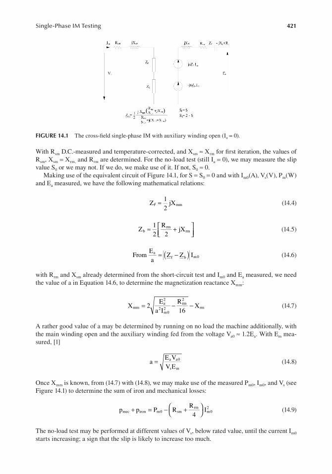
421Single-Phase IM Testing
1Zf ≈ jXmm (14.4)
2
1 R Z ≈ +rmb jX (14.5)
2 2rm
EFrom a ≈ −Z Zf b Im0 (14.6)
a( )
E2 2
X 2= −a Rrmmm 2 2 − X .7)
a Im0 16rm (14
E Va = a a0 (14.8)
V Es m
Rrm p p P 0 s− +R 2mec i+ =ron m m0 (14.9) m I
4
FIGURE 14.1 The cross-field single-phase IM with auxiliary winding open (Ia = 0).
With Rsm D.C.-measured and temperature-corrected, and Xsm ≈ Xrm for first iteration, the values of Rsm, Xsm = Xrm, and Rrm are determined. For the no-load test (still Ia = 0), we may measure the slip value S0 or we may not. If we do, we make use of it. If not, S0 ≈ 0.
Making use of the equivalent circuit of Figure 14.1, for S = S0 = 0 and with Im0(A), Vs(V), Pm(W) and Ea measured, we have the following mathematical relations:
with Rrm and Xsm already determined from the short-circuit test and Im0 and Ea measured, we need the value of a in Equation 14.6, to determine the magnetization reactance Xmm:
A rather good value of a may be determined by running on no load the machine additionally, with the main winding open and the auxiliary winding fed from the voltage Va0 ≈ 1.2Ea. With Em mea-sured, [1]
Once Xmm is known, from (14.7) with (14.8), we may make use of the measured Pm0, Im0, and Vs (see Figure 14.1) to determine the sum of iron and mechanical losses:
The no-load test may be performed at different values of Vs, below rated value, until the current Im0 starts increasing; a sign that the slip is likely to increase too much.

422 Induction Machines Handbook
As for the three-phase IM, the separation of mechanical and core losses may be done by taking the ordinate at zero speed of the rather straight-line dependence of (pmec + piron) of V 2
s (Figure 14.2). Alternatively, we may use only the results for two voltages to segregate pmec from piron.
A standard straight-line curve fitting method may be used for better precision.The core loss is, in fact, dependent on the emf Em (not on input voltage Vm) and on the magnetic
field ellipticity.The field ellipticity decreases with load, and this is why, in general, the core losses are attributed
to the forward component.Consequently, the core loss resistance Rmiron may be placed in series with the magnetization
reactance Xmm and thus (Figure 14.3)
Rmiron ≈ piron
2I2 (14.10)m0
The impedance at no load Zom is
V R 2s rm X Xmm + rm 2
Zom = = R R+ + + + XIm0 sm miron
4 2sm (14.11)
Equation (14.11) allows us to calculate again Xmm. An average of the value obtained from (14.7) and (14.11) may be used for more confidence.
FIGURE 14.2 Mechanical plus core losses at no-load (open auxiliary winding).
FIGURE 14.3 Simplified no-load (S = 0) equivalent circuit with series core loss resistance Rmiron in both circuits (the auxiliary winding is open).
x
xxxx
xx
xx
x
0.1 1
p
p
p + p
iron
mec
meciron
V
V
s
sn
2
( )
jXsa Rsa Z CRsm jXsmI m0
Vs
Ea
ja R + jX I)( miron mm m12
-ja + j I )( mR4rm rmX
2
I a= 0
R
Xj 2
R4
X2j rm
rm
rm
mm
miron

423Single-Phase IM Testing
Now that all parameters are known, it is possible to refine the results by introducing the magne-tization reactance Xmm in the short-circuit impedance, while still Xsm = Xrm, to improve the values of Rrm and Xsm, until sufficient convergence is obtained.
Today numerical methods, available through many general softwares on PCs, allow for such iterative procedures to be applied rather easily.
Example 14.1
An 123 W (1/6 hp), 6 poles, 60 Hz, 110 V, split-phase motor was tested as follows [1]Rsm = 2.54 Ω after locked rotor reading, Rsm = 2.65 Ω after no-load single-phase running.Locked rotor watts at 110 V is Psc = 851 W.No-load current Im0 at Vs0 = 105 V is Im0 = 2.68 A. Locked rotor current is Isc = 11.65 A.
V hs0 = −V Isn mnR csm osϕ =n 110 − × ×3.17 2.85 0.588 ≈ 105 V (14.12)
where Imn = 3.17 A, Rhsm = Ω2.85 , cosφn = 0.588, full-load slip Sn = 0.033. Full-load input power
P1n = 205 W and rated efficiency ηn = 60.5% have been obtained from a direct load (brake) test.The no-load power versus applied volts Vs, produces (piron)Vs0 = 24.7 W and mechanical losses
pmec = 1.5 W.The no-load auxiliary winding voltage Ea = 140.0 V.The value of turns ratio a is found from an additional no-load test with the auxiliary winding fed
at 1.2 Ea (V). With the measured no-load main winding voltage Em0 = 105 V, a is (14.8)
140 × ×140 1.2a = =1.46
105×105
Let us now find the motor parameters and check directly the efficiency measured by the loss segregation method.
The rotor resistance (referred to the main winding) Rrm is (14.1)
851Rrm = − 2.54 = Ω3.73
11.652
The stator and rotor leakage reactances Xrm = Xsm from (14.3) are
1 105 2
X X 2sm = =rm − +(3.73 2.54) = Ω3.237
2 11.65
Rrm is getting larger during the no-load test, due to heating, to the same extent that Rsm does
Ro
Ro 2.65rm = ×R sm
rm = ×3.73 = Ω3.89Rsm 2.54
Now, the magnetization reactance Xmm, from (14.7), is
140.0 2 2 3.89 X 2mm = − − =3.237 77.57 Ω
1.46× 2.58 4
with the core resistance Rmiron (14.10)

424 Induction Machines Handbook
p 24.7Rmiron = =iron = Ω1.87
2I2 2m0 2 ⋅ 2.58
From (14.11), we may recalculate Xmm
105 2 2 3.89 X 2mm = − +2.65 1.87+ − =3.237 74.71Ω
2.58 4
An average of the two Xmm values would be 76.1235 Ω.By now the parameter problem has been solved. A few iterations may be used with the com-
plete circuit at S = 1 to get better values for Rrm and Xsm = Xrm. However, we should note that Xmm/Xrm ≈ 20, and thus, not much is to gain from these refinements.
For efficiency checking, we need to calculate the winding losses at rated slip Sn = 0.033 with the following parameters:
h
Rh h R 2.85sm = Ω2.85 , Rrm = ×Ro sm
rm = ×3.89 = Ω4.1835Ro
sm 2.65
X Xsm = =rm 3.237 Ω =, Xmm 76.12 Ω
The core resistance Rmiron may be neglected when the rotor currents are calculated:
jXI I= mm j76.12
rmf m = ⋅3.117 =1.586 A Rh
rm 4.1835+ +j X( )mm Xrm + +j(76.12 3.237)
Sn 0.033
I Irmb m≈ = 3.117 A
So the total rotor winding losses pCorotor are
Rh Rh 4.1835p I rm rm
Co = +2rotor rmf I2
rmb = +( )3.1172 21.586 = 25.58 W 2 2 2
The stator copper losses pcos are
p 2 h 2cos m= =I R0 sm 3.117 × =2.85 27.69 W
The total load losses Σp from loss segregation are
∑p p= +cos Cp porotor + +iron pmec = +27.69 25.58+ +24.7 1.5 = 79.47 W
The losses calculated from the direct load test are
( )∑p P= −in Pout = −205 123 = 82 Wload
There is a small difference of 2 W between the two tests, which tends to validate the methods of loss segregation. However, it is not sure that this is the case for most designs.
It is recommended to back up loss segregation by direct shaft loading tests whenever possible.

425Single-Phase IM Testing
It is possible to define the stray load losses as proportional to stator current squared and then to use this expression to determine total losses at various load levels
stray load losses p= Σ( ) − Σp R 2 2segregation sload
≈ +tray I Im ( )aa f ile:///.file/id=7329707.54
Rstray may then be lumped into the stator resistances Rsm and Rsa/a2.
14.3 THE CASE OF CLOSED ROTOR SLOTS
In some single-phase IMs (as well as three-phase IMs), closed rotor slots are used to reduce noise.In this case, the rotor slot leakage inductance varies with rotor current due to the magnetic satu-
ration of the iron bridges above the rotor slots.The short-circuit test has to be done now for quite a few values of voltage (Figure 14.4).In this case, the equivalent circuit should contain additionally a constant emf E0sc, corresponding
to the saturated closed rotor upper iron bridge (Figure 14.5).Only the segment AA′-E0sc (on Figure 14.5) represents the voltage drop on the rotor and stator
constant leakage reactances.
V sinϕ − EX X+ = sc sc 0sc
sm rm (14.13)Imsc
FIGURE 14.4 Short-circuit characteristics.
FIGURE 14.5 The forward (f, b) impedances for the closed slot rotor.
V
E
I
A'
A
V
I
ϕϕ
sc
mscmsc (R +R )Ism rm
j(X +X )Ism rm msc
msc
sc
sc
0sc
0scE0sc
E0sc E0sc
2 2
22
2
R R
2 (2 - S)
fb
rm
rm
rm
rmmm
mmjXjX
ZZ
Xjj
X

426 Induction Machines Handbook
14.4 LOSS SEGREGATION IN PERMANENT CAPACITOR IMS
The loss segregation for the permanent capacitor IM may be performed as for the single-phase IM, with only the main winding (Ia = 0) activated.
The auxiliary winding resistance and leakage reactance Rsa and Xsa can be measured, in the end, by a short-circuit (zero speed) test performed on the auxiliary winding:
Psca s≈ +( )R Ra ra sI2ca (14.14)
V 2
X Xsa + = scra
a − +( )R R 2
Isca sa ra (14.15)
When Xra = a2Xrm (with a and Xrm known, from (14.13)), it is possible to calculate Xsa with measured input power and current. With Rsa D.C.-measured, Rra can be calculated from 14.14.
The capacitor losses may be considered through a series resistance RC (see Figure 14.1). The value of RC may be measured by separately supplying the capacitor from an A.C. source.
The active power in the capacitor PC and the current through the capacitor IC are directly measured:
R = PCC
I2 (14.16)C
Once all parameters are known, the equivalent circuit shown in Figure 14.1 allows for the com-putation of both stator currents, Im and Ia, under load with both phases on, and given slip value, S. Consequently, the stator and rotor winding losses may then be determined.
From this point on, we repeat the procedure in the previous paragraph to calculate the total losses by segregation method and from direct input and output measurements, with the machine shaft loaded.
For cage-PM-reluctance rotor capacitor split-phase self-synchronizing IMs, a similar segregation process of loss may be applied [4].
14.5 SPEED (SLIP) MEASUREMENTS
One problem encountered in the load tests is the slip (speed) measurement.Unless a precision optical speedometer (with an error in the range of 2 rpm or less) is available,
it is more convenient to measure directly the slip frequency Sf1.The “old” method of using a large diameter circular short-circuited coil with a large number of
turns, to track the axial rotor leakage flux by a current Hall probe (or shunt), may be used for the scope.The coil is placed outside the motor frame at the motor end which does not hold the cooling fan.
Coil axis is concentric with the shaft.The acquired current signal contains two frequencies Sf1 and (2 − S)f1. An offline digital software
(or a low pass hardware) filter may be applied to the coil current signal to extract the Sf1 frequency component.
The slip computation error is expected to be equivalent to that of a 2 rpm precision speedometer or better.
14.6 LOAD TESTING
There are two main operation modes to test the single-phase IM on load: the motor mode and the generator mode.
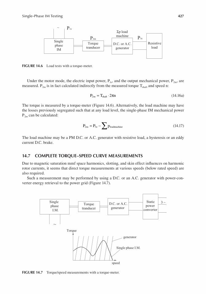
427Single-Phase IM Testing
~
SinglephaseI.M.
Torquetranducer
dc or acgenerator
Resistiveload
P2m
Σp loadmachine P3e
P1e
Singlephase
IM D.C. or A.C.
generator
FIGURE 14.6 Load tests with a torque-meter.
Under the motor mode, the electric input power, P1e, and the output mechanical power, P2m, are measured. P2m is in fact calculated indirectly from the measured torque Tshaft and speed n:
P2m = ⋅T 2shaft πn (14.16a)
The torque is measured by a torque-meter (Figure 14.6). Alternatively, the load machine may have the losses previously segregated such that at any load level, the single-phase IM mechanical power P2m can be calculated:
P2m = −P p3e ∑ loadmachine (14.17)
The load machine may be a PM D.C. or A.C. generator with resistive load, a hysteresis or an eddy current D.C. brake.
14.7 COMPLETE TORQUE–SPEED CURVE MEASUREMENTS
Due to magnetic saturation mmf space harmonics, slotting, and skin effect influences on harmonic rotor currents, it seems that direct torque measurements at various speeds (below rated speed) are also required.
Such a measurement may be performed by using a D.C. or an A.C. generator with power-con-verter energy retrieval to the power grid (Figure 14.7).
FIGURE 14.7 Torque/speed measurements with a torque-meter.
SinglephaseI.M.
Torquetranducer
dc or acgenerator
~
Staticpower
converter
3 ~Singlephase
I.M.
D.C. or A.C.generator
Torque
speed
Single phase I.M.
generator

428 Induction Machines Handbook
Alternatively a slow acceleration test on no load may be used to calculate the torque-speed curve. For slow acceleration, the supply voltage may be lowered from Vsn to Vs.
The core losses are considered proportional to voltage squared. They are measured by the loss segregation method:
= ( ) V 2
piron piron s
(14.18)Vsn Vsn
The mechanical losses are proportional to speed squared:
= ( ) 2n
pmec mp ec (14.19)n0 n0
With Rsm, Rrm, Rsa, Xsm, Xra, Xrm, and Xmm known and with Im and Ia and input power P1 measured, torque can be calculated as for steady state around rated speed:
P p− −= + =
ron s − − 2p 1 i R I2 R I2 2 2
m m sa a R Irm ( )rmf + −I Rrmb C aI mec Te Tshaft (14.20)
2 nπ 2 nπ
The computation of Tshaft is to be done offline. An optical speedometer could be used to measure the speed during the slow acceleration test and during a free deceleration (after turn-off).
With pmec(n) known, the free deceleration test yields
p (J = − mec n)
(14.21)dn2π
dt
The moment of inertia J is thus obtained.With J known and speed n acquired during the no-load slow acceleration test, the torque is
dn pT mec
e (n) J= π2 + (14.22)dt 2 nπ
The torque for rated voltage is considered to be
2
( ) ( Vsn T (e n) T (eV n) (14.23)
sn≈ )Vs Vs
The speed derivative in (14.22) may be obtained offline, with an appropriate software filter, from the measured speed signal.
The two values of torque, (14.20) and (14.22), are then compared to calculate a measure of stray losses:
≈ −( ) V 2
pstray eT T sneEquation(28.22) ( )(n) Equation(28.20) ⋅ 2 nπ (14.24) Vs

429Single-Phase IM Testing
Temperature measurements methods are very similar to those used for three-phase IMs. Standstill D.C. current decay tests may also be used to determine the magnetization curve Ψmm(Imm) and eventhe resistances and leakage reactances, as done for three-phase IMs.
14.8 SUMMARY
• The single-phase IM testing aims to determine equivalent circuit parameters in order tosegregate losses and to measure the performance on load, and even to investigate transients.
• Due to the backward field (current) component, even at zero slip, the rotor current (loss) isnot zero. This situation complicates the loss segregation in no-load tests.
• The no-load test may be done with the auxiliary phase open I 0′a = , after the motor starts.• The short-circuit (zero speed) test is to be performed, separately for the main and auxiliary
phases, to determine the resistances and leakage reactances.• Based on these results, the no-load test (with Ia = 0) furnishes data for loss segregation and
magnetization curve (Xmm(Imm)), provided it is performed for quite a few voltage levelsbelow rated voltage.
• The calculation of rotor resistance Rrm from the zero speed test (at 50 (60) Hz) produces avalue that is acceptable for computing on-load performance, because it is measured at an
Sf + −(2 S)faverage of forward and backward rotor current frequencies: 1 1 = f1.
2• The difference between total losses by segregation method and by direct input/output mea-
surements under load is a good measure of stray load losses. The stray load losses tendto be smaller than in three-phase motors because the ratio between full-load and no-loadcurrent is smaller.
• Instead of single (main)-phase no-load and short-circuit tests, symmetrical two voltagessupplying for the same tests have also been proved to produce good results.
• The complete torque–speed curve is of interest also. Below the breakdown torque-speedvalue, there may be a deep in the torque-speed curve around 33% of no-load ideal speed(f1/p1) due to the third space mmf harmonic. A direct load method may be used to obtainthe entire torque versus speed curve. Care must be exercised that the load machine had arigid torque/speed characteristic to handle the statically unstable part of the single-phaseIM torque–speed curve down to standstill.
• To eliminate direct torque measurements and the load machine system, a slow free accel-eration at reduced voltage and a free deceleration test may be performed. With the inputpower, speed, and stator currents and voltage measured and parameters already known(from the short-circuit and single-phase no-load tests), the torque may be computed afterloss subtraction from input at every speed (slip). The torque is also calculated from themotion equation with inertia J determined from free deceleration test. The mechanicalpower difference in the two measurements should be a good measure of the stray loadlosses caused by space harmonics. The torque in the torque/speed curve thus obtained ismultiplied by the rated to applied voltage ratio squared to obtain the full voltage torque–speed. It is recognized that this approximation underestimates the influence of magneticsaturation on torque at various speeds. This is to say that full voltage load tests from S = 0to S = 1 are required for magnetic saturation complete consideration.
• D.C. flux (current) decay tests at standstill, in the main and auxiliary winding axes, mayalso be used to determine resistances, leakage inductances, and the magnetization curve.Frequency response standstill tests may be applied to single-phase IM in a manner verysimilar to one applied to three-phase IMs (Chapter 13).
• Temperature measurement tests are performed as for three-phase IMs, in general (Chapter 13).• For more single-phase IM testing, see Ref. [5].

430 Induction Machines Handbook
REFERENCES
1. C. G. Veinott, Segregation of losses in single-phase induction motors, Transactions of the AmericanInstitute of Electrical Engineers, Vol. 54, December 1935, pp. 1302–1306.
2. Ch. Gross, Electric Machines, CRC Press, Taylor & Francis, New York, 2006, Chapter 6, pp. 228–229.3. C. Van der Merwe, F.S. van der Merwe, Study of Methods to Measure the Parameters of Single
Phase Induction Motors, IEEE Transactions on Energy Conversion, Vol. 10, No. 2, 1995, pp. 248–253.4. I. Boldea, L. N. Tutelea, Reluctance Electric Machines: Design and Control, CRC Press, Taylor and
Francis, New York, 2018.5. IEEE Standard no. 114–2001: Test Procedures for Single Phase Induction Machines.

431
Index
A
A.C. power grid, 292, 373Active power, 118, 285, 291, 311, 382, 404, 426Applications, 61, 99, 151, 201, 301, 411Artificial loading, 381, 386, 410, 413Auxiliary winding, 72, 232, 307, 419
B
Brushes, 58, 92, 181, 293, 297Brushless doubly fed induction generator (BDFIG), 59, 297
C
Cage rotor, 8, 61, 104, 172, 247, 373, 411Cage rotor induction generators (CRIG), 261, 297, 303Cross-coupling saturation, 72, 281
D
Design above 100kW, 151deep bar cage, 151double cage, 153high voltage stator, 155, 362low voltage stator, 151, 185performance computation, 175, 272, 340wound rotor, 3, 57, 151, 261, 367
Design below 100kW, 123characteristics, 105, 146, 273, 310, 392, 402losses and efficiency, 144, 175, 367, 419resistances and inductances, 138, 257, 389rotor slots, 24, 71, 172, 205, 312, 388, 425stator core, 17, 125, 177, 367stator slot, 56, 83, 114, 148, 196, 231, 323stator winding, 47, 80, 116, 127, 151, 177, 227, 257, 295,
367, 411Design for variable speed, 187
derating, 102, 188, 207increasing efficiency, 193increasing the breakdown torque, 188, 194reducing the skin effect, 190solid iron rotor, 203super-high speed, 188, 337torque pulsations reduction, 192wide constant power speed range, 59, 197
Design principles, 99, 227output coefficient, 110rotor tangential stress, 111, 125
Diode rectifier, 59, 295, 299, 303Doubly fed IG/doubly fed induction generator (DFIG), 58,
186, 285, 292, 301Doubly fed IM, 17, 57, 60, 290, 297, 303
insulation classes, 339through FEM, 16, 73
Dual stator winding (DSW), 57, 263, 290, 297
E
Electromagnetic noise, 409EMF, 43, 111, 173, 202, 251, 295, 314, 360, 422
F
Fault tolerance, 54, 67FEM models, 16, 411Field oriented control (FOC), 59, 291, 300Five-phase IM, 56Flux barriers, 64, 412
G
Generators, 43, 261, 292, 307, 411bi-directional rotor power, 262given speed and capacitor, 273induction motor load, 267, 282mmf harmonics, 193, 390, 419parallel operation, 281parameter sensitivity, 273, 281pole changing, 246, 274second order slip equation, 266, 273simplified, 71, 195, 261, 301, 359, 390, 404simulated annealing, 214single layer winding, 232, 321steady state (SEIG), 7, 63, 208, 241, 275, 308, 374,
400, 428transient operation of SEIG, 281travelling mmf, 321unbalanced steady state, 275winding factor, 49, 110, 156, 172, 232, 275, 322windings, 2, 16, 47, 71, 110, 151, 190, 227, 264, 297,
321, 367
I
Insulation materials, 110differential leakage inductance, 167FEM approach, 206, 353form–wound, 157, 185leakage inductance, 10, 49, 83, 107, 143, 163, 194, 254,
357, 392, 425leakage saturation, 14, 25, 66, 143, 164, 372,
396, 415rotor bar and end ring, 47, 67
Iron losses, 63, 368, 371, 387, 404
L
Leakage inductances, 7, 15, 55, 152, 191, 254, 390, 399, 429
LIM control, 357, 359Line side converter (LSC), 292

432 Index
Linear induction motor/linear induction motors (LIM/LIMs), 121, 317, 321, 331, 338, 345, 353, 357, 411, 412
classifications, 319double sided, 319, 331, 352end–effect waves, 319, 333heavily saturated, 204, 331induction launchers, 360, 363LIM longitudinal end effects, 331linear flat induction actuators, 338optimum goodness factor, 336, 351, 363panoramic, 318primary windings, 321single sided, 317, 331, 341, 357transverse edge effect, 205, 317, 329, 353tubular, 319, 339, 348tubular LIAs, 348urban transportation, 197, 338, 353
Longitudinal end effect, 319, 322, 333, 353, 359Losses, 16, 63, 103, 144, 181, 241, 292, 337, 375, 404, 419
classifications, 319closed rotor slots, 24, 152, 193, 392, 425interbar current, 51, 74, 420single stack, 160, 163slot geometry, 99, 131, 161, 196, 230stray load, 112, 194, 241, 367, 386, 407, 419, 425time harmonics, 54, 77, 102, 189, 208, 367, 399, 411
Low-speed, 70, 100, 187, 193, 200, 227, 246, 258, 283, 298, 319, 338, 363
M
Magnetization current, 12, 19, 72, 118, 125, 137, 166, 175, 239, 264, 390, 415
Magnetization curve, 18, 71, 132, 165, 176, 258, 279, 284, 309, 331, 429
analytical iterative model (AIM), 138equivalent airgap, 64, 329, 342, 391magnetic potential, 89main winding, 61, 77, 229, 243, 298, 314, 419
Multiphase IM, 54, 67, 411Mutual inductances, 1, 47, 61, 65, 88
O
Operation modes, 77, 250, 389, 393, 415, 419autonomous, 293generating, 64, 284, 304, 384, 412ideal no–load, 419motor mode, 426no–load motor, 368short–circuit, 66, 107
Optimization design, 147, 151, 172, 227, 325, 353augmented Lagrangian multiplier, 214genetic algorithms, 217, 355modified Hooke–Jeeves method, 216, 355sequential unconstrained minimisation, 224
P
Parasitic torques, 7, 149, 193, 409asynchronous, 61, 193, 249, 412circulating currents, 193secondary armature reaction, 282
synchronous, 19, 41, 64, 123, 149, 193, 227, 25, 286, 312, 368, 400, 419
Phase resistance, 138, 179, 351, 391Polynomial equation, 47, 266, 282
R
Radial forces, 133, 149, 409capacitor-start, 420characteristics, 105, 146, 273, 310, 355, 392, 425d-q model, 7, 31, 71, 254, 281, 290, 313d-q model for transients, 313guidelines, 190, 243inverter-fed auxiliary winding, 314magnetization reactance, 26, 44, 180, 237, 270, 327,
349, 387, 421optimization design issues, 211, 243performance computation algorithm, 311resistances and leakage reactances, 236, 429rotor magnetic circuit, 231self–excited, 264, 307self–regulated, 307simplified equivalent circuit, 266, 309, 359, 390single–phase IM design, 227, 231split–phase, 71, 227, 419split-phase capacitor, 77, 246starting torque and current, 105, 151, 190, 240, 399stator magnetic circuit, 227stator windings, 71, 192, 227steady state performance, 9, 119, 241, 265, 307symmetrical components, 277tapped-winding, 90, 227, 420
Reactive power, 261, 293, 304, 314, 337, 395Reference current, 54, 300, 357Reluctance motor, 61, 206Rotor side converter (RSC) 292
S
Saliency, 61, 64, 247, 251, 254Self-excitation capacitance, 273, 280, 303Self-synchronization, 61, 64, 412Single–phase IM testing, 419
auxiliary winding open, 421closed rotor slots, 24, 152, 193, 425complete torque–speed curve, 427core losses, 16, 74, 102, 139, 172, 201, 241, 289, 321,
348, 367, 391, 419double cage, 16, 28, 71, 151, 166, 223, 359,
393, 407eddy current losses, 348, 368equivalent circuit, 9, 17, 44, 80, 125, 138, 166, 198,
251, 275, 308, 339, 359, 390, 419in the end rings, 192load testing, 367, 386, 413loss breakdown, 119, 367, 372loss segregation, 367, 404magnetization curve, 15, 71, 132, 165, 268, 284, 309,
331, 429multilayer approach, 185open auxiliary winding, 422parasitic torques, 193, 409permanent capacitor IM, 243, 426single conductor, 89

433Index
skin effect, 7, 16, 44, 71, 105, 140, 159, 188, 239, 275, 324, 342, 357, 385, 407, 419
space harmonics, 55, 74, 192, 206, 368, 409, 427speed (slip) measurements, 426starting torque and current, 105, 151, 190, 240, 399turns ratio a, 423
Single-phase IM transients, 71d-q model, 17, 34, 62, 87, 254, 281, 313multiple reference model, 71space harmonics, 55, 192, 259, 368, 409, 427starting, 21, 47, 71, 105, 133, 170, 227, 283, 357,
372, 402Sinusoidal current, 54, 77, 210Sinusoidal mmf, 54Six-phase machine, 54, 58Space-phasor equations, 17, 58, 290Space vector model, 54, 60, 417Specifications, 99, 116, 123, 147, 207, 227, 243, 344, 353
constant V and f, 99, 120, 151, 193, 209derating, 102, 124, 188load, 7, 21, 61, 99, 113, 166, 189NEMA designs, 107
Starting, 21, 43, 66, 105, 133, 147, 166, 190, 227, 247, 283, 341, 367, 390, 415
of cage-rotor, 62, 112, 154critical slip, 65, 103, 112efficiency and power factor, 65, 103, 112, 121, 149, 166,
187, 205, 252, 319, 337, 342electromagnetic torque, 4, 19, 27, 60, 117, 394, 403pole-changing, 246, 263, 274, 304speed control, 120, 151, 174, 187, 416steady state, 7, 9, 15, 36, 71, 119, 187, 208, 227, 241,
265, 273, 287, 307, 357, 374, 400, 428for wound rotor, 1, 3, 57, 112, 151, 172, 261, 290,
367, 392Structural diagram, 13, 290Super-high frequency models, 79
bearing currents, 91, 94calorimetric methods, 373from catalogue data, 393, 416common mode impedance, 84differential impedance, 82distributed equivalent circuit, 87efficiency measurements, 376leakage flux path saturation, 142, 393, 415line–end coil, 89
loss segregation, 367general regression, 399, 415on load noise test, 409noise and vibration, 111, 133, 149, 319, 355, 384,
409, 411parameter estimation, 389, 400, 411PWM converter supply, 372, 395, 416standstill frequency test, 396stray losses, 112, 144, 151, 196, 370, 388, 407, 419, 428zero sequence impedance, 80, 92
T
3D-FEM calculations, 359Time constants, 25, 31, 66, 291, 396Torque density, 54, 57, 224, 298Transients, 1, 9, 12, 71, 187, 198, 200, 246, 254, 263, 281,
307, 357, 390, 401, 429broken bar, 51, 68, 71, 359complex variable model, 4, 66equivalent circuits for drives, 9first order models, 39, 42magnetic saturation, 14, 44, 58, 71, 112, 125, 149, 251,
275, 282, 307, 331, 357, 389, 419, 427M/Nr winding model, 47most severe transients, 31multimachine, 43phase coordinate model, 1, 54, 65reduced order models, 21saturation and core losses, 18subsynchronous resonance, 44, 274sudden short–circuit, 1, 28, 31, 66, 314torsional torque, 25, 66windings, 2, 7, 16, 47, 61, 87, 102, 127, 141, 184, 201,
227, 243, 264, 275, 297, 321, 346, 367Trapezoidal slots, 129, 149, 192, 231
V
Variable speed, 9, 57, 71, 99, 159, 187, 192, 261, 286, 372, 390, 411
W
Winding configurations, 65, 321

REQUEST A FREE [email protected]
Taylor & Francis eBookswww.taylorfrancis.com
A single destination for eBooks from Taylor & Francis with increased functionality and an improved user experience to meet the needs of our customers.
90,000+ eBooks of award-winning academic content in Humanities, Social Science, Science, Technology, Engineering,
and Medical written by a global network of editors and authors.
TAYLOR & FRANCIS EBOOKS OFFERS:
A streamlined experience for
our library customers
A single point of discovery for all of our
eBook content
Improved search and discovery of
content at both book and
chapter level