Electrical Machines -Mathematical Fundamentals of Machine Topologies
479
Mathematical Engineering Dieter Gerling Electrical Machines Mathematical Fundamentals of Machine Topologies
Transcript of Electrical Machines -Mathematical Fundamentals of Machine Topologies

Mathematical Engineering
Dieter Gerling
Electrical Machines Mathematical Fundamentals of Machine Topologies

Electrical Machines

Mathematical Engineering
Series Editors
For further volumes:http://www.springer.com/series/8445
Prof. Dr. Claus Hillermeier, Munich, Germany, (volume editor)Prof. Dr.-Ing. Jörg Schröder, Essen, GermanyProf. Dr.-Ing. Bernhard Weigand, Stuttgart, Germany

Dieter Gerling
Electrical Machines Mathematical Fundamentals of MachineTopologies

ISBN 978-3-642-17583-1 DOI 10.1007/978-3-642-17584-8 Springer Heidelberg New York Dordrecht London Library of Congress Control Number: 2014950816 © Springer-Verlag Berlin Heidelberg 2015 This work is subject to copyright. All rights are reserved by the Publisher, whether the whole or part of the material is concerned, specifically the rights of translation, reprinting, reuse of illustrations, recitation, broadcasting, reproduction on microfilms or in any other physical way, and transmission or information storage and retrieval, electronic adaptation, computer software, or by similar or dissimilar methodology now known or hereafter developed. Exempted from this legal reservation are brief excerpts in connection with reviews or scholarly analysis or material supplied specifically for the purpose of being entered and executed on a computer system, for exclusive use by the purchaser of the work. Duplication of this publication or parts thereof is permitted only under the provisions of the Copyright Law of the Publisher’s location, in its current version, and permission for use must always be obtained from Springer. Permissions for use may be obtained through RightsLink at the Copyright Clearance Center. Violations are liable to prosecution under the respective Copyright Law. The use of general descriptive names, registered names, trademarks, service marks, etc. in this publication does not imply, even in the absence of a specific statement, that such names are exempt from the relevant protective laws and regulations and therefore free for general use. While the advice and information in this book are believed to be true and accurate at the date of publication, neither the authors nor the editors nor the publisher can accept any legal responsibility for any errors or omissions that may be made. The publisher makes no warranty, express or implied, with respect to the material contained herein. Printed on acid-free paper Springer is part of Springer Science+Business Media (www.springer.com)
ISSN 2192-4732 ISSN 2192-4740 (electronic)
ISBN 978-3-642-1758 -4 8 (eBook)
Dieter Gerling
Neubiberg, Germany
Fakultät Elektrotechnik und InformationstechnikUniversität der Bundeswehr München

Preface
Calculation and design of electrical machines and drives remain challenging tasks. However, this becomes even more and more important as there are increas-ing numbers of applications being equipped with electrical machines. Some recent examples well-known to the public are wind energy generators and electrical trac-tion drives in the automotive industry. To realize optimal solutions for electrical drive systems it is necessary not only to know some basic equations for machine calculation, but also to deeply understand the principles and limitations of electri-cal machines and drives.
To foster the know-how in this technical field, this book Electrical Machines starts with some basic considerations to introduce the reader to electromagnetic circuit calculation. This is followed by the description of the steady-state operation of the most important machine topologies and afterwards by the dynamic opera-tion and control methods. Continuously giving detailed mathematical deductions to all topics guarantees an optimal understanding of the underlying principles. Therefore, this book contributes to a comprehensive expert knowledge in electri-cal machines and drives. Consequently, it will be very useful for academia as well as for industry by supporting senior students and engineers in conceiving and de-signing electrical machines and drives.
After introducing Maxwell’s equations and some principles of electromagnetic circuit calculation, the first part of the book is dedicated to the steady-state opera-tion of electrical machines. The detailed description of the brushed DC-machine is followed by the rotating field theory, which in particular explains in detail the winding factors and harmonics of the magneto-motive force of distributed wind-ings. On this basis, induction machines and synchronous machines are described. This first part of the book is completed by regarding permanent magnet machines, switched reluctance machines, and small machines for single-phase use.
Dynamic operation and control of electrical machines are the topics of the sec-ond part of this book, starting with some fundamental considerations. Next, the dynamic operation of brushed DC-machines and their control is described (in par-ticular cascaded control using PI-controllers and their adjustment rules). A very important concept for calculating the dynamic operation of rotating field machines is the space vector theory; this is deduced and explained in detail in the following chapter. Then, the dynamic behavior of induction machines and synchronous ma-chines follows, including the description of important control methods like field-
v

oriented control (FOC) and direct torque control (DTC). The permanent magnet machine with surface mounted magnets (SPM) or interior magnets (IPM) is ex-plained concerning the differences of both in torque control and concerning the maximum torque per ampere (MTPA) control method. The last chapter gives an overview of latest research results concerning concentrated windings.
In spite of being a new contribution to a comprehensive understanding of elec-trical machines and the respective actual developments the reader may find parts of the contents even in different literature, as this book explains the fundamentals of electrical machines (steady-state and dynamic operation as well as control). Concerning these fundamentals it is nearly impossible to list all relevant literature during the text layout. Therefore, the most important references are given at the end of each chapter. In addition, parts of the lectures of Prof. H. Bausch (Universi-taet der Bundeswehr Munich, Germany) and Prof. G. Henneberger (RWTH Aa-chen, Germany) were used as a basis.
The author deeply wishes to express his grateful acknowledgment to all team members of his Chair of Electrical Drives and Actuators at the Universitaet der Bundeswehr Munich and of the spin-off company FEAAM GmbH for their most valuable discussions and support. In particular this holds for (in alphabetical or-der) Dr.-Ing. Gurakuq Dajaku, Mrs. Lara Kauke, and most notably Dr.-Ing. Hans-Joachim Koebler. Without their beneficial contributions this book would not have been possible in such a high quality.
Last, but not least the author exceedingly thanks his wife and his daughters for their respectfulness and understanding not only concerning the effort being ac-companied by writing this book, but even concerning the expenditure of time the author dedicates to professional activities.
Munich, April 2014 Dieter Gerling
vi Preface

Contents
Preface ................................................................................................................... .v
Contents ............................................................................................................... vii
1 Fundamentals ..................................................................................................... 11.1 Maxwell’s Equations ................................................................................... 1
1.1.1 The Maxwell’s Equations in Differential Form ................................... 11.1.2 The Maxwell’s Equations in Integral Form .......................................... 2
1.1.2.1 Ampere’s Law (First Maxwell’s Equation in Integral Form) ....... 21.1.2.2 Faraday’s Law, Law of Induction (Second Maxwell’s Equation in Integral Form) ........................................................................................... 31.1.2.3 Law of Direction ........................................................................... 41.1.2.4 The Third Maxwell’s Equation in Integral Form .......................... 41.1.2.5 The Fourth Maxwell’s Equation in Integral Form ........................ 41.1.2.6 Examples for the Ampere’s Law (First Maxwell’s Equation in Integral Form) ........................................................................................... 51.1.2.7 Examples for the Faraday’s Law (Second Maxwell’s Equation in Integral Form) ........................................................................................... 7
1.2 Definition of Positive Directions ............................................................... 141.3 Energy, Force, Power ................................................................................ 161.4 Complex Phasors ....................................................................................... 281.5 Star and Delta Connection ......................................................................... 301.6 Symmetric Components ............................................................................. 311.7 Mutual Inductivity ..................................................................................... 321.8 Iron Losses ................................................................................................. 341.9 References for Chapter 1 ........................................................................... 35
2 DC-Machines .................................................................................................... 372.1 Principle Construction ............................................................................... 372.2 Voltage and Torque Generation, Commutation ......................................... 382.3 Number of Pole Pairs, Winding Design ..................................................... 412.4 Main Equations of the DC-Machine .......................................................... 45
2.4.1 First Main Equation: Induced Voltage ............................................... 452.4.2 Second Main Equation: Torque .......................................................... 472.4.3 Third Main Equation: Terminal Voltage ............................................ 48
vii

viii Contents
2.7 Permanent Magnet Excited DC-Machines ................................................. 622.8 Shunt-Wound DC-Machines ...................................................................... 692.9 Series-Wound DC-Machines ..................................................................... 732.10 Compound DC-Machines ........................................................................ 772.11 Generation of a Variable Terminal Voltage ............................................. 782.12 Armature Reaction ................................................................................... 802.13 Commutation Pole ................................................................................... 842.14 References for Chapter 2 ......................................................................... 88
3 Rotating Field Theory ...................................................................................... 893.1 Stator of a Rotating Field Machine ............................................................ 893.2 Current Loading ......................................................................................... 903.3 Alternating and Rotating Magneto-Motive Force ...................................... 933.4 Winding Factor ........................................................................................ 1043.5 Current Loading and Flux Density........................................................... 114
3.5.1. Fundamentals .................................................................................. 1143.5.2. Uniformly Distributed Current Loading in a Zone .......................... 1143.5.3. Current Loading Concentrated in the Middle of Each Slot ............. 1153.5.4. Current Loading Distributed Across Each Slot Opening ................ 1163.5.5. Rotating Air-Gap Field .................................................................... 116
3.6 Induced Voltage and Slip ......................................................................... 1203.7 Torque and Power .................................................................................... 1263.8 References for Chapter 3 ......................................................................... 134
4 Induction Machines ........................................................................................ 1354.1 Construction and Equivalent Circuit Diagram ......................................... 1354.2 Resistances and Inductivities ................................................................... 141
4.2.1 Phase Resistance .............................................................................. 1414.2.2 Main Inductivity ............................................................................... 1424.2.3 Leakage Inductivity .......................................................................... 142
4.2.3.1 Harmonic Leakage .................................................................... 1424.2.3.2 Slot Leakage ............................................................................. 1434.2.3.3 End Winding Leakage............................................................... 145
4.3 Operating Characteristics ......................................................................... 1454.3.1 Heyland-Diagram (Stator Phase Current Locus Diagram) ............... 1454.3.2 Torque and Power ............................................................................ 1514.3.3 Torque as a Function of Slip ............................................................ 1544.3.4 Series Resistance in the Rotor Circuit .............................................. 157
2.4.4 Power Balance .................................................................................... 482.4.5 Utilization Factor ............................................................................... 49
2.5 Induced Voltage and Torque, Precise Consideration ................................. 512.5.1 Induced Voltage ................................................................................. 512.5.2 Torque ................................................................................................ 53
2.6 Separately Excited DC-Machines .............................................................. 56

4.5 Possibilities for Open-Loop Speed Control ............................................. 1794.5.1 Changing (Increasing) the Slip ......................................................... 1794.5.2 Changing the Supply Frequency ...................................................... 1794.5.3 Changing the Number of Pole Pairs ................................................. 181
4.6 Star-Delta-Switching ............................................................................... 1824.7 Doubly-Fed Induction Machine ............................................................... 1834.8 References for Chapter 4 ......................................................................... 188
5 Synchronous Machines .................................................................................. 1895.1 Equivalent Circuit and Phasor Diagram................................................... 1895.2 Types of Construction .............................................................................. 195
5.2.1 Overview .......................................................................................... 1955.2.2 High-Speed Generator with Cylindrical Rotor ................................. 1965.2.3 Salient-Pole Generator ..................................................................... 196
5.3 Operation at Fixed Mains Supply ............................................................ 1965.3.1 Switching to the Mains ..................................................................... 1965.3.2 Torque Generation............................................................................ 1985.3.3 Operating Areas ............................................................................... 2005.3.4 Operating Limits .............................................................................. 203
5.4 Isolated Operation .................................................................................... 2055.4.1 Load Characteristics ......................................................................... 2055.4.2 Control Characteristics ..................................................................... 207
5.5 Salient-Pole Synchronous Machines ........................................................ 2095.6 References for Chapter 5 ......................................................................... 217
6 Permanent Magnet Excited Rotating Field Machines................................. 2196.1 Rotor Construction ................................................................................... 2196.2 Linestart-Motor ........................................................................................ 2206.3 Electronically Commutated Rotating Field Machine with Surface Mounted Magnets ......................................................................................................... 220
6.3.1 Fundamentals ................................................................................... 2206.3.2 Brushless DC-Motor ........................................................................ 2226.3.3 Electronically Commutated Permanent Magnet Excited Synchronous Machine ..................................................................................................... 228
6.4 Calculation of the Operational Characteristics; Permanent Magnet Excited Machines with Buried Magnets ..................................................................... 2306.5 References for Chapter 6 ......................................................................... 230
Contents ix
4.3.5 Operation with Optimum Power Factor ........................................... 1594.3.6 Further Equations for Calculating the Torque .................................. 164
4.4 Squirrel Cage Rotor ................................................................................. 1664.4.1 Fundamentals ................................................................................... 1664.4.2 Skewed Rotor Slots .......................................................................... 1704.4.3 Skin Effect ........................................................................................ 175

7.2.5 Main Characteristics ......................................................................... 244
7.3 References for Chapter 7 ......................................................................... 244
8 Small Machines for Single-Phase Operation ................................................ 2478.1 Fundamentals ........................................................................................... 2478.2 Universal Motor ....................................................................................... 2478.3 Single-Phase Induction Machine ............................................................. 250
8.3.1 Single-Phase Operation of Three-Phase Induction Machine ............ 2508.3.2 Single-Phase Induction Motor with Auxiliary Phase ....................... 2528.3.3 Shaded-Pole (Split-Pole) Motor ....................................................... 253
8.4 References for Chapter 8 ......................................................................... 254
9 Fundamentals of Dynamic Operation ........................................................... 2559.1 Fundamental Dynamic Law, Equation of Motion .................................... 255
9.1.1 Translatory Motion ........................................................................... 2559.1.2 Translatory / Rotatory Motion .......................................................... 2559.1.3 Rotatory Motion ............................................................................... 2569.1.4 Stability ............................................................................................ 257
9.2 Mass Moment of Inertia ........................................................................... 2589.2.1 Inertia of an Arbitrary Body ............................................................. 2589.2.2 Inertia of a Hollow Cylinder............................................................. 259
9.3 Simple Gear-Sets ..................................................................................... 2609.3.1 Assumptions ..................................................................................... 2609.3.2 Rotation / Rotation (e.g. Gear Transmission) ................................... 2609.3.3 Rotation / Translation (e.g. Lift Application) ................................... 261
9.4 Power and Energy .................................................................................... 2629.5 Slow Speed Change ................................................................................. 264
9.5.1 Fundamentals ................................................................................... 2649.5.2 First Example ................................................................................... 2649.5.3 Second Example ............................................................................... 265
9.6 Losses during Starting and Braking ......................................................... 2679.6.1 Operation without Load Torque ....................................................... 2679.6.2 Operation with Load Torque ............................................................ 270
9.7 References for Chapter 9 ......................................................................... 271
x Contents
7 Reluctance Machines ...................................................................................... 2317.1 Synchronous Reluctance Machines ......................................................... 2317.2 Switched Reluctance Machines ............................................................... 232
7.2.1 Construction and Operation.............................................................. 2327.2.2 Torque .............................................................................................. 2347.2.3 Modes of Operation .......................................................................... 2397.2.4 Alternative Power Electronic Circuits .............................................. 242

xi
10.5.1 Overview ........................................................................................ 29110.5.2 Adjusting to Optimal Response to Setpoint Changes (Rule “Optimum of Magnitude“) ........................................................................ 29210.5.3 Adjusting to Optimal Response to Disturbances (Rule “Symmetrical Optimum“) ................................................................................................ 29310.5.4 Application of the Adjusting Rules to the Cascaded Control of DC-Machines ................................................................................................... 294
10.6 References for Chapter 10 ..................................................................... 295
11 Space Vector Theory .................................................................................... 29711.1 Methods for Field Calculation ............................................................... 29711.2 Requirements for the Application of the Space Vector Theory ............. 29811.3 Definition of the Complex Space Vector ............................................... 29911.4 Voltage Equation in Space Vector Notation .......................................... 30311.5 Interpretation of the Space Vector Description ...................................... 30511.6 Coupled Systems ................................................................................... 30611.7 Power in Space Vector Notation ............................................................ 30911.8 Elements of the Equivalent Circuit ........................................................ 313
11.8.1 Resistances ..................................................................................... 31311.8.2 Inductivities .................................................................................... 31411.8.3 Summary of Results ....................................................................... 316
11.9 Torque in Space Vector Notation .......................................................... 31711.9.1 General Torque Calculation ........................................................... 31711.9.2 Torque Calculation by Means of Cross Product from Stator Flux Linkage and Stator Current ....................................................................... 31811.9.3 Torque Calculation by Means of Cross Product from Stator and Rotor Current ............................................................................................ 31911.9.4 Torque Calculation by Means of Cross Product from Rotor Flux Linkage and Rotor Current ........................................................................ 31911.9.5 Torque Calculation by Means of Cross Product from Stator and Rotor Flux Linkage ................................................................................... 320
11.10 Special Coordinate Systems ................................................................. 32111.11 Relation between Space Vector Theory and Two-Axis-Theory .......... 32211.12 Relation between Space Vectors and Phasors ...................................... 32311.13 References for Chapter 11 ................................................................... 324
Contents
10.2.2 Response to Setpoint Changes ........................................................ 27810.2.3 Response to Disturbance Changes .................................................. 283
10.3 Shunt-Wound DC-Machines .................................................................. 28610.4 Cascaded Control of DC-Machines ....................................................... 28810.5 Adjusting Rules for PI-Controllers ........................................................ 291
10 Dynamic Operation and Control of DC-Machines .................................... 27310.1 Set of Equations for Dynamic Operation ............................................... 27310.2 Separately Excited DC-Machines .......................................................... 277
10.2.1 General Structure ............................................................................ 277
xii Contents
12.5 Field-Oriented Control of Induction Machines with Impressed Stator Voltages ......................................................................................................... 35612.6 Field-Oriented Control of Induction Machines without Mechanical Sensor (Speed or Position Sensor) ............................................................................. 35812.7 Direct Torque Control ............................................................................ 36012.8 References for Chapter 12 ..................................................................... 367
13 Dynamic Operation of Synchronous Machines.......................................... 36913.1 Oscillations of Synchronous Machines, Damper Winding .................... 36913.2 Steady-State Operation of Non Salient-Pole Synchronous Machines in Space Vector Notation ................................................................................... 37413.3 Sudden Short-Circuit of Non Salient-Pole Synchronous Machines ....... 381
13.3.1 Fundamentals ................................................................................. 38113.3.2 Initial Conditions for t = 0 .............................................................. 38113.3.3 Set of Equations for t > 0................................................................ 38313.3.4 Maximum Voltage Switching......................................................... 39013.3.5 Zero Voltage Switching .................................................................. 39413.3.6 Sudden Short-Circuit with Changing Speed and Rough Synchronization ......................................................................................... 39513.3.7 Physical Explanation of the Sudden Short-Circuit ......................... 400
13.4 Steady-State Operation of Salient-Pole Synchronous Machines in Space Vector Notation ............................................................................................. 40213.5 Sudden Short-Circuit of Salient-Pole Synchronous Machines ............... 410
13.5.1 Initial Conditions for t = 0 .............................................................. 41013.5.2 Set of Equations for t > 0................................................................ 412
13.6 Transient Operation of Salient-Pole Synchronous Machines................. 41513.7 References for Chapter 13 ..................................................................... 423
14 Dynamic Operation and Control of Permanent Magnet Excited Rotating Field Machines ................................................................................................... 425
14.1 Principle Operation ................................................................................ 42514.2 Set of Equations for the Dynamic Operation ......................................... 42614.3 Steady-State Operation .......................................................................... 432
14.3.1 Fundamentals ................................................................................. 43214.3.2 Base Speed Operation .................................................................... 432
12 Dynamic Operation and Control of Induction Machines ......................... 32512.1 Steady-State Operation of Induction Machines in Space Vector Notation at No-Load ..................................................................................................... 325
12.1.1 Set of Equations ............................................................................. 32512.1.2 Steady-State Operation at No-Load................................................ 326
12.2 Fast Acceleration and Sudden Load Change ......................................... 32812.3 Field-Oriented Coordinate System for Induction Machines .................. 33412.4 Field-Oriented Control of Induction Machines with Impressed Stator Currents ......................................................................................................... 344

15 Concentrated Windings ............................................................................... 44915.1 Conventional Concentrated Windings ................................................... 44915.2 Improved Concentrated Windings ......................................................... 453
15.2.1 Increased Number of Stator Slots from 12 to 24 ............................ 45315.2.2 Increased Number of Stator Slots from 12 to 18 ............................ 46015.2.3 Main Characteristics of the Improved Concentrated Windings ...... 461
15.3 References for Chapter 15 ..................................................................... 462
16 Lists of Symbols, Indices and Acronyms .................................................... 46316.1 List of Symbols ...................................................................................... 46316.2 List of Indices ........................................................................................ 46716.3 List of Acronyms ................................................................................... 470
Index ................................................................................................................... 471
xiii Contents
14.3.3 Operation with Leading Load Angle and without Magnetic Asymmetry ................................................................................................ 43414.3.4 Operation with Leading Load Angle and Magnetic Asymmetry.... 43614.3.5 Torque Calculation from Current Loading and Flux Density ......... 438
14.4 Limiting Characteristics and Torque Control ........................................ 44014.4.1 Limiting Characteristics ................................................................. 44014.4.2 Torque Control ............................................................................... 442
14.5 Control without Mechanical Sensor ....................................................... 44614.6 References for Chapter 14 ..................................................................... 447

1 Fundamentals
1.1 Maxwell’s Equations
1.1.1 The Maxwell’s Equations in Differential Form
The basis for all following considerations are the Maxwell’s equations. In differ-
ential form these are (the time-dependent variation of the displacement current D
can always be neglected against the current density J for all technical systems re-garded here):
1. Maxwell’s equation
dD
rotH J Jdt
= + ≈ (1.1)
2. Maxwell’s equation
dB
rotEdt
= − (1.2)
3. Maxwell’s equation
divB 0= (1.3)
4. Maxwell’s equation
divD = ρ (1.4)
The material equations are:
B H= μ (1.5)
D E= ε (1.6)
© Springer-Verlag Berlin Heidelberg 2015 1D. Gerling, Electrical Machines Mathematica DOI 10.1007/978-3-642-17584-8_1
l Engineering,,

2 1 Fundamentals
J E= γ (1.7)
The used variables have the following meaning:
H the vector field of the magnetic field strength;
J the vector field of the electrical current density;
D the vector field of the displacement current;
E the vector field of the electric field strength;
B the vector field of the magnetic flux density; ρ the scalar field of the charge density;
μ the scalar field of the permeability (in vacuum or air there is: 0μ = μ );
ε the scalar field of the dielectric constant (in vacuum or air there is:
0ε = ε );
γ the scalar field of the electric conductivity.
The expression “vector field” means that the vector quantity depends on all
(usually three) geometric coordinates; the expression “scalar field” means that sca-lar quantity depends on all geometric coordinates.
In the case of homogeneous, isotropic materials the scalar fields μ , ε and γ
are reduced to space-independent material constants.
1.1.2 The Maxwell’s Equations in Integral Form
1.1.2.1 Ampere’s Law (First Maxwell’s Equation in Integral Form)
The first Maxwell’s equation in integral form is
A
Hd JdA= (1.8)
The line integral of the magnetic field strength H on a closed geometric inte-
gration loop (“magnetic circulation voltage“) is equal to the total electric cur-rent flowing through the area A limited by this loop (“magneto-motive force“, “ampere-turns”), if the displacement current is neglected.
For graphical explanation see Fig. 1.1.

1.1 Maxwell’s Equations 3
Fig. 1.1. Explanation of Ampere’s Law.
1.1.2.2 Faraday’s Law, Law of Induction (Second Maxwell’s Equation in Integral Form)
The second Maxwell’s equation in integral form is
A
dEd BdA
dt= − (1.9)
with the magnetic flux being
A
BdA = Φ (1.10)
The line integral of the electric field strength E on a closed geometric integra-
tion loop (“electric circulation voltage“) is equal to the negative time-dependent variation of the total magnetic flux, that penetrates the area A limited by this loop.
For graphical explanation see Fig. 1.2.
J
d H
dA

4 1 Fundamentals
Fig. 1.2. Explanation of Faraday’s Law.
1.1.2.3 Law of Direction
The positive direction of the vectors d and A are defined according to a right-handed screw.
1.1.2.4 The Third Maxwell’s Equation in Integral Form
The third Maxwell’s equation in integral form is
A
BdA 0= (1.11)
The total magnetic flux penetrating a closed surface of any volume is zero, i.e. there are no single magnetic poles.
1.1.2.5 The Fourth Maxwell’s Equation in Integral Form
The fourth Maxwell’s equation in integral form is
A V
DdA dV= ρ (1.12)
B
d E
dA

1.1 Maxwell’s Equations 5
The reason for the total electric field penetrating a closed surface of any vol-ume are the electric charges inside this volume.
1.1.2.6 Examples for the Ampere’s Law (First Maxwell’s Equation in Integral Form)
The Ampere’s Law is an integral law. It shows the dependency of the magneto-motive force (ampere-turns) and the magnetic circulation voltage, but in general it cannot be used to calculate the magnetic field strength. For the calculation of the
magnetic field strength H at given magneto-motive force additional knowledge of the field is necessary (e.g. symmetry characteristics or simplifying assumptions).
1. Example:
case a) case b)
Fig. 1.3. Example for explaining Ampere’s Law.
• The magneto-motive force, the integration loop and the magnet-ic circulation voltage are the same in both cases (Fig. 1.3).
• But the distribution of the magnetic field strength on the integra-tion loop is different (because of the additional current in case b)).
• The calculation of the magnetic field strength is not possible in both cases without additional information.
2. Example:
Calculation of the magnetic field of a straight, current carrying con-ductor (with the radius R) in air.
Because of the symmetry the magnitude of the field strength is con-stant at constant distance r from the center of the conductor.
a) Solution outside the conductor:
2
2out out out
out
J RHd H 2 r J R H
2 r= π = π = (1.13)
electric current into the sheet of paper
loop

6 1 Fundamentals
b) Solution inside the conductor (J is assumed being equally distrib-uted across the conductor cross section):
2in in in in in
JHd H 2 r J r H r
2= π = π = (1.14)
3. Example:
The following magnetic circuit is given (Fig. 1.4):
Fig. 1.4. Example for explaining Ampere’s Law.
The following is assumed:
• The magnetic circuit may be separated in a finite number of parts ( 1 6ν = ).
• Hν is constant in each part.
• A closed loop may be described by using a mean field line length.
• The leakage flux is negligible: const.νΦ = Φ =
Now, the Ampere’s Law is:
6
1
BHd H wi with H ; B
Aν ν
ν ν ν νν= ν ν
Φ= = = =
μ (1.15)
For Fe,νμ → ∞ it is further:
4 4Hd H wi= = (1.16)
It follows:
1
2 3
4
5 6
wi
iron yoke
air-gap
winding with w turns

1.1 Maxwell’s Equations 7
4 04
wiB
l= μ (1.17)
and
4 4 4B AΦ = Φ = (1.18)
Therefore, the flux density in the different parts becomes:
44
AB B
Aν
ν
= (1.19)
1.1.2.7 Examples for the Faraday’s Law (Second Maxwell’s Equation in Integral Form)
In a closed conductor loop (that is used as integration loop) there is an electrical circulation voltage (“magnetic loss”), if the magnetic flux linked with this conduc-tor loop changes with time:
A
d dEd BdA
dt dt= − = − Φ (1.20)
Regarding a winding with w turns, the Faraday’s Law becomes:
A
d d dEd w BdA w
dt dt dt= − = − Φ = − Ψ (1.21)
The time-dependent variation of the flux may originate from:
• time-dependent variation of the induction with stationary conductor loop; • movement of the conductor loop (totally or partly) relative to the stationary
magnetic field.
Obviously, the difference comes from the choice of the coordinate system. 1. Example: stationary winding, time-dependent induction
There is:

8 1 Fundamentals
d di di
Ed Ldt i dt dt
∂Ψ= − Ψ = − = −
∂ (1.22)
This voltage is called “transformer voltage”. 2. Example: moved winding, induction constant in time
The following movement of a conductor loop is regarded (Fig. 1.5):
Fig. 1.5. Example for explaining Faraday’s Law.
From divB 0= it follows:
A A(t dt) A(t ) cylinder wall
BdA BdA BdA BdA 0+
= − + = (1.23)
The variation of the flux linked with the regarded winding is:
A(t dt) A(t )
d BdA BdA+
Ψ = − (1.24)
For the cylinder wall it is:
( )dA t dt+ B
( )dA t
vdt
d
( )dA cylinder wall
position of the conductor loop: ⋅ time instant t+dt ⋅ time instant t

1.1 Maxwell’s Equations 9
( ) ( )dA vdt d dt v d= − × = − × (1.25)
Therefore:
( ) ( )
( )
cylinder wall
BdA dt B v d dt B v d
dt v B d
= − × = − ×
= ×
(1.26)
and further:
( ) ( )d
d dt v B d 0 v B ddt
ΨΨ + × = − = × (1.27)
In total this results in:
( )d
Ed v B ddt
= − Ψ = × (1.28)
This voltage is called “voltage of movement”.
3. Example: short circuit of a conductor loop
A conductor loop (cross section wireA , conductivity γ and resistance
R) is penetrated by a time-dependent magnetic field, see Fig. 1.6.
Fig. 1.6. Example for explaining Faraday’s Law.
From d
Eddt
= − Ψ and J E= γ it follows:
d , J, i
dB
B
dA

10 1 Fundamentals
J d
ddt
= − Ψγ
(1.29)
Because on each point of the conductor the directions of d und J are
identical, with wire
iJ
A= the following is true:
wire
d d di iR 0 iR
A dt dt= = − Ψ = + Ψ
γ (1.30)
If B
0t
∂>
∂ is true, J E= γ will flow against the direction of d .
Lenz’s Law: The current caused by induction variation (induced current) always flows in that direction that its magnetic field opposes the generat-ing induction variation.
4. Example: conductor loop in open-circuit
Opening the above conductor loop the situation shown in Fig. 1.7 is obtained.
Fig. 1.7. Example for explaining Faraday’s Law.
There is
1 2
2 1
Ed Ed Ed= + (1.31)
where the direction of d determines the execution of the integral. As on the path from “1“ to “2“ the conductivity γ is limited, but the current
iE, u
1 2
d
dB
B
dA

1.1 Maxwell’s Equations 11
(and therefore even the current density) is zero because of the open ter-
minals, from J E= γ even E 0= is obtained. It remains:1
1
i2
dEd Ed u
dt= = − Ψ = − (1.32)
Note: The negative sign is valid only for the positive directions shown in Fig. 1.7!
5. Example: Electrical Circuit
Fig. 1.8. Example for explaining Faraday’s Law.
In Fig. 1.8 the voltage at the outside terminals should be fixed by a voltage source to a certain value u; the current i is flowing. It follows:
i
d u Ri u Ri
dt= + = + Ψ (1.33)
Even here the signs are used according to the defined positive direc-tions.
6. Example: moved coil in a stationary magnetic field
There is a flat rectangular coil with a single turn (the extension in x-
direction is τ , the extension in z-direction is z ; please refer to Fig. 1.9).
This coil is moved in x-direction with the speed v, penetrating a station-ary stepwise magnetic field being constant in time with
1 In the field theory often iEd u= is defined; the definition of iu used here turned out to be
appropriate for electrical machines and therefore will be used further. Sometimes the induced voltage (also called “back electromotive force”, “back emf” or “counter emf”) is nominated with
“e”. As it has the nature of a voltage, here the name “ iu ” is preferred.
i
iu u
R
2
1

12 1 Fundamentals
B(x) B(x )= − − τ (1.34)
The following holds true:
( )i i
z
u E d v B d
2v B(x)
= − = − ×
= (1.35)
Fig. 1.9. Example for explaining Faraday’s Law.
Even here the signs are valid regarding the positive directions of circu-lation and voltage.
For constant speed v the time-dependent characteristic of the induced voltage corresponds to the space-dependent characteristic of the induc-tion.
7. Example: stationary coil in a moved magnetic field:
There is a flat, stationary, rectangular coil with w turns and a magnetic
travelling field
ˆB(x, t) B cos t x , 2 fπ
= ω + ϕ − ω = πτ
(1.36)
iu
iE
iE
⊗ d
flux density distribution
v
( )B x
( )B x − τ
z
τ coil
B
B
x
y
z
x
z
y
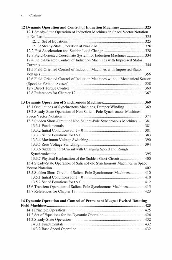
1.1 Maxwell’s Equations 13
with the angular frequency ω , the phase angle ϕ and the pole pitch τ
(half wave length). The extension of the coil in the direction of move-ment of the travelling wave (x-direction) is s (effective width), the exten-
sion perpendicular to the direction of movement (z-direction) is z (ef-
fective length), see Fig. 1.10.
Fig. 1.10. Example for explaining Faraday’s Law.
The flux linked with the coil is:
( )
( )
s2
zsA
2
s2
zs
2
ˆw B(x, t)dA wB cos t x dx
ˆwB cos t cos x
sin t sin x dx
−
−
πΨ = = ω + ϕ −
τ
π= ω + ϕ −
τ
π− ω + ϕ −
τ
(1.37)
This integral can be solved like follows:
x y
z
/ 2τ = λ
coil
iu
z
d
dA
v f= λ ⋅ B
dΦ
s
dx
x
z
y

14 1 Fundamentals
( )
( )
( )
( )
( )
z
s2
s2
z
z
z
ˆ wB cos t sin x
sin t cos x
s sˆwB cos t sin sin2 2
sˆwB cos t 2 sin2
2 sˆw B cos t , sin2
−
τ πΨ = ω + ϕ − −
π τ
τ π− ω + ϕ − − −
π τ
τ π π= ω + ϕ − − −
π τ τ
τ π= ω + ϕ
π τ
π= ξ τ ω + ϕ ξ =
π τ1≤
(1.38)
This equation can be interpreted like follows:
• 2
Bπ
is the mean value of a half harmonic flux density wave.
• z
2B τ
π is then the mean flux penetrating through the area zτ .
• The factor ξ is called “short-pitch factor” and it reduces this
flux to that amount penetrating through the area zs .
• The number of turns w transforms the flux to the flux linkage. • The cos -term shows the time dependency and the phase shift.
The induced voltage is (the positive directions of dA and B or dB are identical):
( )i z d 2ˆ ˆ ˆu sin t , w Bdt
= Ψ = −ωΨ ω + ϕ Ψ = ξ τπ
(1.39)
1.2 Definition of Positive Directions
For the unambiguous description of electrical circuits, directions have to be as-signed to voltages, currents, and power. The definition of the direction may be chosen arbitrarily. In principle there are two different possibilities as it is shown in Fig. 1.11:

1.2 Definition of Positive Directions 15
energy consumption system energy generation system
Fig. 1.11. Examples for the energy consumption system (left) and the energy generation system (right).
Poynting’s vector describes the power density in the electromagnetic field, please refer to Fig. 1.12:
S E H= × (1.40)
i
Ru
i
Ru
i
u
iu
i
u
iu
i
u C
i
u C
i
Lu
i
Lu
u iR 0
u iR
− =
=
u iR 0
u iR
+ =
= −
i
i
u u 0
du u
dt
diL
dt
− =
Ψ= =
=
i
i
u u 0
du u
dt
diL
dt
− =
Ψ= = −
= −
1u idt
C=
1u idt
C= −
diu L
dt=
diu L
dt= −
u
i
P
i
u P

16 1 Fundamentals
Fig. 1.12. Poynting’s vector for the energy consumption system (left) and the energy generation system (right).
1.3 Energy, Force, Power
The principle of electromechanical energy conversion will be explained using the example of a simple lifting magnet, see Fig. 1.13. The occurring energies can be calculated as follows.
Fig. 1.13. Electromagnetic system with movable armature.
The different possible kinds of energy are electrical energy, electrical losses, magnetic energy, and mechanical energy:
el W uidt= (1.41)
2
loss W i Rdt= (1.42)
i
u E HS
i
u E HS
H, B
u
i
x
1x 2x
w turns
movable armature (iron)

1.3 Energy, Force, Power 17
mag
V
W HdB dV
id
=
= Ψ
(1.43)
mech,lin
mech,rot
W Fdx
W Td
=
= α (1.44)
The B-H-curve of the iron and the Ψ -i-curve of the magnetic circuit in general (i.e. considering magnetic saturation) have the characteristics shown in Fig. 1.14.
Fig. 1.14. Principle B-H- and Ψ -i-characteristics.
The energy density of the magnetic field in air is:
2
mag0
1 Bw HB
2 2= =
μ (1.45)
With 2
VsB 0.5T 0.5
m= = (typical value) and 7
0
Vs4 10
Am
−μ = π ⋅ it follows:
2 2
45 5
mag 3 27
V s0.25
VAs Nmw 0.995 10 1 10Vs m m
8 10Am
−
= = ⋅ ≈ ⋅
π ⋅
(1.46)
The energy density of the electrical field in air is:
2el 0
1 1w ED E
2 2= = ε (1.47)
i
Ψ
H
B

18 1 Fundamentals
With kV
E 3mm
= (breakdown field strength in air) and 120
As8.854 10
Vm
−ε = ⋅ it
follows:
2
12 6el 3 2
1 As V VAs Nw 8.854 10 3 10 39.8 40
2 Vm m m m
−= ⋅ ⋅ = ≈ (1.48)
Because of the considerable lower energy density there are virtually no electro-static machines, except for extremely small geometries (please refer to equations (1.46) and (1.48)). In the following, the energy stored in the electrical field will be neglected against the energy stored in the magnetic field.
The energy balance of the lifting magnet is:
el loss mag mechdW dW dW dW= + + (1.49)
The electrical energy supplied via the terminals is equal to the sum of losses, change of magnetic energy and change of mechanical energy. Case 1: fixed armature ( x const.= , see Fig. 1.15):
( )
( )
( )2
mech el loss mag
el loss mag
mag
i mag
mag
mag
dW 0 d W W dW
d W W dW
ui i R dt dW
u idt dW
didt dW
dt
dW id
= = − −
− =
− =
=
Ψ=
= Ψ
(1.50)
Fig. 1.15. Ψ -i-characteristic for case 1.
i
Ψ
idΨ

1.3 Energy, Force, Power 19
The total magnetic energy is:2
mag0
W idΨ
= Ψ (1.51)
Case 2: movable armature, constant current:
The armature is moved from 1x x= to 2x x= with 0i const.= . Do-
ing this the flux linkage changes from 1Ψ = Ψ to 2Ψ = Ψ .
( ) ( )2el loss 0 0 i 0
0 0
d W W ui i R dt u i dt
di dt i d
dt
− = − =
Ψ= = Ψ
(1.52)
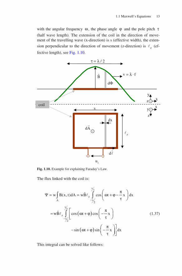
This equals area plus area in Fig. 1.16.
1 2
mag mag,1 mag,20 0
dW W W id idΨ Ψ
= − = Ψ − Ψ (1.53)
This equals area + minus area + , being equivalent to area mi-nus area (please refer to Fig. 1.16). Therefore:
( )mech el loss magdW d W W dW= − − (1.54)
which equals area plus area (see Fig. 1.16). Consequently:
( ) ( )
0 0i i
mech 1 20 0
mag
dW x di x di
dW
= Ψ − Ψ
′=
(1.55)
magW′ is called the magnetic co-energy. The force can be calculated like
follows:
2 The tilde serves for the differentiation between integration limit and integration variable.
20 1 Fundamentals
magmech
i const.
dWdWF
dx dx=
′= = (1.56)
Fig. 1.16. Ψ -i-characteristics for case 2.
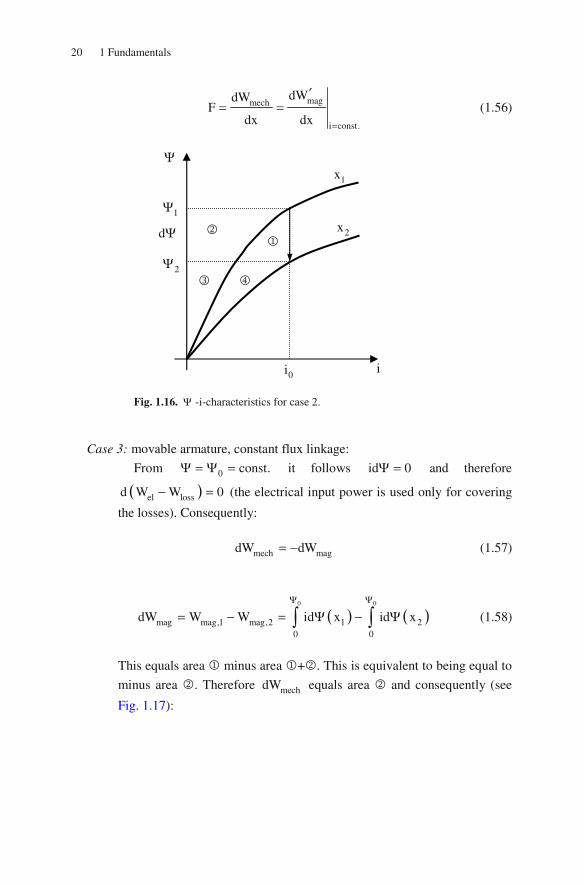
Case 3: movable armature, constant flux linkage:
From 0 const.Ψ = Ψ = it follows id 0Ψ = and therefore
( )el lossd W W 0− = (the electrical input power is used only for covering
the losses). Consequently:
mech magdW dW= − (1.57)
( ) ( )0 0
mag mag,1 mag,2 1 20 0
dW W W id x id xΨ Ψ
= − = Ψ − Ψ (1.58)
This equals area minus area + . This is equivalent to being equal to
minus area . Therefore mechdW equals area and consequently (see
Fig. 1.17):
0i
2Ψ
1Ψ
i
Ψ
dΨ
1x
2x

1.3 Energy, Force, Power 21
( ) ( )
( ) ( )
1 2 2
1
2 2
i i i
mech 1 0 20 i 0
i i
1 2 mag0 0
dW x di di x di
i di i di dW
= Ψ + Ψ − Ψ
′= Ψ − Ψ =
(1.59)
The force is calculated as follows:
magmech
const.
dWdWF
dx dxΨ=
′= = (1.60)
Fig. 1.17. Ψ -i-characteristics for case 3.
Case 4: arbitrary case; movable armature, current and flux linkage are variable (see Fig. 1.18):
Fig. 1.18. Ψ -i-characteristics for case 4.
0Ψ
i
Ψ
1x
2x
1i 2i
2i
2Ψ
1Ψ
i
Ψ1x
2x
1i

22 1 Fundamentals
The changes of energies calculated in the following for this case are based on the solutions of the above cases 1 and 2.
Case 4.1 (see Fig. 1.19): a) firstly the armature is fixed, change of current and flux linkage b) secondly the current is constant, movable armature and change of
flux linkage
Fig. 1.19. Ψ -i-characteristics for case 4.1.
a) 1x const.= ;
i is changed from 1i to 2i ; Ψ is changed from 1Ψ to aΨ .
( ) ( )
( )
a1
mech,1a
mag,1a 1 10 0
el,1a loss,1a mag,1a
dW 0
dW id i x d i x d
d W W dW
ΨΨ
=
= Ψ = Ψ − Ψ
− =
(1.61)
b) 2i const.= ;
x is changed from 1x to 2x ; Ψ is changed from aΨ to 2Ψ .
2i
2Ψ
1Ψ
i
Ψ1x
2x
1i
aΨ

1.3 Energy, Force, Power 23
( ) ( )
( ) ( )
( ) ( )
2 2
a 2
i i
mech,1b mag,1b 1 20 0
mag,1b 1 20 0
el,1b loss,1b 2 2 a 2
dW dW x di x di
dW i x d i x d
d W W i d i
Ψ Ψ
′= = Ψ − Ψ
= Ψ − Ψ
− = Ψ = Ψ − Ψ
(1.62)
Case 4.2 (see Fig. 1.20): a) firstly the current is constant, movable armature and change of flux
linkage b) secondly the armature is fixed, change of current and flux linkage
Fig. 1.20. Ψ -i-characteristics for case 4.2.
a) 1i const.= ;
x is changed from 1x to 2x ; Ψ is changed from 1Ψ to bΨ .
( ) ( )
( ) ( )
( ) ( )
1 1
b1
i i
mech,2a mag,2a 1 20 0
mag,2a 1 20 0
el,2a loss,2a 1 1 1 b
dW dW x di x di
dW i x d i x d
d W W i d i
ΨΨ
′= = Ψ − Ψ
= Ψ − Ψ
− = Ψ = Ψ − Ψ
(1.63)
b) 2x const.= ;
i is changed from 1i to 2i ; Ψ is changed from bΨ to 2Ψ .
2i
2Ψ
1Ψ
i
Ψ1x
2x
1i
bΨ

24 1 Fundamentals
( ) ( )
( )
b 2
mech,2b
mag,2b 2 20 0
el,2b loss,2b mag,2b
dW 0
dW id i x d i x d
d W W dW
Ψ Ψ
=
= Ψ = Ψ − Ψ
− =
(1.64)
Comparison of cases 4.1 and 4.2:
a) change of mechanical energy mechdW (Fig. 1.21)
Fig. 1.21. Ψ -i-characteristics: different change of mechanical energy in both cas-es.
b) change of magnetic energy magdW (Fig. 1.22)
Fig. 1.22. Ψ -i-characteristics: equal change of magnetic energy in both cases.
2i
2Ψ
1Ψ
i
Ψ1x
2x
1i
bΨ
2i
2Ψ
1Ψ
i
Ψ1x
2x
1i
aΨ
2i
2Ψ
1Ψ
i
Ψ1x
2x
1i
aΨ
2i
2Ψ
1Ψ
i
Ψ1x
2x
1i
bΨ

1.3 Energy, Force, Power 25
c) change of difference: electrical energy and losses ( )el lossd W W−
(Fig. 1.23)
Fig. 1.23. Ψ -i-characteristics: different change of difference between electrical energy and losses in both cases.
For linear materials mag magW W′= holds true. This means that in this case (and
only in this case!) the force may be calculated from the magnetic energy. The magnetic pulling force on the surface area of flux carrying iron parts can
be calculated as follows (Fig. 1.24):
Fig. 1.24. Explanation of the magnetic pulling force.
Because of r,Feμ → ∞ and r,air 1μ = the used materials are linear. Consequent-
ly the force may be calculated from the change of the magnetic energy.
Because of FeH 0→ the iron paths may be neglected. Therefore, the force will
be calculated from the change of magnetic energy in the air-gap.
x
dx
iron
air-gap: H, B
surface area A
F
2i
2Ψ
1Ψ
i
Ψ1x
2x
1i
aΨ
2i
2Ψ
1Ψ
i
Ψ1x
2x
1i
bΨ

26 1 Fundamentals
2
mag mag
0
dW w Adx 1 BF HB A A
dx dx 2 2= = = =
μ (1.65)
The specific force (force per cross section unit, “Maxwell’s attractive force“)
is:
2
0
F Bf
A 2= =
μ (1.66)
Calculating the force from the power balance A cylindrical coil shall have the Ohmic resistance R and an armature movable on-ly in x-direction. The inductivity of that coil depends on the position of the arma-
ture: ( )L L x= . Saturation will be neglected: ( )L L i≠ (Fig. 1.25).
Fig. 1.25. Explanation of calculating the force from the power balance.
The voltage equation is:
d
u iR , Lidt
Ψ= + Ψ = (1.67)
Case 1: armature is fixed at position x (then L is constant)
From the voltage equation (1.67) the power balance follows by multi-plication with the current i:
2 diui i R Li
dt= + (1.68)
F
x
⊗ ⊗ ⊗ ⊗ ⊗ ⊗ ⊗ ⊗ ⊗ ⊗
u
i armature (iron)

1.3 Energy, Force, Power 27
From the magnetic energy 2mag
1W Li
2= it follows:
2 2mag
d d 1 d 1 diW Li L i Li
dt dt 2 dt 2 dt= = = (1.69)
From equations (1.68) and (1.69) it follows further:
2 2d 1ui i R Li
dt 2= + (1.70)
Therefore, the electrical input power is equal to the sum of electrical losses and change of magnetic energy.
Case 2: movable armature ( L L(x)= )
In this case the voltage equation becomes:
di dL
u iR L idt dt
= + + (1.71)
and consequently the power balance:
2 2di dLui i R Li i
dt dt= + + (1.72)
From the magnetic energy 2mag
1W Li
2= it follows:
2 2mag
d d 1 di 1 dLW Li Li i
dt dt 2 dt 2 dt= = + (1.73)
From equations (1.71) and (1.72) it follows further:
2 2 2d 1 1 dLui i R Li i
dt 2 2 dt= + + (1.74)
The additional term in the power balance compared with case 1 must be the mechanical power. Therefore the mechanical power is
28 1 Fundamentals
2 2dx 1 dL 1 L dxF i i
dt 2 dt 2 x dt
∂= =
∂ (1.75)
and the force can be calculated like follows:
21 LF i
2 x
∂=
∂ (1.76)
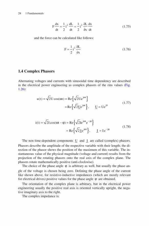
1.4 Complex Phasors
Alternating voltages and currents with sinusoidal time dependency are described in the electrical power engineering as complex phasors of the rms values (Fig. 1.26):
{ }{ }
j t
j t j0
u(t) 2U cos( t) Re 2Ue
Re 2Ue , U Ue
ω
ω
= ω =
= = (1.77)
{ }{ }
j t j
j t j
i(t) 2I cos( t ) Re 2Ie e
Re 2 I e , I I e
ω − ϕ
ω − ϕ
= ω − ϕ =
= = (1.78)
The non time-dependent components U and I are called (complex) phasors.
Phasors describe the amplitude of the respective variable with their length; the di-rection of the phasor shows the position of the maximum of this variable. The in-stantaneous value of the physical magnitude (voltage and current) results from the projection of the rotating phasors onto the real axis of the complex plane. The phasors rotate mathematically positive (anti-clockwise).
The choice of the phase angle ϕ is arbitrary as well, but usually the phase an-
gle of the voltage is chosen being zero. Defining the phase angle of the current like shown above, for resistive-inductive impedances (which are mostly relevant for electrical drives) positive values for the phase angle ϕ are obtained.
The orientation of the complex plane is arbitrary, but in the electrical power engineering usually the positive real axis is oriented vertically upright, the nega-tive imaginary axis to the right.
The complex impedance is:

1.4 Complex Phasors 29
j j
2 2
U UZ e Ze Z cos( ) jZ sin( ) R jX
I I
XZ R X tan( )
R
ϕ ϕ= = = = ϕ + ϕ = +
= + ϕ =
(1.79)
The complex apparent power is the product of the complex rms-value of the voltage and the conjugate complex rms-value of the current:
jS U I UIe P jQ∗ ϕ= = = + (1.80)
The different kinds of power are the
• active power (real power)
{ }P Re S UI cos( )= = ϕ (1.81)
• reactive power (wattless power)
{ }Q Im S UI sin( )= = ϕ (1.82)
• and apparent power
2 2S S UI P Q= = = + (1.83)
Fig. 1.26. Phasor diagram.
Re
Im−
U
I ϕ
ω

30 1 Fundamentals
1.5 Star and Delta Connection
Regarding symmetric three-phase systems without neutral line there are the possi-bilities illustrated in Fig. 1.27:
star connection delta connection
Fig. 1.27. Star and Delta connection.
For the phase voltages phaseU and currents phaseI it holds:
• for star connection: phaseI 0=
• for delta connection: phaseU 0=
The terminal voltages lineU and terminal currents lineI are:
• for star connection: line phase line phaseU 3 U I I ;= =
• for delta connection: line phase line phaseU U I 3 I; = =
The electrical power is:
• for star connection: linephase phase line
US 3U I 3 I
3= =
• for delta connection: linephase phase line
IS 3U I 3U
3= =
Therefore, it is always:
lineU
lineI
phase
phase
U
I
u v w
u
v w
lineU
phaseU
lineU
lineI
phase
phase
U
I
u v w
u
v w
lineI
phaseI

1.6 Symmetric Components 31
line lineS 3 U I 3 U I = = (1.84)
Usually the index “line” is omitted. The values on the name plate of electrical machines are always the terminal values!
1.6 Symmetric Components
A symmetric three-phase system may be operated asymmetrically, e.g. by:
• supplying with asymmetric voltages or • single-phase load between two phases or between one phase and the neutral
line.
Describing these asymmetric (unknown) operating conditions by symmetric ones, a simplified calculation method is gained. The method of symmetric compo-nents is qualified for this: An asymmetric three-phase-system is separated into three symmetric systems (positive, negative, and zero system), the circuit calculat-ed and the results superposed.
The preconditions are:
• The three currents or voltages have the same frequency and they are sinusoidal-ly in time (i.e. there is no harmonic content); phase shift and amplitude are ar-bitrary.
• Because of the superposition of the results the system must be linear.
In the following the complex phasor 2
j3a eπ
= will be used. There is:
4 2
j j2 23 3a e e ; 1 a a 0π π
−
= = + + = (1.85)
The following asymmetric current system u v wI , I , I (Fig. 1.28) will be rep-
resented by the components p n 0I , I , I (Fig. 1.29).
Fig. 1.28. Asymmetric current system.
uI
vI
wI
Re
Im−

32 1 Fundamentals
Fig. 1.29. Three symmetric current systems.
The following holds true:
u p n 0 u p2 2
v p n 0 v n2 2
w p n 0 w 0
I I I I I 1 1 1 I
I a I a I I I a a 1 I
I a I a I I I a a 1 I
= + +
= + + ⇔ =
= + +
(1.86)
Solving this results in:
2 p u
2 n v
0 w
I 1 a a I1
I 1 a a I3
I 1 1 1 I
= (1.87)
Now, the asymmetric system u v wI , I , I can be separated into three symmet-
ric systems p n 0I , I , I according to the above equation; these three systems can
be calculated easily and the solution is gained by inverse transformation (superpo-sition of the three single results).
1.7 Mutual Inductivity
There are two coils, each generating a magnetic field. Both magnetic fields shall penetrate both coils, see Fig. 1.30. As an example, one coil produces a homogene-ous field, the other coil an inhomogeneous field.
pI pa I
2 pa I
u
v
w
positive system
(positive phase sequence)
negative system
(negative phase sequence)
nI
na I 2 na I
u v
w 0I
zero system
(in phase)
0I 0I
u v w

1.7 Mutual Inductivity 33
Fig. 1.30. Magnetic fields of a system made of two coils.
Calculation of the magnetic energy (the tilde is introduced to distinguish be-tween integration limit and integration variable) if supplying
a) only coil 1:
1 1i
21 1 1 1 1 1 1 1 1 1 1
0 0
1dW i d W i d i L di L i
2
Ψ
= Ψ = Ψ = = (1.88)
b) only coil 2:
2 2i
22 2 2 2 2 2 2 2 2 2 2
0 0
1dW i d W i d i L di L i
2
Ψ
= Ψ = Ψ = = (1.89)
c) coils 1 and 2:
( ) ( )
1 2 1 1 2 2
1 1 1 12 2 1 1 1 12 2
2 2 2 21 1 2 2 2 21 1
1 1 1 12 2 2 2 2 21 1
dW dW dW i d i d , with
L i L i , d L di L di
L i L i , d L di L di
dW i L di L di i L di L di
= + = Ψ + Ψ
Ψ = + Ψ = +
Ψ = + Ψ = +
= + + +
(1.90)
Assuming const.μ = it follows:
a) firstly increasing the current 1i from 0 to 1i
1i
22 2 1 1 1 1 1
0
1i 0, di 0 W i L di L i
2= = = = (1.91)
then increasing the current 2i from 0 to 2i
coil 1: generates a homogeneous field
⊗ ⊗ ⊗ ⊗ ⊗ ⊗ ⊗ ⊗ ⊗ ⊗ ⊗ ⊗ ⊗ ⊗ ⊗ ⊗ ⊗ ⊗
⊗
coil 2: generates an inhomogeneous field

34 1 Fundamentals
2 2i i2
1 1 1 1 1 1 12 2 2 2 20 0
2 21 1 12 1 2 2 2
1i i , di 0 W L i i L di i L di
2
1 1W L i L i i L i
2 2
= = = + +
= + +
(1.92)
b) firstly increasing the current 2i from 0 to 2i
2i
21 1 2 2 2 2 2
0
1i 0, di 0 W i L di L i
2= = = = (1.93)
then increasing the current 1i from 0 to 1i
1 1i i2
2 2 2 2 2 1 1 1 2 21 10 0
2 22 2 1 1 21 2 1
1i i , di 0 W L i i L di i L di
2
1 1W L i L i L i i
2 2
= = = + +
= + +
(1.94)
Independent from the sequence of increasing the currents (switching on the coils) the magnetic energy must always have the same value. Therefore, the fol-lowing is true:
12 21L L= (1.95)
1.8 Iron Losses
In addition to the copper losses (caused by current flow in wires having a re-sistance) iron losses are known in electrical machines. These iron losses mainly are composed of two parts:
According to Lenz’s Law the flux change in the electrical conducting iron ma-terial causes eddy currents that oppose their generating induction variation. The eddy current losses are proportional to the squared frequency, the squared flux density and the iron volume:
2 2Fe,edd Fe
ˆf B VP (1.96)
1.9 References for Chapter 1 35
These eddy current losses can be reduced by using isolated lamination sheets and by using iron laminations with low electrical conductivity.
Because of ever changing magnetizing direction inside the iron hysteresis loss-es are generated that are proportional to the area of the hysteresis loop enclosed during each cycle; these losses are proportional to the frequency, the squared flux density and the iron volume:
2Fe,hys Fe
ˆf B VP (1.97)
The hysteresis losses can be reduced by using iron material with a narrow hystere-sis loop.
Mostly, the iron losses are calculated according to the following Steinmetz equation:
22
Fe edd hys Fe Fe
ˆf f BP a a V
50Hz 50Hz 1T ρ= + (1.98)
where Feρ is the specific iron weight. The material specific loss factors (eddy cur-
rent loss factor edda and hysteresis loss factor hysa , both in W kg ) are given by
the iron material suppliers.
1.9 References for Chapter 1
Küpfmüller K, Kohn G (1993) Theoretische Elektrotechnik und Elektronik. Springer-Verlag, Berlin
Lehner G (1994) Elektromagnetische Feldtheorie. Springer-Verlag, Berlin Müller G, Ponick B (2005) Grundlagen elektrischer Maschinen. Wiley-VCH Verlag, Weinheim Müller G, Vogt K, Ponick B (2008) Berechnung elektrischer Maschinen. Wiley-VCH Verlag,
Weinheim Richter R (1967) Elektrische Maschinen I. Birkhäuser Verlag, Basel Schwab AJ (1993) Begriffswelt der Feldtheorie. Springer-Verlag, Berlin Simonyi K (1980) Theoretische Elektrotechnik. VEB Deutscher Verlag der Wissenschaften, Ber-
lin Veltman A, Pulle DWJ, DeDoncker RW (2007) Fundamentals of electrical drives. Springer-
Verlag, Berlin
2 DC-Machines
2.1 Principle Construction
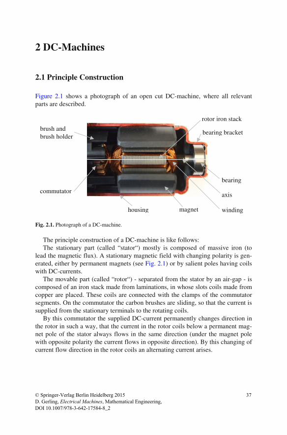
Figure 2.1 shows a photograph of an open cut DC-machine, where all relevant parts are described.
Fig. 2.1. Photograph of a DC-machine.
The principle construction of a DC-machine is like follows: The stationary part (called “stator“) mostly is composed of massive iron (to
lead the magnetic flux). A stationary magnetic field with changing polarity is gen-erated, either by permanent magnets (see Fig. 2.1) or by salient poles having coils with DC-currents.
The movable part (called “rotor“) - separated from the stator by an air-gap - is composed of an iron stack made from laminations, in whose slots coils made from copper are placed. These coils are connected with the clamps of the commutator segments. On the commutator the carbon brushes are sliding, so that the current is supplied from the stationary terminals to the rotating coils.
By this commutator the supplied DC-current permanently changes direction in the rotor in such a way, that the current in the rotor coils below a permanent mag-net pole of the stator always flows in the same direction (under the magnet pole with opposite polarity the current flows in opposite direction). By this changing of current flow direction in the rotor coils an alternating current arises.
commutator
housing
rotor iron stack
bearing bracket
bearing
axis
windingmagnet
brush and brush holder
© Springer-Verlag Berlin Heidelberg 2015 37
DOI 10.1007/978-3-642-17584-8_ 2D. Gerling, Electrical Machines Mathematica l Engineering,,

38 2 DC-Machines
2.2 Voltage and Torque Generation, Commutation
In principle each electrical machine can be operated as motor or as generator. In generator operation usually voltage production constant in time is required, in mo-tor operation usually torque production constant in time is asked for.
In a rotating coil a voltage is induced according to the induction law, see Fig. 2.2.
Fig. 2.2. Principle sketch of voltage induction in rotating representation.
The induced voltage is:
( )i i z
i
z
u E d v B d 2 B v
u Ri u
u Ri 2 B v
= − = − × =
= +
= +
(2.1)
For the signs the following is true:
• i iu E d= − is defined like this in Sect. 1.1, see Eq. 1.32;
• iE and d (in the direction of the current i) are opposite to each other.
Figure 2.3 shows the same situation in a “wound-off” representation. The in-duced voltage for this situation can be calculated like follows:
i
zi z mech
d du w , w 1
dt dt
B dA B 2 vdtu 2 B v, v r 2 nr
dt dt
Ψ Φ= = =
= = = = ω = π
(2.2)
N
u
i
B
v iE
z S
B
v iE

2.2 Voltage and Torque Generation, Commutation 39
For the signs the following is true:
• i
du
dt
Ψ= is deduced in Sect. 1.1;
• d (in the direction of the current i) and B in the left part of Fig. 2.3 (increase
of B ) are linked together like a right-handed screw.
Fig. 2.3. Principle sketch of voltage induction in “wound-off” representation.
The spatial characteristic of the flux density and the time-dependent character-istic of the voltage are like follows (Fig. 2.4):
Fig. 2.4. Flux density and induced voltage characteristics.
Between the electrical angular frequency ω and the mechanical angular fre-
quency mechω the following relation is true ( p being the number of pole pairs):
vdt
v v
u i
z
⊗
BB
x
x
B spatial characteristic of flux density B(x)
0 2π 2−π π
tω
iu
time-dependent characteristic
of the voltage ( )iu tω
0 2π 2−π π
with commutator

40 2 DC-Machines
mechp
2 f p 2 n
f pn
ω = ω
π = π
=
(2.3)
The commutator converts the AC-voltage in the coil into a DC-voltage (with harmonics) at the terminals. By series connection of several coils evenly distribut-ed along the rotor circumference a higher DC-voltage with lower harmonic con-tent is obtained.
The procedure of commutation is explained in Fig. 2.5:
Fig. 2.5. Procedure of commutation.
As a first approximation it may be assumed that the current in the coil changes linearly from its maximum to its minimum value (maximum absolute value, nega-
S N a b
i
n
S N b a
i
n
S N
a
b
n
1) The current flows via a carbon brush, a commutator section, through a coil and via the counterpart com-mutator section and carbon brush. For motor operation a torque in the direction of mo-tion occurs.
2) Under each carbon brush both commutator sections are located; there is no current in the coil (begin and end of the coil are short-circuited via the brushes) and no torque is generated. The rotor of the DC-motor stays in rotational movement because of its inertia.
3) Like in case 1) current is flowing in the coil, but the commutator (after 180° rotation of the rotor) has forced a change of current flow direction in the coil. Therefore, torque and current at the terminals have the same direction like in case 1).

2.3 Number of Pole Pairs, Winding Design 41
tive sign). In the time period between two commutation events the current in the coil is (approximately) constant.
The force onto a current conducting wire is: ( )F i B= × . From this speed di-
rection and torque of the DC-machine in motor operation follow. In generator operation the voltage u Ri 2B v= − + is produced (here the ener-
gy generation system is assumed, see Fig. 2.6).
Fig. 2.6. Motor operation (above) and generator operation (below).
2.3 Number of Pole Pairs, Winding Design
Up to now two-pole machines were presented. Nevertheless, DC-machines with even more poles are possible. For these constructions the arrangement is repeated p times along the circumference (e.g. for p 2= there are 4 carbon brushes and 4
magnets or excitation poles). The advantages of a high number of poles are:
i
n
F
F
N S
u
B
+ -
i
n
F
F
N S
u
B
+ -

42 2 DC-Machines
• The total flux is divided into 2p part fluxes. By this the cross section of the yokes in stator and rotor can be chosen smaller (material savings).
• A smaller pole pitch results in shorter end windings (with smaller resistance and lower losses).
The disadvantages are:
• By having smaller distances between the poles the leakage between the poles is increased.
• The losses are increased by the higher rotor frequency.
Therefore, the choice of the number of pole pairs is an optimization task. The pole pitch is calculated according to:
p
2 r
2p
πτ = (2.4)
Between the mechanical angle α and the electrical angle β the following rela-
tion is true:
pβ = α (2.5)
The winding placed in the slots of the rotor stack often is realized as two-layer winding: The forward conductors are in the upper layer (i.e. towards the air-gap), the return conductors in the lower layer (i.e. towards the slot bottom). In Figs. 2.7 to 2.9, showing the general situations “wound-off”, solid lines represent the for-ward conductors (upper layer) and dashed lines the return conductors (lower lay-er). For DC-machines each coil at the beginning and at the end is connected to a commutator section, i.e. the number of coils and the number of commutator sec-tions are identical; in the following this will be named with the variable K .
For DC-machines the following nominations are introduced: K number of commutator sections (equal to number of coils) u number of coils sides side-by-side in a single slot N number of rotor slots
Sw number of turns per coil (number of conductors per coil side)
z total number of conductors in all slots The distance between two carbon brushes (i.e. between the positive brush and
the negative brush) is:
B
Ky
2p= (2.6)
Moreover, the following relations are true:

2.3 Number of Pole Pairs, Winding Design 43
S
K Nu
z 2w K
=
= (2.7)
Mostly u 1> is true, then the number of rotor slots is smaller than the number of commutator sections ( N K< ).
Examples (lap winding):
• In Fig. 2.7 the three upper sketches show the conductors in a rotor slot for dif-ferent winding layout.
• The lower sketches illustrate the according winding layout (in each sketch on the left side only the upper layer and on the right side only the lower layer is shown).
Fig. 2.7. Sketches of conductors in a slot (above) and the according winding layout (below).
The coils can be connected to the commutator in two different ways: Having a lap winding (Fig. 2.8) the end of a coil is connected directly to the
beginning of the next coil of the same pole pair at the commutator. Between two commutator sections only one coil is placed. All p pole pairs are connected in se-ries by the carbon brushes; the number of parallel paths in the rotor is: 2a 2p= .
The total rotor current is therefore divided into 2p parallel conductor currents.
Naming the coil width with 1y (in numbers of rotor slots) and the connection step
with 2y (in numbers of rotor slots), then the commutator step y for the lap wind-
ing is (see Fig. 2.8): 1 2y y y 1= − = .
Having a wave (or series) winding (Fig. 2.9) the end of a coil is connected with the beginning of a corresponding coil of the next pole pair, so that - until reaching the neighboring commutator section - a path along the circumference of the rotor with p coils is completed. Between positive and negative carbon brush all p pole
upper layer
lower layer S
u 1
w 1
=
=
S
u 3
w 2
=
=
S
u 2
w 1
=
=
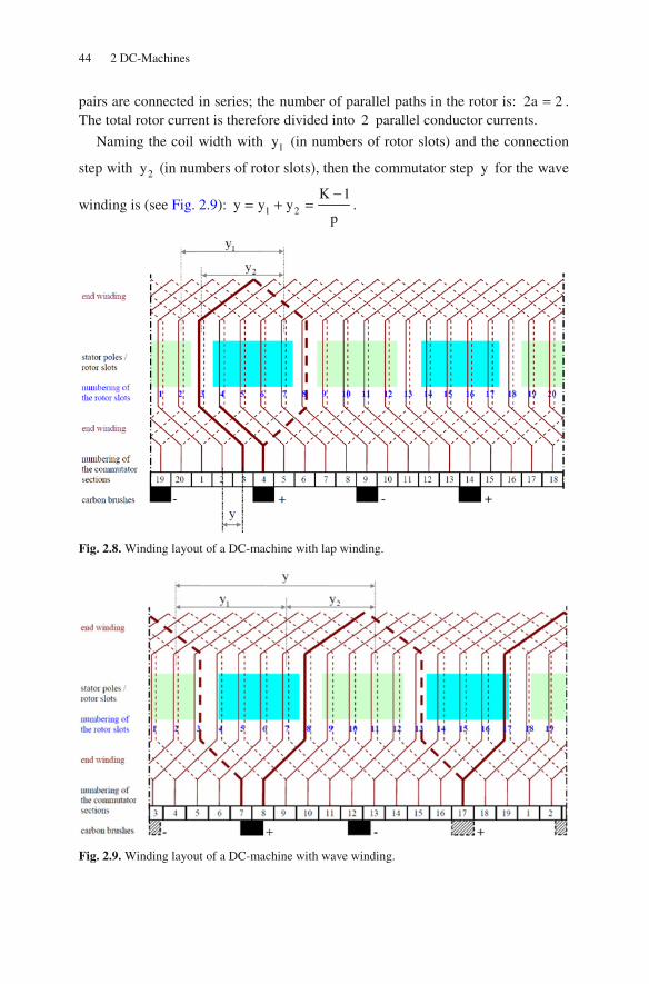
44 2 DC-Machines
pairs are connected in series; the number of parallel paths in the rotor is: 2a 2= . The total rotor current is therefore divided into 2 parallel conductor currents.
Naming the coil width with 1y (in numbers of rotor slots) and the connection
step with 2y (in numbers of rotor slots), then the commutator step y for the wave
winding is (see Fig. 2.9): 1 2
K 1y y y
p
−= + = .
Fig. 2.8. Winding layout of a DC-machine with lap winding.
Fig. 2.9. Winding layout of a DC-machine with wave winding.

2.4 Main Equations of the DC-Machine 45
For the wave winding an arbitrary number of pole pairs can be realized with just two carbon brushes, because all positive brushes and all negative brushes are connected in series, respectively. This is illustrated in Fig. 2.9 by hatching one positive brush and one negative brush.
2.4 Main Equations of the DC-Machine
A two-pole DC-machine is regarded in the following (please refer to Fig. 2.10).
Here iα is the pole arc in parts of the pole pitch ( iα is a dimensionless number
that gives the ratio between pole arc and pole pitch).
Fig. 2.10. Cross-sectional sketch of a two-pole DC-machine.
The number of turns of the rotor winding (armature winding) is:
A
z 2 zw
2a 4a= = (2.8)
Under the 2p poles i A2 wα turns are effective.
2.4.1 First Main Equation: Induced Voltage
The induced voltage in a single rotor conductor is: iu B v= . For every rotor path
there are z
2a conductors in series; in each element dα (see Fig. 2.11) there are
X
X
X
XX X
X
X+ -
Θ
I I
Φ
Φ
Φ
n
XX
XX
XX
XX
XX
XX X
XXX+ -
Θ
Φ
niα
Φ
Φ/2 Φ/2
Φ
A I A I

46 2 DC-Machines
z d
2a 2 p
α
π conductors in series, if all z conductors are distributed evenly along the
circumference.
Fig. 2.11. Sketch of a two-pole DC-machine (above) and respective flux density distribution in “wound-off” representation (below).
The induced voltage in the conductors of a circumference element dα becomes:
( ) ( )i
z du d B v
2a 2 p
αα = α
π (2.9)
Because of the parallel connection of the paths the total voltage of a path is equal to the induced voltage. This voltage is gained by integration between the limits given by the carbon brush position (shifted brushes). For 2p poles there is:
( )
2
i
2
z du 2p B v
2a 2 p
π+ β
π− + β
α= α
π (2.10)
With v 2 rn= π it follows:
β
α
dα
n
β
( )B α
α β
2π+ 2
π−
pτ = π
geometrical
neutral zone z conductors evenly
distributed along the
circumference

2.4 Main Equations of the DC-Machine 47
( )
2
i
2
p ru z n B d
a p
π+ β
π− + β
= α α (2.11)
Here the integral describes the flux Φ , which is enclosed by the brushes. With
A
pk z 4pw
a= = (2.12)
(the constant k is called motor constant or rotor constant) it follows:3
iu k n= Φ (2.13)
For 0β = (i.e. no shift of the brushes, brushes in neutral position) and the air-gap
flux density below the excitation poles Bδ it follows:
( )
i i
i i
2 2 2p
2 2 2
i p
r 2 rB d B d B d
p 2 p
B
π π πα α
δ δπ π π
− − α − α
δ
τπΦ = α α = α = α
π π
= α τ
(2.14)
2.4.2 Second Main Equation: Torque
The torque can be calculated from the force on current conducting wires (here for 0β = ):
i A
Ai p
T w i B 2 r
4pwB i
2
δ
δ
= α
= α τπ
(2.15)
Therefore, it follows:
3 Sometimes the induced voltage (also called back electromotive force, back emf, counter emf) is
nominated with “e”. As it has the nature of a voltage, here the name “ iu “ is preferred.

48 2 DC-Machines
k
T i2
= Φπ
(2.16)
2.4.3 Third Main Equation: Terminal Voltage
For the terminal voltage there is (in the energy consumption system), see Fig. 2.12:
i
diu u Ri L
dt= + + (2.17)
Fig. 2.12. Equivalent circuit diagram of the DC-machine.
For steady-state operation it follows:
iU U RI= + (2.18)
2.4.4 Power Balance
By means of the voltage equation a power balance can be made (multiplication of the voltage equation with the current i):
2i
diui u i i R Li
dt= + + (2.19)
From this can be deduced: The electrical input power equals the internal power of the DC-machine plus the electrical losses plus the change of magnetic energy.
u
i R L
iu
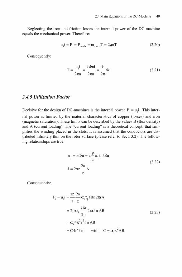
2.4 Main Equations of the DC-Machine 49
Neglecting the iron and friction losses the internal power of the DC-machine equals the mechanical power. Therefore:
i i mech mechu i P P T 2 nT= = = ω = π (2.20)
Consequently:
iu i k ni kT i
2 n 2 n 2
Φ= = = Φ
π π π (2.21)
2.4.5 Utilization Factor
Decisive for the design of DC-machines is the internal power i iP u i= . This inter-
nal power is limited by the material characteristics of copper (losses) and iron (magnetic saturation). These limits can be described by the values B (flux density) and A (current loading). The “current loading“ is a theoretical concept, that sim-plifies the winding placed in the slots: It is assumed that the conductors are dis-tributed infinitely thin on the rotor surface (please refer to Sect. 3.2). The follow-ing relationships are true:
i i p
pu k n z Bn
a
2ai 2 r A
z
= Φ = α τ
= π
(2.22)
Consequently:
i i i p
i
2 2i
2 2i
zp 2aP u i Bn2 rA
a z
2 r2p 2 r n AB
2p
4 r n AB
C4r n with C AB
= = α τ π
π= α π
= α π
= = α π
(2.23)

50 2 DC-Machines
The value C is called utilization factor (Esson’s number); the internal power is now described by the geometry, the speed, and the utilization factor.
Example:
Some typical values are: i 0.65α = , A 500 A cm= and B 0.8T= . From this
the utilization factor 3C 4.28 kW min m= can be obtained. Now a DC-machine
with iP 100kW= , 1n 2000 min−= and p 2= shall be designed.
Choosing pτ = , it follows:
2 2 2 3i ip
i3
P P2 r4r 4r 4r 2 r
Cn 2p Cn
Pr 0.123m
2 Cn
π= = τ = = π
= ≈π
(2.24)
and
3i2 2
P1 1 12 r r 0.193m
4r Cn 4r 2= = π = π = (2.25)
A transformation gives:
i2 2 2 2 2 2
P2 2 2 2 nT TC C
4r n 4r n r
π′ = = = =
π π π π (2.26)
Consequently, the utilization factor C is proportional to the torque divided by the bore volume.
Further it follows:
2 2
T Fr FC 2 2f
r r 2 r′ = = = =
π π π (2.27)
The utilization factor C also is proportional to the (tangential) force divided by the bore surface area.
With 2iC AB= α π it is true:
i
i
C 2 AB
f AB
′ = α
= α (2.28)

2.5 Induced Voltage and Torque, Precise Consideration 51
2.5 Induced Voltage and Torque, Precise Consideration
2.5.1 Induced Voltage
Up to now the calculation of the induced voltage and the torque was performed as-suming that the conductors of the rotor are lying in the air-gap field. But the con-ductors of the rotor are placed in the rotor slots; the magnetic field is guided around the rotor winding by means of the surrounding iron (Fig. 2.13).
Fig. 2.13. Sketch of the DC-machine in rotatory presentation (above) and “wound-off” represen-tation (below).
δ
F
1
2Θ
0 x
( )H x pτ
conductor coil
0x
X X
α
δ
F
1
2Θ X
X
X
XX X
X
X
-Θ
I
Φ
Φ
Φ
n
XX
XX
α

52 2 DC-Machines
With
x r = α (2.29)
both coordinate systems (Cartesian and cylindrical) can be transformed to each other.
For calculation of the induced voltage Ampere’s Law is used with a circulation
path over one pole pitch (for the permeability of iron Feμ → ∞ is assumed; the ro-
tor current is zero; r is the rotor radius):
( ) ( )
( )( )
F p
0
Hd H x H x
B x2 H x 2
= Θ = δ + − + τ δ
= δ = δμ
(2.30)
Because of the symmetry the field strength at two points, shifted by the pole
pitch pτ , has the same absolute value, but different sign. Performing the circula-
tion path (which has the width of one pole pitch) not under the poles, but in the gap between the poles, the circulation integral gives the value zero. Therefore, the air-gap flux density becomes:
( )0
FB in the area of the poles B x 2
0 in the gap area between poles
δ
μ± = ± Θ
= δ (2.31)
Now a conductor coil of width pτ (pole pitch) and length (axial length of the
machine) is looked at. This conductor coil has placed its forward and return wires in the rotor slots. Moreover, the forward and return wires always shall be located in the areas of the stator poles. This last requirement is fulfilled for
( ) ( )p pi 0 i1 x 1
2 2
τ τ− α ≤ ≤ + α (2.32)
if 0x describes the beginning of the conductor coil. For the flux surrounded by
this conductor coil it follows:
( ) p p0 p 0 0
p
2x B x B 2 x
2 2δ δ
τ τφ = − τ − = − −
τ (2.33)

2.5 Induced Voltage and Torque, Precise Consideration 53
Shifting now the conductor coil by the value xΔ (i.e. rotating the rotor by
x rΔα = Δ ), but this coil remains under the stator poles, the surrounded flux is:
( ) ( )p0 0x x B 2 x x
2δ
τφ + Δ = − − + Δ (2.34)
The induced voltage equals the change of flux with respect to time (see Sect. 2.2); therefore it follows:
( ) ( )
( )0 0
i
x x x
B 2 x
xU B 2 B 2 v
t t
δ
δ δ
Δφ = φ + Δ − φ
= − −Δ
Δφ −Δ= = − =
Δ Δ
(2.35)
The sign of the induced voltage depends on the direction of movement of the conductor coil (i.e. depending on the direction of movement of the rotor, because the conductor coil is placed inside the rotor slots).
In total the following can be stated: The induced voltage of wires placed in slots can be calculated as if these wires would lie in the air-gap field.
2.5.2 Torque
In the preceding section the calculation of the induced voltage was performed us-ing the “wound-off” representation, in this section the computation will be done using the original rotatory geometry (of course, both calculations can be per-formed using the other alternative).
A conductor coil placed inside the rotor slots is assumed having a rotor (arma-
ture) current AI 0> (see Fig. 2.14). At time instant 1t t= the rotor has the posi-
tion shown in the upper part of Fig. 2.14, at time instant 2t t= the rotor has the
position shown in the lower part of Fig. 2.14. For both cases the shown circulation path along one pole pitch (which is identical for both cases and which is illustrated
by the black solid line) is evaluated. At time instant 1t t= the circulation path in-
cludes the excitation magneto-motive force (of the stator) and the return wire of
the current conducting rotor coil, at time instant 2t t= the circulation path in-
cludes the excitation magneto-motive force and the forward wire of this coil.

54 2 DC-Machines
Fig. 2.14. Sketch of the DC-machine in rotatory presentation for two different rotor positions at two different points in time: t1 (above) and t2 (below); these different rotor positions are noticea-ble from the different locations of the current conducting rotor coil.
By means of symmetry conditions it follows for time instant 1t t= , if 0α de-
scribes the mid-point of a stator pole:
( )( )
( )
0 1F A 0 1
0
0 0 00 1 F A A
B , tI H , t 2 2
B , t I B I2 2 2
δ
αΘ − = α δ = δ
μ
μ μ μα = Θ − = −
δ δ δ
(2.36)
The same circulation path at time instant 2t t= gives, because the forward
wire of the conductor coil is included:
X
X
X
XX X
X
X+ -
Θ
I I
Φ
Φ
Φ
n
XX
XX
X
α
F
1
2Θ
X
X
X
XX X
X
X+ -
Θ
I I
Φ
Φ
Φ
n
XX
XX
X
α
F
1
2Θ
1t t=
2t t=

2.5 Induced Voltage and Torque, Precise Consideration 55
( )( )
( )
0 2F A 0 2
0
0 0 00 2 F A A
B , tI H , t 2 2
B , t I B I2 2 2
δ
αΘ + = α δ = δ
μ
μ μ μα = Θ + = +
δ δ δ
(2.37)
Rotating the rotor by Δα changes the magnetic energy in the volume element V 2 rΔ = δ Δα like follows (the magnetic energy outside this volume element
does not have to be regarded, because the magnetic field outside the space de-scribed by the moved conductor coil does not change):
( ) ( )
( ) ( )
0
mag mag 2 mag 1
2 22 0 1 0
0
A
A0
W W t t W t t
B t , B t ,2 r
2
2B2 I
2 2 r 2B I r2
δ
δ
Δ = = − =
α − α= δ Δα
μ
μδ= δ Δα = Δαμ
(2.38)
The force onto a single conductor is calculated from the change of magnetic energy with respect to movement (please note that up to now two conductors, for-ward and return conductor of the coil, were regarded):
mag
A
W1F I B
2 rδ
Δ= =
Δα (2.39)
The sign of the force is – at constant stator field – depending on the direction of the current in the coil (i.e. depending on the direction of the voltage switched to the conductor coil).
In total the following can be stated: The force onto wires placed in slots can be calculated as if these wires would lie in the air-gap field.
The force does not act directly onto the wires, but it acts onto the iron teeth be-cause of different flux densities. From the force calculation the torque generated by the machine can be deduced. Therefore, even the torque direction depends on the current direction in the rotor (i.e. depending on the direction of the DC-voltage switched to the rotor coils).

56 2 DC-Machines
2.6 Separately Excited DC-Machines
The excitation winding of a separately excited DC-machine is supplied by an addi-tional voltage source, therefore this machine topology in the steady-state operation can be described by the following equivalent circuit diagram (Fig. 2.15):
Fig. 2.15. Equivalent circuit diagram of the separately excited DC-machine.
The terminal voltage U and the excitation voltage FU are independently ad-
justable. By the variable series resistance SR the total resistance in the rotor cir-
cuit S AR R R= + can be increased.
From the three main equations (here for steady-state operation)
iU k n= Φ (2.40)
A
kT I
2= Φ
π (2.41)
i AU U RI= + (2.42)
the following speed characteristic is deduced:
i AU RIUn
k k k= = −
Φ Φ Φ (2.43)
In no-load operation ( AI 0= ) there is:
U
AI SR AR
iU
FU
FI

2.6 Separately Excited DC-Machines 57
0
Un n
k= =
Φ (2.44)
At stand-still ( n 0= ) the so-called stall current (also called short-circuit cur-rent) is:
A stall
UI I
R= = (2.45)
This stall current has to be limited by the series resistance SR . The stall torque
amounts to:
stall stall
kT I
2= Φ
π (2.46)
At operation with (positive) nominal voltage NU U= , nominal flux NΦ = Φ
(at F F,NU U= ) and SR 0= the fundamental characteristic of the separately ex-
cited DC-machine becomes (Fig. 2.16):
A A0
N
R In n
k= −
Φ (2.47)
N A
kT I
2= Φ
π (2.48)
Fig. 2.16. Torque and speed versus current of the separately excited DC-machine.
AI
n, T
A,NI stallI
0n
Nn
NT
T
n motor operation

58 2 DC-Machines
In the regarded energy consumption system motor operation is for
n 0> , T 0> , AI 0> (i.e. in the first quadrant for A stallI I< );
generator operation is for
n 0> , T 0< , AI 0< .
For A stallI I> it is true: n 0< , T 0> , AI 0> . This is the braking operation of
the machine. The power flow in such a DC-machine is depicted in Fig. 2.17, assuming the
energy consumption system for the definition of positive directions.
Fig. 2.17. Equivalent circuit diagram of the general DC-machine with power flow.
Generally, the following operational conditions are possible (assumed is the energy consumption system and a positive terminal voltage U 0> ) (Table 2.1):
Table 2.1. Possible operational conditions (assuming positive terminal voltage and energy con-sumption system)
AI n T elP mechP
0> 0> 0> 0> 0> motor operation (@ positive speed) 0> 0> 0< 0> 0< braking operation (@ positive speed) 0> 0< 0> 0> 0< braking operation (@ negative speed)0> 0< 0< 0> 0> motor operation (@ negative speed)0< 0> 0> 0< 0> not possible 0< 0> 0< 0< 0< generator operation (@ positive speed) 0< 0< 0> 0< 0< generator operation (@ negative speed)0< 0< 0< 0< 0> not possible
Two operational conditions are not possible, because these would mean that the
DC-machine delivers electrical power as well as mechanical power (having a per-petuum mobile). For negative terminal voltage U 0< an additional, similar table can be deduced.
U
AI AR
iU
elP mechP
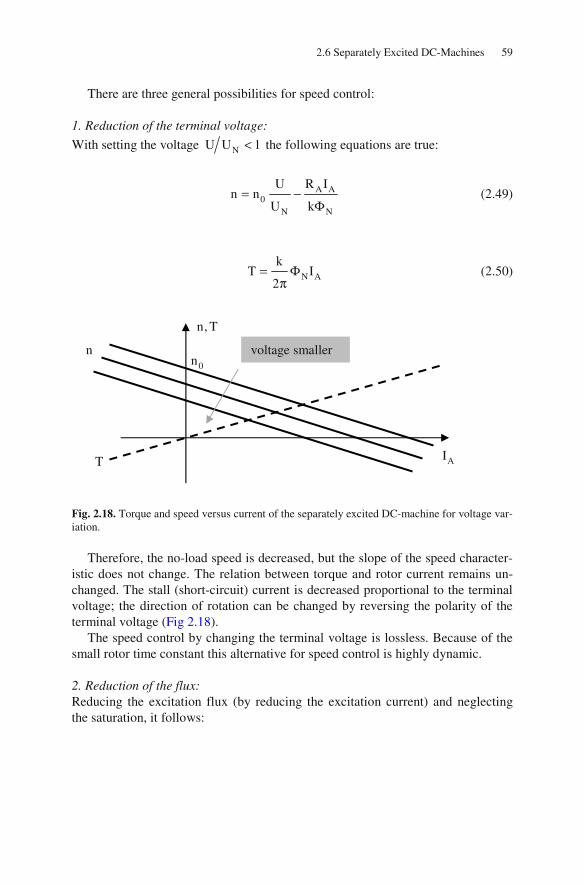
2.6 Separately Excited DC-Machines 59
There are three general possibilities for speed control:
1. Reduction of the terminal voltage:
With setting the voltage NU U 1< the following equations are true:
A A0
N N
R IUn n
U k= −
Φ (2.49)
N A
kT I
2= Φ
π (2.50)
Fig. 2.18. Torque and speed versus current of the separately excited DC-machine for voltage var-iation.
Therefore, the no-load speed is decreased, but the slope of the speed character-istic does not change. The relation between torque and rotor current remains un-changed. The stall (short-circuit) current is decreased proportional to the terminal voltage; the direction of rotation can be changed by reversing the polarity of the terminal voltage (Fig 2.18).
The speed control by changing the terminal voltage is lossless. Because of the small rotor time constant this alternative for speed control is highly dynamic.
2. Reduction of the flux: Reducing the excitation flux (by reducing the excitation current) and neglecting the saturation, it follows:
AI
n, T
0n
T
n voltage smaller

60 2 DC-Machines
F
F,N N
I 11
I f
Φ= = <
Φ (2.51)
A A0
N
R In fn f
k= −
Φ (2.52)
NA
kT I
2 f
Φ=
π (2.53)
Fig. 2.19. Torque and speed versus current of the separately excited DC-machine for flux varia-tion.
With increasing field weakening (field weakening factor f 1> ) the no-load speed is increased and the slope of the speed characteristic rises (i.e. loading the machine means an exceeded speed reduction). At constant rotor current the torque decreases with increasing field weakening (Fig. 2.19).
The speed control by field weakening is lossless, but (because of the usually large time constant of the excitation winding) it is less dynamic compared with the speed control by changing the terminal voltage.
3. Increasing the rotor resistance (series resistance):
By inserting a series resistance SR into the rotor circuit the total resistance is in-
creased. The following equations are obtained:
AI
n, T
T
n
flux smaller

2.6 Separately Excited DC-Machines 61
( )A S A
0N
R R In n
k
+= −
Φ (2.54)
N A
kT I
2= Φ
π (2.55)
Fig. 2.20. Torque and speed versus current of the separately excited DC-machine for series re-sistance variation.
The no-load speed 0n remains unchanged, the same holds true for the relation
between torque and rotor current. The slope of the speed characteristic increases, i.e. loading the machine means an exceeded speed reduction. The stall (short-circuit) current is reduced by increasing the series resistance, therefore this alter-native is used for starting the motor (Fig. 2.20).
Because of the additional losses in the series resistance ( 2S AR I ) this method is
not lossless. The following general operational limits have to be obeyed:
• In continuous operation the acceptable heating may not be exceeded:
A A,NI I≤ .
• Even in field weakening operation the machine may not be overloaded:
N2 nT Pπ ≤ .
• Because of the centrifugal forces onto the rotating parts the maximum accepta-
ble speed may not be exceeded: maxn n≤ .
AI
n, T
T
nseries resistance larger

62 2 DC-Machines
In literature the characteristics of DC-machines are often shown versus the ro-
tor current AI (see Figs. 2.18 to 2.20). Describing rotating field machines, mainly
the speed is used as horizontal axis. To make the comparison of the characteristics easier, Fig. 2.21 shows the torque of a separately excited DC-machine as a func-tion of the speed (this is the same relation like in the preceding figures, it is just il-lustrated in a different way).
Fig. 2.21. Torque versus speed of the separately excited DC-machine.
2.7 Permanent Magnet Excited DC-Machines
The permanent magnet excited DC-machine can be regarded as being a special case of the separately excited DC-machine. Even for this alternative the speed control can be performed by changing the terminal voltage and by introducing a series resistance. But field weakening is not possible (because the permanent magnets impress the magnetic flux). The advantages of the permanent magnet ex-citation against the electrical excitation are (please refer to Fig. 2.22):
• smaller outer diameter • smaller volume and weight • more simple construction (no stator winding, less terminal contacts) • higher efficiency (no excitation losses) • more cost-effective production • better dynamics (no field increase by excitation current increase)
n
T
0n

2.7 Permanent Magnet Excited DC-Machines 63
Fig. 2.22. Separately excited DC-machines: electrical excitation (left) and magnetic excitation (right).
The technical characteristics of a permanent magnet material is described by the hysteresis loop in the second quadrant (Fig 2.23):
Fig. 2.23. Permanent magnet characteristic.
Flux density and field strength are linked by remanent flux density and perme-ability:
( )
( )
M R 0 r M
R
C
r
limit
B B H
B H 0 B remanent flux density
H B 0 H coercive force
1, 0 1,1 reversible permeability
H limiting field strength
= + μ μ
= =
= = −
μ ≈
−
(2.56)
MH
MB
RB
M,0B
M,0H limitH− CH− MH
Δ
MH
Δ
yoke magnets (e.g. ferrite) axis rotor with slots
yoke stator pole excitation winding

64 2 DC-Machines
The development of different magnet materials according to time is illustrated in principle in Fig. 2.24:
Fig. 2.24. Different magnet materials: maximum energy product versus time.
A permanent magnet can only be operated in the linear section of this charac-teristic, otherwise it will be (at least partly) demagnetized. If higher opposite field
strength than limitH is applied, an irreversible flux loss occurs.
Naming the radial magnet height Mh it follows from Ampere’s Law with “cir-
culation path 1“ (please refer to Fig. 2.25):
,1
M,1 M0
B2 H 2h 0
δδ + =
μ (2.57)
The flux densities can be calculated from the according cross sections:
MM
AB B
Aδ
δ
= (2.58)
0
50
100
150
200
250
300
350
400
450
500
1910 1920 1930 1940 1950 1960 1970 1980 1990 2000 2010
year
max
imu
m e
ner
gy
pro
du
ct in
kJ/
m3
steels
AlNiCo
ferrite
SmCo
bonded NdFeB
NdFeB
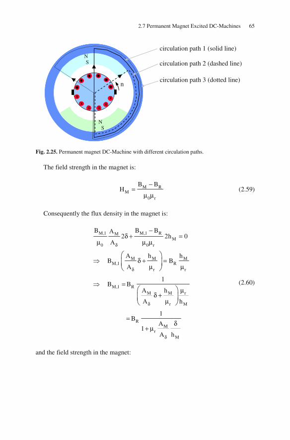
2.7 Permanent Magnet Excited DC-Machines 65
Fig. 2.25. Permanent magnet DC-Machine with different circulation paths.
The field strength in the magnet is:
M RM
0 r
B BH
−=
μ μ (2.59)
Consequently the flux density in the magnet is:
M,1 M,1 RMM
0 0 r
M M MM,1 R
r r
M,1 RM M r
r M
RM
rM
B B BA2 2h 0
A
A h hB B
A
1B B
A h
A h
1B
A1
A h
δ
δ
δ
δ
−δ + =
μ μ μ
δ + =μ μ
=μ
δ +μ
=δ
+ μ
(2.60)
and the field strength in the magnet:
X
X
X
XX X
X
X+ - AΘ
AI AI
Φ
Φ
Φ
n
XX
XXXX XX
XX
XX
NS
SN
circulation path 1 (solid line)
n
circulation path 2 (dashed line)
circulation path 3 (dotted line)

66 2 DC-Machines
RM,1
M0 rr
M
Mr
MR
M0 rr
M
R
M0 r
r M
B 1H 1
A1
A h
A
A hB
A1
A h
B 1
Ah11
A
δ
δ
δ
δ
= −δμ μ
+ μ
δμ
= −δμ μ
+ μ
= −μ μ
+μ δ
(2.61)
These calculated values for M,1B and M,1H are valid in the symmetry plane,
and during no-load operation ( AI 0= ) for the entire magnet.
Now the air-gap flux density at the run-on edge will be calculated (“circulation path 2“). It has to be considered that along the entire circumference of the rotor
A2w conductors are placed, the current loading is A A2w IA
D=
π. The current un-
der one pole is: i pAα τ .
i p
A Ai
i A A
1Hd 0 A
2
2w I1 D
2 D 2p
1w I I
2p
= − − α τ
π= α
π
= α = Δ
(2.62)
Consequently:

2.7 Permanent Magnet Excited DC-Machines 67
,1 ,2M,1 M M,2 M
0 0
M,1 M,2 M,2 RM MM,1 M M
0 0 0 r
M,2 M,1M M RM M,1 M M
0 r 0 0 r
B BH h H h I
B B B BA AH h h I
A A
B BA A B1h H h h I
A A
δ δ
δ δ
δ δ
δ + + δ + = Δμ μ
−δ + + δ + = Δ
μ μ μ μ
δ + = − δ − + + Δμ μ μ μ μ
(2.63)
and further
M
RM,2 0
M M0M r
r M
R RM M
M0 r 0 r
r M
r
M M MM,2 R
M Mr rr
M r M
M
0 rM M
r r MM
r
MM,2 R
Mr
A
AB1B
A A1h 1
A A h
B B1h h I
Ah11
A
h h h1B B
A Ah11 1
A h A
A
A 1I
A A1 h
A h A
hB B
A1
A
δ
δ δ
δ
δ
δ
δ
δ δ
δ
δ
= μ −δμ
δ + + μμ
+ + + Δμ μ μ μ
+μ δ
μ
= − +δ μ μ
+ μ +μ δ
δ
− + μ μ Δδ
+ μ μ δ +
μ
=δ
+ μ
M M
Mrr
M M
0 r M MM
r M
h A 1
AA1
h A h
1H H I
Ah
A
,
δ
δ
δ
+ δ +δμ
+ μ
μ μ Δ Δ = Δ
μ δ +
(2.64)

68 2 DC-Machines
Further it follows:
M,2 R 0 r MM
rM
M,1 0 r M
1B B H
A1
A h
B H
δ
= + μ μ Δδ
+ μ
= + μ μ Δ
(2.65)
Under load the flux density in the magnet MB at the run-on edge is higher than
under no-load condition. For the run-off edge the flux density under load (“circulation path 3“, using an
analogous deduction like above) becomes:
M,3 M,1 0 r MB B H= − μ μ Δ (2.66)
Therefore, under load the flux density in the magnet MB at the run-off edge is
smaller than under no-load condition. The danger of demagnetization occurs (please refer to “armature reaction“, Sect. 2.12)!
Especially for applications with a wide temperature range the demagnetization must be checked in the entire temperature range as the magnet characteristic changes with temperature.
Typical values of remanent flux density ( RB ) and coercive field strength ( CH )
and the respective temperature coefficients for different magnet materials are shown in Table 2.2.
Table 2.2. Main characteristic values of important permanent magnet materials.
remanent flux density coercive field strength value @
20°C temperature coefficient
value @ 20°C
temperature coefficient
ferrite 0.4 T -0.190 %/K 170 kA/m +0.30 %/K NdFeB 1.2 T -0.090 %/K 1900 kA/m -0.60 %/K SmCo 1.1 T -0.032 %/K 1800 kA/m -0.19 %/K Figure 2.26 principally illustrates the influence of the temperature onto the lim-
iting field strength limitH and the value MHΔ .
As counter-measure against the danger of demagnetization the magnet height
Mh can be chosen larger.
To illustrate the effect of different demagnetization danger at the run-on edge and the run-off edge, Fig. 2.27 shows the field lines of a 2-pole 12 slots DC-motor with ferrite magnets with and without rotor currents.

2.8 Shunt-Wound DC-Machines 69
Fig. 2.26. Field strength and limiting field strength versus temperature.
Fig. 2.27. Field lines of a 2-pole 12 slots DC-motor with ferrite magnets without (left) and with (right) rotor currents.
2.8 Shunt-Wound DC-Machines
For the shunt-wound DC-machine the excitation winding is connected in parallel to the rotor circuit. This results in the equivalent circuit diagram shown in Fig.
2.28. In this figure the resistance FR is drawn with the symbol of an inductivity.
This makes obvious that • in the excitation circuit an inductivity is present, but • in the steady-state operation regarded here only the resistance is effective. Similar depictions are even chosen in Figs. 2.30, 2.32, and 2.37.
n
X X
XX
H
H limit
Δ HM
T 20°C -40°C
demagnetization
ca. -0,4%/K
ca. 0,3%/K (ferrite)
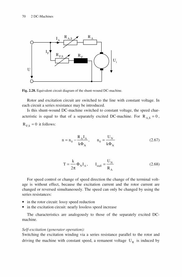
70 2 DC-Machines
Fig. 2.28. Equivalent circuit diagram of the shunt-wound DC-machine.
Rotor and excitation circuit are switched to the line with constant voltage. In each circuit a series resistance may be introduced.
Is this shunt-wound DC-machine switched to constant voltage, the speed char-
acteristic is equal to that of a separately excited DC-machine. For A,SR 0= ,
F,SR 0= it follows:
NA A0 0
N N
UR In n , n
k k= − =
Φ Φ (2.67)
NN A stall
A
UkT I , I
2 R= Φ =
π (2.68)
For speed control or change of speed direction the change of the terminal volt-age is without effect, because the excitation current and the rotor current are changed or reversed simultaneously. The speed can only be changed by using the series resistances:
• in the rotor circuit: lossy speed reduction • in the excitation circuit: nearly lossless speed increase
The characteristics are analogously to those of the separately excited DC-machine.
Self-excitation (generator operation): Switching the excitation winding via a series resistance parallel to the rotor and
driving the machine with constant speed, a remanent voltage RU is induced by
U
AI A,SR AR
iU
FI FR F,SR

2.8 Shunt-Wound DC-Machines 71
the always present residual magnetism in every iron circuit. This voltage generates
an excitation current RI , which strengthens the residual field and the induced
voltage is increased. This happens as long as the induced voltage is equal to the voltage drop across the resistances in the excitation circuit. Then a stable operat-ing point is reached. This is called “dynamo-electrical principle“ (Fig. 2.29) (Wer-ner von Siemens, 1866).
Fig. 2.29. Voltage versus excitation current during self-excitation.
Switching on the excitation winding in opposite direction, the excitation current demagnetizes the circuit and the self-excitation does not take place.
The series resistance in the excitation circuit F,SR has two effects:
• the generator voltage can be set and • the time constant of the excitation winding can be reduced to speed-up the self-
excitation.
This series resistance may not exceed a critical value, because otherwise the self-excitation does not take place.
Loading the generator:
For the separately excited DC-machine the load characteristic ( )U f I= is a
straight line: i A AU U R I= − (energy generation system).
For the shunt-wound DC-machine it follows in the energy generation system (Fig. 2.30):
RU
iU
U
FI
( )F A F F,SI R R R+ +

72 2 DC-Machines
( )
( )
( )( )
i A A F F
A F F F
A A F F
i A F FA
U R I R I
R I I R I
R I R R I
1I U R R I
R
= +
= + +
= + +
= − +
(2.69)
Fig. 2.30. Equivalent circuit diagram of the loaded shunt-wound DC-generator.
By means of the no-load characteristic the load characteristic can be deduced (Fig. 2.31).
Fig. 2.31. Load characteristic of the shunt-wound DC-generator.
The shunt-wound DC-generator only can be loaded until the current maxI , at
further loading the voltage collapses. Then only the stall current stall,RI flows,
which is generated by the residual voltage.
U
AI AR
iU
FI FR
I
loadR
loadR smaller
RU
iU
U
FI
( )F A FI R R+
AR I
A maxR I
ImaxI stall,RI
stable
instable

2.9 Series-Wound DC-Machines 73
2.9 Series-Wound DC-Machines
For the series-wound DC-machine the excitation winding is switched in series to the rotor circuit, see Fig. 2.32. The series resistance in the rotor circuit and the re-sistance parallel to the excitation winding can be used for speed control. As the excitation current of this alternative depends on the load, the speed characteristic of the series-wound DC-machine is principally different to the DC-machines dis-cussed so far.
Fig. 2.32. Equivalent circuit diagram of the series-wound DC-machine.
Neglecting the saturation and for PR → ∞ it follows for steady-state opera-
tion:
F m F m A
m AA m A
F
w L I L I
L Ik 4pw L I
w
Φ = =
′Φ = = (2.70)
For the speed and torque equation it follows:
( )A F AN N A F
m A m
2mA A
R R IU U R Rn
k k L I L
LkT I I
2 2
+ += − = −
′ ′Φ Φ
′= Φ =
π π
(2.71)
Loading this machine the speed decreases drastically (“series characteristic”); the characteristics during motor operation are shown in Fig. 2.33.
In no-load operation ( AI 0= ) it follows n → ∞ , the machine “runs away“.
The speed is only limited by the friction torque (carbon brushes, bearings). The stall current ( n 0= ) is:
U
AI A,SR AR
iU FI FR
PR PI

74 2 DC-Machines
Nstall
A F
UI
R R=
+ (2.72)
This stall (short-circuit) current has to be limited by the series resistance A,SR
during starting operation of the motor.
Fig. 2.33. Torque and speed versus current of the series-wound DC-machine.
By reversing the polarity of the terminal voltage no speed reversal can be ob-tained, because rotor current and excitation current are changed simultaneously.
For speed control the following possibilities can be used (in Figs. 2.34 to 2.36 always the motor operation is illustrated):
1. Reduction of the terminal voltage: The speed and the short circuit current are reduced lossless, the relation between torque and rotor current remains unchanged:
A F
m A m
R RUn
L I L
+= −
′ ′ (2.73)
stallA F
UI
R R=
+ (2.74)
2mA
LT I
2
′=
π (2.75)
The respective characteristics are illustrated in Fig. 2.34.
AI
n, T
A,NI stallI
Nn
NT
T
n

2.9 Series-Wound DC-Machines 75
Fig. 2.34. Torque and speed versus current of the series-wound DC-machine for voltage varia-tion.
2. Reduction of the flux: By switching a resistance parallel to the excitation winding the excitation can be reduced (Fig. 2.35). With
P P F F
A F P
R I R I
I I I
=
= + (2.76)
it follows:
F A AF
P
1 1I I I
R f1
R
= =
+
(2.77)
where f again is the field weakening factor. The characteristics are:
FA
N
m A m
RR
U fn f fL I L
+
= −′ ′
(2.78)
Nstall
FA
UI
RR
f
=
+
(2.79)
voltage smaller
AI
n, T
A,NI stallI
Nn
NT
T
n

76 2 DC-Machines
2
m AL IT
2 f
′=
π (2.80)
Fig. 2.35. Torque and speed versus current of the series-wound DC-machine for flux variation.
3. Increasing the resistance in the rotor circuit (series resistance): The speed reduction when loading the machine is increased, the stall current be-comes smaller, see Fig. 2.36. The relation between torque and rotor current re-mains unchanged:
Fig. 2.36. Torque and speed versus current of the series-wound DC-machine for series resistance variation.
These characteristics can be deduced from the following mathematical descrip-tions:
A A,S FN
m A m
R R RUn
L I L
+ += −
′ ′ (2.81)
AI
n, T
A,NI stallI
Nn
NT
T
nflux smaller
series resistance larger
AI
n, T
A,NI stallI
Nn
NT
T
n

2.10 Compound DC-Machines 77
Nstall
A A,S F
UI
R R R=
+ + (2.82)
2mA
LT I
2
′=
π (2.83)
2.10 Compound DC-Machines
The compound (double shunt-wound) DC-machine contains two excitation wind-ings (Fig. 2.37).
Fig. 2.37. Equivalent circuit diagram of the compound DC-machine.
By dividing the excitation winding into a shunt-wound part and a series-wound part the compound DC-machine has shunt-wound characteristic near the no-load operation and series-wound characteristic when loading the machine.
The torque-speed-characteristics of the three DC-machine alternatives are qual-itatively shown in Fig. 2.38.
The most relevant characteristics are:
• series-wound DC-machine: o weak characteristic (high starting torque and relatively low nom-
inal torque) o danger of “run away “ at low load
• shunt-wound DC-machine: o stiff characteristic (the speed depends only marginally on the
load) o fixed no-load speed
U
I AR
iU
FI
F,SR F,PR
AI

78 2 DC-Machines
• compound DC-machine: o weak characteristic (high starting torque and relatively low nom-
inal torque) o fixed no-load speed (no danger of “run away“ at low load)
Fig. 2.38. Torque versus speed of the series-wound, shunt-wound and compound DC-machine.
2.11 Generation of a Variable Terminal Voltage
A formerly frequently used method for generating a variable terminal voltage was the usage of the so-called “Leonard machine set“ (Fig. 2.39):
Fig. 2.39. Block diagram of the Leonard machine set.
A rotating field machine (induction or synchronous machine) drives a DC-generator with variable flux; this generator supplies the DC-motor with a variable
M
3
G
=
M
=
MΦ GΦ
constant variable
motor generator motor load
U
series-wound
compound
shunt-wound
n
T
0n

2.11 Generation of a Variable Terminal Voltage 79
terminal voltage. With the Leonard-converter operation in all four quadrants is possible.
Today most often the inverter supply is used to generate a variable terminal voltage.
With a controlled three-phase bridge (see left-hand side in Fig. 2.40) an opera-tion in two quadrants is possible (no energy recovery); switching two controlled three-phase bridges in parallel and opposite to each other (see right-hand side in Fig. 2.40) an operation in all four quadrants is possible.
Principle circuit diagram, switching diagram, and the voltages of a controlled three-phase bridge are shown in Fig. 2.41.
Fig. 2.40. Block diagram of inverter supply: controlled three-phase bridge (left) and two opposite three-phase bridges (right).

80 2 DC-Machines
Fig. 2.41. Principle circuit diagram, switching diagram, and voltages of a controlled three-phase bridge.
2.12 Armature Reaction
Up to now it was assumed that the magnetic field in the air-gap of the DC-machine is generated solely by the excitation winding. But this is only the case for
no-load operation ( AI 0= ). Loading the machine (i.e. if AI 0≠ is true), the rotor
current generates a magneto-motive force as well (Fig. 2.42); this is oriented per-pendicular to the magneto-motive force of the excitation winding. By superposi-tion of these magneto-motive forces the resulting field is generated (“armature re-action“).
switching diagram S1
S2
S3
S4
S5
S6
0° 180° 360°
switches closed
I
du
S1 S3 S5
S2 S4 S6
principle circuit diagram
line,1u
line,2u line,3u
line,1u− line,2u− line,3u−
line,3uline,2u line,1u input and output voltages
du
dU

2.12 Armature Reaction 81
Fig. 2.42. Sketch of the DC-machine illustrating the armature reaction.
Neglecting the saturation and the magnetic voltage drops in the iron, there is by means of Ampere’s Law (with α being the angle on the circumference of the ro-tor):
( )
( ) ( ) ( )F A0
B2
αδ α = Θ α + Θ α
μ (2.84)
The resulting air-gap field ,resBδ qualitatively can be deduced from Fig. 2.43.
The magnetic neutral zone is shifted against the geometric neutral zone depend-ing on the load (for motor operation against the direction of rotation, for generator operation in the direction of rotation). If saturation occurs the peaks of the result-ing field are rounded. With this even the mean value of the flux density decreases and consequently even the torque.
X
X
X
XX X
X
X+ - A
Θ
AI AI
Φ
Φ
Φ
2/Φ 2/Φ
n
XX
XX
XX
XXXX XX
XX
XX
n
AΘ FΘ
α

82 2 DC-Machines
Fig. 2.43. Magneto-motive forces of stator and rotor current (above) and resulting air-gap flux density (below).
By this field deformation even the voltage between two commutator segments no longer is distributed evenly along the circumference of the rotor. The voltage between two commutator segments can be locally increased by far (but the mean value remains unchanged, if saturation is neglected).
In field weakening operation it may happen that the field under the run-off edge of the rotor (in motor operation) becomes negative, because the main field de-creases and the armature reaction remains constant.
To compensate the armature reaction and their negative effects a compensation winding may be introduced to the DC-machine. To realize this the main poles are equipped with slots; the conductors placed in these slots have to be supplied with the rotor current in opposite direction. The number of turns of this compensation winding has to be chosen in such a way that the magneto-motive force of the rotor under the poles is compensated. Then the field distribution under the poles is equal to that in no-load operation (as the compensation winding is supplied with the ro-tor current, this is true for arbitrary operating conditions, i.e. independent from the load) (Fig. 2.44).
Θ
FΘ
AΘ
π 2π α
,resBδ
π 2π α

2.12 Armature Reaction 83
Fig. 2.44. Sketch of the DC-machine with compensation winding in the main poles.
The magneto-motive force distribution and the resulting air-gap field is shown in Fig. 2.45.
Fig. 2.45. Magneto-motive forces of stator and rotor current and compensation winding (above) and resulting air-gap flux density (below).
X
X
X
XX X
X
X+ -A
Θ
AI AI
Φ
Φ
Φ
2/Φ 2/Φ
n
XX
XX
XX
XXXX XX
XX
XX
n
AΘ
FΘ
CΘ α
XX X
X
Θ
FΘ
AΘ
π 2π α
CΘ
,resBδ
2π α

84 2 DC-Machines
The axis of the resulting field is now identical to the axis of the excitation field; the commutation takes place in the neutral zone.
A compensation winding increases the costs of a DC-machine by far. There-fore, this is realized only for large machines.
2.13 Commutation Pole
In Sect. 2.2 it was assumed that the rotor current is linear during commutation. This is the case if the inductivities can be neglected and mainly the resistances de-termine the commutation behavior (Fig. 2.46).
Fig. 2.46. Current characteristic during ideal commutation.
Here CT is the commutation time,
BC
C
bT
v= (2.85)
with Bb being the width of the carbon brush and C Cv D n= π being the circum-
ferential speed of the commutator ( CD is the diameter of the commutator).
In reality there is a non-negligible inductivity because of the slot and end wind-ing leakage. By current change in the coil which is short-circuited by the carbon
brushes a voltage of self-induction is generated. With the coil inductivity coilL
this voltage becomes:
coil CAs coil coil coil A
C B
di DI au L L L I n
dt T ab
π= − ≈ = (2.86)
coili
t CT
AI
2a
AI
2a−

2.13 Commutation Pole 85
Therefore, this voltage during current commutation is proportional to the rotor current and the speed. According to Lenz’s Law this voltage has such a direction that it acts against its generating reason (current change). This results in a delayed commutation, producing sparks at the run-off edges of the carbon brushes. This spark generation results in increased wear of the brushes and the commutator (Fig. 2.47).
Fig. 2.47. Current characteristic during non-ideal commutation.
Compensating now this voltage coming from current commutation by a rotato-ry induced voltage, a linear commutation is reached. To realize this so-called commutation poles are inserted in the area between the main poles (commutation zones). The windings of these commutation poles are switched in series with the rotor winding. The principle sketch (Fig. 2.48) shows the cross section of a DC-machine with compensation windings and commutation poles.
Fig. 2.48. Sketch (p=1) and photograph (p=2) of a DC-machine with compensation winding and commutation poles.
coili
t CT
AI
2a
AI
2a−
} spark generation
direct axis
commutation pole winding
compensation winding
main pole (excitation pole)
quadrature axis
commutation pole (CP)
excitation winding
X
X
X
XX X
X
X+ -AΘ
AI AI
Φ
Φ
Φ
2/Φ 2/Φ
n
XX
XX
XX
XXXX XX
XX
XX
nXX
XX X
X

86 2 DC-Machines
Applying Ampere’s Law for one pole pitch (having the integration path through the commutation poles) the following can be deduced:
( )
( )( )
CPCP A C CP
0
CPCP A i CP
0
0CP CP A i A
CP
B2
B1 2
B 1 I2
Θ − Θ + Θ = δμ
Θ − Θ − α = δμ
μ= Θ − Θ − α
δ
(2.87)
For the rotary induced voltage it follows:
( )CP Au v B d nI = × (2.88)
Consequently, the voltage coming from current commutation can be compen-sated. At overcompensation the current is commutating too fast, again resulting in spark generation (Fig. 2.49).
Fig. 2.49. Current characteristic during non-ideal commutation (over-compensation).
As independent variable for adjusting the compensation the air-gap under the
commutation pole CPδ can be used.
The principle field distributions in the air-gap of a DC-machine are summa-rized in Fig. 2.50 (shown in “wound-off” representation, the fields in the gaps be-tween two poles are neglected, the shape of the fields is illustrated to a large ex-tend schematically).
coili
iCT
AI
2a
AI
2a−
} spark generation

2.13 Commutation Pole 87
Fig. 2.50. Principle field distribution in the air-gap of a DC-machine.
X XX X X
X X X X X X X X
N S
X X X X X X X X X XX X X X
torque T n (generator) n (motor)
rotor, main poles, and commutation poles excited
B
saturation
B only rotor and commutation poles excited
B
only main poles excited
B rotor, main poles, commutation poles, and compensation winding excited

88 2 DC-Machines
2.14 References for Chapter 2
Fischer R (2006) Elektrische Maschinen. Hanser-Verlag, München Kleinrath H (1975) Grundlagen elektrischer Maschinen. Akademische Verlagsgesellschaft,
Wiesbaden Mohr A (1987a) Kleinmotoren mit Permanentmagneterregung 1. Robert Bosch GmbH, Bühlertal Mohr A (1987b) Kleinmotoren mit Permanentmagneterregung 2. Robert Bosch GmbH, Bühlertal Richter R (1967) Elektrische Maschinen I. Birkhäuser Verlag, Basel Schröder D (1994) Elektrische Antriebe 1. Springer-Verlag, Berlin Seinsch HO (1993) Grundlagen elektrischer Maschinen und Antriebe. Teubner Verlag, Stuttgart Spring E (1998) Elektrische Maschinen. Springer-Verlag, Berlin Taegen F (1970) Einführung in die Theorie der elektrischen Maschinen I. Vieweg Verlag,
Braunschweig

3 Rotating Field Theory
3.1 Stator of a Rotating Field Machine
Induction machines and synchronous machines are rotating field machines. The stator construction of these machine types are principally the same, they differ in the rotor design. The similarity of these machine types are discussed first, later a detailed consideration of induction machine and synchronous machine will follow.
In the simplest alternative the stator is composed of a stack with electrically isolated laminations to reduce eddy currents. Windings are placed in the slots of the lamination stack. Usually there are m 3= phases, shifted against each other by a spatial angle of
0
2 1 2
pm p 3
π πα = = (3.1)
with p being the number of pole pairs of the machine. These three phases are
supplied by three sinusoidal currents with the same amplitude and frequency,
shifted in time by an angle of 0 2 m 2 3β = π = π . Figure 3.1 schematically shows
this assembly with p 1= ; the phases are named u (with return wires in slot x), v
(with return wires in slot y) and w (with return wires in slot z):
Fig. 3.1. Schematic cross-section of a rotating field machine.
Having a star connection of the phases it schematically looks like it is shown in Fig. 3.2 (“wound-off“ representation):
X
XXX
XXX XXX
u
v w
x
y z
stator rotor air-gap δ
0α
© Springer-Verlag Berlin Heidelberg 2015 89
DOI 10.1007/978-3-642-17584-8_ 3D. Gerling, Electrical Machines Mathematica l Engineering,,

90 3 Rotating Field Theory
Fig. 3.2. Current system of a rotating field machine.
The mechanical angle α and the electrical angle pβ = α are linked by the number of pole pairs. The pole pitch is:
p
D
2p
πτ = (3.2)
Consequently, two pole pitches are ( p2τ ):
• 2π electrical or
• 2 pπ mechanical.
The coils of a phase may be even placed in several slots side by side. The num-
ber of slots per pole per phase is (the total number of stator slots is 1N ):
1Nq
2pm= (3.3)
3.2 Current Loading
The magnetic field in the air-gap of an electrical machine shows decisive im-portance on the characteristics of the machine, e.g. concerning torque generation. Therefore, the air-gap field has to be calculated precisely.
The reason causing this air-gap field are the current containing conductors in the slots of the stator. Because of the complicated geometry (even the description in the last section is very simplified) this is not possible easily. Therefore, in the
Re
-Im
wI vI
uI
0β
u x v y w z
uI vI wI

3.2 Current Loading 91
following the air-gap field will be separated from the field in the slots by means of the idealized assumption of a homogeneous field in the slot openings, please refer to Fig. 3.3 (in other words: after separating both parts of the field – field in the air-gap and field in the slots – not the entire field considering the complicated lamina-tion contour has to be calculated, but both parts may be calculated separately).
For this a single slot is regarded, whereupon the relative permeability of the
surrounding iron is assumed being very large against that of air ( Feμ → ∞ ). Then,
in the slot there will be a so-called slot leakage field, that can be easily deduced
from Ampere’s Law ( Hd = Θ ).
Fig. 3.3. Detailed view of a stator slot.
This slot leakage field joins to the air-gap field at the border between the slot opening and the air-gap. As the air-gap field is to be calculated the slot leakage field is a boundary condition for this calculation. The field in the slot opening
( SOH ), which can be simplified being tangential concerning the machine geome-
try, can be computed easily from Ampere’s Law ( Feμ → ∞ is still assumed):
SSO
SO
Hb
Θ= (3.4)
This boundary condition for calculating the air-gap field can be generated even
differently. It is assumed that the magneto-motive force of the slot SΘ is distrib-
uted evenly in the area of the slot opening SOb and infinitely thin onto the smooth
iron surface (the light blue color in Fig. 3.4 means that the slot notionally is filled with iron). This conception can be described by using the current loading
air-gap
slot opening (width bSO)
slot leakage field
conductors in the stator slot
(direction of the current
into the plane;
magneto-motive force ΘS)
field lines
iron (stator)
X
SOb

92 3 Rotating Field Theory
S
SO
Ab
Θ= (3.5)
This idea is illustrated in Fig. 3.4.
Fig. 3.4. Alternative concept of a stator slot.
Calculating Ampere’s Law using an integration loop around this current load-
ing, the tangential field strength tH on the iron surface in the area of the current
loading is obtained (because of Feμ → ∞ the integration path in the iron does not
contribute to the integral).
S t SO SO
St
SO
Hd H b A b
H Ab
= Θ =
Θ= =
(3.6)
This proves that the boundary condition for calculating the air-gap field is un-changed, if the conductors in the stator slots are replaced by an according current loading on the smooth iron surface (in other words: the effect of the magneto-motive force of the slot onto the air-gap field is represented with sufficient accura-cy by a current loading distributed in the area of the slot opening). With this it is successfully accomplished to separate the air-gap field from the field in the slots.
For the calculation of the air-gap field the field in the slots is not to be consid-ered. In addition, a quite simple geometry can be regarded: The boundary contours of stator and rotor can be assumed being smooth. This results in a machine with constant air-gap and therefore even a constant magnetic air-gap reluctance.
For calculating the magneto-motive force distribution an additional simplifica-tion will be introduced in the next section: The current loading A will be assumed being concentrated in the center of the slot in tangential direction (and not distrib-uted across the area of the slot opening). With this the entire magneto-motive
air-gap
current loading A on the
slot opening (width bSO)
iron (stator)
SOb

3.3 Alternating and Rotating Magneto-Motive Force 93
force of a slot SΘ is concentrated in a single line on the smooth stator iron surface
in axial direction4.
3.3 Alternating and Rotating Magneto-Motive Force
Supplying the winding (with w turns) of a single slot pair with the current i results in magneto-motive forces of these slots of wi+ and wi− .
Now the space-dependent magneto-motive force ( )Θ α shall be calculated. As
the magneto-motive force is defined as an integral value ( HdΘ = ), the cal-
culation of ( )Θ α only makes sense, if the integration loop is defined simultane-
ously. The circulation integral will be defined as follows: The air-gap always is crossed radially and the loop always is going through the middle of the slot „u“.
The field intensity in the iron is neglected ( Feμ → ∞ ), so that the exact path of the
integration loop in the iron is not relevant (see Fig. 3.5). Is the angle α larger than zero, the integration loop includes half of the slot
“u“ (direction of the loop and direction of the current are assigned positive); then
( )Θ α is equal to ½ wi. This is the case for 0 < α < π . At α = π the magneto-
motive force steps by the amount of wi into the negative direction. Therefore, for
2π < α < π there is ( )Θ α = -½ wi (Fig. 3.5).
Fig. 3.5. Magneto-motive force distribution of a single slot pair and integral definition.
For the magnetic flux density it holds:
4 In Sect. 3.5 the effect of different alternatives for the current loading distribution on the mag-netic field characteristics will be discussed.
XΦ
XXX
u
x
α
α
π 2π
½ wi
-½ wi
Θ

94 3 Rotating Field Theory
( ) ( )( )
0 0B HΘ α
α = μ α = μδ
(3.7)
If the current i is an alternating current with
( )i 2I cos t= ω (3.8)
the function for different points in time looks like it is shown in Fig. 3.6.
Fig. 3.6. Current versus angle for different points in time.
The magneto-motive force becomes:
( )( )
( )
w2I cos t 0
2, t
w2I cos t 2
2
+ ω < α < π
Θ α =
− ω π < α < π
(3.9)
10
5
0
-5
-10 0 0.5 1 1.5 2
β π
i A t 0ω = 10
5
0
-5
-10 0 0.5 1 1.5 2
β π
i A t 4ω = π
10
5
0
-5
-10 0 0.5 1 1.5 2
β π
i A t 2ω = π 10
5
0
-5
-10
0 0.5 1 1.5 2 β π
i A t 3 4ω = π

3.3 Alternating and Rotating Magneto-Motive Force 95
This magneto-motive force distribution is characterized by the facts that the ze-ro crossings are constant in space and time. The amplitude changes in time propor-tional to the current. This distribution is an alternating magneto-motive force.
If the machine contains more than one pole pair the magneto-motive force
( ), tΘ α is repeated p-times on the circumference. Distributing the number of
turns on the p pole pairs the alternating magneto-motive force (now characterized by the index “alt“) becomes:
( )
( )
( )alt
w2I cos t 0
2p p, t
w 22I cos t
2p p p
π+ ω < α <
Θ α =π π
− ω < α <
(3.10)
The function of the alternating magneto-motive force is shown in Fig. 3.7 (for p 1= , I 5A= , w 200= ):
Fig. 3.7. Magneto-motive force versus angle for different points in time.
1
0.5
0
-0.5
-1 0 0.5 1 1.5 2
α π
alt kAΘt 0ω = 1
0.5
0
-0.5
-1
0 0.5 1 1.5 2 α π
t 4ω = π alt kAΘ
alt kAΘ1
0.5
0
-0.5
-1
0 0.5 1 1.5 2 α π
t 3 4ω = π alt kAΘ
1
0.5
0
-0.5
-1 0 0.5 1 1.5 2
α π
t 2ω = π

96 3 Rotating Field Theory
In the following mathematical description of the spatial distribution of the al-ternating magneto-motive force a Fourier analysis of the square-wave function will be applied ( g′ is an integer). With this, the distinction between cases can be
replaced by a compact description.
( ) ( )( )( )
altg 1
sin 2g 1 pw 4, t 2I cos t
2p 2g 1
∞
′=
′ − αΘ α = ω
′π − (3.11)
There are an infinite number of waves, each having an odd ordinal number. The fundamental wave is obtained for g 1′ = :
( ) ( ) ( )
( ) ( )
alt,1
alt ,1
w 2, t 2I cos t sin p
p
sin p cos t
Θ α = ω απ
= Θ α ω
(3.12)
Convention: Electrical values (e.g. the current) are described as rms-values, magnetic values (e.g. magneto-motive force, flux density) are described as amplitudes. The differ-entiation between a function and the amplitude will be done in that way, that for the function the dependencies are explicitly given.
The amplitude of the fundamental wave is:
alt,1
w 22I
pΘ =
π (3.13)
The amplitudes of the harmonic waves are:
alt ,1
alt,2g 12g 1
′−
ΘΘ =
′ − (3.14)
The amplitudes of the fundamental and all harmonic waves change proportion-al to the amplitude of the current. Additionally, the amplitudes of the harmonic waves are inversely proportional to their ordinal number. The locations of maxima and zero crossings are constant in time. These are stationary waves. In Fig. 3.8 the
fundamental wave ( )alt ,1 , tΘ α and the first two harmonic waves ( )alt ,3 , tΘ α and
( )alt ,5 , tΘ α are shown (for p 1= , I 5A= , w 200= ) in red, blue, and magenta,
respectively.

3.3 Alternating and Rotating Magneto-Motive Force 97
Fig. 3.8. Fourier components of the magneto-motive force versus angle for different points in time (red: fundamental; blue: first harmonic; magenta: second harmonic).
The harmonic waves are generated only from the spatial distribution of the winding, the current is purely sinusoidal (without any harmonic content)!
Convention:
• A wave is a space-dependent event. • An oscillation is a time-dependent event.
As it is well-known, a stationary wave can be composed of two waves with half of the amplitude travelling with equal speed in opposite direction. Then the fun-damental wave of the alternating magneto-motive force can be described as fol-lows:
( ) ( ) ( )
( ) ( )[ ]
( ) ( )
alt,1 alt ,1
alt ,1
alt ,1a alt ,1b
, t cos t sin p
sin p t sin p t2
, t , t
Θ α = Θ ω α
Θ= α − ω + α + ω
= Θ α + Θ α
(3.15)
1
0.5
0
-0.5
-1 0 0.5 1 1.5 2
α π
alt kAΘt 0ω = 1
0.5
0
-0.5
-1
0 0.5 1 1.5 2 α π
t 4ω = π alt kAΘ
alt kAΘ1
0.5
0
-0.5
-1
0 0.5 1 1.5 2 α π
t 3 4ω = π alt kAΘ
1
0.5
0
-0.5
-1 0 0.5 1 1.5 2
α π
t 2ω = π

98 3 Rotating Field Theory
This decomposition of the fundamental wave of the alternating magneto-motive
force (stationary wave) in two travelling waves is shown in Fig. 3.9. ( )alt ,1 , tΘ α ,
( )alt,1a , tΘ α , and ( )alt,1b , tΘ α are shown in red, blue, and dashed magenta, re-
spectively.
Fig. 3.9. Alternating fundamental wave and decomposition into two travelling waves versus an-gle for different points in time (red: fundamental; blue: right travelling wave; dashed magenta: left travelling wave).
Consequently, the total alternating magneto-motive force can be described as sum of waves travelling in opposite directions:
( ) ( )( )( )
( )( )
( )( )
alt alt,1g 1
alt ,1
g 1
g 1
sin 2g 1 p, t cos t
2g 1
sin 2g 1 p t
2 2g 1
sin 2g 1 p t
2g 1
∞
′=
∞
′=
∞
′=
′ − αΘ α = Θ ω
′ −
′Θ − α − ω= +
′ −
′ − α + ω
′ −
(3.16)
1
0.5
0
-0.5
-1 0 0.5 1 1.5 2
α π
alt kAΘt 0ω = 1
0.5
0
-0.5
-1
0 0.5 1 1.5 2 α π
t 4ω = π alt kAΘ
alt kAΘ1
0.5
0
-0.5
-1
0 0.5 1 1.5 2 α π
t 3 4ω = π alt kAΘ
1
0.5
0
-0.5
-1 0 0.5 1 1.5 2
α π
t 2ω = π

3.3 Alternating and Rotating Magneto-Motive Force 99
The travelling magneto-motive force waves are called rotating magneto-motive forces, as these are spreading along the circumference of the machine.
For a fixed point of the rotating magneto-motive force the following is true:
( )2g 1 p t const.′ − α ω = (3.17)
Then the mechanical angular frequency of this rotating magneto-motive force wave is:
( ) ( ) 2g 1
d d const. t
dt dt 2g 1 p 2g 1 p′−
α ± ω ±ω= = = ±Ω
′ ′− − (3.18)
Consequently, the angular frequency of the fundamental wave is pω ; the an-
gular frequencies of the harmonic waves are proportional to that of the fundamen-tal wave and inversely proportional to the ordinal number (i.e. with higher ordinal number the angular frequency decreases).
After having analyzed the magneto-motive force distribution of the winding of a single slot pair, all three slot pairs of a three-phase machine will be looked at in Fig. 3.10.
Fig. 3.10. Schematic cross-section of a rotating field machine.
The slot pairs of the different phases are shifted by 0 2 3pα = π in space. The
three phases contain w p turns each and they are supplied by three alternating
currents of the same amplitude and frequency shifted by 2 3π in time.
Each phase generates an alternating magneto-motive force which can be de-scribed as follows:
Φ
XXX
XXX XXX
u
v w
x
y z
stator rotor
air-gap δ
0α

100 3 Rotating Field Theory
( ) ( )( )( )
( )( )
( )( )
alt,u alt ,1g 1
alt,1
g 1
g 1
sin 2g 1 p, t cos t
2g 1
sin 2g 1 p t
2 2g 1
sin 2g 1 p t
2g 1
∞
′=
∞
′=
∞
′=
′ − αΘ α = Θ ω
′ −
′Θ − α − ω= +
′ −
′ − α + ω
′ −
(3.19)
( )( )
( ) ( )
( )
alt,v alt ,1g 1
alt,1
g 1
g 1
2sin 2g 1 p
2 3p, t cos t
3 2g 1
2sin 2g 1 p t 2g 2
3
2 2g 1
2sin 2g 1 p t 2g
3
2g 1
∞
′=
∞
′=
∞
′=
π′ − α −
πΘ α = Θ ω −
′ −
π′ ′− α − ω − −
Θ= +
′ −
π′ ′− α + ω −
′ −
(3.20)
( )( )
( ) ( )
( )
alt ,w alt,1g 1
alt ,1
g 1
g 1
4sin 2g 1 p
4 3p, t cos t
3 2g 1
4sin 2g 1 p t 2g 2
3
2 2g 1
4sin 2g 1 p t 2g
3
2g 1
∞
′=
∞
′=
∞
′=
π′ − α −
πΘ α = Θ ω −
′ −
π′ ′− α − ω − −
Θ= +
′ −
π′ ′− α + ω −
′ −
(3.21)

3.3 Alternating and Rotating Magneto-Motive Force 101
The total magneto-motive force of all three phases can be obtained by summing up the three single magneto-motive forces (for this, linearity is necessary, i.e. satu-ration is neglected):
( ) ( ) ( ) ( )alt ,u alt,v alt ,w, t , t , t , tΣΘ α = Θ α + Θ α + Θ α (3.22)
Figure 3.11 shows (again for four different points in time) how the total magne-to-motive force is composed of three evenly shifted alternating magneto-motive forces of equal amplitude and frequency (the zero crossings are constant in time,
but the maximum values are time-dependent). ( ), tΣΘ α , ( )alt,u , tΘ α ,
( )alt,v , tΘ α , and ( )alt,w , tΘ α are shown in red, blue, magenta, and light blue,
respectively.
Fig. 3.11. Total magneto-motive force and three evenly shifted alternating magneto-motive forc-es versus angle for different points in time (red: total magneto-motive force; blue: alternating magneto-motive force of phase u; magenta: alternating magneto-motive force of phase v; light blue: alternating magneto-motive force of phase w).
There is:
kAΘ 1.5
1
0.5
0
-0.5
-1
-1.5 0 0.5 1 1.5 2
α π
t 2ω = π kAΘ 1.5
1
0.5
0
-0.5
-1
-1.5 0 0.5 1 1.5 2
α π
t 3 4ω = π
1.5
1
0.5
0
-0.5
-1
-1.5 0 0.5 1 1.5 2
α π
t 4ω = π kAΘ 1.5
1
0.5
0
-0.5
-1
-1.5 0 0.5 1 1.5 2
α π
kAΘ t 0ω =

102 3 Rotating Field Theory
( )
( )
2 4sin x sin x n sin x n
3 3
0 if n is not divisible by 3
3sin x if n is divisible by 3
π π+ − + −
=
(3.23)
Consequently, only those travelling waves in opposite direction exist, which fulfill the following condition, where g is a natural number including zero:
2g 2 6g or 2g 6g′ ′− = = (3.24)
2g 1 6g 1 or 2g 1 6g 1′ ′− = + − = − (3.25)
It follows for the total magneto-motive force:
( )( )( )
( )( )
alt ,1g 0
g 1
sin 6g 1 p t3, t
2 6g 1
sin 6g 1 p t
6g 1
∞
Σ=
∞
=
+ α − ωΘ α = Θ +
+
− α + ω
−
(3.26)
These two sums can be combined, if negative numbers g are allowed:
( )( )( )
alt ,1g
sin 6g 1 p t3, t
2 6g 1
∞
Σ=−∞
+ α − ωΘ α = Θ
+ (3.27)
This total magneto-motive force is a rotating wave (in the following rotating waves in the air-gap are labeled with an index “ δ ”):
( ) ( ), t , tΣ δΘ α = Θ α (3.28)
with the ordinal numbers
6g 1 1, 5, 7, 11,13, 17,19, ...+ = − − − (3.29)
Decomposing the rotating magneto-motive force (red characteristic in Figs. 3.11 and 3.12) into its Fourier components; the fundamental wave (rotating syn-chronously with the total magneto-motive force, blue) and the harmonic waves with ordinal number -5 (rotating in opposite direction to the fundamental wave,
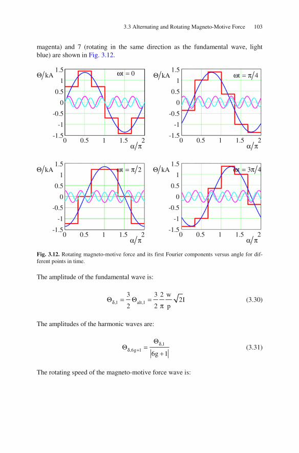
3.3 Alternating and Rotating Magneto-Motive Force 103
magenta) and 7 (rotating in the same direction as the fundamental wave, light blue) are shown in Fig. 3.12.
Fig. 3.12. Rotating magneto-motive force and its first Fourier components versus angle for dif-ferent points in time.
The amplitude of the fundamental wave is:
,1 alt,1
3 3 2 w2I
2 2 pδΘ = Θ =
π (3.30)
The amplitudes of the harmonic waves are:
,1
,6g 16g 1
δ
δ +
ΘΘ =
+ (3.31)
The rotating speed of the magneto-motive force wave is:
1.5
1
0.5
0
-0.5
-1
-1.5 0 0.5 1 1.5 2
α π
kAΘ t 0ω = 1.5
1
0.5
0
-0.5
-1
-1.5 0 0.5 1 1.5 2
α π
t 4ω = π kAΘ
kAΘ 1.5
1
0.5
0
-0.5
-1
-1.5 0 0.5 1 1.5 2
α π
t 3 4ω = π kAΘ 1.5
1
0.5
0
-0.5
-1
-1.5 0 0.5 1 1.5 2
α π
t 2ω = π

104 3 Rotating Field Theory
( ) ( ) 6g 1
d d const. t
dt dt 6g 1 p 6g 1 p+
α + ω ω= = = Ω
+ + (3.32)
The angular frequency of the fundamental wave is equal to pω ; the angular
frequency of the harmonic waves is proportional to that of the fundamental wave and inversely proportional to the ordinal number (i.e. with higher ordinal number the absolute value of the angular frequency decreases).
3.4 Winding Factor
As demonstrated in the last section the rotating magneto-motive force contains harmonic waves with amplitudes decreasing with the ordinal number. Generally, in rotating field machines only the fundamental wave produces a useful torque, all harmonic waves generate parasitic torques, that disturb the machine operation (e.g. no starting or sticking at low speed).
Therefore, measures are necessary to damp the harmonic waves, but only mar-ginally affect the fundamental wave. Mainly, the following two measures are used:
• Distributing the winding per pole and per phase into several slots (distributed winding).
• Distributing the forward and return conductors of a coil in such a way, that they are no longer shifted by an electrical angle of π (i.e. mechanical angle of
pπ ), but by an electrical angle less than π (short-pitch winding).
The effects of both measures will be calculated in the following by a common mathematical deduction. Firstly, the magneto-motive force of a single slot pair (known from the proceeding section) is required:
( )( )( )
g
sin 6g 1 p t3 w 2, t 2I
2 p 6g 1
∞
=−∞
+ α − ωΘ α =
π + (3.33)
The w p turns per pole and per phase will now be distributed into q equally
spaced slots and two layers in radial direction, see Fig. 3.13.
• All 1N 2pqm= stator slots are equally spaced at the circumference of the ma-
chine. The mechanical angle between two slots is then:

3.4 Winding Factor 105
1N1
2 2
N 2pqm pqm
π π πα = = = , the electrical angle between two slots is:
1 1N Npqm
πβ = α = .
• The two layers have a phase shift of Sp
s1
p
πα = −
τ mechanically or
Sp
s1β = − π
τ electrically. This phase shift (it is called „short-pitch“) can
only be realized in integer multiples of a slot pitch (Fig. 3.13).
Fig. 3.13. Explanation of distributed and short-pitched winding.
The total magneto-motive force can now be described as follows:
( )
( ) ( ) ( )( )1
q 2N S
g k 1 1
1
3 w 2, t 2I
2 2pq
sin 6g 1 k 1 1 p t
6g 1
X
∞
=−∞ = =
Θ α = ⋅π
+ α − − α − − α − ω
+
(3.34)
Now, the double sum 1X will be investigated closely; it can be written as fol-
lows:
α
XΦ
XXXXXX XXX
u
x
XXX
XXX
XXXXXX
XXX
N1α
Sα

106 3 Rotating Field Theory
( ) ( )( ) ( )( )
( )( )( ) ( )( )
N S1
N S1
q 2j 6g 1 k 1 pj 6g 1 p j 6g 1 1 p j t
1k 1 1
j 6g 1 p t q 2j 6g 1 k 1 p j 6g 1 1 p
k 1 1
32 XX
1X Im e e e e
6g 1
eIm e e
6g 1
− + − α+ α − + − α − ω
= =
+ α −ω− + − α − + − α
= =
=+
=+
(3.35)
The two sums 2X and 3X will be calculated separately in the following. For
2X it can be obtained:
( )( )
( ) ( )
N1
qj 6g 1 k 1 p
2 Nk 1
qj 6g 1 j 6g 1 kqm qm
k 1
1X e , p
qm
e e
− + − α
=
π π+ − +
=
π= α =
=
(3.36)
This is a finite geometric series which generally can be solved as follows:
( )n j n 1j 2
1
sin n2
e e
sin2
γ
+μγ
μ=
γ
=γ
(3.37)
Consequently:

3.4 Winding Factor 107
( ) ( )
( )( )
( )
( )( )
( )
( )
( )( )
( )( )( )
qj 6g 1 j 6g 1 kqm qm
2k 1
j 6g 1 j q 1 6g 1qm 2qm
j q 1 6g 12qm
j q 1 6g 12qm
Z,6g 1 Z,6g 1
X e e
sin q 6g 12qm
e e
sin 6g 12qm
sin q 6g 12qm
e
sin 6g 12qm
sin q 6g 12qm
q e ,
q sin 6g
π π+ − +
=
π π+ − + +
π− − +
π− − +
+ +
=
π+
=π
+
π+
=π
+
π+
= ξ ξ =
+( )12qm
π
(3.38)
For 3X it follows (even in this case there is a finite geometric series, in addi-
tion rules for trigonometric functions are used):
( )( )
( ) ( )
( )( )
( )
( )( )
S
S S
S
S
2j 6g 1 1 p
31
2j 6g 1 p j 6g 1 p
1
Sp
j 2 1 6g 1j 6g 1 p 2
S
X e
e e
psin 2 6g 1
2e e
psin 6g 1
2
− + − α
=
+ α − + α
=
α− + ++ α
=
=
α+
=α
+
(3.39)
With ( ) ( ) ( )sin 2x 2sin x cos x= there is further
( )
( )
( )( )
S
S
pj 6g 1S 2
3 Sp
pj 6g 1
2
p
p sX 2cos 6g 1 e , p 1
2
s2cos 6g 1 1 e
2
α− +
α− +
α= + α = − π
τ
π= + −
τ
(3.40)
108 3 Rotating Field Theory
and with ( ) ( ) ( ) ( ) ( )cos x y cos x cos y sin x sin y− = + it follows
( ) ( )
( ) ( )( )
( )( )
( )
S
S
3p
pj 6g 1
2
p
pj 6g 1
2S,6g 1 S,6g 1
p
0
sX 2 cos 6g 1 cos 6g 1
2 2
ssin 6g 1 sin 6g 1 e
2 2
s2sin 6g 1 e , sin 6g 1
2 2
α− +
α− +
+ +
=
π π= + + +
τ
π π+ +
τ
π π= + ξ ξ = +
τ
(3.41)
In total it follows:
( ) ( )
( ) ( )
( )
( )
( ) ( )
S
Z,6g 1 S,6g 1
g
pj 6g 1 p q 1 t
2qm 2
Z,6g 1 S,6g 1
g
S
j 6g 12
j 6g 1 q 1 2pqm 2
2 q 3 w 2, t 2I Im sin 6g 1
2 2pq 6g 1 2
e
sin 6g 13 w 2 2
2I Im2 p 6g 1
e
e
∞+ +
=−∞
απ+ α − − − −ω
∞+ +
=−∞π+
απ π+ α− − − +
ξ ξ πΘ α = + ⋅
π +
π+
ξ ξ=
π +⋅
p t2p
−ω
(3.42)
With a coordinate transformation of
( ) Sq 12pqm 2 2p
απ π′α = α − − − + (3.43)
it follows further:

3.4 Winding Factor 109
( )
( )
( )
( )
Z,6g 1 S,6g 1
g
j 6g 1 p t
j 6g 12
3 w 2, t 2I
2 p 6g 1
sin 6g 12
Im e
e
∞+ +
=−∞
+ α −ω′
π+
ξ ξ′Θ α =
π +
π+
⋅
(3.44)
This coordinate transformation is explained in Fig. 3.14.
Fig. 3.14. Explanation of the coordinate transformation.
With
( )
( )
( )
( ) ( )
j2
j 6g 12
0
sin 6g 1 sin 6g 112 2
j ej
cos 6g 1 jsin 6g 1e2 2
π−
π+
=
π π+ +
= = = − =π π
+ + +
(3.45)
it follows
( )( )j 6g 1 p t
Z,6g 1 S,6g 1 2
g
3 w 2, t 2I Im e
2 p 6g 1
π∞ ′+ α −ω −
+ +
=−∞
ξ ξ′Θ α =
π + (3.46)
α
XΦ
XXXXXX XXX
u
x
XXX
XXX
XXXXXX
XXX
( )1
q 1N
π−
S
2
α
2p
π
′α

110 3 Rotating Field Theory
A time transformation according to
1
t t t t t , 2 f2 2 4f
π π′ ′ω + = ω = + = + ω = π
ω (3.47)
delivers:
( ) ( ){ }
( )[ ]
j 6g 1 p tZ,6g 1 S,6g 1
g
Z,6g 1 S,6g 1
g
3 w 2, t 2I Im e
2 p 6g 1
3 w 22I sin 6g 1 p t
2 p 6g 1
∞′ ′+ α −ω+ +
=−∞
∞+ +
=−∞
ξ ξ′ ′Θ α =
π +
ξ ξ′ ′= + α − ω
π +
(3.48)
The resulting factors are called
• distribution factor (zoning factor)
( )
( )Z,6g 1
sin q 6g 12qm
q sin 6g 12qm
+
π+
ξ =π
+
(3.49)
• short-pitch factor
( )S,6g 1p
ssin 6g 1
2+
πξ = +
τ (3.50)
For three-phase windings ( m 3= ) it follows:
( )
( )Z,6g 1
sin 6g 16
q sin 6g 16q
+
π+
ξ =π
+
(3.51)
For a very large number of slots per pole and per phase ( q → ∞ ) there is:

3.4 Winding Factor 111
( )
( )
( )
( )
( )
( )( )
Z,6g 1q 06q
sin 6g 1 sin 6g 16 6
lim lim
q 6g 1q sin 6g 16q6q
sin 6g 16
si 6g 16
6g 16
+ π→∞→
π π+ +
ξ = =ππ
++
π+
π= = +
π+
(3.52)
The effect of the distributed winding is that the fundamental waves of the mag-neto-motive forces of the single slots are added as much as possible undisturbed, but the harmonic waves are nearly compensated.
Table 3.1 reveals this.
Table 3.1. Distribution factor as a function of harmonic number and number of slots per pole and per phase.
Z,6g 1+ξ q =
g = 6g 1+ = 1 2 3 4 ∞
0 1 1,000 0,966 0,960 0,958 0,955 1 7 1,000 -0,259 -0,177 -0,158 -0,136 -1 -5 1,000 0,259 0,218 0,205 0,191 2 13 1,000 -0,966 0,218 0,126 0,073-2 -11 1,000 -0,966 -0,177 -0,126 -0,087
The effect of the short-pitch winding is that by clever choice of ps τ single
harmonic waves of both shifted winding layers are completely (or at least partly) compensated.
There is e.g.:
S,1
p S,7
S, 5
0,951
s 4 5 0, 588
0, 000−
ξ =
τ = ξ =
ξ =
S,1
p S,7
S, 5
0, 975
s 6 7 0, 000
0, 434−
ξ =
τ = ξ =
ξ = −

112 3 Rotating Field Theory
For equal damping of both first harmonic waves with a short-pitch winding, the following compromise often is chosen:
S,1
p S,7
S, 5
0, 966
s 5 6 0, 259
0, 259 −
ξ =
τ = ξ =
ξ = −
The winding factor ξ of a rotating field winding is the product of distribution
factor and short-pitch factor:
6g 1 Z,6g 1 S,6g 1 + + +ξ = ξ ξ (3.53)
Without further deduction it shall be mentioned that even the slot opening has an influence onto the winding factor (the influence of the slot opening onto current loading and flux density is explained in the following Sect. 3.5): the total winding factor is then
6g 1 Z,6g 1 S,6g 1 SO,6g 1 + + + +ξ = ξ ξ ξ (3.54)
with the slot opening factor being
( ) SOSO,6g 1
p
bsi 6g 1
2+
πξ = +
τ (3.55)
and SOb being the slot opening.
For simplification of writing, the following renaming of the coordinates is used:
′α → α and
t t′ →
With this winding factor and renaming of the coordinates, the rotating magne-to-motive force of a rotating field winding becomes:
( ) ( )( )6g 1
g
3 w 2, t 2I sin 6g 1 p t
2 p 6g 1
∞+
δ=−∞
ξΘ α = + α − ω
π + (3.56)
For a better understanding of the winding factors, Figs. 3.15 and 3.16 illustrate the periodicity of distribution factor and short-pitch factor.

3.4 Winding Factor 113
Fig. 3.15. Periodicity of the distribution factor.
Fig. 3.16. Periodicity of the short-pitch factor.
Sξ
1.0
0.5
0.0
-0.5
-1.0 0.7 0.75 0.8 0.85 0.9 0.95 1.0
ps τ
6g 1 1+ =
6g 1 5+ = −
6g 1 7+ =
6g 1 11+ = −
6g 1 13+ =
1.0 Zξ
0.5
0.0
-0.5
-1.0
1 3
5 7
9 q 6g 1+
1 -23
25
-47
49

114 3 Rotating Field Theory
3.5 Current Loading and Flux Density
3.5.1. Fundamentals
From Ampere’s Law it follows:
( ) ( )( )
0 0B HΘ α
α = μ α = μδ
(3.57)
The relation between the magneto-motive force and the current loading be-comes:
( ) ( )A rdΘ α = α α (3.58)
with r being the bore radius of the machine. In total it can be obtained:
( ) ( )B A dα α α (3.59)
Using this deduction, implicitly it is assumed that there is only a radial compo-nent of the air-gap field (see Eq. 3.57). This simplification is allowed as far as the wave length of the regarded field wave is large against the air-gap width (i.e. the equations deduced in the following are not valid for waves with very large ordinal numbers; usually these waves are of minor interest). Furthermore it is assumed that the radial component of the magnetic flux density virtually is unchanged in radial direction inside the air-gap.
By using the concept of electric loading the winding placed in the slots is sim-plified theoretically. In the following different alternatives of this simplification are examined.
3.5.2. Uniformly Distributed Current Loading in a Zone
The most simple alternative is that all conductors are uniformly distributed infi-nitely thin on the stator surface (i.e. q → ∞ ). Figure 3.17 illustrates such a current
loading for a single phase:
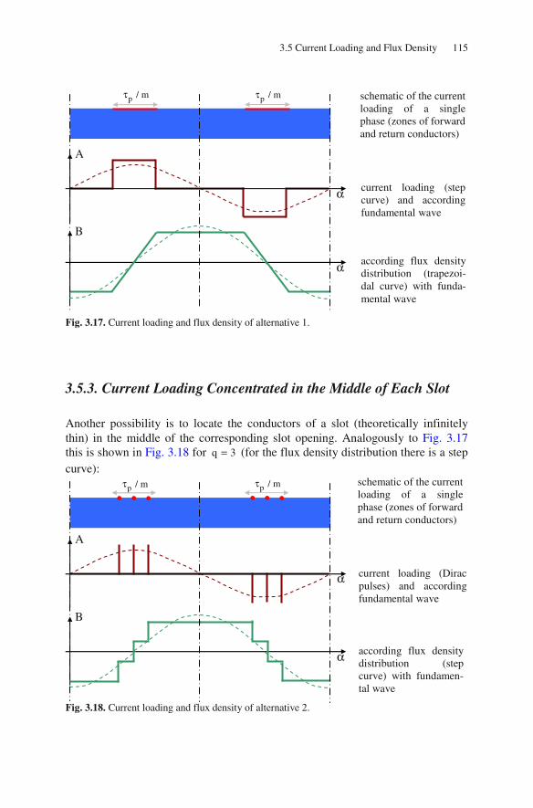
3.5 Current Loading and Flux Density 115
Fig. 3.17. Current loading and flux density of alternative 1.
3.5.3. Current Loading Concentrated in the Middle of Each Slot
Another possibility is to locate the conductors of a slot (theoretically infinitely thin) in the middle of the corresponding slot opening. Analogously to Fig. 3.17 this is shown in Fig. 3.18 for q 3= (for the flux density distribution there is a step curve):
Fig. 3.18. Current loading and flux density of alternative 2.
schematic of the current loading of a single phase (zones of forward and return conductors)
current loading (step curve) and according fundamental wave
according flux density distribution (trapezoi-dal curve) with funda-mental wave
α
A
B
α
p / mτ p / mτ
α
A
α
B
p / mτ p / mτ schematic of the current loading of a single phase (zones of forward and return conductors)
current loading (Dirac pulses) and according fundamental wave
according flux density distribution (step curve) with fundamen-tal wave

116 3 Rotating Field Theory
3.5.4. Current Loading Distributed Across Each Slot Opening
Finally it is possible to distribute the conductors of a slot (theoretically infinitely thin) in the area of the respective slot opening. Then the slope of the steps in the flux density characteristic will be less steep (Fig. 3.19).
Fig. 3.19. Current loading and flux density of alternative 3.
Which alternative has to be chosen for a specific task inter alia depends on the task itself. For example, if the fundamental torque of the machine has to be calcu-lated usually a relatively rough model is sufficient. Computing characteristics where harmonic waves have a significant influence (typically calculating acoustic noise), a much more precise alternative has to be chosen.
3.5.5. Rotating Air-Gap Field
The rotating air-gap field is deduced from the rotating magneto-motive force. In practice, an air-gap width is used which is enlarged against the geometric air-gap width because of:
• field distortion because of the slotting: CK′δ → δ = δ ( CK being Carter’s
factor) and • magnetic reluctance (saturation) of the iron: ′ ′′δ → δ .
Neglecting this field distortion and the magnetic reluctance of the iron
( Feμ → ∞ ), it can be obtained:
α
α
B
A
p / mτ p / mτ schematic of the current loading of a single phase (zones of forward and return conductors)
current loading (rectan-gular pulses) and ac-cording fundamental wave
according flux density distribution (slope of steps less steep) with fundamental wave

3.5 Current Loading and Flux Density 117
( ) ( )
( )( )
0
6g 10
g
B , t , t
3 w 22I sin 6g 1 p t
2 p 6g 1
δ δ
∞+
=−∞
μα = Θ α
δ
ξμ= + α − ω
δ π +
(3.60)
The fundamental wave is:
( ) ( ),1 ,1B , t B sin p tδ δα = α − ω (3.61)
with the amplitude 0 1
,1
w3 2B 2I
2 pδ
μ ξ=
δ π and the angular frequency 1
p
ωΩ = .
The harmonic waves are:
( ) ( )( ),6g 1 ,6g 1B , t B sin 6g 1 p tδ + δ +α = + α − ω
with the amplitude ( )
6g 1,6g 1 ,1
1
B B6g 1
+
δ + δ
ξ=
ξ + and the angular frequency
16g 1
6g 1+
ΩΩ =
+.
The total rotating field can be described as:
( ) ( ),6g 1g
B , t B , t∞
δ δ +=−∞
α = α (3.62)
Figure 3.20 shows this rotating field Bδ (red characteristic) and the rotating
current loading Aδ (air-gap width 1mmδ = ; bore diameter D 0.1m= , blue func-
tion), together with the respective fundamental waves (dashed lines). Please consider:
• the phase shift between magnetic field and current loading always is 90° (or
2π );
• the magnetic field Bδ changes the curve form with respect to time, but the am-
plitude of the fundamental wave ,1Bδ remains unchanged at any point in time.

118 3 Rotating Field Theory
Fig. 3.20. Rotating magnetic field and current loading versus angle for different points in time (solid red: rotating field (Bδ in T); dashed red: according fundamental wave of rotating field (Bδ,1 in T); solid blue: rotating current loading (Aδ in 100Am-1); dashed blue: according fundamental wave of rotating current loading (Aδ,1 in Am-1)).
In Fig. 3.21 the field distribution is illustrated for two different instants in time, obtained by numerical calculation using the Finite Element Method (FEM). The stator contains 4 poles and 36 slots; the rotor is assumed being a cylindrical iron part. In addition, the phasors of the three currents, the current loading and the flux density are shown. The travelling rotating waves can be deduced clearly.
1
0.5
0
-0.5
-1 0 0.5 1 1.5 2
α π
A, B t 0ω = A, B 1
0.5
0
-0.5
-1
0 0.5 1 1.5 2 α π
t 4ω = π
A, B 1
0.5
0
-0.5
-1
0 0.5 1 1.5 2 α π
t 2ω = π A, B 1
0.5
0
-0.5
-1
0 0.5 1 1.5 2 α π
t 3 4ω = π

3.5 Current Loading and Flux Density 119
Fig. 3.21. Field distribution (magnetic field lines) and phasors of the three phase currents and the fundamental waves of current loading and air-gap flux density for different points in time.
t 0ω =
u
v
w
Re
Im−
ω
uI
vI wI
Re
Im−
ω
B
A
Re
Im−
ω
B A
Re
Im−
ω
uI vI
wI
t / 3ω = π

120 3 Rotating Field Theory
3.6 Induced Voltage and Slip
In the following the induced voltage will be calculated, which is generated in a ro-
tor coil (winding with 2w turns) by a rotating field of the stator (winding with
1w turns). The relative position ( )tα is arbitrary (see Fig. 3.22). For this, the
flux linkage of the rotor coil has to be calculated firstly. This is done by integra-
tion of the air-gap flux density across one pole pitch pτ :
Fig. 3.22. Schematic cross-section of a rotating field machine with a single rotor coil.
( ) ( ) ( ) ( )pr
2 2r
, t w , t w B , t d r
α+τ
δ
α
ψ α = φ α = α α (3.63)
The variable describes the effective magnetic length of the machine and r is the bore radius; the tilde is used to distinguish between integration limit and integra-tion variable. It follows:
XΦ
XXX
XXX XXX
u
v w
x
y z
stator rotor
air-gap δ
X
1w p
2w
α

3.6 Induced Voltage and Slip 121
( ) ( )
( )( )
( )( )
( )
( )( )
( )
p
2
p
2 ,6g 1g
p
2 ,6g 1g
,6g 12
g
2 ,6g 1g
, t w B , t rd
w r B sin 6g 1 p t d
cos 6g 1 p tw r B
6g 1 p
B2 rw cos 6g 1 p t
p 6g 1
w , t
πα+
δ
α
πα+
∞
δ +=−∞α
πα+
∞
δ +=−∞ α
∞δ +
=−∞
∞
δ +=−∞
ψ α = α α
= + α − ω α
− + α − ω=
+
= + α − ω+
= φ α
(3.64)
The fundamental wave is:
( ) ( ),1 ,1, t cos p tδ δφ α = φ α − ω (3.65)
with the amplitude 0 2
p 1 1,1 ,1 ,1 p ,1
w2 r 2 3 r 2B 2 B B 2I
p pδ δ δ δ
τ ξφ = = = τ = μ
π π δ π
and the angular frequency 1p
ωΩ = .
The harmonic waves are:
( ) ( )( ),6g 1 ,6g 1, t cos 6g 1 p tδ + δ +φ α = φ + α − ω (3.66)
with the amplitude ,6g 1 p
,6g 1 ,6g 1
B2 r 2B
p 6g 1 6g 1
δ +
δ + δ +
τφ = =
+ π + and the angular fre-
quency 16g 1
6g 1+
ΩΩ =
+.
The induced voltage will be calculated from the time-derivative of the magnetic flux linkage. The time dependency of the magnetic flux linkage may be caused by the time-dependent currents as well as by the time-dependent position of the rotor coil.

122 3 Rotating Field Theory
( )( ) ( ) ( )
( )( )( ) ( )
( )( )( )
i
,6g 12
g
2 ,6g 1g
d , t , t , tdu , t
dt dt t
B2 r dw sin 6g 1 p t 6g 1 p
p 6g 1 dt
d2 r w B sin 6g 1 p t
6g 1 p dt
∞δ +
=−∞
∞
δ +=−∞
ψ α ∂ψ α ∂ψ ααα = = +
∂α ∂
α= − + α − ω + − ω
+
ω α= + α − ω −
+
(3.67)
Prior to calculating the induced voltage in detail, the “slip” shall be introduced here:
The slip is the difference between the speed of the rotating field wave of the
stator and the speed of the rotor (i.e. the mechanical speed), relative to the respec-tive speed of the rotating field wave of the stator.
With the angular frequency of the rotor
d
2 ndt
α= Ω = π (3.68)
and the angular frequency of the harmonic field waves
( )6g 16g 1 p
+
ωΩ =
+ (3.69)
the slip s of such a field wave becomes:
6g 1
6g 16g 1
s+
+
+
Ω − Ω=
Ω (3.70)
The speed of the fundamental wave of the rotating stator field is called syn-chronous speed. This will be indicated with the index “0“:
10
p 2 f p fn
2 2 2 p
Ω ω π= = = =
π π π (3.71)
Then the slip of the fundamental wave is:

3.6 Induced Voltage and Slip 123
011
1 0
n ns
n
−Ω − Ω= =
Ω (3.72)
The following can be deduced easily:
• at synchronous speed ( 0n n= ) there is: 1s 0= ;
• at stand-still ( n 0= ) there is: 1s 1= .
The relation between speed and slip is illustrated in Fig. 3.23.
Fig. 3.23. Relation between speed and slip.
The position of the rotor coil changes with the mechanical speed of the rotor. Therefore it follows
( ) Rt tα = α + Ω (3.73)
Further:
( ) ( ) ( )
( )( )
( )( )
( )
( )
R
R
R
R 6g 1
6g 1 p t 6g 1 p 6g 1 p t t
6g 1 p6g 1 p t 1
6g 1 p6g 1 p t
6g 1 p
6g 1 p s t+
+ α − ω = + α + + Ω − ω
+ Ω= + α − ω −
ω
ω− Ω
+= + α − ω
ω
+
+ α − ω=
(3.74)
and
n
1s
0
0
0n
1

124 3 Rotating Field Theory
( )
( )
( )( ) 6g 1 6g 1
6g 1 pds
6g 1 p dt 6g 1 p
6g 1 p
+ +
ω− Ω
+ω α ω− = = Ω
ω+ +
+
(3.75)
For the voltage induced into the rotor coil it follows (by inserting the last two equations into Eq. 3.67):
( ) ( )( )
( )( )
( )
( )
i 2 ,6g 1 R 6g 1 6g 1 6g 1g
2 ,6g 1 R 6g 1 6g 1 6g 1g
2 ,6g 1 R 6g 1g
i,6g 1 Rg
u , t 2 rw B sin 6g 1 p s t s
2w B sin 6g 1 p s t s r
2w B , t v
u , t
∞
δ + + + +=−∞
∞
δ + + + +=−∞
∞
δ + +=−∞
∞
+=−∞
α = + α − ω Ω
= + α − ω Ω
= α
= α
(3.76)
Here, 6g 1 6g 1 6g 1v s r+ + += Ω is the relative speed between the rotor coil and the
harmonic wave of the rotating field. The induced voltage is composed of an infinite number of separate oscillations
( )i,6g 1 Ru , t+ α . For these oscillations the following holds true:
( ) ( )( )
( )( )( )
( )( )
i,6g 1 R 2 6g 1 6g 1 ,6g 1 R 6g 1
2 6g 1 ,6g 1 R 6g 1
2 ,6g 1 6g 1 R 6g 1
u , t 2w rs B sin 6g 1 p s t
2 rw s B sin 6g 1 p s t
6g 1 p
w s sin 6g 1 p s t
+ + + δ + +
+ δ + +
δ + + +
α = Ω + α − ω
= ω + α − ω+
= φ ω + α − ω
(3.77)
The voltages ( )i,6g 1 Ru , t+ α induced by the rotating field waves offer the fol-
lowing characteristics:
• The amplitudes of the induced voltages are proportional to the flux of the har-monic wave, to the frequency of the supplying voltage, and to the slip.
• The frequency of all induced voltages is equal to the slip frequency.
• At stand-still of the rotor ( n 0= , i.e. 6g 1s 1+ = ) the frequency of all voltages
induced by the harmonic waves is equal to the supply frequency.

3.6 Induced Voltage and Slip 125
• At synchronous speed ( 0n n= ) there is:
( )
( )
( )6g 1
6g 1 p ps 1 6g 1 6g
6g 1 p
+
ω ω−
+= = − + = −
ω
+
Consequently, no fundamental voltage ( g 0= ) is induced; but the harmonic waves induce harmonic voltage oscillations with different frequencies.
• At other speeds the fundamental wave and each harmonic wave of the rotating stator field induce a voltage of different frequency into the rotor coil.
• The phase shift of the induced voltages in the rotor coil only depends on the
spatial position of the coil ( )R 6g 1 pα + .
Incorporating a three-phase winding even to the rotor, the three phases will be
shifted by an angle of 2 3pπ as well. Having a rotor slot number per pole and per
phase q 1> , a winding factor for the rotor (index “2“ for the rotor) has to be con-
sidered. The induced voltage of the kth ( k 1, 2, 3= ) rotor phase becomes
( ( )R k 1 2 3pα = − π ):
( )
( ) ( )
i,2,k 2 2,6g 1 ,6g 1 6g 1g
6g 1
u t w s
2sin 6g 1 k 1 s t
3
∞
+ δ + +=−∞
+
= ξ φ ω
π+ − − ω
⋅
(3.78)
The air-gap field will induce voltages even into the stator winding. If in the
above equation 2 2,6g 1w +ξ is substituted by 1 1,6g 1w +ξ , and considering that for the
stator winding 6g 1s 1+ = is true (because the stator is always in stand-still), the in-
duced voltage into the stator winding becomes:
( ) ( ) ( )i,1,k 1 1,6g 1 ,6g 1g
2u t w sin 6g 1 k 1 t
3
∞
+ δ +=−∞
π= ξ φ ω + − − ω (3.79)
The ratio of induced stator voltages (maximum values) caused by a harmonic wave and the fundamental wave is:
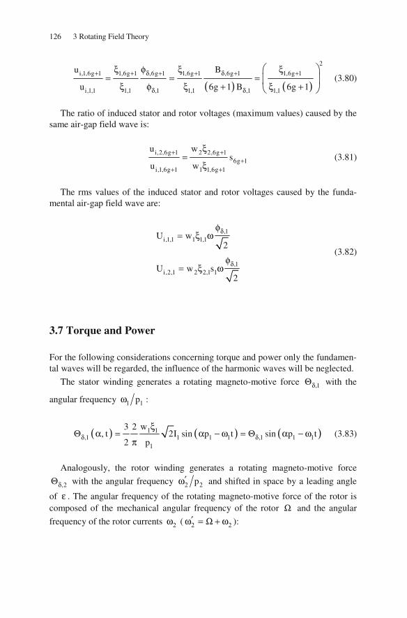
126 3 Rotating Field Theory
( ) ( )
2
i,1,6g 1 1,6g 1 ,6g 1 1,6g 1 ,6g 1 1,6g 1
i,1,1 1,1 ,1 1,1 ,1 1,1
u B
u 6g 1 B 6g 1
+ + δ + + δ + +
δ δ
ξ φ ξ ξ= = =
ξ φ ξ + ξ + (3.80)
The ratio of induced stator and rotor voltages (maximum values) caused by the same air-gap field wave is:
i,2,6g 1 2 2,6g 1
6g 1i,1,6g 1 1 1,6g 1
u ws
u w
+ +
+
+ +
ξ=
ξ (3.81)
The rms values of the induced stator and rotor voltages caused by the funda-mental air-gap field wave are:
,1i,1,1 1 1,1
,1i,2,1 2 2,1 1
U w2
U w s2
δ
δ
φ= ξ ω
φ= ξ ω
(3.82)
3.7 Torque and Power
For the following considerations concerning torque and power only the fundamen-tal waves will be regarded, the influence of the harmonic waves will be neglected.
The stator winding generates a rotating magneto-motive force ,1δΘ with the
angular frequency 1 1pω :
( ) ( ) ( )1 1,1 1 1 1 ,1 1 1
1
w3 2, t 2I sin p t sin p t
2 pδ δ
ξΘ α = α − ω = Θ α − ω
π (3.83)
Analogously, the rotor winding generates a rotating magneto-motive force
,2δΘ with the angular frequency 2 2p′ω and shifted in space by a leading angle
of ε . The angular frequency of the rotating magneto-motive force of the rotor is composed of the mechanical angular frequency of the rotor Ω and the angular
frequency of the rotor currents 2ω ( 2 2′ω = Ω + ω ):

3.7 Torque and Power 127
( ) ( )
( )
2 2,2 2 2 2 2
2
,2 2 2 2
w3 2, t 2I sin p t p
2 p
sin p t p
δ
δ
ξ′Θ α = α − ω − ε
π
′= Θ α − ω − ε
(3.84)
At this time the numbers of pole pairs, the angular frequencies and the phase shift between the stator and rotor rotating magneto-motive forces shall be arbi-trary. Figure 3.24 schematically illustrates the spatial position of the magneto-motive force distributions by means of phasors: the position of each phasor shows the position of the maximum of the magneto-motive force distribution, the length of the phasor is a quantity for the amplitude (please refer to Sect. 1.4).
Fig. 3.24. Cross-sectional view of a rotating field machine with winding distribution and illustra-tion of magneto-motive forces by means of phasors.
By means of Ampere’s Law the resulting air-gap field is obtained by superposi-tion (this means that saturation is neglected here):
( ) ( ) ( )
( ) ( ) ( )( )0
,1 ,2
,1 ,2
H , t , t , t
B , t , t , t
δ δ
δ δ
α δ = Θ α + Θ α
μα = Θ α + Θ α
δ
(3.85)
The magnetic energy in the air-gap is:
( )2
magV 0
B , tW dV, dV r d
2
α= = δ α
μ (3.86)
XΦ
XXX
XXX XXX
u
v w
x
y z
ε
XXX
X
X
,2δΘ
1 1/ p−ω
2 2/ p′−ω
α
,1δΘ

128 3 Rotating Field Theory
As saturation is neglected (linearity was assumed) the magnetic energy is equal to the magnetic co-energy. Then the torque may be calculated from the derivation of the magnetic energy with respect to the mechanical angle:
( )
( )
22mag
0 0
22
00
W B , tT r d
2
rB , t d
2
π
π
∂ α∂= = δ α
∂ε ∂ε μ
δ ∂= α α
μ ∂ε
(3.87)
With
( ) ( )( )
( ) ( )( )( )
2
2,20
,1 ,2
B , tB , t 2B , t
, t2 , t , t
δ
δ δ
∂ α∂α = α
∂ε ∂ε
∂Θ αμ= Θ α + Θ α
δ ∂ε
(3.88)
it follows in total:
( ) ( )( )( )
( ) ( )( )
( )[ ]
( ) ( )[
( )
2 2,20
,1 ,200
2
0 ,1 1 1 ,2 2 2 20
,2 2 2 2 2
2
0 2 ,1 ,2 1 1 2 2 20
22 ,2 2 2 2 2 2
, trT 2 , t , t d
2
rsin p t sin p t p
p cos p t p d
rp sin p t cos p t p
p sin p t p cos p t
πδ
δ δ
π
δ δ
δ
π
δ δ
δ
∂Θ αμδ= Θ α + Θ α α
μ δ ∂ε
′= μ Θ α − ω + Θ α − ω − ε ⋅δ
′Θ − α − ω − ε α
′= − μ Θ Θ α − ω α − ω − ε +δ
′ ′Θ α − ω − ε α − ω −( )2p dε α
(3.89)
Considering ( ) ( )2
0
sin x cos x dx 0π
= it can be obtained:
( ) ( )2
0 2 ,1 ,2 1 1 2 2 20
rT p sin p t cos p t p d
π
δ δ′= −μ Θ Θ α − ω α − ω − ε α
δ (3.90)

3.7 Torque and Power 129
With ( ) ( ) ( ) ( )[ ]1
sin x cos y sin x y sin x y2
= + + − it follows:
( ) ( )( )
( ) ( )( )
2
0 2 ,1 ,2 1 2 1 2 20
2
1 2 1 2 20
r 1T p sin p p t p d
2
sin p p t p d
π
δ δ
π
′= −μ Θ Θ + α − ω + ω − ε α +δ
′− α − ω − ω + ε α
(3.91)
Generally it is true:
( )( )
2
0
0 if n 0sin nx dx
2 sin if n 0
π ≠+ ϕ =
π ϕ = (3.92)
As 1p and 2p are the numbers of pole pairs of stator and rotor, respectively,
these are positive integers. Therefore, it follows:
( ) ( )( )2
1 2 1 2 20
sin p p t p d 0π
′+ α − ω + ω − ε α = (3.93)
and
( ) ( )( )2
1 2 1 2 2 1 20
sin p p t p d 0 if p p pπ
′− α − ω − ω + ε α ≠ = = (3.94)
Consequently, torque is only generated if the numbers of pole pairs of stator and rotor are identical. Then it follows:
( )( ),1 ,20 1 2
rT p 2 sin t p
2
δ δΘ Θ′= −μ π − ω − ω + ε
δ (3.95)
From this equation can be deduced that the torque is sinusoidal in time with a mean value (according to time) of zero. It is a pure oscillating torque.
Only if the angular frequencies of the rotating magneto-motive force waves are
identical ( 1 2′ω = ω = ω ) a torque constant in time is generated:

130 3 Rotating Field Theory
( )0 ,1 ,2
rT p sin pδ δ
π= μ Θ Θ −ε
δ (3.96)
If both rotating magneto-motive force waves ( ),1 , tδΘ α and ( ),2 , tδΘ α are in
phase, i.e. if 0ε = is true, then the torque is equal to zero. The torque is maximum
for p 2ε = π , i.e. if the rotating magneto-motive force waves have an electrically
phase shift of 90° (or 2π ).
The rotating magnetic field has been calculated as follows:
( ) ( ) ( )( ) ( )0 0,1 ,2 ,totB , t , t , t , tδ δ δ δ
μ μα = Θ α + Θ α = Θ α
δ δ (3.97)
This shall be illustrated in Fig. 3.25 with the help of phasors in the complex plain. With their length phasors describe the amplitude of the respective rotating wave, the direction of the phasor shows the position of the maximum of the rotat-ing wave.
Fig. 3.25. Phasor diagram of the magneto-motive forces.
By means of the law of cosines the absolute value of the total rotating magneto-motive force is obtained:
,1δΘ
,2δΘ
,totδΘ
,2δΘ
-Im
Re
( )2 1π − ϕ − ϕ
1ϕ
2ϕ
pε
−ω
−ω

3.7 Torque and Power 131
( )[ ]
( )
2 2,tot ,1 ,2 ,1 ,2 2 1
2 2,1 ,2 ,1 ,2 2 1
2 cos
2 cos
δ δ δ δ δ
δ δ δ δ
Θ = Θ + Θ − Θ Θ π − ϕ − ϕ
= Θ + Θ + Θ Θ ϕ − ϕ
(3.98)
The law of sines gives:
( )( )
( ) ( ) ( ) ( )
( ) ( )
,2 ,tot
2 11
,2 ,tot ,tot ,tot
1 2 1
,2 ,tot 1
sinsin
2
cos sin sin 2 p sin p
sin p cos
δ δ
δ δ δ δ
δ δ
Θ Θ=
π π − ϕ − ϕ− ϕ
Θ Θ Θ Θ= = =
ϕ ϕ − ϕ π − ε − ε
Θ − ε = Θ ϕ
(3.99)
Therefore, it follows for the torque:
( )
( )
( )
( )
( )
0 ,1 ,tot 1
0 ,1 10
,1 1
1 11 1
1 1 1 1
rT p cos
rp B cos
r p B cos
w3 2r p 2I B cos
2 p
3 rw 2I B cos
δ δ
δ δ
δ δ
δ
δ
π= μ Θ Θ ϕ
δ
π δ= μ Θ ϕ
δ μ
= π Θ ϕ
ξ= π ϕ
π
= ξ ϕ
(3.100)
With the rms-value of the induced voltage
i,1 1 1U w2
δφ= ξ ω (3.101)
and the magnetic flux
2 r
Bp
δ δφ = (3.102)
the torque can be calculated like this:

132 3 Rotating Field Theory
( )( ) ( )i,1 1 1 i,1 1 1
i,1 1 11 0
3U I cos 3U I cospT 3U I cos
2 n
ϕ ϕ= ϕ = =
ω Ω π (3.103)
Here, the expression
( )i,1 1 1P 3U I cosδ = ϕ (3.104)
is the rotating air-gap field power. This rotating air-gap field power is equal to the power supplied from the mains minus the copper losses (Ohmic losses) of the sta-tor:
21 1 1P P 3R Iδ = − (3.105)
The rotating air-gap field power is transferred via the air-gap:
( )i,1 1 1 0P 3U I cos 2 n Tδ = ϕ = π (3.106)
The mechanical power at the shaft of the machine is:
( ) ( )mech 0P 2 nT 2 n T 1 s 1 s Pδ= π = π − = − (3.107)
The difference between the rotating air-gap field power and the mechanical power at the axis is transformed to heating losses inside the rotor:
( )loss,rotor mechP P P P 1 s P sPδ δ δ δ= − = − − = (3.108)
Having synchronous speed of the rotor ( 0n n= , i.e. s 0= ), the mechanical
power at the shaft equals the rotating air-gap field power; the rotor losses are zero. The power flow inside an electrical machine is illustrated by the co-called Sankey-diagram, see Fig. 3.26 (iron losses and friction is neglected).
Fig. 3.26. Sankey-diagram.
elP mechP
2loss,stator 1 1P 3R I= loss,rotorP sPδ=
1P Pδ ( )1 s Pδ−
air-gap

3.7 Torque and Power 133
To get a constant torque in time the condition 1 2′ω = ω = ω must be fulfilled.
The angular frequency of the rotating magneto-motive force wave of the rotor 2′ω
can be described like:
( )( )2 0 0 0
2
2
2 f 2 pn 2 p 1 s n sn
f2 p n s 2 pn 2 sf 2 pn 2 f
p
′ω = ω = π = π = π − +
= π + = π + π = π + π
= Ω + ω
(3.109)
In this equation n is the mechanical speed of the rotor and 2f is the frequency
of the rotor currents. Alternative descriptions are:
2 1 1
1 2
f sf sf f pn
f fn
p
= = = −
−=
(3.110)
If the rotor of the rotating field machine contains alternating currents ( 2f 0> )
there is:
10
fn n
p< = (3.111)
Consequently, the rotor rotates with a speed less than the synchronous speed
0n . Such a machine is called asynchronous machine or induction machine. De-
pending on the frequency of the rotor currents the speed of the machine is achieved.
Supplying the rotor of the rotating field machine with DC current ( 2f 0= )
there is:
10
fn n
p= = (3.112)
Consequently, the rotor rotates with synchronous speed. Such a machine is called synchronous machine. The speed of the machine solely depends on the fre-quency of the stator currents.

134 3 Rotating Field Theory
3.8 References for Chapter 3
Bödefeld T, Sequenz H (1971) Elektrische Maschinen. Springer-Verlag, Wien Jordan H, Klima V, Kovacs KP (1975) Asynchronmaschinen. Vieweg Verlag, Braunschweig Kleinrath H (1975) Grundlagen elektrischer Maschinen. Akademische Verlagsgesellschaft,
Wiesbaden Müller G, Ponick B (2009) Theorie elektrischer Maschinen. Wiley-VCH Verlag, Weinheim Seinsch HO (1992) Oberfelderscheinungen in Drehfeldmaschinen. Teubner Verlag, Stuttgart Seinsch HO (1993) Grundlagen elektrischer Maschinen und Antriebe. Teubner Verlag, Stuttgart Taegen F (1971) Einführung in die Theorie der elektrischen Maschinen II. Vieweg Verlag,
Braunschweig

4 Induction Machines
4.1 Construction and Equivalent Circuit Diagram
Stator and rotor of an induction machine - separated by an air-gap - contain each a symmetric winding in their slots.
The stator with the number of phases 1m 3= and the effective number of turns
1 1w ξ is supplied by a symmetric three-phase system with the frequency 1f . Con-
sequently, a rotating field is generated, that rotates with the synchronous speed
0 1n f p= . To produce a constant torque, the number of pole pairs of stator and
rotor are identical ( 1 2p p p= = ).
The rotor winding can either be short-circuited directly or it can be passed out-side the rotor via slip rings, and there be short-circuited directly or via series resis-
tors. In the 2m phases of the closed rotor winding with the effective number of
turns 2 2w ξ currents are induced by the rotating field. These rotor currents togeth-
er with the rotating field of the stator generate the torque that rotates the rotor with
the mechanical speed ( ) 0n 1 s n= − .
During motor operation the rotor always rotates with a speed lower than the
synchronous speed 0n (i.e. asynchronous to the rotating field of the stator cur-
rents), because at synchronous speed no currents are induced into the rotor wind-ing and therefore no torque is generated. This differential speed between rotating
field of the stator and the rotor is 2 0n sn= ; in the rotor currents with the frequen-
cy 2 1f sf= are induced. These currents generate a rotating field of the rotor that
(relative to the rotor) rotates with the speed 2n . Relative to the stator this rotating
field has the speed 2 0n n n+ = . Consequently, the frequency condition to obtain a
constant torque (please refer to Sect. 3.7) is fulfilled. Figure 4.1 shows the zones and a symbolic representation of the induction ma-
chine windings:
© Springer-Verlag Berlin Heidelberg 2015 135
DOI 10.1007/978-3-642-17584-8_ 4D. Gerling, Electrical Machines Mathematica l Engineering,,

136 4 Induction Machines
Fig. 4.1. Symbolic representation of the induction machine windings (left: distribution of the three stator and rotor windings in zones with 2p=2; right: symbolic representation).
To reach an easier mathematical description of this electrical machine firstly the system of coupled and movable coils shall be transformed to a system with sta-tionary elements with the same numbers of phases and turns in stator and rotor.
For this, in the following only the fundamental waves will be considered. For calculation of the steady-state operation the calculation with complex phasors will be applied. Because of symmetry reasons a single-phase treatment is sufficient.
The windings of stator and rotor can be described with lumped parameters: re-sistance, leakage and main inductivity. Then the equivalent circuit diagram looks like it is shown in Fig. 4.2 (both partial systems are represented as “energy con-sumption system”):
Fig. 4.2. Equivalent circuit diagram of the induction machine with magnetic coupling between stator and rotor.
The voltage equations are (with the mutual inductivities 21L and 12L ):
u
v
w
u
( )tγ
stator
rotor
v
w
u
v w
x
y z u
x
( )tγ
stator
rotor
v
y
z
w
1 1 1 1f , m , w , ξ 2 2 2 2f , m , w , ξ
1U
1I
2U
2I 1R 2R 1L σ 2L σ
2mL 1mL

4.1 Construction and Equivalent Circuit Diagram 137
1 1 1 1 1 1 1 21 2
2 2 2 2 2 2 2 12 1
U R I j L I j L I
U R I j L I j L I
= + ω + ω
= + ω + ω (4.1)
with ( 1mL and 2mL being the main or magnetizing inductivities of stator and ro-
tor):
1 1 1m
2 2 2m
L L L
L L L
σ
σ
= +
= + (4.2)
Now voltages and currents in the stationary stator winding are searched, that have the same effect like the actual voltages and currents in the rotating rotor winding. These transformed voltages and currents will be labeled by a prime. The following conditions must be fulfilled:
1. Unchanged magneto-motive force:
2 2 2 1 1 12 2
2 2 22 2
1 1 1
m w m w4 42I 2I
2 p 2 p
m wI I
m w
!ξ ξ′=
π π
ξ′ =
ξ
(4.3)
2. Unchanged main flux:
i,2 2 2 2 m
i,2 1 1 1 m
i,2i,2 1 1 1
2 2 2
2U w
2U w
2U2U w
w
!
= ω ξ φ
′ = ω ξ φ
′ = ω ξω ξ
(4.4)
For 2 1ω = ω it is true: i,2 2,0U U= (induced voltage is equal to the no-
load voltage). Then it follows further:
1 1 1 1 1i,2 i,2 2,0 2,0
2 2 2 2 2
w w1 1U U U U
w s w s
ω ξ ξ′ ′= = =
ω ξ ξ (4.5)

138 4 Induction Machines
3. Unchanged Ohmic losses:
( )
( )
2 22 2 2 1 2 2
21 1 1
2 2 22 2 2
m R I m R I
m wR R
m w
!′ ′=
ξ′ =
ξ
(4.6)
4. Unchanged magnetic energy (here for the linear, i.e. unsaturated case):
( )
( ) ( )
( )
1 2 11 1 2 2 1 1 2 2
2 21 21 1 21 1 2 2 2 12 1 2
2 211 1 1m 1 2 2 2
m m mI I I I
2 2 2
m mL I L I I L I L I I
2 2
mL I 2L I I L I
2
!′ ′Ψ + Ψ = Ψ + Ψ
+ + +
′ ′ ′= + +
(4.7)
Further:
( )
( )
21 1 1
2 2 22 2 2
2 2 221 1m
1 1 1
2 212 1m
1 1
m wL L
m w
m wL L
m w
wL L
w
ξ′ =
ξ
ξ=
ξ
ξ=
ξ
(4.8)
Please note that the following is true:
221 12
1
mL L
m= (4.9)
Now the voltage equations (Eq. 4.1) can be transformed like follows:

4.1 Construction and Equivalent Circuit Diagram 139
( )
( )
( )
( )
1 1 1 2 2 21 1 1 1 1 1 1 21 2
2 2 2 1 1 1
21 1 11 1 1 1 2 2 2
2 2 222 2 2 2 1 1 12 2 2
21 1 1 1 2 2 2
2 2 222 1 1 12 2 2
1 1 12 12 1
2 2 2
m w m wU R I j L I j L I
m w m w
ww m m wU R I
w m m ww
w m m wj L I
m m ww
wj L I
w
ξ ξ= + ω + ω
ξ ξ
ω ξω ξ ξ=
ω ξ ξω ξ
ω ξ ξ+ ω
ξω ξ
ω ξ+ ω
ω ξ
(4.10)
Inserting the values transformed to the stator (“primed“ values) gives:
1 1 1 1 1 1 1 1m 2
2 2 2 1 2 2 1 1m 1
U R I j L I j L I
U RI j L I j L I
s s
′= + ω + ω
′ ′′ ′ ′= + ω + ω
(4.11)
With the main reactance, the total stator reactance, the total rotor reactance (trans-formed to the stator)
1m 1 1m
1 1 1m
2 2 1m
X L
X X X
X X X
σ
σ
= ω
= +
′ ′= +
(4.12)
and the no-load current
0 1 2I I I ′= + (4.13)
the following set of equations is obtained:
1 1 1 1 1 1m 0
2 2 2 2 2 1m 0
U R I jX I jX I
U RI jX I jX I
s s
σ
σ
= + +
′ ′′ ′ ′= + +
(4.14)
From this the following equivalent circuit diagram can be deduced (Fig. 4.3). It becomes obvious that in comparison to Fig. 4.2 a galvanic coupling is introduced that simplifies the calculation of induction machines.

140 4 Induction Machines
Fig. 4.3. Equivalent circuit diagram of the induction machine with galvanic coupling.
Please note that in this equivalent circuit diagram all values are transformed to stator frequency, phase number of the stator, and effective number of turns of the stator. For s 1= (i.e. stationary rotor) the voltage ratio is equal to the ratio of the effective number of turns:
i,1 1 1
ui,2 2 2
U wr
U w
ξ= =
ξ (4.15)
Operating the induction machine with constant stator flux linkage most often the following transformation ratio is used:
( )1 1u 1
2 2
wr 1
w
ξ= + σ
ξ (4.16)
Then the leakage reactance of the stator vanishes in the equivalent circuit diagram (see Fig. 4.4).
Fig. 4.4. Equivalent circuit diagram of the induction machine without stator leakage reactance.
1U
1I
2U
s
′
2I ′ 1R 2R s′ 1X σ 2X σ
′
1mX
1 1 1 1f , m , w , ξ 1 1 1 1f , m , w , ξ
0I
1U
1I
( )21
U1
s
′+ σ
( ) 21
1I
1′
+ σ
1R
( )221
R1
s
′+ σ
1X1
σ
− σ
1X
0I ⊗

4.2 Resistances and Inductivities 141
Operating the induction machine with constant rotor flux linkage most often the following transformation ratio is chosen:
1 1u
2 2 2
w 1r
w 1
ξ=
ξ + σ (4.17)
Then the leakage reactance of the rotor vanishes in the equivalent circuit diagram (see Fig. 4.5).
Fig. 4.5. Equivalent circuit diagram of the induction machine without rotor leakage reactance.
4.2 Resistances and Inductivities
4.2.1 Phase Resistance
With the mean length of one turn m , the number of turns w of a phase, the cross
section of the conductor wireA and the specific resistance Cuρ the phase re-
sistance becomes:
mCu
wire
wR
A= ρ (4.18)
The mean length of one turn can be calculated from the stack length of the ma-chine and the length of a turn in the end winding region.
1U
1I
2
2
U 1
s 1
′
+ σ
( ) 2 2I 1′ + σ 1R
( )2
22
R 1
s 1
′
+ σ
1Xσ
( ) 11 X− σ
0I ⊗⊗

142 4 Induction Machines
4.2.2 Main Inductivity
Supplying the stator with 1I and 1f at no-load operation (i.e. with no currents in
the rotor), it follows:
1m i1m
1 1 1
X UL
I= =
ω ω (4.19)
According to the rotating field theory, the induced voltage is:
1 1i 0 1 1 12
w3 r 42U w 2I
2 p
ξ= μ ξ ω
δ π (4.20)
Therefore, it follows in total for the main inductivity:5
2
1 11m 0
w3 4 rL
2 p
ξ= μ
π δ (4.21)
4.2.3 Leakage Inductivity
The leakage is composed of harmonic leakage, leakage of the end windings, and the slot leakage. These three parts are calculated separately and then added up. The separate consideration of single field components is already explained in Sect. 3.2 (for the slot and air-gap regions); even here such a separation of the field re-gions is performed. The summation of the partial results (i.e. superposition) is al-lowed because of the assumed linearity.
4.2.3.1 Harmonic Leakage
It has been shown in the rotating field theory that all harmonic waves induce volt-ages of equal frequencies and phase shift in their generating winding. All these voltages may therefore be added. The sum of these voltages can be interpreted as voltage drop at a leakage reactance, because they do not produce a useful magnet-ic field.
5 For the air-gap δ please refer to the remarks in Sect. 3.5.

4.2 Resistances and Inductivities 143
( )
i,6g 11, ,harm
g 01 1
226g 11 1
0 harm 1mg 0 1
U1L
I
w3 4 rL
2 p 6g 1
+
σ≠
+
≠
=ω
ξξ= μ = σ
π δ ξ +
(4.22)
with:
( )
26g 1
harmg 0 1 6g 1
+
≠
ξσ =
ξ + (4.23)
4.2.3.2 Slot Leakage
A single slot will be regarded in Fig. 4.6.
Fig. 4.6. Field distribution in a single slot.
In the slot region filled with conductors Ampere’s Law together with the as-
sumption Feμ → ∞ gives ( slotz : number of conductors in the slot, a: number of
parallel paths):
( )( )
( )
slotslot
slot 0
slot
max max 0slot slot
B xz xx 2I b
a h
z2I
x aB x B , Bh b
Θ = =μ
= = μ
(4.24)
In the region of the slot without conductors (slot opening) there is:
maxB B
x
sloth
soh
slotb
X X X X
X X X X
X X X X
X X X X
X X X X

144 4 Induction Machines
( )
( )
( )
slotslot
0
max
B xzx 2I b
a
B x B
Θ = =μ
=
(4.25)
The slot leakage inductivity will be calculated by means of the magnetic ener-gy. For a phase with 2pq slots it is true:
( )22
mag ,slotV0
1 1W B dV L 2I
2 2σ= =
μ (4.26)
Therefore:
( )
slot slot so
slot
2h h h2
mag max slot max slot0 h0 slot 0
2slot
0slot slot
soslot 0
22
slot slot so0
slot slot
2pq x 2pqW B b dx B b ldx
2 h 2
z2I
b ha2pq hb 2 3
z h h12pq 2I
2 a 3b b
+
= +μ μ
μ
= +μ
= μ +
(4.27)
Consequently:
2
slot slot so,slot 0
slot slot
z h hL 2pq
a 3b bσ = μ + (4.28)
With slotz w
a pq= it follows further:
2
slot slot so,slot 0 slot
slot slot
h hwL 2 ,
p q 3b bσ
λ= μ λ = + (4.29)
Here slotλ is called slot leakage permeance.

4.3 Operating Characteristics 145
4.2.3.3 End Winding Leakage
The end winding leakage is caused by the leakage field of the end winding. Be-cause of the complicated geometry of the end winding a general calculation is not possible. Empirical values lead to the following result:
2
,endw 0 endw endw
wL 2 , 0.2 0.4
pσ = μ λ λ ≈ (4.30)
Here endwλ is called end winding leakage permeance. For simple constructions
of the end winding the leakage inductivity of the end winding can be calculated analytically, see the references list.
4.3 Operating Characteristics
4.3.1 Heyland-Diagram (Stator Phase Current Locus Diagram)
For determination of the stator phase current locus the phase resistance will be ne-
glected in a first step: 1R 0= . This approximation, that generally is allowed for
machines with high power and supplied by line frequency, will be omitted later.
The equivalent circuit diagram with ( )1 1u 1
2 2
wr 1
w
ξ= + σ
ξ is chosen; the rotor
winding is short-circuited, either as squirrel cage rotor or as wound rotor via the slip rings and brushes. Then the equivalent circuit diagram is obtained (Fig. 4.7).
Fig. 4.7. Equivalent circuit diagram of the induction machine.
1U
1I ( ) 21
1I
1′
+ σ
( )221
R1
s
′+ σ
1X1
σ
− σ
1X
0I

146 4 Induction Machines
The following is true:
( )
1 1 0
2 0 1
1
2 2 21 1 1
1
U jX I
II I
1
I RU 1 jX 0
1 s 1
=
′= +
+ σ
′ ′ σ+ + σ + =
+ σ − σ
(4.31)
Defining the voltage 1U being real, the phasor diagram is shown in Fig. 4.8:
Fig. 4.8. Phasor diagram of the induction motor.
Calculating the stator phase current 1I dependent on the slip s, it follows:
( )
2 1 1 1 0
221 11 1
I U UI I
R1 jX1 jX
s 1
′= − = +
′ σ+ σ+ σ +
− σ
(4.32)
Re
-Im
1 1 0U jX I=
( )2 2 21
1
I R1
1 s
′ ′+ σ
+ σ
2
1
I
1
′
+ σ
0I
1I
21
1
IjX
1 1
′ σ
+ σ − σ
•
1ϕ

4.3 Operating Characteristics 147
Fig. 4.9. Complex impedance of the induction motor.
The stator phase current locus (see Fig. 4.9) can be deduced like follows:
• The complex resistance ( ) ( )221 1
RZ s 1 jX
s 1
′ σ= + σ +
− σ is a straight
line in the complex plane.
• According to the locus theory, the complex conductance ( ) ( )Y s 1 Z s=
is a circle, that - reaches the origin of the complex plane for s 0= , - has its midpoint on the negative imaginary axis, and
- possesses the diameter 1
1X1
−σ
− σ.
• By multiplication with 1 1U U≡ (the voltage has been defined being real)
the locus of ( ) 21
1
IU Y s
1
′− =
+ σ is deduced.
• The locus of the stator phase current 1I is calculated by adding the cur-
rent 0I : ( ) 2 1 1 0 1
1 1
I UI I j U Y s
1 X
′= − = − +
+ σ. Therefore, the locus of
( )1U Y s is shifted by the absolute value 1 1U X in the direction of the
negative imaginary axis. The no-load current ( s 0= ) is
Im−
Re
1jX1
σ
− σ
( )221
R1
s
′+ σ
( )Z s ( ) 1Y s U
11
1 UjX
1σ−σ
s = ∞s 0= s = ∞

148 4 Induction Machines
1 0
1
UI j
X= − (4.33)
The rotor current (transformed to the stator system) is
( )
2 1
2211 1
I U
R11 jX
s 1
′− =
′ σ+ σ+ σ +
− σ
(4.34)
The stator current and the “diameter current” are, respectively
2 1 0
1
II I
1
′= −
+ σ (4.35)
10
1
UI
X1
=σ
− σ
(4.36)
The locus of the stator phase current 1I is a circle in the complex plane (this is
also called “Heyland-diagram”, see Fig. 4.10).
Fig. 4.10. Heyland-diagram of the induction motor: complex currents.
Location and size of this circle are determined only by the main reactance 1X
and the total leakage coefficient σ (if the stator resistance 1R is neglected).
Im−
Re
1I
0I
s = ∞
s 0=
2
1
I
1
′−
+ σ
0I
s 0>
s 0<

4.3 Operating Characteristics 149
For parameterization of this circle, the ratio of imaginary part to real part of the
rotor current (transformed to the stator system) 2
1
I
1
′−
+ σ is regarded (for explana-
tion please refer to Fig. 4.11):
( ) { }
{ } ( )
1 2
2 2 2 1
XIm I 1tan sRe I R 1
∗
σ−′ − σϕ = =
′ ′ + σ (4.37)
As this function is linear in s, it can be used (most simply) for parameterization. The “slip line“ for parameterization can be each arbitrarily chosen parallel line to the Im− -axis:
• The tangent to the circle (stator phase current locus) in the point 2I 0′ = cuts
the slip line at the point s 0= .
• Each extension of the current 2
1
I
1
′
+ σ cuts the slip line at the respective slip s,
because ( )tan s∗ϕ is true. To fix the parameterization, the slip of one circle
point must be known (the slip of all other circle points then follows from the linear division of the slip line).
Fig. 4.11. Heyland-diagram of the induction motor: slip line.
1I
s = ∞
0I
1ϕ
∗ϕ
Im−
Re
s 0= s pull outs − s 1=
s = ∞ Im−s = ∞ Im−s = ∞ Im−
2
1
I
1
′−
+ σ 2
1
IIm
1
′−
+ σ 2
1
IRe
1
′−
+ σ

150 4 Induction Machines
The zenith of the Heyland-diagram is called pull-out point; the respective slip value is named pull-out slip. At this point the induction machine generates its maximum torque (pull-out torque). In this point real part and imaginary part of
2
1
I
1
′
+ σ are identical, i.e. ( )tan 1∗
ϕ = is true. Then it follows:
( )2
2 1pull out
1
R 1s
X1
−
′ + σ=
σ
− σ
(4.38)
Further it follows generally:
( )pull out
stan
s
∗
−
ϕ = (4.39)
At stand-still s 1= is true; the stall current (also called short-circuit current) is
then 1,stall 1,NI 5 8I≈ . Here, 1,NI is the stator phase current in the nominal opera-
tion point. As proven previously, location and size of the Heyland-diagram are determined
only by 1X and σ (if 1R is neglected). From (Eq. 4.38) it can be deduced that
the location of the slip points depends on 2R ′ .
The following three operating areas can be distinguished:
• Motor operation:
For motor operation there is: 0 s 1< < (i.e. 0n n 0> > ), therefore the arrow-
head of the stator current phasor is located in the left part of the upper circle half. The nominal operation point of an induction machine is in the region of:
N pull out0 s s −< < .
• Braking operation: For braking operation there is: s 1> (i.e. n 0< ), therefore the arrow-head of the stator current phasor is located in the very right part of the upper circle half.
• Generator operation:
For generator operation there is: s 0< (i.e. 0n n> ), therefore the arrow-head
of the stator current phasor is located in the lower circle half.
For small induction machines or when supplying the machine with small fre-
quencies (e.g. by means of an inverter) the resistance 1R generally may not be

4.3 Operating Characteristics 151
neglected. The Heyland-diagram then is changed concerning location, diameter, and parameterization. These changes are shown schematically in Fig. 4.12.
Fig. 4.12. Heyland-diagram of the induction motor: influence of the stator resistance.
For the angle α there is:
( ) 1
1
Rtan
Xα = (4.40)
4.3.2 Torque and Power
Neglecting the stator resistance 1R the active power of the induction machine
supplied via the terminals is equal to the rotating air-gap field power:
( )1 1 1 1 0P 3U I cos P 2 n Tδ= ϕ = = π (4.41)
With constant terminal voltage 1U the rotating air-gap field power Pδ and the
torque T are proportional to the real part of the stator current ( )1,real 1 1I I cos= ϕ .
Im−
Re
s = ∞
s 0=
0I
s
s 1=
2α
α
diameter
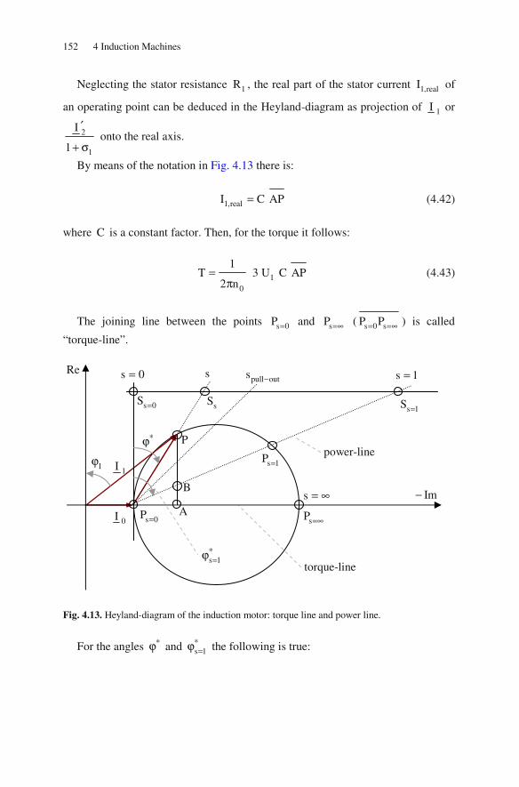
152 4 Induction Machines
Neglecting the stator resistance 1R , the real part of the stator current 1,realI of
an operating point can be deduced in the Heyland-diagram as projection of 1I or
2
1
I
1
′
+ σ onto the real axis.
By means of the notation in Fig. 4.13 there is:
1,realI C AP= (4.42)
where C is a constant factor. Then, for the torque it follows:
10
1T 3 U C AP
2 n =
π (4.43)
The joining line between the points s 0P = and sP =∞ ( s 0 sP P= =∞ ) is called
“torque-line”.
Fig. 4.13. Heyland-diagram of the induction motor: torque line and power line.
For the angles ∗ϕ and s 1
∗=ϕ the following is true:
s = ∞
1I
0I
1ϕ
P
A
B
s 0P = sP =∞
torque-line
s 1P = power-line
s 0= s pull outs − s 1=
s 0S = sS s 1S =
∗ϕ
s 1∗=ϕ
Im−
Re

4.3 Operating Characteristics 153
( )( )
( )( )
s 0 s s 0 s 0 s 0 s
s 1 s 0 s 1 s 0 s 0 s 0 s 1
s 0
s 1 s 0
tan S S P S S S ss
tan 1S S P S S S
tan P A AP AB
tan P A AB AP
∗
= = = =∗= = = = = = =
∗
=∗= =
ϕ= = = =
ϕ
ϕ= =
ϕ
(4.44)
Therefore:
AB
sAP
= (4.45)
and consequently:
BP
1 sAP
= − (4.46)
Therefore, the distance AP is divided by the so-called “power-line” s 0 s 1P P= =
by the ratio s to ( )1 s− . With this it can be deduced directly from the Heyland-
diagram how the rotating field power (this corresponds to the input power if the
stator resistance 1R is neglected) is divided into the different parts:
• rotating air-gap field power:
1P 3 U C AP δ = (4.47)
• electrical power (rotor losses):
el 1P 3 U C AB = (4.48)
• mechanical power:
mech 1P 3 U C BP = (4.49)
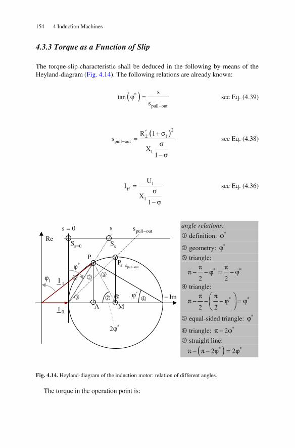
154 4 Induction Machines
4.3.3 Torque as a Function of Slip
The torque-slip-characteristic shall be deduced in the following by means of the Heyland-diagram (Fig. 4.14). The following relations are already known:
( )pull out
stan
s
∗
−
ϕ = see Eq. (4.39)
( )2
2 1pull out
1
R 1s
X1
−
′ + σ=
σ
− σ
see Eq. (4.38)
10
1
UI
X1
=σ
− σ
see Eq. (4.36)
Fig. 4.14. Heyland-diagram of the induction motor: relation of different angles.
The torque in the operation point is:
angle relations:
definition: ∗ϕ
geometry: ∗ϕ
triangle:
2 2
∗ ∗π ππ − − ϕ = − ϕ
triangle:
2 2
∗ ∗π ππ − − − ϕ = ϕ
equal-sided triangle: ∗ϕ
triangle: 2 ∗π − ϕ
straight line:
( )2 2∗ ∗π − π − ϕ = ϕ
Im−
Re
1I
s 0=
0I
1ϕ
s pull outs −
P
A
s 0S = sS
∗ϕ pull outs sP
−=
M
∗ϕ
2 ∗ϕ

4.3 Operating Characteristics 155
11
3pT U C AP =
ω (4.50)
The torque in the pull-out point is:
pull outpull out 1 s s
1
3pT U C MP
−− ==ω
(4.51)
Therefore:
( )( )
( ) ( )( )( )
( )
( )( )
( )( )
pull out
2
0
pull out s s0
2
1sin 2 I
T AP 2 sin 21T MP I2
sin2sin cos 2 cos
cos
12 tan
1 tan
2
1tan
tan
−
∗
∗
− =
∗
∗ ∗ ∗
∗
∗
∗
∗
∗
ϕ
= = = ϕ
ϕ= ϕ ϕ = ϕ
ϕ
= ϕ+ ϕ
=
ϕ +ϕ
(4.52)
From this, directly Kloss’s Law is obtained:
pull outpull out
pull out
T 2
ssT
s s
−−
−
=
+
(4.53)
The pull-out torque can be calculated like follows:

156 4 Induction Machines
0pull out 1 1,real,pull out 1
1 1
21 1
11 1
1 1
I3p 3pT U I U
2
U U3p 3pU
22X X
1 1
− −= =ω ω
= =σ σω ω
− σ − σ
(4.54)
Consequently, the pull-out torque is determined by the total leakage coefficient (high torque for small leakage).
As approximation the graph of the torque-slip-characteristic can be separated into the following two regions:
pull outpull out pull out
T 2ss s
T s−
− −
= (4.55)
pull out
pull outpull out
2sTs s
T s
−
−
−
= (4.56)
Figure 4.15 illustrates the evaluation of Kloss’s Law and this approximation:
Fig. 4.15. Torque-slip-characteristic of the induction motor.
pull out
T
T −
pull outs s −
Kloss’s Law
approximation
-5 -4 -3 -2 -1 0 1 2 3 4 5
2
1
0
-1
-2

4.3 Operating Characteristics 157
Kloss’s Law and the pull-out torque are independent of the rotor resistance.
Just the absolute value of the pull-out slip pull outs − is determined by the rotor re-
sistance. The stable operating area of the induction motor is: pull out1 s s 1−− < < .
In Fig. 4.16 pull outT T − is shown as a function of 0n n for pull outs 0.1− = .
Fig. 4.16. Torque-speed-characteristic of the induction motor.
4.3.4 Series Resistance in the Rotor Circuit
Having machines equipped with slip rings on the rotor, series resistances can be added to the rotor circuit. Doing this the Heyland-diagram remains unchanged (it is independent from the rotor resistance, see above). But the parameterization is changed.
Transforming even the series resistance SR to the stator system it follows:
( )
( )
21 1 1
S S 22 2 2
m wR R
m w
ξ′ =
ξ (4.57)
The identical point on the circle is described, if for the new parameterization
with s∗ the following holds true:
pull out
T
T −
0n n 0 0.2 0.4 0.6 0.8 1.0 1.2 1.4 1.6 1.8 2.0
2
1
0
-1
-2

158 4 Induction Machines
2 S S2
2
R R RRs s 1
s s R
∗
∗
′ ′ ′′+= = +
′ (4.58)
Analogously the pull-out slip is changed (see Fig. 4.17):
Spull out pull out
2
Rs s 1
R
∗− −
′= +
′ (4.59)
Fig. 4.17. Heyland-diagram of the induction motor: series resistance in the rotor circuit.
When introducing series resistances to the rotor circuit the absolute value of the pull-out torque remains unchanged; but the starting point is shifted into the direc-tion of the pull-out torque. It is even possible to start-up the machine with the pull-
out torque ( pull outs 1∗∗− = ). Simultaneously, the phase current at stand-still is re-
duced. These advantages are opposed by higher rotor losses. Moreover, with the series resistances an open-loop speed control under load is
possible, but this generates losses in the series resistances and therefore it is used only occasionally.
In Fig. 4.18 pull outT T − is shown as a function of 0n n for
pull outs 0.1; 0.2 and 1.0− = (torque-speed-characteristics):
Im−
Re
s 0= pull outs − s 1= s 0∗
=
Spull out pull out
2
Rs s 1
R
∗∗− −
′= +
′
s 1∗= pull outs∗
−
s 0∗∗= pull outs 1∗∗
− =
larger series resistance

4.3 Operating Characteristics 159
Fig. 4.18. Torque-speed-characteristics of the induction motor for different values of the pull-out slip.
4.3.5 Operation with Optimum Power Factor
During no-load of the induction machine the stator phase current is a pure reactive
current 0I . This corresponds to the magnetizing reactive (wattless) power re-
quired for the operation of the induction machine. This reactive power is supplied by the mains. There is:
( )
1 1 0 2
1 1 11 1 0
U UI j
jX w3 4 r1
2 p
= = − δξ
ω + σ μπ δ
(4.60)
To reduce the no-load current as far as possible, the air-gap should be as small as possible. But technical limits (bending of the axis, bearing tolerances) as well as economic limits (precision of the production) have to be considered. Usually it is reached
( ) ( )0
N
I0.2 low pole number 0.5 high pole number
I≈ (4.61)
pull outs 0.1− =
pull outs 1.0− =
pull outs 0.2− =
0n n 0.0 0.2 0.4 0.6 0.8 1.0 1.2
1.0
0.5
0.0
-0.5
-1.0
pull out
T
T −

160 4 Induction Machines
The maximum reachable torque (pull-out torque) of the induction machine is determined by the diameter of the Heyland-diagram. Therefore, the current
0 0I I I∞ = + should be as large as possible. The following is true:
1 1
11
10 0 01
N N N N N
U UUX
XI I II X 11
I I I I I∞
+σ
+ σ− σ= = = =σ
(4.62)
Generally reachable values for the total leakage coefficient are: 0.03 0.1σ ≈ . From this the ratio of the currents becomes:
N
I5 7
I∞ = (4.63)
The nominal operating point of the induction machine often is chosen to max-
imize the power factor ( )cos ϕ (then the load to the supplying mains because of
the reactive current is smallest). The operating point with maximum ( )cos ϕ is
called “optimum point”. It is obtained by a tangent of the stator current onto the Heyland-diagram (Fig. 4.19):
Fig. 4.19. Heyland-diagram of the induction motor: operation with optimum power factor.
Having the nominal operation point identical with the optimum point, the fol-lowing is true:
Im−
Re
optI
s 0=
0I
optϕ
opts
opt∗
ϕ
opt∗
ϕ optϕ
•

4.3 Operating Characteristics 161
opt opt2 ∗ϕ = ϕ (4.64)
( )( )
( )
( )
( )
00
opt
0 00
0 0
0 N N N
0 00 N
N N
1 1I I I
2 2cos1 1
I I I I2 2
I I1
I I I I I 1
I I1I I I 1
I I
∞
∞
∞
∞
−
ϕ = =
+ +
−− σ − σ
= = =+ + σ
+σ
(4.65)
Usually reachable in practice is: ( )optcos 0.8 0.9ϕ ≈ .
( ) ( ) ( )
( ) ( )
2opt 0 opt 0 opt0
2 2 20
0 0
2 20 0
0
1 1I I I sin I I 1 cos
2 2
I1 1 1 1 1 1I I 1
2 1 2 1 1
I I1 1 4
2 2
I
∞= + ϕ = + − ϕ
− σ σ + + σ − σ= + − = −
σ + σ σ + σ + σ
= + σ − − σ = σσ σ
=σ
(4.66)
For the slip in the optimum point the following is true:

162 4 Induction Machines
( )
( )( )
( ) ( )
( ) ( )
optopt
pull out
opt optopt pull out pull out
opt
pull out pull out
pull out
stan
s
1 coss s tan s
2 1 cos
11
1 11s s1 1 1
11
s
∗
−
− −
− −
−
ϕ =
ϕ − ϕ= =
+ ϕ
− σ−
+ σ − − σ+ σ= =− σ + σ + − σ
++ σ
= σ
(4.67)
In practice the pull-out slip is about pull outs 0.05 0.2− ≈ and the nominal slip
is about Ns 0.01 0.05≈ .
The torque ratio in the pull-out operating point and the optimum point is:
pull out opt
pull out opt pull out
opt
s s 1
T s s 1
T 2 2 2
−
− −
+ + σ+ σσ
= = =σ
(4.68)
With the given values for the total leakage coefficient it follows for the over-
load capability: pull out optT T 1.7 3.0− ≈ .
Up to now the stator copper losses, the iron losses, and the friction losses were neglected; only the rotor copper losses were considered. Then the efficiency is:
mech mech
1 rot
P P1 s
P Pη = = = − (4.69)
For the optimum point it follows:
opt opt pull out1 s 1 s −η = − = − σ (4.70)
For s 0= or s → ∞ the equivalent circuit diagrams (see Fig. 4.20) can be de-duced:

4.3 Operating Characteristics 163
Fig. 4.20. Equivalent circuit diagrams of the induction machine.
Directly from Fig. 4.20 the stator currents for s 0= and s → ∞ can be calcu-lated:
10
1
UI
X= (4.71)
( )
1 1
1 11
1 1
1 1
1 11 1
1
X XX1I U U
1X X 1
1
UU X
X
− −
∞
−
σ
− σ= =σ − σ
+ +− σ σ
= σ =σ
(4.72)
Further there is:
( ) ( )( )
( )( )
( ) ( )( ) ( )
1 1 1m1 2
1 1m2
1 2 1m 1 2 1m 1 2
1X 1 1 X
1 1
11 X
1
1 1 X X X Xσ σ
σ = − + σ+ σ + σ
= + σ −+ σ
′≈ + σ − − σ = σ + σ = +
(4.73)
and therefore:
1U
0I
1X
s 0=
1U
I ∞ 1X
1
σ
− σ
1X
s → ∞

164 4 Induction Machines
1
1 2
UI
X X∞
σ σ
≈′+
(4.74)
Remark: For the total leakage coefficient the following holds true:
( )( )
1 2 1 2
1 2 1 2 1 2
1 21 2
1 2
11
1 1 1
1
σ + σ + σ σσ = − =
+ σ + σ + σ + σ + σ σ
σ + σ≈ ≈ σ + σ
+ σ + σ
(4.75)
Changes of the machine parameters have the following influences onto the Heyland-diagram and therefore onto the operational characteristics:
• Increasing the air-gap the main reactance 1X is decreased. This means that the
magnetizing current 0I is enlarged.
• By decreasing the leakage reactance (e.g. decreasing 2X σ′ by utilizing the skin-
effect) the current I∞ increases. By this the pull-out torque and the stand-still
current are getting larger.
• Increasing the rotor resistance 2R ′ (e.g. by utilizing the skin-effect) changes the
parameterization of the slip line. It is possible to start-up the motor with higher torque and lower phase current, but this is opposed by higher rotor losses.
4.3.6 Further Equations for Calculating the Torque
In the following the equivalent circuit diagram with stator and rotor leakage reac-tance is used (Fig. 4.21).
Fig. 4.21. Equivalent circuit diagram of the induction machine.
1U
1I
2U
s
′
2I ′ 1R 2R s′ 1X σ 2X σ
′
1mX
0I

4.3 Operating Characteristics 165
The appropriate phasor diagram is shown in Fig. 4.22 (if 1R 0= is true).
Fig. 4.22. Phasor diagram of the induction machine.
From the rotating field theory it follows:
( )
( )
1 1 1 1
1m 1 1 1m 1 1
T 3 rw 2 I B cos
3 3p 2 I cos p 2 I sin
2 2 2
δ= ξ ϕ
π= Ψ ϕ = Ψ − ϕ
(4.76)
With 1j 1 1I 2 I e − ϕ
= and j2
1m 1m eπ
−
Ψ = Ψ it follows:
1m 1 1m 1 1I 2 I sin2
πΨ × = Ψ − ϕ (4.77)
and consequently:
( )1m 1
3 ˆT p I2
= Ψ × main flux and stator current
• With 1 1 1 1mˆL IσΨ = + Ψ it follows: 1m 1 1 1
ˆ ˆI IΨ × = Ψ × and therefore:
( )1 1
3 ˆT p I2
= Ψ × stator flux and stator current
• With ( )1m 1m 1 2ˆ ˆL I I ′Ψ = + it follows: 1m 1 1m 2 1
ˆ ˆ ˆI L I I′Ψ × = × and therefore:
( )1m 2 1
3 ˆ ˆT pL I I2
′= × rotor current and stator current
1I
2′Ψ
-Im
Re
1ϕ
0I
2I ′
1Ψ
2σ′Ψ
1σΨ
1mΨ

166 4 Induction Machines
• With 2 2 2 1m 1ˆ ˆL I L I′ ′ ′Ψ = + it follows: 2 1 2 2 1
ˆ ˆ ˆI L I I′ ′ ′Ψ × = × and therefore:
( )1m2 1
2
L3 ˆT p I2 L
′= Ψ ×′
rotor flux and stator current
• With 1 1 1 1m 2ˆ ˆL I L I ′Ψ = + it follows: 1 2 1 1 2
ˆ ˆ ˆI L I I′ ′Ψ × = × and therefore:
( )1m1 2
1
L3 ˆT p I2 L
′= − Ψ × stator flux and rotor current
• With ( ) ( )( )1m 1 2 1m 1 2 2 1m 2ˆ ˆ ˆ ˆ ˆ ˆL I I L I I I I′ ′ ′ ′× = + × = Ψ × it follows:
( )1m 2
3 ˆT p I2
′= − Ψ × main flux and rotor current
• With 1m 2 2 2ˆL Iσ
′ ′ ′Ψ = Ψ − it follows: 1m 2 2 2ˆ ˆI I′ ′ ′Ψ × = Ψ × and therefore:
( )2 2
3 ˆT p I2
′ ′= − Ψ × rotor flux and rotor current
• With 2 2 2ˆL I′ ′ ′Ψ = it follows:
( )1m1 2
1 2
L3T p
2 L L′= − Ψ × Ψ
′ stator flux and rotor flux
With A B B A× = − × further equations can easily be deduced. The above equations are valid for supplying the machine with sinusoidal volt-
ages and currents (the capital letters symbolize rms-values or peak-values, de-pending if electrical or magnetic variables are indicated). The torque calculation for arbitrary time dependencies of the supplying voltages and currents is per-formed in Sect. 8.9. With arbitrary time dependencies even dynamic operation conditions can be calculated, generally the torque is then no longer constant but time-dependent (in contrast to the steady-state behavior regarded in this chapter).
4.4 Squirrel Cage Rotor
4.4.1 Fundamentals
The squirrel cage rotor (cage rotor) of an induction machine in its simplest form is composed of stacked iron laminations; in the slots of this stack bars (made from copper or aluminum) are inserted and these bars are connected with rings (made from copper or aluminum) in both axial end regions. For machines with small power the slots are filled by aluminum die-cast and the end rings are realized in
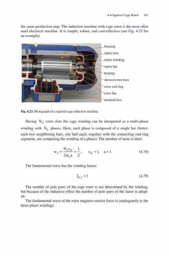
4.4 Squirrel Cage Rotor 167
the same production step. The induction machine with cage rotor is the most often used electrical machine. It is simple, robust, and cost-effective (see Fig. 4.23 for an example).
Fig. 4.23. Photograph of a squirrel cage induction machine.
Having 2N rotor slots the cage winding can be interpreted as a multi-phase
winding with 2N phases. Here, each phase is composed of a single bar (better:
each two neighboring bars, one half each, together with the connecting end ring segments, are composing the winding of a phase). The number of turns is then:
2 N2 N
2
N z 1w , z 1, a 1
2m a 2= = = = (4.78)
The fundamental wave has the winding factor:
2,1 1ξ = (4.79)
The number of pole pairs of the cage rotor is not determined by the winding, but because of the inductive effect the number of pole pairs of the stator is adopt-ed.
The fundamental wave of the rotor magneto-motive force is (analogously to the three-phase winding):
housing
stator iron
stator winding
stator fan
bearing
skewed rotor bars
rotor end ring
rotor fan
terminal box

168 4 Induction Machines
2 2,12 22,1 2 bar
2bar
11wm N4 4 22I 2I
2 p 2 p
N2I
p
ξΘ = =
π π
=π
(4.80)
Here 2 barI I= is the current of a rotor bar.
Now the relation between the bar current and the ring current shall be calculat-ed. Figure 4.24 illustrates the notation:
Fig. 4.24. Rotor currents of a squirrel cage induction machine.
There is:
2
p 2p
N
πβ = α = (4.81)
From
2N
kk 1
i 0=
= (4.82)
(there are no current sources in the rotor) and
1i
2i
3i
4i
1,2i
2,3i
3,4i α

4.4 Squirrel Cage Rotor 169
k 1,k k k,k 1
k k,k 1 k 1,k
i i i
i i i 0
− +
+ −
= +
+ − = (4.83)
the phasor diagram can be deduced (Fig. 4.25):
Fig. 4.25. Phasor diagram of the rotor currents of a squirrel cage induction machine.
The phase shift between two neighboring bar currents is equal to the phase shift of two neighboring ring currents. It follows:
bar
barring
2
1I
I2Ip
sin 2 sin2 N
= =β π
(4.84)
Therefore, the cross section of the end rings have to be dimensioned according-ly larger than the cross section of the bars (because usually equal current densities should be achieved).
The voltage transformation ratio is (see Sect. 4.1):
2 1 1 1 1u 1 1
bar 2 2
U w wr 2w
1U w1
2
′ ξ ξ= = = = ξ
ξ (4.85)
The current transformation ratio is (see Sect. 4.1):
2
2 2 2 2 2i
bar 1 1 1 1 1 1 1
1N 1
I m w N2rI m w 3w 6w
′ ξ= = = =
ξ ξ ξ (4.86)
4i
1,2i
2,3i
3,4i
β
3i
2i

170 4 Induction Machines
The rotor resistance is composed of the bar resistance and the corresponding segmental ring resistance. The transformation of the rotor resistance onto the sta-tor system is performed on the basis of equal losses:
( )
2 21 2 2 2 2 2
2 22 bar bar 2 ring ring
2
2 bar2 bar bar 2 ring
2
m I R m I R
N I R 2N I R
IN I R 2N R
2 sin p N
′ ′ =
= +
= +π
(4.87)
Further it follows:
( )
( )
( )
( )
( )
( )
2
22 bar
2 bar ring2 21 2 2
2 1 1 12 bar ring2 2
1 2 2 2
21 1 1
bar ring 22 2
21 1
bar ring 22 2
R 2 2 bar ring 2
N I 1R R 2R
m I 2sin p N
N 2m w 1I R 2R
m I N 2sin p N
4m w 1R 2R
N 2sin p N
12 w 1R 2R
N 2sin p N
1r R , R R 2R
2sin
′ = +′ π
ξ′= +
′ π
ξ= +
π
ξ= +
π
= = +( )2p Nπ
(4.88)
4.4.2 Skewed Rotor Slots
Apart from the fundamental wave there are even harmonic waves of the flux den-sity distribution in the air-gap of the machine, e.g. because of the winding distribu-tion and the slotting effect. These harmonic waves can be regarded as “leakage fields” (air-gap leakage, harmonic leakage). However, having a cage rotor these field waves can induce voltages and corresponding currents like the fundamental wave and consequently generate (disturbing) torque components. By skewing the rotor bars the effect of the harmonic waves can be reduced, because the flux pene-trating a cage mesh is different:

4.4 Squirrel Cage Rotor 171
• for skewed and unskewed bars the flux of the fundamental wave is nearly the same, whereas
• the flux of a higher harmonic wave is large for unskewed bars and it is reduced for skewed rotor bars.
Figure 4.26 schematically illustrates a rotor with skewed rotor bars.
Fig. 4.26. Sketch of a squirrel cage rotor with skewed rotor slots.
The ordinal numbers of the rotating field generated by a symmetric three-phase winding are (please refer to Chap. 3 “Rotating Field Theory”):
12m g 1
6g 1, g 0, 1, 2,
ν = +
= + = ± ± (4.89)
For g 0= , i.e. 1ν = , the fundamental wave is obtained.
Regarding a skewed rotor mesh in a “wound-off” representation (x-coordinate: circumferential direction; y-coordinate: axial direction), Fig. 4.27 can be drawn.
For the fundamental wave and the harmonic waves of the air-gap field the fol-lowing is true (for better distinction here the amplitude of the magnetic flux densi-ty is marked by “ ˆ “):
( ), , 2ˆB B cosδ ν δ ν= νγ (4.90)
Consequently, the flux in the (skewed) rotor mesh becomes:
skewing angle skewα
effective length
cage mesh
rotor radius r

172 4 Induction Machines
( )
skew2
skew2
skew2
skew2
r y rN2
, ,r y
r2 N
p y pN2
, 2 2p y
p2 N
B dx dy
rB cos d dy
p
π+ − α
δ ν δ νπ
− − − α
π+ − α
δ νπ
− − − α
Φ =
= νγ γ
(4.91)
Fig. 4.27. Sketch of a squirrel cage rotor with skewed rotor slots.
Solving firstly the inner integral of Eq. (4.91), it follows:
Bν
x
2
r
N
π−
2
r
N
π+
2+
2−
skew
yrα
d B dxdyν νΦ =
y
2
rx
p= γ

4.4 Squirrel Cage Rotor 173
( )2 skew
2
2 skew2
p y p2 N
, , 2 p y p
N2
r 1B sin dy
p
πγ = + − α
δ ν δ νπ
γ = − − α−
Φ = νγν
(4.92)
and further:
2
2
2
, , skew
2
skew
2
, skew2
2
2
, skew2
2
r 1 p yB sin p
p N
p ysin p dy
N
2r y pB cos p sin dy
p N
2r p yB sin cos p dy
p N
δ ν δ ν
−
δ ν
−
δ ν
−
ν πΦ = + − να −
ν
ν π− − να
ν π= −να
ν
ν π= −να
ν
(4.93)
Now the remaining integral is solved:
( )
y2
, , skewy2 skew
2
skew skew
,2 skew
skew
,2 skew
2r p yB sin sin p
p N p
p psin sin
2r p 2 2B sin
p N p
p2 cos 0 sin
2r p 2B sin
p N p
=
δ ν δ ν=−
δ ν
δ ν
ν π −Φ = −ν α
ν ν α
ν α −ν α−
ν π=
ν ν α
ν α
ν π=
ν ν α
(4.94)
A transformation gives:

174 4 Induction Machines
skew
2, ,
skew2
2
skew
2,
skew2
2
skew,
2 2
p psin sin
N2r p 2B
p pp N
N 2
p psin sin
N2 r 2B
p pN
N 2
p2 r pB si si
N N 2
δ ν δ ν
δ ν
δ ν
ν π ν α
ν πΦ =
ν π ν αν
ν π ν α
π=
ν π ν α
ν απ ν π=
(4.95)
The flux of a harmonic wave in a single rotor mesh therefore is composed of the maximum value of the harmonic flux density wave, the air-gap area of a rotor mesh, the coupling factor
C,2
psi
Nν
ν πξ = (4.96)
and the skewing factor
skewskew,
psi
2ν
ν αξ = (4.97)
For the coupling factor it holds:
C, 1νξ → for 2N → ∞ (4.98)
The effect of skewing is that the harmonic waves are damped to a large extent, whereas the fundamental wave is hardly influenced. The skewing factor becomes zero for:
skewskew,
skew
p0 k , k 1, 2,3,
2
p k, k 1, 2, 3,
2
ν
ν αξ = = π =
α= =
π ν
(4.99)

4.4 Squirrel Cage Rotor 175
The skewing factor for the fundamental wave and the first four harmonic waves is shown in Fig. 4.28 as a function of the skewing angle.
Fig. 4.28. Influence of skewed rotor slots onto the skewing factor for different harmonics.
4.4.3 Skin Effect
Because of the massive bars there is always a single-sided skin effect (towards the slot opening) with cage rotors: the slot leakage fields cross the bars and induce voltages, that are accompanied by eddy currents and consequently uneven current distribution. According to Lenz’s Law these induced voltages are directed in such a way, that the hereby generated eddy currents act against their reason; please re-
fer to Fig. 4.29 for the principle geometry, the current density distribution ( )J x
and the flux density distribution ( )B x .
The integral of the superposed eddy currents across the slot cross section is equal to zero, i.e. the total current is unchanged (only the current distribution is changed across the cross section).
Generally, the skin effect is unwanted in electrical machines, because this gen-erates additional losses in the bars and therefore is the reason for higher heating and lower efficiency.
0.0 0.05 0.1 0.15 0.2 0.25 0.3 0.35 0.4
skewp 2α π
skew,νξ 1ν =
5ν = −
7ν = 11ν = −
13ν =
1.0
0.5
0.0
-0.5

176 4 Induction Machines
Fig. 4.29. Current density and flux density distribution in massive rotor bars (above: DC current; below: AC current).
For induction machines with cage rotor this skin effect however can be used to improve the starting behavior: Because of the skin effect the rotor resistance is higher at starting operation (i.e. at high frequency of the rotor currents) and there-fore even the starting torque is higher. Simultaneously, the leakage reactance be-comes smaller (the flux density in the rotor bar is smaller), which means an in-crease of the diameter of the Heyland-diagram.
With increasing speed of the motor the skin effect gets smaller (because the frequency of the rotor currents gets smaller), until it is hardly noticeable at nomi-
nal operation. The Heyland-diagram C can now be composed of a diagram stC for
starting and a diagram opC for operation (the current 0I is identical in both cas-
es, because 1X is unchanged), see Fig. 4.30.
It is:
s 1= (i.e. 2 1f f= ) 1X unchanged; 2X σ′ small, 2R ′ large
s 0→ (i.e. 2f 0→ ) 1X unchanged; 2X σ′ large, 2R ′ small
X sloth
soh
slotb
NJ J
x
maxB B
x
X sloth
soh
slotb
NJ J
x
maxB B
x
⊗
superposed eddy currents

4.4 Squirrel Cage Rotor 177
Fig. 4.30. Heyland-diagram of the induction motor: starting diagram and operating diagram.
This effect specifically is utilized in so-called “skin effect rotors” (Fig. 4.31).
Fig. 4.31. Different kinds of skin effect rotors; from left to right: round bar (small skin effect), rectangular bar, keyed bar, double bar.
Changing the rotor resistance and the rotor leakage inductivity with frequency usually is described by the following factors:
( ) ( ) ( )
( )
( )
2 2 R 2 2 2
R
R 2 1
R f K f R f 0
K 0 1
K f f 3 5
= =
=
= ≈
(4.100)
( ) ( ) ( )
( )
( )
22 ,slot 2 I 2 2 ,slot
I
I 2 1
L f K f L f 0
K 0 1
K f f 0.25 0.4
σ σ= =
=
= ≈
(4.101)
For rectangular bar cages with the slot height h and the specific resistance ρ
the following is true (here without deduction):
Im−
Re
0I
stC
opC
C
s 1=
s 1=
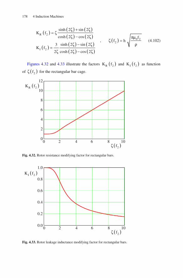
178 4 Induction Machines
( )( ) ( )
( ) ( )
( )( ) ( )
( ) ( )
( )R 2
0 22
I 2
sinh 2 sin 2K f
cosh 2 cos 2 f, f h
sinh 2 sin 23K f
2 cosh 2 cos 2
ζ + ζ= ζ
ζ − ζ πμζ =
ζ − ζ ρ=
ζ ζ − ζ
(4.102)
Figures 4.32 and 4.33 illustrate the factors ( )R 2K f and ( )I 2K f as function
of ( )2fζ for the rectangular bar cage.
Fig. 4.32. Rotor resistance modifying factor for rectangular bars.
Fig. 4.33. Rotor leakage inductance modifying factor for rectangular bars.
0 2 4 6 8 10
( )R 2K f
( )2fζ
12
10
8
6
4
2
0
0 2 4 6 8 10
( )I 2K f
( )2fζ
1.0
0.8
0.6
0.4
0.2
0.0

4.5 Possibilities for Open-Loop Speed Control 179
4.5 Possibilities for Open-Loop Speed Control
The main possibilities for open-loop speed control of induction motors can be de-duced from the following equation:
( )1fn 1 sp
= − (4.103)
4.5.1 Changing (Increasing) the Slip
Either by resistances in the rotor circuit of a slip ring rotor or by decreasing the
terminal voltage ( 21T U ) the slip is increased. In both cases the additional slip
power is transformed to heat and the efficiency is decreased:
1 sη = − (4.104)
The no-load speed does not change.
4.5.2 Changing the Supply Frequency
The power is taken from the 50Hz three-phase mains, rectified and given to an inverter via an intermediate circuit (DC-current or DC-voltage) that supplies the induction machine with variable voltage (Fig. 4.34):
Fig. 4.34. Induction motor with inverter supply.
For the Heyland-diagram (stator current locus) it follows for variable frequen-cy:
=
3 =
3
M
3
mains

180 4 Induction Machines
1 10
1 1
U UI
X f = (4.105)
0 1
1
I UI
f ∞ =
σ (4.106)
Therefore, the circle remains unchanged in its size, if the supplying voltage is changed proportional to the frequency. Then even the pull-out torque remains un-changed:
221 1
pull out1 1
1
U U3pT
fX
1
− =σω
− σ
(4.107)
But the parameterization of the Heyland-diagram is changed:
( )( )
1
1 222 1
X1tan s s f f
R 1 ∗
σ
− σϕ = =′ + σ
(4.108)
With decreasing supply frequency the stand-still operating point (starting, short-circuit) is shifted in the direction of the no-load operation point (Fig. 4.35).
Fig. 4.35. Heyland-diagram of the induction motor: different supply frequencies.
The torque-speed-characteristics are illustrated in Fig. 4.36.
Im−
Re
0I
1s 1 (f 50Hz)= =
1s 1 (f 25Hz)= =
1s 1 (f 10Hz)= =
s 0=

4.5 Possibilities for Open-Loop Speed Control 181
Fig. 4.36. Torque-speed-characteristics of the induction motor for different supply frequencies (with nominal supply frequency of 50Hz).
If the supply frequency 1f gets smaller, the stator resistance 1R has to be con-
sidered, because then 1R cannot be neglected any more against 1X . Considering
1R , the Heyland-diagram gets smaller and the pull-out torque decreases (because
of the voltage drop at 1R ). For compensating the voltage drop at 1R at low fre-
quency the voltage is reduced less than proportional to the frequency (to reach a constant stator flux).
If the further increase of the voltage with frequency is not possible (this point is called “nominal operation point”) the pull-out torque decreases inversely propor-
tional to the squared frequency, see the characteristic for 1f 60Hz= in Fig. 4.36.
This operating region is called “field weakening region”.
4.5.3 Changing the Number of Pole Pairs
As the cage rotor adopts itself to any number of pole pairs, the synchronous speed
(no-load speed) 0 1n f p= can be varied in discrete steps by changing the number
of pole pairs p. For this the stator
• can be equipped with several separated three-phase windings, placed in the same slots (high effort, small utilization) or
• contains a single winding with switchable winding segments (see Fig. 4.37).
The pole switching is used for example in the so-called “Dahlander circuit“.
0.0 0.2 0.4 0.6 0.8 1.0 1.2
pull out
T
T −
( )0 1n n f 50Hz=
1f 50Hz= 1f 25Hz= 1f 10Hz=
1f 60Hz=
1.0
0.75
0.5
0.25
0.0

182 4 Induction Machines
Fig. 4.37. Pole switching winding (with zone plan and magneto-motive force characteristics).
4.6 Star-Delta-Switching
When switching the induction machine with zero rotor speed to the mains the en-tire stall (short-circuit) current flows. This is a multiple of the nominal current. As this means a high load to the machine, the starting current has to be limited.
A possibility for limitation of this current is the introduction of series resistanc-es to the rotor circuit, if a slip ring rotor is present (please refer to Sect. 4.3).
This is not possible with cage rotors. Here, the voltage is decreased by means of a starting transformer (at high power) or by means of star-delta-switching (low and medium power).
If the motor phases are connected in star there is:
phase,Y line phase,Y line,Y
1U U , I I
3= = (4.109)
For delta connection it is true:
phase, line phase, line,
1U U , I I
3Δ Δ Δ= = (4.110)
zone plan and magneto-motive force for p=2 (case a)
zone plan and magneto-motive force for p=1 (case b)
case a switchable
case b

4.7 Doubly-Fed Induction Machine 183
As the torque is proportional to the squared phase voltage it follows:
2
phase,YY
phase,
UT 1
T U 3Δ Δ
= = (4.111)
For the mains current it follows:
phase,Y phase,Yline,Y
line, phase, phase,Y
I II 1
I 33 I 3 3 I Δ Δ
= = = (4.112)
Consequently, torque and mains current are decreased by a factor of 3 in start-ing operation. The switching to the delta connection is realized near the nominal operating point.
4.7 Doubly-Fed Induction Machine
The slip-ring rotor of an induction machine can be supplied with voltages having slip frequency (formerly the slip power was supplied by another machine set-up, today generally this is done using an inverter) (Fig. 4.38).
Fig. 4.38. Doubly-fed induction machine.
Via the inverter additional power can be fed to or drawn from the rotor. Feed-ing the power an operation above synchronous speed is reached, drawing the pow-er an operation below synchronous speed is realized (for motor operation).
Apart from the inverter losses this kind of speed control (nearly) is lossless. The advantage of this alternative is that the inverter has to be dimensioned only for the slip power. A typical application of this kind of speed control e.g. is in wind power plants (generator operation).
=
3 =
3
M
3
line
Pδ 1f
s Pδ
2 1f s f=
s Pδ
1f

184 4 Induction Machines
To calculate the torque characteristic the equivalent circuit diagram in Fig. 4.39 is regarded.
Fig. 4.39. Equivalent circuit diagram of the doubly-fed induction machine.
There is:
( ) ( )
( )
( )
1 0 21
1 0
1
22 2 2 1 1 1 1
1
2 1 1 2
212 1 1
1I I I
1
UI
jX
R U1I 1 jX 1 U
1 s 1 s
U 1 sU1I
1R 1 jsX
1
′= −+ σ
=
′ ′σ′ + σ + = + σ −
+ σ − σ
′ + σ −′ =
σ+ σ ′ + σ +− σ
(4.113)
It can be deduced that the rotor current is composed from the superposition of
two parts: The first part comes from the terminal voltage of the stator 1U , the sec-
ond part comes from the rotor voltage 2U′ which is used as control variable.
In no-load operation 2I 0′ = is true. This is fulfilled for
( )2 1
01
U 1s s
U
′ + σ′= = (4.114)
The value 0s′ is called no-load slip. As the no-load slip has to be a real number,
even 2 1U U′ has to be a real number, i.e. these two voltages have to have the
same phase angle (or opposite phase angle). Therefore, the no-load speed
1U
1I ( ) 2
1
1I
1′
+ σ
( )221
R1
s
′+ σ
1X1
σ
− σ
1X
0I
( )21
U1
s
′+ σ

4.7 Doubly-Fed Induction Machine 185
( ) ( )10 0 0 0n n n 1 s 1 s
2 p
ω′ ′ ′= = − = −
π (4.115)
can be adjusted by the voltage 2U′ ; e.g. it follows
• for 00 s 0.5′< < a no-load speed of 0 0 0n n 0.5n′> > is obtained;
• for 00.5 s 0′− < < a no-load speed of 0 0 01.5n n n′> > is obtained.
The torque can be calculated from the power of the rotating field. With
{ } 1 21
1Re I Re I
1′= −
+ σ (4.116)
it follows:
( )
( )
1 21 1 1
1 2 11
212 1 1
p 3p 1T P U Re I
1
sU U 13pU Re
R 1 jsX1
δ′= = −
ω ω + σ
′− + σ=
σω ′ + σ +− σ
(4.117)
With
( )2
2 1pull out
1
R 1s
X1
−
′ + σ=
σ
− σ
(4.118)
it follows further, if 1 1U U= is chosen being real:

186 4 Induction Machines
( )
( )( ) ( )
212
1 1
1 pull out1
21 pull out2
1 12 2
1 1 pull out
Us 1
U U3pT Re
s jsX
1
Us 1 s js
U 1 U3pRe
X s s
−
−
−
′− + σ
=σω +
− σ
′− + σ −
− σ=
ω σ +
(4.119)
Now just the rotor voltages that are in phase with the stator voltage are consid-ered (it has been shown above that only for those voltages no-load of the machine is possible), then it follows:
( )( ) ( )
( )( )
21 pull out2
1 12 2
1 1 pull out
2pull out1 2
1 2 21 1 1 pull out
Us 1 s js
U 1 U3pT Re
X s s
sU 1 U3ps 1
X U s s
−
−
−
−
′− + σ −
− σ=
ω σ +
′− σ= − + σ
ω σ +
(4.120)
Setting this torque in relation to the pull-out torque at zero rotor voltage (see Sect. 4.3), the result is:
( )
2
2
21
pull out ,U 01
1
pull out21 2 2
pull out,U 0 1 pull out
U3pT
2X
1
sUT2 s 1
T U s s
′− =
−
′− = −
=σω
− σ
′= − + σ
+
(4.121)
A further transformation finally gives:

4.7 Doubly-Fed Induction Machine 187
( )
2
21
ratiopull outpull out,U 0 1
pull out
U1
T 2sT 1s sT U
s s
−′− =
−
′+ σ
= = −
+
(4.122)
Figure 4.40 exemplarily shows the torque (in relation to the torque at 2U 0′ = )
for a machine with pull outs 0.4− ≈ as a function of speed (in relation to the syn-
chronous speed).
Fig. 4.40. Torque-speed-characteristics of the doubly-fed induction machine.
The advantage of this kind of speed control is that the inverter has to be dimen-sioned only for the slip power. Therefore it is smaller than an inverter supplying the machine on the stator side.
A disadvantage of this alternative of speed control is that only a limited speed variation can be reached (the larger the speed variation, the larger is the required power of the inverter) and that the machine has to be equipped with slip rings. This pays off only for large power machines (typically more than 500kW).
Designing the machine-side converter as a pure rectifier, it is only possible to draw power from the machine. Consequently, only the speed area below synchro-nous speed is reachable with the advantage that the power electronic complexity
0.0 0.2 0.4 0.6 0.8 1.0 1.2 1.4
2
1
U0 0.5
U
′= −
2
1
U0 0.5
U
′= +
2U 0′ = ratioT
0n n
1.0
0.8
0.6
0.4
0.2
0.0

188 4 Induction Machines
and costs is reduced considerably. Such a layout is called sub-synchronous con-verter cascade.
4.8 References for Chapter 4
Ban D, Zarko D, Mandic I (2003) Turbogenerator end winding leakage inductance calculation using a 3 D analytical approach based on the solution of Neumann integrals. In: IEEE Inter-national Electric Machines and Drives Conference (IEMDC), Madison, Wisconsin, USA
Gerling D (1999) Analytical calculation of leakage and inductivity for motors / actuators with concentrated windings. In: International Conference on Modeling and Simulation of Electric Machines, Converters and Systems (ELECTRIMACS), Lisbon, Portugal
Gerling D, Schramm A (2005) Analytical calculation of the end winding leakage inductance based on the solution of Neumann integrals. In: International Symposium on Industrial Elec-tronics (ISIE), Dubrovnik, Croatia
Gerling D, Schramm A (2005) Calculation of the magnetic field in the end winding region of un-saturated electrical machines with small air-gap. In: International Symposium on Electro-magnetic Fields in Mechatronics, Electrical and Electronic Engineering (ISEF), Baiona, Vi-go, Spain
Jordan H, Klima V, Kovacs KP (1975) Asynchronmaschinen. Vieweg Verlag, Braunschweig Jordan H, Weis M (1969) Asynchronmaschinen. Vieweg Verlag, Braunschweig Kleinrath H (1975) Grundlagen elektrischer Maschinen. Akademische Verlagsgesellschaft,
Wiesbaden Müller G, Ponick B (2009) Theorie elektrischer Maschinen. Wiley-VCH Verlag, Weinheim Nürnberg W (1976) Die Asynchronmaschine. Springer-Verlag, Berlin Richter R (1954) Elektrische Maschinen IV. Birkhäuser Verlag, Basel Seinsch HO (1993) Grundlagen elektrischer Maschinen und Antriebe. Teubner Verlag, Stuttgart Spring E (1998) Elektrische Maschinen. Springer-Verlag, Berlin

5 Synchronous Machines
5.1 Equivalent Circuit and Phasor Diagram
Like the induction machine the synchronous machine contains a stator with three-phase winding (it is a rotating field machine), but the rotor winding is supplied with DC-current. In the following the voltage equations and the equivalent circuit of the synchronous machine will be derived from those of the induction machine.
The three-phase winding of the stator is supplied from a three-phase mains with
constant voltage 1U and constant frequency 1f . The rotor shall have a three-phase
winding of the same pole number as well, which is connected to slip rings. Be-
tween two of these slip rings a DC-current is fed (excitation or field current FI ).
Therefore, the frequency of the rotor currents is 2f 0= .
According to the rotating field theory the synchronous machine is only able to produce a torque that is constant in time and different from zero, if the frequency condition is fulfilled:
2 1f s f= (5.1)
With 2f 0= and 1 linef f= it follows:
10
fs 0 n n
p= = = (5.2)
Consequently, in stationary operating conditions the rotor always rotates with
the synchronous speed 0n . At any different speed 0n n≠ an oscillating torque
with a mean value according to time equal to zero is generated. In contrary to the induction machine, which does not generate a torque for
0n n= , the synchronous machine generates a torque only at 0n n= .
Now, coming from the general circuit diagram of the induction machine with slip ring rotor, the circuit diagram of the synchronous machine will be deduced. Here the “energy generation system” is applied, because synchronous machines mainly are used as generators (Fig. 5.1).
© Springer-Verlag Berlin Heidelberg 2015 189
DOI 10.1007/978-3-642-17584-8_ 5D. Gerling, Electrical Machines Mathematica l Engineering,,

190 5 Synchronous Machines
Fig. 5.1. Equivalent circuit diagram of the synchronous machine.
The voltage equations are:
( ) ( )
21 1 1 1 1
1
22 2 21 1 1
1
21 1
1
IU R I jX I 0
1
U I R1 1 jX
s 1 s 1
IjX I
1
′+ + + =
+ σ
′ ′ ′ σ+ σ = + σ +
+ σ − σ
′+ +
+ σ
(5.3)
Multiplying the voltage equation of the rotor with s and regarding that s 0= holds true, it follows:
( )1 1 1 1 1m 1 1m 2
2 2 2
U R I j X X I jX I
U R I
σ′+ + + = −
′ ′ ′= (5.4)
2I ′ is the excitation current FI transformed to the stator side. A current 2I ′ in
the stator winding having the mains frequency will generate the same rotating
magneto-motive force (MMF) like the DC-current FI flowing in the rotor having
synchronous speed. The relation between 2I ′ and FI is as follows:
1. The number of turns of the excitation winding is:
F 2w 2w= (5.5)
2. The winding factor of the excitation (field) winding (nominated in the following with the index “F“) can be calculated by means of the rotating field theory from the distribution factor and the short-pitch factor. For the
1U
1I
( )21
U1
s
′+ σ
( ) 21
1I
1′
+ σ
1R
( )221
R1
s
′+ σ
1X1
σ
− σ
1X

5.1 Equivalent Circuit and Phasor Diagram 191
fundamental wave and a distribution of the winding in a large number of slots ( q → ∞ ) it follows, please refer to Fig. 5.2:
( )
F Z Sp
ssi sin
6 2
2 1sin6 3 2sin sin
2 36 6
3 3
2
π π
ξ = ξ ξ =τ
π ππ π
= =π ππ
=π
(5.6)
Fig. 5.2. Explanation for calculating the winding factor.
3. The fundamental waves of the MMF have to be the same in both cases:
1 1 F F2 F
F F F F F2 F
1 1 1 1
2F 2 F
1 1 1 1
w w3 4 42I I
2 p p
w w I1 2 p 2I I
p 3 w 3 w2 2
3 32w
I 2w I2 32
3 w w2 2
ξ ξ′ =
π π
ξ ξ′ = =
ξ ξ
π= =ξ ξ π
(5.7)
4. The complex value can be obtained from the fact that the current 2I ′ in
the stator winding having the mains frequency generates the same rotat-
ing magneto-motive force (MMF) in the air-gap like the DC-current FI
flowing in the rotor having synchronous speed. Against the voltage 1U
the current 2I ′ has a phase shift of angle 2ϕ (see the phasor diagram in
Fig. 5.4):
2w
2w
2 3π
π

192 5 Synchronous Machines
2j 2 2I I e − ϕ′ ′= (5.8)
The excitation current 2I′ transformed to the stator side induces a voltage at the
main reactance 1mX . This voltage is called internal machine voltage (or open-
circuit voltage or no-load voltage):6
P 1m 2U jX I′= − (5.9)
The stator voltage equation of the synchronous machine becomes:
( )1 1 1 1 1m 1 PU R I j X X I Uσ+ + + = (5.10)
From the voltage equation of the stator the circuit diagram of the synchronous machine can be deduced. The rotor part must not be considered separately, be-
cause the voltage PU induced from the excitation field into the stator winding is
already included and in stationary operating points there is no reaction from the
stator to the rotor. In Fig. 5.3 the directions of 1U and 1I are reversed against the
beginning of this chapter. Therefore, even here the “energy generation system” is used.
Fig. 5.3. Equivalent circuit diagram of the synchronous machine.
The internal machine voltage PU can be measured directly at the terminals of
the machine, if excitation with FI , driving with synchronous speed 0n and no-
load operation ( 1I 0= ) is used.
The entire phasor diagram of the synchronous machine in generator mode with resistive-inductive load is shown in Fig. 5.4.
6 This voltage sometimes is also called back emf (electromotive force) and nominated with “e”.
1U
1I 1R 1X σ 1mX
PU Uδ

5.1 Equivalent Circuit and Phasor Diagram 193
Fig. 5.4. Phasor diagram of the synchronous machine in generator mode.
The induced voltage Uδ coming from the resulting rotating air-gap field corre-
sponds to the magnetizing condition (saturation) of the machine:
1m U jX Iδ μ= − (5.11)
The internal machine voltage PU is:
P 1m 2U jX I′= − (5.12)
The armature reaction becomes:
1m 1jX I− (5.13)
The angle ϑ is called rotor angle. It shows the phase shift of the internal ma-
chine voltage PU against the voltage at the terminals 1U . In generator operation
ϑ is positive, in motor operation ϑ is negative. In no-load operation ( 1I 0= )
and operating the synchronous machine purely with reactive power ( 1 2ϕ = ± π
and 1R 0= ) the rotor angle is equal to zero ( 0ϑ = ).
Im−
Re
1I
1U
1 1R I Uδ
1 1jX Iσ
1m 1jX I
PU
1ϕ
ϑ
2I ′
I μ
2ϕ

194 5 Synchronous Machines
The angle
1Gδ = ϑ + ϕ (5.14)
is called load angle. In generator operation the excitation MMF is leading the ar-
mature MMF by G2
π+ δ , in motor operation it is lagging by G2
π− δ .
Having large synchronous machines generally the phase resistance 1R can be
neglected against the phase reactance 1X . Moreover, for the description of the op-
erating performance only the stator voltage equation is required. Therefore, the in-dices may be omitted. Then there is the following equation:
PU U jX I= + (5.15)
From this the equivalent circuit and phasor diagram (see Fig. 5.5) can be de-
duced (in the following the angle 2ϕ is not needed any longer, therefore the phase
angle 1ϕ will be used without index: 1ϕ = ϕ ).
Fig. 5.5. Equivalent circuit (above) and phasor diagram (below) of the synchronous machine.
Im−
Re
I
U
jX I
PU
ϕ
ϑ
U
I X
PU

5.2 Types of Construction 195
5.2 Types of Construction
5.2.1 Overview
Synchronous machines have the same stator construction like induction machines: A three-phase winding is placed in the slots of the lamination stack. For the rotor there are two different types of construction, see Figs. 5.6 and 5.7.
Fig. 5.6. Cylindrical rotor (non-salient pole) synchronous machine (example: p=1).
Fig. 5.7. Salient pole synchronous machine (example: p=2).
XΦ
XXX
XXX XXX
u
v w
x
y z
XXXXXX XXX
XXXXXX
N S
XΦ
XXX
XXX
XXX
u
v
w
x
y
z
XXX
XXX
XXXXXX
N
N
S S
u
XXXx
v
XXX
y
XXXz
w

196 5 Synchronous Machines
5.2.2 High-Speed Generator with Cylindrical Rotor
If synchronous generators are driven by steam or gas turbines (thermal power sta-tion) the speed is chosen as high as possible to reach an as good as possible tur-bine efficiency. For a mains frequency of 50Hz the maximum speed is
13000 min− (2-pole construction, i.e. p 1= ). The rotor diameter is limited by the
accelerating forces. Because of the high mechanical stress the rotor construction is chosen being cylindrical. The volume required for the desired power is achieved by using a quite long rotor.
5.2.3 Salient-Pole Generator
The turbines of hydroelectric power stations rotate at very low speed
( 1100 750 min− ). To adapt this speed to the mains frequency the number of pole pairs have to be chosen very large ( p 30 4= ). As the acceleration forces are
low (because of the low speed) single poles with concentric excitation coils may be realized. The salient-pole synchronous generator has a large diameter and a short axial length. Using this construction type the air-gap is not constant at the circumference of the rotor, i.e. the magnetic reluctance varies at the circumfer-ence.
5.3 Operation at Fixed Mains Supply
5.3.1 Switching to the Mains
The synchronous machine may only be switched to the mains with constant volt-age and frequency (Fig. 5.8), if the following conditions for synchronization are fulfilled:
• The synchronous machine is rotated by a driving motor with synchronous
speed: 0n n= .
• The excitation current FI of the synchronous machine is adjusted so that the
generator voltage is equal to the mains voltage: gen lineU U= .

5.3 Operation at Fixed Mains Supply 197
• The phase sequence of the terminal voltages of generator and mains have to be the same: abc – uvw.
• The phase shift of the voltage systems of generator and mains must be identi-cal, i.e. the voltage difference at the terminals that shall be connected must be zero: U 0Δ = .
If these conditions for synchronization are not fulfilled, there are very high torque and current pulsations after switching the generator to the mains.
Fig. 5.8. Principle diagram of switching a synchronous machine to the mains
The phase shift of the voltage systems of generator and mains is illustrated in Fig. 5.9.
Fig. 5.9. Phase shift of the voltage systems of generator and mains.
a b
c
V V V
drive
FU
FI
V
V
UΔ
lineU
genU
a b
v
c
u w
lineU genU
UΔ
Δω

198 5 Synchronous Machines
5.3.2 Torque Generation
The torque can be calculated from the rotating field power divided by the syn-
chronous angular frequency. Neglecting the stator losses ( 1R 0= ) the input active
power equals this rotating field power:
( )
0 1
3UI cosPT
pδ ϕ
= =Ω ω
(5.16)
The phasor diagram of the synchronous machine is shown in Fig. 5.10:
Fig. 5.10. Phasor diagram of the synchronous machine.
From this it can be deduced:
( ) ( )
( ) ( )
P
P
XI cos U sin
UI cos sin
X
ϕ = ϑ
ϕ = ϑ (5.17)
Therefore, the torque becomes:
( ) ( )Ppull out
1
UU3pT sin T sin
X−= ϑ = ϑ
ω (5.18)
Im−
Re
I
U
jX I
PU
ϕ
ϑ
ϕ
( )XI cos ϕ

5.3 Operation at Fixed Mains Supply 199
This torque equation is true only for stationary operating points with
FI const.= and 0n n= . Generator operation is given for 0ϑ > , motor operation
is given for 0ϑ < . A stable operation is possible only for 2 2− π < ϑ < π : In-
creasing the load slowly, the torque and the rotor angle ϑ are increased as well,
until the synchronous machines reaches the pull-out torque at 2ϑ = ± π and the
machine falls out of synchronism. As a motor the machine stops, as a generator it runs away. High oscillating torque components do occur, combined with high cur-rents pulses. In this case the synchronous machine has to be disconnected from the mains immediately.
These characteristics are illustrated in Fig. 5.11.
Fig. 5.11. Torque versus rotor angle characteristic of the synchronous machine.
The overload capability of a synchronous machine is:
( ) ( )
N P
pull out 1 P
N N NN N N
1
U U3p
T X U
3pT XI cosU I cos
− ω= =
ϕϕ
ω
(5.19)
In practice, often an overload margin of pull out
N
T1, 6
T
−> is called for. A measure
for the stability in stationary operation is the synchronizing torque (also see Fig. 5.12):
( )syn pull out
dTT T cos 0
d−= = ϑ >
ϑ (5.20)
stable
T
ϑ
Nϑ
NT
pull outT −

200 5 Synchronous Machines
Fig. 5.12. Synchronizing torque of the synchronous machine.
The larger dT dϑ , the larger is the restoring torque synT after a load step. The
smaller the absolute value of ϑ , the more stable is the operating point.
5.3.3 Operating Areas
There is:
( ) ( )( )
( ) ( )( )
jP P P
j
U U e U cos jsin
I Ie I cos jsin
ϑ
− ϕ
= = ϑ + ϑ
= = ϕ − ϕ (5.21)
Consequently (if the terminal voltage U is defined being in the real axis):
( ) ( )( ) ( ) ( )( )P
PU U jX I
U cos jsin U jXI cos jsin
= +
ϑ + ϑ = + ϕ − ϕ (5.22)
Separated into real and imaginary parts it follows:
( ) ( ) ( )( )
( ) ( ) ( ) ( )
PP
PP
U cos UU cos U XI sin I sin
X
UU sin XI cos I cos sin
X
ϑ −ϑ = + ϕ ϕ =
ϑ = ϕ ϕ = ϑ
(5.23)
From this four operating areas can be deduced. In the “power generation mod-el” they look like follows:
T
ϑ
synT
synT, T

5.3 Operation at Fixed Mains Supply 201
• ( )I cos 0ϕ > ( 0ϑ > ): production of active power
(generator)
• ( )I cos 0ϕ < ( 0ϑ < ): consumption of active power
(motor)
• ( )I sin 0ϕ > ( ( )PU cos Uϑ > ): delivering reactive power
(over-excited) machine operates as a capacitor
• ( )I sin 0ϕ < ( ( )PU cos Uϑ < ): consumption of reactive power
(under-excited) machine operates as an inductor
The characteristic phasor diagrams are illustrated in Fig. 5.14. The active power is determined only by the driving turbine (generator opera-
tion) or by the load torque (motor operation). The reactive power can be adjusted independently just by the excitation (deliv-
ering reactive power when being over-excited, consuming reactive power when being under-excited). This is illustrated in Fig. 5.13; the phasors belonging to dif-ferent excitations are shown in different colors (the phasors of voltage and current are presented in the same color).
Fig. 5.13. Phasor diagram of the synchronous machine and different excitations.
Im−
Re
I
U jX I
PU
PU
I
jX I
( )XI cos ϕ
( )XI sin ϕ
( )I cos ϕ

202 5 Synchronous Machines
Fig. 5.14. Operating areas of the synchronous machine.
Sometimes synchronous machines are used as reactive power generators with-out producing active power for phase shift operation. With this the inductive reac-tive power of transformers or induction machines can be compensated and there-
generator
motor
capacitor inductor
Im−
Re
I
U jX I
PU ϕ
ϑ
Im−
Re
I
U
jX I
PU
ϕ
ϑ
Im−
Re
I
U jX I
PU ϕ
ϑ
Im−
Re
I
U
jX I
PU
ϕ
ϑ

5.3 Operation at Fixed Mains Supply 203
fore the load of the mains can be reduced. Then the internal machine voltage PU
is in phase with the terminal voltage U ; the current I is a pure reactive current
(in phase shift operation the machine may be over-excited or under-excited). In
no-load operation the current is I 0= and PU and U are identical (same ampli-
tude and phase).
5.3.4 Operating Limits
From
PU U jX I= + (5.24)
and
jP P N,phaseU U e , U Uϑ
= = (5.25)
it follows for the current:
jP N,phase N,phase j P
jj N,phase N,phase2 P2
N N N,phase N
U e U U UI j je
jX X X
U UUIe e
I I X U I X
ϑ
ϑ
ππ − +ϑ
−= = −
= +
(5.26)
With P FU I and ( )P F F,0 N,phaseU I I U= = (no-load) it follows:
P F
N,phase F,0
U I
U I= (5.27)
The reactance X related to the nominal impedance is:
N
N,phase N N,phase
I XXx
U I U= = (5.28)
Consequently the current becomes:

204 5 Synchronous Machines
jj
2 F2
N F,0
II 1 1e e
I x I x
ππ − +ϑ
= + (5.29)
From this equation the current diagram of the synchronous machine together with the operation limits can be deduced (Fig. 5.15).
Fig. 5.15. Operating limits of the synchronous machine.
Im−
Re
NI I
U
ϕ
ϑ
limit of rotor heating
F F,NI I≤
limit of stator heating
NI I≤
stability limit 2
πϑ <
limit of active power
( ) N
N,phase1
TI cos
3pU
ϕ ≤
ω
j2
1e
x
π
j2 F
F,0
I 1e
I x
π− +ϑ

5.4 Isolated Operation 205
5.4 Isolated Operation
5.4.1 Load Characteristics
Having a single synchronous machine as a generator connected with some loads, this is called “isolated operation”. Typically, such an operation is used where a connection to the grid would require very long distances and therefore would im-ply unreasonable high costs. Frequently, synchronous machines in isolated opera-tion are driven by wind or hydroelectric power stations.
Contrary to the previous considerations, no stable grid can be assumed any more, but the voltage at the terminals of the generator changes with the load (even with constant excitation current).
At first, the well-known phasor diagram of the synchronous machine (Fig. 5.16) can be taken as a basis:
Fig. 5.16. Phasor diagram of the synchronous machine.
From this phasor diagram it follows:
( )( ) ( )( )
( ) ( )
2 2 2P
22 2P
U XI sin XI cos U
U 2UXI sin XI U
+ ϕ + ϕ =
+ ϕ + = (5.30)
For 0n n= and F F,0I I= there is: P N,phaseU U= (this voltage can be meas-
ured at the terminals of the synchronous machine at no-load operation). Further:
Im−
Re
I
U
jX I
PU
ϕ
ϑ
ϕ
( )XI cos ϕ

206 5 Synchronous Machines
( ) ( )
( )
( )
22 2N,phase
2 2
N,phase N,phase N,phase N,phase
2 2
N,phase N,phase N N
U 2UXI sin XI U
U U XI XI2 sin 1
U U U U
U U I I2 x sin x 1
U U I I
+ ϕ + =
+ ϕ + =
+ ϕ + =
(5.31)
Herewith, the so-called load characteristics (terminal voltage U of the genera-tor depending on the load current I ) of the synchronous machine in isolated oper-ation are given. Figure 5.17 shows the terminal voltage U as a function of the
load current I for different loads ( )cos ϕ .
Fig. 5.17. Load characteristics of the synchronous machine in isolated operation.
For resistive-inductive loads the voltage decreases with increasing load, for purely capacitive loads the voltage increases with increasing load (for resistive-
( ) ( )cos 0 1 cap.ϕ =
( ) ( )cos 0 1 ind.ϕ =
0 0.2 0.4 0.6 0.8 1
2
1.8
1.6
1.4
1.2
1
0.8
0.6
0.4
0.2
0
N,phase
U
U
N
Ix
I

5.4 Isolated Operation 207
capacitive loads with phase angles less than 30 6° π the voltage may even de-
crease, depending on the value of the load current).
5.4.2 Control Characteristics
Even in isolated operation the loads should be connected to a constant voltage source, independent from the load current. Therefore, the excitation current has to be controlled in dependency of the load (amplitude and phase shift of the load cur-rent). From the phasor diagram (Fig. 5.16) it follows with the requirement
N,phaseU U= :
( ) ( )22 2
N,phase N,phase PU 2U XI sin XI U+ ϕ + = (5.32)
With P F
N,phase F,0
U I
U I= it follows further:
( )
( )
2
F
F,0 N,phase N,phase
2
N N
2XI sinI XI1
I U U
I I1 2x sin x
I I
ϕ= + +
= + ϕ +
(5.33)
With this the so-called control characteristics (excitation current FI of the
generator in dependency of the load current I ) of the synchronous machine in iso-lated operation are given, to fix the terminal voltage to the constant nominal volt-
age at synchronous speed 0n n= . Figure 5.18 shows the excitation current FI as
a function of the load current I for different loads ( )cos ϕ .
For resistive-inductive loads the excitation current has to be increased to fix the terminal voltage to the nominal voltage at increasing load; for purely capacitive loads the excitation current has to be decreased (for resistive-capacitive loads with
phase angles less than 30 6° π the excitation current maybe has to be in-
creased, depending on the value of the load current).

208 5 Synchronous Machines
Fig. 5.18. Control characteristics of the synchronous machine in isolated operation.
In Fig. 5.19 the main load and control characteristics are summarized.
Fig. 5.19. Main load (left) and control (right) characteristics of the synchronous machine in iso-lated operation for zero (capacitive and inductive) and unity power factor in red, blue, and black, respectively.
( ) ( )cos 0 1 ind.ϕ =
( ) ( )cos 0 1 cap.ϕ =
0 0.2 0.4 0.6 0.8 1
2
1.8
1.6
1.4
1.2
1
0.8
0.6
0.4
0.2
0
F
F,0
I
I
N
Ix
I
0 1
1
2 N,phase
U
U
N
Ix
I
0 1
1
2
N
Ix
I
F
F,0
I
I
2

5.5 Salient-Pole Synchronous Machines 209
5.5 Salient-Pole Synchronous Machines
Because of the distinct single poles the air-gap on the circumference of the salient-pole machine is not constant (contrary to the induction machine or the non salient-pole synchronous machine). Therefore, a simple summation of the rotating magne-to-motive forces of stator and rotor is not allowed to get the resulting air-gap field. In fact, the magneto-motive force of the stator has to be decomposed in two com-ponents, one in parallel to the rotor pole axis (d-axis, direct axis), and the other perpendicular to the rotor pole axis (q-axis, quadrature axis):
( )
( )d
q
G
G
sin
cos
Θ = Θ δ
Θ = Θ δ (5.34)
This is illustrated in Fig. 5.20.
Fig. 5.20. Magneto-motive forces of the salient-pole synchronous machine.
Similarly, the main reactance has to be decomposed according to the d- and q-axis (because of the different air-gap widths in d- and q-axis):
d md 1
mq mdq mq 1
X X X, X X
X X X
σ
σ
= +<
= + (5.35)
Now, the phasor diagram (Fig. 5.21) can be drawn (the stator resistance 1R
further is neglected).
XXX
XXX XXX
u
v w
x
y z
XXX
Gδ FΘ
Θ
qΘ
dΘ axis of the phase u
ϕ
ϑ

210 5 Synchronous Machines
Fig. 5.21. Phasor diagram of the salient-pole synchronous machine.
By decomposing the magneto-motive force of the stator into the components, the armature reaction is determined separately for d- and q-direction and the result is superposed.
Thus, from the original system with three stator phases a two-phase system is generated as a replacement, see Fig. 5.22.
Im−
Re
I
U
PU
ϕ
ϑ
d djX I
q qjX I
q d
qI
dI

5.5 Salient-Pole Synchronous Machines 211
Fig. 5.22. Sketch of the salient-pole synchronous machine: original system (above left), replace-ment (above right) and two-phase replacement (below).
The main reactances (synchronous reactances) dX and qX can be measured:
For this the stator winding is energized and the rotor – with open excitation wind-ing – is driven with nearly synchronous speed. Because of the small slip between rotating field of the stator and the rotor the respective axes are alternately coinci-dent or perpendicular. From the ratio of the oscillographically measured phase voltage and phase current the reactance can be calculated; this reactance is oscil-
lating between the extreme values dX and qX .
Performing this measurement with a single phase at stand-still, the result will be falsified because of the short-circuited damper winding and the eddy currents in the massive iron parts. The measured values will be too small.
ud id
uq
iq
uF
iF
XXX
XXX XXX
u
v w
x
y z
XXX
( )tγ
uu
( )tγ
iu
uv
uw
iv
iw
uF
iF
212 5 Synchronous Machines
Decomposing the voltage U into the components in d- and q-direction, there is
(please refer to the phasor diagram in Fig. 5.21):
( )
( )
jP d d
jq q
U cos e U jX I
jU sin e jX I
ϑ
ϑ
ϑ = −
ϑ = (5.36)
From this it follows for the stator current:
( ) ( )j j
P d q
d q
U cos e U jU sin eI I I
jX jX
ϑ ϑϑ − ϑ
= + = +−
(5.37)
With ( ) ( )je cos j sinϑ= ϑ + ⋅ ϑ it follows further:
( ) ( ) ( )( )
( ) ( ) ( )( )
( ) ( ) ( )( )
( ) ( ) ( )( )
P
d
q
2P
d
2
q
U cos cos j sin UI j
X
U sin cos j sin
X
1jU cos U cos sin jU
X
1U cos sin jU sin
X
ϑ ϑ + ϑ −=
ϑ ϑ + ϑ+
= ϑ − ϑ ϑ −
+ ϑ ϑ + ϑ
(5.38)
With ( ) ( ) ( )1
cos x sin x sin 2x2
= the following is true:
( ) ( )
( ) ( )
2P
d
2
q
1 1I jU cos U sin 2 jU
X 2
1 1U sin 2 jU sin
X 2
= ϑ − ϑ −
+ ϑ + ϑ
(5.39)
and further
5.5 Salient-Pole Synchronous Machines 213
( )
( ) ( )
q d
2 2P
d q d
1 1 1I U sin 2
2 X X
1 1 1j U cos U sin U
X X X
= ϑ −
+ ϑ + ϑ −
(5.40)
An additional transformation with ( ) ( )( )2 1sin x 1 cos 2x
2= − and
( ) ( )( )2 1cos x 1 cos 2x
2= + leads to:
( )
( )( ) ( )( )
( )
( )
q d
Pd q d
q d
Pd q d q d
1 1 1I U sin 2
2 X X
1 1 1 1 1j U 1 cos 2 U 1 cos 2 U
2 X 2 X X
1 1 1U sin 2
2 X X
1 1 1 1 1 1 1j U U cos 2 U
2 X X 2 X X X
= ϑ −
+ + ϑ + − ϑ −
= ϑ −
+ + + ϑ − −
(5.41)
Choosing the terminal voltage as real value ( U U= , please refer to the phasor
diagram in Fig. 5.21), it follows with ( ) ( )P P PU U cos jU sin= ϑ + ϑ and
( ) ( )[ ]jI Ie I cos jsin− ϕ= = ϕ − ϕ :
{ } ( )
( )
( )
q d q d
Pd
Im I I sin
1 1 1 1 1 1U U cos 2
2 X X 2 X X
1U cos
X
= − ϕ
= + − ϑ −
− ϑ
(5.42)
and

214 5 Synchronous Machines
{ } ( )
( ) ( )Pq d d
Re I I cos
1 1 1 1U sin 2 U sin
2 X X X
= ϕ
= ϑ − + ϑ (5.43)
Neglecting the losses the torque can be calculated from the power of the rotat-ing field:
( )
( ) ( )
1
0 1 1
2P
1 d q d
3UI cosP PT
2 n p p
UU3p U 1 1sin sin 2
X 2 X X
δ ϕ= = =
π ω ω
= ϑ + − ϑω
(5.44)
The first summand corresponds to the torque of the non salient-pole synchro-nous machine which is excitation-dependent, the second summand is the so-called reaction torque which is excitation-independent (caused by the difference of the magnetic reluctances in d- and q-axis). Because of this reaction torque the pull-out torque of the salient-pole synchronous machine is reached at smaller rotor angles
than 2π , please refer to Fig. 5.23. Moreover, it can be deduced from that figure,
that the salient-pole machine – because of the additional reaction torque – delivers a higher pull-out torque than the non salient-pole machine, compared at the same
excitation current (assuming d,salient pole non salient poleX X− −= ). Additionally, it be-
comes obvious that for the assumed ratio d qX 2X= the pull-out torque without
excitation (i.e. the reaction pull-out torque) is only half of the pull-out torque of the non salient-pole synchronous machine.
From the equations for the real part and the imaginary part of the stator current the ratio of reactive power to active power (as a function of rotor angle and excita-tion) can be deduced:
( )
( )
( ) ( )
( ) ( )
P
q d q d d
P
q d d
UI sinQ
P UI cos
U1 1 1 1 1cos 2 2 cos
X X X X U X
U1 1 1sin 2 2 sin
X X U X
ϕ=
ϕ
− + + ϑ − + ϑ
=
ϑ − + ϑ
(5.45)

5.5 Salient-Pole Synchronous Machines 215
From active and reactive power the power factor can be calculated like follows:
( )2 2
Pcos
P Qϕ =
+ (5.46)
In Figs. 5.23 to 5.25 the characteristics are presented as a function of the rotor
angle ϑ and for different excitations PU U .
• ratioT : the torque of the salient-pole machine relative to the pull-out torque of
the non salient-pole machine with nominal excitation ( PU U 1.0= ) and
comparable machine data ( d,salient pole non salient poleX X− −= ) is shown in Fig.
5.23,
• ratioP : the ratio of reactive power to active power is presented in Fig. 5.24,
• ( )cos ϕ : Figure 5.25 depicts the power factor.
Especially for non-excited rotors (i.e. synchronous reluctance machines, red
characteristic in Figs. 5.23 to 5.25) it is decisive to realize a high ratio of d qX / X
to improve the torque capability as well as the power factor.
Fig. 5.23. Torque versus rotor angle with the parameter excitation.
ϑ π
ratioT 3
2
1
0
-1
-2
-3
-1 -0.5 0 0.5 1
salient-pole machine:
red: PU U 0=
blue: PU U 0.5=
green: PU U 1.0=
magenta: PU U 2.0=
non salient-pole machine:
black: PU U 1.0=

216 5 Synchronous Machines
Fig. 5.24. Ratio of reactive power to active power with the parameter excitation.
Fig. 5.25. Power factor versus rotor angle with the parameter excitation.
ϑ π
ratioP 6
4
2
0
-2
-4
-6
-1 -0.5 0 0.5 1
salient-pole machine:
red: PU U 0=
blue: PU U 0.5=
green: PU U 1.0=
magenta: PU U 2.0=
non salient-pole machine:
black: PU U 1.0=
ϑ π
( )cos ϕ
1.0
0.5
0.0
-0.5
-1.0
-1 -0.5 0 0.5 1
salient-pole machine:
red: PU U 0=
blue: PU U 0.5=
green: PU U 1.0=
magenta: PU U 2.0=
non salient-pole machine:
black: PU U 1.0=

5.6 References for Chapter 5 217
5.6 References for Chapter 5
Kleinrath H (1975) Grundlagen elektrischer Maschinen. Akademische Verlagsgesellschaft, Wiesbaden
Müller G, Ponick B (2009) Theorie elektrischer Maschinen. Wiley-VCH Verlag, Weinheim Richter R (1963) Elektrische Maschinen II. Birkhäuser Verlag, Basel Seinsch HO (1993) Grundlagen elektrischer Maschinen und Antriebe. Teubner Verlag, Stuttgart Spring E (1998) Elektrische Maschinen. Springer-Verlag, Berlin

6 Permanent Magnet Excited Rotating Field Machines
6.1 Rotor Construction
Having a synchronous machine and substituting the DC excitation current (which generates a constant magnetic field according to time) by an excitation with per-manent magnets, the following is saved
• voltage source for the excitation current, • excitation winding and • excitation current supply via slip rings and brushes.
However, the excitation field is no longer controllable. Figure 6.1 illustrates different alternatives for the positioning of the permanent magnets (surface mounted permanent magnet machines, also called SPM or SMPM machines and interior permanent magnet machines, also called IPM machines, which carry the permanent magnets inside the rotor iron).
Fig. 6.1. Different alternatives of positioning the permanent magnets in the rotor: a) surface magnets; b) inset magnets; c) to f) buried magnets; the main magnetic axes are described with d and q.
q q q
q q q
d d d
d d d
a) b) c)
d) e) f)
© Springer-Verlag Berlin Heidelberg 2015 219
DOI 10.1007/978-3-642-17584-8_ 6D. Gerling, Electrical Machines Mathematica l Engineering,,

220 6 Permanent Magnet Excited Rotating Field Machines
6.2 Linestart-Motor
Incorporating a starting cage into such a permanent magnet synchronous machine, it is called “linestart-motor“: The motor is supplied directly from the line voltage, the speed-up is realized as an induction motor. Near to the synchronous speed the rotor is synchronized to the rotating field. Then the machine operates as synchro-nous motor at the line.
The advantages of self-starting, good power factor, and high efficiency during operation are opposed by a small utilization (because of the combination of two different machine types in the rotor). In addition, during starting operation the permanent magnets produce considerable torque pulsations as the frequencies of the magneto-motive force waves are not identical (please refer to Sect. 3.7). Ap-plications for such linestart-motors are drives with very long operation duration and small power (e.g. small pumps and blowers, etc.).
6.3 Electronically Commutated Rotating Field Machine with Surface Mounted Magnets
6.3.1 Fundamentals
Again, the synchronous machine contains permanent magnets to generate the exci-tation field, but now no starting cage is present. The machine is supplied by an in-verter which realizes a sinusoidal three-phase current system.
For explaining the operational behavior it is recommended to start with the simplified equivalent circuit of the synchronous machine (Sect. 5.1), but with the following changes:
• The “energy consumption system” is applied, because mostly this machine type is used as a motor.
• The stator resistance R will be considered, because neglecting (e.g. for motors with small power or operation at low frequency) often is not allowed.
• In this chapter rotors with surface mounted magnets are regarded (so-called surface-mounted permanent magnet machines, SPM or SMPM machines). This means that the magnetically effective air-gap length is constant along the cir-cumference, as permanent magnets have a relative permeability near to 1 (i.e. near to the value of air). Therefore, the inductivities in d- and q-direction are the same and they do not have to be distinguished.

6.3 Electronically Commutated Rotating Field Machine with Surface Mounted Magnets 221
The equivalent circuit diagram is shown in Fig. 6.2.7
Fig. 6.2. Equivalent circuit diagram of the permanent magnet excited rotating field machine.
The fundamental frequency of the supplying three-phase system determines the frequency of the rotating magneto-motive force and therefore even the rotor speed. The rotating magneto-motive force together with the field of the permanent mag-net rotor generates the torque. Mostly, this torque shall be as smooth as possible. The rotation of the rotating stator field is realized depending on the rotor position by means of the inverter in such a way, that the electrical angle between rotating
magneto-motive force of the stator and the rotor field is 2π (i.e. ϑ = −ϕ ). With
this the load angle in the “energy consumption system” becomes
M G 0δ = −δ = −ϑ − ϕ = (please compare to the load angle Gδ in the “energy
generation system” in Sect. 5.1). The rotor position can be measured by using sen-sors or it can be deduced from the terminal voltages and/or terminal currents. The explained operation is described by the phasor diagram (see Fig. 6.3).
Fig. 6.3. Phasor diagram of the permanent magnet excited rotating field machine.
7 The internal machine voltage (open-circuit voltage, no-load voltage) PU sometimes is also
called “back emf” (electromotive force) and nominated with “e”.
U
I R X
PU
Im−
Re
I
U
PU
ϕ
ϑ
q d
R I
jX I

222 6 Permanent Magnet Excited Rotating Field Machines
As this machine type mostly is used as a motor, the relations are given here for the “energy consumption system“.
An operation is obtained that does no longer correspond to the synchronous machine, but to the DC-machine:
• DC-machine: magneto-motive force of the armature and excitation field build
an electrical angle of 2π ; this adjustment is realized mechanically by means
of the commutator. • Synchronous machine: the rotor angle ϑ and the phase angle ϕ are adjusted
depending on the operation point; there is no active influence on the phase shift between magneto-motive force of the stator and excitation field.
• Electronically commutated permanent magnet excited rotating field machine: magneto-motive force of the stator and rotor field build an electrical angle of
2π ; this adjustment is realized electronically by means of the inverter.
This machine topology shows very good dynamics and the control is quite sim-ple. The brushless technology is wear-resistant and maintenance-free. This kind of motor often is used for machine tool drives and for robot drives.
From the phasor diagram there is:
PU U R I jX I= + + (6.1)
The input active power is:
( )21 P loss,1P 3 U I RI P Pδ= + = + (6.2)
Now, the torque can be calculated from the rotating field power:
P1 1
P 3pT U I
pδ= =
ω ω (6.3)
To achieve good operational characteristics as a motor (generally the torque should be as smooth as possible), the permanent magnet field, the stator winding and the motor supply have to be adjusted to each other very carefully. Some ex-amples are given in the next sections.
6.3.2 Brushless DC-Motor
Firstly, a motor without short-pitch winding (i.e. a motor with diameter winding) and a two-pole ( p 1= ), radially magnetized permanent magnet ring is regarded.

6.3 Electronically Commutated Rotating Field Machine with Surface Mounted Magnets 223
The three phases of the motor (usually in star connection) are supplied from a three-phase inverter (illustrated by the six switches in Fig. 6.4). The electrical
power is drawn from the DC-voltage DCU .
Fig. 6.4. Two-pole permanent magnet excited rotating field machine (left) and power electronic supply (right).
In the following the torque will be calculated from the change of the flux link-age with respect to the rotational angle (in the linear case it follows for a single
phase of the motor magT W∂
=∂α
and mag0
1W id i
2
Ψ
= Ψ = Ψ ):
m m
kk k
k 1 k 1
d1T T i
2 d= =
Ψ= =
α (6.4)
Here pα = β is the mechanical angle ( β is the electrical angle) and m is the
number of phases. In this special case there is α = β (because of p 1= ).
The characteristics of flux linkage, change of flux linkage, current, and torque are shown in Fig. 6.5. It can be deduced that the chosen current characteristics lead to an ideally smooth torque characteristic.
Because of the kind of operation, which is similar to the operation of a DC-motor, and because of the sectional DC-characteristic of the currents (which is the same as for DC-motors), the names of this kind of motor (together with the kind of operation) are derived:
• electronically commutated DC-motor (sometimes referred to as EC-motor); • brushless DC-motor, BLDC-motor (which is most common).
DCU
u
x
v
y z
w

224 6 Permanent Magnet Excited Rotating Field Machines
Fig. 6.5. Flux linkage, its derivative, phase current and torque versus electrical angle.
kd
d
Ψ
β
π 2π β
uΨ vΨ wΨ
ki
π 2π β
kT, T
π 2π β
kΨ
π 2π β

6.3 Electronically Commutated Rotating Field Machine with Surface Mounted Magnets 225
It can be deduced that for square-wave currents only two phases are energized at the same time. This current waveform is optimally adapted to the radial magnet-ization of the permanent magnets to achieve the smoothest possible torque charac-teristic (when neglecting the slotting effect).
It has to be emphasized here that the Eqs. (6.1) to (6.3) and the phasor diagram (Fig. 6.3) are only valid for sinusoidal voltages and currents. Nevertheless, the torque calculation according to Eq. (6.4) is valid for any time-dependency, please refer to Chap. 1. Therefore the shown characteristics in Fig. 6.5 are valid.
However, to achieve a torque characteristic as smooth as possible the flux per phase characteristics of the brushless DC-motor may be different from the above shown functions outside of the power-on time of the respective phase currents. From this additional degree of freedom the possibility to choose the magnetization or the winding layout differently arises.
For example the torque contribution of each phase and the entire torque remain unchanged, if the value of the derivative of the flux linkage of each phase is
changed at the discontinuity of the flux linkage characteristic in a range of 6± π
(e.g. because of a gap between two poles or because of magnetic leakage between two poles). Therefore, trapezoidal flux linkage characteristics because of leakage together with ideal square-wave currents generate a constant torque, as long as the constant part of this trapezoidal characteristic is not less than the critical power-on
time period of 2 3π .
However, the practical realization of steep current slopes (square-wave cur-rents) require especially in the middle and upper speed region with high induced back emf voltages a high voltage reserve of the inverter. This means an overdi-mensioning of the inverter and consequently high costs. In addition, high acoustic noise is generated, which is not acceptable for many applications. Therefore, in many cases a deviation from the idealized square-wave current is accepted, which is accompanied by a higher torque oscillation, but even lower costs and lower acoustic noise.
Another often used winding topology can be deduced from the above described diameter winding by incorporating an extreme short-pitch: the winding of a phase is concentrated onto one stator tooth; please refer to Fig. 6.6 for a four-pole motor.
This winding topology contains two main advantages:
• The conductor length in the end winding is extremely short; this means a low stator resistance as well as low copper weight. Consequently, cost and losses are reduced.
• With a respective geometry of the lamination (e.g. stator teeth with parallel shoulders or separated lamination) the coils can be wound before and then mounted to the teeth. This reduces the manufacturing costs.

226 6 Permanent Magnet Excited Rotating Field Machines
Fig. 6.6. Four-pole permanent magnet excited rotating field machine.
Generally, using this concentrated winding means that the width of a rotor pole is larger than the width of a stator tooth. Therefore, the flux linkage characteristic
is trapezoidal: for a part of the rotor rotation, always parts of 2 2 2 3 3π − π = π
electrical degrees, the flux in the stator coil is unchanged; this is different to the above example of the two-pole machine with diameter winding.
In practice this extreme short-pitch winding is characterized by torque dips, be-
cause the parts with constant d dΨ α are shortened and the magnetic leakage at
the pole edges (transition between north and south pole) becomes more prominent. Flux linkage, change of flux linkage, current, and torque for this case are
shown in Fig. 6.7 for idealized assumptions: To achieve a torque as smooth as possible even in practice the following means
can be implemented:
• skewing of the stator slots or the rotor poles (disadvantages: high costs, flux leakage);
• distributed, short-pitch two-layer winding (disadvantage: high costs); • choosing a fractional number for the ratio of stator slots and rotor poles (disad-
vantage: for non-symmetric winding topologies there are radial forces onto the rotor);
• sinusoidal flux linkage combined with sinusoidal currents (disadvantage: com-plex current shaping).
u
x
x
u
v
y v
y
w
z
z
w

6.3 Electronically Commutated Rotating Field Machine with Surface Mounted Magnets 227
Fig. 6.7. Flux linkage, its derivative, phase current and torque versus electrical angle.
kΨ
π
2π
β
kT, T
π
2π
β
ki
π
2π
β
uΨ vΨ
wΨ
kd
d
Ψ
β
π
2π
β

228 6 Permanent Magnet Excited Rotating Field Machines
6.3.3 Electronically Commutated Permanent Magnet Excited Synchronous Machine
Operating the supplying inverter appropriately with high switching frequency (at low power the switching frequency for the voltage waveform generally is above the human threshold of hearing of about 20kHz ), the phase currents of the motor can be nearly sinusoidal because of the low-pass effect of the phase impedances. With this an artificial three-phase system with variable voltage and variable fre-quency is realized. The permanent magnet excited synchronous machine supplied by such a frequency variable sinusoidal current system in literature often is re-ferred to as “permanent magnet synchronous machine (PMSM)” or “brushless AC operation”.
A motor construction that is adapted concerning winding topology and magnet design to this sinusoidal operation (to reach a smooth torque) is illustrated in Fig. 6.8.
Fig. 6.8. Two-pole (diametrically magnetized) permanent magnet excited rotating field machine.
The two-pole rotor is magnetized diametrically and it generates a sinusoidal air-gap field. The stator contains a diameter winding.
The idealized characteristics of flux linkage, change of flux linkage, currents, and torque are shown in Fig. 6.9.
u
x
v
y z
w

6.3 Electronically Commutated Rotating Field Machine with Surface Mounted Magnets 229
Fig. 6.9. Flux linkage, its derivative, phase current and torque versus electrical angle.
kΨ
π 2π β
uΨ vΨ wΨ
ki
π 2π β
kd
d
Ψ
β
π 2π β
kT, T
π 2π β
230 6 Permanent Magnet Excited Rotating Field Machines
From
m
kk
k 1
d1T i ,
2 d p
=
Ψ β= α =
α (6.5)
it follows:
m
kk
k 1
dpT i
2 d=
Ψ=
β (6.6)
However, considering the magnetic leakage at the pole edges (transition be-tween north and south poles with not perfectly shaped poles) the torque is not in-creasing linearly with the number of pole pairs. With increasing number of pole pairs the leakage percentage (depending on the geometry) gets increasing rele-vance and consequently there is an optimum at moderate numbers of pole pairs.
6.4 Calculation of the Operational Characteristics; Permanent Magnet Excited Machines with Buried Magnets
To calculate the operation conditions of the above described machines, it is possi-ble using the “Rotating Field Theory” (Chap. 3) for the permanent magnet excited synchronous machine (PMSM), because this machine shows sinusoidal voltages and currents. However, this is not possible for the brushless DC-machine (BLDC), because this kind of operation makes step-by-step DC-currents necessary. As the machine topology of both alternatives can be described with the same equations (just the supply is different), the calculation of the operational characteristics shall be done using a theory where arbitrary current waveforms can be used. This theo-ry is the “Space Vector Theory” dealt with in Chap. 11. Therefore, the operational characteristics of PMSM and BLDC will be described in the later Chap. 14. In this chapter even the possibility of buried magnets (see Sect. 6.1) is described.
6.5 References for Chapter 6
Dajaku G (2006) Electromagnetic and Thermal Modeling of Highly Utilized PM Machines. Shaker-Verlag, Aachen
Gieras JF, Wing M (2002) Permanent Magnet Motor Technology. Marcel Dekker, New York Krishnan R (2010) Permanent magnet synchronous and brushless DC motor drives. CRC Press,
Boca Raton

7 Reluctance Machines
7.1 Synchronous Reluctance Machines
The torque of the salient-pole synchronous machine is composed of two parts; the first one is generated by the excitation current and the second one by the different reluctance in d- and q-axis:
( ) ( )2
P
1 d q d
UU3p U 1 1T sin sin 2
X 2 X X= ϑ + − ϑ
ω (7.1)
Omitting the excitation winding, the slip rings, and the brushes the torque be-cause of the different reluctance is remaining:
( )2
1 q d
3p U 1 1T sin 2
2 X X= − ϑ
ω (7.2)
The advantages of such a machine are:
• simple construction (no excitation winding, no slip rings, no brushes); • no (excitation) losses in the rotor.
A challenge is the fact that the reachable torque is depending on the reactances
in d- and q-axis: E.g. for d qX 2X= it had been calculated for the salient-pole
synchronous machine (Sect. 5.5) that the reluctance torque was just half of the torque generated by the nominal excitation current. Another disadvantage is the
poor power factor ( )cos ϕ (see Sect. 5.5), so that an inverter with large power rat-
ing has to be used. Because of this synchronous reluctance machines have only relevance, if the
difference of the reactances in d- and q-axis can be increased considerably (e.g. by proper rotor design with multiple flux barriers).
© Springer-Verlag Berlin Heidelberg 2015 231
DOI 10.1007/978-3-642-17584-8_ 7D. Gerling, Electrical Machines Mathematica l Engineering,,

232 7 Reluctance Machines
7.2 Switched Reluctance Machines
7.2.1 Construction and Operation
The construction of the switched reluctance machine (SR-machine, SRM) is sim-ple, robust and cost-effective. The stator is composed of teeth (poles) with concen-trated coils. Generally, opposite coils are representing a winding phase. The rotor contains teeth without windings, the number of rotor teeth is lower than the num-ber of stator teeth. Figure 7.1 illustrates a switched reluctance motor with six sta-tor poles (stator teeth) and four rotor teeth (6/4-motor).
Fig. 7.1. Principle construction of a 6/4 switched reluctance machine.
The shown SRM has three phases. To rotate the rotor the stator phases have to be switched on and off cyclically depending on the actual rotor position.
For moving the rotor clockwise (relative to the mechanical angle α in negative direction), the phase with coils w-z has to be switched on next at the above pre-sented motor. If in the following the rotor teeth are aligned to the stator teeth of this phase („aligned position“), it is not possible to generate further torque (in the desired direction) with this phase. It has to be switched off and the phase with coils u-x will be switched on. After accordant rotation of the rotor, this phase will be switched off and the phase with coils v-y will be switched on. Then the rotor moves further until it reaches the above presented position; here this phase will be switched off again and the phase with coils w-z will be switched on.
For knowing the actual rotor position it must be measured: directly via sensors or indirectly via the terminal values (current and voltage).
u
x
x
y
v
y
v
z
z
w
u w
α

7.2 Switched Reluctance Machines 233
From the described operation of the SRM it becomes obvious that the rotor moves in opposite direction to the rotating field (energizing the stator phases in anti-clockwise direction a clockwise movement of the rotor is created).
Having m stator phases and 2p stator poles per phase, the number of stator
teeth is:
SN 2pm= (7.3)
With every impulse the stator field rotates by the angle:
SS
2 2
N 2pm
π πα = = (7.4)
The number of rotor teeth is:
( )R SN 2p m 1 N= − < (7.5)
With every impulse the rotor field rotates by the angle:
RR
2
N m
πα = (7.6)
Therefore, the rotor moves by the factor 8
R
S R
2pa
N
α= =
α (7.7)
slowlier than the rotating stator field. Therefore, depending on the application a speed reduction gear-set can be omitted because of the motor design. However, the switching frequency has to be accordingly larger, if the speed of the SRM should be as high as for a motor rotating in synchronism with the rotating field.
8 There are even SRM alternatives with ( )
R SN 2p m 1 N= + > . For this number of rotor teeth
the rotor moves in the same direction like the rotating stator field. Generally, such variants are not used, because the mechanical construction is less robust and the frequency is higher for a cer-tain speed. Therefore, in the following these alternatives are not regarded further.

234 7 Reluctance Machines
7.2.2 Torque
The voltage equation for a single phase is:
( )
( ) ( )
d i,u Ri
dt
i, i,di dRi
i dt dt
ψ α= +
∂ψ α ∂ψ α α= + +
∂ ∂α
(7.8)
The sum on the right-hand side is composed of three parts:
• voltage drop at the Ohmic resistance; • induced voltage because of current change (transformer effect); • induced voltage because of rotational movement of the rotor.
The torque can be calculated from a power balance (please compare the force calculation of the lifting magnet in Chap. 1). Multiplying Eq. (7.8) with the phase current, it follows:
( ) ( )
( ) ( )
2
2
i, i,di dui Ri i i
i dt dt
i, i,uidt Ri dt i di i d
i
∂ψ α ∂ψ α α= + +
∂ ∂α
∂ψ α ∂ψ α= + + α
∂ ∂α
(7.9)
The electrical input energy at the terminals is:
elW uidt= (7.10)
The electrical losses are:
2lossW i Rdt= (7.11)
The magnetic energy is:
magW id= ψ (7.12)
The magnetic co-energy is:
magW di′ = ψ (7.13)

7.2 Switched Reluctance Machines 235
The mechanical energy is:
mechW Td= α (7.14)
As the change of electrical energy at the terminals has to cover the change of electrical losses, the change of magnetic energy and the change of mechanical en-ergy, it follows:
el loss mag mech
2mag mech
dW dW dW dW
uidt Ri dt dW dW
= + +
= + + (7.15)
By comparing with the above equation it is:
( ) ( )
mag mech
i, i,dW dW i di i d
i
∂ψ α ∂ψ α+ = + α
∂ ∂α (7.16)
In an intermediate step the change of magnetic energy will be calculated: As the magnetic energy is dependent on the phase current as well as on the rotor position, it follows:
mag mag
mag
W WdW di d
i
∂ ∂= + α
∂ ∂α (7.17)
For a fixed rotor position angle α there is (the tilde is introduced to dif-ferentiate between integration limit and integration variable) (see Fig. 7.2):
i
mag mag0 0
W id i W i diψ
′= ψ = ψ − = ψ − ψ (7.18)
Fig. 7.2. Flux linkage versus current diagram of the switched reluctance machine.
i
ΨidΨ
i
Ψ

236 7 Reluctance Machines
Further it follows:
i
mag
0
Wi di i
i i i i
∂ ∂ψ ∂ψ ∂ψ= ψ + − =
∂ ∂ ∂ ∂ (7.19)
and:
( )mag mag magW W Wi
i′ ′∂ ∂ ∂∂ ψ ∂ψ
= − = −∂α ∂α ∂α ∂α ∂α
(7.20)
In total it follows from this intermediate step:
mag
mag
WdW i di i d
i
′∂∂ψ ∂ψ= + − α
∂ ∂α ∂α (7.21)
Inserting the result from this intermediate step (Eq. (7.21)) into Eq. (7.16), there is:
( ) ( )
( ) ( )
mag mech
magmech
magmech
mag
mag
i, i,dW dW i di i d
i
Wi di i d dW
i
i, i,i di i d
i
WdW d
WTd d
WT
∂ψ α ∂ψ α+ = + α
∂ ∂α
′∂∂ψ ∂ψ+ − α +
∂ ∂α ∂α
∂ψ α ∂ψ α= + α
∂ ∂α
′∂= α
∂α
′∂α = α
∂α
′∂=
∂α
(7.22)
Consequently, the torque of a single phase is obtained from the partial differen-tiation of the magnetic co-energy of the regarded phase with respect to the rotor position angle. The torque of the entire machine is calculated by summation of all phase torques.
The magnetic co-energy has a very important relevance:

7.2 Switched Reluctance Machines 237
magW
i
′∂ψ =
∂ (7.23)
magW
T′∂
=∂α
(7.24)
Consequently it follows:
T
i
∂ψ ∂=
∂α ∂ (7.25)
Torque and flux linkage of the switched reluctance machine are directly linked to each other via the rotor position and the phase current.
If there is no saturation during machine operation, the following is true:
( ) ( )i, L iψ α = α . Then it follows:
( ) ( )
( )( )
i imag
0 0
2 2
WT i, di L idi
L1 1L i i
2 2
′∂ ∂ ∂= = ψ α = α
∂α ∂α ∂α
∂ α∂= α =
∂α ∂α
(7.26)
Because in the linear case (i.e. if there is no saturation) mag magW W′= and
2mag
1W Li
2= are true, the same solution for the torque even with a calculation by
means of the magnetic energy is obtained. From the equation for the linear opera-tion
( )2 L1
T i2
∂ α=
∂α (7.27)
the following can be deduced:
• The torque is proportional to the squared current. This means that the current direction (sign “+“ or “-“) has no influence on the direction of the torque (this corresponds to the general experience: an iron object is attracted from an (elec-tro-) magnet independent from the polarity of the magnet).

238 7 Reluctance Machines
• The torque increases the higher the difference in inductivity between “aligned position” and “unaligned position” is (i.e. dependent on the rotor position).
Therefore, the switched reluctance machine in contrary to induction machines, synchronous machines or brushless DC-machines can be operated with unipolar currents.
The torque as change of the magnetic co-energy with respect to the rotational angle can be deduced from the iψ − − diagram. Because of the different inductivi-
ties in the “aligned position“ and the “unaligned position“ different characteristics are obtained (Fig. 7.3).
Fig. 7.3 Torque of the switched reluctance machine without saturation.
Operating the machine in the unsaturated region a torque per switch-on period of a single stator tooth is generated that corresponds to the shaded co-energy area in Fig. 7.3.
In contrast, operating the machine far in saturation (in the “aligned position“), a far higher torque is achievable (this can be deduced from the considerably larger co-energy area per switch-on period, see Fig. 7.4):
Fig. 7.4 Torque of the switched reluctance machine with saturation.
unaligned
aligned ψ
i
unaligned
aligned ψ
i
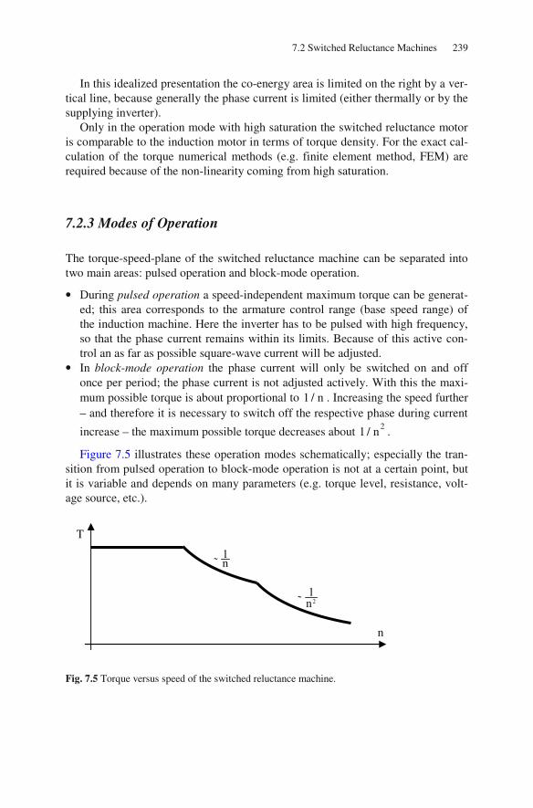
7.2 Switched Reluctance Machines 239
In this idealized presentation the co-energy area is limited on the right by a ver-tical line, because generally the phase current is limited (either thermally or by the supplying inverter).
Only in the operation mode with high saturation the switched reluctance motor is comparable to the induction motor in terms of torque density. For the exact cal-culation of the torque numerical methods (e.g. finite element method, FEM) are required because of the non-linearity coming from high saturation.
7.2.3 Modes of Operation
The torque-speed-plane of the switched reluctance machine can be separated into two main areas: pulsed operation and block-mode operation.
• During pulsed operation a speed-independent maximum torque can be generat-ed; this area corresponds to the armature control range (base speed range) of the induction machine. Here the inverter has to be pulsed with high frequency, so that the phase current remains within its limits. Because of this active con-trol an as far as possible square-wave current will be adjusted.
• In block-mode operation the phase current will only be switched on and off once per period; the phase current is not adjusted actively. With this the maxi-mum possible torque is about proportional to 1 / n . Increasing the speed further – and therefore it is necessary to switch off the respective phase during current
increase – the maximum possible torque decreases about 21 / n .
Figure 7.5 illustrates these operation modes schematically; especially the tran-sition from pulsed operation to block-mode operation is not at a certain point, but it is variable and depends on many parameters (e.g. torque level, resistance, volt-age source, etc.).
Fig. 7.5 Torque versus speed of the switched reluctance machine.
1n
21n
n
T

240 7 Reluctance Machines
The pulsed operation will be explained in the following by means of a single phase. Each phase of the machine is connected via two power transistors (shown as simple switches in Fig. 7.6) and two power diodes as a half bridge. The differ-ent switching states are illustrated in Fig. 7.6, where the machine phase is symbol-ized as an inductivity.
a) b) c)
Fig. 7.6 Different switching states of a half bridge of the switched reluctance machine inverter.
Neglecting the voltage drops across the transistors and diodes, in case a) of Fig.
7.6 the voltage DCU supplies the phase winding; the current increases in the
shown direction.
If the phase current exceeds the desired current HiI by a specific amount, both
transistors T1 and T2 are opened and the voltage DCU supplies the phase winding
in opposite direction to case a): In this case b) of Fig. 7.6 the current decreases un-til a certain value below the desired current is reached. At this point in time it is switched back to case a).
The current and voltage characteristics (Fig. 7.7) show these time-dependent functions (so-called “hard chopping“) including the magnetizing and demagnetiz-ing of the phase.
If the current does not reach the desired value, the voltage will be switched on
at the rotor position angle onα (case a)) and switched off at the rotor position an-
gle offα (case b)). Then block-mode operation is active. At the rotor position an-
gle endα the phase current is zero again. The time function of the phase current is
shown in Fig. 7.8.
i
DCU D2
D1
T2
T1
i
DCU
T1
DCU D2
D1
T2
T1
i
D2
D1
T2

7.2 Switched Reluctance Machines 241
Fig. 7.7 Current and voltage during hard chopping operation.
Fig. 7.8 Current during block-mode operation.
During the pulsed operation there are high switching losses because of the high switching frequencies of the power transistors. To avoid this, per switching period only one of both power transistors is switched and for the following switching pe-riod the other power transistor is switched (in Fig. 7.6 in case c) the switching of the power transistor T1 is shown as an example). The current and voltage charac-teristics for this so-called “soft chopping“ look like it is shown in Fig. 7.9.
u
i
-UDC
+UDC
IHi
βAβ Kβ Eβ
β
i
u
α
onα offα endα
α
i IHi
Aβ Kβ Eββ
i
α
onα offα endα

242 7 Reluctance Machines
Fig. 7.9 Current and voltage during soft chopping operation.
7.2.4 Alternative Power Electronic Circuits
The inverter already shown in Fig. 7.6 for one phase is called 2n inverter, because it contains 2n switchable power electronic devices, if the number of phases is called n (see Fig. 7.10 for a four-phase machine).
This configuration has the advantage of being most flexible concerning current waveforms, but there is even the disadvantage of a large number of power elec-tronic devices, resulting in high costs.
Fig. 7.10 Four-phase switched reluctance machine with 2n inverter.
u
i
-UDC
+UDC
IHi
Aβ Kβ Eββ
β
i
u
α
onα offα endα
α
DCU

7.2 Switched Reluctance Machines 243
This circuit can be simplified by far, if the so-called n+1 inverter is used. This inverter (see Fig. 7.11) is characterized by one low-side power electronic switch that may switch at low frequency and just selects the phase of the machine that shall be energized. In addition, there is one single high-side switch for all phases together, being responsible for high-frequency PWM switching. This alternative reduces the effort concerning number of power electronic switches and their ac-companied driving circuit and concerning the quality of most of the switches (just one power electronic device has to be capable to switch at high PWM frequency).
On the other hand, this circuit has the disadvantage that the phases cannot be switched independently, which decreases the degree of freedom for machine con-trol.
Fig. 7.11 Four-phase switched reluctance machine with n+1 inverter.
A compromise between low effort and high degree of freedom is the so-called n+2 inverter. Here, the phases of the machine are organized in two groups, so that two phases may be energized simultaneously, see Fig. 7.12.
Fig. 7.12 Four-phase switched reluctance machine with n+2 inverter.
DCU
PWM 1 PWM 2
DCU
PWM

244 7 Reluctance Machines
7.2.5 Main Characteristics
The main positive characteristics of switched reluctance machines are:
• The construction is simple, robust, and cost-effective. • Heating because of Ohmic losses only does occur in the stator (and there good
possibilities for cooling exist). • Short-term overload is no problem for the SRM. • The rotor has low inertia and it is robust; therefore it is qualified for high-speed
applications. • The torque is independent from the current direction; consequently simple elec-
tronic circuits for the inverter may be used.
The main disadvantages are:
• The actually energized coil has to be switched off at high phase current and maximum stored energy: Therefore, the inverter usage is relatively low.
• To achieve a high difference in inductivity between the “aligned position“ and the “unaligned position“ the air-gap width in the “aligned position“ has to be very small. This increases the costs and it makes the SRM sensitive to produc-tion tolerances.
• The torque is pulsating. To smooth it, e.g. the number of phases can be in-creased or the teeth (reasonably the rotor teeth, as these do not carry windings) can be skewed. Both measures increase the costs and decrease the utilization.
• Because of the high difference in inductivity between the “aligned position“ and the “unaligned position“ high pulsating radial forces occur. These forces are the reason for serious acoustic noise.
• By influencing the current waveform the torque and/or the acoustic noise can be influenced. To do so, generally a voltage reserve is necessary and the utiliza-tion is reduced.
• In analogy to induction machines, a reactive current component is necessary for the magnetization of the machine. With this reactive current component the ap-parent power of the inverter is increased.
7.3 References for Chapter 7
DeDoncker RW, Pulle DWJ, Veltman A (2011) Advanced electrical drives. Springer-Verlag, Berlin
Barnes M, Pollock C (1998) Power electronic converters for switched reluctance drives, IEEE Transactions on Power Electronics, 13:1100-1111
Krishnan R (2001) Switched reluctance motor drives. CRC Press, Boca Raton Miller TJE (1993) Switched reluctance motors and their control. Magna Physics Publishing, Ox-
ford

7.3 References for Chapter 7 245
Miller TJE, McGilp M (1990) Nonlinear theory of the switched reluctance motor for rapid com-puter-aided design, Proc. Inst. Elect. Eng. B, 137:337-347
Schinnerl B (2009) Analytische Berechnung geschalteter Reluktanzmaschinen, Shaker-Verlag, Aachen
Schramm A (2006) Redundanzkonzepte für geschaltete Reluktanzmaschinen. Shaker-Verlag, Aachen

8 Small Machines for Single-Phase Operation
8.1 Fundamentals
The generation of electrical energy, its distribution and its industrial application for high-power drives is done by means of three-phase systems with high voltage. For this, three-phase machines are used that produce a torque that is constant in time.
At the low-voltage level for low power in households mostly there is just a sin-gle-phase system available. For such applications, single-phase machines have to be used. The construction of such single-phase machines often deviates signifi-cantly from high-power machines, because:
• inherent to their functional principle they are non-symmetric, • often they have to be integrated into the application and • concessions to manufacturing needs of the (usually existing) high-volume pro-
duction have to be made.
There is a steadily growing market for these kinds of machines and their eco-nomic relevance is increasing. Main importance for the direct connection to the single-phase mains have the universal motor and the single-phase induction ma-chine.
In addition, more and more BLDC-machines with inverter supply are used with the single-phase mains. Because of the electronic supply these machine are able to draw a constant power from the mains and to deliver a constant power (torque) to the application.
8.2 Universal Motor
Fundamentally, the construction of the universal motor is like the DC-motor, but it has a laminated stator. It can be operated by DC currents and AC currents, hence the name comes from. For operation with AC currents of the frequency f the main equations of the DC-machine in their time-dependent formulation are valid.
Induced voltage:
( ) ( ) ( ) ( )iU t k t n, t sin t= φ φ = φ ω (8.1)
Torque:
© Springer-Verlag Berlin Heidelberg 2015 247
DOI 10.1007/978-3-642-17584-8_ 8D. Gerling, Electrical Machines Mathematica l Engineering,,
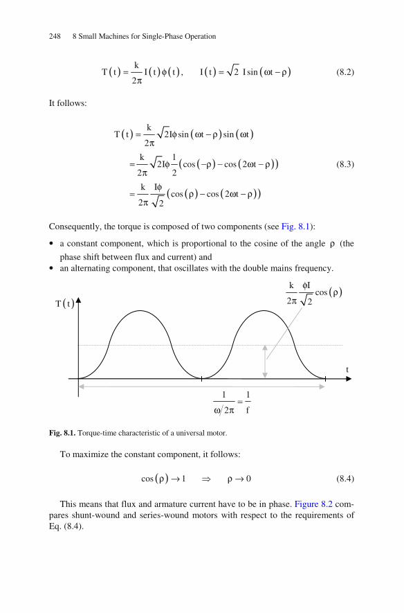
248 8 Small Machines for Single-Phase Operation
( ) ( ) ( ) ( ) ( )k
T t I t t , I t 2 I sin t2
= φ = ω − ρπ
(8.2)
It follows:
( ) ( ) ( )
( ) ( )( )
( ) ( )( )
kT t 2I sin t sin t
2
k 12I cos cos 2 t
2 2
k Icos cos 2 t
2 2
= φ ω − ρ ωπ
= φ −ρ − ω − ρπ
φ= ρ − ω − ρ
π
(8.3)
Consequently, the torque is composed of two components (see Fig. 8.1):
• a constant component, which is proportional to the cosine of the angle ρ (the
phase shift between flux and current) and • an alternating component, that oscillates with the double mains frequency.
Fig. 8.1. Torque-time characteristic of a universal motor.
To maximize the constant component, it follows:
( )cos 1 0ρ → ρ → (8.4)
This means that flux and armature current have to be in phase. Figure 8.2 com-pares shunt-wound and series-wound motors with respect to the requirements of Eq. (8.4).
( )T t
t
1 1
2 f=
ω π
( )k I
cos2 2
φρ
π

8.2 Universal Motor 249
Fig. 8.2. Equivalent circuit diagrams of shunt-wound and series-wound motors.
The requirement mentioned above ( ( ), I 0φ = ) is fulfilled only for the series-
wound machine. The ripple torque is damped by the inertias of the rotor and the load, so that in steady-state operation there are only minimal speed variations. The useful torque is the mean value of the torque (constant component).
Compared to the DC-motor the universal motor delivers a lower torque when operated by AC voltage (if the DC voltage is equal to the rms-value of the AC voltage), because there is an additional voltage drop at the reactance X L= ω (see the qualitative speed-torque-characteristics in Fig. 8.3).
Fig. 8.3. Speed-torque-characteristics of the universal motor (for different supply).
U
AI AR
iU
FI L
shunt-wound motor:
( ), I 2φ ≈ π
U
AI AR
iU FI L
series-wound motor:
( ), I 0φ =
T
n
DC supply
AC supply

250 8 Small Machines for Single-Phase Operation
For the sake of completeness Fig. 8.4 shows the same qualitative fact as torque-speed-characteristics:
Fig. 8.4. Torque-speed-characteristic of the universal motor (for different supply).
8.3 Single-Phase Induction Machine
8.3.1 Single-Phase Operation of Three-Phase Induction Machine
Disconnecting one phase of the three-phase induction machine from the symmet-ric three-phase mains, a single-phase supply at two phases of the machine is ob-tained. The stator MMF produces an alternating air-gap field, which – according to the “Rotating Field Theory” (Chap. 3) – can be regarded as being composed of two rotating fields travelling in opposite direction and having half the amplitude.
That field component travelling in the same direction like the rotor (defined as positive direction, index “p”) induces voltages into the rotor windings, that pro-
duce the currents 2,pI with the frequency 2,p p 1f s f= . Here, ps s= is the same
slip like for the three-phase machine. The slip of the rotor relative to the field component rotating in negative direc-
tion (index “n”) is:
0 0 0 0n
0 0 0 0 0 0
n n n n n nn ns 1 1 2 2 s
n n n n n n
− − −= = + = + − − = − = −
− (8.5)
Therefore, additional rotor currents 2,nI occur, having the frequency 2,n n 1f s f= .
Both rotating components of the stator field together with both rotor currents produce some torque, i.e. there are four torque components. The torque compo-
T
n
DC supply
AC supply

8.3 Single-Phase Induction Machine 251
nent coming from the positive rotating stator field together with the negative rotat-ing rotor MMF and the torque component coming from the negative rotating stator field together with the positive rotating rotor MMF are oscillating torques with the mean value equal to zero. They do not deliver any useful torque. In addition there are the torque components of the positive and negative rotating stator fields, pro-duced with their “own” (i.e. the self-induced) rotor currents. These two compo-nents deliver a mean torque different from zero.
At stand-still the rotor has the slip s 1= to the positive rotating stator field as well as to the negative rotating stator field. The torque components from both ro-tating fields have the same amplitude, but opposite direction. The motor does not accelerate.
If the rotor rotates in one direction, there are different slip values for ps and
ns . Consequently, the reaction of the squirrel-cage rotor onto both rotating stator
MMFs is different. The negative rotating field is strongly damped at ns 2≈ , the
positive rotating field at ps 0≈ is exposed only to a small reaction. Therefore, an
elliptical rotating air-gap field is generated, which results in producing a useful torque in the direction of rotor rotation. Consequently, this means: The three-phase induction machine rotates further, if one phase is disconnected from the mains and the load torque is not too high (but the slip will increase and therefore the efficiency will decrease, see the torque-speed-characteristics in Fig. 8.5). By mechanical starting the rotor from zero speed, the motor can accelerate further.
A detailed calculation can be performed by means of the symmetric compo-nents (see Sect. 1.6). The resulting torque-speed-characteristic is identical to that of two three-phase induction motors connected in series, which rotors are mechan-
ically coupled and which stators are supplied with opposite phase sequence at 3 times the phase voltage. The qualitative torque-speed-characteristics look like it is shown in Fig. 8.5.
Fig. 8.5. Torque-speed-characteristics: single-phase operation of a three-phase induction motor.
positive direction
sum
negative
direction
0n n
pull out
T
T −
-1.0 -0.6 -0.2 0.2 0.6 1.0
1.0
0.5
0.0
-0.5
-1.0

252 8 Small Machines for Single-Phase Operation
8.3.2 Single-Phase Induction Motor with Auxiliary Phase
If the induction motor in single-phase operation shall deliver a torque even at zero speed, at least an elliptical rotating air-gap field has to be present at stand-still. This can be realized by means of an auxiliary winding “a”, that is shifted against the main winding “m” by a spatial angle ε and that is supplied by a current with a phase shift by an (electrical) angle ϕ .
If p 0ε = ϕ = holds true, a purely oscillating air-gap field is obtained. If
p 2ε = ϕ = π holds, the amplitude of the negative rotating field is minimal and
the amplitude of the positive rotating field is maximal. The phase shift between
the current mI of the main winding and the current aI of the auxiliary winding is
realized by an additional impedance in the auxiliary winding, like it is shown in the equivalent circuit diagram in Fig. 8.6.
Fig. 8.6. Equivalent circuit diagram of the single-phase induction motor with auxiliary phase.
There are three possibilities for this impedance in the auxiliary winding:
• Resistance: A resistance is very cost-effective, but only a small starting torque is generated; because of the losses it has to be switched off after starting the motor.
• Inductivity: An inductivity delivers only a small starting torque (a pure induc-tivity produces no phase shift of the current; only because of the unavoidable resistance there is a generally small phase shift); in addition the inductivity is costly and heavy.
• Capacity: Starting capacity (switching off by centrifugal switch) or operating capacity (improvement of power factor and efficiency); the use of a capacity results in a high starting torque, from technical point of view this is the best so-lution.
U
I a
m Z
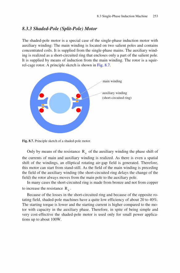
8.3 Single-Phase Induction Machine 253
8.3.3 Shaded-Pole (Split-Pole) Motor
The shaded-pole motor is a special case of the single-phase induction motor with auxiliary winding: The main winding is located on two salient poles and contains concentrated coils. It is supplied from the single-phase mains. The auxiliary wind-ing is realized as a short-circuited ring that encloses only a part of the salient pole. It is supplied by means of induction from the main winding. The rotor is a squir-rel-cage rotor. A principle sketch is shown in Fig. 8.7.
Fig. 8.7. Principle sketch of a shaded-pole motor.
Only by means of the resistance aR of the auxiliary winding the phase shift of
the currents of main and auxiliary winding is realized. As there is even a spatial shift of the windings, an elliptical rotating air-gap field is generated. Therefore, this motor can start from stand-still. As the field of the main winding is preceding the field of the auxiliary winding (the short-circuited ring delays the change of the field) the rotor always moves from the main pole to the auxiliary pole.
In many cases the short-circuited ring is made from bronze and not from copper
to increase the resistance aR .
Because of the losses in the short-circuited ring and because of the opposite ro-tating field, shaded-pole machines have a quite low efficiency of about 20 to 40%. The starting torque is lower and the starting current is higher compared to the mo-tor with capacity in the auxiliary phase. Therefore, in spite of being simple and very cost-effective the shaded-pole motor is used only for small power applica-tions up to about 100W.
main winding
auxiliary winding (short-circuited ring)

254 8 Small Machines for Single-Phase Operation
8.4 References for Chapter 8
Stepina J (1982) Die Einphasenasynchronmotoren. Springer-Verlag, Wien Stölting HD, Beisse A (1987) Elektrische Kleinmaschinen. Teubner-Verlag, Stuttgart Stölting HD, Kallenbach E (2001) Handbuch Elektrische Kleinantriebe. Hanser Verlag, Mün-
chen Veinott CG (1959) Theory and design of small induction motors. McGraw Hill Book Company,
New York Veinott CG (1970) Fractional- and subfractional-horsepower electric motors. McGraw Hill Book
Company, New York

9 Fundamentals of Dynamic Operation
9.1 Fundamental Dynamic Law, Equation of Motion
9.1.1 Translatory Motion
A mass m with the velocity v has the impulse mv (kinetic quantity). The sum of all from outside acting forces leads to a time-dependent change of the kinetic quantity.
a
d d dF F (mv) m (v) v (m)
dt dt dtν
ν
= = = + (9.1)
For m const.= it follows (Newton’s equation of motion):
a
dvF m ma
dt= = (9.2)
If all outside forces can be described by a driving force F and a load force
loadF , where both are acting in the same direction (x-axis), it follows:
2
load a 2
dv d xF F F ma m m
dt dt− = = = = (9.3)
9.1.2 Translatory / Rotatory Motion
In the following a combined motion of two bodies will be regarded, translatory (body 1) and rotatory (body 2) – see Fig. 9.1. The bodies are closely coupled to each other. The following forces F and torques T exist (the rotating body has the mass m 0= , ω is the angular frequency of this rotating body):
© Springer-Verlag Berlin Heidelberg 2015 255
DOI 10.1007/978-3-642-17584-8_ 9D. Gerling, Electrical Machines Mathematica l Engineering,,

256 9 Fundamentals of Dynamic Operation
Fig. 9.1. Principle of combined translatory and rotatory motion.
It follows:
load
load
2load
dvF F m
dt
d(r )r(F F ) rm
dt
d dT T mr
dt dt
∗
− =
ω− =
ω ω− = = Θ
(9.4)
The inertia of the rotating body Θ is zero, because the mass was assumed be-
ing zero. 2mr∗Θ = is the translatory moved mass, transformed to the rotatory
movement.
9.1.3 Rotatory Motion
A rotating mass Θ with the angular frequency ω has the rotating impulse Θω (kinetic quantity). The sum of all from outside acting torques leads to a time-dependent change of the kinetic quantity.
a
d d dT T ( ) ( ) ( )
dt dt dtν
ν
= = Θω = Θ ω + ω Θ (9.5)
For const.Θ = and loadT as sum of all load torques it follows:
2
load a 2
d dT T T
dt dt
ω γ− = = Θ = Θ (9.6)
vmF
loadF
T, ω loadT v r= ω
m 0=
r

9.1 Fundamental Dynamic Law, Equation of Motion 257
9.1.4 Stability
From the equation of motion
load
d dnT T 2
dt dt
ω− = Θ = πΘ (9.7)
it follows (see Fig. 9.2): dn
0dt
> if loadT T> acceleration, starting
dn0
dt< if loadT T< deceleration, braking
dn0
dt= if loadT T= constant speed, static
balance (stable or unstable)
Fig. 9.2. Static stability (above) and static instability (below).
Static stability is given for loadT T
n n
∂ ∂>
∂ ∂, static instability for loadT T
n n
∂ ∂<
∂ ∂.
load
T
T
n
T
loadT
load
T
T
n
T
loadT

258 9 Fundamentals of Dynamic Operation
9.2 Mass Moment of Inertia
9.2.1 Inertia of an Arbitrary Body
An arbitrarily sized, inelastic body shall rotate around an arbitrary axis (see Fig. 9.3). The equation of motion for a mass element dm is:
2a a
dv ddT r dF r dm r dm
dt dt
ω= = = (9.8)
The total acceleration torque is:9
aT m
2a a
0 0
d dT dT r dm
dt dt
ω ω= = = Θ (9.9)
with the inertia:
m
2
0
r dmΘ = (9.10)
Fig. 9.3. Calculating the inertia of an arbitrary body.
9 The tilde is introduced to distinguish between integration limit and integration variable.
r
dFa dm
body
ω
rotating axis
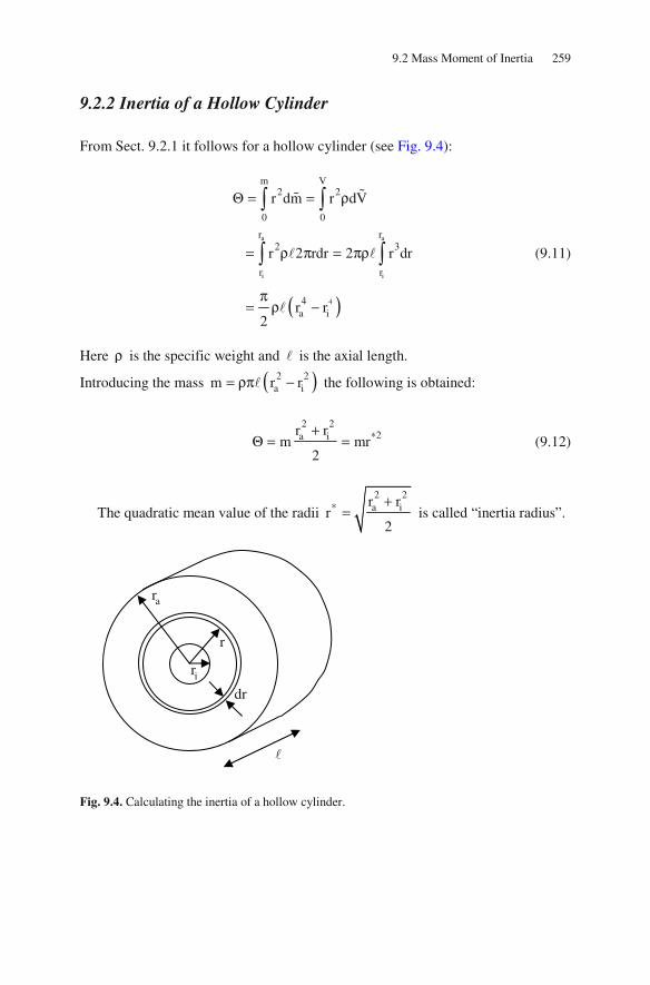
9.2 Mass Moment of Inertia 259
9.2.2 Inertia of a Hollow Cylinder
From Sect. 9.2.1 it follows for a hollow cylinder (see Fig. 9.4):
( )
a a
i i
4
m V2 2
0 0
r r2 3
r r
4a i
r dm r dV
r 2 rdr 2 r dr
r r2
Θ = = ρ
= ρ π = πρ
π= ρ −
(9.11)
Here ρ is the specific weight and is the axial length.
Introducing the mass ( )2 2a im r r= ρπ − the following is obtained:
2 2
2a ir rm mr
2
∗+Θ = = (9.12)
The quadratic mean value of the radii 2 2a ir r
r2
∗ += is called “inertia radius”.
Fig. 9.4. Calculating the inertia of a hollow cylinder.
dr
r
ir
ar

260 9 Fundamentals of Dynamic Operation
9.3 Simple Gear-Sets
9.3.1 Assumptions
The transmission (gear-set) is assumed being lossless and form-fit: Then there is no slip, no backlash, no hysteresis and no elasticity.
9.3.2 Rotation / Rotation (e.g. Gear Transmission)
In Fig. 9.5 the principle rotation / rotation gear set is shown:
Fig. 9.5. Rotation / rotation gear-set.
Defining 1
2
r 1
r u= , the condition of identical displacement at the point of transmis-
sion delivers:
11 1 2 2
2
r r uγ
γ = γ =γ
(9.13)
From identical speed ( v r= ω ) at the point of transmission it follows:
1
2
uω
=ω
(9.14)
From “actio = reactio“ at the point of transmission the following can be de-duced:
1r
1 1 1 1, , , Tγ Θ ω 2 2 2 2, , , Tγ Θ ω
2r

9.3 Simple Gear-Sets 261
1 2 1
1 2 2
T T T 1
r r T u= = (9.15)
The acceleration torque of the rotating bodies is (if they are regarded as single, independent bodies):
a ,n n n
dT , n 1, 2
dt= Θ ω = (9.16)
Because of the inelastic coupling of these bodies, body 2 has to be accelerated as well, if body 1 is accelerated. Then it follows from the law “actio = reactio“:
1a ,1 1 1 2 2
2
11 1 2
1 2 12
rd dT
dt r dt
d 1 d
dt u dt u
1 d
u dt
= Θ ω + Θ ω
ω= Θ ω + Θ
= Θ + Θ ω
(9.17)
Consequently, the transformation of inertia 2Θ onto axis 1 gives:
1,tot 1 22
1
uΘ = Θ + Θ (9.18)
9.3.3 Rotation / Translation (e.g. Lift Application)
In Fig. 9.6 the principle rotation / translation gear set is shown.

262 9 Fundamentals of Dynamic Operation
Fig. 9.6. Rotation / translation gear-set.
The acceleration torque is:
( )
( )
2
2
d d d d T r m v r m r
dt dt dt dt
d dr m
dt dt
dr m
dt
= Θ ω + = Θ ω + ω
= Θ ω + ω
= Θ + ω
(9.19)
Consequently, the transformation of the mass m onto the rotational axis is:
2tot r mΘ = Θ + (9.20)
9.4 Power and Energy
From the equation of motion
load
dT T
dt
ω− = Θ (9.21)
the power balance is obtained after multiplication with ω :
load
dT T
dt
ωω = ω + Θω (9.22)
r
m, v
,Θ ω

9.4 Power and Energy 263
This equation means: The input power ( Tω ) is equal to the sum of power of
the load ( loadT ω ) and change of kinetic energy (d
dt
ωΘω ).
The energy balance can be calculated as follows: In the time period
2 1t t tΔ = − , in which the speed of the drive is changed as 2 1Δω = ω − ω , the
work
2 2 2
1 1 1
t t t
loadt t t
dT dt T dt dt
dt
ωω = ω + Θω (9.23)
is supplied. The increase of kinetic energy of the rotating masses is:
( )2 2
1 1
t2 22 1
t
d 1dt d
dt 2
ω
ω
ωΘω = Θω ω = Θ ω − ω (9.24)
After an acceleration from 1 0ω = to 2 0ω = ω the kinetic energy of
2kin 0
1E
2= Θω (9.25)
is stored in the rotating masses of the drive. If there is a complex drive with different speeds of the different rotating mass-
es, their effect can be concentrated virtually into a single rotating body. In most cases the rotating mass is calculated relative to the motor axis (motor speed). Dur-ing transformation the kinetic energy is unchanged. Therefore, the following holds true (transformed values are marked with “ ′ “):
2 2
2 2
1 1
2 2
n
n
′ ′Θ ω = Θω
ω′Θ = Θ = Θ
′ ′ω
(9.26)

264 9 Fundamentals of Dynamic Operation
9.5 Slow Speed Change
9.5.1 Fundamentals
From the equation of motion (Eq. (9.21)) the mechanical transient operation of a drive can be calculated, if the torque characteristics as function of time or angular frequency are known.
The torque of the electric machine can be calculated by means of the system equations of the electromagnetic circuits. The phase currents of the machine are determined even by the equation of motion. Therefore, generally there is a cou-pling between the electrical and mechanical transient behavior (dynamic opera-tion).
This coupling can be neglected, if the operation is a quasi steady-state one. Such an operation is characterized by slow speed changes (compared to the elec-
trical time constants). Then the steady-state characteristics ( )T ω and ( )loadT ω
can be used.
9.5.2 First Example
A constant acceleration torque aT const.= is assumed (i.e. the electrical machine
always produces a torque that is constantly higher than the load torque). It follows:
aTd
dt
ω=
Θ (9.27)
For the acceleration the following holds true:
aTtω =
Θ (9.28)
Consequently, there is a linear speed increase with time. Dividing this equation
by the final angular frequency 0ω it follows:
0
0 a
t,
T
ω Θω= τ =
ω τ (9.29)

9.5 Slow Speed Change 265
If the acceleration torque is equal to the nominal torque ( a NT T= ) and the final
angular frequency is equal to its nominal value ( 0 0,Nω = ω ), the mechanical time
constant becomes:
0,N
mechNT
ω Θτ = (9.30)
9.5.3 Second Example
If the acceleration torque decreases linearly with increasing speed
0a a,0
0
T Tω − ω
=ω
(i.e. the difference between torque of the electrical machine and
load torque gets smaller and smaller with increasing speed), it follows:
( )a ,00
0
Td
dt
ω= ω − ω
ω Θ (9.31)
Consequently:
a ,0 0
mechmech a,0
Td 1with
dt T
ω Θω′+ ω = τ =
′τ Θ (9.32)
For the run-up characteristic it follows (Fig. 9.7):
mech
t
0
1 e−
′τω= −
ω (9.33)

266 9 Fundamentals of Dynamic Operation
Fig. 9.7. Run-up characteristic.
Often the acceleration torque aT is not known explicitly as a function, but as a
characteristic ( )aT ω that is complex to describe analytically. In these cases a
numerical integration is strongly recommended. The differential equation is then substituted by an equation of differences
aTt
Δω= Θ
Δ (9.34)
The acceleration torque aT is approximated by a constant value in every time
interval (but generally different for separate time intervals). Then for every time
interval 1t t tν ν+ νΔ = − the change of angular frequency is calculated as
a ,T
tν
ν νΔω = ΔΘ
(9.35)
and added to the value of the preceding time interval:
( ) ( )1t tν+ ν νω = ω + Δω (9.36)
0ω
ω
t mech′τ

9.6 Losses during Starting and Braking 267
9.6 Losses during Starting and Braking
9.6.1 Operation without Load Torque
The mechanical energy during acceleration or braking of drives follows from the fundamental equation of dynamic operation:
2 2 2
1 1 1
t t
mech loadt t
E T dt T dt dω
ω
= ω = ω + Θ ω ω (9.37)
For the operation without load torque ( loadT 0= ) it follows:
2 2
1 1
t
mecht
E T dt dω
ω
= ω = Θ ω ω (9.38)
As an example a three-phase induction machine will be regarded in the follow-ing. The inertia Θ is the inertia of the rotor and that of the coupled rotating mass-
es ( rotor loadΘ = Θ + Θ ). The schematic energy distribution is shown in Fig. 9.8.
The angular frequency of an induction machine is (with s being the slip):
( )0
0
0
1 s
d ds
dt dt
d ds
ω = ω −
ω= − ω
ω = − ω
(9.39)

268 9 Fundamentals of Dynamic Operation
Fig. 9.8. Schematic energy distribution.
By introducing Eq. (9.39) into Eq. (9.38) it follows:
( ) ( )( )
( ) ( )
( ) ( )
2 2
1 1
2 2
1 1
2 2
1 1
2
1
t
mecht
t s
mech 0 0 0t s
t s2
mech 0t s
s2 2
mech 0s
2 2 2mech kin 1 2 1 2 kin 0
E T dt d
E T 1 s dt 1 s ds
E P 1 s dt 1 s ds
1E s s
2
1 1E 2E s s s s with E
2 2
ω
ω
δ
= ω = Θ ω ω
= ω − = Θ ω − −ω
= − = −Θω −
= −Θω −
= − − − = Θω
(9.40)
In this equation Pδ is the air-gap power and kinE the kinetic energy stored in
the drive at synchronous speed. For the run-up from zero speed to (nearly) syn-
chronous speed ( 1s 1= , 2s 0≈ ) it follows:
mech kinE E= (9.41)
The rotor heat losses occurring during this run-up are (with 0P Tδ = ω ):
elE
rotorΘ
loadΘ
T, ω
loss,1E
loss,2E mechE
Eδ

9.6 Losses during Starting and Braking 269
( )
2 2 2
1 1 1
2
1
t t s2
loss,2 0 0t t s
s2 2 2 20 kin 1 2s
E sP dt s Tdt s ds
1s E s s
2
δ= = ω = − Θω
= −Θω = −
(9.42)
With 1s 1= , 2s 0≈ (run-up from zero speed) it can be further deduced:
loss,2 kinE E= (9.43)
Consequently, the rotor heat losses during run-up are identical to the kinetic energy stored in the rotating masses after this run-up.
The heat losses in the stator will be calculated by using a quite simple approx-
imation: Neglecting the magnetizing current means 1 2I I′≈ . Then the heat values
in stator and rotor are proportional to the respective Ohmic resistances:
loss,1 1
loss,2 2
E R1
E R≈ ≈
′ (9.44)
Consequently during this run-up there is:
loss,1 kinE E= (9.45)
From the mains the following energy has to be delivered for this run-up (ne-glecting the iron losses and friction losses):
el loss,1 loss,2 mech
kin
E E E E
3E
= + +
= (9.46)
For electrical braking ( 1s 2= , 2s 1= ) the energy values become:
mech kinE E= − (9.47)
loss,2 kinE 3E= (9.48)

270 9 Fundamentals of Dynamic Operation
loss,1 kinE 3E= (9.49)
el loss,1 loss,2 mech
kin
E E E E
5E
= + +
= (9.50)
Starting the motor by changing the number of poles (from p′ to p′′ ) the fol-
lowing rotor losses are obtained:
( ) ( )2 2 2 2loss,2 kin 1 2 kin 1 2E E s s E s s′ ′ ′ ′′ ′′ ′′= − + − (9.51)
Selecting p 2′ = and p 1′′ = , it follows:
0 0 0
1 2 1 2
kin kin kin
1 1
2 2
s 1, s 0, s 0.5, s 0
1 1E E E
4 4
′ ′′ω = ω = ω
′ ′ ′′ ′′= = = =
′ ′′= =
(9.52)
Consequently:
( ) ( )2 2 2 2loss,2 kin kin
kin
1E E 1 0 E 0.5 0
4
1 E
2
= − + −
=
(9.53)
Having the same final kinetic energy like for the run-up without changing the number of poles (because the final speed is not changed), there are only half the losses in the rotor (and therefore there is considerably reduced rotor heating).
9.6.2 Operation with Load Torque
From

9.7 References for Chapter 9 271
loadload
d T dT T T
dt T T dt
ω ω− = Θ Θ =
− (9.54)
it follows:
( )
2 2 2
1 1 1
2 2
1 1
2
1
t t t
loss,2 0 0t t t load
s s2
0 0 0s sload load
s
kins load
T dE sP dt s Tdt s dt
T T dt
T 1 Ts ds 2 sds
T T 2 T T
T2E sds
T T
δ
ω= = ω = ω Θ
−
= ω Θ −ω = − Θω− −
= −−
(9.55)
The factor load
T1
T T>
− (usually depending on ω or s ) increases the losses
(heating) during speed change against the case without load torque ( loadT 0= ).
For example this is important for Y − Δ − starting: in Y -connection the torque
is reduced to 1 3 , but the load torque remains unchanged (this means ( )loadT T−
may become very small). The mains loading is reduced by smaller phase currents,
but the driving machine has to withstand increased heating for loadT 0> . The
same holds true for the run-up with reduced terminal voltage.
For the special case a loadT T T 0= − = (no acceleration torque, e.g. locked ro-
tor) the loss energy loss,2E increases to infinity.
Only for the case loadT 0= the loss energy loss,2E is independent from the kind
of run-up. The loss energy (heating) calculated above is present if the machine is operated
at mains supply (constant voltage and constant frequency). With inverter supply at changing voltage and frequency the losses are much lower.
9.7 References for Chapter 9
Leonhard W (1973) Regelung in der elektrischen Antriebstechnik. Teubner-Verlag, Stuttgart White DC, Woodson HH (1958) Electromechanical energy conversion. John Wiley & Sons,
New York

10 Dynamic Operation and Control of DC-Machines
10.1 Set of Equations for Dynamic Operation
In comparison to the steady-state operation of the DC-machine the energy storage
elements (inductivities AL , FL and inertia Θ ) have to be considered additionally
for the dynamic operation. For a detailed analysis it is even necessary to consider the voltage drop across
the brushes BUΔ , the frictional torque fricTΔ and the nonlinearity of the magnetic
circuit because of saturation of the iron. In total the following set of equations and equivalent circuit diagram (Fig. 10.1) can be deduced for the dynamic operation:
AA A A A i B
i A
F F F F
i load fric
i A
dIU I R L U U
dt
k 1U c , c 4pw , 2 n
2 2
dU I R w
dt
dT T T
dt
T c I
= + + + Δ
= Ωφ = = Ω = ππ π
φ= +
Ω− − Δ = Θ
= φ
(10.1)
Fig. 10.1. Equivalent circuit diagram of the DC-machine for dynamic operation.
AU
AI AR AL
iU
FU
FI
=BUΔ
FR FL Θ load fricT , TΔ
i, TΩ
© Springer-Verlag Berlin Heidelberg 2015 273
DOI 10.1007/978-3-642-17584-8_ 10D. Gerling, Electrical Machines Mathematica l Engineering,,

274 10 Dynamic Operation and Control of DC-Machines
The nonlinear dependency of flux and exciting current (field current) is shown in Fig. 10.2 (nominal values are denoted with the index “N“ in the following).
Fig. 10.2. Nonlinear characteristics of the DC-machine: flux versus exciting current (above) and field winding inductivity versus exciting current (below).
The inductivity of the field winding depends on the current: ( ) FF F
F
wL I
I
φ= .
At nominal operation the field exciting circuit usually is saturated:
F NF,N
F,N
wL
I
φ= .
From the above relations a system of three coupled differential equations fol-lows. With this system (armature circuit equation, field circuit equation, torque equation) all operational conditions of the DC-machine can be described:
AA B A A A A
dIU U U I R L c
dt′− Δ = = + + Ωφ (10.2)
Nφ
φ
FI F,NI
FIφ ( )Ff Iφ =
( )F F,NL I
FL
FI F,NI
F,0L

10.1 Set of Equations for Dynamic Operation 275
( )F F F F F
dU I R w , f I
dt
φ= + φ = (10.3)
( )A load fric load
d dc I T T T
dt dt
Ω Ω′φ = Θ + + Δ = Θ + (10.4)
The differential equations of the armature circuit and the torque are coupled by
the speed 2 nΩ = π and the armature current AI .
The inductivity of the field winding is assumed being dependent on the current, whereas the inductivity of the armature winding is assumed being constant. This assumption of constant armature inductivity is valid, because the armature circuit proceeds perpendicular to the main pole axis and here either a large air-gap is dominating or just a small leakage inductivity is present if commutation poles and / or compensation windings are used.
To get a universally valid solution a normalization to the nominal values is ad-vantageous:
A A,NA AA A A
N A,N N
F F,NF FF F F
N F,N N
loadload
N 0 N
F NF,N N N 0 N N A,N
F,N
R IU IU , I , R
U I U
R IU IU , I , R
U I U
T, n , T
T
wL , U c , T c I
I
⊗ ⊗ ⊗
⊗ ⊗ ⊗
⊗ ⊗ ⊗
′= = =
= = =
φ Ωφ = = =
φ Ω
φ= = φ Ω = φ
(10.5)
In addition the armature time constant, the field time constant, and the nominal-starting time constant, respectively, are introduced as follows:
F,N 0A
A FA F N
LL, ,
R R TΘ
ΘΩτ = τ = τ = (10.6)
By means of transformations and substitutions the following set of equations is deduced:

276 10 Dynamic Operation and Control of DC-Machines
( )AA A A
A
FF F
F
A g
dI 1U n I
dt R
UdI
dt R
dnI T
dt
⊗⊗ ⊗ ⊗ ⊗
⊗
⊗⊗⊗
⊗
⊗⊗ ⊗ ⊗
Θ
τ = − φ −
φτ = −
τ = φ −
(10.7)
These equations lead to the block diagram that usually is used in control engi-neering (Fig. 10.3).
Fig. 10.3. Block diagram of the DC-machine in dynamic operation.
The input values are AU⊗ , FU⊗ and loadT⊗ . The system composed of three differ-
ential equations is nonlinear because of the multiplications n⊗ ⊗φ and AI⊗ ⊗
φ
and because of the magnetizing characteristic ( )Ff I⊗ ⊗φ = . The coupling of these
differential equations is performed via n⊗ and AI⊗ .
This coupled, nonlinear set of differential equations can be solved completely only by means of numerical methods. In the following some typical applications are discussed, which can be calculated analytically because of simplifications.
AU⊗ +
−
AI⊗ iT⊗
+
−
loadT⊗
n⊗
FU⊗ +
−
FI⊗
⊗φ
in U⊗ ⊗ ⊗φ =
A1 R⊗
F1 R⊗
Θτ Aτ
Fτ
×
×

10.2 Separately Excited DC-Machines 277
10.2 Separately Excited DC-Machines
10.2.1 General Structure
Speed-variable DC-machines are often operated with constant excitation (constant field e.g. by means of permanent magnets). Then torque and speed are adjusted by
varying the armature voltage. In this case N const.φ = φ = is valid and the block
diagram (Fig. 10.4) gets quite simple by 1⊗φ = .
Fig. 10.4. Block diagram of the separately excited DC-machine in dynamic operation with
N const.φ = φ = .
By means of the Laplace transformation the representation as block diagram usually used in control engineering is deduced (Fig. 10.5).
Fig. 10.5. Block diagram of the separately excited DC-machine in Laplace notation with
N const.φ = φ = .
Output value is the speed of the DC-machine, which is controlled by the set-point (armature voltage). The disturbance quantity is the load torque.
AU⊗ +
−
A iI T⊗ ⊗=
+
−
loadT⊗
n⊗
in U⊗ ⊗=
A1 R⊗ Θτ Aτ
1
s Θτ
( ) ( )AW s U s⊗=
+ −
( )iT s⊗
+
−
( ) ( )loadZ s T s⊗=
( ) ( )Y s N s⊗=
A
A
1 R
1 s
⊗
+ τ
( )1G s ( )2G s

278 10 Dynamic Operation and Control of DC-Machines
The following relations are valid:
( )( )
2 i
i 1
Y G T Z
T G W Y
⊗
⊗
= −
= − (10.8)
By substitutions and transformations it is obtained:
1 2 2
1 2 1 2
G G GY W Z
1 G G 1 G G= −
+ + (10.9)
10.2.2 Response to Setpoint Changes
“Response to setpoint changes” is called the change of the output value because of a variation of the input (setpoint), when the disturbance is equal to zero.
Therefore, the response to setpoint changes of the DC-machine is the speed
change when changing the armature voltage for ( ) ( )loadZ s T s 0⊗= = . This situa-
tion is described with the block diagram in Fig. 10.6.
Fig. 10.6. Block diagram of the separately excited DC-machine in Laplace notation for the op-eration “response to setpoint changes”.
For the mathematical description the following is obtained (the additional index “S“ at speed and armature current indicates the characteristic functions for re-sponse to setpoint changes in the following):
( )S 1 2 A S
1 2S A
1 2
N G G U N
G GN U
1 G G
⊗ ⊗ ⊗
⊗ ⊗
= −
=+
(10.10)
1
s Θτ
( )AU s⊗
+ −
( )SN s⊗ A
A
1 R
1 s
⊗
+ τ
( )1G s ( )2G s

10.2 Separately Excited DC-Machines 279
With
( )
( )
( )
( )
( ) ( )
( ) ( )
A
S 1 2 A
AA 1 2
A
1 R 1
Y s N s G s G s 1 s s
1 R 1W s U s 1 G s G s1
1 s s
⊗
⊗Θ
⊗⊗
Θ
+ τ τ= = =
++
+ τ τ
(10.11)
it follows further
( )
( ) ( )A A
Y s 1
W s s R 1 s 1⊗Θ
=τ + τ +
(10.12)
Introducing the mechanical time constant
A A,N0 0 0 0
mech AN stallN N stall
N NA A,N A,N
R IR
U I1T U TT T
R I I
⊗Θ
ΘΩ ΘΩ ΘΩ ΘΩτ = τ = = = = (10.13)
it follows:
( )
( ) ( )S
2A A mechmech A
A mech A
N s 1 1
U s 1 1 s s s 1s
⊗
⊗= =
+ + τ ττ τ + +
τ τ τ
(10.14)
Now at time t 0= a step function of the setpoint shall happen, e.g. switching the nominal voltage to the DC-machine at zero speed. Consequently:
( )A
1U s
s
⊗= (10.15)
and therefore:
( )S2
mech AA mech A
1 1N s
s s 1s
⊗=
τ τ + +τ τ τ
(10.16)

280 10 Dynamic Operation and Control of DC-Machines
The time-dependent speed variation is obtained by reverse Laplace transfor-mation:
( )2
1 0S 2 2
0 0
1n t L
s s 2sD
⊗ − ω=
+ ω + ω (10.17)
with
20 0
mech A A
mech
A
1 1, 2D
D4
ω = ω =τ τ τ
τ=
τ
(10.18)
The solution is (taken from literature concerning Laplace transformation):
( ) ( )( )0D t
2 2S 02
en t 1 sin 1 D t arcsin 1 D
1 D
− ω⊗
= − ω − + −−
(10.19)
For D 1= the time-dependent speed is obtained by considering small x-values:
( )sin x x≈ , ( )arcsin x x≈ . It follows:
( ) ( )
( )
0
0
D t2 2
S 02
D t0
en t, D 1 1 1 D t 1 D
1 D
1 e t 1
− ω⊗
− ω
= = − ω − + −−
= − ω +
(10.20)
Figure 10.7 shows the results of these equations for different values of
mech Aτ τ .

10.2 Separately Excited DC-Machines 281
Fig. 10.7. Normalized speed versus time of the separately excited DC-machine for the operation “response to setpoint changes”.
From
( ) ( ) ( )S 2 A,SN s G s I s⊗ ⊗= (10.21)
the armature current becomes:
( ) ( )A,S SI s s N s⊗ ⊗Θ= τ (10.22)
This means a differentiation for the reverse Laplace transformation:
( ) ( ){ }1 S SA,S S mech
A
dn dn1I t L s N s
dt R dt
⊗ ⊗⊗ − ⊗
Θ Θ ⊗= τ = τ = τ (10.23)
In total it follows:
0 2 4 6 8 10
1.4
1.2
1.0
0.8
0.6
0.4
0.2
0.0
At τ
Sn⊗ mech A
mech A
mech A
mech A
mech A
0.5
1.0
2.0
4.0
8.0
τ τ =
τ τ =
τ τ =
τ τ =
τ τ =

282 10 Dynamic Operation and Control of DC-Machines
( ) ( )( )
( )( )
( )( )
( )( )
0
0
0
D t 2 2mech 0A,S 02
A
D t 2 20 0
D t 2 2mech0 02
A
2 20
DI t e sin 1 D t arcsin 1 D
R 1 D
e cos 1 D t arcsin 1 D
De sin 1 D t arcsin 1 D
R 1 D
cos 1 D t arcsin 1 D
− ω⊗
⊗
− ω
− ω
⊗
τ ω= ω − + −
−
−ω ω − + −
τ= ω ω − + −
−
− ω − + −
(10.24)
Even here the result for D 1= is obtained by considering small arguments:
( ) ( )( )
( )( )
( )
( )( )
0
0
D t 2 2mechA,S 0 02
A
2 20
D t 2 2mech0 02
A
2 20
DI t e sin 1 D t arcsin 1 D
R 1 D
cos 1 D t arcsin 1 D
De 1 D t 1 D
R 1 D
cos 1 D t arcsin 1 D
− ω⊗
⊗
− ω
⊗
τ= ω ω − + −
−
− ω − + −
τ= ω ω − + −
−
− ω − + −
(10.25)
Further:
( ) ( ) ( )[ ]
( )[ ]
0
0
D tmechA,S 0 0
A
D tmech0 0
A
I t e D t 1 cos 0R
e D t 1 1R
− ω⊗
⊗
− ω
⊗
τ= ω ω + −
τ= ω ω + −
(10.26)
These functions are shown in Fig. 10.8.

10.2 Separately Excited DC-Machines 283
Fig. 10.8. Normalized armature current versus time of the separately excited DC-machine for the operation “response to setpoint changes”.
10.2.3 Response to Disturbance Changes
“Response to disturbance changes” is called the change of the output value be-cause of a variation of the disturbance, when the input (setpoint) is equal to zero.
Therefore, the response to disturbance changes of the DC-machine is the speed
change when changing the load torque for ( ) ( )AW s U s 0⊗= = . The resulting
block diagram is shown in Fig. 10.9 (the additional index “D“ at the speed indi-cates the characteristic functions for response to disturbance changes in the fol-lowing).
0 2 4 6 8 10 At τ
A,SI⊗ mech A
mech A
mech A
mech A
mech A
8.0
4.0
2.0
1.0
0.5
τ τ =
τ τ =
τ τ =
τ τ =
τ τ =
1.0
0.8
0.6
0.4
0.2
0.0
-0.2

284 10 Dynamic Operation and Control of DC-Machines
Fig. 10.9. Block diagram of the separately excited DC-machine in Laplace notation for the op-eration “response to disturbance changes”.
Therefore:
( ) ( ) ( ) ( ) ( )( )
( )( )
( ) ( )( )
D 2 load 1 D
2D load
1 2
N s G s T s G s N s
G sN s T s
1 G s G s
⊗ ⊗ ⊗
⊗ ⊗
Δ = − − Δ
−Δ =
+
(10.27)
and further:
( )
( )
( )
( )
( )
D A A
Aload A A
A
A A2
mech mech A
1
N s R 1 ss
1 R 1T s 1 R s 1 s1
1 s s
R 1 s
1 s s
⊗ ⊗Θ
⊗⊗ ⊗Θ
Θ
⊗
−Δ − + ττ
= =+ τ + τ
++ τ τ
− + τ=
+ τ + τ τ
(10.28)
Switching on the nominal torque ( )loadT s 1 s⊗= , the speed change is:
( )
( )
( )( ) ( ){ }
1 A AD 2
mech mech A
1A S A S
R 1 sn t L
s 1 s s
R L N s s N s
⊗⊗ −
⊗ − ⊗ ⊗
− + τΔ =
+ τ + τ τ
= − + τ
(10.29)
( )loadT s⊗ −
−
( )DN s⊗Δ
( )2G s
1
s Θτ
( )1G s
A
A
1 R
1 s
⊗
+ τ

10.2 Separately Excited DC-Machines 285
With the solution of the preceding section it follows:
( ) ( )( )
( ) ( )
( ) ( ) ( )
SD A S A
AA S A A,S
mech
2 AA S A A,S
mech
dn tn t R n t
dt
RR n t I t
R n t R I t
⊗⊗ ⊗ ⊗
⊗⊗ ⊗ ⊗
⊗ ⊗ ⊗ ⊗
Δ = − + τ
= − + ττ
τ= − −
τ
(10.30)
Now, the speed-time-characteristic shall be calculated, when just before the
load change the DC-machine is in no-load operation ( n 1⊗= , AI 0⊗
= ) at nominal
excitation ( 1⊗φ = , see Sect. 10.1). Then it follows:
( ) ( )D Dn t 1 n t⊗ ⊗= + Δ (10.31)
For different values of the parameter mech
A
τ
τ the speed change is shown in Fig.
10.10.
Fig. 10.10. Normalized speed versus time of the separately excited DC-machine for the operation “response to disturbance changes”.
0 2 4 6 8 10
1.0
0.8
0.6
0.4
0.2
0.0
-0.2
-0.4
-0.6
-0.8
At τ
Dn⊗ mech A
mech A
mech A
mech A
mech A
8.0
4.0
2.0
1.0
0.5
τ τ =
τ τ =
τ τ =
τ τ =
τ τ =

286 10 Dynamic Operation and Control of DC-Machines
The separately excited DC-machine with its energy storages AL and Θ is an
oscillatory system for mech
A
D 14
τ= <
τ.
For mech
A
D 14
τ= >
τ aperiodic characteristics are obtained when changing the
armature voltage or the load torque. The case D 1= is called “critical damping”.
10.3 Shunt-Wound DC-Machines
For DC-machines with variable exciting flux φ the investigation of dynamic op-
eration has to be performed by numerical calculation, because the set of differen-tial equations is nonlinear and cannot be solved analytically. Such a case is present e.g. for starting the shunt-wound DC-machine.
At the time t 0= the machine at standstill shall be switched to the mains. Dur-
ing the entire run-up the machine is unloaded ( loadT 0= ). The time-dependent
characteristics of armature current, speed, torque, and field exciting current are calculated in the following by means of normalized quantities.
With A FU U 1⊗ ⊗= = it follows:
( )
( )
AA A
A
F F FF
A
dI 11 n I
dt R
d 1I , f I
dt R
dnI
dt
⊗⊗ ⊗ ⊗
⊗
⊗⊗ ⊗ ⊗
⊗
⊗⊗ ⊗
Θ
τ = − φ −
φτ = − φ =
τ = φ
(10.32)
The iron saturation is considered by using the function ( )Ff I⊗ ⊗φ = .
This set of equations will be solved step by step by numerical integration using
a digital computer. The values at time k 1t + are calculated from the values at time
kt and the respective changes in the time interval k 1 kt t t+Δ = − . This is done by
transforming the differential equations into equations of differences:

10.3 Shunt-Wound DC-Machines 287
( )
( )
A,k 1 A,kA k k A,k
A
k 1 kF F,k k F,k
F
k 1 kk A,k
I I 11 n I
t R
1I , f I
t R
n nI
t
⊗ ⊗+ ⊗ ⊗ ⊗
⊗
⊗ ⊗⊗ ⊗ ⊗+
⊗
⊗ ⊗⊗ ⊗+
Θ
−τ = − φ −
Δ
φ − φτ = − φ =
Δ
−τ = φ
Δ
(10.33)
An additional transformation of the equations gives:
( )
k kA,k 1 A,k
A A A
k 1 k F,k k F,kF F
k 1 k k A,k
1 nt tI 1 I
R
t 1I , f I
R
tn n I
⊗ ⊗⊗ ⊗
+ ⊗
⊗ ⊗ ⊗ ⊗ ⊗+ ⊗
⊗ ⊗ ⊗ ⊗+
Θ
− φΔ Δ= − +
τ τ
Δφ = φ + − φ =
τ
Δ= + φ
τ
(10.34)
An evaluation of this set of equations during run-up of the DC-machine is shown in Fig. 10.11 for typical time constants and typical normalized resistances (all quantities are shown as normalized values; armature current in red, speed in blue, torque in black, and field exciting current in magenta).
Fig. 10.11. Normalized characteristics of the shunt-wound DC-machine in dynamic operation.
At τ
1.75
1.50
1.25
1.00
0.75
0.50
0.25
0.00
-0.25 0 20 40 60 80 100 120
FI⊗
AI⊗
T⊗
n⊗

288 10 Dynamic Operation and Control of DC-Machines
The steep increase of the armature current and the slow increase of the field ex-citing current lead to a reduced torque during acceleration. Because of
mech
A
D 14
τ= >
τ (see Sect. 10.2, “separately excited DC-machine“) aperiodic
characteristics would be expected initially, but the speed and the armature current show overshooting characteristics. The reason for this difference between the sep-arately excited DC-machine and the shunt-wound DC-machine is:
• For the separately excited DC-machine the flux always is constant at its nomi-
nal value, i.e. for all times 1 const.⊗φ = =
• The field of the shunt-wound DC-machine is increased during starting, i.e. the nominal value is reached delayed.
10.4 Cascaded Control of DC-Machines
For control purposes in the electrical drive engineering often PI- (proportional-integral-) controllers are used. In addition to a simple structure they have the ad-vantage of stationary preciseness (i.e. after disturbances the initial value is reached again, after change of setpoint the new value is reached, both without any station-ary difference).
Block diagram and transfer function of a PI-controller are shown in Fig. 10.12:
Fig. 10.12. Block diagram and transfer function of a PI-controller.
Figure 10.13 shows a commonly used control circuit composed of permanent magnet excited DC-machine, power electronic converter, and cascaded control. The cascaded control consists of a speed control circuit (realized by a PI-
controller: ( )C,nG s ) and a subordinate current control circuit (realized by a PI-
controller as well: ( )C,IG s ). In addition, a limitation for the armature current is
introduced.
C CK , τ
( )x t ( )y t C
CC
1 sK
s
+ τ
τ
( )CG s
( )X s ( )Y s

10.4 Cascaded Control of DC-Machines 289
Fig. 10.13. Block diagram of the cascaded control circuit of DC-machines.
For the step by step solution of the set of differential equations numerical methods are used. Therefore, the PI-controllers have to be discretized. There is:
( )
( )
( )
( ) ( ) ( )
CC C
C
C C C
Y s 1 sG s K
X s s
s Y s K 1 s X s
+ τ= =
τ
τ = + τ
(10.35)
In the time domain this gives:
( ) ( ) ( )
C C C
CC
dy dxK x
dt dt
1y t K x t dt x t
τ = + τ
= +τ
(10.36)
In discretized description this equation is:
setN⊗
+−
N⊗
A,setI⊗
+ −
AI⊗
AI⊗Δ N⊗
Δ A,setU⊗
AU⊗
T
Θ
M
C,nC,n
C,n
1 sK
s
+ τ
τ
( )C,nG s A,maxI
C,IC,I
C,I
1 sK
s
+ τ
τ
( )C,IG s

290 10 Dynamic Operation and Control of DC-Machines
k 1
k C i i ki 1C
1y K x t x
−
=
= Δ +τ
(10.37)
For the following calculation of the dynamic operation the dead time (time constant) of the power electronic converter will be neglected, i.e. there is
A A,setU U⊗ ⊗≡ . For the permanent magnet excited DC-machine ( 1⊗
φ = ) the equa-
tions in normalized form are:
( )AA A A
A
A load
dI 1U n I
dt R
dnI T
dt
⊗⊗ ⊗ ⊗
⊗
⊗⊗ ⊗
Θ
τ = − −
τ = −
(10.38)
Figure 10.14 shows the time-dependent characteristics of speed (solid blue line) and armature current (solid red line) together with their respective set values (dot-ted lines) for a step function of the speed set value from 0 to 1 and later to -1 (starting and reversing) without any load. In this case the armature current is lim-ited to the double nominal value. Because of the constant excitation the armature current (in normalized representation) is identical to the torque. From the over-shootings and oscillations can be deduced that the parameters of the controllers are not adjusted optimally (concerning oscillations, speed adjustment, and precise-ness).
Fig. 10.14. Characteristics of the separately excited DC-machine in cascaded control operation.
2
1
0
-1
-2
At τ 0 5 10 15 20 25
setn⊗
AI⊗
A,setI⊗
n⊗
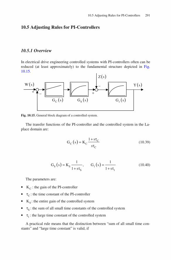
10.5 Adjusting Rules for PI-Controllers 291
10.5 Adjusting Rules for PI-Controllers
10.5.1 Overview
In electrical drive engineering controlled systems with PI-controllers often can be reduced (at least approximately) to the fundamental structure depicted in Fig. 10.15.
Fig. 10.15. General block diagram of a controlled system.
The transfer functions of the PI-controller and the controlled system in the La-place domain are:
( ) CC C
C
1 sG s K
s
+ τ=
τ (10.39)
( ) ( )S S 1S 1
1 1G s K , G s
1 s 1 s= =
+ τ + τ (10.40)
The parameters are:
• CK : the gain of the PI-controller
• Cτ : the time constant of the PI-controller
• SK : the entire gain of the controlled system
• Sτ : the sum of all small time constants of the controlled system
• 1τ : the large time constant of the controlled system
A practical rule means that the distinction between “sum of all small time con-stants” and “large time constant” is valid, if
( )W s
+− +
−
( )Z s
( )Y s
( )CG s ( )SG s ( )1G s

292 10 Dynamic Operation and Control of DC-Machines
1 S4τ ≥ τ (10.41)
is true. Without detailed derivation adjusting rules for the parameters of the PI-controller will be given for two special cases.
10.5.2 Adjusting to Optimal Response to Setpoint Changes (Rule “Optimum of Magnitude“)
For the optimum of magnitude the controller parameters have to be chosen as fol-lows; the results are illustrated in Fig. 10.16.
1C 1 C
S S
1 1K
2 K
ττ = τ =
τ (10.42)
Fig. 10.16. Rule “optimum of magnitude”: relative output amplitude versus time for response to setpoint changes (above) and response to disturbances (below).

10.5 Adjusting Rules for PI-Controllers 293
10.5.3 Adjusting to Optimal Response to Disturbances (Rule “Symmetrical Optimum“)
For the symmetrical optimum the controller parameters have to be chosen as fol-lows:
1C S C
S S
1 14 K
2 K
ττ = τ =
τ (10.43)
Testing by means of step functions (of the setpoint or the disturbance) the charac-teristics shown in Fig. 10.17 are obtained.
Fig. 10.17. Rule “symmetrical optimum”: relative output amplitude versus time for response to setpoint changes (above) and response to disturbances (below).
1.5
1.0
0.5
0.0
0.1
0.0
-0.1
-0.2
-0.3
St τ
St τ
relA
relA 1 Sτ τ 50
10 5
1 Sτ τ 50
25
10
5
0 5 10 15 20
0 5 10 15 20

294 10 Dynamic Operation and Control of DC-Machines
10.5.4 Application of the Adjusting Rules to the Cascaded Control of DC-Machines
Applying the rules of optimal response to setpoint changes (“optimum of magni-tude”) to the current controller and to the speed controller of the cascaded control (see Sect. 10.4) the following results are obtained (Fig. 10.18).
Fig. 10.18. Characteristics of the separately excited DC-machine in cascaded control operation when applying the rules of optimal response to setpoint changes.
In this case, the “optimum of magnitude” is applied to both controllers, because speed and current are exposed to changing setpoints. For the current controller this is the usual case, for the speed controller sometimes even the “symmetrical opti-mum” rule is applied. This is the case if not changing setpoints, but changing load torques have to be controlled.
From Fig. 10.18 it can be deduced that the armature current follows its set val-ue quite precisely, i.e. the adjusting rule “optimum of magnitude” works very good. Between the speed and its set value there is quite a large deviation. This comes from the fact, that the structure analyzed for the adjusting rules is just an approximation to the speed control loop. Nevertheless, compared to the results shown in Fig. 10.14, the control behavior is improved by far.
By varying the control parameters even a better performance will be achieva-ble.
0 5 10 15 20 25
2
1
0
-1
-2
At τ
A,setI⊗
setn⊗ n⊗
AI⊗

10.6 References for Chapter 10 295
10.6 References for Chapter 10
Krishnan R (2001) Electric motor drives. Prentice Hall, London Nasar SA (1970) Electromagnetic energy conversion devices and systems. Prentice Hall, London Pfaff G, Meier C (1992) Regelung elektrischer Antriebe II. Oldenbourg Verlag, München Schröder D (1995) Elektrische Antriebe 2. Springer-Verlag, Berlin White DC, Woodson HH (1958) Electromechanical energy conversion. John Wiley & Sons,
New York

11 Space Vector Theory
11.1 Methods for Field Calculation
For the description and calculation of electro-magnetic fields in electrical ma-chines mainly the following four methods are used:
1. The wave-description of the electro-magnetic fields (see Sects. 3.3 to 3.5) has proven its value if stationary characteristics are to be calculated. This method may be used for the fundamental-wave characteristics of electrical machines, but it may be even used if additionally to the fundamental wave higher harmon-ics are to be considered. E.g. this is the case if harmonic torque components (torque oscillations) or acoustic noise shall be computed.
2. The symmetric components (please refer to Sect. 1.6) are mainly used for the examination of asymmetric events with constant frequency (this may be even transient reactions).
3. The usage of complex space vectors is advantageous if the transient characteris-tics of (controlled or uncontrolled) electrical drives are regarded. This method will be explained in the following sections.
4. When using the Finite Element Method (FEM) the electrical machine is divided in many small parts (“finite elements”) and the electro-magnetic behavior of the machine is calculated numerically for each of these elements and for each operating point: The Maxwell’s equations are solved in each element and the solutions are adapted to each other at the element borders. The disadvantages of this method are on the one hand a quite high computation time, on the other hand it is more suited for the analysis of a known machine than for the design of a new one (the relevance of different influencing factors on the machine characteristics cannot be directly observed). The main advantage of this method is that virtually all relevant attributes can be considered simultaneously, where-as for the other three mentioned (analytical) methods always limiting con-straints have to be regarded.
As can be seen from the above description of the different methods the choice of the suitable alternative depends on the task that has to be solved.
© Springer-Verlag Berlin Heidelberg 2015 297
DOI 10.1007/978-3-642-17584-8_ 11D. Gerling, Electrical Machines Mathematica l Engineering,,

298 11 Space Vector Theory
11.2 Requirements for the Application of the Space Vector Theory
For the following considerations some limiting assumptions are made:
1. Each phase winding of stator and rotor produce a sinusoidal magneto-motive force in space, all of the same wave length. This means a limitation to the fun-damental wave of the magneto-motive forces (and therefore even a limitation to the fundamental waves of current loading and air-gap flux density); the wind-ing factors of all harmonic waves are assumed being zero. Each single wave can be represented by a vector; the location of the vector shows the instantane-ous position of the maximum of the wave, the length of the vector represents this maximum value.
2. Magnetically the machine is completely symmetric (i.e. constant air-gap along the circumference) and the influence of the slots is neglected. Within one ma-chine part (stator or rotor) the self- and mutual-inductivities are independent from the rotor position.
3. Partly, these requirements can be disclaimed: If stator or rotor contains two magnetically or electrically perpendicular preferred orientations, the space vec-tor theory still can be applied if the coordinate system is fixed to the asymmet-ric machine part.
4. Saturation is neglected, i.e. the magnetic permeances are independent from the magneto-motive forces, and the magnetic voltage drop in iron is neglected
(Fe
μ → ∞ ); linear relationships do exist. Now (as a main advantage of the rep-
resentation of the waves by vectors) the common effect of the single waves can be calculated by vector addition.10
It is important for understanding the space vector theory, that there is no limit-ing requirement for the time-dependency of the single currents: The currents may have arbitrary time-dependency which even may be asymmetric (this is crucial for the calculation of transient characteristics). In spite of the arbitrary time-dependency of the currents the magneto-motive force, the current loading, and the air-gap flux density generated by each single current are sinusoidal in space at every moment;11 this is realized by a clever winding distribution in the slots of the machine.
In the following only the very important three-phase system is regarded. Never-theless, the method of the complex space vector is applicable for arbitrary number of phases.
10 This requirement can be attenuated: It is sufficient, that there is a constant saturation condition inside the machine. By linearizing at the operation point the vector addition is still applicable. 11 This gives a hint for the origin of the name “space vector theory”: main importance have the spatially sinusoidal waves inside the machine, there are no requirements to special time-dependencies.

11.3 Definition of the Complex Space Vector 299
11.3 Definition of the Complex Space Vector
The representation of the waves by means of vectors will now be transformed to a representation by means of complex numbers. For this, a complex plain is defined, where the real axis and the axis of the phase “u“ enclose a (time-dependent) angle
( )tα , please refer to Fig. 11.1.
Fig. 11.1. Machine axes in a complex plain (left) and definition of the complex operator a (right).
Now a complex number (called “space vector” in the following) is defined as follows (here shown for the example of the phase currents of a three-phase sys-tem):12
( ) ( ) ( ) ( )( ) ( )j t2u v w
2i t i t a i t a i t e
3 − α
= + + (11.1)
12 In the following complex space vectors, for distinguishing them from other complex numbers, are identified by arrows under the variable. The calculation rules for complex numbers are valid even here; the arrows under the variable just label the special definition of these complex num-bers. In literature even a simple underscore can be found to label complex space vectors. For sys-
tems with m phases the space vector is: ( ) ( )m
k 1 jk
k 1
2i t i t e
m − − α
=
= , with
2jme
π
= .
By means of this definition even the rotor of a squirrel cage induction machine can be described with space vectors.
+
1
2a a
Re
Im−
( )tα u
w
v
Re
Im−
2 3π

300 11 Space Vector Theory
The multiplication with the operator 2
j3a eπ
= means a rotation by 120° in pos-
itive direction. The factor 2 3 secures a scaling of the absolute value of the space
vector in a way, that this absolute value is equal to the amplitude of a phase cur-rent when having symmetric supply of all phases. To simplify the notation, in the following the explicit statement of the time-dependency of the angle α is omitted.
The projection of the complex space vector onto the respective phase axis gives the instantaneous value of the phase current.
Regarding a symmetric three-phase current system at the time t 0= , at which
the current ( )ui t shall be maximum (i.e. the real axis coincides with the axis of
the phase “u“, this means 0α = ), it follows in normalized description (please re-fer to Fig. 11.2):
( )
( ) ( )
u
v w
i t 0 1
1i t 0 i t 0
2
= =
= = = = − (11.2)
Fig. 11.2. Symmetric three-phase current system in a complex plain (left) and definition of the x-y-coordinate system (right).
Separating the complex space vector into real and imaginary part, there is:
( ) ( ){ } ( ){ }
( ) ( )x y
i t Re i t j Im i t
i t j i t
= +
= − (11.3)
u
wv
Re
Im−
1
22 1a
3 2−
2 1a
3 2− 2
13
⋅
x
y

11.3 Definition of the Complex Space Vector 301
From
( ) ( ) ( ) ( )( ) ( ) ( )2 ju v w x y
2i t i t a i t a i t e i t j i t
3 − α
= + + = − (11.4)
both components of the space vector can be computed:
( ) ( ) ( ) ( )
( )
( ) ( ) ( )
( )
u v
x u v
w
w
2 2i t cos i t cos i t
3 3
4cos i t
3
2 2cos i t cos i t
3 3
2cos i t
3
π= −α + −α +
π+ −α +
π= α + α −
π+ α +
(11.5)
and
( ) ( ) ( ) ( )
( )
( ) ( ) ( )
( )
y u v
w
u v
w
2 2i t sin i t sin i t
3 3
4sin i t
3
2 2sin i t sin i t
3 3
2sin i t
3
π= − −α + −α +
π+ −α +
π= α + α −
π+ α +
(11.6)
Together with the equation for the zero component of the current ( )0i t :13
( ) ( ) ( ) ( )u v w 0i t i t i t 3 i t+ + = (11.7)
the following matrix equation can be set-up:
13 The factor 3 in the equation for the zero component of the current is chosen arbitrarily.

302 11 Space Vector Theory
( )
( )
( )
( )
( )
( )
( )
( )
x u
y xy0 v
0 w
xy0
i t i t
i t T i t
i t i t
2 2cos cos cos
3 3
2 2 2T sin sin sin
3 3 3
1 1 1
2 2 2
=
π πα α − α +
π π= α α − α +
(11.8)
Likewise, the inversion can be easily calculated:
( )
( )
( )
( )
( )
( )
( ) ( )
u x1
v xy0 y
w 0
1
xy0
i t i t
i t T i t
i t i t
cos sin 1
2 2T cos sin 1
3 3
2 2cos sin 1
3 3
−
−
=
α α
π π= α − α −
π πα + α +
(11.9)
If, as a special condition, the zero component of the current is (time-independent) always equal to zero, as it is the case for star-connected three-phase systems without neutral line, the above equations can be simplified to:
( ) ( ) ( ) ( )0 w u vi t 0 i t i t i t= = − − (11.10)

11.4 Voltage Equation in Space Vector Notation 303
( )
( )
( )
( )
( )
( )
x uxy
y v
xy
i t i tT
i t i t
2cos cos
2 3T
23sin sin
3
=
πα α −
=π
α α −
(11.11)
( )
( )
( )
( )
( ) ( )
1 xuxy
yv
1
xy
i ti tT
i ti t
cos sin
T 2 2cos sin
3 3
−
−
=
α α
= π πα − α −
(11.12)
In the same way like the space vector of the current at the beginning of this sec-tion, even the space vectors of voltage and flux linkage are defined:
( ) ( ) ( ) ( )( )2 ju v w
2u t u t a u t a u t e
3 − α
= + + (11.13)
( ) ( ) ( ) ( )( )2 ju v w
2t t a t a t e
3 − α
ψ = ψ + ψ + ψ (11.14)
11.4 Voltage Equation in Space Vector Notation
In the following, the space vector theory will be developed in the energy con-sumption system, which becomes obvious from the signs in the used voltage equa-tions (please refer to Sect. 1.2).
Firstly, the three voltage equations of the (symmetric) system

304 11 Space Vector Theory
( ) ( )( )
( ) ( )( )
( ) ( )( )
uu u
vv v
ww w
d tu t R i t ,
dt
d tu t R i t ,
dt
d tu t R i t
dt
ψ= +
ψ= +
ψ= +
(11.15)
are multiplied with j2e
3
− α , j2a e
3
− α and 2 j2a e
3
− α , respectively. Afterwards
these equations are summed up. By means of the relation for the differential of the flux linkage with respect to time
( )( ) ( ) ( )
( ) ( ) ( )( )( )
( ) ( ) ( )
( )
( ) ( ) ( )
( )( )
2 ju v w
2 ju v w
2 ju v w
2 ju v w
d t 2 d d dt a t a t e
dt 3 dt dt dt
2 dt a t a t j e
3 dt
2 d d dt a t a t e
3 dt dt dt
dj t
dt
2 d d dt a t a t e
3 dt dt dt
d t dj t
dt dt
− α
− α
− α
− α
ψ= ψ + ψ + ψ +
αψ + ψ + ψ −
= ψ + ψ + ψ
α− ψ
ψ + ψ + ψ
ψ α= + ψ
(11.16)
the voltage equation in space vector notation is found:14
( ) ( )( )
( )d t d
u t R i t j tdt dt
ψ α= + + ψ (11.17)
14 For the special case ( )t const.α = (i.e. the real axis of the coordinate system has a time-
independent angle to the axis of the phase “u”) it is true: ( ) ( )( )d t
u t R i tdt
ψ= + . This is
even the case, if the real axis coincides with the axis of the phase “u”, i.e. for ( )t 0α = .

11.5 Interpretation of the Space Vector Description 305
For this derivation it is important that the linear combination of the three gener-ally valid voltage equations requires no limitation concerning the spatial distribu-tion of the fields or concerning the time-dependent functions of the currents.
11.5 Interpretation of the Space Vector Description
Like shown in the preceding sections, the space vector can be calculated from the values of the three phases or from the sum of real and imaginary part. With other words this means that the three-phase system can be transformed into a two-phase system, like it is schematically shown in Fig. 11.3.
Fig. 11.3. Interpretation of the space vector description: three-phase system (left), two-phase sys-tem (right).
Additionally, by means of an arbitrary angle α a transformation into a coordi-nate system rotating with arbitrary angular frequency is successful: The time-dependency of the angle α is not limited.
As the currents (and the voltages and flux linkages) of an arbitrary m -phase system can be described in two (perpendicular) coordinates, the space vector theo-ry is applicable to arbitrary phase numbers. The phase numbers of stator and rotor may be even different (an example for this is the squirrel-cage induction machine).
By applying the space vector defined in Sect. 11.3 in total the following trans-formation is achieved:
• from the m-phase system in stationary coordinates • into a two-phase system in (arbitrarily) rotating coordinates.
ui u
wv
vi wi
x
yi
xi
y
α

306 11 Space Vector Theory
11.6 Coupled Systems
Regarding three-phase systems of stator (index “1“ and “I“) and rotor (index “2“ and “II“), respectively, the spatial position of the rotor system against the stator
system has to be considered by the time-dependent angle ( )tγ . It is assumed here
that the rotor values are already transformed to the stator system (a special nota-tion for this is omitted to simplify the description).
The coupling of both systems is realized via the flux linkages. As it is obvious from Fig. 11.4 (example for 0α = ), the coupling via the flux linkages is depend-
ent on the rotor position because of the time-dependent angle ( )tγ .
Fig. 11.4. Coupling between stator and rotor system.
Introducing an additional rotation with je γ for the space vectors of the rotor (Fig. 11.5), both systems are transformed to a commonly rotating coordinate sys-tem.
stator
rotor
I, x
I,yi
I,xi
I, y
II, x
II,yi
II,xi
II, y
( )tγ
coupling is dependent on the rotor position

11.6 Coupled Systems 307
Fig. 11.5. Transforming three-phase systems (left) to two-phase systems (right); stator: above, rotor: below.
Then the space vectors of the rotor system are:
( ) ( ) ( ) ( )( ) ( )j2 II 2,u 2,v 2,w
2i t i t a i t a i t e
3 − α−γ
= + + (11.18)
( ) ( ) ( ) ( )( ) ( )j2II 2,u 2,v 2,w
2u t u t a u t a u t e
3 − α−γ
= + + (11.19)
( ) ( ) ( ) ( )( ) ( )j2II 2,u 2,v 2,w
2t t a t a t e
3 − α−γ
ψ = ψ + ψ + ψ (11.20)
I, x
I,yi
I,xi
I, y
α
II, x
II,yi
II,xi
II, y
α
1,ui 1, u
1, w 1, v
1,vi 1,wi
2,ui
2, u
2, w
2, v
2,vi
2,wi
γ

308 11 Space Vector Theory
whereas the space vectors of the stator system against the definition in Sect. 11.3 simply get the respective indices:
( ) ( ) ( ) ( )( )2 j I 1,u 1,v 1,w
2i t i t a i t a i t e
3 − α
= + + (11.21)
( ) ( ) ( ) ( )( )2 jI 1,u 1,v 1,w
2u t u t a u t a u t e
3 − α
= + + (11.22)
( ) ( ) ( ) ( )( )2 jI 1,u 1,v 1,w
2t t a t a t e
3 − α
ψ = ψ + ψ + ψ (11.23)
By means of the deduction from Sect. 11.4 the voltage equations of stator and rotor are in space vector notation:
( ) ( )( )
( )II I I I
d t du t R i t j t
dt dt
ψ α= + + ψ (11.24)
and
( ) ( )( ) ( )
( )IIII II II II
d t du t R i t j t
dt dt
ψ α − γ= + + ψ (11.25)
With the angular frequency of the coordinate system CS d dtω = α and the me-
chanical angular frequency of the rotor mech d dtω = γ the voltage equations of
stator and rotor become in space vector notation:15
( ) ( )( )
( )II I I CS I
d tu t R i t j t
dt
ψ= + + ω ψ (11.26)
15 It has to be considered that the angle γ describes the relative movement between stator and rotor in electrical degrees (relative movement of the magnetic fluxes). The relation between the mechanical angular frequency and the rotor speed is obtained by means of the number of pole
pairs p : mech p 2 pnω = Ω = π , with n being the mechanical speed.

11.7 Power in Space Vector Notation 309
( ) ( )( )
( ) ( )IIII II II CS mech II
d tu t R i t j t
dt
ψ= + + ω − ω ψ (11.27)
It is to emphasize here that there are no limitations concerning the time-
dependent angles ( )tα and ( )tγ . Therefore, even the angular frequencies CSω
and mechω may have arbitrary time-dependencies. This is crucial for the calcula-
tion of dynamic or transient operation conditions. In the following the explicit de-scription of the time-dependency of the angular frequencies (analogously to the angles α and γ ) will be omitted to simplify the writing.
11.7 Power in Space Vector Notation
The instantaneous electrical power of the machine can be calculated from the sum of the instantaneous power of all three phases:
( ) ( ) ( ) ( ) ( ) ( ) ( )
( ) ( ) ( ) ( ) ( ) ( )1,u 1,u 1,v 1,v 1,w 1,w
2,u 2,u 2,v 2,v 2,w 2,w
p t u t i t u t i t u t i t
u t i t u t i t u t i t
= + + +
+ + (11.28)
The following is true:
( ) ( ){ }
( ) ( ) ( )( ){( ) ( ) ( )( )
( ) ( ) ( ) ( ) ( ) ( )
( ) ( ) ( ) ( )
( ) ( ) ( ) ( )
( )
I I
2 j1,u 1,v 1,w
2 j1,u 1,v 1,w
2
1,u 1,u 1,v 1,v 1,w 1,w
21,u 1,v 1,w
21,v 1,u 1,w
21,w
Re u t i t
2Re u t a u t a u t e
3
2 i t a i t a i t e
3
2Re u t i t u t i t u t i t
3
u t a i t a i t
u t a i t a a i t
u t a
∗
− α
∗− α
∗∗
∗
= + + ⋅
+ +
= + + +
+ +
+ +
( ) ( )21,u 1,vi t a a i t
∗
+
(11.29)

310 11 Space Vector Theory
With
{ } { } { } ( ){ }2
j 2 23 1Re a Re e Re a Re a Re a
2
π∗∗
= = = = = − (11.30)
it follows further
( ) ( ){ }
( ) ( ) ( ) ( ) ( ) ( )
( ) ( ) ( )( )
( ) ( ) ( )( )
( ) ( ) ( )( )
I I
2
1,u 1,u 1,v 1,v 1,w 1,w
1,u 1,v 1,w
1,v 1,u 1,w
1,w 1,u 1,v
Re u t i t
2u t i t u t i t u t i t
3
1u t i t i t
2
1u t i t i t
2
1u t i t i t
2
∗
= + + +
− + +
− + +
− +
(11.31)
If the zero component of the current ( )0i t 0= holds, there is further16
( ) ( ){ }
( ) ( ) ( ) ( )
( ) ( ) ( ) ( )
( ) ( ) ( ) ( )
( ) ( ) ( ) ( ) ( ) ( )( )
I I
2
1,u 1,u 1,v 1,v
1,w 1,w 1,u 1,u
1,v 1,v 1,w 1,w
1,u 1,u 1,v 1,v 1,w 1,w
Re u t i t
2u t i t u t i t
3
1u t i t u t i t
2
u t i t u t i t
2u t i t u t i t u t i t
3
∗
= + +
+ +
+
= + +
(11.32)
16 It can be shown that the following deduction is true even for the general case ( )0i t 0≠ . Be-
cause of simplification the general derivation is omitted here. As a hint may be taken that the ze-ro component of the current does not contribute to the space vector because of
20 0 0i a i a i 0 + + = .

11.7 Power in Space Vector Notation 311
Performing an analogous calculation for the rotor values and comparing this to Eq. (11.28) the electrical power in space vector notation becomes:
( ) ( ) ( ) ( ) ( ){ }I I II II
3p t Re u t i t u t i t
2
∗ ∗= + (11.33)
Now the voltage equations Eq. (11.26) and Eq. (11.27) are introduced to this equa-tion:
( ) ( )( )
( ) ( )
( )( )
( ) ( ) ( )
( ) ( ) ( ) ( )
( )( )
( )( )
( ) ( )
II I CS I I
IIII II CS mech II II
I I I II II II
I II I II
CS I I
d t3p t Re R i t j t i t
2 dt
d tR i t j t i t
dt
3Re R i t i t R i t i t
2
d t d ti t i t
dt dt
j t i t
∗
∗
∗ ∗
∗ ∗
∗
ψ= + + ω ψ +
ψ+ + ω − ω ψ
= + +
ψ ψ+ +
ω ψ + ψ ( ) ( )
( ) ( )
II II
mech II II
t i t
j t i t
∗
∗
−
ω ψ
(11.34)
Writing the flux linkages by means of self- and mutual inductivities (with
I,II II,IL L= ) it follows
( ) ( ) ( ) ( )
( ) ( )[ ] ( )
( ) ( )[ ] ( )
( ) ( ) ( ) ( )
( ) ( ) ( ) ( )
( ) ( ) ( ) ( )
( ) ( )
I I II II
I I I,II II I
II II I,II I II
I I I II II II
I,II II I I II
I I I II II II
I,II II I
t i t t i t
L i t L i t i t
L i t L i t i t
L i t i t L i t i t
L i t i t i t i t
L i t i t L i t i t
L i t i t
∗ ∗
∗
∗
∗ ∗
∗ ∗
∗ ∗
∗
ψ + ψ
= + +
+
= + +
+
= + +
( ) ( )( ) II Ii t i t∗∗
+
(11.35)

312 11 Space Vector Theory
Consequently, this expression always is real. It follows
( ) ( ) ( ) ( ){ }CS I I II IIRe j t i t t i t 0∗ ∗ω ψ + ψ = (11.36)
The power in space vector notation is therefore simplified to
( ) ( ) ( ) ( ) ( ){
( )( )
( )( )
( ) ( )
I I I II II II
I II I II
mech II II
3p t Re R i t i t R i t i t
2
d t d ti t i t
dt dt
j t i t
∗ ∗
∗ ∗
∗
= + +
ψ ψ+ −
ω ψ
(11.37)
In this equation three parts of the power can be separated:
1. The losses (in the resistances of stator and rotor)
( ) ( ) ( ) ( ) ( ){ }loss I I I II II II
3p t Re R i t i t R i t i t
2 ∗ ∗
= + (11.38)
2. The change of the stored magnetic energy
( )( )
( )( )
( )I II I II
d t d t3p t Re i t i t
2 dt dt
∗ ∗μ
ψ ψ= + (11.39)
3. The mechanical power
( ) ( ) ( ){ }mech mech II II
3p t Re j t i t
2 ∗
= − ω ψ (11.40)

11.8 Elements of the Equivalent Circuit 313
11.8 Elements of the Equivalent Circuit
11.8.1 Resistances
For the Ohmic losses the following is true:
( ) ( ) ( ) ( )
( ) ( ) ( )
( ) ( ) ( ) ( ){ }
2 2 2loss 1 1,u 1 1,v 1 1,w
2 2 22 2,u 2 2,v 2 2,w
I I I II II II
p t R i t R i t R i t
R i t R i t R i t
3Re R i t i t R i t i t
2
∗ ∗
= + + +
′ ′ ′+ +
= +
(11.41)
Considering the part of the stator losses it follows:
( ) ( ) ( ) ( ) ( ){ }2 2 21 1,u 1,v 1,w I I I
3R i t i t i t Re R i t i t
2 ∗
+ + = (11.42)
Inserting the stator current space vector leads to:
( ) ( ) ( )
( ) ( ) ( ){( ) ( ) ( ) }
2 2 21 1,u 1,v 1,w
2 jI 1,u 1,v 1,w
2 j1,u 1,v 1,w
R i t i t i t
3 2R Re i t a i t a i t e
2 3
2i t a i t a i t e
3
− α
∗ α
+ +
= + + ⋅
+ +
(11.43)
With an analogous calculation like in Sect. 11.7 it follows:
( ) ( ) ( ) ( ) ( ){ }2 2 21 1,u 1,v 1,w I I I
3R i t i t i t Re R i t i t
2 ∗
+ + = (11.44)
By comparison of the coefficients it follows finally
1 IR R= (11.45)

314 11 Space Vector Theory
By means of an analogous calculation it is obvious17
2 IIR R= (11.46)
This calculation shows that the transformation in space vector notation is re-sistance-invariant and concerning the Ohmic losses it is power-invariant.
11.8.2 Inductivities
Considering firstly only the flux linkage of phase “1,u“ (please refer to Fig. 11.5),
it follows with 11L as self-inductivity of the stator and 1L σ as leakage inductivity
of the stator:18
( ) [ ] ( )
( ) ( )
( ) ( )
( )
1,u 11 1 1,u
11 1,v 11 1,w
11 2,u 11 2,v
j11 2,w
t L L i t
2 4L i t cos L i t cos
3 3
2L i t L i t cos
3
4L i t cos e
3
σ
γ
ψ = + +
π π+ +
π+ +
π
(11.47)
This expression can be transformed like follows:
( ) ( )
( ) ( ) ( )
( ) ( ) ( )
1,u 1 1,u
11 1,u 1,v 1,w
j11 2,u 2,v 2,w
t L i t
1 1L i t i t i t
2 2
1 1L i t i t i t e
2 2
σ
γ
ψ = +
− − +
− −
(11.48)
17 Like usually done the rotor parameters of the machine are transformed to the stator system (the representation with primed variables is omitted here to achieve a more simple writing). This transformation is described e.g. in Sect. 4.1 for the induction machine. 18 The transformation of the rotor values to the stator system will be done analogously to Sect. 4.1; this transformation is assumed here (please see the beginning of Sect. 11.6). The difference to the deduction in Sect. 4.1. is that here not the stationary operation condition is calculated by means of the single-phase complex phasors, but all time-dependencies in all phases of stator and rotor are considered explicitly.
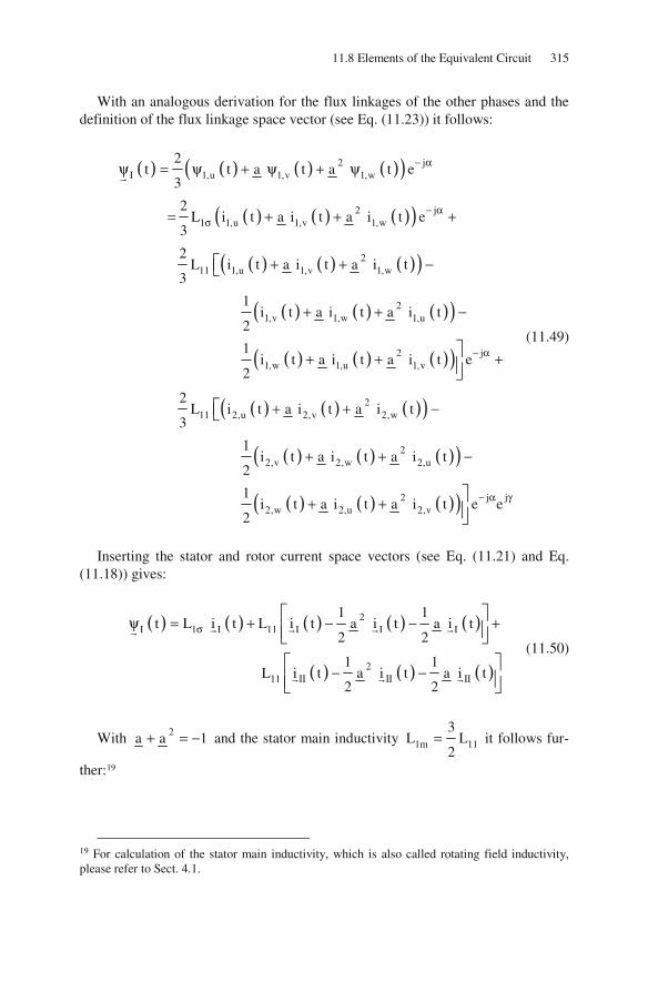
11.8 Elements of the Equivalent Circuit 315
With an analogous derivation for the flux linkages of the other phases and the definition of the flux linkage space vector (see Eq. (11.23)) it follows:
( ) ( ) ( ) ( )( )
( ) ( ) ( )( )
( ) ( ) ( )( )
( ) ( ) ( )( )
( ) ( ) ( )( )
( ) ( ) ( )( )
( ) ( )
2 jI 1,u 1,v 1,w
2 j1 1,u 1,v 1,w
211 1,u 1,v 1,w
21,v 1,w 1,u
2 j1,w 1,u 1,v
211 2,u 2,v 2,w
2,v 2,w
2t t a t a t e
3
2L i t a i t a i t e
3
2L i t a i t a i t
3
1i t a i t a i t
2
1i t a i t a i t e
2
2L i t a i t a i t
3
1i t a i t a
2
− α
− ασ
− α
ψ = ψ + ψ + ψ
= + + +
+ + −
+ + −
+ + +
+ + −
+ + ( )( )
( ) ( ) ( )( )
22,u
2 j j2,w 2,u 2,v
i t
1i t a i t a i t e e
2
− α γ
−
+ +
(11.49)
Inserting the stator and rotor current space vectors (see Eq. (11.21) and Eq. (11.18)) gives:
( ) ( ) ( ) ( ) ( )
( ) ( ) ( )
2I 1 I 11 I I I
211 II II II
1 1t L i t L i t a i t a i t
2 2
1 1L i t a i t a i t
2 2
σψ = + − − +
− −
(11.50)
With 2a a 1+ = − and the stator main inductivity 1m 11
3L L
2= it follows fur-
ther:19
19 For calculation of the stator main inductivity, which is also called rotating field inductivity, please refer to Sect. 4.1.

316 11 Space Vector Theory
( ) ( ) ( ) ( )
( ) ( ) ( )
I 1 I 11 I 11 II
1 I 1m I 1m II
3 3t L i t L i t L i t
2 2
L i t L i t L i t
σ
σ
ψ = + +
= + +
(11.51)
Introducing the stator inductivity 1 1m 1L L L σ= + it follows:
( ) ( ) ( )I 1 I 1m IIt L i t L i t ψ = + (11.52)
Analogously it follows for the space vector of the rotor flux linkage (after
transformation of the rotor values to the stator system and with 2 1m 2L L L σ= + ):
( ) ( ) ( )II 2 II 1m It L i t L i t ψ = + (11.53)
11.8.3 Summary of Results
The transformation of the machine parameters from the existing (three-phase) ma-chine to the space vector notation is done like explained in Table 11.1. Conse-quently, the components of the machine in space vector notation are identical to the components, which are already deduced for the stationary operation of the ma-chine. Therefore, the transformation is resistance- and inductivity-invariant.
Table 11.1. Parameters of existing machines and in space vector notation.
parameter existing machine (rotor values transformed
to the stator system)
space vector notation (rotor values transformed
to the stator system) stator resistance
1R I 1R R=
stator leakage inductivity 1L σ 1L σ
stator main inductivity 1mL 1mL
stator inductivity 1 1m 1L L L σ= + 1 1m 1L L L σ= +
rotor resistance 2R II 2R R=
rotor leakage inductivity 2L σ 2L σ
rotor inductivity 2 1m 2L L L σ= + 2 1m 2L L L σ= +

11.9 Torque in Space Vector Notation 317
11.9 Torque in Space Vector Notation
11.9.1 General Torque Calculation
For a machine having an arbitrary number of pole pairs p the mechanical power can be calculated from torque and mechanical angular frequency like follows:
( ) ( ) ( ) ( )
( ) ( )
mechmech
d dtp t T t T t T t
p p
t 2 n t
ω γ= Ω = =
Ω = π
(11.54)
Together with Eq. (11.38) for the mechanical power the torque in space vector notation becomes:
( ) ( ) ( ){ }II II
3T t p Re j t i t
2
∗= − ψ (11.55)
This equation will be slightly transformed to calculate the torque from stator values. With
( ) ( ) ( ) ( )II 2 II 1m II 1m It L i t L i t L i t σψ = + + (11.56)
and
( ) ( ){ } II IIRe j i t i t 0∗= (11.57)
it follows
( ) ( ) ( ){ }1m I II
3T t p Re j L i t i t
2 ∗
= − (11.58)
Because ( ) ( ) I Ii t i t∗ always is real, it follows further
318 11 Space Vector Theory
( ) ( ) ( ) ( ) ( ) ( ){ }
( ) ( ) ( ) ( ){ }
( ) ( ){ }
( ) ( ){ }
1m I II 1m 1 I I
1m II 1m 1 I I
I I
I I
3T t p Re j L i t i t j L L i t i t
2
3p Re j L i t L L i t i t
2
3p Re j i t t
2
3p Im i t t
2
∗ ∗σ
∗ ∗σ
∗
∗
= − + +
= − + +
= − ψ
= ψ
(11.59)
11.9.2 Torque Calculation by Means of Cross Product from Stator Flux Linkage and Stator Current
The torque can be calculated even as cross product from flux linkage and current. This will be shown in the following. The space vectors of current and flux linkage can be written as ( ϕ and ξ are the phase angles of current and flux linkage, re-
spectively):
( ) ( ) ( )
( ) ( ) ( )
j t I I
j tI I
i t i t e
t t e
− ϕ
− ξ
=
ψ = ψ (11.60)
where all amplitudes and phase angles may have arbitrary time-dependencies. Then:
( ) ( ) ( ) ( ) ( ){ }( ) ( ) ( ) ( ){ }
( ) ( ) ( ) ( ){ }
( ) ( )
j t j t I I
j t t I I
I I
I I
3T t p Im i t e t e
2
3p i t t Im e
2
3p i t t sin t t
2
3p t i t
2
∗− ϕ − ξ
− ϕ −ξ
= ψ
= ψ
= ψ ξ − ϕ
= ψ ×
(11.61)

11.9 Torque in Space Vector Notation 319
11.9.3 Torque Calculation by Means of Cross Product from Stator and Rotor Current
The above equation
( ) ( ) ( ){ }1m I II
3T t p Re j L i t i t
2 ∗
= − (see Eq. (11.58))
can be transformed to
( ) ( ) ( ){ }
( ) ( ){ }
1m I II
1m I II
3T t p Im L i t i t
2
3p L Im i t i t
2
∗
∗
=
=
(11.62)
Analogously to the above calculation it follows:
( ) ( ) ( )1m II I
3T t p L i t i t
2 = × (11.63)
11.9.4 Torque Calculation by Means of Cross Product from Rotor Flux Linkage and Rotor Current
According to Sect. 11.9.1 it is true:
( ) ( ) ( ){ }II II
3T t p Re j t i t
2
∗= − ψ (see Eq. (11.55))
Analogously to the above calculation it follows:
( ) ( ) ( ){ }
( ) ( )
II II
II II
3T t p Im t i t
2
3p i t t
2
∗= ψ
= × ψ
(11.64)

320 11 Space Vector Theory
11.9.5 Torque Calculation by Means of Cross Product from Stator and Rotor Flux Linkage
From the torque equation in Sect. 11.9.1
( ) ( ) ( ){ } I I
3T t p Im i t t
2
∗= ψ (see Eq. (11.59))
and
( )
( )
( )( )
I 1 I 1m II
21 I 1m II
2
1m 1m2 II 1m I 1 I 1m I
2 2
1mII 1 1m I
2 2
1mII 1 I
2 2 1
1mII 1 I
2
L i L i
LL i L i
L
L LL i L i L i L i
L L
L 11 L i
L 1
L 11 L i
L 1 1
L L i
L
ψ = +
= +
= + + −
= ψ + + σ −+ σ
= ψ + −+ σ + σ
= ψ + σ
(11.65)
it follows
1mI II I
1 2
L3 pT Im
2 L L
∗= ψ − ψ ψ
σ (11.66)
With
{ }I IIm 0 ∗ψ ψ = (11.67)
it follows further
{ }1mII I
1 2
L3 pT Im
2 L L
∗= − ψ ψ
σ (11.68)
11.10 Special Coordinate Systems 321
Together with
( ) ( )
( )( )
( )
1m 1m
1 2 1 1m 2 1m
1m 1 2
1m
L L
L L 1 L 1 L
1 1
L 1 1
11
L
=+ σ + σ
=+ σ + σ
= − σ
(11.69)
it follows
{ }II I1m
3 1T p Im
2 L
∗− σ= − ψ ψ
σ (11.70)
Analogously to the above calculation this results in:
I II1m
II I1m
3 1T p
2 L
3 1p
2 L
− σ= − ψ × ψ
σ
− σ= ψ × ψ
σ
(11.71)
11.10 Special Coordinate Systems
For rotating field machines it is often necessary to perform the calculations in dif-ferent coordinate systems. Examples are:
• Realizing constant mutual inductivities for salient-pole synchronous machines → here the calculation in coordinate system fixed to the rotor is advantageous;
• Field-oriented control of induction machines → here the usage of a field-oriented coordinate system is advantageous.
Because of this reason the general transformation to a coordinate system rotat-
ing with arbitrary angular frequency CS
d
dt
αω = is very beneficial. The set of

322 11 Space Vector Theory
equations is generally applicable and depending on the machine topology or use-
fulness the angle ( )tα can be chosen arbitrarily, e.g.:
• ( )t 0α = stationary coordinate system (fixed to the stator), in
literature the axes “ x “ and “ y “ of the coordinate
system are often called in this case “ α “ and “ β “;
• CS mech
d
dt
γω = = ω coordinate system rotating with the rotor speed (fixed to
the rotor), in literature the axes “ x “ and “ y “ of the
coordinate system are then often called “ q “ and “ d “;
• CS 1ω = ω coordinate system rotating with the synchronous speed;
• CS μω = ω coordinate system rotating with the air-gap flux, even
for this coordinate system in literature the axes “ x “ and “ y “are often called “q-axis “ and “d-axis “.
11.11 Relation between Space Vector Theory and Two-Axis-Theory
In addition to the space vector theory described in the preceding sections even the two-axis-theory is known to calculate dynamic operating conditions in electrical machines.
Both theories are strongly linked to each other, especially both theories require the same assumptions that have to be fulfilled for their application (please refer to Sect. 11.2).
The main difference can be found in the definition of the vectors. In the two-axis-theory the vectors are defined as follows (here exemplarily shown for the cur-rents):
( ) ( ) ( ) ( )( ) ( )j t2u v w
2i t i t a i t a i t e
3 − α
= + + (11.72)
Similar definitions hold true even for the voltages and the flux linkages. As a result for the torque of the machine it is obtained:
( ) ( ) ( ){ } I IT t p Im i t t∗= ψ (11.73)

11.12 Relation between Space Vectors and Phasors 323
Apart from the factor 3 2 this equation is identical to the torque equation in
space vector notation. Therefore, the space vector notation has the advantage that voltages and cur-
rents can be interpreted quite clearly: Having a stationary, symmetric operation the amplitudes of current, voltage, and flux linkage space vectors are identical to the amplitudes of the phase values. But this transformation is not power-invariant,
which can be deduced from the factor 3 2 in the torque equation.
In contrary, it can be shown that the two-axis-theory is power-invariant. How-ever, the interpretation of the voltages and currents are not so clear (i.e. for calcu-lation of the really flowing currents a respective factor has to be introduced).
11.12 Relation between Space Vectors and Phasors
Between the space vectors (e.g. Sect. 11.3) and the phasors (e.g. Sect. 1.6) there is a formal similarity. Regarding the current phasor of the positive system when hav-ing symmetric components (see Sect. 1.6), the following is true:
( )2 p u v w
1I I a I a I
3= + + (11.74)
Here pI is the current phasor of the positive system and uI , vI and wI are
the current phasors of the three phase currents. A main requirement for the application of the symmetric components was that
the three phase currents are sinusoidal with the same frequency (then it can be cal-culated with rms-values, which is indicated by the capital letters in the above equation). With other words: Steady-state (but asymmetric) operation conditions can be calculated smartly by means of complex phasors.
The space vectors were defined in the preceding Sect. 11.3. For the currents and the special case 0α = there is:
( ) ( ) ( ) ( )( )2u v w
2i t i t a i t a i t
3 = + + (11.75)

324 11 Space Vector Theory
When introducing the space vectors it was explicitly emphasized that there are no restrictions for the time-dependency of the currents.20 This is the main differ-ence with regards to content to the phasors, and only because of this difference dynamic operation conditions are able to be calculated by space vectors, but not by phasors.
11.13 References for Chapter 11
Dajaku G (2006) Electromagnetic and thermal modeling of highly utilized PM machines. Sha-ker-Verlag, Aachen
Kleinrath H (1980) Stromrichtergespeiste Drehfeldmaschinen. Springer Verlag, Wien Krause PC (1986) Analysis of electric machinery. McGraw Hill Book Company, New York Schröder D (1994) Elektrische Antriebe 1. Springer-Verlag, Berlin Vas P (1992) Electrical machines and drives - a space vector theory approach. Oxford University
Press, Oxford
20 Reminder: When introducing the space vectors it was required that magneto-motive force, cur-rent loading, and air-gap flux density are spatially sinusoidal for every point in time and that there is the same wavelength for all phases. This is realized by a clever winding distribution in the machine and a limitation to the fundamental waves (which, looked at precisely, is an approx-imation).

12 Dynamic Operation and Control of Induction Machines
12.1 Steady-State Operation of Induction Machines in Space Vector Notation at No-Load
12.1.1 Set of Equations
For the calculation of the dynamic operation of the induction machine the general set of equations for rotating field machines (space vector theory, please refer to Chap. 11) can be used. Because of the constant air-gap when neglecting the slot-
ting effect any choice of ( )tα is possible.
Initially, an arbitrary coordinate system is chosen, the angular frequency CSω
and the initial value 0α will be chosen later:
( ) CS 0t tα = ω + α (12.1)
The mechanical speed is (please refer to the footnote in Sect. 11.6):
mech
dp 2 pn
dt
γ= ω = Ω = π (12.2)
The angular synchronous speed is:
1 12 fω = π (12.3)
After transforming the rotor quantities to the stator winding, the voltage equa-tions of the induction machine with short-circuited rotor winding are (see Sect. 11.6):
( ) ( )( )
( )II 1 I CS I
d tu t R i t j t
dt
ψ= + + ω ψ (12.4)
© Springer-Verlag Berlin Heidelberg 2015 325
DOI 10.1007/978-3-642-17584-8_12 D. Gerling, Electrical Machines Mathematica l Engineering,,

326 12 Dynamic Operation and Control of Induction Machines
( )( )
( ) ( )II2 II CS mech II
d t0 R i t j t
dt
ψ= + + ω − ω ψ (12.5)
with the flux linkages (see Sect. 11.8):
( ) ( ) ( )I 1 I 1m IIt L i t L i t ψ = + (12.6)
( ) ( ) ( )II 2 II 1m It L i t L i t ψ = + (12.7)
and the torque equation (see Sect. 11.9):
( ) ( ) ( ){ } I I
3T t p Im i t t
2
∗= ψ (12.8)
12.1.2 Steady-State Operation at No-Load
Now the stationary operation at no-load is to be regarded. It is:
( ) II
dconst., 0, i t 0
dt
ψω = = = (12.9)
If in addition the stator resistance is neglected ( 1R 0= ), the set of equations
becomes:
( ) ( )
( ) ( )
( ) ( ) ( ){ }
I CS 1 I
CS mech 1m I
1 I I
u t j L i t
0 j L i t
3T t p L Im i t i t
2
∗
= ω
= ω − ω
=
(12.10)
These three equations will now be regarded closely. From the defining equation of the stator voltage space vector
( ) ( ) ( ) ( )( )2 jI 1,u 1,v 1,w
2u t u t a u t a u t e
3 − α
= + + (12.11)

12.1 Steady-State Operation of Induction Machines in Space Vector Notation at No-Load 327
and supplying the machine with a symmetrical voltage system
( ) ( )
( )
( )
1 1
1 1
1 1
j t j t1,u 1 1 1
j t j t21,v 1 1 1
j t j t21,w 1 1 1
1u t 2 U cos t 2 U e e
2
2 1u t 2 U cos t 2 U a e a e
3 2
4 1u t 2 U cos t 2 U a e a e
3 2
ω − ω
ω − ω
ω − ω
= ω = +
π= ω − = +
π= ω − = +
(12.12)
the stator voltage equation becomes:
( ) ( )
( )
1
1
1
j t2 2I 1
j t2 2 j
j t j1
2 1u t 2 U 1 a a a a e
3 2
1 a a a a e e
2 U e e
ω
− ω − α
ω − α
= + + +
+ +
=
(12.13)
Thus the stator voltage space vector is performing a circular movement (in
space) with the angular frequency 1ω .
Now a coordinate system is chosen that rotates in synchronism with the rotat-
ing stator field ( CS 1ω = ω ). In addition the initial value is set to 0 0α = . Conse-
quently there is
( ) CS 0 1t t tα = ω + α = ω (12.14)
and further
( ) 1 1j t j tI 1 1u t 2 U e e 2 U ω − ω
= = (12.15)
The real component of the stator voltage space vector is identical to the peak value of the phase voltage, the imaginary component is zero. As the coordinate
system rotates in synchronism with the stator frequency ( CS 1ω = ω had been cho-
sen), this is valid for any point in time. With other words: In stationary operation
and having this choice of CSω all stator quantities become DC values (for the sta-
tor voltages this is shown in the last equation: right of the equal sign there is no time-dependency any more).
Further evaluating the stator voltage equation gives:

328 12 Dynamic Operation and Control of Induction Machines
( )1 CS 1 I2 U j L i t = ω (12.16)
and therefore
( ) 1 I
CS 1
2 Ui t j
L= −
ω (12.17)
This expression is totally imaginary; it is the no-load current of the induction machine in stationary operation. This no-load current has a phase shift of 90° against the stator voltage, which is already known from Chap. 4.
The rotor voltage equation is
( ) ( )CS mech 1m I0 j L i t = ω − ω (12.18)
and can be fulfilled only for CS mechω = ω . As the coordinate system rotates in
synchronism with the rotating stator field (please refer to the choice of ( )tα
above), it follows that 1 mechω = ω is true. With other words the machine rotates
with synchronous speed. As it is well-known, this characterizes the no-load opera-tion (when losses are neglected).
The torque equation gives:
( ) ( ) ( ){ }I I I
3T t p L Im i t i t
2
0
∗=
=
(12.19)
because the multiplication of a complex number with its conjugate-complex value always gives a real number. Even this result is in accordance to the well-known torque of the induction machine in stationary operation at no-load.
12.2 Fast Acceleration and Sudden Load Change
In the following the fast acceleration of the induction machine will be calculated, if at the time t 0= the machine at zero speed is switched to the nominal voltage.
It is assumed that the supplying mains is fixed (concerning the rms-value 1U and
the angular frequency of the voltage 1 12 fω = π ) and that the machine is loaded

12.2 Fast Acceleration and Sudden Load Change 329
just by its inertia. After reaching a (nearly) steady-state condition the machine ab-ruptly is loaded by its nominal torque.
As angular frequency and initial value the following is chosen
( ) 1t tα = ω (12.20)
For numerical solution the set of equations is transformed into the following
shape (here Θ is the inertia and loadT is the load torque; the equation of torque
balance is: load
dT T
dt
ΩΘ = − ):
( )( ) ( ) ( )
( )( ) ( ) ( )
( ) ( ){ }
II 1 I CS I
II2 II CS mech II
mech I I load
d tu t R i t j t
dt
d tR i t j t
dt
d p 3p Im i t t T
dt 2
∗
ψ= − − ω ψ
ψ= − − ω − ω ψ
ω= ψ −
Θ
(12.21)
From the equations of the flux linkages (see Sect. 12.1) it follows
( )
( )
( )
( )
( )
( )
1I I 1 1m
II II 1m 2
I2
II11m
ti t L L
ti t L L
t1 11
t1 1L
−ψ
=ψ
ψ+ σ −− σ=
ψ− + σσ
(12.22)
with
( ) ( )1 2
11
1 1σ = −
+ σ + σ (12.23)
The initial conditions for t 0= are that all currents and voltages in this set of equations as well as the angular frequency and the load torque are zero. For t 0> the excitation is:
( )I 1 loadu t 2 U , T 0 = = (12.24)

330 12 Dynamic Operation and Control of Induction Machines
After finishing the fast acceleration of the unloaded induction machine the fol-lowing values are reached (please refer to the preceding section):
( )
( )
1 I
1 1
II
2 Ui t j
L
i t 0
= −ω
=
(12.25)
At the time 1t t= the induction machine suddenly is loaded with its nominal
torque load NT T= . The excitation quantities are then:
( )I 1 load Nu t 2 U , T T = = (12.26)
In both cases (fast acceleration of the unloaded induction machine at fixed mains and sudden load change) there are transient responses. The data of the simu-lated machine are:
• stator resistance: 1R 1= Ω ,
• rotor resistance: 2R 1′ = Ω
• stator main inductivity: 1mL 260mH=
• stator leakage coefficient: 1 0.1σ =
• rotor leakage coefficient: 2 0.1σ =
• number of pole pairs: p 2=
• inertia: 3 25 10 kgm−Θ = ⋅
The machine is supplied with 1U 230V= and 1f 50Hz= . With this supply the
induction machine generates a pull-out torque of pull outT 26.8Nm− ≈ at a pull-out
slip of pull outs 0.058− ≈ . The nominal torque is NT 15.0Nm= , therefore the over-
load capability is pull out NT T 1.8− ≈ .
The time-dependent characteristics of such an induction motor operation are shown in Figs. 12.1 to 12.4.

12.2 Fast Acceleration and Sudden Load Change 331
Fig. 12.1. Time dependent current in phase u.
Fig. 12.2. Time dependent currents in phase u (red), phase v (blue), and phase w (black).
0.0 0.1 0.2 0.3 0.4 0.5 0.6 0.7 0.8 0.9 1.0
30
20
10
0
-10
-20
-30
t / s
1ui / A
start of run-up sudden load change
0.0 0.02 0.04 0.06 0.08 0.10 0.12
40
30
20
10
0
-10
-20
-30
-40
t / s
i / A

332 12 Dynamic Operation and Control of Induction Machines
Fig. 12.3. Time dependent torque.
Fig. 12.4. Time dependent speed.
0.0 0.1 0.2 0.3 0.4 0.5 0.6 0.7 0.8 0.9 1.0
30
20
10
0
-10
-20
-30
t / s
T / Nm
0.0 0.1 0.2 0.3 0.4 0.5 0.6 0.7 0.8 0.9 1.0 t / s
n / min-1 1500
1000
500
0

12.2 Fast Acceleration and Sudden Load Change 333
Figure 12.5 shows the torque-speed-characteristics of the regarded induction machine. In blue color the steady-state characteristic is shown, in red color the dy-namic characteristic.
Fig. 12.5. Torque-speed-characteristics of the induction machine: steady-state (blue) and dynam-ic (red).
Switching the induction machine at zero speed to the mains at first there are high oscillating torque components (because of the DC current components) ac-companied by high short-circuit AC currents. After decaying of these oscillating torque components the machine accelerates depending on the size of the coupled masses and it swings into the no-load operation (again with some oscillations).
The sudden load change initially decelerates the machine, until the electromag-netic torque is generated. Then an additional transient operation into the next steady-state operation point occurs. The steady-state speed is a little less than the synchronous speed.
The deviations from the steady-state characteristic are remarkable, see the comparison in Fig. 12.5. After decaying of all transient effects all operation points calculated by means of the equations for the dynamic operation are lying on the steady-state characteristic.
Figure 12.6 shows the stator current space vector for these transient operations in the complex plane (red characteristic). In addition, the blue characteristic illus-trates the steady-state current circle diagram of the induction machine (circle dia-gram of the current amplitude, not the circle diagram of the current rms-value).
Even from these characteristics features of transient operations become obvi-ous. High oscillating currents with large deviation from the steady-state character-istic do occur. For fast acceleration as well as for sudden load change the final
0 500 1000 1500
T / Nm
n / min-1
30
20
10
0
-10
-20

334 12 Dynamic Operation and Control of Induction Machines
steady-state values are lying on the circle diagram calculated for pure steady-state operation.
Fig. 12.6. Circle diagram of the induction machine: steady-state (blue, current amplitude) and dynamic (red, current space vector).
The effects of transient operation can be avoided if a slow acceleration accord-
ing to the steady-state 1 1U f− − characteristic is realized; then the acceleration
practically is quasi steady-state (acceleration on the steady-state characteristic). In both cases (dynamic acceleration with oscillations or quasi steady-state ac-
celeration) the induction machine is not suitable being used as a dynamic control unit in a drive system. However, in the following a solution will be developed how to employ the induction machine as such a dynamic control unit (similar to the DC-machine).
12.3 Field-Oriented Coordinate System for Induction Machines
Regarding the separately excited DC-machine the excitation flux FΦ and the ar-
mature MMF (magneto-motive force) AΘ always are perpendicular because of
the impact of the commutator; their location in space is fixed.
0 5 10 15 20 25 30 35 40
{ }IRe i / A
{ }IIm i− / A
25
20
15
10
5
0
-5
-10
-15

12.3 Field-Oriented Coordinate System for Induction Machines 335
The armature quadrature-axis field is assumed being completely compensated by the commutation poles and the compensation windings (in Fig. 12.7 this is not shown for the sake of clarity); because of this the exciting flux is not influenced by the armature current (the armature flux linkage in the quadrature-axis is zero:
A,q 0Ψ = ). This means that the armature flux linkage in the direct-axis just de-
pends on the field excitation current ( A,d FIΨ ); the torque is then produced by:
A FT I Φ
Fig. 12.7. Field excitation, armature MMF, and d-q-coordinate system of a DC-machine.
These features of the DC-machine can be transmitted even to the induction ma-chine, if a coordinate system oriented to the rotor flux is chosen that rotates with the angular frequency of the rotor flux:
( ) 0t tμα = ω + α (12.27)
The instantaneous value of the angular frequency of the rotor flux
mech Rμω = ω + ω (12.28)
must not necessarily be identical to the steady-state value 1ω of the angular fre-
quency of the rotating stator field (with mech d dt pω = γ = Ω and Rω being the
angular frequency of the rotor currents). To better show this analogy to the DC-machine, in the following the space vec-
tors are decomposed into their components and these components are allocated to the respective axes. Firstly, the common set of equations follows from Eqs. (11.26), (11.27), (11.45), (11.46), (11.52), (11.53), and (11.55):
q
d X
X
X
XX X
X
X+ -A
Θ
AI AI
Φ
Φ
Φ
n
XX
XX
XX
XXXX XX
XX
XX+ -
n
FΦ
AI
FΦ
AI
AΘ

336 12 Dynamic Operation and Control of Induction Machines
( ) ( )( )
( )II 1 I CS I
d tu t R i t j t
dt
ψ= + + ω ψ (12.29)
( ) ( )( )
( ) ( )IIII 2 II CS mech II
d tu t R i t j t
dt
ψ= + + ω − ω ψ (12.30)
( ) ( ) ( )I 1 I 1m IIt L i t L i t ψ = + (12.31)
( ) ( ) ( )II 2 II 1m It L i t L i t ψ = + (12.32)
( ) ( ) ( ){ }II II
3T t p Re j t i t
2
∗= − ψ (12.33)
The separation into real components and imaginary components is already in-troduced for the general space vector in Sect. 11.3:
( ) ( ){ } ( ){ }
( ) ( )x y
i t Re i t j Im i t
i t j i t
= +
= − (see Eq. (11.3))
Using this separation of the components the following equations are obtained from the initial voltage and flux linkage equations:
( ) ( )( )
( )
( ) ( )( )
( )
I,xI,x 1 I,x CS I,y
I,yI,y 1 I,y CS I,x
d tu t R i t t
dt
d tu t R i t t
dt
ψ= + + ω ψ
ψ= + − ω ψ
(12.34)
( ) ( )( )
( ) ( )
( ) ( )( )
( ) ( )
II,xII,x 2 II,x CS mech II,y
II,yII,y II,y CS mech II,x2
d tu t R i t t
dt
d tu t R i t t
dt
ψ= + + ω − ω ψ
ψ= + − ω − ω ψ
(12.35)

12.3 Field-Oriented Coordinate System for Induction Machines 337
( ) ( ) ( )
( ) ( ) ( )
I,x 1 I,x 1m II,x
I,y 1 I,y 1m II,y
t L i t L i t
t L i t L i t
ψ = +
ψ = + (12.36)
( ) ( ) ( )
( ) ( ) ( )
II,x 2 II,x 1m I,x
II,y 2 II,y 1m I,y
t L i t L i t
t L i t L i t
ψ = +
ψ = + (12.37)
The torque equation is transformed like follows:
( ) ( ) ( ){ }
( ) ( ) ( ) ( ){ }
( ) ( ) ( ) ( ){
( ) ( ) ( ) ( ) }
( ) ( ) ( ) ( )
II II
II,x II,y II,x II,y
II,x II,x II,y II,y
II,x II,y II,y II,x
II,x II,y II,y II,x
3T t p Re j t i t
2
3p Re j t j t i t j i t
2
3p Re j t i t t i t
2
t i t t i t
3p t i t t i t
2
∗= − ψ
= − ψ − ψ +
= − ψ + ψ −
ψ − ψ
= ψ − ψ
(12.38)
As the coordinate system rotates with the angular frequency of the rotor flux
(please refer to the choice of ( )tα in Eq. (12.1)), the above given description in
components is representing the stator and rotor MMF decomposition in direct axis (d-axis, y -component) and quadrature axis (q-axis, x -component) with respect to
the rotor flux. As this is a flux-oriented coordinate system, the y - and x -
components are named in the following d-component (direct component) and q-component (quadrature component).21
This decomposition into d- and q-components leads to a clear decoupling and by clever control enables the impression of suitable phase currents that the follow-ing aims are achievable:
• the rotor flux linkage in the quadrature axis is zero ( II,q 0ψ = )
• the rotor flux linkage in the direct axis only depends on the magnetizing current
( II,d ,diμψ )
21 The identification with “d“ and “q“ is just a different naming of the components, that usually is introduced for flux-oriented coordinate systems.

338 12 Dynamic Operation and Control of Induction Machines
• the torque is then only generated by the perpendicular components of rotor flux
and stator current: II,d I,qT iψ .
The described operation is called “field-oriented”. An observer, stationary to
the system rotating with ( )tα , sees the same field distribution and torque genera-
tion like for the DC-machine. Simple relations for the control variables rotor flux and active stator current are obtained, that can be adjusted independently from each other like for the DC-machine.
In the following it will be described, how to reach the above mentioned aims (for the sake of clarity the explicit description of the time dependencies is avoided in the following equations). For the rotor flux linkages it is required in direct axis and in quadrature axis, respectively:
II,d 2 II,d 1m I,d
1m ,d
L i L i
!L iμ
ψ = +
=
(12.39)
II,q 2 II,q 1m I,q L i L i
!0
ψ = +
=
(12.40)
Here ,diμ is a magnetizing current defined being proportional to the rotor flux
linkage. From the requirement to the rotor flux linkages it follows for the rotor currents:
( )
( )
1mII,d ,d I,d
2
1mII,q I,q
2
Li i i
L
Li i
L
μ= −
= −
(12.41)
and for the angular frequencies:
( )
mech CS mech R
R
d dp ,
dt dt
d
dt
μ
γ α= ω = Ω = ω = ω = ω + ω
α − γ= ω
(12.42)

12.3 Field-Oriented Coordinate System for Induction Machines 339
As the rotor windings are short-circuited (e.g. for the squirrel-cage rotor) the re-spective voltage equations are:
( )
( )
II,q2 II,q II,d
II,d2 II,d II,q
d d0 R i
dt dt
d d0 R i
dt dt
ψ α − γ= + + ψ
ψ α − γ= + − ψ
(12.43)
Introducing the above equations for the currents, flux linkages, and angular fre-quencies this leads to:
( )
( )
1m2 I,q R 1m ,d
2
,d1m2 ,d I,d 1m
2
L0 R i 0 L i
L
diL0 R i i L 0
L dt
μ
μ
μ
= − + + ω
= − + −
(12.44)
With the rotor time constant 22
2
L
Rτ = the rotor voltage equations in field-oriented
coordinates are obtained:
I,qR mech
2 ,d
,d2 ,d I,d
i
i
dii i
dt
μ
μ
μ
μ
ω = = ω − ωτ
τ + =
(12.45)
The torque equation in field-oriented coordinates is:
( ) ( )1mII,q II,d II,d II,q II,d I,q
2
21m 1m
1h ,d I,q ,d I,q2 2
1m,d I,q
2
L3 3T p i i p i
2 2 L
L L3 3 pL i i p i i
2 L 2 L
L3 p i i
2 1
μ μ
μ
= ψ − ψ = − ψ −
= =
=+ σ
(12.46)

340 12 Dynamic Operation and Control of Induction Machines
For the stator flux linkages, after introducing the rotor currents, the following is true:
( )
I,d 1 I,d 1m II,d
1m1 I,d 1m ,d I,d
2
2 21m 1m
,d 1 I,d2 2
L i L i
LL i L i i
L
L Li L i
L L
μ
μ
ψ = +
= + −
= + −
(12.47)
( )
I,q 1 I,q 1m II,q
1m1 I,q 1m I,q
2
21m
1 I,q2
L i L i
LL i L i
L
LL i
L
ψ = +
= + −
= −
(12.48)
Now the stator voltage equations can be transformed:
I,qI,q 1 I,q I,d
2 2 21m 1m 1m
1 I,q 1 I,q ,d 1 I,d2 2 2
2 2 2I,q1m 1m 1m
1 I,q 1 ,d 1 I,d2 2 2
du R i
dt
L L LdR i L i i L i
dt L L L
diL L LR i L i L i
L dt L L
μ
μ μ
μ μ μ
ψ= + + ω ψ
= + − + ω + −
= + − + ω + ω −
(12.49)
I,dI,d 1 I,d I,q
2 2 21m 1m 1m
1 I,d ,d 1 I,d 1 I,q2 2 2
2 2 2,d I,d1m 1m 1m
1 I,d 1 1 I,q2 2 2
du R i
dt
L L LdR i i L i L i
dt L L L
di diL L LR i L L i
L dt L dt L
μ
μ μ
μ
μ
ψ= + − ω ψ
= + + − − ω −
= + + − − ω −
(12.50)

12.3 Field-Oriented Coordinate System for Induction Machines 341
With the stator time constant 11
1
L
Rτ = and the total leakage coefficient (please re-
fer to Eq. (4.75))
( )( ) ( ) ( )
21m
1 2 1 1m 2 1m
21m
1 2
L11 1
1 1 1 L 1 L
L1
L L
σ = − = −+ σ + σ + σ + σ
= −
(12.51)
the stator voltage equations in field-oriented coordinates are obtained:
( )I,q I,q1 I,q 1 I,d 1 ,d
1
di ui i 1 i
dt Rμ μ μστ + = − ω στ − − σ τ ω (12.52)
( ) ,dI,d I,d1 I,d 1 I,q 1
1
didi ui i 1
dt R dt
μ
μστ + = + ω στ − − σ τ (12.53)
By means of these equations the block diagram of the induction machine in field-oriented coordinates can be deduced (Fig. 12.8). For the sake of clarity the five equations (two stator voltage equations, two rotor voltage equations, and the torque equation) are highlighted in grey. The coordinate transformation and the torque balance can be described by the block diagrams shown in Fig. 12.9.

342 12 Dynamic Operation and Control of Induction Machines
Fig. 12.8. Block diagram of the induction machine in field-oriented coordinates.
Fig. 12.9. Block diagrams of coordinate transformation and torque balance.
+ −
I,du −
+
1στ
I,di −
+,diμ T
−−I,qu
−
+
1στ
I,qi
μω
21 τ
mechω Rω +
+
L3 1mp
2 1 2+σ
( )1 1−σ τ
( )1 1−σ τ
21 τ
11 R 1στ
1στ
2τ
11 R
×
×
×
×
÷
T
+
−
loadT
mechω γ1pΘ
1α μω
1,uu
1,vu
1,wu
I,du
I,qu xy0T

12.3 Field-Oriented Coordinate System for Induction Machines 343
The equation
,d
2 ,d I,d
dii i
dt
μ
μτ + = (12.54)
shows that the direct component of the stator current ( I,di ) determines the magni-
tude of the rotor flux (that is proportional to ,diμ , see above). Like for the field
winding of the DC-machine a large time constant (the rotor time constant 2τ ) is
relevant. Therefore, the magnitude of the rotor flux is not suitable for realizing fast control actions.
The equation
I,q
R mech2 ,d
i
i μ
μ
ω = = ω − ωτ
(12.55)
shows that the angular frequency of the slip (angular frequency of the rotor cur-
rents Rω ) is determined by the quadrature component of the stator current ( I,qi )
and the magnitude of the rotor flux ( ,diμ ). The angular frequency of the rotor
flux is calculated from the angular frequency of the slip and the mechanical angu-lar frequency of the rotor.
The equation
21m
,d I,q2
L3T p i i
2 Lμ= (12.56)
describes the torque generation. Analogously to the DC-machine the torque is
produced by the direct axis flux ( ,diμ ) and the quadrature component of the sta-
tor current ( I,qi ). If (like required) II,d 1m ,dL i const.μψ = = is true, then the torque
T and the angular frequency of the slip Rω are directly proportional to the quad-
rature component of the stator current I,qi .
The equations
( )I,q I,q1 I,q 1 I,d 1 ,d
1
di ui i 1 i
dt Rμ μ μστ + = − ω στ − − σ τ ω (12.57)

344 12 Dynamic Operation and Control of Induction Machines
( ) ,dI,d I,d1 I,d 1 I,q 1
1
didi ui i 1
dt R dt
μ
μστ + = + ω στ − − σ τ (12.58)
are completing the machine model concerning the interaction of stator voltages and stator currents. Regarding the stator current components the induction ma-chine acts like a first-order delay element (PT1 element) with the time constant
1στ and the gain 11 R . The stator current components are coupled by the right-
hand terms in the above equations. The expressions 1 I,qiμω στ and 1 I,diμω στ are
the rotatory induced voltages, that are caused by the currents of the respective dif-
ferent axis. ( ) ,d1
di1
dt
μ− σ τ is the transformatory induced voltage that occurs by
changing the magnetizing current. ( ) 1 ,d1 iμ μ− σ τ ω is the rotatory induced voltage
of the main field. These equations and the deduced block diagram (see Fig. 12.8) describe the in-
duction machine equivalently to the equations in Sects. 12.1 and 12.2. Switching the mains voltage suddenly to the machine at zero speed the same acceleration characteristics (and the same transient characteristics when suddenly loading the machine) like in Sect. 12.2 are obtained!
The advantage of the field-oriented description for the dynamic operation of the induction machine will become clear in the following Sect. 12.4.
12.4 Field-Oriented Control of Induction Machines with Impressed Stator Currents
The advantage of the description shown in the last section is that now the same control strategy like for the separately excited DC-machine can be applied to the induction machine, by which the induction machine is qualified to be applied as a highly dynamic drive: The magnetizing current and consequently the rotor flux shall be hold constantly at their nominal values, the torque shall be adjusted only by means of the quadrature component of the stator current.22 To reach this the transformed stator currents must be independently controllable in direct and quad-rature axis. This kind of control (field-oriented control, FOC) has been developed end of the 1960s, begin of the 1970s by Karl Hasse and Felix Blaschke inde-pendently from each other.
The above described controllability is enabled by
22 Here it is to be regarded that the stator flux increases with the load, therefore saturation may occur in the stator.

12.4 Field-Oriented Control of Induction Machines with Impressed Stator Currents 345
• power electronic devices with high switching frequency (for small power about 20kHz ) and
• short sampling intervals for the control (for small power some 100 sμ for the
current control, for the speed control some ms ).
If these conditions are valid, it can be assumed that the stator currents are im-pressed. Then the equations of the relations between stator voltages and stator cur-rents can be omitted because these are handled intrinsically in the power electronic converter. The respective block diagram is shown in Fig. 12.10.
Fig. 12.10. Block diagram of the induction machine in field-oriented coordinates with impressed stator currents.
The block diagram of the induction machine in field-oriented coordinates with impressed stator currents corresponds to the block diagram of the separately excit-ed DC-machine with neglected armature time constant (please refer to Sect. 10.1). This means that the torque production at constant rotor flux follows the quadrature
component of the stator current I,qi without any delay and the rotor flux is con-
trollable only by the direct component of the stator current. Consequently, the aim of a highly dynamic drive system is reached in principle.
But if the induction machine shall be controlled in field-oriented coordinates, it is necessary to know the instantaneous amplitude and phase of the rotor flux. Having a squirrel-cage rotor the rotor currents and voltages cannot be measured and the measurement of the air-gap flux, which is just an approximation, is very costly and susceptible to faults.
1
pΘ
1,ui
1,vi
1,wi
I,di −
+ × ,diμ L3 1m
p2 1 2+σ
T
I,qi
21 τ
÷
mechω Rω +
+α μω
+
−
loadT
2τ
xy0T

346 12 Dynamic Operation and Control of Induction Machines
However, amplitude and phase of the rotor flux can be calculated from meas-ured values of the stator currents and the speed, by evaluating the rotor voltage equations of the induction machine. This is called “flux model“:
,d2 ,d I,d
I,qmech
2 ,d
dii i
dt
i d
i dt
μ
μ
μ
μ
τ + =
α+ ω = ω =
τ
(12.59)
Then there is the block diagram shown in Fig. 12.11.
Fig. 12.11. Block diagram of the flux model.
It is obvious that the rotor time constant 2τ is decisive for the quality of the
flux model. Particularly, there is the challenge to precisely know the rotor re-
sistance 2R depending on the actual temperature during operation.
Once the rotor time constant 2τ is known, the induction machine can be con-
trolled highly dynamic. For a drive system with speed controller, torque controller, and flux controller the block diagram in Fig. 12.12 is obtained.
1
1,ui
1,vi
1,wi
measured
values
I,di −
+,diμ
I,qi 2τ
÷
mechω
Rω
+
+α μω
measured value
2τ
xy0T

12.4 Field-Oriented Control of Induction Machines with Impressed Stator Currents 347
Fig. 12.12. Block diagram of the field-oriented controlled induction machine with impressed cur-rents.
If at the time t 0= a step function 1 setω = ω = ω is applied to the machine at
zero speed, the phase currents 1,ui , 1,vi and 1,wi are impressed by the control via
the power electronic converter (named “PWM” in the block diagram) in such a way, that
• the magnetizing current ,diμ increases with the rotor time constant
( )2 1m 2 22
2 2 2
1 L L L
R R R
′+ στ = = =
′ ′ to its nominal value and
• the acceleration happens nearly linearly according to the impressed quadrature
current I,q I,q,maxi i= during the run-up time 1
maxp TΘ
ωΘτ = .
control
Tmechω
setω −
+ setT −
+
,d,setiμ −
+ I,d,seti
I,q,seti
αspeed controller torque controller
flux controller field weakening
1
xy0T−
1,u,seti
1,v,seti
1,w,seti PWM
machine model
T
,diμ
2τ
mechω
Rω +
+ μω
α
I,qi
I,di
α
xy0T 1m
2
L3p
2 1+σ
1÷
×
2τ
M
3
Θ
T
1,wi
1,vi
1,ui

348 12 Dynamic Operation and Control of Induction Machines
The time-dependent characteristics shown in Fig. 12.13 are obtained assuming
that 2 Θτ τ is true. Because of the control this drive does not show any over-
shoot or oscillation; the drive is highly dynamic.
Fig. 12.13. Time-dependent characteristics during acceleration.
In the following the torque that is usable during run-up is calculated: The no-
load flux linkage shall be maintained. Then for 1R 0≈ (please refer to Sect. 12.1)
it follows:
( ) 1 I I,q I,d
CS 1
1I,d ,d,0 0
CS 1
2 Ui t j i j i
L
2 Ui i 2 I
L
μ
= − = −ω
= = =ω
(12.60)
This magnetizing current increases with the time constant 2τ :
2
t
,d I,di i 1 e−
τμ = − (12.61)
In steady-state operation the maximum torque is obtained at the pull-out operation point:
1ω ω
I,q,maxi I,qi
I,di ,d,0iμ
Θτ t
, iω
0

12.4 Field-Oriented Control of Induction Machines with Impressed Stator Currents 349
( )
( )( ) ( ) ( )
( ) ( )( )( )
22 1 2
R pull out 2 11m 2
1
2 12 1 2 2
R 1 R1 1 1
L 1L
1
1 1 11 1 1 1
1 1
−
′ ′+ σω = ω = = + σ + σ − σ
σ σ + σ
− σ
= + σ + σ − − =στ + σ + σ στ
(12.62)
For the quadrature current (i.e. the torque producing current) it follows (at
field-oriented control and R 21ω = στ ):
I,q R 2 ,d 0
1i i 2 Iμ= ω τ =
σ (12.63)
The usable torque is then:
1m 1m,d I,q 0 0
2 2
22 1
1 0 pull out1 1
1
L L3 3 1T p i i p 2 I 2 I
2 1 2 1
U3p 1 3p X I 2 T
X1
μ
−
= =+ σ + σ σ
− σ= = =
σω σ ω
− σ
(12.64)
During the acceleration with field-oriented control at R 21ω = στ the double
torque (against the steady-state operation at symmetric, fixed mains) is obtained. Having the same machine data as for the example in Sect. 12.2 (fast accelera-
tion and sudden load change at fixed mains), the time-dependent characteristics shown in Fig. 12.14 are obtained (just the acceleration is shown; therefore the time is limited to an interval from 0s to 0.12s).
The flux generating current ,diμ (shown in red in Fig. 12.14) is increased quite
slowly in this example because of the relatively large time constant 2τ . However,
the torque generating current I,qi (shown in blue in Fig. 12.14) is switched from
its nominal value to zero after about 0.097s, because the run-up period is already finished.
Figures 12.15 and 12.16 show the torque and the speed during this acceleration period (the scale of the vertical axes are the same like in Sect. 12.2). The torque is
increased analogously to the magnetizing current ,diμ as long as I,qi 0> is true.
The acceleration time is considerably shorter (compared to the operation at fixed mains) and there are no oscillations.
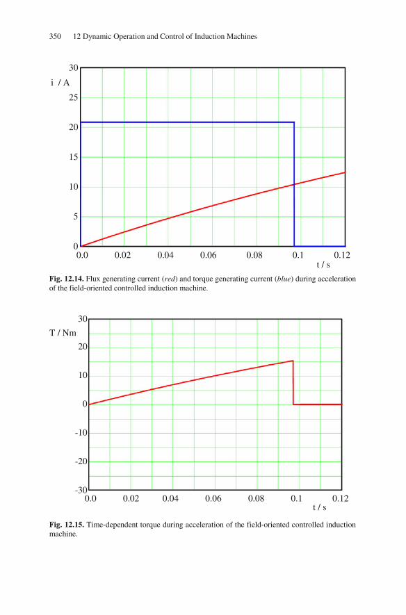
350 12 Dynamic Operation and Control of Induction Machines
Fig. 12.14. Flux generating current (red) and torque generating current (blue) during acceleration of the field-oriented controlled induction machine.
Fig. 12.15. Time-dependent torque during acceleration of the field-oriented controlled induction machine.
0.0 0.02 0.04 0.06 0.08 0.1 0.12 t / s
i / A
30
25
20
15
10
5
0
30
20
10
0
-10
-20
-30
T / Nm
t / s0.0 0.02 0.04 0.06 0.08 0.1 0.12

12.4 Field-Oriented Control of Induction Machines with Impressed Stator Currents 351
Fig. 12.16. Time-dependent speed during acceleration of the field-oriented controlled induction machine.
Figure 12.17 shows the time-dependent characteristics of speed, torque produc-
ing quadrature current I,qi and field producing magnetizing current ,diμ .
• The acceleration period, finished after 0.097s, is characterized by I,q I,q,maxi i=
and a very steep speed increase (the magnetizing current is increased quite
slowly because of the large time constant 2τ ; this is true even for the further
simulation time). • After finishing the acceleration and until switching on the load at the time 0.6s
the quadrature current is set to I,qi 0= , then the speed is constant.
• After switching on the load the influence of the control can be recognized clearly: small speed changes provoked by the control of the torque producing
quadrature current component I,qi are noticeable.
For a better comparison the speed-time-characteristics for acceleration at fixed mains (red line) and for acceleration with field-oriented control (blue line) are pre-sented once again in Fig. 12.18. The entire acceleration period is shown from 0s to 0.6s. The improvement of the dynamic behavior against the operation at fixed mains (please refer to Sect. 12.2) is impressive. The additional effort to realize this operational behavior mainly is a powerful controller and the power electronic converter.
n / min-1
t / s 0.0 0.02 0.04 0.06 0.08 0.1 0.12
1500
1000
500
0

352 12 Dynamic Operation and Control of Induction Machines
Fig. 12.17. Time-dependent characteristics during acceleration of the field-oriented controlled induction machine: speed (red), torque generating current (blue), flux generating current (black).
Fig. 12.18. Speed versus time characteristics of the induction machine: operation at fixed mains supply (red) and operation with field-oriented control (blue).
0.0 0.2 0.4 0.6 0.8 1.0 t / s
n / 50min-1
I,qi / A
,diμ / 0.1A
40
30
20
10
0
n
I,qi
,diμ
0.0 0.1 0.2 0.3 0.4 0.5 0.6 t / s
n / min-1
1500
1000
500
0

12.4 Field-Oriented Control of Induction Machines with Impressed Stator Currents 353
The time-dependent characteristics of the three phase currents are obtained
from the currents I,di and I,qi by means of reverse transformation. With the de-
duction presented above it follows:
( )
I,d 0
0I,q
10
1
i 2 I const.
12 I , for 0s t 0.097s
i t
0, for 0.097s t 0.6s
UI
X
= =
≤ ≤= σ
≤ ≤
=
(12.65)
Further there is (please refer to Sect. 11.3):
( ) ( )1,u I,q I,d
1,v I,q I,d
1,w 1,u 1,v
i i cos i sin
2 2i i cos i sin
3 3
i i i
= α + α
π π= α − + α −
= − −
(12.66)
with the time-dependent angle
( ) ( ) ( ) ( )
t
mech R0
R 2
t t dt with t t
1
μ μα = ω ω = ω + ω
ω = στ
(12.67)
Inserting these equations, the solution for the first 0.097s of the acceleration peri-od is:
( ) ( )1,u 0
1,v 0
1,w 1,u 1,v
1i 2 I cos sin
1 2 2i 2 I cos sin
3 3
i i i
= α + ασ
π π= α − + α −
σ
= − −
(12.68)

354 12 Dynamic Operation and Control of Induction Machines
These equations are valid as long as I,di and I,qi are maintained constantly on-
to their respective maximum values ( 02 I and 02 I / σ ). As soon as the de-
sired speed is reached the current component I,qi is switched to zero (see Fig.
12.17), and therefore even the acceleration torque gets zero (the magnetizing con-
dition of the machine remains unchanged, i.e. I,d 0i 2 I const. = = , the magnet-
izing current ,diμ is increased with the time constant 2τ ). To get the phase cur-
rents by means of reverse transformation for the entire simulation time, the time-
dependent current component ( )I,q I,qi i t= has to be considered. It follows:
( ) ( ) ( )
( )
1,u I,q I,d
1,v I,q I,d
1,w 1,u 1,v
i i t cos i sin
2 2i i t cos i sin
3 3
i i i
= α + α
π π= α − + α −
= − −
(12.69)
The time-dependent characteristics of the three phase currents, calculated by these equations, are illustrated in Fig. 12.19 for the starting period (the scale of the vertical axis is the same like in Sect. 12.2).
Fig. 12.19. Time-dependent currents in phase u (red), phase v (blue), and phase w (black) during acceleration of the field-oriented controlled induction machine.
0.0 0.02 0.04 0.06 0.08 0.10 0.12
40
30
20
10
0
-10
-20
-30
-40
t / s
i / A

12.4 Field-Oriented Control of Induction Machines with Impressed Stator Currents 355
In contrast to the acceleration at fixed mains (see Fig. 12.2) the amplitudes of the three phase currents are identical and (during acceleration and during steady-state operation) constant in time. In addition, the maximum phase current is lower than for the uncontrolled acceleration.
The change of frequency of the phase currents is characteristic for the influence of the power electronic converter, this would not be possible at fixed mains (con-stant voltage concerning amplitude and frequency).
When finishing the acceleration period (at about 0.097s) the current component
I,qi is set to zero. This is noticeable in the characteristics of the phase currents by
the simultaneous change of amplitude and phase; then the frequency is not changed any longer. During the entire operation the slip is maintained at the pull-
out slip of the steady-state operation ( R 21ω = στ ); the torque is adjusted by the
current (more precisely: the current component I,qi ).
Figure 12.20 shows the stator current space vector at field-oriented control (in red) and the circle diagram of the current amplitude in steady-state operation (blue curve). Even with this graph the differences to the dynamic operation at fixed mains supply (please refer to Fig. 12.6) become obvious.
Fig. 12.20. Circle diagram of the induction machine: steady-state operation (blue, current ampli-tude) and during dynamic acceleration with field-oriented control (red, current space vector).
0 5 10 15 20 25 30 35 40
{ }IRe i / A
{ }IIm i− / A
25
20
15
10
5
0
-5
-10
-15
356 12 Dynamic Operation and Control of Induction Machines
12.5 Field-Oriented Control of Induction Machines with Impressed Stator Voltages
Up to now the field-oriented control (FOC) of induction machines has been re-garded assuming that current injecting electronic power converters with high switching frequency and sufficient voltage reserve are available as well as fast mi-crocontrollers for calculating the control algorithms. Regarding electrical drives with a power of up to some kW this is given (servo drives with transistorized in-verters and switching frequencies up to about 20 kHz). For larger drives often pulse-width modulated inverters with intermediate DC-voltage and switching fre-quencies of a few kHz are used. Then the above mentioned conditions are no longer fulfilled. This means that the stator voltage equations have to be regarded
in addition ( 1 1 1L Rτ = ):
( ) ,dI,d1 I,d I,d 1 I,q 1
1
didi 1i u L i 1 L
dt R dt
μ
μστ + = + ω σ − − σ (12.70)
( )( )I,q1 I,q I,q 1 I,d 1 ,d
1
di 1i u L i 1 L i
dt Rμ μ μστ + = − ω σ − − σ ω (12.71)
Both control paths are coupled via the stator currents, therefore they are not in-dependent from each other. However, a decoupling is required so that the current controllers can be adjusted independently. This can be achieved if negative com-
pensation voltages are added to the output voltages of the controllers ( C,du and
C,qu ) in such a way that the coupling voltages are zero. Now the controllers see
decoupled paths. For the compensation usually it is assumed that the rotor flux
linkage is constant, i.e. ,ddi dt 0μ = . Then it follows:
( )
C,d 1 I,q I,d
C,q 1 I,d 1 ,d I,q
u L i u
u L i 1 L i u
μ
μ μ μ
− ω σ =
+ ω σ + − σ ω = (12.72)
Further:

12.5 Field-Oriented Control of Induction Machines with Impressed Stator Voltages 357
I,d1 I,d C,d
1
I,q1 I,q C,q
1
di 1i u
dt R
di 1i u
dt R
στ + =
στ + =
(12.73)
The block diagram of this decoupling network is shown in Fig. 12.21.
Fig. 12.21. Block diagram of the decoupling network.
Figure 12.22 shows the entire diagram of a field-oriented controlled induction machine with impressed voltages realized by a power electronic converter (“PWM“). For the currents in direct axis and quadrature axis a cascaded control is applied respectively; the control parameters can be adjusted independently by means of the decoupling network. The instantaneous values of rotor flux ampli-tude and phase, which are required for the control, are calculated by means of the flux model.
I,di
,diμ
1Lσ
I,qi +
+
μω +
−
( )1 L1−σ+
C,du
I,du
+
C,qu
I,qu
×
×
×

358 12 Dynamic Operation and Control of Induction Machines
Fig. 12.22. Block diagram of the field-oriented controlled induction machine with impressed voltages.
12.6 Field-Oriented Control of Induction Machines without Mechanical Sensor (Speed or Position Sensor)
The mechanical speed has to be known for the field-oriented control (FOC) of in-duction machines: This value is necessary for the speed control as well as for the
machine model
T
,diμ
2τ
mechω
Rω +
+ μω
α
I,qi
I,di
α
xy0T 1m
2
L3p
2 1+σ
1÷
×
2τ
control
T
mechω
setω −
+ setT −
+
,d,setiμ −
+ I,d,seti
I,q,seti α
speed controller
torque controller
flux controller
field weakening 1
xy0T−
1,uu 1,wu
−
+
I,qi
current controller
+ C,qu I,qu
+
−
+
I,di
current controller
+ C,du
I,du −
PWM
decoupling network
I,di I,qi ,diμ μω
M
3
Θ
T
1,wi
1,vi
1,ui
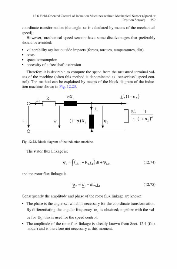
12.6 Field-Oriented Control of Induction Machines without Mechanical Sensor (Speed or Position Sensor) 359
coordinate transformation (the angle α is calculated by means of the mechanical speed).
However, mechanical speed sensors have some disadvantages that preferably should be avoided:
• vulnerability against outside impacts (forces, torques, temperatures, dirt) • costs • space consumption • necessity of a free shaft extension
Therefore it is desirable to compute the speed from the measured terminal val-ues of the machine (often this method is denominated as “sensorless” speed con-trol). The method can be explained by means of the block diagram of the induc-tion machine shown in Fig. 12.23.
Fig. 12.23. Block diagram of the induction machine.
The stator flux linkage is:
( )1 1 1 1 1,0u R i dtψ = − + ψ (12.74)
and the rotor flux linkage is:
2 1 1 1L iψ = ψ − σ (12.75)
Consequently the amplitude and phase of the rotor flux linkage are known:
• The phase is the angle α , which is necessary for the coordinate transformation.
By differentiating the angular frequency μω is obtained; together with the val-
ue for Rω this is used for the speed control.
• The amplitude of the rotor flux linkage is already known from Sect. 12.4 (flux model) and is therefore not necessary at this moment.
1u
1i ( ) 2 2i 1′ + σ
1R
( )2
22
R 1
s 1
′
+ σ
1Xσ
( ) 11 X− σ
i μ
1ψ 2ψ

360 12 Dynamic Operation and Control of Induction Machines
• The above equations for calculating the phase of the rotor flux linkage are evaluated for a two-phase system, after measuring the three-phase values (phase currents and voltages) and subsequent coordinate transformation.
• The evaluation of the integral is difficult for small voltages or small frequen-cies (preciseness and size of the time interval); i.e. for very small speed this method is quite incorrect. The method is reliable from about 5% of the nominal speed onwards.
The flux model from Sect. 12.4 (that solely is based on current measurement) showed the disadvantage of temperature dependency (dependency of the rotor
time constant 2
τ ); the model presented in this section possesses the disadvantage
of inaccuracy at small speed. By clever combination the area of reliable operation without mechanical speed sensor can be considerably increased.
12.7 Direct Torque Control
The direct torque control (DTC) has been developed independently, nearly simul-taneously and in similar form at the beginning of the 1980s in Germany (Manfred Depenbrock) and in Japan (Isao Takahashi and Toshihiko Noguchi) for induction machines. In the meantime this method also is applied to different rotating field machines. The principle of DTC is that by choosing the phase voltages the flux and the torque are directly influenced.
To explain this, a simple switch-model for the power electronic converter and a machine with Y-connected phases is regarded. The diagram is shown in Fig. 12.24.
Fig. 12.24. Diagram of the inverter-fed induction machine.
DCU
1 1 1
0 0 0
uu
wu

12.7 Direct Torque Control 361
The three switches with two different switching positions each (“0“ and “1“)
define eight voltages that are illustrated in Fig. 12.25; the voltages 0u (000) and
7u (111) are called zero-vectors and they are drawn in the origin of the coordinate
system:
Fig. 12.25. Possible voltage vectors of the inverter-fed induction machine.
If only these positions of the power electronic switches are allowed, there is – for any point in time (except for the positions “000“ und “111“) – a series connec-tion of one machine phase with the parallel connection of the other two phases (like it is shown in Fig. 12.26).
Fig. 12.26. Connection of phases of the inverter-fed induction machine at any point in time.
u
wv
α
β
1u (100)
2u (110)
3u (010)
4u (011)
5u (001)
6u (101) 0
7
u (000)
u (111)
DCU
1U 2U

362 12 Dynamic Operation and Control of Induction Machines
With the phase impedance Z and the total current I it follows:
DC 1 2
1
U U U
Z Z 1Z I I 1 Z I
Z Z 2
3U
2
= +
= + = ++
=
(12.76)
Consequently there is always one phase with a voltage drop of 2/3 of the inter-
mediate voltage DCU , and the voltage drop across the parallel connected phases is
1/3 of the intermediate voltage. Then the voltage space vector 1u becomes (see
the definition of the complex voltage space vector in Sect. 11.3):
( ) ( ) ( )( ) ( )
( )
j t21 u v w
2 j0DC DC
DC DC
DC
2u u t a u t a u t e
3
2 2 1U U a a e
3 3 3
2 2 1U U
3 3 3
2U
3
− α= + +
= − +
= +
=
(12.77)
The other voltage space vectors can be calculated analogously. Summarizing, the phase voltages of the machine can be described by space vectors like follows:
( )j 13
DC
2U e if 1, , 6
u 3
0 if 0, 7
π
ν−
ν
ν ==
ν =
(12.78)
By choosing a stationary coordinate system ( ( )t const.α = , here as a special
case ( )t 0α = ) it follows for the stator flux linkage from the stator voltage equa-
tion in space vector notation (see Sect. 11.6):
( )I I I I I I I I
du R i u R i dt
dt = + ψ ψ = − (12.79)

12.7 Direct Torque Control 363
If the stator resistance IR can be neglected, the stator voltage space vectors 1u
to 6u are causing a continuous motion of the stator flux space vector, whereas the
stator voltage space vectors 0u and 7u are stopping the stator flux space vector.
If the stator voltage space vectors 1u to 6u are switched just once per period
(which is called “block-mode operation”), the stator flux space vector moves on a hexagon. Consequently the first task (adjusting the flux of the machine) is fulfilled (see Fig. 12.27).
Fig. 12.27. Possible locations of the stator flux space vector.
The torque can be calculated like it is shown in Sect. 11.9:
{ }I I
3T p Im i
2
∗= ψ (12.80)
With
( )
( )
2I 1 I 1m II 1 I 1m II
2
1m 1m2 II 1m I 1 I 1m I
2 2
1mII 1 1m I
2 2
LL i L i L i L i
L
L LL i L i L i L i
L L
L 11 L i
L 1
ψ = + = +
= + + −
= ψ + + σ −+ σ
(12.81)
α
β
possible location of Iψ

364 12 Dynamic Operation and Control of Induction Machines
and further
( )( )
1mI II 1 I
2 2 1
1mII 1 I
2
L 11 L i
L 1 1
L L i
L
ψ = ψ + −+ σ + σ
= ψ + σ
(12.82)
it follows
1mI II I
1 2
L3 pT Im
2 L L
∗= ψ − ψ ψ
σ (12.83)
With
{ }I IIm 0 ∗ψ ψ = (12.84)
it can be deduced finally
{ }
{ }
1mII I
1 2
II I1m
L3 pT Im
2 L L
3 1p Im
2 L
∗
∗
= − ψ ψσ
− σ= − ψ ψ
σ
(12.85)
Consequently, the torque generation is determined by the amplitudes of the sta-tor flux linkage, the rotor flux linkage, and the relative phase shift of both.
In the following it is assumed that the speed and the amplitude of the rotor flux linkage is constant during one switching condition of the stator voltage space vec-tor. Then the stator flux linkage and the torque are adjusted directly by the choice of the stator voltage space vector. For this choice of the stator voltage space vector – required in the actual operating condition of the machine – the following steps have to be performed:
• division of the α - β -plane into sectors;
• calculation, in which sector the actual stator flux linkage is located; • evaluation, if the stator flux linkage and the torque have to be increased or de-
creased; • adjusting the resulting stator voltage space vector.

12.7 Direct Torque Control 365
The sectors in the α - β -plane can be chosen e.g. like it is shown in Fig. 12.28.
Fig. 12.28. Definition of the sectors in the α-β-plane.
By means of a machine model the instantaneous location and amplitude of the stator flux linkage and the value of the torque can be calculated at any time. By comparison with the respective set values differences are obtained that are fed to a hysteresis controller each. From the instantaneous location of the stator flux link-age and the necessity to increase or decrease the stator flux linkage and the torque (outputs of the hysteresis controllers “1” or “-1”), the next stator voltage space
vector is obtained by means of a table. Respective switching signals us , vs and
ws activate the power electronic switches of the converter. The corresponding
block diagram is given in Fig. 12.29. The according table for choosing the stator voltage space vector is shown in
Table 12.1.
Table 12.1. Switching table for the direct torque control.
φ τ sector 1 sector 2 sector 3 sector 4 sector 5 sector 6
1 1 2u 3u 4u 5u 6u 1u
1 -1 6u 1u 2u 3u 4u 5u
-1 1 3u 4u 5u 6u 1u 2u
-1 -1 5u 6u 1u 2u 3u 4u
sector 1
sector 2
sector 3 sector 4
sector 5
sector 6
α
β
possible location of Iψ

366 12 Dynamic Operation and Control of Induction Machines
Fig. 12.29. Block diagram of the inverter-fed induction machine with direct torque control.
The main advantages of the direct torque control against the field-oriented con-trol are:
• The calculation load in the microcontroller is much lower, because no coordi-nate transformation is required.
• Flux and torque are adjusted by means of simple hysteresis controllers; there is no need for current controllers or for pulse width modulation. Consequently the switching frequency of the power electronic switches is quite low.
• There is only low sensitivity against varying rotor parameters, because only flux and torque calculation is needed.
• For torque and flux control no knowledge of the speed is required; having the field-oriented control this was necessary to calculate the angle α .
• Depending on the preciseness of the machine model even for the speed control the speed sensor can be omitted.
• Generally, the torque control using DTC is faster than using the field-oriented control.
machine model
control
Tmechω
setω −
+ setT −
+
I,setψ −
+
φ
τ
Iψ
T
speed controller torque hysteresis controller
flux hysteresis controller
field weakening table for choosing the stator voltage space vector
us
vs
ws
calculation:
( )I I I Iu R i dt ψ = −
{ }I I
3T p Im i
2
∗= ψ
sector
power electronic converter
M
3
Θ
T
1,wi
1,vi
1,ui

12.8 References for Chapter 12 367
However, disadvantages of the DTC are:
• Because of the missing current controllers there is no possibility of active form-ing of the current waveform. This results in considerable deviations from the ideal sinusoidal function and therefore leads to increased losses of the induction machine.
• Having non-sinusoidal currents the preciseness of the flux and torque calcula-tion strongly depends on the sampling interval and preciseness of the current measurement as well as on the cycle period of the controller.
• The torque ripple depends on the current waveform and the chosen widths of the hysteresis controllers; usually this torque ripple is larger than for the field-oriented control. This results in mechanical load and acoustic noise.
• The switching frequency of the power electronic devices is not fixed and it changes with the speed of the machine. Consequently, even the switching loss-es of the power electronic devices are speed-dependent.
Generally the DTC is characterized by simplicity, robustness, low switching losses, and fast torque control. These features are especially interesting for varia-ble-speed drives with high power.
The DTC described until now can be extended, e.g. by
• consideration of the measured intermediate voltage when calculating the stator voltage space vector;
• high-frequent switching (e.g. PWM) and utilization of all voltage vectors 0u to
7u (by this and with increasing frequency the motion of the flux space vector
can be approximated more and more to a circle); • increasing the number of sectors; • hysteresis controller with three steps (additional step “0“, i.e. no change of flux
or torque).
By these means the technical features (e.g. current waveform and torque ripple) are improved, but the effort is increased.
12.8 References for Chapter 12
Blaschke F (1973) Das Verfahren der Feldorientierung zur Regelung der Drehfeldmaschine. Dis-sertation Technische Universitaet Braunschweig
Boldea I, Tutelea L (2010) Electric machines. CRC Press, Boca Raton Buja GS, Kazmierkowski P (2004) Direct torque control of PWM inverter-fed AC motors – a
survey. IEEE Transactions on Industrial Electronics, 51:744-757 Casadei D, Profumo F, Serra G, Tani A (2002) FOC and DTC: two viable schemes for induction
motors torque control. IEEE Transactions on Power Electronics, 17:779-787

368 12 Dynamic Operation and Control of Induction Machines
DeDoncker RW, Pulle DWJ, Veltman A (2011) Advanced eldectrical Drives. Springer-Verlag, Berlin
Depenbrock M (1988) Direct self-control (DSC) of inverter-fed induction machine. IEEE Trans-actions on Power Electronics, 3:420-429
Hasse K (1969) Zur Dynamik drehzahlgeregelter Antriebe mit stromrichtergespeisten Asyn-chron-Kurzschlußläufermotoren. Dissertation Technische Universitaet Darmstadt
Krishnan R (2001) Electric motor drives. Prentice Hall, London Li Y (2010) Direct torque control of permanent magnet synchronous machine. Shaker-Verlag,
Aachen Nasar SA (1970) Electromagnetic energy conversion devices and systems. Prentice Hall, London Schröder D (1995) Elektrische Antriebe 2. Springer-Verlag, Berlin Takahashi I, Noguchi T (1986) A new quick-response and high-efficiency control strategy of an
induction motor. IEEE Transactions on Industry Application, 22:820-827 White DC, Woodson HH (1958) Electromechanical energy conversion. John Wiley & Sons,
New York

13 Dynamic Operation of Synchronous Machines
13.1 Oscillations of Synchronous Machines, Damper Winding
In this section the behavior of the synchronous machine will be regarded, if the ro-tor angle ϑ is changed by small values Δϑ from the operation point (index “0”). As only small changes are considered, the description of the synchronous machine in steady-state operation (Chap. 5) will be used. There is:
0ϑ = ϑ + Δϑ (13.1)
In steady-state operation the external driving torque of the turbine is equal to the torque of the synchronous machine in every operating point:
( ) N,phase Pext pull out 0 pull out
1
U U3pT T sin , T
X− −= ϑ =
ω (13.2)
The torque of the synchronous generator and the acceleration torque are:
( )gen pull outT T sin−= ϑ (13.3)
a
dT
dt
Ω= Θ (13.4)
with Θ being the inertia of all rotating masses and 02 nΩ ≠ π being the speed of
the synchronous machine: 23
0
d p2 n
dt
ϑΩ = π + (13.5)
23 In the following it will be assumed that the stator current angular frequency 1ω always is
adapted to the speed of the machine. Otherwise the frequency condition for generating a constant torque (see Chap. 3 “Rotating Field Theory”) would not be fulfilled and a pure oscillating torque would occur. The influence of this frequency change on other data (e.g. the pull-out torque) is neglected because just small changes are regarded; in addition the friction is neglected.
© Springer-Verlag Berlin Heidelberg 2015 369
DOI 10.1007/978-3-642-17584-8_ 13D. Gerling, Electrical Machines Mathematica l Engineering,,

370 13 Dynamic Operation of Synchronous Machines
The torque balance
ext gen aT T T− = (13.6)
leads to the following differential equation:
( ) ( )2
pull out 0 pull out 2
d dT sin T sin
dt p dt− −
Ω Θ ϑϑ − ϑ = Θ = (13.7)
This differential equation will be linearized by a Taylor expansion and truncation after the first term:
( ) ( )
( )
( ) ( ) ( ) ( )0 0 0
f xf x x f x x
1!
sin sin sin cos
′+ Δ = + Δ +
ϑ = ϑ + Δϑ ≈ ϑ + Δϑ ϑ
(13.8)
Moreover there is:
( )22 2
02 2 2
dd d
dt dt dt
ϑ + Δϑϑ Δϑ= = (13.9)
Then the differential equation becomes:
( ) ( ) ( )( )
( )
2
pull out 0 pull out 0 0 2
2
pull out 02
dT sin T sin cos
p dt
dT cos 0
p dt
− −
−
Θ Δϑϑ − ϑ + Δϑ ϑ =
Θ Δϑ+ Δϑ ϑ =
(13.10)
With the synchronizing torque in the operating point ( )syn,0 pull out 0T T cos−= ϑ it
can be deduced:
2
syn,0
2
Td0
dt p
Δϑ+ Δϑ =
Θ (13.11)
The solution of this differential equation is an undamped harmonic oscillation:
13.1 Oscillations of Synchronous Machines, Damper Winding 371
( )e,0sin tΔϑ = Ω (13.12)
with the mechanical resonance frequency (eigenfrequency)24
syn,0
e,0 e,0
T2 f
pΩ = π =
Θ (13.13)
Most often the frequency of this mechanical oscillation of the synchronous ma-
chine is in the range of e,0f 1 2Hz= .
During operation of the synchronous machine oscillations can be evoked by electrical or mechanical load changes, which are accompanied by current oscilla-tions. Especially for drives with a non-constant torque (e.g. diesel engine or piston compressor) these oscillations may reach critically high values, if the excitation is near to the eigenfrequency. It is also possible that different generators may excite each other until they fall out of synchronism.
For damping of these oscillations all synchronous machines are equipped with a damper winding. The effect of such a damper winding is comparable with the squirrel-cage of an induction machine.
For high-speed generators with cylindrical rotor damper bars are inserted into the slots of the rotor in addition to the excitation winding; these damper bars are short-circuited at their axial ends (even electrically conductive slot wedges may be used as damper bars). Solid rotors have a damping effect as well, because eddy currents may develop. For salient-pole synchronous machines there are additional slots with bars in the poles; then again the bars are short-circuited at their axial ends.
The calculation of the damper winding can be started from the equations of the induction machine (the torque is negative as it decelerates the machine):
( )
2D 1
pull out ,IMpull outpull out,IM 1
1
pull out
22 1
pull out
1
T U2 3p, T
ssT2X
1s s
R 1s
X1
−−−
−
−
−= =
σω+
− σ
′ + σ=
σ
− σ
(13.14)
Near to the synchronous speed (just small changes Δϑ are regarded) there is:
24 In the mechanical analogon the synchronizing torque corresponds to the spring stiffness, the inertia divided by the number of pole pairs corresponds to the mass.

372 13 Dynamic Operation of Synchronous Machines
pull out
pull out
ss
s s
−
−
(13.15)
Consequently it follows:
D pull out,IMpull out
2sT T
s−
−
≈ − (13.16)
The slip can be described as:
0 0
0
0 0 0 0
d p
1 d 1 ddts
p dt p dt
ϑΩ − Ω +
Ω − Ω ϑ Δϑ= = = − = −
Ω Ω Ω Ω (13.17)
Therefore the damping torque becomes:
pull out,IM
Dpull out 0
2T d dT D
s p dt dt
−
−
Δϑ Δϑ= =
Ω (13.18)
Introducing this damping torque into the differential equation it follows:
2
syn,0
2
Td D d0
dt p dt p
Δϑ Δϑ+ + Δϑ =
Θ Θ (13.19)
The solution of this differential equation is a damped oscillation of the following kind:
( )D
t
ee sin t−
τΔϑ = Ω (13.20)
with the mechanical resonance frequency
22D
e e,01
Ω = Ω −τ
(13.21)
the damping

13.1 Oscillations of Synchronous Machines, Damper Winding 373
( ) ( )
( )
21
21 11
pull out ,IM 12 2
pull out 0 2 1 2 1 00
1
21
221 2 1
U3p2 3p
U2X2T 1 Ds p R 1 R 1 p
p
X1
U3p
R 1
−
−
σωω− σ= = =
′ ′Ω + σ + σ ΩΩ
σ
− σ
=′ω + σ
(13.22)
and the time constant
D
2
pD
Θτ = (13.23)
For maximizing the effect of the damper winding (and therefore damping the
oscillations caused by load changes most quickly) the time constant Dτ must be
small or the damping D must be large. This means that the resistance 2R ′ must be
small. Consequently there is high copper mass and costs needed for the damper cage.
Besides the damping of oscillations the damper winding has two additional tasks:
• From asymmetric loading an opposite rotating field with harmonic oscillations in stator voltage and stator current is generated, which causes additional iron losses and copper losses. In the damper winding currents are evoked that (ac-cording to Lenz’ Law) act against their cause. Therefore, these harmonic oscil-lations and the additional losses are strongly reduced.
• With sufficient heat capacity of the damper winding the synchronous machine may be started with the damper cage like an induction machine. Because of the large slip during run-up the rotating field of the stator would induce high volt-ages in the not-connected excitation winding; therefore the excitation winding is short-circuited at first. Reaching the no-load speed the excitation voltage is switched on and the machine synchronizes suddenly. This is accompanied by current pulses and oscillating torque components, so that this kind of run-up can be applied only for small power machines.
374 13 Dynamic Operation of Synchronous Machines
13.2 Steady-State Operation of Non Salient-Pole Synchronous Machines in Space Vector Notation
Starting with the equations in space vector notation (which are also valid for the dynamic operation of electrical machines) the steady-state operation of the sym-metric synchronous machine with non salient-pole (cylindrical) rotor shall be cal-culated in this section.
The air-gap is assumed being constant; the rotor shall be symmetric, i.e. there are two identical windings shifted electrically by 90°. The excitation winding is supplied with DC current via slip rings, the damper winding is short-circuited.
According to Sects. 11.6 and 11.9 it follows in space vector notation:
( ) ( )( )
( )II I I I
d t du t R i t j t
dt dt
ψ α= + + ψ (13.24)
( ) ( )( ) ( )
( )IIII II II II
d t du t R i t j t
dt dt
ψ α − γ= + + ψ (13.25)
( ) ( ) ( ){ } I I
3T t p Im i t t
2
∗= ψ (13.26)
In the following a coordinate system is chosen that rotates in synchronism with
the rotor: CS mechd dt d dtω = α = γ = ω . This coordinate system is rotor flux ori-
ented, consequently the axes are nominated with “d“ and “q“ (instead of “y“ and “x“). The stator systems are then called I, d and I, q , the rotor systems II, d and
II, q . The splitting up of the above shown complex equations into their compo-
nents gives (analogously to Sect. 12.3):
( ) ( )( )
( )
( ) ( )( )
( )
I,qI,q 1 I,q CS I,d
I,dI,d 1 I,d CS I,q
d tu t R i t t
dt
d tu t R i t t
dt
ψ= + + ω ψ
ψ= + − ω ψ
(13.27)
13.2 Steady-State Operation of Non Salient-Pole Synchronous Machines in Space Vector Notation 375
( ) ( )( )
( ) ( )
( ) ( )( )
( ) ( )
II,qII,q 2 II,q CS mech II,d
II,dII,d 2 II,d CS mech II,q
d tu t R i t t
dt
d tu t R i t t
dt
ψ′= + + ω − ω ψ
ψ′= + − ω − ω ψ
(13.28)
( ) ( ) ( ){ }
( ) ( ) ( ) ( ){ }
( ) ( ) ( ) ( )
I I
I,q I,d I,q I,d
I,d I,q I,q I,d
3T t p Im i t t
2
3p Im i t j i t t j t
2
3p t i t t i t
2
∗= ψ
= − ψ + ψ
= ψ − ψ
(13.29)
During steady-state operation there are no changes of the flux linkages
( d dt 0ψ = ) and the speed is constant ( mech d dt const.ω = γ = ). Now the excita-
tion winding is laid into the II, d -axis and the (short-circuited) damper winding into the II, q -axis. For most synchronous machines (in particular for large genera-
tors) the Ohmic resistance of the stator winding can be neglected. This is done in the following.
Then the above set of equations becomes ( 1 CS d dt const.ω = ω = α = ):
( ) ( )
( ) ( )
I,q 1 I,d
I,d 1 I,q
u t t
u t t
= ω ψ
= −ω ψ (13.30)
( )
( ) ( )
2 II,q
II,d 2 II,d
0 R i t
u t R i t
′=
′= (13.31)
( ) ( ) ( ) ( ) ( )I,d I,q I,q I,d
3T t p t i t t i t
2= ψ − ψ (13.32)
As the space vector theory has been developed in the energy consumption sys-tem, this is the set of equations for the synchronous machine in the energy con-sumption system. Usually the synchronous machine is described in the energy generation system (because generally this machine type is used as a generator, see

376 13 Dynamic Operation of Synchronous Machines
Chap. 5), therefore in the following the synchronous machine shall be described in
terms of the energy generation system. To reach this the voltages I,du and I,qu
are changed in sign. Even the torque equation has to be attached with a negative sign, see below. The two stator voltage equations become:
( ) ( )
( ) ( )
( ) ( )
( ) ( )
I ,d
I,q 1 I,d
1 1 I,d 1 1m II,d
1 I,q
1 1 I,q 1 1m II,q
u t t
L i t L i t
u t t
L i t L i t
= −ω ψ
= − ω − ω
= ω ψ
= ω + ω
(13.33)
The initial value of the rotating coordinate system shall be:
( ) 1 0t tα = ω + α (13.34)
The reverse transformation of the stator voltage equations
( )
( )
( )
( )
( ) ( )
11,u I,qxy
1,v I,d
1
xy
u t u tT ,
u t u t
cos sin
T 2 2cos sin
3 3
−
−
=
α α
= π πα − α −
(13.35)
then gives:
( ) ( ) ( ) ( ) ( )
( ) ( ) ( ) ( )
1,u I,q I,d
I,q 1 I,d 1
u t u t cos u t sin
u t cos t u t sin t
= α + α
= ω + ϑ + ω + ϑ (13.36)
Considering
( ) { }( ) { }( ) { } { }
1
1
1 1
j t1,u 1
j t j1
j t j tj j1
u t Re 2U e
cos t Re e e
sin t Im e e Re je e
ω
ω ϑ
ω ωϑ ϑ
=
ω + ϑ =
ω + ϑ = = −
(13.37)
it follows:

13.2 Steady-State Operation of Non Salient-Pole Synchronous Machines in Space Vector Notation 377
{ } { } { }1 1 1j t j t j tj j1 I,q 1,dRe 2U e u Re e e u Re je eω ω ωϑ ϑ
= + − (13.38)
As there are no currents induced into the damper winding in steady-state opera-
tion, there is II,qi 0= . Consequently:
{ } { } { }
( ) { }
{ }
1 1 1
1
1
j t j t j tj j1 1 I,d 1 1,q
j t j1 1 I,d 1m II,d
j t j1 1 I,q
Re 2U e Re e e Re je e
L i L i Re e e
L i Re je e
ω ω ωϑ ϑ
ω ϑ
ω ϑ
= −ω ψ + ω ψ −
= −ω +
+ ω −
(13.39)
The left side of this equation describes a harmonic oscillation of a single fre-quency. This has to be true even for the right side of the equation. Then the equali-ty of both sides is unchanged if on both sides the respective imaginary compo-nents are added. It follows:
( ){ } { }
( ) ( )
1 1 1j t j t j tj j1 1 1 I,d 1m II,d 1 1 I,q
j j1 1 1 I,d I,q 1 1m II,d
2U e L i L i e e L i je e
1U j L j i i e j L j i e
2
ω ω ωϑ ϑ
ϑ ϑ
= −ω + + ω −
= ω − + ω (13.40)
Now the following currents are defined:
I,q j
1,q
iI e
2
ϑ= (13.41)
I,d j
1,d
iI j e
2
ϑ= − (13.42)
II,d j
2
iI j e
2
ϑ′ = − (13.43)
Then the above voltage equation becomes:
( )1 1 1 1,d 1,q 1 1m 2U j L I I j L I ′= ω − − − ω (13.44)

378 13 Dynamic Operation of Synchronous Machines
With
1 1,q 1,dI I I= + (13.45)
and
P 1 1m 2U j L I ′= − ω (13.46)
it follows further:
P 1 1 1 1U U j L I= + ω (13.47)
This is the well-known voltage equation of the synchronous machine with cylin-drical rotor (please refer to Sect. 5.1). Choosing the terminal voltage being real
1 1U U= (13.48)
the phasor diagram in the well-known form (see Sect. 5.1 and Fig. 13.1) can be drawn:
Fig. 13.1. Phasor diagram of the synchronous machine in steady-state operation.
Splitting the stator current into d-axis component and q-axis component leads to the flux generating and torque generating parts. This becomes obvious by trans-forming the torque equation:
1I
1 1U U=
1 1 1j L Iω
PU
ϕ
ϑ
1,dI
1,qI
2I ′
d
q
Im−
Re

13.2 Steady-State Operation of Non Salient-Pole Synchronous Machines in Space Vector Notation 379
( ) ( ) ( ) ( )
( ) ( )[ ] ( )
( ) ( ) ( )
( ) ( ) ( ) ( )
( ) ( )
( ) ( )
I,d I,q I,q I,d
1 I,d 1m II,d I,q
1 I,q 1m II,q I,d
0
1 I,d I,q 1m II,d I,q
1 I,q I,d
1m II,d I,q
1m 2
3T p t i t t i t
2
3p L i t L i t i t
2
L i t L i t i t
3p L i t i t L i t i t
2
L i t i t
3p L i t i t
2
3 2p L I
2 j
=
= − ψ − ψ
= − +
− +
= − +
−
= −
′= −−
( )
( )
j j 1,q
j2 j21m 2 1,q P 1,q
1 1
j j j2P 1,q P 1,q
1 1
P 11
P 1 G1
e 2 I e
p pj 3 X I I e 3 U I e
p p3 U e I e e 3 U I
p3 U I cos
p3 U I cos
− ϑ − ϑ
− ϑ − ϑ
ϑ ϑ − ϑ
′= − =ω ω
= =ω ω
= ϑ + ϕω
= δω
(13.49)
The angle Gδ is called load angle (angle between stator current and internal
voltage of the machine, please refer to Sect. 5.1). With the relations
( ) ( )P 1U cos U cosϑ + ϕ = ϕ (13.50)
and
( ) ( )P 1 1U sin X I cosϑ = ϕ (13.51)

380 13 Dynamic Operation of Synchronous Machines
it follows further:
( )
( )
1 11
P 1
1 1
pT 3 U I cos
U Up3 sin
X
= ϕω
= ϑω
(13.52)
The equations obtained for calculating the torque of the synchronous machine with cylindrical rotor are already known from Chap. 5:
• Torque from internal voltage, phase voltage and rotor angle
( )P 1
1 1
U UpT 3 sin
X
= ϑ
ω (13.53)
• Torque from phase voltage, phase current and phase angle
( )1 11
pT 3 U I cos = ϕ
ω (13.54)
• Torque from internal voltage, phase current and load angle
( )P 1 G1
pT 3 U I cos = δ
ω (13.55)

13.3 Sudden Short-Circuit of Non Salient-Pole Synchronous Machines 381
13.3 Sudden Short-Circuit of Non Salient-Pole Synchronous Machines
13.3.1 Fundamentals
As an example for the dynamic operation of the synchronous machine the sudden three-phase short-circuit of a non salient-pole synchronous generator at no-load and nominal excitation will be calculated (no-load means: open terminals and ro-tor mechanically driven at synchronous speed). Sudden short-circuit is the transi-ent process that is occurring directly after short-circuiting of the stator terminals (in contrast to the permanent short-circuit that is present when all transient pro-cesses are subsided); i.e. it is the transient phase between steady-state no-load op-eration to steady-state short-circuit operation.
For the sake of simplification the following approximations are introduced:
• The speed of the rotor shall remain constant at synchronous speed during the transient operation (the generator further shall be driven mechanically with synchronous speed).
• The non salient-pole machine shall be symmetric with two identical rotor wind-ings shifted electrically by 90°. The excitation winding is supplied with DC current via two slip rings; the damper winding, lying in the quadrature axis, is short-circuited.
• A rotating coordinate system with CS 1 mechd dt d dtα = ω = ω = ω = γ (like in
Sect. 13.2) is chosen. The stator is composed of systems I, d and I, q , the ro-
tor shows the systems II, d (excitation winding) and II, q (damper winding).
• The initial condition is defined by the switching moment: ( ) 1t tα = ω + ε .
Here ε is an (at this time) arbitrary phase angle.
13.3.2 Initial Conditions for t = 0
The original state before the sudden short-circuit is the no-load operation at nomi-nal excitation. In this steady-state operation the Ohmic resistances of the stator
winding generally can be neglected: 1R 0= (this assumption will be abolished
later). In the following the values just before the moment of switching get the addi-
tional index “0”. For the initial conditions it follows:

382 13 Dynamic Operation of Synchronous Machines
• The stator currents are zero, because the terminals are not connected; the damper current is zero, because there is a steady-state operation at synchronous speed.
I,d,0 I,q,0 II,q,0
II,d,0II,d,0
2
i i i 0
ui
R
= = =
=′
(13.56)
• For the flux linkages the following is true:
I,d,0 1 I,d,0 1m II,d,0 1m II,d,0
I,q,0 1 I,q,0 1m II,q,0
L i L i L i
L i L i 0
ψ = + =
ψ = + = (13.57)
II,d,0 2 II,d,0 1m I,d,0 2 II,d,0
II,q,0 2 II,q,0 1m I,q,0
L i L i L i
L i L i 0
′ ′ψ = + =
′ψ = + = (13.58)
• The stator voltages are (calculation in the energy generation system):
I,q,0I,q,0 1 I,q,0 1 I,d,0 1 I,d,0
I,d,0I,d,0 1 I,d,0 1 I,q,0 1 I,q,0
du R i
dt
du R i
dt
ψ− = + + ω ψ = ω ψ
ψ− = + − ω ψ = −ω ψ
(13.59)
Introducing the flux linkages into the stator voltage equations gives:
I,q,0 1 1m II,d,0
I,d,0
u L i
u 0
= −ω
= (13.60)
and further:

13.3 Sudden Short-Circuit of Non Salient-Pole Synchronous Machines 383
II,d,0I,q,0 1 1m
P,0 1,N 1 1m F,0
iu L 2
2
2 U 2 U 2 L I
= −ω
= = = ω
(13.61)
From this last equation it follows:
1,N
II,d,01 1m
U 2i
L
−=
ω (13.62)
Now the voltage of phase u will be calculated by reverse transformation. As there is a symmetric operation before the moment of switching, the other two phase voltages are symmetrical to the first one; therefore it is not necessary to cal-culate them separately.
( ) ( )
( )
( )
1,u,0 I,q,0 I,d,0
1,N
1,N 1
u u cos u sin
2 U cos 0
2 U cos t
= α + α
= α +
= ω + ε
(13.63)
From this equation it can be deduced that the phase angle ε introduced before characterizes the moment of switching:
• For 0ε = and time t 0= the flux linkage in phase u is zero, i.e. the peak value of the voltage is induced.
• For 2ε = π and time t 0= the flux linkage in phase u is maximum, i.e. the
induced voltage is zero.
13.3.3 Set of Equations for t > 0
Now the above introduced approximation of neglecting the Ohmic resistances of
the stator winding is abolished ( 1R 0≠ ), because these resistances are responsible
for the subsiding of the stator currents (damping characteristic). The stator voltage equations are now in matrix notation (because of the short-
circuit of the terminals this is identical for the energy consumption system and the energy generation system):

384 13 Dynamic Operation of Synchronous Machines
I,d I,d I,d I,q
1 1I,q I,q I,q I,d
u i0 dR
u i0 dt
ψ −ψ= = + + ω
ψ ψ (13.64)
The rotor voltage equations become (as the excitation does not change with
time, and it is further true CS 1 mechd dt d dtα = ω = ω = ω = γ ):
1,NII,d 2 II,d,0 2
1 1mII,q
II,d II,d2
II,q II,q
U 2u R i R
Lu 0
0
i dR
i dt
′ ′−= = ω
ψ′= +
ψ
(13.65)
According to the space vector theory the torque is calculated like (here in the energy consumption system):
I,d I,q I,q I,d
3T p i i
2 = ψ − ψ (13.66)
The flux linkages are:
I,d I,d II,d
1 1mI,q I,q II,q
i iL L
i i
ψ= +
ψ (13.67)
and
II,d II,d I,d
2 1mII,q II,q I,q
i iL L
i i
ψ′= +
ψ (13.68)
or summarized:

13.3 Sudden Short-Circuit of Non Salient-Pole Synchronous Machines 385
[ ]
I,d I,d1
I,q I,q11m
II,d II,d2
II,q II,q2
i1 0 1 0
i0 1 0 1L
i1 0 1 0
i0 1 0 1
L
ψ + σ
ψ + σ=
ψ + σ
ψ + σ
(13.69)
The currents are calculated by means of the inverted matrix [ ] 1L
−:
[ ]
I,d I,d2
I,q I,q2
II,d II,d11m
II,q II,q1
1
i 1 0 1 0
i 0 1 0 11
i 1 0 1 0L
i 0 1 0 1
L−
ψ+ σ −
ψ+ σ −− σ=
ψ− + σσ
ψ− + σ
(13.70)
This set of equations together with the torque equation and the flux equations can be solved numerically. For easier programming the flux equations are trans-formed like follows:
I,d 1 I,d 1 I,q
I,q 1 I,q 1 I,d
1,NII,d 2 2 II,d
1 1m
II,q 2 II,q
dR i
dt
dR i
dt
U 2dR R i
dt L
dR i
dt
ψ = − + ω ψ
ψ = − − ω ψ
′ ′ψ = − −ω
′ψ = −
(13.71)
The currents are obtained by means of reverse transformation. According to the requirements the excitation current is located in the II, d -axis and the damper cur-rent in the II, q -axis; therefore the rotor currents transformed to the stator winding
are:

386 13 Dynamic Operation of Synchronous Machines
II,dF
II,qD
ii
ii= (13.72)
The stator phase currents are calculated like follows (please refer to Sect. 11.3):
( ) ( )
11,u I,qxy
1,v I,d
1
xy
1,w 1,u 1,v
i iT ,
i i
cos sin
T 2 2cos sin
3 3
i i i
−
−
=
α α
= π πα − α −
= − −
(13.73)
With ( ) 1t tα = ω + ε it follows further:
( ) ( )1,u I,q 1 I,d 1
1,v I,q 1 I,d 1
1,w 1,u 1,v
i i cos t i sin t
2 2i i cos t i sin t
3 3
i i i
= ω + ε + ω + ε
π π= ω + ε − + ω + ε −
= − −
(13.74)
Using some approximation (which generally are fulfilled) the set of equations can be solved even analytically. The main advantage is that even qualitative pre-dictions are possible and the influence of the different parameters can be investi-gated on principle. In the following, this analytical solution is not shown in detail, just the results are given.
The envelopes of the different time-dependent characteristics are:
• current in phase u

13.3 Sudden Short-Circuit of Non Salient-Pole Synchronous Machines 387
( )
( )
( )
( )
( ) ( ) ( )
F,stall
1,stall
F,stall
1,stall
t
1,u ,min 11 1,stall 1
t
1,stall
t
1,u ,max 11 1,stall 1
t
1,stall
1,u ,min 1,u 1,u,max
i t 2 U
i t 2 U
1sin e
X
i t i t i t
1 1 1 e
X X X
1sin e
X
1 1 1 e
X X X
−
−τ
−τ
−τ
τ
= −
= −
ε
≤ ≤
+ − +
ε
− − − + (13.75)
• permanent short-circuit current (i.e. short-circuit current after subsiding of the transient processes) in phase u
11,u,min,perm
1
11,u,max,perm
1
1,u,min,perm 1,u,perm 1,u,max,perm
2 Ui
X
2 Ui
X
i i i
= −
=
≤ ≤
(13.76)
• for t → ∞ there is:
( ) ( )1,u,min 1,u,min,perm 1,u,max 1,u,max,permi t i ; i t i→ ∞ → → ∞ → (13.77)
• for t 0= there is:

388 13 Dynamic Operation of Synchronous Machines
( ) ( )[ ]
( ) ( )[ ]
11,u,min
1,stall
11,u,max
1,stall
2 Ui t 0 1 sin
X
2 Ui t 0 1 sin
X
= = − + ε
= = − − + ε
(13.78)
• excitation current
( )
( )
( ) ( ) ( )
F,stall 1,stall
F,stall 1,stall
t t
F,min F,0
t t
F,max F,0
F,min F F,max
1 1i t i 1 e e
1 1i t i 1 e e
i t i t i t
− −τ τ
− −τ τ
− σ − σ= + −
σ σ
− σ − σ= + +
σ σ
≤ ≤
(13.79)
• damper current
( ) ( )
( ) ( ) ( )
1,stall 1,stall
t t
D,min F,0 D,max F,0
D,min D D,max
1 1i t i e ; i t i e
i t i t i t
− −τ τ− σ − σ
= − =σ σ
≤ ≤
(13.80)
• torque
( )
( )
( ) ( ) ( )
F,stall 1,stall
F,stall 1,stall
t t2 1
min1 1
t t2 1
max1 1
min max
U3pT t e e
X
U3pT t e e
X
T t T t T t
− −τ τ
− −τ τ
= −ω σ
=ω σ
≤ ≤
(13.81)
In these equations the time constants and the reactances are:
• no-load time constant of the rotor winding

13.3 Sudden Short-Circuit of Non Salient-Pole Synchronous Machines 389
( )2 1m
F2
1 L
R
+ στ =
′ (13.82)
• short-circuit (stall) time constant of the rotor winding
F,stall Fτ = στ (13.83)
• short-circuit (stall) time constant of the stator winding
11,stall
1
L
Rτ = σ (13.84)
• synchronous reactance
1 1 1X L= ω (13.85)
• short-circuit (stall) reactance
1,stall 1X X= σ (13.86)
It is obvious from the above equations that the short-circuit values F,stallτ ,
1,stallτ and 1,stallX determine the transient change between sudden short-circuit
and permanent short-circuit. For high-speed generators the following orders of magnitude are quite usual:
11,stall 1
N N
F,stall
1,stall
Xx x 0.15 0.25
U I
0.5 2s
60 250ms
= σ = σ =
τ =
τ =
(13.87)

390 13 Dynamic Operation of Synchronous Machines
Now the time-dependent characteristics of stator current (in phase U), excita-tion current, damper current, and torque shall be illustrated. For this a high-speed generator with the following data is calculated:
1,N 1,N N
1 F,stall 1,stall
N
U 11kV, I 758A, P 20MW
X 21.77 , 0.2s, 104ms
T 127kNm
= = =
= Ω τ = τ =
=
(13.88)
13.3.4 Maximum Voltage Switching
As it can be deduced from the above equations for the enveloping characteristics, the moment of switching (for maximum voltage switching there is 0ε = ) has no influence onto the maximum values of torque, excitation current, and damper cur-rent. However, there is an influence onto the phase current. In the following Figs. 13.2 to 13.6 all currents are given in kA, the torque is given in kNm and the time in s.
Figure 13.2 shows the characteristic of the stator current in phase u (red) to-gether with its medium value (magenta), the envelopes of the sudden short-circuit current (black dotted) and the envelopes of the permanent short-circuit current (blue dotted). The maximum value of the permanent short-circuit current is
11,u,max,perm
1
2 Ui
X= (13.89)
and this is for the considered machine 715A (at a nominal value of 758A). The current for sudden short-circuit is
( ) ( )[ ]11,u,max
1,stall
2 Ui t 0 1 sin
X
= = − − + ε (13.90)
and this is for the considered machine for maximum voltage switching ( 0ε = )
4764A (a factor of 1 σ larger than the permanent short-circuit current). Conse-
quently the sudden short-circuit current is several times larger than the nominal current. The mean value of the current for maximum voltage switching is zero.

13.3 Sudden Short-Circuit of Non Salient-Pole Synchronous Machines 391
Fig. 13.2. Stator current in phase u (red) together with its medium value (magenta), the enve-lopes of the sudden short-circuit current (black dotted) and the envelopes of the permanent short-circuit current (blue dotted).
The time dependent characteristics of torque, excitation current, and damper current are shown in Figs. 13.3 to 13.6 (in red each); the respective enveloping functions are shown as dotted black characteristics.
Fig. 13.3. Torque (red) together with the envelopes of the sudden short-circuit torque (black dot-ted).
i / kA 6
4
2
0
-2
-4
-6
-8
-10
t / s 0 0.05 0.1 0.15 0.2 0.25 0.3 0.35 0.4 0.45 0.5
T / kNm 800
600
400
200
0
-200
-400
-600
-800
0 0.05 0.1 0.15 0.2 0.25 0.3 0.35 0.4 0.45 0.5 t / s

392 13 Dynamic Operation of Synchronous Machines
A torque is generated that oscillates with the mains frequency and that subsides with time. The maximum value is
( )21
max1 1
U3pT t 0
X= =
ω σ (13.91)
and for the regarded generator amounts to 707.7kNm (at a nominal torque of 127kNm; i.e. about a factor of 5.6 higher than the nominal torque). When con-structing synchronous machines this high mechanical load has to be considered.
The permanent short-circuit stator currents generate losses in the stator re-sistances. These losses have to be covered by the driving torque (the power loss has to be equalized by the input power). As the speed has been assumed being constant, the acceleration torque is zero. Therefore, the torque balance gives
extT T= − (13.92)
As the external torque has to cover the losses, it follows
( )
2
1 1,u ,max,permlossext
3R iPT
2 n 2 n= =
π π (13.93)
and consequently (inserting the numbers from above)
( )
2
1 1,u,max,perm3R iT 488Nm
2 n= − ≈ −
π (13.94)
This low torque cannot be recognized in the above Fig. 13.3. But evaluating the same simulation like before with a different scale of the vertical axis results in Fig. 13.4, which supports the above calculation.
The currents I,di , I,qi , II,di , II,qi are independent from the moment of switch-
ing ε . Therefore, even the time-dependent characteristics of the torque (Figs. 13.3 and 13.4) and the time-dependent characteristics of the rotor currents (excitation current in Fig. 13.5 and damper current in Fig. 13.6) are independent from the moment of switching. The excitation current as well as the damper current reach multiples of their nominal values during sudden short-circuit (similar to the phase current).
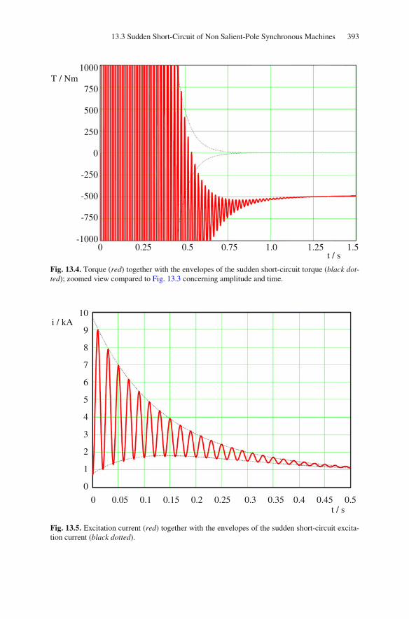
13.3 Sudden Short-Circuit of Non Salient-Pole Synchronous Machines 393
Fig. 13.4. Torque (red) together with the envelopes of the sudden short-circuit torque (black dot-ted); zoomed view compared to Fig. 13.3 concerning amplitude and time.
Fig. 13.5. Excitation current (red) together with the envelopes of the sudden short-circuit excita-tion current (black dotted).
T / Nm 1000
750
500
250
0
-250
-500
-750
-1000
0 0.25 0.5 0.75 1.0 1.25 1.5 t / s
t / s
i / kA10
9
8
7
6
5
4
3
2
1
0
0 0.05 0.1 0.15 0.2 0.25 0.3 0.35 0.4 0.45 0.5

394 13 Dynamic Operation of Synchronous Machines
Fig. 13.6. Damper current (red) together with the envelopes of the sudden short-circuit damper current (black dotted).
13.3.5 Zero Voltage Switching
In contrast to the rotor currents and the torque the stator phase current depends on the moment of switching ε . Switching at a time instant where the voltage is zero
( 2ε = π ), the minimal and maximal values of the sudden short-circuit current are
( ) ( )[ ]
( ) ( )[ ]
1 11,u,min
1,stall 1,stall
11,u,max
1,stall
2 U 2 Ui t 0 1 sin 2
X X
2 Ui t 0 1 sin 0
X
= = − + ε = −
= = − − + ε =
(13.95)
Comparing the amplitudes of the extreme values of the stator phase current for
t 0= , it is true that for 2ε = π the double is reached than for the case 0ε = :
9528A (factor 2 σ higher than the permanent short-circuit current). In this case
the sudden short-circuit current for 2ε = π excesses the nominal value (758A)
by more than a factor of 12.
t / s
i / kA5
4
3
2
1
0
-1
-2
-3
-4
-5 0 0.05 0.1 0.15 0.2 0.25 0.3 0.35 0.4 0.45 0.5

13.3 Sudden Short-Circuit of Non Salient-Pole Synchronous Machines 395
The mean value of the phase current for t 0= is 1
1,stall
2 U
X
− and subsides to ze-
ro with the short-circuit time constant of the stator winding 1,stallτ (see Fig. 13.7).
Fig. 13.7. Stator current in phase u (red) together with its medium value (magenta), the enve-lopes of the sudden short-circuit current (black dotted) and the envelopes of the permanent short-circuit current (blue dotted).
13.3.6 Sudden Short-Circuit with Changing Speed and Rough Synchronization
So far the sudden short-circuit of the non salient-pole machine has been calculated assuming that the speed is constant. This assumption shall be retracted now. For the following calculation it is assumed that:
• At the time t 0s= the machine operates with synchronous speed. • At the time t 0s= the machine will be short-circuited, zero voltage switching
for phase u ( 2ε = π ) is assumed (please refer to the preceding section).
• The external driving torque extT shall be zero for the entire regarded time peri-
od.
t / s 0 0.05 0.1 0.15 0.2 0.25 0.3 0.35 0.4 0.45 0.5
i / kA6
4
2
0
-2
-4
-6
-8
-10

396 13 Dynamic Operation of Synchronous Machines
• The speed decreases after switching on the short-circuit, because the short-circuit currents generate losses in the Ohmic resistances.
• The slope of the speed decrease depends on the inertia; this is assumed being 3 22.5 10 kgmΘ = ⋅ .
• At the time t 0.2s= the machine is switched to the mains again (still with
extT 0= ). As generally not all synchronizing conditions (please refer to Sect.
5.3) are fulfilled, a rough synchronization happens.
The stator terminal voltages in d-q-representation after the rough synchroniza-tion are time-dependent, because there is a time-dependent instantaneous angle ς
between the q -axis (rotating with mech d dtω = γ ) and the location of the voltage
1U (which rotates with 1ω ): 1 mechd dtς = ω − ω (see Fig. 13.8).
Fig. 13.8. Terminal voltages in d-q-representation after rough synchronization.
( )
( )
I,d 1,N
I,q 1,N
I,d I,d I,q1
I,q I,q I,d
I,d I,d I,q1 mech
I,q I,q I,d
u U 2 sin
u U 2 cos
i d dR
i dt dt
i dR
i dt
− ς + ε=
− − ς + ε
ψ −ψγ= + +
ψ ψ
ψ −ψ= + + ω
ψ ψ
(13.96)
It follows:
( )
( )I,d I,d I,q
1 mech 1,NI,q I,q I,d
i sindR U 2
i cosdt
ψ ψ ς + ε= − + ω +
ψ −ψ − ς + ε (13.97)
1U
1 mechω > ω
d
q
Im−
Re
I,qu I,du
ς

13.3 Sudden Short-Circuit of Non Salient-Pole Synchronous Machines 397
Figures 13.9 to 13.13 on the one hand show the influence of the now time-dependent speed, on the other hand the impact of the rough synchronization at the time t 0.2s= is illustrated (like before the currents are represented in kA, the torque in kNm; the scale of the speed axis is in min-1).
Figure 13.9 shows the time-dependent characteristic of the phase current. The small deviations compared to the respective figure in Sect. 13.3.5 (Fig. 13.7) in the first 0.2s , provoked by the slightly decreasing speed (time-dependent characteris-tic of the speed see Fig. 13.13), are only noticeable by detailed analysis. The rough synchronization again evokes a transient operation with remarkable current oscil-lations. As the machine is supplied by the mains voltage after this rough synchro-nization, the final steady-state value of the phase current is no longer the perma-nent short-circuit current, but it is equal to zero (because for these calculations the machine was assumed being unloaded).
Even for the torque there is a transient in the time-dependent characteristic at time t 0.2s= coming from the rough synchronization, see Fig. 13.10. It is obvi-ous that the torque is negative directly after the short-circuit ( t 0s= ), directly af-ter the rough synchronization ( t 0.2s= ) it is positive. Of course this depends on the relative position between the rotating stator field and the rotor at the time in-stant of rough synchronization.
Fig. 13.9. Stator current in phase u (red) together with its medium value (magenta), the enve-lopes of the sudden short-circuit current (black dotted) and the envelopes of the permanent short-circuit current (blue dotted).
t / s 0 0.1 0.2 0.3 0.4 0.5 0.6 0.7 0.8 0.9 1.0
i / kA10
8
6
4
2
0
-2
-4
-6
-8
-10

398 13 Dynamic Operation of Synchronous Machines
Fig. 13.10. Torque (red) together with the envelopes of the sudden short-circuit torque (black dotted).
Fig. 13.11. Excitation current (red) together with the envelopes of the sudden short-circuit exci-tation current (black dotted).
t / s 0 0.1 0.2 0.3 0.4 0.5 0.6 0.7 0.8 0.9 1.0
T / kNm800
600
400
200
0
-200
-400
-600
-800
t / s 0 0.1 0.2 0.3 0.4 0.5 0.6 0.7 0.8 0.9 1.0
i / kA12
10
8
6
4
2
0
-2
-4
-6

13.3 Sudden Short-Circuit of Non Salient-Pole Synchronous Machines 399
Fig. 13.12. Damper current (red) together with the envelopes of the sudden short-circuit damper current (black dotted).
Even the excitation current (Fig. 13.11) shows the transient effect after rough synchronization, the final steady-state value is the respective nominal value. The maximum value of the excitation current after the rough synchronization has about the same value like after the short-circuit.
The amplitude of the damper current after rough synchronization is even a fac-tor of 1.5 larger than after the short-circuit; the final steady-state value is zero for each transient operation, see Fig. 13.12.
Finally the speed-time-characteristic is shown in Fig. 13.13 (the synchronous speed for this machine is 1,500min-1). This speed-time-characteristic correlates with the torque-time-characteristic shown in Fig. 13.10: after the short-circuit the torque acts decelerating, after the rough synchronization it accelerates the rotor.
During short-circuit ( 0s to 0.2s ) the mean value of the speed in decreased, be-cause the phase currents generate losses in the Ohmic resistances; this energy is taken from the reduction of rotational kinetic energy of the rotor (friction was ne-glected). After the rough synchronization the machine is accelerated again and the speed oscillates transiently to the synchronous speed; this is done by means of the damper cage analogously to the operation of an induction machine. As in this sim-ulation the entire load torque was assumed being zero (and therefore friction was neglected), the machine reaches the synchronous speed.
t / s 0 0.1 0.2 0.3 0.4 0.5 0.6 0.7 0.8 0.9 1.0
i / kA10
8
6
4
2
0
-2
-4
-6
-8
-10

400 13 Dynamic Operation of Synchronous Machines
In reality the synchronous speed has to be adjusted by increasing the external driving torque (compensation of friction and other load torques) and stabilized by control (avoiding the overshoot).
Fig. 13.13. Speed-time-characteristic.
13.3.7 Physical Explanation of the Sudden Short-Circuit
In this section the physical conditions during sudden short-circuit of a synchro-nous machine will be explained in principle.
• During no-load operation the excited and rotating rotor generates a rotating flux distribution and consequently sinusoidal terminal voltages
( ( )1,uu 2 U sin t = ω ); this is illustrated in Fig. 13.14.
t / s 0 0.1 0.2 0.3 0.4 0.5 0.6 0.7 0.8 0.9 1.0
1580
1560
1540
1520
1500
1480
1460
n / min-1

13.3 Sudden Short-Circuit of Non Salient-Pole Synchronous Machines 401
Fig. 13.14. Principle situation just after the sudden short-circuit.
• If the terminals of the machine are short-circuited, u 0≡ is true. Neglecting the
Ohmic resistances ( 1R 0= ) the stator flux linkage becomes: d dt 0ψ = , there-
fore const.ψ =
• The stator flux linkage remains constant because of the short-circuited termi-nals, therefore the situation shown in Fig. 13.15 is valid after half a period:
Fig. 13.15. Principle situation half a period after the sudden short-circuit.
The flux is pushed to a magnetically poor conducting leakage path, i.e. the sta-tor winding has to deliver a MMF (i.e. a respective current must be conducted) that is able to drive the flux even along the leakage path. This demonstrates
why the current has to be larger by a factor of 1 σ compared to the permanent
short-circuit (during permanent short-circuit the flux is conducted across stator
XΦ
XX
XX XX
u
v w
x
y z
XXXXXX XXX
XXXXXX
N S
XΦ
XX
XX XX
u
v w
x
y z XXX
XX
N S
X

402 13 Dynamic Operation of Synchronous Machines
and rotor again and no longer along the leakage paths, i.e. 1L is relevant and
no longer 1Lσ ).
13.4 Steady-State Operation of Salient-Pole Synchronous Machines in Space Vector Notation
In contrast to the synchronous machine with cylindrical rotor the salient-pole syn-chronous machine is not constructed symmetrically, but the magnetic permeance
is different in direct axis and quadrature axis ( d qX X> ). Therefore, the transfor-
mation may not be done arbitrarily, but it has to be oriented to the asymmetric part (rotor): only then constant mutual inductivities are obtained.
Figure 13.16 is taken from Sect. 5.5. Here the replaced winding system of the salient-pole synchronous machine is designed in such a way that all windings are located in the d-axis (direct axis, axis of the excitation current) or perpendicular to this (q-axis, quadrature axis). Voltages and currents are shown here for the energy consumption system.
Additionally it shall now be considered that a damper winding is present in the
rotor having a direct component with the current Di and a quadrature component
with the current Qi .
Analogously to Sect. 13.2 the following set of equations (here in the energy
generation system) is obtained with CS mechω = ω :
( ) ( )( )
( )
( ) ( )( )
( )
I,qI,q 1 I,q CS I,d
I,dI,d 1 I,d CS I,q
d tu t R i t t
dt
d tu t R i t t
dt
ψ− = + + ω ψ
ψ− = + − ω ψ
(13.98)
( )( )
( )( )
( ) ( )( )
DD D
QQ Q
FF F F
d t0 R i t
dt
d t0 R i t
dt
d tu t R i t
dt
ψ= +
ψ= +
ψ− = +
(13.99)

13.4 Steady-State Operation of Salient-Pole Synchronous Machines in Space Vector Nota-tion 403
( ) ( ) ( ) ( ) ( )I,d I,q I,q I,d
3T t p t i t t i t
2= − ψ − ψ (13.100)
Fig. 13.16. Sketch of the salient-pole synchronous machine: original system (above left), re-placement (above right) and two-phase replacement (below).
Setting up the equations for the flux linkages the correct consideration of the sign is important. In the direct axis the stator winding and the excitation winding are magnetizing in the same direction, if they conduct positive current. However the damper winding magnetizes in opposite direction. In the quadrature axis the stator winding and the damper winding are magnetizing in opposite direction. There is no magnetic coupling between the direct axis and the quadrature axis. The following matrix equation is obtained for the flux linkages:
XXX
XXX XXX
u
v w
x
y z
XXX
( )tγ
uu
( )tγ
iu
uv
uw
iv
iw
uF
iF
ud id
uq
iq
uF
iF

404 13 Dynamic Operation of Synchronous Machines
( )
( )
( )
( )
( )
[ ]
( )
( )
( )
( )
( )
[ ]
I,d I,d
F F
D D
I,q I,q
Q Q
d dF dD
dF F DF
dD DF D
q qQ
qQ Q
t i t
t i t
t i tL
t i t
t i t
L L L 0 0
L L L 0 0
L L L 0 0L
0 0 0 L L
0 0 0 L L
ψ
ψ
ψ =
ψ
ψ
−
−
− −=
−
−
(13.101)
The external driving torque extT has to overcome the electrodynamic torque T
of the machine and the acceleration torque accT :
( ) ( ) ( )
( ) ( ) ( ) ( )
ext acc
2
I,d I,q I,q I,d 2
T t T t T t
3 dp t i t t i t
2 p dt
= +
Θ γ= − ψ − ψ +
(13.102)
With the equations for the flux linkages, the stator voltage equations, and the torque equation the salient-pole synchronous machine is described completely in a coordinate system rotating in synchronism with the rotor.
Starting from these equations in space vector notation (for the calculation of the dynamic behavior) firstly as a special case the steady-state operation of the salient-pole synchronous machine is regarded. In steady-state operation there is no time-
dependent change of the flux linkages ( d dt 0ψ = ) and the speed is constant
( mechd dt const.γ = ω = ). In addition, in the following the stator resistance will be
neglected ( 1R 0= ). Then the set of equations becomes:
( ) ( )
( ) ( )
I,q CS I,d
I,d CS I,q
u t t
u t t
= −ω ψ
= ω ψ (13.103)

13.4 Steady-State Operation of Salient-Pole Synchronous Machines in Space Vector Nota-tion 405
( )
( )
( ) ( )
D
Q
F F F
0 i t
0 i t
u t R i t
=
=
= −
(13.104)
( ) ( ) ( ) ( ) ( ) ( )ext I,d I,q I,q I,d
3T t T t p t i t t i t
2= = − ψ − ψ (13.105)
( ) ( ) ( )
( ) ( )
I,d d I,d dF F
I,q q I,q
t L i t L i t
t L i t
ψ = +
ψ = (13.106)
All currents and voltages are now DC values; therefore in the following an ex-plicit time-dependency is to be omitted. The other flux linkages are not interesting
any longer. Inserting the flux linkages gives (with CS mechω = ω ):
( )
( )
I,d mech q I,q
I,q mech d I,d dF F
F F F
I,d I,d I,q I,qmech
u L i
u L i L i
u i R
3 pT i u i u
2
= ω
= −ω +
= −
= +ω
(13.107)
Using an analogous calculation like in Sect. 13.2 the reverse transformation is per-
formed; for the rotating coordinate system the angle ( )tα is chosen as:
( ) 1 0 0t t ,α = ω + α α = ϑ (13.108)
( ) ( ) ( ) ( ) ( )
( ) ( ) ( ) ( )
1,u I,q I,d
I,q 1 I,d 1
u t u t cos u t sin
u t cos t u t sin t
= α + α
= ω + ϑ + ω + ϑ (13.109)
and further (analogous to the calculation in Sect. 13.2):
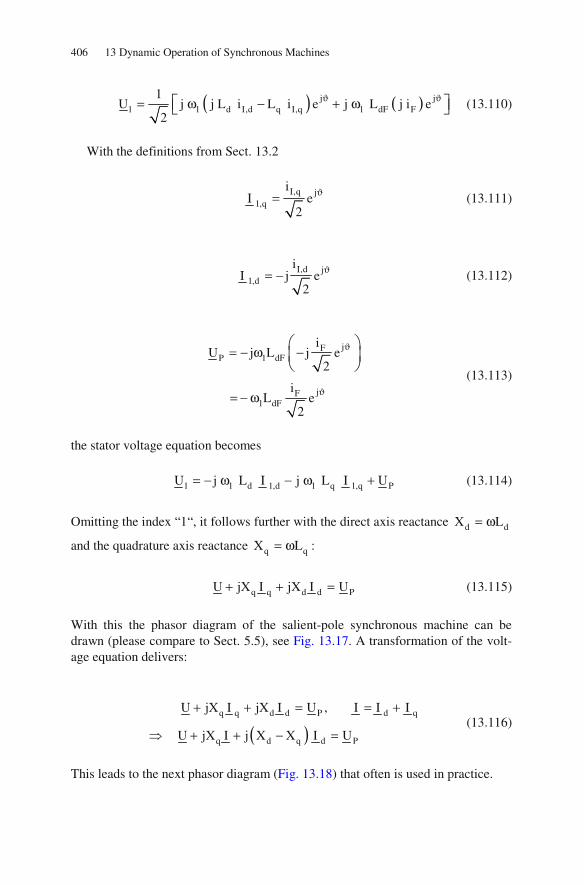
406 13 Dynamic Operation of Synchronous Machines
( ) ( )j j1 1 d I,d q I,q 1 dF F
1U j j L i L i e j L j i e
2 ϑ ϑ
= ω − + ω (13.110)
With the definitions from Sect. 13.2
I,q j
1,q
iI e
2
ϑ= (13.111)
I,d j
1,d
iI j e
2
ϑ= − (13.112)
jFP 1 dF
jF1 dF
iU j L j e
2
iL e
2
ϑ
ϑ
= − ω −
= − ω
(13.113)
the stator voltage equation becomes
1 1 d 1,d 1 q 1,q PU j L I j L I U = − ω − ω + (13.114)
Omitting the index “1“, it follows further with the direct axis reactance d dX L= ω
and the quadrature axis reactance q qX L= ω :
q q d d PU jX I jX I U+ + = (13.115)
With this the phasor diagram of the salient-pole synchronous machine can be drawn (please compare to Sect. 5.5), see Fig. 13.17. A transformation of the volt-age equation delivers:
( )
q q d d P d q
q d q d P
U jX I jX I U , I I I
U jX I j X X I U
+ + = = +
+ + − = (13.116)
This leads to the next phasor diagram (Fig. 13.18) that often is used in practice.

13.4 Steady-State Operation of Salient-Pole Synchronous Machines in Space Vector Nota-tion 407
Fig. 13.17. Phasor diagram of salient-pole synchronous machines.
Fig. 13.18. Alternative phasor diagram of salient-pole synchronous machines.
Im−
Re
I
U
PU
ϕ
ϑ
d djX I
q qjX I
q
d
qI
dI
Im−
Re
I
U
PU
ϕ
ϑ
( )d q dj X X I−
qjX I
q
d
qI
dI
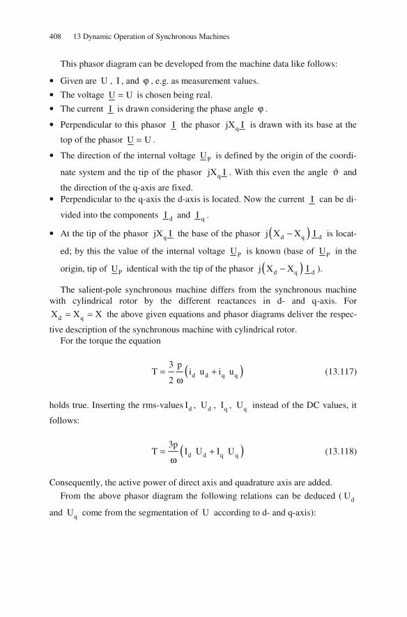
408 13 Dynamic Operation of Synchronous Machines
This phasor diagram can be developed from the machine data like follows:
• Given are U , I , and ϕ , e.g. as measurement values.
• The voltage U U= is chosen being real.
• The current I is drawn considering the phase angle ϕ .
• Perpendicular to this phasor I the phasor qjX I is drawn with its base at the
top of the phasor U U= .
• The direction of the internal voltage PU is defined by the origin of the coordi-
nate system and the tip of the phasor qjX I . With this even the angle ϑ and
the direction of the q-axis are fixed. • Perpendicular to the q-axis the d-axis is located. Now the current I can be di-
vided into the components dI and qI .
• At the tip of the phasor qjX I the base of the phasor ( )d q dj X X I− is locat-
ed; by this the value of the internal voltage PU is known (base of PU in the
origin, tip of PU identical with the tip of the phasor ( )d q dj X X I− ).
The salient-pole synchronous machine differs from the synchronous machine with cylindrical rotor by the different reactances in d- and q-axis. For
d qX X X= = the above given equations and phasor diagrams deliver the respec-
tive description of the synchronous machine with cylindrical rotor. For the torque the equation
( )d d q q
3 pT i u i u
2 = +
ω (13.117)
holds true. Inserting the rms-values dI , dU , qI , qU instead of the DC values, it
follows:
( )d d q q
3pT I U I U = +
ω (13.118)
Consequently, the active power of direct axis and quadrature axis are added.
From the above phasor diagram the following relations can be deduced ( dU
and qU come from the segmentation of U according to d- and q-axis):

13.4 Steady-State Operation of Salient-Pole Synchronous Machines in Space Vector Nota-tion 409
( )
( )Pd d
d
U U cosI , U U sin
X
− ϑ= = ϑ (13.119)
( )
( )q qq
U sinI , U U cos
X
ϑ= = ϑ (13.120)
Inserting this, the torque becomes:
( )
( )( )
( )( )
( ) ( ) ( )
( ) ( )
d d q q
P
d q
2P
d q d
2P
d q d
3pT I U I U
U U cos U sin3pU sin U cos
X X
U U3p 1 1sin U cos sin
X X X
UU3p U 1 1sin sin 2
X 2 X X
= +ω
− ϑ ϑ= ϑ + ϑ
ω
= ϑ + − ϑ ϑω
= ϑ + − ϑω
(13.121)
This result is already known from Chap. 5: the first summand corresponds to the torque of the non salient-pole synchronous machine and it depends on the ex-citation, the second summand is the so-called reaction torque (reluctance torque) and it is not dependent on the excitation (it is merely generated by the difference in the magnetic permeance in d- and q-axis). Because of this reluctance torque the
pull-out torque is reached at a rotor angle less than 2π , see Fig. 13.19 (and Fig.
5.23). This figure shows the ratio of torque and pull-out torque
( ratio pull outT T T −= ) versus the rotor angle ϑ for different excitations PU U :
• red: PU U 0=
• blue: PU U 0.5=
• green: PU U 1.0=
• magenta: PU U 2.0=
• black: torque of the non-salient-pole synchronous machine for
PU U 1.0= (for comparison reasons)

410 13 Dynamic Operation of Synchronous Machines
In addition to the shift of the pull-out torque to smaller rotor angles it can be deduced that the salient-pole synchronous machine delivers a higher pull-out torque for the same excitation current, because of the additional reluctance torque
component (assumed is d,salient pole non salient poleX X− − −= ). In addition it becomes
obvious that for the assumed relation d qX 2X= the pull-out torque without exci-
tation (i.e. the reluctance pull-out) is just half of the pull-out torque of the non-salient-pole machine.
Fig. 13.19. Ratio of torque and pull-out torque versus rotor angle for different excitations.
13.5 Sudden Short-Circuit of Salient-Pole Synchronous Machines
13.5.1 Initial Conditions for t = 0
With some approximations the sudden short-circuit of the salient-pole synchro-nous machine can be calculated analytically. As there is a considerable calculation effort, in the following only the numerical solution is regarded.
Firstly the initial conditions have to be determined. The situation before the sudden short-circuit shall be the no-load operation with nominal excitation (this
ϑ π
ratioT 3
2
1
0
-1
-2
-3
-1 -0.5 0 0.5 1
salient-pole machine:
red: PU U 0=
blue: PU U 0.5=
green: PU U 1.0=
magenta: PU U 2.0=
non salient-pole machine:
black: PU U 1.0=

13.5 Sudden Short-Circuit of Salient-Pole Synchronous Machines 411
means that the excitation winding is supplied by its nominal voltage and the rotor rotates with synchronous speed). The values before the switching moment are nominated in the following with the additional index “0”. The initial conditions then are:
• The stator currents are zero, because the terminals are not connected; the damper current is zero, because there is a steady-state operation at synchronous speed.
d,0 q,0 D,0 Q,0i i i i 0= = = = (13.122)
• The stator voltages are (calculation in the energy generation system):
( )
d,0 q,0 q q,0
q,0 d,0 d d,0 dF F,0 dF F,0 1,N
u L i 0
u L i L i L i 2 U
= ωψ = ω =
= −ωψ = −ω + = −ω = (13.123)
• From the last equation it follows:
1,N
F,0dF
2 Ui
L= −
ω (13.124)
• In addition it is true:
( )
F,0 F F,0
ext,0 d,0 d,0 q,0 q,0mech
u R i
3 pT i u i u 0
2
=
= + =ω
(13.125)
Similar to the calculation of the non salient-pole machine the angle
( ) 1t tα = ω + ε is chosen. Then it follows by means of reverse transformation:
( ) ( )
( )
( )
1,u,0 I,q,0 I,d,0
1,N
1,N 1
u u cos u sin
2 U cos 0
2 U cos t
= α + α
= α +
= ω + ε

412 13 Dynamic Operation of Synchronous Machines
The angle ε therefore characterizes the moment of switching (like for the cal-culation of the non salient-pole machine):
• For 0ε = and time t 0= the flux linkage in phase u is zero, i.e. the peak value of the voltage is induced.
• For 2ε = π and time t 0= the flux linkage in phase u is maximum, i.e. the
induced voltage is zero.
13.5.2 Set of Equations for t > 0
Transforming the set of equations of the salient-pole synchronous machine (see Sect. 13.4) into the description in state space, it can be solved with numerical methods on a digital computer. The set of equations in the energy generation sys-
tem and for CS mechω = ω is (the explicit time-dependency and the index “I“ are
omitted for the sake of simplicity):
( )
dd d 1 q
qq q 1 d
FF F F
DD D
QQ Q
ext d q q d
du i R
dt
du i R
dt
du i R
dt
di R
dt
di R
dt
d p 3T p i i
dt 2
ψ= − − + ω ψ
ψ= − − − ω ψ
ψ= − −
ψ= −
ψ= −
ω= − ψ − ψ
Θ
(13.126)
The relation between the currents and the flux linkages is given by the inductiv-
ity matrix [ ]L .

13.5 Sudden Short-Circuit of Salient-Pole Synchronous Machines 413
[ ]
d d
F F 1
D D
q q
Q Q
i
i
i L
i
i
−
ψ
ψ
ψ=
ψ
ψ
(13.127)
with
[ ]
d dF dD
dF F DF
dD DF D
q qQ
qQ Q
L L L 0 0
L L L 0 0
L L L 0 0L
0 0 0 L L
0 0 0 L L
−
−
− −=
−
−
(13.128)
For calculation of the sudden short-circuit the stator voltages for t 0> are set to zero:
d qu u 0= = (13.129)
The block diagram shown in Fig. 13.20 illustrates the above set of equations. Performing a respective simulation for calculating the sudden short-circuit of
the salient-pole synchronous machine (for this the machine data have to be known), time-dependent characteristics are obtained that are similar (but not iden-tical) to those obtained for the sudden short-circuit of the synchronous machine with cylindrical rotor:
• In the case of sudden short-circuit the stator current reaches a very high value, which subsides to the permanent short-circuit current.
• The excitation current increases to a very high value as well; subsequently it decreases analogously to the stator current.
• The transformed stator currents di and qi are DC currents in steady-state op-
eration; di is the reactive component (magnetizing), qi is the active compo-
nent (torque). • The damper currents (for the regarded salient-pole synchronous machine these
are Di and Qi ) are only relevant during a small time interval directly after the
switching, otherwise they are zero.

414 13 Dynamic Operation of Synchronous Machines
Fig. 13.20. Block diagram of the salient-pole synchronous machine.
1 dR i
du
+
qωψ
−
−
qu
−−
−
dωψ
1 qR i
ω
1R
1R
p
Θ
+
−
d
dt
ω
extT +
dψ
di
qψ
qi
3p
2
3p
2
×
×
×
×
−
Q QR i QR Qi
Qψ
Fu
−−
F FR i FR Fi
Fψ
−
D DR i DR Di
Dψ
[ ] 1L
−

13.6 Transient Operation of Salient-Pole Synchronous Machines 415
Having a constant driving torque extT instead of a constant speed, the speed
decreases after the short-circuit (analogously to the behavior of the non salient-pole machine), because the short-circuit currents generate losses in the Ohmic re-sistances. These losses are supplied by a reduction of the kinetic energy of the sys-tem.
The calculation of the salient-pole synchronous machine is more complex than the calculation of the synchronous machine with cylindrical rotor, because there is an additional differential equation for the damper winding.
13.6 Transient Operation of Salient-Pole Synchronous Machines
The dynamic operation can be calculated similar to the steady-state operation if some simplifying requirements are assumed. The integration of a nonlinear set of equations is avoided, but it has to be checked always, if the assumptions are valid for the regarded operation:
• The speed of the salient-pole synchronous machine is assumed being constant. The larger the inertia of the rotating masses, the better this assumption is ful-filled.
• The effect of the damper winding is not considered: Either the transient process of the damper currents subsides very quickly (considerably faster than the tran-sient process of the stator phase currents), or there does not exist a damper winding.
• The transformatorily induced voltage components can be neglected compared
to the rotatorily induced voltage components (e.g. dq
d
dt
ψωψ ).
• The excitation flux linkage Fψ is constant during the entire transient period.
This is valid, e.g. if the machine is equipped with a voltage controller that com-pensates the Ohmic voltage drop at the resistance in the excitation circuit if the
current changes: FF F F
du R i 0
dt
ψ− − = = .
If these conditions are fulfilled it is called the “transient operation” of the syn-chronous machine (compared to the “dynamic operation” regarded in the preced-ing section). From the general set of equations for the salient-pole synchronous machine the following set of equations for this transient operation can be deduced:

416 13 Dynamic Operation of Synchronous Machines
( )
d d 1 q
q q 1 d
F F F
D D
Q Q
ext d q q d
0 u i R
0 u i R
0 u i R
0 i R
0 i R
p 30 T p i i
2
= − − + ω ψ
= − − − ω ψ
= − −
= −
= −
= − ψ − ψΘ
(13.130)
Neglecting the Ohmic voltage drop at the stator resistance it follows:
( )
d q
q d
F F F
D
Q
ext d q q d
u
u
u i R
i 0
i 0
3T T p i i
2
= +ωψ
= −ωψ
= −
=
=
= = ψ − ψ
(13.131)
The flux linkages are:
[ ]
d d
F F
D D
q q
Q Q
i
i
iL
i
i
ψ
ψ
ψ =
ψ
ψ
(13.132)
with

13.6 Transient Operation of Salient-Pole Synchronous Machines 417
[ ]
d dF dD
dF F DF
dD DF D
q qQ
qQ Q
L L L 0 0
L L L 0 0
L L L 0 0L
0 0 0 L L
0 0 0 L L
−
−
− −=
−
−
(13.133)
Consequently (with D Qi i 0= = ) there is:
F F F dF d
d d d dF F
q q q
L i L i
L i L i
L i
ψ = +
ψ = +
ψ =
(13.134)
The set of equations for this transient operation has the same form like the set of equations for the steady-state operation, but there is one main difference:
• steady-state operation: excitation current Fi const.=
• transient operation: excitation flux F const.ψ =
Because of the constant excitation flux it follows (the index “0“ characterizes the steady-state situation before the switching):
( )
F F F dF d
F,0 F F,0 dF d,0
dF dFF d F,0 d,0
F F
dFF F,0 d,0 d
F
L i L i
L i L i
L Li i i i
L L
Li i i i
L
ψ = +
= ψ = +
+ = +
= + −
(13.135)
Therefore the excitation current Fi changes with the stator current di . For the in-
ternal voltage there is:
P FdFu L i= −ω (13.136)
With this an additional difference between steady-state and transient operation becomes obvious:

418 13 Dynamic Operation of Synchronous Machines
• steady-state operation: internal voltage Pu const.=
• transient operation: internal voltage Pu const.≠
Further:
( )
( )
( )
P dF F
dFdF F,0 d,0 d
F
dFdF F,0 dF d,0 d
F
dFP,0 dF d d,0
F
u L i
L L i i i
L
LL i L i i
L
Lu L i i
L
= −ω
= −ω + −
= −ω − ω −
= + ω −
(13.137)
With
2dF
dFd F
L1
L Lσ = − (13.138)
it follows:
( )
( ) ( )
dFP P,0 dF d d,0
F
P,0 dF d d d,0
Lu u L i i
L
u 1 L i i
= + ω −
= + − σ ω −
(13.139)
The flux linkage in the d-axis becomes:
( )
( )
d d d dF F
dFd d dF F,0 d,0 d
F
2 2dF dF
dF F,0 d d d d,0d F d F
dF F,0 dF d d dF d d,0
L i L i
LL i L i i i
L
L LL i L i 1 L i
L L L L
L i L i 1 L i
ψ = +
= + + −
= + − +
= + σ + − σ
(13.140)
Consequently the voltage equation of the quadrature axis becomes:

13.6 Transient Operation of Salient-Pole Synchronous Machines 419
( )[ ]( )
q d
dF F,0 dF d d dF d d,0
dF F,0 dF d d dF d d,0
u
L i L i 1 L i
L i L i 1 L i
= −ω ψ
= −ω + σ + − σ
= −ω − ω σ − ω − σ
(13.141)
With the internal voltage before the switching moment P,0 F,0dFu L i= −ω and the
transient reactance d dF dX L ′ = σ ω the voltage in the quadrature axis is:
( )
( )
q dF F,0 dF d d dF d d,0
P,0 d d dF d d,0 d d
u L i L i 1 L i
u X i 1 X i with X L
= −ω − ω σ − ω − σ
′= − − − σ = ω (13.142)
A transformation (all constant values before the switching moment are written on the left side) gives:
( )P,0 dF d d,0 q d d Pu 1 X i u X i u ′ ′− − σ = + = (13.143)
The value P q d du u X i′ ′= + therefore is a constant during the transient operation
(analogously to the value P q d du u X i= + , which is constant for steady-state op-
eration). For the internal voltage it holds:
( ) ( )
( )P P,0 dF d d d,0
P dF d d
u u 1 L i i
u 1 X i
= + − σ ω −
′= + − σ (13.144)
The voltage in the direct axis is unchanged:
d q q qu X i= +ω ψ = (13.145)
Now the description can be changed from space vectors to rms-values by using the respective equations of the preceding sections. The voltage equations for the transient operation then are:

420 13 Dynamic Operation of Synchronous Machines
( )
( )
P P,0 dF d d,0
q d d
P P dF d d
d q q
U U 1 X I
U X I const.
U U 1 X I
U X I
′ = − − σ
′= + =
′= + − σ
=
(13.146)
For the rms-values (and for the phasor diagram developed from the above equa-
tions, see Fig. 13.21) it holds: During transient operation no longer PU is constant
(like in steady-state operation), but PU′ is constant. The value of PU′ can be cal-
culated from the conditions just before the switching moment.
Fig. 13.21. Phasor diagram of the salient-pole synchronous machine in transient operation.
For the torque it holds during the transient operation:
( )d d q q
3pT I U I U= +
ω (13.147)
From the phasor diagram the following relations can be deduced:
( ) ( )
P q dd q
d q
d q
U U UI I
X X
U U sin U U cos
′ −= =
′
= ϑ = ϑ
(13.148)
qU
q qjX I
Im−
Re
I
U
PU
ϕ
ϑ
qjX I
q
d qI
dI
PU′
d djX I′

13.6 Transient Operation of Salient-Pole Synchronous Machines 421
By insertion it follows:
( )( )
( )( )
( ) ( ) ( )
( ) ( )
P
d q
2P
d q d
2P
d q d
U U cos U sin3p T U sin U cos
X X
U U3p 1 1sin U sin cos
X X X
U U3p 1 1 Usin sin 2
X X X 2
′ − ϑ ϑ= ϑ + ϑ
′ω
′= ϑ + − ϑ ϑ
′ ′ω
′= ϑ + − ϑ
′ ′ω
(13.149)
With the nominal torque of the synchronous machine (please refer to Chap. 5)
( )N N N
N
3U I cosT
p
ϕ=
ω (13.150)
the ratio of the torque during transient operation to the nominal torque of the syn-chronous machine becomes:
( ) ( )
( )
( ) ( )
( )
2P
d q dN
N N NN
NP
d q d
N N
U U3p 1 1 Usin sin 2
X X X 2T, U U
3U I cosT
p
UU 1 1sin sin 2
X X X 2
I cos
′ϑ + − ϑ
′ ′ω= =
ϕ
ω
′ϑ + − ϑ
′ ′=
ϕ
(13.151)
With
N PN P
N N
qdd q
N N
U UX u
I U
XXx x
X X
′′= =
′′= =
(13.152)
it follows in normalized description:

422 13 Dynamic Operation of Synchronous Machines
( )
( ) ( )Pratio
N N d q d
uT 1 1 1 1T sin sin 2
T cos x x x 2
′= = ϑ + − ϑ
′ ′ϕ (13.153)
Relating the torque to the pull-out torque of a respective non-salient-pole syn-chronous machine, Fig. 13.22 is obtained (this figure can be compared directly to
the figures shown in Sects. 13.4 and 13.5; PU U 0.5= has been chosen). It be-
comes obvious that during transient operation a considerably higher pull-out torque is achieved than during steady-state operation. Moreover the pull-out
torque is reached for a rotor angle 2ϑ > π , whereas for the steady-state operation
the pull-out torque is reached for 2ϑ < π . This effect comes from the fact that
during transient operation the excitation flux is kept constant by increasing the ex-citation current (and therefore even the torque) to a considerably higher value. Af-ter subsiding of the time-dependent characteristics the new steady-state operation is obtained.
Fig. 13.22. Torque (normalized to the pull-out torque) versus rotor angle characteristic of the sa-lient-pole synchronous machine in steady-state and transient operation.
Having the synchronous machine supplied from the mains the transient opera-tion can be evoked by two different load changes:
transient
steady-state
ratioT
ϑ π
3
2
1
0
-1
-2
-3 -1.0 -0.5 0.0 0.5 1.0

13.7 References for Chapter 13 423
• Electrical load change: A switching action in the supplying mains suddenly
changes mains voltage and mains reactance. For calculating PU′ the values of
the steady-state operation just before the switching moment have to be taken. For the time period after the switching moment the new values of mains volt-
age and mains reactance have to be considered. Because of PU′ being constant
the currents dI und qI change nearly according to a step-function. Therefore
the machine generates a different torque than before the switching moment. Because of the inertia the rotor moves with synchronous speed; consequently a
torque difference occurs resulting in a movement ( )tϑ of the rotor angle.
• Mechanical load change: When the driving torque is changed suddenly, mains voltage and mains reactance remain unchanged. Directly after this disturbance the same currents like before are flowing, consequently the torque generated by the synchronous machine is unchanged. Because of the change of the driving
torque there is a torque difference resulting in a movement ( )tϑ of the rotor
angle. Subsequently even the currents and the torque of the synchronous ma-chine are changed.
13.7 References for Chapter 13
Boldea I, Tutelea L (2010) Electric machines. CRC Press, Boca Raton DeDoncker RW, Pulle DWJ, Veltman A (2011) Advanced electrical drives. Springer-Verlag,
Berlin Nasar SA (1970) Electromagnetic energy conversion devices and systems. Prentice Hall, London Schröder D (1995) Elektrische Antriebe 2. Springer-Verlag, Berlin White DC, Woodson HH (1958) Electromechanical energy conversion. John Wiley & Sons,
New York

14 Dynamic Operation and Control of Permanent Magnet Excited Rotating Field Machines
14.1 Principle Operation
As already described in Chap. 6, the principle operation of the permanent magnet excited rotating field machine is like follows:
The synchronous machine contains permanent magnets to generate the excita-tion field, but there is no starting cage present. The three-phase machine is sup-plied by an inverter which realizes a three-phase current system. As a main differ-ence to what is described in Chap. 6, here no limiting assumptions concerning the time-dependency of the currents is made (especially there is no need for sinusoidal currents).
The fundamental frequency of the supplying three-phase system determines the frequency of the rotating magneto-motive force and therefore even the rotor speed. The rotating magneto-motive force together with the field of the permanent mag-net rotor generates the torque. Mostly, this torque shall be as smooth as possible. The rotation of the rotating stator field is realized depending on the rotor position by means of the inverter in such a way, that the electrical angle between rotating
magneto-motive force of the stator and the rotor field is 2π (i.e. ϑ = −ϕ ). With
this the load angle in the energy consumption system already defined in Sect. 6.3
becomes M G 0δ = −δ = −ϑ − ϕ = .
The rotor position can be measured by using sensors or it can be deduced from the terminal voltages and/or terminal currents.
An operation is obtained that does no longer correspond to the synchronous machine, but to the DC-machine:
• DC-machine: magneto-motive force of the armature and excitation field build
an electrical angle of 2π ; this adjustment is performed mechanically by
means of the commutator. • Synchronous machine: the rotor angle ϑ and the phase angle ϕ are adjusted
depending on the operation point; there is no active influence on the phase shift between magneto-motive force of the stator and excitation field.
• Electronically commutated permanent magnet excited rotating field machine: magneto-motive force of the stator and rotor field build an electrical angle of
2π ; this adjustment is performed electronically by means of the inverter.
© Springer-Verlag Berlin Heidelberg 2015 425
DOI 10.1007/978-3-642-17584-8_14 D. Gerling, Electrical Machines Mathematica l Engineering,,

426 14 Dynamic Operation and Control of Permanent Magnet Excited Rotating Field Machines
14.2 Set of Equations for the Dynamic Operation
In Fig. 14.1 a two-poles machine is shown; the ratio of pole arc per pole pitch is
i 1α < . Moreover a magnetic asymmetry with d qL L≠ is present. This is caused
by the fact that the geometric air-gap along the circumference is constant whereas the magnetic effective air-gap is not constant (magnet materials have a relative
permeability of about r,PM 1μ ≈ ; compared to this iron shows a very high relative
permeability: r,Fe 1μ ). The special case that the magnets are placed onto the
surface of a cylindrical iron rotor is included in the following description, if
d qL L L= = is used.
Fig. 14.1. Sketch of a two-poles permanent magnet excited rotating field machine.
Assuming that there is no damper winding also means that the rotor is manu-factured from iron sheets (solid iron is electrically conductive and therefore would have a damping effect) and that rare-earth magnets (SmCo or NdFeB) have to be made of several isolated parts, because even these materials are electrically con-ductive (this is not the case for the much cheaper ferrite magnets).
For such a permanent magnet excited rotating field machine just a system of three windings has to be considered (as the coordinate system is oriented to the ro-tor flux, the axes are nominated with “d“ and “q“):
• I, d : stator direct axis (reactive current, flux generating) • I, q : stator quadrature axis (active current, torque generating)
• II, d : rotor direct axis (permanent magnets) • II, q : rotor quadrature axis (no winding)
1′
1′
2′
2′
3′
3′
x
v
y
w
z
u
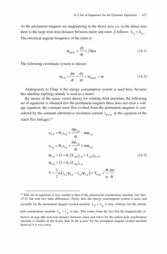
14.2 Set of Equations for the Dynamic Operation 427
As the permanent magnets are magnetizing in the direct axis, i.e. in the direct axis
there is the large iron-iron-distance between stator and rotor, it follows: d qL L< .
The electrical angular frequency of the rotor is:
mech
d2 pn
dt
γω = = π (14.1)
The following coordinate system is chosen:
CS mech
d d
dt dt
α γω = = = ω = ω (14.2)
Analogously to Chap. 6 the energy consumption system is used here, because this machine topology mainly is used as a motor.
By means of the space vector theory for rotating field machines the following set of equations is obtained (for the permanent magnets there does not exist a volt-age equation; the constant rotor flux evoked from the permanent magnets is con-
sidered by the constant substitutive excitation current II,d,0i in the equation of the
stator flux linkage):25
( )
( )
( )
I,dI,d 1 I,d I,q
I,qI,q 1 I,q I,d
I,d 1 md I,d md II,d,0
I,q 1 mq I,q
I,q I,d I,d I,q load
du R i
dt
du R i
dt
1 L i L i
1 L i
3 dT p i i T
2 p dt
ψ= + − ωψ
ψ= + + ωψ
ψ = + σ +
ψ = + σ
Θ ω= ψ − ψ = +
(14.3)
25 This set of equations is very similar to that of the salient-pole synchronous machine (see Sect. 13.5), but with two main differences: firstly, here the energy consumption system is used, and
secondly for the permanent magnet excited machine d qL L< is true, whereas for the salient-
pole synchronous machine d qL L> is true. This comes from the fact that the magnetically ef-
fective air-gap (the iron-iron distance between stator and rotor) for the salient-pole synchronous machine is smaller in the d-axis than in the q-axis; for the permanent magnet excited machine however it is vice versa.

428 14 Dynamic Operation and Control of Permanent Magnet Excited Rotating Field Machines
No-load operation with nominal voltage and nominal frequency is character-ized by:
I,d I,qi i 0= = (14.4)
Then it follows for the flux linkages
I,d md II,d,0
I,q
L i
0
ψ =
ψ = (14.5)
and for the voltages
I,d
I,q I,d md II,d,0
u 0
u L i
=
= ωψ = ω (14.6)
If sinusoidal time-dependencies can be assumed, it follows with
I,q
1,N
uU
2= (14.7)
for the substitutive excitation current
I,q 1,N md II,d,0
1,NII,d,0
md
u 2 U L i
2 Ui
L
= = ω
=ω
(14.8)
The substitutive internal voltage is
P md II,d,0u L i= ω (14.9)
Now the flux linkages are inserted into the voltage equations and the torque equation. It follows:

14.2 Set of Equations for the Dynamic Operation 429
( )[ ] ( )
( ) ( )[ ]
( )[ ] ( )( )
I,d 1 I,d 1 md I,d md II,d,0 1 mq I,q
I,q 1 I,q 1 mq I,q 1 md I,d md II,d,0
I,q 1 md I,d md II,d,0 I,d 1 mq I,q
load
du R i 1 L i L i 1 L i
dt
du R i 1 L i 1 L i L i
dt
3T p i 1 L i L i i 1 L i
2
d T
p dt
= + + σ + − ω + σ
= + + σ + ω + σ +
= + σ + − + σ
Θ ω= +
(14.10)
Further
( ) ( )
( ) ( )[ ]
( ) ( )( )
I,d 1 I,d 1 md I,d 1 mq I,q
I,q 1 I,q 1 mq I,q 1 md I,d md II,d,0
I,q 1 md 1 mq I,d md II,d,0
load
du R i 1 L i 1 L i
dt
du R i 1 L i 1 L i L i
dt
3T p i 1 L 1 L i L i
2
d T
p dt
= + + σ − ω + σ
= + + σ + ω + σ +
= + σ − + σ +
Θ ω= +
(14.11)
With
( ) ( )d 1 md q 1 mqL 1 L , L 1 L= + σ = + σ (14.12)
it follows:
[ ]
( )
I,d 1 I,d d I,d q I,q
I,q 1 I,q q I,q d I,d md II,d,0
I,q md II,d,0 q d I,d load
du R i L i L i
dt
du R i L i L i L i
dt
3 dT p i L i L L i T
2 p dt
= + − ω
= + + ω +
Θ ω= − − = +
(14.13)
Introducing the time constants

430 14 Dynamic Operation and Control of Permanent Magnet Excited Rotating Field Machines
qd
d q1 1
LL,
R Rτ = τ = (14.14)
the following differential equations are obtained:
I,dd I,d I,d q I,q
1
I,q II,d,0q I,q I,q d I,d
1 1
qII,d,0d I,d I,q load
1 d
udi i i
dt R
u idi i i
dt R 1
Lid 3pL 1 i i T
p dt 2 1 L
τ + = + ωτ
τ + = − ωτ ++ σ
Θ ω= − − −
+ σ
(14.15)
where rotor position and speed are linked by:
d d
2 pndt dt
γ α= = ω = π (14.16)
With this set of differential equations the permanent magnet excited rotating field machine is described completely.
In the base speed region the machine is operated in such a way that stator MMF
and rotor field (excitation field, md II,d,0L i ) are perpendicular to each other. Then
the stator current component in the direct axis has to be zero ( I,di 0= ); the stator
current component in the quadrature axis I,qi is the torque generating component.
The voltages in the direct axis and in the quadrature axis can be deduced from the above equations.
However, if a control method with I,d I,d,i i 0∞= ≠ is used (e.g. with I,di 0<
for field weakening), stator MMF and rotor field are no longer perpendicular to each other (this operation mode will be explained in detail in the next Sect. 14.3). For the direct axis voltage equation in steady-state operation (i.e. no more change
of the currents I,di and I,qi ) there is:
I,d
I,d, q I,q1
ui i
R∞ = + ωτ (14.17)
Then for the dynamic operation it follows:

14.2 Set of Equations for the Dynamic Operation 431
d I,d I,d I,d,
di i i
dt∞τ + = (14.18)
The solution of this differential equation is well-known, the current characteristic is:
d
t
I,d I,d,i i 1 e−
τ
∞= − (14.19)
The block diagram of the controlled permanent magnet excited rotating field ma-chine can be deduced from the above equations; it is shown in Fig. 14.2.
Fig. 14.2. Block diagram of the controlled permanent magnet excited rotating field machine.
T +
1,wu
1,vu
1,uu
α
I,du
I,qu
I,d,i ∞
setω
I,qi
ω
+ I,q,seti
+
+ I,d,setu
I,q,setu
αspeed controller torque controller
qL −
1R
1,u,setu
1,v,setu
1,w,setu
1
R1
1
R1
I,qi
−
−
+ I,di
−
Lq1
Ld−
− −
control
iII,d,01 1+σ
qτ
−
dτ
machine model
×
×
×
+
+
+
+
×
3pLd
2
xy0T
1
xy0T−
Θ
M
3
T
dτ
qτ
α1
P W M

432 14 Dynamic Operation and Control of Permanent Magnet Excited Rotating Field Machines
14.3 Steady-State Operation
14.3.1 Fundamentals
In the following the steady-state operation of permanent magnet excited rotating field machines will be calculated. As in principle they show the same motor con-struction, permanent magnet synchronous machines (with sinusoidal currents) and brushless DC-motors (with step-by-step constant currents) will be regarded simul-taneously. Because not always sinusoidal currents are used, the space vector theo-ry has to be used even for the steady-state operation. In addition, the general case of machines with buried magnets will be considered by having different inductivi-
ties in d-axis and q-axis as d qL L< (surface mounted magnets are covered as a
special case for d qL L L= = ).
In steady-state operation the time derivatives of currents and speed are zero. Consequently the set of equations can be simplified to:
[ ]
( )
I,d 1 I,d q I,q
I,q 1 I,q d I,d md II,d,0
I,q md II,d,0 q d I,d
u R i L i
u R i L i L i
3T p i L i L L i
2
= − ω
= + ω +
= − −
(14.20)
With P md II,d,0u L i= ω it follows further:
( )
I,d 1 I,d q I,q
I,q 1 I,q d I,d P
I,q P q d I,d
u R i L i
u R i L i u
3 pT i u L L i
2
= − ω
= + ω +
= − ω − ωω
(14.21)
14.3.2 Base Speed Operation
For the permanent magnet excited rotating field machine (BLDC-motor as well as PMSM) the positive q-direction is defined in the real axis and the positive d-

14.3 Steady-State Operation 433
direction in the negative imaginary axis (please note that this d-q coordinate sys-tem has the positive horizontal axis opposite to the positive horizontal axis of the complex plane).
During base speed operation the angle between the magneto-motive force of the stator and the rotor field is 90° electrically. The rotor field is drawn in the di-rect axis (negative imaginary axis), see also Sect. 14.2; the magneto-motive force
of the stator merely is composed of the current I I,q I,Ni i i= = (quadrature axis,
real axis), the current in the direct axis is I,di 0= . Then the load angle becomes:
M 0δ = −ϑ − ϕ = . The described operation condition usually is reached with a
power factor of about cos 0.8ϕ ≈ and without magnetic asymmetry
( d qL L L= = ). The set of equations then becomes
I,d I,q
I,q 1 I,q P
I,q P
u Li
u R i u
3 pT i u
2
= −ω
= +
=ω
(14.22)
The equations of the machine are illustrated in the vector diagram of Fig. 14.3.
Fig. 14.3. Vector diagram of the permanent magnet excited rotating field machine in base speed operation.
d
I,qLiω
Im−
Re
Iu
Pu
ϕ
ϑ I,q Ii i=
1 I,qR i
q

434 14 Dynamic Operation and Control of Permanent Magnet Excited Rotating Field Machines
In this vector diagram26 the voltage space vector is (please refer to Sect. 11.3)
{ } { }
( )
I I I
I,q I,d
1 I,q P I,q
1 I,q P I,q
u Re u j Im u
u j u
R i u j Li
R i u j Li
= +
= −
= + − −ω
= + + ω
(14.23)
14.3.3 Operation with Leading Load Angle and without Magnetic Asymmetry
During operation with leading load angle Mδ and without magnetic asymmetry it
is still true: d qL L L= = . But now, in addition to the torque producing current
I,qi (quadrature axis), a negative current component I,di 0< is supplied to the di-
rect axis. As this negative d-axis current is opposite to the rotor field (in the nega-tive imaginary axis), it has a demagnetizing effect (therefore, this is called “field
weakening“). Consequently, I,qi has to be decreased, so that the total current Ii is
not exceeding the nominal value (to avoid overheating). Therefore:
I,d I,q I,N I I,Ni 0, i i , i i< ≤ = (14.24)
The set of equations becomes
I,d 1 I,d I,q
I,q 1 I,q I,d P
I,q P
u R i Li
u R i Li u
3 pT i u
2
= − ω
= + ω +
=ω
(14.25)
26 Please note that complex phasors were introduced as the non time-dependent components of the complex description of sinusoidally time-dependent variables (please refer to Sect. 1.6). In this chapter, explicitly non-sinusoidal time-dependencies of the variables are permissible. There-fore, the respective illustration is called vector diagram and not phasor diagram.

14.3 Steady-State Operation 435
Because of this additional current in the negative d-axis I,di the angle between
the magneto-motive force of the stator ( Ii ) and the rotor field (in the negative im-
aginary axis) is enlarged to more than 90° electrically. Consequently, the angle ϕ
between voltage and current decreases, i.e. the power factor is changed into the di-
rection cos 1ϕ → . Moreover, for I,di 0≠ even for the load angle holds true
M 0δ ≠ . These characteristics are illustrated in the vector diagram shown in Fig.
14.4.
Fig. 14.4. Vector diagram of the permanent magnet excited rotating field machine with leading load angle and without magnetic asymmetry.
Neglecting the Ohmic voltage drop in the voltage equations, the current in the
negative d-axis I,di has the following consequences:
• The current I,qi decreases, because the total current is limited.
• Consequently the absolute value of the voltage I,d I,qu Li= −ω decreases as
well.
• Then the voltage I,q I,d Pu Li u= ω + may increase because of
( ) ( )2 2
I I,q I,d I,Nu u u u= + ≤ . As furthermore I,dLiω and Pu are oppo-
I,qLiω
Im−
Re
Iu Pu
ϕ
ϑ I,qi
1 I,qR i
I,di
1 I,dR i
I,dLiω
Ii
d
q

436 14 Dynamic Operation and Control of Permanent Magnet Excited Rotating Field Machines
site to each other, the voltage Pu increases. Because the magnetization is con-
stant, this can only be realized by increasing the speed.
• From the torque equation I,q P
3 pT i u
2=
ω it is obvious that the torque decreas-
es: Pu
ω describes the magnetization and this is constant; the lower current I,qi
leads to a lower torque.
Therefore, a typical field weakening operation is obtained (lower torque at higher speed; please compare e.g. with the field weakening operation of the induc-tion machine).
If the lowering of the torque shall be omitted, an additional torque component has to be generated to compensate for this effect. This is reached by an additional reluctance torque component by introducing a magnetic asymmetry.
14.3.4 Operation with Leading Load Angle and Magnetic Asymmetry
During operation with leading load angle Mδ and with magnetic asymmetry it is
now d qL L< . Like in the preceding section the following holds:
• In addition to the torque generation current I,qi (quadrature axis) a current in
the negative d-axis I,di 0< is applied; for the load angle M 0δ ≠ holds true.
• This current in the negative d-axis has a demagnetizing effect.
• The torque generation current I,qi has to be decreased, so that the total current
Ii is not exceeding the nominal value (to avoid overheating).
The according vector diagram is shown in Fig. 14.5.

14.3 Steady-State Operation 437
Fig. 14.5. Vector diagram of the permanent magnet excited rotating field machine with leading load angle and with magnetic asymmetry.
The torque can be calculated from:
( )I,q P q d I,d
3 pT i u L L i
2= − ω − ω
ω (14.26)
At constant speed the torque can be increased to the initial value by means of
the positive reluctance torque component ( )q d I,d I,q
3 pL L i i
2− ω − ω
ω. Depending
on the design of the electromagnetic circuit the torque may be even higher than in-itially. This can be used in two different ways:
• increase of the speed; • reduction of the current.
By suitable electromagnetic design of the machine the current can be reduced and simultaneously the power factor cos ϕ can be improved. This leads to lower
losses in the machine and the supplying inverter (because of the lower current lev-el) as well as to a lower apparent power of the inverter (because of the improved power factor).
q I,qL iω
Im−
Re
Iu Pu
ϕ
ϑ I,qi
1 I,qR i
I,di
1 I,dR i
d I,dL iω
Ii
d
q

438 14 Dynamic Operation and Control of Permanent Magnet Excited Rotating Field Machines
14.3.5 Torque Calculation from Current Loading and Flux Density
With P Pu = ω Ψ the torque equation becomes
( )
( ) ( ) ( ){ }
( ) ( ) ( )( )
I,q P q d I,d
I M P q d I M
2I M P I M M q d
3 pT i L L i
2
3p i cos L L i sin
2
3 3p i cos p i cos sin L L
2 2
= ωΨ − ω − ωω
= δ − − − δ
= δ + δ δ −
Ψ
Ψ
(14.27)
With ( ) ( ) ( )M M M
1cos sin sin 2
2δ δ = δ it follows further
( ) ( )( )2I M P I M q d
3 3T p i cos p i sin 2 L L
2 4= δ + δ −Ψ (14.28)
The flux linkage of the permanent magnet field can be calculated from the flux density amplitude of the working wave and the effective number of turns
( effw w = ξ ; the factor 2 π is the result of integrating the assumed sinusoidal
flux waveform over the pole area, i.e. over a half period):
P eff
eff
2 r 2w B
2p
2rw B
p
π=
π
=
Ψ
(14.29)
The amplitude of the current loading of the working wave can be calculated by
means of the amplitude of the current Ii (the factor 2 in the following equation
comes from the fact that each turn is composed of forward and return conductor):
effI
m 2wA i
2 r=
π (14.30)
With the number of phases m 3= it follows:

14.3 Steady-State Operation 439
Ieff
ri A
3w
π= (14.31)
In total, for the torque this results in:
( )
( )( )
( )
( ) ( )
M effeff
2
M q deff
2M
2
q d Meff
3 r 2rT p A cos w B
2 3w p
3 rp A sin 2 L L
4 3w
r A B cos
3 rp A L L sin 2
4 3w
π
= δ +
πδ −
= π δ +
π− δ
(14.32)
Applying the calculation of the inductivity from Sect. 4.2 to the calculation of
dL and qL results in
( )
( )
2
effd 1 0
d
2
effq 1 0
q
w3 4 rL 1
2 p
w3 4 rL 1
2 p
= + σ μπ δ
= + σ μπ δ
(14.33)
where dδ and qδ are the magnetically effective air-gaps in d-axis and q-axis, re-
spectively. Inserting this to the above torque equation gives
( )
( ) ( )
( ) ( ) ( )
2
2M
eff
2
eff1 0 M
q d
2 2 2 0M 1 M
q d
3 rT r A B cos p A
4 3w
w3 4 1 11 r sin 2
2 p
1 1 r A B cos r A 1 r sin 2
2p
π= π δ +
+ σ μ − δπ δ δ
μ= π δ + π + σ − δ
δ δ
⋅
(14.34)

440 14 Dynamic Operation and Control of Permanent Magnet Excited Rotating Field Machines
As this has been deduced on the basis of the space vector theory, this result is valid for every moment in time, even for supplying the machine with non-sinusoidal currents. The torque is made of two components, the permanent magnet excited torque and the reluctance torque. These components are:
( )2PM MT r A B cos= π δ (14.35)
( ) ( )2 2 0Rel 1 M
q d
1 1T r A 1 r sin 2
2p
μ= π + σ − δ
δ δ (14.36)
The permanent magnet excited torque is proportional to the bore volume
( 2rπ ), to the current loading ( A ), to the flux density ( B ), and to the cosine of
the load angle Mδ . For M 0δ = the maximum permanent magnet excited torque
is reached, which is the usual operating condition in the base speed region (except for the so-called MTPA control, see Sect. 14.4.2).
The reluctance torque as well is proportional to the bore volume ( 2rπ ). In
addition, main influencing factors are the squared current loading ( 2A ), the dif-
ference of the inverse values of q-axis and d-axis air-gaps q d
1 1−
δ δ, and the si-
ne of the double load angle. For machines without magnetic asymmetry (i.e. ma-
chines with surface mounted magnets where d qL L= is true) or without field
weakening ( I,di 0= , i.e. load angle M 0δ = ) this torque component is zero.
14.4 Limiting Characteristics and Torque Control
14.4.1 Limiting Characteristics
From the two stator voltage equations
I,d 1 I,d q I,q
I,q 1 I,q d I,d P
u R i L i
u R i L i u
= − ω
= + ω + (14.37)

14.4 Limiting Characteristics and Torque Control 441
it follows by neglecting the Ohmic resistance ( 1R 0= ) and with P Pu = ωΨ
I,d q I,q
I,q d I,d P
u L i
u L i
= −ω
= ω + ωΨ (14.38)
Now, the current and voltage limits, depending on the perpendicular current com-
ponents I,di and I,qi , will be computed. The current limit is a circular function
2 2 2 2max I,d I,qi i i i≥ = + (14.39)
and for the voltage limit there is an elliptic function
( ) ( )
( ) ( )
( ) ( )
2 2 2 2max I,d I,q
2 2
q I,q d I,d P
2 22q I,q d I,d P
22 2max
q I,q d I,d P2
u u u u
L i L i
L i L i
uL i L i
≥ = +
= ω + ω + ωΨ
= ω + + Ψ
≥ + + Ψω
(14.40)
Figure 14.6 illustrates these limits in the I,di - I,qi -plane.
Fig. 14.6. Voltage and current limits.
current limit voltage limit at low speed
voltage limit at high speed
I,d P d
I,q
i / L
i 0
= −Ψ
=
I,di
I,qi
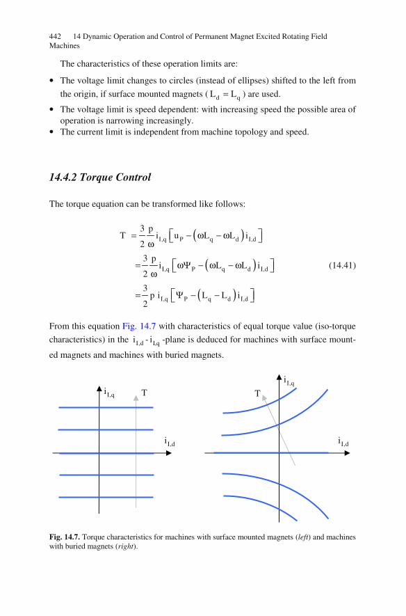
442 14 Dynamic Operation and Control of Permanent Magnet Excited Rotating Field Machines
The characteristics of these operation limits are:
• The voltage limit changes to circles (instead of ellipses) shifted to the left from
the origin, if surface mounted magnets ( d qL L= ) are used.
• The voltage limit is speed dependent: with increasing speed the possible area of operation is narrowing increasingly.
• The current limit is independent from machine topology and speed.
14.4.2 Torque Control
The torque equation can be transformed like follows:
( )
( )
( )
I,q P q d I,d
I,q P q d I,d
I,q P q d I,d
3 pT i u L L i
2
3 pi L L i
2
3p i L L i
2
= − ω − ωω
= ωΨ − ω − ωω
= Ψ − −
(14.41)
From this equation Fig. 14.7 with characteristics of equal torque value (iso-torque
characteristics) in the I,di - I,qi -plane is deduced for machines with surface mount-
ed magnets and machines with buried magnets.
Fig. 14.7. Torque characteristics for machines with surface mounted magnets (left) and machines with buried magnets (right).
T
I,di
I,qi T
I,di
I,qi

14.4 Limiting Characteristics and Torque Control 443
From Fig. 14.7 it is obvious that torque control is much easier for machines
with surface mounted magnets ( d qL L= , here a linear relation exists between the
current I,qi and the torque) than for machines with buried magnets ( d qL L< , for
these machines I,di and I,qi have to be controlled simultaneously, in addition the
relation is non-linear). Now, the question shall be answered how to choose the current components
I,di and I,qi to reach the required torque with minimum total current (minimum
losses, maximum efficiency).27 In literature, this is often referred to as “MTPA - maximum torque per ampere” control. However, more precisely it should be called “MTPC - maximum torque per current” control. For this, three cases are distinguished:
1. Low speed, i.e. voltage limit is not relevant
For a certain torque the total current is then minimal if the current vector and
the vector ( )grad T have the same direction. In Fig. 14.8 this is given on the
dark blue curve. Therefore, this curve gives the optimum operating points of the machine.
Fig. 14.8. Optimum torque characteristic at low speed.
27 Minimum total current leads to minimum losses and maximum efficiency, if the iron losses and permanent magnet losses are neglected. This approximation is valid for low speed (i.e. low frequency), at high speed iron and permanent magnet losses may even become dominant.
I,di
I,qi
current limit
voltage limit at low speed
I,d P d
I,q
i / L
i 0
= −Ψ
=
Ii
( )grad T

444 14 Dynamic Operation and Control of Permanent Magnet Excited Rotating Field Machines
2. Medium speed (low field weakening); i.e. voltage limit is relevant
Because of the voltage limitation the maximum torque is lower than in the case above; moreover, the optimum curve for reaching the required torque (dark blue curve) partly proceeds along the voltage limit curve, see Fig. 14.9. Fig. 14.9. Optimum torque characteristic at medium speed.
3. High speed (strong field weakening); i.e. current limit is not relevant At strong field weakening only the voltage limit is relevant; the limit of the maximum total current is not longer reachable. The additional black characteristic in Fig. 14.10 features that limitation, for which the torque is decreasing again if the current is further increased and the voltage is hold on its limit. With other words: the black characteristic shows those operating points, where the required torque is reached with minimum flux (as can be deduced from the ellipse equation for the voltage limit, the el-lipses are the operating points with constant flux). As this lower torque can be reached even with lower current, such an operation is not suitable. Therefore, this operating area is excluded.
I,di
I,qi voltage limit at medium speed
I,d P d
I,q
i / L
i 0
= −Ψ
=
current limit

14.4 Limiting Characteristics and Torque Control 445
Fig. 14.10. Optimum torque characteristic at high speed.
4. Summary The suitable operation area of the machine according to the above discussion is marked in grey in Fig. 14.11.
Fig. 14.11. Optimum torque characteristic for the entire speed range.
I,di
I,qi voltage limit at high speed
I,d P d
I,q
i / L
i 0
= −Ψ
=
current limit
I,di
I,qi current limitvoltage limits for
different speeds
maxT for minimum current maxT for minimum flux
I,d P d
I,q
i / L
i 0
= −Ψ
=

446 14 Dynamic Operation and Control of Permanent Magnet Excited Rotating Field Machines
14.5 Control without Mechanical Sensor
The mechanical speed has to be known for the speed controlled permanent magnet excited machine, see Sect. 14.2. However, as already mentioned in Sect. 12.6, me-chanical speed sensors have some disadvantages that preferably should be avoid-ed:
• vulnerability against outside impacts (forces, torques, temperatures, dirt) • costs • space consumption • necessity of a free shaft extension
Therefore, even for the permanent magnet excited machine it is desirable to calculate the speed from the measured terminal values of the machine (often this method is referred to as “sensorless” speed control).
In the following just a short overview of different possibilities will be given for the sake of completeness, a detailed description of the alternatives would be far beyond the scope of this book.
A first group of methods deals with direct electrical measurement (DC-voltage, DC-current, phase voltages, and / or phase currents) and a calculation of the re-quired values by means of a nonadaptive machine model (similar to what is de-scribed in Sect. 12.6 for the induction machine).
These calculations can be improved by adaptive methods. Among these “Model Reference Adaptive Systems (MRAS)”, observer based estimators (e.g. Luen-berger observer, sliding mode observer), and Kalman filters are the most im-portant ones.
A third group makes use of machine saliency and / or signal injection (with ro-tating or alternating carrier). In many AC machines, the position dependence is a feature of the rotor. In the case of the interior PMSM there is a measurable spatial variation of inductances or resistances (saliencies) in the d- and q-axis due to ge-ometrical and saturation effects, which can be used for the estimation of rotor po-sition (e.g. used for the INFORM-method). Another method to estimate the rotor position is to add a high frequency stator voltage or current component and evalu-ate the effects of the machine anisotropy on the amplitude of the corresponding stator voltage or current component.
Finally there is a group of methods making use of artificial intelligence. Most prominent are neural networks, fuzzy logic based systems and fuzzy neural net-works.

14.6 References for Chapter 14 447
14.6 References for Chapter 14
Benjak O, Gerling D (2010) Review of position estimation methods for PMSM drives without a position sensor, part I: Nonadaptive Methods. In: International Conference on Electrical Ma-chines (ICEM), Rome, Italy
Benjak O, Gerling D (2010) Review of position estimation methods for PMSM drives without a position sensor, part II: Adaptive Methods. In: International Conference on Electrical Ma-chines (ICEM), Rome, Italy
Benjak O, Gerling D (2010) Review of position estimation methods for PMSM drives without a position sensor, part III: Methods based on Saliency and Signal Injection. In: International Conference on Electrical Machines and Systems (ICEMS), Incheon, South Korea
Dajaku G (2006) Electromagnetic and thermal modeling of highly utilized PM machines. Shak-er-Verlag, Aachen
Fitzgerald AE, Kingsley C, Umans SD (1983) Electric machinery. Mc-Graw Hill Book Compa-ny, New York
Krause PC (1986) Analysis of electric machinery. Mc-Graw Hill Book Company, New York Krishnan R (2001) Electric motor drives. Prentice Hall, London Krishnan R (2010) Permanent magnet synchronous and brushless DC motor drives. CRC Press,
Boca Raton Kwak SJ, Kim KJ, Jung HK (2004) The characteristics of the magnetic saturation in the interior
permanent magnet synchronous motor. In: International Conference on Electrical Machines (ICEM) Cracow, Poland
Li Y (2010) Direct torque control of permanent magnet synchronous machine. Shaker-Verlag, Aachen
Meyer M (2010) Wirkungsgradoptimierte Regelung hoch ausgenutzter Permanentmagnet-Synchronmaschinen im Antriebsstrang von Automobilen. Dissertation Universitaet Pader-born
Schroedl M, Lambeck M (2003) Statistic properties of the INFORM method for highly dynamic sensorless control of PM motors down to standstill. In: Annual Conference of the IEEE In-dustrial Electronics Society (IECON) Roanoke, USA

15 Concentrated Windings
15.1 Conventional Concentrated Windings
Electrical machines with non-overlapping concentrated windings have become an increasingly popular alternative to machines with distributed windings for certain applications. Concentrated winding machines (characterized by the fact that each coil is wound around a single tooth) have potentially more compact designs com-pared to the conventional machine designs with distributed windings, due to short-er and less complex end-windings. With such windings, the volume of copper used in the end-windings can be reduced in significant proportions, in particular if the axial length of the machine is small. Consequently, lower costs and lower losses can be expected. Even the process of manufacturing the coils is simplified, resulting in a very cost-effective solution. In addition such a winding design is bet-ter qualified for safety critical applications, because phase-to-phase short-circuits become very unlikely. The photographs (Fig. 15.1) illustrate these differences ex-emplarily.
Fig. 15.1. Photographs of different winding topologies (left: concentrated winding, right: distrib-uted winding).
There is a large variety of possibilities to realize an electrical machine with concentrated windings, e.g.
• coils wound around every tooth (often referred to as “two-layer winding”) or coils wound around every other tooth (“single-layer winding”);
• different number of teeth side by side with coils of the same phase; • torque producing rotating field wave (in the following called “working wave”)
being the fundamental or a higher harmonic.
© Springer-Verlag Berlin Heidelberg 2015 449
DOI 10.1007/978-3-642-17584-8_ 15D. Gerling, Electrical Machines Mathematica l Engineering,,

450 15 Concentrated Windings
Some of these windings can be calculated according to Sect. 3.4, considering the concentrated winding as a special case of a distributed winding with an ex-treme short-pitch factor.
In the following, the concentrated winding will be analyzed analogously to Sect. 3.3 (supplying the machine with a symmetric current system and calculating the time-dependent MMF distribution). Afterwards, for this MMF distribution a Fourier analysis will be performed, which gives the harmonics of the MMF distri-bution.
Because of the large variety of possibilities, this will be done in the following by looking at the example of a double-layer three-phase machine with twelve sta-tor slots, having two teeth side by side with coils of the same phase. This winding layout is shown in Fig. 15.2.
Fig. 15.2. Winding layout of a machine with concentrated coils (“wound-off” representation of the stator lamination); red: phase u, yellow: phase v, blue: phase w.
The MMF distribution for t 0ω = and t 2ω = π is illustrated in Fig. 15.3.
Fig. 15.3. MMF distribution of the winding shown in Fig. 15.2 versus circumference coordinate,
functions normalized to a maximum value of 1; t 0ω = (left), t 2ω = π (right).
The harmonic analysis, which results in a time-independent characteristic for the given example, is presented in Fig. 15.4. A large number of MMF harmonics with high amplitude becomes obvious. The presence of these harmonics is the main disadvantage of concentrated windings, as they cause a variety of problems (mainly additional losses and acoustic noise).
1
0.5
0
-0.5
-1 0 0.5 1 1.5 2
α / π
ωt = 0 Θ
Θmax
ΘΘmax
α / π
1
0.5
0
-0.5
-1 0 0.5 1 1.5 2
ωt = π/2

15.1 Conventional Concentrated Windings 451
Fig. 15.4. Harmonic analysis of the MMF distribution (normalized amplitude versus harmonic number) of the winding shown in Fig. 15.2.
For calculating the torque of an electrical machine, not the amplitude of the MMF working wave is essential, but the amplitude of the current loading working wave (please refer to Sect. 14.3.5). From Sect. 3.5 it can be deduced that the cur-rent loading waves can be calculated from the spatial derivative of the MMF waves. Having a Fourier analysis of the MMF distribution means that all MMF waves are harmonic ones. Therefore, the respective spatial derivative means that the current loading waves are harmonic as well (with a phase shift of 90° electri-cally) and the amplitudes are proportional to the amplitudes of the MMF waves multiplied by the respective harmonic number. The result of the harmonic analysis of the current loading distribution is shown in Fig. 15.5.
Fig. 15.5. Harmonic analysis of the current loading distribution (normalized amplitude versus harmonic number) of the winding shown in Fig. 15.2.
Θ / Θmax 1
0.8
0.6
0.4
0.2
0
1 3 5 7 9 11 13 15 17 19 harmonic number
1 3 5 7 9 11 13 15 17 19 harmonic number
A / Amax 1
0.8
0.6
0.4
0.2
0

452 15 Concentrated Windings
It is obvious that the waves with the harmonic numbers 5 and 7 may be used for torque production. Usually, higher harmonics are not used because the slot opening effect (that was not regarded in these calculations) increasingly reduces the amplitude with rising harmonic number. Using the waves with harmonic num-ber 5 or 7 as working wave means that 10 or 14 poles are generated (e.g. a wave with harmonic number 5 contains 5 complete sinusoidal waves per circumference, which means that there are 5 north poles and 5 south poles).
Using a permanent magnet machine, the number of magnet poles in the rotor determines the working wave (please refer to Sect. 3.7: the number of poles of sta-tor and rotor must be identical to generate a time-independent torque). Using this kind of winding with an induction motor (e.g. with a squirrel-cage rotor) torque generation will be very problematic, because the rotor adapts itself to any pole number of the stator. As the stator generates several pole numbers this will result in a very poor torque output.
If the 5th harmonic is used as working wave, the number of slots per phase per pole is according to Eq. (3.3)
1N 12q 0.4
2pm 10 3= = =
⋅ (15.1)
If the 7th harmonic is used as working wave, the number of slots per phase per pole is
1N 12q 0.29
2pm 14 3= = ≈
⋅ (15.2)
Therefore, these kinds of windings are called “fractional slot winding”. The existence of a large number of MMF harmonics with high amplitudes has
some severe disadvantages:
• harmonics with similar, but not identical ordinal number and high amplitudes cause radial force waves with high amplitudes and low ordinal number, result-ing in annoying acoustic noise;
• for permanent magnet machines the harmonics (and especially the sub-harmonics with respect to the working wave) cause additional losses, namely iron core losses and eddy current losses in electrically conductive permanent magnets (like NdFeB or SmCo);
• for induction machines it will be hardly possible to generate a useful torque, as the squirrel-cage rotor adapts to any pole number of the stator.

15.2 Improved Concentrated Windings 453
15.2 Improved Concentrated Windings
15.2.1 Increased Number of Stator Slots from 12 to 24
Because of the severe disadvantages it is necessary to reduce the unwanted har-monics by far (at least to an amount where their disturbing effect is nearly negligi-ble). This will be explained exemplarily using the winding described in Sect. 15.1 and a rotor with 10 poles. Therefore, all low-order harmonics except for the 5th one have to be reduced to achieve an acceptable machine behavior.
The stator MMF distribution can be calculated by the following equation:
Mp
w
w
3(x, t) cos t x
2
ˆ8 i N
5 1cos sin
6 2 6 2
ν
ν
ν ν
ν
πΘ = Θ ω − ν + δ
τ
Θ = ξπν
π πξ = ν ν
(15.3)
where νΘ is the amplitude of the ν th MMF space harmonic, w
νξ is the winding
factor, i is the phase current amplitude, Mδ is the load angle, ω is the angular
frequency, and N is the number of turns per coil. Splitting this winding system in-
to two identical winding systems, shifted against each other by an angle wα , the
resulting MMF distribution for the combined winding system becomes:
wZ M
p
wZ
3(x, t) cos t x
2 2
cos2
ν ν
ν
ν
απΘ = ξ Θ ω − ν − + δ
τ
αξ = ν
(15.4)
where Zν
ξ is called distribution factor.
Figure 15.6 shows this distribution factor Zν
ξ for the first three relevant MMF
harmonics ( 1,5, 7ν = ) as a function of the shifting angle wα . This shifting angle

454 15 Concentrated Windings
wα is given in number of stator slots, because only these discrete values are pos-
sible for shifting the two winding systems against each other.
Fig. 15.6. Winding factors of the first three relevant MMF harmonics as a function of the shifting angle (measured in number of stator slots).
It can be deduced from Fig. 15.6 that reducing the 7th harmonic and maintain-ing the 5th harmonic results in a shift of the two winding systems of about 2.5 sta-tor slots.28 As mentioned before, it is only possible to shift the two winding system by an integer number of stator slots. To realize the desired shift, the number of sta-tor slots will be doubled, resulting in a shift of five stator slots. This is illustrated in Fig. 15.7.
The combination of both winding systems is shown in Fig. 15.8. Of course it becomes obvious that the resulting winding is no longer purely concentrated, but partly overlapping. Nevertheless, this winding has the great advantages that the unwanted 7th harmonic is reduced by far and the end winding in circumferential direction is maintained as short as for the purely concentrated winding. Even if the end winding in total gets a little bit larger compared to the purely concentrated winding (because of the partly overlapping design), the end winding Ohmic losses are reduced by far compared to a conventional overlapping winding.
28 For a machine with 14 rotor poles the 7th harmonic has to be maintained and the 5th harmonic has to be reduced. This results in a shift of the two winding systems of about 3.5 stator slots.
1 2 3 4 5 6 7 8 9 10 11 12wα
1.0
0.8
0.6
0.4
0.2
0.0
-0.2
-0.4
-0.6
-0.8
-1.0
Zν
ξ

15.2 Improved Concentrated Windings 455
Fig. 15.7. Winding layout of a machine with two identical winding systems shifted against each other (“wound-off” representation of the stator lamination, please refer to Fig. 15.2); red: phase u, yellow: phase v, blue: phase w.
Fig. 15.8. Combination of both winding systems shown in Fig. 15.7 (“wound-off” representation of the stator lamination); red: phase u, yellow: phase v, blue: phase w.
The MMF harmonics of the winding layout of Fig. 15.8 is presented in Fig. 15.9. It becomes obvious that the 7th harmonic is reduced by far.
Fig. 15.9. Harmonic analysis of the MMF distribution (normalized amplitude versus harmonic number) of the winding shown in Fig. 15.8.
Now, two additional measures are introduced to further reduce the 7th harmonic and to reduce the fundamental wave:
wα
wα
1 3 5 7 9 11 13 15 17 19 harmonic number
Θ / Θmax 1
0.8
0.6
0.4
0.2
0

456 15 Concentrated Windings
1. Slightly different tooth widths are used to shift both winding systems a little bit more than the 2.5 slots shown in Fig. 15.6, please refer to Fig. 15.10 for a prin-ciple sketch. This results in completely reducing the 7th harmonic.29
2. The fundamental wave can be reduced by using different turns per coil for the neighbouring phase coils, which is also illustrated in Fig. 15.10.30
Fig. 15.10. Principle winding and lamination layout for reduction of the fundamental and 7th harmonic (“wound-off” representation of stator and rotor; only one phase shown for the sake of clarity; n1 and n2 denote different number of turns per coil).
With suitable design and optimization concerning the reduction of the funda-mental harmonic and the 7th harmonic, an MMF distribution with a very low num-ber of harmonics can be achieved. Such a design is illustrated in Fig. 15.11, show-ing the spectrum of the stator MMF distribution. The main advantages of such a winding design are:
• Low Ohmic stator losses because of short end windings. • Low eddy current rotor losses because of low harmonic content in the MMF
spectrum (especially low fundamental MMF harmonic). • Low radial forces (as a reason for acoustic noises) because of low harmonic
MMF waves near to the harmonic number of the working wave. • Low torque ripple (please refer to Fig. 15.12). • Low production costs because of short end windings and nearly concentrated
coils.
29 Of course, this additional feature can even be used differently. Possible alternatives are the maximizing of the 5th harmonic (which is the working wave) or the additional reduction of fur-ther harmonics that are not shown in Fig. 15.6. 30 An alternative to reduce the fundamental wave is using coil windings with different turns per coil side; this implies that a single coil has to be connected from both axial ends of a radial flux machine (however, the phase winding may be still connected from one side).
stator
rotor
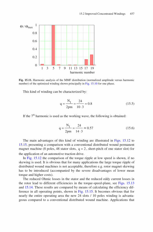
15.2 Improved Concentrated Windings 457
Fig. 15.11. Harmonic analysis of the MMF distribution (normalized amplitude versus harmonic number) of the optimized winding shown principally in Fig. 15.10 for one phase.
This kind of winding can be characterized by:
1N 24q 0.8
2pm 10 3= = =
⋅ (15.5)
If the 7th harmonic is used as the working wave, the following is obtained:
1N 24q 0.57
2pm 14 3= =
⋅≈ (15.6)
The main advantages of this kind of winding are illustrated in Figs. 15.12 to 15.15, presenting a comparison with a conventional distributed wound permanent magnet machine (8 poles, 48 stator slots, q 2= , short-pitch of one stator slot) for
the application of an automotive traction drive. In Fig. 15.12 the comparison of the torque ripple at low speed is shown, if no
skewing is used. It is obvious that for many applications the large torque ripple of distributed wound machines is not acceptable, therefore e.g. rotor magnet skewing has to be introduced (accompanied by the severe disadvantages of lower mean torque and higher costs).
The reduced Ohmic losses in the stator and the reduced eddy current losses in the rotor lead to different efficiencies in the torque-speed-plane, see Figs. 15.13 and 15.14. These results are compared by means of calculating the efficiency dif-ference in all operating points, shown in Fig. 15.15. It becomes obvious that for nearly the entire operating area the new 24 slots / 10 poles winding is advanta-geous compared to a conventional distributed wound machine. Applications that
1 3 5 7 9 11 13 15 17 19 harmonic number
Θ / Θmax 1
0.8
0.6
0.4
0.2
0

458 15 Concentrated Windings
are mostly used in low-load operating points (like e.g. automotive traction drives, industrial pumps and fans) benefit best from this development.
Fig. 15.12. Torque versus rotor position: Comparison of torque characteristics of a 24 slots / 10 poles permanent magnet machine and a conventional distributed wound permanent magnet ma-chine.
Fig. 15.13. Efficiency of the conventional distributed wound permanent magnet machine in the torque-speed-plane.
T / Nm
280
210
140
70
0 0 40 80 120 160 200 240 280 320 360
rotor position / °
distributed winding, q=2
new winding, 24 slots / 10 poles
T / Nm
250
200
150
100
50
0 0 2000 4000 6000 8000 10000 12000
speed / min-1
efficiency / %
100
90
80
70
60
50
40
30
20
10
0

15.2 Improved Concentrated Windings 459
Fig. 15.14. Efficiency of the new 24 slots / 10 poles permanent magnet machine in the torque-speed-plane.
Fig. 15.15. Efficiency difference of the machines in Figs. 15.13 and 15.14 in the torque-speed-plane (positive values mean an advantage for the new 24 slots / 10 poles machine).
T / Nm
250
200
150
100
50
0 0 2000 4000 6000 8000 10000 12000
speed / min-1
efficiency / %
100
90
80
70
60
50
40
30
20
10
0
T / Nm
250
200
150
100
50
0 0 2000 4000 6000 8000 10000 12000
speed / min-1
efficiency diffe-rence / %
15
10
5
0
-5
-10
-15

460 15 Concentrated Windings
15.2.2 Increased Number of Stator Slots from 12 to 18
Another possibility to improve the MMF spectrum of the winding shown in Sect. 15.1 is to increase the number of stator slots from 12 to 18 in such a way, that within two neighboring stator teeth of the same phase an additional (unwound) stator tooth is placed, see Fig. 15.16.
Fig. 15.16. Winding layout of a machine according to Fig. 15.2 with additional teeth (“wound-off” representation of the stator lamination); red: phase u, yellow: phase v, blue: phase w.
Afterwards, a similar approach like described in Sect. 15.2.1 is used: The initial winding is separated into two identical winding parts, shifted against each other by four stator slots. In addition, coils with different turns per coil side are used to re-duce the fundamental wave.31 The resulting winding layout is illustrated in Fig. 15.17.
Fig. 15.17. Winding layout of a machine according to Fig. 15.12 with two identical winding sys-tems shifted against each other (“wound-off” representation of the stator lamination); red: phase u, yellow: phase v, blue: phase w.
The main advantage of this solution against the alternative presented in the pre-ceding section is that here all coils are concentrated ones wound around a single stator tooth. A disadvantage is the higher number of single coils, which increases the effort for manufacturing the connections. However, this can be realized fully automated. In addition, a new harmonic wave with ordinal number 13 occurs, but this will not be an issue if the rotor magnetization is selected suitably. The result-ing spectrum of the MMF distribution of such a winding is illustrated in the fol-lowing Fig. 15.18:
31 Even coils with different number of turns may be used like described in the preceding section.
wα

15.2 Improved Concentrated Windings 461
Fig. 15.18. Harmonic analysis of the MMF distribution (normalized amplitude versus harmonic number) of the optimized winding with concentrated coils (18 stator slots with purely concen-trated coils).
15.2.3 Main Characteristics of the Improved Concentrated Windings
Purely concentrated windings generally are characterized by a large number of MMF harmonics with high amplitude. As considerable rotor losses and radial forces (resulting in acoustic noise) are generated by these harmonics, this kind of winding topology is unsuitable for many applications like e.g. in the automotive industry (traction, steering, and others), even if the production process of purely concentrated windings is beneficial.
For such applications alternatives are required that are advantageous compared to the well-known distributed windings (please refer to Chap. 3) which can be re-garded as benchmark. The improved concentrated windings described in this chapter substantially maintain the advantages of concentrated windings like low production effort and short end windings (resulting in compact design and low Ohmic stator losses), whereas the disadvantages (high number of harmonics with large amplitude) to a large extend are eliminated. Especially the efficiency in part-load operation conditions can be improved considerably by these winding topolo-gies, which is important for many industrial applications like pumps, blowers, traction drives, etc. Summarizing, these winding topologies are advantageous in production and operation of such electrical machines.
The positive effects of the improved concentrated winding designs were shown in this chapter using the example of permanent magnet rotors (synchronous ma-chines as well as brushless DC machines). However, this kind of winding design
1 3 5 7 9 11 13 15 17 19 harmonic number
Θ / Θmax 1
0.8
0.6
0.4
0.2
0

462 15 Concentrated Windings
is of course even applicable to electrically excited synchronous machines and in-duction machines.
15.3 References for Chapter 15
Dajaku G (2006) Electromagnetic and thermal modeling of highly utilized PM machines. Shak-er-Verlag, Aachen
Dajaku G, Gerling D (2008) Analysis of different permanent magnet machines for hybrid vehi-cles application. In: ANSYS Conference & 26th CADFEM Users' Meeting, Darmstadt, Ger-many
Dajaku G, Gerling D (2009) Magnetic radial force density of the PM machine with 12-teeth/10-poles winding topology. In: IEEE International Electric Machines and Drives Conference (IEMDC), Miami, Florida, USA
Dajaku G, Gerling D (2010) Stator slotting effect on the magnetic field distribution of salient pole synchronous permanent-magnet machines. IEEE Transactions on Magnetics, 46:3676-3683
Dajaku G, Gerling D (2011) A novel 24-slots/10-poles winding topology for electric machines. In: IEEE International Electric Machines and Drives Conference (IEMDC), Niagara Falls, Ontario, Canada
Dajaku G, Gerling D (2011) Eddy Current Loss Minimization in Rotor Magnets of PM Machines using High-Efficiency 12-teeth/10-poles Winding Topology. In: International Conference on Electrical Machines and Systems (ICEMS), Beijing, China
Dajaku G, Gerling D (2011) Cost-Effective and High-Performance Motor Designs. In: Interna-tional Electric Drives Production Conference (EDPC), Erlangen, Germany
Gerling D (2008) Analysis of the Magnetomotive Force of a Three-Phase Winding with Concen-trated Coils and Different Symmetry Features. In: International Conference on Electrical Ma-chines and Systems (ICEMS), Wuhan, China
Gerling D (2009) Influence of the stator slot opening on the characteristics of windings with con-centrated coils. In: IEEE International Electric Machines and Drives Conference (IEMDC), Miami, Florida, USA
Gerling D, Dajaku G, Muehlbauer K (2010) Electric machine design tailored for powertrain op-timization. In: 25th World Battery, Hybrid and Fuel Cell Electric Vehicle Symposium & Ex-hibition (EVS), Shenzhen, China
Ishak D, Zhu ZQ, Howe D (2006) Comparison of PM brushless motors, having either all teeth or alternate teeth wound. IEEE Transactions on Energy Conversion, 21: 95-103
Libert F, Soulard J (2004) Investigation on pole-slot combinations for permanent-magnet ma-chines with concentrated windings. In: International Conference on Electrical Machines (ICEM), Cracow, Poland
Magnussen F, Sadarangani C (2 003)Winding factors and Joule losses of permanent magnet ma-chines with concentrated windings. In: IEEE International Electric Machines and Drives Con-ference (IEMDC), Madison, Wisconsin, USA
Polinder H, Hoeijmakers MJ, Scuotto M (2007) Eddy-current losses in the solid back-iron of PM machines for different concentrated fractional pitch windings. In: IEEE International Electric Machines and Drives Conference (IEMDC), Antalya, Turkey

16 Lists of Symbols, Indices and Acronyms
16.1 List of Symbols
Table 16.1. List of Symbols.
symbol meaning latin letters
A area A current loading a complex operator a number of parallel paths a loss factor a factor
a, b, c labeling of mains (line) phases B magnetic flux density b width C capacity C Esson’s number c constant D displacement current D diameter D damping constant d differential operator d d-axis
div divergence operator E electric field strength E energy e back electromotive force e Euler’s number F force f force per surface area f frequency f field weakening factor f function G transfer function g numbering H magnetic field strength h height
I, i current Im imaginary operator
© Springer-Verlag Berlin Heidelberg 2015 463
DOI 10.1007/978-3-642-17584-8_ 16D. Gerling, Electrical Machines Mathematica l Engineering,,

464 16 Lists of Symbols, Indices and Acronyms
J electrical current density j imaginary unit K number of commutator sections K factor K gain of a PI-controller
CK Carter’s factor
k motor constant k numbering of slots L inductivity L Laplace operator
length numbering of layers complex operator
m number of phases m mass N number of slots N speed in the Laplace domain n speed n numbering
n1, n2 number of turns per coil side P, p active (real) power
p, n, 0 positive, negative, zero component p number of pole pairs Q reactive (wattless) power q number of slots per pole per phase q q-axis R resistance
R, r radius r ratio
Re real operator rot rotation operator S apparent power s distance s slip s Laplace variable s switching signal for power electronic device T torque
T, t time U, u voltage
PU internal machine voltage (open circuit voltage)
u, v, w labeling of machine phases u number of coils side-by-side in a single slot u transmission ratio

16.1 List of Symbols 465
v velocity V volume
W, W′ energy, co-energy W input quantity w energy density w number of turns X reactance x circumference direction (x-direction)
x, y, z return wires of phases u, v, w Y conductance Y output quantity y radial direction (y-direction)
By distance between brushes
Z impedance Z disturbance quantity z axial direction (z-direction) z total number of conductors in all slots
greek letters α mechanical angle
iα pole arc as a fraction of pole pitch
β electrical angle γ electric conductivity γ angle Δ difference ∂ partial differential operator δ air-gap width δ load angle
0,ε ε dielectric constant, dielectric constant of vacuum
ε angle , Φ φ magnetic flux φ output of flux hysteresis controller ϕ phase angle , Ψ ψ flux linkage ξ winding factor ζ parameter λ wave length
0,μ μ permeability, permeability of vacuum μ numbering ν harmonic number (order)

466 16 Lists of Symbols, Indices and Acronyms
η efficiency ρ electric charge ρ specific resistance ρ specific weight ρ angle σ leakage coefficient τ dimension in circumference direction (x- or α -direction) τ time constant τ output of torque hysteresis controller
pτ pole pitch
ϑ rotor angle Θ magneto-motive force Θ inertia Ω mechanical angular frequency ω angular frequency

16.2 List of Indices 467
16.2 List of Indices
Table 16.2. List of Indices.
index meaning 0 zero component 0 steady-state
0, 1, 2… numbering 1, 2 stator, rotor I, II stator, rotor A armature a auxiliary a acceleration
a, b, c… numbering air air alt alternating B brush
bar rotor bar C coercive force C commutation, commutator C compensation winding C constant factor C coupling C characteristic in the Heyland-diagram C controller
CP commutation pole CS coordinate system Cu copper coil coil D disturbance changes D damping d d-axis
DC direct current (intermediate circuit) e eigen
edd eddy current eff effective el electric
end end endw end winding
F field (exciting) winding Fe iron fric friction G generator

468 16 Lists of Symbols, Indices and Acronyms
gen generator
harm harmonic Hi high hys hysteresis
I inductivity I current i induced i current i internal
IM induction motor in inside k numbering
kin kinetic limit limit lin linear (straight) line line, mains load load loss losses m main m mean M magnet M motor
mag magnetic max maximum mech mechanical min minimum N nominal n speed
non salient-pole non salient-pole off off on on op operation opt optimum out outside p parallel
perm permanent phase phase PM permanent magnet
pull-out pull-out q q-axis R remanence R rotor R resistance r relative

16.2 List of Indices 469
ratio ratio real real part of a complex number Rel reluctance res resultant ring rotor ring rot rotational
rotor rotor S short-pitch S stator S setpoint changes S small s series
salient-pole salient-pole set set value
skew skewing slot slot SO slot opening st starting
stall stand-still, short-circuit stator stator syn synchronizing tot total u voltage
u, v, w labeling of phases w winding
wire wire x circumference direction (x-direction) x x-direction of a two-phase-system Y star connection y radial direction (y-direction) y y-direction of a two-phase-system Z distribution (zoning) z axial direction (z-direction) α α -direction of a two-phase-system β β -direction of a two-phase-system
Δ delta connection δ air-gap μ magnetic ν numbering index Θ nominal starting Σ sum σ leakage
0 diameter

470 16 Lists of Symbols, Indices and Acronyms
∞ operating point with (ideally) infinite slip ∞ infinite time
16.3 List of Acronyms
Table 16.3. List of Acronyms.
acronym meaning AC alternating current
BLDC brushless DC DC direct current
DTC direct torque control EC electronically commutated
FEM finite element method FOC field-oriented control
INFORM indirect flux estimation by online reactance measurement IPM interior permanent magnet machine
MMF magneto-motive force MRAS model reference adaptive system MTPA maximum torque per ampere MTPC maximum torque per current
PI proportional-integral PMSM permanent magnet synchronous machine PWM pulse width modulation
SMPM surface mounted permanent magnet SPM surface permanent magnet SR switched reluctance
SRM switched reluctance motor

Index
air-gap 37, 90, 102, 116, 127, 135, 159, 191, 196, 220, 244, 298, 426
air-gap field 125, 151, 171, 193, 228, 250 Ampere’s Law 2, 5 armature reaction 80, 193 armature winding 45 asynchronous 135 auxiliary winding 252
block-mode operation 239, 363 brushes 37, 46 brushless DC-motor 223, 432
Carter’s factor 116 cascaded control 288 coarse synchronization 396 co-energy 19, 234, 236, 238 commutation 40, 84 commutation poles 85 commutator 37 commutator segments 37, 82 compensation winding 82 complex plane 28, 147 concentrated winding 226, 449 coupling factor 174 critical damping 286 current control 288 current loading 49, 91, 114, 298, 438, 451
damper winding 371 d-axis 209, 322, 337, 378, 432 DC-machine 37, 273 demagnetization 68 direct torque control 360 distributed winding 104 distribution factor 110 disturbance changes 283 dynamo-electrical principle 71
efficiency 62, 162, 443 electrical angle 42, 90
electrical braking 269 energy 16, 48, 128, 144, 234, 263, 267,
273, 312, 399, 415 Esson’s number 50
Faraday’s Law 3, 7 field calculation 297 field weakening 181, 434 field-oriented control 344 finite element method 297 flux density 7, 14, 39, 49, 65, 93, 114,
175, 298, 438 flux linkage 14, 120, 140, 223, 237, 303,
318, 438 flux model 346 fractional slot winding 452
generator 38, 41, 58, 71, 150, 183, 189, 369
harmonic 96, 102, 142, 170, 298, 449 Heyland-diagram 148 hysteresis controller 365
induced voltage 11, 45, 51, 120 induction machine 135, 325 inductivity 142 inertia 258 interior permanent magnet machines 219 internal machine voltage 192 inverter 79, 179, 183, 220, 223, 239, 356,
425 iron losses 34 isolated operation 205
Kloss’s Law 155
Laplace transformation 277 leakage 142 Lenz’s Law 10 Leonard-converter 79 load angle 194, 433, 434, 436
© Springer-Verlag Berlin Heidelberg 2015 471
DOI 10.1007/978-3-642-17584-8 D. Gerling, Electrical Machines Mathematica l Engineering,,

472 Index
losses 16, 42, 48, 132, 153, 234, 267, 312, 392, 399, 437, 443, 449
magnetic circuit 6, 17 magnetic field 5, 17, 32, 37, 80, 90, 117 magnetizing current 164, 337, 344 magneto-motive force 5, 93, 114 maximum torque per ampere 443 maximum voltage switching 390 Maxwell’s equations 1 mutual inductivity 32
non salient-pole 209, 214, 374 non-linearity 239
operation limits 204 optimum of magnitude 292
permanent magnet 63 permanent magnet excited rotating field
machine 425 permanent magnet synchronous machine
228, 432 permeability 2, 52, 63, 220, 426 phase angle 28, 194 phasor 28, 136, 192, 225, 323, 408 PI-controller 288 pole pairs 42, 89 pole pitch 42 power 29
active power 29 apparent power 29 reactive power 29
power factor 160 Poynting’s vector 15 pull-out torque 150, 199 pulse width modulation 366 pulsed operation 239
q-axis 209, 322, 337, 378, 432 quasi steady-state 264
reluctance 92, 116, 196, 214, 231, 409, 436, 440
resistance 141 rotating wave 102 rotor angle 193
salient-pole 196, 209, 402 Sankey-diagram 132 saturation 17, 101, 238, 298
sector 364 sensorless speed control 359 setpoint changes 278 shaded-pole motor 253 short-circuit current 57 short-pitch factor 14, 110 short-pitch winding 104 single-layer winding 449 Single-Phase Induction Machine 250 single-phase machines 247 skewing 170 skewing factor 174 skin effect 175 slip 122 slot opening factor 112 space vector 299 speed control 59, 74, 179, 187, 288 squirrel cage rotor 166 Stability 257 stall current 57 star-delta-switching 182 Steinmetz equation 35 surface mounted permanent magnet
machines 219 switched reluctance machine 232 symmetrical optimum 293 synchronization 197 synchronizing torque 199 synchronous machine 189, 369 synchronous reluctance machine 231 synchronous speed 133, 135, 189, 196
three-phase 30, 31, 99, 135, 189, 220, 247 torque 47, 55, 128, 152, 198, 222, 234,
248, 317, 438 torque ripple 457 torque-speed-characteristic 158, 333 transformer voltage 8 two-layer winding 42, 449
unipolar 238 universal motor 247 utilization factor 50
voltage of movement 9
wind power plant 183 working wave 449
Zero voltage switching 394