GPS-Denied Navigation Using Low-Cost Inertial Sensors and Recurrent NeuralNetworks?

Ahmed AbdulMajuida,∗, Osama Mohamadya, Mohannad Draza, Gamal El-bayoumia

aAerospace Engineering Department, Cairo University, ElGamaa St., Giza 12613, Egypt

Abstract

Autonomous missions of drones require continuous and reliable estimates for the drone’s attitude, velocity, and position.Traditionally, these states are estimated by applying Extended Kalman Filter (EKF) to Accelerometer, Gyroscope,Barometer, Magnetometer, and GPS measurements. When the GPS signal is lost, position and velocity estimatesdeteriorate quickly, especially when using low-cost inertial sensors. This paper proposes an estimation method that usesa Recurrent Neural Network (RNN) to allow reliable estimation of a drone’s position and velocity in the absence of GPSsignal. The RNN is trained on a public dataset collected using Pixhawk. This low-cost commercial autopilot logs theraw sensor measurements (network inputs) and corresponding EKF estimates (ground truth outputs). The dataset iscomprised of 548 different flight logs with flight durations ranging from 4 to 32 minutes. For training, 465 flights areused, totaling 45 hours. The remaining 83 flights totaling 8 hours are held out for validation. Error in a single flight istaken to be the maximum absolute difference in 3D position (MPE) between the RNN predictions (without GPS) andthe ground truth (EKF with GPS). On the validation set, the median MPE is 35 meters. MPE values as low as 2.7meters in a 5-minutes flight could be achieved using the proposed method. The MPE in 90% of the validation flights isbounded below 166 meters. The network was experimentally tested and worked in real-time.

Keywords: GPS-Denied Environment, Recurrent Neural Network, Inertial Navigation, UAV Sensor Fusion

1. Introduction

Many applications require accurate positioning in theabsence of GPS. Examples include indoor navigation per-formed by robots in warehouses or garages, underwateroperations performed by Autonomous Under Water Ve-hicles (AUVs), and self-driving cars or drones moving intunnels, under bridges, or in dense urban environments.

Many approaches were taken to solve the navigationproblem in GPS-denied environments. In robotics andself-driving cars, it is common to assist the inertial sen-sors with cameras [1], laser scanners [2], radar [3], or carOn-Board Diagnostics (OBD) [4]. However, aside fromthe added cost, these sensors impose constraints on theenvironment or vehicle operation to function properly.

Before GPS, the classical aerospace positioning methodwas the Inertial Navigation System (INS). INS utilizesthoroughly calibrated high-grade inertial sensors and com-plex navigation algorithms to estimate the position fromacceleration and angular rates [5]. However, the cost of

?©2021. This manuscript version is made available un-der the CC-BY-NC-ND 4.0 license https://creativecommons.org/

licenses/by-nc-nd/4.0/∗Corresponding authorEmail addresses: amajuid@hotmail.com (Ahmed

AbdulMajuid), o.mohamady@eng.cu.edu.eg (Osama Mohamady),m_draz@cu.edu.eg (Mohannad Draz), gelbayoumi@cu.edu.eg(Gamal El-bayoumi)

such an approach is not justifiable in a commercial con-text.

A newer trend is to use Artificial Intelligence (AI) meth-ods to assist the INS. These methods can both reduce theneed for costly calibration [6] and allow the use of lower-cost inertial sensors [7].

Different AI algorithms can be utilized in various stepsin the inertial navigation process. One popular algorithmis Radial Basis Function Neural Network (RBFNN), whichwas used to predict the errors in position and velocity es-timated by the INS given a window of estimates [8] or Ac-celerometer measurements [9]. It can also be used alongwith an EKF to estimate position and attitude from theAccelerometer, Gyroscope (collectively Inertial Measure-ment Unit IMU), and Magnetometer measurements [10].

Variations of Multi-Layer Perceptrons (MLP) are alsocommonly used. MLPs were used to predict position in-crements from velocity and heading [11], and predict theerrors in heading and velocity given their changes fromone time step to another [12]. They were also used to pre-dict the changes in latitude and longitude given the IMUmeasurements and INS velocity [13].

Recently, Recurrent Neural Networks (RNN) are beingutilized for their superiority with time series problems.RNNs were trained to predict the INS position and ve-locity errors using the INS change in velocity and head-ing as input [14]. Long Short-Term Memory (LSTM) net-

arX

iv:2

109.

0486

1v1

[ee

ss.S

P] 1

0 Se

p 20

21

works, which are enhanced RNNs, can also use the historyof Kalman gain from the Kalman Filter to predict the INSvelocity and position errors [15].

Other methods like Input-Delay Neural Networks(IDNN) [16], Ensemble Learning [17], Nonlinear Autore-gressive with exogenous input (NARX) [18, 19], and FuzzyInference Systems (FIS) [20] are also applied with promis-ing results.

Contributions in this Paper

• None of the work pointed above used an aerial vehi-cle as a host; using an aerial vehicle introduces morevector components in position, velocity, and attitude.Aerial vehicles are also capable of performing morecomplex maneuvers than cars or boats.

• Most of the previous work used relatively high-gradesensors (cost 2000$ to 9000$), which are easier tomodel. This paper utilizes extremely low-cost sensors(¡ 50$). Low-cost sensors usually have more sourcesof errors and exhibit non-consistent error behaviors.

• The experiments carried in earlier work use the samehardware to collect both training and validation data.That is, a single sensor is used to collect data in a sin-gle long trip using the same host vehicle. The workpresented in this paper uses data collected from manydifferent sensors and host vehicles under different con-ditions. The error characteristics of each sensor unitdiffer from the others even if all these units are of thesame sensor model.

2. Pixhawk and PX4 Drone Flight Stack

The Pixhawk is a commercial low-cost (about $170)flight controller board suitable for research and indus-trial applications. It integrates an ARM processor, IMU,Barometer, Magnetometer, and additional components re-quired for flight monitoring and control [21]. It also ac-cepts a micro SD card, on which it saves the flight data,including raw sensor measurements, control actions, hard-ware status, and other important information. The com-munity that developed the first Pixhawk is PX4; theymaintain a fully functional and open source autopilot soft-ware called PX4 autopilot [22]. In addition to the low-levelsensor drivers, control loops, and planning algorithm, PX4autopilot features an INS/GPS integration routine, calledEKF2 [23], as a part of its Estimation and Control Library(ECL) [24]. EKF2 fuses measurements from IMU, Barom-eter, Magnetometer, and GPS to estimate the drone’sstates, namely, attitude represented in quaternions, veloc-ity, and position in local frame (North-East-Down). EKF2estimates, too, are logged on the SD card.

The PX4 team maintains a database of flight logs [25],where users worldwide upload actual flight data collectedfrom real flights. The database contains thousands of logs

collected using different Pixhawk versions and using var-ious host vehicles. The data used in this work are down-loaded from the PX4 database, no simulated data is used.Only flight logs for Pixhawk4 [26] - the most recent Pix-hawk version - were downloaded. Figure 1 shows the Pix-hawk4 board and the standard M8N GPS used with it.Sensors models used in the Pixhawk4 board are listed inTable 1.

Figure 1: Pixhawk4 autopilot hardware with a Neo M8N GPS Mod-ule connected

Table 1: Pixhawk4 sensorsSensor Model Price

IMU ICM-20689 [27] & BMI055 [28] $3Magnetometer IST8310 [29] $3

Barometer MS5611 [30] $10

The logs downloaded from the PX4 database contain theraw sensor measurements (IMU, Barometer, and Magne-tometer); those are treated as network inputs (features).The logs also contain the flight states estimated by theEKF2 (attitude, velocity, and position); those are treatedas network outputs (labels). Other hardware health dataare also logged, and those are used to remove the corruptedlogs.

Flights used for this work ranged from 4 to 32 minutes,with an average flight duration of 6 minutes. A total of548 flights are used, with a combined duration of about54 hours. Only 465 flights are used for training (about 45hours), and the remaining 83 flights (about 8 hours) areheld for validation.

The logs are collected using different types of host ve-hicles, although mostly Quadcopters, some Fixed Wing(FW) and Vertical Takeoff and Landing (VTOL) vehicleswere used. Figure 2 summarizes different vehicle typesfound on the database and used for this work. The most

2

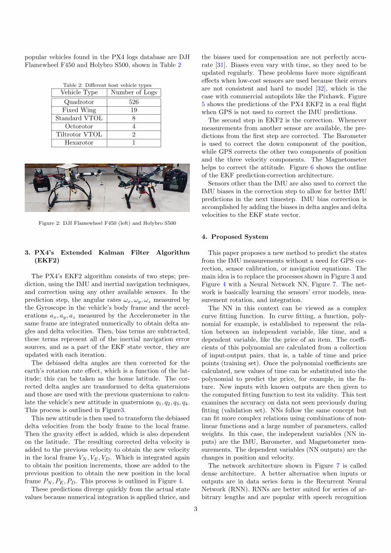
popular vehicles found in the PX4 logs database are DJIFlamewheel F450 and Holybro S500, shown in Table 2

Table 2: Different host vehicle types

Vehicle Type Number of Logs

Quadrotor 526Fixed Wing 19

Standard VTOL 8Octorotor 4

Tiltrotor VTOL 2Hexarotor 1

Figure 2: DJI Flamewheel F450 (left) and Holybro S500

3. PX4’s Extended Kalman Filter Algorithm(EKF2)

The PX4’s EKF2 algorithm consists of two steps; pre-diction, using the IMU and inertial navigation techniques,and correction using any other available sensors. In theprediction step, the angular rates ωx, ωy, ωz measured bythe Gyroscope in the vehicle’s body frame and the accel-erations ax, ay, az measured by the Accelerometer in thesame frame are integrated numerically to obtain delta an-gles and delta velocities. Then, bias terms are subtracted,these terms represent all of the inertial navigation errorsources, and as a part of the EKF state vector, they areupdated with each iteration.

The debiased delta angles are then corrected for theearth’s rotation rate effect, which is a function of the lat-itude; this can be taken as the home latitude. The cor-rected delta angles are transformed to delta quaternionsand those are used with the previous quaternions to calcu-late the vehicle’s new attitude in quaternions q1, q2, q3, q4.This process is outlined in Figure3.

This new attitude is then used to transform the debiaseddelta velocities from the body frame to the local frame.Then the gravity effect is added, which is also dependenton the latitude. The resulting corrected delta velocity isadded to the previous velocity to obtain the new velocityin the local frame VN , VE , VD. Which is integrated againto obtain the position increments, those are added to theprevious position to obtain the new position in the localframe PN , PE , PD. This process is outlined in Figure 4.

These predictions diverge quickly from the actual statevalues because numerical integration is applied thrice, and

the biases used for compensation are not perfectly accu-rate [31]. Biases even vary with time, so they need to beupdated regularly. These problems have more significanteffects when low-cost sensors are used because their errorsare not consistent and hard to model [32], which is thecase with commercial autopilots like the Pixhawk. Figure5 shows the predictions of the PX4 EKF2 in a real flightwhen GPS is not used to correct the IMU predictions.

The second step in EKF2 is the correction. Whenevermeasurements from another sensor are available, the pre-dictions from the first step are corrected. The Barometeris used to correct the down component of the position,while GPS corrects the other two components of positionand the three velocity components. The Magnetometerhelps to correct the attitude. Figure 6 shows the outlineof the EKF prediction-correction architecture.

Sensors other than the IMU are also used to correct theIMU biases in the correction step to allow for better IMUpredictions in the next timestep. IMU bias correction isaccomplished by adding the biases in delta angles and deltavelocities to the EKF state vector.

4. Proposed System

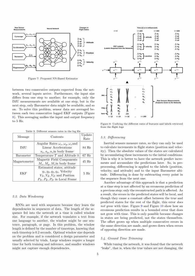
This paper proposes a new method to predict the statesfrom the IMU measurements without a need for GPS cor-rection, sensor calibration, or navigation equations. Themain idea is to replace the processes shown in Figure 3 andFigure 4 with a Neural Network NN, Figure 7. The net-work is basically learning the sensors’ error models, mea-surement rotation, and integration.

The NN in this context can be viewed as a complexcurve fitting function. In curve fitting, a function, poly-nomial for example, is established to represent the rela-tion between an independent variable, like time, and adependent variable, like the price of an item. The coeffi-cients of this polynomial are calculated from a collectionof input-output pairs, that is, a table of time and pricepoints (training set). Once the polynomial coefficients arecalculated, new values of time can be substituted into thepolynomial to predict the price, for example, in the fu-ture. New inputs with known outputs are then given tothe computed fitting function to test its validity. This testexamines the accuracy on data not seen previously duringfitting (validation set). NNs follow the same concept butcan fit more complex relations using combinations of non-linear functions and a large number of parameters, calledweights. In this case, the independent variables (NN in-puts) are the IMU, Barometer, and Magnetometer mea-surements. The dependent variables (NN outputs) are thechanges in position and velocity.

The network architecture shown in Figure 7 is calleddense architecture. A better alternative when inputs oroutputs are in data series form is the Recurrent NeuralNetwork (RNN). RNNs are better suited for series of ar-bitrary lengths and are popular with speech recognition

3

Gyroscope RawMeasurements

angles

angles  bias

Resolution angle

due toearth's

rotation 

To BodyFrame

Earth's RotationRate Constant

anglescorrected QuaternionsTo

QuaternionsQuaternionsIncrement

PreviousQuaternions

New Attitude inQuaternions

Home Latitude PreviousQuaternions

Figure 3: Attitude prediction from Gyroscope measurements in the EKF2 prediction step

Accelerometer RawMeasurements

velocity

velocity  bias

Earth's GravityGravityModel

HomeLatitude

velocity due to gravity

To LocalFrame

Previous LocalVelocity New Local

Velocity

Previous LocalPosition

New LocalPosition

PreviousQuaternions

Figure 4: Velocity and position prediction from attitude and Accelerometer measurements in the EKF2 prediction step

0 1 2 3 4 5 6-1

0

1

2

3

4

5

east

pos

ition

(m)

104

EKF with GPSEKF without GPS, unbounded

Figure 5: EKF2 east position predictions when no GPS aiding isused

and time series forecasting applications. RNNs pass mem-ory information from earlier points in the sequence to laterpoints and use them for later predictions. The architectureused in this paper is composed of recurrent layers followedby a single dense layer.

Gyroscope

Accelerometer

StatePrediction State Correction

hB

arom

eter

Mx 

, My 

, Mz 

Mag

neto

met

er

V N ,

V E ,

V DP N

 , P E

 , P D

GPS

q1q2q3q4

VNVEVD

PNPEPD

Attitude

Position

Velocity

Flight States

Figure 6: EKF Prediction-Correction Architecture

5. Data Preprocessing

No filtration is applied to the raw sensor measurementsgiven to the network. All the preprocessing steps men-tioned here are used to control the input rates, removecorrupted data from the training set, or divide the inputsinto segments.

5.1. Different Update Rates of Different logged messages

In the flight log file created by the PX4 stack, differentsensor data are stored in different messages. The frequencyof the logged data is not the same in all messages; differ-ent frequencies are shown in Table 3. This means that

4

Gyroscope

Accelerometer

hBarometer

Mx , My , Mz Magnetometer

Attitude

Position

Velocity

Changes inFlight StatesNeural Network

q1 q2 q3 q4

 VN VE VD

 PN PE PD

Raw SensorMeasurements

Figure 7: Proposed NN-Based Estimator

between two consecutive outputs expected from the net-work, several inputs arrive. Furthermore, the input sizediffers from one step to another; for example, only theIMU measurements are available at one step, but in thenext step, only Barometer data might be available, and soon. To solve this problem, sensor data are averaged be-tween each two consecutive logged EKF outputs (Figure8). This averaging unifies the input and output frequencyto 5 Hz.

Table 3: Different sensors rates in the log file

Message ContentsUpdate

Rate

IMUAngular Rates ωx, ωy, ωzand

Linear Accelerationsax, ay, azin body frame

84 Hz

Barometer Temperature T and Altitude h 67 Hz

MagnetometerMagnetic Field ComponentsMx,My,Mzin body frame

45 Hz

EKF

Estimated states, attitudeq1, q2, q3, q4, Velocity

VN , VE , VD and PositionPN , PE , PD in Local Frame

5 Hz

5.2. Data Windowing

RNNs are used with sequences because they learn thedependencies in sequences of data. The length of the se-quence fed into the network at a time is called windowsize. For example, if the network translates a text fromone language to another, the window might be one sen-tence, paragraph, or page. In this problem, the windowlength is defined by the number of timesteps, knowing thateach timestep is 0.2 seconds. Optimal window size dependson the problem and is considered a design parameter andusually selected by trials. Large windows require a longertime for both training and inference, and smaller windowsmight not capture enough dependencies.

t = 0 t = 200 t = 400 t = 600

t = 12 t = 15 t = 22 ... t = 200

IMU

mag

baro

attitude

position

velocity

axayaz

h

axayaz

Time (t) is in milliseconds

MxMyMz

...

...

EKF outputs(Labels Required from the Network)

Raw Sensors Measurements(Features Given to the Network)

q1 q2 q3 q4

 VN VE VD

 PN PE PD

q1 q2 q3 q4

 VN VE VD

 PN PE PD

q1 q2 q3 q4

 VN VE VD

 PN PE PD

Figure 8: Unifying the different rates of features and labels retrievedfrom the flight logs

5.3. Differencing

Inertial sensors measure rates, so they can only be usedto calculate increments in flight states (position and veloc-ity). Then the absolute values of the states are calculatedby accumulating these increments to the initial conditions.This is why it is better to have the network predict incre-ments and accumulate the predictions later. So, in pre-processing, differencing is applied to the labels (position,velocity, and attitude) and to the input Barometer alti-tude. Differencing is done by subtracting every point inthe sequence from the next one.

Another advantage of this approach is that a predictionat a time step is not affected by an erroneous prediction ofa previous step; only the reconstructed path is affected. Asa result, the errors in the predicted states will be local, andthough they cause a constant offset between the true andpredicted states for the rest of the flight, this error doesnot grow with time. Figure 9 and Figure 10 show how anerroneous prediction results in a bounded error that doesnot grow with time. This is only possible because changesin states are being predicted, not the states themselves.The offset grows up when multiple consecutive errors inthe same direction are made, and grows down when errorsof opposing direction are made.

5.4. Ground Time Trimming

While tuning the network, it was found that the network“leaks”, that is, when the true values are not changing, the

5

0 1 2 3 4time (minutes)

1.0

0.5

0.0

0.5

1.0

Ch

ang

e in

nort

h p

osi

tion

(m

)

EKF with GPS

Network without GPS

Figure 9: Changes in a state as predicted by the network as opposedto the true changes

0 1 2 3 4time (minutes)

0

20

40

60

80

100

120

140

nort

h p

osi

tion

(m

)

EKF with GPS

Network without GPS

Figure 10: A mispredicted change results in an offset when recon-structing the state path, but it does not grow

network drifts slowly. But when the true values are chang-ing, the network predictions follow the changes correctly.This can be seen in Figure 11. The network learned thisbehavior from the ground truth values. It turns out thatthe EKF2 estimates drift when the drone is on the ground,before takeoff and after landing, even if a good GPS signalis available.

Figure 12 is an example of a thirty-minute log of whichabout ten minutes are erroneous ground truth values. Thisbehavior exists in most flights, so it is difficult for thenetwork not to learn it. This behavior can be correctedby trimming the ground time from the logs before feedingthem to the network.

5.5. Manual Dataset Cleanup

Further manual cleanup was applied to remove otherproblems in the dataset. For example, some logs where

0.0 2.5 5.0 7.5 10.0 12.5 15.0 17.5time (minutes)

0

50

100

150

200

250

nort

h p

osi

tion (

m)

EKF Output

NN predictions

Figure 11: Network predictions drifting when the true values are notchanging

0 5 10 15 20 25 30time (minutes)

50

40

30

20

10

0

Dow

n P

osi

tion

(m

ete

rs)

Figure 12: EKF estimates drifting when the drone is on the ground

the drone did not even takeoff might be as long as 20minutes. Other logs collected with a poorly tuned EKF,or when a hardware fault occurred are also removed. Thisintensive cleanup reduced the number of logs from 943 to548. Figure 13 shows a log found in the database with aclaimed duration of about 21 minutes. After trimming theground time it was found that the entire log is corrupted,and no actual takeoff took place.

6. Network Design and Hyperparameters Tuning

Neural Network design is an iterative process. Manydesign parameters that determine the network shape andcharacteristics are to be selected. Other design decisionsare concerned with how the network is trained, that is, howthe weights are updated. These decisions result in the se-lection of proper hyperparameters. This section describeshow each design parameter and hyperparameter was se-lected. Figure 14 shows the general network architecture.The number of layers, their types, and the number of nodesin each layer are some of the design decisions.

6

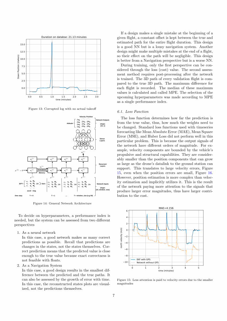
0.0 0.5 1.0 1.5 2.0 2.5 3.0time (minutes)

0.0

2.5

5.0

7.5

10.0

12.5

15.0

Dow

n P

osi

tion

(m

ete

rs)

Duration on databse: 21.13 minutes

Figure 13: Corrupted log with no actual takeoff

T = 0

Memory

gyro

accel mag

baro

T = 1 T = window_size (e.g 50)...

RecurrentLayers

DenseLayers

Network Outputs

shape:(10, 1)

time step:

Network Inputs

shape:(10, window_size)

Activations

q1q2q3q4

VNVEVD

PNPEPD

MxMyMz

axayaz

haxayaz

hMxMyMz

axayaz

MxMyMz

haxayaz

MxMyMz

h

Attitude

Velocity Position

Figure 14: General Network Architecture

To decide on hyperparameters, a performance index isneeded, but the system can be assessed from two differentperspectives

1. As a neural network

In this case, a good network makes as many correctpredictions as possible. Recall that predictions arechanges in the states, not the states themselves. Cor-rect prediction means that the predicted value is closeenough to the true value because exact correctness isnot feasible with floats.

2. As a Navigation System

In this case, a good design results in the smallest dif-ference between the predicted and the true paths. Itcan also be assessed by the growth of error with time.In this case, the reconstructed states plots are visual-ized, not the predictions themselves.

If a design makes a single mistake at the beginning of agiven flight, a constant offset is kept between the true andestimated path for the entire flight duration. This designis a good NN but is a lousy navigation system. Anotherdesign might make multiple mistakes at the end of a flight,so their effect on the path will be negligible. This designis better from a Navigation perspective but is a worse NN.

During training, only the first perspective can be con-sidered through the loss (cost) value. The second assess-ment method requires post-processing after the networkis trained. The 3D path of every validation flight is com-pared to the true 3D path. The maximum difference foreach flight is recorded. The median of these maximumvalues is calculated and called MPE. The selection of theupcoming hyperparameters was made according to MPEas a single performance index.

6.1. Loss Function

The loss function determines how far the prediction isfrom the true value, thus, how much the weights need tobe changed. Standard loss functions used with timeseriesforecasting like Mean Absolute Error (MAE), Mean SquareError (MSE), and Huber Loss did not perform well in thisparticular problem. This is because the output signals ofthe network have different orders of magnitude. For ex-ample, velocity components are bounded by the vehicle’spropulsive and structural capabilities. They are consider-ably smaller than the position components that can growas large as the drone’s datalink to the ground station cansupport. This translates to large velocity errors, Figure15, even when the position errors are small, Figure 16.However, position estimation is more complex than veloc-ity estimation and implicitly utilizes it. This is the resultof the network paying more attention to the signals thatproduce larger error magnitudes, thus have larger contri-bution to the cost.

0 1 2 3 4 5time (minutes)

10

8

6

4

2

0

2

4

6

nort

h v

elo

city

(m

/s)

MAE=4.156

EKF with GPS

Network without GPS

Figure 15: Less attention is paid to velocity errors due to the smallermagnitudes

7

0 1 2 3 4 5time (minutes)

0

20

40

60

80

100

120

nort

h p

osi

tion

(m

)

MAE=0.691

EKF with GPS

Network without GPS

Figure 16: More attention is paid to the large position components,so higher accuracy is acheived

To solve this, a modified MAE was used to account fordifferent signals magnitudes. Equation 1 shows the stan-dard MAE, where yi is the state value predicted by thenetwork, yi is the true state value, and n is the number ofpredicted values, n = 6 if only velocity and position are re-quired and n = 10 if the attitude is required too. Equation2 is the weighted version, for each signal, the error is mul-tiplied by the signal’s weight so that small errors comingfrom small signals contribute more fairly to the final loss.The weight for each signal is the reciprocal of its mean inthe training set.

MAE =

∑ni=1 |yi − yi|

n=

∑ni=1 |ei|n

(1)

MAEweighted =

∑ni=1 |yi − yi|wi

n=

∑ni=1 |ei|wi

n(2)

Using Mean Absolute Percentage Error (MAPE) losscancels the need for weighting. However, MAPE dividesthe error by the true value which is often zero. Catchingzero divisions and replacing them with machine precisiondid not solve the problem because the resulting errors weretoo high. MSE was not better than MAE because mostvalues are small, and squaring made them even smallerresulting in small loss values.

6.2. Network Architecture

Different combinations of dense and recurrent layerswere tested, from a single recurrent layer of 10 nodes to12 layers of 200 nodes each. The best performance wasachieved by four recurrent layers, 200 nodes each, followedby a single dense layer of 6 nodes to reshape the data tothe shape of the labels (if only velocity and position arerequired).

6.3. Recurrent Cell Type and Activation Functions

Three different types of recurrent cells were tested; theVanilla Cell, the Gated Recurrent Unit (GRU), and theLong Short Term Memory (LSTM) cell. Despite tak-ing longer to train and resulting in more parameters, theLSTM cells gave the best performance. Two activationsare applied within an LSTM cell, one for the new inputsand another for the recurrent inputs. Sigmoid, tanh andReLU activations were tested. While tanh had the bestperformance, it could only be used for input activation.The recurrent activation must be sigmoid for the GPUaccelerated training to work.

6.4. Window Size

Window sizes from 20 steps to 200 steps were tested.Increasing the window size increases the accuracy butsignificantly increases both training and inference time.Too large windows might decrease the accuracy becausea larger than needed context leads to network confusion.Table 6.4 shows the effect of inreasing window size on bothaccuracy and training time.

Table 4: Effect of increasing window size on accuracy and trainingtime

Windowsize

Median of maximumposition errors in

validation set (meters)

Training time, 100epochs (hours)

50 72.4 1.94100 52.78 4.94150 35.59 7.25200 34.26 9.21

6.5. Learning Rate

Learning rates from 0.00001 to 0.1 were tested. In theinitial epochs, when the weights are far from their opti-mal values, high learning rate can be used. When the lossapproaches its minimum, the learning rate should be de-creased to prevent overshooting. Table 5 was used as alearning rate schedule.

Table 5: Learning rate schedule

Epochs (from - to) Learning rate

0 - 50 0.00551 - 100 0.0025101 - ... 0.001

6.6. Batch Size

The number of training examples (windows) fed to thenetwork in one optimizer step is called batch size. Batch-ing was initially used because GPU memory could not ac-commodate the entire dataset. Using batches can lead tofaster convergence because of the more frequent weights

8

updates. Batch sizes from 512 to 16,384 windows weretested. The chosen batch size is 1024, as it achieves thefastest learning and provides some regularization.

6.7. Regularization

Regularization is needed to prevent the network frommemorizing the training data and allow it to generalize tothe validation data. The most popular regularization tech-nique is dropout, which randomly turns off hidden nodes intraining time when propagating each input vector. Sincetwo activations are applied, two dropouts are applied, onefor the input and another for the recurrent activations. Inthe earlier trials, dropout gave very good regularizationwhen small number of flight logs was used. Unfortunately,recurrent dropout prevents GPU acceleration, so, it couldnot be used with large datasets. L1 and L2 regularizationwere also tested, but they could not achieve similar perfor-mance as dropout. The final design and the results shownin this paper do not use any formal regularization.

6.8. Training Time and Number of epochs

An epoch is a single pass through the entire dataset,that is, processing all the batches. Longer training in-creases training accuracy but may reduce validation accu-racy when overfitting occurs. Different numbers of epochswere tested from 100 to 1500, but the accuracy did notincrease much after 200 epochs. This takes about 5 hoursusing two Nvidia RTX 2070 Super GPUs connected viaNVLink.

6.9. Final Design

The final network design and hyperparameters used aresummarized in Table 6.

Table 6: Network Architecture and Hyperparameters

Number of recurrent layers 4Number of nodes in a recurrent cell 200Input activation in recurrent layers tanh

Recurrent activation in recurrent layers sigmoidNumber of dense layers 1

Number of nodes in the dense layer 6Dense activation None

Optimizer AdamAdam’s first & second moment decay

rates0.9, 0.999

Number of Epochs 100 (≈ 5 hours)

Learning rate schedule0.005, 0.0025,

0.001Regularization None

Window size200 steps = 40

secondsBatch size 1024 examples

Loss functionWeighted MAE

(custom)

7. Results and Discussion

The MPE index defined in section 6 is enough to com-pare different designs given that the flights in both trainingand validation sets are unchanged. But when comparingthe accuracy of a design in two different flights, MPE aloneis not sufficient, because different flights vary in durationand traveled distance. Traditionally, an INS is assessedby the growth of positioning error with time, because themajor estimation errors in INS accumulate proportionallyto the time since positioning starts. A similar index isused in the following discussions, obtained by dividing theMPE by the flight duration to arrive at Time-NormalizedMaximum Position Error (TN-MPE), expressed in metersper minute (m/min).

7.1. Performance on the Training Set

Training performance is usually examined to make surethat the network is at least fitting the training data. Noenhancements should be applied to the validation perfor-mance until the network sufficiently fits the training data.However, training performance is not a sufficient indica-tor, and the network must not be expected to providesimilar performance on newer data. Training performancemight also be treated as a goal to look for in the validationset when tuning the regularization parameters, because itshows the potential of a particular design. Table 7 summa-rizes the performance on the training set, which consistsof 465 flights. The shown median position error indicatesthat positioning error never grew beyond 7.23 meters in232 different flights.

Table 7: Performance on the training dataset

MPE (m) TN-MPE (m/min) MVE (m/s)

Mean 16.78 2.98 3.78Median 7.23 1.39 2.26

Best Flight 1.13 0.45 0.57Worst Flight 1666.31 262.69 168.02

7.2. Performance on the Validation Set

Validation performance reflects how the system per-forms with new flights not used during training. The val-idation dataset is comprised of 83 flights totaling about 8hours. Table 8 summarizes the performance on the valida-tion set. Mean and median are calculated from the max-imum errors reached in every flight. It is noted that thevalidation mean MPE and TN-MPE are five times largerthan those of the training. This resulted from the lack ofproper regularization.

Figure 17 shows the flight path of the validation flightwith the lowest MPE and TN-MPE. The S letter in a plotindicates the true start position and the E letter indicatesthe true end position. Some flights seem to start mid-airbecause the ground time is trimmed as described in section5.4, and the takeoff portion lies within the first window. As

9

Table 8: Performance on the validation datasetMPE (m) TN-MPE (m/min) MVE (m/s)

Mean 85.79 17.79 6.40Median 34.26 6 4.15

Best Flight 2.66 0.61 0.76Worst Flight 871.54 142.08 67.65

mentioned in Table 6, the window size is 200 steps. Thismeans that the network makes its first prediction after40 seconds. By that time, the drone might have alreadyreached the mission altitude.

Despite the path in Figure 17 having some acute direc-tion changes, the network could still predict these maneu-vers correctly. One reason is that this flight pattern iscommon in the dataset, so the network had enough datato relate the associated sensor behavior to the resultingchanges in position.

East (m)

6040

200

2040

6080

100

North (m

)

020

4060

80100

120140

Up

(m

)

10

20

30

40

50

Duration: 4.37 min, MPE: 2.66 m,Distance: 934.09 m, TN-MPE: 0.61 m/min

EKF with GPS (True Path)

Network without GPS (Predicted Path)

S

E

Figure 17: Path of the best validation flight

Figure 18 shows another validation flight with differentmaneuvers. The blue arrow marks a sudden change inturn rate; an erroneous prediction is made at this pointresulting in an offset that persists until the end of theflight.

Figure 19, Figure 20, and Figure 21 show three morevalidation flights. Despite having the shortest flight dura-tion, the flight in Figure 19 has the highest MPE amongthe three, and has more than twice as much TN-MPE asany of them. This is because predictions in Figure 19 con-tain multiple errors near the beginning.

7.3. Aggressive Manual Maneuvers

A common practice in the database flights is that pilotsusually start the flight by some aggressive manual maneu-vers before switching the autopilot to “Auto” mode thatexecutes the mission autonomously. These aggressive ma-neuvers might excite some error sources in the IMU that

East (m)

100

80

60

40

20

0North (m)

020

4060

80100

120

Up (

m)

0

10

20

30

40

Duration: 4.74 min, MPE: 7.20 m,Distance: 1238.18 m, TN-MPE: 1.52 m/min

EKF with GPS (True Path)

Network without GPS (Predicted Path)

S

E

Figure 18: Validation flight path -1

East (m)

4020

020

40

North

(m)

0

50

100

150

200

Up (

m)

0

10

20

30

40

Duration: 4.55 min, MPE: 11.53 m,Distance: 1086.34 m, TN-MPE: 2.53 m/min

EKF with GPS (True Path)

Network without GPS (Predicted Path)

S

E

Figure 19: Validation flight path -2

are not active in steady flights. Furthermore, the man-ual sections of the flights are considerably smaller thanthe autonomous ones. This, combined with the fact thatthese maneuvers have much more combinations than thesteady ones, means that the data capturing their underly-ing mappings are rare in the dataset. Consequently, thenetwork performance in manual flights is worse than thatin autonomous ones. Fortunately, manual flights do notrequire accurate positioning, and these aggressive maneu-vers are usually performed within the pilot’s line of sight.It is the remote autonomous missions and steadier flightsthat require the proposed system the most.

Figure 22 and Figure 23 show two validation flights withrelatively long manual sections. It can be noted that pre-dictions made in these manual sections are worse thanthose made in the autonomous ones. Despite these er-roneous predictions preceding the correct ones, they didnot affect them. This means that a single external reset(using an external sensor) can remove much of the error

10

East (m)

200

150

100

50

0

North (m

)

40

20

0

20

40

60

Up

(m

)

0

5

10

15

20

25

30

Duration: 6.16 min, MPE: 7.62 m,Distance: 1099.70 m, TN-MPE: 1.24 m/min

EKF with GPS (True Path)

Network without GPS (Predicted Path)

S

E

Figure 20: Validation flight path -3

East (m)

175

150

125

100

75

50

25

0North (m)

020

4060

80100

120140

160

Up (

m)

0

10

20

30

40

50

Duration: 5.10 min, MPE: 4.84 m,Distance: 904.93 m, TN-MPE: 0.95 m/min

EKF with GPS (True Path)

Network without GPS (Predicted Path)

S

E

Figure 21: Validation flight path - 4

in the latter segments.

Figure 24 shows another flight where much of the man-ual maneuvers are hidden in the first window. The onesoutside the window were enough to introduce an error thatexceeds 120 meters.

The TN-MPE index does not represent the error growthrate, despite having rate units (m/min). This is becausemuch of the prediction errors shown do not grow with time.They are little-varying offsets introduced by rare flightphenomena scattered in different and spaced timesteps.For example, the flight in Figure 24 has a TN-MPE of28.83 m/min, but this does not mean that if it contin-ued to fly one more minute, the error would have grownby 28.83 meters. Instead, this error was introduced earlyin the flight and did not change much afterward. This isalso visible in Figure 22 and Figure 23, where much of theerrors are introduced in the beginning but do not growlater.

East (m)

200

150

100

50

0

50

100

North (m

)

025

5075

100125

150175

Up (

m)

5051015202530

Duration: 5.66 min, MPE: 80.84 m,Distance: 2099.10 m, TN-MPE: 14.28 m/min

EKF with GPS (True Path)

Network without GPS (Predicted Path)

S

E

Figure 22: Validation flight with both manual and autonomous sec-tions

East (m)

300250

200150

10050

050

North (m

)

50

0

50

100

150

200

Up (

m)

0

10

20

30

40

Duration: 8.53 min, MPE: 131.35 m,Distance: 1853.92 m, TN-MPE: 15.39 m/min

EKF with GPS (True Path)

Network without GPS (Predicted Path)

S

E

Figure 23: Validation flight with both manual and autonomous sec-tions -2

7.4. Underrepresented Vehicle Types

It was seen from Table 2 that approximately 94% of theflights in the dataset used a Quadrotor as a host vehicle.The dataset is split randomly into training and validation.Only four flights from the underrepresented vehicles fallinto the validation set, of which three used an FW vehicleand one used a VTOL. Performance in these four flightsis summarized in Table 9. The TN-MPE Rank column inTable 9 is the position of a flight’s TN-MPE among theentire validation set in descending order. It can be seenthat these four flights are ranked among the five highestTN-MPEs (lowest accuracy) in the validation set.

Figure 25 shows the FW validation flight # 1. Despitethe shorter than a minute duration, positioning error growsbeyond a hundred meters. The flight does not have aggres-sive manual maneuvers either.

The same observation applies to the VTOL validationflight in Figure 26. This, too, is a short flight with smooth

11

East (m)

150100

500

50

Nor

th (

m)

50

0

50

100

150

Up (

m)

5101520253035

Duration: 4.32 min, MPE: 124.46 m,Distance: 1193.04 m, TN-MPE: 28.83 m/min

EKF with GPS (True Path)

Network without GPS (Predicted Path)

S

E

Figure 24: Validation flight with wrong predictions at the beginning

Table 9: Validation performance in underrepresented vehicle types

FlightDuration

(min)Distance

(m)MPE(m)

TN-MPE

(m/min)

TN-MPERank

FW #1 0.73 488.73 103.72 142.08 1st

FW #2 6.52 5424.57 871.54 133.74 2nd

FW #3 2.6 2062.32 289.82 111.47 4th

VTOL 5.53 3620.59 551.58 99.8 5th

maneuvers; still, positioning error grows to almost 300 me-ters in less than three minutes.

Some factors contributing to the relatively high TN-MPE with underrepresented vehicles are:

1. The network learns to compensate for the Magne-tometer errors at some point in the prediction process.These errors are affected mainly by the magnetic fieldof the vehicle’s motors, which varies from one vehicletype to another. For example, an FW drone usuallyhas only one motor, but the Quadrotor has four, andthe Standard VTOL has five.

2. The network may be learning to compensate for vi-brations, which vary from one vehicle type to another.

3. These flights have relatively high average velocities,the average velocities of the flights in Table 9 rangefrom 10.91 m/s to 13.87 m/s. The mean value ofaverage velocities in the validation set is only 4.66m/s.

Other than these worst five flights, the sixth-highest TN-MPE in the validation flights is only 52.38 m/min, followedby 38.94 m/min. This explains the large gap between themean and median values for the TN-MPE in Table 8.

7.5. Velocity Predictions

The network described in Table 6 predicts both posi-tion and velocity differences (increments) independently,

East (m)

50 25 0 25 50 75 100 125 150

North

(m)

8060

4020

020

4060

Up

(m

)

20

30

40

50

60

70

80

Duration: 0.73 min, MPE: 103.72 m,Distance: 488.73 m, TN-MPE: 142.08 m/min

EKF with GPS (True Path)

Network without GPS (Predicted Path)

S

E

Figure 25: FW Validation Flight # 1

East (m)400

2000

200400

600

North (m

)

200

100

0

100

200

300

400

500

Up

(m)

0

10

20

30

40

50

60

Duration: 2.60 min, MPE: 289.82 m,Distance: 2062.32 m, TN-MPE: 111.47 m/min

EKF with GPS (True Path)

Network without GPS (Predicted Path)

S

E

Figure 26: VTOL validation flight

so errors in some direction in velocity are not necessarilyreflected in position errors in the same direction. Anothermethod to calculate the velocity is to divide the positiondifferences calculated by the network by the time step.Since the time step is fixed to 0.2 seconds, any predictedposition difference can be divided by 0.2 to get the veloc-ity in the same direction. Not only does this reduce thenetwork size and computations, but it also improves theaccuracy of the calculated velocity.

Figure 27, Figure 28, and Figure 29 compare the twomethods in the three velocity components in a validationflight.

7.6. Attitude Predictions

The PX4 EKF2 estimates the attitude expressed inquaternions. These attitude estimates do not diverge whenthe GPS signal is lost, because Gyroscope and Accelerome-ter can predict reliable roll and pitch angles, and the Mag-netometer helps correct the yaw angle. Another advantage

12

0 1 2 3 4 5time (minutes)

8

6

4

2

0

2

4

Nort

h V

elo

city

(m

/s)

Accumulated MAE= 2.29, From Pos MAE= 0.10

Ground Truth

NN Position Differences Divided by t

Accumulated NN Velocity Differences

Figure 27: North velocity component of a validation flight as pre-dicted by the network vs. as calculated from position differences

0 1 2 3 4 5time (minutes)

4

2

0

2

4

East

Velo

city

(m

/s)

Accumulated MAE= 0.56, From Pos MAE= 0.11Ground Truth

NN Position Differences Divided by t

Accumulated NN Velocity Differences

Figure 28: East velocity component of a validation flight as predictedby the network vs. as calculated from position differences

of the EKF’s attitude is that it is produced at a relativelyhigh rate of 84 Hz. The network, on the other hand, istrained using 5 Hz logs, so it is limited by this rate. Sometrials where the network predicted the attitude along withvelocity and position were performed. Figure 30, Figure31, Figure 32 and Figure 33 show the attitude as predictedby the network and as estimated by the EKF when GPSis lost. The EKF errors here result from the numericalcomplications caused by the massively diverging positionand velocity estimates. In the PX4 code, this is curedby feeding zero position and velocity measurements to theEKF when the GPS fix is lost to preserve the numericalstability of other estimated quantities like the attitude.

These reasonable estimates produced by the GPS-lessEKF are the reason why the final network design does notpredict attitude. Adding more elements to the labels vec-tor makes the network more complex and requires more

0 1 2 3 4 5time (minutes)

3

2

1

0

1

Dow

n V

elo

city

(m

/s)

Accumulated MAE= 1.07, From Pos MAE= 0.16

Ground Truth

NN Position Differences Divided by t

Accumulated NN Velocity Differences

Figure 29: Down velocity component of a validation flight as pre-dicted by the network vs. as calculated from position differences

time for both training and inference. Requiring more la-bels from the network also diverts some focus from theposition and velocity calculations and reduces their per-formance.

0 1 2 3 4 5time (minutes)

2.0

1.5

1.0

0.5

0.0

q1

NN MAE=0.075, GPS-less EKF MAE = 0.082EKF with GPSNetwork without GPSEKF without GPS

Figure 30: Attitude quaternions - q1

8. Field Testing and Real-time Inference

Inference time is the time taken by the network to pre-dict one labels vector. That is, given a window of sensormeasurements, how much time does the network need topredict the corresponding change of position and velocityat the end of this window? Since the network is trainedto predict position at 5 Hz, inference time must be lessthan 200 milliseconds. Inference time is determined bythree factors, the embedded hardware on which the net-work is deployed, the length of the input window, and thesize of the network itself. Larger networks achieve higher

13

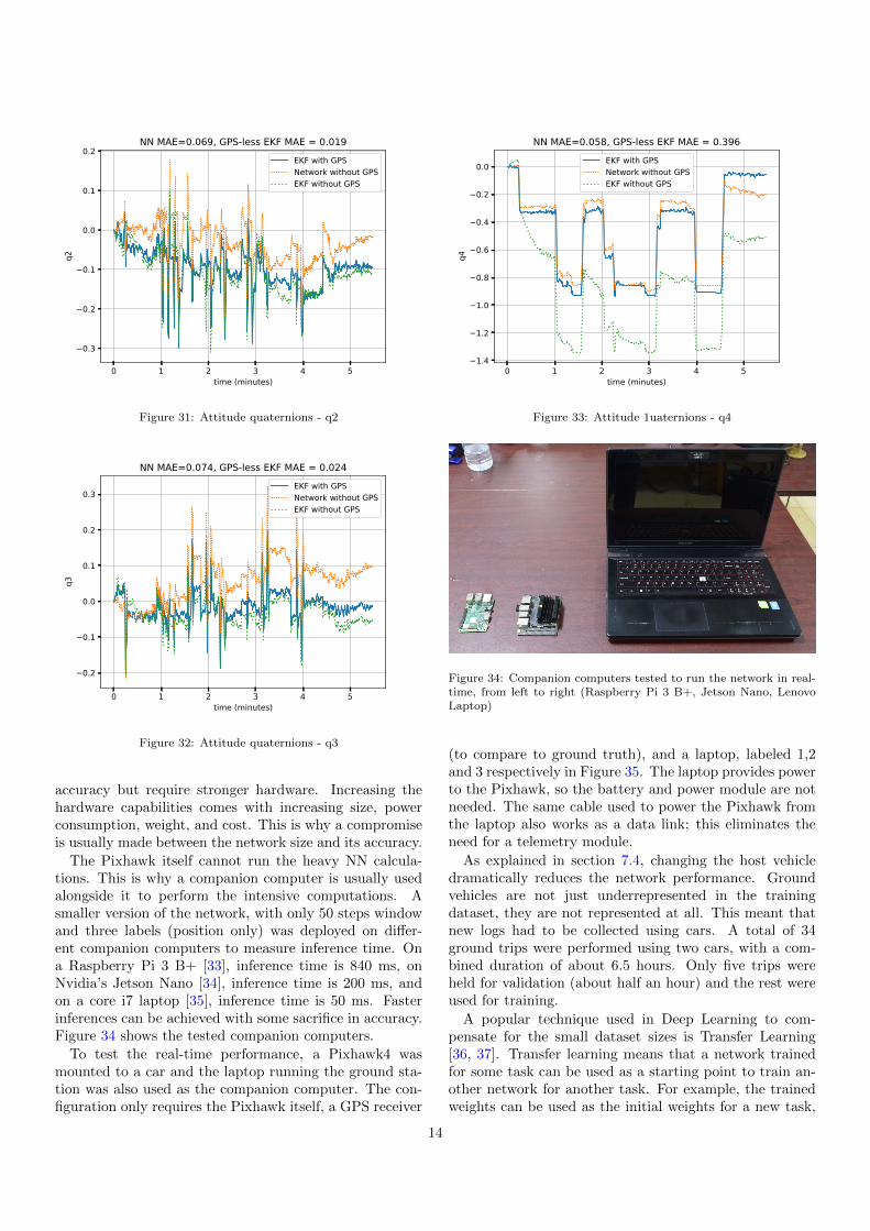
0 1 2 3 4 5time (minutes)

0.3

0.2

0.1

0.0

0.1

0.2

q2

NN MAE=0.069, GPS-less EKF MAE = 0.019EKF with GPSNetwork without GPSEKF without GPS

Figure 31: Attitude quaternions - q2

0 1 2 3 4 5time (minutes)

0.2

0.1

0.0

0.1

0.2

0.3

q3

NN MAE=0.074, GPS-less EKF MAE = 0.024EKF with GPSNetwork without GPSEKF without GPS

Figure 32: Attitude quaternions - q3

accuracy but require stronger hardware. Increasing thehardware capabilities comes with increasing size, powerconsumption, weight, and cost. This is why a compromiseis usually made between the network size and its accuracy.

The Pixhawk itself cannot run the heavy NN calcula-tions. This is why a companion computer is usually usedalongside it to perform the intensive computations. Asmaller version of the network, with only 50 steps windowand three labels (position only) was deployed on differ-ent companion computers to measure inference time. Ona Raspberry Pi 3 B+ [33], inference time is 840 ms, onNvidia’s Jetson Nano [34], inference time is 200 ms, andon a core i7 laptop [35], inference time is 50 ms. Fasterinferences can be achieved with some sacrifice in accuracy.Figure 34 shows the tested companion computers.

To test the real-time performance, a Pixhawk4 wasmounted to a car and the laptop running the ground sta-tion was also used as the companion computer. The con-figuration only requires the Pixhawk itself, a GPS receiver

0 1 2 3 4 5time (minutes)

1.4

1.2

1.0

0.8

0.6

0.4

0.2

0.0

q4

NN MAE=0.058, GPS-less EKF MAE = 0.396EKF with GPSNetwork without GPSEKF without GPS

Figure 33: Attitude 1uaternions - q4

Figure 34: Companion computers tested to run the network in real-time, from left to right (Raspberry Pi 3 B+, Jetson Nano, LenovoLaptop)

(to compare to ground truth), and a laptop, labeled 1,2and 3 respectively in Figure 35. The laptop provides powerto the Pixhawk, so the battery and power module are notneeded. The same cable used to power the Pixhawk fromthe laptop also works as a data link; this eliminates theneed for a telemetry module.

As explained in section 7.4, changing the host vehicledramatically reduces the network performance. Groundvehicles are not just underrepresented in the trainingdataset, they are not represented at all. This meant thatnew logs had to be collected using cars. A total of 34ground trips were performed using two cars, with a com-bined duration of about 6.5 hours. Only five trips wereheld for validation (about half an hour) and the rest wereused for training.

A popular technique used in Deep Learning to com-pensate for the small dataset sizes is Transfer Learning[36, 37]. Transfer learning means that a network trainedfor some task can be used as a starting point to train an-other network for another task. For example, the trainedweights can be used as the initial weights for a new task,

14

Figure 35: Hardware Setup in a Car

instead of randomly initializing the weights. This shouldbe done carefully to avoid the loss of the relations learnedfrom the large dataset and at the same time accommodatethe new relations introduced by the smaller set.

The same concept can be applied to different vehi-cle types, for example, a network can be pretrained onQuadrotors, then the knowledge is transferred to a net-work that works with fixed-wing aircraft, or in this case,a car.

Three experiments were conducted on the light network.The first experiment was to train it on the drones datasetfrom Table 2 then to use it without any modifications onthe cars dataset. The second experiment trains it fromscratch on the cars dataset for 100 epochs without utilizingtransfer learning. The last experiment is to pretrain iton the drones dataset and then to retrain it on the carsdataset, which is a form of transfer learning. Figure 36shows the effect of utilizing transfer learning. It is seenthat fresh training starts overfitting after 17 epochs, whileretraining overfits earlier (around five epochs). This is thepoint where the network starts to forget the relations ithas learned from the drones dataset. It is also noticeablethat the validation loss is reduced when transfer learningis applied.

0 20 40 60 80 100

0.5

1.0

1.5

2.0

Tra

inin

g L

oss

(M

AE) Without Transfer Learning

With Transfer Learning

0 20 40 60 80 100epochs

1.2

1.4

1.6

Valid

ati

on L

oss

(M

AE)

Without Transfer Learning

With Transfer Learning

Figure 36: Effect of transfer learning

A comparison between the three experiments is shownin Table 10. The validation results listed utilize early stop-ping, i.e., overfitting is avoided and the weights used arenot the final overfitted weights.

Table 10: Results on the car validation dataset with and withouttransfer learning

Trainedon drones

only

Trainedon cars

only

Trained ondrones, retrained

on cars

Median MPE (m) 4250.92 732.12 520.19Mean MPE (m) 7261.254 1133.324 707.854

Median TN-MPE(m/s)

799.04 99.41 72.99

Mean TN-MPE(m/s)

817.474 181.124 97.222

Table 11 shows the results on the validation car tripsobtained when transfer learning is applied.

Table 11: Validation performance on the car dataset

Trip Number 1 2 3 4

Duration (minutes) 5.32 5.58 9.2 11.35Traveled Distance

(Kilometers)3.314 1.385 8.55 13.79

NN MPE (Kilometers) 0.52 0.136 0.388 1.282TN-MPE (m/min) 72.99 24.42 56.52 113.05

NN MPE as a Percentof Traveled Distance

11.72 % 9.83 % 6.1 % 9.3 %

GPS-less EKF MPE(Kilometers)

24.184 25.752 203.77 421.99

It is seen from Table 11 that the TN-MPE values ofthe car trips are lower than those of the FW and VTOLflights mentioned in Table 9. This is because the collectedcar trips are longer than those of FW and VTOL, andbecause of the retraining, which gave more attention tothis small set.

The accuracy on the car dataset is smaller than thatof the flight dataset because the latter is much larger. Ifhigher accuracy is needed on ground vehicles, then morelogs must be collected. However, the purpose of car testingin this context is mainly to address the challenges associ-ated with real-time inference (edge computing).

Several complications arise when edge computing is per-formed. Aside from accuracy loss resulting from the in-evitable network size reduction, other issues like timing,proper preprocessing, data validity, and latency also affectthe NN predictions. Most of these complications affectthe features consumed by the network. For example, thenetwork makes a prediction every 200 milliseconds; tim-ing this loop on a full operating system -rather than areal-time OS- is hard to guarantee. Consequently, a ±1ms timing error is introduced, this affects both averag-ing and differencing steps in preprocessing. Furthermore,

15

since sensors operate at different rates, multi-threading isneeded to capture every sensor’s measurements as soon asthey are published. And to avoid data loss, these mea-surements should be stored in queues before they are fedto the NN. But if these queues are allowed to grow indefi-nitely, then latency in NN predictions will be noticed, so acompromise should be made. Another issue is data valid-ity; having different functions writing to the features arraycan easily result in data corruption due to race conditions.After addressing all these issues, the NN predictions madein real-time are compared to those made offline using thelogged data. Figure 37, Figure 38 and Figure 39 show theonline and offline position predictions made on a validationtrip.

0 1 2 3 4 5time (minutes)

30

25

20

15

10

5

P_d

(m

)

Down Position, Online-Offline MAE=2.507

True (EKF with GPS)

Offline NN Predictions (ulg)

Online NN Predictions (ROS)

Figure 37: Validation ground trip, online vs. offline predictions,north position

0 1 2 3 4 5time (minutes)

1750

1500

1250

1000

750

500

250

0

P_e

(m

)

East Position, Online-Offline MAE=26.718

True (EKF with GPS)

Offline NN Predictions (ulg)

Online NN Predictions (ROS)

Figure 38: Validation ground trip, online vs. offline predictions, eastposition

0 1 2 3 4 5time (minutes)

0

250

500

750

1000

1250

1500

1750

2000

P_n

(m

)

North Position, Online-Offline MAE=11.945

True (EKF with GPS)

Offline NN Predictions (ulg)

Online NN Predictions (ROS)

Figure 39: Validation ground trip, online vs. offline predictions,down position

9. Summary and Conclusion

The paper presented a Neural Network capable of pre-dicting a drone’s 3D position and speed in the absence ofGPS using the IMU, Barometer and Magnetometer rawmeasurements. The developed network was tested on sev-eral hardware targets, and can run with acceptable speedon embedded devices like the Jetson Nano. Errors in 3Dposition as low as 2.7 were achieved using the proposedsystem in 5-minutes GPS-less drone flight using low-costsensors. The system is well integrated with the PX4 flightstack running on Pixhawk4 and can be used with a quicksetup. The system can also predict the attitude, but theEKF is more reliable in such a task. The network is de-signed to make inferences at 5 Hz, so it is slower thanthe EKF. This is why the network’s main role is to re-place the GPS, not the entire EKF. The network is ideallyused with Quadrotors running on “Auto” flight mode be-cause most of the training data have these characteristics.Transfer learning is also used, and the system was testedin real-time with a ground host vehicle. The network’serrors associated with manual maneuvers or less popularhost vehicles can be reduced by collecting more trainingdata focusing on these conditions. Navigation accuracyalso increases when a larger network and window size areused. But this comes at the expense of both training andinference times. The median positioning error on the vali-dation set is five times larger than that of the training set.This signals the need for proper regularization to help thenetwork generalize better.

References

[1] M. Bloesch, S. Omari, M. Hutter, R. Siegwart, Robust vi-sual inertial odometry using a direct EKF-based approach, in:2015 IEEE/RSJ International Conference on Intelligent Robotsand Systems (IROS), IEEE, 2015. doi:10.1109/iros.2015.

7353389.

16

[2] K. Chiang, G. Tsai, H. Chang, C. Joly, N. EI-Sheimy, Seamlessnavigation and mapping using an INS/GNSS/grid-based SLAMsemi-tightly coupled integration scheme, Information Fusion 50(2019) 181–196. doi:10.1016/j.inffus.2019.01.004.

[3] T.-D. Vu, J. Burlet, O. Aycard, Grid-based localization andlocal mapping with moving object detection and tracking, In-formation Fusion 12 (1) (2011) 58–69. doi:10.1016/j.inffus.

2010.01.004.[4] E. Choi, S. Chang, A consumer tracking estimator for vehicles in

GPS-free environments, IEEE Transactions on Consumer Elec-tronics 63 (4) (2017) 450–458. doi:10.1109/tce.2017.015064.

[5] J. W. David Titterton, Strapdown Inertial Navigation Tech-nology, Institute of Electrical Engineers, 2009.URL https://www.ebook.de/de/product/21923218/david_

titterton_john_weston_strapdown_inertial_navigation_

technology.html

[6] K.-W. Chiang, A. Noureldin, N. El-Sheimy, Multisensor in-tegration using neuron computing for land-vehicle naviga-tion, GPS Solutions 6 (4) (2003) 209–218. doi:10.1007/

s10291-002-0024-4.[7] K.-W. Chiang, H.-W. Chang, C.-Y. Li, Y.-W. Huang, An artifi-

cial neural network embedded position and orientation determi-nation algorithm for low cost MEMS INS/GPS integrated sen-sors, Sensors 9 (4) (2009) 2586–2610. doi:10.3390/s90402586.

[8] L. Semeniuk, A. Noureldin, Bridging GPS outages using neu-ral network estimates of INS position and velocity errors, Mea-surement Science and Technology 17 (10) (2006) 2783–2798.doi:10.1088/0957-0233/17/10/033.

[9] C. Shen, Y. Zhang, J. Tang, H. Cao, J. Liu, Dual-optimizationfor a MEMS-INS/GPS system during GPS outages based on thecubature kalman filter and neural networks, Mechanical Sys-tems and Signal Processing 133 (2019) 106222. doi:10.1016/

j.ymssp.2019.07.003.[10] Z. Wu, W. Wang, INS/magnetometer integrated position-

ing based on neural network for bridging long-time GPSoutages, GPS Solutions 23 (3) (jun 2019). doi:10.1007/

s10291-019-0877-4.[11] N. El-Sheimy, K.-W. Chiang, A. Noureldin, The utilization of

artificial neural networks for multisensor system integration innavigation and positioning instruments, IEEE Transactions onInstrumentation and Measurement 55 (5) (2006) 1606–1615.doi:10.1109/tim.2006.881033.

[12] J. J. Wang, J. Wang, D. Sinclair, L. Watts, A neural networkand kalman filter hybrid approach for gps/ins integration, in:Proceedings of the Korean Institute of Navigation and Port Re-search Conference, Vol. 1, Korean Institute of Navigation andPort Research, 2006, pp. 277–282.

[13] Y. Yao, X. Xu, C. Zhu, C.-Y. Chan, A hybrid fusion algorithmfor GPS/INS integration during GPS outages, Measurement 103(2017) 42–51. doi:10.1016/j.measurement.2017.01.053.

[14] H. fa Dai, H. wei Bian, R. ying Wang, H. Ma, An INS/GNSSintegrated navigation in GNSS denied environment using recur-rent neural network, Defence Technology 16 (2) (2020) 334–340.doi:10.1016/j.dt.2019.08.011.

[15] C. Shen, Y. Zhang, X. Guo, X. Chen, H. Cao, J. Tang, J. Li,J. Liu, Seamless GPS/inertial navigation system based on self-learning square-root cubature kalman filter, IEEE Transactionson Industrial Electronics 68 (1) (2021) 499–508. doi:10.1109/

tie.2020.2967671.[16] A. Noureldin, A. El-Shafie, M. Bayoumi, GPS/INS integration

utilizing dynamic neural networks for vehicular navigation, In-formation Fusion 12 (1) (2011) 48–57. doi:10.1016/j.inffus.

2010.01.003.[17] J. Li, N. Song, G. Yang, M. Li, Q. Cai, Improving positioning

accuracy of vehicular navigation system during GPS outagesutilizing ensemble learning algorithm, Information Fusion 35(2017) 1–10. doi:10.1016/j.inffus.2016.08.001.

[18] X. Li, W. Chen, C. Chan, B. Li, X. Song, Multi-sensor fusionmethodology for enhanced land vehicle positioning, InformationFusion 46 (2019) 51–62. doi:10.1016/j.inffus.2018.04.006.

[19] Y. Bai, B. Zhang, S. Chai, X. Jin, X. Wang, T. Su, Continuous

estimation of motion state in GPS/INS integration based onNARX neural network, in: 2018 37th Chinese Control Confer-ence (CCC), IEEE, 2018. doi:10.23919/chicc.2018.8483157.

[20] V. Havyarimana, D. Hanyurwimfura, P. Nsengiyumva, Z. Xiao,A novel hybrid approach based-SRG model for vehicle positionprediction in multi-GPS outage conditions, Information Fusion41 (2018) 1–8. doi:10.1016/j.inffus.2017.07.002.

[21] L. Meier, P. Tanskanen, F. Fraundorfer, M. Pollefeys, PIX-HAWK: A system for autonomous flight using onboard com-puter vision, in: 2011 IEEE International Conference onRobotics and Automation, IEEE, 2011. doi:10.1109/icra.

2011.5980229.[22] L. Meier, D. Honegger, M. Pollefeys, PX4: A node-based mul-

tithreaded open source robotics framework for deeply embed-ded platforms, in: 2015 IEEE International Conference onRobotics and Automation (ICRA), IEEE, 2015. doi:10.1109/

icra.2015.7140074.[23] J. Garcıa, J. M. Molina, J. Trincado, Real evaluation for de-

signing sensor fusion in UAV platforms, Information Fusion 63(2020) 136–152. doi:10.1016/j.inffus.2020.06.003.

[24] P. Riseborough, R. Bapst, L. Meier, C. Olsson, SiddharthBharat Purohit, M. Sauder, J. Oes, Georgehines, B. Tak,D. Agar, W. Johnson, M. Charlebois, Nickolasrossi, Pickledga-tor, B. Kung, Ecl: V0.9.0 release (2016). doi:10.5281/ZENODO.55367.

[25] PX4.Community, Px4 flight logs database.URL https://review.px4.io/browse

[26] H. Willee, P. Fjare, Pixhawk 4 flight controller.URL https://docs.px4.io/v1.9.0/en/flight_controller/

pixhawk4.html

[27] Invensense, High performance 6-axis mems motiontrackingdevice in 4x4 mm package.URL https://invensense.tdk.com/wp-content/uploads/

2017/08/ICM-20689-v2.2-002.pdf

[28] B. Sensortec, Bmi055 small, versatile 6dof sensor module.URL https://www.bosch-sensortec.com/media/

boschsensortec/downloads/datasheets/bst-bmi055-ds000.

pdf

[29] Isentek, Ist8310 3d magnetometer brief datasheet.URL http://www.isentek.com/en/dlf.php?file=../ISENTEK/

(201703-09)IST8310Datasheetv1.2_brief-105.09.20.pdf

[30] TE, Ms5611-01ba03 barometric pressure sensor, with stainlesssteel cap.URL https://www.te.com/commerce/DocumentDelivery/

DDEController?Action=showdoc&DocId=

DataSheetMS5611-01BA03B3pdfEnglishENG_DS_

MS5611-01BA03_B3.pdfCAT-BLPS0036

[31] J. T. Jang, A. Santamaria-Navarro, B. T. Lopez, A. ak-bar Agha-mohammadi, Analysis of state estimation drift ona MAV using PX4 autopilot and MEMS IMU during dead-reckoning, in: 2020 IEEE Aerospace Conference, IEEE, 2020.doi:10.1109/aero47225.2020.9172736.

[32] M. S. Grewal, A. P. Andrews, C. G. Bartone, Global NavigationSatellite Systems, Inertial Navigation, and Integration, JohnWiley and Sons Ltd, 2020.

[33] R. P. FOUNDATION, Raspberry pi 3 model b+.URL https://www.raspberrypi.org/products/

raspberry-pi-3-model-b-plus/

[34] NVIDIA, Nvidia jetson nano datasheet.URL https://developer.nvidia.com/embedded/dlc/

jetson-nano-system-module-datasheet

[35] Lenovo, Lenovo z510 laptop.URL https://www.lenovo.com/us/en/laptops/lenovo/

z-series/z510/

[36] C. Tan, F. Sun, T. Kong, W. Zhang, C. Yang, C. Liu, A surveyon deep transfer learningarXiv:1808.01974v1.

[37] K. Weiss, T. M. Khoshgoftaar, D. Wang, A survey of transferlearning, Journal of Big Data 3 (1) (may 2016). doi:10.1186/

s40537-016-0043-6.

17