COUPLING AND FEEDBACK EFFECTS IN EXCITABLE SYSTEMS: ANTICIPATED SYNCHRONIZATION

!"#$%&'$(#$)November 8, 2004 17:39 WSPC/147-MPLB 00769

Modern Physics Letters B, Vol. 18, No. 23 (2004) 1135–1155c! World Scientific Publishing Company

COUPLING AND FEEDBACK EFFECTS IN EXCITABLESYSTEMS: ANTICIPATED SYNCHRONIZATION

MARZENA CISZAK!,‡, RAUL TORAL!,† and CLAUDIO MIRASSO!

!Departament de Fısica, Universitat de les Illes Balears,E-07122 Palma de Mallorca, Spain

†Instituto Mediterraneo de Estudios Avanzados, CSIC-UIBE-07122 Palma de Mallorca, Spain

‡[email protected]

Received 15 October 2004

This paper reviews our recent work on the synchronization of excitable systems in amaster–slave configuration and when the slave system includes a delayed self-couplingterm. Particularly, we address the existence of the so-called anticipated synchronization,i.e. a dynamical regime in which the slave system is able to reproduce in advance theevolution of the master. This is most remarkable since the anticipated synchronizationappears even when the excitable spikes are induced by random terms, such as whitenoise. After providing a short review of the general theory of synchronization as well asthe main features of excitable systems, we present numerical and experimental resultsin coupled excitable systems of the FitzHugh–Nagumo type driven by di!erent typesof noise. The experiments have been done in electronic implementations of the modelequations. We present the conditions (values of the coupling intensity and delay time) forwhich the anticipated synchronization regime is a stable one and show that it is possibleto increase the anticipation time by using a cascade of several coupled systems. We usea particular limit of the FitzHugh–Nagumo system, as well as a simple excitable model,to give evidence that the physical reason for the existence of anticipated synchronizationis the lowering of the excitability threshold of the slave due to the coupling. Finally, wepropose a hypothesis for a possible explanation of the zero-lag synchronization observedin some real neuron systems.

Keywords: Excitable systems; anticipated synchronization; cascade; zero-lagsynchronization.

1. Introduction

1.1. Synchronization phenomenon

Interactions between the constituents of physical or biological systems occur dueto the existence of di!erent types of connections: global, local, unidirectional, mul-tidirectional or others. Coupled interacting systems have been the subject of deepobservation since the 17th century. This interest has led to mathematical theorieswhich enable the understanding (at least partially) of the behavior of many coupledsystems including very complex ones in wide areas of natural and technical sciences.

1135

November 8, 2004 17:39 WSPC/147-MPLB 00769

1136 M. Ciszak, R. Toral & C. Mirasso

Under particular conditions, coupled systems may exhibit coherent behavior.Such a phenomenon is called a synchronization and it describes a situation whenseveral identical objects performing initially, in the absence of interactions, oscil-lations or rotational motions with di!erent frequencies may, even in the presenceof very weak interactions, start moving with the same or multiple frequencies.1

Typical examples of synchronized behavior in the biological systems are the co-incident pulses of light produced by male fireflies or the synchronized sounds ofcrickets.2 In these examples, the interactions between the insects are mainly throughmutual perception, although they are also determined by environmental externalstimuli. Some experiments showed that an external periodic stimulus can influencethe degree and quality of the synchronization in fireflies. Another biological ex-ample is that of cardiac cells whose global synchronized activity results in regularheartbeating.

The first recorded observation of synchronization in physical systems was madeby Christian Huygens in the 17th century. In order to improve the time accuracyin long sea trips, he came up with the idea of using two pendulum clocks hang-ing from the same rack. To his surprise, he noticed that the two pendula werebeating in synchrony. This synchrony was due to the small coupling through thecommon frame supporting both clocks. Some advances were made in the next twocenturies, when the study of synchronization was developed by E. Appleton, B.van der Pol, A. A. Andronov and A. A. Vitt.3,4 They developed a synchronizationtheory of electric and electromagnetic oscillations in electronics and radio-physics.Further contributions by other scientists concerned synchronization in many typesof nonlinear oscillators: relaxation and forced ones, as well as in oscillators drivenby noise.5

In the late 1980s researchers turned their attention to the synchronization ofchaotic systems. This interest arose from the complex but at the same time de-terministic characteristics of chaotic systems. Some studies were motivated by thepossible applications of chaos in secure communication systems. More precisely,it was suggested the possibility of hiding a message in a chaotic signal during atransmission.6 The advantage of this type of transmission lies in the di"culty ofthe separation of the message from the chaotic signal with the correct receiver. Ifan observer knows neither the equations of motion which were used to generate thechaotic signal carrying the message nor the initial conditions, then the observer willnot be able to extract the hidden message. Nevertheless, it has to be said that therehave been some suggestions for methods for decryption and the usefulness of suchan encryption method is still under investigation. Pioneering work on synchronouscoupled chaotic systems was made by Yamada and Fujisaka in 1983, Afraimovich,Verichev and Rabinovich in 1986, and Pecora and Carroll in 1990.7–10

As was mentioned above, the interest in the synchronization of chaotic systemsarises from their complex, unpredictable, but nevertheless deterministic dynamics.Other types of systems which exhibit very complex and unpredictable dynamicsare stochastic systems, which are non-autonomous since they include noise in an


Coupling and Feedback E!ects in Excitable Systems 1137

additive or multiplicative (parametric) form.11 Contrary to the chaotic systems,the stochastic ones exhibit unpredictable dynamics even for short periods. Manybiological systems operate in a stochastic regime, for example, neurons in the brain,cardiorespiratory systems and population systems.12–14 For that reason, a greatdeal of interest has been given to the synchronization of stochastic systems.15

In many cases of interest it is essential to include in the model, feedback loopswhich inject a delayed signal back to the system.16 These dynamical terms aregenerically known as time-delayed self-interactions. Delayed feedback appears inmodels of nonlinear optical resonators, the ocean-atmosphere system or the neu-ronal activity in the brain. Systems with delayed feedback become very complex tostudy since the e!ective number of degrees of freedom are very large. This can beeasily understood by observing that the initial condition of a delayed di!erentialequation is a whole interval [x(t0 ! !), x(t0)] of function values.17,18 Thus, delayedfeedback, even in linear systems, can lead to very complicated dynamics.

Acting together, coupling and delayed feedback can lead to a phenomenon calledanticipated synchronization. This was first reported by Voss in 2000.19 Anticipatedsynchronization can occur in two unidirectionally coupled systems, when one ofthem (the so-called slave, y) becomes synchronized with the output of the other(the master, x), but its signal is shifted back in time such that y(t) = x(t+!), i.e. theslave has the dynamics which the master system will have a time ! later. There aretwo known delayed coupling schemes which can lead to anticipated synchronization.One of them is the so-called complete replacement:

x(t) = f(x(t),x(t ! !))y(t) = f(y(t),x(t)) ,

(1)

where x and y are dynamical variables, f is a vector function and ! is a constantdelay time. In Eq. (1) the time-delayed variable is replaced by a variable comingfrom the master system. The anticipation time can be only equal to the delaytime which is present in the master system. Then the solution for the equations isy(t) = x(t + !). The other scheme which, contrary to the above case, permits toobtain di!erent anticipation times, is that with dissipative (di!usive) coupling:

x(t) = f(x(t))

y(t) = f(y(t)) + K(x(t) ! y(t ! !)) ,(2)

where x and y are dynamical variables, f is a vector function, K is a matrix rep-resenting the coupling parameter and ! is a constant delay time. In this case, adelayed term appears in the equation for the slave system.

Since its discovery by Voss, there has been a wide variety of systems in whichanticipated synchronization has been observed. These systems range from the sim-plest linear systems to complex chaotic ones, suggesting that this phenomenon isquite general. It appears in delayed coupled linear systems, for which a full sta-bility analysis has been provided.20 Besides the systems described by di!erentialequations, chaotic maps with delayed di!usive coupling have also been studied.21



The phenomenon has been found in chaotic Rossler and Lorenz systems, which maybe of some interest from a practical point of view since it could enable simultane-ous prediction of the chaotic signal without involving any previous calculations.22

However, in the case of coupled chaotic systems with a dissipative delayed couplingterm it is very di"cult to perform a stability analysis and only limited results canbe obtained using linearization or numerical methods. Anticipated synchronizationwas also found in the delay-induced chaotic Ikeda system which describes phaseshifts in nonlinear optics.19 In this system a complete replacement scheme wasused since the master contains an internal delayed feedback. It was also studied incoupled laser models.23 Interestingly, larger anticipation times can be achieved byusing a chain of master–slave systems.24 Finally, anticipated synchronization hasbeen demonstrated experimentally in electronic circuits as well as in semiconductorlasers.25,26

1.2. Excitable systems

Neurons are classical prototypes of excitable systems: their response to an externalperturbation is highly nonlinear and depends on its magnitude and timing. If theperturbation is small the system evolves back to the steady state; but if the per-turbation exceeds a certain threshold (which may be well or not well defined), thesystem fires a pulse-like spike (action potential ). According to the intuitive defini-tion of excitability, small perturbations near the equilibrium global attractor cancause large excursions for the solution before it returns to the equilibrium. Thus adynamical system having a stable equilibrium is excitable if there is a large ampli-tude periodic pseudo-orbit passing near the equilibrium.27 Following the onset ofthe excitation, there is an interval time, during which another perturbation doesnot induce a new pulse, called refractory period.

Real neurons are complicated nonlinear systems involving a large number ofvariables. Nevertheless, the essential features of their excitable behavior can becaptured with a much reduced description introduced by Hodgkin and Huxley.28

The model originally concerned the axon of the giant squid. Because of the still-large complexity of the Hodgkin–Huxley (4-dimensional) system, various simplermathematical models, which capture the key features of the full system, have beenproposed. One of the best known is the FitzHugh–Nagumo model.29,30 The resulting2-variable model can be described by the dimensionless system:

x1 = f(x1) ! x2 + Ia

x2 = "(x1 ! bx2) ,(3)

where f(x1) = x1(a ! x1)(x1 ! 1), 0 < a < 1 (for the excitable regime) and "and b are positive constants. Here x1 is a fast variable called the activator which isproportional to the membrane potential V ; x2 is a slow variable called the inhibitor.In the excitable regime and for Ia = 0 the system remains in the steady state(x1, x2) = (0, 0). For Ia "= 0 and for particular values of Ia, a limit cycle oscillationappears.



|µ| > 1|µ| < 1 µ = 1

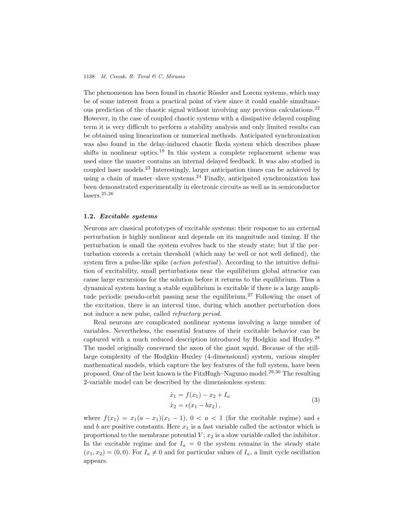
Fig. 1. Schematic presentation of the dynamics during the saddle-node bifurcation on invariantcircle.

The most important features of neuron models are that they can generate reg-ular beatings of a limit cycle nature when the applied current Ia is within anappropriate range. There are two types of bifurcations which allow the system tobe excitable and which result in a stable limit cycle when the controlled parameterchanges: saddle-node bifurcation on an invariant circle (or Andronov bifurcation)and Hopf bifurcation (or Andronov–Hopf bifurcation).31–33 Saddle-node bifurcationcan appear in any dimension (excitability requires dimensions equal or larger thantwo) and its mechanism consists of the creation and annihilation of fixed points.As a parameter of the system is varied from above to below threshold, two fixedpoints, one stable and one unstable move toward each other, collide, and mutuallyannihilate. A saddle-node bifurcation on an invariant circle appears, for example,in a model of overdamped pendulum. The dimensionless form of this model, in anoverdamped limit, is the following:

x = µ ! sin x (4)

with x = d#/dt, t = mgL/b and µ = #/mgL, where m is a mass of pendulum, L itslength, b is a viscous damping, # is a constant applied torque and # is an angularvariable. As defined above, the parameter µ is the ratio of the applied torque to themaximum gravitational torque. Since viscosity is large, the oscillations are possiblebecause of the applied torque — the energy is lost by damping and pumped byan applied torque. If µ > 1 then the applied torque can never be balanced bythe gravitational torque and the pendulum will always make an excursion over anunstable fixed point x+ = arcsinµ which is a saddle, and the flow consists of anoscillation of the variable x (limit cycle regime). This limit cycle develops througha saddle node bifurcation on an invariant circle (Andronov) at µ = ±1 (see Fig. 1),where the two fixed points collide and annihilate. In the latter case, if µ < 1, theunperturbed pendulum will never be able to reach an unstable fixed point and itwill always turn back to the stable fixed point x! = arcsinµ. Nevertheless, in thiscase the system displays an excitable behavior: if we kick the system out of its stablestate with a large enough perturbation (larger than 2|arcsinµ|), the trajectory willreturn to the initial state through a deterministic orbit that closely follows theheteroclinic connection of the saddle and the node [an orbit which connects twofixed points is called heteroclinic, while an orbit which connects a saddle point withitself is called homoclinic (see Fig. 2)]. It is worth noting that in a system with



Heteroclinic Orbit Homoclinic Orbit

Fig. 2. Schematic presentation of the heteroclinic and homoclinic orbits.

Supercritical Hopf

Subcritical Hopfµ > 0µ < 0 µ = 0

µ < 0 µ = 0 µ > 0

Fig. 3. Schematic presentation of the dynamics during the Hopf bifurcation.

a saddle-node bifurcation the key element to obtain excitability is the heteroclinicconnection between the manifolds of the fixed points. Equation (4) appears notonly in mechanics in the form of overdamped pendulum with a constant torque,but it also appears in condensed-matter physics to model dynamics of Josephsonjunctions, as well as in biology to model oscillating neurons, firefly flashing rhythmand human sleep–wake cycle. Usually this prototype equation carries the nameAdler’s equation.

Opposite to a saddle-node bifurcation, Hopf bifurcation can occur only in dimen-sionality two or higher and appears for example in the FitzHugh–Nagumo system.The Hopf bifurcation can be either supercritical or subcritical (see Fig. 3). A su-percritical Hopf bifurcation appears when a stable spiral changes into an unstablespiral surrounded by a limit cycle and is responsible for an excitable behavior of thesystem. A subcritical Hopf bifurcation is responsible for bistable behavior. Beforethe bifurcation, the system has two attractors: a stable limit cycle and a stablefixed point at the origin. Between these two attractors lies an unstable limit cycle.At the bifurcation point (µ = 0 at Fig. 3) the unstable limit cycle shrinks to theorigin, which becomes unstable, while the stable limit cycle remains but with largeramplitude of oscillations than before the bifurcation. A definition of the Hopf bifur-cation is formulated in the Hopf bifurcation theorem: a Hopf bifurcation appearsif when changing some parameter of the system we observe that both eigenvalues



(in a two-dimensional case) change from real negative to complex ones with its realparts positive. The parameter value at which the eigenvalues become complex withthe vanishing real parts corresponds to the bifurcation point.34

Excitable systems were categorized by Hodgkin according to the bifurcation typeinto two classes. Class 1 excitable systems are the ones with a saddle-node bifurca-tion on an invariant circle (for example Adler’s and Morris-Lecar systems). Class 2excitable systems are characterized by the appearance of the Hopf bifurcation, asthe previously described Hodgkin–Huxley and FitzHugh–Nagumo models.35 Thetype of bifurcation determines the neuro-computational properties of the cells. Ifin the system a saddle-node bifurcation occurs, the cell can fire all-or-none spikeswith an arbitrary low frequency, it has a well-defined threshold manifold, and itacts as an integrator: the higher the frequency of incoming pulses, the sooner itfires. On the other hand, when a Hopf bifurcation occurs in the system, the cellfires at a certain frequency range, its spikes are not all-or-none, it does not have awell-defined threshold manifold, it can fire in response to an inhibitory pulse, andit acts as a resonator: it responds preferentially to a certain (resonant) frequencyof the input.27

2. Anticipated Synchronization in Excitable Systems Drivenby Noise

2.1. Numerical results

Coupled excitable systems driven by noise in the regime of anticipated synchroniza-tion were recently studied.36,37 The following scheme with di!usive coupling wasconsidered:

x(t) = f(x(t)) + I(t)

y(t) = f(y(t)) + I(t) + K[x(t) ! y(t ! !)],(5)

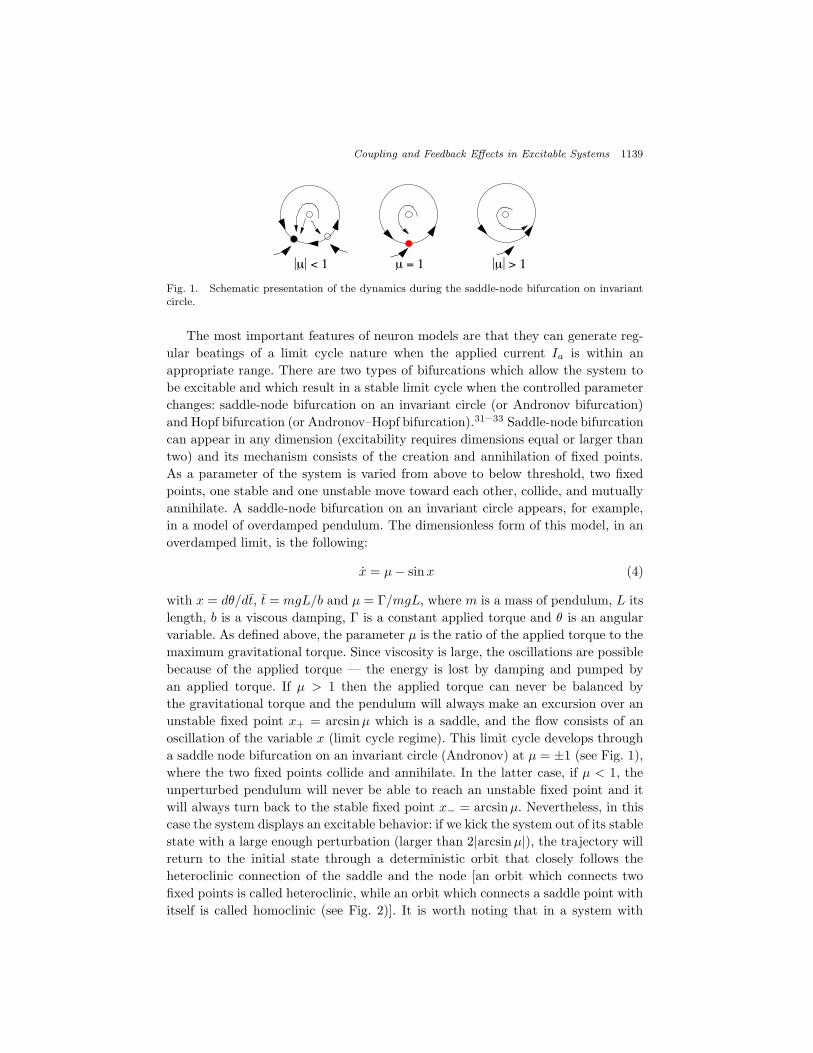
where x and y are dynamical variables, K is a positive defined matrix and I(t)represents a common external forcing. It was shown that under appropriate couplingconditions there can be a very good correlation between y(t) and x(t + !), even ifthe external forcing I(t) is a noise.36

SlaveNeuron

MasterNeuron

stimulusexternal

τ+ −feedbackdelayed

Fig. 4. Schematic diagram of two model neurons coupled in a unidirectional configuration, sub-jected to the same external forcing and with a feedback loop (with a delay time !) in the slaveneuron.



In particular, the authors studied anticipated synchronization in the FitzHugh–Nagumo and Hodgkin–Huxley neuron models (see Sec. 1.2). By coupling two ofsuch systems in an unidirectional configuration as in scheme (5), they found thatthe slave system fires the same train of spikes as the master system does, but at acertain amount of time earlier when both systems are subjected to the same externalrandom forcing. It appears that the slave can predict the response of the master.Two FitzHugh–Nagumo systems, the master x = (x1, x2) and the slave y = (y1, y2),under unidirectional coupling are, respectively (see the schematic diagram shownin Fig. 4):

x1 = !x1(x1 ! a)(x1 ! 1) ! x2 + I(t)

x2 = "(x1 ! bx2) ,(6)

andy1 = !y1(y1 ! a)(y1 ! 1) ! y2 + I(t) + K[x1(t) ! y1(t ! !)]

y2 = "(y1 ! by2) ,(7)

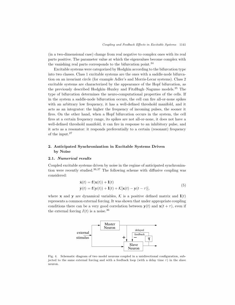
where a, b, and " are constants, K is the positive coupling strength and ! is a delaytime. Di!erent types of random external forcing I(t) (see Fig. 5) were considered.The first one, “telegraph-like noise,” corresponds to a random process whose am-plitude remains constant for a time T , switching subsequently to a new randomvalue chosen uniformly in [I0 ! D, I0 + D], where D is the noise intensity and I0

(a) (b)

(c) (d)

Fig. 5. Return map fk(t) versus fk(t " 1) for (a) white noise (k = w), (b) colored noise (k = c),(c) telegraph-like noise (k = t) and for (d) fk(t) versus fk(t"200) for telegraph-like noise (k = t).Diagrams (c) and (d) for telegraph-like noise show that it remains constant during a particularperiod of time.



(a)

(b)

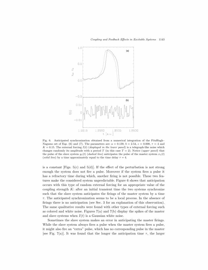
Fig. 6. Anticipated synchronization obtained from a numerical integration of the FitzHugh–Nagumo set of Eqs. (6) and (7). The parameters are: a = 0.139, b = 2.54, " = 0.008, ! = 4 andK = 0.15. The external forcing I(t) (displayed in the lower panel) is a telegraph-like noise whichchanges randomly its amplitude with a period T (in this case T = 2). Notice (upper panel) thatthe pulse of the slave system y1(t) (dashed line) anticipates the pulse of the master system x1(t)(solid line) by a time approximately equal to the time delay ! = 4.

is a constant [Figs. 5(c) and 5(d)]. If the e!ect of the perturbation is not strongenough the system does not fire a pulse. Moreover if the system fires a pulse ithas a refractory time during which, another firing is not possible. These two fea-tures make the considered system unpredictable. Figure 6 shows that anticipationoccurs with this type of random external forcing for an appropriate value of thecoupling strength K: after an initial transient time the two systems synchronizesuch that the slave system anticipates the firings of the master system by a time! . The anticipated synchronization seems to be a local process. In the absence offirings there is no anticipation (see Sec. 3 for an explanation of this observation).The same qualitative results were found with other types of external forcing suchas colored and white noise. Figures 7(a) and 7(b) display the spikes of the masterand slave systems when I(t) is a Gaussian white noise.

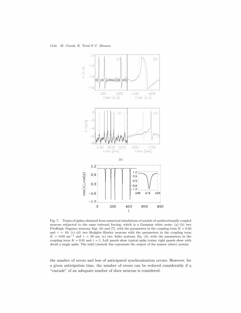
Sometimes the slave system makes an error in anticipating the master firings.While the slave system always fires a pulse when the master system fires a pulse,it might also fire an “extra” pulse, which has no corresponding pulse in the master[see Fig. 7(a)]. It was found that the longer the anticipation time ! , the larger



(e)

Fig. 7. Trains of spikes obtained from numerical simulations of models of unidirectionally coupledneurons subjected to the same external forcing, which is a Gaussian white noise: (a)–(b) twoFitzHugh–Nagumo neurons; Eqs. (6) and (7), with the parameters in the coupling term K = 0.03and ! = 10; (c)–(d) two Hodgkin–Huxley neurons with the parameters in the coupling termK = 0.03 ms"1 and ! = 50 ms; (e) two Adler systems, Eq. (4), with the parameters in thecoupling term K = 0.01 and ! = 1. Left panels show typical spike trains; right panels show withdetail a single spike. The solid (dashed) line represents the output of the master (slave) system.

the number of errors and loss of anticipated synchronization occurs. However, fora given anticipation time, the number of errors can be reduced considerably if a“cascade” of an adequate number of slave neurons is considered.



(a) (b) (c)

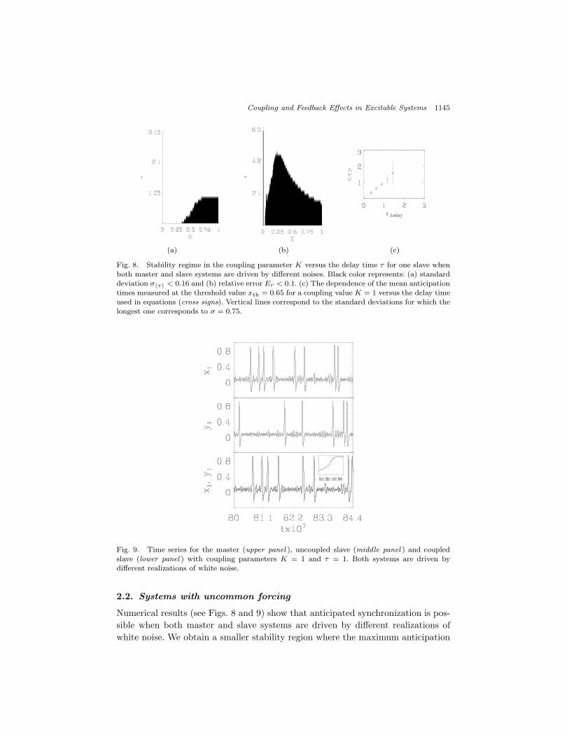
Fig. 8. Stability regime in the coupling parameter K versus the delay time ! for one slave whenboth master and slave systems are driven by di!erent noises. Black color represents: (a) standarddeviation ##!$ < 0.16 and (b) relative error Er < 0.1. (c) The dependence of the mean anticipationtimes measured at the threshold value xth = 0.65 for a coupling value K = 1 versus the delay timeused in equations (cross signs). Vertical lines correspond to the standard deviations for which thelongest one corresponds to # = 0.75.

Fig. 9. Time series for the master (upper panel ), uncoupled slave (middle panel ) and coupledslave (lower panel ) with coupling parameters K = 1 and ! = 1. Both systems are driven bydi!erent realizations of white noise.

2.2. Systems with uncommon forcing

Numerical results (see Figs. 8 and 9) show that anticipated synchronization is pos-sible when both master and slave systems are driven by di!erent realizations ofwhite noise. We obtain a smaller stability region where the maximum anticipation



time ! is shifted in the direction of larger coupling values. This result shows thateven in the presence of di!erent white noise sources in both master and slave sys-tems, a good anticipated synchronization can still be observed, although for largercoupling values. In an instability region, two types of errors are observed: additionalspikes which occur only in the slave system and the deviation of the anticipationtime when compared to the spikes from the same time series. The appearance ofadditional spikes is described by a relative error which is defined using the relativenumber of spikes in master (Nm) and slave (Ns) systems: Er = (Ns ! Nm)/Nm,while the deviation of the anticipation time is described by the standard deviationof an average anticipation time #!$: $"!#. The result shows that the anticipatedsynchronization can appear even if di!erent noises are injected into the master andslave, which is interesting from a practical point of view. In real systems, biologicalones or artificially designed ones, it is very rare to find two systems that are sub-ject to the same noise. Thus, the robustness of this phenomenon in this case couldbecome a useful feature.

2.3. Experiment

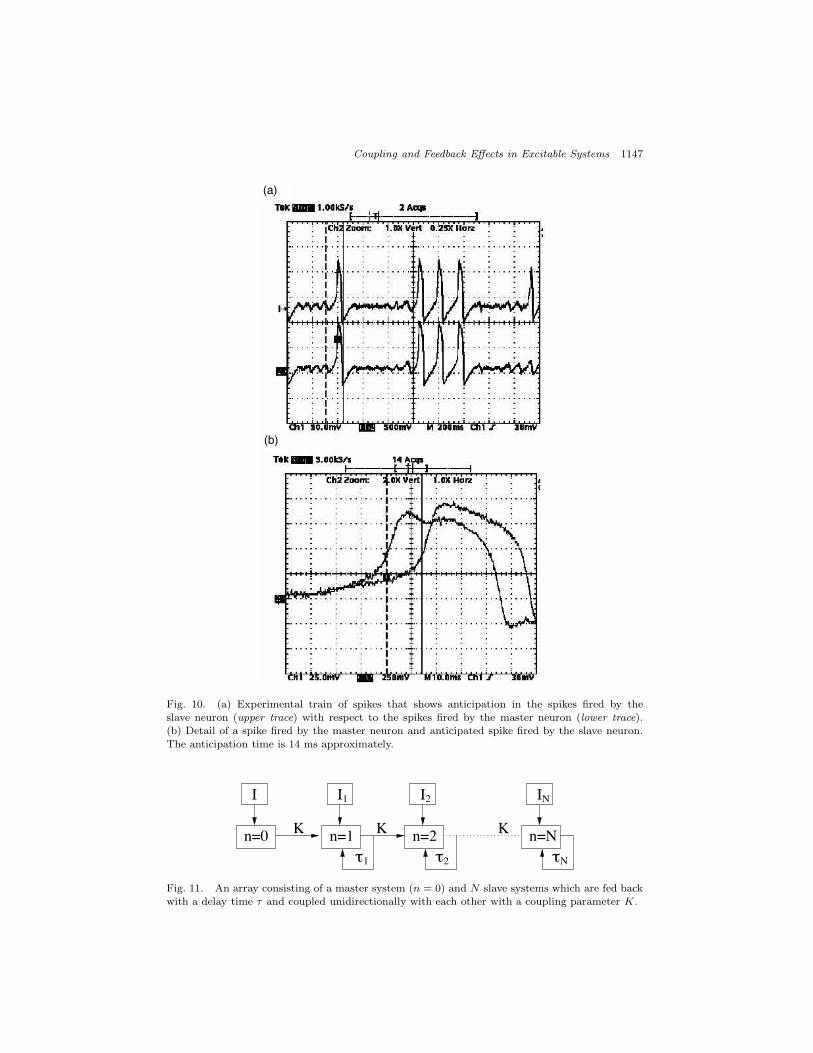
The implemented FitzHugh–Nagumo model in analog hardware was constructedwith two coupled electronic neurons. The electronic neurons were built using op-erational amplifiers and the cubic nonlinearity described by x(x ! a)(x ! 1) wasimplemented (see Ref. 36 for technical details). The electronic coupled neurons be-haved very similar to that in the numerical simulations. For an appropriate valueof the coupling resistance RC (which plays the role of a coupling constant), it wasobserved that after a transient, the master and slave electronic neurons synchronizein such a way that the slave neuron anticipates the fires of the master neuron by atime interval approximately equal to the delay time ! of the feedback mechanism.Figure 10(a) shows a typical spike train, and Fig. 10(b) displays in detail a singlespike. Without coupling and feedback (RC = RD = 0) the neurons fired pulseswhich were in general, unsynchronized (due to the mismatch between the circuits).

2.4. Cascade of neurons

In this section, we present the results of the e!ect of cascading several slaves units.For this purpose we assume an array of slave systems that are connected unidi-rectionally, as it is shown in Fig. 11, that can be described by the following set ofequations:

x = f(x) + I0(t)y1 = f(y1) + I1(t) + K(x(t) ! y1(t ! !1))

...yN = f(yN ) + IN (t) + K(yN!1(t) ! yN (t ! !N )) ,

(8)



(a)

(b)

Fig. 10. (a) Experimental train of spikes that shows anticipation in the spikes fired by theslave neuron (upper trace) with respect to the spikes fired by the master neuron (lower trace).(b) Detail of a spike fired by the master neuron and anticipated spike fired by the slave neuron.The anticipation time is 14 ms approximately.

Kn=0 n=1τ

n=NK n=2 K

τN2τ1

I I II 1 2 N

Fig. 11. An array consisting of a master system (n = 0) and N slave systems which are fed backwith a delay time ! and coupled unidirectionally with each other with a coupling parameter K.



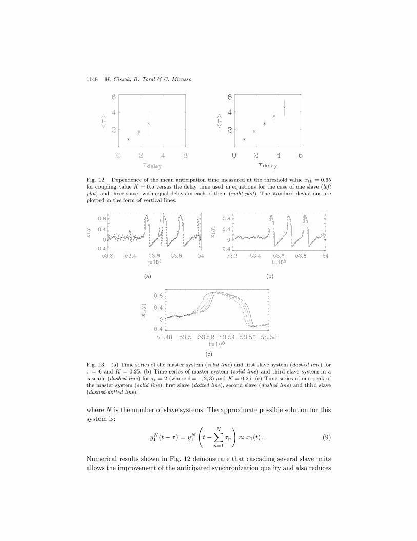
Fig. 12. Dependence of the mean anticipation time measured at the threshold value xth = 0.65for coupling value K = 0.5 versus the delay time used in equations for the case of one slave (leftplot) and three slaves with equal delays in each of them (right plot). The standard deviations areplotted in the form of vertical lines.

(a) (b)

(c)

Fig. 13. (a) Time series of the master system (solid line) and first slave system (dashed line) for! = 6 and K = 0.25. (b) Time series of master system (solid line) and third slave system in acascade (dashed line) for !i = 2 (where i = 1, 2, 3) and K = 0.25. (c) Time series of one peak ofthe master system (solid line), first slave (dotted line), second slave (dashed line) and third slave(dashed-dotted line).

where N is the number of slave systems. The approximate possible solution for thissystem is:

yN1 (t ! !) = yN

1

!t !

N"

n=1

!n

#% x1(t) . (9)

Numerical results shown in Fig. 12 demonstrate that cascading several slave unitsallows the improvement of the anticipated synchronization quality and also reduces



(a) (b) (c) (d)

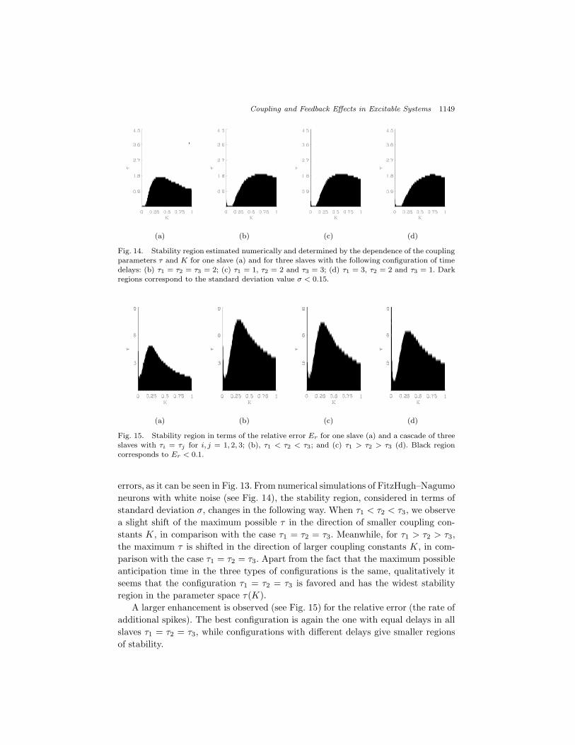
Fig. 14. Stability region estimated numerically and determined by the dependence of the couplingparameters ! and K for one slave (a) and for three slaves with the following configuration of timedelays: (b) !1 = !2 = !3 = 2; (c) !1 = 1, !2 = 2 and !3 = 3; (d) !1 = 3, !2 = 2 and !3 = 1. Darkregions correspond to the standard deviation value # < 0.15.

(a) (b) (c) (d)

Fig. 15. Stability region in terms of the relative error Er for one slave (a) and a cascade of threeslaves with !i = !j for i, j = 1, 2, 3; (b), !1 < !2 < !3; and (c) !1 > !2 > !3 (d). Black regioncorresponds to Er < 0.1.

errors, as it can be seen in Fig. 13. From numerical simulations of FitzHugh–Nagumoneurons with white noise (see Fig. 14), the stability region, considered in terms ofstandard deviation $, changes in the following way. When !1 < !2 < !3, we observea slight shift of the maximum possible ! in the direction of smaller coupling con-stants K, in comparison with the case !1 = !2 = !3. Meanwhile, for !1 > !2 > !3,the maximum ! is shifted in the direction of larger coupling constants K, in com-parison with the case !1 = !2 = !3. Apart from the fact that the maximum possibleanticipation time in the three types of configurations is the same, qualitatively itseems that the configuration !1 = !2 = !3 is favored and has the widest stabilityregion in the parameter space !(K).

A larger enhancement is observed (see Fig. 15) for the relative error (the rate ofadditional spikes). The best configuration is again the one with equal delays in allslaves !1 = !2 = !3, while configurations with di!erent delays give smaller regionsof stability.



3. Dynamical Mechanism of Anticipated Synchronization inExcitable Systems

The anticipated synchronization regime has often been described as a rather coun-terintuitive phenomenon because of the possibility of the slave system to anticipatethe unpredictable evolution of the master one.19,20,25 It was given however, a simpleexplanation for the physical mechanism behind the anticipated synchronization.38

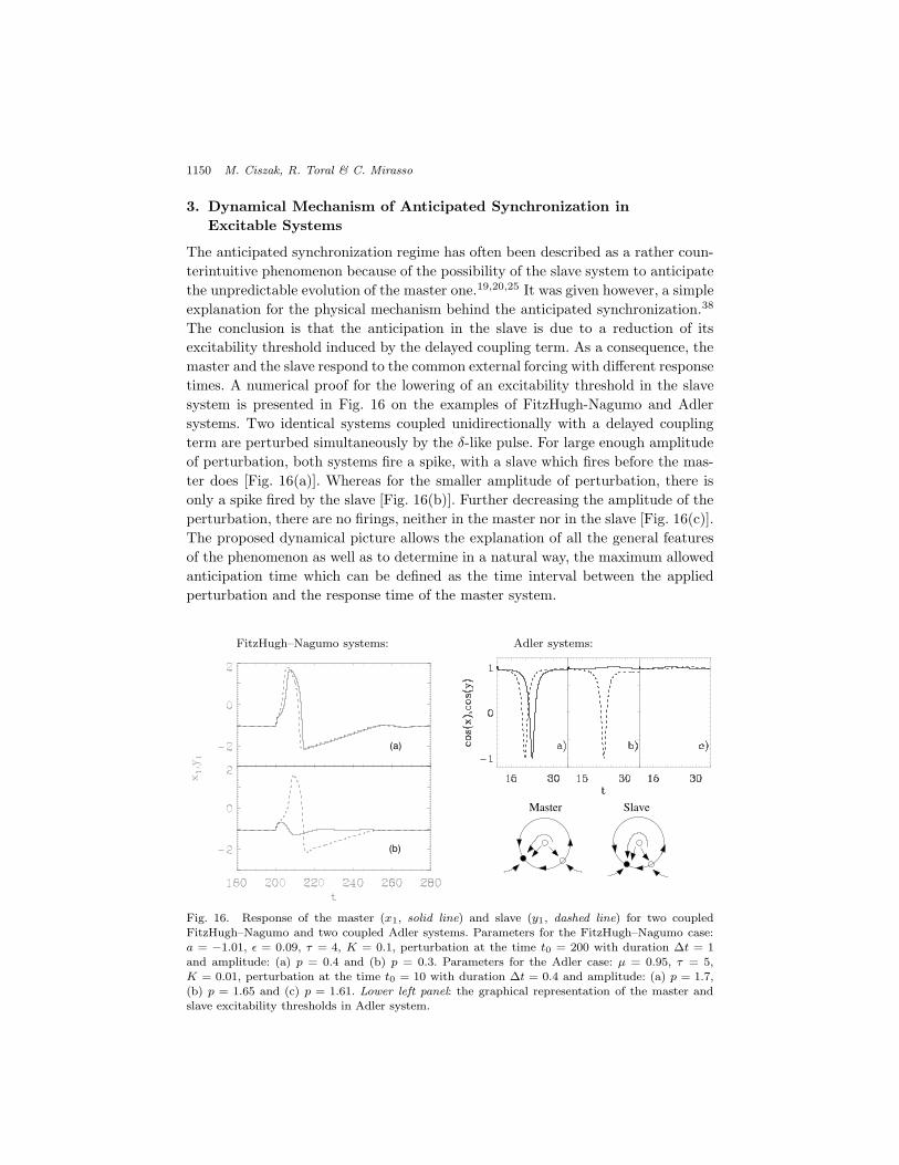
The conclusion is that the anticipation in the slave is due to a reduction of itsexcitability threshold induced by the delayed coupling term. As a consequence, themaster and the slave respond to the common external forcing with di!erent responsetimes. A numerical proof for the lowering of an excitability threshold in the slavesystem is presented in Fig. 16 on the examples of FitzHugh-Nagumo and Adlersystems. Two identical systems coupled unidirectionally with a delayed couplingterm are perturbed simultaneously by the %-like pulse. For large enough amplitudeof perturbation, both systems fire a spike, with a slave which fires before the mas-ter does [Fig. 16(a)]. Whereas for the smaller amplitude of perturbation, there isonly a spike fired by the slave [Fig. 16(b)]. Further decreasing the amplitude of theperturbation, there are no firings, neither in the master nor in the slave [Fig. 16(c)].The proposed dynamical picture allows the explanation of all the general featuresof the phenomenon as well as to determine in a natural way, the maximum allowedanticipation time which can be defined as the time interval between the appliedperturbation and the response time of the master system.

FitzHugh–Nagumo systems: Adler systems:

(a)

(b)

Master Slave

Fig. 16. Response of the master (x1, solid line) and slave (y1, dashed line) for two coupledFitzHugh–Nagumo and two coupled Adler systems. Parameters for the FitzHugh–Nagumo case:a = "1.01, " = 0.09, ! = 4, K = 0.1, perturbation at the time t0 = 200 with duration "t = 1and amplitude: (a) p = 0.4 and (b) p = 0.3. Parameters for the Adler case: µ = 0.95, ! = 5,K = 0.01, perturbation at the time t0 = 10 with duration "t = 0.4 and amplitude: (a) p = 1.7,(b) p = 1.65 and (c) p = 1.61. Lower left panel: the graphical representation of the master andslave excitability thresholds in Adler system.



4. Zero-Lag Synchronization in Real Neurons

Experiments on brain activity revealed the existence of simultaneous oscillationsin the activity of cortical areas separated by several millimeters, or even locatedin di!erent hemispheres, and between gamma oscillations (30–100 Hz) of neuronsseparated by millimeter distances.39,40 One explanation for these zero-lag correla-tions suggests that it could be simply a statistical artefact, while other explana-tions involve models for coexistence of doublet firing of single neurons which en-able coherent oscillations.41,42 Some authors suggest that the existence of zero-lagoscillations is necessary for spatiotemporal integration of the activity of the axons.43

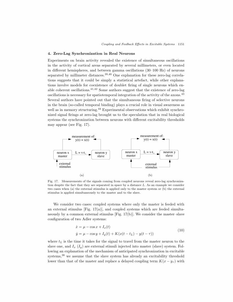
Several authors have pointed out that the simultaneous firing of selective neuronsin the brain (so-called temporal binding) plays a crucial role in visual awareness aswell as in memory structuring.44 Experimental observations which exhibit synchro-nized signal firings at zero-lag brought us to the speculation that in real biologicalsystems the synchronization between neurons with di!erent excitability thresholdsmay appear (see Fig. 17).

L = v t L.

master slaveneuron x neuron y

measurement of:y(t) = x(t)

stimulusexternal

L = v t L.

master slaveneuron x neuron y

measurement of:y(t) = x(t)

stimulusexternal

(a) (b)

Fig. 17. Measurements of the signals coming from coupled neurons reveal zero-lag synchroniza-tion despite the fact that they are separated in space by a distance L. As an example we considertwo cases when (a) the external stimulus is applied only to the master system or (b) the externalstimulus is applied simultaneously to the master and to the slave.

We consider two cases: coupled systems where only the master is feeded withan external stimulus [Fig. 17(a)], and coupled systems which are feeded simulta-neously by a common external stimulus [Fig. 17(b)]. We consider the master–slaveconfiguration of two Adler systems:

x = µ ! cosx + Ix(t)

y = µ ! cos y + Iy(t) + K(x(t ! tL) ! y(t ! !))(10)

where tL is the time it takes for the signal to travel from the master neuron to theslave one, and Ix (Iy) are external stimuli injected into master (slave) system. Fol-lowing an explanation of the mechanism of anticipated synchronization in excitablesystems,38 we assume that the slave system has already an excitability thresholdlower than that of the master and replace a delayed coupling term K(x! y! ) with



a synchronization coupling term K(x ! y). Thus we consider two coupled Adlerequations with di!erent parameter values in the master and the slave:

x = µ ! cosx + Ix(t)

y = µ$ ! cos y + Iy(t) + K(x(t ! tL) ! y(t)) .(11)

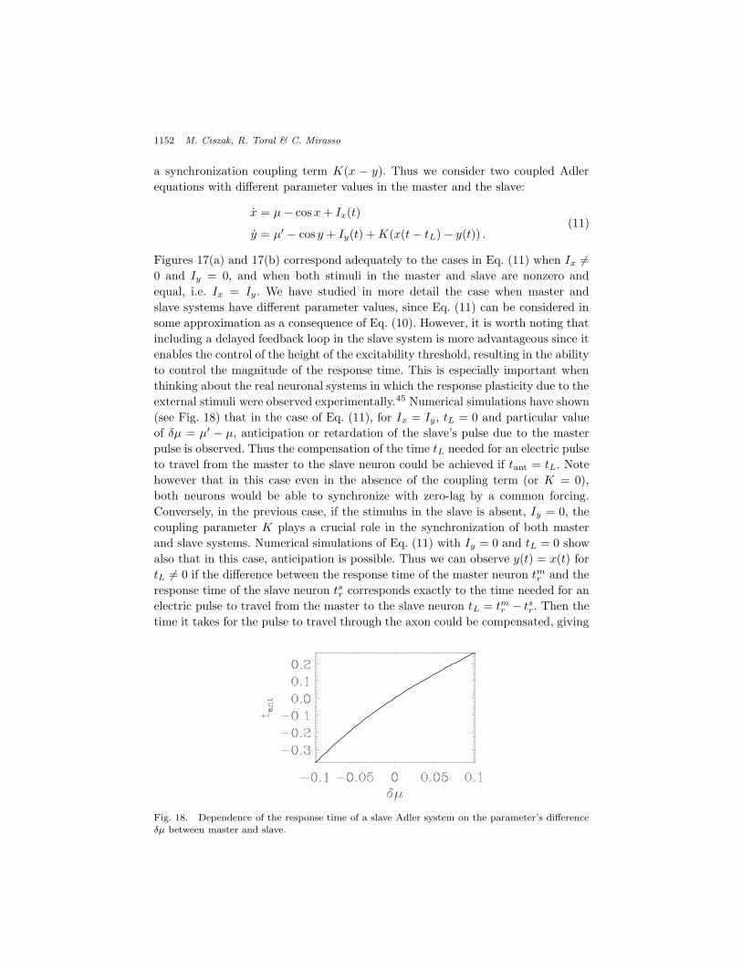
Figures 17(a) and 17(b) correspond adequately to the cases in Eq. (11) when Ix "=0 and Iy = 0, and when both stimuli in the master and slave are nonzero andequal, i.e. Ix = Iy. We have studied in more detail the case when master andslave systems have di!erent parameter values, since Eq. (11) can be considered insome approximation as a consequence of Eq. (10). However, it is worth noting thatincluding a delayed feedback loop in the slave system is more advantageous since itenables the control of the height of the excitability threshold, resulting in the abilityto control the magnitude of the response time. This is especially important whenthinking about the real neuronal systems in which the response plasticity due to theexternal stimuli were observed experimentally.45 Numerical simulations have shown(see Fig. 18) that in the case of Eq. (11), for Ix = Iy, tL = 0 and particular valueof %µ = µ$ ! µ, anticipation or retardation of the slave’s pulse due to the masterpulse is observed. Thus the compensation of the time tL needed for an electric pulseto travel from the master to the slave neuron could be achieved if tant = tL. Notehowever that in this case even in the absence of the coupling term (or K = 0),both neurons would be able to synchronize with zero-lag by a common forcing.Conversely, in the previous case, if the stimulus in the slave is absent, Iy = 0, thecoupling parameter K plays a crucial role in the synchronization of both masterand slave systems. Numerical simulations of Eq. (11) with Iy = 0 and tL = 0 showalso that in this case, anticipation is possible. Thus we can observe y(t) = x(t) fortL "= 0 if the di!erence between the response time of the master neuron tm

r and theresponse time of the slave neuron tsr corresponds exactly to the time needed for anelectric pulse to travel from the master to the slave neuron tL = tmr ! tsr. Then thetime it takes for the pulse to travel through the axon could be compensated, giving

Fig. 18. Dependence of the response time of a slave Adler system on the parameter’s di!erence$µ between master and slave.



Fig. 19. Appearance of anticipated and retarded response of a slave in Adler system, dependingon the magnitudes of coupling parameter K and di!erence $µ = µ% " µ between the parametersin the master and slave systems with µ = 0.95 in the master. The white region corresponds to:tmr " tsr < 0 (the slave responds later than the master), grey: 0.25 > tm

r " tsr > 0; and black:tmr " tsr > 0.25 (in the two last cases the slave responds faster than the master); where tm

r (tsr) isthe response time of the master (slave).

rise to a simultaneous firing of neurons. In Fig. 19 we present numerical results forthe appearance of retardation and anticipation of the slave in the parameter spaceK and %µ.

5. Conclusions

In this review we have presented results on delayed coupled equations for excitablesystems driven by a common and even uncommon external forcing, which underappropriate conditions may lead to anticipated synchronization. This happens de-spite the fact that the anticipated synchronization manifold is not a solution of theequations. The FitzHugh–Nagumo model was also implemented in analog hardware,showing that the anticipation phenomenon is very general and robust.

Two types of errors appearing only in the slave system have been observed,relative error and standard deviation of anticipation times, have been revealed tobe proportional only for small delay times, and deviations of anticipation timesappeared more often, even in the absence of additional firings. It was also shownthat the anticipated synchronization can be improved by cascading several units ofslave systems. The appearance of additional firings in the slave system and the factthat the response time of an excitable system depends on its excitability threshold(which is determined by the parameters of the system), lead to the explanationof the anticipated synchronization in excitable systems in terms of a thresholdreduction.

Finally, we have proposed a hypothesis that the phenomenon of anticipatedsynchronization might be responsible for the experimental observations of the zero-lag synchronization between spatially separated coupled neurons.

Acknowledgment

R. Toral and C. Mirasso acknowledge the project CONOCE2: FIS2004-00953.



References

1. I. I. Blekhman, Synchronization in Science and Technology (Asme Press, New York,1988).

2. S. T. Strogatz, Nonlinear Dynamics and Chaos: With Applications to Physics,Biology, Chemistry and Engineering (Addison-Wesley, 1997).

3. E. V. Appleton, Proc. Cambridge Phil. Soc. (Math. Phys. Sci.) 21 (1922) 231.4. B. van der Pol, Phil. Mag. 3 (1927) 64; A. A. Andronov and A. A. Vitt, Zhurnal

Prikladnoy Fisiki 7 (1934) 4.5. A. Pikovsky, M. Rosenblum and J. Kurths, Int. J. Bifurc. Chaos 10 (2000) 2291.6. K. M. Cuomo and A. V. Oppenheim, Phys. Rev. Lett. 71 (1993) 65.7. T. Yamada and H. Fujisaka, Prog. Theor. Phys. 70 (1983) 1240.8. T. Yamada and H. Fujisaka, Prog. Theor. Phys. 72 (1984) 885.9. V. S. Afraimovich, N. N. Verichev and M. I. Rabinovich, Inv. VUZ Rasiofiz. RPQAEC

29 (1986) 795.10. L. M. Pecora and T. L. Carroll, Phys. Rev. Lett. 64 (1990) 821.11. W. T. Co!ey, Yu P. Kalmykov and J. T. Waldron, The Langevin Equation: With

Applications in Physics, Chemistry and Electrical Engineeing (World Scientific, 1996).12. R. Ritz and T. J. Sejnowski, Curr. Opin. Neurobiol. 7 (1997) 536.13. B. Schafer, M. G. Rosenblum and J. Kurths, Nature (London) 392 (1998) 239.14. B. Blasius, A. Huppert and L. Stone, Nature (London) 399 (1999) 354.15. J. A. Freund, L. Schimansky-Geier and P. Hanggi, Chaos 13 (2003) 225.16. J. D. Murray, Mathematical Biology (Springer-Verlag, 1993).17. F. C. Hoppensteadt, Analysis and Simulation of Chaotic Systems, Applied Mathe-

matical Sciences (Springer-Verlag, 1993).18. D. Zwillinger, Handbook of Di!erential Equations (Academic Press, 1992).19. H. U. Voss, Phys. Rev. E61 (2000) 5115.20. O. Calvo, D. R. Chialvo, V. M. Eguiluz, C. Mirasso and R. Toral, Chaos 14 (2004) 1.21. C. Mirasso, E. Hernandez-Garcia and C. Masoller, Phys. Lett. A295 (2002) 39.22. H. U. Voss, Phys. Rev. Lett. 87 (2001) 014102.23. C. Masoller, Phys. Rev. Lett. 86 (2001) 2782.24. H. U. Voss, Phys. Lett. A279 (2001) 207.25. H. Voss, Int. J. Bifurc. Chaos 12 (2002) 1619.26. P. Davis, T. Aida, S. Saito, Y. Liu, Y. Takiguchi and J. M. Liu, Appl. Phys. Lett. 80

(2002) 4306.27. E. M. Izhikevich, Int. J. Bifurc. Chaos 10 (2000) 1171.28. A. L. Hodgkin and A. F. Huxley, J. Physiol. (London) 117 (1952) 500.29. R. FitzHugh, Biophys. J. 1 (1961) 445.30. J. S. Nagumo, S. Arimoto and S. Yoshizawa, Proc. IRE 50 (1962) 2061.31. A. A. Andronov, E. A. Leontovich, I. I. Gordon and A. G. Maier, Qualitative Theory

of Second-Order Dynamic Systems (Wiley, New York, 1973).32. P. Coullet, T. Frisch, J. M. Gilli and S. Rica, Chaos 4 (1994) 485.33. E. A. Jackson, Perspectives of Nonlinear Dynamics, Vol. 1 (Cambridge University

Press, 1989).34. J. Marsden and M. MacCracken, The Hopf Bifurcation and its Applications (Springer-

Verlag, 1976).35. A. L. Hodgkin, J. Physiol. 107 (1948) 165.36. M. Ciszak, O. Calvo, C. Massoler, C. Mirasso and R. Toral, Phys. Rev. Lett. 90 (2003)

204102.37. R. Toral, C. Massoler, C. Mirasso, M. Ciszak and O. Calvo, Physica A325 (2003)

192.

https://www.researchgate.net/publication/243773399_Nonlinear_Dynamics_and_Chaos_With_Applications_to_Physics?el=1_x_8&enrichId=rgreq-a0f9a654979acf0ae46bf66ec662e7f8-XXX&enrichSource=Y292ZXJQYWdlOzM5NDAyNTQ1O0FTOjk5NjU3NTM5NjUzNjM4QDE0MDA3NzE2MTc0NjQ=

https://www.researchgate.net/publication/243773399_Nonlinear_Dynamics_and_Chaos_With_Applications_to_Physics?el=1_x_8&enrichId=rgreq-a0f9a654979acf0ae46bf66ec662e7f8-XXX&enrichSource=Y292ZXJQYWdlOzM5NDAyNTQ1O0FTOjk5NjU3NTM5NjUzNjM4QDE0MDA3NzE2MTc0NjQ=

https://www.researchgate.net/publication/258982794_A_Handbook_of_Differential_Equations?el=1_x_8&enrichId=rgreq-a0f9a654979acf0ae46bf66ec662e7f8-XXX&enrichSource=Y292ZXJQYWdlOzM5NDAyNTQ1O0FTOjk5NjU3NTM5NjUzNjM4QDE0MDA3NzE2MTc0NjQ=

https://www.researchgate.net/publication/242444676_Qualitative_Theory_of_Second_Order_Dynamic_Systems?el=1_x_8&enrichId=rgreq-a0f9a654979acf0ae46bf66ec662e7f8-XXX&enrichSource=Y292ZXJQYWdlOzM5NDAyNTQ1O0FTOjk5NjU3NTM5NjUzNjM4QDE0MDA3NzE2MTc0NjQ=

https://www.researchgate.net/publication/242444676_Qualitative_Theory_of_Second_Order_Dynamic_Systems?el=1_x_8&enrichId=rgreq-a0f9a654979acf0ae46bf66ec662e7f8-XXX&enrichSource=Y292ZXJQYWdlOzM5NDAyNTQ1O0FTOjk5NjU3NTM5NjUzNjM4QDE0MDA3NzE2MTc0NjQ=

https://www.researchgate.net/publication/256492627_Synchronization_in_Science_and_Technology?el=1_x_8&enrichId=rgreq-a0f9a654979acf0ae46bf66ec662e7f8-XXX&enrichSource=Y292ZXJQYWdlOzM5NDAyNTQ1O0FTOjk5NjU3NTM5NjUzNjM4QDE0MDA3NzE2MTc0NjQ=

https://www.researchgate.net/publication/256492627_Synchronization_in_Science_and_Technology?el=1_x_8&enrichId=rgreq-a0f9a654979acf0ae46bf66ec662e7f8-XXX&enrichSource=Y292ZXJQYWdlOzM5NDAyNTQ1O0FTOjk5NjU3NTM5NjUzNjM4QDE0MDA3NzE2MTc0NjQ=

https://www.researchgate.net/publication/224043955_The_Hopf_Bifurcation_and_Its_Applications?el=1_x_8&enrichId=rgreq-a0f9a654979acf0ae46bf66ec662e7f8-XXX&enrichSource=Y292ZXJQYWdlOzM5NDAyNTQ1O0FTOjk5NjU3NTM5NjUzNjM4QDE0MDA3NzE2MTc0NjQ=

https://www.researchgate.net/publication/224043955_The_Hopf_Bifurcation_and_Its_Applications?el=1_x_8&enrichId=rgreq-a0f9a654979acf0ae46bf66ec662e7f8-XXX&enrichSource=Y292ZXJQYWdlOzM5NDAyNTQ1O0FTOjk5NjU3NTM5NjUzNjM4QDE0MDA3NzE2MTc0NjQ=

https://www.researchgate.net/publication/265371746_Analysis_and_simulation_of_chaotic_systems_2nd_ed?el=1_x_8&enrichId=rgreq-a0f9a654979acf0ae46bf66ec662e7f8-XXX&enrichSource=Y292ZXJQYWdlOzM5NDAyNTQ1O0FTOjk5NjU3NTM5NjUzNjM4QDE0MDA3NzE2MTc0NjQ=

https://www.researchgate.net/publication/265371746_Analysis_and_simulation_of_chaotic_systems_2nd_ed?el=1_x_8&enrichId=rgreq-a0f9a654979acf0ae46bf66ec662e7f8-XXX&enrichSource=Y292ZXJQYWdlOzM5NDAyNTQ1O0FTOjk5NjU3NTM5NjUzNjM4QDE0MDA3NzE2MTc0NjQ=



38. M. Ciszak, F. Marino, R. Toral and S. Balle, Phys. Rev. Lett. 93 (2004) 114102.39. P. Konig, W. Singer, A. K. Engel and A. K. Kreiter, Proc. Natl. Acad. Sci. USA 88

(1991) 6048.40. P. Konig, W. Singer, P. R. Roelfsema and A. K. Engel, Nature 385 (1997) 157.41. W. J. Freeman, Int. J. Bifurc. Chaos 10 (2000) 2307.42. I. M. Stanford, J. G. R. Je!erys, R. D. Traub and M. A. Whittington, Nature 383

(1996) 421.43. J. M. Barrie and W. J. Freeman, J. Neurophysiol. 84 (2000) 1266.44. Ch. Koch and F. Crick, Sci. Am. 12 (August 2002), p. 11.45. V. Dragoi, J. Sharma and M. Sur, IETE J. Research 49 (2003) 2.

COUPLING AND FEEDBACK EFFECTS IN EXCITABLE SYSTEMS: ANTICIPATED SYNCHRONIZATION

Documents

Transcript of COUPLING AND FEEDBACK EFFECTS IN EXCITABLE SYSTEMS: ANTICIPATED SYNCHRONIZATION