Synchronization Protocols in Distributed Real-Time Systems

Jun Sun Jane LiuDepartment of Computer Science,

University of Illinois, Urbana-ChampaignUrbana, IL 61801fjsun, janeliug@cs.uiuc.edu

Abstract

In many distributed real-time systems, the workload can be modeled as a set of periodic tasks, each of which consists of a

chain of subtasks executing on different processors. Synchronization protocols are used to govern the release of subtasks so

that the precedence constraints among subtasks are satisfied and the schedulabilityof the resultant system is analyzable. When

different protocols are used , tasks can have different worst-case and average end-to-end response times. This paper focuses

on distributed real-time systems that contain independent, periodic tasks scheduled by fixed-priority scheduling algorithms.

It describes three synchronization protocols together with algorithms to analyze the schedulability of the system when these

protocols are used. Simulation was conducted to compare the performance of these protocols with respect to the worst-case

and average case end-to-end response times. The simulation experiment and the performance of the protocols are described.

1 Introduction

In many real-time systems, the workload can be modeled as a set of periodic tasks [1]. Each periodic task is an infinite

stream of execution requests that are released (i.e., made) at a fixed maximum rate. We call each request an instance of the

task. When the context is clear, we may simply say “a task” to mean an instance of that task. Each task is typically constrained

by a relative deadline, which is the maximum allowed response time of each task instance. A real-time system is said to be

schedulable if the worst-case response time of every task in the system is no longer than its relative deadline.

It is well known that fixed priority scheduling is an effective means to schedule periodic tasks on a single processor and

1

to ensure that the time constraints of the tasks are satisfied [1, 2, 3, 4]. According to this approach, each task is assigned a

fixed priority (i.e., all instances of the task have the same priority). At any time, the scheduler simply chooses to run the task

with the highest priority among all the tasks whose instances are released but not yet completed. A great deal of work has

been done on how to assign the priorities [1, 5, 6] and how to bound the response times of tasks [1, 7, 2] for single processor

systems.

In a distributed real-time system, each instance of a task may need to execute on different processors in order. An example

is a monitor task that collects remote sensor data and displays the data on the local screen. We will refer to this example as

Example 1 in later discussion. Three steps are involved in the monitor task: sampling the sensor reading on the field processor,

transmitting the sample data over the communication link1 and displaying the data on the local screen. Here we call each step

a subtask of the monitor task, and the task is the parent task of the subtasks. Subtasks that have the same parent task are sibling

subtasks of each other. In this example, the monitor task is a chain of three subtasks, sample, transfer and display, executing

sequentially on three different processors.

We say that a task in a distributed system is periodic if its first subtask is released periodically. Whether or not the later

subtasks on the chain are released periodically depends on the synchronization protocol used in the system. A synchroniza-

tion protocol governs how subtasks are released so that their precedence constraints are satisfied and the schedulability of the

resultant system is analyzable. The relative deadline of a task that consists of a chain of subtasks is the maximum allowed

length of time from the release of an instance of its first subtask till the completion of the corresponding instance of its last

subtask. The relative deadline of the task is often called the end-to-end relative deadline, or simply the end-to-end deadline,

and its response time is called the end-to-end response time. We will abbreviate the latter as the EER time in our discussion.

We confine our attention to systems that contain independent, preemptable periodic tasks and are scheduled on a fixed

priority basis. In such a system, each subtask has a fixed priority, which may or may not be the same as the priorities of its

sibling subtasks. We are not concerned with the problem of how to assign priorities to subtasks. Rather, we assume that the

priorities of subtasks on each processor have been assigned according to some priority assignment algorithm (e.g., one of the

known algorithms in [8, 9, 10]).

In this paper, we focus on various ways to synchronize the execution of sibling subtasks on different processors. Specific-

ally, we describe three synchronization protocols. The first protocol is a straightforward implementation to enforce the preced-1In many cases, the communication links can be modeled as processors, and consequently message transmissions can be modeled as communication taskson the “link” processors.

2

ence constraints among subtasks. The second protocol is an extension to the one proposed by Bettati, which was designed for

flow-shop systems [11]. This protocol has certain limitations. The third protocol combines the strengths of the previous two

protocols while avoiding their shortcomings. We measure the performance of these protocols according to two performance

criteria, the estimated worst-case and average EER times of tasks, and compare the performance of these protocols based on

these two criteria.

The synchronization problem studied in this paper resembles the problem of jitter and rate control of real-time traffic in

ATM networks. (An overview of the latter can be found in [12].) Indeed, one of the protocols described here is similar to the

method used in the jitter-EDD algorithm [13] for shaping inter-arrival patterns of packets. Packet transmissions at each switch

(in our terminology, subtasks on the “switch” processor) are scheduled on the earliest-deadline-first (i.e., dynamic priority)

basis. By contrast, our focus is on fixed priority systems. Furthermore, we provide schedulability analysis algorithms to bound

the worst-case EER times.

Harbour et al. studied a similar problem in [14]. In their model, each task is periodic and consists of a chain of subtasks.

Subtasks are assigned fixed priorities and scheduled on the fixed-priority basis. The only difference from our model is that all

tasks execute on a single processor. Each subtask starts to execute as soon as its predecessor completes, and the synchroniza-

tion of subtask execution is not concerned. Their paper focuses on the algorithm that analyzes the worst-case response times

of tasks. As we will see shortly, when the system has more than one processors and subtasks execute on different processors,

synchronizing the execution of sibling subtasks becomes the deciding issue. Different synchronization protocols not only lead

to different performance, but also require different algorithms to analyze the worst-case EER times.

The rest of the paper is organized as follows. Section 2 formally presents the synchronization problem addressed in this

paper and defines the criteria used to measure the performance of synchronization protocols. Section 3 describes three syn-

chronization protocols in detail. Schedulability analysis algorithms for these protocols are described in Section 4. Section 5

compares the performance of the synchronization protocols, and Section 6 concludes the paper.

2. The Problem Formulation

We consider here a distributed real-time system that consists of a set fPig of processors and a set fTig of independent, pree-

mptable tasks. Each processor has its own scheduler, and schedulers on different processors coordinate with each other accord-

ing to one of the synchronization protocols described here. Each taskTi consists of a chain of ni subtasks, Ti;1; Ti;2; : : : ; Ti;ni,3

sample transfer display

field processor "link" processor central processor

T1

T1,1

P1

T1,2

2P

1,3T

3P

Figure 1. Example 1 - The Monitor Task with Its Three Subtasks

and subtasks can execute on different processors. The execution time of each subtask Ti;j is �i;j . The scheduler on each pro-

cessor uses a fixed priority scheduling algorithm to schedule subtasks on the processor. The priority of Ti;j is �i;j.Each task Ti is a periodic task, i.e., instances of Ti;1 are released periodically. The period pi of Ti is the minimum inter-

release time of instances of Ti;1. The phase of Ti, denoted by fi, is the release time of the first instance of its first subtaskTi;1. Depending on the particular synchronization protocol used in the system, instances of a later subtask Ti;j (j > 1) may

or may not be released periodically. For the sake of discussion, we define the period of a subtask to be equal to the period of

its parent task, even if the subtask is not released periodically.

In this paper, we do not explicitly model inter-processor communication, and assume that the cost of inter-processor com-

munication required to synchronize subtasks on different processors is zero. This assumption is not as restrictive as it seems.

In some cases, such as in CAN [15], where message transmissions are prioritized, communication links can be modeled as

processors, and message transmissions can be modeled as communication subtasks on “link” processors. In some other cases,

such as when dedicated communication links are used, the links can be modeled as resources, and message transmissions can

be either modeled as critical sections or taken into account as blocking times of the sending subtasks. For this reason, our

model remains applicable even when the communication overhead is not neglectable. As an example, suppose that the com-

munication link in Example 1 can be modeled as a “link” processor. The monitor task, T1, is then modeled as a parent task

of three subtasks executing on three different processors, as shown in Figure 1. The cost of communication between the pro-

cessors is zero.

To illustrate the problem dealt with by a synchronization protocol, we consider a second example, Example 2, shown in

Figure 2, where the system consists of two processors, P1 and P2, and three periodic tasks, T1, T2 and T3. Task T1 and T3have only one subtask. (We use T1 and T3 to refer to the subtasks also.) T2 has two subtasks, T2;1 and T2;2. The period and

the execution time of each subtask are given by the 2-tuple in the rectangular box representing the subtask: the first number

4

P2

(6,2) (6,3)

(6,2)(4,2)T

1

T2

T3

T2,2

T2

T2,1

P1

Figure 2. Example 2 - Illustration of the Synchronization Protocol Problem

in the 2-tuple gives the period, and the second one gives the execution time. The phases of T1 and T2 are zero, and the phase

of T3 is 4. On processor P1, T1 has a higher priority than T2;1, and on processor P2, T2;2 has a higher priority than T3. The

relative deadline of each task is equal to its period.

Figure 3 shows the schedules on the two processors for the first 10 time units. In this schedule, each instance of T2;2 is

released on P2 as soon as the corresponding instance of T2;1 completes on P1. This is achieved by a synchronization signal

sent from P1 to P2 whenever an instance of T2;1 completes. (The synchronization signal is represented by a dotted arrow in

the figure.) As a matter of fact, this scheme is the first synchronization protocol described in the next section. We notice that,

although subtask T2;1 is released periodically, T2;2 is not. It is easy to verify that the instances of T2;2 are released at times 4,

8, 16, 20, 28, : : : . The first instance of T3 is preempted by the first and the second instance of T2;2. As a result, this instance ofT3 misses its deadline at time 10. On the other hand, if T2;2 were released periodically every 6 time units, each instance of T3would be preempted at most by one instance of T2;2, because T2 and T3 have the same period. Task T3 would have a worst-

case response time of 5 time units and would never miss a deadline. As we shall see later, other synchronization protocols

achieve this result by controlling the releases of T2;2. Different protocols have the different impact on the worst-case EER

times of tasks, which in turn translates to different upper bounds on the EER times of tasks.

In next section, we will describe three synchronization protocols. Their performance will be measured according to the

following three criteria.

Implementation complexity and run-time overhead : We look for protocols that are easy to implement and have low run-

time overheads.

Average EER times of tasks : For many applications, especially interactive applications, it is important for the average

EER times of tasks to be as short as possible.

5

5 10

misses its deadline

phase = 4T

3

T2,2

T2,1

T1

2

1

T ’s3

T3

on P

on P

Figure 3. The Schedule of Example 2 Using the DS Protocol

Estimated worst-case EER times of tasks : For each protocol, we apply the best known schedulability analysis algorithm

to obtain an upper bound on the EER time of each task and use the upper bound as an estimate of the worse-case EER

time of the task.

The estimated worst-case EER time of a task may be larger than the actual worst-case EER time since existingschedulability

analysis algorithms do not yield tight bounds on the EER times in general. The actual worst-case EER times of tasks can be

found only via exhaustive search, which is too time consuming to be practical even for small systems. Consequently, it is a

common practice to determine the schedulability of a real-time system based on upper bounds of response times computed

from the best known schedulability analysis algorithms (i.e., the algorithms that yields the tightest upper bounds). For this

reason, we compare the protocols proposed here according to the tightest upper bounds of EER times found for the protocols.

In subsequent discussion we will use the terms, the estimated worst-case EER time or the upper bound of the EER time of a

task, interchangeably.

Sometimes applications also require small output jitters. The output jitter is the difference in the EER times of two con-

secutive task instances. We will see in subsequent sections that one of the protocols proposed here can keep output jitters of

all tasks small.

6

3 The Synchronization Protocols

We call the synchronization protocol that leads to the schedule in Figure 3 the Direct Synchronization protocol, abbreviated

as the DS protocol. Again, according to this protocol, when an instance of a subtask completes, a synchronization signal is

sent by the scheduler on the processor where subtask executes to the scheduler of the processor where its immediate successor

executes. Upon the receipt of the synchronization signal, the latter releases an instance of the immediate successor immedi-

ately. The DS protocol is obviously easy to implement and has the minimum necessary run-time overhead. It is also expected

to yield relatively short average EER times because instances of later subtasks are released as soon as possible. However, the

performance of this protocol is poor when measured in terms of the estimated worst-case EER times. Upper bounds of the

EER times of tasks can be computed by the iterative algorithm described in Section 4. This is the only known algorithm that

provides reasonably tight bounds on the EER times of tasks under this protocol. As we will see later, when the subtask chains

are long and the processor utilizations are high, the algorithm may fail to obtain finite bounds. In cases when we do obtain

finite bounds, they are considerably larger than those yielded by other protocols.

The Phase Modification protocol and the Release Guard protocol are two alternative ways to control the release of successor

subtasks. By ensuring that instances of each subtask are not released too soon, they attempt to improve the schedulability of

the tasks at the expense of their average EER times.3.1 The Phase Modi�cation (PM) ProtocolThe Phase Modification protocol, abbreviated as the PM protocol, was initially proposed by Bettati and used to schedule

periodic flow-shop tasks [11]. Unlike the DS protocol, the PM protocol insists that instances of all subtasks of each task are

released periodicallyaccording to the period of the task. To ensure that the precedence constraints among subtasks are satisfied,

each subtask is given its own phase. The phases of subtasks are properly adjusted as follows. Let Ri;j denote an upper bound

on the response time of subtask Ti;j. The phase of the first subtask, fi;1, is the same as the phase of the parent task Ti. For a

later subtask Ti;j (j > 1), its phase is delayed to (fi;1 +Pj�1k=1Ri;k), namely, the phase of its parent task plus the sum of the

upper bounds on the response times of its predecessors. Clearly, if the clocks in the system are synchronized, whenever an

instance of a subtask is released, the corresponding instance of its immediate predecessor must have completed. The schedule

shown in Figure 4 illustrates the application of the PM protocol to taskT1 in Figure 1. The subtasks are synchronized according

to the PM protocol. We let the phase of task T1 be 0. Hence, the phase of T1;1 is also 0. The phases of T1;2 and T1;3 are set to

7

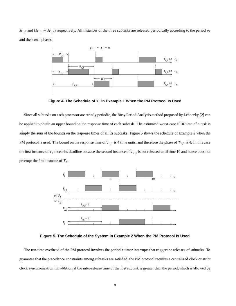
R1;1 and (R1;1 + R1;2) respectively. All instances of the three subtasks are released periodically according to the period p1and their own phases.

1,2R

= = 0

on

on

on

R1,1

1,1f

1f

1,2f

1,3f

1,3R

1,3T

1,2T

1,1T

1P

2

3P

P

Figure 4. The Schedule of T1 in Example 1 When the PM Protocol Is Used

Since all subtasks on each processor are strictly periodic, the Busy Period Analysis method proposed by Lehoczky [2] can

be applied to obtain an upper bound on the response time of each subtask. The estimated worst-case EER time of a task is

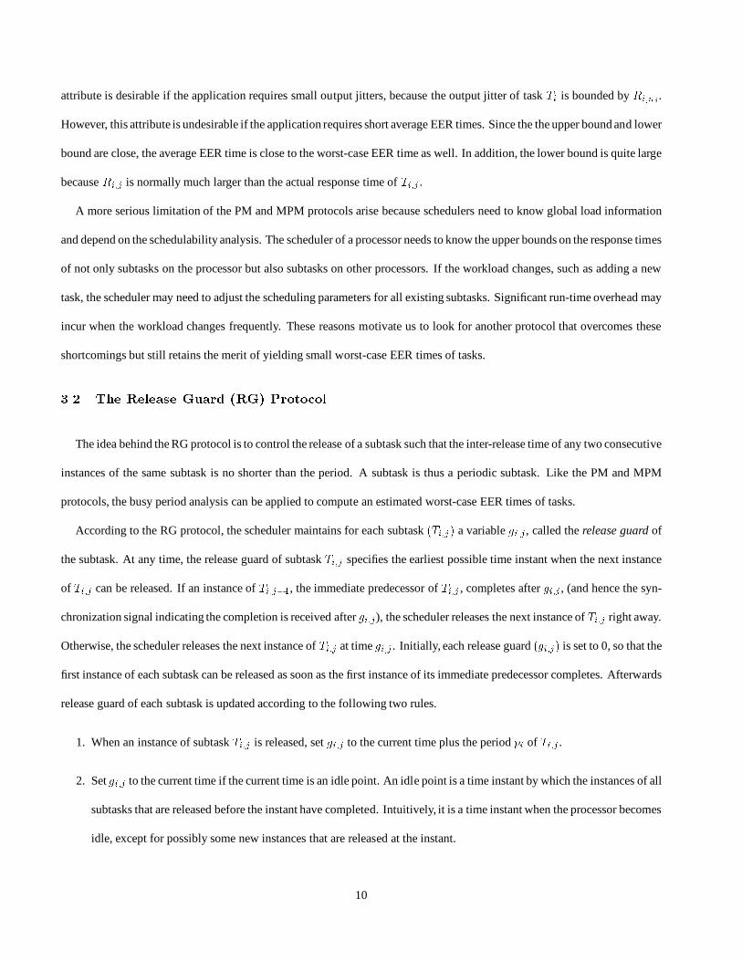
simply the sum of the bounds on the response times of all its subtasks. Figure 5 shows the schedule of Example 2 when the

PM protocol is used. The bound on the response time of T2;1 is 4 time units, and therefore the phase of T2;2 is 4. In this case

the first instance of T3 meets its deadline because the second instance of T2;2 is not released until time 10 and hence does not

preempt the first instance of T3.

5 10

T2,1

T2,2

T3

f3,1

= 4

f2,2

= 4

on P1

on P2

T1

Figure 5. The Schedule of the System in Example 2 When the PM Protocol Is Used

The run-time overhead of the PM protocol involves the periodic timer interrupts that trigger the releases of subtasks. To

guarantee that the precedence constraints among subtasks are satisfied, the PM protocol requires a centralized clock or strict

clock synchronization. In addition, if the inter-release time of the first subtask is greater than the period, which is allowed by

8

the periodic task model, the protocol does not work correctly because the precedence constraints can be violated. This severely

limits the scope of application where the PM protocol can be applied. A modified version of the protocol, called the Modified

Phase Modification protocol or the MPM protocol, overcomes these shortcomings at a slightly higher run-time expense.

We notice that as long as the interval between the releases of Ti;j and Ti;j+1 is equal to Ri;j, the precedence constraint

between these two sibling subtasks is preserved. To ensure that the interval between the release of Ti;j and Ti;j+1 is equal toRi;j, the MPM protocol employs both a timer interrupt and a synchronization interrupt. When an instance of Ti;j is released at

time t on processor Pk, the scheduler on Pk sets a timer interrupt at time t+Ri;j. When the timer interrupt occurs, the instance

of Ti;j should have completed, sinceRi;j is an upper bound on the response time of Ti;j . (This timer interrupt can also be used

to check if the subtask overruns.) The scheduler then sends a synchronization signal to the processor where Ti;j+1 executes.

Like the DS protocol, the scheduler of the processor on which Ti;j+1 executes releases an instance of Ti;j+1 immediately upon

receipt of such a signal.

It is easy to verify that under the ideal conditions, i.e., clocks are synchronized and the first subtasks being strictly periodic,

the PM protocol and the MPM protocol produce identical schedules. However, the MPM protocol achieves this without re-

quiring global clock synchronization and strictly periodic release of first subtasks. Hence, it is applicable to applications that

do not have these ideal conditions. Figure 6 illustrates the application of the MPM protocol to task T1 in Figure 1. In the figure,

there are several places where the response time of a subtask instance is shorter than the upper bound and the synchronization

signal is sent later when the timer interrupt occurs. The resultant schedule is the same as the one in Figure 4.

R1,2

R1,1

R1,3

: delay in sending synchronization signals

T1,1

P1

on

P2

T1,2

on

P3

T1,3

on

Figure 6. The Schedule of Task T1 in Example 1 When the MPM Protocol Is Used

According to the PM protocol and the MPM protocol, each instance of subtask Ti;j is released Ri;j�1 time units after the

corresponding instance of subtask Ti;j�1 is released, no matter how soon Ti;j�1 might actually complete. A simple induction

gives that the EER time of a task Ti is upper bounded by (Pnik=1Ri;k) and lower bounded by (Pni�1k=1 Ri;k + �i;ni). This

9

attribute is desirable if the application requires small output jitters, because the output jitter of task Ti is bounded by Ri;ni.However, this attribute is undesirable if the application requires short average EER times. Since the the upper bound and lower

bound are close, the average EER time is close to the worst-case EER time as well. In addition, the lower bound is quite large

because Ri;j is normally much larger than the actual response time of Ti;j .

A more serious limitation of the PM and MPM protocols arise because schedulers need to know global load information

and depend on the schedulability analysis. The scheduler of a processor needs to know the upper bounds on the response times

of not only subtasks on the processor but also subtasks on other processors. If the workload changes, such as adding a new

task, the scheduler may need to adjust the scheduling parameters for all existing subtasks. Significant run-time overhead may

incur when the workload changes frequently. These reasons motivate us to look for another protocol that overcomes these

shortcomings but still retains the merit of yielding small worst-case EER times of tasks.3.2 The Release Guard (RG) ProtocolThe idea behind the RG protocol is to control the release of a subtask such that the inter-release time of any two consecutive

instances of the same subtask is no shorter than the period. A subtask is thus a periodic subtask. Like the PM and MPM

protocols, the busy period analysis can be applied to compute an estimated worst-case EER times of tasks.

According to the RG protocol, the scheduler maintains for each subtask (Ti;j) a variable gi;j, called the release guard of

the subtask. At any time, the release guard of subtask Ti;j specifies the earliest possible time instant when the next instance

of Ti;j can be released. If an instance of Ti;j�1, the immediate predecessor of Ti;j , completes after gi;j, (and hence the syn-

chronization signal indicating the completion is received after gi;j), the scheduler releases the next instance of Ti;j right away.

Otherwise, the scheduler releases the next instance of Ti;j at time gi;j. Initially, each release guard (gi;j) is set to 0, so that the

first instance of each subtask can be released as soon as the first instance of its immediate predecessor completes. Afterwards

release guard of each subtask is updated according to the following two rules.

1. When an instance of subtask Ti;j is released, set gi;j to the current time plus the period pi of Ti;j .

2. Set gi;j to the current time if the current time is an idle point. An idle point is a time instant by which the instances of all

subtasks that are released before the instant have completed. Intuitively, it is a time instant when the processor becomes

idle, except for possibly some new instances that are released at the instant.

10

Figure 7 shows the schedule of Example 2 if we use the RG protocol. The schedule is similar to the schedule produced by

the DS protocol up until when the second instance of T2;1 completes at time 8. We notice that the second instance of T2;2 is

not released when the synchronization signal reaches P2 at time 8, because the release guard g2;2 of T2;2 is equal to 10, which

is set at time 4 when the first instance of T2;2 is released. Thus we would expect that the second instance of T2;2 will not be

released till time 10. This gives T3 a chance to complete by time 9 and meets its deadline. As T3 completes, time 9 becomes

an idle point on processor P2, and g2;2 gets updated to the current time according to the second rule of updating the release

guard. As a result, the second instance of T2;2 is released at time 9. As we will see later in Section 4, such an early release

does not lengthen to the worst-case response times of other subtasks.

f3,1

= 4T

3

T2,2

T2,1

T1

on P1

on P2

5 10

Figure 7. The Schedule of the Second Example in Figure 3 When the RG Protocol Is Used

Compared with the schedule produced by the DS protocol in Figure 3, Figure 7 is different in that T3 meets it deadline. As

a matter of fact, as we will show in the next two sections, the RG protocol yields the same estimated worst-case EER times

as the PM and MPM protocols, which are much shorter than those yielded by the DS protocol.

Comparing with the schedule in Figure 5 produced by the PM and MPM protocols, we see that according to the schedule in

Figure 7 the EER time of the second instance of T2 is 1 time unit shorter. In general, the RG protocol is expected to yield shorter

average EER times than the PM and MPM protocols. To see why, suppose that we were to apply only rule (1) of updating the

release guard. It easy to see that the EER time of a task would monotonically increase with time, until it eventually reaches

the actual worst-case EER time. Because existing schedulability analysis algorithms are not optimal, the actual worst-case

EER time is typically much smaller than the estimated worst-case EER time computed by a schedulability analysis algorithm.

Since the average EER times yielded by the PM and MPM protocols are close to the estimated worst-case EER times, the

11

RG protocol could thus yield shorter average task EER times even with rule (1) alone. Rule (2) further reduces the average

EER time because the release guard of a subtask can be set to an earlier time instant and hence causes an earlier release of

an instance of that subtask. In Section 5, we will present the simulation results that quantify their performance difference in

average EER times of tasks.

In addition to the above merits, the RG protocol does not require global load information, and, when the workload changes,

it does not need to know schedulability analysis results to schedule the new set of tasks. Furthermore, like the MPM protocol,

the timer interrupt is set with respect to the local clock. Neither a centralized clock nor global clock synchronization is required.3.3 Implementation Complexity and Run-Time OverheadThe implementation complexity and run-time overhead of these protocols are buried in the previous description of the

protocols themselves. This section summarizes them for a comparison.

In terms of algorithmic complexity, these protocols are all very simple. When the tasks in the system are fixed, all operations

take constant time. The difference comes from the requirement of interrupt support and the number of variables associated

with each subtask. Two kinds of interrupt supports were mentioned, timer interrupt and synchronization interrupt. The DS

protocol only requires the synchronization interrupt support; the PM protocol requires the timer interrupt support; and the

MPM and RG protocols require both the synchronization and timer interrupt support. On the number of variables associated

with subtasks, the PM and MPM protocol need one variable for each subtask to store the upper bound on its response time,

and the RG protocol needs one to store the release guard. The DS protocol does not need any. Again, the PM protocol requires

a centralized clock or strict clock synchronization.

The run-time overhead includes the number of context switches and the number of interrupts associated with each subtask

instance. Due to the nature of fixed priority scheduling, each subtask instance is associated with two context switches in all

protocols. However, each subtask instance involves different numbers of interrupts when different protocols are used. In the

case of the DS and PM protocols, there is one interrupt per instance. In the case of the MPM and RG protocols, two interrupts

are associated with each subtask instance. The costs of the interrupt(s) and context switches can be easily taken into account

in the schedulability analysis [2].

12

4 Schedulability Analysis

Synchronizationprotocols not only preserve the precedence constraints among subtasks, but also ensure that the schedulab-

ility of the resultant system is analyzable. In the previous section, we demonstrated that the precedence constraints among

subtasks are satisfied. In this section, we show how to analyze the schedulability of the systems that use these protocols.

To verify if a task is schedulable, we need to compute an upper bound on its EER time and compare this upper bound with

its relative deadline. The task is schedulable if the upper bound on its EER time is no greater than its relative deadline. A

system is schedulable if and only if all tasks in the system are schedulable. In this section, we first describe a schedulability

analysis algorithm that compute upper bounds of the worst-case EER times of tasks synchronized according to the PM and

MPM protocols. We then argue that the same algorithm can be used to compute upper bounds on task EER times for the RG

protocol. Lastly, we describe a schedulability analysis algorithm for the DS protocol. For the convenience sake, we assume

that the run-time overhead is negligible in our discussion; the overhead can be accounted for in any of the known ways.4.1 Schedulability Analysis for the PM and MPM ProtocolsIf a system use either the PM protocol or the MPM protocol, every subtask is a periodical subtask. The Busy Period Analysis

technique, which was first proposed by Lehoczky [16, 2] and later extended by Audsley [3], Tindell [17, 18], and Burns [19],

can be applied to obtain upper bounds on the response times of subtasks. For each task, the sum of the upper bounds on

the response times of all its subtasks is naturally an upper bound on its EER time. This is the idea behind the schedulability

analysis algorithm for the PM and MPM protocols.

To describe this algorithm and the algorithms for other protocols, we first introduce two notions: �-level idle point and�-level busy period.

Definition 1 In the schedule of a processor P , a time instant t is a �-level idle point if and only if every subtask instance

that is released on P before time t and has priority higher than or equal to � has completed by time t.Definition 2 A �-level busy period is a time interval of non-zero length between two consecutive�-level idle points in a sched-

ule.

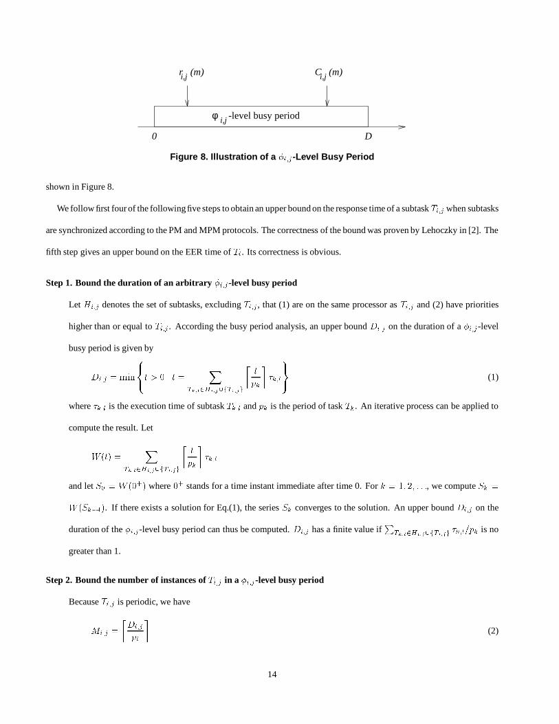
Specifically by a �i;j-level busy period we always mean a �i;j-level busy period in the schedule of the processor whereTi;j executes. Without loss of generality, in our discussion, we take the beginning of a �i;j-level busy period as the origin, as

13

φ i,j -level busy period

i,jr (m) i,jC (m)

0 D

Figure 8. Illustration of a �i;j-Level Busy Period

shown in Figure 8.

We follow first four of the followingfive steps to obtain an upper bound on the response time of a subtask Ti;j when subtasks

are synchronized according to the PM and MPM protocols. The correctness of the bound was proven by Lehoczky in [2]. The

fifth step gives an upper bound on the EER time of Ti. Its correctness is obvious.

Step 1. Bound the duration of an arbitrary �i;j-level busy period

Let Hi;j denotes the set of subtasks, excluding Ti;j, that (1) are on the same processor as Ti;j and (2) have priorities

higher than or equal to Ti;j. According the busy period analysis, an upper bound Di;j on the duration of a �i;j-level

busy period is given byDi;j = min8<:t > 0 j t = XTk;l2Hi;j[fTi;jg� tpk � �k;l9=; (1)

where �k;l is the execution time of subtask Tk;l and pk is the period of task Tk. An iterative process can be applied to

compute the result. LetW (t) = XTk;l2Hi;j[fTi;jg� tpk� �k;land let S0 = W (0+) where 0+ stands for a time instant immediate after time 0. For k = 1; 2; : : :, we compute Sk =W (Sk�1). If there exists a solution for Eq.(1), the series Sk converges to the solution. An upper bound Di;j on the

duration of the �i;j-level busy period can thus be computed. Di;j has a finite value ifPTk;l2Hi;j[fTi;jg �k;l=pk is no

greater than 1.

Step 2. Bound the number of instances of Ti;j in a �i;j-level busy period

Because Ti;j is periodic, we haveMi;j = �Di;jpi � (2)

14

Step 3. Find an upper bound on the response time of each possible instance of Ti;j in a �i;j-level busy period

Let us consider the mth (1 � m � Mi;j) instance of Ti;j released in a �i;j-level busy period, as shown in Figure 8,

and denote this instance by Ti;j(m). According to the busy period analysis, an upper bound Ci;j(m) on the completion

time of Ti;j(m) is given byCi;j(m) = min8<:t > 0 j x = m�i;j + XTk;l2Hi;j � tpk � �k;l9=; (3)

Again, the iterative process described above can be applied to compute the solution. The lower bound on the release

time of Ti;j(m) is (m � 1)pi. Hence an upper bound Ri;j(m) on the response time of Ti;j(m) is given byRi;j(m) = Ci;j(m) � (m � 1)pi (4)

Step 4. Bound the response time of Ti;jThe maximum of Ri;j(m)’s (1 � m � Mi;j) must be a correct upper bound on the response time of any instance ofTi;j. In other words, the maximum of Ri;j(m)’s (1 � m �Mi;j) is an upper bound on the response time of Ti;j.Ri;j = maxfRi;j(m)g; for m = 1; 2; : : : ;Mi;j (5)

Step 5. Bound the EER time of task TiOnce we obtain upper bounds on the response times of subtasks, we can sum up the bounds on the response times of

all its subtasks to obtain an upper bound on the end-to-end response time of a task.Ri = niXj=1Ri;j (6)

We call the algorithm consisting of the above five steps Algorithm SA/PM, standing for the schedulability analysis al-

gorithm for the PM protocol.4.2 Schedulability Analysis for the RG ProtocolWe now argue that Algorithm SA/PM can also be used to bound the worst-case EER times of tasks in a system that uses

the RG protocol. We argue for this in two steps.

This first step is to show that the upper bounds on the response times of subtasks computed in the first four steps of Al-

gorithm SA/PM are also correct bounds if the system uses the RG protocol. If we only use the first rule of updating the release

15

guard, the inter-release time of each subtask is no less than its period, and every subtask is a periodic subtask. The second

rule, however, may cause the inter-release time to be shorter than the period. On the other hand, there can never be a processor

idle point in a busy period. As a result, the second rule is never applied inside any busy period. Hence, subtasks are periodic

inside any busy period, and the busy period analysis for periodic tasks (i.e., the first four steps of Algorithm SA/PM) yields

correct upper bounds on the response times of subtasks synchronized according to the RG protocol.

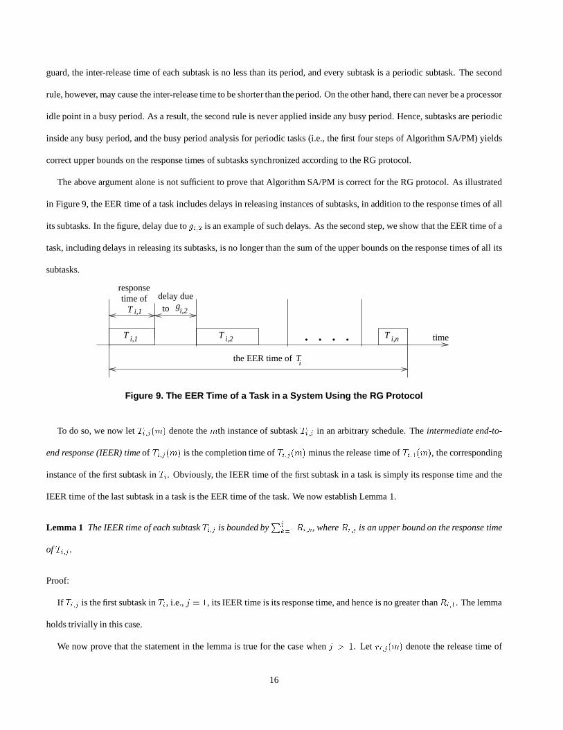
The above argument alone is not sufficient to prove that Algorithm SA/PM is correct for the RG protocol. As illustrated

in Figure 9, the EER time of a task includes delays in releasing instances of subtasks, in addition to the response times of all

its subtasks. In the figure, delay due to gi;2 is an example of such delays. As the second step, we show that the EER time of a

task, including delays in releasing its subtasks, is no longer than the sum of the upper bounds on the response times of all its

subtasks.

gi,2

T i,1 T i,2 T i,n

Ti

the EER time of

T i,1

responsetime of

. . . .

delay dueto

time

Figure 9. The EER Time of a Task in a System Using the RG Protocol

To do so, we now let Ti;j(m) denote the mth instance of subtask Ti;j in an arbitrary schedule. The intermediate end-to-

end response (IEER) time of Ti;j(m) is the completion time of Ti;j(m) minus the release time of Ti;1(m), the corresponding

instance of the first subtask in Ti. Obviously, the IEER time of the first subtask in a task is simply its response time and the

IEER time of the last subtask in a task is the EER time of the task. We now establish Lemma 1.

Lemma 1 The IEER time of each subtask Ti;j is bounded byPjk=1Ri;k, where Ri;j is an upper bound on the response time

of Ti;j .

Proof:

If Ti;j is the first subtask in Ti, i.e., j = 1, its IEER time is its response time, and hence is no greater thanRi;1. The lemma

holds trivially in this case.

We now prove that the statement in the lemma is true for the case when j > 1. Let ri;j(m) denote the release time of

16

Ti;j(m) and Ci;j(m) denote the completion time of Ti;j(m), the mth instance of Ti;j in an arbitrary schedule. To prove the

lemma, we need to demonstrate that Ci;j(m) � ri;1(m) � Pjk=1Ri;k for j = 2; 3; : : :; ni and m = 1; 2; : : :. BecauseCi;j(m) � Ri;j � ri;j(m), this inequality is the same as ri;j(m) � ri;1(m) + Pj�1k=1Ri;k. We will prove the later by

induction on m, the instance index of Ti;j(m).Induction basis : The first instance Ti;j(1) of each subtask Ti;j (j > 1) is released as soon as Ti;j�1(1) completes becausegi;j is initially set to 0 and delays due to the release guards will not occur. Therefore, the release time of Ti;j(1) is equal

to ri;1(1) plus the sum of response times of all its predecessor. In other words, the release time of Ti;j(1) is no greater

than ri;1(1) +Pj�1k=1Ri;k.

Induction hypothesis : Suppose that ri;j(m � 1) � ri;1(m � 1) +Pj�1k=1Ri;k for some m � 2.

Induction : According to the RG protocol, subtask instance Ti;j(m) for j > 1 and m > 1 is released either when its imme-

diate predecessor completes or when its release guard is due, whichever is later, i.e.,ri;j(m) � maxfCi;j�1(m); ri;j(m � 1) + pig� maxfri;j�1(m) + Ri;j�1; ri;j(m � 1) + pigBy the induction hypothesis, we have ri;j(m� 1) � ri;1(m� 1)+Pj�1k=1Ri;k. Because Ti;1 is a periodic subtask, we

have ri;1(m � 1) + pi � ri;1(m). The above inequality can then be written asri;j(m) � maxfri;j�1(m) +Ri;j�1; ri;1(m) + j�1Xk=1Ri;kgWe can expand the above inequality recursively by itself on ri;j�1(m) and obtain ri;j(m) � ri;1(m) +Pj�1k=1Ri;k.2

Because the EER time of a task is equal to the IEER time of its last subtask, the following theorem follows directly from

Lemma 1.

Theorem 1 Algorithm SA/PM yields correct upper bounds on the EER times of tasks in a system that uses the RG protocol.4.3 Schedulability Analysis for the DS ProtocolIf a system uses the DS protocol, the timing behavior of tasks is more difficult to analyze. According to the DS protocol,

an instance of a subtask is released as soon as the corresponding instance of its immediate predecessor completes. Since the

17

response time of each subtask instance may vary widely depending on the interference from higher-priority subtasks during the

execution of the instance, the release of its immediate successor subtask may vary widely as well. As we have seen in Figure 3,

although subtask T2;1 is released periodically, subtask T2;2 is not. As a consequence, T3 misses its deadline. The busy period

analysis for periodic tasks cannot be applied directly to obtain an upper bound on the response time of each subtask.

In general, when the DS protocol is used, we may see several instances of a subtask released rather close together in time or

even back-to-back consecutively. This phenomenon, clumping effect, is demonstrated in detail in [20]. The upper bounds on

the subtask response times, even if we can find them, can be quite pessimistic due to the clumping effect, and the final bound

on the EER time of a task based on these bounds can be quite pessimistic as well.

AlgorithmSA/DS, standing for the schedulabilityanalysis algorithmfor the DS protocol, was designed to find upper bounds

on task EER times when subtasks are synchronized according to the DS protocol. According to Algorithm SA/DS, we iterat-

ively apply another algorithm called Algorithm IEERT, which computes upper bounds on the IEER times of subtasks instead

of upper bounds on the response times of subtasks. In order to calculate the “extra interference” (i.e., additional delay) from

the clumping effect, Algorithm IEERT takes as input the parameters of all subtasks and a set of initial upper bounds on the

IEER times of subtasks. It computes a set of new bounds on the IEER times of subtasks. Its pseudo-code is listed in Figure 10.

The four steps of Algorithm IEERT are similar to the first four steps of Algorithm SA/PM. The difference lies primarily in the

computation of the maximum time demanded by equal and higher-priority subtasks whose instances may delay the completion

of any instance of Ti;j . Algorithm IEERT makes use the given response time bounds and calculate the number of instances

whose time demands must be taken into account, while Algorithm SA/PM relies on the periodicity of interfering subtasks to

calculate this number. The proof of correctness of Algorithm IEERT can be found in [20].

In the description of Algorithm SA/DS, we let R = fRi;jg and IEERT (T;R) denote the set R0 of new upper bounds

obtained by Algorithm IEERT (R0 = IEERT (T;R)). Figure 11 lists the pseudo-code of Algorithm SA/DS. In the initial-

ization step, for each subtask Ti;j, we use the sum of the maximum execution times of Ti;j and its predecessors as an initial

estimate of the bound on its IEER time. Obviously, this estimate is overly optimistic. In each iteration step, we apply Al-

gorithm IEERT to compute a set of new bounds on the IEER time of subtasks, based on the bounds computed in the initial

step or in the last iteration step. The iteration stops when the new bound is equal to the current bound for every subtask in the

system. The bound on the IEER time of Ti;ni computed during the last iteration is naturally the bound on the EER time of Ti.Theorem 2 says that these bounds are correct upper bounds on the task EER times when Algorithm SA/DS terminates. The

18

Algorithm IEERT

Input :

1. A set fTig of end-to-end periodic tasks.

2. A set fRi;jg of bounds on the IEER times of subtasks.

Output : A set fR0i;jg of new bounds on the IEER times of subtasks.

Algorithm :For each subtask Ti;j

1. Compute an upper bound Di;j on the duration of a �i;j-level busy periodDi;j = min8<:t > 0 j t = XTu;v2Hi;j[fTi;jg� t+Ru;v�1pu � �u;v9=;2. Compute an upper bound Mi;j on the number of instances of Ti;j in a �i;j-level busy periodMi;j = �Di;j +Ri;j�1pi �3. For m = 1 to Mi;j do

(a) Compute Ci;j(m) by solving the following equation.Ci;j (m) = min8<:t > 0 j t =m�i;j + XTu;v2Hi;j � t+ Ru;v�1pu � �u;v9=;(b) Compute an upper bound Ri;j(m) on the IEER time of the mth instance in a �i;j -level busy periodRi;j(m) = Ci;j(m) +Ri;j�1 � (m� 1)pi

4. Compute the new bound R0i;j byR0i;j = maxfRi;j(m)g; for 1 � m �MFigure 10. Pseudo-Code of Algorithm IEERT

19

proof of the theorem can be found in [20].

Theorem 2 If for each subtask Ti;j there exists someXi;j > 0 such thatX = IEERT (T;X) whereX = fXi;jg, then Xi;jis a correct upper bound on the IEER time of Ti;j.Algorithm SA/DS

Input : Task setT.

Output : The setR of upper bounds on the EER times of tasks.

Algorithm :

1. For each subtask Ti;j ,Ri;j = jXm=1 �i;mR0i;j = 02. Repeat until (Ri;j = R0i;j for every subtask Ti;j )

(a) R0 = R.

(b) R = IEERT (T;R0).3. For each task Ti , Ri = Ri;ni .

Figure 11. Pseudo-Code of Algorithm SA/DS

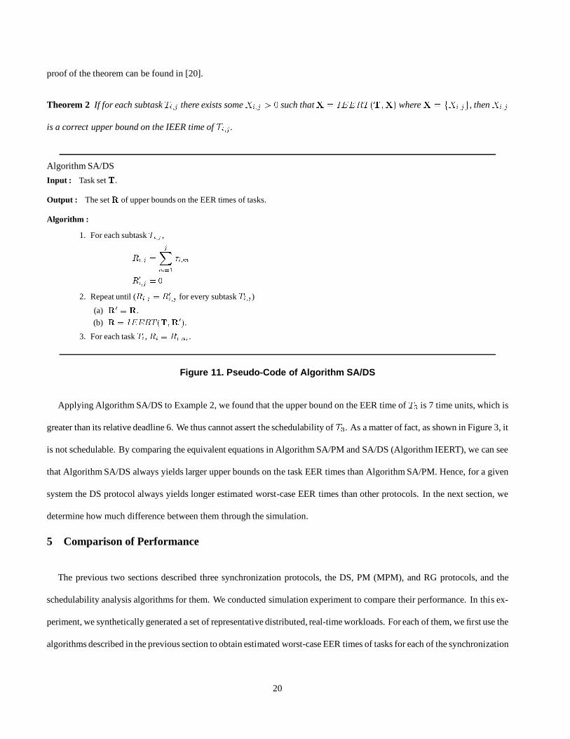
Applying Algorithm SA/DS to Example 2, we found that the upper bound on the EER time of T3 is 7 time units, which is

greater than its relative deadline 6. We thus cannot assert the schedulability of T3. As a matter of fact, as shown in Figure 3, it

is not schedulable. By comparing the equivalent equations in Algorithm SA/PM and SA/DS (Algorithm IEERT), we can see

that Algorithm SA/DS always yields larger upper bounds on the task EER times than Algorithm SA/PM. Hence, for a given

system the DS protocol always yields longer estimated worst-case EER times than other protocols. In the next section, we

determine how much difference between them through the simulation.

5 Comparison of Performance

The previous two sections described three synchronization protocols, the DS, PM (MPM), and RG protocols, and the

schedulability analysis algorithms for them. We conducted simulation experiment to compare their performance. In this ex-

periment, we synthetically generated a set of representative distributed, real-time workloads. For each of them, we first use the

algorithms described in the previous section to obtain estimated worst-case EER times of tasks for each of the synchronization

20

protocols. Then, we simulate the actual execution of these systems when each protocol is used and measured the average EER

times of tasks. The protocols are compared based on these two criteria.5.1 Generation of WorkloadsThrough preliminary experiments, we identified two system parameters that influence the performance of synchronization

protocols most: the number of subtasks in each task and the utilization of each processor. For the sake of simplifying the

analysis, we let every task in the system have the same number of subtasks and every processor have the same utilization. Each

configuration is a unique combination of the number of subtasks in each task and the utilization of each processor, denoted

by a 2-tuple (N;U ). For example, configuration (5; 60) represents systems where each task has 5 subtasks and the utilization

of each processor is 60%. In the configurations evaluated, the number of subtasks in each task ranges from 2 to 8 and the

utilization of each processor are 50%, 60%, 70%, 80%, or 90%. Consequently, we have a total of 35 configurations.

For each of the configuration, we generated 1000 systems. Each system has 4 processors and 12 tasks. (Again, we found

that the performance of the protocols are not sensitive to these parameters. These values were chosen to keep the simulation

time from becoming impractically large.) The periods of tasks are exponentially distributed from 100 to 10000 (i.e., the prob-

ability density function of task period is a truncated exponential function). This yields task periods with more variation than

when the periods are evenly distributed in (100; 10000). Subtasks are randomly assigned to processors, with no two consec-

utive subtasks of the same parent task assigned to the same processor. Subtasks on each processor divide the utilization of

the processor randomly. Specifically, to determine the utilization of a subtask, we generate a random number from 0.001 to 1

for each subtask. The utilization of the subtask is equal to the total processor utilization times the ratio of the random number

and the sum of the random numbers of all the subtasks on the same processor. The execution time of the subtask is equal to

its utilization times its period.

The last parameter of a synthetic system is the priority assigned to each subtask. We choose the Proportional-Deadline-

Monotonic priority assignment method to assign priorities to subtasks. (This method is similar to the Equal Flexibility assign-

ment in [9].) According to this method, each subtask has a proportional deadline (PDi;j) defined as follows.PDi;j = �i;jPnik=1 �i;kDiwhere Di is the relative deadline of Ti, which is equal to its period for this simulation. A subtask has higher priority if it has

a shorter proportional deadline.

21

Failure Rate

50 60 70 80 90

utilization(%)

345678

# ofsubtasks

0

0.5

1

50 60 70 80 90345678

# of

0

0.5

1

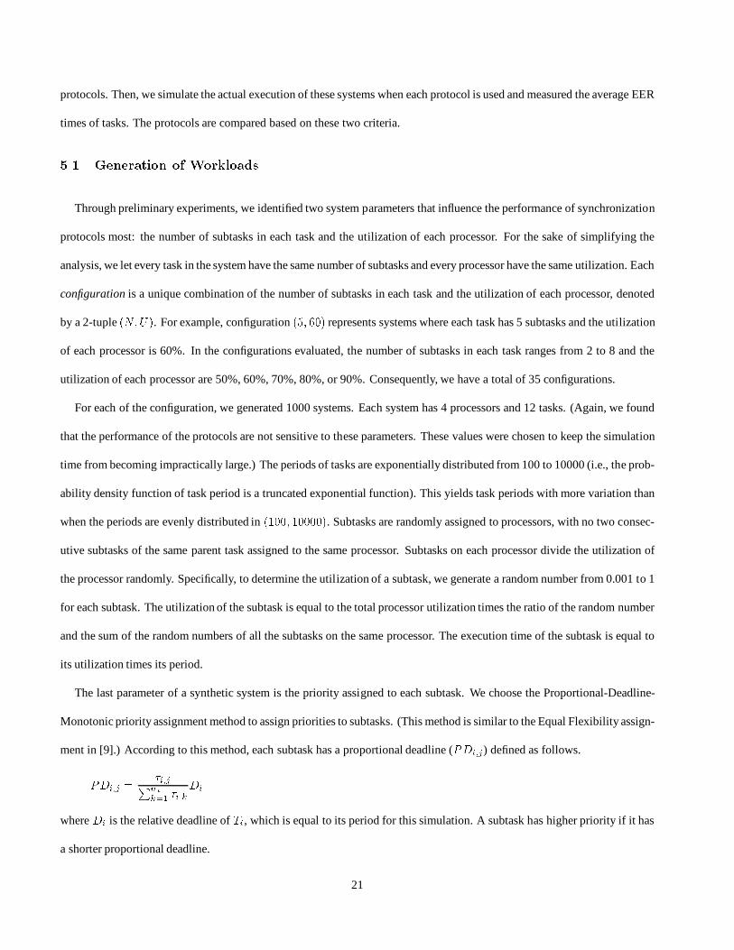
Figure 12. The Failure Rates as a Function of Configurations for the DS Protocol5.2 Comparison of the Estimated Worst-Case EER Times of TasksThe PM, MPM and RG protocols have the same upper bounds on the EER times of tasks. Hence we only compare the PM

protocol and the DS protocol according to this performance measure.

We use Algorithm SA/PM to compute the estimated worst-case response times of the tasks when tasks are synchronized

according to the PM protocol, and use Algorithm SA/DS to bound the EER times of tasks synchronized according to the

DS protocol. Given the same system, the estimated worst-case EER times of tasks are larger when tasks are synchronized

according to the DS protocol than when tasks are synchronized according to the PM protocol. For some systems, the bounds

on the EER times of tasks under the DS protocol were found to be extremely large. We say that a failure occurs when we find

that the upper bound of the EER time of a task is larger than 300 times of its period and hence for all practical purposes equals

to infinity. (We say that the bound is infinite in this case.) By analyzing the systems generated in the way described above, we

determined under what conditions (1) the estimated worst-case EER times for these two protocols are close, (2) the estimated

worst-case EER times of tasks for the DS protocol are much greater, and (3) failures occur when the DS protocol is used.

Figure 12 shows the failure rate, which is the percentage of systems that we fail to obtain finite bounds on the EER times

when the DS protocol is used as a function of the system configuration. We notice that the failure rates are mostly zero and

quickly rise to one when number of subtasks in each task approaches 8 and the processor utilizations are close to 90%. In

the case of configuration (8; 90), we could obtain finite bounds for only 4 out of 1000 systems. Similarly, we observe that

failure rates are greater than 0:1 for configuration (8; 80), (7; 90), (7; 80), and (6; 90). This indicates that the DS protocol is

not suitable for systems where processor utilization is high and tasks have many subtasks.

For the systems that have finite estimated worst-case EER times for both the PM protocol and the DS protocol, we use

22

Bound Ratio

50 60 70 80 90

utilization(%)

345678

# ofsubtasks

1

10

20

50 60 70 80 90345678

# of

1

10

20

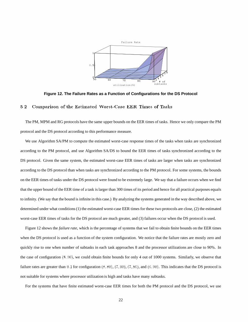
Figure 13. Bound Ratios as a Function of Configurations

the average bound ratio to compare their performance. A bound ratio is the ratio of the estimated worst-case EER time of

a task synchronized according to the DS protocol to the estimated worst-case EER time of the task under the PM protocol.

For each configuration, we average the bound ratios of all the tasks in the systems that have finite estimated worst-case EER

times for the DS protocol. A large average bound ratio for a configuration indicates that the DS protocol performs poorly. The

average bound ratios as a function of configurations is plotted in Figure 13. The 90% confidence interval is negligibly small

for most configurations. The average bound ratios for configurations with large number of subtasks and high utilizations are

not statistically significant due to the high failure rates they have, although they seem to fit the overall curves well.

From Figure 13, we see that for low utilization configurations, the ratio curve stays relatively flat as the number of subtasks

in each task increase. However, for high utilization configurations, the curve goes up quickly as the number of subtasks in

each task increases. Roughly one-third of configurations have the ratios greater than 2, making the DS protocol less appealing

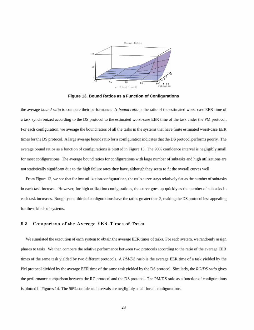
for these kinds of systems.5.3 Comparison of the Average EER Times of TasksWe simulated the execution of each system to obtain the average EER times of tasks. For each system, we randomly assign

phases to tasks. We then compare the relative performance between two protocols according to the ratio of the average EER

times of the same task yielded by two different protocols. A PM/DS ratio is the average EER time of a task yielded by the

PM protocol divided by the average EER time of the same task yielded by the DS protocol. Similarly, the RG/DS ratio gives

the performance comparison between the RG protocol and the DS protocol. The PM/DS ratio as a function of configurations

is plotted in Figures 14. The 90% confidence intervals are negligibly small for all configurations.

23

PM/DS Ratio

50 60 70 80 90utilization(%)

345678

# ofsubtasks

1

2

3

4

50 60 70 80 90345678

# of

1

2

3

4

Figure 14. The PM/DS Ratio

We notice that for a fixed number of subtasks in each task, the PM/DS ratios goes down slightlywhen the utilizationon each

processor goes up. With low utilizations, the processor is under-loaded and the PM protocol may unnecessarily postpone the

releases of subtasks. Therefore the average EER times are larger than those yielded by the DS protocol in these cases. For a

fixed processor utilization, the PM/DS ratio increases as the number of subtasks in each task increases. For configurations with

5 or more subtasks in each task, the values of the ratio are all greater than 2, indicating that for these kinds of configurations, the

average EER times of tasks synchronized according to the PM protocol are more than twice than when tasks are synchronized

according to the DS protocol. For configurations with 8 subtasks in each task, the ratio is around 3 or 4. Overall, we see that

the DS protocol yields much shorter average EER times than the PM (MPM) protocol.

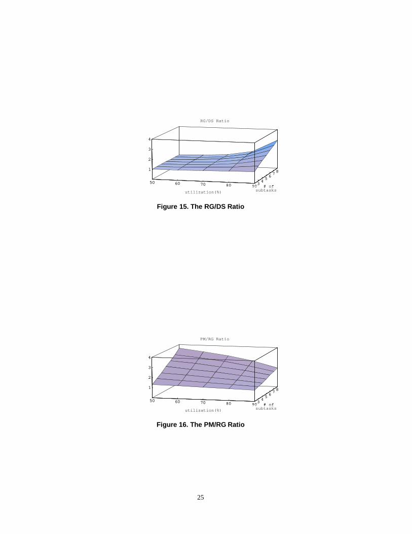
Compared with the DS and PM protocols, the performance of the RG protocol is in the middle in terms of the average EER

times of tasks. The RG/DS ratio as a function of configurations is plotted in Figure 15. The ratio varies mostly from 1 to 2

for all configurations, except for some configurations with 90% utilization on each processor. When the processor utilization

is 90%, the processor is busy almost all the time, and rule (2) of updating the release guard becomes less frequently applied.

As a result, the releases of subtasks according to the RG protocol become more periodical. This leads to longer average EER

times. Overall, the performance of the RG protocol is still close to the DS protocol with regard to the average EER times.

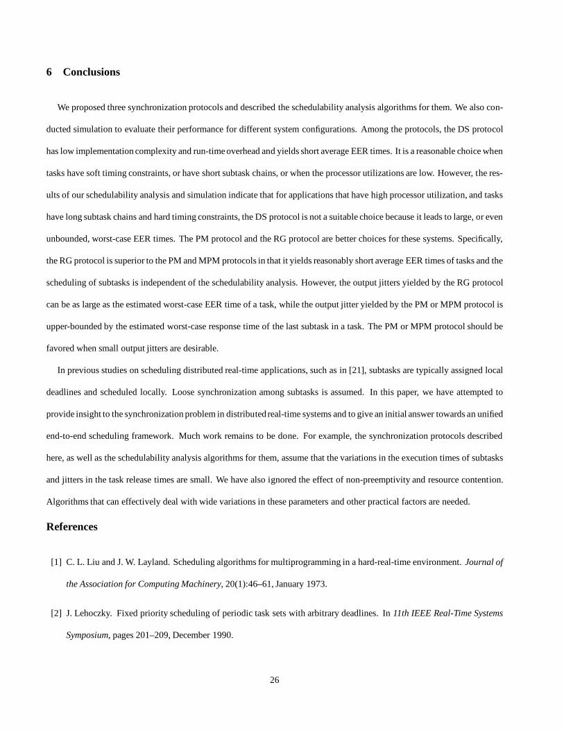
The PM/RG ratio compares the relative performance between the PM and RG protocols. Figure 16 plots the ratio as a

function of configurations. We see that the ratio is consistently higher than one. For configurations with 6, 7 or 8 subtasks in

each task, the PM/RG ratio even reaches 2 or 3. If shorter average EER times of tasks are desirable in the application, the RG

protocol has the obvious advantage over the PM protocol.

24

RG/DS Ratio

50 60 70 80 90utilization(%)

345678

# ofsubtasks

1

2

3

4

50 60 70 80 90345678

# of

1

2

3

4

Figure 15. The RG/DS Ratio

PM/RG Ratio

50 60 70 80 90utilization(%)

345678

# ofsubtasks

1

2

3

4

50 60 70 80 90345678

# of

1

2

3

4

Figure 16. The PM/RG Ratio

25

6 Conclusions

We proposed three synchronization protocols and described the schedulability analysis algorithms for them. We also con-

ducted simulation to evaluate their performance for different system configurations. Among the protocols, the DS protocol

has low implementation complexity and run-time overhead and yields short average EER times. It is a reasonable choice when

tasks have soft timing constraints, or have short subtask chains, or when the processor utilizations are low. However, the res-

ults of our schedulability analysis and simulation indicate that for applications that have high processor utilization, and tasks

have long subtask chains and hard timing constraints, the DS protocol is not a suitable choice because it leads to large, or even

unbounded, worst-case EER times. The PM protocol and the RG protocol are better choices for these systems. Specifically,

the RG protocol is superior to the PM and MPM protocols in that it yields reasonably short average EER times of tasks and the

scheduling of subtasks is independent of the schedulability analysis. However, the output jitters yielded by the RG protocol

can be as large as the estimated worst-case EER time of a task, while the output jitter yielded by the PM or MPM protocol is

upper-bounded by the estimated worst-case response time of the last subtask in a task. The PM or MPM protocol should be

favored when small output jitters are desirable.

In previous studies on scheduling distributed real-time applications, such as in [21], subtasks are typically assigned local

deadlines and scheduled locally. Loose synchronization among subtasks is assumed. In this paper, we have attempted to

provide insight to the synchronization problem in distributed real-time systems and to give an initial answer towards an unified

end-to-end scheduling framework. Much work remains to be done. For example, the synchronization protocols described

here, as well as the schedulability analysis algorithms for them, assume that the variations in the execution times of subtasks

and jitters in the task release times are small. We have also ignored the effect of non-preemptivity and resource contention.

Algorithms that can effectively deal with wide variations in these parameters and other practical factors are needed.

References

[1] C. L. Liu and J. W. Layland. Scheduling algorithms for multiprogramming in a hard-real-time environment. Journal of

the Association for Computing Machinery, 20(1):46–61, January 1973.

[2] J. Lehoczky. Fixed priority scheduling of periodic task sets with arbitrary deadlines. In 11th IEEE Real-Time Systems

Symposium, pages 201–209, December 1990.

26

[3] N. Audsley, A. Burns, K. Tindell, M. Richardson, and A. Wellings. Applying new scheduling theory to static priority

pre-emptive scheduling. Software Engineering Journal, 8(5):284–292, 1993.

[4] K. W. Tindell. Fixed Priority Scheduling of Hard Real-Time Systems. PhD thesis, University of York, Department of

Computer Science, 1994.

[5] J. Leung and J. Whitehead. On the complexity of fixed-priority scheduling of periodic, real-time tasks. Performance

Evaluation, 2:237–250, 1982.

[6] N. C. Audsley. Optimal priority assignment and feasibility of static priority tasks with arbitrary start times. Technical

Report YCS 164, Dept. of Computer Science, University of York, December 1991.

[7] M. Joseph and P. Pandya. Finding response times in a real-time system. The Computer Journal of the British Computer

Society, 29(5):390–395, October 1986.

[8] K. Tindell, A. Burns, and A. Wellings. Allocating real-time tasks. An NP-hard problem made easy. Real-Time Systems

Journal, 4(2), May 1992.

[9] B. Kao and H. Garcia-Molina. Deadline assignment in a distributed soft real-time system. In The 13th International

Conference on Distributed Computing Systems, pages 428–437, May 1993.

[10] J. Garcia and M. Harbour. Optimized priority assignment for tasks and messages in distributed hard real-time systems.

In The Third Workshop on Parallel and Distributed Real-Time Systems, pages 124–132, April 1995.

[11] R. Bettati. End-to-EndScheduling to Meet Deadlines in DistributedSystems. PhD thesis, Universityof Illinoisat Urbana-

Champaign, 1994.

[12] H. Zhang and D. Ferrari. Rate-controlled service disciplines. Journal of High Speed Networking, ?(?):?, ? 1994.

[13] D. Verma, H. Zhang, and D. Ferrari. Guaranteeing delay jitter bounds in packet switching networks. In Proceedings of

Tricomm’91, pages 35–46, Chapel Hill, North Carolina, April 1991.

[14] M. G. Harbour, M. H. Klein, and J. P. Lehoczky. Timing analysis for fixed-priority scheduling of hard real-time systems.

IEEE Transactions on Software Engineering, 20(1):13–28, January 1994.

27

[15] B. Hunting. The solution’s in the CAN — Part 1. Circuit Cellar, pages 14–20, May 1995.

[16] J. Lehoczky, L. Sha, and Y. Ding. The rate monotonic scheduling algorithm: Exact characterization and average case

behavior. In IEEE Real-Time Systems Symposium, pages 166–171, December 1989.

[17] K. W. Tindell, A. Burns, and A. J. Wellings. An extendible approach for analyzing fixed priority hard real-time tasks.

Real-Time Systems, 6(2):133–152, March 1994.

[18] K. Tindell and J. Clark. Holistic schedulability analysis for distributed hard real-time systems. Microprocessing and

Microprogramming, 50(2):117–134, April 1994.

[19] A. Burns, K. Tindell, and A. J. Wellings. Fixed priorityscheduling with deadlines prior to completion. In Sixth Euromicro

Workshop on Real-Time Systems, pages 138–142, June 1994.

[20] J. Sun and J. Liu. Bounding the end-to-end response times of tasks in a distributed real-time system using the direct

synchronization protocol. Technical Report UIUCDCS-R-96-1949, University of Illinois at Urbana-Champaign, Dept.

of Computer Science, March 1996.

[21] S. Chatterjee and J. Strosnider. Distributed pipeline scheduling: End-to-end analysis of heterogeneous, multi-resource

real-time systems. In The 15th International Conference on Distributed Computing Systems, pages 204–211, May 1995.

28