Conservation Halton Ecological Monitoring Protocols

Conservation Halton

Ecological Monitoring Protocols

Version 1.0

February 2017


2

Table of Contents 1 Introduction ..................................................................................................................................................... 3

1.1 Monitoring Questions and Study Design ............................................................................................... 3

1.2 Inventories vs. Long-term Monitoring ................................................................................................... 4

1.3 Monitoring Protocols .............................................................................................................................. 5

2 Aquatic Monitoring ......................................................................................................................................... 6

2.1 Fish Community ....................................................................................................................................... 6

2.2 Channel Morphology and Fish Habitat .................................................................................................. 9

2.3 Benthic Macroinvertebrates ................................................................................................................. 10

2.4 Freshwater Mussels ............................................................................................................................... 12

2.5 Water Quality Monitoring .................................................................................................................... 13

2.6 Stream Temperature ............................................................................................................................. 15

3 Terrestrial Monitoring ................................................................................................................................... 17

3.1 Vegetation Communities ...................................................................................................................... 17

3.2 Forest Health Monitoring ..................................................................................................................... 18

3.2.1 Tree Health ........................................................................................................................................ 18

3.2.2 Shrub and Sapling Regeneration...................................................................................................... 19

3.2.3 Ground Cover (Vegetation) Biodiversity .......................................................................................... 21

3.2.4 Plethodontid Salamanders ............................................................................................................... 21

4 Wildlife Monitoring ....................................................................................................................................... 23

4.1 Birds ....................................................................................................................................................... 23

4.1.1 Forest Birds ........................................................................................................................................ 23

4.1.2 Marsh Birds ........................................................................................................................................ 24

4.1.3 Additional Bird Surveys ..................................................................................................................... 25

4.2 Amphibian Monitoring ......................................................................................................................... 25

4.3 Butterfly Monitoring ............................................................................................................................. 27

4.4 Significant Wildlife Habitat ................................................................................................................... 28

4.5 Photomonitoring .................................................................................................................................. 28

References ............................................................................................................................................................. 30


3

1 Introduction Conservation Halton’s Long-term Environmental Monitoring Program (LEMP) was first initiated in 2005 with the completion of the Sixteen Mile Creek monitoring project. Since that time, staff have used scientifically-based monitoring protocols to monitor both the biotic and abiotic features within the aquatic and terrestrial ecosystems across the Conservation Halton watershed. In doing so, ecological information has been collected to support planning initiatives within the watershed while also addressing the core monitoring question “Is the health of the Conservation Halton watershed changing over time?” (Conservation Halton 2005).To answer this question, Conservation Halton has incorporated scientifically-based monitoring protocols, many of which are provincial standards, into the monitoring program. After ten years of monitoring staff ecologists are starting to identify trends in watershed health and are investigating ways to reverse and prevent decreases in ecological health.

While the LEMP is effective in monitoring long-term changes at set monitoring stations, ecological information is lacking in areas that are currently most under threat from development and alteration in the watershed; a watershed that is specifically identified in the provincial Places to Grow Act (2005) as an area of settlement. While the Places to Grow Act recognizes the need to accommodate future population growth and support economic prosperity, one of the main purposes of the act was to “enable decisions about growth to be made in ways that sustain a robust economy, build strong communities and promote a healthy environment and a culture of conservation” (Province of Ontario 2005). In doing so, growth areas and natural landscapes must coexist together, without one element impacting the other. In order for this to happen, sound decision making and planning must occur in order to ensure that ecologically integrity is maintained.

Ecological inventories and monitoring provides the baseline information for these decisions to be made. Baseline studies to address aquatic and terrestrial species and their habitats, groundwater conditions, water quality conditions etc. are all used to both ensure that the form and function of the natural environment is maintained and healthy while also ensuring that risk to infrastructure is low and community safety remains a priority. Similarly, long-term monitoring of the same parameters helps identify potential concerns and effects that may limit or decrease ecological health, which helps practitioners address concerns and learn from mistakes. Unfortunately, the monitoring and inventory component of a project is often not considered as important and instead is often thought of as a hindrance in moving projects forward in a timely and cost-effective manner. Within the Conservation Halton watershed and across Southern Ontario, this has resulted in inadequate data collection to address both the needs to guide decisions through the planning process as well as the required information to assess impacts from landscape changes within the watershed.

In an effort to remedy this situation and to incorporate additional high quality data into Conservation Haltons Long-term Environmental Monitoring Program, Conservation Halton has developed this external guide of approved monitoring protocols and methodologies for data collection within the Conservation Halton watershed and where applicable, across Southern Ontario. The guide outlines the specific methodologies that are recommended for use in the Conservation Halton watershed, with additional details pertaining to how data should be collected, analyzed and provided to Conservation Halton as part of baseline inventories or long-term monitoring initiatives related to landuse changes within the watershed.

1.1 Monitoring Questions and Study Design While the Conservation Halton Long-term Environmental Monitoring Program was developed to answer the question ”Is the health of the Conservation Halton watershed changing over time?”, the program was not intended to address other monitoring questions related to localized projects on the landscape (for e.g. whether a storm water management pond is having an immediate effect on water temperature and quality


4

in the immediate reaches downstream). These monitoring initiatives, specifically those related to urban, commercial or residential growth, require additional monitoring identified in the early stages of the project to address questions related to the specific project. Monitoring only to fulfil planning requirements is no longer adequate and does not provide a mechanism by which impacts can be clearly identified and improvements can be made. Instead, efforts to identify clear monitoring questions should be implemented. These questions should be developed up-front, in collaboration with stake holders, partners and those who will be evaluating the monitoring to ensure that the goals of the monitoring program fit the needs of the project. Similarly, the monitoring question will help to identify what features need to be monitored, how the monitoring will be completed, how the data will be analyzed and most importantly at what threshold the results indicate that an impact has occurred. This information will help guide the monitoring initiatives and when followed properly will help to identify impacts and as equally as important, help to identify what techniques work to on the landscape.

As part of the initial stages of any monitoring project, a thorough examination of the study design should be completed. This would involve a thorough understanding of the monitoring question, consideration of whether the monitoring study relates to temporal or spatial change and how the data will be analyzed. Only once these components of the study design have been determined, can data collection begin.

1.2 Inventories vs. Long-term Monitoring Ecological “inventories” and “monitoring” terminology has been long been used as synonyms however, these two types of survey methodologies are quite distinct. Ecological inventories are typically used in the early stages of a project to characterize a site and obtain as much baseline information on the species, habitats and physical and chemical environments within a study area. While these inventories often used science-based monitoring protocols, they can also include random observations and searches for species and habitats, such as rare species, that are often missed using standardized monitoring protocols. Conversely, long-term monitoring programs are similar to inventories in the sense that they collect the same types of data and can use similar protocols; however data collected as part of a monitoring program is typically collected over a number of years at a number of set locations and limits the amount of random observations collected in an area. Long-term monitoring programs instead provide a thorough understanding of what is happening at a point in time, over a longer period of time and at a more specific location within a study area.

Both of these survey methodologies are important components of any project where change may occur within the local environment. In the initial stages, multiple inventories across an entire study area helps to characterize a site and identify any environmental, cultural of socioeconomic concerns within the area. This information is then used to assist land-use planners, ecologists and engineers in determining the best ways to help mitigate issues or concerns within the study area. Once baseline information is collected and projects move forward, monitoring of specific sites within the study area help identify whether change is occurring and information collected can help to direct those involved in the project to address impacts as they occur.

While inventories and monitoring programs may be different in scope, a well thought-out monitoring program can use the baseline inventories as “Year 1” of a long-term monitoring program. That is to say, that well-thought out inventories are the initial stages of long-term monitoring programs and as such, they should be initiated with an understanding of how the information can be collected, analyzed and used in subsequent monitoring programs. Similarly, how and where the inventories are completed within an area should also consider where future monitoring stations can be initiated.

While most baseline inventories can be used as the initial stages of a long-term monitoring program, it is recognized that randomized observations that are not collected according to protocol but are helpful in characterizing an area are not suited to long-term monitoring programs due to the random and non-repeatable nature of the survey type. However, very few inventories are truly random enough to not be


5

replicated in future years and as such, a thorough understanding of future goals, study designs and monitoring questions should be considered in the initial stages of a project when inventories are conducted.

1.3 Monitoring Protocols

The following sections outline a number of protocols recommended for use within the Conservation Halton watershed. While a number of other protocols may allow for sufficient data collection, the protocols recommended herein are those that are currently in use as part of Conservation Halton’s Long-term Environmental Monitoring Program and as a result, parameters collected as part of the program follows those of the recommended protocols. Information collected as part of the LEMP can then be compared against similar local monitoring programs following the same protocols for data collection.

Data collected as part of the LEMP is available to provide background information for projects within the watershed. Available data holdings and a data request form can be found on the Conservation Halton website at: http://www.conservationhalton.ca/mapping-and-data


6

Using backpack electrofishing to sample the local fish community

2 Aquatic Monitoring

2.1 Fish Community Fish are often used as indicators of aquatic health as individual species have preferred habitats types, thermal requirements and sensitivities to disturbance. As a result, fish are often used as surrogates when information is lacking (e.g. coldwater species being indicative of ground water discharge). The presence or absence of species within a site can help one determine aquatic health and identify impacts.

Methodology

Fish community data can be collected through a variety of methods and high quality data may require more than one sampling methodology to be used in order to obtain a comprehensive understanding of the fish community present at a site. Alternative methodologies may also be required to minimize harm to species at risk in occupied, historical or potential habitats. As a result, it is recommended that the proponent complete both a thorough search to locate historical records and contact local and provincial agencies to obtain fisheries data prior to sampling.

The Ontario Stream Assessment Protocol (OSAP) Section 3 Module 1 is the recommended methodology used to sample the fish community (Stanfield 2017). According to this protocol, sampling stations are first identified by locating both an upstream and downstream crossover that are separated by a minimum of 40 metres and are comprised of at least one riffle/pool sequence. Once identified, the sampling station is sampled using a backpack electrofishing unit progressing across all available habitats from bank to bank. The amount of effort expended at each sampling station is dependent on the total area of the site. The stream area is then multiplied by two and five, to determine the minimum and maximum number of electrofishing seconds. This ensures that sampling is standardized at minimum, within the OSAP screening level assessments (Stanfield 2017). All fish captured are then bulk weighed and measured with the exception of any sport fish species, which are individually weighed and measured. The condition of the fish and any identifiable diseases are also noted. Voucher photographs with key identifying features clearly photographed are recommended for all species groups whereas voucher photographs and/or specimens are required for all unconfirmed species so they can be later identified by a certified taxonomist. For species at risk observations, voucher photographs with identifiable features are required. Once species documentation is complete, all fish are then released back to the stream.

In instances where electrofishing is not appropriate (deep, wide etc.), seine netting of a reach is recommended. Seining in relatively still areas should progress from the downstream end of the reach progressing upstream with samplers on either bank to ensure that the entire stream is sampled. In large fast flowing rivers and when sampling for specific species, sampling should extend from the upstream limits of the station quickly to the downstream end in line or ahead of the speed of the current. All fish should be processed the same in the same way as electrofishing.


7

Smallmouth Bass (Micropterus dolomieu) captured during electrofishing surveys

Data Management and Analysis

Fish unlike sedimentary aquatic organisms (e.g. benthic macroinvertebrates) have the physical ability to leave an area in response to a disturbance. As a result, species composition, numbers and overall biomass of a sampled community may change in response to a physical or chemical disturbance, both within the stream itself or within the drainage area. As a result, documentation of the following information is recommended:

• Full species list (in tabular format) of all fish caught including species names, number of fish caught, maximum and minimum lengths within a species group, total (bulk) weight of groups and individual lengths/weights for all sport fish.

• Voucher photographs (through viewing window) to confirm species identification and required for unconfirmed species or species at risk.

• Documentation of physical habitat, either observed or quantified, identifying habitat conditions, riparian habitat, instream habitat, substrate quality (sorting) and size. Adjacent landuse and habitat conditions according to OSAP Section 1 Module 1-5 is also recommended.

• Documentation of sampling methodology including equipment used, date/time and effort (i.e. electrofishing seconds, # of seine hauls etc.).

• Mapped locations, descriptions and UTMs.

Further analysis using an Index of Biotic Integrity may also be completed. Conservation Halton Fish community monitoring uses a modified Index of Biotic Integrity (IBI) first adapted to Southern Ontario Streams by Steedman (1988). This methodology measures fish community associations to identify the general health of a stream ecosystem based on its upstream drainage area. Steedman’s original IBI utilizes ten different indices including indicator species, trophic composition, fish abundance and health. Although these metrics are useful indicators of stream health, all indices may not be suited to all streams. In order to use the IBI analysis for both warmwater and coldwater tributaries throughout the watershed, two sub-indices are modified to better reflect stream conditions. The first sub-index removed is the presence of blackspot, a common parasite of fish. Although this may affect stream fish, it does not necessarily reflect unhealthy stream conditions and as such is removed from the analysis. The second sub-index modified, the

presence or absence of Brook Trout, is removed to better reflect stream conditions where Brook Trout would not naturally occur (i.e. warmwater tributaries with no historical evidence of Brook Trout). In order to account for the removal of these sub-indices, IBI scores for coldwater stations are based on nine sub-indices whereas warmwater stations are based on eight sub-indices and are standardized to be equally weighted for comparison with coldwater stations, as was done in the Humber River Fisheries Management Plan (OMNR and TRCA 2005).

Indices used to form the modified Index of Biotic Integrity are found below:


8

SPECIES RICHNESS

• Number of native species

• Number of darter and/or sculpin species

• Number of sunfish and/or trout species

• Number of sucker and/or catfish species

LOCAL INDICATOR SPECIES

• Presence or absence of Brook Trout (historical reaches only)

• Percent of Rhinichthys species

TROPHIC COMPOSITION

• Percent of sample as omnivores

• Percent of samples as piscivores

FISH ABUNDANCE

• Catch per minute of sampling

It should be noted that with the IBI methodologies, assessment appears to be sensitive to the capture of particular species such as darters, trout and suckers. Generally, a year catch that fluctuates by the number of darter, sucker or trout species could shift the IBI scores significantly. Scores may also fluctuate in response to catch per unit effort (CPUE) as annual changes in staff may affect catch efficiency. It is also important to note that if suitable information is not collected (i.e. the number or biomass of fish) IBI analysis cannot be completed. Table 1 provides a summary of IBI ratings and associated scores.

Table 1: IBI ratings and associated scores using the modified Index of Biotic Integrity (IBI)

IBI Rating Modified IBI Scores

Poor 9 – 20

Fair 21 – 27

Good 28 – 37

Very Good 38 – 45

Additional analytical tools to assess fish communities are currently under development by Conservation Authorities in Ontario. Once completed, these methodologies will address species tolerance and issues related to richness/diversity in aquatic systems. These tools should be incorporated into the analysis once available.


9

2.2 Channel Morphology and Fish Habitat Fish habitat assessments are often completed in conjunction with fish community assessments to give an overall characterization of fish utilization within stream reaches. Assessments can include detailed measurements of channel morphology to assess channel stability and habitat suitability and a number of other morphological characteristics and/or it can include visual observations throughout the study reach.

Methodology

Fish habitat and channel morphology measurements should be completed according to the Ontario Stream Assessment Protocol (OSAP) Point Transect Sampling for Channel Structure, Substrate and Bank Conditions (section 4 module 2). As part of this module, specific physical characteristics of stream channels are documented including, water depth, velocity, substrate type and size, cover types and amount, instream vegetation, woody debris, undercut banks and bank composition, riparian vegetation and bank angle. All these characteristics can provide insight into the physical conditions of streams on both a spatial and temporal level and may also identify the limiting features of a stream’s physical habitat (Stanfield 2017). It should be noted that morphological assessments completed as part of the OSAP methodology is geared towards fish habitat use and additional surveys to monitor channel form, structure and stability from a fluvial geomorphology/engineering perspective may be required.


While more detailed engineering-based protocols are important to assess channel morphology and stability, these protocols do not provide a thorough understanding of fish habitat conditions within a stream. In addition to the OSAP Channel Morphology protocol and/or any engineering-based protocols additional information to assess fish habitat should include an evaluation of:

• under cut banks • base flow conditions including water velocity, stream order, discharge, water depth, stream width

and bankfull width • water chemistry (dissolved oxygen, temperature, pH, conductivity, water colour and clarity)

substrates (texture, presence of aquatic vegetation, odours/discolouration of the sediments) • identification and classification of headwater drainage features (HDF’s) • in-stream riparian cover (presence and extent) and shading • critical habitats (spawning, nursery or rearing grounds) • groundwater discharge and upwellings (e.g. presence of watercress or iron floc) • surrounding land uses • identification of in-stream barriers to fish passage • other measurements that indicate the quality of the habitat such as entrenchment, erosion etc. • point source impacts • degradation, debris, barriers, sources of pollution, etc. • recreational opportunities • rehabilitation opportunities


10

Collection of benthic macroinvertebrates through the OBBN kick and sweep method

Benthic macroinvertebrates being identified under a microscope

2.3 Benthic Macroinvertebrates Benthic macroinvertebrates are often used as indicators of water quality and instream habitat because they are abundant, ubiquitous, sedentary and are sensitive to changes in the quality of the aquatic ecosystem (Jones et al. 2007). As a result, benthic macroinvertebrate communities at a given site can be used to determine the aquatic health of that site.

Methodology

To sample the benthic macroinvertebrate community, the Ontario Benthos Biomonitoring Network Protocol (OBBN) is recommended. Similar to the OSAP protocol, sampling stations are first identified by locating both a downstream and upstream crossover that are separated by a minimum of 40 metres and are comprised of at least one riffle/pool sequence. At each station, three transects are sampled. Two transects are selected at stream crossovers (riffle habitat) at the upstream and downstream limits of the station and the third transect is selected to traverse pool habitat between the two crossovers.

Samples are collected using the kick and sweep method, whereby the sampler stands upstream of a 500µm D-net and excavates the top 10 centimetres of sediment with their feet. This allows any attached and free moving benthic macroinvertebrates to flow into the 500µm D-net and be collected. The sampler continues this action across each stream transect thereby sampling all available habitats. Once collected, live samples are taken back to the lab and randomly sub-sampled. A minimum of 100 organisms are collected per sub-sample (transect) and are preserved in 95% ethanol. Preserved specimens are then returned to the lab and identified to family or lowest practical level for analysis (Jones et al. 2007).

Habitat characteristics of the site are also recorded and included stream width, stream depth, maximum hydraulic head, canopy cover, presence of macrophytes and algae, presence of detritus and woody debris. Dominant substrate type is determined through random pebble counts at each transect.


The benthic macroinvertebrate communities are analyzed using a variety of biological indices. Two richness indices are used where the total number of families present in a sample are counted. The richness indices includes EPT (Ephemeroptera, Trichoptera and Plecoptera) richness and taxa richness. One composition indices is used to look at the percent of each sample made up by a given family or group. This indice helps to define the species composition of a stream and assist in determining the likelihood that a stream has been impacted based on the amount of pollution tolerant taxa. The Hilsenhoff Biotic Index (HFI) is used to


11

determine the impact of organic pollution on each station. The HFI assigns tolerance values to each family based on its ability to survive in areas with varying amounts of organic pollution. Families with high pollution tolerance have high tolerance values; as a result, lower scores on the HFI indicate that a station has been less impacted by organic pollution (Hilsenhoff 1988). The Shannon-Weiner Diversity Index (SDI) uses both species evenness and species richness to score the diversity of a site. It is expected that healthy sites would be better able to support a variety of species and would result in higher diversity scores (Credit Valley Conservation 2010).

Each index is assessed separately against the target values as set out in Table 2. Final assessments of unimpaired, potentially impaired or impaired are based on the cumulative results of each individual metric in a manner similar to the Citizens Environmental Watch methodology (Citizens’ Environment Watch 2009). All index values are added up and grouped into the three categories that define the health of the stream. The majority of the indices determine if it meets the criteria for an unimpaired, potentially impaired or impaired benthic community (i.e. if three of five indices are considered unimpaired, the site is categorized as unimpaired).

Table 2: Benthic Invertebrate Indices and Associated Classifications

Water Quality Index Unimpaired Potentially Impaired Impaired

EPT Richness ≥10 5-10 <5

Taxa Richness ≥13 <13

% Insect 50-80 40-50 or 80-90 <40 or >90

HFI <6 6-7 >7

SDI >4 3-4 <3

Documentation of benthic invertebrates should include the following:

• A complete list of benthic invertebrates and numbers captured for each replicate sample (downstream riffle, pool and upstream riffle)

• Documentation of physical habitat, either observed or quantified, identifying habitat conditions, riparian habitat, instream habitat, substrate quality (sorting) and size. Use of the Ontario Benthic Biomonitoring network field sheet is recommended

• Mapped locations, descriptions and UTMs

• Documentation of sampling methodology including equipment used, date/time, water quality parameters etc.


12

2.4 Freshwater Mussels Freshwater mussels (Unionidae) are one of the most endangered species groups within North America and their decline has been directly related to habitat alteration and degradation (Cudmore et al. 2004). Since 1994, after COSEWIC (Committee on the Status of Wildlife in Canada) expanded its mandate to include invertebrates, monitoring and inventory projects to identify these species have been implemented to minimize further impacts on this order.

Methodology

Since freshwater mussels are often observed within the substrate surface surveys are best conducted during summer low-flow conditions between July- September when there is maximum visibility within a stream reach and temperatures are below 16°C. Qualitative timed surveys are often completed looking for the presence/absence of live mussels and/or dead shells to first indicate potential presence at a site. Timed surveys of approximately 4.5 man hours should be conducted at each site according to the protocol outlines in Metcalfe-Smith et al. (2000) and Mackie et al. (2008).


Documentation of freshwater mussels should include:

• A complete list of freshwater mussel species and numbers collected at each site including documentation of live animals, dead shells and/or mussel beds.

• Documentation of physical habitat including substrate type, water depth, velocity etc.

• Mapped locations, descriptions and UTMs

• Documentation of sampling methodology including equipment used, date/time, water quality parameters etc.

Freshwater mussels observed in Grindstone Creek


13

2.5 Water Quality Monitoring Surface water quality sampling is an integral component of monitoring aquatic systems as it helps provide an understanding of the chemical composition of aquatic systems and the potential effects of pollution that may result from the alteration of natural landscapes.

Methodology

In order to sample the surface water quality a combination of wet and dry drab samples should be collected between the months of April to October. Three wet samples, classified as those with > 2mm of rain within 24 hours, should be collected at minimum with one sample collected during the springs months in association with the spring freshet and the remaining samples collected during rain events through the summer and fall months. Dry samples, classified as those without any preciptiation within 48 hours should be sampled during periods of high stress largely from June to early September with one sample collected during the spring months (for comparison against the spring freshet). In intermittent systems, sampling should be attempted during periods of high stress (June to early September) however if the system runs dry sampling should focus in the spring and fall months where the chances of flowing water is more probable. All samples should be collected after the sampling containers have been rinsed in-stream three times. In addition to grab samples field measurements of of water temperature, conductivity, dissolved oxygen, pH and turbidity (where available) should be collected through the use of a calibrated water quality probe. Water quality samples should be stored in a cooler with ice until they are delivered to an accredited laboratory for analysis.


The Provincial Water Quality Objectives (PWQO) outlined by the Ministry of the Environment and Climate Change are recommended for use to assess surface water quality parameters to ensure the protection of the fresh water aquatic environment. If a parameter does not have a PWQO, the Canadian Water Quality Guidelines (CWQG) should be used (MOE 1999). Table 3 provides examples of select Provincial Water Quality Objectives and Canadian Water Quality guidelines.

Table 3: Provincial Water Quality Objectives (PWQO) and/or desired objectives

Parameter PWQO Desired Objective (CWQG)

Chloride N/A <120 mg/L

Nitrate + Nitrite N/A <2.93 mg/L

Total Suspended Solids N/A <25 mg/L above background

Total Phosphorus (TP) <0.03 mg/L N/A

Copper <5 µg/L N/A

Lead <5 µg/L N/A

Zinc <20 µg/L N/A


14

Minimum data requirements for surface water quality monitoring include:

• Documentation of date/time of sampling events and documentation of precipitation events and amounts (wet vs. dry sampling and degree of rain events) from an approved nearby weather station

• Laboratory results from an accredited laboratory certified in completing required water quality samples

• Comparison of water quality results across sites, between sampling years and against Provincial Water Quality Objectives and/or Canadian Water Quality Guidelines.


Further analysis using the Canadian Council of Ministers of the Environment (CCME) Water Quality Index (WQI) is also recommended. This index uses measures of variance from a desired objective to classify a site’s water quality into one of five categories based on a numerical index value (Canadian Council of Ministers of the Environment 2001). The five categories are described in Table 4.

Table 4: Water Quality Index Classifications*

Category CCME WQI Value Description

Excellent 95-100

Water quality is protected with a virtual absence of threat or impairment; conditions very close to natural or pristine levels. These index values can only be obtained if all measurements are within objectives virtually all of the time

Good 80-94 Water quality is protected with only a minor degree of threat or impairment; conditions rarely depart from natural or desirable levels

Fair 65-79 Water quality is usually protected but occasionally threatened or impaired; conditions sometimes depart from natural or desirable levels

Marginal 45-64 Water quality is frequently threatened or impaired; conditions often depart from natural or desirable levels

Poor 0-44 Water quality is almost always threatened or impaired; conditions usually depart from natural or desirable levels

*Table adapted from Canadian Council of Ministers of the Environment, 2001


15

Temperature datalogger used to collect instream temperatures (Onset)

2.6 Stream Temperature

Temperature is an important factor in determining the composition of aquatic communities. Species with that rely on cold water with high oxygen levels are typically less tolerant than species with able to withstand thermal stress and low oxygen levels. As a result, thermal monitoring provides insight into the health and stressors within an aquatic community.

Methodology

Water temperature monitoring should be conducted using automated samplers/temperature dataloggers (e.g. Hobo Water Temp Pro V2 dataloggers), set to record temperature at minimum every 30 mins. Loggers are to be installed at each monitoring location out of direct sunlight and at the bottom of a deep pool in order to reduce thermal radiation and to ensure that loggers are underwater for the duration of the study period. At minimum, loggers are to be installed in late spring and left in place for the duration of the monitoring season (removed in September/October). Temperature dataloggers should be re-visited regularly to ensure that they remain under water at depth and out of direct sunlight. In instances where significant shading is not possible, radiation shields should be employed.

Analysis

Analysis of temperature data can provide valuable insight into the potential impacts and associated condition of the stream environment. As temperature data can be highly variable and reflective of weather conditions all data should be compared against air temperature and precipitation data from an appropriate and nearby climate station. In order to fully assess instream conditions the following information should be included:

• Graph of raw temperature data against precipitation and air temperature for the duration of the sampling period

• Chart of the monthly average, maximum and minimum values

• Overall stream classification using the nomogram developed by Stoneman and Jones (1996) and/or Chu et al. (2009)


The nomogram developed by Stoneman and Jones (1996) classifies stream sites based on their thermal stability. The nomogram uses point in time data and considers both water temperature and ambient air temperature in determining thermal stability. Conditions for the protocol are met between the months of July and August and the first week of September when the air temperature is above 24.5 °C and after 3 days of similar weather conditions. Water temperature readings are then recorded between the hours of 4:00 p.m. and 4:30 p.m., the times typically representative of the maximum daily water temperature of a stream. Once the thermal stability of a stream is known, it can be classified as a cold, cool or warmwater system.


16

Thermal Classifications

Cold

Cold-Cool

Cool

Cool-Warm

10

12

14

16

18

20

22

24

26

28

30

24 26 28 30 32 34 36

Maximum Daily Air Temperature

Water Temeperature

Stoneman Cool

Stoneman Cold

The nomogram developed by Chu et al. (2009) essentially uses the same protocol but has identified 5 water temperature classifications including cold, cold-cool, cool, cool-warm and warm. In doing so, this nomogram better identifies transition zones and areas with potential groundwater input. It is especially helpful in identifying water temperature classifications in areas where temperatures previously overlapped categories and a definitive classification is not clear.

Figure 1 illustrates the nomogram completed by Chu et al. (2009). The dashed lines on the nomogram also indicate the coldwater and coolwater limits according to Stoneman and Jones (1996). In order to obtain an accurate assessment of thermal stability, all temperature values that met protocol conditions can be considered and graphed against the Chu et al. (2009) nomogram. Streams are then classified based on the overall proportion of values within each representative classification. It should be noted that although the classification is based on instream temperatures between July to September, temperatures outside of the range (including spring and fall months) should still be used to further assess thermal response to rain events, spring freshet/melt events and weather variations outside of the seasonal norms and in relation to climate change.

Figure 1: Water Temperature Nomogram. Chu et al. (2009)


17

Mapping and documenting plant species during ELC surveys

3 Terrestrial Monitoring

3.1 Vegetation Communities

Classifying vegetative communities is important in understanding the ecological characteristics of an area. Understanding the larger vegetation community also provides insight into the the more detailed plants and animals that can be found. As these communities are able to respond to change (i.e. climate change, invasive introduction etc.) they are important features that help to determine management options and can be used to identify disturbance.

Methodology

Conservation Halton uses Ecological Land Classification (ELC) to identify and classify vegetative communities in the watershed. ELC uses a hierarchical approach to identify recurring ecological patterns on the landscape in order to compartmentalize complex natural variation into a reasonable number of meaningful ecosystem units (Bailey et al. 1978). This facilitates a comprehensive and consistent approach for ecosystem description, inventory and interpretation (Lee et al. 1998).

ELC is first initiated by completing through air photo interpretation, which identifies and groups plant communities by Community Series. Community Series classifications are fairly broad descriptors distinguishing between the types of communities based on whether the community has open, shrub or treed vegetation cover as well as whether the plant form is deciduous, coniferous or mixed (Lee et al. 1998). A site visit is then completed to collect data for determining the Vegetation Type (e.g. Dry-Fresh Maple-Oak Deciduous Forest Type). Vegetation Types are the finest level of resolution in the ELC and include specific species occurrences within the site. As surveyors inventory each polygon, a complete list of all vascular plants observed should be collected.


Extensive data collection is usually completed as part of ELC inventories and as such proper documentation of vegetation communities and vascular plants is required. Data included as part of the ECL inventories should include:

• A detailed map, superimposed on an air photo, indicating all vegetation communities in relation to watercourses and other local natural heritage features

• Documentation of inventory details (date, time, surveyor etc.)

• Mapping of all federally, provincially and locally rare communities and species.


18

• Additional data related to specific community types and species observed should be documented as follows:

For each community type:

• An assessment of soil type(s), drainage regime and moisture regime. • An identification, where possible, of the Ecological Land Classification unit (Lee et al., 1998). • The element ranking for each ELC community types identified and local vegetation community ranks • Calculation of the following floristic quality indicators (Oldham et al. 1996) by community:

number of native species, number of non-native species, number of conservative species (conservatism coefficient >=7), mean conservatism coefficient and sum of weediness scores.

• A summary of tree species, with age and/or size class distribution • A summary of disturbance factors, including their intensity and extent

For all vascular plaints:

• The extent of habitat for each species of conservation concern should be outlined. • Details on the population size, condition and significance of the site for all species of concern • Details on the rarity ranks for each species, • Whether the species was planted or natural

3.2 Forest Health Monitoring Conservation Halton monitors forest health as a way to ensure that we can best manage forested communities and ensure that these important ecosystems are sustainable. Through the use of indicator species such as forest birds and salamanders, one is able to evaluate species biodiversity and detect, identify and determine the extent of forest disturbances.

Methodology

Under the Ecological Monitoring and Assessment Network (EMAN) monitoring program, tree health, shrub and sapling regeneration, groundcover biodiversity, downed woody debris volume and plethodontid salamander abundance are monitored to gain an understanding of overall forest health. Plots are established following the protocols outlined in the EMAN program, using both 1 ha and stand-alone plots at appropriate sites. Plots are set up according to standard EMAN protocols outlined in Roberts-Pichette and Gillespie 1999.

3.2.1 Tree Health

Monitoring individual tree health conditions and stem defects is an important component in understanding the overall health of a forest and can provide early warning signs of a forest in decline. Furthermore the identification of forest pests and/or disease can assist with with early treatment and management of forests.

Methodology:

Tree health monitoring plots take place within established 20 m X 20 m plots. Within each plot, the health of each tree over 10 cm diameter at breast height (DBH) is monitored. Health of each tree is assessed based on the following parameters:

• tree status (alive, broken, dead standing, dead leaning, dead fallen),


19

EMAN plot set-up with ground cover and shrub and sapling subplots

• stem defects (i.e. fungus, open wounds, closed wounds, blights or cankers),

• crown class (place in the forest strata: dominant, co-dominant, intermediate or suppressed) and

• crown rating (amount of crown dieback).

DBH measurements are conducted every five years. Methodology follows standardized EMAN protocols (Roberts-Pichette and Gillespie 1999)


All data collected should be documented on the field sheets developed as part of the EMAN protocol to ensure that all data to be assessed has been collected. Minimum requirements needed to fully assess tree health within a plot should include:

• All species names and health status (in tabular format) listed according to the parameters listed above

• UTM’s and details related to any SAR or rare trees/plants observed during the surveys

• Plot mapping in relation to previously classified ELC communities

• Sampling details (date, sampler, location, mapping etc.).

Plots should be established and the first year of monitoring conducted prior to commencement of the project in order to obtain true baseline conditions for comparisons. Analysis of tree health data should include:

• annual tree mortality (and mortality rates from one year to the next)

• changes in crown health and abundance of stem defects

• tree abundance

• tree species richness

• dominance by basal area

3.2.2 Shrub and Sapling Regeneration

Shrubs and saplings are monitored as part of the forest health monitoring program as they are important indicators of succession within a forest ecosystem and can provide insight as to how well a forest is naturally regenerating.

Methodology

Shrub and sapling regeneration is measured within each plot using 2 x 2 m subplots. These are located outside of the main plot at the middle of each edge with the centre of each subplot placed 2 m out from the edge of the main plot and marked with a plastic pipe. Within the 1ha plots, the subplot is located within the plot, at the middle of each edge with the centre placed 2 m in from the edge. All trees and shrubs 0.16 – 2 m tall are recorded as seedlings in


20

various size classes, and those greater than 2 m are recorded as saplings. Methodology follows standardized EMAN protocols (Roberts-Pichette and Gillespie 1999).


All data collected should be documented on the field sheets developed as part of the EMAN protocol to ensure that all data to be assessed has been collected. Minimum requirements needed to fully assess shrub and sapling regeneration within a plot should include:

• All species names listed in tabular format

• UTM’s and details related to any SAR or rare plants observed during the surveys


• Sampling details (date, sampler, location, mapping etc.).

Shrub and sapling regeneration should be analyzed using the five following indices:

• Floristic Quality Index (FQI)

• Mean Coefficient of Conservatism (MCC)

• Richness

• Shannon’s Evenness

• Shannon’s Diversity Index

Dominance is also analyzed for groundcover biodiversity because cover of each species within the quadrats is also recorded.

The Floristic Quality Assessment System for Southern Ontario (Oldham et al. 1995) assigns Coefficient of Conservatism (CC) scores to native vegetation in Ontario. These scores are based on a species’ tolerance to disturbance and habitat fidelity (dependence upon a specific habitat type). Mean Coefficient of Conservatism is calculated by averaging the CC values for each species present at a site. Both the Floristic Quality Index (FQI) and Mean CC are measures of the floristic quality of a given site. The MCC value is based solely on the requirements of the species detected at the site, while FQI incorporates native species richness into the calculations (MCC x √native species richness). Richness refers to the total number of species present at a site and is useful for examining whether a site is able to support a variety of species. However, it does not take into account the abundance of a species and can be misleading when species composition within a plot is uneven (i.e. the plot has a high number of species, but only one species has a high number of individuals compared to low numbers of the other species species).

The Shannon’s Index of Diversity (SDI) is based on species evenness and species richness and is used to determine how diverse a site is. A site with only one species present would have an SDI value of 0; as diversity increases, the SDI value increases as well. The Shannon’s Evenness Index is used to determine how equal the abundance of a species is. Evenness is important for understanding if plots with similar richness have an even distribution of individuals among all species or an uneven distribution, with one or two species having the most numerous individuals. Values range between 0 and 1, with a value of 0 indicating that a plot is predominantly covered by few individuals and a value of 1 indicating that a plot is evenly covered by all individuals or few individuals are present. Ground vegetation quadrat data is used to measure these parameters because they require abundance values.


21

1 X 1 m groundcover quadrat

3.2.3 Ground Cover (Vegetation)

Biodiversity

Ground cover vegetation monitoring provides important information to the health of a forest as ground vegetation with a forest floor is often diverse allowing for varying response to environmental change. It is also within the ground floor of a forest where invasive species are first observed and most easily tracked.

Methodology

Groundcover biodiversity is measured at each EMAN monitoring location using 1 x 1 m subplots marked by PVC pipe. The 1 x 1 m subplots are placed within the 2 x 2 m shrub and sapling subplots. These are re-located each year and a 1 x 1 m wooden square is laid with the PVC pipe in the centre, in the same location as previous years. All herbaceous vegetation (forbs, grasses, sedges, ferns) and trees and shrubs less than 16 cm in height are recorded along with the overall percent cover for each species within the 1 x 1 m subplot. Only species which originate from inside of the wooden square are counted. Stems which originate from along the edge of the wooden square are only counted on two sides of the square (west and north). Ground vegetation using quadrats is monitored annually, in spring. Methodology follows standardized EMAN protocols (Roberts-Pichette and Gillespie 1999).

In addition to the sub-plots, timed inventories of the plots are undertaken to more accurately capture the full complement of species within each plot (Bowers 2013). For 20 minutes, the plot is walked (in a concentric circle starting at the outer edge) and all vascular plant species less than 2 m in height are recorded. If a species cannot be identified in the field, a sample (from outside of the plot wherever possible) is taken to be examined in the lab. These surveys occur in the summer (July).

Data Management and Analysis:

Data management and analysis is completed as per section 5.3.2 above. In addition to the methodologies above ground cover biodiversity incorporates a timed inventory within each plot. The timed ground vegetation inventories are used to measure species richness, FQI and Mean CC as they do not rely on abundance values, and because the timed inventories better represent the full complement of species present. Ground vegetation quadrat data is used to measure Shannon’s Diversity and Evenness as they require abundance values.

3.2.4 Plethodontid Salamanders

Plethodontid salamanders, or lungless salamanders, are useful indicators of forest heath for a number of reasons. They play an important role in the food chain in many forests, are typically found in high densities, are easy to be captured and handled without injuring the animal and most importantly they are sensitive to air and water pollution and their sensitivity can allow one to measure change within a forest ecosystem.


22

Artificial cover objects (ACO) used to monitor plthodontid salamanders

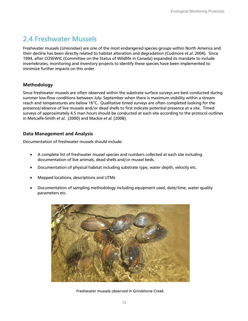
Methodology:

Conservation Halton’s Artificial Cover Object (ACO) design is based on the MNR plethodontid salamander sampling protocol (OMNR 2001). Wooden boards, approximately 20 x 75 cm in size and 1 inch thick, are used. In the fall, prior to the first year of monitoring, the boards are placed on the forest floor in direct contact with the soil. This allows the boards to weather over one winter before the first field visit is conducted. Beginning in the spring when temperatures are a minimum of 5°C and snow is gone, the ACOs are surveyed for salamanders every other week for a twelve week period, for a total of 6 visits. Each visit is completed at the same time of day and the species and age class of each individual is recorded. Total number of salamanders under each board is also recorded.


Information collected as part of the plethodontid salamander monitoring should include:

• All species names listed in tabular format

• UTM’s and details related to any SAR/rare species observed during the surveys


• Sampling details (date, sampler, location, mapping etc.) as well as ground and air temperature, precipitation in the last 24 hours, and Beaufort sky and wind codes

Analysis should include an assessment of overall abundance of salamanders within each plot area. Long term monitoring of plots should include analysis of soil temperatures for comparison against salamander abundance.


23

4 Wildlife Monitoring

4.1 Birds Birds play an important ecological role on the landscape and are found in a wide variety of habitats. Habitat preferences, varying sensitivities to change and the ability to make observations by sight and/or sound makes birds excellent indicators to assess change across a variety of habitats.

4.1.1 Forest Birds

Methodology

Conservation Halton employs the Forest Bird Monitoring Program (FBMP), originally administered by the Ontario Region of the Canadian Wildlife Service, Environment Canada (Environment Canada 2006) to monitoring breeding birds within wooded areas. Information collected through the FBMP provides information on population trends and habitat associations of birds that breed in the forest interior. Surveys are performed twice yearly using 10 minute point counts at stations between late May and early July, identifying all birds by sight or song. The first visit is made between May 24 and June 17, and the second visit between June 13 and July 10, with at least 6 days between visits. The stations are visited in the early morning hours between 5:00 a.m. and 10:00 a.m. Surveys are conducted in calm to light winds (< 15kph) and in clear or slightly damp conditions. Surveys are not conducted in the rain. All stations within a site are completed on the same day. Stations are 100 m circular unlimited distance sampling areas; however birds are recorded as being either within or outside of the 100m and birds obviously not associated with the forest being sampled are not recorded.


Information collected should include:

• All species names listed in tabular format, along with breeding evidence and number of birds observed. Details as to whether observations were within the 100m point count stations or fly-thrus should also be identified.

• Point count station locations and SAR/rare species in relation to previously classified ELC communities (UTM’s and mapping)

• Sampling details (date, sampler, location, mapping etc.)

Forest bird diversity is assessed using the following indices:

• Species abundance

• Species richness

• Shannon’s Diversity Index

Species richness refers to the number of species counted at each station and species abundance refers to the number of individuals.

Birds are also divided into guilds based on nesting and migratory behaviour as well as habitat assemblages. Proportion of species richness in each guild is analyzed, as well as total abundance within each guild.


24

Surveys for marsh birds are completed using the Marsh Monitoring Protocol (MMP)

4.1.2 Marsh Birds

Methodology

Conservation Halton marsh bird monitoring follows the Marsh Monitoring Protocol (BSC 2006b), which uses a "fixed distance" semi-circular sampling area. Surveys are conducted from a central point located on the edge of a 100 metre radius semi-circle sample area. Each marsh bird monitoring station is surveyed twice between May 20 and July 5, no less than 10 days apart. Routes are surveyed in their entirety, in the same station sequence each time. All surveys begin after 5 p.m. and end at or before sunset. Surveys are conducted in warm weather, with no precipitation, and with wind speed no more than a three on the Beaufort scale. As per the MMP protocol, each station is surveyed for 15 minutes and is comprised of a 5 minute silent (passive) period, followed by a 5 minute call broadcast period (using the official MMP broadcast recording), followed by another 5 minute silent listening period. All species within the 100m semi-circular station are recorded with any focal species observed, recorded within an unlimited distance semi-circle. Focal species for the MMP include American Bittern, American Coot, Black Rail, Common Moorhen, King Rail, Least Bittern, Pied-billed Grebe, Sora and Virginia Rail.


When conducting marsh bird surveys all data should be recorded on the marsh monitoring sheets provided by the Marsh Monitoring Program. In doing so, all data required is collected and species mapped within the semi-circular station. Additional information to provide as part of the marsh bird monitoring should include:

• All species names listed in tabular format, listed as within the “fixed” station or within the unlimited distance station (for focal species). Additional observations outside of the survey area or “fly-thrus” are also noted



Analysis should include an assessment of species richness, relative abundance, richness of marsh obligates and proportion of marsh obligates calculated for each point and summarized for each site. Species richness refers to the number of species counted at each station and species abundance refers to the number of individuals. Richness of marsh obligates refers to the number of species recorded that breed exclusively in marsh habitats. The proportion of these species relative to non-marsh obligates is then determined.

The Index of Marsh Bird Community Integrity (IMBCI) is used to examine each marsh’s ability to support indicator bird species. This index uses species characteristics (nesting habitat, foraging habitat, migratory status and breeding range) and the richness of marsh obligates to determine the health of a marsh ecosystem (DeLuca et al. 2004).


25

4.1.3 Additional Bird Surveys

Methodology

In habitats other than forests or marshes, bird surveys should be conducted using the Ontario Breeding Bird Atlas (OBBA) methodology (OBBA 2001). In doing so, 5 minute point counts are completed between dawn and 5 hours after dawn, within a 100m circular station, with the surveyor identifying all birds by sight and sound. Similar to the the FBMP protocol, birds are identified as being either within or outside of the 100m station with all breeding evidence noted. Two surveys conducted between May 24 and July 10, should be conducted and spread out over time to ensure that surveyors cover breeding periods for the highest number of bird species. Similar to other bird surveys, the OBBA methodology requires certain weather conditions to ensure the highest probability of detecting a variety of species. As a result, surveys should NOT be completed in thick fog or when winds are >3 on the Beaufort scale (over 19 km\h).


When conducting bird surveys as per the OBBA methodology all data should be recorded on the OBBA point count forms. Additional information to provide as part of bird monitoring surveys should include:

• All species names listed in tabular format, listed as within or outside of the 100m station



Analysis should include an assessment of species richness, relative abundance, richness and proportion of obligate species (per habitat type) and calculated and summarized for each point within a site.

4.2 Amphibian Monitoring Amphibians (frogs) are excellent indicators of environmental change as they are sensitive to changes in climate, atmospheric conditions and water quality and can be easily monitored through male calling. Their semi-terrestrial life cycle which consists of an aquatic larval stage and terrestrial adult stage also makes them sensitive to habitat alteration in both aquatic and terrestrial ecosystems.

Methodology

Amphibian monitoring is conducted following the Marsh Monitoring Program (MMP) (BSC 2006a). This protocol uses an "unlimited distance" semi-circular sampling area. Each amphibian station is visited on three nights, no less than fifteen days apart, during the spring and early summer. The visits are dictated by ambient air temperature as follows:

• The first visit is undertaken with a minimum night-time air temperature of at least 5°C and after the

warm rains of spring have begun;

• The second visit is undertaken once the night-time air temperature is at least 10°C; and,

• The third visit is undertaken once the night-time air temperature is at least 17°C.

Each station is surveyed for three minutes and the surveys start one half hour after sunset and end before midnight. All surveys are conducted in weather conducive to monitoring amphibians (i.e. on a warm, moist night with little or no wind). All amphibians heard and their associated calling codes are documented to provide a general index of abundance. The call codes are as follows:


26

• Code 1 – Individuals can be counted; calls not simultaneous. This number is assigned when individual

males can be counted and when the calls of individuals of the same species do not start at the same

time.

• Code 2 – Calls distinguishable; some simultaneous calling. This code is assigned when there are a few

males of the same species calling simultaneously. A reliable estimate of the abundance (rough

number or range of individuals heard) should be made.

• Code 3 – Full chorus; calls continuous and overlapping. This value is assigned when a full chorus is

encountered. A full chorus is when there are so many males of one species calling that all the calls

sound like they are overlapping and continuous. There are too many for a reasonable count or

estimate, therefore no abundance is recorded.


When conducting amphibian monitoring surveys all data should be recorded and mapped within the semi-

circular stations on the field sheets supplied by the Marsh Monitoring Program (Bird Studies Canada).

Additional information should include:

• All species names listed in tabular format and mapped on the field sheets within the semi-circular station.



Due to the survey methodology, abundance is represented through calling codes and as a result abundance of individual species is not reliable. As a result, typical analysis cannot be conducted on amphibian surveys. Instead an Index of Biotic Integrity (IBI) developed as part of the Great Lakes Coastal Monitoring Program is used to assess changes in biotic integrity at a site. The amphibian IBI uses the following metrics in its calculation:

• rTOT: Mean total species richness across survey stations in a wetland

• rWOOD: Mean species richness of woodland associated amphibian species across survey stations in a wetland

• pWOOD: Probability of detection of woodland-associated amphibian species across survey stations in a wetland

The IBI is than calculated based on the methodology outlined in the Great Lakes Coastal Wetlands Monitoring Plan (Great Lakes Coastal Wetland Consortium 2008). Scores are weighted out of 100, with higher scores indicating amphibian communities in better biotic condition.


27

4.3 Butterfly Monitoring Butterflies are often used as indicator species as they are dependent on specific plants as part of their larval life stage and require diverse nectar sources to support their adult life stage. As a result butterflies can be used as indicators species for grassland and meadow habitats.

Methodology

Following the methods outlined by Pollard and Yates (1993), observers walk a transect within an identified station and record the species name and number of individuals detected during each transect survey. To ensure consistency, the observers only record butterflies within a 5m2 area while walking a consistent speed. If a butterfly cannot be initially identified on the wing, the survey will be “paused” and no sightings recorded while the observer investigates and identifies the butterfly. The surveyor may leave the set transect route to identify the butterfly. Once the butterfly is identified the surveyor will return to the location where the transect was “paused” and will resume walking at the set pace, recording observations. Ideally, the transects will be conducted between the first week of April to the last week of September repeated as close to every two weeks as possible. If weather is unfavorable during the designated survey date then the surveys could occur up to three weeks apart. In order to best detect butterflies, the surveys should be completed on warm, clear sunny days with little wind, with the following survey conditions being met:

• Temperature must be a minimum of 13 C°

• When temperatures are between 13 C° and 17 C°, cloud cover must be less than 50%

• When over 18 degrees C°, cloud cover can be marginally higher than 50% but more sun is preferred

• Wind should be a 3 or lower on the Beaufort scale

Butterfly monitoring transects should be implemented across different habitat types within a site.


Butterfly monitoring information should include:

• All species names listed in tabular format,

• Transect locations and SAR/rare species in relation to previously classified ELC communities (UTM’s and mapping)

• Sampling details (date, sampler, location, transect #, mapping etc.)

Butterfly transect counts should be used to calculate overall butterfly and/or species abundance within an identified habitat type. All butterfly species identified within the transects are analyzed independently of each other due to differences in flight periods and behaviours. Data collected through the use of transects can also be useful in identifying habitat and nectaring preferences between species.


28

4.4 Significant Wildlife Habitat Wildlife habitat is an important natural heritage feature and is defined within the 2014 Provincial Policy Statement (PPS) as “areas where plants, animals, and other organisms live, and find adequate amounts of

food, water, shelter and space needed to sustain their populations.” Areas considered to be significant under the PPS are those that are “ecologically important in terms of features, functions, representation or

amount, and contributing to the quality and diversity of an identifiable geographic area or natural Heritage

System”. Development and site alterations are not be permitted on or adjacent to these areas “unless it has been demonstrated that there will be no negative impact on the natural features or their ecological

functions” (Ministry of Municipal Affairs and Housing 2014) identification of significant wildlife habitat is important when implementing any monitoring program related to the development or site alteration of natural lands.

Methodology

Numerous methodologies to identify significant wildlife habitat can be employed and may be dependent on the specific genera or species of interest. Randomized surveys and investigations outside of widely-used monitoring protocols are often required and as such no specific methodology is recommended for generalized wildlife habitat surveys.


Significant wildlife habitat including but not limited to, any rearing habitat, dens, nesting , breeding, migratory stopover, spawning, nursery and overwintering areas should be identified and mapped according to the criteria outline in the Significant Wildlife Habitat Criteria Schedules for Ecoregion 7E (OMNRF 2015). Additional wildlife Other important wildlife areas should be identified and mapped accordingly. These habitats may include, but are not limited to, waterfowl staging areas, fish spawning and/or nursery habitat, herpetofaunal breeding or hibernacula areas, wintering grounds, areas that provide temporary shelter or feeding areas for migratory wildlife, areas that provide critical life cycle habitat, and wildlife corridors. Information to provide as part of significant wildlife assessments includes:

• Mapping of habitat within previously classified ELC communities and superimposed on air photos • List of species including number of species, associated rarity ranks and identification of ELC codes of

habitat in which they were found. • Number of observations across the sampling period (multi-year studies may be required) • Sampling details (date, weather conditions, surveyor etc.)

4.5 Photomonitoring Photomonitoring is often used to illustrate the extent of visual change largely associated with lands or projects undergoing significant change such as through restoration, naturalization, development etc. In order for photomonitoring to be effective, the photomonitoring standards and documentation methods must be stringently followed. Conservation Halton photomonitoring standards are as followed:

• Monitoring points should be located throughout study areas and should be established to provide multiple views of the feature being monitoring (i.e. upstream/downstream views etc.)


29

• When a photomonitoring point is established (and for any new points added from thereon), a new point location that allows a clear view in all directions should be chosen. A marker is installed and the distance and compass bearing to a nearby permanent object(s) in each direction that photos will be taken, is recorded on the field sheet. A diagram showing the marker location and any permanent objects is drawn. Where possible, the following six photos should be taken in order to properly document the photomonitoring location:

� Field sheet: This allows for distinguishing between points once back at the office in

order to accurately label the photos.

� North of marker (0°)

� East (90°)

� South (180°)

� West (270°)

� Tripod location

• Permanent markers should be installed using PVC pipe spray painted and labeled with the point code. A tripod should be placed over the permanent marker such that the middle of the tripod is located directly over the marker. The tripod legs should be fully extended so that photos are always taken from the same height.

• A compass should be used to orient the camera in order to take photographs in all cardinal directions.

• After the camera is set up, images should be checked through the view finder in all directions to ensure images line up with previous years’ photographs. Check and record the camera settings. Photos should be taken at the same zoom-level each time (i.e. photos should not zoom in or out from previous years)

• Baseline photos should be taken for all photomonitoring points prior to the commencement of works. Photomonitoring should then occur on an annual basis once the project has been implemented. Photos should be taken during late summer when weather conditions are conducive to taking clear photographs.

• A note of the order the photos are taken in is recorded on the field sheet. Record any notable objects, plants, etc. that may assist in reorientation. Pictures should be checked while still at the point to ensure that an appropriate image was captured. If it is necessary to retake photos, ensure that a note is made of which pictures have been retaken.

• Immediately after returning to the office, photos are uploaded and renamed according to the field sheet. This allows for errors in recording to be corrected as the visit is fresh in your mind. Photos are filed according to site and should be labeled according to date and view (e.g. STN5_upstream of road looking upstream_July12_2016).

All photos provided as part of a report should be properly referenced with the following information for each photograph:

• Station name (or feature)

• View

• Date


30

References Bailey, R.G., R.D. Pfister and J.A. Henderson. 1978. Nature of land and resource classification: A review. Journal of Forestry 76: 650-655.

Bird Studies Canada (BSC). 2006a. Marsh Monitoring Program Guide to Amphibian Monitoring. Bird Studies Canada (BSC). 2006b. Marsh Monitoring Program Guide to Bird Monitoring. Canadian Council of Ministers of the Environment 2001. Canadian water quality guidelines for the protection of aquatic life: CCME Water Quality Index 1.0, Technical Report. In: Canadian environmental quality guidelines, 1999, Canadian Council of Ministers of the Environment, Winnipeg. Conservation Halton 2006. Long Term Environmental Monitoring Program. March 2006. Chu, C., N.E. Jones, A. R. Piggot and J.M. Buttle. 2009. Evaluation of a Simple Method to Classify the Thermal Characteristics of Streams Using a Nomogram of Daily Maximum Air and Water Temperatures. North American Journal of Fisheries Management 29: 1605-1619. Citizens’ Environment Watch. 2009. Water Quality Monitoring with Benthic Macroinvertebrates: Field Manual. Citizens’ Environment Watch. Toronto. Credit Valley Conservation. 2010. Monitoring Forest Integrity within the Credit River Watershed. Chapter 3: Forest Vegetation 2005-2009, Credit Valley Conservation. vi + 104 pp.

Cudmore, B., C.A. MacKinnon and S.E. Madzia. 2004. Aquatic species at risk in the Thames River

watershed, Ontario. Can. MS Rpt. Fish. Aquat. Sci. 2707: v + 123 p.

DeLuca, W.V., C.E. Studds, L.L. Rockwood, and P.P. Marra. 2004. Influence of land use on the integrity of marsh bird communities of Chesapeake Bay, USA. Wetlands 24(4): 837-847. Environment Canada. 2006. Ontario Forest Bird Monitoring Program (FBMP). Ontario Region of the Canadian Wildlife Service. http://www.on.ec.gc.ca/wildlife/newsletters/fbmp06-e.html [Accessed October 1, 2006] Great Lakes Coastal Wetland Consortium. 2008. Great Lakes Coastal Wetland Monitoring Plan. Hilsenhoff, W.L. 1988. Rapid field assessment of organic pollution with a family-level biotic index. Journal of North American Benthological Society 7:65-68. Jones, C., K. Somers, B. Craig and T. Reynoldson, 2007. Ontario Benthos Biomonitoring Network Protocol Manual. Ontario Ministry of Environment, Environmental Monitoring and Reporting Branch, Dorset, Ontario.

Lee, H.T., W.D. Bakowsky, J. Riley, J. Bowles, M. Puddister, P. Uhlig and S. McMurray. 1998. Ecological Land Classification for Southern Ontario: First Approximation and Its Application. Ontario Ministry of Natural Resources, Southcentral Science Section Field Guide FG-02. 225 pp.


31

Metcalfe-Smith, J., G.L. Mackie, J. Di Maio and S. Staton. 2000. Changes Over Time in the Diversity and Distributio of Freshwater Mussels (Unionidae) in the Grand River. Journal of Great Lakes Research. Volume 26, Issue 4, 2000, Pages 445–459

Mackie, G., Morris, T.J., and Ming, D. 2008. Protocol for the detection and relocation of freshwater

mussel species at risk in Ontario-Great Lakes Area (OGLA). Can. Manuscr. Rep. Fish. Aquat. Sci. 2790: vi

+50 p.

Ministry of Municipal Affairs and Housing. 2014. 2014 Provincial Policy Statement. Queens Printer for

Ontario.

Ministry of the Environment. 1999. Water Management: Goals, Policies, Objectives and Implementation Procedures of the Ministry of the Environment. Oldham, M.J., W.D. Bakowsky, and D.A. Sutherland. 1995. Floristic Quality Assessment System for Southern Ontario. Natural Heritage Information Centre, Ontario Ministry of Natural Resources, Peterborough, Ontario. 29 pp. Ontario Breeding Bird Atlas (OBBA). 2001. Guide for Participants. Atlas Management Board, Federation of Ontario Naturalists, Don Mills. Ontario Ministry of Natural Resources (OMNR). 2001. A Sampling Protocol for Red-backed Salamander (Plethodon cinereus) Populations in Ontario: 2nd Pilot Study. Queens Printer for Ontario. Ontario Ministry of Natural Resources (OMNR) and the Toronto and Region Conservation Authority (TRCA). 2005. Humber River Fisheries Management Plan. Published by the Ontario Ministry of Natural Resources and the Toronto and Region Conservation Authority. Queens Printer for Ontario. Ontario Ministry of Natural Resources and Forests (OMNRF). 2015. Significant Wildlife Habitat Criteria Schedules for Ecoregion 7E. Regional Operations Division. Peterborough, Ontario.

Province of Ontario. 2005. Places to Grow Act. Ontario Regulation 415/05: Growth Plan Areas

Roberts-Pichette, P. and L. Gillespie. 1999. Terrestrial Vegetation Biodiversity Monitoring Protocols. EMAN Occasional Paper Series Report No 9. EMAN Coordinating Office. Burlington, Canada. Pollard, E, and T.J. Yates. 1993 Monitoring Butterflies for Ecology and Conservation. Chapman & Hall, London, UK. Stanfield, L. (Editor) 2017. Ontario Stream Assessment Protocol. Version 10.0, Fish and Wildlife Branch. Ontario Ministry of Natural Resources. Peterborough, Ontario. 546 pp. Steedman, R.J. 1988. Modification and Assessment of an Index of Biotic Integrity to Quantify Stream Quality in Southern Ontario. Canadian Journal of Fisheries and Aquatic Sciences 45:492-495. Stoneman, C.L. and M.L. Jones. 1996. A Simple Method to Classify Stream Thermal Stability with Single Observations of Daily Maximum Water and Air Temperature. North American Journal of Fisheries Management 16:728-737.

Conservation Halton Ecological Monitoring Protocols

Documents

Transcript of Conservation Halton Ecological Monitoring Protocols