Error Reconciliation Protocols for Continuous-Variable ...
139
General rights Copyright and moral rights for the publications made accessible in the public portal are retained by the authors and/or other copyright owners and it is a condition of accessing publications that users recognise and abide by the legal requirements associated with these rights. Users may download and print one copy of any publication from the public portal for the purpose of private study or research. You may not further distribute the material or use it for any profit-making activity or commercial gain You may freely distribute the URL identifying the publication in the public portal If you believe that this document breaches copyright please contact us providing details, and we will remove access to the work immediately and investigate your claim. Downloaded from orbit.dtu.dk on: Jan 30, 2022 Error Reconciliation Protocols for Continuous-Variable Quantum Key Distribution Mani, Hossein Publication date: 2020 Document Version Publisher's PDF, also known as Version of record Link back to DTU Orbit Citation (APA): Mani, H. (2020). Error Reconciliation Protocols for Continuous-Variable Quantum Key Distribution. Department of Physics, Technical University of Denmark.
-
Upload
khangminh22 -
Category
Documents
-
view
3 -
download
0
Transcript of Error Reconciliation Protocols for Continuous-Variable ...

General rights Copyright and moral rights for the publications made accessible in the public portal are retained by the authors and/or other copyright owners and it is a condition of accessing publications that users recognise and abide by the legal requirements associated with these rights.
Users may download and print one copy of any publication from the public portal for the purpose of private study or research.
You may not further distribute the material or use it for any profit-making activity or commercial gain
You may freely distribute the URL identifying the publication in the public portal If you believe that this document breaches copyright please contact us providing details, and we will remove access to the work immediately and investigate your claim.
Downloaded from orbit.dtu.dk on: Jan 30, 2022
Error Reconciliation Protocols for Continuous-Variable Quantum Key Distribution
Mani, Hossein
Publication date:2020
Document VersionPublisher's PDF, also known as Version of record
Link back to DTU Orbit
Citation (APA):Mani, H. (2020). Error Reconciliation Protocols for Continuous-Variable Quantum Key Distribution. Departmentof Physics, Technical University of Denmark.
Ph.D. ThesisDoctor of Philosophy
Error Reconciliation Protocols forContinuous-Variable Quantum Key Distribution
Department of PhysicsTechnical University of Denmark
Hossein Mani
Supervisor: Professor Ulrik Lund AndersenCo-supervisor: Associate professor Tobias GehringCo-supervisor: Senior researcher Christoph Pacher
Kongens Lyngby 2020

DTU PhysicsDepartment of PhysicsTechnical University of Denmark
Fysikvej,Building 3112800 Kongens Lyngby, DenmarkTel.: +45 4525 [email protected]://www.fysik.dtu.dk/english

SummaryContinuous-variable quantum key distribution (CV-QKD) utilizes an ensemble of co-herent states of light to distribute secret encryption keys between two parties. One ofthe key challenges is the requirement of capacity-approaching error correcting codesin the low signal-to-noise (SNR) regime (SNR < 0 dB). Multi-level coding (MLC)combined with multi-stage decoding (MSD) can solve this challenge in combinationwith multi-edge-type low-density parity-check (MET-LDPC) codes which are idealfor low code rates in the low SNR regime due to degree-one variable nodes. How-ever, designing such highly efficient codes remains an open issue. Here, we introducethe concept of generalized extrinsic-information transfer (G-EXIT) charts for MET-LDPC codes and demonstrate how this tool can be used to analyze their convergencebehavior. We calculate the capacity for each level in the MLC-MSD scheme and useG-EXIT charts to exemplary find codes for some given rates which provide a betterdecoding threshold compared to previously reported codes. In comparison to the tra-ditional density evolution method, G-EXIT charts offer a simple and fast asymptoticanalysis tool for MET-LDPC codes.
A linear optimization approach to design highly efficient MET-LDPC codes atvery low SNR, which is highly required by certain applications like CV-QKD will bediscussed. The cascade structure is introduced in terms of three disjoint submatricesand a convex optimization problem is proposed to design highly efficient MET-LDPCcodes based on cascade structure. Simulation results show that the proposed algo-rithm is able to design MET-LDPC codes with efficiency higher than 95%, especiallyat very low SNR.

ii

AbstraktKontinuert variable kvante-nøgledistribution (CV-QKD) bruger et ensemble af ko-hærent lysttilstande til at distribuere hemmelige krypteringsnøgler mellem to parter.Én af udfordringerne er kravet om fejlkorrektionskoder der nærmere sig Shannon-kapaciteten i detlave signal-til-støj (SNR) regime (SNR < 0 dB). Flerniveaus-kodning(MLC) kombineret med flerstadie-afkodning (MSD) kan løse denne udfordring i kom-bination med flerkants-type lavdensitetsparitetscheck (MET-LDPC) koder, som erideel for lave koderater i det lave SNR-regime pga. grad-1 variable knuder. Imidler-tid er design af sådanne effektive koder stadig etåbent problem. Her introducerervi konceptet af diagrammer for generaliseret overførelse af udefrakommende informa-tion (G-EXIT) for MET-LDPC-koder og demonstrerer, hvordan dette værktøj kanbruges til at analysere deres konvergensadfærd. Vi beregner kapaciteten for hvertniveau i MLC-MSD-ordningen og bruger G-EXIT-diagrammer i eksempler på at findekoder til givet rater, der giver en bedre afkodningstærskel sammenlignet med tidligererapporterede koder. Sammenlignet med den traditionelle tæthedsudviklingsmetode(density evolution method)tilbyder G-EXIT-diagrammer et simpelt og hurtigt asymp-totisk analyseværktøj til MET-LDPC-koder.
En lineær optimeringsmetode til at designe meget effektive MET-LDPC-koder vedmeget lav SNR, hvilket kræves af visse applikationer som CV-QKD, bliver diskuteret.Kaskadestrukturenintroduceres i form af tre usammenhængende undermatricer, ogder foreslås et konveks optimeringsproblem til at designe effektive MET-LDPC-koderbaseret på kaskadestruktur. Simuleringsresultater viser, at den foreslåede algoritmeer i stand til at designe MET-LDPC-koder med effektivitet højere end 95%, især vedmeget lav SNR.

iv

PrefaceThis PhD thesis was prepared at the department of Physics at the Technical Universityof Denmark in fulfillment of the requirements for acquiring a PhD degree in Physics.
Kongens Lyngby, August 31, 2020
Hossein Mani

vi

AcknowledgementsThis Ph.D thesis is the output of the effort and support of several people to whomeI am deeply greatful. At first, I thank my supervisors professor Ulrik Lund An-dersen, Associate professor Tobias Gehring, and associate professor ChristophPacher. It has been a great advantage to work with you all. I could not have imag-ined having better advisors and mentors for my Ph.D study.Ulrik, thanks for all your support and responsiveness that brought me to the Den-mark. Your advices were of great help.Tobias, I am sincerely greatful for your presence and attention during these years.Many thanks for your supports both technically and personally.Christoph, thanks for facilitating my transition to Vienna and for your technicalsupports. I learned a lot from you.
Besides my advisors, I would like to thank the rest of my thesis committee: Pro-fessor Søren Forchhammer, Professor Vicente Martin, and Associate Professor. JesúsMartínez Mateo, for their insightful comments and encouragement.
I would like to thank all the people (fellow Ph.D students and postdoctoral re-searchers, professors, administration, guest researchers, ...) in both the QuantumPhysics and information Technology (QPIT) center and the Austrian institute ofTechnology (AIT) who created a great work environment (Mikkel, Casper, Ulrich,Alexander, Jonas, Tine, Sepehr, Ilya, ...). Especially, I thank my fellow labmatesboth in DTU and AIT for the helpful discussions, for the great environment we wereworking together, and for all the fun we have had in these years: Dr. Nitin Jain, Dr.Hou-Man Chin, Dr. Dino Solar Nikolic, Dr. Arne Kordts, Dr. Fabian Laudenbach,Mr. Philipp Grabenweger, ....
I am greatly indebted to my ceremonial assistant Mahtab Madani who madethe years my Ph.D run safe and sound.Mahtab, my love, thank you very much for being by my side for 5 years. Could nothave done it without you.
Also I thank my friends in the University of Idaho and Tarbiat Modares University.In particular, I am grateful to Prof. Saied Hemati and Associate professor HamidSaeedi for all the supports.
Fortunately, I have also the privilege of having a lovely family who had a funda-mental role in getting me through the PhD process successfully. Thank you all.

viii Acknowledgements

AcronymsIn this thesis we also use standard terminology and acronyms. Here we present listof acronyms.
ADC Analog-to-Digital Converter
AES Advanced Encryption Standard
AWGN Additive White Gaussian Noise
BEC Binary Erasure Channel
BER Bit Error Rate
BF Bit-Flipping
BI-AWGN Binary-Input Additive White Gaussian Noise
BIOSM Binary-Input Output-Symmetric Memoryless
BP Belief Propagation
BPSK Binary Phase Shift Keying
BSC Binary Symmetric Channel
CN Check-Node
CSI Channel Side Information
CV Continuous Variable
CV-QKD Continuous-Variable Quantum Key Distribution
DAC Digital-to-Analog Converter
DE Density Evolution
DES Data Encryption Standard
DV-QKD Discrete-Variable Quantum Key Distribution

x Acronyms
EB Entanglement Based
EXIT Extrinsic-Information Transfer
FER Frame Error Rate
FR Forward Reconciliation
G-EXIT Generalized Extrinsic-Information Transfer
i.i.d Independent and identically distributed
KL Kullback-Leibler
LDPC Low-Density Parity-Check
LLR Log-Likelihood Ratio
LSB Least-Significant Bit
MET Multi-Edge-Type
MET-LDPC Multi-Edge-Type Low-Density Parity-Check
MLC Multi-Level-Coding
MLC-MSD Multi-Level-Coding Multi-Stage-Decoding
MP Message Passing
MS Min-Sum
MSB Most-Significant Bit
MSD Multi-Stage-Decoding
PC Polarization Controller
PDF Probability Density Function
P&M Prepare and Measure
QC-LDPC Quaci-Cyclic LDPC
QKD Quantum Key Distribution
QRNG Quantum Random Number Generator
RR Reverse Reconciliation
RSA Rivest Shamir Adleman
SCA Stochastic Chase Algorithm

Acronyms xi
SCE Socket Count Equality
SNR Signal to Noise Ratio
SNU Shot-Noise Unit
TMSVS Two-Mode-Squeezed Vacuum State
VN Variable-Node

xii
ContentsSummary i
Abstrakt iii
Preface v
Acknowledgements vii
Acronyms ix
Contents xiii
List of Figures xv
List of Tables xvii
1 Introduction 11.1 Cryptography: History, Present, Future . . . . . . . . . . . . . . . . . 11.2 Important challenges in post-processing of QKD . . . . . . . . . . . . 21.3 Thesis outline . . . . . . . . . . . . . . . . . . . . . . . . . . . . . . . . 41.4 Academic publications . . . . . . . . . . . . . . . . . . . . . . . . . . . 5
2 Quantum Key Distribution with Continuous Variables 72.1 Introduction . . . . . . . . . . . . . . . . . . . . . . . . . . . . . . . . . 72.2 CV-QKD with Gaussian modulation . . . . . . . . . . . . . . . . . . . 82.3 Security Analysis and Secure Key Rate . . . . . . . . . . . . . . . . . . 142.4 Experimental setup . . . . . . . . . . . . . . . . . . . . . . . . . . . . . 19
3 Information Reconciliation of CV-QKD 213.1 Multidimensional Reconciliation . . . . . . . . . . . . . . . . . . . . . 223.2 Multi-Level-Coding Multi-Stage-Decoding . . . . . . . . . . . . . . . . 253.3 Comparison between reverse and forward reconciliation . . . . . . . . 433.4 Randomized Reconciliation . . . . . . . . . . . . . . . . . . . . . . . . 483.5 Reconciliation for a wide range of SNRs . . . . . . . . . . . . . . . . . 51
4 On the Design of Highly Efficient MET-LDPC codes 55

xiv Contents
4.1 Multi-Edge-Type LDPC codes . . . . . . . . . . . . . . . . . . . . . . 554.2 Density evolution and other asymptotic analysis tools . . . . . . . . . 604.3 G-EXIT charts for MET-LDPC codes . . . . . . . . . . . . . . . . . . 664.4 Code design optimization problem . . . . . . . . . . . . . . . . . . . . 744.5 Optimization for cascade structure . . . . . . . . . . . . . . . . . . . . 784.6 Highly efficient codes . . . . . . . . . . . . . . . . . . . . . . . . . . . . 834.7 Simulation Results . . . . . . . . . . . . . . . . . . . . . . . . . . . . . 87
5 Conclusion and Future Directions 91
A Introduction to LDPC codes 95A.1 Preliminaries . . . . . . . . . . . . . . . . . . . . . . . . . . . . . . . . 95A.2 Channel entropy and channel capacity . . . . . . . . . . . . . . . . . . 97A.3 Low-density parity-check (LDPC) codes . . . . . . . . . . . . . . . . . 98A.4 Belief Propagation . . . . . . . . . . . . . . . . . . . . . . . . . . . . . 100A.5 EXIT and G-EXIT charts . . . . . . . . . . . . . . . . . . . . . . . . . 101A.6 Plotting EXIT and G-EXIT Charts . . . . . . . . . . . . . . . . . . . . 102
B Reconciliation software for CV-QKD 105B.1 About the Software . . . . . . . . . . . . . . . . . . . . . . . . . . . . . 105B.2 How to install the software . . . . . . . . . . . . . . . . . . . . . . . . 107
C Software to design highly efficient MET-LDPC codes 109C.1 About the software . . . . . . . . . . . . . . . . . . . . . . . . . . . . . 109
Bibliography 111

List of Figures2.1 Simple illustration of QKD system . . . . . . . . . . . . . . . . . . . . . . 102.2 Phase-space representation . . . . . . . . . . . . . . . . . . . . . . . . . . 122.3 Ideal homodyne detection . . . . . . . . . . . . . . . . . . . . . . . . . . . 132.4 Effect of reconciliation efficiency-Asymptotic . . . . . . . . . . . . . . . . 172.5 Effect of reconciliation efficiency-Finite-size . . . . . . . . . . . . . . . . . 182.6 Experimental setup . . . . . . . . . . . . . . . . . . . . . . . . . . . . . . . 19
3.1 Multidimensional reconciliation . . . . . . . . . . . . . . . . . . . . . . . . 243.2 Reconciliation: Multi-level coding . . . . . . . . . . . . . . . . . . . . . . . 273.3 Binary set partitioning . . . . . . . . . . . . . . . . . . . . . . . . . . . . . 273.4 Digitizer intervals and levels . . . . . . . . . . . . . . . . . . . . . . . . . . 293.5 Digitization effect . . . . . . . . . . . . . . . . . . . . . . . . . . . . . . . . 303.6 Reconciliation: One-level coding . . . . . . . . . . . . . . . . . . . . . . . 313.7 Reconciliation: Two-level coding . . . . . . . . . . . . . . . . . . . . . . . 363.8 Channel coding rates for individual levels . . . . . . . . . . . . . . . . . . 393.9 Mutual information for individual levels . . . . . . . . . . . . . . . . . . . 403.10 Numerical joint PMF at SNR = −5 dB . . . . . . . . . . . . . . . . . . . 413.11 Forward vs Reverse reconciliation . . . . . . . . . . . . . . . . . . . . . . . 433.12 Admissible rate region . . . . . . . . . . . . . . . . . . . . . . . . . . . . . 453.13 Differential entropies . . . . . . . . . . . . . . . . . . . . . . . . . . . . . . 453.14 Decoding by measured soft information . . . . . . . . . . . . . . . . . . . 483.15 Reconciliation efficiencies for SNR range . . . . . . . . . . . . . . . . . . . 523.16 Shortening process . . . . . . . . . . . . . . . . . . . . . . . . . . . . . . . 53
4.1 Graphical representation of MET-LDPC code . . . . . . . . . . . . . . . . 584.2 KL divergence for Gaussian approximation . . . . . . . . . . . . . . . . . 634.3 KL divergence for edge type two . . . . . . . . . . . . . . . . . . . . . . . 644.4 KL divergence for edge type three . . . . . . . . . . . . . . . . . . . . . . 644.5 EXIT chart for rate 0.5 . . . . . . . . . . . . . . . . . . . . . . . . . . . . 684.6 G-EXIT chart for MET-LDPC with rate 0.02 . . . . . . . . . . . . . . . . 714.7 Convergence behavior on a BEC . . . . . . . . . . . . . . . . . . . . . . . 724.8 G-EXIT chart for MET-LDPC with rate 0.02 on a BI-AWGN channel . . 754.9 EXIT chart for base code with additional noise . . . . . . . . . . . . . . . 814.10 Optimization problem for the connector part . . . . . . . . . . . . . . . . 83
xvi List of Figures
4.11 Optimization algorithm . . . . . . . . . . . . . . . . . . . . . . . . . . . . 844.12 The FER Comparison for rate 0.02 . . . . . . . . . . . . . . . . . . . . . . 884.13 The efficiency Comparison for rate 0.02 . . . . . . . . . . . . . . . . . . . 89
A.1 The schematic representation of standard BIOSM channels . . . . . . . . 96A.2 The capacity of the BEC and BSC channels . . . . . . . . . . . . . . . . . 99A.3 The capacity of the BI-AWGN and AWGN channels . . . . . . . . . . . . 99
C.1 EXIT chart for rate 0.8 irregular LDPC code . . . . . . . . . . . . . . . . 110

List of Tables2.1 CV-QKD vs DV-QKD . . . . . . . . . . . . . . . . . . . . . . . . . . . . . 8
3.1 Digitization effect . . . . . . . . . . . . . . . . . . . . . . . . . . . . . . . . 303.2 Decoders complexity . . . . . . . . . . . . . . . . . . . . . . . . . . . . . . 51
4.1 Table format for MET-LDPC codes . . . . . . . . . . . . . . . . . . . . . 564.2 Rate 0.02 MET-LDPC code . . . . . . . . . . . . . . . . . . . . . . . . . . 574.3 MET-LDPC code with cascade structure . . . . . . . . . . . . . . . . . . 594.4 Complexity comparison for different algorithms . . . . . . . . . . . . . . . 654.5 G-EXIT curves on BE channel . . . . . . . . . . . . . . . . . . . . . . . . 704.6 EXIT curves on BIOSM channel . . . . . . . . . . . . . . . . . . . . . . . 734.7 G-EXIT curves on BIOSM channel . . . . . . . . . . . . . . . . . . . . . . 734.8 Table presentation for MET-LDPC code with rate 0.02 . . . . . . . . . . 774.9 MET-LDPC code with Rate 0.01 . . . . . . . . . . . . . . . . . . . . . . . 844.10 MET-LDPC code with Rate 0.02 . . . . . . . . . . . . . . . . . . . . . . . 854.11 MET-LDPC code with Rate 0.05 . . . . . . . . . . . . . . . . . . . . . . . 854.12 MET-LDPC code with Rate 0.10 . . . . . . . . . . . . . . . . . . . . . . . 864.13 MET-LDPC code with Rate 0.25 . . . . . . . . . . . . . . . . . . . . . . . 86
5.1 Summary of designed codes . . . . . . . . . . . . . . . . . . . . . . . . . . 92
A.1 The distribution of the L conditioned on the X = 1 . . . . . . . . . . . . 97A.2 The parametric representation of an EXIT chart . . . . . . . . . . . . . . 103A.3 The parametric representation of G-EXIT chart . . . . . . . . . . . . . . . 103

xviii

CHAPTER1Introduction
1.1 Cryptography: History, Present, FutureHistorically, cryptography was used mainly for military purposes. The famous Caesarcipher or scytale of Sparta in ancient Greece are examples of historical cryptographysystems. For encryption the Caesar cipher substitutes each letter in the message(plain-text) by another letter shifted by some fixed number (key). Decryption is thereverse operation which is applied to the encrypted message (cipher-text) to recoverthe plain-text. The number of fixed shifts for the Caesar cipher was allegedly 3. It isclear that the number of possible keys for this cipher is 26. Thus, one unauthorizedperson can test all the possible keys in a brute-force attack to recover the plain-text. In addition, some efficient attacks also exist based on frequency analysis of thecipher-text. The academic research in the field of cryptography was started in late1970s. Today, the cryptography is an integral part of everyday life. It is impossibleto imagine an internet based activity without cryptography. It can be a simple Webbrowsing, sending email or a money transfer in a bank system.
The science of cryptography and the science of cryptanalysis are considered witheach other as the filed of cryptology. Classical cryptography after the computer ageconsists of two main categories, symmetric and asymmetric cryptography.
In symmetric cryptography two legitimate parties perform encryption and decryp-tion with a shared secret key. The Data Encryption Standard (DES) is an exampleof symmetric cryptography, created by IBM in early 1970s. In 1977 with modifi-cations from the United States National Security Agency (NSA) it was used as agovernment standard suitable for commercial applications. The private key of DESis 56-bit which makes it vulnerable for brute-force attack. In 1997 the United States’National Institute of Standards (NIST) organized an open competition and in 2000they announced the Advanced Encryption Standard (AES) as a block cipher withthree different key sizes 128, 192 and 256. Regardless of encryption standard the pro-cedure to share the secret key plays an important role in the security of the system.One practical method to share the secret key is the use of smart cards which is notvery promising and cost efficient solution in large scale networks. Another solution isthe use of asymmetric or public key cryptography. Public key cryptography uses twodifferent keys for encryption and decryption. The public key is used for encryptionand the private key remains secret for decryption. In public key cryptography theencryption procedure corresponds to a public key and should be a simple task. The

2 1 Introduction
decryption task should be easy for everyone who has the private key, but shouldbe very complicated for someone who does not have the private key. In principle,asymmetric cryptography algorithms like Rivest Shamir Adleman (RSA), Elgamaland ECDSA are based on mathematical problems (integer factorization, discrete log-arithm and Elliptic curves). It implies that the security of these algorithms dependson the eavesdropper computational power.
In practice, if two parties want to send each other a long message, they use ahybrid encryption system. First they use an asymmetric cipher to share key betweeneach other and then use a symmetric cipher to transmit the actual data. It is dueto the fact that for large amounts of data the symmetric ciphers are faster than theasymmetric ciphers.
The security of today’s asymmetric cryptography, e.g. the RSA protocol and theDiffie-Hellman key-exchange protocol, is based on mathematical complexity assump-tions of basic problems like the discrete log problem and the factorization of largenumbers [1]. These classical algorithms provide computational security. The adventof the quantum computer or an unexpected algorithmic innovation can compromisetheir security with drastic consequences for the internet.
One possible solution is quantum key distribution (QKD) [2, 3] which providesinformation theoretical secure cryptographic key exchange for two parties, Alice andBob, based on the properties of quantum mechanics (no cloning theorem, superposi-tion, entanglement and nonlocality). The idea of using quantum physics for cryptog-raphy was first introduced in the 1983. The idea was taken from the fact that in aquantum system cannot be measured without perturbing the system. Thus Alice andBob can share a key based on transmission and measurement of quantum states andEve cannot extract any information about the communication without introducingperturbations. Thus, thanks to the fundamental principles of quantum physics theQKD makes us able to detect illegitimate parties and provide a secure communicationlink.
1.2 Important challenges in post-processing of QKDSeveral commercial QKD implementations have already exists worldwide. Apart fromdifferent variations of QKD systems which are based on discrete-variable (DV) orcontinuous-variable (CV) the post-processing of QKD protocols still remained chal-lenging for long distance. Recent results show that for continuous-variable quan-tum key distribution (CV-QKD) using optical fibers the longest possible distance is202.81 km with output key rate of 6.24 bits/s [4]. For discrete-variable quantum keydistribution (DV-QKD) the maximum reported distance is 307 km with output keyrate of 3.18 bits/s [5]. The motivation of this thesis is to address two of the keychallenges that exists in post-processing of QKD system by focusing on CV-QKD:
1. High throughput reconciliation for CV-QKD: In the case of CV-QKD two dif-ferent approaches can be used to extract binary information from Gaussian

1.2 Important challenges in post-processing of QKD 3
variables. Currently the best known reconciliation method for CV-QKD usesa multi-dimensional reconciliation [6]. Though this method denotes high effi-ciency specifically at very low SNRs it is limited to extract just one bit from theGaussian symbols. In principle for the CV-QKD in contrast to DV-QKD it ispossible to extract more than one bit from Gaussian symbols. One of the bestknown methods to extract more than one bits from Gaussian symbols is multi-level-coding multi-stage-decoding (MLC-MSD) [7]. The MLC-MSD method hasbeen used for reconciliation but particular advantage of MLC-MSD reconcilia-tions remained unclear due to lack of study [8, 9].
• In this thesis we provide a detailed analysis of the MLC-MSD schemeand denote that it is possible to extract two-bits from Gaussian symbols.Specifically, we calculate the soft information for two levels which then canbe used by soft decoders.
• We will show that the MLC-MSD scheme requires multiple encoders anddecoders each working at specific rate. In addition we provide both an-alytical and numerical methods to calculate the code rates for each level.Details are provided in Section 3.2.5.
• In this thesis also we introduce the concept of randomized reconciliationwhich can be used to increase the throughput of the reconciliation taskby sacrificing the frame error rate performance. The idea of randomizedreconciliation is to use a fast hard-decoder instead of complicated soft-decoder and feed different error patterns to the hard-decoder. The errorpatterns should be generated randomly using the soft information that weextracted from the channel. More details about randomized reconciliationis provided in Section 3.4.
2. Long distance CV-QKD: Current implementations of CV-QKD shows that forefficient reconciliation an error correction task is required at very low signal-to-noise ratio (SNR). For instance in [10] an SNR of −15.37 dB was reported fora transmission distance of 80 km and in [11] an SNR of −16.198 dB for 100 km.Designing highly efficient forward error correction codes (FECs) at such a lowSNR is one of the core problems. Though multi-edge-type low-density parity-check (MET-LDPC) codes have been widely applied to QKD for error correc-tion the characteristics of these codes and their design procedure are not widelyunderstood. Few researchers have addressed the problem of designing highly ef-ficient degree-distribution (DD) for MET-LDPC codes but unfortunately theirworks are limited to high SNR regime (SNR > 0) and require high computa-tional complexity for their optimization algorithm [12, 13, 14]. To the bestof our knowledge the only available DD for a rate 0.02 MET-LDPC code waspresented in [10] and has an asymptotic efficiency of 98%.
• In this thesis we analyse the charactristics of the MET-LDPC codes andfocuse on MET-LDPC codes with cascade structure. More details aboutthe cascade strucures and MET-LDPC codes can be found in Section 4.1.

4 1 Introduction
• We propose a new approximation method for density evoution (DE) ofMET-LDPC codes called semi-Gaussian approximation.
• In addition the concept of extrinsic-infromation transfer chart (EXIT) andgeneralized-EXIT (G-EXIT) chart are introduced for MET-LDPC codes.Then we will show how these tools can be used to analyse the performanceof the MET-LDPC codes.
• Furthermore, in this thesis we provide an algorithmic approach to designhighly efficient DD for MET-LDPC codes for low SNR.
• Using our proposed algorithm we design some new highly efficient DDsfor MET-LDPC codes. For example we designed a new DD for rate 0.02which has an asymptotic efficiency of 99.2%. Also we designed a new codefor rate 0.01 which can works at SNR −18.48 dB.
.
1.3 Thesis outlineThis thesis is divided into five chapters. Chapter 2, gives a brief overview of theCV-QKD. Some important steps in CV-QKD protocols are explained. Also we talkabout the secure key rate and some of the important factors for long distance CV-QKD. Finally our the experimental setup is presented.
Chapter 3, focuses on the reconciliation process of CV-QKD. First, a brief overviewof multi-dimensional reconciliation is represented. Secondly, we focus on reconcilia-tion based on MLC-MSD and a detailed analysis is presented. We calculate the softinformation for deocders at each level and denote how to find the optimum code ratein MLC-MSD scheme. Then, we propose a new reconciliation scheme called Random-ized Reconciliation to increase the throughput of the reconciliation scheme. Finallywe talk about existing tools and methods to provide a robust reconciliation for a widerange of SNRs.
In Chapter 4, a detailed analysis of MET-LDPC codes is presented. First, itstarts by defining this class of error correction codes. Secondly, we talk about DEand other asymptotic analysis tools for MET-LDPC codes. We also propose our semi-Gaussian approximation method. Thirdly, we introduce the concept of generalizedextrinsic-information transfer (G-EXIT) chart and explain how we can develop thisconcept for MET-LDPC codes. In addition we explain how the convergence behaviorof MET-LDPC codes can be described by G-EXIT charts. Fourthly, we propose ournew algorithmic optimization process to design highly efficient MET-LDPC codes.Then we present for the first time some new DDs for MET-LDPC codes designed byour new algorithm. These codes are specifically designed for low rate applicationslike CV-QKD. Finally we show the performance of the rate 0.02 code.
In Chapter 5 we conclude the thesis. In addition this thesis contains three ap-pendices. In Appendix A, we explain requirements related to the LDPC codes. In

1.4 Academic publications 5
addition the definition of EXIT and G-EXIT functions for irregulr LDPC codes arepresented. In Appendix B, useful information can be found about our software toolsrelated to the reconciliation of the CV-QKD. Appendix C explains how to use thesoftware tools to design new degree distributions for MET-LDPC codes.
1.4 Academic publicationsThe results of this thesis have been presented in posters and presentations at theconferences [15, 16, 17] and also some of the results are submitted to peer-reviewedjournals where the arXived version are also available [18]. Here is the list of ourpublications:
1. H. Mani, T. Gehring, C. Pacher, and U. L. Andersen, “Multi-edge-type LDPCcode design with G-EXIT charts for continuous-variable quantum key distribu-tion,”ArXiv, vol. abs/1812.05867, 2018. [Online]. Available: https://arxiv.org/pdf/1812.05867.pdf
2. H. Mani, T. Gehring, C. Pacher, and U. L. Andersen, “An approximation methodfor analysis and design of multi-edge type LDPC codes,” 2018. [Online]. Avail-able: http://2018.qcrypt.net/others/accepted-posters/
3. H. Mani, T. Gehring, C. Pacher, and U. L. Andersen, “Algorithmic approach todesign highly efficient MET-LDPC codes with cascade structure,” 2019. [Online].Available: http://2019.qcrypt.net/scientific-program/posters/
4. H. Mani, B. Ömer, U. L. Andersen, T. Gehring, and C. Pacher, “Two MET-LDPC codes designed for long distance CV-QKD,” 2020.[Online]. Available:https://2020.qcrypt.net/accepted-papers/#list-of-accepted-posters

6

CHAPTER2Quantum Key
Distribution withContinuous Variables
This chapter is about the principles of the QKD. After a short introduction, Sec-tion 2.2 talks about the basic steps of CV-QKD. In addition important steps in QKDprotocols will be discussed. In Section 2.3, we will talk about the security analysisand different attacks in CV-QKD. Finally, the experimental setup of our CV-QKDis presented in Section 2.4.
2.1 IntroductionSimilar to classical information, quantum information uses two types of variables:discrete-variables and continuous-variables. One example of a discrete quantum vari-able is two polarization states of a single photon and the best-known example of con-tinuous quantum information [19, 20] is the quantized harmonic oscillator describedby continuous variables such as position and momentum. In this thesis, we tried tofocus on the quantum information processing specifically for QKD using continuousvariables. It means that instead of working with the properties of the single photons,the quadratures of the electromagnetic field can be used as continuous variables.
The first DV-QKD protocol was investigated by Bennet and Brassard in 1984,known as BB84 [21]. The main limitation of DV-QKD is the requirement of single-photon counting technology. In a major advance, almost fifteen years later, Grosshansand Grangier proposed the first and simplest CV-QKD protocol known as GG02 [22].Nowadays, CV-QKD is attracting considerable interest due to its simpler practicalimplementation, thanks to the existence of many electro-optical components devel-oped for optical telecommunication. For instance, the alternative of the single-photoncounting technology for CV-QKD is coherent detection techniques, which are widelyused in classical optical communications. Though, CV-QKD provides a convenientpractical implementation, its security proofs are still not mature in comparison withDV-QKD protocol. Two important factors to evaluate practical performance of QKD

8 2 Quantum Key Distribution with Continuous Variables
systems are secure key rate and transmission distance. Table 2.1 briefly compares therecent results related to these two families of the protocols and some of their basicdifferences.
DV-QKD CV-QKDYear 2019 2019Light Discrete Photon Continuous Wave
Information carrier Photon polarization/phase Field phase or amplitudeState representation Density matrix Wigner function
Detector single-photon detector Homodyne/HeterodynePractical maximum range 104 km (307 km) 202.81 km
Output key rate 12.7 kbps (3.18 bps) 6.24 bps
Table 2.1: Respective comparison of DV-QKD and CV-QKD protocols. The resultsare taken from [5, 4].
This chapter aims to provide a short review of CV-QKD protocols focusing inparticular on protocols using Gaussian modulation (GM) of coherent states. Gaussianstates are continuous variable states that have a representation in terms of Gaussianfunctions. A very comprehensive collection of literature about the Gaussian quantuminformation plus topics related to CV-QKD can be found in [20, 22, 23, 24, 25, 26,27, 28].
2.2 CV-QKD with Gaussian modulationThere are different types of CV-QKD protocols where the simplest class are one-wayprotocols with Gaussian modulation. Other variants like two-way protocols [29, 30]or non-Gaussian modulation [31] fall outside the scope of this thesis. In general,the state-of-the-art in GM CV-QKD has two possible implementations: prepare andmeasure (P&M) and entanglement based (EB). In the P&M based protocol, Bobmeasures the quadrature components of the displaced coherent states where generatedby Alice and transmitted through a Gaussian channel. In the case of EB protocol,Alice generates a two-mode squeezed state in her lab, performs the measurementon one mode, and sends the other mode to Bob. It has been proven [26] that forGaussian protocols, as long as Alice’s lab is trusted, these two implementations are

2.2 CV-QKD with Gaussian modulation 9
equivalent. Thus, providing a security proof for the EB protocol is equivalent to thesecurity proof of the P&M protocol which has simpler implementation.
A CV-QKD protocol contains multiple steps including:
• State preparation and measurement
• Information reconciliation
• Parameter estimation
• Privacy amplification.
These are the basic steps of any QKD protocol and different implementationchoices for these steps provide a variety of different protocols. For example, usingsingle-mode or two-mode states for state preparation, using homodyne or heterodynedetection, forward or reverse reconciliation would cause different implementations andprotocols. There are different reasons for choosing different protocols, for instance,some of the protocols have simpler implementations, some of those are better forlong distance transmission and some of those have better security proofs. In [28] acomprehensive comparison is done for variety of CV-QKD protocols including thefinal status of their security proofs.
Additionally, it is important to notice that the CV-QKD protocol consists of twodifferent phases. The first phase is related to the transmission of the quantum statesin a quantum channel and the second phase is related to the classical post-processingtasks. Thus, it is convenient to consider two types of channels including quantumchannel and classical channel for these two phases.
Finally, the goal of the whole system is to generate a secure shared key betweentwo distant parties using transmission of quantum states on an untrusted quantumchannel and later by exchanging classical data through an authenticated classicalchannel as presented in Figure 2.1. The following subsections briefly describe eachsteps of a CV-QKD protocol.
2.2.1 State preparation and measurement2.2.1.1 Quadrature operators
The definition of the electric field using the annihilation and creation operators (a, a†)can be written for a single mode as:
E(r, t) = E0 e [q cos(k · r − ω t) + p sin(k · r − ω t)] , (2.1)
where ω is the angular frequency, e is the polarization vector and operators q and pare called quadratures of the electromagnetic field
q = a† + a , (2.2)p = i(a† − a) . (2.3)

10 2 Quantum Key Distribution with Continuous Variables
Figure 2.1: Simple illustration of the QKD system with two channels. The quantumchannel and the classical channel.
These dimensionless operators are then measurable and satisfy the commutation re-lation
[q, p] = 2i , (2.4)
which then gives the Heisenberg uncertainty relation
δq δp ≥ 1 . (2.5)
Finally, the photon number operator is defined as:
n = 14
(q2 + p2) − 12, (2.6)
and all the above formulations are in shot-noise units (SNU).
2.2.1.2 Gaussian modulation
Let us consider a Gaussian modulated scenario. In this case, Alice prepares a sequenceof coherent states |α1⟩ , · · · , |αj⟩ , · · · , |αN ⟩ where
|αj⟩ = |qj + ipj⟩ . (2.7)
Then, the two quadrature components q and p can be considered as real valued out-comes of two independent and identically distributed (i.i.d) normal random variablesQ and P with zero mean and variance
Vmod4 ,
Q ∼ P ∼ N (0,Vmod
4). (2.8)

2.2 CV-QKD with Gaussian modulation 11
Since, coherent states |αj⟩ are eigenstates of the annihilation operator, thus
a |αj⟩ =αj |αj⟩ , (2.9)12
(q + p) |αj⟩ =(qj + ipj) |αj⟩ . (2.10)
Furthermore, the corresponding variance for the quadrature operators are equal andrelated to the modulation variance by
Var(q) = Var(p) = V = Vmod + 1 . (2.11)
It is clear that even with Vmod = 0, the modulation variance of quadrature operatorsequal to V0 = 1, which is referred to as shot-noise. In addition, the correspondingphase-space representation of a coherent state |αj⟩ can be visualized by using theWigner function, which serves as a quasi-probability distribution in phase space. Themarginal probability distribution of a quadrature measurement can be obtained fromthe Wigner function by integration over the other conjugate quadrature as presentedin Figure 2.2. More details about the continuous variables and phase-space represen-tation can be found in [19, 20, 23, 24].
2.2.1.3 The covariance matrix
After Alice’s preparation of coherent states |αj⟩, she sends them through a quantumchannel to Bob. Then, Bob uses a homodyne or heterodyne detection to measure theeigenvalues of one or both quadrature operators (P&M protocol). It has been shownthat for Gaussian modulation, this is equivalent to the case when Alice generates atwo-mode-squeezed vacuum state (TMSVS), performs a measurement on one mode,and sends the other mode to the Bob (EB protocols). The covariance matrix of thistwo mode bosonic system can be described as:
ΣA,B =
V 0
√V 2 − 1 0
0 V 0 −√V 2 − 1√
V 2 − 1 0 V 00 −
√V 2 − 1 0 V
, (2.12)
where V = Vmod + 1 denotes the variance of the quadrature operators. It can bewritten in a more compact form by considering the Pauli matrix σZ =
( 1 00 −1
)ΣA,B =
(V I2
√V 2 − 1 σZ√
V 2 − 1 σZ V I2
), (2.13)
where I2 is the identity matrix with dimension 2. In terms of the Vmod the covariancematrix is:
ΣA,B =
(Vmod + 1) I2√V 2
mod + 2Vmod σZ√V 2
mod + 2Vmod σZ (Vmod + 1) I2
. (2.14)

12 2 Quantum Key Distribution with Continuous Variables
4 3 2 1 0 1 2 3 4
p
432101234
q0.0 0.1 0.2 0.3 0.4
density
432101234 P(p)
4 3 2 1 0 1 2 3 40.000.050.100.150.200.250.300.350.40
dens
ity
P(q)
Coherent state
Figure 2.2: Phase-space representation of a coherent state |αj⟩. For any coherentstate, the quadratures have the same variance.
Finally, according to [32] the corresponding covariance matrix after transmissionthrough a Gaussian channel and Bob’s homodyne detection is:
ΣA,B =
(Vmod + 1) I2√T (V 2
mod + 2Vmod) σZ√T (V 2
mod + 2Vmod) σZ (TVmod + 1 + ξ) I2
. (2.15)
where T stands for the transmittance and ξ denotes the total excess noise which isthe combination of the excess noise, electric noise etc. A comprehensive calculationof the covariance matrix and the relation between the P&M based protocol and EBprotocol can be found in [32].
2.2.1.4 Homodyne detection
As shown in Figure 2.3, one of the quadratures of an electromagnetic field can bemeasured using an ideal balanced homodyne detector. It contains a local oscillator

2.2 CV-QKD with Gaussian modulation 13
and a balanced beamsplitter. The input mode is combined with the local oscillatorand then the intensity of the outgoing modes are measured using two photodiodes.Let us denote the quadratures of the local oscillator by (xLO , 0) where for each mode
BS
θ
–
Input mode
LO
mode 2
mode1
Figure 2.3: Simple block diagram of ideal homodyne detector.
Ii = k
2(q2
i + p2i − 1) , for i = 1, 2 , (2.16)
where k is a prefactor contains all the dimensional, and
q1 =qin + xLO√
2, (2.17)
p1 =pin√
2, (2.18)
q2 =qin − xLO√
2, (2.19)
p2 =pin√
2. (2.20)
Then, to obtain an estimation of the q, one can write
I1 − I2 = k
2((qin + xLO)2 − (qin − xLO)2) = k qinxLO . (2.21)
To measure the other quadrature, it is enough to apply a phase shift of π2 to the
local oscillator and then, follow the same procedure. The realistic implementation ofthe homodyne detection is not addressed here. Detailed and relevant information forhomodyne and heterodyne detection can be found in [23, 32].
2.2.2 Post-processingThis section gives a brief overview of how Alice and Bob can generate a secure keyfrom their raw data. There are three main tasks during the post-processing, but theorder of these steps might be different according to the protocol.

14 2 Quantum Key Distribution with Continuous Variables
2.2.2.1 Information reconciliation
After state preparation and measurement, it can be assumed that Alice and Bob haveaccess to their list of real-valued data. If Bob uses heterodyne detection, then he hasa list of n = 2N real valued data denoted by XB = (XB,i)n−1
i=0 and Alice has accessto her own list of data denoted by XA = (XA,i)n−1
i=0 . If Bob uses homodyne detection,then n = N and he informs Alice about the choice of his quadratures and Alice thenignores half of her data accordingly. If Alice and Bob agree to remove all uncorrelateddata before starting post-processing, an extra step known as sifting is necessary. Forthe case of heterodyne detection no sifting is required.
In Chapter 3, a detailed description of different reconciliation schemes are pre-sented. Two possible options for the reconciliation are forward reconciliation (directreconciliation) and reverse reconciliation. In forward reconciliation (FR), Bob cor-rects his data according to Alice’s data and in reverse reconciliation (RR), Alicetries to correct her data to estimate the Bob’s data. In general, RR provides betterperformance in comparison to FR [25].
2.2.2.2 Parameter estimation
The goal of this step is to obtain an upper bound on Eve’s information. This canbe done by accurate estimation of the covariance matrix. Considering RR, the upperbound for Eve’s possible information about the Bob’s key is denoted by XEB . A moredetailed description about the Holevo information and the security of the CV-QKDare presented in Section 2.3. In general, in the case of ideal post processing, it ispossible to extract a secure key, if the mutual information between Alice and BobI(A;B) (sometimes shown as IAB) is higher than the Holevo bound between Eve andBob, which is known as Devetak-Winter formula [33].
2.2.2.3 Privacy amplification
Finally, Alice and Bob have access to a same bit string which they can use as asecret key, but it might be possible that Eve also has some correlation with this data.Thus, Alice and Bob extract a shorter string from their common string by applyinga hashing function.
2.3 Security Analysis and Secure Key RateThere are three kind of attacks in the CV-QKD:
• Individual attack,
• Collective attack,
• Coherent attack.
2.3 Security Analysis and Secure Key Rate 15
In all of these attacksit is assumed that Eve has full access to the quantum channel,but in the case of classical channel she is not able to manipulate the classical channel.In another words, it is assumed that the protocol has an authenticated classical channelto exchange some classical information between Alice and Bob. All the informationtransferred in this classical channel is considered available to Eve.
In the case of individual attack, Eve performs her measurement right after Bobreveals his quadrature before doing reconciliation. In this case, Eve’s informationis limited by the Shannon information and it has been shown in [34] that the rawShannon key rate is:
KRawind, RR = IAB − IBE , (2.22)
which is secure for Gaussian and non-Gaussian individual attacks, even with finitesize length for reverse reconciliation. IAB is the mutual information between Aliceand Bob, and IBE is the classical mutual information between Eve and Bob’s data.
For collective attack, it has been shown that the asymptotic secret key rate forreverse reconciliation is:
KAsympcoll, RR ≥ (1 − FER)(1 − ν)(βIAB − XEB) , (2.23)
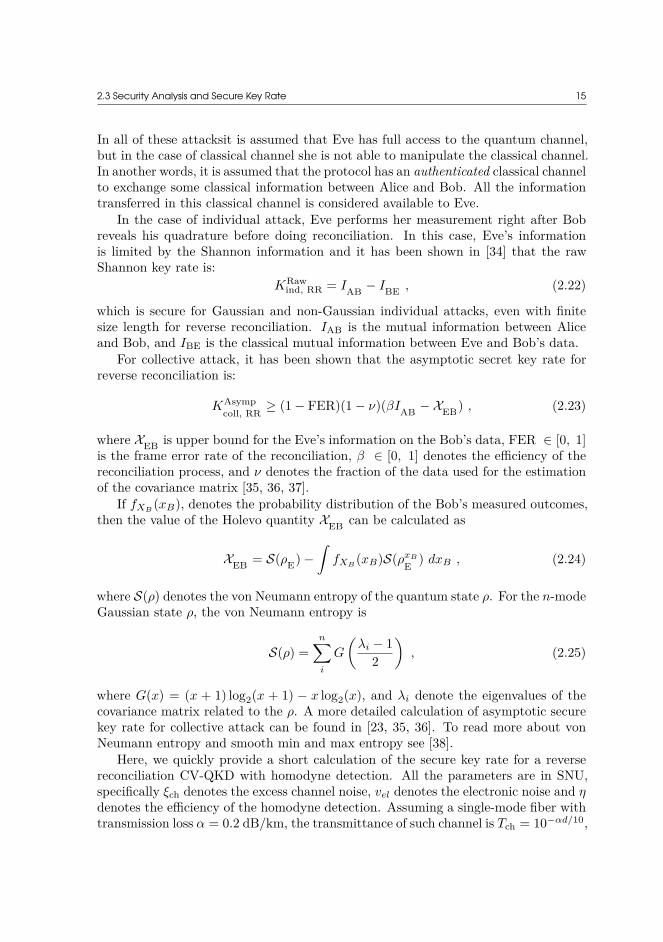
where XEB is upper bound for the Eve’s information on the Bob’s data, FER ∈ [0, 1]is the frame error rate of the reconciliation, β ∈ [0, 1] denotes the efficiency of thereconciliation process, and ν denotes the fraction of the data used for the estimationof the covariance matrix [35, 36, 37].
If fXB(xB), denotes the probability distribution of the Bob’s measured outcomes,
then the value of the Holevo quantity XEB can be calculated as
XEB = S(ρE) −∫fXB
(xB)S(ρxB
E ) dxB , (2.24)
where S(ρ) denotes the von Neumann entropy of the quantum state ρ. For the n-modeGaussian state ρ, the von Neumann entropy is
S(ρ) =n∑i
G
(λi − 1
2
), (2.25)
where G(x) = (x + 1) log2(x + 1) − x log2(x), and λi denote the eigenvalues of thecovariance matrix related to the ρ. A more detailed calculation of asymptotic securekey rate for collective attack can be found in [23, 35, 36]. To read more about vonNeumann entropy and smooth min and max entropy see [38].
Here, we quickly provide a short calculation of the secure key rate for a reversereconciliation CV-QKD with homodyne detection. All the parameters are in SNU,specifically ξch denotes the excess channel noise, vel denotes the electronic noise and ηdenotes the efficiency of the homodyne detection. Assuming a single-mode fiber withtransmission loss α = 0.2 dB/km, the transmittance of such channel is Tch = 10−αd/10,

16 2 Quantum Key Distribution with Continuous Variables
where d denotes the distance between the two parties. As presented in [35], total noisebetween Alice and Bob is:
ξtotal = ξline + ξhomTch
,
where ξhom = 1 + vel
η− 1 is the homodyne detector noise and ξline = ( 1
Tch− 1) + ξch.
Then, according to [35] and as presented in (2.15), the variance of Bob’s data afterhomodyne detection, in SNU is:
VB = ηTch(V + ξtotal) = ηTch
(V + ξline + ξhom
Tch
)
= ηTch
V + ( 1Tch
− 1) + ξch +
1 + vel
η− 1
Tch
= ηTchV − ηTch + ηTchξch + 1 + vel
= T (V − 1) + Tξch + 1 + vel
= TVmod + 1 + ξ ,
where T = ηTch, V = Vmod + 1 and ξ = Tchξch + vel as shown in (2.15). In addition,the mutual information between Alice and Bob is:
IAB = 12
log2(1 + SNR) = 12
log2
(1 + V + ξtot
1 + ξtot
). (2.26)
According to [35], Eve’s classical mutual information from Bob’s data is:
IBE = 12
log2VB
VB|E, (2.27)
where VB|E = η
[1
T (1/V ) + ξline+ ξhom
]. Finally, Holevo bound XEB is calculated
as:
XEB = G
(λ1 − 1
2
)+G
(λ2 − 1
2
)−G
(λ3 − 1
2
)−G
(λ4 − 1
2
), (2.28)
where the eigenvalues are calculated from:
λ1,2 =√
12
(A±
√A2 − 4B
),
λ3,4 =√
12
(C ±
√C2 − 4D
),

2.3 Security Analysis and Secure Key Rate 17
where
A = V 2(1 − 2T ) + 2T + T 2(V + ξline)2,
B = T 2(V ξline + 1)2,
C = V√B + T (V + ξline) +A ξhom
T (V + ξtot),
D =√BV +
√Bξhom
T (V + ξtot).
From this we can plot the the asymptotic secret key rate for reverse reconciliation.In Figure 2.4, the asymptotic secure key rate is plotted against distance for differentreconciliation efficiencies where all other parameters are assumed to be fixed. It canbe observed that the overall transmittable distance between the two parties dependssignificantly on the reconciliation efficiency.
0 25 50 75 100 125 150 175 200Distance [km]
10 6
10 5
10 4
10 3
10 2
10 1
100
Secu
re k
ey r
ate
[bits
per
sym
bole
]
= 70%= 80%= 90%= 95%= 98%= 100%
Figure 2.4: Effective asymptotic secure key rates against collective attack. Thereconciliation efficiency β = {0.7, 0.8, 0.9, 0.95, 1.00}. The parametersused in the calculations are Vmod = 8.5, ξch = 0.015, η = 0.6, vel =0.041, and the fiber loss is assumed to be 0.2 dB/km.
To read more about the security proof of the CV-QKD for finite length and most

18 2 Quantum Key Distribution with Continuous Variables
general coherent attack see [39, 40]. Let us repeat a similar simulation by consideringthe finite size effects. It is assumed that the length of the data for the privacyamplification is nprivacy = 1010 bits. The number of the quantum symbols used forreconciliation is nquantum = 2 × nprivacy (ν = 0.5). We assumed that the securityparameter ϵsecurity = 10−10. From [39], the secure key rate considering the finite-sizeeffect is:
KFinitecoll, RR ≥ (1 − FER)(1 − ν)(βIAB − XEB − ∆(nprivacy)) , (2.29)
where ∆(nprivacy) is the finite-size offset factor and for nprivacy > 104 can be approxi-mated by:
∆(nprivacy) ≈ 7
√log2(2/ϵsecurity)
nprivacy.
0 25 50 75 100 125 150 175 200Distance [km]
10 6
10 5
10 4
10 3
10 2
10 1
100
Secu
re k
ey r
ate
[bits
per
sym
bole
]
= 70%= 80%= 90%= 95%= 98%= 100%
Figure 2.5: Effective finite secure key rate against collective attack. The reconcilia-tion efficiency β = {0.7, 0.8, 0.9, 0.95, 1.00}. The parameters used in thecalculations are Vmod = 8.5 , ξch = 0.015, η = 0.6, vel = 0.041, ν = 0.5,nprivacy = 1010, ϵsecurity = 10−10, and the fiber loss is assumed to be 0.2dB/km.
Finally, a very comprehensive comparison for the CV-QKD protocols and theirbest available security proof until 2015 is available in [28]. In this thesis we focus

2.4 Experimental setup 19
on the reconciliation protocols for the CV-QKD and represent how it is possible todesign highly efficient reconciliation scheme with lowest FER. A detailed descriptionof different reconciliation schemes will be discussed in Chapter 3.
2.4 Experimental setup
Figure 2.6: The experimental setup of our CV-QKD. The schematic was generatedby Dr. Nitin Jain.
The experimental setup for the Gaussian modulated CV-QKD that we have es-tablished in our lab is shown in Figure 2.6. It has a continuous-wave laser (Tx laser)operating at 1550 nm and contains standard fiber optics and telecommunication com-ponents. On the transmitter side, an in-phase and quadrature (I-Q) electro-opticalmodulator is driven by Tx laser. It produces coherent states at a single side-bandof the optical field at a rate of 100 MSymbols/s. In addition, to generate a com-plex coherent state amplitudes of the quantum signal, a quantum random numbergenerator (QRNG) with a security parameter ϵqrng = 10−10 is used. The QRNGdelivered Gaussian distributed symbols for discrete Gaussian modulation of coherentstates. After attenuation to the desired mean photon number count, the coherentstates were transmitted through a 20 km standard single mode fiber. The receiverside contains a frequency detuned laser (local oscillator) of the same type (Rx laser),a balanced beam splitter and a balanced receiver for radio-frequency heterodyne de-tection. As shown in Figure 2.6, a polarization controller (PC) is used to manuallytune the polarization to match with Rx laser’s polarization. Then, the signal andthe local oscillator were interfered on a balanced beam splitter and detected by a bal-anced receiver. In addition, the I-Q-modulator was driven by two digital-to-analogconverters (DACs) with 16 bit precision and 1 GSample/s and the receiver’s output

20 2 Quantum Key Distribution with Continuous Variables
was sampled by a 16 bit analog-to-digital converter(ADC) at 1 GSample/s. Finally,the data was stored on a hard drive for offline post processing. For more details aboutour experimental setup, machine learning based approach for carrier phase recoveryand the QRNG see [41, 42].
The secret key was established by the following protocol:
1. Gaussian distributed random numbers were generated by the random numbergenerator and stored in a file.
2. The transmitter and receiver were calibrated.
3. Using the 20 km fiber, we transmitted the coherent states using frames prere-corded in a file and played out using the arbitrary waveform generator.
4. After the experiment was conducted, digital-signal-processing was performedoffline to obtain the raw key.
5. Information reconciliation was performed using a multi-level coding, multi-stagedecoding scheme by using multi-edge-type low-density-parity-check codes. Moredetails about the reconciliation scheme, will be discussed in Chapter 3.
6. After error correction the entropy of the received symbols was estimated as wellas the channel parameters for bounding the Holevo information.
7. By using a randomly chosen Toeplitz hash function for privacy amplificationthe final secret key is generated.

CHAPTER3Information
Reconciliation ofCV-QKD
Information reconciliation is a method by which two parties, each possessing a se-quence of numbers, agree on a common sequence of bits by exchanging one or moremessages. In CV-QKD with Gaussian modulation, the two sequences of numbers arejoint instances of a bi-variate random variable that follows a bi-variate normal dis-tribution. Physically, in a prepare-and-measure CV-QKD setup, these sequences aregenerated by one party modulating coherent states and the other party, measuringthese states. The amplitude of each modulated coherent state, which can be visu-alized by a point in the quadrature-phase space, is determined by the values in thesequence. In other words, in QKD, two parties share correlated random variables andwish to agree on a common bit sequence. However, imperfect correlations introducedby the inherent shot noise of coherent states and noise in the quantum channel andthe receiver, give rise to discrepancies in the two sequences of numbers which have tobe corrected by exchanging additional information. As discussed in Section 2.3, theefficiency and performance of the error correction codes for reconciliation stronglyaffects the secure key rate of CV-QKD, which makes it one of the most crucial stagesin the protocol (See Figure 2.4 and Figure 2.5).
This chapter is about the problem of reconciliation of Gaussian variables for CV-QKD. Two different reconciliation methods will be discussed. First, in Section 3.1, themulti-dimensional reconciliation will be introduced. Then, Section 3.2, talks aboutthe reconciliation based on multi-level-coding multi-stage-decoding (MLC-MSD) anddifferent variations of the method will be discussed (See also our arXived article [18]).In Section 3.4, the randomized reconciliation scheme, which is a modified versionof the MLC-MSD approach for high throughput reconciliation will be introduced.Finally, Section 3.5 talks about reconciliation for a continuous range of SNRs.
22 3 Information Reconciliation of CV-QKD
3.1 Multidimensional Reconciliation
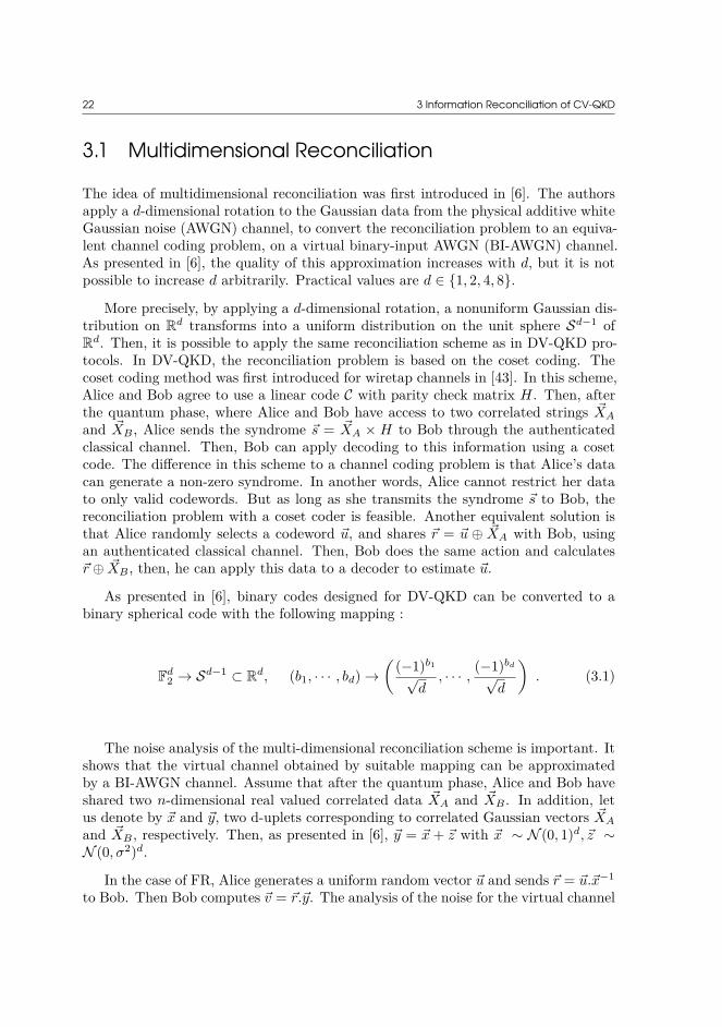
The idea of multidimensional reconciliation was first introduced in [6]. The authorsapply a d-dimensional rotation to the Gaussian data from the physical additive whiteGaussian noise (AWGN) channel, to convert the reconciliation problem to an equiva-lent channel coding problem, on a virtual binary-input AWGN (BI-AWGN) channel.As presented in [6], the quality of this approximation increases with d, but it is notpossible to increase d arbitrarily. Practical values are d ∈ {1, 2, 4, 8}.
More precisely, by applying a d-dimensional rotation, a nonuniform Gaussian dis-tribution on Rd transforms into a uniform distribution on the unit sphere Sd−1 ofRd. Then, it is possible to apply the same reconciliation scheme as in DV-QKD pro-tocols. In DV-QKD, the reconciliation problem is based on the coset coding. Thecoset coding method was first introduced for wiretap channels in [43]. In this scheme,Alice and Bob agree to use a linear code C with parity check matrix H. Then, afterthe quantum phase, where Alice and Bob have access to two correlated strings XA
and XB , Alice sends the syndrome s = XA × H to Bob through the authenticatedclassical channel. Then, Bob can apply decoding to this information using a cosetcode. The difference in this scheme to a channel coding problem is that Alice’s datacan generate a non-zero syndrome. In another words, Alice cannot restrict her datato only valid codewords. But as long as she transmits the syndrome s to Bob, thereconciliation problem with a coset coder is feasible. Another equivalent solution isthat Alice randomly selects a codeword u, and shares r = u ⊕ XA with Bob, usingan authenticated classical channel. Then, Bob does the same action and calculatesr ⊕ XB , then, he can apply this data to a decoder to estimate u.
As presented in [6], binary codes designed for DV-QKD can be converted to abinary spherical code with the following mapping :
Fd2 → Sd−1 ⊂ Rd, (b1, · · · , bd) →
((−1)b1
√d
, · · · , (−1)bd
√d
). (3.1)
The noise analysis of the multi-dimensional reconciliation scheme is important. Itshows that the virtual channel obtained by suitable mapping can be approximatedby a BI-AWGN channel. Assume that after the quantum phase, Alice and Bob haveshared two n-dimensional real valued correlated data XA and XB . In addition, letus denote by x and y, two d-uplets corresponding to correlated Gaussian vectors XA
and XB , respectively. Then, as presented in [6], y = x + z with x ∼ N (0, 1)d, z ∼N (0, σ2)d.
In the case of FR, Alice generates a uniform random vector u and sends r = u.x−1
to Bob. Then Bob computes v = r.y. The analysis of the noise for the virtual channel
3.1 Multidimensional Reconciliation 23
(w = v − u) shows that:
w = v − u
= r.y − u
= u.x−1(x+ z) − u
= uz
x∼ u
z
||x||,
where as presented in [6, 10], the last equality holds due to the fact that x and z areindependent. It means that the virtual channel can be considered as a Fading channelwith known channel side information (CSI) [44]. The fading coefficient is the normof x. When d goes to infinity, the distribution of the norm of x becomes closer to aDirac distribution, and the virtual channel becomes closer to a BI-AWGN channel.The maximum possible value for d is 8, because the division operator does not existsfor d > 8.
Now, let us consider the case of RR. In this case, x = y − z with y ∼ N (0, 1 +σ2)d, z ∼ N (0, σ2)d. It is important to notice that in RR, y and z are not independent(actually, they are highly correlated). Thus, accurate noise analysis is necessary toobtain the distribution of the virtual channel. More precisely, in RR, Bob sendsr = u.y−1, and Alice calculates v = r.x. Thus, the noise of the virtual channel is
w = v − u
= r.x− u
= u.y−1(y − z) − u
= −u zy,
where in the last equation z and y are not independent. It shows that there is stilla need for discussion on the precise definition of the virtual channel in the RR case.Despite of the lack of understanding (only in the case of RR), this method has beenwidely used in CV-QKD, and most studies tend to focus on the high reconciliationefficiency for this algorithm [4, 45, 46]. There is still significant concern over thesecurity of RR.
Finally, let us consider the practical implementation of the multi-dimensional rec-onciliation. First, Alice and Bob normalize their data to have a uniform distributionon the unit sphere Sn−1 of Rn. Then, Bob generates a binary sequence u of length kwith uniform distribution using a quantum random number generator (QRNG) [47],and uses a linear code to generate a codeword c of length n. In the next step, thisbinary code is mapped to a binary spherical code c′ using (3.1). Then Bob calculatesa mapping function M(X ′
B , c′) and sends it back to Alice. The mapping functionM(X ′
B , c′) should satisfyM(X ′
B , c′).X ′B = c′ ,

24 3 Information Reconciliation of CV-QKD
where X ′B denotes the normalized data of Bob. Then, Alice can use the mapping
function and calculate a new sequence of e = M(X ′B , c′).X ′
A. Alice is allowed to use adecoder designed for an BI-AWGN channel to recover estimation of u. The followingblock diagram shows the RR protocol, using the multi-dimensional reconciliationapproach.
Alice
~XA ∈ Rn
Normalization
~X ′A ∈ Rn
Mapping function
~e ∈ Fn2
Decoder
~u′ ∈ Fn2
Estimated bits
Bob
~XB ∈ Rn
Normalization
~X ′B ∈ Rn
Mapping function
~c ∈ Fn2
Encoder
~u ∈ Fn2
QRNG
M( ~X ′B ,
~c′)
Syndrome check
Figure 3.1: RR using multidimensional reconciliation scheme. X ′A and X ′
B are twocorrelated sequences of real valued data. X ′
A and X ′B denote the cor-
responding normalized sequences. M(X ′B , c′) represents the mapping
function. The raw key is generated by a QRNG is denoted by u. Theencoded key using a linear code is denoted by c .

3.2 Multi-Level-Coding Multi-Stage-Decoding 25
3.2 Multi-Level-Coding Multi-Stage-DecodingThis Section introduces a reconciliation scheme based on MLC-MSD scheme. In thefollowing, we start by representing the block diagram of RR protocol based on MLC-MSD scheme. Then we talk about digitization of continuous sources and try to showthe effect of digitization levels. Then we talk with more details about the MLC-MSD scheme for RR. Starting with the one-level reconciliation method, which is aspecific type when just the most-significant bit (MSB) is used for the reconciliation,we define and calculate the soft information for decoders. Then, the extension for two-level reconciliation and multi-level will also be explained. In addition, we determinehow to calculate the code rates for individual levels. We represent both analyticaland numerical methods to calculate the individual rates and mutual information.Finally, a comprehensive comparison for FR and RR is presented for the MLC-MSDreconciliation.
It is assumed that readers are familiar with the concept of error correction codesand low density parity check (LDPC) codes. Details about the definition of LDPCcodes, their parity check matrix and their standard decoder can be found in Ap-pendix A. For a more detailed introduction into these concepts see [44].
Through this thesis we denote a vector with real valued symbols of length n byx = (xi)n
i=1 = (x1, · · · , xn), where xi ∈ R. In addition a m-bit digitization of a realvalued symbol at jth index is denoted by Q(xj) = (xi
j)m−1i=0 = (x0
j , x1j , · · · , xm−1
j ).For example, a vector of Bob’s real valued symbols is denoted by xB = (xB,i)n
i=1 =(xB,1, · · · , xB,n) and the quantized version of its jth symbol is Q(xB,j) = (xi
B,j)m−1i=0 =
(x0B,j , x
1B,j , · · · , xm−1
B,j ). Sometimes, it is more convenient to consider Bob as a con-tinuous Gaussian source denoted by a random variable XB and its instant value isthen denoted by xB . Then the discretized source is denoted by Q(XB) = (Xi
B)m−1i=0 .
In addition I(X;Y ) denotes the mutual information between two random variablesX and Y , where X and Y could be continuous or discrete random variables. BesidesH(X) denotes the entropy of secrete random variable and h(X) denotes the differen-tial entropy for a continuous random variable. Sometimes we are interested to findthe entropy or mutual information at specific SNR s, then Is(X;Y ) = I(X;Y )|s,Hs(X) = H(X)|s.
3.2.1 Introduction and system modelIn general, multi-level reconciliation using error correction codes can be describedin two steps. The first step is digitization, which transforms the continuous Gaus-sian source XB , into an m bit source Q(XB), with its binary representation vectors(Xi
B)m−1i=0 = (Xm−1
B , . . . , X1B , X
0B). There is an inherent information loss due to the
digitization process of the source. The second step can be modeled as source cod-ing with side information on the MLC-MSD scheme. In RR Bob sends an encoding(compressed version) of Q(XB) to Alice, such that she can infer Q(XB) with highprobability, using her own source XA as side information. Let us define the efficiency

26 3 Information Reconciliation of CV-QKD
β as
β = H(Q(XB)) −RSource
I(XB ;XA), (3.2)
where I(XB ;XA) is the mutual information and H(Q(XB))−RSource is the net sharedinformation between two parties, resp. per symbol, [48, 49] with H(·) being Shannonentropy and RSource the source coding rate. Thus, the efficiency of reconciliationdepends on the ability to design very good digitizers and highly efficient compressioncodes with minimum possible source coding rate (RSource). Slepian and Wolf [50]have shown that H(Y |Z) is the lower bound to the source coding rate when decodingY given side information Z. Therefore, Rs ≥ H(Q(XB)|XA).
A detailed schematic representation for the MLC-MSD scheme is presented in Fig-ure 3.2, where Bob encodes his data onto m different individual levels. Let us denoteby RSource
i the corresponding source coding rate for each sub-level i in the MLC-MSDscheme. Then using the Slepian-Wolf theorem, all RSource
i are lower bounded by theconditional entropy of the ith bit of Q(XB), given side information XA and all theremaining least significant bits (LSBs) of Q(XB):
RSourcei ≥ H(Xi
B |XA, Xi−1B , . . . , X0
B) . (3.3)
The total source coding rate is given by summing over the individual source coderates RSource
i :
RSource =m−1∑i=0
RSourcei ,
which resembles the Slepian-Wolf theorem:
RSource ≥m−1∑i=0
H(XiB |XA, X
i−1B , . . . , X0
B) = H(Q(XB)|XA) .
The detailed block diagram for the MLC-MSD scheme is depicted in Figure 3.2.We consider a digitization scheme with M = 2m, m > 1, signal points in a D-dimensional real signal space, with signal points taken from the signal set S ={a0, a1, . . . , aM−1}, with probabilities Pr{ak}. Each signal point has its equivalent bi-nary form defined by a bijective mapping a = M(x) of binary representation vectorsx = (xm−1
B , . . . , x0B) to signal points a ∈ S. Two well defined mappings are binary and
Gray mapping. As an example, for m = 3 levels, in one-dimensional signal space (D =1), the M = 23 signal points are taken from S = {−7,−5,−3,−1,+1,+3,+5,+7}.Fixing the values of co-ordinates i to 0, i.e. xi
B , . . . , x0B , we obtain subsets of the signal
set S by defining:
S(xiB , . . . , x
0B) = {a = M(x) | x = (bm−1, . . . , bi+1, xi
B , . . . , x0B), bj ∈ {0, 1},
j = i+ 1, . . . ,m− 1} . (3.4)

3.2 Multi-Level-Coding Multi-Stage-Decoding 27
Bob’s Side Alice’s Side
~xB = (xB,1, . . . , xB,n) ~xA = (xA,1, . . . , xA,n)
Quantizer Q(·)
QUANTUM CHANNEL
QuantizerQ(·)
xm−1B,1 , . . . , xm−1
B,n
xiB,1, . . . , x
iB,n
Enc m− 1
Enc i
pm−11 , . . . , pm−1
n(1−Rchm )
pi1, . . . , pin(1−Rch
i )
Dec i
Dec m− 1xm−1B,1 , . . . , xm−1
B,n
xiB,1, . . . , x
iB,n
// //
x0B,1, . . . , x
0B,nx0
B,1, . . . , x0B,n
......
...... · · · · · ·
Figure 3.2: The MLC-MSD scenario for RR. First the input is quantized into anm-bit source. Then each of the m sources is encoded and sent to Alice.The decoder has the side information from its own source and withthe m encoded sources produces an estimate of the quantized source.Usually we transmit the least significant bits as plain-texts..
For more details about set partitioning and mapping see [7]. For the above mentionedconstellation points, with M = 8 and binary partitioning:
S(x0B = 0) = {a = M(x)|x = {000, 010, 100, 110}} = {−7,−3,+1,+5} ,
S(x1Bx
0B = 10) = {a = M(x)|x = {010, 110}} = {−3,+5} ,
S(x2Bx
1Bx
0B = 010) = {a = M(x)|x = {010}} = {−3} .
Figure 3.3 illustrates the schematic representation of the binary set partitioning forthe above constellation points. In Section 3.2.2 we talk with more details about thedigitization effect.
S
S(0) S(1)
S(11)S(01)S(10)S(00)
S(000) S(100) S(010) S(110) S(001) S(101) S(011) S(111)
Figure 3.3: The binary set partitioning and the corresponding mapping.

28 3 Information Reconciliation of CV-QKD
In addition Figure 3.2 contains m individual levels. Some of the levels are trans-mitted as plain-text and some of the levels contain encoder and decoder blocks. In Sec-tion 3.2.5 we propose both analytical and numerical methods to calculate the coderates for individual levels. In addition, in Section 3.2.3 we explain with more de-tails how encode the corresponding binary data in each level and how to use softinformation for decoding purpose. Also we assume that LDPC codes are used fordecoding.
3.2.2 Digitization effectA digitizer converts continuous values to some discrete levels, characterized by arange R and number of output bits m. It is assumed that the digitizer uses the thefollowing signal values: {−(M − 1), . . . ,−3,−1, 1, 3, . . . , (M − 1)}, where M = 2m.The constellation symbols are normalized so that the average energy is equal to 1.Usually, R = 6σ is enough for the range of the digitizer. The digitizer provides a setof M = 2m non-overlapping intervals with equal length δ = 2R
M − 2as follows:
Ij =
(−∞,−R] if j = 0 ,(−R+ (j − 1)δ,−R+ (j)δ] if 0 < j < M − 1 ,[R,+∞) if j = M − 1 .
(3.5)
Let us denote by Q(xB) the m-bit quantized version of xB with its binary repre-sentation vector (xm−1
B , . . . , x1B , x
0B). Also, it is possible to assign different mappings
to the output of the digitizer. For example, as depicted in Figure 3.4, an m = 4bit digitizer with range R is considered. Some possible mappings for the output arealso presented. Considering a fixed step size δ for digitization, the entropy of thequantized source can be approximated by
H(Q(XB)) ≈ h(XB) − log2 δ ,
where h(XB) is the differential entropy defined for continuous variable XB . A similardigitization can be applied on the Alice’s side to get Q(XA). This also holds for theconditional entropy:
H(Q(XB)|Q(XA)) ≈ h(XB |XA) − log2 δ .
For the mutual information, if m is large enough:
I(Q(XB);Q(XA)) ≈ I(Q(XB);XA) ≈ I(XB ;XA) ,
where the equality holds when δ → 0.
Example 3.2.1. The m-bit digitizer

3.2 Multi-Level-Coding Multi-Stage-Decoding 29
-R +Rδ
Qp(xB)−Qn(xB) = −8
0 1 2 3 4 5 6 7 8 9 10 11 12 13 14 15
0 1 3 2 7 6 4 5 15 14 12 13 8 9 11 10
+0 -0+1 -1+2 -2+3 -3+4 -4+5 -5+6 -6+7 -7
Figure 3.4: A digitizer with 4 bits. It provides 16 non-overlapping intervals. Thebinary, Gray and sign-magnitude mappings are also considered. It isclear that the distance between two points with equal least-significantbits (LSB)s is always fixed and it is equal to 8. Two quantized pointsQp(xB) and Qn(xB) have equal LSBs, but their MSBs are assigned to0 and 1, respectively.
As an example, consider a case when the covariance matrix of a bi-variate normaldistribution is:
Σ =[
1 0.90.9 4
].
Then, the theoretical value for the differential entropy, can be calculated as:
h(X,Y ) = 0.5 log2((2πe)2 det(Σ)
),
where det(Σ) denotes the determinant of the covariance matrix and the correspond-ing mutual information is equal to I(X;Y ) = h(X) + h(Y ) − h(X,Y ), as presentedin Table 3.1. In addition, using a Monte-Carlo simulation, numerical estimationsare calculated for m ∈ {3, 4, 5, 6}, where m denotes the m-bit digitizer. Also, thecorresponding histograms are plotted in Figure 3.5 for marginal and the joint distri-butions. It is clear that for the m = 3, the estimated values are not accurate, but forthe m ≥ 4, the numerical calculations are close to the theoretical values.

30 3 Information Reconciliation of CV-QKD
Theoretical valuesI(XA;XB) h(XA) h(XB)
– 0.1632 2.0471 3.0471Numerical estimations
m I(Q(XA);Q(XB)) H(Q(XA)) H(Q(XB))3 0.136293 2.103829 3.1038654 0.155513 3.061083 4.0611035 0.160985 4.050079 5.0499736 0.162606 5.047190 6.047170
Table 3.1: The theoretical values and the numerical estimations for m-bit digitizerwith δ = 23−m.
4 3 2 1 0 1 2 3 40.00.10.20.3
Prob
abili
ty
4 2 0 2 442024
Q(X
B)
4 3 2 1 0 1 2 3 40.00.10.20.30.4
Prob
abili
ty
4 2 0 2 442024
Q(X
B)
4 3 2 1 0 1 2 3 40.00.10.20.30.4
Prob
abili
ty
4 2 0 2 442024
Q(X
B)
4 3 2 1 0 1 2 3 4Q(X)
0.00.10.20.30.4
Prob
abili
ty
4 2 0 2 4Q(XA)
42024
Q(X
B)
Figure 3.5: The digitization effect on the 1-D histogram (related to XA) and corre-sponding 2-D histogram of the normalized quantized data.
3.2 Multi-Level-Coding Multi-Stage-Decoding 31
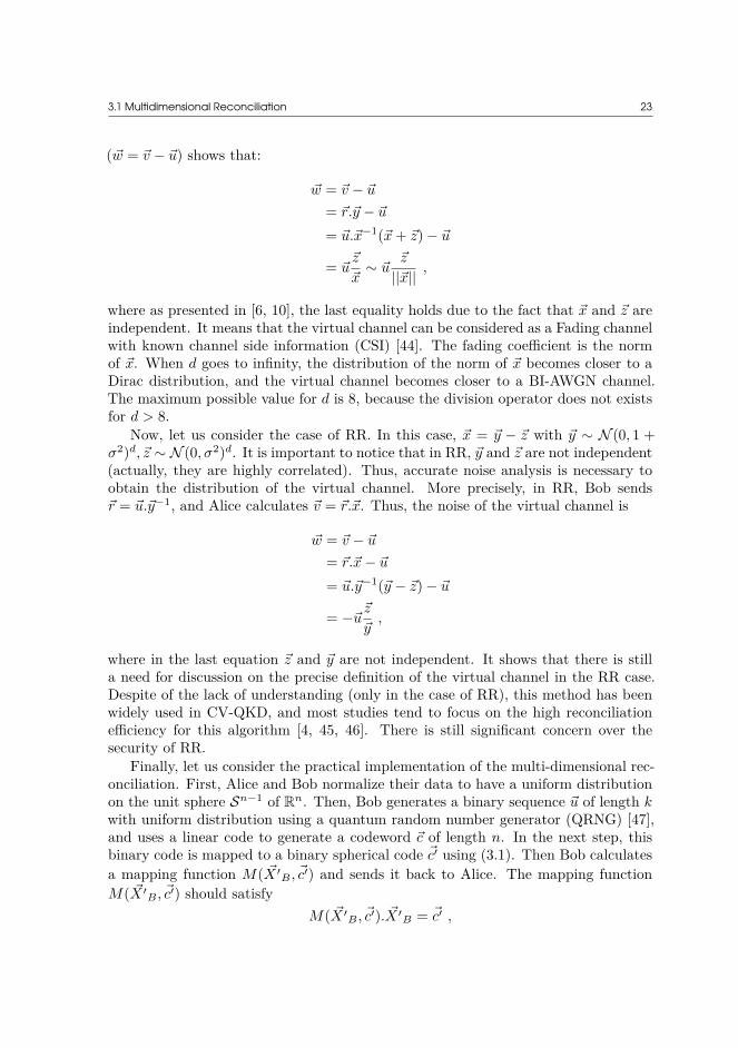
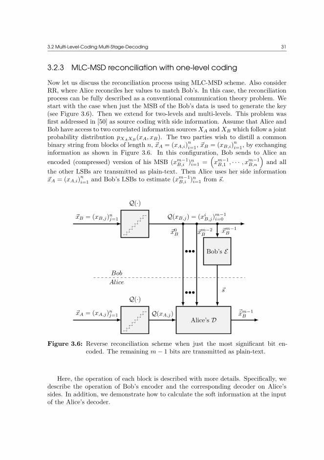
3.2.3 MLC-MSD reconciliation with one-level coding
Now let us discuss the reconciliation process using MLC-MSD scheme. Also considerRR, where Alice reconciles her values to match Bob’s. In this case, the reconciliationprocess can be fully described as a conventional communication theory problem. Westart with the case when just the MSB of the Bob’s data is used to generate the key(see Figure 3.6). Then we extend for two-levels and multi-levels. This problem wasfirst addressed in [50] as source coding with side information. Assume that Alice andBob have access to two correlated information sources XA and XB which follow a jointprobability distribution pXAXB
(xA, xB). The two parties wish to distill a commonbinary string from blocks of length n, xA = (xA,i)n
i=1, xB = (xB,i)ni=1, by exchanging
information as shown in Figure 3.6. In this configuration, Bob sends to Alice anencoded (compressed) version of his MSB (xm−1
B,i )ni=1 =
(xm−1
B,1 , · · · , xm−1B,n
)and all
the other LSBs are transmitted as plain-text. Then Alice uses her side informationxA = (xA,i)n
i=1 and Bob’s LSBs to estimate (xm−1B,i )n
i=1 from s.
~xB = (xB,j)nj=1
Q(·)
Q(xB,j) = (xiB,j)
m−1i=0
~xm−1B~x0
B ~xm−2B
Bob’s E
Alice
Bob
~s
Alice’s D~xA = (xA,j)
nj=1 Q(xA,j) ~xm−1
B
Q(·)
Figure 3.6: Reverse reconciliation scheme when just the most significant bit en-coded. The remaining m− 1 bits are transmitted as plain-text.
Here, the operation of each block is described with more details. Specifically, wedescribe the operation of Bob’s encoder and the corresponding decoder on Alice’ssides. In addition, we demonstrate how to calculate the soft information at the inputof the Alice’s decoder.

32 3 Information Reconciliation of CV-QKD
3.2.3.1 Bob’s encoder
Let us denote by s the syndrome generated by Bob. For a given parity check matrixH(n−k) n and a bit string xm−1
B = (xm−1B,i )n−1
i=0 of length n, the syndrome s is calculatedas:
s = xm−1B HT , (3.6)
where HT denotes the transpose of the parity check matrix of the LDPC code (see Ap-pendix A). Bob’s encoder is actually a hash function, which compresses the data oflength n to a syndrome of length n − k. Some other important facts, regarding thesyndrome and Bob’s encoder are the following:
• The syndrome is a vector of length n− k.
• The syndrome can be a non-zero vector depending on the Bob’s received se-quence.
• Each 0 value in s denotes that the corresponding parity equation is satisfied forXm−1
B .
• Each 1 value in s denotes that the corresponding parity equation is not satisfiedfor Xm−1
B .
3.2.3.2 Calculation of the soft information
According to [44] the a-priori log-likelihood ratio (LLR) for a single bit is defined as:
λX = ln(
Pr{x = 1}Pr{x = 0}
)= ln
(p
1 − p
), (3.7)
where p = Pr{x = 1}. In a similar way, at the input of the decoder on Alice’s side,the a-posteriori LLR for Bob’s MSB, given Alice’s quantized data and Bob’s LSBscan be defined as:
λXm−1
B|Q(XA), (Xi
B)m−2i=0
= ln
(Pr{xm−1
B = 1|Q(xA),(xi
B
)m−2i=0 }
Pr{xm−1B = 0|Q(xA),
(xi
B
)m−2i=0 }
). (3.8)
In addition, using the rules of the conditional probabilities
Pr{X, Y |Z} = Pr{X|Z} Pr{Y |X, Z}, (3.9)
one can write
Pr{Xm−1B |Q(XA),
(Xi
B
)m−2i=0 } =
Pr{Xm−1B ,
(Xi
B
)m−2i=0 |Q(XA)}
Pr{(Xi
B
)m−2i=0 |Q(XA)}
, (3.10)

3.2 Multi-Level-Coding Multi-Stage-Decoding 33
where (3.10) can be used to simplify both numerator and denominator of (3.8) asfollows:
λXm−1
B|Q(XA), (Xi
B)m−2i=0
= ln
(Pr{xm−1
B = 1,(xi
B
)m−2i=0 |Q(xA)}
Pr{xm−1B = 0,
(xi
B
)m−2i=0 |Q(xA)}
). (3.11)
Now, let us define two new random variables Qp(XB) and Qn(XB). Qp(XB) takesthe LSBs of Bob’s data and assumes the MSB is equal to 0 and Qn(XB) takes theLSBs of Bob’s data and assumes the MSB is equal to 1. As depicted in Figure 3.4,Qp(XB) belongs to the set of symbols on left hand side of the plane and Qn(XB)belongs to the set of symbols on the right hand side.
Furthermore, it is clear that
Pr{Q(XB)|Q(XA)} ≈exp
(− (Q(xB) −Q(xA))2
2σ2
)√
2πσ2, (3.12)
where σ2 in (3.12) is the combination of the quantum channel noise and the digitizernoise. Using (3.12), equation (3.11) can be simplified to:
λXm−1
B|Q(XA), (Xi
B)m−2i=0
= ln
exp
(− (Qn(xB) −Q(xA))2
2σ2
)
exp
(− (Qp(xB) −Q(xA))2
2σ2
)
= (Qp(xB) −Q(xA))2 − (Qn(xB) −Q(xA))2
2σ2
= (Qp(xB) −Qn(xB)) (Qp(xB) +Qn(xB) − 2Q(xA))2σ2
= −2m−1 (Qp(xB) +Qn(xB) − 2Q(xA))2σ2 , (3.13)
where on the last equation, as depicted in Figure 3.4, for a digitizer with m-bits,Qp(xB) −Qn(xB) = −2m−1. Thus
λXm−1
B|Q(XA), (Xi
B)m−2i=0
=−2m−1 (Qavg(xB) −Q(xA)
)σ2 , (3.14)
where, Qavg(xB) = Qp(xB)+Qn(xB)2 denotes the average. This soft information can
be used at the input of the LDPC decoder to estimate XmB .
3.2.3.3 Alice’s decoder
Let us describe Alice’s decoder. Here we show how Alice needs to modify her decoderto use the non-zero syndrome s. The conventional LDPC decoder [51, 52] accepts soft

34 3 Information Reconciliation of CV-QKD
information, and tries to recover the codeword from noisy received data by applyingthe message passing (MP) algorithm (See [44] and Appendix A). Let λ0
v denote Bob’sMSB soft information as shown in (3.14) for variable-node (VN) v, on iteration 0. Inaddition assume that λl
vc (µlcv) denotes the message from variable-node to check-node
(from check-node to variable-node) after l iterations. The update equations for themessages under belief propagation are:
λlvc =
λ0
v if l = 0λ0
v +∑
c′∈Cv\c
µlc′v if l ≥ 1
µlcv = 2 tanh−1
∏v′∈Vc\v
tanh
(λl−1
v′c
2
) ,
where Cv\c denotes all the check-nodes (CN) connected to the VN v, except theCN c and Vc\v is the set of VNs connected to CN c, except the VN v. The aboveformulation is valid when the syndrome s is an all zero vector, or all the parityequations are satisfied with zero parity.
In contrast to the conventional LDPC decoder, for the 1-level scheme the decoderon the Alice’s side, as denoted in Figure 3.6, accepts one more additional input,denoted by syndrome s, which is the syndrome of Bob’s MSB which can be calculatedfrom (3.6). The syndrome s is in general, a non-zero vector. Thus, we need to changethe CN operation according to the received syndrome s. The modified CN operationthen can be represented as:
µlcv = (−1)Sc · 2 tanh−1
∏v′∈Vc\v
tanh
(λl−1
v′c
2
) , (3.15)
where Sc ∈ {0, 1} represents the parity value at index c. It is clear that for Sc = 0,the CN operation remains the same as standard decoder, but for Sc = 1, the CNoperation would flip the sign of the outgoing message.
3.2.3.4 Noise estimation
Accurate estimation of noise variance plays an important role for the calculation ofthe soft information. According to (3.14), incorrect estimation of the noise variancecan highly affect the reliability of the soft information. Here, we present a method toobtain an accurate estimation of the noise variance. Under the assumption that thechannel variance is not changing very fast, one can use some portion of the quantizeddata to estimate the noise variance.
Let us assume that we have sufficient samples of two jointly zero mean Gaussianrandom variables XA and XB , with standard deviations σA and σB , respectively. The

3.2 Multi-Level-Coding Multi-Stage-Decoding 35
bi-variate normal distribution can be described by:
fXB ,XA(xB , xA) = 1
2π√
|Σ|exp
(−1
2(xA, xB)Σ−1(xA, xB)T
), (3.16)
where the covariance matrix is equal to:
Σ =[
σ2A ρ σA σB
ρ σA σB σ2B
], (3.17)
andρ = E{XAXB}
σAσB, (3.18)
is the correlation coefficient between XA and XB . By normalizing Alice’s and Bob’sdata by their respective standard deviation, i.e.
xjA → xj
A/σA ,
xjB → xj
B/σB ,
the covariance matrix becomes
Σ → Σ =[1 ρρ 1
]. (3.19)
The conditional probability distribution describing Alice’s outcome conditioned onBob’s is given by:
fXA|XB(xA|xB) = N (ρxB , (1 − ρ2)) . (3.20)
Using the given covariance matrix in (3.17), the mutual information of a bi-variatenormal distribution can be calculated as:
I(XA;XB) = −12
log2(1 − ρ2) . (3.21)
For prepare and measure protocols, another interpretation of the mutual informationis
I(XA;XB) = 12
log2(1 + SNR) = 12
log2(1 + σ2A
σ2N
) , (3.22)
where σ2A denotes the variance of the Alice’s data and σ2
N denotes the variance of theadditive white Gaussian noise channel. Then,
SNR = ρ2
1 − ρ2 . (3.23)
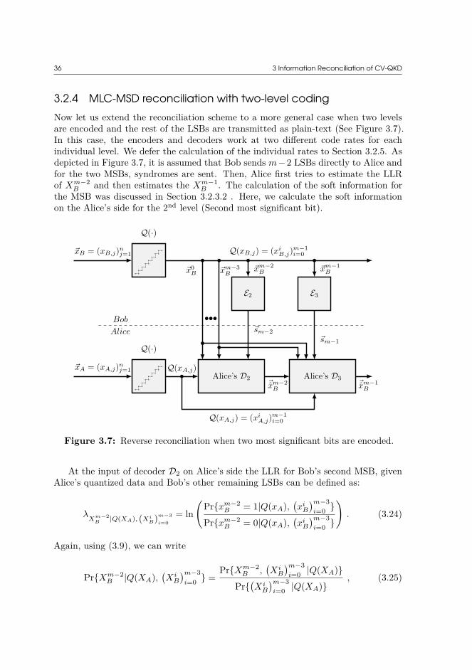
36 3 Information Reconciliation of CV-QKD
3.2.4 MLC-MSD reconciliation with two-level codingNow let us extend the reconciliation scheme to a more general case when two levelsare encoded and the rest of the LSBs are transmitted as plain-text (See Figure 3.7).In this case, the encoders and decoders work at two different code rates for eachindividual level. We defer the calculation of the individual rates to Section 3.2.5. Asdepicted in Figure 3.7, it is assumed that Bob sends m−2 LSBs directly to Alice andfor the two MSBs, syndromes are sent. Then, Alice first tries to estimate the LLRof Xm−2
B and then estimates the Xm−1B . The calculation of the soft information for
the MSB was discussed in Section 3.2.3.2 . Here, we calculate the soft informationon the Alice’s side for the 2nd level (Second most significant bit).
~xB = (xB,j)nj=1
Q(·)
Q(xB,j) = (xiB,j)
m−1i=0
~xm−2B~xm−3
B~x0B
~xm−1B
E2 E3
Alice
Bob~sm−2
Alice’s D2~xm−2B
~sm−1
Alice’s D3~xm−1B
~xA = (xA,j)nj=1 Q(xA,j)
Q(xA,j) = (xiA,j)
m−1i=0
Q(·)
Figure 3.7: Reverse reconciliation when two most significant bits are encoded.
At the input of decoder D2 on Alice’s side the LLR for Bob’s second MSB, givenAlice’s quantized data and Bob’s other remaining LSBs can be defined as:
λXm−2
B|Q(XA), (Xi
B)m−3i=0
= ln
(Pr{xm−2
B = 1|Q(xA),(xi
B
)m−3i=0 }
Pr{xm−2B = 0|Q(xA),
(xi
B
)m−3i=0 }
). (3.24)
Again, using (3.9), we can write
Pr{Xm−2B |Q(XA),
(Xi
B
)m−3i=0 } =
Pr{Xm−2B ,
(Xi
B
)m−3i=0 |Q(XA)}
Pr{(Xi
B
)m−3i=0 |Q(XA)}
, (3.25)

3.2 Multi-Level-Coding Multi-Stage-Decoding 37
where (3.25) can be used to simplify both numerator and denominator of (3.24) asfollows:
λXm−2
B|Q(XA), (Xi
B)m−3i=0
= ln
(Pr{xm−2
B = 1,(xi
B
)m−3i=0 |Q(xA)}
Pr{xm−2B = 0,
(xi
B
)m−3i=0 |Q(xA)}
). (3.26)
In addition, let us define four new random variables Qpp(XB), Qpn(XB), Qnp(XB)and Qnn(XB). Where, Qpp(XB) takes LSBs of Bob’s data and assumes that the twoMSBs are equal to 00 and so on. The numerator of (3.26) can be expanded as:
Pr{xm−2B = 1,
(xi
B
)m−3i=0 |Q(xA)} = 1
2Pr{xm−1
B = 0, xm−2B = 1,
(xi
B
)m−3i=0 |Q(xA)}
+ 12
Pr{xm−1B = 1, xm−2
B = 1,(xi
B
)m−3i=0 |Q(xA)}
= Pr{Qpn(xB)|Q(xA)} + Pr{Qnn(xB)|Q(xA)}2
,
where in the last equation, it is assumed that Pr{xm−1B = 0|Q(xA)} = Pr{xm−1
B =1|Q(xA)} = 1
2 . This assumption is valid, because at this step, decoder D2 does nothave any information about X3
B . In other words, it can take zero or one with equalprobability. Then, (3.26), can be simplified to:
λXm−2
B|Q(XA), (Xi
B)m−3i=0
= ln
exp(
−(Qnn(xB)−Q(xA))2
2σ2
)+ exp
(−(Qpn(xB)−Q(xA))2
2σ2
)exp
(−(Qnp(xB)−Q(xA))2
2σ2
)+ exp
(−(Qpp(xB)−Q(xA))2
2σ2
) ,
(3.27)which is the soft information at the input of the decoder D2.
The generalization to the higher levels is straight forward but in practice just twoMSBs are encoded. In fact the channel coding rates for LSBs are very close to zeroand no practical error correction exists for LSBs. In Section 3.2.5 we calculate theindividual code rates for each level. Then it would be clear that just two MSBs areenough for the reconciliation tasks and all the remaining LSBs are then transmittedas plain-text.

38 3 Information Reconciliation of CV-QKD
3.2.5 Calculation of the individual source coding rates3.2.5.1 Analytical method
For an m-bit digitizer, the individual conditional mutual information for each level isdefined as:
Ii = I(XA;XiB |Xi−1
B , . . . , X0B) ,
= H(XiB |Xi−1
B , . . . , X0B) −H(Xi
B |XA, Xi−1B , . . . , X0
B) . (3.28)
Thus, using (3.3) it is clear that:
RSourcei ≥ H(Xi
B |Xi−1B , . . . , X0
B) − Ii . (3.29)
Equation (3.29) offers an analytical way to calculate the individual source rates foreach level and, the only non-trivial quantity is the individual conditional mutualinformation Ii. To calculate Ii, the MLC-MSD approach is used [7]. Using thechain rule, we can always describe the total mutual information as a summation ofconditional mutual information for individual levels
I(XA;Q(XB)) = I(XA;Xm−1B , . . . , X0
B) = I(XA;X0B) + I(XA;X1
B |X0B)
+ . . .+ I(XA;XiB |Xi−1
B , . . . , X0B) + . . .
+ I(XA;Xm−1B |Xm−2
B , . . . , X0B) , (3.30)
which motivates our definition of the individual conditional mutual information in (3.28).According to [7], we can expand Ii as follows:
Ii = I(XA;XiB |Xi−1
B , . . . , X0B) (3.31)
= I(XA;Xm−1B , . . . , Xi
B |Xi−1B , . . . , X0
B) − I(XA;Xm−1B , . . . , Xi+1
B |XiB , . . . , X
0B) ,
where each term on the right hand side can be calculated separately. More precisely,
I(XA;Xm−1B , . . . , Xi
B |Xi−1B , . . . , X0
B) =Exi−1
B,...,x0
B∈ {0,1}i { I(XA;Xm−1
B , . . . , XiB |xi−1
B , . . . , x0B)},
where E denotes the expectation value and can be calculated by averaging over allpossible combinations of xi−1
B , . . . , x0B . Finally, according to [7], the full character-
ization of Ii requires a set of probability density functions (PDF)s f XA|XiB
(xA|xiB)
which can be defined as:{fXA|XB
(xA|xi
B , xi−1B , . . . , x0
B
)|(xi−1
B , . . . , x0B
)∈ {0, 1}i
},
where,
fXA|XB(xA|xi
B , xi−1B , . . . , x0
B) = Eb ∈ S(xiB
,...,x0B
){fXA|XB
(xA|b)},
where the signal point b is taken from the subset S(x0B . . . x
iB) and fXA|XB
(xA|b) is theequivalent conditional quantized PDF of the continuous conditional PDF presentedon (3.20).

3.2 Multi-Level-Coding Multi-Stage-Decoding 39
Example 3.2.2. Simulation results for a 4-bit digitizer
As an example, we present simulation results for individual rates for 16 bins, whenBob’s quantized data has a discrete Gaussian PDF. The results for individual channelcoding rates are presented in Figure 3.8. The equivalent channel coding rate is equalto Rch
i = 1 − RSourcei . We assumed that Alice’s data has a continuous Gaussian
distribution with variance equal to 1 and both Alice and Bob use 4 level digitizers.Also, a fixed step size δ = 0.32 is assumed for digitization of normalized continuousvariables.
20 15 10 5 0 5 10 15 20SNR [dB]
0.0
0.2
0.4
0.6
0.8
1.0
Rat
es [b
its p
er s
ymbo
l]
Rch0
Rch1
Rch2
Rch3
Figure 3.8: The equivalent channel coding rates (Rchi = 1 − RSource
i ) for 4-levelswith binary partitioning versus SNR.
Figure 3.9 denotes the conditional mutual information for the ith individual chan-nel (Ii) as a function of the SNR. It is clear that the summation of the all individualconditional mutual information is very close to the Shannon capacity of the AWGNchannel, and the small difference is a results of the digitization effect.
By summing up over all the individual mutual information taken from (3.28) it isclear that:
m−1∑i=0
Ii = I(Q(XB);XA) ≤ I(XB ;XA) .
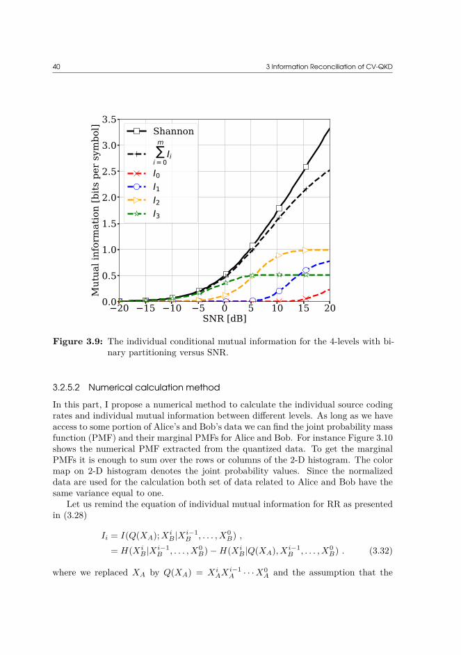
40 3 Information Reconciliation of CV-QKD
20 15 10 5 0 5 10 15 20SNR [dB]
0.0
0.5
1.0
1.5
2.0
2.5
3.0
3.5
Mut
ual i
nfor
mat
ion
[bits
per
sym
bol] Shannon
m
i = 0Ii
I0I1I2I3
Figure 3.9: The individual conditional mutual information for the 4-levels with bi-nary partitioning versus SNR.
3.2.5.2 Numerical calculation method
In this part, I propose a numerical method to calculate the individual source codingrates and individual mutual information between different levels. As long as we haveaccess to some portion of Alice’s and Bob’s data we can find the joint probability massfunction (PMF) and their marginal PMFs for Alice and Bob. For instance Figure 3.10shows the numerical PMF extracted from the quantized data. To get the marginalPMFs it is enough to sum over the rows or columns of the 2-D histogram. The colormap on 2-D histogram denotes the joint probability values. Since the normalizeddata are used for the calculation both set of data related to Alice and Bob have thesame variance equal to one.
Let us remind the equation of individual mutual information for RR as presentedin (3.28)
Ii = I(Q(XA);XiB |Xi−1
B , . . . , X0B) ,
= H(XiB |Xi−1
B , . . . , X0B) −H(Xi
B |Q(XA), Xi−1B , . . . , X0
B) . (3.32)
where we replaced XA by Q(XA) = XiAX
i−1A · · ·X0
A and the assumption that the

3.2 Multi-Level-Coding Multi-Stage-Decoding 41
4 3 2 1 0 1 2 3 4Q(XA)
4
3
2
1
0
1
2
3
4
Q(X
B)
0.0 0.2 0.4Marginal PMF
4
3
2
1
0
1
2
3
44 3 2 1 0 1 2 3 40.0
0.10.20.30.4
Mar
gina
l PM
F
0.00
0.05
0.10
0.15
Join
t PM
F
Figure 3.10: Numerical joint PMF for quantized bi-variate normally distributedrandom variables and their marginal PMFs for a 4-bit digitizer atSNR=−5 dB.
same digitizer is used on both sides. In the following we show how to calulate bothparts of the right hand side of the above equation by using joint and the marginalPMFs.
For the first term, from the fact that H(X|Y ) = H(X,Y ) −H(Y ):
H(XiB |Xi−1
B , . . . , X0B) = H(Xi
B , Xi−1B , . . . , X0
B) −H(Xi−1B , . . . , X0
B) .
Then, to calculate the term H(XiB , X
i−1B , . . . , X0
B), we can directly apply thedefinition of the entropy for discrete variables as follows:
H(XiB , . . . , X
0B) = −
∑Xi
B,...,X0
B
PrXi
B,...,X0
B
{xiB , . . . , x
0B} log2
(Pr
XiB
,...,X0B
{xiB , . . . , x
0B}
).
All the probabilities can be calculated from Bob’s marginal PMF. For examplePrX0
B{1} denotes the probability that the LSB of Bob is equal to 1. In a similar way,
PrX1B
X0B
{01}, denotes the probability that the two LSBs of Bob are 01.

42 3 Information Reconciliation of CV-QKD
For the second term in (3.32) it is possible to write
H(XiB |Q(XA), Xi−1
B , . . . , X0B) = H(Xi
B , . . . , X0B |Q(XA))
−H(Xi−1B , . . . , X0
B |Q(XA)) .
And to calculate each term
H(XiB , . . . , X
0B |Q(XA)) =
a2m−1∑Q(XA)=a0
PrQ(XA)
{ai}H(XiB , . . . , X
0B |ai) ,
where ai is a realization of Alice’s quantized data and H(XiB , . . . , X
0B |Q(XA) = ai)
denotes the instant entropy value when Q(XA) = ai. The probability PrQ(XA){ai}can be obtained by looking at Alice’s marginal PMF and H(Xi
B , . . . , X0B |Q(XA) = ai)
can be calculated as:
−∑
XiB
,...,X0B
PrXi
B,...,X0
B|Q(xA)
{xiB , . . . , x
0B |ai} log2
(Pr
XiB
,...,X0B
|Q(xA){xi
B , . . . , x0B |ai}
),
where the probability values PrXiB
,...,X0B
|Q(xA){xiB , . . . , x
0B |ai} can be obtained from
the joint PMF of Alice and Bob. Our numerical calculations confirm the same theo-retical values for individual rates and individual mutual information (See Figure 3.9and Figure 3.8).

3.3 Comparison between reverse and forward reconciliation 43
3.3 Comparison between reverse and forwardreconciliation
In Section 3.1 the difference between FR and RR was discussed in the context ofmultidimensional reconciliation. Here, we compare FR and RR for the MLC-MSDscheme. As illustrated in Figure 3.11, Alice and Bob are connected through twodifferent channels (classical and quantum channels). First, Alice sends quantum statesto Bob through a noisy quantum channel and later, depending on the reconciliationprotocol, the two parties share some information on an authenticated classical channel.In the case of FR, Alice encodes her data and sends it to Bob who would correct hisdata according to syndromes generated by Alice, plus his own side information. Onthe other hand, in the case of RR, Bob sends the data, and Alice corrects her dataaccording to his data (For detailed information see Figure 3.11).
Alice’s Side Bob’s Side
~xA = (xA,1, . . . , xA,n) ~xB = (xB,1, . . . , xB,n)
Quantizer Q(·)
QUANTUM CHANNEL
Quan
tizerQ(·)
xm−1A,1 , . . . , xm−1
A,n
xiA,1, . . . , x
iA,n
Enc m− 1
Enc i
pm−11 , . . . , pm−1
n(1−Rchm )
pi1, . . . , pin(1−Rch
i )
Dec i
Dec m− 1xm−1A,1 , . . . , xm−1
A,n
xiA,1, . . . , x
iA,n
// //
x0A,1, . . . , x
0A,nx0
A,1, . . . , x0A,n
......
...... · · · · · ·
Bob’s Side Alice’s Side
~xB = (xB,1, . . . , xB,n) ~xA = (xA,1, . . . , xA,n)
Quantizer Q(·)
QUANTUM CHANNEL
QuantizerQ(·)
xm−1B,1 , . . . , xm−1
B,n
xiB,1, . . . , x
iB,n
Enc m− 1
Enc i
pm−11 , . . . , pm−1
n(1−Rchm )
pi1, . . . , pin(1−Rch
i )
Dec i
Dec m− 1xm−1B,1 , . . . , xm−1
B,n
xiB,1, . . . , x
iB,n
// //
x0B,1, . . . , x
0B,nx0
B,1, . . . , x0B,n
......
...... · · · · · ·
Figure 3.11: The comparison of forward (upper) and reverse (lower) reconciliation.Through the quantum channel Alice always sends quantum states oflight to Bob. In the classical channel the direction of the messages arenot the same and is determined by the protocol.
In both cases, the quantum channel can be described by XB = XA + N , where
44 3 Information Reconciliation of CV-QKD
N is the additive white Gaussian noise with zero mean and variance σ2N . Since, the
two quantities XA and N are independent, the following bounds are valid for thecontinuous data:
H(XB) ≥ H(N) ,H(XB) ≥ H(XA) ,
For the reconciliation, it can be assumed that Alice and Bob have access to pairsof samples of a joint Gaussian distribution. Also, let us denote by H(Q(XA)) andH(Q(XB)) the entropy of the quantized version of Alice and Bob’s data. Accordingto Table 3.1 and Figure 3.5, for an efficient digitizer
I(XB ;XA) ≈ I(Q(XB);Q(XA)) ,H(Q(XB)) −H(Q(XB)|Q(XA)) ≈ H(Q(XA)) −H(Q(XA)|Q(XB)) ,H(Q(XB)) +H(Q(XA)|Q(XB)) ≈ H(Q(XA)) +H(Q(XB)|Q(XA)) ,H(Q(XA), Q(XB)) ≈ H(Q(XB), Q(XA)) .
According to the results presented in [50], and as depicted in Figure 3.12, in thecase of FR (RR), it is enough for Alice and Bob to shareH(Q(XA)|XB) (H(Q(XB)|XA))information (bit/symbol) through the classical channel to achieve perfect reconcilia-tion. In this case the corresponding mutual information is
FR: H(Q(XA)) −H(Q(XA)|XB)RR: H(Q(XB)) −H(Q(XB)|XA).
The quantity H(Q(XA)|XB) (H(Q(XB)|XA)) is a lower bound on source codingrate for FR (RR). For better understanding of the difference between these quantitiesas a function of SNR, a comparison has been done for the continuous variables onquantum channel using the differential entropy for Gaussian variables. The resultsare shown in Figure 3.13.
Now, let us compare with more details the forward and reverse reconciliationprotocols. Also, let us denote by Is(X;Y ) = I(X;Y )|s and Hs(X) = H(X)|s, themutual information and the entropy at specific SNR s. The specific definition ofthese quantities would be clear from the context. In addition, remember that RCh
i =1−RSource
i . For simplicity, we denote here the channel coding rate at SNR s by RiRR |s
and RiFR |s for RR and FR, respectively.
3.3.1 Individual rates for reverse and forward reconciliationsIt is known from (3.3) that for RR, the channel coding rate of the individual levels
Ri
RR |s ≤ 1 −Hs(XiB |XA, X
i−1B , . . . , X0
B) ,

3.3 Comparison between reverse and forward reconciliation 45
H(Q(XA), XB)
H(Q(XB), XA)
I(Q(XA);XB)
I(Q
(XB);X
A)
H(Q(XA))H(Q(XA)|XB)
H(Q(XB))
H(Q(XB)|XA)
x
y
0
Figure 3.12: Admissible Rate Region according to Slepian-Wolf method.
-20 -15 -10 -5 0 5 10 15 20
-2
-1
0
1
2
3
4
5
6
Figure 3.13: The theoretical values for differential entropies for continuous data onquantum channel.

46 3 Information Reconciliation of CV-QKD
thus,
RRR |s =∑
i
Ri
RR |s ≤ m−Hs(Q(XB)|XA) ,
Ii
RR |s = I(XiB ;XA|Xi−1
B , . . . , X0B) ,
Ii
RR |s = Hs(XiB |Xi−1
B , . . . , X0B) −Hs(Xi
B |XA, Xi−1B , . . . , X0
B) .
In a similar way, for FR:
Ri
FR |s = 1 −Hs(XiA|XB , X
i−1A , . . . , X0
A) ,
RFR |s =∑
i
Ri
FR |s ≤ m−Hs(Q(XA)|XB) ,
Ii
FR |s = I(XiA;XB |Xi−1
A , . . . , X0A) ,
Ii
FR |s = Hs(XiA|Xi−1
A , . . . , X0A) −Hs(Xi
A|XB , Xi−1A , . . . , X0
A) .
Finally, for both schemes
IRR =m∑
i=1Ii
RR = I(XA;Q(XB)) ≈ I(Q(XA);XB) =m∑
i=1Ii
FR = IFR , (3.33)
where in (3.33), it is assumed that the digitization error is small and I(XA;Q(XB)) ≈I(Q(XA);XB) ≈ I(XA;XB).
3.3.2 Individual rates in terms of I i|∞ and I i|sThe rate of the error correction codes can be represented in terms of the mutualinformation. In the case of FR:
Ii
FR |s = Hs(XiA|Xi−1
A , . . . , X0A) −Hs(Xi
A|XB , Xi−1A , . . . , X0
A) , (3.34)
and at s = ∞
Ii
FR |∞ = H∞(XiA|Xi−1
A , . . . , X0A) −H∞(Xi
A|XB , Xi−1A , . . . , X0
A) .
since, s → ∞ then, XB = XA and H∞(XiA|XB , X
i−1A , . . . , X0
A) = 0, thus:
Ii
FR |∞ = H∞(XiA|Xi−1
A , . . . , X0A) = Hs(Xi
A|Xi−1A , . . . , X0
A) . (3.35)
The last equality is valid, because the Alice’s data is independent of the SNR. Then,for the case of FR
Ri
FR |s = 1 − [Ii
FR |∞ − Ii
FR |s]. (3.36)
This can be checked by substituting (3.34) and (3.35) in (3.36), which is equivalentto the results presented in [9].
3.3 Comparison between reverse and forward reconciliation 47
In a similar way for RR,
Ii
RR |s = Hs(XiB |Xi−1
B , . . . , X0B) −Hs(Xi
B |XA, Xi−1B , . . . , X0
B) , (3.37)
when s → ∞, again XA = XB and XiB = Xi
A for i = 1, . . . ,m, thus:
Ii
RR |∞ = H∞(XiB |Xi−1
B , . . . , X0B) −H∞(Xi
B |XA, Xi−1B , . . . , X0
B) ,
which can be simplified to
Ii
RR |∞ = H∞(XiB |Xi−1
B , . . . , X0B)
= H∞(XiA|Xi−1
A , . . . , X0A) = Hs(Xi
A|Xi−1A , . . . , X0
A) . (3.38)
Finally, subtracting (3.37) from (3.38):
Ii
RR |∞ − Ii
RR |s = Hs(XiB |XA, X
i−1B , . . . , X0
B)
+Hs(XiA|Xi−1
A , . . . , X0A) −Hs(Xi
B |Xi−1B , . . . , X0
B)︸ ︷︷ ︸−∆s
i
,
or equivalently
Hs(XiB |XA, X
i−1B , . . . , X0
B) = Ii
RR |∞ − Ii
RR |s + ∆si , (3.39)
where ∆si = Hs(Xi
B |Xi−1B , . . . , X0
B) − Hs(XiA|Xi−1
A , . . . , X0A). Thus, for RR, the
individual channel coding rate is:
Ri
RR |s = 1 −Hs(XiB |XA, X
i−1B , . . . , X0
B) = 1 − [Ii
RR |∞ − Ii
RR |s] − ∆si , (3.40)
which is not completely similar to (3.36) for FR, and has a correction term ∆si .
Finally, it is clear that at s → ∞, the two quantities IiRR |∞ and Ii
FR |∞ are equal(See (3.35) and (3.38)). By assuming that individual mutual information for FR andRR are almost equal to each other, for all the SNR points1, i.e, Ii
FR |s ≈ IiRR |s then:
Ri
RR |s = 1− [Ii
RR |∞ −Ii
RR |s]−∆si ≈ 1− [Ii
FR |∞ −Ii
FR |s]−∆si ≈ Ri
FR |s −∆si . (3.41)
Finally, if we sum up over all individual channels
RRR |s ≈ RFR |s −m∑
i=1∆s
i = RFR |s +H(Q(XA)) −H(Q(XB)) . (3.42)
1This assumption could be valid with a good approximation. At least, it can be assumed thatthe code rates are designed in such a way that the mutual information between the two scenarios(FR and RR) be equal and the summation of the mutual information of the individual levels aremaximized on both cases.

48 3 Information Reconciliation of CV-QKD
3.4 Randomized ReconciliationThe concept of randomized decoding was first introduced in [53]. The other relatedalgorithms in this family are known as list decoding and Chase algorithm [54, 55],where they use the soft measurement information at the input of a hard decoder.Specifically, the Chase algorithm uses a simple hard decoder and generates a listof candidate test-codewords by flipping the least reliable positions in the receivedsequence.
Before describing the algorithm for the randomized reconciliation, let us brieflydescribe the concept of reconciliation using list decoding. The concept behind thissoft decoder is depicted in Figure 3.14. Here we assume that the core of the decoder isa simple hard decoder with the capability to find a unique codeword, when the noisyreceived sequence is surrounded by a sphere of radius ⌊ d−1
2 ⌋, where d is the mini-mum distance of the error correction code. Also, we assume four possible codewordsC1, C2, C3, C4, and the received sequence yH . Thus, in this case, a hard decisiondecoder provides a unique codeword C1, with its unique error pattern yH ⊕ C1. Thegoal of the list decoding is to generate different error patterns, by changing the leastreliable positions in the received sequence yH . For the new test-vector yT , it is pos-sible for our hard decoder to find a new codeword depending on whether or not yT
falls into the sphere of a new codeword.
~Cy2 ~C3
~C1
~C4
~yH
r = d− 1
r = b(d− 1)/2c
~yT
Figure 3.14: Decoding using measured soft information and hard decoder. Takenby some modification from [56] .
More specifically, in this section the same procedure is used for a reconciliationscheme. For the reconciliation, a channel code induces a partitioning of the sourcedata space into cosets that can be indexed by their respective syndromes. Let C bea (n, k)-linear block code. The problem of decoding reconciliation using the corre-sponding channel code is to find the transmitted codeword, given the measured side

3.4 Randomized Reconciliation 49
information vectors XA and SB at the decoder. The encoder computes the syndromeof the sequence yH = (yH,i)n−1
i=0 by computing s = yH × HT , where H is the paritycheck matrix of the code. Then the decoding operation is equivalent to finding acodeword with the same syndrome. By assuming that each coset contains only onevalid codeword this problem is equivalent to our channel coding problem.
Here, we propose a randomized reconciliation for CV-QKD using a modified ver-sion of the Chase algorithm called stochastic Chase algorithm (SCA) [57, 56]. In theSCA, the test-codewords are generated according to their reliability. Let us denoteby λ = (λi)n−1
i=0 the log likelihood of Bob’s soft information on Alice’s side which is avector of length n. It was shown in Section 3.2.3.2, how to calculate the soft measure-ment information (See (3.14)). Equivalently, its hard decision value yH = (yH,i)n−1
i=0can be calculated as:
yH,i =
{1 if λi ≥ 00 if λi < 0
.
Also, in the probability domain, the vector p = (pi)n−1i=0 denotes the probability that
the corresponding bit at position i ∈ {0, . . . , n− 1} is equal to 1, where
pi = eλi
1 + eλi.
It is clear that λi ∈ (−∞,∞), and pi ∈ (0, 1). When λi → ∞ the value of pi → 1,and in similar way, when ri → −∞ the value of pi → 0, and for ri → 0 the value ofpi → 1
2 . This shows that the least reliable positions in a received codeword have LLRvalues close to 0, which are most likely the error positions.
The algorithm for the randomized reconciliation can be found in Algorithm 1. Inthe initialization, the algorithm extracts two kinds of information from r. First, itfinds the first τ least reliable positions in the received codeword and finds its equivalenthard decision yH . Second, it finds the probability of being 1 for each unreliable index.Then, in the main loop, the algorithm generates L different test-vectors. This can beeasily done by flipping the value of the index i in yH based on its flipping probabilitypi. Then for each test-vector yT , the hard LDPC decoder finds the syndrome sT
and compares it with the Bob’s syndrome s. The algorithm ends when it finds atest-codeword which has zero Hamming distance with Bob’s syndrome. Otherwise,the algorithm looks among all the L test-codewords and finds the one with minimumHamming distance.
3.4.1 Complexity of the algorithmLet us consider a reconciliation process based on MLC-MSD. The complexity of ran-domized reconciliation using SCA is compared with the complexity of a soft LDPCdecoder. For the soft LDPC decoder a min-sum (MS) algorithm is used. The coreof the SCA is a hard decoder using a bit-flipping (BF) algorithm. Let us denote theaverage number of VNs (CNs) by dv
(dc
). For each iteration of the MS algorithm,

50 3 Information Reconciliation of CV-QKD
Algorithm 1 Randomized Reconciliation—————————— InitializeStep 1) Find τ least reliable bits in rStep 2) j = (ji)τ
1 ▷ index of least reliable bitsStep 3) p = (pi)τ
1 ▷ probability of being oneStep 4) yH ▷ equivalent hard decision vector—————————— Main loopl ⇐ 0 ▷ counter for test-codewordsL ▷ maximum number of test-codewordswhile l ≤ L do
yT = yH
for i ∈ j doyT,i = BSCpi
(0)end forDecode yT , to get xT and the syndrome sT
Calculate the distance: DsT ,s =m∑
i=1Si
⊕ST,i
l ⇐ l + 1end while—————————— Best codewordThe output codeword is the one with minimum DsT ,s .
the VN v sums over all the incoming messages. Thus in average n · dv summationare required. On the other hand, for each CN c, assuming an average CN degree dc,the output message is calculated by finding the minimum of all incoming messages.Thus in general m · dc comparisons are necessary. Also, the same number of xor (⊕)operations are required in order to find the sign of the output message.
In contrast, the BF algorithm just acts on the binary data and all the operationsare ⊕ operations. The algorithm at each iteration finds the syndrome, which requiresm · dc xor operations and then flips the position of some VNs when the specific bithas a set of non-zero syndromes larger than specific threshold T . The summary ofour discussion can be found in Table 3.2.
Considering the fact that the complexity of bit-wise operations are negligible incomparison with operations acting on real numbers, it is clear that the MS algorithmhas much higher complexity than BF algorithm.
Now, if we assume that the SCA uses L different codewords to find the best one,we can compare the complexity of MS and SCA. The SCA can apply L completelyindependent test-codewords and selects the best codeword by measuring the distanceof the final syndrome to Bob’s syndrome. Thus, the SCA requires L comparisonsto find the best codeword. It is clear that to have the same complexity on MS andSCA L should be approximately very close to n2. For example, for a code of length103 bits, the complexity of the SCA with 106 test-vectors would be the same as the

3.5 Reconciliation for a wide range of SNRs 51
Table 3.2: The complexity per iteration.
# of # of # ofadditions comparison ⊕
MS algorithm n · dv m · dc m · dc
BF algorithm 0 0 m · dc
complexity of the MS algorithm.
3.5 Reconciliation for a wide range of SNRsSo far, we have described how to design different reconciliation schemes for CV-QKDfor a specific signal to noise ratio. The efficiency of these reconciliation schemes can bedefined as the ratio of the net shared information revealed for the reconciliation andthe mutual information. The precise definition depends on the reconciliation protocol,for example in RR, in the case of multidimensional reconciliation, the efficiency canbe defined as:
βmulti-dimensional = RCh
IAWGN(XB ;XA)
= RCh
IBI-AWGN(XB ;XA)· IBI-AWGN(XB ;XA)IAWGN(XB ;XA)
= βCode · βMapping ,
where βCode denotes the efficiency of the error correction code on BI-AWGN channel,and βMapping denotes the mapping efficiency between the AWGN channel and virtualBI-AWGN channel. On the other hand, the efficiency of the MLC-MSD scheme, inthe case of RR, is defined as:
βMLC-MSD = H(Q(XB)) −RSource
I(XB ;XA)
= H(Q(XB)) −RSource
I(Q(XB);XA)· I(Q(XB);XA)
I(XB ;XA)
= H(Q(XB)) −m+RCh
I(Q(XB);XA)· I(Q(XB);XA)
I(XB ;XA)= βCode · βDisc ,
where βCode denotes the code efficiency, and βDisc denotes the digitization efficiency.The common issue in all the above reconciliation schemes is the fixed code rate. It
means that the code rate is designed for a certain SNR value for reliable reconciliation.

52 3 Information Reconciliation of CV-QKD
Then, by moving forward from this value using the same code, the efficiency movesdown from the optimal value. On the other hand, by moving backward from thispoint, higher efficiency can be obtained, with lower reliability or higher frame errorrate. One approach to solve this issue is to use multiple LDPC codes with differentcode rates to cover a wide SNR range [58].
-15.5 -15 -14.5 -14 -13.5
60
65
70
75
80
85
90
95
100
Figure 3.15: Reconciliation efficiencies for different SNRs. The gray line denotesthe efficiency when a fixed code of rate 0.02 is used. The other curvesdenote the cases when other LDPC codes are used for different SNRranges.
Designing multiple LDPC codes for each SNR is not an efficient solution since ahuge parity check matrix is required for each code rate. Two other techniques, widelyused to create rate adaptive codes, are puncturing and shortening. By using thesetwo techniques one can create new code rates from a code with a fixed code rate.For instance, assuming that the original code rate is R = k
n , then the rate of thepunctured code is
RPunc = k
n− p, (3.43)
where p denotes the length of the puncturing. Puncturing enables us to increasethe code rate. During the puncturing process, p symbols are eliminated from thecodeword. The punctured bits are not transmitted, and at the decoder they are

3.5 Reconciliation for a wide range of SNRs 53
replaced by least reliable bits. For example, in the case of a binary erasure channel(BEC) they are considered as erasure and in the case of an AWGN channel they arereplaced with zero LLR values.
The second technique is known as shortening and the rate of the shortened codeis defined as
RShort = k − s
n− s, (3.44)
where s denotes the length of the shortened symbols. Figure 3.16 demonstrates theprinciple of shortening for standard error correction codes.
k − sInsert
s known symbols
kEncoder
R = k/n
nDiscard
s known symbols
n− s
k − sdiscard
s known symbols
kDecoder
R = k/n
nInsert
s known symbols
n− s
Figure 3.16: The block diagram of the shortening process. The base code has rateR = k
nand the shortened code has the rate RShort = k − s
n− s.
Rate adaptive techniques were developed for both DV-QKD and CV-QKD, wherethey combine shortening and puncturing methods to design rate adaptive reconcili-ation [58, 36]. Recently, a rate adaptive reconciliation technique was developed byusing Raptor codes [59], where authors combined a multi-dimensional reconciliationscheme with Raptor codes to develop a rate-less reconciliation protocol. The mainissue of this scheme is that the two parties need extra communication to send anadditional check code to finish the reconciliation process [60].

54

CHAPTER4On the Design of
Highly EfficientMET-LDPC codes
This chapter investigates how to design highly efficient multi-edge-type low-densityparity-check (MET-LDPC) codes for CV-QKD. The readers are invited to see ourarXived article [18]. It is assumed that readers are familiar with Irregular LDPCcodes. For the readers, who are not familiar with this class of error correction codes,more details are provided in Appendix A.
Section 4.1 introduces the MET-LDPC codes and provides all the requirementsfor understanding the code structure. In Section 4.2, we describe the density evolu-tion (DE) for the MET-LDPC codes and some of its approximations are presented.In Section 4.3, we propose the concept of G-EXIT charts for MET-LDPC codes.In Section 4.4, the code design optimization problem is defined and we talk moreabout the structure of these codes. Our new proposed optimization algorithm ispresented in Section 4.5 and some examples codes designed with the optimizationalgorithm are presented in Section 4.6. Finally, Section 4.7 provides some simulationresults to show the finite size performance of our designed codes.
4.1 Multi-Edge-Type LDPC codesMET-LDPC codes are a generalization of the concept of irregular LDPC codes [44,61]. These codes provide improvements in performance and complexity by givingmore flexibility over different edge types. In this structure each node is characterizedby the number of connections (sockets) to edges of each edge-type. An irregular LDPCcode can be considered as a single-edge-type LDPC (SET-LDPC) code in this context.Using MET-LDPC codes we are able to design capacity achieving codes without usingVNs with very high degree which provides a less complex implementation. Also, itexploits the advantage of using degree one VNs, which are very useful for designingLDPC codes at low rate and low SNR[61]. It is important to recall that in the caseof irregular LDPC codes the minimum usable VN degree is 2.

56 4 On the Design of Highly Efficient MET-LDPC codes
It is very convenient to begin with a comprehensible table format representationof MET-LDPC codes as presented in Table 4.1. The left side of the table correspondsto the VNs and the right side describes the CN structures.
Table 4.1: Table presentation of a MET-LDPC code with ne edge types.variable-node check-node
νbd b dv µd dc
ν1ν2...νi
...νQ
b0,1 b1,1b0,2 b1,2
......
b0,i b1,i
......
b0,Q b1,Q
dv1,1 dv
2,1 · · · dvne,1
dv1,2 dv
2,2 · · · dvne,2
...... . . . ...
dv1,i dv
2,i · · · dvne,i
...... . . . ...
dv1,Q dv
2,Q · · · dvne,Q
µ1µ2...µi
...µP
dc1,1 dc
2,1 · · · dcne,1
dc1,2 dc
2,2 · · · dcne,2
...... . . . ...
dc1,i dc
2,i · · · dcne,i
...... . . . ...
dc1,P dc
2,P · · · dcne,P
For instance, the ith row at the CN side corresponds to a CN of type dc,i =(dc
1,i, dc2,i, · · · , dc
ne,i) where each element dcj,i in dc,i describes the degree of the CN i
along jth edge type. ne denotes the total number of edge-types. Then, the matrix
dc =
( dc,1
...dc,P
)describes the edge distribution of the CN side. In addition, the vector
µd = (µ1, . . . , µi, . . . , µP ) describes the node distribution of the CN side, where P
is the number of different CN types. Similarly, dv =
( dv,1
...dv,Q
)describes the edge
distribution of the VNs, where each row vector dv,i = (dv1,i, d
v2,i, · · · , dv
ne,i) describesa specific VN type. The node distribution on the VN side is denoted by νbd =(ν1, . . . , νi, . . . , νQ), where Q is the number of VN types. Finally, the vectors bi =(b0,i, b1,i) describes the channel to be punctured or not. Here, in this article, we denotea non-punctured node by bi = (0, 1). In addition, it is noteworthy to mention thatthe elements of the vectors νbd and µd are non-negative fractional numbers and theelements of the matrices dv and dc are non-negative integer numbers. For example,let N be the length of the code-word, then for each CN of type i the quantity µiN isthe number of constraint-nodes of type i in the graph. Similarly, the quantity νjN isthe number of VNs of type j in the graph.
Furthermore, the code ensemble for a MET-LDPC code can be specified bytwo multi-variable-polynomials, one associated to VNs and the other associated toCNs (constraint-nodes). The node-perspective representation of these multi-variable-polynomials are:
ν(r,x) =Q∑
i=1νirbixdv,i , µ(x) =
P∑i=1
µixdc,i , (4.1)
respectively. In (4.1), x := (x1, · · · , xne) and r := (r0, · · · , rnr
), where nr is thenumber of different channels. In this thesis it is assumed that, nr = 2. r0 stands

4.1 Multi-Edge-Type LDPC codes 57
for punctured channel and r1 is the channel parameter for te code. Finally, xdc,i :=∏ne
j=1 xdc
j,i
j , xdv,i :=∏ne
j=1 xdv
j,i
j and rbi :=∏nr
j=1 rbj,i
j .In addition, the edge perspective degree distribution can be described as a vector
of multi-variable polynomials, for VNs and CNs, respectively,
λ(r,x) =(νx1(r,x)νx1(1,1)
,νx2(r,x)νx2(1,1)
, . . . ,νxne
(r,x)νxne
(1,1)
),
ρ(x) =(µx1(x)µx1(1)
,µx2(x)µx2(1)
, . . . ,µxne
(x)µxne
(1)
), (4.2)
where,νxi
(r,x) = ∂
∂xiν(r,x) , µxi
(x) = ∂
∂xiµ(x) ,
and 1 denotes a vector of all 1’s where the length being determined by context. Thecoefficients of ν and µ are constrained to ensure that the number of sockets of eachtype is the same on both sides (variable and check) of the graph. This gives rise tone linear conditions on the coefficients of ν and µ as follows:
νxi(1,1) = µxi(1), i = 1, · · · , ne .
Finally, the nominal code rate for non-punctured codes is given by
R = ν(1,1) − µ(1) .
Example 4.1.1. A MET-LDPC code with rate 0.02
Consider a MET-LDPC code ensemble with rate 0.02, with the following structureas presented in Table 4.2:
Table 4.2: Rate 0.02 MET-LDPC code with 3 edge types.
νbd b d µd d
0.020.020.96
[0 1]2 51 03 60 00 0 1
0.0160.0040.300.66
4 0 09 0 00 3 10 2 1
BI-AWGN: σ∗DE = 5.94
The corresponding polynomial representation for this code is:
ν(r,x) = 0.02 r1x21x
512 + 0.02 r1x
31x
602 + 0.96 r1x3 ,
µ(x) = 0.016x41 + 0.004x9
1 + 0.30x32x
13 + 0.66x2
2x13 .
The code has ne = 3 edge types, Q = 3 types of VNs and P = 4 types of CNs. Thecorresponding Tanner graph, for this code is shown in Figure 4.1.

58 4 On the Design of Highly Efficient MET-LDPC codes
Edge 1
Edge 2
Edge 3
0.02 N
0.02 N
0.96 N
0.016 N
0.004 N
0.30 N
0.66 N
2
51
4
93
60
1
1
1
3
2
Figure 4.1: Graphical representation of a three-edge type-LDPC code presented inTable 4.2, where ⃝ represents the VNs and □ represents the CNs. Inaddition different node types have different colors. The percentage ofnode types are shown as fractions of the code length N , where N is thenumber of transmitted code-word bits. This code consists of 3 differenttypes of VNs and 4 types of CNs. It is composed of 3 different edge-types.
4.1.1 MET-LDPC codes with the cascade structure
In this subsection we exploit the advantages of the cascade structure [61] for MET-LDPC codes. First, we introduce the structure and then an optimization method todesign highly efficient cascade structures. The main advantage of the cascade struc-ture is its simple edge distribution, which means that many of the elements of thematrices dv and dc are zero. This useful feature provides considerable reduction insearch space when designing degree distributions. An example of schematic represen-tation of the cascade structure for the MET-LDPC codes is depicted in Figure 4.1.It is clear that the structure of the whole graph is a combination of three connectedsub-graphs. The first part belongs to an irregular base code (red color). The secondpart belongs to VNs and CNs of degree one (black color). Finally, the last part, whichwe call connector part, connects these two sub-graphs to each other (blue color). The

4.1 Multi-Edge-Type LDPC codes 59
corresponding parity check matrix for this code has the following structure
H =(
I C0 B
). (4.3)
These three disjoint sub-matrices should be optimized to generate the overall codewith rate R. The sub-matrix B, is related to an irregular LDPC code with rate rb
(base code). The sub-matrix I corresponds to degree one VNs and CNs and the sub-matrix C corresponds to the connection part which connects the base code to nodeswith degree one. The connector part could contain just one edge type (as presentedon Figure 4.1) or it can contains more than one edge type (Fig. 5.a [14]). Thus, thisclass of codes can contain different edge numbers.
Now, consider a cascade structure with ne = 3 edge types. The overall degreedistribution and its table format representation are as follows:
ν(r,x) =Q−1∑i=1
νi xdv
1,i
1 xdv
2,i
2 + ν3 x3 ,
µ(x) =P −2∑i=1
µi xdc
1,i
1 + µP −1 xdc
2,P −12 x3 + µPx
dc2,P
2 x3 .
Table 4.3: MET-LDPC code with cascade structure and 3 edge types.νbd b dv µd dc
ν1ν2...
νQ−1νQ
0 10 1...
...0 10 1
dv1,1 dv
2,1 0dv
1,2 dv2,2 0
......
...dv
1,Q−1 dv2,Q−1 0
0 0 1
µ1...
µP −2µP −1µP
dc1,1 0 0...
......
dc1,P −2 0 0
0 dc2,P −1 1
0 dc2,P 1
Each column in the dv and dc matrices corresponds to one of the 3 different edgetypes highlighted by different colors. For instance, the edge-type one correspondsto the sub-matrix B and is presented in column one (red color), the edge-type twocorresponds to sub-matrix C and is presented in column two (blue color) and thesub-matrix I corresponds to the edge-type three and degree one nodes (black color).The schematic of the Tanner graph of the cascade code is similar to Figure 4.1. In Ex-ample 4.1.1, it is assumed that the VN and CN degree distributions have three andfour terms, but in general they could have Q and P terms.
60 4 On the Design of Highly Efficient MET-LDPC codes
4.2 Density evolution and other asymptotic analysistools
Now, let us describe how the belief-propagation (BP) algorithm works in the METframework, and how the intermediate densities are defined. Assume that ml
vc(e)(respectively, ml
cv(e)) denotes the LLR message from VN to CN (respectively, CN toVN) along edge-type e at iteration l. Similarly, assume that, f(ml
vc(e)) (respectively,f(ml
cv(e))) denotes the probability density function (PDF) of the messages from VNto CN along edge-type e, (respectively, CN to VN), and f(m0) denotes the PDF ofchannel LLR. Then the PDF at the output of a VN of type dv,i along edge-type e is:
f(mlvc(e)) = f(m0) ⊗
[f(ml−1
cv(e))]⊗(dv
e,i−1) ne⊗j=1,j =e
[f(ml−1
cv(j))]⊗dv
j,i
, (4.4)
where just messages which belong to specific edge-type e are assumed to be indepen-dent and identically distributed. Similarly, the PDF of the message at the output ofa CN of type dc,i along edge-type e is equal to
f(mlcv(e)) =
[f(ml
vc(e))]⊠(dc
e,i−1)ne⊠
j=1,j =e
[f(ml
vc(j))]⊠dc
j,i
. (4.5)
Also, we use ⊗ and ⊠ to denote the convolution for VNs and CNs respectively. Moredetails about the BP algorithm for MET-LDPC codes can be found in [44, 61, 13].
In addition, assume that, alv = (al
v,1, · · · , alv,ne
)1 and alc = (al
c,1, · · · , alc,ne
) denotethe vector of L-densities at the output of VNs and CNs after l ≥ 1 iterations. Then,the density evolution (DE) for the L-densities can be written as:
al+1v = λ(aBIOSMC, al+1
c ) , (4.6)al+1
c = ρ(alv) , (4.7)
where, ρ(x) and λ(r,x) are presented in (4.2) and aBIOSMC is the L-density of thebinary-input output symmetric memory-less (BIOSM) channel. The initial L-densityvector is a0
v = ∆0. ∆0 is a vector of densities, where each density is δ0, whichis equivalent to erasure with probability 1. In the following some approximationmethods for density evolution for MET-LDPC codes are discussed, including:
1. Gaussian approximation,
2. Hybrid-density evolution,
3. Semi-Gaussian approximation,
4. Generalized extrinsic-information transfer (G-EXIT) chart.1al
v denotes a vector of L-densities and alv,i corresponds to the L-density along the ith edge. The
deffinition of the L-densities can be found in Appendix A.

4.2 Density evolution and other asymptotic analysis tools 61
4.2.1 The Gaussian approximationThe Gaussian assumption is the easiest approximation (in terms of computationalcomplexity) for the density evolution (DE). Here we discuss about the accuracy ofthis approximation of DE. In [44], it has been shown that for irregular-LDPC codesfor a BI-AWGN channel the channel densities CN to VN and VN to CN can be esti-mated by symmetric Gaussian distribution. This approximation is valid because theintermediate densities during the belief propagation algorithm remain symmetric [44].As long as the CN degrees are small, the VN degrees are large and the code rate isin typical range, the Gaussian approximation for irregular-LDPC codes can be accu-rate [13]. Unfortunately most of above mentioned assumptions are not satisfied in thecase of MET-LDPC codes, where degree one VNs exist and the codes are designedfor applications with low code rate and very low SNR. To see if Gaussian assumptionremains accurate during the BP, we have to consider three types of densities includingthe channel density, the density of messages at the output of VNs and at the outputof CNs. In the following these three types of densities are discussed separately.
4.2.1.1 Accuracy of Gaussian assumption for channel densities
First, let us discuss the channel densities. Assume that a binary codeword C =(c1, · · · , cn) is transmitted on a BI-AWGN channel with Binary Phase Shift Keying(BPSK) transmission (0 → +1, and 1 → −1). The received symbol can be modeledas yi = xi +ni, where xi ∈ {±1}, and ni is white Gaussian noise with zero mean andvariance σ2
n. In the LLR domain we can write for the a-posteriori probability:
m0 = ln(
Pr(xi = +1|yi)Pr(xi = −1|yi)
)= ln
(Pr(xi = +1)Pr(xi = −1)
)+ ln
(Pr(yi|xi = +1)Pr(yi|xi = −1)
),
where for equally likely inputs it can be simplified to:
m0 = ln(
Pr(xi = +1|yi)Pr(xi = −1|yi)
)= ln
(Pr(yi|xi = +1)Pr(yi|xi = −1)
)= 2σ2
n
yi .
Assuming that the all-zero codeword is sent, the channel LLR for MET-LDPC codes isa Gaussian random variable with mean 2/σ2
n and variance 4/σ2n. Thus, the symmetric
Gaussian assumption is valid for channel densities in the LLR domain.
4.2.1.2 Accuracy of Gaussian assumption for variable-node densities
Now, let us discuss the validity of the Gaussian approximation at the output of theVNs. According to (4.4), and the VN operation during the BP algorithm, the PDFof the message from a VN to CN along edge e is equal to the convolution of PDFsfor m0 and independent messages from its neighbor CNs. Since the channel densityis Gaussian the output density is Gaussian if and only if all the other independentincoming messages from the other CNs are Gaussian. On the other hand, if the

62 4 On the Design of Highly Efficient MET-LDPC codes
incoming messages from CNs are not Gaussian it can be observed that as long as thenumber of terms are large enough (for VNs with high degree) the output density canbe approximated by a Gaussian distribution, which is a consequence of the centrallimit theorem.
4.2.1.3 Accuracy of Gaussian assumption for check-node densities
Finally, consider the Gaussian approximation for the densities at the output of CNs.It has been shown in [62] that by treating the signs and magnitudes of the LLRsseparately, the CN update rule can be expressed as:
mlcv(e) =
∏j =e
sign(ml
vc(j)
)ψ
∑j =e
ψ(∣∣∣ml
vc(j)
∣∣∣) , (4.8)
where | · | denotes the magnitude of the LLRs which determines the certainty of themessage. The function ψ(·) is a decreasing function for positive real numbers withself inverse as follows:
ψ(x) = ψ−1(x) = ln(ex + 1ex − 1
)·
Now assume that in (4.8) just one of the inputs has LLR close to zero, then ψ wouldbe close to ∞ and that specific term would be dominant in the summation. It followsthat the final value of (4.8) would be 0. On the other hand, assuming a high value forinput LLR, ψ would be close to zero and thus it does not have significant effect onthe summation of the LLRs. Thus one can interpret the CN operation as a soft-minoperation. It means that there is no guaranty that the output of the CN would beGaussian.
Example 4.2.1. Inaccuracy at CNs
As an example, in Figure 4.2 we show the Kullback-Leibler (KL) divergence [63]between CN to VN messages and their corresponding symmetric Gaussian PDFs atEb
N0= −1.0 dB for rate 0.1 MET-LDPC code with the following degree distribution,
ν(r,x) = 0.1 r1x31x
202 + 0.0025 r1x
31x
252 + 0.875 r1x3 ,
µ(x) = 0.025 x151 + 0.875 x3
2x13 .
Small value for the KL divergence means that the two PDFs are similar to eachother, and large values means that the divergence is high. As depicted in Figure 4.2the Gaussian approximation is only accurate after many decoding iterations. Specif-ically, for edge-type one, which has a CN of degree 15, the Gaussian approximationdoes not follow a predictable pattern.
It is also possible to see the effect of SNR and number of iteration on the Gaus-sian approximation. Specifically, as depicted in Figure 4.3 and Figure 4.4, the KL

4.2 Density evolution and other asymptotic analysis tools 63
20 40 60 80 100
0
0.1
0.2
0.3
0.4
0.5
Figure 4.2: The KL divergence between messages from CN to VN and their equiv-alent symmetric Gaussian PDFs for all edge-types for rate 0.1 MET-LDPC code at Eb
N0= −1.00 dB. The iteration number increased gradu-
ally until we achieve error probability less than 10−11.
divergence has smaller values only at high SNRs and after some decoding iterations,which shows that the validity of the Gaussian approximation is not assured at lowSNRs. Also it is clear that at very low SNRs the KL divergence can not reach zero,even after many iterations. Besides, even at high SNRs, at the very beginnings theGaussian approximation is not accurate.
4.2.2 Hybrid density evolutionAs discussed in Section 4.2.1, the Gaussian approximation is not accurate because itcannot be assured that the PDF at the output of CNs can be estimated by a symmetricGaussian distribution. According to our the simulation results it is clear that theGaussian approximation is not accurate at very low SNRs and for MET-LDPC codeswith large CN degrees. Even if we use a Gaussian approximation and wish to obtain anaccurate Gaussian estimation at later iteration, it is not an accurate estimation for thetrue distribution of the messages. The reason is that the Gaussian assumption at veryearly iterations will cause an unexpected error between the Gaussian estimation andthe expected true distribution. Thus using the Gaussian approximation for designingMET-LDPC codes would not provide highly efficient codes.
In [13] the authors introduced a new approximation method called hybrid densityevolution (hybrid-DE). In their proposed algorithm they used a combination of the

64 4 On the Design of Highly Efficient MET-LDPC codes
5 10 15
0
0.05
0.1
0.15
0.2
0.25
0.3
0.35
Figure 4.3: The KL divergence between output PDF of the CN to VN for edge-typetwo of rate 0.1 MET-LDPC code and the symmetric Gaussian PDF ofthe same mean. The iteration number increased gradually until weachieve error probability less than 10−11.
2 4 6 8 10
0
0.05
0.1
0.15
0.2
0.25
0.3
0.35
Figure 4.4: The KL divergence between output PDF of the CN to VN for edge-typethree of rate 0.1 MET-LDPC code and the symmetric Gaussian PDFof the same mean. The iteration number increased gradually until weachieve error probability less than 10−11.

4.2 Density evolution and other asymptotic analysis tools 65
full density evolution and a Gaussian approximation. The reason is that makingthe assumption of a symmetric Gaussian distribution at later decoding iterations isreasonable (See Figure 4.2). The hybrid-DE starts with the full density evolutionand then switches to the Gaussian approximation. In addition, they introduced twohard and soft switching approaches. In the hard approach a fixed value was assumedfor the maximum number of iterations, and in soft method the KL divergence wasused to decide when the output PDFs can be estimated by a symmetric Gaussiandistribution. If α ∈ [0, 1] denotes the portion of algorithm when full DE is used, then(1 − α) of the algorithm would be based on Gaussian approximation. A large valueof α means that the complexity of the hybrid-DE would be similar to full-DE anda small value of α means that the complexity of algorithm should be similar to theGaussian approximation method. When working at very low SNRs and for codeswith high CN degrees which is the case of interest for quantum key distribution, thevalue of α should be high in order to get an accurate threshold estimation.
4.2.3 Semi-Gaussian approximationThe idea of Semi-Gaussian approximation was first introduced in [64] for irregularLDPC codes. Here we present a modified version of this algorithm for MET-LDPCcodes on BI-AWGN channel. This analysis tool is significantly more accurate thanthe conventional Gaussian approximation. For simplicity assume that there are nopunctured VN in the MET-LDPC code. Thus, as discussed in Section 4.2.1.2 theassumption of a symmetric Gaussian approximation for the PDFs at the output ofVNs is always accurate and valid. This was also shown in [13] and was confirmedby our simulation results. For the CNs the true CN operation is used to find theoutput densities and we assume that the input densities are Gaussian. Since theGaussian assumption is just used on the VN side, this algorithm is called the Semi-Gaussian approximation. The key idea in Semi-Gaussian approximation is that aGaussian approximation is not used for the densities at the output of CNs but onlyfor messages from VNs to CNs.
Table 4.4: Average number of operations per iteration. The average degree of VNis denoted by dv and the average degree of CN is dc .
Full-DE Gaussian Hybrid-DE Semi-Gaussian
VN CN VN CN VN CN VN CNSums - - dv dc (1 − α) dv (1 − α) dc dv -
Lookup-tables - - - dc - (1 − α) dc - -Exponentials - - - dc-1 - (1 − α) (dc − 1) - -Convolution dv dc − 1 - - α dv α (dc − 1) - dc − 1
The semi-Gaussian approach starts with a symmetric Gaussian distribution atthe input of CNs and calculates the output densities using a single step densityevolution. Then for the next iteration the output density is estimated by a symmetricGaussian PDF. Thus, there is no need to convolve the input messages to calculate the

66 4 On the Design of Highly Efficient MET-LDPC codes
PDF at the output of VN. Table 4.4 compares the number of average operations perdecoding iteration for density evolution and some approximation algorithms includingGaussian approximation, Hybrid-DE and our semi-Gaussian algorithm. The numberof operations are compared for one iteration. The full-DE requires convolution atboth VNs and CNs. The results for hybrid-DE with parameter α is taken from [13].
The overall complexity of the semi-Gaussian algorithm is significantly less thanHybrid-DE and density evolution. In density evolution and hybrid-DE we need to waitfor the PDF of former iterations in order to analyze the next iteration. In contrast,for the semi-Gaussian approximation it is possible to start from any arbitrary point.This amazing fact gives us the possibility to use the semi-Gaussian approach forcalculation of EXIT or G-EXIT chart as introduced later in this chapter. One cancalculate some points of the G-EXIT chart and interpolate the remaining points. Itis also possible to focus on points very close to the threshold to increase the numberof analysis points. Simulation results show that our proposed method provides anaccurate estimate of convergence behavior and threshold of the MET-LDPC codes.
4.2.4 Generalized Extrinsic-Information Transfer (G-EXIT) ChartsThe EXIT charts [65] and G-EXIT charts [66, 67] play a remarkable role in analysisand design of LDPC codes [67]. For the sake of simplicity detailed definitions of theEXIT and G-EXIT functions are provided in Appendix A. In addition, for a detailedreview on this analysis tool for irregular LDPC codes see [44, 66, 68, 69].
4.3 G-EXIT charts for MET-LDPC codesThe EXIT and G-EXIT charts are widely used to design irregular LDPC codes [65,67]. Despite their powerful advantages this tool has not been used to design MET-LDPC codes and the characteristics of these tools for designing MET-LDPC codes arenot well understood. In this section, we first review the concept of G-EXIT charts fora simple irregular LDPC code by an example. Then, we describe our novel methodto introduce and plot the G-EXIT charts for the MET-LDPC codes. For simplicitythe BE channel is considered here, because the EXIT charts and G-EXIT charts areequivalent in the BE channel [66, 67]. However all the results can be extended to otherBIOSM channels (For more details about different BIOSM channels see Appendix A).
Consider an irregular LDPC code (the definition of the irregular LDPC codes andtheir degree distribution can be found in Appendix A) with edge perspective degreedistribution λ(x) and ρ(x). On a binary erasure channel with parameter q (BEC(q)),the density evolution can be described as:
ϵl+1v = q λ
(1 − ρ
(1 − ϵlv
)), (4.9)
where ϵlv denotes the erasure probability after l iterations at the output of VN. Theiterative density evolution in (4.9) means that the erasure probability at the output of

4.3 G-EXIT charts for MET-LDPC codes 67
VN is considered as the erasure probability at the input of CN for the next iteration.This iterative equation can be represented as:
ϵlv = q λ(ϵl−1c ) , ϵlc = 1 − ρ(1 − ϵlv) ,
where ϵ0c = 1.To plot the EXIT (G-EXIT) curves one can use the parametric form of the EXIT
curves for VNs and CNs as presented in Table A.2. In the case of BEC this can besimplified because h = H(ϵ) = ϵ. Thus, the parametric form of the CN EXIT curveis {ϵlv, ϵlc = F(ϵlv)} and the parametric form for the inverse of the VN EXIT curve is{ϵlv = G(ϵl−1
c ), ϵl−1c
}. The EXIT (G-EXIT) function for the CN is denoted by F(·),
and G(·) denotes the EXIT (G-EXIT) function for the VN. It can be shown that forthe BEC(q), the EXIT functions for the VN and CN are
G(x) = qλ(x) , (4.10)F(x) = 1 − ρ(1 − x) . (4.11)
In addition, the convergence behavior of this code can be simply explained by theG-EXIT chart on a BE channel. One can plot two curves as presented in Table A.2.In Example 4.3.1 we plotted the G-EXIT chart for an irregular-LDPC code on a BEchannel.
Example 4.3.1. G-EXIT chart for irregular-LDPC codes on BEC
Consider a simple irregular LDPC code with node perspective degree distributions
ν(q, x) = 0.5 q x2 + 0.5 q x3 , µ(x) = 0.4 x4 + 0.1 x9 .
The corresponding edge perspective degree distribution is
λ(q, x) = 0.4 q x+ 0.6 q x2 , ρ(x) = 0.64 x3 + 0.36 x8 .
The G-EXIT chart for this code on BEC(q) is shown in Figure 4.5, where q takesthree different values q ∈ {0.2, 0.4, 0.6}. The threshold of this code on BEC is q∗ = 0.4.For channel parameters q ≤ q∗ the two curves do not cross, which determines thatthe density evolution converges with error probability goes to zero, but for q > q∗
the two curves cross each other which means that the density evolution stops at anon-zero error probability.

68 4 On the Design of Highly Efficient MET-LDPC codes
0 0.2 0.4 0.6 0.8 1
0
0.1
0.2
0.3
0.4
0.5
0.6
0.7
0.8
0.9
1
Figure 4.5: The dashed lines are for VN with different channel parameters and thesolid line is for the CN. The curves belong to a code with rate 0.5 withmaximum VN degree 3 and maximum CN degree 9.
4.3.1 MET-LDPC codes on BEC
Consider a MET-LDPC code with cascade structure and ne = 3 edge types. Thedegree distribution of this code on a binary erasure channel with parameter q is:
ν(q,x) = q
Q−1∑i=1
νi xdv
1,i
1 xdv
2,i
2 + q ν3 x3 ,
µ(x) =P −2∑i=1
µi xdc
1,i
1 + µP −1 xdc
2,P −12 x3 + µP x
dc2,P
2 x3 .
To analyze the density evolution for MET-LDPC codes the edge perspective degreedistribution is required. For MET-LDPC codes the edge perspective distribution canbe obtained from (4.2). For the VNs
λ(q,x) =(λ1(q,x), λ2(q,x), λ3(q,x)
),

4.3 G-EXIT charts for MET-LDPC codes 69
where
λ1(q,x) = q
Q−1∑i=1
νi dv1,i x
dv1,i−1
1 xdv
2,i
2
Q−1∑i=1
νi dv1,i
= λ1(q, x1, x2) ,
λ2(q,x) = q
Q−1∑i=1
νi dv2,i x
dv1,i
1 xdv
2,i−12
Q−1∑i=1
νi dv2,i
= λ2(q, x1, x2) ,
λ3(q,x) = q = λ3(q) .
For the CNsρ(x) =
(ρ1(x), ρ3(x), ρ3(x)
),
where
ρ1(x) =
P −2∑i=1
µi dc1,i x
dc1,i−1
1
P −2∑i=1
µi dc1,i
= ρ1(x1) ,
ρ2(x) =µP −1 d
c2,P −1 x
dc2,P −1−1
2 x3 + µP dc2,P x
dc2,P −1
2 x3
µP −1 dc2,P −1 + µP dc
2,P
= ρ2(x2, x3) ,
ρ3(x) = µP −1 xdc
2,P −12 + µP x
dc2,P
2µP −1 + µP
= ρ3(x2) .
To investigate the convergence behavior of this code the vectors of erasure probabil-ities at the output of VNs and CNs along different edge types has to be considered,which is denoted by ϵlv = [ϵlv,1, ϵ
lv,2, ϵ
lv,3] and ϵlc = [ϵlc,1, ϵ
lc,2, ϵ
lc,3]. Then, at iteration l,
the update rule for the VNs are:
ϵlv,1 = G1(q, ϵl−1c,1 , ϵ
l−1c,2 ) = λ1(q, ϵl−1
c,1 , ϵl−1c,2 ) ,
ϵlv,2 = G2(q, ϵl−1c,1 , ϵ
l−1c,2 ) = λ2(q, ϵl−1
c,1 , ϵl−1c,2 ) ,
ϵlv,3 = G3(q) = q .
For the CN the update rules are:
ϵlc,1 = F1(ϵlv,1) = 1 − ρ1(1 − ϵlv,1) ,ϵlc,2 = F2(ϵlv,2, ϵ
lv,3) = 1 − ρ2(1 − ϵlv,2, 1 − ϵlv,3) ,
ϵlc,3 = F3(ϵlv,2) = 1 − ρ3(1 − ϵlv,2) .

70 4 On the Design of Highly Efficient MET-LDPC codes
The initial erasure values at the starting point are ϵ0c = [1, 1, 1]. Table 4.5 shows theparametric form of the G-EXIT curves for individual edges. For edge type 1 the CNcurve (F1) is a function of erasure probability at the output of VN on edge 1 (ϵlv,1).The CN curve along edge type 2, (F2), is a function of the erasure probabilities atthe output of VNs along edge types 2 and 3 (ϵlv,2 and ϵlv,3). We can be simplify thisbecause ϵlv,3 = q and thus, F2 is a function of ϵlv,2, and q. Finally, for edge type 3 theG-EXIT curve is a vertical line at point ϵlv,3 = q.
On the other hand, the VN curve along edge type 1 (G1) and edge type 2 (G2) areboth functions of erasure probabilities at the output of CNs along edges 1 and 2 (ϵlc,1and ϵlc,2). For edge type 3 just after one iteration all the erasure probabilities reacha fixed value q and the two curves for VNs and CNs are two completely matchingvertical lines.
Table 4.5: The parametric representation of EXIT (G-EXIT) charts for MET-LDPCcodes on BEC(q).
EXIT curve of CN Inverse of EXIT curve of VNEdge 1
{ϵlv,1, F1(ϵlv,1)
} {G1(q, ϵl−1
c,1 , ϵl−1c,2 ), ϵl−1
c,1}
Edge 2{ϵlv,2, F2(ϵlv,2, q)
} {G2(q, ϵl−1
c,1 , ϵl−1c,2 ), ϵl−1
c,2}
Edge 3{ϵlv,3, F3(ϵlv,2)
} {G3(q), ϵl−1
c,3}
As an example, consider the MET-LDPC code with cascade structure representedin Table 4.2. The corresponding G-EXIT charts on a BE channel are presentedin Figure 4.6.
In addition, the overall convergence of the code depends on the combination ofthe densities along different edge types. For example, the convergence behavior ofthis code is depicted in Figure 4.7 for different channel parameters. It is clear thatthe threshold of this code on BEC is q∗ = 0.97505. For the channel parametersq > q∗, the code does not converge and for the q < q∗ the code converges to zeroerror probability after 200 iterations.
4.3.2 MET-LDPC codes on a BIOSM channelAs discussed above, in the case of a BEC we are able to plot the G-EXIT charts alongeach edge type by knowing the L-densities. Here, we introduce G-EXIT charts forthe BIOSM channel. Assume that al
v = (alv,1, · · · , al
v,ne) and al
c = (alc,1, · · · , al
c,ne)
denote the vector of L-densities at the output of VNs and CNs after l ≥ 1 iterations.Then the density evolution for the L-densities as presented in (4.6) and (4.7) can bewritten as:
al+1v = λ(aBIOSMC, al+1
c ) ,al+1
c = ρ(alv) ,

4.3 G-EXIT charts for MET-LDPC codes 71
0 0.2 0.4 0.6 0.8 1
0
0.1
0.2
0.3
0.4
0.5
0.6
0.7
0.8
0.9
1The EXIT Chart for edge 1 BEC
0 0.2 0.4 0.6 0.8 1
0.9
0.91
0.92
0.93
0.94
0.95
0.96
0.97
0.98
0.99
1The EXIT Chart for edge 2 BEC
0 0.2 0.4 0.6 0.8 1
0.9
0.91
0.92
0.93
0.94
0.95
0.96
0.97
0.98
0.99
1The EXIT Chart for edge 3 BEC
X 0.97505
Y 1
0 0.2 0.4 0.6 0.8 1
0.9
0.91
0.92
0.93
0.94
0.95
0.96
0.97
0.98
0.99
1The EXIT Chart for edge 3 BEC
X 0.97505
Y 1
Figure 4.6: The G-EXIT charts for separate edges for the rate 0.02 MET-LDPCcode detailed in Table 4.2. The threshold of this code on a BEC is0.97505, the Shannon limit on binary erasure channel for rate 0.02 is0.98.
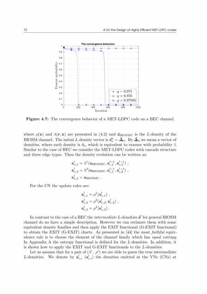
72 4 On the Design of Highly Efficient MET-LDPC codes
0 200 400 600 800 1000
0
0.1
0.2
0.3
0.4
0.5
0.6
0.7
0.8
0.9
1The convergence behaviour
Figure 4.7: The convergence behavior of a MET-LDPC code on a BEC channel.
where ρ(x) and λ(r,x) are presented in (4.2) and aBIOSMC is the L-density of theBIOSM channel. The initial L-density vector is a0
v = ∆0. By ∆0 we mean a vector ofdensities, where each density is δ0, which is equivalent to erasure with probability 1.Similar to the case of BEC we consider the MET-LDPC codes with cascade structureand three edge types. Then the density evolution can be written as:
alv,1 = λ1(aBIOSMC, al−1
c,1 , al−1c,2 ) ,
alv,2 = λ2(aBIOSMC, al−1
c,1 , al−1c,2 ) ,
alv,3 = aBIOSMC .
For the CN the update rules are:
alc,1 = ρ1(al
v,1) ,al
c,2 = ρ2(alv,2, a
lv,3) ,
alc,3 = ρ3(al
v,2) .
In contrast to the case of a BEC the intermediate L-densities al for general BIOSMchannel do no have a simple description. However we can estimate them with someequivalent density families and then apply the EXIT functional (G-EXIT functional)to obtain the EXIT (G-EXIT) charts. As presented in [44] the most faithful equiv-alence rule is to choose the element of the channel family which has equal entropy.In Appendix A the entropy functional is defined for the L-densities. In addition, itis shown how to apply the EXIT and G-EXIT functionals to the L-densities.
Let us assume that for a pair of (λi, ρi) we are able to guess the true intermediateL-densities. We denote by al
v,i (alc,i) the densities emitted at the VNs (CNs) at

4.3 G-EXIT charts for MET-LDPC codes 73
iteration l along edge type i. The parametric forms for the EXIT curves can then bedisplayed in Table 4.6.
Table 4.6: The parametric representation of the EXIT chart for MET-LDPC codeson a BIOSM channel.
EXIT curve of CN Inverse of EXIT curve of VNEdge i
{hl
v,i, hlc,i
} {hl
v,i, hl−1c,i
}In Table 4.6 the entropy functional2 for the L-densities are defined as
hlc,i = H(ρ(al−1
v,i )) , hlv,i = H(aBIOSMC ⊗ λ(al
c,i)) .
and for the G-EXIT curves the parametric forms are displayed in Table 4.7.
Table 4.7: The parametric representation of G-EXIT chart for MET-LDPC codeson BIOSM channel.
Inverse ofG-EXIT curve of CN Dual G-EXIT curve of VN
Edge i{
hlv,i, G(al
v,i, alc,i)} {
hlv,i, G(al
v,i, al−1c,i )
}In the following example we show how to plot the G-EXIT curve for a MET-LDPC
code on a BI-AWGN channel.
Example 4.3.2. G-EXIT chart for MET-LDPC codes on a BI-AWGN
In this example we show how the G-EXIT charts can be used for MET-LDPCcodes on a BI-AWGN channel. Consider the MET-LDPC code with rate 0.02 inTable 4.2. The Shannon limit for rate 0.02 is equal to Eb/N0 = −1.53 dB (σ∗
Sh= 5.96)
and our proposed code has a threshold equal to −1.5 dB (σ∗DE = 5.94) which is just
0.03 dB away from capacity. With Eb being the energy per bit and N0 being theenergy of the noise, the relation between Eb/N0, the SNR and σ for an AWGNchannel with binary transmission is given by (linear scale)
SNR = 2Rch Eb
N0,
σ = 1√SNR
.
Using (4.2) the edge perspective degree distribution of this code can be written as
λ(r,x) =[0.6 r1x
21x
602 + 0.4 r1x1x
512 , 0.54505 r1x
31x
592 + 0.4595 r1x
21x
502 , r1
],
ρ(x) =[0.64x3
1 + 0.36x81, 0.4054x2
2x3 + 0.5946x2x3, 0.3125x32 + 0.6875x2
2],
2The definition of the entropy functional, EXIT and G-EXIT functionals are presented in Ap-pendix A.

74 4 On the Design of Highly Efficient MET-LDPC codes
where for the VNs
λ1(r1, x1, x2) = 0.6 r1x21x
602 + 0.4 r1x1x
512 ,
λ2(r1, x1, x2) = 0.54505 r1x31x
592 + 0.4595 r1x
21x
502 ,
λ3(r1) = r1 ,
and for the CNs
ρ1(x1) = 0.64x31 + 0.36x8
1 ,
ρ2(x2, x3) = 0.4054x22x3 + 0.5946x2x3,
ρ3(x2) = 0.3125x32 + 0.6875x2
2 .
Then, for the density evolution the intermediate densities on the VN side are
alv,1 = aBIOSMC ⊗
[0.6
(al−1
c,1)⊗2 ⊗
(al−1
c,2)⊗60 + 0.4 al−1
c,1 ⊗(al−1
c,2)⊗51 ]
,
alv,2 = aBIOSMC ⊗
[0.54505
(al−1
c,1)⊗3 ⊗
(al−1
c,2)⊗59 + 0.4595
(al−1
c,1)⊗2 ⊗
(al−1
c,2)⊗50]
,
alv,3 = aBIOSMC ,
where ⊗ denotes the convolution of VNs, and for the CNs
alc,1 = 0.64
(al
v,1)⊠3 + 0.36
(al
v,1)⊠8
,
alc,2 = aBIOSMC ⊠
[0.4054
(al
v,2)⊠2 + 0.5946 al
v,2
],
alc,3 = 0.3125
(al
v,2)⊠3 + 0.6875
(al
v,2)⊠2
,
where ⊠ denotes the convolution of CNs. Figure 4.8 shows the convergence behaviorof each edge for the above mentioned code.
4.4 Code design optimization problemLet us denote the decoding threshold of a MET-LDPC code by θ. The parameterθ describes the maximum noise level in which the decoder can provide a reliabletransmission. For a BI-AWGN channel the parameter θ = σ, which is standarddeviation of the noise. For the BE channel θ = q, which is the erasure probability.The parameter θ is related to the code structure and can be written as θ (ν(r,x), µ(x)).Thus, for a given rate, the code design problem can be written as an optimizationproblem with cost function θ as follows:
θ∗ = argmax.ν(r,x), µ(x)
θ (4.12)
s.t.{νxi
(1,1) = µxi(1), i = 1, · · · , ne .
R = ν(1,1) − µ(1) .
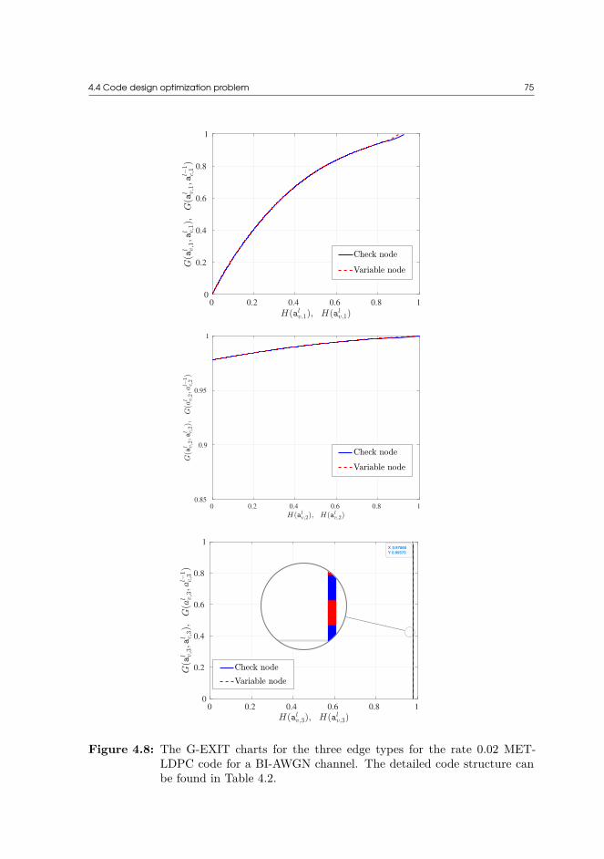
4.4 Code design optimization problem 75
0 0.2 0.4 0.6 0.8 1
0
0.2
0.4
0.6
0.8
1
0 0.2 0.4 0.6 0.8 1
0.85
0.9
0.95
1
0 0.2 0.4 0.6 0.8 1
0
0.2
0.4
0.6
0.8
1X 0.97868
Y 0.99575
0 0.2 0.4 0.6 0.8 1
0
0.2
0.4
0.6
0.8
1X 0.97868
Y 0.99575
Figure 4.8: The G-EXIT charts for the three edge types for the rate 0.02 MET-LDPC code for a BI-AWGN channel. The detailed code structure canbe found in Table 4.2.

76 4 On the Design of Highly Efficient MET-LDPC codes
This means that the optimization problem looks among all valid degree distribu-tions and finds the code with maximum threshold. The precise calculation of thethreshold can be done using density evolution. Using the density evolution this prob-lem is an optimization problem with non-linear cost function. Though the constraintsof this optimization problem can be simplified to a convex set, solving (4.12) is com-plicated due to the non-linearity of the objective function even in the case of irregularLDPC codes.
4.4.1 Constraint setsLet us consider the constraint sets of the original optimization problem in (4.12) fora MET-LDPC code with degree distribution as presented in Table 4.1. The ne linearconstraints for the socket count equalities (SCEs) imply that the weighted sum of theVNs and CNs for each edge type should be equal. For the jth constraint it can bewritten as
Q∑i=1
νidvj,i =
P∑i=1
µidcj,i ,
where 1 ≤ j ≤ ne. Its matrix representation is
dv1,1 dv
1,2 · · · dv1,Q
...... . . . ...
dvj,1 dv
j,2 · · · dvj,Q
...... . . . ...
dvne,1 dv
ne,2 · · · dvne,Q
ν1ν2...νQ
=
dc1,1 dc
1,2 · · · dc1,P
...... . . . ...
dcj,1 dc
j,2 · · · dcj,P
...... . . . ...
dcne,1 dc
ne,2 · · · dcne,P
µ1µ2...µP
. (4.13)
By calling the above matrices Dv = dTv , ν, Dc = dT
c and µ respectively, we have
Dvν = Dcµ . (4.14)
If a nonsingular matrix Dv exists the vector ν can be calculated by solving
ν = (Dv)−1Dcµ . (4.15)
Thus, by considering Dv, Dc and µ as independent variables the vector ν is athe dependent variable and (4.15) satisfies the validity. This means that to findthe best degree distribution it is possible to reduce the dimension of the search space.Furthermore, there is no need for joint optimization of CN and VN coefficients becauseof their linear dependency. Hence (4.15) introduce a linear dependency for nodedistribution of the VNs.
In addition, the second constraint is related to the code rate R. Since we assumethat there are no puncture nodes,
∑Q1 νj = 1 and
∑P1 µi = 1 − R, where R is the
rate of the code. In total the optimization algorithm therefore needs to find P − 1fractional parameters and ne(P +Q) integer parameters.

4.4 Code design optimization problem 77
Example 4.4.1. Linear dependency
As an example, Table 4.8 describes a rate 0.02 MET-LDPC ensemble presentedin [10]. Using (4.14) the matrix form representation for the socket count equality is
Table 4.8: Table presentation of Rate 0.02 degree structure for a MET-LDPC codewith 3 edge-types.
νbd b dv µd dc
0.02250.01750.96
[0 1]2 57 03 57 00 0 1
0.0106250.009375
0.60.36
3 0 07 0 00 2 10 3 1
BIAWGN: σ∗DE = 5.93
given by
2 3 057 57 00 0 1
ν1ν2ν3
=
3 7 0 00 0 2 30 0 1 1
0.01060.0094
0.60.36
.
Solving this equation for ν by using (4.15) we obtain ν1ν2ν3
=
0.02250.01750.9600
,
which are exactly the same result as obtained by an optimization method in [10] (c.f.Table 4.8).
4.4.2 Cost function for irregular LDPC codesOn a binary erasure channel and for irregular-LDPC codes, i.e. ne = 1, the densityevolution is equivalent to monitoring scalar value erasure probability. Thus, theEXIT chart can be used to convert this optimization problem to a linear curve fittingoptimization problem on a convex set [65, 67, 69, 70]. Remember that the EXIT chartprovides two curves related to the CNs and the inverse of VNs. For any convergedcode these two curves do not cross each other and the VN curve is always on top ofthe CN curve. Then, using the Area theorem [68, 66], the best code can be obtainedby matching these two curves. If A denotes the area between these two curves the

78 4 On the Design of Highly Efficient MET-LDPC codes
(4.12) can be simplified to
argmin.ν(q,x), µ(x)
A (4.16)
s.t.{νx(1, 1) = µx(1),R = ν(1, 1) − µ(1) .
This simplified optimization problem presented in (4.16) looks for an ensembleof irregular-LDPC codes where the area between the two curves related to VNs andCNs is minimal. This can be done by starting with a simple CN polynomial and thenuse curve fitting using Taylor series [65].
4.4.3 Cost function for MET-LDPC codesIn the case of a MET-LDPC code the optimization problem is not always straight for-ward. Here we propose a design approach by using the concept of EXIT charts alongdifferent edge types. Let us denote by Ai the area between the curves of EXIT chartsalong ith edge. Then, for the MET-LDPC codes the optimization problem (4.12) canbe simplified to
argmin.ν(q,x), µ(x)
ne∑i
Ai (4.17)
s.t.{νxi
(1,1) = µxi(1), i = 1, · · · , ne .
R = ν(1,1) − µ(1) .
This problem is a generalization of the curve fitting problem for irregular-LDPCcodes. Here we jointly optimize the EXIT curves for all edges. Luckily, in thecascade structure the EXIT curves for the thirs edge are vertical lines related to thedegree one nodes. Tthe area between the two curves is allways zero (See Figure 4.6and Figure 4.8). Thus the optimization problem simplified to jointly optimize theEXIT curves for edges 1 and 2. Since the EXIT curves for CN sides along edge 1 andedge 2 are independent, we can start by designing two EXIT curves for CNs and thenfit two VN curves jointly to these CN curves.
4.5 Optimization for cascade structureAfter having defined the optimization problem in the las section, we now focus onsolving it. The design of MET-LDPC codes is still a challenging problem. Justvery recently some optimization algorithms were developed for designing MET-LDPCcodes [14, 13, 12]. In general all the design approaches solve the non-linear optimiza-tion problem as presented in (4.12). Usually a brute-force search is running on a setof valid degree distributions to find the best ensemble. The density evolution (DE)

4.5 Optimization for cascade structure 79
or one of its approximations [13, 14] are used to check the performance of the codes.For example, the author in [13] used a hybrid-Gaussian approximation to reduce thecomplexity of DE for MET-LDPC codes. Recently a joint optimization was developedby [12], where two complicated inner and outer optimizations were conducted to findthe node and edge distributions. The major disadvantage of [13, 12] is that they arelimited to code rates higher than 0.1. Our proposed algorithm can however designhighly efficient codes at low rate. In Section 4.2, we proposed a new semi-Gaussianapproximation as to reduce the complexity of the DE for MET-LDPC codes. In addi-tion, we denoted in Section 4.4 that a linear dependency exists between the CNs andVNs in terms of code rate, which greatly reduces the search space for valid structures.In this section, for the case of MET-LDPC codes with cascade structure, we proposea novel optimization algorithm to design highly efficient codes. We use the conceptsof EXIT chart and semi-Gaussian approximation to design the codes.
Remember from Section 4.1.1 that the MET-LDPC codes with cascade structurecan be described by three sub-graphs as presented in Figure 4.1. In cascade structurethe red part of the graph can be considered as an irregular LDPC code with rate rb
which we call the base code (See Figure 4.1, and delete all the other blue and blackedges and all other connected nodes). Later in this section we will see how to designan appropriate base code using the EXIT charts for the cascade structures. It isimportant to mention that designing good base codes is not equivalent to designinggood irregular LDPC codes for BIOSM channels. For the moment, assume that abase code with rate rb exists. In the following theorem we will prove that the portionof the degree one nodes in the overall cascade structure is determined b knowing thedegree distribution of the base code (red part).
Theorem 4.5.1. Consider a MET-LDPC code with rate R in cascade structure. Theportion of degree one VNs is equal to 1 − R
rb, where rb is the rate of the base code.
Proof. Let us assume that the base code has the following degree distribution :
ν(x) =Q−1∑i=1
ν′i x
dv1,i , (4.18)
µ(x) =P −2∑i=1
µ′i x
dc1,i . (4.19)
whereQ−1∑i=1
ν′i = 1 and
P −2∑i=1
µ′i = 1 − rb. The socket count equality for the base code is
Q−1∑i=1
ν′i d
v1,i =
P −2∑i=1
µ′i x
dc1,i . (4.20)
In addition, assume that the degree distribution of the overall cascade structureis according to Table 4.3 and the socket count equality for edge-type 1 of the overall

80 4 On the Design of Highly Efficient MET-LDPC codes
cascade structure is given by
Q−1∑i=1
νi dv1,i =
P −2∑i=1
µi xdc
1,i . (4.21)
It is clear that (4.20) and (4.21) are scaled versions of each other. Let us denotethe scale factor by s. This yields
Q−1∑i=1
νi =
Q−1∑i=1
ν′i
s= 1s, (4.22)
P −2∑i=1
µi =
P −2∑i=1
µ′i
s= 1 − rb
s. (4.23)
(4.24)
In addition, for the overall cascade structure
ν(1,1) =Q−1∑i=1
νi + νQ = 1 , (4.25)
µ(1) =P −2∑i=1
µi + µP −1 + µP = 1 −R , (4.26)
νQ = µP −1 + µP . (4.27)
Thus, (4.25) and (4.26) can be simplified to
ν(1,1) = 1s
+ νQ = 1 ,
µ(1) = 1 − rb
s+ νQ = 1 −R .
Finally, solving this equation for s yields
s = rb
R, (4.28)
which implies that νQ = 1 − 1s = 1 − R
rb.
The main practical result of Theorem 4.5.1 is that if we use an irregular base codewith rate rb to design a cascade structure of rate R, the scale factor s = rb
Rand the
scaled-down version of the designed base code with rate rb can be considered as redpart in overall cascade structure.

4.5 Optimization for cascade structure 81
4.5.1 Design of good base codes using EXIT chartsTo design highly ??? MET-LDPC codes in cascade structure a good irregular LDPCbase code is required. However the procedure of designing an optimal base code differsfrom the procedure of designing conventional irregular-LDPC codes (See Section 4.4.2)because the noise model is different. As discussed in Section 4.4.2, designing anirregular LDPC code for a given channel parameter is a curve fitting problem and wehave to minimize the area between the EXIT curves as the gap between the two EXITcurves determines the distance to capacity. The design procedure for the base code,however, has to take into account the additional noise comming from edge type 2. Forexample, consider the Irregular code presented in Figure 4.5. The modified versionof this code showing the effect of edge type 2 has the following degree distribution
ν(q, x1, x2) = q (0.5 x21x
dv2,1
2 + 0.5 x31x
dv2,2
2 ) , (4.29)µ(x) = 0.4 x4
1 + 0.1 x91 . (4.30)
0 0.2 0.4 0.6 0.8 1
0
0.1
0.2
0.3
0.4
0.5
0.6
0.7
0.8
0.9
1The EXIT Chart for edge 1 BEC
Figure 4.9: The EXIT chart for base code by considering the effect of additionalnoise coming from edge type 2. The channel parameter is q = 0.975.The code rate is 0.5 and the maximum degree of VN along edge typeone is 3 and the maximum VN degree along edge type two is 60.
The corresponding EXIT chart which considers the effect of the additional noisecoming from the output of CNs along edge type 2 is presented in Figure 4.9. Thecorresponding curves are plotted for dv
2,1 = 50 and dv2,2 = 60. Comparing Figure 4.5
and Figure 4.9 demonstrates that the base code designed for MET-LDPC codess isnot always the optimal irregular LDPC code for the BE channel. More precisely, ifthe additional noise along edge type 2 is just considered as pure noise (equivalently,

82 4 On the Design of Highly Efficient MET-LDPC codes
ϵlc,2 = 1) the EXIT chart in Figure 4.9 would be the same as the EXIT chart inFigure 4.5.
4.5.2 Optimization for the connector partAfter designing the base code with rate rb and determining the portion of the degreeone nodes according to Theorem 4.5.1 the final step is to find the best connector partto build an overall MET-LDPC code with rate R. Thus, as presented in Table 4.3,just the parameters related to edge type 2 remain unknown (blue part). The SCEsfor edge type 2 and edge type 3 readd
c2,P −1 µP −1 + dc
2,P µP =∑Q−1
i=1 dv2,i νi ,
µP −1 + µP = νQ = 1 − 1s.
(4.31)
In (4.31) the parameters νi for i ∈ {1, · · · , Q} and s are known. The unknownparameters are µP −1, µP , dc
2,P −1, dc2,P and dv
2,i for i ∈ {1, · · · , Q − 1}. We notethat dv
2,i are integers. Solving this set of equations for µP −1 and µP gives us theparametric solution for connector parts satisfying the SCE. The parametric forms forthe CN coefficients µP −1 and µP are
µP −1 =dc
2,P νQ −∑Q−1
i=1 dv2,i νi
dc2,P − dc
2,P −1, (4.32)
µP = νQ − µP −1 , (4.33)
where µP −1 and µP should be between 0 and νQ.In addition, the schematic representation for the solutions of this set of equations
for µP −1 and µP are presented in Figure 4.10 which is the cross point of the followinglines {
y = −m x+ b ,
y = −x+ νQ ,
where
m =dc
2,P −1
dc2,P
, b =∑Q−1
i=1 dv2,i νi
dc2,P
.
It is clear from Figure 4.10 that by changing the unknown integer parameters (dv2,i),
we can change the slope (m) and y-intercept (b) to find different pairs of (µP −1, µP ).It it important to mention that each point determines a new connector part for theoverall MET-LDPC code. Finally to find the best connector part for the overall codewe can use the semi-Gaussian approximation (or any other approximation of DE) tofind the best threshold for the overall code. This can be done by testing differentpairs of (µP −1, µP ) according to (4.32) and (4.33).

4.6 Highly efficient codes 83
(µP−1, µP )
(νQ, νQ)
y = νQ − x
y = −m x+ b
µP−1
µP
x
y
0
Figure 4.10: The inner optimization problem finds sets of points (µP −1, µP ) satis-fying µP + µP −1 = νQ .
The flowchart for the code design procedure is presented in Figure 4.11. In thefirst step a base code with rate rb is designed according to Section 4.5.1. Then, inthe second step the scaling parameter s is found from Theorem 4.5.1. Putting thescaled-down version of the base code in the cascade structure determines the fractionof degree one VNs and CNs. In the next step a new connector part is tested to buildthe overall MET-LDPC code with rate R. This procedure continues until we find aset of highly efficient codes or until all the unique connector parts have been tested.If for all the created connector parts the efficiency of the overall code was not goodenough a new base code has to be considered with different rate rb.
In Section 4.6 some examples of highly efficient MET-LDPC codes with cascadestructure are represented, where we used our new optimization algorithm for thedesign.
4.6 Highly efficient codesIn this section we propose some of our highly efficient MET-LDPC codes. To comparethe performance of these codes we define the asymptotic efficiency of each code asβDE = R
C(pDE) , where R is the code rate and C(pDE) is the capacity of the binary-input output symmetric memory-less (BIOSM) channel with parameter p = pDE. pDE
is the threshold of the code obtained by running full density evolution and pSh is theShannon threshold. To see how we calculate the capacity of BIOSM channels seeAppendix A.

84 4 On the Design of Highly Efficient MET-LDPC codes
Design degree one nodes
Create a connector part
Find the efficiency βDE
Design base code using
EXIT chart
Set base code rate (rb)
No
No
Yes
Save the code
Unique
> 0.98
Figure 4.11: The block diagram for the optimization algorithm of a rate R MET-LDPC code with cascade structure using a base code of rate rb.
Example 4.6.1. MET-LDPC code with rate 0.01.
The degree distribution of the code is
Table 4.9: Rate 0.01 MET-LDPC code.νbd b dv µd dc
0.010.010.98
[0 1]2 103 03 125 00 0 1
0.0080.0020.320.66
4 0 09 0 00 3 10 2 1
σ∗Sh
= 8.46 σ∗DE = 8.41 βDE = 98.7%
Based on our knowledge, there is no MET-LDPC code in other literature specifi-cally designed for rate 0.01. A rate 0.01 code can be obtained by augmenting a rate

4.6 Highly efficient codes 85
0.02 MET-LDPC code with a length 2 repetition code.
Example 4.6.2. MET-LDPC code with rate 0.02.
We propose two MET-LDPC codes with rate 0.02. The first code was representedbefore in Table 4.2. Here we present the second code with rate 0.02 with the followingdegree distribution in table format
Table 4.10: Rate 0.02 MET-LDPC code.νbd b dv µd dc
0.0240.0160.96
[0 1]2 43 03 61 00 0 1
0.0020.0180.0880.872
3 0 05 0 00 3 10 2 1
σ∗Sh
= 5.96 σ∗DE = 5.94 βDE = 99.2%
The only existing MET-LDPC code with rate 0.02 was designed by [10] with thefollowing degree distribution
ν(r,x) = 0.0225 r1x21x
572 + 0.0175 r1x
31x
572 + 0.96 r1x
13 ,
µ(x) = 0.010625 x31 + 0.009375 x7
1 + 0.6 x22x
13 + 0.36 x3
2x13 .
The threshold of this code in BI-AWGN channel is σ∗DE = 5.91 with asymptotic
efficiency of βDE = 98.22%.
Example 4.6.3. MET-LDPC code with rate 0.05.
Table 4.11 shows the degree structure of a rate 0.05 MET-LDPC code. Thethreshold of this code using DE on BI-AWGN channel is equal to σ∗
DE = 3.68 ( Eb
N0=
−1.32 dB). The theoretical Shannon limit for a code of rate 0.05 is equal to σ∗Sh
= 3.73(−1.44 dB) and this code is just 0.12 dB away from capacity. Another code designed
Table 4.11: Rate 0.05 MET-LDPC code.νbd b dv µd dc
0.0540.0460.90
[0 1]2 22 03 22 00 0 1
0.0260.0240.400.50
3 0 07 0 00 3 10 2 1
σ∗Sh
= 3.73 σ∗DE = 3.68 βDE = 97.36%
for rate 0.05 was presented in [45] and has the following degree distribution
ν(r,x) = 0.04 r1x21x
342 + 0.03 r1x
31x
342 + 0.93 r1x
13 ,
µ(x) = 0.01 x81 + 0.01 x9
1 + 0.41 x22x
13 + 0.52 x3
2x13 .

86 4 On the Design of Highly Efficient MET-LDPC codes
The threshold of this code in BI-AWGN channel is σ∗DE = 3.67 with asymptotic
efficiency of βDE = 96.78%.
Example 4.6.4. MET-LDPC code with rate 0.10.
Table 4.12 shows a code with ne = 3 edge type and the threshold of this codein a BI-AWGN channel using DE is equal to σ∗
DE = 2.57 ( Eb
N0= −1.22 dB). The
theoretical Shannon limit is equal to σ∗Sh
= 2.6 (−1.28 dB) and this code is just 0.06dB away from capacity.
Table 4.12: Rate 0.10 MET-LDPC code.νbd b dv µd dc
0.0750.0500.875
[0 1]2 23 03 18 00 0 1
0.0250.875
12 0 00 3 1
σ∗Sh
= 2.6 σ∗DE = 2.57 βDE = 98.33%
For comparison another code with rate 0.1 designed by [14] has the degree distri-bution
ν(r,x) = 0.0775 r1x11x
12x
213 + 0.0477 r1x
21x
12x
203 + 0.8747 r1x
14 ,
µ(x) = 0.0011 x61x
42 + 0.0028 x6
1x52 + 0.0214 x7
1x52 + 0.0412 x2
3x4 + 0.8335 x33x4 .
The threshold of this code in BI-AWGN channel is σ∗DE = 2.54 with asymptotic
efficiency of βDE = 96.37%.
Example 4.6.5. MET-LDPC code with rate 0.25.
The corresponding polynomial representation for this code is:
ν(r,x) = 0.1875 r1x21x
122 + 0.125 r1x
31x
42 + 0.6875 r1x
13 ,
µ(x) = 0.0625 x121 + 0.6875 x4
2x13 .
The corresponding table representation is also presented in Table 4.13.
Table 4.13: Rate 0.25 MET-LDPC code.νbd b dv µd dc
0.18750.1250.6875
[0 1]2 12 03 4 00 0 1
0.06250.6875
12 0 00 4 1
σ∗Sh
= 1.55 σ∗DE = 1.50 βDE = 95.07%

4.7 Simulation Results 87
Now let us compare the threshold of our designed code with some other codeswith rate 0.25 designed in [14] and [12]. For example in [14] the authors designedanother non-punctured code with rate 0.25 with the following degree distribution
ν(r,x) = 0.1512 r1x31 + 0.006 r1x
41 + 0.0928 r1x
121 + 0.75 r1x
22 ,
µ(x) = 0.6588 x21x
22 + 0.0912 x3
1x22 .
The threshold of this code in BI-AWGN channel is σ∗DE = 1.48 with asymptotic
efficiency of βDE = 93.08%.The second code is a punctured code with rate 0.25 designed in [12] with the
following degree distribution
ν(r,x) = 0.1563 r0x41x
43x
14 + 0.0938 r1x
23x
14 + 0.9062 r1x
12x
14 ,
µ(x) = 0.3125 x21x
12 + 0.1875 x1
2x44 + 0.4063 x1
2x23x
14 .
The threshold of this code in BI-AWGN channel is σ∗DE = 1.49 with asymptotic
efficiency of βDE = 93.65%.
4.7 Simulation ResultsFinally, to evaluate the performance of our codes, Figure 4.12 shows the simulatedframe error rate (FER) of our rate 0.02 MET-LDPC code, represented in Table 4.2,with finite block length. We compare our results with the simulated FER of a rate0.02 code designed by [10] and used in Ref. [71] for multi-dimensional reconciliationfor CV-QKD.
As can be seen in Figure 4.12 our proposed code outperforms the code publishedin [10] even with a shorter block length of n = 1.5 × 106 bits. For both codesthe progressive edge growth (PEG) algorithm [72] was used to construct quasi-cyclicMET-LDPC codes with Z ×Z circulant permutation matrices. Based on our simula-tion results it is clear that by increasing the length of the code to n = 1.5 × 106 bits,0.1 dB additional gain can be obtained at FER = 0.1. In addition, in Figure 4.12 thevertical dashed lines respectively show the Shannon asymptotic threshold for rate 0.02on a BIAWGN channel and the asymptotic threshold obtained by density evolutionfor our code and the code of [10].
The efficiencies of the two codes versus the FER are compared in Fig. 4.13. Itcan be observed that for all FERs the efficiency of our code is higher than the codeof [10]. For instance, for an efficiency of 95% the code in [71, 10] has a FER of 0.6but our code is able to provide the same efficiency with a FER of as low as 0.3.

88 4 On the Design of Highly Efficient MET-LDPC codes
15.6 15.5 15.4 15.3 15.2 15.1 15.0SNR (dB)
10 3
10 2
10 1
100
Aver
age
Fram
e E
rror
Rat
e (F
ER
)
Shannon capacity[33, Appendix A], Asym.Table I, Asym.[33, Appendix A], n = 1.6e06Table I, n = 3.8e05Table I, n = 1.5e06
Figure 4.12: The frame error rate vs SNR for rate 0.02 MET-LDPC code. To plotthe FER curves we set the maximum number of iterations to 500 andfor each point 100 frames of errors were counted. We used Z = 256 forthe solid orange curve and Z = 1024 for the solid red and blue curves.

4.7 Simulation Results 89
10 210 1100
Average Frame Error Rate (FER)
88
90
92
94
96
98
100
Eff
icie
ncy
()
[33, Appendix A], n = 1.6e06Table I, n = 1.5e06
Figure 4.13: The efficiency vs frame error rate for rate 0.02 MET-LDPC code. Toplot the FER curves we set the maximum number of iterations to 500and for each point 100 frames of errors are counted..

90

CHAPTER5Conclusion and Future
DirectionsThis thesis addressed some of the important topics in the post-processing of the CV-QKD to provide long distance secure key rate. More specifically, for the reconciliationschemes in CV-QKD some of the ubiquitous reconciliation schemes were discussed indetails. Some of the major contributions in Chapter 3 are
• Numerical and analytical methods to precisely calculate the individual channelcoding rates for MLC-MSD reconciliation.
• Calculation of soft information at the input of the soft decoder for one-leveldecoding and two-level decoding for MLC-MSD reconciliation.
• Detailed comparison between forward and reverse reconciliation.
• Randomized reconciliation scheme was introduced to increase the throughputof the system. In randomized reconciliation a high throughput hard decoderwere used instead of complicated soft decoder.
Another important topic which was addressed in this thesis is the major need todesign highly efficient codes for low rate regime in applications like QKD. In Chapter 4,we focused on MET-LDPC codes. A new precise approximation method for DE,called semi-Gaussian approximation was proposed for the MET-LDPC codes. Inaddition, we developed the concept of EXIT charts for the MET-LDPC codes. TheEXIT chart is one of the powerful tools for designing the codes. A new algorithmicapproach was proposed to design highly efficient MET-LDPC codes. Then somenew highly efficient MET-LDPC codes were designed using the proposed algorithm.The application of these MET-LDPC codes are not limited to the CV-QKD andmany of the published codes can be used also in other applications including satellitecommunication, wireless communication and optical communication. More preciselysome of the major contributions of Chapter 4 can be summarized as follows:
• A new approximation for DE of the MET-LDPC codes called semi-Gaussianapproximation. In this method the Gaussian approximation is applied just toVN operations and the CN operations are calculated precisely. This method
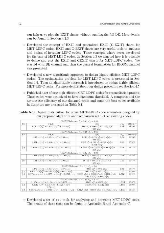
92 5 Conclusion and Future Directions
can help us to plot the EXIT charts without running the full DE. More detailscan be found in Section 4.2.3.
• Developed the concept of EXIT and generalized EXIT (G-EXIT) charts forMET-LDPC codes. EXIT and G-EXIT charts are very useful tools to analysisand design of irregular LDPC codes. These concepts where never developedfor the case of MET-LDPC codes. In Section 4.3 we denoted how it is possibleto define and plot the EXIT and GEXIT charts for MET-LDPC codes. Westarted with BE channel and then the general formulation for BIOSM channelwas presented.
• Developed a new algorithmic approach to design highly efficient MET-LDPCcodes. The optimization problem for MET-LDPC codes is presented in Sec-tion 4.4. Then an algorithmic approach is introduced to design highly efficientMET-LDPC codes. For more details about our design procedure see Section 4.5.
• Published a set of new high efficient MET-LDPC codes for reconciliation process.These codes were optimized to have maximum threshold. A comparison of theasymptotic efficiency of our designed codes and some the best codes availablein literature are presented in Table 5.1.
Table 5.1: Degree distribution for some MET-LDPC code ensembles designed byour proposed algorithm and comparison with other existing codes.
BIAWGN channel, R = 0.01, σ∗Sh = 8.46
Ref ν(r,x) µ(x) σ∗DE Efficiency
0.01 r1x21x
1032 + 0.01 r1x
31x
1252 + 0.98 r1x
13 0.008 x4
1 + 0.002 x91 + 0.32 x3
2x13+ 8.41 98.70%
0.66 x22x
13
BIAWGN channel, R = 0.02, σ∗Sh = 5.96
Ref ν(r,x) µ(x) σ∗DE Efficiency
0.02 r1x21x
512 + 0.02 r1x
31x
602 + 0.96 r1x
13 0.016 x4
1 + 0.004 x91 + 0.3 x3
2x13+ 5.94 99.20%
0.66 x22x
13
0.024 r1x21x
432 + 0.016 r1x
31x
612 + 0.96 r1x
13 0.002 x3
1 + 0.018 x51 + 0.088 x3
2x13+ 5.82 95.52%
0.872 x22x
13
[10] 0.0225 r1x21x
572 + 0.0175 r1x
31x
572 + 0.96 r1x
13 0.010625 x3
1 + 0.009375 x71 + 0.6 x2
2x13+ 5.91 98.22%
0.36 x32x
13
BIAWGN channel, R = 0.05, σ∗Sh = 3.73
0.054 r1x21x
222 + 0.046 r1x
31x
222 + 0.90 r1x
13 0.026 x3
1 + 0.024 x71 + 0.40 x3
2x13+ 3.68 97.36%
0.50 x22x
13
[45] 0.04 r1x21x
342 + 0.03 r1x
31x
342 + 0.93 r1x
13 0.01 x8
1 + 0.01 x91 + 0.41 x2
2x13+ 3.67 96.78%
0.52 x32x
13
BIAWGN channel, R = 0.1, σ∗Sh = 2.6
0.075 r1x21x
232 + 0.05 r1x
31x
182 + 0.875 r1x
13 0.025 x12
1 + 0.875 x32x
13 2.57 98.37%
[12] 0.1063 r1x31x
232 + 0.0216 r1x
21x
82 + 0.8722 r1x
13 0.0278 x13
1 + 0.8722 x32x
13 2.55 96.95%
[13] 0.0775 r1x11x
12x
213 + 0.0477 r1x
21x
12x
203 + 0.8747 r1x
14 0.0011 x6
1x42 + 0.0028 x6
1x52 + 0.0214 x7
1x52+ 2.5424 96.41%
0.0412 x23x4 + 0.8335 x3
3x4
BIAWGN channel, R = 0.25, σ∗Sh = 1.55
0.1875 r1x21x
122 + 0.125 r1x
31x
42 + 0.6875 r1x
13 0.0625 x12
1 + 0.6875 x42x
13 1.5031 95.07%
[14] 0.1512 r1x31 + 0.006 r1x
41 + 0.0928 r1x
121 + 0.6588 x2
1x22 + 0.0912 x3
1x22 1.4839 93.08%
0.75 r1x22
[12] 0.1563 r0x41x
43x
14 + 0.0938 r1x
23x
14 + 0.9062 r1x
12x
14 0.3125 x2
1x12 + 0.1875 x1
2x44 + 0.4063 x1
2x23x
14 1.4894 93.65%
• Developed a set of c++ tools for analyzing and designing MET-LDPC codes.The details of these tools can be found in Appendix B and Appendix C.

5 Conclusion and Future Directions 93
• Implemented the reconciliation scheme for CV-QKD based on MLC-MSD method,in c++. More details can be found in Appendix B.
Findings of this research have considerable applications for long distance QKD.To further our research we are planning to investigate the potential advantages ofMLC-MSD reconciliation and resolve some of the existing limitations in both multi-dimensional reconciliation and MLC-MSD scheme. In addition, further studies whichtake high-throughput reconciliation into account will need to be considered. Weare currently in the process of investigating high throughput reconciliation scheme,with two possible options. First, we are trying to implement an efficient decoderwhich is specifically designed for the MET-LDPC codes. Since, a big portion of theMET-LDPC codes are degree one nodes, it can be very useful to tailor a decodingalgorithm specifically for MET-LDPC codes instead of using min-sum algorithm orother variants of decoding algorithm which is typically used for the irregular LDPCcodes. In addition, graphics processing unit (GPU) or Field Programmable GateArrays (FPGA) implementations should be considered in future. Second, we areinvestigating to design new reconciliation methods with higher number of bits persymbol. For example, the multi-dimensional reconciliation scheme extracts one bitper symbol, but in contrast the MLC-MSD scheme in principle is able to extractmore than one bit per symbol. Also, other variants of the reconciliation algorithmsare considered. For example, our new proposed stochastic reconciliation scheme canbe used to increase the throughput while decreasing the complexity of the decoding.
Besides, the code design algorithm can be developed to optimize different costfunctions. Our current algorithm optimizes the codes to have the best asymptoticthresholds. In practice the best MET-LDPC codes with finite block length can beconsidered to have the best decoding performance with minimum decoding iteration.

94

APPENDIXAIntroduction to LDPC
codesA.1 PreliminariesThis section is technical and some basic definitions and examples are used to describethe basic concepts. We advise to quickly skim it to see what materials are discussedbut a detailed study is not recommended. At any later point when needed, you canreturn and find the specific materials. For a more detailed introduction into theseconcepts we refer reader to [44].
A.1.1 Channel modelLet us denote by X the channel input alphabet and Y the channel output alphabet.Then the conditional density fY |X(y|x) completely describes the channel model withrandom variables X and Y . For discrete channel models we simply replace the condi-tional density by the conditional discrete probability PrY |X(y|x). In addition let usclarify that the lower case letter x ∈ X denotes a specific outcome with probabilityfX(x) of random variable X. If |X | = 2 the channel is known as binary input channel.Conventionally the binary input alphabets are X = {−1,+1} or X = {1, 0}.
Binary erasure channel (BEC) The binary erasure channel with parameter ϵ isdenoted as BEC(ϵ). The random variable X at the input can take values x ∈ X ={−1, +1} and the output random variable can take values from the output alphabetY = {−1, ?, + 1}. The transition probability is discrete and equal to
PrY |X
(y|x) =
1 − ϵ , y = x ,
ϵ , y =? ,0 , otherwise .
Binary symmetric channel (BSC) The binary symmetric channel with param-eter δ is denoted as BSC(δ). The random variable X at input can take valuesx ∈ X = {−1, + 1} and the output random variable can take values from the

96 A Introduction to LDPC codes
same alphabet Y = {−1, + 1}. The transition probability is discrete and equal to
PrY |X
(y|x) =
{1 − δ , y = x ,
δ , otherwise .
Binary input additive white Gaussian noise channel (BI-AWGN) The bi-nary input additive white Gaussian noise channel with parameter σ is denoted asBI-AWGN(σ). The channel noise model is described by Gaussian noise with zeromean and standard deviation σ. The random variable X at input can take valuesx ∈ X = {−1, + 1} and the output random variable can take values from thereal-valued numbers Y = R. The transition probability density function is equal to
fY |X(y|x) = e−
(y − x)2
2σ2√
2πσ2.
+1
-1
+1
-1
?
1 − ϵ
1 − ϵ
ϵϵ
+1
-1
+1
-1
1 − δ
1 − δ
δ
δx
Z
Y+
x yPrY |X(y|x)
BEC(ϵ)
x yPrY |X(y|x)
BSC(δ)
fY |X(y|x) = fZ(z) =e
−(z)2
2σ2√
2πσ2
BI-AWGN(σ)
Figure A.1: The schematic representation of standard BIOSM channels.
Binary-input output-symmetric memory-less channels A channel is said tobe output-symmetric if and only if fY |X(y|x) = fY |X(−y|−x). It can be easily shownthat all the channels introduced above are output-symmetric. It is convenient tocall this family of channels the binary-input output-symmetric memory-less (BIOSM)channels.
In addition, the channel parameter p can be defined for all of the above mentionedBIOSM(p) channels. For example the channels parameters for BEC, BSC and BI-AWGN channels are ϵ ∈ [0, 1], δ ∈ [0, 0.5] and σ ∈ [0, ∞]. Later we demonstratehow the channel parameters can be used to calculate the channel entropy H(X|Y ).
Log-Likelihood Ratio (LLR) Consider a BIOSM channel with transition proba-bility PrY |X(y|x). The log-likelihood ratio (LLR) function l(y) is defined as
l(y) = lnPrY |X(y|1)
PrY |X(y| − 1).

A.2 Channel entropy and channel capacity 97
The log-likelihood ratio associated to the random variable Y is defined as L = l(Y ).l(y) is said to be the output of the channel in the L-domain. It is important to noticethat L is a random variable itself.
In [44] the authors demonstrated that L is a sufficient statistic for decoding. Itmeans that an optimal decoder can be based on the LLR l(y) instead of y itself.
Definition of the L-Density a(y) The distribution of the log-likelihood ratiosL = l(Y ) of the BIOSM channels conditioned on X = 1 is defined as the L-density.Here we represent the L-densities for all the BIOSM channels
Table A.1: The distribution of the L conditioned on the X = 1.BIOSM(p) L-Density a(y) Description
BEC(ϵ) a(y) = ϵ ∆0(y) + ϵ ∆∞(y) ϵ = 1 − ϵ
BSC(δ) a(y) = δ ∆ δδ(y) + δ ∆ δ
δ(y) δ = 1 − δ
BI-AWGNC(σ) a(y) =√σ2
8πe
−(y − 2
σ2 )2σ2
8
The symmetry of the probability density function Let f(x) be a probabilitydensity function over R. The density is said to be symmetric if f(−x) = e−xf(x).All the L-densities in Table A.1 are symmetric.
A.2 Channel entropy and channel capacityConsider a BIOSM channel with input alphabet X , output alphabet Y and transitionprobability PrY |X(y|x). Also assume that a(y) denotes the L-density of this channel.Then according to [44]-Lemma 4.36 the capacity of this channel is a linear functionalof its L-Density and can be represented as
C(a) =∫
a(y)(1 − log2(1 + e−y)) dy , (A.1)
where C(a) is the capacity functional of the BIOSM channels in bits. Using thefact that for symmetric channels the optimal input distribution is uniform and the

98 A Introduction to LDPC codes
input alphabet has equal prior probability PrX(x) = 12
, for x ∈ {−1,+1} then theconditional entropy H(X|Y ) can be defined as
H(X|Y ) = H(X) − I(X;Y ) = H(X) − C(a) =∫
a(y) log2(1 + e−y) dy . (A.2)
In addition let us call h = H(aBIOSMC) the entropy functional for a BIOSMC.Later in this chapter we will see how these functions can play an important role inthe definition of the extrinsic-information transfer (EXIT) function and how we usethose to design highly efficient degree distribution for multi-edge-type low-densityparity-check (MET-LDPC) codes.
Example A.2.1. Capacity functional for BSC and BEC
Here we use (A.1) to find the capacity of the BEC(ϵ) and BSC(δ) channels. ForBEC(ϵ) we have
C(aBEC(ϵ)) = 1 −∫ ∞
−∞[ϵ ∆0(y) + (1 − ϵ) ∆∞(y)](log2(1 + e−y)) dy = 1 − ϵ .
In similar way for the BSC(δ)
C(aBSC(δ)) = 1 −∫ ∞
−∞[δ ∆ δ
1−δ(y) + (1 − δ) ∆ 1−δ
δ(y)](log2(1 + e−y)) dy = 1 − h2(δ),
where h2(δ) = −δ log2(δ) − (1 − δ) log2(1 − δ).
Example A.2.2. Capacity functional for BI-AWGNC
To calculate the capacity for the BI-AWGNC the following integral has to besolved numerically:
C(aBI-AWGN(σ)) = 1 −∫ ∞
−∞
√σ2
8πe
−(y − 2
σ2 )2σ2
8 (log2(1 + e−y)) dy ,
In Figure A.3 the capacity of the BI-AWGN channel is compared with the capacityof the AWGN channel with real-valued inputs.
A.3 Low-density parity-check (LDPC) codesThe LDPC codes are linear codes with a sparse parity check matrix H. Assuming Hhas dimensions m × n then it is possible to assign a bipartite graph to this matrix,named Tanner graph. The associated Tanner graph for this H has n variable nodescorresponding to the codeword of length n (columns of H) and m = n−k check-nodes

A.3 Low-density parity-check (LDPC) codes 99
0.0 0.2 0.4 0.6 0.8 1.0Erasure probability ( )
0.0
0.2
0.4
0.6
0.8
1.0C
apac
ity [b
its p
er c
hann
el]
BEC( )
0.0 0.2 0.4 0.6 0.8 1.0Crossover probability ( )
0.0
0.2
0.4
0.6
0.8
1.0BSC( )
Figure A.2: The capacity of the BEC and BSC channels.
25 20 15 10 5 0 5 10 15SNR [dB]
0.0
0.5
1.0
1.5
2.0
Cap
acity
[bits
per
cha
nnel
]
AWGNBI-AWGN
Figure A.3: The capacity of the BI-AWGN and AWGN channels.

100 A Introduction to LDPC codes
corresponding to the set of n−k parity constraints (row of H). k shows the number ofinformation bits. The check-node j is connected to the variable-node i if H(j, i) = 1.
LDPC codes can be represented by their degree distribution. The node perspectivedegree distribution of the LDPC code is given by
ν(x) =∑i=1
νi xi, µ(x) =
∑i=1
µi xi ,
where νi is the portion of the variable-nodes of degree i and the µi is the portion ofcheck-nodes of degree i in the Tanner graph. Considering this definition the followingrelations are valid
ν(1) = 1 , µ(1) = 1 − r , ν′(1) = µ′(1) .
The corresponding edge-perspective degree distribution of this code is
λ(x) =∑i=1
λi xi−1 = ν′(x)
ν′(1), ρ(x) =
∑i=1
ρi xi−1 = µ′(x)
µ′(1),
where λi (ρi) shows the fraction of edges that are connected to the variable-node(check-node) of degree i. The node perspective representation can be obtained fromedge perspective representation as follows:
ν(x) =∫ x
0 λ(z)dz∫ 10 λ(z)dz
, µ(x) =∫ x
0 ρ(z)dz∫ 10 λ(z)dz
,
Furthermore, the following relation holds
r = ν(1) − µ(1) = 1 −∫ 1
0 ρ(z)dz∫ 10 λ(z)dz
.
A.4 Belief PropagationConsider a LDPC code with degree distribution (λ, ρ) on a BIOSM channel. Inaddition assume that a0 = aBIOSMC denotes the corresponding L-density at iteration0. Then for iteration l ≥ 1
al = a0 ⊗ λ(ρ(al−1)) , (A.3)
whereλ(a) =
∑i=1
λi a⊗(i−1) , ρ(a) =∑i=1
ρi a⊠(i−1) .
Sometimes it is convenient to write the densities in terms of variable nodes and checknodes:
alv = a0 ⊗ λ(al−1
c ) , alc = ρ(al
v) . (A.4)For more details about BP please see [44]-Section 2.5.

A.5 EXIT and G-EXIT charts 101
A.5 EXIT and G-EXIT chartsBefore introducing EXIT charts we present some useful definitions and then showhow we can exploit those for plotting EXIT and G-EXIT charts.
EXIT functional According to [44]-DEFINITION 4.43 the EXIT functional isdefined as the entropy functional, see (A.2). The associated EXIT kernel in L-domainis l(y) = log2(1 + e−y).
G-EXIT functional Again according to [44]-DEFINITION 4.44 the GeneralizedEXIT (G-EXIT) functional for a BIOSM(h) applied to a symmetric L-density b isdefined as
G(aBIOSMC(h), b) = d
dhH(aBIOSMC(h) ⊗ b) ,
and the corresponding G-EXIT kernel is defined as
l(y) =∫
daBIOSMC(h)
dhlog2(1 + e−z−y)dz .
Sometimes it is convenient to consider a family of BIOSMC with parameter h.It means that we parameterize the channel with the entropy. For example for BECh = ϵ, for BSC h = h2(δ) and and for BI-AWGNC h = H(aBI-AWGNC(σ)).
EXIT function According to [44]-DEFINITION 4.131, let X be a vector of lengthn chosen uniformly at random from a binary code C, and Y be the transmittedversion of X over the BIOSMC(h). Then the individual and average EXIT functionsare
hi(h) = H(Xi|Y∼i(h)) ,
h(h) = 1n
n∑i=1
H(Xi|Y∼i(h)) = 1n
n∑i=1
hi(h) .
G-EXIT function According to [44]-DEFINITION 4.154, let X be a vector oflength n chosen uniformly at random from a binary code C and Y be the transmit-ted version of X over the BIOSMC(h). Then the individual and average G-EXITfunctions are
gi(h) = gi(h1, · · · , hn) = ∂H(Xi|Y (h1, · · · , hn))∂hi
,
g(h) = 1n
n∑i=1
gi(h1, · · · , hn) .
Now, in the following, we show how it is possible to calculate the EXIT and G-EXIT functions for LDPC codes. First we need to find the L-density of the extrinsicmaximum a-posteriori (MAP) estimator.

102 A Introduction to LDPC codes
Extrinsic MAP estimator Let X be a vector of length n chosen uniformly atrandom from a binary code C and let Y be the transmitted version of X over theBIOSMC(h). Then the extrinsic MAP estimator of Xi is
ϕi(y∼i) = lnPrXi|Y∼i
(+1|y∼i)PrXi|Y∼i
(−1|y∼i),
and Φi = ϕi(Y∼i). Φi is a sufficient statistics for Xi given Y∼i. H(Xi|Y∼i(h)) =H(Xi|Φi).
We now calculate the EXIT function for linear codes using the EXIT functionalof the extrinsic MAP estimator. Let ai denotes the L-density of Φi and assume thatan all-one-codeword was transmitted. With a = 1
n
∑ni=1 ai
hi(h) = H(ai) , h(h) = H(a) .
and for the G-EXIT functional
gi(h1 · · · , hn) =∂H(aBIOSMC(hi) ⊗ ai)
∂hi
= G(aBIOSMC(hi), ai) =∫
ai(y) laBIOSMC(hi)(y)dy .
wherelaBIOSMC(h)(y) =
∫daBIOSMC(h)(z)
dhlog2(1 + e−z−y)dz .
A.6 Plotting EXIT and G-EXIT ChartsAs presented in (A.3), a0 = aBIOSMC and after l ≥ 1, al = aBIOSMC ⊗ λ(ρ(al−1)).Unfortunately the intermediate L-densities al do no have simple descriptions, butestimating them with some equivalent density families, we can apply the EXIT func-tional (G-EXIT functional) to obtain the EXIT (G-EXIT) chart. As presented in [44]the most faithful equivalence rule is to choose the element of the channel family whichhas equal entropy.
Now, assume that for a pair of (λ, ρ), we were able to guess the true intermediateL-densities. As presented in (A.4), al
v (alc) is the density emitted at the variable-node
(check-node) at iteration l. Then, using the entropy functional
hlc = H(ρ(al
v)) , hlv = H(aBIOSMC ⊗ λ(al−1
c )) .
The EXIT curves can be obtained by plotting the entropy values for the input-output of the variable nodes and check nodes. The EXIT chart for a given pair of(λ, ρ) is realized by plotting the EXIT curve of a variable-node against the inverse ofa check-node. The parametric form of the EXIT curve for the check-node is givenby {hl
v, hlc}, and the inverse of the EXIT curve for the variable-node is {hl
v, hl−1c }.
Finally, the EXIT chart is then given by

A.6 Plotting EXIT and G-EXIT Charts 103
Table A.2: The parametric representation of an EXIT chart.EXIT curve of check-node
{hl
v = H(alv), hl
c = H(alc)}
Inverse of EXIT curve of variable-node{
hlv = H(al
v), hl−1c = H(al−1
c )}
A similar concept can be used for G-EXIT curves. In particular, in [66] the G-EXIT chart is realized by plotting the inverse of the dual G-EXIT curve of a variable-node against the G-EXIT curve of a check-node. For a pair of densities the G-EXITcurve of the check-node can be given in the parametric form by
{hl
v = H(alv), G(al
v, alc)}
.Similarly the dual G-EXIT for the variable-node can be written in parametric formas{G(al
v, al−1c ), hl
v = H(alv)}
and the inverse of the dual G-EXIT curve is then{hl
v = H(alv), G(al
v, al−1c )
}. Thus, the G-EXIT chart is given by
Table A.3: The parametric representation of G-EXIT chart.G-EXIT curve of check-node
{hl
v = H(alv), G(al
v, alc)}
Inverse of the dual G-EXIT curve of variable-node{
hlv = H(al
v), G(alv, al−1
c )}

104
APPENDIXBReconciliation
software for CV-QKDIn this appendix you will find some useful information about the tools related to thereconciliation of the CV-QKD. All the codes are available on a private git repository.If you need to get access to the repository you can send email to Prof. TobiasGehring. All the tools have a shell script which helps you to start the simulation. Forany technical help regarding the software contact me.
B.1 About the SoftwareThe repository contains different tools required for the reconciliation process of CV-QKD. It it not limited to but contains the following folders:
MET-DE The density evolution for MET-LDPC codes.
Gen-LDPC Generates the parity check matrix for a MET-LDPC code.
Sim-LDPC Checks the performance of the MET-LDPC codes on BI-AWGN chan-nel.
MLC-MSD The reconciliation for the MLC-MSD scheme.
Stochastic Chase Reconciliation using the stochastic Chase algorithm.
MET-DE: Density evolution for the MET-LDPC codes. The density evolution isan asymptotic analysis tool for the LDPC codes. Here we developed a shared librarynamed “libmetawgnde.so”. This library is designed for MET-LDPC codes whichare a generalized version of the irregular LDPC codes. The algorithm is based on anefficient implementation of the variable nodes and check nodes operations accordingto [44]. For the variable node operations we use a fast Fourier Transform using the“fftw3” library and for the fast implementation of the check node operations theTable-method is used according to [44].

106 B Reconciliation software for CV-QKD
This tool is able to read the structure of an MET-LDPC code and checks theasymptotic error probability after l iterations on a BI-AWGN channel under the as-sumption of a all-zero codeword transmission. The software accepts a “structure.txt”file which is equivalent to the table format representation of a MET-LDPC code(See Table 4.8) and contains :
1 3 # ne : The number of edges2 2 # nr : The number of channels3 12 # number of bits for digitization4 25 # max LLR5 1500 # maximum number of iterations6 -1.1 # SNR value : Eb/N07 3 # the length of v_bd vector8 4 # the length of mu_d vector9 0.010625 0.009375 0.6 0.36 # The mu_d vector
10 0.0225 0.0175 0.96 # The v_bd vector11 # The variable node degrees matrix in vector format :12 2 57 0 3 57 0 0 0 113 # The Check node degrees matrix in vector format :14 3 0 0 7 0 0 0 2 1 0 3 115 # The channel node degrees matrix in vector format16 0 1 0 1 0 117 1e-10 # minimum error probability
Listing B.1: The input file for the code structure.
Gen-LDPC This tool generates a codec file “codec.it” which can be used fordecoding. It accepts a description of LDPC codes as an input file and generatesa codec file. Two common input formats are “*.alist” and “*.peg”. The first isusually used for the description of an irregular LDPC code and the second is used todescribe Quaci-cyclic LDPC (QC-LDPC) codes.
Basically the “*.alist” file describes a parity check matrix. To read more aboutthe sparse codes and the alist format see http://www.inference.org.uk/mackay/codes/data.html.
Sim-LDPC After generating a codec file this tool simulates the performance ofthe code on BI-AWGN channel by plotting the bit-error-rate (BER) and frame-error-rate (FER) of an arbitrary MET-LDPC code. The performance of the code canbe simulated for a single specific signal-to-noise (SNR) or for a range of SNRs. Bydefault it counts 100 frame of errors for each single SNR value and the default iterationnumber is 25.
MLC-MSD The reconciliation of a CV-QKD system based on multi-level-codingmulti-stage-decoding method using MET-LDPC codes. It contains two different im-plementations including single-level reconciliation and two-levels reconciliation. Thecorresponding software accepts a set of real valued data corresponding to Alice’s andBob’s data after the quantum phase. Then an appropriate code rate will be chosen

B.2 How to install the software 107
according to the SNR of the raw data for each level. The calculation of the individualcode rates are discussed in Chapter 3.
Stochastic Chase Stochastic Chase decoder for reverse reconciliation. As ex-plained in Chapter 3 a hard LDPC decoder can be used instead of a soft decoderfor the reconciliation purpose with the goal of obtaining performance close to thesoft decoder but with higher throughput. The implementation of this tool is notcompletely finished yet.
B.2 How to install the softwareTo be able to work with the above tools the IT++ library is required. IT++ is an opensource c++ library for signal processing and communication. It includes an efficientimplementation of the forward error correction codes. For more information see :
http://itpp.sourceforge.net/4.3.1/.
Before installing the IT++ make sure that LAPACK and BLAS are available on your system.1 # First, you have to install BLAS before LAPACK, because LAPACK needs it.2 # Download BLAS and Extract it3 wget http://www.netlib.org/blas/blas -3.8.0.tgz4 tar jxf blas -3.8.0.tgz5 cd blas -3.8.06 make7 # Rename the library to libblas.a and copy it to your local library8 mv blas_UNIX.a libblas.a9 sudo cp libblas.a /usr/local/lib/
10 # Now we have installed the BLAS package. Let's get LAPACK11 wget https://github.com/Reference -LAPACK/lapack/archive/v3.9.0.tar.gz12 tar jxf lapack -3.9.0.tar.gz13 cd lapack -3.9.014 # Adjust the file “make.inc.”example to address the BLAS. Find the line
that reads15 BLASLIB = ../../librefblas.a16 # and change it to :17 BLASLIB = /usr/local/lib/libblas.a18 # Save this file as "make.inc" and19 make20 sudo cp ./liblapack.a /usr/local/lib/
Listing B.2: LAPACK and BLAS liraries.
The official installation guide for IT++ is not friendly. Here is a simpler way toinstall it:
1 # Download itpp and extract the file2 wget https://netcologne.dl.sourceforge.net/project/itpp/itpp/4.3.1/itpp
-4.3.1.tar.bz23 tar jxf itpp -4.3.1.tar.bz2
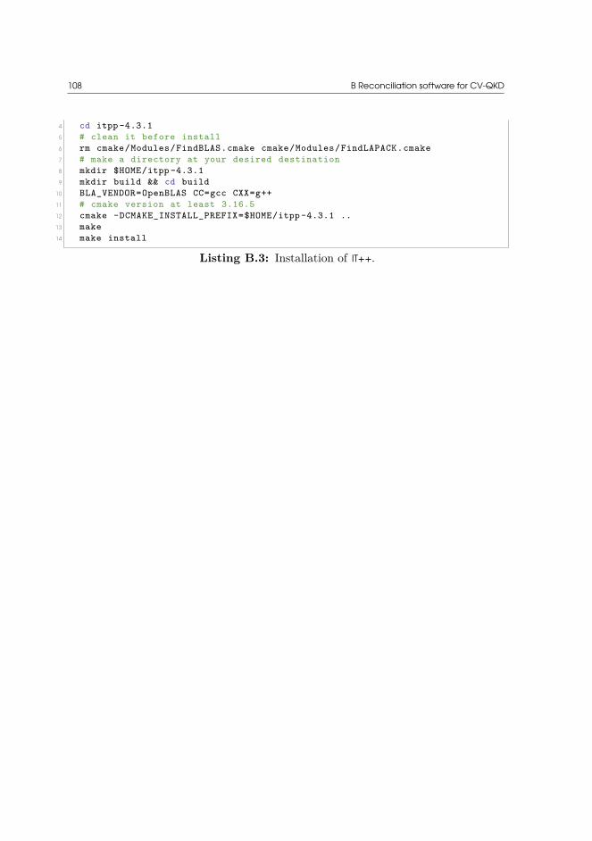
108 B Reconciliation software for CV-QKD
4 cd itpp -4.3.15 # clean it before install6 rm cmake/Modules/FindBLAS.cmake cmake/Modules/FindLAPACK.cmake7 # make a directory at your desired destination8 mkdir $HOME/itpp -4.3.19 mkdir build && cd build
10 BLA_VENDOR=OpenBLAS CC=gcc CXX=g++11 # cmake version at least 3.16.512 cmake -DCMAKE_INSTALL_PREFIX=$HOME/itpp -4.3.1 ..13 make14 make install
Listing B.3: Installation of IT++.

APPENDIXCSoftware to design
highly efficientMET-LDPC codes
C.1 About the softwareThis tool helps to optimize a degree distribution for MET-LDPC codes with cascadestructure. Details of the optimization problem for cascade structures is describedin Chapter 4. The goal is to design a MET-LDPC code with rate R when a basecode with rate r is available. The optimization of the base code with rate r wasdescribed in Section 4.4. Here we assume that a base code is available and the goal ofthe optimization problem is then to find the best degree distribution for the cascadestructure. The optimization software consists of three different tools:
EXIT-Chart Plots the EXIT chart for the base code.
Connector Generates a list of all possible connector parts in the cascade structure.
Find best Finds the best degree distribution by testing different connector parts.
EXIT-Chart This tool provides a quick pictorial representation for the base code.For a given base code with rate rb it generates a EXIT.txt file which can be usedby a python script (plotEXIT.py) to generate the EXIT chart. The code is designedfor the BEC(q) channel. For example, for a base code of rate 0.8, the correspondingEXIT chart for BEC(0.15) is plotted in Figure C.1. The node perspective degreedistribution of this code is
ν(q, x) = 0.6 q x2 + 0.4 q x3 , µ(x) = 0.2 x12 .
The corresponding edge perspective degree distribution is
λ(q, x) = 0.5 q x+ 0.5 q x2 , ρ(x) = x11 .

110 C Software to design highly efficient MET-LDPC codes
0.0 0.2 0.4 0.6 0.8 1.0IvE, Ic
A
0.0
0.2
0.4
0.6
0.8
1.0Ic E,
Iv A
Variable nodeCheck node
Figure C.1: The output of the EXIT tool for a base code of rate 0.8 on BEC(0.15).
Connector This tool generates a DEGREE-x.txt file which contains different codestructures (See Listing B.1) for a MET-LDPC code with base code of rate rb andoverall code of rate R. If the number of candidate codewords is more than 1000 anew file with appropriate numbering will be generated.
As input it accepts the structure of the base code in the node perspective mode andthe overall code rate of the MET-LDPC code. It also accepts some further informationrequired for the density evolution. The parameters are presented in Listing B.1.
This tool checks the constraint sets for the candidate codes and only generatescodes with the accepted structures. For more details to see how the candidate codesare generated based on a base code see Section 4.4.
Find Best This tool accepts DEGREE-x.txt as the input and then checks the per-formance of the codes to find the best code in forms of the threshold. It runs DE forall the candidate codes and from all codes which converged with a specified numberof iterations, it selects the best code.

Bibliography[1] Peter W. Shor. “Polynomial-Time Algorithms for Prime Factorization and Dis-
crete Logarithms on a Quantum Computer.” In: SIAM J. Comput. 26.5 (October1997), pages 1484–1509. issn: 0097-5397. doi: 10.1137/S0097539795293172.url: http://dx.doi.org/10.1137/S0097539795293172.
[2] Valerio Scarani et al. “The security of practical quantum key distribution.”In: Rev. Mod. Phys. 81 (September 2009), pages 1301–1350. doi: 10.1103/RevModPhys.81.1301. url: https://link.aps.org/doi/10.1103/RevModPhys.81.1301.
[3] Nicolas Gisin et al. “Quantum cryptography.” In: Rev. Mod. Phys. 74 (1 March2002), pages 145–195. doi: 10.1103/RevModPhys.74.145. url: https://link.aps.org/doi/10.1103/RevModPhys.74.145.
[4] Yi-Chen Zhang et al. “Long-distance continuous-variable quantum key distri-bution over 202.81 km fiber.” In: Physical Review Letters (June 2020). url:http://eprints.whiterose.ac.uk/161908/.
[5] Boris Korzh et al. “Provably secure and practical quantum key distribution over307 km of optical fibre.” In: Nature Photonics 9.3 (March 2015), pages 163–168.doi: 10.1038/nphoton.2014.327. arXiv: 1407.7427 [quant-ph].
[6] Anthony Leverrier et al. “Multidimensional reconciliation for a continuous-variable quantum key distribution.” In: Phys. Rev. A 77.4 (2008), page 042325.doi: 10.1103/PhysRevA.77.042325. url: https://link.aps.org/doi/10.1103/PhysRevA.77.042325.
[7] U. Wachsmann, R. F. H. Fischer, and J. B. Huber. “Multilevel codes: theoreticalconcepts and practical design rules.” In: IEEE Transactions on InformationTheory 45.5 (July 1999), pages 1361–1391. issn: 0018-9448. doi: 10.1109/18.771140. url: https://ieeexplore.ieee.org/document/771140.
[8] G. Van Assche, J. Cardinal, and N. J. Cerf. “Reconciliation of a quantum-distributed Gaussian key.” In: IEEE Transactions on Information Theory 50.2(2004), pages 394–400. doi: 10 . 1109 / TIT . 2003 . 822618. url: https : / /ieeexplore.ieee.org/document/1266817.
112 Bibliography
[9] M. Bloch et al. “LDPC-based Gaussian key reconciliation.” In: 2006 IEEE In-formation Theory Workshop - ITW ’06 Punta del Este. March 2006, pages 116–120. doi: 10.1109/ITW.2006.1633793. url: https://ieeexplore.ieee.org/document/1633793.
[10] Paul Jouguet, Sébastien Kunz-Jacques, and Anthony Leverrier. “Long-distancecontinuous-variable quantum key distribution with a Gaussian modulation.” In:Phys. Rev. A 84 (6 December 2011), page 062317. doi: 10.1103/PhysRevA.84.062317. url: https://link.aps.org/doi/10.1103/PhysRevA.84.062317.
[11] Duan Huang et al. “Long-distance continuous-variable quantum key distribu-tion by controlling excess noise.” In: Scientific reports 6 (January 2016), page 19201.doi: 10.1038/srep19201. url: https://doi.org/10.1038/srep19201.
[12] S. Jeong and J. Ha. “On the Design of Multi-Edge Type Low-Density Parity-Check Codes.” In: IEEE Transactions on Communications 67.10 (October 2019),pages 6652–6667. issn: 1558-0857. doi: 10.1109/TCOMM.2019.2927567. url:https://ieeexplore.ieee.org/document/8758347.
[13] S. Jayasooriya et al. “A New Density Evolution Approximation for LDPC andmulti-edge Type LDPC Codes.” In: IEEE Transactions on Communications64.10 (October 2016), pages 4044–4056. issn: 0090-6778. doi: 10.1109/TCOMM.2016.2600660. url: https://ieeexplore.ieee.org/document/7544625.
[14] S. Jayasooriya et al. “Joint optimization technique for multi-edge type low-density parity-check codes.” In: IET Communications 11.1 (2017), pages 61–68.issn: 1751-8628. doi: 10.1049/iet-com.2016.0287.
[15] Hossein Mani et al. “An Approximation Method for Analysis and Design ofMulti-Edge Type LDPC Codes.” In: url: http://2018.qcrypt.net/others/accepted-posters/. Poster presented at 8th International Conference on Quan-tum Cryptography, Shanghai, China, 2018.
[16] Hossein Mani et al. “Algorithmic Approach to Design Highly Efficient MET-LDPC Codes with Cascade Structure.” In: url: http://2019.qcrypt.net/scientific-program/posters/. Poster presented at 9th International Confer-ence on Quantum Cryptography, Montreal, Canada, 2019.
[17] Hossein Mani et al. “Two MET-LDPC codes designed for long distance CV-QKD.” In: url: https : / / 2020 . qcrypt . net / accepted - papers / #list -of-accepted-posters. Poster presented at 10th International Conference onQuantum Cryptography, Amsterdam, Netherlands, 2020.
[18] Hossein Mani et al. Multi-edge-type LDPC code design with G-EXIT chartsfor continuous-variable quantum key distribution. 2018. arXiv: 1812 . 05867[cs.IT].
[19] U.L. Andersen, G. Leuchs, and C. Silberhorn. “Continuous-variable quantuminformation processing.” In: Laser & Photonics Reviews 4.3 (2010), pages 337–354. doi: 10.1002/lpor.200910010. url: https://onlinelibrary.wiley.com/doi/abs/10.1002/lpor.200910010.
Bibliography 113
[20] Samuel L. Braunstein and Peter van Loock. “Quantum information with con-tinuous variables.” In: Rev. Mod. Phys. 77 (2 June 2005), pages 513–577. doi:10.1103/RevModPhys.77.513. url: https://link.aps.org/doi/10.1103/RevModPhys.77.513.
[21] Charles H. Bennett and Gilles Brassard. “Quantum cryptography: Public keydistribution and coin tossing.” In: Theoretical Computer Science 560 (December2014), pages 7–11. doi: 10.1016/j.tcs.2014.05.025. url: https://doi.org/10.1016%2Fj.tcs.2014.05.025.
[22] Frédéric Grosshans and Philippe Grangier. “Continuous Variable QuantumCryptography Using Coherent States.” In: Phys. Rev. Lett. 88 (5 January 2002),page 057902. doi: 10.1103/PhysRevLett.88.057902. url: https://link.aps.org/doi/10.1103/PhysRevLett.88.057902.
[23] Raul Garcia-Patron Sanchez and Nicolas J. Cerf. “Quantum information withoptical continuous variables: from Bell tests to key distribution.” In: 2007. url:https://difusion.ulb.ac.be/vufind/Record/ULB-DIPOT:oai:dipot.ulb.ac.be:2013/210655/Holdings.
[24] Christian Weedbrook et al. “Gaussian quantum information.” In: Rev. Mod.Phys. 84 (2 May 2012), pages 621–669. doi: 10.1103/RevModPhys.84.621.url: https://link.aps.org/doi/10.1103/RevModPhys.84.621.
[25] Frédéric Grosshans et al. “Quantum key distribution using gaussian-modulatedcoherent states.” In: Nature 421.6920 (January 2003), pages 238–241. issn:1476-4687. doi: 10.1038/nature01289. url: https://doi.org/10.1038/nature01289.
[26] Frédéric Grosshans et al. “Virtual Entanglement and Reconciliation Protocolsfor Quantum Cryptography with Continuous Variables.” In: Quantum Info.Comput. 3.7 (October 2003), pages 535–552. issn: 1533-7146. url: https ://dl.acm.org/doi/10.5555/2011564.2011570.
[27] Bing Qi et al. “Experimental study on the Gaussian-modulated coherent-statequantum key distribution over standard telecommunication fibers.” In: Phys.Rev. A 76 (5 November 2007), page 052323. doi: 10.1103/PhysRevA.76.052323. url: https://link.aps.org/doi/10.1103/PhysRevA.76.052323.
[28] Eleni Diamanti and Anthony Leverrier. “Distributing Secret Keys with Quan-tum Continuous Variables: Principle, Security and Implementations.” In: En-tropy 17 (August 2015), pages 6072–6092. url: https://www.mdpi.com/1099-4300/17/9/6072.
[29] Christian Weedbrook, Carlo Ottaviani, and Stefano Pirandola. “Two-way quan-tum cryptography at different wavelengths.” In: Phys. Rev. A 89 (1 January2014), page 012309. doi: 10.1103/PhysRevA.89.012309. url: https://link.aps.org/doi/10.1103/PhysRevA.89.012309.
114 Bibliography
[30] Stefano Pirandola et al. “Continuous-variable quantum cryptography usingtwo-way quantum communication.” In: Nature Physics 4.9 (September 2008),pages 726–730. issn: 1745-2481. doi: 10.1038/nphys1018. url: https://doi.org/10.1038/nphys1018.
[31] Anthony Leverrier and Philippe Grangier. “Continuous-variable quantum-key-distribution protocols with a non-Gaussian modulation.” In: Phys. Rev. A 83(4 April 2011), page 042312. doi: 10.1103/PhysRevA.83.042312. url: https://link.aps.org/doi/10.1103/PhysRevA.83.042312.
[32] Fabian Laudenbach et al. “Continuous-Variable Quantum Key Distributionwith Gaussian Modulation—The Theory of Practical Implementations.” In: Ad-vanced Quantum Technologies 1.1 (2018), page 1800011. doi: 10.1002/qute.201800011. url: https://onlinelibrary.wiley.com/doi/abs/10.1002/qute.201800011.
[33] Igor Devetak and Andreas Winter. “Distillation of secret key and entanglementfrom quantum states.” In: Proceedings of the Royal Society A: Mathematical,Physical and Engineering Sciences 461.2053 (2005), pages 207–235. doi: 10.1098/rspa.2004.1372. url: https://royalsocietypublishing.org/doi/abs/10.1098/rspa.2004.1372.
[34] Frédéric Grosshans and Nicolas J. Cerf. “Continuous-Variable Quantum Cryp-tography is Secure against Non-Gaussian Attacks.” In: Phys. Rev. Lett. 92 (4January 2004), page 047905. doi: 10.1103/PhysRevLett.92.047905. url:https://link.aps.org/doi/10.1103/PhysRevLett.92.047905.
[35] Jérôme Lodewyck et al. “Quantum key distribution over 25 km with an all-fibercontinuous-variable system.” In: Phys. Rev. A 76 (4 October 2007), page 042305.doi: 10.1103/PhysRevA.76.042305. url: https://link.aps.org/doi/10.1103/PhysRevA.76.042305.
[36] Paul Jouguet. “Security and performance of continuous-variable quantum keydistribution systems.” Theses. Télécom ParisTech, September 2013. url: https://pastel.archives-ouvertes.fr/tel-01174739.
[37] Sarah J Johnson et al. “On the problem of non-zero word error rates for fixed-rate error correction codes in continuous variable quantum key distribution.” In:New Journal of Physics 19.2 (February 2017), page 023003. doi: 10.1088/1367-2630/aa54d7. url: https://doi.org/10.1088%2F1367-2630%2Faa54d7.
[38] Renato Renner. “Security of Quantum Key Distribution.” Theses. ETH Zurich,September 2005. url: https://arxiv.org/pdf/quant-ph/0512258.pdf.
[39] Anthony Leverrier, Frédéric Grosshans, and Philippe Grangier. “Finite-sizeanalysis of a continuous-variable quantum key distribution.” In: Phys. Rev. A81 (6 June 2010), page 062343. doi: 10.1103/PhysRevA.81.062343. url:https://link.aps.org/doi/10.1103/PhysRevA.81.062343.

Bibliography 115
[40] Anthony Leverrier et al. “Security of Continuous-Variable Quantum Key Dis-tribution Against General Attacks.” In: Phys. Rev. Lett. 110 (3 January 2013),page 030502. doi: 10.1103/PhysRevLett.110.030502. url: https://link.aps.org/doi/10.1103/PhysRevLett.110.030502.
[41] Hou-Man Chin et al. Machine learning aided carrier recovery in continuous-variable quantum key distribution. 2020. arXiv: 2002.09321 [quant-ph].
[42] Tobias Gehring et al. Ultra-fast real-time quantum random number generatorwith correlated measurement outcomes and rigorous security certification. 2018.arXiv: 1812.05377 [quant-ph].
[43] A. D. Wyner. “The Wire-Tap Channel.” In: Bell System Technical Journal 54.8(1975), pages 1355–1387. doi: 10 . 1002 / j . 1538 - 7305 . 1975 . tb02040 . x.eprint: https://onlinelibrary.wiley.com/doi/pdf/10.1002/j.1538-7305.1975.tb02040.x. url: https://onlinelibrary.wiley.com/doi/abs/10.1002/j.1538-7305.1975.tb02040.x.
[44] Tom Richardson and Rüdiger Urbanke. Modern Coding Theory. CambridgeUniversity Press, 2008. doi: 10.1017/CBO9780511791338. url: https://dl.acm.org/doi/book/10.5555/1795974.
[45] Xiangyu Wang et al. “Efficient Rate-Adaptive Reconciliation for Continuous-Variable Quantum Key Distribution.” In: Quantum Info. Comput. 17.13–14(November 2017), pages 1123–1134. issn: 1533-7146. doi: 10.26421/qic17.13-14. url: http://dx.doi.org/10.26421/QIC17.13-14.
[46] Xiangyu Wang et al. “High speed error correction for continuous-variable quan-tum key distribution with multi-edge type LDPC code.” In: Scientific Reports8.1 (July 2018), page 10543. issn: 2045-2322. doi: 10.1038/s41598- 018-28703-4. url: https://doi.org/10.1038/s41598-018-28703-4.
[47] André Stefanov et al. “Optical quantum random number generator.” In: Journalof Modern Optics 47.4 (2000), pages 595–598. doi: 10.1080/09500340008233380.url: https://doi.org/10.1080/09500340008233380.
[48] P. Jouguet, D. Elkouss, and S. Kunz Jacques. “High-bit-rate continuous-variablequantum key distribution.” In: Phys. Rev. A 90 (4 October 2014), page 042329.doi: 10.1103/PhysRevA.90.042329. url: https://link.aps.org/doi/10.1103/PhysRevA.90.042329.
[49] J. Cardinal and G. Van Assche. “Construction of a shared secret key usingcontinuous variables.” In: Proceedings 2003 IEEE Information Theory Workshop(Cat. No.03EX674). March 2003, pages 135–138. url: https://ieeexplore.ieee.org/document/1216713.
[50] D. Slepian and J. Wolf. “Noiseless coding of correlated information sources.”In: IEEE Transactions on Information Theory 19.4 (July 1973), pages 471–480.issn: 0018-9448. doi: 10.1109/TIT.1973.1055037. url: https://ieeexplore.ieee.org/document/1055037.

116 Bibliography
[51] T. J. Richardson, M. A. Shokrollahi, and R. L. Urbanke. “Design of capacity-approaching irregular low-density parity-check codes.” In: IEEE Transactionson Information Theory 47.2 (February 2001), pages 619–637. issn: 0018-9448.doi: 10.1109/18.910578. url: https://ieeexplore.ieee.org/document/910578.
[52] T. J. Richardson and R. L. Urbanke. “The capacity of low-density parity-checkcodes under message-passing decoding.” In: IEEE Transactions on InformationTheory 47.2 (February 2001), pages 599–618. issn: 0018-9448. doi: 10.1109/18.910577. url: https://ieeexplore.ieee.org/document/910577.
[53] G. Forney. “Generalized minimum distance decoding.” In: IEEE Transactions onInformation Theory 12.2 (April 1966), pages 125–131. issn: 1557-9654. doi: 10.1109/TIT.1966.1053873. url: https://ieeexplore.ieee.org/abstract/document/1053873.
[54] Peter Elias. “List decoding for noisy channels.” In: (1957). url: http://hdl.handle.net/1721.1/4484.
[55] D. Chase. “Class of algorithms for decoding block codes with channel measure-ment information.” In: IEEE Transactions on Information Theory 18.1 (January1972), pages 170–182. issn: 1557-9654. doi: 10.1109/TIT.1972.1054746. url:https://ieeexplore.ieee.org/document/1054746.
[56] H. Mani and S. Hemati. “Symbol-Level Stochastic Chase Decoding of Reed-Solomon and BCH Codes.” In: IEEE Transactions on Communications 67.8(2019), pages 5241–5252. url: https://ieeexplore.ieee.org/document/8708257.
[57] C. Leroux et al. “Stochastic Chase Decoding of Reed-Solomon Codes.” In: IEEECommunications Letters 14.9 (September 2010), pages 863–865. issn: 2373-7891.doi: 10.1109/LCOMM.2010.09.100594. url: https://ieeexplore.ieee.org/document/5557635.
[58] Jesus Martinez-Mateo, David Elkouss, and Vicente Martin. “Blind Reconcili-ation.” In: Quantum Info. Comput. 12.9–10 (September 2012), pages 791–812.issn: 1533-7146. url: https://arxiv.org/abs/1205.5729.
[59] A. Shokrollahi. “Raptor codes.” In: IEEE Transactions on Information Theory52.6 (June 2006), pages 2551–2567. issn: 1557-9654. doi: 10.1109/TIT.2006.874390. url: https://ieeexplore.ieee.org/document/1638543.
[60] Chao Zhou et al. “Continuous-Variable Quantum Key Distribution with Rate-less Reconciliation Protocol.” In: Phys. Rev. Applied 12 (5 November 2019),page 054013. doi: 10.1103/PhysRevApplied.12.054013. url: https://link.aps.org/doi/10.1103/PhysRevApplied.12.054013.
[61] Tom Richardson, Rüdiger Urbanke, et al. “Multi-edge type LDPC codes.” In:Workshop honoring Prof. Bob McEliece on his 60th birthday, California Instituteof Technology, Pasadena, California. 2002, pages 24–25. url: https://api.semanticscholar.org/CorpusID:13597086.
Bibliography 117
[62] R. Gallager. “Low-density parity-check codes.” In: IRE Transactions on In-formation Theory 8.1 (January 1962), pages 21–28. issn: 2168-2712. doi: 10.1109/TIT.1962.1057683. url: https://ieeexplore.ieee.org/document/1057683.
[63] “Entropy, Relative Entropy, and Mutual Information.” In: Elements of Infor-mation Theory. John Wiley & Sons, Ltd, 2005. Chapter 2, pages 13–55. isbn:9780471748823. doi: 10.1002/047174882X.ch2. url: https://onlinelibrary.wiley.com/doi/abs/10.1002/047174882X.ch2.
[64] M. Ardakani and F. R. Kschischang. “A more accurate one-dimensional anal-ysis and design of irregular LDPC codes.” In: IEEE Transactions on Commu-nications 52.12 (December 2004), pages 2106–2114. issn: 0090-6778. doi: 10.1109/TCOMM.2004.838718. url: https://ieeexplore.ieee.org/document/1369623.
[65] A. Ashikhmin, G. Kramer, and S. ten Brink. “Extrinsic information transferfunctions: model and erasure channel properties.” In: IEEE Transactions onInformation Theory 50.11 (November 2004), pages 2657–2673. issn: 1557-9654.doi: 10.1109/TIT.2004.836693. url: https://ieeexplore.ieee.org/document/1347354?arnumber=1347354.
[66] C. Measson et al. “The Generalized Area Theorem and Some of its Conse-quences.” In: IEEE Transactions on Information Theory 55.11 (November 2009),pages 4793–4821. issn: 0018-9448. url: https://ieeexplore.ieee.org/document/5290273.
[67] H. Mani et al. “On Generalized EXIT charts of LDPC code ensembles overbinary-input output-symmetric memoryless channels.” In: 2012 IEEE Interna-tional Symposium on Information Theory Proceedings. 2012, pages 2336–2340.url: https://ieeexplore.ieee.org/document/6283930.
[68] Cyril Measson. “Conservation laws for coding.” PhD thesis. Lausanne: EPFL,2006, page 146. doi: 10.5075/epfl-thesis-3485. url: http://infoscience.epfl.ch/record/64690.
[69] A. Ashikhmin, G. Kramer, and S. ten Brink. “Code rate and the area underextrinsic information transfer curves.” In: Proceedings IEEE International Sym-posium on Information Theory, June 2002, pages 115–. doi: 10.1109/ISIT.2002.1023387. url: https://ieeexplore.ieee.org/document/1023387?arnumber=1023387.
[70] M. Amin Shokrollahi. “New Sequences of Linear Time Erasure Codes Approach-ing the Channel Capacity.” In: Applied Algebra, Algebraic Algorithms and Error-Correcting Codes. Edited by Marc Fossorier et al. Berlin, Heidelberg: SpringerBerlin Heidelberg, 1999, pages 65–76. isbn: 978-3-540-46796-0. url: https://link.springer.com/chapter/10.1007%2F3-540-46796-3_7.

118 Bibliography
[71] Mario Milicevic et al. “Quasi-cyclic multi-edge LDPC codes for long-distancequantum cryptography.” In: npj Quantum Information 4.21 (2018). doi: 10.1038/s41534-018-0070-6. url: https://doi.org/10.1038/s41534-018-0070-6.
[72] Bernhard Ömer. PEG Software for Quasi-Cyclic LDPC Codes. AIT AustrianInstitute of Technology, Vienna, AT. [email protected]. 2020.