DISTRIBUTED BY - DTIC

AD-A007 582

A SCIENTIFIC APPROACH TO THE DESIGN OF COMPUTER CONTROLLED MANIPULATORS

J. L. Nevins, et al

Charles Stark Draper Laboratory, Incorporated

Prepared for:

Defense Advanced Research Projects Agency

August 1 974

DISTRIBUTED BY:

urn National Technical Information Servici U. S. DEPARTMENT OF COMMERCE

r

R-837

A Scientific Approach to the I)c?ign of

Computer Controlled Manipulators

by

,I.L. Nrvins. D.E. Whitney. A.E. Woodin

S. Drake. M. Lynch. D. Seltzer. R. Sturges. P. Watson

Contract DAn-C-15-73-C-0278 with the Defense Advanced Research

Projects Agency. ARPA Order No. 2455. Project Code 31330

August in74

The Charles Stark Draper Laboratory. Inc. Cambridge. Massachusetts

Approved N. Sears

I

r

ACKNOWLEDGE IIENT

This report was proparod by The Charles Stark Draper Laboratory,

Inc., under contract DAH-C,-15-73-C,-0278 with the Defense Advanced

Research Projects Agency. AHl'A Order No. 2455, Project Code 3D30.

Publication of this report does not constitute approval by the

Defense Advanced Research Projects Agency of the findings or conclusions

contained herein.

11

TABLE OF CONTENTS

I. Irtruduction 1

A. Rpsearch Objectives 1

1. Arm deisgn consideration 1

2. Design method 7

B. Design Goals for a Research Arm 8

C. Report Organization 9

II. Survey of Existing Arms 10

A. Purpose of Survey 10

B. Criteria for an Arm 10

C. Sources of Information 11

D. Survey Results 12

1. Arm and wrist motion 12

2. Control 12

3. Power actuators 14

4. Hands (end effectors, grippers) 14

5. Areas of application 16

E. Robot Assemblers 16

III. Basic Tradeoffs and Considerations in Arm Design 18

A. Introduction 18

B. The Assembly Problem and its Impact on 18 Arm Design

C. Major Design — Control Issues 22

D. Accommodation as a Possible Servo-Sensor 29 Control Strategy

E. Summary 31

IV. Technical Aspects of Design Methods: Tools for 32 a Scientific Approach to Arm Design

A. Gross Motion Size, Payload and Speed 32

1. Task Inrluence 32

iii

TABLE OF CONTENTS (conU

2. Technology influence 34

a. Inlroduclion 34

b. Influence.' of choice of actuator 34

c. Gearing on electric actuators 40

d. Influences on accuracy, repeatability and resolution 42

e. Influon^es on servo design 46

B. Kinematic Configuration 48

1. Approach 48

2. Dispositions of freedoms 49

3. Types of joints 54

4. Optimization of arm geometry 59

C. Relation Between Servo Bandwidth and Structural Vibration 64

D. Servo Control Methods and Force Feedback 66

E. Error Analysis 74

F. Summary of Design Tools 76

V. Discussion of Draper Laboratory Arm Design (POPEYE) 78

A. Description of Arm 78

B. Critrique of POPEYE as a Research Tool 81

1. Advantages of POPEYE design 81

2. Disadvantages of POPEYE design 83

VI. Summary of Draper Laboratory Arm Specifications 8-*

84

84

84

85

85

85

A. Dexterity

B. Size

C. Accuracy

D. Performance

E. Subsystem Specification

1. Actuators

IV

— • ■ - ■ -■- - - - J

TABLE OF CONTENTS (.ont)

2. Angular position transdut ors

3. Wrist force sensor 86

86

VII. Subsystems

A. Actuator Selection and Design

1. Power source solection

2. Hydraulic motor/actuator design

3. Vane actuator design specification B. Structure

1. Mechanical properties

a. Requirements and materials

Structum design

Support and worktable

Shafts and couplings C.

D.

h,

c.

().

Sensors

!• Angle sensors

2.

s.

Phase-locked loop rcsolver to digital converter

Force sensors

a. System considerations

b.

c.

d.

e.

f.

Arm force sensing by joint torque measurement

Pedestal (orr ? sensors

Wrist force sensors

Laser force sensor specification

Other sensors

Hydraulic Control

1. Introduction

2. Analytical development

3. Modeling types of hydraulic control systems

a. Position error control

b. Position and rate feedback

87

87

87

88

93

99

99

99

102

107

111

114

114

1?7

120

120

123

125

127

131

131

135

135

135

141

143

145

TABLE OF CONTENTS (cont)

c. Position feedback with lead filter on rate feedback 148

d. Position, rate, and pressure feedback 154

4. Discussion 154

E. Hydraulic Control Servo Experiments 158

VIII. Conclusions and Recommrndations for Future Work 161

A, Conclusions 161

B. Recommendations 162

References 165

Appendices 167

1. Survey of Commercial Industrial Robots 167

2. Derivation and Simplification of Hydraulic System Equations 169

3. Abstracts of Theses Performed Under This Contract 177

a. "A General Planar Positioning Dcvlc?" by Jonathon David Rock 178

b, "Design of an Automatic Assembly System Multipurpose End Effector" by Thomas 179 Barry Lyons

VI

I. INTRODUCTION

A. Heseatch Objective!

The purpose of this study was to develop a science for the

design of computer controlled manipulator systems which

could be scaled for small manipulators. At the outset of the study the

lack of specific tasks or the specific scale of a design environrient

forced consideration of a working volume consistent with pecpie in order

to determine the relationships between tasks, task scale and perfornance

requirements for actuators, sensors (both force and position), etc.

The work therefore had four principal activities, namelv:

a. establish a scientific base for

determining manipulator require-

ments as a function of task and

task scale

b. identification and development

of general design tools needed

c. implementation of a design for a

laboratory system to determine

the validity of the approach

d. evaluation of design concepts via

simulations and small laboratory

experiments

In addition, a survey was made of existing manipulator systems

and a novel, patentable. hydraulic actuator was conceived and documented.

1. Arm Design Considerations

Arm design is really a misnomer. One cannot consider an

arm out of context of the tasks expected to be performed or the environ-

ment that the tasks will be performed in. For example, Figure 1-1

diagrams the interlationships that must be considered between technology,

environment, parts design, and task descriptors if the focus is

J

CO c: z uo U o UJ •—

z < O LU

i a O QC H- >— r- _ UJ < < Q E t— a QC •^ LU C

PER

A

ON

SI 1—

CO

JFO

Rf

NEE

D

>

o o

^ A > z E

A V m ■ *l

u.

58 ATI

O

DED O

*— CO g c

tn ' LU UJ Q O

<

INFO

RM

NE

E

AS

K

ES

CR

IP 5 ? < LU

(X Q s Aii^ "c

I t— Q

M i t / LO t

9 z on ii wo 1 ^ 2i c

o 1 O LU >- O B ^^ / —»— -AI- *■"

o WA

RE

IDE

RA

T

0 o

DES

CR

I

IDE

RA

J

i

on Q un ■E Z

2 C r D

5S u 3

UJ o < O z E

O L — h CO -

^^ o UJ (_)

s MS ^o LU

3^ t/> 5 O

uo ii

mampuiato, svsUvns tor MM«Mj in a manufarl irimi fr.vuo,.,,.......

Ii.sid.-s thrnc issu.s. aMWl itlMllM11' 2, hav.-

shown .hat ,hr MMta. <.• Mwtrtol ^s.Mnl.K requir.-s .onsM.-,.-

tion of a «hoi., s,.... ,r;,„, of m, »• bMMM nMtiM SNSUM, s as .11 ...rated

hv Tahle I. In general, motion or manipulator svstf.ns m .s. !,.■

concerned with fet.h.np pans. h..id.ne „arts, and assemhl.np parts.

These alone impK man-. d.-C,e..s-of-tre.-do,r not rmrrraiK cns.dered In

'he sin.pit- arm req lirvmml that the t-nd point of the- man.p .la-.m he able

to achieve all possible stare po.m. .n so. .e arhitrars ^.„kmc v..l .me.

F.rfher. these stmJi.s'1* showed that th.- thro. ia.sk. .u-trhing

parts, holdrn, parts, and th.- ..ssemnh pro. .ss) ran he rate,o, u.-d into ,ross

•mi fme motions. r.rOM motions are th.- Ulf. r^M. less ar.urate motion,

necessarv to mow oh,, cts :rom on. lo. ation to another. Ih.se motions . an

isuallv be don-, m an open-loop rontrol manner with mtaimuin informa-

tion required fron, »he environment. Fme moMons are the s.nall precise

motions needed when two ob.ect.s mterac t. It ,s th.s latter motion which

is most dependent on the mt.-rmation acquired from the env.ronment.

An interfa. e region has also been defined between gross

motion and fine ^notion to identifv the bounda^ of uncertaintv m

knowledge of the location of parts, their size variation or the

imprecise technology (sensor ar ravs. mechanical SNstems.

control strateg.es. etc | ava.lable for accomplishing the desired Motion.

For other tasks, other considerations as well as the above

must be taken into ■ecottnl. Two thumbnail design scenarios rmlZht serve

to illustrate these points. Suppose one wishes to use a small arm <50 cm

reach) to remove or insert common integrated circuits. It is known that

each pin on such a circuit module requires a force of about 200e to msert

• t. Thus, a common 8 pin mod. le will require 1.6 kilogram of force at

the hand or 0. 8 kilogram-me;er of stall torque at the shoulder of the arm

which does the inserting or removing. This stipulates a minimum static

strength for this actuator. Other actuators with axes parallel to this one.

at the elbow or wrist, will have * be capable of correspondingly

= J

TABUE 1 AWEMBLY BYBTEM ELEMENTS

(II PARTS MANAGEMENT, GROSS AND FINE

Gross (scheduling): inventory orders, conveyors, dispatchers, etc.

Fine (parts feeding): shakers, conveyors, etc. (note the trend to make parts on site).

(2) INSPECTIOM EXPLICIT AND IMPLICIT

Explicit (are all the holes present?)

Implicit (do the parts go together as expected?)

(3) MOTION. TO BRING THE FED. INSPECTED PARTS TOGETHER POSSIBLY USING JIGS AND FIXTURES

(4) FASTENING, USING SCREWS. RIVETS. GLUE. ETC.

(If not glue, then fastening involves additional assembly tasks).

(5) NON-DESTRUCTIVE TESTING (e.g.. TEST FOR FREE MOTION).

(6) DIAGNOSTICS

(If some assemblies fail, find out why and correct parts manufacture or assembly)

(7) MONITORING

(To determine if the assembly system Is operating properly)

- - ■ —______—

calculated stall torques. A separate calculation is required for the

torques required to accelerate and decelerate the arm. See below.

Here it sufficies to say that the specified payloads are a tiny fraction of

the arm's total weight, which therefore governs the dynamic and gravity

torque problem independent of payload. If speed is not a factor, then

insertion forces will determine the actuator characteristics.

As a second example, consider the arm studied in detail in this report (Fig. 1-2), Here, payloads will be a substantial fraction of the arm's

weight, perhaps 20% to 30%. This percentage is beyond the capabilities of current industrial robots. Their efficiency of design might yield only

10 to 15%. That is, their arms are quite heavy in comparison to the

objects they are designed to move about. High speeds and payload

requirements dominate the torque sizing problem for the arm designed here, far exceeding gravity or insertion forces. It is possible to solve this

problem badly and end up with unbalanced capabilities among the actuators.

Weak wrists are common among commercial industrial arms. Procedures for avoiding such difficulties are given in this report, along with the

necessary technology of actuators, actuator location and transmission

methods, and computer techniques for performing the balance.

Similar calculations, based on arm size and task

characteristics, are required to determine the accuracy, and therefore

the technology required for joint position sensors. Technology limitations

in sensors and structure may lead to the conclusion thai a single arm

cannot be built which simultaneously has the required reach (a gross

motion characteristic) and the required accuracy and ability to make

very small motions (fine motion characteristics). A properly designed

system capable of dealing meaningfully with such a task would therfore consist of two or more mobility systems.

J

2. Design Method

To deal with this problem in a systematic way, therefore,

required detail consideration of manipulator tasks and an environment.

With contractor agency support it was decided to use the detailed task

and environment analysis being done under an NSF sponsored research

grant into "Exploratory Research in Industrial Modular Assembly. "(1' 2)

This work was concerned with a system organized about force

and torque sensor arrays for performing industrial mechanical assembly

within a working volume of 0.3 meter cubed (1 foot cubed). This

approach for assembly is similar to the way a blind person might assemble

things - b/ touch and feel. In order that this kind of system be efficient

its world must be highly structured. That is. the location of parts, jigs.

tools, etc. must be known a priori to some tolerance. Otherwise, a

great deal of time would be required to grope around and find things.

Groping around, or a less structured world, was left to later considerations

of higher level systems that include visual or non-visual imaging sensors.

The decision to use the NSF sponsored work had the following advantages:

a. It was concerned with a work volume in which

tasks can easily be identified and studied.

I. It gave access to detailed task analysis being

performed on a variety of mechanical assemblies.

c. Since assembly is a composite of many kinds

of tasks the lack of task specificity would not

be a problem.

d. The dynamic coupling of manipulator require-

ments and task and task scale could be analyzed

to determine the design tools needed.

NSF Grant No. GI-39432Xand Gl-43787

,^

B. Design Goals for a Research Arm

The principal activity of this work was to implement a research

tool (arm) for determining the validity of the approach taken. The design goals were as follows:

a. examine the dynamic geometry requirements for motion/

manipulator systems for a variety of tasks and task scale

b. determine both the static and dynamic relationship between the

requirements for actuators, sensors, kinematics, structures and task and task scale

c. explore various task execution strategies and the associated

envirorment-task related information needed and assess the impact which strategy/information have on arm performance requirements,

What was found was that the design effort for this research tool

became the prime focus for all the other work. That is, arm design

clearly identified the performance that could be obtained and this in turn

sharpened the categorization of the gross and fins motion regions and

caused an interface region to be defined that encompassed the combined uncertainties of the technology and the pieces to be assembled.

The following conclusions could therefore be drawn from this activity a. arm design requires a use context

b. context provides scale, speed, loads, accuracies - also

strategies, information, (system organization?), and servo sensor loop closure

c. both design and use are not well understood disciplines

d. parallel development of each discipline stimulates both and identifies the real world constraints

e. developments at this level provide the lower order systems

necessary for interacting with an environment and coupling it

with eventual high order artificial intelligence planning systems

f. it would appear that the existence of technologically real lower

order systems would aid and stimulate the development of

effective and realistic higher order planning systems just as

consideration of task contexts stimulates the development of lower order systems.

C. Report Organization

In six major sections this report discusses a survey of existing

arms (Section II), basic trade offs and considerations in arm design

(Section III), the technical aspects of design and design tools for a

scientific approach to arm design (Section IV), discussion of the Draper

Lab. Arm Design which has been nick named POPEVE (Section V),

details of POPEYE's specification (Section VI), and SectionVII POPEYE's

subsystems.

A wooden mockupo." .X)PEVE shown in its actual mounting is illustrated by Figure 1-2.

II. SURVEY OF EXISTING ARMS

A. Purpose of Survey

The ultimate goal of this research was to gain knowltJge

applicable to the design and use of very small robot arms for miniature

assembly tasks. It was decided that a larger size would be more

appropriate as a start to bring out the generic problems, since very

small arms pose some special design difficulties as well as general

ones.

A survey of existing robot arms was undertaken to see what

could be learned. We were interested in how such general problems

as servo control, kinematic configuration, actuator type, transmissions

and angle readouts were attacked. We also needed to know if any

existing robot could be utilized to test assembly strategies. This would

be useful for parallel work going on as well as showing how the

problems of implementing such strategies influenced arm design. The

survey therefore concentrated on accuracy, payload and speed

characteristics suitable for man-sized tasks. (No commercial

industrial mini-robots "ere available at the time the survey was conducted. )

B. Criteria for an ^rm

The criteria used for the design of an arm are given elsewhere in

this report (e.g., see Sections 111 & VI). It suffices to say here that the static

characteristics (size, reach, stiffness, load capacity, etc.) of an arm are

determined by the nature of the assembly tusk (size, weight, etc. ) and the

dynamic characteristics are determined by how fast the assembly is to be

accomplished. Also, it was assumed at the outset that the six degrees of

freedom needed for assembly could not be divided up between an arm and

NSF Grant GI 39432X and GI 43787

10

^^

a pallet orienter. The requirement that the ana retain all six degrees of

freedom would make it simpler to couple into an existing assembly line.

Extra degrees of freedom in a pallet orienter are not ruled out, of course.

C. Sources of Information

Th«. information for this survey came from three sources:

1. "industrial Robots - A Survey", published

by In t errat ion al Fluidics Services Ltd., 1972

2. "The Robots Are Here", Assembly Engineer-

ing, Vol. 15/No. 4, April 1972

3. Information direct from the robot manufacturer

in the form of brochures, drawings, and

specificiations.

Source number 1 was originally a Swedish report but was updated and

enlarged by Dr. Brian Rook of the University of Birmingham. This

survey is especially useful for information concerning the many robots

being built in Japan. Sources 2 and 3 were used to gather information

on the robots built in this country.

D. Survey Results

Some of the data sheets for the robots that looked interes:ing are

included in Appendix I of this report. An interesting robot is me that

satisfies any one or more of the requirements of load capacity ^ 10 kgm),

accuracy (< 1 mm), or number of degrees of freedom (> 6). The list shown

in the appendix is not intended to be exhaustive. On the contrary, there

are many more robots, especially from Japan, with similar characteristics.

To get a more exhaustive survey the refortnces cited above should be

consulted.

11

»^^^^■^MM^M^^

From an examination of the available data on industrial robots

one can make the following observations.

1. Arm and Wrist Motions

With few exceptions industrial robots accomplish the three trans-

lational degrees of freedom necessarv for arm motion using either cylindrical

(r, 6. z) or spherical (r, co, 6) coordinates. Typical examples of these

are shown in Figure Il-I. Also shown in these figures is the general outline

of the work volumes. These motion geometries optimize the quantity of

work volume for a given base size. Furthermore, these work volumes

are optimized for the work volumes normally used by humans while work-

ing at machines currently found in industry. For example, the sequential

task — (a) pick up piece from incoming conveyor line, (b) place piece in

machine, (c) place piece on outgoing conveyor line — is a typical task

well suited to the work volume geometries of these robots.

The wrist motions are limited to one and two degrees of

freedom making the total number of degrees of freedom four or five.

The exceptions to this are the L NLMATE MK. II, both series 2000 and

4000, and a few of the Japanese designs.

2. Control

Control for these industrial robots runs the range from

energy absorbing mechanical stops coupled with simple relay sequential

12

lal CYUNDP'CAi. (r, 0. t)

WRIST HAND (TOOL)

llil SPHERICAL (r. «, 0)

WRIST HAND

WORK VOLUME

Figure II-1. Illustrating Robot Motion Geometries and Work Volume.

13

u.a^^^M.a^^^^^^^—^_ MIMaMHMHMMMiHaM

logic, to continuDus path control employing position feedback, electronic

memory (e.g., magnetic drum, tape, or wire) and logic circuits. Most

controllers are the so-called point-to-point variety, where each degree

of freedom is commanded to move in sequence. The effect of this is that

the robot hand moves in a sequential series of straight lines or circles.

The advantage of this type of control is that it is conservative of memory

locations, potentiometers, etc.

In one of the more sophisticated control systems the robot is

"taught" by leading it through the desired task pattern while recording

the desired positions in memory. Three classes of position entries can

be recorded; low accuracy, intermediate accuracy, and high accuracy.

The first two are used at intermediate points in the task pattern so that

the servos do not have to slow or stop when passing through these points.

The high accuracy entry of coursi brings the arm to a stop and positions

it to its rated accuracy. A schematic of this system is shown in Figure II-2.

The hand held teach controller allows the task programmer to get close to

the task stations so that he can make more accurate entries.

3. Power Actuators

Most available industrial robots employ either hydraulic or

pneumatic actuators. Most of these are in the form of pistons which are

directly connected or coupled through rack and pinion gears and/or

sprocket chains. A few, such as the Sundstrand and the

experimental "Scheinman Arm" use electric motors and gearing.

4. Hands (End Effectors, Grippers)

A study of the hands used with the various robots is also a

study of the various tasks that these robots have been put to. Each robot

comes with one or two "standard" hands usually in the form of two finger,

parallel grippers. However, many of the tasks have special attributes

about them (Geometry, fragileness, surface texture, etc. ) that require

special tooling at the hand. Because of this, most arms come with

mechanical interfaces at the wrist that allow for quick removal and

replacement of hands. Source 1 above has an excellent review of some

14

1

c c B

9 -c e ^^

re E B

N

18

J

of the hand designs that have heen employed (see pages 8-10 of Source 1).

5. Areas of Application

Since the passage of the Occupational Safety and Health Act of

1970 (OSHA) many tasks previous I v done by humans are no.v being

automated. As OSHA standards • xtend to cover other tasks more

opportunities will offer themselves for automatic equipment. Many of

these tasks fall within the domain of capability of the industrial robot.

This is especially true for tasks that are monotonous or involve dangerous

environments. Examples are: conveyor line feeding, unloading die

casting machines; servicing machines such as machine tools, presses,

stakers, punches, riveters. These tasks are easily handled by point-to-

point or continuous-path controlled robots. Tasks such as spray painting

and spot welding require robots with continuous-path controls.

E. Robot Assemblers

Very little has been accomplished in the area of assembly using

presently available industrial robots. Exceptions to this observation are notable in the following areas.

1. I sing a specialized tool in the place

of the robot hand, two parts are fastened

together. Examples are: screw

machines, nut runners, pop riveters, and

spot welders.

2. I sing fixtures and gravitational force,

two or three parts are stacked, then

loaded or held in a fastening machine

such as a staking or riveting machine.

3. A combination of 1 and 2.

These assembly techniques will get greater use as more

subassemblies are deliberately designed or redesigned so as to take

advantage of the assembly capabilities of present arms. Likewise as

arm designers produce faster, stronger (greater pay load) and more

16

1

III. BASIC TRADEOFFS AND CONSIDERATIONS IN ARM bESTCTT

A. Introduction

This section of tL_ report discusses the issues which influence

arm design, and describes (but does not solve) various technical problems

and tradeoffs which must be considered. Section IV presents technical

solutions in the form of tools applicable to the design of arms in a wide

range of sizes. These matters are discussed in reference 1 as to their

effect on assembler system architecture and for fhe insight they yield into

the assembly problem in general. Here they are discussed to show how

they impact the design of an arm and give rise to specific design approaches

and design tools for specifying and evaluating assembler arms.

B. The Assembly Problem and Its Impact on Arm Design

Figure III-l is an attempt to organize the processes and methods

of assembly . The process is described in two stages, parts presentation

and assembly, the two separated by the point at which the part

is interfaced firmly to that portion of the assembly device which carries the

part to its final destination in the assembly and assembles it. According

to this definition, everything else is parts presentation. The boundary

between parts presentation and assembly occurs for manual assembly

approximately at the point where the person grasps the part from the bin,

conveyor or whatever, except in some cases where the person reorients

the part in his hand or places the part in an assembly tool or fixture.

For fixed automation, it would appear that the entire process is really

part presentation. This is especially evident in bowl feeding of small

parts, where the feeder removes uncertainty 3f the order of a meter and

replaces it with uncertainty on the o er of half a millimeter.

The entire assembly process appears, in fact, as a staged process

of removal of uncertainty until positions and orientations are known with

enough certainty so that assembly can occur. This does not necessarily

mean that uncertainty is removed merely by navigation. This is clearly

Many items on this figure are estimates.

18

^^^^-^—^-—g

not true for manual assembly, because people cannot navigate objects open

loop with sufficient accui acy. The ability of force feedback to reduce

uncertainty by testing, taking data during attempts at assembly, is one of

our research topics, and a major question is where the boundary between

part presentation and assembly can be placed for the purposes of force

feedback assembly. The farther to the left on Figure III-l it can be put,

the better, because this reduces constraints on part feeding mechanisms,

although it puts added burdens on the strategy-making process of evaluating

the force feedback data. It also removes much of the physical hardware

used for uncertainty removal by fixed automation, freeing the assembler to

be reprogrammed to do other tasks.

It would appear from our studies of a washing machine gearbox

that its internal uncertainties are so smal that once the parts are brought

to final positions to within that uncertainty then assembly will occur. This

is clearly the strategy inherent in fixed automation, and seems to be

successful on carefully machined items like the gearbox, small engines,

and so on. This method will not work on parts whose uncertainty ^s

relatively large compared to the clearances through which the p-^rts must

be pushed or moved, because merely knowing where the parts are at some

convenient reference points will not guarantee that the crucial mating

sections will be in the correct relative positions.

Although this argument divides items assemblable by fixed

automation from those which are not, it does not mean that gearbox-like

items must be assembled by fixed automation. tJut if one can bring the

parti.' of the gearbox to within 1 mm of certainty, then it may be relatively

easy to bring them to within 0. 1 mm and use a spring- .oaded jig to remcve

the rest of the uncertainty. (0. 02 mm is really necessary) Most fixet'

automation machines attempt the entire uncertainty reduction to the 0. L? mm

level by rigid structures. Anything less rigid and precise may not stand

up in industrial environments. Somewhat less precision might reduce

design and setup costs of such machines, as well as maintenance and

adjustments during operation.

20

Research sponsored by NSF is pursuing the above issues as they pertain to assembly system architecture. For our purposes here, these issues strongly influence arm design because they illustrate different

scenarios by which assembly could be accomplished. Some combination

of arms, feeders, sensors and control algorithms must be used to reduce uncertainty to the level where assembly can occur. In particular, the

"uncertainty gap" between 1. 0 mm and 0.1 mm contains most of the significant uncertainties in parts, feeders and arm.

Part uncertainties are determined mostly by their function: items like engines, shafts, gearboxes and so on. which transmit large amounts

of mechanical power, are carefully machined to small clearances, small

tolerances, good surface finish and small uncertainties in key internal

dimensions within each part. Plastic parts usually have good surface

finishes but may bulge or shrink alter being molded. Stamped metal pieces

may become bent in handling. The.e latter two types of part will function

well in their bent or bulged condition if the deformation is not too large. But assembly will be hampered.

Feeder uncertainties are mostly a function of the degree of feeding accuracy needed by the assembly system. The cost of part feeding rises

rapidly as part size increases and as more uncertainty removal is demanded of the feeder.

Arm uncertainties are governed by technological limitations on structure, sensors, control algorithms, design techniques, physical size of the arm, and the amount of money available. There is a tradeoff

between arm size and feeder size, both governed by part size. Minimal

investment in feeders will require large arms merely to reach for the parts.

A strong arm capable of rapidly moving neavy parts UO Kg) will be large

simply to support itself and its actuators. Large investment in feeders will increase the degree of fixed automation associated with what is

supposed to be flexible automation. Furthermore, automatic assembly of

large numbers of small parts of low uncertainty is common practice.

Thus, a major research problem is how to design an arm to transport

21

r

large items of medium uncertainty from medium uncertainty feeders to

receiving parts of similar uncertainty and successfully assemble them.

It is clear that multiple sensor systems integrated into the servo and

strategy control systems of the arm will be needed to bridge the uncertainty

gaps. This in turn requires the following kinds of tools for a scientific approach to arm design:

• kinematic synthesis to generate candidate arm rorfigurations

• methods Of obtaining geometric and dynamic

equations of motion for use in speed, mass and actuator studies

• servo control techniques for obtaining fast,

smooth motion and utilization of sensor data

in a tight closed loop

• structural analysis methods for studying low

weight high speed designs and their vibration modes

• error analysis techniques for predicting

arm uncertainties from component inaccuracies

C. Major Design - Control Issues

Four main questions thus dominate design of a mechanical arm:

What is the arm going to do?

How shall it be built ?

How shall it be controlled?

How shall it utilize sensory data?

22

The first concerns task specifications 'ike reach, speed, and

payload. The second concerns structure and actuators. The third involves

both simple stabilization, vibration supression. and general strategy of

operation for high efficiency and accuracy with low over-shoot and power

consumption. The fourth concerns feedback sensors in the hand, joints and elsewhere.

A comparison of current industrial robots and the people they

augment or replace yields some insights. A typical step in the manual

assembly of a washing machine gearcase reads "Obtain pinion and assemble

to gearcase. " That is. fetch some object and do something with it. More

concretely, a gross motion (much larger than the pinion itself) followed by

some fine motions (usually much smaller than the pinion or whatever).

Most industrial robots are incapable of fine motions because they were

designed for gross motions and because fine motions require sensory

feedb-ck from the task of a kind which no current industrial robots have access to.

An important measure for both human and robot arms is the ratio

of gross motion time to fine motion time. A high ratio may indicate wasted

time in mere parts feeding activities which crowds the time needed for the

careful work of assembly. But. for people, the gross motion time is fairly

consistently lower-bounded for a given task. Overall task time is usually

shortened by strategies which group many gross motions, such as carrying

several little parts simultaneously, and take advantage of the human hand's

dexterity. One can hope to build a robot arm strong enough to exceed a

human's gross motion speed. Some of the problems of doing so are discussed below.

Exceeding a human's fine motion speed, which includes measure-

ment and strategy - invocation time along with mere speed of motion, is

much more difficult. The human equipment actually consists of two devices,

an arm of 5 degrees of freedom which positions the hand and wrist, plus

the hand, a fine motion device with several dozen degrees of freedom and

many sensors. One can gain some design freedom in a robot fine motion

23

device by separating it from the gross motion device but this still leaves

the robot at a disadvantage. Current technology and understanding of the

problem indicate that

1. robot gross motion must be very

fast to gain time for fine motion to

occur, or else strategies like

multipart handling must be adopted

2. robot fine motion must be specialized

and carefully designed with limited

degrees of freedom and other simplifi-

cations

3. contradictions could arise in attempt-

ing to build an arm which simultaneously

is intended to perform both gross and

fine motions economically, especially

if the arm is physically large

A relation between structure and servo occurs in design of

industrial arms where unwanted interactions between servo and structural

natural frequencies could occur or an attempt to avoid these interactions

could result in a structurally overdesigned arm. Some examples below

discuss these points.

Questions Related to Gross Motion Patterns

1. how large is the arm to be and what

kinematic articulations should it have

2. how fast should it be able to make a

gross motion of some meaningful size

3. what range of inertial and gravitational

loads must it be able to carry at the

above speeds.

24

- - --- ■ --■ ■

Actuator Type and Location

4. for the torque requirements from above,

what type of act'iator should be used

5. what sort of transmission should couple

the actuators to the arm

6. how much accuracy should the arm have

7. how much resolution should it have

Remarks: Families of actuators can empirically be described

rather accurately, relating their peak torque or rotor inertia to their

total weight. For a family of DC torque motors all operating at the same supply voltage, relation is

mass in kg - 2. 1 x (torqi-e in nt-m)0,875

while for a family of hydraulic rotary vane actuators, all operating at the

same supply pressure, the relation is

kg ■ 0.235 x (torque)0,55

Comparison of these relations indicates that for these torque motors to

compete on a torque to mass basis with these vane actuators, gears of

ratio at least 10 or 15 to one will be necessary. Even with vane actuators,

the weight of a hydraulically driven arm is mostly actuator weight. One

can locate the actuators in the arm's base and transmit power through shafts,

cables, tapes or chains, which will save weight but introduce compliance.

Gears contribute both compliance and backlash, which decreases accuracy,

resolution and servo stability. Hydraulic actual rs directly coupled to the

joints develop high torque but compliance appears in the fluid, an effect

which can be reduced by careful design of the control system. Large

hydraulically driven arms with fast gross motion requirements will need

large servo valves which in turn have low enough bandwidth to affect

settling tim and the speed of fine motions.

Thus, the issue of actuators, their type and location on the arm

is a complex one affecting all aspects of design and control. It is not clear

26

■ 1 _J^__J.—^.M^^^^^^^.—^^_^JJ_^_^ , ,. _ . .. ,

whether here is one clear cut solution suitable for all situations.

Technical aspects of this are discussed in Section 1V-A. Note that

although miniature hydraulic actuators are not commercially available,

there does not seem to be any reason in principle why they should not

be applicable to mini-robots. Wheti-r they are the right choice is an open question.

Fine Motion Patterns

8. how small must the fine motions be

9. how rapidly must they be performed

10. what and how many arm degrees of

freedom must be involved

Remarks: Resolution of the joint sensors, size of the arm,

backlash in gears and friction in the actuatois or joints all can limit the

fineness. If a rotary actuator far from the hand must contribute to the

fine motion, then the radius from the joint to the hand times the joint

sensor resolution indicates but does not absolutely limit the fineness.

(Some types of actuators can be jogged open loop with predictable results.)

The rapidity of fine motions is an issue for industrial arms

equipped with touch or force feedback. References 2 and 3 describe a

force vector measuring system, located in the wrist, capable of resolving

three components of force and three of torque about a chosen point. Such

a system can be used to assemble objects in much the same way people do.

by making some small deliberate collisions occur and judging from the

direction of the resulting contact force how to move next. To avoid large

contact forces, the appropriate change in the arm's trajectory must be

made quickly. A way of accomplishing this is to interpret the force vector

as a servo command. However, contact forces build to large values

quickly if arm inertia is large and the objects and their supports, including

the arm itself, are stiff. Technical aspects of this are discussed in Section 1II-D and 1V-D.

Any type of low pass cutoff will make rapid fine motions

difficult. For hydraulics the crucial items are the servo valve and the

compliance represented by the fluid within the actuator. Sizing the arm

and valves for rapid gross motions and heavy loads will yield large slow

valves and large fluid compliances, inconsistent with rapid fine motions.

27

Computation time lags and filtering time associated some types of high

accuracy joint sensors also add to this problem.

Structural Members

11. for the given kinematic configuration,

how strong or thick should the structural

members be

12. should the members be sized for sta r

stiffness (an issue related to accuracy

in a gravity environment) or dynamic

stiffness in conjunction with the arm's

masses (related to structural vibration

and its interaction with the servos)

Remarks: The links must not only support their own weight and

that of the actuators and payload, but should not create, in concert with

these masses, structural natural frequencies close to those of the servo

because this will make gross and fine motions difficult to accomplish

quickly and could prevent using the servo to damp out structural vibrations.

These issues are discussed in some detail in Section IV C.

Design Evaluation

Some competing criteria are:

13. how closely does the arm meet the

speed, reach, strength and accuracy

requirements originally posed

14. how efficiently, in terms of arm weight

and power consumption, are these

requirements met

Remarks: For industrial arms, the idea of load factor efficiency

criterion for item 14 makes sense, where load factor means the ratio of

dynamic payload, (usually less than mere lifting capacity since an economic

time to move the payload is usually enforced) to the weight of the movable

parts of the arm itself. Experience indicates that a load factor of 5% to

28

^^M^^aM--a_^__MB_aaM^-MHaBMM_-MM^_^^M^M ------

10% may be typical and that 20% would be quite an improvement. Substitu-

tion of control techniques for structural weight as a vibration supression

method could allow increases in load factor.

An allied efficiency criterion is energy consumption. Typical

large industrial manipulators use 10 to 30 horsepower. It seems reasonable

to compare this to a "payload power" such as (payload) x (reach)/(slew time).

D- Accommodation as a Possible Servo-Sensor Control Stragegy

Accommodation is a basic servo-sensor strategy for making an

arm modify its fine motions. Detailed explanations are contained in

references x' 1 ) and ( 2 ). The basic idea is that the arm or a device on the

end of the arm or work surface will move slightly in response to forces

exerted on it as manipulative actions occur. We may distinguish two basic

types of accommodation: passive and active. Passive accommodation is

accomplished by mounting the work in a spring-loaded slide or other base.

Active accommodation is accomplished by putting a force sensor on the

arm or work surface and involving this sensor iniumately in the servo

control loops of the arm. Uoth kinds of accommodation are intended to

allow small errors of placement or gripping of parts, or small errors in

positioning the arm. without the intended actions of the arm being impaired or halted.

Passive accommodation seems best suited to very small errors and

when "getting out of the way" is the appropriate strategy for assembling two

items. For this to be successful, the force levels needed to push the arm

or part into position must not damage the part. The forces can be taken up

by guides on the base which holds the parts. This will involve a lot of guides

plus the necessity of accurately jigging the part to the base a:id guide. The

forces involved may not be too high if there is some backlash in the arm,

but backlash involves problems of its own.

Active accommodation is a more general solution to the error

problem because other strategies besides getting out of the way can be

used. The extra jigs and guides are eliminated, and less accurate initial

29

jigging can be tolerated. Larger errors can be tolerated without excessive

force buildup because the force sensor informs the servo how to move the

arm to reduce the forces. Reference ( 1 ) shows how active accommodation

can accomplish tasks such as edge following, putting pegs in holes, placing

holes over studs, packing items into corners, and so on.

Active accommodation acts by generating velocity :ommands

which are superimposed on the gross motion commands. This will cause

the arm to keep moving until all forces exactly reach their desired levels,

which can be controlled by the gross motion commands. The dynamic

characteristics of the arm's response are determined by the magnitude of

velocity command generated per unit of force sensed. These forces are.

of course, generated by the arm's motion, so the force feedback loop

comprises an extra element in the arm's servo and must be designed with

care. This will be discussed in some detail in the next section. Briefly, the issues are these:

• servo stability when the arm is in contact

with an object is radically different than

when it is not in contact -- the servo must

be designed accordingly

• the physical stiffness of the coupling between

the arm and its environment influences

stability -- a compliant coupling is the most

benign -- since force sensors generally are

instrumented compliant systems, the physical

stiffness of the sensor affects not only its

sensitivity Hut also the dynamic behavior of

the arm

• the arm must respond rapidly to force-

generated commands, so that any phase lags,

caused by servos or computation, must be

kept small

30

• this rapid, continuous response should

be distinpuished from binary or threshold

lorce tests, which mav also be made by

an accommodation loop -- binary tests

usually involve stop and go motions of the

arm, which are inherently slow but require less of th«- servo

• backlash which occurs between the actuator

and the load mav he tolerable if good force

sensor readings are available -- a lot depends

on how much friction there is in the arm and

how the servo is designed.

Ref ( 4 ) discusses freeinpsome of an arm's joints as a technique

for achieving a kind of accommodation. This is suitable for direct electric

drives where true "freeing" can he obta.ned, but poses problems of friction

in gear drives and the need for extra valving to free hydraulic drives. More

basic, one cannot "free" an arbitrary axis relevant to a task, but rather one

must free a joint of the arm. This lack of generality severely limits the

usefulness of this strategy, since often no suitably oriented arm axis exists.

Active accommodation overcomes this by finding the right combination of

axes to move slightly. The desired effect of freeing occurs but no axis is actually free.

E. Summar a: This section posed the assembly problem as one of uncertainty

reduction, and qualitatively discussed the factors influencing assembly

arms. The next section will go into technical detail on these points and

demonstrate the design tools needed to specify an arm which will perform

assembly at a given level of accuracy, speed, strength and reliability.

31

heaviest parts weigh over 20 pounds (9 kg) and their size dictates moving them several feet.

These requirements combine to make a difficult design problem, even to produce a high performance gross motion device. It is

debatable whether this device should also be capable of fine motions. The

issues are these: General gross motion devices and fine motions devices

both need six degrees of freedom, the difference being the size of motions.

A fine motion device will not be as massive as a gross motion device which

supports the same payload since it probably will not have to support its

actuators. These actuators will be designed for limited motion range and hence can be lighter for the same torque output. Ml ch less torque is

required to produce small angular motions than large ones of the same

angular acceleration. Motion sensors can be located closer to the work

in a fine motion device (see Error Analysis below), allowing more accurate

motions. Some of these advantages of a separate fine motion device are

offset by the need then for two motion devices. Furthermore, the gross motion device will have most of the attributes needed for fine motion,

including low friction and backlash as well as accurate angle sensors. These

are needed so that the arm can position the part properly and participate in

the motions even if the fine motions are performed by another device.

33

i ■ —a^^—II^MM —■■ HI

2. Technology Influences

a. Introduction

Available technology places limits on the ability of a

piece of real hardware to perform C3rtain tasks. Obvious limitations

include the fact that the actuators required to move the manipulator are

limited in their ability to exert force or torque, thereby limiting the

loads and accelerations that can be handled. Other factors, such as

friction, quality of workmanship, and number of bits of position sensing

will influence the accuracy, repeatability and resolution of the resulting

equipment. These qualities determine the fineness of work that the arm

is capable of doing as well as influencing the quality of the resulting servo

control sj'stem.

In practice we must design by choosing between alternatives,

each with its own set of technological limitations. For example, in the

following discussion it will be shown that hydraulic actuators possess a

different set of technological limitations than electric actuators. To make

an intelligent decision, we must understand the consequences of the sets

of limitations of the technological alternatives.

b. Influences of Choice of Actuators

Once an arm configuration has been chosen the require-

ments for actuators for moving the manipulator arm can begin to be

specified. First, it is necessary to specify the torque requirements for

each of the actuators. This torque requirement is influenced by each of

the following:

• Arm mass and dimension

• Actuator masses and location

Desired gross motion trajectory (task)

Payload mass

Required gross motion task completion time

34

•

The desired gross motion trajectory, or task, and the required task

completion time establish the accelerations necessary for completion.

These required accelerations plus the net inertia of the manipulator,

actuators, and payload determine the torque required of the actuators.

The less the alloted task completion time, the greater the required

accelerations and so the greate. the required torques. It is also clear that the greater the moment of inortia of the mass distribution ol the

arm, the greater the torques required for the same trajectory.

Besides inertial loading, there is gravitational loading. This is a function of the gross motion trajectory that the arm must

execute since each point in the trajectory path has a corresponding set

of gravitational moments generated on the actuators. Consequently,

gravitational loading is not a function of the speed with which the arm

executes the trajectory. The total loading on the actuators at each point

of the trajectory is the sum of the inertial and gravitational loadings.

It should be pointed out here that the torques spoken of are only what is ideally required to execute the task in open loop fashion.

No control system is assumed. A realistic actuator control system may

overlay the ideal torque history with its own dynamic effects, but these

perturbations should be small if the control system is properly designed.

The effects of task time and payload can be displayed in a performance curve such as Figure IV- 1 taken from reference 2.

Specified task time is shown as the abscissa and payload is the ordinate.

The curves represent lines of constant peak torque for a specified trajectory for each actuator of a given arm design. (Specific details of the arm and task will be given later. )

The curves represent a boundary on the performance of the arm. Points below the net curve represent task time and payload that

are possible for the arm to execute. Points above the curve represent points beyond the ability of the actuators of the arm.

35

u o

m ü o n o

in o in

o

00

(fl

<N

00

^

(N

t o in

I

w nj

E-t

•O C 3 O

CQ

u 0)

0 -3

i i > a u o be ™

E I c i

w 0)

u 0) o c CO

E

C a» c

o o in •0

n o

O

36

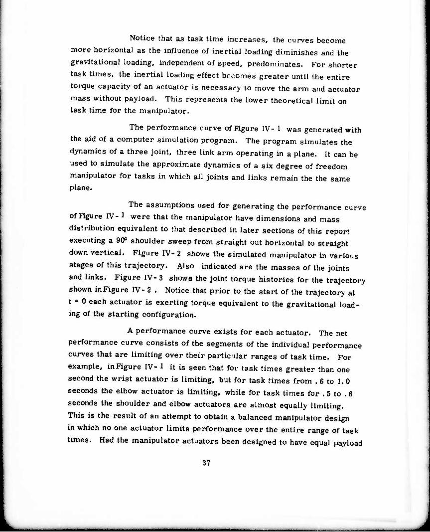
Notice that as task time increases, the curves become more horizontal as the influence of inertial loading diminishes and the

gravitational loading, independent of speed, predominates. For shorter

task times, the inertial loading effect brco-nes greater until the entire torque capacity of an actuator is necessary to move the arm and actuator

mass without payload. This represents the lower theoretical limit on task time for the manipulator.

The performance curve of Figure IV- 1 was generated with the aid of a computer simulation program. The program simulates the

dynamics of a three joint, three link arm operating in a plane. It can be

used to simulate the approximate dynamics of a six degree of freedom

manipulator for tasks in which all joints and links remain the the same plane.

The assumptions used for generating the performance curve of Figure IV- 1 were that the manipulator have dimensions and mass

distribution equivalent to that described in later sections of this report

executing a 90° shoulder sweep from straight out horizontal to straight

down vertical. Figure IV- 2 shows the simulated manipulator in various

stages of this trajectory. Also indicated are the masses of the joints

and links. Figure IV- 3 shows the joint torque histories for the trajectory

shown inFigure IV- 2 . Notice that prior to the start of the trajectory at

t ■ 0 each actuator is exerting torque equivalent to the gravitational loading of the starting configuration.

A performance curve exists for each actuator. The net performance curve consists of the segments of the individual performance curves that are limiting over their particular ranges of task time. For

example. inFigure IV- 1 it is seen that for task times greater than one second the wrist actuator is limiting, but for task times from . 6 to 1.0

seconds the elbow actuator is limiting, while for task times for . 5 to . 6

seconds the shoulder and elbow actuators are almost equally limiting.

This is the result of an attempt to obtain a balanced manipulator design

in which no one actuator limits performance over the entire range of task

times. Had the manipulator actuators been designed to have equal payload

37

1 m

1 3.43 kg

7.08 kg

3.43 kg

r—• 45m_^l ,. 45m4-. ImJ

Osec-

t=.2

t=.4

t=l. t=.8

Figure IV-2 Typical Downsweep Task Trajectory

-Masses at joints are actuators and associated hardware.

Masses between joints are links.

38

es

CO

vo

rsi

u

0) E

c u o n «

h

s a c

i M o

IM

to n 0

M

0)

er

u

g I

>

(N

o o O o o O o o o tn o in o in o in in m r-i

ID

fN i-t ^ i

3 cre er n 1 QJ 0 -u ■ H c

39

capacities at long task times - for essentially pure gravitation loading -

then the payioad capacities for short task times would have been widely

distributed with certain actuators very overdesigned and others under

designed. For this particular manipulator design the shoulder would have

been much too weak and the wrist much too strong for the shorter task

times. An informal survey of commercial manipulators indicates that many have weak wrists, for reasons to be discussed below.

Obviously two important components of the total inertial loading are the actuator masses themselves and the payioad. The more

massive the outboard actuators are, the more torque is required from the

inboard actuators to move them. However, more torque required from an actuator generally means a more massive actuator.

Figure IV-4 shows maximum torque vs. mass for families of hydraulic and electric actuators. It can be seen that torque increases

faster than mass for these families of actuators. Hence, it should always be possible to find a set of actuators with sufficient torque to move a

certain payioad over a trajectory in specified time by choosing sufficiently

large actuators, up to reasonable limits. However, the less mass

required of a given actuator, the less the torque requirements for the actuators inboard of it and so the less massive they need to be also.

Consequently, it is important to choose actuators with as high a torque

density as possible, especially for the outboard (elbow and wrist) actuators.

Figure IV- 4 shows that for a wide variety of hydraulic and electric

actuators, the hydraulic ones are about an order of magnitude better in

torque density than the electric ones. This means that arms designed for

hydraulic actuators will not only have less mass but also will require less torque to move the arm and payioad.

c. Gearing on Electric Actuators

The low torque density of electric actuators can be increased by adding appropriate gearing. However, the gearing presents several problems from the control point of view.

• Increased weight of the gears

40

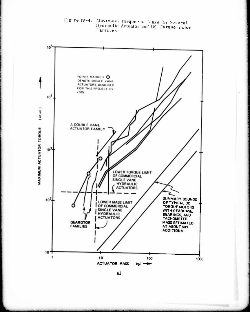
Figure IV-4 Viaxiimini torque vs. Mass for Sever«! Hydraulic Actuator and DC' Torque Motor Families

SUMMARY BOUNDS OF TYPICAL DC TORQUE MOTORS WITHGEARCASE BEARINGS, AND TACHOMETER MASS ESTIMATED AT ABOUT 50% ADDITIONAL

100 1000 ACTUATOR MASS (kg)

41

J

• Backlash between actuator and load

• Additional compliance in drive train

as the meshing teeth deflect under load

• Increased apparent inertia of the actuator

These problems degrade the ability of the actuators to

perform fine motion servoing — a serious drawback for an assembly

machine.

Designers of commercial arms often solve the problem

of heavy outboard actuators by utilizing small ones or little if any gears.

This saves load on the inboard actuators but results in a weak wrist.

d. Influences on Accuracy, Repeatability, and Resolution

A discussion of the influences of technology on accuracy,

repeatability and resolution of a manipulator requires good operational

definitions from which to work.

Accuracy is an error measure representing the ability

of the manipulator to achieve an arbitrarily selected position in space.

The operational definition is as follows:

(1) Choose an a priori endpoint position

in space in shoulder coordinates.

(2) Compute the corresponding set of

joint angles.

(3) Command the arm to achieve that set

of joint angles.

(4) Measure the error between the actual

endpoint position and the desired end-

point position in shoulder coordinates.

The resulting measured error represents the accuracy of the manipulator

system.

/

42

Repeatability is an error meacur« representing the

consistency of operation of the manpulator system. Its operational definition is as follows:

(1) Command the manipulator to execute a

particular trajectory, ending with a certain

set of joint angles.

(2) Measure the ondpoint position in shoulder

coordinates.

(3) Command the manipulator to move away

and then repeat the same trajectory as above.

(4) Again measure the endpoint position in

shoulder coordinates.

(5) Compute the error between the first

measurement and the second.

This error represents the repeatability of the system. It

is the error to be expected between identical system commands.

Resolution is a measure representing the

smallest consistent incremental position change the system can make. An operational definition is as follows:

(1) Command the manipulator to execute a

particular trajectory ending with a certain

set of joint angles.

(2) Measure the endpoint position in shoulder

coordinates.

(3) Choose an incremental direction from the

endpoint position in shoulder coordinates

and command a small increment in position in that direction.

43

^——-—^^—■■Maaaaa

(4) Measure the new endpoint position in

shoulder coordinates.

(5) Compute the difference between the

first measurement and the second.

This operation is repeated several times to determine the

smallest consistent incremental position change of the actual manipulator

for an incremental command. The smallest actual incremental change

is the resolution of the system.

Resolution is limited by things such as nonlinear frictional

force characteristics. Typically, before a machine with moving parts

can begin to move from a standstill, a certain breakaway force or torque

must be exerted to overcome the static friction between the parts. After

the parts begin to move, they must still face a constant running friction

which is usually less than the static friction.

Due to the servo compliance between the desired

manipulator position and the actual manipulator position an error between

the actual and desired positions causes the servo to exert a restoring

force. Hence, there is a certain incremental command error required to

generate the breakaway force necessary to overcome the static friction.

Now assume that a certain command error existed that provided enough

actuator force to just overcome the static friction. Then how far the system

travels will depend upon how different the running friction is from the

breakaway friction. If the running friction is much less than the break-

away friction, then the system may move a comparatively large increment

before the running friction brings it to a stop. However, if the running

friction is only a little less than the breakaway friction, than the resulting

actual position increment may be rather small.

Consequently, it can be seen that the resulting increments

in actual manipulator position, which correspond to the resolution of the

manipulator, depend on nonlinear frictional characteristics and servo

compliance at least. Also, it is clear that the commanded increment

in position does not necessarily equal the resulting actual motion. In

44

fact, it usually will not. Based on this analysis, the resolution of a

manipulator may be improved by increasing servo stiffness (decreasing

servo compliance), by reducing friction in general, and by making

breakaway friction as close to running friction as possible.

In general, backlash will not affect the resolution as we

have defined it. However, it will affect the command errors that must be

given to generate the small actual increments. In particular, if a change

of direction is involved in executing a particular increment of position,

the length of the backlash will have to be added to the required command increment.

If the manipulator control system is based on commands

issued from a digital computer, then the quantization of commands may

itself determine the resolution of the manipulator. This is entirely

dependent on the design of the control system. It follows that a design

criterion for the control system would be not to limit the resolution of the device unnecessarily.

The physical processes that lead to repeatability errors

are hard to find, but can be assumed to lie in variations of the physical

processes themselves and surrounding conditions. Our operational

definition of repeatability requires that the test point be approached along

the same trajectory. This was done to insure equal processes; for

example, that all backlash elements were in the same state from test to

test. We may find a different repeatability measure if this condition were

relaxed and we allowed the test point to be approached from arbitrary

directions. Not only backlash but also other factors, such as friction,

may vary with trajectory history, leading to a larger repeatability figure.

Accuracy errors involve a larger part of the system than

do resolution and repeatability. Accuracy measures the ability of the

system to execute a position command open loop. All of the following

will contribute to errors in accuracy:

(1) Structural deflections

(2) Servo compliance

45

motions of the real manipulator hardware must have good fidelity to the

ideal motions prescribed by the computer.

There are two broad influences on the design of a servo

system. One is the nature of the input commands to the servo system.

If the manipulator is expected to accomplish gross motions in .5 sec, then

the frequency response, or bandwidth, of the entire controlled system,

including payload, certainly ought to be well above 2 Hz in order to

reproduce the desired motions. Computer simulations have been used to

determine that, for 0. 5 sec task completion times, 5 Hz control bandwidth

produces adequate performance, but that 10 Hz control bandwidth produces

very good performance for a variety of simulated gross motion tasks of

the arm shown in Figure 1V-2.

The second broad influence on the design of a servo system

is the frequency response of the components of the system. Each component

of a system has its own dynamic characteristics, some of which may limit

the performance of the overall closed loop system. For example, the servo

valve controlling the hydraulic actuator cannot open and close instantaneously

on command. Typically, it has a frequency response bandwidth of about

100 Hz. The resolvers used to detect angular position and rate (discussed

in section VII) are read by a phase locked loop which will probably have a

bandwidth of between 60 and 100 Hz. (Conventional angle readouts have

little or no bandwidth limitations but do not generate rate information. )

There is a possibility that components such as these with similar band-

width can interact to produce system instabilities and resonances. The

control system must be designed to prevent this.

Another component whose frequency response is important

to the control system design is the physical manipulator structure. Work

by Book (reference 5 ) and Maizza (reference 6 ) has shown that the

resonance characteristics of the arm structure are intimately related to

the servo bandwidth. This relationship is discussed further in section

IV-C.

47

B. Kinematic Configuration

1. Approach

The approach to determining an optimum arm design with

respect to its geometrical abilities and properties is basically threefold: number, type, and dimension. The number of freedoms required and

their disposition will first be analyzed. Then the types of joints needed

to realize these freedoms, e.g. revolute. spherical, cylindric. etc.

Finally, dimensional data will be obtained through a generalized synthesis procedure.

The und --rlying guide for this entire process is with respect to the tasks at hand; thus, the configuration issues treated here bear

primarily on the size and dexterity of the moving elements involved in assembly tasks. These elements include:

1. part(s)

2. end effector(s)

3. means of causing relative motion between the above

The size of the parts and subassemblies is determined by comparing a range of tasks in which a need to automate is clearly

demonstrated, but where manual assembly is currently employed. Also. it is our aim to select a range that does not materially imply an advance

in the state-of-the-art in mechanical design, e.g., a microscopic or gargantuan assembly environment.

Since modern fixed automation techniques have shown competence

in handling subassemblies of up to about 10 cm diameter (spherical), the

range chosen for our tasks was between half and one order of magnitude greater, viz. 30 cm to 1 m. Once the requirements for dexterity are

defined and met, the overall size and geometry of the mobility subsystem can be matched to the task.

43

2. Disposition of Freedoms

The range of assembly tasks to be attacked has been concep-

tually limited by size, weight, etc. but not with respect to dexterity. In

general, at least 6 degrees of freedom (dof) are required to orient and

place a body in space. These freedoms may be divided between two

mobility subsystems for binary assembly tasks (those that involve the

interfacing of no more than two elements): one system per element. (Figure IV-5)

More freedoms cou)d aid mobility by:

a. increasing range of motion

b. avoiding singularities of motion

that occur in practical mechanical

design

c. allowing redundant positions of the

members for the same end-point

position

There is a case where fewer freedoms would be helpful: when

fewer than six dof are required, extra freedoms could add position errors

and compliance. For example, an assembly task requiring only the

insertion of parts from one direction into an accurately positioned sub-

assembly might require less than completely general motion.

Indeed, a prime consideration of this effori is to include

mobility to accomplish parts-fetching and jig-holding. For the outset,

however, an arm that embodies both gross and fine motion capabilities

is desirable. Experiments and evaluation of both modes of operation can

proceed while peripheral devices are designed and constructed for the

more specific chores.

Moving base design, i.e., a mobile fixture for holding

subassemblies, is currently being investigated. A 3 dof platform design

(Figure IV- 6 ) featuring x, y, and 6 motions of a limited range is being

optimized, and a 6 dof platform of limited range has been suggested for

49

"n" do.i. '6-n" dot.

Minimum Freedoms for Binary Assembly

Figure I\ -5

50

J

use in high speed "accommodation" U ;ks. (Figure IV-7)

Another system consideration is 'he ability to interface with

existing assembly lines. This may severely limit the dividing up of

the mobility subsystem freedoms. Therefore the system under considera-

tion embodies all six dof in one "arm." Additional freedoms can of

course be added later. Recall also that for our purposes as a laboratory

tool, this system should feature as much flexibility of operation as possible.

To take full advantage of the work volume afforded by the chosen

arm configuration, the work should be (conceptually at least) at the center

of the ranges of the primary position axes. Since a consideration of the

system was "current assembly line techniques. " the range of position of

the work is quite limited. For an object resting on a table (a most

common occurance) the optimal placement of a single arm would be directly above it as shown in Figure 1V-8.

An obvious additional freedom now presents itself: vertical

traverse, to vary the position of the work volume vertically above the

work. This freedom is present in the laboratory system as a series of fixed mounting points along a vertical column.

Since this system will be computer controlled some attention

must be paid to the mathematical tractibihty of the configuration. The

following rules might be observed in picking an arm geometry. These

considerations may of course be in conflict with other design goals and

should be considered to be of secondary importance.

a. Offsets between joints should be

avoided.

b. Successive axes should intersect in

angles a multiple of 7r/2.

c. Adjacent rotary joint axes should

be parallel, i.e., planar geometries

are preferred.

51

E o

■n

K u (1) CO

i

ti u

I K! I

• m h i—i

& rt E >

o

8

52

Figure IV-8

Arm Mounting and Work Volume

53

J

1 d. Sliding joints are preferred over

rotary.

e. Number of joints should be minimized.

3. Types of Joints

An arm may be divided into two parts of 3 dof each: positioning and orienting. These are not necessarily independent in that one

could cause perturbations in the other. Clearly, the latter requires

rotational motion, whereas the former can be implemented with a combination of either rotational or telescoping (linear) motions.

Four different configurations for the positioning degrees of freedom can be realized: all three linear degrees of freedom, two

linear degrees of freedom and one rotary degree of freedom, two rotary

degrees of freedom and one linear degree of freedom,or all three rotary

degrees of freedom. These are shown schematically in Figures IV-9 and

IV-10. The different configurations have different advantages and

disadvantages. The all linear degree of freedom configuration is best for

computational purposes as the wrist point can be specified directly in

cartesian coordinates. It is probably the best design for stiffness but is

the worst design for volume accessed compared to the volume required

for the structure. It would also be difficult to use two such arms to work

on one assembly. At the other end of the scale, the all rotational degree of freedom arm has the best ratio of volume accessed to volume of

structure, particularly if the arm is hung from an overhead structure. This configuration has an additional advantage in that there are two

solutions for having the wrist point at a particular point in space. It is,

however, the worst design for stiffness and for computation.

As the manipulator was to be used to penorm assembly

experiments and it was desirable that it be able to inte-face with

existing assembly lines, the all rotational degree of freedom configuration

54

mmm

was chosen. This decision was largely based on the accessibility that

this configuration affords with a minimum of structure.

The orienting set of freedoms presents another pair of

candidate designs (Figure IV-11). The only functional difference between

them is the orientation of the motion singularity: the point at which

"you can't get there from here. " To illustrate, when type R-P-R is in the

"straight out" orientation, the roll axes coincide thereby reducing the

number of freedoms by 1: you can roll and pitch, but can't yaw.

Similarly, when either joint P or Y in the R-P-Y type is "bent 90°" the

roll motion (with respect to the end effector) is impossible, and is

extremely difficult within 15° or so of the 90° position.

The RPY design was adopted since the loss of freedom when

"bent 90 " was deemed less a problem than when "straight out. " Until

a truly spherical joint is devised or a 4th freedom added, we'll just have to live with the singularity.

55

3 PRISMATIC JOINTS

2 PRISMATIC. 1 ROTARY JOINT.

Figure IV-9

Manipulator Arm Configurations 56

C12>

1 PRISMATIC. 2 ROTARY JOINTS

C[2>

3 ROTARY JOINTS

Figure IV-10

Manipulator Arm Configurations

57

ROLL - PITCH - ROLL

ROLL - PITCH - YAW

Figure IV-11

Candidate Wrist Configurations

58

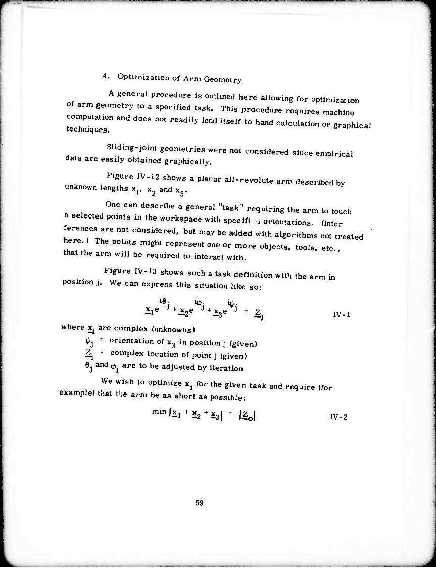
4. Optimization of Arm Geometry

A general procedure is ouUined here allowing for optimization

of arm geometry to a specified task. This procedure requires machine

computation and does not readily lend itself to hand calculation or graphica! techniques. e TI-HIUM

Sliding-joint geometries were not considered since empirical data are easily obtained graphically.

Figure 1V-12 shows a planar all-revolute arm described by unknown lengths Xj, x2 and x3.

One can describe a general "task- requiring the arm to touch

n selected points in the workspace with specifi J orientations. (Inter

ferences are not considered, but may be added with algorithms not treated

here. ) The points might represent one or more objects, tools, etc that the arm will be required to interact with.

Figure 1V-13 shows such a task definition with the arm in position j. We can express this situation like so:

iS- Up U

*le +Ji2e J +Ü3e J = Zj IV-1

where ^ are complex (unknowns)

(tj ' orientation of x3 in position j (given)

Zj - complex location of point j (given)

•j and 0. are to be adjusted by iteration

We wish to optimize xi for the given task and require (for example) that tbt arm be as short as possible:

min|x1+x2+x3| ' fej IV-2

J

Figure iV-12

Arm Model

\.. 1 *» 1

Figure IV-13

Arm with Several Task Vectors

60

MM^_^^_ ■ ■ - ■ *

The n ♦ 1 relations may be written out like so:

ie.

or, equivalently:

ie. >©t 1*1

»e. ^n

Fii i .

53

Z

Z

IV-3

L Mx ■ Z. 1V-4

A root-mean-square solution of (4) for x can be obtained by

IV-S

introducing the complex conjugate of M, viz M1:

x • (M1 M)"1 M1 Z.

For non-tr-vial solutions, (M1 M) will be invertable.

Convergence error can be given by

Minimization of (zj can be assumed by including it in the error parameter-

KWE + xtx IV-7

where K weights convergence error to the same order of magnitude as |Z0|: typically 102 or 103.

The optimization procedure is now reduced to the adjustment of

the 2n quantities Ij and «,.. This will be accomplished, with a pattern-

search algorithm, with f as the objective parameter.

Good initial estimates may be obtained graphically. A

computer program to implement the above procedure has been written

and used. Input values depicted a single planar view of the Briggs and

Stratton 3 Hp. gasoline engine.

Nine test positions (Z and $ ) were given. The arm was

considered directly above the work at a distance y. This distance entered

the solution process as a "patch" by adding y (real) to the imaginary

parts oi Z^. An initially large estimate for y was needed to avoid solutions

that imply the interference of a vector (arm member) thiough the implied

task bom !ary. The results are as follows:

Constraints: "elbow" angle (^ - Q.)< +2.355 rad (135°) J J

Variables: 9- . o- . y J J

Run 1 results:

x3 forced to zero, results inconclusive

Run 2:

x3 constrained ■ 8 in. (20. 3 cm)

Results:

17.9 in (45.4 cm)

x2 ■ 17.9 in

y ■ 33.8 in (mounting distance) (85.8 cm)

Curiously enough, an "arm" with rather anthropomorphic

proportions is implied by the procedure: equal lengths of "forearm" and

"upperarm". The 8" value for x3 was picked in consideration of the

mechanical outlines of possible end effectors and other tools.

Other tasks of a more complex nature might not indicate such

proportions, and one might well conjecture whether this result is due to

a product designed with human assembly in mind.

The greater-than-human-size indicated by the procedure is

probably due to the immobility of the "shoulder": with only 6 dof allowed.

62

the mobility subsystem can have "hands, " but no "feet. "

The final dimensions of the arm reflect the values obtained above and are shown in Figure V-l.

63

j

C. Relation Between Servo Bandwidth and Structural Vibration

Because all structures are flexible and because pressure to

reduce structural weight increases the structure's flexibility, one must

be cautious about exciting structural vibrations through the action of

the control servo. If the arm is moved slowly enough then such vibrations

will not be bothersome. This may, however, require intolerably slow

motions.

Flexibility may occur in structural members and in drive trains

(shafts, gears, bearings, etc. ). Gear teeth and long shafts are especially

severe sources of flexibility. The stiffness of a long shaft or beam

decreases with the cube of its length, so the flexibility problem is much

worse for long arms than for short ones. Servo-induced vibrations can

arise either during fine motions or during the startup or slowdown phase

of controlled gross motions in places where trajectory accuracy is important.

Work on this problem has been conducted on the assumption that

each arm joint has its own servo control which acts independently on sensor

data derived from that joint alone. Two simplified models have been

used, a one-joint arm and a two-joint arm. In the former, the joint is in

the middle of the arm, forming a controlled elbow, while the shoulder is

locked. In the latter model, the shoulder is also controlled. Reference (5)

contains detailed studies. In each model, the joint servo gains are chosen

to achieve a natural frequency (undamped) of w . Damping is provided by

velocity feedback and provides damping ratio C relative to w . Both s

w and ^ are calculated on the assumption that the structural members are s rigid. These members are assumed to be uniform tubes of radius r with

wall thickness of r/5. With the joints locked solid the structure will exhibit

a lowest frequency w of structural vibration. A study was conducted to

determine the relationship between w and w with these results: s c

Work supported in part by NASA MSFC Contract NAS8-28055.

64

• if ws < wc/3' the structure appears to be essentially rigid

• ifwc/3< ws< wc/2. some structural

vibration occurs but is well damped

• if ws > wc/2, insufficient damping is

available and structural oscillations will

be troublesome or even destructive.

Most arms seem to be designed conservatively, with w well

below wc/3. This causes the arm to be heavier than it needs to^e for

the bandwidth it can achieve. The extra weight penalizes gross motion

times (for fixed strength actuators) approximately in proportion to w .

Joint angle resolvers must be located inboard of any joint-related

compliances, or else servo instabilits will occur (ref. 7 ). This fact is

still being discovered empirically by »me arm designers.

Additional studies have been performed with more complex servo

control schemes. A rigid arm servo design technique is explained in

reference ( 1 ). consisting of providing sensor data from all joints to the

control decision at each joint. The same ws can now be obtained with

lower servo gains, especially at the shoulder, than in the former servo

method. The main result with respect to structural vibration is that

ws « wc or more can be achieved with good performance. No commercial

manipulator operates with this more complex servo. It would seem

however, that much lighter or faster arms (for the same actuators)'would thereby be possible. (See Ref. 6)

In addition to stiffness considerations, one must also pay

attention to strength. We find that for many arms, stiffness requirements

exceed strength requirements and the latter are automatically satisified

if the former are. This is not always the case, as reference ( 5) shows

For the record, however, it should be clear that plastic deformation in

an industrial arm is tantamount to a failure and must be avoided.

One may utilize the torque-speed studies in Section IV. A. 2 to

obtain operating torque levels. In Section VII. B it is shown that an arm

of adequate stiffness will have an area moment of 5 in4 at the shoulder

where a torque of 500 ft-lb may be encountered during gross motions, if

65

r ■ 3 in, then the stress at the outside edge of the structure is only

3600 lb/in . less than 3% of the yield stress for ordinary steel. The

bulk of the analysis in Section VII. H therefore deals with stiffness, not strength.

D. Servo Control Methods and Force Feedback

In the previous part of this section, it was noted that servo controls

can be synthesized to utilize information from all joints in determining

control at each joint. Besides the benefit of better vibration control, other

advantages are possible. These are discussed here.

In reference 1 it is shown that the dynamic equations of motion of a rigid arm can be put in the form

t) () I

() O

1 o -i

where_e_ is a vector of controllable arm degrees of freedom (joints), e_

is a vector of joint velocities, £ the corresponding accelerations, I is

the inertia matrix and^ is a vector of control torques applied at the joints.

This model is linearized but experience with simulations indicates that

the nonlinear Coriolis terms usually account for less than 10% of the

torque in such maneuvers as those in section IV . A. 2. Reference 1 also shows that a control of the form

KT(e-6c) ♦ KTD(e-e( )

can be used to cause the arm to follow a commanded trajectory described

by ec and ec. Interesting choices for matrices KT and KTD will not only

place the poles of the overall system at desired places but will cause the

system to have characteristic oscillation modes in convenient coordinates

and with good damping. One can, for example, make the arm behave as

a set of completely independent damped second order systems whose

independent axes are those of the hand coordinates of the arm. This is

♦ Ü is an identity matrix.

66

.mporum b. .he design of accommodatio„ st.a.egies „here one needs .o have an arm which will respond dynamicaiiy only in the desired direction

as tndtcated by force feedback, with no bothersome dynamic crosstalk "

mto uncommanded directions. Reference 1 gives a general procedure for accomphshmg this which wtll produce the correct K and K for any configuration of a given arm. TD

A basic accommodation loop functions by converting force sensor readings into se™> commands which modify 9C and 9c. Generalized force/ orque vector P is measured by a sensor on the arm or work surface. 1,

the sensor is on the arm at the wrist. F is in hand coordinates

Accommodation works by generating velocity modification commands -DM1" hanc' ( 10rdinates:

-DM ' KF—

where KF is called the accommodaUon matrix. If this matrix is chosen

to be dtagonal then simple "get out of the way" strategies will be executed

because a force in aoy hand coordinate w.l, request a velocity modification m tha same direction, and „ill result in a reduction in the felt force

Tins modification is in the class of fine motions discussed in Section 111

and may be superimposed on the gross motion commands, which are also in hand coordinates. The net command is then converted into joint

ZT, .hic "■>by means °! Resolved Motion Rate CoM™1 f~«»~— 81. Note that the resulting motions will cause force.P to change. Thus a

new servo loop has been added. If F arises from elastic interactions between the arm and its environment, then a small motion of the hand x will cause a force F according to

£ " Kjj,

where x is measured in hand coordinates and KE is the stiffness of everything between the force senso: and the "solid" ground relative to which

Sta measured. The resulting equations are third otxier in matrix form. If KF is chosen to be other than diagonal or if zero entries are placed

strategtcally on the diagonal, then other interesting tasks can be performed

67

involving other strategies besides "get out of the way. " See reference 1.

In reference 9 a detailed study of the behavior of accommodation

loops is made for the ctse of a three joint arm about the size and strength

of that described in later sections of this report. It is shown that matrices KT' KTD' KF and KE must a11 be designed simultaneously, although some latitude is possible. KE can be "designed" to the extent that it represents

sensor stiffness (all force sensors seem to be instrumented compliances)

although othf r compliances, such as the environment contacting the hand

or the arm's cwn structure, are involved. High K is good for sensor

design since the sensor then introduces little structural distortion,but high

KE makes the design of the rest of the servo more difficult. It can be

shown that the product KFKE must be smaller than some limit or else

oscillations will occur when contact is made.

Reference 9 investigates two manipulation tasks by means of

servo design techniques and computer simulation: collision with a boundary

and putting a peg in a hole. Experience gained with the first task indicates

that good stable response can be obtained. The simulated arm, which is

quite strong and large, can be brought to a stop in about 0. 3 seconds upon

impact, utilizing only the control servo. This indicates that control

techniques which need no computer are possible. In the second task, pegs

are put in holes with clearance to diameter ratio of 0. 001. A fundamental

analysis of this task is also made, predicting regions of success or failure

in this family of tasks, depending or friction, angular approach error and

clearance to diameter ratio. Tasks near the limit of these success regions

have been successfully simulated. Figure IV-14 shows a sample plot from

such a simulation, where the peg approaches the hole at 10 cm/sec, with

2° misalignment. The coefficient of friction is 3. This is a difficult

insertion task. The plot shows the rate of turn of the peg as it aligns

itself with the hole. The "desired turn rate" is requested by the accommo-

dation loop. The "actual turn rate" is the peg's response to this request

work supported by NSF Grant No. GI 39432X and GI 43787.

68

and to the forces «Brted directly on the peg by the hole. As accommodation

builds up. these foires die out and the peg goes smoothly into the hole.

A one degree of freedom simulation of the collision task has been

set up to investigate the effects of backlash. Backlash can result from

gear, chain and spline drives, and can occur in power drive trains or in

sensory readout devices. Backlash is not a problem in put-take industrial

robots or in devices like auto transmissions, derricks and so on. It

causes difficulty in servos or other controlled devices which must reverse

direction as they seek a commanded position under tight servo control.

The issues studied here are backlash location and angle readout

location. One quickly discovers than an angle readout with internal

backlash causes servo oscillations or instabilities. The same occurs if

a readout is located on a load which is connected to its drive motor through

drive train backlash. If the readout is on the motor, however, then the

accommodation loop still functions, although not as effectively. This is

illustrated in the next three figures, which show desired and actual

velocities of a simple one degree of freedom arm colliding with a barrier.

In Figure IV-15 there is no backlash. Curve 1 is the position of the arm's

endpoint. curve 2 is its velocity, curve 5 is the desired position and

curve 6 is the desired velocity, the latter two being modified sharply by

accommodation after the collision occurs at around time = 0.18 sec.

Stable behavior occurs and all velocities recede to zero as the arm comes

to rest against the barrier. Figure IV-16 shows the effect of adding 0. 005

radians of backlash between the motor and the load. The load's speed

jumps up suddenly at time - 0. 1 seconds when the backlash closes and

the motor first begins driving the load. The backlash remains closed

during contact and stable behavior results. Figure IV-17 shows the result

when the backlash of 0. 005 radians is shifted from the load to the angle

readout. The high velocity of the load near time - 0. 1 is caused by the

servo's belief that the load is not moving, since the backlash on the angle

readout does not close until around time - 0. 07. The ultimate result is

instability. This indicates that if. in the previous test, there were

70

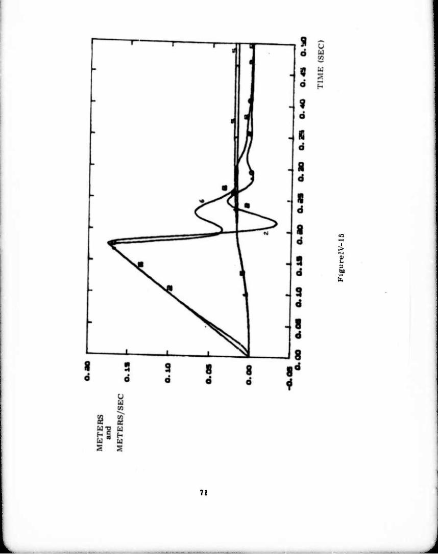
in

t 9 be

■ -^

71

/.

I

BQ /:

M 1 :.-

72

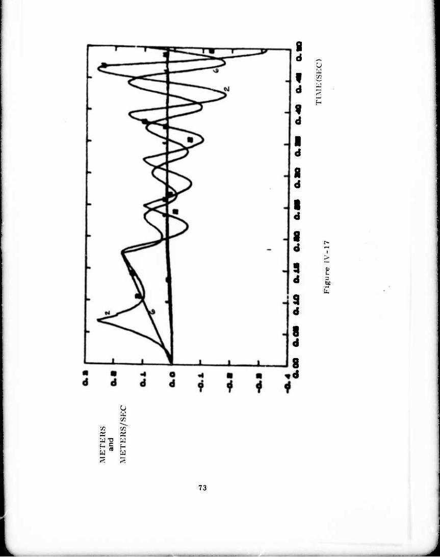
2 72 03 OS BE

H H

Cfl

u

f—I

I

a

L 73

J

additional backlash in the force sensor, the result would be instability.

Thus high quality force sensing can make up for sloppy drive trains to

some extent, although income cases it appears that one must pay a penalty

in decreased aim speed and ^ncreused contact forces between tve arm and its environment.

E. Error Analysis

An error analysis is not an exercise in pessimism but is the key to understanding whether a proposed design will in fact perform as intende-i.

It also points out reasons for weak performance and indicates how and

where to make improvements. It shows how accurate sensors need to be, for example, or how stiff compliant elements must be made, in order

that desired performance goals be met. Error analyses usually do not concern themselves with malfunctions.

Error analyses can be carried out in three areas of assembly arm studies:

• the arm itself

• the objects it interacts with

• the strategies it utilizes for carrying out tasks

A general procedure for determining errors in manipulator arms is discussed in reference 2 . The error sources analyzed are

angle sensors, bearing location and eccentricity, structural compliance

and thermal expansion. An appropriate arm design should balance these

contributions to error so that no one source dominates while effort is

expended to reduce the others. Some types of error are predictable arid

can be compensated while others are random. This analysis method was used in the design of the arm described in Section VII to specify angle

readout accuracy and to determine that certain bearings and shafts were too compliant.

74

Normally one is not interested in the accuracy of an arm itself

but rather the combined accuracy of the arm and the items it interacts

with. Errors can appear in the objects grasped by the arm. in the exact

position of the object in the gripper. and in the position of the assembly

into which the grasped object is to be placed. One quickly concludes, for

example, that it is fruitless to build ultra-accurate arms to move floppy

rubber hoses around (unless special precautions are tsken). A conclusion

of ongoing assembly task analysis is that automated assembly will involve

many gripping tools whose major function is to accurately locate a grasped object with respect to the gripper.

Error analysis of strategies is really an investigation in depth of

the strategies themselves. If execution of a strategy requires that a force

of no more than 10 newtons be exerted, then success depends on how

accurately om can measure the force and how quickly one can cease to

increa£5 applied force once the 10 newton level has beer reached. Other

strategics may call for the determination of the direction in which force

is acting, There will be an error in this determination. If success of

the strategy depends critically on the accuracy of this direction measure-

ment, the strategy may be failure-prone. Thus we see that hardware and

strategies interact; a good strategy on paper may be beyond an arm's

capability; shortcoming, in an arm may force one to employ additional

compensating strategies at a cost in task completion time.

In this vein, we have identified a number of arm design

inadequacies which detract from performance in various ways:

• structural compliance (task completion

time is lengthened while one waits for

vibrations to die out. or the arm must

be moved slowly)

• backlash (to ensure repeatibility. the

arm must be moved slowly near the

end of a gross motion; reversing direction

during fine motions leads to errors;

75

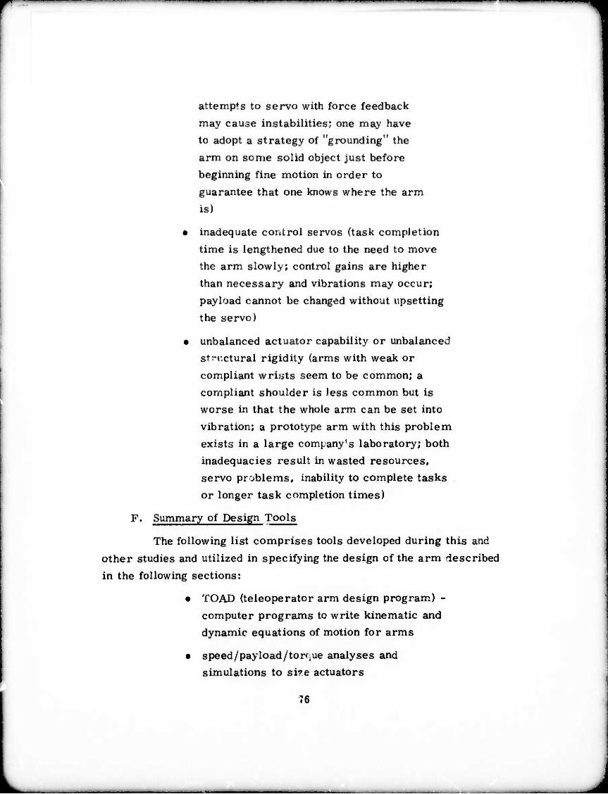
attempts to servo with force feedback

may cause instabilities; one may have to adopt a strategy of "grounding" the

arm on some solid object just before beginning fine motion in order to

guarantee that one knows where the arm

is)

• inadequate control servos (task completion

time is lengthened due to the need to move the arm slowly; control gains are higher

than necessary and vibrations may occur;

payload cannot be changed without upsetting

the servo)

• unbalanced actuator capability or unbalanced

structural rigidity (arms with weak or compliant wrists seem to be common; a

compliant shoulder is less common but is worse in that the whole arm can be set into

vibration; a prototype arm with this problem

exists in a large company's laboratory; both

inadequacies result in wasted resources,

servo problems, inability to complete tasks

or longer task completion times)

F. Summary of Design Tools

The following list comprises tools developed during this and

other studies and utilized in specifying tne design of the arm described

in the following sections:

• TOAD (teleoperator arm design program) -

computer programs to write kinematic and dynamic equations of motion for arms

• speed/pay load/torque analyses and

simulations to sire actuators

76

• actuator technology studies

• servo analysis and simulation of

accommodation strategies and other

fine motion methods, including effects

of compliance and backlash

• structural analysis and its relation to servo control of arms

• servo control techniques for determining dynamic performance

• error analysis to criticize arm designs

and strategies for assembly

77

J

V. DISCUSSION OF DRAPER LAB ARM DESIGN (POPEYE)

A. DiscriptiOB of Arin

The Draper Lab arm was designed as a research tool for

automatic assembly. The basic requirements were that the device be

capable of assembling items as large as a cube one meter on a side,

be capable of picking up parts as heavy as 20 kilograms, be capable of

slewing 1 1/2 radians in all axes in 0.5 sec unloaded, have an overall

absolute accuracy of less than 1 mm (0.04 in) and be capable of quickly

interchanging tools or end effectors used for different assembly tasks.

Designing to these difficult specifications brings out many problems and

solutions applicable to mini-robot arms.

While there are a number of different kinematic configurations

that could successfully be used, an overhead hung six degree of freedom

elbow type of arm design was selected as it was quite compact for the work

volume it could access and was judged to be more easily adaptable to

existing assembly lines. A rigid gallows structure that bolts to a work

table was designed to suspend the arm (see figure V-l). The horizontal

beam of this structure can be set at different heights for different tasks.

Eventually this movement was to be powered although not to be used as a

high speed degree of freedom. The arm proper had shoulder azimuth and

elevation degrees of freedom, an elbow ele^ ation degree of freedom, and

wrist roll, pitch, and yaw degrees of freedom. The links beiween the

shoulder and elbow and between the elbow and wrist were idealized as being an

equal 0.45 m (~ 17.75 in) in length. However, it was not possible to

design a universal joint for the wrist that would allow sufficient movement

for both pitch and yaw. Therefore the pitch and yaw axes are separated

by 82.5 mm (~ 3.25 in) and the 0.45 m length between the elbow and wrist

extends to a point equidistant between the pitch and yaw axis. The idealized

load point was considered to be 0.20 m (~ 8 in) from this point. Thus, the

overall straightout length of the arm is 1. 10 m (~ 43. 3 in).

78

Shoulder Azimuth Actuator-

Shoulder Klevation Actuator

Klbow Actuator

Wrist pitch

Actuator

6 DOF Wrist Force Sensor

Workpiece

Variable Height Support Structure

\ X-

Shoulder Azimuth Hearings

I pper arm Structure

Wrist Roll Actuator

Wrist Roll Bearing?

Wrist Y .w Actuator

Quick Disconnect

End Effector

meters

H f- H—4 —\- —I 1 1 0.5 1.0

Figure V-l

Side View of Draper Arm, Work Surface, and Support Structure

79

All of the degrees of freedom are driven by direct coupled single

vane hydraulic actuators with a working pressure of 14 x 106 Pascals

(~2000 PSD. At this pressure the shoulder actuators will develop

690 Nt-m (~ 510 ft lb) of torque; the elbow actuator, 350 Nt-m (~260 ft lb)

of torque and the wrist actuators. 82 Nt-m C-60 ft-lb) of torque. Except

for the shoulder azimuth and the wrist roll, the bearings for the actuators

also act as the bearings for the structure. Due to the large moment loads

possible on the shoulder azimuth and the wrist roll degrees of freedom,

additional larger diameter bearings were incorporated. Where possible

the actuator housings form part oi the arm structure. The wrist roll

actuator is bolted directly to the elbow actuator. The wrist pitch and yaw

actuators were designed with a single Siamese housing. To avoid backlash,

connections between the actuator shafts and structural yokes were made

using friction clamps as opposed to keyways or splines. In all degrees

of freedom, the position feedback sensor, which is a dual speed pancake resolver

(IX and 64X). is designed into the actuator housing and uses the actuator

bearings.

80

B. Critique of POPKYIJas a Research Tool

The POPEYE design reflects the need for a research arm that

attempts to meet the research goals as reviewed in Section 1 of this report.

The design reflects the dual attributes of a good pick-and-place arm and an assembler. These attributes are:

For Pick-and-Place

• Speed

• Accurac'

• High Load Capacity

• Large Work Volume

For Assembly

Accuracy (good positional accuracy)

Accurate Control of Small Motions (good rate control and high damping)

• Accurate Control of Forces at the Hand (accurate, wide dynamic range, low drift wrist force sensor)

• Versatile Set of Articulations (at least six degrees of freedom with the ability to reach around objects)

1. Advantages of POPEYE Design

Of course the arm could not be designed to optimize all

attributes. However, the design does have inovations that should result

in an arm that will have excellent kinematic and dynamic behavior. The

more important of these design inovations are:

a. Overall kinematics: six degrees-of-freedom,

shoulder connected to a stiff overhead beam

(see figure V-l). an elbow which allows

articulation around five sides of t isk. The

large work volume afforded by this design

should also help with the parts feeding

problem. i

Because of its husky lower arm. this design has come to be called POPEYE. 81

b. Loads connected directly to the actuators

thus eliminating backlash due to gearing.

c. Position feedback sensors — 1 and 64 speed

pancake resolvers wound on the same pole

pieces — designed into the motor housing and

on the load shaft. This eliminates shaft

windup and backlash between the actuator

output and the feedback element — often a

source jf servo instability.

d. The use of the two speed resolvers has many

advantages. Among these are:

(1) 16 bits position accuracy

(2) 18 bits servo quantization

(3) A rate signal derived from the Phase Lock Loop method of reading out and digitizing the resolver signals

(4) The 64 speed winding glv«0 the equivalent of a 64 speed gearup of a tachometer without introducing the extra apparent inertia of real gears, backlash or shaft windup. This in turn results in a sensitive rate signal (approximately 1 volt/rad/sec)

e. The hydraulic vane actuators were designed

without internal (vane) seals. This has the

advantage of eliminating much of the cause of

stiction and also aided in servo damping.

f. The design of a six-degree-of-freedom, wide

dynamic range force sensor array. Ti;is will

be incorporated in the wrist force sensor and

used, in conjunction with the control computer,

to resolve the forces at the hand into the six

components — three rectilinear, and three

torque.

82

2. Disadvantages of POPE YE Design

The principle disadvantage of the POPEYE design is the

cost of producing it. The hydraulic motors, motor and bearing houses

arm linkages, force sensor arruy and housing all had to be designed

The machining of all these parts wil! be relatively expensive compared

to present systems; however, the inherent reliability of its very clean

design offers compensating advantages as a research tool.

83

J

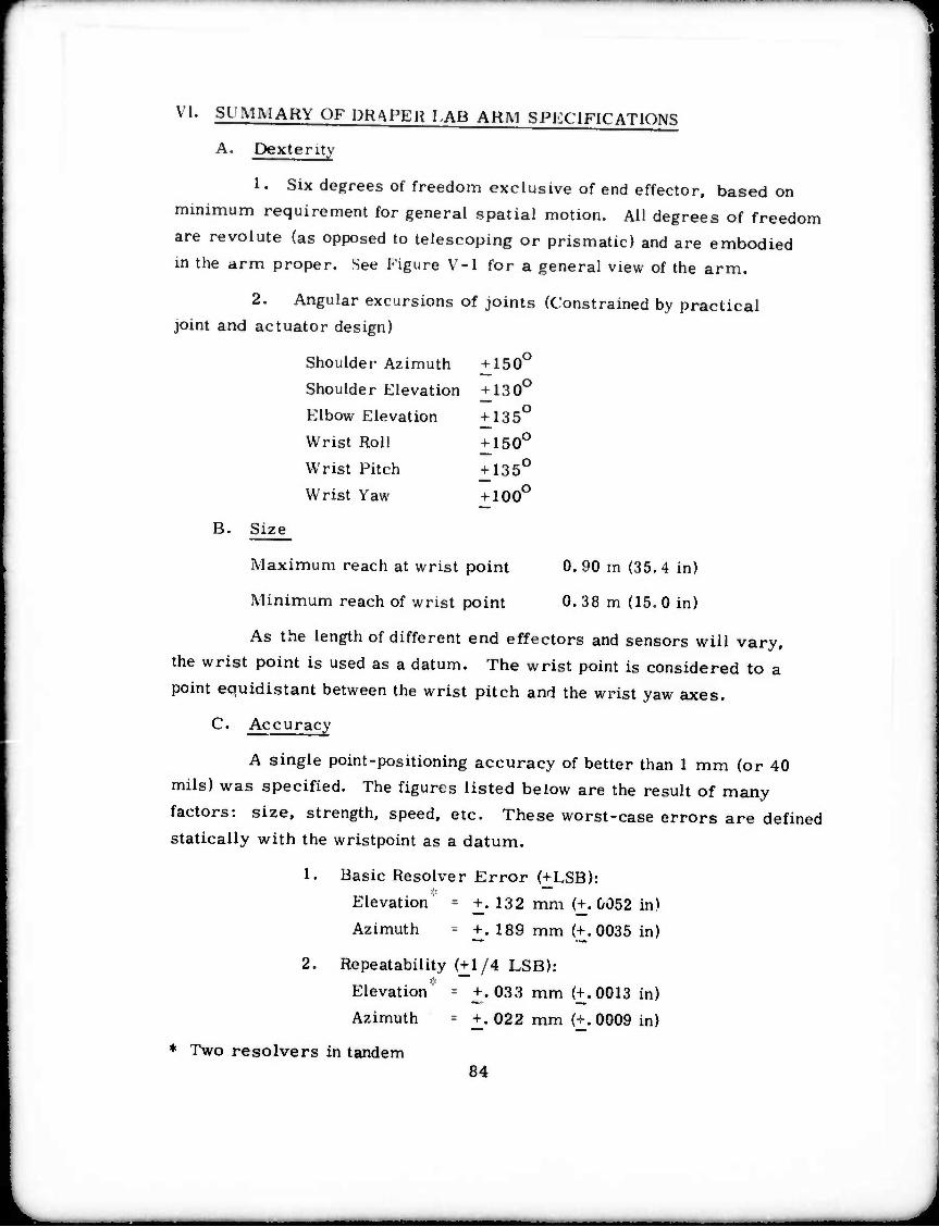
VI. SUMMARY OF PRAPEB LAB ARM SPl-X IFICATIONS

A. Dexterity

1. Six degrees of freedom exclusive of end effector, based on

minimum requirement for general spatial motion. All degrees of freedom

are revolute (as opposed to telescoping or prismatic) and are embodied

in the arm proper. See Figure V-l for a general view of the arm.

2. Angular excursions of joints (Constrained by practical joint and actuator design)

Shoulder Azimuth + 150u

Shoulder Elevation + 130°

Elbow Elevation ^135°

Wrist Roll + 150°

Wrist Pitch + 135°

Wrist Yaw ^100°

Size B.

Maximum reach at wrist point 0.90 m (35.4 in)

iMinimum reach of wrist point 0. 38 m (15. 0 in)

As tiie length of different end effectors and sensors will vary,

the wrist point is used as a datum. The wrist point is considered to a

point equidistant between the wrist pitch and the wrist yaw axes.

C. Accuracy

A single point-positioning accuracy of better than 1 mm (or 40

mils) was specified. The figures listed below are the result of many

factors: size, strength, speed, etc. These worst-case errors are defined

statically with the wristpoint as a datum.

1. Basic Resolver Error (+LSB):

Elevation' = +.132 mm (+. &052 in)

Azimuth - +. 189 mm (+.0035 in)

2. Repeatability (+1/4 LSB):

Elevation = +.033 mm (+.0013 in)

Azimuth = +. 022 mm (+. 0009 in)

♦ Two resolvers in tandem 84

3. Structural Error (RMS) - +.26 mm K0104 in)

4. Vertical Droop (unloaded) - .16 mm (.0062 in)

Accuracy for "fine" motions has not been defined.

D. Performance

Fine-motion operating bandwidth: 10Hz

Gross-motion "task" time: 0.5 sec.

Stiffness (referred to wristpoint):

Arm extended - 1050 Nt/mm (6000 lb/in)

Elbow f 90° - 1230 Nt/mm (7000 lb/in)

Lowest structural natural frequency ■ 30 Hz

Inertia t shoulder with 10 Kg load m 22-1/2 Kg-M2 (200 in-#-sec2)

The gross motion task referred to above is to move any or all

axes of the unloaded arm in a 90° slew motion stop to stop.

E. Subsystem Specifications

1. Actuators

TyPe: Hydraulic, single vane, airect acting

Seals: no internal, shaft seals on'y

System Press: 17.5 MPa (~ 2500 PSD

Displacement:

Shoulder 51. 1 x 10'6m3/rad (3.12 in3/rad)

Elbow 25. 6 x 10"6m3/rad (1. 56 in3/rad)

Wrist 6.22 x 10-6m3/rad (0.38 in3/rad)

Rated Actuator Torques @ 14. 0 MPa (~ 2000 PSD

Shoulder Azimuth and Elevation 690 nt i (510 ft #) Elbow 350 nt M (258 ft #)

All Wrist 82 nt M (61 ft #)

Speed (at rated torque): 6 rad/sec

Valve pressure drop at speed: < 3.5 MPa (500 PSD

85

Angular Position i'ranscucers

Tvpe:

Size:

Excitation;

Transformation Ratio:

Accuracy:

Speed:

Tachometer Output:

Mounting:

Wrist Force Sensor

Type:

Two speed, IX and 64X;

«.rewound pancake resolvers

76. 3 mm 0 in) O. D.

44.5 mm (1. 74 in) I. D.

15V. 1000 Hz

1/2 watt 'unit

IX 64 X

IX

64 X

1 to 1

4 to 1

1.5 deg (8 bits)

20 sec (16 bits)

adjustable - a tracking Phase-locked loop is used

Supplied by PLL, analog

Integral with actuators

laser interferometer

Degrees of freedom: 6

Full Scale Force: 500 nt (110 lbs)

Overload Force: 5000 nt des' ■ ^ goal (1100 lbs)

Displacement: 0. 04 mm (0. 0016 in) full scale

Resolution: 14 bits or 1:8000

86

Vll. SI BSYSTKMS

A. Actuator Selection and Design

1« Power Source Selection

The major decision in the selection of the actuators for the

manipulator arm was whether to use D. C. torque motors or to use

either hydraulic motors or hydraulic actuators. Uoth have their

advantages. The main advantage of the electric motors is that they

are considerably easier to control than the combination of hydraulic

servo valves and hydraulic actuators. In general, it is easier to design

for wiring for an electric motor than for hydraulic lines. The

hydraulic systems have a potentially serious leakage problem.

Noise may be somewhat more of a problem with a hydraulic system.

The main disadvantage of a D. C. torque motor is that its torque

to weight ratio is much lower than that of a hydraulic motor or actuator.

In order to increase the torque to weight ratio of the electric rmtor.it

would probably be necessary to use mechanical gearing of some type.

In general, the ase of gearing will cause backlash which will in turn

cause control problems.

It should be realized that the choice of actuator types is not

independent of the assembly machine or assembly arm configuration.

If the assembly machine employs linear degrees of motion, preloaded

zero backlash ball screws can be used to amplify the force available from

an electric motor. Also, if the degrees of freedom can be arranged so

that the motor masses do not create large inertias and/or large

gravitational forces that must be overcome by other motors,the torque

to weight ratio is less important.

For reasom that are detailed in section B on Kinematic Configura-

tion, an elbow type of arm design was chosen with all six degrees of freedom

invested in the arm proper. To achieve the necessary drive stiffness and

to ovoid backlash, remote drive mechanisms were ruled out. Therefore, it is necessary that the shoulder actuators have sufficient torque to overcome

the intrtia and gravitational loads caused by the elbow and the wrist

actuators in addition to those caused by the end effector and load. The

87

elbow actuator must have sufficient torque to overcome the inertia and

gravitational loads caused by the wrist in addition to those of the ena

effector and load. This causes a pyramiding effect on the required

actuator torque which virtually rules out any consideration of using direct

drive IXC. torque motors. Thus, if electric motors were to be used they

would need to be geared, probably in the range of 10:1 to 20: 1. While it

might be possible to develop a zero backlash gearing system using

preloaded gear pairs or perhaps using all rolling element cycloidal gear

reducers or a counter driving double motor arrangement on each

axis, it was decided that the more straight-forward approach would be

to use either a hydraulic motor or a hydraulic actuator.

2. Hydraulic Motor/Actuator Design

Preliminary design work was done for both a continuous

rotation hydraulic motor and for a single vane hydraulic rotary actuator

capable of up to 300° o^ rotation. The hydraulic motor design was for an

orbital gerotor type of motor. This motor essentially consists of a rotor

with externally cut cycloidal gear teeth that rotates inside a stator with

internally cut cycloidal gear teeth. See Figure V1I-1. 2. As the stator

has one more tooth than the rotor, the rotor will make n, orbits per

rotation where n^ is the number of (eeth or lobes on the rotor. If the

rotor rotation is used as the shaft output, a planetary gear effect with a

ratio of n^l will be achieved without resorting to external gearing. This

effective gearing has the same effect as external ge-ring in raising the

apparent torque and stiffness of the hydraulic motor.

While orbital gerotor motors are commercially available

from several sources, they do not appear to be suitable for use as servo

motors. In the commercial motors, the rotor rotation is picked up with a

shaft that has loose fitting balled-over splines at both ends. This shaft

is free to wobble which allows the rotor to orbit while preserving the

rotation. Unfortunately, this shaft with its loose fitting splines becomes

a source of backlash and wear. In our design, the splined shaft was

replaced with a pair of freely rotating cranks. The free rotation of the cranks allows the rotor to orbit while the cranks will rotate as a pair

88

o o ^

o

u c

9 M u

aj u u o 00 P

Ü

9 O

89

ii / /

GERCTOR DETAIL

i ■

.090

ECCENTRIC CRANK DETAIL

Figure VII-2

Gerotor Hydraulic Motor Details

90

——^-^a,.

to preserve the rotation of the rotor. This feature not only eliminates the

backlash but also makes the motor mechanically stiffer and more compact.

The initial design was for a motor that would produce

approxin^itly 625 Nt-m of torque at a working pressure of 17.5 x 106

Pascals (460 ft-lbf at 2500 PSI). This estimated torque is found quite

easily by multiplying the fluid displacement per radian rotation of the

output shaft by the working pressure. The working pressure is the pump

pressure minus an estimated pressure drop due to losses in the fluid lines and the servo valve. This pressure drop is proportional in a non-linear manner

to the flow rate and the servo valve opening. The other parameter of

interest is the actuator stiffness which.along with the arm inertia.is needed

to predict the open loop resonant frequency. The compliance of the

actuator is largely due to the bulk modulus of the hydraulic fluid. Other

factors that may contribute are hydraulic line compliances and output

shaft torconal compliance, etc. As the servo valves are mounted directly

on the actuators and the shaft stiffness is treated in the section on

structural stiffness, only the compliance due to the bulk modulus is

treated here. For a piston type hydraulic actuator it can be shown that the stiffness is

K - 2/3A2

Vi

where ß is the hydraulic fluid bulk modulus in Pascals (or PSD. A is

piston area in square meters (or sq. in. ) and V. is the fluid volume

between one side of the piston and the servo whe'n the piston is centered in

cubic meters (or cu. in. ). Fo- a rotary actuator or a motor.this becomes

K - 20D 2

r

where Dr is the displacement per radian in cubic meters (or cu. in. ).

• See Fluid Power Control by Blackburn. Reethof. and Shearer, IU.1.T. Press, 1960, pages 510-516.

91

For a non-orbital motor V| becomes vD assuming that the non-displaced

volume is neglible (this may or may not be a good assumption depending

on the motor design). For an orbital type motor

V. ■ TTD i r

which again makes the assumption that the non-displaced volume is

neglible, a fairly good assumption for the motor that was designed. Thus,

the stiffness is given by

K 2ßn D r r

For motors of equal displacement per radian and thus equal output torque

at a given pressure,the stiffness of the orbital motor will be greater than

that of a non-orbital hydraulic motor by a factor of n . For a single vane

actuator

and

'i ■ RD r 2

K ■ 4/3D r

where R is the maximum rotation of the actuator in radians. o

Using 1.5 x 10 Pascals (~ 220. 000 PS1) as the bulk modulus

(the actual bulk modulus for phosphate ester is 2. 67 x 10 Pascals or

387, 000 PSD and with nr equal to 12 and D equal to 35. 7 x 10'6 cubic

meters per radian (~ 2. 2 cu in/rad), the open loop stiffness for the designed

orbital motor is

K = 4. 1 x 105Nt-m/rad(~ 3 x 105 ft-lb/rad)

While the orbital hydraulic motor inherently has a much

higher torque density (torque to weight ratio) and a much higher stiffness

than a non-orbital motor or a rotary actuator, it was decided that there

would be less risk in placing the primary emphasis on the design of single

vane rotary actuators for the arm. The main design problem with the

orbital motor was in determining the tolerances and clearances to allow it

92

-- - ■■ ■

to run smoothly but not leak excessively. Although the orbital motor would have

superior performance it would probably require more of a development

effort. A further problem was that there was only one source for the

precision gerotor elements and they would not promise quick delivery on

anything not normally stocked even though the tooling existed.

The design of the single vane hydraulic actuator is similar

in principle to that of the commercially available vane actuators. However,

as commercial actuators designed for high pressure hydraulics were not

available in a range of sizes suitable for use as wrist actuators, it was

necessary to design our own vane actuators. Also by designing special

actuators, several very important advantages could be realized. The most

important functional difference is that our design has no seals except for

low pressure seals on the output shafts^and relies on close tolerances

between the vane and the housing to maintain low leakage rates. Eliminating

the seals eliminates the principal source of friction in the actuator and will

allow smoother control. The other important functional difference is that

the position transducet - a pancake resolver with a single speed and 64

speed winding - is built into the actuator. By designing our own actuators

it was also possible to use the actuator cases as part of the arm structure

and to use the actuator bearings as the arm bearings in four of the axes

(in all cases the actuator bearings also serve as the resolvers'bearings).

By accurately sizing the actuators to meet the desired performance

specifications it was possible to minimize their weight and overall size.

It was also possible to design the servo valve manifold, the cross-over

pressure relief valves, the pressure transducer ports and the low pressure

drain relief valve and manifolding into the case. See Figure Vll-3a and b.

3. Vane Actuator Design Specifications

The specific sizes of the actuators for the differer.. axes

were found by computer simulation. See Section IV-B. A somewhat

arbitrary performance specification on slew time was used as basis for

this simulation as it was believed that the ability to slew rapidly in order

to change end effectors or tools and to fetch parts was an important

function. The initial specification was that

93

Servo Valve Manifolding

Drain Relief Valve

Pressure Relief Valve

Dual Speed Resolver

Angle Contact Bearings

Figure VII-3a Elbow Actuator Layout (sideview)

94

Interface for Wrist Roll Actuatoi

Limits of Vane Travel

and Shaft

Pressure Relief Valve

Pressure Transducer Mounts

Servo Valve Manifolding

Figure VII-3b Elbow Actuator Layout (endview)

95

M^^^^^M^M^MM

all axes be capable of slewing 1 1/2 radians (~ 90 degrees) in one second

with a 10 kilogram load. As the arm would probably slew much more

frequently with either no load (to change the end effector or to fetch a new

part) or with a light load, the performance specification was changed so

all axes would be capable of slewing 1 1/2 radians in 1/2 second with no

load. This is a somewhat more stringent requirement for the elbow and

shoulder actuators. See Figure IV-1. A model ^or the mass and inertia was

developed, working from the wrist requirements back by estimating the mass

for the end effector and wrist structure. This yielded a torque requirement for

the wrist actuators. From this, the actuator could be sized and the mass

estimated. This, along with the required structure and the previous

estimated masses for the end effector and wrist structure, determines the

torque requirement for the elbow actuator. Then, knowing the size of

the elbow actuator, the torque requirements for the shoulder actuator can

be determined. See figure V1I-4 for the discrete mass model used for

the simulation. The simulation yielded torque requirements of 82 Nt-m

(~ 60 ft- ib) for the wrist actuators, 350 Nt-m(~ 260 ft-lb) for the elbow

actuator and 690 Nt-m(~510 ft-lb) for the shoulder actuator. For a single

vane actuator the torque is given by

T ■ 4LV) where P is the working pressure (pump pressure minus an allowance for

losses), l is the length of the vane, r, is the outer radius of the vane and

r_ is the inner radius of the vane. The working pressure was set to 6 R

14 x 10 Pascals '~ 2000 PSI) with a pump pressure of 17.5 x 10 Pascals

(~ 2500 PSD. The actual dimensions of the shoulder and elbow actuators

were set by using the largest possible bearing size (largest bore)

consistent with mounting the pancake resolver as both the output shaft

torsional stiffness and the bearing radial stiffness were critical. A single

pair of 35 mm extra light angle contact bearings (ABEC 7) were used in

the elbow actuator and two duplex pairs were used in the shoulder actuators.

The inner radius of the vane, rg. was set at ~2. 22 cm (~0. 875 in), the outer

radius, r«, was set at ~ 4. 60 cm(~ 1. 812 in) and the length of the vane for the

shoulder actuator was set at ~ 6.34 cm(~2. 50 in) while the lengthof the vane for the

96

^__^—^__

elbow actuator was set at ~ S. 17 cm( ~ I. 25 in). The wrist actuators

were designed around a single pair of 25 mm bore extra light angle

contact bearings. The inner vane radius, r . was set to ~ 1. 90 cm

(~ 0.75 in), the outer vane radius. rv was set to ~ J. 17 cm (-1.25 in),

and the vane length was set to ~ 1. 90 cm (~ 0. 75 in). In order to mi umize

leakage.the clearances between the vane and the housing were designed to

be between 0. 008 mm (0. 0003 in) and 0. 018 mm (0. 0007 in). The hydraulic

leakage around the vane and through other clearances is given by

where b is the clearance, w is the total width of the leakage path and

L is the length of the leakage path along the flow direction, ß is the

absolute viscosity, and (Pj-iy is the pressure difference across ihe

vane. The important parameter is b, as the leakage flow is proportional

to the third power of the clearance . i. e.. doubling the allowed clearance

will increase the leakage eight-fold.

The required servo valve size is determined by the flow

rate at the maximum rotation velocitv plus the leakage flow. This total

flow rate should not cause a pressure drop across the servo valve greater

than the pump pressure minus the working pressure or in *his case

~ 3.5 x 10 Pascals (~ 500 FSI). If the actuator traverses 1.5 radians

in 0.5 seconds.the maximum velocity, assuming a triangular velocity

profile, is 6 radians sec. For the shoulder actuators.the required flow

rate is ~0. 3 x 10 m ,'sec with an allowed pressure drop of 3.5 x 106

Pascals across the servo valve (~ 18 CIS S 500 PS1 pressure drop). A

conservative servo valve choice, allowing for a leakage flow with clearances

of 0. 025 mm (~ 0. 001 in) and a hydraulic fluid temperature of 520C

(125 F). is the stock Moog series 34 aerospace servo valve. A Moog

series 32 servo valve was specified for the elbow actuator and Moog

series 31 servo valves were specified for the wrist actiators. The

aerosoace valves were selected for their small size and mass at a given

flow performance. There is a price penalty but it is not that significant

for small quantities (the quantity discount is much higher for the so-called

commercial valves). 98

B. Structure

1. Mechanical I'ropertivs

a. Kequireir.ents and Materials

The design of the loa<l-carr\ iriß members both movable

and stationary is constrained h\ a t9m ImportaM fand interrelated)

requirements necessarv to achieve the stated svstem goals. Among these are:

(1) minimum weight

(2) maximum stiffness

(3) sufficient strength and fatigue life

(4) lowest resonance tj be above 25 to :<0ll/

The minimum weight propertv reduces power requirements

insofar as the arm is a significant fraction of the total mass. Lower

mass means that servo gains can be relaxed somewhat and still obta n

reasonable positional accuracv. I.o-Aer gain requirements in turn enhance gain and phase margins.

We desire maximum stiffness so we can know where the

hand is under varying load conditions. It is desirable to know this without

reiving on external devices (wrist-trackers) and compensating routines

in the software. A stiff arm allows accurate position data with only the

use of good encoders or resolvers at the joints.

Sufficient strength is available from a wide variety of

materials. Considering the loads we have in mind and the endpoint

tolerances, stress is less a problem than strain.

The 25 Hz requirement stems from the relation between

servo bandwidth and structural vibration. This is discussed at length in Section IVC.

Table I lists a few candidate materials. To choose on

the basis of weight and stiffness, the stiffness/weight ratio is included.

On this basis alono, the best material is Beryllium. Without digressing

into all the specific problems inherent in the use of Bervllium, one should

realize that toxicity, stress-corrosion, cost and reluctance to fabrication

are all severe compared to the other candidate materials.

99

J

ml 8

B o o c o ^5 CM

m X O

I- CM

T T ■ m 3C X

^^ M -1 Oi M CM u;

7 'S

7

o o o

■ i-'

■ o r- M

u d d d

X CM

X CM

xo s s X

x

31 X

T O x tc M —

B i

o o

C- o in T o

x o o o

ir> o

X

o

2 la

—•

S o cc

I? t0

£ pi o r«

3

c I x

m 6 P 2

o c to tis

MS

ft Q. K W «

a x

Ü ^<

100

L

An important question is whether there is an upper bound to the stiffness requirement independent of materials selection. Other

components will incur a certain amount of positional error by themselves, among them: bearing and encoder eccentricity, bearing play and elasticity under load.

We do not need to worry too much about the stiffness of the actuators themselves as long as there is feedback of some kind to compensate for it. and the stored energy component is small.

The thermal properties of the arm should be considered in any serious design effort since changes in temperature can add yet

another degree of uncertainty to the structure. Significant heat sources

can be realized in electric and hydraulic actuators under high cyclic loading conditions.

Low coefficient of thermal expansion should be a desirable property. For our 90 cm arm made out of. say. aluminum alloy, a

50 C range cf uniform arm temperature results in a 3/4 mm length change. More significantly, non-uniform heating of the members can cause greater distortions over smaller temperature changes.

The material finally selected is steel for all load-carrying members, owing to its cost, ease of fabrication, and stiffness. The thin wall sections possible with steel allow potentially greater design

freedomfor internal components: valves and plumbing. For non-load- bearing parts, aluminum or brass (for fittings) will be used.

101

b. Structure Design

To meet the 'AO Hz resonance requirement, assumptions

were made concerning mass distribution and end-point loading. Figure

VII-4 illustrates these assumptions. The inertia seen from the shoulder

(with the 91 nt [20 f] load) is approximately 21.4 Kg-m2 (184 in | sec2).

An equivalent inertia can be modeled as a point im ss of 25. 5 Kg (56. 1 f)

at the wrist-point, 91 cm (36 in) from the shoulder. This point mass

approximation is actually conservative since most of the distributed mass

is inboard of the wrist-point.

A 30 Hz natural frequency (f ) is predicted from a

point mass load. The required stiffness,

K - mw2 ■ 900 nt/mm (5030 #/in)

where m = endpoint mass

and cü ■ angular frequency 2 2 With no load present, the inertia drops to 11.1 Kg-m (95 in # sec ),

and f - 42 Hz. It is assumed that all vibrational energy is caused by

small linear motions of the load. This value of K can be built-in easily

by considering an equal-stifmess model of the arm in two sections:

upperarm and forearm (Figure VH-5).

Consider the relation between deflexions and area-

moments:

Total deflexion - Ij.g^,^ ♦ 62-SHEAR + ^2-SHEAR

+ ^-MOMENT + ^-MOMENT

6- = Pi3r i + i + i + i + n "* T-K+^ ^ ^ ¥j

= p^3 LL + 71 r^i/^J

102

Figure VII-5

Two Part Distributed Stiffness Model of Ami

NOTE: Deflexions shown greatly exaggerateJ

103

If we let each section of the beam be equally stiff with respect to the

wrist-point,

'2 ' 7I1

Values for Ij and !„ which satisfy the overall stiffness

requirement of 900 nt/mm (5030 */in) are

Ij - 26.6 cm4 (0.65 in4),

and 12 - 187. cm4 (4.55 in4).

If ah sections of the arm structure meet this criterion, we are assured adequate stiffness (in that bending mode at least).

An analogous criterion for torsional stiffness does not

exist, since arm payloads and performance have not been defined for

rotational (moment) loads. However, one case can be analyzed: when

the elbow is cocked 90°, the upper arm is subject to a torsional load

caused by payload and arm weight. An equivalent torsional stiffness is

now calculated, based on the required lateral stiffness.

When the elbow is bent 90° and a simple load is applied

to the wristpoint, three sources of deflextion exist: bending of the

forearm, bending of the upper arm, and torsion of the upper arm due to

the moment loads that previously applied to bending. Since the upper

arm is much stiffer than the forearm, we will ignore this source of

deflexion. The stiffness of the forearm alone is just twice the overall

bending stiffness (since the deflexions of each member in bending were

set eq aal to each other). The effective lateral stiffness at the wristpoint

due to torsional rigidity of the upperarm is just

K - Kt/X2 -- 1800 nt/mm (10.6 #/mil)

We can solve for the required polar moment of inertia of the upper arm

like so:

I = K.l - 252 cm4 (6.15 in4) P

104

'

where G - shear modulus, 70GPa (107 psi),

and i '- upperarm length - forearm length.

For reasonable cross sections, 1^1 + [ thu* P xx vv' 0

insuring us of adequate torsional stiffness i; the lateral criterion is met.

An additional bending mode requires treatment, however,

parallel bending of yoke-type elements pictured in Figure VI1-6.

These elements appear at every joint except azimuth and wrist roll (joints

1 and 4, counting from the shoulder). While these elements are stiff with

r-spect to lateral bending, they are not necessarily adequate in parallel

bending. To assure sufficient stiffness we require that the sum of the

parallel compliance and lateral compliance of the separate sections be

less than or equal to the required lateral compliance assumed adequate:

YT^ YL ' Yl

i\ U-y)3. va

1, ^ 1 y 3 i ^ 1 y

—5 2 f- 8(.v - a/y'1 4 SiayJ

where X - total beam length, forearm or upperarm y ■ yoke length

I ■ sufficient lateral area-moment

ij - required parallel area-moment of one yoke side

105

J

I measurer) from yoke centrode

LATERAL BENDING

1 T^TJ

a=0

Ij measured from each ear's

cent rode

PARALLEL BENDING

Figure VI1-6

Lateral and Parallel Mending Modes of Yokes

106

1 A similar expression can be derived for sections with more than one

yoke.

For the dimensions typical of this arm,

Ij « 1/150.

and this requirement is easily met by the designer.

In addition to the above, the torsional stiffness of the >okes

must be checked against that derived for the upper arm member.

Referring to figure VII- 7 , torsion of a yoke may be divided into axial

twist along each ear plus bending along its "stiff" axis, thus:

K s Kr

r = radial distance to ear centrode, since the ears are relatively weak

in axial twist. To obtain an adequate Kt as noted above, r2^ 51 mm (2 in).

For all proposed yokes, this condition is automatically met.

c. Support & Worktable

In the section on "Configuration" (IV B) an over-the-work type

mounting arrangement was indicated. A straightforward support for the

arm was designed as shown in Figure IV- 8 . The rigidity of the members

was determined by the > 30 Hz vibration criterion, and the assumption

that the support should be "overbuilt" in that respect.

The inertial load seen by the horizontal members is

approximately 750 in#sec ; for a 100 Hz f^ a stiffness, K , of 3 x 108 in^/rad

is indicated. Since

I = Ktt ,

4 we require an area moment of at least 80 in . This is easily obtained with

a 10 square by 1/2" wall welded steel box beam.

107

-J

i 5

ii tr ^>

ii < c

C

c 0/ B

B 0

i 0/

el X

■4-I

c b B C a

108

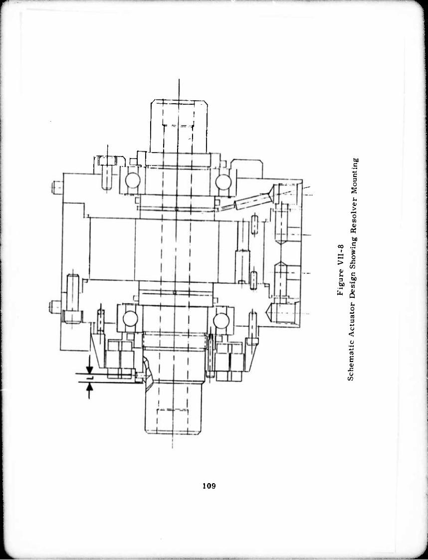
tt T-^

\

TXdL

--i

c

c o 1

8

oo |

B E > «

g" i

<

109

Similarly, the load seen by the vertical member (in

bending) is approximately 5300 vi^sec2, where at 100 Hz, K = 21 x 108

in#/rad. Thus, I must be at least 150 in . This is easily obtained with

a 12" square x 1/2" wall box beam.

Checking the torsional loading, the inertia seen by the

vertical member« 810 in#sec2. Over a length of 60". a stiffness of

about 2 x 10 in#/radian is present, thus making OJ ■ 500 rad/sec, or

about 80 Hz. It is important for the users to consider (1) additional

loads that the vertical beam will see in torsion, (2) resonant length of

the beam caused by changes in mounting distance.

The worktable upon which the support is mounted may

also be a significant source of compliance. As originally ordered, the

table consisted of a 48" x 60" x l" steel plate supported in a thin (1/4M

thick) sheet steel frame. The iuertial load seen at the base of the upright

column is approximately 3400 in#sec without the arm present.

The frame contributed little stiffnes* to the ensemble and thus

several bending (vibrationai) modes of the table top (due to the mounted support)

^6 were observed:

6

(1) Bending, lateral axis; K = 4 x 10

in#/rad, 1 ■ 4 in4, f = 10 H . AX n z

(2) Bending, longitudinal axis; K = 15 x 10

in#/rad, I = 5 in4, f = 10 Hz. jj n

(3) Torsion, longitudinal axis; K = 2. 6 x 10fi

in#/rad. fn = 4 Hz, applicable only if

table lifts off floor.

Additional stiffeners have been designed, and once installed

(under the table-top) the lateral and longitudinal frequencies will each be up to about 100 Hz.

110

HMBMMaai

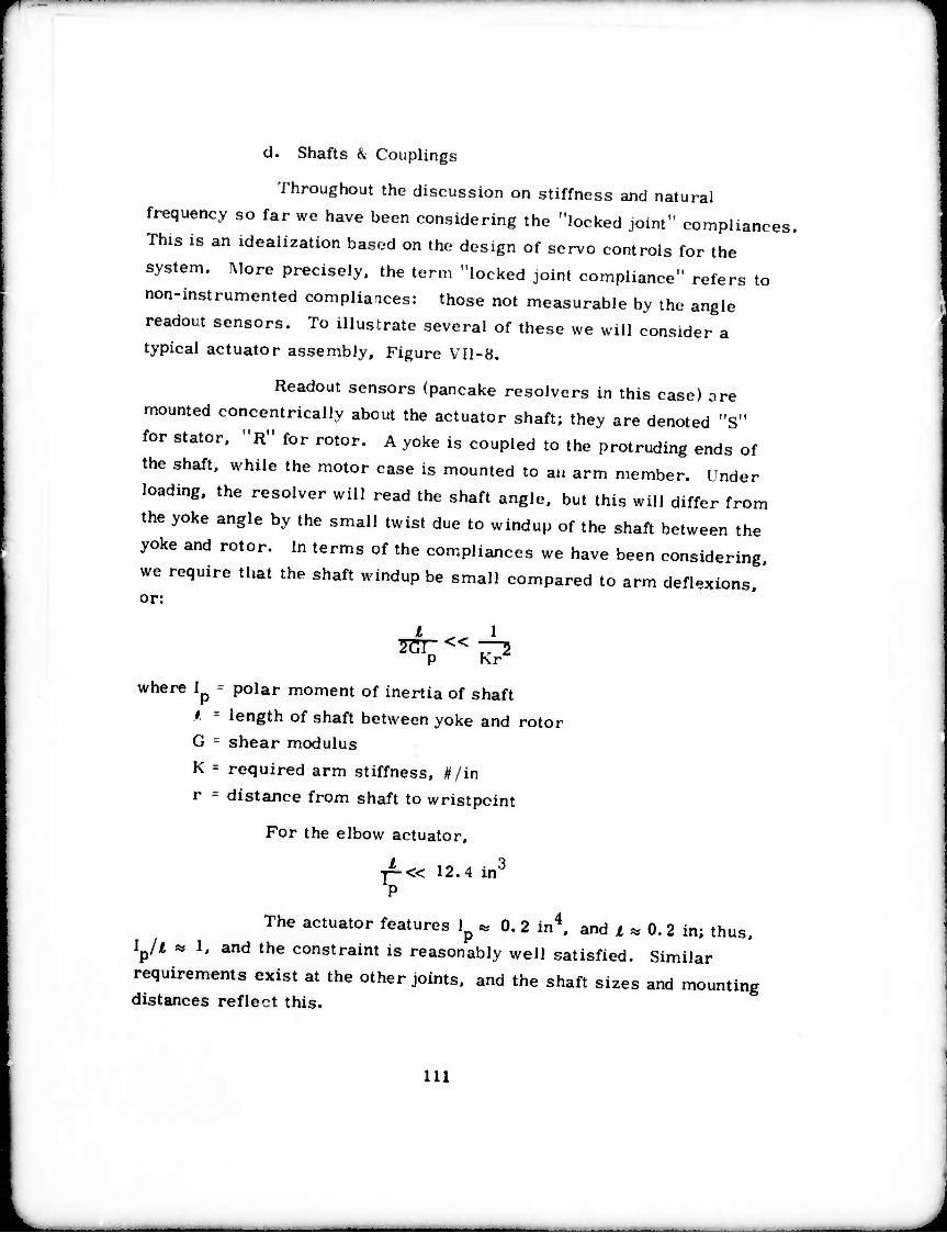
d. Shafts A Couplings

Throughout the discussion on stiffness and natural

frequency so far we have been considering the "locked joint" compliances.

This is an idealization based on the design of servo controls for the

system. More precisely, the term "locked joint compliance" refers to

non-instrumented compliances: those not measurable by the angle

readout sensors. To illustrate several of these we will consider a

typical actuator assembly. Figure V1I-8.

Readout sensors (pancake resolvers in this case) are

mounted concentrically about the actuator shaft; they are denoted "s"

for stator. "R" for rotor. A yoke is coupled to the protruding ends of

the shaft, while the motor case is mounted to an arm member. Under

loading, the resolver will read the shaft angle, but this will differ from

the yoke angle by the small twist due to windup of the shaft between the

yoke and rotor. In terms of the compliances we have been considering,

we require that the shaft windup be small compared to arm deflexions. ' or:

P Kr

where L - polar moment of inertia of shaft

» ■ length of shaft between yoke and rotor

G ■ shear modulus

K ■ required arm stiffness, f/in

r ■ distance from shaft to wristpcint

For the elbow actuator,

-r-« 12.4 in3

The actuator features lp « 0. 2 in4, and * * 0. 2 in; thus.

Ip// m 1. and the constraint is reasonably well satisfied. Similar

requirements exist at the other joints, and the shaft sizes and mounting distances reflect this.

Ill

Other compliances exist beyond the scope of measurement

by the resolvers, e.g., axial and radial bearing compliance. Choice of

bearings effects overall stiffness considerably, and the ideal 5000#/in

figure will be degraded to some extent. An analysis of this situation

revealed that the bearings chosen (practically the largest possible given

the present actuator design) contribute large concentrated compliances.

The overall effect can be (very) conservatively estimated by summing the

compliances of each bearing set and the structural compliance. The

result indicates a natural frequency of about 19 Hz, when the arm is

loaded with 9. 1 Kg (20 #). Unloaded, the estimate is 27 Hz.

A more detailed treatment of this problem appears in

Section III of Ref. ( 2 ).

Several requirements were enumerated for the shaft

couplings that tie the actuators to the arm members:

(1) must transmit required torque safelv

(2) must have short axial dimension

(3) must be rigid

(4) should be easily installed, aligned,

disassembled

Tapers, press-fit splines, expanding keys and other

possibilities were investigated. The device adopted was an expandable

locking ring assembly manufactured in a wide range of standard sizes. (Figure VII-9).

112

£ o Ol 3

0 » a at

a, <b

U 0) "I a ^. TO

re 1> ^ 03

' S s C

p a>

£ o ■D £ «1) u i- " V 01 Q. ^ in

■a * r

-O ^ ■3 ri o —

•D

r. S ? 5 * ] ai

O < X- IT

O c 2

a5 E o a

r- N a — u ■5 k.

>- c X5 B 3) C ~ | «

I

ii ■• c

0) r

8»- o 5 s - ^ — re S • h a c o O) o 3.

?~ b e- ,. o

u^

cJi;

55

Si

a

c

c g

r. ~ n U ~ r

On

- « o K 1 *

i J — C w

x: C

e a I S ü n

Q. C

V c « I f — r

— o

.

/

y. /. <■

o ^

1 ^ ta* w

p^

^ M. u "J e CX 7"

U. X s

S.

%.

113

. Sensors

1. Angle Sensors

The position of the assembler arm is determined by the measurement

of the six joint angles ind a '.nowledge of the geometry of the arm. The

measurement devices that were chosen are dual speed resolvers. The

decision to use resolvers was made after comparisons with other kir,ds of

angle sensors, including potentiometers and optical encoders.

Among the criteria considered were:

16 Accuracy - 1 part in 2 desired (20 arc seconds)

Resolution - could motions smaller than 1/2 6 be detected?

Analog or Digital Output

Absolute or Incremental Output

Physical Configuration

Mechanical Coupling - no form of gearing was considered acceptable

Cost and Delivery

Future Technological Prospects

Slew Speed

Environmental Sensitivity

Potentiometers;

Advantages

Potentiometers offer the advantages of low cost, availability,

theoretically unlimited resolution, and convenient interfacing (requiring an A/D convertor).

Disadvantages

The major disadvantages are limited life due to contact wear, and

curacy of only one part in 2 to 2 (1") to 12 1

basis of accuracy, potentiometers were eliminated.

an accuracy of only one part in 2 to 2 (1") to 12 binary bits). On the

114

Absolute Optical Encoders:

Advantages

From the viewpoint of interfacing to a computer, absolute optical encoders are the most convenient choice. The output is in binary form

and requires the simplest of interfaces. Units with an accuracy of 16 bits are available.

Disadvantages

The phvsical configuration is awkward to use, especially at the wrist joints. Typically, such encoders are cylindrical with a diameter of about 3", and a length of more than 5". Another negative factor is

susceptibility to noise, which could be a severe problem in an industrial

environment. The decisive factor, however, which eliminated absolute

optical encoders from further consideration, was their prohibitive cost.

For full 16 bit encoders, with no internal mechanical gearing, the price

quoted was $5500 per axis. Furthermore, it does not appear likely that technological improvements will lower this price significantly in the future.

Incremental Optical Encoders:

Advantages

Incremental optical encoders offer the same accuracy as absolute types at a fraction of their cost ($1600 for a 16 bit unit). The only

conversion electronics necessary are Up/Down counters to receive the digital output pulses.

Disadvantages

As with the absolute type, the encoder package is bulky. Noise

immunity is an even greater problem. Missed count pulses, or glitches

causing extra pulses cause errors that carry over to all subsequent

readings, until the system is reinitialized. Large errors can quickly

accumulate in this manner. A momentary loss of power results in total loss of angle information, which could be catastrophic in this application.

115

Resolvers;

Advantages

Resolvers, like potentiometers, have infinite resolution. Accuracy of single speed units is limited to about 13 or 14 bits, but multispeed

resolvers (a form of electrical "gearing") can easily obtain accuracies of

16 bits and better. Cost is generally less than incremental optical encoders, especially in production quantities. Shaft mounting is extremely

convenient, with resolvers that come in the "pancake" type package.

The technological prospects for resolvers are also very good. A

recent development is the printed pattern resolver. which appears to be

promising for multispeed units. Formerly, printed pattern resolvers suffered from poor transformation ratios - ratio of output signal to input voltage. Improvements in design, however, have resulted in a very

acceptable ratio of .7/1. The advantages of printed pattern resolvers are

very low cost, small size, and the possibility of making the resolver an integral part of the actuator shaft.

Disadvantages

Of all the angle sensors considered, resolvers are the most difficult to interface to a computer. Complex convertors are neeJed to

derive a digital value from the resolver outputs. The cost of commercially

available convertors can exceed the cost of the resolver. Several resolvers can be multiplexed to a single convertor, but only at the expense of the information update rate.

Ai; additional problem with mult speed revolvers is an ambiguity in tht output. A 64x resolver, for example, has an output that goes through

64 electrical cycles for each shaft revolution. A particular output can

therefore correspond to any of 64 different shaft angles. One method of resolving this ambiguity is to count the cycles as the shaft rotates. This

is essentially an incremental method, ari suffers from some of the

drawbacks of incremental measurements. More reliable is the addition

116

of a .fa«!, speed reso.ver for .he coarse measuremen., ieaving fine

measure™, .o .he mU.ispeed resoWer. The penaHy of .his me.hod is

.he ex.ra cos. for .he addi.ional resclver and convertor elec.ronics.

Af.er much considera.ion of the above factors, a decision was

reached .o use dua. speed reso.vers. each consis.ing of a singie speed and a 64x resoiver moun.ed in . single pancake shaped package. The I.

resoiver provides .he 6 mos. significan. bi.s of angie measuren.en.. whiie the 64x un« measures an addi.ional II bi.s. Of .he .o.ai 18 bi.s. U are read by the compu.er.

Each resolver has a separate resolver/digital convertor. allowing frequent position updates and the tracking of high speed slewing motions.

The convertors are not commercial units, bu. ra.her a special in house

design. Cos. is under $100 per axis. The six dual speed resolvers are «1250 each in small quan.i.iea. This would drop .o $450 each in lo.s of 100.

2. Phase-Locked Loop Resolver .o Digi.al Converter

The deCision to use d^Peed resolvers for angular measuremen, was based in par. upon the abi,i.y .o build .he resolver I digj

convertors in house. Commercially available convertors are generally

Th T rn " n0ted abOVe" eVen ra0re eXPenSi™ "- "* -°'v— At the C.S. Draper Laboratory, however, research and development in

ha e- ocked loop circuitry has resulted in the design of a PLL resolver

o dtgual convertor. This convertor circuit is simpler, and less expensive than convenuona. me.hods. and will of.en have beUer performance.

'Thebasico|wrati°"0"he convertor is shown in Figure V'i-10 The .npu.s are the resolver modula.ed signals, cos , cos (w.) and ' '

sm ecos (w.) e is .he shaf. angle, and .he cos (w.) carrier term is .he

re olver excUa.ion, a 1 kiloher.. sine wave. The purpose of .he converter i. to generate .he arc .angen. of .he ra.io of the .wo inpu.s.

6 ■ arc .angen. (sin e cos w. \ \cos Ocos w. /

117

.M^^B^^MA

I

9

b)

> c o U a o

o o I

8 OH

O u

c

118

J

The novel feature of this phase-locked loop circuit is the use or two phase detec.ocs and two reetlhacK loops. The output o

Phase de ectocs is the product or theic inputs, cos (wt, ,cos 0 sin,wt-0),

and cos (w.) (sine cos(wt.üll. These are summed to p^duce:

1/2 sin(2wtte-<») + 1/2 sin(e-o)

The filter passes only the Ü. C. term. I/J ,ta(,^,. TKs

CelTT'ln ,he ,oop•which conlro,s the vco —' -*- - frequency. The servo actton of the l«>p drives the error term to zero by

maklng0 the loop phase shift, equal to ,, the resolver shaft angle. The

P se to d.gltal conversion of „ is ,hen performed hy a standard echnique of tnserttng a counter in the feedback loop, and strobing its contents imo a regtster when the reference, cost«), has a phase of zero.

By including an integrator in the filter network, a type 11 servo „ created. This enaMes the tracking of both constant posUions and

Zl"^ With negligible l00P — A" «" b— ^ he - «ha. the loop error stgnal is proportional to de/dt. making it equivalent to

a tachometer signal. This tach signal c.n be used in anafog compen ä In ne.works for controlling the hydraulic actuators.

One feature of this circuit th.-u is characteristic of all Phase-locked ioops is that there is a filtering effect upon the signal.

the "r^ ?Sirable" SlnCe " redUCeS the leTCl 0f ™^- "• n-rower

;;.": hi greater the noise attenuauon- ™s -— ^ • "^ rade off, however, stnee a wide bandwidth is necessary for a fast response to changing inputs. Through testing, a suitabie compromise value wL

ach.eved. The converter's characteristics are similar to that of alecond

f 7 aTdpa:: rrwith a break ireqae^ * ^ ^ ^ ^S of. 7. and a 40 db/decade high frequency roll off. This size bandwidth is

w.de compared to the assembler's, ye. is sufficiently narrow to filter out most noise.

Each of the six dual speed requires two PLL convenors. The ir:; i T:4freso,ver has a ,2 bit ^ ^«- «* ^ ^HL bus. of which the least significant is an oveWap bit for the MSB of the 64X secton. Additional logic combines the two outputs into a single 18

h« word. The .6 most signmcant of these are available to the computer.

119

3. Force Sensors

a. System Considerations

One device which 1 being studied in the current research

is a six degree of freedom force sensor. This device can be used between

the arm and the hand of a manipulator/assembler, or it may be used in a

pedestal form as part of the work mounting. The following analysis covers

some of the general considerations of the use of this type of device.

General Case

Suppose that forces, pressures, and moments are

applied to a rigid body mounted on a force sensor. This corresponds to

the case of a pedestal force sensor. These forces, pressures, and

moments can be summed (or integrated) to find a resultant applied moment

Ma plus a resultant applied force Fa. There is also a gravitationally

induced force mg, acting downward and located at the center of mass:

Figure VI1-11

Work Object Mounted on a Force Sensor

Now suppose that the force sensor is instrumented in a coordinate

system, xyz, and that the sensed forces anc moments are read as fs and

Ms. Also, define the location vector of the center of mass as Reg, and

the location vector of the resultant applied torce as Rf. We then have:

VII-1

and

Fs = mg + Fa

Ms ■ mg X Reg + Fa X Rf + Ma VII-2

120

Obviously the vectors in VII-1 and VII-2 have dimensionality 3.

It is possible to evaluate the terms in mg, by letting

Fa and \Ia go to zero. This corresponds to removing ehe arm from

contact with the body. We then have:

Fs m|_ VII-3

M« m^XRcg VII-4

VU-3 and VII-4 can be combined mto VII-1 and VII-2 . moving the

known quantities to the right hand side of the equations, and the quantities

to be determined to the left. The result is:

Fa - Fs - mg

and Va+l^XiU-\]s-mgX}<cß

VII-5 and VI1-6 can be coordinatized in xyz to obtain

VH-5

VI1-6

Pax 1 ̂ sx

Fay Fsy

Faz Fsz - j nag

"Max' '-Faz R fy ♦ I •ay Rt '.Ms X

May + Faz Hfx - Fax Hfz Msy LMaz_ L-Fay H fx ► I •'ax Rf y Ms /.

VII-7

■mg Rcgy

mg Rcgx

0

VII-8

VII-7 and VII-8 show that Fa can be evaluated in all cases. However.

Ma cannot be evaluated without additional information since Kq. VII-8 is

insufficiently specified. We can substitute the three components of Fa as

found from VII-7 into Eq. VII- 8 , and are left with three equations in six

unknowns. (The unknowns are Max. May. Maz. and Rfx, Rfy. and Rfz. )

No solution can be obtained, which is tantamount to saying that the location

of the applied force and the applied moment vector are both indeterminate

unless additional information besides the output of the force sensor is

available. Some possible cases which allow a complete solution are:

121

Zero Applied Moment

The nature of the contact applied to the body ma> be

such that only a force is induced. In this case, the sensed moment arises

from the applied force. In this case, the appropriate equations are:

0 -Faz Fay" -Rfx- Msx ■ ■ mg Hcgy

Faz 0 -Fax Hfy - Msy ■ - mg Rcgx

.-Fay Fax 0. Rfz . 0

VII-9

This is to be solved for the Rf vec or, but the coefficient matrix is

singular. Howver, physical consideration shows that a line on which

the point of accion of the force lies can be determined, since the moment

and the force are both known.

Force Application Point Known

It may be that the point of force application is known,

either from the body/.^rm geometry, or from measurements of the joint

angles. If this is true, it is possible to specify something about both the

applied force and the applied moment. Under these conditions the

equations become:

"known Max

May

Maz

quantities

from VII-8 VI1-10

Response to Gravitation

It is instructive to coordinatize VII-3 and VII- 4 . The

result is

Fsx ' 0 '

Fsy = 0

_Fsz_ _-mg_

Msx" -mg Rcgy

Msy = mg Rcgx

M sz 0

VII- 11

VII- 12

122

Note that no information is given about Rcgz. This is to be expected since the sensed moment is indeper dent of the vertical location.

Conclusion

The above equations indicate the amount of information available from a force sensor. The analysis is similar, independent of whether the sensor is mounted on a pedestal or on a wrist, but the

coordinatization and the orientation of the mg term are differen. in the

two cases. It is also true that in the case of the wrist sensor, in genial

the application point is on or near the . axis of the sensor, with correspond-

ing effects on the components which appear in the equations. However in

the wrist case, the orientation of the mg vector is arbitrary, as contrlsled with the pedestal case, in which the orientation of the mg vector is known to be in the sensor z direction.

b. Arm Force Sensing by Joint Torque Measurement

Description of the Method

If the torques in the arm joints can be sensed, it is possible to calculate the hand contact forces using the analysis in the

following sections. The advantage of doing this is that the necessity for

a separate sensor no longer exists, and the cost and space requirements

are saved. The disadvantage is that the available sensitivity may be less since the desired forces have to be separated from the friction forces

which are unwanted. In order to perform this separation, the desired forces should be sufficiently large to permit eas- separation. The exact force levels which can be measured in this system will have to be

determined by experiments, but it may be possible to make a partial

analytic prediction. The joint torque system is especially adapted to

the Draper Laboratory arm. because the Draper Lab arm is designed to

use low friction hydraulic actuators, since the vane motors are designed

to be used with non-contacting vanes, permitting a .light leakage between

the vanes and the housings. Under these conditions, the torque developed is given quite closely by the pressure differential between the two sides of

the vane. It is then possible to measure the forces/torques developed on

123

the work by the following analysis.

Calculation of the Hand Forces

The problem is the determination of an arm joint

torque vector which will give rise to a specified force (and torque)

vector at the hand. A simple and direct derivation follows: Let dx

be a small motion of the hand, expressed in hand coordinates, de the

corresponding joint motions, and_J the Jacobian matrix of the arm. If

the arm structure is sufficiently stiff, then

dx ■ _Jde V1I-13

If this displacement is the result of a force vector

applied to the hand, the energy developed must go into the joint drivers,

thus:

r J de T1 de VI1-14

Since the angular displacement vector de is independent, it follows that

T* VII-15 ^J

w hich can be transposed to

.^f VI1-16

the desired result.

Note that the present derivation implies linearity. This

means that it can only be applied if the arm stiffness is sufficiently great

that J is essentially constant under the application of the force and torque

vectors _f and T.

Now suppose that the arm joints are instrumented to

read their torques as vector T. In the case of hydraulic actuators, the

torque can be measured as a pressure difference, while in the case of

electric motors, the torque may be measured as a current. Then, con-

sidering equation VII-15 we can postmultiply byjJ to obtain the applied

force

ft = Tt j-1 VII-17

See Ref. 8. 124

J is available since it is computed to obtain desired effects in hand coordinates. Since T is hypothesized to be instrumented the S1mple multiplication in VII-17 ls aI1 that is required to ^^ ^

desrred force vector. Also note that if T is contaminated bv an error Lt the corresponding error in the computed force is given oy

F1 - F1 r"1

-f it— VI1-18

In the presence of gravity, the above equations apply to deviations from the nominal forces and torques due to gravity.

Engineering Considerations

If pressure sensors are applied to the two sides of a vane-type or other hydraulic actuator, it is possible to define the torque

Tn " Kn(P2n " Pln> VII-IS

Errors in the torques are primarily caused by errors m the pressure sensors, and also by friction in the joint. The joint

friction can be resolved into components proporHond to the various force

components applied to the joints, plus any stick effects which may coexist.

A friction coefficient matrix for any actual proposed joint can be measured or calculated from specs. Once this matrix is known It is simple to predict the expected error in the force.

It appears obvious that a re?.onably good force measurement is available without any instrumentation. In any event it is easy to

test this proposal since only the relevant software need be generated, and

the force calculation may be tested by applying known forces to the hand

and comparing the calculated forces as derived from the pressure sensors.

This may be expressed conveniently as the relevant error ellipsoid,

c. Pedestal Force Sensors*

* Summary of work sponsored by NSF grant no. ATA74-18173 A01.

125

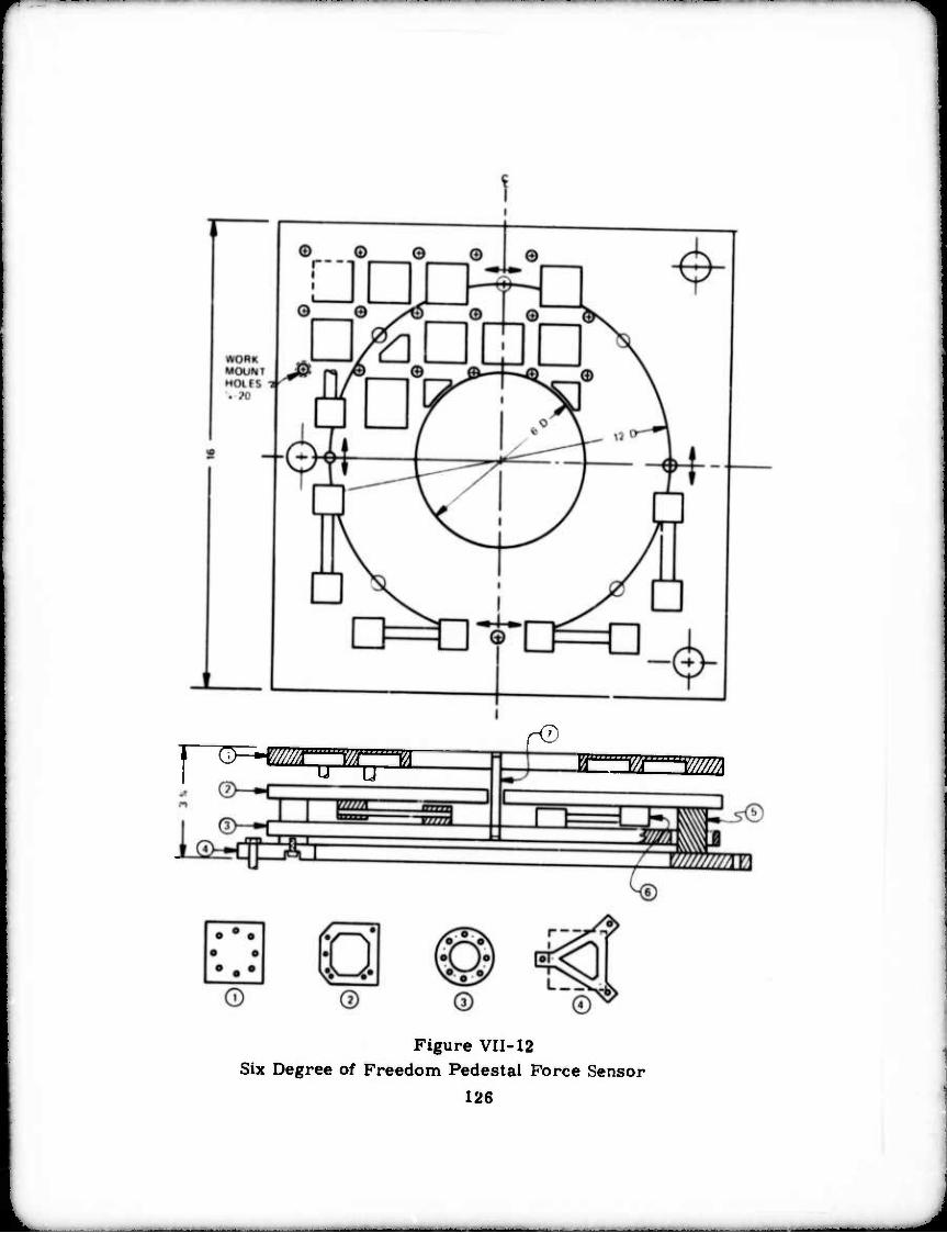
I ^^mw^w^i a vr^i/jm

Figure VII-12 Six Degree of Freedom Pedestal Force Sensor

126

A Strain Gauge Pedestal Force Sensor

A strain gaus« type pedestal force sensor has been designed and is currently under construction. The general layout of this

design is shown in Figure VII-12. This is a three layer design adapted

from the wrist force sensor concept previously described. The sensing

elements ar? to consist of load beams, assuming satisfactory performance of the sample load beam which is currently being awaited.

A BLH product exists which has capacities directly applicable to some of our sensor problems. This is called a load beam,

and is a beam and strain gauge assembly. The attached data sheet shows

some of its features. Sheets arc also attached describing platform

transducers, which illustrate technology directly applicable to some of the force components to be sensed. (Tables VIM, 2)

A Laser Pedestal Force Sensor

The sensor structure of c is to be designed to accept laser instrumentation as soon as this becomes available. In order to

expedite the actual construction, it is proposed to order two sets of

structural components, one of which will be instrumented with strain gauges, and the other with the laser system.

d. Wrist Force Sensors

Draper Arm Wrist Force Sensors

A preliminary structural concept of this sensor has been devised and is shown in Figure VII-13. This design can also be

instrumented with either laser displacement detectors or strain gauges.

e. Laser Force Sensor Specifications

The current specifications are shown in Table VII-3 for the Draper Arm Wrist Force Sensor. Figures VII-14 and VII-15

use sin and cos functions, to avoid the discontinuities which might be encountered if an attempt were made to use the arc tangent function.

The functions are guaranteed to be well behaved, and to be monotonic

under the presence of a certain amount of distortion in the input waves. 127

m^^m-—^mmmM

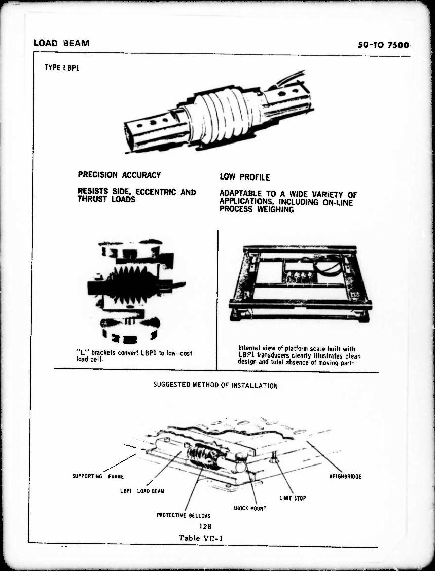
LOAD BEAM 50-TO 7500

TYPE LBP1

PRECISION ACCURACY

RESISTS SIDE, ECCENTRIC AND THRUST LOADS

*■ ' "L" brackets convert LBP1 to low-cost load cell.

LOW PROFILE

ADAPTABLE TO A WIDE VARIETY OF APPLICATIONS. INCLUDING ON-LINE PROCESS WEIGHING

Internal view of platform scale built with LBP1 transducers clearly illustrates clean design and total absence of moving part-

SUGGESTED METHOD 0«^ INSTALLATION

SUPPORTING FHA«E

/ LBP1 LOAD BEAM

WEIGHBRIDGE

LIMIT STOP

SHOCK MOUNT

PROTECTIVE BELLO«

128

Table VII-1

L^^^—^^—- ' - -

MOUNTING

MOUNTING

Pifur« vii-13

Six Degree of Freedom Wrist Force Sensor Concept

130

f. Other Sensors

Consideration is being given to the incorporation of proximity sensors as a fault hazard avoidance device. These sensors

would shut down the arm motion in case any obstacle/object was detected in a location not expected by the computer.

131

-i leg CC K

k! 0 ^ C U OQ

a a> et

c o

rf. CO -H (0

■ *** ~ a

u I. TO is

o

01 C M

133

Ixl

i-i U- «/> Lil >-• '-I

f\! t/J ijj; ee 1

LLI

a:

»-• U- i/>

n: CD CO CO 1-1

DC

IS)

UJ 00

o Di O

— >

K 3 M

■-■

[X,

A

134

J

D. Hydrauiic Control

1. Introduction

The choice of hydraulic actuators for the manipulator brings with it a particular set of control problems that must be dealt with by the

hydraulic control system. This system must take commands issued by

the computer and then control the actuators to produce the desired perform-

ance. The problems that complicate the job of the hydraulic servo include

the non-linear behavior of certain hydraulic elements, compliance of the

hydraulic fluid, and the dynamic effects of several components in the control loop. The desired performance of the control system includes basic-

stability, smooth motions of the manipulator structure, and graceful

failure of the control system should the computer fail to function properly.

2. Analytical Development

The overall plan of analysis began with formulation of the non-linear equations of motion of the system consisting of the hydraulic

actuator and load. Then a computer program to simulate this system was

written and debugged. Next, hydraulic control systems we.^e formulated

and added to the basic simulation. The performance of the combined

system was then tested through simulation. Usually, in order to design

the various control systems a simplified, linearized form of the non-

linear hydraulic equations was assumed for the purpose of analysis. The

resulting designs were then tried on the simulated non-linear system.

In the modeling process decisions had to be made concerning which effects or properties were sufficiently important to include in the

system model and which were not. The following are effects that were included:

a. Fluid compliance in the chambers or. both sides of the hydraulic actuator vane.

b. Non-linear vaive characteristics.

c. Fluid viscosity in ehe actuator leakage

from one side of the vane to the other.

135

d. Hydraulic valve dynamics between the

input electric current and the valve

opening size.

e. Inertial load on the actuator.

f. Dynamic effects of the angle reading

resolver circuitry.

Among the effects not included were the following:

a. Inertial effects of the fluid between the

valve and the actuator. These effects

should be small because the valves are

mounted on the actuators and so the

relevant fluid mass is small.

b. Inertial effects of the fluid between the

pump accumulator and the valve. These

effects should be small because of the

sufficiently large diameter of the hose

which causes slower fluid velocities.

c. Friction in the actuator. Friction is

designed to be minimized by the lack of

seals between the vane and the outer

wall of these actuators. Hence, there is

no rubbing contact. The only friction

should be the low friction in the shaft

bearings.

The non-linear model of the hydraulic system with inertial

load is illustrated in Figure VII-^. Table VIi-4 is a list of variable

definitions used in the tenmiltltOB. The derivation of the equations is

carried out in Appendix II . The final non-linear equations are repeated

136

J

Supply Pressure, P or Exhaust Pressure, P^

Hydraulic Valve

Rotary Hydraulic Actuator

Pair of Identical Variable Orifices

Pressure P

in Volume V

Leakage Flow q^

PD =

Pressure P,

in Volume V.

Vane Displacement Flow, qv

Inertial Load I Rigidly Attached to Vane

Figure VII-16

Hydraulic System Schematic

Exhaust Pressure Pg or Supply

[Pressure p

137

Table VII-4 Variable Definitions

Q angular position of vane, rad

W

s

q i

q 2

p u

X s

angular rate of vane, rad/sec

p supply pressure, psi

P exhaust pressure, psi

P pressure in left actuator chamber, psi

P pressure in right actuator chamber, psi

Y -^v (9) volume of left chamber, in

V =V«(e) volume of right chamber, in 2 ■

. 3

3 flow through left orifice, cis(- in1 /sec)

flow through right orifice, eis 3

D displacement of vane rotation, in /rad

q leakage flow past vane, eis

"flow" due to displacement of actuator vane, eis v

ß effective bulk modulus of fluid, psi

Q =v /ß fluid capacitance of volume Vj, in /psi 3

Q ^v /3 fluid capacitance of volume V2, in /psi

pressure upstream of orifice 1 on left, psi(= Ps or PE)

P pressure downstream of orifice 2 on righ*. D ptU- PE or Ps)

valve spool position 2

inertia of load, in-lbf-sec

138

J

here.

- Dto + f (x q s

VII-20

"3r"T(prp2)

de . HF -w

where P = p u

P ^ P ! if x > 0 s

VII-21

The first of equations VII-20 expresses the rate of change of

pressure in the left hand chamber of the actuator in Figure VII-16 as the

sum of the flows into the chamber divided by the capacitance (compliance)

CjO) of the total fluid in the chamber. As indicated in Table VII-4 . this

compliance is a function of the fluid modulus 0 and the volume of the fluid

chamber, which itself is a function of angular position §. The second

equation is like the first but for the other fluid chamber. The third equation

is Newton's equation for a rotary load, and the last equation just defines

angular rate M. The function fq (• , .) is short hand for the quadratic flow function of an orifice:

*-KVxs

J]Äpf| for AP> 0 . 1 VII-22

yiAPN for AP< 0

where AP pressure drop across orifice

xs ■ valve spool position

Ky ■ valve orifice gain

q ■ flow through orifice

139

For a single orifice x is considered only positive or zero.

Hence, the flow through the orifice as defined by the above function is

always in the direction of the pressure drop. In a standard fourway

hydraulic valve a negative spool position corresponds to a reversal of the

connections of supply pressure and exhaust pressure to the hydraulic

actuator. This is so actuators may be driven in both directions. This switch

in supply and exhaust pressure is the purpose of equations (VI1-21) since

they define which orifice is connected to exhaust and which to supply.

The non-linear equations (V1I-20) were implemented in the

computer program that was used in subsequent simulation testing. For

the purpose of ease of analysis, however, it is useful to simplify these

equations as much as possible. The following assumptions were used to

make these simplifications:

a. CjO)) -- eye) - Cj that is, that the fluid

capacitance is relatively constant and

equal on both sides of the vane. This

means that the vane is assumed to

remain essentially near the center of its

range of motion.

b. We assume linearization of the flow

functions f for the valve orifices as

follows:

fq(xs' AI>) -• % + VVso* + VAP-AP0) VII-23

where xso ■ valve spool linearization position

APo • pressure drop linearization value

ks - spool position gain ■ Jjf /^x

k - pressure drop gain ■ %f /gAP

c. We further assume that the pressure

drop across both orifices in the valve is

about the same, i.e., both AP k P /2. o s'

assuming exhaust pressure PE ■ 0. These

140

assumptions combine to make k approximately

equal for both orifices.

d. Assume that xso 0. This means that the

valve is operating about its closed position

and furthei implies that q - 0 and k - 0. ^o p

e. Assume that k is the same for both orifi^ps

This is a safe assumption because hydraulk

servo valves are almost invariably designed

with matched orifices.

Working with these assumptions as shown in Appendix II

gives us the following simplified, linearized equations:

AP - P -P

AP

U

2D T

D I

AP

CO

2k

VII-24

Figure VIM7 shows these equations in block diagram form.

3. Modeling Types of Hydraulic Control Systems

The purpose of the hydraulic control system is to convert

the commands from the computer into the desired actions of the arm and

load. This control system will physically reside in the interface equipment

connected between the computer and the manipulator. Digital words

corresponding to computer commands \' ill be fed into the interface f-om

the computer. The output of the interface is a properly modulated analog

electric current which will control the valve orifice openings. Actually,

since there will be six hydraulic actuators to control, there will be six

such hydraulic control circuits in the system interface.

141

mm^m^^

Tne hydraulic control circuits must still function if the

computer does not. This is the concept of "graceful failure": the

computer must not be so vital to the operation of the system that it goes

unstable if the computer i^ils or if there is a program error and t. :e

computer stops. This will put requirements on the contral system

configuration. The criteria by which the control system is judged are that

the performance of the manipulator must be stable, smooth, and sufficently

fast.

The control system design process will be to use the

simplified linear model of the hydraulic and load system to design

alternative control systems. These alternative control designs will be

tested by simulating them with the non-linear hydraulic simulation. There

are four types of control systems tested:

a. Pure position feedback

b. Position feedback with rate feedback

c. Position feedback with lead filter on

rate feedback

d. Position Vedback, rate feedback, and

actuator load pressure feedback

The simulated system includes additional effects that will

not be used in the simplified analysis. For example, the simulated

hydraulic control system includes the dynamic effects of the hydraulic

valve and the angle reading resolver circuitry. The bandwidth^ of both

of these components are well above the hydraulic resonance frequency

and so were excluded from the simplified analysis.

a. Position error control

Position error control is illustrated in Figure VII-18 by

a block diagram. The basic idea here is that the electric current through

the hydraulic valve is made proportional to the error between desired

position and actual position. A root locus diagram for this system,

assuming the simplified linear equations, is also shown in Figure VII-18.

143

2KSD/(IC)

RLC no

e Desired öd /"

>- Ke

*zm j_ s

, » .

"■"v. T ' r Actual 0

(a) Block Diagram.

.lu;

-^ H

(b) Root Locus of Closed Loop Poles for Increasing K .

Figure VII-18

Position Krror Control

144

The locus of the poles of the closed loop system is shown for increasing values of position error gain K .

Notice that as the position error gain K is increased, the

pole pair associated with the hydraulic/load resonance is driven unstable

Qualitatively what is happening is the following: At the resonant frequency

of any complex pole pair, their phase lag is 90°. The integrator in the

system possesses an additional 9V> phase lag. Obviously, these two

elements together in the open loop posses a total of 180° phase lag at the

resonant frequency of the load resonance poles. Consequently, sufficient

error gain will simply drive the system unstable. Also, a look at the root

locus shows that pure position error control will not damp the resonant

poles. Figure VII- 19 shows the results of a simulation of pure position

feedback on the non-linear system using component values corresponding

to the shoulder actuator of the manipulator design. Clearly the resonant poles have not been damped.

Position error control cannot be abandoned completely After all. to control the manipulator position there must be a position

error loop somewhere in the control system. And. some position loop

closure must occur in the interface to insure gracetui failure when the computer is not functioning.

b. Position and rate feedback

The addition of rate feedback is a common cure for

oscillatory position servo systems. Figure VII-20 contains a block

diagram of the system with the additional rate feedback. Also shown is

a root locus diagram showing the pole motion of the closed rate loop system

for increasing values of rate feedback gain Kp. In this case a particular

value of position error gain Ke is assumed and held constant. Hence

the initial pole positions in the root locus of Figure VII-20 correspond to

the poles for a certain value of position error feedback.

145

. . T

n

_ X

A 0 - i S ^ Kjf-

4/1 ? K S UJ

P i

—■

^ o a c ^-.2 ^ — ^^ CI 3 Z 'r- .— n ~

to _ —<

III

146

r

(a) Block Diagram

I lb) Root Locus of Closed Loop Poles for Increasing Rate Feedback gain K

Figure V1I-20

Position and Rate Feedback

147

As can be seen from the root locus diagram, as the rate

feedback gain K^ increases the frequency of the resonant poles increases

and the freoupncv. or speed, of the dominant real pole decreases. This

means that for high values of rate, or "tach", feedback the overall

system performance becomes sluggish (the real pole) but with high

frequency ringing overlaying the basic response. Figure Vll-21 shows

the result of a simulation of the step response of a typical system with

excessively high rate feedback. The simulation used the position and

rate feedback scheme on the non-linear model of the hydraulics and load.

c. Position feedback with lead filter on rate feedback

The high frequency ringing apparent in the previous

section occurs because at the frequency of the ringing the total phase lag

of the open loop system is almost 180° with nearly too much gain. One

possible way to eliminate the ringing is to reduce the phase lag in the rate

loop at that frequency by introducing a lead filter.

Alternatively, one can imagine the ringing problem arising

from the two resonant poles. These poles occur in the transfer relationship

between hydraulic valve electric current (spool position x ) and Q, angular

rate. Since the output variable is f), rate in this case, the poles may be

damped by the addition of feedback of the output derivative, 6, or accelera-

tion. By adding lead compensation to the rate feedback, we obtain the

effect of differentiation, resulting in an acceleration feedback «ignal.

A block diagram of this control scheme is shown in

Figure VII-22. The form of the lead compensation is

1 ♦ s/ajd

where COJ ■ ^ead frequency, rad/sec

co - lag frequency, rad/sec g

O) , <(J0 d g

148

_^M^^MM«^

3 •- 0,

5 P rt

UJ tr _i O — O oc ü < LU

149

.jjäu^ä^M

r 9d +

1 1

Ke s

2KSD/(IC) b 1 s

i» 1 0

r>rvH i

2 + s J_ + 2_Di RLC (IC)

i <

1 1 i

i ^

1 _ _ — —

1 1

sKr 1 + S/^H

1 + s/wg

(a) Conventional

r i r~ i 1

2KSD/(IC)

s2 + s 2 +-2D2

RLC IC ^m:l 1 1

r-

v

nY 1 n s r i 1 + s/ug 1 1 i

i_ 1 .. 1

j

1 ' 1 — — J

i S IVCJjj

(b) Redrawn for Root Locus Work.

Kigure VI1-22

lilock Diagram

Position Feedback with Lead Rltor on Kate Feedback

150

■ ■ • — ■ ■■■ - ■

■^ K

LEAD FILTER POLE

/

■*+

(a) First Stage of Root Locus. -£- - 0. Locus of closed d

loop poles as rate feedback gain Kr is increased.

X »

1

t

(b) Second Stage of Root Locus, Kf fixed. Locus of

1 closed loop poles as ^ increases.

Figure VII-2.S

Hoot Locus of Position Feedback with Lead Filter on Hale Feedback

152

I

- ^ ■f. -z o

i i e -a «

, ~ re i: C a.—

S 3511 E - ^ a! ^ ci — 'S a

i ^ s

153

d. Position, rate, and p-es sure feedback

In the previous section it was explained that acceleration feedback would damp the resonant poles. Besides lead compensation on the rate signal, another way to obtain an acceleration signal is to use

pressure feedback. Pressure sensors are placed on both sides of the

actuator and used to measure the pressure difference acting on the rotary

vane. Because this pressure drop is proportional to the torque of the

actuator, and because torque on an inertial load is proportional to acceleration, then this pressure drop can be taken as proportional to the load acceleration.

Figure V1I-25 shows a block diagram indicating the use of position, rate, and pressure feedback. Also in the figure is a root locus

indicating how the poles move for increasing pressure feedback gain for a

given set of position and rate feedback gains. It can be seen that increasing

pressure feedback will tend to increase the frequency (speed up) of the

dominant real pole -up to a point. Excessive pressure feedback will then bring lightly damped low frequency resonant poles.

An alternative way to conceive of pressure feedback is to think of the pressure loop as creating a pressure or torque servo xn the

middle of the entire system. Then the position error and rate signal can

be thought of as driving a torque source in a stable, conventional position servo.

Finally. Figure VII-26 shows a step response of the simulated system using an appropriate amount of pressure feedback.

Notice that the response is smooth, quick, and without oscillation.

4. Discussion

When position, rate, and pressure feedback are all used, then there are three parameters to adjust in the simplified third order system.

Theoretically, it should be possible to arbitrarily assign the three pole

positions and compute the required position, rate, and pressure gains to achieve them.

154

POSITION AND RATE LOOPS

^o1 PD

PRESSURE LOOP

(a) Block Diagram.

Double Zero

(b) Root Locb. of Closed Loop Poles, fixed K , K .

Pressure Fr, dback Gain K increasing.

Figuie VII-25

Position, Rate, and Pressure Feedback

155

^M^—^^^^—^^^^^M- -

N i

C ■ •Ml

ft) -U 90 ~ C

0 ."S a

3 "At CX' "U ^ -

co -- - — Ox = ^ y;

y. <2.

m cr -i O

z tr < LU

156

with rubbing contac. leading to significant stiction effects. This type of friction was not included in the simulation. The second primary area of work is the addition of computer control. A PDP9 with A/D and D/A

equipment is being used to experiment with the problems of computer

control, such as update rates of command and measurement.

Other possibilities for future work in this area include the

use of more sophisticated signal filter! called observers. Their function is to use the measured signals, such as rate signal or electric current

through the valve, to estimate needed signals that are not measured, such

as pressure drop in the actuator. This could be very helf/uJ since not

only can pressure senrors be expensive, but they also require additional design work on the actuators and instrumencation circuitry to read them.

Some preliminary simulation work has shown that a pressure observer

designed on the basis of the simplified linearized model can work well for

estimating pressure in the non-linear simulation but only when operating

in regions where the linear model is most accurate. When the actuator system is operating outside this region the observer performance

deteriorates. Consequently, control schemes which would use observers

in place of genuine sensors would also deteriorate. Work here has

proceeded only in analysis and simulation. Experiments will be done when additional electronic hardware is available.

E. Hydraulic Control Servo Experiments

In support of the theoretical work in the previous part of this section, we have an ongoing program of hydraulic control experiments.

The apparatus is illustrated in Figure VII-27. It consists of a hydraulic

power supply, a commercial rotary vane actuator, position and rate

sensors, and servo electronics. The apparatus can be operated from a signal generator or under computer control. So far the experiments have

been utilized to verify our models of rotary vane actuators and to provide

values for physical constants for use in computer simulations. Work

under way is aimed at testing out the various control configurations

outlined above. Wo-k with pressure sensors has been completed and

their stabilizing properties, as predicted by the theory, have been amply

158

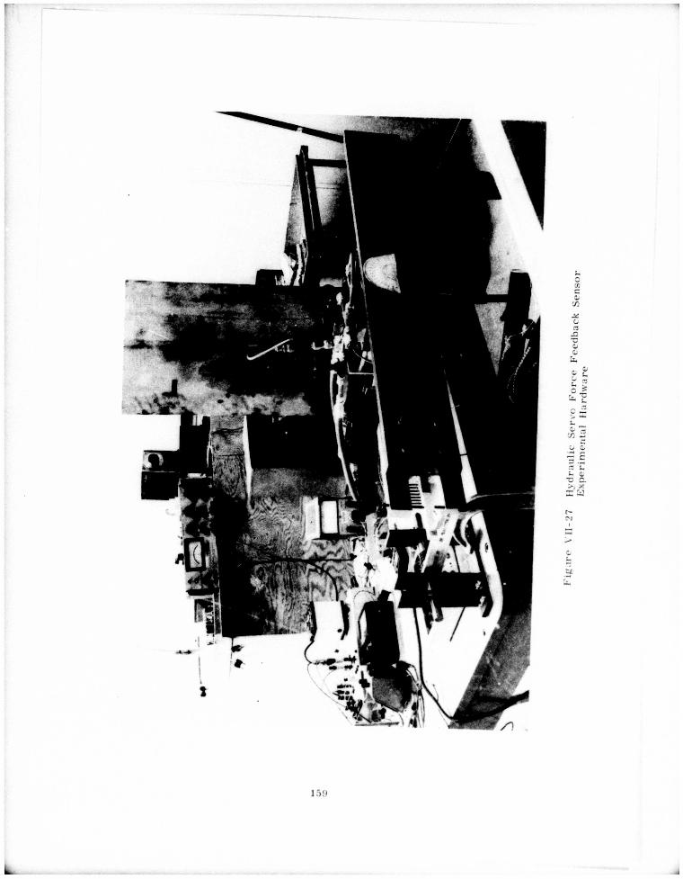
verified The figure a,so shows a one degree of f^-doo, force .senso.-

w c w.,, be u.iii.ed in fonce feedback „ervo expeHn.nf. .n oonneculn w.th the above mentioned companion NSF funded work.

160

■^^MBiiMMM^ J

VIIL CQNSLUSIONS AND RECOMMENDATIONS FOR FURTHER WORK

A. Conclusions

This report contains three major themes:

• development of a science of manipulator design

• linking that science with the problem of industrial assembly

• study of a particular arm geometry to determine the technological requirements for high performance and operational reliability

The contributions to manipulator design science cover aspects of

geometry, kinematics, actuators, servo controls, structure, sensors

and task execution strategies. It has been shown that these aspects of

arm design and use interact strongly and must be considered together

in formulating a design. New design tools have been developed for

achieving this. The impetus for any design problem must be a goal for

the proposed system. Our efforts were directed at the problem of

industrial assembly, where economic and technological success demand

high performance arms - arms with strength, high speed, high accuracy

and resolution, and rapid, efficient use of sensory information. This set

of requirements was combined with a particular choice of scale to produce the geometry which was studied in detail and to focus on problems which

arise in other scales, such as mini-robot. Because of this emphasis the

design is simple and straightforward. Thus, its potential reliability as a

piece of equipment to support laboratory experiments is much higher than

commercial or experimental hardware currently in existence. In addition, its capabilities cover a broader spectrum than any currently existing

laboratory equipment. Hence, it can support a broader spectrum of experimental activity or tasks.

The requirements of .ssembly have two aspects: gross motions, which are large, rapid, largely free of sensory feedback and reasonably well understood, and fine motions of two parts interacting as they are

assembled. The fine motions are quite small, highly dependent on

sensory feedback and thus far not well understood despite some laboratory

assembly demonstrations. These demonstrations, both in private industry 161

and universities, are ad hoc and pragmatic, showing that a particular

arm (not specifically designed for assembly) can put some small, well

machined smooth parts together. None of these demonstrations has

produced any data [except, in one case, the completion time, (an

industrial experiment), which was uneconomically slow by a factor of

two] shedding light on the class of task attempted in any of the following

key areas:

• what design factors in the arm contribute to or- detract from success in the demonstrated task, or in other types of tasks

• what control strategies work in this case and which do not — where else will they work

• what sensory information is really necessary to accomplish this or other kinds of tasks

• what forces and torques are being generated during the demonstration tasks

• what is needed to perform these or other tasks more rapidly and reliably

Until a better understanding of the process of assembly is achieved, these

demonstrations will be of no value in generating a science of assembly

capable of making valid performance predictions with respect to arms and

control strategies.

B. Recommendations

Work funded by NSF is going on at the C. S. Draper Laboratory

to study the assembly process, classify and analyze tasks, develop control

strategies and use the above to specify hardware and software requirements

for industrial assembly systems. In the course of this work, a number of

strategies, models, and factors influencing success have emerged. These

models need to be tested. The strategies assume employment of novel

designs in sensors, servo control organization and actuators. Details of

the actuators and sensors have been developed during the current work and

are discussed in this report. To carry on this work a high performance

computer controlled manipulator arm should be built. Its major contribu-

-NoF-RANN Grant GI-39432X and GI-43787

162

study on this design and on the assembly

process revealed the distinction between

gross and fine motions. Virtually all

existing arms were designed as gross

motion devices. We have determined

that the requirements for fine motion

conflict sufficiently often with requirements

for gross motion to make feasible the idea

of having two "arms" available for study -

one capable of gross motions, accurate

positioning and smooth application of force,

the other capable of fine motions of high

resolution and high speed. A frank assess-

ment of the POPEYE design is that it will be

capable of gross motions and some fine

motions but for research on fine motion it might

be better to ultimately specify a less accurate

arm and devote resources to a companion

fine motion device. Thus, while POPEYE

would make valuable contributions to the science

of assembly, we do not claim at this time that

it can do assembly by itself or than it even

vaguely resembles an industrially satisfactory

configuration. Some device designed with

foreknowledge of assembly requirements is

needed, however, to advance assembly science.

164

2.

3.

4.

5.

REFERENCES

Nevins, .J.L.. Whitney. D.E. and Simunovic. S. N

System Architecture for Assembly Machines "

CS. Draper Lab Report No. R-764, Novembe'r 1973.

Nevins. J.L., Whitney. D. E et .1 ••■. . _ J' ■'•■••• et. al., Exploratory Research in Industrial Modular Assembly. " C S

Draper Lab Report No. R-800. March 1974.

Nevins. J. L. and Whitney. D.E.. "The Force Vector

Assembler Concept. " C. S. Draper Lab Report No

E-2754. March 1973. presented at First International

Symposium on Robot and Manipulator Systems. Udine Italy. September 1973.

Paul. R.P.. "^inz. Trajectory Cakulation and Servoing of a Computer Controlled Arm, " Stanford

Untversity Artificial Intelligence Lab Memo AIM-177 November 1972.

Book, W..!., "Modeling, Design and Control of Flexible Manipulator Arms, " M. I. T. Mech. Eng. Opt. PhD

Thesis. April 1974.

6. Maizza-Neto. O.. "Modal Analysis and Control of

Flexible Manipulators. " M. 1. T. Mech. Eng. Dept. PhD Thesis. August 1974.

7. Whitney. D.E.. and Scott. P.. "The Shaft Wind up

Problem. ' C. S. D. L. Internal Memo No MAT 170 October 1973.

165

8. Whitney. D.E., "The Mathematics of Coordinated

Control of Prosthetic Arms and Manipulators, "

ASME Journal of Dynamir Systems. Measurement

and Control, December 1972, pp 303-309.

9. Doherty, H. J., "Fine Motion Stability of a Manipulator. "

M. I.T. Mech. Eng. Dept. S. M. Thesis. June 1974.

166

J

Survey of Commercial Industrial Robots

DOK Acjuracy Control System Price, $

1972 Floor Area

Corona i I ♦ 3mm D. C. Servo-Mag Tape 15K 800»; Ü00 mm

Fujikosbi 4 ♦ 1mm Hydr. C>l. -Mag Tape - 1530x730 mm

Hawker Siddeley i 1 ♦ 3mm Hydr. -Computer 37.5K 1188x711 mm

Howa I > • 1. Omm EL-Hydr. - 1380x900 mm

Kawauchi 1 Tekko

i ♦ 1. 0mm Hydr. -Mag Tape 2.8K 1300x750 mm

Kojin 1 1 ♦ 2. 0mm Hydr.-May Tape UK «50x1270 mm

Liberator i i ^ 0.4mm Klect-Hydr. 20 to 25 K

1320x610 mm

Scheinman ( i ♦1.3mm D. C. Motor« 10K

Sunstrand ; i +.3mm EL. Motor-Mag Tape 21. to 3 OK

410x410 mm

Tesa . ! i *_. 1mm D. C. 4 Stepper- Mag Tape

• 750x750 mm-rontrol 600x600 mm-Ar:n

Tokyo Keikl t 1 + 1mm Hydr. (A to D) 12. 5K 1900x1300 mm

Tokyo Sokuhan ; i • 1mm D. C. Motor-HOT Input

12. SK 1300x1000 mm

Tralle Fabrikken ( * 2mm Hydr.-Mag Tape 20K Ii00x75D mm

Veraatran < 0. 8n-.m-l horz vert

Hydr.-Mag 12 to 25K

Unlmate ( 1 ♦ 2min Hydr. -Mag Tape 37. 5K 1500xlSOO-Brm 1200x450-control

Preceding page blank 168

J

Derivation and Simplification of Hydraulic System Kqnations

We begin the derivation by discussing the nature of the flow through

the valve orifices. For any given valve opening, the pressure drop across

either orifice is ideally proportional to the square of the flow through the

orifice with the sense of the pressure drop in the direction of the flow.

The proportional constant varies with the area of the orifice opening so

that a flow-pressure relationship is obtained as illustrated in Figure All-l.

Notice that for the largest valve orifice opening, corresponding to valve

spoolposition xg - 1.0, the greatest flow is obtained for any given

pressure drop. When the valve is closed, x^ - 0, there is of course no

flow no matter what the pressure drop AP. In the fallowing derivation

the orifice flow function will be expressed as

q • fq(xs.AP)

where q ■ flow through orifice

AP^ pressure drop across orifice

xg - valve spool position, relative to full travel

When the orifice is ideal the flow function is

W AP) KV |AP|

x ffÄPi

for AP> 0

for AP< 0

AIM

In the non-hnear simulation program the ideal flow functk)n is used.

The fluid capacitance, or compliance, in either actuator chamber

is proportional to the volume and inversely proportional to the effective fluid modulus

Cjtll - VjH)

cye) - Vgf») 7

P

All-2


Figure All-l

Ideal Valve Orifice Pressure/Flow Kelation.ship

x

flow

pressure drop

valve spool position (size of orifice)

171

where 0,(0) - ftuid capacitance in left chamber of Figure VII-16

C„(9) ■ fluid capacitance in right chamber

V^e) - actuator fluid volume on left side of actuator vane in Figure VII-16

Vpte) - actuator fluid volume on right side

3 ■ effective fluid modulus

Notice that the volume, and therefore capacitance, of the fluid on one side

of the vane is a function of the position of the vane.

The rate of change of pressure in either chamber is equal to the net

flow into the chamber divided by the fluid capacitance of the chamber. The

net flow into the left hand chamber is

-^L^V fql

where qT - actuator leakage flow from left chamber to right

q ■ apparent flow due to displacemer

q. ■ flow through the left hand orifice

q ■ apparent flow due to displacement of the actuator vane

The net flow into the right chamber is

+qL ♦ qv - q2

where q9 - flow through the right hand orifice.

Consequently the equations for pressure rate are

dPl 1 ■ar "-ü7^)l-qL-qv'qi]

dP2 ,

TT r ran (+qL + qv - q2l

AIM

We now derive expressions for these flows. The leakage flow qT

past the actuator vane can be expressed as

qL = Pl " P2 AII-4

172

*M

We now consider the effect of an inertial load Imposed on the

actuator. The characteristic equation of the load is

1 & torque on load D(P|-PJ All-9

where 1 - rotary inertia of load which is equivalentlv expressed as follows

da; ^ 11> _ p \ Tit "P1 1 ^2'

de dt

Al I-10 Ui

Now we finally can present the set of non-linear equations for a rotary

hydraulic actuator and load:

1 dt

dFr

1

"ar ' rjö)

p -p 12 R i

Du *1 (x . P -P.) o s u 1

Ji-l+Du-t (xBt P2.PJ I.

A1I-11

du; '^ /p PI Hi ' T (1 1 V

de Tt '«

where P - P u s I i D E

P - P., u L

P» P D s

for x - 0

for x < 0 s

These equations can be simplified to a linear form by making a

series of assumptions as discussed in Section VII-D. They are

essentially the following:

i. c^e)«ca<d)«c

174

3. AP F -P

Substitution of thpse relations in the non-linear equations AII-11 gives:

dP

dt 1 r AP

- T> IJCL' + K x rfj SS

dp2

dt i r AP

* SAP

All-12

All-13

AH-14

Notice that the number of necessary equations has been reduced by one

because | no longer plays a part in the functional relationships. Further-

more, the second equation (AII-l3)mav be subtracted from the first (All-12) to yield

2AP ITT

dAP 1 2lJu; + 2K x

s s

If ?^ AI1-15

or, in matrix form.

AP

U

R I.

I) T

2Ü AP

ÜÜ

2K

AI1-16

Notice that the system order is again reduced by one because the pressure

difference AP is the important variable, noi the values of the pressures themselves.

175

Appendix III

Abstracts of Theses Performed Under this Contract

a. "A General Planar Positioning Device" by

Jonathan David Hock

b. "Design of an Automatic Assembly System Multipurpose

End Effector", by Thomas Barry Lyons


DISTRIBUTED BY - DTIC

Documents

Transcript of DISTRIBUTED BY - DTIC