DISTRIBUTED BY: - NASA Technical Reports Server

DATA USERS HANDBOOK

National Aeroliautics and Space Administration Greenbelt, Maryland

LOAN copy: 15 September 1991 AFWL TECHNIC

. --. KIRTLAND A

DISTRIBUTED BY:

.~

National Teclinical Information Service U. S. DEPARTMENT OF COMMERCE 5285 Port Royai Road, Springfield VA. 22151

-?g- ,]

NASA ;CR

122287 ;c.l(R) ,

TECH LIBRARY KAFB, NM

NATlO%iil%$lNlCAL ’ INFORMATION SERVICE ’

SpringhId, Va. ZZlSl

”

GODDARD SPACE

DOCUMENT ISSUED TO: e... --

-:

‘NOTICE

THIS DOCUMENT HAS BEEN REPRODUCED FROM THE

BEST COPY FURNl$HElb US BY T.HE SPONSORI[NG

AGENCY, ALTHOUGH IT IS RECOGNIZED THAT CER-

TAIN ~ORTION~ ARE ILLEGItiLE, IT IS BEING RE-

LEASED IN THE INTEREST OF MAKING AVAILABLE

AS MUCH INF.ORMATIbN AS POSSIBLE.

. .

TABLt OF CONTENTS

Section Description

1 INTROOUCTlON . . . . . . . . . . . . . . . . . . . . . . . . . . . . . . . l-1

2 ERTSPROGRAM DESCRIPTION . . . . . . . . . . . . . . . . . . . . . . . . . . . 2-1

2.1 I ERTS Mission . . . . . . . . . 2.2 Observatory System . . . . . . . 2.3 Payloads . . . . . . . . . .

2.3.1 Return Beam Vidicon Camera 2.3.2 Murtispectral Scanner . . . 2.3.3 Wideband Video Tape Recorders 2.3.4 Data Collection System . .

2.4 Orbit and Coverage . . . . . . . 2.5 Operations Control Center. . . . . . 2.6 NASA Data Processing Facility . . .

2.6.1 Bulk Processing . . . . . 2.6.2 Precision Processing . . . . 2.6.3 Special Processing . . . . 216.4 DCS Data Processing . . . 2.6.5 Support and User Services . .

. . . . . B.......‘.........

.......................

......................

......................

......................

......................

................... ., ....

... . ...................

......................

....... . ...............

................. / ....

......................

......................

.......................

......................

3 OUTPUTDATAPRODUCTS .............................

3.1 Photographic Products ............................ 3.1 .l Bulk Photographic Products ....................... 3.1.2 Precision Photographic Products ......................

3.2 Computer Compatible Tapes .......................... 3.2.1 Bulk MSS Computer Compatible Tapes ..................... 3.2.2 Bulk RBV Computer Compatible Tapes ................... 3.2.3 Precision MSS and RBV Computer Compatible Tapes ...............

3.3 Data Collection System Products .........................

4 USER SERVICES . . . . . . . . .

4.1 Ordering Procedures . . . . . . 4.1.1 Standing Orders for Images 4.1.2 Data Request for Images . 4.1.3 Delivery Schedule . . . 4.1.4 Requests for DCS Data . .

4.2 Data Catalogs . . . . . . . . 4.2.1 Standard Catalogs . . . 4.2.2 Image Descriptor Index . 4.2.3 DCS Catalog . . . . .

4.3 Microfilm Images . . . . . . . 4.4 User and Visitor Assistance . . . 4.5 Computer Query and Search Capability

. . . . . * . . . . . . . . . . . . . . . . .

....................... 4-1

.................. .../. 4-2

....................... 4-2

....................... 4-8

....................... 4-8

....................... 4-8

....................... 4-8

....................... 4-l 1

....................... 4-14

........................ 4-17

....................... 4-18

....................... 4-19

APPENDIX A: PAY LOAD . . . . . . . . . . .

A.1 Return Beam Vidicon . . . . . . . . A.l.l Operation . . . . . . . . . A.l.2 Performa.uze . . . . . . . .

A.2 Multispectral Scanner Subsystem . . . . . A.2.1 Operation and Calibration . . . . A.2.2 Performance . . . . . . . .

A.3 Data Collection System . . . . . . . . A.3.1 Data Collection Platform . . . . A.3.2 DCS Spacecraft Equipment . . . A.3.3 Treatment of Data at the Receiving Site A.3.4 Treatment of Data at the GDHS . ,

. . . . . . . . . . . . . . . . . . . . A-l

....................

....................

....................

....................

....................

....................

....................

....................

.......... ...........

...................

....................

I’llfp

2-1 2-6 2-7 2-7 2-7 2-6 2-8 2-9 2-9

2-11 2-11 2-11 2-12 2-12 2-12

3-1

3-1 3-2 3-9

3-11 3-12 3-15 3-15 3-17

4-1

A-l A-2 A-5 A-7 A-8 A-9

A-14 A-16 A-17 A-17 A-17

ORIGINAL

SEPTEMBER 15. 1971

Section

APPENDIX 6: OBSERVATORY . . . . . . . . , . . . . . . . . . . . . . . . . . . . . . 6.

B.l B.2 8.3 B.4 B.5

Attitude Control Subsystem . . . . . . . . Attitude Measurement Sensor . . . . . . . . Wideband Video Tape1 Recorder Subsystem . . . Power Subsystem . . . . . . . . . . Communications and Deta Handling Subsystem . . B.5.1 WidebandTelemetry Subsystem . . . . B.5.2 Telemetry, Tracking and Command Subsystem Thermal Control Subsystem . . . . . . . . Orbit Adjust Subsystem . . . . . . . . . Electrical Interface Subsystem . . . . . . . .

.................. B

. .................. B

................... B

.a.. ............... El

.................. B

........ ; ......... B

................. El

................... B B.6 B.7 8.8

APPENDIX C:

C.l c.2

c.3

APPENDIX D:

D.l 0.2 D.3

APPENDIX E:

E.l

E.2

E.3 E.4 E.5 E.6

E.7

TABLE OF CONTENTS (CoNi’D) _’

Description

. . . . . . . . . . . . . . . . . . I3

. . . . . . . . . . . . . . . . . . B-

GROUND STATIONS AND GROUND CDMMUNICATIDNS . . . . . . . . . . . . . . . . . C-

General Description ............................ C- Payload Wideband.Communicetions ...................... C- c.2.1 Spacecraft to Ground Communication .................. C- c.2.2 Ground Receiving and Recordings .................... C- Telemetry, Tracking and Command Data Handling ................. C- c-3.1 Telemetry Data ......................... C- C-3.2 Command Data ......................... C- c-3.3 Tracking Data ......................... C- c.3.4 DCS Data ........................... c-

OPERATICINS CONTROL CENTER ........................

System Scheduling .............................. Data Acquisition .............................. Command Generation ................... ,-: ........

D-

fl- D- D-

NASA DATA PROCESSING FACILITY ........................ E-

Bulk Processing Subsystem ........................... E- E.l.l RBV Video Processing ......................... E- E.1.2 MSS Video Processing ......................... E-- E.1.3 Framing ............................. E-1 Precision Processing Subsystem ................... ., ..... E-1 E.2.1 lmput Screening and Ground Control Selection ................. E-: E.2.2 Image Measurement, Transform Computation .................. E- E.2.3 Image Conversion and Annotation, Image Digitization ............... E- Special Processing Subsystem .......................... E-l Photographic Processing Facility ......................... E-! Quality Control .............................. E-ll Computer Services Subsystem .......................... E-l : E.6.1 DCS Processing ........................... E-l: E.6.2 Image Annotation Processing ....................... E-l: User Support Services ............................ E-l:

APPENDIX F: SYSTEM PERFORMANCE . . . . . . . . . . . . . . . . . . . . . . . . . . F-l

F.l

F.2

Geometric Accuracy . . . . . . . . . . F.l.l Measures of Geometric Accuracy . . F.1.2 Error Sources and Their Magnitude . . F.1.3 Output Product Geometric Fidelity . . Radiometry . . . . . . . . . . . F.2.1 Return Beam Vidicon Camera Radiometry F.2.2 Multispectral Scanner Radiometry . .

1

..................

..................

..................

.................. ................. .................

..................

F-l F-l F-l F-2 F-l F-9

F-15

-‘GINAL

TABLE OF CONTENTS (CONT’DI

Section Description

F.3 Resolution ........... 1 ..... ‘, .............. F.3.1 MSSResolu’on ........... , ................ F.3.2 RBV Resolution ...........................

F-16 F-16 F-20

APPENDIX G: CALIBRATION .............. , ................. G-l

G.l

6.2

Return Beam Vidicon (RBV) ........................... G-l G.l.l Calibration Methods ......................... G-1 6.1.2 NOPF Calibration Processing ....................... G-8 6.1.3 Geometric Calibration ............................ G-15 Multispectral Scanner (MSS) ........ :’ .................... G-17 6.2.1 Initial Calibration Methods

NDPF Radiometric Calibration Procersing’fMSSi : : 1’ : : : : : : : : : : : : : : G-17

6.2.2 G-20

APPENDIX H: FILM AND DEVELOPER CHARACTERISTICS ...................... H-l

H.l Photographic Image Quality ........................... H-l H.l.l Tone Reproduction .......................... H-3 H.1.2 MTF and Resolution ......................... H-5 H.1.3 Granularity ............................ H-5

H.2 Dimensional Stability ............................ H-6

APPENDIX I: ORBIT AND COVERAGE .......................... I-1

I.1 Earth Coverage ............................ I-1 1.2 Imagery Overlap ............................ l-2 1.3 Repeatability ............................. l-3 1.4 Altitude Variations ........................... l-3 1.5 Determination of Local Observation Time .................... l-4

APPENDIX J: ORBIT CONTROL ..........................

. J.l Attainment of Required Orbit ..................... J.l.1 Period Errors ....................... J.1.2 Inclinat.on Errors ...................... 5.1.3 Error Correction ......................

J.2 Maintenance of Required Orbit ........ : ...........

. .

. .

. .

J-1

J-l J-l J-2 J-2 J-2

APPENDIX K: MISSION PLANNING . . . . . . . . . . . . . . . . . . . . . . . . . . . . . K-l

APPENDIX L: SUN ELEVATION EFFECTS . . . . . . . . . . . . . . . . . i . . . . . . . . . L-l

APPENDIX M: LIST OF NASA PRINCIPAL INVESTIGATORS ................. Ml

APPENDIX N: SAMPLE PRODUCTS ......................... N-l

v/vi SEPTEMBER 15. 1971

LIST OF CURRENT PAGES

Section 1 l-1 thru l-2 15 Sep 71

Appendix H H-l thru H-7/8 15 Sep 71

Section 2 2-l thru l-12 15 Sep 71

Appendix I I-1 thru I-10 15 Sep 71

Section 3 Appendix J 3-l thru 3-20 15 Sep 71 J-l thru J-3/4 15 Sep 71

Section 4 Appendix. K 4-1 thru 4-21/22 15 Sep 71 K-l thru K-3/4 15 Sep 71

Appendix A Appendix L A-l thru A-19120 15 Sep 71 L-l thru L-3/4 15 Sep 71

Appendix B B-l thru B-4 15 Sep 71

Appendix M M-112 15 Sep 71

Appendix C C-l thru C-4 15 Sep 71

Appendix N N-112. 15 Sep 71

Appendix D Aeronyms D-l thru D-1 15 Sep 71 D-1 thru 02 15 Sep 71

Appendix E Glossary E-l thru E-13/14 15 Sep 71 P-l thru P-2 15 Sep 71

Appendix F F-l thru F-25126 15 Sep 71

References Q-l thru Q-2 15 Sep 71

Appendix. G G-1 thru G-25/26 15 Sep 71

i.-”

SECTION 1 INTRODUC’ ION

The Earth Resources Technology Satellite (ERTS) program is a majre first step in the merger of space and renrote sensing technologies into an R&D system for developing and demonstrating the techniques for efficient management of earth’s resources. To establish the feasibility of these techniques, NASA will launch two experimental satellites into orbit: ERTS A in 1972; ,ERTS 8, during the following year. ‘Each will acquire muiti- spectral images of the earth’s surface and transmit this raw data through ground stations to a data processing center, at the NASA Goddard Space Flight Center, for conversion into black-and-white or color photographs and computer tapes to fulfill the varied requirements of investigators and user agencies. In addition, ERTS systems will collect environmental data from remote, earth-based instrument platforms and relay this information to the data processing center at Goddard for final processing and dissemination’ to investigators.

The role of the “user” is an integral and indispensable part of the ERTS program. Investigator’s experimentation with, and analysis of, the ERTS data products is the only meaningful route to developing and demor,- strating the utility of data acquired by satellite systems of this type for use in earth resources management. ,Future operational earth resources satellite and data system requirements will be derived from investigators’ experience with ERTS A/B data.

This handbook has been designed to satisfy investigators’ needs for pertinent and sufficient information about ERTS data products, and how to acquire them..The main body of the handbook provides information required by all investigators. The appendices provide more detailed treatment of topic&equired by many investigators to varying degrees. A brief description of the section contents follows:

Section 2 ERTS Program Description Provides a concise explanation of the

l-l

. . . _..-.bL.,

total ERTS system and its mission. An overview of the various major system elements and their characteristics, the observatory, payloads, orbit and cover-

.‘age, ground facilities and services availa- ‘ble to investigators is included in this ‘section.

Section 3 Output Data Products Provides a detailed description of each type of data that is available to investigators, with information on data format, content, znnotation, and pertinent characteristics.

Section 4 User Services Provides a discussion of how ERTS output data products are obtained, and what catalogs, listings, facilities, and other materials and services are available to assist the investigator in identification, selection and use of these products.

APPENDICES

These provide indepth treatment of selected topics considered to be of special interest to many investigators. These topics are:

A. Payload - Describes equipment, characteristics, and operating modes of RBV (Return Beam Vidicon), MSS (Multi Spectral Sensor), and DCS (Data Collection System) payloads.

B. Observatory - Describes spacecraft configuration and subsystems which control and support payload and mission activities.

C. Ground Stations and Ground Com- munication - Describes STADAN (Space Tracking and Data Acquisi- tion Network) and MSFN (Manned Space Flight Network) stations sup- porting the mission and the transfer of data between those stations and the GDHS (Ground Data Handling System) at Goddard Space Flight Center.

D. Operations Control Center - De- scribes the function performed by this facility in planning and conduct-

ORIGINAL

SEPTEMBER 15. 1971

I

APPENDICES

ing the flight operations and its role in the collection of payload data.

E. NASA Data Processing Facility - Describes the conversion and correction of raw video tapes into useful photographic and digital tape products. The different types of processing within the NDPF are considered and the equipments that perform these processes are described.

F. System Performance - Describes the expected quality. of the various imagery and data tapei principally in terms of resolution, geometric accuracy and radiometric fidelity.

G. Data Calibration - Describes the source of data and application of the corrections made to the data products prior to distribution from the NDPF.

H. Film and Developer Characteristics - Describes the intermediate and final film products and their processing characteristics.

I. Orbit and Coverage - Describes the orbital constraints on the collection of data, the systematic coverage which results, and the time at which images are collected.

J. Orbit Control - Describes the process of establishing and maintaining the desired orbital coverage and its limitations.

K. Mission Planning - Describes the system used to obtain the maximum amount of useful data within overall system constraints and environmental conditions.

L. Sun Illumination - Describes the earth illumination conditions and their variability with latitude and season of the year.

M. List of NASA Principal Investigators - Provides the names of the principal investigators selected by NASA and their planned field of investigation.

N. Sample Products - Provides samples of imagery and calibration data avail-

ORIGINAL

able prior to launch of the spacecraft.

Acronyms, Glossary and References Provides suggested reference materials for further treatment of selected topics; a definition of terms used throughout this handbook which may require explanation to avoid misinterpretation; and a list of acronyms frequently used to minimize repetition of multiple-word titles.

Development of the ERTS Observatory and the Ground Data Handling System is proceeding concurrently with preparation of this handbook. Consequently, the document. is bound in loose-leaf form to facilitate continuous updating. Each page is identified .in the lower outside corner as an original or a revised page (including the revision number and da&). New or changed information affecting investigate:? participation in the program will be issued periodically. A change bar will be printed in the left-hand margin, opposite revised information. Sample data products of the Ground Data Handling System, produced during system integration and testing, are provided in Appendix N o-F the handbook. In many cases, this data will actually be products of calibration tests; hence, they will serve a dual purpose of providing ERTS product samples, as well as calibration data relative to ERTS products.

Distribution of this handbook and subsequent update material will be made in accordance with a controlled list established by NASA. Each recipient is assigned a control number for each handbook. To insure rapid response, this control number must be used for all EdTS correspondence. For additional information or related inquiries regarding this handbook or its contents, please address all correspondence to:

ERTS PROJECT OFFICE National Aeronautics and Space

Administration Goddard Space Flight Center Greenbelt. Maryland, 20771 Attention: Thomas M. Ragland, Code 430

SECTION 2 El?+5 PROGRAM DESCRlPTlON

The Earth Resources Technology Satellite (ERTS) Program has been designated as a research and development tool to demonstrate that remote sensing from space is a feasible and practical approach to efficient management of the earth’s resources. The knowledge gained from the application of data acquired by the two satellites (ERTS A and 6) will point the Nay toward development of fully operational and more effective systems for earth resources management.

Figure 2-l is a photographic reproduction to match the ERTS 1 : l ,OOO,OOO scale to give the user an appreciation of the scale and image quality that can be expected.

The photograph was made from an Apollo SO-65 color photograph with three contact printing stages and two enlargements. It is estimated that its resoiution, as reproduced here, is similar to an ERTS Precision color photograph. Because the picture was made from a single originai negative, there is no registration error.

These and other types of ERTS data products will be used by investigators for developing practical applications in the various earth

resources study disciplines including agriculture, forestry, geology, geography, hydrology, and oceanography. With the knowledge gained from the application of ERTS data in these and other disciplines over the next few years, it is anticipated that mankind can realize widespread benefits.

2.1 ERTS MISSION

To achieve its broad objectives, the mission of ERTS A and E3 provides for the repetitive acquisition of high resolution multispectral data of the earth’s surface on a global basis. Two sensor systems have been selected for this purpose: A four channel Multispectral Scanner (MSS) subsystem for ERTS A (Five Channels for ERTS B), and a three camera Return Beam Vidicon (RBV) system. In addition, the ERTS Observatory will be utr- lized as a relay system to gather data from remote, widely distributed, earth-based sensor platforms equipped by individual investigators. The data acquired by the total ERTS System will thus permit quantitative measurements to be made of earth-surface characteristics on a spectral, spatial, and temporal basis.

ORIGINAL

SEPTEMBER 15. 1971

PRECI5ION PROCESSED IMAGE

Figure 2- 7. Color Composite of b

Precision Proceawed Jmage

!of Salton Sea)

ORIGINAL

E “9EP 15. 19’ 7-7

- ‘C

N O T R E P R O D U C IB L E

-

The overall ERTS A/B Sys’em is illustrated in Figure 2-2. The Observatc,.!? carries a payload of imaging multispectral sensors (MSS and RBV). wideband video tape recorders, and the spaceborne portion of d Data Collection System (DCS). The c acecraft “housekeeping” telemetry, trxkrng, and command subsystems are compatible with stations from

Y”LIs..lL LI\ . - L I i I Li”,

either NASA’s Manned Space Flight Network (MSFN) or its Space Tracking and Data Acquisition Network (STADAN). Wideband payload video data is received at one STA- DAN site at Fairbanks, Alaska and at two MSFN sites: Goldstone, California and the GSFC ‘Network Test, and Training I’xility (NTTF) at Greenbelt, Maryland.

NASA DATA USER GOLDSTONE (MSFN) NTTF (MSFN) ALASKA (STA~ANI BACKUP STADAN (EXCEPT OCS AN0 VIDEO) TRKG BACKUP MSFN (EXCEPT DCS AN0 VIDEO)

PAYLOAD VIDEO TAPES (MAILED FROM ALASKA AND GOLDSTONE)

Figure 2-2. Overall ERTS System

2-5 ORIGINAL

SEPTEMBER 15. 1971

OBSERVATORY SYSTEM

Ttie Operations Control Center (OCC) is the focal point of mission orbital operations. Here the overall system is scheduled,. spacecraft commands are originated and orbital operations are monitored and evaluated. DCS, telemetry, and command data transfer between the OCC and remote ground sites is accomplished by NASA Commuhications (NASCOM). The NASA Data Processing Faci- lity (NDPF) accepts payload video data in the form of magnetic tapes received in real time at. the NTTF Station via the OCC or by mail from Alaska and Goldstone. The NDPF then performs the video-to-film conversion and correction, producing black and white images from individual spectral bands and color composites from several spectral bands. The NDPF includes a storage and retrieval system for all data and provides for delivery of data products and services to the investigators and other data users. Together the OCC and

NDP’F comprise the CRTS Ground .D;IL~ Handling System (GDHS)..

29 . . OBSERVATORY SYSTEM

The elements of the Observatory system include the payload subsystems and the various support subsystems comprising the spacecraft vehicle. The Observatory configuration is shown in Figure 2-3. Control of observatory attitude to the local vertical and orbit velocity vectors within 0.7 degree of each axis is achieved by a three-axis active active attitude control subsystem. it uses horizon scanners for pitch and roll control, and a gyro-compassing mode for yaw orientation. An independent passive Attitude Measuring Subsystem (AMS), operating over a narrow range of about 2 degrees, provides

SOLAR ARRAY ‘ITUDE CONTROL SUBSYSTEM

ELECTRONXS

ORBIT ADJUST TANK WIDEBAND ANTENNA

ATTITUDE MEASUREMEN

IWULTlSPECTtiAL SCANNER

T SENSOR

DATA COLLECTION ANTENNA’ / k S-BAND ANTENNA RETURN BEAM

VIDICON CAMERAS 1;) -

Figure 2-3. Observatory Configuration

( “NAL

‘!

pitch and roll attitude data accurate to within 0.07 degree lo aid irr itn .gc location. Orbit ,rdjustmcnt capabi’lily is furnished by a mono- propellant hydratine subsystem employing one-pound force thrusters. This system is used to remove launch vehicle i jection errors, and to provide periodic trim to maintain a precise orbit.

Payload video data are transmitted to ground stations over two b*;ideband S-Band data links. Traveling Wave Tube amplifiers, with commandable power output and shaped beam antennas, are used in th’is subsystem to provide maximum fidelity’of the payload data at minimum power. The two links are identical and interchangeable, compatible with data from either of the two imaging sensors (the RBV and MSS). Cross-strapping and dual mode operation with a single amplifier is provided to assure system operation even in the event of some hardware failures. Tele- metry, tracking, and command capability, fully compatible with both the STADAN and MSFN systems, is achieved with a subsystem design synthesized largely from existing hardware and designs used on various NASA programs.

Electrical power is generated by two inde- pendently driven solar arrays, with storage provided by batteries for spacecraft eclipsa periods and launch. Independent conversion and regulation equipment is used to supply payload and spacecraft power.

The spacecraft configuration packages payload equipment centrally in a circular structure at the base of the spacecraft, providing close proximity between the payload sensors, their electronics, and wideband communications equipment. The three RBV camera heads are mounted to a common baseplate, structurally isolatea from the spacecraft, to maintain accurate alignment. A superinsula- tion thermal blanket surrounds equipment on the circular structure, except for specified radiator areas, where heat is rejected from the center section. During minimum operating periods heaters are used to maintain temperature levels.

2.3 PAY LOADS

2.3.1 Return Beam Vidicon Camera .

The Return Beam Vidicorr (LCl%V) I.,~II~I:I.~ system operates by shuttering Ll~ruc ~rrck:frc:rt. dent cameras simultaneously. each sctr\ing ,I. different spectral band in the range of 0.48 to

’ 0.83 micrometers. Since these are visible wavelengths, the RBV is operated only in daylight. The viewed ground scene, 100 by 100 nautical miles in area, is stored on the

‘photosensitive surface of the camera tube and, after shuttering, the image is scanned by an electron beam to produce a video signal output. Each camera is read out sequentially, requiring about 3.5 seconds for each of the three spectral images. To produce overlapping images along the direction of spacecraft motion, the cameras are reshuttered every 25 seconds. The video bandwidth during readout is 3.5 MHz. Orientation of the three c.amerd heads is shown in Figure 2-4.

THREE RBV CAMERAS MOUNTED IN SPACCCRAFI

X 185 km X lOOurn)

\ DIRECTION OF FLIGHT

Figure 24. R 8 V Camera Head Orientation

2.3.2 Multispectral Scanner

The Multispectral Scanner (MSS) is a line scanning device which uses an oscillating mirror to continuously scan perpendicular to the spacecraft velocity as shown in Figure 2-5. Six lines, with the. same bandpass, are scanned

ORIGINAIL

SEPTEMBER 15. 19 ”

WIDEBAND VIDEO TAPE RECORDERS

DATA COLLECTION SYSTEM

simultaneously in each at the four spectral band for each mirror sweep. Spacecraft motion provides the along-track .progression of the six icanning lines. Optical energy is sensed simultaneously by an array of detectors in four visible spectral bands from 0.5 to 1.1 micrometers for daylight operation of ERTS A . A fifth band in the near (thermal) infrared from 10.4 to 12.6 micrometers is included on ERTS B. The detector outputs are sampled, encoded to six bits and formatted into a continuous data stream of 15 megabits per second. During image data processing in the

Ground Data Handling System facility, the continuous’ strip imagery is transformed to framed images with a 10 percent overlap of consecutive frames and an area coverage approximately equal to that of the RBV images.

NOTE

ACTIVE SCAN IS

WEST TO EAST MILES WIDE

_/-------- ,.--%oRTH /

INES/S scAN/BAND

PATH OF SPACECRAFT TRAVEL

4

Figure 2-5. MSS Ground Scan Pattern

2.3.3 Wideband Video Tape Recorders

The use of data from the RBV and MSS sensors are complementary in several respects, and both sensors are generally operated simultaneously over the same terrain during daylight hours. When operated over a ground receiving station, their data aie transmitted in real time to the ground receiving site and recorded there on magnetic tape.

When thti RBV and MSS seniors are operated at locatiorls remote from a ground receiving station, twb wideband video fape recorders (WBVTRj, $uded as part of the observatory payioad, are used to record the video data. Each WBVTR records and reproduces either RBY or MSS data upon command and each has a recording capacity of 30 miputes.

2.3.4 DataCollection System

The Data Collection System (DCS) obtains data from remote, autotnatic data collection platforms, ,which are equipped by specific investigators, and relays the data to ground stations whenever the ERTS spacecraft can mutually view any platform and any one of the ground stations, as shown in Figure 2-6. Each DCS platform collects data from as many as eight sensors, supplied by the cogni- zant investigator, sampling such local environmental conditions as temperature, stream flow, snow depth, or soil moisture. Data from any platform is available to investigators within 24 hours from the time the sensor measurements are relayed by the spacecraft.

Figure 2-6. Data Collection System

‘GINAL

2.4 ORBIT AND COVERAGE

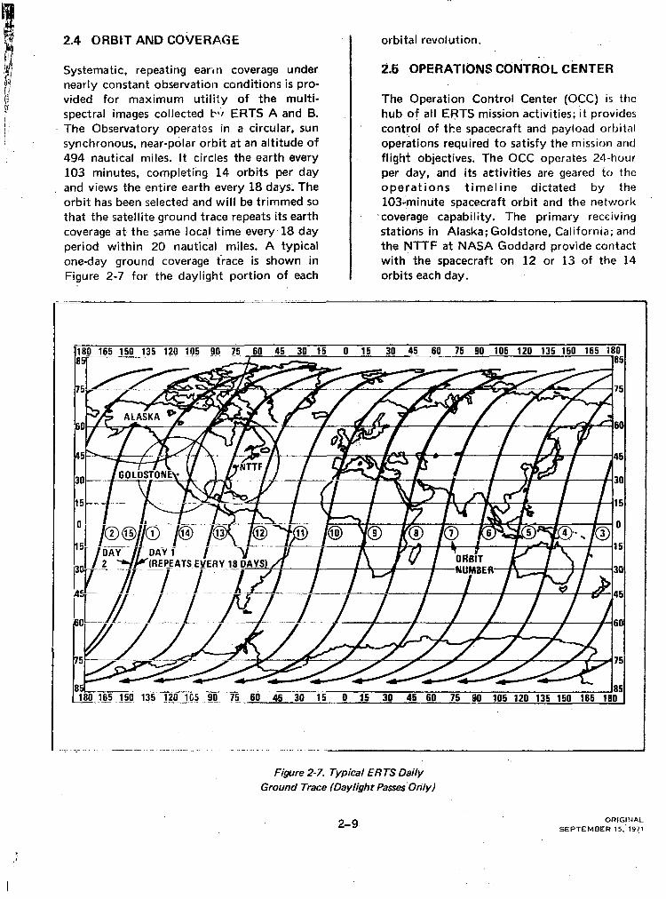
Systema tic, repeating earin coverage under nearly constant observation conditions is provided for maximum utility of the multispectral images collected blr ERTS A and B. The Observatory opera& in a circular, sun synchronous, near-polar orbit at an altitude of 494 nautical miles. It circles the earth every 103 minutes, completing 14 orbits per day and views the entire earth every 18 days. The orbit has been selected and will be trimmed so that the satellite ground trace repeats its earth coverage at- the same loca,l time every 18 day period within 20 nautical miles. A typical one-day ground coverage trace is shown in Figure 2-7 for the daylight portion of each

.I orbital revolution.

2.5 OPERATIONS CdNTFiOL CENTER

The Operation Control Center (OCC) is the hub of all ERTS mission activities; it provides control of the spacecraft and payload orbital operations required to satisfy the mission and flight objectives. The OCC operates 24-hour per day, and its activities are geared to the operations timeline dictated by the 103.minute spacecraft orbit and the network

‘.coverage capabitity. The primary receiving stations in Alaska; Goldstone, California; and the NTTF at NASA Goddard provide contact with the spacecraft on 12 or 13 of the 14 orbits each day.

--~. ho ifi 160 136 l7n in5 90 ir; 60 45 30 15 0 15 30 45 60 75 90 105 120 135 150 165 1aol

60

L- 85L,- 180 365 150 1?5 ..,-- J&l .^“... jc_s= __-_ 75 60 - .- 45 -30 15 0 15 30 48 60 hi 90 105 120 135 150 165 d5 I

F&we 2-7. Typical ER TS Daily Ground Trace (Daylight Passes’Only)

2-9

:

I

ORIGINAL

SEPTEMBER 15.’ 19!1

ORBIT AND COVERAGE

OPERATIONS CONTROL CENTER

The Operations Control Center system is shown in Figure 28. The OCC computer performs spacecraft and sensor “housekeeping”, telemetry processing, command generation, display processing, system scheduling, and processing of DCS information. Interacting with the computer and its software are the OCC operations consoles; each console has a cathode ray tube display and other station and alarm indicators. The consoles provide the operations personnel with all the information required to assess the health of the spacecraft and payloads, and to make and implement rapid command and control decisions. Each cathode ray tube is under

control of the computer, and an operator can display any data in the computot- syslom library, by immediate keyboard rcquesl, 10 evaluate the performance of any subsystem OI payload on board the spacxrafi.

The WV and MSSground station equipment provides the capability to record, process and quickly display video data acquired locally by the NTTF -station during orbits which pass over the eastern part of the United .States. DCS data is received from the three primary stations and pre-processed in the OCC for subsequent formatting and cataloging in the NDPF.

I

I kl M ANALOG

CENTRAL COMPUTER (SIGMA 6) CMD COMMUNICATION

PROGRESSORS

Q

PCM AND OCS TAPES

HIGH -) SPEEO

FRINTER

TO/FROM RECEIVING SITE STATIONS

Figure 2-8. OCC System

IMAGE DISPLAYS 000 000 0 ------

KEYBOARD KEY BOARD

OPERATIONS CONSOLES (5)

TO B= NOPF

.TO NOPF

2.6 NASA DATA PROCESSING FACILITY

The NASA Data Processing Facility is a jut)-oric!nlctl filcility which produces high quality data IlJr distribution to investigators. Figure 2-9 shows the sys..<m functional configuration.. Spacecraft ephemeris, derived from tracking data acquired by the data acquisition stations, is provided to the NDPF from the Operation Control Center. This data, along with teiemetry data containing spacecraft attitude and sensor operation information, is used to produce an Image Annotation Tape for identification, location and annotation of all imagery during image processing. There are three types of image processing performed in the NDPF: Bulk, Precision and Special. All data is Bulk processed while only selected data is Precision or Special processed.

2.6.1 Bulk Processing

Payload video data tapes are the principal input to Bulk Processing. Here an electron beam. recorder (EBR) produces corrected 55 mm images on 70 mm film of data from all

video tapes. During video-to-filln conversion, alphanumeric annotation data. tntagc IOC~I- tion, and a gray scale for calibralioll i\ recorded. Initial radiometric nntl (J~OIII(!~I I(. corrections are also made to 111~: iln,lge. 1 hc 70 mm film images produced by Bulk Pro~css- ing are developed in the Photographic Process- ing subsystem and- inspected for quality and cloud cover. The images which are requested by investigators are enlarged (if required), printed, inspected, logged, and distributed.

2.6.2 Precision Processing

Precision Processing is performed on selected image data when requested by investigators. The 70 mm film images produced by Bulk Processing are re-processed by a hybtiid system which produces corrected film images on a 9-l/2 inch format. This process removes

_ additional geometric errors not corrected in Bulk Processing and performs precision location and orthographic projection of the corrected image. relative to Universal Transverse Niercator (UTM) and geographic map coordinates.

EPHEMERlS TELEMETRY AND - DCS TAPES

RBV & MSS VlDEO- TAPES

D NDPF COMPUTER SYSTEM DCS DATA TAPES

(SIGMA 5) 1 I IMAGE

ANNOTATlON I WORK ORDERS I $ f TAPES f

BULK FlLM D PHOTO FILM

- PROCESSlNG - STORAGE

CORRECTION PROCESSING

I t TAPE t, ABSTRACTS

1 I CATALOGS

BROWSE FlLE t-

. I 1

SPEClAL TAPES t

TAPES PROCESSlNG

lNVESTlGATORS AND

--w USER AGENClES

Figure 2-9. NASA Data Processing Facility

2-11 ORIGINAL

SEPTEMBER 15. 1971

SPECIAL PROCESSING

DCS DATA PROCESSING

SUPPORT AND USER SERVICES

2.6.3 Special Processing

Special Processing is .performed on selected image data when requested by investigators. Special Proc:essing edits, calibrates, corrects, and formats digital data produced from Bulk or Preci.sion processing and outputs this data on a computer compatible digital tapes for distribution.

2.6.4 DCS Data Processing

Data Collection System data is processed, formatted and distributed to investigators on magnetic tape, computer listing or punched cards within 24 hours from the time data collection platform sensor measurements are relayed by the spacecraft to ground receiving sites.

2.6.5 Support and User Services

All of the NDPF equipment and processes are scheduled by work orders which are generated to match investigator requests against received data through the NDPF information system. The information system also serves as a data base to generate catalogs of image coverage, microfilm, abstracts, and DCS data for distribution to investigators.

It is anticipated that close to one-half million master images will be processed and stored at the NDPF each year. The storage and retrieval system aids the investigator to select only

those images that are of significance to him. Investigators have access to all NDPi dc!lcl through several files to $rovide efficiency in searching areas of interest. These aids include:

0 Browse Files - C+plete microfilm file of all available images arranged . by date and location, with a data base query and search system and image viewing equipment.

0 Coverage Catalogs - Listing in two separate catalogs of all U.S. and non-U.S. images that are returned over each 18day coverage cycle. These catalogs are updated and distributed on a regular schedule.

0 DCS Catalog - Listing of information ava;!able from the remote, in- strumented data collection platforms.

Imagery requested by investigators is processed in ‘either black and white or color frc.)m archival images stored in the master file. Samples of Bulk and Precision imagery and color composites are available to permit the investigator to select the material most useful for his purposes. Other (such as DCS tapes and listings, digital image tapes, catalogs, and calibration data) are provided to investigators either to fill a standing order or specific data requests.

C-‘C-INAL .- .

SECTIOF. :J OUTPUT DATA PRODUCTS

Investigators may choose the product or products most useful to their specific area of investigation. It is expected, for example, that investigators performing digital analyses based on scene radiance will choose computer compatible tapes of Bulk Processed Multispectral Scanner images. Those requiring the best resolution will select 70mm products; for precise location of topographical features Precision products will be used. It is not implied that a single product necessarily serves the total needs of an individual investigator, but only that the best possible quality in terms of such individual parameters as geometric accuracy, resolution or radiometric accuracy will be found in different data product. No single data product is best in

PHOTOGRAPHtC PRODUCTS

terms of all qua’lity parameters. Figure 3-1 summarizes all output data products of the NASA Data Processing Facility (NDPF) that are available to investigators. Photographic products are discussed in Section 3.1. digital products are presented in Section 3.2. and the Data Collection System (DCS) products in Section 3.3.

3.1 PHOTOGRAPHIC PRODUCTS

.The following terms and definitions are used in this section when discussing all ERTS photographic products.

Bulk refers to all imagery that contains the radiometric and initial spatial corrections introduced during the process of video tape to film conversion but not those corrections provided by the Precision Processing subsystem. Bulk photographic products are discussed in Section 3.1.1.

PRODUCT TWE

Figure 3- 1. ERTS Output Products Available to Investigators

3-l ORIGINAL

SEPTEMBER 15. 1971

. ‘.,

, , ;

PHOTCGRAPHIC PRODUCTS BULK PROOUCTS

Precision refers to all imagery that has received the radiometric and spatial corrections, including transformation into UTM coordinates which are provided by the Precision Processing subsystem. Precisron photographic products are discussed in Sect,ion,3.1.2.

Generat ion number assigned to photographic product is referenced to the bulk, archival output from the Electron Beam Recorder which is designated as the first generation. Each successive photographic product generated adds one generation. Thus, the bulk enlargement from a 70mm archival image is a second generat ion product.

Sensor Spectral Band

The relationship between the sensor, the spectral band numbers, wavelengths, and the NDPF Band Code numbers are shown in Table 3-1.

Table 3- 7. Sensor Sper: tral Band Relationships

WWdC@iS NLIPF Sensor Spectral Lnd No. (Micrometers) Bed Code

1 .475. .515 RBV 2 360 - 580 :

3 .690 - .B30 3

MS :

.5 . .6 4

.6 . .7 3 .7 . .6 6”

4 .B . 1.1 5 (ERTS B only) 10.4 -12.6 8’

Size and Scale of Photographs

Photographic products are available in two basic film sizes - 70mm and 9.5 inch (240 mm nominal). The 70 mm size is only used for bulk products. The 9.5 inch size include bulk enlarged images and precision images. Bulk processing uses the spacecraft altitude at “imCge cerjter time” to scale each 70mm image to 1:3,369,000. -When the image on 70mm film is enlarged by a factor of 3.369 and printed on 9.5 inch film, the scale is 1: 1 ,OOO,OOO. The NDPF preci.sion processed image on 9.5 inch film is also generated to a scale of 1: l ,OOO,OOO.

3.1.1 Bulk Photographic Products

3.1 .l,l image Production

The product ion flow for each of the bulk photographic products available to investigators is shown in Figures 3-2 through 3-4.

3.1.1.2 Image Format and Annotation

A sample of the RBV and MSS bulk image format, including registration marks, tick marks, gray scale and alphanumeric annotation, is shown in Figure 3-5. The MSS image format is identical, except the data does not

STRIP PRINTER GENERATE MULTIPLE c “LRCnnlLmYL .TLL

70 M M NEGATIVE

- INDICATES ALTERNATE PATH

‘

Figure 3-2. Production Flow of a 70mm Positive and Ntya tive Product

(Black and White Only)

__ Figure 3-3. Production Flow of a 9. Sinch

Bulk Black and White Films or Paper Product

COLOR PRINTER (FILM)

_._ PRINT COLOR FILM COLOR FORSHIPMENT TO

NEGATIVE USERS

PRINTS FOR SlItWENt

SE(IUFNTIALLV EXPOSE B&W 1 RIPLETS ON TR, EMULSION FILM

- INDICATES ALTERNATE PATH

SHIPTO USERS

Figure 3-4. Production Flow for Bulk Color Film and Prints

3-3 ORIGINAL SEPTEMBER 1s. 1971

BULK RBV IMAGE FORMAT

)I N 3 3

0 0

lwiie-m Iw116.30 1W11b.00 Wll4.301

ORIGINAL

5, -UBER 15. II

Figure 3-5. L&d& RBV image ‘-wmat - 9.5 Inch Film

3-4

This page is reproduced ogoin ot the bat this rqxri hy a different reproduction r _

A- I i.r, thr An.*. _ - .’

t ?

cotitain the fiduciai refer :nces (reseau and anchor marks). The spa <craft heading is always toward the annotation block.

Tick Marks GRAY SCALE

Latiiude and Longitude tick tnclrkc ,Ir(* pl,lcccl --.A-- ..- I-..

‘.

70 mm T Dncription l--izE-

Film WI& 70 70 240

NomId I&I Sizr (cross track) 560 650 185.3

Ymind lrmgr Size (in trick) 550 530 185.3

Writin4Arrr (cross trwkl 110 w 2022

Wtitin( Am fin track) rq 55.5 202.2

Awtotr:ion Block 619th a 52 175.3

Ryistmtion Mark kpwation (cross track) 55.5 59.6 197.5

Rjnntion Mark Lparation‘(in track) ” 64 59.5 215.7

Cd

9.5

REV

NOTES: ’

0 Bulk Ptouuin9 urn rpsacraft Jtituds ot “imyr cmfer time” to scat@ arch 70 mm Imae to I ratio ot 1:3,363,0W. The Eulk~nl~r~n5 factor ir 3.349 which providn l

scald of 1:1,000,000 tlw Bulk wdnrged irm9#.

0 Equivalent to 100 nwtical mllar.

0 Equivolmt IO 09.3 nmaol mllr.

Figure 3-6. Bulk Pdduc t Dimemions

The dimensions for the 70 mm and 9.5 inch RBV and MSS film products are given in Figure 3-6.

Registration Marks

Four registration marks are placed beyond the image corners to facilitate alignment of different spectral images of the same scene from the same payload sensor. The image is posi- tioned within the writing area so that when the registration marks from two or more spectral images are superimposed, the imagery will be registered. The dimensional detai-is of these registration marks are shown in Figure 3-7.

The intersection of diagonals drawn through the four registration marks is the Format Center of the image. The Format Center of a scene imaged at the same time by both the RBV and MSS will be identical. Annotation not otherwise specified refers to properties af the Format Center.

3-5

outside the edge of the image writing area at intervals of 30 arc minute. The geographic reference marks are anndtated in degrees- minutes with the appropriate direction indicator. At latitudes above 60 degrees north or south, tick marks are spaced at one-degree intervals to prevent crowding.

Gray Scale

A 15step gray scale tablet is exposed on every frame of imagery as it is produced on the Electron Beap Recorder (EBR). This scale is subject to the same copying and processing as the image to which it is attached. The gray scale gives the relationship between a level of gray on the image and the electron beam density used to expose the original image. The electron beam density is related to the sensor signal voltage which, in turn, is related to the energy incident on the sensor. This incident energy is shown in Table 3-2 for the MSS and in Table 3-3 for. the RBV.

:

ORIGINAL

SEPTEMBER 15. 1971

REGISTRATION MARKS

PASS GRAY SCALE DATA

I, A.-d

Dimension I

A

B

c

70 mm 70 mm 9.5 in. 9.5 in. RBV MSS RBV MSS

2.0 2.0 6.74. 6.74

0.0532 0.0468 9.1793 0.1578

0.0266 0.0234 0.0896 0.0788

NOTE: Dimen Isions are in millimeters

Figure 3-7. Bulk Products Registration Mark Details

Table 3-2. lrradiance at MSS Versus Image Gray Scale

Gray Scale step

1 White

2

3

4

.5

6

7

a

9

10

11

12

13

14

15 Black

Band 1 iand 2 Band 3 Band 4 Band 5 Normal Hi Gain Normal Hi Gain Normal Normal Normal Hi Gain

DATA TO BE SUPPLIED

IN REVISION

ALPHANUMERIC ANNOTATION

Alphanumeric Annotntiotl

Figure 3-9 details the alphanumeiic annota-

tion shown at the bottom, ol ‘Figure! Paragraplls a through i expl;lill the contained in this annotation.

I b c

1 2 3 1234567 901234567690123466789012345676901

07JUN72 C N33-65/Wll5-18 N 133.04/W115-20 RBV 1 DXA

Character Positions 01.08. 07JUN7i Day. month and year of picture CXpOS”V2

Character Pos111ons 09.25. CN3345/Wl15-la Format Center Latitude and I<,“- gttude dt the center (,I the RBV and MSS image lormat IS mdtcated m degrees and minuier The MS5 For ma! Center IS Idenlul to the RRV Formal Center. Form,~~ Cenler 15 defmerl as the gc<nc,r,c exton,,wt of the Lpacecraft ydw axis to the earth’s rurface.

Character Posltmns 26-42. CN33-W/W11520 Labtude and longitude of the nadnr (the Intersection with the earth’s surface of a perpendicular line from the spacecraft to the earth ellipsond) IS indicated in degrees and minutes. The NASA Efltpsoid II the Earth model.

Character Positions 43.54. RBV 1 DXA The characters an thlr group are sensor and spectral band specific: For RBV Images:

4343 Sensor and NDPF. spectral band ldentiflcation code. Note that the spectral identification code numbers are purposely staggered (see Flgure 3-9) to permit identn- flcaiion of the spectral tmager used to make a color composite transparency.

50

51-52

ERTS

NLlTES:@‘THE LETTEk”THRd”GH “i” ;EFER TO PhAGRAPHS IN THIS ChClIMENT THAT EXPLAIN THE ANNOTATION BLOCK.

0 2 CHARACTER “POSlT!ON” IN THE ANNOTATION BLOCK.

“0” indicates direct trans- mtssion (rear time); “R” indicates stored data playw back from Ihe satellilc wldeband video tape rccord- cr.

“XA” means the shutter this mago was ret for 16 milliseconds.

RBV duration of exposure wll be encoded by alpha- betlc letters ds follows:

Alphabetic Durstion of Code Exposure Tlmo

(msec)

A 16 B 12 C 8.8 D 8.0 E 7.2 F 6.4 G 5.6 H 4.8 I 4.0

For MSS images

43-51 The sensor and NDPF spectral band identification code.

#3 Type of transmission. direct or rc corded.

s. Character Position 5568. SUN EL30 AZ015 Sun Angles. the sun elevation angle and sun azimuth angle measured clockwise from true North at the time of RBV exposure or midpoint of MSS frame is specified to the nearest deprce.

r. Character. Positions 69 2. 194.1234-A Spacecraft heading, orbit revolution number. and type of ephemeris dala.

The “194” is spacecraft headmq to the nearest degree. measured clockwise from true North. It is the orbital path plus spacecraft yaw. Heading relative to an Image is al. wdys toward the ~mapo dnflotdtion block.

The “1234” is d four dlgil orbit evolution. Rev “CKIO~” starts with the first ascending node (south to north equator crossing) after launch.

NOTE: Compressed data will bede- compressed duringprocgrsing.

The “A” indiotes the ground recording tation. G’Goldstone. A=Alask&

d=NTTF.

Character positions 80.89 N-P-II-I

The “N” means the image was processed using normal processing procedures. Abnormal processing will bc indicated with “A”.

The “P” means “predicted” orbit ephemeris data WI used tc compute image center: I “0” indicates “defi- nitive” or best fit ephemeris was used. Normally tho latter IS used since It is more accurate.

w EXAMPLE

The “1” indicates a fmear mode. a “2” indicates a compressed mode of MSS signal processing prw to tranr- mission from satellite to ground $td- tion.

(This applies to Bands 4. 5. and 6 only. See Appendix A.2)

“H” is high gam. “L” II lo* 9‘“” ll,, Bands 4 and 5 only. whlrh h.wr: ., commsndablo gain optmn.

Chrrscter posltionr YW,H NA’.A ERTS

Identifies the Agency and thr! Iw,- ject.

Character positions 99.114 E-1042. 160??-10

Frame ldentificaiton Number - each image or frame will have a unique ldmtifier which wtll contain encoded infxmation consisting primarily of tirnn of exposure relatwe to launch. It5 format is E-ADDD-HHMMS-8 and is interpreted as follows:

E - Encoded Project ldentlfw A - ERTS Mission: l=ERTS A,

2=ERTS B DOD - Day number rclatw ta,

launch at t ime of obrerva tion

HH - Hour at t ime of o’wrvat~ou M M - Minute at tmw ot obserw

tion 5 - Tens of seconds ~1 tnmr: of

obserwtmn B - NDPF tdent,f,cal,on Code

(RBV: 1. 2. 3. MSS 4. 5. 6. 7. 8)

R - Blank for earth ~rnnqw, either 0, 3. or a for Rf1V radiometric callbratlon nrn- ages. indicalinq 0%. 30%. 08 80% exposure level

Figure 3-9. Details of Bulk image Annotatihn Block

7F -‘VAL - 0 -- .- .-

3.1 .1.3 Pbrformance Characteri, tics 3.1.2 Precisitin Photographic Products

A complete discussion of product characteristics is given in Appendix F. These characteristics include the effects o! the corrections (geometric and radiomet%) normally made during bulk processing.

3.1.1.4 Delivered Form

Mcst photographic products will be delivered in cut form. In special cases, when *he order is for a large number of consecutive images, film products will be delivered in roll form. Prints will always be delivered in cut form.

Roll form products will appear as shown in Figure 3-10. Note that the MSS images are grouped by spectral band; that is, sequentially adjacent images on the roll are for sequential geographical areas. These images are followed by the same sequence of adjacent images in the next spectral band, etc.

3.1.2.1 image Production

The functional production flow lor IIw WI- dus Precision photographic products is showt~ in Figure 3-11. This flow includes the initiill Bulk Processing pridr to Precision Process- ing.

Figwe 3- 11. Production Flow for Precision, Black and White and Color Products

MS FILM ROLL LAYOUT @

REV FILM ROLL LAYOUT

No TE: @ THE MSS VIOEO TAPE-TO.FILM CONVERSION PERFORMED BY THE EIJLK PROCESSING ELECTRON BEAM RECOROER (EBRI “GROUPS”THE IMAGES ON THE ARCHIVAL FILM ROLL BY SPECTRAL BANDS AS ILLUSTRATED. THE NUMBER OF IMAGES. n, IN A SPECTRAL “GROUP” IS OETERMINED BY THE NUMBER’OF SCENES ON THE lysS VIDEO TAPE. THIS NUMBER CAN VARY FROMSOME NOMINAL MINIMUM OF.SAY 12, TO A MAXIMUM OF 48. (A SCENE MEANS ONE 25SEC0110.100 BY 100 NAUTICAL MILE OBSERVATION). THE INTEGRITY OF THIS SPECTRAL GROUPING WILL BE MAIMTAINEO IN THE ROLL-FORM PRODUCTS THAT ARE SENT TO THE USER. A GIVEN ROLL WILL CONTAIN ALL SPECTRAL IMAGES FOR EACH SCENE.

Figure 3- 70. Bulk Roll Form Scene/Band Layout

ORIGINLI

3-9

I .

SEPTEMBER 15, ,!I:,

IMAGE FORMAT

PRECISION IMAGE SAMPLE

3.1.2.2 Image Format and Anyotation directly from the Bulk image. The tick marks and alphanumeric ‘annotation blocks in the

A sample of the Precision image is shown in lower left and lower right corners are unique Figure 3-12. The alphanumeric and gray scale to pt’ecision,‘data and are expl’ained in Table blocks at the left of the image area are copied 3-4.

ANNOTATION BLOCK

/ AND GRAY SCALE

E.10,2.18323 1224687&1~~

30-MINUTE LONGITUDE COORDINATIZ ALONG THE TOP EDGE OF THE TICK ;

30-MINUTE LATITUDE COORDINATES ALONG LEFT EDGE OF TICK MARK FRAME

50, OOD-METER “UTM” EASTI NG COORDINATES ALONG BOilOM EDGE OF TICK MARK FRAME

- IMAGE IDENTIFICATION NUMBER

50, DDO-METE R “UTM” NORTH IN G , COORDINATES ALONG RIGHT

J EDGE OF TICK MARK FRAME

REGISTRATION MARKS

/

(4 PLACES)

\ CARTOGRAPHIC & POSITIONAL \ DATA. BOl7OM LINE FOR

ACQUISITION DATA

OTHER DATA

Figure 3 12. Precision Processetj Image Format This page is reproduced again at the back

c ‘4L -T ihis report by a different reproduction mp” I I

Table 3-4. Format and Annotation . -. -.. .., . .._- ---- ~~

A. TICK MARK ANNOTATlON

The tick marks are indi,,iduaily printed in an unexposed band 3, millimeters wide, framing tbe outer four edges of the .iage writing are& and are slanted in the direction of the coordinate they designate.

The origin and length of the tick marks in the tick mark frame depend on the designated coordinate:

1. Latitude-longitude tick marks extend inward from the outside edges of the bands; evod- degree ticks extend 2.3 mm inward, 30-minute ticks extend 1.0 .mm inrr#rd. Degrees-minutes labeling is along the left and top margins.

2. Universal Transverse Mercator (UTM) tick marks extend outward from the inside edges of the bands; integral 100,000 meter tiiks extend 2.3 mm outward: 50.000 meter ticks extend 1.0 mm outward. libeling is along the right (Northing) and bottom (Easting) margins.

Each tick mark will. be approximately 0.1 mm thick and oriented (inclined) to within -+ one degree of the corresponding (N-S or E-W) direction.

6. INTERNAL TICK MARK CROSSES

When requested, small (2 mm) crosses desig nating the intersection of the map tick marks bordering the image writing area are printed upon the image. These tick mark lines are typically 0.5 mm widr!. The crosses locate either geographic or UTM coordinates as follows:

In geographic coordinat’es, the crosses define the intersection of each 30 arc minute latitude with each (a) 30 minute longitude for format-center lati-

tudes between 0 and 60 degrees; (b) one-degree longitude, for format-center lati-

tudes between 60 to 75 degrees: (c) even numbered degree longitude, (e.g., 0, 2,

4,. . .356, 358 degrees), fnr format-center latitudes above 75 degrees.

In UTM coordinates, the internal crosses are located at

(d1 the &rsectioa of each 50,000 meter North- ing ad Easting coordinate.

The crosses are printd with a video intensity sufficient to produce a contrast of about 0.5 density units zbove the local image density.

C. CARTO&?APHlC AND POSITIONAL DATA (lower left data block)

The first linit indicates UTM zone number in tiich tbc image is projected. (Some images will indude two UTM zones, blit the projection will be in only one zone.)

The second line indicates the positional quality as, determined by computation of the Ground Control Point (GCP) msiduel errors. Let&Is A through 0 are used as folio+:

Letter Residual Error

A This information will be

CB SUpplied in a supplement to be published later.

D

The third line is the approximate elevation in meters. It is a four digit number representing the elevation of the Ground Control Point (GCP) closest to the image rentsr.

The fourth row of characters is reserved for special data. A “P” indicates Precison Processing w done with predicted ephemeris; a blank (the normal case) indicates bet fit ephemeris was used. Other special data is TED.

0. ACQUISITION DATA (lower right data block)

The first lina is the date and time of image acquisition in Greenwich Meridian Time (GMT).

The second line denotes the date at which the Precijion image was printed.

The third line denotes the format center to the nearest tenth-minute in geographic coordinates.

The fourth row is reserved for up to 32 charac- ten of standard or special annotation data. These cfiracten are TBD.

3.4.2.3 Performance Cllarecteristics

A complete discussion of the Precision product parameters is contained in Appendix F.

3.1.2.4 Delivered Form

All Precision photographic products are de-

livered as individually cut images.

3.2 COMPUTER COMPATIBLE TAPES

Digital data is available upon request in the f&m of Computer Compatible Tapes (CCT). These tapes are standard half-inch wide magnetic tapes and may be requested in either a

3-11 ORIGINAL

SEPTEMBER 15. 1971

BULK MS5 TAPES

MSS SYMBOL EXPLANATION

9-W& or -/-track format. Coding on the g-track is EBDIC for alphanumeric data and binary for video data. All data on the 7-track tape is binary.

Four CCT’s are required for the digital data corresponding to one scene observation by either the RBV (three spectral images) or the MSS (four or five spectral images).

One of three different CCT formats are used depending upon whether the CCT’s are Bulk MSS data, Bulk RBV data or Precision data (either RBV or MSS). Data content and format of these tapes is described in Sections 3.2.1 through 3.2.3. Detailed information on CCT’s necessary to write software to process these tapes is contained in a separate document “Digital Image Tape Format” which is available through the ERTS User Services section of NDPF.

3.2.1 Eriik MSS Computer Compatible Tapes

The full frame 100 by 96.3 nautical mile image is segmented into four 25 by 96.3 nautical mile strips for conversion into CCT format.

The MSS data is spectrally interleaved as illustrated in Figure 3-13. The interleaving is

done in groups of 8 bytes, 2 bytes from each spectral band. The staggering of the spectral samples in each interleaved 8-byte group corrects for a 2-byte spatial misregistration that is introduced by the arrangement and sampling sequence of the detectors on the spacecraft. As a result of the correction, the two bytes for each band in the group repre- sent the same ground data. Dummy bytes, indicated by “O”, are used to fill in at the beginning or end of a line.

Radiometric calibration data for each spectral band is also inserted as a 56-byte calibration group following each block of 435 8-byte groups of interleaved video data.

Figures 3-13 through 3-16 illustrate the Bulk MSS CCT format and data content; symbols used in these illustrations are defined in Table 3-5.

ORIGINAL

SC ‘UBER 15. 19

Table 3-5. Explanation of Symbols Used lMSSl

item/Symbol Gescription

%kj Semglr within e,scan linezorrespond- ing to a specibed Bulk MSS video picturs element’locetion Aerr:

b%pactral bmd number (15. b< 5) kwquentiel scan !inl: index jremple number within line length

edjusted seen line Sbki Comprisinp 7 bits of video right judified in a B-bit byte

Rik Rqord corresponding to a specific ret Of/!&i comprising a segmented inter- IIUV~~ Bulk MSS scan line where:

i=image segment and Computer Compatible tape number

kisepuential scan Iills index

Bill Fifth spectral bend reco*d Mere:

Knage segment and CC tape number

k=sequential bend 5 seen line index

b line set number assigned to a set of three 4-band records (plus one 5th bend record for ERTS-B) where:

i=image segment and CC tape number

p=sequentiel line set number. For ERTS-A eech Lip contains three

4-band records. f-or ERTS B eech Lip contains three 4.band records plus one fifth band record.

CALb,k Calibration data and line length infor rnction for scan fine k of band b. Each CAEb,k is a 14.byte string.

Gk,m Group of 8 spectrally interleaved sgetially registered samples, 2 bytes from each of 4 bands where:

m=sequential group within an interleaved scan line ksequentiel full fnme scan line index Gk m contains Bulk &S video s&k Sbki in the order:

;1 ,$, si, , sp , S3 . S3 I s4 # sq k k Zm-1 2m :m-1 :m

k k k k 2m-1 2m 2m-1 2m

An interleaved entire scan line may contain a maximum of 1740 Gk m groups.

IOA Two data records consisting of scene and annotation data for each image strip recorded on CCT.

EOF End of file

Gk,m (O-BYTE “GROUP”,

I 2m.l 2m 2mLl 2m 2m-1 2m Zm-1 4 2m

NUTtS:

0 = ;‘DUMMY- ~~YTE x’ = “DATA” BYTE k, = “SCAN LINC”INDEX. THERE ARE

4086 SCAN LINES IN EACH STRIP m = “GROUP INDEX. THERE ARE 435

GROUPS IN EACH 25 NAUTICAL MILE INTERLEAVED SCAN LINE.

/’ BAND 3

SCAN LINE

ADVANCE,

(k)

EQUIVALENT MSS SCENE ON FILM.

l-l SPACECRAFT

HEADING

Figure 3- 73. Bulk MS.9 4-Band Scene to Interleaved CCT Conversion

ORIGINAL

SEPTEMBER 15. 1971

MS5 FORMAT DIAGRAMS

Figure 3- 74. Bulk MSS Full Scene, Four CC7 Format

I

mc,., 1 j G3n.1,k 1 G3n,k j "%,k j CAL2,k ) CA$, jCAQ,k 1

32 1011'111 1 j G6n.l,k j G6n,k j CAL1,k j CAL2,k i w/cLLII

%3 1-j / j G9n-l.k j'9n.k i CAL1,k jcAL2,k j cALr/

IIip.ril/ / 1 G12n-1,k iG12n,k i ':$I, j CAL2,k j CAL3,k jiAL4.k ,k

Figure 3- 15. Bulk MSS Full Scene Interleaved Record Format

I

PRECISION MSS/RBV TAPES

cA$,k(l4 BYTES)

i 6 BYTES .-+ 2 BYTES +- 2 BYTES 44-Z BYTES + 2 BYTES

/

1 1 ___-__-- .-

NOTE: LLC.IS A 2.BYTE BINARY NUMBER DENOTING THE NUMBER OF VIDEO OATA SAMPLES PER UNCDRRECiED (RAW) SCAN LINE

Figure 3- 16. Bulk MSS Calibration Group Detail

3.2.2 Bulk RBV Computer Compatible Tapes

A significant difference between the formats of the Bulk RBV and MSS Computer Com- patible Tapes (CCT) is that the MSS rorrnat has the four spectral bands interleaved, while the REV format has each band separate and sequential on the CCT - Band 3, Band 2 and Band 1. See Figure 3-17. Another difference is that there are no “calibration bytes” associated with each scan line of RBV data as is the case with MSS. No geometric or radiometric corrections are performed on Bulk RBV CCT data.

Figure 3-18 illustrates, the Bulk RBV CCT format; symbols are defined in Table 3-6.

3.2.3 Precision MSS and RBV Computer Compatible TZIXZS

The format for RBV and MSS data on a Precision Computer Compatible Tape (CCT.) is the same. A basic difference between the Bulk and Precision format is that the Preci- sion CCT in effect segments the fullframe image into 8 strips. Each strip is- further segmented into 8 blocks that contain 512

3-15

scan lines per block. Figure 3-19 illustrates the correlation between a 100 by 100 nautical mile image and the four CCT’s. Each of the four CCT’s contains approximately 1500 feet of data for a full RBV, scene or 2000 feet of data for a full MSS scene.

Table 3-6. Explanation of Symbols IRB VI

Item/Symbol Description

‘ijk Sample number within a data rocord Video Data corrasponding to a specified REV video picture element location along a

storage

segmented scan line where

i=image strip index and Compute: Compatible Tape number.

j=rgotanted sample index k=regmented seei, line index

Each Sijk contains 6 bits of video data, right justified in en O-bit byte.

Lilr A specific set ot Sijk compromising a segmented RBV scan line where:

Format Notarlon

i=imrge strip indek and CC tape number and

k=segmented sun line index.

IDA TWO data records consisting of identification and annotation data for each segmented image strip recorded on CCT.

ID Data Storage

ORIGINAL

SEPTEMBER 15. 1971

BULK RBV CONVERSION DlAGRiM COMPATIBLE TAPE FORMAT

,m NA”TICAL YILLS. ww SYTLS ,115 KY) 15 NAUTICAL Yt?ES. 1152 BYTES

I44 KY1

YACECRAFT HEAOll lG RELATIVE T” 7°F IY.BF

Figure 3- 7 7. Bulk RR V Conversion from Scene to 4Compu ter Comoatible Tape Format

BAND 3 BAND 2

TAPE 2 1=2 Lpi IG

IO AN0 ANNOTATION R2.bRZ. J375

TAPE3 L 1=3 ‘hl IG

ID AND VIDEO OATA-RECORDS ANNOTATION R3,1-R3, 1375

-

if’,‘” LpM IG IO AND ANNOTATION

EACH 25 BY 100 nm SPECTRAL BAND CONTAINS 1375 RECORDS. EACI! RECORD CONTAINS 3456 BYTES.

( ‘VAL

Figure 3- 18. R B V Bulk Scene, I-Computer Compatible Tape Format

-

I MADE AREA

4

9

4

CC TAPE 4 CC TAPE 3 CCTAPEZ

4 tl l 4

.

.

CCTAPEl

Q Q Q Q .

Figure 3- 19. Conversion of Precision Image to Computer Compatible Tape

The radiometric and geometric corrections applied to the Precision film images also applied to the digital output from Precision Processing.

Figure 3-20 illustrates the Precision CCT format; symbols are defined in Table 3-7.

3.3 Data Collection System Products

The NDPF produces three types of Data

3-17

Collection System (DCS) data products, ‘punch cards, computer listings and magnetic tapes. These products along with their contents and formats are described in Figures 3-21 through 3-23. DCS data transmission format is listed in Table 3-8.

In addition. a DCS catalog summarizing the platform transmission activity, IS prepared and distributed to subscribers on a routine basis. The catalog is described in Section 4.2.3.

ORIGINAL. SEPTEMBER 15. 1171

ITEM/SYMBOL DEFlNlTtON DATA TRANSMISSION FORMAT TAPE AND DATA RECORD FORMAT

Table 3-7. Item/Symbol Oefinitioh -.-.-.

Itsmfymbol Dwcription

sikj BarnpIe element within a dab record corrmponding to I specifiad precision video picturs slsmsnt location dongr siwn line k wiwra:

i=inwgs strip index j=sequantid sample ind.ex within

scan line krqusntial run linn within imap

s1rip

Each Siki conbins 7 bib of yideo dab. right justified

Li,k Sun lina within an inwp strip where:

i=inuge strip index krquentid yin line index

Them wa 512Siki within Bach Li k

Rin Ruord corresponding to a cd&ion of night squantial scan linn Li k of an imga strip when:

i=image strip index n=imsge strip record index

Each Rin contains 4066 bytm of precision nidso corresponding to scan lines Lik wfmm 811-7 5 k I In

IDA Two data records consisting of scene, spectral band and ‘annotation data for aach image strip racordsd on CCT

EOF End of file

fable 3-8. DCS Data Transmission Format - -.-I- ._..___ .r_.-

Word Git

1 015 16-23 2431

2 0.16 16-31

3 Eli 16.23 24-31

4 iti5 16.17 18.23

24.28 29.31

5 0.31

6 o-31

7 o-31

a o-31

Item

hform IO Batdlits IO siltion ID

‘ilays (GMT) Days Sfnca Launch

H&n (GMT) kk’nutn (GMT] Siconds (GMT) Year (GMT)

Not Used Pfatfor& ID Puality Not Used Error Flogs:

Invalid Station Coda Invalid Platform ID Poor Platform ID Oudity lnnlld Timi Coda Oupliuts,Mesuge Redundant Message

Not uwd hkmga Quality

Dab Bib

Dab Bib

Quality Bib

Ouality Bib

Mode

Binary EBCDIC EBCDIC

Binary Ei”WV

Binary Binary Binary EBCDIC

Binary Binary Binary

Bit 18 Bit 19 Bit 20 Bit 21 Bit 22 Bit 23

Binary

Binary

BiiWV

:ir-:y

BilWV

Format

xxxx

:,G,N

1.366 1.N

O-23 o-59 o-59 0.9

k- BAND 1 --+ BAND 2 -+ $7 BAND N *--q

STRIP 1 STRIP 5 CC TAPE 1 IDA 512 RECORDS ID 512 RECORDS : IDA STRIP 1

Rl.1 . R1.512 R5.1 . R5.512 F _

CC TAPE 2 STRIP 2

IDA 512 RECORDS ID 512 RECORDS 0 IDA STRIP2 R2.1 . AZ.512 R&l . R6.5?2

STRIP 3 STRIP 7 E CC TAPE 3 IDA 512 RECOROS IO 512 RECORDS 0 IDA STRIP 3

RJ.1 R3.512 , R7,l . R7.512 F

STRIP4 STRIP 3 E : CC TAPE 4 IDA 512 RECORDS ID 512 RECORDS 0 IDA STRIP4

FM.1 . R4.512 RB.1 . R5.512 F

N-CCT FORMAT, N-BAND) Rl,” 4096 BVTES 1

(DATA RECORD FORMAT) PRECISION CCT OATA RECORO RECORD n STRIP i SCAN LINES k = En-7 TO k = En 512 SAMPLES PER SCAN LINE

Figure 3-20. Precision, N-Band 4-Computer Compatible Tape and Data Record Format

r”I”,#-“. L . . L ._ . . . . . . ._ . .,I\,“,,.

1 2 3 4 6 6 7 . ‘I 1 0 1 1 1 2 1 3 1 4 1 6 1 6 1 7 1 B 1 8 2 0 2 1 2 2 2 3 2 4 2 6 2 S 2 7 2 8 1 3 4 - 4 9 - - - 5 1 1 6 7 - 7 2 D A T A D U A L I T Y (IF D E S I R E D )

D A T A F O R M A T

I ID

C A R D C O L U M N C O N T E N T C O N T E N T

1 - 2 C A R D I D S C T O INDICATE P R O D U C T R E Q U E S T , 2 6 M E s s A G E Q U A L ~ T V W H E R E : 3 - 6 U S E R I O - C O N S I S T I N G O F 4 A L P H A B E T I C 0 n L O N G O R S H O R T M E S S A G E D E P E N D I N G

C H A R A C T E R S U P O N S V N C H R O N l Z A T l O N 7 - 1 0 P L A T F O R M IO.CONSIT ING O F D E C I M A L l-l . T O INDICATE L O W E S T T O

DIGITS R A N G I N G F R O M l - loo0 H I G H E S T D U A L I T Y 1 1 S A T E L L I T E IO, 1 F O R E R T S A, 2 F O R E R T S B 2 6 D A T A F O R M A T F L A G W H E R E : 1 6 T IMC C O O E . R E P R E S E N T l N & T H E T I M E W H E N 0 = O C T A L DIGITS ( 2 2 C O L U M N S )

T H E P L A T F O R M T R A N S M I T T E D T H E D A T E . H - H E X I O E C I M A L DIGITS ( 1 6 C O L U M N S ) T H E F O R M A T IS D D O H H 1 A Y G S W H E R E : 2 8 F O R O C T A L DIGITS, D A T A S T A R T S H E R E

D O D = D A Y S I N C E L A U N C H 3 4 F O R H E X I D E C I M A L DIGITS, D A T A S T A R T S H H = H O U R O F D A V H E R E w = M I N U T E S 5 1 G U A L I T V g IGITS (IF D E S I R E D ) F O R ss = S E C O N D S ’ O C T A L S T A R T H E R E

2 2 R E C E I V I N G S T A T I O N ID W H E R E : 6 7 G U A L I T V 0 lGlTs (IF o E S ~ R E O J F O R = F A I R B A N K S , A L A S K A H E X I D E C I M A L S T A R T H E R E = G O L D S T O N E , C A L I F O R N I A

N = G R E E N B E L T , M A R Y L A N D (NTTFI 2 3 . 2 4 E N C O D E D E R R O R F L A G W H E R E :

3 2 = I N V A L I D R E C E I V I N G S T A T I O N IO 1 6 = I N V A L I D P L A T F O R M IO s = P O O R P L A T F O R M D U A L I T Y 4 = I N V A L I D T I M E C O D E 2 = D U P L I C A T E M E S S A G E 1 = R E D U N D A N T M E S S A G L

A S U M M E O V A L U E T O INDICATE A N Y C O M B I N A T I O N O F T H E A B O V E

6 3 = A L L O F T H E A B O V E C O N D I T I O N S E X I S T

_-- .--.-.-- _.. .~-. . -~ - - .-

Figure 3 -2 1. D C S Data Card Format

l U D , C A T E S T H E M G U T H . O A Y A U 0 “E A R T H A T W E L U T l U G W A S G E W E R l T E O

- U S E R ID . F O U R A L P H A B E T K C H A R A t T E A S .

r P R O D U C T L A # E L THISWILL B E O F T H E F G R Y S L A G G G l Y F O R STAl lOl”G A E G U E S T S W W E R E .

S L = S T A W O I K G R E O U E S T L IST ,GG A = E R T S A 0 0 0 - G A Y W W C E L A U M ” T H A T D A T A W A S

A C P U I R E G II” = S E O U E Y E E R U Y B E R T H A T “A R I E S F R G U

0 4 * - - - -_-_ .._ ._. .----.. .~.~.

E R T S D A T A C O L L E C T l O l l S Y S T E Y “S E A P R O D U C T S ww/oo/vv U S E R ID P G O G U C T L A B E L P A G E N M

H S S i E N C O O E G I G A T A I A U G O A T A GUALITV I B ITS -- If E H C O G E O . E G C O O E F L A O E N C O D E O V A L 0 - G A T A BIT = O W U A L I T V BIT = 1 ( G O O D , 2 = O A T A BIT - I IGUALITV BIT = G B O O l l ) F L A G

1 - D A T A BIT = 1 IGUAL ITV BIT - , l G O O O l 3 = D A T A BIT . I IGUALITV llT = O / P O O R 1

T H E P L A T F O R Y IO S A T E L L I T E IO. T IME C O P E . A ”0 T H E STATIOI I C O D E A R E O F T H E S A M E F O R Y A T S G E S C R I B E O F O R Ot# C A R D S .

FFF I H O I C A T E S T H A T G U A ‘ITV IS G O O D . A I IVTHINO E L S E I H O I C A T E S T H A T G U A L I T V IS G U E S T T I O I A G L E

E R R O R F L A G A G O T H E M E S S A G E O U A L I T V F O R Y A T S A R E T H E S A M E AI O E S C F G B E O F O G O C S CAI IOS. IF O A T A O U A L I T V IS IW E L U D E D . A N A S T 6 R U K W I L L A P P E A R II T”E “E B C O O E F L A G ” C O L U M N . IF O A T A W U A L I T V O O E S I O T A F P E A B . T”E D A T A 1 1 1 1 1 A P P E A R A S E l T H E R A S G O R A l . I F O A T A G U A I I T V I S I Y C L U O E G . A 2 O R A 3 W A Y A L S O A P P E A R

. .-- .

Figure 3-22. D C S Compu te r L ist ings Format

3 - 1 9 O R I G I N A L

S E P T E M B E R 15. 1 9 7 1

DCS MAGNETIC TAPE FORMAT

e TAPE MOTION

l OATA RECORD

HEAOER RECORD FORMAT: SEE BELOW RECOROS CONSISTS OF BG DATA BLOCKS (480 WOROS). EACH DATA BLOCK CONSISTS OF ONE DATA TRANSMISSION (8 WOROS). EACH DATA TRANSMISSION IS IN THE FORMAT OF AN AOF ENTRY

HEADER RECORO FORMAT:

STANDING REQUEST TAPE: STaOOOnnULlUUYY/MM/OO VARIABLE REQUEST TAPE: VTaODOnnUUUUYY/MM/DD

THE 1ST B EBCOIC CHARACTERS ARE THE STANDARD NDPF TAPE’LEBEL - a = SATELLITE NUMBER (1 OR 2). DDO = DAYS SINCE LAUNCH

(OF TAPE GENERATION) nn = SEQUENCE NUMBER (BINARY), UIJUU = USER ID, YY/MM/DD = DATE

OF PROCESSING (STANDING) OR DATE OF REQUEST (VARIABLE)

Figure 3-23. DCS Magnetic Tape Format

SEiZilOhi 1 USER SERV CES

The User Services Section of the NASA Data Processing Facility funct JnS as the single source of contact for all investigators and user agencies on all matters relating to ERTS data products.

Users of ERTS Lata will be able to place orders for any data product described in Section 3, and seek information and advice regarding these data, data availability and ordering procedures through this section. Contact may be by phone, mail or personal visit to the following address:

ERTS USER SERVICES Investigators may request data products either Code 563 by direct ‘mail to the NDPF or by placing a Building 23, Room E203 telephone order with a representative in the NASA/Goddard Space Flight Center User Services Section. These representatives Greenbelt. Maryland 20771 are trained to assist investigators in formatting Phone (301) 982-4018 their requests.

Users are defined to be either intiividu,lt investigators or agencies which have IWCII approved by the NASA/ERTS Project OIIKC: for receipt of ERTS data. All other data &I~~ should apply to the User Services ScctiorI which will forward their requests to thcr NASA/ERTS Project Office for approval.

I The flow of information between User Ser- vices and the user/investigator community is shown in Figure 4-1. Table 4-1 summarizes the user services acti,vities and can be used as an index to the remainder of this section.

4.1 ORDERING PROCEDURES

USER

SERVICES

e STANDING ORDERS

W DATA REQUESTS

+ IMAGE CONTENT DESCRIPTORS - REQUESTED DATA I STANDARD CATALOGS M IMAGE DESCRIPTOR INDEX A DCS CATALOGS b MICROFILM IMAGES - USER AND VISITOR ASSISTANCE F

c QUERIES OF DATA BASE

USER

AGENCIES

AND

INVESTIGATORS

-.. - .

Figure 4- 7.‘. der Services lnforma tion Flow

4-1 ORIGINAL

SEPTEMBER 15. 1971

. .

: STANDING ORDERS

DATAREQUEST

Photographic images may be ordered in one of two ways:

Standing Orders for image data which is yet to be acquired by the Observatory Data Reauests for image data that already exists in the NDPF

Digital products are available in the form of computer compatible tapes containing digitized imagery that is produced by Bulk or Precision processing. They can be ordered only by using Data Requests (see Paragraph 4.1.2).

NOTE: In the discussion that follows, the forms used by User Services are identified. The use of these forms, however, is primarily an internal function; requestors do not necessarily need to submit their ‘requests on the form but need only provide sufficient information to support the completion of the forms illustrated. This information may be provided by letter, telephone or personal visit.

4.1.1 STANDING ORDERS FOR IMAGES

The Standing Order is designed to help investigators obtain those specific photographic products he will need throughout his investigation. It permits the ordering of image products which may not yet have been acquired by the Observatory. Once generated, the Standing Order applies unless cancelled or changed by the investigator. It is expected that many Standing Orders will be submitted prior to launch, although new ones may be submitted or old ones altered at any time.

A Standing Order can specify several elements describing an image, a location, or quality attributes of the imagery desired. For example investigators may request all images taken of an area bounded by specific latitude and longitude points (up to a maximum of six points) with one of three levels of image

- “GINAL

quality, with one of eleven levels of acceptable cloud cover and a specific time period; (Example: “points of latitude and longitude for Greenbelt, Maryland, ‘good’ quality, with cloud .cover less than 20 percent, between June 1 and October 13, 1972.“) These de- limiters are placed in the NDPF computer system as a Standing Order. As observations are made and images are processed, a comparison is made to the Standing Orders. When a match occurs, a Work Order to reproduce the images and a Shipping Order to ship them to the ,investigator are automatically produced by the NDPF computer system. In this way, all data matching the investigator’s request is automatically generated for distribution to him. All data which satisfies a Standing Order will be reproduced and distributed to the requestor. No prior notification of intent to distribute data wilt be mailed out, thus it is imperative that the requestor keep his Stand- ing Orders up to date and consistent with his requirements. Figure 4-2 shows the form used in placing Standing Orders for all imagery and/or catalogs. The figure includes explanations of each entry plus an illustrative example of a complete form.

4.1.2 DATA REQUEST FOR IMAGES

The second type of order, called a Data Request, is used to order data that already exists in the NDPF. The requestor specifies the observation identification, the sensor and band identification code, the product format and product type desired. This request, like the Standing.Order, is entered into the NDPF system. Since the master images already exist, a Work Order to produce the products and the Shipping Order to ship them are generated immediately.

Figure 4-3 shows the Data Request form. The figure includes explanations of each entry plus an illustrative example of a completed form. Again it is emphasized that the User Services staff will provide assistance in com- pieting the forms. The discussion here is Intended mainly to illustrate the kind of information required.

i tem

StendinB Orders

Data Rquesk

Standard Catalogs

Image Descriptor Index

DCS Catalog

Microfilm images

Browse Facility

Queries of the Data Base

Summary Omcrfption ., --_-- - - -.~_ A- ..---.

Users may placa u Standing Order far irnqaiy wbicb may not yet have bwn squired by the Obsn~tary. All drta produced till be m&hod rgrinst Standing Orders.Whsnever an imagrr is pmmted which satisfies i Standing Drdrr, an internal NDPF rqurt will be generated to automaticoIly reproduce ud send the htttge to the rquastor. In this my the user mey request d@e wfrich dam not yetexist’Naminrl delivery tinin fs two waks from the date of rpacrtraft obamtion’to tba deto’ofsbipmmt.

Users may pface a Datl Request for the reproduition of data rlrwdy on file at tbs NDPF. The user must $ccurstely specify the data rquired. The nominal delivery time is one week if the product exists and two mekc if a n&u product must be cratd.

Standard caulk announcing the ima@ available are producml and sent to users. Separate caklop for both U.S. and non-U.S. CM#IPI are genrnted and contain data describing the irmges cdlected from a complete 18 day oovrnge cycle.

A cumulative~caklq of image dmcriptdra is produced every 30 days and distributed to the users. Tb& atelqf b generated from u stendrrd~list of irnqa descriptors supplied by individual invnstigatun’,bosed on their WUII& of imy.

A catalog summmizin~, all DCS tnr,krnissions is published on a 3Odsy cycle and distributed to’tbe users. Since the data content of tie DCS mrcrga are I function of the individual platforms which are owned by tbr investigators, the catalog only summarizes the number of messages by platform and not the mmsqe content.

The Microfilm Images provide users with data whfch they can screen to select useful images. They grossly display what ima& is available and are not fcr data analysis. Each set of microfilmed images is in exact correspondence with the Stmrdard cl&slog and is produced on an 15day cycle.

The Browsa Facility in Building 23 at GSFC is available to assist visitors in their examination and selectfon of irnagsry data. Trained personnel are available to instruct and assist visitors to the facility.

User Services maintains an interactive information system which can query and search the computerized data base to identify images of interest to an investiprtor. Access to this system is available to visitors and via telephone and mail rquesk.

Table 4-?. User Services Summary

4-3

Reference Section

4.1.2

4.2.1

4.2.2

4.2.3

4.3

4.4

4.5

ORIGINAL

SEPTEMBER 15. 1971

I .

STAtiDlNG ORbER FORM

--

ERTS 1 STANDING ORDER FORM NDPF USE

D DATE - N

ID AA

PRINCIPAL INVESTIGATOR REP

TELEPHONE NO.

SHIP TO: CATALOGS ~SIRED (NAME)

(C IT+‘)

(AGENCY)

(STREET)

(STATE)

STANDARD Cl U.S. 0 NON-U.S. DCS Cl MICROFILM 0 U.S. 0 NON-U. S.

(ZIP) _ CHECK IF ADDRESS IS NEW 0

I GEoGR*PHlC POINTS IF 2 1; 1 COVERAGE PERIOD 1-1 *L” A

ova/o L -T 2, IeA ^c @ L

UE I START STOP .yy RCRj.. F

LATITUDE LONGITUDE D R ; MMDDYY _, MMDDYY, ,E A .‘p MKKTy ’ 2 3 1234 E

---

1 i i i ii-i i i i

OF AREA OVER NORTH RANSPARENCY

AMERICA TO 10 31 72

IMAGES ONLY RECISION COLOR IMAGE

nRIGINAL --.,-CD .r

Figure 4-2. Standing Order Form

c ”

@ Gcagrsphlc Pomts

e. Letnude (Format DDMMd) where:

DD = Degrees (0’ .90°1 M M = Minoter (0’. Ss7 d = Hemisphere (N or S)

b. Longitude (lormat DDDMMd) where.

DOD = Degrees (00 . 1900) M M = Minutes (0’ . 59’1 d = Ditectmn (E or WI

The requestor specifier eitner (1 L one point or (2) three to six points es defined ov a latitude end e longitude. The defined polygon must be convex. That is, the line joining any two points wtthin the polygon must be wholly witnin the polygon as illurtrated below. Ali of the continental U.S., Alaska or Hawaii may be ordered ‘imply by inserting “U.S. , ” “A!esks” or “Haweii”. All other enws must be ordered by &g&hic poi&.

0 2 Cloud Cover, where:

0 = No cloud cove, acceptable 1 = 0.10% cloud cover acceptable 2 = 0.20% cloud c”ver acceptable 3 = 0.30% cloud cover acceptable 4 = 040% cloud cover acceptable

5 = 0.50% cloud cover acceptable 6 = O-60% cloud cover acceptable 7 = 0.70% cloud cover acceptable 8 = 0.80% cloud cover acceptable 9 = 0.100% cloud aver acceptable

Thn 1s the percem of the unsge obscured by clouds above which the image is of no value to lhe investigator.

0 9 Return Beam Vidicon Images (1 through 3 spectral bends) Multlrpatrsl Scanner Images (1 through 4 spectral bands far ERTS Al

@ Dualitv specifws the minimum acceptable quahty es defined below. (There quelitv prrsmeters refer to processmg quality and are not related to & xsge content)

G = Good Complete images with good tone. resolution end gnnularltv. Litlls or no noise.

0 10 Delete = Delete Standing Order. where entry is YES = Delete Standing Order for Products Described BLANK, or NO = Do not delete Stending Order

F = Fear Lighter or darker than good imagery or noticeable noise. P = Poor Imagery whuch is too light or too dark; partial images. or s~gmficantlv

When the NDPF system processes the users’ Standing Orders. en area number wall be assigned by the system. The requestor will be informed by mad of the afed number when his Statding Order is confirmed by User Services. If the user wahc\ to delete the area from his set of Stendmg Orders he mev enter that number I” place of letitude and the word “YES” in the delete column rather thdn rupplvmy information for the entirs form.

noisy. The requestor should speclfv the accl,ptable degradatmn. 11 any, he will accept by using one of the above codes. For ex.lmple “F” would order all good images plus ,maget which are far.

P= Processing Prod Type Method

. _.

Blank Bulk

A Precision

6 Sulk Color

C Precision Color

G Bulk

N/A. Not Applicable

0 4 Coverage Timu when:

M M = Month (start, stop) DD = Dev 01 month Istart. stop) YY = Year of month (iten. stop)

This is the coversge time perioll over which the reques!nr dewrn mugctv

0 5 Product Type where:

Blank = Bulk Photogreph!c lm& (9% mchcs) A l Precision Pbologrcphic lmege B = Bulk Color Photographic Image C * Precision Color Photographic lmege G = Bulk 70mm

0 .. 6 Product Formet where:

. N = Negetive T = Trenrpwcocv P = Print

NOTE: The prmiwbk combination of podoct tyfws end product formets ate summarized in tbr table at the bottom of tbii pa)c.

@ Tick Mbrk where (Precision image only):

Blank = No’intarnal tick marks in image aree ll = Universal Transverse Mcrcetor (UN) tick marks (See reference

‘“gridding”) L = Geographic tick marks

@ Numbe! of Copies, where NN designates the acruel number of products drsurrd buner~ul). Maximum number bf copies is 63.

SUMMARY OF PRODUCT TYPE AND PADDUCT FORMAT c.i

I :_-- F = Format ~

I N = Negetive . T = Transparency P = Prmt

Black and White 70 M M Negetive Black and White 9.5” x 9.5” Black and White 9.5” I 9.5” Positive Tranrperencv Positive Print

Black and White 9 5” x 9.5” Negative ’

Black and.Whitr 9 5” x 9 . . 5” Bleck and White 9.5” x 9.5” Positive trenpsrency Positive Print

N/A Color lv X 1D” Positive Calcr 10” x lo” Positive Prmt Trensperency

N/A Color lo” x 10” Positive Trensperency

Color 10”~ 10” Positive Print

Black and White 70 M M Neptirs Black sod White 70 M M Positive Tnrirperencv

N/A

4-5 OHIGINLL

SEPTEMBER I :. ,971

DATA REQUEST FORM

DATA REQUEST FORM

DATE

1. USER ID 2. -.

3. NAME 4.

5. 6. USER ADDRESS

7.

a. TELEPHONE NO.

9. DATA REQUESTED

ADDDHHMMS ,=

EXAMPLES

113210223

t ERTS A I

t

R&I

f I

L - I

I POSITIVE

f .--f

I 5 &ES 132 DAYS SINCE LAUNCH / TRANSPARENCY 1

P= PROD. TYPE

-

F= T= NN PROD. TICK NUMBER FORMAT MARKS COPIES

CD

T

NEW0 CHANGED ADDRESS/“-J

AGENCY A&R.

NDPF REPRESENTATIVE

CATALOGS DESIRED

STANDARD Q U.S. q NON-U.S.

DCS q MICROFLLM /JIJ.S ANON-U.S.

u ‘5

COMMENTS

-0

10 HOURS OF THE DAY 22 MINUTES OF THE HOUR 30 SECONDS

PRECISION COLOR IMAGE

UTM TICK MARKS

NO COMMENTS

ORIGINAL -‘c. -PC-” .

Figure 4-3. Data Request Form *

* c

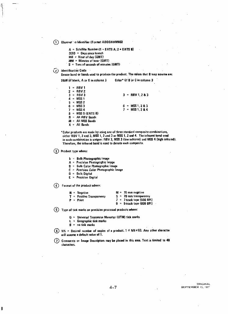
0 1 Observar XI Identifier (Format ADDOHHMMS)

A = Satellite Number{1 = ERTS A;2 = ERTS 6) DDD = Days since launch HH = Hour of day (GMT) M M = Minutes of hour (GMT) S = Tens of seconds of minutes (GMT)

3 identification Code Sensor band or bands used to produce the product. The values that 6 may assume are:

E&W (if blank, A or G in column 3 Color* (if B or C in column 3

1 = RBVl 2 = RBVP 3 = REV3 4 = MSS 1 5 =. MSS2 6 = MSS3 7 = Mssll 9 = MSS5(ERTSB) R = All.RBV Bends M = All MSS Bands X = All Bands

3 = RBV1,2&3

6 = MSSl,2&3 7 = MSS1.2914

‘Color products are made by using one of three standard composite combinatiuns, either RBV 1, 2 and 3, MSS 1,2 and 3 or MSS 1,2 and 4. The infrared band used in each combination is unique: RBV 3, MSS 3 (low infrared) and MSS 4 (high infrared). Therefore, the infrared band is used to denote each composite.

0 3 Product type wfrere:

b = Bulk Photograpfric Image A = Precision Photographic Image B = Bulk Color Photographic Image C = Precision Color Photographic Image 0 = Bulk Oigital E = Precision Digital

0 4 Format of the product where:

N = Negative M = 70 m m negative T = Positive Transparency S = 70 m m transparency P = Print 7 = ‘I-track tape (556 BPI)

9 = g-track tape (BOO BPI)

@ Type of tick marks on precision processed products where:

U = Universal Transverse Mercator (UTM) tick marks 1 = Geographic tick marks B = no tick marks

@ :!I zsu,a default value of 1. Desrred number of copies of a product. 1 i NNr63. Any other character

@ Comments or Image Descriptors may be placed in this area. Text is limited to 40 characters.

4-7 ORIGINAL

SEPTEMBER 15. 1971

DELIVERY SCHEDULE

DATA CATALOGS

4.1.3 Delivery Schedule

All data produced as a result of Standing Orders are normally shipped within two weeks after the date of sensor observation. Depending upon the data requested and the data processed, the. imagery sent to the investigator may consist of only the -data requested or it may also include unreque&ed data which was processed at the same time. In general, ati attempt will be made to produce only the requested materials; the economics of production may, however, result in the distribution of additional products.

Data Requests which require only reproduction of existing master imagery will normally be shipped within one week. Requests involv- ing the generation of new products from in-hand raw data require two weeks. To hasten delivery of requested data, the NDPF will prepare partial shipments when a delay of five or more days is required to complete the order.

4.1.4 Requests for DCS Data

Requests for Data Collection Systems data are processed separately from the image requests. Data may be requested on a Standing Order basis or on a Data Request basis. All orders must specify product type and platform number. A fuller discussion of the DCS products and their distribution is contained in Section 4.2.3. Because the NDPF anticipates a relatively stable DCS user community, no request forms have been prepared. All requests will be processed on an individual basis by User Services.

4.2 DATA CATALOGS

One of the most important functions of User Services is the prompt announcement of the image and DCS data acquired by the observatory. Because the user community has many and varied requirements, the catalogs are designed to provide a maximum degree of announcement flexibility. Thus, for example, Standard Catalogs are divided into discrete U.S. and non-U.S. volumes. The user may choose to subscribe to either or both catalogs.

In addition to producing Standard Catalogs, the NDPF generates 16 trim microfilm data sets which correspond to each of the Standard Catalogs. These catalogs and &,icrofilm sets are published etiery 18 days. A cumulative index of image descriptors and a catalog OI DCS transmissions are generated for dislribu- tion every 30 days. The d&tents and format of edch catalog are treated in the following

.pariigraphs.

4.2.1 Standard Catalogs

Every 18 days a U.S. Standard Catalog, covering the continental US: plus Alaska and Hawaii, is produced by the NDPF and issued approximately three weeks after the start of the 18-day orbital coverage cycle (see Appen- dix I). Each Standard Catalog contains image data for an 18-day period and consists of an outline map graphicaliy ciisp!;;ing coverage, and a computer listing tabulating by observation number the imagery obtained in sequential order. Catalogs for non-U.S. data are identical in format arid are prdduced nine days out-of-phase with the U.S. catalog.

4.2.1 .l ,Standard Catalog Outline Map

Each of the two Standard ,Catalogs contains an outline map. The U.S. Standard Catalog has outline maps of the$Jnited States including, Alaska and Hawaib?‘jsee Figure 4-4), and the non-U.S. Standard Catalog contains an outline map of the world (see Figure 4-5). Each of these maps indicates which areas have been imaged during the 18-day period covered by the, catalog. In addition, the U.S. outline map shows an estimate of the cloud cover contained in the imagery by a four shade spectrum along the subsatellite path for each north to south pass. No shading indicates that no imagery was collected.

4.2.1.2 Standard Catakg Page Listing

A large part of the Standard Catalog consists of computer listings produced from the infor- r.,ation systems data base. All listings are in se;quence by observation identifier. The NDPF has established three nested levels of ERTS imagery identification: an Observation iD.

- “GINAL -.. .-

_ .-~ ..-._.- .: . 7

Figure 4-4. Sample Con tinen tal U.S. Ou the Map

1no l!x 120 90 60 30 0 30 60 90 I20 160 190

0 30 60 90 i20 150 190

Figure 4-5. Sample World Map

4-9 ORIGINAL

SEPTEMBER 15. ,971

ID FORMAT AND CONTENT

an Image ID and a Product ID. Figure 4-6 MSS Band 2 images are also available ir explains the format and content of each type continuous tone microfilm format as de- of identification. All orders, announcements, scribed in Section 4.3. For every 18 day queries and image annotations utilize one of observation cycle, the microfiim roll number these identifiers. is listed, followed,by entries for the individual A sample catalog page with an explanation of observations which are on the specified nricro- its contents is shown in Figure 4-7. RBV and film,roli. ‘,

. _--.. -_.

OBSERVATION ] r

DAYS SINCE LAUNCH

HOUR OF DAY (GMT)

MINUTES OF HO&-I (GMT)

TENS OF SECONDS OF MINUTES (GMT)

-A I, ii000H~~MSj B=SENSOR SPECTRAL BAND OESIGT~ATOR

IO I

t

-

IMAGE IO } [A~~~RHMMSB .BANO B

1 2 3 4 5 6 7 8

R M X

RBVI RBV2 RBV3 MSSl ’ MS!%? MSS3 MSS4 MSSS (ERTS B ONLY)

\TELLITE NUMBER (l=ERTS A; P=ERTS B)

’

SI

P=PROCESSItiG DESIGNATOR

P

BLANK A B C 0 E X

PROCESSING TYPE

BULK PRECISION BULK COLOR PRECISION COLOR BULK DIGITAL PRECISION DIGITAL NON-STANDARD PROCESSING

L

ALL RBV BANDS ALL kjSS BANOS ALL BANDS

Figure 4-6. Observatic ,I, Image and Product identification Number Formats

4.2.2 Image Descriptor imex

4.2.2.1 Index

The NDPF does not perform any content analysis of the images, nor ‘s any examination conducted of the data to determine terrain features or other phenomena.The NDPF I nformation System, however, accepts and records image descriptors supplied by investigators. An image. descriptor is a term which assists in defining the content of an image. For example, an image may show a rain forest with mud flats surrounding a pasture. A user

inspecting this imitge may choose lo tl~c~ II)L* the image with the terms Rain F~~rt:~,l. M~rtl

’ Flats, and Pasture.. All irnagc! tlc!~ I ~t)I(rt*. returned to the NDPF by inveslig,rlor5 WIII 1~: compiled and ,entered into the Li~‘l S &ILI batik for subsequent user query servicing.

Every 30 days a cumylative Image Descriptor Index is published, containing each image descriptor that- is stored in the Image Descrip- tor Data Bank file. This index allows investigators to tabulate various findings pertaining to each image, and to index these findings via image descriptors in a catalog available to all investigators.

0 2 0 I . 04/29/72 STANOAR CATALOG 04/10/72 TO 04/27/72 PAGE t

KEY 10 WAGE CLAAIIY

0 3 G : : GooD F FAIR P POOR 0 4

THE IMAGES INDICATED BELOW ARE ON YICROFILY ROLL NUYBER:OOl

BULK PREC. ORSERV. IC YICR. PPS.# DATE CLOUD PRINCIPAL POINT SUN SUN RBV YSS EiULK COLOR PREC. COLOR DIGITAL DCS

RBV 11SS COVER OF IMAGES ELEV. AZIY I 2 3 I 2 3 4 RBV YSS RBV YSS R9V YSS REV YSS RBV YSS OATA

A00112250 0001 0002 07/01/72 45 44.29011 83.2901 31.2 31.2 C G GPP PF X X X X X X X X X X K

A00112255 0003 0004 07/01/72 60 42,5t~UH~)j5OOW )0.4 30.4 9 G G 0 C G 0 X X X X ‘X X X X X X

A00112258 0005 0006 07/01/72 40 40.4OOtt (4.2101 30.0 30.4 F F F 0 0 F F X X X X X X X X X X

100112263 0007 0006 07/01/72 30 40,lOON 80,413OW 28.8 30.4 PF 0 F F 0 P X X X X X X X X X X

A00112265 0009 0010 07/01/72 35 3.9.5101 115.2601 28.0 30.5 C G G C F F F X X X X X X X X X X

A00212250 0011 0012 07/02/72 20 37.19011 85.5001 28.0 30.2 P PP PPGG X X X X x x x

A00212255 0013 0014 07/02/72 30 35.19OW 16.19OW 27.9 29.9 F F F GG P F X X X X X X

A00212258 0015 0016 07/02/72 IO 34.34011 86.59OW 27.9 29.8 G G G G G G G X X X x x x x

100212263 0017 OOIB 07/02/72 I5 35.29011 87.1001. 27.0 29.7 F F F G G G F X x x x x X

A00212265 0019 0020 07/02/72 45 31.49011 87.49011 278 29.7 G G F F F F G X X X X X X X X l sTOPn 0

0 12 0 13

I COdY Meaning Definition

Blank Band not pacnt (no image WA rnltablr in tbir band)

G ,Good Imap Complete image with good tone, raolution and gnn. ularily. Littte or no noise

F Fair Image Lighter or darker than”good” imagery or noticeable now

P Poor Image Very light or dark image. @aI image or slgmbcant noise

.-.

Figure 4-7. Annotated Sample of Standard Catalog

4-11 ORlGlPlAL

SEPTEMBER 15. ,971

IMAGE DESCRIPTOR INDEX

INDEX SAMPLE PAGE

Figure 4-8 shows a representative page from the Image Descriptor Index. The index is organized alphaketicaJly by image descriptors and each descriptor has the product, ID’s for the images which have been assigned this descriptor listed below it. Each image descriptor is presented along the left side of the printed page followed by up to 10 columns of product ID’s. It should be noted that in some cases the reference is to an observation; i.e., all spectral images in that scene contain that feature, whereas in other cases the reference is to a single spectral image or product type. In the latter case the descriptor applies only to the specific product and not to other images in the observation. By way of example, note the first column listed under flood plain. The first entry indicates that only the image of MSS Band 4 (spectral band code - 7) contains useful data related to a flood plain. The second entry indicates that,all bands of both sensors contain data showing flood plain.

The format of the Image Descriptor Index is a series of pages, as illustrated, preceded by a

concordance, which lists all image descriptors and. the number of times each was used. A sample concordance list is shown in Figure

I 4-4.

Februarjr23,Nfi _’

COjUCORDANCE LISTING

NO. DESCRIPTORS

CANYONS HYDROLOGY VOLCANO CITIES FOREST ZOLOGY GEOLQGY OCEANOGRAPHY MILITARY DESERT

Figure 4-9. Sample Page, Concordance Listing of image Descriptor Index

Figure 4-8. Sample Page of Image Descriptor Index

‘GINAL

4.2.2.2 Forms

When images are shippetl to investigators, a forum IS included lot. lisling lhe appropriate im,lge clcscriplors a11d idclltificrs. Figure 4-10 illustrates a sample lmag Descriptor Form. Investigators are requested to mail this form back to the NDPF after they have analyzed the images and noted the descriptors they feel pertain to each image.

After the Investigator’s Name, Date, Investi- gator’s ID and Agency fields are completed, the investigator should decide if there are any descriptors he. believes will be used consider-

ably more frequently than others. If there are such descriptors, the investigator writes them in the first row of blank columns under the header, FREQUENTLY USED DESCRIP- TORS. Each image ID to which th(h inveslig,ll(~t assigns, descriptors is written III Itw I?~().

D.UCT ID column. The identificaliorr IIIC~LI~~C~~

band and product type codes.

If an image is’.to be described by a descriptor inthe FREQUENTLY.USED Dl%CRIPTORS column, a check (,/) mark is all that is required. ‘Other descriptors which are not frequently used are written separately in fhe DESCRiPTORS column.

ERTS IMAGE DEX;F?IPTOR FORM

USER NAME DATE

USER ID

AGENCY ~~

Figure 4- 10. Image Descriptor Form

ORIGINAl

SEPTEMBER 15. 1971

VOCABULARY

DCSCATALOC

4.2.2.3 Vocabulary

The possibilities of cooperative exchange of information through the use of irhage descriptors are numerous. The ease of exchange, however, can be greatly increased by establishing a common vocabulary. The NDPF computer system has been implembnted to handle two types of image descriptors; the first type is from a suggested vocabulary supplied to e&h user and the second type is one which an investigator creates and is not contained in the suggested vocabulary. The two types of descriptors together comprise what is known as an open vocabulary. No restrictions are placed on investigators who wish to supply their own descriptors.

The suggested vocabulary has several advan- tages over the open vocabulary:

1. It maintains a consistent use of descriptors from one image. to another

2. It simplifies the exchange of information among different user groups.

As a step toward the development of a suggested vocabulary, a list of approximately 400 terms has been compiled that pertain to remote sensing of earth resources; the vocabulary is presented in Table 4-2. The terms were chosen for their diagnostic potential in evaluating ERTS imagery.

The suggested vocabulary is provided as the basis for which individual investigators may describe image contents which fall within their field of interest. As might be expected from such an abbreviated grouping, all earth resource disciplines may not yet be eve,nly represented in the suggested vocabulary.

Information searches of the data base may be made using descriptors from the open vocabulary. The difficulty here is that the descriptors from the user-created vocabula.ry are only known to the person or group entering them into the system, which tends to reduce the

overall.value of the analysis and d,ecreases the exchange of inforinatio.n between groups of users.

4.2.3 DCS Catalog

The Data Collection System (DCS) ~clay: messagei from platforms to the NDPF- lot- distribution to users. The nature of the messages is a function of the platform and its instrumentation sensors. Since each, platform is different and separately owned by specific investigators, the NDPF limits its processing to validations, sorting, arid formatting. As a result, the DCS Catalog is restricted. to a summary announcement of the data collected during a 30day reporting period.

The Catalog is printedanddelivered every 30 days and contains the following for each platform:

1.

2.

3.

4.

5.

6.

7.

Platform identification

Primary user’s iaentification

Platform geographic location (lati- Jude and longitude)

Time of first transmission in the reporting period.

Time of the Ias.; transmission in the reporting period

Total number of messages within this time range

Total number of messages sent by the platform since its inception

The format of this DCS Catalog listing is shown in Figure 4-l 1. Additional information concerning the platform sensor package, the sensor units and calibratiuns, and the message formats are normally available from the primary user. The User Services Section maintains an up-to-date list of all primary users dnd platform owners and will provide assistance in obtaining information for other investigators.

Table 4-2. Earth Resources Vocabulary -- . ..-.- - - .._ -~ ~-~ - -

A AC clinal vdk)’

ACl ivc Glaclcr

Active Volcano Actiniform Clouds Adobe Flat Advancing Glacier Advancing Shoreline Aerial Imagery Used Agriculture Airfield Alfalfa Algal Bloom Alkali Flat (use Salt Flat) Alluvial Cone Alluvial Fan Alluvial Flat Alluvial Plain Alluvial Terrace Altocumulus Altostratus Anaclinal Stream Anaclinal Valley Annular Drainage Pattern Anticlinal Mountain Anticlinal Valley Anticline Anticlinorium Anvils Aquifer Arroyo Ash Cone (use Cinder Cone) Atoll Atoll Reef Avalanche Avalanche Scar Axial Stream

% Back Bay Backshore Badland Baiada Barbed Tributary Barchan Barley Barrens Barrier Bar Barrier Beach Barrier Flat Barrier Island Barrier Lagoon Barrier Lake Barrier Reef Basin Basin and Range Batholith Bay Bay-Head Bar Bay-Head Beach Bay-Head.Delta Bay Ice Baymouth Bar Bayou Bed Bedrock Belt Belted Plain

-. . . .-- .._-.

% (conr ‘d) UIIIOW Billow Cloud I~iolumlncscence Bird-Foot Delta Blight (use Diseased) Bog (use Marsh) Braided Stream Breakwater (ULC Jetty Bridge Broken Clouds Brush Butte

C Caldera Canal Canyon (use Valley) Cape Cartography Catchment Area Cay Chaotic Cloud Pattern Chaperral Cinder Cone Cirque Cirrocumulus Cirrostratus Cirrus Cirrus Shield Citrus City Clearing Closed Basin Closed Fault Closed Fold Cloud Streets Coast Coastal Current Coastal Dune Coastal Marsh Coastal Plain Coast Line Col (use Gap) Cold Front Cone Conifer Consequent Lake Consequent Stream Consequent Valley Contact Continental Shelf copses Coral Head Coral Reef Corn Cotton Coulee Crater Cropland Cross-Bedding Cross-Fault Cuesta Cumulonimbus Cumulus Current cusp Cyclone

D Dam tMUOU5

Deltalc Coastal Plain Dendrltic Drainage Depre5siort Desert Desertline Dlke Discased’Vegetation Divide Dome Dormant Vegetation Drought Conditions Drumlin Dune

E Earthquake Damage Echelon Fault Eddy EE6 (Excellent

Example of) Keyword End Moraine Entrenched Stream Erosion Esker Estuary

F Fall Line Fallow Field Fan Fault Flngcr Lake Fiord Fire Firebreak Fire Damage Flood Flood Damage Floodplain Fog Fold Forest Forest Fire Forest Fire Damage Frost Damage Frontal Wave Frozen Lake Frozen Soil

G Gap Geofracture Geography Geology Geosyncline Glacier Gorge (use Valley) Graben Grass Grassland Gravel Deposit Grazing Land (use Pasture) Ground Truth Used Gulf

H Harbor Hardwood t.orr\t

I Hav Haie Highway Hogback Horst Hourglass Valley Hurricane Hurricane Damage Hydrology

I Ice tceberg Ice Floe Ice Jam Ice Pack Ice Shelf tRt (Image .

Referenced in) Journal Industrial Area Inlet lnlier Insect Damage Inshore Zone Insequent Stream tnterlacing Drainage lntermontane Floor Intrusion Irrigation island Island Arc Isthmus

J Jet Stream Indicated Jetty

K Kame Karst Kelp Kettle Key (use Cay) Klippe

L Lagoon Lake Lake Bed Landslide Laterite Lattice Drainage

Pattern Lava Lee Wave Lineament Littoral Current Littoral Drift Littoral Transport Locust Swarm Locust Damage Longshore Bar Longshore Current Lumbering Area

4-15

VOCABULARY LIST

Table 4-2. Earth Resources Vocabulary

M Maar Marsh Massif Mature Stream Mature Vegetation Meadowland Meander Mesa (use Butte) Meteor Crater Meteorology Metropolitan Area Microwave Data Used Millet Mine Monoclinal Valley Morainal Delta Morainal Lake Moraine Mountain Mud Mud Flat Muskeg

Z$pe Nunatak

0 Oasis Oats Occluded Front Oceanography Oil Field Oil Slick Open Pit Mine Orchard Orographic Cloud Outlet Outlier Outwash Plain

F Parallel Drainage Park Pass (use Gap) Pasture

~(cottt ‘d) , Pediment

Pediplain Pcncplain Peninsula Permafrost Piedmont Piedmont Plain Peidmont Scarp Pier (use Jetty) Pinnacle Plain Plankton Bloom Plateau Playa Playa Lake Plowed Field Pond(use Lake) Potatoes Prairie Pressure Ridge Protozoans

Q Quarry

R Radial Drainage Pattern Railroad - Rain Forest Raised Reef Rangeland Rapids Ravine (use Valley) Rectangular Drainage Red Tide Reef Reservoir (use Lake) Residential Area Retrogressive Shoreline Rice Ridge Rift Rift Valley River Road (use Highway) Runoff Rural Area Rust

S’ Saline Dome Saline Sol1 Salt Salt Flat Salt Marsh Sand Dune (use Dune) Savannah Scar Scattered Clouds Scrub Sea Sea Grass Sea Wall Secondary Front Sediment Shallow Water Shield Shipyard Shoal Sitt Sink Slash Slick Smcg Smoke Snow Snow Pack Soil Soy bean Split Spring Squall Line Stationary Front Step Fault Steppe Stoss-and-Lee Topography Strait Strath Stream Suburban Area Sugar Beet Sugar Cane Swamp (use Marsh) Synclinal Valley Syncline Synclinotium

T Tarracc Tidal Fldt

Tidal Wave Tidal Wave Damage Thrust Fault Timber line Tobacco Tombolo Tornado Tornado Damage Towering Cumuli Transverse Fault Transverse Valley Trellised Drainage Trench Tributary Tsunami Tsunami Damage Tundra Typhoon Typhoon’ Damage

‘u Upwelling Urban Area

"V Valley Vegetation Vineyard Volcano

Wadi (use Arroyo) Warm Front Wave Wharf (use Jetty)

XYZ

-lGlNAL

DATA COLLECTION SYSTEM CATALOG MM/OD/YY PAGE N’N

CATALOG CYCLE: ttIOM MM/DD/YV TO Ml’~~Si/DD/VV

PLAT. IO USER ID LATITUDE LONGITUDE TIME PERIOD TOTAL NO. OF NO. OF

FROM TO MESSAGES MESSAGES

N E -- S, DEG, MiN W-JJEG-M1N - -

Figure 4- 11. Format of DCS Catalog Listing

4.3 MICROFILM IMAGES

Every 18 days the NDPF fvlicrofilm Facility produces high quality 16-mm microfilm of

.representative imagery covering one 18 day observation cycle. These images are soleiy to indicate to the investigators what imagery is available and are not in?ended for data analysis.

As in the case of the Siandard Catalog, the microfilm data is divided into U.S. and non-U.S. segments. Each set of microfilm images is in exact correspondence to a Stan- dard Catalog and can be used in conjunction with the catalog for selecting desired, images. The catalog contains roll and position numbers and data which, along with the microfilm image, provides the investigator with enough information to decide whether or not the observation (scene) is useful to him.

Because the microfilm Images are intended to provide only a summary of the data available, the images are limited to one band each for the RBV and MSS. Thus, although a single observation will produce seven (eight for ERTS B) images, in the production of microfilm only the RBV Spectral Band 2 images and the MSS Spectral Band 2 images are

reproduced on microfilm. Each image 15 o photograph of a bulk processed image antJ contains the image identifier and full annotation block as described in Section 3. A typical roll of microfilm contains the following:

0 1 Leader Frame of Microfilm Identi- fication

l 1 Leader Frame of Map Coverage (Outline Map as contained in the Standard Catalog)

0 Up to 1000 Frames of RBV Images

l Up to 1000 Frames of MSS lrnages

The microfilm is on open reels suitable for mounting by the user in a cartridge of his choice. Two rapid search capabilities are incorporated on the microfilm. The first allows counting images for precise location of them and requires the counting capability on the viewer being used. The second is a moving bar indicator which permits gross locating of images to within about 200 images. Details of these two schemes are described in the Stan- dard Catalog..

MICROFILM IMAGES lJSER/ViSlTOR ASSISTANCE

I v

ERTS OBSERVATlbN NO. 1 2 ETC. (TO 1000)

Figure 4- 12. Sample Format of Microfilm Roll

The RBV and MSS image frames will be alternating per observation on the. roll of microfilm as shown in Figure 4-12. The total number of rolls of microfilm pr,oduced in an 18-day cycle is:

Approx Total No. Coverage No. of Rolls of Images Breakdown

U.S. 1 2000 1000 RBV images 1000 MS5 Images

NonUS. 3 5000 2500 RBV images 2500MSS!moges

A complete set of microfilm data is maintained in the NDPF Browse Facility for visitor’s perusal. High volume production of the microfilm data has been provided and data se.& are available for routine distribution to users.

4.4 USER AND VISITOR ASSISTANCE

Assistance is provided to users and NDPF visitors by specialists in the Browse Facility where a means of examining and selecting products in a convenient and well-equipped facility is provided. Visitors to the Browse Faciiity may place orders for images here and receive technical aid through associated pubii- cations contained in the Browse Facility library.

The Browse Facility, located in Room 204, Building 23, at Goddard Space Flight Center.,

-RIGINAL -C. -co . .

Greenbelt, Maryland, contains the products and references listed in Table 4-2.

Table 4-2. Broke Facility Contents

9

I. Selected data samples of 9-112 x 9-l/? inch positive traaparancies end prints consisting of:

a b:

Eulk pr’ocesred REV and IWSS images Pracision processed RBV and MSS images

C. Color compositg images

2. l&mm roils of microfilm (black and white images) . quantity equal to the number of l&day coverage cycles completed.

a. U.S. data coverage (1 roll per 19 days) b. NowU.S. data coverage (3 rolls per 19 days)

3. Data Collection System data

4. Image annotation data

References and Facilities

1. Atlases (U.S. and World)

2. Date Catalogs

a. Standard Catalog b. Image Descriptor Index

3. Light tables for image msptition 4. Microfilm vw.wers (manual al&index search) 5. Remoie CRT Computer Terminal (for a NDPF InformatIon

Systems data base search and query.

6. Table workspace

I. Traineri ERTS perspnnel for,oser assistance

A full-time Browse Facility assistant is available to instruct and assir visitors in the capabilities and operational aspects for the NDPF Browse Facility. The assistant will place orders lor imagery, catalogs, or microfilm for investigators desirip retention copies and will instruct and aid investigators in the use of the query system.

The Browse Facility assistant is available to demonstrate the 2-d of catalogs, atlases and use. guides. A log of all reference material is maintained in the Browse Facility and ii available to visitors. The assistant will provide instruction for operation of light tables, microfilm viewing equipment, and the CRT terminal.

4.5 COMPUTER QUERY AND SEARCH CAPABILITY

Information about every image processed is maintained in a data base in the NDPF computer. This information consists of two basic types:

1. Imagery parameter information always available from the normal NDPF activities such as in Table 4-3.

2. Information resulting from investigator analysis of images and subsequent submission to the NDPF in the form of user supplied image descriptors.

In order to permit investigators to con- veniently search this data base in a flexible manner, a special computer program known as Query Processing is available. It can be used either in a batch mode or in an interactive mode directly from a remote Cathode Ray Tube (CRT) terminal in the Browse Facility. In addition, investigators may phone a User Service representative and research the data base with the User Service representative operating Query Processing from his remote computer terminal.

A complete manual describing the Query Processing program is available at the NDPF or can be obtained from the NDPF.for those

investigators expecting to make frequent use of this service. 1

Table 4-3. Imagery Parameter II I fortr t;t riot t Stoked irj NDPF Computtcr

Observelion IO Sun Elevation

Orbit No. Sun Azimuth

Station ID Duality (Good. Fair, Poor)

Ephemeris Type Cloud Cover (percent) (Best fit or predicted)

innsmission Mode Geograpliic Area (Direct or Worded)

Altitude Time

Heading Sensor

Track lmrge Product (Type & Spectral Band1

The program is such that a search can be made for given time periods, given geographical areas, any one of the items listed in Table 4-3 or by any descriptor in the Image De- scriptor Catalog supphed to users. Moreover, the program is sufficiently flexible to allow almost any logical combination of search criteria to be specified.

The normal output of a search is the number of images found which meet the specified search criteria. Additional outputs can be specified as follows:

1.

2.

3.

A Listing of all image identification numbers for those images satisfying the search.

A Catalog as shown in Figure 4-13 containing one-line descriptions of each image which satisfy the search criteria. The information for each image is essentially the same as detailed in the Standard Catalog.

An Image Output which is a printout of all data in the data base for each image which satisfy the search criteria. See Figure 4-14.

4-19 ORIGINAL

SEPTEMBER 15. 1971

BROWSE PROCESSING EXAMPLES

-1 --

04/29/72 STANDARD CATALOG 04/10/72 TO 04/27/72 PAGE I

KEY TO IYAGE CLARITY e

G : GOOD

F : FAIR

P : POOR

THE IMAGES INDICATED BELOW ARE ON MICROFILM ROLL NUMBER:001

BULK PREC.

OBSERV. IC MR. PAS.# DATE CLOUD PklNClPAL POINT SUN SUN RBV YSS BULK ” COLOR PREC. COLOR DIGITAL DCS

REV YSS COVER OF IMAGES ELEV. AZIY. I 2 3 I 2 3 4 RBV YSS RBV YSS RBV MSS f@V MSS RBV YSS DATA

A00112250 0001 0002 07/01/72 45 44.290N 63.2901 31.2 31.2 G G G P P P F X X X X X X X X X X X

A00112255 0003 0004 07/01/72 60 42.5001 83.5OOW 30.4 30.4 G G G G G G G X X X X X X X X X X

A00112256 0005. 0006 07/01/72 40 40.400N 64.2801 30.0 30.4 F F F G G F F X X X X X X X X X X

A00112263 0007 0006 07/01/72 30 40.lOON 80.46OW 26.5 30.4 P F G F F G P X X X X X X X X X X

A00112265 0009 0010 07/01/72 35 38.5hON 85.2601 28.0 30.5 6 G G G F F F X X X X X X X X X X

600212250 0011 0012 07/02,‘72 20 37.190N 85.5001 28.0 30.2 P P P P P G G X X X X x x x

A00212255 0013 0014 07/02/72 30 35.19Oi 86.1901 27.9 29.9 F F F G G P F X X X X X X

A00212256 0015 0016 07/02/72 IO 34.3401 66.5901 27.9 29.6 G G G G G G G X X X x x x x

Ah;1??*3 0017 0016 07/02/72 I5 35.2901 67.lOOW 27.6 25.7 F F F G G G F X I Y X X X

100212265 0019 0020 07/02/72 45 &.490N 87.49OW 27.9 29.7 G G: :: FF6 X X X X , 1, ,! X X X J

*STOP* 0 *

INAGE AVAILABLE QUALITY PRODUCTS

j_r , -,---1

Figure 4-,73. Browse Processing - Display Catalog Output - .-1

OBSERVATION IO: 143100361 bATE: 06/W/73 I

ORBIT NUMBER: TOTAL CLOUD COVER: STATION- EPHEMERIS TYPE: TRANSMISSION MODE: SUBLAT POINT (LONGI: SVBLAT POINT (LATI: BLOCK:

2345 93 GOLDSTONE REFINED DIRECT 256.791 OEG 73.428 OEG

CONT. U.S.

NUMBER OF PRODUCT ENTRIESPRESENT: 43

PICT CENTER (LONG): 7.300 PICT CENTER (1~~1: 39.710 ALTITUDE: 23.2 HEAOING: 741.7 TRACK: 321.2 SUN ELEVATION: 0.1 SUN ALIMVTH: -1.Q OCS OATA: YES

OEG DEG DEG NM OEG DEG OEG

INOIVIDVAL SENSOR STATUS QUALITY CLOUD COVER TABLE

2 7 0 3

5 9 6 7

Cl84

REV 1 01 REV 2 OFF RSV 3 ON

MsSl Oti hm2 OFF MSS 3 OFF

GO00 GO00 POOR I

GOOO, POOR FAIR

I hiss 4 ON GOOD

1 5 6 3

ABSTRACT DfSCRIPTORS: ‘RIVERS ’ LAKES - DESERT

‘PRODUCT ENTRY’ PRODUCT CODE 175.1.19.U I

SAND

RBVl REV2 REV3

PRESENT

YES NO YES

BANO

hSSI

MSSP MSSl MSSll

PRESENT

Nil YES YES YES

TYPE: SIZE: GRID NUMBER: TICK MARKS:

BULK 50150 19 VNIVEESAL

DATE PROOVCEO: 01/01/72 DATE OF LAST REQUEST: 03/15/73 ORIGINAL REWEST NUMBER. 471 NUMBER OF REGVESTS: 31762

Figure 4-14. Browse Processing - Display Image Output

In addition to any or all of t’,e above outputs, a request can be made fo. copies of those images satisfying the search criteria.

An example of the use of Query Processing via telephone is as follows:

0 The ,User Services representative receives a telephone request. The investigator says that he wants all pictures for April 1972 for which

. users have identified cornfields (keyword: Corn).

0 The representative dials the computer and, through the Query Pro- cessing Program, receives a count of such images. If the count is ex- cessively large, he might ask the investigator to delimit his request.

0 The jnvesticjator decides he really wants only those pictures with cloud cover less than 20 percent. !

0 The representative asks the computer to select from the first results those meeting this new criterion. Again, a count is returned.

0 This delimitation can continue as long as necessary. At the end the investigator can order those images that satisfy his final search.

For investigators using Query Processing at the Browse Facility, the option exists to have special header labeling printed on the various outputs of the program. This option facili- tates the investigator’s preparation of reports based on his searches of the NDPF computer data base.

4-21122 ORIGINAL

SEPTEMBER 15. 1971

APPENDIX + PAY LOAC

The Earth Resources Technology Satellite payload includes: a Ret1:r.r Beam Vidicon (RN) camera subsystem, a Multispectral Scan- ner (MSS), and a Data Collection. System (DCS). The RBV and MSS furnish independent views of the earth beneath the Observa- tory, while the DCS relays local environmental information from remote platforms to the grourid stations for processing and delivery to users. This appendix contains a complete description of the performance characteristics of each of these payloads.

A.1 RETURN BEAM VIDICDN CAMERA

The Return Beam Vidicon (RN) camera subsystem contains three cameras that oper-

REIVCAMERA <PI CIFICAIION~

ate in the following spectral bands:

Camera No. Spectra/ Band (micronretwi

1 .475 - 575 2 ,580 - .&SO 3 ,698 - .830

Each camera contains an optical lens, a shutter, the RBV sensor, a thermoelectric cooler, deflection and focu$ coils, erase lamps and the sensor electronics. The cameras are similar except for the spectral filters contained in the lens assemblies to provide separate spectral viewing regions. The sensor electronics contain the logic circuits to program and coordinate the operation of the three cameras as a complete integrated system and provide the interface with the other spacecraft subsystems. Table A.l-1 shows the major camera parameters and their expected performance.

Table A. l-l. RBV Camera Specifications

Item

Crosstrack Resolution (with high contrast target)

Edge Resolution (% of center)

Signal-to-Noise Ratio (at 100% highlight)

I Camera 1 Camera 2 CamaX 3 ,475 - 576 pm .580 - 680 pm .699 - .830 /.m

90 iplmm 90 Ip/mm 99 lplmm

89 80 80

33d8 33d8 25 d8

Gray Scale ( 2 transmission steps) 10 10 8

Horizontal Scan Rate (lines/second) 1250 1250 1250

Number of Scan lines (active video) 4125 4125 4125

Readout Time (seconds of active 3.5” 3.5’ 3.5’ video)

Video Bandwidth (MHz) without aperture correction

32 (-20d8) 3.2 (-29d9) 3.2 (-20d8)

Time Between Picture Sets (second) 25 25 25

Exposr*re Set Time (milliseconds) (No.) 1 4.0 4.8 6.4 (No.) 2 5.6 6.4 7.2

8.0 8.8 8.8 (No.) 3 (No.) 4 12.0 12.0 12.0 (No.) 6 16.0 18.0 16.0

Focal length of Lens f Number 126 mm 126 mm 126 mm

*Readout time includes 33 seconds ground scene video, and 0.2 second sync and time code information

A-l

c

ORIGINAL

SEPTEMBER 15. 15371

REV CAMERA OPERATION

A.l.l Operation

The three RBV cameras are aligned in the spacecraft to view the same nominal 185 kilometers (100 nautical mile) square ground scene as depicted in Figure A-1-1. When the cameras are shuttered, the images are stored on the RBV photosensitive surfaces, then scanned to produce video outputs. The shutter provides uniform exposure over tfie photoconductor within a maximum variation of +5 percent. As shown in the RBV timing relationships illustrated in Figure A.l-2, the three cameras are scanned in sequence during the last 10.5 seconds of the basic 25 second picture time cycle. The video from each- is serially combined with injected horizontal and vertical sync.

THREE REV CAMERAS MOUNTEO IN SPACECRAFT

185 km X 185 km (100pm X 100pm)

DIRECTION OF

Figure A. I- 1. RB V Scanning Pattern

The video data interval for each camera lasts for 3.3 seconds, lines 251 through 4375 of the composite video output. The format of the video data is presented in Figure A.l-3. The 720 microseconds of active ‘video in each of the lines will be replaced with 1.6 MHz sine wave when a camera is turned off and the camera controller-combiner is still operating.

Two modes of operation are possible and are selectable by ground command.

1. Continuous cycle - This mode is the normal operating mode of the three-

camera system. The system continues to take pictures every 25 seconds, the three cameras operatiny by,one command, until the system is commanded off.

2. Single cycle. - The camera will take one picture and then revert back to hold mode until a “start prepare” command is received. This mode allows a single 25second picture cycle to be taken of selected areas with the enabled cameras.

Figure A. 7-3. video Data Format for One Horizon ta! Line

In addition a calibration mode is provided and is exercised by command. In this mode the erase lamps provide three different exposures to each camera which are nominally 0. 30 and 80 percent of the maximum specified input radiance for each camera (designated as Cal 0, 1 and 2 respectively).

The calibration command exercises the sequence depicted in Figure A-1-4. The shutters of each camera are inhibited and the cameras then proceed through three 25-second picture cycles producing 9 images corresponding to three illumination level for each of the three cameras.

Figure A. 7-4. Calibrate Mode Operation

‘QIGINAL

P CA7

PRESENT WHEKEVER COMPOSITE HORIZONTALSVRC ISPRESENT

LINERULSE NUkSERINC FORMAT

TIME CODE EMISLE

PHASE RELATIONSKIPAT START OF LINE 151

RIASE RELATIONSHIP AT 5rART OF LINE 75,

Figure A. 7 -2. RBV Camera Subsystem Timing Re1arionshi.o

+ --xl ret __c( TIME- (SECONOSI

TURN ON 1 2 3 4 5 s 1 8 9 ID II 1; , 1; , 1; I5 16 I7 IS 19 20 21 7.2 2, 24 75 I,l,I,I,I,I,I,I. I, I, I I I I I I I I I, I I I I

START RUN TAPE EXPOSE 2 CSWERAS

CAMERA ID. 1 WE0 CAMERA NO. 2 VIDEO -c CAMERA 30.3 VIDEO -

f.- BLACK WTH HORIZOrnAL SING “ERTS”NCNO.l VERT SYNC hO 2 VERT SV”C 10 3

SLACK VI,” REPHASEO HORlZOKTAL SYNC- LINE 751 1% LllE 4375 LINE 251 (Ml LI.‘E4375 LINE 251 ,:W LINE4375 j

403 KHz TONE WITH REPHASEO HORIZONTAL SYNC-----,

REPHASETO I HZ END RUN TAPE EN0 RUN TAPE EN0 RUN TAPE

IFCUleRA7OR3OFF IF CAMERA, OFF IF CkMERA SON

BLACI(~i~IH”EPHASEO”ORlZONTALSVllC---

CONTINUOUS FIX YoOE RECYCLE TO lo

YERTICAL SYNC INTERVAL &tE FIX MOUE ENlER Ii010

0 140 no .12 .I6 2sEmttD LINE I LIME 5, LINE IO, LIKE 151 LINE 201 LINE 251

AUXILIARY VIDEO OUTPUT HORIZOMTAL FORMATS

LINES 14 750.pt”

I- d, I; AZ I_ I- I. I-

n) I-

64 I'

1

COMWSITE VIDEO NORIANTAL LINE FORMATS TWE CDDL ENABLE

b.3 OATA FORMAT * hFTER EDSE OF

SYNC TIP = 0” l.um AFIER EDGE OF -1 mnREsmmINETluE

REF ILACK = .I.O” CoORRESPoMDIIG TIME REF ILACK-

CDOESVRCNLSE COOE SVNC PULSE

REF WHITE = .I.i”

30. AOT REF SLACK AOT 4ol HI

Al 3osHz ~2 FIEF ILACK ~3 REF FIGURE A4 TIME CODE nS TIME UlOE A6 VIDEO IIF CAMERA OFF VIDEO OATA

REPLACED BY 1.5 MHz TONEI

REFMITE-

SWIMTERVAL FORMAT

1l.MARKYIORD ICY.PLHz KJSVNCIKIL 5CY.5Hlk

VIYNCNO 1 REFWHF7E I3 VSYNCNOZ 6CV.WUlz

VSVNCNOZ REFlMlTE I4Y 6 cr. Yktll

VIYNCNO~I REFWHITE I6 LINKTEST 4CY.Yklb

WPWSLEM FROM I: - 54 SHARP RISE TIYE

RESEAU MARKS AND

SCAN @RIENTATI@N

A.1 .l .l Reseau Marks and Scan Orientation

A reseau pattern is inscribed on the photo- conductive surface of the RBV tube. Figure A.l-5 shows the reseau pattern as it projects into t,he scene being viewed by the camera. T,he orientation of the pattern is indicated by using two unique anchor marks in the pattern. These marks are defined in Figure A.l-6, along with the other pattern elements. The arrows in Figure A.l-5 marked “H” and “V” (lower right hand corner) indicate the direction of the line and frame scan. The two digit numbers are assigned to identif.y each cross in the reseau pattern; the first digit is a row number and the second digit is a column number.

DETAIL A’ DETAIL B*

,99 98 \ i/---- 91 ++++++ +.+ + 8 89 I 61 6 +++++++++ 6

+ + + ” g : DETAlLO*

+ + + “; 1. -+-+-+-“$ 411 I? i(‘i i ++++ ‘I 34 33 32 31 2

+ + + + +, L 19 + 12.702 16 + 17 + 0.05 16 + 15 + 14 + 13 + 12 + Jl 11 + /

+$&&-&=j

DETAIL C’ ,rr,,,,,rrr,l,,lrlrrI,llrlrll,lrll I//l?

CAMERA FEET

‘SEE FIGURE A.16 FOR DETAILS A-D

Figure A. 7-5. Resew Marks on Scene

The orientation of the whole camera with respect to the projection of the reseau pattern into the scene is given by the “camera feet” indication in Figure A.l-5. The camera lens reverses and inverts the scene, so that the actual orientation of the reseau pattern on the vidicon in the camera is also inverted and reversed (shown in Figure A.l-7). The orbit track direction and shutter motion direction are also shown. The shutter mechanism in each RBV camera consists of two adjacent

--‘GINAL - ._

Figure A. 1-6. Resew Pattern Orientation

blades with offset cutouts which sweep across the vidicon aperture .to provide the pre- commanded exposure time to each portion of the photoconductor.

The unique anchor ‘marks are located at the (nominal) edges of the scans. The edges will drift’ somewhat because of circuit tolerances (the overall size-centering tolerance is +_2 percent,); however, the starting point of the scan is somewhat tighter. The reseaus will be mapped on the vidicon faceplate with approximately 3 micrometer accuracy.

Figure A. 1-7. Camera-Scene Orientation

RAOlUMt 1 W C b UtiLITY

image. All ‘errors are effects associated with the electromagnetic characteristics of the vidicon camera.

A.1.2. Performance

A.1 2.1 Resolution

Typical modulat ion transfer functions (fvlTF) for the RBV (lens, vidicon Jnd amplifier) are shown in Figure A.l-8. An improvement in the basic MTF, with a corresponding decrease in signal-to-noise ratio, is possible by utilizing the aperture compensat ion command. W ith this command es-h RBV camera employs a set:ondary amplifier system for the raw video which incorporates specific f requency ra- sponse shaping networks. It is important to note that this improvement in MTF will apply to the cross-track direction only and cannot compensate for smear degradat ions occurr ing in the along-track direction. Annotat ion on each image will state if aperture compensat ion was “in” or “out.”

Figure A-7 -8. Typical Sine Wave Response - RBV Camera (at ten ter of image, with

high contract target)

The limiting resolution at the center of each camera at the video bandwidth of 3.2 MHz is 90 I/mm, which is equivalent to a bar width of approximately 45 meters on the ground. Edge resolution will be no less than 80 percent of center resolution. A more detailed presentat ion of resolution with other than high contrast targets <an be found in Para- graph F.3.2 of Appendix F.

A.1 2.2 Geometric Fidelity

Table A.l-2 shows the raw internal RBV errors and includes, for reference only, the positional effect of these errors on the output

Table A. l-2. Positiond Effects pf Raw Internal RBV Errors

777

IMOE ITEM NIYE OF EkOR

IL~Lp~~ON RSV OESlON SPECIFIC~TIOW PoSlTlONAL

TWE VALUE EfFECT ,m, _- --_ -lo--

1 I-

MAGNETIC LENS OlWJRTiDN

43 1XOF YIXlWUY I.32

1 OEOREE 154

__ J-- -... -..

A.1.2.3 Radiometric Fidelity

Based upon the definitions of shading given in ‘Figure A.l-9 and test results, it is expected that for cameras 1 and 2 at points 10 percent down, the center, and 10 percent up on the image, the shading characteristics will be approximately 60 percent signal shading at the corners and 36 percent black shading in a one inch radius quality circle. For camera 3 (red) the shading goes up considerably; approximately 40 percent in the circle of quality and greater than 100 percent at the corners. These condit ions are summarized in Table A.l-3.

.t

-9- .: P WHITE

/-------- - _ WHITE SHADING vsy,

WOE0 VOLTAGE

.B al+---

_--- L.--g BLACll SHAOING vtlw

DISIINCE &LONG HORlZONTAl AXIS. OR mSlTlONALONG HORlZONTAL WOE0 LlNE

Figure A. 1-9. Shading Definitions

ORIGINAL SEPTEMBER 15. 1971

II

RADIOMETRIC ERROR EFFECTS

REV EXPOSURE CAPABILITIES

Table A. I-3. R B V Shading

-:::::::~~~,-:~-~~~~~

IIAll;Ils llllAl.l1 Y 1:1111:1 ; (":,I

As described in Appendix F and Appendix G, shading is compensated utilizing RBV radiance maps in the NDPF correction processes.

Figure A.l-10 illustrates the RBV camera subsystem and graphically shows the effects of radiometric errors as an input is processed through the camera subsystems.

Figure A. l- 10. 17 BV Camera Subsystem and Radiometric Error Sources

A.l.2.4 RBV Exposure Capabilities

The capability of the RBV cameras to recognize specific scene radiance without saturating is a function of the light transfer characteristics (LTC) and time of exposure of each camera. The LTC relates voltage output to exposure for mean levels or levels in large areas (near zero spatial frequencies). Figure

“GINAL

I

A.l-11 presents a typical LTC for Bands 1 and 2. An estimate for Band 3 is also shown. This information will be updated in a supplement to the Handbook.

I I I 1 /-l-L -. _ .L .-.- I O.Wl 0.002 0.005 0.01 0.02 0.05 2.1 0.2 05 1

EXPOSURE -FOOT CAUOLE SECONDS

Figure A. l-l 1. Light Transfer Characteristics at 3#OoK for RBV Bands 1 & 2

The saturation level for Bands 1 and 2 is 0.78 p joules/cm2 and 1.2 /J joules/cm2 for Band 3. The maximum mean radiance of a scene ai the vidicon faceplate is related to the saturation levels and exposure time by:

N = 4T2Ex (watts/cm2 -ster) t

WHERE

N = Mean radiance of scene at vidicon faceplate

T = Effectke f number of lens t = Exposure time Ex = Saturation exposure

Based on this equation, Table A.1-4 delineates the exposure time jettings along with the value of scene radiance at saturation of the vidicon.

Table A. l-4. Scene Radiance at Saturation for Various Exposure Times

Exposure sn Exposure sn Band I Band I

c c Nail Nail

(mrl (mrl hv/cm*5r1 hv/cmL1 1 1 16 16 0.61 0.61

2 2 12 12 0.85 0.85

3 3 8 8 127 127

t t 4 4 5.6 5.6 1.62 1.62

I 5 4 2.54

Rand 2 -

'I NSAT

lmsl hw/cm2srt 16 .63

12 .a5

8.8 1.16

6.4 1.54

4.8 2.12

Band 3 -- .I"

1% NSAT

IIllS) Imw/ml2 II,

16 1.02

12 1 36

8.8 1.85

1.2 2.26

6.4 2 55

I

IVa, , - -_- . . - _. . . . . . , ,

approx ima te ly + 2 .89 d e g r e e s a b o u t its n o m i - na l pos i t ion as s h o w n in F igu re A .2-1.

T a b l e A .1 4 s h o w s calcu later i va lues o f ,scene r a d i a n c e at s e n s o r inpu t & o r va r ious so la r Len i th a n g l e s n n d typical E R T S scenery . Thcsc v ;~ lues w e r e cn l cu la l~?d wi th a so la r cons tan t of 0 . 1 3 2 2 W /C&~, two a t m o s p h e r e t raverse a n d an . a t m o s p h e i % t ransmiss ion of 0.8. T h e s e d a t a a r e s h o w n on ly as rep resen ta - t ive e x a m p l e s a n d s h o u l d no t b e in te rp re ted as p rec is ion values.

W E S T T O E A S T

A .2 M U L T I S P E C T R A L S C A N N E R S U B S Y S T E M 1 1 5 h l

1 1 1 0 Nn l

T h e Mul t ispect ra l S c a n n e r ( M S S ) subsys tem ga the rs d a t a by i m a g i n g the sur face of the ea r th in severa l spect ra l b a n d s s imu l taneous ly t h r o u g h the s a m e opt ica l system. T h e M S S for E R T S A is a 4 - b a n d s c a n n e r o p e r a t i n g in the so lar - re f lec ted spect ra l b a n d r e g i o n f rom 0 .5 to 1 .1 mic romete r w a v e length . It scans cross- t rack swaths of 1 8 5 k i lometers ( 1 0 0 n m ) width, i m a g i n g six scan l ines ac ross in e a c h of the four spect ra l b a n d s s imu l taneously. T h e ob jec t p l a n e is s c a n n e d by m e a n s of a n osci l la t ing flat m i r ro r b e t w e e n the s c e n e a n d the doub le- re f lec tor , t e lescope type of opt ica l cha in . T h e 1 1 . 5 6 d e g r e e cross- t rack f ie ld of v iew is s c a n n e d as the mi r ro r osci l la tes

5 L I N E S I S C A N , I A N D

Figure A .2- 1. h & S S c a n n i n g A r r a n g e m e n t

T h e ins tan taneous f ie ld of v iew of e a c h de tec to r s u b t e n d s a n e a r t h - a r e a s q u a r e o l 7 9 mete rs o n a s ide fo rm the n o m i n a l orb i ta l a l t i tude. F ie ld s tops a r e f o r m e d for e a c h l ine i m a g e d d u r i n g a scan, a n d for e a c h spect ra l b a n d , by the s q u a r e inpu t e n d of a n opt ica l

Tab le A . l-5. Total S c e n e Rad iance IN) m W /cm2-sr -i T B a n d 1

(Zen i th A n g l e ) B a n d 2

(Zeni th Ang le ) B a n d 3

(Zeni th Ang le )

3 0 4 5

2 .63 2 .16

1 .65 1 .52

2 .07 1 .70

1 .91 1 .58

1 .16 0 .96

1 .04 0 .86

0 .57 0 .48

0 .25 0 .22

2 .38 1 .96

I Typica i S c e n e P

6 0

1 .54

1 .09

1 .22

1 .13

0 .69

0 .62

0 .29

0 .17

1 .40

_ _ - = _

3 0

3 .83

2 .91

2 .82

2 .23

1 .Q 2

0 .70

0 .47

0 .60

2 .81 --.

0

4 .21

2 .37

0 4 5 6 0

3 .01 2 .21

2 .32 1 .61

2 .43 1 .78

2 .16 1 .67

0 .88 1 .08

0 .62 0 .99

0 .43 0 .64

0 .54 0 .46

2 .35 1 .74 _ _ L ~ ~ L _

3 0

3 .38

2 .56

2 .69

2 .37

1 .07

0 .53

0 .31

0 .33

2 .94 ---

4 5 6 0 0

2 .79 2 .02 3 .04

2 .12 1 .54

2 .22 1 .62

1 ;97 1 .44

0 9 0 0.68

0 .46 0 .37

0 .28 0 2 5

0.3 0 .26

2 .43 1 .76 2 .76

3 .39

3 .42

Specu la r

F resh S n o w

Icy s n o w

Clay

S a n d

+ I 0 Plants

- lo P lan ts

" 2 0

Overcas t L

N O T E : Typica l‘va lues, no t to b e taken as abso lu te .

O R I G I N A L S E P T E M B E P 15. 1 9 7 1 A - 7

MSS SCAY PATTERN MSS OPERATION

fiber. Six of these fibers in each of four bands are arranged in a 4 by 6 matrix in the focused area of the telescbpe.

Light impinging on each glass .fiber is conducted to an individual detector through an optical filter, unique to the spectral band served. An image of a line across the swath is swept across the fiber each time the mirror scans, causing a video signal to be produced at the scanner electronics output for each of 24 channels. These signals are then sampled, digitized and formatted into a serial digital data stream by a multiplexer.

The along-track scan is produced by the orbital motion of the spacecraft. The nominal orbitai velocity causes an along-track motion of the subsatellite point of 6.47 km/set neglecting spacecraft perturbation and earth rotation effects. By oscillating the mirror at a rate of i3.62 Hz, the subsatellite point will have moved 474 meters along track during the 73.42 millisecond active scan and retrace cycle. The width of the along track field-of- view of six detectors is also .474 meters. Thus, complete coverage of the total 185 kilometer wide swath is obtained. The line scanned by the first detector in one cycle of the active mirror scan lies adjacent to the line scanned by the sixth detector of the previous mirror scan. Figure A.2-2 shows this composite scan pattern.

I sJACECRr4FT VELOCITY VECTOR

185 KM COMPOSITE

- ,lm NM1 WlOT” -f TOTAL PlREA SCAN

C”D .

Figure A.2-2. Ground Scan Pattern for a Single MSS Detector

‘T;,NP’

The MSS subsystem is used on two missions; for the’ first missicn (ERTS A), the four selected spectral bands are:

Band 1 0.5 to 0.6 micrometers Band 2, 0.6 to 0.7 micrometers Band 3 0.7 to 0.8 micrometers Band 4,. 0.8 to 1.1 micrometers

Bands 1 through 3 use photomultiplier tubes as detectors; Band 4 uses silicon photodiodes.

Forthe ERTS 5 mission, a fifth band is added that operates in the thermal (emissive) spectral rkgion from 10.4 to 12.6 micrometers. This band uses mercury-cadmium-telluride, long wave IR detectors that are cooled to approximat@y lOOoK by a passive radiation cooler. Resolutic,, dimcnzionq are three times greater than for Bands 1 through 4. Energy is accepted through a slit near the fiber matrix and’. conducted by relay optics onto the detectors which form the field stops. The 5-band MSS has 26 video channels.

A.2.1 Qperation and Calibration

A.2.1 .I Operation

The analog video’ouiputs of each detector are sampled by the multiplexer during the active portion of the west-to-east sweep of the mirror. Since the sampling rate is constant (derived from an internal clock) and the mirror motion is not exactly constant, a variable number of samples per scan line results. This is accommodated ‘by using mirror scan position monitors which detect the angular Positions of the mirror corresponding to the edges of the 185-kilometer swath. Sampling of the detectors is initiated at the mirror position corresponding to the west- ward edge of the swath. Sampling is pre- empted by an end-of-line code as the mirror reaches the position corresponding to the eastward edge of the swath. By this method rhe scan line may be corrected by NDPF processing to exactly 185 kilometers in length.

A.2.1.2 Calibration

During the retrace interval, when the scan mirror makes the transit from east to west, a shutter wheel closes off the optical fiber view to the earth and a light so ce is projected onto the fibers through a variable neutral density filter on the shutter wheel. This process introduces a calibration wedge into the video data stream of Bands 1 through 4 during this retracp interval. The nominal characteristics of the calibration or gray wedge are as shown in Figure A.2-3.

Figure A.23. Nominal Calibration Wedge Outpr ‘t

Knowledge of the lamp spectrum makes it possible to obtain a check of the relative radiometric levels and also to equalize gain changes which may have occurred in the six lines for one spectral bdnd. Experience has shown that the eye discerns very slight variations among adjacent lines. Corrections will be performed in the NDPF processing equipment to equalize these levels so that striping will be avoided.

The shutter is actually designed to rotate once for every two scans so that the calibration signals are available during alternate retrace intervals. Band 5 is calibrated at the two ends of the sensitivity scale by means of absorbing (black body) and reflecting (sensor self temperature) targets located on the shutter wheel.

Once in each orbit, shortly after spacecraft sunrise, a small four-faceted mirror, located below the scan mirror, deflects a sample of sun light through a neutral density filter and

A-9

, - .

on to the scan mirror. The level of the data output during this time provides an absolute calibration point by which the calibration lamps may be checked-

The video outputs from each detector in the scanner are sampled’ and commutated once in 9.96 microseconds and multiplexed into a pulse amplitide modulated (PAM) stream. The commutated samples of video then can be transmitted cfirectly to the anal’og-to-digital (A/D) converter for encoding, or bands 1 through 3 can be directed to a logarithmic signal compression amplifier and, then, to the encoder. This selection is made by ground command. The signal compression mode is normally used since the photomuitiplier detectors have a better signal-to-noise performance. By compressing the high light levels and expanding the lowet light levels, the quantization noise more nearly matches the detector noise. Noise for the channels of Band 4 is established by the equivalent load resistor noise and is best matched by the linear quantization. Thus, no signal compression is performed on Band 4. A high gain mode is also selectable by ground command. In this mode a gain of three is applied to Bands 1 and 2 prior to A/D conversion, and allows use of the large dynamic range of the detectors for scene/illumination conditions producing low irradiance into the sensor. Annotation on each image will indicate the setting of compression and gain.

A.2.2 Performance

The characteristics by which the quality of the Multispectral Scanner are measured include:

1. Amplitude resolution which is determined by signal-to-noise (SNR) ratio

2. Spatial resolution which is nominally defined by a modulation transfer function (MTF) analysis

3. Band-to-band registration

4. Geometric fidelity

5 Relative radiometric accuracy

ORIGINAL

SEPTEMBER 15. 1971

SIGNAL-TO-NOISE RAT10 PARAMETERS AFFECTING SNR

The amplitude resolution and MTF are inherent characteristics of the sensor system and cannot be improved by ground processing. The last three characteristics tit-e representative of properties which are amenable to ground processing correction if errors are systematic or slowly time varient. These five characteristics are treated in. Paragraphs, A.2.2.1 through A.2.2.5.

A.22.1 Signal-to-Noise Ratio (SNR)

Parameters which enter into the voltage SNR calculations at the scanner output are tabu- lated in Table A.2-1. Estimates of SNR performance for two-scene conditions are shown in Table A.2-2.

Table A.2-2.. Scanner Sensitivity

Noim Bquivalatrt incremenud tvmperature (NE AT)

Scans tsmperaturo (OK)

Table A.2- 1. MSS Parameters Affecting Signal-To-Noise Ratio

Instantaneous Field-of-View (mr)

Paramcicr :‘Jnits)

Mean photocathode sensitivity over rpectnd band 9 me watt-l)

PMT sensitivity enhancement factor

Electrical Bandwidth (kffa)

Optiul efficiency, including obscuration

Electron multiplier noise factor

Preamplifier noise factor

Noise equivalent power (10-14 watts Hz?

Noise equivalent power (19’* watls Hz?

Radirnce into sensor to produce full scale output (milliHstts cm-* stei’)

Spatial frequency response (MTF for sine wave)

Entrance aperture (cm)

Ratio of filter effective noise bandwidth to information bandwidth

f Number

Black body radiance changer per unit tempsnture change (lo’- v~tts cm-* OK1 stoil pm-l) .- -- .- - - .--- - --- .--- ---.

--,- bnd

-- l-4 5

1 2 3

l-3

14 5

14 5

l-3

4 5

4

5

1 2 3 4

15

16

15

5

5 - -.--

020’

ERTS B (Bmll 5)

,oBO nominr

300

d, (ERTS A)

Nominal

0.086 0.268

345 26.0 12.0

2.40

42.3 14.1

0.26 0.34

1.40

1.35 1.30

11.0

1 .o

2.48 2.00 1.76 4.60

1

22.62

1.05

2

0.131 ,- ..m_y__, .- - 4. --

mQIGINAL - a.7 .-. ___ .

The minimum system voltace SNR output, in both the compression ant linear modes of operation, versus input radiance levets are shown in iiigure A.24

racy with which points can be sampled 01 :., reg’isiered from one spectral band to another.

The single.optics nature of the scanner make\ excellent registyaticin possible and the primary

1P -

-SCANNER OUTPUT @a-

-SCANtiER bITPUT - -SVSTEMOUlPUT, LINEAR MODE --‘-~REYOUTPUT.LlNUllYlDE -- - - -SYWEY OUTPUT, COWAESSIOY WOE -- ~--SYSTEY63TP6T,Cl lW#EPIOHNDOE

BAND 2

am1 0.002 0.01 am 0.1 0.2 1 Mu au2 Ml I.62 a1 0.2 1 SIONAL RELATIVE TO YAXIYUM SRlqHTEST SL!ENF *EN11 RELATIVE TO MAXIMUM IRISHTEST SCENE

am1 aGo 0.01 0.02 a1 a2 1

SIGNAL RELATIVE IO MAXIMUM SRIGHTESI SEEWE

am M m 0.01 0.01 0.1 a2 1

SIWAI. RELATIVE 10 UIXlyW IRIWTESI SCENE

: ey.:- 1 . . ._.

Figure A.&. Signal Relative to Maximum .’ ” Brightest Scene ’

ii A.2.2.2 Modulation Transfer Function.(MTF).j

The modulation transfer function for thgMSS is shown in Figure A.2-5 along witti the components which are the principal contributors to the total MTF. Not included are MTF’s for the ground processing equiphent and target contrast modulation at the TMSS image plane.

A.2.2.3 Band-To-Band Registration

The utility of the scanner for signature analysis is largely dependent upon the %cu-

source of error lies in the accuracy with which the optical fibers can be aligned and the

I variation in scan rate across the swath. Effects of these tolerances of the optical fibers are Ii&$ in Table A.2-3.

.;_ 2

Tab& A.2-3. Systematic Registration Errors Among

Spectral Bands Due to Fiber Pattern .; I

Direction I Maunitude 3

Across Track

Along Track

210 meters

220 meters

A- lJ ORIGINAL

SEPTEMBER 15. 1971

-.

:. MTF CURVES

DETECTOR LAYOUT/SAMPLING

REGISTRATION DELAYS

0.0

0.70

; ,; m.

._

0.10 -

o-

0.10 -

a20 - .

Due to the fiber optics physical sepa$tiori”$. and the detector time sampling, the sp&ing..$ between fibers is set for different sp&tral$$ bands to permit the radiometric levels.yb b’e,;:;.. compared without interpolating data. tcor a ;‘;; given selected spacing, this time interval be-,:,‘: tween commutator samples ‘in adjacent bands ‘., is “ideally” (under the assumption of a .’ constant velocity during active scan) made to .j., coincide with the time interval between in- ;: stantaneous fields of view. The commutator $, will then sample exactly the same point on :!: the ground in each band a known number of ,‘:r. .I samples apart (known time interval). t 7;.

Figure A.24 Detector Spatiaf Layout and Sampling Sequence

‘.],’

Fib&a I&k shows the detector layout and sar$ling ‘$$&encs ,while Figure A.2-7 shows the&and t&band:rQistratitin delays required to$eld’ the,&ame sa6ple on the ground under the#ssurnpHon of a constant scan velocity.

~.?. ,i’

2 COYLETE SCAN ELG”EN’CLS PLUS

1 IEQUENlIAl IANPLE

:.:r .NOTfI: ;. .’

Fi&re A!-.%7. Band-to- Band Registration Delay .; . .

‘i

For a nonlinear mirror swe ,p rate there &ill be misregistration at the en s of the scan. The expected error is small as shown below:

Band (Band 1 is Reference)

KLisregia!ra$on qt Scan ~,xtrrme’ .,

2 5 meters .

3 10 tietefs

‘4 15meters ,

Unprocessed errors due to the inaccuracies in the fiber matrix and variat,ions in scan rate for the MSS prototype model are given belay. ‘;.

0 Horizontal Registratipn E+rors: s worst case:

Between +

I

Bands

4 1 2 3

4

3

Meters an Ground ‘,

15.25 7.92 7.83

7.92 3.35 -

2 I 7.32 - -

a Vertical Registration Errors: worst case 2.74 meters

This type of tabulation, with a microscope photograph of the fiber matrix, will be supplied with each flight subsystem.

A.2.2.4 Geometric Fidelity

A tabular summary of scanner errors 4hich introduce positional errors in the imagery is shown in Table A.2-4.

The scan nonlinearity arises from the nonlinear torque due to the mirror sueport pivots.

Cross scan jitter is defined in terms of deviations from a straight line active sw*p. It can be considered as being made u@ of systematic and random components. For a systematic cross-axis input from scan to scan, the consecutive scans would be distorte& but

? Teble A.2.4. MS.7 Geometric Errors

fla$orn Ciadcan Jitter .., , ,) .L’

&&o-Scan @peatabilitjr :;. “.

+i”:s,rt Variation 2,.

,.b;e&or Alignment

+I.4 to -3.9% (lo) within a band

9pradrms 17pradpeak

4 ~1 rad rms 8 P rad peak

Us= : ‘% resolution element

120 ns sample and hold

(Data will be supplied in a latqr supplement)

lo4 crystal error

npt :.klurred ‘as the full area would be covered. The random or scan to scan variation results in ai blurring. effect which can be described by an’equivalent MTF (measurements indicate a 0.9Q:MTF):

,:. Scan to scan,,repeatabiIity errors of the mirror contilbute t&the amount by which one set of six ,l:/hes is tiiitiligned along the scan direction with’ respect to the adjacent six lines after the line lengths have been normalized. These errors are dependent on mirror repeatability, line length adjustment electronics, and the setting of the time delay before data sampling begins.

The other characteristics noted in Table A.2-4 include: scan start variation, detector or fiber optics alignment, sample time, scan end variation$,‘and sampling uncertainties.

-/

A.2&5 On-Board Calibration

./ During the retrace interval, when the scan mirror make$ the transit from east to west, a shutter whe$ closes off the optical fiber view to the earth/and an incandescent light source is projected’on the fibers by way of a prism. A continuously variable neutral density filter is iwept across the light path so that each

. .‘/ video channel carries a triangular pulse of abdut 10 mi-lliseconds duration, which begins with’ an abrupt transistion from black to

A-f3 ORIGINAL

SEPTEMBER 15, 1971

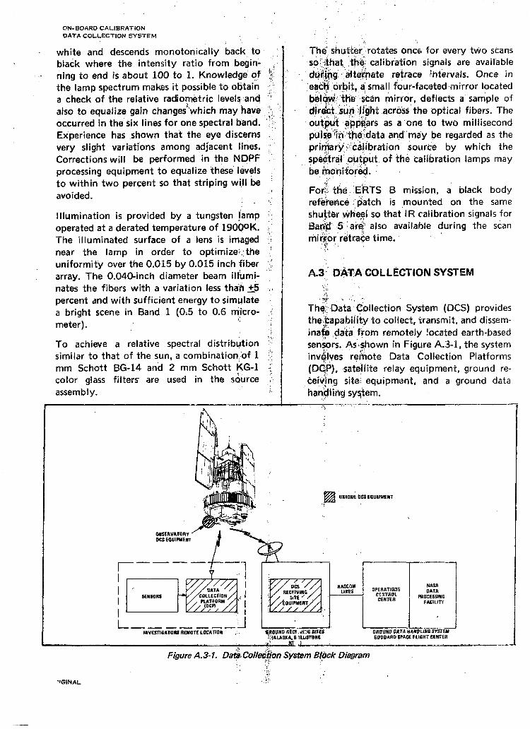
ON-BOARD CALIBRATION DATA COLLECilON SYSTEM

white and descends monotonically back to black where the intensity ratio from begin- ,‘l ning to end is about 100 to 1. Knowledge of !i:’ the lamp spectrum makes it possible to obtain I!. a check of the relative radiometric levels:and. ir, also to equalize gain changes”which may have ,,‘:I:, occurred in the six lines for one spectral band. ,c, Experience has shown that the eye discerns .,, very slight variations among adjacent lines. Corrections will be performed in the NDPF processing equipment to equalize these levels to within two percent so that striping will be ’ avoided.

Illumination is provided by a tungsten lamp I’: operated at a derated temperature of 190QoK. ,: The il luminated surface of a lens is imaged ,j near the lamp in order to optimize::;the : uniformity over the 0.015 by 0.015 inch fiber ” array. The 0.040-inch diameter beam ilfumi- ” nates the fibers with a variation less thati 25 ‘,I percent dnd with sufficient energy to simulate a bright scene in Band 1 (0:5 to 0.6 micro- :j meter).

To achieve a relative spectral distribution ii similar to that of the sun, a combination,of 1 :: mm Schott BG-14 and 2 mm Schott KG-1 i color glass filters are used in the source :. assembly. i.

-’

‘_

The, shutter-j rotates once for every two scans so:.&at, .the: calibration signals are available dr$&g.‘, alte&ate retrace intervals. Once in

‘ea&$,or~bit, @small four-faceted.mirror located b$l&$;;t~e~‘stan mirror, deflects a sample of dlr.$ct .:sufi $&hi across the optical fibers. The out&t &sars as a’one to two mill isecond pUl$“in~‘th%$ata and’may be regarded as the pri’r$ar)i,:~~c@ibration~ Source by which the spe%tral’;output. of the calibration lamps may be m,dnifored.

,j.; For:: the.!,;E’RTS B mission, a black body ref&ence ;.patch is moun”;ed on the same shutter v&e$ so that IR calibration signals for Bar@ 5’ ; are’ also available during the scan mir@‘fetrate time.

:.

A.3’ O~~A’COLL~CTION SYSTEM :. I. _L ;j. . . ..‘, _1.

The!: Data’ Collection System (DCS) provides the;$apabiiity to collect, transmit, and dissem- inat% ,d& ftiom remotely !bcated earth-based sensors.. As;9lown in Figure A.3-1, the system inv@lves remote Data Collection Platforms (DCP), ,satglite relay equipment, ground recei\i!n,g site; equipment, and a ground data handl ing system. : .

.p “Nlnui 0CSEP”IPmENT

INvEsrlGlrOlU RFMOR lOCATION ?(AUSKA. 8 ILWOHE GODOARD SPACE FLIGHT CEWER

.,! N-T-- __I- 2:. ‘.J..

“GINAL

F&e A.3- 1. Da$+ Coliet$on Si/stem B&ick Diaspslm .j 1 ‘f

‘,/’ .c ,* ,;I,

The DCP is corm.ected to ,ndividua!’ analog sensors which’ are selectee rnd proyidtid by the investigator or user agency to sati&y his own particular needs. Up to eight in@$cjud analog sensors may be connected to ,a’:$ingle DCP. The DCP transmits the senso$,data i: which is relayed to the ground receivi:#g sit6 ‘I through an on-board receiver/tran?mitS@# Th6 ground receiving site equipment .accept;s the data and decodes and formats it.for trapsmjs- ,: sion to the Ground Data Handling System (G;)HS) at Greenbelt, Maryland.’ The &&a is received in the Op,erations Cofitroj. denter (OCC) where it is reformatted a& writ& on magnetic tape and passed to the;:NAS/$Daia ProcesGng Facility (NDPF) for furitier ewes- ‘, sing required for dissemination to th+ user agencies.

The geometry involved in relaying DCS data is shown in Figure A.3-2. The satellite is’llat an altitude of approximately 492 na$tical biles. The transmitting antenna of the DC@ sub- tends an angle of *70 degrees from the$vertical and the ground receiving sitd visib$ity is nominally *85 degrees from fhe v&tical. When the satellite is in mutual vi& of zi&ans-

:i/! mitting DCP and one or more of the.‘gtound receiving sites, the message frort$ the ‘FP is relayed to the receiving site and transpitted over land lines to the,OCC. The DCP’s &rate continuously, sampling the sensors pgiodi- tally and transmitting a 38-millisecondigburst of data containing all sensor channels at?!nter- vals of about every three minutes, Not&! that the satellite acts as a simple real time.seiay with no on-board data storage. Th$zDCP transmissions are received at thy gro,$$ receiving site immediately except for pr?paga- tion and fixed svstem time delavs: ‘::

Figure A.3-2. DCS Data Relay G~~try:,~~ .

.j: I

i/! / ::’ _-’

, .Figy$e A.3-3: Mutual DCP-Receiving Site Visibility ;

/’ : , : .

, I .A:!;5 ‘; :: ORIGINAL

SEPTEMBER 15. 1971 ;;, .I,’

‘: ,I :; ,..

T, .. ‘.

I

;

I

,’ ‘.

.I: I’. ‘

,’ 4..

,, T~el,,bi)lpa,~a.mete~s of 492 nautical mile aIti- .t*:’ ” , b&$andY.lq3;, m!$ute period allow for up to 9 __, ,I, ,t,:-.: ,:- !:,A, l~~~~~~es.;of:~.~y~~,~l~~,irisibiIity for some DCP’s. .;* .: :

,., ..I+; : i, -,,,, ..,$$;J~. ,,&Z$, $K+S the potential area of . / :’ .~~#$a~~~isi~~l~~ f.o{ one orbital pass. In these :I,: ,, ,:. .., I’:.

,; .:, : ;$+.s@$ it .is.%&ible to receive up to three sepa- ;. ‘I ,:: I.,..., ,.i’! 1:: ‘I t~f@~an~!-ni;si~~s, ffpm a DCP fbr each orbital

.,,, ,I .’ .J’. ‘YL ‘;:y;

p@!+iof the Mtell i@&;The use of three receiving : ‘/ ’ site& Alaska, Go&tone, and NTTF, provide : -~ -;;y.,

.;; ’ ‘, ’

I riln9;:.acti~e~~passes:-bver the North American ,..: :,

~~%$$jn~nt e&h -da$, It is ejtpected that there :.;‘. ‘:.. ’ wi@be :. five:~ daili&it passes and four night

-, I::,, ‘.t ‘;, ,’ -,: ,,

8.:~ i FoI!$ ,parti&lhr~::bCP, the orbit parameters ” ,.,and”rj$he ‘r&ei&g “.site locations cause the i ,, “!: ’ Ibpa&&ft &’ be in’ mutual view of a platform

I”” .lb;&&d ~‘&-t-&t ‘!. .Q’ anywhere in North America Y..’ ,: eland% ground recei&j site during at least two

orbits per, day-one about 9:30 in the morn- ,;; ? ing ind, the other about 9:30 in the evening. ‘I’.’ Af &ast one message is relayed from each

@atform every 12 hours. .;: I, ,- I’,

The’lPata Coilection System is designed to as- ,*:,: .I 4 II:, :~ur&that tti@ propability of receiving at least iif 1 :‘.jo@%alid, tiessage from any DCP every 12 ’ lb’ ‘ho$6 is at;a<east 0.95 for as many as 1000 I,., D&s ioca&d throu,ghout the United States. $

,;r ;:”

Int&ference of signals from two or more ‘!,>. DCP’s transmitting simultaneously may cause ,,. _>I incorrect or partial messages to be received. . To minimize this possibility, the system uses

error coding and other schemes to correct or

MESsAGE BURSTS DATA COLLECTION PLATFORH

identify messages containing errors and to .’ identify incomplete messages. The probability of erroneously indicating that a given meSsage, ., is valid (i.e., stating that a message which .$on;‘. tain,s an error does not) is less than 0.01. ’ ‘. ‘.

L:

In order to improve performance for locai’ion$ ’ ‘where there is a relatively’short period of’ :‘:, m&al DCP-ground station visibility <r&i the Observatory, the average- rate of DCP mes- .‘. sage bursts can be switched to a more rapid, ’ rate: One message burst each 90 seconds. Using this feature., DCP’s may be located.:anp where in ‘Continental U.S. or Alaska ‘land’ 1 achieve this performance. DCP’s may be’de- : p loyed beyond these bounds, however, with : degraded performance in terms of probability I of receiving a valid message each 12 hours,, ::

1, :: ,’ ; .:

As shown in’ Figure A.3:1, operat ion of$ the ” Data Collection System requires three hard- ‘T, ware subsystems-the Data Collection PIat- ; forms, the receiving and transmitting equip- :, ment in the satellite, and special rece&jng i equipment located at each of three ground ‘$ receiving sites. In addition, the system ruses >.

”

’

existing ground communicat ion facilities and the hardware/software capabilit ies of the OCC and NDPF at Goddard. These facilities are described in the following sections.

A.3,l Data Collection Platforni

The Data Collection Platform (DCP) collects, encodes, and transmits ground sensor data to the ERTS Observatory. A block diagram is shown in Figure A.3-4 and a sketch in Figure A.3-5.

Figure A.34 Data Collection Platform Block ,Di&pam

“GINAL

nAl-rEnY OR DC CDllLR BlURCE lwEnPnOVIDED)

.,., -. I’

Th$DCP WJII accept ar,alog, serial-digital, or para@!-digit&l input,.data a; well as combinations of tho$. Eight analog inputs or 64 bits of $gital ,input can be accepted. Combined inputs are selected by individual analog inputs and,,groups of 8 bits of digital input up to a total equivdjent to 64 bits.

Selection of the type of input is made by the switch. posit ions on the front panel of the platform. For all types of inputs the nominal sign$ ampli tude range is from 0 to +5 Vdc. Thg’:,,source impedance must be less - than lo,@0 ohms resistive and less than 1000 pi&arads ‘capacitive. Input impedance is gre&er than :l megohm.

,‘,:

For:,..analog ?nputs, the analog-todigital converter cohve,ts the normal signal range of 0 to +5 Vdc into’eight bits of binary with a resolution,“of 19.53 millivolts per bit: conversion errok is less-,than one percent of full scale,

“inchjdi.ng quantization.

Se& digital data (of up to 64 bits) is ac- . cepted as a single input. An enable command

and:!a 2.5 kHz C&k is supplied to enable the tra+fer of the serial digital data.

-

Up to 64 parallel digital bits can be accepted by the DCP. These parallel l-its are sampled in sequence during a 68-milli:e;ond period corresponding to the entire ‘platform “on” tim,e (warm-up .and message transmission)., A, data, gate is provided during this period.

Format of a DCP message prior to encoding consists of 95 bits in the format of -Table A.3-1.

Table 4.3-l. OCP Messaae Format

Bits

l-15 16-17 18-27

E 44-51 52-59 60-67

!-ii Sk91 92-95

Preamble Synchronization “i. j Platform ID Data Word Number 1 Data Word Number 2 Data Word Number 3 Data Word Number 4 Data Word Number 5 Data Word Number 6 Data Word Number 7 Data Word Number 8 Encoder run-out bits ”

Before transmission, each DCP message ‘is encoded using a rate l/2 constraint length five convolutional code, to produce a 190-b& message output. A message is sent every ‘60,or 180 seconds, depending on the setting of the time selection switch on the front panel of the equipment.

A.3.2 DCS Spacecraft Equipment

The spacecraft acts as a simple relay: receiving, frequency translating and retran?mitting the burst messages from the DCP$ No on-board recording, processing. or’decodmg of’ the data is performe,d. A DCS unique.UHF antenna and receiver is provided. Unified S-Band (USB) equipment, used for n$rrow band telemetry, is used to retransmit thg:DCP messages to the three primary receiving;sites.

A.3.3 Treatment of Data at the Rec$ving Site

At the receiving site, the composite S&and signal is received, tbe DCS data extracted and inputted to special DCS Receiving’Site E,$uip

-.

‘._

1,’ j ,: .i

.:!

:I/ /’

.I:

,.’

/

‘!! f

: ’

IL

ment (bCS/RSE). The DCS/RSE performs a matched filter operation on each encoded bit recei;)‘ed, and quantitizes the output of ,that operation to three bits. Each bit representa- tion, recover,& frorri:, the DCP transmission is in the for,m:.of a four-bit byte; one bit, indi- cati,nb the presence or lack of signal, and the threejbit quanfitation of the matched filter. When’ no sig‘al is present, the output byte is set ‘to all’ zetas. The quantized bits are decoded, and quality bits are assigned to each decoded bit -and the overall message to indi-

.cate the decoding confidence level.

The: DCS/RSE formats the decoded data with the quality indicators and a 30-bit site time code, which was converted from the NASA 36-b@ time code. This data is outputted to a site modem in real time as messages are received. The data is buffered and formatted i’nto’.‘a 1200~bit NASCOM block and trans- mittejdi to the OCC by hardline. The DCS/RSE adds .&he NASCOM header and the filler and ch$ck bits, along with buffering the data and site&&? information. In the event of equipment ‘problems, the data is also recorded for post-pass playback.

A.3.4 Treatment of Data at the GDHS

The NASCOM data blocks are received at the OCC where the NASCOM header is stripped and DCS data messages are written, in the order received, on a magnetic tape. One magnetic’tape may contain messages from one or more receiving sites. At the conclusion of one or more station passes, this tape is transferred to the. NDPF. The usual mode of operation involves the transfer of data to the NDPF at the conclusion of each pass.

When ‘the DCS tapes arrive at the NDPF from the OCC, they are read, edited, and the data is sorted according to platform identification and the time the data was received. Redun- dant data resulting from overlapping station coverage is remo*red. The criteria for determining redundant data is an exact match b-e- tween messages except for receiving site (station ID). An active data file is generated which maintains a record of the most recent


ACTIVE DATA FILE DATA CARD ENTRIES DCS REQUESTS

24 hours of DCS messages. This resides in random-access storage in the NDPF computer.

The active data file contains the platform message data in addit ion to the resuCts,of the editing checks and certain identifying information. Four editing checks are : performed: the station code is checked to assure that it is one of the three valid codes ‘for Goldstone, Alaska, or NTTF; the platform ID is checked to assure that it matches a valid ID maintained in a platform ID file; a flag is set if any one of the quality bits associated with the platform ID is zero; a fourth check is made on the time of reception. If any part of the time code exceeds possible values for day, hour, minute, or seconds, a flag is set in the active data file. These checks and flags do not cause any messages to be rejected.

An active data file entry is made for each platform message and consists of eight words as shown in Table A.3-2. The platform ID is a binary coded decimal from 1 to 1000. Each platform has a unique designator. The platform ID quality bits are those that were associated with the platform ID during transmission. Words 5 and 6 contain the actual data bits in the order in which they were received. For convenience, the associated quality bits have been separated and put in words 7 and 8.

Table A.3-2. DCS Active Data File Entry

SITS

6-m 16.23 24.31

0.6 16.31

o-7 S-6 1923 24.31

f6 16.17 1.23

24.if 28-31

031

031

031

0.31

ITEM

Not Uud Era Flqs: lnrdid hstian Code lnnlidflatlorm ID Poor Pbtfarm ID Nudity InnlidTime Code Ovpllcrn &sage Adunhlt Matags Notllud r*rg, DudiW

MODE

oimy EBCDIC EBCDIC

hlry @nrl Binvy EBCDIC

Bit II Bit19 Bit20 Bit 21 Oit 22 Bit23

Bin&

FORMAT

xxxx l/2 A/G/N

1.366 1.11

O-23 0.69 069 0% ‘1

0 ‘3FF’ 0

Available products consist of magnetic tapes, punched cards, or computer listings. All pri$tucts.art$ iimited to uncalibrated data; that is,:yata bits,are dissemiriatsd to the user without$onversion to engineering units. Magnetic tapes.. contam message data records ordered according ia platfo& ID’and time with ID, and, in thelame 8&ord format as the active da& file e&y. The entries are blocked 60 to a tape rec,ord. A tape header is included for identificatioh. The details of this tape format : i’ are{containeci in Figure 3-22 of Section 3.

The data card format for DCS products is shown in Figure 3-20. Entries for these cards are also given in Table A.3-3. The listing format is given in Figure 3-21.

Table A.3.3. DCS Data Card En tries

I l-2

r 38

7.10

11 ’

12

13.21

22

2w

2s

28

an449

61167-R L;

-- I

ITEM I - FORMAT

Phtfo~mlD

SItallitalD

Tim* Ccdm (GMTJ

StationID

Emadd Errah4q: 32=InvalidSbtion ID 16 = lnvslid Fltiorm ID 8 = Poor Fladonn ID Duality 4 = lnvdid Tha Coda

(Dr~nycombhionofL~ah; a.&

63=Atl Condit iom Eain

Dab Pwlify in Octal or Hwadaimd Di*

I AMA

l.loDO

N

1%

DODHtWhlSS

AlGIN

003

:I

07

O/H

DCS data products may be requested in two ways. A standing order may be permanent ly establ ished with the NDPF to require that all d2ta’from a set of platforms be sent to the user agency. The capability is provided in a standing request either to keep or eliminate the quality bits for card or listing outputs. It is also possible for the investigator to desig-

-WGINAL

III

nate the level of message qut ity which is ac: trieved), or individual ‘platform ID. It is possi- ceptable to him. ble to qualify the *arch based on a given time

period or geographical area. All three product A variable request allows the investigator to ‘: medial are availabie and data can be qualified do retrospective searches. The capability is as to message quality. A DCS catalog is availa- provided to search the arch&s baskd on user ble to users and is’ explained in Section 4.23. ID (all platforms listed for this user ars’ re- :

I .1

A-19/20

I r.

SEPTEMBER 15. 197;

APPENDIX F OBSERVATO’4Y

The ERTS observatory (Figure B-1) is an earth-pointing stabilized spacecraft consisting of integrated subsystems that provide the power, control, environment, orbit maintenance, attitude control,and information flow required to support the payloads for a period of one year in orbit. It weighs 1,800 pour-r& (818 kg) and has an approximate overall height of 10 feet (3.04 m) and a diamete,r of 5 feet (1.52 m), with solar paddles extending out to a total of 13 feet (3.96 m).

Figure B- 1. ER TS Observatory

B-1 ATTITUDE CONTROL SUBSYSTEM

,,The Attitude Control Subsystem (ACS)’ provides spacecraft alignment with both local earth-vertical and orbit velocity vectors, and provides rate control about the pitch, roll and yaw axes. The ACS achieves pointing accura- cies of the spacecraft axes within 0.4 degrees of the local vertical (about ‘the pitch and roll axes) and within 0.6 degrees of the veiocity vector (about the yaw axis). The expected rotation rates encountered during Multi- spectral Scanner (MSS) and Return Beam Vidicon (RBV) operations are less than 0.015 degrees per second about all axes. These rates

produce image motions which are negligible during the short exposure of the RBV can)- eraf,, but cause a slight distortion in the MSS ima^ges. Compensat’ion for these distortions is provided during ground image processmg in the,,::,NASA Data Processing Facility (NDPF) by :applying, correction factors for the measured attitude rates. The’3-axis active ACS uses horizon scanners for ‘roll and pitch attitude error sensing. The rate; .gyros sense yaw rate and, in a gyro compassing mode,. ,sense yaw attitude. A torquing syste’m uses a combination of reac- tion jets to. provide spececraft momentum con,trol and, large control torques when required; flywheels al’e utilized for fine control and residual momentum storage.

B.2:., ATTITUDE MEASUREMENT SENSOR

The Attitude Measurement Sensor (AMS) is an independent component (not used for attitude control purposes) that determines precise spacecraft pitch and roll attitude. This data, is used for image location and correction during ground processing. The AMS detects the rddiation level change in the 14 to 16 micron range between the earth’s atmosphere and the spatial background and establishes the spacecraft pitch and roll axis positions relative to the local vertical. After ground compensation of telemetry data for variations due to seasonal radiance and other effects, the pitch and roll attitude can be determined to within about 0.07 degree.

8.3 WlDEBAiUD VIDEO TAPE RECORDER &JBSY~TEM

Two Wideband Video Tape Recorders (WBVTR) record, store, and reproduce the data outputs from either the RBV or MSS during remote sensing, operations. Each recorder can record. 30‘ minutes of either 3.5-MHz video analog data from the RBV or 15-Mbps digital data from the MSS. Data are recorded by four heads (on one wheel) rotating across the 2-inch wide tape. Record-- ing and playback are each at 12 inches per second (30 cm/set) and in the same direction. Total usable tape length is 1,800 feet (548 m) for each recorder.

B-l ORIGINAL SEPTEMBER 15. 1971

PbWER SUBSYSTEM COMMUNICATIONS AND DATA HANDLING SUBSYSTEM

The RBV analog video signal is transformed into the FM domain by video circuitry in the W’BVTR. The signal is received as a negative analog signal, is dc level shifted, frequency modulated, amplified and recorded. To insure head switching during the horizontal blanking interval of the video signal during playback, the RBV signal is rephased to the WBVTR hehdwheel at the beginning of each triplet exposure during recording. In playback, the RBV signal is read out sequentially by the same four rotating heads, with appropriate switching, producing a continuous RBV signal in the FM domain. The signal is then demodulated on the ground, producing. the original analog video waveform.

The MSS digital video data is received as a Non-Return to Zero Level (NRZ-L), 15-Mbps data stream. In the WBVTR, the data stream is re-clocked and then frequency modulates an FM carrier. The resulting frequency-shift keyed (FSK) signal is recorded by four rotating heads. The MSS data are recorded asynchronously; that is, the data stream and rotating heads-are not synchronized. In playback, the MSS signal is read out sequentially by the same four rotating heads, with switching and demodulation producing a continuous NRZ-L, 15 Mbps data stream.

Each WBVTR can record and playback either RBV or MSS data at any given time. The selection of RBV data or MSS data for each WBVTR during record or playback, plus appropriate tape motion to select the proper tape location, is made by approwiate ground commands which can be stored by spacecraft equipment for subsequent remote execution.

B.4 POWER SUBSYSTEM

The Power Subsystem supplies the electrical power required to operate all spacecraft service and payload subsystems. During sunlight periods the subsystem delivers a maximum output of 980 watts of regulated -24 volts for short periods. This power is derived from the load sharing of the 550-watt solar array panels and the eight, 4.5-amp batteries. The expected power requirements during payload

operation’ is 480 watts-for,real-time operation and 521 watts for rem&s operation. Consid- ering the subsystem as an .energy balanced system,..’ iit. can su,Ppor~ an average of 21 minutes &f payload, (both RBV and MSS) “qp -’ time” per orbit initially and 13.5 m@utes after ohe yoor; The reduction in “ON - tjme”~iGnainly due to efficiency loss of the so&& array$from s’mall particle impact during thi$,yeai irr’orbit. However, the actual payload “QN - “@me” is “limited by other system c’o$strainf&,,(such as station pass time, record capability,’ etc.) to an average of 12 minutes p&orbit:

All power is provided from the batteries during the launch phase and while the spacecraft is within the earth’s umbra. Energy from the solar array not required for spacecraft loads during the lighted periods is used to recharge the batteries and any excess power is dumped via auxiliary loads.

B.5 COMMUN ICLJTIONS AND DATA HANDLING SUBSYSTEM

The Communications and Data Handling Sub- system (Figure Bi2) provides for all spacecraft infdrmation flow and is composed of the Wideband Telemetry Subsystem and the narrowband Telemetry, Tracking and Command Subsystem.

h -I PAYLOAD S-BAND USE VHF

c

I ,: V J \ V J

WIOEBANO NARROWBANLI TELEMETRY,

I TELEMETRY TRACKING AND COMMAND -_I_

F&e B-2. ERTS Communication Lioks

8.5.1 WIDEBAND TELEMETRY SUBSYSTEM

The Wideband Telemetry Subsystem accepts and processes data from the RBV, the MSS both Wideband Video Tar? Recorders and transmits it to the ground leceiving sites.

The. subsystem consists of two, 2b-watt S-Band FM transmitters and associated filters, antennas, and signal conditioning equipment. As shown in Figure B-3 the subsystem permits transmission of any two data sources simultaneously, either real time or recorded, over either of the two down links (one data source . each). Commandable power level traveling wave tube (TWT) amplifiers and shaped-beam antennas provide maximum fidelity of the sensor data at minimum power. Cross- strapping and dual mode operation (two data sources) with a single TWT amplifier is ?vaila- ble in the event of hardware malfunctions.

-..

A total of 912 telemetry points (576 analog; 16, lo-bit digital words; and 320, l-bit binary wards) can be sampled at rates between.onco pf&*,i16 seconds to twice in one second. The datir ,is pulse’ code modulated (PCM) and call theh be trsnsmitted in real time either over

.’ the, VHF or Unified S-Band (USB) links at a

t l-Kbps rate,. Up’ to-,210 minutes can be stored of ,each of two narrowband tape recorders

:

_:..

,‘-’

.:’

_’

/:,

:

.,

(N&R) for subiequent playback at a 2+bps rate. Analog data has 8-bit accuracy .oi’:i; part in 256 (i.e. 19.53 mv.)

.:,.

The: USB equipment has the capability to transmit on separate subcarriers real-time tele- t+$y (768 KHz), playback data (597 K’Hz), DCS data (1.024 MHz) and pseudo-random ranging information simultaneously over the same 2,287.5 MHz carrier. The playback data can ‘be derived from either of the NBTR’s or either of the auxiliary tracks of the WBVTR’s.

REALTlYE -c COIILIITIOIYER

mvrR 1 - mvrn I - AUXVIDEO -

WOE0 FllTEFullO

AN0 WTCHlNC ‘)

REALTlYE 1 - REl‘TlYE Z-

WIVTR 1 - mVTR 2 _

i: B.5.2 TELEMETRY, TRACKING AND

COMMAND SUBSYSTEMS f

Figure @. Wideband Telemetry Subsystem .:Functional B&k Diagrtim .‘i I : ., ‘.

.’ Onfy real-time or playback data (from either

.r .’ of the NBTR’s) can be transmitted .at one time over the 137.86 MHz VHF equipment.

I ‘/,

Al,f:;,,three of the ERTS receiving sites will

., normally use the USB downlink. :.,

The Telemetry, Tracking and Command Sub- system collects and transmits spacecraft and sensor housekeeping data to the ground~sites, provides tracking aios, receives commands from either the Manned Space Flight Network (MSFN) or Satellite Tracking and,.Data Acqui- sition Network (STADAN), and implements those commands on board the spacecraft. In addition it provides the link for transmitting the Data Collection System data.

Co$manding can be performed via either the :_ S?fiOAN VHF link at 154.20 MHz or by the

“::. MSEN USB. link at 2.106.4 MHz into redun- d&i, sets of ,receivers on the spacecraft. These commands can be any of the 512 possible commands executable by the command/clock or any of the 8 commands recognizable by

5.3 ORIGINAL

SEPTEMBER 15. 1971

ThERMAL CONTROL SUBSYSTEM ORBIT ADJUST SUBSYSTEM ELECTRICAL INTERFACE SUBSYSTEM

the Command Integrator Unit. A total of 30 command/clock commands can be “stored” for execution outside of the range of the ground stations. All remote payload operations are performed using stored commands..

-.

B.6 THERMAL CONTROL SUBSYSTEM

The Thermal Control Subsystem provides a controlled environment of 20 f 10°C for spacecraft and sensor components. Thermal control is accomplished by both semipassive : (shutters and heaters) and passive (radiators, insulation, and coatings) elements. Shutters are located on each of the peripheral compart- ments on the sensory ring, and are actuated by two-phase, fluid-filted bellows assemblies.

I These assemblies are clamped tightly to heat dissipating components and position the shutter blades to the proper heat-rejection level. Heaters are bonded at Larious locations in the 1 sensory ring to prevent temperatures from fatling below minimum levels during extended 1. periods of low equipment-duty cycles.’ The ” heaters are energized selectively by ground $ command when the temperature level at these 1 locations falls below a predetermined value. ’ The upper and lower surfaces of the sensory : ring are insulated to prevent gain or loss of heat through those areas. External structure :: and radiating surfaces are coated to provide L the required values of emissivity and absorpti- . vity.

Passive radiators coated with a low-absorpti- ‘j: vity, highemissivity finish are used to assist the shutters in rejecting the heat from the : sensory ring. Radiators are provided for the : RBV, the MSS, the Wideband Video Tape Recorders, and the Narrowband Recorders.

B.7 ORBIT ADJUST SUBSYSTEM

The Orbit Adjust Subsystem (OAS) estab-

lishes, the Precise. ERTS orbital parameters aft& orbit ;insertion and ‘makes adjustments thiqughout. the life of the mission to maintain ov&$lappj,m$ coverabe, of -sensor imagery and Io,n&esm ‘rdpeatabiiity. ,:,

:’ . ‘: Th& OA$ ’ is a ‘m&&ropellant, hydrazine- fuejed, pr,opulsion. system constructed as a smgle module con&sting .of three rocket engines, a;’ ;p~opellani”‘tbnk and feed system, a support structure .a$d the necessary intercon- nect plumbing and” electrical’ harnessing. The OAS is mbunted ko the spacecraft sensory ring with, a thruster’ located along each of the (+j’ roil, .(-)‘roll,“a’nd ‘(-) pitch axes, such that each. th&t vector pas& approximately th’rough ‘the spacecraft center of mass. With these thr’u$t vectors, the, orbit adjust sub- sy&m I, dank, impa& incremental velocities to the:.‘&pace&ft to. ‘corrdct in-plane injection ert$rs, ~hc,l$nation injection errors, and orbit [email protected]$rs due to atmospheric drag and other erroflsources, over an orbital life of one y&t.

B;q ELECTRICAL INTERFACE SUBSYSTEM.

The Electrical Interface Subsystem functions include power switching, telemetry signal generation, switching logic, power fusing, data rotit,i,ng, t ime-code processing and automatic “shut-off” ‘of equipment. Time-code data are received from the command/clock, assembled into storage registers and relayed to the RBV and MSS,. when requested. Timers associated with the. payloads, WBVTR and S-Band Trans-

.niitter are ,provided to automatically remove power after, 34 minutes of operation if the nor.mal turn-off does not occur. Power switch- .ing,.(regulate,d and unregulated), transient load circuitry, L.&d fusing are included in this subsystem for the ,RBV, MSS, WBVTR’s and the Orbit Adjust Subsystem.

-“GIN 4L

w I - . . . - - -

A P P E N D I X C G R O U N D STAT iOf I A N D

G R O U N D C O M M U N t C A T l O N S

C.l G E N E R A L DESCRIPT IJN

Commun ica t i ons b e t w e e n the spacecra f t a n d the g r o u n d a r e h a n d l e d v ia g r o u n d stat ions

wh ich a r e par t of e i ther N A S A ’s M a n n e d S p a c e Fl ight Ne twork ( M S F N ) o r S p a c e Track ing a n d Da ta j Acqu is i t ion Ne twork ( S T A D A N ) . T h e N A S A Commun ica t i ons

‘. ( N A S C O M ) Sys tem p rov ides the necessa ry commun ica t i on of d a t a b e t w e e n these g r o u n d stat ions’ a n d the G r o u n d Da ta’ H a n d l i n g Sys- te rn- ( G O H S ) loca ted at G o d d a r d S p a c e Fl ight C e n t e r (F igu re C-l) .

E R T S P R O J F C T

B A C K U P S T A O A N ( E X C E P T D C S A N L V I D E O ) . n. ..““Y .I”..” l n r L Y ,ml”lLcY’r”“m Pt l . l lan* fl”Y -- - - -

“.CCr... 1 c p r t M A N O S O P E R A T I O N S ’ N A S A D A T A U S E R C O N T R O L P R O C E S S I N G w E V A L U A T I O N C E N T E R FACIL ITY

Figure C-.7. Commun ica t ions a n d Data F low C o n f&ra t ion

C-l’ O R I G I N A L S E P T E M B E R IS. 1 9 7 1

GENERAL DESCRIPTION

Three primary ground stations accomplish all of the necessary communications in support of the mission:

STATION NETWORK

Goldstone (Calif.) -., MSFN NASA Test and

Training Facility (NTTF) -- MSFN Alaska - STADAN

These are the only sites equipped to receive the Multispectral Scanner (MSS), Return Beam Vidicon, and Data Collection System (DCS) data, and perform all narrowband telemetry, tracking and command functions. Other MSFN and STADAN stations will be used as a backup for narrowband telemetry, tracking or command functions only.

Figure C-2 summarizes the various spacecraft to ground communications links and Table C-I lists the capabilities of the ground stations to receive and transfer the various types of data.

I Table C-1: Spacecraft/Ground Communications Summary

CAPA6lLilY

: P&yladOttI

Rniw RBV/MSS Via R4wiw DCS oatl u6B) Tnwfm REV/M.% Vii@0 To OtC tiil RWMSS V&h Tapa :o NDPF Trmf8r DC!3 hta tu OCC

comlNnd oh

usn Commrd VHF Command Cmitputer Contiolld Commdr Wkntrl Comounh

Raaiw USB PCM Rwaiw VHF PCM Tnllitn Rul Time PCM to OCC Tnmfir P*ybJ PM tn OCC

Tr&lw Data

US6 Tracking Mini-tnck Tracking

l Rtiw Only

I

f $4

X X

X X

X

X

X

X

X

::

X X

X X X

X X

E

X

-

E

X X X

X

X X

X

X X

X’

j- EJ % f -

X

X

X X

X

2106.4 MHz

DCS UPLINK

PLATFORM MESSAGES (5 KBPS)

S-BAND Mss (15.06 MBPS~

AND RBV 13.7 MHz)

REALTIME AND PLAYBACK

USE - (JpL)N((: COMMAND (70 KHz, lKBPS/175 BPS)

PSEUDO-RANDOM RANGING

DOWNLINK: REALTIME PCM (76B KHz, 1KBPS) PLAYBACK PCM (587 KHz, 24 KBPS) DCS (l.P24 MHz, 5 KBK)

VHF

&NK: COMMAND 1128 BPS)

DOWNLINK: PCI - MALTIME (1 KBKI -PLAYBACK (24 KBPS)

: SERVES AS TRACKING BEACON

Figure C-2. Spacecraft/Ground Communication Links

C.2 PAYLOAD WIDEBAND COMMUNICATIONS

C.2.1 Spacecraft to Ground Communication

RBV and MSS widetand d. .a are normally telemetered simultaneously to one of the three prime ground stations over two S-Band links operating at center frequencies of 2229.5 MHz and 2265.5 MHz. The RBV camera has a video Landwidth of 3.5 MHz and is u,ed to frequency modulate the carrier within an RF bandwidth of 20 MHz. fhe MSS output is a single Pulse Code Modulation- Non-return to Zero Level (PCM-NRZL) encoded bit stream at a bit rate of 15.06 Mbps. This PCM signal Frequency Shift Key (FSK) modulates the carrier.

Both RF links contribute a small degradation to the data. For the RBV the degradation in signal-to-noise ratio is less then 1 dB. The MSS bit error rate is less than 1 in 105. These are worst-case values expected at the 2’ elevation limit of the three primary ground station viewing cones.

I C.i.% Ground Receiving and Recordings -

Figure C-3 illustrates the flow of the wido- band .data as it is received and recorded. At the Alaska and Goldstone stations the rlal‘r is received and demodulated and then hardwired into special Receiving Site Equipment where it is processed and recorded. For the NTTF station at GSFC, the Receiving Site Equip- ment is physically located. in the Operations Control Center rather than at the station. This permits operations personnel to directly monitor the display equipment during data reception from NTTF.

The Receiving Site Equipment for the RBV includes equipment to resynchronize and re- clamp the video, a video display CRT, and various test equipment. This equipment monitors the data as it is received and supplies the necessary timing and control signals to the video ta-pe recorder. The recorder, an RCA TR-70, records the composite video signal on tape for physical transfer to the NDPF.

c-3 ORIGINAL SEPTEMBER 15. 1971

TELEMETRY, TRACKING AND COMMANG DATA HANDLING

The Receiving Site Equipment for the MSS demultiplexes the serial ,bit stream into individual data channels corresponding to each of the detectors in the sensor. It add.s a pre: amble, line start code, line length code, and other data to each channel, and outputs the digital data on parallel lines for recording on an Ampex FR1928 tape recorder. An A-scope provides the capability to monitor one of the output channels after demultiplexing,

C.3 TELEMETRY, TRACKING AND COMMAND DATA HANDLING

The spacecraft telemetry, tracking and command equipment operates with either the MSFN or STADAN type stations. S-band equipment is provided for the former and VHF equipment for the latter. The stations and the NASA ground communication facilities provide the link for the near real-time transfer of this data between the spacecraft and the Operations Control Center at GSFC. ’

C.3.1 Telemetry Data

The spacecraft transmits real-time telemetry data at 1 Kbps, using the VHF downlink to STADAN stations or a subcarrier of the unified S-band (USB) downlink to MSFN stations. This data is received whenever the spacecraft is in view of one of &he three prime ground stations, and is directly relayed to the occ.

The spacecraft also continuously records telemetry data on one of two on-board narrowband tape recorders. This data is played back at 24 Kbps using another of the USB subcarriers (or VHF backup downlink). This data is normally received during station contacts at Alaska or NTTF and is transferred in real time to the OCC. This stored data provides a

continuous history of the spacecraft and sensor status.

C.3.2 Corrimand Data’

Normally alt: commands. are generated in the OCC and relayed to the spacecraft from one of the three:$rime stations. These commands may .be real-time commands executed immediately upon receipt, or time-lagged commands that are stored for execution at a prescribed later time. In emergency situations commands may be sent from other stations. Commands from MSFN stations are transmitted on a subcarrier of the USB link and from STADAN stations on the VHF link.

C.3.3 Tracking Data

Primary tracking data is abtzined using the MSTN USB range/range rate system. Tracking data .is processed at the ground stations to de&mine range, velocity and direction para- met&s. These are then transmitted by tele- typ6)to GSFC where the orbital parameters and%pacecraft ephemeris are computed.

Secondary tracking can be provided by the VHF minitrack interferometer tracking system at STADAN stations.

C.3.4 DCS Data

Data from individual Data Collection Plat- forms is transmitted to the spacecraft at UHF where it is received, frequency translated, and retransmitted over the US6 downlink to one of the three prime stations. Special DCS receiving site equipment at these stations decodes and processes the data as it is received and reformats it for transmission to the OCC. (Refer to Appendix A.3 for a more complete discussion of the Data Collection System.)

APPENDIX ‘3 OPERATIONS CONTR .)e CENTER

The Operations Control &nter (OCC) is the focal point of all communications with the ERTS spacecraft. All sp& :craft and operations scheduling, commanding and spacecraft related data evaluation for the ERTS mission is controlled by the OCC. Its 24.hour-aday activities are geared to the operational timeline dictated by iire orbit and ground station coverage capabilities. The major elements of the OCC are shown in Figure D-P. -,’

D.l SYSTEM SCHEDULING .,:’ . I

At the beginning of each spacecraft day the activity plans for that day are generated by the OCC for each orbit’s operation, based on sensor coverage requirements, spacecraft and payload status, network availability and the current cloud-cover predictions. Priorities are assigned to coverage requirements for selecting the data to be collected over various geographic locations as described in Appendix K. Sensor operations including real-time, remote coverage, and calibrations afe scheduled. Current spacecraft and payload stat& are examined to ensure effective utiliration of the observatory capabilities. Tracking and orbit adjust requirements are obtained from the NASA Orbit Determination Group when required and integrated with the coverage planning. Scheduling is coordinated with the network operations center and station availability is determined for both routine contact operations and orbit-adjust maneuvers. After integration of all the required data sources and support activities, a final activity plan is issued. This plan is the integrated time- ordered sequence of events defining the spacecraft, payload, and ground system operations for each orbit, and serves as the basis for the compilation of spacecraft command lists:

D.2 DATA ACQUISIT’[ON

After acquisition of telemetry signals from the spacecraft, the narrowband housekeeping data (real time and playback) and Data

1’

:

D-l

Collection System (DCS) information arc ‘routed via NASA Communication Nctwor k

(NASCOM) to the OCC. The real-time space!- craft data are then displayed on five OlJt?ril-

tions consolas where computer-driven status, lights and CRT displays provide the spacccralt evaluators with a complete on-line dctcrmimr- tion’: of vehicle and payload status, performance, and health, as well as command verification. DCS data are also processed in the TCC on-pass and placed on magnetic tape. These tapes: ,are available jmmediately post- .psjs,” for continued processing in the NASA Data, Processing Facility (NDPF).

Indepth spacecraft evaluation and image annot&on information are derived from the data stored an the narrowband tape recorders. These data contain all the satellite telemetry for the entire orbit, including all remote areas.

Playback data are received during the station pass dt the OCC but are processed post-pass to produce detailed spacecraft evaluation parameters and trends. The Spacecraft Per- formance Data Tape is also generated from this playback data and given to the NDPF for use. in generation of image annotation parameters.

Video data received during Network Test and Training Facility (NTTF) station passes are relayed directly to the OCC where they are processed in the identical manner as at other

remote sites as outlined in Appendix C. The video tapes generated in the OCC are hand- carried to the NDPF for image processing.

D.3 COMMAND GENERATION

Commanding of .the ERTS spacecraft is performed by an operator at either of two operations consoles located in the OCC. All commands are checked and then routed by the OCC computer system to the remote receiving site that is in contact with the satellite. At the site an “as transmitted” command check is performed and command acknowledgements are relayed back to the OCC. Final command verification is made through analysis of telemetry data.


cm REMOTE - GROUND TLM

RECEIVING - SITES

bA

- I M

N 1 M

c- MODEM CMD- ”

: I

- N AND TLM ’

i I_. TERMINALS -5

-I t 0

I

N NTTF COMMANDS S

I NTTF I PAYLOAD VIDEO

0 A T A

s

in T D R

I B lt T I 0 N

SPACECRAFT PERFORMANC DATA TAPES TO NDPF

INtERACTING

M!SlRBV VIDEO TAPES TO NDPF I (EXCEPT NTTF)

I

Figure D-l. Major Elements of Operations Control Center

APPENDIX E NASA DATA PROCESS11 ? FACILITY

The NASA Data Processing Facility (NDPF) processes and stores all sensor data and dis- seminates large quantities of his data to users in the form of film imagery, computer corn- patible tape, and Data Collection System (DCS) tapes, cards, and listings. To accomplish these functions, the NDPF utilizes the .following subsystems:

l Bulk Processing Subsystem (BPS)

l Precision Processing Subsystem (PPS)

l Special Processing Subsystem (SPS)

l Photographic Processing Facility (PPF)

l Quality Control Subsystem

l Computing Services Subsystem

l User and Support Services

I . I .dM Urr‘A CwdLL3>,1.t i T,+C,L, , ,

Figure E-l illustrates the flow of data through the- NDPF and its ielationship to the various ” subsystems.

The Bulk Processing Subsystem processes all imagery data received at the NDPF. Data is accepted in the form of video tapes and transferred to film imagery using an electron beam recorder. Image annotation tapes produced by image annotation processing provide descriptive and positional data to Bulk Proc- essing. Liser and Support Services determine and control the- .process flow through the system by means of work orders.

Latent film from Bulk Processing is developed and transferred to the Photographic Proc- essing Facility where multiple copies are made for distribution to investigators. Based on investigator requests, selected film images are inputted to the Precision Processor, where their data contents are corrected both spatially and radiometrically. The corrected images are written out onto film which is also processed by the Photographic Processing Facility.

DCS TAPES

TELEMETRY TAPES

VIDEO TAPES

COMPUTING SERVICES

ocs rROCEsslNC

I OCS OATA

1 I I---- --I MASTER DIGITAL DATA TAPES I I

IMAGE ANNOTATION

BULK PROCESSING l--l . .v....

PHOTOGRAPHIC - CORRECTION PROCESSl l lG

IMAGES *

0 I LATENT -

PRECISION IMAGES

- PRUCESSING

F BULK IMAGERY

WWF

Figure E-7. NDPF Functions

E-l ORIGINAL

SEPTEMBER 15. ,971

BULK PROCESSING

Both the Bulk Processing and Precision Proc- essing Subsystems are capable of writing image data on High Density Digital Tape (HDDT). These tapes are used in the Special Processing Subsystem to produce digital image data on computer compatible tapes (CCT). The CCT’s are then duplicated by support services and distributed to the investigators.

Processing of DCS information in the NDPF consists of editing, storing the data received on magnetic tape, and reformatting it into products suitable for distribution to investigators. This process is completely independent of image acquisition and processing.

E.l BULK PROCESSING SUBSYSTEM

The Bulk Processing Subsystem, shown in Figure E-2, produces latent images on 70 mm film from the data received for each spectral band of the RBV and MSS sensors. The data is also digitized, reformatted, and placed ‘on

’ high density digital tape.

_.

Certain corrections and annotation are applied to the data during the.Bulk Processing operation and include:

0 Geometric correction for spacecraft platform instabilities

) l Reduction of systematic errors caused by RBV camera distortion and image generation

l Radiometric correction for each RBV and MSS spectral band

l Framing of MSS data to be spatially coincident with RBV data

I The Bulk Processing Subsystem equipment includes video tape recorders for handling input data, a computer digital tape recorder for input of annotation data, an annotation generator, high resolution film recorder, and a high density digital tape unit and associated control units. Operation of all of this equipment is controlled by the process control

IKB mss - Mss - VIDEO ---c “‘OEO “TR w

TAPES TAPE RECORoER *--* CONTfmL *-----

XOB ‘3 i r

COMPUTER __c - CONTROL -* - HIGH . ANNOTATlOM - MAGNET’C CONTROL COMPUTER HOUTR DENSITY

TAPES TAPE COMPUTER RECOROER *--*

^I- * WrERFACE - CONTROL ~-- 9-

OlGlTAl TAPE

I RECOPOER

. IMAGE COARECTION

! t t

COEFFlClENTS I

TELETYPE ANNOTATION GENERATION

-

WOE0 - RB” --- J RB” RB” - WOE0 ---m TPIPL VTR

L, EBR ‘ELECTRON EXPOSE0

CONTROL - BFAM - 7Omm

TAPES RECORDER - -- CONTROL , FILM - --e RECORDER

I

- WOE0 OATA

---m CONTROL SIGNAlE

F&we E-2. Bulk Processing Suhystems Equipment

Configuration

computer which is a small scale, dedicated computer providing. control 33d timing of all hardware in BPS, formatting of annotation data, and computation of geometric corrections to be applied to imagery.

The high resolution film recorder is an Elec- tron’Beam Recorder (EBR), and all images are generated ,through this device. The recorder

d has a continuous film transport to minimize degradations at the corners of the image and to ;!low dynamic framing of the MSS data. Its functional parameters and performance’ dab are given in Tables E-l and E-2. ’ ’

Control Unit accepts the analog RBV data, performs necessary signal conditioning. and error signal generation, and outputs thb data to the EBR control unit. ”

E.l .I RBV Video Processing

RBV data is entered into BPS via the RBV Video Tape Recorder (VTR). The RBV VTR Control Unit accepts the analog RBV data, performs necessary signa! conditioning and.,

. . error signal generation and outputs the, data to the EBR control unit.

During RBV data processing, geometric and radiometric corrections are applied to the video data. These corrections are derived from measurements of actual RBV imagery and pre-flight calibration data by the Precision Processing Subsystem. They remove systematic RBV camera non-linearities, alignment errors, and shading errors, as well as ‘EBR internal errors. The correction coefficients are transferred to the BPS from the PPS on computer-readable tape, stored in the control computer, and used to control writing

beam. position and intensity during image generation.

The Video Tape Recorder control unit also digitizes the, RBV video data and outputs it to high density digital tape. This data is essentially raw video, with no calibration or corrections applied.

E.1.2 klSS Video Processing

MSS data is inputted to the BPS Bulk Proc- essing Subsystem via the MSS Video Tape Recorder (nilSS VTR). The MSS VTR control unit decommutates image and calibration data, time, line length, and frame ID codes

,#nd performs calibration and digital-to-analog co,nversion of the ‘MSS data. The BPS then outtjuts the .video ‘data in analog form to the EBR control unit. ”

The MSS VTP control unit also outputs reformatted digital data to the high density digital tape recorder control unit. However, the MSS data on fhe .HDDT is not corrected or calibrated by Bulk Processing. All calibration and correction of the MSS digital data is later done by the Special Processing Sub- system.

E.1.3 Framing

The RBV and MSS sensor systems are normally operated in time coincidence, i.e., both sensors are taking imagery data at the same time. Since framing of the RBV images is inherent in the simultaneous shuttering action of the three cameras, the centers of the RBV images are nominally identical. There are, however, slight offsets between the image centers due to misalignments between the cameras. During Bulk Processing, the EBRIC

Table E- 1. Electron Beam Recorder Functional Parameters

MSSVFC 4312 163.44 I 3300 f 300 2100 39.27 .768 27.0 26 23LO 1.811 466 12.26 11.7 * 30 15.38 M A X

VFC = Video Data To Film Cowanion

E-3 ,

_: ;. ‘: i ,


, : ,’

.i

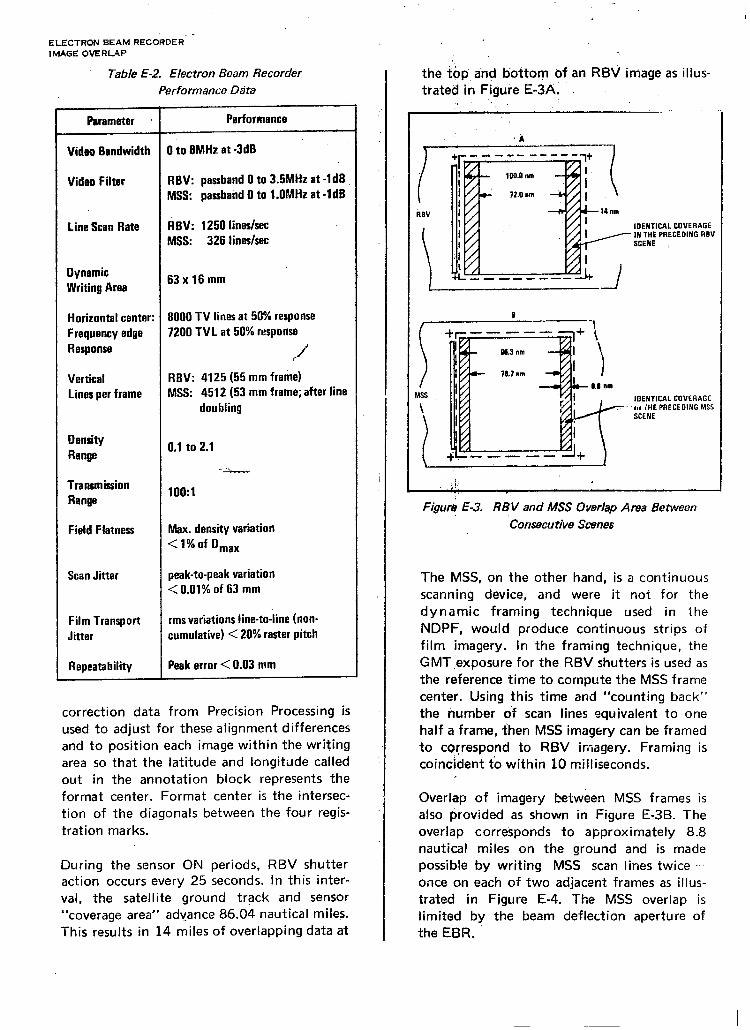
ELECTRON BEAM RECORDER. IMAGE OVERLAP

Table E-2. Electron Beam Recorder

Performance D&a

Parameter

Video Bandwidth

Video Filter

Line Scan Rate

Dynamic Writing Area

Horizontal center: Frequency edge Response

Vertical Lines per frame

Density Range

Range

Field Flatness

Scan Jitter

Film Transport Jitter

Repeatabil i ty

Performance

D to BMHz at -3dB

RBV: passband 0 to 3.5MHz at -1dB MSS: passband 0 to l .OMHz at -1dB

RBV: 1250 line&c MSS: 326 line&c

63 x 16 mm

BOO0 TV lines at 50% response 7200 TVL at 50% response

RBV: 4125 (55 mm frame) MSS: 4512 (53 mm frame; after line

doubl ing

0.1 to 2.1

- .%

1OO:l

Max. density variation < 1 % of D,,,

peak-to-peak variation < 0 .01% of 63 mm

rms variations line-to-line (non- cumulative) < 26% raster pitch

Peak error < 0.03 mm

correction data from Precision Processing is tised to adjust for these al ignment dif ferences and to position each image within the writing area so that the latitude and longitude called out in the annotat ion block represents the format center. Format center is the intersection of the diagonals between the four registration marks.

During the sensor ON periods, RBV shutter action occurs every 25 seconds. In this interval, the satellite ground track and sensor “coverage area” advance 86.04 nautical miles. This results in 14 miles of overlapping data at

I

the top and bottom of an RBV image as illustrated in Figure E-3A.

IOENTICAL COVERAGE ‘an iHE PRECEDING MSS

SCENE

‘ii, ._ .-.

Figuti E-3. RBV and MSS Overlap Area Between

konsecu rive Scenes

The MSS, on the other hand, is a cont inuous scanning device, and were it not for the dynamic framing technique used in the NDPF, would produce cont inuous strips of film imagery. In the framing technique, the GMT,exposure for the RBV shutters is used as the reference time to compute the MSS frame center. Using this time and “counting back” the number of scan lines equivalent to one half a frame, then MSS imagery can be framed to correspond to RBV imagery. Framing is coincident to within 10 mill iseconds.

Overlap of imagery between MSS frames is also provided as shown in Figure E-3B. The overlap corresponds to approximately 8.8 nautical miles on the ground and is made possible by writing MSS scan lines twice - once on each of two adjacent f rames as illustrated in Figure E-4. The MSS overlap is limited by the beam deflection aperture of the EBR.

r

ELECTRDN GUN

f=l 1 BEAM INDEX POSITIONS

-- -. FILM ?.:4VEL “.

L FILM . .

Figure E-4. MSS Dynamk Framing Technique

E. 2 PRECISION PROCESSING SUBSYSTEM

The Precision Processing Subsystem (PPS) accepts selected bulk-processed 70 mm imagery and, through a hybrid analog-to-digital processing system, produces geometrically and radiometrically corrected images on a 9-l/2 inch format. Automated reseau measurements and ground control point corrala- tion techniques are used to remove geometric distortions, and perform precision location and scaling of the corrected data relative to map coordinates.

A’ key feature of PPS is the use of ground control coints to measure and correct oosi- iional eriors in the MSS and RBV images.‘The ground control points used for precision location of imagery are objects having a known position on the earth’s surface and which can be identified in an image. Data bbtained frorri measurements of these control points are used to perfoim geometric cbrrections in PPS and provide. data to BPS for systematic error removal;

The P’PS. also has the capability to digitize the corrected data, and record it on high density

:,tape fortconversion to a computer compatible ‘tape by the Special Processing Subsystem.

The PPS consists of a viewer/scanner assembly which receives the 70 inm film input from BPS, a icanner/printer assembly to produce the 9-l/2 inch precision-processed film image, a high density digital tape recorder and a process co’ntrol computer. Figure E-5 shows the major hardware components of the PPS.

The image measurement functions are performed using the viewer/scanner. This in- strunx+nt is basically a precision, two-stage image comparator with automatic and manual image-matching and coordinatermeasuring

-me-- ----\

SCANWE~IPRINTER

WING OPTICS CORRELATOR Cl/2 INCH ROLL FILM

INTERFACE

--. DATA * ENTRY& -

DISPLAY

‘;i;;kiA;D

MAGNETIC VIIJEO OIGlTltER TAPE ACCEP

PRECISION IMAGE DISC EBR IYAGE.

ANNOTATION TAPES t 1

CORRECTION - TA?ES ------ I l-----A-- -- Q -a$

INPUTS OUTPUTS

Figure E-5. Precision Ptvcessing Subsystem Equipment Configuration

E-5 ORIGINAL SEPTEMBER 15. 1971

INPUTS TO PRECISION PROCESSING

capability. The operator. station includes a data entry device, binocular viewing optics, X-Y handwheels. and a video monitor.

The image ‘conversion and annotat ion functions are performed by the scantier/printer. This is a precision, two-stage instiument -one stage equipped with a CRT scanner, the other with a CRT printer. The operator station contains a teletype, X-Y handwheels, and a video monitor. The digitized image output equipment includes an analog-to-digital converter to encode the video signals, a Newell high- density digital tape recorder, and associated control electronics.

The computer operates as a real-time control computer for the image measurement, conversion and annotation, and tiideo digitization fcnctions. It is connected through a direct input/output channel with the viewer, printer, and video digitizer electronics. The computer, with associated magnetic tape unit and rapid- access disc memory, also functions as a data processor for other syster;- operations. It

reads 2nd checks the annotat ion tape during in&al scteening, maititains control point and scene files,. And pecfdrms the qeqmetric and radiometric transform computations.

Figure E-6 shows the major internal functic)rl\ of the Precision Processing Subsystems and their relation to the system inputs and but- puts. The normal throughput path is from bu Ik-processed imace inputs to precision latent-image film aild digital-image tape outputs. The major functions are separated into thrp groups, performed sequentially for a given set df scene images,’ but otherwise independent in time.

E.2.1 Input Screening and Ground Control Selection

The ir,put images are received as 70 mm cut- film positives, accompanied by a daily work order and a’precision image annotat ion tape. The work order p&ides precision processing instructions and the annotat ion tape defines satellite position, attitude, and attitude-rate

INPUT SCREENING

BATCHED AND MOUNTED J 7OAtM BULK IMAGES

MEASUREMENT

n I I TRANSFORM COMPUTATION GEOMETRIC

TRANSFORM DATA

AND ANNOTATION IMAGES

DIGITIZATION

L-J I UPOATED CONTROL POINT

I 70MM REFERENCE FILM CHIP PLATES I em------ t- ---.---------)

ERG IMAGE

cl I

CORRECTION __--- ---.,------------------ TAPES

SPECIAL PROCESSED -w NORMAL THROUGHPUT PATH

DIGITAL IMAGE TAPES

Figure E-6. Prec&on Processing Opeiation

:MAGE : MEASUREMENT. TRANSFORMS CONVERSION AND ANNOTATION

data for each image. Each scene is evaluated by the system and additional control points are selected if required. In preparat ion for subsequent functions, the images are batched and mounted on transfer fr, nes.

E.2.2 Image Measurement, Transform Computat ion

The mounted images are placed in the viewer/scanner and measurements are made of the coordinates of all (81) reseaus in each RBV image, and the coordinates of each.control point (typically 9) in one RBV and one MSS image per scene. These measurements are made by automatic scanning and correlation equipment and referenced to an image coordinate system establ ished by the image- corner registration marks provided in the bulk images.

In the geometric transform computation, separate spatial resection computat ions are performed for the RBV and MSS scenes to determine the position, attitude, and attitude-rate for each sensor which p:o~ides

I 1’ the best least-squares fit to the control points. RBV :and MS!$ image coordinates are then

.computed to be used in each of 64 output print blocks.

,, ::

:! !; :

W h e n radiometric calibration images are in- c luded with the input RBV images, they are batched separately For transmission measurements,. .The RBV radiometric transform is not computed until after gray scale measurements are’ made on the scene images during the ‘i+ige”conversion process.

E.2’3 Image’ Conversion and Annotation, Image ‘Digitization

The mounted images are transferred to the scanner/printer. After gray scale measurements are made, the scene information in each input image is converted to a video signal, processed to make the required radiometric transformation, and printed on the output film in UTM projection at a scale of 1:1,000,000. The geometric transformation is implemented by linear ‘interpolation between

HDDS HODT FAOM FROM PPS BPS

IMAGE ANNOTATION TAPE

\

-m--J

-7

CCT

INVESTIGATOR

Figure Er7. Special Processing Subsystem Equipment Configuration

E-7 ORIGINAL SEPTEMBER 15. 1971

SPECIAL PROCESSING

the computed input-image coordinates for t,he corners of each of the 64 print blocks in an 8 by 8array. Image annotation information tick marks and alphanumerics are printed around the image periphery. When requested, the corrected video signals are also digitized and recorded on high density digital tape during image conversion.

Figure E-6 also indicates two occasional, low- throughput operations by dotted input and output lines. One retrieves digital image data from Special Processing and produces 9-l/2 inch latent images. The other generates EBR Image Correction (EBRIC) tapes for use in the Bulk Processing Subsystem.

E.3 SPECIAL PROCESSING SUBSYSTEM

The Special Processing Subsystem (SPS) provides transformation of selected Bulk or Precision digitized data to a computer compatible tape (CCT) format. The SPS equipment consists of a process control computer, five magnetic tape units, a data controller’

corrector, and, a high density digital tape recorder (HDDTR). These items and the SPS relationshjip to$he Bulk and Precision Process- ing Su’bsystems.;.are shown in Figure E-7. .:,

.: The h?gh density digital tape (HDDT) and associated FlDDTR are essential to the efficient flow of,’ data within the NDPF. The HDDTR provides high bit packing density and transfer rates during, Bulk ,and Precision Process,ing, along with playback at lower speedsto retain compatibility with the average recording rate on the SPS computer compatible,,tapes.

.<

The control computer is used ‘in a prucess control mode whereby the digital image data is transferred to the memory modules and the main frame computer performs the data cor- rectiop computation. As shown .~n Figure E-8 the subsystem reads data into the control compqter memory, accepts manual instruction inputs, operates on the stored data to correct, edit, yeformat, and annotate it, and records the processed data on CCT.

,:

BULK PROCESSING SUBSYSTEM

c OR PRECISION PROCESSING SUBSYSTEM

BULK DID HOOT i ,- PRECISION DID HODT i

READ ’ m HDDT --z

EDIT

SPECIAL IMAGE I REFORMAT + RECoRD -

ANNOTATION TAPE l ’ ANNOTATE lZCT ’ * READ -)

NDPF ! . CCT I COMPUTER SERVICES SUBSYSTEM

J

WORK ORDER lN~RUCTlONS+w]

I 1 ANNOTAl ED

i I ,SUBSYSTEM I

I I

l- SPECIAL PROCESSING SUBSYSTEM ----------- J

NOTE: ACRONYM -. OEFINITION DID DIGITAL IMAGE DATA HDDT HIGH OENSITY DIGITAL TAPE CCT COMPUTEP COMPATIBLE TAPE

Figure E-8. Special Processing Operation

-

For MSS data, selected 1 srrections are performed by the Special Data Controller/ Corrector consisting of line length adjust, radiometric calibration, and decompression.

E.4 PHOTOGRAPHIC PROCESSING FACi LITY

The Photographic Processing Facility.“(PPF) accepts the Bulk and Precision processed film images and produces large volumes of imagery. The facility is capable of producing 70 mm and 9-l/2 inch black and white i$agery; 9-l/2 inch color imagery, and 1‘6 mm$nicro- film. Equipment used to accomplish this includes continuous tone automatictlblack- and-white processors, automatic color film and paper processors, high speed stripsprint- ers, and step-and-repeat contact piinters. Specialized equipment includes a ,photographic enlarger modified to a fixed: focus enlargement of 3.37, a color composite: print-’ er, and microfilm copying, processing, and duplicating equipment.

PHOT#.XAPHlC PROCESSING

The PPF also intludes a centralized chcrnic;rl mixing and storage. facility incorporating <I po!!ution abate?nent system consisting of elec- trqfytic silv& ‘recovery units, black-and-white, fixer recirculation, and color bleach regenera- tio,n and recirculation. i

>:

Inputs to the PPF are latent film from Bulk and Precision Processing, stored imagery from Support Services, and computer generated work orders. The orders specify images to be reproduced and type and quantity of products required.

Black-and-white processing includes the following activities as illustrated in Figure E-9:

0 Processing of 70 mm latent film from BPS and 9-l/2 inch latent film from

.:

ii;

PPS

,, 0 Enlargement and processing of 9-l/2 in& master bulk imagery negatives

Figure E-9. Black and White Processing

E-9

I


NDPF QUALITY CONTROL

0 Printing and processing of all 70 mm and 9-l/2 inch internegatives and interpositives

0 Printing and processing of the 70 mm input for Precision Processing

0 Printing and processing of 9-l/2 inch triplet sets used for generation of composite negatives

0 Duplicating and processing 70 mm negatives and 9-l/2 inch positive transparencies and paper prints for dissemination to users

Color processing as shown in Figure E-10 includes the following activities:

0 Punching of registration points in black-and-white triplet sets

l Generation of color ccmposite negatives from Bulk and Precision black- and-white triplet sets

l Printing and processing 9-l/2 inch color transparencies and color paper prints for users

Figure E-11 .shows the flew of microfilm prepaltation and processing. Each print is filmed to produce an archival negative. Inven- tory.,,.!s. updated by denotin.g the identifiers conta$ned, on1 the roll, and the roll number.

: The drchival .]negative is processed, analyzed for quality, and spot-checked’to assure the images are ‘in, proper order. Negative masters are converted. to positive copies which are then shipped to the investigators;

;, :._

E.5 QUALITY CONiROL I : 1 :

‘Process control testing and process independent litesting iare performed in the NDPF photographic facility. The basic tool used to monitor’~proc$$s activities is a quality control strip $ontain$g four. 21-step wedges, each with’:a differqnt crlentation. The strip mea- s;lres : “with& frame” variability as well as gammb, film ‘speed, and base plus fog. The wedge’ is use&every half hour, or after each 500 square feet of film is processed. When a procegsor is in control, a go-no go sample of

-three’ steps ih each wedge is used to assess . quality. Qual.ity control is also exercised

through incoming material and mixed them-

I

istry tests, archival evaluation, and p’rinting master evaluation.

B/w ‘?

PROCESSOR 4 QC -CUT&

REGISTRATION 4 -

PUNCH INOlihJAL FRAMES :

I A

B% + B/W TRIPLETS

COLOR I- COMPOSITE PRINTER H COLOR

FILM PROCESSOR H 9!4 (-

9% PAPER

I STEP &,REPEAT CONTACT PRIYTER

Figure E- 10. C&or Processing‘

. .a . - . ._ ._ -- - , . .__

7 *

P H O T O - M I C R O F I L M O R G A N I Z E ‘ 1 6 m m f--b R O L L P R O C E S S I N G -

9 l /2 IN. + PRINT T E C H N I C I A N - + INVE l iTO i iV

--) C A M E R A F,w M I C R O F I L M -

c /- b

, I N V E N T O R Y ’

P R O O U C T I O N O F ’ U P D A T E D C O N T R O L I M A G E S F O R

c CJ

I N V E N T O R Y

R E F I L M I &w-------- i I ’ I

I- 1 I 7 t I , M I C R O F I L M I N V E N T O R Y

P R O C E S S - A N D -) O U P i D U P E * T E C H N I C I A N - IX 5(- l - P R O C E S S - ac --) 3 5 0 (+ )

, c \ I

r I r- - -

I . _ I

-,--,----L----------,------- I

d ’ .:, . ,

-! ’ P R O C E S S - U C

P A C K A G E 1 6 m m )’ - L A B E L - M I C R O F I L M - S H ’P P I Y Q T O I N V E S T I G A T O R S

Figure E - 11. Micro f i lm Process ing

T h e qual i ty cont ro l p r o c e d u r e s for pr in ters consist of observa t ions , tests, a n d p r e p a r a t i o n of cont ro l char ts o n c e p e r d a y for:

l Pr in te r o p e r a t i n g s p e e d

l Reso lv ing p o w e r

l Phys ica l character is t ics l L igh t s o u r c e intensi ty a n d e x p o s u r e

du ra t i on

0 E v e n n e s s of i l luminat ion

T h e successfu l i m a g e d e v e l o p m e n t of d rch iva l fi lm, p r in t ing of mas te rs a n d u s e r p roduc ts is p red i ca ted o n r ig id cont ro l of the p rocess ing

E - 1 1 O R I G I N A L S E P T E M B E R 15, 1 9 7 1

COMPUTING SERVICES INFORMATION SYSiEMS

equipment and it is necessary to frequently monitor variables encountered in the processing equipment operation. Those factors .requiring continual monitoring and the frequency of monitoring are:

0 Processor operat ing speed - once per hour

0 Processor solution temperature - once per hour

0 Solution replenishment flow rate - once per day

0 Sensitometric response - once per shift

0 Physical characteristics - once per shift

Processing chemistry is prepared from standard commercial package mixes. To maintain quality control standards, a fraction of each incoming lot of chemicals is evaluated to determine that its action is within limits prescribed by previous testing of individual developers.

‘E.6 COMPUTING SERVICES SUBSYSTEM

A ce$ral ‘computer system, utilizing a comprehensive data base and information storage and (etrieva.1 capability, provides control of NDPF, operations. The’ NDPF Information System, utilizes a dedicate,d Xerox Sigma-5 computer’ and provides the capability for product ion control, management reporting, data storage and retrieval, service to users, and preparat ion of digital products.

The l.nformation System, i!!ustrated in Figure E-12, is buil f .around a central data base providing support for computat ion and production control functions. it provides accurate “account ing and storage of all data pertaining to:-observations, product ion sched- ules,7%nd management control. All phases of operat ion are eniaied into ?ha data base, including data received at the NDPF, condi- t ions under which the observat ions were made, results of image quality assessment, results of c loud assessment, status of production, and status of shipment. All data is readily available for general searches, in addition to being availabie to satisfy the more specific requirements of product ion control.

.- .-_- --r_.,r _ .-

PROCESS DATA

OBSERVATION DATA

EPHEMERIS AND TELEMETRY

DCS PROCESSING

WORK COMPLETE

Figure E- 12. NDPk Jnformation Systems

The various reports and catal?& generated in the NDPF are prepared by this system. In addition two specific types of processing are performed which are associated directly with the payload data: they are DCS processing and image annotation process lg.

E.6.1 DCS Processing

DCS data transmissions are relayed by land lines from receiving stations to the Operations ConlLiol Center where the data is decoded and recorded on the Data Collection System Mag- netic Tape (DCST). The DCST is forwarded to the NDPF where the data is edyed,’ &formatted, and stored on disc for up to,48 hours. At the end of each 24-hour period, the preceding 24 hours of collected data is placed:on a permanent archive tape. This transfer allows for retrieval of data at any time in the future, while permitting quick access to current (the most recent 24-48 hours) data.

DCS processing also prepares the platform data products for the DCS investigators. Capa- bility is provided to produce, on request, digital tapes, listings, and punched cards codi- taining a selected subset of available, uncalibrated platform data. Means are also provided to accumulate and print summary data suitable for the DCS catalog.

E.6.2 Image Annotation Prdcessing

Image annotation processing accepts ephemeris and spacecraft performance data and g&rrp?es the correlative data required for

., annot’btion and geometric correction of the ,. imagery. The annotation and computational

data are passed to the image processing subsystems in the form of an Image Annotation Ta’pe‘(I’AT). This tape also contains processing instructions. and. supplements the work orders generated, by Production Control. IAT’s are

i ‘generated for each of the three subsystems: ‘!,‘.,: E+!k : Processing, Precision Processing, and :I;(,’ Specia(GProcessing. .,‘. 5; ,,!.., ‘,.-. ::,: .; it :c :

‘, ; E.7 U$ER AND SUPPORT SERVICES

The NDPF information system provides computer support for the User Services section of the NDPF. This section services investigators in a t’imely and selective manner by providing a full range of activities including: catalogs, a comprehensive data retrieval system, microfilm services, dissemination of all imagery and DCS data, image descriptor maintenance, and the data ordering system. A detailed discussion of these services is contained in Section 4.

E-13/14 ORIGINAL SEPTEMBER 15. 1971

. . . . .

APPENDIX .- SYSTEM PERFOI .,VlANCE

F.l GEOMETRIC ACCURACY .

Performance of the system is considered in this appendix from the point of view of geometric fidelity, Section F.l; radiometric fidel-

ity,, Section F.2; and image reso’lution, Section F.3.

F.l .l Measures of Geometric Accuracy.

The geometric accuracy of imagery can be measured in several ways including: ’

I l Positional accuracy (sometime$I’called mapping accuracy) refers to the ability to locate a point in an ,image. Positional location is usually referenced, in an absolute sense, to geocen- tric latitude and longitude. Thus, positional accuracy is a measure of the ability to locate a point in an image in terms of its latitude and longitude.

l Registration accuracy refers to the ability to superimpose the same point in two different images.

l Spatial registration accuracy is used when referring to two different spectral images. of the same ground scene taken at the same time.

0 Temporal registration accuracy refers to comparisons between two images of the same ground scene taken at different times. When the term “registration accuracy” is used unqualified, spatial registration is implied. ,i,

It is convenient to r54ate all measures of geometric accuracy to expected error in terms of meters on the ground. Expected error is taken as 68 percential (rms). This estimate ,is not meant to imply that all errors are random errors normally distributed about zero. The use of the rms error is intended only to present typical error figures, since the maximum errors often are misleading. (For example, the

F-l

positional effects of some errors are proportional to radial distance from the image center, and a maximum error in the extreme corner gives an incorrect picture of over,rll error distribution,)

P.1.2 Error Sources and Their Magnitude

The ability to positionally locate or register ERTS imagery is based upon the ability to define all error sources, to quantify these- errors, and to compensate for or remove them inthe process of generating the images. Indi- vidual error sources may affect either or both positional and registration accuracy. It is convenient to group these individual error sources in~t$!three categories:

i” “ii; 0 Externa! Sensor Errors-those errors .:‘,

external to the RBV or MSS. principally related to the spacecraft attitude, ephemeris, etc.

0 Internal Sensor Errors-those errors originating within the sensor, such as nonlinearities, offsets, etc.

0 Processing Errors-those errors associated with creating, transforming, and copying images, including errors or residuais resulting from applying corrections

The nature and expected magnitude of each of these categories of error sources are discussed in the following paragraphs. Considera- tion of the extent to which they may be corrected and how this correction is implemented is discussed in Section F.1.3.

F.lZ.1 External Error Sources

A summary of the external error sources is shown in Table F.l-1. Brief discussions of significant items are presented in the following paragraphs.

Item 1: Knowledge of Sensor to Spacecraft Align- ment

U,ncertainty’ in the knowledge of the alignment of imaging sensors to the spacecraft’s

ORIGINAL

SEPTEMBER 15. 1971,

INTERNALSENSORERRORS RBV INTERNAL ERRORS

Tebje F. 1-I. Positional Effects of External Sources

Name of Error rms Positional Effect (meters)

I RBV MSS I

Sensor Alignmrni 656 656

Ephemeris Position 128 128

ExposureTime 22 22

Attitude 656 614

Resultant 1090 1052

attitude control reference system mahifests itself as a positional mapping accuracy. The resultant error indicated in Table F.l-1 re- flects the uncertainty in alignment which may exist after the spacecraft is injected into orbit.

Item 2: Spacecraft Ephemeris

Table F.l-1 indicates image positional errors which result from the estimated orbit deter: mination inaccuracies for the Manned Space Flight Network (MSFN). range-rate tracking system using the prime ERTS -stations when tracking all spacecraft passes.

Item 3: Exposure Time ITEM N( NAME OF EtiAOR

The “moment of exposure” for the RBV cameras is taken as the mid-point of their actual exposure. The uncertainty in determining the initiation of the exposure cycle results in a positional mapping error. Similar uncertainties exist for the MSS sensor.

Item 4: Attitude

Table F.l-1 indicates the positional mapping uncertainty resulting from uncertainties introduced in determining the attitude of the spacecraft. Examples of sources contributing to such uncertainty are:

l Attitude sensor measurement uncertainty

l Attitude sensor measurement noise

l Attitude telemetry quantizafion

There’ spacecraft induced attitude uncertainties result in different’-image mapping uncertainties for th@ REV and MSS sensors as a result’bf their different imaging processes.

F.1.2.4 lpternd &sor Errors .’ : .I

The charac&istics of ‘the internal sensor errors ar! ur@ue tb the particular sensor; therefore, Rl%I and MSS internal errors are discussed se,paiately.

F.1.2.2.1 RBV Internal EKors

Table F.l-2 shows the raw internal RBV errors. The optical distortion accounts for errors introduced by the optical imaging portion of the sensor from the lens to the RBV faceplate. Thi:: error is stat.ic (and thus can be calibrated) except f3: small trariations caused piima!.ily bjr .‘temperature variation in the spacecraft and small residual calibration uncertainties. Except for optical distortion, all other $rror sources are effects associated with

i I’

Table F. l-2. R B V In ternsl Errors

1

2

3

4

5

6

-

“3

n I i

RASTER

L CENTERING --

RASTER SIZE

ci RASTER SKEW a

OS0

ROTATION 10

OPTICAL DISTORTION

MAGNETIC OIST’ORTION

FIELU MTERACTION ’

RASTER NONLINEARITY

AMOUNT OF ERROF (MAX)

*2x

30 pm

1%

46~

1%

the electromagnetic charactr ristics of the vidicon camera. The values fr’r these errors are maximum estimates based on current RBV specifications. ’

These RBV internal dista>r Lions result in an uncompensated rms positional ma,pping uncertainty of 1530 meters. This uncertainty, combined with the external uncertainties for RBV imagery (Table F.l-1), result in an RBV posit ional mapping uncertainty of 1888 rrelers as input to the NDPF.

F.1.2.2.2 MSS Internal Errors

Table F.l-3 indicates the most significant of the internal MSS error sources which contribute to MSS imagery positional mapping inaccuracy. These internal MSS uncert,ainties combine to contribute an rms positional mapping uncertainty of 25 meters. ,1.

.‘,

MSS internal error sources, when cor&bined with the external uncertainties affectin$‘%%S imagery (Table F.l-1), result in an MSS positional mapping uncertainty of 1053 meters as input to the NDPF.

Table F. 1-3. Positional Effects of M S S

Internal Sensor Errors

Item No. Name of Error ‘:

1 Mirror Jitter ‘,,

2 Scan Start Time

3 Detector Alignment

4 Sample Tim=

5 Scan End Time

6 Scan Repeatability

7 Uncertainty in Calibration of wrror Scan Profile and Drift .:

F.l’.3 Output Product Geometric Fidelity

The following paragraphs summarize the effects of the NDPF .on geometric fidelity of theoutput products.

F.l.b.1 Bulk image Products

The geome$rric fidelitly of NDPF output product+ is a complex function of numerous soirjces of ‘,,degradation and correction. These .sou$ces cdn be classified into three major grg$@ings:,

“4 ,,

,gi,; \ ““i!.‘;l. lhp3t er&:sources which the NDPF

;:’ ,; i,!., do&” not ‘operate -on nor attempt to

‘IL’,’ retdive :. .I

2. Sources of degradation within the NDPF system itself

:,.3. Input error sources or imaging conditions which the NDPF attempts to remove or model in order to improve

! geometric fidelity

The geographic location of bulk images is de- rivad from spacecraft data relating time(s) of.’ .&posure, estimated spacecraft ephemeris; and the spacecraft’s attitude profile. Errors in these data fall into the first classifi- cation for bulk image products, and these input sources of error contribute directly to bulk output image positional mapping error.

During the conversion of raw image data to bulk image products, the NDPF itself slightly degvades the geometric fidelity of the imagery.‘Such degradations are introduced by the system hardware, by the software, and by image modeling approximations. Examples of suclf sources of error which are common to both RBV and MSS images are listed in Table F. 1-4.

The, NDPF also improves the geometric fidelity of bulk image products. This is accomplished by determining image corrections for significant systematic mapping errors and image distortions existing in the input imagery.. These corrections are determined for 81

ORIGINAL

SEPTEMBER 15. 1971

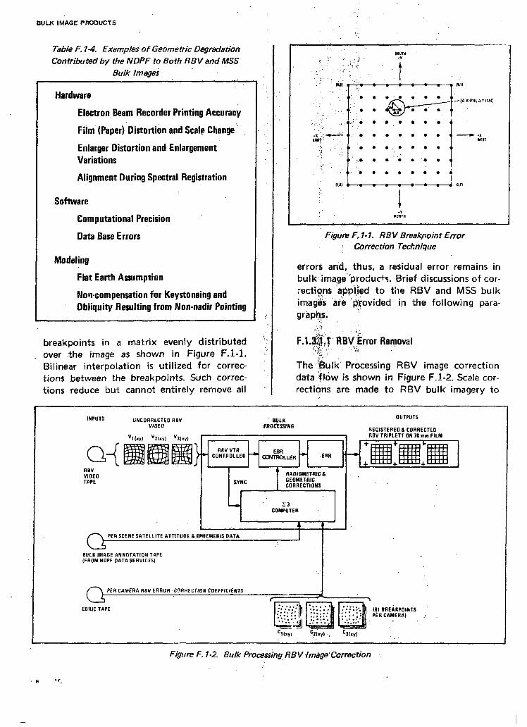
BULK IMAGE PFiODUCTS

Table F. 1-4. Examples of Geometric Degradation

Contributed by the NDPF to Both RBV and MSS Bulk lrn%ei

Hardware

Electron Beam Recorder Printing Accuracy

Film (Paper) Distortion and Seal? Clian@

Enlarger Distortion and Enlargement Variations

Alignment During Spectral Registration

Software

Computational Precision

Data Base Errors

Modeling

Flat Earth Assumption

Non-compensation for Keystoneing and Obliquity Resulting from Non-nadir Pointing

breakpoints in a matrix evenly distributed over .the image as shown in Figure F.l-1. Bilinear interpolation is utilized for corrections between the breakpoints. Such corrections reduce but cannot entirely remove all

I.

‘I,,

.&

Figunz F. I- 1. RBV Breakpoint Error Correction Tecl;nique

errors an’& thus, a residual error remains in buIk,image”produc+s. Brief discussions of cor- rectio-ns applied to the RBV and MSS bulk imag& ‘are piovided in the following para- grbphs. ‘i ;:

,:,‘I I,:. ;.., :’ F.1.@&1: R’BVkor Removal

1, ,yc : ‘, ,!‘,,

The %ulk~ Processing RBV image correction data $6~ is shown in Figure F.l-2. Scale cor-

rections are made to RBV bulk imagery to

INPUTS UNCORRECTED RBV BULK VIDEO PROCESSING

OUTPUTS

REGISTERED& CORRECTED

w REV WOE0 TAPE

..I 7 ,‘““E\ ij ~

PER SCENE SATELLITE ATTITUOE 8 EPHEMERIS DATA

BULK IMAGE ANNOTATION TAPE (FROM NDPF DATA SERVICES1

PEA CAMERA RBV ERROR -C@ARECTION COEFFICIENTS

EERIC TAPE

Figure F. l-2. Bulk Piocessing RB V Image’ Correction

account for frame to frame variations in altitude. In addition, calibrati,-r-s, of the systematic and stable portions of the RBV internal errors and distortions .are performed on a regular basis. Corrections for calibrated distortions and errors are determined and applied to all RBV bulk images. Residual distortion errors in the RBV bulk imagery are present as a result of calibration errors, RBV drift from calibration, and RBV random errors. ,.‘,

Table F.l-5 shows the total, rms, geometric errors in RBV Bulk Output Products resulting from all of the contributing error source&

Table F. 1-5. RB V Bulk Output Product Residual Errors (rmsl

__.--. --_

Positional Mapping Accuracy

Film Products

Paper Products

Registration Accuracy

All Products ._

1120 meter8

1130 meters

340 meters

F.1.3.1.2 MSS Error Removal .I ‘. I’ .: /

9’ WS. imagery is obtained under dynamic con- :@tidns,‘and conversions of MSS image data to

:j’output products without accounting for these ‘dy&mic imaging conditions.would introduce I ,> i, sii&ble image mapping errors.and distortions.

;; To reduce ,these dynamic errors the NDPF models the significant MSS imaging dynamics

‘: (no:minal and systematic variations from 2, .) ‘. ‘nominalj aed. corrects the MSS output images

accqrdingly.. I ,:

The:. Bulk Processing MSS image correction data flow is shown in Figure F.l-3. Examples ‘of corrections which are applied include:

0 Altitude variation from frame to frame and within a frame

0 Attitude variations within a frame

0 Variations in velocity from nominal orbital.velocity

0 Image skew caused by earth rotation and finite scan times

INPUTS BULK PROCESSING

OUTPUT

hw VIDEO TAPE

X.Y.R = fll) I-

TIMING 8 CAL OATA

FRAMED TO MATCH REV

AAOlOMETAlC ‘. MIRROR VELOCITY CALIB. DATA FUNCTION

Q SATELLITE ATTITUDE 13 EPHEMERIS DATA VSTIME

BULK IMAGE

ANNOTATION TAPE

Figure F. l-3. Bulk Processing M S S Image Correc ticn

FS ORIGINAL

SEPTEMBER 15, 1971

MS5 Errudn dtMOVAL PRECISION IMAGES

0 Systematic band-to-band off-sets resulting from finite detector sampling sequences

0 Non-l inear mirror scan profile

l Electron Beam Recorder and MSS mirror scan differentials

Residual error in this correction process re- suits from dynamic model ing assumptions and limitations. Table F-1-6 shows the total, rms,. geometric errors in MSS Bulk Output products resulting from all of the contributing ill. error sources. : ;.!

i :

Table F. 1-6. MSS Bulk OU&UI~ Product

Residual Errors frms)

Positional Mapping Accuracy

Film Products

Paper Products


All Products

1075 meters

1085 meters

155 meters a

I . ._, ;

,i :” ,!

F.i.3$. Preciypn Image Pioducts .. ,,

Con$epiually; Precision Processing’ is an ex- tensi’on bf the correction process discussed in Se&ion ‘,. ,F;fi3.1. However, the correction mechanismfor Precision Processing is totally diffeirent thti,n that for Bulk Processing. Errors are d&ermi&d by .measurements of the input ima&ry an’$I comparison with known quantities; X’@-rce - image distortion corrections are determined,-;-the input image is scanned by a CRT scanner in subareas of approximately 1/64,the ‘are? of thi:input image. Inverse correct@ns are.:!pplied.@ the scanning CRT. The sca.‘$‘ing ,CRT is hat&wired to. a printing CRT

. wh@ pnnf$,exact f/64 ima’ge sub-areas, thus cor#ting the ima&.‘distortions. In the same prc$&, .the;:,image ,:is en’larged to a scale of 1: l~~&W,~ In a$dition, corrections for

‘ima@, , locat@n are determined and corrected irnaF. I~o~~~‘on tick marks appiied to the prir-@d, ima.@ Precisibn. Processing image correction flow’% shown in Figure F.i-4.

Bulk 70 mm film products are the source of input imagery for conversion to Precision Output products. Thus, the output geometric

BULK INPUT

\ , c SCAN-PRINT e

EPHEMERIS ERROR ROUNDG{F ERROR, c

A 1

v APPLY TRANSFGRY

r l EVALUATE I C--M’

EOUIF’MENT, CORRELATION - -W

MEASURE COMPUTE - SPATIAL

COMPUTE ROUNDOFF

POINTING AND RESEAUS IMAGE - -- ERROR

CALIBRATION ERROR ANO GCPS RESECTION TRANSFORM

ENVIRONMENTAL. ORIENTATiON. EOUIFMENT AND SCANNING ERRORS PRINTING ERRORS

i I I

t

95 INCH PRECISION PROCESSED LATENT IMAGE

4 4A t , BAD coo0 GCPS

RECOMPUTE f-1) GCP

EPHEMERIS DATA , L RE.EVALUATE GCP ILATEAI J BLUNDER

YAP. ERRORS, EOUIPMENT AND - - POINTING ERROR

OC UPDATE j - - -D ERROR SOURCE

- -

Figure F. 1-4. Precision Processing Data Flow and Error Sources

W ’-WAL -.. _

fidelity discussed in Sectio., F.1.3.1 is the input fidelity for Precision P-c.cessing.

An initial step. in Precision Processing is the measurement’ of distortion in the input image. For RBV input images, shese residual distortions result from:

0 Those introduced by the RBV camera since the !act calibration and notcom- pensated in Bulk Processing (see Section F.1.3.1)

0 Those introduced by Bulk Processing

0 Those for which no compensation was attempted in Bulk Processing

0 Those where compensation was not exact.

Similar residual distortions exist in the;,input MSS imagery. Image corrections are determined for a matrix of 81 points with b&near interpolation between points and corrtdtions are applied during the’scanning/printing.~bper- ation.

In addition to the measurement of imagedis- tortions, identifiable control points in the input image are measured relative to known stored locations of the control points. By utilizing photogrammetric spatial rese!ct.ion techniques, the position and attitude of the spacecraft can be estimated. Utilization of redundant (i.e., more than necessary) cqntrol points within an image increases the acchracy of such estimates to better than those &hich are obtainable from spacecraft telemetry and the ephemeris derived from tracking. The resulting increased accur;rcy in spacecraft;position and attitude increases the positional location accuracy of the ilnage. Based on:these estimates, corrected geographic tick marks are then computed and applied.

Tables F.l-7 and F.l-8 show the total, rms, geometric fidelity for RBV and MSS Precision Output Products.

Table F. 1-7. Rt3 V Precision Output Product Residual Err&s Inns)

P+tional Mapping &cuncy

Film Products 95 meters

‘I -” Paper ‘Products 135 meters : :,.

&$stmtia~ ‘Accuracy ,’ ,’ . All Rpduti 115 meters

‘, /

!’ ,$le F. l-8. M S S &vcision Otiiput Product

Residual Errors lrmsl I!.

Paper Produetr


All Products

235 meters

250 meters

150 meters

F.2 kk40i0~~TRV

The radiometric fidelity of the ERTS system described in this appendix considers the macro-scale or low spatial frequency effects primarily caused by non-repetitive variations, such as short term drifts of dc-reference levels, bursts of low-frequency noise smudg- ing due to developer and developing process local variations--effects that are systematic in nature. and removable by proper calibration methods. These effects include referencing to

,. r the electronically introduced gray scale located on the sides of the electron beam

: recorder film images.’ The relatively high frequency noise components are excluded. These are noise phenomena at spatial frequencies’equal to the size of a resolution element, where the SNR ratios are low, i.e., about 5/l or less.

At high spatial frequencies (i.e., very small sampling apertures) the effects of film granularity are large. Selwyn’s Law, shown graphically in Figure F.2-1, holds only for small apertures and density ratios approaching

F-7 ORIGINAL

SEPTEMBER 15. 1971

MICRO-SCALE DENSITOMETRY

--i

loot

100

~ACROSCAU DEiVsl~oh~~rkY

\

FOR 70 MM IMAGES:

dA

21 pm

50

100

1 mm

KM2

0.004

0.023

0.09

11.0

02 (ANI

1

2.5

4.8

50.0

WHBRE:

u A = GRANULARITY @ APERTURE A Q

uG(A) = GRANULARITY @ INCR. APER. AN

II u

=, DENSITY b APERTURE A

u

‘N

= DEUSITY @ INCR. APER. AN

, ( I

10-3

Figure F.2- 1. Macro Scale Densitometry

< “4L .

I -

unity, but for illustrative PI (poses it can be used to show the reason b-l”.ind macro-scale radiomtric analysis and why noise effects at that level are negligible.

Sampling with small apertures, like 50 pm, produces relative inverse granularity in the, order of 2,. thus precluding radiometric evaluation with any degree of certainty. In order to increase the’ certairlry of radiometric evalua- tier,. the sampling aperture must be increased (equivalent to increasing the ‘actual’ area covered on the ground) to a point where the relative inverse granularity becomes .,high, about 50/l or more. As can be seen from Figure F.2-1, to obtain such a ratio at a density level of 1.0. the aperture should be at least 1 mm in diameter, or, in terms’of an equivalent covered area on the ground, it becomes a minimum of 11 square kilometers.

In practice the University of Purdue uses a minimum SNR criterion of 30, or about 30 dB in their analyses of digital data. Since the precise relationship between relative inverse granularity and SNR has not been defined, using a ratio of 50/l or a sampling area of 1 mm diameter is conservative, and analysis based on it entirely justifiable.

jn order to make the results more coherent, all video signals have been normalized to the equivalent dynamic density range AD of 2.0, where 2.0 represents 100 percent. Further, since most film and process data are published for a density of 1.0, this value was’ used throughout the calculations. Also, a particular film/chemistry combination has no impact on the results since experimentation has indicated a similar and uniform behavior between combinations.

The difference between relative and absolute radiometry should be noted here. The radiance seen by the payload sensor is a relative measure of the true spectral signature of the target. The atmospheric path contributes a significant amount of spectral radiance through Rayleigh, Mie, and selective scattering

F-9

processes. This path radiance is directly additive to scene radiance and since it will not be sentid separately on ERTS A or 6. measurc- ment of the true or absolute radiometric spectral signatures of scenes will not be poiible.

F.2.i Return Beani Vidicon Camera Radiom- *etry

The major error contributors to RBV radiometry are:

1. RBV camera subsystem

2. Communications elements

3. Restabilization of the signal

4. Image recording processes

The overall flow of RBV data from a radiometric viewpoint is shown in Figure F.2-2.

F.2.1.1 RBV Subsystem

The most important error sources in the RBV are residual image effects and shading. Resid- ual image effects, illustrated in Figure F.2-3, are known to exist in all slow scan vidicons. Careful ’ clean sweep” (i.e., photoconductor preparation) will minimize it, but values much lower than 5 percent of the peak signal output amplitude a-e difficult to obtain.

Shading found in some images produced by the RBV has been densitometrically traced with the results shown in Figure F.2-4. Shad- ing within the camera can be as large as 30 to 60 percent of the total signal (black and white amplitude) over the full picture frame. Pre- flight calibration data taken at fixed points over a 9 by 9 matrix in the camera image will provide shading correction information. This data will be applied during Bulk Processing and will reduce the shading error to less than 5 percent of AD. The resulting 5 percent is illustrated by the lower trace in Figure F.2-4. The corrections will be made by linearly interpolating between the calibration data ‘points of the 9 by 9 matrix.


RBV SYSTEM FLOW

/

,AYLOADSEWSOR /. SIC

j

OROUllD : 1tms WIOEBAFIO ¶KnoEnANO

SCENE -c wolcoN I vmti TELEMETRY -

l AYILWIER RECORDER SunvsttY . CAMERA CONTROLLER

L COYSllER

WOE0 TMES I

TO WlPF .“LI?ROCESSlYG RECElVlM SITE SUrJVltEY

WSFW EOUIPYEYT WSWRICTL -

7Sl+ll!i ENLARGEA #.6~-lq STRIP

- LFILWJ - PRINTER DEVLLOPER L PAPER

,

STRIP PRIITER

- LFILU DEVELOPER

o.w~3a

. VIDEO PROCtssOR

. FILM

STRIP PRIYTER 6 ?APER

Figure F.2-2. RBV System Flow

RBV RESIDUAL IMAGE&SHADING EFFECTS

--

1ST PICTURE

5

AFTER ER.ME

SCAN SCAN ‘. ,/

NEXT PICTURE

f W ITH RESIDUE

SCAN

Figure F.2-3. RB V Residual lniage Effect

I I I I IROW5 I

I LINEAR

INTiRPOL TION

+ CALIBRATION MATRIX POINTS

ERRORS BEFORE CORRECTlOt

ERROR AFTER CORRECTION (COhlPbSiTE, ROm5.6 87)

Figure F.2-4. R B V Shading Effects and Calibration

F-11 ORIGINAL

SEPTEMBER 15. 1971

RBV RADIOMETRY SIGNAL RESTABILIZATION

In addition to the preflight calibration, in- orbit calibration will be made *using lamps within the RBV. These corrections w,ill also be applied during Bulk Processing at the same time as the preflight calibration corrections are made. A comprehensive description ofthe calibration methods is given in’ Appendix G.

F.2.1.2 Communication Equipment

The components contributing to radiometric degradation in the communication path are also shown in Figure F.2-2 starting with,the on-board wideband video tape recorder (WBVTR) and proceeding through the ground tape recorder playback stage in the NDPF. Considered here are such effects as doppler shift, RF polarization, second detector drift, level adjustment inaccuracy, and AGC effects in the receiver. Best estimates of the degradations due to this portion of the system are 3

.,’

to 5’percent of AD. Most of this degradation is removable on the ground.

F.2.1.3 Restabilizatioti bf Signal

Due to variou? effects, such as dc level shifts in the ,camera electronics and low ,frequency noise pick-up from. .spacecraft ground loops which tend to modulate dc signals, the RBV signal guffers from amplitude variations on a line-totline basis. These variations consist of both dc level drift and zero to full scale amplitude: changes. To eliminate these variations, the RBV signal. is reclamped in the NDPF Video Processor andSync Separator (VPASS). This ‘process effectively establishes a new dc reference (black) level and nullifies nearly all preceding dc,level variations including the 3 to 5 percent :jink errors illustrated in Figure F.2-5. Resulting radiometric error will be less than one percent of AD.

SYNC

7r

DC-ClAMPiN& & AGC

T 0- I VARIABLE

I

r CLAMP Lc”FI

i.- AGC SENSING

* BEFORE DC-CLAMPING AND AGC

r + DC-CLAMP ERROR

----- ----- -e-e- -

AFTER CLAMPING AND ACC

Figure F.2-5. DC Clamping and AGC

Automatic Gain Control ‘(A(.C) in the electron beam recorder (EBR) ;ontrol unit, by sensing the sync tip to peak wh*tie amplitude, tends to keep the absolute peak-to-peak value of the signal constant..

F.2.1.4 RBV Bulk Processed Data

Additional errors are introduced by photo reproduction. Initial photo processing involves developing the SC-L19 film emerging from the electron beam recorder. The output is the first generation, 70 mm imagery for th+ RBV as shown in Figure F.2-2. The error contributors are primarily due to the fitm variations and developing process and contribute .less than 2 percent of AD.

The contributors to radiometric performance degradation during photo processing are:

Film and developing processes * 1.00/0

Strip printer f 0.50”/0

Contact printer

Enlarger f .5%

The RSS total of these contributors is also less than 2 percent.

F.2.1.5 RBV Precision Processed Date

The overall radiometric linearity and dc level stability in the Precision Processing subsystem is determined by:

.:, 1. Characteristics of the leveler and video

photomultiplier tubes of the fr,aming stage in the viewer/printer

2. Video processing electronics stability and linearity

3. Residual optical effects in the optical portion of precision processing. Auto- matic correlation is performed in the viewer/scanner, but since the characteristics of the correlator operation

., 1

F-13

KtlV PRECISION PROCESSED DATA

are primarily geometric, they do not affect the system’s radiometric per- 1. formance.

1 Theradiometric effects are:

! ,, . . 1. Optical Effects-Co8 losses and vi- : gnetting. l-!owever, due to a cancelling

effect in the leveler loops, a residual ‘. of only f 0.7 percent remains.

.1’2. Photo Multipliers-PM’s are regarded as the most critical components affecting radiometric performance. The most important parameters are quantum efficiency, stabilityjdegrada- tion, gain linearity and repeatability. PM’s are calibrated every four minutes, or every half minute if required by out-of-spec temperature variations in :.i the operating environment. The calibration is determined by its stability and is better than 0.1 percent.

;;3. Video Processor-The main param- 1,. eters. are de-level and gain stability

with: respect to temperature. Due to indiv.idual precision temperature compensation the corresponding AD effect is less than one percent.

F.2.1.5.1 EBRIC

The generation of the radiometric corrections to be used in Bulk Processing is one of the functions of the Precision Processing subsys- tern. This process consists of the following:

1. Taking as input uncorrected bulk cali- jr. 3 bration reference images generated in 1’ the Bulk Processing subsystem,

2. Measurement of calibration images to derive the relationship between the

. . actual signal from, (1) above, and the ’ corrected, pr.oper value,

3. ‘Generation of Electron Beam Record- er image Correction (EBRIC) data utilizing calibration reference data

The corrections are subsequently transferred to the electron beam recorder control and the

ORIGINAL

SEPTEMBER 15. 1971

‘.

EBRIC REV SPECIAL PROCESSING

original images are corrected by gain’ adjustment of the electron beam recorder signal. during Bulk Processing.

The corrections remain valid as long as new inflight calibrations do not indicate any change in RBV radiometric calibration. Should this occur, however, the new corrections will be derived by forming difference signals between the old and new calibration (in-flight) information. The. “revised” information is subsequently applied to the EBRIC.

F.2.1.6 RBV Special Processing

F.2.1.6.1 Bulk

The RBV recorded video data must be converted from analog to digital form before re-

forn$rtting and conversion to computer com- patibl’e tapes- (CCT). There is essentially no degradation to the data during this process and, ihe RBV data recorded on bulk Ccl’s represents the raw data received, on tape in the MbPF. It. should be noted that no calibration i,s perfor’med on th.is data at all and it still contains up .to 30 to 60 percent radiometric error$‘d,ue to shading alone. The user desiring to interpret this data must be prepared to apply his own corrections; see Figure F.2.6.

F.2.1.6.2 Precision

Precision processed CCT’s are derived from the precision .processor and since the data has already beenbulk processed, the data is corrected prior to digitizing. The contributed error’,during &is digitization process is negligi- I I ‘I). ble; ae Figu&‘F.2-7. I .

- .

VIDEO TAPE

r

VIDEO TAPE VTR

- CONTROLLER -w. HDDiA’ - HOOT

RECORDER CONTROLLER RECORDER

I BULK PROCESSING 1 J BULK COMPUTER COMPATIBLE TAPE

HOOT HODTR’ RECDRDER --c CONTROLLER/ - COMPUTER .-m

CORRECTOR CONTROLLER

c

- CCT -jZJ

I SPECIAL PROCESSING I

l HDDTR = HIGH DENSITY DIGilAL TAPE RECORDER

Figure F.2-6. RBV and MSS Bulk Computer Compatible Tape Generation

‘)F “‘AL

MS OR RBVC ::. .’

BULK 70mm FILM IMAGE

I,,... ,,‘j,l.

- -..i-- *.j E; ---. ---_

.z- =- ---

0

_-I -2 --...

-=ZZ f--

I

:, .,p li . ,PRECISIDNPROC~~lNQ I ;: :

‘. PRECISION COMPUTER

/ COMPATIBLE TAPE

I- SPECIAL PROCEFING 1

.--- _.

F&we c-2-7. Precision Digital Image Data

- . .

F.2.1.7 RBV Summary

The net effect of all radiometric errors for the RBV is given in Table F.2-1. The table shows the radiometric accuracy for all output products. All error sources in the flow are root- sum-squared with the exception of the re-

Table F.2.1. Summary of RB V Radiometric Errors

&,tQ,, t Product

Bulk Processed:

Archivll Film

70 MM potiie

9.5 In. PO*

70 MM Nqaiwe

Recision Pramsd:

9.5 In. Positin

9.6 In. Nc@ire

CCT Bulk Tapes

CCT Precision Process Tapes

70 WI 1G

70 (+I36

9.5 (+I 3c

70 (--I 46

Yt 6.1)

t 7.5

t 7.5

+a 7.7

9.5 (4 56 ?B.l

9.5 (4 6G * B.3

Digital Magnetis Tape Uncomrwtod Raw Digital Vidan

Digital Magnetic Tw * 7.8

NOTE: 70 (+I 36 = 70 MM, positive tnnrpwency, 3rd gmwmtion.

sidual RBV shading after EBR-CTL which is added directly to the RSS total. The VPASS removes the 3 to 5 percent link errors, and EBR-CTL reduces original shading error.

F.2.2 Multispectral Scanner Radiometry

F.2.2.1 Spacecraft and link Errors Sources

The initial stages of the MSS sensor are analog in nature. Bands 1. 2, and 3 use dc coupling wh,ile Band 4 utilizes ac coupling with dc re- clamping. The bulk (1.5 percent) of the MSS-contributed radiometric error is due to dc voltage instabilities in the baseband amplifier. The analog signals are applied to a,n analog-to-digital converter and finally to a mu Itiplexer. Temperature variations will cause quantization errors of 0.8 percent. Total radiometric error out of the MSS sensor amounts to 1.7 percent of AD.

F-185 ORIGINA

SEPTEMBER 15. 197

MSS R&XOMETRlC ERROR SUMMARY

MSSRESOLUTION

The signal emerges’ from the MSS in digital form and is transmitted and handled in this form up to the digital-to-analog converter in the NDPF as shown in Figure F.3-1. Theerror sources down through the D/A converter can be attributed to within-the-line amplitude jitter, clamping inaccuracies, and spurious A/D and D/A -conversions lasting over many resolution cells, but values of these contributing errors are negligible.

F.2.2.2 MBB Bulk Processed Da&

The image recording and reproduction procedures and functions are essentially the ime for both RBV and MSS data. The error sources and contributed degradations are identical; they are described in Sedtjon F.2.1.4. The combined effect of all radiometric errors for the MSS as seen in the photo output products is given in Table F.2-2. -

Table F.2-2. Summary of M S S Radiometric Err06

Output Pmduct

Bulk Procased:

Archival Fi lm

70 M M Poaitius

9.5 In. Porith

70MMN19ntive

Pm&ion Processed:

9.5 In. Posit&

9.5 In. N*ptiva

CCT Bulk Tqsr

CCT P~siiion Procms TQM

TYPO

70 (+I 1G

70 I+) 36

9.5 (+I 36

70 (.-I 46

9.5 I+) 5G

9.5 l-1 6G

Digital Magnetic Taps

Digital Magnetic Taps

f2.4

i2.8

* 2.9

t3.1

i3.5

f 3.6

t1.7

+ 3.1

NOW 70~+~3G~70YM,po~mnrpmrry,3rd~nmb’~n.

F.2.2.3 MSS Precision Processed Data

The precision processing function is also corn mon to the RBV and MSS data. The errors sources and contributed degradations are identical and are described in Section F.2.1.5.

F.2.2.4 MSS Special Processing

F.2.2.4.1 Bulk

The MSS signal on the video tape received in the NDPF is already in digital form. The re-

recording pr.ocess to generate bulk CCT’s involves merely a reformatting and contributes.‘,less&t~ally no .degradation in terms of rad&‘metry;‘see Figure F.2-6. ’ vj

.‘:,.

F;2.2:4.2 Pr&iion

Precision CCT’s are derived from the precision processor tihich in itself contributes less than 0.1 pertent d,egsadation; see Figure F.2-6. The total radiometric degradation in the MSS output’CCT’s is’given in’Table F.2-2.

F.3 ‘RESOLUTION .; ..:;,;d, .’

F.*$ Me Fpolution /x ,./ 1: .\‘. .*

The@lSS se&or instantanequs field of view fIF*j Is Q$@6 mift,i,r:adianJ:‘~orresponding to 7B,i&tets as%easured on the grolqd. Due to the~$&tegratf#g effects of the’fiber optics in the ,#SS, &$ution is limited to the I FOV dir-$&ion. Resolution, as used in this handbook@ refers/to the ,ability of an observer to recoznize adjacent fields of a certain width (e.g.:;,,‘80 meters). It is possible that the ex- istence of boundaries between radiance fields as small as l/2 IFOV can be sensed in certain scenes, however, this is not the same as recog- nizing the actual field dimension.

Scene radiance, as measured from nominal ERTS altitude, serves as the input to the MSS sensor. Since the radiance is measured thro$gh the’ aimosphere, it 1s a relative mea- sur$$f fhe,.@tual radiance on the ground. Tabf$ ,F.3-J-,h$ts some apparent. radiance levels for .ii’arious, ,$bservables as. viewed by the sensor.’ This .data is representative of the radiance.“levels to be sensed by the various bands of the MSS. ’

The scene radiance is sensed in the MSS, transformed to a video signal and immediately converted to a digital bit stream. It remains in digital form throughout transmission to the ground and until it reaches the digital to analog (D/A) converter in the Bulk Processing stibsystem. Figure F.3-1 outlines the flow of MSS data from ground scene input, through the spacecraft sensor, wideband telemetry,

C “4L

IYU I ,\L, I\“-..-.- MSS SYSTEM l=LO(H

L

VlDEOT&I ., ~ULKtiOCEUlYG

RECEIVING SITE suarng ‘.,

-. WSF” EO”lrYE*T ;, l wevrni;GTL I . ?AYLOAO RSE :/ . EBR L CT1 . wlvrn ‘, . FILhl *“,

L . VPMC

T -* ijRI? I,

FIIINTER 8.5wa i, I’ - L FILM/

OEVELOF.EEII

. VIDEO PROCESSOR

. FlLY

na STRIP 8.5wEE FRIITER L FAPER

SrRI? “RIP / PRIITER PRIHTER

L FIN/ 6 FILU DEVELOPER

I

OEVELWII

,

Figure’F.3-1. MSS System Flow .

ORIGINAL SEPTEMBER 15. 1971 ; FL17

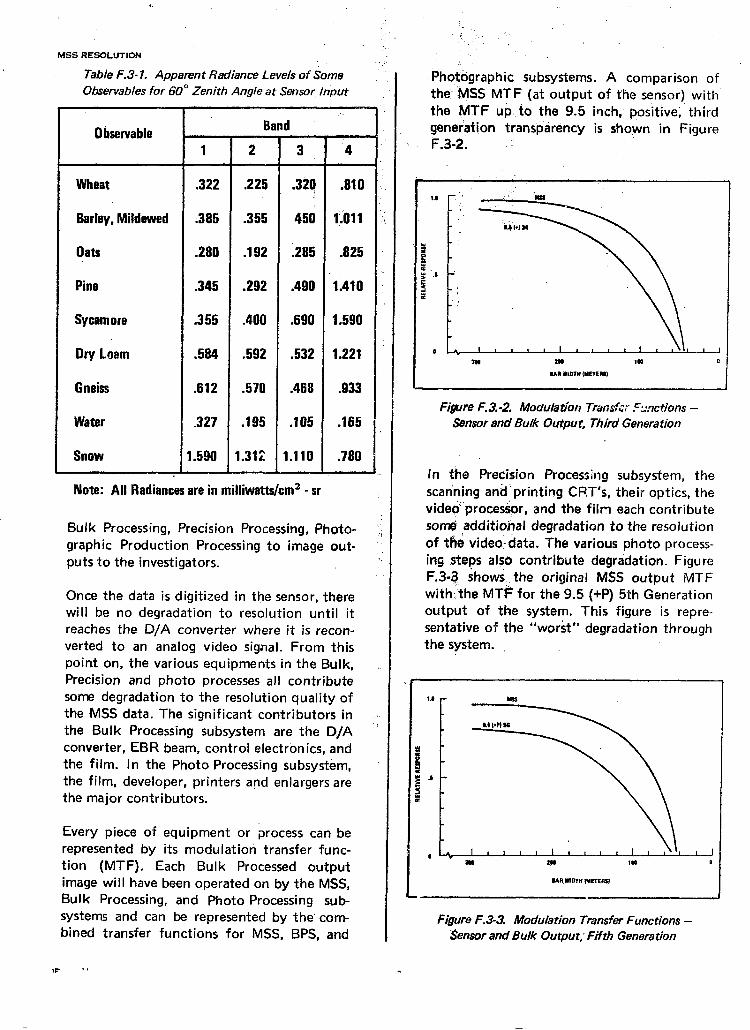
MS.5 RESdLlJTlON

:

Table F.3- 1. Apparent Radiance Levels of Some Observables for 60” Zenith Angle at Sensor, input

Observable Band "

1 2 3 ‘4

Wheat .322 ,225 .32q .810

Barley,Mildewed ;385 .355 450 11011

Oats .280 .192 .285 .825

Pine .345 ,292 .490 .lAlO

Sycamore .355 .400 .690 1.590

Dry Loam .584 .592 ,532 1.221

Gneiss .612 .570 .468 .933

Water .327 .195 .195 ,165

SMU 1.590 1.312 1.110 .780

Note: All Radiancesarein milliwatts/cm2 - sr

Bulk Processing, Precision Processing, Photo- ‘: graphic Production Processing to image out- : puts to the investigators.

Once the data is digitized in the sensor, there will be no degradat ion to resolution until it reaches the D/A converter where it is recon- verted to an analog video signal. From this point on, the various equipments in the Bulk, Precision and photo processes all contribute some degradat ion to the resolution quality of the MSS data. The significant contributors in the Bulk Processing subsystem are the D/A converter, EBR beam, control electronics, and the film. In the Photo Processing subsystem, the film, developer, printers and enlargers are the major contributors.

Every piece of equipment or process can be represented by its modulat ion transfer function (MTF). Each Bulk Processed output image will have been operated on by the MSS, Bulk Processing, and Photo Processing subsystems and can be represented by the combined transfer functions for MSS, BPS, and

Photographic subsystems. A comparison of the- tvJSS MTF (at output of the sensor) with the &lTF upto the 9.5 inch, positive; third generat ion t ransparency is shown in Figure F.3-2.

Figure F.3.9 Modulat ion Transf~; !=z.xtions - Secsor and Bulk Output, Thkd Generation

In the Precision Processing subsystem, the scanning and’printing CRT’s, their optics, the video processor, and the film each contribute so& additional degradat ion to the resolution of the video::data. The various photo processing steps also contribute degradation. Figure F.3-3 shows, the original MSS output MTF with--‘the MTF for the 9.5 (+P) 5th Generat ion output of the system. This figure is representative of the “worst” degradat ion through the system.

L UR 1107” ,METEfLs, Figure F.3-3. Modulation Transfer Functions -

sensvr and Bulk Output,’ Fifth Generation

Resolution is defined by ‘hat value of signal- to-noise ratio which just Fermits recognition of a tri-bar pattern by a human observer. This criterion was developed by Otto Schade through experiments wh,ich yielded 4;O:l as the SNR threshold. Tha Lrnctional relationships for determining SNR output of the MSS detectors are as follows:

PMT (Bands 1-3)

SNR = G -N;

(N;)l” x MTF X Kn

Photodiode (Band 4)

SNR = (N2 -N;) x MTF x K,

Where

N’ = apparent radiance in optical passband of bars in test pattern as seen from space,mw/cm* -sr

MTF = system modulation transfer-function

Kn = unique constant for each spectral band, n

Note that the SNR is directly dependent on the input radiance, hence the resolution is directly dependent on the scene itself.

The resolution characteristics for the four spectral bands of the MSS have been plotted in Figures F.3-4 through F.3-7. The curves show performance at two different poi,nts in the system : a’

1. MSS output--representing the resolution performance of the sensor itself, or, the performance of the system were there no degradations due to ground processing. Resolution cannot be better than this

2. 9.5 (+P) 5G-represents the most degraded output that is sent to investigators. All other imagery will have better resolution.

F-19

To interpret the results for any two observables, the scene radiances are selected from Table F.3-1 corresponding to the observables in question. The smaller of the two’ radiances is subtracted from the larger and the resulting value entered on the ordinate of the graph. The larger of the two radiances is plotted on the abscissa..The boundary line directly below the ‘resulting point represents the recognizable bar width for those scene characteristics.

.

For :example, in Band 1, wheat versus mildewed barley will have N1) = 0.322 (wheat), N; = 0.385 (mildewed barl,ey) and (N2 -Hi) = 0.063. Plotting 0.063 on the ordinate and 0.385 o,n the abscissa of Figure F.3-4 yields a resoiution limit for this scene of:

1. 100 meters at the MSS output

2. slightly less than 300 meters on a 9.5 (+P) 5G image

This means that a human observer, hypo- thetically placed at the MSS output, could recognize adjacent fields of wheat and mildewed barley if they each exceeded 100 meters in width. If he were viewing a 9.5 (+5) 5G image, he could recognize the same fields if they exceeded 300 meters in width.

The investigator can use the curves of Figures F.3-4 through F.3-7 to determine the MSS system resolution for any pair of observables using Table F.3.1 or his own input values.

The Special Processing subsystem takes digitized MSS video data from the NDPF WBVTR and converts it to computer com- pat.ible tapes for distribution to investigators. Since this is s?rictly a reformatting process and does not involve any digital-to-analog conversion, no degradation to resolution results; and the resolution will be essentially the same as at the MSS output. Any photographic reproduction which, is subsequently done by the investigator will have an effect on resolution commensurate with the MTF’s of the equipment used.

Computer compatible tapes (CCT) generated by the Precision Processing subsystem will


.

MSS RESOLUTION

RBV RESOLUTION

Figure F.3-5. MSS System Resolution - Band 2

have a resolution only slightly better than that of the Precision Processing imagery outputs. This is because the data on the precision CCT’s has already passed through the Bulk photo and part of the Precision Processing equipment and has been degraded by these equipments.

,.I

1.1

9

1

;

_’ ;

.u

.”

Figure F.3-6. MSS System Resoiu riurr” - Band 3

q --------e_-----

IlMltlllf

1---------------- ii

Figure F.3-7. MSS System Resolution - Band 4

F.3.2 RB\i Resolution

Scene radiance and contrast, as measured from the nominal ERTS altitude, serve as input to the RBV sensor. Since these parameters are measured through the atmosphere, they- are a relative measure of the actual

C ‘WAL - -cI

III

parameters on the ground. - able F.3-2 lists some apparent contrast and r .c:iance levels for various combinations of observables as viewed by the sensor. This data is representative of the scene characteristics to be viewed by the RBV.

Table F.3-2. Resolution Analysis Typical Scene Characteristics

BAND

Wn1l1ngtJt lntwvll brn)

Avsn~Plantvs. Dry Loam

GhndContnst spice Contrelt Maen lhdiiucs

mw/cm’-u

Average Pbntvr Watw

Ground Contrast spree Contrest Muan Radiance

Avenga Plsntvr.Wet Loam

GroundContrast Space Contract M m Radiance

t (I Plant vs. Averep flant

GroundContrast Spece Contract h&en Radiansa

Averagr Plantvr. --4 Plant

GroundContrast Space Contrast MeanRadiance

1 2 3

.475 - .575 ‘.680 - mo .BW - A30

2.1&l x12:1 1.5&l 1.5 :l 2.0 :1 1.3 :l

.465 A34 &zs

1.32:1 1.79:1 1.1 :l 1.2 :l

,386 ,255

1.16:1 1.0 :l

.3a2

1Al:l 1.57:1 1.4 :l 1.2 :l 1.2 :l 1A :1

,425 ,366 .653

1.9O:l 1.2 :l

.351

1.79:1 13 :l

,314

2.29:1 1.57:1 1.4 :l 1.5 :1

.238 A48

19.&l 3.w

.364

1.66:l 1.4 :l

A76

The scene characteristics are sensed by the RBV cameras, and converted to an analog video signal (Figure F.3-8). The video, in- analog form, passes through the camera controller and combiner, spacecraft WBVTR, wideband telemetry system, receiving site electronics, and is recorded on a receiving site video tape recorder (VTR). The tapes are then transported to the NDPF for processing. :

At the NDPF, the data is played back on a VTR, fed through the electron beam recorder (EBR) control unit and written on 70 mm film by the EBR. The latent image is developed, printed and possibly enlarged depending on the path taken through the Photo- graphic subsystem. ’ : ’ :,; ;L

Each component in the video path contributes some degradation to the signal-to- noise ratio o’f the video and hence the resolution of the RBV,imagery. The degradation is a function of the modulation transfer functions

_, (MT.F): ,of the. individual components. The only exception is the- video processor and sync ‘Separator (VP&X), a major piece of equipment both at the receiving site and at the NDPF. It has a very wide frequency response, -1dB at 8 MHz, and contributes essentially no degradation to the signal. ;

The output signal-to-noise ratio of the RBV is determined using the following equation:

fN FA too)

f FA (f) o-

C 2ym& tf)]

The full scale signal-to-noise ratio of the RBV (SNRFS) is read from Figure F.3-9 given the full scale exposure value (ExFS) for each channel. For a given exposure time (ts) and using the effective f-number of the lens (T) then the following equation is used with mean radiance (N’) of the scene in each channel to determine the mean.exposure of the scene at the vidicon faceplate:

E nN’t,

-- ’ - 4~2

microjoules/cm2.

The slope (7) of the light transfer characteristic for the camera is 0.9.

The input scene modulation is calculated from the space contrast ratio (Co) of the scene at the vidicon faceplate using:

m, = co -- 1 co + 1

where

co = Ni

N! ,

F-21 ORIGINAL

SEPTEMBER 15. 1971

REV SYSTEM FiOW ---.~-

‘_

F JlfwlLIw~P -, I .I

PAILOAOSEISOR I S/C I

oROU*o : LENS WIOEIAYO S/CWlOES;RO

SCENE VIOlCON

I _ WOE0 . c TELEMETRY -

. AYILIFIER RECORDER SUGSVSTEH

. CAMERA COGTROLLER a CoumER

WOE0 TAPES BULI( PROCESSING

SUnSvsrEH

+. MSFY EGGIPMEHT . PAVLOAO RSE . WSVTR

I 701rllG E”LARGER 9.51~IZG

- 6 FILM/ - = ’ DEVELOPER

STTRIP 1

PRllTER - hFILY/

9.5itm

DEVELOPER

T CGWTACT STRIP STRIP

7WfG PRlWER 7OI-120 PRIITER 7OW30 PA,Y~ER 7Gl-I40 - i FILM, - L FILM, * &FILM! ’

DEVELOPER OEVELOPER DEVELOPER

PtloCEsslnC

PROCESSGR

Figure F.38. RBV System Flow

“GINAL --. e-22

I I I I I I

0.1 0.2 0.6 1.0 2.0

EXPOSURE WROJOULE/CM2~

5.0 10

Figure F.3-9. Spectral Signal-to-Noise Characteristic

(Typical)

The video amplifier is assumed to be ideal with a 3.3 MHz bandwidth so that FA (f) = f and FA (-) = 2440.. fn is the Nyquist frequency of the raster in cycles/line. The units for spatial frequency (f) will be cycles/line as defined below:

cycles/line = (cycles/millimeter) x (width of sca,lned format in millimeters)

= (video frequency (MHz) x (active scan time (microseconds)).

The conversion of resolved spatial frequency to meters on the ground is accomplished through :

RG +x+,,

where W is the width of the scanned format, h is the spacecraft altitude and F is the focal length of the RBV lens.

The average square wave response rR of the RBV is determined from the modulation transfer function (MTF) of the lens, vidicon and amplifier by: I

ik(f) =+ “;(3f) : ?R(5f) rR(f) + 9 1 25 *

where

‘;R(f) = ‘?RBV(f) TLiNS(f) yAMP(f) -

Figures F.3-10 and F.3-11 show the resolution expected if a human observer were placed at the RBV output. This is a hypo- thetical point, representing no additional degradations due to rest of the system, i.e., refolution can be no better than this. The curves ware generated by applying Schade’s criterion, which is that threshold value (4:l) on SNR which just permits target recognition. Figures F.3-12 and F.3-13 show the resolution at the most degraded output-a 9.5 (+) 5G paper print after Precision Processing. Calculations were performed using a 12 millisecond exposure time. The effect of using another exposure time, t,, would be to modi- fy the ordinates (mean radiance) of Figures F.3-10 through F.3-13 by a factor of 12/t,.

-- - LuoIlhZ I --- m m 3

PACE COlVRCln

I

l lElOLYE0 STARAL FIEI IUENCV ICVCLEULIIE) -.-.

I I 1 31 10

I I1 45.7

I m m

EROUIID RESDl.Ul lD* METE~ESOLVED ELEYNTI C Figure F.3- 10. RB V System Resolving Power -

RBV Output Cross-tr-track

F-23 ORIGINAL

SEPTEMBER 15. 1971

RBV RESOLUTION ANALYSIS

SPACE CONTRAST

0 - I I I I 0 ma 1W 16w zm

RESOLVED SPATIAL FREOUENCV ICVCLES/LIIEI

I 1 I I I 365 I,, 01.5 61 a.7

GROUND REIOLUTlOM ~METERS/RESOLVEO ELEMENT)

Figure F.3- 11. RBV Sy&em Resolving Power -

RBV Output Along-Track

--- lAUD 3

PACE CONTRAST

-- i- . 1’

I

I

I ! I . ..-.-i

n E m I

Tow 15w tow

I RESDl.VEDSPLTlAL FREWERCV ICYCLESILINEI

I I I I I --I 336 183 llD.5 91.5 61 45.7

GROUNO RESOLUTION (METERS/RESOLVED ELEMENT)

Figure F.3- 12. RB V System Resolving Power -

9.5 (+PI 56 Precision Cross-track

S?ACE CONTRAST

I -..JW

RESOLVED SPATIAL FREWENCV lCVCLES/llNEI

--i-- -.--iv--1 350 103 01.5 8, 45.l

GROUND RESOUJTION IMETERWlESOLVEO CLEMENT,

Figure F.3- 13. RB V System Resolving Power -

9.5 (+P) 5G Precision Alonb-Track

In or.der to effectively use the curves, they must be related to a parficular ground scene. Table F.3-2 presents characteristics for a number of typical ERTS scknes. The values of radiance are predicated upon a sun angle (refer to Appendix J) of 30 degrees, which represents the worst case for the continental United States. Lower sun angles result in some resolution degradation due to poorer illumination conditions.

As an example, the average plant vs. water has a mean radiance of 0.366 mW/cm* -sr and a space contrast of l.l:l, as shown in Table F.3-2. On Figure F.3.2-10, the cross-track resolution at the RBV output can be read as 78.9 meters/reso!ved element. By comparison, the resolution of a 9.5 (+P) 5G image will be 130.5 meters for the same scene, as shown in Figure F.3-12. Note that using a fifth generation image is an extreme example. However, by showing curves at PBV output (best

REV RESOLUTION ANALYSIS

1 ERTS A), cross-track resolution at the RBV output is 71.4 meters while along-Crack is 93.3 meters.

.’

possible resolution) atid on 9.5 (+P) 5G (worst expected resolutiort) the performance of the system has been effectively bounded.

Along-track resolution CP’I be determined using Figures F.3-11 and F.3-13, which were also calculated with an exposure time of 12 mi Iliseconds. Comparison with Figures F.3-10 and F.3-12 indicates’sliphtly worse resolution,. which is due to smear. The effect of sma!ler exposure times, by reducing smear, is to cause along-track resolution to approach the cross- track values. Larger exposure. times, however, increase smear and fqther degrades along- track resolution. As an example, for a 16 millisecond exposure time (maximum for

F-25/26

The Special .Processing subsystem takes digitized ,video data from the Bulk Processing subqistem and converts it to computer corn patible tapes. for distribution to investigators. Perfect image generation by the investigator results in resolution slightly worse than at the RBV output. With Precision Processed video data; the resolution of images generated from these computer compatible tapes (CCT) woulcl be that of ,the Precision Processed subsystem OUtpUti i.e., slightly better than the resolution on 9.5 (+P) 5G.

ORIGINAL

SEPTEMBER IS. 1971

H

APPENDIX 3 CAL’IBRATIQN

The ERTS Image Processing Subsystems generate and apply radiomearic and geometric corrections to the’ sensor data during the initial process of converting received video tapes into film images. These operations require appropriate: radiometric calibraiion data for the RBV cameras and the MSS. :

.,.

Two types .of calibration data are employed for the RBV: (1) radiance maps obtained tiJa a uniform calibrated source, such as a H&is sphere, and (2) internal calibrat6-r (e&se) lamp radiance maps. From ‘the uniform tali- brated source radiance maps, the light transfer characteristics (LTC) and radiance’correcfion maps for each camera are derived..: The &TC defines the calibrated relationship betv$en the RBV signal voltage and input (scene) irradiance. ‘_

‘7;

The radiance correction maps provide ‘the two-dimensional functions to linearize :the spatially-variable signal and black-level chaiac- teristics of a given camera to its LTC. The calibration-lamp maps for each camera provide the two-dimensional calibration functions to relate the in-flight calibration images of a given camera to its LTC.

In addition geometric calibration determmes the two-dimensional projective geometry of each camera, the axial alignment of the three cameras to each other, and the alignment of the camera system to the axes of the splice- craft.

,’ For the MSS, three types of calibration data are employed: (1) calibration of the scat$ner via the l-lovis integrating sphere, (2) calibration of the scanner via a calibrated coilim~tor, and (3) the calibration wedge of the collimator itself. From the integrating sphere, the response characteristics of the individual detectors are obtained. Each detector is adjusted so that maximum radiance corresponds to’:full voltage. Utilizing the scanner as the tranifer function, the collimator is calibrated to’$he integrating sphere. The calibration wedge r&di- ante versus voltage and radiance vet,sus w.ord-

,. count response .are then derived by correlating ‘i, the calibrated collimator response at various .’ .. radiance levels to the calibration wedge out- . ’ put: The calibration wedge supplies the cali- pi. bration function to provide conversion be-

tween; input radiance and output voltage. 1

Gil RETURN BEAM VIDICON (RBV)

G.l .l Calibration Methods

G.1 .l .I Radiometric Calibration

;.,, Radiometric calibration is based on measuring ; .;;-, and ?egording RBV output signal versus posi- . . . . ;:I, tion’ in the twodimensional RBV image for- :., ‘:; rnat$f$r a number of known input radiance 1;‘; lev$$$vhich span (1) the spectral band, and

’ (2) th@range,of scene radiance for which each cam&#,is designed.

.’ Two types of RBV radiometric calibration data are util?d for the purpose of calibra-

1 tion:. ,.

1. Initial calibration data, describing the complete (spatial, spectral, voltage level) response of each camera to known, through-the-lens exposures,

. which is obtained prior to flight. This ,consists of uniform calibrated

‘, source radiance mapping, calibration- lamp radiance mapping, and test data.

2. lnflight calibration images, indicating <: -.

)k~ the response of each camera to fixed j J: and precalibrated on-board exposure

sources, which are obtainable upon I” ground command.

Initial calibration consists of a radiance mapping utilizing: (1) a uniform calibrated sourceand (2) the calibration (erase) lamps of the RBV’s. Through the calibrated source mapping, radiance corrections are derived for the scene and are applied to “correct” the calibration-lamp maps. The corrected calibration-lamp maps are then used as the standard to which all future.LTC and spatially variant corrections are based. RBV radiometric calibration, is illustrated in Figure G.l-1.

G-l ORIGINAL

SEPTEMBER 15. 1971

1’

CALlt iRATlON FLOW DIAGRAM RADIANCE MAPPING ‘.

NORMALIZED RADIANCE

\

RADIANCE CORRECTION

MAPS RELATIVE TO IMAGE

m2i_. --. --.- -. -.-Lb -. -~ ‘I,,>

Figure G. I- 1. Return:‘Beam Vidico6‘ Calibre tiqn

G.1.1.2 Uniform CalibratedSourte Radiance Mapping

This mapping is performed utilizing a Spectra-Prilchard Photometer “light-box” with a 0.25degree field of view which has been calibrated against a Hovis sphere. The useful diameter of the photometer is 5 inches and is uniform about an average intknsity of 2147 foot-Lamberts, to within limits of +2.9 percent and -3.1 percent. The mapping is performed at two radiance levels for each camera:

Camera 1 - full black and 0.85 mW/cm2-sr at 12 ms exposure

For each of the two radiance levels, the mapping is obtained by utilizing a radiance calibration computer program which provides a map of the video cutput on an 18 x 18 matrix (324 points) based on the reseau spacing. To smooth out the noise and eliminate spurious readings, each value presented is the average of data taken on 64 sequential lines. The -individual samples are integrated for. 10 seconds along the horizontal direction; thY.s the program collects 18 x 18 x 64 = 20’:736 individual samples;

Gamer-a 2 - full black and 0.85 mW/cm2-sr at 12 ms exposure

Camera 3 - full black and 1.36 mW/cm2-sr at 12 n-is exposure

utilizing the appropriate neutral density filters with the calibrated source.

The sample points are uniformly spaced over the active raster according to the scheme presented iii Table G.I-3.. Size and centering corrections are made to correct for raster distortion by comparing the known posit ions of the reseaq, as measured through the lens by the United States Geological Survey, with the position of the reseau determined by the same

I

. . - 7

SAMPIJL WIN ,b run I ESTS

The ecjuations for the reformatting trans- ‘, formation are presented below and are refer-

: erice$ to Figures GA-3. through (3.145 in- clusive. I.

configurational test equiprrmt used for the mapping. This correction J-ovides a linear stretch in the vertical or horizontal directions and a shift of the entire set of sample points.

In addition, gain and offset *ralues are applied to the measured values For the radi&e mapping, in order to correct the raw data input for minor variations to the al ignment and calibration of the circuitry in the test set-up.

OnLa the data is obtai,ied on the 18 x ,18 matrix it is t ransformed to a 9 x- 9 matrix which is based on l/8 subdivision of’.l$he n o m i n a) image format dimensio\s. Fi$$re 6.1-2 shows the relationship of the 18 xf’18 points presented in Table G.l-1 to’;Rhe 9.:x-9 matrix of points. ;, :..

The 9 x 9 correction-breakpoint matrix does not coincide with the radiance mapping data matrix. Therefore, radiance data values corresponding to the breakpoints located within the 18 x 18 radiance data a.rray are computed by interpolation within the four nearest data points; radiance data values correspondinq.to each breakpoint located at the edges of the image format are computed by extrapolation from the four nearest breakpoints.

Table G. 1-I. Sample Points for Tess (18 x 18 Matrix)

1 _-..m Vertical _ Line Number at_ amllle

Start of Sample Numlhr

39220 548 776

1004 1232 1460 1688 1916 2144 2372 2600 2828 3086 3284 3512 3740

-. ii . ~? . . 3968 .~ _ -.-_. - 18 I_-

‘.

Ititeypolation . ‘2’ ;& = (X-Xi) / (Xi+1 -Xi)

!!b k (Y-Yi) / (Yj+l -Yj) ./ :,

.,i

;;vxy =. (l-b).[(l-a)Vi,j + a Vi+ld ]

.?. ,;iQ. ,!tb (l-a) Vi,j+f + aVi+l,j+l .i’ c I ; :

‘::

$1 Co&#-Point ,Extrapolation .i.,,

? vxsY(c) = (l+b@+a) Vg,g -a b3,9 3

-b [ (l+a) Vg,3 -a va,l3 I

EdgePoint Extrapolation

Vxy(R,L) = (l-b) (l+a) V9.j +, aV&j 1 +b (l+a) vg,j+l + aVti,j+ 1 1

Horizontal

Line lime at Element Number at Start of Sample Start of Sample

z ‘5.9

it*: 60

2; 4:1 ~3.8 3.5

G-3 ORIGINAL

SEPTEMBER 15. 1971

‘_

,

!

MATRIX RELATIONSHIP

-- .- .i . .~._.

:

+ 0 0 0 +O m m h . . h A ” \# ” v

o+o of 0 0 +o of0 0 0 o+

- .c? :,, 0

I. *‘. :: o+

: 0 : 0

+ 0 0

*.

-

0 :: o+

p 0 ,

0 .o +

0 0 I

I 0 0

0 0

__ + 0 0

0 0

p 0+

0 0’

0 Of

0 0

0 0+

$BREAKP~INT LOCATIONS FOR 9 X 9

BULK-PROCESSING IMAGE CORRECJIONS

55 m m RBV IMAGE

019 X 18 MEASUREMENT POINTS (RCA)

+ESEAUS

‘0 c

O+C

0 c

+ Q c

h ”

Of0

0 0

o+o

c c

------k 0 0

0 0

--It- 0 0

0 0

o+o

0 0

o+o

0 0

30

.

0 0

o+o.

d 0 + 0 0 h 0 o+o 0 0 o+o

0 0 -1 L

0 0

0 0

+ .o -0

.o 0

+ 0 0

0. 0

o+o .-

0 0

o+o

F&e G. 7-2. Relationshp of 78 x 78 Matrix to 9x 9 Matrix

--I

i, i

Figure G. l-3. Interpolation

% 1 Cl

?

i,j+l itl,jtl VLI b I A I

(8,s) EM) .- T I I I

I (8,8)

i, i

Figure G. 1-4. Cdrner Extrapolation

! 1..

‘.- ,,.A t ::, i .? ’ ‘/

,..L. ,; ,’ .,,

:

i, 9

., ‘..: -i, fi

.; ,’

Figure G. l-5. Top- Bottom Extrapolation

8,j+l 9,j+l

-m 8J 9,i

a

Figure G. 7-6. Right-Left Extrapolation


RADIANCE MAPPING

SHADING EFFECTS

From this reformatted data, the radiometric .’ trahsfer characteristics of each camera can be !, “mapped” as a two-dimensional function of : image position.

: -- ;. I.:

The two-dimensional exposure-response ! characteristics of a typical RBV camera is p shown in Figure G.l-7. The upper figure represents a unifor’m 100 percent input radi- ante level which (for a given shutter- time) produces a full-scale RBV output signal, indicated by the lower figure. The mapof the ’ RBV voltage signal corresponding to the 100 .: percent input exposure level is indicated by .. the upper surface; the lower surface is a map ,y: of the RBV voltage signal Vo, corresponding ,,;‘: to zero input exposure. ,!

The variation in voltage response over the photoconductor is called “shading”. Such shading effects are inherent in RBV operation. They are associated (mainly) with spatial

i’

differences .in the sensitivity of the photoconductor, and off-axisvariatidn in the efficiency of ,b,hotoco.nductor’ charge preparation as well as :&her effects much more complicated in their nature. The shading effects of a given

.vidicon tube tend to be stationary, i.e., they are a fixed characteristic of that tube and its con’figuratidh, and thus. are ameanable to correction by post-acquisition processing of the.:RBV signal. The radiance,mapping data is therefore used to derive the correction functions that are applied to remove the shading effects.

.-_------

/

REFERENCE WHITE

i REFERENCE BLACK

I I

.l 1.0

NORMALIZED RACIANCE INPUT R/RN

‘RN = M A X SPECIFIED RADIANCE

R = INPUT RAnlANCE

Figure G. 1-8. Calibrated Light Transfer Characteristics - Image Cefl ter

A calibrated LTC, as shown in Figure G.l-8, is then defined as the relationship of the output signal at the image center to the known range cl input radiance. The radiance map is used to define the ratio of camera response at all other points relative to the image center calibrated LTC as shown in Figure G-1-9.

Figure G. 7 -7. RB V Exposurr-Response Characteristics

VOLT. 5:

.---m-e -- --- ..3 BLACK CLIP

1

: * (OFF-AXIS) . l

vc

ON-AXIS LIGHT-TRANSFER CHARACTERMIC

RADIANCE MAP OATA INPUT RADIANCE --- ~___ ~-.

Figure G. 1-9. Ddva tion of Li&t Transfer CharacmStics

6.1.1.3 Calibration Lamp Radiance Mapping

This mapping, using the RBV calibration lamps, is performe,d before and after the calibrated source radiance mapping. Three fixed radiance levels are utilized; O%, 30% and 80% of the foliowing levels for each camera:

Camera 1 - 0.85 mW/cm*-sr at 12 ms

exposure

Camera 2 - 0.85 mW/cm*-sr at 12. ms exposure ..,.

Camera 3 - 1.36 mW/cm*-sr at 12’ ms exposure

The mapping is performed utilizing the previously mentioned radiance calibration program over the 18 x 18 matrix of points a,nd then transformed to rhe 9 x 9 matrix of points.

,

Radiance corrections for the scene, derived via the calibrated source mapping, are applied to this data. The “corrected” calibration-lamp maps serve as the standard against which..the relative degradation will be measured.

G-7

G.l .l A Test Dlt~

Radiometric mapping is performed during testing of the RBV, and consists of a mapping using the calibration lamps. The radiance calibration program and procedures previously described are utilized.

The calibration lamp maps are compared with those previously obtained during initial calibration, i.e., compared with the baseline/ standard. This provides the relative degradation (if any) for each camera. The correction coefficients obtained from the final test data are $ised as the initial corrections for flight data;-

G.l .1;5 In-Fli&t Calibmtion

In-flight calibrations are performed periodically throughout the mission. In-flight calibration consists of again using the calibration (erase) lamps as described in Appendix A. The calibration imagery for each of the three radiance levels (0. 30, and 80%) is analyzed in the Precision Subsystem of the NASA Data Processing Facility.

ORIGINAL

SEPTEMBER 15. 1971

IN-FLIQHT CALlBi?ATloFJ

NDPF CALIBRATION PROCESSING (RBV)

During the orbital operation, the in-flight radiometric images are read out and transmitted in the same manner as normal-scene. RBV images. Owing to the stability of the erase lamp exposures, differences between in-flight radiometric images and the initial calibration data are indicative of electronic changes occurring in the camera, tihich would be applicable to scene images produced by that camera as well.

Typical characteristics of the erase-lamp calibration exposures are shown in Figure G.l-10. The upper figure shows the “actual” irradiance distribution of the erase lamps on the photoconductor. The resulting exposures are not spatially uniform (due to the location of the four erase lamps). But the levels and distribution of exposure are spatially and temporally invariant. The lower figure indicates the resulting two-dimensional voltage response to the err&e-lamp exposure. The zero-level in-flight calibration images are thus used to detect changes in the black-level voltage response and/or (less likely) changes in the black-level shading function of each camera. The two finite-levelresponse functions indicate the response of the camera to the in-flight calibration exposures, modified by the camera signal shading characteristics. The high-level exposure is used to determine the response to a radiant input near the maximum design limit of the camera. Because of the radial increase in erase-lamp radiance, the high-level exposure signal will be saturated at the outer edges of the image, so it is not used for shading evaluation. The intermediate-level erase-lamp exposure signal however will not be saturated, and will be used for evaluating the spatial stability of the shading. Subse- quent finite-level in-flight exposures can thus be compared with the black Jevel exposure and initial calibrated response to detect changes in the gain of the video system, and/or discriminate between gain and black- level changes, and/or to detect any change in spatial shading characteristics.

G.1.2 NDPF Calibration Processing

RBV radiometric calibration data is used in

Figure G. I- 10. RB V Erase- Lamp Exposurm and Response Characteristics

the NASA Data Processing Facility (NDPF) for two purposes:

1. To derive correction functions for removing stationary RBV shading errors from all RBV images during bulk image processing (initial corrections).

2. To update bulk-processing correction functions as required to compensate for major changes or long-term variations in sensor response, and to compensate for short-term sensor response variations, if required, in precision RBV image processing (updating corrections).

The flow of RBV calibration and correction data to implement these operations is dia- grammed in Figure G.l-11.

Easic to the use of the RBV radiance-mapping data, originating in the lower block of Figure G.l-11, is a reformatting operation. As previously described this operation reduces and

LAUNCH

I S/CINTEGAATION

RBV WOE0 TAPES

---P-P---

SULK PROCESSING 1

BEAM BEAM ESR

NDPF l SULK tfbOCESSE0

--) RBVVTR PHOTO IMAGESTO USER

+ INTENSITY --) PUSlTlON --) CONTROL COMTROL

I

PROCEalNG -

L---------- I RI I )I

I

PREClSlOll PROCESSOR HOD DATA TA?ES

I f T,=kV

l- PRECISION PROCESSING --------

Figure G. I- 11. Now and Utilization of RBV Radiometric Calibration and Corrections

.

NDP’F CALIBRATION PROCESSING

SHADING CORRECTION

transforms the arrays of RBV radiance calibration-data into a spatial format compatible with the methods by which the processing corrections are applied.

From the light-box calibration data input, the bulk shading corrections required for each- RBV camera are derived prior to spacecrajt launch. These corrections comprise arrays of digital coefficients, which are output to the Bulk Processing Subsystem via the Electron Beam Recorder Image Correction (EBRIC) tape, as shown. The initial set of correctjons are also premanently stored for reference in Precision Processing.

To the erase-lamp calibration data input, the Precision Processing subsystem applies the initial EBRIC radiance correction functions, sod a gray-scale calibration (i.e., the input signal-voltage-to-film-transmission characteristics) of the Bulk Processing Electron Beam Recorder. The results of this computation are arrays of data signifying the fi!m-transmission distribution of the in-flight radiometric calibration images. Since this data is derived (a) from the erase-lamp calibration data, (b) from shading correction functions derived frdm the RBV input-radiance calibration data, and (c) from the calibrated EBR transfer characteristics, the computed obtained data is presumed to present the reference calibration of the bulk-processed radiometric images produced from the three known erase-lamp exposures. These data are stored i.n the Precision Pro- cessor memory, for comparison against subsequent measurements of in-flight RBV erase- lamp images obtained periodically during the ERTS orbital operation.

The basic processes involved for the removal of stationary RBV shading errors are described in the following paragraphs.

G.1.2.1 Shading Correction

Due to the presence of shading effects, the voltage response to the same range of input radiance at some point off-axis in the RBV may be different from the on-axis response. The shading characteristics of a given camera

are defined quantitatively from the voltage difference labelled A, BM, and C on Figure (3.1-12.

From calibration measurements of the black- level shading effect, a level-correction voltage (Lx. ), equal to’ the twodim&sional variation of t t e black:level voltage VB(o,o) - VB(~~)

L XY = VB(O,Oj - ‘43(xy) ’

is derived and stored for each camera.

To, correct for the off-axis variation of the video signal range (Axy) , a two-dimensional gain correct function Gxy is also derived and stored for each camera, where the magnitude of the gain correction is inversely proportional to the signal shading characteristic:

G xy = A’0

A0 - k(xy)

During signal recording, the level correction voltage is added to the unconnected input signal’ V’ thus resulting .in the level-corrected

VOiiS

$

--yj -Y

0 +Y

A = ON.AXISSIGNAL RANGE iMAXIMUM)

%l = BLACK LEVEL VOLTAdE VARIATION (MAXIMUM) C = OFF-AXIS~~NAL RANGE (MINIMUM)

BLACK LEVEL SHADING 2 3 0

A .C SIGNAL SHADING r -

43

Figure G. I- 12. RB V Shading Parameters

I .! --- signal which is then multiJied by the gain correction to form thr: radiometrically- corrected output signal V”.

v” = (V. + Lxy) Gxy .

This is the basic equation describing the shading-correction operation periormed by the EBRIC circuitry. In the actual case, the on-axis black reference voltage.may be non- zero so a simtiitalreous solution is performed ic; the two correction terms.

Also due to shading, the on-axis 100 percent video level will tend to be at some signal value less than the white reference level. Therefore the Gxy term may include a constant component to expand the on-axis video range to the white reference level and occupy the full ,dynamic range of the film.

G.1.2.2 Derivation of Shading Corrections

I

The RBV radiometric correction functions are derived from the light-box response data and internal processing relationships.

6.1.2.2.1 Input Data

Light-box radiance mapping data per camera for R = O%, 30%, and 80% input exposure:

‘l,O,i,j ‘1,3O,i,j ‘1,8O,i,j

‘2,O,i,j ‘2,3O,i,j ‘2.80,i.j

‘3,O,i,j ‘3,3O,i,j ‘3,8O,i,j

6.1.2.2.2 Reformatting

The above radiance-map data is reformatted from the i,j data point array to the x,y breakpoint array. Letting the subscript n = camera number (n = 1,2.3),

‘0,nij =’ VO,nxy n = 1.2,3

‘30,nij =’ ‘30,nxy n = 1,2,3

‘80,nij =’ ‘80,nxy n = 1.2.3

G.l.ii2.3 Voltage Sciling

During reformatting, the camera volt,rges (V). i.e., the recorded camera-controller outhaul voltages, a& plso transformed to the EBRIC input voltage scale U’.

“0,nxy =’ “‘0,nxy

“30,nxy => %O,nxy

“80,nxy =’ %O,nxy

This transformation involves scaling, offset, and sign reversal:

V’ = KIV+ K2.

The constants K1, K2 are derived from respective white clip (WC) and black clip (BC) voltage levels. Assuming K2 is positive,

“WC = K1 VwC + K2

“bc = K1 VBC + K2

Hence

“kc K1 = - %c

“WC - “BC

K2 = %C ‘WC - ‘WC ‘BC

Since (at this time),

V BC = -0.3 volts

V WC = -1.65 v0its

V’ BC = 0. volts

V’ WC = 2.048 volts (or 2.000 volts)

Thus

2.048 ‘K1 =-- 2.000 -1.35 --Mb2 (or ~35 -1.485)

K2 = (2.048) (0.3) = 0.6144 (or 0.6000)

Hence,

V’= -1.52 V + 0.6144 volts

or

V’ = -1.485 V + 0.6000 volts ‘-


._.

. .

SHADING Cd?RECTION DERIVATION

DYNAMIC RANGE COMPENSATION

6.1.2.2.4 Establish Calibiation-Reference Volta&

The calibrated camera response is defined as the on-axis response value. Reference voltages corresponding to the “0” (zero exposure) and “H” (high exposure) calibration (C) levels are derived from the on:axis (x,y = 5.5) 0% and 80% radiance-map data values:

‘;)C,n A = Zero-level Calibration voltage

%C,n E ‘b,n,5,5

Vi-iC,n A = High-level Calibration voltage

‘;(C,n E ‘80.n5.5

6.1.2.2.5 Derive Spatial-Correction Coeffkients

The basic equation for the spatial correction function is

v ” nxy = (‘;lxy + Lnxy) G07xy.

Referring to Figure G.l-13, the gain term Gnxy at an off-axis point x,y must correct the video amplitude response at that point

(“‘Hxy - V’Oxy) to the calibrated on-axis amplitude (V’ HC _ V’CC)

I I OFF.AXIS POINT, ON-AXIS POINT

X.Y (CALIBRATED V’s]

DETERMINE Gxy SUCH THAT (Vhxy -V;xy) Gxy = Vie -Vbc

DETERMINE Lxy SUCH THAT V;,+Lxy = VbC/Gxy

Figure G. I- 13. Determination of Spatial- Correction Coefficients

Therefore Cfnxy terms are derived from the data as.

Gi-lxy = ‘FIC,n - ‘bC,n

Yi,nxy - ‘~b,nxy

Since gain is applied after the video level correction,. the magnitude of the level Lxy

‘required to bring. the off-axis zero level voltage V’n,b,x,y into coincidence with the calibrated zero level voltage, ‘V’n,OC must include the applied gain.

From

“bC,n = (Vb,nxy + Lnxy) Gnxy

then

L %C, n

nxy = G w

substituting Gnx\, gives the expression for the level shading corrections:

nxy (“6C.n “i&-rxy) - (V;lC,n ‘b,nxy) IL =

‘iiC,n ,- “bC,n

G.1.2.3 Dynamic Range Compensation

The 81 x,y level coefficien’.s and 81 x,y gain coefficients derived above define the breakpoints of two spatially bivariant linear functions. These functions correct the RBV video signal over the entire image to the calibrated black-level and calibrated video range of the signal at the image center.

However, the tendency of black-level shading to exceed signal-shading essentially reduces the dynamic range of the on-axis video signal. The on-axis peak-to-pezk video signal (0 to 100% exposure) may be typically 30% (TBV) lower than the zero-to-white-reference voltage range, ostensibly available through the communication channel and film recorder. As a result, the radiometrically corrected signal may not cover the full dynamic range available on film.

Therefore, for image-processing purposes, the “calibrated” video signal range is altered by redefining the high-leve! on-axis calibration voltage (V’HC,n) as 0.8 x V’ reference white and replacing V’HC,n in the previous equations by this value.

II

G.1.2.4 Sulk-Processed Film Trmsfer Characteristics

The bu I k-processing film LrJnsfer characteristic is designed to produce a first-generation (master positive) image whose transmission is linearily proportional to the corrected signal and defined by

T xy = To + KVzy

where To is the t: artsmission bias level corre- spending to a zero-voltage signal. This relationship will be calibrated as follows.

A set of fifteen accurate reference voltages

v, = V, + (n-l) A V n=1,2. . .15

will be recorded by the electron beam recorder as a 15-level gray scale acrdss the bottom of each image.

Each voltage increment AV is one-fourteenth of the maximum input signal voltage:

AV= Vmax 14

where

V max = 2048.000 x 1O-3 volts (+ TBD*);

hence

AV = 146.285 x 1O-3 volts (2 TBD*)

*To be determined later and included in revised page.

The base voltage V. will be a stable bias applied to the writing electron beam (corresponding to zero input signal volts). The base voltage will be blanked during the video blanking interval.

Transmission characteristics of the shading- corrected RBV signal superimposed on -the film will tend to appear as shown in Figure G.l-14. The figure shoN,vn is derived from the typical on-axis LTC response curves.

G-13

Figure G. l-14. Transmission Characteristics of RBV Corm ted Signals

G.1.2.5 Updating Corrections

Basic to refining the corrections for the RBV imagery are certain image inputs to Precision Processing.

One routine input of such imagery to Preci- sion Processing is indicated by the dotted path labelled RI in Figure G-l-11. which stands for Reference Images. These images have two purposes: (a) for selection of ground control points, for which the internal flow path is not shown, and (b) for periodic measurement of imagery for EBRIC update, as shown. These manipulations include a routine or periodic (e.g., weekly) measurement of in-flight RBV erase-lamp images to check the radiometric and geometric stability of the RBV system. If and when significant changes occur, new sets of (updated) bulk- correction coefficienb are computed, and an updated EBRlC tape is generated and sent to Bulk Processing.

The other image, input path to Precision Processing is labelled PI, Precision Images, which are the user-selected images to be precision processed. ‘This interface is organized so that in-flight RBV calibration images, obtained during .the orbit in which the scene images were obtained, are included as inputs along with the scene images to be processed.


SENSOR STABILITY

REFERENCE CALIBRATION

IMAGE MEASUREMENT

The inflight calibration images bracketing (or closest in time toj each scene image are automatically measured. From these meqsure- ments, radiometric corrections, .e.g., as required to compensate for minor or short-term variations in RBV response, are applied to the appropriate scene images during the precision processing operation.

The routine (periodic) radiometric measurement/correction-update function is provided to maintain a semi-continuous evaluation of the RBV signal stability, and to ensure some amount of flexibility in the determination and correction of temporal or temperature- dependant variations in sensor response in both bulk and precision image processing.

G.1.2.6 Se&or Stability Considerations

Stability is one of the most important sensor performance characteristics to be initially evaluated.

The precision processing operation performs a detailed evaluation of the radiometric (and geometric) stability of the RBV System once a week, after some initial period of more frequent evaluation, specifically for purposes of updating bulk-processing corrections.

G.1.2.7 Reference Calibration of In-Flight Erase- Lamp Images

Fundamental to detecting changes in gain, level, or shading characteristics of the RBV system is the ‘derivation of reference data defining its as-calibrated condition.

The reference erase-lamp calibration for each camera is computed from the following data:

1. The 0%. 30% and 80% Erase-Lamp Radiance Mapping Data, spatially reformatted as per Sectic-n G.1.1.5.

2. The Bulk-Processing EBRlC coefficients, from the light-box calibration data.

3. The Bulk-Processing Film Transfer Characteristics, defined in Section G.1.2.4.

Eras&lamp images are recorded just as though they are scene images. That is, during bulk recording, the spatial shading and gain correc.- tions ‘for a given camera are applied to ihc in-fliQht erase-lamp signals from that camera. as they are recorded on film. ThB erase-lamp images are ‘sent to Precisibn Processing, where their transmission and transmission distribution aie measured and compared with the reference erase-lamp data.

Therefore the reference data are computed as sets of reference transmission values (TR) for the O%, 30% and 80%(Hj exposure-level erase lamp images:

TRO.nxy TR 30. my TRH. my

where the subscripts n (camera number), 0, 30, 80 (exposure level) and x, y (breakpoint locations) are as before.

Each reference transmission value is computed as

TRO,rlxy = (%I. nxy + Lnxy) Gnxy Kf + T,, [ I

TR30, nxy = (‘i30. my + Lnxy) G,,xy Kf C I

I- To

TRH, nxy = %8o. my + Lnxy) %xy Kf + ‘, r 1

where v’E()nxy are the reformatted erase- lamp radiance-map data points vCE()ij, scaled to the EBRIC voltage range.

G.1.2.8 Measurement of In-Flight Erase-Lamp Images

Film transmission is measured in the Precision Processing equipment by scanning cathode ray tubes and photomultipliers that are maintained in continual calibration against stabilized radiance sources. The transmissions of the in-flight erase-lamp images are recorded as photomultiplier currents (I):

‘MO,nxy I M30,nxy lMH,nxy

The film may contain slight transmission errors due to normal tolerance on photo- processing uniformity. These errors are

compensated routinely (for every image) ‘as followsi The calibrated r~‘;ry scale of each erase-lamp image is measured and stored as photomultiplier currents:

IMGg,o,n lMG,g,Xc ,n IMG,g,H,n

where the subscript rotation refers to “Mea- sured gray-scale current of the gth gray-scale step of the (0, 30, H) exposure-level image of car,,=ra (n).”

For each gray level g, g + 1. , there .are theoretical transmission values TG g, TG;~+~ corresponding to the calibrated voltages which exposed them, with a uniform ‘interval between levels:

TG,g -TG.g+l = A TG

Thus “measured” transmission values TM are computed from the measured photomultiplier currents corrected for film errors by

TMO. nxy ’ TG.g+ 1 (TG. g+l - TG. g) ‘M30. nxy ‘MGg30. n

T~30, nxy = TG.g + .-. .-____

‘MCig30. .I ‘M30. “xy 1

tTG. g+l - TG. g)

TMH. nxy TG, g ‘MH. nxf. ‘MGgH. n

+ ~ -___

‘MGgH. II ‘MH. nxy 1

tTG. g+l TG. g)

G.1.2.9 Derivation of Updated Correction Coefficients

The following derivation assumes a spatial error has occurred, requiring the use of the 0 and 30% exposure-level measurements.

The measured transrr:ission of the in-flight calibration image relates to the extant gain correction terms Gxy Lxy by

TM,O,X.Y.n = W~0,x.y.n + L,,y) %xy Kf + To

TM30.x.y.n = (Vk30x.y.n + L,xy) G,xy Kf + To,

The measured transmission values arc then compared to the reference transmission values. If

lTR - ‘T)nxy * TM;nxy s (‘1-2 ’ ( T)nxy

(where eT is some allowable error value, to be determined later) the existing correction coefficients are acceptable.

If however

(TR - eT)nxy l TM, nxy 2 (TR + eT)nxy

the present correction coefficients are no longer valid. A new set, denoted by primes,

G’ w Lilxy

must be generated.

One, several, or perhaps entirely new sets of G;lxy Lhxy coefficients may be required (owing to spatial and/or temporal changes in either or both of the received signal voltages Vko, nxy,VE30, nxy) to provide the signal processing corrections required to regain the calibrated Reference Transmission values. Thus the new coefficients relate to the required transmission distribution as

TRO. nxy = (VkO,nxv + L;lxy) G;lxy Kf + T,,

TR30, nxy = %30. nxy + L;lxy) G,xy Kf + To

Manipulation of these equations yields the new level coefficients

URN. my -To) (TM~o. nxy - TMO, nxy) (Tr430. nxy To)

Gxy = Lnxy + ‘9 %xy fTR30.nxy~ TRO.nx~) ‘5 %xy

The bulk image processing corrections are updated by generating a new EBRIC tape, forwarded to Bulk Processing, and the new set of corrections is stored in Precision Processing.

G.1.3 Geometric Calibration

The primary sources of geometric calibration of the RBV system come from initial calibration measurements. The initial data include


GEOMETRIC CALlsRATION RESEAU CALIBRATION

calibrated measurements of- the position of the reseaus in the image plane of each camera and the projection of the reseaus in object space; the alignment of the a::es of the three camera relative to one another: and the alignment of the camera system to the attitude measurement axes of the spacecraft. These measurements are described in this section. j

Geometric calibration data are also derived after the- spacecraft is launched, from measurements of ground points obtain.ed in the image. These measurements are made throughout system operation.

6.1.3.1 Reseau Calibration

Two types of reseau calibration measurements are performed: Reseau Measurement determines the positions of the reseau marks on the tube faceplate; Reseau Mapping determines the projection of the reseau field through the lens, and the location of the imaging axis of the fens on the image plane.

G.1.3.1.1 Resaw Measurement

The location of the reseaus on the RBV face plates is measured by the United States

Geological Survey. The measurements are mada with a precision-cafibrated, two-axis optical, monocomparator having a stage resolution of oni? micrometer. The comparator is equipped wcth digital coordinate readout and a cld .,punct$

The,;yeseau field of each camera is measured fou&times by three operators. The calibrated reseiw locations are then determined by averaging the operator bias. The mean position of the reseau marks xi, yj, and the four anchor marks, are defined in millimeters relative to a coordinate system originating at the central reseiu. (The;standard deviation of the error from the mean values. is expected to be 0.85 (TBV) pm) These calibration data will be published for all flight-model RBV tubes.

G.1.3,1.2 Resaau Mapping

Reseau mapping is the measurement operation to determine the angular projection of each of the reseau marks into space. The reseaus will ,be mapped with a catadioptric theodolite, mounted on precision orthogonal ways capable of being rnoving in a plane perpendicular to the lens axis as shown in Figure G .l-15.

CATADlDPTRldTHEODOLITE RESEAU FILED ON RBV PHOTOCONDUCTOR

REFLECTED ENTRANCE LIGHT FROM APERTURE RESEAU

MIRROR RBV RBV CAMERA (3) . mm,_

m -

ILLUht:NATION

Figure G. I- 15. RBV Reseau M yping (Conceptual, per U.S. GeOlogical Survey)

%-16

The reseau marks on tl-e tube face are observed (in crossharrs in t!~ eyepiece of the theodolite) through the lens of the camera system. The marks are illuminated by 1 beam projected into the lens from a mirror mounted concentric with the thee ‘elite axis.

Angular measurements are made of those reseau marks appearing within the theodolite field of view. The theodolite is then transkted (orthogonally to ++e camera axis), the apgles of next group df reseau marks are mea$yled and so oi?, until all the marks in the field;,and the four anchor marks, are mapped. ‘The angular and orthogonal-translation measurements are then processed to cal.ibrate: the following parameters of each camera:

1. Lens focal length

2. Lens principal point

3. Radial lens distortion.

It is anticipated that the focal length of each lens will be determined to an accuracy of about 20pm. It is desirable to deiermine the principal point and the lens distortion,to a higher accuracy. The principal point is that point in the image plane which is pierced by the optical axis, or it can be defined as that point in the image about which the (radial) component of lens distortion is symmetrical. The location of the principal points and calibrations of the lens distortion is expected to be determined to an accuracy of about 5pm.

G.1.3.2 Camera-to-Camera Aljgnment

The angular alignment of the three cameras relative to one another (relative boresight alignment) is calibrated with the three cameras installed on the RBV baseplate. The measurements are performed during, and with the same equipment used for, reseau mapping. The relative alignment between the three cameras is referred to the reflecting axisof a mirror mounted on the baseplate of the assembled camera system for subsequent alignment of the camera system with the spacecraft.

The specified toierance of the relative camera mi:&/ignment between any two of the three Camq:ras is (TBD) minutes of arc (TBD dc- gre@& The accuracy to which the relative cat%&a. alignment will be calibrated is’ antici- $a## to be about 3 arc seconds (TBV).

,*;: ?

G.& C~IIW~ system to Spacqeraft Alignment

The RBV system is aligned to each spacecraft axis to 0;l degree and known to 14 arc Wqqds.

62 1 MULTISPECTRAL SCANNER (MSS)

G.2.1 Initial Calibrrition Methods.

lniti$l calibration cchsists of (1) adjusting the g$$ .‘and caiibrating each detector using the Hcivij integrating sphere, (2) calibration of the MSS collimator and (3) determining the response of the calibration wedge for each det&or. The response of the calibration wed*, volt& versus word count, and radiance:versus word count, is used to provide the standard function from which all future conversions between output voltage and input radiance are derived.

G.2.1 .l Gain Setting and Calibration of Detectors

The output of each detector is adjusted using the Hovis integrating sphere such that four volts output represents the maximum specified radiance for that given band as specified below.

Max. Specified Radiance Band (mWhm2 - fr)

1 2.48 2 2.00 3 1.76 4 4.60

In bands 1 and 2 these specified radiance values cannot be obtained utilizing the Hovis sphere, since it is physically limited in these bands. The values obtainable using the Hovis sphere for each band are given below. Thus, each detector is adjusted to a voltage other than four volts such- that the 4 volts will correspond to the radiance values shown above. These voltages are given below.

G-17 ORIGINAL SEPTEMBER 15. 1971

MCC -

CALIBRATION W&GE RESPONSE

TEST DATA

IN-FLIGHT CALIBRATION

Hovis Sphere Output (mW/cm2 - sr)

Det~toiV&age for.which Band Gain is Adjusted

1 2.20 3.68 2 1.98 3.96 3 1.78 4.05 4 4.61 4.01

6.2.1.2 MSS Collimator Calibration

Once the gain is adjusted and each detector calibrated, the collimator is calibrated using the MSS as. the transfer function; i.e., the collimator is calibrated through the scanner.

The output of the collimator lamp is constant and seven neutral density (nd) filters are used for various radiance levels. The radiance output of the collimator for a particular nd filter and MSS detector is determined by relating the MSS detector output voltage to a given radiance value as previously obtaihed with the Hovis sphere. This radiance level is now the calibrated level for the MSS detector and collimator setting/nd filter. The: appropriate radiance levels for the nd filters are:

1. max. (open) 5. 5ol~ max.

2. 50% max. 6. 2.5% max.

3. 25% max. 7. opaque

.4. 10% max.

Table G-2-1 is a sample of the calibrated collimator radiance output for the seven levels for each detector. It is apparent from the table that each detector within a band does not have the identical calibrated radiance for a given nd filter. This is due to the particular spectral characteristics of each detector. Also, note that the maximum radiance for a detector is not exactly the maximum specified reference level. This is because the transmission factors of both the filters and detectors are not contained in these stated reference levels. ,Thus, for example, the 50 percent transmission .nd filter is slightly less, but is acceptable since the numerical values for these levels are only for reference.

j ,‘$

On& the dollimator is calibrated with the :f&$$t;becomes an integral portion of the test equ@‘ment:f$r the pa’rticular:~MSS unit.

‘-‘$: );_ i!..? ,I : ‘.’ : i. iv, . ‘.

G.2.@ TCcilrbrjtlori W&&e Response ,-:

The&librated collimator determines the calibration wedge response for each detector at the-i&fferent., gak-rs ,and modes of ttie MSS. Thj$,is:&omplished by correlating the cali- brafion”,\yyedge response to the response using the.“!colfimat’or. The’ response utilizing the colli:9ator~ govides;. ,for each detector, the curv$$ielhting voltage to radiance. This pro- videf’ a ‘radiance value for each voltage on the calibration wedge. Thus, tables are prepared relating voltage, radiance and word count for the calibration wedge. This response is used to. provide the standard/reference base to which conversions between output voltage and input radiance are derived.

53,

G.2jj$ Test pata

Du&g spacecraft testing the calibration wedge is checked and compared with the statiard obtained in initial calibration. In add&on, the’radiometer response of the MSS is &&in ascertained using the collimator/nd filteis.

These two tests will determine the degradation; if any, of the detectors. The calibration wedge will provide the‘initial check on degradation. The seven radiance levels utilizing the colljmator will provide a correlation of calibration wedge results.

G.2.P.5 In-Flight Calibration

In-flight calibration consists of utilization of the ,calibration wedge on alternate scans, as described in Appendix A, and a sun calibra- ticn. The sun calibration, also described in 4ppendix A, serves as a standard against vhich the calibration wedge will itself be calibrated.

3F -“JAL C *Q

Table (3.2.I. Sam&of Calibrated Collimatoi Radiance Output

_.

Radiance(mW/cn&

1c 'JO 1A li

2.45452 1.16393 0.65536 0.24941 0.13444 0.05495 0.[51201 0.00000

2.44298 1.18325 0.65194 0.24258 0. 2788

1 0. 6130 0.91713 0.00000

2A 2%

1.82591 2.97511 1.45667 1.49127 0.76634 0.77498 0.29270 0.29424 0.16346 0.16346 0.07982 0.07950 0.02432 0.02377 0.00000 0.00000

1E 1F

2.48455 1.19054 0.65424:

%E oj5769 0.61503 omwb

‘.

2.ki38'67 : -: 1.1@390 1.' .0;65#57 " i ' IL24921 . <<'

2.56689 2.36073 1.19664 1.17485 0.65732 0.65651 0.24718 0.24781 0.13117 0.13104 0.06166 0.06227 0.01640 0.01686 0.00000 9.00000

.2c ,‘. SD-

2.72668 1.49@9 &?2I408

: ',' O.TfQ,gS .: 0.1~5@3 .' o.o7$q4

g om92 .'.j ' OJmopl 0

3ct:

2E PF

2.81786 1.44130 liJ5339

2.87797 1.49517 0.76499 0.29113 0.19076 #;;g:

igoooo

2.89951 1.46484 0.76223 0.28880 0.15948 0.07543 0.02298 0.00000

3E 3F 3A 38

2.?1157 1.39537

%Y 0:1'4910 0.97236

%z!l *

2.60236 2.63401 2.74429 1.37351 1.38888 1.42527 0.69102 0.70399 0.70998 026796 0.27605 0.27240 0.15461 0.16047 0.15503 0.07541 0.07928 0.07534 (I.02561 0.02722 0.02463 0.00000 0.00000 0.00000

2.54976 2.71020 1.36503 1.41395 0.69234 9.79673 0.27423 9.27481 0.15984 0.15950 0.08099 0.07879 0.02745 0.02$42 0.00000 0.00000

4A 4B iqC 4D 4E 4F

7.59612 7.22850 6.72398 7.98225 8.01650 4.16707 4.10776 4.36098 4.39057 4.46220 1.95591 1.95626 1.99802 2.06782 2.10426 0.78295 0.17400 0.78659 9.80003 .0.72790 0.47574 0.47010 0.49752 0.4B423 0.25353

0.43830 0.24798 0.26726 0.24509 0.63670

0.09204 0.99553 0.12625 0.09519 0.05567 0.00000 o.ooooo o.oowo 0.00000 0.00000

7.47004 4.05189 1.91425 0.76029 0.46001 0.23566 0.09930 0.00000

G-l? ORIGINAL

SEPTEMBER 15. 1971

NDPF CALIBRATION PROCESSING (MSS)

SENSOR CALIBRATION

CALIBRATION ALGORITHMS

G.2.2 NDPF Radiometric Calibration Processing (MSS)

6.22.1 Sensor Calibration

Each of the four spectral bands of the MSS on ERTS A contains six sensor channels;,:jhat 11, effectively sweep across. the ground scene. :‘, The gain. and offset of each channel ‘may :,: differ slightly, resulting in stripes appearing ‘:: on the reproduced photographic image. To j prevent this and to provide a constant c&vet= sion gain between input radiance and output “. voltage for each mode of operation;, the :, received voltage from each channel must be :;” adjusted.

A calibration signal wedge is supplied on : alternate mirror sweeps for each channel, The -’ Bulk Processing Subsystem samples : this wedge and decommutates six points Nhose ? radiance levels and locations in the calibration ’ wedge are determined from initial calibration .; tables. Using linear regression (6 points), the .’ channel gains and offsets are calculated. Since ‘;’ these values will vary due to noise on. the 1 calibration wedge, they must be filtered. These filtered values are the3 used to calculate the calibration coefficients which inturn ,, are used to adjust ‘the received signal voltage; The calibration procedures for the Bulk Pro- : t

I- ..‘,;

:. SIGNAL

F,.. I . VOLTAGE WORD RADIANCE

NUMBERS VAlUbS .’

i VI

:i :’

i

ce$ng Subgystem a.nd Special Processing Sub- system

..,, are the same with Bulk Processing

s~$$l,yin~ tie six caljbration wedge voltage I&&,to’$@cial Processing. Functionally, the co&lete~c&ibration procedure is as shown in Fi,.&$&&..

, _: :., ,...r..

Ik23.2 ,&biation Algorithm ?! -., .,,>; e._. ,_ . . ,.“:: :

[3.2,!:?,9: l$+ir Flegmsshn 5, ?. : -i *,.. I ~~.;~I,;:~~:

Th&,tnitial .caiibration tables, radiance versus versus word count for

calibration wedge, supply the for decommutating the

for supplying the rela- the regression analysis

so$$$‘o~ ‘program. The radiance values in the in@$$alibration tables are normalized. to the ti&im&-r specified radiance presented in S&&n, G:2.1.1. Figures G.&;i and G-2-3 sho.&‘,in graphical form how these tables are use& to obtain the standard for word count, : <.6’: e%qcted voltage levels, and relative radiance leti&..

>:,. . ‘.j.:

Ide$ly, without detector degradation, each voltage on the calibration wedge, Vi, corre- lat& ,directl$ with the radiance value at that wq& count. as determined in initial calibra- tio$ some error is expected such that

Nl . . . . Ng RI..... rig

---

1 V

CAL. ’ Vl

WEDGE C

- SAMPLER LINEAR

REGRESSION I

> V6

S = C CjVi b = Z OiVi.

: SUN CAL. I

MAX,‘@AND COEF. RAO

ih- Rn I I

V, = K,R : V, = At/,-B

Figure GjZ 1. M S S Sensor Calibta tion Functional Flow

LINE START CODE

-

Figure 6.2-2. MSS Typical Calibration Wedge

Vi = a + b Xi + ei

where:

Vi = voltage, OUtpUt

Xi = ratio of calibration signal radiance (R)to maximum specified radiance value (R,)

ei = error associated with the actual calibration wedge reading

\

'. I I I I I

0 200 400 m III 1m

WORD COUllT

Figure G.2-3. Example of MSS Radiometric Level vs Word Count

Figure G. 2-4. Example of MSS Voltage vs Radiometric Level

Solving for. the root-sum-square error, dif- ferentiating and setting to zero, the gain b and offset a for an ideal linear radiance vs voltage is obtained. Figure G.2-4 shows how the 6 sampled voltages, when combined ,with the chosen 6 relative radiance levels, can be used to determine the best straight line fit using linear regression.

I II I* BJ 01 IO

X

G-21 ORIGINAL

SEPTEMBER 15. 1971

CALI,~RATION ALGdRlTHMS

DATA SMOOTHING

The equations used to calculate a and b, given k relative radiance levels (Xi) and the corresponding k voltage measurements. (Vi), are:*

a = C Civi

b = C DiVi

Ci = (Xxi* ) - (ZXi ) Xi

k(Z Xi2) - (ZXi:2

KXi - tzxi)

Di = k(EXi*) - (xxi)*

*All summations are from i = 1 to k. The values of a and b will be calculated for all 24 channels for high and low gains.

The desired straight line can then be represented by,

Vi = a + bXi

The values of Xi may be different for each mode of operation and channel, but are constant otherwise. They will be provided from initial calibration so that all values of the constants Ci and Di may be calculated.

6.2.2.2.2 Data Smoothing

Since the calibration wedge contains noise, the calculated values of a and b must be smoothed. A Kalman type filter is used and implemented with an optimum variable weighting factor for the first 16-64 calibration data samples and then held constant for the run’s duration. When the MSS data is inter- rupted, the filter is initialized again. Data interruption .is defined as the changing of video tape or when the recorded data has a time discontinuity. This type of filter was chosen because the optimum variable weighting factor reduces signal variance due to noise very rapidly and allows reasonable initial transient response time. The constant weighting factor keeps the signal variance low and’ allows low-frequency signal variations to be followed.

c -INAL

-

. The filter, noise reduction properties are shown in ki&re.G.2-5 and are such that the error variance is reduced Sy the factor(n+l) as compared to each individual parameter measurement. variance when using the optimum variable weighting factor, and will be K/2 for the constant value.

The filter equations for the smoothed channel gain b and offset a coefficients are:

as(n) = a,(n-1) + w(n) (a(n) - a,(n-1))

bs(n) = b&n-l) + w(n) (b(n) - b&n-l))

where . .

.” = sample number

subscript s means smoothed value

M -4 =&for n ZZI 16 (or 64)

‘= K for n > 16 (ar.64)

I! K==

Figure G..?5. Noise Reduction Properties of Kalman Filter

Initial values of a, and tj are supplied from the initial calibration tab’-!c.

6.2.2.2.3 Calibrator

The calibrator section of the calibration procedure is the memory lcor+up table. where the conversion from received signal voltage V, to calibrated voltage V, can, be obtained from the relationship

V,=AV,- S

where

Kn Rn A =-

bS

Kn Rn As B =

bs

K, = full scale voltage

full scale band radiance

6.2.2.2.4 Summery of Equations

A summary of all the equations used for sensor calibration follows:

1. General Equations

Vi = Calibratior; wedge voltage sample No. i

Xi = Ratio of calibration signal radiance (R) to maximum value (R,)

i = Sample No. (i = 1, 2, . _ . . . , 6).

(CXi2) - :~Xi) Xi Ci =

k(ZXi2) - (CXi)*

kXi Di=

- tcxi)

k(~Xi2) - (xxi)*

z = summation of i = 1 to k

k = no. of samples actually ,used (either 4 or 6)

2. Channel Offset (a)

a = k Ci Vi i,=i

3.. Channel Gain (b)

a =’ k’ L?iVi i=l

,_ .’

4. .&ltered Values of a and b

is (n) = as (n-l) + w(n) (a(n)-a,(n-1))

b,(n) = b, (n-l) +‘w(n) (b(n)-bs(n-1))

w(n) 16 (or 64)

= K for n > 16 (or 64)

K = l/64

5. Calibration Coefficients

VC = K,R

VC = AV,-6

where

R = signal input radiance

K, = conversion gain = full scale voltage

Rn

v, = received signal voltage

v, = calibrated signal voltage

KnRn A =b

s

KnRnas 6 = b

5

Rn = full scale band radiance (maximum specified radiance for band)

ORIGINAL

SEFiTEMBER 15. 1971

SUN CALIBRATION SENSOR CALIBRATION IMAGE LOCATOR

6.2.2.2.5 Sun Calibration

Sun calibration data is received.and stored on Computer Compatible Tape (CCT) and, at a later time, the data is processed in order to obtain updated calibration coefficients. The acquisit ion of sun calibration data occurs tit a maximum of once per orbit. Data is obtained in the MSS data format during the sensor data time interval and the Bulk P:ocessing Sub- system (BPS) makes a normal f ramed image. This cont inues until the data ends, which is normally less than the equivalent of 100nm on the ground (see Figure G.2-6). The Bun appears in the image as a smeared disk with a flat central port ion that covers about 0.05. degrees.

I

I I I I

L _______ ---------AA +--- 1OONM ------4

NOTE: R ISMEASURED AS A FRACTION OF IMAGE WIDTH

Figure G. 2-6. MSS Sun Calibration

W h e n the BPS is in the image generat ion mode and the Image Annotat ion Tape indicates the time that sun calibration data was received, the BPS makes a f ramed image. W h e n this sun image frame is developed, an interpreter locates the sun w,thin a 25-nm strip. The start of this strip must be measured with respect to the left edge (West) of the frame. The interpreter then has a work order made so that the BPS can make High Density Data Tape of the desired image. The Special Processing Subsystem (SPS) then receives this tape and makes one CCT which contains the desired sun disk in all four spectral bands.

At a later time when the sun data is processed, the CCT is inputted to the SPS. This data,:; ii continuously calibrated for channel gairr?nd offset variations. Next, the sun image is lqcated by requiring the data level to excyd ‘a set threshold. When- the sun image is located, al! of the da,ta exceeding the threshold level is outputted to the line printer so that a special plot of sun voltage levels may be obt$,ned. The data is also entered into memory and a histogram made of the number of t imes a given data voltage level has been received. From this histogram, a larger threshold value more representative of the sun disk loca$ion is determine; and the CCT run again. The,,‘sun disk plateau is then averaged. This average value for each spectral band is used to calculate the sun calibration coefficients. The actual calibration procedure is shown in Figure G.2-7.

G.2.2.2.6 Sensor Calibration

The calibration of each channei is performed as descr ibed in Section G.2.2. Since approximately 20 sweeps are required for the channel calibration data averaging filter to settle down if the input channel gain and offset initial estimates are not correct, it is necessary that the sun disk be 20 or more sweeps down from the top of the image to obtain accurate sensor calibiation. This will normally occur since the MSS sensor is turned on prior to the actual viewing of the sun.

6.2.2.2.7 Image Locator

The Sun Image Locator Program receives the sun data one record at a ti,me and calibrates each byte as it is read out of memory. Each calibrated byte of a record is compared with a set threshold. W h e n N1 consecut ive bytes exceed this threshold for N2 consecut ive records, the sun image is assumed to be located. All of the following data that exceeds the threshold is then put into the Central Disk Averager memory. This cont inues until N2 consecut ive records have not output data. Once the sun image has been completely scanned, the CCT is back-spaced to’ the beginning of the sun image. The program is repeated for each spectral band.

CCT 4 SENSOR

CALIERATOR H IMAOE CENTRAL %

LOCATOR A DISK c COEFFICIENT b AVERAGER CALCULAiOR

t

1

R

J -- .:

Figure 6.2-7. MSS Sun Calibration Procedure

6.2.2.2.8 Central Disk Averager their relationship to input radiance is:

All data obtained from. the Image Locator Program is put into memory in such a way that a histogram is created. From this histogram, a new larger data threshold is determined by finding the largest memory address containing a‘ count of N3 or more. This memory address is then used as a new threshold and the CCT is started again. The actual sun disk is now bounded by this new threshold and all values within this bound are averaged together to form the average sun voltage value. This program is repeated for each spectral band and the numbers are supplied to the coefficient calculator program. The actual value of NS depends upon the amplitude statistics of the central disk of the sun which normally contains a plateau of about 100-200 data bytes of constant amplitude. The plateau contains the maximum data values. Using this model of sun disk plateau, NS would be smaller and would be determined analytically from the printout of the sun image. The data averaging technique depends critically upon this model being correct and that the plateau contains the maximum data values. Should the sun disk plateau be surrounded by a ring of peak values, for example, the averaging technique software program would have to be modified to average only those data values of interest.

VC = K,R

where K, = system conversion gain for the given band and mode of operation. Since the sun radiance value for each spectral band remains constant, the only way that the received calibration sun voltage values (Vz) could change would be for K, to change. Collecting values of Vz each time sun calibration ,is performed and calculating the average value as a function of time, the change in K, with time is determined. The change in K, is then :

s, = Vs (ave)l - V: (ave)2

I Kn (Old)

V: We) 1

where

Vz (ave)i = average value determined during initial sun calibration runs.

Vz (ave)2 = average value determined during subsequent sun calibration runs. ._

6.2.2.2.9 Coefficient Calculator

The gain constant K, can then be adjusted by,

The calibrated voltages are denoted as V, and Kn (new) = K, (old) + S,.

G-25&& ORIGINAL

SEPTEMBER 15. 1971

t

PHOTOGRAPHIC IMAGF OIIALI rY

APPENDIX H FILM AND DEVELOPER CHARACTERISTICS ~:

Table H-l indicates the film/developer combinations used in the,photographic subsystem. All black and white products are processed in Kodak Model 11-C Versamats. Color negatives and transparencies are processed in Kodak Model 1811 Versamats.

All films selected are “standard” materials that are commonly used for military aerial reconnaissance duplication tasks as well as other applications. The single exception to this is the Kodak SO-219 film specifically designed and used for electron beam recording. This film differs from ordinary film in that it has a special layer between the emulsion and base that is electrically conductive. The layer effectively normalizes any electrical charges between exposed and unexposed portions of a frame while the Elec- tron Beam Recorder (EBR) is writing the image. If this layer were not present, it would be possible, in theory, for geometric distortions to occur in the images because of electrical charge differentials between exposed and unexposed portions of the image.

H.l PHOTOGRAPHIC IMAGE ‘QUALITY I’

Photographic image quality is mainly depen-

H-l 1

dent upon the choice of film, although the developer is sometimes significant. Generally, films of high light sensitivity have relatively. inferior image qual’ity while films of low light sensitivity’have relatively high image quality. Aerial duplicating films used in the ERTS photographic faci!ity are all of low light sensitivity and consequently have good image quality characteristics.

Image quality is broadly defined by three parameters

1. Tone reproduction

2. Modulation Transfer Function (MTF) or resolution

3. Granularity or graininess

These parameters were originally used as criteria to select the films used in the photo processing subsystem and are described in the following paragraphs.

ORIGINAL

SEPTEMBER 15. 1971

PH&GRAPHlC IMAGE 9UALl-h’

Table H- 1. t%m/Developer Ctjmbina&ns

70 m m archival positive

8.5 in. master negative

70 m m intermediate negative

8.5 in.print for user

PRECISION BLACK & WHITE

70 m3 nogutive for user

8.5 in. archival negative

8.5 in. print for user

8.5 in. input for color

BULK COLOR

8.5 in. ne8stive for user

8.5 in. archival negative

PRECISION COLOR

8.5 in. transparency for user-

8.5 in. print for user

8.5 in. archival positive

EKTAPRINT-3

8.5 in. print for user EKTAPRINT-3

16 m m original negative

16 m m intermediate negatiw

l Product is used internally within NOPF and is not available to investigators l * All TBD’s refer to one film/developer combination that has not vet been selected

TONE REPRODUCTION

ula’te the blue light exposures used. in the printers. The exposure time was l/5 sec. The curve is nominal; however, the deviations from the avenge are small and consistent because of the extensive quality control and inspection procedur& used. Because of these procedures the tonal range of user generat ion products is.not compressed and simulates the original SO-219 photos accurately.

H.l.l Tone Reproductior.

Tone reproduct ion can be illustrated by a plot of resultant film density (D) against the log of exposure. The nominal D ‘og E curve for the ERTS duplication fi!ti-r/chemistry combination is shown in Figure H-l. This figure was determined by exposing the duplication film in a Hernfeld Sensitometer filtered to, .sim-

3.m

2.1 ColOlTlDns

2.w EXFQSURE TIYE - 1hSEC TfYERATUllE - 110

2.44 FlLTERllQ - ILUE LIOWT EXFQSURES I EPUllYn - HERIfI lD SEYSIlOYElER

2.n

2.m .:

l.Jn ‘.

i 1.w il.;

1.P

~l’l/.’

1.W i’

l.SS j

.m

.M

.w 8

ID

, .w 1.w 2.02 3.w ..I0

RELATIVE LOG SXrOSUM

Figure H- I. Tone Reproduction Ctiaracteristics of lTBD) Film and I TRD) Developer

Figure H-2 represents the effect of the second and. third generat ion processes have a gamma and third generat ion copying processes on the of 1.0 and because the correct printing tone reproduction, The SO-219 density when exposure has been. chosen, a gray scale re- il luminated by light becomes the exposure for the second generat ion and the ‘illuminated

corded on SO-219 is reproduced exactly in the third generation.

second generat ion becomes the exposure for the third generation. 1 he ‘intensity of the light is chosen to position the D-log E curve optimally relative to the curve for the preceding generation. The SO-219 density scale is translated clockwise through Figure H-2 and becomes the ordinate for quadrant IV. The SO-219 exposure is brought down to become the abscissa of quadrant IV. This is indicated by the construction lines.

Paper prints, both black and white and color, are processed to a’ gamma higher than 1.0 so that a more pleasing subjective impression will result. Necessarily, these photos are not linear over a very wide exposure range because of their higher gamma characteristics and, consequently, will be of limited use for gathering quantitative density data.

The fidelity of the reproduct ion process is obtained by comparing quadrant IV to the SO-219 D-Log E curve. Because the second

The color negative and transparencies also have a limited linear range. Their exact tone reproduct ion is to be determined.

H-3 ORIGINAL SEPTEMBER 15. 1971

. _, -. . . .a, .

TONE REPRODUCTION

VII” DUPLICATING FILM ZND GEN. .

I 2,4 , 2.0

e - DENVIJY 0.8 I 0.4

Ill TBD I DUPLICATING I

-. .

0.4 I 0.8 1 i .’ 1.2

EXPOSURE -

I

I

i

FILM 1 3RD GEN. I

/

I

DENSITY

I 1.6’ I I

- - - 1.35

1.2,

I 0.8.

EXPOSURE __C

.o DENSITY \

:D-216 EBR FILM IST GEN.

4’ .B5 I \

I.3

. - 1.4

REL. LOG EXPDSUR’E 4

IV PRINT-THRU DF QUADRANT l

I REL. LOG :XPDStiRE’ __P

, 0.4 0.6 I:* 1.6 2.0 2.4

. __ 0.4 0.6 1.1 1.2 1.6 2.0 2.4

a = .3

Figure H-2. Tone P ?production Characteristics of Photo

Processing Subsystem

H.1.2 MTF and Resollitir ,n H.i.3 Granularity

A typical MTF response for the duplication films is shown in Figure H-3. These duplication films have very good MTF characteristics relative to the electronic. xtsor systems. They are capable of resolving about 250 lp/mm using a 1OOO:l contrast targets and high resolution contact printers.

Granularity 01 the products at various stages 07 reproduction ‘has been estimated from

.a$~oximat$y. 5000 independent density .’ sa.r@ples and is defined as 1000 times the stafiiiard deviation of the density of an evenly expbsed p<r?ior? of a photograph when ,scatked with ji. microdensitometer (f/2.0) using a 4,8pm aperture in the white light mode. Granularity vs density curves of the various products are useful for placing confidence limi.ts on microdensity areas. Figure H-4 is an estimated granularity vs density curve for SO-213. Figure H-5 estimates the granularity vs density of each stage.

P FILM - T&l CHEMISTRY - TBO CoWDlTlOHS - TBO

MOOlJLATlON TRANSFER FUNCTION

2 6 10 20 50 loo 2w

SPATIAL FAEPUENCY KYCLESRIMI

Figure H-3. Typical M JF Response

Because of the high resolving power capability of the duplication films being used, resolution of the original EBR photographic image is not seriously reduced. Using the limiting resolving power capability of the sensor and recording systems of 38 lp/mm (70mm format), the limiting resolution at the various generations of photography are as shown in Table H-2.

Table H-2. Estimated Limiting Resolution

*r;r;Iron Stage i$--yzzq

1st Gen. (SO-2191 positive I

.34 I

2nd Gen. Negative I 30 I

3rd Gen. Positive 26

H-5

F&we H4. Estimate of SO-219 Granularity

. H.l-4 Photoqaphic Micro-image Quality

: Fol?“-jnvestigators tiishing to scan photographs with a microdensitpmeter, aperture size will be critical. Because of MTF, granularity and sensor and recording systems considerations, scans using apertures smaller than approximately 20 pm diameter will be essentially


MICRO-IMAGE QUALITY

DIMENSIONAL STABILITY

meaningless. Even scans with aperture sizes of approximately 40 pm will probably.not cor- relate well with macro-density readings, even when assuming that the invosligdtot has made’ neoessary corrections from specular to diffuse density. This problem originates from the fact that system MTF and therefore contrast is affected differently at .higher spatial, frequencies than at the lower frequencies. If absolute density comparisons are needed at these frequencies, it will be necessary to consider micro-image effects.

Figure H-5. Estimate of Granularity at Each Generation

figure H-6 gives an estimate of the difference that can be expected between macro and micro characteristic curves. The micro-curve has a higher slope mainly because of photographic chemical adjacency effects. Quanti- tative data on the micro-density characteristics of the various products will be made available at a later date in an addendum to this document.

c ‘UAL

1‘” l-

LlllHT

, fINl.IINIS

16 ,tm

/’

/’

BROAD AREAS

:: z

3 0

0 . I 1 -.-A-

T 0 1’ 2

RELATIVE LOG EXPOSURE

Fipre H-6. Difference Between Macro and Micro Characteristic Curves

H.2 DlMENSlONAL STABILITY

All films used in the NASA Data Processing Facility use either Estar or Cronar polyester film bases which are relatively insensitive to dimensional changes. However, polyester bases do exhibit minor size changes due to three independent factors:

1. Thermal changes

2. Humidity changes

3. Processing

Environmental operatronal parameters within the photographic laboratory are:

Temperature 70°+50

Humidity 50% + 10%

Thus, maximum changes could be as high as 10 degrees for temperature and 20 percent for relative humidity. Using data supplied from Eastman Kodak these changes are equal to 0.028 percent maximum size change for Estar based material. Processing dimensional change

and aging shrinkage adds a lother 0.04 percent so that the total maxim*.,m change would be approximately 0.0680 percent per image generation. A third generation photo would have a maximum dimensional error :of apbrox’i- mately 0.204 percent. Tt ?se valu,es are maximum’ dimensional error; the actual :value should be much less because the.environment within the laboratory is not expected to be. at its maximum limits. Also, because there will be shrinkage as weil as expansion, the net change will be less than that given above.

Random dimensional changes of 5 pm have been’ reported in the Jiterature. Using an RSS summation, ithis change is 8.7 pm over three

-gen$rations.- For comparison with the above figu$@s, this Is equivalent to 0.01 percent.

.:.: It should be noted that all data used in makfhg color composites are generated in a given batch. Because of this, dimensional differences ‘should .be less than, 0.01 percent. ‘Moveover, al! images have tick marks for good relative accu’racy.

II

H- 7/‘ d

ORIGINAL

SEPTEMBER 15. 1971

APPENDIX I ORBIT AND COW -1AGE

Systematic, repeating, globai earth cover&e under nearly constant obsen .tion conditions is required for maximum utility of the mu’lti- spectral images collected by ERTS A and B. A circular sun-synchronous orbit with a 930 a.m. descending node (equatorial crossing) has been selected. The p , .aminal orbital parameters for ERTS A are given in Table l-l.

I.1 EARTH COVERAGE

The ground coverage pattern selected is shown in Figure l-l for two orbits on two consecutive days. The orbit causes the daily coverage swath to be shifted in longitudit’at the equator by 1.43 degrees correspondin&to 159 kilometers. The revolutions progress in a westwardly direction and the pattern continues until all the area between orbit N end orbit N+l on day M is covered. This consti- tutes one complete coverage cycle, consisting of 251 revolutions, takes exactly 18.days, and provides complete global coverage between 81 degrees north and 81 degrees south latitude. On any given day, the satellite makes approximately 14 revolutions of the earth as shown by the typical ground trace in Figure l-2.

Table I-1. Nominal Orbit Parameters

‘Figure I- 1. Ground Coverage Pattern

Figute i-2. Tvoical ERTS Grvubd Trace for One Day (Only Southbound Passes Shown)

l-l ORIGINAL

SEPTEMBER 15. 1971

EARTH COVERAGE

IMAGERY OVERLAP

Figure l-3. ERTS Coverage of Contikmtal United Spates

States (i’nciuding Alaska but excluding Hpwaii) ij obtained in approximately 18 minutes of operation per day.

Coverage over the United States is depicted in Figure l-3. The observatory proceeds along each swath from top to bottom in the illustra- tion and the orbits proceed from right to left. On the first day, coverage is provided in Orbit Numbers 1, 2. and 3. On the second day, images are returned during Orbit Numbers 15, 16, and 17. Adding 14 orbits for each suc- ceeding day, U.S. coverage is completed after orbit 251, and is repeated beginning with Orbit Number 1. With the three ground stations used for ERTS, data covering the United

Figure l-4. imagery Sidelap at the Equator

L$‘.IMAG:FRY OVERLAP ..:

The coverage pattern. provides 14 percent c&s-track imagery overlap at the equator as shown in Figure l-4.; Table l-2 indicates the i&ease in cross-track overlap of the swaths as hi&her latitudes are reached. At latitudes with greater than 50 percent overlap, complete duplicate .coverage is achieved on sequential dqjis. The duplicate coverage affords the possibility of obtaining images of a given ground area via portions of images taken on days M-l and M+l even though an image was r@obtairied on day M (Figure l-5).

Tabje.1~2, O.$erlap ofAdjacent ERTSCoverage Swaths

Latitujle (@I.

0

‘0 20 30 40 50 60

4

I 70 60 .,

Image Sidelap (%I

14.0 15.4 19.1 25.6 34.1 44.6 57.0 70.6 85.0

nL, . , r rL . m * . . . . . . -* . . . ,

I .;, .centt is of p ic tures taken eve ry 1 8 days a rc Te, ‘-,i a l i gna a l o n g - the in- t rack d i rect ion. This is

‘. ” accomp l l shed by re fe renc ing al l p a y l o a d 1. o & ? r a t i o n to the e q u a t o r as ind ica ted in

F igu ie l -6. Fo r examp le , if i m a g e r y of R e g i o n 4 ‘.w@ .des i red it-r the orb i t s h o w n in F igu re

,_ l -6, ‘it wil! no t b e o b t a i n e d as o n e p ic ture c e n t e r e d o v e r the reg ion , bu t wil l consist of two p ic tures taken .125 a n d 1 0 0 s e c o n d s p r io r to th&equa to r ia l c ross ing. T h e r e p e a t i n g orb i t cha$cter is t ics a r e such that n o m o r e t h a n 3 7 k i lometers cross- t rack p ic tu re-center var ia t ion

I; wii l occu r o v e r the a n e - y e a r miss ion life. T h e ” in- t rack schedu l i ng wil l a s s u r e that n o m o r e ’ t h a n ,> O , k i lometers. f i r- track p ic tu re-center

var ia t ion wil l occur . :+ :

Figure l-5. E R T S Over lapp ing Cove rage

1 .3 R E P E A T A B IL ITY

T h e E R T S orb i t h a s a lso b e e n d e s i g n e d so

IF4 ;+ T ITlJDE V A R IA T IO N S

Selec t ion of a c i rcu lar orb i t min imizes the that the swaths v i e w e d d u r i n g o n e M - d a y var ia t ions in the a l t i tude of the spacecraf t . c o v e r a g e cycle r e p e a t o r over lay the cor res - Howeve r , e v e n a p u r e c i rcu lar orb i t c a n n o t p o n d i n g swaths v i e w e d o n al l s u b s e q u e n t ma in ta in a cons tan t a l t i tude prof i le d u e b o t h c o v e r a g e cycles. This faci l i tates c o m p a r i s o n of to the ob la te character is t ics (po la r f la t tening) i m a g e r y of a g i ven a r e a co l lec ted dur ing.d i f - of the’ear th a n d to pe r tu rb ing forces u p o n the ferent c o v e r a g e cycles. In add i t ion , p ic ture- satel f i te such as the grav i ta t iona l effects of tak ing s e q u e n c e s wil l b e s c h e d u l e d such tnat ear th , s u n a n d m o o n . T h e c o m b i n e d effects of

_ -,’

R E G IO N A

F R A M E S H O T E X A C T L Y O N E Q U A T O R , O i H E R F R A M E S S P A C E D A T 2 5 S E C O N D S

Figure 1-6. In-Track Pic ture & h e & d i n g

I II

l -3 : O R I G I N A L

S E P T E M B E R 15. 1 9 7 1

:

L O C A L O B S E R V A T I O N T IME

L O C A L T IME V A R I A T I O N

ob ia teness a n d pe r tu rb ing forces wil l c a u s e the a l t i tude of the satel l i te to vary per iod ica l - ly wi th in the r a n g e of 9 0 0 to 950, . k m t h r o u g h o u t the miss ion life.

1 .5 D E T E R M l N A i l O N O F L O C A L O B S E R - V A T IO N TIM E

T h e E R T S orb i t is sun -synch ronous , as s h o w n .” in. F igu re l-7; h e n c e , the geomet r i c re la t ion- : sh ip b e t w e e n the orb i t’s d e s c e n d i n g n o d e ( s o u t h b o u n d equa to r ia l c ross in$) a n d the m e a n s u n ’s p ro jec t ion in to the. equa to r ia l p l a n e wil l r e m a i n near l y cons tan t t h r o u g h o u t the miss ion. A s a resul t , t he m e a n s u n t ime at e a c h ind iv idua l po in t in the orb i t wil l r e m a i n f ixed a n d , in fact, al l po in ts at a g i ven la t i tude o n d e s c e n d i n g passes wil l h a v e the s a m e m e a n s u n t ime. Fo r E R T S A a n d 6 the m e a n s u n t ime at’ the d e s c e n d i n g n o d e wil l b e es tab- l i shed at l a u n c h a n d wil l b e b e t w e e n 9 : 3 0 a n d 1 0 : 0 0 a.m. This es t imate d o e s no t m e a n ’that the loca l c lock t ime wil l r e m a i n f ixed for al l po in ts at a g i ven lat i tude, b e c a u s e of the fact that d iscre te t ime z o n e s a r e u s e d to d e t e r m i n e loca l t ime t h r o u g h o u t the wor ld . F igu re l -8 i l lustrates a typical var ia t ion in loca l t ime for 1

sequen t ia ! ‘satel l i te equa to r ia l c ross ings. Fo r orb i t n the e q u a t o r c ross i ing is taken as 9 : 3 0 in :I f ime z o n e a. O n e - h o u r a n d 4 5 minu tes la ter ( o n e orb i ta l pe i i od ) .on orb i t n+ l ; the e q u a t o r c r&s, ing occurs in t ime z o n e ti. T h e loca l t ime

‘. of $ h e ’: ,c$#mg is 1 ,‘1 :1 3 in t ime z o n e a a n d 9 :I3 in . t~& z o n e c. r : .,.! ;

Figure l-7. Mot ion of 0:bit P l a n e in S u n -

Synch ronous Or& i t

+ W E S T

- h - o & - - g +

n + 3

/

9 4 0

- f -m

N O T E : M E A N S U N T I M E = 9 :30 F O R A L L R E V S .

R E V ~ 4 ( N E X T D A Y )

\

- d - - m - - r c c - o + . b - r

S A T E L L I T E G R O U N D T R A C E R E V n ’

E Q U A T O R

L O C A L T I M E O F E G U A T O R I A L C R O S S I N G

T I M E Z O N E S ~ 1 6 ~ E A C H

Figure l-8. Var ia t ion in Loca l T i m e of Equator ia l Cross ing

fi ‘Y A L *

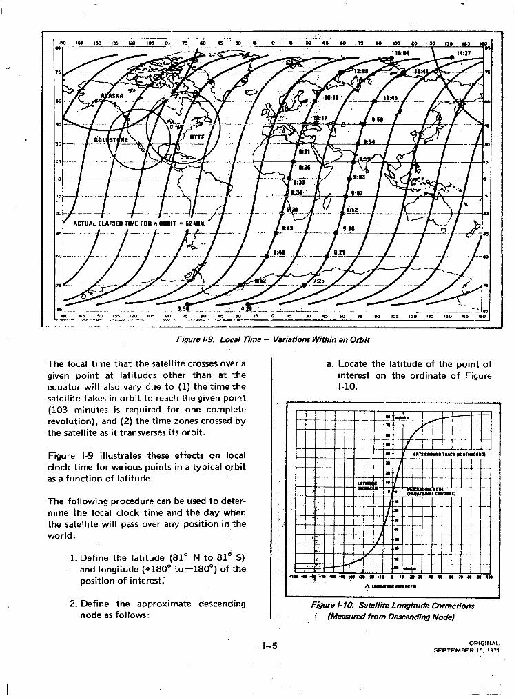
Figure i-9. Local Time - Variations Within an Orbit

The local time that the satellite crosses over a given point at latitudes other than at the equator will also vary due to (1) the time the satellite takes in orbit to reach the given point (103 minutes is required for one complete revolution), and (2) the time zones crossed by the satellite as it transverses its orbit.

Figure l-9 illustrates these effects on local clock time for various points in a typical orbit as a function of latitude.

The following procedure can be used to determine the local clock time and the day when the satellite will pass over any position in,the world:

1. Define the latitude (81” N to 81” S) and longitude (9180” to-180°) of the position of interest:

2. Define the approximate descending node as follows:

a. Locate the latitude of the point of interest on the ordinate of Figure l-10.

F&m? I- 10. Satellite Longitude Cornxtions )! lMea.wn?d from Descending Node}

l-5 ORIGINAL

SEPTEMBER IS. 1971

LONGITUDE CORRECTIONS

DESCENDING NODE PARAMETERS

b. Read the value of A longitude from the curve;

c. Add the A longitude’to the ‘longitude of the point of interest. If the value of the result is more negative : than -180”, add 360° to the result..

or

If the value of the result is mare positive than +180°. add --360’ to the result, carefully noting algebraic signs.

3. Find the actual descending node as : follows:

a. Using Table l-3, find the value of descending node nearest to -the value determined in step 2-c This represents the descending node of the actual satellite orbit revolution that will image the point of interest.

Table 1-3. Descending Node Parameters *

Longitude (deg) of Orbit Descending Node Day

(Equatorial Crossing; M

- .!I4 - 2.37 - 3.81 - 5.24 - 6.67 - 8.11 - 9.54 - 10.97 - 12.41 - 13.84 - 15.28 - 16.71 - 18.14 - 19.58 - 21:Ol - 22.44 - 23.89

Orbit Number

3 38 4 52 5 66 6 80 7 94 8 106 9 122

10 136 11 150 12 164 13 178 14 192 15 206 16 220 17 234 18 248

1 111

I Node

09zl.l 09:17 0922 09:28 09:34 09:40 09:45 09:51 09: 57 10:03. lo:08

.10:14 10:20 lo:25 10:31 10:37 10:43

Table l-3. Descending Node Parameters l (Continued)

Lor&ude(deg) of Des@ndingNode

Equokrriai Cro,ssing

- 25.32 ::, - 26.0~ - 28.19,

:- 29.62 - 31.69 - 32.49.

::- 33.92 ii;,- 35.36 .;:.A 36..i9 ;;- 38.23,., ;A $I.@ & :‘- 41';69‘ '.:- 42,53

- 43,96: - 46.39 - 46.83 - 48.26 - 49.70 - 51.14 - 52.57 - 54.01

1 ,- 55.44 - 56.87' -

'., % - 58.31 59.74 - 61.17

'(. - 62.61 : -t @$a

,'. r 6,5.4$. A ,.:. - @@%a? ,.. : :; - 68& /Y :.' - 69.'#8

- 71.21 - 72.64 - ., 74.08 - 75.52 - 76.95 - 78.39 - 76.62 - 61.26 - 62.69 - 84.12 - 65.56 - 86.99

Oibi Day M

Orbit Nun&

N

Greenwich Mean Tinieof

Giscending Node

--

2 25 lo:48 3 39 10:54 4 53 1l:OO 5 67 11:06 6 81 11:ll 7 95 11:17 8 109 11:23 9 123 11:29

10 137 11:34 11 151 11:40

12 165 11:46 13 179 11:52 14 193 11:57 15 267 12:03 16 221 12:09 17 235 12:14 18 249 12:20

1 12 12:26 2 26 12:32 3 40 12:37 4 54 12:43 5 68 12:49 6 82 12:55 7 96 13:oo 8 110 13:06 s 124 13:12

10 138 13:18 11 ,152 13~23 12 .166 13:29 13 180 13:35 14 194 13:41 15 208 13:46 16 222 13:52 17 236 13:58 18 250 14:03

1 13 14:09 2 27 14:15 3 41 14:21 4 55 14:26 5 69 14:32 6 63 14:38 7 97 14:44 8 111 14:49 9 125 14:55

Table i-3. Descending Node Parameters* (Continuad~ i

Longitude(deg) of Descending Node

Equatorial Crossing

- 88.42 - 89.86 - 91.29 - 82.73 - 94.16 - 95.59 - 97.03 - 96.46 - 99.90 -101.34 -102.77 -164.20 -105.64 -107.07 -108.51 -199.94 -111.37 -112.81 -114.24 -115.68 -117.11 -118.54 -119.98 -121.41 -122.84 -124.28 -125.72

-127.15 -128.59 -130.02 -131.46 -132.89 -134.32 -135.76 -137.19 -138.62 -140.06 -141.49 -142.93 -144.36 -145.79 -147.23 -148.66 -150.09

-- Orbit Oibit I- Day Number

M P'

10 139 11 153 i2 167 13 181 14 195 15 209 16 223 17 237 18 251

1 14 2 28 3 42 4 56 5 70 6 84 7 98 8 112 9 126

10 140 11 154 i2 168 13 '182 14 196 15 210 16 224 17 238

.3 29 4. 43 5 57 6 71 7 85 8 99 9 113

10 127 11 h 141

-t- GtichYean

Timeof Doseending

Node: .

15:Ol 15:07 15:12 l&18 15:24 15:30 15:35 15:41 15:47 15s 15:58 16:ti 16:li 16:15 16:21 16:27 16:33 16:3# 18:44 lJ:5d 18:56 17:Ol 17:OT 17:!3 17:19 17:24 17:30

17:36 17:41 17:48 17s 17:59 18:94 18:10

-18:16 18% 18:27 18:33 18:39 18:45 18:50 18:ti 19:62 19:66

. .

I, !

:.

1.

/

Table l-3. Des&ding Node Parameters l lContinued~

l-7

-.-.-

Lor@ude(d~ of @sWdilg,Node

(Eqiwtoriai Crwng ! ;.

4151.54 ' 452.97

454.40 A55.84 -7137.27 ,158.71 -160.14

'.+l61.57 --163.01 . 464.44 2165.i7 -167.31 -168.74 -170.18 -171.61 -173.94 -174.48 -175:91 -177.35 -178.79 +179.78 +118.35 +i76.91 +175.48 +174.64 +T72.61 +171.18 +169.74 +168.31 +166.87 +165&I +164.01 +162.57 +161.14 +159.71 +158.27 +156.83 +155.40 +153.96 +152.53 +151.69 +149.66 +148.23 +146.79 +145.36 _. .

lrbit Orbit hf Yumba M N

1 .2

: 5 6 ,7 8 9

10 11 12 13 14 15 16 17 18

1 .2 3 4 5

,6 7 8 9

10 11 12 13 14 15 16 17 18

1 2 3 4 5 6 7 8 9

2 19:13 16 19:19 30 19:25 44 19:31 58 19:36 7? 19:42 86 19:48

100 19:53 114 19:59 126 20:05 142 2O:ll 156 20:16 170 20:22 184 20:28 198 20:34 212 20:39 226 20:45 240 20:51

3 20:57 17 21:02 31 21:08 45 21:14 59 21:19 73 21:25 87 21:31

101 21:37 115 21:42 129 21:48 143 21:54 157 22:oo 171 22:05 185 22:ll 199 22:17 213 22:23 227 22:28 241 22:34

4 22:40 18 22:45 32 22:51 46 22:57 60 2333 74 23:08 88 23:14

102 23:20 116 23:26

ireenwichMean Timeof

Descending Node

SEPTEMBER 15. 1971

r :

. , : ;

C”,

D E S C E N D I N G t U O D E P A R A M E T E R S

Tab le l-3. Descend ing N o d e Paramete rs l (cont inued) I T a b & 1-j. ‘Discendi r ig N d d e Paramete rs l (Cont inued)

Long i tude (deu) of D m e n d i n g N o d e

E q u a torial Cross iq

+ 1 4 3 .93 + 1 4 2 .49 t141.06 t139.62 + 1 3 8 .19 t136.76 t135.32 t133.69 t132.46 + 1 3 1 ;01 t129.56 t128.15 t l26.71 t125.28 + 1 2 3 & I t122.41 t120.98 t119.54 t118.11 t116.68 t115.24 t113.81 t112.37 t116.94 t109.51 t108.07 t106.64 + 1 0 5 .20 t103.76 + 1 6 2 .33 + 1 0 0 .90 + 99 .46 + 98 .03 + 96 .59 + 9 5 . 1 6 > + 93 .73 + 92 .29 + 90 .86 + 89 .42 + 87 .99 + 86 .56 + 85 .12 + 83 .69 + 82 .26 + 80 .82

Orb i l Day M

A 1 0 1 1 1 2 1 3 1 4 1 5 1 6 1 7 1 8

1 2 3 4 5 6 7 8 9

1 0 1 1 1 2 1 3 1 4 1 5 1 6 1 7 1 8

1 2 3 4 5 6 7 8 9

1 0 1 1 1 2 1 3 1 4 1 5 1 6 1 7 1 8

Orb i N u m b

N

Gr 'eenw ishMe T ime of

Descend ing N o d e

1 3 0 23 :31 1 4 4 23 :3? 1 5 8 23 :43 1 7 2 23 :49 l & S 23 :54 2 0 0 0o:oo. 2 1 4 00 :06 2 2 6 00 :12 2 4 2 @ I:17

5 0 0 2 3 1 9 00 :29 3 3 00 :35 4 7 00 :40 6 1 0 0 4 6 7 5 00 :52 8 9 00 :57

1 9 3 01 :M 1 1 7 01 :o jB 1 3 1 01 :15 1 4 5 01 :20 1 5 9 01 :26 1 7 3 01 :32 1 8 7 01 :38 2 0 1 01 :43 2 1 5 01 :49 2 2 9 01 :55 2 4 3 02 :Ol

6 0 2 : W 2 0 02 :12 3 4 02 :18 4 8 02 :24 6 2 02 :29 7 6 02 :35 9 0 02 :41

1 9 4 02 :47 1 1 8 02 :52 1 3 2 02 :58 1 4 6 03 :64 1 6 0 03 :09 1 7 4 03 :15 1 8 6 03 :21 2 0 2 03 :27 2 1 6 03 :32 2 3 0 03 :38 2 4 4 03 :44

/ + . ? @ a + . .J7 .96 + ,76 i51 + 7 & 6 8 + 7 3 3 4 + 72 .21 + '~ ? o .% l + e s > 4 + la .91 + . 6&46 + 6 !$64 t-Q .61 + SF.!? + 6 9 $ 4 + 59 .31 + . -57.87 + 56d4. ' + 5 5 1 0 1 + 53 .56 t .52.13 + 50 .70 + 49 .26 + 47 .83 + 46 :39 + 44 .96 + 43 .53 + 42 .09 + 46 .66 + . 3 8 7 2 3 + 37 .79 + ,36.36 + 34 .92 + 33 .49 + 32 .06 + 39 .62 + 29.1.9 + 27 .75 + 26 .31

‘+ 24 :88 + 23 .45 + 2 2 .0 1 + 20 :58 + 19 .14 + 17 .71 + 16 .28

Orbi t Orb i w N u m b .M . . . N

-T -7 2 ?I 3 " 3 5 4 4 9 5 6 3

3 7 7 7 9 1 8 1 0 5 9 1 1 9

1 0 1 3 3 1 1 14 j 1 2 1 6 1 1 3 1 .75 ?4, 1 8 9 .j5 2 0 3 1 6 2 1 7 1 7 2 3 1 :18 2 4 5

1 8 2 2 2 3 3 6 4 5 0 5 6 4 6 7 8 7 9 2 8 1 0 6 9 1 2 0

1 0 1 3 4 1 1 1 4 8 1 2 1 6 2 1 3 1 7 6 1 4 1 9 0 1 5 2 0 4 1 6 2 1 8 1 7 2 3 2 1 8 2 4 6

1 9 2 23 ' 3. 3 7 4 5 1 5 6 5 6 7 9 7 9 3 8 1 0 7 9 1 2 1

03 :50 63 :55 64:Ol . 04 :07 04 :13 04 :18 64 :24 04 :30 04 :36 a l :41 04 :47 o k 5 3 IW ill 05 :04 05 : lO 05 :16 05 :21 05 :27 05 :33 05 :39 05 :44 05 :50 05 :56 06 :02 06 :07 06 :13 lx:19 06 :25 06 :30 06 :36 06 :42 06 :47 06 :53 06 :59 07 :05 07 : lO 07 :16 07 :22 07 :28 07 :33 07 :39 07 :45 67 :51 07 :56 0 8 ’0 2

Greenw ich M e a T imeof

Descend ing N o d e

Table 1-3. Descending Node Paran eters l (Continuedl

Longitude (dw) of Orbit Orbit Time of Descending Node w Yumber Drrcendiw

(Equatorial Crossing) M N Nod.

+ 14.84 10 + 13.41 ii + 11.97 12 + 10.54 13 -i 9.11 14 + 7.67 15 + 6.24 16 + 4.81 17 + 3.37 18 t 1.93 1 + .50 2

*This table contains parameters for a typical orbit. ihe table will be republished after launch with paramers corresponding to the exact orbit

: ,:. :

135 * 149

163 177 191 205 219 233 247

10 24

08:08 . . 08:14 66:19. ':: ':~:25 ; b8:31 66:36 -, OS.42 o&49 '. 08:54 '

.'0&59 ,:- 69:05

-- irwnwich Mean

b. The orbit day, orbit nuqtber, Md the Greenwich Mean Tim& (GMT) of the descending node can bs rL’ad from the table.

4. Determine the GMT at the position of interest as follows :

a. Locate the latitude of the position of interest on the ordinate of the graph of Figure l-11.

b. Read the A time from the curve.

c. Add the A time to the GMT of the descending node determined in step 3-b. carefully noting algebraic signs.

5. Determine the Siandard Mean (Local) Time of satellite passage over the position of interest

a. Determine the number of hours between the local time zone and the Greenwich time zone from Figure l-12.

Figure I- 11. Time Difference Measured from Descending Node

b. If the longitude of the position of interest is west of the Greenwich meridian, subtract the number of hours from the GMT determined in step 4-c.

or

if the longitude of the position of interest is east of the Greenwich meridian, add the number of hours to the GMT determined in step 4-c.

The fdllowing example illustrates the procedure:

Step 1

Point, of Interest: Latitude = 45’ North Longitude = -120” West

ORIGINAL

SEPTEMBER 15. 1971

CORRECTION PROCEDURE EXAMPLE

WORLD TIME~ZONE MAP

Figure I- 12. Time-Zone Map @f t& wt?rid .,;:

Step 2

From Figure l-10, the A longitude for 45’ north latitude is -12.5O. The approximate descending node longitude is then (-120°) + (-12.5’) or --132.5”. Since this does not fall outside the limits of -180” to 180” there are no adjustments required.

Step 3 .:

The closest descending node from Table i-3 is -132.89”. Hence, imagery will be taken of the desired point on day 6 in revolution 71. The GMT at the descending node will be 17:59.

Step 4

From Figure l-11 the A time for 45’ North latitude is -13 minutes. Hence, the GMT

when imaging of the desired point will occur is (17:59) + (-:13) or 17:46.

Step 5

From Figure l-12 the number of hours from Greenwich at the desired location is 8. Since the desired location is West of the Greenwich meridian,- subtract 8 hours from 17:46 or 9:46. This is, the Standard Mean (local) Time of jmaging the desired location.

Note that Table l-3 is for a typical orbit, that is, the exact longitudinal placement of the ground traces cannot be determined before launch. Actual placement of ground traces wiil be determined post.launch and a table for the: exact orbit ground traces will then be provid$d as a replacement for Table l-3.

APPENDIX J ORBlTCONTR6L

Several significant characteristics of the$RTS orbit are discussed in this app?dix $hich have been selected to enhance ti&‘uti@ty of the returned imagery. In general, these @rat- teristics have been selected to minimizer:paria- tions in observation conditions and provide a systematic process of imagery collection. Precise control of the orbital parameters is required for the attainment and maintenance of the desired characteristics. Hence, the ERTS spacecraft includes an orbit adjust capacity which is used to attain the orbit initially and maintain this orbit throughout the life of the mission.

The orbit adjust subsystem is a monopropel- lant system consisting of three rocket engines fed by a common propellant/pressurant tank. The three thrusters are aligned to provide impulse along or opposed to the spacecraft velocity vector and also perpendicular to the orbital plane. Each thruster imparts a thrust of approximately one pound force.

J.l ATTAINMENT OF REQUli3ED ORBIT

The Delta launch vehicle injects the spacecraft into its final orbit to within the limits of the errors inherent in the launch vehicle system.

3-I

Lau~~ch vehicle errors at injection are random anc@an be$f magnitudes which impact the des&d ob+rvation’ characteristics. When re- qui@d, the ‘spacecraft orbit adjust capabilities ait3’i%tiIiz43d after spaceciaft separation to r&V&e any”residuat launch vehicle injection errors.

The orbital parameters most critical to providing the desired imagery characteristics are the semi-major axis (or equivalently the period of the orbit), the inclination, and the eccentricity. For ERTS, a unique combination of orbital period and inclination are required to establish the desired coverage pattern’ and sun synchronism. Errors in eccentricity will also affect these characteristics. However, for the expected range of injection errors, the eccentricity errors have a negligible eifect compared to the effect of inclination and period errors.

dl.1 Period Errors

The maximum expected injection error in the orbital period exceeds by a wide margin the accuracy required for satisfactory systematic coverage and cross-track repeatability. For example, an injection period error of only one

ORIGINAL

SEPTEMBER 15. 1971

ERRORS AND CORRECTION

MAINTAINING AEOUIRED ORBIT

percent of the maximum (30) error will result : in a 35 kilometer sidelap error in the. second ;:’ 18;day cycle relative to ‘imagery from the :: corresponding revolutions ‘in the first 184ay ‘. cycle. This error, as illustrated in the lower ..

’ left portion of Figure J-l, will continuk to ,.! expand, with time.resulting in 3 relative e’rror of approximatety 750 kilometers after ‘one ,;‘. year.

J.1.2 Inclination Errors

Injection inclination errors cause a drift in the time of the descending node and also imagery sidelap errors. Without an orbit adjustment capability, an injection inclination error equal : to the maximum (3~) error will result in a .: relative sidelap error of 417 kilometers after one year. These inclination effects can be compensated by adjusting the orbital period. ”

I J.1.3 Error Correction

Thus, injection period errors have to b& re- .Xi: moved and compensation provided fof;iit+ ,$i inclination error. Period adjustments:$“are L$$‘: accomplished by utilizing one of the.:&0 thrusters which impart impulse along’:the velocity vector. Because of the .one p&nd force of these thrusters, the weight of: the spacecraft, the magnitude of the period adjustment, and other scheduling criteria, the period adjustment process can take up to 6 days from injection to completion. A typical adjustment sequence consists of: 1

1. Several days to ascertain spacecraft health, to track, and to determine maneuver requirements

2. Several consecutive orbits with, approximately 20-minute rocket firings on each orbit

3. Several orbits to track and ascertain that adjustments were executed as planned

4. Continued interspersing of several orbits of adjustments with several orbits of tracking until the correct orbit has been attained

Th8 launch.vehicle can inject the spacecraft into. an prbit with an eccentricity.of accept- _’ able. accuracy. However, an orbit with circular characteristics is most preferable to minimize the variations in observation altitude. It is sometin& possible when adjust.ing the period of .ihe orbit to schedule tire ,adjustments to more nearly’ circularize the orbit. Therefore, whdn. period adjustments. are required and when they can. be scheduled to circularize the orbit,, the injection eccentricity errors will be reduced. Otherwise, no orbit adjustments are pla’nned to specifically remove injection eccentricity errors.

J.2 $AINTENANcE 0F REQUIRED ORBIT

Several forces (such as: atmospheric drag, the gravitational attraction of the sun and moon, and the spacec+ ’ .“,t s own attitude control ma& expulsion subsystem) act upon the spa&craft after the desire‘d orbit has been

dur@g the mission to compensate for these for.@sl I ,;

‘,i. 1

Du$g tde &rst several weeks of the mission, sev$Ial small although significant perturbing factqrs @kg., the -force due to the attitude control system mass .expulsion subsystem) will:::be determined. Once .these factors are det~rmine.d,‘.they will be included in orbit planning. operations’ to minimize the number of subsequent adjustments: Several small adjustments: may .be necessary during this period to optimize the deshed coverage characteristics. These adjustments are minor and wilf, be scheduled so not to interfere with imaging operations.

Subsequent to the first.several weeks of the mission, the requirements for adjustments will become minimal, systematic, and predictable. The requirements for these adjustments result from the perturbing forces on the spacecraft

:: DRIFT AND ADJUSTMENT PROFILE

which, over long periods c.f time, cause,bre- .f, kilometers during the entire mission. Figure dictable perturbations to :he orb.it. Th$ sig- ‘..i* J-l shows a typical drift and adjustment pro. nificant impact of these perturbations: is’ a systematic cross-track drift of imagery ‘from

::;‘I flie. ‘Acceptable coverage can be maii~t.rinctl YI : qy’er,..a onq.year mission by several small

revolutions of one l&day, Earth covqaga :‘L: ;@blnl peri@ adjustments. These adjuslments :t’ cycle relative to imagery I. om c+reiponding -.* i!. .!4&@iy of ‘feveral Ywconds duration and are revolutions of other l&day cycle&,durin$.the mission. Orbit adjustments will b$sch$uled

;I,: - Jcfheduled over primary ERTS ground stations :; .durir$ night time portions of the orbit, so not

to limit this cross-track imagery Wift $“. 37 ? i;

;.to-iriierfere with imaging operations. ..c ,-. . . . .

I, ’

0

‘1 .’ 7 : ,,:A

‘.

,,’

:.

L . . ‘/

ADJUST P = P, ,/ . ADJUST P = P,

P, (AFTER INJECTION ERROR REMOVAL)

‘u’

DRIFT THAT RESULTS F&OM NOT REMOVING AN INJECTlOll PERIOD ERROR EQUAL TO 1% OF~~AXIMUM

- \ EXPECTED T, = SEVERAL DAYS TO SEVERAL WEEKS AFTER

INJECTION WHEN SUBSEQUENT ADJUSTMENT

\ PROFILE BECO,MES PETERMINISTI~.

PO = PER100 REQUIRED TO MAINTAIN DESIRED

\ COVERAGE

\ I I- I I 5 10 20

18 DAY CYCLES

I ..I 1 1 90 190 210 JBO

DAYS

Figurn J- 1. ,: Typical Cross-Talk Drift of Ground Trace‘iind Period Adjustmt+‘ro file .

J-3 4 ORIGINAL

SEPTEMBER IS, 1971

II

1; .The ,purposeof the mission planning function : .’ . . is to define .the sequence of spacecraft ancl

;;.:: ground-station operations to maximize the ,/. : : . :, tn$v#ry yield while operating within Illesc! .j; .,. ‘Con$ir&nts. The output, is a time-.c)rdero~l

‘: -‘&iqu$nce of, .evetitJ which define all sensor. y, wiciiband tape recorder, and assorted routine

spk&raft functions. This sequence of events ir;;ffi& used,to ,dafine the specific commands : .::

., .:, I f,pr {operating the spacecraft. In addition, the ,:A- L. ,,,’ mi’s$on planning function defines the events :I:. ;..., wht@ are to occur during every spacecraft/ ; &&id-stat&n cot-&t. ,$, :, .a’: ,.. ,y, ‘,: ‘. ;,:

.:<?y t’ I :’ :- T@;‘bulkYcj~i’~he mission planniig operation is

I :I.

.’ don+, once 9 day arid”‘results in activity plans for that day’s operation. These plans are up- dat& onan orbit-by-orbit basis as required to include,the latest cloud cover information and to &count for any last-minute anomolous occulrences’such as ground station outages.

APPENDIX K MISSION PLAI JJING ._

: i

The spacecraft has access to all global. area between 81 degrees Nort,l and. 81 degrees South Latitude every 18 days; e(s shown in Figure l-2 in Appendix I. However, due to constraining factors both within and external to,the ERTS system, not all of this are+ can be imaged all the time. The constrain{?’ in- elude :

.’ ‘.

. :: : ,..:. 1. On-board tape recorder capacity@ 30

minutes maximum ./ ‘$7 I

2. On-board command memory capability for switching sensors on an’d off

3. Ground station availability and=contact time duration

4. Global landmass distribution

I

5, Ground scene illumination condttions .a; I\

6. Cloud cover

’ . Figure K-l illustrates the coverage for a

typical day’s operation. The spacecraft will normally be scheduled to send real-time

-$: <LJf t (direct) data whenever it is concurrently over

7’ ; : an @ea of .interest’ and is within view of a ,.< %.

K-1. ORIGINAL

SEPTEMBER IS. 19il

\

III

DAILY LANDMASS CdERAGE .

ground station that can receive ERTS data. The three primary ERTS stations shown in Figure K-l (NTTF, Goldstone, and Alaska) ” provide coverage of most of )NoAh Am&x i,’ and real-time imagery transmission is normal- ‘: ly scheduled during this time. Data recovery

-over the rest of the globe is performed by ; recording the data on the on-board wideband video tape recorders and playing back during s&sequent ground station contacts.

The bar chart of Figure K-2 shows the total time during daylight when the spacecraft is over any land area for one day’s operation, and the amount of land area that can typically be imaged by the spacecraft. Figure K-2 corresponds to the typical day of Figure K-l. During remote operations the spacecraft has access to much more coverage area than .can be accommodated by the wideband tape ‘;; recorders. Therefore, a selection process is ‘I required to determine which areas are to be : recorded during any given remote opera$on. To assist in this selection process, a system of ‘. priorities is used for all coverage areas o;f,the :.:” .wo.rld. By scheduling payload operations based on these priorities, coverage of the areas ..’ of greatest investigator interest is assured.

‘;.

in ,order to. establish. the priorities several fac$%must; be considered. These include:

A’., f. ., “L’l. &ientific imbortance of the area -- is

-. ” !.! .theii ihvestigator interest in a given ‘~~~~.~~~a&.and how. often need it be imaged? ,‘.I ‘-:$’ *

-..i ‘T-:;!: 2~~LS$as&of thp year - : when is imagery

\.:‘: ‘-‘$f that area +dstpeast desirable? . ;. ;/ ,I ., ,: 3. &hting conditions - image quality

varies with’scene contrast and bright- ness which “in turn varies with local sunangle; what lighting conditions are required for the given scene?

+.‘.Time since the area was last imaged - : how recent is, the imagery for that

,, area:.was it obscured by clouds? ,.

The Qriorities in the system are quite dynamic, jn thatthey must be periodically updated to ,ieflect cha,nges ,in the desirability of imaging+t he’: v$rious areas. The investigator’s reqC&sts fo:idata provide information to the ERTS. Project to assist in defining the various area5 of interest and. priorities.

1

35

30

25

E

g 20

E

a!

I 16

Y

F

10

‘5

0 AVAILABLE LANDMASS

Ezl TYPICAL SENSOR COVERAGE

’ II ll+1 n+t n+3 n+4 n + 5 ‘;C&l + 5 n+7~:..n+B ‘.ii+B n+;tO n+‘ql n+lZ nt13

Figure K-2. Availabfe Laymass and Typical Daily Coverae 1.. .. ,I

Predicted cloud cover data ,‘s used in mission planning to minimize the n;!mbdr of obscured images. Prediction data is received from National Oceanographic & Atmospheric Administration (NOAA) on a periodic ,basis and the spacecraft schedule ‘s updated as near as possible to the upcoming data pass to include the most recent clou,d information. Due to spacecraft command constraints, ‘the sensors and recorders can be switched on and off only a limited number of times; hence, some imagery of fully cloud-covered areas may be takeri.

The decision not.to schedu1.e sensor operation over a given area depends both on the percentage cloud cover expected and the degree of investigator interest in that particular area.

Areas of very high investigator interest are normally scheduled even though a fairly high percentage of cloud cover is predicted, Areas of low, or no investigator interest tend not to be scheduled .eveb for a lesser percentage of cloud cover. The objective is to maximize the number of cloudif,ree images while at the same time making every attempt to image the are& of greatest interesi.

The possibility of cloud obscured scenes has one major implication to investigators who require periodic repeating coverage. Since the satellite has access td a given scene only once every 18 days (except for higher latitudes-see Section 1.2), cloud cover could result in the repeating coverage being intizrrupted for periods of 36, 54, or more days for any particular scene.

,

K- 314 ORIGINAL

SEPTEMBER 15. 1971

I_- --

,

APPENDIX L SIJN ELEVATIOR EFFECTS

The choice of orbit for ERTS causes the spacecraft to pass over the same point on the earth at essentially the sa,.~e’ l,ocal time every 18 days. However, even though the local time remains essentially the same, changes in solar elevation angle, as defined in Figure L-l, cause variations in the lighting conditions under which imagery .is obtained. These changes are ,due primarily to the north/south seasonal motion of, the sun.

Changes in solar elevation angle cause changes in the average scene irradiance as seen by the sensor from space. The change in irradiance is influenced both by the change in intrinsic reflectance of the ground scene and by the change in atmospheric backscatter. Exposure time of the RBV will be varied by ground commands to accommodate the changing illumination levels. At certain times of the year imagery will not be obtained in the high and low latitude regions of the earth due to inadequate scene illumination.

The actual effect of changing solar elevation angle on a given scene is very dependent on

\

.2A /! I ,.,’

Figure L- 1. Solar Elevation Angle

the scene itself. Fey example, the intrinsic reflectance of sand is significantly ‘more

. sensitive to changmg solar elevation angle than are most types of vegetation. Due to this scene dependence, each type of scene must be evaluated individually to determine the range of solar elevation angles over which useful imagery will be obtained.

Figure L-2 shows the solar elevation angle as a function of time of year and latitude. This family of curves i’s for a 9:30 a.m. descending

-- _. -- Figure L-2. Solar Elevation Angle History as a Function of Subsatellite

Latitude - Descending Node at 9:30 a.m.

L-l ORIGINAL

SEPTEMBER IS. 1971

SOLAR ELEVATION PARAMETERS

node time which is the nominal expected time of ,equatorial crossing for the satellite, By drawing a horizontal line for a given latitude, the solar elevation angle can be determined for. any time of year. Portions of this data have been transferred to the global maps in Figure L-3. These maps show the range of possible sensor operation (i.e., daylight) for the various seasons. Depending on the scene, it may or may not be possible to obtain useful imagery at the,lower solar elevation angles. At solar elevation angles greater than 30 degrees, it is expected that all scenes can’be satisfac- ,: torily imaged. .it

-9. .’ ::

Two other parameters may ,affect the local ..;’ solar elevation angle. These are the ERTS 1, launch window and perturbations to the orbit. The launch window (allowable launch time variation) is plus 30 and minuszero minutes, which results in a possible descending node time anywhere in the range of 9:30 to 10:00 a.m. The effects of launch time variations on solar elevation angle are shown in Figures L-4 through L-6 for various latitudes.

.

i

I ‘“::1111 twlNdi l lNTElSOlITICE Wl8::, l t iTD8fDATWlE COVEWI: I~W~OD~~LAT~TUPE

.

Figure L -3. Seasonal VaiL &xS in solar Elevation Angle - 9:3O a.m.

Descending !Uodc

( 'LATITUDE

I I 1 I I I I I I I I UNV ULV : Yfl IOV JAN

‘. TWE OF YEAR .’

Figure L -4. Launch window and Orbit Perturbhg Etkts on Solar .Elevation Angle at 0 Degrees Latitude

< ‘NAL - ?

Whatever time the spacecrift is launched, the local times would then re rl,in fixed throughout the mission were it not for perturbing forces to the orbit. These forces, such as atmospheric drag and the sun’s gravity, will shift the time of descendi J node throughout the year, resulting in changes to the nominal

solar elevation angle. The changes due to these perturbing effects are also shown in Figures L-4 through L-6. Under worst case conditions, the solar elevation angle changes due to perturbing forces will amount to no more than 4 degrees throughout the year.

n - 1

Figure L-5. Launch Window and Orbit Perturbing Effects on Solar Elevation Angle ar 30 kgrees North Latitude

Figure L-6. Launch Window and Orbit Perturbing Effects on Solar Elevation Angle at 50 Degrees North Latitude

L- 3/)r ORIGINAL

SEPTEMBER 15. 197 1

APPENDIX M LIST OF NASA

PRINCIPAL ItiV~STIGATORS

At the time this document went to press, identification of the principdl investigators of ERTS data was not complete. A comprehensive list will be published as a supplement to this document at a later date.

M-1/2 ORIGINAL

SEPTEMBER 15. 1571

API-

APPENDIX .N SAMPLE PRODUCTS

A pocket is provided on the inside of the back cover of this document for the storage of sample products. These products will be supplied later as an addendum to this handbook.

A/D AGC AMS

Analog to Digital Automatic Gain Control Attitude Mea! iring Subsystem

BIT

bps BPS BTE

Bench Integration Test Bits per second Bulk Processing Subsystem E?n,r?c:, Test Equipment

C&Dt

ccc CCT CIU CP

-I Communications and Data Hand- ling Camera Controller Combiner Computer Compatible Tape Command Integrator Unit Communications Processor

D/A Digital to Arialog DCP Data Collection Platform DCS Data Collection System DCS/RSE DCS Receiving Site Equipment

LIST OF ACRCNYMS

DCST DEMUX DID DTR DTU

EBDI C

EBR EBRI C

ELC EMI ERTS

EU

FFS FFSPS FOV FSK

GCE GCP GDHS GMT GPE GSFC

Data Collection System Tape Demultiplexer Digital Image Data Digital Tape Recorder/heaaer Data Transfer Unit

Extended Binary Decimal Inter- change Code Electron Beam Recorder Electron Beam Recorder Image Correction End of Line Code Electromagnetic Interference Earth Resources Technology Satellite Electronics Unit

Full Field Source Full Field Source Power Supply Field of View Frequency Shift Keying

Ground Checkout Equipment Ground Control Point Ground Data Handling System Greenwich Meridian Time Ground Processing Equipment Goddard Space Flight Center,

HDDT HSD

IAT ID I iov

kbps

LNS LSB, LTC

MOI MSFN MSS MTF MUX

NASCOM NBTk nd NDPF NRZ N’RZ-L NTTF

OAS occ ODG OGO

PAM PCM PDU PM PPF PPS PRN PSK

RBV REA RSE

WC SIAT SMDE

High Density Dicjital Tape High-Speed Data

Image Annotation Tape Identification instantaneous Field of View

Kilobits per second

Link Noise Simulator Least Significant Bit Light Transfer Characteristics

Moments of Inertia Mannad Space Flight Network Multispectral Scanner Modulation Transfer Function Multiplexer

NASA Communication Network Narrowband Tape Recorder Neutral Density NASA Data Processing Facilitv Non-Return to Zero Non-Return to Zero Logic Network Test and Training Facil- ity

Orbit Adjust Subsystem Operations Control Center Orbit Determination Group 0 r biting Geophysical Observa- tory

Pulse Amplitude Modulated Pulse Code Modulation Power Distribution Unit Photo Multiplier Photographic Processing Facility Precision Processing Subsystem Pseudo-Random Noise Phase Shift Keying

Return Beam Vidicon Rocket Engine Assembly Remote Site Equipment

Spacecraft Special Image Annotation Tape Scan Mirror Drive Electronics

ORIGII-IAL

SEPTEMBER IS, ,971

ACRONYMS

SME TO WTS

SME SNR SPDT

SPS

s/s STADAN

STC STE STS

TBD TBV

T/C TCS TPG TT&C

Scan Mirror Electronics Signal-to-Noise Ratio i Spacecraft Performance Data Tape Special Processing Subsystem Su’bsystem Satellite Tracking and Data Acquisition Network Scanner Temperature Controller Special Test Equipment Scanner Test Set

To Be Determined To Be Verified Time Code Thermal Control Subsystem Test Pattern Generator Telemetry Tracking. and Com- mand

TU

UHF USB UTM

VIP VPASS

VPIR

WBT WBVT R WTS

Transport Unit

Ultra-High Frequency Unified S-Band Universal Transverse Mercator (map coordinates)

Versatile Information Processor Video Processor and Sync Sepa- rator Video Processor and Image Re- corder

Wideband Transmitter Wideband Video Tape Recorder Wideband Telemetry Subsystem

-

The enclosed supplement to the ERTS Data Users Handbook.has been prepared by personnel

in the U.S. Geological Survey to destiribe the EROS Program Data Center at Sioux Falls.,

South Dakota. Please incorporate this material in the ERTs Data Users Handbook which

you recently received in the mail.

SUPPLEMEN’c’ to the

ERTS DATA USERS HANDBOOK Prepared by

EROS Progam, U.S. Geol-rgical Survey

A Data Center in Sioux Falls, South Dakota, is operated by the EROS Program of the Department of the Interior to provide access to ERTS imagery for the general public, industry, educational institutions, and foreign and domestic government agencies at all levels. The Center serves all persons and groups not qualified, as ERTS Principal In- vestigators, to receive the imagery directly from NASA.

In addition to the reproducible ERTS imagery, the Center also holds NASA aircraft imagery, current USGS aerial photography, and computer compatible tapes of, ERTS and NASA aircraft data. Facilities are available for imagery storage, retrieval, reproduction; and dissemination, and for user assistance and training.

The EROS Data Center is presently located at:

10th & Dakota Avenue Sioux Falls, South Dakota 57101

This is a temporary location until the permanent center is completed at a site north of Sioux Falls. The same services and products that are available at the interim facility will be available at the permanent Data Center.

PRODUCTS

All products of the EROS Data Center are for sale. Price lists are available on request.

ERTS Imagery paper prints )

ERTS imagery, originally processed at the Goddard Space Flight Center, NASA Data Processing Facility (NDPF), is a significant part of the Data Center imagery file. Each scene, covering 10.000 square nautical miles, is imaged seven times from ERTS-A and eight

times from ERTS-B: three images from the Return Beam Vidicon (RBV) and four or five images from the Multispectral Scanner (MSS). The raw data are either bulk-processed and provided to the Data Center in the form of 70mm film, or precision-processed and provided on film at a scale of 1:1,000.000. The Data Center has a. catalog of the ERTS imagery and a browse file including only one RBV image and one MSS image per scene for evaluation of coverage and cloud cover. The image formats are the,same as those available from the NDPF.

Copies of bulk-processed individual images and color composites, derived by processing the three RBV and four MSS images together, may be purchased as:

contract paper prints

contact film positives

contact film negatives

or

1:1,000,000 (3.38X enlargement) paper prints

1:1,000,000 film positives

1 :l,OOO,OOO film negatives

roughly 2% x 2%

inches

roughly 9x9

inches including marginal

data

Copies of precision-processed images may be obtained only at scales of 1:1.000.000 or larger. These images have been rectified to truly orthographic photographs and have been overprinted with the UTM grid. Both individual images and color composites at 1:1,000,000 are available in various forms:

film positives roughly 9 x 9 inches, including marginal data

film-negatives )

Only about 5 percent of the images available in the Data Center are. precision-processed.

ORIGINAL

SEPTEMBER 15. 197,

Orders for all the above items will ordinarily be filled within a week .of receipt of the

v’ request.

Paper prints of individual bulk- or precision- processed images enlarged to 1 a scale of 1:250,000, or a paper print coldr compdsite at the same scale may be ordered. However, it will take at least two weeks to fill such a request.

Orders for other forms of the ERTS imagery will be honored whenever possible, but delivery time and costs will be determined on an individual basis. Film negative and film positives of 1:250,000-scale enlargements of ERTS imagery are in this category.

NASA Aircraft Imagery

‘V

Imagery obtained by NASA, as part of its Aircraft Program in support df the development of Earth Resources Surveys by aircraft and spacecraft, is processed at the Manned Spacecraft Center. This imagery was acquired for specific purposes and to varied specifications as to time, areal coverage, and sensors, and is primarily of test sites within the continental United States. A catalog of this imagery, and a browse file, is also at the Data Center.

Copies of these images may be purchased at contact scales and enlargements, in color or black-and-white, on film or on paper. Each image is reproduced with marginal information that provides, among other things: frame number, date, geographic coordinates, and order number in an understandable code. A request for reproductions is normally pro-’ cessed within 1 week.

USGS Aerial Photography

Aerial photog!aphs, made by the U.S. Geo- logical Survey primarily for purposes of topo- graphic and geologic mapping, are available from the Data Center. The vast majority are black-and-white, vertical photographs at a

- scale of approximately 1:24.000, and contact prints are 9 x 9 inches. Because of the need to

‘s&e the ground surface,, these photograpi were usually made in the late fall or ear! spring. Coverage. is. of discontinuous are< throughout the conterminous U.S., Alask Hawaii, and the Territories. The remainder J either low oblique, taken with cameras tilts approximately 20° from the vertical, or I-rig altitude photographs. Both. are black-an white, and in a 9 x 3 inch format. Catalogs 1 the USGS photographs and a browse file f. evaluation of coverage are available at ti Data Center.

All photographs are available at contact seal and enlargements, on film or on paper. Ear scene is reproduced with marginal inform tion that provides, aniong other things: fran number,. date, geographic coordinates. ar order number in an understandable cod Photographs obtained privl to 1941 are he

,by the National Archives and Record Servic Material is available on request but not with the normal l-week reproduction time.

Magnetic Tapes

Computer-compatible magnetic tapes of bo- ERTS data and NASA Aircraft Program da are available for reproduction through tt Data Center. Of the total ERTS data, about percent of the raw R8V data, about 5 percel of the raw MSS data, and 100 percent of tk precision-processed data are available in th form. Tapes of data from Aircraft Program investigations, ai with NASA Aircra imagery, cover a variety of sites and situa tions, but all that have been produced ar available.

Browse Files

The catalogs of ERTS imagery, Aircraft Prc gram imagery, and USGS imagery produce1 on 16mm film are available for purchase. Th browse files have. two indexes to identif: scenes at high speeds: Kodamatic lndexe Code Lines and Image Control. Each film i also designed so that it can be cut ant mounted by the user for microfiche present; tion. Browse files for the ERTS data ;Ir updated every 18 days and are available on i

subscription basis. Updatin;l of the- other browse files is irregular and films must be purchased individually.

Thematic or Special Subject Laps

Thematic maps produced systematically or mechanically from ERTS imagery are available at the Data Center. The special subjects covered are: extent of standing water, infrared-reflective vegetation, massed works of man, and snow cover. Maps are prepared for the entire United States or parts thereof if the subject, as for example snow cover, is not applicable to the entire country. The maps are produced as single-color transparent overlays to a base map series, both with UTM grid to expedite registration.

The subject data are extracted periodically for comparative purposes, in order to detect changes in these dynamic phenomena. The data for the overlays are also available on magnetic tape.

SERVICES

Search and Retrieval

The EROS DATA Center staff is prepared to assist in locating imagery to suit individual needs. They respond to inquiries by telephone, letter, and personal visits.

The computerized imagery storage and retrieval system is based on a geographical system, including the UTM grid, supplement- ed by such information as date and scale. The staff will convert inquiries into searches of the computer-based system. They will also assist in ordering reproductions. Visitors to the Center may consult the browse file to evaluate the frames of particular .interest before placing a purchase order.

Assistance In Interpretation Techniques

Users who visit the Data Center will find special equipment available for the manipulation of the imagery, such as ‘densitometers,

additive color viewers, and stereo viewers. The scientific staff is available for consultatiorj OII the use of this equipment and on interpret+ tive problems.

Training.

Periodically, the scientific staff at the Data Center offers courses in various aspects of remote sensing. The instructions offered are a cartography course, an interpretation course, -. and a scientific research course, all of which involve field and laboratory exercises.

The cartography course is designed to train cartographers and engineers to appiy ERTS data to mapping techniques. Topics covered include: ERTS instrumentation and orbital characteristics, space data characteristics, ground control requirements, information ex- traction techniques, and cartographic processes.

The interpretation course is designed to train resource scientists and managers to apply simple interpretation tools and techniques to ERTS data. Topics covered include: the electromagnetic spectrum, ERTS instrumentation and orbital characteristics, space data characteristics, multidiscipline approach to remote sensing interpretation, interpretation instrument requirements, and ERTS imagery search procedures.

The scientific research course is designed to giveremote sensing scientists an opportunity to study various reseaich techniques in the field of remote sensing. Topics covered are: computer manipulation of digital data, clen- sity slicing, and analysis’of the color additive process.

Details on course coverage, duration, sche- dules, and costs may be obtained by writing to:

EROS Data Center Training Officer 10th & Dakota Avenue Sioux Falls, South Dakota 57101


ERRATA SHEET,

w ERTS DATA USERS HANDBOOK GE DOCUMENT ~0. 7lsi54249

APPENDIX A

Page A-2, Figure A.l-1

In center of figure, change:

(100 pm X 100 pm) to (100 nm X 100 nm)

Page A-9, Figure A.2-3’

Change: 1.63 MSEC to 1.43 MSEC 7.35 MSEC to 8.8 MSEC

10.2 MSEC to 9.0 MSEC . 1000 WORDS to 903 WORDS

Corrected figures are reproduced below. the original drawings.

THREE RGV CAMERAS YOUNTEO IN SPACECRAFT

FLIGHT

Figure A.l-1

APPENDIX I

1

-

These may be cut out and pasted over

- 1.43 MSEC

Figure A.2-3

For ease in reading data from the charts, full-page enlargements.of Figures l-10 (page l-5) and l-11 (page l-11) are attached.

OR CT’

Ii

-

..-.

-

-

-

--

-

.-

-

--.

--

-

- -

i-- I--

-100 +90 +80 +70 +60 +50 +40 +30 +20 +lO 0 -10 -20 -30 40 -50 -60 -70 -80..' -!IO-!-,lOO/ , :.I

A LDNGITUDE(DEGREES) I ' -. . , .*,.:;

Figure I- 70. Satellite Longitude Corrections .’ *: I ,G ‘, 1.1 ., : d,” ..

(Measukd from Descending Node) ’ ,. i’~;‘:!Li’,‘.” . . .** : .( I-. .

. . . . 1.. . . . .

-

L

60

70

60

20

si ii

10

E

i 0

i 2 Fc -10

-I

-20

TORIALCROSSING)

liiiiifiiiii t i i i i Vi i, i i i i

30 25 20 2ll 15 18 5 0 -5 -10 -15 -20 -25 -30

ATIME MINUTES)

Figure I-J 1. Time Difference M-asured from.Descending Node


GLOSEAPY

Acruss-tlack act us i.hC diruction of spacecraft ground track; so’nWimes called horizontal whon referring 1,; output, product coor- dlnates.

Along-track - in the direction of the spacecraft. grourld track; sometimeS called,vertical when referring to output product coordinates.

Altitude -the disfance from the nadir ground point to the spacecraft.

Bulk Processing Subsystem - converts all video data from RBV an@ .MSS sensors to 55 by 55 (or 53) rnm’annotated and corrected images, on 70 mm film.

Charincl -. there are Q chanr)els por MSS spectral Bands 1, 2, 3, and 4, and 1 charm/o1 for MSS spcc:~ro~ Band 5; hence, the MS?,ii a 25”channel scanner. ,,.’

,J” / .’ Contrast - the ratio of twqLiQ‘BjaQr&t scene radiances expressed as a nuniber equal to or greater than one.

,’ /

,/ Earth Ellipsoid - the NA~~~.,~llipsoid which is used to model the earth,;

./ Format Center - t;d’center of the RBV and MSS total imagT;%riting area in Bulk Proc- essing. MSS FKmat Center is identical to

k RBV Forma>,enter; the intersection of the film regist.&ion mark diagonals, defined as the g-n- ,ric extension of the spacecraft axis

d to the,darth’s surface.

x dometric Accuracy

if ,# l Geographic (latitude-longitude), -

sJ

based on the standard earth-fixed coordinate reference system, which employs latitude and longitude.

a Positional - ihe ability to locate a point in an image with respect to a map.

P-l

-c ACROSS-T&K IO OA!~F I<VA 1 I )’ )N

l Scene Registration - the ability to superimpose the same point in tv//o images of a icene taken ;It the sanI(! time (different spectral bands) 2

9 Temporal Registration --- the ability \!.I superimpose a point in two images of the same scene taken at different titnes’ (same or different spcctrnl bands). . .

. Tick Marks -- positional marks placc?d on lrnagery to enable a locational grid coordinate system l.o be constructed. ‘.

I Ground Control Pdint -- & ggi;; that has a known location on the ezft+.‘s-&fetd which can be identified in ERTS imagery.

<

‘CI round Track/Trace -. the stream ,A ctit;ttl Surface points which pass directly umckr the vehicle as it revolves in orbit.

I mag&/Frame -- that data from CJnC! spcclr,ll band of one sensor for a nominal framing area of the earth’s surface.

Image Processing Subsystems .-. rcceivcs video data, image annotation, and correction datd to produce both film imagery and digital image data.

Master Image.- the 70 mm film output frorr: video data as originally processed in Bulk Processing; this image is held in archive.

Modulation Transfer Function .-- the sine wave amplitude response of a coTponent versus its spatial frequency.

Nadir - the intersection with the earth’s surface of a line from the spacecraft pcrpendic- ular to the nearest plane tangent to the earth ellipsoid.

Nominal - desired conditions within recll~lire- me&s.

Observation/Scene - the collection of thr: image data of one nominal framing arc<? ;,f ttv

earth’s surface; this includes all data lrolrl each spectral band of each sensor.

.;

GLOSSARY ORTHOPHOTO TO UTM

Orthophotograph -a photograph of the earth taken or rectified such that the dptical axis of the taking camera is perpendicular to the plane tangent to the earth’s surface at the nadir point; this photograph can then be used as a map with appr.opriate annotation.

Platform - a Data Collection System sensor package on the earth’s surface.

Playback - the later transmission of data which was recorded locally ,at the time of occurrence.

Precision Processing Subsystem (PPS) - the, PPS receives user-selected, Bulk-Processed imagery and prodwces precision-located and corrected imagery on 9-l/2 inch (241.3 mm) film.

Principal Point - the intersection with the earth’s surface of a line which is an extension of the optical axis of an REV camera. This point differs from the format center by the boresight angle error from nominal alignment.

Radiometric’ - concerned with the combined electronic and optical transmission of data.

Real Time - generally associated with data transmission; transmission at the time. of occurrence, i.e., no delay.

Registration Marks - locations on the film plane outside the image writing area of Bulk Processing; there are four marks, one outside each corner of the writing area, fixed in position such that their diagonals intersect at the format center, or center of the tick mark coordinate center.

Reseau - the rectangular grid pattern inscribed on the RBV faceplate.

Saturation - the point at which additional input energy to the jensor results in no increase in sensor output.

S/C Heading -- the direction of the spacecraft velocity vector plus yaw in the plane formed by the roll and pitch axes.

Sensor/Band identification - the RBV spectral bands .are identified as Bands 1. 2, and 3; the MSS as Bands 1, 2, 3; 4, and 5.

Shading - varying output across the RBV photoconduct ive surface when a uniform input energy expose5 it.

Skew - image distortion caused by scanning the scene in a direction non-parallel to the plane formed by the spacecraft and the in- s tantaneous ground track velocity vector.

Special Processing Subsystem (SPS) - the SPS receives digitized image data from Bulk and Precision Processing and produces digital image data in a computer-compatible format.

Spatial - that which exists in the physical world and can be located and descr ibed by linear dimensions.

Subsatellite Point - the intersection with the earth’s surface of a line from the spacecraft to the center of the earth.

Swath - the dimension on the ground seen as transverse to spacecraft velocity, within the sensor field of view (FOV).

Temporal - that which exists in the physical world and is not spatial, such as telemetry information.

Universal Transverse Mercator (UTM) - the standard ERTS imagery grid projection system.

- Ql’-‘UAL -_ .-- - .-.

HEFERENCES

BIBLIOGRAPHY

The following docu rents provide directly pertinent reference material for investigators

.interested in additional detailed information on selected topics.

Remote Sensing

“Ecological Surveys From Space”; Scientific & Technical Information Division, Office of Technology Utilization; NASA SP-230; Na- tional Aerotrautics and Space Administration, 1970.

“Remote Sensing of Coastal Waters Using Multispectral Photographic Techniques”; Yost, Edward, and Wenderoth, Sondra; 1970. Final technical report, Long Island University, Greenvale, N.Y., Science Engineering Re- search Group, report no. SERG-TR-10, Con- tract N00014-67-C-0281, 1 January 1970; 219 pp.

Sensors “ERT S Return Beam Vidicon Carnera Flight Equipment SIbsystem - Interface Agreement Document”; Document No. 70SD4258; prepared by General Electric Company for God- dard Space Flight Center, - Latest Revision.

“ERTS Multispectral Scanner Flight Equip- ment Subsystem - Interface Agreement Document”; Document No. 70SD4259; prepared by General Electric Compaily for Goddard Space Flight Center, - Latest Revi- sion.

“Final Report for Multispectral Point Scanner Study and Multispectral Scanning Point Scanner Camera System”; V. Norwood and J. Lansing, HAS/SBRC, 30 January 1970.

DCS

“System Specification-Data Collection Sys- tern”; Specification NO. SVS-7847; prepared

by General Electric Company for Goddard Space Flight Center, - Latest Revision.

Gridding

“The Universal Grid Syst1!111”i .I M’, ;‘I,1 (Arnry), TO 16l-233 (Air I.OIIII), ,r 1 ‘I Government Printing Office. W.I~III~I~~OII, D.C., 1951.

Digital Image Tab Format

“Computer Compatible Tape Format”;, ICI J’

No. (later).

User Services Query Program .’

“Users Manual for NDPF Data Base (?uery Program”, Document No. (later).

Photograptiy

“An Evaluation of Photographic Image !&-r,~l ity and Resolving Power”, Otto Schatl~~ Journal of SMPTE, February 1964.

REFERENCE LIBRARIES

There are several reference libraries whicJI collect the current materials related 1;) ICIINJI~.

sensing of earth resources and as!,o( i;rh:c I technologies. These libraries are not(:ll f( 1: possible further.reference.

EROS Program Library Room 1109 801-19th Street, N.W. * Washington, D.C. 20242 Telephone (202) 343-7500

Maintains copies of reports generated by EROS Program activities and general refer.- ences on remote. sensing of earth resnurces. Materials may be borrowed or used there.

Technology Application Center University of New Mexico Albuquerque, New Mexico 87106, Telephone (5052 277-3118, 3111

A NASA Regional Dissemination Center providing bibliographic service. Has.access tc. all .reports produced and collected by NASA, except raw data collected by NASA’s Earth Resource Aircraft Program. Provides complete‘

REFERENCES

bibl iography on remote sensing in three VOI-

umes ($125) from 1962 to f.;;:sent and updated annually. .Provides microfiche or hard copy of included reports at cost and also provides bibliographic services including searches. Sells Gemini and r\pollo photos. Price lists available on request.

Earth ‘Resources Research Data Facility

NASA, Manned Spacecraft Center Houston, Texas 77058 Telephone (713) 483-7681

Maintains reports, photos, and magnetic tapes of raw data and reports produced from NASA Earth Resource Aircraft Program. Material available for use at facility only. Special ar- rangements can be made for reproduct ion of materials.

National Technical lnfoimation Service Springfield, Virginia 22151 Telephone (703) 321-8543 Sales

(703) 321-8523 Bib. Info. Ser. (703) 321-8888 Gen. Info. NTIS

A distribution center for reports pewd with Federal funds. A biweekly abstract journal is prepared for their new accessions, U.S. Government Reseatih and Development ~ Reports, that gives information necessary for ordering the reports: annual subscriptlbn $30.00. Reports are now available in had copy ($3.00) or microfiche ($0.95). if less than 500 pages. A brochure describing all of the services. available can be obtained by writing:

Mr. Eric Tietz Assistant to the Director

National Technical Information Service Springfield, Virginia 22151

I

THE FOLLOWING PAGES ARE DUPLICATES OF

ILLUSTRATIONS APPEARING ELSEWHERE IN THIS (

REPORT. THEY HAVE BEiN REPRODUCED HERE B

A DIFFERENT METHOD’ TO PROVID’E BETTER

’ I MACE FORMAT

-I? 15. 1971

i 3 3

3 0

ii 3 3

0 0

Y 2

3 0

Figure 3-5. Bulk RBV Image Format - 9.5 Inch Film

3-4

This pcse is reproduced again at <he bock of this rap;rl by a different reproducrion mrthod so OS to furnish the best possible detail to the user.

_, I

-.

ORMAT IN IMAGE SAMPLE

2 image Format and Annotation directly from the Bulk image. The tick marks and alphanumeric annotation blocks in the

mple of the Precision image is shown in lowev left and lower right corners are unique -e 3-12. The alphanumeric and gray sca1.e to precision data and are explained in Table :s at the left of the image area are copitid 3-4.

- _ . _... _.-.. -__-.-.-. . -. ~.

ANNOTATION BLOCK

/ AND GRAY SCALE

USA NASA ERTSI ~.,032.,632,I1,.!,61” 1

30-MINUTE LONGITUDE COORDINATES ALONGTHETOPEDGEOFTHETICK MARK FRAME

I 50,000-METER “UTM” EASTI NG COORDI NATES ALONG BOTTOM EDGE OF TICK MARK FRAME

\ CARTOGRAPHIC & POSITIONAL DATA. BOTTOM LINE FOR OTHER DATA

- IMAGE IDENTlFlCAtlON NUMBER

50, OOO-METER “UTM” NORTHING

/ COORDINATES ALONG RIGHT

” EDGE OF TICK MARK FRAME Y

REGISTRATION MARKS

/

(4 PLACES)

‘ACQUISITION DATA

R 15. 1971

Figure 3 12. f’redsion Processed image Format fhis page is repruduced ogoin ot Ihe bock of this tepcrt by a different reproduction method

3-10 so or to furnish the best possible detaP to this

user.

DISTRIBUTED BY: - NASA Technical Reports Server

Documents

Transcript of DISTRIBUTED BY: - NASA Technical Reports Server