'i "~' ~ If , ..

"

I

..

, ' io

GEORGE C.

HUNTSVILLE, ALABAMA

Final Report ' NAS8-11422 May 25, 1966

AN ANALYS; S OF THERMALLY INDUCED FLOW OSCILLATIONS IN THE NEAR-CRITICAL

AND SUPER-CRITICAL THERMODYNAMIC REGION )

{/1/ 123

N67 13534 g' -~=-=-==-=-~~-,--::E (ACCESSION NUMBER)

~ ~f~ ~ --~(~PAG=ES~) ...:::.-.--

~ -£J~tJ

.,'-_ ....... ~ .................... " .... , .-.......... ..

BY

NOVAK ZUBER

(THRU)

(CATEGORY)

-. '<T

~ --- ---- -

GPO PRICE $ . ------CFSTI PRICE(S) $ ____ _

Ha~ .. ~py (He) k a-v Microfiche (M F) /.. ,S::Q

ff 653 Julv 65

National Aeronautics and Space Administration

-...

. i

-,

AN ANALYSIS OF THERMALLY INDUCED FLOW

OSCILLATIONS IN THE NEAR-CRITICAL AND SUPER-CRITicAL '.

THERMODYNAMIC REGION

by

Novak Zuber

May 25, 1966

Research and Development Center General Electric Company

Schenectady, New York, 12305

Prepared for: Marshall Space Flight Center NASA Huntsville, Alabama 35812 Attn.: PR-EC Contract No. 8-11422

t.., Sponsored by: Missile and Space Division

Valley Forge Space Technology Center General Electric Company Philadelphia, Pennsylvania

; . _0 - -~,_~, ___ ~_

Abstract

Three mechanisms which can induce thermo-hydraulic oscilla.tions at

near-critical and at super-critical pressures are distinguished and dis- i .-

cussed.

Experiments show that low frequency flow oscillations are most pre-

valent in systems of practical interest. A quantitative formulation and

analysis is therefore presented concerned with predicting the onset of

these "chugging" oscillations as function of fluid properties, system

geometry and operating conditions. ,r f i/ IA ~'l ~H

The problem is analyzed by perturbing the inlet flow, linearizing ~ iI ,. i J i

the set of governing equations and integrating them.along the heated duct i

i I • to obtain the characteristic equation. The latter is given by a third

~ 1 .. ,j . , I

order exponential polynomial with two time delays • )

Conditions leading to aperiodic as well as to periodic flow

phenonema. are investigated. The first pertains to the possibility of

flow excur~ion the latter to the onset of flow oscillation.

Stability maps and stability criteria are presented which, previously,

were not available in the literature. They can be used to determine:

a) The region of stable and unstable operation and

b) The effects which various parameters have on either promoting

or preventing the appearance of flow oscillations.

The effects of various parameters are analyzed and improvements are

suggested whereby the onset of flow oscillation can be eliminated.

The similarity between "chu.gging" combustion instabilities and

thermally induced flow oscillations at near and super-critical pressures

is pointed out.

A review of the present understanding of the near-critical thermo-.-~

dynamic region is also presented.

I I' r

r 'i • f1 T'

•

Acknowledgments

The author wishes to express his appreciation to the

NASA, George C. Marshall Space Flight Center, Huntsville,

Alabama, for the support of this work and to Mr. Max Nein

of this Center fo'r his encouragement and assistance in the

course of the research.

The author is indebted also to Dr. J.,Boure' for the

many fruitful and stimulating discussions on boiling

instabilities during Dr. Boure's stay at the Research and

Development Center of the General Electric Company •

, i

f I

I~ ! I I,

f

ht

~ f~

T • iii r

i, t !" !,

q !l 1;1

t< Li j,

\1 ,'. i, 'i

H !l .j Ii I

It

"

1.

2.

3.

4.

5.

I.

II.

Table of Contents

Program Objectives

Summary and Conclusions

Recommendations

Nomenclature

List of Illustrations

Introduction

1.1 The Problem and Its Significance

1.2 Pr~vious Work

1.3 Purpose and Outline of the Analysis

1.4 The Significance of the Results

General Considerations

11.1 The System and the Thermodynamic Process

11.2 The Time Lag and The Space Lag

11.3 Organized Oscillations

11.4 The Mechanism of Low Frequency (Chugging) Oscillations at Supercritical Pressures

11.5 Method of Solution and Approximations

11.6 The Characteristic Equation and Its Applications

11.7 Additional Mechanisms Leading to Unstable Operation

III. The "Heavy" Fluid Region

111.1 The Gover.ning Equations

111.2 The Equation of Continuity and the Divergency of Velocity

111.3 The Energy Equation

111.4 The Time Lag and The Space Lag

111.5 The MOmentum Equation

. , -~-"'-'","---<" ~ ...... ~.- --

I

II

VIr

VIII

XVI

Page.

1

2

7 ~~ .,

10

'i

·1 ;"! 'oj, :, ij ii

13 ~{ l! i:

15 r· ~

17

19

21 ~ , , 1\

23 ii 1

25

28

29

30

32

34

, --..

'\ '

~

I : .I

• '. i

IV. The "Light" Fluid Region

IV.l The Governing Equations

IV.2 The Equation of State

IV.3 The Equation of Continuity and the Divengence of Velocity

IV.4 The Energy Equation

IV.5 The Residence Tinle

IV.6 The Density and the Density Perturbation

IV.? Ibe Momentum Equation

IV,?l The Ine~tia Temm

IVo7.2 The Convective Accele~aticn Term

IV.?3 The Gravitational Term

IV.7.4 The Frictional Pressure Drop

IV.1~5 The Exit Pressure Drop

IV.7.6 The Inte~grated Momentlw Equation

IV.8 Comparison with Previous Results

IV.9 The, Density Propagation Equation

v. The Characteristic Equation

V.l The MOmentum Equation for the System

V.2 The Cha~acterist1c,Equation

V!$ Excursive Instability

VI.l Derivation of the Stability Criterion

VI.2 Significa,nce of the Stability Criterion

VI.2 0 1 Constant Pressure Drop Supply System

VI.2.2 Constant Flow Delivery System

VIo2.3 Delivery Specified 'by Pump Characteristics

VI.3 The Effects of Various Parameters and Methods fo~ Improving Flow Stability-

38

40

43

48

53

54

60

60

61

66

70

74

76

7?

80

82

88

91

94

98

100

100

101

I'

'I f t' j ,

;-~ ,

't

b H i: I r "

.. . , Til

r' f:l " , l

, i

" 11 ., t: " {, fi

~ .1, IJ n jj il

l! •

\1 I) 't

~ Ir

I: rl W 1] ~I l~

H 'i

11 i

1 \ tl 1I

tl fl Ii 'j ~ U Ii 1'1 Ii ,I ,j q ,l 'I " j-I

H ;1 I:

-3-

VII:. Oscillatory Instability at Low Subcooling

VII.l The Characteristic Equation and the Stability Map

VII.2 Stability Criterion for the Case of Small Inertia

VII.2.1 The Characteristic Equation

VII.2.2 Unconditional Flow Stability

VII.203 Conditional Stability

VII.3 Effects of Various Parameters and Methods for Improving Flow Stability

VIII. Oscillatory Instability at High Subcooling

104

107

107

108

III

115

VIII. 1 The Characteristic Equation·; and the Stability Criterion 118

VIII.2 Effects of Various Parameters and Methods for Improving Flow Stability 122

IX. Discussion 123

x. References 125

Appendix A

The Near Critical Thermodynamic Region 129

References Appendix A 141

List of Illustrations Appendix A 143

Appendix B

The Steady State Pressure Drop 144

Bol The System - The Three Region Approximation 144

B.2 The Frictional Pressure Drop 146

, B.3 The Inlet and Outlet Pressure Drop 150

B.4 The Acceleration Pressure Drop 150

B.5 The Total Pressure Drop 151

B.6 The Two-Region Approximation .152

Appendix C

The Upper and Lower Bounds of the Integrals 156

1.

, ,

" ,

i-t r

I ,.. ')1 ~~

i • \.'

H II

(I "

.' !l [,

~i 1:

r! , ii "

tl

'I

~'\ ,'.: H U E J

if I' :1

II fl 11

n 11

tl II

"

1 ~ <' fl ~, , tl rr il 1.1 [,j Ii t· ,j

:1 j " I 1

1. Research Objectives

This research was conducted to determine the fundamental nature of

oscillation, and of instabilities in the flow of cryogenic fluids with heat

addition.

The inve.stigation was motivated ,by the f,act that ·severe oscillations

h.ave been experienced in rocket engines heat exchangers utilizing oxygen

and hydrogen,at,bothsubcritical and supercritical pressures.

, The particul.ar ,objectives of this investigation were:

1. To distinguish a number 'Of mechanisms which may be respon-

sible for thermally induced flow oscillations ~t near cri~

tical .and at supercriticalpressures.

2'0 To present a quantitative formulation of the mechanisms

which appear. to be m9stsignificant from the point of sys-

tern design and operation.

3. To predict the ,onset of these oscillations in terms of the

geometry and of the operating ,c~ondition of the system.

4. ,To analyze the co~sequences of the theoretical predictions

and to, suggest improvements whereby the onset of these

oscillations can be eliminated.

I

r

i

." ,I

;

r .,

2. Summary and Conclusions

1. Mechanisms Leading to Unstable Operation

Three mechanisms which can induce thermo-hydraulic oscillations at near

critical and at supercritical pressures have been distinguished.

One is caused by the variation of the heat transfer coefficient at the

transposed i.e., at the pseudo-critical point.

The second is caused by the effects of large compressibility in the

c.ritical thermodynamics region.

Finally, the third mechanism is caused by variations of flow character~

istics brought about by variations of fluid density during the heating pro-

cess. The propagations of these variations through the system introduce ..

various time delays which, under certain conditions, can cause unstable flow.

This la~t mechanism, which induces low frequency oscillations, was

investigated in detail because ava.ilable experimental data show that this

type of flow oscillations is most prevalent in systems of practical interest.

20 Formulation of the Problem

The problem was formulated in terms of an equation of state and of

three fi.eld equations describing the conservation of mass, energy and mo-

mentum.

The subcritical pressure range of operation was differentiated from the

superc.ritical one by using the appropriate equation of state.

The problem was analyzed by perturbing the inlet flow, linearizing the

set of governing equations and integrating them along the heated duct to

obtm.n the characteristic equation.

II

,; , I

..

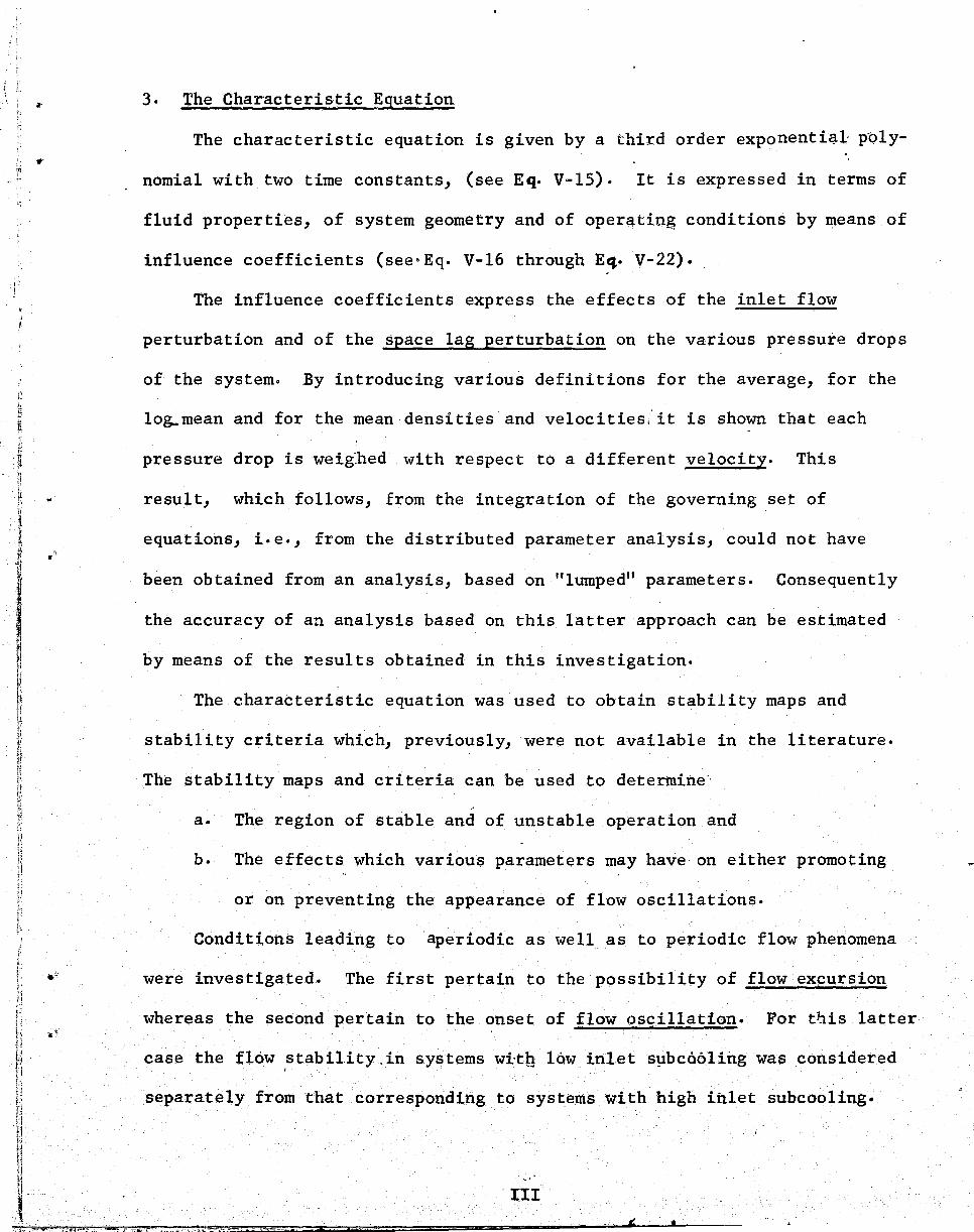
3. The Characteristic Equation

The characteristic equation is given by a third order exponentigl p~ly-

nomial with two time constants, (see Eq. V-IS). It is expressed in terms of

fluid properties, of system geometry and of operating conditions by means of

influence coefficients (see·Eq. V-16 through E~. V-22).

The influence coefficients express the effects of the inlet flow

perturbation and of the space lag eerturbation on the various pressure drops

of the system. By introducing various definitions for the average, for the

log..mean and for the mean densities and velocities:it is shown that each

pressure drop is wei~hed with respect to a different velocity. This

result, which follows, from the integration of the governing set of

equations, i.e., from the distributed parameter analysis, could not have

been obtained from an analysis, based on·"lumped" parameters. Consequently

the accuracy of an analysis based on this latter approach can be estimated

by means of the results obtained in this investigation.

The characteristic equation was used to obtain stability maps and

stability criteria which, previously, were not available in the literature.

The stability maps and criteria can be used to determine'

"

a. The region of stable and of unstable operation and

b. The effects which various parameters may have on either promoting

or on preventing the appearance of flow oscillations.

Conditions leading to aperiodic as well as to periodic flow phenomena

were investigated. The first pertain to the possibility of flow ex~ursion

whereas the second pertain to the onset of flow oscillation. For this latter

case the flow stability.in systems wi-th low inlet s!1bc661ing was considered ,

separately from that corresponding to systems with high inlet subcooling.

III t

I . -'I

f ,j

I I 1 I I

t j

. i ! .l

I I

The stability problem at intermediate subcooling will be considered in a

future report.

4. Excursive Flow Instability

It was shown that, at supercritical pressures, a flow system with heat

addition can undergo flow excursions because the hydraulic characteristics

of the system are given by a cubic relation between the pressure and the

mass flow rate (see Eq. VI-20). The latter is a consequence of density

variations in the system.

This excursive flow instabilitYJ! at supercritical pressuresJ is the

equivalent of the "Ledinegg" excursive instability in boiling systems at

subcritical pressures. This equivalence is supported by experimental data

(see Figure VI-I) which show:! that in both pressure regions, the flow system

has similar hydraulic characteristics.

A stability criterion which predicts the onset of the excursive in-

stability was derived in terms of system geometry, of fluid properties and

of operating conditions, i.e., of system pressure, flow rate, inlet temp-

erature and power input (see Eq. VI-l3). Various aspects of this type of "' .. ;'

instability are discussed together v.rith provisions required to prevent its

appearance (see Section VI-2).

50 Flow Oscillations at-Low Inlet Subcooling

It was shoyffi that for a system with low inl~ subcooling the character-

istic equation can be reduced to a second order polynomial with one time

delay.(see Eq. VII-7). For such a system the propensity to flow oscillation

can be analyzed by means of the stability maps recently presented by Bhatt c::'~

'ahd -H..su (see Figure VII-l).

•

...

-

."" ! - ~

~ ~ ]1 , l \

,j

Ii 'I ~ H I.j 'i

L I

'"

~' ~

j( !

,

.' I , ! n !

! I

It

1. . ) l:itT7i5YtriTN!

It was shown further that, when the inertia can be neglected in a system

with low inlet subcooling then the characteristic equation reduces to a first

order exponential polynomial'.' with one time delay (see Eq. VII-16).

For such a system the flow will be unconditionally stable if the

stability number Ns (defined by Eq. VII-39) is larger than unity. If

,Ns is smaller than uni ty, stable operation i'fi s till possible if the angular

frequency,of the inlet perturbation is larger ,than the critical one (given

in Eq. VII-40) or if the transit time is shorter ~han the critical one

(given by Eq.'VII-4l).

The region of stable and of unstable operation are shown in a stability

map (see figure VII-2) which can be used to' analyze the effects that various

parameters have on the' propensity to induce or to prevent flow oscillations

(see 'Section VII.3).

Although 'i:he ana.lytical predictions have not yet been tested quantita-

tively, ,the trends predicted by this map and by the stability criterion

(see Eq. VII-22 or Eq. VII .. 29) are in qualitat;ive agreement with experimental

observations (see Section VII.3).

6. Flow Oscillation at High Inlet.Subcooling

It was shown.that when the effects of the two time delays can be

neglected then the characteristic e'qu'ationreducei"to a""thi~.a',,9rdet" pb.1ynomial

(see Eq. VIII-2). A stability criterion was also derived (see Eq. VIII-IS)

which specifies the conditions fOF stable operation.

Various aspec,ts of this type of oscillations were discussed together

with provis,ions r~quired to prevent their appearance (see Section VIII-2).

It ie shown that th~ flow is more stable at high subcoolings than at low.

Furthermore, it,is concluded that the destabilizing effect of subcooling

v •

-

.~

,J I

must go through a maximum at intermediate range, (see Section VIII-2).

7. Significance of the,Results

The results of this analysis indicate several improvements in the design

and/or in the operating conditions which can be made to prevent the onset of ,

t flow excursions or of flow oscillations. These are discussed in more detail

I ! in relation to each type of instability (see Sections VI-2, VII-3, and

VIII-2) •

It was shown that the predominance of a particular parameter results

in a particular wave form and in particular frequency (see Eq. VII~40 and

Eq~ VIII~l7)o This result indicates that the primary cause of the instability

can be determined from the trace of flow oscillations.

Perhaps the result of greatest significance revealed in the present

investigation is the similarity between the characteristic equation which

predicts "chugging" combustion instabilities and the characteri.stic equation

. which predicts the thermally induced flow oscillati.ons for fluids in the

near crit·ical and in the supercritical thermodynamic region. Since it is

well known that "chugging" combustion instabilities can be stabilized by an

appropriate servo-control mechanism, the, resul ts of this investigation

indicate that low frequen.cy flow oscillations~ at near critical and at

supercritical pressures may be also stabilized.

The preceding conclusions have not yet been tested against experimental . dataq If confirmed, then the results of this study will provide a method

whereby stable operation can be insured in an intrinsically unstable region.

VI i

L~':~j, :;.::2. ac;;:; .'tl:rldSt5:;(::::ilj;y ;;==·;z;.r"J~I'+ii' ;a::.;,·: ;;;;;:;.i,;lj"'-;i:i! ;i;lg'EH~-i:iiii=~';ii.nii;;i'·Ei~,,;;;;;a;;;;o;;;;;;;*Iiii· = ....... ===-= ........ ___ ........ ___ ;:;::;::;:;;; __ ~s._~ ___ • _.. --'

.• ~

.;

I ¥ .., ~

r ,. ,. ~ I' i i I

~ 11 }I, i, L

.)

r I .. . ,

.f·

: 1 .

I<

,..

3. Recommendqtions

The reconunendations listed in .the four tasks below, define the effort

needed to complete and to verify the results obtained in this investigation.

1. Verify the stability criteria based on .the second and first order

exponential polynomials which hC3,ve been derived in the course of

these investigations ... For this purpose use 'available experimental

data .for various fluids at subcritical .and at supercritical pres ~

sUI'es.

2., . From the characteristic equation given by the third order exponential

polynomial with two time delays (Eq. V-IS) derive .stability maps and

stability criteria applicable to the ent:t're range of subcoolings.

Test these results again~d:.: available' experimental data.

3. ModifY the cha~acteristic equation to t:ake into account 'j::he effects

of the en.tire flow system i.e., of the flow loop. In particular in~

clude the effects of the inertia of the liquid in the storage tank and

in the supply lines together with the flow and elastic characteristi.cs

6f these lines.

4.. B,ased on .the results obtained from the preceding three tasks specify a

servo-c,ontrol mechanism which could be used to stabilize the flow for

. a system of practical i.nterest ·and verify the results by experiments to

VII

f'l I '

.,

I r

i; 'i i

I i Ii

.~ 11

Ac

A

a

a*

B

Bie'

b

h*

c

c*

cp

D

f

Fl

F2

F3

F4

F5

F6

F1

G

4. Nomenclature

MLTQ System of Units

with H defined by H = ML2 T=2

= cross sectional area of the duct lL2)

= coefficient defined by'Eqo VII~l6

= coefficient defined byEq .. VII=10

= coefficient defined by Eqo VI=21

= coefficien.t defined byEqo VII~17

= coefficient defined byEqo VI~4

= coefficient defined by Eqo VII-ll

= coefficient defined byEqo VI-23

= coefficient defined by'Eqo VII-l2

= coefficient defined byEqo VI-23 -,

= specific heat of the,· fluid in the "lig~t" fluid region I mrlQ-l j

= diameter of the duct( L l = friction factor

= Influence coefficient defined by Eq. V-5

= n' Eq. V-6

= " Eq .. V-7

= " Eqo V-8

= " Eq. V-9, .

= tt Eq. V-lO

= " Eq. V-Il

= Mass flux density ~ML-2T-l1

VIII

I1 l! If

I ,

I

i

L

Mg

Ns

P

~ Pex

.6 Pol

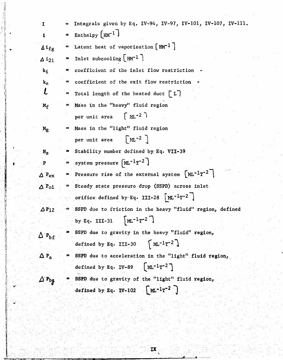
= Integrals given by Eq. IV-94, IV-97, IV-lOl, IV-l07, IV-Ill.

= Enthalpy (HM-ll

= Latent heat of vaporization [HM-l 1 = Inlet subcooling [HM-l l = coefficient of the inlet flow restriction

= coefficient of the exit flow restriction

= Total length of the heated duct eLl

= Mass in the "heavy" fluid region

per unit area r M.L -2 I

= Mass in the "light" fluid region

per unit area [ML -2 l = Stability number defined by·Eq. VII-39

= system pressure [ML- l T-21 = Pressure rise of the external system [ML -,1'1'-21

=

=

=

=

-

Steady state pressure drop (SSPD) across inlet

orifice,defined,by'Eq. 111-28 l ML-lT~2l SSPD due to friction in the heavy "fluid" region, defined

by Eq. 111-31

SSPD due to gravity in the heavy "fluid" region,

defined by Eq. III-3~

SSPD due to acceleration in the "light" fluid region,

defined byEq. IV-89

SSPD, due to gravity of the "light" fluj.d region,

defined by,Eq. IV-I02

IX , • . *

-

J

-t- -t, Y

fi h :!1 it ;1 :1 "

if

~ II ~

~

I .,

f

,

!

~

L1 P34

q

Q

R

S

S T

t

1A

U1 U

g(Z)

,-U3

(u ') g

ltlm

= SSPD due to friction of the light fluid region,

defined by Eq. IV-112,

= SSPD across exit flow restriction defined by Eqo' 1V~122. ( M )

=

=

=

h f1 d · \HJ.,- 2T- 1 "\ eat ux ens1ty L ' I

total heat input rate [ HT- 1 1 gas constant

= Exponent of the inlet velocity perturbation = 'Stability criterion defined by Eq VI-28 = Period of the inlet velocity perturbation

time

= velocity

= steady state velocity in the "heavy" fhtid region L'r~l

= SoS~ velocity of the light fluid region defined byEq. IV~28.(L)

= So S'o velocity at the exit from the duct

defined by Eqo IV.;!.'31.·

= average velocity in the "light" fluid region

defined by Eq. IV-32.

= Log mean velocity of the "light" fluid region

defined by Eq. IV-36

= mean velocity of the "light" fluid region

=

defined b~ Eq. IV-38. ,

t •

inlet velocity perturbation given by-Eq.t 111-7.

(L)

(L)

(L)

(L)

(L)

"x· ::3i~l=trc .. >l~j l·~n'ii:'li:r"!ii:;' ';::=~G~~iftili" I;i$,;:;;, ';;;;:,;;,zj' "~-i \)Oi;iOi'H4=,~·-';;:dti~· .. 'i.ill'fOii:-"*=~--.... ;;;;o,,;;;;;;*~, ...... ====-==-_______ ~~J,"- ___ -<-. __ '".. '-'

-...

i !

4 i

T

I 1 i

"''\I

J

".

l~ lj .~ " .. I

.! '" fc

J·,,;,ttt; ,r,.,'#i 'r

II Vfg

W

z

= velocity perturbation of the "light" fluid region

given by Eqo IV-30 ..

= specific volume of the heavy fluid LL~~l I = specific volume of the "light" fluid l L~=ll = change of specific volume in vaporization r L3M~1 j = total steady state mass flow rate

length

Green Letters

Y = heated perimeter l L 1

-cb

't'3-1:1

l:2

..n ~f

~g ~3

~t~ ( ~g)

~~

=

=

space lag defined byEqo 111-20

perturbation of the space lag

eLl

[Lj

amplitude of inlet velocity perturbation

time lagy defined by" Eq. III-18 [T) = tl T = total transit time" defined by' Eqo 111=63 [ T\ = critical transit time.9 defined byEqo VII-41o

= characteristic reaction frequency, defined by' Eqo IV=21o

.- density of the "eavy" fluid [ ML- 3l - density of the light fluid [ ML

w 3 j

= density at the exi.t from the heated ductJl defined by Eqo IV-72D

= log mean den.sity in the light fluid regiorLJ defined by·Eqo IV ... 76e

= average density in the light fluid region defined by Eqo IV ... 73 0

= mean density in the "light" flui.d region defined by Eq. IV-77o

; ..

•

'I L

i 'I

--I ,~

i , j

I

~ = angular frequency of the inlet velocity perturbation

We = critical angular frequency defined by Eq. VII-40.

'-S = dimensionless exponent defined by Eq. VII-B.

Subscripts

OJ 1, 2, 3, 4 correspond to the locations of the duct

indicated on Fig. 11-28

-1 T

.. ii "

t .~ ri ,. r ~ Ii ,;

tj I' \.1 ;j )J

!i L 1"! M ~A

if

~ ,. i!I

~ r ~

II I. I~ li

~ .....:. 1;1

~~ lAt ii it {.~ f~ , ;

i

"". 1: i' , " t, i

.... !

,

f I,

r

J,' t

'\

'\ ! I

'.'

50 List of Illustrations

Figure I=l~

Hydraulic Characteristic for Water at Supercritica1

Pressure(P = 250 atm} Flowing Through a Heated Ducto

Data of Semenkover for Inlet Entha1pies (Kca1/Kg) of

1-400, 2-350, 3-300, 4-200, 5-100 Kca1/Kge

Figure II~l~

The System

Figure 1I-2~

Specific Volume and Temperature Versus Enthalpy

for Oxygen at ·Pr = 1010

Figure II-3~

"Two Region" Approximation Showing. the Time

Lag and the Space Lago

Figure 1I-4~

The Effects of Time Lag and of Space Lag in

Inducing Flow Osci11ationo

Figure VI-I~

Hydraulic Ch~racteristics of Water Flowing

Through a Heated Duct at Subcritica1 and at

Supercritica1 Pressureso (Data of Krasiakova

and G1usker)o

Figure VI-2 g

Excursive Flow Instability_

. ·XIII

Page

7~a

13-a

l4-a

16-a

97-a

97-b

-

.1

i i , ~

Figure VII-l~

The Bhatt-Hsu Stability;Map for the' Second

Order Exponential Polynomial: 1. ~

~ +a ~ +b + c - = 0

Figure VII-2~

The stability Map for the First Order

Exponen.tial Polynomial~

S +·A +'B -s61: ..

Figure VII-3~

= O.

Percentage of Heat Exchanger Data Samples

Showing Steady Operation Vs. Heat·Flux

Per Unit Area Per Unit Mass Flow Rate

Reported by Pla.tt and. Wood.

Page

l07-a

ll4-a

l16-a

I~ !

Io Introduction

i IGl The Problem and Its Significance

A fluid in the vicinity of the critical, "point is an efficient heat 1.\

;

transfer medium because of the large specific heat and of the large co-

efficient of thermal expansion. Consequently, the demand for increased

efficiency of several advanced systems generated an interest in employing

fluids at critical and supercritical pressures either as cooling or working

media. For example, nuclear rockets, power reactors, high pressure once-

through boilers, regenerative heat exchangers for rocket engines and a new

sea water desalinization process are designed to operate in the critical

and the superc'ritical thermodynamic region. These developments made it

necess,ary to obtain data on and to improve the understanding of the thermal

and the flow behavior over a broad range of fluid states.

A great number of investigations conducted for such a purpose have

revealed that, in the critical as well as in the supercritical thermo-

dynamic region, flow and pressure oscillations may occur when certain

operating conditions are reached. These oscillations were observed in , -systems with forced flow as well as with natur,al circulation. 1

The occurrence of sustained pressure and flow oscillations and the

"" 'attendant temperature oscillations are very'undesirable and detrimental to

reliable operation of a system. Mechanical vibrations and thermal fatigue "-

induced by these oscillations very often result in a rupture of the duct.

In liquid propellant rocket engines flow and pressure oscillations can also

induce 'combustion instabilities resulting in a breakdown of the system.

I

I

Furthermore, in nuclear reactor systems flow and pressure oscillations may

induce divergent power oscillations leading to the destruction of the

entire system. Consequently, there is considerable practical interest and

incentive to investjgate, quantitatively, the conditions leading to the

inception of these oscillations~

102 Prey'ious Work

Severe pressure and flow oscillations were observed in experiments

performed with various fluid in the supercritical thermodynamic regions

Such oscillations were reported by Schmidt~ Eckert ~nd'Grigull [11, (ammonia);

Goldman [2, 31, (water); Firstenberg [41 ' (water); Harden [51, (Freon-114);

Harden and Boggs (61, (Freon-114); Walker and Harden [7l, (water, Freon-ll(..,

Freon-12, carbon dioxide); Holman and Boggs lB1, (Freon-12); Hines and

Wolf [91 (RP-l and diethycyclohexane); Platt and Wood (101 (dxygen);

Ellenbrook, Livingood and Straight (111, (hydrogen); Thurston [121, (9ydrogen~

nitrogen); Shitzman [13, 141 (water); Semenkover [151" (water); Cornelius and

Parker [161 (Freon-114); Cornelius (171 (Freon-114); and Krasiakova and

(' 1 Glusker LIB (water) 0

For a given fluid the characteristics (frequency and amplitude) of

these oscillations varied with operating conditions. In general, two types

of oscillations were observed: acoustical and chugging oscillations. For

example, . Shitzman (131 reports that, for water at 250 atm, the pressure and

temperature oscillations had a period of 80 sec. and an amplitude of 25 atm.,

and of 1000C res.pectively. Decreasing the ~flow rate and the power density

resulted in decreasing the period to 15 sec. However, at a pressure of

5000 psi, Goldman (2, 31reports" pressure o~cillations with frequencies

from 1400 to 2200 cps. Similar high frequency oscillations (1000-10,000 cps

-2-

- - , , ,

, "

and 380 psi peak to peak) were reported by Hines and Wolf (91 for RP=l ..

Three c~asses of pressure oscillations in the supercritical region

were observed i.n the exper!ments of Thurston [121; these were described as~ 1) Open~open pipe resonance observed at medium and high flow rateo

This mode is associated with the fundamental wavelength of an

open=open pipeo

2) Helmholtz re~onance!l associated with a resonator composed of a

ca'!'ity connected to an external atmosphere via an orifice or neck~

3) Supercritical oscillations appearing usually at low flow rateso

Hines and Wolf [ 91, however, report only two general types of oscilla~

tions: a high frequency (3000-75000 cps) oscillations audible as a clear

and steady scream and an oscillation with a lower frequency (600=2400 cps)

which was audible as a chugging or pulsating noise. The domina~t frequencies ,

of these oscillations did nQt correspond to simple acoustic resonant fre a•

quencies for the tubes.

Corneliu.s and Parkerl16 , 171 describe in detail the two types of

oscillations and note that the frequency of the acoustical oscillations .-;,

decreases with temperature whereas the frequency of the ch~gging oscillati.ons

increases with temperatureo Occasionally, both types of oscillations occured

simultaneously.

A quantitative formulation and explanation of the conditions leading

to the appearance of the, pressure and flow oscillations has not been reported

yett although several qualitative explanations have been advanced 0 It is

~enerally agree~ that the osc+llations are caused by the large variations

of the thermodynamic and the transport properties of the fluid as it passes

.through the critical thermodynamic region.

\

--..

Several investigators (12, 13, 14) note that the appearance of oscil~

lations occurs when the temperature of the heating surf.ace exceeds the

"pseudo critical" or the "transposed" critical temper~tures, i.e., the tem~

. perature where the specific heat reaches its maximum value (see Figure .A1 in

Append~x A). Oscillations were not observed if the inlet temperature was ,

above this temperature. From this it was concluded that the mechanism for

driving the osc.i1lation occurred only when a "pseudo liquid" state was present

i.n some parts of the heated duct.

Firstenberg (4) attributes the oscillations to the variations of the heat

transfer rates to the fluid, .whereas Goldman (2, 3) explains the oscillations

as well ·as the steady state heat transfer mechanism in the critical and super=

critical thermodynamic region as "boiling like" phenomena associated with non~

equiliprium conditions. According to Goldman, below the pseudo-critical temper=

ature the fluid is essen.ti.a1Iy a liquid, above this temperature it behaves as a

gas 0 At the pseudocritical temperature, the density gr·adient and the specific

heat reach maximum values giving ,an indication of the energy required to over-

come the m~tuc?l attraction between the molecules. The fluid in the inunediate

vicinity of the heated wall is in a gas-like state; whereas the bulk fluid may

still be in the 1iquid ... l:Lke state. If by means of turbulent fluctuations a

liquid-like cluster is brought into contact with the heating surface·a large a-

mount of energy will flow from the surf.ace to the cluster bec·ause of the ·large

temperature difference and because of the high conductivity of the liquid-like

fluid. This energy mpy be large enough ·to "explode" clusters of mplecules from

the liquid..,like state to the gas-like state. Thus, according to Goldman (2, 3),

one may visualize the superctiticalregion as a region where explosions of liquid-

-4-

I iI :1 if il~

\ ~

'"

I >;

~ U It ij, Ii f' il q \1

~

~ , t

like clusters into gas-like aggregates take place. Goldman considers this

process to be similar to the formation of bubbles in liquids during boiling

at subcritical pressures.

The conditions under which oscillations occur were summarized by

Goldman as fol1aNs~

1) Heat transfer with IVwhistle H {ioe. ~ 'with oscillations} occurs

only at high heat flux densities and wit.h bulk t.emperatures lower

than the pseudocr~tical temperature.

2) At a given flow rate and inlet temperatu.re:,) whistles occur at

higher flux densities for nigher pressure levels.

3) At given flow rate and pressure$ whistles occur at lower heat

flux densities for higher inlet temperatures.

4) At a given pressure and inlet temperature~ whistles occur at

higher heat flux densities for higher flow rates.

5) Whistles can be produced with various lengths of the test sections

but the heat flux or inlet temperature must be increased to bring

it about if the tube is shortened.,

Visual observaiion that bailing-like phenomena can exist at supercritical

pressure.s was reported by Griffith and Saberski. [19J in e~'periments corqducted with

R~114. The photographs of the process revealed a behavior similar to

that observed in pool boiling at. subcritical pressures.

Similarly ~ high spee,d movies of hydrogen, at supercritical pressures

ta~en by Graham!! et al (20 1 reveale.d a phenomenon resembling boiling. Clusters

of low density fluid were observed rising th.rough a denser fluid+giving

boiling-like appearanceo

=5-

-

" , , '

I .

Hines and Wolf [91 attribute the appearance of the flow oscillations .a

at supercritical pressures to the variat~ons of liquid viscosity. They

note that a small change of temperature near the critical point results

in a large change ~of viscosity. C-onseq~ently, a sudden increase in wall ..

temperature could cause a thinning of the laminar boundary layer due t9

variation of the viscosity. Thinning of the boundary layer would result . ,;,'~ .. "

in a drop of the wall temperature and a corresponding increase of viscosity.

This would cause a thicker boundary layer and produce another rise of tem­

perature, thus repeating the cycle. It was shown by Bussard and DeLauer [21J

and by Harry [ 22] that a viscosity-dependent mechanism can induce an unstable

flow in single phase flow systems when the absolute gas temperature +s in-,

creased by a factor of 3~6 or more.. Such flow oscillations were observed

by Guevara et al~3Jwith helium flowing through a uniformly heated

channel.

Harden and co-workersl5, 6, 71 concluded from their experiments that

sustained pressure and flow oscillations appeared when the bulk fluid reached

a temperature at which the product of the density and enthalpy has its maximum

value 0 'I'his explanation was, however, criticized by Cornelius ( 1701. Cornelius and Parker (16, 171 postulate that both acoustical and the

chugging oscillations originate in the heated boundary layer. When the

fluid in the heated boundary layer is in a "pseudo vapor" state, a pressure

wave passing the heated s,urface would tend to compress the boundary layer,

improve the thermal conductivity and cause an increase of the heat transfer

coefficient. Ararefraction wave passing over the heated wall would have

just the opposite effect. Thus, this pressure--dependent--heat-transfer

rate cC),l,1ld induce and maintain an acoustic oscillation. Cornelius and Parker

-6-

.1 i

u w " ... !l II ~ II H it " n 1+ " " Ii >i

~

U ~ ~ " if " J :'j ~.! il hi :1 d ,1 'I u 1 ~ ;j t, iI :",j 'i

d r.!

->1

:1 ;'! d

! 'j

':i U

,

I , \

•

i i

, I

+-

attribute the appearance of chugging oscillations to "boiling ... like" phenomena

. and a s~dden improvement of the heat transfer coefficient. An approximate

numerical solution verified the importance of the heat transfer improvement

in trigge~ing and maintaining oscillationso

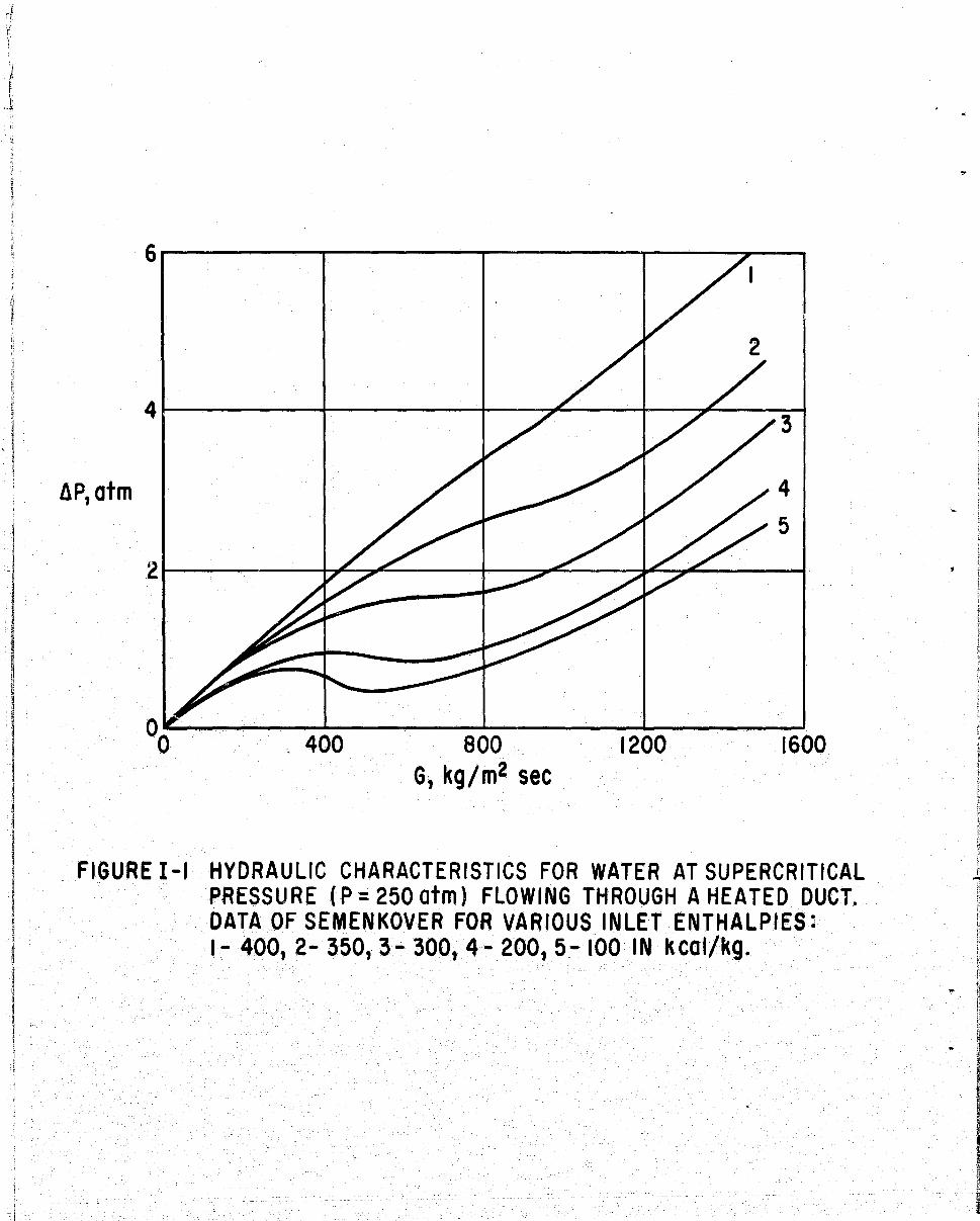
Of particub,\r interest to the analysis""presented in this paper are the

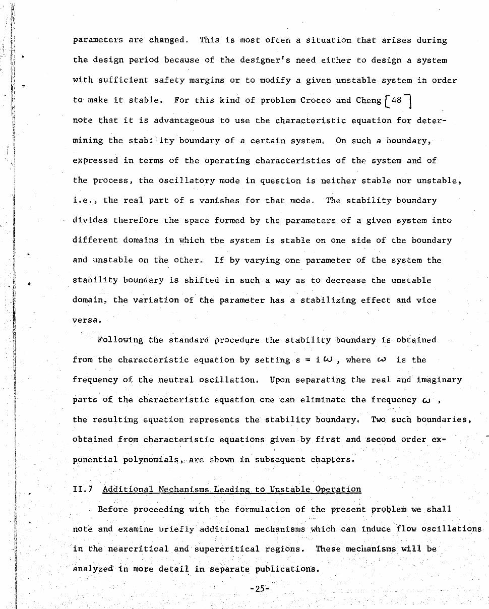
experimental results of Semenkover» [15 J and of Krasiakova and Glusker [ 18 J, •

for water at 250 atm. For a constant power ~nput Q to the system their data

show a pressure versus mass flow relation that is illustrated in Figure 1-1.

It ~an be seen that for large values of inlet enthalpy 1» there is a monotonic

increase of pressure drop with flow rateo At a certain lower value of i»

the curve shows an infl~ction pointo For still lower values of inlet enthalpy~

there is a region where the pressure drop decreases with increasing flow rateo

Such a pressure drop=flow rate relation occurs in boiling systems and gives

rise to an excursive type of instability which was analyzed first by Ledinegg

[24J and by numerous investigators since.[25 ... 47Jo Consequently, the data

of [15» 18 J tend to confi:rrn the similarity between instabilities.) observed

during subcritical boiling'and those observed at supercritical pressure

suggesting therefore a common mechanismo

103 Pu~pose and Outline of the Analysis

From the preceeding brief review of the present understanding of flow

.... f""' oscillations at supercritical pressures» it can be concluded that several modes u

oscillation existo It can be expected» therefore» that several mechanisms can

be effective in inducing unstable flowo Indeed~ as discussed in the preceeding

section» several qualitative explanations of the phenomenon bave been already

advanced. However, a quantitative formulation of the problem is still lacking.

-7-

J 'f ~ ;

\ " 'J I j

-. ill

ii ~ ; 1

1 J

1

l~ j

I , I 1 i

6

4~------~~-------+--~'----+--~----~ 3

l1P, atm

FIGURE I-I

. 400 800 G, kglm2 see

1200

4

5

1600

HYDRAULIC CHARACTERISTICS FOR WATER AT SUPERCRITICAL PRESSU RE (P = 250 atm) FLOWING THROUGH A HEATED DUCT. DATA OF SEMENKOVER FOR VARIOUS INLET ENTHALPIES: 1- 4'00, 2- 350, 3- 300, 4 - 2'00, 5- 100 IN keal/kg.

...

I The analysis presented in this paper has four objectives:

1) To distinguish a number of mechanisms which may be responsible for

thermally induced flow oscillations at nearcritical and at supercritical

pressures ..

2) To present a quantitative formulation of the mechanism which appears to

be most significant from the point of view of system design and operation.

3) To predIct the onset of these oscillations in terms of the geometry and

of the operating conditions of the system.

4) To analyze the consequences of the theoretical predictions and to suggest

improvements whereby the onset of these oscillations can be eliminated.

The particular mechanism which is formulated and analyzed in this paper

is based en the effects of time lag and of density variations. It is well

known that these effects can induce combustion instabilities in liquid pro~

pellantrocket motors as discussed by Crocco and Cheng (48~. It was shown

by Profos (49~ ,Wallis and Heasley ( SOl and by Bour~ (511 that the effects

of time lag and of density variations can also induce unstable flow in

boiling mixtures at subcritical pressures. The.suggested similarity of

flow oscillations observed at supercritical pressures with those observed in

two phase" mix:tures at subcritical pressures prompts us to formulate and

to analyze the problem in terms of this mechanism. In particular, the ex­

perimental results of Semenkover L151 and of Krasiakove and Glusker l18~

discussed in the preceding section~ together with the chugging oscillations

described by several authors provide enough evidence to warrant a more de-

tailed analysis of flow oscillations at supercritical pressures in terms

of the time lag.effect.

The present analysis' is similar to those. reported by Wallis and Heasley

-8-

...... ,

i "

!.

I

, I I

[soJ and by Bour~ (51J in two respects~ the formulation and the assumptions

a~e the same. In pa~tic~la~~ it is assumed that the density of the medium

is a function of enthalpy only. The effects of p~essu'ite vall:'iations arel)

thell:'efore neglected.* As noted by Wallis and Heasley [jO] this assumption

results in the decoupling of the momentum equation from the energy and the

continuity equatioose The momentum equation can be integ~ated then separately

after the velocity and density variations are obtained from the contin~ity and

the energy equations. Following Bour~ [51J the problem is formulated in terms

of an equation of state and of th~ee field eq~ations describing the ~onse'it=

vati~n of massl) energy and mementum.

Apatitt f1t'om the fact that the arnalyses of Wallis and Heasley [50] and

of J.Bour~ [sI] were derived to predict unstable flow in boiling two phase

mixtu.res th,e present analyses (concerned with flow oscillations at nealr=

critical and at supercritical pressures) differs f~om tneirs in two respects~

1) tne form of the constitutive equation of state is different» 2) the

cha~acteristic equation describing the onset of oscillations is differente

F~om tnis characteristic equation 9 we shall derive stability maps an~

staDility inertia which~ pl'evio~sly', 'V1ere !1£S. available in' the literature~

T~e outline of the paper is as follows. In Chapter II some general

comments are made regarding 1) the nature of tne tnermal1y induced flow

oscillations at nearcritical and at supel'critical pressures)) 2) the effect

IQ)f tne time lagl) 3) tne implication and limitations of tne assumptio~s and

4) tne general metnod of solution. In Cnapters III and IV tn~ problem is

formulated and cne set of gove~ning equation is solved. Toe cnaracte~istic

equation wnicn predicts tne onset of flow oscillation is derived in Chapter V;

i~ 1s of tne form of a thi~d order exponential polynomial with two time

delays. From the characteristic equation a criterion is derived in

*The limitations and implieati,ons of this assumption are discu8sed in Chapter II.

-9-

, J' j; 1 J j

; :/ " f]

•

Chapter VI which predicts the onset of an excursive type of instability at

supercritical pressures.* This excursive i~stability at $upercritical

pressure is the equivalent of the so called Ledinegg excursive instability

for boiling at subcritical pressures. The effect of time lags in inducing

flow oscillations is analyzed in Chapters VII and VIII wh~ch consider first

and second order expotential polynomials., Stability diagrams which predict

the regions of stable and u~stable flow in terms of the operating parameters

are given in these two chapters together with suggested improvements whereby

the onset ofJO>Slcillations can be eliminated. The recqmmendaticms for

future work and the conclusions are given in Chapters IX.

The status of the present understanding of thermodynamic phenomena that take

place in the critical thermodynamic region is discussed in Appendix A.

1.4 The Significance of the Results .f.)

Three mechanisms whicncan induce thermo-hydraulic oscillations at

supercritical pressures have been distinguis~ed in this paper. One is

caused by the variation of the heat transfer coefficient at the transposed~

ioe.~ pseudo critical point. The second is caused by the effects of la~ge

compressibility and the resultant low velocity of sound in the critical

region. Finally\). the third mechanism is caused by the large variation of flow

characteristics brought about by density.variations of the fluid during the

heating process. 'The prnpagations of these variations in particular of ~he

enthalpy a.nd of the density, through the system introduce delays which,

*This criterion was first derived by the writer in the Second Quarterly Progress Report, "Investigation of the Natufe of Cryogenic Fluid Flow Instabilities in Heat Exchangers, II Contract NAS8-:i,,1422, 1 February 1965.

-10-

-

,1

~ ;

-,\ ,

\ I

." r i

under certain conditions, can cause unstable flow. This last mechanism, that

induces ~ frequency oscillations, i~ investigated in detail because ex-

periment~l data show that this type of oscillation is most p~~!a1ent.

It is shown that at supercritica1 pressure unsteady flow Qonditions

both excursive and oscillatory can occur. A characteristic equation is

derived that predicts the onset of flow instabilities caused by density

variations in the critical and supercritica1 thermodynamic region. The

same characteristic equatipn can be used to predict the onset of flow

instabilities in boiling at subcritical pressure, iJ the effect of the

relative velocity between the two phases can be neglected. Experimental

evidence shows that this effect becomes negligible at reduced press~r~s

above say 0.85. Consequently, at ne ar critical and supercritica1 pressures,

the characteristic equation, which is expressed in terms of system geometry

and operative conditions, can be used to determine:

a) The region of stable and unstable behavior.

b) The effect which various parameters may have on either promoting

or on preventing the appeara~ce of flow oscillations.

From this characteristic'equatio1;l simple "rule of thumbs" criteria are

also derived based on the assumption that one or the other of the various

parameters is do~inant. It is shown that the dominance of a particular

parameter results in a particular frequency and wave form. This results

permits a diagnosis of the primary cause of the instability from the trace

of flow oscillations.

It is 6f particular interest to note that~the characteristic equation

derived in this paper for predicting flow oscillations at sup~rcritical

pressure is' of the same form as ~ characterist~c ~quation derived by Crocco

-11-

-

I j { ,

and Cheng[4S]to predict combustion instabilities of liquid p~opellant

rocket motorso* It is well established in the combustion literatu~e that

a servo~control mechanism can be used to stabilize the low freque~cy com=

bustion instability.. The si:milarity of the characteristic equations iSl)

therefo2t'e ll significant because it indicates that stable operation could

be insured also in the nearcritical and in the s~percriti~al regi@D by

using an appropriately designed servo-control mechanism ..

*This similarity between combust:1pn and two phase flow instabilities should not come as a surprise if one recalls that the processes of combustion and of boiling are both cbeml.cal processes involving large enthalpy and density changes.

-12..,

, .. •

;. t

l d;/! r';( ~"

,L... ..

• i j..: i'; t t, ~ ,

r ~ i ,.

" il '.I ~

,; 'i ,i },

i! ~

n . ij n H ~ i,

I j ~ 11 Ii ,I

n !J H

I I ~ ~ ~ ~ i ~ 11 ~

I d.

~

I ~

I !!

~ r~

» ~ ~

~ ~

110 General Considerations

1101 The System and the Thermodynamic Process

In order to understand the mechanisms of the thermally induced flow

oscillations at supercritical pressures s it is necessary to examine

briefly the system and the thermodynamic processo

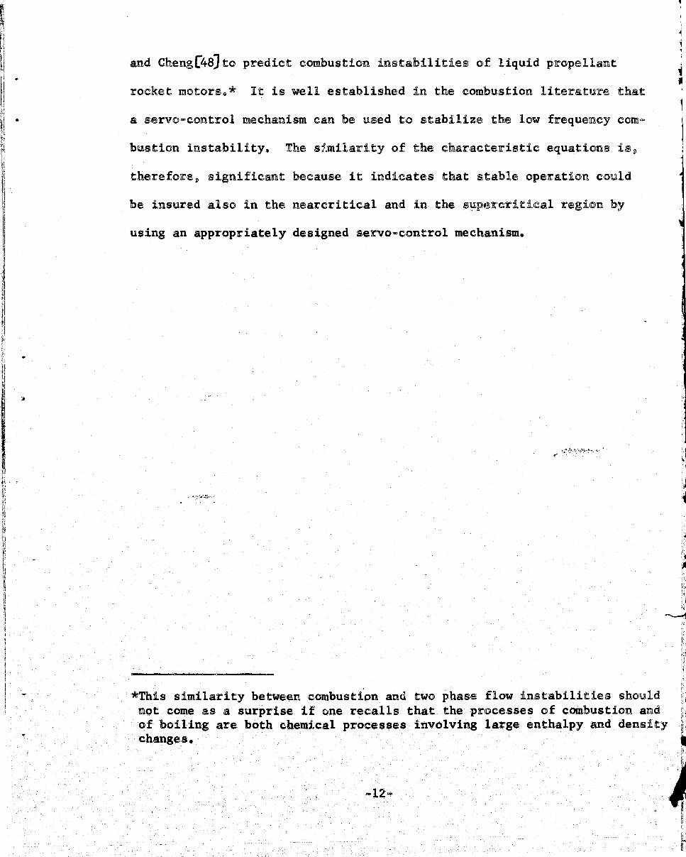
The system of interest is shown in Figure 11-10 It consists" of a

fluid flowi.ng through a heated duct of length 1. Wit.hout loss of

generalit.y it will be assumed that the du.ct is uniformly heated at a

rate of Qo Two flow restrictions are located one at the entrance~ the

other at the "exit of the duct.

The the,rmodynamic process starts with the fluid at Ii. supercritical

pressure P s entering the heated duct with velocity tAB' The temperature

To~ of the fluid at the inlEtt' is well 'below the critical temperature of the

fluid under considerations. As the energy is being transferred from the

heated duct to the fluid its temperature T~ speci.fic volume Vs and enthalpy

i, will increase. Thus~ the temperature T3

, at the exit may be considerably'

above the" critical temperature. In a number of systems of practical i:n~erest

it can be 'assumed that this process takes place at an approximately constant

pressur.e.

In orde.r to formulate the problem it is necessary to specify the

constitutive equation of state which describes the relation between say

the. specific volume; the pressur(~ 'and the enthalpy for the part.fcular

f:iuid~ This r.e"qu~t.~s da'ta, o'n t:he thermodynamic, properties of the fluid in

the region of interest. The 'region of interest-to this study are the

nearcritical"'and the supercritical regions.

-13-'

f t , I I

\

I i f I ! . 1

I

I~ l l'

I

8 _

-4

C

-rt - en c

t

::0

,.

"

t=I

o·

-I

:::I:

rt1 en

-<

(j) ~

rrI ==

(9

-4 ~

bI

bI

®

<

".

~ 1

" .~

The present understanding of the thermodynamic properties and phenomena

at nearcritica1 and supercritical pressures is. reviewed in Appendi.x A.

It is shown there that at these pressures the fluid has the characteristics

of a liquid when the temperature is sufficiently below the critical one.

However~ if the teIIlperature is increased sufficiently above the critical

temperature~ the fluid will have the characteristics of a gaso This is

illustrated in Figure II~2 which is a plot of the specific volume and of

the temperature versus the enthalpy for oxygen at a reduced pressure of

It can be seen from this figure that at low enthalpies the specific

volume is essentially constant~ this is a characteristic of l~quids. As

the enthalpy increases the specific volume increases approaching values

predicted by the perfect gas law. It can be seen also that this change

from a liquid~like state (region CD = @) to a gas=like s,tate (region

® = 0) ·occurs Over a t.ransition n~gion denoted by' @ = 0 on Figure II~2.

It appears~ therefore~ that at supercritica1 pressures the relation

between the specific volume and the enthalpy can be approximated by con-

sidering three regions: a 1iquid-like~ a t~ansition and a gas like region.

For oxygen Figure II-2 indicates also. tha't~ as a first approximation~ the

transition region can be reduced to a transition poipt reducing, therefore,

,~pe .. ,problem to a "tw9.,;region" approximation. * Since oxygen is the fluid

of primary interest to this analysis., we shall use the "two-region"

*The "three region" approximation was first introduced. by the writer in analyzing the excursive instability at supercritical pressures (see foot­note on page 10). Following this work Dr. R. Fleming, from the Research and Development Center of the GECo o , introduced the "two region" approxi­mation for oxygen. These two approximations are discussed further in Appendix B.

-14-I

1"

I

c­.'

approximation for describing the relation between the specific volume

and the enthalpyo It is assumed~ therefore~ that the "heavy" fluid (of

constant density) persists until the transition point is reached; above

this point the fluid will have the properties of the Ulight U ph_seo It

remains now to define this transition pointo \

In boiling at subcritical pressure the transition from the heavy to

the light phase corresponds to the onset of boiling. Consequently, it

will be a.ssumed that in the nearcritical region the tra1l:~sition point

corresponds to the enthalpy at saturati.on. temperature 0

At supercritical pressures it will be assumed that the transition point

corresponds to the transposed critical point~ ioe.~ to the pseudo critical

pOint which is defined as the point where C reaches its maximum value. p

It is discussed in Appendix A that the locus of pseudo critical points

can be regarded as the extension of the saturation line in the super-

cri.tical reg.ton.

II. 2 lime .La~ and S ,Eace Lag

It is of interest to consider n.ow the timewise and spacewise des~

cription of the process.*

If we follow a particle from the ti.me it enters the heated section

until it leaves it, we shall observ'e that its properties change from VI

----------------*We follow here Crocco and Cheng (481 who gave an equivalent description for combustion instabilities. The same con~ent applies to the three sec~ions that followo Indeed, this reference proved to be most stimu­lating and useful in. the course of this investigationo

~15-

and il

at the inlet to v3 and i3 at the exit (see Figure 11-3)0 In

view of the "two-region" approximatilJ.n we wou.ld note that the transiti.on

from the "heavy" to the "light!D fluid occurred when the properties (specifically

the enthalpy) reached values that correspond to the transition pointe The 1i Ij MS- time elapsed between the injection of the heavy particle "in the heated duct ;j :\

[I and its transformation to the "light" fluid will be denoted as the tim§., :1

il " ~ !?Z, r~· a UI , n

I It is of interest also to consider the spacewise description of the

1 process. In 'this case the time lag W'~st be replaced by the space l£g

I

I

, 1

"

which is a vectorial quantity indicating the location in the duct where

the transformati.on from the HheavyH to the ':light" fluid takes place.

The space lag is denoted by ~ on Figure 11=3. Of course ~ the space

la.g can be related to the time lag when the particle velocity is known.

Like, in combustion~ the location in the duct where the transformation

II II takes place can be regarded as the source of the light fluid. It is

II " obvious that the flow properties in the region occupied by the light

fluid will depend UpO'l.1 the intensity of this source. If it is assLmed

II II that the injection' rate of the heavy fluid is constant and that the time

, and space lags were constant, then the intensity of the sour~e would also

be independent of time resulting in a .steady flow in the "light" fluid

region. However s _ this is not the case because fluctuation,s which affect

. the time lag and/or the injection rate are pr~Lent both at supercritical

and at subcritical pressures. In the vicinity of the critical thermo~

dynamic pOint large fluctuations of properties, in particular of densitv ,

are observed even in non-flow systemso In boiling systems fluctuations

are always present be'cause of variations of the rate of bubble formation

'.

v

"--.-----.---.----__ i . L, L2 L3

v

- 1 ~. 1

I v

~----------------------z

®<D ® ® @)

FIGURE 1I-3 IIrwo- REGION" APPROXIMATION SHOWING THE .. , TIME LAG AND THE SPACE LAG.

I

I 'i

i !

1

4 !

and population, .of flow regimes, of the heat transfer coefficient~ etc.

Consequently~ the strength of the source may fluctuate even when the in-

jection rate is kept constant. It is evident also that variations of

" inlet velocity will introduce additional effects.

;1

The nucleation and evaporation at subcritical pressures and the

transformation of "heavy" clusters to "light" clusters at supercritical

pressures are rate processes that occur during and have an effect upon

the length of the time lag. Both of these transformation rates are af-

fected by the pressure, temperature and by other rate processes such as

the rate of energy transfer, flow ~ate, etc. If one of these factors

changes or fluctuates, the transformation rates will fluctuate also

resulting in a fluctuation of the time lag, i.e., in the fluctuation·

of the source. Since the source affects- the flow conditions in the "light"

fluid region the flow in this region may become oscillatory.

11.3 Organized Oscillations

Oscillations of a system can be always produced if properly excited.

Such oscillations can be distinguished by a characteristic time,. 1. e·. , period if the process is periodic or by a relaxation time if it is

aperiodico

Like in combustion and fallowing Crocco and_Cheng [481 we shall

distinguish two cases: random fluctuations and organized or coordinated

oscillations.

As random fluctuation we consider those that are Similar: to fluctuations

observed in ordinary turhulent flow. In this case it can be assumed that

the transfOrmation process, fer example the rate of evaporation in boiling

-17- .

at subcritical pressures, is not excited. The fluctuations at one poin~

do not have any effect on other fluctuations somewhere else in the systemo

Since the integrated effects of these fluctuations vanish they do not pose

a problemo

In the case of an organized oscillation the transformation process

,I will be excited by one or more coordinating processes such as the oscillation

of the inlet flow rate,j) of the heat transfer coefficients etco The exciting

force for maintaining the oscillation o.f the: coordinating process is in

turn provided by the transformation process 0 For example~ in boiling sys=

terns oscillat.ions of pressure will affect the saturation temperature wh!.ch

may induce oscillations in the rates of evaporationo These in turn may

, induce flow oscillations and provide the excitation force for maintaining

the pressure fluctuations.

The fundamental character of organized oscillations is that a well

defined correlation exists between fluctuations at two different points

or instantso In other words that a disturbance is propagated,9 Leo:'J dis= ~

placed in time add space through the systemo When these organized oscil-

lations are present their integrated effect does not vanish whence the interest

in these oscillationso Furthermore)) an oscillatory system may become unstable.,

ioe.~ it may have the tendency to amplifyo In the example cited above

pressure fluctuations of an increasing arrlplitude may be generated leading

to the destruction of the systemo When the effects are proportional to

the causes the system is defined as 1inearo In this paper we are interested

in such systemso

I J

-18- ~ I f

11.4 :r.he. Mechanism of IJOW Frequ.ency (Chugging) Oscillation ~ Supercritical Pressures

It was noted in the preceding section that the characteristic of

organized oscillatio!ls is the propagation of disturbances through one system.

These disturbances can be variations of density, pressure, enthalpy, entropy,

etc. In this section we shall examine the effects which these propagations

may have on the oscillating propensity of the system. In particular, we

shall consider the propagation of density disturbances and the effect of the

Lime lag, i.e., of the space lag. The effects of pressure waves are discussed

together wit.h the other mechanisms which may induce flow

oscillations in the nearcri.tical and supercritical regions.

We note that the effect of the time lag in inducing combustion in­

stabili.ties was alrea~y analyzed by Summerfeld [521 ' Crocco and Cheng l4~ t

among others. In boiling systems, this effect was already analyzed by

Profes ( 491 ' Wallis and Heasley [ sOland by Bourt& [5~. In these analyses·

the flow was assQ~ed to be homogeneous, i.e~~ the effect of the relative

velocity between the gas the liquid. phase was neglected •. A density propa-

gation equation, applicable to two··phase mixtures, which takes this effect

into aCCoUlnt was formulated in (531 and solved in [.54, 551 . Let UlS examine now the effects of the finite rates of propagation and

of the resulting time lag and time delays on the flo'w in a system consisting

of a constant pressure tank connected by a feeding system to the heated duct.

Consider first t~e tank and the feeding system only and let us perturb

suddenly the inlet flow. If there is no feedback between the heated unit

and the '}.pstream part of the system, the steady state conditions will be

restored •. tn particular, if the variation of the £low rate is small during

-19-

OSCILLATION OF:~

INLET VELOCITY --~----------~------~------~~----~----------.t

SPACE LAG --------------+-~,~----~------~~----~---------.t

tb: I I I

FLUID VELOCITY I --------------~~~------~------~------~------. t

I I

FLUID ENTHALPY

19u1 I

--------------~--~~------+-------~------~--~ t I 9· I

L I

I I

FLUID DENSITY I I

,19PI I I

I I

t

SYSTEM PRESSURE DROP I ~--------~~+------I~I------~------~------~---' t

I I 19A~

FIGURE :n -4 THE EFFECTS OF TIME LA() AND OF SPACE LAG IN INDUCING FLOW OSCILLATION.

-

the time a, pressure wave propagates back and forth through the tank and

the·feed system~ then the pressure effects can be neglected. As discussed

in [ 481 the process can be described then, with sufficient accuracy, by

an exponentially decaying flow which is characterized by the relaxatidn

time constant. i.e., by the line relaxation time. Therefore, the system

is stable becau.se the steady state conditions will be eventually restored.*

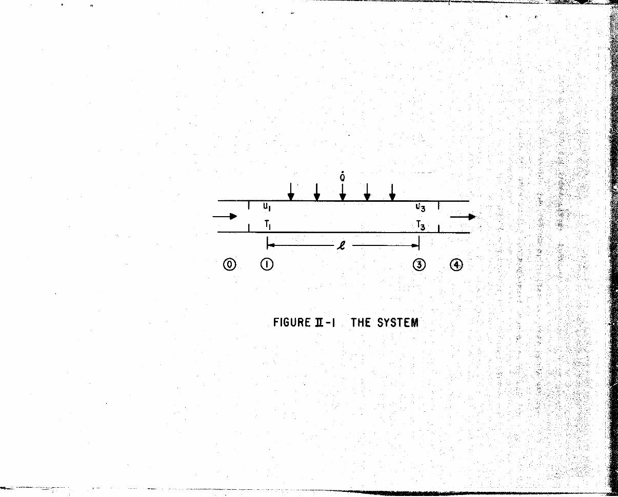
Consider now the effect of a perturbed flow at the inlet of the heated

d.uct (See Figure 11=4). It is obvious that an oscillatory flow at the inlet

will induce an osci.l1.atory flow of the fluid in the ducto However~ in

absence of a driving mechanism these oscillations would also exhibit an ex-

ponential decay. We are looking for a mechanism whereby these flow oscil=

lations at supercritical pressures can be maintained. Like in boiling and

in combustion such a mechanism is provided by the propagation phenome.na

which introduce different d,elay times in the response of the system. This

is shown in Figure II-4.

It can be seeD on Figure 11-4 that an oscillatory inlet flow can induce

oscillations of the space lag; this is in accordance with the discussion of

the preceding section. The onset of these oscillations is delayed however

by the lag time ~b~ because of the finite rate of propagation of the dis­

turbance. An oscillat.oryspace lag, which is equivalent t.o an oscillatory

source~ will induce flow oscil1ation~ in the "light" fluid region. These

so~rce=in.duced esc.illations will be present in addition to those already

induced by the inlet flow. Because of these two oscillat.ory motions there

will be a delay time 9'\1, in the flow response. Oscillati,ons of. the flo'tll

*We are assu.ming.here that any servo-cont.rol mechanism in the feeding system will not have a destabilizing effect.

-20-

·1 I

;J I' t j

. i :

will induce oscillations of enthalpy and of density both delayed by a

certain delay time. With flow and density oscillating, the pressure drop

in the duct will also oscillate. If the conditions are such that the mini=

mum pressure drop in the duct occurs when the inlet flow is 'maximum, it is

apparent then that the oscillations can be maintained. It is also obvious

that whether or not this will occur will depend on the time lag t:b and on

the delay times , When these delay times do B2t

depend upon iC b' it can be seen that increasing the lag time 1:b" has a

destabilizing effect. Since the time lagLl:, (see Figure 11-·4) depends

upon the enthalpy difference i2 - iI' it can be concluded that, for this

particular case, a decrease of inlet enthalpy i 1 , i.e., that an increase

of Ai21 has a destabilizing effect.

From this qualitative description it can be already seen that at

supercritical pressures an unstable flow can be induced by the delayed

response of various perturbations. It remains now to advance a qualitative

description. We shall do this in the following chapters by modifying and

applying the method proposed in 150, 511 for boiling at sl1bcritical

pressur.es.

11.5 l1~thod of Solution

In what follows we shall consider the "heavy" and the "light" fluid

regions separately. Each will be desQ.ribed in terms of three conservation

equatione and the equation of state. We shall use the one dimensional

representation and obtain solutions for each region. These solutions will

be matched at the transition point, i.e., at the end pOint of the space

lag to provide a solution valid for the entire system.

i

-

Following [48, 50, 511 it will be assumed that the variation of

pressures can be neglected. This is implied by the assumption that the

density is function of enthalpy onl~. It can be seen that this assumption

will be valid only if the variations of flow, density, enthalpy, etc. are

relati.vely small during the total time for propagation of a pressure wave

back and forth through the duct. Under this condition it can be assumed

that the various disturbances move through a uniform medium. It is ap-

parent also that this will be true only if the rate of propagation of

preSSU1-e waves is considerably faster than the rate o£ propagation of the

disturbances. However, both in boiling systems as well as in the nearcritica1

region the velocity of sound reaches ve~; low values.* Consequently, it can

be expected that there will be a range of operating conditions for which

the assumption that the properties do not depend upon pressure variations

will not be satisfied. For boiling systems this limitation has been already

recognized and discussed by Christensen and Solberg [561 0 In general,

it can he expected that the assumption 'Will be satisfied in the low frequency

range, L e .. , in fichugging" oscillati.ons. When the effects of pressure vari­

ations can be neglected then one can use the formulation put forward in [50l

and carried out in [511 for boiling systems at subcritical pressures.

The method of solution used in this paper is as follows. A small per-

turbation is imparted to the inlet velocity. The velocity of the fluid is

determined then by integrating the divergence of the velocity. With the

~Indeed, in the critical region some authors reported values approaching a zero velocity. At present neither the exact value of the velocity of souq4 at the critical point is available nor a satisfactory understanding of the phenomenon has been attained~

-22-

~

•

I! "

'i

~ ~ u f; " l ~

t:'

~r ~ If IF l; Ii, ! ~

j; I~

a

II ; t:'

.ii If< 'I j~ ,~

If. IT

'11 i

~

i~ , I j',

d' F

, f f ,I j , \ I

'f

, .;

.,:J ~

I

i~~.J "

f ·

I,

11

~ ~ n :j I

;! H I,

Ii )1 q }~ 'l ;;j I,

I" ,I

11 'J fl ,I ri fl n 'I \! .: H ~ :

l! ~J ;j H t ~ Tl

.'

velocity known the energy equation is integrated to obtain the time lag Lb

as well as the rate of propagation of enthalpy disturbanceso From the

enthalpy and from the equation of state we then obtain the density of the

medium. The differentiation between the nearcritical region and the

supercr.itical region is achieved by assigning the appropriate expression

to the equation of state. With the velocity and the density known, the

momentum equation can be integratedo Since the inlet disturbance is small~

the momentum equation is first linearized and then integrated to give the

characteristic equation.

Because of the linearization of the momentum equation the analysis

will be applicable only to cases where the effects of the instability are

not so strong to produce large amplitude oscillations. It can be used the~e-

fore to predict the conditions of incipient instability, i.e., to determine

stability limits. As discussed in [481 andl50, 511 linear effects and formu-

lations have been successful in predicting certain type of instabilities

("chugging" instabilities) in combustion and in boiling systems respectively.

A similar result could be expected, therefore, with the present formulation if

it is used to predict the onset of "chugging" instabilities at supercritical

pressures.

II~6 The Characteristic Equation and Its Applications

The characteristic equation for this problem is an exponential poly-

nomial, it is therefore of the same form as the characteristic equation for

combustion instabilities [481 , thus

11-1

-23-

where Ll and L2 are polynomials with coefficients independent of the time

and where s is a root of the characteristic equationw

In general, the root s is a complex numbe~; the real part gives the

amplification coefficient of the particular oscillatory mode, whereas the

imaginary part represents the angular frequency. Since the original per-

i1

Ii turbation is assumed to be of the form expl st 1 ' a given oscillatory mode ;

j ;

,1 j l i

,

I -1

will be stable, neutral or unstable depending upon whether the real part

of s is less, equal or greater than zero. A sufficient condition for the

system to be stable is therefore that the characteristic equation (Eqo II-I)

has no roots in the right half of the complex s plane.

Let us examine now what information can be obtained from the character-

istic e,,"tuation as well as the type of practical problems where this information

can be applied most usefully. I

Two such problems were discussed by Crocco and

Cheng f 481 in connection with the stability analysis of combustion systems .•

The same discussion can be applied to the present problem.

In the first class of practical problems one is interested irl~deter-

mining whether a given system with specified characteristics, i.e., with

specified numerical coefficients is stable or unstable. This is most often

a situation that arises during the planning period; i·.e., before the system

is designed and tested. The characteristic equation can be uS'ed to pr~vide

an answer to this type of problem. In particular, since th~ numerl'cal co­

efficients in the characteristic equation are known, Crocco and Cheng (48r1 note that the use of Satche's [5B~ diagram is most useful for analyzing the

exponential polinomial obtaining th~reby a solution f~r this type.o~ problem.

In the second class of practical problems one is interested in the

qualitative trends of the stability behaviour of a system when various

-24"

parameters are changed. This is most often a situation that arises during

the design period because of the designer's need either to design a system

with sufficient safety margins or to modify a given unstable system in order

to make it stable. For this kind of problem Crocco and Cheng [48l note that it is advantageous to use the characteristic equation for deter-

mining the stabilty boundary of a certain system. On such a boundary,

expressed in terms of the operating characteri.stics of the system and of

the process, the oscillatory mode in question is neither stable nor unstable,

i.e., the real part of s vanishes for that mode. The stability boundary

divides therefore the space formed by the parametere of a given system into

different domains in which the system is stable on one side of the boundary

and unstable on the other. If by varying one parameter of the system the

stability boundary is shifted in such a way as to decrease the unstable

domain, the variation of the parameter has a stabilizing effect and vice

versa o

Following the standard procedure the stability boundary is obtained

from the characteristic equation by setting s = i W, where W is the

frequency of the neutral oscillation. Upon separating the real and imaginary

parts of the characteristic equation one can eliminate the frequency ~ ,

the resulting equation represents the stability boundary. Two such boundaries,

obtained from characteristic equations given by first and second order ex- .......

ponential polynomials, are shown in subsequent chapterso

1107 Additional Mechani.sms Leading to Unstable Operation

Before proceeding with the formulation of the present problem we shall

note and examine briefly additional mechanisms which can induce flow oscillations

in the nearcritical and supgrcritical regions. These mechanisms will be

analyzed in more detail in separate publications.

-25-

.\

1

, \ ,

It is instructive to note first a general characteristic of oscillatory

systems. A necessary condition for maintaining oscillations is that enough

energy is supplied to the system at the proper frequency and phase relation

in order to overcome the losses due to various damping effects which are

ruways present in real systems. When the rate of energy supplied is control-

led by an external source and is independent of the fluctuations inside the

systems, the oscillations will build up when the energy is released at a

cha.racteristicfrequency gi.ving rise to the resonance phenomenon. However,

when the system contains itself an energy sourc~with a property that the

energy release depends upon a fluctuation inside the system, then an accidental

small disturbance in the system may interact with the source resulting in

oscillations of increasing amplitude. For this to take place it is necessary

that the energy from the source be fed to the disturbance during part of

the cycle.

It was discussed in preceding sections that the system which is analyzed

in this paper has the property that the energy release depends upon fluctu-

ations inside the system. Oscillations of the time lag and of the space lag

are examples of such fluctuations. We shall examine now other energy sources

and fluctuations which may be present in the system;

It was discussed by RaYleigh[591that internally driven pressure

oscillations can occur in a system consisting of a gas flowing through a

heated duct. For such oscillations to be maintained Rayleigh notes that

the energy must be added to the gas during the moment of greatest conden-

sation and removed during the rarefaction period. This le~ds to the Rayleigh's

criterion which states that a component of the fluctuating heat addition must

b~ in phase with the pre$8Ure wave if oscillations are to be thermally driven.

-26-,

.... j ,

The same criterion can be used to explain a type of oscillation ob-

served at critical and supercritical pressures as well as in boiling

mixtures at subcritical pressures. In both systems the heat transfer CO~

efficient is a strong function of pressure. Thus, pressure oscillations

may interact with the heat transfer coefficient inducing oscillations of

the latter. If these oscillations are in phase, the system may be thermally

driven and become oscillatory.

Another mechanism which may induce oscillations at both subcritical

and at supercritical pressures is caused by the large compressibility of

some parts of the system. At high pressures this is the section of the

system where the properties of the fluid pass through the nearcritical

region. At pressures below the critical point, this will be the section

of the system where subcooled boiling takes place.

Still another mechanism that can induce oscillations at subc,ritical

pressures is caused by the change of flow regime which can induce large

fluctuation of the mixtute density. These in turn may induce both os-

cillations of the tlow and of the heat transfer coefficient thus providing '"

the driving force necessary for maintaining the oscillations.

It can be expected that each of the mechanis~s may be effective'over

some range of operating conditions. It can be also expected that the

resulting oscillations are characte~ized by a certain frequency range and

by particular wave forms. Indeed, several frequency ranges and wave shapes

have been reported and described in the references discussed in Chapter I.

The mechanisms just described will be the subject of future investigations;

in what follows we shall proceed with an analys~s of the "chugging" oscillations.

-27- ~

11 i

·i

<ii' r f: j j

; i

• 1 I

•

III. The "Heavy" Fluid Region

111.1 The Governing Equation

For a "two-region" approximation the "heavy" fluid region extends

from the entrance of the heated duct to the transition point. Note,

that for a system with constant energy input, the location of this point

will move along the duct when the inlet velocity and/or the inlet enthalpy

vary.

It will be assumed that the fluid in this region is incompressible

and that the thermodynamic properties are constant. The problem is formu~

1ated by considering the three field equations describing the conservation

of mass, momentum and of energy in addition to the constitutive equation

of state describing the properties of the fluid.

For a one dimensional formulation, used in this analysis, the con-

tinuity, energy and momentum equations are given respectively by:

111-1

III-2

. 1II-3

where the· -symbols are defined in the. Nomenclature.

-28-

I: ..

.j

! 1

1 'I

I 1 ' 1 I

I I

I

The constitutive equation of state is given by:

-- 111-4

Equations III-I, 2, 3 and 4 are four equations which specify the four

variables "P, \ 1A I

and i in the "heavy" fluid region. These four

equations will be integrated to yield 1, ~,\ 1A and i as function of space , and of ,time. These will be then used to determine the time lag and the

spac.e lag.

111.2 The Equation of Continuity and the Divergence of the Velocit'y

In view of the assumption of an incompressible "heavy'" fluid the con-

tinuity equation reduces to the divergence of the velocity

111-5

whence upon integration we obtain

U; ,Vi l t) 111-6

The velocity in the "heavy" fluid region is therefore independent of

-position, it is a fu~ction of time only.

In order to analyze the ntability problem we shall assume that a small,

time dependent vel,?city variation 5~, , is 'superimposed on a steady inlet

-velocity 'lA 1 ,thus:

111-7

-29-

f I r

-+ I 1, ;-

'I: t: i' 'j h

~ Ii JT,

" " ! i

~ ! ,

--'--,-

! i i

..

•

where the bar indicates steady state conditionso

111-3 The Energy Equation

With the fluid velocity given by Eq. 111-7, the energy equation becomes~

111:-8

This is a first order partial differential equation whose solution can be

obtained by meD~3 of characteristics [60, 61l ~ The general solution of

Eq. 111-8 is of the form:

111-9

where

III-10

are solutiJ~ns of any two independent diff~rential equations which imply

the relationships:

fil df: d~ III-II -. - -1A(~) ~l

\fA:c..

For example, by ~aking alternately the first and the second equation, the

first and the third equation we obtain the fofiowing set

- ~t = 'tA, + E e

-30-

111-12

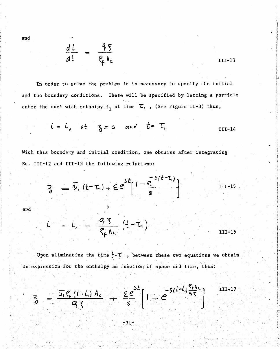
and

111-13

In order to solve the problem it is necessary to specify the initial

and the boundary conditions. These will be specified by letting a particle

enter the duct with enthalpy i1 at time iCe , (See Figure 11-3) thus,

• t

(., -= t... at 111-14

With this bounda~y and initial condition, on~ obtains after integrating

Eq. 111-12 a~d III-1~ the following relations:

111-15

and

L I

L, 111-16

Upon eliminating the time b-7, ' between these two equations we obtain

an expression for the enthalpy as function of space and time, thus:

U7 ~i (l- ~,) At '1~

+ ,51::[ ,-S(L-i.')~'-l f.e I-e .tI,.~,

S . ;

. 111-17

-31-

.'

d ~ I)

~ 'i !

[1 [I

11 )1 Ii d

II 0 tl

~ ..

~l t~ 'i t~

m '1 l' :j ~ j ;) :1 :"1 :1 d iI 'i H r '~I

;i ,

The first term on the right-hand side is the steady state term, whereas

the second one is the transient which accounts for the perturbation of the

inlet velocity.

111.4 The Time Lag and The Space Lag

In Section 11- 2 the time lag Lb

, was defined ,as the time required for

increasing the enthalpy of the fluid from the inlet value i l up to the

enthalpy at the transition point i2 (See Figure 11-3). Consider now a

fluid which enters the duct at time Ll and attains the enthalpy i2 at

time l:2; it follows then from Eq. III-16 that the time lag is given by:

-- 111-18

which, in view of Eq. 111-13 can be also expressed as:

t I

T~ 4 L.ll aLll III-19 --- ~ i 0,') -af- -~f~C.

It can be seen that for a given 'system and at a given pressure the time

lag depends only upon the enthalpy difference (i 2 - i l = A.i -a., \ ) and the

heat flux density.

We shall determine now the space lag. For a "two region" approximation.

Figure II-3 indicates that the "heavy "fluid region extends up to the transition

point where the bulk fluid enthalpy reaches the value of i 2• Inserting i2

in Eq~ 111-17 we obtain the following expression for the space lag:

~ef ~l11 A" 111-20

q\

-32-

'}

.~ ! ! !

I i I

J

For steady state operation E.= 0, whenc.e we obtain from Eq. 111-20

the steady state space lag ~, thus:

A 111-21

. Several comments are appropriate.

1) Equations 111-18 and 111-21 indicate that for steady state, i..e.,

when ~ = ° the time lag 1:b corresponds to the transit time.of a fluid

partic.1e through the "he\avyU.· fluid region.

2) Equation 111-22 shows that the response of the space lag to a

variation of the inlet velocity is delayed by a time period equal to the

time lag L.b

•

3) If we interpret the enthalpy i2 as the enthalpy at saturation and

therefore the difference ~ i21

by the subcoo1ing then Eq. 111-22 predicts

the locatio.n of. t~e boiling boundary, i.e., the location where boiling

starts in a two-phase mixture at subcri tical pressures. Indeed, such an

expression was derived previously (in [1+9,.50, 511 among others, usirrg

somewhat different approaches) for ana1yzipg oscillations in boiling mixtures.

-33-

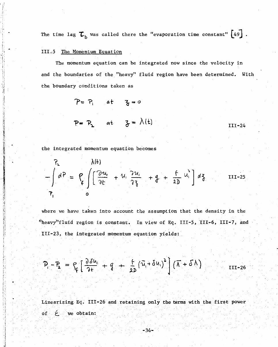
I :1 /

The time lag 'tb was called there the "evaporation time constant" [49]

:.'

i I , . 111.'5 The Momentum Equation

The momentum equation can be integrated now since the velocity in

and the boundaries of the "heavy" fluid region have been determined. With

the boundary conditions taken as

111-24

the integrated momentum equation becomes

f \] + } + iD lAl d~ 111-25

o

where we have taken into account the assumption that the density in the

r'heavy~tfluid region is constant. In view of Eq$ 111-5, 111-6, 111-7, and ,

111-23, the integrated momentum equation yields: i

I , ~

i

111-26 I I I r

·fii

Linearizing Eq. 111-26 and retaining only the terms with the first power

of we obtain:

-34-

- ,.

-+

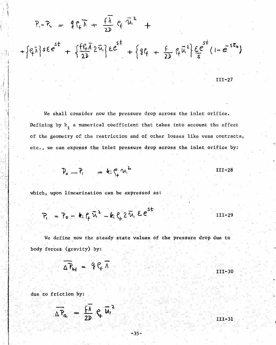
111-27

We shall consider now the pressure drop across the inlet orifice.

Defining by k. a. numerical coefficient that takes into account the effect ~

of the geometry of the restriction and of other losses like vena contracta,

etco, we can express the inlet pressure drop across the inlet orifice by:

111-28

whi~h, upon linearization can be expressed as:

1II-29

We define now the steady state values of the pressure drop due to

body forces (gravity) by:

III-3D

due to friction by:

-111-31

-35-

i ! ! ,i ~ I

i , I

and due to the inlet orifice by~

III-32

In view of these three relations and upon substituting Eqo III-29

in Eq. III-27, we call express the pressure drop in the "heavy" fluid

region by:

where

III-34

and

1II-35

The fir~t line on the right-hand 'side of Eq ~,' III-33 represents

the sum of the steady state pressure drops, whereas the second one accounts

for the transient responseo In particular, the first term is the inertia

of the "heavy" fluid region; the' second termare the pressur.e losses due to

variation of inlet velocity whereas the last term shows the effect of the

-3.6-

\

.~ i v , I

f I,

1 ' , '

varying space lag. Equation III-35 indicates that this last effect is

delayed by time lag Lb· We shall proceed now with the analysis of the 50

: ·i "light" fluid region.

-37-

f! .' ~.

•

IV The "Light" Fluid Region

IV.l The Governing Equation

For a "two region" approximation the "light" fluid region extends

from the transition point to the exit of the heated duct. The problem

is formulated again in terms of three field conservation equations and

of a constitutive equation of state. However, ·in contrast to the "heavy"

fluid the density in the "light" fluid region is function of enthalpy

and of pressure. It was discussed in Chapter II that for "chugging"

oscillations, the effects of pressure variations can be neglected.

Consequently, the density will be a function of enthalpy only.

The "light" fluid region is described, therefore, in terms of the

continuity equation

of the energy equation

the momentum equation

.-J- af +-

and the constitutive equation of state

-38-

- 0

f 2.D

IV-l

IV-2

IV-3

IV-4

or

IV-5

when expressed in terms of the spec ific volume 'iJ'"

Equations IV-I, 2, 3 and 4 are four equations in terms of four

variables 1', ~ ,'\A and i. They are applicable to the "light" fluid

region at supercritical pressures. They can be also applied to the

two phase flow region at subcritical pressures if, and only if, the

relative velocity between the phases can be neglected.

It is emphasized here that the form of the energy and the form of

the momentum equation, as given by Eq. IV-2 and Eq. IV-3, are correct

only if the relative velocity between the phases is either zero or its

~ffect is negligibly small. If such is not the case, then both Eq. IV-2,

and Eq. IV-3 !ID:!§t be modified.

It was discussed in Section 11-5 that at high pressures, say above

0.85 of the reduced pressures, the effect of the relative velocity is

so small that it can be neglected. The region of interest to this analysis

is the high pressure region. It can be expected, therefore, that, in

this investigation, both Eq. IV-2 and Eq. IV-3 can be used to approximate,

with sufficient accuracy, the energy and the momentum equation for the

two phase mixture in the nearcritical region.

In what follows we shall use, therefore, Eq. IV-I through 4 to des-

. cribe both the "light" fluid at sup~.rcriticalpressures and the two phase

-39-

..

j.

II :"( ~,} .( , , , ;~,.

j

1

, !

~/i 'i :/ • i

1 ., ; j i 1 \ i

mixture in the nearcritica1 region. The differentiation between the

"light" f1ui~ and the two phase mixture will be realized by assigning I

the appropriate expression to the constitutive equation of state. This

will be done in the section that follows.

IV.2 The Equation of State

For the "light" fluid the relation between the specific volume and

the enthalpy can be obtained either empirically, i.e., from experimental

data or it can be approximated by an equation of state such as the per~

fect gas or the van der Waals' equation etc. It was noted in Section 11.1

that for oxygen the perfect gas equation predicts with sufficient accur~cy

the relation between the specific .volume and the enthalpy. Sin.ce this

fluid is of primary'interest to this investigation, the perfect gas

equation will be used as the constitutive equation of state for the "light"

fluid at supercritica1 pressures.

Assuming a constant pressure process we have for a perfect gas the

following relations

aT IV-6

and

IV-7

whence

IV-8

}., \.'

For a "two-region" approximation the boundary condition for the "light'

fluid region is given by:

a.r IV-9

We obtain then the equation of state for the "light" fluid 'i'egion by

integrating Eq. IV-8 subject to the boundary condition given by ·Eq. IV-8,

thus:

IV-lO

J ~ We shall derive now the equation of state for the two phase mix-h :\ I ture in the nearcritical region. We recall first that the quality x, $ ~ R of a two phase mixture is defined by: # :1 1&

x -- IV-II

where Gg and Gf

are the mass flow rares of the vapor phase and of the

liquid phase respectively. We recall also that the specific volume

and the enthalpy of a two-phase mixture are given by:

'\r = (I-X)"\T't + X~ IV-12

and

, , , IV-13 l" (l-X)\'t ""1- X (,~ -

-41-

\

..

. ~

"

c·

}:

•

Where ~f~ if and V-g , ig are the specific volume and the enthalpy of

the liquid and of the vapor respectively.

We obtain then the equation of state for the two phase mixture by

eliminating the quality x, between Eqc IV-12 and Eq. IV-13, thus:

f\l(i) - 11+ + IV-14

Where 6 'V fg = '\)' g ~ Vf , and where ~ i fg is the latent heat of vapori-

zatiOD. Differentiating Eqc IV-14 we obtain for the two phase mixture:

IV-15

which can be compared to Eq. IV- 8 applicable to the "light" fluid at

supercritical pressures.

It is important to note that both, the equations of state for the

"light" fluid at supercritical pressures, Leo, Eq. IV-IO, and the equation

of state ~ a two-phase mixture at subcritical pressures, i.e., Eq. IV~14,

are of the same form, i.e., both can be expressed as:

IV-16

We can use, therefore, Eq. IV-16 for the equation of state in the near-

critical as well as in the supercritical region. We shall distinguish

one region from the other by substituting either Eq. IV-15 or Eq. IV-8

in Eq. IV-16.

-42-

J

\

,1 I

". I ~"I

,1

j

J

I I

t I j I

I j

I I I

I , !

I '\

IV.3 The Equation of Continuity and the Divergence of Velocity

Several methods are available [49, 50, 51, 62J for determining the

velocity in a boiling mixture. Any of these could be mod,ified and used

to determine the velocity in the "light" fluid region. In what follows

we shall use the method of Boure (511 .

As in the "heavy" fluid region we shall determine the velocity by

integrating the divergence. However, in contrast to the "heavy" fluid

region where the divergence is given by Eq. 111-5, the divergence in the

fV1ightH fluid region is not zero but is obtained from Eqo IV-1, thus:

IV-17

In order to integrate the divergence it 1s necessary to evaluate

the right-hand side of Eq. IV-17. Following Boure this can 'be done by

means of the energy equatio~.

Since the density is function of' enthalpy only one can write

cJ~ f'dL - --' -d t.i fO t IV-18

Substituting Eq. IV-2 in Eq. IV-l8, it follows that:

IV-f9 .

whence from Eq. IV-l9 and IV-l7 we can express the divergence as:

-43-.

'.",

"~ '\ l-I I

I .

•

~1 L l! ~; II 11

I , Ij d 11 h il 11

\1

•

It

fl l.1 !I II H

ti lj N ~J

" n ;1 " fl ji ,; II , ' ij

r. ~ H

11

1\ t; '{':

i I

•

IV-20

We shall define now the reaction frequency* Jl by: I

It follows then from Eq. IV-8 and Eq. IV-2l that the reaction frequency

for the ."ligh::" fluid in the supercritical region is given by:

IV-22

whereas it follows from ;Eq. IV-·15 aIld Eq. IV-2l that for boiling at sub~

critical pressures the reaction frequency is given by:

IV-23

With the reaction frequency defined by Eq. IV~2l, it follows then

fromEq. IV-20 that we can express the divergence as:

-Sl. IV-24

*The reasons for using this definition are discussed in Section IV-9

-44-

! ! 1

1 R

I

i I ,

The physical sig~ificance of this equation is simple: the divergence

of the velocity in the "light" fluid region is equal to the volumetric

rate of formation of the "light" fluid per unit volume of space.

In order to integrate Eq. IV-24 it is necessary to spe.cify the

boundary conditions; these are given by considering the velocity in the

'/, "heavylU fluid region, i.e.~ Eq. 111-7. The boundary condition for

I ',I ]

I I

Eq. IV-24 is therefore:

tv-- /\AI + cf 1,1'1

_ st '=. AA, 1" £ e

IV~25

'whence upon integration of Eq. IV-24~ we obtain for the velocity in the

IUlight H fluid region the following expression:

- Sr \( (~ltJ- = \.1\, '\- €. e -;a..n. [ \ - idt-) 1 IV-26

We note that Eq. IV-26 with JrL given by Eq. IV~23 is the velocity

in the two phase boiling mixture, as such it was used already in (49"SO,5land 62.)

It is instructive to examine further Eq. IV-26, which~, by' means of

Eq. III~23, can be expressed as~

IV-27

~

We obtain the. steady state velocity in the "light" fluid region by letting

E. = 0 in Eq. IV-27 fi thus:

-45-

'.

, ..

-IV-28

We can rewrite then Eq. IV-27 as:

-LAl~lt) ~ Uti') -t- cfLA~ tt) IV-29

where the time dependent perturbation of the "light" fluid is given by:

_ olA, - n d"

, ..

l It can be seen from Eq. IV-29 and IV-30 that the flow'in-the "light"

fluid region is affected by both the inlet perturbation as well as the

perturbation of the space lag. This last perturbation, is delayed by the

time lag 1:b (see Figure 11-4).

We shall define now several steady state relations which shall be

used in following chapters.

By letting z = t in Eq. IV-28 we obtain the steady state velocity

at the exit of the heated duct, ,thus:

.' -' - IV-31

'-46-

The lengthwise average velocity in the "light" fluid region is defined

by:

i-A

L -A f ~1\J~} o

whence from Eq. IV-28 we obtain:

tAl +

From Eq. IV-3l we have:

.n(l-7\) 2.

IV-32

IV-33

IV-34

Substituting this relation inEq. IV-33 we have the following expressions

for the average velocity:

1. IV-35 < IA,) _ - ..nIL-X) 'lA, +

The log mean velocity in the "light" fluid region is defined by:

1:: .n.( t-X)

IV-36

where we have taken into account Eq. IV-3l ...

"47-

J I

..

1 'f I

,lr, it 11

..

A fourth relation of interest to this inveGtigation can be obtained

from the conservation of momentum G~and the definition of the log mean

densityo If we denote by ~ 3' the density of the fluid at the exit from

the heated duct, then the log mean density in the "light" fluid region is

given by:

IV-37

The mean velocity, based on the log mean density, is then obtained by

considering the mass flux density, i.e., the momentum G, thus:

IV-38

which, in view of the preceding relations can be expressed also as:

- -c. -lA,

--\.t~

IV-39

We can proceed now with the solution or-the energy equation •

IV-4 The Energy Egu~tion .

We can solve the ~nergy equation now since the velocity and the equation

-

of state in the "light" fluid region are specified. By substituting Eq. IV-26 ~

-48-

J t ,

and IV-l6 in Eq. IV-2 we can express the energy equation as:

IV-40

~

Taking the enthalpy i2 at the transition point for reference and in view

of the definiti.on of the reaction frequency .J1. ,given by Eq. IV-2l,

we can rewrite Eqe IV-36 as:

IV-4l

The initial and boundary conditions for the energy equation are de-

termined by considering the conditions at the transition point (See Figure

II~3); they are given therefore by:

L- t~ - 0 Oft t =: 't'1-IV-42

-~t I • ~~ ~ '::! "(~Z::L)

_ sr~ (' -e b l- Ll- a - A -to- ee .s) -

IV-43

Equation IV-4l is again a linear partial differen"tial equation, it

can be solved therefore by the method used in solving the energy equation ~

for the "heavy" fluid (See Section 111-3). Following this procedure, we

obtain in place of Eq. III-II the follpwing set:

"49-

!, i , . ~

/ ......

clt

IV-44

whence:

and

IV-46

Integrating first Eqt IV-46 and taking into account the initial con-

ditions given byEq. IV-42 we obtain:

IV-47

whence:

IV-48

--50-

1 . \

i , ,

I . '1

I I

'I I ! \ , j I

j

I

1

I

I .{

!

I I I 1

In order to integrate Eq. IV-45 we note that it is of the form of:

. IV-49

,whose solution is:

.. ~ - ( P(~) ~ l>i) c.l J - C.o,",st. I

IV-50

where -fA ~'S -.!l t

e = e The integral of Eq. IV-45 is therefore:

(~-Jl.) t -stb . - . .n I: I \A; - .J -1l t f. e . (S -J\ +.Jl. e ) ~ e '. + - -" e - - C,

~ S-~ ~ IV-51

,.

which, in view of Eq. IV-48 , can be expressed as:

S-Jl. +Jl. e-SC,!,] = C

5CS-.n) I IV-52 ......

The value of the constant of integration is eva1uatedby means of Eq. IV-42

and IV-43, thus:

-S~] S -Jl-tJl..t! '.

S (.$-~) IV-53

-51-

,'''',' l' <,\

• r \

'. ,I ! :J .

. ~ , :"/.,

_ i ';

I ~,_t

!

; t ~i ;. ~ . -. , ...

; , ,:(-

..

Substituting Eq. IV-53 in Eq. IV-51 we obtain after some re-

arrangement: .

.S1. s-.n.

.s t: IV-54 -5 (t-'Z:2.) St( 1- e- 0) -5(t-rt) S~ -S'"C! }

e-Jl1:'1. ~ -I 1lA,+ .n..e E.e __ JL e 'Ee [J-Sl(,-e )J

s S-n ~

which, in view of Eq. 111-23 and Eq. IV-3v, can be expressed as

IV-55

By substituting Eq. IV-48 in Eq. IV-55 we obtain the solution of the

energy equation for the specified initial and boundary conditioqs, thus

I + J'\. ft At. ( L - L).) '==­

q~

- --s(t-'t\.)

+ e .nol\

from which we obtain the enthalpy. for the. "light" fluid region

... 52.-

IV-56

)~ . \i

~

I . i

I I 1

!.;

.J 'I ;1

-I •

L - (.,2.. s-.n. -I _ -s(t-r .. )

.IA, T e ...n SA JL. - S (t-tl,. ) -- e (f~1~ ~ ... .n

IV-'37

Expanding and retaining only the first power of ~ we obtain after some

rearrangement

'11 (~-A) lAl et- Ac.

I f we let the perturbation go to zero, i. e. , e = 0, we obtain from

Eq. IV-58 the enthalpy for steady state operat~on, thus

IV-59

IV-5 The Residence Time

It is of interest to evaluate now the steady state residence, i.e.,

the transit time of a particle in the heated duct. Denoting by i3 the

enthalpy at the e'xit and by 1:' 3 the time when a particle reaches this

enthalpy we obtain from Eq. IV-47 the residence time in the "light"

fluid region, thus:

-53-

i

,{ .,.~. .. '"

I 1 l 'l!i<O>

! i I 'j

I ,j

I

.. r -r,. - 3 ."

which, in view of Eq. IV-2l, can be expressed also as:

II>

Denoting by Q =~~t, the rate of energy transfer to the entire

IV-60

IV-6l

duct and by \Ar', the mass flow rate, we can express the total energy

balance in steady state as:

• IV-62

Substituting this relation in Eq. IV-6l and in view of Eq. 111-18 we

obtain the following expression for the residence time in the heated

duct:

IV-63

IV-6 The Density and the Density Perturbation

The density in the "light" fluid region is given by the equation of

-54-

J'

! j !

I .. , ! " !

j j

state, i.e., by Eq. IV-16, which, in view of the definition of the re-

action frequency Jl.., given by Eq. IV-2l, can be expressed also as:

IV-64

Since the enthalpy in the "light" fluid region is given by the

solution of the energy equation, i.e., by Eq. IV-56 we can express the

density as function of time or as function of time and space.

substituting Eq. IV-6+ in Eq. IV-47 we obtain:

whereas by

~l~il-J --e+

-Jl(+-"r2.) e

substituting Eq. IV-64 in Eq.

iX, ~,s(t-rl.) "

+e ..n~ 51.

s- n..

-- JL Vi, ("\) cf lA 1 --s- Jk

IV-56 we obtain:

_S(t-'C2.) e J' 14,

Thus by

IV-65

IV-66

which, by means of Eq. IV-30, 111-20 and 111-18, can be expressed also

as

e (~,t) e~

,n s -.J1..

- s ( t - '!' 2..) (' e VIAl

IV-67

-55-

or, in view of Eq. IV-65, it can be transformed in

~r~,t) - ~ l ~ ~:' t ) t!l. -e-S 1: b 614, (AI ,

$- .!L IV-68

e'r LA~l,) - St eftA" s- .n

Using again the binomial expansion and retaining only the first power

of ~ we can express Eq. IV-67 as:

u, +-­

S-jl

Similarly, we can expand Eq. IV-68 and express it as:

-U~ l"b I

n. +--s-..n..

where the steady state velocity fj,(~J is given by Eq. IV-28.

IV-69

IV-70

By letting l:.. = 0 in Eq. IV-66 we can obtain the local steady state

density in the "light" fluid region, thus:

,/' j j ,

We shall define now several steady state relations which will be

used in the following sections.

By letting ~ =.L in Eq. 'IV-7l we obtain the density at the exit

from the heated duct thus:

~(.l) - ~~ - IV-72

where we have taken into account Eq. IV-3l.

We shall define now the average density in the "light" fluid region ".

by:

IV-73

whence from Eq. IV-7l we obtain:

Jt (~- A) -lA, IV·,74

In view of the definition of the log mean velocity Ul~ given by Eq. IV-36

this average density can be expressed as:

-57-

I I '1'

!

I I E

i ~ I

~

t

I

, I ; !

, ,',' ) ,J

, , !

.. j

I 1

J i ! I

I '1

I

it

IV-75

We have already defined the log mean density by:

IV-76

where ~~ is given by Eq. IV-72.

A fourth expression can be obtcHned from the definition of the

average velocity (IA}/ given by Eq. IV-35 and the momentum Gr . We

can express therefore a mean density, based on the average velocity,

by:

G- 2G-

IV-77

With the steady state density ,in. the "light" fluid vapor given by -"

Eq. IV-7l, we can express Eq. IV-69 as

-+ IV-78

-58-

'I J J ~

!

I , .

where the density perturbation is given by

n G ~ DI,41 _S(f-LI)

~u, 1 ~ ~ (~,t) . e i \ - IV-79 r - -;

,5-j'l lA1(~J lA~ll\ tA, , t l , 1

i 'i ,

which, in view of Eq. IV-30, can be expressed also as:

fl. S-.n IV-80

I

'I

I -'I By letting ~ =.{ in Eq. IV-79 we obtain the density perturbation

at the exit from the heated duct, thus

I i ,

I IV-8l "

It can be seen from the preceeding equations that in the "light"

fluid region the density perturbation is affected by both the perturbation

of the inlet velocity and by the variation of the space lag. Further-

more, the effect of the inlet velocity perturbation is delayed by a .. "

delay time. Equations IV-3~ and IV-80 are the quantitative expressions

for the flow and density variations in the "light" fluid region whij:h

were qualitatively described in Section II~*.

-59-

With the density and the velocity in the "light" fluid region

given by the expressions derived in this section and in Section IV-3

respectively, we are in the position to integrate the momentum equation.

IV.7 The Momentum Equation

! In order to integrate the momentum equation it is necessary to

specify the boundary conditions, these are given by:

j

1

IV-82

whence the in.tegrated momentum equation becomes: i_ ...

r3 ,t

f JP [r~ ()~ +~~~ ~~ f + f ~~).~ ~~

~t- tD~ 2.'D IV-B3

'it ''It \

The expressions for the density and the velocity which should be

substituted in this equation are given by Eq. tV-7B and Eg. IV-27,

i.e., Eq. IV-29 respectively. We shall consider now each term of Eq.

IV-B3 separately.

IV.7.1 The Inertia Term

The inertia term in the momentum equation is given by:

L

[ A (t) IV-B4

-60-"

Substituting Eqo IV-78 and Eq. IV-27 in Eq. IV-84 and retaining only

the first power in £ we get:

IV-85

In view of the definition of the average density and of the velocity

perturbation given by Eq. IV-75 and Eq. IV-30, l-espec tively, the inertia

term can be expressed as:

~.

IV-86

IV.7.2 The Convective Acceleration Term

The convective acceleration term in Eq. IV-83 is given by:

t

r IV-87

substituting Eq. IV-78 and Eq. IV-27 in Eq. IV-87 and retaining only the

first power in ( we obtain upon integration:

-61-

1 i

1 , '; 'i

:.

,-

_ G-

sf. -STb G.- J1 ()- A \ _ G.n c e I--e

lA,

.51 S-fl

5

T

IV-88

It is of interest to examine the physical significaJ'!e of the various

terms.

If we let ~ = 0 in Eq. IV-8S, we obtain the steady state acceleration

pressure drop i.l PC! , which, in view of the definitions given in Sections

IV-3 and IV-6, can be expressed as:

G n (~ - t\ )

IV-89

The second term in Eq.IV-88 can be expressed by means of the

Eq. IV-89 and of the space lag variation defined by Eq. 1II-22, thus

-62-

. (:

I 'I; ;:.

-'

iI

IV-9D

It shows, therefore, the influence of the variatLon of the space lag on

the acceleration pressure drop in the "light" fluid region.

In view of Eq. IV-89 and Eq. IV-3D, the third term in Eq. IV-88

can be expressed as

St -rto!. ~ e S-ll-t..ll e

S - G ~ lA~,- Ci, ) c>lA, _ l1 r" 5 Lt~

~~~ ~(~

IV-9l

M g It expresses, therefore, the 'influence of the velocity perturbation in t1 ,·1

,~ the "light" fluid region on the acceleratIon pressure drop. fl t! The last two terms in Eq. IV-88 stem from the density perturbation H t! ~'l term in Eq. IV-7D, i.e., from :J ,:r , ·f .s

- -;-1

(' IAI ).n. ~~ {\)

IV-92

st ..J7L

= n \' G 11\'\ ~ l £. e S - n +..ft t ~-j"\. ,lAi S

-63-

...

•

( I i J

,I

r· .~ .

~ I 'j ; ~

1 i I ! l

..

The third term in Eq. IV-88, i.e., the first term on the right hand side

of Eq. IV-92 can be expressed in terms of Eq. IV-89 thus

~

S-.n..

-IV-93

It shows, therefore, the effect of the variation of the velocity in the

"light" fluid region on the density and, therefore, on the acceleration

pressure drop in that region.

The physical meaning of the last term on Eq. IV-88, i.e., Eq. IV-92

is not as clear as that of the other terms in Eq. IV-88. An insight can

be gained however, by conSidering the upper and lower limits of the

integral

(

Iit = ~~~~~ r f ( Altl

~~I~) '";)!, I11 JJ 'J~

It is shown in the Appendix C that this integral is bounded by:

--"",

-64-

IV-94

IV-95

j. I

·-.1 1 ! ,

j

'I

which, in view of Eq. IV-89, can be expressed as

- - s("r~- 1:, )

e 8\;4 a <.IJt·< 5-Jl .. -lA, IV-96

We note that a simple expression can be obtained by setting;' /IA,l'\) = ~ J ~ in Eq. IV-94, this approximation results in the following expression for

the integral 14:

T* -Lf

IV-97

S-J).. LAI

The physical meaning of the integral 14 is now clear: it expresses the

effect of the perturbation of the inlet velocity on the density (see

Eq. IV-69) and, therefore, on the acceleration pressure drop in the

"light" fluid region~ This effect is delayed by a delay time equal to

"!b or to ( !\ - "!, ) depending on whether we use this upper or lower

bound for the integral 14'

By substituting Eq. IV-89, IV-90, IV-9l, IV-93 in Eq. IV-88 and by

expressing the integral 14 in terms of the approximation given by , .

Eq. IV-97 we obtain for the acceleration pressure drop on the "light"

fluid region the following expression:

-65-

,'1 ! )

j: . i

If j Ii ; it . !, •

! ,. ,. /.

i - +

!L.

S-SL 5-JL

IV-98

~

where the steady state acceleration pressure drop d~ is given by

Eq. IV-89.

IV.7.3 The Gravitational Term

The gravitational term in the momentum equation is given by

k

f ~ \ k~ IV-99

~ It}

Substi.tuting Eq. IV-78 and retaining only the first order terms of

we obtain after integration:

IV-IvO

s T .-~

-66-

i ,

(

I = '1 F~ (~~Ll \ where

Altl

IV-IOI

The physical meaning of the various terms is as follows: ".

We obtaln the steady state gravitational pressure drop by letting • ~io' •• t

<C = tJ in Eq. IV-IOO) thus in view of the definitions given by

Eq. IV-36 and IV-75 we have.:

- ~(l-A)_G-.......... 1,4.(\110

IV-I02

The second term in Eq. 1V-I02 can be expressed by means of Eq.

1V-I02 and Eq. 111-22) thus

,

. ~l ( - oS Ti. .

1(/-") i

1- e ) ef-II'\ \A{~ ~ j ~et E e O'~ I

J

1 - - !

(J-A) IAh .. IA\ I

S I ~

I ,',' :;,.

! IV-I03 ~ ~ g

I ---- f ~P~I)

;

lA~..,.. 6" J

I ~ - ,

(1-A) lA, i 1I

1J

-67-. L I

! , I

, • ;1:1

{ i \-: l.r I ,-t! j: \ r 1i II i ~,! R

f ,1 11 II ~i

~ ]

It expresses, therefore, the effect of space lag variation on the .

gravitatLonal pressure drop •

The third term in Eq. IV-IOO can be expressed by means of Eq. IV-39,

IV-75 and IV-I03, thus

f4- CSt- -JT,-Jl- 1lJ- A) ~ ~ (~-A) (.! ..n- S-ll+.J\e cf~i -

14\ S-/'1... ..5 s-n \4) \.1, >lr~~?,"~~<"- ....

-A?b~ fL (~t IV-I04 -~ffl\ S-.n

·where the mean velocity ~~ is defined by Eq. IV-39. This term then

represents the effect of velocity perturbation in the "light" fluid

region on the density and therefore on the gravitational pressure drop

in. this region.

The physical meaning of the last term in Eq. IV-IOO can be ex-

plained again by expressing the integral 14 in Eq. IV-IOI by its upper

and-lower bounds (see Appendix C)

St S-.n

which in view of Eq. IV-39, IV-75 and IV-I03, can be expressed as

-68-

IV-I05

i1 l

oJ 'I 1

..---stb

A q>1t~ -S{t3--r..)

A ?Ia~ .n, e d~, ( IL; < J1 U(~ e SiA, --~-FL- V\M\ s-~ \AI \A.

IV-106

A simple expression for the integral 14 can be obtained by using the same

approximation 'which was used in deriving Eq. IV .. 97. Thus ll if we let

-IAI/tAa(~)-: ~I /ii:!; in Eq,~ IV-IOI we obtain after integration the following

appirOlximation ..... -5 ("t!-1:,) -~ ~e\- JYI, u:?, .itt

j1... e [~, -~-S\ .n. \AI

Ll ?b'd - s (~~--CI) IV .. 107 fl. ~~, - - e ~-n \)1

By comparing Eq. IV=107 with Eq. IV~106 it can be seen that 14* has a value

which falls petween the two bounds given by Eq~ IV-I06. The last term in

Eqo IV~lOO expresses therefore, the effect of the inlet velocity perturbation

cn one density (see Eq. IV-79) and on the gravitatiollal pressure drop in

the "light" fluid region. Furthermore, this effect is delayed by a time

de-lay equal to LA.. or"t} -7, depending on w'hether we use the upper or lower bound

for the integral 140

By substituting Eq. IV-102l! IV-103l! IV-I04 in Eq. IV-IOO and by

expressing the integral 14 in terms of the intermediate approximation

14* given by Eq. IV-107 we obtain for the gravi.tational pressure drop

in the "light" fluid region the following expression:

-69-

'I

..

r .' !

r

J, , "

jj H '1

1\

~ , ~

~ 'I

!i 11 f, li ,

-6. ?b~ b ?Io~ - ~ ?~~ IA~~ f~ L-A \A,

.n 6Pb~ ft.. ~fb~ _ s(r~ -1'1)

~t..4 e OIA\ "\ - IV-lOB S-n- IA~ ~-~ iA,

where the steady state gravitational presure drop is given by Eq.

IV-102.

IV.7.4 The Frictional Pressure Drop

The frictional term in the momentum equation is given by

l

I J~ "2.D IV-lOg

Aft)

Subs-cituting Eq. IV-7B and IV-27 in Eq. IV-lOg and retaining only the

first order terms in <t. we obtain after integration the following ex-

pression

f (I-A' >f -St'b

l Pt

lA, c. e ~-jH- Jl e IV-110 +- + 2» > , :

f(~-X) ~t- -j"rb I fl., e .. "U, fe S-I) -tJ,le TS': \

+ - r

1 S-IL 1.~ S

-70-

t

f ~ ,I i

I'

!1 ;:

j I

) .'

..

-,

IV-Ill

n. S-ft

The physical meaning of the various terms is as followsc

We obtain the steady state frictiorial pressure drop by letting

~ = D in Eq. IV-lID, thus in view of Eq. IV-35 we can write

11 ?23 = tl ~-A ) e, lA, [lA, + ll(:-A ) 1 l.,b

IV-112

f(~ -A) G- (\At) 21)

The second term in Eq. IV-lID can be expressed by means of Eq. IV-112

and Eqc 1II-22 thus:

-IV-113

It expresses therefore the effect of the space lag variation on-the

frictional pressure drop.

The third term in Eq. Iv-lID can be expressed in terms of Eq. IV-~O

.'

-71-

r il,

t '" i

i rr'i! , ,

f i'

I • h ~i ki R' 11 f, (, ~ : , 1; [, i\

M '.1 ~ !, d l'

:1 ti ,I H ;1 11

I1 , I !I

I to

~ tj

11 I l-i ! t II II fI

\1 I-t:

~ I' ,1 n ij N n Ii d H

H H 1! ;i \1

:1 --I l

'.

and Eq. IV-35 thus

-2 A~l3

IV-114

This term expresses therefore the effect of velocity perturbation in the

"lightli fluid region on the frictional pressure drop.

Similarly the fourth term in Eq. IV-lID can be expressed as

IV-115

In view of Eq. IV-79 this term shows the effect of the velocity

perturbation. in the "light" fluid region on the density perturbation and

therefore on the frictional pressure drop in this region.

The physical meaning of the last term in Eq. IV-lID can be explained

again by expressing the integral 15 in Eq. IV-Ill by its upper and lower

bound (see Appendix C) thus

-~c[~-r, ) IV-116

e dIAl < Is < ~ s-n

--72-

which in view of Eq. IV-lIS and IV-3S can be expressed as:

JL s-n ;)1

IV-117

A simple expression for the integral IS can be also obtained by using the

same approximation that was used in deriving Eq. IV-97 and Eq. IV-I07.

Thus, if we let V.1/IA~n) = L:\, I~!:> in Eq. IV-Ill we obtain after integration

Sl­

S-.llr ",

IV-lIB

The last term in Eq. IV-IIO expresses therefore the effect of the inlet

velocity perturbation on the density (see Eq. IV-79) and therefore on the

frictional pressure drop in. the "light" fluid region. Furthermore this

effect is delayed by a delay time equal to lb or (r,-r, ) depending on

whether we use the upper or lower bound for the integral.

By substituting Eq. IV-112, IV-113, IV-114, IV-lIS in Eq. IV-IIO and

expressing the integral IS in terms of the approximation given by

Eq. IV-118 we obtain for the frictional pressure drop in the "light"

fluid region the following expression:

-73-

•

,.

.1

•

•

+

-

n­s-n

U-X)

s -J'}...

-

-lA,

-where the steady state frictional pressure drop ~~11 is given by

Eq. IV-ll2o

IV.7.S The Exit Pressure Drop

IV-ll9

We can include the effect of the exit pressure drop in the momentum

equation. For this p~rpose we shall define by ~~ the coefficient for the

exit losses, then the exit pressure drop can be expressed as

IV-l20

By substituting Eq. IV-69 and Eq~ IV-27, both evaluated at ~ = i, and

by retaining only the first power in <t.. we obtain:

+ IV-l2l

n

-74-

\' i !

I I I . ~

I I

! t

We obtain the steady state exit pressure drop by letting ~ = 0

in Eq. IV-l2l thus

-=- IV-l22

Consequently Eq. IV-l2l can be expressed as

-+

IV-l23

- - ..

+ s- J1.. LA,

The second term in Eq. IV-l23 represents the effect of velocity

pertu.rbation in the "l,ight" fluid region on the exit pressure drop •

The last two terms in Eq. IV-l22 can be expressed as

IV-l24

-75-

1: /.

f

f · -iJ-:

~. :

1'1 i,

f'i ~,!

!

, , , i i

"j '.I :;1 ~ I

•

•

where we have taken into account Eq. IV-8l. Consequently the last two

terms express the effect of the density perturbation on the exit pressure

drop.

IV.7.6 The Integrated Momentum Equation

By adding Eq. IV-86, IV-98, IV-lOB, IV-119 and IV-123 we ob~ain the

integrated momentum equation for the light flui4 region thus

-~ 'r" -r ~ l'b~ -r!o 6 fl.!> --t- ~f~'1+

-+

-+ \ ~ ~ t:\ + II f b\ +

lAtM, IA~

n. ~A~' -~.~~ -r S-Sl U t T

~"WI lAM

IAI

-,

-~P2.~ '-

(.~~>

---.

Ar~!> <IA~)

-

-c._P~~ ~ +

1.43

-~P3" } +

[11

elL! ~

JU}

T

-

- .- ~} -.s(r3- L,) -:n\ .6 ~ '" ~Pr" ~ (2.3 -t-' ~ l~ e J \,\ \ + i-.- -lA, lA, ~, lit I .

-76-

IV-125

'1

~ I

! I

i

"

By adding the momentum equations for the "heavy" and "light" fluids

we shall obtain the momentum equation for the system whence the characteristic

equation for predicting the onset of unstable flow. This will be done

in the chapter that follows.

IV.8 Comp.arison With Previous Results

Before we proceed with the derivations of the characteristic

equation, it is of interest to compare the results derived in this chapter

with those reported previously in (49, 50, 51, 53, 55). In this section

: we shall make comparison with the results of (49, 50 and 51] whereas in

the section that follows we shall compare the present results to those

: of {53, 55] . . j

I I I j

I

n

I I I I

It was already discussed in Section 1.3 that the assumptions made

in the present analysis as well as the general formulation of the problem

are the same as those reported previously the Wallis and Heasley {50] and

Boure (5LJ for boiling, two phase system. It was also noted in Section

1.3 that the present analysis differs from those reported in (49, 50 and

511 in the following respect: 1) the constitutive equation of state is.

different and 2) the characteristic equation is different.

The analyses of {49, 50 and 511 were derived for boiling sy~tems,

j the present investigation is applicab1.e to bo.th subcritical and supe.r-

critical pressures. It is emphasized here again that neither this in-

vestigation nor those reported in (49, 50 and 511 take into account the

effect of relative velocity between the two phases in the boiling region

at subcritical pressure.* If the effects of the relat~ve velocity are

*The conditions under which the effects of relative velocity can be neglected are discussed in more detail in (55J.

-77-

-...

.~

I

to be taken into account then the momentum and the energy equation, i.e.,

Eq. IV-2 and IV-3 must b,,~ modified o Furthermore, a diffusion equation

should be added to the field equations ~escribing the process. An in-

vestigation along these lines will be reported separately.

If, in the b:oiling region, we express the reaction frequency.ll by

means of Eq. IV-23, then the density given by Eq. IV-6,5 becomes identical

to that derived first in (491 and to those in (50, 51, 55) using different

approaches. We shall examine now Eq. IV-66 which can be expressed also

as ~

- -5(t~L&.) -Sr~ e (~,t) lA, J1- ~(~It) ~ Jt. e e c5U, __ oo''''!,", - _.- -t -el- tA1 (~) S-Jl et- lA,I~J S-.l'l ~I1J

IV-126

whence, in view of Eq. IV-65, and IV-3D, the perturbation can be written \

as:

-s -Co)' By adding and subtracting e oS

~~

~\(~It) = te u~l~)

we can express this relation as

- ~ 't ~ -(S-.J1)( t-- t"1,) } e ( \ ._ e ) IV -12 8

S-Jl

If we replace now n by Eq. IV-23, then Eqo IV-128 becomes identical

-78-

*-

.it,

to Eq~ 38 in the paper by Wallis and Healsey (50) derived using a different

approach~

We can insert Eq~ IV-65 in Eq~ IV-l26 and express the latter as

~ (~d) -

et- IV-l29

if the density terms which appear on the right hand side of Eq. IV-129

8.lr'e .a.pproximated by the stea.dy state relation, i.e .. jI by

~,

IV-130

as was done in (51) we obtain

~, .. ,

~ (,Ii) s!- [ -s to f - ,1-- ~ r,. . _ 2. ;. \ }

. - LA, e lA I .:Sl te· Jl. S- Jl +..Ile VI'_ S -Il. (-t; 1 (\) ) IV -131 ft-

-t (A. 5 (S-.Il.) M111J lA11bl

which is equivalent to Eq .. 5, Appendix A of Bourevs report (51).

Apart from the difference in the equations of state used in this

analysis, the difference betw,:een the present results and those of (50 ~ 51)

is in the handling the momentum equatione In (50) the momentum equation

was n2! integrated along the duct;, it was first integrated by Bour~ (51) 0

Indeed~ it can be shown!> that after some rearrangement, Eq. IV .. 88, IV-IOO and ...

• IV-ltO can be put in the form of those given in (51). In (51) the integration

of the momentum equa.tion lead to a characteristic equation in ,the form of an

exponential polynomial of the fourth (or higher) order~

-79-

I .~

..

In the present analysis we have introduced various definitions for

the mean, for the average and for the log mean density as well as for the vel=

OlcitielEl in the "light" fluid region which enabled us to give physical

interpretation to the various terms in the integrated momentum equation.

It will be seen in what follows that these relation~ together with the

approximation used in deriving Eq. IV-97, IV-107 and IV-118)result in a

characteristic equation given by an exponential polynomial of the third

order. It will be seen also in what follows that these results will

enable us to derive stability criteria and stability maps which,

previously, were ~ available in the literature.

IV.9 The Density Propagation Equation

It is of interest to note an alternate way for determining the density

perturbation.

If we substitute Eq. IV-2l in Eq. IV-19 we obtain:

+ IV-132

This equation was called the energy equation in (51) where it was first

derived. Several remarks are relevant here.

We note first that Eq. IV-132 predicts the propagation of the

density caused by the source term SL. A "void propagation equation"

was formulated in (53 and 55) in terms of.kinematic waves which predicts

the pr0pagation of density perturbations through a two-phase system.

-80-

I

I 1

1

I I i I

i l I r i

I

'iJ

This void propagation equation takes into account the effect of the

relative velocity between the two phase as well as the effect of the

non-uniform velocity and concentration profiles in the two phase mixture.

It can be easily shown that if these effects are neglected the void

propagation equation can be reduced to Eq. IV-132.

We note also that Eq. IV-132 is of the same form as the continuity

for a given species in a multicomponent, chemical reaction system. In

chemical kinetics the source term in Eq. IV-132 is referred to as the

reaction frequency. It is for this reason that in (53, 55J the term

was called the "characteristic frequency."

Finally, we note that Eq. IV-132 is a first order partial differential

equation which can be solved by the standard method used in Sections 111-3

and IV-4. Indeed following this procedure, used already in [53 and 55),

one can derive Eq. IV-66 and Eq. IV-68.

-81-

V. The Characteristic Equation

V.la !he Momentum Equation for the System

The momentum for the "heavy" fluid is given by Eq. 111-33, whereas

that. for the "light" fluid is given by Eq. 1V-125. By adding these two

equations, we obtain the momentum equation for the system.

We note that if the downstream pressure P4' is constant we can ex-

press the overall pressure drop, i.e., the external pressure drop of the ~ .. "

system as a ~teady state term and a pressure perturbation caused by the

fnlet flow. Thus

-i, 1'0 - itt V-I

where the aecond term on th~ right hand side is determined by the pump

characteristics and has a negative value.

By adding Eq. 111-33, Eq. 1V-125 and Eq. V-I we obtain the integrated

momentum,equation for the heated duct, thus

- - - - --/j PC\ + b.l1L + .d ~bf + A?~ -\- ~ Pb~ + C1 r1-} -r IJ rl'f '-r

V-2 1 I

-r\ etA} I cl ofA, {<e,.) ( i-A" ) 1 d 0" I,.} ,J -..: '\ '-\- -+

1

I I

:1 de- tAb 1

I , !

I !

....., ---, I I T\ ~6r'l V 6~'l. ~ llf~ 1 OlA, D ~ • I ij

I + +-'V ~I «) 'lo1 , rv~, f

if • I fI " " l' .I ......... ......, ---.

~ ;

+~ ~t~ 2l\f· 3 :2 ~r~\, f rLt~ " ) 11 + + " T 1, }!

fAt.., , l,i~) -11 lit,. JI

l II ·-82-.1 ~

I p

I

, ft!

" ,i ,'j:1

\ , "J

~!

i , \ -

I '1

,I '" i " ... , t

,

'\'."11

"

- --~

~ -~f" ~ f"*t A fl.} ~ p~~ ~ J lA1

fL t + + -r- - -S-Jl 1At~ 1Il~ ~ lA, '> IA~

--I\A , -+-+

-- o

We obtain the stead~ state pressure drop for the system by letting

the pertutbat"iGRS :~go '"to ,·-zero, thus

---, - - -_ d fo. + ~ ~l + .6r" + Af" -t- Afl.a + 6 fz.~ + i ~\'f

-V-3

By subtracting Eq. V-3 from Eq. V-2 we obtain the perturbed form of

the momentum equation, thus

-83-

I I f' 1

I I

I i! ~! ,

it ,f ,

li I,

L [

+~

11. + .s-j"L

-

-

-

-

+

+

+

-0

+

-V-4

-

-ti,

The formulation is now essentially complete because Eq. V-4 is the

expression which gives the response of the system to the initial flow

pertubation as function of the influence coefficients defined below.

The influence coefficients F 1 and F2 represent the mass of the "heavy"

fluid and of the "light" fluid respectively, thus

V-5

and

V-6

-84- i I

r 1

I

· i 1 ,

\ ~ 11 t ~

; I ,I

The coefficient F3 describes the effect of the inlet flow variation

on the pressure drops in the "heavy" fluid region, thus

- --~-

V-'l

f, This coefficient, which is well known from studies of the transient t f~ ':

~ response of single phase flow systems, has always a positive value. ,- ,

The coefficient F4 shows the effect of the velocity perturbation in

the "light" fluid region on the pressure drops in that region, thus

V-8 + + -1,13

It is of considerable importance to note that each pressure drop i8

differentiated and is ';.]eighed therefore by a different velocity. This

important result is a consequence of the integration of the momentum

equation, i.e., of the distributed parameter analysis. W!i2! note that in

the "lumped" parameter analysis the three pressure drops in Eq. V-8 would

have been divided by:the same velocity, say by the velocity u) at the

exit from the test section as is most often the case for analyses reported

in the literature.

The influence coefficien~F5 and F6 are given by

-85-

-

"

"

I

I

~ • I

,

" . j I, I I) I

/II

. ,

,- --V-9

and

-- -rlo

.Df~ ~f~~ aP1.l l1 R\{ - "i- T -t-tAl (,.(, lA, lAt V-10

It can be seen from Eq. IV-69 and Eq.V~2 that these two coefficients account

for the effect of the density perturbation on the various pressure drops in

\ the ftllight!! fluid region. Note!) that the density perturbation depends on both

Two observations are noteworthy. First, the coefficient FS

shows that the effects of the velocity perturbation on the "light" fluid

region,~' are weighed. by various velocities • This, again, is a consequence of

'·the distributed parameter approach. Two, the exponential which multiplies

the coefficient F6 indicates that the effects of the inlet perturbation are

delayed by the delay time -Z:~-t:t •

Finally the coefficient F7

, defined by

---. ',' I' i 0 6~1t A~

~ - V'!"ll ...n.. 0 (I-A) nl~-A)

shows the effect,of the space lag perturbation on the acceleration pressure

drop in the H1ight"fluid region. It is important to notice here that in

Eq. 111=33 and Eq. IV~l25 all other tenns-which arediffet"entiated with

respect to the length cancel each other in the momentum equation for

!r -86-

. -

~ , ,

the system. This result could not have been anticipated in a "lumped""

parameter analysis. Indeed, in several studies of boiling systems using the

"lumped" parameter approach these terms were introduced and retained in

the analysis. In view of the foregoing) the results and conclusions based

I; \\ on such formulations can be considered as spurious. :,; Ii I) By introducing Eq. V-5 through V-II in Eq. V-4 the perturbed momentum

I I ij

l I I ! I d

I l

I i J I I 1

I :l

I I I !

,equation for the heated duct can be expressed by

V-12

-r .5- J'1,.

Before deriving the characteristic equation it will be instructive

to express the perturbations in Eq. V-12 in terms of the perturbations of

the inlet flow and of the space lag. Taking into account Eq. IV-30 we can

express Eq. V~12 as

V-13

o

It can be clearly seen from Eq. V-13 that the dynamic response of the

heated channel depends upon both the inlet flow perturbation and the

;..87-

......

I i'

variation of the space lag. This latter effect is an example of a

fluctuation which occurs inside the system. It was discussed in Sections

11-4 and 11-7 that such fluctuation have a destabilizing effect. The

destabilizing effect which the space lag variation has in combustion

systems and in boiling systems has been already demonstrated in (48, 52)

and (50, 51) among others. Equation V-4 shows that,'at supercritical

pressures, the space lag variation has a similarly d~stabilizing effect.

-Furthermore, the negative sign in the third term on the left hand side of

Eq. V-13 shows the destabilizing effect of the inlet velocity perturbation,

We have noted already that this effect stems from the density perturbation

in the "light" fluid region,

V.2 The Characteristic Equation

In view of the definitions of the inlet velocity perturbation and'of

the space lag perturbation given by Eq. 111-7 and Eq. IV-3~ respectively,

we can express Eq. V-13 as

s-.n. F. s

+

-s (7.~--r,) _.1/.... __ fi e ~- .n...

V-14 -SZ

F.+~).n('-; )}=o

From this relation we obtain the characteristic equation by noting that

since E:. '* 0 the sum of the terms within the bracket must be equal to

zero. Thus, after multiplying by (S-.n..) and after some, rearrangement we

-88-

-

" , "

T,

I, ~ ,

obtain the characteristic equation for the heated duct:

_ sl'J-r:,) -5 -a- { F,..,. Fla] + j [ Fi + ~ - .n.. ( F, 't fl.o ) ] - ..!l [ F 3 f F4 - Fs ] -.fL Ii ~

V-IS

- n( }- :-5rl) f s""" F". + s r ftt -t F'7 -...!l F~ J - .!l [F., + ~ - F=. J } -=- 0

It can be seen that the characteristic equation is a third order polynomial

with two time delays. From the definitions of the influence coefficients

we have the following relations for the various terms which appear in

Eq. V-IS.

R -t F1... =- Nf-t H'J, - ef- 7\ T < e,') (1-1:) V-16

- - -I)-t~

2~fol l.~f,L i'" r~ t.f~ I .0 PI\. 2Afz3 2..6 ~~ - t +- + +- V-17 W a- ~1It, /A( "wi (~1) -tA3

- -- -Fs-

~f4, + Df .. " /:) G'l} ~~~~

-t + V-18 tA~ , lA~-- (\A~) Ci')

--. - ---. -F~ i"F'1-FS-

2~fo, ~

24((',l. \'Jt.f~ I b.f. l ~f~~ ~~l~ V:-19 - + 'T + LA, ~ to !AI <lA~) -IA~ 1-13 .'

--- "-

F\f1 F7 hf~ ·l·~~~l.J l';')11 ;6 f'1

-t- i- +-IA I""" < LA~> - ft{ I-~) !Ill

V-20

V-21 .

----- ---. -f~-tF7 -fs - A 4'" +

~f~, a.fbl1 ~(J'J It

< "'~) "r .nIL-A) IA~ -1113 V-22

---, -Ii Ilf~

+ ~f~~ ~f'"l J a {jj, ~

- - + T Ci, lAl l-t7 -LfI,

-89-

..

J

1,1

H tl 'j L

tl 1,1

M 11 11 ,j

~ ·li H )1

H 11 jl '1 ' h q

II 'l I)

tl il U

~ n

I I, I

I

..

•

It was discussed in Section 11-6 that the characteristic equation

predicts the value of-S as function of the pressure terms given by Eq.

I

V-16 through V-22. In general s is a complex number S = Ct-tl.4) , the real

part gives the amplification coefficient of the partlcular oscillation

mode, whereas the imaginary part represents the angular frequency GJ

Since the original perturbation of the inlet velocity was assumed to be !)t"

of the form alA,: r. e J a given oscillating mode will be stable, metastable

or unstable depending on whether the real part of S is less, equal or larger

than zero, i. e ., whether ct.. (0, ~;O or _0) 0 .

A general study of the flow behaviour entails an investigation of

conditions leading to aperiodic as well as to periodic phenomena. The

first pertains to the possibility of flow excursion whereas the second

pertains to the onset of flow oscillations 0 Following the standard pro-

cedure we shall study aperiodic phenomena by considering the case of

S = a withGu = 0. Again, following the standard procedure we shall study

periodic phenomena by setting s=ic.v (a = 0, w#o ) in the characteristic"

equation. Such an approach will enable us to determine the stability

boundary which defines regions of stable and of oscillating behaviour in

a stability map. In the study of the oscill~tory phenomena we shall con-

sider separately the case of high subcooling and the case of low subcooling.

The stability problem at intermediate subcoolings will be considered in a

separate· report.

-90-

j

I I

VI. Excursive Instability

VI.l Derivation of the Stability Criterion

The study of excursive, i.e .. , of aperiodic instabilities is con-

ducted by considering the exponent S of the velocity perturbation to be

real, i.e., by letting the angular frequency ~ of the disturbance be zero.

It follows then from Eq. V-lS that for small values of S , we have the

following relation:

Vl-l

whence after rearrangement:

Vl-2

which is o·f the form

~ n'W SA;-u=O Vl-3

-91-

... ,1. ,

~

Equation VI-2 predicts the value of the exponent S in terms of the

influence coefficientse Since the inlet velocity perturbation is of the .st"'

form of J~ = te.. , and since the coefficient A'k is positive and exponent

S is real, Equation VI-3 indicates that the flow will be stable, i.e.,

the disturbance will decrease with time if B* is positive, thus from

Equation VI-2

VI-4

If B is negative then Equation VI-3 indicates that s will be real

and positive, consequently any flow disturbance will be amplified

with time resulting in flow excursions. Substituting the definitions

for the influence coefficients given by Equation V-5 through Equation

V-II we can express Equation VI-4 in terms of steady state pressure

drops, thus - -'- -Z..6fol

2~'Y,). -t-/ d de'l + \ II 'i>., .. ~ ~?b~ :I)y i (I-.n. r.J 1--- 4- ;-Ci, tA, lOlA, t... Vt~) V1''r101 IA;!>

VI-5 ---. - --. -

-+-L)?4.. .61b 'J . +- ill..} ~?3'f JrA

Jl L£. ~ 0 _. +- +-1-1, i:\, [AI ~I Jt( i-A) I

1 This inequality can be cast in a compact form by means of the

identities listed below:

-92-

•

•

Vl-6

These relations can be easily derived from the definitions of the steady

state pressure drops.

-93-

I~ I

Substituting Eq. VI-6 through VI-12 in Eq. VI-5 we obtain the stability

criterion:

-VI-13

li Ii ;! which can be expressed also in terms of the total mass 'flow rate W, thus il h fl

~1

i

I -

VI-14

For boiling systems, this simple criterion was first derived by

Ledinegg (24) using a different approach, it was analyzed further in

{25 through 47] and t51J. The results of this analysis show that this

"Ledinegg instability" can occur also at supercritical pressures.. The

significance of the stability crite~ion given by Eq. VI-14·, can be best

analyzed by considering the steady etate 1.1?-vr relation fpr the he'ated

ducto This will be done in the section that follows.

VI.2 Significance of the Stability Criterion

If, for simplicity, we neglect the effect of the gravitational force

and if we express the steady state pressure drops in the heated. ci.uct in ;

terms of the total mass flow W, and of the total heat .input a ,we have

the following relations:

-- VI-15

·-94-

11.:1' ,. l

11 ,~

~. I

i ,j Ii

r

VI-16

, VI-17

_W-(~_Q At.. rJi p AI..

ffl-it) /'[-\.A- ~I l'

l.t> VI-18

-l\f~~ = .K~{'~LAl2. = -ke Go';; = k~ ~ r U; -t-.n.(~-A>J = Vl-19

At . .

-The total pressure drop for the heated duct is ohtained by adding

Eq. VI-IS through VI-19, thus

VI-20

where the coefficients a, band c are given by

VI-21

.. 95-

-...;

I

.~ ...

'\

;J p ,~

I 3 , ,

I

I 1

!

I I I J i I j J j ,

i I !

~ ~ j

I I ~ 11 j

boX- f.t ~ (~)/1i~\ (I +fn - I (, - ~j») - 2 l),\ \.. - '+ f~ + e{-VI-22

~e '2.D I

[ (dV- ) , *J1 T f-1 fii P A Ll.l -

\.

c...'i(- ~~

~ 2,D 4tc~ ~ (_~) + VI-23 - +-

2DA'\- t~ L. ~.{ r1 i if>

It should be noted that Eq. VI-20 is applicable to subcritical as

well as to supercritical pressures. By assigning the proper expression

to' (r).tr/r)i ), which we obtaiD: from the equation of state, we can

differentiate the process of boiling at subcritical pressures from the

process of heat transfer at supercritical pressures. Thus, for boiling

at subcritical pressures we have from Eq. IV~15

VI-24

whereas at supercritical pressures we obtain from Eq. IV-8

Vl-25

When Eq. VI-24 is substituted in Eq. Vl-2l, Vl-22 and Vl-2.3, then Eq. VI-20

becomes the pressure drop relation first derivecl and discussed by

Schnackenberg (25) and Ledinegg (24) for boiling systems. For super-

critical pressures Eq. Vl-20 was derived by: the writer(63) (see also

Appendix B)"

-96-

...

"

.:. i ~

. i\ ~1 ~. \ ,-" .

•

It can be seen from Eq. Vl-20 that whether in boiling at subcritical

pressures or in heating at supercritical pressures the steady state

press'ure drop in the heated duct has the same cubic dependence upon the

total mass flow rate. This important conclusion from analysis is indeed

supported by the experimental data reported by Krasiakova and Glusker (18)

for water in forced flow through a circular heated duct. Figure VI-I,

which is reproduced from (18), shows that in boiling at subcritical

pressures (P = 140 bars) as well as in heating at supercritical pressures

(P = 226 bars) the pressure drop in the heated duct has the same cubic

dependence upon the mass flow rate. It could be anticipated therefore that

the system will have similar dynamic characteristics at these two pressure

levels. This is indeed the case as it will be shown later.

The significance of the stability criterion given by Eq. Vl- ,.4 can be

best analyzed by plotting Eq. Vl-20 together with the pump characteristic

on the same graph. Figure Vl-2 shows such a plot together with three 1..:'t .• ~.:~.N.:..t .

possible flow delivery characteristics, i.e., 1) constant pressure drop

delivery system, 2) constant flow rate delivery system and 3) delivery

system specified by the pump characteristics o The intersection of the

pressure drop for the heated duct with the pressure drop curve of the

delivery system determines the operating point of the system. The

stability .criterion given by Eq., Vl-14 indic'ates that for some of these

operating points the system may be unstable with respect to some small

flow perturbations. In order to show this we shall consider each flow

delivery system separatelYe

-97-

_.,,_ " ____ ._ ... _._~_ ... (.~>-~~' .. :~:'=~=t';;. .. "!4":;~-:::::,::;::::,;':::::;'...:.."":l;:t:::.:~§:r..:i~*'..:~=t-~~;;;;..;;;~~~~ .. ~7!::r.::;""t:t1'~~~

rt')

8 o X

40· •.

P = 140 bar

301 "

xxxxx

q=58 kw/m2

.,

P=226bar

JXXXX '= 201 I§ t---------+----------:~xxxxx·-----t

........... Z .. a.. <J

00

.. .... \ \

\ I 2 '-'q = 35 kw/m

500 1000

(0)

1500 0 500 Gt kg/m2 hr

xx xx

/ xxxxxx

1000

(b)

FIGURE Jl[-I HYDRAULIC CHARACTERISTICS OF WATER FLOWING THROUGH A HEATED CIRCULAR DUCT AT SUBCRITICAL AND AT SUPERCRITICAL PRESSURES (DATA OF KRASIAKOVA AND OF GLUSKER)

1500

_"""_~':'::::: .... :":-"'_~:~' """"",""",=-,~"""·_l'"·>-="·''''''·''V·"·'''''''-___ ;·''''f'''''· __ 7''''-__ ~'''''''''-~·'''''''''''''''''''':.;::00><'. ..-... --.~~,.,...-~"~--'-~=" ~-..... ~;~_~r='" , ~.,.~~~,.;:: ~:·'~::-;'~=-T:,,::.·";T._7 --:J:r"".""Ljc;.~':~1~.-.".:;:~-;;:;~t-==~'Z"'=-."=·~-,,,·~,

.j

. I I ~

I

-

I ALL VAPOR - ....,

I , , , -- --. I --..

Q. -------o a:: o L&J a:: => en V) L&J a:: CL

I..--CONSTANT FLOW DELIVERY SYSTEM

. .

Q = CONSTANT

MASS FLOW RATE w, grams/sec

All LIQUID

CONSTANT IlP SYSTEM

FIGURE lZI-2 EXCURSIVE FLOW INSTABJLITY

1

I I 1 l i

I j

1

V1.2.1 Constant Pressure Drop Supply System

The operating point for a constant pressure drop delivery system are

indicated by points 1, 2 and 3 in Figure Vl-2. The stability criterion

given by Eq. V1-1~ indicates that operation at points 1 and 3 will be

stable whereas that at point 2 will be unstable. For example, if a points

1 and 3 the flow is slightly increased the pressure drop of the heated

duct increases, i.e.: the "demal'l:d" curve of the system increases above the

"supply" curve of the del:h;8ry, con.sequent1y the flow will return to its

original value. Similarly) if at points land 3 the flow is decreased

the pressure drop of the delivery will-be above that required by the ..

heated duct resulting in an increased flow and return to the original

operating point. However, the operation at point 2 will be unstable with

respect to either a flow increase or a flow decrease. If the flow is

slightly increased at point 2 the external system supplies more pressure

drop than that required to maintain the flow. Consequently the flow rate

will increase until the new operating point is reached. Similarly, if the

flow is decreased at point 2 more pressure drop is required to maintain

the flow than is being supplied by the delivery system. Consequently

the flow will decrease until the new operating point 3 is r~ached.

The preceeding considerations can be expressed in a mathematical form

by noting that for a constant pressure drop delivery system Eq. Vl-20

reduces t.o

'- Vl-26

,:,,98-.

which in view of Eq. Vl-20 becomes

-- 1. d ~tl:P 3C: (,if' - 2 t:W-- r- Vl-27

• -+ C. Q >0 aw- Q

It can be seen from Eq. Vl-26 that flow stability requires an in-

creasing pressure drop with flow rate. This is indeed the characteristic

of most flow systems. However, the negative term in Eq. Vl-27 indicates

that for boiling systems as well as for systems at supercritical pressures

the pressure drop may decreas~ with flow rate resulting in flO\\1 excursion.

Instead of the stability criterion given by Eq. Vl-26 one can introduce

the coefficient of stabil~ S, apparently first proposed by Schnackenberg (25J

.,- and defined by

-$ Vl-28

which in view of Eq. Vl-20 and Vl-27 can be expressed as

Vl-29 ,

\-Q

LV +

where the coefficients a, band c are given by Eq. Vl-2l, Vl-22 and Vl-23.

As observed by Schneckenberg (25) the stability coefficient S, defined

by Eq. Vl-28,represents the per cent change in the pressure drop by a 1%

-99-

variation. in the mass flow rate. It can be seen from Eq. VI-28 and VI-26 that

fGr stable flow S must be positive, thus

$1 > 0 VI-30

VI.2.2 Constant F'low Deliver.y Sys tem

The operating point for a constant flow delivery system is given by the

in.tersection of the pressure supply with pressure demand curves o It can be

seen from Figure VI",,2 that for such a system

VI-3l

'whence Eq" Vlr>14 indi.cates that for such a system p.o flow excursions are possible.

VI.2.3 Deli~ry Specified by Pump Characteristics

The operating poin.ts for a system whose flow delivery is specified by

the characteristics of the pump are shown as points 4, 5 and 6 on Figure VI-2.

Using eX8.ctly the same arguments as those used in discussing a constant pressure

drop de,livery system:! it can be shown that the operating points 4 and 6 are

sta.ble whereas operating point 5 is unstable with respect to small flow

-di.sturba.nces •. A.tthis latter point any flow perturbation will cause a flow i 1 . ! excursion to either point 4 or to point 6.

""100-

i i.i

I u

~ i ~ I ~

I \

I

VLe3 The Effects of Various Parameters and the Methods for Improving Flow Stability

The effects which various pa.rameters ha.ve on the propensity for flow

excursions can be evaluated by examing Eq. Vl-14, Vl-21, Vl-22, Vl-23 and

Eq. Vl-27. It can be seen that the variation of any parameter which tends

to increase the value of the coefficient b given by Eq. Vl-22 will have a

destabilizing effect. Consequently, increasing the value of the exit pressure

drop coefficient ~e is destabilizing whereas the flow can be stabilized

by a high inlet pressure drop, i.e., by appropriate orificing~ In view

of Eq. Vl-24 and Vl-25 it can be also seen that increasing the system

pressure will have stabilizing effect whereas a decrease in system pressure

has the opposite effect. Furthermore, the flow can be also stabilized by

changing the pump characteristics a

Before closing the discussion of excursive instabilities it will he

instructive to illustrate the destabilizing effect of the compressibility

of the fluid in the heated duct. It was discussed in Section 1.3 that the

instability mechanism which is analyzed in tqis paper is based on the

effects of time lag and of density variations in the heated duct.

For simplicity we shall consider only the effect of the frictional

I

pressure drop in a system with zero inlet subcoo1ing, i.e., with AL-.1=o

For sucli a system Eq. 111-20 shows that the space lag is also zero. The ,

frictLona1 pressure drop is given by

Vl-32 2"D

where the mean specific volume ~~in the heated duct is obtained from

Eq. IV-77, thus

\

e~ Vl-33

-101-

If We insert in Eq. Vl-32 the expression for the average velocity <lA~) given

" . - · 1 by Eq. IV-35 and since the space lag is zero, we can express the mean

specific volume 'V"'-.. as

V1-34

or in view of Eq. IV-21 as

f"1J f- + V1-35

whence

('~) tAt 'P

I

Q - V1-36

Since Eg.' V1-32 and Eq. V1-35 show that both 6f and '\T~ qre . '.

functions .of W we can express the stability coefficient defined by

Eq. V1-28 as

2 -t V1-37

whence from Eq. V1-36 we have

I

1- L (t)~~ ~~ V1-38

-102-

is given by Eq. IV-15 or Eq. IV-8 depending on whether

we are interested in the subcritical or in the supercritical region.

It can be seen from Eq. VI-37 and Eq. VI-30 that for a system where

the me~n specific volume does not depend on the mass flow rate the flow

will be stable. For such incompressible flow system the coeffi.cient of

stability S has a value equal to 2. This is also the maximum value of S

because when the fricition factor f in Eq. VI-32 is a function of the

Reynolds number then Eq. VI-28 shows that S will have a value less than

two. For example) for laminar flow it will have a value equal to unity.

For a boiling system at subcritical pressures or for a process of . .

heating at supercritical pressures Eq. 'VI-38 shows that the value of S

can become negative because of the compressibility of the fluid. For

such systems Eq •. VI-30 shows that the flow may become unstable.

In closing it should be emphasized that the density effect per se)

can lead to excursive flow instabilities. Oscillatory flow instabilities

results from a combined effect of time lag and of density variation. This

will be analyzed in the two chapters that follow.

-103-

r: 1

...

•

.li.

VII. Oscillatory In~tabil~ty at Low §ubcoolill.g

VII .. 1 The Characteristic Equat:Jon ang the Stability Map ) .

In this chapter, and in the following one we shall investigate periodic,

i.e", oscillatory f.low phenomena. For this purpose we shall assume that the

exponent S of the inlet velocity perturbation is given by S = i. f.AJ where the

angular frequency GJ , is a root of the characteristic equation, i.e., of Eq. V-15.

In this chapter we shall consider the case of low subcooling, whereas, in the one

that follows we shall consider the case of high subcooling.

For the case of low subcooling the characteristic equation, i.e., Eq. V-15,

can be si.mplified by recalling that for low subcooling the time lag Lb, given by

Eq. 111-19 will be short.. Note, that the total transit time T~- "t: 1 , which also

appears in Eq •. V-15 need not be short. This can be seen by considering Eq. IV-63,

which can be also expressed as:

VII~2

.Jl !AI (1- {) 1 !~ -1:, 1+

or as

'\ -VII-3

'"

-104-

'-"

.~ j

I \

I I j

I i 1 .•

Consequently, for short a space lag t:. , and a short time lag !'D, the transit

time may be long for suft}.ciently long ducts and/or for low inlet velocities.

It can be seen from Eq. VII-3 that the effect of time lag will be small if

VII-4'

which for subcritical pressures implies

~\ VII-5

~ ¥: .

Jhereas, at supercritical pressure this inequality 'implies:

(\ VII-6

When the time lag ~ is short, then in Eq. V-15 the exponential term

which contains -r b, can be expanded and the charac teris tic equatior reduces

to

S ... ~ F,1" F"l, -- F'z rtl:"b) 'T ~ ~ F3'T F't -.11..( r,+Fl..) -.J-l. !;~( 1=4;- r='7 -.sL F"L.) }

- s tr; ~ - "'C, ) - "(l. ~ I=~ + F£t - Fs - n LID (F~ + 1=7 - I::~- ) ) - .!L r ~ e = 0

VII-7

This equation can be cast in ~ dimensionless form .by defining a dimensionless

exponent.

VII-8

-105-

I I I ..... I

! I I. I

! j l ~

• ~ r, Ii t ~

I .~ i! ~ '] 1

H " B

using this new variable) Eq. VII~7 can be expressed as ,.)

i ~~ " .'~ . \..J L. \j - '!

!) + C4 J .,... b + ce =- 0 VII-9

•

where the dimensionless coefficients a) band c are given by:

Q ;::. L1 [f F'!, .... t=''f -:-.n. ( Pi -f/i ) - 1l rb (F'j + h7 -J].. h. ) ) 1=/ + I=~ - {:L.n rt:.

VII-IO

} VII-II

VII-12

t l-,

and where the total transit time b. 1: is given by Eqo VII-7. The coefficients

a) band c can be expressed also in terms of the pressure drops) thus

-+

1- i ~ ..-, --. .......

6 JL ~ 1: 2A~101 lA ~." +\Q~I + .11'" _ AP,,! + .6 P3'1

=- - Mf-i ~'t(I- ,S}"tL) ~ t-- -t;;', 1) ~I <L1.~) t.t,., 1.4~ VII-14

-...., - --m~[ A~ ~ f"3.; Af~" A'?i~

J1 + < \.\~> + -..n.l~-A ) "'''''''

\A)

+ VII-15

, ,

-106-

I 1 l 1 I

I i I j I I I ! I I I

Equation VII-9 is a second order exponential polynomial with one time

delay~ Stability maps for such polynomials have been recently presented by

Bhatt and Hsu [65", 641. One such map is shown in Figure VII-I, it is in

the c-b plane with the coefficient "a" as a parameter. The lines for which

the coefficient· "a" is constant are stability boundary curves. For example,

for given values of the coefficients "ob';' and "a", the stable region of variation

for the coefficient "c" is shown by the line segment AB. The segment CD is another

stable range for constant values of "b" and of "a".

Figure VII-l is the stability map which can be used to differentiate

the regions of stable operation from the region of unstable, i.e., of oscillatory

flow in the heated duct. However, because of the complicated nature of the

coefficients "a", "b", and "c" which appear on this map, it is rather difficult

to discuss and analyze the effects of the various parameters. It is desirable,

therefore, to simplify thE'! characteristic equation in order to obtain simple

stability criteria. This will be done in the section that follows by neglecting

the inertia terms in Eq. VII-7.

VII.2 Stability Criterion for the Case of Small Inertia

VII~2 The Characteristic Equation

If we neglect the inertia terms Fl and F2 in Eq. VII-7, the

characteristic equation reduces to its simplest form given by

where the: coefficients A and B are given by

F~ ,. F\/ .... r=,s- - . .n.-CJ. ( F" l' F7 -/= r) 1. F ~ + F'I - .11"e", (F '1-+ r." 1 ) {

. o.

-107-

VII-16

VII-17

~~~~~!U;~"!!~!~~~~~~::::~~~=-~~""'.rnt;::!d...~~;:~~~="-~""-""":';<'!4-"''''''''''''~_o..=~~"~""","'\...'J;'4~~","~::;':::-~...!:;llW"::.!;:~-tr-~''71:'·~~'·~:·'t'-_, ~:::..:;:::,;;,,~'~ -e ~ ''S W5iHt . ~-=-~~~!:W~"(.~~'-_.'-J.,_~_=,::-7:-:~_>-c":":. :~~:~._~»>-<,c\J.,,~-,.;;t..<:.~ .. !::'",'~;':1;!-':;;;:;1:':;::"':::"":;;

a·

c

37T2

211'2·

1(2

0=1.617" ' 0581T '

0.41T~ '" 0.27T~ "" 0-

-0.217" -0.417"

.. ~ ..

0 1 "''' - -...., «< ,

-17"2

-2.".2 o = -0.41T~_=~:===~::::;:::~~~~~;~

-0.2~Tr~~~ ___ ~~~~ o

-3V2 0.21T======::~;::::;~~~~~~:;~_, O.41T_-----~~--~ O.81T 1.617"--------.-......

o 21T2 41T2 61T2 81T2 I01T2 b

FIGURE ]l]I-1 THE BHATT- HSU STABILITY MAP FOR THE SECOND ORDER

- ~,: :1 r:: ._~.:~

. ElPONENTIAL POLYNOMIAL: t2 + at + b + ce- t = 0 , : .- ...... ' ""'~·~-~·--."" .... ,'~"'l:~~ :,!'r<,;.:..":::~~-':, '.~. _ "., , ,;.;, ,,::-,.' ::':r.:':,::,::~,~ :::- --' -. :-~'. " • - " l ' ... - .. - ',' --.-' -."-: _ - _ -"- _.:J. of. d. t .f!!!II. nUm 21# s ~. "riSi . = rt ... b *' ;; . s ft' ,_ aC' ..... · .: •• ' Ie. , 'tn~;: 'I' '.:.' ___ ; -- - - ... --~- ....... _-, S _ ....

and B -Sl.

VII-18

It is important to note that a characteristic equation of the form of

a first order exponential polynomial with one time delay describes the onset

of "chugging" combustion instabilities as shown by Crocco and Cheng (48).

Since Eq. VII-16 is of such a form, we can use the results of Crocco and Cheng k4~]

.-'

to analyze the flow stability in this problem. The difference between the present

problem and that of combustion is the physical meaning of the coefficients A and Be

In this proilem they depend on various pressure drops in the system which were

obtained from the momentum equation. In the combustion problem the coefficients

are obtained from the continuity equation and depend, among others, on the process

of combustion.

We note also that the results of Stenning (62J can be expressed in terms

of a characteristic equation of the form of a first order exponential polynomial

with one time delay. However, since Stenning (62) did not formulate his analysis

., * . of boiiinginstabilities in terms of the momentum equation, the coefl.icients in

his characteristic equations do not depend upon the pressure drops.

VII.2.2 Unconditional Flow Stability

It was shown by Crocco and Cheng (48) that no matter what the value of

the time delay At: may be the flow will be unconditionally stable if the co-

efficients A and B in Eq. VII~16 satisfy the following inequality

...

VII-19

* The problem was formulated in terms of the contin~1ty and of the energy equation.

-108-

,j r

;1 J{

if ~

Because of its importance, we shall define this ratio as the Stability Numb~Ns.

In view of Eqo VII-17 and VII-18, it can be expressed as

N~ - F ~ -+ F\, - F~- - 11"L", ( F", 1" (:7 - 1="5)

F~ /1

This stability criterion can be put also in the form of

VII-20

VII-21

whence upon inserting the values for the influence coefficients in Eq,. VII-27

we obtain the inequality which must be satisfied for unconditional flow stability~

thus

+ +-VII-22

- -Jl f>l.~ (-l- UI) LI ;~~ ( / ~ ~, J /1 r"3 y (/ - ~ ) ttl <IA~) - ~-n, !it, 1.43

---.,

-.fl"l:b (llt. + -.

.Q 1'11 :~1~) > 0 Af>l> -t

JL (~-i\) (l.i~) ""l'1>l>I "'} This criterion clearly indicatesot~e destabilizing effect of the pressure drops

0'

in the "light" fluid region and the stabilizing effect of the pressure drops

in the "heavy" fluid region.

For once .. through systems, when the acceleration and the g,ravitational

terms can be neglected, Eq •. VII-22 reduces to -~ --. - - lIf3~ (\_~ )_ 16(;" 2 ~q 11- ) 6f4 h!»(I_~)_ t- -\- .-

\AI ~I I() lA, lA, (I-t~) ~I , t.(~ VII-23

-109- . t

If we now approximate <l.1~ ') by \..1 3 we can express Eq. V11-23 as

- ---. ~~ -t A?lt;. - - -........,

2~r,l 1AfL, I 1A~-lAl Jlrb ( 1~f'1.3 T~P3'f) > \) 2.1 f", T + -- - -iAl !.A, '0 IA I t\i \"f~ U3

VII-24

-j ! Defining by A f I- the sum of the pressure drops in the "heavy" fluid region.

}

'- i

j I i I I i

I j 1 j I

I I I ! I • ~

,

I

-VII-25

-and by 6"?) the sum of the frictional and of the exit pressure drops in the

"light ll fluid region

we can express

~

-U-P+ -~r~

whence

Eq .. VII~24

-lAo!>

~-iAl '-~

lA, +Jl{ ~-A)

n (~-A)

VI1-26

as

VI1-27 tAl ) n '"to, ) - -tA,!>-LA I

----...n r~ '\11, VI1-28

.Il(I-A)

Inserting now the expressions for the characteristic reaction frequency Jl.,

for the time lag £:&, given by Eqo IV-23 and 111-19, respectively, we obtain

V11-29

-110-

"

\: Ii

This inequality can be expressed also in terms of the total mass flow rate and I

of the total heat flow a • Thus

, Again, we differentiate the process of boiling at subcritical pressure from the

process of heating at supercritica1 pressures by using the appropriate equation

of state, thus at subcritica1 pressure we use Eq. IV-lS, ioe.,

VII-31

whereas at supercritica1 pressures we use Eq. IV-8, i.e.,

VII-32

The implication of Eq. VII-30 will be discussed in Section-. VII .. 3.

VII~2.3 Conditional Stability

Following again Crocco and Cheng [481 we can determine the relation

between the critical transit time b.-c..t,. and the critical frequencies ''i.Jc,. correspondil l'

to neutral oscillations. Such a relation is obtained by separating the real and

imaginary parts of Eq. VII-16, thus

whence

-111-

We.

~

VII-33

VII-34

'4 - :,i

I.

i i j

: . l

I 1 i

I 1 I .

I j l I

I ~I

f

I i i

and

VII-35

where the coefficient B) given by Eq. VII-18) can be expressed in terms of the

pressure drops thus

VII-36

where

----- ---, -Fv

6f(A t1fbj ~f2.3 AP~~ - -4---. +- + + - tt, lA, ct; ~ VII-37

and - - -~ t ;=; - .n t:b ( Fvr F.,) = 2~fdJ l.6f,J, 'l~i.: I ,i" l.il ~j 2~~'f r t- -+ -1- + lA, \.1, 1]1.#1 t~t"" <41,> 1A3

- -

VII-38

-

The stability number Ns' given by Eq. VII-2~becomes when expressed in

terms of the pressure drops:

--

";112-

"

' ......

The critical frequency We.., is obtained from Equation VII-34 and Equation

• VII-:35, thus

'. VII-40

whereas, the critical transit time IJ 1:.. is given by Eq. VII-35 and Eq. VII-40,

thus

VII-4l --

As discussed by Crocco and Cheng~ [48\ if the inequality given by

Eq. VII-19 is not satisfied, then stability is still Eossible if the angular

frequency of the perturbation and the transit time satisfy the following

• 1 • t· l.nequac.l. l.es

VII-42

and

VII-43

The system is intrinsically unstable if the directions of the inequalities

are reversed. Furthermore, when

VII-44

then Eq. VII-16 has an oscillatory solution with an angular freque~cy c,..;,.

-113-

-.; l

I i

i I J I 1. I i

I ~ i

, ... :~ ..... '

The preceding results can be plotted against the stability number N , s

given by Eq. VII-20, i.e., by Eq. VII-34. For this purpose we shall define

also the period of the oscillation by

T = VII-45

We can form now the ratio of the critical transit time to the period

and express it as function of the stability number N , thus from Eq. VII-45 s

and Eq. VII-4l we obtain

L 21i VII-46

The critical angular frequency can be also expressed as functions of

N , thus from Eq. VII-40, s

VII-47

Similarly, by means of Eq. VII-4l we can express the critical transit

time as function of N , thus s

- I VII-48

Eq. VII-48, VII~47, and VII-46 are plotted versus the stability number N , in Figure s

VII ... 2. The significance of this map is discussed in the following section.

-114-

• ·1)

" ,

i ~

u --..,;- = I t:: ~ N -

ul-a.!!!.

u -

1.2

1.0

0.8

0.6

0.4

0.2

0

1.0

0.8

0.6

0.4

0.2

o 0.6

0.4

0.2

, J

/ If-..,. STAB LE

J

/ V

~ ~

l------""

, ~ R ~

1\ \ ,

~

~ ~ -...... STABLE

0.2 0.4 0.6 0.8 1.0 N - A

S - B

FIGURE llII -2 niE STABILITY MAP FOR THE FIRST ORDER EXPONENTIAL POL)'NOMIAL:s + A + Be-sA, = 0

. A •

.~ J

f 1 ,

J

\ VII.3 Effects of Various Parameters and Methods for Improving Flow Stability

The effects which various parameters have on the propensit;:y to induce flow

oscillation at low subcoo1ing can be evaluated by examining.Eq. VII-22 or

Eqo VII-30. It can be seen that the variation of any parameter that tends to

decrease the positive value of the left hand side of these equations has a

destabilizing effect.. For example, increasing the various pressure drop terms

in the "light" fluid region has a destabi'lizing effect. Similarly, an increase

of subcooling tends to destabilize the flow o Vice versa, an increase of the

inlet pressure drop or a change of the pump characteristics will stabilize the

flow.

Although the preceding results have not yet been tested against experimenta.1

data, the form of the simplified stability criterion given by Eq. VII-29, seems

to be correct. This statement is based on a comparison of Eq •. VII-29 with the

empirical criterion for predicting boiling instabilities recently proposed by

Serov and Smirnov (66). In the nomenclature of this paper, their criterion is r: •.•

given by .

,'VII-49

where a and bare two constants to be determined from experiments, D is the

diameter of the pipe; V 0 is the volume occupied by the stearn and (oI"i I~(p) is

the varia.tion of the specific volume of the steam with pressure. Consequently,

the secon4 term on the right hand side of Eq. VII-49 represents the effect of

compressibility. This effect was neglected in the present :analysis.

It was reported by Serov and Smirnov(66) that 2q •. VII-49 was successful

in correlating data and predicting the onset of flow instabilities in boiling of

water at pressure of 30, 50, 70 a~d 100 atmospheres.

-115-

..

i

i I

I ! --; l

" I

J I' ,

~l: -- '\

i

• i'"' Ii

I

•

If we neglect the effects of compressibility in Eq. VII-49 and compare it

to Eq. VII-29 and VII-31, it can be seen that Eq. VII-49 is incorporated in

Eq. VII-29. We note also that this latter equation is a simplified form

of Eqo VII-23; i.e. of Eq .. VII-9 which are therefore more general and

complete ..

Further experimental evidence that gives support to the form of

Eqo IV-29 is shown on Figure VII-3 which is reproduced from the paper

by Platt and Wood lio/. It can be seen from this figure tha,t eithet'

increasing the power input and/or decreasing the mass flow rate has a

destabilizing effect. The same results are predicted by Eq. IV-29.

Perhaps the result of greatest significance revealed in the present

investigation is the similarity between the characteristic equations for

predicting "chugging" combustion oscillations and the characteristic

equation for predicting low frequency flow oscillations in heated ducts

at near critical and at super-critical pressures. Since it is well

known (see for examp1e[48) ) that "chugging" combustion instabilities can

be stabilized by an appropriate servo-control mechanism, the results of

this investigation indicate that low frequency flow oscillation at near

critical and at supercritica1 pressures may be also stabilized. This

important conclusion is demonstrated on Figure VII-2 which shows also the

effect of various parameters on the propensity toward oscillatory flow.

It can be seen on Figure VII-2 that even when the stability number

Ns is less than unity, the flow may be stable if the frequency of the

inlet perturbation is higher than the critical frequency iJ L. Simi1a.r1y,

the flow can be stable if the total transit time is shorter than the critical

one. The values of /.J L and of (1:1;)-7:,)" :: ~'!( are plotted in Figure VIII-2

in terms of the stability number Ns and of the coefficient B given by

Eq. VII-39 Eq. VII-36 respectively.

-116-

.... ,.- ... :

( "-.-'---..... '-'-.-.~~~-~~ ..... -

..

SlNGLE TUB!E DATA

I (I) COIL PRESSURE 600-700 psio

100· ., , > .. • •

lIJ -J a. :E «z (1)0 «.­~« «a: o lIJ

STABLE ~a. (I) 0 50. lIJlIJ ~-J ~ ~ '.' .' ,/, ~~ z(l) lIJ o a: lIJ a.

0

50

01 V / X / /\ I I 1100 o 10 20 30 40

•

RATIO OF HEAT FLUX PER UNIT AREA/SINGLE TUBE LOX FLOW RATE fw (-F~~~h)

~

I (I) lIJ -J a. :E « (I) «(I) .-z «2 0.-~« (1)-' lIJ: '-0

CI) ~o .-Z lIJ 0 a: lIJ a.

FIGURE E - 3 PERCENTAGE OF HEAT EXCHANGER TEST DATA SAMPLES SHOWING STEADY OPERATION VS. HEAT FLUX PER UNIT AREA PER UNIT MASS FLOW RATE, REPORTED BY PLATT AND WOOD .

... ·,·'7"'~r~-.~~~~=;-~ ! _ ~1"'''""''''''''''''''''~~'<'';:"'"~~~~~:::-.~-:r.t.~~~::t;~:;",.::;';2::S;.t....",,*~~--·-··

.f,

J ) ~l I

: ~ , ,)

: '

\ :~

t

): I

.. The effects which the variations of the various parameters have on

the flow stability can be evaluated from Figure VII-2 by considering Jr, ." •••. ,~- ........

whether the variation results in an increase of the stable region. For

example, it can be seen from Figure VII-2 that for a constant value of Ns

an increase of the delay time has a destabilizing effect because for

sufficiently long delays A 1.. will become larger than h"l t... We note that

this quantitative conclusion is in agreement with the qualitative des-

cripti.on of the destabilizing effect of the time delay presented in Section

11-4. It can be also seen from Figure VII-2 that increasing the frequency

of the inlet perturbation at a constant value of Ns ' has a stabilizing

" effect because for sufficiently high frequency CJ will become 'larger

than c.Jc.. 0 Furthermore, Figure VII-2 shows that an unstable flow; i.e., •

a flow for which /,Jt.wc. and ~t ') 6"Cc, can be stabilized by increasing the

value of the stability number Ns -

We close this section by observing that the foregoing conclusions

and results are new and have not yet been verified against experimental

data. If confirmed, then the results of this study provides a method

whereby stable operation can be insured on an intrinsically unstable

region.

«

..

-117-

I VIII. Oscillatory Instability at High Subcooling 1

VIII.l The Characteristic Equation and the Stability Criterion

We shall consider now the case of high inlet subcooltng which implies a

-long time lag L4and a long space lag A • For such system Eqs VII-3 indicates

that the transit time and the time lag will be of the same order of magnitude.

Since both time delays are long, we shall neglect the exponential terms in the

characteristic equation given by Eq~ V-15, which reduces then to

VllI-l

IJ ='0

•

which can be rearranged and expressed as

~ S1- ) S + I 1=1 i F~ - Jl ( F,-tF:c ) -It F,.-7

rl t'FI- 1 VIII-2

"~'\ " - s 1

.Q [ F,;- F~- Fs:. - ll='I;-F1 -.fl. F~) 1 Jl~ f F.rtF7 -Fr] + =0 . 1-I-tF~ _ \ 1=, -+ r'L-\: . ,

\ . ~

where the. sums pf the influence coefficients are related to the pressure drops

by the following relations

VIII-3

-118-

i \

I. I

.~ - ~Ptt ,

_La\-\ 2. .b~11. I Obq~ I F 1 +F\./- n (Fi-r ~ )-n '1.. - + -t "4- 'T Cit ~I '"l)~ I lAl~

-- VIII-4 2or2.") ~~3Y (~~ )f q.~ (.J~t t k\) - (;:)p err ~\-;- ;- -

(IA~) c; Al- A(

-T 'il.DP~ 1 !=~ + Fy - Fs- - ( f:"y + F7 - J1 ii...)

2..o~JI 2~~tl -

Cij t VIII-5 LA, '0"',

- - -·~r~~: 6 ~t. 2.LI~2..:?> 2 llfS'1

] + ( cl(T-~ 4l M) '1- -I- ;-

J1tl-A) ( 1.4 1) iA~ (Ji p At... ..... '

VIII-6

It can b~~een that the characteristic equation is a cubic equation of the

form of

VIII-7

where the coefficient" a;, b, c and d are given by the correspondiI'l;g terms of -Eq. VII-2.

The problem of determining the conditions for neutral stability is solved \.

again by substituting S = (.. c....J in Eq. VII-7.

Thus VIII-8

-119-

. : ". • ,

whence upon separating the real and the imaginary parts we have

7

'l... C. c.v ::-

and

b

VIII-9

VIII-IO

Con~equentlyfor oscillations to be possible the coefficients a,b,c and

d in Eq. VII-9 and Eq. VII-IO must satisfy the following r.elation,:

c d -a... b

VIII-II

'lwhence, the values of the influence coefficients must be such as to satisfy the

,following expression:

F~ -rF'I -Fr - (n,+F7 -.n.~\.)

$ (F, -tF,..) - VIII-12

It can be seen from Eq. VIII .. 4 and Eq. VIII-6 that, unless the effects

of inertia or of gravity become dominant, the right hand side of Eq. VIII-12

is a positive quantity. Consequently, Eq. VIII ... 12 indicates that

oscillation can occur only if

VIII-13

-120-

-

i f'

1, j t;

i

The refore, the flow will be stable if

VIII-14

In view of Eq. VIII-5, this inequality can be expressed also as:

2..0"'1-

lAl VIII-15

--. Ll 'Pbj ~Pt\ .6f'~

+ -- T IA~ Jl((-A) ~~

'> 1

For oscillatory flow, Eg. VIII-13 and Eq. VIII-9 indicate that the angular

frequency will be given by

r ,"'-::. 1 c. I...N -;:-

cA - VIII-16 b

which', when expressed in terms of the influence coefficients, becomes

/ ,

-. -VIII-17

It should be noted, again, that the values of these influence coefficients should

satisfy Eq. VIII-16, ioe .. Eq. VIII-12.

-121-

..

..

-VIII.2 Effects of Various Parameters and Methods for Improving Flow Stability

The effects of the various parameters can be evaluated by examining the

inequality given by Eq. VIII-IS. It can be seen that any variation which tends

to increase the value of the left hand side of this equation will have a stabilizing

effect. Thus, the flow can be stabilized by increasing the pressure drops in

the "heavy" fluid region, whereas it will be destabilized by increasing the

pressure drops in the "light:!'fluid region. .

The effect of subcooling can be evaluated by comparing.Eq. VIlI-l4 and

Eq .. VTII=IS with Eq .. VII-20 and Eq .. VII-39. Since the velocities in the "lightU

fluid region are higher than. the inlet velocity it can be seen from such a

compar'ison that the inequality applicable at high subcoolings, i.e. Eq. VIII-14

• . \ is less restrictive than that corresponding to ,low subcoolings, i .. e., than

,Eq. VII-20.. Co~sequently, the flow is more s table at ~igh subcoolings.

However, sinceEq. VII-20 indicates also' that an increase in subcooling destabilizes

the flow, we conclude that this destabilizing effect must go through a maximum

at inte'rmediate subcoolings. For boiling systems, this l'.,onclusion is in agree-

mentwith the experimental results of Gouse (67) who was app~rently the first

to notice this ~ffect •. At super critical pressures, experimental data,which

... could be used to test this conclusion, are not yet· available.

-122-

I I . , ~ 1

'1

IX. DISCUSSION

The instability mechanism investigated in this paper was based on the

destabilizing effects of time lags and of density variations in the heated

duct.* It was shown that, in the near critical and in the supercritical

region, these destabilizing effects can induce flow excursioq.s as well as "

I

i: flow oscillations.

The characteristic equation, i .. e., Eq. V-15, which predict~) the onset

of these instabilities is given bya third order exponential polynomial

with two time delays. Because of its complex nature this equation was not

solved at this timeo Instead, simplified stability criteria were sought

and derived by assuming that the inlet subcooling was either low or high. ,.

This approach seemed preferable for several reasons.

j First, the simple stability criteria are more instructive and helpful

for gaining an understanding of the essential nature of the instability.

Two, the result shows that the dominance of a particular parameter re-

suIts in a particular angular frequency of oscillations (see Eq. VII~40 and

VIII-17). Consequently, the cause of instability can be determined from a

trace of the flow oscillation.

*Other mechanisms which may induce flow osci,llation were discu~sed in

1i Section 11-7.

.' I -123- I

f

4 I

f'

I I, ' ,

Finally, simplified stability criteria such as Eq. VI-20, VII-22,

VII-42 and VIII-IS are more amenable to a qualitative study of the effects

which variations of the various parameters may have on inducing or on pre-

venting flow excursions and/or flow oscillations. Indeed, only if the

results from such a study are in agreement with experimental observations,

a detailed quantitative solution of the more complicated characteristic

equation can be justifiedo

It was discussed in Sections VI-2, VII-3 and VIII-2 that the pre-

dictions based on the simplified stability criteria are indeed in qualitative

agreement with the experimental datae This agreement warrants therefore a

more complete study of the characteristic equation together with a quantita-

tive comparison with the expe~imental data.

Last but not least the simple criteria are most useful in indicating

the improvements and changes in the design or in the operation of the system

in the near critical and in the supercritical pressure region, could be

stabilized by an appropriate servo-control mechanism. Whether this important

~ conclusion is indeed correct remains to be shown by future experiments. ~ ~ ~ i1 II 1\ h p

~124-

• ..

,.

•

f .. : ;

I

x- REFERENCES

1) E. Schmidt, E. Eckert and U. Grigu11, Jahrbuch der Deutchen Luft­fahrtforschung, v. 2, pg. 53, 1939.

'J

2) K .. Goldman, Proc. of the 1961 Int. Hea.t Transfer Conf., pg. 561, 1961.

3) K. Goldman, Chern. Progr.. Symposium Ser. Nuclear Engr., v. 50, no. 11, 1954.

4) H. Firstenberg, NDA-2131-12, June 1960.

5) D. G. Harden, ANL-6710, May 1963.

6) D. G. Harden and J. H. Boggs, 1964 Heat Transfer and Fluid Mecho Inst., University df.Calif., Berkeley, 1964, pg. 38e

7) Wo J. Walker and D. G. Harden,·ASME paper 64-WA-37, ASME Annual Meeting 19645

8) J~ P. Holman and J~ H. Boggs, Jo of Heat Transfer, v. 83", Jpg. 176, 1961 •.

9) W & S. Hines and He v101f, ARS Journal, v. 32, pg. 361, 1962.

10) C& K. Platt and C. C Wood, Adv. in Cryogenic Engr., v. 7, pg. 296, Plenum Press, 1962.

11) H .. H. E1lerbrook, J" N. Livingood and D. W. Straight, NASA-SP-20, ,pgo 27, 1962.

12) R" So Thurston~ LAMS-3070,. TID-4500, 1964.

13) l-f., E. Shitzman, Teplofizika Vysokih Temperatur, v. 1, pg. 267, 1965.

74) M. E. Shitzman!j paper no.1-59, Second All-Union Conference on Heat and Mass Transfer, Minsk, 1964.

15) I. E. Semenkover, Energomashinostroenie, noD 3, pg. 16, 1964.

16) A. Jo Cornelius and J •. D. Parker, 1965 Heat Transfer and Fluid Mechanics Institute, Univ. of Calif, Los Angeles, 1965.'

.' 17) Ao JD Corn~iius, ANL, 7032, April 1965~ r

18) L~ I. Krasfakova, B. N. G1usker, Energomashin9stroenie, no. 9, pg. 18, 1965.

19) J .. D. Griffith and R() H. Sabersky, ARS Journal, v. 30, pg. 289, 1960.

-125 -

1{ ." II l

' :i!

f

I

I I

20)

21)

22)

REFERENCES (Continued)

R. W. Graham, R. Ca .. Hendricks and R. C. Ehlers, NASA TMX-52039, , Aug. 1964.

R. W. Bussard and R. D. DeLauer, Nuclear Rocket Propulsion, McGraw­Hill, Inc~f~1958.

D. P. Harry, NASA TND-2084, Feb. 1964.

23) F. A. Guevara, Bo B. Mclnteer and R. M. Potter, LAMS-2934, July, 1964.

24) M. Ledinegg, Die warme, v. 61, no. 48, pg. 891, 1938.

25) H. Schnackenberg, Die W~rme, v. '60 noo 31, pg. 481, 1937;

26) Po A. Petrov, Sovetskoe Kot10turhostroenie, no. 10, pg. 381, 1939.

27) M. Leginegg, Maschinenbau und W~rmewirtschaft, v~ 3, no. 4, pg. 49, 1948.

28)

29)

30)

31)

M. Legineeg, The Engineer8s Digest, v. 10,

R. HBger, Die W~rme, v. 63, pg. 209, 1940.

R Hu D· WIt . uger, 1e arme, v. 62, pg. 579, 1940.

W. Maas, Die W~rme, v. 64, pg. 1, 1941.

no. 3, pg. 85, 1949.

32) P. Profos, Schweizer Archiv f. ang. Wissenschaft und Technik, no. 1, pg. 1, 1947.

33) P~ Profos, Sulzer Technical Review, no. 1, pg. 1, 1947.

34) P. Profos, Energie, v. 11, no. 6, pg. 241, 1959.

35)

36)

37)

R. Michel, Energie, no. 6, pg. 193, 19~6.

A. K1einhaus, Archiv fur Warmewirtschaft und Dampfkesse1wesenv. 20, pg. 135, 1939.

F. Ko11aritsch, Energietechnik, v. 5, no. 4, pg. 181, 1955.

38) E. Jurowsky, Energietechnik, v. 9, no. 6, pg. 276, 1959.

't"

~

39) A: A. Davidov and B. Ie Sheinin, Tep10energetika, no. 4, pg. 53, 1956".

40) A. A. Davidov and Ao I. Krasnov, E1ectricheskie Stantzii, no. 3., pg. 4, 1956.

41) A. Ao Davidov, Hydrodynamics and Heat Transfer During Boiling in High Pressure Boilers, pg. 141, Akad Nauk S •. S .• S.R., 1955; AEC-tr-4490 •.

-126-

-

I •.. ~

1

!

, I • ~ j

REFERENCES (Continued)

42) I. E. Semenkover, ibid, pge 161.

43) A. P. Abovskii, Izvestia Vyshih Ucheb~ih Zavedenii, Energetika, no. 4, pg. 84~ 1958.

4~.) E. F. Leib, discussion of paper by J. van Brunt, ASME Trans., pg. 344, 1941.

45) H. Chilton, Nuclear Energy, v. 5, pg. 273~ 1957.

46) J. L. Schweppe and A. S. Foust, Chern. Engr. Progr. Symp. Ser.' v. 49, no. 5, pg. 77, 19540

47) Mo Harkels, Chern. Engr~ Progr:, Symp. Sere v. 52, noo 19, pg. 73, 1956.

48) L. Crocco and S. I. Cheng, Theory of Combustion Instability in Liquid Propellant Rocket Motors, Pergamon Press 1956.

49) P. Profos, Die Regelung von Dampian1agen, Springer Verlag, Berlin, 1962.

50) G. B. Wallis and J. H. Heasley, J .. of Heat Transfer, ASME Trans., Series C, V. 83, 363, 1961.

Sl) J. Bour~, Report TT No. 55, Centre d'Etudes Nuc1eaires de Grenoble, France, 19650

52) M. Summerfield, J. Amer. Rocket Soc. 21, pg. 108, 1951.

53) N. Zuber and F. W. Staub, "An Analytical Ir.:vestigation of the Transient Response of the Volumetric Concentration in Boiling Forced Flow Systems," submitted for publication in the Nuclear Science and Engineering.

54) F. W. Staub~ N. Zuber and G. B. Bijwaard, "Experimental Investigation of the Transient Response of the Volumetric Concentration in a Boiling Forced Flow System," submitted for publication in the Nuclear Science and Engineering.

55) N. Zuber and F. ~J. Staub, "The Propagation and the Wave Form of the Vapor Volumetric Concentration in Boiling Forced Convection Systems Under Oscillatory Conditions" -submitted for publication in the Int. J. of Heat & Mass Transfer.

56) H. Chri..stansen and K. O. Solberg, "Incomplete Thermal Equilibrium in Two-Phase Flow," Paper presented at the Two-Phase Flow Symposium, Exeter~ England, June 1965.

_57) R. Bellman and K. L. Cooke, Differential-Difference Equations, Academic Press, N. Y. 1963.

-127-&. , •

-

i , I'

I ,

'I

I , .

I

(

\ r \ \ ,

, \

REFERENCES (Continued)

58) Mo Stache, Jo Apple Mecho, Vo 16, pgo 418, 1949 0

59) Lord Rayleigh, Theory of Sound, v. II, Dover Publ, N.Y. 1945.

60) Ro Courant and Do Hilbert, Methods of Mathematical Physics, v. II, Interscience Publo No Y., 1962.

61)

62)

63)

Fo a~ Hildebrand, Advanced Calculus for Appli~tions, Prentice Hall, Englewood Cliffs, No J., 1963.

Stenning A. II, Trans~ ASME, J. of Basic Engineering, v. 86, pgo 213, 1964"

"Second Quarterly Progress Report," Investigation of the Nature of Cryogenic Fluid Flow Instabilities in Heat Exchangers," contract NAS 8-11433, February 1, 1965 0

64) Bhatt, So Jo and C. So Hsu,_ "Stability Criteria for Second Order Dynamical Systems with Time Lag" ASME Paper, 65-APMW-ll presented at the Western Conference of the ASME Appl .. Mech. Div., Sept. 1, 1965.

65) "Second QuarterlyP:rogres,sReport," Investigation of the Nature of Cryogenic Fluid Flow Instabilities in Heat Exchangers," contract APMW-12.

66) E. Po Serov and 0 .. Ko Smirnov, Teplophysiks Vysorih Temperature, v~ 2, no .. 4, po 623, 1964.

67) Gouse, S" Woand C. D. Anaryniak, ASMEMulti-Phase Flow Symposium, 1963 rg. 8y.

-128-

-

i i

J , d 1 ! l " II

i I' 11 n J' 1,1

~l I! H n !·1 y! .j

P d . , I' I ~ I' JI iJ

~l L II i1 kl tl ;j q I ~

d [1

;1 i

i I,

f!

!i ! " :; ,

...

Appendix A

The Near-Critical Thermodynamic Region

The success of an investigation concerned with predicting or in-

terpreting the behaviour of a thermo-dydraulic system depends on the

availability and on the accuracy'of data giving the values of thermodynamic

and transport properties of the fluid in the region of interest. It is . .

the purpose of this appendix to summarize, briefly, the status of present

understanding of thermodynamic phenomena that take place in a region near

the critical thermodynamic point. For'additional d.iscussion, the reader

is referred to the extensive reviews by Rice (AI) and by Hammell (A2).

Consider a fluid at a pressure slightly above the critical pressure

flowing through a heat exchanger. If the temperature of the fluid at the

entrance is considerably below the critical tempera'ture, ,i. e. , T« T , the c

fluid will have a density close to that of a liquid whereas at the exit,

if the fluid temperature is considerably above T , the density will ap­c

proximate that of a perfect gas. Consequently, in passing through the

heat exchanger the fluid will undergo a change of properties from a,· liquid-

like fluid at the entrance to a gas-like fluid at the exit. Since the

properties. of the fluid will affect the performance of the, system is

becomes necessary first1to examine the nature of this change and then to

express it quantitatively.

At subcritical pressures the presence of two phases is distinguished

by a difference in density and by the existence-of an interface between

the phases. At supercritical pressure~ such a distinction cannot be made

becau'Se at these pressures as well as at the critical one the interface,

•

\~ . ,I : -f

l 1 I f

- )

the heat of vaporization, as well as the surface energy, all vanish.

There is no general agreement as to the structure of the medium and

of the mechanism of phase transition in the critical and in the supercritical

region. Different explanations and descriptions are adv·anced by different

authors.

Some authors like Rosen (A3) and Semenchenko (A4) analyze the thermo-

dynamic characteristics· of a medium in the supercritical region by assuming

an equation of state like th~ Van der Waals' or the Dieterici equations.

Hirschfelder~ Curtis and Bird (AS) describe the fluid in the neighbor-

hood of the critical point as consisting of a large number of clusters of

molecules of various sizes. The system can be idealized by assuming that

the density can be described by a distribution function which has for its

two limits the densities of the two phases. The fluctuation in density,

which can be expected from the theory of fluctuations, becomes very large

in th.e vicinity of the critical point. These large fluctuations and the

formation of molecular clusters in the neighborhood of this point result

in a large increase of the specific heat at constant volume.

Mayer and co-workers (A6) propose a theory of condensation based on

the cluster theory of imperfect gases from which they predict the existence

of an anomalous region above the temperature of the usually observed critical

point. This region extends up to the highest isotherm for which (d P/)v)T'

has any~lhere a zero value. In this region, isotherms exist having no vari~

ation in pressure over a finite density range, but having at all densities

continuous derivatives with respect to pressure. Various aspects of this

theory are discussed further in (AS).

n'va-) t - po.,. S ? t - " f} , F= ~ .' • "

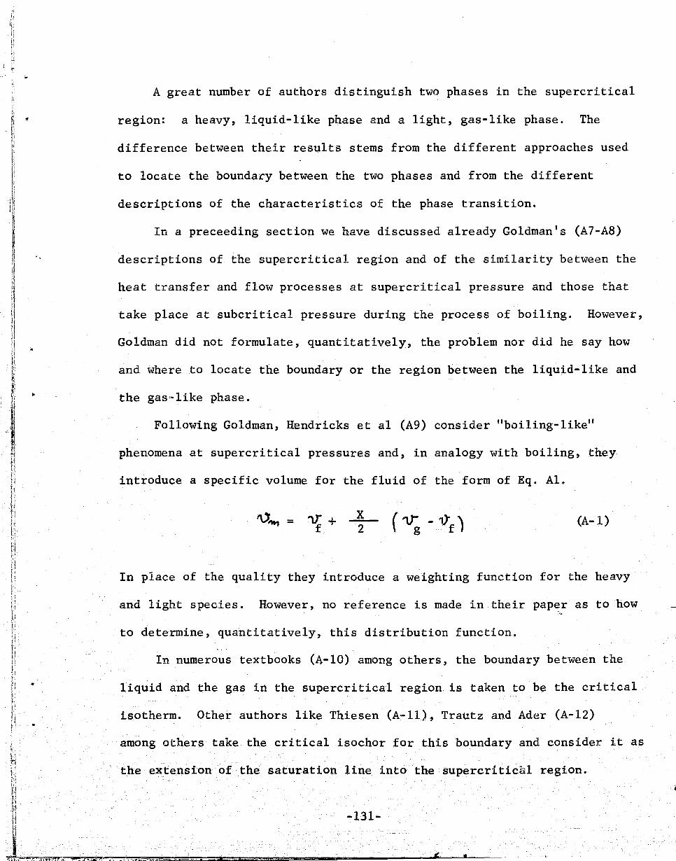
.. A great number of authors distinguish two phases in the supercritica1

region: a heavy, liquid-like phase and a light, gas-like phase. The

difference between their results stems from the different approaches used

to locate the boundary between the two phases and from the different

descriptions of the characteristics of the phase transition.

In a preceeding section we have discussed already Goldman's (A7-A8)

descriptions of the supercritical region and of the similarity between the

heat transfer and flow processes at supercritica1 pressure and those that

take place at subcritica1 pressure during the process of boiling. However,

Goldman did not formulate, quantitatively, the problem nor did he say how

and where to locate the boundary or the region between the liquid-like and

the gas-like phase.

Following Goldman, Hendricks et a1 (A9) consider "boiling-like"

phenomena at supercritica1 pressures and, in analogy with boiling, they

introduce a specific volume for the fluid of the form of Eq. A1.

X 2

(A-I)

In place of the quality they introduce a weighting function for the heavy

and light species. However, no reference is made in their paper as to how ;~

to determine, quantitatively, this distribution function.

In numerous textbooks (A-10) among others, the boundary between the

liquid and the gas in the supercritica1 region is taken to be the critical

isotherm. Other authors like Thiesen (A-11), Trautz an.d Ader (A-12)

among others take the critical isochor for this boundary and consider. it as

the extension of the saturation line into the supercriticeL1 region.

-131-

•

-...

j

1

j I

1

I i I I

I i ! 1 I

I l i j

I I Ii

ff

ih,-t,P··'·'·

In the subcritical region various thermodynamic properties such

as the specific heat, the compressibili~y, the coefficient of thermal ex~

pans ion and others change discontinuously or reach a maximum value at the

coexi.stence, i.e., the I aturation line. This line can be therefore looked

upon as the locus of points for these discontinuities or maxima. Conse-

quently, numerous authors consider the extension of the saturation line

into the supercritical region to be the lirie which is the locus of points

where the thermodynamic properties listed below reach a maximum:

')2i =( dCE ) T =( ;:~ L = 0

'Or t>1> '0 p (A-2)

( ~2iJ ~ ;TCE)p 0 = = OT2

p (A-3)

C)2 i )= 0 t"() p2

'T

(A-4)

~2u = (PCv) = ('d2p) 0 = t""()V')T 'I) v ro T2 T v

(A-5)

(tV2U) = (~Cv) = 0 roT2 "1> T

v v

(A-6)

Several authors (A-13 - A-17) assume that one single line represents

the locus of points of all these maxima. This is indeed the case for sub-

critical pressure where the saturation line is the locus for all discontinuities.

However, the experiments of Kaganer (A-IS) and of Sirota and co-workers (A-19)

-132-

•

I ! ~

show that this is not the case but that for a given supercritical pressure ,.~ ~

different thermodynamic properties reach a maximum value at different

temperatures. Thus, for each of the thermodynamic properties, i.e.,

spe~ific heat c , the coefficient of thermal expansion, etc., there is a p

different line which represents the locus of the maxima. This raises the

question which of these lines can be regarded to be the extension of the

saturation line in th~ supercritical region, i. e., which of these li.nes can

be considered as the boundary between the liquid-like and the gas-like

phase.

Plank (A-20~ and Semenchenko (A~21) consider the line along which

(A-7)

to be the extension of the saturation line in the supercritical region.

Eucken (A-13),.however, takes the curve represented by Eq. A-2 for this

extension; whereas numerous authors (A-B, A-9, A-22 - A-25) take Eq. A-3.

Of particular interest to the analysis of this paper are the results

reported in (A-14, A-17, A~19 and A-16) which will be therefore discussed

in more detail.

Sirota and co-workers (A-19) discuss t;'e transition phenomena at sub-

critical and supercritical pressures in tetms of the Frenkel's theory of

heterogeneous fluctuations (A-14, A-26). According to this theory in any

gas at subcritical temperature heterogeneous fluctuations result in the

formation of molecular complexes which canbe'regarded as finely dispersed

-133-

aa II·

nuclei of a phase within a homogeneous phase. In approaching the saturation.

line the fluctuations increase and "micro-heterogeneities" appear in the

macroscopic, homogeneous phase. This marks the beginning of the "pre-transi-

tion region" which is characterized by the fact that various thermodynamic

properties exhibit variations which become more pronounced as the saturation

line is approached. This accounts for the anomalous effects of the proper-

ties in the vicinity of the saturation line. At the saturation line the

properties change in a discontinuous fashion which is a characteristic of

phase transitions of the first order. As the pressure is increased the

effect of heterogene9us fluctuations increases whereas the effect of phase

change, i.e., of the discontinuous change of properties becomes less

important and disappears at and above the critica~ point. Since the change

of phase at subcritical pressure is characterized by an obsorption of energy

and an expansion of volume the transition at supercritical pressure should

be characterized by the maximum values of c and of the thermal expansion, p

i.e., of ( r;;v/ ') T) 0 See Figures A-I and A-2 which show these properties p

for oxygen at supercritical pressures. However~ the authors of (A-19) show

from experiments that at a given pressure the two maxima do not occur at

the same temperature. The values of the maxima for C are correlated by p

c - c 9.05 Pmax Pg _----:= ____ -'"1_.... = ------- + 1. 30 'R

•

P .' P . crJ.t

-134-

- 1

,Il .~, _

(A-8) ",

:l 1 !

i 11 1

-o~ S b.O --til Q)

r-t ::s 0 IJ -~ .r-f 0 cd 0.. cd U +J cd Q)

::t: () .....

f+-t ..... (j Q)

0.. rJ1

10

9

8

7

6

5

4

3

2

1

o 80

~

. :::-::':::;":::''=:''-:;:'--~-::;:'-==")::.,.~~, .... ·_=a~~;;;:>-="=~;;t..U:::~~J;:::~-.-: ... :::::,::7,·-:-_:::::.~-:··-~T.':.--~~·t:~~~.-::::.:=: ;",::k"'~':';"'k=-;::;;"'··"-·~.'~-;:m:r:r---'''''· f'"""'~~." _'1""":'.::"'_~;~"","-~~-: .. '_ ._~

.. 'w

p= p r P "t crr

-.1

; , . ' P " for Oxygen crlt . P = 1.1 'r 50.8 Bars

(737 psia)

j

L L vCr:: ~p 1.5 r

/L \ \ P = 2.5

~~' 'r

(/~ --........ - ~ '" ~~

"'- ~ ... ~ r f=!'-- -=--~_ ---- -~~ -- -CD

. ®

100- 120 140 160 180 200 220 o

Temperature ( K)

-

240

Figure Al Specific Heat Versus Temperature for Oxygen at Supercritical Pressures.

•.

-"l

-

260

~;..-. ... , • .". .. ~"",>-<-,"-,*"""",,,,,, '.-.-.~""'.,.....--~ .. --~--~ "'-..... ".--.,.--.,~~~t-.::-:t'~r.:-~~~:.::;:· '1~"-:"r:-;--"'(-'::""":-='r'~

. .=- ... -".----,-~,~.~---~,...- 'M------,..-"' •• --~·.~.--u,.:.'_ ... .:..~~~~~~:I"!=7:.=z;f.~;:t.;.z~~~::w.;~::Gi.te_::,;:;.=_".:.._.~:lr.'.:Z!!2:.~(-::~~~~l,~.!1!~.!t~-::r:!!!~_LJt\li:lt!lel InlO£.I. ~1e:~-;~

•.

0.25 1

0.20

-O~ O. 15 be -­M

S C) -Ili -E-t

rc -..;,

> rc -0.10

0.05

o 120 140

1"\ I \ I \

\ \

160

P = 1.1 r

180 200

P P =-

r P erit

PerU for 02 = (5?._~ B~rs). 737 pSla

220

Ideal Gas

Asymptotes I

-----------:a.-----------------=------~------. -- -- --=---

240 Temperature (oK)

Figure A2 {ov/oT)p Versus Temperature for Oxygen at Supercritical Pressures . . :.~~ ~"~~~'-..:...... .' .. : .. , _:'J_-';: .. ·_ .. ~~"-:.--:.-.:··'-::C~.. ", - .. ' -, '~''''''''~~-'''T.,.""",~~~~.:=z-~~ •• ",.::::u:::;:;; .... _ ... :z:;..c'' ~;::-=::-"",-" ............. ::.~~~.-. ........ __ ,~.~-.::-_~.~z~-=r.::::~;><c--z:~~_,_ .... _ ..... -.;::~~.=..~c~~:;,:";:=::::.:',:;:.:::.::;< • .::::",","-~~-.--,..,.- .... -......... ~-....... -.-<------

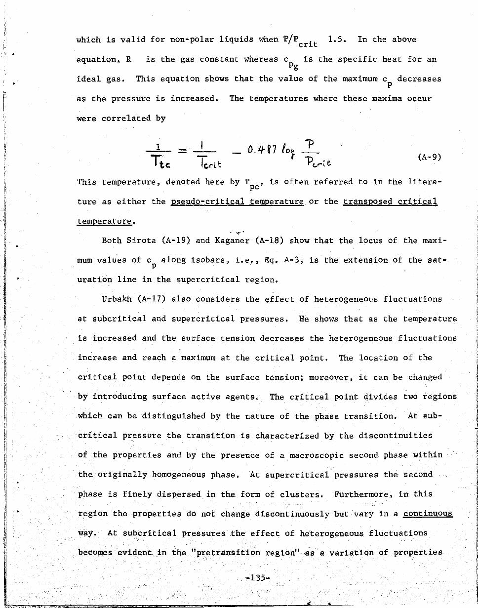
which is valid for non-polar liquids when p/pcrit 105. In the above

equation, R

ideal gas.

is the gas constant whereas c is the specific heat for an Pg

This equation shows that the value of the maximum c decreases p

as the pressure is increased. The temperatures where these maxima occur

were correlated by

1 (A-9)

This temperature, denoted here by T ,is often referred to in the litera­pc

ture as either the pseudo-critical temperature or the transposed critical

temperature 0

. ~. Both Sirota (A-19) and Kaganer (A-18) show that the locus of the maxi-

mum values of c along isobars, 1. e.~, Eq. A-3, is the extension of the sat­p

uration line in the supercritical region.

Urbakh (A-17) also considers the effect of heterogeneous fluctuations

at subcritical and supercritical pressures. He shows that as the temperature

is increased and the surface tension decreases the heterogeneous fluctuations

increase and reach a maximum at the critical point. The location of the

critical point depends on the surface tension; moreover, it can be changed

by introducing surface active agentso The critical point qivides two regions

which Cdn be distinguished by the nature of the phase transition. At sub-

critical pressure the transition is characterized by the discontinuities

of the properties and by the presence of a macroscopic second phase within

the originally homogeneous phase. At supercritical pressures the second

phase is finely dispersed in the form of clusters. Furth.ertnore.~ in this

r~gion the properties do not change discontinuously but vary in a continuous

way. At subcritical pressures the effect of heterogeneous fluctuations

becomes evident in the "pre transition region"as a variation of properties

-135-

..

i :j

1 I

I J

in the vicinity of the saturation line. This is shown in Figure A-3 which

is the volume-temperature plane for oxygen. At a subcritica1 pressure,

say at P = 0.9, the line l' - 2' is the phase transition of the first r

order occurring at a constant temperature. The effect and magnitude of

the fluctuation in specific volume in the two pre-transition regions is

sho=n as the l1.°nes 1 - l' and 2 - 2'. Th f1uct atl.°on 1 l' Os us d by the w e u .. - 1. cfl e

" formation of vapor nuclei in the pre-transition region of the liquid.

Similarly, 2 - 2' are the fluctuations caused by the formation of liquid

nuclei in the pre-transition region of the gas. It can be seen from this

Figure that at low pressures in the subcritica1 region the effect of

fluctuation is negligible when compared to the phase transition of the

first order. For example, at P = 0.5, they are almost absent. Increas­r

ing the pressure increases the effect of heterogeneous fluctuations which

reach a maximum at the critical point. At this point and above it)the

phase transition of the first order vanishes so that only the effect of

heterogeneous fluctuations remains. Urbakh notes further than with the

phase transition and the fluctuations are associated energy requirements

which can be determined from the T - s or v - s diagrams shown on Figures A-4

and A-5. At low pressure the only energy required is heat of vaporization

for the phase transition of the first order, thus

(A-IO)

However~ as the pressure is increased the energy associated with the

fluctuation becomes important. At supercritica1 pressu:re it is the only

which remains, and it can be determin.ed either from Figure A-4 Or A-5,

thus

• At. = T (s2 - sl) (A-11)

-136 ...

..

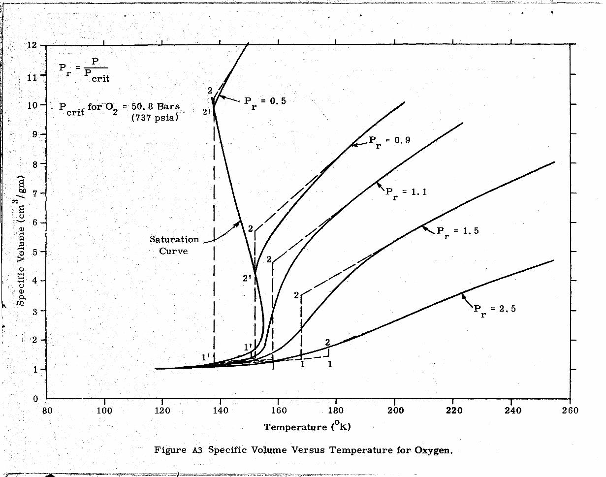
""~~='~w..:+-~'=' "M"';,'qq; ;;=W~."...,... _~~~,:'~':::::K:""'*"~W""'; -~~~"'#.~ ~ ~~:.;;:t..""t~~.:::;;;-...>..:~~:;~.;::::~~~,=::,;;::::c~::::-,:-,,;::'::::::L·~~-·-.,.-;::t;;t::·,!<"' !:"--:..!.:.:;;;::.~ _.':-~..:;:!'".;~_:.:' .'~-~~ .

:.

12 I- ~ 7

11

10

9

8 ........ 8 bJl ~ 7

:t:l

S C,) - 6 OJ s

5J ::s ~

0 :> C,) ..... ~ 4 ..... C,)

OJ 0..

r.n 3

2

1

o 80

p p =-

r P crit

P .t for-02

= 50.8 Bars crl (737 psia)

SaturatiQn Curve

100 120 140

.

160 180 o Temperature ( K)

•

200 220

Figure A3Specific Volume Versus Temperature for Oxygen.

~WO'..l:;~,"-)~~~J.:.~,ma""-$tI£;;.o-4~:;~~~if'''::;:;;;;;':;''ri:.::;:;J.:.:~:"",,;::C>:;d:;';.{G.-T.~."," ...... ..;_z.::::::L.~~~::-::.t:!~:'J..:.;::::=,:';'i..-::;.:....-1::;='7l--·-·:,:.·--:-'*···"·~·····+.,.--:-

..

240 260

260 __ ------~------~----~~----~------~------~------~------~------~

250

240

230

220

2:10

200

.190

180

170

160

15·0

14·0 .

130

120

110

100 0.2

p = p r P 't crl

P 't for 02 = 50. 8 Bars crl (737 psia)

/

'/ /

Ij

----------------- U 2 l' . 2'

0.4 o .. 6

Liquid Saturation Line

0.8 1.,0 1.2

Vapor Saturation Line

1. 4. 1.6

Specific Entropy (Joules/ gm oK)

Figure A4 Temperature-Entropy Diagram for Oxygen ..

1.8

:1 ']

rl ~ ., j

" .' ,!

II fl " ~ ~ M .~ , ~ ~ J

i

'I

I

I 1 j

•

•

..

-S bO --M

S C;) -Q)

s .E ~

C;)

c::: ..... C,) Q)

0.. 'Cf1

71-------f

6

5

4

3

p = p r P crit

P 't for 02 crl = 50.8 Bars

(737 psia)

Saturation Curve

2r-~----~-------+------~--------~~~~~--~-----4--------~----~

1,~----"~~~--~------~------~----~,~--------~------~------~

0.4 0.6 0.8 1.0 1.2 1.4 1.6 1.8 2.0

Specific Entropy (Joules I gm oK)

tdtt:-·H'.':ftt '-~'i+X';"i -0 +"."$0- 2 _. -~ & . a;

FigureA5 Specific Volume Versus Entropy for Oxygen. #! •

:j , ! , , i !

fl " f'

Frenkel (A~l4, J\~26) considers two variations~ a transition of the

first order at subcritical pr'essu;re and a transition of the gcond order at

supercritical pressure. The first, ~haracterized by discontinuities of

properties, is described' by Glaus1us-Ciapeyron's equation~

hf .f!f g

= " dT T (v vf

) 0 g

(A-l2)

and takes place at a constant temperature T. The phase transition of o

the s'econd order takes place over a t.emperature interva1 l\T=T =·T ~ 2 l'

in which the properties change continuously. In this temperature interval

both c and (ovldT) reach a maximum. FiguresAl andA2 show these varia·-p , p

tions for oxygen at three supercritical pressures. As a generalization

9f the transition of. the first order Frenkel formulates the equivalent

energy of·· transition for the second order .transition~ thus

= T (s2 - sl) = -tc A c dT P

(A-13)

where Ttcis the temperature corresp~nding .to the peak of c p qnd: A cp is

the value of c above the "normal". value, i. e. , . above the dashed line on p

Figure 1. Similarly, the change of volume is given by

dT (A-14) p

-137-

-' « 4·

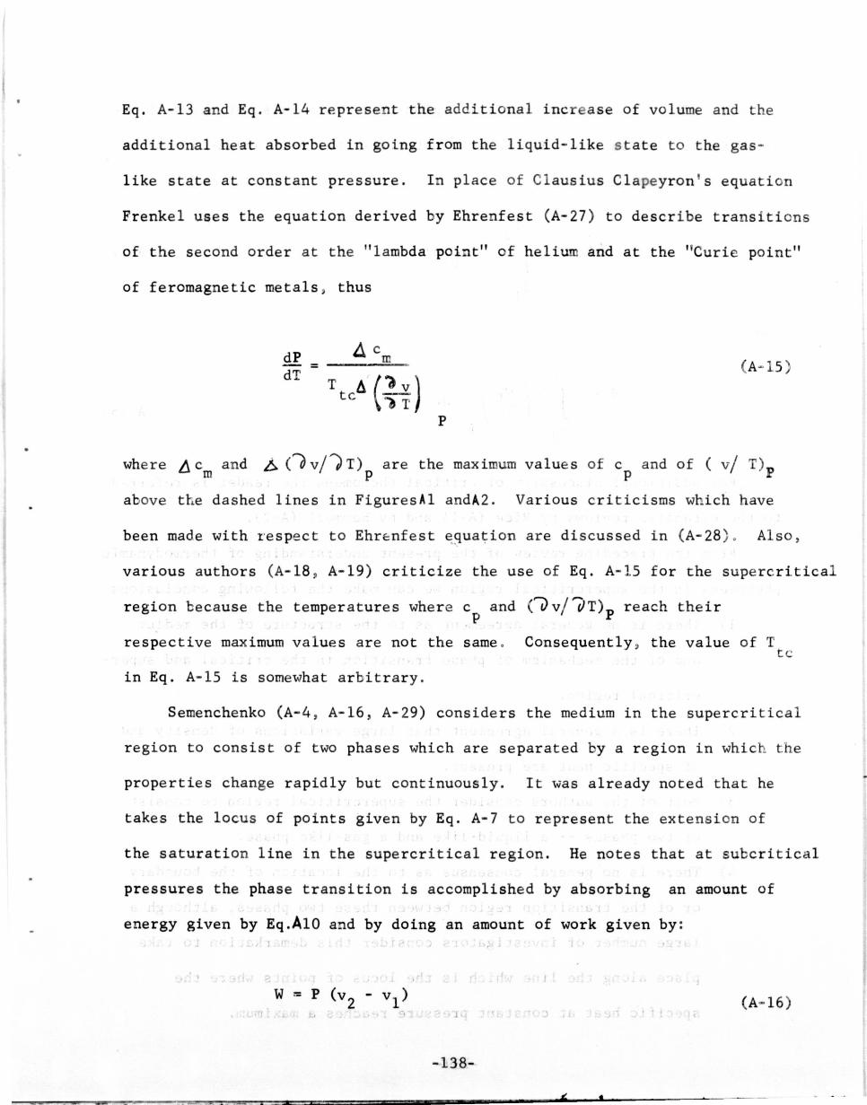
Eq. A-13 and Eq. A-14 represent the adQitional incr ase of volume and the

additional heat absorbed in going from the liquid-like s t ate to the gas -

like state at constant pressure. In place of Clausius Clapeyron ' s equation

Frenkel uses the equation derived by Ehrenfest (A-27 ) to descr ibe transitions

of the second order at the "lambda point" of heliu and at the "Curie point"

of feromagnetic metals thus

dP dT

AC = ___ =m:..-...

Ttcl1 (").Y.) '")T

(A- I S)

P

where !!l c and b ( '0 vi; T) are the maximum values of c and of ( vi T) p m p p

above the dashed lines in FiguresAl andA2. Various criticisms which have

been made with respect to Ehr~nfest ~9uation are di scussed in (A-28 ) . Also,

various authors (A-18 , A- 19) criticize the use of Eq. A-IS for the supercritical

region because the temperatures where cp and ( j) vi VT)p reach their

respective maximum values are not the same .

in Eq. A- IS i s somewhat arbitrary .

Consequently ~ the value of T tc

Semenchenko (A-4 , A-16 , A- 29) considers the medium in the supercritical

region to consist of two phases which are separated by a region in which the

properties change rapidly but continuously. It was already noted that he

takes the locus of points given by Eq. A-7 to represent the extension of

the saturation line in the supercritical region. He notes that at subcri tica l

pressures the phase transition is accomplished by absorbing an amount of

energy given by Eq.AlO and by doing an amount of work given by:

(A- l6 )

-138-

I I :: , ; == . oa so £ • * , •

However, since in the supercritica1 region there is no discontinuous change ., 1 ,

of volume and of entropy, Semenchenko notes that Eq. A-10 and A-1S must be

modified and replaced by:

• /2 ~II = c dT P

(A-17)

T1

and

W = f2 (~) dv

v T 1

For additional discussion of critical phenomena the reader is referred

to the extensive reviews by Rice (A-1) and by Hammell (A-2).

From the preceding review of the present understanding of thermodynamic

phenomena in the supercritica1 region we can make the following conclusions:

1) There is no general ~greement as to the structure of the m~dium

I and of the mechanism of phase transition in the critical and super-

critical region.

2) There is a general agreement that large variations of density and

of specific heat are present.

3) Most of the authors consider the supercritica1 region to consist

of two phases -- a liquid-like and a gas-like phase.

4) There is no general consensus ~s" ~o the location of the boundary i, -,

or of the t·ransition region between these two phases, although a

large number of·investigato;rs consider this demarkation to take

place along the line whi.ch is the locus of points where the

specific heat at constant pressure reaches a m~ximum.

5) There is no general consensus as to the nature of phase transition

at supercritica1 pressures and of the energy required to bring it

about. Three different methods for evaluating this energy of if <!

transition have been proposed: 1) the graphical method of

Urbakh (A-17) resulting in Eq. A-11; 2) the second order transition

proposed by Frenkel (A~14, A-26) given by Eq. A-13, and Eq. A-1S; and

3) the pseudo transition region proposed by Semenchenko (A~4, .A~16,

A-29) given byFq.A-15 and Eq. A-17. By examining the proposed methods

and equations, i.e., Eq. A-I1, Eq. A-15 and A-17, it can be seen that

these different methods will yield different values for the transition •

energy.

It is evident from the preceding results that the success of any analysis

concerned with the mechanism of flow oscillations and of heat transfer at

supercritica1 pressures will depend to a great extent upon the ability to

< ~

I describe more accurately the thermodynamic state of a fluid and the transi-

tion phenomena that take place at supercritica1 pressures .

•

, \

-14·0-

• "

I 1 -I

I 1 I !

1

-j

REFERENCES Appendix A

AI) o. K. Ri.ce, Thermodynamics and Physics of Mat~, T. D. Rossini, Ed.itor, Princeton Univ. Press, Princeton, N. J., 1955, pg. 419.

A2) E. F. Hamme11,"Critical Phenomena in Fluids," paper presented at the Course on Liquid Hydrogen in Technical and Space Programs, CGNoRoS., Grenoble, June, 1965.

A3) A. A. Rosen, Dok1adi Akademii Nauk SSSR, v. 49, no. 1, pg. 133, 1954.

A4) V. K. Semenchenko, Dok1adi Akademii Nauk SSSR, v. 49, no. 6, pg. 1045, 1954.

A5) J. o. Hirschfe1der, C. F. Curtis~ R. B. ·Bird, Molecular Theory of Q..ases and Liquids, John Wiley and Sons, Inc., NoY., 1954, Ch. 5.

A6) J. E. Mayer and M. G. Mayer, Statistical Mechanics, John Wiley and Sons, Inc., NaY., 1954, Ch. 14.

A7) K. Goldman, Proc. of the 1961 Int. Heat Transfer Conf., pg. 561, 1961.

A8) K. Goldman, Chern. Progr. Symposium Sere Nuclear Engr. v. 50, no. 11, 1954.

A9) R. C. Hendricks, R. W. Graham, Y. Y. Hsu, A. A. Mederios, A.R.So Journal, v. 32, pg. 244, 1962.

A10) M .. W. Zemansky, Heat and Thermodynamics, McGraw-Hill Book Co., Inc., N. Y.~ 1951, Ch. XI, Ch. XV.

All) M. Thiesen, Z. Kompr. f1Uss Gase, v. 1, 86, 1897.

A12) M. Trautz and H. Ader, Phys. Zs. v. 35, pg. 446, 1934.

A13) A. Eucken, Phys. Zeitsch. V. 35, pg. 708, 1934.

A14) J. I. Frenkel, Statistical Physics, Akad. Nauk, SSSR, Moscow, 1948.

A15) G. M. Bartenev andA. A. Remizov, Zh. Fiz. Khim. V. 31, pg. 341, 1957.

A16) V. K. Semechenko, Zh. Fiz. Khim. V. 21, pg. 1461, 1947.

A17)

A18)

A19)

A20)

I. Urbakh, Zh. Fiz. Khim. V. 33, pg. 515, 1959.

M. G. Kaganer, Zh. Fiz. Khim, v. 32, pg. 332, 1958.

A. M. SirOta, B. K. Ma1tzev and P. E. Be1ijakova, Tep1oenergetika, V. 7, no. 7, pg. 16, 1960.

R. Plank, Forschungsarb. Geb. Ingenienrwesens, v. 7, pg. 161, 1936.

-141 ...

'" t'

II r H ,. l: Ii

"

RE~'ERENCES - Appendix A (Continued)

A21) V. K. Semenchenko, Dok1. Akad. Nauk SSSR, v. 99, pg. 1045, 1954.

A22) M. Jakob, Physik. Zeitschr. v. 36, pg. 413, 1935.

A23) J. Havlicek and L. Mishoysky, He1v. Phys. Acta. v. 2, pg. 161, 1936.

A24)' T. P. Andrianov, Zh. Tekhnicheskoi Fiziki, v. 23, pg. 1014, 1953.

A25) A. V. Sheid1in, Tep10energetika, v. 2, no. 3, pg. 26, 1954.

A26) J. I. Frenkel, Kinetic Theory of Liquids, Dover Pub1ic~tions, Inc., No Y., 1955, Ch. II and Ch. VII.

A27) P. Ehrenfest, Proc. Acad. Sc. Amsterdam, v. 36, pg. 153, 1933.

A28) P. S. Epstein, Textbook of Thermodynamics, John Wiley and Sons, Inc., N. Y .. , 1937,'~h. VII.

A29) V. K. Semenchenko, Dok1. Akad. Nauk, SSSR, v. 92, pg. 625, 1953.

-142-

• •

-

I ! I I i

! i f

,~

j

il '[''','1

r , ~ ;

"

11 r l,

11 i!

tl , '~

U

I i , ~

LIST OF ILLUSTRATIONS - APPENDIX A

Figure A~l

Specific Heat versus Temperature for Oxygen ~t Supercritical Pressures.

Figure A~2

(U~~T)p versus Temperature for Oxygen at Supercritical Pressures.

Figure A-3

Specific Valume versus Temperature for Oxygen.

Figure A-4

Temperature - Entropy Diagram for Oxygen~

Figure A-.5

Specific Volume versus Entropy for Oxygen.

-143-

.'

l34-a

134-b

l36-a

f

In l36-b i

! j I. t 1

136-c I I \

I I I

I I I I

I ;

I

i ! J , j

I 1

I ~ I !

! i I I

I I t'

t r I: j i: t

I I,

~ .... 11

! n U

I I r.e: ,

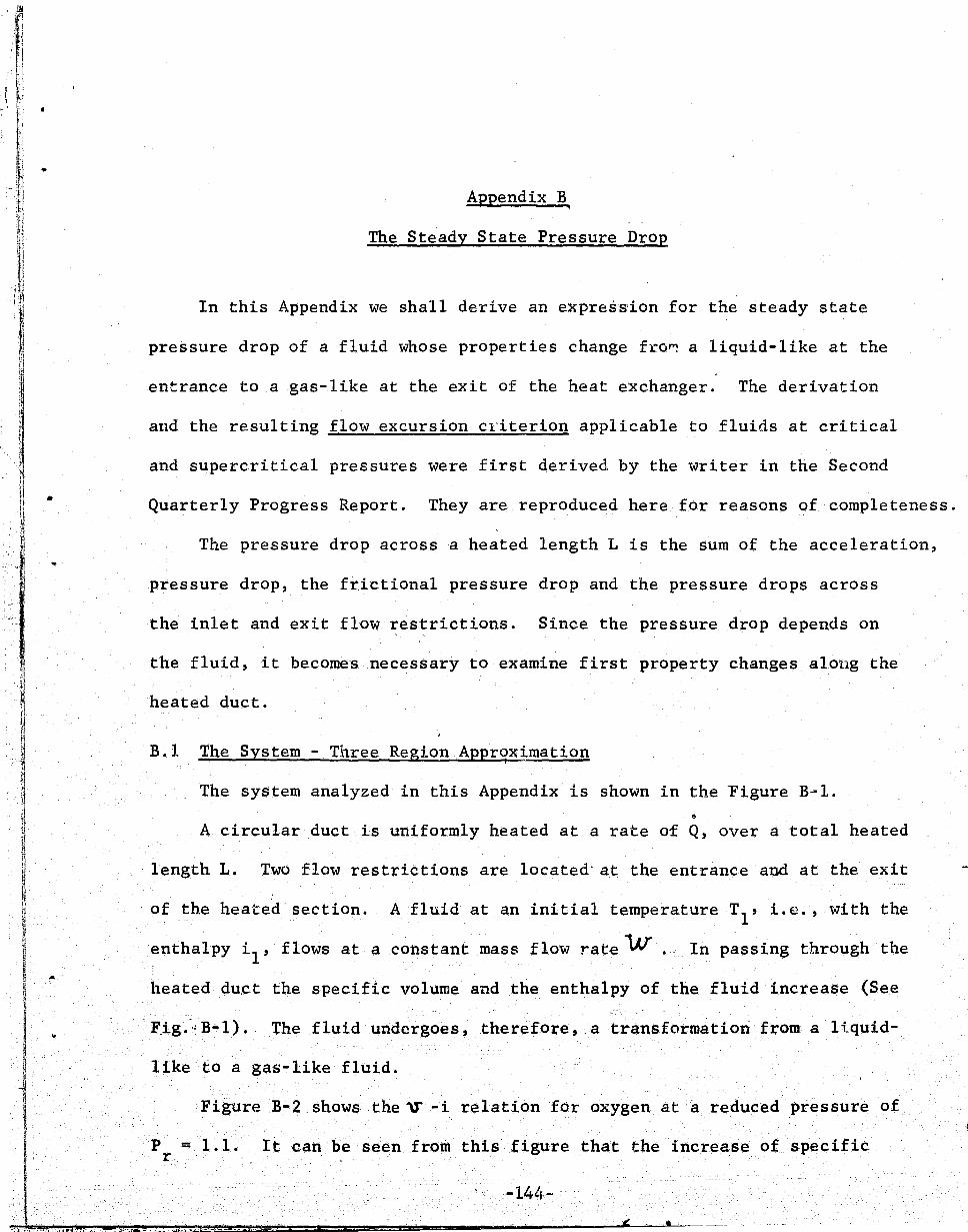
, ','I'~, ! ~

':,1 . 0\

! ;i

I ; I ' \

1 '. ~

Appendix B

The Steady State Pressure Drop

In this Appendix we shall derive an expre~Bion for the steady state

pressure drop of a fluid whose properties change fro~ a liquid-like at the

entrance to a gas-like at the exit of the heat exchanger. The derivation

and the resulting flow excursion c~iterion applicable to fluids at critical

and supercritical pressures were first derived. by the writer in the Second

Quarterly Progress Report. They are reproduced here for reasons of completeness.

The pressure drop across a heated length L is the sum of the acceleration,

pressure drop, the frictional pressure drop and the pressure drops across

the inlet and exit flow restrictions. Since the pressure drop depends on

the fluid, it becomes necessary to examine first property changes along the

heated duct.

B.l The System - Three Region Appr~xtmation

The system analyzed in this Appendix is shown in the Figure B~l. 6

A c.ircular duct .is uniformly heated at a rate of Q, over a total heated

length L. Two flow restrictions are located' at the entranceapd at the exit

of the heated section. A fluid at an initial temperature Tl , i.e., with the

enthalpy iI' flows at a constant mass flow rate 1Ar. In passing through the

heated dU,ct the specific volume and the enthalpy of the fluid increase (See

F,ig:,'B-l). The fluid undergoes, therefore, a transformation from a l:i.quid-

like to a gas-like fluid~

Figure B-2 shows the V -i relation fOr oxygen at a reduced pressure of

P = 1.1. It can be seen from this figure that the increase of specific r"

-14L~ ...

" •

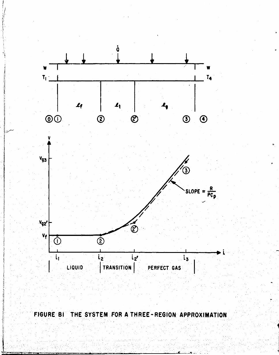
• Q

w,-L* .~ i ~ W

TI' T4

4

@CD

v

® ~----------~------~----------~----~i

t2 i2'

LIQUID I TRANSITION I i3

PERFECT GAS

FIGURE 81 THE SYSTEM FOR A THREE- REGION APPROXIMATION

-

1 " t

I f , , I.

:{

I I ,. I.

•

volume from a liquid-like·state to a gas-like state occurs gradually over

an enthalpy interval.

In order to simplify the problem, we shall assume that the entire

transformation can be approximated by considerding three regions. In the

first region of length If' between stations CD and CD in Figure B-1, the

heavy clusters resemble a liquid. In this region the specific volume of

the fluid is constant having a value of vf~ We shall assume that the com­

plete transformation, from heavy to light clusters, takes place within the

transition length It' i. e., between sfations ® and 0. In this transition

region the specific volume of the fluid changes from a value of v f to a value

of v g2

The enthalpy change associated with this expansion is given by . . \

~ L2,2, = tl! -12. .

resemble a gas.

In the third region of length 1 , the light clusters g

The specific volume of the fluid in this region can be

approximated by that of gas and, in particular, by that of a perfect gas.

It is apparent from the discussion in Appendix A that the initial and

the final conditions of the transition region, i.e., the conditions at stage QD and ® respectively, will depend upon the model selected for describing

the pseudo-phase transition in the supercritical region. This follows from

the fact ~hat the temperature or the enthalpy that marks the start of the

pseudo-phase transition will determine the location of station ~, whereas

the location of station 0 will depend on the energy required to complete

the transition from heavy to the light clusters. In this report we shall I

denote this energy requirement by ll~i2· which can be determined by the best

three region approximation indi~ated in Figure B-1.

As discussed in the preceeding sections,we are considering in this

report only the effects of density variation on the flow stability.

-145-

•

-

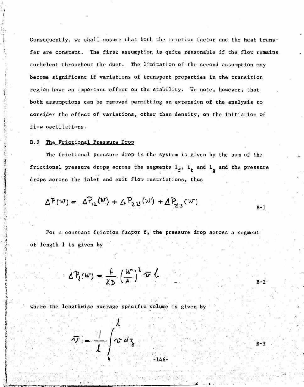
i:

Consequently, we shall assume that both the friction factor and the heat trans-

fer are constant. The first assumption is quite reasonable if the flow remains

turbulent throughout the duct. The limitation of the second assumption may

become significant if variations of transport properties in the transition

ii! region have an important effect on the stability. We note, however, that i!

both assumptions can be removed permitting an extension of the analysis to

consider the effect of variations, other than density, on the initiation of

flow oscillations.

B.2 The Frictional Pressure Drop

The frictional pressure drop in the system is given by the sum of the

frictional pressure drops across the segments If' It and 19 and the pressure

drops across the inlet and exit flow restrictions, thus

B-1

For a constant friction fac~or f, the pressure drop across a segment

of length 1 is given by

B-2

where the lengthwise average specific volume is given by

1 - I ~ ---

L B-3

-146 ..

-....

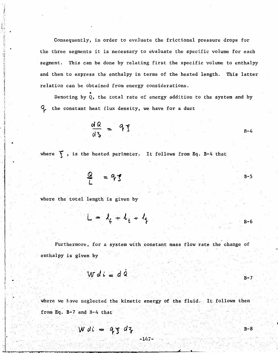
Consequently, in order to evaluate the frictional pressure drops for

the three segments it is necessary to evaluate the specific volume for each

segment. This can be done by relating first the specific volume to enthalpy

and then to express the enthalpy in terms of the heated length. This latter

relation can be obtained from energy considerations . ..

Denoting by Q, the total rate of energy addition to the system and by

~ the constant heat flux density, we have for a duct

-- B-4

where ); , is the heated perimeter. It follows from Eq. B-4 that

~ ..... B-5 L

where the total length is given by

B-6

. Furthermore, for a system with constant mass flow rate the change of

enthalpy is given by

where we b.;3.ve neglected the kinetic energy of the fluid, It follows then

from Eq. B-7 and B-4 that

B-8

-147-

.. _ ...

,

I i I

~

f

I , !

X and in view of Eq. B-5 we obtain

".:.I. 9 .... .u-

Substituting Eq. B-4, B-3 in Eq. B-2, we obtain the pressure drop across

a heated segment where the enthalpy of the fluid ch~nges from i to i +di,

thus • t.-t-li.L

~ W ( 'j. I t1. ." -= ~) J 'V'!l) ~t

• '2.::1) Q B-lO

t (..

For a three region approximation the relation between v(i) and i

is shown in Figure B-1. We shall consider now each region separately.

a) The Liquid-Like Region

In this region the specific volume of the fluid is constant arrd equal

to vf (See Figure B-1). In the segment of length If' the enthalpy of ~he

fluid increases from it to i 2• The frictional pressure drop across If be­

comes then

B-11

b) The Transition Region

In the transition region we shall approximate the relation between the

specific volume v, and the enthalpy i, by a linear equation. The average

specific volume in this region can be written then as:

B-12

-148-

•

..

~ 1 ,

I "I

I • I

Denoting by L\ i.,lll-=- L1

:- t..2 the change in enthalpy, the frictional

pressure drop in the transitional region then becomes

B-13

c) The Gas-Like Region

In view of the assumption that in this reg~on the fluid has the prop-

erties of a perfect gas we have, for a constant pressure process, the fo1-

lowing expression for the specific volume

B-14

Inserting this expression in Eq. B-10 we obtain

B-15

The change of enthalpy A,i32 ' can be expre,ssed also in terms of the total

heat input thus from an ene.rgy balance

..

t·:;·· B-16

Inserting this expression in Eq. B-15, we obtain for the frictional

pressure drop in the gas-like region the fo11owtng expression

B-17

-149-

•

.j . I

B.3 The Inlet and Outlet Pressure Drops

Denoting by k. a numerical coefficient that takes into account the 1.

geometry of the restriction and of other losses like vena contract a etc.,

we have the inlet pressure drop

B-18

Similarly; we define by k a numerical coefficient that accounts e

for the geometry and the losses at the exit. The exit pressure can be then

expressed as:

B-19

which, in view of Eq. B-14 and B-16, can be also written as:

~

1< (Q I ')J - - -ll~ I -AL 2 "PC~ W 22 ., B-20

B.4 I.,he Acce1er'llon Pressure Drop'

The acceleration pressure drop is given by

dp z:::... \ ~ olv., B-21

as

B-22 ':!l ~ ~ itA - ~ A V

-150-

.,

l

then

B-23

The total acceleration pressure drop required to accelerate a fluid of

specific volume vf

at the inlet up to the exit where it attains a specific

volume Vg3 is given therefore by

B-24

Inserting Eq. B-14 in Eq. 24 we obtain

B-25

or in view of Eq. B-16 we have

B-26

B.5 The Total Pressure Drop

The total pressure drop is obtained by summing Eq. ·B-26, B-20, B-18,

B~17 and B-ll, thus after so~ rearrangement

"2. • - b W- +c Q.VV B-27

-151-

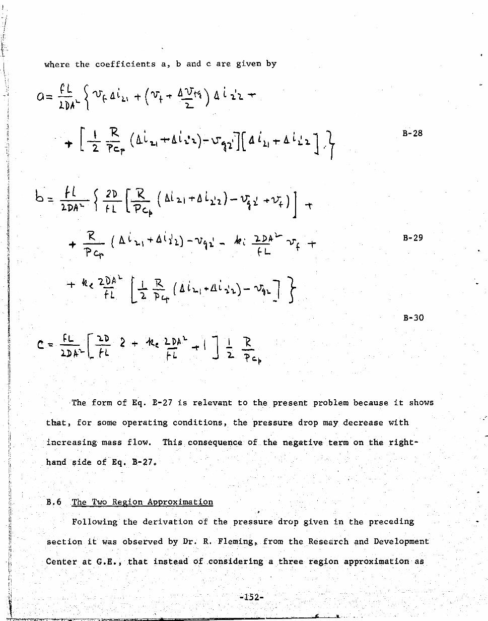
I I i

;f'

t-,ll where the coefficients a, band c are given by

" rl }; ~. ! U Ii i1 f"j h i: ~l

fL

+ ~< 2~\.. fL

B-28

B-29

B-30

-The form of Eq. E-27 is relevant to the present problem because it shows

that, for some operating conditions, the pressure drop may decrease with

increasing mass flow. This consequence of the negative term on the right-

hand side of Eq. B-27o

~f ti B.6 The Two Region Approximation Ii H

R Following the derivation of the pressure drop given in the precedirtg n H Jl ii section it was observed by Dr. R. Fleming, from the Research and Development H If II 'n Center at GoE., that instead of considering a three region approximation as \1

-152-

• J

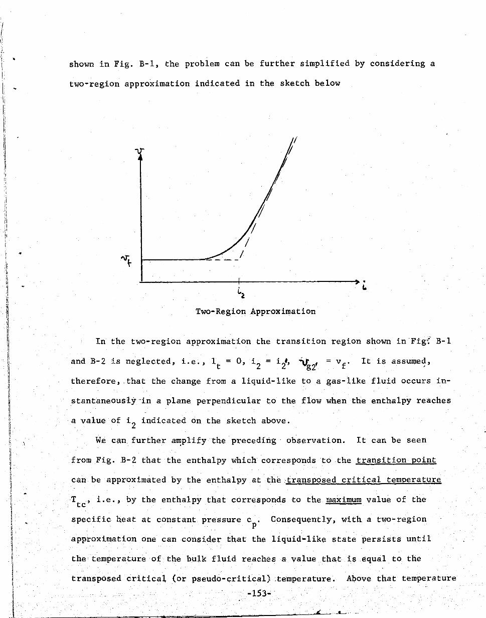
- i 1

1' .. 1

j ]

shown in Fig. B-1, the problem can be further simplified by considering a

two-region approximation indicated in the sketch below

I---------~ - - -

~----------------------~--------------------~> . .. Two-Region Approximation

In the two-region approximation the transition region shown in 'Fig'( B-1

It is assumed, ,

therefore, that the change from a liquid-like to a gas-like fluid occurs in-

stantaneously"in a plane perpendicular to the flow when the enthalpy reaches

a value of i2 indicated on the sketch above.

We can further amplify the preceding - observation. It can be seen . from Fig. B-2 that the enthalpy which corresponds to the transition point

can be approximated by the enthalpy at the .-transposed critical temperature

Tt ' i.e., by the enthalpy that corresponds to the maximum value of the . c

specific heat at constant pressure c. Consequently, with a two-region p

approximation one can consider that the liquid-like state persists until

the temperature of the bulk fluid reaches a value that is equal to the

transposed critica~ (or pseudo-critical) ~temperature. Above that temperature

-153-

..:. e . =E~;iC; •

L

!

!

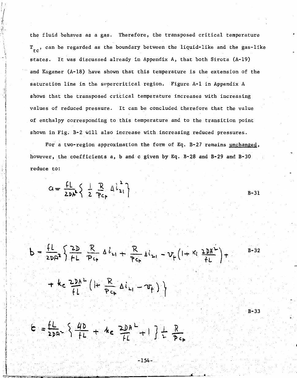
I i I 1 1 i

. 1 J

I I I i f

i

the fluid behaves as a gas. Therefore, the transposed critical temperature

T ,can be regarded as the boundary between the liquid-like and the gas-like tc

states. It was discussed already in Appendix A, that both Sirota (A-19)

and Kaganer (A-18) have shown that this temperature is the extension of the

saturation line in the supercritical region. Figure A-I in Appendix A

shows that the transposed critical temperature increases with increasing

values of reduced pressure. It can be concluded therefore that the value

of enthalpy corresponding to this temperature and to the transition point

shown in Fig. B-2 will also increase with increasing reduced pressures.

For a two-region approximation the form of Eq. B-27 remains unchanged,

however, the coefficients a, band c given by Eq. B-28 and B-29 and B-30

reduce to:

B-31

~t 'lbA"'\...\) f' 1" . L .

B-32

B-33

~154 ..

.-

, '.

~

~ -r 'it

" , r

il " 11

R JI

! J d

II q b ,

ij

l' }

II 11 fl !I .1

11 q t[

t\ \'i t, !,~

f L ,

II U f!

..

,.

which we obtain by setting Ai2'2 = 0, ~Jlfg = 0, Vg2

, = vf in Eq. B-28,

B-29 and B-30;

As noted by Dr. Fleming the use of the two~region approximation simplifies

considerably the form of the coefficients a, band c. The three region

approximation retains however a closer similarity with phenomena that take

place at subcritica1 pressure. The transition region shown in Fig. B-1 can

be regarded as corresponding to the boiling region at subcritica1 pressures.

The liquid and the gas region in Fig. B=l would then correspond to the pre~

heating and to the superheating region in. a once-through boiling system

where the liquid at the entrance is subcoo1ed and the steam at the exit is

superheated. We have noted already in Appendix A that the enthalpy change I

ll.lt"L may be considered as being equivalent to the heat of vaporization

hf

. g

The selection of either the two or three region approximation shou~d

be determined by the desired simplicity and accuracy. The important result

is however the fact that, because of the negative term on the right-hand side,

of Eq. 27, there exist a possibility of a decrease in pressure drop with

increasing flow in the supercritical thermodynamic region. It was shown

in the body of the report that such a .pressure drop vs flow relation can

lead either to excursive flow or to oscillatory flow.

-155 ...

·1 I ,

~

n ;:

it ~ : :1 i', "

11 I' ji

;i ii t: H

)

;i "

fi ~ Ii H

Ii ,I

tl q

1\

fl

I i ~, 'i

. ! ,

.. Appendix C

The upper and lower bounds of the integrals

The integrals given by Eq. IV-94 ,IV-IOI and IV-Ill can be all

expressed in the form of

T -X

which integrates in

I l< -~ -\ til

where K is a coefficient and m an exponent. For example, the

integral given by Eq. IV-Ill is

fe~ Ll>

L·

It can be expressed by

L J1, 'vt, f (~.]~-I J-y

S--'" IA,(~)

i\ {t'J

-156-

C-I

C-2

C-3

C-3

,., , ,

,~

.>.

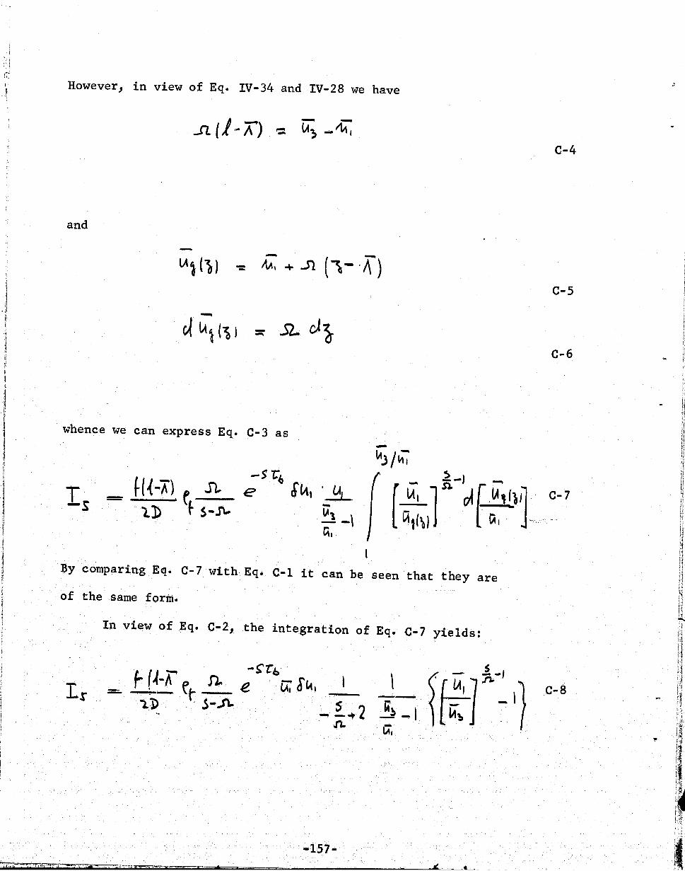
However, in view of Eq. IV-34 and IV-28 we have

and

whence we can express Eq. C-3 as

tl{--"A) e n - 1]) f S-J\..

'U ~ -\,41 _\

~I

By comparing EC1l. C-7 with Eq. C-l it can be seen that they are

of the same form.

In view of Eq. C-2, the integration of Eq. C-7 yields:

\ li~ _I

-157-

C-4

C-5

C-6

f i,.;

which, after some rearrangement, can be expressed in the form of

Eq. IV-111, thus

In order to obtain the upper and lower bound of Eq. IV-94,

IV-101, IV-Ill we note that Eq. C-I can be written as

-

where F is the mean value of F given by

-F --b --J ~ ()c) oiy -

.b-~

PI.

whence by the mean value thereom

-158-Il

C-9

C-10

C-11

C-12

, '1

• l J ; , -

I \

which togethet' with Eq. C-IO yields the upper and lower bounds given in

Eq. IV-95, IV-105 and IV-ll6, thus

For example, from Eq. C-7 and Eq. C-l2 we obtain

since - SIn.

[ ~ ]

'­ , \

it can be seen that Eq. C-l4 can be put in the form of Eq. IV-ll6.

-159-, , ... ;. . --.. ~ ., 5 . a •

C-l3

C-l4

C-l5

--.