1

INSTITUTE OF SCIENCESUNIVERSITY OF FLORIDA

APPLICATION OF SATELLITE FROST

FORECAST TECHNOLOGY TO OTHER PARTS OF

THE UNITED STATES

PHASE II

"Made f ifable tmder NASA sponsors^in the^pterest of early and wide dis

ft*

(E83- IO!UU) A P P L I C A T I O N OF S A T E L L I T E FBOSTFOEECAST T E C H N O L O G Y TO O T H E E P A B 1 S CF THEONITED STATES Final Repor t (Florida Un iv . )321 p HC A 1 U / M F A01 CSCL 02C

N82- 35448T H E UN83-35456Unclas

G3/U3 0 0 4 1 4

35445

APPLICATION OF SATELLITE FROST

FORECAST TECHNOLOGY TO OTHER PARTS OFTHE UNITED STATES

PHASE II

FINAL REPORT

PRESENTED TO:

NATIONAL AERONAUTICS AND SPACE ADMINISTRATIONSI-PRO-33/WILLIAM R, HARRIS

JOHN F, KENNEDY SPACE CENTER

FLORIDA 32899

SUBMITTED BY:

CLIMATOLOGY LABORATORY, FRUIT CROPS DEPT.,

IFAS/UF, 2121 HS/'PP

GAINESVILLE, FL, 32611

CO-PRINCIPAL INVESTIGATORS: CONTRACT NO, NAS10-9876

J. DAVID NARTSOLF NOVEMBER, 1981

ELLEN CHEN (revised)

STANDARD TITLE PAGE

1. Report No.

CR-166827

2. Government Accession No. 3. Recipient's Catalog No.

4. Title and Subtitle

Application of Satellite Frost ForecastTechnology to Other Parts of the United StatesPhase II Final Report

5. Report Dote

November 19816. Performing Organization Coda

PT-SPD7. Author(s) J. David Martsolf, Dr. Ellen Chen,

KSC Monitor: R. Withrow8. Performing Organization Report No.

9. Performing Organization Name and Address

Climatology Laboratory, Fruit Crops Dept,IFAS/UF, 2121 HS/PPGainesville, FL 32611

10. Work Unit No.

11. Controct or Gronf No.

NAS10-9876

12. Sponsoring Agency Nome and Address

National Aeronautics & Space AdministrationJohn F. Kennedy Space Center, NASAKennedy Space Center, FL 32899

13. Type of Report ond Period Covered

Final14. Sponsoring Agency Code

15. Abstract

This is the final report of the second year's activities of a two-year effortto ascertain the application of satellite freeze forecast technology. Theeffort is periodically referred to as CCM II (Cold Climate Mapping Phase II).Input to this report was provided by Pennsylvania State University(C. T. Morrow) and Michigan State University (Dr. Stuart H. Gage andDr. Jon F. Bartholic). Thermal infrared data is taken from the GOES satelliteover a period of several hours and color enhanced by computer according totemperature. The varying temperatures can then be used to assist in frostforecasting.

16. Key Words

Remote Sensing, GOES, Freeze Forecasting

17. Bibliographic Control

STAR Category 4318. Distribution

Unlimited Distribution

19. Security C\assil.(of this report)

Unclassified

20. Security Clossif.(of this poge)

Unclassified

21. No. of Pages 22. Price

KSC FO«M 1«-27«N§ <»««V. 7/Tt>

TABLE OF CONTENTS

CCM II

Introduction 1

Task Reports 5

Task 1 - P-model 5a. P-model exportability 5b. Correlation with ground truth 8c. Environmental fit 8d. Key station locations 11

Task 2 - S-model 12

Task 3 - Limitations 15a. Michigan 15b. Pennsylvania 16

Task M - Recommendations 171) Navigation of satellite data 192) Dissemination of SFFS products 223) Satellite data acquisition 224) Alternative models 255) Rapid communication of weather data 26

Appendices

1. PSU Report . C.T. Morrowa. Reportb. Appendices I - IX

2. MSU Report S.H. Gagea. Test of P-modelb. Preliminary Report

3. Reprint of traverse article J.D. Martsolfij. NSF manuscript J.D. Martsolf5. Japan manuscript J.F. Gerber, J.D. Martsolf6. Letter of 06 October 1981 C.T. Morrow

35450

INTRODUCTION

This is the final report of the second year of activity of a

two-year effort to ascertain the application of satellite freeze

forecast technology to other parts of the U.S. This effort has been

periodically referred to as CCM II (Cold Climate Mapping Phase II);

this acronym appears in the report occasionally.

The first year's activity was accomplished under NASA Contract

NAS10-9611. The final report under that contract is dated October

1980 with the final revision dated March 1981. Although the second

year of activity was clearly a continuation of the first year's work

(notice "Phase II" used in title), a new contract number, NAS10-9876,

was designated and a lapse in the funding occurred from 05/03/80 to

07/10/80. That funding lapse included the frost period in both

Michigan and Pennsylvania. The lapse left Dr. Ellen Chen, a very

productive post doctorate on the first year of the contract, to be

funded by other contracts during the lapse, with the result.that

her full attention was never returned to this effort. Communications

to get Michigan State University and Pennsylvania State University

back on target were time consuming and met with varied success during

the period of this contract.

The Phase II contract (NAS10-.9876) includes a three month period

of "forebearance". This period was granted in response to a request

for a no-cost extension to aid in the development of the final report

-2-

to include final reports from the two subcontractors (copy of letter

dated March 26, 1981 from William R. Harris is included in the 3rd

Quarterly report as Appendix 1). This extension changed the end

date of the contract from July 9, 1981 to October 9, 1981.

This report covers the period from July 10, 1980 through

October 9, 1981. In the case of Pennsylvania, the most productive

data collection period was during the lapse in funding between the

two phases of the contract, i.e. the spring of 1980. Three quarterly

progress reports have been submitted (see Table 1).

TABLE 1. PREVIOUS REPORTS

Quarterly Report

FirstSecondThird

Dated

December, 1980January, 1981April, 1981

Shorthanddesignation

PSU

MSU

TABLE 2. List of COM II SubcontractorsContract WAS10-9876

Institution

The PennsylvaniaState University

Michigan StateUniversity

Investigator Location

Dr. C. TerryMorrow

Dr. StuartGage (Dr. JonF. Bartholic)

UniversityPark, PA

E. Lansing,MI

-3-

As was the case with Phase I (NASA Contract NAS10-9611), the same!

two subcontractors (see Table 2) are involved in Phase II (NASA*;

J Contract NAS10-9876).

Throughout the report the subcontractor's contributions are referred

*" to as the PSU and the MSU Reports, respectively. The PSU Report

j may be found in Appendix 1. All references to Appendices with Roman!

numerals that appear in this report are referring to appendices of

I the PSU Report and are all contained within Appendix 1. The next

4 paragraphs appear to contain exceptions to this rule but noticeii that the Roman numerals refer to appendices of previous reports to

i NASA. Reference to the table of contents will aid in .clearing upi

any confusion that may result from this effort to retain the

| contributions from the subcontractors in as near to original format

as possible. The MSU Report makes up Appendix 2b of this report.!i A very elaborate proposal was submitted by Dr. Stuart H. Gage

\ of MSU and is contained in the First Quarterly Report as AppendixJ

I of that report. While it does not directly address the Tasks as

i outlined in the Statement of Work, it places the CCM II effort very

convincingly in the midst of the development of a broad based -remote?

' sensing capabiity that is under development at MSU. MSU's contribution

I to the second Quarterly report was late (arrived January 20, 1981,*J

a few days after our Second Quarterly Report had left-for KSC) and

f I was-retained for the Third Quarterly Report, becoming Appendix V of

that Report. After a series of phone calls and an attempt by Dr.

-it-

Gerber to aid in the procurement of a draft of the final report

while he visited MSU in September, the draft was received on October

7, 1981. This was in time to include the MSU draft in the draft of

the CCM II final report (the latter report was in the process of

being mailed when the MSU draft arrived). However, there were very

few cross references in the CCM II final draft that concerned the

MSU report. Most of these have been added since the MSU draft

arrived in October. Some modifications to that MSU draft are still

expected at the time of refinement of the CCM II report, i.e.

mid-November, 1981. It might be added at this point that it is our

understanding that both Dr. Jon F. Bartholic and Dr. Stuart Gage

worked over a weekend to get the draft to us as soon as it arrived.

It is included in this report as Appendix 2b.

A phone call from MSU on October 1, 1981, passed (verbally)

the data that MSU had collected to test the P-model. Mr. Robert

Dillon, a programmer I, received that data and prepared it for input

into the P-model evaluation programs. The results of those runs

make up Appendix 2a.

The proposal from the PSU subcontractor arrived too late to

include in the First Quarterly Report even though that report was

held for some time in anticipation of receiving that PSU proposal.

Consequently, it became Appendix I of the Second Quarterly (Mid-term)

Report. The PSU proposal followed the tasks in the Statement of

Work closely and disclosed that data collected on 5 frost nights

-5-

] during the Spring of 1980 would be used to test P-model. Veryi

productive communications resulted in the delivery of that data for

y P-model runs at UF/IFAS and the communication of the results back

PJ . to PSU for evaluation. These results are covered in detail in the

PSU Report that makes up Appendix 1 of this report. Note that there

j are nine (9) appendices to the PSU Report which are numbered in!

Roman numerals."!j The following portion of this report entitled TASKS REPORTS is

: written in a format in which the individual task is first declaredji' and then a discussion of progress toward that task follows. In the

i case of Task I there are four parts of the task denoted by a, b, c,

and d.

i

- TASK REPORTS

Task 1: From data bases collected, make sample runs of the

P-model and/or concept and present observations/conclusions as to:«

j

a. Can the P-model and/or concept work in that particular41 geographic setting;

J .Data from Michigan State University documenting the frost of

y May 6-7, 1981 were passed to IFAS/Climatology by telephone (verbally)

on October 1, 1981. Mr. Robert Dillon copied the data and prepared

-6-

it for input to the P-model. The results of that analysis make up

Appendix 2a.

The average error made by P-model in 55 predictions made using

the MSU data was -0.02U°F with a standard deviation of 2.374 degrees.

The worst prediction was a 6-hour forecast made at midnight that

predicted a 6AM temperature 6.1°F too low. The large positive errors

were all made in the 9PM forecast for the remainder of the night,

i.e up to 10 hours ahead. The 10-hour forecast for 6AM was slightly

over 3 deg. F too high. The P-model's performance was judged quite

acceptable.

Sample runs of the P-model were made on data from Pennsylvania

(see Appendix VI of PSU report for detail). Numerous phone

conversations, magnetic tape exchanges, and visits by the investigators

(see Table 3) improved computer to computer communications between

Dr. C.T. Morrow's Lab at PSU and the Climatology Lab at UF/Gainesville

to the ext'ent that such analyses can be quite effective in the

future. The visits helped clarify communication problems and resulted

in the depth of interpretation that characterizes the remainder of

this report (see also Appendix 6).

A copy of PSU's proposal makes up PSU Appendix I, i.e. Appendix

1, Appendix I. While it suggests that 5 nights of data are available

for the Spring of 1980 and more data would be collected for the

Spring of 1981. The data was first received at Gainesville in the

format indicated in Appendix II. While such graphs of temperature

-7-

Table 3. Exchange visits by COM II investigators.

J Visitor Location Dates (1981)uJ.D. Martsolf Pennsylvania State Univ. August 26-27

m T_'niv. Park, PA.H Ag. Engr. Lab, Environ.

MeasurementsI4 C.T. Morrow University of Florida September 28-29

Gainesville, FLClimatology Lab, HS-PP

!«j

data versus time served in the selection of particular nights that

[ • qualified as typical frost nights, they did not provide input

appropriate to the P-model. Consequently, a procedure to go back

to the original magnetic tape records and transfer appropriate

records to a tape that was later sent from Pennsylvania to Florida

was developed (see PSU Appendix III). The testing data base was

reduced to the first 4 nights of the 1980 data (see page 9 of PSU

report, Appendix 1). Dew point temperatures were located in aa

hand-written log and called down from Pennsylvania to Florida (see

(! PSU Appendix IV) and incorporated in the P-model input files (shown

in PSU Appendix V). The results of the P-model input runs of the

; Pennsylvania data comprise PSU Appendix VI. Dr. Morrow discusses

these results on page 10 through 13 of the PSU report (Appendix 1).i

•-^ It is possible to add to his discussion that he was surprised that

n the model worked as well as it did for the particular site that was

used. The main criteria for choosing the site was that it was

available (a rather arbitrary choice).

-8-

Conclusion: Comparisons of the PSU P-model runs with those on

pages 36 through 42 of the SFFS V Mid-term report, i.e. runs on

Florida Key Station data, with those of Michigan (Appendices 2, a

& b) and with those of Pennsylvania (Appendix 4) indicate that thes

P-model seems to do as well in mountainous terrain as it does on

the gentle rolling to flat Florida or Michigan terrain (c.f. pages

11 and 15 of Appendix 4). The P-model concept may be considered

effectively independent of geographic setting. However, if P-model

were determined by future analyses to show bias it is conceivable

that such bias could be corrected by some minor modification to

P-model. In other words, these studies revealed no reason to feel

that the P-model will be a problem in the exportation of the SFFS

concept.

b. Degree of correlation with ground truth data;

Table 3 of Appendix 2b summarizes the error analysis of the

MSU data, i.e. the difference between the P-model predictions and

the observations. There was a mean error by P-model of -0.024°P in

55 comparisons. This is very acceptable.

Table 6.3 of the PSU Appendix VI summarizes the error analysis

performed on the PSU data. There was a mean error by P-model in

264 comparisons of only 0.6°F (see Table 6.1, PSU Appendix VI) which

is quite acceptable (page 11, PSU report, Appendix 1).

-9-

I c. Appropriateness to agricultural/meteorological

environment;

y

a Pages 8 and 9 of the MSU Report (Appendix 2b) describes 5

reasons that the P-model seems appropriate to the Michigan environment.

.1 These point primarily to the similarity in the expected energy

transport mechanisms, i.e. both radiative and convective, during•-;

•j • freezes in both Florida and Michigan.

; Page 13 of the PSU Report (Appendix 1) initiates a discussionI' by Dr. C.T. Morrow of the appropriateness of the P-model to the

agricultural needs of Pennsylvania and by inference to the fruit

growing areas of Northwestern U.S. He concludes that the model has

: quite a bit of applicability (see pages 15 and 16 of PSU Report,

Appendix 1; and also Appendix 6).

It seems to this author (who feels somewhat qualified to speak

to this question by virtue of 13 years of experience in frost

protection research in Pennsylvania) that two characteristics oft

I fruit production in temperature zones have permitted growers to

register less concern about frost or cold damage in comparison to

'' those who grow tropical plants in sub-tropical climates, e.g. citrus.

i One of these is that the production areas in. the temperate zonesJ

are generally more .scattered over the total area and consequently

^j when frost damage occurs its localized effects define a minority of

affected growers. Secondly, only the crop is in jeopardy; the trees

-10-

live on to potentially bear another year. However, while producer

pressures may not be as high in deciduous fruit areas for frost

warning services the total extent of the damage is large. The

consumer pays for the losses in higher fruit prices and some of the

transportation and marketing mechanisms suffer greater fluctuations

in their volume, leading to operations inefficiencies and finance

problems.

Regarding, the appropriateness of the P-model to the meteorological

environment there are no apparent reasons that the large scale

weather is significantly different from that in Florida, i.e. the

frosts occur primarily in the presence of a large high pressure

dome. On the micrometeorological scale there seems to be some reason

for concern because the P-model is a one-dimensional model, i.e.

the vertical components of the energy budget are primarily involved.

Cold air drainage, horizontal flow of heat, would seem to be ignored

except for the wind speed indicators that have the opportunity of

tipping off the model that down slope flow is occurring. The

resulting mixing is likely to forestall as rapid a temperature drop

as would otherwise occur. This mechanism is apparently handled

quite effectively because the model seems to have predicted the

temperatures at the Rock Springs site in Pennsylvania rather well;

That site is on the West slope of Mt. Tussey, i.e. very much in a

cold air drainage pattern.

-11-

d. If feasible, discuss parameters important to the

location of key weather stations, i.e. numbers,

settings, etc.

The MSU Report (Appendix 2b) does not directly address this

question but contains a statement on Page 9 that indicates there

has been a persistence of temperature differences between stations

in the MOSS product analysis. They interpreted this as an indication

that there are good correlations between key (weather forecasting

sites) locations and agricultural weather measuring locations.

While it is not explicit in Appendix 2b it should be noted that

Michigan already benefits from one of the largest and most effective

network of agricultural weather stations in the nation.

Dr. C.T. Morrow discusses a computerized dissemination network

that PSU is planning (see pages 16-18, PSU Report, Appendix 1).

There are possibilities that the communication network may include

automatic weather stations to support integrated pest management

programs as well as to facilitate a warning system similar to the

Satellite Frost Forecasting System. The Meteorology Department of

PSU has had an automated weather station in operation for some time

on top of the 5-story building in which their department is housed.

There have been negotiations underway to move that station off the

building roof and onto agricultural lands of the Agricultural

Experiment Station that are'likely to remain in similar service for

-12-

years to come in order to make the observations more characteristic

of the surrounding countryside. This has immediate implications in

the feasibility of the acquisition of ground data for the Nittany

Valley.

' The National Weather Service has provided frost warning services

from a station in Kearneysville, West Virginia, but under the manpower

reductions this position has remained vacant in recent years. The

previous weather service provides some tradition around which an

automated station might be located since the University of West

Virginia operates a branch station of their Agricultural Experiment

Station there. The branch station at Biglerville is another

possibility. Several possibilities exist to represent the concentration

of fruit production in what is referred to as the Cumberland-Shenandoah

production region. The region is well represented by a meeting of

researchers and extension specialists serving the fruit industry in

a group called the Cumberland- Shanandoah Fruit Worker's Conference.

There is a good possibility that this group would play a very active

part in the placement of automated stations in the event of the

implementation of a SFFS-like program.

Task 2: Give observations/conclusions as to the applicability

of the S-model and/or concept from the data base at the two areas.

This portion of the study must be general as this subject cannot be

, I

-13-

covered comprehensively without substantial work in statistical

evaluation of temperature correlations which is beyond the scope of

this contract.

Recent developments with the S-model indicate that there are

good possibilities that the coefficients for the model may be produced

by the minicomputer system supporting a SFFS-like system. This

certainly could be the case for areas like Pennsylvania and Michigan.

However, this possibility was not sufficiently apparent at the time

that the subcontracts were drawn up to attempt to test the concept

through the subcontracts.

The S-model represents the possibility of developing a SFFS

that can recall the distibution of temperatures during previous

freezes in a particular area and bring that cold climate climatology

to bear upon present forecasts. Since compouters have excellent

memories, the concept of recalling such information from memory and

influencing the forecasts with it is good climatology and very likely

will be attracive to any who adapt SFFS to their locations. However,

the S-model in its current configuration fails to live up to these

expectations. It may not be a trivial matter to bring past freeze

information to bear readily upon current freeze events until the

navigational problems with the satellite data from one year to

another are resolved. That problem is defined well enough to declare

it nontrivial. This line of thought is discussed in more detail

under Task 5.

-14-

Certainly, there will be pressure on SFFS developers and adapters

to lengthen the period over which the system can be expected to

successfully or usefully forecast. The possibility of using the

excursion of temperatures above a common base during the day previous

to the freeze as convincingly related to the amount that temperatures

may be expected to drop below that base on the subsequent clear

night gives hope of lengthening the forecast period. Drs. Hartwell

Allen and Ellen Chen have been perfecting a method of determining

the heat capacitance of soils by observing the temperature excursions

through clear days using day and night IR image sequences after the

fact. The moisture conditions in a particular locality have been

found by Dr. Ellen Chen to be clearly involved in the amount that

one may expect that locality to cool under radiant frost conditions.

It is likely that the development of this heat capacitance mapping

technology will spin-off into the SFFS development with the possibility

of extending the points in time from whence the system will forecast

into the previous day, i.e. develop forecasting periods approaching

20 hours, double the current capability. Without the present

limitation on the range of temperatures that can be acquired via

1200 Baud link with Suitland, Maryland has prevented the acquisition

of daytime IR maps in sequence with nighttime IR maps due to over

or under ranging problems at NOAA/NWS. This program is discussed

in more detail under Task 4.

Pages 10 and 11 of the MSU Report (Appendix 2b) describe in

-15-

some detail the conviction that similar temperature patterns persist

from one frost night to the next indicating a stong dependence on

surface vegetation and soil characteristics. Figures 1 through 4

of Appendix 2b were submitted as evidence of such persistence.

Task 3: Identify and discuss any peculiarities of the Michigan

and Pennsylvania sites which might limit conclusions from being

applied elsewhere in the United States as a general case.

a. Michigan: A peculiarity of Michigan under frost conditions

is that the wind speed seems to be less likely to go to zero during

the event, making wind machines and other frost protection methodology

difficult to adopt without some qualification. This peculiarity in

the case of a SFFS-like system works in favor of the system when

used in Michigan. The more the wind tends to mix up the -air near

the surface the more likely the pixel temperatures determined by

the satellite are to very closely represent the temperature of the

whole area. If other areas of the Midwest were thought to have

greatly different frost conditions than Michigan has there would be

a problem in extrapolating the experience from Michigan to Ohio,

Indiana, Illinois, Kentucky, Missouri, Wisconsin, Minnesota, Iowa,

Nebraska, etc. However, all of this area of .the United States seems

to have high pressure domes that continue to move with the westerlies

across the country during the frost season (both spring and fall)

-16-

so that the periods of dead calm under the center of the high are

relatively short. The further south one goes, the more likely the

high pressure domes are to become stalled between the westerlies

and easterlies, resulting in longer periods of cold, clear and calm

weather.

Since the paragraphs above were developed the MSU Report

(Appendix 2b) arrived with an explicit statement concerning Task

III (see pages 11 and 12 of that report). It declares the Florida

and Michigan cases to be very similar but an earlier statement (item

3 on page 8) indicates that Ceel Van Den Brink had interpreted in

earlier work that approximately 70% of Michigan's frosts were

radiational and 30% were advective. Since this ratio would be more

like 90:10 in Florida the author of this report has let the following

conclusion stand.

Conclusion: The Michigan case provides a good example for the

remainder of the Midwest. The Florida experience is more likely to

be a good example for the southern U.S.

b. Pennsylvania: The PSU site is on the slope of one of the

narrow ridges that separates the broad fertile valleys of the fruit

growing portion of the Appalachian Mountains. The diagram that

makes up Figure 2 in Appendix 3 demonstrates-two points:

1) the variations in temperature under frost conditions

in mountain-valley topography are very similar from

-17-

one frost to another.

2) these variations closely follow the topography and

have distance scale very similar to the intervalley

topographical features.

Figure 1 relates this situation to a typical pixel from GOES,

i.e. approximately 25 square miles in area. If the pixel location

is known, i.e. the pixel is oriented relative to the geography of

the covered area there is an excellent possibility that the relationship

between the pixel temperature and that of particular sites covered

by the pixel will become known and used with reliability.

Conclusion: small scale (relative to pixel size) variations

in topography and hence in temperature distribution may not pose a

serious limitation to the usefulness of a SFFS-like system in

mountainous terrain. However, in order for the products to be

convincing it is likely that a period of time is necessary during

which the product users become calibrated or convincing research

must be accomplished for each area that relates individual site

temperatures to pixel temperatures. Finally, it is assumed in this

discussion that it will become possible in these systems to orient

the pixels with respect to the location they actually cover.

Task 4: Give recommendations as to whether the concept should

-17a-

ORIG1NAI PAQS Ii'OF POOR QUALITY

T

Tr

A X

Fig. 1. Sketch of pixel with dimensions larger than elements of

temperature fluctuation implying that if the pixel remains constant

relative to the topography (AY = AX = 0) and the temperature

distribution remains constant relative to the topography for post

events (a well documented horticultural observation) then given

locations will have predictable AT with respect to the pixel

temperature (Tp).

-17b-

°0'o

N0*

^A

UT

f

oQQ(TO)

COQh-

LUcrCOLUo

0) 0>

H -H

9

M•u

6 to

a, aj a)

nj w

ao a>>%

-o

en m4J

13CO

-HT

3 -H

M

0) 43

OCO

H

t-HO

P

Ma.o

• ~

t-i « co•H

iH

C

M -H

a) o

>

(11 rH

C

O42 PM

a)C

-rl

COcfl -H

cflO

4-1

•>

4JQ

) rH

fi

a 4J co a)cu

cd c* g

4->

M

r-t 4J

co cu

^>% &,

~ cdco

o •-1 ft0)

^

P H

«<u

CO

O

CO-d

CO

QJ

O•U

<U

•H

CrH<U

cd4-1

4J

Cd

td

O(UQ

co

W

w8

-HrHrHa>

QJJ3

4-1•u

cdca4-1o <u^0 4J

cdM

<u00 Ncd

-H•H

>-<

P O4Jo

• a)C

N

CO

<u TJ^ a

3 cdoo

•HEn

4-1U

-H

3 3

o

n.n

fen]

curH

X

!C

d 4-1

Mo c

•H -rl

4Jcd

jat-t

cda) >-)o.o

>^60

0) O

e HO

O

O

4Jcu

cd

^ O

rH4-1

O

T3

C

OQ

) <J

4->

PH

O M

0)CU

0)X

X

!0)

4J

-18-

be pursued further and if so, what specific studies should be

performed. .

On pages 20 and 21 of the PSU Report (Appendix 1), Dr. Morrow

makes six recommendations regarding the future of this type of study.

These might be summarized to have indicated that while there is

additional work that is identifiable, the concept is useful and is

likely to be pursued (see Appendix 6) . Communications with Dr.

Morrow along these lines permits this author to indicate that a

joint effort between the Pennsylvania State University and some

private company is the likely future developer of this sort of

service in the Northeastern U.S.

The Department of Meteorology of INPE, Brazil, is down linking

GOES-East IR data to document the location and intensity of freezing

temperatures during very cold nights in the coffee and citrus

producing areas of Brazil. Mr. Michael Allan Fortune made contact

with IFAS/Climatology when he was visiting NOAA/NESS in Suitland,

MD on Oct. 5, 1981, to describe the Brazilian acquisition system

and request information about SFFS. At our suggestion he also made

contact with NASA/KSC and NASA/HQ (Mr. James M. Dodge, in the latter

case). We have exchanged some information and it is apparent that

both parties would probably benefit from closer communications

concerning the nature of the efforts.

Appendix 2b contains MSU's recommendations for additional work

in the following areas: P-model performance when Michigan soils

-19-

are frozen in the early Spring; collection of GOES data from NOAA/NESS

on a real time basis; correlation of temperature patterns with~"!fj general surface conditions during freeze events. On page 12 of

ra Appendix 2b indicates that, "Clearly, the conceptual theme of using

GOES data to aid in characterizing the thermal regimes in a stateiI both in non-real and real time, need to be further prusued. The

data proves to be very accurate, particularly during freeze eventsi

I and correlations of temperarture patterns with general surface

conditions would indicate more information could be obtained."

; Appendices 4 and 5 contain manuscripts that describe the SFFS

system as reported to a group of scientists having responsibilities

for the communication of agricultural weather data and to an

international symposium on citriculture in Japan. Both manuscripts

describe SFFS as a rapidly developing methodology that has potential

i application in horticulture when the industry experiences frost

hazard. Most horticultural industries are climatically temperate

1 or subtropical and consequently experience frost hazards.

The following are specific studies that it would seem from our

experience to be necessary to the utilization of a SFFS-like thermal

] map display and forecasting system:IttJ

11 1) Navigation of the Satellite Data

-20-

The user of the information in real-time must know where his

fruit is located in relation to the thermal map or the value of the

information is greatly reduced in his decision-making process.

While survey results published in NAS10-8920 Reports indicate that

Florida growers can find their location within a couple of pixels

on thermal maps of the entire peninsula, the growers are quick to

expect geographic references that have some reliability. It. should

be noted at this point that if the information is to be valuable to

the real-time user it must be available to him within a matter of

minutes after it becomes available from the satellite.

The use of the data in the assessment of damage and subsequent

planning of transportation and marketing scenarios is a near real-time

operation and seems even more dependent on good geographical

orientation of the data in order to couple the data with densities

of crops for which the critical temperatures are known. The Jan.

13, 1981 freeze in Florida demonstrated this use of SFFS products

convincingly. At this point the need for some standardized pixel

location becomes apparent. The data bases upon which assessment

programs will depend will undoubtedly be fixed in space and require

that some interpolation of the satellite data be made to line up

the temperature fields directly on top of the areas for which the

crop densities have been determined.

Finally, the long-term user of the temperatures for climatological

studies which we have been terming, "cold climate mapping," or CCM,

-21-

• must be able to relate thermal maps one with another over extended

periods of time, i.e. years. Consequently, not only do the navigational

tJ studies need to deal with orientation on the face of the globe but

g with the software that seems necessary to develop time series of

data that have acceptable space orientation. It is becoming apparent~\

.j that this includes stretching and rotation as well as the simple x

and y offsets of the rectangular coordinate system.!

4 The navigation or orientation of the satellite data was indicated

• i under Task 2 to be critical to the successful operation of S-model

as it currently exists. But fairly sophisticated tools to study

this problem are becoming available in the SFFS software. Consequently,j

there is hope that the goal of developing a system that will have

a recollection of past freezes and be able to bring such information

not only into display to remind the forecaster of the scenario but

also to incorporate the patterns into the forecasted product through

*: the S-model is realistic. The effort would seem to be dependent

upon the ability of the system to stack the pixels in time over ae

particular geographical location. The changes in temperatures of

I these pixels (even during the previous day) become the principal!

ingredient upon which the model forms its predicted product. The

j memory of past events comes into play by the development of software

that can relate the current happening with a similar one of the

La past, either automatically or with aid from the user. In its present

configuration, the potential power of SFFS is far from its zenith.

-22-

This is an emphatic recommendation that the effort with S-model

development continue.

2) The Dissemination of SFFS products

This is viewed as a continual process that is necessary to

achieve the maximum value from the observed and forecasted products.

We appear to be on the threshold of an era of the home computer

controlled communication device that brings in all manner of

information from which the user can make decisions in finance,

purchasing, services such as transportation, lodging, etc.

Opportunities to interface with these various private, quasi-public

and public service communication networks should be investigated

and capitalized upon where appropriate. Funding from the USDA/SEA-

Extension has been requested and some obtained (Agreement 12-05-300-535,

Amendment 1) for this purpose. Further efforts along this line are

anticipated by UF/IFAS. These include the pursuit of contacts with

television firms. So far there have been two promising contacts in

this latter area, one from Ft. Myers, and the second from St.

Petersburg.

3) Satellite Data Acquisition

Currently, the satellite freeze forecast system (SFFS) is

-23-

dependent on a 1200 Baud link to a NOAA/NWS queue in Suitland,

Maryland, that in turn is dependent upon the successful operation

of at least two batch programming operations to transfer the data

from the antenna to a data base from which it is sectorized for the

Florida queue. While this experimental link worked rather well in

the 79-80 frost season, it was quite unsatisfactory during the 80-81

season and little hope has been provided by NOAA/NESS, or for that

matter NOAA/NWS, that much better performance can be expected from

an experimental link on a system that has as much operational pressure

as theirs. The MSU Report (Appendix 2b) indicates on Page 7 that

the method of obtaining GOES data from NESS in Suitland was no longer

operative and that they should use the historical archiving system

at Wisconsin. MSU on pages 13 and 1*1 of Appendix 2b describes

difficulties and frustration in acquiring satellite data due to a

rapid change in NESS policy. IFAS attempts to acquire the data on

MSU's behalf were disrupted by the declaration of center of sector

being within the NOAA/NESS program at Suitland and not under IFAS

control.

The direct downlink described in Figure 2 has been proposed

and largely funded by IFAS to be operational during the 81-82 season.

Since there is no redundancy in the system, it will serve simply as

a back-up to the current method of satellite data acquisition

described earlier in the paragraph.

Initially, SFFS acquired satellite data from the GOES-TAP link,

-24-

an analog linkage through the NOAA/NESS field station in Miami.

The analog data was digitized at the SFFS site in Ruskin, Florida,

for use in the SFFS display and forecast software. Presently, the

digital data in the NOAA/NWS queue in Suitland, Maryland, is in the

form of ASCII characters.

The number of characters in the ASCII set is 95, restricting

the temperature range over which data can be transmitted to 95/2 or

7.5 C (85.5 F) since the infrared temperature resolution of GOES

is 0.5 C. Actually the data is downlinked in binary and the complete

range 000 through 255 (256 temperature divisions from -110.2°C to

56.8°C or -165.3°F to 13 .3 ). If the data could be passed from

NOAA/NWS to SFFS in binary instead of translation to ASCII, it is

much more likely that most of the full scale would be available

(some combinations become illegal due to control character assignment

through the various software interfaces involved). Mr. Art Bedient

at NOAA/NWS is presently trying to develop the binary data transfer

possibility. IFAS/Climatology is trying to ready SFFS to accept

binary data input since the antenna link will transmit in binary

format.

SFFS's acquisition of digital satellite data from GOES has been

taking place in parallel with an effort connected with with a much

more sophisticated (and consequently expensive) acquisition system

known as McIDAS. The development of McIDAS has reached a stage in

which a private company, Control Data Corporation, appears to be in

-25-

the process of producing systems that used to be available in limited

numbers through the University of Wisconsin. Both SFFS and, we

understand, McIDAS are NASA developments. There may be some mutually

beneficial exchanges of information between the developers. Certainly

SFFS would benefit from increased reliability in satellite data

acquisition and aid in the navigational aspects of the data orientation.

Contact has been made with Control Data Corporation (CDC) to identify

several possibilities that SFFS may benefit from the presence of a

McIDAS in Florida and that CDC may benefit from the incorporation

of an additional application, i.e. the frost warning products, into

McIDAS.

4) Development of Alternative Forecasting Models

There is every reason to believe that with time the forecasting

models, i.e. the P-model and the S-model, will be improved. Certainly

there is a need to develop simpler models that will operate on less

expensive computer systems, e.g. the APPLE 11+ system that is being

used by 6 counties currently interfacing to the SFFS/Florida system.

One much simplified S-model uses coefficients that simply relate

the pixels to changes in key station temperature as weighted by the

distance of the pixel being forecasted from the particular key

station.

With increased use of the SFFS systems there is little doubt

-26-

that various resarch efforts will find it both convenient and

advisable to experiment with new models and test their performance

against the present models. As the users of the system become more

sophisticated in their demands for options on the system, there will

be continued pressure to develop additional features as justified

by need.

5) SFFS's potential role in rapid communication of weather data

Currently, SFFS products are communicated to users in the

following manner: first the NWS forecasters at Ruskin see the

products displayed on the color monitor and, in the case of the key

station data, on a clip board on their data board. They make their

forecasts and communicate them to radio stations and other media by

the same procedures that they have used before having SFFS. SFFS

may be mentioned in this process but it is more likely that the

users of the NWS frost warnings will not be aware that such a tool

exists and is influencing the forecasts.

Secondly, SFFS products are beginning to be linked to other

display systems from both the Ruskin and the Gainesville components

of SFFS. Last winter, APPLE II computers at the Lake County and

the Polk County Agriculture Extension Centers received satellite

maps from a third APPLE in Gainesville, and built displays for the

agents, John Jackson and Tom Oswalt. The impressions they gained

-27-

from viewing the thermal maps were relayed through the tapes they

played to subscribers of phone links to electronic secretaries.

These agents carry out very effective educational programs in frost

protection on freeze nights through these verbal telephone links

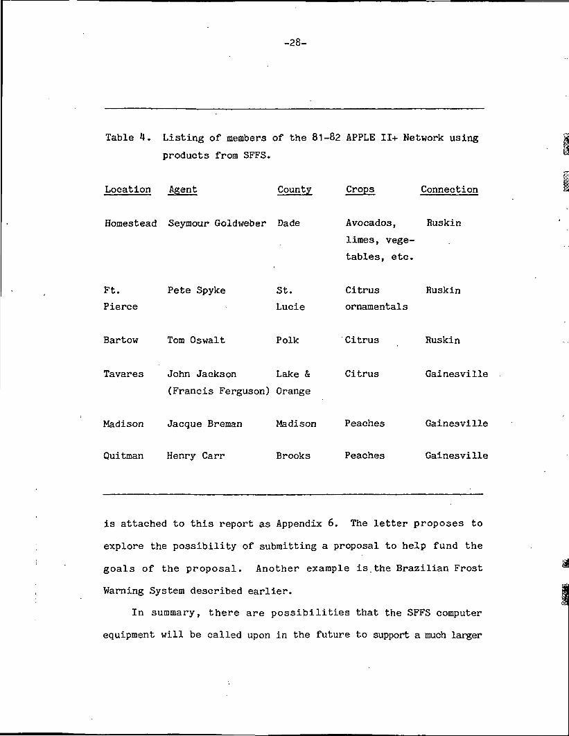
with growers. Largely because of the popularity of the concept,

this APPLE 11+ network has been increased to six county offices this

year. Four are in counties with citrus and two in peaches (see

Table 4).

The rate at which the ASCII character string can be communicated

from queues in the Hewlett-Packard minicomputers that service them

has been increased this year to 1200 Baud. It requires about 3

minutes to transmit a thermal map to a user by the new network.

In addition to serving the new APPLE 11+ network from Ruskin

the HP mini is expected to acquire the dew point information it

needs to make its P-model forecast through a port in the NWS/AFOS

mainframe. Once this link is established it seems possible and

quite likely that other weather data available in the.AFOS system

will become available to SFFS and be transmitted by the APPLE 11+

Network to users. Digitized radar maps are likely to be targets

for this link as well as many of the text formated weather summaries

that are not communicated by AFOS.

Finally, SFFS in Florida, may have additional opportunities to

support similar efforts in other states. For example, PSU outlines

an attractive possibility in a letter dated October 6, 1981, which

-28-

Table 4. Listing of members of the 81-82 APPLE 11+ Network using

products from SFFS.

Location Agent County

Homestead Seymour Goldweber Dade

Ft.

Pierce

Pete Spyke

Bartow Tom Oswalt

St.

Lucie

Polk

Tavares John Jackson Lake &

(Francis Ferguson) Orange

Madison Jacque Breman

Quitman Henry Carr Brooks

Crops Connection

Avocados, Ruskin

limes, vege-

tables, etc.

Citrus

ornamentals

Citrus

Citrus

Madison Peaches

Peaches

Ruskin

Ruskin

Gainesville

Gainesville

Gainesville

is attached to this report as Appendix 6. The letter proposes to

explore the possibility of submitting a proposal to help fund the

goals of the proposal. Another example is.the Brazilian Frost

Warning System described earlier.

In summary, there are possibilities that the SFFS computer

equipment will be called upon in the future to support a much larger

-29-

menu of products than simply the SFFS products. To accomplish this

there is a need to develop some very flexible software to handle

the link between SFFS and AFOS. Secondly, the link into AFOS may

permit other areas of the United States to capitalize on SFFS products

by picking up summaries or renditions of them off the AFOS schedule.

However, this possibility is clearly in the domain of NOAA/NWS and

will be explored at their instigation.

811118 "1278::45

3 35451

APPENDIX 1

P S UPennsylvania State University

Report

Author: Dr. C. Terry Morrow

d

APPLICATION OF SATELLITE FROSTFORECAST TECHNOLOGY TO OTHER PARTS OF

THE UNITED STATESPHASE II

FINAL REPORTPENNSYLVANIA SUBCONTRACTOR

Submitted to: University of FloridaInstitute of Food and Agricultural Science2121 HS/PFGainesville, Florida 32611

Submitted by: C. T. Morrow, Principal InvestigatorDepartment of Agricultural EngineeringThe Pennsylvania State UniversityUniversity Park, Pennsylvania 16802

Submitted on: September 21, 1981

Signature

C. T. Morrow, Principal Investigator

Table of Contents

Page

Introduction 1

Task 1. Collection of Data for P-Model 2

A. Description of Test Site 2i. Topography 3ii. Physical Description 3iii. Climatological Features 4iv. Aerial Photographs and Topography Maps 4

B. Data Collected 8

C. P-Model Analysis . . 10

Task 2. Description of the Major Apple Growing Regions ofPennsylvania 13

Task 3. P-Model Limitation 15

Task 4. Future Projections and Recommendation 16

Cited References 22

Appendices

Appendix I - Proposal from Penn State to University of Florida

Appendix II - Frost Data for Pennsylvania Test Site

Appendix III - Tape Description for Pennsylvania Frost Data

Appendix IV - Dew Point Temperatures for Pennsylvania Test Plots

Appendix V - Reduced Data for Pennsylvania Test Plot

Appendix VI - P-Model Analysis Results

Appendix VII - Pennsylvania Orchard and Vineyard Survey

Appendix VIII - Climate of Pennsylvania

Appendix IX - The Office for Remote Sensing of Earth Resources

Introduction

This final report of work performed under a grant for application of

satellite frost forecast technology to other parts of the United States,

Phase II is being submitted by The Pennsylvania State University to the

University of Florida for inclusion in a final report to the National

Aeronautics and Space Administration. The work being described in this

report is the result of the second year of support from NASA relating to

this topic.

The work performed by The Pennsylvania State University is in

accordance with a proposal which had been submitted from The Pennsylvania

State University to the University of Florida on December 1, 1980. A copy

of this proposal is included as Appendix I of this final report. Thei

findings at The Pennsylvania State University will be described in terms

of the objectives of that proposal. In order to make the task easier for

j the University of Florida to prepare a consolidated final report, however,

the findings and conclusions will also be reported in terms of tasks which

i had been requested by NASA for Phase II of this project.

: There was a large amount of data collected at The Pennsylvania State

University experimental sites for the purposes of this study. Much of the

, raw data has been included as an appendix to this final report and will be

discussed where appropriate. In order to make the most concise conclusions;,

LJ relative to the objectives of this project isolated portions of that data

pf have been analyzed in detail. Many findings which will be presented during

the course of this report are results of interpretation of selected data as!

; opposed to an overall evaluation of all data collected for the project.

This approach was believed to be very desirable in view of the time required

for data analyses. There is, however, believed to a sufficient quantity of

data fully analyzed to enable some clear indication of the merits of the

techniques being evaluated as a part of this contract.

Task 1. Collection of Data for P-Model

A. Description of Test Site

The data which was collected for use in running the freeze

prediction model, P-Model, as described by Sutherland (1980) was

obtained at the Rock Springs Agricultural Research Center. This

facility is the location of the primary agricultural research

station for The Pennsylvania State University. For the past

several years extensive frost protection research has been

conducted at this location. There are two primary orchard

facilities available at this station. One of these orchards is

equipped for heaters for studying the use of heating as a frost

protection technique. An adjacent orchard has the facilities

for providing overhead sprinklers as an alternate method of frost

protection. The sprinkled orchard was the location of the test

instrumentation for obtaining the measurements reported for this

study.

-3-

i. Topography

The Rock Springs Agricultural Research Center is located

about nine miles west of State College, PA, latitude 40°42'23"

north, longitude 77°57'20" west. The orchard elevation is 1240

. feet above sea level. The site is located at the base of

"Gobbler's Knob", a mountain ridge with an average top

elevation of 1840 feet (peak 1860 feet). The orchard is 3500

feet NNW of the peak directly downslope.

The general slope of the orchard area is a 1 foot drop in

elevation to 50 feet horizontal. The slope of the orchard

itself is about 1.5 foot drop to 100 fee horizontal sloping

down towards NNW.

ii. Physical Description

The orchard is made up of two blocks, 209 trees per block.

Each block consists of 19 rows, 11 tree per row, 10 foot spacing

between each tree. The site size is 324 x 230 feet, each block

324 x 100 feet with a 30 foot space between the blocks. The

rows are oriented NNW-SSE.

A stream 300 feet to West of the orchard provides water for

a large and thick stand of conifers. This sets up a year- round

wind break for the prevalent west wind. A stand of pines 50

feet to the NE provides a wind break for the Easterly winds.

The NNW and SSE directions are exposed. To the SSE between the

mountain and the orchard there is a large open field and there

are some small orchards with short trees to the NNW.

-4-

iii. Climatological Figures -

The following table shows average monthly climatological

information for the State College area (Spring months):

Dry bulbtemp. F

Max. drybulb °F

Dew pointtemp. F

Precipitationinches

Wind MPH •

Solar inso-lation BTU's

Solar fraction

March

36.6

46.0

27.0

3.43

10.0

1090

.466

April

49.0

59.0

38.0

3.34

9.0

1404

.472

May

59.9

71.0

48.0

4.03

9.0

1685

.494

June

68.1

79.0

58.0

3.34

6.0

1914

.530

iv. Aerial Photographs and Topography Maps

The location of the Rock Springs Agricultural Research

Center and the test plot is shown on the enclosed copies of

an aerial photograph and a portion of the reproduction of a

topological map. As may be seen from the aerial photograph

the test site, denoted by an X on the photograph, is located

in an open field at the base of a large stand of mountaineous

forest. The location is further documented on a portion of

the topological map. As may be seen from the enlarged topo-

logical map, the test plot is at an elevation of about 12,020

feet above sea level. The terrain to the south of the test

ORIGINAL PAGE ISOF POOR QUALITY

-5-

ORIGINAL PAGEBLACK AND WHITE PHOTOGRAPH

Aerial Photograph Showing Test Plot(Test Plot Denoted by X)

\

NA

L P

AG

E §§

OF P

OO

R Q

UA

LITY

\

\

\

\

O

V\

-8-

site increases rather rapidly as shown by the enclosed contour

line depictions. A full description of the topography in the

vicinity of the test site may be obtained from a U.S. geological

survey map for the Pine Grove Mills quadrangle in the Pennsylvania

series. The map currently available was produced in 1973 and is

a part of the 7.5 minute series. Copies of this map are available

either through the U.S. geological survey or from the principal

investigator at The Pennsylvania State University.

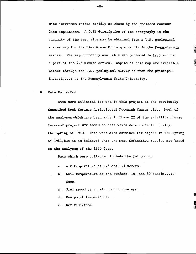
B. Data Collected

Data were collected for use in this project at the previously

described Rock Springs Agricultural Research Center site. Much of

the analyses which have been made in Phase II of the satellite freeze

forecast project are based on data which were collected during

the spring of 1980. Data were also obtained for nights in the spring

of 1981, but it is believed that the most definitive results are based

on the analyses of the 1980 data.

Data which were collected include the following:

a. Air temperature at 9.3 and 1.5 meters.

b. Soil temperature at the surface, 10, and 50 centimeters

deep.

c. Wind speed at a height of 1.5 meters.

d. Dew point temperature.

e. Net radiation.

-9-

The air temperature data were collected by means of mechani-

cally aspirated and shielded type T thermocouples. The soil

temperatures were measured with type T thermocouples. The dew

point temperature was obtained with a lithium/chloride type of

sensing element. The wind speed was evaluated with a climatronics

anemometer. All of these data were collected on an Esterline-Angus

data logger. The collection was in the form of a printed paper

tape and for part of the time the data were also accumulated on a

seven track magnetic tape. After appropriate processing and

reduction of the data, a nine track ASCII formated tape was pro-

duced and sent to the University of Florida for use in the P-Model

analysis program.

Many nights of data were available for inclusion in this study.

As may be indicated by the plots of frost data given in Appendix II,;

it was decided that primary concentration should occur for the nights

of May 7-8, May 8-9, May 9-10, and May 15-16, 1980. Several

additional nights of data are available at the University of Florida

or at The Pennsylvania State University if additional questions

occur. As may be seen from the plots shown in Appendix II, there

is significant variation in the parameters being studied for the

afore mentioned nights.

A log describing the various channels and the format of the

tape which was provided to the University of Florida is included

as Appendix III of this report.

Upon analysis of the data which had been collected it was

discovered that on occasion the dew point sensor which had been

used was apparently giving erroneous results. It was, therefore,

-10- ;

i

believed appropriate to use manually recorded dew point temperatures

which had been collected for the nights under question. These dew

point temperatures were provided to the University of Florida in ai

format as shown in Appendix IV. The device which was used'for the

collection of these dew point temperatures was an Ortemp d£w point

indicator. ,

A summary of the final resultant data which was used in P-Model

predictions by the University of Florida is shown in Appendix V. Iti

will be noted that the radiation data was believed to be insufficient

to include in the model at the preliminary stage. Radiation has,

therefore, been assumed to be zero for the purposes of P-Model

computation.

C. P-Model Analysis

The data which had been supplied to the University of Florida

by The Pennsylvania State University in the form of a nine track

magnetic tape was used in the analysis of P-Model prediction. The

results for this analysis are given in Appendix VI. As may be

noted from the data in that appendix, the technique that is used

with the P-Model analysis is to make predictions of temperature at

a later point in a night using baseline temperatures for a three-houri

period. For the present study the initial prediction hours that

were used were 1800, 1900, and 2000. This prediction was then1

increased by one hour in hourly increments until the final predicting

itime of 0100, 0200, and 0300. The model predicted the temperature

t

for hourly scan times until 0700 the following morning. '

-11-

A complete summary of the P-Model analysis is given In

Appendix VI. It is not very surprising to note that the best

predictions normally occur during the time when a minimum number

of hours occur from the baseline until the predicted point in

time. It will be noted that the overall error analysis as also

shown in Appendix VI is believed to be quite acceptable. The

cumulative P-Model error analysis for all four nights and all.

prediction times was found to have a mean error of only 0.588.

This error was based upon a population count of 264 data points.

The P-Model error analysis by nights was also found to be \

quite good as shown in Table 6.3 in Appendix VI. It will be

noted that the error analysis by prediction time also tends to

be much better for minimum prediction cycles. As may be seen

from Table 4 in Appendix VI, the mean error ranges from a value

of 3.123 when predicting ten hour temperatures to a value of

minus 0.3 when only predicting one hour temperatures. A careful

perusal of the predictions over the entire set of data indicates

that this model does appear to have applicability to terrain

such as was found in Pennsylvania for the purposes of this study.

It must be realized that a great amount of additional data would

probably need to be included to use this model in fruit growing

operations, but the preliminary indications are that the technique

is very applicable to predicting potential frost conditions in

fruit growing regions such as are found in Pennsylvania.

The figures which are also shown in Appendix VI once again

indicate a deviation between the predicted and observed temperature.

As may be seen from those figures, the predictions are much better for

-12-

a minimum number of hours deviation from the baseline temperatures.

The heavy line which is shown on those figures indicates the

observed temperatures. The lighter colored lines indicate pre-

dicted temperatures starting at various baseline times. Figure

6.1 shows P-Model prediction using the raw baseline as provided

by The Pennsylvania State University. In Figure 6.2 this raw

data for baselines was adjusted to provide a smooth function during

the three hour baseline period. As may be seen by comparing Figure

6.1 and Figure 6.2 for any given night, there does not appear to be

any significant benefit to using the error correction terra in the

P-Model. Examination of Figures 6.1 and/or 6.2 indicates the

prediction as shown by P-Model for the nights of May 8-9 and May

15-16 was particularly good. The prediction of the other nights

was not quite as accurate, but was still believed to be sufficiently

useful to warrant further exploration of the application of this

technique to Pennsylvania conditions. As previously stated, the

P-Model certainly predicts temperatures much better during a time

when a minimum number of hours occurs from the baseline. For

example, in Figure 6.2.1, the predictive results are quite good>

for baseline times ending after 2200 hours. For predictions prior

to that time there are significant deviations between the predicted

and the observed temperatures. It is anticipated that additional

inputs such as more radiation and additional inversion temperature

data may help to enhance the ability of the P-Model to predict

conditions over a longer period of time. It should be realized,

however, that even if the P-Model is only able to make predictions

two hours in advance it still would have a very useful benefit to

growers who are attempting to provide frost production in a

commercial orchard or grove.

-13-

Task 2. Description of the Major Apple Growing Regions of Pennsylvania

The primary apple growing region of Pennsylvania is located in fthe

South Central area, between a 77 longitude and 78°W and at at 40°N latitude.

The region covers two counties; Adams and Franklin, which have a total of

almost 20,000 acres of apple orchards. The area has mountains with feak

ridges 1500-2000 ft above sea level, generally running NE-SW, and valleys

averaging 500-600 ft above sea level and several miles wide. Most of the

orchards are located on the lower slopes of the mountains and on the

gentler slopes in the valleys.

The following climatological information was taken from the centrally

located point in each county; Gettysburg in Adams and Chambersburg im

Franklin:

Mean Elevation Latitude longitude(ft)

Chambersburg 640 39°56' WSS1

Gettysburg 540 . 39°50' 77°14'

Mean Temperature (°F)

March April May June

ChambersburgGettysburg

ChambersburgGettysburg

ChambersburgGettysburg

40.141.2

Mean

51.352.8

Mean

29.830.5

51.452.6

Maximum Temperature

62.764.6

Minimum Temperature

38.239.3

62.163.0

C°F)

73.675.2

(°F)

47.649.0

70.871.5

81.282.8

56.759.7

Average Precipitation (inches) Both Locations

3.71 3.47 4.13 3.83

-14-

A full description of the Pennsylvania orchard fruit production

areas by country and growers is included as Appendix VII to this

report. This publication was compiled by the Pennsylvania Crop

Reporting Service during 1978. As may be noted from the enclosed

publication, there was a total acreage of 61,382 acreas of fruit

production in Pennsylvania in 1978. Of that acreage 32,791 acreas

were in apples. This survey included 893 apple growers of whom

825 qualified as commercial. As may be seen from Page 3 of the

publication, 14,417 acreas of apples are present in Adams County

and 4,266 acres in Franklin County as of 1978. These values should

have not changed significantly since that time. The Pennsylvania

orchard and vineyard survey will be updated approximately every

five years.

Climatology data for the state of Pennsylvania is most easily

obtained from a NOAA (National Oceanic and Atmospheric Administration)

publication entitled Climatography of the United States No. 60,

Climate of Pennsylvania. A copy of the material included on a

microfilm of this publication has been attached as Appendix VIII to

this report. Since this material was obtained from a microfilm it

was very difficult to read in the presented form. If the user of

this report needs to obtain more complete data he/she is referred

to either the original publication or a microfilm. The Pennsylvania

State University personnel involved in this project can also provide

additional data upon request.

A careful examination of the principal fruit growing regions

for Pennsylvania indicates that topography information can most

easily be obtained from U.S. Geological Survey maps. These maps

-15-

are available from USGS, Reston, Virginia 22092. The following

quadrangles in the 7.5 minute series have significant acreage of

orchards shown on them. All of these quadrangle maps were photo

revised in 1973.

1. Arendtsville, PA

2. Biglerville, PA

3. Iron Spring, PA

4. Mont Holly Springs, PA

5. St. Thomas, PA

6. Scotland, PA

7. Waynesboro, PA

A number of other topological maps in Adams and Franklin

County are also applicable, but the above mentioned ones upon

examination have the highest percentage of orchards shown. If

required The Pennsylvania State University can supply copies of

these maps to any interested persons. As was previously stated,

they are also available from USGS.

Task III P-Model Limitations

As was previously was discussed under Task I, the P-Model

appears to have quite a bit of applicability to Pennsylvania

conditions. It is believed that modifications may need to be made

in this model in order to be suitably used for many of the fruit

growing regions, but even in its present state the model does

appear to offer some very definite advantages to a grower who is

concerned with frost protection of his fruit crop.

-16-

A more detailed discussion of the manner in which the P-model

may be applied to Pennsylvania growing conditions will be provided

under Task IV of this report. The important concept that is being

spelled out at this time, however, is that it is firmly believed

that the model does appear to offer a benefit to Pennsylvania growers.

This statement is supported by the error analysis and prediction

charts that were presented in Appendix VI of this report.

Task IV Future Projections and Recommendations

Considerable time has been devoted to discussing the application .

of the P-model and satellite forecasting technology to Pennsylvania

fruit growers needs. Many of the projections which are being made

are, of course, speculative in nature but these projections are

based upon present plans and predictions for Pennsylvania.

One of the necessities for Pennsylvania growers to make fullest

use of satellite forecast technology is for a computerized information

dissemination network. Discussions with Dr. G. A. Hussey, a computer

specialist with the College of Agriculture at The Pennsylvania State

University, indicates that present plans call for a microcomputer

network to be made available in county offices under the control

of the Pennsylvania Agricultural Extension Service. These

microcomputers will probably be connected to a

main frame computation system at University Park, Pennsylvania.

Individual counties will then have the capability of accessing large

data files by microwave and telephone links to the central computer

complex. In addition to being able to provide many management type

programs for Pennsylvania farmers and fruit growers, it will be

possible to conceivably also provide' forecasting capabilities for

individual fruit growers.

-17-

Many farmers conceivably will .also link to either the county

extension offices or the central computer complex in order to

obtain up-to-date forecast information for their own needs. It

is anticipated that the P-model approach may be very conveniently

used on individual large farms in Pennsylvania by making a series

of adjustments to the prediction equations used in the P-model.

These adjustments would take into account individual climatological

histories and topographical features for a particular fruit growing

region or farm. By making the fine adjustments indicated, it should

be possible for a grower to obtain a very reliable forecast for his

particular operation. It is anticipated that he may well decide to

obtain forecast technology through the Agricultural Extension Service.

Alternately he may wish to link to a commercially available service

which could have available forecasting capability.

Dr. Hussey, who is previously cited, indicates that The

Pennsylvania State University has negotiated with at least one

commercial communication service for including agricultural data in

their communication netxrork. This type of communication service is

of a format similar to that used by Source or CompuServe computer

services currently available throughout the United States. Addresses

for these commercial services are given in the cited references to

this report. It is anticipated that it might be possible for individual

states such as Pennsylvania to use commercial computer networks for

information dissemination. By so doing material could more easily be

upgraded and made available to growers throughout the United States

without requiring an extensive computer network maintained specifically

for a given state. Such a projection will need to be refined before it

becomes practical, but it is the belief of this investigator that such

a system is certainly feasible.

-18-

Other inputs which will be needed in order for 'a satellite

forecast program to be useful to Pennsylvania fruit growers

includes much better defined climatological data for Pennsylvania.

This data will need to be calibrated and adjusted for individual

fruit growing regions. The Office for Remote Sensing of Earth

Resources at The Pennsylvania State University has for many

years been involved in processing, analysis, and interpretation of

remotely sensed data, most of which has been supplied by NASA

in both imagery and digital format. Appendix IX to this report

includes a discussion of the capability of that office. It is

anticipated that one of the future continuations of the work

described in this report would be to collect and define climato-

logical data for a more wider portion of Pennsylvania than was

included in this study. It is conceivable that the Office for

Remote Sensing would be involved in such a collection and reduction

of data. Having reduced temperature data for various portions of

Pennsylvania, it then should be possible to refine the P-model in

order to take into account climatological and topological variations

throughout the fruit growing regions. This series of refined models

would then be applied to individual fruit growers and/or areas in

order to provide optimal predictions for frost potential.

Having developed individual calibrated models for various parts

of Pennsylvania the grower would then need to have available a system

for rapid access of the data such as had been previously described in

this section. It is believed that growers may not all chose the same

system, but in fact some growers might prefer to use a commercial

service while others might tie into an agricultural extension service

run by the state of Pennsylvania. Regardless of which route the

-19-

individual grower should chose to take, it is believed quite

probable that he or she should have access to timely data and

projections for their individual farms. In order to get such

projections, it is probably very desirable to have an ability to

access satellite data quite rapidly. In order to do this

efficiently one possibility may be to utilize down-link capability

currently being developed at the University of Florida for

obtaining directly satellite data. This data could be segmented

and provided to Pennsylvania within a very short period of time

after it was obtained from the satellite. By so doing, it would

be possible to provide the grower with a very current projection

of freeze forecast conditions. Such an operation would be somewhat

expensive but is probably justified in view of the increasing costs

for oil and the rapidly depleting water resources available to many fruit

growers. It is anticipated that the satellite data would be provided by

an institution similar to the University of Florida directly to

Pennsylvania. The data would then be incorporated into either a

single P-type model or a series of P-models which had been

individually calibrated to fruit growers.

The fruit grower would call for the data via a personal computer

available on their farm. Several modes of operation would be possible-

The farmer could call at various time intervals and determine the

probability of a frost. Alternately, an automatic dialing system and

alarm network could be used to alert a grower to probable frost

conditions on his or her individual operation. This technology

would be the most effective, but would also be the most expensive

for an individual grower to implement.

-20-

An alternate method of utilizing satellite projection in .

Pennsylvania would be to make P-model projections available to

cable television networks in fruit growing regions. Many such

cable television networks at the present time have channels which

are devoted to news and similar materials. It is possible that the

frost forecast could be incorporated as a part of these services

Of course, the National Weather Service is also providing in

some areas of the United States, an agricultural forecasting service.

It would be very desirable to use satellite forecast technology

similar to that employed in this study for improving frost forecasting

by the National Weather Service. A number of commercial forecasting

services such as Accu-weather also could conceivably make use of

the technology being described at this time. In conclusion several

useful findings have resulted from this study. These findings can

be enumerated as follows:

1. The P-model in its present form appears to give quite

reasonable predictions for night-time temperatures over

a short time interval under Pennsylvania conditions.

2. It appears feasible to modify the P-model in order ,'

to take into account topographical variations for individual

fruit growing regions.

3. Present microcomputer technology appears to be very

appropriate to enable individual fruit growers to use

results from satellite freeze forecast technology.

4. In a continuation of this study it is suggested that a

more detailed collection of climatological data is

needed. This data would then be incorporated into the

P-model in order to statistically evaluate the effective-

ness of this model over a wide range of climatological conditions.

-21-

1 5. It is believed that in the next few years growers will

j have the capability and desire to quickly access results from

1 forecast technology such as was used in this study. It would

"-. be desirable, therefore, to continue to work on anu

information dissemination network which will rapidly make

j|] satellite-based forecasts available to the grower. This information

. dissemination may well be offered by both commercial and public

.i' institutions.

; 6. A minimum of two additional years of data are needed in order to

accurately evaluate the suitability of P-model to Pennsylvania

i • growing conditions. It is hoped that some mechanism will be

. developed by which additional studies of the suitability of

this model may be achieved.

-22-

CITED REFERENCES

Sutherland, R. A. 1980. A Short-Range Objective Nocturnal TemperatureForecasting Model. Journal of Applied Meteorology. March 1980.pp. 247-255.

Pennsylvania Crop Reporting Service. 1978. Pennsylvnaia Orchard and VineyardSurvey. Pennsylvania Department of Agriculture. Harrisburg, PA.

National Oceanic and Atmospheric Administration. 1977. Climate ofPennsylvania. Environmental Data Service. National Climatic Center.Asheville, NC.

Hussey, G. A. 1981. Personal Communication, College of Agriculture,University Park, PA 16802.

Peterson, G. W. 1981. Personal Communication Office for Remote Sensingof Earth Resources. The Pennsylvania State University, University Park,PA 16802.

Source. 1981. 1616 Anderson Road. McLean, VA.

CompuServe. 1981. 5000 Arlington Centre Boulevard. Columbus, Ohio 43220

y

Appendix I

Proposal from The Pennsylvania State University

to

The University of Florida

7?

Application of Satellite Freeze ForecastTechnology to Other Parts of the U.S.

Phase II

Proposal for Continuing Support

Submitted to: University of FloridaInstitute of Food and Agricultural Science2121 HS/PPGainesville, Florida 32611

Submitted by: C. T. Morrow, Principal InvestigatorDepartment of Agricultural EngineeringThe Pennsylvania State UniversityUniversity Park, Pennsylvania 16802

Submitted on: December 1, 1980

Note: This proposal is submitted from The Pennsylvania State Universityas a sub-contractor to the University of Florida. The Universityof Florida is designated as the prime contractor to John F. KennedySpace Center, NASA.

Signatures

<'ft-.•?''.'•.*'— C. T. Morrow, Principal Investigator

H. V. Walton, Head, Dept. of Ag. Engineering

^_ R. G. Cunningham, Vice President for Research

Application of Satellite Freeze ForecastTechnology to Other Parts of the U.S.

Phase II

Introduction

Improved methods of freeze forecasting would greatly benefit agriculturalinterests throughout the contiguous United States. NASA has entered into ajoint effort with the National Oceanic and Atmospheric Administration (NOAA)to demonstrate the technology necessary to accomplish more accurate freezeforecasting in the state of Florida. To this end NASA has engaged theUniversity of Florida, Institute of Food and Agricultural Sciences (IFAS), todevelop and demonstrate a satellite freeze forecast system under NASA contractNAS10-9168.

During the past year, NASA also has had IFAS investigate the "Applicationof Satellite Freeze Forecast Technology to Other Parts of the United States"under NASA contract NAS10-9611. The first year's work concentrated in gatheringkey weather station data bases and comparing this data with the NOAA GOES-2satellite or any other available satellite gathering temperature data and eval-uating the usefulness of such satellite data in two selected test areas, whichare located in Michigan and Pennsylvania. The collected data would be evaluatedand conclusions/observations presented as follows:

The ability to correlate GOES data with surface data and its applicabilityto cold climate mapping considering such factors as:

a. Accuracy, resolution, and reliability of the satellite data;b. Geometric distortions;c. Terrain variables;d. Atmospheric effects; ande. Other.

Under the proposed extension of the project, the Pennsylvania StateUniversity shall be responsible for accomplishing the following tasks:

Task 1. Collect data to be used in running a freeze prediction model(P-Model) by the University of Florida. This model wasdescribed by Sutherland, 1980. Data will be collected at asite located at the Rock Springs Agricultural Research Center.The site chosen for the data collection provides a uniform andlevel agricultural terrain. The following data will becollected at the site:

a. Air temperature at 9.3, and 1.5 metersb. Soil temperature at the surface, 10, and 50 centimetersc. Windspeed at 1.5 metersd. Dewpoint temperaturee. Net radiation

-2-

In anticipation of continuing funding for the project data were collectedduring the Spring of 1980 for the following nights:

May 8, 1980May 9, 1980May 10, 1980May 15, 1980June 11, 1980

Additional data will be collected for nights in early Spring, 1981.

The above data will be supplied to the University of Florida for runningthe P-Model on their computer.

Archived GOES satellite data will be procured by the University of Floridafor use in evaluating the applicability of the P-Model to Pennsylvania conditions.

Task 2. The Pennsylvania State University will supply terrain, surfaceand topographic information to the University of Floridaconcerning fruit growing regions in Pennsylvania. Thisinformation will be used to develop preliminary specificationsfor a statistics model such as the one previously developed atthe University of Florida and described by Chen, 1980.

Task 3. The Pennsylvania State University will study the P-Model(Sutherland, 1980) and discuss limitations and pecularitiesof the Pennsylvania test site which might limit generalizationof the P-Model to other areas of the United States.

Task 4. The Pennsylvania State University will make recommendations tothe University of Florida relative to specific concepts andstudies that could be pursued for further application.

Cited References

Chen, Ellen. 1980. Personal Correspondence. University of Florida,Gainesville, Florida.

Sutherland, R. A. 1980. A Short-Range Objective Nocturnal TemperatureForecasting Model. Journal of Applied Meteorology. March, 1980.pp. 247-255

Sub-Contact Budget, 1980-81

The Pennsylvania State University

Salaries

C. T. Morrow, Principal InvestigatorM. A. Wittman, Electronics TechnicianP. A. Mark, Technician

Salaries Sub-Total

$1,000300300

1,600

Wages

Part-Time Hourly Help 400 hours @ ave. $3.40 1,360Wages Sub-Total 1,360Total-Salaries and Wages 2,960

Fringe Benefits

22.10% of Salaries6.60% of Wages

35490

Fringe Benefits Sub-Total 444

Travel

Mileage to Rock Springs Agricultural Research CenterTravel to University of Florida and KSC

Travel Sub-Total

100500600

Other

Computer - IBM 370/3033 @ $252/hrExpendable Supplies and Materials

Other Sub-Total

Total-Direct Costs

504700

1,204

5,208

Indirect Costs

64.30% of Total Salaries and Wages

Total Estimated Costs

1,903

7,111

Appendix II

Frost Data for Pennsylvania Test Site

Channel Descriptions for Pennsylvania Data

May 8-9, 9-10, 10-11, and 15-16, 1980

Channel Description Units

..J

45678910111213141516171819202122232425262728

North blockSouth blockSouth blockNorth blockSouth blockSouth blockSouth block

Bud thermocouple, North blockBud thermocouple, North blockBud thermocouple, North blockAspirator chamber,Aspirator Chamber,Bud thermocouple,Bud thermocouple,Bud thermocouple,Bud thermocouple,Bud thermocouple,Surface temperatureTower ground level thermocoupleTower 1.5 meter aspiratorTower 15 meter aspiratorTower 5 meter thermocoupleTower 3 meter thermocoupleTower 3 meter aspiratorTower 9 meter aspiratorTrench 10 cm thermocoupleTrench 10 cm thermocoupleTrench 50 cm thermocoupleTrench 50 cm thermocoupleWind speedWind peakWind average

Deg. CDeg. CDeg. CDeg. CDeg. CDeg. CDeg. CDeg. CDeg. CDeg. CDeg. CDeg. CDeg. CDeg. CDeg. CDeg. CDeg. CDeg. CDeg. CDeg. CDeg. CDeg. CMeters per secondMeters per secondMeters per second

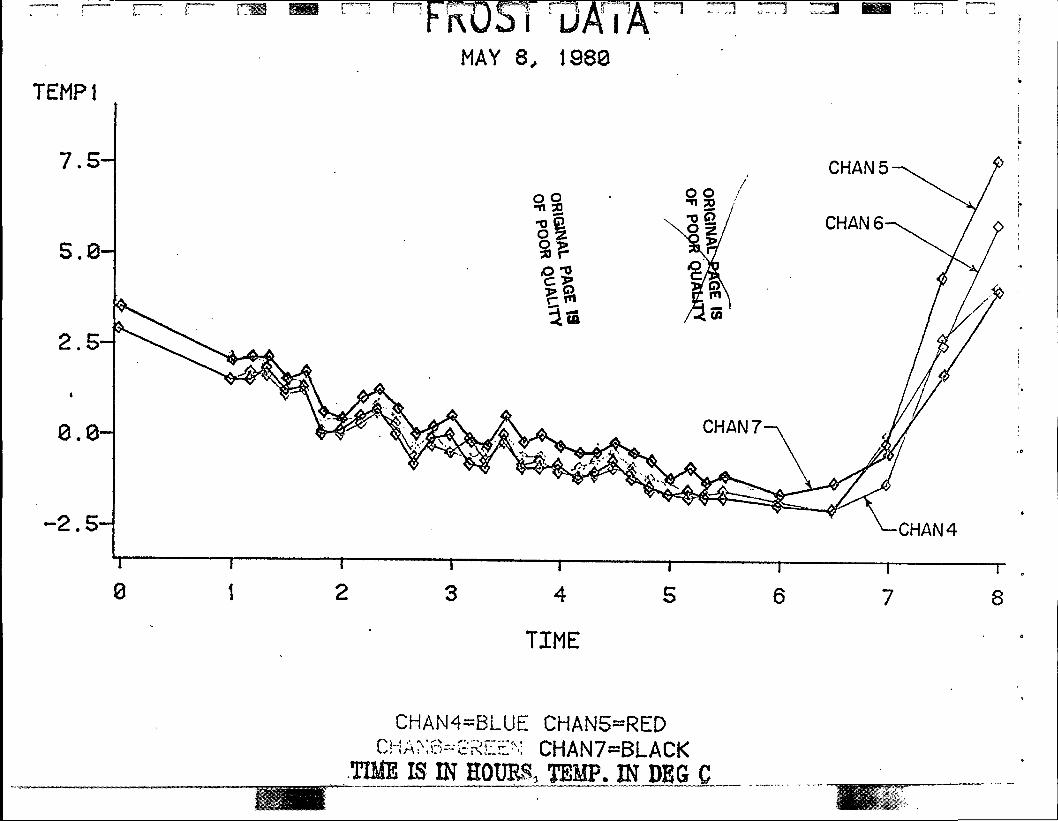
TEMPI

7.5-

5.0-

2.5-

0.0-

-2.5-

0

TJATAMAY 8, 1980

8

TIME

E CHAN5=REDCHANC^eSESM CHAN7«BLACK

.TIME IS IN HOURS, TEMP. JN DEG C

TEMPI

5.0-

2.5-

0.0-

-2.5-

I U

MAY 8, 1980

CHAN 10T

3

1—

4

TIME

~r5 •7 2°7 ^2

•o ao £0 >» Fo -^^ >> o

8

CHAN8=BLUE CHAN9=REDC(-;4X 1 f—C-'^f"'-"''•'

TIMF K IN HOMES. TTtdJp' IM HF^ r

TEMPI

7.5-

5.0-

2.5-

0.0-

-2.5-

, ^ __ —A f—•—>• f—•——i i ! ' s »

FRDSi uAiAMAY 8^ 1980

, Ji I'- L .1

CHAN I -CHAN 13T

3

1—

4

TIME

8

CHANH-BLUE CHAN12=REDCHAM 13- rfsEtN CHAN 14=BLACK

TEMPI

6

3

0

~i\i r\ 1 I~I3

MAY 8, 1980

CHAN 16

-6

"T

30

1—4

TIME

T

5

CHANI5-.BLUE CHAN16=RED

TIME IS IN HOURS, TEMP. IN DEC C

"T

6 00"" 5T3 O

30

,0C

o

8

o

TEMPI

7.5-

5.0-

2.5-

0.0-

-2.5-

•j i J A . A j

MAY 8, 1980

CHAN 19

I

4

TIME

I5

i6 oo 7•n 31 /

•TJ 581

&

CHAN18=BLUE CHAN19=RED•p;_; •. \ •'~. ,"> «"." ;\" ••_ • -\ i

TIME IS IK HOURS, TEMP. IN DEC C

I

8

TEMPI

MAY 8, 1980

6

I

2i i3 4

TIME

i5 6 7 8

CHAN21=BLUE

TIME IS IN HOURS, TEMP, IN DEG C

TEMPI

1 1

8

IrvMAY 8, 1980

CHAN 23

CHAN 24

CHAN 22

F4

i5

i6

TIME

i8

r

9

© o

«OC

CHAN22=BLUE CHAN23=RED:::-;A: :2 ;-:?^-^ : CHAN25=BLACKTIME IS IK HOURS, TEMP. IN DEC C

WIND1

0.75-

0.50-^

0.25-

0.00- •CHAN 28

r i^ iMAY 8, 1 980—00 : 00-8 : 00A . M .

0

t

2i3

i4

TIME

CHAN26-BLUE CHAN27«RED^S I i f « *—' ^--, ^ ^ v*» •- i -• •—™ ,._ •

TIME IS TN TioURS^ WIND IN MPS

r

7 O t-

o &35 rlO T;c ;,-•> t'.-i

8

TEMPI

4

2

0

f

MAY 9, 1980—00:00-8:00A.M.

CHAN4=BLUE CHAN5=REDCi-iA>i:5«7f%iv::\

1 CHAN7=BLACKTIME IS IN HOURS, TEMP. IN DEC C

TEMPI

rj DATA™ ^

MAY 9X 1980—00:00-8:00 A . M .

0

TIME

CHANS-BLUE CHAN9=RED^''1' — ^:-T>' •

iy..l,.."-»'".-l

TEMPI

5.8-

2.5-

8.8-

•2.5-

MAY 9, 1988—80:08-8:88A. M.

T

21

3

i4

i5

i

6

i

7

i

8

TIME

CHAN11=BLUE CHAN12=REDnA?Mc.«cF.:i£^ CHAN14=BLACK

GEGUCL.

TEMPI

5.0-

2.5-

0.0-

-2.5-

-5.0

8

MAY 9, i 980—08:00-8:80A. M

TIME

7 8

CHAN15=BLUE CHAN16=RED,- . . i •-- -»•- — • — i: j—• i ' IT — — — —

TIME IS IM'HOURS, TEMPi IN DEG C

| ™».

L ]

MAY 9, 1988—00:08-8:90A. M.

8.8-

-2.5-

8

TIME.

CHAN18=BLUE CHAN19=RED

8

TIME IS IN HOURS, TEMP. IN DEG C

TEMPI

0

MAY 9, 1980—88:88-8:'00A.M.

0 4

TIME.

~r5 o

CHAN21=BLUE

TEMPI

9.5 ~

9.9 ~

8.5

8.0 -

7.5 -

0

MAY 9, 1983—00:00-8:00A. M.

-CHAN 23

CHAN22=BLUE CHAN23=REDCHAN2~--=S^Tr::' CHAN25=BLACKTIME IS IN HOURS, TEMP. IN DEC C

WIND]1 .5 -\

1 .0

0.5 -

0.0 -

8

^ VRvJSi' DATA ^ :

MAY 9, 1980—00:00-8:00A.M.

,3 , , _J

TIME.

CHAN26-BLUE CHAN27=RED

TIME is IN'HOURS* WJND IN MPS

~ 1 —

HAY I 938--09: 90-8: 33A.M.

TIME

CHAN4«B-LUE CHAN5=REDCHAN3«SREEM CHAN7=BLACK

TIME IS IN HOURS, TEMP. IN DEG C

ff»r~i+* T "~\ f"

"ix',> '"v.* • "*•»..-

8

TIME

CHANS-BLUE CHAN9-RED-v, ^ . ' ! • " « . _ _ ' • " .'" '

TIME IS IN HOURS, TEMP. IN DEC C

8

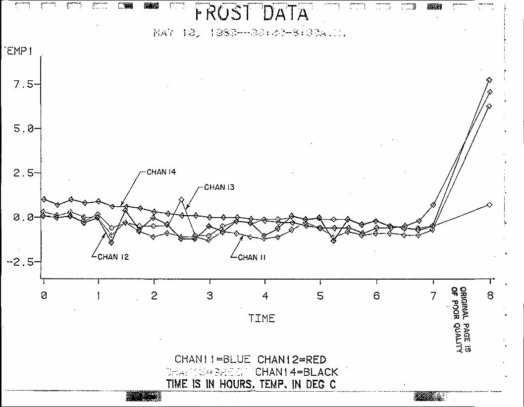
DATA

'EMPl

7.5-

5.8-

2.5-

0.0

-2.5-

0

CHANH=BLUE CHAN12=RED>-:A: •'. o--?r::: Ci' CHAN 1 4=BLACKTIME IS IN HOURS, TEMP, IN DEC C

'EMPI

6

6

TIME

CHAN15-BLUE CHAN16=RED

TIME IS IN HOURS, TEMP. IN DEC C

EMP1

5.0-

2.5-

0.0-

-2.5-

I

TIME.

CHANI8=BLUE CHAN19=RED

TIME IS IN" HOURS, TEMP. IN DEG C

MAY !33.2—-o*,. '*»'.»•O"'~j».

FEMP1

0

i

5

T

8

TIME

CHAN21=3LUE

TIME IS IN HOURS, TEMP. IN DEC C

h'RbSI 'DATA1

TEMPI

CHAN 24

CHAN23=RED-i,0'24«o?i£:-:-' CHAN25=BLACK

I!Mi.JSJMJiffiJSS,JlMP. JM .DES. CL

8

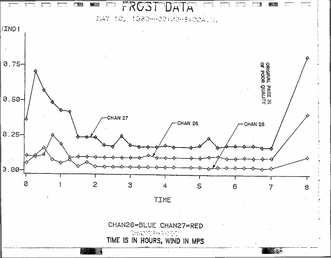
~iI UM

/INDJ

0.75-

0.58-

0.25-

3.00

0

CHAN26-BLUE CHAN27=RED>:, ;.V-T: ?«•-:-::-.-- •

TIME: is IN HOURS, WIND IN MRS

TEMPI

5.0-

2.5-

0.0-

-2.5-

'I31DATA

MAY 16, 1980—00: 00-8: 00A.M.

T

30

1—

4

TIME

T

6T

7 8

CHAN4=BLUE CHAN5=REDCiiAKS^SREEN CHAN7=BLACK

DEGJC

TEMPI7.5-

5.0-

0.0"

MAY 16, 1980—00 .-08-8 s 00A. M.

0

TIME

T"5

T

700•n 2TJ C5O

<O 13C 2>> C)

8

CHAN8«BJ-UE CHAN9«REDCHAN 10»8REEN

TIME IS IN HOURS, TEMP. IN DEG C

r—"i

TEMPI

j -7JATA; 5 ~MAY 16, 1980—00:00~8:00A.M,

CHAN 12

T

2

TIME

~r6 8

CHAN 11-BLUE CHAN12=REDCHAN 13«8REEN CHAN14=BLACKTIME IS IN HOURS, TEMP. IN DEG C

!__ ,JS"*'* J flRimJBSk JfO£&~JS£&S9

rfv3SrMAY 16, 1980—00:00-81 00A.M.

TEMPI

18.0 -

7,5 -

5.0 -

2,5 -

0.8 -

0 4

TIME

T

5

CHAN18«BLUE CHAN19«REDCHAN20-3REEN

TIME IS IN HOURS, TEMP. IN DE6 C

T

7 8

MAY 16, 1980—00:00-8100A. M.TEMPI6

TIME

. CHAN21

TIME IS IN HOURS, TEMP. IN DEG C

, ^— — J,^ •— _»•»•

KOSi i „ ,-i

MAY 16, 1 980—00 : 88-8 * 88A . M .

TEMPI12

•CHAN 23

9

TIMEo o"" 2•o SO ^*O >3D &

O -ac >> or m

CHAN23=REDCHAN25«BLACK

TIME IS IN HOURS, TEMP* IN DEG C

WIND1

0.75-

0.50-

0.25-

0.00-

0

^ 'TKOST DATA ^ r

MAY 16, 1989—00:00-8:08A.M.

.,..!

TIME

CHAN26-BLUE CHAN27=RED

Appendix III

Tape Description for Pennsylvania Frost Data

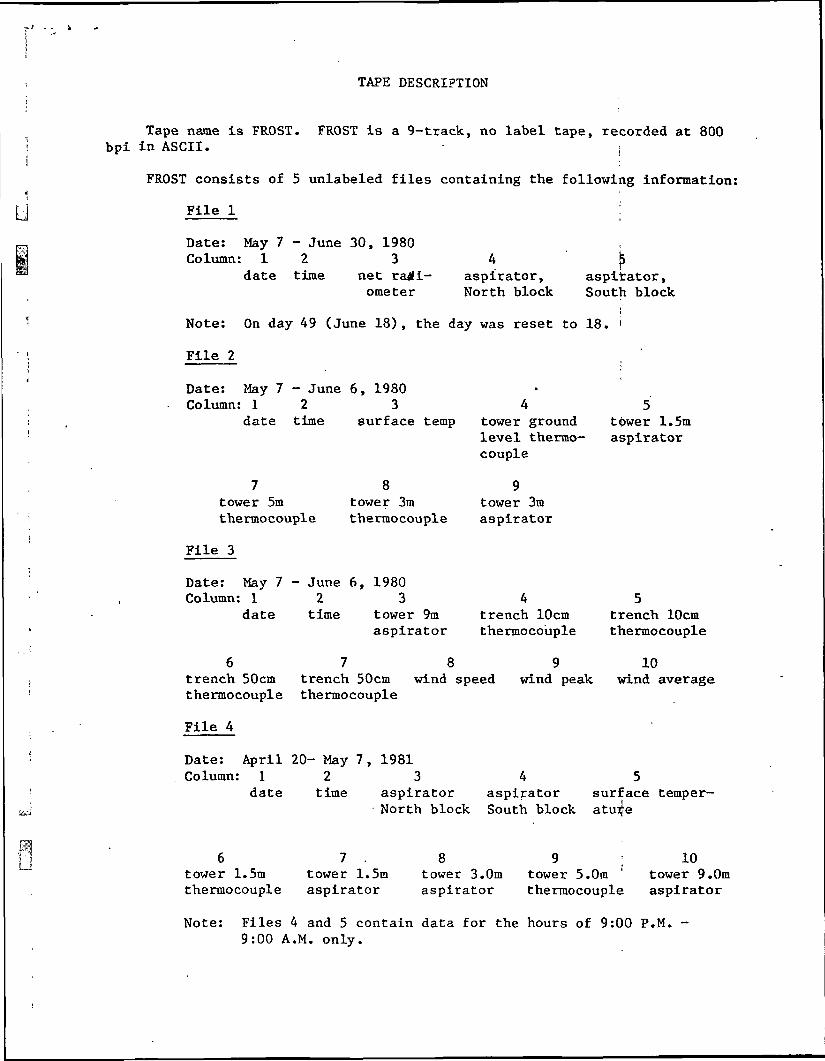
TAPE DESCRIPTION

J

Tape name is FROST. FROST is a 9-track, no label tape, recorded at 800bpi in ASCII. ;

FROST consists of 5 unlabeled files containing the following information:

File 1 !

Date: May 7 - June 30, 1980Column: 1 2 3

date time net radi-ometer

aspirator,North block

aspirator,South block

Note: On day 49 (June 18), the day was reset to 18.

File 2

Date: May 7 - June 6, 1980Column: 1 2 3 4

date time surface temp tower groundlevel thermo-couple

tower 1.5maspirator

tower 5mthermocouple

8tower 3mthermocouple

tower 3maspirator

File 3

Date: May 7 - June 6, 1980Column: 1 2 3

date time tower 9maspirator

trench 10cmthermocouple

8

trench 10cmthermocouple

10trench 50cm trench 50cm wind speed wind peak wind averagethermocouple thermocouple

File 4

Date: April 20- May 7, 1981. Column: 1 2 3 4 5

date time aspirator aspirator surface temper-North block South block atu^e

tower 1.5mthermocouple

tower 1.5maspirator

8tower 3.0maspirator

tower 5.0mthermocouple

10tower 9.0maspirator

Note: Files 4 and 5 contain data for the hours of 9:00 P.M. -9:00 A.M. only.

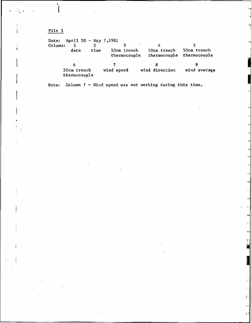
I File 5

Date: April 20 - May 7,1981Column: 1 2 3 4 5

' date time 10cm trench 10cm trench 50cm trenchthermocouple thermocouple thermocouple

II 6 7 8 9

50cm trench wind speed wind direction wind averageI thermocouple

Note: Column 7 - Wind speed was not working during this time.

i

i

d

Appendix IV

Dewpoint Temperatures for Pennsylvania Test Plots

Dew Point Temperatures for Pennsylvania Test Plots

Date Time Dew Point Date Time Dew Point

May 8-9,1980 0215

02350320041004360500

272729262526

May 9-10,1980 0045

011501420145024003000410056705300631

30302930282827272627

May 8-9,1980 2350

23550115015003080322040004430450052506000617

333129282727262930302827

May 15-16,1980 0100

01510202024803050305033403530410041404200425

353534323233323231303131

Appendix V

Reduced Data for Pennsylvania Test Plot

a

ORIGINAL PAGE ISOF POOR QUALITY

PENNSYLVANIA STATE GOLD WEATHER

TIME

18.019-020.0"21.022.023.00.01.02.03.04.05.06.07.0

SOIL

53.452.548.947.844.239.437.635.834.734.033.432.031.634.2

PENNSYLVANIA

•

TIME

18.019.020.021.022.023.00.01.02.03.04.0

. 5.06.07.0

SOIL

52.049.144.8•41.037.436.335.134.033.132.430^434.932.039.0

10CHSOIL

54 . 754.554.153.653.152.752.051.3 .50.750.249.648.948-647.7

STATE

10CHSOIL

53.452.552.251.851.350.449.549.348.448.046.846.445.946.0

50CtiSOIL

49.849.850.050.049-850.050.049.649.849.849.849.649.849.6

1.5MA III

53.453.150.748.746.643.740.839.434.033.331.530.427.732.0

COLD .WEATHER

50CMSOIL

48.448.648.748.948.948.948.648.748.748.6

. 47.848.047.848.6

1 . 511AIR

48.045.344.141.937.438.837.435.434.732.231.532.532.234.5

DATA

3. OHAIR

53.853.150.748.746.044.140.138.834.234.01*2.'029.731.138.3

DATA

3.011AIR

49.645.744.140.838.738.336.936.035.233.430.932.731.335.6

9.0liAIR

54.053.251.449.647.846.843.543.537.836.934.532.933.334 . 7

9. OiiAIR

47.845.745.043.240.839.938.538.137.6'36.333.434.733.836.3

DEWPOINT

27.027.027.027.027.027.027.027.027.027.026.026.026.026.0

DEWPOINT

33.033. U33.033.033.033. U31.029.02ft. 027.026.030.030.030.0

MAY 7-8, 1980

WINDSPEED I

2.84.22.3.3.6.2.2.2.1.1.1.1.1

• .1

r

MAY 8-9, 1980

WINDSPEED

4.9.8

l-i.4.1.1.2.2.4-.2.1.1.1.1

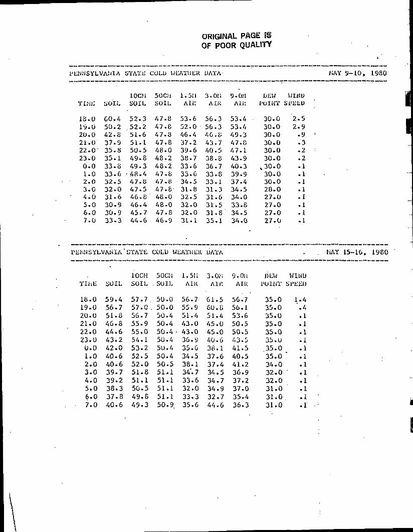
ORIGINAL PAGE ISOF POOR QUALITY

PENNSYLVANIA

Tir-ili

18.019.020.021.022. 0-23.00.01.02.03.04.65.06.07.0

SOIL

60.450.242.837.935.835.133.833.632.532.031.630.930.933.3

PENNSYLVANIA'

Tlhli

18.019.020.021.022.023.00.01.02.03.04.05.06.07.0

•

SOIL

59.456.751.846.844.643.242.040.640.639.739.238.337.840.6

STATE

10CMSOIL

52.3.52.251.651.150.549-849.3

• 48.447.047.546.846.445.744.6

STATE

10CMSOIL

57.757.056.755.955.054.153.252.552.051.851.150.549.849.3

COLL) WEATHER

50CMSOIL

47.847.847.847.848.048.248.247.847.847.848.048.047.846.9

1.5MAll;

53.652.046.437.239.638.733.633.634.531.832.532.032.03L.I

GOLD WEATUEU.

50CM. SOIL

50.0. 50.0

50.450.450.4 -50.450.450.450.551.151.151.151.150.9.

l.SiiAIR

56.755.951.443.043.036.935.634.538.134°. 733.632.033.335.6

DATA

3.011A IK

56.356.346.843.740 . 538.836.733.833.131.331.631.531.835.1

UATA

3.0;-;Alll

61.560.051.445.045.040.638.137.637.434.534.734.932.744.6

9 . OHAll'.

53.453.449.347.847.143.940.339.937.434.534.033.834.534.0

9. OHAIR

56.756.153.650.550.543. S41.540.541.236.937.237.035.436.3

DEW1'OIMT

30.030.030.030.030.030.0

X30.030.030.028.027.027.027.027.0

DEWPOINT

35.035.035.035.035.035. U35.035.034.032.032.031.031.031.0

KAY 9-10, 1980

WINDSPlitD '

2.52.9

.9 '

.3

.2

.2

.1

.1

.1

.1

.1

.1

.1

.1

. HAY 15-16, 1980

WINDSPEED

1.4'.4.1.1.1.1.1.1.1.1.1.1.1 '.1 :

"I

d

Appendix VI

P-Model Analysis Results

Table 6.1 P-Model Error Analysis (Total)Table 6.2 P-Model Analysis by NightTable 6.3 P-Model Analysis by Prediction PeriodTable 6.4 P-Model Error AnalysisFigure 6.1 P-Model Predictions (Without Error Analysis)Figure 6.2 P-Model Predictions (With Error Analysis)

lii

ORDINALOF POOR QUALITY

Table 6.1 P-Model Error Analysis (Total)

F-;iODL'L J'iKUCll ANALYSIS

PhiJHSYLVAtt'IA STATI-: CULI) l.'iJATii.L'i: i;ATA

ALL KIUilTS - 1-iAY 7-8, 3-9, 9-10, 15-16, 1J»SO

POPULATIUH = 204J-iLy\.N JiKKOK =STWU. DKV. = 4.117

ORIGINAL PAGE ISOF POOF? QUALITY

Table 6.2 P-Model Analysis by Night

I'-iiOfJfvL ANALYSIS JiY HICIIT

l-.kl:Gl; ANALYSIS OF HAV -/_<{,

1'Oi'ULATlOi-; = 66MHAi; LKKOK = 3.333STiiD. DEV. = 4 .^17

liliilOU ANALYSIS 01' liAY 3-9, 1(J80

POPULATION = 66;-;EAN K K N O I C = -.712UTuU. DKV. = 2.ii26

liKKUK ANALYSIS OF MAY 9-10,

POi'ULATlOI-I = 6GI-il^\ii IIKKOU = -.280STi:ii. LLV. <=•• 3.51fJ .

Li'.uOU ANALYSIS OF iiAY 15-16,

POriJLATiOli « 66 ' .il = .018

I;T.-;U. DEV. A. 2 70

ORIGINAOF POOR Q A * - ' ' '

Table 6.3 P-Model Analysis by Prediction Periods

P-iiODL'L a-lsiOR ANALYSIS CV PiU:UiCVlOii

L-RKOI; AiiALYSIS 01'- l-l;OUK PIU-lUlC'i'IGi-S ( rOuK

POPULATION = A/i;u-^K JiKKUI'. = -.300STI-iU. UKV. = 2.7A9

LIIKOK ANALYSIS OK 2-UOUi;

POl'ULATIOi; = 401-M^M LKUOJt = -.250STKU. DlvV. = 2.921

iS (1-oui:

LUUOK AWALYKIS UK 3-liOUk' PUCUlCVlOiia (FOUR MIGHTS)

POPULATION = 36I'ih'AW KKUOii '= -.020STKD. DEV. = 3.474

KHKOU ANALYSIS OF 4-liOUU PaiiiilCTIUUy (l-UUit KIGUTS)

POPULATION = 32IJEAX LRKOU « .368STI'il). DEV. = 3.y50

iiKROli ANALYSIS OF 5-HOUK PUlIL'lC.-L'lONS (FGUK J.lCtfTK)

POPULATION =MF.AU liiiuoi; «=ST.NU. OL'V. =

HUUOlt ANALYSIS OF 6-IiOUK PHEUlCTIOt/S (FOUR NIGHTS)

POPULATION = 24hLAK -JiKKOrt .«24STN1)..D1-:V. = 4.449 i

ERIvOLi AU'ALYSIS OF 7-HOUR PKKDICTIGILS (FOUR NIGHTS)

POPULATION = 20liEAK luvRoK = 1.447STI-.'D. UF.V. = 5.099

ORIGINAL PAGE ISOF POOR QUALITY

Table 6.3 (Continued)

I:I;;:I.-K /\:i/M.Y:>i:; 01* ii-iiuui: j'l'j.Pici'iufi.s (Four »:it ; i iTS)

I-HOM-: I:I;U(JK ^ i.y'77sruu.

LP.KOR At.'ALYSIS OF y-iJOUK I'UliblCTIOliS (FOUJ; I-ilCliTS)

POI'ULATIOK = 1 2I-if-yiti I'-RCOU = 2.179ST.NLi. 1>LV. = 0.262

LRROK Ai,:AI.YSI5 Oi-1 10-I!OliK PUKUICTIOliS (FOUR KIGHTS)

= o •= 3. 123

STUD. DCV. = 6.170

ORIGINAL PAGE !SOF POOR QUALITY

Table 6.4 P-Model Error Analysis

Pi-iODL ERROR ANALYSIS FOR JiAY 7-fa, 1980

IIOUK 1800 1900 2000 2100 2200 2300 0000 0100 0200 0300 0400 0500 0600 0700wjs vc ic vc/f

I'UKIJ $$$0 $$$$ $$0$ 49.4 4*1.2 47.2 46.2 45.3 44.4 43.5 42 . f i 42.0 41.3 40.7OUS 53-3 53.0 50-6 48.7 46.5 43.6 40.7 39.3 33.9 33.2 31.4 30-3 27. 'C 31 0ERR $$$$ $$$0 5$$$ .7 1.7 3.5 5.4 5.9 10.5 10.4 11.4 11.7 13.7 8^7

MKAM OF EURO US = 7.609STD. DEV. Of ERRORS = 4-380

PMODL ERROR ANALYSIS FOR MAY o-9, 1980

HOUR 1800 1900 2000 2100 2200 2300 0000 0100 0200 0300 0400 0500 0600 0700.LASE ** ** **PKED $$$$ $$$$ $$$$ 42.5-41.2 40.0 38.9 37.9 37.0 36.2 35.4 34.7 34.0 33.4OLS 47.9 45.2 44.0 41.8 37.3 38.8 37.3 35.3 34.6 32.1 31.4 32.5 32.1 34.4liHU $$$$ $$$$ $C-S$ -6 3.8 1.2 1.6 2-6 2.A 4.1 4.0 2.2 1.9 -1.1

MEAN OF EUUOUS =2.126STD. 1)EV. OF OIROKS -= 1.555

1'tiODL JiuUoiC ANALYSIS FOk IIAY 9-10, 1980

HOUR 1800 1900 2000 2100 2200 2300 0000 0100 0200 0300 0400 0500 0600 0700EASE ** ** **PKED $$$$ $$$$ $$$$ 44.4 42.9 41.7 40.7 39.8 39.1 3o.3 37.7 37.1 36.5 35.9OLS 53.5 51.9 46.3 37.1 39.5 30.6 33.5 33.5 34.4 31.7 32.5 31.9 31. 9 31.0ERK $$$$ $$$$ $$$$ 7.2 3.4 3.1 7.2 6.3 4.6 6.6 5.2 5.1 4.6 4.9

OF ERRORS =5.302'STD. DEV. OF ERRORS «= 1.389

PMODL ERROR ANALYSIS FOR HAY 15-16, 1980

HOUR ICOO 1900 2000 2100 2200 2300 0000 0100 0200 0300 0400 0500 0600 0700BASE ** ** **L'RKJ; $$$$'$$$$ $$$$ 49.5 47.9 46\5 45.3 44.2 43.2 42.4 41.6 40.9 40.3 39.7UliS 56.6 55.9 51.4 42.9 42.9 36.8 35.5 34.4 38.0 34.6 33.5 31.9 33.2 35.5ERR S$S$ S$$$ $$$$ 6.5 5.0 9.7 9.7 9.8 5.2 7.0 S.I 9.0 7.1 4.2

MEAN OF ERRORS = -7.457STD. DEV. OF ERRORS = 2.036

ORtGiNALl.r.(,m. KKI lOK AI.'Al.V'SJ.:; !••(;;> ; ;AY /-;., I 'AM, OF POOrc Qt .'>•*•

I IUUR IWOO 1900 2000 2100 220!) 2300 lil.ai: 0100 0200 0300 0400 0500 0600 0700' **

$§;;? $o$s $$?$ 47. u 4 5 . 7 /./...-. /,:-../, /,2.5 41.7 40.9 40.2 30.0 39.101;S 33.3 53.0 50. (> 4i;.7 /,<;.. 3 43.1. An. 7 3V. 3 33.0 33.2 3 L . A 30.3 27.0 31.9i:n: 0?^? 5?fv 0;:^? C??C .5 -..". 3.7 $.1 c.6 S.5 9.5 9.9 12.0 7.1

PMOD1. KKUOll AKAJA'SIS FOR MAY y-9, 1980

liOUU 1800 1900 2000 2100 2200 2300 0000 0100 0200 0300 0400 0500 0600 0700BASK ** ** **I'UHU $$$$ $$^$ $5$$ $$$$ 40.3 3B. y 37.7 3 b . f > 35.6 34.6 33.7 32.9 32.1 31.4OUS 47.9 45.2 44.0 41. i5 37.3 38.8 37.3 35.3 34.6 32.1 31.4 32.5 32.1 34.4DKU C-$$C- $$$$ $$$$ $$$$ 2.9 .2 .4 1.3 1.0 2.5 2.4 .4 .0 -3.0

f l E A l / . O F El'.UORS = .009STlJ. IJliV. OF LUUOHS = 1.702

W-iODL 1CUKOU ANALYSIS FOU iiAY 9-10,

HOUR liJOO 1900 2000 2100 2200 2300 0000 0100 0200 0300 0400 0500 0600 0700liAShl ** ** '•»'•PkKD $$$$ $$$$ $$$$ $$$$ 34.9 33.5 32.4 31.6 30.9 30.3 29.9 29.4 29.0 2b.7OUS 53.5 51.9 46.3 37.1 39.5 3C.6 33.5 33.5 34.4.31.7 32.5 31.9 31.9 31.0liKU $$$$ $$$$ $$$$ $?$$ -4.6 -5.1 -1.1 -2.0 -3.6 -1.4 -2-b -2.5 -2.9 -2.3

1-JEAN OF KRKORS = -2.810STIJ. liEV.' OF ERRORS = 1.27C

PHODL E1CROK ANALYSIS FOR HAY 15-16, 1980 '

IIGIW 1COO 1900 2000 2100 2200' 2300 0000 OlOO 0200 0300 0400 0500 0600 0700LASli • *"' *>'« ''<*PKED $$$0 $$0$ $$$$ $$$$ 40.2 38.2 36.7 35.5 34.6 33.8 33.1 32.5 32 0 n 5OIIS 56.6 55.9 51.4 42.9 42.9 36. G 35.5 34.4 30.0 34.6 33.5 31.9 33 2 35*5EKU $$$$ $$$$ $$$$ $$$$ -2.8 1.4 1.2 1.1 -3.5. -.9 -.5 .5 -1.2 -A!O

iiEAn OF ERRORS = -.864STD. DtV. OF ERRORS = 2.000

PAGE ISOF POOR QUAUTY

I'JUIOR AliALYUIii L-'OU MAY 7-ci, I'j80

i -OUK 1800 li>00 2000 21CO 2200 2300 0000 0100 0200 0300 0400 0500 0000 0700BASE ** ** ** ' i •PRL'D $$$$ $$$$ $5$5 $$$$ ?$$$ 44.7 43.2 41.8 40.6 39.4 38.4 37.4 36.fa 35.7OliS 53.3 53-0 50.6 48.7 46.5 43.6 40.7 39.3 33.9 33.2 31.4 30.3 27.6 31.SERU • $$$$ $$$$ $$$$ $$$$ $$$$ 1.0 2.4 2.5 6.7 6.2 7.0 7.4 CJ.O '3.8

MEAN OF ERRORS = 5.086STD. DEV. OF ERRORS = 2.703

H-sOUL ERROR ANALYSIS FOR HAY 8-9, 1980

HOUR 1800 1900 2000 21CO 2200 2300 0000 OluC 0200 0300 0400 050!0 0600 0700UASK ' ** ** A*I'KU) $$$$ $$$$ $$$$ $$$$ $$$y 35.1 33.3 31.8 30.6 29.5 28.5 27..9 27.7 27.6OliS 47.9 45.2 4^..0 41-8 37.3 38.8 37.3 35.3 34.6 32.1 31.4 32.:5 32.1 34.41IKK $$$$ $$$$ $$$$ .$$$$ $$$$--3.7 -4.0 -3.5 -4.0 -2V.6 -2.K -4.6 -4.4 -6.9

HliAZJ OF lil'.UOKS = -4.060 ;5iTD. D£V. Of iiRRORS = 1 . 2 3 4 i

ERROR ANALYSIS FOR MAY 9-10, 1980

HOUR 1800 1900 2000 2100 2200 2300 0000 0100 0200 0300 0400 0500 0600 0700; • >:'{

PltLD $$$$ $$$$. $$$$ $?$$ $$$$ .37.1 35.2 33-6 32.2 31.0 30.0 29.1 28.3 27.5OUS 53.5 51.9 46.3 37.1 39-5 38.6 33.5 33-5 34.4 31.7 32.5 31.9 31.9 31.0liHR $0$$ $$$$ $?$$ $05$ $$$$ -1.5 1.7 .1 -2.2 -.7 -2.5 -2.8 -3.7 -.3.5

MJiAN OF LRRORS =, -1.684STD. UEV. UF ERRORS = 1.752

fcKi'.UK ANALYSIS FOR HAY 15-16, 1980

HOUR 1800 1900 2000 2100 2200 2300 0000 0100 0200 0300 0400 0500 0600 0700BASE ** ** *'••i'RMD $$$? $$C? ?0?C- v$?v 5Cv? 40.5 38.7 37.3 36.1 35.1 34.2 33.5, 32.8 32.2OBS 56.6 55.9 51.4 42.9 42.9 36.8 35.5 34.4 38.0 34.6 33.5 31.9} 33-2 35.5ERR $$$$ $$$$ $$$$ $$$$ SOSS 3.7 3.2 2.8 -2.0 .5 .7 1.6: —A -3.3

^

MKAN OF ERRORS «= .754STU. DEV. OF ERRORS = 2.364

A.'-.'Ai.v.sj..1; KOK HAY 7-a, I9iso

ORIGINAL PAGE !SOF POOR QUALITY

HOUR 1800 1900 2000 2100 2200 2300 0000 0100 0200 0300 0400 0500 0600 0700iiASli •"'• ** **PKfcD $$$$ $$$$ $$$$ $$$$ $$$$ $$$$ 41.5 39.7 38,2 36.8 35.5 34.3 33.3 32.3OBS 53.3 53.0 50.0 48.7 40-5 43.6 40 -7 39.3 33.'J 33.2 31.4 30.3 27.6 31.9EUft 5$$$ $$$$ $$$$ $$$$ $$$$ $$$$ -7 .4. 4.3 3.6 .4.1 4.0 5.7 -4

MEAN Or EKKOUS = 2.K97STH. DEV. OF ERRORS = 2.070

ri-]ODL ERROR ANALYSIS FOR MAY Jj-9, 19«0

IlpUU IfcOO 1900 2000 2100 2200 2300 0000 0100 0200 0300 0400 0500 0600 0700BASK ' ** ** **P1U;J) $$$$ $$$$ $$$$ $$$$ $$$$ $$$$ 37.2 36.1 35.0 33-9 33.0 32.1 31.3 30.50^)S 47-9 45.2 44.0 41.8 37.3 38.8 37.3 35.3 34-6 "32.1 31.4 32.5 32.1 34.4E(;K ?$$? $$$$ $$$$ $$$$ $$$$ $$$$ • -.1 .7 .3 1.8 1.6 -.4 -.8 -3.9

HKAN Of l-.r.UOKS • = -.093STL). LiKV. Of IIUROUS = 1.804

1'MOUL KUKOii ANALYSIS l-'OU i-i/vY 9-10, 19UO

HOUR 1£00 1900 2000 2100 2200 2300 0000 0100 0200 0300 0400 0500 0600 070UJiASJi ** ** **I'UKIJ ?•$$$ v$$$ $0$$ $0$$ $$$$ $5?$ 37.» 37.2 36.7 36.2 3b.7 35.2 34.o 34.3OliS ^3.5 51.9 46.3 37.1 39-5 3«.G 33.5 33.5 34.4 31.7 32.5 31.9 31.9 31.0ERR $$S? $$$$ $$$$ 5$$$ $$$$ $$$$ 4.2 3.7 2.3 4.5 3-2 3.3 2.1! 3.3$$S? $$$$ $$$$ 5$$$ $$$$ $$$$

OF tRkOKS ' = 3.416STU. DliV. OF JiKKOKS = .713

FiiODL CKi:OU ANALYSIS FDil M/vY 15-16, 19t!0 j

liOUR liiOO 1900 2000 2100 2200 2300 0000 0100 0200 0300 0400 0500 0600 0700' •

PRED $$$$ ?$S$ $$$$ $$$$ $$$$ $$$$ 34.7 33.2 32.0 31.1 30.6 30.2 30.0 29.8OliS 56.6 55.9 51.4 42.9 42.9 36,8 35.5 34.4 38.0 34.6 33.5 31.9 33.2 35 5ERR $$$$ $5$$ $$$$ $$$$ $55$ $$$$ _.« _i . 2 _(,.! -3.5 -^.9 -1.7 -3.2 -5.7.

MEAN OF LKKOUS = -3.140 ;

STD. DliV. OF ERRORS = 1 / 9 5 4

ORIGINAL1'i.GJjL FJtKOR ANALYSIS FUR i-iAV 7-8, 1'JoO OF POOR QUALITY

UUUK 1800 1900 2000 2100 2200 2300 0000 0100 0200 0300 0400 0500 0600 U700'*>'« ft is

1'UKIJ KM $$$? $$$$ $$$$ $$$$ $$^ $$$§ 38.4 ,6.6 35. x 33>7 3

CI5S 53.3 53.0 50.6 48.7 46-5 43.6 4U.7 33.3 33.9 33.2.31.4 30.3 27 6 31 yLRK $$$? $$$$ $$$$ $$$$ 005$ $$$$ $?$$ _.9 2.7 1.9 2.3 2.2 3*.8 -K5

i-UiAU OF liKUORS = 1.505STD. L/EV. OF I-:KUORS = 1 . 9 5 1

PKUDL ERROR ANALYSIS FOR MAY 8-9, 1980

HOUR 1800 1900 2000 2100 2200 2300 0000 0100 0200 0300 0400 0500 0600 0700

i"! I iSl 11 £|sj £1 a.suats1-iEAN OF ERRORS = 1 . 5 0 9STIJ. DJiV. OF ERRORS = 1.553

i'MOI.1L i:iiUOU Al;AlA'j;iS FOR HAY 9-10, 1 9WO

liOUU 1800 1900 2000 2100 2200' 2300 0000 0100*0200 0300 OAOO 0500 0600 0700BASE ** ''"': **I'KKD $$$$ $$$$ $$$$ $$?$ $5$$ $5$$ r;S?$ 31. d 30.2 29.1 2o.l 27V 2 20.4 25.8OJiS 53.5 51.9 46.3 37.1 39.5 38.6 33.5 33.5 34.4 31.7 32.5 31.9 31.9 31.0EUR ?$$$ $$$$ $$$$ $$$^ $$$$ $$$$ $$$$ -2.0 -4.2 -2.7 -4.4 -4.7 -5.5 -5.2

liKAN OF ERRORS = -4-111STD. DCV. OF EUKOUS = 1.314

KRROR ANALYSIS Foii I.;AY 15-10, isao

I.OUU 1800 1900 2000 2100 2200 2300 0000 01CO 020O 0300 0400 0500 0600 0700id:

PKED $$$$ $$$$ $$$$ $5$? $$$$ $$s? $$$$ 33.3 3K? 30>? 30>Q 29<6

OLb 56.6 55.9 51.4 42.9 42.9 36.0 35.5 34.4 3S.O 34.6 33.5 31.9 33.2 35 5ERR ?$?$ $$$$ $$$$ $$$$ $$5$ $$$-c ?$$$ _K1 _6>3 _^J ;| fj^ ».2 35.5

KHAH OF KKKOUS «= -3.901STD. JjKV. OF I-RRORS •== l.yjii

J iOUK 1SOO 1900 2000 2100 2200 2300 0000 0100 0200 0300 0400 0500 060U 0700JiASIi. -A:'c i.it .;:*

I'Riil)' $?$$ $$$$ $$$$ $$'$$ $$$$ $$$$ $$$$ $$$$ 37.3 35.3 34.5 33.3 32>2 3 2

OBS 53.3 53.0 50.6 48.7 46. 5 43.6 40.7 39.3 33.9 33.?. 31.4 30.3 27. f-EUR $$$? $$$$ $$$$ §5$$

MCAN OF tilir:ORS = 2-664STU. UEV. OF EUROnS = 1.7yi

i'l-iODL ERROll ANALYSIS FOR DAY 3-fJ, 19GO

HOUR 1800 1900 2000 2100 2200 2300 0000 0100 0200 0300 0400 0500 0600 0700BASE ** . ** ft*PRI-ID $$$$ $$$$ $$$$ $$$$ $$$$ $$$$ $$$$ 5$$$ 33.7 32.5 3L.5 30.5'29.6 2S.8OBS 47.9 45.2 44.0 41.8 37.3 38.C 37.3 35.3 34.6 32.1 31.4 32.5 32.1 34.4ERR $$$$ $$$$ $$$$ $$$$ $$$$ $$$$ $$$$ $$$$ -.9 .4 .! _2.o -2.5 -5.6

MKAH OF ERRORS = -1.753STU. DEV. Ul' EJ-IUORS = 2.19CJ - •'

KUKOH ANALYSIS 1'OJt I1A.Y 15-16, 1'jiiO

IIOUK liiOO 1900 2000 2100 2200 2300 0000 0100 0200 0300 0400 0500 0600 0700BASE . • ** V.--A- y;APKED $$$5 $$$$ $$$$ $$$$ $$$$ $$$$ $$$¥ $$$$ 33.3 32.7 32,2 31.8 31.5 31.3ObS 56.6 55.9 51.4 42.9 42.9 36.8 35.5 34.4 3<';.0 34.6 33.5 31.9 33.2 35.5El:R $$$$ $$$$ $$5$ $$$? $$$$ $$$$ $$$5 5$$$ -4.7 -2.0 -1.4 -.1 -1.7 -4.3

• J I K A I i OK lilUtOKS = -2.353STU. UEV. Oi' KP.ROKS = 1.769

^ ORIGINAL PAGE ISOF POOR QUALITY

!i-.:i»i/i. r.UKni; Ai.iAi.Y.si.1; KOI: LAY '/-<:, io;;o!

iIOUR 1800 1000 2000 2100 2200 2300 0000 0100 020u 0300 0400 0500 0600 0700liASli ** . ** *•<1'UhU ?$?$ $$$$ 55 $$ $?$$ ?':$$ $S$$ $0?$ ?$$$ $$C5 31.6 30.1 28.8 27.7 26.801;;; 53-3 53.0 50.6 48.7 46.5 43.6 4U-7 30.3 33-0 33-2 31.4 30.3 27.6 31.0I;KU 5 $$ ?$$$ $?$$ $$$$ $$$$ $$5$ $$$$ $v$$ $$;>'; -1.6 -1.3 -1.5 .1 -5.2"

j t - iKAi; or ERRORS = -i.aosSTU. DLV. OF nraious = 1.951

|K-iOUL ERROR ANALYSIS FOR MAY • 8-0 , 1980

iiOU'R 1800 1900 2000 2100 22UO 2300 0000 0100 02uO 030U 04uu 0500 0600 0700; ;lA<.;j; . ** ** *st

1 V&M $$$$ $$$$ $$$$ $$$$ $$$$ $$$$ $$$$ $$$$ $$$5 33.1 32.1 31.2 30.3 29.647.0 43.2 44.0 41.8 37.3 38.8 37.3 35.3 34.6 32.1 31.4 32.3 32.1 34.4$$$? $$$$ $$$$ $$$$ $$$$ $$$$'$$$$ $$$$ $$$$ 1.0 .7 -1.3 -1.8 -4.9

.LAN OF'UKKORS = -1.228STU. l)CV. OF CKUOUS = 2.381

W.OUL KKROil ANALYSIS FOR /1AY 0-10, 19cJ(JI

I1UUU 1800 1000 2000 2100 2200 2300 0000 0100 0200 0300 0400 0500 0600 070013ASE *>'c *1: -;:*

ri;u;-?$$$ $?:;$ 5;.$$ ?$$$ *$$<; $$$$ §$$?_ $55$ 5555 33.3 33.0 32.5 32.0 31-5OJiS 53.5 51.0 46.3 37.1 30.5 3i>.6 33.5 33.5 34.4 31.7 32.5 31.y 31.9 31.0LttU $$$$ $$$$ $$$$ $$$$ $$$$ $$$$ $$$$ $$$$ $$?$ i.fc .5 .5 .0 .4

I/ OF liKROUS •= .655-S'iU. DliV. OF LRI;ORS = .653

i'iiOUL ERROR ANALYSIS FOR IlAY 15-16, 1980

I1UUK 1800 1000 2000 2100 2200 2300 00*00 0100 02LJ 0300 04GU 0500 0600 0700liASii . ** i<* *i:*) '" i> *' (• f' & £' *'• t* t4* *** i1* f* C* t* f* f* f* !*• ^ f* f* C* (* (* ( f' <" f* (.* O (** ^' tf' i" >.'• •'• {• c- 1 "I I 1 /" /I *\ f \ '1C ? *l t~ it *»i.u »,»VW WVV V V v V Wvv vVv V V v v V vVvv VvW VWV J / * l J U » O Ju * 1 J _ ) » O j^ • J

Oi:S 56.6 55.9 51.4 42.9 42.0 36.8 35.5 34.4 33.0 34.6 33.5 31.9 33.2 35.5ERR 0$$$ $$S$ $$$$ $$$$ $$$$ $$$$ $$$$ $$$$ $$$$ 2.5 3.0 4.2 2.4 -.3

1-iMAri UF liKROUS = 2.372STu. L/EV. OF LUUORS =» 1.632

ORIGINAL PAGE ISnF poOR QUALITY

HiGlJi, i;UROl; AiiALV.SiS FGll iiAY 7-8, 1980 Ur rv/v"_ ^

JiOUR 1800 1900 2000- 2100 2200 2300 0000 010U 0200 0300 0400 0500 0600 0700HASH . . ** ** isaPIU-U 0$$$ $$$$ $$$$ $$$$ $$$$ ?$$$ $$S$ ^5$$ $$$$ $$$$ 31.0 29.C 28.5 27.5OKS 53.3 53.0 50.6 48.7 46.5 43.6 40.7-39.3 33.9 33.2 31-4 30.3 27.6 31.i?KRIi $$$$ $$$$ $$$$ $$$$ v$$? $?$$ $?iiV $$$? $$$V $$v$ -.3 -.7 .8 -4.5

MI-IAN Ol' KKUGUS = - l .K i l:;TU. L>L:V. of uumus = 2.304

LUUOU ANALYSIS l-'Of; l./AY {)-fJ, I'.KiO

HOOK IftOO i'JOO 2000 2100 2200 2300 0000 0100 0200 0300 0400 0500 0600; 0700

r«KJ> ?$$$ 5$$$ $$$$ $$$$ $$$$ $$$$ $$$$ ^$0$ $$$0 $$^5 30.5 29.4 2<i.5 27.7Oi;S 47.9 45.2 44.0 41.8 37.3 38-8 37.3 35.3 34.6 32.1 31.4 32.5 32.1^34.4LKK $Ci$$ .-?$$$ $$?$ $$$$ $$$$ $$$$ $$$$ $$••;$ $$$? $$$$ -«(J -3.0 -3.6 -6.8

£-iEAN Of BU1GRS = -3-5oOSTD. UKV. OF liKKOIlS = 2.430

1'liOOL KI'.KOK ANALYSIS FOR MAY 9-10, 1980I

HOOK 1800 1900 2000 2100,2200 2300 0000 0100 0200 0300 0400 0500 0600 0700 'HASH ** ** **FKKU $$$$ §$$$.$$$$ $$$$ $$$$ 5$$? $$$$ ?$$$ 5$$$' $$$$ -50.-6 29.9 29.2 28.6

53.5 51.9 46.3 37.1 39-5 38.G 33.5 33.5 34.4 31.7 32.5 31.9 31.9 31.0^$$$ $$$$ $$$$ -1.9 -2.1 -2.7 -2.4

. Of iiKRORS . = -2.265.- Of ERUOtlS = .361

PilOiJL liKKOi; AUALY^IS fOK iiAY 15-16,

liOUU 1800 1S»00 2000 2100 2200 2300 0000 01CO 0200 0300 0400 0500 OGGO 0700LASE *•': is* ** . '

PUKD $555 $$$$ $$$$ $$$$ $?$$ $$$$ $$$$ $$<>$ $$$$ $$$$ 33.7 33.1 32.6 32.2OliS 56.6 55.9 51.4 42.9 42.9 36.8 35.5 34.4 35.0 34.6 33.5 31.9 33.2 35.5EKU $$$$ $$$$ $$?$ $$$$ $$$$ $$$$ $$$$ $$$$ $$v,$ $$0;j .! 1.2 -.6 -3.4

Or I'RUOUS = -.655STD. DLV. Of ERRORS =1.951

Figure 6.1.1

55 ^

LL.

LDLU

LUcc

crLU

LUI-

50 ..

35 ..

30 ..

25

P-MQDEL PREDICTIONSMAY 7- 8* 1380PENNSYLVANIA

Without Error Corrjection

ORIGINAL PAGEOF POOR QUALITY

1 J 4 1

TINE C E5T)

C

LL,

CJUJC3

111

a:LU

LUh-

55 _

50 ..

35 ^

30 ..

25 1

CO CD O *-*ru cu

Figure 6.1.2

P-MDDEL PREDICTIONSMAY' 8- 3, 1980PENNSYLVANIA

Without Error Correction

PAGE $$OF POOR QUALITY

j - 1 - J - 1 - {

oo o • o o o o .o

TIME C EST)

Utf

IriLte

LL.CJLUa

a:

111

LUH-

55 ^

50 1

35 1

30 ..

25

Figure 6.1.3

P-iMQDEL PREDICTIONSMAY 3-10, 1980PENNSYLVANIA

Without Error Correction

POOR QUALITY

CD CT O »~» CU Nl O» - * c u a l r u r u o o o o o Q o o

TIiV£ C EST)

Figure 6.1.4

Uctla

<r

LUcr

IXIU

LU

60 ^

55 1

"- solL3LU

35

30

P-NDDEL PREDICTIONSMAY 15-16, 1980PENNSYLVANIA

Without Error Correction

ORIGiWAL fiOF POOR QUALITY

H 1 1 1 } -f 1 1 3 h

o cxi' in- to

TINE ( EST)

Figure 6.2.1

1 c§u 23S

1*2

IL.

dLUa

LUcc

enLU§k-1C.

LU

P-MQDEL PREDICTIONSMAY 7- 8, 1380PENN5YLVANIA

With Error Correction

- s a i r u r u c x i o o o o o o o

TIME C EST)

LL,CDLUa

LLlcc

ccLU

LU

55 ^

50 ..

35

25'

Figure 6.2.2

P-MQDEL PREDICTIONSMAY 8- 3, 1380PENNSYLVANIA

With Error Correction

ORIGINAL PAGE &OF POOR QUALITY

! 1 i 1 -i \ 1

TIME ( EST)

LL.LDLU

tr

a:LU

55 ^

ORIGINAL PAGE IS Figure 6.2.3OF POOR QUALITY

50 1

10 1

35 I

30 I

P-N1GDEL PREDICTIONSMAY 3-10, 1380PENNSYLVANIA

With Error Correction

1 i ico en o

CXJ CU SI o o o o o o o o

TIME C EST)

"*2§

C3LU

£cccU4

h-

55

50 1

451

30 1

25

Figure 6.2.4

P-MODEL PREDICTIONSMAY 15-16, 1380PENNSYLVANIA

With Error Correction

ORIGINAL PAGE ISOF POOR QUALITY

-} H H j j.

co en o*-* ru cxi O J O O O O O O O O

TLV£ C EST)

35452

Appendix VII

Pennsylvania Orchard and Vineyard Survey

•??r^J!»"^irH«-*^r -I •"'••* "0 "'''S iS1 --•./: • - . • ' • - ifrvA- !•?:.',rvJijS

•3K£'i?^-v:--:'^^' - '"'.^V.,;'. ..,,: v^ovU:»:--^'^W"-^^ 1'Q"JQ" '^ 'woiNAl^i

" . " • ^3 f ^^ :-•::':-•*%•- i<>:' «"ii.vi;

- . . . . . . . , , t

11S';OF ?°01*

rSS^SSV ;

v^fSjfe"-

,' compiled by; 5; !.- ,._.;. . , :Hr

PENNSYLVANIA CROP REPORTING SERVICED' ,- 2301 NORTH CAMERON STREET : / iJ-,;

HARRISBURG, PENNSYLVANIA 17110 X^TELEPHONE — 717-787-3904 , -', i'i--

,jp;. .;•' ,X^^'^V;^^^-T-: K#".!- -• v^f^,,.'-•*, " '

WALLACE C. EVANSP. GREGORY TRUCKOR ...... . .

. ....... Statistician in ChargeAssistant Statistician in Charge

- • . ; • ' ' . • • -v;.^ '- .i?

" - " ' mBE^^^r* ^^^ ^H .^ •_ ' "-' " *.\f*^' *i'-. \'. "-"'A*'-«* r

OLJB.O. OF THE SURVEYCADWALLADER. AGRICULTURAL STATISTICIAN

•-•V,^;:^t^S

Cooperative Function of

ORIGINAL PAGE ISU OF POOR QUALITY

PENNSYLVANIADEPARTMENT OF AGRICULTURE UNITED STATES

DEPARTMENT OF AGRICULTURE

ORIGINAL PAGEBLACK AND WHITE PHOTOGRAPH

FOREWORD

• The Commonwealth of Pennsylvania has a prominentposition in the nation's production of deciduous fruit.

Pennsylvania usually ranks fourth or fifth in apple andpeach production, fifth in grape production, sixth incherry production and eighth in pear production.

The fruit industry is a dynamic one and adapting to achanging fruit market takes considerable foresight,courage, work and money — fruit trees and grapevinesneed several years of care before a crop is produced.

This bulletin, which records significant developmentsin the important fruit industry of Pennsylvania, isintended to provide basic information as a guide inproduction and marketing plans for all sectors of thePennsylvania fruit industry.

Accordingly, the Department is pleased to present the1978 Orchard and Vineyard survey publication. Thisbulletin has been made possible through the joint effort ofthe U.S. Department of Agriculture and the PennsylvaniaDepartment of Agriculture.

Sincerely yours,

Penrose HallowellSecretary of Agriculture

y

PHOTO CREDIT: Grant HeilmanLititz, PA ACKNOWLEDGEMENTS

THE PENNSYLVANIA CROP REPORTING SERVICE EXPRESSES APPRECIATION TO ALL FRUIT PRODUCERS WHO

VOLUNTARILY COOPERATED IN FURNISHING DATA PERTAINING TO THEIR OPERATIONS. SPECIAL RECOGNITION

IS EXTENDED TO THE FOLLOWING PEOPLE WHO CONTRIBUTED IN VARIOUS WAYS:

WILLIAM J. FLUKE, RETIRED STATISTICIAN-IN-CHARGE, PENNSYLVANIA SSO

CHARLES W. HAMMOND, STATISTICIAN-IN-CHARGE, NEW ENGLAND SSO

MARSHALL R1TTER, EXTENSION SERVICE - PENNSYLVANIA STATE UNIVERSITY

THOMAS E. PIPER, EXTENSION SERVICE - ADAMS COUNTY

THOMAS OBOURN, EXTENSION SERVICE - ERIE COUNTY

RAYMOND REITER, PENNSYLVANIA DEPARTMENT OF AGRICULTURE - BUREAU OF MARKETS

J. WARD COOPER, PROCUREMENT OFFICER - KNOUSE FOODS COOPERATIVE

THE ENUMERATIVE STAFF OF THE PENNSYLVANIA CROP REPORTING SERVICE

THE OFFICE STAFF OF THE PENNSYLVANIA CROP REPORTING SERVICE:

HOWARD M. JONES, J. NEIL WOODWARD - ELECTRONIC DATA PROCESSING

CHARLES D. WILLIAMS, ADMINISTRATIVE OFFICER

MIRIAM STOCKJOANN LIPPERTJUDITH PALMERBETSY IBAUGH

JAN IE JACKSONVIVIAN LONGMOLLY BEHNEYELIZABETH MILLER

LOUANN ENSM1NGERBARBARA CLEMENSJAKES GOLDENSUE WAGNER - TYPIST

ORIGINAL PAGE •BLACK AND WHITE PHOTOGRAPH

OF POOR TABLE OF CONTENTS

PageDescription of survey iHighlights of survey results iiOrchards & Vineyards: Number of growers, trees and acresby kind of fruit 1964, 1967, 1972 and 1978 iiiAll Fruit: Number and percent breakdown by age groups iv

APPLESHighlights of survey results 1Comparison of commercial grower and tree numbers byregion - 1967, 1972 and 1978 1Comparison of number and size of commercial orchards byregion - 1967, 1972 and 1978 1Region and district maps, illustrated total number of treesby county 2Total growers, acres, types of trees and production bycounty and region 3Total growers, acres, trees and production by size ofoperation and region 4Comparison of commercial and non-commercial growerand tree numbers, 1967, 1972, and 1978 4Cold storage bushel capacity by county and region 5Production, disposition and value 1930-1978 6Comparison of total growers and trees of all ages bycounty, 1967, 1972 and 1978 7Number of total trees by counties and age groups 8Number of total standard size trees by counties and agegroups 9Number of total size controlled trees by counties and agegroups 10Total all types by variety and age groups 11Total trees, percent age breakdown of trees, productionand yield 12Total standard trees by variety and age groups 13Total size controlled trees by variety and age groups 14

PEACHESHighlights of survey results 15Comparison of commercial grower and tree numbers byregion - 1967, 1972 and 1978 15Comparison of number and size of commercial orchards byregion - 1967, 1972 and 1978 15Region and district maps, illustrated total number of treesby county 16Total growers, acres, trees and production by county andregion 17Total growers, acres, trees and production by size ofoperation and region 18Comparison of commercial and non-commercial growerand tree numbers, 1967, 1972, and 1978 18Production, disposition, and value 1930-1978 19Comparison of total growers and trees of all ages bycounty, 1967, 1972 and 1978 20Number of total trees by counties and age groups 21Total trees by variety and age groups 22

PEARS:Highlights of survey results 23Comparison of commercial grower and tree numbers byregion - 1967, 1972 and 1978 23Region and district maps, illustrated total number of treesby county 24Total growers, acres, trees and production by county andregion - 1972, 1978 25Total growers, acres, trees, and production by size ofoperation and region 26Comparison of commercial and non-commercial growerand tree numbers, 1967, 1972, and 1978 26Production, disposition and value 1930-1978 27Number of total trees by counties and age groups 28Total trees by variety and age groups .' 29

CHERRIES:Highlights of survey results 30Comparison of commercial grower and tree numbers byregion 1967, 1972, and 1978 30Region and district maps, illustrated total number of treesby county 31Production, disposition and value 1940-1978 32Total growers, acres, trees and production by county 33Tart Cherries: Total growers, acres, trees and productionby size of operation and region 34Sweet Cherries: Total growers, acres, trees and productionby size of operation 34Tart Cherries: Comparison of total growers and trees of allages by county 1967, 1972 and 1978 35Tart Cherries: Number of total trees by counties and agegroups 36Total trees by variety and age groups 37

GRAPES:Highlights of survey results 38Comparison of total number of vineyards and acres byregion - 1972 and 1978 38Region map, illustrated total number of acres by county . 38Total growers, acres and production by size of operation —1972 and 1978 39Total growers, acres and production by county and region 39Total number of vineyards by size of operation and county 39Total acres of vines by variety, county and age groups... 40Comparison of varieties by total acres — 1972 and 1978 . 41Average price paid by Pennsylvania wineries andprocessors for Pennsylvania grown grapes by variety 1976,1977 and 1978 41Production, disposition and value 1930-1978 41Pennsylvania grown grapes by variety delivered to wineriesand processing plants — 1976, 1977 and 1978 42Utilization by variety used in Pennsylvania wineries andprocessing plants — 1976, 1977 and 1978 42Utilization by variety of Pennsylvania grown grapes to allwineries and processors — 1976, 1977 and 1978 42

PLUMS & PRUNES:Highlights of survey results 43Comparison of commercial and non-commercial growerand tree numbers — 1967, 1972, and 1978 43Region and district maps, illustrated total number of treesby county 44Total growers, acres, trees and production by county andregion 45Total growers, acres, trees and production by size ofoperation 46Total trees by variety and age groups 46Number of commercial ofchards and trees by size groups,selected counties i 46Total number of trees by counties and age groups 47

NECTARINES:Highlights of survey results 48Comparison of commercial and non-commercial growerand tree numbers 1967, 1972, and 1978 48Region and district maps, illustrated total number of treesby county 49Total growers, acres, trees and production by county andregion 50

Total growers, acres, trees and production by size ofoperation 51Total trees by variety and age groups 51Number of commercial orchards and trees by size groups,selected counties 51Total number of trees by counties and age groups 52

APPENDIX: iAll fruit — acres by kind and county 53Pennsylvania — peaches, nectarines, pears, plums andprunes — reported average weight pej bushel of production- 1977 .• 54Apples and peach varieties reported in Pennsylvania 55Other fruits — varieties reported in Pennsylvania 56Apples, peaches, pears — comparison of leading varietiesin selected states 57Pennsylvania — Usual dates of full bloom, harvest andmarketing for principal fruit crops 58Tree Density Guide 58Orchard and Vineyard Survey Questionnaire 59-62

J

ORIGINAL PAGE ISOF POOR QUALITY

DESCRIPTION OF THE 1978 PENNSYLVANIAORCHARD AND VINEYARD SURVEY

By: Chris L. Cadwallader

INTRODUCTION: Pennsylvania has a prominent position indeciduous fruit production on the National level. TheCommonwealth usually ranks fourth or fifth in apple and peachproduction, fifth in grape production, sixth in cherry productionand seventh in pear production. To some, Pennsylvania maynot easily be recognized as a major fruit producing state becauseof the relatively small, intensified fruit producing areas inrelation to the size of Pennsylvania.

Of the total 67 counties in the state, ten counties had 78percent of the apple acreage. Erie county alone had 96 percentof the grape acreage, and six counties had 76 percent of thestate's peach acreage. There are 28,692,480 acres in theKeystone state with approximately 61,900 acres in orchards andvineyards. Therefore, fruit acreage accounts for only 2 tenths ofone percent of Pennsylvania's total land mass. Adams, Berks,Cumberland, Erie, Franklin, Lancaster, Lehigh and Yorkcounties had 81 percent of the total fruit acreage inPennsylvania.

The fruit industry is a dynamic one, annually contributingapproximately 60 million dollars, or 10 percent, to the state'stotal value of cash receipts from all crops.

SURVEY OBJECTIVES: Each kind and variety of fruit hasspecial production and marketing characteristics and challenges.Some are best adapted to certain exposures, slope and soil;some are needed as pollinators and some can be planted onsize-controlled root stock. Some ripen early, mid-season andlate season, helping to spread out the production and marketingwork load. Some are quite perishable while some are firm,storable and transportable. Some are best eaten fresh or inculinary preparations such as salads, sauce, fruit cocktail, etc.;whereas some are best baked whole or as pie filling and someare best utilized for juice, wines, or brandy.

The purpose of this survey is to satisfy requests by varioussegments of the fruit industry for a detailed inventory ofPennsylvania's fruit tree numbers and grape vine acreage byage and variety. Growers, wholesalers, cooperatives, brokers,processors, retailers, input suppliers, research workers, countyagents and government need and use the survey data for manyimportant purposes. Growers provide the survey information,and the benefits derived through analysis of this data arechanneled back to the growers through improved services.

This is the sixth in a series of Orchard and Vineyardinventory surveys conducted in 1953, 1957, 1964, 1967 and1972 for Pennsylvania. This report will also be comparable with

, surveys compiled by other State Statistical Offices. If copies ofthe reports for other States are needed, they may be obtained bywriting to the Pennsylvania Crop Reporting Service.

DEFINITION OF COMMERCIAL FRUIT OPERATION:A commercial orchard is defined as one having 100 or moretrees of one of the following fruits being maintained forproduction: apples, peaches, pears, plums and prunes, sweetcherries, tart cherries or nectarines. A commercial vineyard isdefined as one having two acres or more of grape vinesmaintained for production.

Fruit operations which did not meet these requirementswere excluded in this survey. Also excluded from this surveywere mature orchards and vineyards which qualified ascommercial but were not being maintained for production at thetime of data collection. The tables contained within thispublication with (total) in the heading include counts from allcommercial fruit operations regardless of number of trees oracres of the specified fruit. Tables with (commercial) in theheading exclude growers who do not have 100 or more trees forthe respective fruit or two acres or more for grapes.

SURVEY METHODOLOGY: In June of 1977 the CropReporting Service began to solicit lists of potential fruit growersfrom County Agents, processing firms, grower associations andcooperatives, trade publications and various fruit directories.Over 80 lists were received and reviewed. This effort yielded4,230 names. These names were then checked for duplicationwithin the listings and upon completion, 2,680 names ofpotential fruit growers remained for inquiry.

In November of 1977 a screening cpiestionnaire wasdeveloped and mailed. A second and third request were mailedto the non-respondents. A telephone follow-up was conductedin January and February of 1978 for the remaining non-respondents. Of the 2,680 names of potential fruit growers, 175could not be contacted or verified.

In addition to the list building process mentioned above, thescreening questionnaire and the survey questionnaire askedeach individual to list names of fruit operations nearby. This"snowball technique" netted an additional 140 names ofpotential fruit growers for further inquiry.

The overall list building project resulted in a master list of1,510 commercial fruit grower operations. The remainingpotential fruit growers were either out of business or did notqualify as commercial operations.

The master list was mailed a survey questionnaire in March1978 with a second request mailed in April to 1,100 non-respondents. Of the 870 non-respondents to the secondrequest, 550 had over 10 acres of fruit and were personallycontacted while 320 with less than 10 acres in fruit wereinterviewed by telephone.

From the master list of 1,510 fruit growers, 1,275commercial fruit reports were summarized. The balance of 235were non-commercial, abandoned, out of business, etc. Every •effort has been made to publish survey results in a detailedformat as possible without relaxing restrictions on disclosure ofindividual operations. Crop utilization and value estimatespresented herein were obtained through the annual estimatingprograms of the Pennsylvania Crop Reporting Service.

OTHER VARIETIES: This category includes minor varietiesof the specified frui t . Included are fruit tree numbers fromgrowers who reported a small quality of "miscellaneous" or"other" varieties. A small percentage of data for some of themajor varieties may be included in the "other" category.

HIGHLIGHTS OF SURVEY RESULTS

LJ

Number Of Commercial Orchards/Vineyards: Thenumber of commercial fruit operations accounted for inthe 1978 survey was 1,275 compared with 1,035 in the1972 survey, a 23 percent increase. Commercial nectarineorchards increased 61 percent from 44 in 1972 to 71 in1978. A total of 436 commercial grape vineyards werecounted in 1978 compared with 348 in 1972, an increaseof 25 percent. Apple orchards at 825, increased 22 percentfrom 674 in 1972. Commercial pear orchards increased 7percent from 180 in 1972 to 193 in 1978, and peachorchards increased from 472 to 498, or 6 percent.

On the declining side, tart cherry orchards dropped 30percent from 201 in 1972 to 140 in 1978. Commercialplum and prune orchards declined 28 percent from 108 in1972 to 78 in 1978. Sweet cherry operations at 61 in 1978compared with 73 in 1972, down 16 percent.

Trees In Commercial Orchards: For commercial treenumbers (100+ for each fruit), nectarine trees more thandoubled, pear trees increased 23 percent, sweet cherrytrees increased 19 percent and apple trees increased 18percent, while plum and prune, tart cherry and peachtrees declined 20, 16 and 3 percent respectively from1972.

Age Of Trees: Of the total trees accounted for on allcommercial fruit operations, 15.9 percent were in the 1-3year age group, 14.6 percent in the 4-6 year age group,48.2 percent in the 7-21 year age group and 21.3 percentin the 22 years plus age group.

Acreage Of Commercial Trees: The correspondingacreage for commercial fruit trees (100+ for each fruit)on the 1,275 commercial fruit farms in 1978 was 47,137.5.This is a 6 percent decline from the 50,304 acres in 1972.Increased tree planting densities are primarily responsiblefor the decline in acreage.

Acreage Of Commercial Vineyards: The acreage ofcommercial vineyards in 1978 was 14,245.4 comparedwith 9,865.8 in 1972, a 44 percent increase. All fruitproduction regions were up sharply from 1972 acreagelevels.

Age Of Acreage In Vineyards: Of the total 14,271.3 acresof grapes on all commercial fruit farms, 10.0 percent werein the 1-3 year age group, 9.3 percent in the 4-6 year agegroup and 80.7 percent in the 7 years and older age group.

Photo Credit: Tom Piper

ORIGINAL PAGEBLACK AND WHITE PHOTOGRAPH

PENNSYLVANIA: ORCHARDS AID VINEYARDS (TOTAL & COMMERCIAL): NUMBER OF FARMS, TREES AND ACRESBY KIND OF FRUIT - 1964. 1967, 1972 & 1978

Fruit Faras

Total - Ccnmercial -

Trees I

Total \ Commercial \

Acres

Total | Commercial

Trees Per Acre

Total I Commercial

•1964

ApplesPeachesPearsTart Cherries..Sweet Cherries.GrapesPlums & Prunes.NectarinesAll Fruit

I/T/TVVTVT/T/I/

1,446 3/

984742188353

91303I/T/

I/I/TVTVI/

I/H

1,710,1151,050,311

73,255322,41627,680

I/T/T/

39,83713.509

9943,518489

7,292I/

65,619

MT7

8I/

4278749257

1967

ApplesPeachesPearsTart Cherries..Sweet Cherries.GrapesPlums & Prunes.NectarinesAll Fruit

968780580481386420353141

87966523728386

12735

1,321 3/

1,774,8851,074,108104,934275.47332,944

49,50526,931

1,771,5821,069,598. 94,421'270,90626,296

42,17324,039

38,55813,2971,3013,236702

8,644944352

67,034

I/

T/

4681818547

5277

Ii7I/

1972

Apples 715 674 1,815,608Peaches 545 472 837,001Pears 401 180 104,288Tart Cherries.... 318 201 220,667Sweet Cherries... 232 73 32,343Grapes 379 348Pluns & Prunes... 281 103 41,573Nectarines 130 44 21,352All Fruit 1,035 3/

1,813,756882,55096,373

217.61028,230

36,32719,024

34,60111,075

,2122.613

6189,887.7

528253

60.779.7

34,54710,955

1,0732,550

5269.865.8

431222

60.169.8

5280668452

7984

5381908554

8486

1978

ApplesPeachesPearsTart CherriesSweet Cherries...

Plums & Prunes...NectarinesAll Fruit

893616477302259474319224

1,275 V

825498193140614367371

2,145,658856 342127,158186,38738,019

35,47947 938

2,142,214852 052118 874183,768 .33,068

29,12044 877

32,858 49 781 71 499 82,000.5545.7

14 271 3386.5527 1

61 871 0

32,790.99 727 51 380 71,967.0472.5

14 7K 4319.3470 fi

fil Ifl? d

65flft859370

92Ql

65ooftfi

9370

91

I/ Data not available.Z/ Does not include plum, prune or nectarine data.3/ Total number of ccnr.ercial fr-jit farms in Pennsylvania. Fanns (total) is the total nurnber of commercial fruit farms reporting.

Farras (commercial) is the nurbsr of coorercial fruit farms reporting 100 or more trees for each particular fruit or two or moreacres for grapes.

ORIGINAL PAGE ISOF POOR QUALITY

ORIGINAL PAGEBLACK AND WHITE PHOTOGRAPH

Photo Credit: Tom Piper

Photo Credit: Tom Piper

PENNSYLVANIA: ALL FRUIT (TOTAL): NUMBER AND PERCENT BREAKDOWN BY AGE GROUPS - 1978 V

y

Apples

Peaches

Pears

Tart Cherries

Sweet Cherries...

Plums & Prunes...

TOTAL

Grapes

1975-1977 :(1-3 Years) :

Number '.

311,944

176,261

11,546

27,597

6,084

4,454

9,909 '

547,795

1,428.6

Percent !

14.5

20.6

9.1

14.8

16.0

12.6

20.7

15.9

10.0

1972-1974(4-6 Years)

Number '.

262,664

158,743

18,318

31 ,239

4,019

5,622

19,974

500,579

1,320.6

Percent

12.3

18.5

14.4

16.8

10.6

15.8

41.6

14.6

9.3

: 1957-1971: (7-21 Years)

'. Number !

1,000,463

470,106

68,579

64,065

T5.444

20,775

17,868

1,657,300

11,522.1

Percent

46.6

54.9

53.9

34.4

40.6

58.6

37.3

48.2

80.7

1956 & Earlier: (22 Years +)

I Number

570,587

51,732

28,715

63,486

12,472

4,628

187

731 ,807

i/

'. Percent

26.6

6.0

22.6

34.0

32.8

13.0

.4

21.3

I/

Total All

Number !

2,145,658

856,842

127, 15S

186, 3S7

38,019

35,479

47,938

3.437,481

14,271.3

Ages

Percent

100.0

100.0

100. 0

100.0

100.0

100.0

100.0

100.0

100.0

i/ Ni,-mtBr of acres for grapes, number of trees for all other fruits.21 Included in the 7-21 year age group

APPLESORIGINAL PAGE

BLACK AND WHITE PHOTOGRAPH

Number of Orchards and Trees: A total of 893 applegrowers were accounted for in the 1978 survey svith 825qualifying as commercial (100+ trees). In 1972 the totalnumber of growers was 715 with 674 qualifying ascommercial. Tree numbers have shown a continued gainsince the first commercial fruit tree survey conducted in1953. Commercial apple growers in 1978 had 2,142,214trees compared with 1,813,756 trees in 1972, an 18percent increase. Of the total 2,145,658 apple trees in1978, 65 percent were standard size trees and 35 percentdwarf, semi-dwarf, spur type or trellis. Comparablepercentages for the 1972 survey were 75 and 25respectively. Of the 825 commercial apple growers, 180 or22 percent accounted for 81 percent of the trees.

Acreage In Orchards: A total of 32,790.9 acres of landwas being used by commercial apple orchards in 1978.This is a decline of 1,756.1 acres from 1972. The fact thatcommercial apple acreage declined 5 percent from 1972while corresponding trees increased 18 percent isindicative of the 10 percent increase in size controlledrootstock during the same period. Trees per acreincreased from 53 in 1972 to 65 in 1978.

Location Of Trees: Apples are widely grown throughoutPennsylvania but the inventory of commercial trees inFruit Region I accounts for 64 percent of the total. This isa 2 percent decline from 1972. The ten leading counties(Adams, Franklin, Lehigh, Berks, York, Erie, Bedford,Cumberland, Snyder and Allegheny) contained 78percent or 1,748,167 of the total 2,145,658 trees.

Age Of Trees: Of the total 2,145,658 apple trees, 14.5percent were 1-3 years old, 12.3 percent 4-6 years old,46.6 percent 7-21 years old and 26.6 percent 22 years orolder. New plantings of standard size trees continued todecline in relation to the increase in size controlled treeplanting. For trees planted since 1972, 75 percent were ofsize controlled types.

PENNSYLVANIA: APPLES (COMMERCIAL): COMPARISON OF GROWERS

g?91

Photo Credit: Grant Heilman, Lititz, PA.

Varieties: Red Delicious continues to be the leadingvariety accounting for 28 percent of all trees in 1978. Thenumber of Red Delicious trees increased 54 percent from1972. Other leading varieties as a percent of total treesare: York Imperial — 19, Golden Delicious — 16, RomeBeauty - 11, Stayman — 9, Jonathan andMcIntosh — 4.Of the total trees 1-3 years old, 40 percent were RedDelicious and 11 percent Golden Delicious.

AND TREE NUMBERS BY REGION - 1967, 1972, and 1978

Region

III.IllIV 4 V

1967

NumberOf Orchards

319188197175

Survey

Nun-.be rOf Trees

1,074,964296,071203,522196,925

I 1972: Number•' Of Orchards

272147144111

Survey

NumberOf Trees

1,189,904276,350205,173142,329

1978

NumberOf Orchards

281188181175 •

Survey: Numberj Of Trees

1 ,362,784340,801252,169186,460

Percent Change

NumberOf Orchards

+ 3+28+26+58

72/78

NumberOf Trees

+15+23+23+31

PENNSYLVANIA. 879 1,771,582 674 1,813,756 825 2,142,214 +22 +18

PENNSYLVANIA: APPLES (COMMERCIAL): COMPARISON OF NUMBER AND SIZE OF ORCHARDS 8Y REGION - 1967, 1972 and 1978

Region :

IIIIllIV i V

PENNSYLVANIA

Number Of Orchards

1967 :

319188197175

879

1972 :

272147144111

674

19/« :

281183181175

825

Number Of Orchards

100-499 Trees I

1967

7597

10239

363

1972 :

63706651

250

1978 :

749690103

368

500-2,499 Trees I

1967 :

142597671

348

iy/2 :109445447

254

1978 :

101616352

277

In Each Size Group

2,500-4,999 Trees '.1967 :

54191311

97

1972 :

4421158

88

1978 :

45171510

87

5,0001967 :

481364

71

Trees & Over1972 :

561295

82

1978

6114135

93

Fruit Production Regions in Pennsylvania

Number of Apple Trees by County -1978

Pennsylvania Crop Reporting DistrictsWA«BSN| M.KEAN porrtul TOGA| .. «HfSKsn>\ susc

NORTH CENTRAL

WEST CENTRA

ESTERN

50.000

2 OR1G5IMAL PAGE ISOF POOR QUALITY

PENNSYLVANIA: APPLES (TOTAL): GROWERS, ACRES, TYPES OF TREES AND PRODUCTION BY COUNTY AND REGION, 1978

CountyAnd

RegionGrowers

Standard Type

AcresTotalTrees

Dwarf, Semi -Dwarf,Spur Type & Trellis

AcresTotalTrees

All Types

Trees

AcresTotal

TreesPer

Acre

ProductionBushels

REGION I:Adams 161 12,433.8 673,950 1,983.1Cumberland 16 722.0 39,799 121.5Franklin 48 3,770.9 239.668 495.4Perry..1 10 94.5 3,125 9.0York... 55 887.9 35,292 470.3TOTAL.: 290 17,909.1 991,834 3,079.3

REGION II:Berks 35 399.0 35,577 816.2Bucks 20 163.1 10,822 68.1CarbonJ Monroe & Pike 9 40.4 1,428 13.2Chester 14 222.2 11,038 149.5Dauphin 9 122.0 6,604 85.7Delaware 8 53.0 1,541 19.1Lancaster 23 224.6 8,779 139.4Lebanon 4 45.0 2,133 31.5Lehigh 20 833.5 71,016 721.7Montgomery 16 155.9 4,562 41.3Northampton.- 6 261.0 15,140 222.0Schuylkill 42 249.0 12,828 63.5

TOTAL 206 2,768.7 181,468 2,371.2

RE6ION III :Bedford... 21 496.0 24,261 200.0Blair 6 509.0 22,514 130.0Bradford 8 144.5 4,630 34.6Centre 4 89.0 4,682 98.0Clinton & Potter 4 29.1 1,076 1.2Columbia 15 40.3 1,824 90.5Huntingdon & Fulton 5 35.0 1,039 10.0Juniata 14 307.7 17,397 81.0Lackawanna 10 112.3 5,338 11.8Luzerne 22 144.3 5,541 43.9Lycoming 16 116.3 4,104 59.6Mifflin 4 37.0 1,606 43.UMontour 8 Northumberland... 30 230.7 8,759 58.8Snyder 19 488.8 24,550 145.5Tioga 3 50.0 1,796 .6Union 6 22.3 1,137 8.1Wayne &• Susquehanna 5 44.0 978 28.0Wyoming' 4 150.0 6,296 4.0

TOTAL 191 3,046.3 137,518 1,048.6

REGION IV:Allegheny 19 507.0 19,556 169.2Armstrong 4 66.2 3,568 36.0

• Beaver 16 60.5 2,798 35.8Butler 6 17.0 1,247 12.4Cambria 4 9.0 369 25.0Clearfield 4 40.1 2,187 28.0Crawford 7 17.5 714 27.0Elk & McKean 4 13.5 648 1.2Fayette, Somerset & Greene. 5 81.0 4,166 15.5Indiana! 16 124.7 5,545 74.8Jefferson & Clarion 3 21.0 423 17.0Lawrence 10 59.6 2,491 24.0Mercer.S 12 56.0 2,475 8.7Venango: 4 65.0 3,961 16.0Washington 17 214.6 13,784 19.3Westmoreland 8 25.2 840 29.5

TOTAL..: 139 1,377.9 64,772 539.4

REGION V:Erie 62 421.2 22,827 296.7TOTAL 62 421.2 22,827 296.7

PENNSYLVANIA 893 25,523.2 1,393,419 : 7,335.2

\J Some counties are combined to avoid disclosure of individual operations.21 Production in 1977 from acreage maintained for production in 1978.

255,34111,68260,127

35243,952

371,454

51,4338,5832,668

20,0285,1742,287

12,3864,622

30,8084,790

10,5556,952

160,286

27,31712,5802,279

11,600174

7,0101,0137,1611,1963,755

12,5432,9926,171

15,75460

6252,600

650

115,480

16,382,461

5,263588600

2,7922,070

1181,3495,4693,7751,783

6011,7562,7943,343

51,144

48,87548,875

14,416.9843.5

4,266.3103.5

1,358.220,988.4

1,215.2231.253.6

371.7.207.7

72.1364.076.5

1,555.2197.2483.0312.5

5,139.9

696.0639.0179.1187.0

30.3130.845.0

388.7124.1188.2175.980.0

289.5634.3

50.6-30.4

72.0154.0

4,094.9

676.2102.296.329.434.068.144.514.096.5

200.238.083.664.781.0

233.954.7

1,917.3

717.9717.9

929,29151,481

299,7953,477

79,2441,363,288

87,01019,4054,096

31,06611,7783,828

21,1656,755

101,8249,35225,69519,780

341.754

51,57835,0946,909

16,2821,2508,8342,052

24,5586,5249,296

16,6474,598

14,93040,304

1,8561,7623,5786,946

252,998

35,9386,0298,0611,835

9694,9792,784.

7665,515

11,0144,1984,2743,0765,717

16,5784,183

115,916

71,70271,702

747,239 32,858.4 2,145,658

65*!70345865

72at7684575358886647S363

67

745539G7nes466353499558K6*37535045

62

53598462297363555755

1105148717177

61

100100

65

5.157,369367,563

1.826,46423,611

512.6147,887.621

400.86382.85312,970

152.97286,00118.621136.60233.160

284.35351.726

115,648128.273

1,504.042

164.992227,40034.32345.2767,689

44.68412,596

112,76921,71745,85350,19019,15373,138

217,3315,6756,059

15.82624.400

1,129,071

94,5315,955

20,5363,5105,175

12,7706,0034,340

44,62910,2674.385

20,47514.45923,23130.700

300

301,266

94,52294,522

10,916,522

ORIGINAL PAGE JSOF POOR QUALITY

PENNSYLVANIA: APPLES (TOTAL): GROWERS, ACRES, TREES AND PRODUCTION BY SIZE OF OPERATION AND REGION, 1978

1

"I

1

j

i!

11

tj

1

!j

ii

]

i

<

j

Size Of Opere(Trees)

Region I :1-99100-199200-499500-9991,000-2,4992,500-4,999..'5,000+

Total

Region II:1-99100-199200-499500-9991,000-2 499 ..2,500-4 999 .5,000*

Total

Region III:

1-99100-199200-499500-999 '1,000-2,4992,500-4,9995,000+

Total

Region IV:

1-99100-1992CO-499500-9991,000-2,4992,500-4,9995,000+

Total

Region V:

1-99100-199200-499SCO-9991,000-2,4992,500-4,9995,000+

Total

All Regions:1-99100-199200-499500-9991,000-2,4992,500+

PENNSYLVANIA

tlon i Growers !; Number

9205449524561

290

18455134271714

206

15484234291513

196

10404618169

2/

1 39

169

137

1133

62

68162206142135180

893

; Percent

37

1917181521

100

92225161387

100

82421171587

100

72933

,13126

100

2614211116

55

100

81823161520

100

! Number

5042,870

18,51333,04286,665

168,2361,053,458

1,363,288

9535,823

15,99622,62841,51763,222

191,615

341,754

8296,447

13,86124,19245,34553,422

108,902

252,998

5076,197

15,89813,47026,44953,395

115,916

6511,5865,9365,393

18,23611,81528,085

71,702

3,44422,72370,20498,725

218,2121,732,350

2,145,658

2 If Production in 1977 from acreage maintained for production in2/ Co~bined with the 2,500-4,999 size group to avoid disclosure

IPENNSYLVANIA: APPLES - COMPARISON OF COMMERCIAL

J

Trees

1-9S I/100+.7Total i/

; 1967

89879

968

Number

.

Of Growers

1972 !

41674

715

Trees

Percent

137

1277

100

257

121856

100

35

10182143

100

514122346

100

1288

251739

100

135

1081

100

; Acres

1 Number I

9.069.1

347.6675.8

1,723.42,984.5

15,179.0

20,988.4

15.5117.4303.9413.0663.6783.2

2,843.3

5,139.9

18.0141.9284.2551.3908.2687.0

1,504.3

4,094.9

15.0132.2291.8

' 228.8415.5834.0

1,917.3

10.020.077.181.7

193.7169.4166.0

717.9

67.5480.6

1,304.61,950.63,904.4

25,150.7

32,858.4

1978.of individual operations.

& NON-COMMERCIAL GROWER AND T?,EE

I Production ly

Percent

238

1572

100

268

131556

100

47

13221737

100

17

15122243

100

13

1111272423

100

0146

1277

100

NUMBERS

I Bushels

2,14317,353

138,534240,183725,639

1,105,3845,658,330

7,887,621

5,11138,575

100,079114,238178,183309,622758,233

1,504,042

5,47033,82663,084

121,351227,441220,017457,882

1,129,071

1,64530,93542,07258,54073,78394,29!

301,266

7513,5128,564

16,26716,59018,08330,750

94,522

15,120124,207352,383550,579

1,221.6368,652,597

10,916,522

1967, 1972, 1978

'. Percent

239

1472

100

278

122150

100

36

11201941

100

11014192531

100

149

17181932

100

135

1180

100

Number Of Trees

1978

68825

893

1967

3,3031,771,582

1,774,385

1,

1,

1972 ;

1,852813,756

815,608

1978

3,4442,142,214

2,145,658

I/ Includes trees in orchards classified as corrmercial (100+ trees) for any fruit

ORIGWAL PAGE 33OF POOR QUALITY

PENNSYLVANIA: APPLE COLD STORAGE BUSHEL CAPACITY BY COUNTY AND DISTRICT - 1978

.I-'' 150,000 \

'-•.cco./j , (.-.Ai. ,-^~{ ..' 77.175 .r Ty( a.u*«.

45.04026.100 \ 256.350

24,500

PENNSYLVANIA: APPLE COLD STORAGE CAPACITY BY DISTRICT - 1978

District Bushel District Bushel District Bushel

(1) Northwestern..'2} North Central.(3) Northeastern..

117,30075,25024,650

(4) West Central.(5) Central(6) East Central.

104,300 (7) Southwestern..483,940 (8) South'Central.435,825 (9) Southeastern..

Total Apple Cold Storage Bushel Capacity - 3,726,030

192,5001,716,900575,315

Photo Credit: Tom Piper

ORIGINAL PAGE"UCK AND WHITE PHOTOGRAPH

PENNSYLVANIA: APPLES (COMMERCIAL): PRODUCTION, DISPOSITION AMD VALUE, 1930-1978

""• 1) Year

. i

Il 1930

1940

U' 1950

,— , 1970

c3 1971

1972

\ 1973

' 1974

.,- , 1975; 1976

1977

~"< 1978

Production I/

Total

424.0

359.0

263.0

322.0

540.0

540.0

400.0

500.0

480.0

550.0

360.0

460.0

400.0

Utilized

424.0

348.5

263.0

322.0

510.0

505.0

400.0

500.0

480.0

503.5

359.0

460.0

400.0

Utilization

SalesFresh & :Home Use :

100.5

225.3

141.5

150.4

195.0

185.0

169.9

186.9

168.1

228.2

151.5

166.1

158.9

Juice :-

— Million

y

yyy

78.9

124.4

64.0

50.1

62.7

62.2

69.2

89.9

70.3

Canned

Pounds

61.3

67.1

125.4

225.1

186.8

163.7

250.1

222.1

201.5

128.5

186.9

151.8

Frozen

5.8

19.7

2.6

1.5

.8

4.4

3.8

3.9

6.1

10.4

3.2

: Other: Sales

323.5

61.9

48.6

26.5

8.4

7.3

1.6

8.5

23.3

7.7

3.7

6.7

15.8

: AllProcessed

323.5

123.2

121.5

171.6

315.0

320.0

230.1

313.1

311.9

275.3

207.5

293.9

241.1

PricePerPoundI/

Cents

1.10

.60

1.60

3.90

3.80

3.90

5.40

8.70

8.30

5.90

8.30

9.10

8.90

Value OfUtilizedProduction

Thousjtols

10,704

4,728

9,718

12,526

19.329

19,695

21 ,680

43,500

39,840

29,707

29,797 :

41 ,860

35,600

' J/ Total production is the quantity actually harvested plus quantities not harvested because of economic reasons.is the amount sold plus the quantities used at home or held in storage. When total and utilized production areabandonment and cullage quantities are considered at a "normal" level.

\y Juice is included in "other sales".:3/ Fresh and processing prices combined.

Utilized productionequal, economic

Photo Credit: Tom Piper

ORIGINAL |>AG£BLACK AND WHITE PHOTOGRAPH

PENNSYLVANIA: APPLES (TOTAL): COMPARISON OF ORCHARDS AND TREES OFALL AGES BY COUNTIES, 1967, 1972 AND 1978

ORIGINAL PAGE ISOF POOR QUALITY

County S DistrictTree Survey, 1967

NumberOf Orchards

TotalTrees

Tree Survey. 1972 V

NumberOf Orchards

TotalTrees

Tree Survey, 1978

NumberOf Orchards

TotalTrees

Crawford 2Erie....j 94Forest..}Mercer.' 4Venango.! 6Warren..!NORTHWESTER*. TOTAL.. 106Bradford 1 S~Cameron. iClinton.: 3Elk iLy coming, 8HcKean..j 3Potter..! 1SullivanTioga 5NORTH CENTRAL. TOTAL 28Lackawanrja 11Susquehanna 3Wayne 5Wyoming 9NORTHEASTERS. TOTAI 28Armstrong 3Beaver... 14Butler 6Clarion 1Indiana 9Jefferson 2 •Lawrence 13WEST CENTRAL. TOTAL 48Blair 12~~Cambria 2Centre 3Clearfield 5Columbia 13Dauphin 5Huntingdon..., 4Juniata 15Miff 1 in 6Montour 2Northumberland 25Perry 6Snyder 25Union....- 3CENTRAL. TOTAL 126Carbon 5Lehigh 26Luzerne 23Monroe...: 3Northampton 10PikeSchuylkill 42EAST CENTRAL. TOTAL 109Allegheny 20Fayette..?. 2Greene 2Somerset 3Washington 17Westmoreland 6SOUTHWESTERN. TOTAL 50Adams < ]83Bedford..:. 26

• Cunberl and 15Frankl in.. 78Fulton...;. 1York 56SOUTH CENTRAL. TOTAL 359Berks 39Bucks 10Chester 15Delaware 6Lancaster 23Lebanon 6Montgomery... 14Philadelphia 1SOUTHEAST;^, TOTIL 114TOTAL. OTHER -

PENNSYLVANIA.

1,45052,164

29,97210,005

93,591

64

4

61,011

9,351

762

124

85

2,78471.702

3.0765.717

83,2794,334

8,973944y

2,50117.684

3,253

1,122

7,416

23

1612

3_25_

6.909

16,647

1.856?7,428

3,2941,9201,7786,428

13.420

2,388

5,309

10234

19

6,524

3.5786,946

17.0485,037

10,91917,633

3,415

5,59145.758

4,4057,013

5,305

2,136

41,594

16,046

5,63911,071

19.7572,613

44410,7692,539

28.358

41662

161

10

6,0298,0611,835

2/11.014

4,27435.411

38,279206

10,3403,1475.471

13,3575,078

15,2343,489

36216.063

• 3,08828,048

555142.717

10

3

125

1233

193

18

6444159414422810196

35,094969

16,2824,9798.834

11,7781,502

24,5584,598

14,9703.477

40,3041,762

169.067894

81,78311,477

66810,450

23,166128.438

1716

7

30

56675,5166,906

18,410

17,301

7,150

62022261

42_aa_

2,661101,824

9,296

25,695

19,780160.691

30,4442,227

4085,380

12,6133,387

54.459

14

6,8862,324

19122

178

35,9382/

. 916,5784,183

62.214693,82839,64842,225

277,4253/

59,1921.112.318

165201450

44

806.14545',23948,204

275.991

57,305

161211648

155

JQ2

929,29152,12851,481

299,7953/

79,24~41.411.939

86,7999,312

29,0472/

20,39011,1496,569

2/,166.500

348

113

184

1

80.78111,41719^,4262,655

21,1539,2495,105

3520148

234

16

120

87,01019,40531,0663,828

21,1656,7559,352

178.581

30 46,340

PENNSYLVANIA 953 1.774.835 715 1.815.608 893_

V Comparable data only available on counties listed for 1972 survey. 21 Not published senar-ateiy to avoid disoperations. 3/ Susquenenna County co-noined wi th Wayne County; FuUon County combined wif" 5»dford Countv Montriortt)'jmber! = r,c County :z avoid disclosure of individual operations. " '

2.145,658disclosure of individualMontour Ccj.ity combined '.,ith

ORIGINAL PAGE &OF POOR QUALITY

PENNSYLVANIA: APPLES (TOTAL): NUMBER OF TREES BY COUNTIES AND AGE GROUPS, 1978 If

County And District

Number Of Trees Maintained For Production According To Year Set Out

1975-1977 ; 1972-1974 : 1957-1971 ;1956 5 Earlier ;T . . .(1-3 Yrs.) : (4-6 Yrs.) ; (7-21 Yrs.) ! (22 Yrs +) -'°tal All Ages

PercentOf Total

I Crawford 281j Eri e 15,688Forest. ..'.Mercer 460

--i Venango 2.075I JHarrenyNORTHWESTERN, TOTAL 18,504

Bradford 2,116Cameron

ILycoming 10,389Potter, Clinton & McKean 45SullivanTioga 31

-"!NORTH CENTRAL, TOTAL 12,581

*|Lackawanna 596'Wayne & Susquehanna 853Wyomi ng 700NORTHEASTERN, TOTAL 2,149

i Armstrong 825J Beaver 1,118J But!er 995

Clarion & Jefferson 650... Indiana 1,831

-| Lawrence 347j WEST CENTRAL, TOTAL 5,766

"' Blair 3,450Cambria

. Centre 1,255jClearfield 2,325! Coluirbia 2,2591 Dauphin 876Huntingdon 220

•Juniata 4,773; Miff] in 100j Montour & Northumberland 3,036Perry 3Snyder 8,921

.Union 384'CENTRAL, TOTAL 27,602

._, Lehigh 17,111Luzerne 1,427Northampton 4,065

,«Pike, Carbon & Monroe 255! Schuy 1 ki 11 3,993.EAST CENTRAL, TOTAL 26,851

Allegheny 2,859Somerset, Greene & Fayette 260

i Washington 1,054* Westmoreland 1,611

..j SOUTHWESTERN, TOTAL 5,784

Adams 118,428. Cumberland 5,414.' FranKl in 35,512• Fulton & Bedford 12,930

— York 13,463SOUTH CENTRAL 185,747

-, Berks 11,6775 Bucks 2,703

~A Chester 7,862Delaware 988Lancaster 2,733

» Lebanon 485m Montgomery 512j Philadelohia

J SOUTHEASTERN, TOTAL 26,960

, PENNSYLVANIA 311,944

PERCENT OF TOTAL TREES 14.5

7017,696

175506

18,447

398

261678

10

1,347

635125101861

751,279

3273,125

239191

5,2362,375

207,275

1452,2151,428

1301,934

1002,295

2256,239

224,383

11,128769

5,1102,0412,932

21,980

1,501224

1,169180

3,074

87,7944,246

50,5224,240

10,837157,639

12,7)13,8316,237

83,5512,2471,112

29,697

262,664

12.3

. 2,00226,519

1,9462,035

32,502

1,382

1152,770

184

184,469

1,3881,742

2223,352

3,7184,145

221140

.7,6801,843

17,74724,018

6685,3342,0133,3056,880

81213,7973,5487,6191,666

16,709623

86,99251,6842,164

15,584379

8,78778,59825,3044,957

12,9582,011

45,230455,096

16,813114,68828,16739,196

653,96041,3636,362

11,8151,4789,3682,8124,415

77,613

1,000,463

46.6

43111,799

4951,101

13,826

3,013

1252,8101,276

1,8079,031

3,905858

5,92310,686

1,4111,519

292283

1,2641,8936,6625,251

2812,418

4961,0552,594

3404,054

8501,9801,5838,435

75330,09021,901

4,936936

1,4214,068

33,2626,274

741,397

3818,126

267,97325,00899,073' 6,79115,748

414,59321,2596,509

' 5,1521,354

.5,5131,2113,313

44,311

570,587

26.6

2,78471,702

3,0765,717

83,279

6,909

50116,647

1,515

1,85627,428

6,524.3,5786,946

17,0486,0298,0611,8354,198

11,0144,274

35,411

35,094969

16,2824,9798,834

11,7781,502

24,5584,598

14,9303,477

40,3041,762

169,067

101,8249,296

25,6954,096

19,780160,691

35,9385,515

16,5784,183

62,214

929,29151,481

299,79552,12879,244

1,411,939

87,01019,40531,0663,828

21,1656,7559,352

178,581

2,145,658

100.0

.133.34

.14

.27

3.88

.32

.02

.78

.07

.091.28

.31

.17

.32

.80

.28

.37

.09

.20

.51

.201.65

1.64.05.76.23.41.55.07

1.15.21.69.16

1.88.08

7.88

4.75.43

1.20.19.92

7.49

1.67.26.77.20

2.90

43.312.40

13.972.433.69

65.804.05

.901.45.18.99.31.44

8.32

100.QO

I/ Soire counties are combined to avoid disclosure of individual operations.

ORIGINAL PAGE S3OF POOR QUALITY

PENNSYLVANIA: APPLES (TOTAL): NUMBER OF STANDARD SIZE TREES 8V COUNTIES AND AGE GROUPS - 1978 I/

County & District

Number Of Trees Maintained For Production According To Year Set Out

1975-1977(1-3 Yrs . )

1972-1974(4-6 Vrs.)

1957-1971 ;1956 & Earlier '., .(7-21 Yrs.) ; (22 Yrs +) :'0tal

PercentOf Total

Crawford 56 70 157Erie 2,594 1,705 8,845Forest - - -Mercer - 135 1,845Venango 1,000 - 1,860Warren - - -NORTHWESTERN, TOTAL 3,650 1,910 12,707

Bradford 515 185 1,087Carveron - - -Elk - 213 115Lycoming 105 5 1,184Potter, Clinton & McKean 25 - 20Sullivan - - -Tioga - - -NORTH CENTRAL, TOTAL 645 403 2,406Uckawanna 85 110 1,228Wayne 4 Susquehanna - - 120Wyoming 50 101 222NORTHWESTERN, TOTAL 135 211 1,570

Armstrong 125 75 1,957Beaver 95 65 1,540Butler 485 315 155Clarion & Jefferson - - 140Indiana 94 127 4,060Laurence 102 20 476WEST CENTRAL, TOTAL 901 602 8,328

Blair - - 17.263Cambria - 20 68Centre 35 . 120 2,139Clearfield - - 1,691Columbia 35 57 715Dauphin 87 79 3,894Huntingdon - 60 89Ouniata 761 320 12,262Hifflin 100 100 566Contour & Northumberland 329 452 5,998Perry - 143 1,439Snyder 723 701 14,935Union 374 2 8CENTRAL, TOTAL 2,444 2,054 61,067

Lehigh 7,561 7,264 34,625Luzerne 100 34 572Northampton 1,205 1,180 11,821Carbon, Monroe & Pike 12 12 3Schuylkill 176 991 7,610EAST CENTRAL, TOTAL 9,054 9,431 54,631

Allegheny 2,346 596 10,501Fayette, GreeneS Somerset 100 - 4,017Washington 19 425 11,943Westmoreland - 6 453SOUTHWESTERN, TOTAL 2,465 1,027 26,914

Adams 15,879 35,054 358,580Cumberland 364 1,496 15,751Franklin 16,137 29,373 99,367Bedford S Fulton 100 140 18,089York 854 1,772 18,551SOUTH CENTRAL, TOTAL 33,334 67,835 510,338

Berks 428 3,642 13,223Bucks Ill 833 3,393Chester 85 185 6,286Delaware 80 - 152Lancaster 172 228 3,009Lebanon - 75 847Montgomery 10 130 1,269PhiladelphiaSOUTHEASTERN, TOTAL 886 5,143 28,179

PENNSYLVANIA 53,514 88,666 705,140

PERCENT OF TOTAL TREES 3.8 6.4 50.5

4319,683

4951,101

11,710

2,843

1252,8101,226

1,7968,800

3,905858

5,92310,686

1,4111,098

292283

1,2641,8936,241

5,251281

2,388496

1,0172,544

3404,054

8401,9801,5438,191

75329,67821,5664,835

9341,4014,051

32,7876,113

491,397

3817,940

264,43722,18894,7916,482

14,115402,013

18,2846,4354,4821,3095,370

,2113,153

40,244

550,099

39.3

71422,827

2,4753,961

29,9774,630

4534,1041,271

1,79612,254

5,328978

6,29612,602

3,5682,7981,247

4235,5452,491

16,07222,514

3694,6822,1871,8246,604

48917,3971,6068,7593,125

24,5501,137

95,24371,0165,541

15,1401,428

12,828105,953

19,5564,166

13,784840

38,346

673,95039,799

239,66824,81135,292

1,013,520

35,57710,82211,0381,5418,7792,1334,562

74,452

1,398,419

100.0

.051.63

.18

.28

2.14.33

.03

.30

.09

.13

.83

.38

.07

.45

.90

.25

.20

.09

.03

.40

.181.15

1.61.03.33.16.13.47.04

1.24.11.63.22

1.76.08

6.81

5.08.40

1.08.10.92

7.58

1.40.30.98.06

2.7448.192.85

17.141.782.52

72.482.54

.77

.79

.11

.63

.15

.33

5.32

100.00

•*•!

_!/ Some counties are combined to avoid disclosure of individual operations.

ORIGINALOF POOR QUALITY

PENNSYLVANIA: APPLES (TOTAL): NUMBER Or SIZE CONTROLLED TREES BY COUNTIES AND AGE GROUPS. 1978 I/

County 8 District

Number Of Trees Maintained For Production According To Year Set Out

1975-1977(1-3 Yrs . )

1972-1974 : 1957-1971 '.1956 4 Earlier J- .„(4-6 Yrs.) : (7-21 Yrs.) : (22 Yrs +) ;Total All Ages

PercentOf Total

Crawford ................................. 225 -Erie ..................................... 13,094 15,991Forest . . . . . . . . . . . . . . . . . . . . . . . . . . . . . . . . . . . . .Mercer ................................... 460 40

"Venango .................................. 1.075 506! Barren . . . . . . . . . . . . . . . . . . . . . . . . . . . . . . . . . . . . .LIlORTHWESTERN, TOTAL ...................... 14,854 16,537

Bradford ................................. 1,601 213,-Xameron .................................. -

flk ...................................... - 48Llycoming ................................. 10,284 673hotter, Clinton & McKean ................. 20 10

Sullivan ................................. -,-Tioga .................................... 31 -

NORTH CENTRAL, TOTAL ..................... 11,936 944

Lackawanna ............................... 511 525Wayne S Susquehanna ...................... 853 125Wyoming .................................. 650

-fORTHEASTERN, TOTAL ...................... 2,014 650

Armstrong ................................ 700 -3eaver ................................... 1,023 1,214Butler ................................... 510 12Clarion 4 Jefferson ...................... 650 3,125

""Indiana .................................. 1,737 112Lawrence ................................. 245 171iJEST CENTRAL, TOTAL ...................... 4,865 4,634

Blair .................................... 3,450 2,375.Cambria .................................. - -tentre ................................... 1,220 7,155Clearfield ............................... 2,325 145Columbia ................................. 2,224 2,158Dauphin .................................. 789 1,349

.Huntingdon ............................... 220 70Juniata .................................. 4,012 1,6)4tofflin .................................. - -Jtontour & Northumberland ................. 2,707 1,843Perry .................................... 3 82Snyder ................................... 8,198 5,538Union .................................... 10 -CENTRAL, TOTAL ........................... 25,158 22,329

- Lehigh ................................... 9,550 3,864Luzerne .................................. 1,327 735Monroe, Carbon & Pike .................... 243 2,029Northampton .............................. 2,860 3,930Schuylkill ............................... 3,817 1,941

.-..2AST CENTRAL, TOTAL ...................... 17,797 12,499

Allegheny ................................ 513 905Somerset, Greene & Fayette ............... 160 224Washington ............................... 1,035 744Westmoreland ............................. 1,611 174

- SOUTHWESTERN, TOTAL ...................... 3,319 2,047

Adams .................................... 102,549 52,740Bedford & Fulton ......................... 12,830 4,100Cumberland ............................... 5,050 2,750>ranklin ................................. 19,375 21,149York ..................................... 12,609 9,065SOUTH CENTRAL, TOTAL ..................... 152,413 89,804

Jerks .................................... 11,249 9,069. 3ucks .................................... 3,592 2,948Lthester .................................. 7,777 6,052

Delaware ................................. 908 8Lancaster ................................ 2,561 3,323

Hiebanon .................................. 485 2,172j Ijontgomery ............................... 502 982LJ'hiladel jhia ............................. -

SOUTHEAS~£RN. TOTAL ...................... 26,074 24,554

PENNSYLVANIA ............................. 258,430 173,993

PERCENT OF TOTAL TREES ................... 34.6 23.3

"1,84517,674

.101175.

19,795

295

1,586164

182,063

1601,622

1,782

1,7612,605

66

3,6201,3679,419

6,755600

3,195322

2,5902,986

7231,5352,9821,621

2271,774

61525,925

17,0591,592

3763,7631,177

23,96714,303

940•1,0151,558

18,316

96,51610,078

1,06215,32120,645

143,622

23,140969

5,5291,3266,3591,9653,146

49,434

23i,323

39.4

2,116

2,IIP

170

50

11231

421

421

30

3850

10

40244

412

33510120

217

475

16125

186

3,536309

2,8204,2821,633

12,580

2,97574

67045

' 143

160

4,067

20,488

2.7

2,07048,875

6011,756

53,302

2,279

4812,543

244

6015,174

1,1962,600

6504,446.2,4615,263

5883,7755,4691,783

19,339

12,580600

11,6002,7927,0105,1741,0137,1612,9926,171

35215,754

62573,824

30,8083,7552,668

10,5556,952

54,738-16,3821,3492,7943,343

23,868255,34127,31711,68260,12743,952

398,419

51,4338,583

20,0282,287

12,3864,6224,790

104,129

747,239

100.0

.286.54

.08

.23

7.13

.30

.011.68.03

.012.03

.16

.35

.08

.59

.33

.70

.08

.51

.73

.242.591.69.08

1.55.37.94.69.14.96.40.82.05

2.11.08

9.884.13

.50

.361.41

.937.33

2.19.18.37.45

3.19

34.173.661.568.055.88

53.326.881.152.68

.311.66

.62

.64

13.94

100.00

I/ Sore counties are combined to avoid disclosure of individual operations.

10

ORIGINAL PAGE ISOF POOR QUALITY

PENNSYLVANIA: APPLES (TOTAL): ALL TYPES OF TREES BY VARIETY AND AGE GROUPS - 1978

Variety 1975-1977(1-3 Yrs.)

1972-1974(4-6 Yrs.)

1957-1971(7-21 Yrs.)

1956 & Earlier(22 Yrs +)

TotalAllAges

PercentOf

Total

SUMMER: ;

Beacon 1,644 1,464 7,759 131 10,998

Earl); Blaze 359 1,128 1,635 240 3,372

Early Mclntosh 2,355 1,348 3,817 1,255 9,286

LodU 555 464 2,698 913 4,630

Rambo 851 1,166 7,587 7,143 16,757

Other Summer 2,364 1,055 4,125 1,916 9,460

TOTAL SUMMER 8,559 6,625 27,621 11,598 54,503i

FALL:

Grimes Golden 117 112 1,539 2,876 4,64.4

Jonathan 7,658 5,565 44,216 23,793 81,232

Paulared (Size Controlled Only).. 3,890 426 775 - 5.091

Smokehouse 195 556 1,467 1,260 3,478

'Tydemans Red (Size Controlled Only) 926 7,928 1,669 - 10,523

Other'Fall 2,425 1,280 5,198 2,642 11,545

TOTAL FALL 15.211 15,867 54,864 30,571 116,513

WINTER:

Cortland 6,168 4,180 10,678 9,740 30,766

Empire (Size Controlled Only) 2,339 216 620 - 3,775

Golden Delicious 3",117 35,299 176,463 95,881 341,760

Greenings 2,945 1,976 8,285 2,888 16,094

Idared 7,593 1,652 4,532 540 14,417

Macoun 1,369 870 1,153 520 3,912

Mclntdsh 17.C63 12,861 32,512 18,517 80,958

Northern Spy 3,545 1,699 2,920 4,565 13,029

Red Delicious 124,537 109,791 288,282 72,627 595,237

Rome Red 22,666 18,923 88,453 38,136 168,178

Rome Regular 10,507 7,551 25,109 33,003 76,275

Sparta;n 1,745 1,067 3,143 7 5,963

Stayman 19,i-2 12,374 71,140 79,702 183,058

Winesap 2,365 2,590 13,269 5,923 24,148

York Red 11,655 12,317 90,443 46,567 161,022

York Regular 16,522 13,826 96,686 115,727 242,767!

Other Winter 1,5-3 2,980 - 4,290 4,070 13,283

TOTAL WINTER 23S.C7- 240,172 917,978 528,118 1,974,642

.5

.2

.4

.2

.8

.5

2.6

.2

3.8

.2

.2

.5

.5

5.4

1.4

.2

15.9

.8

.7

.2

3.8

.6

27.7

7.8

3.6

.3

8.5

1.1

7.5

11.3

.6

92.0

TOTAL APPLES 311,5-.: 262,664 1,000,463 570,587 2,145,658 100.0

11

,' .fPENNSYLVANIA: APPLES (TOTAL): TOTAL TREES, PERCENT AGE BREAKDOWN OF TREES,

PRODUCTION AND YIELD BY VARIETY 1978

Variety Total TreesPercent Of Trees Planted In:

1975-1977H-3 Yrs.l

1972-1974 : 1957-1971(4-6 Yrs.) : (7-21 Yrs.l

M956 & Earlier: (22 Yrs. +1

Production I/IYield

PerTree 2/

_„, Beacon .......................... 10,998

lJ Cortland ........................ 30,766

Early Blaze .................... . 3,372

§ Early Mclntosh .................. 9,286

Empire (Size Controlled Only)... 3,775

Goldan Delicious ................ 341,760

«j Greenings ....................... 16,094;

Grimes Golden ................... 4,644

"i Idared .......................... 14,417

i Jonathan ........................ 81,232

Lodi ............................ 4,630

] Macoun .......................... 3,912

"' Mclntosh ........................ 80,958

1 Northern Spy .................... 13,029

; Paulared (Size Controlled Only). 5,091

Rambo ........................... 16,757

. Red Delicious ................... 595,237

' Rome Red ........................ 168,178

, Rore Regular .................... 76,275

; Smokehouse ...................... 3,478

Spartan ......................... 5,963

* Stayman ......................... 183,058

,i Tydemans Red (Size Controlled). . 10,523

Winesap ......................... 24,148

* York Red ........................ 161,022

York Regular .................... 242,767

; Other Sunrner .................... 9,460t

" Other Fall ...................... 11,545

Other Winter .................... 13,283

3 All Varieties ................... 2,145,658

Percent

15

20

11

31

78

10

18

3

53

10

12

35

21

30

77

5

21

13

14

6

29

11

9

10

7

7

25

21

15

14

Percent

13

13

34

15

6

10

12

2

12

7

10

22

16

13

8

7

18

11

10

16

18

7

75

11

8

6

11

Tl

22

12

Percent

71

35

48

41

16

52

52

33

31

54

58

30

40

22

15

45

49

53

33

42

53

39

16

55

56

40

44

45

32

47

Percent

1

32

7

13

28

18

62

4

29

20

13

23

35

-

43

12

23

43

36

43

24

29

47

20

23

31

27

Bushels

28,502

126,430

5,125

31,460

1,700

2,152,577

54,901

34,719

31,101

384,364

24,196

11,948

302,432

42,271

5,147

101,726

1,864,410

919,494

509,751

22,125

13,393

1,108,363

9,221

103,529

1,160,075

1,730,408

34,600

38,973

63,581

10,916,522

Bushels

3.0

5.1

1.7

4.9

2.0

7.0

4.2

7.7

4.6

5.2

5.9

4.7

4.7

4.6

4.3

6.4

4.0

6.3

7.8

6.7

3.2

6.8

1.0

4.8

7.8

7.6

4.9

4.3

5.6

6.0 '

V Production in 1977 from acreage maintained for production in 1978.

y Yield calculations are derived excluding the 1-3 year age category trees.

ORIGINAL PAGE 19OF POOR QUALITY

12

Variety

FE.ViSYLVANIA: APPLES (TOTAL): STANDARD TREES BY VARIETY AND AGE GROUPS - 1978

1975-1977(1-3 Yrs . )

1972-1974(4-6 Yrs.)

1957-1971(7-21 Yrs.)

1956 & Earlier(22 Yrs. +)

TotalAll Ages

SUMMER

Beacon (Fenton) 93Earliblaze 64GravensteinLodi 95Rambo 39^Strawberry 520Yellow Transparent 32Early Mclntosh 118Other Summer 119

TOTAL SUMMER 1.441

FALL

Winter BananaGrimes Golden 30Jonathan 1,201WealthyTydemans RedSmokehouse 15Other Fall 452

TOTAL FALL 1,693

WINTER

' BaldwinCortland 757Delicious (Red) 17,5?-;Golden Delicious 8,324Idared 113MacounHclntosh 1,145Northern Spy... .• 1,495N.W. GreenlingOpalescantSpartanStayman 1,709TurleyLoweryRed GoldRome P.ed 8,775Rome Regular 3,359York Red 3,485York Regular 1,661Other Winter 41Winesap 316

TOTAL WINTER 50,375

TOTAL STANDARD 53,514

776297

119777

5302330

2,606

452,794

91375

3,305

58322,65311,899

620210

1,828240

1,9765066

2,879

12,4205,708

10,2279,730303

1,363

82,755

88,666

3,0641,599

1,7646,761

78304

2,1211,739

17,430

1,29932,442

46

1,1882,764

37,739

1076,759

183,165123.3772,497750

19,4591.8728,082

202,24656,524

484200654

63,86923,73969,43276,8441,2679,624

650,971

706,140

7165

8887,128210338

1,2191,297

11,216

2,86423,173

705

1,2581,905

29,905

1,5628,02567,25593,606

540475

18,3474,4702,8884697

78,74769754122

36,88932,84341,283115,006

7624,544

508,978

550,099

4.0092.025

2,86715,060

808679

3,7603,485

32.693

4.23859.610

751

2.5525.496

72.647

1.66916,124290,768237,7063.7701.435

40,7798,07712,946

5392.319

139,8591.181741676

121,95366.149124,427203,2412,37316.347

1.293.079

1.398.419

ORIGINAL PAGEBLACK AND WHITE PHOTOGRAPH

Photo Credit: Tom Piper

13

PENNSYLVANIA: APPLES (TOTAL): SIZE CONTROLLED TREES BYVARIETY AND AGE GROUPS - 1978

Variety1975-1977

(1-3 Years)1972-1974

(4-6 Years)1957-1971

(7-21 Years)1956 & Earlier(22 Years +)

TotalAllAges

"1 SUMMER:i Beacon (Fenton) 1,546i Earliblaze 305

Lodi 459Jersey Mac 695

UEarly Mclntosh 2,748Ottawa - T-441 (Quinte). 199Rambo 467

Other Sunmer 799

R TOTAL SUMMER 7,218

FALL:Grimes Golden 87

'"I Jonathan 6,457^ Paulared 3,890! Smokehouse 180

Tydeman's Red 926

••t Other Fall 1,973:

j TOTAL FALL 13,513

WINTER:Cortland 5,411

! Delicious (Red) 106,842i Empire 2,939J Golden Delicious 25,293

Granny Smith 57Idared 7,580

1 Macoun 1,369', Mutsa 1,020.! N.W. Greening 2,945

Northern Spy 2,350, Stayman 18,133

Winesap 1,550; Mclntosh 15,293

Rome, Red 13,891Rome, Regular 6,748Spartan 1,746

: York, Red 8,210; York, Regular 14,867

Other Winter 825

i TOTAL WINTER 237,699

"TOTAL SIZE CONTROL 258,430

688831345160

1,046336389

224

4,019

672,771426465

7,928

905

12,562

3,59787,138

21623,4001,3821,032660258

1,4599,4951,22711,0336,5031,8431,0012,0904.096

987

157,417

173,998

' 4,69536934

1,696910826

1,094

10,191

24011,774

775279

1.669

2,388

17,125

3,919105,117

62053,086

2,035403589203

1,04814,6163,64513,05324,5841,370897

21,01119,842

969

267,007

294,323

6017525

36

15

71

382

12620

32

666

1,7155,372

2,275

45

95955

1,379170

1,247165

5,284721

17

19,440

20,488

6,9891,3471,763855

5.5261.4451.697

2.188

21.810

40621,6225,091926

10,523

5,298

43.866

14,642304,4693,775

104,0541,43910,6472,4771,8673,1484,95243,1997,80140,17946,22510,1263,64436,59539,526

2,798

681,563

747,239

ORIGINAL PAGEBLACK AND WHITE

Photo Credit: Tom Piper

14

PAGE IS

PEACHESPOOR

Number Of Orchards And Trees: The number ofcommercial peach growers (100+ trees) increased from472 in 1972 to 498 in 1978, or 6 percent. Commercialpeach tree numbers have declined 60 percent from the1953 survey total and 3 percent since 1972. The numberof trees in. 1978 at 852,052 compares with 882,550 in1972, down 4 percent. Of the 498 commercial growers,76, or 15 percent, accounted for 67 percent of the trees.

Acreage In Orchards: Commercial peach acreagedeclined 11 percent from 10,955 acres in 1972 to 9,727.5acres in 1978. Trees per acre increased from 81 in 1972 to88 in 1978.

Location Of Trees: Fruit Region I accounts for 541,510trees or 64 percent of the total. The ten leading counties(Adams, Franklin, York, Lehigh, Berks, Lancaster,Juniata, Erie, Northampton and Snyder) contains 86percent of the total 856,842 trees.

Age Of Trees: Of the 856,842 total peach trees, 20.6percent are 1-3 years old, 18.5 percent 4-6 years old, 54.9percent 7-21 years old and 6 percent 22 years or older.

Varieties: Redhaven is the leading variety, comprising 13percent of the total 856,842 trees. Other leading varietiesas a percent of total trees are: Sunhigh — 11, Loring —11, Elberta — 7, Redskin — 6, and Blake — 5. Of the totaltrees 1-3 years old, 14 percent were Redhavens.

Photo Credit: Mrs. Gail McPherson

PENNSYLVANIA: PEACHES (COMMERCIAL) COMPARISON OF GROWERS AND TREE NUMBERS BY REGION - 1967, 1972 and 1978

Region

IIIIllIV & V

1967

.V.-berOf Orchards

23115598

121

Survey

NumberOf Trees

613,891288,324103,41263,971

1972

NumberOf Orchards

2251087762

Survey

NumberOf Trees

562,919204,76477,80737.060

I 1978

! Number! Of Orchards

1981339176

Survey

'. NumberI Of Trees

541,510199 57374,71636.253

Percent Change

NumberOf Orchards Of

-12+23+18+23

72/78

NumberTrees

-4.3-4-2

PENNSYLVANIA. 665 1,069,598 472 882,550 498 852,052 + 6 -3

PE.V.SYLYANIA: PEACHES (COMMERCIAL): NUMBER A,'G SIZE OF ORCHARDS BY REGION, 1957, 1972 and 1978

Region

IIIIllIV & V

I.'jn-.ber Of

1957 : 1972

231 225165 ' 10393 77

121 62

Orchards

: 1973

100-499

1967 I 1972

133 90 67133 59 3791 47 3976 8i 39

Trees . .

I 1973

6G575251

Number Of

! 500-2,499 T

I 1967 i 1972

125 10375 4941 3135 21

Peach Orchards

rees

: 1978

87493125

: 2,i 1967

401771

By Size Groups

500-4,999 Trees

! 1972

291552

! 1978

31146

5,000 + Trees

1967

261431

! 1972 ! 1978

26 207 32 2

PENNSYLVANIA.. 665 472 230 182 230 276 204 192 51 51 44 35 25

15

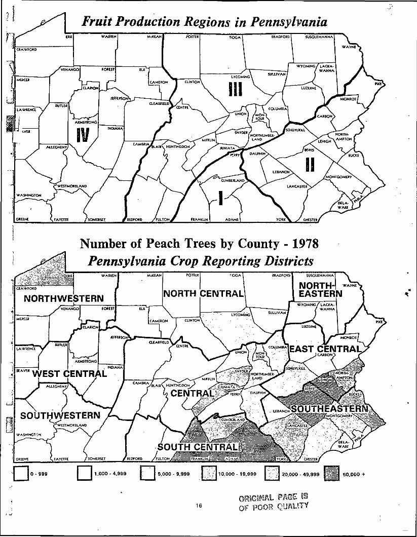
Fruit Production Regions in Pennsylvania

FAYETTC /SOMERSET ^BtOfO«0 /FULTON. FHANKUN ADAMS

Number of Peach Trees by County -1978Pennsylvania Crop Reporting Districts

NORTH-EASTERN

OiAWFORD

NORTHWESTERN CENTRAL

EAST CENTRA

WEST CENTRALBLAIRS. HUNTINGDON

CENTRAL

OUTHEASTERSOUTH\/yESTERN

WESTMORELAND

WASHINGTON

SOUTH CENTRALFAYETTE /SOMEKSEI I BEDfO80 /FULTON

10.000- 19.999 20.000 - 49,999 50.000 +

16

ORIGINAL PAGE ISOF POOR QUALITY

PENNSYLVANIA: PEACHES (TOTAL): GROWERS, ACRES, TREES AND PRODUCTION BY COUNTY AND REGION, 1978 I/

County And RegionGrowers Acres

Number Nyrber

Total Trees

Number

TreesPer

Acre

Production 2/ iBushels. :- per

Bushels ' Z ;Tree 3/

REGION I:

Adams 106 17.2 2,968.5Cumberland 9 1.5 155.0Franklin 43 7.0 1,874.5Perry 7 1.1 25.5York 48 7.8 1,110.4TOTAL 213 34.6 6,134.9

REGION II :

Berks 31 5.0 581.4Bucks 14 2.3 114.5Carbon & Monroe 5 .7 9.3Chester 12 1.9 125.3Dauphin 6 1.0 106.0Delaware 6 1.0 34.7Lancaster 27 4.4 387.5Lebanon 3 .5 58.0Lehigh 16 2.6 524.4Montgomery 16 2.6 84.6Northampton 5 .8 215.0PikeSchuylkill 33 5.4 77.0TOTAL 174 28.2 2,317.7

REGION III :

Bedford « Fulton 8 1.3 52.0Blair 4 .7 34.0Centre, Huntingdon & Hifflin 5 .8 61.0Clinton, Bradford, Susquehanna & Wyoming... 5 .8 10.7Columbia 12 1.9 34.7Juniata 12 1.9 272.6Lackawanna 4 .7 3.2Luzerne 9 1.5 39.0Lyconring 13 2.1 59.1Hontour 4 Northunberland 21 3.4 97.2Potter . . .Snyder 15 2.4 232.2Tioga -Union 4 .7 24.5WayneTOTAL 112 18.2 970.2

REGION IV:

Allegheny 12 1.9 30.7Armstrong 4 .7 26.1Beaver 9 1.5 22.4Butler 3 .5 2.8Cambria -Clearfield -Crawford, Elk 4 Venango 5 .8 3.6Greene . . .Indiana 8 1.3 15.9Lawrence 5 .8 19.1McKeanMercer 8 1.3 46.4SomersetWashington 12 1.9 27.7Westmoreland, Clarion, Fayette & Jefferson. 4 .7 12.5TOTAL 70 11.4 207.2

REGION V:

Erie 47 7.6 151.7TOTAL 47 7.6 151.7

PENNSYLVANIA 616 100.0 9,781.7

.301.

19

1162.7

5.91.2

1.31.1.3

4.0.6

5.4.9

2.2

.823.7

.6

.3

.6

.1

.92.8

.4

.6

.9

2.4

.3

9.9

.3

.3

.2

.2

.2

.5

.3

.12.1

1.61.6

255,65414,551

179.4352,294

90,423542,357

50,78710,045

7209,7588,2813,504

29,5414,685

55,9006,393

16,120

5,670201,404

5,1693,4133,COS

846561755271

2,5385,9197,867

721

15,192

1 ,863

75,402

2,3212,2851,554

250

382

1,7751,759

3,301

2,3071,437

17,371

20,30820,308

29.81.7

20.9.3

10.663.3

5.91.2.1

1.11.0.4

3.4.6

6.5.7

1.9

.723.5

.6

.4

.3

.1

.92.5

.3

.71.0

1.8

.2

8.8

.3

.3

.2

.2

.2

,4

.3

.12.0

2 .42.4

100.0 856,842 100.0

869396908188

3788777878

1017681

1077675

7487

99100497989808565

10081

65

76

78

76886989

106

11292

71

8311584

134134

88

422,69826,664

448,5463,395

221,0411,122,344

78,00920,9531,015

21,15519,0205,359

65,87211,075

113,60212,08124,720

12,800385,661

7,223400

4,765125

17,53619,710

222961

4,05510,329

25,112

2,413

92,851

2,5662,1051,162

35

552

352,071

4,479

1,655280

14,940

8,0508,050

26.01.7

27.6.2

13.669.1

4.81.3.1

1.31.2.3

4.1.7

7.0.7

1.5

.823.8

.4

.3

1.11.2

.1

.3

.7

1.5

.1

5.7

.2

.1

.1

.1

.3

.1

.9

.5

.5

2.11.92.92.03.02.5

2.42.21.52.72.31.72.83.62.72.52.3

2.S2.6

1.7.1

2.5.2

2.81.2.9.5

1.42.1

1.9

1.4

1.6

1.41.21.0.2

2.1

1.6

1.5

.8

.5I . I

.6

.6

1,623,846 100.0 2.4

V,I/

Some counties are combined to avoid disclosure of individual operations.Production in 1977 from acreage maintained for production in 1978.Yield calculations are derived excluding the 1-3 year age category trees.

ORIGINAL BOF POOR QUALITY

17

OF POOR QUALITY

PENNSYLVANIA: PEACHES (TOTAL): GROWERS, ACRES, TREES AND PRODUCTION BY SIZE OF OPERATION AND REGION, 1978

Size Of OperationJ (Trees)

-Region I:

1-99100-199200-499500-999

-1,000-2,4992,500-4,999

LJ.ooo*Total

pjteglon II:

F -1-99MflO-199

200-499..-500-999

1,000-2,499,',500-4, 9993,000*

Total

Region III:

4-99100-199200-499

"500-9991,000-2,499>»5QO-4',9995,000*

Total

Region IV:

1-99100-199"!00-499iOO-999

_i, 000-2, 4992,500-4,9995,000+

"Total

Region V:

1-99-JOO-199"200-499500-999

—1,000-2,4992,500-4,9995,000+

Jotal

All Regions:

,1-99100-199200-499

. -1500+

:

I Number

15194140473120

213

413037242514

3

174

21252716158

2/

112

2710249

2/

..

70

145

12115

..

..

47

11889

141268

Growers

i Percent

79

191922159

100

241721141482

100

1922241414

7-

100

39143413---

100

3011252311--

100

19152343

Number

8472,829

14,67732,96876,227

112,143302,666

542,357

1,8313,597

12,08217,01440,81452,08873,978

201 ,404

6863,4168,315

10,61122,03630,338

-

75,402

1 ,0841,2157,6917,381_

--

17,371

342715

3,5517,8227,878

--

20,308

4,79011,77246,316

793,964

Trees

I Percent

_

-36

142156

100

126'8

202637

100

14

11142941-

100

67

4443_

--

100

23

173939--

100

115

93

:

; Number

10.545.2

191.1411.6942.5

1,277.03,257.0

6.134.9

27.557.3

159.3233.6508.0636.0696.0

2,317.7

6.354.3

108.5148.7269.4383.0

-

970.2

7.417.697.285.0

---

207.2

2.57.7

31.957.552.1

--

151.7

54.2182.1588.0

8,957.4

Acres

i Percent

.137

152153

100

137

10222730

100

16

11152839-

100

48

4741---

100

25

213834--

100

126

91

Production

I Bushels

2,2094,976

25,19072 ,069

184,362225,688607,850

1,122,344

4,0607,139

21,47130,71772,858

125,305124,111

385,661

7846,666

10,6398,597

24,15042,015

-

92,851

980780

7,1506,030

---

14,940

69720584

5,3451,332

--

8,050

8,10220,23165,034

1,530,429

U

Percent

.'126

172054

100

1268

193232

100

17

129

2645-

100

65

4841---

100

197

6617--

100

114

94

PENNSYLVANIA. 616 100 856,842 100 9,781.7 100 1,623,846 100

M-4J

Production In 1977 from acreage maintained for production in 1978.Cor*ined with the 2,500-4,999 size group to avoid disclosure of individual operations.

PENNSYLVANIA: PEACHES - COMPARISON OF COMMERCIAL & NON-COMMERCIAL GROWER AND TREE NUMBERS 1967. 1972. 1978LJ "

.Trees

1-99 I/100+.7

! 1967

115665

Number Of Growers

; 1972

73472

! 1978

Number Of Trees

1967 ;

118 4,510498 1,069,598

1972 I

4,451882,550

1978

4,790852,052

Total II. 780 545 616 1,074,103 887,001 856,842

I/ Includes trees in orchards classified as commercial (100+ trees) for any fruit.

18

PENNSYLVANIA: PEACHES (COMMERCIAL): PRODUCTION. DISPOSITION AND VALUE, 1930-1978

Year

1930

1940

1950

I960

1970

1971

1972

1973

1974

1975

1976

1977

1978

ProductionI/

50.1

94.8

105.3

139.2

84.0

105.0

30.0

81.0

100.0

90.0

90.0

95.0

85.0

Utilization

HoneUse

15.0

11.5

10.0

2.9

yyyyyyyyy

Fresh

76.7

89.6

112.3

74.0

88.7

71.8

70.3

86.4

83.4

81.8

88.4

70.4

Sales

! All Processed '.

4.8

24.0

10.0

16.3

8.2

10.7

13.6

6.6

8.2

6.6

14.6

All Sales

95.3

136.3

84.0

105.0

80.0

81.0

100.0

90.0

90.0

95.0

85.0

PricePerPound3/

Cents

3.54

1.98

4.33

4.48

7.70

6.52

13.00

11.30

11.80

12.20

13.00

12.90

15.80

ValueOf

Production

Thous Dols

1,775

1.830

4,607

6,236

6,468

6,846

10,400

9,153

11,800

10,980

11,700

12,255

13,430

Includes some quantities not harvested and excess cullage. 2/ Included in fresh utilization. 3/ Fresh and processing prices combined.

BLACK AND WHITE PHOTOGRAPH

Photo Credit: Tom Piper

Photo Credit: Tom Piper

~^^^_. — — :> -v-^akLf '— ' — &•— *~ -*

> * - ^S - 'i 1

19

ORIGINAL PAGE ISOF POOR QUALITY

PENNSYLVANIA: PEACHES (TOTAL): COMPARISON OF ORCHARDS AND TREES OF ALL AGES BY COUNTIES, 1967, 1972 AND 1978

County & DistrictTree Survey, 1967

Number-Orchards . Total Trees

Tree Survey, 1972 ]_/

Number-Orchards ! Total Trees

Tree Survey, 1978

Number-Orchards ; Total Trees

Crawford - - - - 2 2/~|Erie 103 38,144 55 23,572 47 20,30~8

Forest. - - - - -j Mercer 3 1,877 - - 8 3,301

Venango 3 1,707 - 2 2JWarren

< NORTHWESTERN. TOTAL . 109 41.728 - : 59 ?3.«fi1/Bradford 3 y - - 1 2/~LJ Cameron

Clinton - - - 1Elk - - - i

§Lycoroing 7 3,230 - - 13 5.9T9HcKean - - - - _ -.PotterSullivan - - - - . _Tioga 1 2/ -

-! NORTH CENTRAL. TOTAL 11 4_.324 = : 1£ 6.J&32; Lackawanna 5 282 6 650 4 2711 Susquehanna 1 2] - 1 2/'Wayne 1 2] ~_Wyoming 3 1,510 - - 2 2/

., NORTHEASTERN. TOTAL 10 2.064 - - Z 5MI Armstrong. 3 1,762 3 930 4 ' 27285'Beaver 6 832 3 705 9 1,5541 Butler 3 188 - 3 250

Clarion 1 21 - I 2/Indiana 3 395 - 8 1,775

JOefferson 1 21 - 1 2]'Lawrence 10 2,523 - - 5 1,759'• WEST CENTRAL. TOTAL 27 6.725 : ; & 8.'635Blair 5 1,616 5 1,968 4 374T3Cambria 2 2/ - -

| Centre 1 21 - 1 2/j Clearfield 4 1,157 - -J Columbia 14 14,478 12 10,804 12 7,561

Dauphin 5 10,649 4 9,119 6 8,281,, Huntingdon 2 2,840 - - 2 2/i Juniata 10 32,048 10 26,812 12 21,755! Miff 1 in 4 2,497 - 2 2J: Montour 2 2J - 1 3_/

Northumberland 19 7,482 16 5,565 20 7,867Perry 3 940 7 2,294

] Snyder 18 16,103 11 14,028 15 15,192J Union 5 6,160 - . 4 1,863

,J CENTRAL. TOTAL 94 98.374 : - 86 71.234Carbon 5 1,063 - - 4 720Lehigh 23 70,372 15 . 57,935 16 55,900

i Luzerne 7 3,071 5 2,125 9 2,5381 Monroe 3 170 - - 1 3/•Northampton 7 12,230 4 7,078 5 16,120

~" Pike - - - • - -Schuylkill 30 ' 15,342 28 8,521 33 5,670

i EAST CENTRAL. TOTAL 75 102.248 - - 6J 80.948j Allegheny 18 6,408 12 5,146 12 2,321j Fayette 1 2/ 1 2l

Greena 1 2 / - - . . .Somerset - - - -

. , Washington 14 6,187 6 4,897 12 • 2,307i Westmoreland 3 1,794 - 1 21J SOUTHWESTERN. TOTAL 37 15.989 ;. : 25 5.053

Adams 147 265,837 126 270,498 106 255,654Bedford 10 9,478 8 2,071 7 5,169

.Cumberland 10 15,193 - - 9 14,551I Franklin 75 217,280 47 177,913 43 179,435j Fulton 1 3/ - 1 3/

"^ York 62 115,489 46 94,979 48 90.4F3SOUTH CENTRAL. TOTAL 305 623.277 :_ __. 214 545.232 .

.-. Berks 41 100,341 32 65,551 ' 31 50,787I I Bucks 11 11,382 6 7,425 14 10,045i Chester 14 8,731 9 6,545 12 9,758LJ Delaware 4 2J 3 2,484 6 3,504

Lancaster 22 32,805 18 26,717 27 29,541Lebanon 6 17,567 4 10,270 3 4,685

I Montgomery 13 5,669 12 5,103 16 6,3931 Philadelphia 1 2] - -J SOUTHEASTERN, TOTAL 112 179.379 : - 109 114.713

TOTAL. OTHER : : 39 3Z*52fl : :

; PENNSYLVANIA 780 1.074.108 545 857,001 6J£ 856.842• J/ Cor.parable data only available on counties listed for 1972 survey. 2J Not published separately to avoid disclosure of individual oper-

ations, y Monroe county combined with Carbon county; Fulton county combined with Bedford county; Montour county combined with Northumber-land county to avoid disclosure of individual operations.

i 20i

PENNSYLVANIA: PEACHES (TOTAL): NUMBER CF TREES BY COUNTIES AND AGE GROUPS, 1978 I/

County And District

Number Of Trees Maintained For Production According To Year Set Out

1975-1977(1-3 Yrs.)

1972-1974(4-6 Yrs.)

1957-1971(7-21 Yrs.)

'1956 4 Earlier; (22 Yrs +) Total All Ages

PercentOf Total

Erie 7,290 5,643 ' 5,800 1,575 20,308 2.*Forest - - - - - -Mercer 275 583 2,333 110 3,301 .4Venango & Crawford 165 60 23 4 252Warren - - - - - -NORTHWESTERN, TOTAL , 7,730 6,236 8,156 1,689 23,861 '2.8

Bradford, Clinton & Elk 10 - 703 - 713 .1Cameron • - - - - -' -Lycoming 2,950 728 2,225 16 5,919 .7McKean - - - - -, -Potter , - - - - - . -Sullivan ' - - - - - -Tioga . . . - - ' -NORTH CENTRAL, TOTAL 2,960 728 2,928 16 6,632 .8

Lackawanna 12 124 . 135 - 271 .1Wayne - - - - - -Wyoming & Susquehanna 215 6 42 263NORTHEASTERN, TOTAL 227 130 177 0 534 .1

Armstrong 525 560 700 500 -2,285 .3Beaver 366 2 1,156 30 1,554 .2Butler 80 120 50 - 250Indiana 820 836 99 20 1,775 .2Jefferson & Clarion - 520 492 - 1,012 .1Lawrence 482 515 662 100 1,759 .2WEST CENTRAL, TOTAL 2,273 2,553 3,159 650 8,635 1.0

Blair 166 3,085 120 42 3,413 .4Cambria - - - - - -Centre, Huntingdon & Mifflin 1,098 492 1,290 128 3,008 .3Clearfield - - - - - -Columbia 1,399 1,485 2,957 1,720 7,561 .9Dauphin 1,177 1,225 5,788 91 8,281 .9Juniata 5,420 1,385 14,950 - 21,755 2.5Montour S Northumberland 2,949 1,628 3,210 80 7,867 1.0Perry 636 149 1,509 - 2,294 .3Snyder 1,947 5,695 5,712 1,838 15,192 1.8Union 100 253 1,510 - 1,863 .2CENTRAL, TOTAL 14,892 15,397 37,046 3,899 71,234 8-3

Carbon & Monroe 61 420 239 - 720 .1Lehigh 14,326 11,051 27,670 2,853 55,900 6.5Luzerne 536 1,094 851 57 2,538 .3Northampton 5,385 2,840 7,895 - 16,120 1.9Pike - - - - - -Schuylkill 451 1,443 3,519 257 5,670 .6EAST CENTRAL, TOTAL 20,759 16,348 40,174 3,167 80,948 9.4

Allegheny 437 176 1,702 6 2,321 .2Fayette & Westmoreland - 325 100 - 425 .1Greene - - - - - -Somerset - - - - - -Washington 351 307 1,596 53 2,307 .3SOUTHWESTERN, TOTAL 788 808 3,398 59 5,053 .6

•Adams 53,755 *2,504 141,369 17,926 255,654 29.8Bedford 4 Fulton 877 859 3,266 157 5,169 .6Cumberland 645 2,155 11,750 - 14',551 1.7Franklin 23,973 34,459 107,772 13,221 179,435 20.9York 17,120 19,391 48,705 5,207 90,423 10.6SOUTH CENTRAL, TOTAL 95,370 39,439 312,862 36,511 545,232 63.6

Berks 13,675 5,355 23,804 1,953 50,787 5.9Bucks 615 896 6,753 1,780 10,045 1.2Chester 1,923 4*2 6,976 417 9,758 1.1Delaware 261 2,879 364 - 3,504 .4Lancaster 5,697 3,515 19,270 1,059 29,541 3.5Lebanon 1,575 430 2,630 ' - ' 4,685 .6Montgomery 1,515 1,937 2,409 532 . 6,393 .7Philadelphia ' - - - - -SOUTHEASTERN, TOTAL 30,262 16,504 62,206 5,741 114,713 13.4

PENNSYLVANIA 176,261 158.743 470,106 51,732 856,842 100.0

PERCENT OF TOTAL TREES 20.5 18.5 54.9 6.0 100.0

_!/ Some counties are combined to avoid disclosure of individual operations.

21

ORIGINAL PAGE f9OF POOR QUALITY

PENNSYLVANIA: PEACHES-(TOTAL): TREES BY VARIETY AND AGE GROUPS, 1978

Variety1975-1977 : 1972-1974 : 1957-1971 : 1956 & Ear l ier

(1-3 Years) : {4-6 Years) : (7-21 Years) : (22 Years +)Total

All Ages % Of Total

LJ

larly:j Dixie Red

Earliglo' Early Red Haven.

Early Red Fre.... Jerseyland1 Redhaven

RedskinSunhavenOther Early

Total Early

1,142535305539

1,28023,87911,563

3,4215,353

48,017

1,0801,9851,536

592433

27,65610,6715,6144,187

53,754

1,1151,964

761,1491,961

55,53929,19711,079

2,010104,090

300

140816

4,748834217126

7,181

3,6374,4841,9172,4204,490

111,82252,26520,33111,676

213,042

.4

.5

.3

.3

.513.16.12.41.4

25.0

9lid-$eason:Ambergem 60

, Baby Gold 6,915.1 Belle of Georgia 288l Blake 2,4071 Cresthaven 7,984

Garnet Beauty 3,662Glohaven 1,323

j Hale Harrison Brilliant 129j Halehaven 969I Harbelle 1,561

Harken 3,004Harmony 4,408

i Golden Jubilee 451j Loring 16,966

Hadisen .' 897Ranger • 85Red Elberta 82Red Crest 73Richhaven 213Southhaven 65Suncrest 4,000Sunhigh 16,653Triogem 7,453Washington 4,963Other Mid-Season 9,570

Total Mid-Season 94,181

late:Brackett

J Elberta , 1,686Gemmers Late 300

. J. H. Hale • 1,778< Jefferson 700! Jerseyqueen 11,285- Late Sunhaven - Slaybaugh.. 870

Monroe 2,289Rio Oso Gem 10,608Sweet Sue 1,451

] White Hale 236; Other Late 2,860Total Late 34,063

TOTAL ALL VARIETIES 176,261

1,

1754,170211

3,6928,350791

1,372357

2,2531,441810

3,019548

13,03397833031091

,358303

3,69520,2473,5242,3324,75878,148

932,466245

1,5841,5768,2791,192662

8,09760392

2,19526,841

158,743

6,70016,2961,00738,3551,092249

1,1042,62910,236

176200577

2,43758,644,2842,090928797

6,203813

2,05752,31615,5339,48616,984253,193

15633,758

40010,55817,77317,645

6461,93125,391

801,6472,837

112,823

470,106

100132

1,4366035125440

5,784

6561,069

40954943438550

5,8372,808109

1,81821,507

23817,361

101,664317242

1001,785

1541.17323,044

51,732

6,93527,4811,63845,89017,4864,7373,9243,55519,2423,1784,0148,0044,09289,7128,1992,6001,814995

8,1591,2319,75295,05329,31816,89033,130447,029

48755,271

95515,58420,36637,4522.7084,98245,8811,5912,4299,065

196,771

856,842

.83.2.2

5.42.0.6.4.42.2.4.5.9.5

10.51.0.3.2.11.0.11.011.13.42.03.852.0

.16.5.11.82.44.4.3.65.3.2.31.023.0

100.0

ORIGINAL PAGE ISPOOR

22

PEARSORIGINAL PAGE

BLACK AND WHITE PHOTOGRAPH

Location Of Trees: Fruit Region I accounts for 57 percentof the 118,874 commercial trees. Adams county alonecontains 45 percent of the total 127,158 trees. The leadingsix counties (Adams, Schuylkill, York, Erie, Lehigh andFranklin) contain 73 percent of the total trees.

Age Of Trees: Of the 127,158 total pear trees, 9.1 percentare 1-3 years old, 14.4 percent 4-6 years old, 53.9 percent7-21 years old and 22.6 percent 22 years or older.

Varieties: The Bartlett pear is by far the most popularvariety in Pennsylvania comprising 65 percent of the total127,158 trees. Other leading varieties as a percent of totaltrees are: Bosc — 17, D'Anjou — 7, Clapps Favorite andSekel — 2 percent each.

PENNSYLVANIA: PEARS (COMMERCIAL): COMPARISON OF GROWERS AND TREE NUMBERS BY REGIOH - 1972 &'1978

Number of Orchards And Trees: Commercial pearorchards (100+ Trees) at 193 in 1978 increased 7 percentfrom the 180 total in 1972. The corresponding treenumbers increased 23 percent from 96,373 in 1972 to118,874 in 1978.

Acreage In Orchards: Commercial pear acreageincreased 29 percent from 1,073 acres in 1972 to 1,380.7in 1978. Trees per acre declined from 90 in 1972 to 86 in1978. Pears were the only fruit to decline in trees per acresince the 1972 survey.

Region1972 Survey 1978 Survey

I.Number Of Orchards' Number Of Trees ^Number Of Orchards' Number Of Trees Nunber Of Orchards" Number Of Trees

Percent Change 72/78

Iii.:in.IV & V

754428

, 33

48,93626,21012,0479,180

80554117

68,10731 ,29213,5355,940

+ 7+25+46-48

+39+19+12-35

PENNSYLVANIA. 180 96,373 193 118,874 + 7 +23

Photo Credit: Tom Piper

23

Fruit Production Regions in Pennsylvania

Number of Pear Trees by County - 1978Pennsylvania Crop Reporting Districts

NORTH-IEASTERNNORTH CENTRALNORTHWESTERN

EAST CENTRA

r~ WEST CENTRAL

CENTRAL

OUTHEASTSRMSOUTHVyESTERN

WESTMODELANO

-*ASHINGION

SOUTH CENDH/FULTON/

50.000

24

ORIGINAL PAOE SSOF POOR QUALITY

PENNSYLVANIA: PEARS-(TOTAL): GROWERS, ACRES, TREES AND PRODUCTION BY COUNTY HID REGION, 1972 & 1978

County&

Region

Region I:

FranklinYorkOther

Total

Region II:

BerksBucksChester

Lancaster .

NorthamptonSchuylkillOther

Total

Region III:

BedfordBlairBradford

Lackawanna

HifflinNorthumberlandSnyderOther

Total

Region IV:

WashingtonOther

Total

Region V:

Erie

Total

PENNSYLVANIA

Growers

1972

731738

5

133

22663

153

1386

248

114

443

1056

103

1399

76

10333

12

31

4?

47

401

j 1978

72223615

145

211185

193

1486

3211

138

944

1077

. 163

141225

112

105

103

27

55

27

27

477

Acres

1972

432388725

582

471625305415759

17698

355

214

524172

173

131523

135

8135

22

39

91

91

1,212

I 1978

678.049.096.025.0

843.0

36.718.014.030.943.38.0

90.36.1

13.0101.710.1

372.1

16.219.07.9

22.021.12.0

1^.06.0

18.015.849.2

191.2

6.03.05.01.0

12.5

27.5

61.0

61.0

1,499.8

Trees

Total .

1972

37,9943,2027,8352,226

51,258

2,6151,044

7382,8914,8221,1107,194

4551,3716,350

448

29,039

1532,729

5351,9801,126

183466169652

1,2154,078

13,286

45573

131353

1,791

2,818

7,387

7,887

104,283

.' 1978

57,1074,8536.9811,530

70,471

3,1401,4951,1833,4402,9151,0305,541

3851,771

12,012702

33,521

1,2932,203

6321,9191,912

197925297

1,3271,2023,517 .

15,454

363203417

24875

1,881

5,731

5,731

127,155

Trees

1972

88859089

88

5667309690769650819252

80

831951078466

11027504779

177

98

60103447481

72

87

87

86

Per Acre

; 1978

84997261

83

868385

11167

1296163

136118

70

90

80116808791996650747672

81

6167832470

68

94

94

85

(Bushels)i/11

82,7096,769

12,068965

102,511

4,7089.9892,2925,3336,3123.065

13,063768

5,55212,893

664

64,639

5549,700

5854,0051,260

232919700

1,7771,0337,164

27,929

919105

74

431

1 ,529

8,305

8,305

204,913

_!/ Production in 1977 from acreage maintained for ored'jction in 1978. Comparable data for 1972 not available.

ORIGINAL PAGE 19OF POOR QUALITY

25

OF POOR QUALITY

PENNSYLVANIA: PEARS (TOTAL): GROWERS, ACRES, TREES MO PRODUCTION BY SIZE OF OPERATION AND REGION, 1978

Size Of Operation Growers .; (Trees)

•Talon I:

j-99.00-199200-499500-999%000-2,499

K 1.50074,999£J,OQO+

Total

kiJ-99100-199200-499

""00-999i,000-2,499

1,50074,9995,000

.Total

'eglon III:

t-99100-199••00-49930-999,000-2,499

^,5007,4,9995,000

" 'otal

'eglon IV & V:

1-99'00-19900-49900-999

-'.000-2,4992,5007.4,9995yOOO+

otal

All Regions:

1-99.00-19900j499

.00+

PENNSYLVANIA

Number

65272512115

y145

83251776

3/

138

711816

74/

112

65674

4/-

82

284766552

477

Percent

451917883-

100

601813

54_-

100

6416146---

100

79795-.-

100

60161410

100

! Number

2,3643,4557,5688,277

16,91731 ,890

-

70,471

2,3293,6794.4234,285

18,905

-

33,621

1,9192,4795,1085,948

---

15,454

1,672840

2,0723,028

-_-

7,612

8,28410,45319,17189,250

127,158

Trees

Percent

35

11122445-

100

711131356

-

100

12163339---

100

22112740---

100

69

1669

100

Acres

; Number

29.353.6

105.584.5

165.1410.0

-

848.0

36.849.362.854.2

169.0

-

372.1

27.234.564.565.0

---

191.2

25.811.321.929.5

---

88.5

119.1148.7254.7977.3

1,499.8

Percent

46

12102048-

100

1013171545_

-

100

14183434---

100

29132533---

100

8101765

100

Production \J

Bushels

6,1497,129

11 ,0529,592

26,19542,394

-

102,511

5,21116,9159,3998.388

24,726--

64 ,639

2.5462,7615,217

17,405-

-

27,929

1,761469

1,9455,659

-*-

9,834

15,66727,27427,613

134,359

204.913

I Percent

67

119

2641-

100

826151338--

100

9101962---

100

185

2057-

.-

100

8131366

100

j/ Production from 1977 from acreage maintained for production in 1978./ Combined with the 2,530-4,999 size group to avoid disclosure of individual operations.3/ Combined with the 1,000-2,499 size group to avoid disclosure of individual operations.4/ Combined with the 500-999 size group to avoid disclosure of individual operations.

PENNSYLVANIA: PEARS - COMPARISON OF COMMERCIAL & NON-COMMERCIAL GROWER AND TREE.NUMBERS 1957, 1972, 1978

TreesNumber Of Growers Number Of Trees

1967 1972 1978 1967 1972 1978

-99 I/.00+

Total I/-

343237

580

221180

401

284193'

477

10,51394,421

104,934

7,91596,373

104,288

8,284118,874

127,158

/ Includes trees in orchards classified as comnercial (100* trees) for any fruit.

26

PENNSYLVANIA: PEARS (COfflERCIAL): PRODUCTION, DISPOSITION AND VALUE, 1930-1978

Year

19301940195019601970197119721973 , .1974.'1975.,1976.'19771978

I/ Includes3/ Included

Production I/

14 25512 4255 2502,7504 100

. .. . 3,7003,700

. . . 1,9004,1004,5003,7004,7003,300

some quantities notin fresh utilization

Utilization

HomeUse

5,9503,9752.500650

I

Iu

Fresh

8,2757,3252,7502,100

2/2/

3,3001,900

2/2/27

\,harvested and excess cullage. 2/. 4/ Fresh and processing prices

Sales

'. All Processed ; All Sales

2/If

21

II

Not publishedcombined.

8,2757,8252,7502,1004,1003,7003,3001,9004,1004,5003,7004,7003,300

to avoid dislosure of

PricePer

Ton £/

Dollar

443478102153128196230235216232252286

individual

: Value! Of• Production

626401410280627474647437964972858

1,184944

operations.

Photo Credit: Tom Piper

CRiGiNVVu PA~GT£BLACK AND WHITE PHOTOGRAPH

27

PENNSYLVANIA: PEARS (TOTAL): NUMBER OF TREES BY COUNTIES AND AGE GROUPS - 1978 I/

County & DistrictNumber Of Trees Maintained For Production According To Year Set Out

1975-1977(1-3 Years)

1972-1974 : 1957-1971 11956 & Earlier!,. , ,, . '(4-6 Years) 1(7-21 Years) 1(22 Years +) ;r<Kal A11 A9es;

PercentOf

Total

(Crawford 15, (Erie 350" ''Forest

Mercer & Venango 39.-—Warren

INQRTHWESTERN. TOTAL 404i .Bradford ~^Cameron

ClintonElk ....

{IjLyconiing 35• HcKean '.'•Sullivan

Tioga & Potter_ NORTH CENTRAL. TOTAL 35

'Lackawanna 10jWayne/•Wyoming & Susquehanna

.NORTHEASTERN, TOTAL 10Beaver 8~

"^Butler, Armstrong, Clarion & Jefferson 20' ) Indiana 124., j Lawrence

WEST CENTRAL. TOTAL. 152Blair........ 400""

""'Cambria & Centrei Columbia 185| Dauphin 971Huntingdon & Clearfield 7Ouniata 1,077

• •-] Mif fl iniMontour & Northumberland 137! Perry 12* Snyder 82Union 40

'CENTRAL. TOTAL 2.911;Carbon, Monroe & Pike 8j Lehigh 6Luzerne 97Northampton 45

, Schuylkill 141I EAST CENTRAL. TOTAL 297; Allegheny 56~Fayette, Somerset & Westmoreland 30Greene 'Washington

j SOUTHWESTERN. TOTAL 861 Adams 3,546

• : Bedford 675Cumberl and 396Franklin 1,308

; Fulton« York 339

...'SOUTH CENTRAL. TOTAL.... 6.264Berks 719Bucks 215

; Chester 332i Delaware 2

,,j Lancaster 119LebanonMontgomery

"", Philadelphia, : SOUTHEASTERN. TOTAL. 1,387

*"" PENNSYLVANIA 11.546

En PERCENT OF TOTAL TREES 9.1

348

6

354

1421,749

46

1.937

123,284

3..296_

1695,731

91

5.991

.14.5

.1

-A.2-467

1.244

1311.842

165

801

2501.216

632

2.085

3813,098

.5

1.6

.32.4

21

21

111

557668104

35152103391

55 197

557754

.4

.65725

117

199

3316242093

20296-

417123838

.2

.1

.3

.1

.777310023945460

57420

1832

2,405

73050

1,0411,884

225835297502272754115

6,705

30015

454131

50

179

18355

1.367

2,203165

i,9193,440

3421,912

2971,392

3041,202

21213.38R

1..1

1.52.7

.31.5

.21.1

i!o.2

10.5263211103298316

1,191

81,211

2141,4277,847

10.707

524,113

5111

3,7083.385

3315,541

9251,771

12,01220,580

.34.4

.71.49.4

16.22575

100

19531

226

87

24JLLL

363136

24_523_

.3

.1

.48,932480127720

2,54012.799

34,075118703

1,911

2,97739.784

10,55420

914

1,12512.613

57,1071,2931,2264,853

6,98771.460

44.91.01.03.8

5.556.2

20620823

63940

128

1.244

1,8121,066

80772

1,48999080

6.316

4036

26297669

178

1.579

3,1401,4951,188

3712,9161,030

386

1Q.526

2.51.2.9.3

2.3.8.3

8.3

,18,318 68.579 28.715 127.158 100.0

14.4 53.9 100.0

I/ Some counties are combined to avoid disclosure of individual operations.

ORIGINAL PAGE ISOF POOR QUALITY

28

PENNSYLVANIA: PEARS (TOTAL): TREES BY VARIETY ADO AGE GROUPS, 1978

Variety

REGION I:Bartlett

Clapps Favorite

SeckelStarksOtherTOTAL

REGION II:BartlettBoscClapps FavoriteD'Anjou

HagnassSeckelStarksOtherTOTAL

REGION III:Bartlett

Devoe

SeckelOtherTOTAL

REGION IV:Bartlett

OtherTOTAL

REGION V:Bartlett

OtherTOTAL

ALL REGIONS;Bartl°ttBoscClapss Favor*! *° ....0' AnjouDevoeGorheiit''2gn°ssKoongloSeckelStarksOther

PENNSYLVANIA . ..

1975 - 1977 :(1-3 Years) :

2,5511,950

252 ,53339

80

70;,601

1 ,C£S95047171712

'CO

"92,5:3

1,719555

221

1055

* ": 32,r-5

-•;

— ~t

;»'

\ -'- -P

33353

- 7^33 , r ". 5

£ 7

-i

~/ >2 5

7

255

1972 - 1974(4-6 Years)

6,7743,551

255650

5213

6010

3'1300200

12,339

1,530686

97212

5

846

1162,786

1,982401

702055

111

2,540

2852

17305

2556033

348

10,8774.7CO

4228S2

55233

6210

£25306335

13,313

1957 - 1971(7-21 Years)

22,6167,706

7454,912

302689

1,320177736220515

39,938

13,4821,483

2221 ,258

16965

675345994

18,693

5,732342363215331

1142

no7.145

71385

2551,053

1,061501187

1,749

43,60410,117

1 ,42-

6,415727908

1 ,425203

1,509614

1,626

63,579

: 1956 & Earlier: (22 Years +)

10,578391101518

3212

39

1217

11812,593

7,53370211839513253

29565

2919,584

2,1482771756030

32211

3,023

1421079

231

2,479503197

3,284

22,3802.4S8

414989

44^1192

75772

558

23,715

TotalAll Ages

42 ,54914,1381,3636,668

3451,1141,419

1871 ,258

527903

70,471

23,6613,861

4841,882

323130

1,254416

1,61033 621

11,5811,585

608532416116381235

15,454

1,343130408

1,881

3,9771,307

447'5,731

83,11121,0212,5699,136

8661,6191,605

4152,9871,0142,815

127,158

PercentOf Total

60.420.01.99.5

51.62.0.3

1.8.7

1.3100 0

70.411.51.45.61.0

.43.71.24.8

100 0

74.910.33 93.42.7

.82.51.5

100.0

71.46.9

21.7100.0

69.422.87.8

100.0

65.416.52.07.2.7

1.31.3.3

2.3.8

2.2

100.0

29

ORDINAL PAGE ISOF POOR QUALITY

CHERRIESORIGINAL PAGE fS'°F POOR QUALITY

lumber Of Orchards And Trees: The number ofcommercial tart cherry growers (100+ Trees) has steadily

""leclined since the first commercial fruit tree survey(onducted in 1953. Commercial growers (100+ Trees) in1978 at 140 was down 30 percent from the 201 accounted

.Jjor in 1972. Commercial tart cherry growers had 183,768tt frees in 1978 compared with 217,610 in 1972, a 15percent decline. Commercial sweet cherry growers at 61

declined 16 percent from 1972 while corresponding tree

tumbers increased from 28,230 to 33,068, or 17 percent,

creage In Orchards: Commercial tart cherry acreage at1,967 declined 23 percent from 2,550 in 1972 whileiommercial sweet cherry acreage declined from 526 to472.5 or 10 percent during the same period. Tart cherrytrees per acre increased from 85 in 1972 to 93 in 1978

,,while sweet cherry trees per acre increased from 54 to 70|n 1978.

, jLocation Of Trees: Adams, Erie, Franklin and York

"?ounties contain 94 percent of the total 186,387 tart;herry trees. Fruit Region I accounts for 80 percent of the

total trees. For sweet cherries, Lancaster, Erie, Adams,Franklin and Northampton counties contain 73 percent ofhe 38,019 total trees.

Age Of Trees: Of the total 186,387 tart cherry trees, 14.8percent were 1-3 years old, 16.8 percent 4-6 years old,14.4 percent 7-21 years old and 34.0 percent 22 years or

wilder. Of the total 38,019 sweet cherry trees the agepercentage breakdown was 16.0, 10.6, 40.6 and 32.8'espectively.

" Varieties: Montmorency tart cherry trees account for 97percent of the total trees, English Morello 2 percent andither varieties 1 percent. Dark sweet cherry treesjomprise 72 percent of total trees while light sweet cherrytrees accounted for 23 percent. Leading varieties as a•percent of the total 38,019 trees are: Windsor — 16.3,3ing — 15.2, Napoleon — 10.1, Hedelfingen — 9.9 and

- Jchmits Biggereau — 9.2.

PENNSYLVANIA: TART CHERRIES: COMPARISON OF COMMERCIAL AND NON-COMMERCIAL GROWER AND TREE NUMBERS, - 1967. 1972. and 1978

if". %'" '^ * /

AND WHITE

41 ' Trpps

1967

-99 198^0 283Total 481

III PENNSYLVANIA: SWEET CHERRIES:

ft

1967

99 3001 00* 86Total 386

Number Of Growers

! 1972 !

117201318

COMPARISON OF COMMERCIAL AND

Number Of Growers

i 1972

15973

232

1978 ;

162140302

NON-COMMERCIAL

1978 :

20861

269

1967

4 567 '270 906275 473

GROWER AND TREE

1967

6 64826 29532 .944

Number Of Trees

: 1972 :

3 057017 cin??n fifty

NUMBERS, - 1967, 1973, and

Number Of Trees

; 1972 :

4 113OQ port

32.343

1978

1Q-S 7CO

1 ftfi "3R7

1978

1978

4 95111 nfirt38.019

30

umber of Sweet Cherry Trees by County - 1978Fruit Production Regions in Pennsylvania

SOMUST Xaofcxo /FULTON

Number of Tart Cherry Trees by County -1978«iPennsylvania Crop Reporting Districts

NORTH-!EASTERNNORTH CENTRAL

WEST CENTRAL

SOUTHWESTERN

SOUTH CENTRAL

31 ORIGINAL PAGE ISOF POOR QUALITY

PENNSYLVANIA: TART & SWEET CHERRIES (COMMERCIAL): PRODUCTION, DISPOSITION AMD VALUE, 1940-1978

•! Year

Total I Utilized

Utilization

Processed

Fresh J* Canned '. All Processed

PricePerPoundy

ValueOf

UtilizedProduction

12.616.818.014.012.712.36.313.112.67.63.26.2

12.616.818.014.012.711.16.3

13.111.57.63.26.2

6.15.02.9.5.9.7.4.9

1.11.0.5.8

Tart Cherries (Mil.Los.)

5.5 6.510.4 11.89.8 15.15.5 13.57.0 11.87.9 10.44.7 5.98.6 12.26.8 10.45.3 6.62.6 2.74.5 5.4

Cents

3.58.28.47.811.38.719.819.811.425.829.841.7

Thous.Dols.

4411,3781,5121,0921,435966

1,2472,5941,3111,961954

2,585

Sweet Cherries (Tons)

1940j1950'i960i'1970"19711972 ,,1973H974:1975..._•197619771978!

2,2001,500

. . . 500600

. . . 800200660730860460350

. .. . 750

2,1001 ,500500600800190660730860460350750

1051713705004494156407f'j730792836836

22025618530035979422511628364293627

il_/ Total production is the quantity actually harvested plus quantities not harvested because of economic reasons. Utilized productionis the amount sold plus the quantities used at home or held in storage. When total and utilized production are equal, economicabandonment and cullage quantities are considered at a "normal" level.

•!il Fresh and processing prices combined.

Photo Credit: Tom Piper

32

ORIGINAL PAGEBLACK AND WHITE PHOTOGRAPH

PENNSYLVANIA: CHERRIES (TOTAL): GROWERS, ACRES, TREES AMD PRODUCTION BY COUNTY - 1978 V

County & DistrictGrowers

Tart I Sweet

; Acres

i Tart I Sweet :

Total Trees [Trees Per

Tart I

Acre

Sweet I Tart '. Sweet

Production 2] \ Yield Per Acre 3_/

Tart I

Number

Crawford & MercerErieForestVenangoWarrenNORTHWESTERN, TOTAL

BradfordCameronCl intonElkLycomingMcKeanPotterSullivanTiogaLackawannaSusquehannaWayneWyomingNORTH CENTRAL & NORTHEASTERN TOTAL..

Armstrong, Clarion, and Jefferson.. .Beaver & LawrenceButlerIndianaWEST CENTRAL, TOTAL

Blair, Cambria, Huntingdon & MifflinCentre & ClearfieldColumbiaDauphinJuniataHontour & NorthumberlandPerrySnyderUnionCENTRAL, TOTAL

Carbon & LuzerneLehighMonroeNorthamptonPikeSchuylkillEAST CENTRAL, TOTAL

AlleghenyFayette, Somerset & WestmorelandGreeneSOUTHWESTERN, TOTAL

AdamsBedford & FultonCumberlandFranklinYorkSOUTH CENTRAL, TOTAL

Berks & LebanonBucksChester, Delaware 4 MontgomeryLancasterPhiladelphiaSOUTHEASTERN, TOTAL

PENNSYLVANIA

332---

35

4/-.-

10-----

V--

12

56-5

16

436548673

46

48-3-8

23

56-

11

6353

1529

115

1359

17

44

302

320---

23

i/---9---_

*/*/--

13

37-3

13

5-5679473

46

68-3-9

26

58-

13

3784

182794

1257

17

41

269

.6290.8

--.

291.4

4/-_

-3.7

---__

V

-10.7

3.7.3-

1.75.7

7.010.02.48.34.56.15.8

13.3.1

57.5

.2

.5_

2.2-

1.64.5

.51.8

-

2.3

1,375.43.0

17.0100.851.1

1,547.3

34.55.65.2

35.8

81.1

2,000.5

.3145.8

--_

146.1

4/-.-

9.1----

4/V--

11.5

2.5.4-

.73.6

12.6-

3.318.612.53.23.84.9

.559.4

.23.0

-18.1

-1.1

22.4

.33.6

-

3.9

48.813.22.8

31.218.0

114.0

4.61.6

23.1155.5

184.8

545.7

5523,791

--_

23,846

4/---

346---__

?/--

1,021

19927-

133359

524800100470270464485

1,0157

4,135

1249

_215

-122398

51151

-

202

133,670297

1,37610,3674,146

149,856

3,046340289

2,895

6,570

186,337

228,999

--_

9,021

4/-.-

1,092----

V5/--

1,320

17538-

61274

1,018-

12276994620520327543

3,581

17300

_1,958

-68

2,343

26247

-

273

2,8381,062

1312,2411,3377,609

47083

1,16811,377

13,598

33,019

9282--_

82

V

--

94----_

«/--

95

5490-

7863

75804257607684767072

6098-

98-

7688

10284-

88

979981

1038197

88615681

81

93

73fi?

-_

62

47-._

120----

4/

</

-lib

7095-

8776

81-

3741766453568660

85100

_108

_62

105

8769-

70

588047727467

102s25176

74

70

798404,970

--_

405,768

4/

_-

3,470---._

V--

19,470

950--

1901,140

10,5001,0001,3506,0046,100

15,2557,208

35,970166

83,553

461,095

-6,100

-1,6458,886

-100

-

100

2,151,8393,500

12,565116,200137,806

2,421,910

60,0365,2855,800

44,918

116,039

3,056,866

Sweet !

Lbs. -

220171,865

,-«

172,085

i/

.-

2,380---.I/I/--

. 6,210

100--

50150

5,700_

3,91017,07422,2508,5843,500

32,3501,080

94,448

941,513

-

25,000-

52027,127

_1,630

-

1,630

55,0982,3952,850

43,325.15,386119,054

12,315810

9,00079,633

101,758

522,462

Tart I

1,3301,393.._

1,393

</

--

938-

----

y--1,820

257--

112200

1,500100563723

1,3562,5011,2432,7051,6601,453

2302,190

_2,773

-1,0281,975

_56-

44

1,5651,167

7391,1532,6971,565

1,740944

1,1151,254

1,431

1,528

Sweet

7331,179

--.

1,178

y-.-

262----

4/I/--

540

40--

7142

452-

1,185918

1,7802,683

9216,6022,1601,590

470504

-1,381

-473

1,211

_453

-

418

1,129181

1,0181,389

8551,044

2,677506390512

551

957

I/ Some counties are combined to avoid disclosure of individual operations.Zl Production in 1977 from acreage maintained for production in 1973.37 Actual yield will be slightly higher due to non-bearing acres included in calculations.4/ Included in North Central and Northeastern total.

ORIGINAL PACE ?8OF POOR QUALITY

33

PENNSYLVANIA: TART CHERRIES (TOTAL): GROWERS, ACRES, TREES AND PRODUCTION BY SIZE OF OPERATION AND REGION, 1978

Size Of Operation(Trees)

Region I:

1-99- 100-199

200-499500-9991,000-2,4992,500-4,999

- .5,000+

1 {TotalyRegion II:

j—J-99lJjlOO-199M200-499"^00-999

1,000-2,499, -2,500-4,999' 5.000+

"total

Region III:

' i-99J100-199

. .200-499500-9991,000-2,499

r 2,500-4,9995,000+

Total

. Region IV & V:

1-99100-199200-499500-999

' 1,000-2,4992,500-4,9995,000+

Total

' "All Regions:

. il-99100-199 '.200+t

' PENNSYLVANIA

I/ Production in 1977y Combined with the !

Number

3519301110

76

118

52585

U

..

70

3968

3/

.

.

53

369745

4/5761

16239

101

302

from acreage00-999 size

Growers

'. Percent

3016259965

100

747

127---

100

741115----

100

591511

78--

100

531334

100

maintained forg>-oup to avoid

:

I Number

7562,4409,9887,727

14,08624,66090,369

150.026

550602

2,0264,272

---

7,450

665849

2,948---.

4,462

6481,0462,2782,587

17,890--

24,449

2,6194,937

178,831

186,387

production indisclosure of

Trees

I Percent

12759

1660

100

88

2757---

100

151966----

100

349

1173--

100

13

96

100

1978.individual oper

:

; .timber

9.035.5

122.078.8

165.0286.0851.7

1,548.0

7.58.3

28.745.5

---

90.0

8.013.530.9

----

52.4

9.012.525.527.0

236.1--

310.1

33.569.8

1,897.2

2,000.5

•ations.

Acres

'. Percent

1285

111855

100

89

3251---

100

152659----

100

3489

76--

100

23

95

100

! Production

I Pounds I

14,93085,365

313,970255.786294,842545,698915,027

2,425.618

9.0307,800

43.99670.101

---

130,927

11,58313,98067,750

----

93,313

2,0649.450

40.20018.190

337.104--

407,008

37,607116,595

2,902,664

3,056,866

I/

Percent

•

14

1310122238

100

76.

3453---

100

121573--_

_

100

_

2105

83--

100

14

95

100

3/ Combined with the 200-499 size group to avoid disclosure of individual operations.i4/ Combined with the 1,000-2,499 size group to avoid disclosure of individual operatirations.

PENNSYLVANIA: SWEET CHERRIES (TOTAL): GROWERS, TREES, ACRES AND PRODUCTION BY SIZE OF OPERATION AND REGION, 1978

' ~ Size Of Operation! : (Trees)U i

1-99fijlOO-199PeOO-499

PENNSYLVANIA

Growers

Number '. Percent

208 7729 1116 616 6

269 100

Number

4,9513,7765,267

24,025

38,019

Trees

Percent '.

13101463

100

Number

73.256.488.9

327.2

545.7

Acres

• : Percent

14101660

100

Production

Pounds :(000) :

85,30195,769

103,197238,195

522,462

I/

Percent

16182046

100

I/ Production in 1977 from acreage maintained for production in 1978.

34

ORIGINAL PAGE £OF POOR QUALITY

ORIGINAL PAGE ISOF POOR QUALITY

PENNSYLVANIA: TART CHERRIES (TOTAL): COMPARISON OF ORCHARDS AND TREESOF ALL AGES BY COUNTIES - 1967, 1972 and 1978

County & District

CrawfordErieForestMercerVenangoWarrenNORTHWESTERN, TOTAL....BradfordCameronClintonElkLycorai ngMcKean ...PotterSul 1 ivanTiogaNORTH CENTRAL, TOTAL...LackawannaSusquehannaWayneWyomi ngNORTHEASTERN , TOTALArmstrongBeaverButlerClarion

JeffersonLawrenceWEST CENTRAL, TOTALBlairCambriaCentreClearfieldColumbia ...DauphinHuntingdon ...JuniataHifflinMontourNorthumberlandPerrySnyder. .

CENTRAL, TOTALCarbonLenigh

Monroe

PikeSchuylkillEAST CENTRAL, TOTALAlleghenyFayetteGreeneSomersetWashingtonWestmoreland . .SOUTHWESTERN, TOTALAdamsBedfordCumberland . . .FranklinFultonYork ....SOUTH CENTRAL, TOTALBerksBucks

Del awa reLancasterLebanon

PhiladelphiaSOUTHEASTERN, TOTAL

TOTAL, OTHER

PENNSYLVANIA

Tree Survey

Ilumber-Orchards ;

92

_

922

1

3

11412183311315

17.... 2

123

. . 54363164121

531

10321

7248_

15216

12586

35_

34208

8621633-56

4S1

, 1967

Total Trees

58,587

58,587520

y

490

211,220

21212121

23114039y21682142572600212252082160636569686421

307-2,0512,006

8,030212962121y127

2,171140

2158721794

160,697250

3.3C324,033

9,030197,3182,2902073 Co

i isoiy

6,550

275. 473I/ Comparable data only a/ailable on counties listed for 197:I/ Bradford and Susquehanna Counties combined rti-.n Lyco-in; Co7- *. o_ t_ -..~cj ,4,-e-i-lnc.irp of individual Gopratin'n1;

! Tree Survey, 1972 ]_/

I Number-Orchards ; Total Trees

55 36,869

-

-

-

4 ' 374

5 380

4 1,7029 764

5 96

6 124

3 '81

3 485

104 141,2495 3296 4,66920 -12,492

29 11,379

10 1,035*• 95

12 . 2,054

34 5,490

?13 220.557survey. 2/ '.?•_ published to avoid., Lucerne Co. cor.b-.ned with Cart-en

Tree Survey,

Number-Orchards ;

232

i i

35. i :

10

i

ni

i35

15

161

2

65

4226673463 '81

3

82351

13

11 i63 i53

15

29 !11512563

17 '•

44 !

302disclosure of indivioualCo., Lebanon Co. combined

1978

Total Trees

23,791

23.846I/

1,031

1.021

U

3/64

1359!/ -

%10047021270

361485

1,0157

4,1351249

215

12239851yy2121202

133,670297

1,37610,367

4,146149,856

1,411340

364,530

3/

6,570

186,387operations,with

Lancaster Co. to avoid disclosure o.35

PENNSYLVANIA: TART CHERRIES (TOTAL): NUMBER OF TREES BY COUNTIES AMD AGE GROUPS, 1978 I/

County And District

Number Of Trees Maintained For Production According To Year Set Out

1975-1977 ; 1972-1974 | 1957-1971 ;1956 1 Earlier ' .(1-3 Yrs.) I (4-6 Yrs.) '. (7-21 Yrs. ) : (22 Yrs +) -T°tal All Ages

PercentOf Total

I Crawford & Mercer 34- 'Erie

Forest„.»Venango

[WarreniiJNORTHWESTERN, TOTAL 341 1

Bradford, Susquehanna X Lycoming 272Carceron

MI Cl i nton

jllj McKeanPotter ,Sullivan

r™|Tiogai Lackawanna{Wayne

WyomingNORTH CENTRAL & NORTHEASTERN, TOTAL 272

iArmstrong, Clarion & Jefferson: Beaver & Lawrence 2jButler

IndianaWEST CENTRAL, TOTAL 2

: Blair, Huntingdon & Hifflin 210\ Carcbri a1 Centre & Clearfield 200Columbia 35Dauphin 47

jOuniata 30s Northumbe rl and & Montour 252

. .! Perry 125Snyder 704Union

i CENTRAL, TOTAL 1,603

[Lehigh 18Luzerne & Carbon 7Monroe

, Northampton 105|PikeiSchuylkill 2

- ; EAST CENTRAL, TOTAL 132

AT legheny- Fayette, Somerset & Westmoreland 70• Greenei Washington 2

- SOUTHWESTERN, TOTAL 72

Adams 23,028, Bedfordi Cumberl and 20, Franklin 550FultonYork 822

'SOUTH CENTRAL, TOTAL 24,420

• Berks & Lebanon 8•'Bucks 85

Chester 158, Delaware 2'. Lancaster 809I Montgomery

^PhiladelphiaSOUTHEASTERN, TOTAL 1,062

if PENNSYLVANIA 27,597

PERCENT OF TOTAL TREES 14.8

2,674

2,674

234

32,023

2,026

400

1819,094

19,112

115

5523,791

23,846

'1,021

12.8

12.8

.6

234

1212

34

3508

171

1013

1587

312

1

22,37260

1653,600

68026,877

4198

20

. 395

842

31,239

16.8

400

15418

117289

250

1255515

240102132183

3,105

10

110

112232

2060

1999

48,391225525

5,666

2,01756,8241,959

2177533

806

3,090

54,065

34.4

115

457

45630

1252

237

100215128

.3840

125

522

30

30

39,87912

666551

62741,735

66030

1885

.1,576

63,486

34.0

;1,021

I 199

! 27

133359

524

800100470

. 270464485

1,0157

4,135

4912

215

122398

51130

21202

133,670297

1,37610,367

4,146149,856

3,046340253

362,895

6,570

186,387

100.0

.6

.1

.1

.2

.3

.4

.3

.1

.3

.3

.5

2.2

.1

.1

.2

.1

.1

71.7.2.7

5.6

2.280.4

1.7.2.1

1.5

3.5

100.0

1 _!/ Some counties are combined to avoid disclosure of individual operations.

ORIGINAL 19OF POOR QUALITY

36

PENNSYLVANIA: SWEET CHERRIES (TOTAL): TREES BY VARIETY AND AGE GROUPS - 1978

Variety :

DARK:

Black TartarianHedelf ingenLambertSmidts BiggereauVistaWindsorOtherTOTAL DARK

LIGHT:Emperor FrancisNapoleonStarks GoldOtherTOTAL LIGHT

TOTAL ALL VARIETIES....

PERCENT OF TOTAL

•

Variety

English MorelloOther

TOTAL ALL VARIETIES....

1975-1977(1-3 Years)

74112995087916429160719

4,131

2732242

1 ,6161 ,953

6,084

16.0

PENNSYLVANIA:

1975-1977(1-3 Years)

27,467

130

27,597

! 1972-1974 !I (4-6 Years) |

1 109207536113295192261507

3,220

28077124318799

4,019

10.6

TART CHERRIES (TOTAL)

1972-1974; (4-6 Years) ;

29,8251,000414

31,239 .

1957-1971(7-21 Years)

2 490293

T 274690

1,430542

2 4662,53311,718

755959628

1 3843,726

15,444

40.6

: TREES BY VARIETY

1957-1971(7-21 Years)

62,794603668

64,065

1956 & Earlier(22 Years +)

'pQ3

995140871

3 302960

8 210

4312 775123933

4 262

12,472

32 8

AND AGE GROUPS -

1956 & Earlier ;(22 Years + ) :

60,8732,407206

63,486

TotalAll Ages

5 77QQpp

1 0303,512

6 ion

A 71Q77 ?7Q

1 739

077A OCl

10 740

38,019

100 0

1978

TotalAll Ages

180,9594,0101,418

186,387

PercentOf Total

1C 0

2 4

9 Q

2 79.2

1C 0

174

n 7

4 fiin i? An o

100.0

PercentOf Total

97.12.2.7

100.0

PAGE ISPOOR QU&UTY

37

GRAPESORIGINAL PAGE ISOF POOR QUALITY

1 Number And Location Of Vineyards: The number ofcommercial grape vineyards (2+ Acres) increased from

| 348 in 1972 to 436 in 1978, a 25 percent increase. Of thej total 474 vineyards in 1978, 361 or 76 percent were in ErieCounty. The number of vineyards throughout the rest of

. Pennsylvania more than doubled from 1972.

Acreage In Vineyards: The acreage in commercial grapevineyards in 1978 was 14,245.4 compared with 9,865.8 in1972, a 44 percent increase. Of the total 436 commercialvineyards 177 with 20.0 acres or more accounted for 86percent of all commercial grape acreage. Geneva doublecurtain acreage increased from 657.1 acres in 1972 to2,771.9 acres in 1978. This is 19.4 percent of the total14,271.3 acres. An additional 90.9 acres of Genevadouble curtain were intended for 1978.

Age Of Grape Acreage: Of the total 14,271.3 acres ofgrapes, 10.0 percent were 1-3 years old, 9.3 percent 4-6years old and 80.7 percent 7 years or older. For Concordacreage 7.8 percent was 1-3 years old, 5.4 percent 4-6years old and 86.7 percent 7 years or older.

Varieties: Concord acreage at 11,751.2 accounted for82.3 percent of the total 14,271.3 acres. Although allvarieties increased in acreage since 1972, French Hybrids,Delaware and Catawba acreage more than doubled. Of allthe French Hybrid acreage in the 1-3 year age group 80percent was in counties other than Erie. This is primarilydue to an increased number of wineries established inrecent vears.

PENNSYLVANIA: GRAPES (TOTAL): COMPARISON OF NUMBER OF VINEYARDS AND ACRES BY REGION, 1972 I, 1978.1Region

III „IllIVV

! 1972

! Number Of Vineyards

714

.... 1312333

Survey

'. Number Of Acres

12.336.122.817.6

9,798.9

j 1978 Survey

'. Number Of Vineyards '.

16562120361

Number Of Acres

90 4251 5163 697 7

13.668.1

PENNSYLVANIA.i 379 9,887.7 474 14.271.3

Acreage of Grapes by Counties - 1978Fruit Production Regions in Pennsylvania

38

PENNSYLVANIA: GRAPES (TOTAL): GROWERS, ACRES AND PRODUCTION BY SIZE OF OPERATION, 1972. And 1978 I/

Size OfOperationIn Acres

Growers '. Acres

N'jcber

1972J 1973

Percent '. Number '. Percent

1972 : 19781 1972 '. 1973 '. 1972 - 1978

Production I Yield

Tons

1972 \ 1977

Percent '. Tons/Acre

1S72 1 1977 | 1972 j 1977

Geneva DoubleCurtainAcres

1972 • 1977 j 1978

.1-1.92.0-4.95.0-9.9

10.0-19.920.0-49.950.0-99.9

100.0-199.9....200.0 & Over...

PENNSYLVANIA...

31

7573

10^3511

•»

373

38809089

10544208

474

812201928

g31

100

8 21.917 142.619 -99 719 937 422 3138.6

9 2525.64 1425.42 1145.5

100 9337.7

25.9236 0579 7

1202 03243.53022.72761.03200.5

14271.3

15

1032261412

100

24g

23211923

100

67609

24004922

160071188465615269

47719

30393

113425247856754466256127

32233

15

1034251411

100

]4g

24232119

100

3 14 34 85 05 14 74.64.6'

4.8

1 21 72 02 12 42 52.41.9

2.3

2 55 o

16 5109 6

70 583.0

370.0

657.1

3 219 680 286 6

289 5481 2836.1975.5

2771.9

3 220 686 692 6

294 5533 2841.1991.0

2862.8

\J Production in 1977 from acreage maintained for production in 1978.

PENNSYLVANIA: GRAPES (TOTAL): GROWERS, ACRES AND PRODUCTION BY COUNTY AND REGION - 1978

County & Region

REGION I:

CumberlandYork

, TOTAL

REGION II:Berks

Dauphin

Lehigh ...

OtherTOTAL

REGION III:Blair

OtherTOTAL

REGION IV:

OtherTOTAL

REGION V:

Total

PENNSYLVANIA

44816

68317461256

43e.1021

633370

351351

474

20 320.449.790.4

12.336.012.6111.611.530.437.1251.5

76 19.330 048 2163 6

19 512 943 o22 397 7

13,668.113,668.1

14,271.3

: Production

Harvested :

28 419 522 470 3

9 550 212 2141 47 o

41 735 '297 2

250 02

15 624 8290 6

1.32 260.013.877.3

31,497.831,497.8

32,233.2

- Tons I/

Not Harvested

6 0

3 09 0

4 Q3 81 51 110 4

21

3

_

195.0195.0

214.7

V Production in 1377 from acreage maintained for production in 1978

PEYiSYLVANiA: GRAPES (TOTAL): NUMBER Or GRAPE VINEYARDS 3V SIZE OF C?EVT:Cf! AND COUNTY - 1978

County

Erie

PENNSYLVANIA

Number Of Vineyard Acres In

: .1-1.923533

! 2.0-1.9

c.±3580

I 5.0-9.9

6525SO

i 10.0-19.9

79106.9

I 20.G-49.9

1005

iC5

Each Size Groun

! 50.0-99.9 :iCO. 3-199.9

-3 201

-- 20

;200.0 & Over!

8

8

Total

361113474

ORIGINAL PAGE SSOF POOR QUALITY

39

PENNSYLVANIA: GRAPES

Variety CountyNumber :Of :

Growers :

(TOTAL): NUMBER OF GROWERS, ACRES OF VINES BY VARIETY, COU

Number Of Acres Maintained For ProductionAccording To Year Set Out

1975-1977(1-3 Years)

1972-1974(4-6 Y,ears)

1971 « Older(7 Years +)

Total AcresAll Ages

iTY I AGE GROUPS

Geneva Double Curtain

Total Acres •1977 :

Total AcresIntended 1978

i!

*] Delaware

La

pSj Niagara

*iBaco Noir

'i Chancellor....

* Chelois

' DeChanac

Seyval Blanc..

• Foshi

i Vidal 256

' Other Native. .

Other French

, t

Total Native..

- Total FrenchHybrids

* Total Vinifera

Total< All Varieties!

»•

- j Percent Of All!

ErieOtherPA...

OtherPA...ErieOtherPA.ErieOtherPA...ErieOtherPA...ErieOtherPA...ErieOtherPA...ErieOtherPAErieOtherPA...ErieOtherPA...ErieOtherPAErieOtherPA...

OtherPAErieOtherPA...

ErieOtherPAErieOtherPA...

ErieOtherPAErieOtherPA

ErieOtherPA

Acres

7715Q?occ

64dlQ"

18c-i

in16?fi7934

412161110?15

1116518233141712223432477g1422352964

83745

ifai/

}-i1217

361113474

202 54.6

207.1890 926.4

917 316.03.519 5

8.68.6

87.42.690.0

12.812.83.42.15.510.010.420.41.52.84.3

10.910.92.014.116.1

10.610.615.010.325.35.114.819.9

53.853.8

1201.960.5

1262.4

31.9127.8159.71.35.26.5

1235.1193.51428.6

10.0

305 06.8

311 8621 017.7638 722.511.333 8

71.01.7

61.85.0

66.81.52.43 93.810.214 05.69.615.26.0

28.934.94.811.616.418.830.749.5

21.921 96.0

•18.524.532.04.336.3

3.530.734.2

1043.046.1

1089.1

50.0164.5214.512.05.0

17.0

1105.0215.61320.6

9.3

394 41.4

395 810103 2

92.010195 2315 93.5

319 436 611.748 3287 327.1314 416.0.9

16 910.0.6

10 66.3.26 53.55.18.64.0

4.028.05.6

33.69.02.4

11 46.5

6.569.724.394.0

16.617.434.0

11207.1160.0

11367.1

99.932.2132.121.01.9

22.9

11328.0194.1

11522.1

80.7

901 912.8

914 711615 1136.1

11751 2354 418.3372 737 321.358 6436.534.7

471 217 516.133 617.212.930 121.920.242 111.035.847.88.822.531.348.850.499.29.034.943 927 528.856 3106.843.4150.2

20.1101.9122.0

13452.0266.6

13718.6

181.8324.5506.334.312.146.4

13668.1603.2

14271.3

100.0

197 03.7

200 72222 0

1.42223 4189 02.2

191 28 01.2

. 9 278.82.481 23.0

3 0, 8.5

8 55. 0

5 0

-

4.8

4.88.52.0

10.5

2.02.08.0

8.019.21.2

20.4

2.02.04.0

2714.012.1

2726.1

39.86.0

45.8

2753.818.1

2771.9

19.4

197 04.7

201 72307 6

1.42309 0189 03.6

192 68 01.29 280 83.384 13 0

3 08.5

8 55 0

5 0

-

4 8

4 88.52.010.5

2.02 08 0

8 019.21.220 4

2 02.04 0

2801.615.4

2817 0

39 86.045 8

2841.421.4

2862 8

LJ jy pata unavailable.

ORIGINAL PAGE IS"OF POOR QUALITY

ORIGINAL PAGE ISOF POOR QUALITY

PENNSYLVANIA: GRAPES (TOTAL): COMPARISON OF VARIETIES BY ACRES, 1972 & 1978

Variety :

Ccncord

Delaware

-Fredonia

Niagara

Other Native

Total Native

Total French Hybrids

Total Vinifera

Total All Varieties

1972 Survey Acres

3^4 5

3,835.3

130.8

55.3

235.5

85.0

9,688.5

176.3

22.9

9,837.7

: Percent Of Total

3.5

89.3

1.3

.6

2.4

.9

98.0

1.8

.2

100.0

: 1978 Survey Acres

914 7

11,751.2

372.7

58.6

471.2

150.2

13,718.6

506.3

46.4

14,271.3

: Percent Of Total

6.4

82.3

2.6

.4

3.3

1.1

96.1

3.6

.3

100.0

Percent Change 78/72

+166

+ 33

+185

+ 4

+ 99

+ 77

+ 42

+187

+103

+ 44

PENNSYLVANIA: GRAPES: AVERAGE PRICE PAID BY PENNSYLVANIA WINERIES AND PROCESSORSFOR PENNSYLVANIA GROWN GRAPES BY VARIETY 1976-1978 I/- 2/

Year !

1976

1977

1978

I/ Dollars Per Ton.

Year

193019401950I960197019711972197319741975197619771978

Concord ! Catawba ;

S 195

254

210

S 128

175

226

Delaware

S 198

199

279

; Niagara

% 170

220

177

I Other Native IFrench Hybrids!

S 250 S

225

301

2/ Source - Graps production and utilization survey.

PENNSYLVANIA: GRAPES (COMMERCIAL) : PRODUCTION, DISPOSITION AND VALUE,

Production V

Total

22, JOO17,30030,90033,50045,00057,00037,60040,00053,00048.0CO59,00030,00057,500

I Utilized

22,40017,30029,70033,50045,00057,00037,500iO.OOO53,000i3,00059,00029,65057,500

258

304

326

1930-1978

Utilization

Fresh

4,68010,3502,9001,9401,8002,1702,2752,3901,2751,6601,3501,3501,300

'. Juice

6,95026,80031,56036,23051,47032,41033,36742,21739,25046,27023,35042,300

Sales

': Other Sales '.

17,7203/3/3/

3,9703,3602,9154,2439,5087,09011,3804,95013,900

I/ Total production is the quantity actually harvested plus quantities not harvested because ofthe amount sold plus the quantities used at home or held in storage. When total and utilizecment cullage quantities are considered at a "normal" level.

2J Fresh and processing prices combined.3/ Included in fresh sales.

All Sales

22,40017,30029,70033,50045,00057,00037,60040,00053,00048,00059,00029,65057,500

Other :

$ 600

744

861

PricePer

UnitI/

_ t/Tnn

4339112119147137172221198168168231232

Average

$ 193

252

212

ValueOf

Production

963675

3,3263,9366,6157,8096.4678,84010,4948,0649.9126.84913.340

economic reasons. Utilized production isproduction are equal, economic abandon-

41

ORIGINAL PAGE IS

BY

Variety

PENNSYLVANIA: GRAPES: QUANTITYVARIETY DELIVERED TO WINERIES AND

PennsylvaniaPlants And Wineries :

1976 1 1977 ! 1978 ! 1976

OF PENNSYLVANIA GROWN GRAPESPROCESSING PLANTS, 1976-1978 ]_/

OF

Out-0f-5tate :Plants And Wineries :

i 1977 ': 1978 I 1976 1

POOR Ql

Total y

1977 !

JALITY

1978

Tens

Concord 42,690.6 21,409.5 38,622.5 10,155.0 5,155.0 13,490.0 52,845.6Catawba -2- -2- -2- -2- -2- -2- 2,092.9Delaware -3- -3- -3- -3- -3- -3- 194.9Niagara -4- -4- -4- -4- -4- -4- 1,489.4

f Other Native -5- -5- -5- -5- -5- -5- 176.9*-** (2+3+4+5) 1,862.1 1,054.5 2,478.8 2,092.0 593.0 764.0 3,954.1

French Hybrid 592.1 517.0 696.7 187.0 43.0 73.9 779.1(-Other 47.9 7.9 17.6 0.0 0.0 0.0 47.9

OTAL 45,192.7 22,988.9 41,815.7 12,434.0 5,791.0 14,327.9 57,626.7

26,564.5693.1152.7712.589.2

1,647.5560.07.9

52,112.61,523.4239.4

1,300.2179.8

3,242.8770.617.6

28,779.9 56,143.6

V Source - Grape production and utilization survey. 2/ Excludes small amount of cullage.

PENNSYLVANIA: GRAPES: UTILIZATION BY VARIETY OF GRA?ES USED IN PENNSYLVANIAWINERIES AND PROCESSING PLANTS, 1976-3978 V

Wine

1976 ; 1977 ; 1978

Sweet Juice + Other

1976 ; 1977 ; 1978

Total 2/

1976 ; 1977 ; 1978

Tons

Other Native

pther

TOTAL

.J Source -

258.5912.372.9282.4140.9705.851.3

... 2,424.1

1,143.0311.1141.7334.5134.2595.19.7

2,669.3

2,508.91,070.4295.5565.6248.7847.625.6

5,562.3

72,097.00.00.0

2,295.00.00.00.0

74,392.0

y Excludes

32,8'3.93.00.0

1,199.00 00 00 0

34,025.9

small ancunt

57,836.20.00.0

2,015.00 00 00 0

59,851.2

of cullage.

72,355 5912.372 9

2,577.4140 9

• 705 851 3

76,816.1

33,972 9311.1141 7

1,533.5134 2595 19 7

36,698 2

60,345 11,070 4295 5

2,580 6248 7847 625 6

65 413 5

PENNSYLVANIA: GRAPES: UTILIZATION BY VARIETY OF PENNSYLVANIA GROWN GRAPES TOALL WINERIES MO PROCESSORS, 1976-1973 I/

Tons

; Concord ; Catawba ; Delaware ; Niagara : Other: Hative

: French: Hybrids

: Other: Varieties

; Total y

Wine

T976.1977.'978.

8,1)55.64,383.2

10,605.3

44,790.022,103.341,507.3

2,092.9693.1

1,523.4

0.00.00.0

194.9152.7239.4

0:00.00.0

305.4239.5510.2

176.989.2

179.8

Juice + Otrer

,184.0473.0790.0

0.00.00.0

779.1560.0770.6

0.078.00.0

Total

47.97.9

17.6

0.00.00.0

11,643.76,125.613,846.3

45,983.022,654.342,297.3

1976977978

52,845.626,486.552,112 6

2,092.9693.1

1,523.4

194.9152.7239.4

1 ,489 471?. 5

1 300 2

175 9-•3 Z

173 8

779 1638 6770 6

47 97 9U c.

57 626 728 779 9EC 1AT fi

I/ Source - 2/ Excludes small er.cunt of cullage.

42

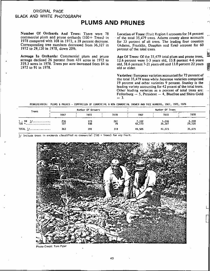
.ORIGINAL PAGEBLACK AND WHITE PHOTOGRAPH

PLUMS AND PRUNES

Number Of Orchards And Trees: There were 78commercial plum and prune orchards (100+ Trees) in1978 compared with 108 in 1972, a 28 percent decrease.Corresponding tree numbers decreased from 36,327 in1972 to 29,120 in 1978, down 20%.

Acreage In Orchards: Commercial plum and pruneacreage declined 26 percent from 431 acres in 1972 to319.3 acres in 1978. Trees per acre increased from 84 in1972 to 91 in 1978.

Location of Trees: Fruit Region I accounts for 54 percentof the total 35,479 trees. Adams county alone accountsfor 33 percent of all trees. The leading four counties(Adams, Franklin, Dauphin and Erie) account for 60percent of the total trees.

Age Of Trees: Of the 35,479 total plum and prune trees,12.6 percent were 1-3 years old, 15.8 percent 4-6 yearsold, 58.6 percent 7-21 years old and 13.0 percent 22 yearsold or older.

Varieties: European varieties accounted for 72 percent ofthe total 35,479 trees while Japanese varieties comprised19 percent and other varieties 9 percent. Stanley is theleading variety accounting for 42 prcent of the total trees.Other leading varieties as a percent of total trees are:Fellenburg — 5, President — 4, Bluefree and Shiro Gold

PENNSYLVANIA: PLUMS & PRUNES - COMPARISON OF COMMERCIAL & NON COMMERCIAL GROWER AND TREE NUMBERS. 1967, 1972, 1978

Trees

1 - 99 I/100 +.,.7

TOTAL I/

.

I 1967

236127

363

Number Of Growers

! 1972 ;

173108

281

1978

24178

319

:

; 1967

7,33242,173

49 505

Number Of Tre«

; 1972

5,24636,327

41 ,573

>s

; 1978

6,35929,120

35,479

V Include trees in orchards classified as commercial (100 + Trees) for any fruit.

Photo Credit: Tom Piper

43

Fruit Production Regions in Pennsylvania

Number of Plum and Prune Trees by County -1978Pennsylvania Crop Reporting Districts

NORTH CENTRAL EASTERNNORTHWESTERN

WEST CENTRALAIBS. HUNTlNODOi ^ JUN1AIA

CENTRAL

SOUTHEASTERNMONTGOMUrSOUTHVVESTERN

WESTMO»ELAND

WASHINGTON

SOUTH CENTRAL/ / /

/FULTON/ •

5,000 - 9.999 I y-T.| 10,000 - 19,999ORIGINAL PAGE iS

OF POOR

44

PENNSYLVANIA: PLUMS & PRUNES (TOTAL): GROWERS. ACRES. TREES. PRODUCTION BY COUNTY & REGION - 1978 V

:

-

REGION I: 'AdamsCumberlandFranklinPerryYork

TOTAL

REGION II:Berks ,BucksCarbonChesterDauphin & LebanonDelawareLancasterLehighMonroe & PikeMontgomeryNorthamptonSchuylkill

TOTAL

REGION III:BedfordBlair

•Bradford & TiogaHuntingdon, Centre, and HontourCl In tonColumbiaFultonJum'ataLackawannaLuzerneLycomingHi f f 1 inNorthumberlandPotterSnyderSusquehanna & Wyomi ngUnionWayne

TOTAL

REGION IV:AlleghenyArmstrongBeaverClarion, Jefferson, Butler & ClearfieldCambriaMercer, CrawfordElkFayetteGreeneIndianaLawrenceMcKeanSomersetVenangoWestmoreland, and Washington

TOTAL

REGION V:Erie

TOTAL

PENNSYLVANIA

Growers

Number

403

164

32

95

1673674

166245

21

97

4-35-5-6489-

10-533-

65

10344_5---93---5

43

19

19

319 •

%

12.5.9

5.01.3

10.1

29.8

5.02.1

.91.92.21.35.01.9.6

1.31.66.6

30.4

1.3-

.91.6

-1.6

-1.91.32.52.8

-3.1

-1.6.9.9-

20.4

3.1.9

1.31.3

_1.6

---

2.8.9---

1.6

13.5

5.9

5.9

100.0

Acres

Number

122.42:0

56.01.2

25.3

206.9

12.05.5.6

3.421.31.1

15.49.71.12.03.64.4

80.1

1.7-

.92.1

-11.0

-8.0

.54.13.4

-11.3

-10.9

.4

.3-

54.6

3.03.51.9.9-

5.8---

4.02.1

---

1.7

22.9

22.0

22.0

336.5

. %:

.31.7.5

14.5.3

6.6

53.6

3.11.4.2.9

5.5.3

4.02.5.3.3

.91.1

20.7

.4-

.3

.6-

2.8-

2.1.1

1.0.9-

2.9-

2.8.1.1-

14.1

.8

.9

.5

.2-

1.5---

1.0.6---

.4

5.9

5.7

5.7

100.0

'. Total Trees I

• Number•

11,659146

5,18595

1,973

19,058

993580

58315

2,51381

1,293870106185318386

7,692

161-

75175

-922

-73946

318264

-967

-904

4232-

4,645

269335171

73-

527---

334160

---

145

2,014

2,070

2,070

35,479

.a/

• JO

: :

32.9.4

14.6.3

5.5

53.7

2.81.6.2.9

7.1.2

3.72.4.3.5.9

1.1

21.7

.5-

.2

.4-

2.6-

2.1.1.9.8-

2.7-

2.6.1.1-

13.1

.8

.9

.5

.2-

1.5---

.9

.5---

.4

5.7

5.8

5.8

100.0

TreesPer

Acre

9573937978

92

831059793

11874849091938888

96

95-

8383-

84-

92927878-

86-

83105107

-

85

90969081-

91---

8476---

85

88

94

94

92

Production 2/

Bushels

15,531245

6,24516

3,441

25,478

9391,191

26590

3,31755

1,0331,946

20285694774

10,870

48-

298195

-1,709

-2,052

21199454

-889

-3,238

435-

9,142

253548

39-

271---

' 178457

---

185

1,445

2,535

2,535

49,470

%

31.4.5

12.6-

7.0

51.5

1.92.4.1

l.Z6.7.1

2.13.9

-.6

1.41.6

22.0

.1-

.6

.4-

3.5-

4.1-

.4

.9-

1.8-

6.6-

.1-

18.5

.5

.1-

.1-

.5---

.4

.9---

.4

2.9

5.1

5.1

100.0

: Yield: Per• Tree 3/: (Bu.)

1.61.71.2.3

2.0

1.5

1.12.2.6

2.01.3

.7

.92.63.31.93.22.3

1.7

.3-

4.01.4

-1.9

-2.9.6.9

2.8-

1.5-

3.8.3

1.3-

2.4

1.0.2.1--

.6---

.52.9

---

2.2

.9

.8

.8

1.6

!_/ Some counties are combined to avoid disclosure of individual operations.21 Production in 1977 from acreage naintained for production in 1978.3/ Yield calculations are derived excluding the 1-3 year age category trees.

45

ORIGINAL PAGE S3OF POOR QUAL5TY

PENNSYLVANIA.

PENNSYLVANIA: PLUMS & PRUNES (TOTAL): GROWERS, ACRES, TREES, PRODUCTIONBY SIZE OF OPERATION, 1978

Size OfOperation(Trees)

1-99100-199200-499500-9991000 +

Number

2414226

55

Growers '.

: Percent :

75.513.28.21.61.5

Acres

Number :

67.270.285.643.0

120.0

Percent Number

17.4 6,35918.2 5,65922.2 7.69511.1 3,43931.1 12.327

Trees

: Percent

17.916.021.79.7

34.7

Production

: Bushed :

108

108

12

,285,115,220,250.600

I/

Percent

field

Bushels '.Per Tree '.

20.8 1.616.4 1.420.6 1.316.7 2.425.5 1.0

yBushelsPer Acre

153116119192105

319 100.0 386.5 100.0 35,479 100.0 49,470 100.0 1.4 128

!_/ Production in 1977 from acreage maintained for production in 1978.and acres included for this calculation.

2/ Actual yield will be slightly higher due to ram bearing trees

PENNSYLVANIA: PLUMS & PRUNES (TOTAL): TREES BY VARIETY AND AGE GROUPS, 1978

-j Variety

European:Stanley

i Fellenberg

j BluefreOther EuropeanTOTAL EUROPEAN

> Japanese:i Methley

Shiro (Gold)

TOTAL JAPANESE

'TOTAL OTHER

.TOTAL ALL VARIETIES....

\i

1975 - 1977(1-3 Years)

2,31342337262278

3,232

6810289408667

555

4,454

1972 - 1974(4-6 Years)

2,62928246182456

3,910

127256376456

1,215

497

5,622

. 1957 - 1971(7-21 Years)

7,4161,240671730

5,03815,095

587458523

2,3773,945

1,735

20,775

• 1956 & Earlier •: (22 Years +) :

2,520260408

5323,360 -

9341238400772

496

4,628

TotalAll Ages

14,8781,8241,5091,0826,30425,597

875857

1,2263,6416,599

3,283

35,479

PercentOf Total

41 95 14 33 017 872 1

2.52 43 410 318 6

9 3

100.0

J PENNSYLVANIA: PLUMS AND PRUNES (COMMERCIAL): NUMBER OF ORCHARDS AND TREES BY SIZE GROUPS, SELECTED COUNTIES, 1378

County 100 - 199 Trees 200 - 499 Trees 500 + Trees Total

/Adams - No. Of Orchards

Erie - fio. Of OrchardsErie - No. Of TreesOthers - No Of OrchardsOthers - No. Of TreesPENNSYLVANIA - No. Of OrchardsPENNSYLVANIA - No. Of Trees...

5809

4626

334,224

425,659

61,576

41,215

164,904

267,695

48,477

,6

7,28910

15,766

1510352

81,841

5516,*17

7829.120

46

ORIGINAL PAGE i3OF POOR QUALITY

PENNSYLVANIA: PLUMS AND PRUNES (TOTAL): NUMBER OF TREES 3Y COUNTIES AND AGE GROUPS, 1978 I/

County And District

Number Of Trees Maintained For Production According To Year Set Out

1975-1977 : 1972-1974 ; 1957-1971 11956 & Earlier :(1-3 Yrs.) : (4-6 Y r s . ) ; (7-21 Yrs.) I (22 Yrs +) ;

.„ . ocAll Ages

PercentOf Total

Erie 20Mercer and Crawford 70NORTHWESTERN, TOTAL 90

Bradford and Tioga 20Lycomi ng 102NORTH CENTRAL, TOTAL 122

Lackawanna 8Susquehanna and Wyoming 30NORTHEASTERN, TOTAL 38

ArmstrongBeaverButler, Clarion and JeffersonIndiana 8LawrenceWEST CENTRAL, TOTAL 8

Centre, Clearfield, Huntingdon & Montour.. 36Col urcbi a 40

. Dauphin 489Juni ata 40Northurrberland 383Perry 40Snyder 43Union 5CENTRAL, TOTAL 1,076

Carbon 17Lehigh 115Luzerne 105Monroe and Pike 100Northampton 103Schuyl kill 44EAST CENTRAL, TOTAL 484

Al 1 egheny 8Washington and Westmoreland 5SOUTHWESTERN, TOTAL 13

Adare 1,860BedfordCumberlandFranklin 105York 225SOUTH CENTRAL, TOTAL 2,190

Berks 174Bucks 30Chester 25DelawareLancaster and Lebanon 169Montgomery 35SOUTHEASTERN, TOTAL 433

PENNSYLVANIA 4,454

PERCENT OF TOTAL TREES 12.6

192

192

103141

1652812

233

438

2554

334

595

412

520

22108

75

4571

321

5270

122

2,00273

615520

3,210

.253312038

328100770

5,522

15.8

766432

1,198

2581

106

141226

51433670

130384

79628

1,509699525

5053025

4,045

n291

170261733

17770

247

6,46988

1464,2291,079

12,011

509473270

15753

2,025

20,775

1,09225

1,117

205070

16

16

165

2330

218

60200

41

290

591

8350138

6

10512

32

32

1,328

236149

1,713

5741

2818350

359

4,628

13.0

2,070527

2,597

75264339

464288

33517148

334160

1,048

200922

2.37373996795

90432

6,232

58864318106318386

2,050

269145414

11,659161146

,185,973

5,1,

19,124

993580315

811,433

1853,587

35,479

100.0

5.81.57.3

.2

.81.0

.1

.1

.2

.9

.5

.1

.9

.52.9

.62.66.72.12.7.3

2.5.1

17.6

.22.4

.9• 3.9

1.15.8

.8

.41.2

32.9.4.4

14.65.6

53.9

2.81.6.9.2

4.1.5

10.1

100.0

100.0

I/ Some counties are corf>ined to avoid disclosure of individual operations.

ORIGINAL PAGE ISOF POOR QUALITY

47

ORIGINAL PAGEBLACK AND WHITE PHOTOGRAPH

NECTARINES

Number Of Orchards And Trees: Consumer acceptanceof nectarines has increased substantially during recentyears. The number of commercial nectarine orchards(100+ Trees) increased from 44 in 1972 to 71 in 1978, up61 percent. The number of trees in commercial nectarineorchards climbed from 19,024 in 1972 to 44,877 in 1978.

Acreage In Orchards: Commercial nectarine acreagemore than doubled from 222 acres in 1972 to 479.6 in1978. During the same period trees per acre increasedfrom 86 to 94.

Location Of Trees: Fruit Region I accounted for 58percent of the total 47,938 nectarine trees. The leadingthree counties (Franklin, York and Adams) accounted for58 percent of the total trees.

Age Of Trees: Of the total 47,938 nectarine trees, 20.7percent were 1-3 years old, 41.6 percent 4-6 years old,37.3 percent 7-21 years old and .4 percent 22 years orolder.

Varieties: Leading varieties as a percent of total trees are:Redgold — 24, Sunglo — 17, Nectared — 11, andFavertop — 8.

PENNSYLVANIA: NECTARINES - COMPARISON OF COMMERCIAL & NON COMMERCIAL GROWER AND TREE NUMBERS1967 - 1972 - 1978

Trees

1-99 I/100 +Total I/..

Number Of Growers1967 ; 1972 ;

106 8635 44141 130

1978

15371224

1967

2,89224,03926,931

Number Of Trees; 1972 ;

2,32819,02421 ,352

1978

3,06144,87747,938

I/ Include trees In orchards classified as commercial (100 + Trees) for any fruit.

: y

Photo Credit: Tom Piper

48

Fruit Production Regions in Pennsylvania

Number of Nectarine Trees by County -1978Pennsylvania Crop Reporting Districts

NORTH CENTRAL EASTERNNORTHWESTERN

CENTRA

WEST CENTRALBIAIB\ HUNTINGDON/ / JUNIATA

CENTRAL OAUPH'

SOUTHEASTERNMONTGOMERYSOUTHWESTERN

WESTMOSELAND

WASHINGTON \

SOUTH CENTRAL/ / - -•Vv:-'>i'I •-'-.-""-•- • • " - . '

SOMEKS£I / 3EDfO«D /FULION/ "FIANKUM^ ADAMS

49 ORIGINAL PAGE ISOF POOR QUALITY

PENNSYLVANIA: NECTARINES (TOTAL): GROWERS, TREES, ACRES, PRODUCTION, BY COUNTY & REGION, 1978 I/

I Growers

: Number Percent

Acres

Number : Percent

Total Trees ! Trees • Production 2/

Number: rer :

Percent : Acre : Bushels Percent

YieldPerTree 3/

(Bushels)

AdamsCumberland & PerryFranklinYork

, TOTAL., 1i J REGION II:U Berks

BucksCarbon & Schuylkill

II ChesterB Dauphin & Lebanon«» Delaware

LancasterLehigh

: Monroe• Montgomeryt Northampton

Pike

i TOTAL

•••; REGION III:BedfordBlair & Huntingdon

> Bradford! Centre1 Clinton

ColumbiaFulton

: Juniata; Lackawanna •

Luzerne & Susquehanna...' Lycoming '. ..•

MifflinMontour & NorthumberlandPotter

; Snyder' Tioga

Union, Wayne! Wyoming; TOTAL

REGION IV:j AlleghenyI Beaver; Butler

CambriaClarion

: ClearfieldCrawford & MercerElkFayetteGreeneIndiana & Jefferson

, Lawrencei McKean

Somerset & Washington...Venango

! Westmoreland

J TOTAL

REGION V:K-» Eriel-l TOTAL

PENNSYLVANIA

237162672

1551256399-45"

73

33_

-5

5

66

8

7

3--

46

56

--.3

-

-44

5--

27

66

224

10.33.17.111.632.1

6.82.25.42.22.71.34.04.0

-1.82.2~

32.6

1.31.3

_

.2.2

2.2

2.72.7

3.6

3.2

1.3--

20.5

2.22.8

..__

1.3

.

.1.81.8

2.2--

12.1

2.72.7

100.0

75.31.6

172.869.7319.4

43.42.25.78.719.0.83.619.4_

5.23.4

-

111.4

3.23.8

4.5

13.6

1.026.0

3.8

11.7

.9»-

68.5

4.84.2

.5_

9.32.2

1.4_

-

22.4

5.45.4

527.1

14.3.3

32.813.260.6

8.2.41.01.73.6.2.7

3.7

1.0.6-

21.1

.6

.7

.9

2.6

.24.9

.7

2.2

.2_

-

13.0

.9

.8

.1

1.8.4

.3- _

-

4.3

1.01.0

100.0

6,592107

13,2067,86327,768

4,184185308

1,0211,740

57277

1,943

700421-

10,836

413377

479

1,215

862,609

274

1,482

53

-

6,988

437373

33

660225

121

-

1,849

497497

47,938

13.7.?.

27.616.457.9

8.7.4.6

2.13.6

1.6

4.1

1.5.9

22.6

.9

.8

1.0

2.5

.25.4

.6

3.1

.1

-14.6

.9

.7

.1

1 4.5

.3_

3.9

1.01.0

100.0

83677611387

968454117927]77100

135124

97

12399

"

106

89

86100

72

127

59

-

102

9189

~

65

7]102

86_

83

9292

91

6,97962

42,03210,77659.849

l

3,385300465255

1,984'75196

6,197

344162

-

13,363

8680

1,063

1,100

84,011

193

T40

25

-

6,706

375120

48

3306

190

-

1 ,042

219219

81,179

8.6.1

51.713.373.7

4.24.6.32.4.1.27.6

.4

.2-

16.4

.1

.1

1.3

1.4

5.0

.2

.2_

- '

8.3

.5

.1

.1

.4

.2

-

1.3

.3

.3

100.0

1.49

3.61.42.4

.35.6

2.5.651

3 7

.9

.6

1.9

.2

.2~

~

3.8

1.6

.21.6

1.2

1.0

5_

1.4

.9

.3

~*•

1.5~

"

2.2

1 6_

.8

.6

.6

2.1

]_/ Sorce counties are combined to avoid disclosure of individual operations.2/ Production in 1977 from acreage maintained for production in 1978.3/ Yield calculations are derived excluding the 1-3 year age category trees.

ORIGINAL PAGE ISOF POOR QUALITY

50

PENNSYLVANIA: NECTARINES - TOTAL: GROWERS, TREES, ACRES AND PRODUCTION BYSIZE OF OPERATION - 1978

Size OfOperation(Trees)

Growers

Number : Percent

Trees

Number Percent

Acres

Number : Percent

Production V

Bushels Percent

Yield 21

BushelsPer Tree

BushelsPer Acre

1-99100-199...200-499...500-999...1000-2499.2500+

PENNSYLVANIA.

15329191355

224

63.313.08.55.82.22.2

100.0

3,0614,7476,0358,4535,54220,100

47,938

6.49.912.617.611.641.9

100.0

47.549.963.092.754.0220.0

527.1

9.09.512.017.610.241.7

100.0

3,8684,8879,7098,2104,00550,500

81,179

4.86.012.010.14.962.2

100.0

1.0.72.5

1.7

81.497.9154.188.674.2229.5

154.0

I/!/

Production in 1977 frora acreage maintained for production in 1978.Actual yield will be slightly higher due to nonbearing trees and acres included for this calculation.

PENNSYLVANIA: NECTARINES - TOTAL: TREES BY VARIETY AND AGE GROUPS - 1978

Variety

Sun GloRed Gold

ReolgloStarks Delicious..Sun Grande

Other

: 1975-1977: (1-3 Years)

1,3063,042

69011

389571KO13-

1,2052.421

: 1972-1974: (4-6 Years)

3,0016,5862,602

540680455305550

1 ,0894.166

: 1957-1971: (7-21 Years)

3,6632,025

29350

563560

1,88179

2,7655.989

: 1956 & Earlier: (22 Years +)

20

47120

Total All Ages

7 97011 6533 585

6011 6321 6062 326

7635 106

l?.fiqfi

PercentOf

Total

1C £

24 37 c

1 9

3 4•1 A

4 8l fi

10 7?fi R

TOTAL ALL VARIETIES. 9.9C9 19,974 17,868 187 47,938

P-JINSYLVANIi- NECTARINES - COMMERCIAL: NUMBER OF ORCHARDS AND TREES BYSIZE GROUPS, SELECTED COUNTIES - 1973

100.0

County 100-193 Trees 200-499 Trees 500 + Trees Total

Adapts - No Of OrchardsAdams No Of Tr^esFranklin - No. Of Orcnards

Others - No Of Orchards

PENNSYLVANIA - No. Of Orcna'-SPENNSYLVANIA - No. Of Trees...

4-79

-

25.' ?£ -

4,7-7

36-0

31 ,000

13J.395

195,035

4

12

17

3-

4.745

5

14

,3-1823

,095

115,864

8n,oo2

5226.011

7144,377

51

. ORIGSIW ISOF POOR QUALITY

PENNSYLVANIA: NECTARINES (TOTAL): NUMBER OF TREES BY COUNTIES AMD fSE GROUPS, 1978 \J

County & Region

Number Of Trees Maintained For Production According To Year Set Out

1975-1977(1-3 Yrs.)

1972-1974 I 1957-1971 \ 1955 *, Earlier : TfUj<, .„ ,noc(4-6 Yrs.) : (7-21 Yrs.) 1 (22 Yrs +) • T°tal All Ages

PercentOf Total

; REGION I:

• Adams 1,533 1,905Cumberland & Perry 40 15Franklin 1,411 6,194

J York 59 6,697t j TOTAL 3,043 14,811SaJ

REGION II:_ Berks 1,614 1,510• Bucks 0 25• Carbon S Schuylkill 24 142™ Chester 917 30

Dauphin S Lebanon ' 517 482, Delaware 10 12' Lancaster 102 80i Lehigh 262 510-' Monroe 0 0

Montgomery 300 345Northampton 155 210

j Pike 0 0j TOTAL 3,901 3,346

REGION III:

,, Bedford 0 290! Blair & Huntingdon 40 337! Bradford 0 0' Centre 0 • 0

Clinton 0 0Columbia 200 235

1 Fulton 0 0; Juniata 515 15: Lackawanna 0 0

Luzerne S Susquehanna 52 20Lycoming 73 36

j Mifflin 0 0i Montour & Northumberland 116 53! Potter 0 0

Snyder 1,347 32Tioga 0 0

1 Union 2 51Wayne 0 0

j Wyoming 0 0TOTAL • 2,345 1,069

j REGION IV:i Allegheny 25 771 Beaver 0 176

Butler 0 0Cambria 0 0Clarion 0 0

; Clearfield 0 0Crawford 8 Mercer 0 0Elk 0 0Fayette 0 0

; Greene 0 0Indiana & Jefferson 360 250

: Lawrence 85 15McKean 0 0Somerset & Washington 0 60

1 Venango 0 0! Westmreland 0 0

^ TOTAL 470 578

REGION V:

3 Erie 150 170TOTAL 150 170

PENNSYLVANIA 9,909 19,974

PERCENT OF TOTAL 20.7 41.6

3,11944

5,5601,0639,785

1,060160142

74741

3575

1,1700

40510

3,548

1170000

340

6850

142,500

0105

0102

0000

3,557

335197

0000

33000

50125

06000

800

177177

17,868

37.3

358

4144

128

000000

2010

1550

41

60000

100000000010000

17

00000000000001001

187

.4

6,592107

13,2067,863

27,768

4,184185308

1,0211,740

57277

1,9430

700421

a10,836

413377

000

4790

1,2150

862,609

0274

01,482

05300

6,988

437373

0000

33000

660225

0121

00

1,849

497497

47,938

100.0

13.8.2

27.516.457.9

8.7.4.6

2.13.6.1.6

4.1

1.5.9

22.6

.9

.8

1.0

2.5

.25.4

.6

3.1

.1

14.6

.9

.8

.1

1.3.5

.3

3.9

1.01.0

100.0

_!/ Some counties are combined to avoid disclosure of individual operations.

ORIGINAL PAGE S3OF POOR QUALITY

52

PENNSYLVANIA: ALL FRUIT (TOTAL): ACRES BY KIND AND COUNTY - 1978

County

Ada-sAllegnenyArr.strong3eaverBecrordBerksBlairBradfordSucksButlerCambriaCarr.eronCarbonCentreChesterClarionClearfieldClintonColumbiaCrawfordCumberlandDauphinDelawareElkErieFayetteForestFranklinFultonGreeneHuntingdonIndianaJeffersonJuniataLackawannaLancasterLawrenceLebanonLehishLuzerneLyco,TiingPcKeanMercerKifflinMonrce[•"cntcorieryHonto-jr•lort*!a.nptonNorth'jmberlandPerryPhiladelphiaPiKePotterSch'jylkillSnyderSsrersetSullivanSusquenannaTiogaUnionVer.ar.goWarrenWashington "WayneWsst-r.orelandWyom ngYork.

Acreage Not Listed Above.

PENNSYLVANIA

Apples

14,416.9676.2102.2

96.3695.3

.... 1,215.2639.0179.1231.2

29.434.0

....... 1 /

13770371.7

I/68.1

1,'130.844.5

843.5207.772.1

V717.9

V-

4,265.3I/T/I/

200.2I/

388.7124.1354.0

£3.575.5

1,555.'1=3.2175.3

1 /

80.0I/

197.2

483.DI/

103.5....

. . . . /312.5634.3

V

I/50.630. £81.0

233.9V

5i.7154.0

... 1,353.2

633.9

... 32,853.-

Peaches

2.95S.530.726.1

• 77. i

I/531.4

34.0'/

114.52.3

-.

y,12573

"j /

I/34.7

V156.0ICc.C

34.7V

151.7I/-

1,87-1.5}f-

] /1 - Z

'•/272.5

5.2337.5

53. C^i-.-^'. .~ : .

--•; -

i •

C-. C

2 ,;.0

1 125.5

---

77.0232.2

--

V

2-. 5I/

_27.7

-j /'./

i,1.;:. 4

•5 n f •*i-rC . -

9,/s:.7

Pears

673.06.0I/

3.016.235.719.07.9

13.0I/T/

MT/

14.0Mr/

22.02.5

13.030.95.0

-61.0

I/_

•19.0-.

I/5.0I/

21.12.0

-3.3i .5a.o

S3. 314.02i.2

-;/

5.0V

5.1"i .2

13.61S.O

5.0-

</V

ic:.715 8

V.

VTV

3.2I/.

1.0_

-I/—,

35.0

3-. 2

I,i93.3

TartCherries

1,375.4.5

1.3.2

3.019.5

i;5.6

_

I/T/

478I/I/

2.'I/

17703.3.4

290.8.5_

100.8_

I/177I/

4.5

35.8I/T/.5I/

377

I/T/--

I/2.24.05.8...

1.613.3I/

V

I/

.2

I/

51.1

45.6

2,000.5

SweetCherries

43.8.3I/.3

13.14.6I/T/

176

I/

V

22.9I/

3.3V

27818.6I/

145.8I/

31.2I/

I/

_12.5I/

15575I/

3.0I/

971

VT/

I/

18.13.23.8

_

1.14.9M

MT/.5.

2.5___

18.0

19.5

545.7

Plums &Prunes

122.43.03.51.91.7

12.0

I/575I/

_

.6V

374

«

11.0I/

2.0I/

171_.

22.0-_

56.0__

I/4.0

8.0.5

15.42.1I/

9.74.13.4

-V

I/2.0I/

3.611.31.2

-I/

_4.4

10.9-_

I/T/.3-_

I/

I/T/

25.3

34.2

386.5

Nectarines

75.34.8

4.23.2

43.4I/

2.2_

_

_

V

8.7

_

4.5

!_

5.4_

172.8

_

I/I/T/

13.6

3.62.2I/

19.4I/

26.0_

I/

„5.2_

3.43.8I/

__

I/11.7I/

_ -

V.

.9_

V

_

69.7

42.3

527.1

Grapes

20.319.5

y,12.376.1

I/36.0

I/

#!/

i/20.412.6I/

13,668.1

_

12.9

vT/

11176

I/11759.3I/

43.0I/

30.4I/I/

30.0

_

_

I/

„

I/

_

_

I/

I/

49.7

107.6

14,271.3

RankingAll FruitAcreage

1143233116

1027185250

49261551405323428

1735582

61

347594525561234

737295

2421603036572048131931

55 .6216g

38

46444339

2254dl?R

4

_

61,871.0

I/ Iiot published to avoid disclosure of inaivic,:! operations.

ORIGINAL PAGE S3OF POOR QUALITY

53

*i

d

PENNSYLVANIA: PEACHES, NECTARINES, PEARS, PLUMS AND PRUNESAVERAGE WEIGHT PER BUSHEL OF PRODUCTION - 1977

ORIGINAL PAGEBLACK AND WHITE PHOTOGRAPH

- POUNDS -

PEACHES NECTARINES

PEARS PLUMS & PRUNES

54

ORIGINAL PAGE ISOF POOR QUALITY

PENNSYLVANIA: APPLES, PEACHES, VARIETIES REPORTED - 1978 I/

APPLE VARIETIES PEACH VARIETIES

1.2.3.4.5.6.7.8.9.10.11.12.13.14.15.16.17.18.19.20.21.22.23.24.25.26.27.28.29.30.31.32.33.34.35.36.37.38.39.40.41.42.43.44.45.46.47.48.49.50.51.52.53.54.55.56.57.58.59.60.61.62.63.64.65.66.67.68.69.70.71.

Arkansas (Black Twig)AstraginAugust EarlyBaldwinBarryBaxterBeacon (Fenton)Belle FlowerBen Davis (Gano)BentleyBisbeeBlushing GoldenBright HclntoshBurgandyChampionChesepekeConnell Red (Fireside)CortlandCrabappleCrandel 1CriterionDalgo CrabappleDouble RedDutchessEarliblazeEarly DeliciousEarly GloEarly HarvestEarly MclntoshEarly RedEarly Red JuneEmpireFallwaterFranklinGala Beauty (Rone Red)Gold SpurGolden DeliciousGranny SmithGravensteinGreen StarkN.W. GreeningR. I. GreeningHarvest SweetHoldronsHollidayIdaredJersey MacJersey RedJohn BlemishJohn GrimesJonagoldJonagrimeJonaredJonathanJoneeJonee MacJuly RedJumbo (NY16884)Kendell MacKingKing LusciousLaodyappleLakelandLodi (King Lotus)LoweryMacounMadien BlushHclntoshMelbaMel roseMilton

72.73.74.75.76.77.78.79.80.81.82.83.84.85.86.37.88.89.90.91.92.93.94.95.95.97.98.99.100.101.102.103.104.105.106.107.108.109.no.111.112.113.114.115.116.117.118.119.120.121.122.123.124.125.126.127.128.129.130.131.132.133.134.135.136.137.138.139.140.

MinnjonMollys DeliciousMonroeHutsNero RedNiagaraNittanyNorthern SpyOhio NonperillOpalescentOttawa (T441 Quinte)Ozark GoldParadise (Sweet)Paula RedPippinPraire SpyPricillaPrimaPrime GoldPuratinRamboRaritanRed AstrachanRed BirdRed BlissRed DeliciousRed DoctorRed GoldRed RubyRed SpyRed WarriorRome PedRome RegularRussitsSeek-No-FurtherSharon RedSheepnoseSmokehouseSnowappleSpartanSpigoldStarks SplendorStarrStaymanStrawberrySun GoldSutton BeautySweet BoughThompsonsTinsmithTolman SweetTurl eyTurleywineTwenty OunceTydemans RedVikingWagnerWayneWeal thyWellingtonWilliamsearly RedWincesterWinesapWinter BananaWolf RiverYellow HorseYellow TransparentYork ImperialYork Red

1.2.3.4.5.6.7.8.9.10.11.12.13.14.15.16.17.18.19.20.21.22.23.24.25.26.27.28.29.30.31.32.33.34.35.36.37.38.39.40.41.42.43.44.45.46.47.48.49.50.51.52.53.54.55.56.57.58.59.60.61.62.63.64.65.66.67.68.69.70.71.72.

73.

Adaps LateAfter GloAmbergenAutumgloBaby GoldSeek/ranBelle Of GeorgiaBiscoeBlakeBrakettCanadian HarmonyCanadian QueenCandorCardinal 'Carman ;ChampionCollins (M.J. 200) ,ColoraComancheeCoronetCrawfordCresthavenCumberlandDawnDixe QueenOixiredEarigloEariredEarly BlakeEarly EastEarly Red FreEarly Red HavenEarly Red RoseEarly White GiantEclipseEdensElbertaEmoryEnvoyFairhaveTFertile HalaFrost KingGarnet BeautyGenwers LateGlohavenGolden East (N.J. 87)Golden GemGolden JubileeGolden RayHalbertaHalehavenHale Harrison BrilliantHarbelleHarbingerHarbriteHarmonyHarkenHarrowHarvest QueenHoney DewIron MountainJ.H. HaleJefferson ;Jersey SeTle !Jersey landJerseyqueenJuly ElbertaKal havenKeystoneLate GloLate RoseLate Sun Haven(Slaybaugh Special)

Late Yellow

74.75.76.77.78.79.80.81.82.83.84.85.86.87.88.89.90.91.92.93.94.95.96.97.98.99.

TOO.101.102.103.104.105.105.107.108.109.110.111.112.113.114.115.116.117.118.119.120.121.122.123.124.125.126.

. 127.128.129.130.131.132.133.134.135.136.137.138.139.140.141.142.143.144.145.146.

LizzieLoringMadisonMarglowHarhighMarqueenMarsunMarylandMonroeMoore Early RedNewday (N.J. 79)N.J. 178N.J. 193N.J. 233NormanPeachcot •Poppy *RangerRare RipeRaritan RoseRed CapRed CrestRed ElbertaRed GloRed GlobeRed HaleRed HavenRed KistRedqueen (N.J. 212)Red RoseRedskinRedwi nRelianceRichavenRio Oso GemRodchesterRoyal VexeSentenialShippers Late RedSlappySomersetSouth HavenSouthlandSpringoldStarkling DeliciousStarks EarligloStarks Late GloSullivan ElbertaSummercrestSummerqueenSummer RoseSunbrightSuncrestSun havenSunhighSunqueenSunriseSunshineSweet SueTrio GemValiantVedetteVelvetVeteranWashingtonWhite GiantWhite HaleWhite RoseWild RoseWinter GemYakima HaleYellow CrossYellow Elberta

V Some duplication and "Farmer Brands" may be contained in these lists.

55

PENNSYLVANIA: PEARS, CHERRIES, PLUMS-PRUNES, NECTARINES MO GRAPESVARIETIES REPORTED - 1973 I/

ORIGINAL PAGE ISOF POOR QUALITY

1.2.3.4.5.6.7.8.9.10.11.12.13.14.

1.2.3.4.5.

. 6.7.8.9.10.11.12.13.14.15.16.17.

1.

1.2.3.4.5.6.7.8.9.10.11.12.13.14.15.

1.

AuroraBartlettBoscClapps FavoriteD'AnjouDevoeDutchessDymondEwartFameFlemish BeautyGorhamHoneyLawrence

Big JoBingBlack GiantBlack Ox hurtBlack RepublicanBlack TartarianChinookEmperor FrancisGolden SharonHardy GiantHeldelfingenHershey SpecialLambertNapoleonOlstersOnterioPA White

Early Richmond

European- - - 1 - -

Bluefre 1Bradshaw 2Damson 3Duarte 4Fellemberg 5German Blue 6Grand Prize 7Green Gage 8Italian 9Lombard 10N.Y. State 11Ozark Premier 12President 13StanleyYellow Egg

Ace Hariposa 2

PEARS

29. Tyson

CHERRIES - SWEET

CHERRIES - TART

3. Montmorency

PLUMS - PRUNES

Japanese

. Burbank

. Burmosa

. Mamouth Cardinal

. Eldorado

. Elephant Heart

. Formosa

. Great Yellow

. Methley

. Red Heart

. Sant Rosa

. Satsuma

. Shiro (Gold)

. Wicson

American

. Superior

NECTARINES

15.16.17.18.19.20.21.22.23.24.25.26.27.28.

18.19.20.21.23.23.24.25.26.27.28.29.30.31.32.33.34.

2.

1.2.3.4.5.6.7.8.9.10.11.12.13.14.

3.

LincolnMagnessHarlatteMaxineMoongloNew York 10274Red BartlettReinier RedRussitSekelSheldonStarkrimsonStarks DeliciousSugar Pear Miniature

Queen-AnneRainierRed CheSamSchmidts BiggereauSenaca StarStarks GoldSweet ShowerUlsterVanVenusVictorVistaWhite OxheartWicksonYellow OxheartYellow Spanish

English Morel la

Other

DeliciousDuryeaHershey BlueIdahoMac VernaMaxiviewMedleyOxheartRare RipeRed AceSharonStarks DeliciousYellow GageYellow Gold

North Dakota

1.. 2.

3.4.5.6.7.8.9.10.11.12.13.14.15.16.17.18.19.20.21.22.23.24.25.26.27.

AndersonApricotBowdenCavalierChampionChe KeeCremson GreatDeliciousEarly GoldEarly RedFantasiaFlavertopFrancescoFussless BertaGarden StateHarkoHersheyHersieyIndependenceKingLa GrandeLate GloLate La GrandeLexingtonMericrestNectacrestNectaheart

28. Nectalate29. Hectared #130. Nectared £231. Nectared if 332. Nectared #433. Nectared #534. Nectared <?635. Nectared *736. Nectared 8837. Nectared ;938. Nectarose39. New Jersey40. New York State41 . Packhouse42. Pochahontas43. Red Chief44. Red Glow45. Red Gold46. Red June47. Red Bud48. Slaybaugh49; Star Grande50. Starks Delicious51 . Sun Glo52. Sun Gold53. Sun Grand54. Sure Crop

GRAPES

1.2.3.4.5.6.7.8.9.10.11.12.13.14.15.16.17.18.

1.2.3.4.5.6.7.

Native

BuffaloCacoCatawbaConcordDelawareDiamondDutchessFredoniaHimrodIsabellaNiagaraPortlandSenecaSheridanShermanSteubenVan BurenWorden

Other

AgawanAldenChambouronGadwin 113Interlaken SeedlessMoores EarleyMoresdiamond

1.2.3.4.5.6.7.8.9.10.11.12.13.14.15.16.17.

1.2.3.

French Hybrid

Avrora (Seibel 5279)Baco Noir (Baco #1)Cascade (Seibel 13053)Chancellor iSeibel 7053)Chelois (Seibel 10878)Colobel {Seibel 8357)De Chanac {Seibel 9549)Marechal Fosh (KuhlmanRosette (Seibel 1000)Seibel 5276Seibel 9110

188-2)

SeyveT Blanc (Villard 5276)Vidal 256Landot 4511Leon Mi HotMuscatVerdelett

'Vinifers

Cabernet SouvignorJohannisburger ResilingPi not Chardonnay

V Some duplication and "Fanner Brands" may be contained in these lists.

56

APPLES: TOTAL: NUMBER OF TREES FOR LEADING VARIETIES IN SELECTED STATES ]/

123456

TOTAL ALL

Pennsylvania

™«> 0?tLrs

R. Delicious 595 237York 403 789G. Delicious 341 760Rome 244 4~3Stayman 183 053Jonathan 81 23'

2,145 658

New England

„ . . NumberVariety Qf Trees

Hclntosh 791,219R Delicious 238 543Cortland 94 925G Delicious 40 527Macoun 30 163Baldwin 18 631

1 365 109

New York

»«•'•* Oftees

Mclntosh 672 635R Delicious 455 806Rome 335 924RI Greening 290 468G Delicious 282 442Idared 263 394

3 554 996

North Carolina

„ . . NumberVariety Qf Trees

R Delicious 640 520G Delicious 251 754Rome 159 707Staynan 64 835Winesap 4 914

1 173 376

j Virginia

I variety : Number: Variety . Qf Trees

R Delicious 575,432G Delicious 299,427York 275,356Stayman 121,142Winesap 103,551Rome 91 239

1,592,706

Year data pertains to: New York 1975, New England 1976, Virginia and North Carolina 1977, and Pennsylvania 1978.

PEACHES: TOTAL: NUMBER OF TREES FOR LEADING VARIETIES IN SELECTED STATES ]_/

RankPennsylvania '.

VarietyNuir.ber :

Of Trees ;

New Jersey

VarietyNumberOf Trees

i North Carolina

: VarietyNumber •Of Trees ;

South

Variety

Carolina

'.NumberOf Trees

Virginia

Variety• Number| Of Trees

1234•56

TOTAL ALI

... Elberta

... Redskin

... Blake

111,82295,05389,71255,27152,26545,890

856,342

Rio-Oso-GemRsdhavenBlakeJerseyqueenLoringWashington

1741501151038834

1,035

,883,877,076,669,600,337

,516

RedhavenBlakeLoringCandorGeorgia BellWinblo

29,02821,64319,86518,46117,00913.78S

279,315

BlakeRedglobeRedhavenCoronetLoringRio-Oso-Gem

3

355,764289,180233,997199,599182,170142,827

,140,185

SunhighRedhavenElbertaBlakeLoringRedskin

34,79130.51928,83327,46325,01516,218

337,643

I/ Year data pertains to: Maryland 1976, New Jersey and Virginia 1977, Pennsylvania and South Carolina 1978.

PEARS: TOTAL: NUMBER OF TREES FOR LEADING VARIETIES IN SELECTED STATES I/

Rank

1234 ....56 . ..

TOTAL ALL. . ..

. Pennsylvania

: Variety

.... Bartlett

.... D'Anjou

.... Seckel

NumberCf Trees

33,11121,0219,1362,9872,5691,619

127,158

1 Michigan

: Variety :

BartlettBoscKiefferClapps Fav.Flemish BeautyHowe 11

NumberOf Trees

958,88737,30627,68417,3371,7111,368

1,048,562

.' New England

: Variety

BoscBartlettClapps Fav.

NumberOf Trees

14,7238,3321,827

28,170

New York

Variety :

BartlettBoscClapps Fav.SeckelSpartlettDevoe

NumberOf Trees

262,56777,72927,2048,8634,1344,068

392,285

y Year data pertains to: Michigan 1973, New York 1975, New England 1976, and Pennsylvania 1978.

GRAPES: TOTAL: ACRES OF VINES FOR LEADING VARIETIES IN SELECTED STATES I/

Pank

i2345

TOTAL ALL

Pennsylvania

variety Acrea,es

Concord 11,751.2Catawbs 914.7Niagara 471.2Delaware 372.7Seyval 31anc 99.2

14,271.3

New

Variety

ConcordCatawbaNiagaraOe 1 awa reAu ro ra

York

Acreage; Of Vines

27,5683,4772,3552,0511,727

42,653

Michigan

Variety :

ConcordNiagaraDelaware•Baco .NoirFredonia

AcreageOf Vines

15,2749772438471

16,878

; North

: Variety

CarlosMagnoliaScuppernongHigginsFry

Carolina

Acreage; Of Vines

50842228815045

1 677

I/ Year data pertains to: North Carolina and Michigan 1973, New York 1975, and Pennsylvania 1978.

ORIGINAL PAGE 19OF POOR QUALITY

57

OF POOR QU/iLi I r

USUAL DATES OF FULL BLOOM. HARVEST AND MARKETING FOR PRINCIPAL PENNSYLVANIA FRUIT CROPS

Apples

Peaches

Cherries - Swart

Cherries • Tart

Pears

Grapes

APRIL

s 10 IS

8

£

20

;:•::x

:::::

«

25

1

1

1

10

:•:•:%

•:•:•iiiii

1

MAY

s

|

f;

1

10

w

W:

.;•

£

:•:•:i

1

IS

Vl'

::A#

*.v

8

20

$

25

X-

10

JUNE

s 10 IS

3

20

S:

25

1

*;

30

1

JULY

9 10

|p

:>:•

is

1

20

1

25

t

10

:;;

AUGUST

s 10 IS 20

I

/.

if.

25

;.

1

1

30

6

1

SEPTEMBER

s

$

f

10

1

1

1SJ2J.2S1

1%

m

i

i

30

1

M!

!

i

pfe?

OCTOBER

s

£

1

10

y

S

i

IS

%.tit

-

ia

20

$

,

t

1

2S

i

30

J

NOVEMBER

s 10 15 20 2S 30

MARKETING

HostActive

Svtf.10Ufa.. 30

Ajjg.JOs ias

tai 20JrfyB

.MySS

Aog.15Sw.30

Stpt 75O025

Ends

Jun.30

Oct.1

July10

Aug.1

DK.IS

Nov.1

Key: Pu^oon, :•'] Harvesting

TREE DENSITY GUIDE

DISTANCE BETWEEN TREES IN ROW (FEET)rB-4. : : : . : : : : : : : : : : :r cc tr £

1 / *

4

5

6

8.

10

12

14

16

18

20

22

24

26

28

30

32

34

36

38

,40

45

i

I/

1i1

1,815

1,452

1,218

907

726

605

.... 518

.... 453

403

363

. . . . 330

302

279

.... 259

. . . . 242

. . . . 226

.... 213

210

. ... 191

.... 181

.... 161

: 7 :

1,627 1

1 ,240 1

1,037

777

622

518

444

388

345

311

282

259

239

222

207

194

183

172

164

155

138

Distance between rows

8

,261

,089

907

680

544

453

388

339

302

272

247

226

209

194

181

169

160

151

143

136

121

(feet)

g

1 ,210

966

806

605

484

403

345

325

268

242

220

201

196

172

161

151

145

134

127

121

108

10

1 ,089

871

727

544

435

362

311

272

242

218

207

181

167

155

145

136

128

121

114

108

96

: 12 :

907

726

605

453

363

302

259

226

201

181

165

151

139

129

121

113

106

100

95

90

81

NUMBER OF

14

777

622

518

388

311

259

222

194

172

155

141

129

119

111

103

97

91

86

81

77

69

TREES

: 16 :

680

544

543

339

272

226

194

169

151

136

123

113

104

97

90

85

80

75

71

66

61

PER ACRE

18

605

484

403

302

242

201

172

151

134

121

110

100

93

86

80

75

70

67

63

60

54

FOR

: 20

544

435

363

272

218

181

155

136

121

108

99

90

83

77

72

66

• 64

60

57

54

48

: 22

495

396

330

247

207

165

141

123

no

99

90

82

76

70

66

61

58

55

52

48

44

CORRtS?O.NDIMG

: 24 :

453

363

302

226

181

151

129

113

100

90

82

75

69

64

60

55

53

50

47

45

40

SPACI.'iS

26

418

335

279

209

167

139

119

104

93

83

76

69

64

59

55

52

49

46

44

41

37

: 28

388

311

259

194

155

129

111

97

86

77

70

64

59

55

51

48

45

43

40

38

35

: 30

363

290

242

181

145

121

103

90

80

72

66

60

55

51

48

45

42

40

38

36

32

32

340

272

226

169

136

113

97

85

75

66

61

56

52

48

45

42

40

37

35

34

30

: 34

320

256

213

160

128

106

91

80

70

64

58

53

49

45

42

40

37

35

33

32

28

36

302

242

201

151

121

100

86

75

67

60

55

50

46

43

40

37

35

33

31

30

27

58

Zurich. A member of the ORSER staff traveled to Australia and implementedI the system for the Commonwealth Scientific and Industrial Research1 Organization. While there, he also conducted several short courses and

seminars on use of the system.

**

, I Foreign users have also visited Penn State to become acquainted with'-' the system. A planner from Italy spent several months at ORSER, generat-

ing land use maps of Rome and Milan and demonstrating that Landsat dataH could be used as valuable input to planning for densely populated EuropeanM cities. The results of this work were presented to the UN Center for

Housing and Urban Development and to several remote sensing conferences; in Europe.j

The ORSER system is continually expanded and refined to meet theneeds of the growing number of users who are finding that its capabilities,

• flexibility, and portability meet their needs for timely and effective* analysis of remote sensing data. Students trained on the system are highly

employable and find it easy to adapt to other computerized systems of1 remote sensing analysis.

PRECEDING PAGE BLANK NOT FILMED

N83 35453 ORSER PREPRINT

THE ORSER SYSTEM FOR THE ANALYSIS OF REMOTELY SENSED DIGITAL DATA1

Wayne L. Myers and Brian J. Turner2

Abstract.—The ORSER system is a comprehensive packageof computer programs developed by the Office for RemoteSensing of Earth Resources (ORSER) at The Pennsylvania StateUniversity for analyzing various'kinds of remotely senseddigital data. It is now probably the most widespread remotesensing computer analysis package in the world, being avail-able at more than 28 locations in the United States and in 8other countries. A general-purpose interface is being con-structed so that information extracted by the ORSER systemcan be used readily to augment and update geographic infor-mation systems (CIS). Application of this capability forstatewide monitoring of gypsy moth defoliation is discussed.

INTRODUCTION

Remote sensing has been used as an input tonatural resource inventories long before the term"remote sensing" was coined. Such early work,however, was based entirely on aerial photography.Aerial photography from conventional aircraftoffers the advantage of high resolution, making itpossible to associate a high degree of locationspecificity with the information extracted. Onthe other hand, procurement of such imagery isrelatively expensive and extraction of the infor-mation is a manual and somewhat subjectiveprocess. One alternative for reducing costs is touse small-scale imagery from high-flying aircraft.Information taken from small-scale airphotos isles's location specific, and the extraction processbecomes considerably more subjective. LANDSATprovides relatively inexpensive, broad area cover-age in computer-compatible form. The computer-compatible nature of LANDSAT data makes it possibleto replace slow and subjective human interpretationby more rapid and objective statistical techniquesfor extraction of information. LANDSAT usage hasevolved as the computerized equivalent of small-scale aerial photography, with a relatively lowdegree of location specificity being attributedto the information extracted. LANDSAT data are,however, intrinsically quite location specific.The next step in evolution of LANDSAT usage is totake advantage.of that location specificity. When

'Paper presented at the SAP National Workshop,"In-Place Resource Inventories: Principles and ,.Practices" [University of Maine, Orono, August10-14, 1981].

2Wayne L. Myers is Associate Professor ofForest Biometrics and Brian J. Turner is Associ-ate Professor of Forest Management and Co-Directorof ORSER, The Pennsylvania State University,University Park, Pa.

this step is taken, computer analysis of remotelysensed digital data becomes a very versatilemethod of augmenting and updating natural resourceinformation systems. The ORSER system has provenitself repeatedly in the traditional mode ofLANDSAT analysis, and is now undergoing expansionfor in-place applications.

BASIC STRUCTURE OF THE ORSER SYSTEM

The ORSER system is a comprehensive packageof computer programs developed by the Office forRemote Sensing of Earth Resources (ORSER) at ThePennsylvania State University for analyzing vari-ous kinds of remotely sensed digital data. It isnow possibly the most widespread remote sensingcomputer analysis package in the world, beingavailable at more than 28 locations in the UnitedStates and in 8 other countries. It has the sub-stantial advantage of being relatively easy toimplement on any large general-purpose computerhaving a FORTRAN compiler.

The system is dynamic and continually evolv-ing and, because of its modular'construction, itcan be easily updated. The preprocessing sub-system can now read data from most satelliteswhich have collected earth resources information.Data can be merged, edge-joined, transformed in avariety of ways, and geometrically corrected. Theanalysis subsystem provides the user with an arrayof analytical programs, including both supervisedand unsupervised classification procedures. Thedisplay subsystem can produce output maps fordisplay on a wide variety of devices includingline printers, cathode ray tubes, film recorders,and incremental plotters. Line data from a digi-tizer can be superimposed on these displays andused to delineate areas for area statistics.

ORIGINAL PAGE ISOF POOR QUALITY

n

The basic approach in the ORSER system is totreat channels of data as vector dimensions inhyperspace. Original channels and ancillary dataof a metric nature may be recombined in variousways to produce additional "synthetic" channels.The entire vector space can undergo both Euclideanand non-Euclidean transformations. Transformationto canonical axes has proven particularly useful.Geometric registration is achieved by translation,rescaling, rotation, and rubber-sheet stretchthrough resamoling processes. Extensive use ofvector and matrix notation is made in documenta-tion of the system.

As of this writing, the ORSER system consist-ing of some 35 individual programs can be purchasedas FORTRAN code on magnetic tape for 53,000. Mostorganizations which have acquired it have had largeIBM computers, although the system has also beeninstalled on large COC, Honeywell, and Burroughsmain frames. Ease of installation has varied,depending more on the ability of the installerthan on the particular computer configuration.Since all code is now in near-ANSI FORTRAN IV, thelatest ve.-sion should be easier to install thenprevious ones.

Students and short-course participants havefound the system to be relatively easy to use.Typical run decks, or "stems," are shown in the"ORSER User Manual" (Turner et al. 1978). Cardusers can use these as a base, and teletypewriter-terminal users can call the stems for all programsfrom stored files and edit them. Control cardsare set up as a keyword followed by appropriate-parameters. In most cases, format is fixed.Defaults are used extensively. Most programs canbe run successfully with only a few control cards,and users can then refine the results by modifyingor adding control cards. Control cards aredescribed in the manual, and many of them arecommon to several programs.

A user-friendly "front-end" to some of therrost commonly used ORSER programs, called OCCULT,has been developed at NASA/Goddard Space FlightCenter. It has been used extensively in theirtraining sessions (National Aeronautics and SpaceAdministration 1979). At Penn State, we have usedour INTERACT editing system to develop a similarprocedure for all programs. The role of both ofthese "front-ends" is to allow the user to set upa run file (JCL and control cards) in a conversa-tional manner and submit it for batch processing.Such an interactive system, however, is not essen-tial for operation of the ORSER system.

Typical applications of the ORSER system havedealt with land use, soils, geology, and vegetation.Typical end products have been classification mapsand enhanced color images.

ORSER IN RELATION TO IN-PLACE INVENTORIES

Research on natural resource informationsystems at Penn State and a NASA project to monitor

gypsy moth defoliation in Pennsylvania have bothprovided impetus for enhancing the capabilitiesof the ORSEP, system to extract location-specificinformation. Although the capacity to isolateand process data from polygonal areas has existedwithin the system for some time, it has beennecessary to go through the entire analyticalsequence on a polygon-by-polygon basis. Thisbecomes quite cumbersome when the polygons aresmall or nu.T.erous. Furthermore, there were nonrovisions for subsequent compilation or logicaloverlay operations by polygon classes when theclasses were defined in terms of attribute data.Such limitations are typical of the current stateof the art in systems for analyzing remotelysensed digital data.

There are two possible avenues of approachto overcoming these limitations. One is to buildthe capabilities into the remote sensing systemitself. Success in this endeavor would almostsurely lead to a very large and complex system—rajch more.so than the current 40,000 lines ofFORTRAN code already comprising the ORSER system.Such a systen would also have a rather largeinertia to overcome in keeping pace with therapidly moving technology of geographic informa-tion systerrs. Complexity and inertia of thisorder are contrary to the philosophy of design inthe ORSER system. We wish to keep the system.-.odular and retain the ability to alter one compo-nent easily without affecting the other components.

The second approach to developing the desiredcapabilities is to build an interface between theremote sensing analysis system and a companiongeographic information system (GIS). This waytne main data base containing all sorts of infor-mation is hosted and manipulated by the GIS. Theremote sensing analysis system becomes one ofr.any methods for augmenting and updating the database. The essential feature of such an interfaceis the ability to summarize information extractedfrom the remotely sensed data for each of thegeounits already defined in the GIS, and to pro-vide these summaries in a form that can be loadeddirectly into the data base as an additional layerof information. The geounits can be counties,townships, forest districts, timber stands, eco-types, sampling strata, etc. Given this linkagefor one GIS, liaison with another GIS becomesrostly a proalem of reformatting the geounitsummaries.

This latter approach has been chosen as therethod of giving the ORSER system capabilitiesfor providing truly location-specific informationfrom LANDSAT or other sources of remotely sensedDigital data. The interface system currentlybeing developed is called ZONAL (ZONation ALgo-rithms). Given a set of polygonal geounits, ZONALwill simulate the action of a raster scanner andProduce a set of "pixels" for each geounit thatcorresponds to the pixels in the remotely senseddigital data. Instead of reflectance values, how-ever, the ZC.'iAL pixels will contain geounit iden-tifiers. The geounit identifiers in the ZONAL

ORIGINAL PAGE ISOF POOR QUALITY

pixels constitute the incexfor compilation by geounit.

This procedure has the -aj?-requiring -odifications in eitherremote sensing an.ilysis systen.the capability for accurately re;remotely sensed data to the Tao :GIS. It also requires the cas^c^blocks of data large enough to enunits of interest. The CR5E3 sysnprp<;<:ari/ rpni tra f.inn -ansm" 1 • ••'

ir, formation needed

.necessary registration :ato process a full LA'IDSAT

aoi 1scene.

- advantage of notthe CIS or the

It does requiregistering the

ase used in the-.y to orccessco-oass the geo-ce-T. has both the

-es and the ability

OEVELOPMi.'l* C-.r A 3i'"r' MOTHMONITORING SYSTEM

A proposed statewide syste-gypsy moth defoliation in Pennsylcise the full capabilities of C?_3opment of the prototype sysiei ;sby NASA/Goddard Space Flight Centdirection of Mr. Oarrel WilliarsOottavio, and in coocera-.ion witState. The general strjcture pisystem is as follows.

for monitoringvania will exer-EP/ZONAL. Dsvel-ceing sponsored

er under theand Or. LisetteCRSER at Penn

nned for the

A map-registered set of L.the entire State of Pennsy1 «by NASA. This initial scatewicclassified by NASA into forestecategories. Pixels in the forassigned a value of one and rnxareas will be assigned £ valuebinary mask that can be su3an>cative fashion on LA'.'DSAT dataquently. The reason for this boast research at NASA/Coward acated an overlap of L.-'CS.-T sidefoliated forest areas and c£'-nonforested areas. Tne binaryanalyses to forested ars:::;, :-IL,confusion with features ;n non7LANOSAT data collected S'jcsec'jetered to the sane mao c-ase, anaregistration v/ith the binary rr^

.'.'DSAT data coveringa is being asse/rbled

ta set wil l bed and ncnforestedster area wil l oeeis ~n nonforestedf zero to form a

;osed in multipli-col lected subse-inary mask is that-- C?S'-:?- has indi-;:jrES between

: = '.n features in--.z'- -/ill restrictS -.} •'-•mating any2:'ssz='J areas."-";/ w i l l be regis--nil thus be in

Three different sets cf gec^mts (polygons)wi 11 be used in the ^oni tc-i ing S _ . S * £ T . Countieswill consti tute one set cf recur;". Forestdistricts wi l l consti ';[j"e =. sscc ' -d set of geo-units. And, units in ".2 -enn^y", .ania State ForestPest Locator Grid wi l l cc-;-ise i --ird set ofgeounits. The syste-i is design:: :o arcvide areastatist ics on moderate aid severs Defol iat ion by

any of these three types of geounits. as well aschanges in defoliated area from year to year.

Since gypsy moth defoliation tends to move inprogressive fashion from areas affected the pre-vious year, it should not be necessary to obtainor process LAflOSAT data over the entire stateevery year. Data procurement and processing inany given year can be restricted to, areas havinglikelihood of infestation as judged from occurrencein the previous year.

For this particular application, the GISneed not be very sophisticated. In fact, some-thing as simple as SYMAP with a small "front-end"should suffice. A background information systemwill also be needed to handle the mask, ZONALindexing sets, and large quantities of LANDSATdata that will be accumulated over a period oftime. For this purpose, the various data setswill be partitioned and stored in a series offiles. A file management subsystem is beingdeveloped to retrieve specified partitions andedge-join them into larger blocks as required.

When the monitoring system calls attention tospecific geounits, currently available facilitiesof ORSER for handling individual polygons can beused to prepare detailed maps showing distributionor defoliation within a particular geounit.

If inclement weather makes it appear unlikelythat LANOSAT data will be available over the areaof interest, estimates of defoliation can still bedeveloped from aerial observation and entereddirectly into the GIS. This ability to bypassLANDSAT processing and substitute informationfrom other sources is an additional virtue of theZONAL interface technique, as opposed to makingthe GIS logic an integral part of the system forprocessing remotely sensed data.

LITERATURE CITED

National Aeronautics and Space Administration.1979. OCCULT users' manual. Goddard SpaceFlight Center, Greenbelt, Md.

Turner, 8, J., D. .'I. Applegate, and B. F.Merenibeck. 1978. Satellite and aircraft•nul tispec'tral scanner digital data usermanual. 0S.SE2 Technical Report 9-78, ThePennsylvania State University, UniversityPark, Pa.

N83 35454

.0

APPLICABILITY OF SATELLITE FREEZE FORECASTINGAND COLD CLIMATE MAPPING TO THE OTHER PARTS OF THE

UNITED STATES

Subcontract to Michigan State UniversityAgriculture Experiment StationCenter for 'Remote SensingDepartment of Entomology

East Lansing, Michigan 48824

TABLE OF CONTENTS

Page

I. Introduction 1

II. MSU GOES Data Analysis System 3

A. Interactive Image Processing System 5

B. The Earth Resources Data Analysis System 6

C. Contour Program 9

III. Data Bases . 9

A. GOES Data • 9

B. Surface Environment Data Base 17

IV. Analysis of GOES Thermal Data 23

A. Comparison of Satellite and Weather Station 23Temperatures

B. Analysis of Apparent Temperature Patterns 29

C. Contouring Temperature Difference Images 38

V. Significant Freeze Events in 1981 41

VI. Physical Model and Specific Task Discussion 47

VII. Data Access Difficulties 51

VIII. References 54

.!-J

' List of Figures

! Page

1. MSU GOES data analysis systems 4

| 2. Color display sequence of GOES thermal data of Michigan acquired 121 June 24-25, 1979

1 3. Line printer output of GOES pixel temperatures in Michigan from 13§ 3:00 p.m., June 24, 1979

4. Line printer output of GOES pixel temperatures in Michigan from 14j 4:00 a.m., June 25, 1979

5. Land cover classification of Michigan 19

Ii 6. Percent of land in forest for Michigan 20

} 7. Local relief (elevation change per pixel) in Michigan 22

8. Water holding capacity of the upper 3 feet of soil in Michigan 25

9. Apparent temperature at selected synoptic weather station sites 27from GOES 3:00 p.m. data for June 24, 1979 (circuled pixel tempera-tures differed by more than 4° F. from recorded air temperatures)

10. Apparent temperature at selected synoptic weather station sites 28from GOES 4:00 a.m. data for June 25, 1979 (circled pixel tempera-tures differed by more than 4° F. from recorded air temperatures)

11. Average pixel temperatures derived from GOES data acquired at 303:00 p.m. and 10:00 p.m., June 24; 4:00 a.m. and 10:00 a.m.,June 25, 1979

12. Apparent temperature change from 3:00 p.m., June 24 to 4:00 a.m., 31June 25, 1979 derived from GOES data

13. Comparison of GOES thermal patterns with the distribution of • 32selected surface features in Michigan

14. Areas of minimum and maximum apparent temperatures at 3:00 p.m., 33June 24, 1979 from GOES thermal data

15. Reference map of Michigan showing county boundaries and selected 34geographic features

16. Areas of minimum and maximum apparent temperatures at 4:00 a.m., 36June 25, 1979 from GOES thermal data -

17. 8° F. temperature difference boundary from GOES thermal data ac- 39quired 3:00 p.m. and 11:00 p.m., June 24, 1,979

18. 20° F. temperature difference boundary from GOES thermal data ac- 40quired 3:00 p.m. and 11:00 p.m., June 24, 1979

List of Figures (Con't) Page

19. 24 F. temperature difference boundary from GOES thermal data 42accquired3:00 p.m. and 11:00 p.m., June 24, 1979

20. Weather data at MSU Horticultural Farm on April 20-21, 1981. 46

List of Tables Page

1. Comparison of GOES pixel temperatures with 1.5m air temperatures 26recorded at selected synoptic weather stations.

2. Selected April minimum temperatures in Michigan (1.5). 43

ACKNOWLEDGEMENTS

t

This project has involved a number of MSU faculty, specialists,

and students, all of whom have contributed to the process of!

I! developing and utilizing satellite imagery for applications in

~V Michigan. The development of the various software and displays

i 1 required the use of several different computing facilities at MSU

/ including those in the Department of Entomology, the Center for

i Remote Sensing and the Univeristy mainframe. The project has

grown through stimulation from a rather small contract. As more

individuals are exposed to the system developed at MSU, additional

-; applications are perceived and suggested. The information and

! displays provided by the system are currently shown at remote

sensing training sessions and the technology transfer process is

:. being extended further through these educational channels.

This report and the results contained herein, are a product

of many individuals who have worked on various aspects of this

i project. Following is an alphabetical listing of those who have

made significant contributions to the project.

-• - John Baleja, Programmer Analyst, Center for Remote SensingJon Bartholic, Associate Director, Agricultural Experiment StationWilliam Corcoran, Student Programmer, Department of GeographyWilliam Enslin, Manager, Center for Remote Sensing

* Stuart Gage, Associate Professor, Department of Entomology' Ardeshir Goshtasby, Graduate Research Asst. Center for Remote Sensing

David Lusch, Research Specialist, Center for Remote SensingJames Pieronek, Systems Analyst, Department of Entomology

We also acknowledge the efforts of Liz Bartels and Rosie

Spagnuolo who assisted in preparing the final report.

I. INTRODUCTION

The physiography of Michigan provides a ideal conditions to

evaluate the use of GOES thermal imagery for assessing freeze

I events in the state. Since fruit is among the major commodities

grown in Michigan and freezing temperatures can severely limit

|J production, a frost assessment and prediction system can be a113

definite asset.

For example, 1981 showed that spring frosts can have a major

impact on the fruit crop. This year, frosts during April destroyed

a major portion of the Michigan cherry crop and were also

responsible for diminishing apple production. The cherry crop was

reduced by about 75% in the major growing area and apple

production was reduced by up to 50/6. These events exemplify the

need to enhance frost prediction methods and to develop methods to

analyze and assess the impact of such events.

This project has addressed some of these aspects and real

progress has been made in identifying the value of using GOES

thermal imagery in Michigan. The process of technology transfer is

a difficult one and we appreciate the efforts of NASA and The

University of Florida in this activity.

At MSU we are convinced of the utility of using satellite

information to aid in the enhancement of crop production for

Michigan. It should be recognized that our growth in this high

technology area has been variable. Within the University it has

been important to disseminate some of the technology to other

units. We have been successful in moving the efforts related to

this project to the Center for Remote Sensing from the Entomology

Department where the project was first established. Additional

state resources were allocated so that we could approach the use

of thermal imagery as part of an integrated system. Hardward has

been acquired and existing hardware has been used toward these

developments.

We now believe that we are on the trajectory of developing an

independent and integrated project which will be able to grow on

its own accord. This should be truly indicative of the process of

technology transfer.

It is the intent of this report to describe the progress we

have made and to identify the developments relative to the tasks

which were assigned. First, since a great deal of effort was

placed on development of a system to process satellite imagery, an

overview of the processing system will be presented. Second, GOES

thermal images and several surface environmental data bases were

prepared to comply with the various tasks which we were able to

accomplish. These data bases were developed so that we could

begin to assess the physical models developed in Florida. Third,

the data bases were then analyzed to identify correlations between

satellite apparent temperature patterns, and earth surface

factors. Fourth, a discussion of significant freeze events in

1981 and the physical models are presented to provide our

perspective on how these models could be applied in the context of

the Michigan environment. Next, we felt it necessary to describe

3

some of the difficulties we encountered in obtaining data to

develop the system for Michigan.

II. MSU GOES DATA ANALYSIS SYSTEM

New data analysis and display capabilities were developed andT$

implemented around the existing basic software system used at MSU

to manage image data obtained from the GOES satellite (Figure 1).

The previous system includes a projection conversion program

and several display options. GOES thermal infrared data, stored

on nine-tracK magnetic tape by NESS, are read onto a permanent

disk file on the MSU CDC Cyber 170/750 mainframe computer. These

data are converted to text and transmitted to a Terak 8510 via a

1200 baud telephone connection and stored on diskette for further

processing.

Once the data are available on the Terak microcomputer, they

are reconverted into the original format—a 129 by 129 array of

integers corresponding to infrared intensities as measured by the

GOES/SMS satellite. The projection conversion program converts

the satellite's perspective projection centered at 75 degrees west

longitude, 0 degrees latitude, to an orthographic projection of

Michigan centered at 85 degrees west longitude, 42 degrees north

latitude. Although this program corrects the perspective

distortion, it does not correct for drift in the satellite's

position, which can introduce a registration error of 5 to 30

kilometers in a given data set. Software programs allow an

operator to produce several different types of maps interactively

OR

IGIN

AL

PA

GE

19O

F P

OO

R

QU

ALIT

Y

cuco00c•HcoProces

I* <uOCCO

MCD

•H4-'

CO

M

registrationLsterlowlifyit

CO 00

G

00

-H

•H

CU

-H

C

O h

S P

i S S

P-i

vD r**^ co o^

^30)6

cj

4-1 C

O

C•w

C

cu

M

cuC

01

00

00

M

01 -H

C

O

O

CU

00 CO

CU

CO

4-1

CU M

>

-H

1-1

CO O

<J 33

Q

sCOM00"ormation Pro"ransiOC

M

X-N

COiz

;LEVE).erleaving (I(GREFMT)

C

-u4-1 IH

' C

OC

6

0) 01

M

00

cfl 4-1

CO

M

O5

iH

CN

CO

tS System: Processing

§00CO

w

6MCUOC

•Hco

P4 W

-

WrH

W J

C

N

WO

^0 C

O ^2

ti

PT1

CO

" CO

f

^-4

t yl j

Q/3

E~4 C

J \

CO

^^ ^>

^^ H

™^

tf p^

^^ ^^

^^ *

| ^^

^>

*p^ ^-$

^^

pp^ P

j pr^

^_j

^^

43 g

. .

. U

iH

CN

C

O

MP.

3CO

O•H

4->O

• CJ

M

*"

H rH

{—

I

—f

CO

WCO

PU

W

^sS

H

J

* S

pio•HCOM0)^§

6cj

cd4-1

OO

X

oCU

MH

P-i

T3cdCO

QWc^

co•HCO^_la)O

C

OO

M00

a

oo

n•H

P

-i4JCJ

CU•t-Jo^4P-.

03

r <°

*l

COp.

CO•HQJ

_j

014-J31Oaoo•HaoCO01H

M

-O3

01

4J -H

CO 4-1

M

v-fcu

co' oft

&

O)

go

o.

0) T3

CO

H

C•H

CO

4-1 S

O

Tl)

0) C

0) M

O

00

3

>^ &

C

4J Q

J O

O

CO

P

3

idP

i M

C

cu co i-i

H

O. C

O &

iH

E C

U3

C

U M

PCH EH

<tj

• •

.H

CN

m

01Eocanv>cacCOa**a)

COWOCAa>D)

iZ

using a data value-to-temperature conversion scheme which is

j basically a two-part linear approximation of an exponential curve

) (Chen, 1979). The display program produces the following:i

j | a. Map of full range of temperatures across Michigan.

a^ b. Map of areas falling into a specified temperature

H window.

\ c. Map of areas with temperatures above or below a• i

, specified temperature.

All of the above temperature displays are available in

; . degrees Fahrenheit, Celsius or Kelvin. The program operator

selects the desired mapping option and the computer produces an'i

j image on either a 12 inch black-and-white video monitor with 320

by 240 on/off pixel resolution or an eight-color video monitor.

i A. Interactive Image Processing Systemi

", All of the new programs access GOES data that has been

transferred back onto a data file on the mainframe computer after

"i being run through the projection conversion program.

>,An interactive image processing system (UPS) was developed

which contains module subprograms that perform selected operations

y on image data. The system resides on the Cyber 170/750 mainframe

n computer and is operated interactively from a terminal. The image•

*** operation routines (except for file handling and management)

available are:

6

1) SEGMENT—segments an image into regions of specified

gray levels using up to 15 threshold values.

2) GRADIENT—finds the gradient of an image by the maximum

difference method. If the input image is a segmented image,

the result is a contour image.

3) AVERAGE—finds the average gray level of corresponding

pixels of several images.

4) HISTOGRAM—produces a histogram of data values of an

image.

5) DIFFERENCE—finds the difference between the data values

of pixels in two images.

6) MISREGISTRATION—finds the translational misregistration

between images by using a sequential similarity detection

method on gradient images of the original data.

7) REGISTER—corrects for translational misregistration

through x,y shift.

8) WINDOW—will window out a portion of an image.

9) MAGNIFY—will enlarge an image to a specified

magnification factor.

10) PRINT—outputs an image as gray level values on a printer,

B. The Earth Resources Data Analysis System (ERDAS)

Image data generated through the above routines can be

transferred via a 1200 baud telephone connection to the ERDAS

microcomputer system at the Center for Remote Sensing. One of the

following image transformations, accomplished with software which

resides on the Cyber 170/750, must be executed prior to data

transfer:i

] 1) SEGMENT (LEVE)—groups the Fahrenheit or Celsius

temperature value into 2-16 ranges.

,1 2) IMAGE INTERLEAVING (ITRANS)—transforms four GOES\ M

sv images into a band interleaved by line format file.HI 3) REFORMAT (GREFMT)—processes GOES image data for

; transfer to the ERDAS system.

-j A geographic information system, IMGRID2, is available on the

ERDAS for the manipulation of grid-based data files. This system

• will display a data file on a 512 x 480 x 4 bit pixel array

capable of a maximum of 16 color-coded categories. The following

; display, analysis and utility options are available within this

CIS:

i . . .

J DISPLAY

*!] 1) . DISPLAY 1—displays a user-specified data file on the color

. monitor in the 512 x 480 display mode.

~J 2) MAGNIFY—magnifies a user-specified data file on the color

1 monitor in the 512 x 480 display mode....*J

3) CHARACTER MAP—prints a character.overprint grey scale map

y of a user specified data file on the Anadex printer.

II .4) GREYSCALE MAP—prints a dot matrix grey scale map of any

user-specified data file on the Anadex printer.

! 5) DISPLAY2—displays a data file that includes user-generated

alpha-numeric graphics.

ANALYSIS

1) INDEX—performs a weighted summation on 2-5 variable files

and outputs a new variable file. ;

2) OVERLAY—creates a new file by combining from 2-5 user-

specified variables and taking the highest value for any grid

cell from the old variables and assigning it as the new data

value.

3) MATRIX—compares the occurrences between two variable files

and create a new variable file of the coincidences.

UTILITY

1) LISTEN—A system communication package used primarily for

mainframe to micro data transfer.

2) ENTER—Allows the user to enter data to create a new

variable file.

3) RECODE—Allows the user to change or group specific values

in a given variable file.

4) UPDATE--Allows the user to change the value of any data

element in a given.file.

5) RESAMPLE—Changes the pixel size of any user-specified image.

6) WINDOW—Creates a user-specified subimage from a larger image

file.

7) SAVEIMAGE--Stores an image exactly the way it is displayed on

the RGB monitor.

£. Contour Program

The Interactive Image Processing system also transfers GOES

data, via a 1200 baud telephone link, to the Texas Instrument

minicomputer in the Department of Entomology. The contour program

on the T.I. computer is designed to, find the boundary between

regions of different temperature ranges in a GOES thermal image.

After the contours are found, they can be displayed either on the

graphics terminal or the plotter.

The program is composed of 3 parts:

1) Thresholding, by which the image is segmented into regions

of different temperature ranges which are specified by the

user.

2) Contour extractor which produces contours by following the

boundary between regions.

3) Plotter program which generates plotting data both for the

graphics display and the plotter.

III. DATA BASES

A. Goes Data Base

Computer line printer maps were crea/ted from each of the 18

GOES images within the time frame of 3:00 p.m., June 24 to 10:00

a.m., June 25, 1979 which were available for the study. These

I 10})

maps display the Fahrenheit temperature value for each GOES pixel

in a given scene. Based on a comparison of all of these line

printer maps, the 10:00 a.m. image was selected as having the

! widest temperature variation for a daytime image (8:00 a.m. - 6:00

~1 p.m.) and the 5:00 a.m. image was selected as having the widest

temperature variation of the night images (8:00 p.m. - 7:00'

U a.m.). The 10:00 a.m. and 5:00 a.m. printer maps were

, hand-contoured using a 2 degree F contour interval and optimum*

' landmass and water temperature ranges were determined. This

j process was necessitated by the IMGRID2 graphic information system. -,}

which is limited to a maximum of 16 color-coded categories. These

temperature ranges were used to process all of the GOES data sets

using the segment routine on the mainframe computer.

Since the June 24-25, 1979 GOES digital tape did not contain

: the orbital information necessary for digital geometric correction

; procedures, a less accurate registration method was employed..J

Once the 10:00 a.m. data file was contoured and color coded via•i) the IMGRID2 package, it required resampling since the screen

' pixels on the color monitor are square. Hence, the color-codedA •

-J image on the monitor could not be used for "fitting" to the baseJ

map.• I

, -i Initial photographic enlargement of color-coded GOES data had

jjjT suggested that the average pixel size was approximately 9 x 12

B km. Using this pixel aspect ratio, a line printer map of

contoured (categorized in 16 classes) temperature data was created\\ at a scale of 1:1,000,000. This map was found to be very

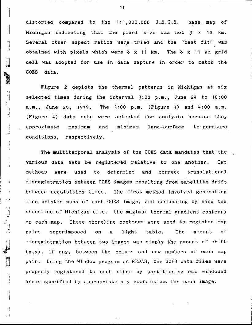
! 11

distorted compared to the 1:1,000,000 U.S.G.S. base map of

Michigan indicating that the pixel size was not 9 x 12 km.

"| Several other aspect ratios were .tried and the "best fit" was

obtained with pixels which were 8 x 1 1 km. The 8 x 11 km grid•""tfj cell was adopted for use in data capture in order to match the

u, GOES data.iFigure 2 depicts the thermal patterns in Michigan at six

- 1*i selected times during the interval 3:00 p.m., June 24 to 10:00\

% a.m., June 25, 1979. The 3:00 p.m. (Figure 3) and 4:00 a.m.

*: (Figure 4) data sets were selected for analysis because they

! , approximate maximum and minimum land-surface temperature

conditions, respectively.

The multitemporal analysis of the GOES data mandates that the

; various data sets be registered relative to one another. Two

methods were used to determine and correct translational

,< misregistration between GOES images resulting from satellite drift

•: between acquisition times. The first method- involved generating

line printer maps of each GOES image, and contouring by hand the

*| shoreline of Michigan (i..e. the maximum thermal gradient contour)

J on each map. These shoreline contours were used to register mapj

,.*> pairs superimposed on a light table. The amount of

f] misregistration between two images was simply the amount of shift-yW (x,y), if any, between the column and row numbers of each map

P pair. Using the Window program on ERDAS, the GOES data files were

properly registered to each other by partitioning out windowed

i areas specified by appropriate x-y coordinates for each image.

12 ORIGINAL PAGECOLOR PHOTOGRAPH

Figure 2 . Co lo r d isp lay s e q u e n c e o f GOES t h e r m a l da ta o f Mich igan a c q u i r e d

June 24 -25 . 1979.

00010002000300040005000600070008000900100011001200130014001500160017001300190020002100220023002400250026002700230029003000310032003300340035003600370033003900400041004200430044

13

000000000000000000000000000000000000000000000000000000000000000000000000000000000000000000000000000000000000000000000000000001111i111iI222222222233333333;=!;d4444444444555555b'551234067390 i 23*557390 i 34567890i 234567390123455/330 i 23^ob78

P. . , -COPW*COOCCC**COC-, . . -» *C--CL- ,*OCC--*CO»-*— : , t*CCCGPPPP,*PWPO* -PWPOWPWPOC*, ,c

•-, *c.VWWP*,OWC

.PftftWPWWFPPOC--COWWSfffcWWWW'WWWP*

,CPffftftWftftWPWWPPWWWPC

VWCPVWW,VPWWWWW

oc-P*.,0¥VVVftftffVWWWWPPPftftP«

-PWftPCOPftWVVVftVyVWWPWWPPPPO

sswwvwfflSEWVWWEV-

,,.-cc.<WVPPD***PWVWP-

WFffffiSWffiE*fflfflCEWOEP

SJfBOswcKF3W.

ffifflWfflWC

00000000000000000000000000000000000000000000000000000000000000000000000000000000000000000000000000000000000000000000oooooooooi i m i l l 11222222222233333333334444444444555555555i 234567390123456739012345673901234567390123456X39012345578

00010002000300040005000600070008000900100011001200130014001500160017001800190020002100220023002400250026002700230029003000310032003300340035003600370033003900400041004200430044

<53 53-54 55-56 57-58 59-60 61-62 63-64 65-66

* * «

» « «

**#**********#**

cccccccccccccccc

0000000000000000

PPPPPPPPPPPPPPPP

wwwwwwwwwwwwwwww

LJ67-68

ftsftftftftSSftftftft

J59-70vvvvvvvvvvvvvvvv

71-72 73-74 75-76"fflfflfflfflfflfflfflWfflfflfflW

77-78 79-80 > 80l i fKKKKfKtfK

ORIGINAL PAGE ISOF POOR QUALITY

EEEE

Figure 3. Line printer output of GOES pixel temperatures in Michigan f rom

3:00 p.m., June 24, 1979.

WQJQJO;

] 15

, A second, digital method was developed which automatically!1 determines the translational misregistration between images. The

| registration is accomplished using a sequential similarityl

detection method (Barnea & Silverman, 1972).

This method works as follows:

1) Gradient.images of each GOES image are provided."I1 2) A search area (a subpicture) of one of the two images to be

: registered is selected.t

3) A window area from the other image (which is smaller in size-i

'• • than the search area) is selected which covers (approximately)

the same region on the ground as the search area.

•4) The window area is shifted exhaustively over the search area

and the difference between the search and the window area is

computed.

; 5) The registration is determined by the (x,y) translation which

produce the minimum difference value.

The following table shows the amount of translational« ':

corrections (x,y shift) needed to register each GOES image to the

; previous one in the sequence (relative shift) and to the 3:00 p.m.*;

image (absolute shift). The 3:00 p.m. image was selected as the

; base because it displays the maximum thermal gradient along&

Michigan's coastline.

PRECEDING PAGE BLANK NOT FILMED

;J

IMAGE TIME

16

RELATIVE SHIFT VALUE

(x,y)

ABSOLUTE SHIFT VALUE

(x,y)

I 3:00 p .m .

U 4:00 p .m.

\ 5:00 p .m.

6:00 p .m.

8:00 p .m.

9:00 p .m.i

; 10:00 p .m.

1 1 :00 p .m.

! 12:00 a .m.

1 :00 a .m.

2:00 a .m.

4:00 a .m.

( 0 , 0 )

( 0 , 1 )

( 0 , 0 )

( -1 ,0)

( 0 , 0 )

(-1,0)

( 1 , 0 )

( -1 ,0)

( 0 , 0 )

( 0 , 0 )

( 1 , 0 )

( 0 , 0 )

( 0 , 1 )

( 0 , 1 )

( - 1 , 1 )( -1 ,1)( -2 ,1)

( - 2 , 1 )

( -3 ,1 )

( -3 ,1 )

(-3,1)

( -2 ,1)

1

17 .

13. Surface Environmental Data- Base

Several environmental factors were selected because of their

potential to significantly influence surface temperatures. These

included land cover/use, local relief, percent forest land and

water holding capacity in the upper three feet of soil. With the

exception of statewide land cover/use information, published data

were available for each of these variables.

Level I land cover/use data were photo interpreted from

1:1,000,000 scale, diazo-enhanced Landsat imagery. Seven

categories were derived: urban, agriculture, deciduous forest,

coniferous forest, barren land, water and wetlands. Local relief

data were extracted from the very small scale (approximately 1:3

million) map in Pawling (1969). Information on the percent of

land in forest was available from a 1:2.5 million map of the state

(Michigan Department of Natural Resources, 1970). Data on the

water holding capacity of Michigan's soils were obtained from

1:1.8 million maps of the state (Schneider and Erickson, n.d.).

Although information was available for several solum depths, data

for the upper three feet were selected to take into account the

many two-storied soils in Michigan.

All of these maps were brought to a common scale of 1:1

million cartographically. Each factor map was registered to the

1:1 million U.S.G.S. base map of Michigan and overlaid with a

computer-generated orthogonal coding grid composed of 8 x 11 km

cells. Dominant factor categories were encoded in each cell and,

subsequently, placed on diskette storage via direct keyboard entry

18

on the ERDAS microcomputer. These four digital files were output

to line printer hardcopy and compared for registration accuracy.

Additionally, the percent forest land and land cover/use files

were digitally overlaid to assess their compatibility and assist

in editing the files for encoding errors. The general patterns of

the four surface characteristics are discussed below. •

The generalized land cover/use of Michigan's southern

peninsula is shown in Figure 5. The large cell size of the

encoding grid (determined by the GOES pixel dimensions), is

compatable with this Level I categorization of land cover/use.

Urban centers large enough to dominate this cell si-ze occur only

in the southern half of the peninsula which is dominated by

agricultural land use. The two forest categories predominate in

the northern half of the Lower Peninsula and water bodies

sufficiently large to.dominate a coding cell are also restricted

to this part of the state.

The forest lands in the southern part of the state are

scattered and small in extent compared to the woodlands in the

northern half of the Lower Peninsula. With the exception of the

Allegan State Game Area in southwestern Michigan, which 'is 70-95$

forested, most of the woodland in southern Michigan is less than

40$ forested (Figure 6). The northern Lower Peninsula, on the

other hand, has at least 70/6 forest cover in most places. A

notable exception to this generalization is the agricultural area

of northwestern Michigan around Grand Traverse Bay which has less

than 40$ forest cover.

19

J

0001000200030004000500060007'"0008000900100011001200130014001500160017001800190020002100220023002400250026002700280029003000310032003300340035003600370038003900400041004200430044

,1

000000000000000000000OOOUOOOOOOOO'OOOOUGOOOOUOOOOOpOOpOOOUU00CO0000000000000000000COOOOOOOOOOOUO0000000000000000000000000000001 1 1 1 1 1 1 1 i 1222222222233333333*3444 44444453355555.::i 23456735012345S7S90 i 23456739 0 i 2345673=:0 1234567330 i 234^S/b

** CCU***C -C-*******

CCC-O'U******-***-*-- ***1J****-******--*•>.****#*cccc**-*-**

# - -• **-*w*CC***-* »•*** - -***-* *****0--**c-- oo****#***c********-*c— -*******#ccc****c*o**

cc** — #** -*****cc**-********— *c-***--*****cccc*c*******--ccc-*-****#****c*cc***ccc**

**-**- - * # * # W W W W * < J * - * * - C C * *—****#** -#-**ow*** - - * * - * * * *

-********-*- -****#**-***-***c*****c*c *c*#* -#*** * *#- *cc--*****—*-***** — ***-**-

I t*****-**-*****--***--** - * * * c c * *#*- -** -*** -** **** * ***

* ***** **** , **-** ***

-***--**** : , **-•***0.* **

: W,, w* " ~ ~ ~ ~ » « — — — —— — — — — — *- — — ——— — — — — — — — ^ — — — ^— — - — f — — -- — — — — - . _ - _ . _ _ _ _ « ^

— _ _ _ _ _ — _ — — _ — _ _ » _ ^ s —_ — __ — — _ - — (

— — ^ -J f -— ——— — — — — — — — — — — — — — — — — — —— — -.—V «

T f f — — — — — » — - ^--* w ,~ — — t — — — — y— t I-— » -— -— — — - , —— — — , ,

w

000000000000000000000000000000000000000000000000000000000000000000000000000000000000000000000000000000000000000000000000000001 1 1 1 i 1 1 1 1 122222222i»233333333334444444444SS553t>5S51234567^890 1234567890 1234567890 i 234567890 i 234567-890 i 2345678

DECIDUOUS INLAND

URBAN FORESTS LAKES WETLAND- - A •-••:- A :- • .- - - A - ~-~ A -: ,,,, **** CCCC 0000 PPPP WWWW

, ,,, **** CCCC 0000 PPPP WWWW, ,,, **** CCCC 0000 PPPP WWWW, ,,, *•»** CCCC 0000 PPPP WWWW

T - T - V

AGRICULTURE CONIFEROUS BARREN

FORESTS LAND

Figure 5. Land cove r c lassi f icat ion of Michigan.ORIGINAL PAGE 2SOF. POOR QUALITY

0001000200030004000500060007OOOS0009ooio0011001200130014001500160017001800190020002100220023002400250026002700280029003000310032003300340035003600370038003900400041004200430044

20

000000000000000000000000000000WO00000000000000000000000000oooooooocouooooooooooooopopooooooooocpopoooougoooooooooooo•0000000001 1 i 1 i 1 1 i 1 12^22222222:;j!333d33d334444*444*4533Sb~:;'d5i'1^34567390 i 2345578;;01234b'S7330 i 2345673S0l^3^567330123-SA73

CCPP

P-*PG-P-P

0

C-*-

FFPP --- , , , PPPPP

-CPP*P***P**P- -**#CP*PPPPFP***PF* * * * * OPPFFFFPPO * P * OP****0-->PPPPPPO**PCP**00*0-***OC.PP,**,P,C-000-QOOCCPPPPPP*P*COOCO--0000*PPPP,PP

CCCC --- 00- -000000000 *OPPP*0-P***CC-C ---- OOOOOOOOOOOOOF*P*F*** --- C-OOOOOOOOCPCOO*OOPPPPP— O--CC--CCCOUOPPPGO**C*PP-P--- OO-OC-C-C--0*PPPP--CC*P-PP

*OOOOOCCC--, , OOOOOOP-OPP***P00*000000* ****OOOC** , CPPPPC**

00- -00000* *,0-OOCCC--*CP- , * , ,— oooooo*oo--occ ---- cp*. , *,0--OOOOO --- *-*-C --- *--CC» , ,,- , -**ooo ---- c ..... --P-, * , * ,,,

c-, , *-ooo* --------- CPPC, ,, * , . * , , , ,--*#--0*PP ------- , .FCC, , .......-PPP--OOPP ----- * ....... *,,,,, **0-

*-*

-o* »

**-,,,"JCTCn^ f «— — — — •*•

**,,*,- -*-

*, --*-* *

C-

• - »' « »

* « « » » » - * • " - — « - » - - * * * — — — - - « » * •* »*» * * * « * » * — » * * * *•*« « — — - — —-***#--**00 * . . • . . ****,«0* *-, * *,,,,*,o* ***#,#-* ,,,,

'*****-*-*,****»*, ,*--*** ,*» , ,* • • » » » « » » - * * * * " » * » « ~ ~ - * » * « »

, , , » ,***, ,***** * ,*****» — — ~ » ***** —*— — — — * """"'"* * ******** T*~ ~" * * ^ * " ™ ^ — " " * " " " * * " * — * * * ' * " ' * *

«> ^ > « J t K a * > v k * M V V ^ 1 ^>vjf.» — «.^v^ * -It V* * * 4 * w ~ K * * # * 4 T T W w

000000000000006606000006606600000000060000066600000000000000000000000000000000000000000000000000000000000000000000000000000001111111111222222222233333333334444444444555555555i 234567890123456739012345678901234567890123456789012345678

0001000200030004000500060007OOOS00090010oo n00120013001400150016001700180019002000210022002300240025002600270028002900300031003200330034•0035003600370038003900400041004200430044

0_5% 5-15% 15-40% 40-70% 70-95% 95-100%

"Y7T, -~- **** cccc oooo PPPP.,,, **** cccc oooo PPPP,,,, **** CCCC OOOO PPPP* , ---- **** CCCC OOOO PPPP

F i g u r e 6 . Pe rcen t of l and in f o r e s t for M i c h i g a n . PAGE ISOF POOR QUALITY

i 21i

Local relief, a measure of absolute elevation difference peri; unit area, in the Southern Peninsula ranges from less than 49 feet

"| per cell (GOES pixel) to more than 500 feet per cell (Figure 7).

Areas of lowest relief (0-49 feet/cell) correspond to the glacial

y| lacustrine plains around and southwest of Saginaw Bay and along

•L. • the southeastern coast of the state. The narrow, linear,

H" north-south trending area of low relief on the east side of

"1 Michigan's "thumb" correlates with the Black River Valley. A much

1 broader zone of higher relief, up to 249 feet/cell, trends

1 southwestward from the central "thumb" area. This more rugged

topography is associated with interlobate ice-contact glacial

• * deposits. A more diffuse zone of high relief relates to other

1 interlobate deposits occurs in southwestern Michigan and trends,,j

northwards where it merges with the nearly ubiquitous rugged• i

j topography of the northern Lower Peninsula. The very hummocky

terrain (greater than 200 ft/cell) of this part of the state

J results from the abrupt juxtaposition of high coastal dunes or

•} inland morainic masses with broad flat valley-train deposits. A.j

localized area of somewhat subdued local relief (less than 150

•j ft/cell) occurs in the northeastern-most part of the state..

)J The distribution of soil types in Michigan at the order level

„/• " '

I is characterized by the predominance of Spodosols in the northern

and west-central parts of the state and Alfisols in the southerni

and east-central regions of the Lower Peninsula. The gross

textural differences between these soil orders results in low

water holding capacities for most northern Michigan soils and much

higher capacities in the soils of central and southeastern

22

oooi0002000300040005000600070008000900100011001200130014001500160017001800190020002100220023002400250026002700280029003000310032003300340035003600370038003900400041004200430044

00000000000000000000000000000000000000000000000000000000000000000000000000000000000000000000000000000000000000UOUOQOOOOOQOOOOl 11 11 1 1 1 i 1222222222233333333334444-444444555535535i 23456733012a4DS7330 i 234bS7B30 i 234567390 i 23 5b>'ii50 1 2d45f-.7&

****

W- WSWWtoot

W

PP*#*WWP**P**--WWWW.COCPPOO

8PPOOCCCOOOQCCCWWft#WGO* ****---**CPWW*tWWOCCC***--CC*

, , * *-*- » C •> *-c . -*

00#WWCOCCC**WWOPO?PCCOWWC**OCC*CCCWOOOWPCCwo***wc****coc-ooccoooowwocccWWOO*POCCCC-OPPCCPOP*OOWPOC***WWPP**CCOPOCOOOOPOOOOOPPCCC,WO-OWfcWWOOPCCC»**CCCWC-**CCC,WOCPCWWCO C,-,-CCWW*--***,,**w*ccww-oooccc--oooo

**c--ccwwoow*—c*o**--***-,,**--*occcwcoo*-*oco* *--.,OCC***-PPCPOO,-0*0>--.--'CCWO**CCCOPC*OOOO-,, -,,CCW-**C*PCC**0*-U « -

WWWC*CCC*PCOO*OO*--4oc******c****cc*--.**--**PCC*-**-**C--**PCCC*-**»-* —c --*-*,— *ccoc-cc — *** *cc**»--*c»

**CCPCC--*C* ,, ,-*--*-***,,,C - , CCC*COOOO -* * **OPPC »c-****coc* — ** * *oo*coo .,o******ccc* cccccccoc-, --,,CC-00'**PWOC***** C-C*CC-*C-» . f ,**-O**-PPC--* **-'--*ccc--oc-, •,*-*-ccoc-**** **—***#**cc--..»

*--**ccoc-c*** — ***--cc*ccc*c»»,»c-c*-****cc **-* c*-c — » » »*c*c--c*.. *-c*--cc***--*--cc--.. cc*ccc**,, 4,,,,

**c-cc*ccc **c*-*c*****CCC-*****. ** *C**C** » . » . - »

***cc*--*c» c-*c-* —..». -000000000000000000000000000000000000000000000000000000000000000000000000000000000000000000000000000000000000000000000000000001 1 1 1 1 1 1 1 1 12222222222333333333344444444445555555.':}.t>1234567890i234567890i2345678901234567890i23456/89012345678

00010002000300040005000600070008000900100011001200130014001500160017001800190020002100220023002400250026002700280029003000310032003300340035003600370038003900400041004200430044

FEET/PIXEL

0-49 50-99 100-149150-199200-249250-299300-399400-599

I » » »» t t 1

***#*****#******

cccccccccccccccc

0000000000000000

pppppppppppppppp

wwwwwwwwwwwwwwww

#####£&#ttttftftftttss

Figure 7. Local relief (elevation change per pixel) in Michigan.

ORIGINAL PAGE ISOF POOR QUALITY

23

Michigan and the "thumb" area (Figure 8). The stratified

ice-contact and glaciofluvial drift of the two interlobate zones

of southern Michigan produce soils of low water holding capacity

as well. Each of the five areas of highest water holding capacity

(greater than 20") are associated with areas of Histosols.

i

IV. ANALYSIS OF GOES THERMAL DATA

A. Comparison of Satellite and Weather Station Temperatures

The recorded ambient air temperatures at selected synoptic

weather stations were compared to the 3*00 p.m. and 4:00 a.m.

temperatures derived from GOES data as shown in Table 1. Overall,

there is a good agreement between GOES pixel temperatures and

recorded air temperatures. At 3:00 p.m., 63% of the GOES pixels

examined agreed within ^ 4 degrees F with corresponding recorded

air temperature, while at "4:00 a.m., there was 88% agreement. The

majority of 3:00 p.m. GOES temperature values were warmer than the

1.5m air temperatures, but at 4:00 a.m. the positive and negative

departures were about equal. The nine pixels which varied by more

than 4 degrees F from the synoptic station temperatures at 3:00

p.m. are all located in the southern part of the state and are

circled on Figure 9. The three pixels circled on Figure 10

differed by more than 4 degrees F from the 4:00 a.m. station

temperatures. The discrepancies between these two data sets are

probably due to the inherent differences between thermal radiance

values integrated across 88 square kilometers and point sampled

ambient air temperatures, as well as the +/- 2 to 4 degrees C

24

accuracy- limitation of the VISSR thermal channel (NOAA, 1978:C2)

.J

2500000000000000000000000000000000000000000000000000000000000000000000000000000000000000000000000000000000000000000000000 00 00 001 1 i 1 1 1 11 1 122222222223333333333444/4444444d!D5d5s.15;55'12345b73SO i 234bt>73biO i 234bt>," 330 I 2345b7S9Q1 23*t.b/dyQ i 23^bb/ 3

0001 00010002 00020003 - 00030004 -- , , , , - 00040005 -- P, ,* 00050006 ,**CC»C.» 00060007 -,,,--CC.CC-- 00070008 -* ,-CC.CCC-- 00080009 C .-,,.,CC.--- 00090010 - - W-....000..- 00100011 . - - * C .-000. • 00110012 C* -.C.-O, 00120013 C* -.-,.,-- 00130014 , ,.,.-- -.0--, 00140015 -0--. .-- 0....-.C- 00150016 ,--,.. - 00160017 --. C ..WWWW.,,0-0 0017001S --.. ,,0--.-,W,,.OOOO,,0,, 00180019 --..-O- 0--000,. 00190020 ,,.C 0-. ....--., .0.000 00200021 ...0 --.--..-.OOOC..0000. 0000 00210022 ,,......--.--...,OOCC..COO 0000000 00220023 -- 0-. .-OCC. ,CCOO OOOOCOOO 00230024 , ..--0 .OOCC...COO OOCCCOOOO 00240025 ,-.--,,,C-00 OOOOOOOOOOCCCOOOO 00250026 -.-.--., 000, CCOOOOOOOOO, . OOOOOO 00260027 0. .00....0-CC--OOOCCCCOOOOOO...CCCOOOOO 00270028 0.-.CC 0-COOOCCCO. ,C. .CCCOCOOOOp 00280029 . .,.O.Q--.C--0-OOOCCCOO.CC OOOOO 00290030 , ,000--0-C,OOOOOCCCCOOO-l)0-C WOOOC, 00300031 ,.000--0-CCCOCCCCCCCCCCCQOCCCCCCWOOO,, 00310032 ,.,0 CCCCCCCCC-*CCCCOOOC COOOOOO 00320033 ,,OOOOOC**CCCCCCC--****CCCC COOOOOO 00330034 000**C CCCCCCCCC-CCCCCCC CO-OOOOO 00340035 .,.*C-. CCCCCCCCCCCCCC COOOOO 0 00350036 0..*C CCCCCCCCC*** CCCOO-00 00360037 C.*** C-CCC*#**W CCCO 000 00370038 ,CC,C* ****-**W CCCOO--00 00380033 ,,CC-. *-*--*** CCOO .0 00390040 .,CC-W--*--CC-****»* 000-,-.00 00400041 ,-.-., *C**-C--0-000--,00 00410042 , *C-C****CCOOO-00,--00 00420043 000 * **0-OOOQ--G, . ,0 00430044 .00 . 0000000000000.0 0044

00000000000000000000000000000000000000000000000000000000000000000000000000000000000000000000000000000000000000000000000000000111111111122222222223333333333444444444455S353S5Si234567S90i234567390123456789012345678901234567890i2343678

INCHES

3.75-6.5 9.0-10.25#*#**********#**

cccccccccccccccc

JM.5-15.0

0000000000000000

ppppPFPPpppppppp

>20.0

wwwwwwwwwwwwwwww

6.5-9.0 10.25-11.5 15.0-20.0

Figure 8. Water holding capaci ty of the upper 3 fee t of soil in Michigan.

ORIGINAL PAGE ISOF POOR QUALITY

26

;/ Table 1. Comparison of GOES pixel temperatures with 1.5 m. air

temperatures recorded at selected synoptic weather stations

4;00 a.m. Temp (F) 3;00 £.m. Temp (F)

GOES STATION GOES STATION

Allegan 42-43 41 74-75 66Alpena City 42-43 40 63-64 61Alpena WSO 40-41 38 65-66 61Bad Axe 40-41 38 • 73-74 60Benton Harbor 46-47 46 - 79-80 66Detroit WSFO 46-47 42 73-74 69

, Eau Claire 44-45 42 73-74 66Flint WSO 40-41 41 75-76 66Grand Haven 44-45 47 67-68 63

! Grand Rapids 42-43 45 74-75 72J Hart 46-47 52 61-62 61

Hesperia 40-41 41 71-72 71Holland 44-45 41 67-68 61

I Houghton Lake WSO 46-47 38 65-66 66Lake City 38-39 37 71-72 67Lansing WSO 40-41 39 79-80 66

I Lapeer 36-37 36 67-68 65-> Ludington 42-43 47 61-62 63

Muskegon WSO 44-45 42 69-70. 631 Newaygo 42-43 39 71-72 71J Onaway 38-39 40 63-64 63

Paw Paw 42-43 45 73-74 73Sandusky 38-39 41 65-66 60

1 Traverse City 38-39 40 65-66 63

J

o

270000000000000000000000000000000000000000000000000OOU00000000000000000000 QOOOUOOOQ 000000000 00 OOOOsjQC'OOOOOOOOuOOOOOOOOOOOOOOOQOi 1 1 1 1 11 1 1 l2222222222c:d3333:i3334-4444444445t:So2dsd1 234057SSO1234b67 390123^567390 i 2343*7390 i 2345673 0 i 23-bS78

0001 . ooui0002 00020003 T 00030004 00040005 00050005 00060007 P - 00070008 OOOQ0009 - - 00090010 WP 00100011 00110012 -- '- 00120013 . -- 00130014 W 00140015 00150016 . 00160017 00170018 W W 00180019 00190020 00200021 00210022 . 0 _ 00220023 (D 00230024 0 00240025 00250026 W ^ 00260027 W © -~ 00270028 -- 00280029 ,_ " -- 00290030 © . - 00300031 Y _ # 00310032 _, ® - 00320033 ffl © - 00330034 (D • - 00340035 -' -- 00350036 (g) 00360037 00370038 ^ 00380039 £ ® 00390040 00400041 * 00410042 (D 00420043 00430044 0044

0000000000000000000000000000000000000000000000000000000000000000000000000000000000000000000000000000000000000000000000000000011111111112222222222333333333344444444445355D5G03i 23456739012345678901234567890 i 234567890123456789012345673

57-58 59-60 61-62 63-64 65-66 67-68**#**#**#*******

cccccccccccccccc

00000000UOOO0000

pppppppppppppppp

wwwwwwwwwwwwwwww ORIGINAL PAGE SSOF POOR QUALITY

69-70 71-72 73-74 75-76

V W V t f J W W W K E S 5 S I B I H W f f lyyvv wwwwvvvv wwwwvvvv wwww

77-78 79-80

SEESKffiSSSEES

Figure 9. Apparent temperature at selected synoptic weather station sites from

GOES 3:00 p.m. data for June 24, 1979 (circled pixel temperatures

d i f fe red by more than 4° F. f rom recorded air temperatures) .

28

ORIGINAL PAGE' SSOF POOR QUALiTY

0000000000UO00OupOO0000000000UOOOOOp0000000UOCU0 000000000000000 00 0 000 00 U00000000 0 000 0 p 000 0 0000 U 00 0 0 000 (j 0 U000000000 1 i i 1 1 1 1 1 1 i2i22222222333o33333*444^444444ooodOoobo1 23456/890i2345673SOI234O67 890 i 234Ob/3bO i 2345673501234bS73

0001 000 i0002 00020003 00030004 00040005 00050005 -- 00060007 . 0 -- 00070008 00080009 00090010 PW - 00100011 00110012 -- . 00120013 -- 00130014 -- --- 0 00140015 00150016 00160017 _ 00170018 0 © 00180019 00190020 00200021 00210022 W 00220023 _ P --- 00230024 © 00240025 --- 00250026 --- P --- 00260027 </i 0 -- 00270028 -- 00280029 -- 00290030 ft - 00300031 -----* . C 00310032 P - 00320033 W P - 00330034 . fc - 00340035 --- 00350036 W 00360037 00370038 -- 00380039 W V 00390040 ^ 00400041 -@ 00410042 ' # 00420043 00430044 0044

000000000000000000000000000000000000000000000000000000000000000000000000000000000000000000000000000000OOOOOQOOOOOOOO0000000001 1 1 1 11 1 1 1 12222222222333333333344444444445o-5o'55b.-3b-1234567390123455789012345578901234567390123456789012345678

33

#*##************

34

cccccccccccccccc

35

0000000000000000

36-37 38-39 40-41 42-43 44-45 46 -47 ,48 -49

FPPPPPPPPPPPPPPP

wwwwWWWWwwwwWWWW

VV'VVvvvv WWWWwwwwvvvv

fflffifflfflfflffiftWfflfflfflfflFiiffifflW

Figure 10. Apparent temperature at se lec ted synopt ic weather stat ion si tes f rom

GOES 4:00 a.m. data for June 25, 1979" (circled pixel temperatures

d i f fe red by more than 4° F. f rom reco rded air temperatures) .

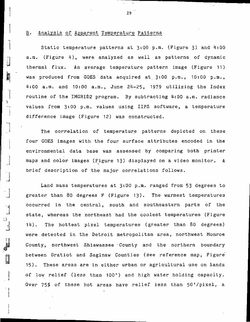
29

B. Analysis of Apparent Temperature Patterns

"i

! Static temperature patterns at 3:00 p.m. (Figure 3) and 4:00

-j a.m. (Figure 4), were analyzed as well as patterns of dynamic

Jthermal flux. An average temperature pattern image (Figure 11)

i was produced from GOES data acquired at 3:00 p.m., 10:00 p.m.,

4:00 a.m. and 10:00 a.m., June 24-25, 1979 utilizing the Index

routine of the IMGRID2 program. By subtracting 4:00 a.m. radiance

i values from 3:00 p.m. values using UPS software, a temperaturei

difference image (Figure 12) was constructed.

'"Ii, J The correlation of temperature patterns depicted on these

j four GOES images with the four surface attributes encoded in the';i

environmental data base was assessed by comparing both printer

j maps and color images (Figure 13) displayed on a video monitor. A

brief description of the major correlations follows.

i rfj

Land mass temperatures at 3:00 p.m. ranged from 53 degrees to

- !J greater than 80 degrees F (Figure 13). The warmest temperatures

,j occurred in the central, south and southeastern parts of the

state, whereas the northeast had the coolest temperatures (Figure

1 14). The hottest pixel temperatures (greater than 80 degrees)

were detected in the Detroit metropolitan area, northwest Monroenjlj County, northwest Shiawassee County and the northern boundaryUpm between Gratiot and Saginaw Counties (see reference map, Figure

15). These areas are in either urban or agricultural use on lands

j of low relief (less than 100') and high water holding capacity.

Over 75$ of these hot areas have relief less than 50Vpixel, a

0001000200030004000500060007OOOS00090010.001100120013001400150016001700 IS0019002000210022002300240025002600270023002900300031003200330034.0035003600370038003900400041004200430044

30

00000000 000000000000000000 0000000 00 00 00 000 000 UO 000000 000000000000000000000000000000000000000000000000000000000000000000000000 1 1 1 1 1 1 1 1 i 1222222222233333333334444-444444555D.r.oc.t:.i1 2345S7390 i 234!5t>/ 3bO i 234S6/ 320 i 345t./ S90 1 234557830 1 234b5/ 3

QPOQPPPFPOOPPPPPPFFPPPPPPOQUPWWPPOPWWPFVJOPWPPGGGOOFPWWWFWPPPPPFPPOPOOFPPFFFPPOOOCQOCQOOFFWFOCUCCOCCCCCOOCOOPFOFFFPFWOOFFPPGFOuPPPPWWPOCCCCCCCCOOOOOPPOGOOCeCCCCCCCCCeOOOPWwWwWOPPPPPPPPPPPWPPFCCC***CCOGOOQOPPWFPOCCC****** s-****GCCOPFWWPPOOPPPPPCrpPPPOC*******COGCOOPWPPPPPGCCC**************CCuPPFOOPPPOPPPOOCCC --- ****CCCCCOOWWWWWWPPQCCC**********- *****PFPPPPPOFPPOCCC* --- ****CCCCCCOPWWWWWPPGOPQC**C** **** ----- *PPPPPPWPPFGOCC** ---- ******QCCPPWWWPPPPPPPPOOCCC*>*** ----- *WWWPPWPFOOOCCC* * ---- ***CCCCOPWWWPWPPQPPOPPPPPOCC** --------WWWPWWPPOPCC*C** --- ***CCCCOWPWWWPPPPPPPOPPPPPPOCC*** --- ***WWWWWWPPPOCC * * ---- *CCCCOOCCW#WPPPWPPOPPPPPPPWWOCC * ** ---- * *WWSffWPOPO*C**» --- *CCCCCPOCOP$WWPPPPPOPPPOPWWWPOOCC ***--**-WS&WPPPPCCC ----- *CCOOPPWOOOPPWWPPOPPPPPOPPPPPWPCCC *******-WVfc#WWPCC** ----- CCCPPPWWOOPPWPPPPPPPQOPPPPPPPPPOCCC*******fc*WWWWO*C* ----- *CCCPWPWS*PPPWPPPPPPOPQOPPPOPPPPCCCC*******# ftWft WPOC * * ----- *CCOWWWWWWPPWWPPPPPPPOOOPPPPPPPPCCCCCC *****VtttWPOC*** ----- CCCPSWWSSWPPWWFPFFFFFPOFPFFFFFFPOCCC *******fc#WWPO*C** ----- *CCW»SWWWWWPWWFFPWWWPWWPFWWWPWPPOCCCCCC****SWWWWOCCC * --- * *CCOPWWWWWPWWPWWFPFFFFWWWWWWWWWWPOOCCCCCC * * *#&WWWPCC**-***CCOPWPWWPPWWWSWWWPWPPPPWWWWWWPPPQQOOOQOCC***ftS»WWCCCC****CCCOWWWWWWWWWftttftWWWWWWWWWPWWWttttWWPPPOOOCOCC**

0000000 000000000000000000 000000000000000 00 0000000000000000000000000000000000000000000000000000000000000000000000000000000000011111111 1 1222222222233333333334444444444 y:5555-l35i)1 234567890 i 234567390 1234567390 12345B7S90 1234567890 1 2345673

LOW

000100020003000400050006000700080009001C001100120013001400150016001700180019002000210022.0023/00240025002600270028002900300031003200330034003500360037003t.

« t1 «t •

**** CCCC 0000**** cccc oooo**** cccc oooo**** cccc oooo

PFFP WWWWPPFF WWWWFPFF WWWWPFPF WWWW

ftftfcftvvvvvvvvvvvvvvvv

uuuu XXXX HHHHffllflffifflfflfflfflftf

ES£K HifflfflrH SSEffi

KKKKRU If, t7. A

WWIDW

HIGH

Figure 11 . A v e r a g e p i x e l t e m p e r a t u r e s d e r i v e d f r o m GOES data a c q u i r e d a t3:00 p.m. and 10:00 p.m. , J u n e 24; 4:00 a.m. and 10:00 a.m.,J u n e 25, 1979.

ORIGINAL ISOF POOR QU&UTY

310000000000000000000000000000OUOOOOOOOOOOOOOOOUOUOOUUOUOOOO00000000000000000OCOOOOOOOOOOOOOOOOOCOOOOOOOOOO00000000000000000000 1 1 1 1 11 1 1 i 122222222223333333333*44-*4-*444.ft5;i;=SbSS3:31 34567830 i 234567390 i 2345678901 234ct>7890 12345S78i 0 i 23^rbS7S

OOOi0002000300040005000600070008000900100011001200130014001500160017001800190020002100220023002400250026002700280029003000310032003300340035003600370038003900400041004200430044

OPPFWPPWWWPWWWftVVfcF-PPOPPPPWPWPPPWPOCP#W*WPWPWWPPC** «PPPWWfcswWPCPWPWWSSWW,PWPWWfcPPCPftPPWWW-ppppppQ

PPPPPCWWPPF- CPPPC ,PWO C,PP , CWPPC *#PPC , W VVPVWSWSPPwwvswwty{jJY^!££ Q

WVVftP 0VWVVW- -PWVVfcP PWVftVW tWttV&V* P#frVV, 0*VWWH -PWwgy, *WWWE- CWUwv, ,ccwe *cW -GfflV *wv,¥#•KWCSK*SSOwwcWS t »SV CWftO PWVP • *wuWVF- WWFVWVW *WPFVSEW. OWPP«

, **-» *00*«-OPP***0, *OCCOPPOOC-COPPWWWWPPPFC,

CPPPPPPWPWWPPPPPO-*OWUiWPWPPFPPOFWOOOOCCPWVVVWWPPPPPOCOPQ

* OWVWft##V#*WWHPCOPU-PP* . , OWWVVVVWWWSWPPPPPOU*HVtCCWWVWVWWVWWWWWVWPPOOO*

* » »> t » t ~ ^ *

t -ft- *

, OWSC

0#PPWWWVWWVVVWWKKVW##PVWO, -OWfiWWVWWP-

OWPP*VV#W#WVWWfflfflfflfflfflKWWE£tfWEERRffl£EO00000000000 0000000000000000000000000000000000000000 00000000000000000000000000000000000000000000000000000000000000000000000000111111111 12222222222333333333344444444445t>otioSd5d1 234567890 i 234567390 i 234557890 123456739 0 1 234567890 i 2345678

0001000200030004000500060007OOOS00090010OOil001200130014001500160017001800190020002100220023002400250026002700280029003000310032003300340035003600370038003900400041004200430044

<16 16-17 18-19 20-21 22-23 24-25 26-27 28-29

» *

* *

********#***#***

CCCCCCCCCCCCCCCC

0000000000000000

ppppFPPPFPFFFFFF

WWWWWWWWWWWWWWWW

30-31 32-33

vvvvvvvv

34-35 36-37 38-39 40-41 42-43 >43

WMWWWWWW

wwww

fflfflfflWWMfflfHfflfflfflfflfflfflfflffl

RffiRS2RSRSRRRR

KKKKKJjf tfyKKKK

(DOJWOJCKDHJO!

\3WWW

Figure 12. Apparent temperature change f rom 3:00 p.m., June 24 to 4:00 a.m..

June 25, 1979 derived froived f r o m GgESp-daSORIGINAL FASE R5OF POOR QUALITY

32ORIGINAL PAGE

COLOR Pi-iOTOGRAPH

GOES SPM TEMPERATURES

• JUNE 24, 1979 < 5353-5455-56

*£ 57-58» 59-60• 61-62» 63-64

65-6667-6869-70

73-7475-76

79-80> 80

GOES 4ftM TEMPERATURES

JUNE 2S, 1979

V, -,

S3• 343536-3?38-39

« 40-41m 42-4344-4546-4748-4950-5152-5354-5556-57> 57

LnHU CGUER CLASSIFICATION LOCAL RELIEF

URBAN

AGRICULTURE

DECIDUOUS

FORESTSINLAND

L«t ESBARREN

LMMDWETLAND

M •* -H IM [>•-

100-149'

* 150-199'.

200-249'

R 250-299'

7.00-399'

400-599'

PERCENT TOPEST COUER

40-70X

70-95*

95-100*

SOIL UATER HOLDING CAPACITY UPPER 2 FEET

9 0-10 2"

10.2-11.

11.5-15.8"

CCHTCB FC* RCMOtr

GOES AUERAGE TEMPERATURESJUNE 24-25, 1979

- HIGH

GOES TEMPERATURE CHANCE

— > 4AM JUNE 24-25, 197 < 1616-17

£• 18-1920-21

• 22-23m 24-25• 26-27a 28-29

30-3132-3334-35

_ 36-37R 38-39

40-4142-43> 43

Figure 13. Compar ison of GOES thermal pat terns with the distr ibutions of

s e l e c t e d s u r f a c e f e a t u r e s i n Michigan.

33

UUOiOU02OU03OU04OU05OOObOOO/U00800090010001 1001200 1300140015001600 1?00180013002000210022002300240025OU2b002?0028002y003000310032U033OU34U0350036003/'003300330040004100420043OU44

u u u v u v u u v e u u u w J u u u u u u ;. u u u 'J v u :.: u v u v ;; J u \ • u i: u v L: u •.; '.: •/ : '.; :.; v : j -••... L' •-/ v './ ij \.- 'J '-• O •-•' •-/ ••-' u w <J v ••-• •) •_•• U >-' l.' v . u j •-> \J -.' U . w '-. '-• « -' ••- >-• -J ••, .' -V u •-. •-.' v --• -. '..' -- -., -• •-• •-' . •- •-'

UUUUUUUUU 1 i 1 i i 1 i .1 ± I 22 : ^ .cJ2 c-i:.i-:.i:-vo.J.J.J-44';;-4 -4--:T.-.J.J r O-J~0:234b&/8'iui^J^3"6V3-JU i 234^b/o^0 ; :j45c/ iyj ; .j- c / a1-" ,! J -• J->- b/ J

C C c'w Uf 'i -

C C C C C C C CC C c C C C C C cC C L- c c C C w C C C C L

C C C C C C c C C C C C 0 '•_• L. C uC C C C C C C C C C t - ' ' ( * * " : [ *C CCCCCcCCOL'v-

C CCC ccCCuCcCcc\j '^j \_j ^/ >_• *_» \_> Vrf — w ' j i j I • 'l •

C C C C C C C « J C C C ; J CC CCC CCCC CCCC

CC CCCCCCcCCC C C C C C C C C c C C CCC C CCcC C C Cc

CCC C CCC cc

C C ' ' ' ' ;c

W C c WwC WWW C c C w CCC

. ". -f

c W w WWWW W WWW wWWwWWWW Cc CCC .CCC Ww w W WWwWwwwwwwwWw cCCC W WWWWWwWwWWV;w w C

WWWWWW WWWW U CC WWW WWWWWW CCc WWWwWwWWWw CcC W Ww WwwwWwwwwWww w CCC w WW WWWW Www c CC

WW WW WWWW wwwCCC Ww WWWwWWwwwWC WW WW WWW Www WWW

C WWWWWWww WwwWWWW Wwww

W WWW WWWC WWWWw WWWW WWWWWW

WW WWW WWWWWWW WWWWWWWC WWWWwWWWWwW WWWWWWww

WWWW WWWWWWWWWWWWWWWWWWWWWWWw0 0 0 0 0 0 0 0 0 0 0 0 0 U 0 0 0 U 0 0 0 0 0 U 0 U U 0 0 0 U 0 0 0 0 0 0 U U 0 U 0 0000 0 0 0 0 0 U 0 U U 0 !; U000000000 0000 0000 UOOOOOOOOOOUOOOOOOL'OOOOOOUOOOuOOuOOOOOuOUUUUUUUUUUi l l l l i l l i 1 i Jijii. i/_/ jZ-JOC>OO-_'C'-_5-..>O-tr'4--'-r--TJ4JT4-ur'tt- ._--J-_i--'-j- .-;w

i 2345b/ 890 i 23456/890 1 2345b/890 1 2345b/ 8bU 1 2345b'/8:JU j 234 6/8

O'jy:V V *J £^r

\j \J W *l5

0 u ; ) 4ij i j -.0 (J 0 b

OOU/\J \J w Cj

V O W —f

0 U i 000; i01)12(it; > •:;W W J. i_'

OU14001500 it,U U 1 >'ooiaOOM'3002UOuk; iU0220 0 '••' -50024002DOOj^b00 '••'/'002SOU29003O00310032UO- 1'3UOJ40035U036OU37OUU8UU39004U0041004200430044

CCCC pixel temperatures WWWW pixel temperatures

.ess than S8F greater tnan 76°F.

Figure 14. A r e a s of minimum and maximum apparent tempera tures at 3:00 p.m.

June 24, 1979 f rom GOES thermal data.

ORIGINAL PAGE ISOF POOR QUALITY

ORIGINAL PAGS IS34 OF POOR QUALITY

1Beaver Island—M Burt L'ake

Mullet t Lake/

Black Lake

North & South

Manitou Islands \J

Figure 15. Re fe rence map of Michigan showing county boundaries and se lec ted

geographic features.

35

water holding capacity of greater than 10.25" in the upper three

feet of the soil and are less than 5% forested. Pixels with

j radiant temperatures greater than 76 degrees F at 3:00 p.m.

(Figure 14) also correlate with urban and agricultural areas of

rj low relief and high water holding capacity. The majority of the

\ coolest temperatures (less than 68 degrees F) are in the forested

y areas of the northeastern part of Michigan, where the land area is

~| over 95$ forested with a soil water holding capacity of less than*)

9".'!

- The coolest (33 - 35 degrees F) and warmest (44 - 4? degrees

I F) pixel temperatures at 4:00 a.m. are shown in Figure 16. Cool

temperatures were recorded in the north-central part of the state}

] on a heavily- forested plateau-like area of well-drained sandy

; soils with low water holding capacities. Within this cool region,

the coldest radiant temperatures were associated with coniferous

; forests composed primarily of jack pine. Additionally, thej

effects of latitude and continentality may also contribute to the• !

I cold temperatures of this area. The linear series of cool pixels

trending southwest from the Houghton Lake area corresponds with

the upper Muskegon River valley and may result from cold air

J drainage. A similar situation in the upper Manistee River valley

produced the pocket of cool temperatures south of Grand Traverse! fJy Bay in northwestern Michigan.

0 The warmest pixels over land at 4:00 a.m. are associated with

areas of high soil water holding capacity, urban centers such as|'< Detroit and Grand Rapids or inland lakes. Houghton Lake, for

000100020003U00400050006OOO/00080003OOlO001100120013001*0015001600170018ooiy00200021002200230024002500260027002S002S003000310032003300340035003600370038003900 0004100*200430044

ORIGINAL PAG1;- ft36 OF POOR QUALiTV

J '-/ <J U L V W' '-- '•_' v U V ••-/' v/ '-.' ••-< \-'' •-> '-J '•-•' '•-' V •_ '•_• --J '%.' -J v ''J • • *-f >j •..' ••-• •-• '•-;' i-- '•-' »-' •- w1 '-' 'J •- '..' '•. •-' 'J '•-..• (.' !.• •-• ••_• !-' '•-• w -.- ••..-

j- >J j U J U U 'w j J >j w w w U U u- ->-•- - W U \! „ v ••-' U •_ -j >-' U u v -J >-' - w '-• w •-• --• -j 'J \j U v •; 0 v/ v '•-' - U \-- '•_• ••_•• ,yJ v -j 0 '-•• U \-- 'J J i l i l i i l i i i jL.ji.i-i i-^-l— i_-..'O •_•._••_•-..••_••_••_.•_• T- *"--, •ur-w^-_. •_ .j...i O •_•-...

i-^-T.^b, U3U i,iO -!••_• 6 / 3_ U i i-O-T.-'C.-/ LJ^U i .' ._-r.-,-._ --J-'IJ li.J-Twt-./ ._._'U l^O-T-J'-./ 0

.

wWW WWWWWWW WW WW

ww www ww wWWW Ww

WWWw Ww

w w w WWW W Ww wi-v W

WWW WWw Cc CCC Ww wW W CCCCuC WWW

W C CCCCCCcCCC w'WW W CCC CCCCCCCCWW CCC CCCC CCCCCCW CC CC CCC

WW WWc w

w cWW C Ww WWWww w w ww w wW WW W W W

WWWW WWWW W WWW Ww . W WwWW WWWW WWW W WWW W WW W WWWWWWWWWW WWWW WWWWWWw W wwwwwwwwwww w wWW'WWWWWWWWW ' WW W W WWWW W W W W W W W W WWWWWWWWWwWwWWW WWWWW'WWW'WWwWWW WW W'WWWW W WW WWWWWWWW WWWWWWWW WWWWWWWWW WWWW

WW'WWWWWWWWWWw . WWWWWWWWWWWWWWWW WWW

WWWWWWWWWWWWw WWWw• ••.•>!'-¥' • .:''fl\*'

WWWWWWWWWWWWwWWW W WWWWWWWWWWWWWWWWWWWWW WWWWW

WWWWWWWWWWWWWWWWWWW WW'WWWW

OOOl00020 U U oOOU-40005OO0600070003'OOOyOOiO001 100120013001-40015001600i700 IS001900200021002200230024 ,002500260027002300230030003100320033003400350036003700ij3003S0040004100 200-S300- 4

0000000000000000000OOOOOOOOOOOOOOOOO00OOOOOOOOOOOOU0000000ooooooooocooooooooo oooooooooqooooqooooooooqoooooou.oooo.oqo>10000000001 i i 1 11 i 1 i 12222222222.j:Joi:!333333-4**4*4*':f*45-JJd55.JuJ

SOO

CCCCo o

pixel temperatures 33 - 35 F.

CCCC

WWWWWWWW pixel temPera tures 44°- 47"WWWW

Figure 16. Areas of minimum and maximum apparent temperatures at 4:00 a.m.,

June 25, 1979 from GOES thermal data.

37

example, had an apparent temperature as much as 10 degrees F

warmer than its surroundings. The close proximity of Black, Burt,

and Mullett Lakes in the northernmost part of the Lower Peninsula

contributed to the warmer temperatures of the east-west trending

Indian River lowland. The highest temperatures detected at 4:00

a.m. (greater than 57 degrees F) correspond to the shallow waters

of Saginaw Bay, Lake St. Clair and Lake Erie (Figure 13).

The lowest average apparent temperatures (based on satellite

observations a.t 3:00 p.m., 10:00 p.m., 4:00 a.m. and 10:00 a.m.,

June 24-25, 1979) are highly correlated with the deepest parts of

Lakes Michigan and Huron indicating the high thermal inertia ofj

these areas. Of the land areas, northeastern Michigan maintained

| , the coolest average temperatures during the observation period

"1 probably as a result of its high percentage of forest land, rugged

topography and low soil water holding capacities. The highest

I average apparent temperatures are associated with the city of< j

Detroit and east-central Monroe county. Warm average temperatures

$ ! are also found in central Michigan's Saginaw lowland which ist

dominated by agricultural land use, has minimal forest cover and

very low local relief.

The greatest diurnal (3:00 p.m. - 4:00 a.m.) apparent

temperature changes (greater than 37 degrees F) occurred primarily

in the agricultural land of south central Michigan. Temperature

changes of less than 28 degrees F were associated with many

coastal areas, the rugged, forested northeastern part of the Lower

Peninsula, the areas of numerous inland lakes in Barry and Oakland

38i

counties, and Houghton Lake and its neighboring wetlands.

)

"\ C_. Contouring Temperature Difference Images

--, Automatic machine contouring of temperature change digital

^ files provides a valuable analysis technique which is particularly

CNI1 useful for studying thermal patterns and gradients. Temperature

difference files record the absolute difference, pixel for pixel,.,.-,

j between thermal data files recorded at two separate times.D--•> Thermal gradients can be studied using this technique by the

1-J repetitive display of multiple contoured images of increasing

"""] , temperature thresholds. Although a detailed assessment of thisi*

technique was not undertaken, a sample data set is included" ^

! herewith to illustrate this data processing capability.

j A temperature difference file was prepared by calculating the

absolute thermal flux between the 3:00 p.m. and 11:00 p.m. GOESt

-J data sets. This file was then thresholded at various temperature

;, ] values (e.g. Figures 17-19) to display regions of different<e*-J»

temperature change. The contours shown in Figure' 17 encompass

*J areas of more than 8 degrees F temperature change (3:00 p.m. to

L- 11:00 p.m.) and depict the land-water interface fairly well. Note

especially that Beaver and North and South Manitou Islands in

•' I northern Lake Michigan are resolved at this temperature

& threshold. In Figure 18, areas of more than 20 degrees F

11 temperature difference are bounded by the contour lines. At this

threshold, several inland areas are depicted which may be

I associated with lakes and/or wetlands. Relative to the 8 degree F

39

ORIGINAL PAGE ISOF POOR QUALITY

I I

Figure 17. 8° F. temperature d i f ference boundary f rom GOES thermal data acquired

3:00 p.m. and 11:00 p.m.. June 24, 1979.

40

U

"•»

G

j

ORIGINAL PAGE ISOF POOR QUALITY

I i Figure 18. 20° F. temperature d i f fe rence boundary f rom GOES thermal data acquired

. 3:00 p.m. and 11:00 p.m.. June 24. 1979.

41

difference image, the more restricted areal expansion of Saginaw

Bay, Lake St. Clair and Lake Erie at this 20 degree F threshold

-1 compared to Lakes Michigan and Huron indicates that these shallow

water bodies are bounded by steeper thermal gradients. This

I I condition is even more pronounced in the 24 degree F difference

* image (Figure 19). At this threshold, mesoscale regions of

S varying thermal flux become apparent within Michigan's land mass.

For example, western and southwestern Michigan as a whole seems to

have a higher thermal inertia than the central and southeastern

parts of the state but also displays more intra-regional

variability. This western region of fluctuating . thermal

differences can also be discriminated in the 3:00 p.m. - 4:00 a.m.

temperature change image discussed previously (Figure 13).

V. SIGNIFICANT FREEZE EVENTS IN 1981

"i In 1981 two significant freeze events occurred during April,

the most serious of which occurred on April 21 . These freezes'* |j seriously affected fruit production in the state. Minimum

temperatures which occurred at 61 weather stations during the two

^ freeze events are shown on Table 2. To document the environmentala] change at one location, hourly data were collected at the HSU!j

weather station.

The variables measured were:

1. Screen temperature (1.5 m)

2. Outside temperature (1.5 m)

42

ORIGINAL PAGE S3.OF POOR QUALITY

D

D C—_- *—

_; LJ

D

Ln

D

D

D

J

n !

in

i?

L_

._ __ ^

--- J

•~in

u nz:L

H

iLo

' ^r^

D XTL1i i i~l '.j ' i Li ! i

L- • __

f.

Ljr

J 1_c-^ J u

(1I1

_.,.- — „ -

Figure 19. 24 F. temperature d i f ference boundary f rom GOES thermal data acquired

.3:00 p.m. and 11:00 p.m., June 24, 1979. _

Table 2. Selected April minimum temperatures in Michigan (1.5m)

STATION APRIL 15, 1981 MINIMUM APRIL 21, 1981 MINIMUM

Li

AlpenaDetroitEscanabaFlintGrand RapidsHoughtonHoughton LakeJacksonLansingMarquetteMuskegonPellstonSaginaw AirportSault Ste. MarieTraverseGlendoraSodusWatervlietPaw PawGrand JunctionFenvilleColdwaterAllendaleHudsonvilleHollandNunicaMearsBeldingClarksvillePeach RidgeKent CityGraham StationEdmoreGrantFremontBerrien SpringsMSU Horticultural FarmBad AxeBear Lake

232926262622233026172515MM18212830282826272926272423252325252525202323Msg.252524

192526252724192824172716251616282824282427252929282525262727262924272630242020

OF POOR QUALITY

43

Table 2. Con't.

STATION APRIL 15, 1981 MINIMUM APRIL 21, 1981 MINIMUM

BeulahEmpireImlay CityKewadinLake CityLake LeelanauLexingtonLudingtonMontroseN.W. HorticulturalOld MissionOssinekeRogers CitySaginaw ValleySalineSanduskyStandishToledoUnionvilleWashingtonRiversideKeeler

2420262218222623242220222122262522272630

222021221621MM221922222020212123192524252727

OF POOH

44

45

3« Soil moisture (5 cm)

4. Relative humidity (36)

5. Light intensity (kj/m)

6. Wind velocity (mph)

An attempt made to measure radiation during this period

failed due to technical problems with the device, but radiation

was successfully measured during two successive spring freeze

events.

Plots of each variable during the April 20-21 freeze event

are shown in Figures 20-25. In conjunction with this freeze

event, an attempt was made to procure GOES imagery to validate the

impact of the freeze and to assist in the interpretation of the

physical model and to examine the sequence of thermal events as

the freeze approached. Unfortunately we were informed by NESS

that we could no longer obtain GOES imagery but could only obtain

GOES data from the historical archiving system at Wisconsin (see

Data Access Difficulties section). This led to great

disappointment and discouragement because the image processing

system we developed was based on the GOES format provided by

NESS. We are still hopeful that this problem can be resolved as

we have spent considerable time and effort developing this

component of the system.

ORIGINAL PA@g ISOF POOR QUALITY

'"3

HP'j

M S U SORT FARM April 21,1981

* Relative Humidity

o Wind S e e d

= 40-10)

'I 20 —

ex. •0

— 15

— 10

n i i r i i i i i \ i i i i i i r

-oQ}<D

CL5 <"

0

60 -o.cc

50-

o) 4Q-Ji_D

+-<

^30-Q.E£ 20-

a Screen Temperature

A Soil Temoerature

\.

0

i—|—i—i—i—i—|—i—i—i—i—|—r

5 10 15Time (hours from 6 P.M.) J.V.P.:

; 47

VI. PHYSICAL MODEL AND SPECIFIC TASK DISCUSSIONii

Task I: From data bases collected, make sample runs of the

j P-model and/or concept and present observations/conclusions as to

--, results.ySu Data to characterize the micrometeorological conditions

-' during freezes in Michigan were collected on different spring

nights. The measurements included temperature gradient,

; radiation, wind movement and indication of direction, dew point

«: and soil temperature. This data has been provided to Florida for

,., general analysis.

».$

Our conclusions from the data are the following:i!

1. The radiation, which 'is such an important driving force in

: affecting minimum temperatures, fell in the same range of

, , readings that one might expect over the peninsula of Florida

•'' during freeze conditions.

' i

-J 2. The temperature drops observed, although limited in number,

'. * have indicated that temperature drops were within the rangei

that might be expected during Florida freezes.

I9 \

"J 3- Recently, a thesis in Agricultural Engineering (Levitt, 1981)

[[ has characterized the statistical types of freeze conditions

which tend to verify earlier work by Van Den Brink, (1981),

y showing approximately 60% of Michigan freezes were radiation,

and 2^t% were advection and *\6% were . due to both conditions.i

1 Again, these general characterizations which show freeze

48

conditions on a broad scale are similar to the types of

general freeze conditions from the statistical standpoint that

Florida receives.

M . Persistence of temperature differences between stations seems

to exist. MOSS product analysis has been done that indicates

there are good correlations between key (weather forecasting

sites) locations and agricultural weather measuring

locations.

5. Analysis from Phase I of field measurements with an . airplane

and wit'n temperature Instrumentation mounted in moving

" ' vehicles provided important data. This information showed

i that there is clearly cold air drainage wi.th large temperaturei

differences down moderate slopes. Also, the high degree of

• wind variability and its affect mixing the atmospheric

boundary layer were experienced in Michigan as in Florida.

.,}The main . difference would be the fact, that Michigan's

. ]^l important freezes occur in the spring. Thus, the soil heat flux

, . might be expected to be different from Florida during fall

ij events. Analysis of this effect would show, however, that thereO

I has to be warming periods prior to the freeze for nearly all.j

conditions during later spring freeze events. Thus, for many of

jJ the most significant freezes, the soil would be considerably

warmer than air in a manner similar to that found in Florida. The

"» clear exception would be severe early spring freezes when frozen

'I ground would complicate the physical model.

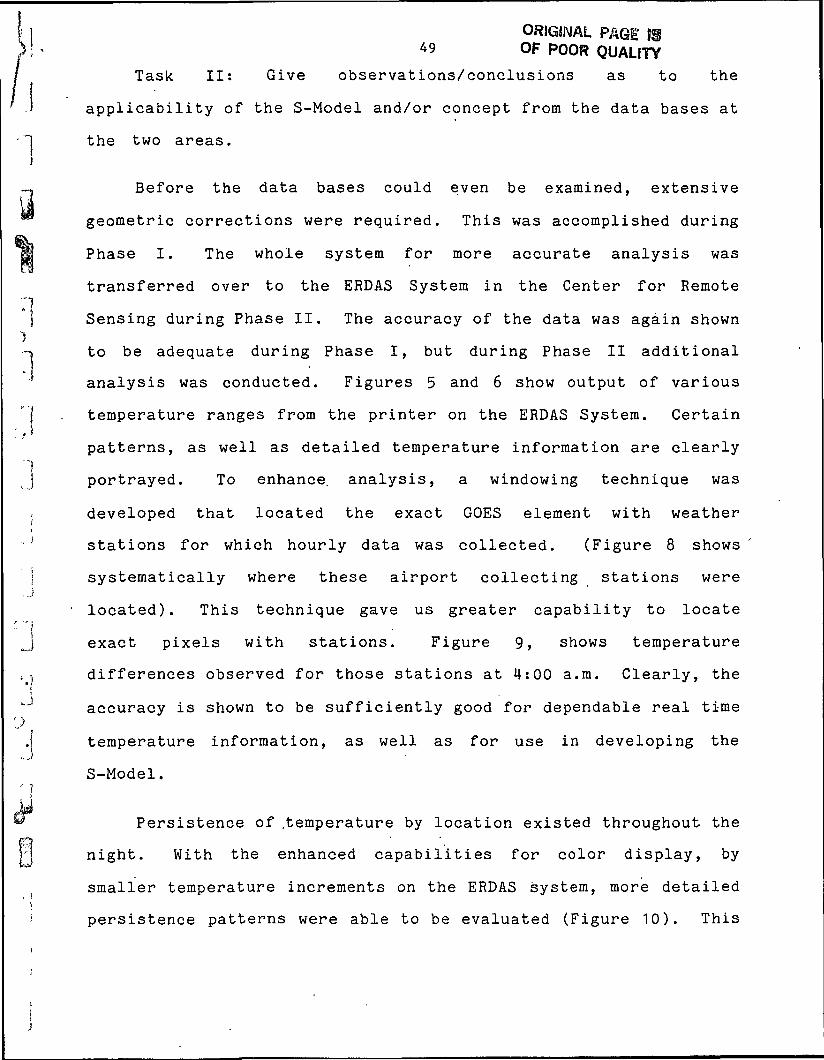
ORIGINAL PAGE 1949 OF POOR QUALITY

Task II: Give observations/conclusions as to the

applicability of the S-Model and/or concept from the data bases at

-1 the two areas.

~» Before the data bases could even be examined, extensive

•* geometric corrections were required. This was accomplished during

g Phase I. The whole system for more accurate analysis was

transferred over to the ERDAS System in the Center for Remote

} Sensing during Phase II. The accuracy of the data was again shown)-* to be adequate during Phase I, but during Phase II additional

analysis was conducted. Figures 5 and 6 show output of various

'I . temperature ranges from the printer on the ERDAS System. Certaint * *

patterns, as well as detailed temperature information are clearly~jt] portrayed. To enhance, analysis, a windowing technique was

developed that located the exact GOES element with weather!

stations for which hourly data was collected. (Figure 8 shows

) systematically where these airport collecting stations weres J

located). This technique gave us greater capability to locate

J exact pixels with stations. Figure 9, shows temperature

,-I differences observed for those stations at 4:00 a.m. Clearly, the

"J accuracy is shown to be sufficiently good for dependable real time„>.[ temperature information, as well as for use in developing the

S-Model., i

Persistence of .temperature by location existed throughout the

r] night. With the enhanced capabilities for color display, by

smaller temperature increments on the ERDAS system, more detailed

persistence patterns were able to be evaluated (Figure 10). This

50

evaluation clearly showed that the coldest temperatures, for

example, occurred at specific locations early in the night and

continued to be the coldest temperature locations throughout the

night. Thus, there was every indication that patterns would

persist throughout a night.

Of extreme importance to the statistical model is the

persistance of similar patterns from night to night. This would

clearly be expected if the temperatures are strongly dependent on

permanent surface vegetation and soil characteristics. For this

analysis, a variety of data bases were digitized on the same scale

as the GOES data. (See Figure 1-4). As a result of an extensive

visual analysis, it is clear that the temperature patterns can be

specifically related to surface features or combinations of

surface features. The conclusion is that one would anticipate the

patterns to be a function of surface conditions, and therefore,

would persist under similar meteorological conditions.

Task III: Identify and discuss any peculiarities of the

Michigan and Pennsylvania sites which might limit conclusions from

being applied elsewhere in the United States as a general case.

' .It has become increasingly clear that there are considerable

similarities between Michigan conditions and Florida conditions.

The significance of the peninsula and its effect on temperatures

inland have- been shown to exist for both locations. The advantage

in geometrically correcting data and overlaying scenes are clearly

easiest when one has a temperature discontinuity as it occurs

between water and land for a peninsula.

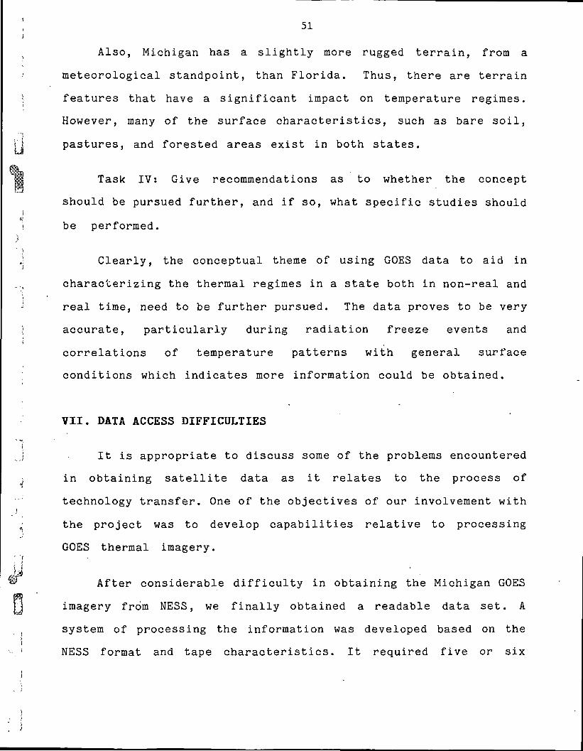
51

Also, Michigan has a slightly more rugged terrain, from a

meteorological standpoint, than Florida. Thus, there are terrain

features that have a significant impact on temperature regimes.

However, many of the surface characteristics, such as bare soil,

pastures, and forested areas exist in both states.

Task IV: Give recommendations as to whether the concept

should be pursued further, and if so, what specific studies should

be performed.

Clearly, the conceptual theme of using GOES data to aid in

characterizing the thermal regimes in a state both in non-real and

real time, need to be further pursued. The data proves to be very

accurate, particularly during radiation freeze events and

correlations of temperature patterns with general surface

conditions which indicates more information could be obtained.

VII. DATA ACCESS DIFFICULTIES

It is appropriate to discuss some of the problems encountered

in obtaining satellite data as it relates to the process of

technology transfer. One of the objectives of our involvement with

the project was to develop capabilities relative to processing

GOES thermal imagery.

After considerable difficulty in obtaining the Michigan GOES

imagery from NESS, we finally obtained a readable data set. A

system of processing the information was developed based on the

NESS format and tape characteristics. It required five or six

I 52

-| tries to get usable information. In April 1981 a request was made

to obtain data for both the freeze events that we had been

] anticipating. The data for April 15 was requested and sent. It,;

however, was not Michigan data nor did it conform to the range of

fj data expected. The request for data for the April 21 freeze event

@L was denied due to a change in policy and we were informed that we

had to obtain the data from Wisconsin. Since we had previously

«] attempted to obtain archived data from this source we were

* discouraged.•~1

One of our objectives was to examine GOES thermal imageryr-j

J ' over a growing season. We requested and paid for the imagery.. j

^ After several months a further attempt was made to obtain thes

-' information. It finally arrived with no documentation. After many

] attempts to read the data on our own, we requested assistance.,j *

again. Some documentation arrived but it still did not seem to' |

I help. The format provided was inadequate and the data was provided

,. in 24 bit binary.

Since the project related directly to the access andij«J processing of GOES imagery we were surprised at the difficulty in

"'j obtaining this information. We expected that we would be assisted

IJrather than discouraged because we felt this was part of the

|j technology transfer process to involve other areas of the U.S.

^ After these difficulties we are still convinced that our

pursuit of analysis of GOES thermal imagery and its application to

j Michigan has been and will continue to be rewarding. We trust that

NASA and NESS will recognize the problem of 'data availability and

53

will strive to assist users who want to use the data to benefit a

state. We look forward to future assistance in this area.

54

:il. REFERENCES

VI

ORIGINAL PAGE mOF POOR QUALITY

Barnea, D. I., and Silvervan, H. F. 1972. A class of algorithmsfor fast digital image registration, IEEE Trans. onComputers, v. C-21, pp. 179-186.

Chen, E. 1979. Estimating nocturnal surface temperatures inFlorida using thermal data from geostationary satellite data.Unpublished Ph.D. disseration. Univ. of Florida. 280 p.

Levitt, Larry J.Unpublished Ph.D,180 p.

Michigan DepartmentRecreation Plan.Services.

1891. Freezedissertation.

climatology of Michigan.Michigan State University,

of Natural Resources. 1970. MichiganLansing, Michigan: Office of Planning.

Pawling, J. W. 1969. Morphometric analysis of the SouthernPeninsula of Michigan. Unpublished Ph.D. dissertation.Michigan State University.

Schneider, I. F., and Erickson, A. E. n.d. Water holdingcapacity and infiltration rates of soils in Michigan.Michigan Ag. Exp. Project *J13. Lansing, Michigan: MichiganDept. of Commerce, State Resources Planning " Division andMichigan Department of Conservation, Water ResourcesCommission.

Van Den Brink, Ceel. 1968. Types of Spring Freezes in Michigan•and their relationships to protection equipment. MichiganState Hort. Society, Vol. 98, 102-107.

?JJ

1Appendix VIII

Climate of Pennsylvania

DEPARTMENT OF COMMERCEOCEANIC AND ATMOSPHERIC ADMINISTRATIONENVIRONMENTAL DATA SERVICE

J78 HEOUCTION RATIO:

Wtf

^2^co>^A^^~~-^^^

Nolionol Climatic Center

Federal Duflding

A:hov;ilo, N.C. 23COI

Th:l tl;j b tn o:fici.J mkr^rcrrn of j!:e Niters] O^jo-yhrr'e A(ir.hl<tr:.'o.i *-.J ij prfprrd fron fccorit reevedCj:i7.-.-l Olr^'.jc f<-^:/r. AOirvil'c, North Csro'Jr.» 26SOI.

J>*n!cl D. MJtchrU

IXtc.'or, Njt'or-sl CimiiJc Ctr-tff

CJ.;-

:-/./.•

mmm$w$?.y-Klvfer

;3Wtv 'lw"-', ^'*_•-»V« ••'X':N??y<»'^v*-SJ.'-'jiAt'n^'jr

CLIMATOGRAPHY OF THE UNITED STXS2S NO. 60

Climate of

NATIONAL OCEANIC AND / CNVIRON«.'ENTAL / MOTION AU CATMOsmzmc ADMINISTRATION/ OATASERVICE / «MIV.H.C.N

,M^ •;

OF POOR QUALITY

Thin publication In a nwdlficd vcralon of "Cllaatoftraphy o' tho UnitedStucco. (60, Climates of cho Stntr-n," vhlch vaa first loaned by thoNational Oceanic and Atuoopherlc Adalnlotratlon cllaatolo£lato aoalcncdto tho vnrlouo States. It is one of oeveml in the ocrloc, "PeriodicSut=iarliatlon of Cllcatc." (PCR5UM), prepared by the Hntlonnl ClltMtlcCenter (KCC) dcoletiert to provide oolcictoJ cllaatic Info nation ofgenoral Interest to o bronil opectru» of uaara.

Tho ctaff of the National Cllnatlc Center oxprcooco Ita t'aan'xa to thoacState Cllcatologlcts, vho, over the ycarc, have nndc olgnlfleant andlooting contributions toward the development of thlo vary uoaful ocrica.Scse oddltiono end deletions to the earlier lasucs have been cade In theintercut . f otcndardizaticn, and to reflect current prosrc:;a within theKCC.

Salo Price: 50 cento per copy. ChccJco cr.d noncy ordcra ohould bo cedepayable to Dcpertaont of Corocrcc, IIOAA. Rcnlttcncco and corrcnpondtnccregarding thin or other publications csntloncd heroin ohould be cent to:Director, national Cllcatlc Center, Federal Duildinc, Achavillc, tlorthCarolina 2GS01.

CLIMATE OF PENNSYLVANIA

Thio publication constt>to of a narrotlve chat dcocrlbco oone of tho.principal climatic features* end n nucber of cltnetoloslcal oucnarleo forntatlona In vnrloua ncoRrophic regions of the State. The detailedinformation prooontcd should be oufficiest for general ucc; however,00=2 uocro nay require additional Inforcicion.

"he National Climatic Center (HCC) located In Aohcvlllc, tie lo author-ized to pcrforo opcctal nervlcca for other government agencies and forprivate clicnto at the expcnco of the requestor. The aaount charged innil caaea la intended oolcly Co defray tho cxpcnoco incurred by thegovernment in oatiofylnc ouch opccific rejjueoto to the beot of itoohllity. It lo castmtlal chat requesters furnich the KCC with a prcciocstatement deccrlbinj; the problen oo that a trutual undcrotondinc of theapcclfica 'ono lo rtoched.

Unpubllahcd cllraatolf>£;lcal cudnarlco have been prepared for a videvariety of unora to fit opcclflc oppHcatlons. Theoc include wind nndtcnperature ntudlea .it clrporto. heating ind coollns decree day Infor—nation for eneruy oLudtcs. and nany others. Tabulatlono produced 03 by-productu of major projccto often contain laforantion useful for unrclftcdcpccial problcas, A copy of each tabulation on file at the Center naybe obtained for the cost of duplication.

The Kcano and Cxtrcnno of cctcorolojlcal vsricblco in the CliasatograpUyof the U.S. Ho.20 ncriea are recorded by sbcervero in tho cooperativenetwork. The Horrcalc, Meanu and Extrcnso In tha Local ClicictoloijlcalData, annualo nro couputcd fron obDervatiof.3 taken by National WeatherService peroonncl uho ore generally located at airports.

:U"ATE OF PENNSYLVANIA

ORIGINAL PAGE ISOF POOR QUALITY

TOPOGRAPHIC FEATU.'tES - The erratic cournc of the Delaware River Is theonly ontur.il boundary of Pennsylvania. AH othcru arc arbitrary bountl-aler, that do not conform to physical fcnturco. (.'ocable contrasts intomography, cllc.itc, and oollo exlat. Within thia 45,126-3quarc-ciloarea lico c great variety of physical lond fomo of which the coatnotable in the Appalachian Mountain oyotca composed of tvo rangca; thenine Rld|;c nod the Allegheny. Theuo countnlnn divide the CoanotiucalthInto three njijor topographical ncctlotic. In addition, two plains areasof relatively oraall size also exist, one in the uouthcaat and tho othortn the northucut.

In the extrcae oourhcnot la the Coaor.al l*lnln oltuntcd olong the Delo—unrc River and covering an area 50 nlloo lone and 10 ollcQ wide. Theland is low, flat, find poorly drained, but hio been ioprovcd for indus-trial and conrscrcial use because of ito proxitslty to ocean trancporca-tion via the Delaware P.lver. Philadelphia lieo alcoac in the center ofthis area.

Bordering the Coauc. Plain and extending CO to CO niloa northuaat tothe P.lue Rtd^c 1« tiie I'icdcont Plateau, with elevations ranging froa 100to 500 feet and including rolling or undulntinj; uplcnda, leu hilla,fertile valleys, and veil drained ooilc. Thccu fcaturca. co=bino.l ulththe prevailing dictate, have aided this ore a in becoming the IcadJ.ngagricultural section of the State. Good pastures, productive lia.l, nndshort distances to r-arketo have reoultcd in dairy fcrainc becoming oneof the loading acrlcultur.-.l activitica. Another activity ia tho crowingof fruit, primarily ay.plc-a and peachco. Gentle hillnidc ulopes providean excellent place for fruit treco, ao cold air draincge helpa to pre-vent un.ic/)3onable freezing teapc.ratures on thsea ollglitly elevatedlands. Tlie ar«;n ha3 r.any orchardo, with Adaus County loading all othorcwithin the region in the production of applca. The clicato and coils inthe Lancaster County area arc eopocially well suited for tho "roving ofcigar leaf tobacco, as is pointed up by the fact that Pcnnoylvania icthe leading producer of cigar leaf of any type in the Nntioa.

JuoC northwest of the Plcd-ont and beti:een the Illua Uldgc end AlleghenyKountaln.t lo the nidge and Valley Region, in uhich forcotcd ridgeaalternate with fertile and extensively famed vallcyo. Vegetcblcu,grown prlcarily for canning, ore Ihc leading crop. Thio has led to awell developed canning industry, u-lilch 1C concentrated in the ciddloSuaquchanna Volley. The Ridge and Valley province is 00 to 100 nilauwldf and characterized by parallel rldjjcu and vnllcyi: oriented north-eaot-GOUthwcoc. The count.iln rldseij vary frou 1,300 and 1,600 footabove oca level, with local relief 600 to 700 feet.

%-Vi<1'',':\?:.VS.'- *;-<-'>\'£i>>v. •:''-;« ;i-_g

North nncl w.-*t of the, Hldgr nntl Valley Hiv.lon and cxlondinj; to thu NewYorU nnd Ohio borders In tlic area known ns chc Allegheny Plateau. TliloIs the largest natural division of the State and occupies coro than halfthe area. It In crossed by many deep r.arrcv vallcy-i and drained! by ChoDelaware, Susquchanna, Allegheny, and Kononjahola Riwor ays Conn. Ele-vations are sencrally 1.000 to 2,000 feet; however, none mountain pookaextend to 3,000 feet. The urea in heavily voodod ami <u:onj> the. mostrup.gcd In the State. Numi-roun lakcc and Bwa.ipo characterize thin oncop.lac lot 1-0 orco, creating a very picturesque landscape; this la par-ticularly outfit.-indlng In the more northerly cnuntleo. The combinationof In ken nntl forcnto at elovat lon-t high enough to ko?p sunnier terapura-tiin-K mnfnrt.it> It* .mil Itn local loo clone- to heavily populated cltioali.-ivt- n.idc- rl»* I'ocono Mountain area a le.idlnj tourlut and recreationalrenter.

Bordering IJI'KO Erie Ic a narrow '.0-nllo atrtp of flac, rlcli land throeto four ralli-H wide called the La!«e Krle Plain. Fine alluvial oollo andfavorable cllrcate pprratt Intensive vegetable and fruit cultivation,which is typical of the ouch larger area surrounding Lake Erie.

Eastern and central Pennsylvania drain into Che Atlantic Ocecn, whilethe western portion of the State lies in the Ohio River Basin, oxcoptfor the Lakr- Erie Plain In the northwest, vMch is drained by a nucbarof small r.tt. i.-.is into Lnko Eric. The Delsuaro Rlvor. which forraa theeastern boundary, dralna the eai-.tcrn portion and flows into DelawareBay. The Sunquchanna River drains the central portion and flown IntoCheospeokc Bay. In the vcntorn portion, the Alloghan/ end the llononga-helo Rivers have their confluence at Pittsburgh to for-.a tho Ohio Rlvor.

Floodr cay occur during ony aonth of the yeir In Pennsylvania, althoughthey occur with greater frequency in tho spring nontln of March nndApril. They nay result froa heavy rains during ony season. Generally,the c->st wider.preJd flooding occurs during chc winter nnd cprlnjj uhcnassociated with heavy ralna, or heavy rains co=Mnod with snovoalt.Serious local flooding oomctltoca r<*oults frcs Ico Jaairt during the cpringthaw. Heavy local thunderstorm rains cause severe flasli flooding Inoany areas. Storao of tropical origin co^sttcee depcalt flood-producingralnn, especially in tho eastern portion of tho State.

Floods njy be expected nt least onci; in L;D;.; yu-r^. !or U'..;L.ince, floodstage at Pittsburgh iu exceeded on tho -vcrajo of 1.3 tinea per year,baaed on the long—term record, liouevcr, floods of notable severity andcagnitude for the State occur about once in eight yearn.

GENERAL CLIKAT1C FEATURES - Pennny1vonla is generally conuldorcd to havea huold continental type of cllcatc, but the varied physiographic featureshave a oarkr-d effect on tho weather and cliuto of th>- various sectionswithin th'j State. The prevailing wcstorly ulnda carry coot of theweather disturbances that affect Pennsylvania froa th.% Interior of thocontinent, no that the Atlantic Ocean has only limited influence upon

i ^ l fl ^

tin: clic-jto of the State. Coastal ntorino do. at tines, nffect the day-to-day weather, copcciolly in cantorn acctionn. It ic here that otornsof tropical origin have the greatest offcct within tho State, causingflood.*) in sonc instances.

Throughout the State tcapcrnluron generally rca.iln between 0* ond 100*F.ind uvcraRp frora neor A7°F annually in the north-central oountolnc to57*F annually in the cxtrcue nouthcaut. Tl>o higlicnt temporaturo ofrecord in Pennsylvania of lll'K uaa obuorvcd ot Phocnixvillo July 9 ond10, 193ft, while the record lou of -'»2°K occurred at Smethport January 5,190/1.

Suaacrn are Rtnerally «nro, averauinx about 6B*F nlonc Lake Erio to 74*Fin Rotithc.-ictvrn conntlcH. HlRh tonj>orat«r<sn, <30*F or ahovo. ocoir on annv<-r/ip.<- nl 10 to 70 dnya |><-i ycor In ir.uat occtloua; but occoaloiiallytout In-.!/.lorn )(..:alil Jen nay experience a scauon with an cany AO 30 dayo,while the extreno northueot overnjjeu nn feu ao fo-;» auyc annually. Onlyrarely does a Burjser pann without excessive temperatures being reportedsomewhere in the State. However, there arc placoa ouch .10 icracdiatolyadjacent to (jke Eric and at eo=e higher olevationo whor«> readingo of100'F have never been recorded. Rally temperatures during the «amseason ..sunlly hove n range of about 20°F ovor n-.uch of thi Stole, whilerhe d.iJ ly rnngc in winter la several dcf;rceo loou. During *-*»o coldestcoothn tcoipcraturco aver.ige near tho froezins point, with Jell;, ninlnurareadlnf.u sorc£tlr.oo near 0*F or below. KroozinC tcciporaturcs occur onthe average of 100 or more daya annually with tho greatoot nu=bor ofoccurrences in countalnouo rcglonn. Rccordo chow that frcoxlnn tcspcra-turca hove occurred coaculiL-rc in the State <!urlnc ull concha of the yearand bclov 0°K rcadingo frcu Kovcmbcr to April, Inclusive.

Precipitation iu fairly evtnly distributed throughout tho year. Annualoir.ounte generally range between 3f» to 52 inches, while the majority ofplaces receive 3fi to 46 Inchon. Croatcot asounto ncually occur inaprlng and ou=cer nonths, uhilo February io the drlor.t conth, havingabout tuo inches lean than the wettest ir.unths. 1'rccipitation tends tobe coseuhat greater In caotorn ccctlono tluc prlcarily to coastal otoraawhich occonionally frequent the area. During the uam iir-nnon th»ncotorn!« brlns heavy rain, uhlli: in vintoi" 1)L'C.«/ uu^w ur .'i mixture of rainond nnow cay bo produced. Thunderstorms, vhich ovora£.c between 30 to 35per year, are concentrated in cho warn r.onths end nro rosponoiblo forcoot of the cuRKierticic rainfall, which averOQca froa 11 Inchon in thonorthwent to 13 inchoo in tho east. Occasionally dry opells nay developand poniir,t for ncvoral oontho during which tlcc monthly precipitationnay total Icsn than one-qunrt'ir inch. 'Ihouo porioda altaoat ncvor affectall nectlons of tVic State at tho oane cluo. nor cro clioy confined to anyport leu] jr uoouon of the year. l/lntcr precipitation to uoually throo tufour inchch Iciic than oumccr rnlnfoll and is produced cost frequentlyfroa northcnstward-aovlng ctorun. UTion tcnporatucoa aro low enoughthese stonan coactiaco cause heavy onou vhich cay cccuaulato to 20inches or no re. Annual snowfall rangca botuaan wldt; lluita froa year toyear and place to place. Sor:e yoaro aro quite light an snoufall uaytotal )coa than ten inches while otlior ycoro nay produce upvardo to 100

*::.' -r» >-' I•y?-.*-V'.V'-I:. .'"-'f.''** /«'.""-*" *

lnchc:>, cuiilly in northern and nountr.lr.oua areas. Annual snowfallaverage:] fro-.i about 20 Inchon in the cxireae aoutheact to 90 Inchon Inpartn of McKean County. Measurable ancv generally occurs between Novcn-bcr 20 and March 15, although onou has been oboorved as early ao thobeginnlns of October and ao late no Hay, oopociolly In northern coun—tlcu. Crcntcot r.onthly acounto unuolly fall In Dccceber and January;however, grcotcnt acounto froa individual otorco generally occur InMarch n:i the tr.oioture oupply .ncroacca v.'.th tho annual carch of tom-pcruturc.

A3 ecntlon..-d earlier, hurrlcaneo or lov pressure oystoaa with a tropicalorigin culiioa offccc the State. Danajc: co a result of iiurrlcano windaare rare and usually confined co extro=-i eastern portiono. Hovevcr,nituro'tt wont violent oto'"r>. the tornado, does occur in I'ennaylvrnla..'.t l"nrjt one tornndo hnn been not<;d in uiraoot all count leu uinco theAdvent of oevcrc Mtorea rccordii in 1054. On the avorn^c, olx or seventornadoc-o .ire observed annually in Pennsylvania, and the State ranku27th nationally. June is the nonth of hiRhcat frequency, followedclosely by July and Au2uot. Principal areas of tornado concentrationarc In the extrc= : northwest, Clio Gouthvooe Plateau, and tho South-eastern Piedaont. The frequency in the latter nrca IB tho hichcot inthe State- nor square nilc, olailar to what ic oboorved in portions oftho Hlducntcrn United Scjtco. l.'any of the tomadoco In Ponnaylvanlchave caused relatively nlnor d-icaaca. :>jv.'ovor, ocvcral have clalccd 'lives ond dealt cevcrc local economic cotbackc. The r.oat deotructlvcactivity occurred June 23, 1944, wtica threo torn^doeo raked tho aouth-ucatcrn portion of tho Co^ctor.ucaltli, killing 4b perions, injuring an-other 3f>2, end cauoing over C2 aillicn in property dac^2o>

t Koro detailed Information is!' cllnatic areaa of the ctatc.

jivcn for eich of the four rather dlotinct

T1IE SOUTHEASTERN COASTAL PLAII.' A-'fO PlFJ:::-;:rT PLATEAU - In tlila rcsion the"n—'Tf are long and at tlce: unccafort.-bly hot. Dally tcsperaturcoreach 90*K or above on the avcrojo of 2i dayu during the cursor cccnon;however, rtradlnga of 100*H or above aro comparatively rara. Krou aboutJuly 1 to the diddle of Scptc=I>ev cliiu orca occasionally cxocricnccauncoafortably vrom pcrlcds, four to Tiv- -."./• ;c . •...•.',. ,:. »<_r.^ch,durinj uhlch Hc^t wind covc^cnc cud lii^h relative hu.iidlcy uako con-dlcionn oppreooivo. In ccncrcl, tho vrin:cro arc co=?arativoly ciild,with on ovcraf.e of Icoo than 100 dayo ulch olnicm tc^.peraturco bclouthe freezing point. Tccperntureo 0*? or Icvor occur at Philadelphia, onan overage, one winter in four, and at H^rrlaliurg one In three. Thefrcerc-frcc acason averages 170 to 200 days.

Avcrace annual precipitation in the circa ranjeo fro= about 30 inchco J.nthe lower Suoquchcnna Valley to about 46 in Chcotcr County. Under theinfluence of an occasional cevcrc co.-.ctal storo, a norsal conth'c rain-fall, or tsorc, nr.y occur within u period of 40 houro. I'hc avcrasesoaoonal oncrjfnll lo about 30 inches, arj fioldo arc ordir^irily cnovcovered about one-third of the tico durin- tho winter ccc-jon.

~JV.'V/'.S-*'.;V"/--.•.:'.Tr.*{5*y~?: *'.•:

THE RIDGE AMD VM.I.KY PP.OVINCE - Thlo region dot-B not have a true moun-tain typo of cliraate, liut It docs have army of the characteristics ofcuch a clluatc. Tlic B'iuntnln-and-v/illey influence on the air covenantscauses soacwhat greater temperature cxtrcnca than arc experienced In thesoutheastern part of the State where the modifying coastal and Chesa-peake Boy Influence hold then relatively constant, and the dully rangeof temperature increases somewhat under the valley influenced.

The cffcctc of nocturnal radiation in the valleys and the tendency forcool air musses Co flow down then at night renult In a shortening of thegrowing season by causing freezes later in cprinj and earlier in fallthan would otherwise occur. The crowing (freeze-free) tseaaon in thiosection ia longest in the diddle Suaquchanna Valley, where it avoragoaabout 165 days, and shortcut in Schuylklll and Carbon Countico, averag-ing leas than 130 doyn.

The annual precipitation In (Ula area tiau a mean value of three or fourInches more thnn in the oouthcaotcrn part of the Stato, but its geo-graphir distribution in leoa uuifora. The oountain ridgco are highenough to have oosie deflecting influence on general storm winds, whilesusscr showero and thundcrstorco are often ohuatcd up the vnlleyo.

Seasonal sm- '-ill of Che Ridge and Valley Province varica conoidorablywithin short dictanccn. It ic grcatcnt in Soaaroct County, avoraglng 08inches In the vicinity of Soaercet, and least in Huntingdon, Itifflin,and Juniata Counties, overusing about 37 inches.

THE ALI.EC11EIIY PLATEAU - Thin region han a continental type of cllnate,with changcjble temperatures and rcorc frcfjuent precipitation thnn otherports of the State. In the uore northerly sections tho influence oflatitude, together with higher elevation and radiation conditions, oervcto Bake thio the coldest areu in thrt <:tatc. Occasionally, uintor nlni-nua tcmpcraturca arc ocvcrc. The daily temperature rnngc ia fairlylarge, avcrdgJng about 20° in nidwlntcr and 26° in mldauczar. In thenourhern counties the daily teaperaturc rcnge iu a few clcgrcco higherand the satie nay be odd of the iiorn.il annual ranc<5. Bccauco of therugged topography tho freeze-free acoi:on ic variable, ranging between130 dayo in the north to 175 dayc in tho couth.

Annual precipitation han o ir.ean of about 'il incitcu, I'iinjjin;; fron Icocthan 35 inchcc in the northern parts of Tioga and Hradt'ord Countloo tocore than 45 incher. in parts of Crawford, Warren, and Wayne Counties.The ncaconnl snowfall averages 54 inches in northern areas, while nouth-ern uectiona receive ccvcral Inchon lecc. Flelda arc norcally snowcovered three-fourths of the tir.c during the winter acason. With rapid-ly flowing ntrea=D In the Ohio Drainage cyatcn (except tho Monongahala),it io fortunate thnt thin parr of the State in not oubjoct to torrentialrains such no ooactiraco occur along the Atlantic alopc. Although avcr-aj?;: annual precipitation la about equal to that for tho Stato as owhole, it usually occurn in cnallcr amounts ot coro froquont Intorvalo;24-hour raina exceeding 2.5 inchoo arc comparatively rare.

••, \ .:.>-:-V-:.;,.,.-.. . • .'' '

t \ .'..*. '•'"...'". ' - *.

:'&:&.->'>'i ••.*"'•i_:?-.:yi'••'-. •" ..,...••

J

Tllli LAKli ERIE PLAIN - Thin region ha: a unique and agriculturally ndvnn-tageoun cllnrtte typical o£ the co.ist^L areau surrounding aiich of theCrcot La\:c;>. B\>th In spring and autumn tho lake uacor cxcrto a retard—Inj? Influence on the tenpcraturc rc -'-e and the frceic-frcb ocason laextended about 45 <layn. In the nutu^n thlo prcventu early freezingtcnperaturco, which to a critical factor In the growing of< fruit nndvecctoblca.

Annual precipitation totala about 34.5 inches, uhlch lo fairly evenlydistributed throughout the year. Sr.cvf.-xll exceeds 5'» inchpo per year,with heavy onows sometimes experienced lace in April.

klSiilliSiilPliilSW

STATIONS IN THE CURRENT SERIES OF CLIMATOGRAPHY OF" THE U.S. NO. 20:

PENNSYLVANIA

CarlisleChambersburg 1 ESEClaysville 3 WDonora 1 SWEphrat.ifrank)inGettysburgHoitwoodJames town 2 fiWJohnstownLawrenccvil loKarcus HookKontrosePhocnixville 1 EPort ClintonReading 3 f<RidgvayState CollegeStroudsburgTowanda 1 ESEWarrenYork 3 SS!/ Pump Sta

•PERIOD UAT. |N)

1951-741951-741951-701951-741951-741951-741951-741951-741951-741951-741951-731951-741951-741951-741951-741951-721951-741951-741951-741951-741951-741951-74

40°13'39°56'40°07'40-10'10° 10'4)V3'39-50'39-50'4r30'40°20'•12°00'39-49'41-50'40-07'40°35'40-22'41-25'40°48'41°00'41-45'41-51'39°55'

77-12'77°33'80-23'79°52 '

76°10-79-49'77-14'76-20'no"?p,'70" S5'77-03-75°25'75-52'75°30'76-02'75°56'70-45'77-52'75-11'76-25'79-03'76-45'

465640

100076?/ \Jf.

405987500187

105012141000

121560105450270

13601170480745

1280390

STATIONS FOR WHICH LOCAL CLIMATOLOGICAL DATA. ANNUAL. IS PREPARED:

PrNMOYLVANIA PERIOD

Allento-.m 1976Avoca 1976Eric 1976HarHsburg 1976Philadelphia 1976Pittsburgh AP 1976Pittsburgh Fed. Bldg. 1976Wllliamsport 197C

t-AT. (

41-20'42-05'40°13'39-53'flO°30'40-27'11-15'

75°44'CO-IT76-5T75-15'60-13'eo-oo1

76°55'

CUEV. (PT.)

337930731330

51137

747524

te yvV 1|{ytvi-Sr;;-::,.

fr i;?'i''C'':-' A^^ .p.ft-&S:/|r,«% ;\ ,few^¥&£&&-•'&>•

CSs^^J: -i$jlm^/ :>--*>s *,.•?• •

SXsAVJf.^-V 'I

M^-vi.:-M»vlS'r-:-2rt:-;C-.::..T

- ! -•; ••••: ••••! •••'••!». •"!*! •! • ! • • • • •-w | «..«! ...'I 11... i.. |n'i. >• '«i.ii | i| •' > . >."

....: ....|,...;..'.. .-•..'..! .: . .' v"•• ••••! •• i S"! «i '. •: •. -".1.1. ....| r..|i.j i. ii |~ji>! .|.i. . ..-> .......

...... i.1 . ' ! .' i>' I.If .11 *! .. I.*' Ill 1 ' i *i * k

, ......j .j ,.>; ,...!„; ...i,,,.; «| .: .'L_ t*"1 *!ifi. *i!* ***^J**1 "•<1"||*1 *i *! *

CHAUatneaunc i esc. I*A

I • !.»

"':"" j'V'j •} ' " '

• •• ii

,...j,.|.,,. i.,:..; .j .'

ii:!;":; " u'.. :!:0"; :i::

i ,

CLAVIVILI.I; i v/. >

. .T-r-

! "^f'fTI!- ;C

:: :.a! i ; :! [si 5a I:'S•-- -r ' f—

.....l.rr, >.| i*.... l......|a.

-:- V-&-V~!.? .-'"• V,--.:•''\\';-.^ l---'i-- /.•;•.•;'-.•;»-•:,•'•.••• • . - • •

CLIMATOLCCICAL SUMMARY

DONonA t t.v. PA till > 117* 4O- 10* H

r;.f;-;•,..:.-: '.

!••»

—

;5 ji . J His:. Iff:: it • i :i ,5,S;:S

i.... .... » .>».»; ...

; ....: .,..; .... ,. ..;,.; ..'i ' i i* 1 • '

i

r

.„,,,

Ml

PR A

*u«

Ml

00

ou.

V."

1 1! " ( '

•.! i ..

.... ....; ....: ., .. .1 ..i i ....' ;......_

;ii si \ Hj i iH

.,..

........

• \i

MA*

mi*ii"

»*

•!." :

T"

si.r.. .1 .. .! .. "..' ,. '"'... ... ,. .J,.! .' ' ' : . C ! ,..... .... ... ..,.. ,.

„ , „., „ , ..

:

"'! "'!; ",', !,' !• "... "'., " "I ! !!.

., -i ..... >«vi"L'biJ

NKLIH. PA

1

• /I

!«.«

»;!•••*

»».*

• »i *«

"T"""-" '~n':'i;J ? ?5 ,'^ ?=

!! ! !> ! ..J"'.'! i!'.... .... .. .. .ri ..

.... ....j » » » ...

.... ....; •• .» .i ..

...» .... .. .. . t.

.1..; I..T: .1 t. .1 i.

it.. .... ! ... .. ..^-t..

PS|»»

•$

:•

• >

n

*«

";;»•

41

•"I*i

•I**i»t

i*

,,

ii

"

•..•It

~

*

1

1

tt

.*

. '

!

:bi!i j J55t i • - »•

1 i' li .; !:»! ...:, .j .; ..... ....

t:.i .; ;:.,L...:

•'Y*. 5 i 3'

.'

"

! " i'

;: ; ••;;! '.'•;;i i! ! Ml! '.".',::j ; ::::] :::;

. IBT4 41* 1

I?!?1!'' 5 : }\..! .' ,..".|"....

j*i i' «.»** ».*»

!.j ." .;..! .;;!.! . ....! .....; / ....j ....

;| ;. ;•;;! ';•;;.| . ....| ....;:; :. :::;; ::;:

10

i tj j := J3;j IJ jl

*.*• •1

vL.':vr.'

-1.1 -s miA»,t-<iiM.

"-1

7 'i"B;n

i

*'

.t

.*

.1

*.« **.•

.. ....

"i

":: :::

j

*•

r

[••

!"

"

•nr.f * *

•i *. •», i i:| : :?! * '»! » i• l * i. . .. . .

-1 :JM »»»

o- ii ir to- w <i> rr.»>tU.I.I. IUI.L.<IKUIt..

'b 3

" :••*"1

! '

'

•;iJ

I*

n

n>*

""

*

*.*»

• .Tf

fl

£

l.it

!.*•

• ••»

..•1

•,*ft

*.!•

M

'*II

*»

3

i**i

»tii••

(' f™—

*-

1

M... „..,.. ....„

•..*•

.0

"

I.I

,.

**i*

• i

ii*t»

5S

11.0

t».*

i.i

.*

***

il t

|

.ii" .:::•e.»j"i!f !>.•

*•.*

11*1

!».*

*».»

;:::....

V

*A»»' »•.*•i ».»

::! ;:"i ....

•in•*

"

3

|*

.."

r5

,

ii

«

* ' • j~• : r i J

• ,'; >

» » I

*' l l

• 1 1

» * t

ff 1 l

» 1 1

' '1 '* •! •i_S ": "l "

'

I

"

"

9ST KT.

1 "* -* ! 5 J

• ' • ' {-l|.»:!.

ti l, •

1

:!::• i i• • i

. . .1 'i *_ii:.". "i .•

j'$

t ^*&t ,y

Vr',j\

^,,

''

>

•.

i

:

^W-*. iMg&rsr

£&&:£;"". afc^'^-^/^r'-V ;b£^&;---{

..in i, .; >| . i..»; ..' ...i|..',.; .» | I I . . i,

"••' •; •; i •; -",' --A ••••;•• -i ••; -h -'v* -! • •iij i-j •> .j n! «J *.i» ..-..! Jt\ i.,.,.,! i>' t..j >.,' i,| ..J ,v ,t •[ ' *

L'LvN/; n"i •!. '-"j. ••V'L'-vl*1' "I .r-'l '-N'.'!-'' ^ !-. '!..!

.«*j ».»»St! I.»»}**;»»

|.t« u..,!t| 4.»«t|ll

JAMK»TOVVN I NW. >

i

>*.•

»!.* M.«

*».»

*•••

EE(.*»I.M

f.lt

i.i. •!

'.J'lll'J-.'J l'i1

J.VJ1:!"!-1"!'.'!'!).'; "i.1"! "i

••••I ••"i-i •••••••:V1 -r-'i-L'-l"

I'l ' »..»li ...

.*i 'I •- •

_.-::'L.'.'-•]" ."•.••• "I •! 'i -•

"l"l 'I ."-'I ":V'I 'It

Fr'''---^?- -'•'• iVH;.- .v,'-.. ~ t >.t-;» 'r.-il' ^^^-^^r;;!

•'. If ili ^^^^^S^^

CLIMATOLOG1CAL SUMMARY

««TOWH.T>K 1»B1-1»7* «0- 10* H >*> «• TV m« FT.

|_ IIWI »%!*-•».•*• J *«f*lttl*l«»*«mM»rt-4M»

«•»»»•

**"•II

M*

MAT

wnni

**«

il•'•t

•T.I

••.ft

*l*ft

•I.I

»».!

•».*

....

*•.»

II.*

Il.l

**.•

__•*•».

— ,..n.

AP*>

MA.

en

MAW

MA*

MAT

Ml

Ml

we

TlAft

... .»«....•*•*

••.i•l.»

•I.I

• ».»

Il.l

1111

• I

*••

II*

«•

••

t*

*r •

sti

II

*f

11

••

«.«,I-A

'•1

i"

i .

Si•I*

I*

"Ift

*!•

V-

.' ivu

2ji«•

*•

• t

•1

"

ii11i

*i*

•MIX sw>

•-t P-

1

*

^ !l.'• !'" ....

r

»»

:

:i:•i •i

.-I-

! !.'!!.; ....

«! ....

. ...t

''*'

..* .JL-f

IOI-II7I

u*n**ii »t.*i. I

l\

-.,

„.,

....

•>**

MIAOk

ii

"*

....

....;

1

" s?' i1'

'

ft*.*

*!.»

••

••*

I.IMI.

1 1:jili

?»

••..1

n

.-

3 a

1

••

»

M

I*

I

•

•

**n•.•i

•in

**

,5i|?!.»» »*

*

I.** M

l.*t >l

l.ll *•

4t- or n

•--s kij»£' J ! 55

MM

I |

1 li\l

1

•

•

•••

'ii. ...i. ....

.1 .

\ "

*.i*

*.*•

1*

II '•"l"

.... ...,| PI-I-M" »i >.|...| »i ...... ...,,'ir:, .... i;

TilT5 1 ii•* ll.'j *».*

l> I.I

1* .•

ll .*

n ... ,

"-4

^^

-; ••

-;*••

T>- »»• W

»II.I.«>U uft.r^

t!**

*•• .•

HII

till

-T

t

"' 1 '

***! -1.....I

»ri

CUft HOOK. FA t»ai»l»M )»• <&• H 73* SV W

»|

•***

• I.*

ft*. I

»%.»

•I.*

*».*

_"'.•

il.

r%.«

M.I

**.*

ft*.*

Il.l

. V:~'

/

{

M.I

ftl.t

»*.!

Il.l

.!V*

'

ft• ••

I**

1*1

»•*

1*

1)

Li!1.:I

3

..

.«

..

it

.i

.1

"

L'l

It*

J

't1

1"

!if

*i*«»

•*

ik*»«

IM

|l

_L

L.1,

-IT.

M

»J

tft

»

Ift

I

I*

!•

It

1

1*

I*

I*

1*

II

M

s*•

1ff

ft

*II

\i

•:

*

**

••

>:iii«

*,

•

1 !'

.-d?! :

V V.

* l.ll

ft l.ll

• •.«*

l.-i :':".12

..

I*.*j

*»»*

ift.*i

*»*!

•>*l

•••1

It.fcl

I.I*

*.tl

I 11. M

I*

"

it!.'

IpJl {.

l.*t 1*

**l* »*

1.** *l

l.*l II

*.!• II

*.»• n*.ti hl.lt H

I.I' *J

I.** U

L-':1.1!!.'

1. 5

I* ».»

|» ».*

11 >l

• I .«

• * •»

• .*

H •»

Il .»

I* ••

• .1

1* ».»

Ill 1*.

^ti.*

».i*.

j i*.

3C

.1

.11il'

»

ill•*.• M

ti* ft*»^

. i rs,j s i*, :

. .! .; .! •> . > i

1 ' '• ' 'i '•-. • •! •":!.'!j.'l ;. _.] i

ia»«rr.

lilil,

1

•.1 *l

: :i *i J ••'!•. . . . .•: *i •] •

. .{ i

. ; ;i ;i. » . .. . .; .

ir rr.

it

i?ii.* *'>».» »*

LL-- i

— lu~.IV.lT

jyj» » * i» « » &• » i

T i t

* • 1

• II

* » t

I I I

ft 1 1

t » 1 1

ii-JL.1!—U^_!M_?J-L

J&fr*

L&Z*$&&TSJ^r£«feH• «f/CN>.s»rt

^fw*?

^>'!»5j•X*rtV.S

&<£&?y*a?*ivrg?'<<>^&y!.'f?

Jll5ftV-

pf^;';•'•'

A^

^

^teSj^i

^

-.#:••..

3^g^.j-/:.*.*^

;

if•M£s*tL^f-5P^5';i^r^if-i Sv.»• .,* j-nS'.Vly.;*-->!Ai*fc--i*k*%$kwwir£t-'-t'."n**-u( **• ,&>.->:6-^fc'fJ-W

?*&£ '••'"••Irm. *+£*!* ' -

ivHr '»* '£. ••

CLIMATOLOGICAL SUMMARY

III.."'.',\ »!ii ";.i ii iii> ii iii

•• - .,.j .. i - | .. ., ...« ,..„,.., . . .

j ....j ii.ij i...I .1 ji. i| .

j »».i| n.i; f'^^V^'J. S »»

.^rrT7vT:~r':"f^frl§rS" 7 ' = T!"r -:rT:v'VTT"_j l ! jl j.! l i i l i 'Wi :J . I S _ ! i ii i ?

»w-» I fl.. *•.» **.*! !• ,**''*| •* '**' *| • * » •' »••• **** »>; ****-ll *» *.*| l..»'l»

•« j »l.i II.tj tt.*l »*.j|t?|t! || ;•*• lj »; i. •[ •! >.»•' t.ti'ti' I.H|)*| if .ij l.ijtl

•Mr ft., »».,! »i,»' •. Lf |«! l» i»f • 1 *. lj •' »-" ».t« i,[ l.l|t4|]|J .»; I

*~ I.,.. ....( ,...i,«.;,.|..»M .»i,.| .1 .; .j .| ..»,,, .•• ....J,,1 ..[ (nx* j »t.ij *i.»! »-.»! i** ("i1*1 •' T* *j (•! »' *i *' *•*•' '•'• " *.»•!»» i* .*' j

— !•••• --I "••!••• !"'••' •• - j - j • •! ••»."•••» •••• j IMI I i».i •».•< •*.»! t*» ;>ii t' ** *» i* i! »| • • I.M i*.i* M ».»• •« ii .»;

,».( •* l*.*-»l I* » I 1

i».».nj •! * *, t!».» t* |ij *. •, I

i

I"- . .

I*.*, •» |«l I »l l» -,

l».l •».» **-! •*•'») t ll*!l* If

i I t

j •»*•[_ ".*i ._**•*! " -'*-*{ *t **_!".!_*

i ••: >'.1 .1

»*.*! *l.ll !».•] i»t«J»|| jf-t* |*tlll] l>| **|l)*| •( •••*». l».»»,lt( t.**l»ll)l, II.*, |».(ikli |l.»I*li •> «|> *»! Ill..- J— ^— 1 _ i ,,L.. .~U- 1 —A t---I-.-L «i.—' *-- - - ' - ' ' ' . *- i.. _—- ' _.-' ' ' \ \^ 11

I»0«T CUIMTOM. »»A

."'.'I ";.'' !."!"'!!C

....I I... .. !..'»> ..

«•.»; .1 |tt

'• *' ''• !.'"!".'.'!;«! I'."i.tt j ..ii .i| i.*it.lt, *.ll'tl' l.tt

II.•ll' *>.<

••I

.. ,.,! .....•i '4 '-I-

13

- - . . . • ,,—^-.—,rr.r,^..^.ur,r~rTrr< '-'>'::rr''?:' "^—rrr%v-:' * •«'.".' - i ' ' '^MM^^M^^^^S^^^^--?n^^^^^?^'^^j*,^^'r^!/--'-' • • " • •

' • • • - • • • • • • • • • ' ' • •

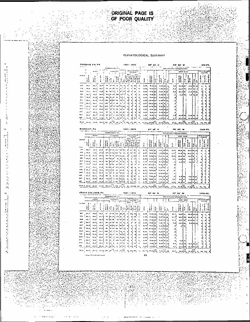
ORIGINAL PAGE IS0F POOR QUALITY

• ' - ' •' -:''-''-' •' - - • - ' - ' -

CLIMATOLCCICAL SUMMARY

I*SI * 1*71

1 ••••: ••••! ":.> ••;-:••.•; •' .;..; .• ..... •...;..; ....;..[.••• ; •••• '•!•-.-.- :«:•; •; •; ••: • •-••; .-M ••«;»••!"A. ...i- ...*_ .!..; it *• »»j i j.*^*! .1 t: ii ., »...} ..i.lii{ i...,!. i.'- ;....: ....' ....i ...;..-..; ,,.j.,i.! ., .| .| ., ,.„; ...,j.,l ,..,j,. .

"' '•.!!'!: !;'!' ",",\ .!Xj!!:!!!«!.!: !j .'i !i!' I"!!''.'", Ill !'"i";;"" : ...ij «.i ...ij in |..j i ii .,'.: .j .{ . ,| .... i..i, ..j ..>. .if .••••• i .1.1 ....! i,..j i.. ;»i .1.,.!.,].i; ij .! . .' „ i.,, i.!,,

'••! '—I"- ' :-.... ....j..: ......; . . . ....i •!.. I. I..*!..<li t| •, i

."I ... MI ... .1 I.' tj •: i

•....... •! • • •

_' !i'j!_«LiLi••t •(>

ft.l H |t.«)H, i) _JUJ_Mj_tt

'- . »>..' .1... n.»: »• |>i iv-i..!..,»»; .; „•.«; , ,...| t.i.;nj i.u.ki].».

-1,.::.; ;::.•.:.:;! M.p.;.; "..;:;;"• \\ \\ "j:: ;:;:j ::::j;;; ;:::;::|;;;" i »:.'i "::=::::!" b":: i::::;i ;| :\ :i :• :::;.:::;::!::;;;::!;;:

«i ,•;::' ::::j ::::j ::t|';:; c::: :j :| :|:; ::;;!:::;!::! ::::;::j.:!«i::::;::::::::: ^1:; ::i::i:! :i::j:; ::;:i :::;d ::xd

i.* n.« fl

* I >T4 <

TITTTT^'.-—•— ' " -r

33^I • : :

CTATC COLLKOJC.

«| .:.»..• .

-..-. ' it.-.i... i «i«~...i.. T [—i j ; | 1M>- 1|ltl pi7Ti»-.s;

• P-^ MHi' -" ;r=,-'^0?J :' : '• ' { :• ' • • • - i l \ \ - ' ' - i , ; ! : ' ; !J.'_il_.1J.Il;:;J .L:r':>5i-i"'k-:' : : i5 - 5i '=:?» '• : " \ - ' : ' « 3 lM'.» : !.« ^.' ...! ...' .-..,.C. ..V.".1,. '»".•".M

1"""r~r1~7"r'—•—p 1 I ' —

... !.,'.- .'' ,'i .:.- j 0 ' ! I ; ! :" 'v>! " i '"'"j ' i" 'I 'i '

...._..... ..... ....j... ,..-5.... ..:;;. .,..;..., ., ....,, .....jc,^.,;.^,....:...-,..,.,......, 14

""

...; ....,.., ...._••-•*.- Ji'L'i:M..I_....;:'I_....[:?I n _....., ,

IT'-'-

v-.-."-:--;.^-..- -.,c:r-^>r---':^:--7-::-r.:-o.-,--;v.-'----'-:••!•••.:--•: l =:'•>•--'-.•;;..-.-;:-- -.v •••-• = -.-.•-. --••- ••K.'ic.Vv"','- ^;^----'--^v^^rt>C^:>ri"i^^ •^'^•^:-: •'• '.-''•' i- '-^i>A--!.vx.-;.;-;'y:-.--- •• ;1

•'•'•• '• ••"•*•- -v'''-^vvi V//':?V;?' -. "|S - i

ry ^•'••vXv^'r'" • v -"- 'J^vv^v'*v^^\^\/^.;'" ^^Vv'^:: •;'V-'v^'"-"v"^ V " ' ' * " % * " ~."

CLIMATOLOOICAU SUM.V.A^v

I»1I - l>74 «r oa- N

. ( M.« | -;"p [ ;"v"j'' j

*""" *. j • ! } U-! ' i»- i J 'I ' T ' •; : -.

T»»» I t !"' '**! * * •»*"* t »*>-

TOWAMDA | CSC.PA l»l • ItM 41* 4B- N

_ ,'J O * J5 i ' != ] " ! - ' j r|i v!jv» *i»iC»: ; 5i ,i| i- ;: i.

I |l» •!• . *• »Tl«B j *»^*l •».»[ •».») 1*1 til' » -l».|»»| t[ tit >l|llll •) »•-»*, *.«l! »*[ *.*( »« Ih_. J_ L l_ I j . J . .J. i. i—I L- J- .1 .1- I t_ . _ » . _i—

WAF1REN, »A l» * l< l»74 41* *l' ..

t t ' ' • ' '»•» I **,»! I*.I »».» •» t*|ll(-ll MJ I • •! |» »| 4.M

1 •.•|it|| |.I» ., ,..

tv« | »».* »t.i »».ij «' ["^*; •' !M' * * •'. *! •{ *•" •>**!>*i !.•>'*. tiM» it.I >?.* •«.• »» i»»j i' t> |»t' » k •[ »' •} ..n[ ».i,jt»| •.».*. .,

-1*- "-'j •*- t »j«!« j,.!.| .! .1 . .; ....; ....j«; ...,'....'H»l j tl.l[ >•.» »!.« It* ,»», I! It 'I'.tfl ij *, »l »> ».'•; *.l* '*' l.*l ». ,.

'*« j »i,*(' M.»| it.i •• jti! »> i» |*> i»- •] .: »| i! t.ji t'tt.t*; *.n ^ ..*-i- j tl.fj lt.*j *«.! It '*i| |i | tljlM •{ •[ l*| •[ »•" **lllli- I.H i« !»,'

%f*» [ tl.*| »».•! **.lj ll» [HI I |'H [*t[ 'j *| **|1*'| *j •*."[ • • I4 | f f . *.fc*"I- T*.

. UMt-t»IUtl DATtl 1 J

n.'-':vL.":*:"i"..'..•»» *»•»».•. »».»jii| >*-*|_k'i », •• "i i

I I I '»*' tt,3J*l,l|l »' t t

r^^-.'I'v.v.!

v^^n-•'^^^or^p?^^^^^>:^.r--•>^^;.'/X.-V-.r-':'r-,- . - x > 1 - vVv'^^^'^v^.v^'A.&'i.^i.:-.'.'* L'-',"-,' i

^?v---v -»i«^\*>:.--T: >. ;'-i-V'--v;''V' J"/ '7^ •->v,-..>.-. •';- • • . - - . » • • . - . ' » , . ' . V*"'-1-*' '' - ' ' f^ l ' " -^ •"• *• :' *•'**'* ' '-' '

1 - • ;-:•'•':;':•'.%

! < • • ^ f t#::*#£

'•'•';' ""'•'•X-i'.-:'£'i-<,r--.:'V.'.?0'-?v

r- ..?.-•'••-.;'»•.:-;»:' .'; •; K -V—;•1.-.•;':-jf-^V'-:

von* > cvj» ruM* CTA. PA ie»i- i i74 j&- 33- n

^ .__ . .^~ ._, . •j^iV.^rs^Lj ^ I i j l l — •

"""V;iJtH '• l^i'U^NM^i'^'55! '- ^^'^'!3'-l •- - ,

.»i i n:::!':::! -;:!; ::'1:!:! :|T:n!~iTi"i:::id :"|i?~3^?.nj~SS \ \ \

"" j «..; i...| «i..| i.i i.| i' i. >iji.j .| •] • • !.••; •.•»'•.! i.n!»|i. .» I» I

^ 1

.

*'-*l*41^ v ^ *M.y^ii, t>. .>

r*' * i

~r^.. Ji .- •,»

*•- r~"^«»^ _*

«

i - •

f'&X

t&>

'& '.v

.fm

$&W

$bO

3ta::-Y

—

:i::-.:

s:}:::

;: iJ

-'I

—

—

"•-•"5

-<

« ••**-!

il.

••_

ijij ^

U: :n

^ni?

.H 5|i

c ! J

"

<

_^

_»»-

-.

r^™

^—

»^

-.,«

,

.•_

..-.

t,

n,j

j.-M

i. n

.J I

T.r.

-i-

r.i%

-_

.-!-

.-•...

-J

ill- j.i--,

-.1-.-

..('r"-'' 1

''*' *

l '•!•

'

•*£:•'";•'.'J!••'.:'?£'?•;""?'V'.v>

yi''T'-

lT

>^v?JV

^SH

':;"

;'"S^^W

3vi'':''

< v""^ '•• '?$'•'•' :':'' : '•

!

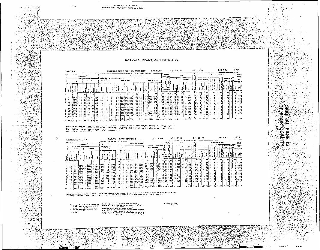
• •-'" ":•"-••>j':\.''-" ••„' i•'.' '•'• ••'.'.•:.•' 'f'

f^f'f}A

fiT-f,<

•; •' '•'-'-" -\<--'-'

p||||g

||K||||

....,..,,..,_,,...,, ...v.fc

ffij;V-, •,

! Mir- hi'-"•&

'•': £&

: :

I J •

I

' ..•

*»»^*..»

.. -

|

J7

I.

^-'

"

i.'.

.'.:• -".. ' :'•'•'-.'(>...'"'.

- - "

-

:-V-. : ^-'..'•••:•;•• w

T^'v

];.v- :--.vvv.-::-::.'^-v>

.3U

^-V

r/v^O

-O-.

-* v ."--.- ----- -r-'t/j

uc:xuO2<t/fZ<U

I

eO;c

r!J!!« !J *--i

'•: ».-_ j

r-<".L'

t i 11- Jir'>r

'|';'"*''~

;~' v"'*

''"j

! i i ' : «ii

~r • « ;

! _~>

z i—,—

,51

j j

-_ .„.„ ..„.,

-.

; :

HI

nl

);

\^h

• —

. ;z;r

:-r -.-

r3t .-

U-.-,.—

1/—

^-._

..-__,._

j L--^

!llI^piJ

l£.£5

_£

'•! ! H

•~

' :; r-..-"

rl^

T~

^s- {

' *rr^.»"» ••-"'= =

j ;iii'

t::

HiJ»::!>:»

'»

; s

;ii: i:

5:i

<:;ft:5

i

|li.[!•;i!

r

JHjiiu

~ ? ..;._

. ~~

>• • i ;

, :,

f; r"^ ;:-<-.

<~

..-T

!)!•-

Jh*\'.

•!•-. ,

£•{- • ~^

? :.' !_ —

-i

s • j i

~

?0

iiii-

-•

.•'-

••

«'

, »

' *

l'

1'.V

_"

- -

.*."

,- —

-T

-*

'-

' *

,»

'.*

•-•'.

.,•

-(

\' -

'{

*.

',' '

' ,.-,".'

. •

• •* •,

I'-

",.>

'.'

•'»

i

' I •

f '•

*

'

r

.

.---'- -•• "

' *

* "*...•!

••*

• J'r

f • •

j '

"'•

"•

"•

. '

, ,

1

*. •.•'-•--1y-'.' ;'- 'i-i--"••- .-,'-.•;'"-A

.'.'J'v •.:-•' •'-. .•.;«. '.'-'-., ;,r••-"-. .-.»',,•.•-•» -.•< *sv.',- ;; • •.<.{.••'.-.•.'-;*••-;?';'.'ji'-'.-..- -•'-•-.;

•?.'>.:• ••'.'". •

• ••>•"-. '.v t-v.-,i; :'v-v-f<•'"•.";-•>-"•:;',•">'•"•','" . •

'••

, l!

..f\

.'•:.i>. :";K'':Vi-\:il#

W.-..•vx

:^;<':

S

{3

^S

JJ

!>jx

fi • {

) i <

*J

' -

',_

,

, jr.

I ;

r ii»«

%?—

A

-ft—i---i

'ii»-i rl—

>

• «:' v^tfrV^' L^r^.

p- —

.. ^

r._

^_

| j

.^^

j\x

- j.^

^

^.

ii .:.. l-_

.j i iil i/-'r,

. ' i ^ g

h.- !*kr- ^

- i]?. !

.^"1/1

INi-i.o

! *

i L

;i.

II , !

; ! |'.-v

/,§

|I? i;

L ics x • i •

;; ! *

^^u; i»

ii- 1 j ;• j ' /^

i-H

i-a.L

j— / o

1 f

j 1 6 s

*=

U_

1j

11

^^

j ,

. , ,-^—,a-i-

r,;|, •». ^i

! }J

.i-.;» !^ -:.

\\ I'sN..-!

:«?»!V

1 If

T--,rr'^

J-i- i 'J iT

I '

"^v-iv :y

H—

J~r'~

i^ N

t~-i T-'ij

> .;»

;./»

i v-.-

i I 1 ^7

^^.! J

i !

I»,!ii

-,*UM.'•

: -,*«-l-j-feL

,-C

i . i*

l^i^: '

te^^-- -

> ' - V

I >

,'.- .

•K^-V:-..'. •.y.'-V

j«r.'".---.- •',

r'-:-;.\r. •-•-',^•/.yy;f.;, /•t~

'• •'.

"!. .- r}"•'"•/'

'' '• :- " "'!

^T

*fi --"^?

':Vi,/,-':' "

' ::

Appendix IX

The Office for Remote Sensing of Earth Resources

ORIGINAL PAGE ISOF POOR QUALITY

1

1

J

THE OFFICE FOR REMOTE SENSING OF EARTH RESOURCES /) .1Institute for Research on Land and Water Resources /•• **TThe Pennsylvania State University

The O f f i c e for Remote Sensing of Earth Resources (ORSER), is aninterdisciplinary group, established in 1970 for the purpose of partici-pating in projects involving the use of remotely-sensed data of earthresources. Investigators involved in ORSER research projects have beenfrom the fields of agronomy, an thropology, civil engineering, computerscience, electrical engineering, forestry, geology, geophysics, hydrology,meteorology, plant pathology, pa t t e rn recognition, regional planning, andsoils. A problems-oriented, rather than a discipline-oriented, approachis taken in the completion of tasks, in order that associates from variousdisciplines may work together toward a common goal.

ORSER has directed most of its efforts toward processing, analysis,and interpretation of multispectral remotely-sensed data, most of whichhave been supplied by NASA in both imagery and digital format. Photo-interpretation has been a vital part of the overall analytical process,but emphasis has been on the use of digital computer algorithms for dataprocessing. The end product of a project is typically a computer mapshowing various environmental and land use characteristics of data points'in the analyzed scenes.

Using th'e IBM 370/3033 Processor at the University Computation Center,ORSER has developed an extensive digital data processing system, employingFORTRAN IV source language, remote job entry (RJE), and an interactivemanagement and editing system (INTERACT). Statistical information, patternrecognition rou t ines , . and a variety of analyses of remotely-sensed datacan be produced. Portability and computation cost efficiency have beenemphasized throughout .

The ORSER facilities include a Ramtek color TV display 'system and aTektronix 4010 remote graphic terminal with associated cathode ray tube(CRT) display, hard copy uni t , and digitizing graphic tablet. Threeadditional terminals (one portable) are available, as well as a completeDatacolor image enhancement system. The laboratory also includes aMap-o-Graph unit and a Bausch and Lorab Zoom transferscope, along withZoom 70 and 95R stereoscope systems, a microfilm reader, a Diazo printerand developer, and a variety of portable stereoscopes and light tables.All s taff members have access to a Saltzman projector in the Departmentof Geosciences and a completely equipped photogrammetry and photointer-pre ta t ion laboracory, including a Kelsh plotter, in the Department ofCivil Engineering.

From 1972 through 1975, ORSER in terpre ted MSS data from ERTS-1 (nowLandsat-1), on a NASA-funded p ro j ec t . The general objectives were toascertain the usefulness of these da ta , to develop interpretation tech-niques , to apply remote sensiag techniques to regional resource managementproblems, to provide s t u d e n t t r a i n i n g in remote sensing, and to evaluatethe e f f e c t i v e n e s s of i n t e r d i s c i p l i n a r y research and university-industryrelated research. Specific object ives were met in the fields of digitalprocessing and p a t t e r n recognit ion, inventory' of natural resources andland use, geology and h y d r o l o g y , and environmental quali ty.

> ' ORIGINAL PAGE ISOF POOR QUALITY

Since 1973, the data processing system developed during the courseof the above project, has been continually refined and expanded. Recentdevelopments include the capability to handle entire Landsat scenes andto merge these scenes with a variety of ancillary data. With the systemimplemented on the IBM 370/3033, NASA's Goddard Space Flight Center andother users as far away as California have access by long-distancetelephone lines to a sophisticated data analysis package for generatingthematic maps suitable for a large variety of applications.

To assist these users, ORSER has conducted several short courses inremote sensing techniques. One of these, for planners from cities acrossthe United States, was sponsored by Goddard Space Flight Center. Severalcourse participants have since obtained terminals of their own in orderto use the ORSER system to assist them with planning and mapping problems.Follow-up courses have been periodically held at Goddard Space FlightCenter, providing further information in the use of remote sensing tech-nology as well as giving users the opportunity to share methods they haddeveloped while applying the ORSER system to their individual planningproblems.

The various thematic maps which can be generated from Landsat, Skylab,and aircraft data using the ORSER system have both general and specific .uses. For example, 17 watersheds were mapped for the Susquehanna RiverBasin Commission. These maps showed generalized categories of land useand were designed to assist in predicting the extent and quality of runofffrom drainage basins. Projects involving the generation of maps onspecific themes have included mapping of saline seeps in Montana andstrip mines in Pennsylvania. A current project, funded in part by thePennsylvania Department of Environmental Resources, is aimed towardsmapping gypsy moth damage from Landsa-t data and incorporating ancillarygeographic and related data, with a view toward creating a comprehensivedata base for Pennsylvania.

The system has been used with aircraft scanner digital data to mapfloodplains, housing developments, 'power plants, and other small scalefeatures. Funding for these and other projects has come from a varietyof sources, including NASA, the U.S. Army Corps of Engineers, severalregional planning commissions, and assorted private corporations. Aerialphotographs have been digitized to develop an automatic system for photo-analysis of specific features. One such project, conducted in cooperationwith the Department of Anthropology at Penn State and the EnvironmentalRemote Sensing Center at the University of Wisconsin, involved digitizationand analysis ,of photographs from Central Mexico. Soil tones and relatedfeatures were mapped to trace ancient canals and settlements near "MexicoCity. Current projects involve Heat Capacity Mapping Mission (HCMM) andSeasat data.

The ORSER software is frequently sold for implementation at otherlocations. This has been done for universities and private corporationsin the United States, as well as for several foreign agencies, such asEURATOM (an interdisciplinary working group in the European Common Market),the Indian Institute of Technology, the Norwegian Water Resources andElectricity Board, and the Geographic Institute of the University of

35455

Appendix 2a

MSU Test of P-Model

j

j

-1-

Table 2 is a copy of the output of P-model evaluation (JDAY

126 = Oct. 6-7). Period denotes the length of the prediction. The

column headed by PRED is the actual prediction of the 1.5m air

temperature. The OBSVD column is the observed value and the

error is the difference between the observed and the predicted

value with a positive value indicating a high prediction.

Table 3 contains a histogram indicating the nature of the

distribution of the error about the mean error. The statistics

of the analysis of the errors follows in that table.

Figure 1 presents the analysis graphically.

-2-

The following items were prepared by Mr. Robert Dillon,

Programmer I, IFAS/Climatology from information he received by phone

from one of Dr. Stewart Gage's technicians on October 1, 1981 (see

Table 1). Mr. Dillon ran the key station data from MSU through

the P-model to obtain these results.

-3-

TABLE 1

KEYSITE # 1 ( THL ) JULIAN DAY: 126 YEAH: 198110CM 50CM 1.5M 3-OM 9.0M DEW WIND WIND NET REF

TIME SOIL SOIL SOIL AIR AIR AIR POINT SPEED DIRCT RADTN VOLTG

18.019.020.021.022.023.00.01.02.03.04.05.06.07.0

0.00.00.00.00.00.00.00.00.00.00.00.00.00.0

0.00.00.00.00.00.00.00.00.00.00.00.00.00.0

0.00.00.00.00.00.00.00.00.00.00.00.00.00.0

50.548.744.841.539.736.133.333.933.131.830.429.429.436.6

51.047.943.040.738.634.933.132.731.630.829.729.831.039.0

0.00.00.00.00.00.00.00.00.00.00.00.00.00.0

0.00.00.00.00.00.00.00.00.00.00.00.00.00.0

0.00.00.00.00.00.00.00.00.00.00.00.00.00.0

0.00.00.00.00.00.00.00.00.00.00.00.00.00.0

-.078-.078-.078-.078-.078-.078-.078-.078-.078-.078-.078-.078-.078-.078

0.0000.0000.0000.0000.0000.0000.0000.0000.0000.0000.0000.0000.0000.000

Table 1. Data received from MSU in appropriate format for input..toP-Model. 0.0 indicates missing data.

-4-

Table 2. Copy of output from P-model run indicating the detail of each

of the 55 error calculations.

PMQDL ANALYSIS

-5-

Table 2.

ORIGINAL PAGE ISOF POOR QUALITY

YEAR JDAY STATION HOUR PERIOD FRED OBSVD ERROR

198119811981198119811981198119811981198119811981198119811981198119811981.1.9811981198119811981198119811981198r19011981198119811981198119811981198119 '111981198119811981198119811981198119813981198.1198119811981198119^11981

1981

126126126126126126126126126126126126126126126126126126126126126126126126126126126126126126126126126126126126126126126126126126126126126126126126126126126126126126

126

MICHIGAN • 2100MICHIGAN 2200MICHIGANMICHIGANMICHIGANMICHIGANMICHIGANMICHIGANMICHIGANMICHIGANMICHIGANMICHIGAN

23000

1002003004005oo600

22002300

MICHIGAN 0MICHIGAN 100.MICHIGAN 200MICHIGANMICHIGAN

300400

MICHIGAN ! bOOMICHIGANMICHIGANMICHIGANMICHIGANMICHIGANMICHIGANMICHIGANMICHIGANMICHIGANMICHIGANMICHIGANMICHIGAN

f, 0 02300

01.00P.OO3004005 0 0600

01 (1 0200

MICHIGAN; 300MICHIGAN 400MICHIGAN 500MICHIGAN & 00MICHIGAN1 300MICHIGAN 200MICHIGAN 300MICHIGAN 400MICHIGANMICHIGAN

SOO600

MICHIGAN '•'r;0

MICHIGAN ^°°MICHIGAN 400MICHIGAN 500MICHIGAN 'a 00MICHIGAN1 300MICHIGAN 4 CiOMI. CUE CAN • 500MICHIGAN' <->noMICHIGAN! 400MICHIGAN 500MICHIGAN 600MICHIGAN 500MICHIGAN J 600"MICHIGAN MIO

i• 2.345678910

<j.

234567391£.

34567bio

5A7i2.34r~3

6i2

34r:

12

iov_

3

41 .339.938.637.436,335.334.333.432.539. i37.335.634. i32.831.530 .329.228.237.435.734. i32,731 .530 .329 223.234. 032.431 . 029.723.427.226 , 030 .929.227.626.124.723.33? . 531,530 . 629.829. 032. 031 .530 .93u .430 .229.223.328 . 627.427.7

41 .539.636. 033.233.833. 031 .730 .32.9.329.339 . 636. 033.233 , 833 , 031 .730 .329.329 . 336 . 033 . 233.833. 031.730 .329.329 . 333.233 . 833. 0

73

313029 . 329 . 333 . 833 . 031.730 ,329.329.333 . 031 .730 . 329.329 . 331 .730 ,329.329.33 0 . 329 .3?.9 , 329 .3?9 .329.3

i .4i ,73.95,43.63.33.64. 04,03. 1— CT

i ,22.4.3

-.2,0

— x

-1 ,2i .42.5.3

, 01

-i . 1.8

-1 ,4-2 . 0-?. .0-i .9-2. i-3 . 3-2 . 9-3.8-4. i-4 . 2-4 .7-6 . 1-.5

'">i f...

,3.4

-.3.3

1 .11 .61 , 0„. /.

- . 1-i , 0•- . B-i ,9-1 ,7

-6-

Table 3.

ORIGINAL PAGE ISOF POOR QUALITY

*****

* **»

* * *** *

1 f-6 -4

** ****:

1

-2

* * **************

i

0

********

i

2

**

* ******

i

4

*

i

6

PMODL ERROR HISTOGRAM(DEGREES FAHRENHEIT)

POPULATION = 55

MEAN ERROR = -.024

STND. DEV. = 2.374

Table 3. Statistics from P-model analyses, MSU test, May 6-7, 1981.

-7-

50 .>

I-Qua

"] "2I 3u3 U 4I Id

P-MODEL PREDICTIONSMAY. 6- 7, 1981MICHIGAN

ORIGINAL PAGE 13OF POOR QUALITY

Li.

CDLUCl

HIQ:Z)

35 ..

criu

LUH-

30 ..

25..

20 \ ! H 1 1 1 1-

c u r u r u r u o o o o o o o o

TIME C EST)Figure 1. Results of P-model run on data submitted by the Michigan

subcontractor. The thicker trace follows the 1.5 meter airtemperature at the site while the thin lines trace out the P-modelpredictions for the remainder of the night beginning at the hourthat they depart from the thicker (observed) trace. The verticalline at 6AM marks the point at which the analysis of the P-modelperformance was stopped because it is obvious the sun came upprior to the 0700 observations.

1

APPENDIX 2 B

M S U

Michigan State University

Report

]•J

APPENDIX 3

Temperature Distribution accross Nittany Valley,

Pennsylvania, during Three Typical Spring Frosts.

J. David Martsolf

Reprinted from Science in Agriculture 18(2):2-3

Penn. Stat Agr. Expr. Station, 1971.

I

FIGURE 1. Four thermistors mounted in

tandem on a vehicle fender. From left to

right, an uncoated disc, an epoxy-coated

bead, a bead set in a stainless steel cyl-

inder, and a small uncoated thermistor.

FIGURE 3. The meter of a t h e r m i s t o r

thermometer is temporarily mounted on

the glove compartment lid with an exten-

sion of the vehicle's instrument lighting

system in front of the meter for a light.

It is advisable to have either a tape re-

corder or a passenger to record the ob-

servations.

FIGURE 2. Temperatures observed on three radiant frost nights, near dawn, indi-

cating very similar patterns, from where Route 322 crosses Bald Eagle Mountain

to where Route 26 crosses Mount Tussey through Nittany Valley near State

College. Thermal belts along the slopes are outstanding features quite important

in site selection.

ORIGINAL PAGEBLACK AND WHITE PHOTOGRAPH

20 30 40

Distance in thousands of feet

j

Thermistor thermometeruseful horticultural tool

J. David Martsolf, Associate Professor of

Agricultural Climatology

The thermistor thermometer has been

found to be a useful tool in at least three

horticultural production practices: (1)

site selection, (2) sensing temperature

inversion strengths and (3) sensing fruit-

blossom temperatures. A thermistor is a

temperature-sensitive resistor, a few are

pictured in Figure 1. The resistance to

current flow decreases as the tempera-

ture of the thermistor increases. The

relatively small size of the thermistor

minimizes disruption of the environment

by its presence.

The best method of frost protection is

undoubtedly good site selection. Tra-

verses of the Nittany Valley in Central

Pennsy lvan ia using thermistor ther-

mometers have revealed that up to 18°

Fahrenheit differences in temperatures

occur between the warmest and coldest

locations in the valley of typical radia-

tion frost nights near dawn. The mean

increase in temperature with elevation

of the site above the floor of the cold air

drainage basin was 3.4° F. per 100 feet

of elevation. Thermal belts on the slopes

of ridges and knolls are readily mapped

by this technique, Figure 2. The same

instruments have sensed temperature in-

version strengths between 5 feet and 50

feet heights in local orchards to be on

the order of 6° to 8° F. in the early

morning with rapid decay as dawn ap-

proaches.

Air temperature in the close vicinity

of fruit-tree blossoms has been sensed

easily and compared with more conven-

tional observations using liquid-in-glass

thermometers mounted in nearby shel-

ters. In large mature trees the air tem-

peratures up near the blossoms were

found to be 1° to 2° F. warmer than the

shelter temperatures at the time the de-

cisions were being made to light heaters.

This knowledge resulted in both a saving

of the crop and fuel oil.

Thermistors help in site selection—The

thermistor thermometer, mounted on a

vehicle, provides a technique of sensing

temperature differences between poten-

tial horticultural sites by direct compari-

son. Figures 1 and 3 indicate a method

of using a thermistor thermometer on a

vehicle to measure air temperature. The

readings are made while the vehicle is

in forward motion to avoid sensing the

heat from the vehicle's engine. Such ob-

servations express the average tempera-

ture of a column of air through which

the vehicle has just moved, even more

desirable information than that from a

thermometer in one location.

To make comparisons between two

horticultural sites, having one of known

productivity and one of undetermined

frost hazard, begin at one site and go to

the other and then return to the first.

Assume that the temperature at the

first site was changing at a constant rate

J SCIENCE IN AGRICULTURE, VOLUME XVIII, NUMBER 2, WINTER, 1971

or POOR

FIGURE 4. A 50 foot tower for monitoringtemperature inversion, showing the ve-hicle at the base of the tower wherewires connected to thermistors on thetower are momentarily plugged into ameter in the vehicle to sense air tem-peratures at various levels on the tower.With practice, the observer can make hisnotations and drive away from the towerbefore the effect of the vehicle on tem-perature readings becomes noticeable.

FIGURE 5. An idealized diagram showing the decrease in blossom temperaturewith time on a typical radiant frost night. (1) The trend from time A to time Bwill erroneously predict that the critical temperature of the blossom will bereached at time C. (2) The goal of the protection plan is to modify the blossomtemperature so that it follows the dashed line from time D until sunrise ratherthan falling below the critical temperature at time E. (3) The minimum value offrost protection required is the number of degrees indicated by the double-headed arrow.

BLOSSOM

TEMPERATURE

Critical temperature

ORIGINAL PAGEBLACK AND WHITE PHOTOGRAPH

Midnight Sunrise

TIME

and was probably at the mean of the twoobservations at the time the observationat the second site was being made. Thisis a defendable assumption near dawnof radiant frost nights, the time of in-terest, since the temperature change withtime is both small and predictable.

Thermistors gauge temperature inver-sion strengths—The difference in airtemperature between a reference heightnear the ground, say at 5 feet, and awarmer location well above the ground,possibly at 50 feet, is termed inversionstrength. Knowledge of this inversionstrength is necessary to predict realis-tically the possible effects of variousfrost protection methods at the disposalof growers. In general, the greater theinversion strength, the greater the possi-bility of the grower modifying blossomtemperatures with heating devices, windmachines, or a combination of the two.Figure 4 illustrates a method of using ameter mounted in a vehicle to quicklyread thermistors mounted on a station-ary inversion tower located in an or-

chard. An alternative method is to placethe inexpensive tower out of the trafficpattern of the row by running it upthrough a tree. In this case the distribu-tion of temperature within the tree ismore directly indicated. The studies in-dicated that a 6° to 8° F. inversionstrength is typical in the University or-chard location near the time when firingwould begin. Inversions of less than 2°or more than 10° were rare.

Blossom temperature estimator uniqueapplication—Quite typically the groweruses liquid-in-glass thermometers to cali-brate temperatures. The success of thismethod rests on the grower's ability todecide when his blossoms are in dangerof being damaged, using knowledge ofthe air temperature some 5 feet abovethe ground. The thermistor thermometeroffers a more direct solution to the prob-lem by placing the sensor in the imme-diate vicinity of the blossoms to in-crease the possibility that a good esti-mate of their temperature is obtained.Figure 5 describes the decision-making

process diagramatically.Small bead thermistors were inter-

twined with the blossoms of large apple,peach, and cherry trees in the Universityorchards during the past two frost sea-sons. Several observations indicated thatblossom temperatures were most oftenfrom 1° to 2° F. above the shelteredliquid-in-glass thermometers nearby. Nothermistor readings were lower thanthermometer readings and none wereover 5° higher. The additional informa-tion resulted in delaying the lighting offires several times. This resulted in nofurther crop loss but a definite savingsin fuel. The thermistor thermometerpromises to take some of the guess workout of decisions regarding lighting oforchard heaters.

Experiences with both "homemade"and several commercially produced ther-mistor thermometers have unfoldedknowledge of some sources as well assome characteristics of the instruments.The author will be happy to share thisknowledge upon request.

THE PENNSYLVANIA STATE UNIVERSITY, COLLEGE OF AGRICULTURE, AGRICULTURAL EXPERIMENT STATION, UNIVERSITY PARK, PENNSYLVANIA 3

U APPENDIX

ai

A SATELLITE FROST FORECASTING SYSTEMFOR FLORIDA

Presented to:

The Workshop on Applications of Weather Data toAgriculture and Forest Production.

Anaheim, CAMarch 30-31, 1981

Funded by: National Science FoundationSponsored by: American Meteorological Society

35456

ORIGINAL PAGE !SOF POOR QUALITY

A SATELLITE FROST FORECASTING SZSTE i

FOR FLORIDA

j. David MartsolfDepartment of Fruit

Institute of Food and Agricultural. Scieace-University of Florida

INTRODUCTION

The first of two minicomputers that are the rnaincomponents of the. Satellite Frost Forecast System (SFFS) wasdelivered in July of 1977 (3artholicr 1977) _ SFFS .hasevolved appreciably since then (Woods, 1977? Sutherland andBarthoiic, 1977? Bartholic and Sutherland, 19787 Woods,1979; Sutherland, et al., 1979; Martsolf, 1979, 1980a,brc,d?Gaby, 1330; Sutherland, 1980; Barnett, et al., 1930). A.geostationary operational environmental satellite (GOES)system provides the " satellite data [SMS-2 (synchronousmeteorological satellite) a prototype for the GOKS-becamethe operational ^east bird' at 75 ',> in April of 1980;Schnapf, 1930J, This past frost season, 80-81, marked thefourth winter in the development of SFFS- The freeze of;January 12-14, 1981, was documented by the system andincreasing interest in potential of such systems (Brandli,1981). Two major changes took place .during these four yearsof development. One is. that the satellite data is nowacquired digitally (from NOAA/NWS in Suit-land,- MDr seefig. 1) , rather than by . redigitiding the GOSS—Taptransmissions. Secondly, the data acquisition has beenautomated, i.e. the computers are programmed to operate the-system -vitrh little, if any, operator intervention^

THE CUP IENT SYST3M

1. Coznpucers•

Figure 1 describes SFFS in block diagram as it wasoperated curing the 1930-31 frost season. The system isoperated by one of two rninicc.r.pucers which acquires the datanecessary to form the SFt'S products automatically. ANASA-Dvr.ed computer located at th? NOAA/NWS Weather ForecastOffice (ivFO) at Rusk in, Florida, served as the main computer

ORIGINAL PAGE IS.OF POOR QUALITY

GOES SATELLITE

NOAA/NESS

NOAA/NWS

SUITLAND,MD

digital-—/(phcne) Y

NASACOM1=UTERNOAA/NWSRUSKINTFL

if DS/lpt>OI (phen*>

KEY

STA» IONS

(!FAS)

/ \ ' [

BACK UPCOMPUTER

!FAS CLtMATGLOGY

GAINESVILLE

PRODUCTS/USERS

FORECASTERS

Rtisxm

AG.EXTENS1OM

OFFICES

OTHER USERS

F-'e 1 Block diagram of SFFS indicating satellite digital dataacquisition bv phone link with NOAA/NWS-NESS in Suitland andlinks with 1C)' automated weather stations in Florida, the twocon-uters l-'aked bv DS/1000 (a distributed system) thatautc-iai-- the acquisitions and process the data into productsfor forecasters at Ruskin, FL and for other users through.Agriculture Extension offices.

ORIGINAL PAGE ISOF POOR QUALITY

with a similar machine located in the Cliiaatology Laboratoryof the Fruit Crops Department, IFAS, University of Florida,Gainesville, Florida, serving as a back—up nachine-

The minicomputers are Hewlett-Packard^ (HP Series 1000}having RTE—IVB operating systems, ami connected as adistributed system (DS/1000) . The Ruskiix machine is a model2112 with 192 Kbytes of memory and accessins a. 15 Hbvfce disc(HP Mdl. 7905) . The Gainesville machine" is a model 2113with 255 Kbytes of memory and accessing _2 -each 5 Mbyte discs(HP ndl. 7900) with a third to be added in the near future.Both systems are controlled through CRT -terminals (HP2645-Vs) and store data on magnetic tape-(300 BPI, HP-Mdl79703)- The major, products are displayed- on. 15 inch ConracRed-Green-Blue .(RGB) Monitors, i.e. color TV displays.Automated use of telephone connections, :botli 300 .and 1200Baud is accompli shed through a Vacic multiple chassishousing both auto-dialers and modems (Hdls 801, 305, 3415).

2. Satellite- Data Link

Initially, GOESTAP analog data arriving at Ruskin WFOvia Miami was redigitized to provide the satellite datainput to SFF3, but planning to obtain the digital data wasin progress during the first year of development (Bartholic,1977).

During the third frost season, the- development of aspecial driver made computer-to-computer communicationbetween the SFFS HP's and NOAA/NWS's IBM's possible. SFFSauto dials a Vadic 3467 modem at NOAA/NWS (supplied by SFFSat first but now by NWS) in Suitland. Upon connection theSFFS computer interrogates a particular storage queueassigned by Mr. Arthur Bedient, Chief, Automation Div.,NOAA/NWS. Previous to this step an NWS batch-mode programmust have., inter negated a large disc file (4 ea Mbyte discs)known as the VTS5R Data Base (VD37 VTSSR = Visible InfraredSpin-Scan Radiometer) via an IBM 360/195 (NOAA uses 2 with athird as a back-up) to select the Florida sector 'from theentire hemisphere of infrared data and pass it into SFFS'squeue. The VD3 must contain the particular VTSSR data forthe hour in. question for the NWS program -to be successful.

The VD3 is filled by a batch-mode program on the IBM350 that passes the satellite data from 22 Mbyte stagingdisks located in Wing 1 of FC3-4 near the 7-m ctish antennae.Collecting the stretched VISSR data by antenna andprocessing it into the VD3 are operations under 1COAA/NBSSjurisdiction (Waters and Green, 1979). Building the output

ORIGINALOF POOR

queues for clients such as SFFS, i.e. the Florida Sector,is a responsibility of KOAA/NWS. During the 1980-31 frostseason the staging disks sustained head crashes during aperiod when GTE was on strike, and the VD3 had to be filledby manually transferring 9-track 1600 BPI magnetic tapesfrom the VISSR Ingest Computers (GTE" ISlOOO's) to transportsserving the IBM 350's. Therefore, during the 80-81 frostseason SFFS was successful in acquiring the sectorizedsatellite data in only 63% of its attempts. When the datawere acquired, it was often 4 to 6 hours delayed during theearly evening when the system is dependent- on timely data tomake convincing forecasts. Since the staging disks havebeen repaired and the data are transferred automatically(but by batch-processing) to the VDB, tha reliability of mappresence has not greatly increased nor has the delaydecreased. Consequently, direct access to the satellite hasbeen ,investigated. Sufficient insight" was developed tosuggest that the- reception of the strertc±ie<3 VISSR data bylarge number's of users was the dissemination methodenvisioned by the- satellite's designers^ Progress towardthe procurement-of an antenna system will be reported undera later section..

3. Automated Weather Stations

Initially these ground stations were manned byvolunteers (irr most cases) . There were a dozen key stationsselected to represent peninsular Florida in locations inwhich volunteers could be obtained to read and report thesensings^ At the beginning of the third frost season 10.remaining stations were automated i>y the addition ofmicroprocessors manufactured by Darcora.

The microprocessor controlled data acquisition systemsthat automate the key stations are Darcom model D303"*s_They are capable of interrogating up to 8 analog channelsand totalizing on 2 additional -six—digit electronic:counters. These pulse counters can be remotely set toaverage the inputs over 7.5, 15, 30, or 60 minute intervals.They can be programmed to reveal the total as well as therate over the selected time interval. These units weredesigned for, and have been extensively used by, gas line-ccKipanies to monitor flow through pipelines by telephone.They have a built-in modem that for i.ts cost handles thetelephone conununications very well. The Darcom RemoteTerminal Units (RTU) , as they are termed, are used- at thekey stations to accumulate counts from light chopperanemometers, and to scan n levels of thermistor sensedtemperatures, a net pyrradiometer-, and a reference voltage(sea fig. 2). V

1ORIGINAL PAQE 13

POOR QUAUTY

1

3-Q"r? ~ t lJ -CMRCCM SYSTEM' ". rS.1 ISEE I^H^T »!.0»t)

. \-\ PHONE SG.ViL OUT SiGhii_*r6 DASCCMSYSTEM TO SUM?DATA Ev£Sr WXIfr

tUTCOiAt.PHCfȣ -HOOEM

MINICOMPOTES

TV

f*-a

Fig. 2. Diagrsn of SFFS showing data acquisition links and feadetails of automated link with 10 surface weather stations. :scattered over peninsular Florida,

Table 1. List of key stations serving SFFS indicating theirloca-tlon and affi Hat-inn

No.

1

7.

3

4

5

6

7

8

9

10 =

Station

Tallahassee

Jacksonville

Gainesville

Tavares

RusJcin

Arcadia-

West Palia Bee

Belleglade

Iminokalee-

Homestead

' Location

Airport

Airport

Horticultural Unit5 miles NW of Gainesville

Agr. Extension CenterRural, SW of Tavares

Site of

Radio Station-

ii • Airport

Branch Experiment Station

Branch Experiment Station

Branch Experiment Station

NWS

NWS

_ZFAS/Frn.ifc Crops

IF-AS/Sjctensian.

NWS

Private

NWS .

IFAS/AEC

IFAS/ABC

• IFAS/AEC

ORIGINAL PAGE SSOF POOR QUALITY

During a frost night they are scanned once per hotzr byone of the SFFS HP'.s by a fairly elaborate software packagethat checks to see if the station has been successfullyinterrogated. If not the computers tries to call the- keystation several additional times (a variable set by theoperator) and -then if unsuccessful,, uses a substitutiontable or prearranged calculation to substitute information,,while leaving a message for the operation that' such asubstitution has been, necessary. This past irost season thekey station data was acquired on 95% of the tries with. mostof the failures caused by chance phone" 15 ne routing thatresulted in very noisy lines. Regular voice gxade lines, areemployed for these interrogations.

Seven phone companies are involved .jin- providing the-service.- While these companies are required by law toprovide similar service from place to place, -experience with.troubleshooting problems has revealed a variety of attitudesand policies regarding such service. For example, a problemdeveloped when the Ruskir system began to interrogate thekey stations (the Gainesville system had handled them daringthe development stage) . Apparently, problems with crankcalls In the Tampa Bay area had caused the phone company tohold lines open when one party hung up while the other heldlong enough, for a trace. The procedure treated our Darcomsas a crank caller and prevented the system from completingadditional calls until the rather long timeout occurred. Asoftware change in our procedure corrected the problemrelatively easily after it was isolated. But tracingproblems through phone companies can not only be timeconsuming but quite frustrating.

Figure 2 diagrams the instrumentation on the keystations, the microprocessor controlled data acquisitionsystem automating the station and the acquisition links thatthe SFFS uses to acquire the ground weather data- and- thesatellite data used to construct the output products.

ORIGINAL PAGE S3OF PCOU QJALITY

Initially, the key stations used thermocouples(copper-constantan for temperature measurement) but whenthey were automated in 1979, a switch to locally availablethermistors (Atkins Technical, Gainesville, FL; Type 3) wasmade. To reduce cost, the bare thermistor beads werepurchased and encased in epoxy. In 1980 the procedure wasmodified to increase the time constant of the sensor and itsspatial integrating character by potting it in a 3.2 inlength, 1/4 in diameter copper tube. The air temperatureprobes (3 each at 1.5m, 3.0m and 9.0ra) are shielded bycircular painted plywood shields (Sin. dia., 1/4 in. thick)on both top and bottom. The sensor and the shields arehorizontal with about 1.2 inch clearance between the shieldswhere the natural airflow aspirates the copper-cladthermistor sensor. The same sensor configuration is usedfor 3 ea soil temperature measurements (surface, 10cm and50cm in depth) except that three sensors are connected inseries and enclosed in a 10 inch long copper tube to providebetter spatial integration. The location of thesethermistor sensors is indicated in Figure 2 but theindication of a bead thermocouple junction is an unfortunatecarryover in the diagram from the first two years of SFFSoperation when the manually operated key stations utilizedthermocouples. Please recall that these stations aredesigned to operate at night only. Their purpose is more todemonstrate the procedure than to be accepted as a solutionto an automated weather station for multiple uses.

The anemometer at each key station is 10 meters high.It is a Gill 3-cup light-chopper anemometer (Model 12202D,R. M. Young) which has been modified to avoid spuriouscounts from light scattered around the shutter and to effecta more reliable interface with the Darcom countingcircuitry. Major changes involve the substitution of a GEsilicon/Darlington Photo detector (Type L- 14-Fl) and a IREmitter (Type LED-55B). Currently the averaging period forthe wind data is one hour but the Darcom has options forshorter periods. A shorter period is likely to be utilizedin the future.

The measurement of net radiation at the key stationsremains a troublesome problem. Early in the development ofthe key stations, shielded net pyrradiometers (Swissteco's)were used at 4 of the key stations. Covers (removableshields) were used to protect the polyethylene domes duringnon-frost periods but the need to manually remove andreplace these was inconsistent with the automated concept.Properly maintained, the Swissteco's are excellentinstruments but; without such maintenance their outputs areless convincing. This past season an attempt was made to

ORIGINAL PAGE ISOF POOR QUALITY

ORIGINAL PAGE is. £F POOR QUALITY

substitute ventilated net pyrradiometers that were on handbut in need of refurbishment. Delays and errors in therefurbishment process by the current vendor of the*Gier—Dunkle type ventilated net radiometer precluded theiruse- during the frost season. Tests with the delayed.Instruments have resulted in their return to the factory.If the ventilated net radiometers fail to providersufficiently reliable sensings of the net radiant, loss fromthe surface, there are several contingency plans underconsideration. Several involve the development- of a simple?sensor that will in effect detect the presence of clouds or-very- moist atmospheric conditions. Others involve the useof the infrared-satellite data.

4. System- Products

The priiaary product of SFFS are a series of color-codedjaaos-^ often termed thermal maps, displayed on the Conraccolor monitors located in Gainesville (the developmentsystem) and in ' Ruskin (the operational system}-^ Theseproducts fall, into two categories: observed maps andpredicted maps- A. scheduling program provides the operatorwith an opportunity to exercise options by modifyinginstructions when initiating SFFS operation. Once started(scheduled) SFFS operates on previous instructions, unlessliiere are changes. Normally, one observed map and three-predicted maps-- are displayed as the generating programscomplete their construction during each hour of the system'soperation. The scheduling program looks in an answer filefor its instructions concerning the options. For example,.the rather broad range of temperatures from 13 F to 50 F isoften chosen for the initial thermal map display to assure-ccaiplete coverage of the data. The operator then has theopportunity to request the system to refine the temperatureresolution of the display by requesting- a narrower:temperature- range.

In addition to flexibility in the temperature range per",color, the operator has options in the type of presentationre.c. split screen permitting comparison: of two thermal mapssice by side, or the enlargement of a particular portion ofthe screen (see figures 3 and 4). With a little practicethe user can slice the temperature range into appropriateincrements that reveal isotherms of temperatures nearcritical values in the forecast or for plant damage.

?hs big freeze of January 13-14, 1981, revealed thatsecondary products from the system were also in demand-Figure 5 is a copy of the printout of the so-called "symbolsmap." A translation table has been added that permits the

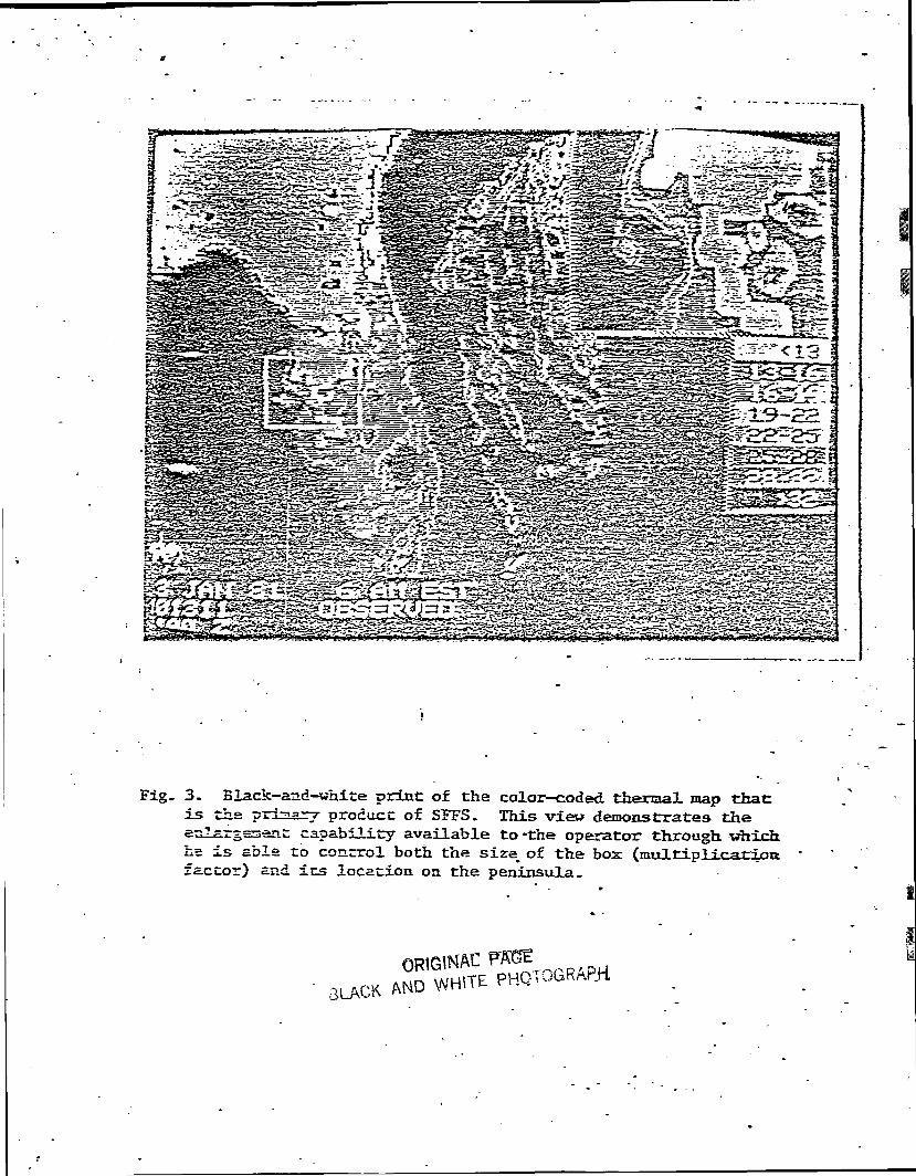
Fig. 3. Black-and-white print of the color-coded thermal map that:is the priaarj product of SFFS. This view demonstrates thes ls-rgesent: capability available to -the operator through, which.ns is able to control both the size of the box (multiplicatioafactor) £nci its location on the peninsula_

ORIGWAC

SLACK AND WHITE

ORIGINAL PAGEBLACK AND WHITE PHOTOGRAPH

1 _— --J» V7 V- _ '

yf^-.:^--n^.

f-*r*>**-~~~zst +*3ti&irff i »csofT • i'—*' *~~y-r\f * •* j. ?^>r'j*j^*^ r 7^^ *—

Pig. 4. 31=.ck-and-v;hite representation of the color SFFS productdanonstrating the split screen opti&n- The operator maybring up for comparison any previously archived map for s.sice—by—side view of the thenoal pattern similarity.

ORTGHTAL" PAGEBLACK AND WHITE PHOTOGRAPH

rt-gftx-rt-r *i.i r i».-s<->*-•_ •- * «»;i.C-» --—>=^sr=-; ***>.t.fcr'- / .'"T-T - - - - : -* *•—~-.— _ft - ->

.Iin^aX..- Ji.l G ^TT!^T»!;;t».>»«CMr_t-...-T^J-.- -3 '. - •J_/^^»,,;l_>*-0i e

i€-._T:'. r.'jittT^^•lurrlwzc^*<:

. i«-"j2l ^-*•tr>*m<. •'^^»vj*».»z\.ncK»jj^<r~ram i»«i

kv7k<*.*»^. It»^»t4**^fc»* *^-r€;j»

»->;r>.;:Fr ^15 A ^*vc«T>*4*7^*Tt<-*f«^i\-~-_»ef-e~r»"l>Tytn\<i*::\ti»^-^«5 L. ISTOMMJCA rvr* r-n> r

W.*JF.»—O* Zi-< =" ;*-r»: ;-.^^***Vo.-»-*^,t^>Tf*^«r:i(^\^I

c; .-*-•;.-I _1_^

#-t_-j^;p^j iX. a "^>* > T^< »> i <^ *~ t r-

JT^<TS^#»*--»; ; % -M. A««*£jmtA%

, M»»- *; ,» .*.»»»t.-* ^fpr*ta-^r^

rf-.i^.*<«*

>^r*»>«^*« •••»tttr>777«1^ «1

, 711——y-fc**.«4.i*»^«*^i.-^?^^A .1 '.*TI-

r-»t3T:r**-»«—** *I»>TTTTTIT«^**-*»<— .11**<*~ft+*t +++*+> **i«^vnnT*«x«^*«-Mccjb**.

Fig, 5. A reduction (size) of the symbols nap^ a product <yf~~SFF3that become popular just after the big freeze Csee date/trrrreon nap) . The translation tabla on left margia permits theuser to determine the teap^.ratiure of any 5 km. by 5 kra. pixelof interest. Users found tihis product nuch easier to a-rchivethan the color product viewed on.' a TV screen. Such maps- werecor^uaicated from APPLE II to APPLE II for display iti oolor.

iTable 2. Printout of SFFS key station data for 1.5m air

temperature for the indicated dates.

i

JAN. 12-13, 19811.5m air temperature (rounded to nearest degree F)

TallahasseeJacksonvilleGainesvilleTavaresRuskinArcadiaWest Palm BeachBelle GladeImmokaleeHomestead

18

28273037383342403640

19

26242635363041393538

20

24172032362838373239

21

18201923342736373638

22

14181823322235363136

23

13131627301934362935

00

16161418281834352733

01

14151428271834352331

02 03

11 1013 913 1217 2226 2416 1833 3235 3422 2231 31

04

10131121221631342229

05

8131014211830332029

06 07

7 71L 1110 915 1821 2017 1730 3033 3220 2029 29

J

I

J

J

JAN. 13-14, 19811.5m air temperature (rounded to nearest degree F)

TallahasseeJacksonvilleGainesvilleTavaresRuskinArcadiaWest Palm BeachBelle GladeImmokaleeHomestead

18

44393834393947414244

19

45303533354147383739

20

34303337343746383441

21

22342834312944363142

22

27192231302843352841

23

25312025292741322741

00

22302022272241333140

01

23292024272239333040

02 03

23 2829 2920 2019 2027 2621 2038 4033 3327 2640 38

04

32292021271940312839

05

34282022271837302836

06 07

37 3227 2821 2722 2328 1919 2037 3730 3130 3039 40

SFFS Key Station Codes:

TLH - TallahasseeJAX - JacksonvilleGNV - GainesvilleTAV - TavaresTBW - Ruskin

ARC - ArcadiaPBI - West Palm BeachBLG - Belle GladeIMK - ImmokaleeHST - Homestead

ORIGINAL PAGE ISOF POOR QUALITY.

user to translate the symbols in a particular area intotemperatures. The map can be. easily reproduced in quantityand many of these have been used by decision makers in. theareas of crop transportation, processing, futures, etc. Adetail that . becomes apparent in viewing this_niap is thatdifferentiation of temperatures ceases below 12.3 P. Thisis an arbitrary limitation that results from the necessityof assigning a symbol set to temperature values in order toeasily move them through the NOAA/NWS program, and into theSEFS queue in Suitland. The raw data covers a much broadertemperature range, i.e. -110 C to 553 C- covered by 255counts.

Another secondary product of the systess -that was foundquite useful after ~a damaging freeze was thve printout of thei.Jfcr temperatrrces- from the key statioiis- These data areasradJLable faster than those from minimum-temperaturethermograph networks. The product is easily reproduced andinexpensively—duplicated for mass dissemination (see Table

5^ Moce-isr_Construct Predictions

Two models operate in series to produce " the predictedproducts. The first, known as P-model, is an energy budg-etmoJel requiring- as inputs data from the key stations andestimated or observed dew points front the SFFS operator.The P-mocel has been published (Sutherland,. 1980) anddiscussed in the literature (Shaw, 1981? Sutherland, 1981}.

a brief summary is made here.

The "?** in P-model stands for predictive as well asphysical The-model outputs 1.5m .air—temperature forecastsfor the remainder of the night, i.e. np to 7AM thefollowing" morning. These forecasts are- printed1 out intaodar form along .with the previously observed l.Snt airtempera-tcrres at the key station for the operators to view atthe system printer. The forecasters use these as part ofthe input information they have available to make- theirfrosr warnings for various areas of the state.

Currently the P-model requires 3 consecutive Jiours ofkey station to produce forecasts for subsequent hours. Sothe forecasts begin 3 hours after' the system beginsoperation, often at 9PM EST. Each hour the system -upgradesthe forecasts for the remainder cf the night using the mostrecent 3—hour sequence of input data.

The second model, called the S-model, requires theit-snt of the P-model and the satellite data to produce

"1

0

J

J

ORIGINAL PAGE ISOF POOR QUALITY

forecasted satellite maps. • The "S" stands' for space,.statistical and satellite. It must build- a precitedsatellite view, a thermal map, from the predicted,teaperature at 10 locations into temperatures for each o£the 3 km by 8 km pixels within the borders of the- peaiasula-& satrix of. coefficients relates the predicted -key stationtemperatures to pixels surrounding the key station.. These'coefficients have been developed from previous freezes- The?operator has as. an option the set of coefficients, that he- orshe wishes to- employ.

TEE FUTUSS SYSTEM

J 1. Direct-Down-link Antenna Syste-s.

H • Experience with SFFS over its 4 years of developmenti ' has provided users and potential users of the systent

products numerous opportunities to voice their concern, for•~j both the speed and the reliability of the delivery o£ the

j • ' products. Iffrthe system products are to influence decisionsccaicemiricf the^- commitment • of energy to heating, wind

'^ ' machines,, irrigation pumps and combinations of theser the-infonnatiorr ratrstz be available to the decision maker as earlyas possible-.

The NOAA/NSSS-NWS communication route In Sultlandthrough which the system has received its satellite datadaring the 79-30 and 80-81 frost season, does not rapidlycosaunicate the satellite data. At least two batchoperations In'the computer-controlled data transmission- are-Involved.. The channel has been classed, as a special projectrather thair an operational effort. During the 80—81 frostseason SFFS' received approximately 63% of the satellite datathat it attempted to acquire. When the staging disks werebrought back on line in March at NO&A/NSSS in Suitlandr the-reliability of map acquisition failed to increase. IFflS/oyhac litrtrie choice but to attempt to directly link to thesatellite by antenna (fig. 6). At the time of this reportall the components indicated in Figure 5 are available or ort-or£er except for the demodulator and the bit streamsynchronizer. . If arrangements can be made for these twoccspcr.entis and all the components are functional whendelivered, the antenna should be feeding satellite data toSF?S by December 1, 1981. -

2. Communication of SF1?S Products to Additional Users

The primary user of SFFS output .is the forecaster. TheITCSA/NWS forecaster is expected to Incorporate SFFSir.^ornation into his frost warnings and conouriicate these to

ORIGINAL PAGE JSOF POOR QUALITY

. BP IKOLAJOULOV NOISE Pȣ-AMJ>

(IN 9JM*CKT HOUSIN6)

SEGMENTED

.REFLECTORMULTf

lPHPCM-

DOUBLE SIOE9&MO ISUPRESSED CAHRIE.4PSK INPUT (7O MM,) I

ADJUSTABLE

MOUNT

ASSZ

FEEO-LINH

SATELLITE

FORECAST

SYSTEM

-HP

2IMX-E

GOES STRETCHED VISSR DATA DOWNLINK

Fig, 6. Proposed antetma system for SFFS penaitting direct access-to digital data. Portions of this sys tea are on-order* .-S3: the

of. this report.

1GOES SATELLITE

GAINESVILLE

UF/IFAS

J

NOAA/NWS

RUSKIN

USERS

IFAS

COMPUTER

NETWORK

AG.EXTENSION

OFFICES

OTHERS

FORECASTERS

RUSKIN

3

J Fig. 7. Block diagram of SFFS when the antenna at UF/Gainesville(Fig. 7) becomes operational. Dissemination of SFFS productsis expected to rely heavily on the IFAS computer network thatis expected to link the county extension offices with the maincampus of UF. Compare with Figure 1.

PAGE ISOF POOR QUALITY

•-users through the normal ccnnnunication - channels thatKGSA/NWS has developed over years of service to Itscllentel. This has occurred during -the developmentalperiod, and is expected to continue independently of the:pr2sence of the--antenna (fig. 7). - .

Additional- users of SFFS information include all other•consumers showing interest in receiving: the information..

_Boxing the 80—32. frost season, two county extension offices(case- in Polk Cotrnty and the other in Lake County) receivedth.2 thermal nraps. by an APPLE II computer link with theGainesville -rainicicsnputer. This was an experimental link inanticipation -of the communication link that is expected toocmr via trte new- IFAS Computer System .in coming years.Grswersr media-,, processors, etc. are expected to- arrange tocoanect with the. county computers or terminals to viewthermal map_s-r as well as to obtain other system productsthrough the: cooperative extension service. This° plan doesnor: preclude- dissemination of SFFS products from the Buskin,portion of. thte- system as well.

SUMMARY'

Duringr 4 years of development, the Satellite Frost"Forecast System has undergone significant change. From asys&em that initially depended upn the redigitizing of theanalog GCSSTAP data, it has retooled to operate with directdigital data from Suitland, MD, and is in the process ofincorporating a direct link with the stretched VTSSR datafrom the GOBS satellite by antenna. - The system began withraarural (verbal) communications of "ground truth (surfaceweather observations) • and graduated to automatedinterrogation of ten key stations. Data, from these two databases (ZR from GOES and air and soil temperature, wind andnet radiation from key stations) are used to produce bothobserved and., predicted satellite views of the temperaturepatterns over" peninsular Florida. These color products,, asweU. as seme black-and-white documentation of the data .acquired, are cciemunicated not only to NWS forecasters butare expected to go to additional-users through computerizedccnsainication channels developing in the Florida CooperativeSstsnsion Service.

ACKNOWLEDGEMENTS

y Both IFAS/OF and NASA (Contracts NAS10-yl58 andNASlO-9892) have funded SFFS development witit SOAA/NWS

j| cooperating. Dr. Jon F. Bartholic served as th.a principal.II investigator (?I) during the first 1.5 years before- becoming

an Assistant Director at Michigan State University,~~* Agricultural Experiment- Station. Dr. John F. Gerber1 served as interim PI for a period of approximately one year

and continues to support the work from his position as'IFAS"1 - Grants Office Director. Dr. Michael J.- Burke, Departmentj' ' Chairman, Dr, Ellen Chen, Post Doctorate Fellowr and Mr.

James G. Georg-r Consultant Meteorologist: have provided-., leadership as=-weil. Dr. James M. Dodge, NASA/HQ, Mr. U.

j • • Reed Barnett,- Jn., and Mr. Frank W. Horn, Jr., both pf* NASA/KSC have-coordinated NASA's support to the development.

Mr_ Frederick: C_ Crosby of NOAA/NWS has coordinated NOAA'sj cooperation and-provided operational testing of SFFS at the^ Ruski-n W?O. Mr-.- Ferris G. Johnson, Jr. has coordinated

the _software-development with recent programming support; from Mr. Fred b^ Stephens, Mr. Steven E. Lasley, Mr.1 Robert A. Dillon and Mr. Bogdan Pelszynski. Mr. Eugene

H. Hannah and .Mr. Michael P. Baker have developed the key"} station instrumentation and the latter-has responsibilityj . for the antenna system. Mrs. Alice E. Grimes has

coordinated secretarial and bookkeeping activities with aid*1 from Miss Cindy M. Weygant and Miss. Nancy S. Guzman. Of

I . the many who have contributed to SFFS development only thosewho constitute the very recent team effort have been named-

ORIGINAL PAGE ISOF POOR QUALITY

LITERATURE CITED

Barnett, U. Reed, J. David Martsolf, and Frederick L.Crosby. 1980. Freeze line system. Proc. 17th SpaceCongress, Cocoa Beach, Fl.r 4:9-20.

Bartholic, Jon F. 1977. First quarterly report on ASVT,SFFS, submitted to NASA Design Engineering Sec.AD-PRO-21, NAS10-9168, September, 10 pages.

Bartholic, Jon F. 1978. Crop freeze protection - Theenergy crisis plus four years. The Citrus Industry,59 (10) :22-28.

Bartholic, Jon F., and Robert A. Sutherland. 1978.Future freeze forecasting. Proc. Fla. State Hort.Soc. 91:334-336.

Brandli, Henry W. 1981. Weather satellites and agricul-ture. Florida Grower and Rancher, 74 (4) :4, 8, 9,34.

Chen, Ellen, L.H. Allen, Jr., J.F. Bartholic, R.G. Bill,Jr., and R.A. Sutherland. 1979. Satellite-sensedwinter nocturnal temperature patterns for evergladesagricultural area. J. Appl. Meteor. 18 (8) :992-1002.

Gaby, Donald C. 1980. Comments on "A real-time satellitedata acquisition, analysis and display system - Apractical application of the GOES network". J. Appl.Meteor. 19:340-341.

Martsolf, J. David. 1979. Frost protection: A rapidlychanging program. Proc. Fla. State Hort. Soc.92:22-25.

Martsolf, J. David. 1980a. An improved satellite frostwarning system. Proc. Fla. State Hort. Soc. 93

press) t

Martsolf, J. David. 1980b. Evolution in frost protectionAmer. Fruit Growers 100 (2) :12,92-94 .

Martsolf, J. David. 1980c. Frost protection. The CitrusIndustry Magazine 61(9):17-26.

Martsolf, J. David. 1980d. Freeze line system. Proc.Workshop on Crop Management Modeling UtilizingEnvironmental Data. VPI & SU, NASA, and USDA/ARSsponsors. Jan. 17-18, pages 49-57.

ORIGINAL PAGE IS-OF POOR QUALITY

1 Scbrrapf, A. 1980. 20 years of weather satellites—1 where we have been and where we are- going. Proc.

17th Space Congress, NASA/XSC, Apr. 30-May 2,i Cocoa Beach, Fl., pages 2-1, 2-2Q.

"Shaw, Roger H. 1381, Comments, on "A short-range objective^ nocturnal temperature forecasting model." 3"_ Appl.i Meteor. 2Ct=9S.

Sutherland, Robert A., and Jon ?. Barthoiic. 1977. A•j - freeze forecasting model based upon meteorological

; • ' satellite data. Proc. International Soc. Cii^riculture131-133. . ' •

'i Sutherland^ "Robert. , Jane L. Laagford, Jon F. Barthoiic,and Robejct G. Bill, Jr. 1979. A real time satellite

1 data acquisition, analysis and display system — Aj oracticzai application of the GOES network. J. Appl.

Meteor. IS(3)r335-360.

j Sutherland,, Robert:-A. 1980. A short range objectivenocturnal temperature forecasting nodel. J. Appl.. Meteor_19:247-265.

Sutherland, Robert A. 1981. Reoly. J. Appl. Meteor.20 r95-97..

' • • Waters, Marshall P., and Robert N. Green. 1979. Amerged satellite infrared and manually digitized

1 radar product. Machine processing-and Re?F»otelyJ Sensed Data Symposium Proceedings, pages- 183—191.

I Woods, Chuck. 1977. Satellite freeze prediction systemj for Florida, Citrus and Vegetable Magazine 40 (1) r

6,24-.

I Woods, Chock. 1979. Satellite paints Florida weather'* portrait. Sunshine State Agricultural Reseach Report

23(1)4,5,22.

: i

(I

APPENDIX 5

Japan Manuscript

* : -^.

IFAS3

I FAS G3ANTS OFFICE20J-1 MCCARTY HAUU

TELEPHONE: 904/392-2357

UNIVERSITY OF FLORIDA

INSTITUTE OF FOOD AfX'D AGRICULTURAL. SCIENCES

GAINESVILLE. FTL.ORIDA 32SU

ORIGINAL PAGE 5SOF POOR QUALITY

October 2, 1981

Secretariat1981 International Citrus Congressc/o The Japan Association forAdvancement of Phyto-Regulators1-26-6 Taito,Taito-ku,Tokyo 1LO, JAPAN

Dear Sir,

Enclosed please find the paper for presentation at the1981 International Citrus Congress entitled, "A WeatherSatellite System for Observing, Forecasting, andDisplaying Cold Temperatures for Citrus Producing Areas",I apologize for getting this to you a few days late.

We will be replacing the copies of Figures 7 and 10xvrith photographs of the appropriate size.

Please do not hesitate to contact me if you haveany questions. Thank you very much.

Sincerely../]

, GerberDirector, IFAS Grants

JFG.jdgEnclosure

COLLEGE OF AO^IC AGRICULTURAL EXPERIMENT STATIONS

SCHOOL OF" FO«EST RESOURCES AND CONSERVATION

COOPERATIVE EXTENSION SERVICE

FOR TROPICAL AGRICULTURE

The Institute; of Foot) and Agricultural Sciences is ao Equal Employment Opportunity - Affirmative Action Employer authorized to provide researcheducational information and other sen-ices only to individuals and institutions tha: function without regard to race, color, sex. or national origin

A Weather Satellite System for Observing, Forecasting, andDisplaying Cold Temperatures for Citrus Producing Areas ORIGINAL PAGE IS

OF POOR QUALITY

J. F. GerberUniversity of Florida, Institute of Food and Agricultural Sciences,IFAS Grants, 2014 McCarty Hall, Gainesville, FL 32611

J. D. MartsolfUniversity of Florida, Institute of Food and Agricultural Sciences,Department of Fruit Crops, HS-PP Building, Gainesville, FL 32611

Additional index words: . Remote sensing, Microcoirputers, MLcrometeorblogy,Mesoclimatology.

Abstract. Thermal, infrared data are acquired from the NOM geostationarysatellite at 75°W. The data are processed by a minicomputer which generatesa false-colored, thermal image geometrically arranged to represent citrusgrowing areas in Florida, USA. Spacial resolution is limited to about 8Ka and thermal resolution at about 1°C. These data are available 'normallywithin one hour of observation. A library of software programs is used tomanipulate the data and to forecast the expected temperatures for the restof the night. The data can also be transmitted to local users over telephonelines and displayed with small irrLcroccmputers and television sets. Thesystem operates under the control of the minicomputer which initiates theaction to acquire the data, generates the thermal data arrays, and estimatesfuture temperatures. The data are compared with automated ground truthstations to verify and irrprove both the observed and predicted data. Thesystem was designed to assist weather forecasters, county extension staff,and citrus gravers.o-1-

Forecasting and observing minimum temperatures for citrus producing areas isdifficult because citrus growers need precision of + 1°C. This precision isespecially important if temperatures are expected to reach lethal thresholds (7).Fere-cast of low temperatures are verified by the minimum temperature observed atofficial sites in standard exposures.2 These sites are limited in number and eachrnay be chooser! to represent an area of several 100 square Kin. Forecast scoringis based upon the differences between the forecast and the observation. Thepredictions are for geographic regions or zones of 100's to 1000's of Kcrr and forofficial sites.

Citrus growers correlate the expected temperature in their orchard to theforecast for the region or zone. This correlation is based upon ambient tempera-tures observed in the orchard coupled with years of experience using both objectiveand subjective techniques.

Received for publication . Florida Agricultural Experiment Station JournalSeries No. . Support for .this work was provided by NASA contracts NAS10-916Sand NAS10-9892. Cooperation of HWS/NOAA was greatly appreciated.2Standard exposures are with glass and alcohol imnimum indicating thermometersexposed either in Standard Cotton Region Shelters or in Standard Fruit ForecastShelters used by the USA, National Weather. Service

Changes in policies of the weather forecasting services, in funding, in person-nel, in observation sites, in urban development, and perhaps climate changes due toland use tend to confound and change the correlation between the observed and pre-dicted temperature at official sites and zones and the observed orchard temperature.This tends to confuse and frustrate the citrus grower.

Areal temperature measurement and forecasts could iinprove the. services to growers,but at prohibitive expense for an intense observational network. The preparationand dissemination of verbal or written forecasts in such detail would be impracticalif not impossible.

Areal measurement and display of surface tenperatures in real time sensed byweather satellites provide a technique to meet nany of the needs of citrus growersfor terrperature information. The satellites are in place and are used for a nulti-tude of purposes - cloud movement, storm tracking, wind fields, etc. Use forhorticultural purposes is simply the exploitation of this existent technology andequipirent.

Satellite Observation of Surface Temperature

The weather satellite data referred to are from the TR (Infrared) 10.5 to 12.6uradioiretric telescopes on the Geostationary Operational. Environmental Satellite(GOES) (Fig. 1) series. These satellites are'located at 75°U latitude, at anorbital height near 36,000 Em above the earth. They operate 24 hours per day,producing area! surface IR data for the entire hemisphere once each half hour. Thesatellite were launched by the NASA (National Aeronautic and Space Administration(KQAA). They are spin oriented and equipped with visible and infrared radiometers,VISSR described by Abbot (1). The IR sensors view the earth through a telescopewhich sweeps an- 8 Km wide path across Florida from Vfest to East. Analog datafrom the sensors are digitized to 256 levels by the National Environmental SatelliteService (NESS) of NOAA producing a temperature resolution of 0.5°C, and a spacialresolution of 8 Km x 8 Kin for 4 Krn pixels. Over 3000 pixels are required torepresent the State of Florida. This is equivalent to a surface temperature obser-vational network 8 Kin apart in the North-South and East-West direction. An entireearrh frare consist of 1821 sweeps, (1821 resolutions of the satellite) andrequires 18 minutes.

The data frota the satellite are telementered to an earth station at WallopsIsland, Virginia, USA, they are navigated and geometrically corrected for viewangle distortion, changes in the satellite spin axis and retransmitted to thesatellite for dissemination to users.

The satellite observed temperatures represent the integrated area! temperaturefor each 8 Jen by 8 Km pixel. The pixels view a fixed geographic position on thesurface and which does not move or change due to surface development. Drift andshift due to satellite orbital changes, and digitization cause movement of oneunit even if adequate navigational data are supplied and properly used.

The data frora the satellite can be transformed into a graphic representationof a plan map of the region. (Fig. 2). Image enhancs-ent techniques are usedto transform the shape into an almost exact outline of the geographic boundariesof Florida. Either colors, gray scales, or syirbols (letters, numbers, etc.) canbe used to represent classes of temperature by different colors because of easein optical assimilation of the data. Thus, surface terperature patterns representing

ORIGINAL PA3£ kSOF POOR QUALITY

physiographic areas are portrayed as colored pixels on a color monitor representingthe entire State of Florida. This includes all of the citrus and other horticultural

.. producing regions. At a glance the observer can view tenrperature distribution,patterns, changes' in boundaries for the entire state.

The surface temperatures as observed by the satellite have been repeatedly veri-fied by ground truth transects (5,8), by automated surface stations, and by minimumtemperature theroooeters in both orchards and official sites (8,9) (Fig. 3). Thethermal patterns which merge have been found to be presistent for weeks and nightsand have been used to do retrospective agroclimatic studies (4). They can be usedas a. basis for delineating forecast regions with specified thermal homogenity.

The satellite observational data is nominally available one hour after observa-tion x>,iiich is satisfactory for now cast of temperature as a weather element. Sincethe entire area is represented there is no interpolation. Forecasts made forexpected changes in each pixel can be used to produce a similar false-coloredthermal image of Florida for the entire nocturnal cold period. A physical coolingmodel (6,11) is used to predict temperature changes for 10 key locations usingboth satellite and surface weather element data (wind, net radiation, soil tempera-ture, surface air- profile temperatures). The 10 key stations were correlated withindividual pixels to produce a map of the entire state.

a

Both the observational data and the forecast data can be conmunicated overtelephone lines as digital data to inexpensive microcomputers. Selection of appro-priate ndcrcxxoputers such as the Apple II Plus can be used to generate the false-colored therrral images on conventional home color television sets. (Fig. 4).

. .The system.is called the Satellite Freeze Forecast System (SFFS). It wasdeveloped by the University of Florida in cooperation with NASA and: NCAA. It is ahighly flexible system which uses high technology (mini and microcomputers),existent satellite resources and a library of software application programs.

1-fost-fruit and citrus growing regions of the world are viewed by GOES WeatherSatellites (10) - The SFFS system could be used with some modification in mostcitrus and fruit groxving regions of the world.

In addition to low temperature freeze observation and forecasts other appli-cations could include, chilling hour accumulation, climate data collection, andobservations, high temperature stress, cloud pattern, storm tracks, rainfall(indirectly fron cloudtop temperatures), etc. SFFS presently is limited to sur-face temperatures during clear weather. Microwave radiotnetry will eventuallypermit tenperature measurement through clouds, and the Vertical AtmosphericSounders (VAS) are already on board some satellites. The polar orbiting satellite(NOAA Series) could be used to provide high resolution IR (1 Kir) but only 4 to6 tires per day.

Description of SFFS

Tne SFFS system (Fig. 5) consists of (1) the GOES satellite, (2) a minicomputersystem, (3) automated surface weather stations, (4) conrrunication links and,(5) software programs. A complete description of the system was made by Martsolf (8)

Q

The name Apple, Apple computer and the Apple symbol are registered trademarksof Apple Cornputer, Inc. Their use in this manuscript are for illustrative purposesonly and does not constitute endorsement.

ORIGINAL PAGE 13OF POOR QUALITY

The GOES satellites are spin oriented and stabilized x-reather satellites launchedI by NASA and operated by NOAA. Nominal location of the satellites used is 75°W[ | longitude above the equator at 36,000 Kn above- the earths surface. The IR and' ' visual data accutrulated by the satellite during a. scan of the earth disk are trans-

mitted to the surface at high baud rates (gigahertz) . These raw data must benavigated to proper earth orientation because the satellite progresses in orbit,the orbit is not perfectly circular, or oriented latitudinally and the spin axisorientation shifts. In addition, to the "navigation, the data are geometricallycorrected for view angle. The navigated, corrected data and the navigation

j information are retransmitted to the satellite and rebroadcast to various users.v-«

The NESS acquires these data and routes them to NWS/IBM 360 computer whichy removes a sector representing Florida and places it in computer quere.

Two Hewlett Packard 1000 series minicomputer systems make up the heart of thej SITS. (Fig. 6), One system is located at the NWS office in Ruskin, Florida, USA.! The other computer is located in the Department of Fruit Crops at the University

of Florida which is the development system and is also used for backup. The" j two computers are linked with a distributed, real titce operating system (KEE-TVB.{ and DS/1000). Both computers are equipped with tape drives, hard disks, cccmini-

cation modems and a color red-green-blue monitor. These computers via software- -, and hardware control the digital telephone cornnunications and acquire the satellite

I -and key station, data automatically.-•I

Ten automated, microprocessor controlled weather stations are used to observe,j store and furnish weather data over telephone links (Fig. 7) . The microprocessori package (Darccra nodel B303' s) was not designed for weather purposes, but has been

a satisfactory, low cost method of observing and acquiring wind, temperature,hxrr-idity and radiation data. The package includes a dial-up modem which dumps

\ data to the iripJLcotnputer when called with the proper security codes. Tamperingwith the stations sets flags to avoid spurious data.

j The conmjnicatians links consists of standard, voice grade telephone lines.The minicomputers are equipped with auto dialers and 1200 and 300 baud rate modems.

. „ Software programs control the cornnunications. The NWS satellite data is acquiredj ovar a 1200 baud link. The software programs repeats the call if a connection is

-J no:: icade. The 10 key stations are dialed automatically over the 300 baud link.Since the data set from the key stations is msall the slower baud rates do not

J constitute a problem. The satellite data requires 3.25 minutes to transfer a.J thermal data set. Each key station requires 45 seconds to transfer data. These

stations are interrogated hourly. Three attempts are made to acquire the data.' j IXiririg the past season (1980-81) data from the key stations were acquired 96701 of the time.

. Software programs are responsible for the coordination and operation of thei j entire SFFS. They control the data acquisition communication and product. generation. The satellite TR data are scaled, arranged in class intervals and

color assigned. The data are used to create an observed, false-colored thermalH image of Florida with the time and date and a color tenparature key. (Fig. 2) . .Li The range of temperatures and the colors assigned can be changed by the operator

to isolate certain temperature ranges. Eight temperature color classes can bej used. Enlargement of a specified area is made by positioning a white rectangularI outline over the image. The enlargement is variable (2x to 9x). The enlarged

rectangle appears in the upper right hand corner of the display. (Fig. 8). Two

OHGMM. WBEBOF POOR QUALITY

thermal naps can be displayed simultaneously on a split screen (Fig. 9) . The.observed thermal maps are nominally available one hour after observations, however,this could be sooner if satellite data -were available more rapidly.

Predicted thermal maps of Florida are produced by the software. Data from thesatellite and the key stations are used with a physical cooling model to estimatethe Tm'm'rmrn and hourly temperatures for the- entire night. These data are corre-lated with pixel temperatures and the key station temperatures to produce a false-colored thermal map of Florida. If red-green-blue color monitor is not availablea standard (NISC) color television signal is produced which can be viewed on ahcoa television receiver. The data can be printed as hard copy (Fig- 10) usingsynbols because the system is not limited to 8 thermal levels.

A ST-dioary of the 10 key stations is printed as acquired (Table 1) so themeasured weather elements are recorded and updated immediately. These data arevaluable to verify the satellite observational data and for planning and mange-rcerit purposes following cold weather.

The software library includes programs for evaluation and analysis of the data.Tenperature difference inaps, cooling rates and persistent cold areas can be obtainedfrcni the software. The operator has control of the SFFS through the keyboard soft-

• ware and can intervene or can allow the system to operate automatically.

Future Developments

The SFFS was designed to assist weather forecasters, extension specialists,extension- agents and growers. A pilot effort is underway to transmit the thermalirragas to county extension offices. The commercial television signal could becormunicated, but would require costly coxial cable or microwave links and would-not allow local taanipjlation of the product. Software programs have been developedto use microcomputers (Apple-II Plus) to acquire the thermal and weather data overtelephone lines and display the thermal maps on home color television sets. Thishas been successfully demonstrated in the 1980-81 cold season. This network willbe expanded to 5 counties, communication rates will be enhanced (300 baud to1200 baud) and additional software developed. The present microcomputers havecolor compatibility limitations but the products are of acceptable quality.

A direct satellite antenna link will be tested during the 1981-82 cold season.This link will intercept the stretched VISSR data and reduce the time delays inprocessing and sectorizing by NESS and NWS. In addition, it may reduce expensivelong distance telephone lines. The main advantage would be more timely data. Theproblems of handling the data stream with the present minicomputer system are amajor part of the present testing "program. Additional software and hardware maybe required.

A two year study of the applicability of SFFS to other regions is nearingcompletion. The preliminary indications are encouraging and lead us to concludethat SFFS nay be useful at higher latitudes in areas with high topographic relief.

During the severe freezes in January 1981 in Florida, the satellite observedterrperatures were lower than expected. Subsequent examination of surface dataand of specific location in identified pixels tend to be in agreement (+ 1°C)with surface observations. These data combined work done by our colleagueDr. E. Chen (3,4) indicate that satellite data have excellent potential fordelineation of agroclimate zones and for the identification of persistent coldand warm locations.

PAGE iSOF POOR QUALITY

The thermal inertia of the earths surface is closely related'to the maximumand minimum temperatures. Diurnal satellite observations should permit theestimation, and mapping of the thermal inertia classes of the surface and chargescaused by rainfall, foliage, cultivation, etc. These data could significantlyassist the forecasters skills and estimates of departures frcrn climatic norms.

As forecasters develop skill in using SETS,, forecast scores and verificationcould became more closely tied to forecasts and observed temperatures for specificregions and areas, as delineated by SFFS thermal images. Coupled with satellitedefined climatic zones in important citrus producing regions the SFFS shouldassist in the development of more meaningful and accurate tenperature observations,warnings and forecasts for citrus and other horticultural producers.

] , ORIGINAL kViCiE i^

' ' OF POOR QUAUT

literature Cited

1. Abot, T. M. 1974. Visible infrared spin-scan radiometer (VISSR) for asynchronous meteorological spacecraft (SMS), Santa Barbara RecordsCenter's Final Report, NASA, Goddard Space Flight Center, Greenbelt,Maryland.

2. Bartholic, Jon F., and Robert A. Sutherland. 1978. Jbture freeze fore-casting. Proc. Fla. State Hort. Soc. 91:334-336.

3. Chen, E., L. H. Allen, Jr., J. F. Bartholic and J. F. Gerber. 1981.Delineation of cold-prone areas vising SMS/GOES thermal data: effectsof soils and water. Submitted for publication to Journal of Applied

. Meteorology (April 1981).

4. Chen, Ellen, and J. David Martsolf. 1981. Fourth Quarterly Report onthe development of nocturnal GOES infrared data as a source ofclimate information, report submitted to National Climate ProgramOffice, NA80AA-D-00129, September 8, 14 pages.

,5. Chen, Ellen. 1981. Comparison of geostationary satellite infraredtemperature with ground-collected temperature in florida, reportsubmitted to John F. Kennedy Space Center, Florida, SL-PRO-33,NAS1Q-9892, 20 pages.

6. Georg, J. G. 1971. A numerical model for prediction of the Nationaltenperature in the atmospheric surface layer, M.S. Thesis, Universityof Florida. 1971, 121 pages.

7. Gerber, J. F., and F. Hashemi. 1965. The freezing point of citrus leaves.Proc. An. Soc. Hort. Sci. 86:220-225.

8- Martsolf, J. David. 1981. A satellite frost forecasting system for florida.Workshop of Weather Data to Agriculture and Forest Production, sponsoredby American Meteorological Society Committee on Agricultural ForestMeteorology, and the American Society of Agronomy, and the AmericanSociety of Agricultural Engineers. March 30-31, 1981, 21 pages,(in press).

9. Ilartsolf, J. D. 1981. Satellite freeze forecast system. Phase V uid-termreport and SFFS evaluation. Submitted to John F. Kennedy Space Center.NAS10-9892, 68 pages.

10. Schanpf, A. 1980. 20 years of weather satellites-where xve have been and. where we are going. Proc. 17th Space Congress, NASA/KSC, Apr. 30-May 2, Cocoa Beach, Fl., pages 2-1, 2-20. .

11- Sutherland, Robert A. 1-980. A short range objective nocturnal temperatureforecasting model. J. Appl. Meteor. 19:247-265.

ORIGINAL PAGE ISOF POOR QUALITY

VSrV.i

1

SCANNER

F-P-. 1. Is a line drawing of the GOSS-D satellitepresently in geosynchronous orbit over the equatorat 75°W latitude. Orbital height is 36,000 Kmabove the surface. The satellite is spin stabi-lized. The infrared data fron the satellite isused by SFFS to produce a false-colored thermallinage of Florida.

ORIGINAL PAGE ISOF POOR QUALITY

Fig. 2. A photograph of a geometrical Image of---Florida created from infrared data from theGOSS-D satellite. The boundary outlines arederived from thermal discounties between, theocean and gulf waters and the. land. Thetenperature classes are displayed in coloron a video nonitor.

ORIGINAL PAGE ISOF POOR QUALITY

JANUARY 13, 1981 6-00 A.M.

=min. thermometer

iJ2I.8

i— s

^0.9I1^0.0

20.0

26.3

203

-203-j

120.0

26.3

NJ26.3

26.3

21.8

<nao

2I'8S

25.4

25.4

22.7

22.7

24.5

25,4

I

24.9

263

24.5

24.5

,lNVf)25.4

2/<r>\Z6°s

24.5

24.5^

25.4

32.6\

293

era^5.4

25.4

45.2

\\

40>x\Vt

34.4 i

32.6

%o

**\v

\m

*

Fig. 3. A corrpariscn of observed tenperature from •satellite data pixels (rectangular outlines)and surface shelter (1.5M) height exposures(Circled numbers).

5SRS&. •• '«T-> '.-~i.;r±£i:

Fig. 4. A photograph of an Apple mcrocoii£ju.ter,disk drive and* television monitor used todisplay the false-colored thermal images incounty extension offices. The data'is trans-ferred from the SFFS conputers to the mLcro-coznputers by telephone lines.

ORIGINAL PAGE 5SOF POOR QUALITY

N

f

GOES SA

XNOAA/NESS

NOAA/NWS

SUITLAND,MD

t

\

LUTE

i

v yHP 1000

COMPUTERNOAA/NWSRUSKIN,FL

.digital \f(phone) y

1:=j —

~

r- KEY

STATIONS

(IFAS)i

.-'

/,,N HP 10COMP

IFCLIMATGAINED

lDS/1000(phone)

00JTERS -11-ASOLOGY5V1LLE

PRODUCTS

USERS

NWS' — FORECASTERS

*FORECASTS

VIA APPLE It NET

— — - AG- r~i_EXTENSION "UOFFICES

nTHFR*' "—,

USERS

Fig. 5. A black diagram of the Satellite Freeze° Forecast System (SFFS).

ORIGINAL PAGE F3OF POOR QUALITY

I

I

PAGE ISOF POOR QUALITY

Fig. 6. Satellite Freeze ForecastSystem Hewlett Packard 1000series minicomputer.

OF PO

OR

QU

ALITY

flJ

L°

I C

D

, j

.UK.GINAL PAGE isOF POOR QUALITY

rig. 8. A false-colored thermal linage of Florida. .vith an enlargement of section enclosed by theVThite rectangular outline displayed in theupper right hand corner. Note: the resolu- ':tion of individual pixels is unchanged, butvisual resolution .is enhanced.

ORIGINAL PAGE ISOF.POOR QUALITY

Fig. 9. False colored images of Florida from 8and 10 EM EST (20:00 and 22:00) displayedsimultaneously to portray rates of coolingand changes in cold areas.

ft - — .•*—•— —-,~-ff* — •—•.»_, —i^^. - - • - L- ^ t. *_ t. V. ^ Tjl V .1 Vi^

- --• e c~c"obc—c " ~ - ~ cc r "'"V~~i%ti"?"f^j'

cbe—c cc &c-c c -lV«fl:-V!— _.—— M^_.M»«-W. *.— — *..--.—**———*• ——r*"—-"'"**"1"—*••***""•**r'"'1*—cc*" C***""*"r * Tri-i n-tiV"-Jf f r^^^- f f^—^f t^r f f - r - — *— faf 1. fc. I- «. ^ 1*^1 *(' *** —' _ JAflUARY 13, 1351 6 AH.

— VLDC3=?>9: 56433^8 )EN

-c cbc

. • 376453 <CK?Uy

££FB3A| c*b "Di3cfc"tLtP=<;:876<CEIKquZYYT.5«ILNGERqKLLR \UI9S

= >?eAA5DcEEEH!r333333333345544 *iSS

ZITYZZC ttYZS>. >9843235933-TAJZ2CZU-tKHYU>i?'

333322233337—-42222222333322222222333122i112222333 4

21111:22233;122223333345111123423359C01234555i

3: : : ;<==-.8999: ;C< —>3A3E78999:;;<==>0AE

. x, • f-tf ,-y

H .73899: : j <==>3AEF.Zf;—beC 67S399; ;; < = >B3hhif:ce'c

673377569?j< H.9==>3653=9;: M. .>AA3: : = »79: $1*$

TT(b-c

FBA3ZFEH-GC?"B=>FCK* JH:FHS

95933A7£CC3E" .

- .5:2

t -55673399:;==F 55667399 :;< = >I^tt;fhi_YG :555667399:<==

J^- 555556S39:;< =1 -4445567399 :< = )ADDCt;J 4444556339:;=>S

5667999: : j < = >ffeuuOY» J -jc~cccbh 1 ]ZUZ\t\U7UZZZt \\ZIYUCJ

1 YYZZZZt t CCYl!?F=><523214;AM'J?INZ-AC"cbQ<6SN:fMZUUYCXXIZZXXZZtZYYU'jr,?*- •:-••--• 1- r '-;FSMHUbbT={QZi

|5H_10HUZQ?7Bq7C

cc"b|! \YYZa-_YYZYZZZC\Z i ZUUZ' ZE t'JZZZC\\£ lUVUUUU

ix v r ^-V-TTX r r x r nimin.ni.

cc h <• 1 YZ\t C C [ZZC \\ZrUWVNM

fi[- 33334456739:;

333"I556.t £ca<io'33335564

- 2345656556799 :;<==JH

: = >=L j t.".913>6C)t>b ]QIZ

plt C t C C C 1 1 YUI

U DeADD3943455667399:;<=V =6ADEA:43345667899::<=AEL^YUVUZCtW ==»«62334556S3999: j=AE

«93723333445568999: ; <=F.-li._, .,: <9521112333556677399 : =DFFF '"JUyU'JUZ--Z\\\\t t 111 i

:99ETHSQ=59:=B?=? : 5=HPQYLBS;==:

59; : :=324=P 1*UI<30 t8<9;=A?439I\bb JTF3

r:L\

IX. 3

EA:211233333455566677383999:iDA9211233333344555566778399:E8<4112222222333445556667789:=E

= 821222222222333455566667899 :AUii!iyWyUULii;1jq3SRPHPq5SSP.Pcb4AC=;<=ae.<89e54I>3EEieob

9A=< = AAH£624l3GZbc"H2-39C=9:56=D<4 :069

F.N \__b-3TTH JX/

b <5323112112112233344455566789:=)

_£_ 95333221 OC lit 12237,34445556789 :;< ==PiiPqS7qSSS?0?qS7qSlpS19 >95655456<> ;PAAJA956<t* E974331100000112223334455567899: ;;<=i4inRS3RS?thMPq77qPF>629>9:9: : : C > = A>9=>CLniO'jP* =864321000000111223333445566589: : ; ; <=M.-1?qP.RSPOOnRSSSl^<63< 89598&559==958<EU* ZZW

IHCA=:577231011illl22333.i344555673399: : < = C^naSSaMnRSSSSPET?=63; >988524 : = <=965SHY"ZPM1T7hKAEqT:;r;a

:>?irM.-<KI«BECCCe>==953211il222233333344555667R3?9: ; = >;Vlf}SSRqR77SSR;j.r}?;33< ?< ;99«B754 :990CJILWn*=CI ; = ITVaM?f:KDIf.Fr-LNHHJIF. A? > ? >9432211112222335333444556678399-.<=p[LnPOfe7aSRO?j|T=6 4= > » » = >95236DFLZYIGA '.''

7U->j7^5ISn^OJn.-!SLH.'iIJf.Lt!?-> = 952 000 0 112?22333333444555567737 : :=K«MXLM3HKUiliBI>; 4 293?>9443 'EIRLI:-RH,17r;t7TqH,-'.P.IrJfi!.MIE9>7< :52 00001122222333.^34444555667699 : =7f~HIJLTK»] »CCr.=.S 39=A=951C 1 35<

5?:4 4;=>95109:3 4<»930

-5Nre< ; 862330 0 1222233^3;<3334445ScJ66f)9 : ; j ;« = -.» 795 69: : 56116>f:jf:D76 : =LZ_ZPA9«HQRH='_?rAP.VpJIPC.".ICniI£A9=:5642 0 11233333333334 4455S6ET7C > 7 » = <=^»94 156337212 :^= » >93:\524CUn.HA<57t>;

~ " ~ O Q l t :

EAO'JUJKU'JIKQ?JAJIAM:jr!LC=A=9562 001 1 1 111222237.33344455S667999 : < C=KJEHLILIU'JLL7QIAH-GSqGCcCA=>9542 0011 1 1 1222223"5333344455«.'=>7S97 : ; «=

ZYRJLCSRL,"JVT:?JPPILOrLIGA=< ;5

U'JTP I Jf,M.-ftHHMi;Qri<n.~EEGCB3 = 9: 57762-542112233331112356623310

f1D&HPQTOA?FJKfiTSf;PI>'.Hr.rDA-< ;: .-874342 0011 •

122245644331259999 ; 900 0013323410 ?39B76<> )< (Ht "ZP.hG

2542 4< 9; j : 59 = 7 >EUUOO=9<'

ORIGINAL. PAGE IBOF POOR QUALITY

JA.V. 12-13, 19811.5m air temperature

TallahasseeJacksonvilleGainesvilleTavaces 'Rusk inArcadiaWest Palm BeachBelle GladeInutiokaleeHomestead

18

28273037383342403640

(rounded

19 20

26 2424 1726 2035 3236 3530 2841 3839 3735 3238 39

21

18201923342736373638

22

14181823322235363136

to r.earss

23

13131527301934362935

00

16161418231834352733

01

14151428271834352331

t r-egree F)

02

11131317261633352231

03

109

1222241332342231

04

1013ii21221631342229

05

8131014211830332029

06 07

7 711.1110' 915 1821 2017 1730 3033 3220 2029 29

JAN. 13-14, 19811.5m air temperature

TallahasseeJacksonvilleGainesvilleTavarasRusk inArcadiaV/est ?alin BeachBelle GladeIrnmokaleeKonestead

18

44393834393947414244

(rounded to nearest degrea F)

19

45303533354147383739

20

34303337343746333441

21

22342334312944363142

22

27192231302343352841

23

25312025292741322741

00

22302022272241333140

01

23292024272239333040

02

23292019272133332740

03

23292020262040332638

04

32292021271940312339

05

34232022271337302336

OS 07

37 3227 2821 2722 2328 1919 2037 3730 3130 3039 40

Table 1. Hourly air temperatures .collected from the ten keystations by the SFFS computerand printed immediately.

APPENDIX 6

,.4

T H E P E N N S Y L V A N I A STATE U N I V E R S I T Y249 AGRICULTURAL ENGINEERING BUILDING

UNIVERSITY PARK, PENNSYLVANIA 16S02

College of Agricultureand

College of EngineeringDepartment of Agricultural Engineering

October 6, 1981

Dr. J. D. MartsolfUniversity of FloridaInstitute of Food and

Agricultural Science2121 HS/PFGainesville, Florida 32611

Dear Dave:

I am writing a letter to clarify a few points which we had discussedduring our session in Gainesville last week. I personally thought that wehad a very productive meeting relative to the conclusion of work on PhaseII of the satellite freeze forecast project in which we have been involved.

As I have indicated to you several times over the past1 two years, Ihad much reservation relative to the possibility of using satellite freezeforecast technology in mountainous regions such as Pennsylvania. As wasevident, I assume, by the final report which I sent you and by our lengthlydiscussions during the time that I was in Gainesville I have certainlyaltered this opinion. I do, in fact, now feel very hopeful that this tech-nology can be successfully applied to Pennsylvania as well as other statesin the Northeast region of the United States. There are a number of develop-ments which have indicated the possibility of applying this technology toPennsylvania and surrounding area fruit growers.

As we have discussed, there is considerable interest at this institutionin the development of a computerized information dissemination network for useby both county extension offices and by individual fruit growers and farmers.This network will lend itself very well to the transfer of technology andpredictions arising from satellite forecast methods.

Work which you had previously conducted while at The Pennsylvania StateUniversity and which has been referred to in the final composite report forthis project has indicated extreme temperature variations over a traverse ofabout 18 ° Fahr. These variations were again supported by studies which wereconducted in Pennsylvania during Phase I of the current project. These studieshave all shown that there is, in fact, a very significant temperature variationwith topological changes. Even with these variations, however, it has beenpossible to very accurately predict night time temperatures for one particularstation such as was used in Phase II of this project.

AN EQUAL OPPORTUNITY UNIVERSITY'

Dr. J. D. MartsolfOctober 6, 1981Page 2

At the present time, I am attempting to gather resources sufficient toallow a proposal for additional research in the area of application ofsatellite freeze forecast technology. The most pressing need, in my opinion,is to use a minimum of three climatological stations for gathering data neededfor input to the P-model. By gathering such information from these threestations and making predictions at various locations in the state ofPennsylvania, a further analysis of the applicability of the P-model will bepossible. It is also believed feasible to attempt to adjust the model fortopological and climatic histories for these stations. It would be possibleto obtain some of the climatological data needed from archived records, butthe total inputs which would be desirable for the P-model are not availableto the best of my knowledge.

Having either used archive or newly collected data and obtained a newset of predictions for the P-model, the next step for the project would beto provide a technique for real time application of said P-model or analternate form of forecasting.

As I discussed with you while in Gainesville, presumably The PennsylvaniaState University might be very much interested in attempting to procure realtime satellite data from the down-link capability for stationary satellitedata acquisition which you are developing at the University of Florida. Thisinformation could be sectorized and transmitted to Pennsylvania on a con-tractual arrangement if agreeable with your organization. Having obtainedin a timely fashion the appropriate satellite data, the P-model would be runin Pennsylvania and forecasts made readily available to fruit growers throughan information distribution network which is concurrently being developed.

In order for this scheme to be feasible, it is necessary that cooperationdoes exist between The Pennsylvania State University and the University ofFlorida. We would very much .like to explore a method by which it would bepossible for us to obtain a listing and/or magnetic tape of the P-model in theform currently being used at the University of Florida. In addition, we wouldalso like to explore the probable cost for obtaining real time sectorized datafrom the stationary satellites once your antenna system and data reductioncapability is operational.

Attached to this letter, I have indicated the resources which are availableat The Pennsylvania State University for coming to bear with this problem. Wewill actively explore the possibility of submitting a proposal for continuationof this work. I would welcome any suggestions you may have in that regard. Weare very anxious to cooperate \<rith the University of Florida in this respect inany way possible.

Dr. J. D. MartsolfOctober 6, 1981Page 3

Once again, I feel we have had a very productive project and am quiteencouraged by the success which has been shown by Phase II of the freezeforecast technology research. I look forward to cooperating with you onceagain in the future and hope that we can identify some mechanism by whichthis research may be continued.

Sincerely yours,

C. T. MorrowAssoc. Prof.

CTM/ds

cc: H. V. Walton

Attachment

••j

J

ORIGINAL PAGE ISOF POOR QUALITY

SATELLITE FROST FORECAST TECHNOLOGY

APPLIED TO PENNSYLVANIA

FOR MULTI-TASK AGRICULTURAL FORECASTING

I. Research Team

-Name

C . Morrow

J. Russo

C. Ritter

G. Hussey

G. Petersen

T. Carlson

D . Thomson

G. Greene, II

G. Jubb, Jr.

S . Pennypacker

>

Credentials Specialty

Ph.D, P.E. EngineeringTeam Leader

Ph.D Climatology

Ph.D PomologyExtension

Ph.D ComputersInformation Network

Ph.D Remote SensingSoil Genesis

Ph.D MeteorologyRemote Sensing

Ph.D MeteorologyInstrumental ion

Ph.D Pomologist

Ph.D Entomologist

Ph.D Plant Pathologist

DepartmentalAffiliation

AgriculturalEngineering

Horticulture

Horticulture

College ofAgriculture

Remote SensingLab, Agronomy

MeteorologyRemote Sen. Lab

Meteorology

Horticulture

Entomology

Plant Pathologist

3

Lt

II

Location;•"

UniversityPark

UniversityParkUniversityPark

UniversityPark

UniversityPark

University'Park

UniversityPark

Biglervii:PANorth EastPAUniversityPark

SATELLITE FROST FORECAST TECHNOLOGY

APPLIED TO PENNSYLVANIA

FOR MULTI-TASK AGRICULTURAL FORECASTING

II. Information Transfer for Phase I (Model Adaptation)

Key-Station Data P-Model Satellite Data

1

1. Rock Springs

2. Biglerville

3. North East

Supplied byUniversity ofFlorida

TemperaturePredictions

Model Modificationand Verification

rFinal ModelIncludingData Requirements

Obtained fromArchives and'Processed byRemote SensingLab

Note: Similar procedures to be followed for integrated pest managementand similar applications.

SATELLITE FROST FORECAST TECHNOLOGY

APPLIED TO PENNSYLVANIA

FOR MULTI-TASK AGRICULTURAL FORECASTING

III. Real-Time Forecasting System

Key-StationData

(As Required)

SatelliteData (FromUniversity ofFlorida orEquivalent)

Processed Data—:> from The Pennsylvania

State UniversityRemote Sensing Lab

VForecastingModel

Cable TVNetworks

HostComputer

Predictions

CountyExtension Offices

Fruit Growers(Active orPassive Mode)

ConraercialData Transfer

Network

Note: Exact nature of outward links from host computer will be finalizedduring the course of the research project.