This work was performed for the Jet Propulsion Laboratory,California Institute of Technology, sponsored by theNational Aeronautics and Space Administration underContract NAS7-100.

Surveyor Spacecraft System

SURVEYOR I FLIGHT PERFORMANCE

FINAL REPORT

Volume "IT of TIT

JPL Contract 950056/October 1966

SSD 68222R

J.D. CLOUD

ManagerSystem Engineering and Analysis Laboratory

K.C. BEALL

Director

Surveyor I Post Flight Evaluation

HUGHES

HUGHES AIRCRAFT COMPANY

SPACE SYSTEMS DIVISION

R.H. LEUSCHNERHead

Post Flight Analysis Section

PRECEDING PAGE BLANK NOT FILMED.

CONTENTS

5.0 PERFORMANCE ANALYSIS (CONTINUED)

5.3 ELECTRICAL POWER SUBSYSTEM

5.3. 1 Introduction

5.3.2

5.3.3

5.3.4

5.3.5

5.3.6

5.3.7

5.3.8

Major Transit Events and Times

Summary of Results

Anomaly DescriptionConclusions and Recommendations

AnalysisReferences

Acknowledgments

5.4 RF DATA

5.4.1

5.4.2

5.4.3

5.4.4

5.4.5

5.4.6

5.4.7

5.4.8

5.4.9

LINK SUBSYSTEM

Introduction

Items Constituting Analysis

Mode, Bit Rate, and Subsystem

Configuration Summary

Summary of Results

Anomaly Description

Conclusions and Recommendations

Subsystem Performance AnalysisReferences

Acknowledgment s

5.5 SIGNAL PROC ESSING

5. 5. l Introduction

5.5.2

5.5.3

5.5.4

5.5.5

5.5.6

5.5.7

5.5.8

Major Signal Processing Subsystem

Events During Transit

Performance Summary

Anomaly SummaryConclusions and Recommendations

Subsystem Performance AnalysisReferences

Acknowledgments

Page

5.3-I

5.3-I

5.3-2

5.3-21

5.3-22

5.3-22

5.3-47

5.3-47

5.4-3

5.4-3

5.4-8

5.4-15

5.4-17

5.4-76

5.4-76

5.5-I

5.5-I

5.5-i

5.5-2

5.5-2

5.5-3

5. 5-35

5.5-35

iii

5.6 FLIGHT CONTROL

5.6.1

5.6.2

5.6.3

5.6.4

5.6.5

5.6.6

5.6.7

5.6.8

5.6.9

Introduction

Analysis Items

Major Events

Flight Control Results Summary

Control System Anomalies

Conclusions and Recommendations

Flight Control System AnalysesReferences

Acknowledgments

5.6-1

5.6-3

5.6-6

5.6-6

5.6-6

5.6-15

5.6-15

5. 6-Z17

5.6-Z19

iv

ILLUSTRATIONS

53-1

53-2

53-3

53-4

53-5

53-6

53-7

5 3-8

5.3-9

5.3-10

5.3-11

5.3-12

5.3-13

5.3-14

5.3-15

5.3-16

5.3-17

5.3-18

5.3-19

5.3-205.4-1

5.4-2

5.4-3

5.4-4

5.4-5

5.4-6

5.4-7

5.4-12

Electrical Power Schematic

Battery Energy RemainingPower Consumed and Loads

Shunt Unbalance Current

Battery Charge Regulator Efficiency

Boost Regulator Efficiency

22-Volt Unregulated Bus

Unregulated Output Current

Boost Regulator Difference Current

Battery Discharge Current

Solar Cell Array Voltage

Solar Cell Array Current

Regulated Output Current

Auxiliary Battery Voltage

Auxiliary Battery Temperature

Unregulated Output CurrentCoast Phase II

Altitude Marking Radar Electronic Temperature

Vernier Line Temperatures

Radar and Squib Current During Terminal Descent

Communications Subsystem Block Diagram

Receiver AGE

Transmitter Frequency Versus Time From Launch

NBVXO Frequency History After High Power Turnon

Signal Levels at Initial Acquisition

Gain Coverage Curve for Omnidirectional Antenna B

During Initial Acquisition

Earth Vector Path Relative to Omnidirectional Antenna

Gain Contours

DSIF Received Signal LevelsReceiver A and B Automatic Gain Control Versus

Time

Bit Error Rate Versus Time

Number of Parity Errors Versus Commutator Word

Position

DSIF Receiver Automatic Gain Control During

Canopus Acquisition

Page

5 3-3

5 3-3

5 3-6

5 3-10

5 3-14

5 3-15

5 3-25

5 3-26

5 3-27

5 3-Z8

5 3-29

5 3-30

5 3-31

5 3-32

5 3-33

5 3-38

5 3-39

5 3-40

5 3-42

5 3-45

5 4-2

5 4-18

5 4-21

5 4-23

5 4-26

5.4-27

5.4-38

5.4-41

V

5.4-13

5.4-14

5.4-15

5.4-18

5.4-19

5.4-20

5.4-21

5.4-22

5.4-23

5.4-Z4

5.4-25

5.4-26

5.4-27

5.4-28

5.4-29

5.4-30

5.4-31

5.4-32

5.4-33

5.5-I

5.5-2

5.5-3

5.5-4

5.6-i

5.6-2

5.6-3

5.6-4

56-5

5 6-6

5 6-7

5 6-8

5 6-9

5 6-10

5 6-I1

5.6-12

Receiver B Automatic Gain Control During Canopus

Acquisition

Receiver A Automatic Gain Control During Canopus

Acquisition

Receiver A Automatic Gain Control During Canopus

Acquisition

Omnidirectional Antenna B Transmitter Power

DSIF Received Signal Strength During ReverseMidcours e Maneuvers

Signal Strength During Reverse Midcourse Maneuvers

DSIF Received Signal Strength During PreterminalMane uv e rs

DSIF Received Signal Strength During Terminal Descent

OmnidirectionaJ Antenna B Transmitter Power

Transmitter A Traveling-Wave Tube TemperatureVersus Time

Receiver Signal Level Variations During A/SPP

PositioningReceiver A Automatic Gain Control Versus Time

Receiver B Automatic Gain Control Versus Time

Receiver A Automatic Frequency Control Versus TimeStatic Phase Error B Versus Time

Static Phase Error A Versus Time

Receiver B Automatic Frequency Control Versus Time

Compartment A Tray Top Temperature Versus Time

Compartment A Tray Bottom Temperature Versus Time

Transmitter A Temperature Versus Time

Transmitter B Temperature Versus Time

ESP Commutator Unbalance Current

AESP Commutator Unbalance Current

Reference VoltagePotentiometer Reference Return

Pitch Gyro Error, FC-16

Low Gyro Error, FC-17

Roll Gyro Response at Beginning of Sun AcquisitionPhase

Roll Gyro Response to a Negative Rate Command atMidcourse

Roll Gyro Response During Sun Acquisition Phase

Roll Gyro Response to a Positive Rate Command

Star Map

Star Intensity Profile During First Canopus

Star Intensity Profile During Postmidcourse Roll

Star Intensity Profile During Ratio Maneuver (Roll I)

Canopus Error Signal Profile During First MidcourseRoll

Canopus Error Signal (Star Map)

Page

5.4-44

5.4-44

5.4-57

5.4-59

5.4-61

5.4-63

5.4-65

5.4-68

5.4-68

5.4-69

5.4-69

5.4-70

5.4-71

5.4-72

5.4-73

5.4-74

5.4-75

5.5-5

5.5-6

5. 5-2Z

5. 5-23

5.6-19

5.6-Z0

5.6-24

5.6-25

5.6-26

5.6-27

5.6-31

5.6-33

5.6-34

5.6-35

vi

5.6-13

5.6-14

5.6-15

5.6-16

5.6-17

5.6-18

5.6-19

5.6-2O

5.6-21

5.6-22

5.6-23

5.6-24

5.6-25

5.6-26

5.6-27

5.6-28

5.6-295.6-3O

5.6-31

5.6-32

5.6-33

5.6-34

5.6-35

5.6-36

5.6-37

5.6-38

5.6-395.6-40

5.6-41

5.6-44

Star Intensity Signal (Star Map)

Roll Gyro Response at Beginning of Star Acquisition

Primary Sun Sensor Pitch Error

Primary Sun Sensor Yaw Error

Primary Sun Sensor Yaw Error

Primary Sun Sensor Pitch Error

215-Minute Sample of Optical Limit Cycle

140-Minute Sample of Inertial Limit Cycle

Gyro Drift Test

Time History of Gyro (Non-g) Drift

Roll Gyro Response for Premidcourse Roll Maneuver

Roll Gyro Response Profile for Premidcourse RollMane uv er

Yaw Gyro Response Profile for Premidcourse YawManeuver

Pitch Sun Sensor Error Signal

Yaw Sun Sensor Error Signal

Canopus Error SignalPremidcourse Maneuver Errors

Yaw Gyro Response Profile for Postmidcourse YawManeuver

Roll Gyro Response Profile for Postmidcourse RollManeuver

Star Intensity, FC-14, During Premidcourse RollManeuver

Canopus Error, FC-12, During Premidcourse RollManeuver

Star Intensity, FC-14, During Postmidcourse RollManeuver

Canopus Error, FC-12, During Postmidcourse RollManeuver

Commanded Angle to Roll Actuator From SC-I

Telemetry of FC-43 at Midcourse

Roll Precession Command From SC-I Telemetry ofFC-49 at Midcourse

Roll Precession Command and Commanded Angle to

Roll Actuator from SC-1 Telemetry of FC-49 andFC-43 at Midcourse

Acceleration Error Signal Profile at Midcourse

Acceleration Error SignalMidcourse Thrust-Time Profile From Flight Control

TelemetryMidcourse Total Thrust-Time Profile

Orientation of Vernier Engines in SpacecraftCoordinates

Moments About Spacecraft X-Y Axes Due to Vernier

Engine Thrusts Using Corrected SC-I Thrust Command

Telemetry for FC-25, FC-26, and FC-27

Pag e

5 6-415 6-425 6-435 6-445 6-455 6-465 6-535 6-555 6-635 6-655 6-68

5.6-69

5.6-70

5.6-73

5.6-73

5.6-73

5.6-79

5.6-79

5.6-8O

5.6-8O

5.6-81

5.6-81

5.6-82

5.6-89

5.6-91

5.6-93

5.6-95

5.6-97

5.6-1015.6-103

5.6-108

5.6-109

vii

5.6-455.6-465.6-475.6-485.6-495.6-50

5.6-51

5.6-52

5.6-53

5.6-54

5.6-55

5.6-56

5.6-57

5.6-58

5.6-59

5.6-60

5.6-615 6-625 6-635 6-645 6-655 6-665 6-675 6-68:5 6-69

5 6-7O

5 6-71

5.6-72

5.6-73

5.6-74

5.6-75

5.6-76

5.6-77

5.6-78

5.6-79

5.6-80

5.6-81

5.6-82

Pitch Gyro Error Signal at Midcourse

Yaw Gyro Error Signal at Midcourse

Roll Inertial, Long Duration Attitude Maneuver

Yaw Inertial, Long Duration Attitude Maneuver

Roll Precession Command (First Roll)

Pitch Gyro Error (First Roll)

Yaw Gyro Error (First Roll)

Yaw Gyro Error (Yaw Maneuver)

Pitch Gyro Error (Yaw Maneuver)Roll Precession Command (Second Roll)

Pitch Gyro Error (Second Roll)

Yaw Gyro Error (Second Roll)

Main Retro Phase Vernier Engine Thrust-Time Profile

From Flight Control Telemetry for FC-25, FC-26,and FC -27

Main Retro Phase Total Commanded Vernier Engine

Thrust From Telemetry for FC-25, FC-26, andFC-27

Moments About Spacecraft X-Y Axes Due to Vernier

Engine Thrusts Using SC-I Corrected Thrust Command

Telemetry for FC-25, FC-Z6, and FC-Z7Moments About Predicted Spacecraft Center of Gravity

Due to Vernier Engine Thrusts Using Corrected SC-I

Thrust Command Telemetry for FC-25, FC-26, andFC-27

Pitch Gyro Error, rC-16

Yaw Gyro Error, FC-17

RoliActuator Signal, FC-43Retro Accelerometer, FC-32

Thrust Command to Engine IThrust Command to Engine 2

Thrust Command to Engine 3

Vernier Descent Trajectory

Vernier Descent Trajectory, Range >1000 Feet

Pitch Gyro Error Signal

Yaw Gyro Error Signal

True V x

True VyTrue Vz

True Slant Range

Thrust Command, Engine I

Thrust Command, Engine g

Thrust Command, Engine 3

Spacecraft Attitude With Respect to Selenographic

Coordinate System

Geometry

Nitrogen Weight History

Nitrogen Weight Curve

Page

5.6-111

5.6-1135.6-1175.6-1185.6-1195.6-1205.6-1215.6-1225.6-1235.6-1245.6-1255.6-126

5.6-139

5.6-145

5.6-147

5.6- 1495.6-1555.6-1565.6-1575.6-158

5.6-1595.6-160

5.6-1615.6-1625.6-1635.6-1675.6-1685.6-1695.6-1705.6-171

5.6-1725.6-1735.6-1745.6-175

5.6-1785.6-178

5.6-1815.6-183

o..

Vlll

5.6-83

5.6-845.6-85

5.6-86

5.6-87

5.6-88

5.6-89

5.6-90

5.6-91

5.6-92

5.6-93

5.6-945.6-95

5.6-96

Nitrogen Pressure Telemetry Calibration Curve

Acceleration Time History

Pitch and Yaw Gyro Signals During Retro Phase

Offset Voltage Due to Unbalanced Commutator Current

Flight Control Variables for Terminal Descent

V z Noise Amplitude

Slant Range Noise Amplitude

V x or Vy Noise AmplitudeRoll Gyro Error and Canopus Sensor Signals

Spacecraft Seen Along Pitch Axis in Positive Direction

Spacecraft Seen Along Roll Axis in Positive Direction

Particle Trajectory

Roll Actuator (FC-43) SC-I Telemetry and PreflightPrediction

Roll Precession Command and Commanded Angle to Roll

Actuator From SC-I Telemetry of FC-49 and FC-43

Acceleration Loop Parameters (Near Cutoff)

Analyses of Precutoff Glitch Anomaly

Page

5.6-184

5.6-190

5.6-191

5.6-193

5.6-195

5.6-197

5.6-198

5.6-1995.6- 204

5.6-206

5.6-207

5.6-208

5.6-211

5.6-213

5.6-215

5.6-216

ix

PRECEDING PAGE BLANK NOT FILM,2D.

TABLES

5.3-1

5.3-Z

5.3-3

5.3-4

5.3-5

5.3-6

5.3-7

5.3-8

5.3-9

5. 3-10

5. 3-II

5.4-I

5.4-2

5.4-3

5.4-4

5.4-5

5.4-6

5.4-7

5.4-8

5.4-9

5. 4-10

5.4-11

5.5-1

5.5-2

5.5-3

5.5-4

5.5-5

Events and Times, Electrical Power

Summary of Results, Electrical Power

Battery Energy Used

Optimum Charge Regulator Efficiency

Boost Regulator Efficiency

Boost Regulator Efficiency Versus EP-30 and

Regulated Power

Selected Equipment Loads

Tabulation of E1m Values Versus Event

Main Battery Efficiency

Solar Panel Output Energy

Index of Mission Plots

Listing of Up-Link and Down-Link Parameters

From FAT, STV, and CDC Tests

Telemetry Mode Summary

Spacecraft Configuration Sheet

Performance Parameter Summary

Acquisition Events

Comparison of Parity Error Rate for "Good" and

"Bad" Tapes

Change of BCD Magnitude in Bad Parity Words

Parity Errors Versus Bit Position in a Word

Midcourse Maneuver Summary Table

Terminal Maneuver Summary

Teletype Data During Receiver Threshold Test

Summary of Signal Processing Performance Parameters

Data Channel Output Impedances

Offset Voltage Corrections Compared to Total Error

for 6 _a Unbalanced Current

Offset Voltage Corrections Compared to Total Error

for 12 _a Unbalanced Current

Comparison of Mechanism Signals in ESP and AESP

Commutators

Average Value of Current Calibration Signals

Temperature Measurements Influenced by Preceding

Temperature Measurement at 4400 bits/sec

Page

5.3-2

5.3-4

5.3-5

5. 3-16

5.3-17

5.3-18

5. 3-Zl

5. 3-34

5. 3-34

5. 3-35

5. 3-48

5.4-4

5.4-9

5. 4-II

5.4-12

5. 4-Z5

5. 4-37

5. 4-40

5. 4-43

5. 4-50

5. 4-55

5. 4-64

5.5-2

5.5-7

5. 5-19

5. 5-Z0

5. 5-Z4

5. 5-Z5

5. 5-Z7

xi

5.5-8

5.5-9

5.5-10

5.6-i

5.6-25.6-35.6-45.6-55.6-65.6-75.6-85.6-95. 6-i0

5. 6-ii

5. 6-12

5. 6-13

5. 6-14

5. 6-15

5. 6-16

5. 6-17

5. 6-18

5. 6-19

5. 6-205. 6-215. 6-225. 6-235. 6-245. 6-255. 6-26

Page

Temperature Measurements That Will Have SignificantPositive Errors at 4400 bits/sec 5. 5-30

Limits of True Values in BCD and Approximate Tempera-ture Error for Those Measurements Listed in Table 5. 5-8 5. 5-31

Commutator Table for Change From Mode g to Mode 3 5. 5-33

Time and Events Log 5. 6-7

Flight Control Results 5. 6-8

Control System Anomalies 5. 6-14

Gyro Temperatures, °F 5. 6-16Events Between Launch and Centaur Separation 5. 6-17

Centaur Separation Phase 5. 6-18Calibration Coefficients for Rate Mode Calculations 5. 6-22

Nitrogen Gas Consumption 5.6-22

Canopus gockon Signal 5. 6-37

Major Events and Times 5. 6-48

Summary of Results 5. 6-49SC-1 Performance Detail 5. 6-. l

Direction Cosine Matrices 5. 6-76

Midcourse Ignition Transient Control Summary 5. 6-83

Midcourse Shutdown Summary 5. 6-85SC-i Performance Detail 5. 6-96

Major Events and Times (Day 153), Preretro Maneuvers 5. 6-i15

Time and Events Log 5. 6-136

Terminal Descent Phase Impulse Dispersions 5. 6-137

Retro Phase Attitude Control Summary 5. 6-138

Calculation of SC-1 Center of Gravity at Retro Ignition 5. 6- 153

Time and Events Log 5. 6-164

Nitrogen Gas Consumption 5. 6- 185

Gyro Nulls 5. 6- 187Estimated Levels for Different Mission Times 5. 6-194

Summary of Significant Roll System Parameters atDifferent Mission Times 5. 6-209

xii

5. 3 ELECTRICAL POWER SUBSYSTEM

5. 3. i INTRODUCTION

The electrical power (EP) subsystem involves the storage, expend-

iture, and allocation of electrical energy. There are two sources for this

energy: l) storage batteries, and 2) radiant energy converted directly to

electrical energy used for system loads or battery charging. During transit

the primary source of power is via the solar panels.

The performance of the EP subsystem during the SC-I mission was

nominal as compared with flight acceptance test (FAT) data and simulation

analyses predictions. Specific comparisons will follow within the body of thissubsection.

The subsystem may conveniently be considered with the followingequipment groupings (Figure 5. 3-i):

1) Solar panel

Z) Battery charge regulator

3) Main and auxiliary batteries

4) Boost regulation of the basic unregulated voltage

An evaluation of the EP subsystem related to the total system involves

power management. The first considerations are efficiencies of the regula-

tors, total energy generated via the solar panels, and energy dissipated

during the transit period of flight. Analysis of specific loads, comparison to

prediction, and explanation of discrepancies will follow.

5. 3. 2 MAJOR TRANSIT EVENTS AND TIMES

In Table 5. 3-I, major events during transit are presented with i) time

from launch for easy reference to mission plots (subsection 5. 3. 6. 3) and,

2) time in GMT for reference to various list information, i.e. , commands and

Engineering Data Reduction System (EDRS) processed data. In general, the

major events correspond to the mission (transit) phases; however, there may

be differences in time when compared to similar mission subdivisions in other

5.3-I

TABLE 5. 3-1. EVENTS AND TIMES, ELECTRICAL POWER

Total Flight Time = 63. 60 Hours

Time, GMT

(day: hour: rain: s ec )

Event From

0 150 14 41 00

1 150 14 53 27

2 150 15 20 44

3 150 18 44 24

4 150 19 21 04

5 151 Q6 O8 25

6 151 07 12 44

7 15Z 11 46 34

8 153 O1 16 42

9 153 05 20 18

Note:

To

150 14 53 27

150 15 20 44

150 18 44 24

150 19 2.1 04

151 06 08 2.5

151 07 12 44

152 11 46 34

153 O1 16 42

153 05 20 i8

153 06 16 OZ

Time From Launch, hours

From To

0 0.21

0.21 0.66

O. 66 4.05

4.05 4.68

4.68 15.40

15.40 16.53

16.53 45.09

45.09 58.59

58.59 62.66

62.66 63.60

Increment

0.21

0.45

3.39

0.63

10. 72

1.13

28. 56

13. 50

4.07

0.94

C omm ent

Launch to Centaur separation

Transmitter high power on

Coast I

Transmitter high power on

Coast I

Transmitter high power on

Coast II

Auxiliary battery on

Coast II

Transmitter high power on

for terminal descent sequence

Total solar panel suntime was 63.60 - 0.8 = 62.8 hours.

subsections. Basically, the transit region is divided into times corresponding

to significant changes in electrical loads. Such increases in load are bestillustrated in the transit mission plot of the battery discharge current (EP-9).

5. 3. 3 SUMMARY OF RESULTS

5. 3. 3. i Tables and Figures

Table 5. 3-2 presents a summary of the comparison of flight data to

predicted or FAT data for the electrical power subsystem.

Figure 5. 3-2 presents the battery energy remaining as a function of

time. Predicted total energy used during transit ((33. 6 hours) was obtained

from a run of the Power Management Program using SC- 1 transit commands.

Battery efficiency was assumed to be approximately the same as the predict

run since the total energy used from flight data and the predicted loads are

approximately identical. Table 5. 3-3 gives the battery energy used in each

mission phase.

5.3-2

EPI2

EP24

EP25

SOLAR FPANEL

EPI0 -I

EP2

FLIGHT I

CONTROL

REGULATOR

._ OVERLOAD 1

TRIP

CIRCUIT

CHARGE j 22v UNREGULATED MAIN ! _J DC/DC VOLTAGE

_ POWER j t._CONVERTER DROP

J -- -- --

AUXILIARY EP23

BATTERY EP31

EP32

BATTERY

CHARGE

REGULATOR

CONTROL

' j'MAIN AUXILIARYBATTERY BATTERY

I I

5_EP17

EP6_

$284

EP91

EP7

R27

R29 EP14

L BOOST REGULATOR

22v

ID UNREGULATED

BUS

c

p 2% FLIGHT

CONTROL

EPI• 29v NON-ESSENTIAL

I1 29v ESSENTIAL

IIIII 22v

II REGULATED

J RETURN

Ij $285 EP4 22v UNREGULATED

RETURN

IJ

Figure 5. 3-1. Electrical Power Schematic

g5

_) 4

o_- 3

_ 2

ii1

INITIAL MAIN BATTERY ENERGY=S750 w-hr

INITIAL AUXILIARY BATTERY ENERGY=BSO w-hr

-- TELEMETRY, T

..... POWER MANAGEMENT PROGRAM, PWRREF TIME: 150-14-41-0

TOTAL

MAIN BATTERY

AUXILIARY BATTERY

h'_1660 w'hr

_238 w-hr

I0 20 30 40 50 60

TIME FROM LAUNCH, HOURS

7O

Figure 5. 3-2. Battery Energy Remaining

5.3-3

TABLE 5.3-2. SUMMARY OF RESULTS, ELECTRICAL POWER

Boost regulator efficiency

©CR efficiency

Battery efficiency

Solar panel output energy

OCR output energy

Battery energy used_:

Total energy used

Selected Eoads

XMTR B high voltage

Vernier ignition reg

Thrust phasepower on

unreg

reg

unreg

Electronic temperaturecontrol survey cameraAMR and vernierline heaters

Gyro heaters

From Flight Data

78.76 percent

80. 34 percent

m

5262 ± Z4Z watt-hr

4225 4- 194 watt-hr

3008 4- 418 watt-hr

7233 + 460 watt-hr

1782 + 160

milliamperes (B) ::"

2043 4- 204

milliampe re s (E)::"

338 4- 210

milliampe re s

2780 4- 179

milliamperes

1452 4- 535

milliamperes

470 + 497

milliamperes

1802 4-638

milliamp ere s

320 milliamperes

540 milliamperes

Predicted Specificationor FAT

75 percent

>78 percent

94 pe rc ent::"::"

5168 watt-hr

4038 watt-hr

711Z 4-345 watt-hr

2159 milliamperes reg

119 milliamperes

3000 milliamperes

1160 milliamperes

470 milliamperes

1830 milliamperes unreg

290 milliamperes

577 milliamperes

Values near beginning (B) and end (E) of flight.

See Table 5. 3-9.

¢Main battery energy at start = 3750 watt-hr (Reference Z:

watt-hr).

3700 4- 200

5.3-4

TABLE 5. 3-3. BATTERY ENERGY USED

Total Watt-Hours = 3008. 9Z + 418

Energy From Batteries

Power, watts Delta Time, Energy, watt-hr.

EP-9 EP-Z (: EP-9 .-:_-EP-2) hours (: Power -':-'Delta Time)Event

0 (8.95)

1 (5. o ± o. 3)

2 (1.4+ 0.2)

3 (5.0 + o. 3)

4 (1.6.4.0.3)

5 (5.6.4-0.4)

6 (i. 73 .4-0. 3)

7 (i. 85 .4-0. 3)

8 (3.7 ± 0. 3}

9 (13. 2)

(22. 2 -4- O. 2)

(22.2 .4-o. 2)

(23. 0 .4-o. 2)

(2i.68 .4-0.04)

(21. 92 .4-O. 04)

(21. 6 .4-O. 04)

(21. 89 .4-O. 04)

(21. 89 .4- O. 04)

(21. 89 + O. 04)

(21. 72 .4- O. O4)

(198.7 .4- 1. 72)

(111.0.4. 6.82)

(32.2 .4-4. 92)

(108.4 .4- 6. 71)

(35.07 ± 6. 64)

( 120.9 6 .4-8. 87)

(37.86 .4-6.63)

(40.50 .4- 6. 59)

(80. 99 .4- 6. 67)

(286. 70 .4-o. 53)

(0.21)

(0.45)

(3. 39)

(0. 63)

(10.72)

(1. 13)

(28.56)

(13. 50)

(4. 07)

(0. 94)

41. 73 .4-0. 36

49. 95 .4-3. 06

109. 16 .4-16. 67

68. 29 .4-4. 22

375. 95 ± 7 I. 18

136. 68 .4-ii. 02

i081. 28 .4-189. 35

546. 75 .4-88. 96

329. 63 .4-33. 41

269. 50

Figure 5. 3-3 shows total power consumed as well as the sum of the

regulated and unregulated loads for launch, midcourse, preterminal descent,

and a period of postlanding. During midcourse (Figure 5. 3-3b), occurrence

of vernier ignition and thrust phase power off can be noted in the unregulated

power. Also, the turnoff of the high voltage of the transmitter shows a drop

of about 58 watts in the regulated power. The preterminal descent (Figure

5. 3-3c) shows the turnon of the temperature control in the survey camera.

There is an approximate 40-watt increase in the unregulated load, whereas

the regulated toad is relatively constant. During postlanding (Figure 5. 3-3d),

the small unregulated (heater) load and the first TV sequence are noted.

Figure 5. 3-4 shows the shunt unbalance current for launch, midcourse,

preterminal descent, and postlanding. The current is generally biased at

about 0. 44 amp during transit. In Figure 5. 3-4d, it follows the regulated

loads during high voltage on, but increases when high voltage is turned off.

Figure 5. 3-5 is a mission plot of optimum charge regulator (OCR)

efficiency. The figure shows an approximate value of 80 percent; Table

5. 3-4 shows a time-weighted average efficiency of 80. 34 percent.

Figure 5. 3-6 is a mission plot of boost regulator efficiency which is

relatively constant at 78. 5 percent. Likewise, Table 5. 3-5 gives a time-

weight average efficiency of 78. 76 percent. In Table 5. 3-6, boost regulator

efficiency (BREFF) is tabulated for a short time period versus boost regulated

preregulated voltage (EP-30) and regulated power (PR).

5.3-5

0

©

0

_D

0

!

e_

M

o_

5.3-6

! !

-0. 20. MO. 81). lO0.

MISSION TIME MINLJTES"

b) Midcour se

Figure 5. 3-3 (continued). Power Consumed and Loads

5.3-7

,i.ii i_L,tiJllJ.J 1---.

4t-÷_

iitt:t:

"7iiibit t

ii!1t

I_4-4--4 -,-+-

lit!:

I 1

ml i I i

'iJILL

IH fHI I ; i: _

:I! 1_

' "!LJ1

ist

D !ill.

S

.iii

I I I

rr ,

!ri!

-1136ELECT,TENPCONT_ONSURVEYCAMERAON

ilIL

lrll

_- _--r'--+_r--

IILII

_o. _ ttio.

c) Preterminal Descent

Figure 5. 3-3 (continued). Power Consumed and Loads

5.3-8

::68189-54 (U)--

• |

c_

cO

0

0

x3

co

E

_0

0

©

0

O_

0

v

cchI

cch

M

<D

5.3-9

_C

cD

Oq

I

M©

5.3-10

1 _i i

I!

i :

b) Midcour se

Figure 5. 3-4 (continued). Shunt Unbalance Current

5.3-11

q

÷L

!I-

-II

_x_'o__'_'r_:_ '°"

I r]

Ill

I1!

_,..---...

_-_t-

!I

c) Preterminal Descent

Figure 5. 3-4 (continued). Shunt Unbalance Current

4

5. 3-12

68189_58 (u)

_3

c__,-.4

o_

4.-1

o

4..IC_

L)

c_c_

,.o

c_

c_.,--4

©

v

x_!

_d

013

5.3-13

i:_4i_i:i!il

Hc_

H

©

m

©

dI

d

5. 3-14

'' _!I! !_11

....' i il]I':',,l_i,!ii_ ....i!i i:]

i'lJ il ili _ ll: ILl 11_I,,, , IL I Ii :; illlj!!i_ i,, I li:,![[_

! i iii I[i_!Jii J ! !il ,!. !_i

.Ill

-i

z ......

_- "::--.JT!T !.__-22 4J:i-2 _ ±__ ' !

,' i I l , i ! i ,

'-_ 2_1 !12 iT'_- '-'-_÷Ts?ITTIl,III i I iI---_

Ti--_ii i_T_ '" " i .... ' ' 'jiL _;i i i!i I;_;,] !!i ,, ';II

_rT 2__ _k4T22122_ !_7£ 22-2 --T£ _.!_

:>..,U

{:1,}

{,..}. ,,..._

O

::::]i::},8

{1.}

............ --_ .......................... _-I ;i j...... ;----_---_-------- ........... --22_222-£_-_!-£ ......... , ii ; ill'i _- Ti _-, ] ._, _ _ , ! i i ;t_- i1 -F TI I x_-- ! I

_.____ _. '' .-n_l ! , !;,; I] li]l ]11

_-,,,,,_;];, .='_;': ,_ :,,, .,,,; i!,',,,!!!! I] ,i,........................ !!1i i'iii i[ :ii I]I,ii ' I I' II w_l i I I ' ' ' i-----[--! .... ' IS i !!i" i,,,l!l!

............ ,, ,i , _ +__ilii !;:,i: i i i I I lil Ill L I I I

II __!i II II! i; ',:':i

_ i II' il_ll !i _ oC}

iil i12__ ......... _:: ':;

I I II IT-'- II i 'k i,_i !i,

&'__i ,ii l!l_i iii!:_,;I :;ill! ._

;!!1!;!_,2

[ r_l i !

_ii 'i ! .... ::!_li[ i ,I _,i

i!l

.,{.

5. 3-15

TABLE 5. 3-4. OPTIMUM CHARGE REGULATOR EFFICIENCY

Tirne-WeightedAverage Efficiency = 80. 34 percent

Event

678

9

Input Power (IP)

(Ee- i0) (EP- 1i)

(48. g + i.4) (i. 77 + 0. 08)

=85.3± 6.44

(48.z • I.4) (I.77 ± o.08)

=85.3±6.44

(48. Z + I.4) (i. 77 + 0. 08)

= 85. 3± 6.44

(48. g + i. 4) (I. 77 ± 0. 08)

=85.3+6.44

(48. Z ± i. 4) (i. 77 ± 0. 08)

=85.3±6.44

(48. 8 i I. Z) (1.78 ± O. OZ)

= 86. 86 ± 3. iZ

(48. 5 ± 0.8) (I. 77 ± O. 06)

= 85. 08 ± 4. 36

Output Power (OP)

(EP-Z) (EP- 16)

(gg. 2 ± 0. Z) (3. Z4 + 0. 04)

= 71. 9Z ± I. 55

(23 ± 0. Z) (3. Z4 + 0. 04)

= 74. 5Z ± I. 58

(Zl. 68 ± 0. i) (3. 24 + 0. 04)

= 70. Z4+ i. 19

(Zl. 68 ± O. I) (3. 17 ± O. 06)

: 68. 72 ± I. 62

(zl.6 • o. I) (3. 3z • o.08)

=71.71 + Z. 06

(ZI. 89 ± 0. 04) (3. 16 ± 0. 03)

= 69. 17 ± 0. 78

(ZI. 7Z) (3. 17 ± 0. 05)

= 68. 85 ± i. 08

Efficiency

(OP/IP) i00

•84. 30.

87. 35

82. 33

80. 55

84. 05

79. 63

80. Z3

5. 3. 3. Z Comments on Individual Items

Load Sharing

Estimates of load sharing of the auxiliary battery and the main battery

were based upon engineering design and tests prior to the SC-I mission.

During high current mode on conditions, the load sharing was assumed to be

i:i without the diode. During auxiliary battery mode on, where the diode was

between the main battery and the unregulated bus, the load sharing was assumed

to be 3:g (auxiliary to main).

The load sharing assumptions were optimistic and conditionally based

upon differences in auxiliary and main battery states of charge and tem-

peratures. The auxiliary battery operated mainly in high current mode during

auxiliary battery mode on in transit. The temperatures of both batteries were

more nearly the same (main battery = II5°F and auxiliary battery = 75°F) at

5. 3-16

TABLE 5. 3-5. BOOST REGULATOR EFFICIENCY

Time-Weighted Average Efficiency = 78. 76 percent

EventInput Power (IP)

(EP-14 + EP-7) (EP-Z)

(4. 36+ 0. 02 + 3. 00 ± 0. 02)

(22. 2 ± 0. 25 = 1630. 39

(2. 32 ± 0. 04 + i. 32 ± 0. 02)

(23 ± 0. Z) =83. 72

(4. 33 ± 0. 08 + 3. 18 ± 0. 025

(21. 68 ± 0. l) = 16Z. 81

(Z. 32 ± 0. 06 + I.60 ± 0. 04)

(21. 92 ± 0. I) = 85. 92

(4. 40 ± 0. 08 + 3. 24 ± 0. 04)

{21. 6 ± 0. I) = 165. 0Z

(Z. 3Z ± 0. 04 + i.6Z ± 0. 015

(ZI. 89 ± 0. I) = 86. 24

(2. 34 ± 0. 04 + i.68 ± 0.01)

(21. 72 ± 0. i) =87. 31

Output Power (OP)

(EP-14) (EP-1)

.(4. 36 ± 0. 02) {29. 08)

= 126. 78

(2. 32 ± O. 04) (29. 08)

= 67. 46

(4. 33 ± O. 08) (29. 08)

= 125. 91

(2. 32 ± O. 06) (29. 24)

= 67.83

(4. 40 ± O. 085 (Z9. 24)

= 128. 65

(2. 32 ± O. 04) (29. 24)

= 67.83

(2. 34 ± O. 04) (29. 24)

= 68. 92

Efficiency(OP/IP) lO0

77. 59

80.57

77. 33

78. 94

77. 96

78/65

78.36

touchdown. In addition, both were assumed to be operating on their respective

lower (voltage versus state of charge) plateaus. It was on this temperature

and lower plateau basis that the above sharing ratios were determined.

Energy Bookkeeping

In the Quick Look Report (Reference 15, total battery energy remain-

ing at touchdown was predicted from telemetry as 72 ± 17 amp-hr. The

variability was 47 percent of the mean predicted value. Similar results have

already been presented in Table 5. 3-Z, based upon telemetry. In addition,

results from computer runs using the Power Management Program indicate

large standard deviations in predicting battery energy remaining. In one

case, the variability is due to the accumulated uncertainties in the telemetry

signal values and, in the other, the variability is due to the predicted inac-

curacies of the model simulating the usage of energy.

5. 3-17

TABLE 5. 3-6. BOOST REGULATOR EFFICIENCY VERSUS EP-30AND REGULATED POWER

Time,day:hr:min:sec BREFF EP- 30150 16 41 Z 0. 7890

0. 78380. 78800. 790 10. 78220. 79080. 77770. 78940. 78690. 78790. 7939O. 7821

0. 7894

0. 7822

O. 7866

O. 7823

O. 7846

O. 7943

O. 7824

O. 7877

O. 7832

O. 7877

O. 7950

O. 7793

O. 7906

O. 78230. 7862

0. 7865

0. 7847

0. 79 37

0. 7816

0. 7885

0. 7873

0. 7857

0. 7898

0. 7848

0. 7911

0. 7853

0. 7838

0. 7909

O. 7828

0. 7926

0. 7823

0. 7901

0. 7867

30. 3961

30. 3925

30. 3990

30. 3860

30. 4006

30. 3974

30. 3982

30. 3990

30. 3925

30. 3999

30. 3974

30. 4055

30. 4023

30. 4120

30. 4023

30. 3909

30. 4066

30. 3958

30. 4088

30. 4104

30. 400 6

30. 4120

30. 3925

30. 4137

30. 3958

30. 4104

30. 4023

30. 3941

30. 4055

30. 402 3

30. 4072

30. 3974

30. 3927

30. 4120

30. 3958

3O. 4055

30. 4072

30. 3974

30. 4055

30. 3958

30. 4104

30. 4006

30. 4055

30. 4023

30. 4104

PR

69. 0862

68. 3875

68. 55 15

69. 1733

67. 3658

69. 575066. 4503

69. 1842

68. 3594

68. 6O 38

70. 0497

67. 6855

69. 5 62O

67. 7 642

68. 8948

68. 605 1

67. 997 6

69. 9911

67. 9274

69. 3959

67. 6395

68. 7248

70. 1960

67. 2900

69. 681467. 7354

68. 8924

69. 230567. 9241

69. 9457

67. 2713

68. 89 35

68. 348 6

68. 4414

69. 7588

67. 9019

69. 1139

68. 0603

68. 6956

69. 7498

67. 7378

69. 7798

67. 8249

69. 2322

68. 3570

5. 3-18

Table 5.3-6 (continued)

Time,day:hr:min: sec

150 16 41 2

BREFF

0.79170. 78110.79O30. 78500. 788Z

EP -30

30. 399030. 402330..402330. 399030. 399O

PR

69. 869367.411069. 294Z67. 736O68. 5355

At some time in the mission (after touchdown), such a prediction(from telemetry or simulation) may become meaningless because of growthin variance-- specifically, when cycles of charge and discharge occur in itsusage during operations on the lunar surface. The actual accounting ofbattery energy remaining from simulation and telemetry is close (Figure5. 3-Z) at touchdown.

Since the computation of energy remaining diverges in time fromactual energy in the batteries, whether computed from a simulation orfrom actual data, what is needed is a new set of initial battery conditions.Updating of initial conditions would give more credence to the energyaccounting system.

Initial conditions for the battery are open circuit voltage, tempera-ture, pressure, and state of charge. Voltage, pressure, and temperatureare available from telemetry. There is, however, no direct method ofcomputing state of charge either during transit, when only discharge con-ditions prevail, or during lunar operations where charge/discharge cyclesOCCUr.

Possible methods of estimating state of charge would depend upon

knowing the rate of charge as a function of battery charge efficiency and

battery charge efficiency as a function of state of charge. These methods

are therefore temperature and state of charge dependent.

Part of the difficulty in measuring the battery's state of charge is

that a chemical (transport) phenomenon is being accounted from external

electrical measurements. No information of the electrolytic state of the

battery is measured except for pressure which is only indirect evidence.

The charge/discharge cycle, when viewed as battery voltage versus

state of charge, shows hysteresis effects and wide variation of the voltage/

charge rate of change as a function of the state of charge. The hysteresis

effects, not easily modeled, are at least functions of rate of charge/

discharge, temperature, present state of charge, and cell structure.

5.3-19

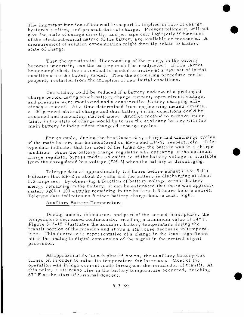
The important function of internal transport is implied in rate of charge,hysteresis effect, and present state of charge. Present telemetry will notgive the state of charge directly, and perhaps only indirectly if functionsof the electrochemical nature of the battery are available or measured. Ameasurement of solution concentration might directly relate to batterystate of charge.

Then the question is: If accounting of the energy in the batterybecomes uncertain, can the battery model be readjusted? If this cannotbe accomplished, then a method is needed to arrive at a new set of initialconditions for the battery model. Then the accounting procedure can beproperly restarted from the inception of new initial conditions.

Uncertainty could be reduced if a battery underwent a prolongedcharge period during which battery charge current, open circuit voltage,and pressure were monitored and a conservative battery charging effi-ciency assumed. At a time determined from engineering measurements,a 100 percent state of charge and thus battery initial conditions could beassumed and accounting started anew. Another method to remove uncer-tainty in the state of charge would be to use the auxiliary battery with themain battery in independent charge/discharge cycles.

For example, during the first lunar day, charge and discharge cyclesof the main battery can be monitored on EP-6 and EP-9, respectively. Tele-type data indicates that for most of the lunar day the battery was in a chargecondition. Since the battery charge regulator was operating in the optimumcharge regulator bypass mode, an estimate of the battery voltage is availablefrom the unregulated bus voltage (EP-2) when the battery is discharging.

Teletype data at approximately 1.3 hours before sunset (165:15:41)indicates that EP-2 is about 25 volts and the battery is discharging at about1.2 amperes. By observing a function of battery voltage versus batteryenergy remaining in the battery, it can be estimated that there was approxi-mately 3200 + I00 watt/hr remaining in the battery 1.3 hours before sunset.

Teletype data indicates no further battery charge before lunar night.

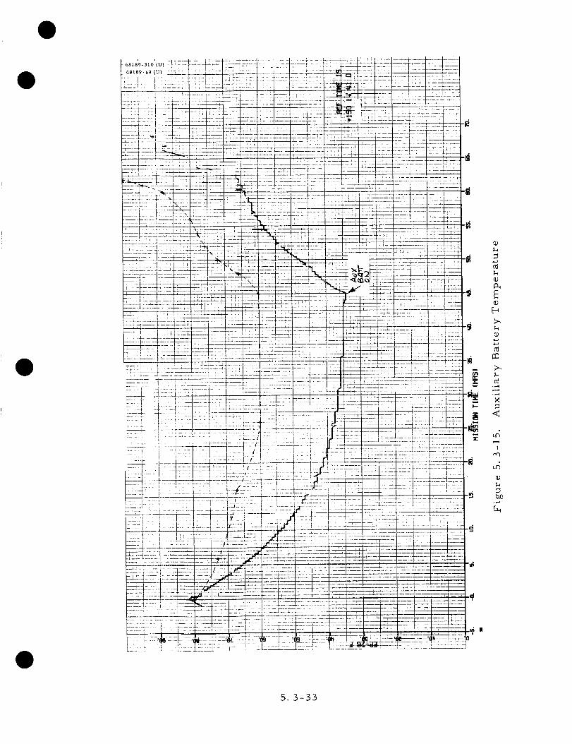
Auxiliary Battery Temperature

During launch, midcourse, and part of the second coast phase, the

temperature decreased continuously, reaching a minimum value of 34 ° F.

Figure 5. 3-15 illustrates the auxiliary battery temperature during the

transit portion of the mission and shows a staircase decrease in tempera-

ture. This decrease is representative of a change in the least significant

bit in the analog to digital conversion of the signal in the central signal

processor.

At approximately launch plus 45 hours, the auxiliary battery was

turned on in order to raise its temperature for later use. Most of the

operation was in high current mode throughout the remainder of transit. At

this point, a staircase rise in the battery temperature occurred, reaching67 ° F at the start of terminal descent.

5. 3-20

D5. 3.4 ANOMALY DESCRIPTION

Owing to the nominal nature of the mission, there was little of an

anomalous nature in the electrical power system during flight. The load

incurred by the unregulated current because of the transmitter B high voltage on

slowly converged during transit time to near the FAT value (Table 5. 3-7).

In addition, there were certain glitches, dropouts, and misrepresenta-

tions in some of the mission plots which have been specially annotated. In

particular, EP-4, EP-9, and EP-14 showed large current drains during a

time of ESP current calibration dropout (launch plus 62.6 to 64. 5 hours).

These excessive values were ignored. All glitches noted as "bad data" on

the mission plots have been shown to be due to ground data processing and

not to the raw data from the spacecraft.

TABLE 5. 3-7. SELECTED EQUIPMENT LOADS

|

Command

0106

XMTR ]5

high voltage on

0106

0110 (0106 off)

0106

0721

ve rnie r

ignition ';_

072.7

thrust phase

power on

1136

electronic tem-

perature control

survey cameraon

Time,GMT

150 18 44 Z

151 06 08 25

151 07 iZ 43

153 05 20 18

151 O6 45 03

EDRS

Telemetry,

milliamp e re s

1782 + 160

1881 ± 180

Z019 ± 84

Z043 ± Z04

338 ± 210

2780 ± 179

FAT,

milliamperes

2159

2159

2159

2159

119

3000

151 06 43 05

153 01 16 42

1452 ± 535

470 ± 497

1802 ± 638

1160

470

1830

Current

Re gulated

Regulated

Regulated

Regulated

Regulated

Unregulated

Regulated

Unregulated

Unregulated

D

0721 was on for approximately 22 seconds.

5. 3-21

5.3. 5 CONCLUSION AND RECOMMENDATIONS

The operation of the electrical power subsystem was nominal through-out the transit portion of the flight.

It may be better to correct telemetry data only when the currentcalibrations exceed an operating bandwidth rather than always updating forany error. Also, continued investigation of battery parameters should bepursued, leading to a better understanding of battery charge as determinedfrom telemetry.

Energy remaining in the batteries during transit is shown in Figure5. 3-2. Agreement between telemetry and simulation (power managementprogram) is excellent. The largest difference is approximately 7.3 percentat L + 45 hours, and it becomes smaller as touchdown approaches. Thepower management program is already a powerful predictive tool that can beenhanced by further knowledge of battery initial conditions, thermal environ-ment, and battery modelling.

5.3.6

of data,

ANALYSIS

The analysis is divided into three areas:and mission plots.

techniques, development

5.3.6. I Techniques

I) Boost regulator efficiency (_]BR)

(output power)BR EP-14 ,:,EP-I

r?BR= (input power)BR = (EP-14 + EP-7) , EP-2

, 100

(Reference 3)

Z) Optimum charge regulator efficiency (_OCR)

(output power)oc R EP-Z -.-"EP-16 .,.= = .,. 100

_OCR (output power)sp EP-11 ,',_ EP-10

(Reference 3)

5. 3-22

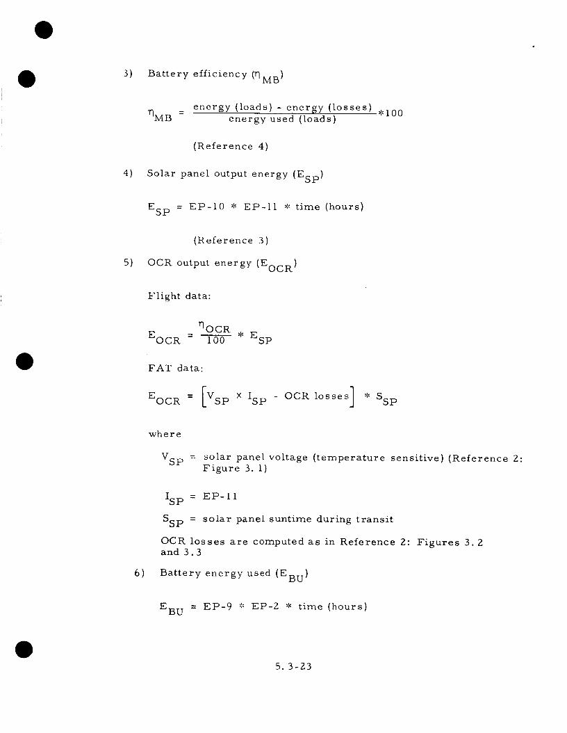
3) Battery efficiency (_MB)

4)

energy (loads) - energy (losses) *i00lIMB = energy used (loads)

(Reference 4)

Solar panel output energy (ESp)

ESp = EP-10 * EP-II * time (hours}

5)

(Reference 3)

OCR output energy (EocR)

Flight data:

_OCR

EOCR - i00 * ESp

FAT data:

EOC R [Vsp X Isp OCR losses] *= - Ssp

where

VSp = solar panel voltage (temperature sensitive) (Reference Z:

Figure 3. I)

Isp = EP- 11

SSp = solar panel suntime during transit

OCR losses are computed as in Reference 2:

and 3.3Figures 3. Z

6) Battery energy used (EBu)

EBU = EP-9 * EP-Z * time (hours)

5. 3-23

where

EP-9 = battery discharge current

EP-Z = ZZ volts unregulated bus voltage

7) Loads are estimated from graphs and are compared to FAT datain References Z and 5.

8) Data summaries from telemetry

Total loads are computed from sources of power

Loads = (EP-9 + EP-16 + EP-17) _',_EP-Z

Power regulated (PR) and power unregulated (BUR)

PR = EP-14 _",-"EP-I

PUR = EP-4 ;',-"EP-2

PR + PUR = power --losses

Unbalanced shunt current (SUNBC)

SUNBC : (EP-9 + EP-16) -- (EP-4 + EP-14 + EP-7)

9) OCR hunting losses (estimate)

The standard deviations from the means of a fairly large sample ofsolar panel voltage (EP-10) and current (EP-II) data are used to estimate theOCR hunting losses at the solar panel maximum power point. A quiet timeduring Coast Mode II where no commands are issued is monitored and anormal distribution is assumed with system noise governing the selection ofthe confidence limits associated with the means of the data samples.

5. 3.6. Z Development of Data

Tabular Information

Table 5. 3-8 is a summary of values to be used in the analysis. Thedata in this table was obtained from the mission plots (Figures 5. 3-7 through5.3-_5).

Tables 5. 3-4 and 5. 3-5 are summaries of the calculations of optimum

charge regulator and boost regulator efficiencies, respectively. In each

table a time-weighted average of the efficiency was computed to obtain a

representative number for transit operation. Table 5. 3-9 summarizes main

battery efficiency up to launch plus 45. 09 hours.

5. 3-24

JJill

-681_9-61_o,_:,,, ii ,,_-_

ii i_-:__ __

II', illi iiiii;_i i;!: !i!i

i _! :Ii !li i _ I, I_

_J4A-

iil iill I:i_

ill Iill I_ :_-__

ill :ii ,il I;I!11i1:,!_I'i

"-o0

o:>

I

!

0

5. 3-25

68189-62 (U)

L ,

T _

©

O9

I

E ©

,,.._

5. 3-26

D

5. 3-27

J,l:_!!!,ll__

68L89-64 {U) -

i

_d

._+

T_V tl_T;#l_ 1-;11 I;Ti -]tT' Tit lilt "_i ;T irz11t _rf_

, ,! ,_ ..... ,

ol,-,-

,_r.

©©

b/3

>,,

c_

I

r',m

©

b.b

I:ii;; i:;

5. 3-Z8

°1.--

¢)bb

0>>.,

.,¢

¢1

rd

0

r,."h

,:D

5. 3-29

68189-66

_7

i

" -7

-_,--7.Z'!

LII

_Z

I I

i:

_ t

! l

* L!

1.

+-.

I

I

I:

I

5. 3-30

0

0

q)

M

_4

5. 3-31

i ¸ .

!r.

Z L: ;_1

[• J ....

J_

0>>.

©

>,

¢g

×

<_

I

_Z©

(

iii _ it: t if ! _ I It

,J

5. 3-32.

5. 3-33

TABLE 5. 3-8. TABULATION OF EP VALUES VERSUS EVENT

1

Event I EP-14

i

0 2.6 ± 0.0Z

1 4.36±0.02

2 2.32±0.04

3 4.33±0.08

4 2. 32 ± 0. 06

5 4.40±0.08

6 I 2. 32 ± 0. 04I

7 ! 2. 32 ± 0.04!

8 ] Z. ";Z ± O. 04

A ] ±o 04

EP-7 EP-Z

2.00 ± 1.00

3.00±0.02

1,32±0.02

3,18 ±O. OZ

1,60 ± 0.04

3. Z4 ± O. 04

1,62 ± 0.0l

1. 62 ± O. Ol

1,62 ± 0. 01

1.68 ± 0. 01

ZZ.2 ±0.

22.2- ±0.

23. ±0.

21.68±0.

21.92 • 0.1

21.6 ±0.

21.89±0.1

21.89±0.

Z1.89± 0.1

11.72±0.1

EP-I EP-10

29. 08

2 29.08 48.2 ± 1.4

2 29.08 48.2 ± 1.4

i 29.08 48.2 ± 1.4

29.24 48.2 ± 1.4

i 29.24 48.2 ± 1.4

29.24 48.8±1.2.

2.9.24 48.8±1.2

29.2.4 48.8±1.2.

?.2.4 48. 5 ± 1.Z

EP-11 EP-16 EP-9 EP-4

1.77±0.08

1. 77 4- O. 08

1. 77 4- 0.08

1.77±0.08

1.77±0.08

1.78±0.02

1.78±0.02.

1.78±0.02

1.77"0.06

3. Z4 ± 0.04

3.24 ± 0.04

3.24 ± 0.04

3.174.0.06

3. 32 ± 0. 08

3.16±0.03

3. 16 ± 0. 03

L16±0.03

3.17±0.05

8.95

5.0 ±0.3

1.4 ±O.Z

5.0 ±0.3

1.6 ±0. _,

5.6 ±0.4

1.73+0.3

1.85±0.3

3.7 ±0.3

3.7 ±0.3

4.25± 1. Z5

1.75 ± 1.25'

O. 64 ± 0. 16

0. 64 ± O. 16

0.84 ± 0.22.

I.Z ±0.16

0.88±0.16

0.96 ± 0.2. I

2..8 ±0.2 ]2.8 ±0.2.

':_Data is taken froln inlssioi_ ph)ts.

TABLE 5. 3. 9. MAIN BATTERY EFFICIENCY

Average efficiency = 94 percent

Event

0-1

1-2

2-3

3-4

4-5

5-6

EMB

76. 98

I15. ZI

73. 80

361.14

161. 44

931.37

Loss

9.03

13.37

9.11

37. 70

7.95

24.75

EMB -- Loss

EMBEMB -- Loss percent

67. 95

101.84

64.69

323.44

153. 49

906.6Z

88. 26

88. _9

87.65

89. 56

95.07

97.34

5.3-34

Output energy of the solar panel computed from flight data is presented

in Table 5.3-10. The solar panel time in sunlight is approximately 62. 8 hours.

The output energy of the OCR is computed to be

_]OCR

EOCR ESp I00

EOC R = (5262 ± 292 watt-hr) * (0.8034)

EOC R = 4225 ± 194 watt-hr

In contrast,Reference Z.

Event

i-5

6-8

the EOC R can be computed from FAT data found in

From flight data

TSp (average) = 108°F = 4Z.Z°C

From Reference 2: Figure 3-i

OCR input voltage : 46. 5 volts

From Table 5. 3-7

OCR input current (EP-II) = i. 77 amps

Solar panel suntime equals 62. 8 hours

Total OCR input energy = (46. 5) _':-"(l. 77) -* (62.8)

= 5168. 44 watt-hr

TABLE 5.3. I0. SOLAR PANEL OUTPUT ENERGY

Total Watt-Hour = 6262.40 ± 242.40

PowL; ............... ] Energy

(EP-10) (EP-I I) Power Time

(42.Z ± 1.4) (1.77 ± 0.08) = (74.69 ± 5.95) (15.73) = 1174.87 ± 93.69

(48.8 ± 1.Z) (1.78 ± 0.0Z) = (86.86 ± 3.12) (46.13) = 4006.85 ± 143.92

(48.5 ± 1.2) (1.77 ± 0.06) = (85.84 ± 5. i0) (0.94) = 80. 68 ± 4.79

5. 3-35

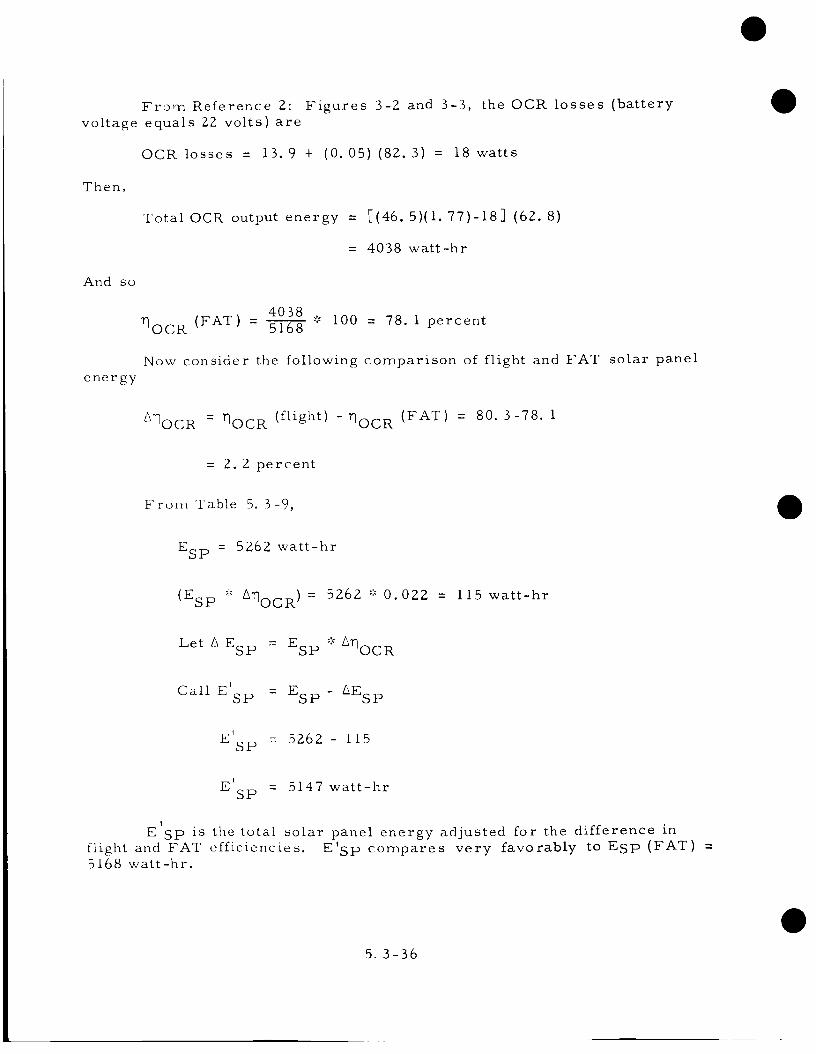
From Reference 2: Figures 3-2 and 3-3, the OCR losses (batteryvoltage equals ZZvolts) are

OCR losses = 13. 9 + (0. 05) (82. 3) = 18 watts

Then,

Total OCR output energy = _(46. 5)(i. 77)-18] (62. 8)

= 4038 watt-hr

And so

4038

rlOC R ""(FAT) - 5168 " 100 = 78. 1 percent

Now consider the following comparison of flight and FAT solar panel

energy

&qOCR : qOCR (flight) - IqOCR (FAT) = 80. 3-78. I

= Z. Z percent

From Table 5. 3-9,

Esp : 5262 watt-hr

(ESp #" AqOCR ) = 5262 ;:_0.022 = I15 watt-hr

Let & ESp : ESp -':' AqOCR

I

Call E SP : ESp - AEsp

E' : 5262- I15SP

E' : 5147 watt-hrSP

I

E SP is the total solar panel energy adjusted for the difference in

flight and FAT efficiencies. E'Sp compares very favorably to ESp (FAT)5168 watt-hr.

5. 3-36

Comparison of Loads: Telemetry and FAT

The comparison of telemetry-measured and FAT-measured loads

(Reference 2) will be made for selected units, various heaters, and largecurrent drains.

Selected E.quipment Loads. The determination of the regulated(EP-14) or unregulated (EP-4) currents used by a selected equipment is

obscured by the general variability of frame-by-frame data on either side of

the point of turnon or turnoff. Data smoothing provided by the EDRS process-

ing was helpful, but the standard deviations of EP-4 and EP-14 within an

averaging interval were often the same order of magnitude as many of the

equipment load changes. For example, during Coast I the average standard

deviation for EP-14 was approximately 60 milliamperes; the same in terminal

descent was I00 to 200 milliamperes. EP-4 showed a standard deviation of

approximately 300 milliamperes owing to cycling loads. Consequently, only

changes in loads which caused significant changes in EP-4 or EP-14 could beconsidered.

The results of selected equipment loads are presented in Table 5.3-7.

Data for command 0106, XMTR HI VOLT ON, is given at various times

during transit, and the current change is seen to approach the FAT value

although initially it was low ('_200 milliamperes during Coast I). Command

0721 was a little high for unregulated current, but its standard deviation

was of the same order of magnitude. Thrust power turnon showed a reason-

able comparison with FAT data. Finally, the turnon of the survey camera

electronics temperature control agreed well with the FAT value.

In general, the large standard deviations associated with unregulated

current loads were due to superimposed cyclic heater loads. The unregulated

load values from EDRS in Table 5.3-7 agree reasonably well with FAT data

even though large standard deviations were associated with the presented

values. Cyclic loads in EP-4 willbe considered separately.

Selected Cyclic Loads

AMR and Vernier Line Heaters

The unregulated current (EP-4), was observed to be cyclic during

transit (Figure 5.3-16). In a plot of EP-4 at 4 hr/in., a gross correlation

of the cycling with the AMR and vernier line heaters operation was apparent

(Figures 5.3=18 and 5.3-19).

If launch plus 20 hours to launch plus 36 hours was considered, a mean

unregulated current (IuR) of 880 milliamperes ± 160 milliamperes could be

measured (Figure 5.3-16). The AMR and vernier line heaters did not have the

same duty cycles nor did these loads turn on or off at the same time, since

each was thermostatically controlled. Superposition of these heater loads

resulting in a somewhat aperiodic plot which can be ovserved in EP-4

(Figure 5.3-16).

Total variation = 320 milliamperes (Figure 5.3-16)

5. 3-37

T

I

+

LL_i

\

I

!I

It

F-I

)iT!

32. _o

i

52.

[7_11

tttt

i_iil

il _-_-,

l

Figure 5. 3-16. Unregulated Output Current

5. 3-38

i

............. [

......... J___.i-J .... I.........

cO

0©

I

c_

5. 3-39

Ill

16° • •

• ' -'l_ Ill

!i: ]1 _/LF

[lii

L

'_J2.

lllllli!

Illl

_ LIiLi

111111

l!lt_i t

..... iii

Figure 5. 3-18. Altitude Marking Radar Etectronic Temperature

5. 3-40

Sum of heater loads = 290 milliamperes (FAT data found in

Reference 3)

These values compare favorably since there are other unregulated loads that

could affect this variation over the long time interval considered.

Gyro Heater

In addition to the long cycles of loading owing to the AMR and vernier

line heaters, a further periodic loading occurred in EP-4 resulting from the

gyro heaters. The load has a short on-off cycle when compared to the AMR

and vernier line heaters. In a 15-minute graph of frame-by-frame telemetry

data {Figure 5.3-19) plotted at l rain/in., the unregulated current is seen to

oscillate 7 or 8 times per minute. This oscillation is not seen in Figure

5.3-16 since EDRS data is averaged, and thus the oscillation due to gyro

heaters appears only as an increase in the standard deviation of EP-4 for

each EDRS data point.

The variation in IUR {one-half period in Figure 5.3-19) represents

the current drawn to operate the IRU heaters and gyro thermal control amplifiers.

Total variation = 540 milliamperes (Figure 5.3-17) (one unit)

IRU heaters and gyro = 577 milliamperes (FAT data found in

control amplifier Reference 5)

This constitutes favorable agreement. Furthermore, gross consider-

ations of Figure 5.3-15 indicate a duty cycle of approximately 25 percent (FAT

value: 26 percent, Reference 5).

RADVS. During the final portion of terminal descent, the RADVS draws

current. The unregulated current drain is observed as EP-17. In EDRS data

at 153:06:15:50 GMT, the RADVS and squib current were recorded at 27.4 ±

1.2 amps. This is close to the expected value of 29 amps. Figure 5.3-20 is

a 360-second plot of EP-17 starting at 153:06:10 GMT. AMR power is on at the

start of this plot, drawing approximately 1.9 amps. The EP-17 signal is noisy,

but changes owing to load differences are apparent. At about 177 seconds, the

AMR is enabled, increasing the current by I. 8 amps. Finally, RADVS power

is completely on at about 310 seconds, drawing about a 27-amps average.

Current Calibration

Observation of mission plots of engineering signal processor (ESP) and

auxiliary engineering signal processor (AESP) current calibration signals

indicates variation throughout the transit portion of the mission. Further

examination of frame-by-frame data and graphs during the coast phases shows

a maximum of a 3 bcd (or 300 milliamperes) noise variation in the zero scale

current calibration (EP-29) of the AESP. The rnidscale current calibration

(EP-28) is more slowly varying around 200 milliamperes, and the full scale

current calibration is essentially constant.

5. 3-41

Figure 5. 3-19.

a) Line l

Vernier Line Ten_peraturcs

5. 3-42

_T

_-÷

F!-

._+_._

"IlL

_'i[

_+

'iF

÷_.

,. !!!

_L ::,

_t ....

!r 1!i

411

_Li_

I',It_,'-

+1 ,

+_ _

-IF1

] I I

I

+ 2

i

- b

_lmml

_L!f:!_

i I

i2

2O

++

+HiK+_;V4-

i I i I ] I

LAZi2_

,iii11_iilr

12r/_TY

r

tl

i_i__LL

_F_ F

]H 11

ill

-iii ,_V2_

_-rt

i iiI I I

LL

tr

Ili1-1 I . _

millI [ I

l;ffiT!i _'4 _

I ÷

ii!i ,",I!I ,,

It ' [_,_ ,,',+ IF

.... il"_ lr[ I I

IIItllll]llillliLiiIiii

b) Line Z

Figure 5. 3-19 (continued). Vernier Line Temperatures

5. 3-43

_-)

t_'igurc 5. {-19 (continued).

Line

Vernier l_ine Ten_peratures

5. 3-44

I

i

PWRIS ON

i li'!

li

Ji!I!

iIJI

J

iI

IIIIII

III

iiII

!__!

F i.

L!WillE i

,11IllII

I1liiIIIllIIIIIIfllIlltllillfllIII

',IIi|1

iijI|IIIIIJIIII|1I|1I|1I'1I II II I! t

. 1ill i

I it

f !

i,

i ii !IiII

I ,.I ,.

l-" .

I :

!,1'I

I

IIL 'L i

kl .1

.._.

III

II

i

I

iJi

JI

iJIIiI

!ii

I

iI

Ii

i

,(r!ii

Figure 5. 3-20. Radar and Squib Current During Terminal Descenl

'YOI._OLTT_ 5. 3 - 4 5 - I

I IIII,III IIilllIIIIllll ""

,'iljiji'ii,,IIIII11111

III iii_I ....... ' '

iII11111;;

IIit1'"II I I I|t I i iIJtttlltJii[llllll ,,

, iiiiiill

ii lit!III ii:ll| • .

Jiiiiiiiii: !!!E!!!!!!

,,iiiiiI I II IIII I II I I IIII I ' "

It IIIIiiI IIIIIIItltll

IIIIt II

ii1!! !!II!!!iii!lli i_iii!!i!!i'rll .!i .!!!!!i ii

I " "

' iiiiiliiIliiitllllI . .

III IIIIIII II1.,IIIIIIIIllJl.llllii!!!!!ttt ::

|11

i,iii,,,!llll!!!_!!i !!,, itlI tlllllll,,

'lll{l",,,I I "ti'"

! tttltiiiii1 ittt ......, llll.iiiii!:l ....

i llllliii::

I_rl_

i i[llllllll

100. llO: 12o.

-FTII:i

' I

i iI

I:! :

!

; !i :: i

i

I

!

iI

II

i tl I,

' I

i : :

I :

• !

ii:! !

ii'I

I ' II : :

I: i !

, l ,: : i: I

: : i

i i

' I '

: i I: : !

i ; I

[

i I ,I i :

i i ;: i i

I I I

i i i

! i i

, ,, ,,

I : 1

-150.

l i i

I00. 190. 200.MI5510N TIME (5EC5)

210.

: I

ilI

i!i :

I

i :i :

iL! ii I

i iI II 'i

i i

j

q

! !

,ii !

: !

_L

=ii

: i i

i:ii i i

_B

FOI_OUT FEAM_

5. 3 - -4 -_ - .._

!t!!!! !

iiii!iiiiiiiillllIll Itlllll I

IIIIIII,llllll I!!!!lli::::II I.... I! !

::::::!I.:;,,I! I::!!!! III1111 I.... ii ,

iiiiiil!!!!!! :

II

iiiiH !!!!!ll ,

:11111

iiiiii

;;IIii !

,_.T! i i $iiil¢i i111111 I!!!!!! !IIIIII

IIIIII ;IIIIII i

!!!!IIiiii_ i!!!!lliiiiiii :it!i!! _;I!!!!! ,iiiill :

!!!!!! :::::!!

:::::: i

!!!!Pt !IIIlll _

IIIIII !

;;;Ptt !

iiiilll'-_L

lllllIIII41L I"'III l_lJ i

III!, _.... I I I

!

i

i

i

!i

--i--

i

i

!

I

l

l

i

-!II+!

i

'¥O_O,U_

, I

'¥O:r.,DOUT FI_._

DA brief examination of the ESP current calibration signals (EP-18,

-19, and -20) also shows a noise variation of approximately 3 bcd counts

(or 300 milliamperes).

This variation can probably be attributed to system noise. Since

these current calibration signals are essentially constant over the mission,

the need for continual updating of telemetry signal values frame-by-frame,

based upon changes in the calibration signals, may not be warranted. It

would be better to change the telemetry current corrections only when the

current calibration signals exceed a specific operating bandwidth, say 4 to

8 bcd counts.

5.3.6.3 Summary of EP Mission Plots

Plots of selected electrical power subsystem signals for the entire

flight phase of the mission are included in Figures 5.3-7 through 5.3-15.

Table 5.3-Ii is an index to these plots.

D 2.

.

4.

5.

REFERENCES

"Surveyor I Flight Performance Quick Look Keport, " Hughes Aircraft

Company, 17 June 1966.

J. Mundy, "System Specification Power Management Data Summary

SC-I Spacecraft 291000," 19 April 1965.

J.C. Jensen, "Power Data Sheets," IDC 2255. 1/1664, 18 May 1966.

Power Management Program, Hughes Aircraft Company.

J. Mundy, "Systeln Specification, Power and Thermal Dissipations by

Functional Event For Engineering Payload 239523, " Revision C,

i July 1965.

5. 5. 8 ACKNOWLEDGMENTS

Appreciation is expressed to W. Mclntyre for technical coordination,

S.A. Volansky and J. Berger for special processing, and J.R. Oelschlaeger

for power management program data. Advice is acknowledged from R. Virzi

of JPL. Thanks are given to R.H. Leuschner and K.C. Beall for review and

criticism.

D5. 3-47

TABLE 5.3-ii. INDEX OF MISSION PLOTS

Name

29 volts nonessential

22 volts unregulated

Main battery man. pressure

Unregulated output current

Main battery voltage

Battery charge current

Boost regulator differential current

Main battery te:npcrature

Butt_ ,'y discharge current

No[ctr array \oltagc

_olat- Ltgl+&} + currellt

Solar array temperature

Boost rcgu[ato r telIlpe Future

t-lcgttlitto r output cur re nt

OCR otltput cttr rent

Radar and squibb current

ES P

Cttrrellt

Ca lib ration

Cornpartlnent e\ heater current

ColTlp.trtlllellt B heater current

Auxiliar_ buttery \oitage

5C-54-currcnt

SC -S6-currcnt

Auxiliary battery temperature

AESP i

Curr_!llt

Calibration

Boost pro-regulator voltage

Battery _harge regulator

telnperature

EP FNumber i Value

1 _(See Table 5.3-8)

6

7

8

9

10

11

12

13

14

16

17

18

19

20

21

22

23

24

Z5

26

27

Z8

29

30

34

(See Table 5.3-8)

(See Table 5.3-8)

(See 'Fable 5.3-8)

88 to 109°F in transit

(See 'Fable 5.3-8)

(See Table 5. 3-8)

(See Table 5.3-8)

108 to II0°F in transit

(See 'Fable 5.3-8)

(See Table 5.3-8)

26. 32 amps at 63. 6 hours

< 80 milliamperes

< 80 milliamperes

0 to 3 BCD change during

coast

Approximately _0.4 volts

109 to 128°F

Graph

Yes

Yes

Yt_s

Yes

Yes

Yes

Yes

Yes

Yes

Comments

Within specification

Within specification

Within specification

23. 2/22. 8 volts first 4 hours

then essentially constant.

Within spe cification.{ Re fe rence

4: minimum 17.4 volts)

Charge intervals after touch-

down were hours 65 to 70.

Within specification (Reference

4: 70 to 125°F)

Reference 4: specification

+122OF e 10°F

See 5. 3. 6. 2,"RADV5"

See 5.3.7. Z,"Currcnt

Calibration"

\_, 1thin specifications

See 5.3.3. g,"Auxiliary

Battery Te:nperature"

See 5. 3. 6. 2,"Current

Calibration"

Within specifications

5. 3-48

5.4 RF DATA LINK SUBSYSTEM

5.4. 1 INTRODUCTION

This section contains a summary and analysis of the performance of

the data link subsystem during Surveyor Mission A.

The data link subsystem consists of the transmitters, transponders,

receivers, command decoders, and antennas. It is the function of this sub-

system: i) to provide engineering data transmission from the spacecraft at

bit rates compatible with specific mission phases, Z) to provide analog data,

such as television and strain gages, at signal levels high enough for proper

discrimination, 3) to provide phase coherent two-way doppler for tracking

and orbit determination, and 4) to provide command reception capability

throughout the mission to allow for complete control of the spacecraft from

the ground. A simplified block diagram of the communications subsystem is

shown in Figure 5.4-I.

The pertinent subsystem units that were on the spacecraft during themission are as follows:

Part Serial

Unit Number Numbe r

Receiver A 231900-3 13

Receiver B 231900-3 14

Transmitter A 263220-4 14

Transmitter B 263220-4 20

Command decoder unit 232000-3 5

Unlike most subsystems, individual data link subsystem parameters

such as losses, threshold sensitivity, modulation index, etc., are not meas-

ured or individually determined from mission data. The composite effect of

the performance of these parameters is measured as received signal power

at the spacecraft and the tracking station (DSIF) and as telemetry and command

error rates. Consequently, it is impossible to compare individual link

5.4-i

OmA

IN: 2111 IdC

U Out_ _lts _

IF o_t

lul out i'_i _

1_,U_li,ll

lwtlcl4

Gm.IN, - _ I

I AIf IN IIKIIVll 0UI - 0101T_I.

A LIM IN_I

nIANI,_ l;lll _ ,'_.a I

ANTINN& IILKI01 |WlICI4 I_-I.Iw C_l lOW

litS

IF OUVMC

_ 0_lW cl_ _

I fM _Fol

¢ o _,IK:TIO N

o.....

ill:lltl/

IKONI

ilUl£ lOI

OEC,_OOEI_0"00

00

I

i,-.i

-.,1

v

Figure 5. 4-I. Communications Subsystem Block Diagram

5.4-2

parameters to specified performance criterion. The best that can be doneis to compare measured signal levels to predicted levels, and telemetryquality and command capability to predicted capabilities. To further cloudthe analysis, omnidirectional antenna gain is a major contributor to theuncertainty in received signal levels. Accurate omni-gain measurementsare difficult to achieve and, in most cases, deviations from predictions canmost likely be attributed to antenna gain uncertainty. Because of the probelmsoutlined above, analysis of the data link subsystem performance will, in gen-eral, be a qualitative analysis of the performance of the entire subsystemversus a quantitative assessment of the performance of the individual subsys-tem parameters. Equally as important as subsystem performance evaluationin this analysis is the qualitative assessment of the premission and real-timeprediction techniques used during Mission A since future missions must relyon [hese techniques as guidelines during the real time operation.

The data link parameters used in the performance predictions aretabulated in Table 5. 4-i. This data is measured data taken from FAT, STV,and CDC tests, as well as specified parameters where measured data wasnot available.

Except for the failure of omnidirectional antenna A to properly deployat separation, the data link subsystem performed exactly as expected. Theperformance was very close to nominal, a_zdall subsystem requirements andobjectives were satisfied.

5.4. 2 ITEMS CONSTITUTING ANALYSIS

The data contained in this report consists of spacecraft telemetered,DSIF, and mission event time data. Where meaningful, the data is correlatedto and compared with equipment specifications, previous test data, preflightpredictions, and in-flight analysis predictions.

5. 4. 3 MODE, BIT RATE, AND SUBSYSTEM CONFIGURATION SUMMARY

The telemetry modes, bit rates and subsystem configuration aretabulated as functions of time from launch to touchdown in Tables 5.4-2 and5.4-3, respectively. Also, the various telemetry signals and the modes inwhich they appear are tabulated in Table 2. Z-i in Section 2. 2. (The timesshown in the these tables are accurate only to ±l.0 minute.) These tablesdo not contain lunar data because of the large number of times that the modesand configuration were changed due to lunar TV and assessment operations.

5.4.4 SUMMARY OF RESULTS

As discussed in the introduction, a quantitative assessment of theindividual subsystem parameters is not possible in most cases. However,the parameters that can be related either to predictions or requirements orboth are summarized in Table 5.4-4.

5.4-3

TABLE 5. 4-i. LISTING OF UP-LINK AND DOWN-LINK PARAMETERS

FROM FAT, STV, AND CDC TESTS

De sc ription

Transmitting system (DSIF)

RF power

Antenna gain

SAA

SCM

Circuit loss

SAA

SCM

Receiving system (SC-1)

Circuit loss

Receiver A

Receiver B

Up-link carrier tracking loop

Equivalent noise

Ban dwi dth

Threshold, SNR

Up-link channel

Threshold, SNR

System noise

Temperature

Equivalent noi se

Bandwidth (predetection)

SCO center frequency

Data/subcarrier

Modulator indices

Value

70. 0 dbm

0.5 dbm

-0.0 dbm

20.0 db + 2.0 db

51.0 db, :el.0 db,

-0.5 db

-0.5 db + 0.0 db

-0.4db + 0.1 db

-3. Z db + 1.3 db

-3.7 db + 0. 3 db

-Z40 Hz + I0 percent

12 db

9 db

2700°K

13430 Hz

2.3 kHz

7.2

5.4-4

Table 5.4- 1 (continued)

Description

Modulator indices

Transmitting system (SC-1)

RF power

Transmitter A

(low power)

Transmitter B

(low power)

Transmitter A

(high power)

Transmitter B

(high power)

Planar array gain

Circuit loss

Omnidirectional antenna A

Omnidirectional antenna B

Planar array

Carrier frequency

Receiving system (DSIF)

Antenna gain

SAA

SCM

Circuit loss

SAA

SCM

Value

1.6 ± I0 percent

20.7 dbm, +1.05 dbm,- I. 8 dbm

20.8 dbm, +0.5 dbm,

- I. 6 dbm

40.5 dbm, +0. 1 dbm,-0.5 dbm

40. 15 dbm, +0. 35 dbm,

-0. 15 dbm

27.0 dbm, +0.5 db

-3.6 db ± 0.6 db

-3.8 db ± 0.6 db

2.7 db± 0.3 db

2295 MHz

21.0 db, ± 1.0 db

53.0 db, ± 1.0 db,

-0.5 db

-0.5 db ± 0.0 db

-0. 18 db ± 0.05 db

5.4-5

Table 5.4- 1 (continued)

Desc ription

Effective noise

Temperature

Maser

Parametric

Ampli fie r

Lunar temperature

Carrier channel

Equivalent noise bandwidth for

maneuvers (at threshold)

Equivalent noise bandwidth for

coast mode (at threshold)

Threshold, SNR

Ac qui sition

Maneuver s

Coast mode

SCO descriptions

Equivalent noise bandwidth

Value

55°K ± 10°K

270°K + 50°K

II0°K ± Z5°K

152 Hz

IZ Hz

3.0 db + 1.0 db

14.0 db± 1.0 db

6 db

(pr edetection)

4400 bits/sec

ii00 bits/sec

550 bits/sec

137. 5 bits/sec

17. Z bits/sec

Strain gage 1

Strain gage Z

Strain gage 3

Reject/enable

Gyro speed check

4770 Hz ± i0 percent

1190 Hz + I0 percent

644 Hz ± I0 percent

158. 5 Hz ± I0 percent

Z5. 1 Hz + I0 percent

281.0 Hz ± i0 percent

524. 0 Hz ± l0 percent

464.0 Hz ± i0 percent

377. 0 Hz ± i0 percent

874.0 Hz ± 10 percent

5.4-6

Table 5.4- 1 (continued)

De sc ription Value

SCO center frequency

4400 bits/sec

ii00 bits/sec

550 bits/sec

137.5 bits/sec

17. Z bits/sec

Strain gage l

Strain gage 2

Strain gage 3

Reject/enable

Gyro speed check

SCO modulator indices

4400 bits/sec

ii00 bits/sec

550 bits/sec (acquisition)550 bits/sec

137.5 bits/sec

17.2 bits/sec

Strain gage 1

Strain gage 2

Strain gage 3

Reject/enable

Gyro speed check

Carrier noise bandwidth for

television modes

600 line

Z00 line

Threshold, SNR, for television

modes

600 line

?00 line

33.0 kHz

7.35 kHz

3.90 kHz

0.96 kHz

0.56 kHz

i. 70 kHz

3.00 kHz

5.40 kHz

Z. 3 kHz

5.4 kHz

1.6 + l0 percent

0.935 ± i0 percent

0. 3 ± l0 percent

I. 15 ± i0 percent

1.45 ± I0 percent

1.45 ± 10 percent

0.615 ± l0 percent

0.615 ± l0 percent

0.61 ± l0 percent

0.655 ± i0 percent

1.600 ± I0 percent

3.3 MHz ± i0 percent

ll.4kHz ± i0 percent

i0.5 db ± 1.0 db

4.5 db± 1.0 db

5.4-7

Table 5.4- I (continued)

Description

Television mode modulation index

parameters

600 line, maximum frequency

deviation

Z. 5 MHz

Value

ZOO line, maximum frequency i0 kHz

deviation

Polarization and pointing loss 0

Atmosphere 0 db, +0 db

Absorption -0. Z db

5.4. 5 ANOMALY DESCRIPTION

5.4. 5. 1 Omnidirectional Antenna A Nonextension During Transit (TFR 18Z33)

The major subsystem anomaly observed during the mission was the

apparent failure of omnidirectional antenna A to deploy just prior to space-

craft separation from the Centaur. Any mechanical problems and any con-

clusions relative to these problems will not be discussed in detail in this

section but will be treated in Section 5. iZ, "Mechanisms." Only the RF data

relating to the anomaly will be treated here.

Without drawing any conclusions as to the actual failure mechanism,

it is necessary to present a brief history of the problem and some possible

causes in order to relate the observed RF data to the anomaly. Real-time

data was not available at the SFOF during deployment. Postmission telemetry

through Centaur shows normal simultaneous leg extension, followed about 9

seconds later by the omnidirectional antenna B deployed signal. Once the

signal went to the "on" condition, it did not return to "off." Further, the

omnidirectional antenna A deployed signal did not, at any time during transit,

indicate "on. "

It was [earned sometime after the mission that omnidirectional

antenna A was slightly misaligned with the clamp that held it in the stowed

position. It is therefore possible that one of the following events resulted

in the observed anomaly:

i) Omnidirectional antenna A extended, but did not actuate the

microswitch from which the omnidirectional antenna extend

signal is derived.

5.4-8

TABLE 5.4-2. TELEMETRY MODE SUMMARY

150

151

Time Mission Phase

Launch14 41 O1

15 10 16

15 34 22

15 39 28

15 42 35

15 48 20

15 54 36

15 56 03

18 31 53

18 34 31

18 39 08

18 44 00

18 44 50

18 49 33

19 14 25

19 21 42

01 38 18

02 22 54

OZ 24 07

02 44 52

02 47 07

04 14 11

04 17 09

04 20 02

04 26 03

04 30 16

04 33 57

06 Ol ZO

06 04 07

06 05 25

06 07 54

06 08 55

06 10 Zl

06 49 26

07 04 30

07 07-

O7 O9 -

Mode

5

5

1

4

4

2

3

5

4

Z

1

1

1

5

5

5

5

5

4

2

5

4

Z

1

Gyro

1

5

4

2

1

1

1

1

5

4

2

1

DSIF Automatic

Bit Rate Gain Control Comment

550

550

550

1100

1100

1100

1100

1100

1100

1100

1100

1100

1100

1100

1100

1100

550

550

550

550

550

550

550

550

550

550

550

550

550

550

550

550

4400

550

550

550

550

-88.0

Low modulation index

Initial acquisition- station 51

Normal bit rate

-120.0

Low power /Pre-Canopus

High power

High power / Star lock

Low power )

- 136.9

-I17,0

-121.0

Bit rate reduction

Station I 1 in two-way

Gyro speed check

Low power }High power

Premidcourse

Increase bit rate for midcourse

(Special reverse midcourse data)

5.4-9

Table 5.4-2 (continued)

151

152

153

Time Mission Phase

07 11 53

07 13 30

08 32 09

08 36 49

08 41 27

16 13 27

16 18 06

16 27 27

20 32 42

20 36-

O4 06 O3

04 08 Z2

04 11 5Z

09 58 52

I0 02 44

10 07 20

15 48 18

15 53 48

16 02 Z0

18 44 16

18 54 05

19 01 20

23 19 53

23 25-

01 55 23

02 O0 22

O2 47 O0

03 13 17

03 16 52

03 55 33

O3 58 54

04 01 06

04 05 52

05 18 13

05 21 26

05 22 10

05 23 O0

06 00 33

06 16 01

06 17 37

Mode

5

5

4

2

5

4

2

5

4

2

4

2

5

4

2

5

4

2

5

4

2

5

4

2

4

5

5

4

5

4

2

1

5

4

4

3

1

2

3

3

DSIF Automatic

Bit Rate Gain Control Comment

550

550

55O

550

550

550

550

550

550

550

550

550

550

55O

550

55O

55O

55O

55O

55O

55O

55O

55O

55O

55O

55O

55O

55O

55O

550

55O

55O

55O

55O

If00

If00

If00

If00

II00

II00

-i17.2

-137.98

-138.9

-143.6

- 142.7

-143. 0

- 146.0

High power / Postmidcour se

Low power )

DSIF 11 having transmitter trouble

DSIF 11 tracking

Low power 1 Preterminal

High power )

Pretouchdown data on touchdown

Touchdown

5.4-10

TABLE 5.4-3. SPACECRAFT CONFIGURATION SHEET

Day Tin e150 14 41 01

14 53 Z6

15 21 00

16 26 00

18 44 24

19 21 04

151 0l 16 20

0Z 35 00

04 26 03

04 30 16

06 08 25

07 12 43

08 53-

09 29 -

15 16-

17 00-

152 04 27 --

06 22-

06 25 -

06 54-

08 50-

17 04--

19 26-

153 0Z 45 11

04 05-

04 12-

05 04 -

05 20 18

05 Z9 47

06 17 37

Mission Phase

Transmitter A/D Receiver A Receiver B Command

Power Omni Converter Decoder

A/B H/L A/B I/Z _L/AFC Xpond _0L/AFC Xpond A/B

B L B l AFC q0L B

H

L ON

Launch

Post -

acquisition

Sta r

Gyro

1

OFF

ON

AFC OFF

_OL ON

AFC OFF

A

B

A

B

A

B

A

Comments

Launch configuration

Centaur command on high power

Modulation interrupt

acquisition phaseStar

Decoder index at stationtransfer (DSIF 51 to 11)

Gyro speed measurement

Midcour se phase

Decoder index at stationtransfer (DSIF l l to 4Z)

Decoder index at station transfer

Decoder index at station transfer

DSIF II transmitter OFF

DSIF ii transmitter GN

Select decoder A/recelver B

Decoder index at station transfer

Select decoder A/receiver B

Decoder index at station transfer

Select decoder A/receiver 13

Decoder index at station transfer

NBVCXO check

Select decoder A/receiver B

Terminal phase

NBVCXO mode ON

Touchdown

z) Omnidirectional antenna A did not get free of the clamp that held

it in the stowed position due to the resulting friction force developed

by the misalignment of the omnidirectional antenna in the clamp.

Throughout the entire coast phase, the omnidirectional antenna A extend

signal never indicated that the omnidirectional antenna had extended even though

the omnidirectional antenna extend command was transmitted during two sep-

arate periods, the first attempt being made at Z+lH 40M and the second

attempt being made at L+39H 50M. Finally, after touchdown, when the telem-

etry modes were interrogated, it was noted that the omnidirectional antenna A

extend signal indicated that omnidirectional antenna A was extended.

Antenna pattern data is of primary importance in determining which of

the above possible failure mechanisms was the true failure. This data can be

determined from RF subsystem data by observing receiver A signal levels

throughout the mission and attempting to relate the observed levels with extended

or stowed omnidirectional antenna pattern data. Unfortunately, as discussed

5.4-11

TABLE 5.4-4. PERFORMANCE PARAMETER SUMMARY

Actual

Parameter Predicted Value Requirement Performance

2294. 994627 2295 mc + 23 kc ***Transmitter frequency

at acquisition

Receiver B frequency

at acquisition

Receiver A* signal

levels during coast

phases

Receiver A* signal

levels duringmaneuvers

Receiver B signal

levels during coast

phases

Receiver B signal

levels during

maneuvers

DSIF signal levels

during coast phases

DSIF signal levels

during maneuvers

Transmitter A high

power output

Transmitter A low

power output

Transmitter B high

power output

Transmitter B low

power output

Phase jitter 12 cps

bandwidth

Phase jitter 152 cps

bandwidth (thrust

phase)

Phase jitter 152 cps

bandwidth (touchdown)

Command reject rate

Telemetry':":'

bit error rate

2113. 312224

Time variable predictions.

Predicts are some nom-

inal value + ='8 db

Time variable predictions.

Predicts are some nom-

inal value ± _8 db

Time variable predictions.Predicts are some nom-

inal value ± =6 db

Time variable predictions.

Predicts are some nom-

inal value ± =7. 0 db

Time variable predictions.

Predicts are some nom-

inal value ± =8. 0 db

Time variable predictions.Predicts are some nom-

inal value ± =7. 0 db

+0. i dbm40.5 -0. 5

20.7 +1.05 dbm-1.8

+0. 35 dbrn40. 15 -0. 15

+0. 5 dbm20.8 -1.6

<36 degrees

< 22 degrees

< 30 degrees

< 1/2000

< 3/lOOO

2113. 31 mc ± 21 kc

> -114 dbm

> -114 dbm

> -114 dbm

> -114 dbm

> -159. 3 dbm

(carrier power)(17. Z

bit s/sec threshold)

> -135. 5 dbm

(carrier power)

(ii00 bits/sec--high

power )

> 39. 6 dbm

> 19. 1 dbm

> 39. 6 dbm

> 19. i dbm

< 36 degrees (3c)

< 22 degrees (3o)

< 30 degrees (3_)

< l/Z000 at signallevel > 114 dbm

3/1000 at inputSNR 2 11 db

Level between 0 and 12 db

above nominal and > -95

dbm

Level between 4. 0 and

-20. 0 db about nominal

and > - 104 dbm

Level between +4. 0 db

about nominal and > -i00

dbm

Level between 6 and -7 db

about nominal and > -i00

dbm

Level between +3. 0 db of

nominal and > -146 dbm

Level between +7 and -3db

of nominal and > -129 dbm

Output between 40. 5 and

39. 7 dbm

No data

Output between 40. 6 and

39. 9 dbm

Output between Z0. 5 and

19. 6 dbm

No rejected commands in

100,000 at signal levels> - 104 dbm

< 3/1000 at input SNR9±ldb

*Predictions are based on gains relative to an extended omnidirectional antenna.

**BIER was allowed to increase above requirement, but this occurred at input SNRs below specification

value of 11 db.

***DSIF data not available for this report

5.4-12

earlier, any single parameter value is difficult to access especially antenna

gain.

Accurate omnidirectional antenna gain measurements are difficult to

make. The omnidirectional antenna data used during the mission and through-

out this report is derived from five complete sets of antenna patterns and

represents the composite gain determined by noting the bounds on the maximum

and minimum gain exhibited by all five patterns for all points on the sphere.

In addition to the actual measurement deviations from pattern to pattern, other

error sources must be included. Range reflections and spacecraft-to-model

differences can cause errors up to_ ±5 db in measured gain values. Null

positions and depths are very susceptible to the above error sources. Because

of these problems, no particular measurement can be used to confirm the

position of omnidirectional antenna A during transit. However, by observing

the data for the entire mission, it is possible to conclude that omnidirectional

antenna A was not fully deployed and, in fact, was probably closer to the

stowed position than to the deployed position.

Examination of a scale model of the spacecraft indicated that a stowed

or nearly stowed omnidirectional antenna position would result in relatively

high gain during most of the transit phase when the attitude was determined

by the sun and Canopus. In addition, the pre-Canopus spacecraft attitude and

the selected maneuvers could result in severe nulls due to a direct interception

of the line of sight from the stowed omnidirectional antenna to earth by either

the solar panel or planar array or both.

Plots of automatic gain control (AGC) data contained in subsection

5.4.7 tend to confirm the stowed or nearly stowed omnidirectional antenna A

position hypothesis. Prior to listing the appropriate figures and drawing any

conclusions from the data, it should be noted that the downlink omnidirectional

antenna B data and the uplink omnidirectional antenna B data was observed to

agree with measured data to within the expected measurement errors. In no

case did either up- or downlink omnidirectional antenna B data go below the

worst-case predicted data. Omnidirectional antenna A data did not agree

well with measured data and did go outside the worst-case predicted gain. The

following is a list of pertinent graphs of telemetry data and conclusions drawn

from this data:

I) Receiver A and B AGC during transit (Figure 5.4-9)--This data

indicates that receiver A experienced large variations in signal

levels prior to Canopus acquisition. A 20-db null can be observed

between L+ 1.5 and Z+2. 0 hours. A null of this depth is not pre-

dicted from extended omnidirectional antenna A pattern data.

After Canopus acquisition, the antenna gain exhibited by omni-

directional antenna A was apparently high since input signal levels

were as much as 12 dbabove predictions.

2) Receiver A AGC during Canopus acquisition compared to extended

omnidirectional antenna A data (Figure 5. 4-14) -- This data shows

receiver A signal level during the roll maneuver instigated to

5.4-13

acquire Canopus. The extended omnidirectional antenna A patterndata is also shown, including the worst-case expected gain level.As can be noted, deep nulls were experienced which were notpredicted. Nulls IZ db below worst-case expected levels wereobserved. Also, a predicted small null did not exist.

3) Receiver A AGC duringCanopus acquisition compared to stowed

omnidirectional antenna A data (Figure 5. 4-15) -- This data con-

tains the same receiver AGC data as Figure 5.4-14 but is compared

to stowed omnidirectional antenna A'data. The stowed data shown

was measured during the mission on the JPL range and represents

a single measurement. Of primary interest is the fact that the

stowed data indicates deep nulls in the same region as the observed

receiver AGC data. Also of concern is the fact that worse nulls

were measured in the region corresponding to the roll maneuver

than were experienced. Relative positional differences of 0. 5 to

1. 0 inch, however, can cause major pattern changes at Zll3 mc,

and it is concluded that the observed data behaved more like the

stowed pattern predictions than like the extended pattern predictions.

4) Receiver A AGC during the reverse midcourse maneuvers (Figure5.4-18)--This data shows the receiver A AGC levels during the

reverse midcourse maneuvers compared to predicted data relative

to an extended omnidirectional antenna. Again, very little correla-

tion can be noted. Also, the signal level went below the worst-case

predicted level during both maneuvers.

The composite picture developed by observing the data outlined in thissectionseemsto confirm that omnidirectional antenna A was stowed or near to

the stowed position. A final bit of evidence occurred during the first roll

maneuver during the terminal maneuvers. At 153:05:38:46, a receiver indexoccurred resulting from a deep null on either omnidirectional antenna A or B.

Neither omnidirectional antenna pattern indicated that a deep null should exist

during this roll maneuver. This leads to the conclusion that the null was dueto a stowed omnidirectional antenna pattern null caused by interference by the

planar array or solar panel. Receiver AGC data is not available during theterminal maneuvers to verify which omnidirectional antenna experienced thenull. However, downlink omnidirectional antenna B data, which is similar to

the uplink data, did not have a deep null as determined from DSIF signal levels.

Based on RF data, it is concluded that omnidirectional antenna A was

not fully extended during transit. Furthermore, it is concluded that the omni-directional antenna was near the solar panel and planar array similar to the

actual stowed position. This conclusion being based on the correlation noted

between the observed data and expected data determined by observing the

spacecraft model, as well as the lack of correlation between the observeddata and extended omnidirectional antenna data. It is not possible to concludefrom this data whether omnidirectional antenna A remained in the clamp or

if it started to extend. However, if omnidirectional antenna A were partially

extended, it is concluded that its position was closer to the stowed than the

extended position.

5.4-14

5.4.5. Z Spacecraft Receiver AGC Telemetry Calibration Anomaly (TFR 27628)

During lunar operations, a special spacecraft receiver threshold test

was performed (see subsection "Special Receiver Threshold List") on

I0 June 1966. This data indicated that the preflight calibration data, when

applied to system performance using telemetered temperatures for the

assumed unit temperatures, does not give adequate results. Data from this

special test was then used to develop new calibration curves for use with the

flight data. These new curves differed from the preflight curves by as much

as 8 db for Receiver A and 2 db for Receiver B. This anomaly is discussed

in detail in subsection "Spacecraft Receiver AGC Data. "

5.4.6 CONCLUSIONS AND RECOMMENDATIONS

Based on data contained in this section of the report, the followingconclusions can be made:

1) The RF subsystem performed as expected with the exception of

omnidirectional antenna A. In most cases _, close to nominal

performance was experienced in both the up- and downlinks.

z) Antenna pattern data for omnidirectional antenna B (up- and down-

link) was relatively accurate. In most cases, actual performance

indicated better than or equal to predicted gain data, and in no

case was the actual data worse than the worst-case predicted data.

3) The RF subsystem premission predictions and real-time analysis

techniques used during Mission A were accurate and in most caseswere conservative.

4) Omnidirectional antenna did not properly deploy until sometime

between retro firing and touchdown. The actual antenna position

was either a stowed or nearly stowed position (see subsection

5.4.5 for details).

As a result of the data contained in this section, including in many

cases the problems encountered in reducing this data, the following recom-mendations are made:

Spacecraft receiver AGC data should be telemetered in every

mode. This fact is emphasized by the lack of data during the

terminal maneuver relative to the observed receiver index, and

the required deviation from normal procedures in order to get

this data during the star and reverse midcourse maneuvers.

z) Spacecraft receiver AGC data temperature sensitivity should

either be lessened or procedures instigated to better calibrate out

the temperature effect. Relatively large errors in absolute signal

level exist in this report due to the lack of knowledge about the

AGC temperature interaction. Considering that the hardware is

5.4-15

3)

4)

5)

S)

7)

8)

built for most spacecraft, a possible solution would be to calibrate

the receiver AGC signals relative to compartment A tray tem-

peratures during the STV tests. This data would be invaluable

during the mission and during postrnission analysis since the STV

data on SC-I was at least similar to the actual mission data.

(The unit tempe rature/AGC calibration data is nearly useless

since the unit temperature data does not correlate well with any

telemetered temperatures and is calibrated at temperatures that

are not experienced during transit. ) .

Temperature transducers should be placed on the transmitter and

receiver modules that contain the respective VCXOs. As in the

case of the AGC signals, it is very difficult, if not impossible,

to correlate unit temperature data to any single presently telem-

etered temperature. The ability to check prelaunch frequency

reports and to update DSIFtracking predictions is severely les-

sened because of this lack of correlation between frequencies and

telemetered temperature data.

Receiver frequency/temperature data should be provided for the

receivers in both the phase lock and AFC modes. Present data

applies only to the phase lock mode. AFC and static phase errors

observed during lanar operations indicated deviations that were

not explainable from available data.

DSIF data, specifically AGC and dynamic phase error signals,

must be made available in a timely manner after a mission. No

valid DSIF data was received for this report; consequently, DSIF

AGC data is very inaccurate since it is made up from verbal

reports, station hourly reports, and, in the case of Goldstone

data, from the real-time analog recorder data provided during

the mission. No dynamic phase error analysis is included in

this report even though it is felt to be of considerable interest.

DSIF station reports should include the zero to peak or peak-to-

peak phase jitter observed. Th_ data should include a measure-

ment every hour and specific measurements during midcourse

thrusting, retro burn, and touchdown phases.

DSIF receiver AGC levels should be reported just prior to and

after going from high to low or low to high power. This data is

necessary to compute the spacecraft transmitter low power output

before and after going to high power. Since this data was not

always available, the low power output during Mission A is not

as well known as it might be.

The allowable telemetry bit error rate or word error rate should

be allowed to go above tile present specification value of 3 bits in

1000 or _ l word in 30. During coast phases, the limit should be

determined by the data users in real time provided the postmission

data reduction requirements are not jeopardized.

5.4-16

5. 4. 7 SUBSYSTEM PERFORMANCE ANALYSIS

This subsection contains plots and analysis of the mission data. Thedata is discussed in subsections 5.4. 7. Z through 5. 4. 7. 7 in relation to specificmission phases and is discussed in subsection 5.4. 7. 8 in relation to missionplots of the subsystem parameters.

Received signal levels for both the up- and downlinks constitute asignificant portion of the analysis contained in this report. The absolute levelsat the spacecraft receivers were established by using considerable engineer-ing judgment. An attempt was made to reduce the errors due to temperaturesensitivity of the AGC signals. Likewise, the absolute levels at the DSIFwere established primarily by attempting to interpret the low resolutionanalog recording of the Goldstone AGC data received in the SPAC operationsarea. The absolute value of both the uplink and downlink AGC signals may besomewhat in error; consequently, a brief discussion of the data accuracy willbe included prior to the actual data discussions.

5.4. 7. 1 Data Accuracy

Spacecraft Receiver Automatic Gain Control Data

Figure 5.4. Z shows the receiver A and receiver B AGC calibration

data as a function of temperature for temperatures of 0, 75, and 1Z5°F. This

data is in agreement with system data taken at the Cape just prior to the mis-sion and is considered to be the most accurate data available. The dotted

90-degree curve represents the curve used in the analysis and was derived

primarily from the special receiver threshold test run on SC-I during the

first lunar day.

As can be noted, receiver A AGC can vary between 5 and IZ db, and

receiver B AGC can vary between 2 and 9 db in absolute signal level over the

range of interest depending on the temperature of the unit (considering only

the 75 and 1Z5°F curves). The tray bottom temperature in compartment A

was between 90 and 100°F throughout the majority of the mission, leading to

the conclusion that the unit temperature was somewhere between the two cali-

bration curves. For the mission real-time analysis, a linear relationship

was considered to exist between the curves, and signal levels were reported

on this basis. However, a threshold test was run on i0 June 1966 in which the

DSIF output signal level was carefully reduced Z6 db in steps, and the receiver

AGC voltages were recorded. The tray bottom temperature during this test

was 91°F, and the tray top temperature was 81°F. Although not exact, the

tray temperatures during this test were similar to the transit temperature.

(The actual data from this test is contained in subsection "Special Receiver

Threshold Test.") By using the linear relationship between the 75 and 125°F

curves, both the receiver A and receiver B AGC levels were obviously in

error (Reference TFR Z76Z8). Receiver A indicated a total change of 33 db

and receiver B a total change of 3Z db, and the final signal value at the

observed point of receiver/decoder indexing was -134 db for receiver A and

-IZ4 db for receiver B. Previous test data taken at the Cape indicated that

receiver/decoder indexing would occur at -IZZ ±I db for receiver A and -116±i db for receiver B.

5.4-17

a) Keceiver A

b) Receiver B

Figure 5. 4-Z. l_eceiver AGC

5.4-18

Based on the above data, it was decided to establish a 90°F curve by

setting the signal levels at the observed point of indexing to -IZZ db for

receiver A and -If6 db for receiver B and work back in increments exactly

equivalent to the change in transmitted power. The obvious error in this

technique is that it is not known which receiver caused the indexing. The

new curve, however, does represent an upper limit on the data and, in the

case of receiver A, makes a considerable change in the absolute value from

the linear relationship used previously. New coefficients were thus gener-

ated from the 90°F curve, and all receiver AGC. voltages were converted to

engineering units from the new coefficients. This new AGC data is esti-

mated to be accurate to =_2. 0 db in absolute value.

DSIF Receiver AGC Data

DSIF AGC data was not made available by the time of this report due

to problems encountered in postmission data reduction (see Section 5. i).

Consequently, the data contained in this report was derived from other

available sources. The data from all stations except Goldstone is primarily

voice report and station report data. It is considered to be quite accurate,

but the time intervals between data points do not allow for transient of "glitch"

evaluation relative to unexpected level changes. A good example of this is the

DSIF data during star acquisition. Fortunately, good verbal reporting took

place during this phase of the mission and the plot contained in this report is

relatively good. Variations may have occurred, however, that are not shown.

But it is impossible to determine this from the available data.

The Goldstone data plotted during the midcourse and terminal maneu-

vers is derived from the analog recorder data discussed earlier. Initial

calibration errors of the recorder, as well as basic resolution, are obvious

error sources. In addition, the exact time correlation of the maneuvers with

the data is difficult since no time code exists on the recorder. An effort was

made to establish time correlation by noting signal level changes correspond-

ing to known commands such as bit rate change, etc. , but this was difficult.

The estimated error in this data is _±2 db.

5. 4. 7. Z Subsystem Mission Performance

This subsection contains data and analysis pertinent to specific mis-

sion phases. Only those parameters directly related to the mission phase

under discussion will be treated here. (All subsystem telemetry for the

entire mission is discussed in detail in subsection 5. 4. 7. 8. )

Prelaunch Phase Performance

During the prelaunch phase, the subsystem performance is assessed

during the launch pad systems readiness test (SRT) and prelaunch countdown

test. Next to assuring normal system performance prior to launch, the most

important subsystem data taken during this phase is transmitter and receiver

frequency data. This frequency data is used to predict the frequencies at ini-

tial acquisition and is transmitted from the Cape prior to launch. The DSIF,

in turn, uses this data to tune the DSIF receiver for one-way lock and the

DSIF transmitter for eventual two-way lock.

54-19

Figure 5.4-3 represents the receiver and transmitter frequency

predictions based on frequency reports received prior to launch. The

receiver data shown is converted to the equivalent DSIF voltage-controlled

oscillator (VCO) frequency by the expression

fDSIF VCO : 2 '

where

fl = upper pull in frequency in frequency report

fz = lower pull in frequency in frequency report

The transmitter data shown is converted to S-band by the expression

ftransmitter : 16 f3 + 5 f4

where

f3 : spacecraft transmitter frequency in frequency report

f4 = i0 mc reference frequency

With the exception of the last receiver B frequency, tt_e frequency

data received during this phase agreed with earlier test data within the

expected uncertainty caused by lack of one-to-one frequency telemetered

temperature correlation. The drop in frequency at L-100 minutes was

caused by an expected temperature increase of --_5°F as indicated by telem-

etered tray temperature changes.

The actual predictions used by the DSIF were made on the indicated

frequencies (L-50 minutes report) because the L-5 minutes frequency report

contained a questionable receiver B frequency.

No attempt was made to adjust the reported frequencies for tempera-

ture changes resulting from going to transmitter high power at separation

since earlier data taken during the DSIF compatibility tests indicated a con-

siderable time lag existed between the high power on time and a resulting

transmitter frequency shift. Figure 5. 4-4 shows this data.

The predicted frequencies, less doppler shift corrections, were asfollows:

Transmitter one-way frequency : ZZ94. 9946Z7 mc

Receiver best lock frequency = ZII3. 31Z24 mc or

ZZ. 013669 mc at DSIF VCO frequency

5. 4-20

iill

1

1

! _i-ii!_-?......!........___a) Two -way

Ground VCO level

Figure 5. 4-3. Transmitter Frequency Versus Time From Launch

5.4-21

b) One -way

Figure 5.4-3 (continued). Transmitter Frequency Ve. rsus Time From lJ_iunch

5,4-22

_d

,L!_

44rr

Jk

7c:I:

_t-4--:

q-I-

4-4

_,t--

.,,-_

+_

_4LH.

41:

m-!-

tt

Figure 5. 4-4. NBVXO Frequency History After High Pow<,r Turn-On

5.4-23

The actual frequencies at initial acquisition, less doppler shift were asfollows:

Transmitter one-way frequency = ':-_

Receiver best lock frequency = *

In addition to the frequency data, the transmitter high power output

was checked at _-13:25 GMT or --_Ihour and 15 minutes prior to launch. The

output power was _40. 4 dbm as determined from" telemetry.

5.4. 7. 3 Spacecraft Initial Acquisition Phase Performance

Table 5. 4-5 is a summary of the significant events during the space-craft initial RF acquisition.

The signal levels at initial acquisition for both receivers are shown in

Figure 5. 4-5. Note the relatively slow increase in signal level at receiver B

and the relatively fast increase in signal level at receiver A. The difference

is due to the fact that receiver B was in the transponder mode and hence did

not actually "lock" to the incoming signal until well after the receiver AGC

had been peaked. Receiver A, however, was in the AFC mode and "captured"

the signal almost as soon as it entered the bandpass.

The DSIF signal level at initial acquisition was _-IZ0 dbm which was

_Z5 db above carrier acquisition threshold. Upon going to the 85-foot antenna,

the signal level increased to _---88 dbm. The omnidirectional B gain at the

downlink frequency was between 0 and -Z db during this phase. Figure 5. 4-6

is a curve representing the expected gain coverage for the downlink at initial

acquisition. Based on this curve, somewhere between 50 and 70 percent of

the gains available during this phase were below the actual gain achieved atacquisition.

The transmitter high power output during acquisition was _-40. 4 dbm.

The transmitter low power output cannot be determined because DSIF AGC

data at the time of high power turnoff is not available.

Low power output is not telemetered and is thus computed on the

assumption that the change in received power at the DSIF at the time of high

power off is identical to the difference between low and high power output.Since the high power output is teien_etered, the low power output is simply

given by the following:

: - + PDSIF (dbm)Plow Phigh PDSIF H L

Data not provided by time of preparation of this report.

5.4-24

TABLE 5.4-5. ACQUISITION EVENTS

Event

Transmitter B

high power on

DSIF acquires

spacecraft in

one-way mode

DSIF switch

from acquisition

antenna (SAA) to85-foot dish

(SCM)

DSIF transmitter

turned on

Phase lock

receiver B

Time,

GMT

14:53:26

15:04:20

15:06:28

15:06:50

='15:08:05

Comments

Spacecraft commanded to

high power by the Centaur

Acquisition ='Z3 minutes

and Z0 seconds from launch

and =_II seconds prior to

predicted first visibility

Signal level at ground

receiver increased 32 db

due to increased gain

DSIF receiver dropped

phase lock indicating phase

DSIF acquires

spacecraft in

two-way mode

lock on Receiver B

15:08:17 DSIF reacquired downlink

indicating a complete two-

way acquisition in 27 min-

utes and 17 seconds from

launch

DSIF confirms

good two-way

phase lock

Transmitter B

high power off

15:08:41

15:20:4Z Spacecraft was in high

power just 39 minutes

42 seconds for the com-

plete acquisition phase.

(A maximum time of

l hour is allowed)

5. 4-25

_CO_L)IS.E ....REF TIME ISj_

- - w .....I

I

I

/ -+

RLd E. ,7

U+. /.a:+_ .+ _- -- / ,:eJ _ /

:++,H' ' ': r 'i ' i

, a=+T- \ ............" ,13= : \ . +

8 \\ : !AcGut K_ x,.---r_ ¢Ir" .............. . ............

I _ -\ : ' 1

.... e+Jr",,.,,........................................ "................... u ...... -----.;................

MIBBI.I_N TIME [MINB)

o',oo

oo,.(3

.... . ..... |

NL.,J

; .,....,

t

i

t

, !. ++

i

I_- + f ' l29. 3)0. :3.

Figure 5. 4-5. Signal Levets at Initial AccD:is£t£on

5.4-Z6

90 ....................

i:,i

80 .................................. i_

7O |

................

I

' i

! .

.!

30

t ...........

6

i

Cr,

iN

t_

A

v

20

10

-i0 -15 -20 -25 -30G -- DB

0

Figure 5. 4-6. Gain Coverage Curve for Om_idirectional

Antenna B During Initial Acquisition

8 assumed to be between 146 and 45 degrees

during acquisition period

5.4-27

where

p __

low

P =high

p ___

DSIF H

p

DSIFL

transmitter low power output

telemetered transmitter high power output

received signal level at high power

received signal level at low power

5. 4. 7. 4 Coast Phase Performance

The coast phases consist of three separate phases which are defined

as follows:

i) Pre-Canopus acquisition phase -- The period from initial space-

craft acquisition until Canopus acquisition during which time the

spacecraft attitude is random in roll and the spacecraft -Z axis

is pointed toward the sun.

Z) Premidcourse phase -- The period from Canopus acquisition untilthe midcourse maneuvers.

3) Postmidcourse phase -- The period from just after the midcourse

maneuvers until the terminal maneuvers.

Figure 5. 4-7 shows the path of the spacecraft-to-earth vector during the

transit phase mapped on omnidirectional antenna B downlink, omnidirectional

antenna A uplink, and omnidirectional antenna B uplink gain contour maps,

respectively. The gain contour maps for each omnidirectional pattern show

contours of equal gain and give a three-dimensional representation of the

omnidirectional antenna pattern over the entire sphere. (Gain contours are

analogous to elevation contours found on relief maps. ) The gains can be

related to the spacecraft geometry by the coordinate system shown in the

upper corner of the figure. The earth vector path during the three coast

phases can be identified on each figure by noting the various maneuver begin-

ning and ending points.

Pre-Canopus Acquisition Phase

By knowing how far Canopus was from the point from which Canopus

acquisition started, and also by noting that the roll gyro drift during transit

drift tests was small, the path of the earth vector during the pre-Canopus

acquisition phase was determined and is shown in these figures. Based on

these figures, the omnidirectional antenna gains expected during this phasewere as follows:

5.4-28

I

0

20 SOLAF OMNIB _ _-'" "-'_-"_PANEL I / _EARTH // /

,_L / / iVECTOR"/ / _HIGH-GAIN_J>,#/ i /

60 OMNIA_+X

\80 +Y I .

90 0<_8_80 _'h"_ _ I IAL

X /

Eo " ¢'--_E/ -'1,._]_ _C_9.,s./+F _U../

i401t. ? ,i. It "_'__."'

180 -- _ "_----9O 60 30 0 -30 -60 -_90 -120 -150 ±180 150 120 90

_,,DEGREES

a) Antenna B Downlink

I

°[i20 -ZSOLAR OMNIB

,o /IH'GH-_N'W_I/ ! "-t-'-_r ;

80 +y I . K_ \ .,_/C_PLIAI-rREI +Z -180<_._<180 I "-J

100 _ -'_---_

'20 I___'CANOPIL_/_ ) END TERMINAL C_NOPTTSIoN

160180

9O 60 30 0 -30 -60 -90 -I20 - 150 +180 150 120 90

!_',DEGREES

b) Antenna A Uplink

Figure 5.4-7. Earth Vector Path Relative to Omnidirectional

Antenna Gain Contours

5.4-Z9

hl

CI

020

4O

60

8O

9O

I00

120

140

160180

90 30 0 -30 -60 .-90 -120 -150 :1::180 150 120 90

oM.,. "-tPANEL / #,EARTH , I . I I

., I /',VECTOR/> I " I I

HIGH-C4LIN"_'// ! /__--_ _ I /\ o"% I lANTENNA_._B iI /-' I I -'I II:.-/ I I

_M,,A , 9 _ _--.-_-..--F-_.J'-._.tK I -_., , ( \, ,

÷

0_:87=I18g, l,x', \I / INITIAL , II /_F_FF-,_

_,_ -_-i TiF _," \_' _,I I ACQUISITION /I / I I'-,\

/ I I t(tLU _ _ _) OFS/,C ..-m:-_ Jl./ I _g)]_

,---J. _ 17 CANOP!JSx\ ENDTERMINAL-- STAR+' :_-_ I/{"-////\ START_C END M/C., CANOPUS

'_=_-_L"_ _+ROLI_)\ Xj)'_.,_,. % ACQUISITION. hi .jMA)NEMu/vC/F2R//

f'-'_l "_,i{-'-'--_Xd_X% 2.AtJ x"-'_,STARTTERMINAL_ _ _ ['/_1 _" I

'--O__w'- %_3k_o-./o I ;" - IYAW__, _...-Tr+R°[___-RO'_ I _ ">_--_:_#_+R_/*'_:_--4-_

60

¢,DEGREES

c) Antenna B Uplink

Figure 5.4-7 (continued). Earth Vector Path Relative toOmnidirectional Antenna Gain Contours

5.4-30

-2 < G < -3 db for the downlink omnidirectional antenna B

-i < G < -3 db for the uplink on omnidirectional antenna B

-6 _G < -8 db for the uplink on omnidirectional antenna A, if omni-directional antenna A were extended

The omnidirectional antenna gains as determined from actual signal levels

for each of the above cases were approximatelyas follows:

-Z >G > -3 db for the downlink (omnidirectional antenna B)

0 > G > -3 db for the uplink on omnidirectional antenna B

-7 >G > -Z5 db for the uplink on omnidirectional antenna A

With the exception of the omnidirectional antenna A uplink, very good agree-

ment was noted between the expected and actual data. As discussed in detail

in the anomaly section, the low gain experienced on the omnidirectional

antenna A uplink is considered to be strong evidence that the omnidirectional

antenna was stowed. It should be noted that if the omnidirectional antenna

were stowed, the planar array would be interfering with the omnidirectional

antenna during this phase since the omnidirectional antenna would be near the

mast and behind the planar array. (Refer to the spacecraft picture and

coordinate system shown in Figure 5.4-7. )

The actual downlink signal level throughout transit, as well as pre-

dicted signal levels, is shown in Figure 5. 4-8, and the uplink signal levels,

also with predicted levels, are shown in Figure 5. 4-9. The pre-Canopus

phase is represented in these figures as the period from 0 to approximately

4. 5 hours. The deep null and somewhat erratic behavior on omnidirectional

antenna A during this period is apparent in the receiver A AGC signal shown

in Figure 5. 4-9.

The transmitter low power output could not be determined for the

start of this phase. However, upon going to high power for the Canopus

acquisition phase, enough data was available to allow a low power output

calculation. The low power output was thus determined to be _--Z0.4 dbm at

the time of high power turnon.

Premidcour se Phase

Based on Figure 5. 4-7, the expected omnidirectional antenna gains

during this phase were as follows:

-I > G > -3 db for the downlink (omnidirectional antenna B)

-3 > G> -6 db for the uplink on omnidirectional antenna B

-6 > G> -I0 db for the uplink on omnidirectional antenna A

5.4-31

-100

-II0

_" -120

-13070

-140

-150

ACQUIRE CANOPUS

LOW POWER MODES/C USING OMNi B

_/ /M IDCOURSE

REDUCE BiT RATE

_......_eeeee_ee ee ® ® TERMINAL MANEUVER

PREDICTED ,_- -_"_ _ _ ', ' Q.. ':'.:,_,_DSIF 11 REPORTS

DSIF I1 REPORTS J

I1 ] I I t I [ I I l I I I I I4 8 12 16 20 24 28 32 36 40 44 4_ 52 56 60 64

TIME FROM LAUNCH (HOURS)

Figure 5. 4-8. DS[F Received Signal Levels

I

-55

-75

-95

- I15

-135m

D

_" -155LU> -40

k/INITIALACQUISITIONF'RECE_VEF_--_, T [ ---- 7_/ _-CANOPUS ACQUISITION I f ,I /^D I;

- _ -- L i _ L_JI_/-_F_ / _oI_ tT_ -- _M/C MANEUVER (REVERSE) 1 OPERATION- _ ,%

- PREDICTED _ -----_ .... _...... 1..... _ .... L-_i'i,[_ I'"SIGNAL

I 't I " .ttt t t t , t I_ t _-'-,--t___ _t-REPRESENTS _" t_REPRESENTS TERMINATION CAUSED B"_ I

DSIF STATION/ "_-- OF GYRO DRIFT TEST,. , _ ASPP -/-] - --

TRANSFER/II ' J ",] "% T T ]POSITIONING '

LLJd

•_ -60z

co -80

-I00

- 120

-140

- 180

-5

/INITIAL ACQUISITION I RECEIVER B

5 15 25

ILUNAROPERATION., ........

\

_-L--'.__ _._-L,:-P__=_"-_-LJJ

t t : __

55 45 55 65 75

MISSION TIME,HOURS

I

Figure 5. 4-9. P_eceiver A and ]5 Automatic

Gain Control Versus Time

5. 4-32

D

D

The omnidirectional antenna gains as determined from measured

signal levels were as follows:

0 >G > -3 db for the downlink (omnidirectional antenna B)

0 > G > -6 db for the uplink on omnidirectional antenna B

6 > G > -2 db for the uplink on omnidirectional antenna A

The actual signal levels are contained in "Figures 5. 4-8 and 5. 4-9

with the phase being represented by the period from 4. 5 hours to 16 hours.

Again, with the exception of omnidirectional antenna A, good agree-

ment between predicted and measured data was observed. The exceptionally

high gain noted on omnidirectional antenna A is somewhat consistant with the

stowed omnidirectional antenna hypothesis since the earth vector during this

phase moved across the head of the omnidirectional antenna with no apparent

spacecraft structural obstructions. A positive gain of 6 db is not normally

found on the primary omnidirectional antenna patterns but could be attributed

to constructive interference resulting from radiated energy reflected from

the solar panel or planar array. The sharp drop in signal level at 9. 5 hours

tends to support this theory. Also, the errors discussed earlier relative to

absolute AGC level could contribute to a_ error in the estimated gain since

the estimated gain is calculated from the following expression:

G R

PR

PT°T( 2Lwhere

G R = received omnidirectional antenna gain (uplink gain)

PR = received signal level (determined from spacecraft AGC)

PT = DSIF nominal transmitter power

G T = DSIF nominal antenna gain

k = wavelength of uplink signal

R = slant range at time of computation

L = nominal spacecraft and DSIF losses

The step change in receiver input signal levels during this phase is

attributed, as noted on Figure 5. 4-9, to the station transfer from

Johannesburg, South Africa(Station 51), to Goldstone, California. A pointing

vector change of _Z to 3 degrees occurs at station transfer.

5.4-33

The transmitter low power output at the beginning of this phase was-----20.0 dbm, and just prior to going to high power at midcourse it was com-puted to be-_Z0. 5 dbm. The increase in output power was not unexpectedsince a dropoff in low power output after high power operation during staracquisition was predicted.

The telemetry bit rate was ll00 bits/sec at the beginning of thisphase and was reduced to 550 bits/sec at _--L+ ii hours. A bit rate reductionwas requested at this time because Station 51 was having trouble with noisespikes on their maser. The computed SNR, based on reported signal levels,at the time of the change in bit rate was 14. 0 ± i db.

Postmidcour se Phase

The earth vector during this phase moved only slightly relative to thespacecraft omnidirectional antenna patterns. Based on the previously dis-cussed contour data, the expected omnidirectional antenna gains during thisphase were as follows:

-I < G < -3 db for the downlink (omnidirectional antenna B)

-3 < G < -6 db for the upiink on omnidirectional antenna B

-8 < G < -i0 db for the uplink on omnidirectional antenna A

The omnidirectional antenna gains, as determined from received signallevels shown in Figures 5. 4-8 and 5. 4-9, were approximately:

I > G > -Z db for the downlink (omnidirectional antenna B)

-Z > G > -7 db for the uplink on omnidirectional antenna ]3

0 > G > -6 db for the uplink on omnidirectional antenna A

As in the two previous coast phases, good agreement between predicted andobserved data was noted for all but omnidirectional antenna A.

Step variations are noted throughout this final coast phase and are

attributed either to station transfers or the termination of gyro drift tests

which were being performed throughout the mission. In both cases, the

variations are the result of pointing vector changes, relative to the olnni-

directional antenna patterns, on the order of 1 to 3 degrees.

The downlink receiver signal level data also shows that Go/dstone

data (Station II) was consistently lower than the other stations during this

phase. Calibration errors of 1 to Z db are presently suspected as the cause

of this discrepancy.

The transmitter low power output at the start of this phase was com-

puted to be _19.6 dbm and was _ 19.7 dbm just prior to going to high powerat the time of the terminal maneuver.

5.4-34

D

D

The telemetry bit rate during this entire phase was maintained at

550 bits/sec. The bit error rate during the later portion of this phase did

go above the specified requirement of 3 × 10 -3 , but this was done intentionally.

A decision was made during the mission to stay at 550 bits/sec, even though

the error rate was above the requirement based on the conclus'ion that a reduc-

tion in bit rate to 137. 5 bits/sec would result in less "good data" per unit time

than the 550 bits/sec data with errors.

Since this was the only time in the mission where the input SNR were

close to threshold, this data is of considerable interest in evaluating telemetry

threshold performance.

A study was thus made of various aspects of parity errors during this

later portion of the mission (each 10-bit telemetry word has an associated

parity bit set by the spacecraft to always have an odd number of "ones" in

the entire ll-bit word). The time interval chosen for study was the last

5 hours before terminal descent high power on; here parity errors were more

frequent than at any other time in the flight. While sampling techniques were

used, rather than an exhaustive examination of the I0 million bits of data sent

in this interval, it is felt that sufficient data was used to justify the conclusionsreached in this discussion.

The first investigation made concerned the variation of the parity error

rate with time. From this data the approximate bit error rate during this

period was deduced. This was accomplished by counting the total number of

parity errors in telemetry words in samples of at least 18, 000 words taken

at 1-hour intervals. The bit error rate is then assumed to be I/ii of the

parity error rate. While this method neglects double bit errors in the same

word (since these are not directly detectable), the error introduced into the

bit error rate is less than 8 percent since single bit errors should occur IZ

times more often than double ones at the worst condition encountered. This

data is shown in Figure 5. 4-i0.

An interesting point was discovered when computing this data. As

noted on Figure 5.4-10, two points fell well above the otherwise smoothly

increasing curve. This effect is assumed to be due to either poor recording

or poor discrimination during playback for the magnetic tape containing data

for this time.

As clearly demonstrated in Table 5.4-6, parity errors during the

same intervals were 3. 5 times higher on one tape as on the other "good" tape.

This demonstrates the need to properly process the telemetry by assuring

optimum discriminator and decornmutator set up.

The telemetry input SNR at the subcarrier discriminator during the

last 5 hours (corresponding to the bit error rate cure in Figure 5.4-i0) was

approximately 9.5 db at the beginning of the period and decreased to approxi-

mately 8.0 db at the end. The above SNRs are computed from the following

exp r e s sion:

MP RSNR :

K Tel f BWsc

5.4-35

[! i[ii

d_

-t

:H

IL_tm:

't

i:i

u!!!i:i,,I,5i_

!J!!_

_!!iliil

'0

03

RD

c_

L

_> . ,_

5 _

0 ",.)

0

tO

,..p

i f7 4,_

.H

_ z

"17

©

TABLE 5.4-6. COMPARISON OF PARITY ERROR RATE

FOR "GOOD" AND "BAD." TAPES

Time

02:54:39

02:56:34

02:58:23

03:00:14

"Good" Tape

Nurnbe r of

Parity Errorsin 3240 words

180

179

210

209

Time

"Bad" Tape

02:56:36

03:01:12

Number of

Parity Errors

in 3240 words

776

777

where

M = Carrier to subcarrier modulation loss adjustment constant

based on 8 = I. 115 (3.9 kc SCO)

PR = Received carrier power reported by the DSIF

K = Boltzmann's constant

Teff = DISF system temperature reported by the DSIF (Tef f reportedas 45°K)

BW = Nominal 3.9 kc SCO discriminator noise bandwidth (BW =sc 664 cps) sc

The SNR computed from the above equation is estimated to be accurate to

±I.0 db. The above data agrees fairly closely with preflight test data taken

during CDC tests. Also, it can be deduced from this data that the present

requirement of maintaining a bit error rate (BER) less the 3 X 10-3 at input

SNRS all db was met quite easily during this mission. The signal to noise

ratio (SNR) at the time when the BER was 3 x I0-3 is estimated to be =9.0 ±1.0 db.

In addition to BER-SNR relationships, a second check was made to see

if parity errors were distributed evenly over the entire telemetry frame of

120 words (see Figure 5.4-11). There was no detectable pattern to the

variations, and a frequency histogram of the good tape sample showed rela-

tively normal distribution. The only point of note is that the maximum of

both curves occurs at word I15, corresponding to FC-14, star intensity.

There is no known reason why maximum bad parity should occur here; when

the error rate is lower, this effect does not occur.

Finally, a check was made for the bit position of errors within a

word. This requires a certain amount of interpretation, since a "true" value

of each word must be known in Order to decide which bit has changed if that

5.4-37

©

c_©

D_

©

04_

4_

8L)

c_

0

0

%

,-.-t

I

©

©

,D

0t_LCT

uN

0

c_

D

D

word shows bad parity. Fortunately, there are 58 temperature signals in

mode C that have extremely stable values, and thus Table 5.4-7was prepared.

A zero change in value for a bad parity word implies that the parity bit itself

must have been changed. Table 5.4-8 summarizes the data and shows essen-

tially a constant distribution of errors, both positive (0 bit changed to i) and

negative (I changed to 0) over all bit positions of the word.

The conclusion drawn from the above is that the spacecraft's signal

processing did not contribute to the telemetry bit error rate. All effects

seen can be explained as being due to random errors resulting from noise,

or else are introduced by subsequent ground processing of the data.

5.4.7.5 Maneuver Phases Performance

The following maneuvers were executed during the mission:

l) Canopus acquisition maneuver -- The spacecraft was rolled to

acquire Canopus.

z) Midcourse maneuver- The spacecraft was maneuvered such that

the vernier engines could be turned on and the trajectory adjusted

slightly.

3) Terminal maneuver -- The spacecraft +Z axis was aligned with

the spacecraft velocity vector and rolled to optimize omnidirectional

antenna B gain for the retro firing to touchdown phase.

Canopus Acquisition

The Canopus acquisition phase was initiated earlier than normally

planned in hopes of gathering enough data to confirm whether or not omni-

directional antenna A had deployed. The acquisition was initiated at 18:53:39,

4 hours and 12 minutes from launch instead of the nominal time of 6 hours and

9 minutes from launch.

The premaneuver analysis indicated that during the maneuver the omni-

directional B antenna gain for the downlink would not go below -15. 0 db, and

that the uplink gain would not go below -15 db for antenna A or antenna B.

Based on the above gain information and an additional gain measurement

uncertainty of ±5 db, the downlinktelemetry margin was calculated to be

=_7.0 db for high power operation, and the uplink command margin was 17 db

for both receivers. As a result of this analysis, it was recommended that

the acquisition be accomplished using omnidirectional antenna B for trans-

mitting at high power, and that the spacecraft could remain in the transpondermode_

Receiver signal levels for the downlink (DSIF) and both receivers{luring

the roll maneuver are shown in Figure 5. 4-1Z through 5. 4-14. Also shown on

the figure is antenna data. The equivalent omnidirectional antenna gain is com-

puted and antenna data plotted in an attempt to show actual performance rela-

tive to predicted performance. The bounds of five sets of antenna pattern data

5.4-39

TABLE 5.4-7. CHANGE OF BCD MAGNITUDE IN BAD PARITY WORDS

Bad Parity,Command

Word

Number

2

13

15

17

27

4O

49

53

56

62

64

68

73

77

82

83

90

96

113

115

116

1

2O

23

24

43

48

53

78

79

105

BCD Value

507

16

0

100

521

621

6

0

784

66

364

69O

256

Z30

515

40

415

68O

481

Assumed

"True"Value

507

0

0

68

525

62O

7

0

528

578

38O

674

0

4 84

531

296

413

552

449

1019 1023

358 486

519 526

96 608

993 992

495 510

2 0

55O 566

4 i 0

583 I 591

741 742

87 6O0

Difference

0

16

0

32

-4

1

-1

0

256

-512

-16

16

256

-254(-256)

-16

-256

2

128

32

4

-128

-7(-8)

-512

1

-15(-16)

2

-16

4

-8

-1

-513(-512)

Bad Parity,C omm_nd

Word

Numbe r

8

17

19

22

26

43

47

57

69

83

88

89

91

94

102

103

106

111

115

1

3

8

11

16

17

18

26

46

62

83

94

95

104

109

110

BCD Value

111

113

116

117

532

69

426

525

367

1

84

772

683

30O

377

53O

368

528

74

8

481

329

I019

59O

516

818

15

333

67

430

367

545

834

424

537

105

568

6O6

545

363

449

230

12

As sumed"True"

Value

562

68

295

541

495

0

115

768

748

296

5O5

786

496

529

586

0

483

331

1023

526

524

562

528

335

68

494

495

6O9

578

296

529

I05

570

544

673

331

449

486

4

5. 4-40

Difference

-30(-3Z)

1

131(128)

-16

-128

I

-31(-32)

4

-65(-64)

4

-128

-256

-128

-i

-512

8

-2

-2

-4

64

-8

256

-513(-512)

-2

-1

-64

-128

-64

256

128

8

0

-Z

62(64)

-128

32

0

-256

8

!

I

Figure 5.4-12. DSIF Receiver Automatic Gain Control During Canopus Acquisition

5.4-41- /

FOLDOUT

TABLE 5.4-8. PARITY ERRORS VERSUS BIT POSITION

IN A WORD

Bit Position

Number of

positive

errors

Number of

negative

errors

l 2 4 8 16 32 64 128 256 512 Par. Total

4 2 4 3 2 3 2 3 4 0 5

4 4 2 3 5 2 3 6 4 5

Total 8 6 6 6 7 5 5 9 8 5 5

32

38

7O

and predicted nominal and worst-case gains are shown on each figure. Thenominal gain is defined as the average of the bounded data, and the worst case

is defined as being 5 db below the lower bound of the measured data. (The

worst-case gain was used during all maneuver evaluations. )

As can be observed, fair correlation between measured and predicted

levels was found for both the up- and downlink on omnidirectional antenna B.

In both cases, the actual levels were slightly above the predicted data during

most of the maneuver. In no case did the levels go below the worst-casepredicted levels.

As discussed in detail in the anomaly portion of this report, omni-

directional antenna A data did not correlate with predictions based on extended

omnidirectional antenna patterns. Figure 5.4-15 shows the same receiver

AGC data compared with a single antenna pattern for a stowed omnidirectional

antenna. This data is better correlated in the area of the observed deep

antenna nulls, thus leading to the conclusion that omnidirectional antenna A

was stowed during this maneuver.

The spacecraft transmitted power during this maneuver is shown in

Figure 5.4-16. High power was actually turned on 5 minutes prior to the

time where the data begins. The telemetry was not available until mode 5

was selected, resulting in no data at initial turnon. The plot shows output

power in watts at the power monitor. This telemetry is converted to output

power at the transmitter in dbm by the following equation:

where

Pxmtr

Ptm

L

Pxmtr(dbm) = I0 log (Ptm × 103) + L

= transmitter power (dbm)

= telemetered power output (watts)

= loss from transmitter to power monitor =*I. 8 db (value

determined from pre-STV 6 hardline calibration data)

5.4-43

-76

-80

-84

-88

-92

-76

-80

-84

i-88

-92 [

-2

-6

_ -I0

_ -142_o 2_5O

2

-6

-I0

-14264 266 268 270 272 274 276 278

MISS:ON TIME, MINUTES

Figure 5.4-13. Receiver B Automatic

Gain Control During Canopus Acquisition

-76

-80

-84

-88

-92

u -96

< -I00rr"W

IT>, -104

W

e:: -76

-80

-84.

-88

-92

-96

CI3C)

$

2

-2

-6

-I0

44

-18

-22

-26

R......_'__Si-ARTROLL T- [ ! CCMP[EIFE5G0%_

OMNIGAIN<_/_ I f- i i \"44.X. ,/A-- i/I,

_" i' WORSTC_SE""X V _%_/_'_- _/i• "! t ,/ PREDICTED- "_---.] _ _l - _ _,i

I/ / 0MN,GAiN %, /: "ll/J!l,'i-_ _ NOI_INAL PREI31CTE]D iS / 1 1]',_L'_j1I II IIOMNI GAIN _. ] _ , If'FII

L2 i....i:....IIL il ......i

250 252 254 256 258 260 262 264

i ...... [

-'°Writ_ t ".--: I ':llVl:: t <:" I J

264 266 268 270 272 274 276

oo

278

MISSION TIME, MINUTES

Figure 5.4-14. 1Leceiver A Automatic Gain

Control During Canopus Acquisition

Extended on_nidirectionat antenna data

5.4-44

r_

-76

-80

-84

-88

-92

-96

-I00

--I04

--1(38

-76

-80

-84

-88

_92

-96

2

-2

-6

-I0

m -14Q

__-_8

_-_

2

-6

-I0 i!-14

-18 '264

252 254 256 258 260 262 264

I /ACQLIIRE CANOPUS

266 268 270 272 274 276 280

MISSION TIME, MINUTES

Figure 5.4-15. Receiver A Automatic Gain

Control During Canopus Acquisition

Folded omnidirectional antenna data

5.4-45

! t ,

I L

, i

ii

[

TIME {MINS)

ii ! ,

Postlaunch High Power I_tterval

Omnidirectional Antenna B Transmitter Power

5.4-46

Figure 5.4-16 (continued).

TI-!-

--g-

b-L

b!I,L-I-i

i

1

I

10.

rli-I

b) Complete Mission

Omnidirectional Antenna B Transmitter Power

5.4-47

| !

tI-r-

i

i

_L

,!

_LL

b

I.i

}__

!-

r

t

±

f.

-i L1

!

:t

_J_L

_° 55. _e 65. 70.

¥OLDOUT FRAME

As noted, the transmitter output power was between 40.4 and 40.27 dbm duringthe period of high power operation.

The star acquisition phase was completed at 19:13:20, taking 20minutes. The spacecraft high power transmitter was on from 18:44:24 to

19:21:04, resulting in a total time in high power of _'37 minutes.

Midcourse Maneuver

The midcourse maneuver was initiated at 151:06:20:20, _'15 hours and

40 minutes from launch. The maneuver executed was a roll yaw maneuverwith a 20 m/sec correction.

Eight possible maneuvers were analyzed from a telecommunications

view point with the roll yaw for a 20 m/sec correction being recommended.Four maneuvers for a 1.0 m/sec correction, and four maneuvers for the

20.0 m/sec correction were analyzed. A summary of the analysis presentedduring the maneuver conferences is contained in Table 5.4-9. Because there

were strong indications that omnidirectional antenna A had not deployed atthis time, a maneuver on omnidirectional antenna B was highly desirable.

As can be observed, the 1.0 m/sec correction maneuvers all indicated good

margins on omnidirectional antenna B. However, terminal burnout velocityconsiderations favored the 20.0 m/sec correction maneuvers. Of the 20.0

m/sec maneuvers, only the roll yaw was acceptable on omnidirectional

antenna B. This particular maneuver required that the spacecraft earth

vector go through an area close to the deep null found at the back of the omni-

directional antennas. Evaluation of the margins indicated that the maneuverwas feasible utilizing omnidirectional antenna B and was thus recommended.

Based on up-link margins, it was also recommended that the maneuver be

made in the transponder mode.

The earth vector path relative to the omnidirectional antenna patternsduring the selected maneuver is shown in Figure 5. 4-7. Signal levels at the

DSIF station and at both receivers during the reverse maneuvers are shown

in Figure 5. 4-17 and 5. 4-18. Data is not available during the forward

maneuvers because the telemetry mode selected during the maneuvers didnot contain AGC data.

As can be observed in Figures 5.4-17 and 5. 4-18, omnidirectional

antenna B data correlated relatively well with predicted data. During the yaw

maneuver, received levels were below the worst-case measured gain attimes,

but were never below the worst-case predicted performance upon which the

margins were computed. This is not surprising since this maneuver skirted

the natural omnidirectional antenna null and some additional gain uncertainty

was expected in this region.

Omnidirectional antenna A data again failed to correlate with extended

omnidirectional antenna predictions and exceeded the worst case prediction

during both the roll and yaw maneuvers. This again is considered to befurther evidence that omnidirectional antenna A was stowed.

5.4-49

TABLE 5.4-9. MIDCOURSE IvIANEUVER SUMMARY TABLE

Maneuvers

Considered

I Roll

Pitch

2 Roll

Yaw

3 Pitch

Yaw

4 Yaw

Pitch

Angle,

degrees

l m/sec Correction Maneuvers

Spacecraft to Earth

Maneuver Duration

Antenna B Margin B,Time,

seconds Gain,* db

179

71

0

71

0

71

71

0

-7

-7

-2

-5

-2

-5

-5

-5

db

Earth to Spacecraft

Antenna B

ZO m/sec Correction Maneuvers

Maneuvers

Considered

I Roll

Pitch

2 Roll**

Yaw

3 Pitch

Yaw

4 Yaw

Pitch

-89.4

35.6

0.6

-35.6

0.4

-35.6

-35.6

-3.0

Spacecraft to Earth

Antenna A Antenna B

Gain,"' db Gain,* db

-7 -2

-7 -15

-7 -7

-l -7

-7 -15

-1 -15

-7 -Z

-7 -15

Margin MarginA B

2 7

2 -6

2 2

8 2

Z -6

8 -6

Z 7

2 -6

Antenna A

Gain,':' db

-8

-15

-15

-5

-15

-2

-8

-15

Gain,* db

Maneuver Duration

Angle, I Time,

degrees seconds

2.4

-58.5

-87.6

-58.5

-58.5

-5.1

-3.9

-58.5

Margin B,

db

-8

-8

-4

-4

-4

-4

-4

-3

Earth to Spacecraft

Antenna B Margin

Gain, * db A

-4 14

-15 7

-7 7

-10 17

-15 7

-15 go

-4 14

-15 7

Antenna gains shown represent minimum measured gain, not worst-case expected gain.

**Selected maneuver.

14

14

18

18

18

18

18

19

Margin

B

18

7

15

12

7

7

18

7

The transmitter high power output telemetry during this phase was not

available until _54 minutes after high power turnon due to the commutatormode selected. When the data was available, the output power was computed

to be --'-'40.3dbm. The transmitter was in high power for --_6Z minutes during

this mission phase.

Terminal Maneuver

Four terminal maneuvers were considered and analyzed during the

mission. As in the case of the midcourse maneuver, a maneuver on omni-

directional antenna B was highly desirable. Three maneuvers using omni-

directional antenna B and one using omnidirectional antenna A were thus

analyzed. The analysis summary of the maneuvers is continued inTable 5.4-10.

5.4-50

68189-Z37 (U)

I | t I I I ;

T 0| l I I l I I I '_

"_H-

0

_o

>

_0

4_

_ m

> m• ,.._ _

I-"t

r.:,ii

i

_d

.r-t

I

m68189-238 (U)

.i

.|

.|

..... i

nQ

(D>

<DO(D

A

0

h

_3

>

C

%©

r_

.el

5.4-53

5.4-54

<

>

>

CD

0

m

>

c_. ,-.-i

c_

c_

• ,-.-i

...2.

0c.j

oo

I

_4

.r-t

a_

D TABLE 5.4-10. TERMINAL _vIANEUVER SUMMARY

Mane uve rs

Considered

1 Roll

Pitch

2 Roll**

Yaw

Roll

3 Roll

Yaw

4 Pitch

Yaw

Maneuver Duration

Angle, Time,Degrees Seconds

179 258

60 120

89 178

60 120

116 232

89 178

60 120

-60 120

0 0

Spacecraft to Earth

Antenna A Antenna B

Gain,* db Gain,* db

-7 -5

-9 -5

-7 -5

-6 -6

-15 -6

-7 -5

-6 -6

-7 -15

-I -15

Margin Margin

A B

-1 1

-3 1

-1 1

0 0

-9 0

-1 1

0 0

-1 -9

5 -9

Earth to Spacecraft

Antenna A Antenna B

Gain,* db Gain,* db

-10 -9

-I0 -9

-10 -7

-I0 -12

-20 -10

-10 -7

-10 -12

-8 -15

-I -15

Margin Margin

A B

9 10

9 10

9 12

9 7

-1 9

9 12

9 7

II 4

18 4

Antenna gains are minimum measured gains, not worst-case predicted gains.

Selected maneuver.

DA roll-yaw-roll maneuver was selected even though three maneuvers

were required. This maneuver used the final roll to optimize the antenna

gain on omnidirectional antenna B for subsequent terminal descent data.

Zero margins were predicted for this maneuver with an uncertainty of + 3 db

in the margin.

It was also recommended that the maneuver be made in one way even

though adequate margins were available for transponder operation. This

recoznmendation was made because one way was required for the terminal

descent sequence and operationally it was safer to go to one way before thete rminal maneuve r.

The maneuver was executed using commutator mode l, which does not

contain receiver signals. Therefore, no data is available on the spacecraft

receiver signal levels during the maneuver. DSIF AGCdata was available, and

the signal levels again followed the downlinkpredictions (see Figure 5. 4- 19).

Data at If00 bits/sec was maintained with no data dropouts as predicted.

During the first roll maneuver, a receiver index was noted indicating

that one of the receivers experienced a severe drop in signal level. This

posed no problem since all subsequent commands were accepted. The

receiver index, however, is considered to be further evidence that omni-

directional antenna A had not deployed up to the time of this maneuver.

The transmitter output power after touchdown and just prior to the

turning on of transmitter A for lunar TV was computed to be _-39.9 dbm.

This data indicates that the output power during the terminal maneuver phase

was at least 39.9 dbm and probably somewhat higher.

5.4-55

5.4. 7.6 Landing Phase Performance

The spacecraft made a successful touchdown at 06:18:20. Touchdown

strain gage data was received at touchdown and DSIF receiver phase lock was

maintained throughout the retro burn to touchdown phase. The touchdown

strain gages were turned on at ='06:16 right after the main retro eject signal.

Preterminal maneuver analysis indicated that during the descent phase

the strain gages would be turned on with the If00 bits/sec PCM data.

It was also predicted that the PCM data would remain good through touchdown

with a bit error rate >3 X I0-3 The analysis was based on a predicted

carrier signal level of -123.3 + 3.0 db at the end of the terminal maneuver.

As can be observed in Figure 5.4-19, the actual signal level at the

end of the terminal maneuver was -122.5 dbm, again showing good agree-

ment with predictions.

Figure 5.4-20 shows the DSIF signal level from the time of retro

ignition through touchdown. The signal level remained relatively constant

from the time of retro ignition through the time when the strain gages were

commanded on. The drop in signal level at this time is due to additionalmodulation 10ss in the carrier. This data is consistent with the fact that the

spacecraft attitude was relatively stable throughout the entire descent phase.

Although DSIF phase jitter data is not available at this time, reported

data indicates that the phase jitter during the retro phase and at touchdown

was very small and well below the maximum specified values. Solid DSIF

receiver phase lock was observed during this phase.

The SNR in the predetection bandpass of each of the telemetry sub-carriers at touchdown is as follows:

if00 bits/sec PCM channel _19 db

Strain gage l _- 21 db

Strain gage 2 _ 18 db

Strain gage 3 -_ 18 db

The above SNR values are estimated to be accurate to

5.4.7.7 Lunar Phase

+1.5db.

-2.5

The data relative to the lunar phase consists of many disjointed topics.

The following discussion will thus deal with each topic in near chronologicalorder.

5.4-56

0

Figure 5.4-19. DSIF Received Signal Strength During Preterminal Maneuv_

5.4-57-!

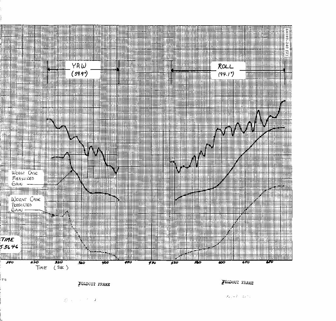
ZOLL

_O7_OUI _

+++, . + ,_+ _+ + '

+

-13¥

go /o /._ /eo .zoo d_¥O

Figure 5.4-20. DSIF Received Signal Strength During k_ern_inal Descent

5.4-59

Post-Touchdown RF Assessment

Shortly after touchdown, omnidirectional antenna A was selected

for transmission for the first time since the prelaunch countdown. The signal

level at the DSIF changed from -IZ3.3 dbm to -133 db as was predicted from

the omnidirectional antenna patterns.

The transmitter 13 output power after touchdown was =_ 39. 9 dbm. At

approximately i hour after touchdown, transmitter A was turned on for the

first time since the prelaunch countdown. The output power for transmitter

A was computed to be 40.4 dbm at turnon and decreased to 39. 7 dbm at turn-

off, which was _ I hour and 45 minutes later. Figure 5.4-21 is a plot of

transmitter A output power from turnon until --_30 minutes before turnoff.

The gradual power dropoff is apparent in this plot.

The traveling-wave tube temperature for transmitter A during the

first 7 minutes after turnonis shown in Figure 5.4-22. STV 6 data adjustedto the same initial conditions at turnon is also plotted on this figure and shows

good correlation between the thermal rise time for both sets of data. Thisdata is included in this report because there was some indication that the

transmitter A temperature rise at turnon increased during the prelaunch testphases. This rise does not seem to be the case, however, based on the data.

TV Performance

The first 200 line TV picture was transmitted at ="49 minutes after

touchdown. Based on reported DSIF signal levels, the con_puted SNR for the

first picture was 15. 5 db + Z db.

The first 600 line TV picture was transmitted at _" 4 hours after touch-

down shortly after the planar array was aligned with the earth. Based on

reported DSIF signal levels, the computed SNR for the first picture was

15.0+ 2 db.

In both cases, the SNR was high enough to provide good quality detected

video data as can be noted in the quality and resolution of the pictures.

Optimum positioning of the planar array and higher transmitter output

power later on during the lunar day increased the 600 line SNR as much as

='4 db above the SNR of the first 600 line TV picture. The SNR for the 600

line TV thus varied between 15 and 19 + 2 db during the picture taking

sequence.

Receiver Signal Level Variations Resulting from A/SPP

Positioning

During the positioning of the solar panel and planar array after land-

ing, large variations in receiver A signal ievels were observed. This was

not surprising since the position of omnidirectional antenna A (now extended)

was such that the A/SPP could interfere with the line of sight between the

5.4-6O

t_,_ _±- J d_- _-_ _-_ ....... m__ .... 4_-- _--_t.--._---_-L_ _-_ _.__

; i l , i I................

.... , .... _ ..... _.... t........ t......t _."_-%::_:

-++..... <:+ .....I__+_ ++ +++ _____+=:....... :++_-ii.... .I ......... + ....... t - - _ ......... _ .... +--

+:+=+t+--::-::.-_:-_+ x -': :_i : • t :t k - +: t_- +:-+ ::::___:--:r "+ _. • - _ _ l + ] " _ i " -" " ::-+::

+.:-:u _=-:.-o _+ ' t ' -I b l i [ t.... t} : / ..... . " + Li : T I _- : - ; : + ---Z

+ " +d _-+-__--_/--_+--: L-+:-_d-:_x :' ! : +._ -I i i -

4 J+i _: i -+. : _ _.p+ i . _ : l +, i - +_' -I

,_++ k .... + _i,+....o___ • iT_< i:., _- I _x _:_--:.: !#.l..a_ Lr,--a._:C_ i i_ L+:--={

o

r,.-i©

r8

@

<+--,t

0

u

0

c-,li

d©

.,--t

5.4-61

PRECEDING PAGE BLANK NOT FILMED.

I

Figure 5.4-22. Transmitter A Traveling-Wave Tube Temperature Versus Time

5.4-63

omnidirectional antenna and the earth. The signal levels for both receivers

during this period are shown in Figure 5. 4-Z3.

This data is quite significant since it demonstrates that large variations

in omnidirectional antenna gain patterns can result from movement of the

A/SPP. Omnidirectional antenna patterns are consequently made invalid once

the position of the A/SPP is moved significantly from the position the A/SPP

was in during the omnidirectional antenna pattern measurements.

Special Receiver Threshold Test

On day 160 at---16:00 GMT, a special spacecraft command receiver

threshold test was run. The DSIF transmitter output power was decreased

from 70 to 46 dbm, at which time a spacecraft receiver/decoder index was

observed. Receiver A and B AGC in raw counts was recorded during this

test, and correlation to previous test data was attempted. As discussed in

subsection 5.4.7, the previously assumed temperature-engineering data

relationship was shown to be in error and, consequently, the data from this

test was used to establish a new calibration curve for postmission analysis

work. The test data is summarized in Table 5.4- ll.

TABLE 5.4-i1. TELETYPE DATA DURING RECEIVER

THRESHOLD TEST

T ime,GMT

16:28:00

16:35:30

16:36:35

16:39:15

16:43:50"

16:51:00

16:52:15

16:53:15

16:54:10

16:56:00

16:56:45

16:57:15

16:59:10

Station I I

Transmitter

Power, dbm

P70

P60

P58

P56

P58

P56

P54

P52

P50

P48

P46

P44

P70

P70

P70

Spacecraft

Receiver/

Decoder

B A

B A

B A

B A

D9-Receiver A

AGC

Z39

338

356

369

357

369

3 80

388

393

396

398

399

Z46

Z46

B A

B A

B A

B A

B A

B A

A B

Oscillating

B B

A A

Command

mode off

B A Z44

D10-Receiver B

AGC

177

262

28O

295

281

Z79

311

3Z5

335

343

349

353

182

182

180

At this point it was found that receiver B was locked to a sideband.

Transmitter power was returned to P58 dbm, and receiver B acquired.

Receiver/decoder selector cycled to obtain original combination.

Note: Phase lock was held on both receivers A and B throughout.

5.4-64

68189-244 (U)

- ,o ,

o

o

°,--t

C_

o

c_.,-t

c_

.,.-(

u?

©

©

c_

c¢3

c,.lI

5.4-65

Voice Transmission via the Transponder

On day 164 during the first lunar day (June 13), an experiment was

run in which the uplink carrier was modulated by voice, tracked by the space-

craft transponder, and relayed back to the ground. The experiment was

considered to be more or less an attempt to determine the feasibility of the

voice transmission scheme. Consequently, no detailed analysis of the expected

voice quality or bandwidth limitations was undertaken.

The basic scheme used was to phase modulate the uplink carrier,

resulting in the voice data being tracked by the spacecraft transponder. The

transponder trackingloop filter has a 3 db information bandwidth of--100 cps

and falls off at 12 db/octave. Due to the low frequency response of the loop

filter, severe attenuation to the voice information occurred.

The ground detection was via a standard FM detector. ]By using FM

discrimination, the amplitude falloff due to the phase lock loop filter response

was partially compensated. The resulting detected voice information at the

ground receiver was of poor quality, as expected, but was audible.

5.4.7. 8 Subsystem Telemetry Data (Transit)

The pertinent subsystem telemetered data for the transit and early

lunar phase are contained in Figures 5.4-24 through 5.4-33. Variations in

the data are explained in each figure. In general, all data indicated nominal

performance, and no variations were noted which were unexplainable or

suspect of anomalous performance.

Due to postmission data processing problems, the subsystem data

from L + 36 to L + 42 hours is missing (see Section 5. l). The plots are thus

invalid during this period even though there appears to be data in the above

mentioned period.

A brief summary of each figure and the more significant points relative

to each figure follow:

Receiver A AGC (Figure 5.4-24) -- In review, the data tends to con-

firm the fact that omnidirectional antenna A was not deployed. Step changes

in signal lew_l occurred whenever the pointing vector changed either due toDSIF station transfer or termination of gyro drift checks.

Receiver t3 AGC (Figure 5. 4-2.5) -- This data compared well withpredictions and also exhibited sensitivity to small pointing vector changes.

Receiver A AFC (Figure 5. 4-26) -- Receiver A was in the AFC mode

throughout transit. This data represents the DSIF transmitter frequency off-

set from the AFC center frequency during the transit phase. A large error

due to dol_pler shift rate is noted at acquisition. Steps in the data occurredat station transfer because the stations retuned their transmitters, to comt)en-

sate for expected doppler shift due to the earth's rotation. The downward

5.4-66

shift between station transfers is caused by the earth's rotation. Signalprocessing induced "glitches" can also be observed in this data. Due to the

high impedance of this signal, several predicted signal processing effects are

apparent. Steps occurred in the data at high power turnon due to return line

drop caused by the additional current in the ground return lines during high

power operation. Spikes occurred during engineering interrogations of mode4

due to step change in commutator unbalance current.

Receiver B Static Phase Error (SPE) (Figure 5.4-27) -- Receiver B

was used for transponding through most of the mission. This data thus

represents the DSIF transmitter frequency offset from the receiver phase

lock center frequency. Since this data is analogous to the AFC data discussed

above, the comments apply equally well to this data. It should be noted,

however, that this signal is not as sensitive to signal processing inducederrors.

Receiver A SPE (Figure 5.4-28) -- Since receiver A was in the AFC

mode, the transponder and, hence, SPE telemetry was not actually used.

However, the telemetered data does contain some interesting points. Signal

processing induced steps occur during high power operation. The temperature

sensitivity of the isolation amplifier is noticeable in the gradual variations in

the telemetry output. These variations correlate exactly wtth variations in

the compartment A bottom tray temperature (see Figure 5. 4-31). The

telemetry value of _- 600 kc offset corresponds to the 0 or near 0 volt telem-

etry output of the isolation amplifier.

Receiver B AFC (Figure 5.4-29) -- Since the receiver was phase

locked during the majority of the transit phase, this telemetry signal was not

a valid signal. Unlike the SPE signal, which has a 0 volt output when notbeing selected, the AFC telemetry does vary with frequency changes even

when the receiver is not in the AFC mode. However, the telemetry is not

valid and is essentially meaningless. As in the AFC telemetry for receiverA,

this signal also shows several signal processing induced "glitches."

Compartment A Tray Temperature (Figures 5.4-30 and 5.4-31) -- This

data represents the temperatures of the top (V-15) and bottom (V-16) of the

compartment A thermal tray. Thereceivers and transmitters are attached

to this tray and, consequently, this data is the only temperature data which

even approximate subsystem unit temperatures. The tray bottom data tends

to be less responsive to local heating at the transmitter traveling-wave tubes

and is considered more indicative of unit temperatures.

Transmitter Traveling-Wave Tube Temperatures (Figures 5.4-32 and

5.4-33) -- This data represents the temperature of the traveling-wave tubes

used for high power transmitter operation.

5.4-67

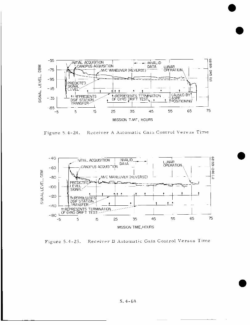
m

F,,

W

wd

_J

zoO3

/INITIAL ACQUISITION 1 _ N'VALID I _-

._/ _CANOPUS ACQUISITION ii n DATA LUNAR

ii_'L, i_-"__M/C MANEUVER (REVERSE)_ OPERATION_ I

PREDICTED J k I I k_-_SIGNAL_ __ 1 _ [ I _

,-REPRE_ - CAUSED B _-_ _

DSIF STATION__ OF GYRO DRIFT TEST_ , 'f _R_,,--,,,,,,,,,,_II

TRANSFER / _ _ _ ........... 7 _L-- L _-

5 15 25 55 45 55 65 75

MISSION TIME, HOURS

Figure 5.4-24. Receiver A Automatic Gain Control Versus Time

E0

C]

W>wii<[zoO0

-4O

-60

-80

-I00

-120

-140

- 180

-NTALACQUSTON T INVALID]-[ _ T ]

_" I 'i DATA _7_ "1 LUNARTn N I_L/CANOPUS ACQUISITION ; 1 ur ..... ,

I , i t t t t 4 tf_-=REPRESENTS _ II[D_IF STATIo_S_

,___TREANSF72 _TERR_i_iN_TIOtN t_- ,,- ' '

OF GYRO DRIFT TEST-_

- 5 ,5 15 25 255 45 55 65 75

MISSION TIME, HOURS

Figure 5.4-25. Receiver ]5 Automatic Gain Control Versus Time

5.4-68

v

>_-(JzbJ

0b.;n_b-

n_bdh-ZW0

I.--w

u_o

25

15

5

-5

-15

-25

-5 0

INITIAL S/C

XMTI_

FREQUENCYADJUSTMENT

iVARIATION DUETO CHANGE INDOPPLER SHIFT

BIT RATEFROM 1100_550 BPS

STEP CAUSED

BY TURNING

ON XPONDERDATA PROCESSINGERROR -(SPIKENOT CONFIRr

IS DUE TO DSIF

STEP DUE TO CHANGE TUNING JUST PRIOR TOIN TM RETURN LINE RETRO PHASE. XMTRVOLTAGE DROP CAUSED WAS TUNED IN A DIRECTIOIkBY HIGH POWER XMTR TO OFFSET EXPECTEDTURN ON/OFF DOPPLER SHIFT AT

t -- REPRESENTS TIME WHENSWITCH TO MODE 41

t - REPRESENTS DSIFSTATION TRANSFER

_INVALID

DATA

I0 20 30 40 50 60

MISSION TIME, HOURS

7O

Figure 5.4-26. Receiver A Automatic Frequency ControlVersus Time

Y

>_-ozw

(31w

b_

w

zw

oo_b_

F-W

b_b_C

I00

6O

2O

-2O

-6O

I I iI

i I9

CHANGE IS DUE TO DSIFTUNING JUST PRIOR TORETRO PHASE.

INITIAL S/C TRANSMITTER WAS TUNEDACQUISITION IN A DIRECTION TOOFFSET

--DSlF XMTR FREQUENCY EXPECTED DOPPLER SHIFT-

ADJUSTMENT _ PREDICTED AT RETRO BURN

/r _1 t t t t t . ' yLSTEP IS DUE TO CHANGE IN TM RETURN LINE _/

-_-_VOLTAGE DROP CAUSED BY HIGH POWER XMTR_--

\TURN ION/OFF [ fJREPRESENTS DSIF /

VARIATION DUE TO CHANGE STATION TRANSFER

IN DOPPLER SHIFTi I

TRANSPONDER B _

(VALUE "" 0 VOLT )

c

0 I0 20 30 40 50 60 70

MISSION TIME, HOURS

Figure 5.4-27. Static Phase Error B Versus 'rime

5. 4-69

I7_!_;_ __.....i_,41

@

-,4

OO

@

>

<

0

(1)

,,--_

odc'd

i

it5

©

5.4-70

-_ 68189-250

¢)

-r-I

r,b

¢)

_>

0

4--)

0

>,u

¢)

o_¢)

0-4--)

<

©>

¢)

@r_

o4o,l

I

d@

5.4-71

E_

;>

©

¢)

0

E_

<

©

©

L)

oI

W

5.4-7Z

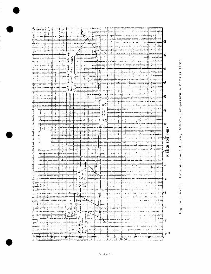
--_ 68189-252 (U)-

?

-r-,I

I"4

I-i

4--1

©.l-I

o

I-t

<

©

o

I

5.4-73

i

t I 17-],

i+17 •' i i • I -I'+i '

I

©

>

I

<

|

t_

5.4-74

-IJ::: -:

o

0

;>o

o

o

_q

o

I

,go

b.0.,-._

5.4--75

.

.

.

8 REFERENCES

M.R. Weiner, "Surveyor Mission A-- Telecommunications Subsystem

Prediction and Performance Summary Document," Hughes Aircraft

Company, SSD 64181R.

J. Votaw, "Telecommunication Subsystem SPAC Detailed Operational

Procedures (Telcom DOP)."

K.C. Beall and L.C. Gee, "Surveyor I Fligl_t Performance Quick Look

Report, " 17 June 1966.

C.M. Meredith, "Surveyor I-- Flight Path Analysis and Command

Operations Report, " Hughes Aircraft Company, SSD 6814ZR, Z4 June1966.

F.K. Rickman, "Data Link and Signal Processing Subsystem Final

Report on the SC-I STV Test, " IDC No. 2253. 3/451, ii April 1966.

5.4.9 ACKNOWLEDGMENTS

Frank K. Rickman, coordinator of this section.

The following people also contributed to the preparation of this section

of this report:

The SPAC Telecommunications Team consisting of John Steineck,

Vern Story, Joe Votaw, and Mike Williams who managed to maintain an

accurate set of records and note significant events on the data in real time

so that the postmission analysis was much more easily accomplished.

The Post Flight Analysis section, headed by R. Leuschner, for their

invaluable aid in processing and presenting the majority of the data containedin this section.

Jan Garrick for her assistance in the plotting of antenna pattern data

on the receiver AGC data plots.

R. Leuschner for the investigation and analysis of the parity errors

observed during the latter portion of the mission.

5. 4-76

5. 5 SIGNAL PROCESSING

5. 5. i INTRODUCTION

The signal processing subsystem is composed of the following units:

l) Engineering signal processor (ESP)

2) Auxiliary engineering signal processor (AESP)

3) Central signal processor (CSP)

4) Signal processing auxiliary (SPA)

5) Low data rate auxiliary (LDRA)

These units contain two electronic commutators with a total of six operational

modes, two analog to digital converters that have available 5 digital bit rates,17 subcarrier oscillators for transmission of pulse coded modulation data and

continuous real-time data, 9 summing amplifiers, and signal conditioning

circuits for the measurement of electrical currents and temperatures. The

subsystem performed normally throughout the transit and lunar phase of theSC-1 mission.

5. 5. 2 MAJOR SIGNAL PROCESSING SUBSYSTEM EVENTS DURING

TRANSIT

The commutator modes and bit rates used throughout the transit

phase are listed in Table 5. 4-2 in Section 5. 4. The signal processing con-

figuration (A/D converter used) is shown in Table 5. 4-3 of Section 5. 4.

5. 5. 3 PERFORMANCE SUMMARY

Listed in Table 5. 5-1 are the significant performance parameters

compared with the values measured during STV.

5.5-1

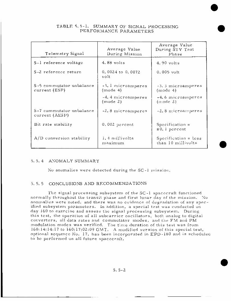
TABLE 5. 5-i. SUMMARY OF SIGNAL PROCESSING

PERFORMANCE PARAMETERS

Telernetry Signal

S-I reference voltage

S-Z reference return

S-5 commutator unbalance

current (ESP)

S-7 commutator unbalance

current (AESP)

Bit rate stability

A/D conversion stability

Average Value

During Mission

4. 88 volts

0. 00Z4 to 0. 007Z

volt

-3. l microamperes

(mode 4)

-4. 4 microamperes

(mode 2 )

-Z. 8 microamperes

0.002 percent

i. 4 millivolts

maximum

Average Value

During STV Test

Phase

4. 90 volts

0. 005 volt

-3.3 microamperes

(mode 4)

-4.6 microamperes

(mode Z )

-Z. 8 microamperes

Specification =

±0. I percent

Specification = lessthan 10 millivolts

5. 5. 4 ANOMALY SUMMARY

No anomalies were detected during the SC-I mission.

5. 5. 5 CONCLUSIONS AND RECOMMENDATIONS

The signal processing subsystem of the SC-I spacecraft functioned

normally throughout the transit phase and first lunar day of the mission. No

anomalies were noted, and there was no evidence of degradation of any spec-

ified subsystem parameters. In addition, a special test was conducted on

day 160 to exercise and assess the signal processing subsystem. During

this test, the operation of all subcarrier oscillators, both analog to digitalconverters, all data rates and commutator modes, and the FM and PM

modulation modes was verified. The time duration of this test was from

160:14:14:17 to 160:17:0Z:09 GMT. A modified version of this special test,

optional sequence No. 17, has been incorporated in EPD-180 and is scheduled

to be performed on all future spacecraft.

5.5-Z

To provide the necessary data to more fully evaluate the subsystem,the following information is requested when the tapes from optional sequenceNo. 17 are processed in the future:

i) Six frames of raw data for all commutator modes with A/Dconverter Z at the 550 bits/sec data rate

2) Six frames of raw data for coast mode commutator with A/D

converter I at the 550 bits/sec data r_te

3) Recorded data rate frequencies for all A/D converter Z data rates,

and for the 550 bits/sec rate for A/D converter 1

4) Recorded frequency of all accelerometer apd touchdown strain

gage subcarrier oscillators

5) Recorded frequency of the gyro speed subcarrier oscillator

6) Recorded maximum and minimum frequency of the enable/reject

subcarrier oscillator

7) Recorded maximum and minimum frequency of all the PCM sub-carrier oscillators

This information was not available for the evaluation of the SC-I subsystem.

Changes to the engineering data reduction program for unbalance

current correction (see subsection 5. 5. 6. i) and for current amplifier

calibration (see subsection 5. 5.6. 3)are also recommended.

5. 5. 6 SUBSYSTEM PERFORMANCE ANALYSIS

5. 5.6. i Commutator Unbalance Current Correction

In the ESP and AESP commutators, transistor switches connect each

analog output voltage, which represents either a spacecraft voltage, tem-

perature, or current, with a common commutator line connected to the input

of one of two analog to digital converters. A bootstrap unloader is connected

to this common line to reduce the stray capacitance, equalize the load imped-

ance, and provide bias current for the commutator and master switches.

Since the bias current required for the commutator and master switches is

not exactly equal, a difference or unbalance current exists, which is delivered

to, or must be supplied by, the telemetry circuit being commutated. The

magnitude of the error in each telemetry channel due to unbalance current isa function of the unbalance current at the time of commutation and the telem-

etry channel's output impedance.

The unbalance current for a specific telemetry channel in the ESP and

in the AESP commutators is measured and commutated in modes 2, 4, and 5.

The telemetry plots of the unbalance current indicated that the approximate

5.5-3

current in mode 2 (Figure 5. 5-i) was -4. 5 microamperes (_a), in mode 4was -3. 1 _a, and in mode 5 (Figure 5. 5-2) was -2.8 _a during the transitphase of the mission. The change in current between modes 2 and 4 iscaused by internal ESP load changes and is listed on the SC-I signaturelist (Reference i) as follows:

S-5, Commutator Unbalance Current, Variations

There is approximately a 1 to i. 5 microamp change in unbal-ance current in going from Mode 4 to Mode Z (Z microampsversus 3. Z microamps}, and a variation of approximately 0. 5microamps within the same mode.

The AESP mode 5 unbalance current initially read -Z. 0 >a at launch, but therewas no good data from launch to g + 15 minutes. After that period, the cur-rent increased to -Z. 8 _a. It was noted that each time the unit was turnedoff, the magnitude of unbalance current at unit turnon was less than -Z. 8 _a.This is particularly evident at mission times l hour and 65 hours. This isattributed to unit warmup, and a similar condition existed during the STVtest phases.

In order to fully correct the telemetry data for unbalance currenteffects, it is necessary to know the value of the unbalance current for eachword in each commutator. This can be done by knowing the relationship ofthe unbalance current for each word to that commutated telemetered unbalancecurrent. This can be shown as a correction to be applied to the telemeteredunbalance current in Reference 2, determined from unit FAT data. The out-put impedance of each channel, used to determine the nominal unbalancecurrent correction, is shown in Table 5. 5-Z.

Automatic Corrections Incorporated in EDRS Program

The engineering data reduction program utilizes the commutated

value of unbalance current, multiplied by the appropriate output resistance,

to correct for offset errors caused by unbalance current in the other telem-

etry channels. Several approximations, which affect the accuracy of these

corrections, are made to simplify this program. The first approximationwas that the commutated value of unbalance current was the same for each

commutator switch. Unit test data for the SC-I units indicates that the unbal-

ance current for certain commutator switches may be as much as -3. 9 to

4. 5 _a offset from the commutated value. For telemetry channels with a

high output impedance (50 K ohms), this approximation could result in a

worst-case correction error of 46 decimal counts.

The second approximation was the assumption that the output impedance

of each telemetry signal was a pure resistance. The majority of the flight

control telemetry channels output circuits (see Table 5. 5-Z) are a parallel

combination of a resistor and capacitor. A typical circuit, such as FC-16

(pitch gyro error), has a resistance of 27. 5 K in parallel with a capacitance

of Z. ? _f. At the high telemetry data rates of 4400, ii00, and 550 bits/see,

the output capacitor will tend to nullify the effects of the unbalance current.

5. 5-4

'1 7i ',

i l _, I, ' , 'J _J !

i,,; I I, I

tl,

_-ii !!il I

_ ,:11 illi

-_ lili !l!i

I i I I i i ! ] I I ]

_+ , , , i I

,i _ hl Ii

_4- ' I

4_

D

N

O

E

, ,_, ,

o

.... _ N

_ ,U3

_4

.,--_

5.5-5

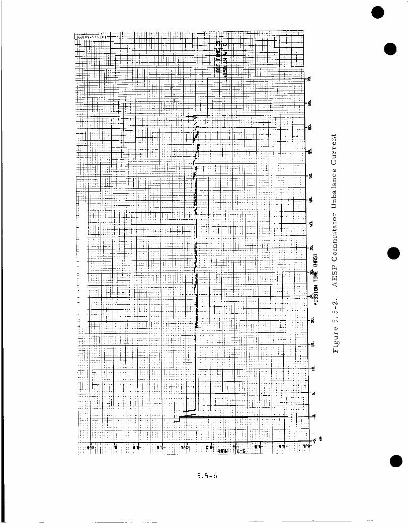
-d

_2

o

U

u

D

o

o

<

4I

IX3

_d©

5.5-6

Correcting for the offset error, without considering the output capacitor,

will introduce an error of approximately 16 decimal counts for this telemetrychannel.

TABLE 5. 5-2. DATA CHANNEL OUTPUT IMPEDANCES

Subsystem

Data Link (D)

I. Omnidirectional antenna A

transmitted power

3. Omnidirectional antenna B

transmitted power

7. Static phase error A

8. Static phase error B

9. Receiver A AGC

10. Receiver B AGC

13. Transmitter A temperature

14. Transmitter B temperature

16. Receiver A AFC

17. Receiver B AFC

Electrical Power (EP)

i. 29 volt nonessential voltage

2. Unregulated bus voltage

3. Main battery manifold

pressure

4. Unregulated output current

5. Main battery voltage

6. Battery charge current

Output Impedance for

Analog TelemetryChannels

Resistance,ohms

5O

5O

800

800

IIK

IIK

7100 at 100°C000 at 250°C

4.7K

4.7K

2.55K

4.125 K

>2K

<40

4.166 K

<40

Capacitance,

Mf

4.7

4.7

5. 5-7

Table 5. 5-Z (continued)

,

Subsystem

Electrical Power (EP) (Cont)

Boost regulator differencecurrent

8. Main battery temperature

9. Battery discharge current

10. Solar cell array voltage

ii. Solar cell array current

12. Solar cell array temperature

13. Boost regulator temperature

14. Regulated output current

16. Optimum charge regulator

output current

17. RADVS and squib current

18. Full scale current

calibration (ESP)

19. Midscale current calibration

(ESP)

Z0. Zero scale current

calibration (ESP)

21. Compartment A heatercurrent

22. Compartment B heatercurrent

Output Impedance for

Analog Telemetry

Channels

Re sistanc e,

ohms

<40

700 at 100°C,1000 at Z50°C

<40

Z. 37K

<40

700 at 100°C,

1000 at Z50°C

700 at 100°C,1000 at Z50°C

<40

<40

Capacitance,

uf

<40

<40

<40

5.5-8

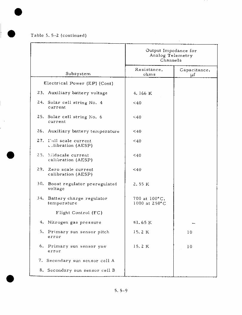
Table 5. 5-2 (continued)

Subsystem

Electrical Power (EP) (Cont)

23. Auxiliary battery voltage

24. Solar cell string No. 4current

25. Solar cell string No. 6current

26. Auxiliary battery temperature

Z7. l',Lllscale current

_libration (AESP)

23. k_dscale current

calibration (AESP)

29. Zero scale current

calibration (AESP)

30. Boost regulator preregulated

voltage

34. Battery charge regulator

temperature

Flight Control (FC)

4. Nitrogen gas pressure

5. Primary sun sensor pitcherror

6. Primary sun sensor yaw

error

7. Secondary sun sensor cell A

8. Secondary sun sensor cell B

Output Impedance for

Analog TelemetryChannels

Resistance,

o_Ims

4.166 K

<40

<40

<40

<40

<40

<40

2.55K

700 at 100°C,

1000 at 250°C

gl. 65 K

15.2K

15. ZK

Capacitance,

_f

l0

10

5.5-9

Table 5. 5-2 (continued)

Output Impedance for

Analog Telemetry

Channels

Subsystem

Flight Control (FC) (Cont)

Secondary sun sensor cell C

Secondary sun sensor cell D

Resistance,

ohms

Canopus error

Star intensity signal

Acceleration error

Pitch gyro error

Yaw gyro error

Z5.5K

50K

ZI.6K

Z7.5K

Z7.5K

o

10.

IZ.

14.

15.

16.

17.

25. Thrust command to vernier

engine No. 1

Z6. Thrust command to vernier

engine No. Z

27. Thrust command to vernier

engine No. 3

3Z. Retro accelerometer

35. Radar altimeter range signal

39. Doppler velocity Vx

40. Doppler velocity VY

41. Doppler velocity Vz

43. Roll actuator signal

44. Flight control electronics

unit temperature No. l

4Z. 5K

4Z. 5K

4Z. 5K

5K

44.6K

31. ZK

31. ZK

44.6K

Z0K

700 at IO0°C1000 at 250°C

Capacitance,

_f

I0

i0

0.68

Z.7

Z.7

0.68

0.68

0.68

i0

I0

i0

I0

I0

5.5-10

Table 5. 5-2 (continued)

Subsystem

Flight Control (FC) (Cont)

45. Flight control electronicsunit temperature No. 2

46. Roll gyro temperature

47. Canopus sensor temperature

48. Nitrogen gas tanktemperature

49. Roll precession command

50. Pitch precession command

51. Yaw precession command

53. Secondary sun sensorcentercell

54. Pitch gyro temperature

55. Yaw gyro temperature

70. Attitude gas jet No_ Ztemperature

71. Roll actuator temperature

Mechanisms (M)

3. Solar panel position

4. Polar axis position

6. Elevation axis position

Output Impedance forAnalog Telemetry

Channels

Resistance,ohms

700 at 100°Ci000 at Z50°C

No effect

700 at 100°Ci000 at Z50°C

700 at 100°C1000 at Z50°C

78K

78K

78K

51.11/

No effect

700 at 100°C1000 at 250°C

700 at 100°C1000 at Z50°C

g525

<510

<525

Capacitance,uf

3.9

3.9

3.9

5. 5-11

Table 5. 5-2 {continuedl

Subsystem

Mechanisms (M) (Cont)

7. Roll axis position

8. Planar array temperature

10. Solar panel stepping motortemperature

iZ. Elevation axis steppingmotor temperature

Propulsion (P)

i. Helium pressure

2. Oxidizer pressure No. 3

3. Upper retro case temperature

4. Vernier lines No. Ztemperature

5. Vernier fuel tank No. 2temperature

6. Vernier oxidizer tank No. 3

7. Vernier engine No. 1

temperature

8. Vernier lines No. l

temperature

9. Vernier lines No. 5

temperature

i0. Vernier engine No. Z

temperature

Output Impedance for

Analog TelemetryChannels

Re sistance,

ohms

<525

700 at IO0°C

1000 at Z50°C

700 at 100°C

1000 at Z50°C

700 at IO0°C

1000 at Z50°C

<i. 65K

<52-5

700 at IO0°C

1000 at Z50*C

Capacitance,

_f

5. 5-12

Table 5. 5-2 (continued)

Subsystem

Propulsion (P) (Cont)

ii. Vernier engine No. 3temperature

12. Lower retro case temperature

13. Vernier fuel tank No. 1temperature

14. Vernier fuel tank No. 3temperature

15. Vernier oxidizer tank No. Itemperature

16. Vernier oxidizer tank No. 2temperatur e

17. Helium tank temperature

18. Vernier engine No. 1 straingage

19. Vernier engine No. 2 straingage

20. Vernier engine No. 3 straingage

22. Retro nozzle temperature

Radar (R)

2. RADVS -- R amplitude

3. RADVS -- D l amplitude

4. RADVS -- D Z amplitude

Output Impedance for

Analog TelemetryChannels

Resistance,

ohms

700 at 100°C

1000 at 250°C

-%

i

,350I

700 at 100°C

I000 at 250°C

II. 7K

II.7K

II.7K

Capacitance,

Mf

i0

i0

l0

5.5-13

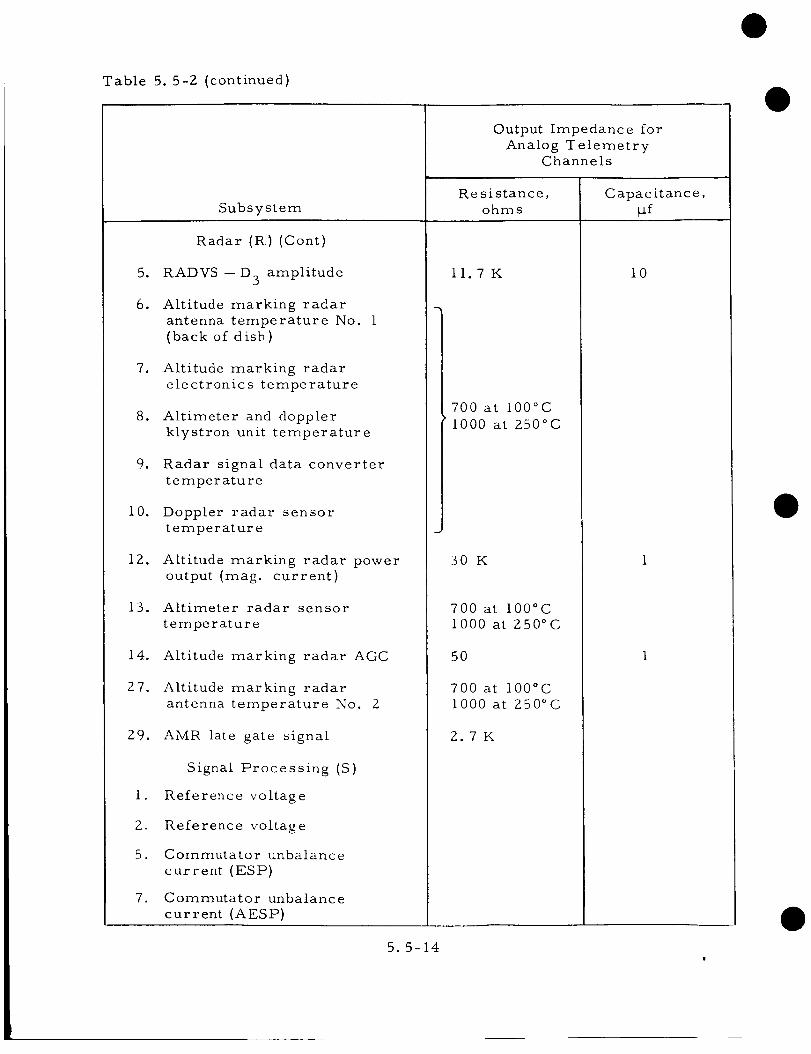
Table 5. 5-2 (continued)

Subsystem

Radar (R) (Cont)

5. RADVS -- D 3 amplitude

6. Altitude marking radar

antenna temperature No. 1

(back of dish)

7. Altitude marking radar

electronics temperature

8. Altimeter and doppler

klystron unit temperature

9. Radar signal data converter

temperature

10. Doppler radar sensor

temperature

12. Altitude marking radar power

output (mag. current)

13. Altimeter radar sensor

temperature

14. Altitude marking radar AGG

27. Altitude marking radar

antenna temperature No. 2

29. AMR late gate signal

Signal Processing (S)

1. Reference voltage

2. Reference voltage

5. Gommutator unbalance

current (ESP)

7. Gommutator unbalance

current (AESP)

5. 5-14

Output Impedance for

Analog Telemetry

Channels

Resistance,

ohms

II.7K

I 700 at lO0°C

I I000 at 250°C

30K

700 at 100°C

1000 at Z50°C

5O

700 at 100°C

1000 at 250°C

2.7K

Capacitance,

_f

I0

Table 5. 5-2 (continued)

Subsystem

Survey Television Camera (TV)

16. Survey camera electronics

temperature

17. Survey camera mirror

assembly temperature

Approach Television Camera (T)

i. Approach camera vidicon

faceplate temperature

3. Approach camera

electronic s temperature

Vehicle (V)

5. Landing gear No. 1 deflection

6. Landing gear No. Z deflection

7. Landing gear No. 3 deflection

15. Compartment A temperature

thermal tray top

16. Compartment A temperature

lower support

17. Compartment A temperatureinsulated retainer

18. Compartment A temperaturecanister

19.

20.

Compartment A temperature

switch No. 5 in contact ring

Compartment A temperature

switch No. 5 in face radiator

Output Impedance for

Analog Telemetry

Channels

Re sistance,

ohms

700 at 100°C

1000 at 250°C

700 at IO0°C

I000 at Z50°C

<656

IIi

I

} 700 at IO0°C1000 at Z50°C

Capacitance,

_f

5. 5-15

Table 5. 5-2 (continued)

Subsystem

Vehicle (V) (Cont)

21.

22.

23.

24.

25.

26.

Compartment B temperature

tray top center

Compartment B temperature

lower support

Compartment B temperaturecanister

Compartment B temperatureswitch No. 4 in face radiator

Compartment A temperatureswitch No. 8 in face radiator

Compartment B temperature

switch No. 4 in contact ring

27. Upper spaceframe

temperature No. 1

28.

Z9.

Lower spaceframe tem-

perature under compartment B

Wiring harness temperaturethermal tunnel

30. Shock absorber No. l

temperature

31. Leg No. g upper web

temperature

32. Shock absorber No. 2

temperature

33. Shock absorber No. 3

temperature

Output Impedance for

Analog Telemetry

Channels

Re sistance,ohms

, 700 at 100°Ci000 at 250°C

Capacitance,_f

5. 5-16

Table 5. 5-2 (continued)

36.

Subsystem

Vehicle (V) (Cont)

A/SP mast temperature

Upper spaceframetemperature No. g

Lower spaceframetemperature under

compartment A

37. Retro attach point No. 1

temperature

38. Retro attach

temperature

39. Retro attach

temperature

46.

47.

48.

point No. Z

point No. 3

Crushable block temperature

Compartment B temperatureswitch No. i in face radiator

Compartment B temperature

switch No. 5 in face radiator

Compartment A temperature

switch No. g in face radiator

Auxiliary battery

compartment temperaturebottom outside 1

Output Impedance for

Analog Telemetry

Channels

Resistance,

ohms

700 at 100°Ci000 at Z50 ° C

Capacitance,

_f

5.5-17

The third approximation was that all temperature channels had anaverage output impedance of 700 ohms, which corresponds to a temperaturevalue of ZI7°F. Since 98 percent of the spacecraft temperatures are below120°F, an approximation of 600 ohms or less is more accurate. The errorhere, however, is negligible.

The following changes to the engineering data reduction program forunbalance current corrections are recommended:

15 The temperature channels should not be corrected for unbalance

current offsets. With a 6 _ta unbalance current, the maximum

uncorrected unbalance current error is 3.6 millivolts, or less

than one decimal count.

z) Telemetry channels that have an output circuit of a paral]el

resistor and capacitor, with an RC time constant greater than20 milliseconds, should not be corrected. The uncorrected

unbalance current error is less than the present correction error

when the capacitor is ignored at the three high data rates.

35 Some provision should be made in the program for specifying theunbalance current for each individual commutator switch as a

function of the commutated value of unbalance current.

Procedure for Applying Unbalance Current Corrections

A method for more completely correcting for commutator unbalance

current has been developed by M.R. Weiner (Reference 25. This method is

intended for use where required for nonreal time, postflight data analysis.

It includes the following.

15 A method for determining for each channel whether it is necessary

to correct for unbalance current.

z) A method for hand calculating the correction for telemetry

channels having an output impedance that is either all resistive

or a parallel combination of a resistor and a capacitor.

3) A computer program for correcting those channels having an

output impedance consisting of a parallel combination of a

resistor and a capacitor.

The computer program has been used to correct data from SC-I STV tests

with very good results.

From the above procedures, Tables 5. 5-3 and 5. 5-4 have been pre-

pared. These tables indicate the ratio of the correction factor (assuming

6 kla and 1Z k_a of unbalance current, respectively) to the total telemetry

error for each voltage channel at each bit rate. The ratio shown is that

obtained at full scale where the offset voltage is greatest and the total error

percentage is minimum. Thus, those channels where the correction factor

5. 5-18

TABLE 5. 5-3. OFFSET VOLTAGE CORRECTIONS COMPARED TO TOTAL

ERROR FOR 6 _a UNBALANCED CURRENT

Channels

Gyro-pitch, yaw (FC-16, FC-17)

Precession command (FC-49, FC-50,

FC-51)

Primary sun sensor (FC-5, FC-6)

Canopus error (FC-1Z)

Star intensity (FC-14)

Secondary sun sensor center cell

(FC-53)

Acceleration error (FC-IS)

Retroaccelero;neter (FC-3Z)

Roll actuator (FC-43)

Radar altimeter (FC-35)

Doppler-- Vx, Vy (FC-39, FC-40)

Doppler-- Vz(FC-41)

Vernier engine thrust command

(FC-Z5, FC-Z6, FC-Z7)

Vernier engine strain gages (P-18,

P-19, P-Z0)

Regulated voltage (EP-I) at 29 volts

Unregulated voltage (EP-2) at 2Z volts

Main battery voltage (EP-5) at Z2 volts

Solar cell array volt (EP-10) at

50 volts

Auxiliary battery voltage (EP-Z3)

at gZ volts

Boost regulator preregulated voltage

Voltage (EP-30) at 30 volts

A/SPP readout potentiorneter

N Z pressure (FC-4)

Helium pressure (P-l)

Manifold pressure (P-Z)

Main battery pressure (EP-3)

Landing gear deflection (V-5, V-6, V-7)

Receiver AFC (D-16, D-17)

Repeatability

Receiver AGC (D-9, D-10)

Repeatability

NOte:

Bit Rates, bits/sec

X

X

X

X

X

X

X X X

X X X

X X X

X

X X X

X X X

X X

Negligible influence

X X X X X X

X X X X X X

X X X X X X

X X X X X X

X X X

Xs denote conditions where ratio of offset voltage correction to total

channel error is < l:10 or < 1:5 as indicated.

X

X

X

X

X

X

X

X X

X X

X X

X x

X

X

X

X

X

X

5.5-19

TABLE 5.5-4. OFFSET VOLTAGE CORRECTIONS COMPARED TO TOTALERROR FOR 12 _a UNBALANCED CURRENT

Channels

Gyro-pitch, yaw (FC-16, FC-17)

Precession command (FC-49, FC-50,

FC-51)

Primary sun sensor (FC-5, FC-6) X X X

Canopus error (FC-12) X X X

Star intensity {FC-14) X

Secondary sun sensor centercell (FC-53)

Acceleration error (FC-15) X

Retro accelerometer (FC-32)

Roll actuator (FC-43) X X X

Radar altimeter (FC-35)

Doppler--V x, Vy (FC-39, 40)

Doppler -- Vz(FC-41 )

Vernier engine thrust command X X(FC-25, FC-26, FC-27)

Vernier engine strain gages

(P-18, P-19, P-20)

Regulated voltage (EP-1) at 29 volts

Unregulated voltage (EP-2) at 22 volts

Main battery voltage (EP-5) at 22 volts

Solar cell array volt (EP-10) at 50 volts

Auxiliary battery voltage (EP-23)at 22 volts

Boost regulator preregulated voltage(EP-30) at 30 volts

A/SPP readout potentiometer

N 2 pressure (FC-4) X

Helium pressure (P-l) X X X

Manifold pressure (P-2) X X X

Main battery pressure (EP-3) X

Landing gear deflection(V-5, V-6, V-V)

Receiver AFC (D-16, D-17)

Repeatability

Receiver AGC (D-9, D-10)

Repeatability

Note:

Bit Rates, bits/sec

440O 1100 55O

1:10 1:5 1:10 1:5 1:10

X X X X

137.5 17.2

1:5 1:10 1:5 1:10 1:5

X

X X X X X

X X X X

X X X

X X X

X

Negligible influence

X X X

X X X X X

X X X X X

X X X

X

Xs denote conditions where ratio of offset voltage correction to totalchannel error is _- 1:10 or < 1:5 as indicated.

X

X

X X

X X

X

5. 5-20

is less than i/5 or i/i0 of the total error need not be corrected as the

correction will not significantly improve the overall accuracy. In addition,

to those indicated in these tables, none of the current channels need be

corrected as their output impedances are very small (see Table 5. 5-2).

5. 5.6.2 Potentiometer Reference Voltage

The 4.85 volt reference voltage is supplied by either the ESP or AESP

units to the landing gear and solar panel positior_potentiometers, to the

helium and oxidizer pressure transducers, and to the secondary sun sensors.

This reference voltage, which is derived from the 29 volt nonessential bus,

varies due to load and input supply voltage changes. The values of the ESP

reference voltage and return is telemetered in modes Z and 4 to increase the

accuracy of the channels using this voltage. Since the value of the AESP

reference voltage is not telemetered, it is necessary to compute its value

and apply the necessary corrections to the telemetry signals.

The method used to compute the difference between the ]ESP and

AESP reference voltage was to record the raw count telemetry value for

signals M-3 (solar panel position), M4 (polar axis position),and M7 (roll

axis position) when commutated in mode 4 (ESP) and mode 5 (AESP). The

data taken during an engineering interrogation prior to midcourse was used

for this purpose. At that time, the antenna solar panel was in the transit

pinned position and thus should be constant. Table 5. 5-5 gives the data

recorded and computations.

From the calculations, it can be concluded that the AESP reference

voltage is approximately 10 decimal counts or 48.8 millivolts greater than

the IESP reference voltage. This correction should be applied to all AESP

telemetry channels that use the reference voltage.

Data plots of the ESP reference voltage (Figure 5. 5-3) and return

(Figure 5. 5-4) indicate normal operation throughout the mission. An

increase of approximately 15 millivolts in the ESP reference voltage was

noted when switching from mode 2 to mode 4. The SC-I signature list

states, "SI (Pot Ref. Volt) will change 20 to 35 mv in going from Mode Z

to Mode 4 due to internal ESP loading changes. "

The ESP reference return voltage was less than i0 millivolts through-

out the mission. Some variations due to load changes at terminal descent

were noted, but these are considered normal when the AMR is commanded on.

5. 5. 6. 3 Current Calibration Signals

Current measurements are accomplished by measuring the voltage

drop across a low resistance shunt which is in series with the power line

being monitored. This measurement is in the range of 0 to 100 millivolts.

Since this voltage is not referenced to ground and is not scaled to the 0 to 5

volt telemetry input level range, it is necessary to amplify it with a differ-

ential amplifier. The nominal gain of this amplifier is 50, but its actual

5. 5-21

il b

Jliiil

j' I' I_

il

......... ±=£::=------

....... i _.; ,_ ..... t; .:i ± i .... ; .I . ;,i ..............

]1.; -_2: ,, : .; I ,; ,l_ I [.LLq[ ;I . _ I ...... t

,! ! • ......................" lit !!: :!'.;t :!::::!tl ::: ;::; .<h:! !!!!:ii!! !:iii!:!! T: :::t_::i:: :i:11:::!: :::: :::: :::: : :: :t:-: ::::Jii: :::il i',il::i : i!:: :ii:

Ub

0

{1,}

U

{1.}

{1,.}

{1,}

m

is ®

{,

q5.5-2.2

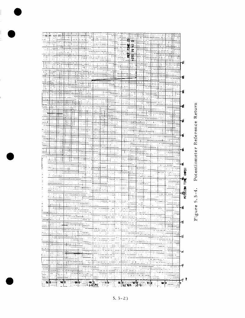
4_

c_

0

S

#I

u3

_d

5. 5-23

TABLE 5.5-5. COMPARISON OF MECHANISM SIGNALS INESP AND AESP COMMUTATORS

Time, GMT Mode Signal Telemetry Value

151:6:1:Z5

151:6:1:6

4 M-3

M-4

M-7

S-1 reference

voltage

M-3

M-4

M-7

Let X = AESP reference voltage

Then

760

353

491

1001

768

357

496

760 768 353 357 491 496

I001 X and 1001 - X and 1001 - X

X : 1011.5 X = 10!Z.3 X : 1011.Z

gain linearity and stability are not specified to a tight tolerance. To determine

these parameters of the current amplifier and thus increase the accuracy of

the current measurements, three calibration signals, which have a specified

stability of 0.2 percent, are individually amplified and commutated by the

telemetry system. The data reduction program uses these telemetered cali-

bration values to define the computer coefficients for the current measure-

ment channels for each frame of data.

Telemetry plots of these calibration values indicate that the gain of

the current amplifiers in the ESP and AESP remained essentially constant

throughout the transit phase of the SC-I mission. The average telemetered

ranges of values for these calibration signals are given in Table 5. 5-6. Some

noise was detected on these calibration signals, and an investigation of the

extent of the variations was completed for the time period beginning on

151:14:41:0Z GMT and ending on 151:14:56:00 GMT. The data indicated that

EP-Z7 was constant at a decimal count of 920, EP-28 was constant at a count

5. 5-24

TABLE 5. 5-6. AVERAGE VALUE OF CURRENT CALIBRATION SIGNALS

Signal,millivolts

Telemetry Range,millivolts

EP-18 current calibration (90) ESP

EP-19 current calibration (50) ESP

EP-Z0 current calibration (i0)

EP-Z7 current calibration (90)

EP-28 current calibration (50)

EP-29 current calibration (i0)

ESP

AESP

AESP

AESP

90.9 ± 0.2

50.6 ± 0.Z

10.3 ± 0.2

90.7 ± 0.2

50.7 ±0.2

10.6 ± 0. Z

of 513 with a jump to 515 every ten or twenty data points, and EP-29 was

varying between a count of i05 and 108. These variations are attributed to

system noise and are listed on the SC-I Signature List (Reference l) asfollow s :

EP-18, 19, Z0, 27, 28, 29, Current Calibration Signals, Variations

Variations of 3 to 5 BCD have been noted on all of the current

calibration signals (ESP as well as AESP) during the SC-1 STV

test phases when the transmitter was operating in low power

and thrust phase power was not on. Variations of up to 7 IBCD

have also been seen during transmitter high-power operation.

The variations in the output level of the current calibration duringthe transit phase indicate that, without any correction for the current

amplifiers' gain, the error of the current readings would be ±0.2 percent

of full scale. The present data reduction program updates the coefficients

for the current measurement channels each data frame. Since the long-term

gain of this amplifier is constant, it is recommended that the program be

modified to update the current measurement coefficients once immediately

after commutator turn on and once every hour following turn on.

5. 5.6.4 Temperature Measurement Errors at 4400 Bits/Sec Data Rate

The errors in temperature signals at 4400 bits/sec data rate result

from insufficient settling time for the constant current source used for these

measurements. The output capacitor on the constant current source, when

it is unloaded, charges to a value of approximately 6. 8 volts. At the high data

rate, this voltage does not reach the correct value by the time the particular

temperature channel is sampled. These errors may be partially corrected

in the manner described in the following paragraph.

5.5-25

The basic accuracy temperature channels can be grouped into twocategories when considering measurement accuracies at 4400 bits/see. Thefirst group, listed in Table 5. 5-7, contains those measurements which willhave errors only if the preceding temperature measurement (as indicatedin the table) is substantially different. These errors _re roughly 10 percentof the difference in the two temperatures and in the direction of the earliermeasurement; i.e., it can be a positive or negative error. The secondgroup, listed in Table 5. 5-8, contains those measurements which will alwayshave significant positive errors at 4400 bits/see. The amount of the erroris a function of the transmitted digital value as well as various circuitparameters. Table 5. 5-9 lists the range of the true value in BCD as afunction of tile transmitted value in BCD. Also, the approximate errors in

degrees Fahrenheit have been computed (using a nolcainal scale factor of

0. 9°F/bcd).

5. 5. 6. 5 Telemetry ]Bit Stream Characteristics

To retrieve the maximum an_ount of reliable telemetry information

froln the spacecraft, it is necessary to understand the characteristics of the

telemetry bit stream during periods when the commutator too(it or the

telemetry bit rate is changed. Erroneous telemetry data may bc processed

at these times, and it must be disregarded.

When the ESP or AESP commutator is turned off in older to switch

to the other commutator, the power supply voltages will not .settle to zero

voltage until approximately 10 n_illiseconds after the acceptance of the of 1-

command. During this period, the connn_utator output will bc unreliable.

Therefore, the last word of data at 17.Z, 137. 5, or 550 bits/see, the lasttwo words of data at 1100 bits/see, and the last five words at 4400 bits/see

should be rejected. When the comnnutator is con_pletely off, the tch'_ctrybit stream should contain data words that have a value of approximately

zero counts.

If a different mode on the same commutator is selected, with tl_e

exception of mode 3, a maximum of two data words nlay be affected (turin a

the n_ode change. The exact transition point can be detern_incd by con_par_u_

each word in the commutator frame during which the mode change took place

with the corresponding word in the preceding and following commutator

frames. Switching nnod_'s will not affect the commutator word counter.

Since mode 3 has a 50 word con_mutator fra:nc and modes 1, Z, and

4 ],ave 100 word frames, several abnormal conditions i_ay exist when

switching to mode 3. If the con_mutator word count is less than 48 at mode

change, a n_aximum of two data words may bc affcc-ed at transition, and th_n

the commutator would process mode 3 data with no interruption of the word

counter. If the commutator word count is greater than 48 _nd less than 89,

the word counter will continue to count to _vord _38 al:d then .]u_n t) to w,)rd 39.The information that will b(, conlrnutatcd from word 49 to 88 is li,,<l,,(l in

Table 5. 5-10. At word {9, normal mode 3 data \viii bc com_lutatcd. If th,,

colnlnutator word count is greater than 89 and 1.,ss than 98, the \vord counterwill continue to count to word 98 and then return to word 00. Th{, inforn_at[(_.

5. 5-Z6

TABLE 5.5-7. TEMPERATURE MEASUREMENTS INFLUENCED

BY PRECEDING TEMPERATURE

MEASUREMENT AT 4400 BITS/SEC

Temperature Measurement Preceding TemperatureAffected Measurement

Word

Mode I

Mode 2

Mode 4

Mode C

Signal Word

P -9 82

R-27 26

V -44 46

EP -26 78

P -3 68

P -5 66

P -6 86

P-12 88

P-13 56

R-13 96

V-3Z 58

EP -8 4

EP-13 l0

M -8 14

M-12 64

P-17 20

TV-16 16

V-16 26

V-18 30

V -20 36

V-22 46

V-26 54

V -27 56

V -29 66

V-33 76

V -36 96

V -37 84

V -38 86

D-13 l0

D-i4 30

EP -8 42

EP-12 36

EP-13 20

EP -26 96

EP-34 46

Signal

P -22 80

FC -45 24

FC -47 44

P-14 76

P-5 66

R-7 64

P-16 84

P -6 86

R-6 54

R-10 94

P-13 56

D-13 2

EP-12 8

D-14 12

V-28 62

FC -48 18

M -8 14

V-15 24

V-17 28

V-19 34

V-21 44

V-24 52

V-26 54

M-12 64

V-35 74

FC -44 94

V -34 82

V -37 84

V-32 8

P-IZ 28

FC -45 40

V -24 34

R-8 18

V -25 94

M-10 44

5. 5-27

Table 5.5-7 (continued)

Temperature MeasurementAffected

Mode C

( ont)

Signal Word

FC -45 40

FC -47 48

FC -48 8z

FC-70 102

FC -7 1 104

M-8 38

M-10 44

P-4 6

P -6 56

P -8 88

P -9 84

P-10 50

P-ll 60

P-IZ Z8

P-13 4

P -14 54

P-15 9Z

P-17 86

R -7 Z6

R-8 18

R-9 22

R-10 76

R-13 Z4

R-Z7 80

T -3 16

TV-17 116

V-15 66

V-16 78

V -18 64

V -Z0 3Z

V-E1 58

V -Z2 74

V -24 34

V -Z5 94

V -27 iZ

V-Z8 14

V -Z9 6Z

V-31 5Z

V-3Z 8

V -38 7Z

V-44 90

Preceding TemperatureMeasurement

Signal Word

M-8 38

EP -34 46

R-Z7 80

P-ZZ 100

FC-70 10Z

EP-I2 36

EP -8 4Z

P-13 4

P-14 54

P-17 86

FC -48 82

FC -47 48

V-Z1 58

R-7 26

P-16 Z

V-31 5Z

V-44 90

P -9 84

R-13 Z4

T -3 16

EP-13 Z0

V-ZZ 74

R-9 ZZ

V-16 78

V-Z8 14

V-47 114

V-18 64

R-10 76

V-Z9 6Z

D-14 30

P -6 56

V-38 7Z

V -Z0 3Z

P-15 9Z

D-13 l0

V-Z7 1Z

P-ll 6O

P-10 50

P-4 6

P -7 70

P -8 88

5. 5-Z8

Table 5.5-7 (continued)

Temperature Measurement Preceding TemperatureAffected Measurement

Signal Word Signal WordMode C(cont)

Mode T

V-45 108V-47 114V-48 106

None

V-48 106V-46 112FC -71 104

that will be commutated from word 89 to 98 is listed in Table 5. 5-10. Duringthe terminal descent phase of the SC-I mission when the commutator modewas switched from 2 to 3, the transition occurred at commutator word 64 at

06:15:59.506 GMT.

The normal sequence for changing the telemetry from a high to low

data rate is: the low data rate is selected, the high data rate subcarrier

oscillator is turned off, and the low data rate SCO is turned on. During the

interval beginning at the execution of the first command and ending at the

execution of the third command, a period of 1 second, all data will be lost.

It will then be necessary to obtain decommutator lock before the data will

be meaningful.

When the telemetry data rate is changed from a low to high data rate

the command sequence is: the low data rate subcarrier oscillator is turned

off, the high data rate subcarrier oscillator is turned on, and the high data

rate is selected. For a period of 1 second, all data will be lost. Since only

five data rate changes were commanded during the SC-I mission, the

telemetry data lost is negligible.

5. 5.6.6 Analog to Digital Conversion Accuracy

Since it is impossible to quantitatively evaluate the accuracy of the

analog to digital converters without making hardline measurements, a

comparison was made of the telemetered value of three current amplifier

calibration signals (EP-ZT, -Z8 and -Z9), using each of the two analog to digital

converters. These three signals were selected because they were stable

throughout the mission, and they range in value from 0.5 to 4. 5 volts. The

period chosen for the comparison was during the postlanding engineering

5.5-29

TABLE 5.5-8. TEMPERATURE MEASUREMENTS THAT WILL HAVE

SIGNIFICANT POSITIVE ERRORS AT 4400 BITS/SEC

Mode 1

Signal Word

FC -45 Z4

FC -47 44

P-4 2

P -8 5Z

P-ZZ 80

ESP

Mode Z Mode 4

Signal Wo rdSignal Word

FC -46 6O

FC -54 Z0

FC -55 8O

P -7 24

P-10 34

P-ll 44

P-14 76

P-15 8Z

P-16 84

R-6 54

R-7 64

R-8 38

R-9 6Z

R-10 94

T -3 70

D-13 Z

D-14 IZ

EP-IZ 8

EP-34 78

FC -44 94

FC -48 18

M-10 i0

V-15 Z4

V-17 Z8

V-19 34

V-Z1 44

V -2.3 48

V -24 52.

V-Z5 38

V -2.8 62.

V-30 68

V-34 82.

V-35 74

V-39 88

AESP

Mode C Mode T

Signal Word

FC -46 68

FC -54 1 i0

FC -55 98

P-7 70

P-16 Z

P-Z2 100

V -46 1 l2

All temperaturesin this mode

5. 5-30

TABLE 5.5-9. LIMITS OF TRUE VALUES IN BCD

AND APPROXIMATE TEMPERATURE ERROR FORTHOSE MEASUREMENTS LISTED IN TABLE 5.5-8

Transmitted Value, Range of True Value, Approximate Error,bcd bcd °F

i023

i022

1020

i016

1008

i000

992976

968

96O

944

936

928

912

9O4

896864

848

84O

832

816

8O8

8OO

784

776

768

736

72O

712

704

688

68O

672

656

648

640

6O8

592

584

58O

576

56O

552

961 -1023

954-996

944-991

932 -985

914-976

961 -963

888 -96O

884 -940

929-931

902 -928

900-901

898 -899

829-897

825-877

867 -868

774 -866

771 -829768-816

8O6 -8O7

732 -805

778 -778

776 -777

716 -775

712-756

746 -747

651 -745

698-701

689-697

687 -688

625 -686

660-661

657 -659

609-656

604-639628-630

562 -627

556 -597

550 -588

569 -572

568-568

522-567

544-548

540-543

0-56

23-61

26 -68

28 -76

29-8533-35

29-104

32-83

33-35

29-52

39-40

33-34

28 -8931 -78

32 -33

27-110

31 -84

29-7230-31

24-9034 -34

28-2922 -76

25 -6526 -27

21 -105

31 -34

20 -28

22 -2316 -71

24-2.5

19-21

14-57

].5-47

16-18

12-70

10-47

4 -38

ll-14

10-11

8 -49ll-148-11

5.5-31

Table 5. 5-9 (continued)

Transmitted Value, Range of True Value, Approximate Error,

bcd bcd °F

548

544

532

528

520

516

51Z

480

47Z

468

466

464

460

457

456

452

45O

448

440

436

434

43Z

428

538-539

504-537

5Z3 -524

497 -5ZZ

495-514

508 -509

44Z -507

468 -473

465 -467

463 -464

46Z -46Z

456-461

455 -455

454-454

440 -453

439 -449

447 -447

419 -446

435-435

43Z -434

431 -431

415-430

4Z5-4Z5

8-9

6 -36

7-8

5 -Z8

5 -Z3

6-7

4-63

6-11

4-6

3-5

3-4

3-74-5

Z-3

Z-14

Z -1Z

Z-3

Z -Z6

4-5

Z-4

2-3

Z-15

Z -3

Except for the followlng BCDvalues, all transmitted4Z8 will have an

424

420

416

4O8

404

4OO

39Z

388

384

368

36Z

360

356

352

344

340

33Z

328

324

320

31Z

304

Z88

Z56

error of no more than Z bcd (Z°F)

41Z -4ZZ

417 -418

398 -414

397 -407

396 -403

387 -399

383 -391

381 -387

361 -383

359 -367

358-361

354-360

35Z -356

349 -35Z

339-344

337 -340

329 -33Z

324-328

3Zl -324

311-3Z0

309-312

300-304

284-288

250-256

values less than

at 4400 bits/sec.

Z-ll

Z-3

Z -16

1-10

i-7

I -IZ

i-8

i-6

l -Zl

i-8

I-4

0-5

0-4

0-3

0-5

0-3

0-3

0-4

0-3

0 -i0

0-3

0-4

0-4

0-5

5. 5-32

TABLE 5. 5-i0. COMMUTATOR TABLE FOR CHANGEFROM MODE g TO MODE 3

Commutator Word Commutator Switch DataNumber Number Channel

4950515Z5354555657585960616Z6364

4-134-144-15

4-1Z

4-16

4-134-144-15

(Full scale)(Full scale)

FC -Z6FC -?.7FC -41

(Full scale)(Full scale)(Full scale)

FC -43(Full scale)

FC -Z5(Full scale)

FC -Z6FC -Z7FC -41

(Full scale)65666768697O717Z737475767778798O

81

8Z

83

84

85

86

87

88

89

9O

91

4-1Z

4-16

4-13

4-14

4-15

4-1Z

4-17

4-13

4-14

4-15

4-12

4-17

4-13

DIG 4

(Full scale)FC -43

(Full scale)

FC -Z5

DIG 4

FC -Z6

FC -Z7

FC -41

(Full scale)

DIG 4

(Full scale)

FC -43

(Full scale)FC -25

DIG 4

FC -Z6

FC -Z7

FC -41

(Full scale)

DIG 4

(Full scale)

FC -43

(Full scale)

FC -Z5

DIG 4

FC -26

5. 5-33

Table 5. 5-10 (continued)

Commutator Word Commutator Switch DataNumber Number Channel

92939495969798

4-144-15

4-12

FC -27FC -41

(Full scale)DIG 4

(Full scale)FC -43

(Full scale)

evaluation. One 30 sample data point for each signal was taken prior toturning A/D i off, and one 30 sample data point was taken after turningA/D Z on. The data is as follows:

Time of sample: 153:07:10:50 to 153:07:11:25Commutator mode: 5

Data rate: ll00 bits/sec

Analog to digital converter No. i:EP-27: 4. 4917 volts

EP-28: 2. 4976 volts

EP-29: 0. 5083 volts

Analog to digital converter No. Z commanded On: 153:07:11:33

Time of sample: 153:07:1Z:2 to 153:07:1Z:37

Commutator mode: 5

Data rate: if00 bits/see

Analog to digital converter No. Z:

EP-ZT: 4. 4906 volts

EP-Z8: i. 4990 volts

EP-Z9: 0. 5083 volts

The maximum difference between the data digitized on A/D No. 1 and No. Z

is I. 4 millivolts. The accuracy of the A/D converters is specified at less

than ±I0 millivolts error.

Based on this comparison, there is no evidence of degradation of the

accuracy of the analog of digital converters at this test time.

5. 5-34

5. 5. 6. 7 Commutator Data Rates

The data rate for analog to digital converter No. 1 was checked duringthe terminal descent phase of the mission for approximately 7 minutes or420 commutator frames. At this time, commutator mode 2 was selected atthe ii00 bits/sec data rate. The start time was 153:06:09:00.625, and thefinish time was 153:06:15:59. 616. The frame time for 100 words, containingIi bits each at the If00 bits/sec data rate, should be l second. The averagetime recorded for each frame during this interval was 0.99998 second. Thisverifies that the ii00 bits/sec data rate in A/D c'onverter No. 1 was withinthe specified value of ll00 bits/sec 4-0. 1 percent.

The other A/D converter No. 1 data rates will also be within the

specified value since they are all derived from one common frequencysource.

A/D converter No. Z was not used during the transit phase of the

mission, and data is not available to accurately determine its data rate.

5. 5. 6. 8 Subcarrier Oscillator Frequencies

Frequency data to determine subcarrier oscillator frequency

stability was not available.

5.5.7

i.

g.

.

.

REFERENCES

SC-I Signature List, IDC ZZ53. 1/636.

M.R. Weiner, "Methods for Correcting Offset Voltage Due to CommutatorUnbalance Current," IDC Z253. 1/575 and IDC ZZ53. 1/584.

Surveyor Spacecraft Functional Description, Volume If, Section V,

Hughes Aircraft Company, SSD Z39524E.

Surveyor I Flight Performance Quick Look Report, Hughes Aircraft_I-'I 2 IDCompany, S_ 641J6_.

5. 5. 8 ACKNOWLEDGMENTS

This section was coordinated by J.A. Steineck.

Assistance was received from M.R. Weiner on commutator unbalance

current corrections, and J. Stivers on temperature measurement errors at

4400 bits/sec.

5. 5-35

D

D

5.6 FLIGHT CONTROL

D

5.6. i INTRODUCTION

The principal requirements of the Surveyor flight control system are

attitude control, accurate angular maneuvers, precision velocity corrections,

and soft lunar landing. In order to accomplish these functions, the control

system utilizes such hardware as gyros, gas jets, solid fuel engine, liquid

fuel engines, optical sensors, timing devices, radars, and acceleration

sensing mechanisms.

5.6. i. I Attitude Control

Attitude control is accomplished by two basic types of active control

systems. During coast phase, a bang-bang type of attitude gas jet system

is employed which utilizes a novel technique of artificial rate feedback for

_,_,p _L_b1±l_._,Li_ axlu, aurlng periods of large moment disturbances such as

the main retro phase, the throttle-controlled vernier engine system is u'sed.

The error signals required for controlling the propulsion systems are derived

from optical sensors or rate integrating gyros which are mounted on the

spacecraft in such a way as to provide a three-axis coordinate system. Dur-

ing coast phase, where the gas jet system is used, two modes of operation

are available. One choice is celestial referencing, using the sun and

Canopus, and the second is self-c0ntained inertial referencing (gyros). The

first mode is used to establish accurate attitude, and the second mode is

generally used when momentary inertial reference is desired; such an

instance occurs during an attitude maneuver.

5.6. i. 2 Angular Maneuvers

The rate integrating gyros are also used for accurate angular maneu-

vers which are accomplished by precessing the gyros at precise rates for

given time intervals and slav;rig the spacecraft to the gyros through the gas

jet system.

5.6. 1.3 Velocity Correction

Midcourse velocity correction capability of exact magnitudes is pro-

vided by a system consisting of three vernier engines, a precision timer,

and an accurate acceleration sensing device. The difference between the

commanded acceleration level and the output from the accelerometer provides

5.6-I

the error signal that commands the vernier engines to the required thrustlevels. The constant acceleration and variable time concept used by theSurveyor flight control system provides the flexibility of choosing velocitycorrections from 0 to 50 n_/sec.

5.6. 1.4 Soft Landing

Surveyor's soft landing capability is provided by a sophisticated

technique utilizing radars for computing velocities and range. The range

information is then used by an on-board computer to provide velocity com-

mands to the vernier engine system according to an approximate, constant

acceleration, V2/R function. The velocity information is used by the vernier

engine-attitude control loop to produce a near gravity turn descent by caging

the spacecraft thrust axis to the true velocity vector. The velocity informa-

tion is also used, along with velocity commands, to generate error signals

for the velocity control loop.

In order to provide the required condition of low velocity for the soft

landing phase, a large amount of approach velocity is removed by a solid

fuel rocket engine during the initial portion of the terminal descent phase.

The spacecraft attitude during this phase is inertially stabilized by the gyro-

vernier engine control system.

5.6. 1.5 Mission Performance

During the successful Surveyor SC-1 mission, each of the above

mentioned tasks was requested of the spacecraft and, in each instance,

without exception, the flight control system performed perfectly. This

overwhelming success is evidence of and bears witness to the sound philoso-

phy incorporated in the Surveyor control system design.

5.6. i. 6 Analysis

In order to properly evaluate the spacecraft, alist of analysis items

was prepared and can be found in subsection 5.6.2. The items arc cate-

gorized under major 1_ission phases (such as Centaur separation, coast

phase, and midcoursc correction) for easier identification and performance

evaluation. A log of time and events is present_d in Table 5.6-I, and a

table of results (Table 5. 6-2) is given in subsection 5.6. 4. In subsection

5.6. 5, a table of anomalies is presented along with a brief description of

each anomaly. Subsection 5.6. 6 contains the conclusions and recommenda-

tion of the investigation, and subsection 5.6. 7 contains the analysis effort.

5.6-2

D

D

5.6.2 ANAEYSIS ITEMS

The following list of items constitutes the postflight performance

analysis effort for the flight control system. The degree to which the

individual items were investigated depended on the impact of that parameter

on the overall flight control performance assessment.

z)

Flight Control System

Prelaunch

3)

4)

a) Verify proper gyro temperature control including tempera-

ture, time to reach steady state, duty cycle, comparisonwith CST and J-FACT.

Centaur separation

a)

b)

Verify proper nulling of separation rates.

Determine the following:

Time required to null rates to less than 0. I deg/sec

Total angular excursion

Magnitude of angular rate at separation

N 2 gas used (see item 12a)

Sun acquisition

a) Verify proper acquisition of sun.

b) Determine the following:

Time required to acquire sun

Angular motion required tO find sun

N g gas used (see item iZa)

Star acquisition

a) Verify proper acquisition and verification of Canopus.

b) Determine the following:

Roll angle froYn beginning of maneuver to Canopus

Other stars identified

Mean roll rate when rolling from first Canopus to second

Canopus

5.6-3

5)

6)

Effective gain (relative to nominal Canopus) of Canopussensor

Margin between acquisition limits and Canopus intensity

Magnitude of window fogging over 63-hour mission

N Z gas used (see item iZa)

Coast mode

a) Limit cycle frequency and amplitude.

b) Sun and star tracking errors and tracking noise.

c) N Z gas used.

d) Give individual and averaged results of gyro drift measure-

ments and compare with FAT results.

e) Gas jet thrust level

Prenqidcour s e n]ancuver

a) From gyro error signals and precession logic signals,

determine gyro precession time to best accuracy and com-

pare to commanded times.

b) Fron_ the above, make best determination, with resultant

tolerances noted, of the midcourse pointing accuracy.

c) Verify roll accuracy by analysis of star map (see item 3b).

7) Postmidcour se maneuver

8)

a) From gyro error signals and precession logic signals,

determine gyro precession time to best accuracy and com-

pare to con_mandcd times.

b)

c)

From the above, make best determination, with resultant

tolerances noted, of the maneuver accuracy.

Verify total l_aneuver accuracy, pre- and postmidcoursc, by

evaluating sun and star pointing errors after lnaneuver com-

pleted but before initiating tracking modes.

Midcourse _ngine firing

a) Determine engine startup characteristics from initial atti-tude transients.

b) Determine engine shutoff dispersions from postshutoff atti-tude transients.

5.6-4

c) Determine thrust misalignment during burning.

Determine roll disturbance during burning and compare topredicted.

e) Determine actual burn time to best accuracy and compare to

that commanded; estimate actual AV to best accuracy and

compare to that indicated by postmidcourse orbitdetermination.

f)

g)

Prepare curves of corrected thrust and attitude parameters

versus time, and determine the moment disturbances during

burning.

Determine N 2 gas used during midcourse phase (including

maneuvers) {see item iZa).

9) Preretro maneuvers

a) From gyro error signals and precession logic signals,

determine gyro precession time to best accuracy and com-

pare to commanded times.

b) From the above and the initial sun and Canopus error signals,

make best determination, with resultant tolerances noted, of

the terminal pointing accuracy.

c) Verify 8b by comparison with pointing error determined' from

main retro burnout conditions (see i0 below).

d) Gas used for maneuvers (see item iZa).

10) Main retro phase

a) Determine accurate time relationships and compare with

expected.

b) Verify, from timing relationships, whether AMP_ or backup

command initiated descent sequence.

c) Determine vernier engine startup characteristics from

initial attitude transients and compare with first startup

(midcourse burn).

d) Evaluate attitude transients during retro ignition.

e) From vernier engine thrust levels and roll actuator position,

determine main retro thrust vector to center-of-gravity rnis-

alignment throughout burning. Compare with that expected

from initial alignment and vernier fuel usage.

f) Plots of raw data.

5.6-5

11)

12)

13)

Vernier descent phase

a) Determine accurate time relationships and compare with

expected.

b) Reconstruct descent trajectory. Compare with predicted.

c) Evaluate attitude control loop performance.

d) Corrected telemetry plots.

P0stlanding

a) Determine landed attitude from gyro error signals.

Miscellaneous

a)

b)

C

d)

e)

f)

g

h)

Determine total N 2 gas consumption, compare with predic-

tions, and modify prediction model, if necessary.

Determine gyro nulls.

Determine the main retro thrust vector offset from space-

craft center of gravity using gyro angles.

Rada r noise.

Analysis of gyro speed.

Vernier system pressurization/Canopus sensor phenomenon.

Roll control system performance.

Terminal precutoff glitch anomaly.

5.6.3 MAJOR EVENTS

A listing of major flight control events and the corresponding tinge

of occurrence is given in Table 5.6-1.

5.6. 4 FLIGHT CONTROL

Table 5.6-Z presents flight control results.

5.6. 5 CONTROL SYSTEM ANOMALIES

A control system anomaly is any deviation of the flight control

performance from that expected and/or specified by the unit, system, and

functional specifications.

5.6-6

TABLE 5.6-1. TIME AND EVENTS LOG

Event

Launch

Electrical separation

Start of sun acquisition

Sun ac qui s ition completed

Start of Canopus acquisition

Star acquisition complete

First gyro drift check

Premidcour se roll

Premidcourse yaw

Midcour se thrust

Postmidcourse yaw

Postmidcourse roll

Second gyro drift check

Third gyro drift check

Fourth gyro drift check

Fifth gyro drift check

Sixth gyro drift check

Preretro roll number 1

Preretro yaw

Preretro roll number 2

AMR mark

Vernier ignition

Retro ignition

3.5 g switch

Retro eject

Start RADVS descent

Segment acquisiti on

1000-foot mark

I0 ft/sec mark

13-foot mark

Touchdown (from telemetry)

Command

0714

0716

0700

0714

0713

0721

0713

0714

0700

0700

0700

0700

0700

0714

0713

0711

GMT (at DSIF),

day:hr:min: sec

150:14:41:01

150: 14: 53:32

150:14:.54:23

150:15:00:35

150:18:53:39

150: 19:13:20

150:20:54:0Z to

150:23:51:10

151:06:30: 12. 888

151:06:34:48. 861

151:06:45:03. 801

151:06:52:55_ 754

15i:06:58:02. 224

151:09:30:14 to151: 12:30:16

152:04:18:39 to

152:06:25:57

152.:07:34:15 to

152:09:52:16

152:09:55:42 to152:13:05:03

152: 19:20:42. to

152.:2.1:41:50

153:05:36:46. 295

153:05:41:47. 766

153:05:45: 17. 745

153:06: 14:39. 708

153:06: 14:47. 558

153:06: 14:48. 958

153:06: 15:27. 957

153:06: 15:39. 956

153:06: 15:42. 093

153: 06: 16:05. 893

153:06: 17: i0. 494

153:06: 17:28. 719

153:06: 17:34. 169

153:06: 17:35. 700

Mission Time,hr:min:sec

00:00:00

000:12:31

00:13:22

00:19:34

04:12:38

04:32:19

06:13:01 to

09:10:09

15:49:11. ll2.

15:53:47. 861

16:04:02. 801

16: 11:54. 754

16:47:01.22.4

18:49:13 to

21:49:15

37:37:38 to

39:34:56

40:53:14 to

43:11:58

43:14:41 to

46:2.4:02

52:39:41 to

55:00:49

62:55:45. 295

63:00:46. 766

63:04: 16. 745

63:33:38. 958

63:33:46. 518

63:33:47. 618

63:34:26. 943

63:34:38. 943

63:34:41. 093

63:35:04. 893

63:36:09. 494

63:36:2.7. 719

63:36:33. 169

63:36:34:700

5. 6-7

0_

0 _

o I_ 4 _

_o_

44_8_

_,._ _0" _

o _ _ 0

o,z/

o ._, o _ _ '_ "_

<._. ._o_ _._

•4 _ h .._

_.__ 0 _0

"_ 0_0

_1_0 0

_._

T_: _4_xZ_

r_

0

r_ _ t'ao • u_

u_ffl

#

= "_ _ _ o_ _o

o_

_0

_._ .._o o__._ _g_ o

,_._0 _ _ _ +

o_

0 o×

0

14

,-1o_

P.,

o_ ._

_ _ _o_o_o _ _ _ _._ o_

_o

0._ o

O_uo_

> _1 _ 0

•_ _ £-_u _"_:_ _ _ o

o

rdI

r4

F_

o_

_ _4 # d

_ 4 ,4 04

.4

_4

#

4

o

S

0

z_0

0

0 _

_ _>

•_ _ °_ o_ _ _o_ _ '_ _ ,_ ._

o_ s _ _ ._

._'s °_ _ _ _ _ _o_o_ _o i_ _ _ _ _ _

_ _,__ _ _ _ _ _o _,_

! o_

_ o

o _u g

_o _._

_ S_o_5_

5.6-8

D

D

Q.)

.i-4

oCO

O,i

$

,.o

QJ,--4

,.oc_

go%)

u

_n

o_

0 _)

_o_(u

~,j

_ r! ,-!

_0'_O_ _

= _._o_

_ o o ._ "_

_'" _'_LH • ,,

_ _'_ _m_

• _ 0 0 _'_ :_

o_ _ _ _o_ 0_°__ _ 0_ _ _

_o _o _ _ _o_ _

o

o0 0

z

u,% u-_ooo

A

_6 ._ ~

_o_

o_

• _

Z666

z d

z d

o

_I_ _Z o

,g o

v A_ o N _ _• _'_ _._

_" "I.

• .

o o o

o_

_ = o_ _ __ _) ,,,

o(..)

_ _ o_ _

o_ o_ _o_ _ ~

_ _ °_°

5.6-9

_oo

_o_

X o

_-¢1t

_2

m

u

_o_

2_

ooco

oa

•_ o

• o._ o . o ,

c

_ _ o

_n oo

O_ ,,-o c_C_ o

_o

o

_.. _, o_ _ o_o: ._{ _ _o __oo _o _ _

.c_ o o _

_,_ o ._ _._

go_

_._

_c_0

0 o o _ o o o

4J

4

o o

_1 rq

0

eqI

,.o

_°_ _o_ _0 ca

oo .o. o ._

o.. oo ._o_ _ _ ._._ _

__i_"_'__. _ _ _.:2

_ _._ _'_

c

_o _0_ _

5.6-10

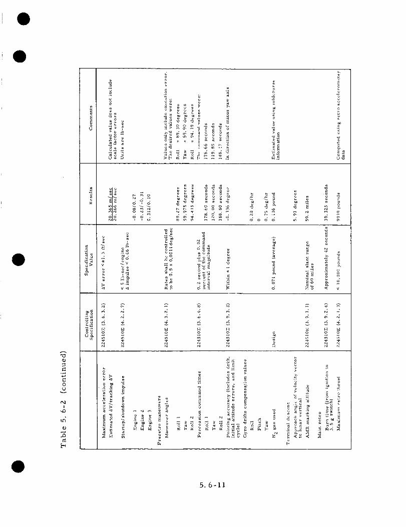
E

o

o_

o'_

o

E °

_o _

i1)

m_

__ _ _: ; _ _

"G;> v ,._-_

<:3 V'_

_ _ -_ _ _ o

o _ .. o _.'_ ._ °_

_._ _ _ _ < v

_,o

_'_ M _o _ o o o

• ,

_ al M kl M

o o _ o o o

c_

"O

0(.)

I

_o

c_

_ ,_ _._o

._s _ _ __'_ _ "_ _

o__ o_ _ _

o_ _°_o o_ o_ _ _°_ o_ o ,o _._ _

- _ _ - _ _'_ _ _ _ -o ....

¢J

5.6-11

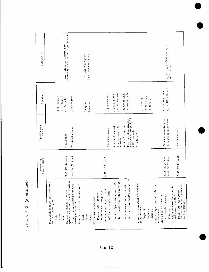
o

u o

IL

_a

+on

ii o

on o on

o o

m

_0_ o_oo o _ _

go

i

o0

_- >_N

o_

o

o')co r.

,J::dv

oo ._

_ om ¢_ u m°

o u

o_o_

Eo_ o_

_4

&&

m

_o

4_

o

_o _ _._ ,_ o_ o_

o_ o o o

g 4 ,4

M M Mo o o

T]

,,-I

0o

v

I

,,O

_go

,,-I

,mG]

o

o_ _ . .o_ __- _ _._ _ .o _

•_._ _o_ _ o _ _ _ _ _ _ o

_o

o

_ o _ _ __

_ O_

5.6-12

M

o_

o

o_o_o

,.Q ,._ ,.Oo o o

o_o_ o_o_

o_o_o_o_ o_

_ _ ,_ 7_ ,_

o 0 0 0 o

.o_

)o

o

o_

N

m

o

_ _ _

_.N_.c _Ng

_'1 blv _ _

,D

L L L

,,_ ,,_ ,,_

z_o

Ii ii

o

m

o

o

m

m o V V V V c_ ,_

(M

o o o

"0

0(J

v

I

_J

,.o

la

o_

_o

°_ _.a

o _._ _ o

<__ +__ _ _ __>_o ,- _ _

_ _•- _ _ =o

'lJ<

5.6-13

For the SC-I mission, only three anomalies, which were of minor

significance, can be attributed to the flight control system. One anomaly

is that Canopus lockon, which is an automatic feature of the optical system,

was not achieved because the output of the sensor, while viewing Canopus,

was greater than the upper threshold of the lockon range. Just prior to the

flight, the Canopus sensor gain was intentionally increased by 50 percent

to compensate for the possibility of sensor window fogging. This action was

brought about _y the window fogging that occurred on the SC-Z sensor which

was at that time in the STV test phase.

Star acquisition was achieved by commanding cruise-mode on (0704)

followed by a manual lockon command (0716).

The second flight control anomaly was the high indications of gyro

speeds. This anomaly has always existed, was expected, and did occur

during the mission. The third anomaly occurred just prior to touchdown at

an approximate altitude of 14 feet. An instant before engine cutoff, it was

noticed that all three engines were momentarily commanded to throttle up

by about 15 pounds. This anomaly did not affect the soft landing performance.

A brief description of each anomaly is presented in. Table 5.6,3.

Canopus lockon anomaly is analyzed in subsection 5.6.7.4, and the other

two anomalies explained in subsection 5.6.7. 13.

The

TABLE 5.6-3. CONTROL SYSTEM ANOMALIES

Anomaly

Canopus lockon

Gyro speeds

Vernier engine

system -- high

thrust glitch

Brief Description of Anomaly

When Canopus sensor viewed a

star of magnitude Canopus,

Canopus lockon was not achieved

Gyro speed checks for FC-1,

FC-2, and FC-3 read much higher

than the required 50 cps

Just prior to vernier engine cut-

off, a momentary high thrust

command was observed

Phase of

Mission

Throughout

the mission

151:04:26:03

Landing

5. 6-14

D

D

D

5.6.6 CONCLUSIONS AND RECOMMENDATIONS

From the tremendous amount of evidence compiled in this section,

the following conclusions were obtained:

i)

z)

3)

4)

5)

6)

7)

The nitrogen fuel supply is adequate.

Gyro drift measurements are feasible and required for accurate

maneuvers.

The flight control system is capable of precise angular maneuvers.

The flight control system is capable of accurate velocitycorrections.

The flight control inertial mode control system can maintain

accurate inertial reference.

The flight control oplical system can maintain accurate attitudereference.

The flight control attitude control system is stable under theinfluence of moment disturbances.

The magnitude register and programmer operates as designed.

9) The terminal guidance scheme, which incorporates the use of

radars, performs well as expected.

Because of the near perfect performance by 'the flight control system,

only a very few recommendations evolved from the analysis:

i) If Canopus sensor fogging is still anticipated for future flights,

the sensor gain should be set to I.Z5 times Canopus instead of1.5.

Z) Delete the gyro speed measurements.

5.6.7 FLIGHT CONTROL SYSTEM

5.6.7. I Prelaunch

Flight control parameters of interest during the prelaunch phase are

the gyro temperatures. (Comparisons between mission data and previous

test data are presented in Table 5.6-4. )

In the final report of the J-FACT ETR test (Reference l) a comment

was made that the values obtained during the test were l0 to 15 ° F higher

than those expected at launch because several sheets of mylar covering the

5.6-15

TABLE 5.6-4. GYRO TEMPERATURES, ° F

FCGyro No.

Roll 46

Pitch 54

Yaw 55

Mission2 Hours

Prior to

Launch

165.4

163

168. 1

Mi s sion

Z Minutes

After

Launch

167. Z

17Z. 0

177.Z

Prelaunch

Countdown

Dry RunTest on

Z6 May 1966

168. 1

174.0

177. l

J - FAC T

(ETR)

Test on

Z5 April 1966

178.6

17Z.6

175.4

J-FACT

(ETR)

Dry RunTest on

18 April 1966

178.6

173. 5

175.4

inertial reference unit (IRU) were not removed prior to encapsulation. While

this appears to be true for the roll gyro, it does not appear to fit the results

obtained during the mission for the pitch or yaw gyro temperatures.

The average duty cycle of the pitch and roll gyro heaters for the

mission were Z9 and 13 percent, respectively. These values are similar

to those seen during the STV test for a low to medium sun condition.

The events that occurred during the period between launch and

Centaur separation are given in Table 5.6-5. Information in this table was

obtained from the Quick Look Report (Reference l) published on 17June 1966.

5.6.7. Z Centaur Separation

After extending each of its landing legs, Surveyor is separated from

the Centaur booster. When the three legs-down signals and the separation

signal have been generated, the programmer removes the logic signal which

has been inhibiting operation of the gas jet amplifiers. At this same instant,

the magnitude register begins to count down a total of 10Z4 counts for a 51-

second interval; register counting inhibits the start of sun acquisition for

these 51 seconds to give the cold gas att{tude control system opportunity

to rate stabilize the spacecraft. Table 5.6-i presents these events in timereference.

Rate stabilization is accomplished by using the three-axis attitude

control system to torque the spacecraft to drive the error sensors (caged

integrating rate gyros) to within the deadband of each of the gas jet ampli-

fiers. Thus, at the end of a nominal rate stabilization maneuver, the space-

craft has achieved a low angular velocity with a random orientation in

inertial space. The system response is dependent upon the magnitude and

direction of the initial velocity vector and the gas jet thrust levels, and is

essentially deadbeat in nature.

Flight control system performance just after booster separation was

evaluated in terms of verification of the proper nulling of the separation

5.6-16

TABLE 5.6-5. EVENTS BETWEEN LAUNCH AND CENTAUR SEPARATION

Time

GMT,Prom Launch

hr:min:sec rain:see

14:41:01

:06 00:05

:18 :17

14:42:56 t:55

14:43:22 2:21

14:43:26 2:25

14:43:54 2:53

14:44:25 3:24

14:45:02 4:01

14:45:06 4:05

14:45:13 4:12

14:47:56 6:55

to6:60

14:49:46 8:45

9:00

sec Expected Event

5 3

Lift off

Atlas roll started

17 16 Atlas pitch

started

115

141 -

145 145.6

173

204 203.5

241 241.7

245 243.6

252 Z51.9

415

525

Inertia switch

opens

Inertia switch

closes

Booster engine

package jettison

(Mark 2)

Atlas-Centaur

attitude stabil-

ized

Jettison nose

fairing

(Mark 4)

Atlas SECO and

VECO (Marks 5

and 6)

Atlas Centaur

separation

(Mark 7)

Start Centaur

main engine

(Mark 8)

Observation

No noticeable effect on telemetry.

Roll precession command, FC-49, indicates start

of a roll. Expected time for start of roll was lift-

off plus 3 seconds. (Note: The spacecraft was

launched at 550 bits/sec. At this bit rate, it takes

2.4 seconds to sample a frame of data. The

differences from the observed telemetry time and

the actual event time is thus partially attributable

to the data bit rate. )

Pitch precession command, FC-50, and pitch gyro

error, FC-16, indicate a pitch of about -0.7 deg/sec

until Z + IM. At L + IM, both FC-16 and FC-17,

pitch and yaw gyro errors, become erratic for

about 20 seconds until L + IM Z3S. The pitch

precession is then -0.5 deg/sec until L + 2M 3S.

At L + 2M 3S, the pitch rate changes to -0.23

deg/sec and remains at this rate until Atlas booster

engine cutoff.

Acceleration reaches about 3. 7 g (FC-63).

Acceleration decays to about 3.5 g (FC-63).

Gyros indicate separation rates caused by booster

engine separation. Pitch at separation rose to

1.72 deg/sec.

Pitch rate goes to about -0. 15 deg/sec

The secondary sun sensors, FC-7, -8, -9, and -I0

go to values between 2. 5 and 3. The primary sun

sensor apparently saw the nose fairings and indi-

cated pitch and yaw sun sensor errors for about

60 seconds or until after Centaur ignition. Canopus

intensity also rose to about 3.2.

Indicated by pitch and yaw gyros.

Indicated by separation rates of gyros.

Indicated by separation rates being eliminated.

Pitch rate returns to -0. 15 deg/sec.

Five-second loss of data.

Fifteen-second loss of data.

5.6-17

rates, time required to null rates to less than 0. 1 deg/sec, total angular

excursion, and magnitude of the angle rates at separation. In addition,

the nitrogen gas expended during the maneuver was estimated.

Spacecraft telemetry data available for analysis of the tipoff tran-

sient is presented in Figures 5.6-i and 5.6-2. Other pertinent data is

found in Reference Z as follows:

I) Time of separation command (commutated data) T + 756. 57+0. 5

sec (or _150-14-53-38 GMT)

2) Time of spring extension

Time of First

Measurement Spring Motion,

No. No. seconds

End of

Motion, Spring Extensionseconds Time, seconds

CY2D l 756. 933 757. 055 0. 1g2

CY4D g 756. 933 757. 054 0. 121

CY5D 3 756. 933 757. 052 0. 120

3) Preseparation Centaur plus SC-I angle rates (deg/sec):

Pitch -0. 05

Yaw +0. 15

Roll + 0.01

Table 5.6-6 presents the results of SC-1 data analysis in comparisonwith other sources as noted.

TABLE 5.6-6 CENTAUR SEPARATION PHASE

Parameter

Pitch gyro error

Yaw gyro error

Roll precession command

FC Null,

Number bcd

FC-16 5Z2. g

• FC-17 518. 4

FC-49 519. 4

Reference 2.

Preseparation Rates

Spacecraft

bcd deg/sec

535 -0.054

560 -0.170

523 -0.014

Centaur,*

deg/sec

-0. 05

0.15

0.01

Note: See Table 5.6-8 for the calibration coefficients used in this analysis.

Peak Rates at

Separation

bcd deg/sec

606 -0. 378

560 -0. 170

524 -0. 018

Time

to Reduce

Separa -tion Rates to

<0. l deg/sec,

seconds

15

0

0

5.6-18

68189-i09 (U) " -_ --c--

;_,, i -' .... I -_ _-_ ' t " i_ I !_xl , _ I , ii- "_" _....... _-....... _-...... _....... ' ..... I :. :J.- ........_ _',....... L._ :___..... ,. +: ......

i w,,l ' : - .4 .... , ' . '--m-' i . _ ' _X,,I i -

_II ' - " + ' i : . , %, : _ V,l "_ •, ' + • _ .... I

• ....... !......__=...... ,.... +......_+............_+: +......._ _ --+_-,_--+-+l v_ ] + : + + ' ,+ ; : / • +_'_ +._--nl :

i_ ...... _ ..... ' -- +_.............. * - .----+..... _--i-+'............ :-I.......... +Z,-+---iu -+-:--I

+ + I + I + I + + '] ; + " :+ . +

i+. ................. T- +?+ .....++,,+- e- _ -, .....i................ /_ .. . '+P,+-it ....................

i

! .... + :

++ +_ : o.j ........... _ ..... .-.._ ..............

..... \ "._ ._,_...,<': __:_;__ . --

. ! . ,

i

........ ,k_ __

• f ........

Z.

/i ....

I

--:._ -

". r+

,+

I •

i

I

• __J: } _

I -

........ = ......

o ++ +I _ . t _ .

_._ : _ ;_ .................... __ -: .......,_..+__L+_.: _]+-__:_#_ P_&_ t,--_,-+.........

L + ' L__L:L_ '

I

0 r_

oo

4-_

• _

.el

5.6-I9

T*

I [ +_i -

....... '---@-:"--,--"-:- -_TI-:" _"I ........ ...... --

J_-_.....! i -::::'-_i _ '' _"''i: _?F .... _...... i....... I--7 , .... -,_-I-T-, ...... , -:-T-_-T -r- ]

.,. i ' t [ !1 I i , t .....

, ,= : i !........I:-

.... _F-- t-:_.

.........i-gk ......b-_..... ,-..............iN,

I

:--]:-

[ .- :!

I

] _

-I-- -_--I

+; :.:

:--I- ......L

ii

tI I

I

I-i--# '- }

I

]t ...... i ....

[.._

!

©

o

o o.,-i

0

o ¢)

,.o c_

u4 ©

blO,,--t

5.6-Z0

D

D

D

D

General Dynamics (GDA) and Surveyor telemetry preseparation

values agree well, lending confidence with regard to the validity of the post-

separation data. The differences in sign are due to different coordinate

references used by GDA and HAC (Reference 29). As expected, the major

tipoff transients occurred in pitch and yaw, with little change in the roll rate.

Although there was a 30-second loss of data beginning 15 seconds after sepa-

ration, it is apparent that proper hulling of separation rates was achieved.

The assumed shape of the pitch and yaw transients at separation is

based on the impulsive nature of the separation force, the Centaur-spacecraft

springs extending in N0. IZ0 second. Correcting torques were applied by

means of the gas jets beginning at electrical separation for rates >0. 067

deg /se c (nominal).

The peak pitch angle rate was _0. 38 deg/sec, the highest rate experi-

enced in any channel. The telemetry channel saturates at "5.6 deg/sec {seeTable 5.6-7 for rate mode coefficients used).

The initial return acceleration of the pitch gyro error signal was

_0. 027 deg/sec 2, which is well within the gas jet torque capability of 0. I

deg/sec 2. If the remainder of the nulling transient is as shown in Figure

5. 6-1, then the hulling time (time to <0. l deg/sec) is _15 seconds, and the

angular excursion due to separation is 2. 3 degrees.

The yaw separation torque tended to null the existing rate, so that

the peak rate was the preseparation value. Further, the time required for

nulling to <0. 1 deg/sec was essentially the separation time.

The roll rate was changed only slightly due to the effect of separation,being very small at all times ("0. 014 deg/sec) so that roll correction torques

were not required.

Telemetered nitrogen usage (pressure and temperature corrected)

indicated that the nitrogen expended during rate dissipation was as expected

from a nominal stabilization maneuver. At 150:15:01:30 GMT, the cumula-

tive nitrogen usage was determined to be (4. 503 - 4.4Z4) = 0. 079 pound (see

Table 5.6-8). It has been estimated that a minus roll of 86 degrees and a

positive yaw rotation of 99 degrees were accomplished during sun acquisition

(see Reference 3, Table I). These rotations indicate a nominal sun

acquisition fuel consumption of 0. 054 pound (see Reference 4, Fuel Budget).

The remaining 0. 025 pound would have been used in rate stabilization.

5. 6.7. 3 Sun Acquisition Phase

Automatic sun acquisition as specified in "System Functional Require-

ments," Revision E, Paragraph 3.4. 1, is as follows:

"Fifty-one (51) seconds after separation, sun acquisition is

initiated by a command from the flight control programmer,

which causes a vehicle roll maneuver of -0.5 deg/sec and

5. 6-Zl

TABLE 5.6-7. CALIBRATION COEFFICIENTS FOR

RATE MODE CALCULATIONS

(SC-1 Telemetry Calibration Handbook 291031)

Coefficient FC-16

A0 0. 731710 E 01

AI -0. 192280 E -01

AZ 0. 229569 E -04

A3 -0. 401800 E -07

A4 0. 324409 E -i0

A5 -0. 101840 E -13

FC -17

A0 0. 708950 E 01

AI -0.225860 E -01

AZ 0. 476819 E -04

A3 -0. I01770 E -06

A4 0. 102760 E -09

A5 -0. 396360 E -13

FC -49

A0 0. 778800 E 01

Al -0. 358289 E -01

AZ 0. i17219 E -03

A3 -0.263310 E -06

A4 0. 278600 E -09

A5 -0. I11960 E -IZ

TABLE 5. e-b. NITROGEN GAS CONSUMPTION*

Day Time N 2 PressureFC-4 [ Corrected

150 I 143001 4906 [ 4650

144558 4906 [ 4650

1456_2 4841 4580

1459 _7 4778 4515

150130 4741 4490

192834 4418 4170

151 105595Z 4225 4000

071225 3957 3725

15_ I 051252 _746 I 3525

N 2 Temperatur, Bit Ng (lbs) Total N 2 N z Expected

FC-48 Corrected Rate Remaining Used Event Used Usage

550 4. 49

85. l 4, 505

8521151 4. 476 O. 027 O. 027

8Z. 5 4.445 0.058 Kate 0.051

Stabilization

and Sun Acq.

81. 6 4. 424 0. 079 0. 0dl 0. 100

56. 9 4. 409 0. 094 Star Acq. 0. 015 0. 159

46. 3 4. 382 O. 121 Coast

44.6 4.145 0.358 MC 0.257 0.405

47.2 3.94 0.565 Coast 0.205 0.511

*Data d_rived from Reference t,

No N 2 pressure data available after T.D, and not available on SPAC format after completion of pre-terl_/inal n_aneuvers.

See subsection 5.6, 7. 13 for a complete analysis of nitrogen consumption.

Remarks

After rate stabilization

and start of minus roll.

After end of minus roll

and start of plus yaw.

Post Canopus Acquisition

Pre MC

Post MC

Pre Terminal

This value of gas con-

sumption is high due to

the many 8yro drift check_

Po_t T, D.

5.6-ZZ

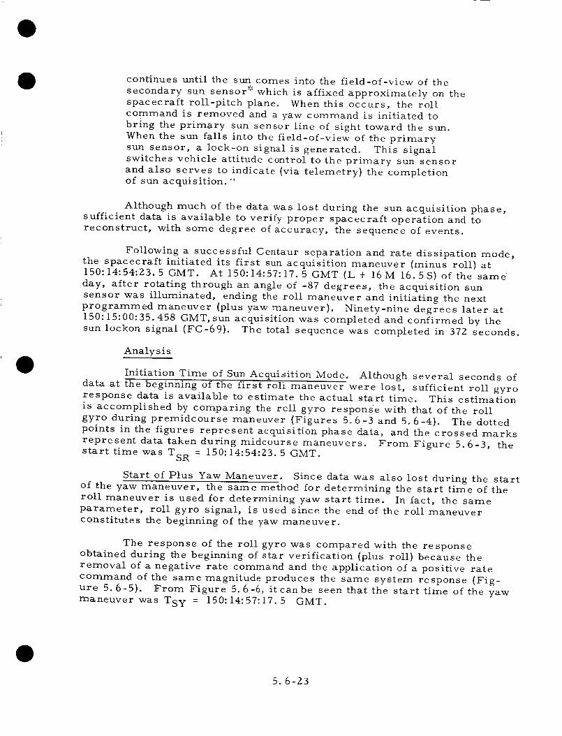
D

D

D

continues until the sun comes into the field-of-view of the

secondary sun sensor ;'_"which is affixed approximately on the

spacecraft roll-pitch plane. When this occurs, the roll

command is removed and a yaw command is initiated to

bring the primary sun sensor line of sight toward the sun.

When the sun falls into the field-of-view of the primary

sun sensor, a lock-on signal is generated. This signal

switches vehicle attitude control to the primary sun sensor

and also serves to indicate (via telemetry) the completion

of sun acquisition. "

Although much of the data was lost during the sun acquisition phase,

sufficient data is available to verify proper spacecraft operation and to

reconstruct, with some degree of accuracy, the sequence of events.

Following a successful Centaur separation and rate dissipation mode,

the spacecraft initiated its first sun acquisition maneuver (minus roll) at

150:14:54:Z3.5 GMT. At 150: 14: 57:17.5 GMT (g + 16M 16.5S) of the same

day, after rotating through an angle of -87 degrees, the acquisition sun

sensor was illuminated, ending the roll maneuver and initiating the next

programmed maneuver (plus yaw maneuver). Ninety-nine degrees later at

150:15:00:35. 458 GMT, sun acquisition was completed and confirmed by the

sun lockon signal (FC-69). The total sequence was completed in 37Z seconds.

Analysis

Initiation Time of Sun Acquisition Mode. Although several seconds of

data at the beginning of the first roll maneuver were lost, sufficient roll gyro

response data is available to estimate the actual start time. This estimation

is accomplished by comparing the roll gyro response with that of the roll

gyro during premidcourse maneuver (Figures 5.6-3 and 5.6-4). The dotted

points in the figures represent acquisition phase data, and the crossed marks

represent data taken during midcourse maneuvers. From Figure 5.6-3, the

start time was TSR = 150:14:54:23.5 GMT.

Start of Plus Yaw Maneuver. Since data was also lost during the start

of the yaw maneuver, the same method for determining the start time of the

roll maneuver is used for determining yaw start time. In fact, the same

parameter, roll gyro signal, is used since the end of the roll maneuver

constitutes the beginning of the yaw maneuver.

The response of the roll gyro was compared with the response

obtained during the beginning of star verification (plus roll) because the

removal of a negative rate command and the application of a positive rate

command of the same magnitude produces the same system response (Fig-

ure 5.6-5). From Figure 5.6-6, itcan be seen that the start time of the yaw

maneuver was TSy = 150:14:57:17.5 GMT.

D5. 6-23

68189-III (U)

........... _'__............................ _ ,_ _ _ - :............__'. _ _'_ _ _ _ _ _ _....._._.....:....._ .__.

r_

0

[b

<

o

bb

r_

b_

o

c_o

©

,--i

©

I

'-D

M

.,--i

5. 6-Z4

CO

0

"0

(d

0

L)

C_

(i);>

4-}

c_b.C

0

C)CO

0

_D

0

,---i

0

4!

• ,..-t

5.6-25

68189-113 (U)

. \

o

br_

b_

.,.._

c_

o

o

©

o

_dI

,.D

5.6-26

68189-114 (U)

...... •.. . " " _ ." ....... . .... ' "................... -x ";" -{-'"."-::" --" :. 7"<"': . Tt:J

-_ ...... : ...... .. __..!..___s_........... ÷ ..... : ,. " '.... _ - ' " " ........ - '7".G"'_

• - , : _.. . .... ............. :............ .i3.. .............. .........

i ................................ .-_- 7! .-'".F ...... i: '_

i' _ ' ' " " ........ " ;'_ -:: ii:!.:- ---F "_ !-_

) .... :i-: :: .... " " ........... " ::" :[ ......... .... '-_ .... _-_:-/ ..... _i_- --': _:-_ '_::..i

-.. _- " '.:: : , ,.-,. , ' . . i _ .... % _".-, ."7:._ '_ _ :..._.- _

i : ..','"", _ ' : ,_ - ; , - '. , _' -: _ i.-:!'4,: _!._:".- --'I [,K._.__/-_' i?.i:i '_7' )"i.. ,::,..,:-i ,. : 2" ::!._ i;_.i;-*:D--_.: "_&.i

7........ " " ................ _........... ; ...... ...... _, ........ _'" "_- _'r- • _-- ..... _- " -

];

.... i

" .............. ".... --_"_- ' "....... :- ..... : ._ :i ..... '_'• :!. :. j / .......... - 1

oL)

>._._

o

o4_

&)

o

o1.4

D

o

,5!

,.o

M

ID

5.6-27

Determination of Maneuver Angles. The angles through which the

spacecraft rotated during the sun acquisition phase were obtained by multi-

plying the maneuver time by 0. 500 deg/sec. Thus the angles were:

_PR = -0. 5 x 174 = - 87 degrees

_y = 0.5 x 198 = 99 degrees

5.6.7.4 Star Acquisition Phase

As defined by the "Surveyor System Functional Requirements

Specification," 224510E, Paragraph 3.4. g, "A star acquisition command

starts a vehicle position roll of 0. 5 deg/sec until a star of the correct

brightness falls into this sensor field-of-view. When this occurs, a lockon

signal is generated which stops the 0.5 deg/sec roll rate and switches the

vehicle roll control to the star sensor error signal."

Automatic lockon was not achieved because the output of the sensor

was greater than the upper threshold of the lockon range. 'This was caused

by an intentional increase in sensor gain to compensate for the possibility

of window fogging. Star acquisition was achieved by commanding cruise-

mode on (0704) followed by a manual lockon command (0716).

Analysis

Star acquisition began with command 0714 (sun and roll) at

150:18:53:39.290 GMT and ended at 19:13:20.723 with command 0716

(manual lockon).

Star Map-- Verification of Canopus. The various stars and the

number of stars that appear in a particular star map are very sensitive to

the hour of the year and the angular position of the sensor axis relative to

the spacecraft-sun line. During the May-June launch, the angle between

the Canopus-spacecraft line of sight and spacecraft-sun line was approxi-

mately 78 degrees. With the aid of a computer program that produces a

star map for any given angle and time, the actual Canopus sensor alignment

was found to be -ll. 7 degrees. The star map that launch personnel used

was for a -12. 0 degree angle that did not indicate Regulus. This was one of

the reasons why launch personnel were intrigued when the star Regulus was

identified during the mission. At an angle of -ll. 3 degrees, the star Merak,

which is located approximately 232 degrees from Canopus, disappears.

With the aid of a computer generated star map as reference, theother stars which can be identified are as follows:

5. 6-28

Angle from Canopus,Star de_rees

Alpha Doradus 16. 58Phi Eridani 37.58

Markab 118.37

Pi Cygni 156.65Alderamin 170.62

Merak 231.55

Algeiba 269.45

Regulus Z77.95

Alpha Hydrae 301.29Naos 338.44

A comparative plot between actual and computed is shown in Figure 5.6-7.

Mean Roll Rate. The mean roll rate equal to the positive roll pre-

cession rate can be determined as follows:

i) Angle between Markab and Naos is 220. 073 degrees.

2) Time interval between the two stars is 439. 792 seconds.

Thus

_Z = 0.5004 deg/sec

Effective Gain of Canopus Sensor. In general, the Canopus sensor

gain is set such that a star of Canopus brightness will produce a signal of

nominal Canopus lockon value. This value is approximately 5 volts.

For SC-I, the sensor gain was increased 50 percent by installing a

sun filter on the sensor's sun input which is used as reference. This action

was initiated to compensate for the possibility of excess fogging of the

sensor' s window.

From the investigation, the Canopus sensor gain appears to have been

slightly greater than 1.5 times Canopus. This value was obtained by compar-

ing the actual data to calibration curves of the particular sensor (Figure

5.6-8). The Canopus error signal was plotted along with star intensity to

determine the zero angle position.

Since the upper acquisition limit is 1.5 times Canopus intensity and

the intensity of Canopus with the high sensor gain setting was determined to

be just slightly higher than i. 5 times Canopus, little margin existed betweenthe two.

5.6-29

Window Fogging. From FC-14 data (star intensity signal), it

appears that very little change occurred in the overall gain of the Canopus

sensor during the 63-hour mission (Figures 5.6-8, 5.6-9, and 5.6-10}. A

slight change in gain appears to have occurred, as indicated in Figure 5.6-i0,

during the beginning of the preretro maneuver, but this is believed due to

telemetry network lag effect. In the first two cases (Figures 5.6-8 and 5.6-9),

the angular rates are at a steady-state value of 0.5 deg/sec; thus, the input

to the telemetry conditioning network is essentially a ramp type function,

whereas during the beginning of a maneuver the input is a parabolic function.

From the three plots, it can be concluded that no fogging or very little fogging

of the sensor window occurred during the mission.

Roll Angle from Beginnin_ of Maneuver to Canopus. From the data

of roll gyro angle, roll was initiated at 18:53:40. i00 GMT. First Canopus

peak occurred at 19:01:00.650 GMT, and the roll rate was 0.5008 deg/sec.

Thus, the angle between the beginning of star mode and first Canopus

appearance was _P = ZZ0. 627 degrees.

Additional Information

During the investigation of Canopus sensor gain, the null level of

FC-12 (Canopus error signal) was much lower than expected. The expected

null (zero angle} value is 520 bcd, and the data during the star mapping

phase indicates an apparent null of 445 bcd, or a difference of approximately

0. 3 degree.

Further investigation of this signal during other phases of the mission,

such as midcourse maneuver, revealed that the null point of the sensor was

indeed 5Z0 bcd when looking at Canopus, but changed to approximately 450

bcd when observing less intense stars or relatively empty space (Figure

5.6-11}.

A false star of considerable intensity is evident at approximately 5

degrees before the first observation of Canopus. This star did not appear on

the second approach to Canopus or on any subsequent maneuver. It was first

theorized that, since the star map is sensitive to the angle which the sensor

makes with the spacecraft-sun line, the change in yaw angle caused by the

optical mode limit cycle possibly was sufficient to introduce another star in

the field of view. However, investigation of the sun sensor yaw and pitch

error signals revealed that this was not the cause.

The results were as follows:

5 degrees before first Canopus (19:00:47.450)

FC-5 = -0. 103 degree (489 bcd)

FC-6 = -0.213 degree (505 bcd)

5.6-30

Figure 5.6-7. Star Map

5.6-31- I

,_H_._LLI I I I_/1111 I[ III

'J llll ,,,• . : ..... : , . .

.....[Jiiiiii iii _l..-_--ii]1111 n_n

.Trzw. _ii !ii

!!i!!!ii iii!!!!iii_ i!!iiii:::: :iiiiii:::: ii:::::::: ;:

........ ii;:::_[:: ,.

:::::::4 ?.[

iiiJ[[[! [[IIIII::: ii

Jiiiiii i!........ Li

--_i i iJii "

-iiiiiii! _:

....... i:iIIIIl:l: .,

[[[[!!!! [:!,L_[Ill:: ,,I

::: : ; ::_ I11........ III

iiii!iii ill

:::: ::: dll

iiii =:_ _!1!!!! !!! tll:::: ::: Ill

|11Jiii;:: Ixi

IIII• '.' IIIIi[" '1,

J . ,

:: I ,,, 1111

,, [ ::: !!!i:: I ::_1111

:: [ Illl:: I iii !t_l

I IIIi_ I iii iItl

'111 "'!II, ,!!II I III !!!

II':: I ::: III,_ I ::: I,.

Ill

LL ![! _!__1 'I, • :._ _ : : :

I_ J ::1 411

]: I ::: III

I J [

nl_:::, iii,= I ::1 iiii : I

II I I_! !!!'::: :!!

II

II iii _±,. 1:: :1:

::: :::

II .l.- ::: nn:

. . I iml,_l : : :

,, I iii i,,r_,

lll_l II:I!_I II• : I I

I i

! IIi l IIi ! II

: ! 11: 1

: 1 11IIiiii ,,: I "I I I

: [ I_1 : 'i it_ i i_ ! ['l ! !

11,I ,,• I : I 'i I i I , i• , i I ; [

:_iI !i,i ',I _!: I :

i I I I

:, 1 ijf.i _ i I

: : I

: ! 1!; i I_1

,_. i I l"!' 1 I:: l,ll!!!IIII::,Iiii

,4_.,:.: ,. _:,, : : .i: : : : : : ; :

: : : :. ; : : ;

! i ;I; i i i

; i ill i i :

i i ;i;iiiI_ III I 1

" !III [

I L II

• I, i_,: _w,I I Ii 'iiii I'

5.6-31-43

/

'FOLDOUr

]

Figure 5.6-8. Star Intensity Profile During First Canopus

5.6-33

Figure 5.6-9. Star Intensity Profile During Postmidcourse Roll

5. 6-34

oot.d

oo

!

7_A

Figure 5.6-10. Star Intensity Profile During Ratio Maneuver (Roll

5.6-35

o

q)

0t)

o10

C?q)

,,-+

o

b/?

oI-I

o

,,D

M

,,-t

5.6-36

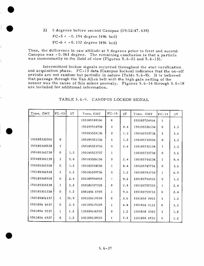
z) 5 degrees before second Canopus (19:12:47.438)

FC-5 = -0. 154 degree (496 bcd)

FC-6 = -0. 152 degree (496 bcd)

Thus, the difference in yaw attitude at 5 degrees prior to first and second

Canopus was -0.061 degree. The remaining conclusion is that a particle

was momentarily in the field of view (Figures 5.6-12 and 5.6-13).

Intermittent lockon signals occurred throughout the star verification

and acquisition phase. FC-13 data (Canopus lockon) indicates that the on-off

periods are not random but periodic in nature (Table 5.6-9). It is believed

that passage through the Van Allen belt with the high gain setting of the

sensor was the cause of this minor anomaly. Figures 5.6-14 through 5.6-18are included for additional information.

TABLE 5.6-9. CANOPUS LOCKON SIGNAL

Time, GMT FC-13 AT

150185332000 0

150185340538 1

150185341738 0

150185344138 1

150185345338 0

150185346538 1

150185348938 0

150185350138 1

150185351338 0

150185402137 1

1501854 4537 0

1501854 5737 l

1501854 6937 0

Time, GMT FC-13

150185510536

150185518936

1501855Z0136

150185521336

150185523736

1.2 150185523737

2.4 150185526136

1.2 150185534536

l.Z 150185535736

Z.4 150185554935

l.Z 150185557335

1.2 1501856 6935

10.9 150185610535

2.3 150185615335

1.2 150185616535

1.2 150185618935

AT Time, GMT FC-13 AT

150185724934 1

8.4 150185726134 0 1.2

l.Z 150185729734 1 3.6

1.2 150185730934 0 1.Z

2.4 15018573Z134 1 1.2

150185735734 0 3.6

Z.4 150185744134 l 8.4

8.4 150185747734 0 3.6

l.Z 150185753733 1 6.0

9.2 150185754933 0 1.2

2.4 150185757333 1 Z.4

9.6 150185759733 0 Z.4

3.6 1501858 0933 I 1.2

4.8 1501858 2133 0 1.2

l.g 1501858 3333 1 l.Z

Z.4 1501858 4533 0 l.Z

5.6-37

Table 5.6-9 (continued)

Time, GMT FC-13 AT

1501854 9337 1 2.4

150185410537 0 1.2

150185415337 1 4.8

150185416537 0 l.Z

150185417737 1 1.Z

150185420137 0 2.4

150185422537 1 2.4

150185426137 0 3.6

150185445337 1 1.2

150185446537 0 1.2

150185447737 i 1.2

150185454937 0 7. Z

150185456137 1 1.2

150185457337 0 l.Z

1501855 3336 1 6.0

1501855 4536 0 l.Z

1501855 6936 1 2.4

1501859 453Z 0

150185923732 1

150185924932 0

150185926132 1

150185928532 0 2.4

150185936932 l 8.4

15018593813Z 0 l.Z

150185940532 l 2.4

150185941732 0 1.2

Time, GMT

150185620135

150185630935

150185633335

150185635735

150185638135

150185646535

150185647735

150185651335

150185652535

150185656135

150185658534

1501857 4534

1501857 5734

150185710534

150185714134

150185718934

1501857Z0134

15019 2081Z9

15019 211729

15019 224929

15019 232129

15019 233329

15019 239328

15019 241728

15019 244128

15019 246528

FC-13

0

1

0

1

0

1

0

1

0

1

0

1

0

1

0

1

0

1

0

1

0

1

0

1

0

1

AT Time, GMT FC-13 AT

1.2 1501858 5733 l l.Z

10.8 1501858 9333 0 3.6

2.4 150185810533 1 1.2

2.4 150185812933 0 Z.4

Z.4 150185814133 1 l.Z

8.4 150185818933 0 4.8

l.Z 1501858Z0133 1 1.2

3.6 150185826133 0 6.0

1.Z 1501858Z9733 1 3.6

3.6 150185830933 0 l.Z

Z.4 15018583Z133 1 l.Z

6.0 150185833333 0 1.2

I.Z 150185845333 1 12.0

4.8 150185846533 0 l.Z

3.6 150185854932 1 8.4

4.8 150185856132 0 1.2

1.0 15018590213Z 1 6.0

15019 4 3327 0

3.6 15019 4 6927 1

13.2 15019 4 93Z7 0

8.2 15019 4105Z7 1

l.Z 15019 411727 0

6.0 15019 414127 1

Z.4 15019 4153Z7 0

Z.4 15019 4321Z7 1

2.4 15019 438126 0

5.6-38

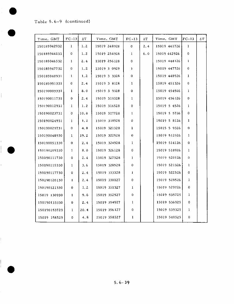
Table 5.6-9 (continued)

Time, GMT FC-13 AT

150185942932 1 1.2

150185944133 0 1.2

150185946532 1 2.4

150185947732 0 1.2

150185948931 l 1.2

150185951331 0 2.4

150190009331 l 8.0

150190011731 0 2.4

150190012931 1 1.2

150190023731 0 10.8

150190024931 l 1.2

150190029731 0 4.8

150190048930 1 19.2

150190051330 0 2.4

150190109330 l 8.0

150190111730 0 2.4

150190115330 1 3.6

150190117730 0 2.4

150190120130 1 2.4

150190121330 0 1.2

15019 130930 I 9.6

150190133330 0 2.4

150190153729 l 20.4

15019 158529 0 4.8

Time, GMT FC-13

15019 248928 0

15019 254928 1

15019 256128 0

15019 3 0929 l

15019 3 3328 0

15019 3 8128 1

15019 3 9328 0

15019 315328 1

15019 316528 0

15019 317728 l

15019 318928 0

15019 321328 1

15019 322528 0

15019 324928 1

15019 326128 0

15019 327328 1

15019 328528 0

15019 333328 l

15019 338127 0

15019 351327 l

15019 352527 0

15019 354927 1

15019 356127 0

15019 358527 l

AT

2.4

6.0

Time, GMT FC-13

15019 441726 1

15019 442926 0

15019 444126 l

15019 447726 0

15019 448926 1

15019 451326 0

15019 454926 l

15019 456126 0

15019 5 4526 1

15019 5 5726 0

15019 5 8126 1

15015 5 9326 0

15019 512926 l

15019 514126 0

15019 518926 1

15019 520126 0

15019 521326 l

15019 522526 0

15019 528526 1

15019 529726 0

15019 535725 1

15019 536925 0

15019 539325 1

15019 540525 0

AT

5.6-39

Figure 5. 6-12. Canopus Error Signal (Star Map)

5. 6-40

%

_÷_

T¢

¢¢p%

¢F

,.-b.

bF_E.

÷/

$_b:-!-

tT

L:k

il

F:[

i:¢

Figure 5.6-13. Star Intensity Signal (Star Map)

5.6-41

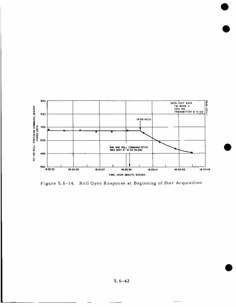
>-r_

z

m 540

c_z

o < 520

zo

2,-,_w_awOac o 500a.

0

m 480_PI

560

460

18:53:33

Q

18:53= 40.10

I

SUN AND ROLL COMMAND (0714)

WAS SENT AT 18:53:39.290

DATA: 'DSI F TAPE

TM MODE C

I I00 bps

TRANSMITTER B HI ON

I I I I

18:53:35 18:53_37 18:53:39 18:53:41 18:53:43

c

18:53:45

TIME, HOUR = MINUTE : SECOND

Figure 5.6-14. Roll Gyro Response at Beginning of Star Acquisition

5.6-42

;! _ i i :1 !--+--p_ -_-+ J, ;_

J4_mFLLi-r.-+-P-P p.t--_

T bi_TI-i--t-t!l!ll-L_

-- 4---I--+_

-!d T FFFP-

_-_ LL!_

d:l:_.-t-+t!T

tit tl_- F i

i LJ_LLL.

LLL.LLLLL

rtrT FFmt

rt!]ridF

[[ti'.iL i i

,![_ ;i II

_,i i H:Fi7i

_1M L_ El:

4-: L+'2-:_

.__.2TZXI-r-!d i-!it-

T_%TR?£2-_1-:- -F] --

_.LLLi LLL

L[ LId LL

_LLE.r_ _-I-I Pj-F_T

-rT1T 1-L

-H F+ EHk,t

:i:l:].:r!::Fg[:_J,f P-!

i: : ::',/,:_

!_ i/-Ft

i ;_i÷i[1LLi*_

:] .i .....

'Y1Nr!I

1_'_'ili.

Figure 5.6-15. Primary Sun Sensor Pitch Error

Approaching Canopus first time

5.6-43

i ]iillltlttlt!!lt-ifiiLtt1_?t!I_2:TH_:ttf:ttit_f_ff7t_:tltHtttt:tbt:tttttHtt_]_-t;t-t77:__1;iltit7_II;

_' i i fttti:tif{7tTfttfTf4tf:htttttft_14tflfl_ttttt-t:tfft_d_7f_-tHt_t_:ktdtfh_f:t;htt_tT:tti_ktt:IfI:tt{f7ttt[t:ttfHtfHT:t:t4::t:t: -t:ttl_4f:;_-_f_Xf{Mttit !fftllt !iL:t_Lt;7fL?7:Hift::+Ntttf'_H_;ft_1_-HMTb__Ht_4qfIfft._;_.L_tff_7:

" _,I f!L_ttltttt!7il_lif/_!ItttHTf!t{_t-it____&,7_!!-ril!i-F[PM 7 HI ttr-iT 7tlftmtppft!iftl,-ttl!_Tm_m_;

i II. 15565. IS5911. 155";5, 15"5110. 155_5. 151_0. ISSil_. 15800, 15_II]_. 15610. IS_II.

MI5510N TIME 15EC51i

Figure 5.6-16. Primary Sun Sensor Yaw Error

Approaching Canopus first time

5. 6-44

i 68189-123 (U) X "

!

0

_4 .,._4_

0 "o

C o

r/l

o

5. 6-45

0

M

.,.-i. ,..-i

0 (-!"m 0

_ m

_ m

0

_ U

, ,...i

<

.,.-i

i

5.6-46

5.6.7.5 Coast Mode

The three-axis cold gas attitude control system is designed to main-

tain an optical or inertial reference during the nonthrusting portions of

the Surveyor flight. The spacecraft pitch and yaw optical references are

provided by a narrow field of view sun sensor; the roll optical reference is

provided by a Canopus sensor whose field of view is 5 degrees latitude and

8 degrees longitude. The spacecraft inertial references are provided by

three body-fixed rate integrating gyros.

The actuators used in the coast mode are the cold gas jets. The on-

off operation of these jets plus the deadbands built into the system at the gas

jet amplifiers cause the spacecraft to function in a three-axis limit cycle. In

the steady state, the Surveyor attitude coasts along a straight line within the

three-dimensional deadband of 8, _p, 4' space. Upon intercepting a bounding

plane, a gas jet pulse is emitted, driving the system back within the deadband

along a new straight line. These motions are entirely analogous to the motions

of a ball bouncing internally within a closed three-dimensional planar-sided

polygon of six sides wherein the law of reflection is that the velocity com-

ponents of the ball change by discrete amounts (as caused by a jet pulse), the

amounts being constant for any one plane. The motions are aperiodic and

are a strong function of initial velocity conditions.

The non-g sensitive drift rates of the integrating rate gyros were

measured six times during Mission A by slaving the spacecraft to the drifting

inertial references and observing the drift rates by means of the telemetered

optical references.

The principal items of analysis for the flight control system coast

phase were as follows:

I) Limit cycle frequency and amplitude

2) Sun and star tracking errors and tracking noise

3) N 2 gas used

4) Individual and averaged results of gyro drift measurements

compared with FAT results

The major events for the coast phase, together with their correspond-

ing times, are presented for reference in Table 5.6-I0. Table 5. 6-II is a

summary of the analysis results for the coast phase.

Conclusions and Recommendations

I) Limit cycle behavior was as predicted except that the roll limit

cycle occasionally exhibited the tendency to double-pulse at each

side of the deadspace (ideally, it should always single-pulse).

About 24 percent of the fuel consumed during the sampled limit

cycle period was a result of double pulsing. However, since the

fuel penalty was very low (about 0.04 pound) and the limit cycle

width was unchanged, this additional pulsing was readily tolerated.

5. 6-47

TABLE 5.6-10. MAJOR EVENTS AND TIMES

Event Time, GMT

Sun lockon 150:15:00:34

Star map (begin)

Canopus acquire (manual lockon)

150:18:53:39

150:19:13:20

Begin gyro drift check 1

End gyro drift check 1

Begin premidcourse maneuvers

End postmidcourse maneuvers

Begin gyro drift check 2

End gyro drift check 2

Begin gyro drift check 3

End gyro drift check 3

Begin gyro drift check 4

End gyro drift check 4

Begin gyro drift check 5

End gyro drift check 5

Begin gyro drift check 6

End gyro drift check 6

Begin preretro maneuvers

150:20:54:02

150:23:51:I0

151:06:30:12

151:07:00:55

151:09:30:14

151:12:30:16

152:4:18:39

152:6:25:57

152:7:34:15

152:9:52:16

152:9:55:42

152:13:05:03

152:19:20:43

152:21:41:51

153:5:36:46

Command

Automaticsequence

0714

0716

0700

0704

0714

0714

0700

0704

0700

0704

0700

0704

0700

0704

0700

0704

0714

Note: The above times were obtained from Reference 5, "Flight-TimeCommand Log, " and from Reference 2, Table I and SectionB.4.

5.6-48

D

TABLE 5. 6-II. SUMMARY OF RESULTS

D

Limit Cycle Frequency

Mission A

Inertial: 50 sec/pulse

Optical: 65 sec/pulse

Limit Cycle Amplitude

Mission A

Inertial, degrees:

Roll 0.415

Pitch 0. 443

Yaw 0.4 17

Optical, degrees:

Roll 0. 441

Pitch 0. 470

Yaw 0.4 57

Roll null:

Pitch null: -0. 058

Yaw null: -0. 053

Nulls obtained from DSIF

data: 153:01:51:23 to,

155:05:36:23

Predicted

I17 sec/pulse (Reference 6, page 3)

80 sec/pulse'(For I o Canopus sensor

noise: Reference 6,

Figure 1).

(Single Axis)

Predicted

0.44

From DSIF data

gyro drift test 0.44number 6

0.44

0.44

From DSIF data

155:01:51:23 to 0.44

153:05:36:23

0.44

Sun and Star Tracking Errors,

Mission A

-0.055

degrees

Specification

±0. I0

+0. I0

• 0. lO

D5.6-49

Table 5.6-11 (continued)

Sun and Star Tracking Noise

The sun and star error signal noise levels were lowenough to have no effect upon limit cycle performance.

Mission A

0. 112 pound

Predicted

0. 070 pound

Fuel Consumption

(Extrapolated for entire mission

using 365-minute sample and assum-

ing Isp = 60 seconds and minimumimpulse = 0.0018 ib-sec.)

(nominal) -- See Reference 3, "Fuel

Budget. ''

Gyro Drift Measurements

The time history of gyro drift measurements is plotted in

Figure 5.6-22. The roll and pitch gyros were relatively con-

sistent from one drift check to the next. The yaw gyro inflight

measurements differed appreciably from most earlier data.

Drift rates (deg/hr) measured in flight* are as follows:

Check Roll Pitch Yaw

1 0.08 0 0.64

2 0.2 - 0.02 0.66

3 0.25 0.03 0. 9

4 -- -- 0.85

5 -- -- 0.85

6 0. 295 0.07 0. 84 No.

0.81 No.

l

2

Taken from Reference 2, Section B.4.

5.6-50

I

D

I

z) Sensor noise did not affect the coast mode control system

performance.

Extrapolated fuel consumption was about what was predicted

(after allowing for the additional double-pulsing of the roll jets).

4) The gyro drift measurements proved the following:

a) The technique used is feasible.

b) They are necessary, if changes between prelaunch gyro

drift rates and postlaunch gyro drift rates are to bedetermined.

Analysis Details

Eimit Cycle Freqllency. The three-axis limit cycle is characterized

by a crosscoupling of the torques resulting from a gas jet pulse. This

coupling is shown by the following:

l) A pulse from the No. I gas jet pair causes a change in rotational

velocity about the roll and yaw axes.

z) A pulse from the No. 2 or 3 gas jet pair causes a change in

rotational velocity about the pitch and yaw axes.

Consequently, limit cycle frequency determination is simply a matter

of simultaneously examining the pitch, yaw, and roll error signals and

counting slope changes, making sure that a pulse is not counted twice because

of the system crosscoupling.

A Zl5-minute sample of the optical limit cycle (Figure 5.6-19) had a

mean time between gas jet pulses of 65 seconds. The data was taken from

DSIF tapes of 153:01:51:23 to 153:05:36:23. A 140-rninute sample of the

inertial limit cycle (Figure 5.6-20) had a mean time between gas jet pulses

of 50 seconds. The data was taken from DSIF tapes of 15z:Ig:Z0:43 to

152:ZI:40:43.

Limit Cycle Amplitude. The roll optical and inertial deadspaces

were determined from the roll error sensors during limit cycle operation.

Both the roll optical and inertial deadspaces were consistent throughout the

sampling period.

In pitch and yaw, there is an additional measurement consideration.

A No. 2 or 3 gas jet will fire whenever the sum or difference of the pitch and

yaw error signals exceeds either's single-axis deadspace voltage. Hence, a

pure pitch or yaw deadspace measurement can only be made when one or the

other is at null. This point will result in the maximum possible swing of the

error signal which is met at null. The values recorded in Table 5.6-11 were

the maximum total deadspaces observed during the indicated sample period.

5.6-51

TrackiLg Noise. Because the single-axis deadspaces are approxi-

mately equal for both inertial and optical modes and because the mean time

between gas jet pulses was actually less for the optical sample than for the

inertial sample, it is certain that optical sensor noise had no harmful effect

upon limit cycle operation.

The difference in pulsing rates (Z3 percent) is probably a result

of differential initial velocities and different durations for this aperiodic

mode.

Tracking Errors. The tracking errors, recorded in Table 5.6-11,

were taken to be the optical nulls during limit cycle operation.

Fuel Consumption. Both samples had double-pulsing at a deadband

boundary which accounts for about 24 percent of the gas jet pulses. (Double-

pulsing is detected from the telemetry signals by noting the magnitude of the

error slope change at a boundary.) All double-pulsing seemed to be confined

to the No. Igas jet pair, but doubtless this additional activity in roll also

caused extra fuel consumption in yaw.

Now, what was the fuel penalty? If the two-limit cycle samples are

weighted according to time, the average combined pulsing rate is 60 sec/pulse.

The elapsed time in limit cycle operation is [time of sun lockon to beginning

of preretro maneuvers] -- [time of star map to Canopus acquisition] --

[beginning of premidcourse maneuvers to end of postmidcourse maneuvers

62.1 hours. So, limit cycle fuel consumption (W)

( l )( as etimp ise)(I)= (62.I hr)average pulsing rate pulse is p

Assuming Isp= 60 seconds and gas jet impulse = 0.06 pound x 0.03 second =0.0018 lb-sec,

( i )(000181bsec)(i )W = (62. I hours) 60 sec/pulse pulse 60 seconds

= 0. i12 pound

The predicted nominal limit cycle fuel consumption (corrected for a

62. l-hour coast mode) is (0.075 pound) (62. 1/66) = 0.070 pound (see Ref-

erence 4, "Fuel Budget"). The overage is thus (0. 112 - 0.070 pound) =

0.042 poundt Reference 3, Table 6, notes that the mission nitrogen usage

exceeded the predicted nominal by 0.052 pound; the bulk of that difference can

be accounted for here.

5.6-52

,I

e I •

La

-'3

Ff'-12 *

_ i w" .. "t : k

. _°

Figure 5.6-19. Zl5-Minute Sample of Opitcal Limit Cycle

5.6- 53 - 1 '_'0_0UT YEAM_

4

_L

ii-

i

Ii-

l.i

i

il.i

6

li_ i;' ' ._il_.! I _ 11_1 l.l_! i. I. :_! i,i_ll_ i

t

'i'o_ou_

Figure 5.6-20. 140-Minute Sample of Intertial Limit Cycle

'¥OI._O_T F1:L_t.l_5.6-55-I

.... ._. 60. _.5C-I LUNRR TRRNSIT,MIN {I.T.=152119120/_2)

_. BS,

=L--F-

i

i

L_[

.._-_

.-+-.

-F

ii

:

t

i-

!

i

i

i

_+--

!

!i

t

_.+--

!

-4--

.._,__ -55- ;Q 'yOI_)Ol_T

1100 *"

4" 4"

-l-I_ i-ii III!! ,

i ii ii :: II.- ii J

: : I

: : ]

!! J: : i

ii L] t

II_t'It,

: I i

; I t

i i

r! :L t :

: t t

i! !: I :

I I I

I! :

ii

t t e

: : t

t t i

I! !: t

II III I

,, i-t i

"_II I

105.

_- _6 I

5"&, -S& -_-,-

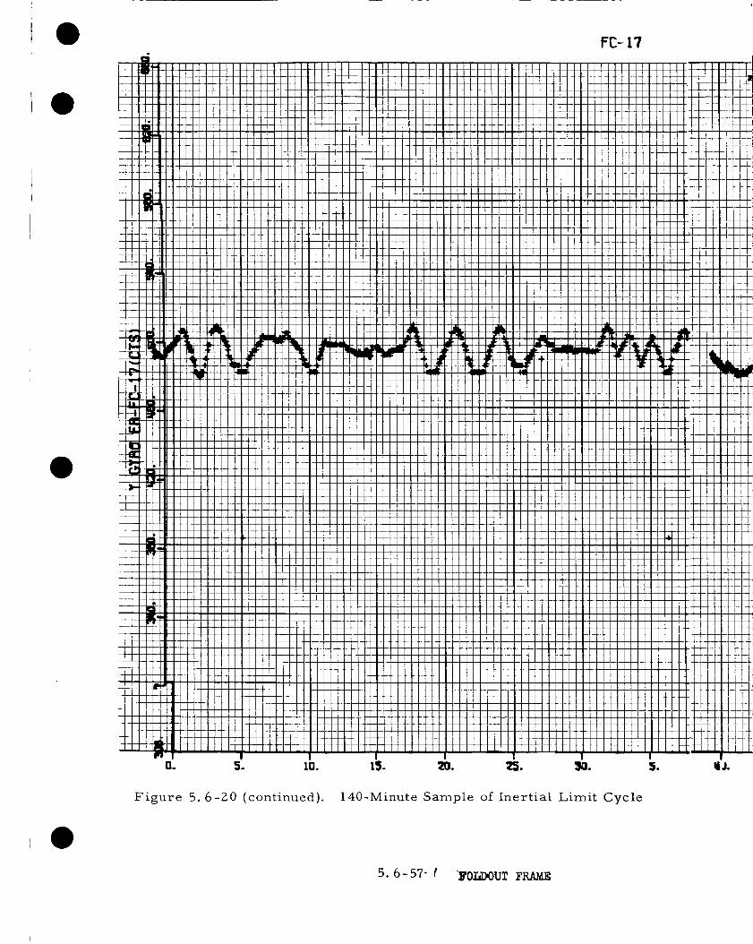
0- 5- 10.

Figure 5.6-Z0 (continued).

FC-17

j_ii

J

L

J+÷fi

i

!

i

±

i

i

Ii

II

I

I

i

I

I

I

15. t_. _. 3O.

140-Minute Sample of Inertial Limit Cycle

+7

i"

±t

I

1

I

_+__+_

I

I

I

iiI

i

Ii

i

5.6 -57- I ¥01_DOUT l_l_A_

_13. 80. 8'3. 70.. _.JL-I I UNRR TRRNSIT,MIN {I.T.:152/19/20/_2}

_o

III

!

i

?I

, !It

I

iiIi

I

IIIIf

i"!

iI

JI

IIJtt

i

iIII

qIJ

ii

I]11

'¥OZ_OU;

.'-._-___

1]0. tlS. L_. 125. 130. II. I_0.

J

1

T

I

I

T

I÷

I

FOLDO_UT FRAME

I

Figure 5.6-20 (continued}. 140-Minute Sample of Inertial Limit Cycle

5.6 -5c)-l '¥OI.,DO_ _'_

II

III

II

II

LO0.

D Gyro Drift Measurements. A procedural form for measuring gyro

drift is included in Reference 7. An analysis of the accuracy of the measure-

ment procedure is reported in Reference 8. The results are summarized in

Table 5.6-11. See also Figures 5.6-21 and 5.6-22.

Gas Jet Thrust Level. Although the "Surveyor Functional Require-

ments Specification," 224510E, does not directly dictate the minimum

allowable thrust level, it does infer these levels by specifying the minimum

allowable gas jet torque values. These values are presented as follows:

Minimum

Torque

Spacecraft Requirement, Moment Number of

Axis in.-lb Arm, inch Gas Jets

Minimum Thrust

Value, pound s

Roll 4. 00 77 I 0. 05Z

Pitch 4. Z5 45 2 0. 047

Yaw 7. 00 68 2 0. 05Z

D

D

It is apparent from the above data that the minimum allowable gas jet

thrust is 0. 05Z pound. The gas jet system was designed for a nominal thrust

value of 0. 057 pound.

In References 9 and Z8, amethod is proposed whereby the gas jet thrust

level can be determined from the time response of the gyro error signal re-

ceived during a roll maneuver. It also mentions that a weighting factor may be

requred for the basic equation derived in the references. The equation is:

z cT -

RtP

From an analog computer simulation program of the gas jet system,

the average weighting value was determined to be 0.85. The values for the

various parameters in the previous equation are as follows:

I = 189 slug-ft Zz

R = 6.4 feet

_c = 0.500 deg/sec

t = 5.66 secondsP

5.6-61

tp represents the time it takes the gyro output to reach its firstmaximum from the time the maneuver command is initiated (Figure 5.6-23).

Multiplying the value of tp with the weighting factor of 0. 85, the correctedtime is 4.81 seconds. Thus the gas jet thrust level for SC-I roll was

T = 0. 054 pound.

5.6. 7.6 Premidcourse Maneuvers

In order to accomplish the required velocity correction, it was

necessary to perform a negative roll maneuver and a negative yaw maneuver

of magnitude 86. 50 degrees and 57.99 degrees, respectively. The analysis

to follow is an attempt to accurately reconstruct the total premidcourse

maneuver phase from the beginning of the first roll maneuver to vernier

ignition and to compute the roll axis final pointing error exclusive of any

tracking data.

Several variables affect the accuracy of an angular maneuver:

precession rate accuracy, precession command time, gyro drift, and initial

attitude errors due to biases and limit cycle. When several maneuvers are

performed with large time intervals between them, attitude errors due to

gyro drift must be included. A list of all parameters affecting the midcourse

maneuver accuracy is presented in Table 5.6-12 along with their allowable 3o

values and actual performance values whenever possible.

Determination of Precession Times

The register was loaded with 433 bits for roll and 290 bits for yaw.

With a clock rate of 2. 5 cps, the respective times are 173.20 seconds and116.00 seconds with a maximum error of 0.20 second.

The gyro error signal data was used in determining the actual pre-

cession time. The sampling rate during the maneuvers was 20 times/second,

giving a resolution of 0.05 second. The results are as follows (Figures

5.6-24 and 5.6-25).

T = 173. 17 seconds (roll)

T = If5. 80 seconds (yaw)

PrecessionRates. The accuracy of the precession rates imposed

by the "Surveyor System Functional Requirements Specification" is

0. 5000±0.0011 deg/sec. The precession rate obtained during the star

mapping phase indicates that the positive precession rate is 0. 5004 deg/sec.

It is unfortunate that data is not available which can be used to

determine the negative roll precession rate with the same degree of accuracy.

A good indication of the negative precession rate value is that after performing

the postmidcourse yaw and roll maneuvers with the same precession times

as those for the prernidcourse maneuvers, the Canopus error signal indicates

that the previous attitude about roll was obtained to within 0.05 degree.

5.6-62

_D!

_0

|

|

P

1.5

i 1.0

0.5

,.,:-

_ o

N -o.5Zw

Z

'7 -I .0

-I.5

Z 0') mI-- U.I ,_03 I--lU tU

z _ "' ,_ oW

u_ W 0 --

_ (_ _ _"r (n X -- " " " _E

T T 1 T r r---[

• KEARFOTT DATA

• HUG_ _--

-'¢ ...,_ = __ = .5 _= -

DATE

L t ) I

CUMULATED ON-TIME, HOURS

Figure 5.6-ZZ. Time History of Gyro

(Non-g) Drift

a) Roll(S/N 57)

D

5.6-65

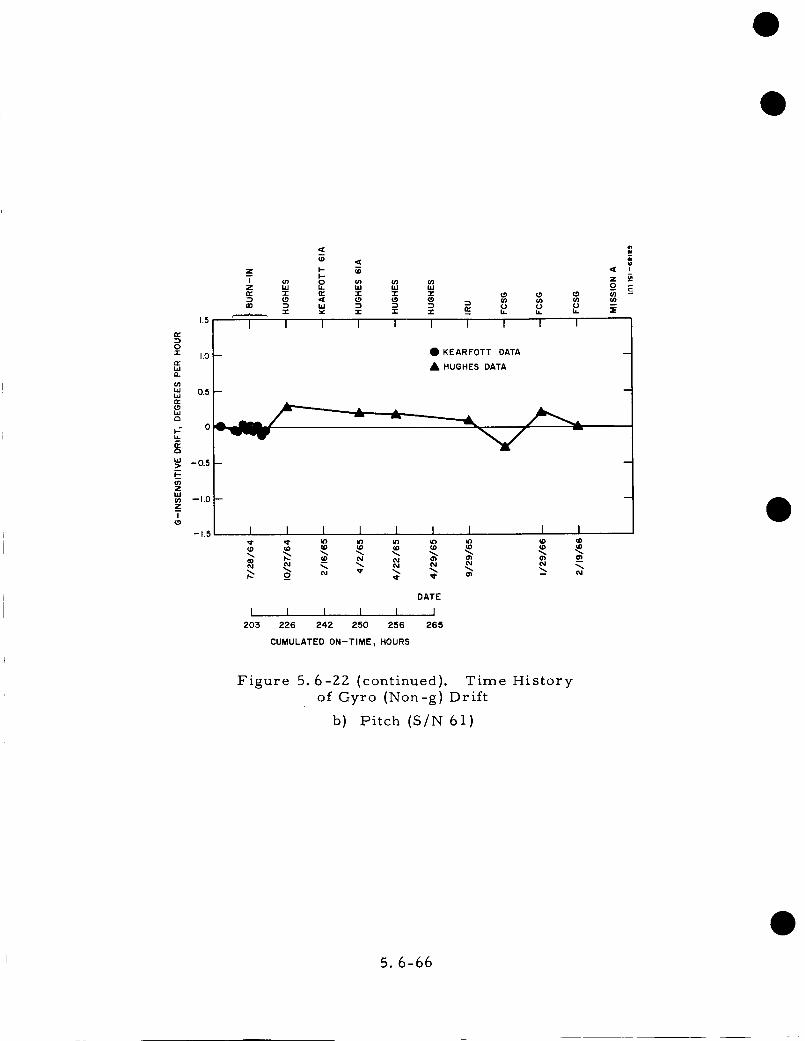
n-

OT

r_

,,Jn_

W

mn-

h,>

F-

ZbJU)Z

I

1.5

1.0 t

0.5

,<

-- I-I

_,. -i- 12: -I- -r z:D to <[ (.o t9 tom :D W :D :D :D :D (3

-r" zr. -r- "r" X n.. t_

I I I I I I I I

• KEARFOTT DATA

• HUGHES DATA

¢=w

<[ I

zo

u) (n u)

" t

t--I.0

-15 I I I I I I I I I

DATE

I I I I I I

203 226 242 250 256 265

CUMULATED ON-TIME, HOURS

Figure 5.6-22 (continued). Time History

of Gyro (Non-g) Drift

b) Pitch (S/N 61)

5. 6-66

IO _ W _O u.

Z z _ uJ w u_ _ _ c

W _ W LU W U. bJ LU _1 0

_ '.0/ . , ,EA,FOTTDATA ___--_g_: 0.5

g o

_ -0.5

_ -I.0

z_l_L_Llml

_- __ _ _ _ _DATE

I I I I I [ I I I I© _ _ _ ® _ o _ _ om o

_m

CUMULATED ON-TIME, HOURS

Figure 5.6-22 (continued). Time History

of Gyro (Non-g) Drift

c) Yaw (S/]',,T 25)

5.6-67

0

@

;>:::l

o ¢}

0

0 o_m

N

• 0

.,--I

M®N

e_

.,.-t

"tJ

o

C_

5.6-68

544

(;3

_z

zo

540

556

552

528

524

520

5i6

5126:30:13.6

START OF ROLL

/_

MANEUVER

w-

173.17 sec

END OF ROLL

MANEUVER

I

%

6:30:14.4 6:30:15.2 6:53:07.0 6:33:07.8

DATA: DSIF TAPE HIGH POWER

433 BITS STORED IN REGISTER

(DIG 2) = 17'3.20 secTELEMETRY MODE !

4400 bps

6:33:08.6

TIME, HOUR: MINUTE: SECOND

Figure 5.6-Z4. Roll Gyro Response Profile

for Premidcourse Roll Maneuver

5.6-69

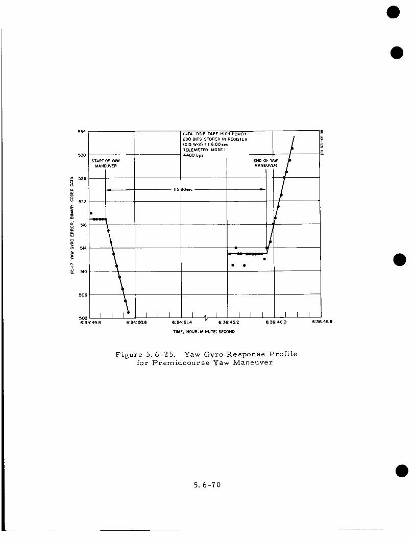
8

z

=-o

uJ

0

i_-T

534

53O

526

522

518

514

510

506

502

6: 34:49.8

START OF YAW

MANEUVER

DATA: DSIF TAPE HIGH POWER

290 BITS STORED IN REGISTER

(DIG W-2) = 116,00sec

TELEMETRY MODE I

4400 bps

1lS.80sec

END OF YAW

MANEUVER

mL__L_6: 34:50.6 6: 34:51.4 6: 36:45.2 6: 36:46.0 6:36" 46.8

TIME, HOUR: MINUTE: SECOND

Figure 5.6-25. Yaw Gyro Response Profilefor Premidcourse Yaw Maneuver

5. 6-70

TABLE 5. 6-IZ. SC-I PERFORMANCE DETAIL

Characteristic: Midcourse Angular Error:Phase: Midcourse Correction

Item

1

30 Performance

Parameter Requirement Specification Value Comments

Initial position errors

Sensor group rollaxis to sun

spacecraft line

Pitch/yaw limit

cycle

Sensor group roll-

pitch plane to

Canopus - spacecraft

line

Roll limit cycle

2 Rotational magnitude

errors

Gyro torquer scale

factor

45-degree rotation

180-degree rotation

Precision current

accuracy (0. 13)

45-degree rotation

180-degree rotation

Timing source

accuracy

45-degree rotation

180-degree rotation

Precession current

circuit drift

45-degre,, • otation

180-degree rotation

3 Rotational axis error

Gyro alignment to

IRU A, B, and C

axis

IRU roll and pitch

axis to sensor group

roll and pitch axis

4 Final position errors

Vernier engine

thrust vector to

nozzle c enterline

Installation align-ment and bracket

bending compensation

Spacecraft roll axis

to sensor group roll

axis

Attitude control

steady state error

Reference axis drift

gyro non-g drift

Midcourse

maneuver duration

Total attitude error

0.2 degree

O. 3 degree

0.2 degree

0.3 degree

0.05 percent

O. 05 percent

O. 13 percent

0. 2 second

0. 1 percent

O. 1 degree

O. i degree

0.33 degree

O. 1 degree

0. i degree

0. 1 degree

1 degree/hr

15minutes

0.7 degree

224510D

4.3.1.1

224510D

4. 3.1. 1

224510D

4. 3. 1.2

234633

234633

3.3.5.7

234610

4.4.2.2.1

234630

4.2.4.3

234600

3. 5. 1

287015

3.5.4

224510D

4. 1.3.7. 1

224510D

4. 3.1.4 EO

224510D

4.3.1.5

224510D

3.6.4.2

3.6.3

0.005 degree

0.014degree/

-0.232 degree

O. 031 degree

0.15 degree

'0.08 percent

O. 015 degree (roll)

O. 1 degree (yaw)

'0.280 degree

SSD 64102R, Table IV (weight,

balance, and alignment report)

See "Initial Attitude Errors"

SSD 64102R, Table IV.

See "Initial Attitude Errors"

From precession rate determina-

tion. Desired rate is 0. 5000

deg/sec. The actual*rate was

0. 5004 deg/sec.

0.005 degree

O. 121 degree

4minutes

36 seconds

O. 313 degree

These values correspond to a

timing error of 0. 03 second for

the roll maneuver and 0. 20 second

for the yaw maneuver.

With respect to spacecraft coordi-

nates, the vector representation is

"IA = -0. 00462 1X -0. 00160 Iy - 1Z

Based on a moment disturbance

value of 74 in-lb. This value was

obtained from "Midcourse-Vernier

Engine System Parameters. !'

Calculated value of pointing error

due to drift ("Analysis" subsection).

From time and events log

Note: The performance values cannot be added algebraically to obtain the total error because the problem is

three -dimensional.

5.6-71

This indicates that the negative precession rate must have been almost thesame as the positive rate. Sun sensor error signals indicate that theprevious attitude in pitch and yaw was obtained to within the limit cyclevalue of 0.2 degree.

For this analysis, a negative precession rate of 0. 5000 deg/sec willbe used for both yaw and roll commands.

Gyro Drifts. During a 3-hour period just following the midcourse

phase, a gyro drift check was made. The drift rate values were obtained

from the plots of FC-5, FC-6, and FC-IZ which are the pitch sun sensor

error signal, yaw sun sensor error signal, and Canopus error signal,

respectively (Figures 5.6-26 through 5. 6-28). The results are asfollows :

Roll drift = 0.202 deg/hr

Yaw drift = 0.675 deg/hr

Pitch drift = -0. 021 deg/hr

Normally, if the pitch gyro drift rate is much larger, a more

sophisticated technique of determining roll gyro drift would be used to account

for coupling between the pitch and Canopus sensor line-of-sight axes.

Initial Attitude Errors.

vers were as follows:

The initial attitude errors prior to maneu-

Start of roll (151:06:30:14.16), degree

Pitch = 0 1 caged to the sun during

Yaw = 0 I first roll maneuver

Roll = -0.015

Start of yaw (151:06:34:50.80), degree

Pitch = 0.014 (FC-5)

Yaw = 0.232 (FC-6)

Roll = -0.150 (FC-49)

Analysis

The initial attitude

(Ixo)11Iyo = _z

Izo _0y

of the spacecraft to that assumed is

l ix I20

-_x I30

Cll

5.6-72

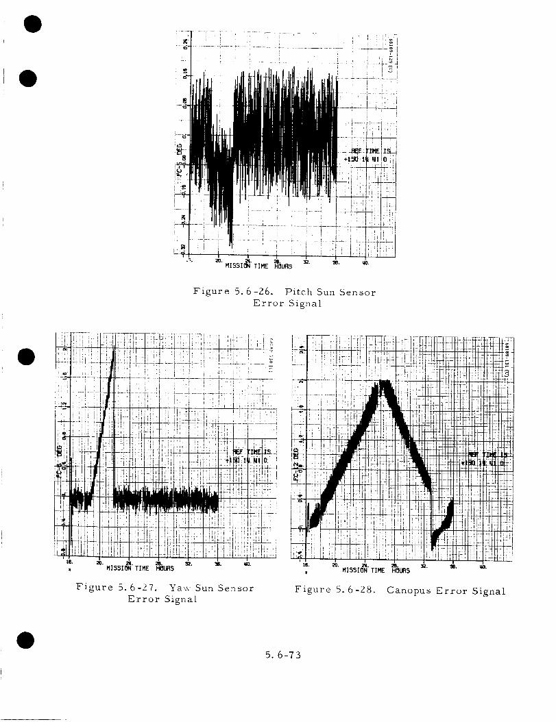
, I

Figure 5.6-26. Pitch Sun Sensor

Error Signal

Figure 5. 6-27. Yaw Sun Sensor

Error Signal

Figure 5. 6-28. Canopus Error Signal

5.6-73

where Iio s are unit vectors of an inertial coordinate system established by

perfect alignment to the sun and Canopus, and the c#matrix is derived from

the small angle approximation of a three-sequential rotation matrix.

For the roll maneuver, q_x and _y will be set to zero since the pitchand yaw axes are slaved to the sun line and are subject to the optical limit

cycle which tends to average the error to zero.

Roll maneuver is represented by the follo.wing matrix representation:

i IxR 1

Iy R =

IzR

I()cos ('_'+cR) S(_ + OR) 0 Ixo

-sin ('_+ ¢R) cos (_ + _R) 0 ly°

0 0 l Izo

(z)

where '#is the desired roll maneuver angle and ¢R is the error in rotation

due to timing error and gyro drift. ¢R = -0. 10 degree.

Attitude change due to gyro drifts is determined from the following:

i lxl 1

ly i =

Iz I

- L I L2 L3 -

M 1 M 2 M 3

_N 1 N 2 N 3 _.

I lxR

lyR

IzR

(3)

where

I) Li(t) =

M. W -N. W

L. cosflT + lo z. .lo Y sin fitxo

+

2L. W + M. W W + N. W W

lO X iO X y IO X Z

f12

(1 - cos fiT)

2)L. W -M. W

Ni(t) = Nio cosset + 1o y 1o x sin fiTfl

+

2L. W W + M. W W + N. W

i0 X Z i0 y z io z

f12

(1 - cos fiT)

5. 6-74

D 3) Mi(tl = M.lOcos f2T+

(N. W - L.io x _oWz)

f_

+

2L. W W + M. W + N.

lo y y lo y lo

_2

sin f_T

W W

y z (1 - cos flT)

4) Lio , Nidand Mio are initial direction cosines

5) i = I, Z, 3

6) _22 = W2 + W2+ W 2y y z

7) W = spacecraft drift rates

8) t = time

Initial attitude error prior to the yaw maneuver is similar to

Equation g.

Yaw maneuver is represented by the following matrix equation:

(x3)IIy 3 =

Iz3

cos (8 +

0

sin (@ +

Cy) 0

cy) 0

sincecYl(Ix2)o Iy z (4)

cos (@ + Cy)_ Iz2

where @ is the desired yaw maneuver angle and Cy is the error in rotationdue to timing error and gyro drifts. ¢ = 0.01 degree.

Y

Equation 3 can be used to represent the attitude change from the end

of the yaw maneuver to the point of vernier ignition.

A digital computer program was developed to facilitate the calculation

of the pointing accuracy. The program output is represented in five differentdirection cosine matrices which illustrate the contribution of each error source

to the final pointing accuracy. The various matrix outputs are as follows:

I) Perfect case (no errors)

2) Initial attitude errors only

3) With gyro drifts only

5.6-75

4) Angular maneuver execution errors only

5) Actual case (all error sources)

The matrices are presented in Table 5.6-13.

TABLE 5.6-13. DIRECTION COSINE MATRICES

Positive Unit Vectors"

3. 23598 E-2

0. 998135

-5. 17664 E-2

3. 05669 E-2

0. 998291

-4. 98048 E-2

3. 57482 E-2

0. 997996

-5. 22124 E-2

3. 14451 E-Z

0. 99824

-5. 02837 E-2

3. 30384 E-2

0. 998263

-4. 87709 E-2

Perfect Case

-0. 529079

6. 10485 E-2

0. 846374

Attitude Error

-0. 525742

5. 84362 E-2

0. 848635

Drift Error

-0. 530651

0. 063228

0. 84 5229

Maneuver Error

-0. 529282

5. 93064

0. 846371

Total Error

-0. 527534

5. 88641 E-2

0. 847492

0. 847956

0

0. 530067

0.85OO95

2.44344

0. 526629

0. 846836

-2. 50886

0. 531848

0. 847863

0

0. 530215

0. 848891

-2. 27153

0. 528563

E-3

5.6-76

The results (Figure 5.6-29) of the investigation are as follows:

l) Gyro drift contribution = 0.121 degree

2) Maneuver execution contribution = 0.0855 degree

3) Initial attitude error contribution = 0.263 degree

4) Actual (all error sources} = 0. 204 degree

Notice that the sum of the individual error source contribution does not equalthe actual pointing error value. This is as expected since the problem isthree-dimensional.

5.6.7.7 Postmidcourse Maneuver

The postmidcourse maneuver is generally used to realign the space-craft to celestial reference after performing a midcourse velocity correction.To accomplish this, two reacquisition schemes are available. One method isto perform the premidcourse maneuvers in reverse and the other is to per-form another automatic sun acquisition sequence. The first method is mostdesirable since real time monitoring of optical sensor signals will providegood indications of premidcourse maneuver accuracy and attitude controlduring the thrust period; that is, if reacquisition of the sun and Canopus isnot achieved to within a fair degree of accuracy, one or more of the followingconditions must have existed:

I) Nonsymmetrical precession commands.

2) Spacecraft attitude change occurred between maneuver periods.

3) Premidcourse maneuvers were not accurate.

4) Postmidcourse maneuvers were not accurate.

The first method was chosen for the SC-I mission and, at approxi-mately 151:07:00:56, the initial premidcourse attitude was successfullyreacquired to within 0. 15 degree.

Determination of Precession Times

For the premidcourse maneuvers, the magnitude register was loaded

with 290 bits for yaw and 433 bits for roll. This corresponds to I16.00 and

173.20 seconds, respectively.

The precession time, using gyro error signal data, was found to be:

T = I15.5 seconds (yaw)

T = 173.0 seconds (roll)

5.6-77

The reason for the large difference between the commanded valuesand the values above is that for the postmidcourse maneuver phase the telem-etry rate was reduced from 4400 to 550 bits/sec, increasing data granularityfrom 0. 25 to 2. 00 seconds (Figures 5. 6-30 and 5.6-31).

Maneuver Accuracy

The total midcourse maneuver accuracy can be appreciated from the

following optical sensor data. These values represent the final attitude

orientation with respect to the sun and Canopus prior to optical control mode

operation:

Pitch sun sensor error signal = -0. 15 degree

Yaw sun sensor error signal = -0.04 degree

Canopus error signal = 0.00 degree

Plots of the star intensity signal during premidcourse and post-

rnidcourse roll maneuvers are included to illustrate the identical nature of

the maneuvers (Figures 5.6-32 through 5.6-35).

5.6. 7. 8 Midcourse Velocity Correction Phase

The Surveyor Imidcourse correction was successfully executed at

06:45:24:651 GMT on 31 May 1966. From orbit determination, the actual

magnitude of the velocity change was estimated to be 20. 266 m/sec. Com-

pared to the desired value of 20. 347 rn/sec and the commanded value of'

20. 396 m/sec, this constitutes an error of 0.081 rn/sec in the desired value

and a AV execution error of 0. 130 m/sec. Also from orbit determination, the

midcourse thrust vector pointing error was calculated to be 0.221 degree.

Using prelaunch alignment information and in-flight data, the thrust vector

pointing error was calculated to be 0.313 degree. The directions of the

actual and calculated thrust vectors were in agreement.

Midcourse Engine Ignition Characteristics

The SC-I midcourse maneuver was characterized by a smooth vernier

ignition followed by a nominal, uneventful thrusting phase. Peak pitch and

yaw gyro errors during thrusting were 0. 15 degree or less during the ignition

transient and virtually zero thereafter until engine cutoff. A summary of the

midcourse pitch and yaw gyro errors is given in Table 5.6-14.

Prior to vernier ignition, pitch and yaw gyro errors were maintained

within +0. 2Z degree by the gas jet system. At the instant of ignition, these

errors were -0. 15 and 0. 04 degree for pitch and yaw, respectively, and the

subsequent transient was reduced to zero in approximately 4 seconds. The

yaw error transient overshoot was -0. 08 degree, while the pitch errorexhibited no overshoot. The transient behavior of both errors was domi-

nated by the I. 0-second time constant of the attitude control loops.

5. 6-78

-z

/MANEUVER

/ I \ /EXECUTION

OR --Y

Figure 5. 6-29. Premidcourse

Maneuver Errors

620

60O

580

<xI-

o

560(:3o(.)

>-nr

<I 5402

£0

r,- 520l¢1

0

>-

500

480

460

AI I

DATA: DSIF TAPE 290 bits STORED IN

REGISTER :116.00 sec TELEMETRY

MODE C 5,50 bits/sec HIGH POWER

I115.5 sec _-_

440 I I I I I I I I6:52"40 6:53:10 6:53:40 6:54:10 6:54:40

T_ME, HOUR: MINUTE: SECOND

==¢=_oi

c

6:5,5:10

Figure 5.6-30. Yaw Gyro Response Profile

for Postmidcourse Yaw Maneuver

5.6-79

580

r_

560

540

i 520

500

480

4606:57:50

I I

6:58:20

/ I

DATA: DSIF TAPE 453 bits STOREDIN REGISTER =173.2 sec TELEMETRYMODE C 550 bits/sec HIGH POWER

I I I

6:58:50

173 sec

I I l

6: 59:20 6:59:50 7:00:20

!!

JW

, I I , I7:00:50

TIME, HOUR: MINUTE; SECOND

Figure 5. 6-31. Roll Gyro Response Profilefor Postmidcourse Roll Maneuver

7"01:20

Z

_J

k-

Ld

rr

Z

b.

I0

8

6

4

2

\ vJ\

==

==

6:30 6:31 6:52 6:33

TIME, DAY 151, HOUR:MINUTE

6:34

Figure 5.6-32. Star Intensity, FC-14,Premidcourse Roll Maneuver

151:06:30:13 to 06:33:06 GMT

During

5. 6-80

8

I-

1.1.1

I-

nr

8

dT

I0

06:30 6:31 6:32 6:33

TIME, DAY 151, HOUR:M]NUTE

6:34

Figure 5.6-33. Canopus Error, FC-IZ,

Premidcourse Roll Maneuver

151:06:30:13 to 06:33:06 GMT

During

go° =0

w

_. 4

z

I"

2

u-

i

6=57:30 6_58:30 6=59:30 7:00=30

TIME, DAY IS1, HOUR,MINUTE;SECONO

7=01:30

Figure 5.6-34. Star Intensity, FC-14,Postmidcourse Roll Maneuver

151:06:58:02 to 07:00:56 GMT

During

5. 6-81

¢n IO

8Z- 8I,--

6

_ 4

_ 21-

d

u. 0

¢

IA

/\

6=57:50 6,58,50 6,59,30 7,00'30

TIME, DAY 151, HOUR:MINUTE_SECOND

7,0630

Figure 5.6-35. Canopus Error FC-IZ,Postmidcourse Roll Maneuver

151:06:58:02 to 07:00:56 GMT

During

5.6-8Z

D

DTABLE 5.6-14. MIDCOURSE IGNITION TRANSIENT CONTROL SUMMARY

Gyro Error Telemetry Resolution = 0.013 degree

Initial(pre-ignition)gyro errors, degrees:

Pitch = -0. 15

Yaw = O. 04

Peak angular overshoot, degrees:

Pitch = 0

Yaw = -0.08

Peak angular rates, deg/sec:

Pitch = 0.25

Yaw = -0.36

Net 0.44

Vernier engine startup time = <0.15 second

D Peak angular rates of (approximately) 0.25 deg/sec in pitch and -0.36

deg/sec in yaw occurred at vernier ignition. The startup impulse dispersions

(deviations from average startupimpulse) of the three engines are

calculated by the procedure outlined to be approximately as follows:

Leg I: -0.08 Ib-sec

Leg Z: -0.23Z Ib-sec

Leg 3: 0.312 Ib-sec

which implies a maximum startup impulse variation (between legs 2 and 3) of

0.544 Ib-sec. This is an order of magnitude less than the allowable variation

between engines specified in Reference 10.

Based on the startup impulse figures listed above, it is concluded that

leg 3 produced thrust first, and leg 2 last. The behavior of vernier engine

throttle-valve signals at ignition corroborate these conclusions. For example,

leg 2 throttle-valve signal (FC-26) remains high longer than either of the other

two in order to compensate for the relatively slow startup. Based on the

acceleration error telemetry signal (FC-15), it is concluded that all three

engines were producing controlled thrust within about 0. 150 second of the

ignition command signal. Therefore, acceleration signal amplifier satura-

tion, which requires a startup delay of 0.26 second, did not occur, and no AVerror information was lost.

5.6-83

Calculation of Engine Ignition and Shutdown Impulse Dispersions

Calculation of engine ignition or shutdown impulse dispersions follows

the procedure outlined in Reference ii. Pitch and yaw angular rate incre-

ments following ignition or shutdown are related to engine impulses by

1

L_i.x = _7--(-2.94 II + 0. 53 IZ + 2.43 13)X

1

A_y - I (-1.08 Ii + 3. I0 12 - 2. I0 I3)Y

where

a_x, A_Y

Ix, IY

= pitch and yaw rate increments (rad/sec)

= pitch and yaw moments of inertia (slug-ft 2)

Ii, 12, 13 = total ignition or shutdown impulse of engines i, Z, and ._(ib-sec)

These relations follow directly from vernier engine locations on the

spacecraft.

Since the difference in impulse between engines is of concern here,

the total impulse of each engine can be expressed as

I. "" I + AI i -" I, 2, 31 O 1

where Io represents average single engine impulse (i.e., one-third of total) and

L_I. represents deviation from average. This means that1

I1 + I2 + 13 _- 3 I°

or

Al I + DI 2 + L\I3 = 0

Combining this last equation with the first two given above yields the following

matrix equation:

(i x)(_2.94032.43)(11)I &by = -I. 08 3. i0 -2. I0 !_I2

0 I I I D.I3

5.6-84

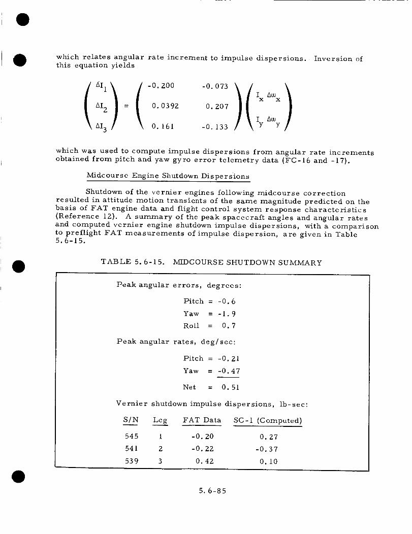
which relates angular rate increment to impulse dispersions. Inversion ofthis equation yields

i)100000AI2 = 0. 0392 0. 207

AI3 0. 161 -0. 133Iy A_y

which was used to compute impulse dispersions from angular rate increments

obtained from pitch and yaw gyro error telemetry data (FC-16 and -17).

Midcourse Engine Shutdown Dispersions

Shutdown of the vernier engines following midcourse correction

resulted in attitude motion transients of the same magnitude predicted on the

basis of FAT engine data and flight control system response characteristics

(Reference 12). A summary of the peak spacecraft angles and angular rates

and computed vernier engine shutdown impulse dispersions, with a comparison

to preflight FAT measurements of impulse dispersion, are given in Table5.6-15.

TABLE 5.6-15. MIDCOURSE SHUTDOWN SUMMARY

Peak angular errors, degrees:

Pitch = -0.6

Yaw = -I. 9

Roll = 0.7

Peak angular rates, deg/sec:

Pitch = -0.21

Yaw = -0.47

Net = 0.51

Vernier shutdown impulse dispersions,

S/N Leg FAT Data

545 l -0.20

541 2 -0.22

539 3 0.42

ib-sec:

SC-I (Computed)

0.2_

-0.37

0. I0

5.6-85

It may be noted that peak gyro angles were less than Z degrees andwell within the required travel range of +i0 degrees. Inertial reference was

therefore retained, and reacquisition of the sun and Canopus were routinely

accomplished via the reverse maneuver sequence.

Vernier engine shutdown impulse dispersions (relative to mean impulse

of the three engines), calculated frolrl pitch and yaw angular rate data as per

the procedure outlined in the "Midcourse Engine Startup Characteristics, "

were well within the specification limit of ±0.63 ib-sec (Reference 8).

Determination of Thrust Vector Misalignment

The following error sources will be considered in the determinationofthe

actual thrust vector position:

I) Premidcourse maneuver errors

2) Limit cycle error

3) Gyro drift errors

4)

5)

Vernier engine alignment offsets and support bracket bending

Attitude error during burn caused by moment disturbance.

The total error in the position of the spacecraft Z axis due to the first

three items above is given in the "Premidcourse Maneuvers." The final

orientation (just prior to vernier ignition) of the spacecraft with respect to the

initial celestial reference in matrix notation is

(,[ I(!o x°ixf _ 3. 30384 E-2 -0. 527534 0. 848891

lyf = 0.998263 5. 88641 E-2 -2.27153 E-3 (i)

]-zf/ -4. 87709 E-Z 0. 847492 0. 528563 zo/

The error due to item 4 above is given in Reference

ctor presented in the reference is given in spacecraft coordinates as

13. The accelera-

tion ve

follows:

AMC = AMC (-0. 00462 Ixf-0. 00160 Tyf -0. 999988 Izf) (2)

Using Equation I, the acceleration vector can be referenced to theinitial celestial reference. The result is

IAM C = 0.0470204 Ixo-0. 8451388 ly O-0. 5324749 Izo (3)

The desired vector position with respect to the celestial reference (from

"Premidcourse Maneuvers") is

T = 0.0517664T -0.8463740T -0. 5300670T (4)o xo yo zo

The pointing error can now be determined by performing a dot product of the

two vectors (3 and 4). The result is a pointing error of (Pc = 0.313 degree.

5.6-86

Roll Control During Midcourse

The roll disturbance torques which were estimated using telemetry

of the roll control nozzle actuator commands (FC-43), the roll precession

commands (FC-49), and the preflight predicted vernier engine bracket bend-

ing were determined to be extremely small. The telemetry data for the roll

actuator angular position during midcourse agreed quite closely with the

values expected due to bracket bending. The predicted roll control nozzle

angle to compensate for bracket bending was computed from the prelaunch

alignment angles, a bracket spring constant of 0. 045 deg/Ib, and predicted

thrust levels of the vernier engines. The roll disturbance torques due to

vernier engine thrust vector misalignments other than bracket bending canhe determined from the difference between the two curves of telemetered

roll actuator position and predicted roll actuator position in Figure 5.6-36.

It is seen that the difference between these curves is a maximum of 0. Z5

degree or a roll disturbance of less than i. 0 ft-lb.

The maximum commanded angle of the roll actuator was 0.9 degree,

and the maximum roll actuator rate (slope) was 0. 4 deg/sec. The commanded

position of the roll control nozzle after initial transients is seen to jump

between 0.6 and 0.75 degree from telemetry signal FC-43. This agrees

quite well with the angle expected from the initial vernier engine alignment

and the bracket bending of 0.75 degree.

To ensure that the commands to the roll actuator were actually due

to roll gyro error signals (Figure 5.6-37), the roll precession command as

determined from FC-49 and the commanded angle to the roll actuator as

monitored with FC-43 are compared on the same graph {Figure 5.6-38). The

two signals are seen to be closely correlated, in that when one signal changes

significantly so does the other value.

Midcourse Velocity Determination

The general concept of midcourse correction capability employed by

Surveyor is to apply a constant acceleration for a finite period of time. Thus,

in theory, once the magnitude of the velocity correction is known, the exact

duration of the constant acceleration phase can be determined. In practice,

this approach is slightly altered to account for such error sources as engine

ignition transients, shutdown impulse, and hysteresis. Thus, the actual

command time AT is slightly higher.

The actual values used during flight were as follows:

I) Desired AV = Z0. 347 m/sec

2) Desired AT = Z0. 800 seconds

3) Register load = 417 bits = Z0.850 seconds

5.6-87

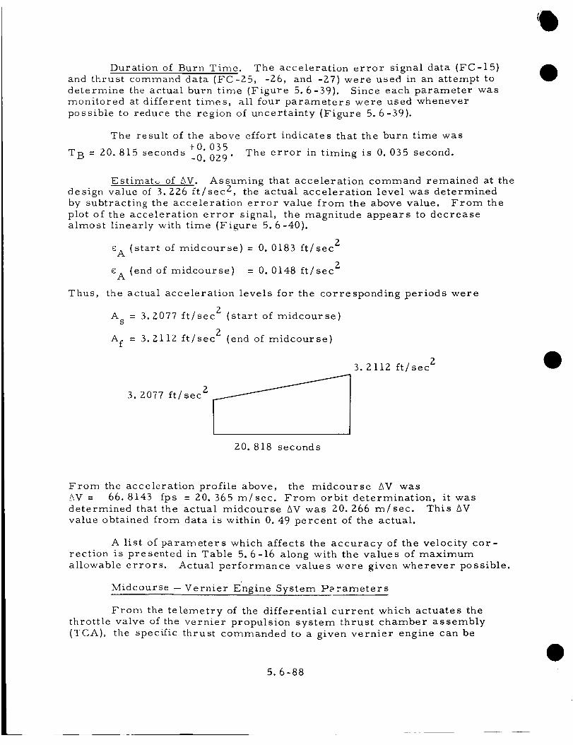
Duration of Burn Time. The acceleration error signal data (FC-15)

and thrust command data (FC-25, -Z6, and -Z7) were used in an attempt to

determine the actual burn time (Figure 5.6-39). Since each parameter was

monitored at different times, all four parameters were used whenever

possible to reduce the region of uncertainty (Figure 5.6-39).

The result of the above effort indicates that the burn time was

+0. 035T B = 20. 815 seconds -0. 029" The error in timing is 0. 035 second.

Estimat_ of _V. Assuming that acceleration command remained at the

design value of 3. ZZ6 ft/sec Z, the actual acceleration level was determined

by subtracting the acceleration error value from the above value. From the

plot of the acceleration error signal, the magnitude appears to decrease

almost linearly with time (Figure 5.6-40).

Z_A (start of midcourse) = 0. 0183 ft/sec

cA (end of midcourse) = 0. 0148 ft/sec Z

Thus, the actual acceleration levels for the corresponding periods were

gA = 3. Z077 ft/sec (start of midcourse)s

Af = 3. ZllZ ft/sec Z (end of midcourse)

3. Z077 ft/secZ_

Z3. gllZ ft/sec

20.818 seconds

From the acceleration profile above, the midcourse AV was

t_V = 66. 8143 fps = 20. 365 m/sec. From orbit determination, it was

determined that the actual midcourse AV was 20. 266 m/sec. This AV

value obtained from data is within 0. 49 percent of the actual.

A list of parameters which affects the accuracy of the velocity cor-

rection is presented in Table 5.6-16 along with the values of maximum

allowable errors. Actual performance values were given wherever possible.

Midcourse- Vernier E'ngine System Porameters

From the telemetry of the differential current which actuates the

throttle valve of the vernier propulsion system thrust chamber assembly

(TCA), the specific thrust commanded to a given vernier engine can be

5.6-88

!

,¢

;jr:

.[

..... ' _:10'1,51n ,L 3 bl "1-10_1 O.L ._79N_

{ T. ,;it" ; • : "' [ ' "_2":]L.._'..--'__ ............. : .............. •_.LL. :_g.:_:.:

" i ] ''F7 -" :........ ' -:' "::_.

...... '............ _ ................ _ " . i ......... -ii

1

.... . L._i- -......... -:

; I ,

L

G3ONVWL40:) -'.... " ' "

I..... i i . i ii::i

F0

0

r.j)

u

"8_

0 .,,-a_' (vl

,..o_,.g"s

0

o©.-,

o

_,._,|

,,,oL...)r..n

do

=:1o_,_

ooI

,.A

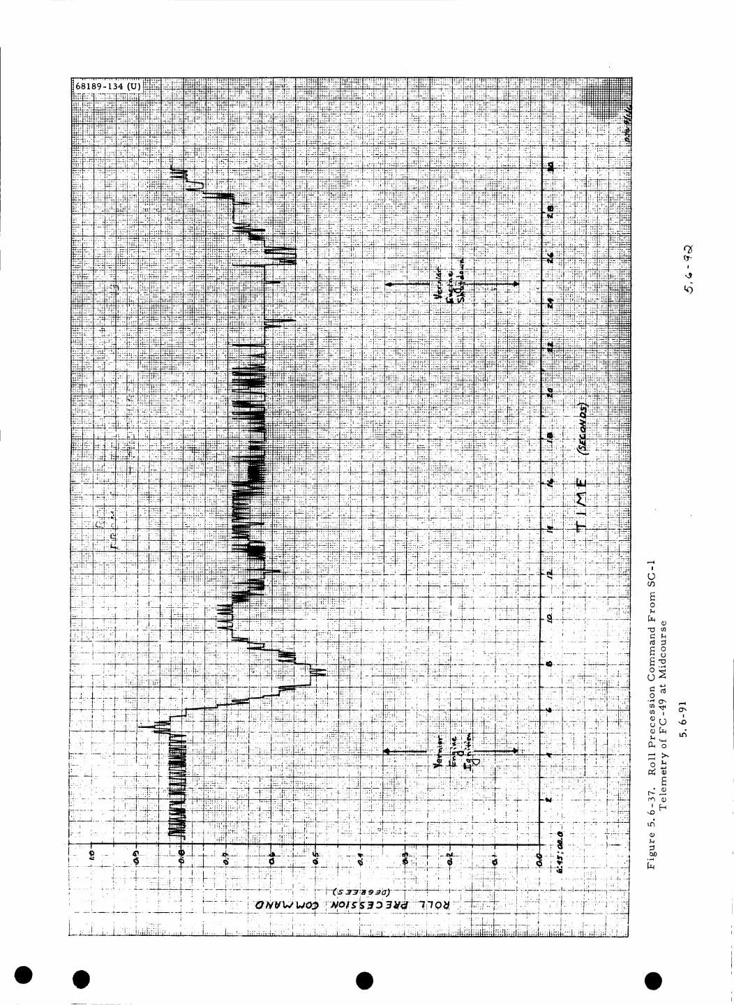
O

¢)m

(o

28_

8o

• <D

em _D

,.4D

u4_D

lab,,-i

I

4

7,.I

,4D

,.d

,--4,--4

0

o0 m

,--, 0

r!,-_

Ue_

_u

_2

_ '

0

0N

da_

_2

_<

.,-I

c_

I

|

'd

u_

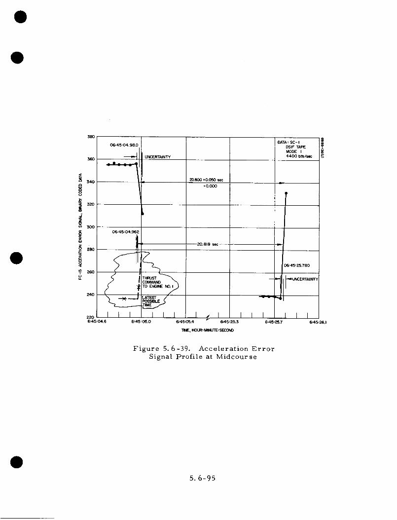
380

360

340

!320

__ 28o

T 260

06:45:04.98.0

06=45:04.962

UNCERTAINTY

I

TO ENGINE NO.I_

f240

_ _TES'r

_20 I I I I I I I6=45:04.6 6:45:05.0

20.800 +0.050 sec

-0.000

20.818 sec

I I

DATA : SC- IDSIF TAPEMODE I4400 bits/sec

06:45:25.780

-- D. "_-UNCERTAINTY

I I I I6:45:05.4 '6=45:25.3

"NME, HOLR: MIMJTE: SECONO

6=45:25.7 6:45:26.1

Figure 5.6-39. Acceleration Error

Signal Profile at Midcourse

5.6-95

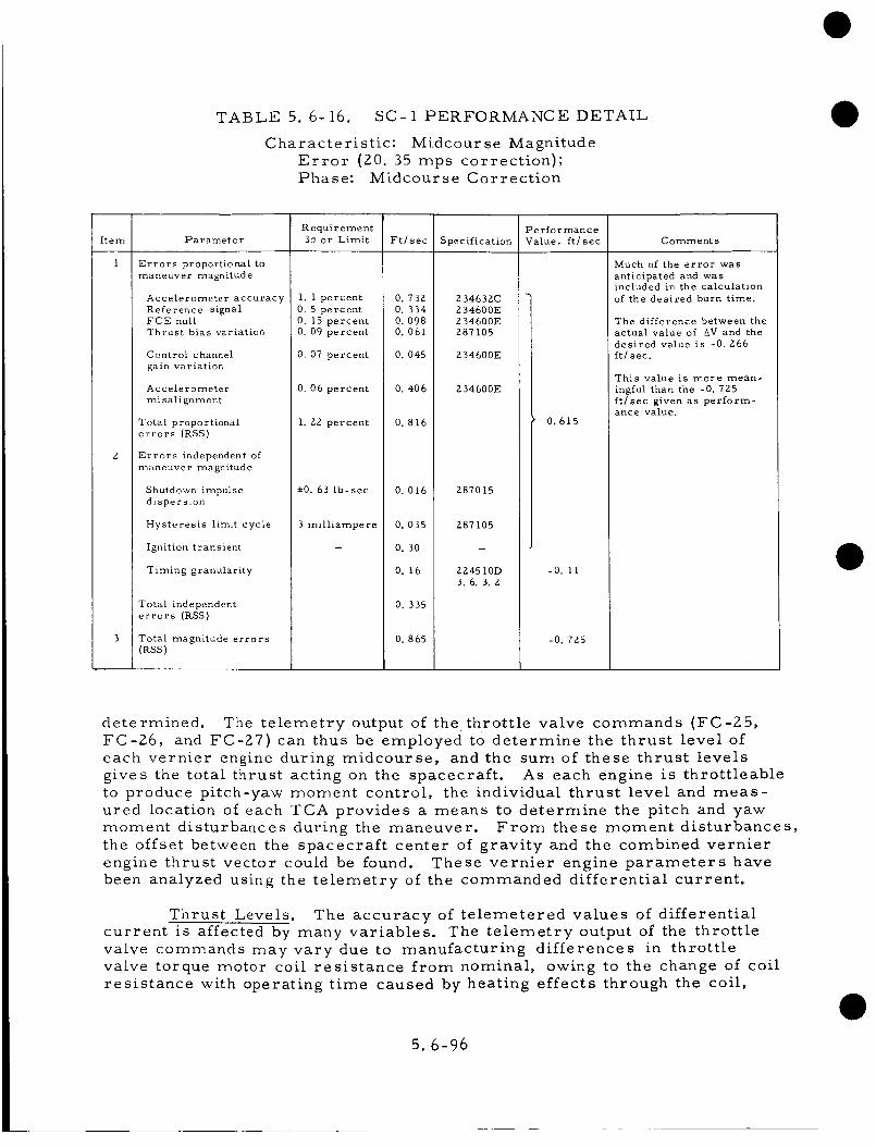
TABLE 5. 6-16. SC-1 PERFORMANCE DETAIL

Characteristic: Midcourse Magnitude

Error (20. 35 mps correction);

Phase: Midcourse Correction

Item

1

Requirement

Parameter 3_ or Limit

Errors proportional to

maneuver magnitude

Accelerometer accuracy

Reference signalFCE null

Thrust bias variation

Control channel

gain variation

Accelerometer

misalignment

Total proportional

errors (RSS)

Errors independent of

maneuver magnitude

Shutdown impulse

dispersion

Hysteresis limit cycle

Ignition transient

Timing granularity

Total independent

errors (RSS)

3 Total magnitude errors

(aSS)

Ft/sec

Performance

Specification Value, ft/sec Comments

I. 1 percent 0.73g 23463ZC

0.5 percent 0.334 234600E

0.15 percent 0.098 Z34600E

0.09 percent 0.061 287105

0. 07 percent 0. 045

0. 06 percent 0. 406

1.22 percent 0.816

±0. 63 Ib-sec 0. 016

0. 035

0. 50

0.16

0. 335

0. 865

3 milliampere

Z34600E

Z34600E

287015

287105

22-4510D

3. 6. 3. Z

0.615

-0. II

-0.725

Much of the error was

anticipated and was

included in the calculation

of the desired burn time.

The difference between the

actual value of AV and the

desired value is -0. Z66

ft/sec.

This value is more mean-

ingful than the -0. 7Z5

ft/sec given as perform-

ance value.

determined. The telemetry output of the throttle valve commands (FC-25,

FC-Z6, and FC-Z7) can thus be employed to determine the thrust level of

each vernier engine during midcourse, and the sum of these thrust levels

gives the total thrust acting on the spacecraft. As each engine is throttleable

to produce pitch-yaw moment control, the individual thrust level and meas-

ured location of each TCA provides a means to determine the pitch and yaw

moment disturbances during the maneuver. From these moment disturbances,

the offset between the spacecraft center of gravity and the combined vernier

engine thrust vector could be found. These vernier engine parameters have

been analyzed using the telemetry of the commanded differential current.

Thrust Levels. The accuracy of telemetered values of differential

current is affected by many variables. The telemetry output of the throttle

valve commands may vary due to manufacturing differences in throttle

valve torque motor coil resistance from nominal, owing to the change of coil

resistance with operating time caused by heating effects through the coil,

5. 6-96

lilill ¸

!!!!!!

: : : : : :

iiLiiiI I_'.I I I

I li_Ll i

!!!!!!iiiiiilllill!!!!.i i : : -- :

ii_iiiii_iIIiiilli

iilill

!!!!!!: : : : ; :

i i_iJi

!!!!!!_,,,i i i i i

-: : : : : :_1 i i | i_o, , , = ,

iiii't:_-i i i i

]}l!.l!_-iiiJi

,, : ,, ,, .- ,,

I IJ_l

I_llll_111|

: : : : .- :NI

"1-.1 | I | I

_11|1

I_0, I I I I

.__ ! ! ! !.... I ,

milll

l_illl_'/ I I I !

I_,,_ Iol | I

I I |ill

III I I | I

,TT-4-,! ! I

_I-I&L

--_-+--I---+--t_

i i i i _ ;

I I _,,x...I I

i -

I

I

1o 2. 3. _. 5. 8. 7. 8.

Figure 5.6-40. Acceleration Error Signal

5.6-97- /

"¥O;[4)O'UT

V

21.

=+-._

-+-I

!ir i

il

iiq

I I

iiI I ,

!! :Ii

: i

i q

i J

i i

: q

Ji

i i

II

I I

i i

qq

II

74IIII

II

-HIII I

and owing to inaccuracy of the telemetry link, including variables such as

commutator unbalance current. To improve the telemetry data, a theoretical

method suggested in Reference 14 was used to convert the telemetry data

from BCDcounts to milliamperes of differential current. This conversion

method attempts to compensate for the inaccuracy in the telemetry signal

caused by the varying resistance of the torque motor coil due to operational

heating and by the difference in the actual torque motor coil from the nominal

value. The signal error due to commutator unbalance current was less than

I bcd so that the telemetry data could not be adjusted to eliminate this

variable. Nevertheless, careful inspection of th_ data indicates that these

corrected values of commanded differential current, AI, are accurate to

within +Z milliamperes.

To establish a specific magnitude of thrust from the corrected values

of _I for each TCA, approximate slopes of differential current versus pounds

of thrust were determined from flight acceptance test (FAT) data. The

calibration curves were generated from FAT data points taken at approxi-

mately -40 and 0 milliamperes. The slope was taken to be linear and extended

up to the appropriate region for midcourse of between i0 and Z0 milliamperes.

It is unfortunate that FAT data points were not taken in this region as this

approximation introduced error in the absolute magnitudes of the thrust

levels of the order of ±0. 5 pound.

The midcourse thrust versus time profile, determined in the above

manner, for each vernier engine is shown in Figure 5.6-41. The accuracy

of any specific value of thrust is no less than ±i. 0 pound. From the thrust-

time plot, the initial transients at ignition are seen to peak out within Z

seconds, and the thrust levels settle into steady-state values. The maximum

and minimum values for each vernier engine are as follows:

During initial transients:

Maximum thrust on engine 1 = 80. 0 pounds

Maximum thrust on engine Z = 77.9 pounds

Maximum thrust on engine 3 = 75. 1 pounds

After initial transients:

Maxlmum thrust on englne 1 = 74. 3 pounds

Maximum thrust on englne Z = 74. l pounds

Maximum thrust on englne 3 = 73. 4 pounds

Minimum thrust on engzne 1 = 7Z. 6 pounds

Minimum thrust on englne Z = 71. Z pounds

Minimum thrust on engzne 3 = 7Z. 4 pounds

5.6-99

It was expected that engine l (the roll control gimbaled engine) would

have a little higher thrust level than the other two engines, and this is veri-

fied by the data. Due to the location of the combined spacecraft center of

gravity being closer to leg 3, the thrust on engine 3 would have to be some-

what higher than the vernier engine located near leg Z. This expectation is

also verified by the reduced telemetry data. The thrust-time profile for

vernier engine Z has a greater slope than the other two engines. No explana-

tion of this observation has been determined. A slight decline in thrust levels

is expected for all three vernier engines since control loop is in a constant

acceleration mode and the engines are expending propellant. Movement of

the spacecraft center of gravity due to propellant consumption was predicted

to be toward the spacecraft coordinate origin which would cause the thrust

on vernier engine 3 to be lowered and engine Z to slightly increase; however,

the data shows the opposite trend. One explanation could be that combined

vernier engine thrust vector was moving away from TCA Z such that the

resultant moment disturbances required these lower thrust levels. Another

reason could be that the telemetry signal for engine Z (FC-Z6) was not com-

pletely corrected for the error due to torque motor coil resistance (which

causes the signal and, thus, the indicated thrust level, to drop). However,

this type of signal change was not evident for FC-Z6 from the terminaldescent data.

The total thrust of the vernier propulsion system during midcourse

for any given time was calculated from the sum of the individual vernier

engine thrust levels that were sampled at that time. Of course, all three

channels were not sampled at the exact same time, but at the high bit rate

during midcourse of 4400 bits/sec, all three channels were sampled within

a time interval of 0. 1 second. Summation of these closely grouped samples

should be a good approximation of the total thrust for that time interval.

The total midcourse thrust versus time plot is given in Figure 5. 6-4Z. For

comparison purposes, the required average thrust level to maintain thetelemetered value of AV for the midcourse time interval of 20.85 seconds

is shown on the graph. Also, the required total thrust to maintain the

expected constant acceleration of 0. 1 g is included in this plot. These curves

were obtained by connecting initial and final points, which were found in the

following manner:

SC-I weight at injection = ZI9Z. 71 pounds

Nitrogen gas used (see =

Figure 5.6-81)

0. Z3 pound

= weight at start ofo

midcourse= ZI9Z. 48 pounds

AVactual = Z0. Z66 m/sec (Reference 15) 3. Z80833 feet = 1 meter

AV

ISp - w

g6n __%o_f

5.6-I00

cl

!

b

0

I

!!!!!ii!!

o

!

4_

O.

o

oU

_4

I

_4

I

I

_W- &',f - _o

Aw = 16.81 (Reference 13)

wf = 2175. 67 pounds

Postflight analysis of the time interval of midcourse (see "MidcourseVelocity Determination") shows that At = Z0. 818 seconds.

From the telemetered average acceleration level:

^ AVAverage acceleration from telemetry = aTM =

^ ZaTM = 3. 19384 ft/sec = 0. 099Z7 g

^ ^Average total thrust = T = m a

At start of midcourse:

_J^ _.2_o

(T)i = g aTM= Z17.65 pounds

At end of midcourse:

^ wf ^

(T)f = -_- a TM = 215.98 pounds

From expected acceleration ofaA = 0. 1 g:o

_2o (0. l g) = Z19.248 pounds(_)i = g

wf(_)f = _-- (0. 1 g) = 217. 567 pounds

The total thrust levels as determined from the commanded differentiaI

current compare very favorably with the values as determined above. Theaccuracy of these values from the sum of the individual vernier engine thrustleveIs is roughly ±3 pounds. After the initial transients, the thrust valuesfrom teiemetry are about Z pounds higher than the level predicted from AVand are very close to that predicted for 0. 1 g of acceleration. The slope ofthe telemetry thrust versus time profile is again somewhat more than pre-

dicted by the constant accelerations. This is due to the steeper decline ofthe thrust on vernier engine g discussed previously.

5.6-105

Moment Disturbances: The orientation of the vernier engines in

spacecraft coordinates is shown in Figure 5.6-43. The pitch and yaw

moments, taken about any point in the spacecraft center of gravity plane

(Xo, Yo), given by the individual thrust levels of the three vernier engines

(T l, T Z, and T3), are:

_7M x = - (Rly - Yo ) T l + (Rzy + Yo ) T Z + (R3y+ Yo ) T 3

VMy = - (Rlx - X o) T 1 + (Rzx + X o) T Z - (R3x - X o) T 3

The SC-I measured values of the vernier engine radial arms ("SC-I Mass

Properties Handbook") are as follows:

R 1 = 37. 734 inches

R 2 = 37. 744 inches

R 3 = 37. 829 inches

Using the orientation of the vernier engines in the X-Y plane shown in

Figure 5. 6-43, the SC-I vernier engine moments about the pitch and yaw

axes taken at (X o, Yo) are found to be as follows:

VMx = 0.9424 (R 1 Yo) T 1 + 0. 1816 (R Z + Yo) T Z + 0.7608 (R 3 + Yo ) T 3

VM = 0. 3345 (R - X o) T + 0.9834 + T Z 0.6489 Ty 1 1 (Rz Xo) - (R3 - Xo) 3

The moment disturbance curves of Figure 5. 6-44 were generated

from the previously presented SC-I corrected thrust command data versus

time plots and the above equations. In this plot, the moments were taken

about the spacecraft coordinate origin such that X o = 0 and Yo = 0. The

commanded thrust levels for a given time interval were all sampled within

0. 05 second, and the moments were computed using these closely grouped

telemetry values as was done to obtain the total thrust-time profile.

The moment disturbances at any given time, as shown, are only

accurate to within ±40 in-lb since the values of T i in the above equations areonly known to within +l pound. As most of the moments found were of this

order, very little can be determined from these plots. On the graph, the

predicted momenta due to the spacecraft center of gravity offset from the

spacecraft origin is shown for the two cases of omnidirectional antenna A

stowed and omnidirectional antenna A extended. Because of the relatively

large inaccuracy of the data points, nothing could be concluded from a com-

parison of these two cases and the telemetered data. Therefore, no attempt

to predict the spacecraft center of gravity to combined thrust vector offsetwas made.

5. 6-I06

The computed moments about the X axis (pitch) are seen to be fairlyconstant (between -30 and i0 in-lb) during most of the Z0-second time periodof the midcourse maneuver. Moments taken about the Y axis (yaw) tend toincrease in magnitude, after the initial transients, from approximately zeroto around -60 in-lb during the time of commanded thrust. This is attributableto the unexplained decrease in the telemetered thrust command of vernierengine Z (Tz) previously discussed. TCA Z is located out along the positiveX axis and the decrease in TZ produced negative moments about the Y coordi-nate axis.

The maximum pitch (Mx), yaw (My) and total (MTOTAL) momentsas determined by using the above equations and the telemetry correctedvalues of commanded thrust on the vernier engines are as follows:

During initial transients:

Maximum magnitudes M = -Z03 in-lbX

M = IZZ in-lbY

MTOTA L = 215 in-lb

After initial transients:

Maximum magnitude s MX

MY

MTOTAL

= -40 in-lb

= -74 in-lb

= 74 in-lb

Corrected plots of the pitch and yaw gyro error signals are included to

illustrate the response of the attitude loop and to confirm the low moment

values calculated above (Figures 5.6-45 and 5. 6-46).

5.6. 7. 9 Preretro Ivlaneuvers

Before retro ignition, it is required that the spacecraft thrust axis

(positive roll axis) be aligned to the translation velocity vector of the

spacecraft. This is an integral part of the gravity turn design for the

terminal descent phase guidance.

This alignment is to be performed by means of two or three sequential

rotations about the spacecraft body axes. The first two rotations are to pro-

vide the actual alignment of the roll axis; the third rotation (if required) is a

roll rotation to align the high-gain planar array with the spacecraft-earth line.

On SC-I the final roll was performed to secure a favorable omnidirectional

antenna pattern.

These maneuvers are accomplished by using the cold gas attitude

control system, with the body-fixed integrating rate gyros as inertial

references. To accomplish a rotation, the appropriate gyro torquer winding is

5.6-I07

SPACECRAFT X AXIS m

i

VERNIER

ENGINE 2

SPACECRAFT

Y AXIS

ENGINE I

VERNIER

ENGINE 3

Figure 5.6-43. Orientation of

Vernier Engines in Space-craft Coordinates

5. 6-I08

I: i

_':-t--:_.r::_; :,i -_ n_l_-.,

:_::I_: .0:_::, :::__<

--*--Tt :.-i . :.2

• --4 ',::I: _

i:k-:: . "-:,,, :;4, L.:_. t ' _ _ _ :

• I. -

:::21

.... t----

--'_ _ .. fL-H .

• ," :r,li

:-: _ I :!-- _:

• :i. " :.V

I

]-- _ :I

ii

i

-" i

i : i

T-.-..,:---v-! ,i ....

__ }

1 ,

[......... q ....

.... : " i

- 4-- -. ...... .... [- - -: -: -

I

I

, :

l: --:i "-t _" : .........i _ ,. ,

-__,. _I_._.f.___ .... ;-

W

i

! i _ _ _. . • ,I I

' --_:- - I*" i _,L__I:___J_._2_ ,(;_

._!.T":._:LI.......:._I_

I'I .,fl :.....

i !

I ....i , i" ...... I - 4--_-

i

1

e,l

o

..... [ ........... : .... :I

..... :,-I}

_" I_ _ 1 T I I _I ' I | ..I _......_ '........i ..:.... ._

0

@

o

_F_o b-

x_L)

N_

_u_

Nou

m r/l _

r/l 4-_

u_ Mo

o_-,_

:.:

o

o.l_

I

u

Figure 5.6-45. Pitch Gyro Error Signal at Midcourse

5.6- I 1 I- t 'FOI_OUT

L)° L?o too

LLiiiii ii!!

-_-_-!! W! =' rlIlliiii :: '

iii i iiiii

iliiii|:::

1111111;;;

ii!jiiii 4lill;;l:::illi;;;:ll

!!!J!iJiii

!!!!!!ii!!

iiiiiii!!!!!!!!!!!ii!iiii!ii]lii.ii!iiill

ii!iii!!!i

llllIl!iii!!!!!!!!!!

[iiiiiii!!!!!!!!!!!i

II!!!!!::,

M_'!!!!!i

!!!!!iiiii

_._-_,_M.-_

2].

'_OZ_O_

_._ II,_..

O. le

Figure

+0.03ll DEG

Yaw Gyro Error Signal at Midcourse

I

II

i

ili

÷III

+L4

5. 6-113-!"¥OI.DOLTT

I0o " MissiS"t:_:t'_3

_-,.D- t _"_- _

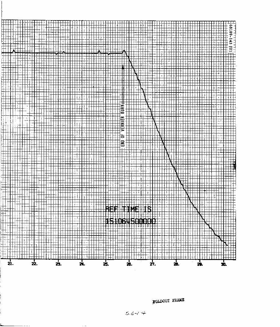
l i

fli l

II

-r-I

qil

iii I

II

ii

-t4: 1

_4_

q-I!

--4---I--

i i,'--e--

--+---l--

ii

ii

Tt

1-1-i !

b4.-4_41-

-t-t-

I I

i i

I21.

II

I

+÷÷+÷

i

+?4-

-t-IIi!

i

I

i÷÷I

++

5, f-i. ,_.L.r

D driven by a constant current source for a precise length of time; the space-

craft is slaved to this changing reference.

The major events and times associated with the preretro maneuvers

are given in Table 5.6- 17.

The preretro maneuvers were analyzed in terms of the following:

I) From gyro error signals and precession logic signals,

determine gyro precession time to best accuracy and

compare to commanded times.

Z) From the above and the initial sun and Canopus error signals,

make best determination, with resultant tolerances noted, of

the terminal pointing accuracy.

3) Verify item 2 above by comparison with pointing error determinedfrom main retro burnout conditions.

TABLE 5.6-17. MAJOR EVENTS AND TIMES (DAY 153),PRERETRO MANEUVERS

DEvent Command GMT Time

0714Begin roll 1

End roll 1

Be gin yaw

End yaw

Begin roll Z

End roll Z

Retro ignition

0713

0711

5:48:Z9.081

5:36:49. 097

5:39:47. 693

5:41:50.320

qb5:45:20.285 j

Determined from

DSIF tabulated

data

6:i4:49.65 (Reference 18, Table II)

Analysis Details

Gyro Transients. One of the primary requirements of the preretro

maneuver is that the inertial reference of the spacecraft never be inadvert-

ently changed; that is, no gyro must be permitted to saturate at any point in

the three rotation sequence. The minimum linear range of each of the

gyros is ±i0 degrees.

D5.6-I15

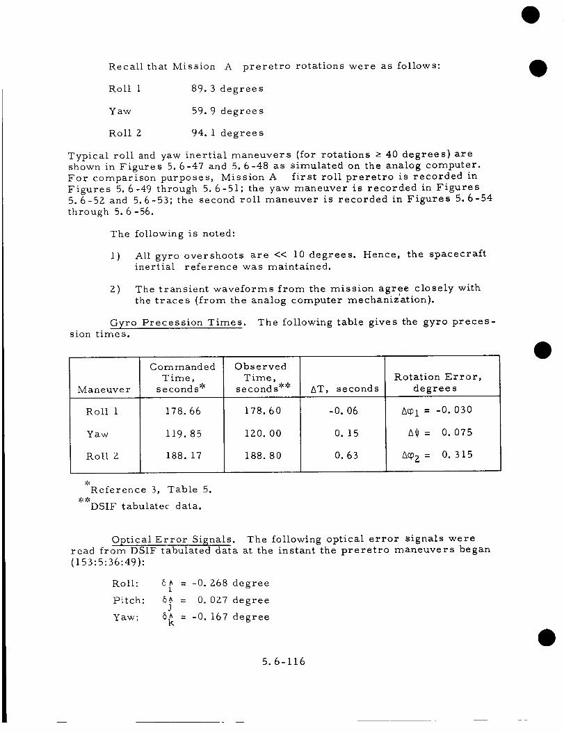
Recall that Mission A preretro rotations were as follows:

Roll 1 89.3 degrees

Yaw 59.9 degrees

Roll 2 94. I degrees

Typical roll and yaw inertial maneuvers (for rotations > 40 degrees) are

shown in Figures 5.6-47 and 5. 6-48 as simulated on the analog computer.

For comparison purposes, Mission A first roll preretro is recorded in

Figures 5. 6-49 through 5.6-51; the yaw maneuver is recorded in Figures

5.6-52 and 5.6-53; the second roll maneuver is recorded in Figures 5.6-54

through 5.6-56.

The following is noted:

l) All gyro overshoots are << i0 degrees.inertial reference was maintained.

Hence, the spacecraft

z) The transient waveforms from the mission agree closely with

the traces (from the analog computer mechanization).

Gyro Precession Times. The following table gives the gyro preces-sion times.

Maneuver

Roll 1

Yaw

Roll Z

Commanded

Time,

seconds _

178.66

i19. 85

188. 17

Observed

Time,seconds $$ AT, seconds

Rotation Error,

degrees

178.60

120. 00

188.80

-0. O6

0.15

0.63

AWl = -0.030

_ : 0.075

_Z = 0.315

Reference 3, Table 5.

DSIF tabulate¢ data.

Optical Error Signals. The following optical error signals were

read from DSIF tabulated data at the instant the preretro maneuvers began

(153:5:36:49):

Roll: 6_ = -0. Z68 degreei

Pitch: 6@ = 0.0Z7 degreeJ

Yaw: 6_ = -0.167 degree

5.6-116

!i_i<

"L-

=:: 122

_<i Ii!,_,i<_:',,

.... LE _a

I:' I II! :i_ !!II

H_ ....

_:i!ii

::KHKX

::::;:::

:KEE

_!t!!!

_iiiii__i_ _'_ _ i_!!"_ii!iii!__

(n)

lil _ i

2:

:,_++

_ tt

Figure 5.6-47. Roll Inertial, Long Duration Attitude Maneuver

5.6-117

Figure 5.6-48. Yaw Inertial, Long Duration Attitude Maneuver

5.6-118

tJ_t

iliii:!!!!

,It_]

]:it

:_qt

!!!I

i:ll

!!!!iJ¼_--+_

!iii

:lit

-+-+-+-+

--+-+-+

;tit

-+-+-+-+

iiii;:]:

iii!

iiii

iiii!!!!

i!!i

!ii!

i!iiiiii

iiii

1111

!

O

v

O

L_

Oo,._

BQ(D

(D

O

i

M

o_

5.6-119

5.6-1ZO

°1--

5.6-121

0

-,-4

v

0

0

L_

!

M

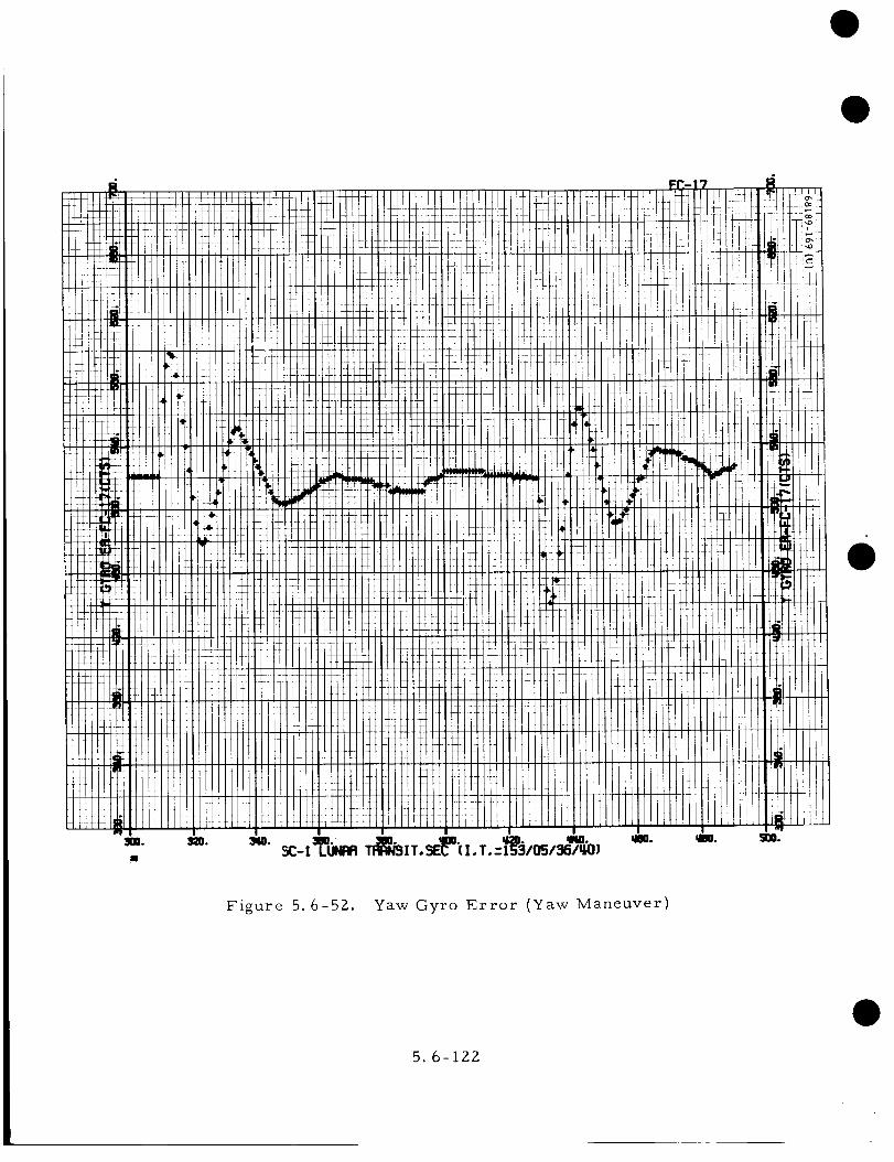
Figure 5.6-52. Yaw Gyro Error (Yaw Maneuver)

5.6-122

J_i±[ i

_ 41DrlM L

q_ F

,llklu

_ _T

,::::_-

gl

::::::

i i,_i ii i [llm[ l

H_

HJI_VI.

ill

3W.

4-LI 14

r!k!![

iiiii

t - I

_! !H-

_T!T!

_+::,:,

d 1.f_lJ

_++_

I I I I_, i++;

±LH L

4_! !-

T_i

: : : : :

LH ;1hi 11

_" ,_C-13e_l_ TI_ZT. _E_oil(]. T.:153105136/1_31_o _i_o

Figure 5.6-53. Pitch Gryo Error (Yaw Maneuver)

5. 6-123

5. 6-124

.i-z, I,

.!-_,I

!!i:; !

lli, li!l

III 1

::ll

Ili !

::l i

/i4 I::1ill

iii

ill. Ii i:_l ,i:. i'lid

';' iiiil ::

Ii

r]! ii[il II

!]!

,ii

ir '_i

_4- ,

[iI ,!:

: !; i

!TL ÷-

li! i

77- i

ri! i

i f

iAi

i rq

!! i_.+_.,_

',I: i

4t-

5.6-125

d

d

i-

,4

I--

Ii

1i

d U

i,,--I

0r_

0

v

0

0

M

I

68189-173 (U)-

,...--40

0

U3v

0

0

,S

I

,,D

M

.,.-i

5.6-126

Preretro Pointing Error Determination. The method used for pre-

retro pointing error determination is that developed in Reference 16.

1)

z)

3)

4)

5)

An initial coordinate system is defined with unit vectors, _, jA,

and _ being along the vehicle's roll, pitch, and yaw axes,

respectively.

Assuming that the position of 4 .A1, j, and _ is known exactly

(initially) and that the rotations _01, 4, and C0Z are performedwithout error, a matrix [(A)]is developed which defines the

relation between (_ _ t_)and the final coordinate systemA A A

(i' j' k').

^Initial

^position errors are represented by 6j, and 6k about

the roll, pitch, and yaw axes. The effect of each one of theseerrors upon the final orientation of _' is determined from

= [A]

I

_I,Z, 3

-- !

ml, Z, 3

--1n

_ i, Z, 3 _

1,2,3

n_ I,Z, 3 _

61

^

= [A] [B1, z, 3 ] J

where [A] represents the ideal transformation ana [B1, z, 3]is the applicabie small angle approximation to the matrix

which represents the disturbing of

IIi

^

J

with an initial position error.

I 1 1

Now the actual errors are obtained by comparing _'I, _Z' and _'3

with _'. The components of each error source are resolved into^ ^

components along the j' and k' axes by taking the dot products of

_I' --' --'3 ^ ^£Z' and _ with j' and k'.

Errors in making rotations are represented by _0 I, A_, andgc,0 zfor the three maneuvers of Mission A. The effect of each one of

these errors upon the final orientation of #' is determined from

A--, ^ Bi

_4 = i' + -_I g_°l

5.6-127

where

6)

[A] =

and

^

^ c_ii' + t_','i'275 = o_

Again, £-' -- ^ ^4 and ,_ are resolved into components along the j'and k'

-, ._,r.4 ^ % ^ -,. _.by taking the dot products £4 " J ' • k', • j', and 6 5

A ^

Now it is a matter of bookkeeping, All errors along the j' and k'

are added and a resultant computed:

tj' = [A] j

ic, ojLc o-s lLc 'oo1-Se@2 C "!"Z 0 0 1 0 -Se@I CCPl 0

0 0 1 S _ 0 C l_ 0 0

(Cg, z C I_ C,], 1 - S_ 1 Sq) 1) (Cq_ z C{Sq)I+SCpzC_ 1)

(-Sq_ z C,_ Cq_ 1 -Cq} 2 S_ 1) (-S,'!, z C_ Sep I+Cq_ 2Ccp 1)

(s _, c q ) (s t, s% )

( -cq, z s _,)

(cl,)

1

m'i

--!

n.1

= [A] [BI_ j = iA] 0 i 0

where the small angle approximations sin 6_ m 6k and cos 6_m ihave been made.

5.6-128

^

T'_-iE(cv2 c, c_ -^

+ j [(c_OZ c j_s_O1

A

+ k [(c£0 Z c _I C_l

+ scOz C_Ol)]

- smz _ml)(-_) - _z s,]

!

m 2

--!

n2

= [A]

1 0

0 1

0 -6.J

w

0

.

J

1

I--!

C2^

= i [(C_pz c_ COOl

A

+j [(c,? 2 c_ s_ 1

+_[(c_2 c, s_I

- s_2 s_11]

+ sq_z _<o)+ 6j.(_oz _,)]

+ s_Pzc_I)(_)+ (-_z s,)]

m

n'

= [A]

1

-6.A1

0

6._ 0 ii

^

1 o j

o i _I

^

= i [(c,'.p2 cq* c_oI -

^

+ j [(cmz c_ c_o1

^ s,]+ k [-c@z

s_o2 SqOl)+ 6iA (-coo 2 c J, sop1 -

- s_oz S_Ol) (6_)+ (c_oz c_ s_ 1

s_z copI) ]

+ s_ z cml)]

5.6-1Z9

Recallfrom [A] _'= (-s%o2 c_ c_oI - cqD2 SCPl ) (_)

+. (-SOP z CO s_O1 + cCp 3 c_O1) (jb)

+ (s_z s,)(_)

and

k' = (sO ccp1) (_)

^

+ (sO s_ I) (j)

^+ (c_) (k)

Now, taking the dot products:

"_'I" _' = [(cCPz c* ccPl - scpz SCPl ) + (-ccpz sO) (61_)] E-s_o z cO ccpI

+ [(cOP Z cO sqO 1 + s_OZ c_l)] I-sop Z c_ SCPl + c_pz CCPl]

+ [(-cq)Z c_ CCPl + scpz SCPl) (+51_) - CCpz s*] [scpz

= s O s_O1 _k

- c_O2 sq) 1 ]

s,][s<oz s,]

_v1 • I_' = [(CCpz C* CCPI

+ [cCp Z cO scp 1

+ [(-C_OzC_ CCP1

- sop Z sqO1)+ (-cqO Z s*) (6_)] (sO cep 1)

+ s_oz c_o1] [s_ s_o1]

+ scpz s_oI)(6_)- CCpzs,] [c,]

= 6_ [SCpz sqO 1 c o - c_Oz cqo 1]

5.6-130

.j = cep 1

+ [(cq) z c_ sqO1

+ [(c_Oz c_ s_p 1

j c%°i

[(c%o Z c _C_l - sq)2 s%°1

+ [(cq_ Z c@ s%o1

+ [(c%o Z c@ sqo I

)] Is, cmI]

+ s_oz cmI)+ 5_ (c_oz s_)] Is, smI]

+ S_z c%oi)(6jA)+ (_cqoZ s@)] [c_]

= 6._ [c_o z + sq)z c_]j SCPl cqa 1

--I

6 3 "

= [(c_gc_cq) 1 - sc_pZsq)l)+ 6_(-cqo z c_ S*l - sqoz C_Ol)][-sq)zc*cml-CCpzscp I]

+ [(Cmz_,cmI- smz _mi)(5_)+(cmz_,smI+ Smz_ml)][-_mz_,_m1+_%amI]

+ [-cm 2 s,] [so0z s_]

= 6._(c_)1

1_' = [(cq_z c_cq_ 1 - scoz scO) + 5_ (-c WZ c_ sq) 1 - Sq_zCq_l)] [s_ Cml]

+ [(CCpz c_cqo 1 - sq_Z Sq)l) (5#)+ (c q)Z

+ [ _mzs,] [c_]

c_scPl+ sopzccp I)] [s_sq) I]

i -scPZ

5.6-131

Considering the errors from incorrect rotations:

-

= _'+_ [.-c<oz d, s_% - s_oz c_I] _I

+ _ [c_oz c_ c_oI - s<oz s_oI ] AcpI

A

--, _, _ i A_Ir_'5 = +_ "

^1 ^

= i + i [-c_O Z s O c_O] A_

^

+ j [-c_o z s_ s_o1] a_

^

+k C-c_zc,]_O

= (CqO Z CO cqO1 - sqOz S_O1) (-sq) Z CO C%01 - c_Oz sqO 1)

+ (C%0Z C_ sqo 1 + sol) z c%01) (-S_z C_ S_Pl + c_z cqO 1)

+(-c_O z s_) (s_oz s_)

+ (-c_O z c_ s_O1 -s_o 2 c_O1)(-S£OzCOC%01 -CqOzS_O 1) gq) 1

+ (c_O z cO cqO 1 - s%0z scP 1) (-s_o ZcO sqo 1+c£0 z cq) 1) AqO 1

= c_ &cO 1

5.6-132

--I ° _'!

L4 = (cO? 2 c_ C_l - sq_ Z SCPl (s_ CCPl )

+ (ccp z c_ SC#l + S_z CCPl ) (s_ S_l )

+ (-c_o2 s_) (c_)

+ (-cOp z c_ scp 1- sqo z CCPl )" (s_ c_O1) A g)]

+ (cq_ z c_ cop 1 - s_o z s_O1) (s_ S_l ) hCpl

= ACp1 (sOp z s_)

-' " _' ( _ I( c_ - I _6 5 = -c_2 cqO1 -scP2 ccpI ccp2 scp1

+(-ccp 2 s_ SCPl ) (-scP2 c_ sopI + ccp2 C_Ol) A_

+ (-cooz c_) (s_z s_) a_

= 0

--! ° k !

g5 = (-c_2 st) C_l ) (st) CCPl ) A_/

+ (-c_P2 st) sCO1 ) (st) SCPl ) 54

+ (-c¢oz s,)(ct)}a,

= _ (-c_oz)

5.6-133

Error Source

So the error tabulation is:

Error Component

Along f'

51_ s * seP 1 61_

Error Component

Along _'

(s_ z S_l c_ - c_ z c_ I) 6_

5.A s_ c%01 6A (c%0z s£01 + sq0z c£01 c_) 5._3 J J

5A c _ 6_l l -s_02 s_ 6Ai

h_ 1 c_ A_ 1 -s_2 s_ h_l

A_ o -c_ 2 A_

For £01 = 89. 3 degrees, _ = 59.9 degrees, and £0Z = 94. 1 degrees,the above table reduces to the following:

Error SourceError Component

Along j '

Error Component

Along k'

61_ O. 866 51_ O. 502 51_

5b 0.010 5b 0.429 5_J 3 3

5A. 0. 500 6_. -0. 865 6.A1 1 1

&_l 0.500 &_l -0.865 &_l

_ o 0.070 _

Using the measured values for 5_, 6._, 5_, A02,Jfollowing:

A.!

I) The net error along j = 0. 026 degree

Z) The net error along _' = -0. 336 degree

and A'@ results in the

The resultant pointing error is _0.34 degree in the direction of the

minus yaw axis.

5.6-134

The pointing error as determined from main retro burnout conditions

was 0.26 degree in the direction of the plus pitch axis.

The above two calculations do not corroborate each other. However,

it is noted that some large error contributors not included in the calculation

must indeed affect the resultant pointing error. These error sources are asfo flow s :

I) Alignment of main retro thrust axis with respect to sensor group

roll axis: 0.40 degree

2) Tracking error: 0.30 degree

3) Control system stiffness: 0.20 degree

It is felt that the combination of the above three errors could well

have dominated the final pointing error at burnout.

Note that at the time of main retro ignition and throughout main retro

burning, the actual main retro thrust axis is required to be aligned to the

actual initial velocity vector plus offset (if applicable) within ±I degree

(Reference 17, Paragraph 3.9.3.2).

The preretro maneuvers were nominal.

5.6. 7. i0 Main Retro Phase

Main retro phase began at 153:06:14:39. 958 GMT with the indication

of AMR mark and successfully ended at 06:15:39. 943 of the same day with

the acknowledgement of retro eject. The approach velocity at the time of

ignition was approximately 8565 ft/sec, and the altitude was 246,636 feet.

At main retro burnout, the velocity was reduced to approximately 431 ft/sec

with a slant range of 27,851 feet. The predicted values for burnout con-

ditions were 393 ft sec at an altitude of Z8, 571 feet.

During th_s phase, the functions of the flight control system were to

maintain the attitude of the spacecraft inertially fixed and to provide and

execute a fixed sequence of commands to accomplish vernier descent phase

conditions. The following analysis reveals that these two functions were

performed to the utmost expectations.

A list of retro phase events and their corresponding time of occur-

rence is given in Table 5.6-18 along with expected time intervals. These

results confirm the performance of the magnitude register and programmer.

The following data confirms that AMR mark occurred prior toemergency AMR:

5.6-135

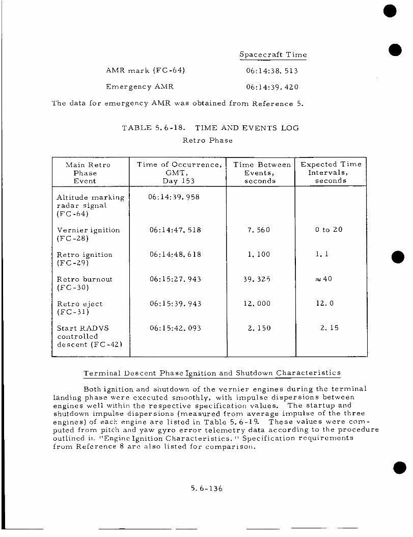
AMR mark (FC-64)

Emergency AMR

Spacecraft Time

06:14:38. 513

06:14:39.4Z0

The data for emergency AMR was obtained from Reference 5.

TABLE 5.6-18. TIME AND EVENTS LOG

Retro Phase

Main Retro

Phase

Event

Altitude marking

radar signal

(FC -64)

Vernier ignition

(FC -Zd)

Retro ignition

(FC -Z9)

Retro burnout

(FC -30)

Retro eject

(FC-31)

Start RADVS

controlled

descent (FC-4Z)

Time of Occurrence,

GMT,

Day 153

06:14:39. 958

06:14:47. 518

06:14:48. 618

Time Between

Events,seconds

7. 560

i. i00

06:15:27. 943

06:15:39. 943

39. 325

IZ. 000

06:15:42. 093 2.150

Expected TimeIntervals,

seconds

0to Z0

i.i

_40

IZ.O

Z. 15

Terminal Descent Phase Ignition and Shutdown Characteristics

Both ignition and shutdown of the vernier engines during the terminal

landing phase were executed smoothly, with impulse dispersions between

engines well within the respective specification values. The startup and

shutdown impulse dispersions (measured from average impulse of the three

engines) of each engine are listed in Table 5. 6-19. These values were com-

puted from pitch and yaw gyro error telemetry data according to the procedure

outlined it_ "Engine Ignition Characterislics. " Specification requirements

from Reference 8 are also listed for comparison.

5.6-136

TABLE 5.6-19. TERMINAL DESCENT PHASE IMPULSE DISPERSIONS

Impulse Dispersions in ib-sec

Startup Shutdown

Leg SC- I Requir ement_-" SC- I Requirement

-0. 02

0.22

-0. 02

<±i0

• 0. 19

- O. 26

0.07

<±0.32

Assuming a startup time of < 150 m/sec.

Owing to the low telemetry sampling rate (2 samples/sec) of gyro

error signals and the low absolute magnitudes of the errors encountered on

SC-I, accuracy of the impulse dispersion figures listed in'Table 5.6-19is

of the order of 50 percent. Therefore, the results are valid only insofar

as giving gross indication that impulse dispersions were small and within

requirements.

Retro Phase Attitude Control

During the main retro phase, extending from vernier ignition through

case separation, spacecraft attitude motion was small in all three axes.

Peak pitch and yaw inertial attitude motion, as read directly from gyro error

telemetry data (FC-16 and FC-17), occurred at vernier ignition and amounted

to -0.89 degree in yaw and -0. 13 degree in pitch. (See figures in "Raw

Plots.") Following ignition, static attitude error was virtually zero in both

pitch and yaw axes. Roll inertial attitude error was maintained less than

0.50 degree throughout the main retro phase (less than 1.0 degree is required).

Since all gyro error signals were maintained within ±I. 0 degree

(during retro burn), each gyro was exercised less than I0 percent of the

available travel range of more than ±I0 degrees. A summary of pitch and

yaw inertial attitude angles produced at various points in the retro phase is

given in Table 5.6-20. No attitude disturbance was noted at retro eject,

indicating a perfectly clean case separation.

Pitch and yaw control moments generated by the vernier engines were

estimated by means of the following equations:

Lx = -2.969 T I + 0. 5723 T 2 + 2.397 T 3

Ly = -1.053 T1 + 3.098 T 2 - 2.045 T 3

5.6-137

TABLE 5.6-Z0. RETRO PHASE ATTITUDE CONTROL SUMMARY

Peak Attitude Motion, degrees

Event Pitch Yaw

Vernier ignition

Retro ignition

Retro burnout

Retro eject

-0. 13

0.08

0. 05

0

-0. 89

0.03

0.09

0

where L x and Ly are pitch and yaw control torques (ft-lb), respectively,and T l, TZ, andT 3 are thrusts (pounds) generated by engines I, Z, and 3,respectively. Values for TI, TZ, and T 3 were estimated from the thrustcommand telemetry signals (FC-25, FC-Z6, and FC-Z7) (Figure 5. 6-57).As indicated by the telemetry data, e.g. , Figure 5. 6-87, very little throttlingof the engines occurred during the retro period. Shortly after retro ignition,differential throttling equivalent to approximately 14 ft-lb of control torquewas produced. And, at about 8 seconds prior to 3. 5 g burnout occurrence,approximately 10 ft-lb of torque was produced. At all other times duringthe retro burn period, there was essentially no differential engine throttling.

The maximum thrust-vector to center of gravity offset can be e_ti-mated from the maximum control torque magnitude of 14 ft-lb. Assuming a9000-pound retro thrust, the offset is estimated as

Maximum center of gravity offset =14 ft-lb 12 inch

9000 pounds feet

= 0. 019 inch

This is an order of magnitude less than the required value of 0. 18 inch

(Reference 17).

The maximum attitude error produced by the retro disturbance

torques is also determined from the maximum torque magnitude of 14 ft-lb.

Since the static gain (stiffness) of the pitch and yaw attitude control loops is

static gain = 1200 ft-lb/deg

the maximum static attitude error is estimated to be

14maximum static error = 1--_-_ = O. 012 degree

which is an order of magnitude less than the allowable value of O. 12 degree.

5.6-138

t

1.1-1

0

t'qI .

_L2

H"o

,_el cqI

E-'L)

o,-I

_,.&

.2

1.i.-I

I:>>,

m_

t,-i

_ o

r!• b.c

Lt'h ,.--_

,..0

0

bO.r-4

[-i

o

o

0".o"1m.-i

I

"43

,.,4

Ii

',,9

Main Retro Phase Vernier Engine Parameters

Using the telemetry of the differential current 'that actuates the

throttle valve of the vernier propulsion system TCA, the commanded thrust

to each vernier engine was determined for the main retro phase. As was

done for the midcourse phase, the telemetered throttle valve commands

(FC-Z5, FC-Z6, and FC-Z7) were corrected and converted to thrust levels

on each engine for the period of main retro burn and the time from retro

burnout (3. 5 g) to retro separation. From these thrust levels, the pitch

and yaw moment disturbances that the vernier propulsion system was

controlling were computed.

Thrust Levels. The same correction procedure for converting the

telemetry data from BCD counts to milliamperes of commanded differential

current employed for midcourse was used for the main retro phase. This

conversion method (Reference 14) requires a time period when a known value

of differential current, AI, is being commanded such as "thrust phase power

on" immediately before and after the time interval of concern. For mid-

course, this known commanded level both before and after the thrust period

is available. However, for the main retro phase, there is only the period

prior to vernier engine ignition which can be used for calibration. This

phase is broken into anominal thrust level period and a high thrust interval

which presents further difficulties. The known commanded current level

before ignition can be used to correct the nominal current commands to

within ±Z milliamperes, as was done for midcourse. However, telemetered

high thrust throttle valve commands will not be as accurate since there is

no recalibration period available. Using the same initial calibration of a

known value of AI for the high thrust portion of this phase reduces the accu-

racy at any specific magnitude of command current to approximately ±3

milliamperes.

FAT data was used to establish the expected resultant thrust level

for a given value of AI. For the nominal thrust period (during main retro

burn), calibration curves generated from FAT data pointsweretakenataround

-40 and 0 milliamperes. The slope of the thrust versus AI curve for the

region of nominal thrust or zero differential current was taken as that

between these two points. The errors in the absolute magnitudes of the

thrust levels due to this AI-to-pounds of thrust conversion for the nominal

thrust period are ±0. 5 pound. However, conversion of the high thrust

commands (between 45 and 55 milliamperes) was not so accurate. There

were no data points taken in the FAT for this region, and hysteresis ramps

had to be employed to estimate the slope of the AI versus thrust curves. The

slope, thus determined, was assumed to be linear from the known data point

at around 0 milliampere. This was a very weak approximation, and the con-

version of high thrust tc]emetered commands is accurate to only ±Z pounds.

The retro phase thrust versus time profiles for each vernier engine,

determined as described above, are shown in Figure 5.6-57. In the nominal

thrust period (from ignition to retro burnout), the accuracy of any thrust

magnitude is of the order of ±l pound. For the high thrust period (from

retro burnout to 2 seconds after retro separation), the specific values of

5. 6- 141

thrust shown are only accurate to roughly +2.5 pounds. From these individualthrust profiles, the initial transients from engine startup settle to steadystate values within4 seconds after vernier ignition.

During initial transients (nominal commanded thrust}:

Maximum thrust on engine l = 87.5 pounds

Maximum thrust on engine 2 = 67.5 pounds

Maximum thrust on engine 3 = 66.6 pounds

After initial transients (nominal commanded thrust}:

Maxlrnum thrust on englne I = 66. I pounds

Maxlmum thrust on englne 2 = 66. 7 pounds

Maximum thrust on englne 3 = 67.6 pounds

Minimum thrust on englne I = 63.5 pounds

Minimum thrust on englne 2 = 64.4 pounds

Minimum thrust on englne 3 = 64.6 pounds

During high commanded thrust:

Maximum thrust on englne I = 93.6 pounds

Maxirnuln thrust on englne 2 = 91. i pounds

Maximum thrust on englne 3 = 93. 5 izounds

Minimum thrust on englne I = 93.0 pounds

Mimmum thrust on englne 2 = 90.3 pounds

Minimum thrust on englne 3 = 91. 8 pounds

5.6-142

During the period of nominal commanded thrust on the vernier enginesor while the retro is firing, the commanded thrust on engine 3 is expectedto be higher than that on the other engines due to predicted spacecraft centerof gravity and measured retro nozzle centerline (assumed to coincide withthe retro thrust vector) locations. Also, the thrust commands to TCA Z areexpected to be somewhat higher than those to vernier engine 1 due to thepredicted center of gravity to centerline offset. From the telemetry data,these expectations are confirmed as, in general, during the period of retroburning: T 3 > TZ > T I.

After retro burnout and before retro separation, the vernier propulsionsystem is commanded to high thrust, and the retro thrust is comparablysmall. During this time, the thrust on TCA 1 is expected to be higher thanT2 or T3 as it is the roll control gimbaled engine. Also, due to the expectedlocation of the center of gravity, the commanded thrust on engine 3 is expectedto be higher than on TCA 2. For the time interval between the retro burnout

signal and retro separation, these predictions from preflight measurements

are in agreement with the thrust command data as: T l > T 3 > T Z.

The total commanded thrust of the vernier propulsion system during

the main retro phase was computed from the sum of the telemetered individual

thrust levels when each was sampled during a time interval of less than 0. 05

second. The word placement of these telemetry channels in mode Z was

again a problem as only one data point per second of total thrust was usable.

The individual channels were all interrogated within a 0. 05-second interval

at 0. 1 second from the start of the frame (FC-25 --word 9, FC-Z6 --word iZ,

and FC-Z7 --word 8), and it was these signals that were used to determine

the total commanded thrust versus time profile. It was felt that comparison

of thrust commands over a larger time interval than 0. 05 second would not

be valid. Therefore, for this determination the other telemetry words could

not be employed with any confidence. This method omitted the sudden jump

of T1 discussed above. The total thrust profile, as determined in this

manner, is shown in Figure 5. 6-58. For the main retro phase, the total

commanded thrust is expected to be constant (for each level). The telemetry

data indicates a total thrust that is constant with a band of 3. Z pounds for

the nominal thrust region and of i. 3 pounds for the high thrust period. As theworst case accuracies of these total commanded thrust values are of the

order of 4-3 pounds for the nominal thrust commands and :57. 5 pounds for the

high commanded level, it is seen that the telemetry does reflect constant

total commanded thrust.

Moment Disturbances. The pitch and yaw moment disturbances for

which the vernier propulsion system was correcting were determined from

the geometry of the system and the individual commanded thrust levels --

T I, T 2, and T 3 --of the vernier engines. The equations for the moments

5.6- 143

about any point in the spacecraft center of gravity plane (Xo, Yo) were pre-viously developed in the analysis of midcourse vernier engine parameters,using the measured radial moment arms of the SC-I engines. From theseequations and the telemetered values of commanded thrust for a specifictime, the pitch, yaw, and total X-Y plane moments were computed aboutthe spacecraft coordinate axes and about the predicted spacecraft center ofgravity at retro ignition. The same sets of telemetry data for T I, TZ, andT 3 were used for determining the moment disturbances for a given time aswas employed for finding the total commanded thrust.

The moment disturbances taken about the spacecraft pitch-yaw axesare shown in Figure 5.6-59. For the period of time between the retro burnoutsignal and retro separation when the vernier engines are commanded to highthrust levels, this plot could be used for determination of the center ofgravity offset from the coordinate origin, assuming the retro thrust isnegligible compared to the combined vernier engine thrust. However, theinaccuracy of the corrected values of commanded thrust preclude such adetermination. The accuracy of the computed moments during this periodof high commanded thrust is no better than ±100in.-Ib. Since the observedvalues of moment disturbance are less than the inaccuracy (which wasexpected from preflight prediction of the center of gravity location), nofurther analysis of this time period was attempted.

For the period from retro ignition to the 3. 5 g burnout signal, the

moment disturbances computed from the telemetered thrust commands areconsidered to be accurate to within ±40in.-Ib. Examination of the moments

about the spacecraft origin for this nominal commanded thrust period is quite

difficult as they are due to the center of gravity offset from the coordinate

origin, the excursions of the center of gravity from the predicted location,

and the offset of the retro thrust vector from the combined center of gravity.

In an attempt to separate these effects, the moments were taken about the

predicted spacecraft center of gravity at retro ignition. The values computed

for the center of gravity location using telemetry values of vernier propel-

lant and nitrogen expended, the measured spacecraft center of gravity at

injection, and the two cases of omnidirectional antenna A stowed or extendedare shown in Table 5. 6-Zl.

The moment disturbances which the vernier engines are balancing,

when taken about the predicted spacecraft center of gravity locations at

retro ignition, are shown,, for the omnidirectional antenna A stowed case

and for the omnidirectional antenna A extended case, in Figure 5.6-60.

These plots are most meaningful for the period from retro ignition to retroburnout. The contributors to moment unbalance are the thrust vector to

center of gravity offset and the movement of the center of gravity due to

vernier and retro propellant usage. As stated above, for this time interval

of nominal vernier engine thrusts, the moments computed from the telemetry

of differential commanded current are accurate to within ±40in.-Ib.

Comparison of the two cases of moments about the center of gravity

locations for omnidirectional antenna A stowed or extended shows them to

be very similar. The measured retro nozzle centerline location for SC-I

5. 6-144

- 17s (u)

",,D

i

:_-;_:-i-=:_--

.l--!:- :l'--_r

"7:i=T-I, , +, i

• .,-.I

I""

N

.,-4

I>_,-el

I

_u

o

_ u

0 q)

°,-,t

2o

u'3 rn

o.._

I

_d

I

o , , _. _. °....... ( "_I"_-"_'.T__- -._

o _

I

u_

I

I

g

0U U .1_

N ._ N

u E__22- om 0

_MO _. o < o_

o_ _ _'

< _ _ . _ '_,,,.;I.._..._L_ ._

r_

,.o m

_ 0

.,.-_

IIT" .......... _T--_

_ _ 2 .... I....... _[ ...... i__:

, i -| _

t . L ! I•:-_--1......... ._---i....... : _ ......-! :T-F...... _-.__-4- _ .I t I .

_ _ : _ _" --IL___"- ___[ __i._ I- __L_: " " '

i

'-:......... _---:--r--T--t]

] _.

•_ F: " --, - !--'_ _ ' i-,..-_

-I...... ---_ ._.-._ :_.-.-_...:..._!__._o_ _ i o ,

I......I -I_. _I- ,,__.L______...z'..:-4- i"I _I-I_ll _" !_,. _ -._ ',I.__--'_II--_-i_ . i.._ , .:-

L-_-:_II_:.'-_:__-< -:._.I-£. ........................

_ _ :,_ ___ ....L.....

-C_ _:: ...._ , _--_......... _....._._ _.._-,,........

. ',

"':" - "

• . j

i

| ,.

]

I ; i-..I__L.L__.....

' i

. _ __-_ _ - -_ - --I- -

: .-_ ! : " i -! ' '

i I

ii [

..........: _ [....,:.....

I

i

i

I

- - t - /

t

]

...................:--- I-........._....,.........!

' lg i.................. [ ............. "t_ ..... , ......

i

........._.......... ¥__. ....... L_.....

: :_:_ :5+_:__i_:L:....! .................[ --' 1 ....:--:_' .......

• " :" "-P'--T:'-::, i t

.... _ ...... _ i , _ T t • _ - I

-q.................. :--*--: ........;""' ......... ' ........... ,......... i

. I '. .. • _ , i : I i , -i ....... :_......__--r---_--:-:-_--:n---F--:-::T -_-:-_ , _"" ""__-=_ I- !:-l:*J.: -i..::t i!_ i ' I ' . ic_

--_,..--: ....... ,- ._ ......... i . [ ---:. I.:: _... - . -_--:_- .... . ..... _ , .L ,. , .... i

..,...-.-i-ff;_,--_! _.:-...... ._- _-i _:. -:-.-,.-I_o.

:;._-4.....i...._.....

.......z_____:__" __:_L._',_.... ,_.

:_-¢ _i _;-_-L_ ....__._.,_ .... ....

i-_ <iu I :

---?---_,-_-:-. :-_r,_" .............

-!....: -i

..... ,,_ t/l

Ii.i

*" _ I ! --L

I

._ ...J {.......: .......... L ................... i ......

• ._ ._.t_

............ L. "'i- "

I

i I

- " I " " i........ r .... ,- .L

_- .... i ] i

r

. [ i '------

' " " i _ I-,J! i _ _'%: - -t t-: 1

.... I ....... :'-r]-- ' ................, _ .._ :-'_ _ ,.. _......._. ,Z.__......................._-.._---_F_--_ -->.........

• ',,', '" i _ i _, _ ; , I,I,#• ;/ ....._---;-I -_............:_,....0 '_ .,e__. ,

, • | ' ,

..... L_.-_ ...... _.-:!:-:- -,V-_ -_ _ "x

--:T'-'_....... :_/" .....!- 7: ...... "--

II

. _ !

I

......io_

- ,_. o _P"';...................!--_'--_'-T

:, "_ i_.i _ :<.._._:______._.___._._._:_ _--

.--'--.-_ • ?_: O. _-.-

-_I.-,.....,_ -I--_....,°'i I,-I'

. _ J_. . l ' .[ ...... "_

, i i

UbJ_

"O {b _

"0__ 00

; .5 -_

°a_

o _

e "UN

,D 0

q)

.,-I

-!

- - 3=- ---J .............. " ....................

"_ i p I • ' '

: _ ..; ........... _-_.. ...... _................... : ....... ,

• ._

............ _ ................... _" _ --_ .......... i........... _ -" ....... "

:i i -,'-,L_', . : i-:-: : ..... ........... : .... :.... :..;.L.-.-_Z.=..... : ........ _........... . --. ;_

..... " -_"_--'-_ ....... _ ...... I_--_._.-_-_. _ __.-..-._

i i " I I I i i

C_-'_'T_ ............... _:z

"0@

"0

"0

I

._ .2

[._ ','_

0

©

XM

<

<_".D

_d

%.,i

_,ej

TABLE 5. 6-Z1. CALCULATION OF SC- 1 CENTER

OF GRAVITY AT I_ETKO IGNITION

Condition

Spacecraft at injection

preflight measure

N Z expended from

telemetry

Vernier propellantused at midcourse

Vernier propellant

(I. I seconds)

Helium redistribution

Omnidirectional

antenna A "stowed to

extended" momeI_ts

AMR expended-AMI_ attachments --

Pyrogen used

Spacecraft at retro

ignition (omnidirectional

antenna A stowed)

Spacecraft at retro

ignition {omnidirectional

antenna A extended)

Weight,

pound s

2 192.71

-0. 70 0

-16. 10 0

-0. 80 0

-0. 092

-0. 083

Yc '

inc_

-0. 145 -201. 729

3.915

19.2

18. 228

I. 08O

0. 110

-317. 943

17. 850

i0. 005

-I. 33

-25. 5 0

ZI6Z. I0

2162. i0

-0. 074

-0. 083

-0. 163

1.0

-0. 125

-0. 175

- 0. 133

I. 875

0. 180

0. 166

-90.8

- 159. 196

-178. 396

- 378. 667

-287. 867

was at X = -0. 088 inch and Y = -0. 137 inch. From this centerline location,

moments about the cente'r of gravity due to approximate retro thrust vector

offset can be predicted for these two cases. For I0,000 pounds of retro

thrust, the case of omnidirectional antenna A stowed could have moments

due to center of gravity-to-centerline offset of M x = -380 in.-Ib, My =

-140in.-Ib, and MTOTA z = 405in.-Ib. No disturbance moments of this size

are observed for the main retro phase. The case of omnidirectional antennaA

5. 6-153

extended could have moments to this offset of Mx = 40 in.-ib, M. = -50 in.-Ib,and MTOTA L = 64 in.-ib, which are closer to the values determ{ned by theabove method. However, neither condition can be taken as correct fromthis analysis as the nozzle centerline is only an approximation to the trueretro thrust vector, and the unequal vernier propellant consumption duringmidcourse was not considered in predicting the center of gravity locations.However, in each of these cases, the following occurrences can be noted:l) for the first 4 seconds after retro ignition, moment disturbances aboutthe center of gravity are as large as -I00 in. -ib.about the pitch axis and-80 in.-ib about the yaw axis; 2) during the next 12 seconds, the momentsare less than the ±40 in.-ib accuracy and are considered negligible; and 3)during the remaining time before retro burnout, total moments of between60 and 100 in.-ib about the spacecraft predicted center of gravity locationhave been determined.

Although determination of the retro thrust vector to combined space-craft center of gravity offset by this method is not highly accurate, an upperbound may be set on the offset from this analysis. The largest total pitch-yaw moment about the predicted spacecraft center of gravity for eitherposition of omnidirectional antenna A during the period from retro ignitionto retro burnout is less than 140 in-lb. This value has an i'naccuracy of theorder of ±40in.-Ib. Thus, assuming a maximum retro thrust of I0, 000pounds, it would not be outside the limits of this analysis to state that themaximum observed center of gravity-to-retro thrust vector was less than0. 0Z inch.

Raw Plots

Figures 5. 6-61 through 5.6-67 are raw plots for the Surveyor Imission.

5. 6. 7. Ii Vernier Descent

The vernier descent phase beganat 153:06:15:42. 093 GMT with initialconditions of Vz = 431 ft/sec and slant range of 27, 851 feet and soft landedon the moon's surface at 06:17:35. 700. The performance of the flight controlsystem during this phase has been summed up on the comparative plot betweenthe actual and expected range-velocity trajectory (Figures 5.6-68 and5. 6-69).

During the vernier descent phase, certain values of range and velocitywere widely accepted as events. These events and their corresponding timeof occurrence are given in Table 5.6-22. Also presented in the table arepredicted times of occurrence..

5. 6-154

+ 0.718DEG

g.

Figure 5.6-61. Pitch Gyro Error, FC-16

5.6-155

Figure 5. 6-6Z.

itll_l

Yaw Gyro Error, FC-17

5. 6-156

Figure 5.6-63. Roll Actuator Signal, FC-43

5.6-157

"",IssI_"T,_ t'_s, _"

Figure 5.6-64. Retro Accelerometer, FC-32

5.6-158

!: I I

:: I i

:i I :

:: Ji i -_-

kt!d T-_ ±

i

:_ 2: t! .

sji_:[j : .

+ Im -+-

,,,, _ T

44 .4- _-i :

.. T 1-

H F52

m t _-

r4 2

Figure 5.6-65. Thrust Command to Engine 1

5.6-159

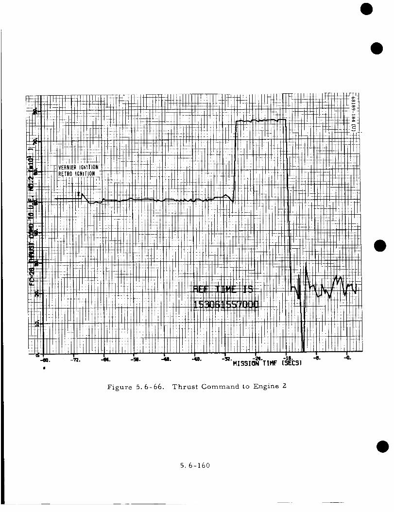
MISSION TTMF

Figure 5.6-66. Thrust Command to Engine 2

5.6-160

"+'.,SS,_'T,,_ t-S_+m -0.

Figure 5.6-67. Thrust Command to Engine 3

5.6-161

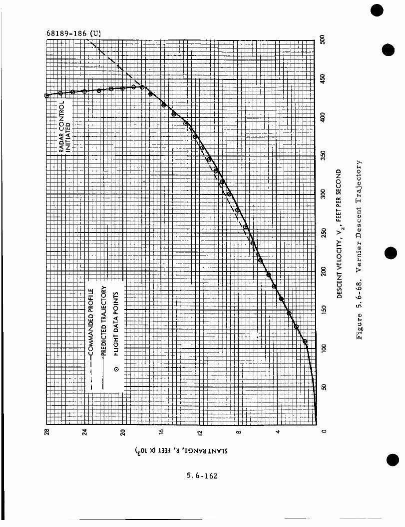
•68189-186 (U)

00, _" 0 ,0 (_l

(_01X)1:13_'_I'3ONV_ 1NVl$

!iII

i i

ili!t i

J_

I 1

IiI I

!iiiii

i i

4-I

l ii i

!!

iii

i

4-

I

+4-!

I

iII

I

Ii

_.+._i

O'J

8C_

o

8

o

Z

0U

W

0.

I--ww

>

0,_1

w

>

zU

u.I

>,

0

°r-._

°_..i

I

M

5.6-162

900

800

700

_- 500

uJ0Z

4oo

300 ¸

2OO

IO0

10 20 30 40 50 60 70 80

DESCENT VELOCITY, Vz, FEET PER SECOND

I I I

i tl: II

II

I I

L "I IA I I,i II

: I III

: II

i I',I I

I! ii: !!

i i ii. . !!

i i !i

ili! : :

i !! :

Ji.li_ :

i ili

i III

I t

! :

i iI

Figure 5.6-69. Vernier Descent Trajectory, Range > I000 Feet

100

5.6-163

TABLE 5. 6-22. TIME AND EVENTS LOG

Vernier Phase

Vernier Descent

Phase Events

Start RADVS

controlled

descent

Segment

Time of Event,

GMT

06: 15:42. 093

06: 16:05. 893

acquisition

End of segment 1

End of segment Z

1000 feet

End of segment 3

10 ft/sec

13 feet

Touchdown

06:16:17. ZZ5

06:17:10.494

06:17:10. 494

06: 17:19. Z81

06:17:28. 719

06: 17:34. 169

06:17:35. 600

Predicted Time

06:15:40

06:16:15

06:17:1Z

06:17:30

(8.6 ft/sec)

06:17:35

06:17:37

Note: Time of events was obtained from Reference 19;

predicted times were obtained from Reference 15.

Range-Velocity Trajectory

The actual range-velocity trajectory is presented in Figure 5. 6-68

along with the commanded profile. The nominal or expected descent

trajectory is also provided to illustrate the fine performance of the flight

control system.

5. 6-164

Vernier Descent Attitude Control

Pitch and yaw attitude motions determined from pitch and yaw gyroerror telemetry signals (FC-16 and FC-17) were maintained less than ±i.0

degree in each axis during the vernier descent phase. Required gimbal

freedom of each gyro is ±i0 degrees. (See Figures 5.6-70 and 5.6-71 in"Corrected Telemetry Plots. ")

Measurable gyro gimbal errors (equival_nt to spacecraft attitude error

relative to the reference established by RADVS signals) occurred only during

certain portions of the vernier descent phase, according to the followingsummary:

PeakGyro Gimbal Errors, degrees

Phase of Descent Pitch Yaw

RODVS (start of alignment

to velocity vector}

R < 1000 feet (due to KADVS

noise)

Following engine cutoff

Following touchdown

0.9 0.65

<0.2 <0.2

1.0 -O. 9

-0. 65 0. 58

Following generation of the RODVS signal by the RADVS, the space-

craft initiated an attitude maneuver to align the thrust axis with the total

velocity vector. Initial velocity conditions preceding the maneuver were as

follows (taken from RADVS telemetry data, FC-39, FC-40, and FC-41).

{See Figures 5. 6-7Z, 5. 6-73, and 5. 6-74 in "Corrected Telemetry Plots. ")

Premaneuver velocity conditions (06:15:44. 5 GMT) are as follows:

V = 31. 1 fpsx

V - 25. Z fpsY

V = 430 fpsz

The alignment maneuver was completed in less than 2 seconds (9 seconds

allowed}, at which time V x and Vy were held at zero and V z became equal to

the total velocity of 432 fps. The attitude maneuver magnitudes were com-puted as follows:

5.6-165

VPitch maneuver: _@ = - tan- 1 __y__

x VZ

Yaw maneuver:

= 3. 4 degrees

V-i x

= tan - 4. 3 degreesA@y VZ

The spacecraft Z axis was therefore maneuvered through a total of 5. 5

degrees.

Gyro gimbal angle errors were maintained virtually at null during the

descent above the 1000-foot range. Following generation of the RADVS 1000-

foot mark, which increases the lateral velocity control channel gains by a

factor of approximately six and thereby increases system sensitivity to noise

on the V x and Vy radar indications, increased gyro gimbal errors were devel-oped but did not exceed 0. Z degree in either axis.

Following vernier engine cutoff, gyro gimbal errors (equivalent to

inertial attitude motion) increased to approximately i. 0 degree in pitch and

-0. 9 degree in yaw during free-fall to the lunar surface. Following touch-

down, these gimbal angles were -0. 65 degree in pitch and.0. 58 degree in yaw.

The vector sum of these two quantities yields a net attitude error of 0. 87

degree. Thus, if it is assumed that the gyro reference was aligned to ver-

tical by the RADVS guidance signals, this would imply a lunar surface slope

of 0. 87 degree. Since the most accurate estimate of surface slope is 0. Z7

degree, it must be concluded that the gyro reference was misaligned to ver-

tical by approximately 0. 6 degree. This is well within the 4. 8-degree allow-

ance (Reference 17).

Corrected Telemetry Plots

The corrected telemetry plots are given in F_gures 5. 6-70 through5. 6-78.

5. 6. 7. IZ Spacecraft Attitude Determination- Postlanding

The following analysis was obtained in its entirety from Reference 20:

I° The spacecraft attitude matrix is defined as the matrix by which

vectors are multiplied to transform them from the selenographic

coordinate system into the spacecraft coordinate system. Three

independent data sources were used to generate attitude matrices.

These sources were the ASPP, the TV camera, and the inertial

reference unit. The ASPP and TV camera matrices were gener-

ated using the least-squared error method described in Reference

[Zl].This method,, rather than the PLAS program, was used to

permit generation of a single matrix for all vectors from a given

data source. The PEAS program is only capable of accepting two

vectors at a time. The gyro matrix was obtained by assuming x

and y axis slopes to be exactly represented by the difference in

5.6-166

_o

Figure 5.6-70. PitchGyro Error Signal

5.6-167

lip

: r I

F_',T-,

i-i_iI I T

|

!!H!!lllIlT,

!iiLiil'

IIiIIIIIIII

H-_÷HffII

tttiJlflJ

!it_ttitt

I]:Iiiilt!

ilt111

i'ttllllilll

_[tltl

I11,,illl-

!!!i!!it....... !!

itlll ]_m.

Figure 5.6-71. YawGyro Error Signal

5.6-168

liO°

:1

Figure 5.6-72. True V x

5.6-169

_tt_tHt iiiiiii_i, , : li il i:lr,

illliiiiJi!

It _'1 !

:i|li *!l Li! _--_--r----t , i i L

!4_ll!!l

ttt!lt',tI ........:ft_÷; I l r i! ......._11I/[ !1_1 I ........

r [ I ,_ ], :

i , ,1tiitl_[ l|rl_

II, I |IJl

ftit ........:::.:::

_ [ 1! I111,1 It,, _lITit]/

il]_ii_il ;,iii::;

li_t_ _ ....

_iiiiii iiiiii_iii;ii:i_,ii .........

,.!!!!!i! _ilti!_4''1_11111

*_ _ME ,SE_

111111il ii

,,I'ii[ !!,,i l

! [[

tl

] ![!

!! i!!Lt

Itt lIII I_

Figure 5.6-73. True Vy

5.6-170

lilO°

il

Figure 5.6-74. Ture V z

5.6-171

_F

ii

I

IiI

L

i

_+_+.

[

• ,JF] [

!l ]

Ill[7

i. ! "_

= i[i]

-+_ FI+

IiI_iliil

I[

iiliiI

+_

[[

_riI

mr

Figure 5.6-75. True Slant Range

5.6-172

Figure 5.6-76. Thrust Command, Engine 1

5.6-173

_°

g

Figure 5.6-77. Thrust Command, Engine Z

5.6- 174

lJlill

_!ItlI

I_ !

il I_|_11

:'!! ! ! !

!Ill _li

_]tt:t:,L

ItttH!tt111411_t I

_o

Figure 5.6-78. Thrust Command, Engine 3

5. 6-175

gyro error signals before and after touchdown, assuming the

spacecraft to be aligned along the gravity vector just prior to

touchdown. The final SC- 1 attitude was in turn obtained by com-

bining the three individual matrices by the method described inl_eferenceE2Z_. All three matrices were weighted equally in this

final combination. Calculations were performed for a landing

site of 43. 345°W longitude and Z. 411°S latitude. The various

matrices and their data sources are as follows:

A. ASPP Matrix

The ASPP matrix was derived from 5 sun vectors and 5 earth

vectors obtained during the first lunar day.

- .01914 ÷. 03088 -. 99934]= 69270 - .72116 00901|

MASPP 72096 +. 69207 + 03520.]

B. TV Camera Matrix

The TV camera matrix was derived from one sighting of

Canopus and two sightings of Sirius during the first lunar

day. A sighting of Jupiter was also obtained, but data wasnot available for inclusion in these calculations. Data from

the three star sightings were corrected for lens and elec-

tronic distortions.

I -. 02980 +. 04129 -.99870 1= 67838 - .73464 -.01013

MTV 73410 +. 67720 +.04991

C. Gyro Matrix (Inertial Reference Unit)

The gyro matrix was derived from differences in telemetry

signals FC-16, FC-77, and FC-49 before and after touchdown.

I -. 01844 +. 05338 - .99840 ]M G = -. 69692 -. 71669 - . 01828 J-. 71691 +. 69534 + . 05041

D. Combined Matrix

SC-I final attitude matrix was obtained by combining MASPP

MTV, and M G using the method outlined in Reference [221.

-.02413 .04018 -.99890 1= 68942 -.72425 -.01248

MSC-I 72396 . 68836 .04518

Using the above final matrix, the computed lunar slope down-

hill direction is 239. 8 ° (WSW) with a magnitude of 0. 27 °

5. 6-176

.

DAY

153

154

155

156

157

158

159

160

161

162

163

164

165

The spacecraft is aligned in the selenographic coordinate sys-

tem such that the angle from selenographic north to space-

craft -y axis is 89 ° as shown in Figure [5. 6-79].

Sun/Earth Positions

The sun earth positions in the tables below are specified in azi-

muths and elevations. Azimuth is defined as the angle from the

spacecraft -x axis to the xy projection of the vector to the body

of interest measured in a clockwise direction. Elevation is

defined as the angle between the vector to the body of interest and

the vectors projection in the spacecraft xy plane. (See Figure

[5. 6-80]. )

Positions are calculated at zero hours GMT for the day specified.

Sunrise is defined as the time at which the leading rim of the sun

would rise above a plane tangent to a spherical moon at the space-

craft landing site. Sunset is defined as the time at which the

trailing rim of the sun drops below the tangent plane. Lunar noon

is defined as the time at which the angle between the spacecraft

sun vector and its projection in the tangent plane reaches a max-

imum. These times are determined solely from landing site and

are not affected by the spacecraft attitude.

A. First Lunar Day

Day Hr/Min

Sunrise 150 2048

Lunar Noon 158 0629

Sunset 165 1541

SUN AZ

88. 9

88. 0

86.8

84. 6

79. 4

48. 4

291. 0

279. 3

275. 9

274. 3

273. 2

272. 5

271.9

SUN EL EARTH AZ EARTH EL

25.4

37. 6

49. 7

61.9

73 9

85 2

80 7

68 8

56 7

44 5

3Z 3

20 1

7.9

88. 4

86.3

84. 3

82. 6

81.1

79.9

78.6

78.5

78.4

78.6

79.3

80. 3

81.9

41.8

41.5

41. 3

41 4

41 7

42 3

43 1

44 2

45 4

46 7

48 1

49. 4

50.5

5.6- 177

SLOPE

GRADIENT

NORTH __

-x '_

S

-y

J _239.8 deg

xlFigure 5. 6-79. Spacecraft Attidude

With Respect to Selenographic

Coordinate System

-.!

ELEVATION ANGLE,E _

-x =

m

¢:

,/_ -YI//, o' /

AZIMUTH ANGLE, (1

Figure 5.6-80. Geometry

5.6-178

D B. Second Lunar Day

Da___X Hr / Min

Sunrise 180 0748

Lunar Noon 187 1725

Sunset 195 0241

DAY SUN AZ SUN EL EARTH AZ EARTH EL

181 89. 2 7. 69 86. 8

182 88. 5 19.8 84. 9

183 87. 7 32. 0 83. 1

184 86. 5 44. 1 81. 6

185 84. 6 56. 3 80. 3

186 80. 7 68. 3 79. 4

187 67. 9 80. 1 78. 8

188 321. 6 85.0 78. 6

189 284. 7 74. 1 78. 8

190 278. 4 62. I 79. 3

19 1 275. 8 50.0 80. 2

192 274. 4 37. 8 81. 5

193 2/3. 4 25. 6 83. 3

194 272. 7 13. 4 85. 4

195 272. I i.2 87. 8

41 2

41 1

41 3

41 7

42 2

43 0

43 9

45 0

46. 3

47. 7

49. 1

50.4

51.6

5Z. 5

53.0

5. 6. 7. 13 Miscellaneous

Nitrogen Gas Consumption

The expected nominal value of nitrogen fuel consumption as per

Reference 4 (revised to fit the actual mission),is 0. 546 pound. The actual

amount of nitrogen consumed during the SC-1 mission was determined to be

0. 680 pound. Of this value 0. 099 pound of nitrogen can be attributed to drift

checks that were not included in the initial estimate of fuel budget. Thus,

the true difference between the actual and expected value is 0. 134 pound. Much

of this difference was caused by a double pulsing action of the roll gas jet sys-

tem which occurred periodically during the coast mode operation, giving rise

to a higher limit cycle frequency.

Nitrogen Weight History. A graphical representation of nitrogenweight history is presented in Figure 5. 6-81. The nitrogen weight values

were determined from the N 2 weight curve ",-"(Figure 5. 6-82), using corrected

_The N 2 weight curve was derived from data obtained from "ThermodynamicsFunction of Gases," Din, Volume 3, Butterworth and Company, 1961.

5.6-179

telemetered nitrogen tank temperature and pressure information. Thetelemetry data of pressure was corrected using the latest available telemetrycalibration information (Reference Z3). (See Figure 5. 6-83.) A summary ofthe nitrogen gas consumption is presented in Table 5. 6-23.

Nitrogen Gas Consumption/Mission Phase.

Rate dissipation phase: The gas consumed during separation phase

appears negligible.

Sun acquisition phase: From Figure 5. 6-81, it appears that approxi-

mately 0. 040 pound of nitrogen was used during sun acquisition. This value

may be affected by the fact that the gas temperature had not reach steady

state.

Star acquisition and verification phase: From Figure 5. 6-81, it

appears that approximately 0. 030 pound of nitrogen was used during this

phase of the mission.

Midcourse maneuvers: From Figure 5. 6-81, the total gas weight

change during midcourse was 0. 200 pound. Extracting the, expected values

for vernier phase and postrate dissipation, the gas consumption for the maneu-

vers is estimated to be 0. 150 pound.

Coast phase: The average gas consumption rate during the period

between the twenty-fourth and fortieth hour of the mission was used for com-

puting coast phase gas consumption. This mission period was chosen becauseof the relative freeness of drift checks which were frequently made. The

average rate was 0. 00219 Ib/hr. Thus, the total amount of gas consumed

during the coast mode was 0. 138 pound.

Preretro maneuvers: Temperature data was not available immediately

after the preretro maneuvers because the telemetry was in a monitoring mode

that did not include nitrogen temperature. It was thus necessary to estimate

the gas used for the preretro maneuvers.

From Reference 24, it was noted that the ratio of gas consumed for a

roll maneuver versus a yaw maneuver is i. 2. With this knowledge and the

amount of gas used during midcourse maneuvers, it was determined that the

actual consumption per maneuver was 0. 0341 pound for yaw and 0. 041 pound

for roll. Since SC-I required three maneuvers consisting of two rolls and a

yaw, the total gas consumed was as follows:

Two roll maneuvers -- 0. 08Z pound

One yaw maneuver = 0. 034 pound

Total gas consumption = 0. i16 pound

5. 6-180

i::

!i " i

!if::

t0

I-q0

f-t

_oI

'_0

(1.}I>

L)

bl[-_r-I

C_

0

Z

I

u_

5.6-183

68189-201 {U)

lk -

.°

\

.,.,,\

\

\\

\

\

7

1

i

: -]

\ ........ _ " t ..... ," . ......... '_ 1

" _ -iJ

\'q'\ NN

\

.. "_

\

o>

C)

0°r-I

;...I

c)>,

@

@

o

0

0.,

0

ooI

,A

_0

5.6-184

TABLE 5.6-23. NITROGEN GAS CONSUMPTION

Mission Phase

Rate dissipation

Sun acquisition

Star acquisitionand verification

Midcour se

maneuver s

Vernier phaseof midcour se

Postmidcour se

rate dissipation

Coast mode

Drift checks

Preretro

maneuvers

Le akag e

Nitrogen Used

During Mission,

pound s

0. 040

O. 030

0.150

0.138

0.099

0.116"*

Total N z

Equivalent total

0.0 57*

O. 68O

0.680

Expected Usage

(Average),

pound s

0 to 0. 046

0. 054

0. 048

0.092

0.033

0. 017

0.075

0.071

0. O57

0. 493

0. 546

Comments

Not observable

Tank temperature

may not have been

at steady state

Values of vernier

phase of midcourse

and po stmidcour se

rate dissipationsubtracted from

0. 200 pound

Calculated value

Drift N z usage isadded to expectedvalue and rate dis-

sipation is sub-tracted from

expected value

Expected values were used.

Estimated value using data from midcourse maneuver.

An IsPof 60 seconds is used for expected values. These values were

obtained from R. H. Bernard, "Revised Gas Jet Consumption for 66Hour Surveyor Flight," IDC 22Z3/843, 19 February 1965.

5.6-185

Leakage: Since leakage information was not available, the expected

value of 0. 057 pound is used.

Drift checks: During the mission, six separate drift checks were

performed. The various times are shown in Figure 5.6-81. Notice that

during the latter period of the mission where three successive drift checks

were made, the gas consumption rate is high. The value for drift check gas

consumption was indirectly obtained by subtracting all accountable gas usage

from the total. Drift check gas consumption -- 0. 099 pound.

Determination of Gyro Nulls

Preflight calibration of the three gyro error signal channels indicatesthat the nulls are as follows:

Pitch (FC-16) = 503 bcd

Yaw (FC-17) = 508 bcd

In the SC-1 calibration handbook the gyro null values are as follows:

Pitch (FC-16) = 509.6 bcd

Yaw (FC-17) = 514.5 bcd

The reason for the difference in the above two sets of figures is that

the calibration handbook compensates for a known error source of magnitude

6.6 bcd. This error is the line drop caused by the difference that exists

between the flight control and telemetry grounds. During thrust phase

power-on periods, an additional line drop of 17.4 bed is known to exist. This

is not accounted for in the calibration handbook.

The apparent null values during inertial mode phases were obtained

and all known errors were removed. The results of the investigation are

presented in Table 5.6-24.

Determination of the Main Retro Thrust Vector Offset From the

Spacecraft Center of Gravity

Spacecraft moment control during large disturbances is provided by

the vernier engine system. The three engines that are capable of being

differentially throttled obtain their commands from the output of three rate

integrating gyros which establish an inertial reference frame. A block dia-

gram representation of the attitude control loop is given below.

M R

Gyro Shaping Network Engine __ _

/ III

,-,1

5.6-1.86

I TABLE 5.6-Z4. GYRO NULLS

Mission Phase

Coast Mode 1

Midcourse _V

During gyro driftTest No. 6

(Coast Phase Z)

Prior to retro

phase (thrust

phase power on',

Prior to retro

{prior to the

above period)

Average null value

Average value

using calibrationhandbook

TelemetryCondition

Low power,

mode C,

550 bits/s ec

High power,thrust phase

power on,mode 1,

4400 bits/sec

Low power,

mode C,

550 bits/sec

High power,thrust phase

power on,mode 2,

1 I00 bits/sec

High power,mode Z,

1100 bits/sec

FC

Number

FC-16

FC-17

FC -49

FC-16

FC- 17

FC-16

FC-17

FC-16

FC-17

FC -49

FC-16

FC- 17

FC-49

FC-16

FC- 17

FC - 49

FC- 16

FC - 17

FC-49

Raw Data,

bcd

5Z6. 5

525.0

5Zl. 5

540

537

Line DropCorrection

6.6

6.6

6.6

Unbalance

Commutator

Current

-3.7

-6.0

-1.90

525

525

543

537

539

524

521

520

-24

-Z4

.6.6

.6.6

-24

-g4

-24

6 ¸. 6

6.6

6.6

-0.7

-0.8

-3.7

-6.0

-Z. 0

-Z. 6

-1.77

-2.5

-Z. 6

-I. 65

Corrected

Value,bcd

516. Z

512. 4

513. 5

515. 3

512.2

514. 7

51Z. 4

517. 0

510. 4

513. 2

514.9

'511. 8

511.8

515. 6

511.8

512. 8

522.2

518.4

519.4

The steady-state relationship between moment disturbance M R andattitude angle @ is as follows:

where

M R x 0.05

K@

K@= shaping network dc gain.

0:05

(i)

5.6-187

where

Replacing T R

K@xed -

0.05 T R

x d for M R, the following relationship is obtained

T = main retro thrustR

d = distance of offset

K@ = 3465

(z)

Retro Thrust Determination. The procedure in determining thrust

is to utilize the acceleration data (FC-3Z) along with spacecraft mass at the

instant of retro ignition.

Corrected acceleration value = 4.0923 g (see Figure 5.6-84)

Spacecraft mass at ignition is given in pounds as follows:

Injected weight = 2192.71

Midcourse fuel = -16.81

Nitrogen = -0.68

AMR = -ll. 68

One second vernier = -0.80

Spacecraft weight = 2162.74at ignition

Thus the thrust level at (near) retro ignite was

I)

z)

2162.74T R - × 4.0923 g = 8850.58 pounds

Gyro Angle Determination.

signals were obtained:

During retro burn, the following gyro

Pitch (FC-16) = 543 bcd

Yaw (FC-17) = 539 bcd

raw data

5.6-188

After applying known corrections, the corrected values are (seeFigures 5.6-85 and 5.6-86):

FC-16 (pitch) = 522.6 bcd

FC-17 (yaw) = 518.6 bcd

From the investigation of gyro nulls, the actual null values of thegyros were as follows:

FC-16 (pitch) = 522. Z bcd

FC-17 (yaw) = 578.4 bcd

5 pitch = O. 4 bcd

A yaw = 0. 2 bcd

Using Equation l, the above values represent a moment disturbance

value of less than 0. 35 ft-lb or a @/T R ratio of 0.08 x i0-5 deg/ib.

Reference Z8 mentions that the above technique is only good for off-

sets greater than 0. 03 inch or _/T ratio of 0. 2 X 10 -5 deg/lb or greater.

Thus, it is concluded that the main retro thrust vector misalignment was

less than 0. 03 inch.

SC-I Radar Noise Levels

Radar noise levels actually experienced in flight were estimated by

visually comparing SC-I telemetered data (Figure 5".6-87) with similar data

generated by the six degree-of-freedom analog computer simulation of the

radar controlled descent phase using various combinations of simulated Vx,

Vy, Vz, and R noise inputs. Because the comparisons were qualitative and

because the telemetry data is sampled rather than continuous, the accuracy

is about ±Z0 percent on any estimate. Three data sources were used in the

estimates: radar outputs, gyro outputs, and differential thrust commands.

The most reliable of these were the differential thrust commands because of

higher sampling rate and resolution. However, all three sources of data

indicated approximately the same radar noise levels at any particular portionof the descent.

The analog computer runs were made from the six degree-of-freedomterminal descent simulation described in Reference 25. These results were

supplemented by the $6-C closed-loop test data described in Reference Z6.

Vz Error Noise. Vz error noise is due to noise on both the range

and Vz radar output signals. This noise caused large thrust command

transients, giving a good data source for extracting the V z error noise level.

The estimated levels for different mission times are given in Table 5.6-25.

5.6-189

i-'a_ -+-T-:....... :-: ...... 'T-_ ........ _ " -, - '

_ I_:: _ _ " i __ - ! , !, :, , i .... _ i + i !

1 I + _ :- _ 4 J:

t_- -_+.............. u_.............I

!-10o............................

_t_ -I ........

.... :" I i 1 '"

o I ' I .

I k __i _L.I

:_, I ",--£+]

.... o _

L__u......._L_.....'.._I_O0__ . -/2/4f _._"C_.+JS_......... __'..J........,........

Figure 5. 6-84. Acceleration Time History

Spaceflight Operations Facility

retro phase data

5.6-190

68189-Z03 (U)

_D

,.ct

0

4-_

_D

or'4

,-., '1:1

.r-I

o ¢1

:>,

o

,-o 0.)

0, 0

u

oo

Z _m _

,,D

u_oN

.r,,_

!

I-iI-i

0

I-to4_

o0

,"el

Do

I:1ID

GII--I

o>

r.fl

',-i,-I

0

,$oo

I

,.o

M

I,-i

e:_,v-I

5.6-193

TABLE 5. 6-25. ESTIMATED LEVELS FOR

DIFFERENT MISSION TIMES

Flight Condition

Range, feet

17, 800 to

IZ, 900

5500 to 980

980 to 300

I00 to Z5

V , ft/secZ

440 to 390

g 15 to 105

105 to 57

Z0 to 8

Time to Touch-

down, seconds

90 to 80

55 to 25

Z5 to 17

llto 8

3_ V

Nois z,

Error

ft/sec

Z.I

1.5

1.0

1.0

Vx and Vy Noise. During maximum and minimum acceleration com-

mand periods, only V x and Vy noise generates a differential thrust command.

This command level is significantly lower than that generated by V z error

noise. The (approximately equal) estimated V x and Vy noise levels for dif-

ferent mission times obtained from thrust command telemetry signals are asfollows:

For i% > i000 feet (based on data from minimum and maximum accel-

eration command periods):

3<_ V noise : 3_ V noise : 5. 0 ft/secx y

For I% < 1000 feet (based on data from maximum acceleration com-

mand period):

3(7 V noise : 3_ V noise : 2. 5 ft/secx y

Comparison to Noise Specifications. The estimated SC-I V x, Vy, andV z error noise levels are plotted in Figures 5. 6-88, 5. 6-89, and 5. 6-90 in

comparison to noise levels specified in the spacecraft functional requirements

document (Reference 17). In Figure 5. 6-88, V z error noise is allotted entirely

to the Vz radar signal, and in Figure 5. 6-89, it is allotted entirely to the

range radar signal. It is noted that SC-I noise levels were generally within

specification.

Analysis of Gyro Speed

The value of the gyro speed indications as to the assessment of the

flight control system's condition has always been questionable. A thorough

analysis on this subject has been performed and the text of the original memo-

randum is presented here as it appeared in Reference Z7.

5. 6-194

68189-Z04

o(n

,.-.4

°v-i

0

,-4

or4

,--4o

0t)

_0

,-4

oo!

,.o

or'4

[)-..

%.f)

I

u_

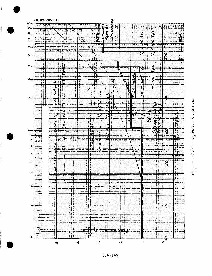
68189-205 {U) P,

eo

2

1 :

: i

+ ,

t_

2!-- £

-I-i

T

t._

4--4-

'iT.r-

r

_E4-

:4-

<:m2L

T

1t--

--a-_

i

_E-T-

i

_:_ i :l-_-::¢ : !_. t- _ ;t _-_-'-

0

r--I

B<

op..+

o2:;

tqt:>

<:Boo

I

,.,4

P,,-i

o,,,.q

,r..m

5.6-197

|K

I00 '°9

io

I 1

Io03 S 2 3 4 5 2

I K I0"

,R, SLANT

Figure 5.6-89. Slant Range Noise Amplitude

5. 6-198

:'F

A

7

4- F

-+-+_

_:

_2r2

I i

'i

q ii t

LL

"4---+---o.-*.--

---4---

ii

i

: :1

=J

r- l-

rt_,

t... _ o

E2 2

2i£:

%::

-_

at--4--

-_-

At

-n'-[

44

N

¢)

ol--I

<

.I--I

0

Z>,

>

0

_4>

I

",.D

5.6-199

Intr od uction

The gyro speed signal processing was turned on once in flight

during Surveyor Mission A and one cycle recorded by Goldstone (DSIF-II)

about two hours before the midcourse maneuver. An analog strip chart of the

5. 4KC gyro speed subcarrier signal for its four minutes of operation was

prepared by R. Lum of JPg's Data Analysis Lab from the on-site magnetic

tape recording. The results of an examination of this analog record are

presented here along with a general assessment of the gyro speed telemetry.

Summary

The history of the SC-I gyro speed telemetry has been characterized

by anomalous behavior which appears to have reached a climax in flight. The

observed "gyro speeds" in flight were approximately 8% (yaw), 16% (pitch)

and Z6% (roll) higher than the corresponding values reported for the launch

countdown. On the basis of test history one would expect the change, if any,

from pre-launch to post-launch to be in the direction of a decrease for the

roll and pitch gyros since both were out of tolerance on the high side before

launch. At present the best explanation for this apparent anomaly lies in the

different methods used to count the "gyro speed. " In view of the problems

associated with "gyro speed checks," it is recommended that they be deleted

from system test and flight sequences.

Evaluation of Data

When first turned on in flight, the gyro speed processing stepping

switch was set to sample theloitch gyro spin motor speed monitor. Since this

switch was set to the null reference position at the conclusion of the pre-launch

check, this might be considered a minor anomaly. A discussion of this with

D. Hersey of the JPL Surveyor Telemetry Group revealed that the stepping

switch assumes an arbitrary position when the gyro speed telemetry ECU is

turned on by command 0221. Test data indicates that the Pitch Gyro selection

is the "preferred" initial condition.

The data sequence and sample readouts are given in the following table

(all times given are on 31 May, day 151):

Surveyor I Flight Gyro Speed Summary

GM Time Event

Command 0ZZI Initiated

5. 4 KC SCO on

Select Pitch Gyro Speed

26 08 Count Pitch Gyro Speed 68

Z7 00 Count Pitch Gyro Speed 67

Gyro Speed Count _:";:"

5. 6-200

GM T

27

27

27

27

28

28

28

28

29

29

29

29

30

30

30

ime

47

48 *

49. 66

50

l0

31

31 *

32. 15

05 *

06. 15

07

36

04

04 *

05. 18

":" Command

Event

Count Pitch Gyro Speed

Command 0222 Initiated

Select Yaw Gyro Speed

Count Yaw Gyro Speed

Count Yaw Gyro Speed

Count Yaw Gyro Speed

Command 022Z Initiated

Select Null Reference

Command 0ZgZ Initiated

Select Roll Gyro Speed

Count Roll Gyro Speed

Count Roll Gyro Speed

Count Roll Gyro Speed

Command 0223 Initiated

Gyro Speed SCO off

Gyro Speed Count *':-"

66

54

54

54

76

75

74

times are taken from CDC Command Printer tape.

*':" Gyro speed count is the number of full cycles during a one-

second interval at the beginning, middle and end of each

readout period.

There was a very noticable variation in amplitude in the pitch and roll

gyro speeds which appears to result from phase shifts. Large phase shifts

on the order of 180 ° occurred frequently on the pitch gyro speed signal (over

25 times in i00 seconds), rarely on the yaw gyro speed, and never on the roll

gyro speed. The amplitude of the yaw signal on the analog record (approx-

imately 3V peak-to-peak) was significantly greater than for pitch and roll,

but this may very well result from discriminator and/or oscillograph recorder

response characteristics, since the yaw gyro signal frequency was lower.

Discussion

The telemetered gyro speed signals are derived by dividing down by

32 the 1600 cps (nominal) signal picked off from the gyro spin motors. The

nominal count should thus be exactly 50 cps. It has been known for some

time that noise on the signal lines upstream from the + 32 circuit produces

variable counts well above the spec tolerance.

A comparison of some SC-1 test data readings with the launch count-

down and flight readings is given below. No actual readings were given, but

5.6-201

no gyro speed anomalies were reported in the Quick Look Reports for Com-bined System Tests at San Diego or Performance Verification Tests at ETI_,leading to the conclusion that test GSE was a major contribution to the anom-alous readings obtained during earlier tests. The STV Mission Sequencereadings in the following table were taken from Quick Look Reports. TheLaunch Countdown values are average readings reported by R. Crabtree.

SC-1 Gyro Speed Test and Flight Comparison

MS Test A MS Test C Launch

Gyro 12/28/65 i/Z i/66 Countdown Flight

Roll 67-73 65-67 59 74-76

Pitch 58-66 66-70 58 66-68

Yaw 51-56 54-56 50 54

It is significant that the Mission Sequence Test C (plugs out) readings

showed no improvement over Test A (or B), indicating that the variation in

readings during the test history may be more dependent on the method of

counting the output signal frequency than on the test configuration. The nor-

mal method used to obtain gyro speed count is to average the output of an

"events-per-unit-time" (EPUT) meter using a Schmitt trigger to detect an

"event" each time the signal voltage passes a certain level in one direction.

Thus the setting of the trigger threshold is critical to insure a correct fre-

quency count. The observed amplitude variation in _he flight data signal

indicates that it would be very difficult to adjust the trigger threshold to obtain

a complete cycle count using this type of frequency counter.

The flight gyro speed counts are based on cycle peaks without regard

to amplitude and therefore represent a true count, but even this count shows

significant short-term variations, due obviously to noise on the signal line.

Thus, the fact that the flight values given are higher than the pre-launch

values which were obtained by a digital counter, does not necessarily mean

that there were any significant changes in the SCO output signal. About the

only valid conclusion that can be drawn from the data table is that the noise

on the yaw gyro signal line was always considerably less than that on the roll

and pitch gyro signal lines.

Value of the Gyro Speed Telemetry

The gyro speed telemetry is intended to provide an output signal pulse

train whose frequency is proportional to the gyro spin motor speed. Its pri-

mary purpose is to verify that the gyros have reached synchronous operation

after flight control power is turned on. This function on Ranger and Mariner

was achieved by means of a hard-line monitor but was incorporated into the

5.6-202

D Surveyor Spacecraft telemetry system because of a severe limitation on the

number of signal leads available through the umbilical cable early in the

Program.

The 1600 pps signal from the gyro Spin Motor Running Detector is fed

through a frequency dividing network and should appear as a 50 cps oscillation

on the subcarrier. Noise spikes of sufficient amplitude and duration tc_ trigger

the divider flip-flops are known to be present on the input signal line. This

accounts for the observed readouts in excess of 50 counts. Since the noise

is a generic design deficiency, the telemetry is virtually worthless for deter-

mining the true gyro spin motor speed.

How useful would the telemetry signal be if the noise problem were

eliminated? Changes from the nominal 1600 of a few cps in the spin motor

speed should not affect the gyro performance. Deviations on the order of

I-Z%, the minimum detectable via telemetry using a digital frequency counter

over reasonable sampling periods, indicate a failed gyro. There are more

reliable telemetry signals available to detect such a failure.

Conclusion and Recommendations

The gyro speed telemetry is worthless as an indication of precession

or commanded turning rates and unreliable as a failure indicator. In recogni-

tion of this fact the SPAC long ago abandoned any requirement for real-time

reduction of this telemetry signal.

The basic design concept of the gyro speed telemetry is poor and.

redesigning the circuitry just to eliminate the noise problem would be a waste

of time and money. In view of the large number of TFR's that have been and

are still being written on this subject which is of such minor consequence to

successful spacecraft operation, and because its testing and evaluation requires

time consuming procedures and special equipment, logic would dictate that

gyro speed checks be eliminated from system tests and flight conditions.

The recommended long-term solution is to remove the circuitry

entirely from the ESP and replace it by a hard line monitor to verify gyro

sync at turn-on and a sensor to monitor the 3-phase 400 cps gyro input signal

from the Programmer with a readout on a PCM commutator.

Vernier System Pressurization/Canopus Sensor Anomaly

The following analysis was obtained from Reference Z and is presented

here in its entirety.

At the time of pressurization of the helium system just prior to midcourse, a

rather interesting anomaly occurred affecting the output of the Canopus sensor.

Figure [5. 6-91] shows a plot of the roll gyro error and the Canopus sensor

signals during the period of interest. It is seen that, within 5 seconds after

activation of the helium squib, the star intensity signal drops considerably

and, in fact, a lock-on signal was generated for approximately two seconds.

5.6-203

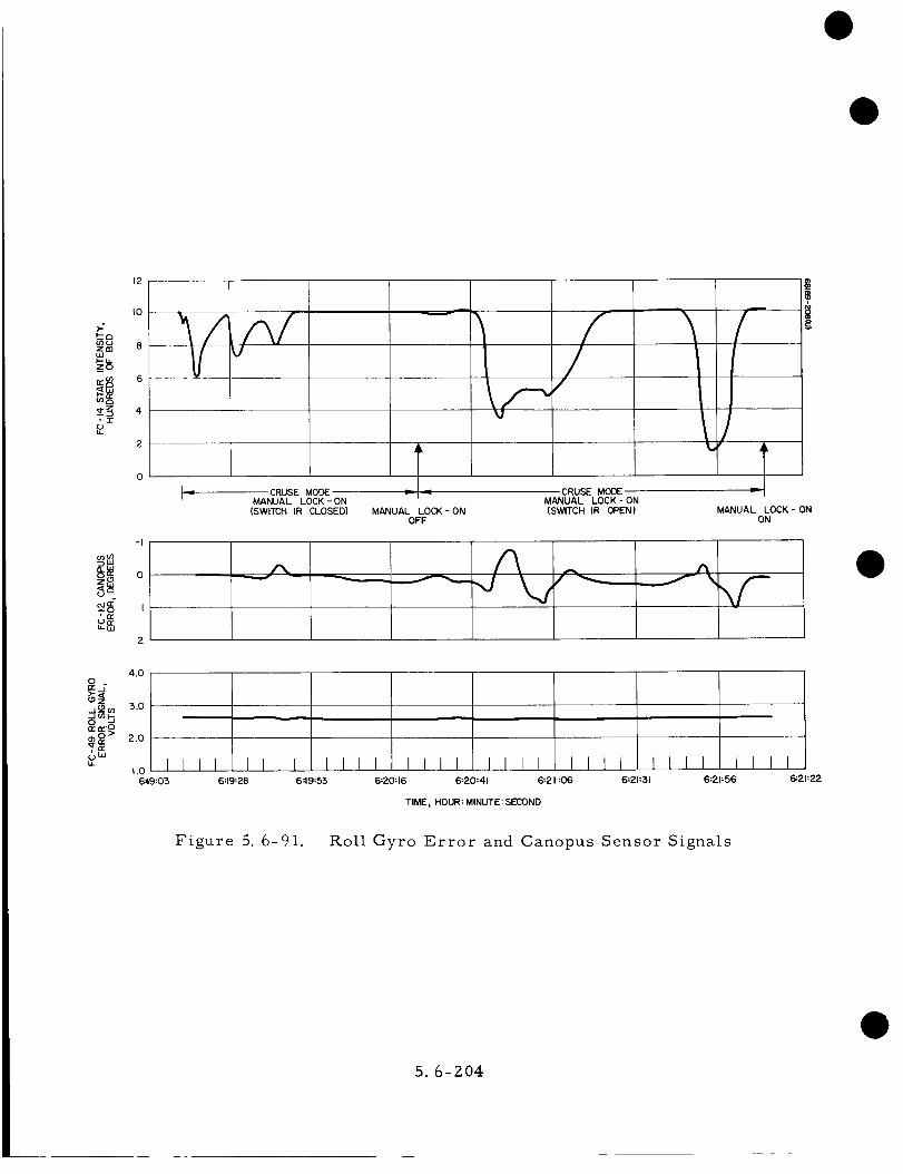
>.-0-o(/)(JZ,,'n

-r

w

030')

, n_u_u- W

12

I0

B

6

4

2

0

-I

/i_ CRUSE MODE _--- _ CRUSE MODE --

I_ MANUAL LOCK-ON MANUAL LOCK-ON

(SWITCH IR CLOSED) MANUAL LOCK-ON (SWITCH IR OPEN) MANUAL LOCK-ON

OFF ON

.v',,

4.0

c9 co 3.0

_ 2.oG"'u.

I.O6=19:03

IIII IIII I]11 IIII IIII ]111 IIII I II]6:19:28 6:19=53 6=20H6 6:20=41 6_21:06 6:21:31 6:Z1:56 6:21:22

TIME, HOUR: MINUTE: SECOND

Figure 5. 6-91. Roll Gyro Error and Canopus Sensor Signals

5.6-204

Remembering that with the sensor calibrated high, it was necessary to attenu-

ate the star light to produce this lock-on signal. The roll error signal was

virtually unaffected suggesting that the cause of this behavior may have been

a cloud of particles probably originating at the helium release squib. Figure

[5. 6-92] shows that the squib valve and Canopus sensor are at the same sta-

tion along the spacecraft Z axis and that there is a clear path from this valve

assembly to the Canopus sensor field of view. It seems quite likely that the

detonation of the squib could have liberated many small particles of white

paint or vapor-deposited aluminum (VDA). Some of our astronauts have in

the past reported a "shower of small particles" freed just by hitting the inside

of their capsule with a hand, a fact which tends to lend some credence to this

theory.

The next two "glitches" appear to be of a slightly different character but still

caused by particles. Since a roll error curve is generated in each case that

has the typical shape but of reduced amplitude, it appears that the cause of

these is a single particle (or small group) and not a cloud of small particles.

In addition, from the polarity of the curve it appears that if truly caused by

particles, they are coming from the other direction. Figures [5. 6-92 and

5. 6-93] show how the coiled line assemblies on leg I, which are coated with

VDA, could liberate particles that could enter the field of view of the sensor.

If one determines the trajectory that a particle must take if it comes directly

off from this coiled line assembly and passes in front of the sensor (contin-

uing in a plane containing this line assembly) the particle velocity computed

checks out exactly (Figure [5. 6-94]) with the length of time that a particle

was in the field of view for the first of these two "glitches. " The second

glitch appears to have been caused by a particle glancing off some other item

on the spacecraft such as the I_ADVS antenna, thus taking longer to get into

the field of view and also traveling up through the field just barely intersecting

the negative side. It is only necessary to postulate a change in the approach

angle from Zl ° (coplanar with coiled tubing) to Z8 ° to come up with a particle

velocity and trajectory consistent with the second glitch characteristic. The

reduced amplitude error signal is probably caused by the size and range of

the particles and the resultant defocusing effect.

The roll gyro error signal through all this remains essentially at null, indi-

cating at least during the two large glitches (gyro in inertial) that no spacecraft

movement took place.

In summary it can be said that the anomaly described here caused absolutely

no difficulty; and although impossible to prove, was probably caused by parti-

cles liberated during helium system pressurization. The fact that all of this

activity was confined to a single 3-minute interval beginning 3 seconds after

squib activation out of a 63-hour mission in which these outputs were monitored

continuously, should leave little doubt as to the correlation of the events. It

is concluded that this operation should be considered quite understandable and

that it will probably reoccur in subsequent flights.

5.6-205

68189-209 (U)

0

_0

_ /r.,.D

!

_4

_._ /

/:>

!

01

o

U

oa_

<

a_la0

o

<

ffl

U

!

M

5.6-206

//

HELIU24 TANK

NEAREST CLEAR PATH

13._<)---_

Figure 5. 6-93. Spacecraft Seen Along Roll AxisIn Positive Direction

5.6-207

TO ENGINE LINE ASSEMBLY

l

N_TE :

DISTANCES NOTED TAKE INTO ---

ACCOUN_AC_JAL ANGLES INVOLVED. _,_

CANOPUS SENSOR

FIELD OF VIEW

POSSIBLE PARTICLE TRAJECTORIES

FOR GLITCH #I

75 in = 0.765 in/seeV 1 =

19 intF.A.V. - 0.765 in/see. = 24.8 sec,

PARTICLE WAS IN FIELD OF

VIEW FOR _ 24 SEC.

_OR GLI'rC_#_

Assume 28 ° approach -

54 in - 0.34 in/see.V2 : 15"8_ see

6.5 in = L8.9 see;t = 0.34 in/see

AND PARTICLE WAS IN FIELD

OF VIEW FOR _18 SEC.

THEREFORE, IT'S POSSIBLE ---

Figure 5. 6-94. Particle Trajectory

5. 6-Z08

Roll Control System Performance

The estimated roll disturbance torque on SC-1 was extremely small

during both midcourse and terminal maneuvers. The principal causes of

vehicle roll disturbances were thrust vector excursions of the three vernier

engines induced by bracket bending. Based on telemetry data, the maximum

values of system parameters at any time in the mission were as follows:

Maximum roll actuator angle = i. 3 degrees

Maximum roll inertial error angle = 0. 7 degree

Maximum roll actuator rate = I. 5 degrees

Maximum roll rate (estimated} = 0. 5 deg/sec

It should be noted that the actuator angle was less than i. i degrees for all

but Z seconds of the mission based on the telemetry. The significant roll sys-

tem parameters at different mission times are summarized in Table 5. 6-Z6.

These values were read directly from roll actuator (FC-43) and roll preces-

sion command (FC-49) telemetry signals.

The close agreement between predicted actuator angle from bracket

bending and time actuator angle indicates that the roll disturbance due to retro

and vernier propulsion systems was small (l to 2 ft-lb) at all times.

TABLE 5. 6-Z6. SUMMARY OF SIGNIFICANT ROLL SYSTEM

PARAMETERS AT DIFFERENT MISSION TIMES

Time

Midcour se

Start of retro

End of retro

Retro burnout

through retro case

ejection

Minimum

acceleration

Segment control

Maximum Roll Actuator

Angle, degrees (from

pickoff, 0volt reference)

0. 9*

-0.4

-0.9

1.2

1. Z

1.3

Magnitude of

Maximum Roll

Actuator Rate,

deg/sec

0.4

0.7

0

1.0

1.5

1.0

Steady-

State

Actuator

Angle,

degrees

0.6

-0. g

-0.8

1.0

0.5

1.1

Predicted**

Steady-State

Actuator Anglefrom Bracket

Bending,

degrees

0.75

O.Z

-0.3

1.0

0.3

0.8

Maximum

Roll

Angle,

degrees*

-0.3

0.2

0.4

-0.7

-0.6

-0.7

Steady-State

Roll Angle,

degrees**

-0.2

0.1

0.4

-0.6

-0.2

-0.6

A plus actuator angle gimbals the No. 1 vernier engine to produce a plus vehicle roll control torque.

See Figure 5.6-95.

Based on a bracket spring constant of 0. 0045deg/lb and SC-1 initial alignment angles. See Figure 5.6-95.

*Based on nominal roll gyro to roll actuator gain of 1.85 percent.

*%Figure 5. 6-96 contains plots of both roll precession command and roll actuator signal during retro phase.

5.6-Z09

Terminal Precutoff Glitch Anomaly

Toward the end of the constant 5 ft/sec descent phase and during a

0. 9-second period beginning at about i. 3 seconds prior to the 14-foot mark,

all three vernier engines were commanded to throttle up by about 15 pounds

from their normal quiescent level. This behavior may be observed on the three

thrust command telemetry signals (FC-Z5, FC-Z6, and FC-Z7) as shown in

Figure 5. 6-97. It is also observed that all three thrust command signals

behaved in unison and responded normally to the acceleration error signal

(FC-15) which exhibited similar behavior, as indicated in Figure 5. 6-97.

This rules out the attitude control system as a possible cause for the anomaly

and directs attention to the velocity control system in general and to the Vz

radar signal in particular.

Figure 5. 6-98 shows a point-by-point, common-time-scale plot of

vernier engine 1 thrust command (FC-Z5), RADVS V z analog output (FC-41),

I_ADVS D 1 gain number Z (P_-Z0), and RADVS D3 gain number Z (I_.-Z4). From

this data, it is possible to make the following observations:

l) The thrust command glitch was preceded by a shift in the V z

analog indication of approximately i. 0 ft/sec. The normal system

response to such a shift would be an up-throttle of the engines to

reduce the V z indication to the 5 ft/sec level. The actual thrust

command response was therefore normal.

z) Integration of the thrust command signals over the anomaly period

indicates that approximately Z0 Ib-sec of thrust impulse were gen-

erated by the engines over and above that required to maintain

constant descent velocity. Since spacecraft mass at this point was

Z0 slugs, the thrust anomaly resulted in a velocity decrease of

i. 0 ft/sec. This is corroborated by the fact that the V z indication

did decrease again by about i. 0 ft/sec following the up-throttle.

This also indicates normal response of the velocity control loop,

which continually acts to maintain the Vz indication at 5 ft/sec.

3) The i. 0 ft/sec shift in V z analog indication was preceded by

several switchings of the RADVS D1 and D3 No. Z gain states.

Since telemetry sampling period for these signals (R-Z0 and R-Z4)

was 0. 5 second, it is not possible to establish if more gain state

changes than indicated in Figure 5. 6-98 actually occurred. How-

ever, since it is known that rapid gain state switching caused DVS

analog output glitches during the two final T-ZN descent tests

(although this was greatly magnified by the specific telemetry cir-

cuitry used on the T-ZN vehicle), it seems reasonable to suspect

that the SC-1 precutoff glitch may have ultimately been due to

switching of Dl and D3 No. Z gain states.

The following conclusions have been reached:

i) The precutoff glitch was caused by a i. 0 ft/sec shift in the RADVS

V analog output signal.Z

5.6-210

l::

I

0

ffl

,._

o

(3

i);

_4

IMI

u_

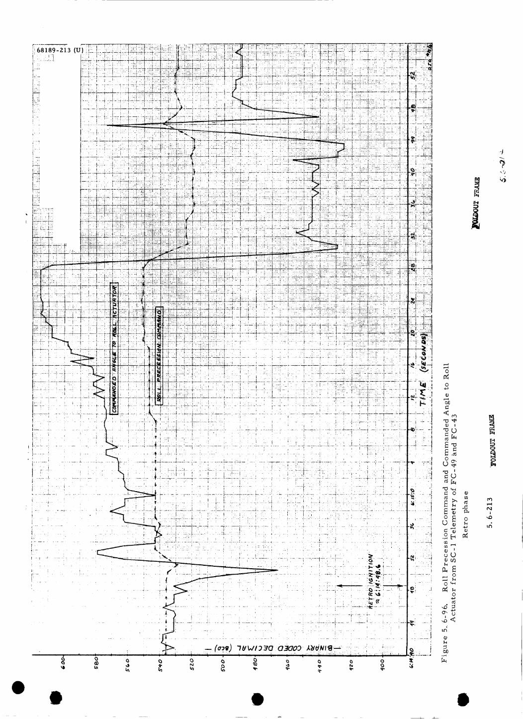
0

0

© I

O(3,..

I

o

0

u__)r.II

,.-4 o

04_

,.0<

u4_)

o _.-I

%

(1)

D_

0

t-t

I

d

LEVITE CORPORATION CLEVELAND OHIO PRINTED IN U S A •

Figure 5. 6-97. Acceleration Loop Parameters (Near Cutoff)

5.6-215

68189-z15(u) (__a__)I "ON

0

<

U

0

0

uco

©

U_

U3

<

!

M©

5.6-216

2)

3)

The cause of the V z shift is not definitely known at present, but

it is suspected to be due to switching of RADVS D1 and DZ No. Z

gain states.

Since the V z analog accuracy specification allowance is ± -/1 + (0.0ZVz)Z,

or ± i. 0 ft/sec for V z = 5 ft/sec (Reference 17), the Vz indication

apparently did not violate its accuracy requirement, at least not

to any great extent, during the glitch.

Spacecraft soft landing performance was in no way compromised

by the glitch.

5.6.8

i.

2.

3.

.

,

.

.

8.

.

I0.

ii.

12.

REFERENCES

"Quick-Look Report," Hughes Aircraft Company, SSD 64110.

"General Dynamics Report," GD/C-BNZ66-036, page 7.

O.N. Hertzmann, "SC-I Mission Performance- Flight Control Report,"IDC ZZZ3/Z341, 23 June 1966.

R.H. Bernard, "Revised Gas Jet Consumption for 66 Hour Surveyor

Flight," IDC 2223/843, 19 February 1965.

S. McCormick and D.R. Partridge,

IDC 2253. 1/69Z, 7 July 1966.

"Time Log of Command Sequences,

R.H. Bernard, "Limit Cycle Behavior of the Surveyor Gas Jet Attitude

Control System with Simulated Canopus Sensor Noise Included in the

Analog Mechanization," IDC 2223/772, 15 February 1965.

Surveyor Flight Control SPAC Handbook, SC-I.

R.H. Bernard, "Flight Measurement of Gyro Random Drift for Surveyor,"

IDC 2223/1509, 20 September 1965.

K. Kobayashi, "A Method of Determining Gas Jet Thrust Level-- Post

Mission Analysis," IDC 2253. 4/25, 1 March 1966.

"Interface Document, Surveyor Vernier Propulsion Thrust Chamber

Assembly," Hughes Specification 287015, Rev. 6, Model SC.

H.D. Marbach, "Angular Rates at Midcourse Shutdown," IDC 2223/731,

3 February 1965.

H.D. Marbach, "Probability of Maintaining Inertial Reference Following

Midcourse Shutdown," IDC 2223/2339, ii May 1966.

5.6-217

13.

14.

15.

16.

17.

18.

19.

Z0.

ZI.

ZZ.

Z3.

Z4.

Z5.

26.

27.

28.

Z9.

T. Zajicek, "Midcourse Acceleration Vector and Thrust Axis AlignmentError," IDC ZZ53. 1/707, 18 July 1966.

P. Massie, "Telemetry of Thrust Chamber Throttle Valve Current,"IDC 2Z58. 8/75, ii March 1966.

"Flight Path Analysis and Command Operations Report, " HughesAircraft Company, SSD 6814ZR, Z4 June 1966.

D.N. Gerding, "The Effect of Erroneous Rotations and Initial PositionErrors in Determining the Final Location of a Vector," IDC 2Z53. 3/167,

15 July 1964.

"Surveyor System Functional Requirements Specification, ZZ4510, "

Revision E, 6 January 1966.

K.C. Beall and L.C. Gee, "Surveyor I Flight Performance Quick

Look Report," Hughes Aircraft Company, SSD 64136R, 17 June 1966.

D. Bender, "SC-I h-v_::r f_mes from Teltab," IDC ZZ53. Z/616,

11 July 1966.

W.R. Heathcote, R.L. Lackman, and P.A. Stephens, "SC-I Attitude

Matrix and Sun/Earth Positions," IDC ZZ9Z/Z0, 19 August 1966.

P.A. Stephens, "Determination of S/C Attitude Matrix by Method of

Least-Squared Error," IDC ZZ9Z/8, ii August 1966.

J. Pachares, "Procedure for Combining Independent Estimates of a

Transformation Matrix," IDC ZZ53. 4/Z4, Z9 February 1966.

"Quick Look and Final Report on SC-1 Helium and Nitrogen Systems

Depressurization and Calibration Test, " Hughes Aircraft Company,

SSD 64098R, Z7 April 1966.

R.H. Bernard, "Restoration and Updating of Surveyor Coast Phase

Analog Computer Mechanization," IDC ZZZ3/77, Z9 July 1964.

•R. Fagerlund, "Surveyor 6-Degree-of-Freedom Analog Computer

imulation," IDC ZZZ3/IIZZ, Z9 April 1965.

"Surveyor S-6C Flight Control System Verification Test," Hughes

Aircraft Company, SSD 56037R, February 1966.

A. E. Dickinson, "Analysis of Surveyor I Flight Gyro Speed Data,"

JPL IM Z9Z-66-148, 15 July 1966.

"Surveyor Spacecraft Post Mission Analysis Handbook--Flight Control,"

Hughes Aircraft Company, SSD 68117R, 5 May 1966.

"Surveyor Spacecraft Model A-Z1 Equipment Specification, ZZ483Z,"15 June 1965.

5.6-218

5. 6. 9 ACKNOWLEDGMENTS

Although the SC-I mission was almost perfect, several hundred

analysis hours were required to properly evaluate the spacecraft performance.

Varied talents were called upon to complete this effort. Those directly

responsible for the contents of this section of the report are as follows:

K.K. Kobayashi,R.H. Bernard

J. H. Green

H.D. Marbach

B.N. Smith

coordinator

5.6-219