NAI SA-CR-128171) rECHANICAL SYSTE!1S'"ADITNESS ASSESSMENT AND PEFFOEMANCEiNONITOEIr4G STUDY linal Rneport (General..ectric Co.) 19 May 1972 338 p CSCL 22B

N72432491

UnclasG3/15 15995

MECHANICAL SYSTEMS READINESS ASSESSMENT

AND PERFORMANCE MONITORING STUDY '

FINAL REPORT

May 19, 1972

Approved ByD. L. Kitchel

Prepared for

Advanced Engineering and Planning Branch DE-DD-SED-4National Aeronautics and Space Administration

John F. Kennedy Space Center

Contract NAS10-7788

REPRODUCED BYNATI.ONAL, TECHlNI,:I-ALI NF.OR-MAT 1ON' S=E.RYICE

U.S. DEPARTMENT OF COMMERCESPRINGFIELD -. A. 22161

_, -i .. .-: ' ,, - ' ' ; betetud a n - iadO d

Apollo and Ground SystemsSpace Division

General Electric CompanyDaytona Beach, Florida

I

I

I

ABSTRACT

This document is the final report for the John F. Kennedy Space Center Study, "Me-chanical Systems Readiness Assessment and Performance Monitoring". This studydealt with the problem of mechanical devices which lack the real-time readiness assess-ment and performance monitoring capability required for future space missions.Structure Borne:Acoustics is a non-destructive test techniques that shows promise forhelping alleviate this problem. This report describes the results of a test programconfigured to establish the practical feasibility of implementing Structure Borne Acous-tics on future space programs.

The test program included the monitoring of operational acoustic signatures of fiveseparate mechanical components, each possessing distinct sound characteristics,e.g., cyclic, transient, and flow noise. Acoustic signatures were established fornormal operation of each component. Critical failure modes were then inserted intothe test components, and faulted acoustic signatures obtained.

Predominant features of the sound signature were related back to operational eventsoccurring within 'the components both for normal and failure mode operations. Analy-sis of these signatures permitted the establishment of parameter limits that can beused to make readiness assessment decisions. All of these steps can be automated.Thus, the Structure Borne Acoustics technique, although having certain limitations,lends itself to reducing checkout time, simplifying maintenance procedures, and reduc-ing manual involvement in the checkout, operation, maintenance, and fault diagnosis ofmechanical systems. A discussion of methods and estimated costs for implementingthis non-destructive test technique on future space programs is also presented in thisreport.

i

FOREWORD

This report summarizes the results of the "Mechanical Systems Readiness Assess-ment and Performance Monitoring" study conducted under Kennedy Space Center Con-tract NAS10-7788. The KSC Technical Representative for this study is R. A. Sanni-candro, DD-SED-4, telephone-(305) 867-2102. The study was conducted by the follow-ing General Electric Company personnel:

C. R. Browning, Reliability Project Engineer, Apollo and Ground Systems,Daytona Beach, Florida.

D. L. Kitchel, Study Manager, Apollo and Ground Systems, DaytonaBeach, Florida.

Dr. O. A. Shinaishin, Acoustic Signature Prediction Analysis, CorporateResearch and Development, Mechanical Engineering Laboratory, Schenectady,New York.

K. A. Smith, Advanced Technology Project Engineer, Corporate Research andDevelopment, Mechanical Engineering Laboratory, Schenectady, New York.

ii

MECHANICAL SYSTEMS READINESSASSESSMENT AND PERFORMANCE

MONITORING STUDY

FINAL REPORT

TABLE OF CONTENTS

Paragraph Title Page

SECTION I-INTRODUCTION

1.1 SCOPE 1-11.2 BACKGROUND INFORMATION 1-11.3 STUDY OBJECTIVE 1-11.4 STUDY PLAN 1-2 1.5 STRUCTURE BORNE ACOUSTICS-A NON-DESTRUCTIVE

TEST TECHNIQUE 1-2

SECTION II-MECHANICAL COMPONENT ANALYSIS

2.1 GENERAL 2-12.2 MECHANICAL TEST COMPONENT SELECTION 2-12.3 MECHANICAL COMPONENT ANALYSIS 2-32.3.1 COMPONENT DESCRIPTION/OPERATIONAL ANALYSIS 2-32.3.2 RELIABILITY ANALYSIS 2-42.3.3 ACOUSTIC SIGNATURE MODEL 2-5

SECTION III-STRUCTURE BORNE ACOUSTIC TEST DISCUSSION

3.1 GENERAL 3-13.2 TEST FLOW 3-23.3 TEST FACILITIES 3-23.4 COMPONENT TEST DISCUSSION 3-63.4.1 SOLENOID VALVE-75M08825-3 3-63.4.2 PRESSURE REGULATOR-75M08831-3 3-93.4.3 AIR MOTOR-GARDNER DENVER 70A-66 3-123.4.4 BLOWER-ROTRON HF P5803L 3-223.4.5 MOTOR GENERATOR SET 3-22

iii

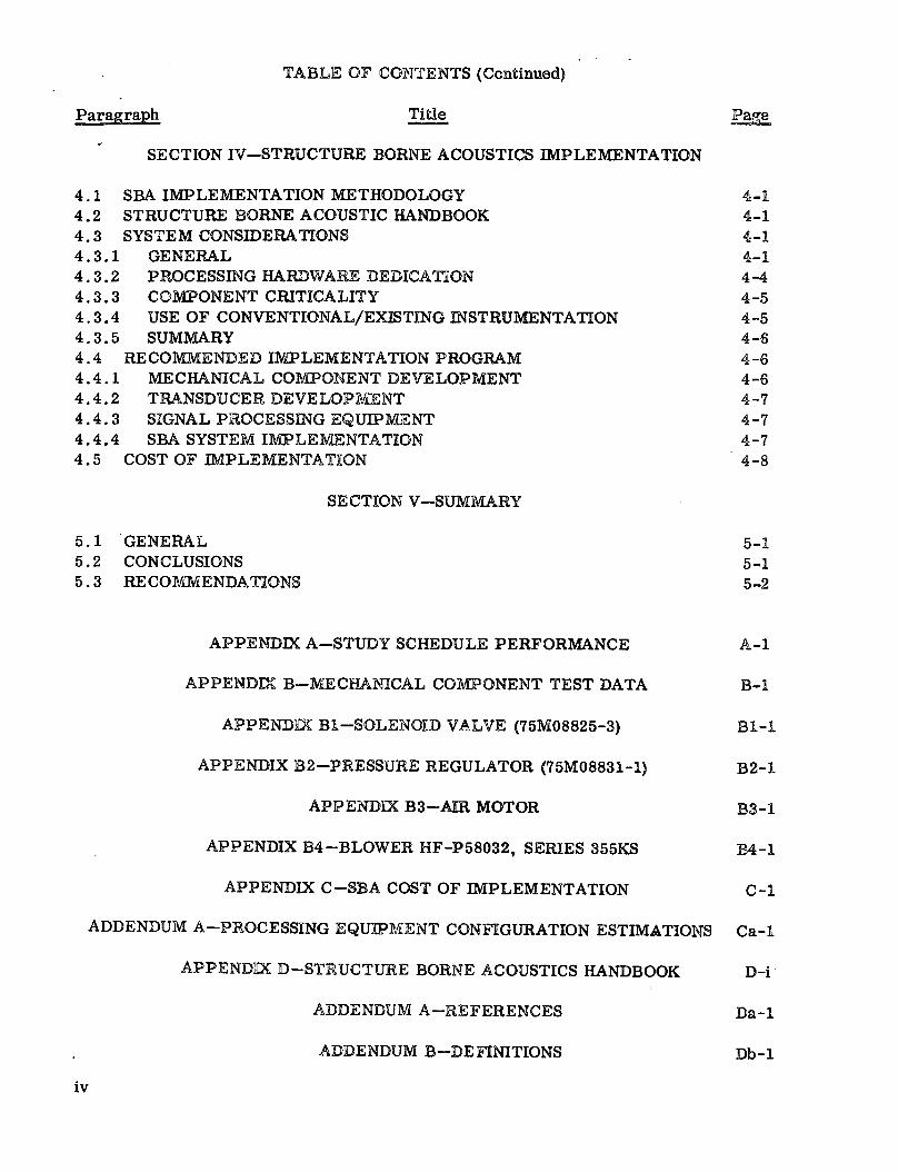
TABLE OF CONTENTS (Continued)

Paragraph Title

SECTION IV-STRUCTURE BORNE ACOUSTICS IMPLEMENTATION

4.1 SBA IMPLEMENTATION METHODOLOGY4.2 STRUCTURE BORNE ACOUSTIC HANDBOOK4.3 SYSTEM CONSIDERATIONS4.3.1 GENERAL4.3.2 PROCESSING HARDWARE DEDICATION4.3.3 COMPONENT CRITICALITY4.3.4 USE OF CONVENTIONAL/EXISTING INSTRUMENTATION4.3.5 SUMMARY4.4 RECOMMENDED IMPLEMENTATION PROGRAM4.4.1 MECHANICAL COMPONENT DEVELOPMENT4.4.2 TRANSDUCER DEVELOPMEENT4.4.3 SIGNAL PROCESSING EQUIPMLENT4.4.4 SBA SYSTEM I1MPLEMENTATION4.5 COST OF IMPLEMENTATION

SECTION V-SUMMdlARY

5.1 GENERAL5.2 CONCLUSIONS5.3 RECOMlMENDATIONS

APPENDIX A-STUDY SCHEDULE PERFORMANCE

APPENDIX B-MECHANICAL COiMPONENT TEST DATA

APPENDIX B1-SOLENOID VALVE (75M08825-3)

APPENDIX B2-PRESSURE REGULATOR (75M08831-1)

APPENDIX B3-AIR MOTOR

APPENDIX B4--BLOWER HF-P58032, SERIES 355KS

APPENDIX C-SBA COST OF IMPLEMENTATION

ADDENDUM A-PROCESSING EQUIPMENT CONFIGURATION ESTIMATIONS

APPENDIX D--STRUCTURE BORNE ACOUSTICS HANDBOOK

ADDENDUM A--REFERENCES

ADDENDUM B--DE FINITIONS

iv

4-14-14-14-14-44-54-54-64-64-64-74-74-74-8

5-15-15-2

A-1

B-1

Bi-1

B2-1

B3-1

B4-1

C-1

Ca-l

D-i

Da-1

Db-1

TABLE OF CONTENTS (Continued)

Paragraph Title ,Page

ADDENDUM C-TEST PLAN (Sample) MECHANICAL SYSTEMS READINESS ASSESS-MENT AND PERFORMANCE MONITORING STUDY Dc-1

ADDENDUM D-PIEZOELECTRIC ACCELEROMETERS Dd-1

ADDENDUM E-STRUCTURE BORNE ACOUSTICS HARDWAREMANUFACTURERS De-1

ADDENDUM G-FREQUENCY ANALYZERS Dg-1

ADDENDUM H-STRUCTURE BORNE ACOUSTICS PROCESSOR Dh-1

ADDENDUM I-SBA SYSTEM HARDWARE CHECKLIST Di-1

V/VI

SECTION I

INTRODUCTION

1.1 SCOPE

This report presents a summation of study tasks performed by the General ElectricCompany during the period October 21, 1971 through May 19, 1972 for the John F.Kennedy Space Center Study, "Mechanical Systems Readiness Assessment and Per-formance Monitoring".

1.2 BACKGROUND INFORMATION

To support future space program plans for real-time status monitoring, fault isola-tion/prediction, and an automatic checkout capability superior to that employed forprevious space programs must be developed and implemented. This capability cannotbe achieved unless the system end-item components can communicate their status.Mechanical devices which are essential to both airborne and ground equipment opera-tion do not have the capability to communicate required status parameters.

NASA has sponsored a number of advanced technology studies in this general problemarea. In 1970, for example, the General Electric Company investigated the overallproblem of future space program mechanical readiness assessment and found thatapproximately 20, 000 mechanical devices will be used on each space program compa-rable in size to the Saturn Program. It was concluded that full implementation ofexisting operational state-of-the-art instrumentation could provide only 70 percent ofthe needed readiness assessment capability. A survey of research laboratory check-out techniques identified Structure Borne Acoustics (SBA) as a non-destructive test'technique having significant potential for improving readiness assessment and per-formance monitoring of mechanical systems.

1.3 STUDY OBJECTIVE

The objective of this study was to pursue the development of structure borne acoustictechnology and to answer the following question: Is it practically feasible to imple-ment structure borne acoustics on future space programs ? Secondary tasks were toprovide a structure borne acoustic handbook to aid system designers in the imple-mentation process and to detail recommendations including cost and schedule estimates,for an orderly implementation of this technique into Kennedy Space Center mechanicalsystems.

1-1

1.4 - STUDY PLAN

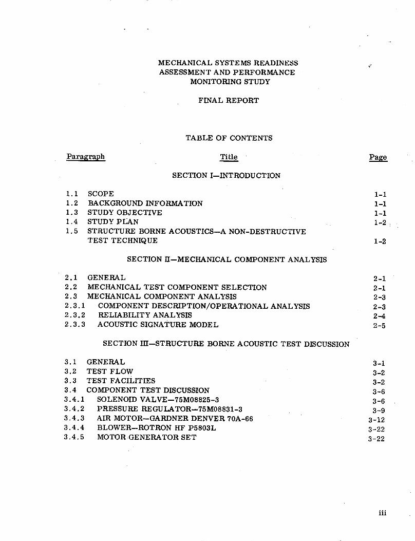
A plan was prepared to provide for a systematic completion of study objeotives. Thework was divided into the following three task areas:

a. Task I -Selection and Analytical Description of Mechanical Componentsand Design of Acoustic Tests

b. Task II -Structure Borne Acoustics Testingc. Task l[I-Test Data Analysis and General Solution Methodology Handbook

The sequence of task accomplishments and a breakdown of task elements are shown inFigure 1-1, Mechanical Readiness Assessment (MRA) Study Flow Chart.

A mid-term study progress report, DB72-A015, was published February 4, 1972, andshould be referenced for detailed data concerning TASKS I and II study results. Ap-pendix A documents contract performance schedules for all study tasks.

The text of this final report is presented in summary form to enhance readability.Whenever possible, backup data is relegated to the appendices which should be refer-enced for detailed information supporting statements and conclusions embodied in thereport.

1.5 STRUCTURE BORNE ACOUSTICS-A NON-DESTRUCTIVE TEST TECHNIQUE

To achieve high and predictable reliability for a mechanical system, it is not sufficientjust to build it from high quality components. Many defects may be initiated first dur-ing assembly or during subsequent tests. Such defects, which are not connected tocomponent quality, reduce the overall system reliability. High reliability is also onlya partial solution of the problem. What is really desired is high availability, i.e.,short total down-time for maintenance or repair as compared to effective operatingtime. There are two general areas, final component or system checkout and earlyfault detection, where effective diagnostic and readiness assessment techniques cansignificantly increase total availability. In both cases the central problem is to evalu-ate internal conditions through external measurements, without disturbing the normaloperation of the tested equipment. Obviously, external detection of internal defectspresents new problems compared to conventional component testing and inspection.This is particularly true for mechanical defects. Internal cracks, loose bolts, wornbearings, etc., are no longer open for visual inspection or direct measurement; there-fore, an information carrier is needed to transmit the internal information to the ex-ternal evaluator.

Sound and vibration are excellent information carriers in mechanical structures. Thefundamental mechanical events which occur in operating mechanical devices, such asrolling, sliding, impacts, etc., all produce sound, which tells the experienced listenermuch about the internal condition.

The total nondestructive evaluation or test technique for assessing the status of amechanical device includes the method of stimulating the device, the response resulting

1-2

I

i.f _Ill

-i v J- 0~~~~~~~~~~~~~~~~~~~~~~~~~~~~

if

Il

I

111 ji:I I

If

1-3

I

m

IIIIIIIIIIII

IIIII

II

I m

I

I

I

I

I

I

I

I

I

I

IL

II1 L I

0

I 'I" I

5 ti9,81

I

I

.___ I___I ---- S I"IEv E

from the stimulation, the transducer for communicating the response, and the hard-ware and software used for data processing and evaluation. The definition of "StructureBorne Acoustics" as used in this report includes all of these elements of a nondestruc-tive test technique. It includes detecting and converting mechanical device noise intoan electrical signal which is then processed, interpreted, and presented in such a formto provide go, no-go, or caution status of the mechanical device. Figure 1-2 pictoriallyillustrates this interrelationship.

AcousticA ccelerometer

Acoustic Signal -- -

0 Correlates With Mechanical Device OperationalEvents

a Can Be Automatically Processed For Status,Displayed For Diagnostic Purposes And RecordedFor Historical Review

Figure 1-2. Structure Borne Acoustics Interrelationship

1-4

SECTlION fI1

MECHANICAL COMPONENT ANALYSIS

2.1 GENUERAL.

Maximum component testing and data analysis efficiency requires considerable insightinto the functional operation of the mechanical component, the testing routine, and theprocessing of acoustic data. During this study, five representative mechanical com-ponents were subjected to structure borne acoustic (SBA) testing. This section dealswith the component analysis process which was developed and is essential for opti-mizing the test data acquisition and processing.

2, .2 MECHANICAL TEST COMPONENT SELECTION

Test components were selected primarily on the basis of the following considerations:

a. Component Acoustical Characteristics:(1) Single transient or transient action, e. g. solenoid valve.(2) Flow noise generator, e.g., pressure regulator.(3) Cyclic action, e.g., air motor.

b. Component Availability and Configuration.c. Adequacy of Other Readiness Assessment Techniques.

The five components selected for structure borne acoustics testing include:

a. Transient Action-A three-way, two-position, nornally open, magneticallyoperated solenoid valve, 75M08825-3, manufactured by Marotta ValveCompany.

b. Flow Noise Generator-A three-way, spring-referenced, preset pressureregulator, 75M08831-1, manufactured by Marotta Valve Company.

c. Cyclic Action-An axial piston, reversible air motor, 70A--66, manufacturedby Gardner-Denver Company.

d. Cyclic Action-A three-phase, 200-volt, 400-Hz, fractional horsepowerblower, manufactured by Rotron, hIc.

e. Cyclic Action--A 220/440-volt, 60-Hz, 1725 rpm induction motor drivinga 1. 5 kw generator, both manufactured by General Electric.

2-1

These five components a re shown below in Figure 2 - 1 .

,;; v,

>*•§.,

CUftEWW J - „^S- .»ATO» w. ••

P r e s s u r e Regulator

Air Motor

Solenoid Valve

Motor Generator

Figure 2 - 1 . Components for SBA Testing

Blower

2-2

2.3 MECHANICAL COMPONENT ANALYSIS

Each selected component was analyzed in order to:

a. Understand the operating mechanics of the device.b. Identify the internal noise producing reactions for normal and malfunction-

ing components.c. Identify those component operational characteristics which can be correlated

with component Go, Caution, and No-Go operation where, by definition:(1) Go-Fully operational.(2) Caution-Operationally adequate, degradation detected or suspected.(3) No-Go-Cannot meet operational requirements.

d. Select data processing technique(s) having the best probability of displayingthe component operational characteristics.

The analysis process developed for this study employs the following steps:

a. Acquire and analyze documentation for selected component.b. Identify normal operation noise sources-flow, impacts, resonances.c. Construct a failure mode tree-identifies failure modes, effects.d. Predict normal signature-RMS amplitude versus time.e. Assess impact of failure modes on normal acoustic signature.f. Predict failure mode signatures.

2.3.1 COMPONENT DESCRIPTION/OPERATIONAL ANALYSIS

A thorough understanding of the component operating characteristics is necessary inorder to interpret the acoustic signature obtained. Source data found useful for com-ponent evaluation and analysis are available as:

a. Design Documentation-Drawings, Specifications, and Vendor Literature.b. Operations and Maintenance Manuals, Procedures.c. Reliability Data- Failure Reports, Failure Mode and Effects Analyses.

Based on the above literature, the five selected components were analyzed to establishthe physical or mechanical interactions taking place within the component during normaloperation. It is these interactions which produce the component' s composite acousticsignature.

2-3

2.3.2 RELIABILITY ANALYSIS

Having thus become familiar with the component' s principles of normal operations and

having identified the internal noise producing events, it is then appropriate to identify

the potential failure modes for the component. This process was accomplished through

review of failure reporting documentation and engineering analysis and was documented

in the form of a failure mode tree. Figure 2-2 is a sample failure mode tree for the

70A-66 air motor which illustrates the approach. The uppermost block(s) of the tree

describe the operational effect, i. e., No-Go or Caution, expected due to the failure

modes identified in the second row, The failure mechanism identifies the failed piece-

part and the specific problem. The bottom row provides explanations for the identifiedfailure mechanisms.

Figure 2-2. Sample Failure Mode Tree

2-4

OPERATIONALEFFECTS

FAILUREMODE

FAILUREMECHANISM

FAILURECAUSE

1··__ I_ ____��---^--·I�-·I·-i-�--ll -�-�al--·I�YL-II-O�-��

2.3.3 ACOUSTIC SIGNATURE MODEL

Subjective acoustic signatures were predicted on the basis of physical and mechanicalevents taking place within the representative components. This was accomplishedthrough examination of the relative timing of each event and estimating the relativeacoustic amplitude. The prediction is displayed by relative RMS amplitude versustime. Figure 2-3 is an illustrative sample and is the predicted signature for the70A-66 air motor.

Mathematical analysis of cyclic component operation is necessary in order to provide:

a. A time or event base for relating noise producing reactions within thecomponent.

b. Preliminary determination of filter frequencies which will allow displayof'specific aspects of component operation, e.g., a gear mesh frequency.

Computer programs exist which predict frequencies and relative amplitudes for goodand defective ball bearings.

Figure 2-3. Air Motor Predicted Signature Envelope

2-5

Notes:

1. Piston sliding noise, background, gears and bearings.2. Piston direction reversal and intake air surge.3. Piston direction reversal.4. Exhaust air surge.

4

i-3

_2

X

=

0.

S)

Si

1

0° 36° 72* 108 ° 144' 180 ° 216* 252 ° 288 ° 324 ° 360°

Angular Rotation (Degrees)

_ _ �I�____

I

-0

Note that the coincidence of several internal events produces the greatest signal ampli-tude. The angular rotation in degrees refers to the internal pinion gear, not the out-put shaft. (For information on the air motor see Appendix B3.) The correlationbetween the predicted air motor signature and that of Figure 2-4 obtained duringacoustic testing is unmistakable.

& A -.A,. c I,.

I' '- :f22"r 7 1-4- ~ ~ ~ -pypv~~~~- -HBi $Y9-H 4,

- --- II -ji7 :41Lh vL L

7 7 - - - 2

I ·~- _' 1i·zIK- I 12 -IH

i~~~ Thi ri~~~1 'I

HH MA ;ISVA2I

Figure 2-4, Normal Piston Signature (Rectified) (5 Pistons/Cycle)

To deduce the acoustic signature for a component containing a given failure mode, itis necessary to evaluate the effect of that failure mode on all component noise sources.This can best be accomplished through a failure mode/acoustic element matrix, asample of which is shown in Table 2-1.

Table 2-1

Air Motor Failure Mode/Acoustic Element Matrix

2-6

.0^r__e ,t-- VA I

Note that the failure mode and mechanisms for this sample are those illustrated inFigure 2-2. Sluggish operation in this case includes erratic angular velocity as wellas reduced rpm depending upon the failure mechanisms. Figure 2-5 displays both ofthese effects.

ia)

Erratic[ (Varying RPM)

Sluggish --(Reduced RPM) I

L IL~~ A

Normal Time Base

Figure 2-5. Failure Mode Effect Upon Air Motor Signature

Detection of reduced or varying rpm is accomplished through peak-to-peak time meas-urments compared with those of a standard. A consistent discrepancy would indicatereduced rpm. A varying time difference indicates an erratic radial velocity within onerevolution.

The component analysis routine described has, as a tangible end product, the predictedacoustic signature envelope for good and malfunctioning components and provides thedesigner/analyst with a knowledge of component operation which facilitates correlationof the acoustic test data with the internal interactions which produced the acousticsignal. The comparison of predicted acoustic signature versus that actually obtainedand the resolution of discrepancies provides a firm basis for a more accurate analysisof succeeding components.

2-7 7t'

_ _ I_ �_

_ 1___11__·I

SECTION III

STRUCTURE BORNE ACOUSTIC TEST DISCUSSION

3. 1 GENERAL

In this section, a brief description of the test program and test facilities is presented.The test results for each of the five components are summarized, and the interpre-tation of acoustic data is discussed.

A statistical approach was employed both for planning tests and evaluating significanceof test data. Having established that:

a. The data distributions for defective and non-defective components arenormal.

b. The variance for defective components does not differ significantly fromthat of non-defectives.

c. The mean for defective components differs significantly from that of non-defectives.

Limits for defective and non-defective components were established at the 90-percentconfidence level. This takes the form shown in Figure 3-1.

istributio stribution1 2

Non-Defective Defective X

5X 95% 5X

Figure 3-1. Non-Defective versus Defective Distributions

In the case depicted, those values of x between the 5-percent and 95-percent pointsof distribution 1: are considered normal operation. Values of x to the right of the 5-percent point of distribution 2 are considered a failure. The shaded areas indicatethat an anomaly exists, but the performance of the mechanical device has not deteri-orated to the point where a failure has occurred.

3-1

3.2 TEST FLOW

A general test methodology was developed and has applicability to each SBA testsequence. For each component tested, there is a fixed pattern of activities requiringcompletion. These activities and their sequences are shown in the Test Flow diagram,Figure 3-2.

Acouatic 'tlU-SUcal

Reduction and of ReducedMdn7utlatlion L DU

Recycle Teets Ui Selection ofDifferent Mcsaurement Tecbniqueor StcbilzaUoa of a Toot Variable '

Will Permit Establishment of1A.oeoasnunt DOicrlmtnant

Figure 3-2. Structure Borne Acoustic Test Flow Diagram

3.3 TEST FACILITIES

Test facilities at General Electric's Research and Development Laboratory, Schenectady,New York, were employed for this test program. A special facility test set-up wasdesigned and built by General Electric as a means of study in the acoustic signaturesof the mechanical components under simulated operating conditions. This test set-up,see Figure 3-3, provided for ready installation and quick replacement of the testcomponents.

General Electric Spectrum Analysis Facility Figure 3-4 and Summation AnalysisFacility Figure 3-5 were used for data reduction and analysis.

3-2

3.4 COMPONENT TEST DISCUSSION

:3.4. 1 SOLENOID VALVE-75M08825-3

:.4.1.1 'I'Test Result Summary

Five different solenoid valves were tested in normal and inserted defect configuration.Results showed that:

a. Repetitive operations of each valve were very consistent in the timedomain.

b. The acoustic signature can be correlated with events taking place withinthe valves.

c. Inserted defects produced a measurable variation in the acousticsignature.

d. Care must be exercised in the insertion of defects to preclude biasingthe data.

3.4.1.2 Acoustic Data Interpretation

Figure 3-6 contains composite acoustic waveforms for the actuation cycle of solenoidvalve 75M08825-3. Shown on the Figure are:

a. Signal A is an acoustic signature with valve actuation at 28 volts, nopressurization, no GN2 flow, and normal operation.

b. Signal B is an acoustic signature with valve actuation at 28 volts, 1000psig, GN2 flow (, 30 milliseconds), and normal operation.

c. Signal C is a signature of valve actuation at 28 volts, no pressurization,no GN2 flow, and simulated sluggish operation. Spring was tightened toincrease force opposing actuation direction by 6 pounds.

d. Signal D is signature of valve actuation at 18 volts input, no pressuriza-tion or GN2 flow.

It should be noted that these signatures are each representative of over 30 individualoperations. Relative amplitudes are specified on the waveform graph, and the timebase is from solenoid voltage application.

From comparison of these waveforms, the influence of failure modes on the acousticsignature timing is apparent.

A comparison of normal valve deactuation acoustic signature (Waveform A) and a fail-ure mode signature (Waveform B) is presented in Figure 3-7. The failure mode signa-ture was simulated by increasing force opposing actuation direction. These signalsclearly show that limit switch indicating valve action triggers 3 to 5 milliseconds beforethe stem actually slams against the valve housing seat to complete deactuation.

3-6

11

0C;

.o iUn U,

a)

0

4.4

C.)0

a)

0c.b1U0

4_

3-7p

o

cq~ ~ ~ ~ ~~~~~~~~r

a) C

t~~~~~~~~~~~tl

C.

0r~

©

!~~~~~~~~~~~~~ °

0

a)

I~~~~~~~~~~~~~~~~~~~~~~~~~~~~~~~~~~~~~~~~~~~~~~~~~~~I

ci

.~~~~~ .- ~ ~ ~ ~

3-8

The real-time frequency analysis, Figure 3-8, display of valve actuation and deactua-tion shows the frequencies excited by the impact transient. The plots are three-dimensional in the sense that they provide time (x axis), frequency (y axis), and ampli-tude information. The display range is 48,000 Hertz. The time base is 27.6 inchesper second or 36 milliseconds per inch. Amplitude is displayed on a relative basis asindicated by the intensity modulation of the frequency scans. The trace at the bottomof each spectrogram is solenoid voltage and correlates the frequency data with valveoperational events. The strongest frequency component is found at 11K Hertz and re-sults from valve body resonance due to stem and seat contact.

The probability density functions of comparative normal and failure mode valve actua-tion and deactuation times are illustrated on Figure 3-9 in histogram form. Failuremode operations were simulated by setting valve spring tension to increase force op-posing actuation direction by 13 pounds. The operating time distributions C and D forfailure mode versus normal actuation show no overlap for approximately 60 total opera-tions. Similar results were obtained for deactuation times. These histograms indi-cate: (1) the stability of valve operating times, (2) variance relates directly to perform-ance, and (3) the failure mode signatures are significantly different from those ofnormal operations. Thus, acoustic go, no-go, and caution limits can be established.

3.4.2 PRESSURE REGULATOR-75M08831-3

3.4.2.1 Test Result Summary

Data was acquired on the pressure regulator from one accelerometer on the housingand one pressure transducer in the regulated line. While correlation was obtainedbetween the RMS value of the flow noise amplitude and the pressure to the regulator,the absence of noise producing interactions within the regulator reduces SBA to flownoise detection. At any given point in time, normal regulator flow can vary betweenzero and full flow depending upon the downstream pressure (which is a function ofdemand). Incipient failure or performance degradation of a regulator is frequentlycharacterized by sluggish operation which can be determined by analysis of absolutedownstream pressure and pressure rate of change. Therefore, the knowledge ofdownstream pressure is required for readiness assessment, thereby making SBAredundant.

SBA instrumentation used for testing purposes was sensitive to flows (or internalleakage) on the order of 4cc/minute. Discussions with KSC operations personnelindicate that leak detection to 1cc/minute or less would be beneficial. KSC is present-ly sponsoring an ongoing leak detection study, thus this investigation was not pursuedfurther.

In consideration of the above, pressure regulator testing was terminated with theconsensus that SBA currently has limited application to devices producing only flownoise.

3-9

n:i

o-

0 >

,.:.

...

,.,, ... .

.',, t

O co cO C 0 D CD co O

suo04idO O jo aqmnKN

3-11

3. 4.2 .2 Acoustic Data Interpretation

On Figure 3-10 the top trace is the raw accelerometer signal; the bottom, that pro-vided by a pressure transducer in the output or regulated line.

On Figure 3-11 the top trace is a negative RMS of the raw accelerometer, and again,the bottom trace is the pressure transducer output (regulator output pressure).

Note on both figures that the largest acoustic signal is obtained when the regulatorrelieves to a lower pressure. The next largest acoustic signal is due to normal regu-lator flow.

3.4.3 AIR MOTOR-GARDNER DENVER 70A-66

3.4.3.1 Test Result Summary

The air motor tests were conducted under simulated operational conditions. The motorwas driven with a 80 psi air supply and loaded with a belt-driven, dc generator. Thegenerator output was monitored to indicate load and to assure repeatability of testparameters. At the beginning of the test procedure, all motors to be used were runin the as-received condition, and test data was recorded on magnetic tape. Severaldefects were inserted in the motors, and data was recorded in the defective mode.All data analysis was performed on the magnetic recordings.

The structure borne acoustic data was obtained from three accelerometers mounted onthe housing (see Appendix B3) along mutually perpendicular axes. A tachometer signalwas obtained from the pulley wheel on the output shaft, and gave six pulses per revolu-tion. The only preprocessing performed before recording was to amplify the accelerom-eter signals to that level required by the tape recorders.

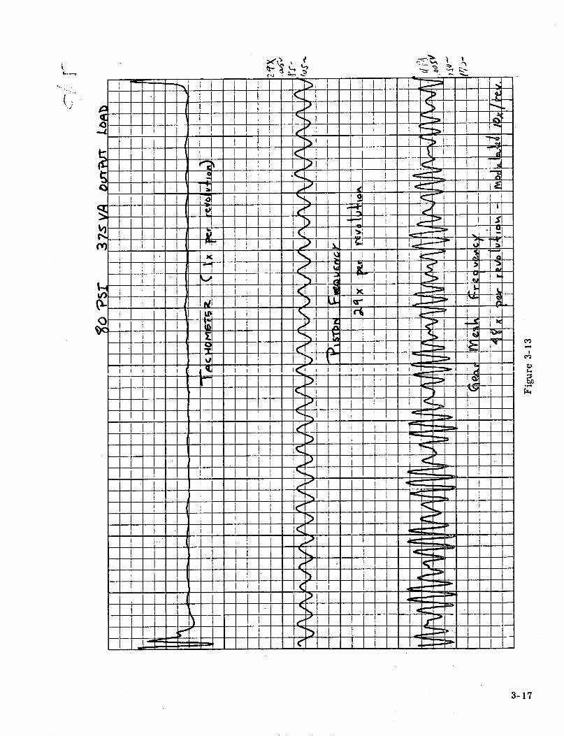
The normal signature of the air motor consists of a broad-band noise signal combinedwith a number of discrete tones. The broad band noise results from the pulsations ofair flow through the valves and cylinders of the motor. The discrete tones were identi-fied through analysis of the motor to be gear-mesh frequencies, the piston frequency,bearing tones, and shaft imbalance component frequencies are tabulated below:

a. Output Shaft Speed 4 rpsb. Piston-29 x 5.5 116 Hzc. Ring Gear-48 x 5.5 192 Hzd. Bearing Tones 17 Hz Harmonicse. Bearing Tones 14.9 Hz

3-12

,_ _ . 4 _ __,,I I,..

, I -i i

. l---': !i-'1 1 . .r-IL Iit~~~~~~~~~~J

[" I' I ' ! I'

'LI ~ ~ ~ '-' I~~~~~~~~~~~~~~~~~~~~~~~~~~~~~~~~~~~~~~~~~~,~ ..- . i .S I ! I ! it I !, . i r I

17717~ ~ ~. 1 4111 1!i I I ! It I I I ii i~~~~~~

| t I - m ,-- 1I ~,,, ~ 0 8 1

1 2 + 1i It I~gt.- r fi f

.IIT _.I I _ I I .. Ill ..T

t11Tv

1·V ( f19

A

o!

I

aZQ,

.r

..r'

3-13

f ~~'-~' J i I' '~I

- -

~'-~

'~

I i I i , I - _, _i !, ~ ~ i ! ~ 1 1 l a ! , ', j~,'1 ~ i t ~ z ,J i

I

_. Ji Ii C [ I i , J I

~, j ~ i , ¸ , i ~~

I .I '"' f ' '~ I r~~-r

J

i ~ i i -J I ,,r 1 ~ I ,

ii~, i tl i I i f i l J I I ~ 1 1 - !

,it j~! ' l f-' i ' ' l ~ j i

· --f t ~ I 1 1 ] '--j--, I ,r F I f ~ -i [ , .~ 1 t~, i j-'~- i j --

-!!!~ ~! 'tfli'li' [ J-'~f'~ I

I : I -I

_1 1 1 [ I .= ~-r ~ '

! ! ~ t l [ ! 1 ! i ~. 1 I

I

R-JA am:'-)

I

Cwas

.,i

3-14

3.4.3.2 Acoustic Data Interpretation

Figure 3-12 illustrates two of the dominant tones generated in this case at a reducedair pressure of 20 psi and no load. The pistons excite the housing at 29 times theshaft speed, i.e., there are 29 piston cycles for every revolution of the output shaft.The ring gear, with the pinion and two associated planets, generates a meshing toneat 48 times per revolution. (There are 48 teeth on the ring gear.) In this Figure,these tones are related to the 6x per revolution tach signal, and derived through sum-mation analysis.

Figure 3-13 shows the effect of a full load at 80 psi operating pressure. Most notice-able is the amplitude modulation on the gear tones at 10 times per revolution. This isthe result of imbalance in the load-pulley system where a 10:1 pulley size reductionhas been used to drive the loading generator at the required speed. The piston vibra-tion data is tightly filtered about the predicted frequency. If instead the data is proc-essed to enhance the pulsating broad-band noise generated by the air flow, Figure 3-14results.

In this case, the data was rectified before processing and the filtering is adjusted topass all the high frequencies (actual settings are not significant). Since the motor is ofa five-cylinder design, five piston noise envelopes constitute one revolution of thepiston swash plate. The chart shows five similarly shaped and equally spaced wave-forms generated during the piston power cycles. In fact, at any given time, two pistonsare opened to the 80 psi line pressure so that each envelope is a composite of two ad-jacent pistons.

Figure 3-15 shows the effect of introducing a defective head gasket to air motorSN 751685. A slot was cut in the gasket between two adjacent cylinders. The gap wasapproximately 1/4 inch. If the joined cylinders are labeled 1 and 2, and it is remem-bered that adjacent cylinders are pressurized simultaneously, then the chart can beeasily understood. Two full revolutions or ten piston excursions are displayed. Atthe second major division cylinders 1 and 2 are pressurized simultaneously. They arejoined by the valve so the defect has no effect. At the third division, 2 and 3 are pres-surized but 2 leaks to exhaust through 1. At the fourth division, 3 and 4 are pressurized;and at the fifth division, 4 and 5 are pressurized but 1 and 2 are not involved. Thenagain at the sixth division, 5 and 1 are pressurized but 1 leaks to exhaust through 2.This pattern repeats every five divisions. The leaky head gasket can be clearlyidentified.

Possible external leakage due to misalignment of the head assembly or impropertorqueing of the bolts is shown in Figure 3-16. This air motor (SN 573139) yieldedthese results as received for testing. The marked differences in amplitude indicateleakage on one side of the head.

Axial scoring of one cylinder wall introduced a waveform peak between the normalpeaks (SN 573098) in Figure 3-17. Speed instability of the motor with respect to theanalysis parameters causes the repetition of this new peak to be partially obscured,but its presence is still visible.

3-15

-4

a)

F:4

3-16

% _ _ _ _ > |i C..-> |qL t i I' ?.) I _±'

I I i I I I' I11

_ _i _ _ _ LT E__._i'EIIII11IIIII

i~~! ~iSta

--, .a'i

...

(:'

IC,-4

C)

. 4

3-17

, I

I I- -- I-

I I i '

' I.-LL__ __I ! !

iiI1 I

. I , .

: I i I- T ;-- ;_. ; I . i'

i i , II r I-

--- --I I I

--I "I!

I . t ; I I i I . ; I' ., , ' i j 1 I

C XI-t,-

1 - Jt VIWffihIL| 0

' -- [- -~- .. -- ' .- I

' , :_ I I ~. I I ' i .J_

I IF ~ ~ ~ I

-C ~ -

____~ ~ -. .. ~___ J

_ilJ _L_ S-rt.vXI,~~~~~,

, i~~-"- ~ I-- i _ , ,~ ... rt.--1 -----.---.. 7- 1 -

:';:'- L;'=- -' - ---- '' i

"~~~~~~ I _~~.,s . ~ ~

_ _._ ____ ; i -+.'., ,, :.

----- T-:-,__ ·__:_ . ~ ,._:____:_.._ .In III_' I f · ' I I

' - . I,--r- I ...... '___L-i_ __ _ _ _ v~ ~ ,. ~ IL-

... j :

-: : i ~~~~~~~~~~~~~~~~~~~~~~~~~~~~~~~~~I~ I II _'_ __ if I

, ~ ~ fi I,, tt..

_ _ , I !'".I

; .i ,I't __ , . ._ i' _ . , .I , : 'i

? -]--! I''-:'--" -II Ii .... I--:'--.-.I---

, r ' F ~~~ I~ e : : i ' I t i_ ,

T -- '__--~ . -K---I-'-

L__ _ - I ~ ' ! 1 -'¥

Iw!

C~

,)op-

3-18

I

II LI D_IiI I II

-

II

I

I

i

-I--I - I i !1.4 :,

'--I

_r! .i

LO-4

4)

;..

3-19

co2

A

0)k9D

Io

3-20

Is-14

A,

0)

3-21

4C

7

v,

A comparison of Figure 3-18 with the normal signature of Figure 3-13 clearly identi-fies the presence of an inserted gear tooth defect. One tooth of the ring gear wasdamaged by partially grinding away the face. On the Figure, the 10x per revolutionmodulation introduced by the generator is still visible but now the dominating factor isthe higher amplitude signal at the point of mesh of the defective gear. The last in-serted defect was a small simulated spall on the outer race of the output shaft bearing.This defect was identified using the crest factor bearing monitor. Normal tests runbefore defect insertion gave meter readings of 20 to 30 when the data was filtered be-tween 100 to 500 Hertz. When the defect had been inserted, the readings increasedto 40. The maximum indication on the meter is 50, but a further enlarged defectcaused the meter to go off scale. It was not possible to get good results with the sum-mation analysis technique, probably because of speed instabilities or bearing ballslippage. The predicted tones and defect periodicities were previously denoted.

3.4.4 BLOWER-ROTRON HF P5803L

Testing of the blower consisted of mounting an accelerometer radially on the outerhousing and counting the blades (5 per revolution) for a speed indicator. Tape recordeddata was analyzed with a tracking frequency analyzer and summation analysis. Fig-ure 3-19 shows three revolutions of averaged data. The top fan blade trace indicatesthe speed was 3600 rpm. The tracking analyzer output in the second trace indicatesthat the speed is varying slightly at twice per revolution. Correspondingly, the vibra-tion amplitude is modulated at twice per revolution as shown in the third trace. Thefundamental frequency of that vibration is 900 Hz, or twice the power frequency. Themodulation also visible in trace four results from interaction between the rotor im-balance and the slip speed.

Figure 3-20 illustrates the presence of a bearing defect in one fan. The top data traceshows a repeating pattern, but more significant is the variance curve showing therepetitive impacts at the predicted period of 8 milliseconds. A second fan analyzedwith the same parameters shows no such defect present (Figure 3-21). The defect infan 960142 was not inserted, but occurred in the as-received condition. Teardownconfirmed the defect was corrosion of the bearing outer race.

3.4.5 MOTOR GENERATOR SET

A 1.5-kilowatt motor generator set was tested for two controlled defects; a spalledball bearing and a defective commutator with one bar lowered by 1 mil. An internalaccelerometer mounted on the brush holder, an external accelerometer mounted on thehousing, and a current probe were used to acquire data from the set. As shown in thescope traces of Figures 3-22 and 3-23, both the external and internal accelerometersdetected the low commutator bar. The current probe also shows the arcing occurringfor each brush crossing the low bar.

A faulty bearing in the set would have a predicted repetition period for an outer racedefect of about 2 milliseconds. With the summation analyzer self-triggered on the peaksin the data, the three traces of Figure 3-24 were obtained. Each trace corresponds toa different accelerometer placement.

3-22

4 ,... z's '

~~~iil. _ I lll1|_ 1-! I Iii~1!_

l i ~ i i , i '-- !, ; , T: ~ ~ ~ ~ ~ ~ :ij ,i~~~~~!

< W: ~~-t-i-i-- 1 -t: -I ) ,

, I.T't , i--Li-- - -- _ ' - ; _

\~~~~~~~~~~~~!. ! ~I !i

_ !-!,-7-1<1- --,-L-N -! + - I, i I, w | | | ! I i , :

l < i l !i i -

, ~ ~ iI!!

w - r # ! i ! 1-,- ', -,: : -, - i I- I -ill_

I ! I i I i : IT ~ _ I i ~ i- ! [ , ! l ' I I ! I I

. ; i ! i ~ - - i

_ rW i1 E ji:! iiji i I jV l

/

00

-4CA

.)

3-23

.--4 zD· 4 )4

, ]a 1 44 D I t i-~

i I I

-p

tiU .1.

FI I'

-Ll!I..

I t --- I .Li -. ..... , i - t - -_ :i I

I _ _ _ _ - !i 1 -.. j -i

E ~~~~~i I,- i i ,,.. !li .

I :XI I t i- _

+. I II . ' l ! Ir I] -.-ItYKV ~IIJ i11/ Ir! ! __ . L.

II1 II, . ! ~,,,r!, i l I l ii '"~ !~ ?i!~,- ' , 1

tr4 WeX<H__T7 ___ _ T _ _I _I

-, I I i.

- f7- < _-I _ _ .-~twr _~~~~f ~ "

p,~~~~~~~~~~~~~~~ I_ II ." , i -:Fl. i[ I -

_ t I~~~~~

= ~ - t IMr _1-

~~~~~~~~~~~4~~~~~~~~~' - --- f-

.... f, I ?I ~ '-I' I _-~ .,i--""_

-4

hwt1.

9b-4

44

3-24

1 , i L.

iL.

al--- wr

l--i' i-I I ,

o

CDCO

so0);-f

?D

3-25

U

-4v*4 r1

WzH

b3w

w1- I

w t

I

3-26

~ 6

-4

C4

w

Current Probe Output (8 mV/cm.)

Internal Accelero-meter (16 g/cm.)

External Accelero-meter (16 g/cm.)

Figure 3-22

^

1/rev marker

Current Probe Output (20 mV/cm.)

Internal Accelero-meter Output (16 g/cm.)

Figure 3-23

3-27

I C! I,.

' ; _f5 _.*f .-- ,- I

I __._I .I ----t -- --

! -

- I--

I~~1 -T -1I I .

I .,..... ... ....

I~~~~~~~~~~~~t

...-........_ ...- . -.

; ,; r= = t .

I_ _ ...__.---- -'' --; !--:.... :.....! ..... r.....

'k -.- j.L.:. ......--- F- 77 ..~_,LL n . --: -....... t-......5 ............. _ !.I _ _-; --- - ---- " ----

-ur! - 4 C= 2 - -. ~ -

.... i :- .. I-- -.-....--1 -'.',,_ ,

I bL

._-t

i Krj T.... . .-':- ....-

! = + -- - '---z-- -

-i ------ -

rI

-' .- 1 ..-- --

L--- Lt- --_ _7- -7-' ' 7C

I~~~_ __ _ _ _ _ _ 1

! - !i_--_

..... --- --- "--- ; " -'-..... .- Z-Z - c -- "

_i .... ~ ......... : L .-- -. 7--

--= I _- _ ------ ic!- -Ir- = .- -1|-I^ !

-_ -_ I--~-- ' - ----- - !--- - - _:- --- i :cr

0)

3-28

I i _ m I

I

_r_~~ ~~~~~~ -- !I__~~~~~~~~

-~~~~~~~

r -_dmj I

[- i -i :;a"I

- -

IrI

-~~~~~~~~~~~_ . - -

v---- - ~- - - - --- -

--t- ---- C --~- _^e

_ ._I -

NMT

i

I . _~~~-I

r-

lf

_ -· -7 ' i -! I+

_ I . .'

F- -'

I j . ~~~~~~~~~~~~~~~~~~~~~~~~~~~~~~It , - --- - -~~~~~~~~~~I

- ... -- ---- ---- -i - -- - : : D J

..... ,i =..

_:=- -- ::C--

=~~~~~~~~~~~~~~~~

.... ~~ :. I-. . I .

t

- . .

I . . ....I -1 -!-- -! , ' ' ';

I

I .

r.

t--

SECTION IV

STRUCTURE BORNE ACOUSTICS IMPLEMENTATION

4.1 SBA IMPLEMENTATION METHODOLOGY

'As an operational non-destructive checkout technique, structure borne acoustics is inthe embryonic stage. While some laboratory work has been accomplished, verylimited operational implementation, and that only in the most rudimentary form, hasbeen achieved. The work performed in this study has shown that an orderly im-plementation of the SBA technique involves a set pattern and sequence of events, eachingredient of the pattern having its own decision-making subroutines. This generalpattern may be followed for each implementation and is shown diagrammatically inFigure 4-1. The general methodology presented can be applied to each mechanicalcomponent or system in a cookbook type approach; thereby minimizing time and costfor multiple component SBA implementation.

4.2 STRUCTURE BORNE ACOUSTIC HANDBOOK

For the purpose of bringing together, under one cover, information concerning thoseelements of the various technologies essential for understanding and implementingstructure borne acoustics, an SBA handbook has been compiled. The handbook isattached to this report as Appendix D and is organized so that it can be removed andstand by itself as a reference document. Detailed information regarding the differentaspects of SBA implementation are documented in this handbook. The contents of thehandbook is shown by the outline tabulated in Table 4-1.

4.3 SYSTEM CONSIDERATIONS

4.3.1 GENERAL

This study was chartered to examine specific mechanical components using structureborne acoustic techniques and to evaluate the applicability of SBA to the three acousticcategories of mechanical devices, transient action, flow noise, and cyclic. Imple-mentation of SBA into an operational environment must consider a systems approachto automatic readiness assessment, application to multiple devices performing inter-related functions, with automated decision (go, no-go, caution) processing.

The capability for readiness assessment of mechanical devices using SBA techniquesexists today but has seen only limited operational implementation. Examples include:

a. Five hydraulic components associated with NASA-Goddard trackingantennas are acoustically monitored. Taped data is analyzed at GSFC.This is not a real-time system.

b. Real-time bearing monitors for the DC-10 aircraft engines are availableas an option.

4-1

0ooV0

c)on

Qa

C)

.)

0

4C)

aC.)

I'44

.C)

rz4

4-2

Q

0 i Q

3 e

1 e i 2

a Bt i 1-

E szz a

r . U

Z w Q

.4

Q i~~ ! w °

=t"fl. -nf

ffi N N N N ~~4 N N

3.340-0r~~~

00~ sc* 3. 3.

U~ ~ 2 I.3-~ 0 3

znr N

U ;; ;

3 ..tY~~~~~

00E

zB 33- ,

3. *gi l*f fi

0*390

4.y z0z

z2

Q-0

zM

U

00U4

i

W

5ay-EU

U2I

W3..4

0.

z

0

'.3 0

3

wa o ; a

I-

h o 2- w

rs -0

a" 02

ox0;. e flc

W2 Ca5· SZ N^

3

4

e

Q n

o s~ 2

-'a Q LV Z Z

_ N n __ N0 N0 r~?Z r rrrr

w

w.2

-C6WyrQt;a1

2

-C'.

2

aC3 3W 0

0 aiz

~ Q -C

:E ., I

Or1 E_ it W

N N NN2 orn(.zk ..N'n

2t

104 w

W

e e

3. 4

w,0

i " B

r~~~~~ w W

_"rwowa za aE........ > -. Z

z .2~~·a W~

04 u

0 rwo 0

3.30;~~~ 4

2 ag004rr r

4~ ~ 2z o

0 IT.

3-9 zz w

-g 0

o o ¢2 4

-Z, U 2 0W0

_c z I N _- - _ Nr0 0.a: o z 0 O.0 S - 3x~4z 4 .Ro.

00 C

U U ', 4" 4 8

js :- ""..fl.

._a , N ai

t vt vt vw *v i ;j j j j ; ir. KjW j, j ;Q j,

4N0

:6

a I3.3 4

Y 0e =

2 e

U 4 4W

E " t I

2ar

a x Zz 4

e0a

4-3

Oa)o

0

-e

1.

7.,

m,

a£ 8

3'

P t;04 e

0.w0 0..4 4C

F.u0

Real-time automatic readiness assessment on a system basis using SBA techniques canyield the greatest efficiencies through consideration of:

a. The level of processing hardware dedication.b. SBA implementation for the more critical mechanical devices.c. Integration with conventional existing instrumentation.

4.3.2 PROCESSING HARDWARE DEDICATION

Consider two system approaches, one typical of present techniques having the capa-bility for limited monitor and control, the other having the additional capability forautomatic self-contained readiness assessment utilizing SBA. The hardware functionsrequired in either approach include:

a. Bidirectional communication between the mechanical device and thedata bus.

b. Command decoding, data encoding (a common bus requires uniqueaddresses for each mechanical device).

c. Electrical/mechanical command interface provides commands to themechanical device and power for execution.

d. Transducers and associated signal conditioning to sense mechanicaldevice physical parameters (e.g., pressure, position).

e. Processing to examine data to determine data validity, mechanical de-vice operational readiness, and proper execution of command inputs.

The major difference between the two approaches is the processing required for auto-matic readiness assessment. Ideally, this processing capability should be located asnear the mechanical component as the overall system concept will allow. The degreeto which this additional processing should be concentrated is dependent on the followingconsiderations:

a. System operational philosophy-need for subsystem autonomy, manual orby-pass modes of operation, control, and monitor.

b. System flexibility philosophy-need for real-time transfer of diagnosticroutines or programs, changing limits, etc.

c. System data transmission-data transfer rates, verification, number ofdata bus interfaces, multiple data buses.

d. System monitoring philosophy-status only, status plus data call up, dis-playtby exception.

e. Component complexity-magnitude of processing required to providereadiness assessment.

f. Component similarities-similarities of component processing require-ments (hardware and software).

g. Component density-population of components requiring readinessassessment.

Implementation of SBA on a system basis is initially expected to involve an area of highcomponent density, e.g., portions of the crawler-transporter or on the ML. Thiswould

4-4

lead to the expectation that SBA processing for that area would be concentrated at onelocation. To be consistent with the data transmission considerations, some pre-proces sing

Ior filtering could be accomplished at the mechanical component to reduce transmissionbandwidth requirements.

4.3.3 COMPONENT CRITICALITY

The operational integrity of a mechanical device is presently established through ex-tensive manual checkout which includes exercising the component in conjunction withobservation, by a trained "eye and ear". This contrasts significantly with the verifi-cation process for electrical/electronic hardware which can be evaluated (automati-cally, if desired) through the many electrical parameters such as power out, voltage,current, resistance, pulse shape, and timing. As a result of mechanical device criti-cality, frequent use of redundancy is required. This improves the probability of suc-cessfully completing a mission, at the expense of increased complexity, periodic main-tenance, and manual verification.

An advanced space program comparable to the Saturn V program in size and complexitywill require over thousands of mechanical components in the flight hardware and associatedground support equipment. The impracticality of instrumenting all mechanical com-ponents is hardly contestable based on cost, reliability, and consequence of failureconsiderations.

Initial reliability efforts should be directed toward the identification of relative criti-cality for each component. Considerations employed in a criticality analysis of thissort include:

a. Potential failure effect for each failure mode.b. Probability of the most severe failure effect actually occurring.c. Probability of failure in a particular mode.d. Time period in which the failure takes place.e. Failure rate of the mechanical device.f. Environment of the mechanical device.

The assignment of relative numerical weights to each of the above provides a quantita-tive basis for comparing the criticality of a number of components, thus providing arationale for selecting components for SBA implementation and the more critical fail-ure modes which must be detected.

4.3.4 USE OF CONVENTIONAL/EXISTING INSTRUMENTATION

SBA instrumentation must be integrated by the processing hardware with existing orconventional instrumentation to obtain maximum readiness assessment capability. Thisreasoning is based on the rationale that:

a. SBA cannot provide all the data necessary for readiness assessmentdecisions.

4-5

b. Where either existing instrumentation or add-on SBA can provide re-quired readiness assessment data, the use of or change to SBA would bedifficult to justify.

c. Conventional instrumentation must provide a frame of reference to thedecision logic. Using an air motor mounted acoustic accelerometer as anexample, the accelerometer should have no output unless supply air hasbeen commanded on and is present at the air motor inlet. Status of thesupply air would be detected by conventional instrumentation and be pro-vided to the readiness assessment decision logic.

4.3.5 SUMMARY

Implementation of real-time SBA techniques, integrated on a systems basis can pro-vide many maintenance and operations efficiencies including:

a. Maintenance when required versus a set time between overhaul based onthe capability of SBA to detect incipient malfunctions.

b. Early detection of failure or degradation, thereby reducing repair costs.c. Reduction of GSE and flight hardware verification time.d. Examination of hardware performance data on an exception basis as

opposed to a lengthy review of all data to determine component condition.

4.4 RECOMMENDED IMPLEMENTATION PROGRAM

To implement the structure borne acoustic test technique efficiently into future spaceprograms will require an orderly approach. The recommendations presented heretake into account past and existing shuttle related studies in terms of their influenceupon structure borne acoustics.

The hardware utilized for the implementation of SBA was considered from the stand-point of what further technique developments would enhance SBA, as well as, whatequipment group needs emphasis. The significant equipment groups are the mechani-cal components, transducers and signal processing equipment.

The recommended developmental programs represent the activity necessary for the ac-complishment of mechanical component readiness assessment by SBA while reflecting1972/1973 technology. The recommended programs permit an incremental fundingapproach which will provide information decision points, as to the most effective meansfor applying the SBA techniques to advanced space programs.

4.4.1 MECHANICAL COMPONENT DEVELOPMENT

Advantages of the SBA techniques cannot be fully exploited until more is known aboutindividual mechanical device functional parameter limits, i.e., what are go, no-go,and caution mechanical discriminants and quantitative boundaries. A testing programis recommended which will establish these discriminants for selected advanced spaceprogram mechanical components. Estimated cost of this program is $150, 000 and therecommended schedule duration is 12 months.

4-6

Identification of mechanical devices requiring readiness assessment by SBA must beestablished. This task includes development of ground rules and selection rationaleand generation of a listing of line replaceable units (LRU's) for each space programrequiring mechanical readiness assessment by SBA. Estimated cost is $50, 000 andthe recommended schedule duration is 6 months. Both of the above tasks can be inte-grated into the early design phases of a specific space program.

4.4.2 TRANSDUCER DEVELOPMENT

Transducer technology, as it exists today, is adequate for SBA implemented in near-future space programs; however, the implementation of extensive "add on" SBAaccelerometers may require the adjustment, variation, or improvement of certainselected transducer parameters such as range sensitivity or resolution. It is feltthe magnitude of these changes is within the scope of existing transducer design capa-bility; therefore, no study or development is needed to support structure borneacoustics. The area of greatest concern is in sensitivity requirements of transducersto detect low-level leak noises. A parallel study in this area is being sponsored byKSC. Hence, this aspect was not researched in detail.

4.4.3 SIGNAL PROCESSING EQUIPMENT

Like transducer technology, the signal processing equipment, as it exists today, isadequate for SBA implementation. There are numerous processing equipment designtrade-offs that can only be efficiently completed subsequent to the definition of mechani-cal components to be assessed by SBA. The most significant of these trade-off areasinclude:

a. Level of processing dedication or distribution-individual componentlogic devices or higher-order processors for multiple components.

b. Degree of processing equipment modularity.c. Memory and software considerations.d. Self-test requirements.e. Packaging techniques, physical size and power consumption.f. Function allocation-hardware, software, or firmware.g. Signal conditioning techniques-dedicated or time shared.h. Processing-amount of analog preprocessing or digital processing.

4.4.4 SBA SYSTEM IMPLEMENTATION

As noted above, there are no equipment studies or development programs that aremandatory prior to design implementation of the SBA technique. Implementation ofthe SBA technique can be achieved with today's transducer and processing equipmenttechnology; tomorrow's equipment advancements will serve to enhance the concept.

The key problem of implementing this technique lies not with individual equipmentdevelopment, but rather in making all of the elements of an SBA system work together.This study has shown that structure borne acoustics test technique has applicability tothe real-time readiness assessment of mechanical devices. The necessity of baseline

4-7

testing for each component, however, coupled with the sophistication of equipment,inherent system variables, and the experience which must be developed to properlyuse the equipment and to interpret the acoustic signature discriminants all work incombination to dictate proceeding with caution for any near-term, wide-scale opera-tional implementation.

It is recommended that no further expenditures of time and energy be made at thistime to study the feasibility or advisability of utilizing this technique in a genericsense. It is further recommended that a prototype operational system be implementedon an on-going program such as the Skylab on a "piggy back" basis. This prototypeoperational system would be applied to real-time readiness assessment and perform-ance monitoring of a limited number of cyclic and transient components (approximately15). Cost would be approximately $260, 000 and the program could be implementedwithin an estimated 10 to 12 month time frame.

The implementation and use of this prototype SBA system will provide the operationaland design experience in component baseline testing, use of equipment, and interpre-tation of acoustic signature discriminants. Additionally, it will provide a data base-line from which a meaningful decision can be made for broader implementation of theSBA technique on future space programs.

4.5 COST OF IMPLEMENTATION

Estimation of SBA implementation cost requires a number of assumptions. Among themore basic costing assumptions are the following.

* Accomplishment of recommended implementation plan.* Incorporation of the data bus communication philosophy.* Implementation of the mechanical device SBA readiness assessment concept

will be initially accomplished through rework of existing mechanical devices,i.e., add on transducers.

* The advanced space program considered will be equivalent in ground andflight hardware requirements to the Saturn V program.

· A significant amount of instrumentation and processing hardware will be re-quired for an advanced space program, regardless of the extent to which thereadiness assessment philosophy is implemented.

The estimated cost for initial implementation of SBA mechanical readiness assessmentcapability is contained in Table 4-2. The summary does not include the sustainingcosts,nor do the costs reflect the considerable return on investment that could be realizedwith the implementation of SBA readiness assessment and fault isolation. Portions ofthe developmental programs could be integrated into, and costed with the actual designphase. For convenience purposes, however, the cost estimates for these activitiesare segregated. Detailed assumptions that were used in arriving at these cost esti-mates are presented in Appendix C.

4-8

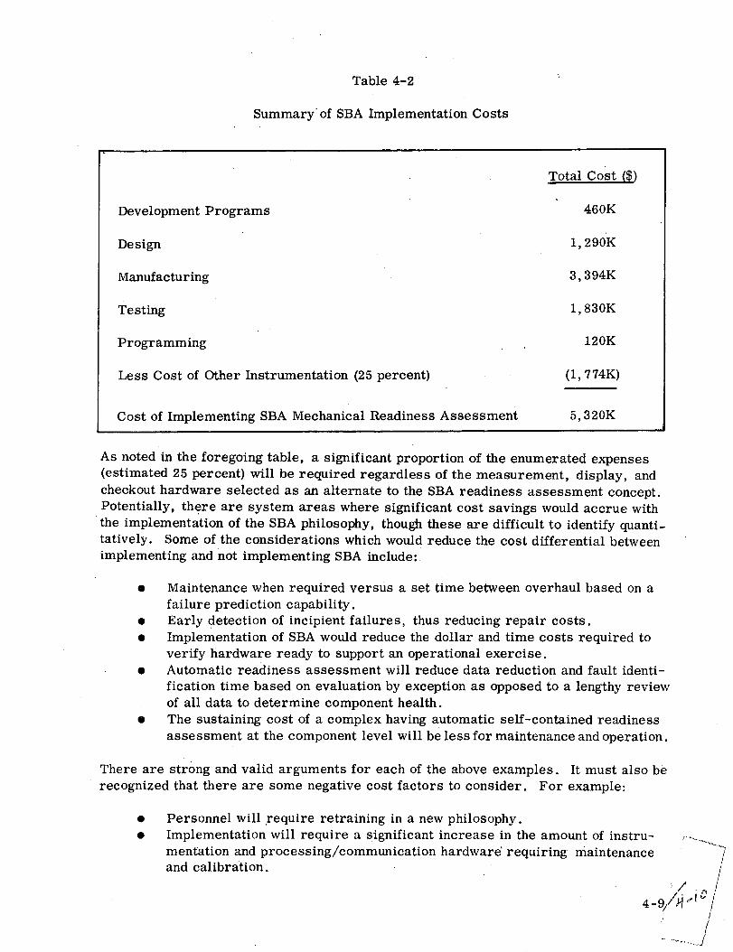
Table 4-2

Summary' of SBA Implementation Costs

Total Cost ($)

Development Programs 460K

Design 1,290K

Manufacturing 3,394K

Testing 1, 830K

Programming 120K

Less Cost of Other Instrumentation (25 percent) (1, 774K)

Cost of Implementing SBA Mechanical Readiness Assessment 5,320K

As noted in the foregoing table, a significant proportion of the enumerated expenses(estimated 25 percent) will be required regardless of the measurement, display, andcheckout hardware selected as an alternate to the SBA readiness assessment concept.Potentially, there are system areas where significant cost savings would accrue withthe implementation of the SBA philosophy, though these are difficult to identify quanti-tatively. Some of the considerations which would reduce the cost differential betweenimplementing and not implementing SBA include:

· Maintenance when required versus a set time between overhaul based on afailure prediction capability.

* Early detection of incipient failures, thus reducing repair costs.· Implementation of SBA would reduce the dollar and time costs required to

verify hardware ready to support an operational exercise.* Automatic readiness assessment will reduce data reduction and fault identi-

fication time based on evaluation by exception as opposed to a lengthy reviewof all data to determine component health.

* The sustaining cost of a complex having automatic self-contained readinessassessment at the component level will be less for maintenance and operation.

There are strong and valid arguments for each of the above examples. It must also berecognized that there are some negative cost factors to consider. For example:

* Personnel will require retraining in a new philosophy.* Implementation will require a significant increase in the amount of instru-

mentation and processing/communication hardware requiring maintenanceand calibration.

SECTION V

SUMMARY

5.1 GENERAL

Those conclusions and recommendations resulting from this study effort are summar-ized herein.

5.2 CONCLUSIONS

1. Acoustic signature limits can be established for specific component failuremode limits; however, much work must be done to define the mechanicaldevice failure mode limit itself, e.g., how much leakage is no-go? Thistask was outside the scope of this acoustic test program.

/2. The structure borne acoustic test technique has greatest applicability to

cyclic mechanical devices./ It also has applicability to transient acousticgenerators, but has little iImmediate practical application to mechanicaldevices that are only "flow noise" generators.

3. Each mechanical component must have its normal-operation acoustic signa-ture emperically established.

4. The existing state-of-the- art accelerometers and signal processing equip-ment is adequate for the i~mplementation of the SBA technique.

5. The SBA test technique h/as significant potential for achieving real-timereadiness assessment of mechanical devices. The necessity of componentbaseline testing, inherent system variables, and the experience which mustbe developed to properly/ use the equipment and to interpret the acousticsignatures dictate proceeding with caution for any near-term wide-scaleoperational implementation.

6. The cost of full-scale nmplementation of the SBA technique on a future spaceprogram equivalent in size to the Saturn program is approximately 5 milliondollars. The cost estimates broken down into broad categories are:

a. Development-$4/60Kb. Design--$1,290i(c. Manufacturing /$3, 394Kd. Test-$1, 830K/e. Programming/-$120Kf. Less Cost of Conventional Instrumentation-$1, 774K

5-1

!.):I I{I,',(¢)MM I,:NI)A'I'I()NS

'I'hoe proglralis which are recoinmendod for implementing SIA areo:

1. Develop basic significant physical parameters of mechanical components.Estimated cost is $150,000 and estimated schedule duration is 12 months.

2. Develop selection rationale and list of mechanical devices that will utilizethe SBA technique for readiness assessment. Estimated cost is $50,000and estimated schedule duration is 6 months.

3. Implement a prototype "piggyback" SBA system on the Skylab Program forselected mechanical components. The estimated cost of implementing thisprototype system is $260,000.

4. The SBA test technique has too much potential to be ignored by users oflarge quantities of mechanical devices. There are applications at KennedySpace Center, other than real-time mechanical readiness assessment, wherethe structure borne acoustic technique may be useful. Examples are compo-nent bench test facilities and support operations analytical laboratories. Itis recommended that these possibilities be fully explored.

5-2

APPENDIX A

SCHEDULED TASK PERFORMANCE

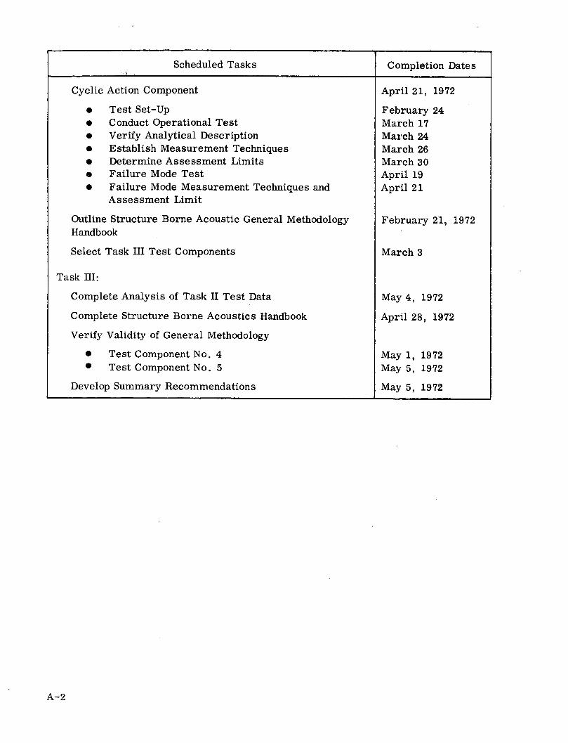
Scheduled Tasks Completion Dates

Task I:

Assemble Acoustic Data and Component Documentation

Select Representative Components

Derive Analytical Description of Acoustical Signature

* Transient Action Component* Flow Control Component* Cyclic Action Component

Develop Test Plan

* Transient Action* Flow Control* Cyclic Action

Task II:

Transient Action Component

* Test Set-Up* Conduct Operational Test* Verify Analytical Description* Establish Measurement Techniques* Determine Assessment Limits* Failure Mode Test* Failure Mode Measurement Techniques and

Assessment Limit

Flow Control Component

* Test Set-Up* Conduct Operational Test* Verify Analytical Description* Establish Measurement Techniques* Determine Assessment Limits· Failure Mode Test* Failure Mode Measurement Techniques and

Assessment Limits

November 24,

November 24,

1971

1971

December 31, 1971

December 1December 6December 31

December 31, 1971

December 15December 23December 31

February 23, 1972

January 6February 4January 28January 28February 2February 29February 23

March 28, 1972

January 24March 7March 10March 10March 17March 17March 28

A-1

:I

A-2

Scheduled Tasks Completion Dates

Cyclic Action Component April 21, 1972

* Test Set-Up February 24* Conduct Operational Test March 17* Verify Analytical Description March 24* Establish Measurement Techniques March 26· Determine Assessment Limits March 30* Failure Mode Test April 19* Failure Mode Measurement Techniques and April 21

Assessment Limit

Outline Structure Borne Acoustic General Methodology February 21, 1972Handbook

Select Task III Test Components March 3

Task III:

Complete Analysis of Task II Test Data May 4, 1972

Complete Structure Borne Acoustics Handbook April 28, 1972

Verify Validity of General Methodology

* Test Component No. 4 May 1, 1972* Test Component No. 5 May 5, 1972

Develop Summary Recommendations May 5, 1972

APPENDIX B

MECHANICAL COMPONENT TEST DATA

This Appendix contains a component description, test schematics/drawings, and typicaltest data, raw and tabulated, for the five representative components which were tested:

B1 - Solenoid Valve 75M08825-3B2 - Regulator 75M08831-1B3 - Air Motor 70A66B4 - Blower HF-PS8032, Series 355KSB5 - Motor Generator-Motor-5K225D38, Generator-1. 5 kw

B-1/B-2

4,

APPENDIX B1

SOLENOID VALVE (75M08825-3)

The 75M08825-3 solenoid valve is a three-way, two-position, normally open, magnet-ically operated valve with a built-in electrical position indicator switch. The valvecontains a coil and core assembly, aposition indicating switch, stem, cage, and sleeve.When the solenoid is deenergized the CYL-1 port and the NO port are common. Whenthe solenoid is energized, the stem is actuated and CYL-1 port is common with the NCport. The flow is bidirectional, and the valve can be mounted in any position and isqualified for use with GN 2 (See Figures B1-1 and B1-2.)

General information about the solenoid valve is as follows:

Operating PressureProof PressureOperating TemperaturePressure Drop

Operating VoltageCoil ResistanceRated CurrentPortsFittingsLeakageOperating TimeDuty

3000 psi4500 psi0°F to +165°FEquivalent sharp edge orificediameter 0.1124 +6 vdc21.5 to 24 ohms at +20 ° C (68°F)1.12 amp at 24 vdcPer MC240-4Per MC237C4Bubble tight, internal and external50 ms (not critical)Continuous

B1-1

Normally ClotInlet Port

IJpe_/en----rlll/ Outlet Portrt

Spring

Figure B1-1. Cross Section View Of Solenoid Valve 75M08825-3

Inlet

B1-2

O0

cq

I

b~(1)

U)a)

lv

>

.,

(d

0

Wl

I

PQa)

bz

P_

B1-3

NOMENC LATURE

Lockwire

Fitting

O-Ring

Screw

Slug

Screw, Adjusting

Spring

Nut

Screw

Cover

O-Ring

Screw

Nut

Washer

Nut

Lock Washer

Armature Assembly

Screw

Washer

Receptacle

O-Ring

Spacer

Insulator

Screw

O-Ring

Coil and Core Assembly

Plunger

Switch Assembly

Retainer

Stem

O-Ring

Sleeve

O-Ring

Seat

Cage

Body

PART NO.

MS20995C20

J53S6C10

J201J4

J67A12

111112-461

144621

168152

116762

102961

102531-2

J200A28

AN500AD2-10

79LH1660-26

107331

107281

107261

221071

J66A4

107241

CF3102R14S-5P

J200A17

168212-1

107311

111071

J200A2

222362-1125

150111-1

228052

154471

142602-1-1-1

J200A7

102831

J200A12

201892

124522-3-1

152704

Figure B1-2. Solenoid Valve (Sheet 2 of 2)

B1-4

INDEXNO.

1

2

3

4

5

6

7

8

9

10

11

12

13

14

15

16

17

18

19

20

21

22

23

24

25

26

27

28

29

30

31

32

33

34

35

36

VENDORCODE

99657

99657

99657

99657

99657

99657

99657

99657

99657

99657

72962

99657

99657

99657

99657

99657

99657

77820

99657

99657

99657

99657

99657

99657

99657

99657

99657

99657

99657

99657

99657

99657

99657

99657

QTY

AR

3

3

1

1

1

1

1

2

1

1

1

1

1

1

1

1

4

4

1

2

1

1

2

2

1

1

1

1

1

3

1

3

2

1

1

-2Cd Q

-sQ CwI

a

2(D FgrB-.Slnd Vave es Mehaica Shemti

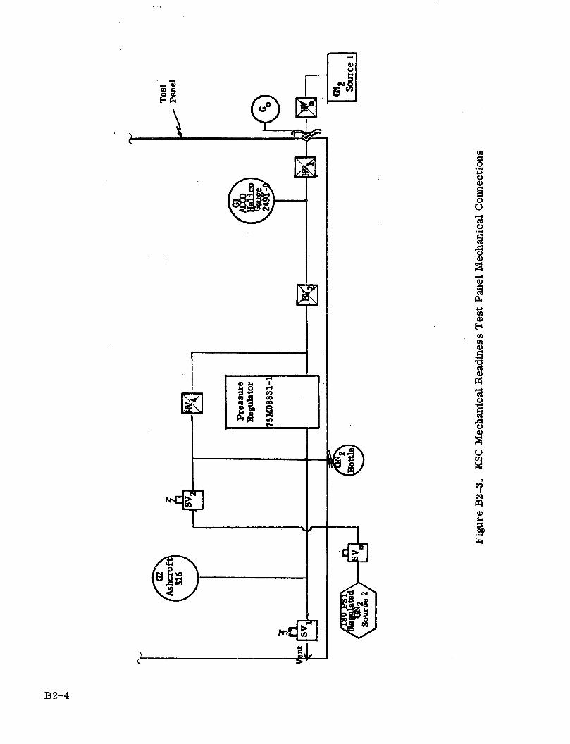
Figure B1-3. Solenoid Valve Test Mechanical Schematic

B1-5

U i|--Ie§3

C,

a4 -

0 C I

I I

bG

Figure B1-4. Mechanical Readiness Test Set Up SolenoidValve 75M08825-3 Electrical Connections

B1-6

p..

8,4?S.9 bA

1

SOLENOID VALVE HISTOGRAMS

The following histograms display solenoid operating time (actuation and deactuation)by valve serial number for both normal and failure mode operations. "Turn on" and"Turn off" refer to the application or removal of voltage to the valve coil. Eachvertical division is one operation, and the horizontal divisions are in milliseconds asindicated.

The data shows the repeatability of operating time and the influence of various inserteddefects upon the operating times.

B1-7

s/t

444

B1-8

.,

B1-9 igi-

.,

APPENDIX B2

PRESSURE REGULATOR (75M08831-1)

The 75M08831-1 pressure regulator is a three-way spring referenced, preset pres-sure regulator. The pressure setting is governed by the spring cartridge assembly.The force exerted on the piston by the spring cartridge assembly forces the poppet toan open position. The poppet is held open until the outlet pressure, acting on thepiston, exerts a force sufficient to overcome the spring cartridge and close the pop-pet. Further increase in outlet pressure will vent the excess outlet pressure down tothe set pressure level. The regulator is qualified for use with GN

2 .

General information about the regulator is as follows:

Inlet Pressure 4500 psi maximumOutlet Pressure 50 to 190 psiProof Pressure 6750N noiBurst PressureOperating TemperaturePorts

Capacity

Weight

11,250 psi0 ° F to +1650 FInlet: per MC240-6Outlet: per MC240-8Flow factorF = 0. 5 scfm/psia2.1 lb

B2-1

0

-4

O

..

4

-4

0

4r

B2-2

NOMENC LATURE

Lockwire

Adapter, Inlet

O-Ring, Inlet Adapter

Adapter, Outlet

O-Ring, Outlet Adapter

Nut, Adjusting

Locknut

Guide, Spring

Spring Cartridge

Tube, Guide

Piston

Nut, End

Washer

Spring, Poppet

Poppet

Retainer

Screen

Washer

Seat

O-Ring, Piston

O-Ring, Poppet/Piston

O-Ring, Seat

O-Ring, Retainer

O-Ring, Retainer Seat

Body

PART NO.

MS20995C20

MC235C19

MS28778-6

MC235C20

MS28778-8

146392

146382

146691

J205A86-22A

160002

160073-Al

146342

120002-104

144331

160052-3

146712

147741

120002-103

154663-11

J200AF136

J200AF12

J200AF15

J200AFl16

J200AF14

176134-Al

Figure B2-2. Pressure Regulator (Sheet 2 of 2)

B2-3

C

INDEXNO.

1

2

3

4

5

6

7

8

9

10

11

12

13

14

15

16

17

18

19

20

21

22

23

24

25

VENDORCODE

99657

99657

99657

99657

99657

99657

99657

99657

99657

99657

99657

99657

99657

99657

99657

99657

99657

99657

99657

99657

QTY

AR

1

1

1

1

1

1

1

1

1

1

1

1

1

1

1

1

1

1

1

2

1

1

1

1

0c9

ao

4.)C)c)

u

Uc-4

Cd

0

C)

a)

q

.)a)

H

a)I

a)

a)

F4

B2-4

.- Q) G)| 4Pt Cq a

A

'-4

-4

co

c[I

O

0

c)

-4

t-I

0

-4

Ce

cn

3

.,

o)CC

0

CI

F-

0

B2-5

/

C.)3 oC) X

o -7-

_

I i t __1_: lT_ _ ,_ _J - .~ tl ___

l~~~~~~~~;U .f0i

t1 ill w -~~~~, I I l 1 1. I'iI1,

414-t~ ~~~ s I a I 1 T I;1-

... iE1 1-, I" I" -I , I -I, I I I , 1 1,I , I , , Ii' i~ 1 1I ~ t . I'

I~~~~~~~~~ I i I , I ; 1

I I i 1 = , I I, I I i ! I I 1 1 ,~i I I l I I

Idt '_, I ~11 ...... Ig 1<

!LL '1 1- i I I I 11

I | ti I r-I' ~:-dIIII1fITIl T H F0

W Isi ~ ~ ne~~a s t~~q- _ 1 >_ §I

(I

Ir

1<

1-J

41:

-L %

mr2 -6

%It

I- I I g

I~~~~~~~~~~~~- ,

- -L~~~~~~~~~~~

I iI .--t+ ~ ~ ~ ~ ~ iI ~ ~ ~

~~II 'I !~I I I]

liii Il~~i :, l' i, 1 i I~ -_--!-_',_i I. I

___~ IiV....~~~~~~~~~~~~~~~~~~~~~~~~~~~~~~~~~~~~~~~~~~~~~~~~~~~~~~~~~~~~~~~~~~~~~~~~~~~~~~~~~~

I~~~~~ ~ ! i !__ ::5 ; i '~

It-_ j- I~ i i~ I r -,: ',- i ! I ] i i i I I I j I '"~ ! , ' ~~~~~II I f =

'---r._L! -!i i- ii . 'I! i [ I.I i '' 1! ...

-r-?,, . , , , . I I-

F.! I IT'i ' i.AJ - I ' I' I ,ii

.: i', ,', I I I iI i I i 1-I I~~~~~~~~i~m tTttI . i I' I I

.,- ~t ~- I -I -- I i i

1- 'r ' II,

',~:=:~ ~I ' , !--t} - ! i , ~ i I t I, 1'__" " I ' , I I- '

I ,_I , ',

~~~~~"^

~i~i~ ' *i' ii Iii I~III~--

'Y tH '7K i_. ~ ~~~~~~ I t…- I -L ii~

Ii~~~ t I- ,~ -, iIEF~~~ I~I VtI ~l'±#

~~~~~~~~~~~~~~~~~~~~~~~~~~~~~~~~~--i--? -...~z !

± ilL I ~ ~, I.F--L i~zB2-8 (K- 8 z

B2-9

i ' i

..%r- -

X e

( I Co. Rr, ;:<

'

1-.I I I I I

I

i, I J ' I J

I I

;~~~~~~~~~~~~~ r

-i

I

4:tT

4

1 :1_ __. I I IJI ! I I.1. I

i i I I -1 I ITF_ Ii ----

! fL Er~

I

L4-

tI

f

:14

IpI

I~~fItIIEEE

L

. * I . I * I I . I I I I IB2-12

_

t]

t

- ---1___L

L

'. I

Tr,I T

I

j-T

I..l I I

l- s~i ITt_!_ _

' L ' I I

t~~~~

<~~~I 3!

IIII

__

-)

X .

II i

.I _! . I II i I I ' q '_ i' I , ! , Ij- I

. I

7II'

I

1

I

;Aq

ML

I

.II

: I-

I

I I

i--Z l 'D , A t

I

I

I

1

I.,- l I I I I

a

6

i

I

F

,_

tt

,

I

I

It-11

- II

Ii

I

I

_

Ii

I

Et

I

E1I

I

T

L

--I

I14

I .

I

'r

I

L-I

l

IIIi

I

I

I

LL

i

FL

r iFi4-

1

Is,< s

N I I I1 I

2?

I

IL_L

C-C

1K1 1

r IIol

8a m .@

_ I ., ;

~~~~~~~~~~~~~~~~~~1~~~~~~~~, _,, ,,1 1 1'ii

. : I ' I.' " 1 "f~~~ ~~~~ i i ii. i ,

_ i I ' i , ' : ! _ _ , ._

I ,

r | s ~~~.,|| , .' . w . , . i. i . .

I i I i .. i l, ; I--j I I I i i --- i : I .I i m

_____ 111 1 E- _ !

i I i . ; ' _-, .. , ' , :' i : l ._ '_.

I i I i

i I !f i ! : , : i i i j j , i

,_ ; i i I.l i

ii: ~~~~~~i

I i ; i ! .: i i ! i i i I i iIt i ! i i i ~ · i- :" ; i' , i i i,' i i

I ! i ! i; !! i . i !.i i [ I ;! ! i --

r. ~~~~~~~~~, i ' I , I ! ! . | |i i i i ~ , !!L

i H: .i I i I , i , I ,i:iii t i ; | :i ! I ; - l1:; ii_ $ s l

: i~ i ! ' 1 i ~ i li-- t- I _ ii- I i ii i , __ i i i I. jj !- -

_ _ -1i j ,. ., ] . ' ,. .

, ,i = t~[i ]!' [! I.

B2-13

(

i

c(

I

I

I

r

I..¢j

II

I

.') - ' "I

^ . o a 7

.- ,- - ,

_ o- -,

I ~ ~~ _ _ i __ i

r _ I

i K _ i

,~ . i i i .. ! : ! T i .- I [.- - -! - - ! _ -t _

-i F - i _, .. I'' ' I

r i I ! ! : '''~ Ii

. I~~~ I -

I ___ I J~li.....L ' j ' I I I j- . j - - - - F,"; I - , I I _.,

r I V I I

i~~~~~~~~~~~~~j ri 'iV~ ~ i Fi I ,~' _L.. i I

' F ' ' F: !i . . ~ :_ , I F

1 - -4.-

B2-14

F ; I ' I I F F ,

_______~ ~--~. I F ''F-i- J t

,~~~~~~~~~~~ I - -

LI~~ i I VI- ,II~i IIfI ~ ~ ~ ' I III I ' =::-. I !I

'III~~~I F. '+'d', FV FF1 1~~~~i *1 1' V - 1"

+~ i Ii . . . . . . _

'F ' I ~ ~ ' Fl _~

_i~ ~ ~ II -! - -~' ,I _ Fir i' F -I~~~~i

I~Lta I ~11 .' !I 1;:::

i .V !~i' _

______ __ _ .1 _, __

-~~~ I .,1{ - Ic- - - -.

-~I -i -

B 2-14

I

B2-15

II.%J'·

3-.

kr

tj L kk

4F Ln1r'

i ·

B2-17

Street~~~~~~~' m-AmX~~~~~~~~~

iAIt

B2-18

L®.

-4

.I,

' />

"- i--:---~~~~~~~~~~~~~~--.,-,--C-~~~~, -F i

ys~~~~~~~~~I tA -I- £<l

I,!~1~~~~~~~~~~~~~~~~~I I !j- !--"'J-i- 11 4'ic~~~~~~~~~~~~~~~~~~~~~~~~~~~~~~~~~~~~~~~~~ ')F 1 I '

i L r ! T I i !i

5 j i

~ t I ' ._ ~ _ i i ih'

I~~~~~~~~~~~~~~~ : I. I - I-'--"WX <1' f=

till~~~~~~~~~~~~~~~~~~~~~~

I. , ! , It

I; ~'I I

I iI

I

___ ~ ~ ~ ~IL ,__ I I , j ).�. ;_ i , i ! t , i l

| - 1fI ~ i i -i |.- ;1,1 I . I

i

iI.... I:- ~mm ,-

i i 1 1 i ! I- . i i I Il iiri i ! I I !'-'I i, i i " ! i " :- ' I i I I~iI

'! i i i** J "' It ":"

lil . !~~~~~i l il , ,,I,' m I

', i t i j ~ ,

( ~ -- - I - I i

l--,

I I I '~ ~ ~ ~~ ~ ~~~~ HI F __ _ _ I

-. -I I I... I I i

-I __ i , I f

-I

i 1/ ).4

F.L

-. ~ ~it I I ) )] IJI

7 ~/ I j i i ;

I ~i Ii i~ v ,vi-I. I~~~~t * ~~' -- "1 I ! -

Kit~~~ L Fly ~ I!, ~ -...

!~~~~~~~~~ I -!_L i ~ i i [ =". l~= ~t~B2-1

-I ! t', ~-T-F~ ~,1i~I i -,,t ;~ '-1

/ B2-19

B2-20

'~%-

'- 19*3

LI) l-

j #

.2

B2-21

L! i, . l., ~ , i~'

-, ~ ' , _ ! !~ i ~ , i ! I ! ! J 1 ! 1

I ~ i i I ~ I ' t I l i'~ I~ ,j l J l , , ~ !· 4 i ,I i i I I i i ] ~ : t ~ ,

t ! i ~ J I

- I ! , ,, ~ 1 , ~ , , , !r ' . , ! ! . t II' ' I i

"

J

'

~ ~ 'x ~ I I I !/ I I I ~ t I !

~ 1 I I l i l , i .7 1 ! " i ! i Ii ! , i . , ! ~ ! , ! ~ ! i .i i f i l i t[ t [ i t i I [ I J J i !~ I ' I ! ! '~ ~ , I [ !' ! i J I i l i I t [ ¥ ~ ~ t i i l i I 1

I

· t , ~ · i i I !i i ~ 1 i i

f ] i ! ' l ~ i r ,i ' , i i i ' 'i ' ~ i .i l i t

.-" [ Ii i ~ I J t ,1-' 1

' ~ j ! I l l I ~ [I.~., I ,-

II ~ .: ....[ .: l..

[ " I I I 'l i l ! i i i t i [

~ ! i I l l ! ,< ~ I ' ! i ! , ~ i I -i) ' 'I I

" ' [r ! i i ) i i i t I ~ i i ! I !

t l l ' ', i I I t

_~[ _~_~ ~--_ -- __ __

-~ ~r it- i l

I [

~>, t i , , ,, ! , i ! , ,, {?~.., I t I I ,' ~ I , i ,~ l I ~ II !~ i ! ~

'

' ~ 1 I iI~ [" II i-~ . I!,L - i I

o

* cn

iI

i.

Ij f

I

I - 'I

sas

F\

q-

. _i I~ ~ I :~, ! i: _ .~~ ,

,i~~~~ i ;j I~i4~~~ ' ~ , i-i ' ' J _ _ ! I . ! I i _ _

:r~~~~~~~~~~~~~~~~~~~~~~~~~~~~~~~~~~~~~~~~~~~~~~~~~~~~~~~~~~~~~~~~~~~~~~~~~~~~~~~~~~~~~~~~~~~~~~~~~~~~~~~~~~~~~~~~~~~~~~~~~~~~~~~~~~~~~~~~~~~~~~~~~~~~~~~~~~~~~~~~~~~~~~~~~~~~~~~~~~~~~~~~~~~~~~~~~~, i~ __ I i I____

i ,1 ' i I i i i 0 , iI | I I ! ! ' - __ !

I i __ ' _' r_

_ , I, ., i . I I i___ , I ! ' ' i ' = _ ' 1

! i i , I ' i , , ! i

I _

i i ii , i I I !. ._:_ __', l . : i . i . ! i ! _ _ ' !i ~

i i I ! ! i

I i j ~ j I i 2 , , ! :' ,j

Is~~~~~~~~~~~~~~. ~, i L A I iIii ji I

++ 4 : . ,L i I I ____________ __ _ _ _I_ i Ii~~~~~~~~~~~~~~~~~~~~~~~~~~~~~~~~~~~

I 4 I i , it | | i i i i 1< -i l Ii

- i _; ! I I I I Ii !}liji-i I __

i~~~~~~~~~~~~~~~~~~~~~~~~~~~~~~~~~~~~~~~~~~~~~~~~~~~~~~~~~~~~~~~~~~~~~~~~~~~~~~~~~~~~~~~~~~~~~~~~~~~~~~~~~~~~~~~ii I, _ i. i tii

._ _ - -i , i- , - - , ' i~ _ _ !_ _ , ' ~ i ! i [I_ _ _ _ , ; _ _ _

__________ I - ! ; !

iT;I ~:1; ' -,;~ IIIBi

; i i l I I *1 i i ,1 i

, , j ! i i ] i I i i ' ~ 1 ! i j ; ,.~ , 1 i , i , i I

_ _ _ _ _ I I , l ' l

-' + T4 ' f' __,

-- ..I'L__ !..B-

~ i i~

,~~~~~~~~~~~~B22

I

Jr' 2)

~i ~,~' , '¥ r ,k--...~' ' F

-! . i t [ .'"'~ '! it l i l l, ~ TJ ,~:,

~ _ : L i ' [ ! -.L I._L _

'--- ~ ! t I I ~ J i I -m T--i--I ' I i 1 i ] i . 1 i f ! f ! tjil

' [ ], t, [,i , ! , ,.o ' I ! , i 11. I· - ]

i i i , l i i i l l i " J i'~ '1 i

"~ ~ I I i I i , i i t ( , t I~-. u-.- k , tr I I , L

' t l i t I ,. I' ! i" i .t ! .. ! .... ! I tI

t I I I i , . I.I,, , i l i l ~ l I i i i i ! i i i ! ii 'l

-... ,~ . I ~.--t t i l l I i l I', ~ i i i I ~ i I i I J i ~ II .. L__J.-_ i L ' I I I'l

I, I I. i"'i[ ' [ii'' [ I, , ,

",,,., I ! :[ I- Ii I I i,~1 I i I I , ! i! i i , ~ [ IIl l I t I i i 'i i', ~ i i ' 'I i '~ ! i i t I i I ! t i ! ~ I ~ .

-- F ! 1 1 I f$1 ~ ~ I i i , ilit ~l,~, ~ i , , t i

Ii ' ' I [ ~I ~ I

I t l ! !'i ~ I IIll i S ' i ,

· ~ 1 [ [ i ! I I, t ) i , I i !I ~ i ~ ' , , I ' i

1

-.-.-[.-i ~ ~ I I I - i I I '~1'~. i I I _B2-26

II

4 (1,

c-OJ

APPENDIX B3

AIR MOTOR 70A-66.

Air Motor 70A-66 is an axial-piston air motor that may be operated as either non-reversible or reversible with full power in either direction. This motor, see Fig-ure B3-1, has high torque characteristics, and its 5 piston power impulse character-istics assure even torque at all speeds.

Figure B3-1. Axial Piston Air Motor

AIR MOTOR FUNCTION

This air motor functions to pneumatically drive or power machinery. It may be usedin such diverse ,applications as rotating turntables, powering cranes, mixing paint,etc. It provides variable speed, reduces spark hazard, and cannot burn out. Ratingsfor this air motor at 90 psi are:

a. Horsepower--1.9.

b. RPM 315.

c. Rated Free Speed RPM-605.

d. Stall Torque-64 ft-lbs.e. Starting Torque-48 ft-lbs.

f. Gear Ratio--5.8:1.

g. Weight with Standard Shaft-26.5 lbs.h. CFM at Maximum Output-62.i. Maximum Overhung Load on Shaft at Stall-1000 lbs.

B3-1

RIGID CONSTRUCTION of entire motor offersmaximum usage during the long life of themotor.

GENEROUS SIZE SPINDLE BEARINGS allow aheavy overhung load on the spindle with noexternal spindle support.

PRECISION MACHINED PARTS insure a longservice life for the motor with a minimum ofmaintenance.

COMPACT DESIGN of motor permits its use inclose quarters and cramped installations wherespace is a limiting factor.

ENCLOSED CONSTRUCTION allows use in cor-rosive and dusty atmospheres. Motors performsatisfactorily when placed in high temperatureareas.

SIDE AND END AIR INTAKE PORTS are providedon the 3 larger series of motors, permittingclose quarter installations and giving addedconvenience for piping connections. Side portsonly are provided on the smallest series.

AN INSPECTION HOLE AND PLUG is providedin the rear housing of the air motor for checkingquantity and condition of lubricant.

FACE MOUNTING OF THE AIR MOTOR to a fix-ture with three bolts equally spaced, allowspositioning of air connections and a positivemount without strapping-motor is readily re-movable for servicing or replacement.

MAXIMUM AMBIENT OPERATING TEMPERA-TURE is 200'F. MAXIMUM OPERATING PRES-SURE is 100 PSI.

Power impulses for the five-piston motors arethe same as those for the radial piston design.At least two pistons are on the power stroke atall times, providing even torque at all speeds.

Axial-piston air motors operate smoothly,with absence of vibration. The unique "wobbleplate" and piston design perform smoothly atall speeds and working pressures.

CYLwrD"0 .

B3-2

_

S z;

_ m~~~~

Serles 70A-62, 64, 66 -- Singl Garod

Series 70A6-29, 17,10--Double Geared

< . 3a a a

IOutput

at 90 PSI

H HP r RPM

1.91.91.9

1.91.91.9

1820535315

1528954

ModelNo..

70A-6270A-6470A-6670A6-2970A6-1770A6-10

RatedFree

SpeedRPM

35001030605290170100

StallTorqueFt. Lbs.

113764

130223370

StartingTorqueFt. Lbs.

8274896

163269

GearRatio

3.4:15.8:1

11.9:120.3:133.6:1

WeightLbs.

WithStandard

Shaft

26.526.526.542.542.542.5

CFMAt

MaximumOutput

626262626262

LMaximumOverhung

LoadOn ShaftAt Stall

1000 lb.1000 lb.1000 lb.1000 lb..1000 lb.1000 lb.

B3-3

PISTON MOTORSIZE 70A-62, 70A-64, & 70A-66

LUBRICATIONUSE NO. A-5 OIL

INSTALL AIR LINE LUEIRICATOiR

FILTER IN AIR LINE AHEAD OF TOOL

GREASE FREQUENTLYUSE NO. A-12377 GREASE

v-SHERHuICII

tv-'I- ICOIItTC

f

A-10056 __DRIVESHAFT COMPLETE

_ V- 23 GRETAINING RING

STEL MILL21t

HOW TO ORDERREPLACEMENT PARTS

I. UANm2 PART 13. PAr AI

_ I _ 10047MIIVIGHAFT

IR7-T

/

t 507490 POWER UNITALTERNATE CONSTRUCTION

FLUSH TYPE MOTOR(EAl KAE PW WI WITH 'llOT NWOUSilNG

FOR ?70-G AND ?O7A-64 USE 1310-IlGEAR CAGE AND 101-I-A SPINDLE,

CHARCES MADE SINCE LASTISSUANCE OF THIS SHEET

WHICH INCLUDES 20OS9-1 KEY AND18326 KEY.

FOR ?OA-GG USE 1321I-I GEAR CAGEAND 1 I31I-1-A SPINDLE, WHICH IN-CLUDES 2069-I AND 10S2 KEYS.

NOTE: FOr OTHER SPINDLES-SEESECTION ?0, PAG 31.

PC-ITO?

Exploded View, Figure B3-2

B3-4

Pt~I{T#O.

LOCK NIUT

i

i

l V" |--- (tU. lm

STEEL LL' SII

U2

0

.,d

m O~~~~~~~~~~~~~~*

A w~~~~.;U

E IC)

,! , /

0

w 9~~;

/~~~~~~~~~~

/4: 4

CO

14

K ~~s /

iit0 = i

APPENDIX B4

BLOWER HF-P58032, SERIES 355KS

The blower is powered by a 200 volt, 3 phase, 400Hz, 3700 rpm motor delivering upto 1150 cfm and is of the type used for cooling in electronic cabinets.

B4-1

* COMPACT · LIGHIT SELF-COTAINED* Size: 10.1"' x 6.12" x 7.7Y' APPROX. · WEIHT: -8 LBS.

· 5060, 400 CPS · 1 PHASE OR 3 PHASE, ALL STANDARD VOLTAGES· AVAILABLE FOR EITHE "PUSH" OR "PULL" ARiFLOW

ROTRON . BUILT TO APPUCALE MILITARY SPECIFICATIONSIINCORPORATED

Chil

I -- ~~aa-t-

MODEL HF * TYPES 801-802-803WHERE TO USE

ROTRON MODEL HF funs -e detgned for flushing adio cabinets,

F,, mi'nt p.r.s . rud . t.. l.r.. tte .cubicles- Thy me et the special

riur.s.rir'rrt I., such o pphcat ons s high output. light weight.

c.rrpl nid r ell oi o.lr d .onstrucrlon low motor winding tem

pcs.,,re s. i;Ii ros]e- d for liFr bchll beorings. ond do NOT haoe to be"'-.l Sor lubrrttlion Slctndtrdd types uover 1700 and 3400

R'M i )rl I lnd 1 i, dellh,is cirl per key graph at top right of

tl..i pi ,e AudLbler loi t. l oall. rs wth shaft speed and pitch

trt ,prop. Rll . crhoen. which c n turn govern pressure.building

For smaller fans refer to ROTRON MODELS NF, MF, and DFE. Forsnilur fons not built to government specifications, refer to ROTRONCARAVEL FAN and GREEN-LABEL fan MODEL PF.

MOTOR

The induction motor is either three-phase or permanent split-phasecapacitor type and is aovilable with either A. F, or H insulation. Thecorrosion-protected case, which totolly encloses the motor, is finned formoximum heat dissipation resulting in a minimum winding tem-pc-lture rise The motor operates on double-shielded. precision bollbeorings which are greased for hfe and ore carefully aligned forquiet, trouble free operation. The case and shaft are of die-costoluminum and stoinless steel respectively. Where "T Frame" motorsare used isee Type Chartl a compact screw-type terminal block isfittid integrally into a recess in the motor case so that hookup cablescan be run rI d..c ly to the motor Eighteen inch spirol-tracer. color-coded leads cil. supplied with "D Frome motors. Motors meet ap-plcohle milllr ry specificotions far ground. sea and airborne serice.Sre cppl cibls. Cctolog Sheet im Section C. MOTORS" US. PatentDesigit 174,14 8 Other U.S. Patents Pending.

AIRFLOWCon h.rip i-ri perfoarmaire grtiphs. includng wrindrig temperature

i,-. lcd -lu rip ul tuises ore gisen on catalog sheets following thispoge All , t .re aohloble for eIther push FLOW "L" or pull

FLOWu R upce.olon The motor .th propeller is permanentlymount u ng h dgned on ng hh , d gned for efficient operationot both drl(llons of c(irllow Ths ventur ring. moreover. allowssimple moeru. orrg of the corplere assembly on a dustfiller housing orrobi-er w-ll No cuor.hary poatls 1,e spocers or rings ore required

Fo i er lrl. ol propeller fols n generol. see Applicotion NoteSELECTION and APPLICATION OF PROPELLER FANS" n catalog

irltiOn ENGINEERING DATA

VIBRATIONAll moors used on MODEL HF fans are finely dynamically bol-

rlnc( In aoidir to mwnrmlrll tronsmiscon of any resldual vibrotion

irn,l, toruto r pot.lsller to Is rrmountirg panel. the MODEL HFV fanriri be speirfed which incroporates vibrotion isolation mounts

b..t*. r.n rouln, g spider ond venturi ring In case of exlernol

,b-lbt1, s (. i h , ock conditions as encountered in most militaory oppli-cutrora lo aot specify the MODEL HFV fans because resonant con-if,- rrn i my .esult in undue exicursons of the fan motor Model HF

iri-s p1i. 'ird by TA3 or DAI flome motols ll pass government

sp.rs-ciihtiri for s r-hot nnl urr1oM vhl n with standord venturis andn eo aut n tuu r. sprled.s Units e,( upped with heavier DA2 ao DA3nl.loul .(i1it1r. nrurt he prouledd wlih heavier nvefturls 1 ' material

Hkr, is isri ldotted Jnoultrng spiders when el rene shock andllcioni roiil{l.lluris nrustl he nmet Thre ei forced unit is designoted

as MODEL HFG. The reinforced spiders are shown on the lower partof Figure 2.

MATERIALS AND FINISHPropeller and aenturi ring are aluminum and anodized. The mount-

ing spider is of steel and cadmium plated. Motors hoave aluminum

Motors co-e.e(f by U S Pao De, 174.148 Other U S Patents Pending.

frames, corrosion-protected blackenameled. and stainless steelshafts. Fans pass applicable gov-ernment specifications for highhumidity. fungus, and altitude op-eration. Special finishes on re-quest. Phase-splitting capacitorsrwhere required. are not normallyfurnished by ROTRON. On largerorders and on special request. suchcapacitors may be mounted direct-ly on the motor frame. The op-tional screen guard is steel andcadmium plated.

ORDERING INFORMATION* Specify Fan Type and Motor Series number by consulting Fan

Type Chart on basis of available power supply and performancerequired.

* Specify flow direction, either Flow "L" or Flow "R" This isexplained on the outline draowing that follows.

* Specify whether or not vibroaion isolator mounts ore requred.If required order Model HFV rather than Model HF

* Screen Guard (see drawing) is optional and must be specified ifrequired

* Specify moximum and minimum temperotutes and densities orotmospheric pressure.

EXAMPLE: Specify Model HF. Type AS-802, Flow I. Series 123JS,-55iC to 70C, 14.7 -2 PSIA.

ROTRON INCORPORATEDWOODSTOCK.

NEW YORK 12498

6.69-10m

B4-2

-Y~B

III

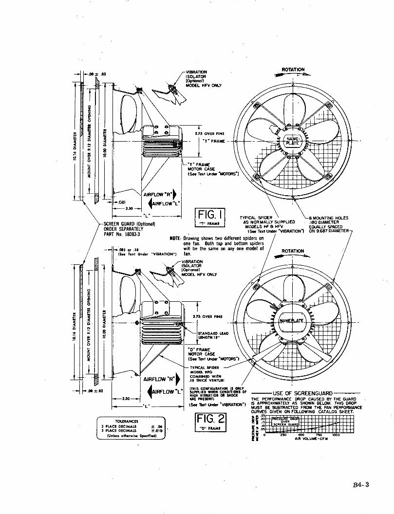
ROTATION_2~B

L- L1 I I V. I I TYPICAL SPIDER ' -8e MOUNTING HOLESN GUARD (Optional) 'IT"FRAM AS NORMALLY SUPPLIED .180 DIAMETER

ISEPARATELY " ' MODELS HF 8 HFV EQUALLY SPAMCED3SEPARATELY (See Text Unde 'VIBRATION') ON 9.687 DIAMETER-

No. 18083-3NOTE: Drawing shows two different spiders on

one fan. Both top and bottom spiders-.081 ,r .18 will be the same on any one model of ROTATION(See Tet Under "VIBRATION") fan. /

"O" FRAMEMOTOR CASE(See Text UnIer MOTORS')

-TYPICAL SPIDERMODEL HFGCOMBINED WITH

.18 THICK VENTURI

TNHIS COrIGCURATION IS ONLYSUPPLIEO WHEN CONOITnIONS oF -U _ SE OF SCREENGUA RDRDHIGH VIBRATION OR SH OCARE PRESENT) THE PERFORMANCE DROP CAUSED BY THE GUARD(See Tet Udr "VIBRATION") IS APPROXIMATELY AS SHOWN BELOW. THIS DROP

MUST BE SUBTRACTED FROM THE FAN PERFORMANCECURVES GIVEN ON FOLLOWING CATALOG SHEET.

FIG. 2 AIR VOLUE-C I"0" FRAME .0 o 5IN~EjURE04R

O ~~~A15R VOLUME -CFM

TOLERANCES2 PLACE DECIMALS - .063 PLACE DECIMALS *.010-

(Unless otherwis Specified)

MODEL HF(V) FANTYPES 801-802-803

SHAFT SPEEDFigures given in the TYPE CHART on page 2 as wellas on the nameplate are nominal only and generallyrefer to MAXIMUM CFM air delivery at sea level andat nominal line voltage and frequency.

DIMENSIONSFor dimensions and tolerances, refer to outline draw-ing except for such dimensions as are listed in thisTYPE CHART under MECHANICAL.

WATTAGE AND CURRENTFigures in this TYPE CHART are for nominal linevoltage and frequency, and generally apply to thecondition of MAXIMUM CFM and sea level operation.In case of 50-60 CPS motors, they apply to 60 CPS.In case of variable frequency motors, they apply to400 CPS.

FREQUENCY RANGEThe line frequency range listed for variable frequencymotors is necessarily arbitrary, because the rangedepends on acceptable variations in speed (air de-livery) with frequency. Performance as a functionof frequency can be adjusted by changes in thedesign of the motor winding. Rotron will designdriving motors which will operate on odd frequenciesas well as over special and extremely wide frequencyranges.

BEARING SHELF LIFERotron military quality motors are built to operate

under humidity conditions as specified in MIL-E-5272.When stored under high .humidity conditions, how-ever, the bearings will deteriorate. It is thereforestrongly recommended that the fans and blowers notbe subjected to more than six months of inoperativeshelf life in humid climates and not more than oneyear in dry climates. Units properly packaged insealed containers with a desiccant may be expectedto withstand longer shelf life.

HOOK-UPThe first suffix letter immediately following the motorSERIES number listed in the accompanying TYPECHART refers to the applicable wiring diagram foundon catalog sheet C-1000 in Section C, MOTORS.Phase-splitting capacitor values, as may be required,are listed in this TYPE CHART.

CAPACITORSWherever phase-splitting capacitors are indicated inthis TYPE CHART, these are not normally supplied byRatron. Their values should preferably be held withina tolerance of -10%, especially for 400 CPS andvariable frequency motors. In selecting capacitors,due attention should be given to variations in capa-city ratings with high and low ambient temperatures.Unless stated differently in this TYPE CHART, WorkingVoltage ratings are 220 VAC for 115 Volt lines and330 VAC for 230 Volt lines. Oil-impregnated, canned,paper capacitors are recommended.

AIR DELIVERYFigures in column AIR of this TYPE CHART representactual amount of air moved at sea level standardatmospheric conditions per AMCA code.

MOTOR INSULATIONThis TYPE CHART lists the NEMA classification foreach motor. Motors with a different class of insula-tion than listed can generally be supplied. To obtainthe actual maximum hotspot winding temperaturefor any unit, add the maximum ambient temperatureto the WIND. RISE°C HOTSPOT reading obtainedfrom the Performance Graphs immediately followingthis page, applying to the air delivery rate -of theselected operating point on the performance curve.Limiting total winding temperatures are 1050 C forClass A, 1500 C for Class F, and 180°C for Class Hinsulation. The 1050 C figure for Class A is conser-vative and could be extended to 115°C where thelife of the equipment is not expected to exceed 2000hours.

Motors covered by U.S. Pat. Des. 174,148. Other U.S. patents pending. Printed in U.S.A.

B4-4

10-67-12m

so10, MEEMM~p i

9®

FAN TYPE CHART

BLOWER MOTOR I f E C T A I C A L AIR MECHANICALor

FAN Wtt Line Amps Locked Dimonsion "" Marx.Cop. Nominal Insul. Input at Free Rotor Max' Tota

.Tp Fram Series Volts Phase CPS Mfd. RPM Class at FIr Delivery Amps. CFM Net Vibration Isolators

Delivery At Lower Voltage Lbs. With Without

KS-801 DAI (12) (12) 1 50-60 2.0 3400 (12) 50 0.52 1.5 510 5.0 63/4 6%LS-801 DAl 268AS 115 1 50-60 2.0 1750 A 25 0.26 0.62 260 5.0 6Y/ 6YAS-o801 TA3 (1) (1) 3 50-60 - 3250 (1) 41 0.3 0.80 480 3.5 6% 63/185-801 DA1 254JS 208 3 50-60 - 1750 A 30 0.25 0.61 260 5.0 6/ 6,4PS-801 DA2 (4) 115 1 400 1.0 3750 (4) 95 1.25 2.10 540 6.0 6U 6 3/2PS-801 DA1 (2) (2) 3 400 - 3800 A 106 1.8 3.2 560 5.0 6 6/4

KS-802A DAl (13) (13) 1 50-60 3.0 3300 A 65 0.55 1.45 630 5.0 6% 6%LS-802A DAt 268AS 115 1 50-60 2.0 1750 A 25 0.26 0.62 330 5.0 64 64AS-802A DAI (3) (3) 3 50-60 - 3350 A 50 0.2 0.77 650 5.0 64 6%85-802A DAI 254JS 208 3 50-60 - 1750 A 30 0.25 0.61 330 5.0 63/ 6%PS-802A DA2 (4) 115. 1 400 1.0 3650 (4) 112 1.35 2.10 700 6.0 6% 6%3NS-802A DA3 589AS 115 1 400 5.0 5875 F 390 3.7 12.0 1050 8.0 - 7YPS-802A DA2 (10) (10) 3 400 - 3800 A 135 2.2 3.90 740 6.0 6/4 6%NS.802A DA2 (14) (14) 3 400 - 5650 F 250 2.45 - 8.0 1050 6.0 6% 6%

KS-802 DA2 (5) (5) 1 50-60 4.0 3300 (5) 130 1.0 2.05 810 6.0 6% 6%LS-802 DAI 268AS 115 I1 50-60 2.0 1700 A 30 0.30 0.62 400 5.0 6Y5 63/AS-802 DA2 (6) (6) 3 50-60 - 3350 (6) 82 0.6 2.30 820 6.0 6% 6%85-802 DAI 254JS 208 3 50-60 - 1750 A 31 0.25 0.61 410 5.0 6Y4 6kNS-802 DA3 (7) (7) 3 400 - 5800 F 420 6.0 13.4 1400 8.0 - 7PS-802 DA3 (11) ( 11) 3 400 - 3850 F 215 3.5 5.0 890 8.0 - 7Y,

1(5KS-803 DA3 413A5 115 1 50-60 8.0 3350 A 165 1.3 3.0 1050 8.0 - 7KS-803 DA3 (8) (8) 1 50-60 2.51 3300 (8) 165 1.5 3.7 1000 8.0 - 7 / sLS-803 DAl 268AS 115 1 50-60 2.0' 1650 A 35 0.34 0.62 500 5.0 64 6Y4AS-803 DA3 (9) (9) 3 50-60 3350 (9) 144 1.0 4.0 1020 8.0 - 7/AS-803 DA2 (6) (6) 3 50-60 3100 (6) 130 0.75 2.4 950 6.0 634 63485-803 DA1 254JS 208 3 50-60 _ 1700 A 43 0.25 0.61 550 5.0 6% 6YAS-803 DA3 697AS 380 3 50-60 3380 F 144 0.31 1.4 tOCO 8.0 - 7%sNS-803 DA3 (7) (7) 3 400 5600 F 680 7.5 13.4 16&0 8.0 - 7/ePS-803 DA3 5I9AS 115 1 400 2. 3600 F 285 3.3 5.0 1080 8.0 - 7 %PS-803 DA3 (11) (11) 3 400 - 3700 F 295 3.8 5.0 1150 8.0 - 7/KS-803 DA2 217AS 115 1 25 4.0 1450 A 43 0.415 0.43 440 6.0 64 6%/

(2) Specify choce f (3) Spe cify choice of: (4) Specify choice of:

Motor n M otor Lin Motor Line Insul.Series Voltage Series VoltaeI Series Voltage Class

272WS 208| 139JS 208 391AS 15 | A

363WS 416 251JS 440 450AS 1 F50SWS 115

(7) Speci choice of: (8) Specify choice of:

Moto Un Motor ine I n nsul. |is io V t Serie VoltageS l Voltoage Class

51W SI 1 25 I 20 3 5 1 328AS 115 1A| | J37Jmo | 115 | | 32BS 11 5!230 A

j73416 328CS 230 A895AS 115 H338AS 115 F3388S 115 /230 F338CS 230 F35185 220/440 A

( 1) Specify chiice of: (12) Specify choice of: (13) Specify choice c

Motor Un i Motor Line Inev . Motor ULineSeries Y /olg Series Voltage CSlass Se Voltego

1561WS I/ 111 364AS 115 F I 564AS 115594WS 200 3648S 115/230 F | 5648S 115/23

.36C5 230 F I 564C 230600AS 115 H9328S 115/230 H

(5) Specify choice of:

(9) Specify cnoice of:

of: (14) Specify choice of:

|Motor | linoSeris Voltoago

518JS 200

0 1028JS 115

B4- 5

Motor Line InsulSeries Voltage Clbs

105JS 208 A237JS 115 A427JS 440 A386JS 208 H

(1) Specify choice of:

(6) Specify choice of:

(10) Specify choice of:

Motor LinSeries Voltage

270WS 208277WS 11

Motor Line Insul.Series Voltage Class

329AS 115 A32965 115 230 A329CS 230 A509AS 115 F692AS 115 H

Motor LiUne InsulSeries Voltoge Clas

123JS 208 A190JS 115 A197JS 440 A197L5 220/440 A3.44JS 208 F

Motor Line Insul.Series Voltage Class

154JS 208 A196JS 115 A207JS 440 A538L5 220/440 A246JS 115 F266JS 208 F353JS 440 F931JS 208 H

I

ACCURACYCu-ves below represent results of measurement of a typicalsamp.e and snzu d be token as rm:ra'. R:t-or w'il odv:setoleronce for o specific opplication. A:lowance should bemade for the effect of 'channeling' of ball beor;ng grease.

' r

i;

rYPE LSOi FLOW R

. - ! tI 1 '- 1

- Ot i

FLOW DIRECTIONNote that 2 sets of grophs ore given foreach type of faon. Tne top set for FLOW

L and t'e Dotton, set for FLOW R'. For

def;nt'ion of f;ow see outline drawing.

TYPE AS403 FLOW L TYPE 7 s FLOW tYpE IS-03 FLOW L T I YPE 5-03 FLOW I =n =rua =~o [ = c- ,, , m .I J_'-;- I _ca tre ._ . .I

.,m r~ lsl I . ' 25

:,0 0''*' ' ' . . , 10200 200 so

1 '°°I I It I '°I 'ZO

4w no I I0)JOrmtD

30 :0110 40 100~~"~- ''

so 35 0~~I-- -- --

TYPE NS403 FLOW L I YPE S46M FLOW I

12~~~~~~~~~~~~~~

nrr rrbtI , I I I I I I IFr : 1l*. I

B~~~~~~~~~~~ ~~~~ ir !t I'%[ }

i r,~ 600 ' | 10Q T << ZO°|O 143 IOO°G l°° 0

j' 5 0 k ~ ~~~~~~~~~5° 1 1

i2- I IO I I I- I0Li i4~~~~~~~~~~~~~4

750 ,03 3~ [ I

73I ID 0 I I1

GMEE 0 I [ I I

TYPE S4P03 FLOW * TYP~ PO F Aa3 FLOW

T I FL I' iF

25 o 2*~ ,Io-t-----N- }l~ ....... - ~ I .i ~'-

.......... '- '1~ . LJ'_?: ' ,t-k+++

rso - C0-ou. - c'. ·II row C. _ c c

Component of In

Fi\''Ite 'sI ai20

44

aterest

-- .- .... f..

i ,I1 voue o1 1

= I ro u l I

1E 21

B4-6

MOTOR HOOK-UP DIAGRAMS

INCORPORATED

MOTOR SERIES NUMBEREoch lype of ROTRON motor corries itl own SERIESnumber (not to be confuled itlh the moto- teriolnumber whRih identifife o single individuol motoronly. Thil number identifie, ilt eletricol bhoroc.tellstlct The motor SERIES number is found in theTYPE CHARTS on oil ROTRON cotolog shees de-scribing font ond blorst.

HOOK-UP IDENTIFIED BY SYMBOLLETTERMotor SERIES number- concr of 2 or 3 digt,i fol-loed by two suff,ng eltetC eg 94AS. 295JS

The f-rl lere cote pond, to the symbol found inthe Ir ts column of the choa. belo_ It ,den-f-el the

proper hook up d-ogrom The second tuffliing

etter. f ot he th n S 'tondord denolte o mehfonscol moditf.olton om stondord ond efer.ence

should be mode to o epoaraoe cpe.il cotion II themotor nomeplole doe. nor lho. o motot SERIESnumbet or *f the SERIES numbr, shoon ., followedby the tuls ng letle X then the hook up doagtomh, to be found by consulrng elher the ROIRON or

the carome s spec foaohn ond ot outline d owing

DEFINITION OF MOTOR ROTATIONStondord motor rotorion it determined by ciewingthe leodwire or term nol block end of the motor.Wiring it dependent on motor rotolion only.If the motor SERIES number denotes other thon ostondord motor e.g. 94A or 295J3i refer to eitherthe ROTRON or customer's specification ond.or out.line dxowing.

TERMINAL CODING jMotoft ilth LEAD wlRES ore coded either by color ormothers on the ndividuol leods. Diogroms belo- giveboth typel of cod-ng

FOR MOTORS WITH TERMINAL BLOCKS note Ihe .ier or.iew. of the terminol block , in the chort belo immed oeily or the right of the op-plcoble hook up diogrom Se-lect rhe vie_ which co.repondl

to the type of erm;inol blockfound on the porticulor moto.Then note the locotion of the CTOE Ccolored coding DOT on the.vi e l oa e 1ll os on the motor :.j

from this locotion the ecoclpoi.ion of eo.h of the te.mn. oll con be olscertoined

SINGLE VOLTAGE MOTORS FOR DUAL VOLTAGE SEE REVERSEcw Icc* I -1 I ccw

c..11 ,_. , _G_ P_ ,.. .

rr 3 y .E- .M ' - ': ; :.--,.t .. ... i- =.~ Ul .- s ' " - -: '.

dI 7 -R __ __-

05:~ ' NOTH 3 g ;v j -vA 5LABLE

_ ~ · _ __,

r - r, -_. - , i ~

-SE sUWE.CE D-0 I BE -U1s UWE9Uj RD Dt- -1E

* . .

: _~~~~.x-._ . . ...... !. n .

..... _ h .......... t ...--- .-.---.-- .-.

. '" . . , .. : .:

W

Y

Z

E.. t J

,NOT _ _T_ " 1

AVAILABLE '.! ' .,"=

I ' - -=.:-:-- ; AAL ABLE

ii -.- I· ··, ·

*For "K" winding dioagrom urrent reodings alwoys refers to Red =1 or Green =2 leaods or terminol.

For 3 phose motors oil voltages ore phose to phose.115 230 or 220 440 indicotes motors con be operoted on either voltoge.

3 phose designs can be supplied 3 wire ("J") or 4 wir, I("Q".

Running copocitors ore not supplied by Rotron.

3-70-2m

B4-7,t' A*1

0

I.

q

p

p

J

K

M

*

a

IIIII.i

i

IW. . . . _ _ _ _ _ _ ...

i

11iI

APPENDIX C

SBA COST OF IMPLEMENTATION

1.0 GENERAL

This appendix documents the rationale and assumptions which were made to estimatethe cost of implementing SBA. The cost elements include development programs,detail design, manufacturing, testing, and computer programming. This cost estimateis based on implmenting SBA readiness assessment for an advanced space program,assumed equivalent in ground and flight hardware requirements to the Saturn V program.

2.0 DEVELOPMENT PROGRAMS

Developmental programs, in general, permit the analysis of a number of concepts ona limited number of test articles. The knowledge gained permits widespread extra-polation of developmental conclusions resulting in a higher probability of success at arelatively nominal cost. Based on an assumed labor rate of $3, 000 per man month,the estimated cost summary for development programs is contained in Table C-1.

Table C-1

Developmental Programs Cost Summary

Manpower TotalDevelopment Program (Man Months) Hardware () Cost $)

Mechanical Component SelectionUtilizing SBA 17 0 50K

Derivation of MechanicalComponent Operating Parameters 25 75K 150K

Prototype SBA System Implementation 34 160K 260K

Total 76MM $235K $460K

C-1

3.0 DESIGN

Application of SBA mechanical readiness assessment in an operational form couldbegin now with some sacrifice in degree and sophistication. SBA application to ad-vanced space programs which might utilize LC-39 will take one of two forms:

* Rework of existing mechanical components to add accelerometers.0 Replacement of existing mechanical hardware with the next generation

hardware which will have a significant amount of built-in mechanical readi-ness assessment transducers and conditioning.

Evaluation of SBA implementation costs, even on a gross scale, will require manysimplifying assumptions. Basic to cost estimates of this section is the approach thatmodification of existing components will precede the coming generation of mechanicalcomponents which will have built-in transducers/signal conditioning. The cost esti-mates are based on hardware designs which will be available in the 1973-74 timeframe.

Additional assumptions include:

* Add-on SBA mechanical readiness assessment will be competitive in costwith components having built-in assessment capabilities, i. e., add-on readi-assessment plus mechanical component cost will be equivalent to the costof a component with built-in readiness assessment.

* The data bus philosophy will be implemented and operational for commandand data transmission.

* SBA will be implemented to the extent that hardware is available off-the-shelf.* The previously recommended development programs will be accomplished.* The ground and flight hardware contains 20, 000 mechanical devices, of

which 20 percent or 4000 will have a criticality high enough to justify theimplementation of mechanical readiness assessment.

* Of the 4000 components, 1000 are transient action components and 400 arecyclic. The remainder are flow noise devices which will not utilize theSBA technique.

* Each mechanical component (1400) will require two accelerometers.* Detail design of system processing equipment is estimated to require six

man years. See Addendum A for assumptions on sizing of processingequipment.

• Detail design of an instrumented mechanical device, including componentlevel logic and transducer integration, is estimated at one man week permechanical component.

* Systems engineering (reliability, logistics, and configuration management)is estimated to require 20 percent of the design cost.

* Preparation of test specifications, end item specifications, test procedures,interface drawings, schematics, and functional drawings additional cost dueto SBA one third man days per instrumented LRU.

* A labor rate of $15 per hour is estimated as an average for design personnel.

The estimated design cost, using the above rationale, is tabulated in Table C-2.

C-2

Table C-2

Design Cost Summary

4.0 MANUFACTURING

The manufacture of SBA mechanical readiness assessment components such as trans-ducers, conditioners, cabling, and processing components presents no insurmountableproblems. Making mechanical readiness assessment a viable philosophy will, however,require ingenuity relative to size, weight, cost, and power consumption.

Manufacturing cost includes:

0

0

0

S

S

S

0

0

Hardware CostsReceiving InspectionFabricationIn-Process InspectionFunctional TestCalibrationPackaging for ShipmentRemoval and Reinstallation of Mechanical Devices.Functional Checkout

The following assumptions were made relative to the manufacturing costs:

* Each accelerometer and associated conditioning hardware will cost $600.* Processing equipment will cost $734, 000 in hardware. See Addendum A

for rationale.* Each transducer and associated hardware will require 1/2 man day for

receiving inspection and calibration and 1/2 day for installation.* Cabling and miscellaneous hardware will cost $100 per mechanical component.

C-3

Total Cost ($)

Basic Design of System Processing Equipment 18 OK

Detailed Design of Instrumented Mechanical Devices 840K

Other Design-Related Functions (Specification, etc.) 63K

Systems Engineering 204K

1. 29M

* Integration of the signal conditioning, transducers, and mechanical com-ponents will require three man days per component.

* Functional testing, in-process and final inspection, cleaning, and packagingfor shipment will reqire one man day per instrumented mechanical device.

· Installation and functional checkout of each mechanical device will require2/3 day.

* Manufacturing labor is estimated at $10. 00 per hour.

The estimated manufacturing costs are contained in Table C-3.

Table C-3

Manufacturing Cost Summary

Hardware Total Cost ($)

Transducers 1.68MProcessing Equipment .734MMiscellaneous Hardware .22M

Total 2. 554M

Fabrication/Assembly

Processing Equipment .09MInspection/Calibration/Installation of Transducers .22MMechanical Device Integration .34MFinal Testing Through Shipment .11MInstallation and Functional Checkout .08M

Total .84M

Manufacturing Total 3.394M

5.0 TESTING

5.1 QUALIFICATION TESTING

Component testing should provide a uniform, direct, and prudent method of obtainingengineering confidence in ground and airborne hardware at a minimum cost of timeand money. The qualification test as a part of an overall testing program will enhancethe effectiveness of SBA implementation. For the advanced space programs, thequalification test program will be of prime importance.

C-4

Qualification by testing as opposed to qualification by usage will be required initiallyfor a number of components used to implement mechanical readiness assessmentbasedon the fact that mechanical readiness assessment will be applied initially to the mostcritical components. With experience, new transducer, condition, and processinghardware will be qualified with less sophisticated, less costly tests based on similar-ity to previously qualified components.

Components/assemblies which will require qualification testing include:

· Accelerometers* Signal.Conditionerso Processing Equipment

As a cost effective means of qualification testing, many different components can betested as overall assemblies. At longer] range, the components having SBA mechanicalreadiness assessment fully implemented will require qualification testing to includeall mechanical readiness assessment hardware. The qualification tests should besignificantly less expensive than testing on a piece-part basis.

Only the cost of performing the test and preparing the test report is included in thisestimate. Facilities, special hardware, and data file maintenance cost is not included,based on the presumption that these iterms are a necessary part of any space program.

5.2 TESTING TO ESTABLISH DISCRIMINANT LIMITS

Implementation of SBA mechanical readiness assessment will require identificationof normal signature and specific limits (go, no-go, and caution) for each mechanicalcomponent.

5.3 TESTING COST SUMMARY

The following assumptions form the ba is for the testing cost summary.

* Testing to determine the baseline signature for the 1400 mechanical com-ponents will be $1K each.

· The number of components and estimated cost for qualification are shown inTable C-4.

Table C-4

Qualificafiion Test Requirements

Component Number Testing Cost ($ Each)

Transducers and Associated Co]nditioners,Power Supplies and Cabling 20 5K

Processing Equipment 5 5K

C-5

* Cost of hardware to be tested is estimated at $124K for two of each compo-nent to be qualified with no salvage value (see Table C-5).

* Hardware for parameter limit testing will be selected from GFE stores andwill eventually be installed for operational use.

* Qualification testing of 20 transducers and 5 processing equipment blackboxes will be adequate to qualify the remainder by similarity.

* A well appointed test and qualification laboratory is assumed to exist.

Table C-5

Testing Cost Summary

Qualification Testing Total Cost ($)

Hardware Costs 124KTransducers 100KProcessing Equipment 25K

Total 249K

Baseline Testing

Hardware Costs None1400 Components at

$1K Each : 1,400KProcessing Equipment 180K

Total 1,580K

Testing Total | 1.83M

5.4 PROGRAMMING COST

In order to accomplish the functions envisioned for the SBA readiness assessmentprocessing, software programs will be required for calibration, parameter limits,self-checks, and mechanical device readiness evaluation. Four man years of pro-gramming effort are estimated (see Appendix C) at cost of $120K.

5.5 COST SUMMARY

Potentially, there are systems areas where sighificant cost savings would accrue withthe implementation of SBA, though these are difficult to express quantitatively. Someof the considerations which could reduce the cost differential between implementingand not implementing SBA include:

· Maintenance when required versus a set time between overhaul based on afailure prediction capability.

* Early detection of incipient failures, th s reducing repair costs.

C-6

* Implementation of SBA will reduce the dollar and time costs required toverify hardware ready to support an operational exercise.

* Automatic readiness assessment will reduce data reduction and fault identi-fication time based on evaluation by exception as opposed 'to a lengthy reviewof all data to determine component health.

* The sustaining cost of a complex having automatic self-contained readinessassessment at the LRU level will be less costly to maintain and operate.

A summary of the estimated SBA implementation cost is shown in Table C-5.

Table C-5

Summary of SBA Implementation Costs

C-7v ,*I A

Total Cost ($)

Development Programs 460K

Design 1,290K

Manufacturing 3,394K

Testing 1,830K

Programming 120K

Cost of Implementing SBA $7,094K

ADDENDUM A

PROCESSING EQUIPMENT CONFIGURATION ESTIMATIONS

1.0 GENERAL

The assumptions made for sizing and costing the SBA processing equipment are includ-ed below. Estimates are made first for cyclic components and next for transient actioncomponents. In this processing equipment sizing exercise it is assumed that databases are predetermined and programmed into the processor in advance. No dynamicreal-time update of the trend data base is assumed. The processed go, no-go, andcaution digital outputs can provide automatic interlocks or be displayed via the KSCLaunch Processor System.

2.0 CYCLIC ACTION COMPONENT ASSUMPTIONS

* 400 components, 2 transducers each* All cyclic components will require summation analysis signal enhancement;

therefore, sync signal is also required by Processor* Average cyclic component speed is 4 rps* 100 revolutions must be assessed on the average (25 sec)* Transducer frequency range is 75 kilohertz; however, information to be

processed will be contained in four 200-hertz bands* Status of components required every 30 minutes* 1000 samples per second required of each of 4 filtered signals for each

transducer* 50 per cent of components will be operating atany one time (200 components)

A block diagram of a processing system configuration capable of handling cyclic actioncomponent processing based on the preceding assumptions is shown in Figure A-1.

The approximate cost of this system is:Total

1 System TotalHardware $96K $576K

* Multiplexer $ 6K* Frequency Sync 40K* Mixers 1-6K* Filters 2-4K* A/D Converter 2-4K* Buffer 1K* Processor 15K* Processor Memory (8K) 8Ko Disc Memory 5K* Peripheral In/Out Equipment 10K

Ca-1

kbo

Q)Q)

-4. 0

Q)o,

$o

g

pa

C1)

$ - 4

r4

8t

Ca-2

Des ignManufacturing/System AssemblyTestingSystem EngineeringProgramming

2 Man Years1/2 Man Year

1 Man Year4 Man Years8 Man Years

Additional notes pertinent to Figure A-1 and the sizing of SBA data handling andprocessing include:

Collection (Every revolution each component)Transfer In 8 inputs x 250 data points x 3 cycles = 6, 000Additions 8 inputs x 250 data points x 2 cycles = 4,000

Divisions 8 inputs x 250 data points x 15 cycles = 30,000

40, 000 x 1. 75/ts = 70MS

BTC 1200 words In 24 MS + 30 MS = 54MS

BTC 1200 words Out 24 MS + 30 MS = 54MS

108MS

Cannot overlap with processingor data collectionCan overlap with data sync

Data Sync Time 250 MS

Processing (Every 100 rev. each component)Orderer 2 inputs x 250 words x 2 comparisons x 3 cycles

RMS 2 inputs x 250 words x 31Correlator Inputs 2 inputs x 2 signals x 250 words x 3 cycles

CorrelatorOutputs 2 x 250 x 3 cyclesComparisons 8 signals x 250 words X 4 comparisons x 3 cycles

= 3,000 cycles= 15,000 cycles

= 3,000 cycles= 1, 500 cycles

= 24, 000 cycles

47, 000 cyclesx 1.75

= 82. 25 MS

This system can monitor and process needed data for one component every +60.8 seconds;therefore, the one system can cycle through 200 components in 3 1/2 hours. This sys-tem needs a multiplier of approximately 6 to achieve complete cycle in 1/2 hour; there-fore total cost is estimated at $1. 05M.

3. 0 TRANSIENT ACTION - COMPONENT ASSUMPTIONS

* 1000 transient components to process* 48 components operating at any one time* Time domain signals to process

* 24 components at any one time* 45 MS maximum actuation time

Ca-3

Total1 System$ 60K

15K30K18K24K

$237K

Total$ 120K

75K150K

24K60K

$1. 05M

* 5 MS minimum actuation time* Accuracy 5 per cent of reading* 2 transducers per component

* Analyze after one execution* Time domain type of signal processing

* 24 components* *RMS* Time to first peak* Time from first peak to silence* Time between internal peaksa All of above compared to limits

* Frequency domain type of signal processing* 24 components* 4 frequency bands, 2 kHz each* RMS (1)* Cross comparison (2)[ Peak to peak (1)

* Sequence of events for monitoring transient data1. Based on input from checkout computer, set low level multiplexer to

monitor desired transducer.2. Based on availability of analog recorders, select the particular recorder

and tracks to receive signal. Erase these tracks.3. Read reference information from disc into working memory based on

next component to be processed.4. Select the appropriate synthesizer frequencies for the next component

to be processed.

5. Sequence high-level multiplexer to next component to be processed.6. Initiate A-to-D's when the sync signal is received.7. Input all data into memory.8. Process data and output result.9. Monitor input from control computer for next measurements, and -

repeat cycle beginning at step 1 or 5 until all measurements have beenprocessed.

A block diagram of a processing system configuration capable of handling transientaction component processing based on the preceding assumptions is shown inFigure A-2.

The approximate cost of this system is:Total

Hardware $158K* Multiplexers 51Ke Frequency Sync 40K* Mixers 1-6K* Filters 3-2Ke Analogue Recorders 20K* A/D Converters 3K

Ca-4

* Buffer* Processor* Processor Memory (8K)* Disc Memory* Peripheral In/Out Equipment

DesignManufacturing/System AssemblyTestingSystem EngineeringProgramming

2 Man Years1/2 Man Year

1 Man Year4 Man Years2 Man Years

Total Cost Estimate

1K15K8K5K

10K

60K15K30K12K60K

$335K

Ca-5

'-40c

c}o

)c>qw

bjDor

-oo

0d

,; Zv _ Q)

cd C)

C a)C,

To

._

U

0

En

.4

6a

C)

4

C)

To

a)

.Qe

m

Iic.C

cr,

Ca-(i

APPENDIX D

STRUCTURE BORNE ACOUSTICS HANDBOOK

D/ I

...., * i/

TABLE OF CONTENTSAPPENDIX D

STRUCTURE BORNE ACOUSTICS HANDBOOK

Paragraph Title

CHAPTER 1-INTRODUCTION

CHAPTER 2-WHAT IS STRUCTURE BORNE ACOUSTIC TEST TECHNIQUE ?

2. 1 INTRODUCTION2.2 ACOUSTIC PRINCIPLES2.2.1 SOUND/VIBRATION INTENSITY AND LOUDNESS2.2.2 FREQUENCY BANDS2.2.3 STRUCTURE BORNE SOUNDS2.3 STRUCTURE BORNE ACOUSTICS AS A METHOD OF ASSESSING MECHANICAL

DEVICE READINESS2.4 STRUCTURE BORNE ACOUSTICS-A NON-DESTRUCTIVE TEST TECHNIQUE

CHAPTER 3-MECHANICAL DEVICES AND STRUCTURE BORNE ACOUSTICS (SBA)

3.1 GENERAL3.2 MECHANICAL DEVICE CATEGORIZATION3.2.1 GENERAL3.2.2 ACTIVE/PASSIVE DEVICES3.2.3 CATEGORIZATION BY ACOUSTIC CHARACTERISTICS3.3 READINESS ASSESSMENT PROBLEM3.4 DETERMINATION OF STRUCTURE BORNE ACOUSTICS APPLICABILITY3.4.1 COMPONENT CRITICALITY3.4.2 STRUCTURE BORNE ACOUSTIC SELECTION3.4.3 SBA APPLICABILITY

3.6 SUMMARY

CHAPTER 4-MECHANICAL COMPONENT ANALYSIS

4.1 GENERAL4.2 COMPONENT DESCRIPTION4.3 OPERATIONAL ANALYSIS4.3.1 COMPONENT OPERATION4.3.2 INTERACTIONS CONTRIBUTING TO ACOUSTIC SIGNATURE4.4 COMPONENT ANALYSIS4.4.1 MATHEMATICAL ANALYSIS4.4.2 FAILURE ANALYSIS4.4.3 FAILURE MODE TREE

D-i

4.5 COMPONENT ACOUSTIC SIGNATURE (SIGNATURE PREDICTION)4.5.1 GENERAL4.5.2 NORMAL OPERATION4.5.3 FAILURE MODE OPERATION4.6 SUMMARY

CHAPTER 5--THE "MEASUREMENT" SYSTEM

5.1 INTRODUCTION5.2 DATA ACQUISITION5.2.1 TRANSDUCERS5.2.2 MOUNTING5.2.3 CABLES5.2.4 ELECTRONIC PREAMPLIFIERS5.2.5 SYSTEMS GROUNDING5.3 DATA PROCESSING5.3.1 MAGNETIC TAPE RECORDERS5.3.2 DATA REDUCTION5.3.3 OVERALL MEASUREMENTS5.3.4 SPECTRUM ANALYZERS5.3.5 SUMMATION ANALYZERS5.3.6 CORRELATERS5.3.7 DIGITAL COMPUTERS5.4 DATA DISPLAY5.5 INSTRUMENTATION SELECTION

CHAPTER 6-ACOUSTIC TESTING

6.1 GENERAL6.2 TEST SEQUENCE6.3 FACILITY REQUIREMENTS6.4 TEST PLANNING

CHAPTER 7-INTERPRETATION OF MEASUREMENT DATA

7. 1 GENERAL7.2 ACOUSTIC LIMIT DETERMINATION7.2.1 o GENERAL7.2.2 NOMINAL OPERATION7.2.3 FAILURE MODE OPERATIONS7.2.3 RELATIONSHIP TO OPERATIONAL LIMITS703 TREND ANALYSIS7.4 STATISTICAL "LIMIT" DECISION MAKING7.4.1 GENERAL7.4.2 STATISTICAL DETERMINATION OF GO, CAUTION AND NO-GO7.4.3 STATISTICAL ANALYSIS OF TRENDS

ADDENDUM A-REFERENCES

D-ii

ADDENDUM B-DEFINITIONS

ADDENDUM C-TEST PLAN (Sample) MECHANICAL SYSTEMS READINESS ASSESS-MENT AND PERFORMANCE MONITORING STUDY

SECTION I-INTRODUCTION

1. 1 PURPOSE1.2 SCOPE1.3 TEST PROGRAM GROUND RULES1.4 APPLICABLE DOCUMENTS

SECTION II-GENERAL

2.1 COMPONENT IDENTIFICATION2.2 TEST SET-UP HARDWARE2.3 TEST FLOW2.4 TEST SCHEDULE2.5 TEST DOCUMENTATION REQUIREMENTS

SECTION m--TEST FACILITIES

SECTION IV-DETAILED TEST PROCEDURES

4.1 TEST SEQUENCE4.2 TEST SET UP4.3 VALVE CHECKOUT TEST PROCEDURE4.4 ACOUSTICS INSTRUMENTATION4.5 CHECKOUT TOTAL ACOUSTIC TEST SYSTEM4.6 CONDUCT ACOUSTIC TEST AND DATA RECORDING4.7 MEASUREMENT TECHNIQUES4.8 TEST RECYCLING

ADDENDUM D-PIEZOELECTRIC ACCELEROMETERS

ADDENDUM E-STRUCTURE BORNE ACOUSTICS HARDWARE MANUFACTURERS

ADDENDUM F-REPRESENTATIVE STRUCTURE BORNE ACOUSTICS HARDWARE(Sample) SPECIFICATIONS

ADDENDUM G-FREQUENCY ANALYZERS

ADDENDUM H-STRUCTURE BORNE ACOUSTICS PROCESSOR

ADDENDUM I-SBA SYSTEM HARDWARE CHECKLIST

D-iii/D-iv

CHAPTER 1

INTRODUCTION

It has become increasingly apparent that mechanical devices lack the real

time readiness assessment and fault prediction capability required for

future space programs. Structure Borne Acoustics (SBA) is a non-destructive

test technique that has shown significant promise for alleviating this

problem. This checkout technique lends itself to reducing checkout time,

simplifying maintenance procedures and reducing manual involvement in the

checkout, operation, maintenance, and fault diagnosis of mechanical systems.

As a sophisticated non-destructive checkout technique, Structure Borne

Acoustics is an infant. While some laboratory work has been accomplished

and limited operational implementation in rudimentary form has been achieved,

this checkout technique remains relatively unused. One key reason is that

it requires the merger of such diverse technologies and disciplines as

Statistics, Acoustic Signature Prediction and Analysis, Mechanics, Spectral

Analysis, Summation Averaging, Electronic Data Acquisition and Computer

Processing, all of which mrust be related to mechanical device nominal and

failure mode operations.

This handbook has been compiled by the General Electric Company (Contract NAS 10

-7788) to bring together, under one cover, information covering those elements

of the various technologies essential for understanding and implementing

"Structure Borne Acoustics". A general solution methodolgy has evolved

which, it is felt, will materially aid system designers and other usersin the implementation process. The text will define and clarify terminology,

describe the mechanical component analysis methodology and measurement system,

and discuss acoustic testing and interpretation of measurement data.

D1-1/D -2i

CHAPTER 2

WHAT IS STRUCTURE BORNE ACOUSTIC TEST TECHNIQUE?

2.1 INTRODUCTION

"Structure Borne Acoustic Test Techniques" will be defined in this chapter.

In addition, some fundamental acoustic principles will be reviewed and the

relationship ,of Structure Borne Acoustics (SBA) to mechanical device

readiness assessment will be established. The intent is to cover these

subjects only to the depth required for an understanding of the

methodology recommended for implementing the Structure Borne Acoustic

test technique. Ample references are provided in Appendix A for those

interested in backup information to the material presented and Appendix B

contains pertinent definitions.

2.2 ACOUSTIC PRINCIPLES

The science of acoustics includes the generation, transmission, reception,

absorption, conversion, detection, reproduction, and control of sound.

Noise is a sound whose character can be defined and whose properties can be

measured. Sound or noise in a true physical sense is a vibration of particles

either in a gas, a liquid, or a solid. These vibrations or pressure alter-

ations act as traveling waves. As illustrated in Figure 2-1, sound distur-

bances are three-dimensional traveling waves having amplitude, frequency

and velocity. The behavior of these sound waves can be mathematically

described by conventional wave theory.I

Figure 2-1. Sound Source Radiation

D2 -1

IIntensity I,power perunit area

ClSrfaeo C_ ~~- Surfc Sor -----

2.2.1 SOUND/VIBRATION INTENSITY AND LOUDNESS

The intensity of a wave at any point in space is defined as the amount of

energy passing perpendicularly through a unit area at this point in unit

time. Figure 2-1 shows this relationship pictorially. The intensity can

be expressed in watts/m2 , or in any other appropriate units. The intensity

of the sound received from any source depends upon the rate at which the

source emits energy, upon the distance of the pick up transducer from the

source, upon the transfer medium, and upon the reflections which the waves

undergo from the surrounding objects. If the size of the source is small in

comparison with its distance from the observer and if no reflection or

absorption takes place, the intensity of the sound at any place will vary

inversely as the square of its distance from the source, but this is rarely

the case with sound-waves. In terms of the sound wave, it can be shown that

the intensity depends upon the square of the amplitude of vibration of the

particles in the wave and upon the square of its frequency.

The loudness of a sound is a sensation experienced by an observer, and

although loudness is related to the intensity of the sound, the relationship

between the two is not a simple one. Waves in air may be detected by the

normal human ear if their frequencies lie between about 20 to 20,000 Hertz

and if their intensities are within a certain range; the range of inten-

sities audible to the ear also depends on the frequency of the wave.

Figure 2-2 shows the range of frequencies and their intensities which is

perceived as sound by the normal human ear; the intensity of the wave is

plotted along the y-axis, while the frequency of the wave is plotted along

the x-axis. One scale shows the intensities in watts/m2. Another scale shows

the intensities in terms of the pressure changes in the wave; since the

pressure in a wave varies sinusoidally, the effective or root mean square

values of the pressure changes are used. The range of intensities to which

the ear is sensitive is about a trillionfold.

D2 -2

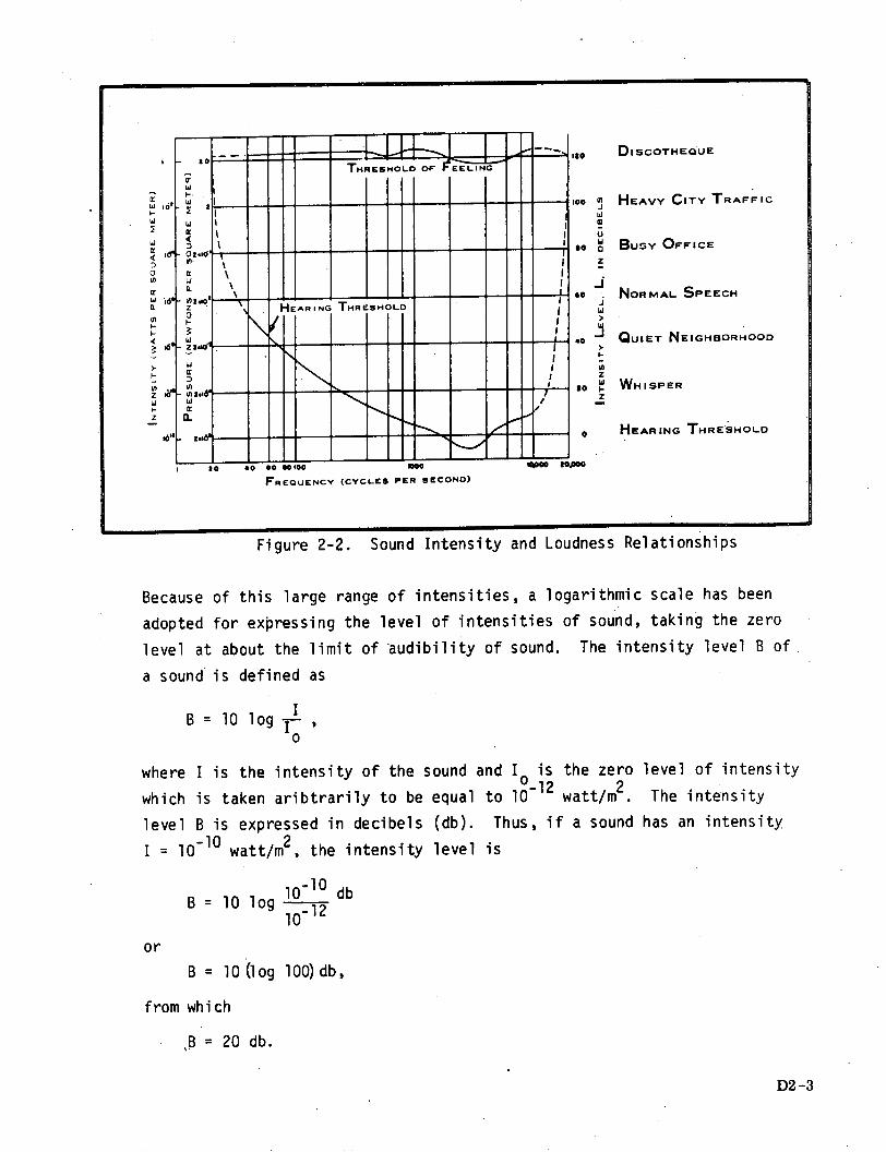
Figure 2-2. Sound Intensity and Loudness Relationships

Because of this large range of intensities, a logarithmic scale has been

adopted for expressing the level of intensities of sound, taking the zero

level at about the limit of audibility of sound. The intensity level B of

a sound is defined as

IB = 10 logI ,

0

where I is the intensity of the sound and Io is the zero

which is taken aribtrarily to be equal to 10-12 watt/m2 .

level B is expressed in decibels (db). Thus, if a sound

I = 10- 1 0 watt/m2 , the intensity level is

10-10 dbB = 10 log 1l2lo-

level of intensity

The intensity

has an intensity

or

B = 10(log 100) db,

from which

,0 = 20 db.

D2 -3

o I __. I _ _ I_2 1 1 yIC EU E 'so

- I -.:F E2 II _os _m_ _ _ _ _ __ 100W HEAVY CITY TRAF'FICI-

w 6Wu

W' -z, O... \o __ - -o ° BUsY OFFICE

a Z

\w ,o w \ _ _ _ _ _ I _0 "._ ___ * NORMAL SPEECHo. z·> 0. - tQIEN I j

0. Z __ g HEARING THRESHOLD

( - >

wI w

z -'° -W

I- :) / Z

- Ia t0FREUENCY WHISPER,., IZ

z EL

J6'". 1.16s ~ / · HEARING THRESHOLD

tO 4 0 So II00 Sao goo" 0,000

FREQUENCY (CYCLEB PER SECOND)

-~~~~~~ ~ ~ ~ I --

TI=I L4-. DISCOTHEQUE

Sound levels have been measured at various places under a variety of

conditions. For example, inside a busy office the sound level is about 80 db,

while the sound level of a whisper in a quiet room is about 20 db. Figure

2-2 also presents some common comparative sound levels.

2.2.2 FREQUENCY BANDS

In practical application, the noises encountered are rarely pure tones.

They are rather a jumble of sounds ranging from low frequency roars to high

frequency screeches. In order to measure this composition of noises, a

frequency analysis is made which displays the sound energy distribution over

the noise frequency range. This analysis is made with filters that sub-

divide the sounds over the entire audible range into standardized frequency

bands, permitting one to measure the pressure levels of only the sound with-

in each subdivision. The filters derive their name from the fact that each

one spans an octave; that is, the upper frequency limit is twice the lower

limit, as shown in Figure 2-3. Sound levels in each octave are measured

in decibels, and are referred to as Octave Band Levels.

For more detailed analysis of the distribution of sound energy as a function

of frequency, narrower bands are used. One popular division is to split

the octaves into three parts (1/3 octave bands). For special applications,

as will become apparent in this handbook, still narrower bands of frequency

must be analyzed to capture needed discriminant information.A - .- - -

Figure 2-3. Octave Bands

BAND BANDESIGNATION LIMITS

(CENTERFREQUENCY) -11300 Hz

8000 Hz-5650

4000-2830

2000-1415

1000- 707

500-353

250-176

125-88

63 Hz44 Hz

D2 -4

2.2.3 STRUCTURE BORNE SOUNDS

Structure borne sounds include all noise propagated through structures which

generate their own vibration or sound signals through active motion of com-

ponent parts. The Structure Borne Acoustic test technique is limited to

the evaluation of this type of sound. Air propagated sound is excluded

because of high attenuation and extremely low penetration at any metal

interface. Also, air propagated sound has greater variability due to

factors such as temperature, air density, and humidity that are impractical

to control 'in a launch checkout environment.

2.3 STRUCTURE BORNE ACOUSTICS AS A METHOD OF ASSESSING MECHANICAL DEVICE

READINESS

It is well recognized that to achieve high and predictable reliability for

a mechanical system, it is not sufficient just to build it from high quality

components. Many defects may be initiated first during assembly or during

qualification tests. Such defects, which are not connected to component

quality, reduce the overall system reliability. It is essential, therefore,

that effective methods be available for non-intrusive checkout of a com-

pletely' assembled product from the outside, before it is finally accepted.

But high reliability of a product may only solve part of the problem. What

is really desired is high availability, i.e., short total down-time for

maintenance or repair as compared to effective operating time. There are two

general areas, final component or system checkout and early fault detection,

where effective diagnostic and readiness assessment techniques can signifi-

cantly increase total availability. In both cases, the central problem is

to evaluate internal conditions through external measurements, without dis-

turbing the normal operation of the tested equipment.

Obviously, external detection of internal defects presents new problems

compared to conventional component testing and inspection. This is par-

ticularly true for mechanical defects. Internal cracks, loose bolts, worn

bearings, etc., are no longer open for visual inspection or direct measure-

ment. Therefore, an information carrier is needed to transmit the internal

information to the external evalualtor.

D2 -5

Sound and vibration are excellent information carriers in mechanical struc-

tures. The fundamental mechanical events which occur in operating mechanical

devices, such as rolling, sliding, impacts, etc., all produce sound of some

kind, which tells the experienced listener much about the internal condition.

Listening is really one of the oldest of all evaluation methods, basically

because it does not require any instrumentation at all. A mechanic listens

to an engine to determine its condition; or he might hold a screwdriver against

a bearing housing to detect a malfunction in that particular bearing. Direct

listening without special instrumentation is extremely useful for early mal-

function detection in many cases. Very often changes in sound signatures

precede the actual performance deterioration of machinery, which can be

detected through other means. The sound from an automobile engine for

example, usually tells about a faulty valve long before it is detectable

through oil pressure and power output changes.

However, this kind of intuitive evaluation is more an art than a science.

It requires a certain skill, which often is very high, on the part of the

listener and the result is not amenable to quantitative definition. To make

acoustic signature evaluation really valuable as a modern screening or

failure prediction tool, much had to be added in terms of problem definition

and mechanized evaluation.

A significant amount of work has been done (see Literature References,

Appendix A) to advance the science of acoustics, mechanical signature analysis,

and digital electronics during the past decade. This progress has made it

possible to now formulate a methodolgy of which enhances the practicality

of larger scale implementation of Structure Borne Acoustics to achieve

Mechanical Systems Readiness Assessment.

2.4 STRUCTURE BORNE ACOUSTICS-A NON-DESTRUCTIVE TEST TECHNIQUE

The total non-destructive evaluation or test technique for assessing the

status of a mechanical device includes the method of stimulating the device,

the response resulting from the stimulation, the transducer for communicating

the response, and the hardware and software used for data processing and

evaluation. Figure 2-4 depicts the interrelation of these elements.

D2 -6

Elements of a Non-Destructive Test Technique

The definition of Structure Borne Acoustics as used in this handbook in-

cludes all of these elements of a non-destructive test technique. It in-

cludes detecting and converting mechanical device noise into an electrical

signal which is then processed, interpreted, and presented in such a form

to provide go, no-go, or caution status of the mechanical device. This

complete process is referred to as "Structure Borne Acoustics."

D2 -7/D-, -8S

_ ___

I

.1

Figure 2-4.

CHAPTER 3

MECHANICAL DEVICES AND STRUCTURE BORNE ACOUSTICS (SBA)

3.1 GENERAL

Structure Borne Acoustics as defined in Chapter 2 is a technique which canbe applied to most noise producing mechanical devices. However, SPA, usedindiscriminately, will result in undue complexity and cost with questionablegains in the capability for readiness assessment and condition nmonitoringof mechanical systems. Therefore, the implementation of Structure BorneAcoustics should be based on due consideration of cost, complexity (usuallyclosely related) and adaptability of the technique to the readiness assess-ment requirements of the specific mechanical device. Consequently, prior toimplementation of SBA, the applicability of SBA to the readiness assessmentproblem must be evaluated.

It is this consideration which will be examined in this chapter. Guidelineswill be provided which will identify those mechanical component applications

where SBA can provide sensitive, selective, economical, and perhaps other-

wise unobtainable diagnostic capabilities.

3.2 MECHANICAL DEVICE CATEGORIZATION

3.2.1 GENERAL

Categorization of mechanical devices into groups of similar characteristics,either acoustically or mechanically, is necessary in order to define theelements of SBA technology applicable to different devices in more specificterms. The categories which will be defined and examined are:

o Mechanical system, device identification.

o Active and passive mechanical devices based on physicalcharacteristics.

o Active and passive components based on acoustical characteristics.

o Cyclic machinery, flow noise and single transient generators.

D3-1

ISO I

Is,

-is0*) t 'o40l4o

JSk I'SlJo) io

15- 40o003 '&#S#

J)$ loll II sI a l~~ (5 4n 0·10 4i

ft0lglneold *lfny

024010 0 II0

- '00(043 1m

uro l l

IlJ I1d

I IIo,~m)

in

.log

4d4 4/1

Hl 01401~, A/1

000111009 Alt

· eel40 A/1

0I t011fI I-j

,Irl lnllld r15

)0

11tN~J IS

0'1

0*

0f·l 0(/0

0ol0. N) S/Il

......... I ni I

I - I I I - m q - . . . p.. I I I -

Glii 0

I--

,- ,..4

it

IN

-4 - -l- HI ~~~~-- H00II -I ~ lJ

" ~ ~ ~ ~~ ~~~- ,. .- -eilq 111[~~~[lI

04

04

1-

Table shows a count of 7,114 activedevices and crawler, for one launchpad, portions of one mobile launcherand one launch vehicle. Mechanicalcomponents located upon or withintwo launch pads, two crawlers, threemobile launchers and all vehicle,spacecraft, and associated mechanicalGSE would total in excess of 20,000.

I"' I!! i !!!!iiii!ijIi!LI.I-.- ...-.-.....I ]-Il 11 ) I1 I I IiH= I I 1 Ic I tIl I-~ I11 t Z! I~ -1111qllllql1. -#4 00

-' n, Ift I. .. I I I I I I I -qllI

..... - -- -I- I~ - - -lllI~ ll0........ i 1 I I 11 -

......ni o ... .I I I II:A )ll..... 'IS .. * @ I

..... v .... + * I IiiN I

'" ~ ~ ~ ~ 4 - I - ~ I9 ·9 161 Y I I - E~II 11 1·121 h lll qI Ifi(4n~~aql~~~oaj ~ ~ ~ ' 1 I-I I 1 t-

...... "Oy , .,I I- i 1 II 1 11t1111I t. i l0Z............ ,,, 1. II1414uls l l I I I la11 J I I : f

............ ' ' 1I· ""l"lM I I i I"". I0I 4l4 J--JeJ

ll~~~~a~~~fl0,01,1~~~~, , , , ................. ~ ..

1fl10$01001] 1 fl ~ d IIIIIi P f I IIII I IilllI1111h~ o b

- - -- -N L

I 3iiI i 1iJ i ti. !i1

Table 3-1 LC-39 Mechanical System/Mechanical Component Matrix.

D3-2

I1r"r-�-�-Cp-

�·I�Bp�·�Eli�Bs�prr�-�·ri;nii�-· �

tpn

I

3

4

I

14go

4I

k

I

J

2,

i

I

z�

II11

I

i

i

i

i

!

iiia I!i

3.2.2 ACTIVE/PASSIVE DEVICES

A study of Saturn V Support, Facility, Launch Vehicle, Spacecraft manl Medhml-ical Ground Support Equipment Systems has shown that over 20,000 mechanik:al

devices wereemployed for this program. The distrillitio, lw ywuh;:l .',:I

and component type is shown in Table 3-1.

A review of mechanical component symbology, (per vMSFC-STD-162A, Figure 3-l)shows

that mechanical components can be placed in two categories:

1. Active mechanical

2. Passive mechanical

Active components are "items that have a measurable output or influence upon

the performance of the system." Mechanical components having moving parts

would, in general, be classified as active mechanical components. Passive

items such as pipes, bleed plates, and couplings were not tabulated.

Acoustical signature analysis techniques have been applied to a number of

problems in the areas of product assurance and "on-condition" maintenance,

(i.e., maintenance upon detection of an incipient fault). Application of

these techniques have been generally resolved into two component categories -

active and passive.

An Active Component is one which, through normal operation, generates a

vibration or sound signal which can be correlated with internal operation/

condition.

A Passive Component is one which must be stimulated, vibrated, or impacted

to produce a sound signal. This technique is useful for determination of

structural integrity, detection of loose particles, internal cracks, loose

fits, etc.

This handbook is addressed toward active component acoustical signature

analysis. Active systems which have been investigated through acoustic

techniques include many kinds of machinery and components such as combustion

engines, gear transmissions, pumps, fluid valves, and ball bearings. All

generate their own sound signature during operation so that fault detection

through listening, becomes passive.

* Addendum A, Section I, Reference 32

D3-3

1 t -Z- - C a, a m-I S Itt = = =-a 4 , a -. a.E* F,~ 055i N N- 7

r I - - ,

a , . _N -:,

5 - -- =-_ _- a_ t .J

V6 7 , _ :, I' -0 00 OC a Ia8f~ ld~

zr=I I8a -

!. Z

_- -a.4 IaCa .. s g vo__ J-< __

i r

2

- . 3.5S i° sZ i;' I_ _ - . _!

ttiltllelkli i I Hf W~ '=

*"~ AP

Ng N-·~ a.

a4~a CCC~ N N N

a CC a a

_ 2 t 2 *, ,. 2 4

I I .9 .-

'' t *.

a.- i e ' ,--.s ; d S

a- - -, -C a, -

e.l 4I. I to 21 1 (; 2

S*c a a .., 52 a· -a

- C- o - :

- o Jz - ,, r

Sn _ O~ E5 Z8 wsa J7 t

_ _-- _ C- =- .0 . a.

N-a C~ C ao a ' r- '_

-F9;7;1 t~ X4CC N *- . C - C

-: 6 . _;

za! . _, ..,,

·1+

3 Pt:

TD,*

o

Y YI

5 - a

C8 5~1 r

3 3 -

:u _i _r '; 8

r r dw . te~

- .

g. _ 55S;fN.N

YzNa''"j°a g_ 'Yo g ,f'io3~ o.

S I

I -I I? I i

|i 9 | a |

C4

V-

LIHI_I5 I

a5 ° a _:; 3;_ I _

.1 :;

_ _

94° :_ _I ._ _C

_ _

8 °

a- I.

-.

I t

ago

- Si

- -I mo B aZo .. o .1 o .-

I 1Ir. - .- .'f t

t :- 2 - !

_ _ 5- a -O

O ,a _ _at JO

., 1- O °__,:o o~ r~ x S v]; ~ ! i -.- H .Z -- .sa

I Iaa fl1

88 h P

Figure 3-1 Mechanical Device Symbology

D3 -4

a(

aI

V

T

o _

_ ae _-

- Z.

I I

_a rI .~ ._ .4 N

HV-

_ _

I

3.2.3 CATEODRIZATION BY ACOUSTIC CHARACTERISTICS

In the discussion of active component analysis, it is convenient to separate

components into three groups:

* Cyclic machinery (e.g., engines, transmissions)

* Flow noise generators (e.g., pumps, boilers)

* Single transient generators (e.g., valves)

Different characteristics in the signature generation process have resulted

in different analysis methods for the three groups.

Cyclic Machinery - In cyclic machinery, the operational events repeat at

prescribed intervals. For example, in a four-stroke engine, the repetition

period is two revolutions of the crankshaft. It would be logical then to

use a detection method which enhances all features in the raw vibration

signal that repeat every two revolutions, and discard everything else.

Sound and vibration data recorded during the operation of engines, bearings,

and generators are complex signals usually containing a high background

signal level.

Digital summation techniques have been found to be an effective tool for

detecting many internal malfunctions in cyclic machinery. This technique

is predicated on the fact that a particular acoustic peak, through its

location in a summed vibration signal and knowledge regarding engine

kinematics, can be related to a particular event in the engine, resulting

in a highly selective technique.

Flow Noise Generators - Fluid in a dynamic state produces sound due to motion

of fluid in a pump, boiling in a reactor, motion through a chemical process,

etc. Sound, traveling easily through a fluid, can propogate information

about a condition' at a point to where the information can be detected by an

acoustic sensor.

Sensor data can be analyzed in real-time, producing a spectral analysis of the

studied signal, with a very high time resolution such that a three dimension

frequency - amplitude - time display is obtained. This display permits a

study of the !spectral content versus time.

D3 -5

Single Transient Generators - This third group of active components includes

relays, valves, etc., which have a short work cycle and usually generate im-

pact transients while operating. Depending upon the particular operating

characteristics of the device, either time domain or spectral analysis, or

both, may be applied to these devices.

Having once secured the component acoustic signature, there are a number of

discriminatory techniques which can be utilized in conjunction with or

rather than signal summation and spectral analyses.

3.3 READINESS ASSESSMENT PROBLEM

There are over 20,000 mechanical components located at Complex 39 in Saturn V

ground and flight hardware. Future manned space programs such as the Shuttle

are expected to require a comparable number of similar mechanical components.

Based on reliability, effect of failure, cost, complexity, and the present

state-of-the-art, it is clearly impractical to instrument all these devices

for readiness assessment. Therefore, a rational selection process, based on

these considerations must be established.

Having once established those devices for which some form of readiness

assessment is required, identification of the assessment technique to be

implemented must be determined. Structure Borne Acoustics is one of a

number of non-destructive test techniques expected to be applicable to

readiness assessment requirements of future space programs.

Operational usage of acoustic information requires identification of the

significant device parameters which characterize normal and abnormal opera-

tion and applying (in most cases) numerical limits as a basis for Go, No-Go,

or Caution decision. For example, bearing noise is a device parameter which

is closely related to device condition. Go, No-Go, and Caution decisions can

be made based on bearing noise established through testing or from trend

information developed from on-line equipment.

D3 -6

The designation Go, Caution, and No-Go, as used above to indicate compoent

status will occur frequently in this handbook and are defined as follows:

GO - The component is fully operational and no degradationhas been detected.

CAUTION - The component can perform the intended function withinoperational limits but performance degradation hasbeen sensed.

NO-GO The component is not capable of performing within normaloperational limits.

3.4 DETERMINATION OF STRUCTURE BORNE ACOUSTICS APPLICABILITY

3.4.1 COMPONENT CRITICALITY

The first readiness assessment question which must be faced for an opera-

tional mechanical system, is"which-are the more critical components in

this system?" This, of course, presumes that the system is of some criti-

cality and that a reasonable readiness assessment budget exists.

Techniques of some rigor exist which will guide the designer in identifi-

cation of component criticality on a relative basis. Considerations involved

in the ciriticality determination include:

* Potential effect of mechanical device failure in the relevant

failure modes.

- Effects descend in severity from loss of life, mission

scrub to no adverse effect.

* Probability of the most severe effect occurring for each relevant

failure mode.

* Probability of failure for each mode.

* Time in which the considered failure mode and effect hold true.

· Failure rate of the mechanical device.

KSC-STD-122 provides a methodology for integrating these Considerations and

providing a quantitative result - criticality number. Comparison of the

criticality numbers obtained for the various parameters, e.g., failure mode 1

vs. failure mode 2, provides guidance as to the most critical combinations.

Comparison of the criticality numbers for two components will identify the

more critical of the two.

D3-7

3.4.2 STRUCTURE BORNE ACOUSTIC SELECTION

Having established the components which require some form of readiness

assessment, the next question is, "What type of assessment should be imple-

mented?"

Advantages/disadvantages to consider when evaluating SBA as an assessment

technique include:

Advantages:

s Technique is non-intrusive.

e Output may be automated.

e No couplants are required.

o Access to only one surface is required.

· Provides remote and continuous surveillance.

* Dynamic rather than static flaw detection.

* Permanent record of event status can be obtained.

o Equipment is reasonably easy to operate.

X Equipment is portable.

· Large amount of developmental work already accomplished. Theresult of this work can be directly applied to solution of theMbchanical Readiness Assessment problem.

o Signal processing techniques are available which permit discrimina-tion between needed acoustical information and undesirable back-ground noise.

o Availability of noise and vibration transducers with adequatefrequency selectivity, bandpass configurations, and sensitivityranges.

Disadvantages:

* Part geometry and mass influences test results; therefore, uniquedata interpretation required for each different component.

o Must establish reference data (Go, No-Go, Caution parameters) inorder to make proper interpretation from test data.

e Transducers must be placed on part surface.

e For active structure-borne acoustics, part must be operating.

a Extraction and processing of characteristic signals from noisebackground is complex.

D3-8

3.4.3 SPR APPLICAB I .ITY

Readiness assessnent throulgh Sl;\ tedclnliques has app.licatioti to al I c)' I i,components, a significant portion of the transient action components mid

limited application to flow noise generators.

An examination of SBA by mechanical device acoustic category; has shown the

following:

Flow Noise Generators - At any given point in time, flow noise in a pressure

regulator, for example, is a function of down-stream pressure which can cause

a flow from zero to a maximum. Therefore, knowledge of the downstream pres-

sure is satisfactory for readiness 'assessment purposes makirig SBA instrumen-

tation redundant. This, plus the absence of noise producing interactions

within flow noise devices, limits !the application of SBA to flow noise

generators.

SBA techniques do

to be useful, the

have applicationlto the detection of internal leakage, but,

detection threshhold must be at least lcc/minute.

Transient Action Components - Considerable information regarding the readi-

ness of transient action devices may be obtained from the SBA techniques.

The basic amplitude domain data (accelerometer output vs. time) can be readilyIprocessed to obtain (using a solenoid valve for descriptive purposes) valve

response time, either actuation or deactuation. Timing information for this

characteristic can be taken from voltage application (or removal) to the

acoustic impact generated at the end of stem travel.

Solenoid valve operation - actuation, deactuation, and response time may also

be obtained from a talk-back switch. If this were the only information

desired, the switch rather than SBA would be the obvious answer. However,

it is expected that SBA will ultimately be able to provide leakage informa-

tion to the lcc/minute level. This would make SBA a much more attractive

form of readiness assessment for solenoid valves and, generally speaking,

transient action devices as a component category.

D3 -9

Spectral analysis of acoustic data provides a time vs frequency plot and

displays amplitude in a form similar to intensity modulation. Figure 3-Z

shows such a plot of solenoid valve actuation and deactuation. The first

dark vertical band is due to the application/removal of the actuation voltage,

the second vertical band of the deactuation trace is due to the position

switch opening and the dark vertical band on the right is the stem to seat

impact. Note the valve body ringing in both plots at approximately 11 KHz.

This resonance was predicated by the mathematical analysis.

Cyclic Components - Structure-Borne Acoustics has wide applicability to

cyclic component readiness assessment. SBA has capabilities which are

economical and practically unobtainable by any other assessment technique.

3.6 SUIMARY

Summarizing the methodology for choosing Structure Borne Acoustics over

conventional forms of mechanical component Readiness Assessment:

a. Assure that the component is an active mechanical device.

b. Assure that the component is of a criticality which justifies

readiness assessment.

c. Establish that conventional instrumentation is inadequate.

d. Determine that the specific discriminant(s) (measurement parameters)

are amenable to SBA techniques.

D3-10

CHAPTER 4

MECHANICAL COMPONENT ANALYSIS

4.1 GENERAL

The SBA methods which may be used vary within a wide range. It is not aquestion of developing any particular sound analysis technique or instrumenta-tion; rather, it is to use all that modern electronics has made available,including digital computer techniques.

The problem is to detect an internal defect while it is still smalland its characteristic sound or its signature is hidden by sound from manyother sources. Therefore, a selective technique must be developed in each

application to extract from a complex sound or vibration signal some character-istic feature, or discriminant, whiclh is highly correlated to the internalcondition under study. This means a technique with the ability to sort out"False Alarms", including high backgr ound levels, and thereby reliably

reveal a very small signature change.

It becomes the central problem to find this most effective discriminant ineach application. Several approaches are possible.

One is entirely statistical. If a su'ficiently large sample of signaturesfrom good and malfunctioning units is \available, it is possible to evaluate

a large number of discriminants and through a correlation program andselect the one most effective. The s lccess of this approach dependsentirely upon a good statistical sample. In most cases, such a sample is

difficult to obtain.

A second approach, which forms the basis of the analysis methodology

recommended in this handbook, is based understanding the process bywhich a particular signature is generateo and transmitted through a structure.This usually requires a thorough study of the mechanics of the equipment to

be investigated so that a model for normal and abnormal signatures can be

established. Once this is done, an analysis method with a good chance of

success can be selected and then optimized experimentally.

D4-1

I�1

This approach offers the outstanding advantage that only a small number of

tests is required. Valuable also is the fact that, if a partly effective

method has been found, the theoretical knowledge gained enables one to

predict how the method must be changed to improve it.

Experience has shown that the key requirements for success are:

1. Understanding the mechanics of the equipment generating the

signals, the failure modes, and failure mechanisms.

2. Understanding the process by which normal and malfunction

signals are generated an'd propagated and predicting the

resulting acoustic signature.

3. Correct selection of a esponsive transducer.

4. Based on Requirements 1 and 2, correct selection of a technique

which extracts the desi ed malfunction signature from the raw

vibration data.

The first two requirements constit te mechanical component analysis and will

be examined in this chapter. The remaining two requirements are treated in

later chapters.

4.2 COMPONENT DESCRIPTION

In the beginning phases of implem nting the SBA technique, knowledge of the

component can significantly redu!e the time frame for implementation. This

is accomplished by elimination of unnecessary data collection and false

starts through a thorough engine ring analysis and verification of analytical

work by pre-operational testing.| As knowledge is gained from analysis,

testing, and operational experi nce, testing can be further reduced by

examination of only those uniqu characteristics of each device.

Source documentation which may e used for component evaluation and analysis

is available in many forms as indicated in Table 4-1.

D4-2

System Functional Drawings

System Sqhematics Operating Records, Logs

Installation Drawings Environmental Records

Interface Control Documents Technical Manuals

Operation & Maintenance Manuals Failure Reports, Summaries

Failure Effects Analysis Studies Relating to MechanicalSystems

Operation Procedures Vendor Data, Technical Reports

Launch Mission Rules Kennedy Approved Parts Lists

Test Procedures Component Operational Profile

Test Reports

Table 4-1 Component Source Documentation

4.3 OPERATIONAL ANALYSIS

4.3.1 COMPONENT OPERATION

The component to be acoustically instr umented must be examined in detail to

establish the physical interactions whi ch take place not only during active

motion of internal elements, but preceding and following internal flow, motion

of internal elements and the forces whi ch produce this motion.

Considerable insight into component oper~ation is possible through correlation

of component test procedures (of the type used for component checkout following

overhaul) vs. what takes place during checkout and adjustment. Test pro-

cedures of this type specify those parameters of significant value in

determination of component condition as well as specifying nominal values of

flow, pressure, temperature, operating time, leakage, position ,et.al. These

values form the basis for Go, No-Go, and Caution parameter values which must

be obtained by the SBA techniques, perhaps in conjunction with other system

instrumentation.D4 -3

I

Specifications

The purpose of this analysis is to:

o Provide an intuitive "feel" for component operation.

o Assist in the identification of noise-producing interactions.

o Assist in the correlation of acoustic signature with the physical

operation of the device.

o Provide insight into potential failures and the effect of failure

upon the acoustic signature.

4.3.2 INTERACTIONS CONTRIBUTING TO ACOUSTIC SIGNATURE

A composite listing of interactions within mechanical devices which con-

tribute to the overall acoustic signatures follows:

o Medium Flow - e.g., hydraulic oil flow through a flow control valve.

o Activation Medium Flow - e.g., GN2 flow causing an LH2 valve to

operate.

o Switch Activation - e.g., a solenoid valve talk-back switch closure.

o Background Noise - Provided by adjacent interactions, flow, impacts,

machinery operation.

o Surface-to-Surface Interfacing - e.g. ,rolling of bearings, relative

motion of two contacting surfaces (sliding), impacts produced by

sudden, forceful surface-to-surface contact.

o Body Ringing - Produced by irpact forces within the component.

o Electrical - Produced by vibrating solenoid turns or core laminations.

o Air in the flow or actuating medium - e.g., pump cavitation.

o Cold Shock - e.g., chilldownlof cryogenic piping.

Using again, for illustration purposes, the example of the solenoid valve

(See Figure 4-1) (75M08825-3), the mechanical interactions which contribute

to the acoustic signature during actuation are:

o Impact of the armature (17) against the coil and core

assembly (26).

o Armature (17)/Plunger (27) contact.

o Plunger (27)/Switch (28)'contact.

o Stem (30)/Nylon Seat (34) impact.

o Secondary ringing of valve body (36)

o Flow f

In addition to the above, some background noise is expected.

D4-4

4(

'-4

.4C)

Q)

._

D4 -5

4.4 COMPONENT ANALYSIS

4.4.1 MATHEMATICAL ANALYSIS

Analysis of components, particularly those cyclic in nature, require mathe-matical treatment in order to understand the relationships of the internalnoise producing interactions. For example, the 70A-66 (reference AppendixB3) motor is a complex device with many ordered interactions taking place.For each rotation of the output shaft, the following interactions must berelated in order to understand the acoustic signature obatined:

o Piston excursion

o Swash plate rotation

o Gear meshes

o Air intake exhaust cycles

o Bearing ball rotationMathematical analysis also provides preliminary filter frequency require-ments which will allow display of a specific aspect of component operation;

e.g., a gear mesh frequency.

It is in the analysis of ball bearings where mathematical techniques havereached the highest degree of sophistication. Computer programs developed

at the General Electric R&D Center provide, based on physical characteristicsof the ball bearing:

o Acoustic frequency and relative amplitudes for a range ofnormal (no defect) bearings

o Repetition rate of transients for inner race, outer race

and rolling element defects

o Frequency and relative amplitudes for defects including:

- Off-size rolling elements

- Misaligned outer race

- Out of round outer race

- Misaligned inner race

- Out of round inner race

o Frequencies for in-plane flexural vibrations of the outer ring.

D4-6

A KSC report (Addendum A, Section I, Reference 38) contains a mathematical

analysis for two mechanical components - solenoid valve 75M08825-3 and pres-sure regulator 75M08831-1 which illustrates the process. These analyses,performed prior to acquisition of test data, were instructive but did notcontribute as much as was initially expected. In general, it was concludedthat a mathematical treatment of this form is necessary when frequency

domain data must be related to internal component reactions.

4.4.2 FAILURE'ANALYSISThe first step in failure analysis requires the acquisition of historicalfailure data for the specific component ard for generically similar data.

From this data, a rather comprehensive summary of failure information can beobtained. For the purposes of this discussion, the following definitions

are important:

Operational Effect - As a result of failure, is the component in a Go,Caution, or No-Go condition.

Failure Mocde - The form in which a component failure is manifested,

e.g., fails to operate, sluggish operation ,leaks internally, etc.Failure'Mechanism - Identifies the component piece part which mal-

functions and the specific problem. e.g., Valve stem mechanicallybinding'.

Failure Cause - The basic anomaly which produced the failure mechanisme.g., corrosion, contaminated,low input voltage, etc.

Three readily available sources of failure data are:

o NASA KSC Failure Data Retrieval System - A typical computer output

is shown on Figure 4-2. Unsatisfactory condition reports (UCR) listed

on the printout are available within KSC.

o FARADA - (Failure Rate Data) provides general failure rate data,

failure modes by percent of total failures. A sample page is shown

as Figure 4·-3.

o Malfunction Investigation Reports - Prepared by KSC SO-LAB-1 when

laboratory analysis of component failure is desired. These reports

can be correlated with UCR numbers.

Other excellent engineering analysis reports exist in the form of:o Failure Mode and Effects Analysis (FEMA) provided by various

reliability organizations.

o Vendor provided analyses and reports.

D4 -7

Figure 4-2KSC DE-SED-2 UCR Tabulation

UJCR P#?-?.-?-'75M08825', LIST P#&PN&R#&MFD&LOC&VEH&FSD&DDREQUEST QUEUEDPG 1 11/09/71 *NRN* VERBR LIST. OBJt P-"'75MO8825'.

PART-NUMBER PART-NAME REPORT-#MFG-DESC LOCAT VEHICLE FUN-SYS-DESC

DEFECT-DESC

75NM8825-3MAROTTA SCIENTIFIC

I NPROPER OUTPUT

SOLENOID VALVE KSC430733ML2 509 SWING ARMS - MECHANICAL

** A TOTAL OF 00q001 RECORD MET QUALIFICATIO0S. **ELAPSED TINE D 19.55 SECONDS.EJD OF REPORTREL P#?-='75M08825%, LIST P#&PN&R#&MFD&LOC&VEH&FSD&DDREQUEST QUEUEDPG 1 11/09/71 *NRN* VERB: LIST. OBJ: PI='75M08825'.

PART-mNU 3ERMFG- NAMEFUN-SYS-DESC

75M08825MAHOTTA VALVE CORP

N275408825MAROTTA VALVE

N275M08825/1MAROTTA VALVE

N275M08825IAROTTA VALVE

N275MO8825 alMAROTTA VALVE

N275M08R25MAROTTA VALVE

M2END OF PAGETHERE ARE 4 F$P*PG 2 11/09/71

CORP

C ORP

CORP

C ORP

CORP

PART-NAMELAUNCH-COMPLEX VEHICLE

DEFECT-DESC

SOLENOID VALVELC39 AS501

SHORTEDC SOLENOID VALVE

ML-I AS501IMPROPER INDICATION

SOLENOID VALVEML-1 AS501

LEAKAGESOLENOID VALVEML-2 AS502

WIRING ERRORC SOLENOID VALVE

ML-2 AS502

IMPROPER INDICATIONC SOLENOID VALVE

ML-2 AS502LEAKAGE

1PAGES IN YOUR REPORT

I *NRN*PART-NUMBERMFG-NAMEFUN-SYS-DESC

DOCUMENT-NO

KSC318195

KSC318569

KSC318578

KSC318604

KSC318790

KSC318862

k VERBR LIST. OBJt P#='75M08825',PART-NAME DOCUMENT-NO

LAUNCH-COMPLEX VEHICLEDEFECT-DESC

D4-8

A ,Jd

A

If ~ ~ ~ 0I

Oa J

.5

. . a .-. K

4 £ .R X4

rL I- z W la2) _ . Z ~CL

- J <.iZ V __r*i J 4 _ I

VI C- Z . 8.

- < Ni 4[ 04 Z

Z .. a M0 0 8

e2 0 iZl 4

B. 0Z hi k.1(Ala WI J04 8.4

O IK Z- 4 0*2<

z z _- 0 o z--

c Z 4 a: ao ~ <. o

a4 414 4KN~~~~~ 0 Eli · 04

idkd OC W ,w : -

- *L 44 -Z-.

- _ ZO1- o .iO

Zll < t. I t. N -- O -Q cc 0 u _

hi K Y4 .4 4 0 o .Y i o0- A. 240 -hits

O- z r -D,v--

10 .. o- <i -0 o

a e _ 0 e 1 0n. - 0 0 -. ..

4 4-a I .4. M2 I -- W'4 a < U- *4 e u

.i . ~ _2 . _ yZ 4 4

-A 4 r Uh 0 l s M AA CL IL IJ I ahiN A O - a Z -

ho2 24W4l I' 00 allK -C.. 4 K2 00v z~ Z Ofv ~ 0 ~ v -J.~ *~. J

-J J _ & l IJ ~l Z M O~ Ok O k ~

hi __J. N -J4 _5 4o K" 00

il~~~~~~~~~ mC. .Io ll.. N C4o ~laloaal.I (MD - ~l | *~II *..I_ t OO

4~~~~~~~~~ ~1-- 4' jN 404 .40 *N--

-0 F ->~ I i. - - 4 Y r O r8.* X z r o Y ~~~~ ~~~Z t s is W a F u

Nt. Qm < Z 4 0 b

nL a it W W W a z z %/zzJ aWW )g U U U be r4 22 20OW MOV IS. EW4. .. jh.IC U

A L A xz -A 0. 42 In2 00 -i A K

P4* ** K Or N. _ _ N

44 WhlS - hi Q v t: -. 4 4-4 4 s* n - u

> -O - W - - -'2 - S I n N NNN 5 * N -

ID . L~ * _ . , O Z , .1C ' .

Z V i.Na.. j Kt.I 2 4 3 0. _ Z / 1 ° ' ° V

NS~~i..Z4144!...* 410~~u .0.0.. W

K - KC Z -- hihi KC 4 -_ .aC-Z _ 22 IC . Z 0

° & hi 4 -. ')SS L.-Y< <- r … -< h< C<

Z J 1h W - _ J -- 1>Jhi~h 2S.04S-hiJ Z VShI 0 ( A

- ~JJur .. JKr oo vO oo 0 e J J J O J4

4~~~~~~~~~~~~~~~~~~~~~~~~~~~~~~~4 0 C4

rs~~~~~~~. C.A 11t IA - -a -4 -- - x I t- ¢-

4044240 4A 4 4[ 444 4 4 [

I )U'-J4- )W-I3A4 4 N

Nfl44g .1 I 0 44-I 4

w4.*g~~~SA N4' 4~~ (A A

A N 0 I A

a a a L"0 0 C

i h K hi hiJ

I 0la W WWO5 4W

g~~~~~ L a, U w a < d

a, ~ ~ r, O M r.- r~ 0 en z0c

I£ N w-. < 2 K

IL.2 - 4 Vt0O- An 4 u-F -.1 z0 A hi VSi. 0 O A-- >^

O0 0h Ol 41 O4 .@ <z -"- UA-. -_ -04 O1*Z! N Ch N< < nNC n JN rla -B O re

nARW 0nl nn a. N . - <0 .S r W ro U hiNIo o0l.

r n WIA - °n- 2 Z~ h nSBhO hi e.I2 hhiA*044Kn o<

20-0-0-- N4 N 41. _.L...0N Ji SA N _ IoWrr |_

4 8. * 4K| <- r .l _ I * 4 I U n n :Ilz |-

o** O 4 * *~' -' -soouv .4 a -. r1. - _ 4n _4IT W , P1 4 40 N N I I N MO 0 4 0 44 A W I 1 0~N Mt1P1 e-n r L r l r. r . r. r. r C D 00 ~- OD 0 0 0 04 M M 4 .4 O Ln r

40 40 0 ID 40 0 _ 0 40 4 0 O 0 4 0 _ 0 40 . 0 40 40 _ r, r-t r-. r ._ .N r-1r_ r-r- r_-4 - - - _ 4-4~ -4 - _- -4 -- _- -_4 - _ 4 - - _-- _ -

-4 -4 iM4 - -4 -.-4/- -4 -4 -.

D4 -9

- Z

z .i* - aI &.,)

* e* - .4

* r -

* 2Z* 3

a,. -oN

· 41 .

* J

* rLU* O O O

. Z

k,. ~f _

II 4£QI,41..'

* u.5

I In o

I o 00

* -44z

F h.z O

,,.J z _-** z NZN

! Z "0 .

14.* -00

1Z

~ .J .. Y

5| 'Y A

:~ ~ KA

!0+0

41

W

hi

Jel

40

0

4

-n

4o

i.

_ <

z.'

-]

-

1..:

.J

*4

r,

_

_4[

ONa

N

u

3~

)-

v

u

U

u

4

1.

0

uhi

,1(

r

3,4t*v

<,_..J

rro 4

n .D

N) h_

8.J./'1 :

Z

elO

hi

A ;U~4

0

IJiN I

0I

o I

_ 1

LU

a La

:

D

W21

7i ar°S

'I

< 5

A :

~.USr *

US

I--

2C

1-- @

Z a

_5 a

O

O A< a

Ni%,

3.5

o rZO

rzo u- Z

a)bD

U

¢

a)

P4

C1

c~

C)

1a)

co

I

--4

-J

4(Ic.

I

I

I[

I

I

-i

0

1.

z

a.

vhi!

I-z_

C40

o~z2° '7

M ~M

_ 0M- -A.30 w'3l

l e

I Z .7 h.0 K o1..

N -oN_An N K:

02 1 t

I* r .:-4v4 < 4n_N r N

From the above literature ,sufficient information, in conjunction with the

designer's own analysis, is available to identify operational effects,

4.4.3 FAILURE MODE TREE

A graphic form is recommended to consolidate and display the information

obtained in the preceding analysis. One such form, a failure mode tree is

shown as Figure 4-4. This form evolved as a variation of fault tree and

failure mode analyses described in reference 34 of Appendix A.

The uppermost branches of the tree describe the operational effect,Go, No-Go,

or Caution ,expected due to the failure modes of the second row. The failure

mechanism identifies the piece part which failed and the specific problem.

The bottom branches list the causes for the identified failure mechanisms.

Note that the failure mode row identifies that information desired to

establish the condition of, in this case, a solenoid valve. That is, if

the valve actuates or deactuates when commanded, in the proper amount oftime, without leakage, the valve could support an operational exercise.

Proper operation of the switch inspires confidence, but would have no effect

upon component operation under the above conditions.

4.5 COMPONENT ACOUSTIC SIGNATURE (SIGNATURE PREDICTION)

4.5.1 GENERALFamiliarization with the internal operation of a mechanical device

identification of the noise sources, permits construction of a predicted

acoustical signature. Once this predicted signature is established for

component normal operation, modification of Ithe envelope due to various

component failure modes can be evaluated.

4.5.2 NORMAL OPERATION

In order to predict the effect of a malfunction on the acoustic signature of

a device, it is necessary to understand the device dynamics and failure modes.

The first step is to develop an acoustic si nature model for normal operation.

Alterations of this normal signature due to the various failure modes can then

be examined.D4-10

c~

Go

o

I,

0

0

I

0

a);-4

F4

D4-11

Taking the above noise generators and ordering their sequence on a time basis,

a plot of relative amplitude (envelope) vs. time was derived. This predicted

signature is shown in Figure-4-5.

Figure 4- 5. Solenoid Valve Signature Prediction

4.5.3 FAILURE MODE OPERATION

Having established those elements which contribute to the overall acoustic

signature for component normal operation, modification of the signature due

to identified failure modes can be accomplished.

D4-12 a

5

4

3-

0)

10 20 30Time (Millisecondi

Actuation End ofCommand Motion

Notes:1. Background Noise.2. Flow Noise, Armature/Plunger Contact.3. Stem/Seat Impact, Plunger/Switch contact.4. Armature Slap.5. Ringing.6. Stabilized Flow.

-_I

f

I

8)

As an instructive process, it is helpful to tabulate component failure modesand mechanisms (of Figure 4-2, for example) vs. the contributors to theacoustic signature identified in Paragraph 4.5.1. This results in a matrix(Figure 4-6) which assesses the impact of each failure mechanism on eachelement which contributes to the acoustic signature. With additional famil-iarity, the effects noted (normal, abnormal, none, etc.) become more definitive.

By modifying the normal acoustic signature prediction (Figure 4-5) per theanticipated changes identified in Figure 4-6, predicted signatures for variousfailure modes can be constructed. Figure 4-7 shows sample presentations forthe solenoid valve.

4.6 SUMMARY

Analysis of component operation, functionally and mathematically, providesa systematic approach to understanding the mechanics of the noise generator,the failuremodes, failure mechanisms and the noise producing interactions.This, in turn, permits construction kof a predicted signature, for both nor-mal and failure mode operations.

Analysis of.the component for normal and failure mode operation is accom-plished in order to relate the acoustic test data to the physical eventstaking place. Identification of the resulting signature characteristicsfor normal and failure mode operation can then be applied for making com-ponent Go, Caution or No-Go decisions. The component analysis also aids inselection of the optimum measurement technique for extracting meaningfulacoustic parameters. Thus, it is concluded that the component analysisprocess is an important step and should be a definite part of methodologyemployed for implementing SBA.

D4-13

lu 7

111111o0 o ,

Z tZ=oP;

; I la I) I

z z ¢~ o X2 z . : .p -z

;.0

C)

O

'- aC4

-

-

a:

;z~

H

0a s

.0 ao

3 0

c .C0

0.

.E!

Y s

S _8 ' e.az

$4

-4Cd

a,

2

0

._

w

a) u

c

s- C

FAQ,

-0

C)

C)

i 12

0

D4-14

0

0

3

o

U)

0

4) 4 )

C~~~~~~~~~~~~~~~~~~~~~~~~~~~~~~~~~~~~~~~C0~~~~~~~~~~~~O u~~~~~~~~~~~~~~~~~~~~~~~~.F~~~~~~~~~~~~~~~~~~~~~~~~~~~~~~~~~~~~~~~ d~~~~~~~~~~~~~~~~~~~~~~~~~~~~~~~~~~~~::4)~~~~~~~~~~~~~~~~~Qo ,.

4)~ ~ ~ ~~~~tcn

W~~~~~ I4)

0

4)~~~~~~~~~~~~~e

0M

4)."'4.)~~4

"o 0

,,4)

C D

cd4

D -1

0~~~~~~~~

~~~~~~~3 ~~~~~~~~~~·c

'4 I I D 41

r~~~~~~~~~~~~~~~

CHAPTER 5

THE "MEASUREMENT" SYSTEM

5.1 INTRODUCTION

The factors relative to the selection and use of a SBA measurement system

are discussed in this chapter. The test equipment necessary for Structure

Borne Acoustic implementation can be grouped in three broad categories, Data

Acquisition, Data Processing, and Data Display. This equipment makes up a

standard "Measurement System" with the elements as depicted in Figure 5-1.

For on-line, automatic non-destructive testing, the tape recorder can be

removed from the test loop.

Measurement System

D5-1

5.2 DATA ACQUISITION

5.2.1 TRANSDUCERS

One of the first decision points in the acoustic instrumentation of amechanical device is the choice of pick-up or acoustic transducers. Struc-ture borne sound is easier to interpret than is radiated sound since it isnot subject to the uncertainties of the vibrating surface's radiation impe-dances and the level of sound variations caused by temperature, air density,etc. Structure borne measurements, however, have their own problem areas,for example, unlike airborne pressure vibrations which are scalar quantities,structure borne acceleration and velocity are direction dependent.

If the full linear frequency range of a pick-up is to be achieved, caremust be taken when mounting a vibration pick-up to attach it ridgidly tothe object being measured. Resonances in the response curve introduced bypoor methods of mounting can be very troublesome when the pick-up is subjectto shock excitation leading to error signals, possible overloading of filtersand amplifiers, and difficulties with interpretation.

Transducers for the measurement of vibration and pressure employing electro-magnetic, electrodynamic, capacitive, piezoelectric or strain gauge principlesof operation are commercially available. Of these, the most widely used inrecent years is the piezoelectric accelerometer, largely by virtue of thefact that it is self-generating, is small in size and weight, can be de-signed to be free of resonances over a wilde frequency range, has good sta-bility, low sensitivity to strain, temperature variations, airborne soundand magnetic fields, a large dynamic range, low cost, and is not easilydamaged. It is this type of transducer recommended for SBA implementa-tion.

Choice of the proper transducer and its correct usage are critical to thesuccessful implementation of SBA. These factors are discussed at lengthin Addendum B. The Enaevcu Corporation instruction Manual for PiezoelectricAccelerometers (#101) is an excellent reference concering this type of trans-ducer and the majority of transducer data presented herein is excerpted fromthis manual (courtesy Endevco Corporation).

D5 -2

5.2.2 MOUNTING

For an accelerometer to generate accurate and useful data, it must beproperly coupled to the equipment under investigation. The method ofattachment must not introduce any distortion. This requires that theaccelerometer mounting be rigid over the frequency range of interest. Inpractice, many mounting methods are suitable for a wide variety of appli-cations and depend on the practical requirements of the test system.

5.2.2.1 Standard Stud Mounting

When possible, the best method is to mount the accelerometer with a stud

so that the entire base of the accelerometer is in good contact with thetest object. Care should be takeln to ensure a flush mating with a smooth,

flat surface. The mounting hole must be at a right angle to the surface.Ordinary machine screws are to be avoided since without a flange or shoulder,it is possible to "bottom" the sqrew in the accelerometer, thereby changingits dynamic response and, in som/ cases, causing damage to the unit.

5.2.2.2 Insulated Mounting Studs

Insulated mounting studs providI isolation of the accelerometer from elec-trical ground, and are particularly useful in preventing ground loops.

5.2.2.3 Cementing Studs

A series of cementing studs is available which permits accelerometer attach-ment to surfaces that cannot e drilled and tapped to accept threaded studs.

Use of these studs rather than cementing the transducer directly to the testspecimen will prevent contam lnating accelerometer mounting threads with

adhesive. Removal of the acc;elerometer will also be facilitated. Adhesivesshould not be scraped or sa ded off from accelerometer since a rough mounting

surface can cause poor freq uency response and/or an increase in transverse

sensitivity.

D5-3

Commonly used cements include Eastman 910 (Tennessee Eastman Company,

Kingsport, Tennessee), EC-1294 (Minnesota Mining & Manufacturing Company,

Detroit, Michigan), and Epon 828 (Shell Chemical Corporation, New York).

Dental cements, such as Grip (L. D. Caulk Company, Milford, Delaware) are

useful when the mounting surface is irregular or when the transducer will be

subjected to high humidity or immersion. Efficiency of this technique

depends entirely on the adhesive used, thorough evaluation is recommended

for the individual application. Remove Eastman 910 Cement with N-Dimenthlyl-

formamide.

5.2.2.4 Application Notes

Poor accelerometer mounting surfaces will! result in unreliable data. It is

recommended that the mounting surfaces an tapped holes conform to the

following specifications. These are cons dered to be easily achieved by

following good machine shop practices:

Surface Flatness: .0003" TIR

Surface Roughness: 3

Perpendicularity of Hole: + 6 minutes

Tap Class 2

For all studs, the use of a drop of light il between the mating surfaces is

recommended when frequencies are above 5000 Hz or shock pulse durations are

short. If no oil is used, the mechanical c nnection to the structure may notbe rigid enough, and the resonant frequency of the mounted accelerometer may

be reduced by 5 to 10 kHz. This means that the rise in response at 10 kHz

for an accelerometer with a nominal 35 kHz r sonance can be cut approximatelyin half through the use of oil. This represe ts an improvement of 5% in the

frequency response at 10 kHz. No evidence of an improvement due to the use

of oil has been noted below 5 kHz.

D5-4

5.2.2.5 Effects of Mounting

In some instances, the very act of performing a measurement affects the.

system being measured and, thus, changes the nature of the data obtained.

With piezoelectric accelerometers, this may occur for two reasons: (1) the

fixture required to couple the accelerometer to a somewhat flexible structure

may introduce local stiffening which changes structural response, and (2)

the added mass of the fixture and/or transducer may change the system

characteristics. Effects due to either cause can be reduced or eliminated

by choosing as small and light an accelerometer as possible. Microminiature

Accelerometers weigh only a few grams and are small enough to approach point

loading in many cases.

For a simple spring-mass system, the effect of added mass is to reduce the

system's resonant frequency. The amount of reduction can be calculated

from the following equation:m \

-fn = fn ( -Jma + m

Where

fn = system resonant frequency.

A fn = change in resonant frequency

m = system mass

ma =' added massa

A more general approach to loading effects is based on mechanical impedance

considerations. Since piezoelectric accelerometers have nearly zero internal

damping, the apparent weight (and mechanical impedance) of the accelerometer

is constant at all frequencies from zero up to approximately 0.9 of its

resonant frequency and must be equal in value to its physical weight. Within

this range, the effect of the accelerometer on the structure motion is given

by:

D5 -5

a a msr 0ms + Wt

Where

ar = resultant acceleration

ao = acceleration without accelerometer attached

wt

= weight of accelerometer

ms = apparent weight of structure

This statement of Norton's Theorem indicates that mounting an accelerometer

will change the motion of a structure if the structure's apparent weight is

not large compared to the total weight of the accelerometer. For mostapplications, the effect of the accelerometer on structure motion is not

significant and the apparent weight of the accelerometer may be ignored.

5.2.3 CABLES

The cable which connects a transducer to its matching electronics is an

important part of the overall measurement system. It must transmit the

transducer signal to the associated signal conditioning equipment without

distortion or introduction of noise.

Noise can be introduced either by pickup from nearby electrical (or magnetic)fields or by internal generation due to cable motion. Since piezoelectric

accelerometers are high impedance devices, the pickup problem could be quite

severe. For this reason, coaxial cables are required. Generated cable noiseis eliminated by a special "treatment" which prevents triboelectric effect,

the primary cause of cable noise. Triboelectric effect can be represented

as shown in Figure 5-2.

D5 -6

Figure 5-2

Triboelectric Effect in Coaxial Cables

When coaxial cable is flexed, squeezed, or in some other way mechanically

distorted, the shield and dielectric may separate, resulting in the genera-

tion of some triboelectric charges. The charges on the dielectric are

trapped by the low conductivity of the dielectric material. The charges on

the shield, however, are mobile and neutralize by flowing from the inner

conductor through the terminating impedance, generally the input stage of

the coupling amplifier. This momentary current flow produces a signal pulse

at the amplifier input. When the cable distortion is relieved, dielectric

and shield are joined together and the formerly trapped electrons now flow

into the shield, resulting in a second pulse of opposite polarity.

(Untreated cables can generate noise of greater amplitude than the output

of the accelerometer).

Noise-treated cables have a conductive coating applied to the surface of the

dielectric which allows redistribution of any local charges during mechanical

separation from the shield.

In addition to good noise characteristics, the cable must not affect trans-

ducer or test specimen characteristics. Good transducer cables are as small,

light and flexible as possible, considering their specific intended appli-

cation. Stiff or massive cables can severely distort normal response, par-

ticularly with light, flexible specimens.D5-7

CENTER -CONDUCTOR

SHIELD

DIELECTRIC

Although fairly rugged, cables should be handled with care - they can be

damaged if misused. They should not be stepped on, kinked, knotted, etc.

When attaching (and detaching) cables, care must be taken not to bend the

center pin of the cable connector, which is relatively susceptible during

these operations. Cable connectors should be securely tightened - careful

use of pliers may be made.

When possible, the cable should be tied down within 2 to 3 inches of the

transducer connection. Long unsupported length of cable may load the test

specimen and lead to cable damage. Good housekeeping should be observed -

excess cable should be neatly coiled and tied down. In humid environments,

it is good practice to provide a drip loop at the accelerometer. It is -also advisable to seal the cable connector to prevent moisture from

entering the cable assembly. If the connector insulation has become damp

(or otherwise contaminated), it should be wiped dry with alcohol or a dry,

clean cloth.

At very high sustained vibration levels, the energy present is sufficiently

high that considerable heat is generated in the accelerometer cable.

(Several minutes at 3000g and 6 kHz heats the cable bend relief enough that

the accelerometer is too hot to touch). For this reason, high temperature

cable should be used in applications where high frequency continuous sinus-

odial vibration exceeding 100g will be encountered.

5.2.4 ELECTRONIC PREAMPLIFIERS

Piezoelectric accelerometers can be operated into either charge sensing or

voltage sensing amplifiers. Both types of equipment are available in a

wide variety of configurations.

D5 -8

Charge amplifiers sense the actual charge developed in the crystal. They

can operate at much lower input impedances than voltage equipment; system lot

frequency response is not a function of RC time constant and is determined

only by the amplifier frequency response characteristic. Lower input

impedance reduces problems with noise pickup and with connector contamination

(even a 10 Mo leakage path across the insulation results in reduced voltage

system performance). Since charge is the parameter sensed, system sensitivity

is unaffected by the length of cable between accelerometer and amplifier, or

by changes in cable length. This means that an accelerometer-charge ampli-

fier system can be calibrated in the Lab with any convenient length of cable

and the calibration will still be valie when installed in, say, a missile

in which the cable is already installed in a pre-wired harness.

A voltage amplifier may provide gain or may be simply a cathode follower,

with unity gain. The high input impedance provides a matched termination for

the high internal source impedance of the accelerometer. The high input

impedance also permits long RC time constants for good low frequency response.

System sensitivity will be reduced as longer interconnecting cables are used

between accelerometer and amplifier.

5.2.5 SYSTEMS GROUNDING

One important system consideration is prevention of ground loops. This

problem can occur when the common connection (or signal return) in the system

is grounded at more than one point (Figure 5-3). Differences in earth

potential up to several volts may exist between various grounding points.

This potential difference can produce circulating ground currents that

introduce noise in the measuring system.

D5-9

FIGURE 5-3

Ground Loops in Typical Piezoelectric AccelerometerInstallation

The only method of preventing ground loops is to ensure that the entire system

is grounded at a single point. In general, the most satisfactory system

ground point is at the readout input. (When several channels of data are

being simultaneously fed to the same recorder, it is mandatory). This requires

that both accelerometer and amplifier be insulated from ground.

One technique of accelerometer isolation involves electrically insulating the

sensing element from the transducer housing to provide a floating output.

With this approach, the accelerometer case is at ground potential, but is not

connected to the "low side" of the signal. This method, however, has a serious

drawback. Capacitive coupling between case and transducer element permits

coupling of AC noise directly into the (high impedance) transducer.

A much better and simpler technique is to electrically isolate a normal

accelerometer from the structure to which it is mounted. Using this method,

while the accelerometer is removed from earth ground, the transducer element

is still shielded by the transducer case which is at circuit ground potential.

This grounded shield is required to prevent capacitive coupling problems.

They provide good transmissibility and insulation over a wide range of frequencies

and acceleration levels.

D5-10

When using cementing techniques, isolation can be ensured by "sandwiching" a

rigid insulating material (such as Mycalex) between the structure and acceler-

ometer (or base of cementing stud). Dental cements alone are also quite

satisfactory insulators.

Matching electronics in which the case is tied to circuit ground can be

satisfactorily isolated by wrapping with insulating material (electrical tape,

etc.), or'by simply placing on paper or cardboard. (In severe environments,

the amplifier can be wrapped with sponge rubber).

If amplifier output cables are unjacketed, care must be taken that any

exposed shields or connectors do not become inadvertently grounded ahead of

the recorder input.

The best method of determining accelerometer system performance is by true

dynamic calibration of the entire operating system. In the laboratory, such

calibration can be readily performed with good accuracy using electrodynamic

shakers. In field testing, however, shaker calibration is usually impractical.

Instead, a voltage substitution technique is frequently employed. This pro-

cedure, also called "calibration simulation," does not calibrate the entire

system. Instead, a simulated transducer output is provided which (1) checks

system continuity, (2) permits proper setting of system gains, (3) evaluates

electrical performance of preamplifiers, signal conditioning equipment, read-

out and data storage devices under conditions which closely simulate the actual

measurement situation.

The usual method is to insert a voltage signal in series with the ground side

of the transducer cable. This may be accomplished by breaking the ground Side

and inserting a calibration resistor, across which a predetermined calibrating

signal is applied.

5.3 DATA PROCESSING

Once the acoustic data has been acquired in a useable form by the data acquisi-

tion subsystem, it must then be manipulated, reduced, analyzed, correlated, and

transmitted to appropriate display devices. The equipment necessary to complete

D5-11

this action includes electronic assembly scanners, filters, analyzers,

meters, correlators, and computers. All of which are classified as Data

Processing hardware and will be discussed in this section.

5.3.1 MAGNETIC TAPE RECORDERS

The acoustic data may be processed "live," i.e., without tape recording, or

the signals may be taped for subsequent analysis. In most applications, some

analysis will be necessary before readiness assessment limits can be estab-

lished, or "trend" baselines established, and the system can operate fully

automatic. Therefore, the magnetic tape recorder is required in the implemen-

tation of SBA.

There are three important factors which contribute to making satisfactory

tape recordings. These include proper documentation, high-fidelity recording,

and suitable calibration.

A tape recording has value only when the information recorded can be meaning-

fully retrieved. This requires complete documetation of all the pertinent

conditions under which the recording is made. The data includes the reel

identification number9 the model of the recorder used, the tape speed, the

date of the recording, and a description of the subject of the recording. It

is a good practice to include a voice commentary on each tape. The redun-

dancy is valuable in case the data sheets are ever lost, and the commentary

is often an aid in identifying important events during tape playback.

Figure 5-4 and 5-5 are examples of acceptable log formats.

Standards for instrumentation recordings have been established by the Inter-

Range Instrumentation Group (IRIG). Compatibility and exchange of recorded

data between various magnetic recording systems demands adherence to such

standardization. "IRIG Telemetry Standards," Document No. 106-69, dated

February 1969, describes these standards.

Three categories of instrumentation recorders have been established by IRIG:

low-band, intermediate-band, and wide-band. These categories provide band-

widths, respectively, of 100 kHz, 500 kHz, and 1.5 MHz.

D5 -12

REEL NUMBER: GSFC MATAPE RECORDER: CEC ft 3J300TAPE SPEED, IPS: G*DATE: ***u-'8 6 40& 49 TEST DESCRIPTION: TM O - r44 A 4

wwt. .,

IRIG CH. 1 2 3 4 5 6 7

FH PREQ. 54Kp. 64 54' '

DIR. REC. ;

IRIG CH. 8 9 .10 11 12 13 14

I _m] PREq. 64 :

DIR. REC. .5i A

6IRI CHANNL : PARAMETER

2 .

3 : .4

10

12

13 r/8|^t + +

14 _ i

Figure 5-4 Sample Tape Recorder Parameter Log

D5-13

EEL uMsaR: GSFe 6A

rConDINO M IN nTR (RWyOUMQIJ. TEST DESCRIPION -

bei~~ W~PdWs <voh, ch. t e, 7

e -- - - - - - - - - - - - - - - - -- j- -eV

1 e0-% P -A 1. p ,4e c'.-Ii

j. . p, 6 ~d'

· v b - :___- _ ' '

I &* 214 -

3 7sZ - N t ! '*

Figure 5-5 Sample Tape Recorder Test Log

D5-14DS -14

For SBA implementation, only the low band recorder is needed. Its standardized

tape speeds are 1-7/8, 3-3/4, 7-1/2, 15, 30, & 60 inches per second.

There are two recording methods employed in today's recorders: Direct

Recording, and Frequency Modulation Recordings. Direct Recording provides

the widest bandwidth. availability and is less expensive than FM recording.

While this type of recorder may be used, its design is subject to amplitude

instability - approximately 10% error near upper bandwidth limits and momentary

signal decreases of over 50%, known as dropouts. FM recording does not have

the high frequency bandwidth response of direct recording. However, as pre-

viously stated, in SBA applications, low-band bandwidth is adequate. FM

recording significantly improves the signal amplitude stability. The signal

reproduction accuracy of FM recording is also on the order of 1%, vs. 5% for

the direct recording process. Therefore, the FM recorder is recommended for

achieving the fidelity needed for mechanical device SBA.

Any of a number of conveniently available recorders are adequate for SBA.

A representative list of magnetic tape recorder manufacturers is included in

Addendum H. Addendum F illustrates a few representative manufacturers speci-

fication sheets.

One of the SBA tests must be a calibration. With this, it will always be

possible to relate the retrieved signals to absolute vibration levels. The

value of being able to measure absolute levels may not be immnediately

apparent; in fact, it may not be necessary. On the other hand, it is

not always possible to forsee all the future uses of recorded data. A cali-

bration can be ignored, but it cannot be.added with confidence at a later

date.

Making a recording which is a faithful reproduction of the original signal

has two aspects. First, the recorder and its mode of operation must have

sufficient signal components. Second, the signal must be recorded so as to

make best use of the recorder's dynamic range. If the signal is too strong,

it will overload the recorder and cause distortion, while if it is too weak,

it will be obscured by the recorder's inherent self-noise. It is common for

magnetic tape recorders to be set up to accept a 1-volt RMS sine wave with

D5 -15

some small (on the order of 3%) distortion. The maximum excursion of such asignal is + 2 volts.. If nonsinusoidal signals are recorded on this machine,their amplitude should be adjusted so that their maximum excursions approxi-mate the range. This ensures that both distortion and noise will have

minimal effects.

5.3.2 DATA REDUCTION

When choosing the type of SBA data reduction or signal processing, the aim isto select processing which can extract from the acoustic signals only thatinformation which is useful in providing readiness assessment.

The main problems are. to obtain a satisfactory ratio of wanted-to-unwanted

signals and a sufficient degree of precision in the signal processing.

These factors and the nature of the signals to be processed whether periodic,narrow, or wide-band random, impulsive, or transient will largely determinethe data reduction technique to be employed. The available data reductiontechniques and resulting discriminants are itemized in Figure 5-6.

'~~" i^~~~"~""m~ . . . . .r ....... n' -- ........

Figure 5- 6 Block Diagram of Data Reduction/Processing Techniques

D5 -16

GENERAL DATAMETHOD REDUCTMION DISCRIMINANIT

- RMS Level

Signal Levelwithin CertainFrequency Hand

Peek Level

Peak LevelRMS Level

Number of Peaksabove Certain LevelLevel ofAutocorrelation Functionfor Certain Delay TimeCross Correlation FunctionH between Siienal and KnownPulse Train

Some Characteristic Feature.Like Peak-F'eek-Diatance inSummed Signal [F(t)]

Signal Level withinCertain Frequency Bandin Rectified Signal

5.3.3 OVERALL MEASUREMENTS*

The simplest physical measure of an acoustic signal is its overall level

and this is normally expressed by its overall rms (root-mean-square) value

as given by:

Arms Tlim T x TIt

where X is the instantaneous amplitude of the signal.

Thus, to measure the true rms value necessitates a correct squaring of the

waveform and "averaging" over a period T sufficiently long to be equivalent

to infinity.

In the case of periodic waveforms, this condition is met by integrating over

the fundamental period, but in practice with traditional rms detectors the

limitation is imposed by the "time constant" To of the averaging circuit.

Thus, even with signals that are periodic and approximate to sine waves, the

time constant To of the rms detector circuit must not be less than about 2/f

seconds (where f = frequency of signal), if the ripple uncertainty is to be

less than 6% (approximately 0.5 db).

When the signal to be processed is random in character, then for a finite

'averaging time T' the observed rms value will fluctuate, the magnitude of

these fluctuations increasing as the frequency bandwidth of the signals

decrease. The standard deviation of the fluctuations in the observed rms

value (as a percentage of the correct, infinite averaging time rms value) is

given by -

M (%= 50

where B = Bandwidth of random signal in Hz.

T = KTo = Effective Averaging time of rms detector in seconds.

(K = 2 for simple RC averaging filter)*Paragraph 5.3.3, 5.3.4, and portions of Paragraph 5.3.6 provided through thecourtesy of Dr. C. M. Brownsey, Section Head of the Acoustics, Vibration,and N.D.E. Section of the Central Electricity Research Laboratories(Leatherhead, Surrey, England), and the Institution of MechanicalEngineers (Westminster, London).

D5 -17

Thus ife is not to exceed 6% (approximately 0.5db) then BT must not be less

than 72 (i.e., BT0 not less than 36).

The determination of the rms value of a signal has obvious advantages when

considering signal power and is equally significant when dealing with pure

tone or random signals.

The 'peak' value of the amplitude of a signal is sometimes used as an overall

measure but such a measurement has no direct meaning when applied to random

signals where the instantaneous amplitude may (theoretically), become infinite.

Thus the quantity indicated is entirely dependent on circuit time constants

and the dynamic range of the measuring equipment. It should also be remember-

ed that so-called peak values are affected by phase shifts in the measurement

circuits.

In general, data processing equipment should be capable of handling signals

having a crest factor (peak/rms ratio), of up to 5 while retaining a dynamic

range of at least 50 db at any setting of the controls.

Where an overall measurement does meet the requirements for a satisfactory

diagnostic test but the mean levels are subject to statistical variations

(e.g., in production testing), then a reliable estimate of a mean level and

the variability about the mean may be found by employing a Statistical Dis-

tribution Analyzer. Subsequent processing to a digital readout is par-

ticularly useful in such cases.

Although a simple measure of the overall level of an acoustic signal is rarely

adequate even for normal noise work, measurements of overall 'weighted'

sound pressure level is sometimes useful. A more detailed frequency analysis

of the signals is likely to prove more helpful.

5.3.4 SPECTRUM ANALYZERS

A generalized signal consists of some combination of discrete-frequency

spectral components and random noise. The discrete-frequency components can

be separated by means of frequency filtering, provided that the energy of the

desired signal exceeds the sum of all other signals, as measured within the

passband of the filter. By decreasing the filter bandwidth, the noise is

D5-18

increasingly discriminated against, while acceptance of sinusoidal signals

within the passband is unchanged. While one might at first conclude that

this process could be continued indefinitely so that weaker and weaker sinu-

soids could be detected, there are practical limitations in building such an

analyzer.

As the filter becomes more selective, its tuning becomes more critical, and

finally a point is reached when it is often found that the supposedly stable

sinusoid actually is wandering somewhat in frequency. Its bandwidth is not

really zero, but finite, and an excessively narrow filter will actually

increase measurement errors. There are other practical problems having to do

with the permissable tuning rate of the filter (which is an important con-

sideration when a tunable filter is to be scanned over a range of frequencies),

filter stability, and the shape of the filter passband. Despite these prob-

lems, the technique is well suited to the separation or extraction of par-

ticular components of complex signals within the limitations described.

A periodic or random signal may be processed to determine how the various

frequency components which together make up the waveform are distributed

throughout the frequency range of interest. In selecting suitable equipment,

the first considerations will be:

(1) the bandwidth to be employed.

(2) the method to be used for scanning the frequency range of interest.

Frequency analyzers fall into two classes according to the type of bandwidth

employed, namely constant percentage bandwidth or constant bandwidth analyzers.

Such analyzers may be further subdivided as either broadband or narrow band.

Constant percentage bandwidth analyzers having bandwidths of an octave or one-

third of an octave are widely used for acoustic work as the audible frequency

range from about 20Hz - 12000Hz may be conveniently covered by nine contiguous

octave filters or twenty-seven one-third octave filters.

D5 -19

Such broadband analyses are often adequate for diagnostic purposes, but wherethe determination of a frequency spectrum in great detail is required, then

a narrow constant bandwidth analyser will be required.

An analyzer having a constant bandwidth in cycles per second will impose moreexacting requirements on the attenuation required outside the pass band thanwill a constant percentage bandwidth analyser, and if these requirements arenot met, will give misleading results usually at the high frequency end ofthe spectrum. With such an analyser, manual searching for components canbecome very difficult and unless the frequency of the components is suffic-iently stable, readings are often impossible.

For the "optimum" conditions, the scanning rate and the rms detector effec-

tive averaging times remain constant for any given constant bandwidth

analysis whereas the scanning rate is proportional to f2 and the effectiveaveraging times inversely proportional to f for any given constant percen-tage bandwidth analysis.

Where detailed examination of the resonance peaks in a random signal isnecessary, then constant bandwidth analysis is required, but the frequencyrange of interest must be restricted to give acceptable processing times. Asa general guide, the filter bandwidth selected should be not more than onequarter of the bandwidth of the narrowest peaks in the spectrum to be analyzed.The times indicated in Table 5-1 also show the general unsuitability of sweptfilter techniques for rapid analysis.

The use of a number of paralleled contiguous fixed filters with the filter

outputs connected successively to a detector, reduces the possibility ofshock excitation and filter transients, but the rms detector time constantis a compromise resulting in degradation of accuracy at the low frequencyend of the spectrum.

D5 -20

This difficulty can be overcome by providing each filter with its own rms

detector having a time constant To appropriate to the frequency rangeinvolved (e.g., varying from 20 seconds at the low frequency end to 20milliseconds at the high frequency end of the spectrum). By scanning atthe output of the detectors, scanning rates are no longer determined by

considerations of detector time constants, and analyses over a wide fre-quency range can be accomplished in a few milliseconds. This is the prin-ciple employed in the recently developed 'Real-time' analyzers.

The increased speed of analysis and constant updating of information whichcharacterize':Real-time' analyzers, have necessitated the introduction ofdigital readout to take full advantage of the much reduced processing time.Digital techniques have also been applied at the detector stage to ensureaccurate well defined 'time slices' and true rms determination.

Real time spectral analyzers are also capable of analyzing impulsive andtransient signals whereas the more traditional methods would require that thesignal to be analyzed be available as a closed-loop magnetic recording.Addendum E contains a representative listing of spectral analyzer manufac-turers and Addendum F itemizes several representative analyzers that aresuitable for SBA type application. A more detailed discussion of FrequencyAnalyzers by I. D. Mcleod, G. Halliwell, and J. G. Hale of the

United Kingdom Atomic Energy authority is presented in Addendum G.

Frequent reference has been made to the use of filters and scanners as anintegral part of the spectral analysis system. Manual scanning of thefrequency range of interest can also be very time-consuming and an automatic

scan at the maximum possible rate without degrading the measurement accuracyrequired, is a distinct improvement.

Automatic scanning can be accomplished by:

(a) Sweeping the frequency range of interest by a filter of continuously

changing frequency.

(b) Applying the signal to the appropriate number of contiguous fixed

filters, the inputs of which are paralleled, the filter outputs

being connected in succession to an rms detector.

D5-21

6e

(c) As (b) except provide each filter output with its own rms

detector and scan the detector outputs.

A brief consideration of the scanning times associated with these methodsserves to highlight the disadvantages of methods (a) and (b).

It has already been pointed out that when determining the rms value of asignal subject to random amplitude fluctuations, the effective averaging timeof the rms detector should not be less than 72 seconds* if the standard

Berror is not to exceed 0.5 db. This relationship, for various bandwidths is

shown in Figure 5-1.

When using a 'swept filter' technique it is also usual to ensure that thebandwidth swept during the 'effective averaging time' of the rms detector

does not exceed the filter bandwidth.

If the above requirements are to be met, then the minimum scan times forvarious filter bandwidths and frequency ranges are as indicated in Table 5-1.

Approxt. Mnimum Soan times (seconds)Frequency rangio Constant Bandwidth Constant Bndwtidthof interest (Hz _otosae 13d Oota00

.,D _. . ._

TABLE 5-1.

In this SBA handbook edition, no further discussion of these more commonelements of the SBA system will be included.Representative examples of this

hardware, however, are shown in Addendum F.

*For discrete frequencies, the limitation could well be the filter responsetime of 1/B seconds.

D5-22

20- 1,000 7 67 1,'400 7 6 :12 29800200 10,000 0.7 6.7 140 70 1120 28S00

20 f 10,0 0 7,2 69 1,440 72 1140 28,500. .. ..[ i __=.II.

I

The final choice of SBA scanners and filters design will be a function of

the number and complexity of mechanical components instrumented, the level of

signal processing required, and the rate and frequency of mechanical system

updating required.

5.3.5 SUMMATION ANALYZERS

If an acoustic signal repeats itself in a cylical manner, a powerful tool

called summation analysis can be used to extract it from other signals which

are non-periodic or of an unrelated periodicity (noise). Since the repiti-

tion rate of the wanted signal is known (from the one/rev trigger), it can be

summed on itself as shown diagramatically in Figure 5-7 to develop the function

F(~:

N

F(t) .fll (u - 1)T

n=lWHERE N IS THE NUMBER OF SUMMATIONS.

TS IS THE PERIOD OF THE REPETITIVE FUNCTION.

T IS THE PERIOD OF SCAN OF THE DEVICE WHICH PERFORMS THE SUMMATION.

T RELATES TO THE RATE AT WHICH THE SUMMED SIGNAL IS READ OUT; THIS REQUIRES

.SECONDS FOR A SIGNAL REPRESENTING T SECONDS IN REAL TIME.

f ()

·~y,·

I = N-1

iien 2

SUMMEDWAVEFORM

Figure 5-7. Example of Summation Averaging

D5 -23

If there is a signal with periodicity Ts in the input, it will sum directly

as n, the number of summations, since there is coherence from one sum tothe next. Signals which are incoherent (noise or signals with different

repetition rate) add not as n, but as its square root. This is analogousto adding together two random signals of equal amplitude; their sum is 2times the amplitude of either component rather than twice the size.

As a result of the difference between the rate at which coherent and inco-herent signals are summed, the ratio of the wanted to unwanted signals in

the sum is n times the same ratio at the input to the summation device.For most signals, on the order of 100 summations (giving a ten-to-one signalto-noise ratio improvement) are adequate to extract the wanted signal fromthe background.

The general organization of a device suitable for forming the function F(?) is shown in Figure 5-8. Two inputs are required: the signal itself,which may be preprocessed as has been described, and a trigger signal havingthe same periodicity as the signal to be extracted. In our application, thedesired signal is the waveform developed by each revolution of a piece ofrotating machinery, so the trigger is a once-per-revolution pulse generatedby a transducer on the shaft.

Figure 5-8. Organization of a Summation Analyzer

D5-24

SIGNAL-

TRIGGER

s~~~·r~~~~p~~~llsPL--rr~~~~~~~~~~~-^·---praas~~~~~~~~~~~~~-- --- ~~~~~~~~ I~~~L II_. ,~~~~~~~~~~~~ ~~~ I~~~~l~~~l~~~qp--~~~~~~- ·-·qm ll

-~~- _-a-·r--r-- I·-ls·a· l

j

The trigger signals are fed to a pre-set counter which controls a gate. If

the number of trigger signals counted is less than the pre-set number, the

signal to be analyzed is passed to the succeeding stages; when the pre-set

number is reached, the gate opens and the summation process ceases.

The summation device itself has three major components:

o Analog to Digital Converter

o Memory Bank

o Scanning Control

The heart of the analyzer is the memory, usually a bank of magnetic cores.

Under the control of the scanner, the analog-to-digital converter looks at

the incoming signal The scanner then advances one step and the process

repeats, with the digitized signal being stored in the second address. The

process continues until all addresses have been contacted, thus storing in

the memory a digitized representation of the selected portion of the incoming

signal.

When another trigger pulse comes along, the process is repeated, each

digitized signal being added to that already stored in the appropriate

address of the memory. This continues until the pre-set counter stops the

process after a predetermined number of summations.

If the signals being studied are bipolar (swing both above and below a 0

line), and have a high frequency, any jitter of the trigger pulse or speed

change of the rotating machinery will cause the positive peaks and negative

peaks to appear in the same position during different portions of the

analysis and they will cancel. This can be avoided by rectifying the signal

and then applying digital time averaging. This technique can be very useful

if the speed of the rotating machinery being studied is not constant.

The transient signal, even though weak, adds energy at the same address on

each summation while other non-synchronized events add randomly, first in

one address then in another, etc., so that their contribution is spread out

rather than concentrated. As a result, these signals with the proper period-

icity are again made evident.

D5 -25

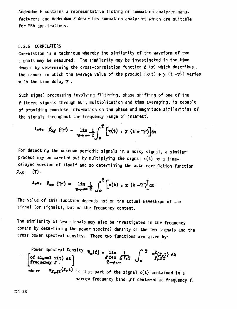
Addendum E contains a representative listing of summation analyzer manu-

facturers and Addendum F describes summation analyzers which are suitable

for SBA applications.

5.3.6 CORRELATERS

Correlation is a technique whereby the similarity of the waveform of two

signals may be measured. The similarity may be investigated in the time

domain by determining the cross-correlation function d (r) which describes

the manner in which the average value of the product [x(t) e y (t -7)] varies

with the time delay 7.

Such signal processing involving filtering, phase shifting of one of the

filtered signals through 90o, multiplication and time averaging, is capable

of providing complete information on the phase and magnitude similarities of

the signals throughout the frequency range of interest.

..ook X M n li At [s(t) . ($t -l)]dt

For detecting the unknown periodic signals in a noisy signal, a similar

process may be carried out by multiplying the signal x(t) by a time-

delayed version of itself and so determining the auto-correlation function

soJuc ('n.

too. l Ci') * him 1 f Ze(t) . Z (t . altT.-a T o

The value of this function depends not on the actual waveshape of the

signal (or signals), but on the frequency content.

The similarity of two signals may also be investigated in the frequency

domain by determining the power spectral density of the two signals and the

cross power spectral density. These two functions are given by:

Power Spectral Density w(£) , Lim 1- T Z2( ,t) et)r gt maa1 (t) at 'f-io JT. ff tJfrequnaoy f . I=

where Zft$£(ft) is that part of the signal x(t) contained in a

narrow frequency band I'f centered at frequency f.

D5-26

The cross-power spectral density Wxy(f) comprises an in phase (Cxy) component

and a quadrature (Q ) component, i.e.:

wheres-

q(f)i 1 A * .l

T.--)~

and 97(f) ma _ f [W(ft) W (f)d

x4~ X(t A s r )phase shifted through 90°.

A measure of the magnitude similarity between the two signals is provided by

the coherence function r.

Y f' Wxy (f)

Measurement and processing equipment for the rapid application of correlation

and spectral density techniques have received much attention in recent years

and these techniques are now amendable to operational usage.

In summary, auto-correlation processing permits detection of significant

internal waveform relationships. Failure mode acoustic waveforms are corre-

latable against normal (idealized) operation waveforms. The idealized

waveform can be shifted in time relative to the actual failure mode waveforms,

and when the correlation function is a maximum, the position of noise bursts

will be located. By then looking between the noise peaks to determine silent

periods and signal amplitudes, measuring the amplitude of existing noise

bursts & identifying the largest of them, and then determining the various

ratios between these measured values and finally comparing these measurements

and ratios, correlation is achieved.

Addendums E & F contain, respectively, examples of correlation manufacturersand hardware suitable for SBA application.

5.3.7 DIGITAL COMPUTERS

Real-time analyzers and correlators discussed in the previous paragraphs

employ digital logic and contain buffers, registers, and memory similar to

that used in digital computers.D5 -27

In a real-time Structure Borne Acoustic Test System, it is also necessary toutilize a general-purpose computer or processor which is not oriented towardone specific task, but may be programmed to compute and manipulate differentdata. The area of SBA can better be serviced by processors emphasizingparticular hardware and software characteristics. The functions required ofa SBA processor are identified in Figure 5-9. A detailed discussion ofthese functional requirements, and a preliminary exercise to size SBA pro-cessor is presented in Addendum H & Appendix C to KSC/GE Report DB72D042,

See Reference 39, Section I, Addendum A.

A processor system is composed of two elements: hardware and software. Ashort discussion of these elements follows.

5.3.7.1 Processor Hardware

The hardware comprises the computing machine and peripheral equipment suchas typewriters and tape punches. The processor is made up of five sectionsinput section, output section, arithmetic unit, memory, and control.

Input: The input section, in conjunction with appropriate external devices,receives data and instructions from various media (e.g., magnetic tape) orvia a manual-entry keyboard. The incoming information is stored by the com-puter in its memory.

The basic function of the input section is to translate the external datainto a form in which it can be stored in the computer memory (e.g., binarywords).

Output: The output section of the processor transmits data to output devicessuch as typewriters, and magnetic tapes performing code translation and form-ulating as appropriate. The output section also transmits signals for con-trolling external devices; for example, function commands for instrumentssuch as analyzers. Some peripheral units can function both as input andoutput devices. For example, the computer can both read from and record on,magnetic tapes.

D5 -28

0

LJ-

U-

0

O

--JwLL.

3KCD

0C)-i-.4

.4

WI,.-LM

,.)

0

W

-J

CJa-0,.

Wn

] U

U,W * toN > LI 1

Oe - Z Z J Q. a j 0 a - 0 0.4w < .) w j , 0

. j0 LA. 22 w

* J o-

I:e e

I

0

I-

-j00

z0

.-

-j.4 U)>; I--LjJ-W -

--IC.- j

-ccOS0

0

L.J 0

a.

J Zco 0. -

Q:4 ao o

000

20

I-

W (

Z J

z _

zo0

0. 0sno

ZL'00

Z0

WInCCLz00

0I-

.4

* - 0

U)

I-

--

k-0 1Z D

'4- -

* * -

aee0 0 0

Z WWo

wO - l- J M 0-J -0 Q j a.= M w 0 4 X

j I-. - z 4

(AncU 000

1- u t(-n o * *

a:0

O

0LaJaMcc

M0

0-

o OC.)0

U <40 Z

- X0 I

*-0La

Z

-- U

- M

- n Wn --

(*A0 -

20

o ZLn -C

(A I 0C) 0 -o (. I-

a. 0 z

0 I -

(A 0 -

U7

J W <

W

'- 4

.- 00

00r c. 55

M W W- . >

o m 0

0a S.O

I I I I

-4-J

-4I.(A

-J0

O W0 a.

W W- I2o k-

_r : oF F z32

CC *

Z

s-O

Z0

m

hLia0° Z

WO0 -

> -

_ u_I -

i

*

c

I-

au

06-4

O

n o

C cL.

C 0

I.-

Cc1 U

I-

o

I

0.55;C)

D5-29

0

V)-

LI-

(A

Cn

0.

o

a-

r

I a L ·

I~~~~~

0

M

II

i1

Arithmetic: The arithmetic unit performs calculations (using basic arith-

metic operations) and manipulates data. Multiplication and division are

accomplished either by successive additions and subtractions initiated by

software, or with additional hardware, usually offered as an option.

The arithmetic unit consists of one or more registers or 'accumulators', and

associated logic circuitry. The accumulators hold the results of arithmetic

and logical operations performed by instructions while the logic enables

data in the accumulators to be combined with information transferred from

memory.

Memory: This section is the heart of the computer; all information pro-

cessed by the computer passes through the memory. Besides word capacity, the

speed with which information can be stored or read from memory is one of the

principal characteristics defining the performance of the processor.

Control: This section controls and coordinates the whole operation of the

processor. It directs the transfer of data between the registers and controls

the operations performed. It also interprets the instructions read from

memory and sets up the gating functions to carry out their execution.

5.3.7.2 Software

Software consists of the programs or lists of instructions that control

operation of the processor; these programs are commonly recorded on punched

tape or magnetic tape, and are then read into the computer through one of

its input devices.

The choice of both processor hardware and software will be dictated by

total system requirements. This not only includes the pertinent SBA

system, but the interfacing and integration with the larger and total check-

out and performance monitoring system employed by a future space program.

Even the simplest tasks involve intricate movements of numerous binary bits

of information within the processor, such that explicit instructions must be

given to the processor to perform each task. Therefore, while it isD5-30

possible to write programs which are coded in the binary form the computer

uses, called "machine language", it is too time consuming and susceptible

to errors to be practical. Various aids have therefore been devised to make

programming easier, and consequently more effective.

Software is the general term given to programs which, when loaded into the

processor, utilize the hardware itself to perform all the detail work.

The purpose of software is therefore to make the computer usable.

Software can be divided loosely into four classes:

a) Translators - programs which translate human-oriented languages into

machine language.

b) Control systems - programs which take care of all the functions essential

to operation of the processor system.

c) Utility routines - program editors, program debugging routines, hardware

diagnostics.

d) Applications programs - these adapt processor system for maximum effective-

ness in a specific application.

5.4 DATA DISPLAY

There are several types of data display essential for a real-time SBA

checkout system. First, some means of visually monitoring the signals prior

to processing and of carrying out overall system calibration is highly

desirable. This type of display aids in initial SBA checkout system.

set-up and calibration. For optimum system flexibility, provisions must

be made for this type of display which includes oscillograms, spectrograms,

and chart recordings. A second type of display is operational analog record-

ings that can be stored and called up for viewing only when requested. The

final display is either digital or analog and provides an operator with

mechanical device Go,No-Go, or Caution status as defined in Chapter 3.

A wide choice of methodsfor final information presentation is available

D5 -31

and the selection will be greatly influenced by the type of acoustic signal

involved, i.e., continuous, intermittent, or impulsive.

Of course, acoustic limits may be stored in the processor and the acoustic

data interlocked to provide no visual display unless the data falls either

into the caution or No-Go category.

A representative listing of data display equipment manufacturers is shown

in Addendum E and some representative samples of this hardware are shown

in Addendum F.

5.5 INSTRUMENTATION SELECTION

The principle determin aits of the "Measurement System" instrumentation

selection are:

1. Type, quantity, and location of mechanical devices.

2. The depth of Readiness Assessment

3. The level of mechanical system readiness assessment that will be

achieved by other than SBA techniques.

Coupled with these determinants are the numerous types of hardware selections

available for each element of the measurement system. The net result is a

potential number of instrumentation selection combinations approaching

infinity. Thus, it is impractical to pursue instrumentation selection

further in this initial handbook release.

The design tradeoffs and the resulting instrumentation do, however, become

apparent with the definition of the principle system determinants listed

above and with the understanding of off-the-shelf equipment availability

and applications. Addendum I provides a checklist to follow in both

instrumentation selection and installation. The majority of instrumentation

equipment required by the SBA system is commercially available equipment.

There will be a requirement for a limited amount of "special design" equip-

ment to facilitate "measurement system" linkage and data traffic control.

The bulk of SBA system design actions will concern itself with software

programming to properly use the hardware in acquiring, switching,

monitoring, filtering, analysing, correlating, and presenting SBA data.

Dt, -32

c

CHAPTER 6ACOUSTIC TESTING

6.1 GENERAL

In the preceding chapters, structure borne acoustics' relationship to

mechanical systems readiness assessment has been defined, and SBA appli-

cation/rationale, component analysis techniques, and the measurement system

selection have been presented. It is currently necessary to empirically

establish each mechanical component's "normal operation" acoustic signature.From this base line signature, it is possible to determine with high con-

fidence upper and lower limits which, when exceeded, indicate abnormal

operation. The establishment of these limits is possible by-the statistical

extrapolation of test data accumulated on previous test programs. Acoustic

limit determination is discussed further in the next chapter.

Care must be taken to establish usable base line acoustic signatures. This

can best be achieved by monitoring each mechanical component's acoustic

signature when activated in the operational environment. An acceptable

alternative is to activate the mechanical device in a test bed which simulatesthe operational environment. The factors that must be considered in obtaining

the "normal operation acoustic signature" are treated in this chapter.

6.2 TEST SEQUENCE

To establish the acoustic signature base line for each mechanical device

tested, there is a fixed sequence of activities which, if followed, will

result in the most efficient collection of data. These activities and their

flow sequence are shown in the SBA Test Flow Diagram, Figure 6-1.

There.are 5 principal task divisions.

I. Obtain component and facility for achieving either actual or simu-

lated operation.

II. Select, secure, and calibrate acoustic detection electronics.

III. Select, secure, and calibrate data processing electronics.

IV. Conduct acoustic tests and record signature.

V. Reduce and evaluate data and establish acoustic limits.

D6-1

These divisions and sub-tasks are delineated in Figure 6-1. This flow

diagram is self-explanatory with the exception of the term "test set up".Within the context of this handbook, "test set up" has a dual meaning.Test set up can mean either the normal operational installation of a mechani-cal component or installation in a simulated operational environment or testbed.

6.3 FACILITY REQUIREMENTS

Where it is feasible to monitor and obtain the normal acoustic signature ofa mechanical component in an operational habitat, the only additionalfacility requirements imposed by implementing this non-destructive testtechnique is that required by the "Measurement System". This "MeasurementSystem" was thoroughly discussed in the previous chapter.

Figure 6 2 is a photograph of a General Electric Company Spectrum Analysisfacility. This provides a physical concept of "Measurement System" hard-ware. However, this facility must service a complete range of research anddevelopment signature analysis problems. Applications other than mechanicaldevice acoustics investigated with this equipment includes heart sounds,noise suppressor problems and speech recognition. Hence, the need for eightracks of diagnostic equipment.

Where a special test bed must be employed to simulate the component operationalenvironment, additional expense,time and hardware is obviously required.Where a large number of components will be tested, this cost can be amortizedto a very small per component cost. This is possible by multiple use of acommon test bed. For example: A special facility test set-up was designedand built by General Electric as a means of studying the acoustic signaturesof five mechanical components under simulated operating conditions. This test

D6 -2

16 i e -4 e

i 'a- 3, -I 1' O

; .- ,

-pa,

T0 = 9 1I- S 28

I - 0 4,

w~ w <

0: t: as,4 S

c4

0

cd

0

'4

:1-

.4

4o

Q)

a

bD._

D6-3

set-up (see Figure 6-3) provided for ready installation.and quick replacement

of the test components. This test set-up, as now established, could

accommodate the testing of many different components with only minor modifi-

cations. These test facilities-located at General Electric's Research and

Development Laboratory, Schenectady, New York, were employed for this test

program. Approximately 80 square feet of space was used for a work bench

and test set-up facilities to acquire magnetic tape recordings of the com-

ponent acoustic signatures. Facilities temperature range of 650 + 5°F.,

humidity range of 45 + 5 percent and normal open laboratory cleanliness and

lighting were maintained.

6.4 TEST PLANNING

To assure maximum benefits from acoustic testing, it is necessary to plan

the particulars of each test. The Test Plan should at a minimum include the

following:

I. INTRODUCTION

1.1 Purpose and Scope of Test

1.2 Pertinent Test Ground Rules

II. GENERAL

2.1 Component Identification

2.2 Test Set-Up Hardware Description

2.3 Test Flow

*2.4 Test Schedule

2.5 Documentation Requirements

III. TEST FACILITY IDENTIFICATION

IV. DETAILED TEST PROCEDURE

4.1 Test Sequence

4.2 Test Set Up

4.3 Component Checkout Test Procedure

4.4 Acoustic Instrumehtation

D6-5

f

View A

^

View B

D6-6

Figure 6 -3 . Test Set Up

4.5

4.6

4.7

4.8

Test System Calibration Checkout

Acoustic Test & Data Recording

Measurement Techniques

Limit Determination

A sample test plan used for acoustic testing of a solenoid valve is contained

in Addendum C. While it may not be necessary to formalize all aspects of

each component test plan, the test plan is highly recommended as part of the

total "methodology" which will ultimately save much wasted effort and back-

tracking.

D6-7,/D68 |

CHAPTER 7

INTERPRETATION OF MEASUREMENT DATA

7.1 GENERAL

The central problems involved in the evaluation of component condition using

SBA are these:

o Identification of the discriminants which characterize the

condition of the component undergoing test

o Selecting the optimum technique(s) to extract the data which best

characterizes the condition of the component undergoing test

o Relating the acoustic data to the events taking place within the

component undergoing test

o Establishing the qualitative characteristics or quantitative

values for the processed data which relate to a Go, Caution or

No-Go component

It is the latter two problems which will be examined in this chapter.

7.2 ACOUSTIC LIMIT DETERMINATION

7.2.1 GENERAL

To establish acoustic limits for component Go, Caution or No-Go status, the

acoustic data must be related to the physical events taking place within the

component. Further, to establish quantitative values of Go, Caution or

No-Go, an analogy between the acoustic signal parameters and the components'

operating parameters must be drawn. At the present state of the art, these

relationships are derived from the testing previously described. With

experience and refinement in the analytical process it will be possible to

minimize the required testing.

7.2.2 NOMINAL OPERATION

A normal operational profile, in acoustic terms, is established through con-

trolled testing of known, fully operational components. Obviously, during

the component testing, there must be sufficient instrumentation, in addi-

tion to the acoustics, to permit quantitative relating of such things as

D7 -1

flow, noise, pressure, RPM and timing to the acoustic signals.

From a component fault tree,those parameters necessary to characterize com-

ponent operation can be identified. Again taking the 75M08825 solenoid

valve as an example, refer to the failure mode tree on Figure 4-3. The

failure modes identified are:

o fails to deactuate

o fails to actuate

o erroneous indication

o venting to atmosphere (leakage)

o sluggish operation

Of the five failure modes, the first three are discrete events which either

occur or do not occur. For these it is only necessary to establish that

the event did or did not take place. The remaining two require comparison

of actual value versus predetermined limits to permit Go, Caution or No-Go

decision s.

If the solenoid valve actuates/deactuates as commanded, provides the proper

position indication, does not leak and operates within a normal time frame,

confidence in the operational integrity would be very high. Therefore, to

be useful the acoustic signature must provide information which can be

related to component operation to establish the operational integrity.

The raw data necessary for determination of r,-iinal limits are obtained

during component testing discussed in the preceding chapter. Determination

of numerical values is discussed in Paragraph 7.4.

7.2.3 FAILURE MODE OPERATIONS

In the case of failure mode operations, failures are introduced into the

device and testing similar to nominal repeated.

Component data characterizing failed or degraded components are more diffi-

cult to derive during testing similar to that for nominal operation. The

factors which present rather severe complications are:

o Specifications rarely clearly identify the transition between

Go and Caution and between Caution and No-Go or the quantitative

D7-2

range for each. This is complicated by the fact that frequently

the Go, Caution or No-Go criteria will vary due to the operational

application of the mechanical device.

o It isvery difficult to install truly representative failures;

that is, introduced failures rarely duplicate "natural" failures.

o When disassembling a device to introduce a failure, a danger

exists that another unknown effect will be introduced, thereby

introducing a bias which can easily produce unwarranted or incor-

rect conclusions based on the acoustic data.

Therefore, in general, the determination of Caution and No-Go limits by sim-

ulating failures is not recommended due to the cost and probability of

introducing an unknown bias into the testing. This philosophy holds where

a change in the characteristic acoustic signature is detected to exceed a

boundary or limit and is thereby detected as a No-Go or Caution.

Where the signature characteristic which indicates a failure does not exist

in a normal signature, testing will be required. For example, the acoustic

signature for a component in a Go condition does not contain a leakage

characteristic. Therefore, it will be necessary to introduce a leakage

failure into the component to establish the signature characteristic of

leakage. Due to the difficulty of identifying leakage using SBA techniques

any leakage detected using SBA would be classified as Caution or No-Go.

7.2.3 RELATIONSHIP TO OPERATIONAL LIMITS

Just as a thermocouple produces a signal proportional to temperature, the

acoustic accelerometer produces a signal proportional or analgous to the

sound produced in a mechanical device. To make an operational decision a

relationship must first be established between the thermocouple output and

the temperature. Second, the Go, Caution and No-Go criteria must be estab-

lished relative to thermocouple voltage. This same logic process applies to

the necessity for relating acoustic signals to physical events, processes

and limit criteria.

Component analysis, discussed in Chapter 4, resulted in the identification

of component failure modes, the internal reactions which form the acoustic

signature, and a predicted signature for normal operation. As a further

D7-3

extension of this process, each failure mechanism and mode should be examin-

ed to identify failure mechanism impact on the nominal signature. That is,

how will the failure mechanism change the acoustic signature.

Table 7-1 tabulates briefly the effects of failure modes and mechanisms

upon the noise produced within the solenoid valve. The definition available

from this approach is primarily a function of insight and experience. The

purpose of the exercise is to sharpen the analytical capability when relat-

ing acoustic data to the noise sources.

Acoustic data can be processed into a limited number of formats involving

frequency, amplitude, and time. Typical formats in general use include:

o Time vs. Amplitude

o Frequency vs. Amplitude

o Time vs. Frequency vs. Amplitude (intensity modulated)

Of the three parameters - time, frequency and amplitude - time repeatability

for a specific event generally has the smallest variation. Frequency has

the next smallest dispersion and amplitude variations are the least reliable

parameter for detecting valid changes. Amplitude, of course, is very import-

ant for determination of timing intervals.

The key feature or characteristic of the acoustic signal which provides the

component operational condition may take a number of forms such as:

o Presence or absence of a discrete frequency or band

of frequencies

o Signal amplitude rate of change for a given frequency

o Frequency rate of change

o Signal amplitude correlation with a constant value

or a variable function

o Absolute or relative timing

o Average or RMs amplitude of a given frequency or

frequency band

o Peak vs. RMS amplitude comparison

The key feature which best displays the operational condition should be

selected and, where applicable, reduced to numerical values for statistical

manipulation, as described in paragraph 7.4. For a discrete feature, e.g.,D7-4

actuation of a value, it is only necessary to establish the presence of a

signal feature which indicates that the prescribed action has taken place.

In many cases it is not necessary to establish numerical No-Go values for

a given feature or characteristic.' For example, the fully loaded shaft RPM

of a cyclic device may be defined in the component specification data. It'

is then only necessary to select the acoustic signal characteristic which

can be related to shaft RPM. Unfortunately, quantitative characteristics

are frequently left unspecified, particularly in regard to allowed leakage.

7.3 TREND ANALYSIS

Trend analysis requires the use of several values of a parameter as a basis

to detect high rates of change, abrupt departures from steady state con-

ditions and gradual drifts toward an out-of-tolerance condition. The occur-

rence of one of these conditions does not necessarily presage a component

malfunction. It should, however, raise questions as to why the change has

occurred.

The noted change would, in general, require correlation with some other

system or component parameter to insure that a false alarm is not generated.

Investigation of the change could provide many different causes.

o The component has, in fact, degenerated

o A system defect outside the instrumented component

is responsible

o A normal, explainable pertubation has taken place

within the component and/or system

Trend analysis, by its nature, requires a time base; i.e., sampling over a

period of time to establish rate of change. This in turn requires a memory

device for evaluation purposes.

Possibilities for placing limits and providing alarms based on trend data

are varied. Common methods include the specification of:

o Allowable parameter change with respect to time

o Number of transient excursions outside a band of valves

o Duration of transient excursions outside a band of valves

D7-5

Trend analysis is best accomplished through the use of computation equipment

where predetermined rate, number or duration of parameter excursions can be

stored for tabulation and comparison purposes. Detection of rapid changes

within a normal band of values as well as a definite drift toward an out.of-

tolerance condition is a valuable indicator of an incipient problem. Detec-

tion of such a trend can provide a Caution flag long before a warning is

received based on exceeding the absolute value of a parameter which defines

a Caution status.

7.4 STATISTICAL "LIMIT" DECISION MAKING

7.4.1 GENERAL

Statistics is a valuable management tool for decision-making in any sort of

readiness assessment instrumentation system. This usefulness lies in two

major areas:

o Determination of quantitative values for Go, Caution,

and No-Go based on component test data

o Analysis of component operational data, subsequent to

limit determination, to establish significant trends,

7.4.2 STATISTICAL DETERMINATION OF GO, CAUTION AND NO-GO

7.4.2.1 General

As previously discussed, the determination of Caution or No-Go limits

through introduction of defects into components for SBA testing is at best

difficult and time consuming. This is brought about by the high probability

of affecting the component in an unanticipated manner when introducing the

defect or the possibility that the simulation is not representative of the

defect for which simulation is attempted. Therefore, the technique having

the greater probability for success involves determination of the quantita-

tive values of each discriminant which characterize a Go condition and

applying statistical techniques to establish Caution and No-Go values.

The SBA elements which must be accomplished to implement the statistical

approach for normal (Go) components are:

o Component analysis to:

- Establish failure modes

- Identify noise sources

- Identify discriminants

D7 -6

o Select the processing technique most definitive

o Process the SBA to establish numerical values for each

discriminant

o Apply tolerance limit technique to establish Go, Caution

and No-Go values.

7.4.2.2 Data Mean (i), Standard Deviation(s)Having secured numerical data through the preceding approach it is necessary

to establish the nominal Go values for the discriminant. A histogram plot

of the data, depending upon the spread of values, can provide a good andperhaps adequate definition of the Go values. A histogram is a frequencydistribution in bar chart form. Take, for example, the operating times, in

milliseconds (ms), for a solenoid value shown in Table 7-1.

38. 37.6 37.2 39.438. 37.8 37.2 38.

38. 38.3 38. 38.8

37. 39.2 36. 39.

38.4 38.6 37. 38.6

38. 38.7 36.8 37.4

38.1 38.1 38.6 37.

38.4 37. 37.2 39.

39.2

TABLE 7-1

SOLENOID VALVE OPERATING TIMES (In Milliseconds)

A histogram is prepared by ordering (arranging in ascending times) andplotting frequency of occurrence in 0.5 millisecond increments (per Table

7-2).

Time Span Number of Occurrences

36.0 - 36.49 1

36.5 - 36.99 1

37.0 - 37.49 8

37.5 - 37.99 2

D7-7

Time Span

38.0 - 38.49

38.5 - 38.99

39.0 - 39.49

Number of Occurrences

6

5

TABLE 7-2

TIME SPAN vs. FREQUENCY OF OCCURRENCE

A histogram of Table 7-2 data is shown in Figure 7-1.

11

10

9

Frequency

of

Occurrence

8

7

6

5

4

3

2

1

35.0 35.5 36.0F7ZFZZR //1

36.5 37.0 37.5

,'///

/ 1

<:1/

38.0 38.5 39.0 39.5

Time Span (ms)

FIGURE 7-1

HISTOGRAM OF SOLENOID VALVE OPERATING TIMES

D7 -8

Ia.j

0

0

0

0

0

0

1

0 e

e

0

00

e

W

0

0

o0

0

0

0

r

I

As a practical matter, one could reasonably conclude that an operating time

greater than 40 ms or less than 35 ms would certainly be unexpected and

might require further investigation.

However, for a more rigorous approach the mean X and the sample standard

deviation(sj are calculated.

= Sum of All Times _ 1254 38Number of Values 3 - 38.0 ms

/Sum of Each (X-2 22.21.83Number of Values-l *

The significance of s is that for a normal distribution (Gaussian):

o 68% of the area under the curve is contained in the

interval between the mean and + the standard deviation

o 95% for + 2 standard deviations

o 99.7% for + 3 standard deviations

There is an underlying assumption, based on the Central Limit Theorem, that

the data to be treated are from a normal distribution. Verification of

probable normality of this data can be demonstrated by a plot on. normal

distribution probability paper, or by using the Wn(N)*test for normality.

Confidence limits are intervals intended to include the true mean (u) with

a stated probability. Frequently only the sample mean (i.e., mean of the

sample data) is known. The sample mean (e.g., X) is an estimate of the

unknown population or true mean, u, but differs due to sampling variation.**

It is possible, however, to construct a statistical interval known as a

confidence interval for the population mean, u. As an example, a 90% con-

fidence interval on the true mean (knowing only X) is an interval which con-

tains u with a probability of 0.90. A moderate deviation of the data from

normality will have little impact on confidence interval determinations

concerning a population mean.

* AddendumA, Section I, No. 37

** Likewise, the sample standard deviation s, is an estimate of the unknownpopulation or true standard deviation,&":

D7-9

For the purposes of establishing Go limits we are more interested in speci-

fying an interval in which a specified proportion, for example 90%, of all

values will fall. For a normal distribution, if u ands aare known rather

than X and s, 90% of the population is located in the interval: u + 1.64a!.

If only X and s are known then we can only specify a probability, e.g., 95%,

that the interval contains 90% of the population. This interval is called

a tolerance interval.

In the absence of other guidelines the following is recommended for estab-

lishing Go, Caution and No-Go values for a given discriminant based on 30

operations of the tested component in its operational environment.

o Calculate X

o Calculate s

Go condition for X values between X and + (2.14)(s)Caution condition for X values outside the Go limits but within

X + 3.35(s)No-Go condition for X values outside the Caution limits

For the solenoid valve:

Go = 38 + (2.14)(.83) = 38 + 1.78 = 36.22 - 39.78

Caution: 38 + 3.35(.83) = 38 + 2.78 = 35.22 - 40.78

Therefore the Caution values are: 40.78 to 39.78

and 36.22 to 35.22

No-Go: Above 40.78, Below 35.22

7.4.3 STATISTICAL ANALYSIS OF TRENDS

The principal aspects of analysis for component performance trends are:

o Routine periodic sampling of those discriminants which

characterize the operation of the instrumented component

o Processing and presentation of the data in a way which

provides quantitative values of the discriminants

D7-10

o A means for making appropriate decisions regarding the

operational integrity of the instrumented component

The first two aspects have been discussed previously. The third can be

treated similarly to control chart techniques forming a part of statistical

quality control. The control chart technique, which,in the quality control

domain can be manual or electronically processed indicates that one-of the

most common types of control charting is that based on the sample average

(X) made during a sampling period. Though for quality control purposes the

sampling is based on individual samples from a number of separate components,

the technique is appropriate for readiness assessment where sequential sam-

ples are taken from a single device.

The values of 7 taken over successive sampling periods are plotted againsttime. When repetitive samples of N observations are taken from a stable

normal or near normal distribution the average, X, for these samples tend

to be normally distributed about a mean u with a standard deviation

a-- X = r//- where n equals the number of samples per sampling period,

with an estimate for'-(s) established during component testing dis-

cussed in paragraph 7.4.2. If the device provides a stable population the

variability of the sample averages, 7, of successive sampling periods canbe predicted. The resulting s/ fJ Nprovides the basis for predicting that

about 95% of the X's should lie within a band of width + 2s4 Tand essent-

ially all should fall between + 3s/N.

Suppose, however, that instabilities appear during successive sampling

periods (rather than the less likely instability of successive samples with-

in the same sampling period). If so, these instabilities will manifest

themselves by the variation of the sampling period 7's and exceed that predicted

on the basis of the variation of X within a sampling period. That is, the

presumption is made that during a relatively short period the discriminant

is essentially stable.

Processing the data for a routine such as that described would take the

following form:

D7-11

Sampling Period

(1)

(2)

(3)

n

Observation

A B C D E

a1 b1 c1 d1 e1

a2

a3

a4

Total

Average (Total

The range for which the component discriminant is

is described by the relation:

7

defined to be a Go value

(n = 5 in the above example;

s developed during component testing)

Decision making, using the above technique, takes essentially the following

approach:

A new data value is subtracted from the mean and the difference compared

with the three sigma(s) limits of the variab'l. If the comparison shows

the difference (mean - data value) to be less than 3s the information is

discarded. If the comparison shows the difference to be greater than 3s a

count is registered. If the count register exceeds a given number for the

sample set a new mean and variance (s2) is calculated.

A new value for the mean indicates a persistently out-of-tolerance condition

greater than 3s over the time span for the sample set. If this out-of-

tolerance condition recurs over several sets, then a trend is indicated.

A No-Go or Caution condition would be indicated when the latest mean cal-

culation differs from a preset mean or when the mean's rate of change

exceeds a predetermined value.

D7-12

X

X

X2

Xnn

+ 3s/

Additional facets of the above technique should be stressed:

o Using either manual or automatic processing, the Go, No-Go

and Caution quantitative values can be developed through pro-

cessing the acoustic data for several operations of the com-

ponent. Then, as the component continues to operate, these

operational limits are adjusted by the incoming data. This

iterative process permits establishing operational parameters

in-line, rather than in a component test program.

o The trend portion of this technique can be circumvented

and the Go, Caution or No-Go decision based on finite limits

without the recomputation of the mean. This, then, is essent-

ially the technique described in paragraph 7.4.2.

D7 -13/D7 -1i4

ADDENDUM A

REFERENCES

Section I of this Addendum lists general "Structure Borne Acoustics" references.

Section II contains a listing of acoustic and mechanical shocks; vibration standards

which can be purchased from the American National Standards Institute, 1430 Broad-

way, New York, New York, 10018.

Da-1

SECTION I

1. Weichbrodt, B., "Mechanical Signature Analysis, A New Tool for ProductAssurance and Early Fault Detection", Schenectady, N. Y., General ElectricCo., Mechanical Engineering Laboratory, Report No. 68-C-197, June 1968.

2. Bruns, R. W., "Detection of Noise-Producing Quality Faults in 3 GPM Motorsby Vibration Pickup", Fort Wayne, Ind., General Electric Co., ComponentsProducts Division, Laboratory Operation, R66FL1280, March 31, 1966.

3. Waechter, A. E., "Structure and Airborn Noise Measurement on 400 HPTorpedo Motors", Pittsfield Mass., General Electric Co., DC Motor andGenerator Department, No. DF67MD704, March 21, 1967.

4. Smith, A. M., "Determination of Engine Thrust Levels from Normally Record-ed Background Noise on Aircraft CVR", Evendale, Ohio, General Electric Co.,Commercial Engine Department, No. R68AEG458, November 15, 1968.

5. Campanella, S. J., Speaker, D. M., "Development of Monitoring Techniques byAcoustical Means for Mechanical Checkout", Falls Church, Va., Melpar, Inc.,Contract No. NAS8-11976, 30 November 1965.

6. Barclay, F. J., Hale, J. C., Ledwidge, T. J., Burton, E. J., Jones, C. H.,"The Application of Acoustic Diagnostics in Nuclear Reactor Operation andDevelopment", United Kingdom Atomic Energy Authority, 1970.

7. Priede, T., Grover, E. C., "Application of Acoustic Diagnostics to InternalCombustion Engines and Associated Machinery", Perkins Engine Company.

8. Brownsey, C. M., "The Measurement System. " Central Electricity ResearchLaboratories, Great Britian.

9. Macleod, I. D., Halliwell, G., Hale, J. C., "Signal Analysis Techniques forUse in Acoustic Diagnostics", United Kingdom Atomic Energy Authority.

10. Passanti, F. A., "Mechanical Signature Analysis for Diagnosis of ReciprocatingEngines", Schenectady, New York, General E 'ctric Co., Mechanical Engi-neering Laboratory, TIS Report No. 69-C-286, August 1969.

11. Anderson, T. E., "Time Delay Recording", Schenectady, New York, GeneralElectric Co., Electronic Engineering Laboratory, TIS Report No. 70-C-279,July 1970.

12. Page, J., "Recognition of Patters in Jet Engine Vibration Signals", DaytonaBeach, Fla., General Electric Co., TIS Report No. R66ASD22, December 1966.

13. Braun, S., "Extraction of Periodi- Signals by Comb Filters: A GeneralizedApproach", Schenectady, New York, General Electric Co., Mechanical Engi-neering Laboratory, TIS Report No. 71-C1209, July 1971.

14. Thomas, Ronald L., "Signal Conditioning for Commonly Used Transducers",Pasadena, Calif., Endevco Dynamic Instrument Division, Tech Paper TP242,1970.

15. "Instruction Manual for Piezoelectric Accelerometers", Pasadena, Calif.,Endevco Dynamic Instrument Division, No. 101, 1968.

Da-2

SECTION I

16. Weichbrodt, B., "Mechanical Signature Analysis for Early Detection of BallBearing Damage", Schenectady, New York, General Electric Co., Research andDevelopment Center, Final Report, March 1966.

17. Peterson, A. P. G., Gross, E. E., Jr., "Handbook of Noise Measurement",West Concord, Mass., General Radio Company, 1967.

18. Allen, Ernest E., "Noise Control in Valves and Regulators", Marshalltown,Iowa, Fisher Controls Co., TM-24, 1970.

19. Beranek, L. L., editor, Noise Reduction, McGraw-Hill, New York, 1960.

20. Beranek, L. L., Acoustics, McGraw-Hill, New York, 1954.

21. Davis, D., Acoustical Tests and Measurements, H. W. Sams, Indianapolis, 1965

22. Kinsler, L. E., and Frey, A. R., Fundamentals of Acoustics, John Wiley,New York, 1962.

23. Stephens, R. W. B., and Bate, A. E., Acoustics and Vibrational Physics,St. Martin' s Press, New York, 1966.

24. Acustica, Hirzel, S., Zurich 4, Switzerland (an international journal on acousticspublished since 1951).

25. Sound and Vibration, Acoustical Publications, P. O. Box 9665, Cleveland, Ohio44140 (Monthly).

26. Crandall, S. H., and Mark, W. D., Random Vibration in Mechanical Systems,Academic Press, New York, 1963.

27. Crede, C. E., Vibration and Shock Isolation, John Wiley, New York, 1951.

28. Harris, C. M., and Crede, C. E., editors, Shock and Vibration Handbook,McGraw-Hill, New York, 1961.

29. Hardy, H. C., "Standard Mechanical Noise Sources, " Noise Control, Vol 5,May, 1959, pp 22-25.

30. King, A. J., The Measurement and Suppression of Noise, Chapman and Hale,London, 1965.

31. Phase HI1 Progress Report for Study of Techniques for Automatic Self-ContainedReadiness Assessment and Fault Isolation for Ground and On-Board MechanicalSystems, 70-831-894, KSC Contract NAS10-7145, Cape Canaveral, Fla.,General Electric Co., Apollo Systems, 19 October 1970.

32. Phase I Progress Report for Study of Techniques for Automatic Self-ContainedReadiness Assessment and Fault Isolation for Ground and On-Board MechanicalSystems, 70-831-892, Cape Canaveral, Fla., General Electric Co., ApolloSystems, 20 July 1970.

33. Failure Rate Data (FARADA) Program, Corona, California, Naval Fleet MissileSystems Analysis and Evaluation Group, December 1971, Table B2, MechanicalHydraulic, Pneumatic, Pyrotechnic, Miscellaneous Component Part FailureModes.

Da-3

34. Burgess, John A., "Spotting Trouble Before It Happens", Machine Design,17 September 1970, pp 150-155.

35. Study for Maintenance of Hydraulic Motors, General Electric Company, Mechani-cal Engineering Laboratory, Contract NAS5-10559, Schenectady, N.Y., June 1967through October 1968.

36. Bendat, J. S. and Piersol, A. G., Measurement and Analysis of Random Data,John Wiley and Sons, Inc., New York, 1966.

37. Shapiro, S.S., "Testing for Distributional Assumptions with Small Samples",Schenectady, N. Y. General Electric Company Information Sciences Laboratory,Report No. 64GL161, October 5, 1964.

38. Mechanical Systems Readiness Assessment and Performance Monitoring Study,Midterm Report, DB 72-A015, Daytona Beach, Fla., General Electric Company,Apollo and Ground Systems, February 4, 1972.

39. Study of Mechanical Systems, Readiness Assessment Performance & Monitoring,General Electric Company, DB 72-D042, Apollo and Ground Systems, 19 May1972.

Da-4

SECTION II

S1. 1-1960S1. 2-1962S1. 6-1960S1. 11-1966S2. 2-1959S3.4Z24.15-1955Z24.21-1957

ISO/R131-1959

ISO/R140-1960

ISO/R357-1963ISO/R31/Part

VII-1965ISO/R495-1966

Acoustical TerminologyPhysical Measurement of SoundPreferred Frequencies for Acoustical MeasurementsOctave, Half-Octave, and Third-Octave Band Filter SetsCalibration of Shock and Vibration PickupsComputation of the Loudness of NoiseSpecifying the Characteristics of AnalyzersSpecifying the Characteristics of Pickups for Shock and VibrationMeasurementsExpression of the physical and subjective magnitudes of sound ornoiseField and laboratory measurements of airborne and impact soundtransmissionPower and Intensity Levels of Sound or Noise

Quantities and Units of AcousticsTest Codes for Measuring the Noise Emitted by Machines

Da-5/Da-3

ADDENDUM B

DEFINITIONS

Acceleration*

Analyzer

Caution

Cyclic Action Component

Confidence Limits

Critical Speed

Decibel*

Acceleration is a vector that specifies the time rate ofchange of velocity.Note 1: Various self-explanatory modifiers such as peak,average, rms are often used. The time interval must beindicated over which the average (for example) was taken.Note 2: Acceleration may be (1) oscillatory, in which caseit may be defined by the acceleration amplitude (if simpleharmonic) or the rms acceleration (if random), or (2)non-oscillatory, in which case'it is designated "sus-tained" or "transient" acceleration.

An analyzer is a combination of a filter system and a sys-tem for indicating the relative energy that is passedthrough the filter system. The filter is usually adjust-able so that the signal applied to the filter can be meas-ured in terms of the relative energy passed through thefilter as a function of the adjustment of the filter re-sponse-vs-frequency characteristic. This measurementis usually interpreted as giving the distribution of energyof the applied signal as a function of frequency.

The component can perform the intended function withinoperational limits but performance, degradation has beensensed.

A device in which the operational events repeat at pre-scribed intervals e. g., an internal combustion engine.Confidence limits are the upper and lower values of therange over which a given percent probability applies.For instance, if the chances are 99 out of 100 that asample lies between 10.and 12, the 99% confidence limitsare said to be 10 and 12.

Critical speed is a speed of a rotating system that cor-responds to a resonance frequency of the system.

The decibel is one-tenth of a bel. Thus, the decibel isa unit of level when the base of the logarithm is the tenthroot of ten, and the quantities concerned are proportionalto power.Note 1: Examples of quantities that qualify are power(any form), sound pressure squared, particle velocitysquared, sound intensity, sound energy density, voltagesquared. Thus the decibel is a unit of sound-pressure-squared level; it is common practice, however, to shortenthis sound pressure level because ordinarily no ambiguityresults from so doing.

*This material is reproduced from the American Standard Acoustical Terminology,S1. 1-1960

Db-1

Directivity Factor*

Discriminant

Effective Sound Pressure(Root-Mean-Square SoundPressure)*

Note 2: The logarithm to the base the tenth root of 10is the same as ten times the logarithm to the base 10:e.g., for a number x 2,log l O o

. 1X2 = 10 log lO x2 =20 log1 ox. This last relationship is the one ordinarilyused to simplify the language in definitions of sound pres-sure level, etc.

(1) The directivity factor of a transducer used for soundemission is the ratio of the sound pressure squared, atsome fixed distance and specified direction, to the mean-square sound pressure at the same distance averagedover all directions from the transducer. The distancemust be great enough so that the sound appears to divergespherically from the effective acoustic center of thesources. Unless otherwise specified, the reference di-rection is understood to be that of maximum response.(2) The directivity factor of a transducer used for soundreception is the ratio of the square of the open-circuitvoltage produced in response to sound waves arriving ina specified direction to the mean-square voltage thatsould be produced in a perfectly diffused sound field ofthe same frequency and mean-square sound pressure.Note 1: This definition may be extended to cover thecase of finite frequency bands whose spectrum may bespecified. Note 2: The average free-field response maybe obtained, for example:(1) By the use of a sperical integrator(2) By numerical integration of a sufficient number of di-rectivity patterns corresponding to different planes, or(3) By integration of on e or two directional patterns when-ever the pattern of the t ansducer is known to possessadequate symmetry.

Characteristics of a device which can be correlated withthe devices operational condition or performance.

The effective sound pressure at a point is the root-mean-square value of the instantaneous sound pressures, overa time interval at the point under consideration. In thecase of periodic sound pressures, the interval must bean integral number of periods or an interval long com-pared to a period. In the case of non-periodic soundpressures, the interval should be long enough to makethe value obtained essentially independent of small changesin the length of the interval.

Db-2

Failure Cause

Failure Mechanism

Failure Mode

FARADA

Flow Noise Generator

Go

Impact*

Intensity (of Sound)

Intensity Level

Loudness*

Loudness Level*

Note: The term "effective sound pressure" is frequentlyshortened to "sound pressure."

The basic anomaly which produces a failure mechanisme.g., contamination, corrosion, wear.

Identification of the piece part which failed and the spc-cific problem. The result of a basic anomaly which pro-duces a failure mode e. g., a sticking valve poppet dueto contamination.

The form in which a component failure is manifested,e.g., fails to operate.

Failure Rate Data fox electrical, electronic, mechanical,hydraulic, pneumatic, pyrotechnic, et. al., compiledand published by the Naval Fleet Missile System Analysisand Evaluation Group, Corona, California.

A mechanical component whose acoustic signature is pro-duced primarily as a result of medium flow. Flow noisegenerators are generally operated on demand due to un-equal pressures e. g., regulator, check valve, reliefvalve

The operational readiness of a device which indicates afully operational status without detection of degradation.

An impact is a single collision of one mass in motion witha second mass which may be either in motion or at rest.

The amount of acoustic energy passing perpendicularlythrough a unit area in unit time.

Logarithmic ratio (INDB) of sound intensity with respectto a reference (10-12 watts per square meter).

Loudness is the intensive attribute of an auditory sen-sation, in terms of which sounds may be ordered on ascale extending from soft to loud.Note: Loudness depends primarily upon the sound pres-sure of the stimulus, but it also depends upon the fre-quency and wave form of the stimulus.

The loudness level of a sound, in phons, is numericallyequal to the median sound pressure level, in decibels,relative to 0. 0002 microbar, of a free progressive waveof frequency 1000 Hz presented to listeners facing thesource, which in a number of trials is judged by thelisteners to be equally loud.

Db-3

Masking*

Mechanical Shock

Microbar, Dyne PerSquare Centimeter*

No - Go

Noise*

Noise Level*

Note: The manner of listening to the unknown sound,which must be stated, may be considered one of thecharacteristics of that sound.

(1) Masking is the process by which the thresholdof audi-bility for one sound is raised by the presence of another(masking) sound.(2) Masking is the process by which the threshold ofaudibility of a sound is raised by the presence of another(masking) sound. The unit customarily usedis the decibel.

Mechanical shock occurs when the position of a system issignificantly changed in a relatively short time in a non-periodic manner. It is characterized by suddenness andlarge displacement, and develops a significant inertialforces in the system

A microbar is a unit of pressure commonly used in acous-tics. One microbar is equal to 1 dyne per square centi-meter.No e: The term "bar" properly denotes a pressure of10t dynes per square centimeter. Unfortunately, the barwas once used to mean dyne per square centimeter, butthis is no longer correct.

The operational readiness of a device which indicatesthat the device is not capable of performing within normaloperational limits.

(1) Noise is any undesired sound. By extension, noise isany unwanted disturbance within a useful frequency band,such as undesired electric waves in any transmissionchannel or device.(2) Noise is an erratic, intermittenty, or statisticallyrandom oscillation.Note 1: If ambiguity exists as to the nature of the noise,a phrase such as "acoustic noise" or "electric noise"should be used.Note 2: Since the above definitions are not mutually ex-clusive, it is usually necessary to depend upon contextfor the distinction.

(1) Noise level is the level of noise, the type of whichmust be indicated by further modifier or context.Note: The physical quantity measured (e. g. voltage),the reference quantity, the instrument used, and the band-width or other weighting characteristic must be indicated.

Db-4

Octave*

Operational Effect

Peak-To-Peak Value*

Power Level

Pressure Spectrum Level*

Primitive Period (Period)*

Random Noise*

(2) For airborne sound unless specified to the contrary,noise level is the weighted sound pressure level calledsound level; the weighting must be indicated.

(1) An octave is the interval between two sounds having abasic frequency ratio of two.(2) An octave is the pitch interval between two tones suchthat one tone may be regarded as duplicating the basicmusical import of the other tone at the nearest possiblehigher pitch.Note 1: The interval, in octaves, between any twofrequencies is the logarithm to the base 2 (or 3. 322times the logarithm to the base 10) of the frequency ratio.Note 2: The frequency ratio corresponding to an octavepitch interval is approximately, but not always exactly2:1.

Failure mode impact on the operational readiness of amechanical device - Go, Caution or No - Go.

The peak-to-peak value of an oscillating quantity is thealgebraic difference between the extremes of the quantity.

Power level, in decibels, is 10 times the logarithm tothe base 10 of the ratio of a given power to a referencedpower. The reference power must be indicated. (Thereference power is taken as 1. 0 x 10-12 watt in thishandbook.)

The pressure spectrum level of a sound at a particularfrequency is the effective sound pressure level of thatpart of the signal contained within a band 1 cycle per sec-ond wide, centered at the particular frequency. Ordi-narily this has a significance only for sound having a con-tinous distribution of energy within the frequency rangeunder consideration. The reference pressure should beexplicitly stated.

The primitive period of a periodic quantity is the smallestincrement of the independent variable for which the func-tion repeats itself.Note: If no ambiguity is likely, the primitive period issimply called the period of the function.

Random noise is an oscillation whose instantaneous mag-nitude is not specified for any given instant of time. Theinstantaneous magnitudes of a random noise are specifiedonly by probability distribution functions giving the frac-tion of the total time that the magnitude, or some sequence

Db-5

of magnitudes, lies within a specified range.Note: A random noise whose instantaneous magnitudesoccur according to Gaussian distribution if called Gaus-sian random noise.

Resonance*

Response*

Reverberation*

Simple Sound Source*

Sone*

Resonance of a system is forced oscillation exists whenany change however small in the frequency of excitationcauses a decrease in the response of the system.Note: Velocity resonance, for example, may occur at afrequency different from that of displacement resonance.

The response of a device or system is the motion (orother output) resulting from an excitation (stimulus) underspecified conditions.Note 1: Modifying phrases must be prefixed to the termresponse to indicate kinds of input and output that arebeing utilized.Note 2: The response characteristic, often presentedgraphically, gives the response as a function of someindependent variable such as frequency or direction. Forsuch purposes it is customary to assume that other char-acteristics of the input (for example, voltage) are heldconstant.

1. Reverberation is the persistence of sound in an en-closed space, as a result of multiple reflections afterthe sound source has stopped.2. Reverberation is the sound that persists in an en-closed space, as a result of repeated reflection or scat-tering, after the source of sound has stopped.Note: The repeated reflections of residual sound in anenclosure can alternatively be described in terms of thetransient behavior of the modes of vibration of the medi-um bounded by the enclosure.

A simple sound source is a source that radiates sounduniformly in all directions under free-field conditions.

The sone is a unit of loudness. By definition, a simpletone of frequency 1000 Hz, 40 decibels above a listener' sthreshold, produces a loudness of 1 sone. The loudnessof any sound that is judged by the listener to be n timesthat of the 1-sone tone is n sones.Note 1: A millisone is equal to 0. 001 sone.Note 2: The loudness scale is a relation between loud-ness and level above threshold for a particular listener.In presenting data relating loudness in sones to sound

Db-6

Sonics*

Sound*

Sound Intensity*

Sound Level*

Sound Pressure Level*

pressure level, or in averaging the loudness scales ofseveral listeners, the thresholds (measured or assumed)should be specified.

Sonics is the technology of sound inprocessing and analy-sis. Sonics includes the use of sound in anynoncommuni-cation process.

1. Sound is an oscillation in pressure, stress, particledisplacement, particle velocity, etc., in a medium withinternal forces (e. g elastic, viscous), or the superpo-sition of such propagated alterations.2. Sound is an auditory sensation evoked by the oscil-lation described above.Note 1: In case of possible confusion the term "soundwave" or "elastic wave" may be used for concept (1),and the term "sound sensation" for concept (2). Not allsound waves can evoke an auditory sensation: e. g. ultra-sound.Note 2: The medium in which the source exists is oftenindicated by an appropriate adjective: e. g airborne,waterborne, structureborne.

The sound intensity is a specified direction at a point isthe average rate of sound energy transmitted in the speci-fied direction through a unit area normal to this directionat the point considered.

Sound level is a weighted sound pressure level obtainedby the use of metering characteristics and the weightingspecified in the American Standard Sound Level Metersfor Measurement of Noise and Other Sounds, Z24. 3-1944or the latest approved revision thereof. The weightingemployed must always be stated. The reference pres-sure is 0. 0002 microbar.Note: A suitable method of stating the weighting is, forexample, "The A sound level was 43 dB."'

The sound pressure level, in decibels, of a sound is 20times the logarithm to the base 10 of the ratio of the pres-sure of this sound to the reference pressure. The refer-ence pressure shall be explicity stated.Note 1: The following reference pressures are in com-mon use:

-4(a) 2 x 10 microbar(b) 1 microbar

Db-7

I

Reference pressure (a) is in general use for measure-ments concerned with hearing and with sound in air andliquids, while (b) has gained widespread acceptance forcalibrations of transducers and various kinds of soundmeasurements in liquids.(The reference pressure used in this handbook is 2 x 10- 4microbar = 20 N/m2.)Note 2: Unless otherwise explicity stated, it is to beunderstood that the sound pressure is the effective (rms)sound pressureNote 3: It is to be noted that in many sound fields thesound pressure ratios are not the square roots of thecorresponding power ratios.

1. The spectrum of a function of time is a descriptionof its resolution into components, each of different fre-quency and (usually) different amplitude and phase.2. "Spectrum" is also used to signify a continuous rangeof components, usually wide in extent, within which waveshave some specified common characteristic: e. g., audio-frequency spectrum. "Note 1. The term spectrum is also applied to functionsof variables other than time, such as distance.

Spectrum*

Transient Action Component

Transducer*

Ultrasonics*

Velocity*

A mechanical device which, upon application of a givenstimulus changes, from one stable state to another e.g.a solenoid valve.

A transducer is a device capable of being actuated bywaves from one or more transmission systems or mediaand of supplying related waves to one or more other trans-mission systems or rri Uia.Note: The waves in either input or output may be of thesame or different types (e.g., mechanical, or acoustic).

Ultrasonics is the technology of sound at frequenciesabove the audio range.Note: Supersonics is the general subject covering phe-nomena associated with speed higher than the speed ofsound (as in the case of aircraft and projectiles travelingfaster than sound). This term was once used in acousticssynonomously with "ultrasonics;" such usage is nowdeprecated.

Velocity is a vector that specifies the time rate of changeof displacement with respect to a reference frame.Note: If the reference frame is not inertial, the velocityis often designated relative velocity.

Db-8

Vibration*

Vibration Isolator*

Vibration is an oscillation wherein the quantity is a para-meter that defines the motion of a mechanical system.

A vibration isolator is a resilient support that tends toisolate a system from steady-state excitation.

*This material is reproduced from the American Standard Acoustical Terminology,S1. 1-1960

Db -9 /'?; K . C

ADDENDUM C

TST fPLAN

MECHANICAL SYST MS READINESS ASSESSMENT

AND

PERFORMANCE MONITORING STUDY

Structure Borne Acoustic Tests

Solenoid Valve 75M08825-3

December 17, 1971

Dc-l/.)I -2

TEST PLAN DB71-L043

TABLE OF CONTENTS

PAGE NO.

I. INTRODUCTION F-5

1.1 PURPOSE F-5

1.2 SCOPE F-5

1.3 TEST PROGRAM GROUND RULES F-5

1.4 -APPLICABLE DOCUMENTS F-5

II. GENERAL F-7

2.1 COMPONENT IDENTIFICATION F-7

2.2 TEST SET-UP HARDWARE F-8

2.3 TEST FLOW F-8

2.4 TESTING SCHEDULE F-8

2.5 TEST DOCUMENTATION REQUIREMENTS F-8

III. TEST FACILITIES F-15

IV. DETAILED TEST PROCEDURES F-16

4.1 TEST SEQUENCE F-16

4.2 TEST SET-UP F-16

4.3 VALVE CH-ECKOUT TEST PROCEDURE F-18

4.4 ACOUSTIC INSTRUMENTATION F-20

4.5 CHECKOUT TOTAL ACOUSTIC TEST SYSTEM F-22

4.6 CONDUCT ACOUSTIC TEST AND DATA RECORDING F-22

4.7 MEASUREMENT TEC-INIQUES F-24

4.8 TEST RE-CYCLING F-28

Preceding pagire blank

Dc-3

LIST OF TABLES

PACE NO.

TABLE 1 MECHANICAL EQUIPMENT LIST F-ll

TABLE 2 ELECTRICAL EQUIPMENT LIST F-12

LIST OF FIGURES

FIGURE 1 SOLENOID VALVE 75M08825-3 F-7

FIGURE 2 KSC MECHANICAL READINESS TEST PANEL MECH. CCNNECTICNS F-9

FIGURE 3 75M08825-3 TEST SET-UP, ELECTRICAL CONNECTIONS F-10

FIGURE 4 75M08825-3 TEST FLOW DIAGRAM F-13

FIGURE 5 75M08825-3 TEST PROGRAM DETAILED SCHEIDULE F-14

FIGURE 6 TEST RECRODING FORM, VALVE CHECKOUT F-17

FIGURE 7 ACCELEROMETER MONTING POSITIONS F-21

FIGURE 8 SPECTRUM ANALYSIS FACILITY F-25

Dc-4

SECTION I

INTRODUCTION

1.1 PURPOSE

This test plan provides a description of hardware and procedures to be used in

conducting structure borne acoustic tests of KSC Solenoid Valve 75M08825-3.

Included in this plan are descriptions of component test set up, test flow and

schedules, acoustic instrumentation and data reduction equipment, and detailed

test procedures.

1.2 SCOPE

Components to be tested per this plan are three Solenoid Valves 75M08825-3.

These components will be operated 30 times each with structure borne sound being

recorded for each operation. Additionally, components will be modified to insert

significant failure modes and actuated 30 additional operations for each failure

mode. The recorded acoustic data will then be electronically reduced to permit

establishment of valve readiness assessment limits.

1.3 TEST PROGRAM GROUND RULES

Ground rules include:

a. Above components will be government finished equipment.

b. All tests will be performed at General Electric, Schenectady,

New York, Research and Development Center.

c. All test equipment and instrumentation will be provided by GE.

1.4 APPLICABLE DOCUMENTS

In completing this test program, compliance will be maintained with the following

documents:

Dc-5

a. Contract NAS 10-7788, dated October 21, 1971

b. NASA KSC Statement of Work for Study of Mechanical Systems Readiness

Assessment and Performance Monitoring, dated July 7, 1971.

c. GE Technical Proposal, Number 730214, dated July 30, 1971.

d. GE Study Plan, Number DB71-J026, dated November 3, 1971.

e. Marotta Valve Corporation Tech. Manual (MV74VE).

f. KSC Technical Manual 440, June 28, 1968.

g. Wilcoxon Research Instruction and Maintenance Manual 37-668.

h. Honeywell Model 5600 Recorder Instruction Manual.

Dc-6

SECTION II

GENERAL

2.1 CCOMPONENT IDENTIFICATICN

Solenoid Valve, 75M08825-3, is a three-way, two-position, normally open, magnetically

operated valve with a built-in electrical position indicator switch (see Figure 1).

Three of these components will receive 30 nominal operations each, these Valves

are Serial Numbers 202, 210, and 444. Component 202 will be modified to simulate

"fails to operate" and "sluggish operations" failure modes while Valve 210 will be

modified to simulate "erroneous indication" and leakage failure modes. After each

failure mode insertion the component will be actuated 30 additional operations.

Figure 1

SOLENOID VALVE 75M08825-3

Dc-7

2.2 TEST SET-UP HARDWARE

Structure borne sound generated by Solenoid Valve 75M08825--3 will be monitored

while the valve is being actuated in a normal operational environment. This

environment will be simulated by the test set up illustrated in Figure 2 and 3.

Hand Valve Number 2 will be closed throughout the valve test program. The KSC

mechanical readiness test panel serves a dual purpose and HV4, HV5 , HV6, and

G2will not be used in the performance of this test program. The detailed pro-

cedures for use of this test set up is presented in Section IV of this report

and listing of equipment utilized is shown in Tables 1 and 2.

2.3 TEST FLOW

The actions which must be accomplished to complete this test program are shown

as steps 1 through 21 in Figure 4, Solenoid Valve 75M08825-3, Structure Borne

Acoustic Test Flow Diagram.

2.4 TEST SCIEDULE

Schedule for the major elements of this test program are depicted in Detailed

Schedule, Figure 5. The test program will commence on or before December 27, 1971

and will be completed prior to February 11, 1972.

2.5 TEST DOQJMENTATION REQUIREBMETS

Sufficient documentation of test program will be provided to insure that test

conditions and variables can be reproduced. The documentation will include

proper recording of test parameters specified in Section IV detailed test pro-

cedures and sufficient records to deiine all test equipment, equipment inter-

connections, and test conditions of facility and hardware. Where possible, docu-

mentation of hardware already in existance will be utilized and referenced as

required.

Dc-8

E. cS-4Ya_ 44: 0,

ACw

) Ng

Dc-9

8aIi

*0

0

4dro

Dc-10

TABLE 1

1MECIANICAL EQUIPMENT LIST

ITEM

Test Specimen75M08825-3

Regulated PressureSource

Gauge (GO)Matherson Co.22025-1

Gauge (GI)Acco Helco2491-0

Gauge G 3Askr.cft10565

Hand Valves

(HV1 , HV2 , HV3 , HV6and HV7 )

TubingASTM-A-213 StainlessSteel

Connectors

0-2500 PSIG Clean,Drg. GN2, 10 M'icronfiltered - Air ReductionCo. or equivalent.

0-3000 PSIG + 1/2%full scale occurring

0-3000 PSIG + 1/2%full scale occurring

0-3000 PSIG + 1/2%full scale occurring

1/4",HOK8

3000 PSIG Serialor equivalent.

3/8" OD - .035" Wall

As required to connecttubing and mechanicalcomponents specified inFigure 2 .

Panel2' x 4'3" x 1/4"Aluminum stock

Dc-ll

QUANTITY

3

REMARKS

1

1

1

1

5

AR

AR

1

TABLE 2

ELECTRICAL EQUIPMENT LIST

ITEM

Test Specimen75M08825-3

Power Supply 2

Lamps (DS 1 andDS 2)

Transducer,Piezoelectric

Amplifier

Recorder, Data

Ammeter

Voltmeter

Power Supply 1

Electrical Cablesand Connectors

REMARKS

GFE

24 + 6 VDC1 Amp Max. Service

28 VDC

Wilcoxon M-III

Wilcoxon lModel AM-1

Minn. Honeywell vbdel 5600or equivalent

+ 5% accuracy

Simpson 260 orequivalent

Variable 0-30 VDC5 amp. max service

As required to interconnectcircuitry specified inFigure 3.

QUANTITY

3

1

2

3

3

1

1

1

1

AR

Dc-12

V) 4i

. i

u, ~ ~ ~~~~~~~~~~~~~~~~~~~~~ @1 ~12 &.W U) .3g8uf 4 6j~

_ _ _ _ _ __co_>_ 4 J 54a

ci' 'V)iU

L~~~~i~~~j Ye ·~~~4 c 4

'a) 4i O~~a- E-4~~~~~~~~~~~~ ) -

44J ~ ~ ~ ~ ~ *

4.3C,,

.4

0., V3 a=, II)

9~~~~~~~~~~~~~~~~~~~~~~~~~~. 4

~l U

I

~~~U

5.N

, 'IT 1T.~~~q~e v4j. is ii ck.3

V-4 uc~~r, E: hi

oH "t" ~ 0

M~~~~

88~~~~~~~~~~~~~~~~~~~~~4bj~~~~~~~~~~~~~~~~~~I~~~~~

De-13

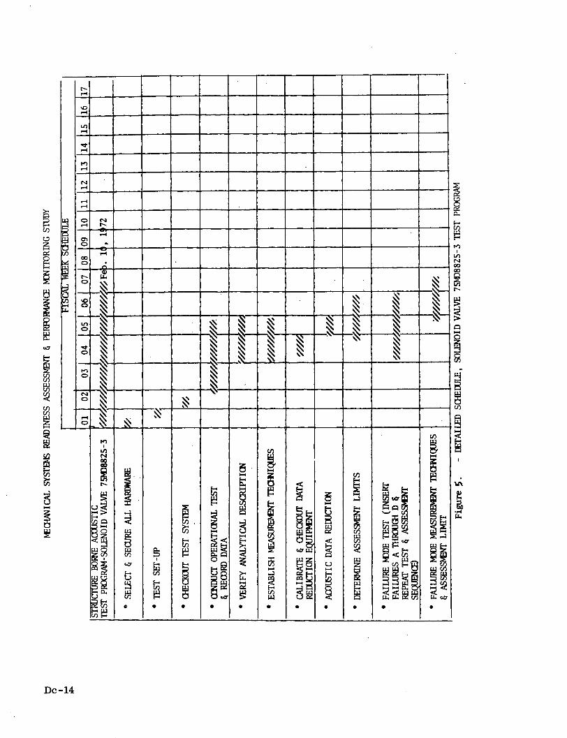
'0N

I~~~~~~~~~~~~~~~~~~~~~~~~~~~~~~~~~I

CD

-4

-4

-4

°

o r{

0i -

rl~~~~~~~~~~~~~~~~~~~~~~~~~~~~~~~~~~~~~~~~~~~~~~~~l

0,

-4

tIj

H

cjcoI

rlrX-

0

tb

1-

I

0

::

al

V)

5

t~r-

I9

H

C

iU7

t:IN,

8

:1

0

I9i~

WU)0

wd

1:9Upu1LU

iIS

H

RfIQ

5u

CS-

I

1

IS

"aS

M B,

S0S

IE0 "I*Yl

- - - - I - I I

I

-4IInV)

cOco

ar-

IV.,

a

U7

.,qP.

cn

U)

u

4

z

R

U)

l.I~a

50

Dc -14

I

'I

I

iiI

SECTION III

TEST FACILITIES

Test facilities at General Electric's Research and Development Laboratory,

Schenectady, New York will be employed for this test program. To acquire acoustic

data, sufficient space in Room 1062 (approximately 80 ft2) will be required. A

work bench will be provided and proper tools will be available to tune and adjust

electrical and mechanical networks shown in Figures 2 and 3. Facilities temperature

range of 650 + 5° F, humidity range of 45 + 5% and normal open laboratory cleanli-

ness will be maintained.

Facility electrical power requirements are 115 volts AC with total current of less

than 30 amp. Sufficient networks will be available to accommodate power supplies

and recorders as shown in Figure 3. Normal laboratory lighting levels will be

maintained.

Dc-15

SECTION IV

DETAILED TEST PRmCEDURES

4.1 TEST SE(QUENCE

The sequence for completing each step of this test program is shown diagramatically

in Figure 5. The order involves, at first, the identification and accumulation

of all electronic and mechanical hardware; Second, assembly and checkout of test

set up, including the test component; Third, assembly and checkout of complete test

systems including instrumentation; Fourth, test operations and recordings; Fifth,

determine measurement technique; Sixth, assembly and checkout of data reduction

equipment; Seventh, acoustic data reduction. Provisions must be made to recycle

tests if later data analysis indicates selection of a different measurement technique

or stabilization of a test variable will permit establishment of value assessment

criteria.

4.2 TEST SET UP

The test panel previously shown in Figure 2 will be installed at test berth in

Room 1062. 3000 PSIG (N2source will be connected to panel, as shown in Figure 2.

All lines must be clean and connections will be bubble tight leak proof checked

at 2500 PSIG GN2. Sherlock type CG-1 leak test solution or equivalent will be

used. Valve Serial #202 will be placed in test panel.

The test set up will be checked out in accordance with following detailed test

procedure. Data will be recorded as for each step of valve checkout as defined

on Test Recording Form (see Figure 6). Should problems be encountered during any

step of this test; KSC TM-440, Failure Mode and Effect Analysis Drawing 65B23278-23,

or Marotta Valve Corporation, Technical Manual Revision B for Model MV74VE should

be referenced for appropriate corrective action.

Dc-16

V4

-4)

E-

:>

Dc-17

\0

IL1..

-

., .,

I v)us 4

ax

go

RQl

4.3 VALVE CBECKOUT TEST PROCDEDUR

STEP PROCEDURE RESULT

.- - -- T - -- - -WARNING ,

Solenoid valve must be secured behind a protective

barrier for personnel protection when valve is

pressurized.

Prepare test setup in

accordance with figure

2, with all hand valves

closed.

Adjust regulated pressure

source to 2500 psig.

Open hand valveHVO,HV-1 & HV-3

Set power supplies 1 and 2

to 28 vdc.

Close HV-1 and open HV-7.

Leak test valve (using

leak test solution, Sherlock

type CG-1).

Close switch SW-l (See Figure 3

Gages G-O, G-D and G-3 indicate

2500 psig. DS-1 illuminates

DS-2 OFF. (See Figure 3)

Valve shall be bubble tight.

DS-1 OFF and DS-2 illuminates.

G-3 indicates zero psig.

1

2

3

4

5

6

De-18

Valve Checkout

Test Procedure (Continued)

STEP PROCEDURE RESULT

Leak test valve.

Cycle SW-1 five times.

Allow 30 seconds in each

position.

Slowly decrease voltage

on power supply 1 from

18 to 0 volts.

Adjust power supply to

zero volts.

Slowly increase voltage

from 0 to 18 volts.

Repeat steps 9, 10 and

11 three times.

Open SW-1.

Set power supply switch

to OFF.

Shut off pressure source

-and open HV-1, HV-3, HV-6

HV- 7.

Valve shall be bubble tight.

Valve must actuate and

deactuate without hesitation.

Solenoid denergizes above

1 vdc. DS-1 illuminates

DS-2 OFF.

Solenoid energizes between

8 to 18 volts. DS-1 OFF

DS-2 illuminates.

DS-1 illuminates

DS-2 OFF

Dc-19

7

8

9

10

11

12

13

14

15

I

4.4 ACOUSTIC INSTRUMEIATICQN

Wilcoxon Peizelectric Transducers Model Mill and Amplifier Model AM-1 will be

calibrated in accordance with Wlilooxn Researdh Tnstmrtim and Mainto*nanco Manuil

(Model AM-1) #37-668.

The transducers will be mounted on Solenoid Valve Housing (Part #36) at location

shown in Figure 7. The transducer mounting surface is 1/4" diameter. The

transducers will be cemented rigidly to the valve housing using either Eastman

910, EC-1294 (3M Company), Epon 828 (Shell), or Dental cement such as GRIP

(L. D. Caulk Company). Eastman 910 may be removed with N-Dimethylformamide.

To prevent ground loops, both the amplifier and transducer must be insulated

from ground with a single point ground being fed from the recorder input.

Honeywell Model 5600, 1 inch, 14 channel tape recorder will be used for magnetic

recording of va ve structure borne acoustics. This recorder will be calibrated

and o erated per Honeywell Mobdel 5600 instruction manual. Data Channel to be

recorded for each test are depicted in Figure 3 and include:

Channel 1 - Valve Accelerometer #1

Channel 2 - Valve Accelerometer #2

Channel 3 - Valve Switch Indicatzr #1

Channel 4 - Valve Switch Indicator #2

Channel 5 - Valve Solenoid energization voltage

Channel 6 - Voice Channel to identify test, tape speed, etc.

Channel 7 - Reference Accelerometer.

Dc-20

!

0)I

4,

E

:8I

, 8a

L.

c g& .2 o. ex

_ i of

4 a %4

I-

= a i .a. ,s L

;a

..

;h;=0&a

0 ts

0.

i

.. .

' .Z. ..

Dc-21

. . .f,..

-...'' °.:

4.5 CHECKOUT TOTAL ACOUSTIC TEST SYSTEM

To insure the total test system is performing properly and that optimum gain

settings are established for amplifiers, several operations of the Solenoid

valve will be monitored. Steps 1 through 4 and step 6 of Valve Checkout Pro-

cedure (paragraph 4.3) will be followed. The seven channels of data specified

in paragraph 4.4 will be recorded and played back or displayed to ascertain the

performance of overall test system. SW-1 should be cycled and resultant out-

puts recorded until overall operation of test system is satisfactorily veri-

fied.

4.6 CONDUCT ACOUSTIC TEST AND DATA RECORDING

The nominal oeprating time for Solenoid Valve 75M)8825-3 is approximately 25 milli-

seconds to actuate and 5 milliseconds to deactuate. With the test circuitry

previously described still in place, Steps 1 through 4 and Step 6 of valve

checkout procedure (paragraph 4.3) will be repeated. All electrical equipment

should be brought to the power-up mode of operation, and tape recorder set in record

mode. Data, Valve identification, nominal operating conditions, and length of

test should be read in on recorder voice channel. SW-1 should then be cycled

30 operations. Sound data will be recorded a minimum of 150 milliseconds after

solenoid energization and 50 milliseconds after deactuation. The time element

between cycles should all be minimized to aid in subsequent data reduction task.

Throughout test G1 and G3 should be monitored to verify that valve is switching

correct pressure levels. Any deviation of GN2pressure will be recorded.

Dc-22

Subsequent to above test, Steps 13, 14, and 15 of valve checkout procedure

will be accomplished and all electrical equipment switched to Power Off mode.

Next, Solenoid Valve 75M08825-3, Serial #210, will be placed in test panel

(Figure 2) and complete sequence of tests described above will be repeated.

Then, Solenoid Valve 75M08825-3, Serial #444, will be placed in test panel

(Figure 2) and once agains the complete sequence of tests repeated.

Solenoid Valve 75M18825-3, Serial #202, will have failure Mode A - fails to

operate - inserted and will be mounted into the test panel and complete sequence

of tests repeated.

Solenoid Valve 75M08825-3, Serial #210, will have failure Mode B - erroneous

indication - inserted and will be mounted into the test panel and complete sequence

of tests repeated.

Solenoid Valve 75M08825-3, Serial #202, will have failure Mbde C - leakage -

inserted and will be mounted into the test panel and complete sequence of tests

repeated.

Solenoid Valve 75M08825-3, Serial #210, will have failure Mbde D - sluggish

operation - inserted and will be mounted into the test panel and complete sequence

of tests repeated.

Dc-23

4.7 MEASUREMENT TECHNIQUS

It is impractical to attempt to predefine the precise measurement techniques

or variations of basic techniques which might be the most advantageous for

ultimately establishing valve 75M08825-3 assessment limits that can discriminate

between GO, NO-GO, and CAUTICN conditions. However, the approach to be pursued

will include the following techniques. Step 1 will consist of an overall (narrow

band) Spectral Analysis presentation of 210 total valve operations. The GE

Research and Development Laboratory Spectrum Pattern Analysis facility, Room 5036,

will be used to present this data. Functions of the facility

include the generation of spectra; recording of spectrum patterns on 35 mm film

spectrograms; local minicomputer processing of spectra; and the recording of

waveforms and spectra on digital magnetic tape for processing in a large G.E. 600

series computer system. Facility equipment includes analog magnetic tape recorders,

two complementary real-time frequency analyzers, a 622/i Varian Minicomputer

equipped with automatic analog to digital and digital to analog input and out-

put systems, a digital magnetic tape recorder, display format generating and

control circuits, display units, a 35 mn film recording camera, and an automatic

film processor. In addition, specially designed interface units are available

to speed data processing.

Dc-24

Twenty percent of Spectrum (every 5th operation) displayed will be recorded

directly on film as a continuous time series of amplitude versus frequency

plots. The remainder of operations will be operated on to create intensity

modulated spectrograms. No more than 10 operations will be displayed on a

single 8-1/2 x 11 sheet.

Based on visual observation of relationship of Spectra distinctive features with

predicted acoustic signatures and the mechanics of solenoid valve operation,

additional measurement techniques will be investigated.

It is anticipated that discrete band pass filtering will enable the investigation

to reduce the volume of analogue data requiring further manipulation. Various

filters are available in Mechanical Signature Analysis Laboratory - Rooam 603 -

which may be used in this process are:

(1) Band Pass Filter 1/3 octave/octaveBruel and Kjar Type 1612.

(2) Variable filter 20 cps-200 KCKrohn Hite Nbdel 315AR.

(3) FilterKrohn Hite Mbdel 3340R.

The filter chosen will be dependent on frequency band selection. The Signature

in reduced form will then be processed to detect transient occurrence of peak

levels, Peak/Time relationship comparison, Number of Peaks during Valve operating

cycle RMS level and Peak level vs. RMS level crest factors. Equipment which

will be used to detect these Peak and RMS level characteristics are:

(1) Hewlett Packard 5480B Memory Scope withHP5486B control and 5488A.

(2) Honeywell Strip Recorder

Dc-25

(3) Valentine Peak to Peak Voltmeter.

(4) Textronix Type 561A Oscilloscope.

(5) Dymec 2401C Integrating Digital Voltmeter.

(6) Hewlett-Packard 2401C Integrating Digital Voltmeter.

Auto correlation processing will be accomplished to detect significant internal

waveform relationships. Failure mode waveforms will be cross correlated against

normal (idealized) operation waveform. The idealized waveform will be shifted

in time relative to the actual failure mode waveforms, and when the correlation

function is a maximum, the positions of noise bursts will be located. The

correlation technique will then look between the noise peaks to determine signal

amplitude in what is normally a quiet period, measure the amplitude of the

existing noise bursts, identify the largest of them, determine the average

amplitude of the predominate noise bursts, and then take various ratios between

these measured valves. These measurements and ratios will be compared to nominal

operation valves. Principle Correlation equipment to be used is:

(1) Honeywell 9410 Correlator.

(2) Princeton Applied Research Correlator

(3) Hewlett-Packard 5488A Average/Cor-: lator.

Completion of the above data procsssing and reduction will terminate tests until

data in the specified form has been statistically evaluated and assessment limits

established.

Dc-26C_

4.8 TEST RECYCLING

Should evaluation of test data show that uncontrolled test variables, faulty

instrumentation, or data reduction problems, invalidate data and limit conclu-

sions that can be drawn to the extent that assessment limits cannot be established,

the problem will be corrected and test recycled.

Dc-27/'3-? ~S

ADDENDUM D

PIEZOELECTRIC ACCELEROMETERS*

ACCELERATION TRANSDUCERS

A piezoelectric accelerometer is an instrument used to measure shock and vibration. It canbe idealized by a mass element connected to the case by a spring and a damping medium.The transducing element produces an electrical output proportional to the displacement ofthe mass element relative to the case and also proportional to the acceleration applied to thecase. Most accelerometers can be represented as a single-degree-of-freedom system andare sensitive only in one axis.

The sensitivity of an accelerometer is the ratio of its electrical output to applied acceler-ation, usually expressed as picocoulombs/g or Volts/g. It is constant at all frequencies upto approximately one-fifth the resonant frequency.

PIEZOELECTRIC MATERIALSA piezoelectric material is one which generates an electrical charge when subjected to amechanical stress or deformation. As a self-generating sensing material, it usually producesa large output for its size, and is useful to extremely high frequencies. Rochelle salt,tourmaline, and quartz are examples of "natural" or single crystal piezoelectric materialsused in some applications, but ferroelectric ceramics are used in most piezoelectric accel-erometers.

Certain ferroelectric substances can be made to exhibit piezoelectricity by a process ofartificial polarization. These polycrystalline ceramics include barium titanate, leadzirconate, lead titanate, and lead mentaniobateo The great importance of the ferroelectricmaterials is that their piezoelectric properties can be controlled in the manufacturing pro-cess to produce the characteristics necessary to make a good accelerometer.

ACCELEROMETER DESIGN

Several designs of accelerometers are illustrated in Figure A. The inertial

mass is identified with the letter M, and the ceramic crystal, shown between

the mass and support and acting as a stiff spring, by the letter K. The

letter K with various subscripts also identifies case walls or other members

which act as springs in the accelerometer.

*The majority of data and all figures contained in this Appendix

are excerpted from the Endevco Corporation Instruction Manual (#101),

(Courtesy Endevco Corporation). Dd-1

1 2STRAIGHT ISOLATED

COMPRESSION COMPRESSIONSINGLE-ENDED SHEARCOMPRESSION

FIGURE A

Accelerometer Designs

The shear design has several unique advantages. As in single-ended compre-

ssion design, the case acts only as a protective cover and is not in contact

with the spring-mass system. Also, if the center post is made hollow and

extended through the case, the resulting accelerometer can be mounted by

simply passing an ordinary machine screw through the hole to attach it to

the test structure. Another major advantage of the shear approach is that

it can quite successfully be built with extremely small dimensions. The

majority of light-weight microminiature accelerometers are shear units.

PIEZOELECTRIC ACCELEROMETER CHARACTERISTICS

EQUIVALENT CIRCUITS

The equivalent circuit for a piezoelectric transducer is shown ..' Figure 1. In practice, theinternal resistance shown in circuit (A) normally exceeds 20,000 megohms and, thus, can beignored when considering the over-all transducer performance. Similarly, effects due to theinternal inductance are far beyond the upper frequency limit of the transducer and can alsobe ignored. The simplified circuit (Fig. IB) is adequate for applications analysis. The pie-zoelectric transducer is effectively a capacitor which produces a charge ,q, across its platesproportional to a force applied to the crystal.

The open circuit voltage ,e, out of the transducer is equal to the generated charge divided by

the transducer capacitance, or e (Volts) = . Thus, the transducer can alsoCp (picofarads)

be represented as a voltage generator and a series capacitance (Fig. 1C).

Dd-2

---- �- i - '--If-··-~- -I I--~

FIGURE 1.

Equivalent circuits for a piezoelectric transducer (A)actual circuit,(B) charge generator equivalent, and (C)voltage generator equivalent.

SENSITIVITY

The sensitivity of an accelerometer is defined as the ratio of its electrical output to itsmechanical input.' It may be expressed in units of charge per unit of acceleration orvoltage per unit of acceleration. It is important to note the terms in which the respectiveparameters are expressed; e.g., average, rms or peak.

Charge Sensitivity

Each accelerometer is provided with a charge sensitivity calibration, Q,

expressed in picocoulombs per g (pC/g). This is measured directly or derived

from Q"EC, where Q is expressed in picocoulombs, E in Volts, and C in pico-

farads. This calibration is used when the accelerometer -is operating into

charge measuring electronics. Note that magnitude of sensitivity can be

expressed in other terms:

g = n spk pC9 cm$ g .

Dd-3

Voltage Sensitivity

Each calibration card also carries the accelerometer voltage sensitivity, E, in millivolts perg (mV/g) as measured with a stated amount of external capacitance connected to the accelero-meter. Use the value 0.707 x E rms mV/pk g when observing the signal level on an rms VTVM.Use 2 x E as the accelerometer sensitivity when measuring peak-topeak voltages with a gal Ivanometer recorder or oscilloscope.

Effect of Cables on Sensitivity

Nhen performing measurements, the transducer circuit involves an external capacitance anda shunt resistance. The external capacitance Ct is commonly cable capacitance plus inputcapacitance of the associated amplifier. The shunt resistance Ri is commonly the inputresistance of the associated amplifier (Fig. 2).

RI · . ..qCp*Ct

(A)

CHARGE EQUIVALENT

(BE

VOLTAGOE EQUIVALENT

FIGURE 2.

Equivalent circuits for a normal piezoelectric transducer system:(A) charge equivalent and (B) voltage equivalen'.

Since the charge generated does not change, regardless of the amount of external capacitanceadded, the charge sensitivity of the accelerometer remains unaffected by the length of inter-connecting cable. This characteristic explains the practical advantage of a system incorpor-ating charge measuring electronics rather than voltage amplifiers.

When using voltage amplifiers the amount of external capacitance must be considered inestablishing the signal at the input of the amplifier. With added capacitance the output

voltage (appearing across Ri) becomes e = C---Cp + Ct

Dd-4

q

I M~~~~~-c '-

--- - -------- ;--------

The total system capacitance during actual use may differ from the capacitance that wasused in the original calibration. This changes the basic voltage sensitivity up or down by acalculable amount. The new sensitivity can be determined with either of two equations:

1. E =C Q x 1000 mV/g (1)

E = new sensitivity being determined, in millivolts per g (mV/g).

Q = factory supplied charge sensitivity, in picocoulombs per g (pC/g).

Cp = transducer internal capacitance, in picofarads (pF).

C t = total capacitance external to the transducer for which E is beingestablished, in picofarads (pF).

-For example:

Q = 34.7 pC/g

Cp = 575 pF

Ct = Ccable (200 pF) = Campl (25 pF)

= 225 pF

34.7 34.7 x 10' = 44 V ItE 575 +225 80010 - 0434 Volts/g

E = 43.4 mV/g = 43,4 pk mV/pk g

Cp + Cca I2. E = E c aI

Cp +C t (2)

Where

E = new sensitivity being determined, in mV/g.

ECal = factory supplied voltage sensitivity, in mV/g.

Cp = transducer internal capacitance, in pF.

Ccal = external capacitance used when calibrated at factory, in pF.

Ct

= total capacitance external to the transducer for which E is being established,in picofarads (pF).

Dd-5

For example:

El = 51.4 mV/g.

CP = 575 pF.

CCal = 100 pF.

Ct = cable (200 pF) + Campl (25 pF).

= 225 pF.

575 + 1O0 675E = 51.45752 = 51 4 0 43.4

E = 43.4 mV/g.

Note: (a) The values for Q, Cp, Eal and CCa i will be found on the individual

calibration cards shipped with each transducer.

(b) The residual capacitance of many voltage amplifiers is approximately25 pF. Consult individual amphefier data sheets.

(c) E and Ecal may be expressed as either rrmmV/pk g or pk mV/pkg,

where: mV/g = rms mV/rms g = pk mV/pk g and rms mV/pk g = .707 mV/g.

Standardization - Voltage Sensitivity

The effect of added shunt capacitance on voltage sensitivity can be used to

advantage in standardizing accelerometer output to a desired value.

Shielded capacitors can be used to standardize the sensitivity of any accelero-

meter to any value E less than its original calibration Ecal such as 10 ms mV/

pkg, so that g levels instead of millivolts can be read directly from the scale

of a vacuum tube voltmeter without interpolation. In other instances where

very high g levels are expected, it may be necessary to reduce the sensitivity

of the accelerometer by a factor of 10 or more in order not to exceed the 5-

volt output limit of most voltage amplifiers. To arrive at the exact capacitance

Dd-6

to be added to an accelerometer for a desired value of E, use Equation 1

above in this new form:

C- C (3)tE P

For example:

E = 10 pk mV/pk g (desired value)

Q = 34.7 pk pC/pk

Cp = 575 pF

C = 34l7-x 10 575 (3470 - 575) x 10 Io

Ct = *2895 pF.

Alternatively, we may use a now form of Equation 2:

EcaCt = E (Cp + Cca I) CpI

For example:

E = 10 pk mV/pk g (desired value)

Eca = 51.4 pk mV/pk g

Cp = 575 pF

CC I 100 pF

51.4Ct = 051 04 (575 +100) - 575

= 5.14 (675) = 575

= 3470 - 575

Ct = 2895 pF

Dd-7

FIGURE 3.

Series swamping equivalent circuit - for reducing transducer charge output.

Standardization - Charge Sensitivity

Although adding shunt capacitance has no effect, addition of series capacitance will reducethe effective transducer charge output. See Figure 3. The charge which appears at thecharge amplifier input is: C

Qamp = Q C + C + (5)

Where

Q = basic transducer charge sensitivity, in pC/g.

Cp = transducer internal capacitance, pF.

Ci = external parallel capacitance ahead of series capacitor, pF.

Cs = series swamping capacitnce. pF.

C2 = external parallel capacitance beyond the series capacitor, pF.

Note that although C2 is, in general, present, it has no effect on system charge sensitivity.

FREQUENCY RESPONSE

Low Frequency Response

A piezoelectric accelerometer is a self-generating transducer that produces an electricaloutput signal that is proportional to accele ation, without the use of an external powersource or carrier voltage. In practice, such a transducer cannot be used to measure constantor steady-state accelerations. At zero frequency no mechanical energy is being put intothe system, thus electrical energy cannot be continuously removed.

When using charge amplifiers the system low frequency response is determined primarilyby the low frequency response of the amplifier. The length of cable between transducer andamplifier will not affect the low frequency of the system, which is limited only by thecharacteristics of the amplifier.

Dd-8

When using voltage amplifiers, the low frequency response of a piezoelectric

accelerometer is a function of the RC time constant of the accelerometer and

the input resistance of the matching electronics.

FIGURE 4.

Low frequency response vs. loading (voltage amplifiers).

The low frequency response of any accelerometer can be improved by swamping

with additional shunt capacitance, such as long cables, to raise the RC time

constant. However, this technique will also affect sensitivity as discussed

on the preceeding pages.

Dd-9

Actual response at any frequency can be measured from Figure 4.

Where

f = frequency in Hz

R = input resistance of the matching amplifier in Ohms

C = total capacitance in farads of the accelerometer, plus additional appliedshunt capacitance, if any

Example:

If frequency (f) of desired measurements if 10 Hz, total capacitance (C) of accelero-meter and cable is 500 pF, and amplifier input impedance (R) is 100 MO (Endevco®cathode follower), we can determine:

f x R x C = 10x 100x 10x 500x 10 -1 = 0.50

Using Figure 4, we find that the relative response corresponding the fRC = 0. 5 is 95%(indicating that the signal at 10 Hz will be dc'in approximately 5%).

Using the same formula in the case of a Model 2215E Accelerometer with an approximatecapacitance of 9,500 pF we can see that for frequency esponse to 10 Hz and 10 MO inputimpedance, we obtain:

fxRxC = 0x 10x 10 x 9,500x1 0-l = 0.95

Again using Figure 4, the relative response is approximately 9 90 /%. Thus, a 10 Hz signalwill be down approximately 1%.

High Frequency Response

High frequency response of a piezoelectric accelerometer is a function of its mechanicalcharacteristics. A piezoelectric accelerometer can be represented as a single-degree-of-freedom spring-mass system, the response of which is shown in Figure 5 as a function offrequency.

Dd-10

a

Si,o

. I .I .I -.

D4 .1 .& .5

FREQUENCY RATIO fan

FIGURE 5.

Response of a sing le-degree-of-freedom spring-mass transducer whenthe case is undergoing sinusoidal acceleration.

For the accelerometer, this curve can be considered as showing the variation in sensitivityof the transducer with frequency. The response curve shows that at 1/5 the resonantfrequency, the response of the system is 1.04. This means that the sensitivity of theaccelerometer is 4% higher at that frequency than at the lower frequencies. For thisreason the "flat" accelerometer frequency range should be considered limited to 1/5 theresonant frequency. Data can, of course, be obtained for frequencies above 1/5 theresonant frequency, as long as appropriate correction factors are applied to compensatefor the "resonant rise".

Resonant Frequency

The USA Standards Institute defines resonant frequency as that frequency at which thesensitivity of the pickup is a maximum. Several methods are currently used to determineaccelerometer resonant frequency.

Accelerometers should be selected with resonant frequencies at least 5 times

higher than the highest frequency of interest (or with a natural period less

than 1/5 that of an input shock pulse duration). To be valid, however, the

resonant frequency specified must be mounted mechanical resonance.

Dd-ll

/

.

_I_

a

Since the accelerometer will be mounted in use, the mounted resonance is the

only one of value to the user.

DYNAMIC RANGE AND LINEARITY

The range of input acceleration levels for which accelerometer sensitivity

remains constant is defined as the range of "Amplitude Linearity." Although

a piezoelectric accelerometer is theoretically linear down to 0 "g", a

practical lower limitation is imposed by the noise level of impedance match-

ing electronics. For very low vibration levels, a high output accelerometer

is required.

Upper limits of linearity may be imposed by either non-linear response of

the piezoelectric element or by fragility of the transducer as a whole. In

either case, the limits can be accurately determined only through actual

evaluation. The sensitivity of all piezoelectric accelerometers increases

with acceleration level.

PHASE SHIFT

In an accelerometer, phase shift is defined as the time delay between the

mechanical input and the resulting electrical output signal. All vibration

encountered in practice is complex, and like shock, is composed of a number

of frequencies superimposed in a specific way. If transducer phase shift is

not linear with frequency, the various frequency components will be shifted

relative to one another and the resultant electrical output will be a distortion

of the mechanical input.

Acoustic Noise

Considerable vibration in flight or static testing is induced by acoustical

energy. It has been shown in numerous cases that random acoustical energy

at 120 db can induce vibrations of the order of 50 g's or higher in structural

members, and it can be assumed that higher acoustic levels may increase the

vibration levels although not necessarily linearly. It has also been shown

Dd-12

that crystal accelerometers have, at the most, noise outputs equal to only a

fraction of a g at 140 db noise levels so that if the usual high level

vibrations are to be measured in acoustic fields, good signal-to-noise ratios

and accuracies are obtainable. There are other cases, however, where low

level evaluations on structures that are not subject to acoustic excitation

must be made in high level acoustic fields. In these cases considerable

attention must be paid to the acoustic response of the measuring system to

assure good signal-to-noise levels and accuracies. The resonant frequency

(fn) of the crystal accelerometer must be at least three times the highestacoustic frequency expected.

RF and Magnetic Fields

Magnetic and RF fields have no effect on most piezoelectric elements. If an

accelerometer includes magnetic materials a spurious output may be observed

when it is vibrated in a high magnetic field or subjected to high intensity

changing magnetic flux. Adequate isolation must be provided against RF

ground-loops and stray signal pickup.

Temperature

In general, Endevco® accelerometers are rated for three temperature ranges: -650 F to+230°F, -650 F to +3500 F, and -3200 F to +5000 F. In addition, Piezite® ElementType P-10 operates from -4520F to +7500 F and is the only material that will coverthese temperature extremes with good stability and large output. Within their usabletemperature ranges, the various crystal materials show variations in sensivitiy, capaci-tance, and resistance. The deviation of voltage output with temperature is almostalways different than the charge output deviation. It is, therefore, important whenusing charge measuring electronics to select accelerometers with flat charge charac-teristics, and with voltage equipment to choose accelerometers with flat voltageresponse curves.

Dd-13

As the accelerometer temperature is increased beyond its rated operating limit, the crystalbegins to depolarize, with a resultant loss of sensitivity. If the unit is exposed to excesstemperatures for only a short period, it may still be usable. It must, however, be recali-brated since it will have a new sensitivity of lower value. If the temperature is increaseduntil the crystal reaches its Curie point, the accelerometer will be completely depolarizedand unusable.

It was mentioned earlier that accelerometer low frequency response is dependent on theaccelerometer-amplifier RC time constant (for voltage amplifiers). At higher temperatures,the internal resistance of piezoelectric crystals decreases, causing a reduction in the effectiveRC time constant. It is, therefore, very important to use accelerometers whose internal re-sistance remains high in high temperature applications.At the very least, internal resistance as a function of temperature should be measured duringcalibration so that correction factors can be applied, if necessary.

Dd-14

ADDENDUM E

STRUCTURE BORNE ACOUSTICS HARDWARE MANUFACTURERS

The following listed vendors comprise only a representative sample of SBA hardware

manufacturers. No endorsement is implied by the presence or absence of the hundreds

of well-qualified vendors of the major equipment categories included within.

De-1

Accelerometers

Columbia Research Labs., Inc.Conrac Corporation, Instruments and Control DivisionEndevco, Dynamic Instrument DivisionKaman Nuclear, Division of Kaman Sciences CorporationKistler Instrument CompanyStatham Instruments, Inc.Systron-Donner Corporation, Inertial DivisionTeledyne Inc., Automated Specialties DivisionWilcoxon Research

Amplifiers, Instrumentation

Where possible it is recommended that instrumentation amplifiers be procured fromthe accelerometer vendor. This assures a match of transducer and amplifier charac-teristics.

Analyzers, Vibration

B and K Instruments, Inc.Bell and Howell, Electronics and Instruments GroupChrysler Corporation, Huntsville DivisionGeneral Electric CompanyGeneral Radio CompanyHamilton Standard Division, United AircraftHewlett-PackardHoneywell Inc., Test Instruments DivisionHughes Aircraft Company, Space and Communications GroupKaman Aerospace CorporationLing Electronics Division, LTV Ling Altec, Inc.Polarad Electronics InstrumentsSignal Analysis Industries CorporationTektronix, Inc.Vibration Instruments CompanyWavelabs Company, Division of Systron-Donner CorporationWeston Instruments

Cabling

Cabling for structure borne acoustics in.plementation is, in general, expected to benon-standard and fabricated to order.

Cabling between accelerometers and associated signal conditioning amplifiers ordi-narily be procured from the vendor supplying these items.

Computers, Digital

Arma Division, AMBAC Industries, Inc.Avco Corporation, Electronics DivisionBunker Ramo Corporation, Electronic Systems Division

De-2

EMR Computer Digital Equipment CorporationElectronic AssociatesFriden Division, The Singer CompanyGeneral Electric CompanyHazeltine CorporationHewlett-PackardHoneywell Information SystemsInternational Business Machines CorporationLear Siegler, Inc., Electronic Instrumentation DivisionLeeds and Northrup CompanyLink Division, the Singer CompanyLockheed Aircraft CorporationMelpar, Division of ITV Electrosystems CorporationMincom Division, 3M CompanyMotorola/Government Electronics DivisionNational Cash Register CompanyNorthrup CorporationPhilco-Ford, Aerospace and Defense Systems OperationsRCARadiation Inc., Subsidiary of Harris-Intertype CorporationRaytheon CompanySystems Engineering Laboratories, Inc.TRW Systems GroupTeledyne Brown EngineeringTexas Instruments, Inc.Univac Defense Systems Division, Sperry RandWang LaboratoriesWestinghouse Electric Corporation, Computer and Instrumentation DivisionWeston Components Division, Weston Instruments, Inc.Wyle LaboratoriesXerox Data Systems

Correlators

Hewlett-PackardSignal Analysis Industries Corporation

Filters, Electronic

Analog Devices, Inc.B and K Instruments, Inc.Bendix Corporation, Electrical Components Division

De-3

Collins Radio CompanyGeneral Electric CompanyGeneral Instrument CorporationGeneral Radio CompanyHewlett-PackardSanders Associates, Inc.TRW Electronic Functions DivisionTeledyne PhilbrickVarian AssociatesVibration Instruments Company

Oscilloscopes

Automation Industries, Inc.B and F Instrument, Inc.B and K Division, Dynascan CorporationBeckman Instruments, Inc.Hewlett-PackardHickok Electrical Instrument CompanyHoneywell, Inc., Test Instruments DivisionInternational Telephone and Telgraph CorporationMagnavox Company, Government Electronics DivisionMonsanto CompanyRCA, Electronic ComponentsSimpson Electric CompanyStatham Instruments, Inc.Tektronix, Inc.

Plotters, Data

Bendix Corporation, Environmental Science DivisionThomas A. Edison Industries, Instrument DivisionEsterline Angus, Division of Esterline CorporationGerber Scientific Instrument CompanyHewlett-PackardHouston Instrument, Division of Bausch and LombHughes Aircraft Company, Aerospace GroupLeeds and Northrup CompanyMilgo Electronic CorporationPotter Instrument Company, Inc.RCAResdel Engineering CorporationScientific-Atlanta, Inc.Teledyne Systems Company, Division of Teledyne, Inc.Texas Instruments, Inc., Digital Systems Division

De-4

Recording Equipment. Magnetic TapeAmpex CorporationBell and Howell, Electronics and Instruments GroupCook Electric CompanyFairchild Industrial ProductsGeneral Instrument Corporation, Electronic Systems DivisionGeneral Radio CompanyHamilton Standard Division, United AircraftHewlett-PackardHoneywell, Inc., Aerospace and Defense GroupLockheed Aircraft CorporationMincom Division, 3M CompanyRCAScientific -AtlantaTexas Instruments, Inc.

ADDENDUM F

REPRESENTATIVE STRUCTURE BORNE ACOUSTICS HARDWARE

SAMPLE - SPECIFICATIONS

The following data are included to provide a small sampling of the SBA hardware avail-

able off-the-shelf. Inclusion should not be construed as an endorsement of these prod-

ucts nor are the data necessarily current. Hardware in the following categories are

included:

Accelerometer

Amplifier, Accelerometer

Analyzer, Averaging

Analyzer, Correlation and Probability

Analyzer, Real-Time

Analyzer, Spectrum

Correlator, Real-Time

Filter, Variable

Recorder, Tape, Magnetic

Recorder, X-Y

Scanner, Input

Df-1

WCOXON RESEA CHP.O. Box 5798

9 Ericsson Rood, Beohesda, Moryland 20014Phone (301) 365-4412

MECHANICAL AND ELECTRONIC DEVELOPMENT * INSTRUMENTS AND SPECIAL DEVICES

o MODEL 111

1 gram

6 mV/g1.2 pC/g$75.00

MSODEL 113 a

4 gram24 my/g5 pC/g

$75.00

The Model 111 and 113 accelerometers are recommended for reliable measurements on light structures since theirlow weight does not appreciably affect the motion of the structure. (See WR Bulletin No. 1 and No. 10).

Model 111 and 113 are cement-on types, Model 104 and 106 are supplied with threaded studs; and Model 112 and114 are triaxials.

To reduce weight no connectors are used at the accelerometer. The cable connection at the accelerometer isextremely rugged. It will not break during normal usage and therefore no detachable cables are necessary.

:'A_~" _..." _ _ m

Df-2

. , .

-m ....... ... ..... . . . . . . . . . . . . . . . . . . . . . . . . . . . . ~ ,i

gI'' 4 oCharge Sensitivity, pC/g, nominal 1.2 5

minimum 1.0 4.0Voltage Sensitivity, mV/g, nominal (1) 6 24Frequency Response, Hz, ±+2 db (2) 2 - 11,000 3 - 8,000

+1 db (2) 1 - 18,000 1.5 - 12,000

Capacitance, pF, nominal 200 200Resonant Frequency, kHz, nominal (2) 55 36

Transverse Sensitivity, % of axial, nominal 5 3;maximum 10 5

Acoustic Sensitivity, equivalent g at 155 db 2 x 10" 10' 1re 0.0002 microbar, nominal (31

Magnetic Sensitivity, equiv. g/gauss, nominal 10' 4 5 x 10°5

Acceleration Range, g 102 -103 3 x 1003 - 103

Temperature Range, °F, +10% sensitivity change -60 to +250 -60 to +250Humidity Range, percent 0 - 100 0 - 100Nonlinearity, percent 1.5 1.5Resistance, Megohm, minimum at 700 F 103 10 3

Weight, gram 1.2 4Dimensions See Drawing See DrawingMaterial of Base S.S. 104 Alum. 111 S.S. 106 Alum. 113Output Connector Microdot at end of Microdot at end of

3 Ft. cable 3 Ft. cableElectrical Isolation of signal and caseground from test structure

Mod.104 Mod. 111 Mod. 1o06 Med. 113

Price: 1 - 5 units $95.00 $75.00 $95.00 $75.006 - 10 units $85.50 :$67.50 $85.50 $67.50

11 - 25 units $81.00 $63.75 $81.00 $63.75

Options: A Triaxial Models 112, 114Price $195.00 each

Calibration Each unit is calibrated for sensitivity, transversesensitivity, frequency response to one half of theresonant frequency, capacitance, This infor-mation is supplied with each transducer.

(1) With 100 pf external capacitance.(2) Mounted on tungsten calibration table with 1,000 megohm electrical load.(3) Tested in accordance with method described in Wilcoxon Research Bulletin No. 7.(4) Tested in accordance with method described in Wilcoxon Research Bulletin No. 3.(5) Minimum acceleration measured using Wilcoxon Research Preamplifiers without filtering with a

signal to noise ratio of 10:1.

As a result of continuing research and developmsnt specifications and prices are subject to change without notice.Df-3

Specification Sheet 95

P.o. Sam 5799 Eicozesin Rad, GO8, 1 m 'y3 d 2.4 '

p@Xang (MI) 36541b2

MECHANICAL AND ELECTROMgC DEVELOM1ENT o INSTRUMENTS AND SPECIAL DEVICES___99 a" A.:: i:5L.2·1E-'- ................. hs.'tn. :' J ... . ,-

3'APPROX. DIA.

JDIA. .1 4'

W HEX. .03H-MICR0OT 6-32

CONNECTOR Y LONG

MODEL 96 MODEL 95

MODEL 95

0. 5 gran1.5 mv/g0.4 pc/g1.5 - 23, Od3 Hz, +1 db

The Model 95 and 96 shear-type accelerometers are recommended for reliablemeasurements on light structures since their low weight does not appreciablyaffect the motion of the structure. (See WR Bulletins No. 1 and No. 10. )

Model 95 is a cement-on type, Modal 96 is supplied with a threaded stud; andModel 97 is a triaxial accelerometer.

To reduce weight, no connectors are used at the accelerometer. The cableconnection at the accelerometer is extremely rugged. It will not break duringnormal usage and, therefore, no detachable cables are necessary.

Df-4

- 3 APPROX. DA.

] DIA.

RO, arcOnECTOR , .38'

.IU

ROCOT CONNECTOR

INSULATED BASE i

SPECIFICATIONS

6del 95 96

Charge Sensitivity, pC/g 0.4 0.4Voltage Sensitivity, mV/g 1.5 1.5Frequency Response, Hz, + 1 db(1 ) 1.5-23, 000 1.5-23, 000

+ 3 db() 0.8-40, 000 0.8-40, 000

Capacitance, pF, nominal 250 250Resonant Frequency, kHz, nominal 75 75

Transverse Sensitivity, % of axial, nominal 5 5maximum 10 10

Acoustic Sensitivity, equivalent g at 155 db 2 X 101 2 X 10 - 1

re 0. 0002 microbar, nominal( 2)Strain Sensitivity, equivalent g at strain of 2 X 10- 3 2 X 10 ' 3

10-6 in plane of base, nominal(3)Magnetic Sensitivity, equiv. g/gauss, nominal 10 - 4 10-4

Acceleration Range, (4) 0.01-104 0.01-10Temperature Range, F, + 10% sensitivity change -60 to +250 -60 to +250Humidity Range, percent 0-100 0-100Nonlinearity, percent 1.5 1. 5Resistance, megohm, minimum at 70°F 103 103

eight, gramensions, inches, excluding connectorerial of Base

Output ConnectorElectrical isolation of signal and case ground

from test structure

0.5See DrawingAluminumMicrodot at end of 3' cableYes

0.8See DrawingTitaniumMicrodot at end of 3' cableNo

Price: 1 - 5 units $ 95.00 $ 110.006 - 10 units $ 85. 50 $ 99.00

11 - 25 units $ 81.00 $ 93. 50

Options: Triaxial Model 97, consisting of three Model 95mounted on a 1/4" X 1/4" X 1/4" aluminum block.$285. 00 each.

Calibration: Each unit is calibrated for sensitivity, transversesensitivity, frequency response to one half of theresonant frequency, capacitance. This informationis supplied with each transducer.

(1) Mounted on tungsten calibration table with 1,000 megohm electrical load(2) Tested in accordance with method described in Wilcoxon Research Bulletin No. 7(3) Tested in accordance with method described in Wilcoxon Research Bulletin No. 3(4) Minimum acceleration measured using Wilcoxon Research Preamplifiers without filtering with a

signal to noise ratio of 10:1. Maximum acceleration for Model 95 depends on cementing technique.

*1 a result of continuing research and development specifications and prices are subject to change without notice.

Df-5

F

WILCOXON MODEL AM-1

ACCELEROMETER AMPLIFIER

SPECIFICATIONS

VOLTAGE GAIN

Gain Stability

Bandwidth

Input Impedance

Output Impedance

Output Current

Input Voltage

Power Requirements

Power Supply Noise Attenuation

Temperature Range

Terminals

Broadband Noise referred to

input, 5-100,000 cps, gain

40,30 or 20 db

Phase Shift

100 cps to 1 KC

20 cps to 10 KC

Selectable steps:-10, 0, 10, 20, 30,40 db ±0.2 db.Continuously variableattenuator 0 to -10 db

+0.1 db

3 to 100,000 cps -3 db, optional atno additional cost 1 to 100,000 cps

1,000 megohm shunted by 30 picofarad

50 ohm maximum

3 ma RMS short circuit

5 volt RMS divided by gain for allgain settinjs

-28 z3 volt, 10 ma

40 db minimum at 60 cps referred tooutput

0° to 500 C, operating

Input BNC: Cal Input BNC; Output BNC

Maximum5 Lvolt RMS with 1000 pf source9 4volt RMS with 200 pf source

1 degree absolute

1 degree relative between any two AM-1

preamplifiers

As a result of continuing research and development specifications aresubject to change without notice.

Df-6

DIGITAL ANAL YZERS H SIGNAL ANALYZER For averaging, variance, histograms, correlation Model 5480A

V •

^ r

5480A Signal Averager

The Model 5480A Signal Analyzer applies statistical principles for real time analysis of data and signal-to-noise improvement. Accurate, detailed information is made avail­able through signal averaging; an example of the results of this technique applied to nerve response is shown in Figure 1. Figure 2 shows the output of the HP 8553/8552 Spec­trum Analyzer; the same spectrum enhanced by signal averaging is shown in Figure 3. Many other applications exist for the 5480A in the fields of medicine, bio-medicine, chemistry, physics, electronics, astronomy**, vibration, tur-bulance, and others.

The plug-in design of the 5 480A provides a more versa­tile instrument and guards against obsolescence. The 5480A Mainframe contains a 1024 word, 24-bit magnetic core memory with related circuits and a CRT display while the two plug-ins chosen (5486A, and either the 5485A, 5487A or 5488A) depend upon the specific application.

Averaging There are three methods of averaging that provide from

0 to 57 dB signal-to-noise ratio improvement. Stable averaging: continuous calibrated on-line display. Sig­

nal amplitude remains constant as noise is attenuated. Weighted averaging: permits signal enhancement of slowly

varying waveforms by exponential weighting of previous information with respect to new information. SWEEP NUMBER setting determines speed at which the average signal follows input.

Summation averaging: algebraic summation process. Signal will grow from stable base line. If placed in AUTO mode, display will be automatically calibrated at the end of the preset number of ,weeps

•HP Journal, April '68 " H P Journal, Juna '69

Variance (Option 001): the variance of channel A is displayed by averaging the square of the noise in channel B.

Multichannel Scaling (MCS) The analyzer sweeps through memory remaining at each

channel for a preset time. A plot of the number of input pulses versus time is displayed.

Correlation The frequency of a noisy signal can be obtained by auto­

correlation, while the common frequency and relative phase difference of two noisy signals can be obtained by cross-correlation. The 5488A Plug-in is required for correlation.

Histograms Probability density generation with respect to time inter­

val and frequency. Time interval: time between synchronization pulses. Hori­

zontal calibration by time base. Frequency: Start and stop determined by time base. Hori­

zontal calibration by time base.

Figure 1. Evoked response, vestibular cortex of rhesus monkey.

Df-7

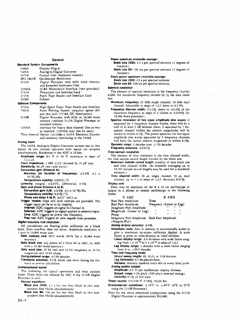
General

Standard System Components5160A Display Plug-in5465A Analog-to-Digital Converter5.175A Control Unit (keyboard console)H51.180AR Oscilloscope Mainframe2115A Digital Processor with 8192 word memory

and Extended Arithmetic Unit12566A 16-Bit Microcircuit Interface (two provided)2752A Teleprinter and Interface Card2737A Paper Tape Reader and Interface Card2940A Cabinet

Optional Components2753A High Speed Paper Tape Punch and Interface7591A Point Plotting System (requires option 005

and two each 17178A DC Attenuators)2116B Digital Processor with 8192 or 16,384 word

memory (replaces 2115A Digital Processor instandard system)

12554A Interface for binary data channel. One or twoas required. (12556A may also be used)

Time Interval Option (includes a 5235A Electronic Counterand necessary interfacing to the 5450A

Analog inputThe 5465A Analog-to-Digital Converter accepts one or two

inputs. In two channel operation both inputs are sampledsimultaneously. Resolution of the ADC is 10 bits.

Amplitude range: 0.1 V to 10 V maximum in steps of1.2,.1,10.

Input impedance: I Mn ±i1% shunted by 15 pF max.Sensitivity: 30 pV rms ( sine wave).Conversion gain (Channel A):

Accuracy (as function of frequency): +0.1% t3 x10-'%/Hz.

Temperature stability: 0.005%/'C.Linearity: integral, -0.05%; differential, ±3%.Gain and phase Channel A to B:

Conversion gain A/B: ±0.2% -2 x 10-"%/Hz.Temperature stability: 0.01%/'C.Phase and delay A to B: +0.2'° 0.5 As.

Trigger modes: slope and level controls are provided. Thetrigger input can be ac or dc coupled.Internal: ADC triggers on signal to Channel A.External: ADC triggers on signal applied to external input.Line: ADC triggers on power line frequency.Free run: ADC triggers on data request from processor.

Digital accuracy and resolutionAll calculations use floating point arithmetic on a block

basis. Data overflow does not occur. Amplitude resolution is1 part in 16,000 worst case.

Data memory size: 3072 words (8192 for a 16,384 wordmemory).

Data block size: any power of 2 from 64 to 1024 (to 4096with a 16,381 word memory).

Data word size: 16 bit real and 16 bit imaginary or 16 bitmagnitude and 16 bit phase.

Computational range: _ 150 decades.Transform accuracy: 0.1% worst case error during the for-

ward or inverse calculation.Computational speed

The following are typical operations and their analysistimes. These times are reduced by 20% if the 2116B DigitalProcessor is used.

Fourier transform:Block size 1024: 3..l s for one data block or two inde-

pendent data blocks simultaneously.Block size 64: 130 ms for one data block or two inde.

pendent data blocks simultaneously.

Df-8

Power spectrum ensemble average:Block size 1024: 2.4 s per spectral estimate (2 degrees of

freedom).Block size 64: 120 ms per spectral estimate (2 degrees of

freedom).Cross power spectrum ensemble average:

Block size 1024: 4.2 s per spectral estimate.Block size 64: 220 ms per spectral estimate.

Spectral resolutionThe element of spectral resolution is the frequency chanfiel

width, the maximum frequency divided by V2 the data blocksize.

Maximum frequency: 25 kHz single channel; 10 kHz dualchannel. Adjustable in steps of 1,2,5 down to 0.2 Hz.

Frequency Channel width: <3.2% down to <0.2% of themaximum frequency in steps of 2 (down to <0.05% for16,384 word processor).

Spectral resolution of two equal amplitude sine waves: ifseparated by 3 frequency channel widths, there will be anull of at least 3 dB between them; if separated by 7 fre-quency channel widths the relative magnitudes will becorrect to within 01%. The power spectrum for two equalamplitude sine waves separated by 5 frequency channelswill have the correct relative magnitude to within 0.1%.

Dynamic range: -I decades over ±150 decades.Frequency accuracy: ± 0.01%.

Time domain resolutionThe element of time resolution is the time channel width,

the time sample record length divided by the block size.Maximum sample record length: product of data block size

and time channel width. (In ensemble averaging up to32,767 sample record lengths may be used for a statisticalestimate. )

Time channel width: 20 As, single channel; 50 /s, dualchannel, up to 5 s in steps of 1,2,5. Accuracy 0.01%.

Display unitData may be displayed on the 8 x 10 cm oscilloscope or

output to a plotter or remote oscilloscope in the followingforms.

Y AXIF X AXISReal Part Amplitude TimeReal Part Amplitude Frequency (Linear or Log)Imaginary Part AmplitudeMagnitude (Linear or Log)PhaseImaginary Part Amplitude Real Part Amplitude(Nyquist Plot)Analog display accuracy: + 1%.Amplitude scale: data in memory is automatically scaled to

give a maximum on-screen calibrated display. A scalefactor is given in volts/division or volts'/division.Linear display range: _4 divisions with scale factor rang-

ing from I x 10o"- to 5 x 10" in steps of 1,2,5.Log display range: 4 decades with a scale factor ranging

from 0 to -99.9 decades.Time and frequency scale:

Lineor sweep length: 10, 10.24. or 12.8 division.Log horizontal: 0.5 decade/division.Markers: intensity markers every 8th or every 32nd point.

Analog plotter output:Amplitude: 0.5 V per oscilloscope display division.Output range: 1-20 pts/s (500 pts/s external timing).Linearity: 0.1% of full scale.

Power source: 115/230 V ±-10%, 50/60 Hz.Environmental conditions: +10'C to +40'C (O0C to 55'C

using the 2116B Processor).Price for the above referenced configuration using the 2115A

Digital Processor is approximately S49,000.

1 _

Figure 2. Spectrum onalysis' using HP 8353/B552. FiGure 3. Enhanced opectrum anolvylo with the HP 5480A%.'See Microwave Journol, October 1969.

Specifications

5486A Control UnitS/N ratio improvement: up to 60 dB can be achieved.Sweep number. manually selected. Dial is arranged in binary

sequence (2N) from single sweep (0 dial position) to 2'(524,288) sweeps.

Sweep time (horizontal sweep): internally generated sweeptime is calibrated in s/cm. Adjustable in 15 steps, in a 1, 2,5 sequence, from 1 ms/cm to 50 s/cm. External sweep capa-bility is provided.

Triggering and synchronizationInternal: sweep is triggered by internally generated pulse

occuring at end of each sweep. Pulse available at backpanel to control experiment; can be delayed by Post-Analysis Delay.

Eternal: requires 100 mV rms signal (+ or -- slope) withrise time less than 10 its.

Uin: synchronized to power line frequency.Pra-onalysis delay: variable in 15 steps (1,2,5) from 20 us

to 0.5 s.Poat-analysis delay: continuously variable from 0.01 to 10 s.

Sensitivity multipller: expands vertical to 64 counts/cm inpower of two increments.

Input characteristics: (Histogram Mode).Bandwidth: dc to 1 MHz.Sensitivity: 100 mV.Input impedance: I MQ shunted by 30 pF.

5480A OutputsDigital: two 50-pin connectors with binary data output. Direct

interface with Hewlett-Packard computers is available withthe 10625A Interface (5481A System).

Sweep voltage: 0 to + I1 V sweep ramp; conveniently adjustedby changing resistors to give output ramp going from 0 Vto any value between 0 to + 10 V.

Sync: "Pos" provides + 12 V, >0.5 ,us pulse at start of eachsweep (before pre-analysis delay); "Neg" provides sameexcept --12 V.

Sampling pulses: pulses (100 ns pulse width) go from +5 Vto ground and return to + 5 V once each time the input issampled.Analog: X and Y outputs for Recorder, Point Plotter, Scopes,

NMR Systems.

GeneralPower: 115 or 230 V -+-10%, 50-400 Hz, 175 watts.Dimensions: 163/4" wide, 12%" high, 243/" deep over-all

(425 x 311 x 593 mm).Weight: 76 lb (34,5 kg) net with plug-ins.

5485A Two Channel InputInput chasrcteristics: two channels with polarity switch for

each channel. Channels can be used individually or theirinputs can be summed.Coupling: ac or dc.input impedance: exceeds 1 MnI shunted by 25 pF.Banrdidth: from dc (2 Hz ac coupled) to 50 kHz.Sampling rate: 2 Hz to 100 kHz, in 1,2,5 steps.Input sensitivity: adjustable from 5 mV/cm to 20 V/cm in

12 steps (1,2,5 sequence) with -5% accuracy. HP am-plifiers, Models 2470A or 8875A, may be used to increasesensitivity.

Analog-to4igital converr:t ramp type with variable resolution1 ms/cm sweep time has 5 bit resolution. 2 ms/cm sweeptime has 7 bit resolution. 5 ms/cm or slower sweep time has9 bit resolution. ADC clock rate 10 MHz.

PulaB requirements: (Multichannel Scaling Mode)Amplitude: >2 V (20 V max).Maximum repettion rate: 1 MHz.Minimum pulse width: 500 ns.Pulse pair rsolution: 500 ns.

input impGdance: 3 kIi minimum.

Dwell time apr channel: 10 us through 0.5 s internal time base: 50 us to oo).

1,2,5 steps (ex-

Sweep modes: sawtooth. External time base input allows anydesired sweep shape.

Triggering: external or internal.

5487A Four Channel InputSame as 5485A except four inputs. deletes summing of inputs

and polarity inversion.Bandwldt: dc (2 Hz dc coupled) to 25 kHz.Senstvft:. 50 mV/cm to 20 V/cm.

54A8A Correlator InputSame as 5485A except adds correlation, deletes summing of

two inputs, and polarity inversion.fBndwidth: dc (2 Hz ac coupled) to 25 kHz.Senaitvty: 50 mV/cm to 20 V/cm.

Prme:5480A Mainframe, 86950.5485A Two-Channel Input, $1500.5486A Control Unit, $1500.5487A Four-Channel Input, 01800.5488A Correlator Input, $2500.Option 001 Variance, add $300.

Df-9

V )N

J? \{fteJ\

J S S r RESOLUTION TO .2u FASTER \PRO

NEW 400 Point ^ -model sai-43

CORRELATION & PROBABILITY ANALYZER

ADVANCED DATA SHEET

The SAI-43 Correlation and Probability Analyzer is an all-digital high speed processing instrument which provides an on-line, real time computation in three primary operating modes-Correlation (auto and cross), Enhancement (or signal recovery) and Probability (Density and Distribution). In all modes, 400 analysis points are computed.

CORRELATION: Correlation is a fundamental time domain processing tool in which waveform similarities are established thru time delay comparisons. In autocorrelation a signal is compared with a time shifted version of itself. In crosscorrelation the similiarity between two signals is determined as a function of the time shift between them.

The SAI-43 provides auto and crosscorrelation functions with incremental lag or time delay values ranging from 1 usee to 1 sec resulting in total time de>ays from 400 usee to 400 sec. Auto or crosscorrelation functions are determined simultaneously at 400 incremental lag points so that a complete correlation function is displayed at one time. Precomputation delay of 800 lag values selected in 200 lag increments allows the correlation function to be viewed symmetrically about zero or up to 800 lag values removed from zero (optlonali;- •< 8000 points). The clipped mode allows rapid determination of time dependencies for low leve; iignals. The averaging Is accomplished digitally with fixed linear summations ranging from 2' to 2" in binary steps. Exponential averaging Is a standard feature.

ENHANCEMENT: Some waveforms are periodic with a known period or are periodically stimulated as in a stimulus-and-response application. Often these waveforms are buried in random or non-coherent interference. The Enhance mode of the SAI-43 allows for the detection of the actual waveshape of this repetitive waveform through a signal averaging or so-called enhancement procedure.

The waveform is divided Into 400 points with resolutions (or spacing between points) ranging from 1 usee to 1 sec. From 2' to 2" (in binary steps) successive pulses can be linearly averaged in addition to the continuous operation mode. Exponential averaging of the pulses is also available. This mode is operable with either an .'xternaliy applied synchronization pulse or an internal pulse provided at the rear panel.

PROBABILITY: Probability analysis provides a description of the instantaneous amplitude characteristics of a waveform. The probability density function (DENS) provides information concerning the likelihood that a function lies within prescribed (amplitude) bounds. The probability that the signal amplitude will not exceed a particular value is provided by the probability distribution function (DIST).

In the probability mode the functions are determined at 400 points. The horizontal axis of the display represents voltage and the range and sensitivity are determined by the setting of the input attenuators. Here again the averaging process is linear and is also available exponentially.

^

Df-10

new 400 pointmodel sai-43

CORRELATION& PROBABIL7TYANALYZER

OPERATING MODES:Correlation - Probabllity - Signal Enhancoment

INPUT (each channel)Two Identical, independent channels (A and B)Full scale Input: 100 MV RMS (sine wave)Impedance: 50KtS NOM shunted by <30 pfAttenuator: 39 dB total in 1 dB stepsFull scale: Peak full scale indicatorCoupling: DC and AC (3 dB corner @ 1Hz)Maximum Input: 200 V peakDynamic Range: 48dBMaximum Freq.: Input Amplifiers down 3db @ 250 KHz

CORRELATION MODE:Auto and cross correlation: 400 lag values: simultaneous compu-

tation and displayTime Scale: 1 usec to 1 sec (total delay span from 400 asec to

400 sec) in 1, 2, 5 sequence with internal clock. Other delayincrements with external clock 1 usec, min., no upper limit.

Standard precomputation Delay: First point selectable from 0 to-800 .t in multiples of 200 At.

Optional precomp delay to 4000 /t in multiples of 200 it.Optional precomp delay to 8000 At in multiples of 200 ht.Quantization Full: Effective 8 bits each channel

Clipped: One bit quantization each channelAveraging: Linear-switch selectable from 512 to 128 x 1024

sums/Point in powers of two. Resume Integration permits re-tention of previous sums and accumulation of new additionalaverage. Start, Stop and Resume commands manual and remote.A continuous average selection results In averaging until anyword storage reaches saturation at which point averaging auto-matically stops. Overriding STOP control permits any prede-termined number of sums/point.

Automatic Reset and Repeat provides a pseudo-continuousaveraging mode for continuous signals. This provides the con-tinuous processing associated with exponential averaging withthe accuracy and signal enhancement associated with linearaveraging.

Digtal exponential (RC) averaging- same range selection asin linear.

Vertical Resolution: One part In 256 switch selectable over a 2'range plus automatic mode. In automatic mode a full scale Inputsignal results In full scale presentation of the correlation func-tion regardless of Integration switch position.

PROBABILITY MODE:Probability density function (p.d.f.) and Probability distribution

(Integral of p.d.f.); 400 discrete levels (channel A or channel B)Density Vertical Resolution: One part in 128 with highest level

normalized to 100%Distribution Vertical Resolution: One part in 128, switch selectable

over a 29 range plus automatic mode as in correlation. Manualoverride, as in correlation

Measurements per Function: Linear-switch selectable from 512to 128 x 1024 per point. See correlation mode discussion ofaveraging flexibility. Exponential averaging available.

Horizontal Resolution: 400 discrete voltage bins: full scale estab-lished by Input attenuator settings

Sampling rate: 1 Hz to 10 KHz In 1, 2, 5, sequence. Other samplingrates with external clock; max rate 10 KHz, no lower frequencylimit

SIGNAL ENHANCEMENT MODES:Detects coherence in repeated events. After internal or external

synch pulse, a series of 400 samples is taken and corresponding

samples from each series are averaged. The 400 averagedsamples are simultaneously collected and displayed.

Vortical rosolutlon: one part in 258, switch selectable over a rangeof 2' plus automatic mode as for correlator.

Synchronization: Either internally or externally triggered. In In-ternal trigger, the start or sync point is marked by an outputpulse (stimulus) used to sync some external event.

External trigger: Positive, peak amplitude from 2.4V to 5V (seetime scale) width 1 us min.

Internal trigger: Stimulus output positive pulse 2.4 to 5V., Width1 sample period.

Time Scale: (interval between samples) 1 Asec to 1 sec, 1, 2, 5sequence. Other intervals available with external sample, mininterval 1 sec, no upper limit.

Number of sums per point: Linear-from 512 to 128 x 1024 inpowers of 2. Exponential averaging available.

Improvement: Improvement in S/N equals square root of numberof sums.

OUTPUT MODES:Oscilloscope: Trigger pm''se provided for external synchronization

of oscilloscope. All functions displayed continuously during andafter processing on a 40 Msec time base (flicker free).

Spectrum: Correlation functions presented continuously after pro-cessing (compatible with Saicor SAI-51 Spectrum Analyzer)forproviding spectrum analysis of correlation functions.

Record: Functions presented continuously after processing with a16 second time base for use with chart recorders.

Plot: Function presented during one 64-second sweep (for usewith X-Y plotters) when "Plot" button is depressed. Calibrationsignals: Zero CAL depressed X - 0, Y = 0; FULL CAL de-pressed X = full scale, Y - full scale.

Bin Marker: Positive, 15V pulse, position located by BIN numberthumbwheel. Depression of "BIN Readout" button causes valueof function at selected location to appear as a DC voltage atfunction jack.

Digital Outputs (optional):Binary:

Correlation Functions - 2's complement 8 bits for amplitudeProbability Functions - 7 bits for amplitudeEnhanced Function - 2's complement 8 bits for amplitudeBin Number (all modes)-- 7 bits

BCD:Correlation function 3 Decimal digits + signProbability function 2 Decimal digits (always +)Enhance 3 Decimal digits + signBin number 3 Decimal digitsFormat: "1" equals 2.4 V min, 5 V max.

"0" equals 0 V min, 0.4 max.Programming Capabilities: Remote start, stop, resume (with over-

ride capability)External sample and sync inputsAll front panel connections appear in parallel on the rear panelRemote selection of optional precomputation delay

LMECHANICAL AND GENERALAmbient Temperature Range: 0°C to 450 C

Power: 115/220V AC, 50-60 HzDimensions: 84" H x 17½" W x 23" D

Weight: 44 lbs.Optional Rack Mounting Available

SOGNAL ANALYSIS INDUSTRIES CORPORATION595 OLD WILLETS PATH, HAUPPAUGE, NEW YORK 11787/516-234-5700

:citications subject to change.__rraanrammramm

March 1971Df-ll

L_ J

I

I

1I

Features: • Full-time detection gives repeatable

accuracy for single impulsive signals • All 38 detector time constants

individually adjustable from 20 msec to 60 sec to meet varying require­ments

• Digital readout possibility for complete spectrum every 2 msec, independent of time constant

• Easy to read 12" bargraph display with electronically generated grid lines giving 0.2 dB resolution

• RMS detection range of 64 dB, display range 50 dB giving full-scale crest factor of 5 (14 dB)

• Internal reference and transducer normalising systems produce direct reading in dB on scope, digital, and meter display

Uses: • Analysis of non-stationary pass-by

or impulsive type signals • Continuous high-speed analysis.

Max. readout rate 2 msec per spectrum for handling large amounts of data or multiple test stations in quality control (during time sharing)

• Analysis and Analog/Digital conversion for computer processing to obtain complex relationships or statistical comparisons

• Visual demonstration of data significance as needed for signature analysis, pattern recognition, data editing, and monitoring

• Fast frequency response plots from pink noise excitation

product data type 3347

real-time 1/3 octave analyzer

Bruel * KJ»er I*r*eiaion I n s t r u m e n t *

Di-12

Frequency Analyzer Type 2130

Analog Signalto 4710

oglcontrol Attenuator

Information

Sync. Signals fromLevel Recorder

VideoMixer

Analc

Frequency Dividers

, Data ControlLinesn.+. Orr

BCD-DecimalConverter Display

Control and Display Unit Type 4710Fig. 1. Block dlagrean of the ReIo-Timo 1/3 Octavo Analyzer Type 3347.

Df-13

Sp u ications 3347Frequency AnalyzerType 2130Amplifiers:Input:Either "Direct Input" or standard B & K 7 pin"Preamplifier Input".Input Impedance:

Direct: 1 MQ//50 pF.Preamp.: 900 kQ//50 pF.

Input Voltage:10 ,/V to 300 V for full meter scale deflection.Input Section Attenuator:3 mV - 300 V in 10 dB steps.Accurate to within ± 0.1 dB at 1 kHz relative to"100 mV" position.Output Section Attenuator:x 0.003, x 0.01, x 0.03, x 0.1, x 0.3 and x 1.Accurate to within + 0.1 dB at 1000 Hz relativeto "x 1" position.Gain Control:0 to -10 dB.Sensitivity Adjustment (DIRECT);+ 4 dB to- 10 dB.Sensitivity Adjustment (PREAMP.):+ 4 dB to- 10 dB.Overload Indicators:

Input Amplifier: Indicator lights for overloadpulse > 5.6 V peak, 1 msec and remains litfor 0.5 sec minimum.

Output Amplifier: Indicator lights for overloadpulse > 56 V peak. 1 msec and remains litfor 0.5 sec minimum.

Frequency Range:10 Hz to 50 kHz, ± 0.2 dB.2 Hz to 200 kHz, + 0.5 dB.

Analogue Read out:From Meter or via "Selected Filter Output"socket.

Channel Selector:50 position switch for manual selection of filters,weighting, and linear networks for analogue andNixie tube read out.

Filters:1/3 Octave Filters:30 filters with centre frequencies from 25 Hz to20 kHz to IEC 225-1966 and DIN 45 652. FulfilsANSI S1.11-1966 Class III for passband andClass II for rejection. With 6 optional filters therange can be extended to 12.5 Hz to 40 kHz.

Weightnqg Meatorks:Curve A, B and C to IEC 179-1965. Curve D toIEC proposal for measurement of jet enginenoise.Filter selection via front panel push buttons.Linear Filter:Linear band pass filter with cut off frequencies22.4 Hz and 22.4 kHz (attenuation approx. 24 dB/Octave from band limits).Lnear Range:Lin 2 Hz - 200 kHz (analogue read out only).

Indicates the signal level in the channel selectedby the 50-position dial.Meter Functions:

RMS "Fast" and "Slow" to IEC 179-1965."§lmpuls®" to DIN 45 633 pt. 2 and to pro-posed IEC 179 extension."ODmpUe®e Hold" indicates maximum RMSlevel of input signal. Decay rate less than0.5 dB/sec at 25°C.

CregS Factor COpnbl~lity:10 at F.S.D. increasing to 40 at 12 dB belowF.S.D.Accuracy of Megotr Circults:

For Signa0 Crest Factor < 10: + 0.5 dB from0-12 dB below F.S.D.+ 1 dB from 12-20 dB below F.S.D.For $,nal Crest Factor between 10 and 20:Add 0.5 dB to above values.For Signal Crest Factor between 20 and 40:Add 1 dB above values.

Seak)CM FiUerB Output Sock®e:AC:

inut Mu mpad2nce: < 50 Q.Iimdumn Load Impedance: 5 kQ.

©Oupmt gor Fougl Scale Meter Deflection:5 V RMS.USxwimu Ou©tput: 56 V peak.

DC:Outlput imp]dance: 25 kQ.Minimum Load Bwpedance: 5 kg.Outpur for FPuN Scale Meter Deflection:- 0.9 V.

xainOum ©Output: - 2.2 V.

RMS e@teftcolo:Accuracy:True RMS detection of the output from filters,weighting, and linear networks. 50 dB dynamicrange for digital read out with the followingtolerance levels at room temperatures (25°C).

Df-14

Steady Sine Waue at Filter Centre Fequoncy:0-20 dB below F.S.D. + 0.2 dB

20-30 dB below F.S.D. + 0.5 dB30-40 dB below F.S.D. + 1 dB40-50 dB below F.S.D. ± 1.5 dBFor Tone Bursts with Crest Factor 5:0-20 dB below F.S.D. + 0.5 dB

20-30 dB below F.S.D. + 1 dB30-40 dB below F.S.D. + 1.5 dB40-50 dB below F.S.D. + 2 dBIn environments with large temperature vari-ations over the range 5°C to 40°C, the figuresfor 40-50 dB below F.S.D. are increased to± 3 dB and + 3.5 dB respectively.

Time Constants:1/3 Octave Filter Detectors:"Sine": 0.2 sec above 200 Hz. Below 200 Hzthe time constant rises with decreasing cen-tre frequency to 3.15 sec at 12.5 Hz."Fast Random": 0.2 sec above 2 kHz. Below2 kHz the time constant rises with decreasingcentre frequency to 20 sec at 20 Hz andthereafter remains constant."Slow Random": 20 sec from 12.5 Hz to 40kHz.Weighting and Linear Filter dotectoe:(Detector for lin. filter to be ordered separate-ly)."Sine": 70 msec (Rise curve 35 msec). Toapproximate IEC 179 proposal and DIN 45633pt. 2 "Impulse" when used together with'Store Max"."Fast Random': 240 msec. To IEC 179 "RMSFast"."Slow Random: 1.5 sec. To IEC 179 "RMSSlow".Other time constants in the 20 msec to 60sec range can be supplied on special orderor by internal modification.

Storage Modes:"Off":For continuous read out of the RMSvalue of a signal.."Store": For read out of the instantaneousvalue of a signal at any particular instant."Max": For read out of the maximum RMSsignal value.Maximum error in "Store" and "Max" modeswith continuous scanning (CRT display) atroom temperature (25°C).Range 0-20 dB below F.S.D. + 0, - 0.3 dB/min.Range 20-40 dB below F.S.D. +0.5, - 1 dB/min.Range 40-50 dB below F.S.D. + 1.5 dB/min.Maximum error in "Store" and "Max" modeswith single scan (Multiplexer Output):Range 0-35 dB below F.S.D. +0, - 0.3 dB/min.Range 35-50 dB below F.S.D. ± 1 dB/min.

Multiplexer Output:Output Dmpedance:

MInimum Load impedance:10 kQ.Output (FSD):+ 7.0 V.Max. Output:+ 15 V (unloaded).

Powe $Supply:100, 115, 127,150, 220, 240 Volts AC + 10/%.50-60 Hz. 110 Watts approx.

Eavironofifment:Temperature Range:(for operation within specifications) + 5°C to+ 40°C.Storage Temperature:- 25° C to + 60° C .

Heating resistors for environments with highhumidity can be supplied on special order.

Cabinet:Supplied as model A (light-weight metal cabinet),B (model A in mahogany cabinet) or C (as A butwith flanges for standard 19" racks).

Dimensions and Weigtht:(A-cabinet)Height: 380 mm (15 in)Width: 380 mm (15 in)Depth: 350 mm (13.75 in)Weight: 26 kg (55 lb).

Control and Display 'UnitType 4710Cathode Ray Tube Display:Display Area:17.5 cm X 23.5 cm (7 in X 9 in).Scale Lines:51 lines are produced electronically directly onthe screen for parallax-free readings. Scaleschange automatically to fit the Y-range.Representation of Channels:In 38 columns, 36 for the 1/3 octave filters, 1 forthe weighting networks, and 1 for the linearpass-band (optional version).Each channel represented by a column consist-ing of 10 CRT lines one of which is darkenedfor column separation.Plexiglass scale identifies 1/3 octave filter cen-tre frequencies in Hz, weighting filter and Lin.filter.

Df-15

Brightness Control:Potentiometer regulation of scale lines and fre-quency spectrum. Scale brightness can also bevaried independently, permitting fade-out so thatonly the frequency spectrum is seen.Overload:

Storage Mode "Off" (2130): CRT displaybrightened when output of Input Section Am-plifier (of 2130) exceeds 5.6 V peak.Storage Mode "Store" (2130): CRT display iskept brightened if output of Input SectionAmplifier (of 2130) exceeded 5.6 V peak when"Store" was selected.Storage Mode "Max" (2130): CRT displaywill be brightened and kept brightened whenoutput of Input Section Amplifier (of 2130)exceeds 5.6 V peak.

Master Oscillator:7.5 MHz crystal controlled oscillator for logiccircuitry as well as CRT line and frame fre-quencies.Line Frequency:18.75 kHz (53.33 usec per line).Frame Frequency:46.875 Hz (400 lines per frame).

Digital Display:Read Out:4 digit Nixie tube display oflevel in range 50 dB, or CRTrange 50, 25, or 10 dB.Figure Height:13 mm (0.51 in).Max. Reading:200.0 dB.Resolution:0.2 dB.

selected channelreference level in

Digital Read-Out:Read Out:14 bit transfer of 4 digits in 8-4-2-1 BCD Code.Range 0 to 200 dB. (For 12 bit transfer the rangeis 0 to 199.8 dB).Logic Levels:

"1": + 2.4 V to 5.0 V."0": 0 V to + 0.4 V.

Control Signals:From 3347:Data Ready.End of Scan.Manual Start.Under-range.Over-range.Overload.To 3347:Data Request.

Data Received.Auto Store.

@gad Ou8 Tim@:(Minimum): Between 2.13 msec and 2.23msec. (For "Y Scale" in pos. 50 dB and a 14bits data acception time of min. 6.6 ,usec).For Y scale in "Lin", "10 dB" and "25 dB"positions the read-out time is increased byapprox. 1 msec.(Maglmum): With the STORAGE MODE in"Store" or "Max" read-out time is limitedonly by the leakage error of the store circuits.See 2130 specifications.

oDyfaffc Inangj:50 dB irrespective of the Y SCALE control set-ting.

0.2 dB.

p ole:upply:100, 115, 127, 150, 220, 240 Volts AC + 10%/a.50-60 Hz. 40 Watts approx.

T®mp®aaure Range@ (for operation within speci-fications):+5°C to +40°C.Storage TYampeya~e:- 25oC to + 60°C.

Cabln®~:Supplied as model A (light-weight metal cabinet),B (model A in mahogany cabinet) or C (as A butwith flanges for standard 19" racks).

0D1an$I~n aned Weight:A-cabinetHeghQt: 380 mm (15 in)Widlh: 380 mm (15 in)DaIpQ' 350 mm (13.75 in)We]ght: 15.5 kg (32.5 lb)

Aece$®tr5e uncrluded with Type 3347Isues, and CoBAeS:2 X AN 0005 (or AN 0006): Mains cable European(or American).2 X AO 0013: B & K coaxial cable.1 X AO 0065: Control cable for connection be-tween 2130 and 4710.1 X AO 0075: Level Recorder control cable(2305).1 X AQ 0025: Pen Lift control cable (2305).1 X JP 2401: 24 pin plug for "Digital Output".metev $caoss:SA 0037: Voltage Scale (with dB). (Fitted on

delivery).SA 0038: Voltage Scale in dB re 1 /uV.

Df-16

SA 0039: Sound Level Scale (dB re 2 X 10-5N/m2) for microphones of sensitivity26-90 mV per N/m2.,

SA 0061: Sound Level Scale (dB re 2 X 10N/m2) for microphones of sensitivity0.8-2.6 mV per N/m 2.

SA0071: Acceleration Scale (with dB) for ac-celerometers of sensitivity 6-17 mV/g.

SA 0086: Scale with 100 divisions.SA 0091: Sound Level Scale (dB re 2X10-5

N/m 2) for microphones of sensitivity9-26 mV per N/m2.

SA 0092: Sound Level Scale (dB re 2X10- 5

N/m2) for microphones of sensitivity2.6-9 mV per N/m2 .

Miscellaneous:3 X DK 0168: Meter scale lock.1 X SD 0008: Light shield for 4710 CRT display.1 X QA 0001: Screwdriver.Various lamps and fuses.

Accessories Available:Filters and Detectors:ZT0997 12.5 Hz filter and detectorZT0998 16 Hz filter and detectorZT0999 20 Hz filter and detectorZS 1010 25 kHz and 31.5 kHz filters and

detectors

ZS 1011 40 kHz filter and detectorTogether with one or more of the above men-tioned filters oneZH 0026 Scanner must be orderedZL 0010 Detector for Lin. filter

I;oter Scales:SA 0070: Acceleration Scale (with dB) for ac-

celerometers of sensitivity 17-60 mV/g.SA 0074: As above, but for accelerometers of

sensitivity 1.7-6 mV/g.SA 0075: As above, but for accelerometers of

sensitivity 60-170 mV/g.SA 0077: dBm scale.

dB above 1 volt and dB above 0.775volts.

Other Options:AR 0500: A set of extension boards and a print

extractor (for service use).GS 0247: Heavy ,u-metal screen for 4710 CRT.KQ 0092: Rack for mounting 2130, 4710 and

2305.KS 0018: Rack mounting frame for 2130 and

4710 (conversion to "C" model, 2 re-quired).

ZH 0045: X-Y Recorder Control.RM 2002: Tropicalisation unit (set of heating

resistors).UA 0328: Blank plexiglass scale.

Specifications X-Y Recorder Control ZH 0045 (optional)X Deflection:Read Out Time:20, 50 or 100 sec. A clock generator steps theMultiplexer in the 2130.Reset Time:1 sec delay from completion of X scan to whenpen starts to move back to start position of re-cording chart.8 sec delay for calibration of X deflection whenCHANNEL SELECTOR set to "Ref. Display".

Ramp Voltage:0 to 5 V (linearity better than + 0.5 /o of fullscale deflection).

Output Impedance:< 1 Q. X output short circuit protected.

Minimum Load Impedance:10 kQ.

Y Deflection:A log amplifier is incorporated in ZH0045 toobtain a linear dB scale for X-Y recording.Output Voltage:

For 50 dB: + 5 V.(100 mV/dB).For O dB: OV.For <0 dB: 0 OV.

Minimum Load impedance:10 kQ.Output Voltage Accuracy:+ 0.4 dB (5°C - 40°C). -

+ 0, - 0.3 dB (room temperature).Output Impedance:< 1 Q. Y output short circuit protected.

Accessories Supplied:AO 0076 Cable for connection of X deflection.AO 0024 Cable for Pen Lift control.

Df-17

Type 1 REAL-TIME ANALYZER

3.15 Hz to 80 kHz 30 to 45 channels

1/1, 1/3, 1/10 octave bands 70-dB dynamic range 60-dB display range calibrated attenuators true rms detection 9 integration periods corrected spectrum

displayed directly

r-4

4

W

The Type 1921 Real-Time Analyzer is a new-generation analyzer. It performs real-time one-third-octave spectr 'm analysis in the frequency range from 3.15 Hz to 80 kHz employing a unique digital detection scheme to achieve performance unattainable with analog techniques. The major components of the analyzer are the Type 1925 Multifilter and the Type 1926 Multichannel RMS Detector.

Filters in the 1925 conform to American and Interna­tional standards. The Multifilter includes a calibrated attenuator in each filter channel to permit pre-whitening or weighting. The attenuators can also be used to correct transducer or tape-recorder errors or to extend the dynamic range of the analyzer. The attenuation is controlled by individual thumbwheels and indicated on a panel display. The Multifilter also includes A-, B-, and C-weighting networks.

The Type 1926 Multichannel RMS Detector is unique in that it processes the signal from the Multifilter digitally. The outputs of the filters are sampled, the sample data converted to digital binary form, and the binary numbers fed to a digital processor which computes root-mean-square level. There are several advantages in this method of rms detection as compared with analog methods. A very wide dynamic range can be realized while maintaining an accu­rate rms characteristic.

The averaging method is true (linear) integration with a choice of nine integration periods from 1/8 second to 32 seconds. A true integration scheme not only gives answers faster than the running average circuits found in analog devices (they "waste" time and are not very useful for transient signals) but also makes it possible to determine exactly what events in time have affected the answer. The

Df-18

computed band levels are stored in a digital memory to beretrieved at a rate limited only by the output recording orstorage device. The analyzer simultaneously produces both

(Type 1925 Multifilter) can also function as a spectrumsynthesizer, equalizer, or shaper.

digital (1-2-4-8 code) and analog outputs. The 1921 Real-Time Analyzer has also been designed toallow great flexibility in the number and bandwidths of

The 1921 is available in eight standard 30-channel ver- filters and for input and output devices. Custom versionssions including four versions with adjustable calibrated with up to 45 channels, octave bands, mixtures of octave,attenuators and four without. The four standard three- one-third-octave, and one-tenth-octave bands, and specialdecade frequency ranges include bands extending down to bandwidths can be supplied. Complete custom systems3.15 Hz and up to 80 kHz. A-, B-, and C-weighted sound from transducer to final data storage (or even including alevel as well as a flat frequency-response channel are computer for rapid data storage, determining ratings, mak-available for all versions. The analyzer's filter section ing comparisons, etc) can also be supplied.

-- See GR Experimenter for May-June 1969.

OPERATIONAL CHARACTERISTICSFrequency Range: 30 1/3-octave filter channels from 3.15 Hz to80 kHz in standard models (see table).Dynamic Renem: 70dB; 60-dB range is displayed, thus allowinga crest-factor margin of 10 dB at full scale.Sensitivity: 0.1 V rms nominal for full scale. Can be increosod to5 mV full scale with GR 1560-P40 Proampliflir (power supplied by1921).

INPUTImpedancos 100 kO.Voltage: AC component, ± 17 V pk max referred to dc componentof input. DC component, +- 35 V max.Gain Adjustment: 18 dB continuous, common to all channels.Peak Monitor: A peak detector senses levels at two circuit pointsand drives a panel meter calibrated in dB referred to overloadlevel. A signal proportional to meter deviation is available at anoutput jack for driving a dc recorder; 1 mA corresponds to full-scale reading.FILTERSCharacteristics: One-third-octave effective (noise) bandwidths. Fil-ters are six-pole Butterworth designs and meet current Americanand International standards: 1/3-octave filters conform to ANSIS1.11-1966 Class III (high attenuation) and IEC RecommendationPublication 225-1966.Accuracy of Center Frequency: -2%.Passband Ripple: 0.5 dB max pk-pk.Uniformity of Levels (at center frequencies, attenuator at +25dB): ±0.25 dB at 25'C; 4-0.5 dB, 0 to 50C.Noise: <15 iV equivalent input noise.Harmonic Distortion (at band centers): For bands centered at 25Hz and above, <0.1% at I-V output. For bands below 25 Hz.<0.25% at 1-V output.We:ghting: A, B, and C characteristics of weighted channels con-form to current American and International standards includingANSI S1.4, IEC R123, and IEC R179.ATTENUATORSRange: Gain in each filter channel adjustable in 14dB steps ovora range of 50 dB by front-panel controls.Accuracys: ±0.25 dB relative to indicated +25-dI setting..Readout: Panel display indicates attenuation in each channel andrepresents the transmission between input and summed output ofmultifilter. Display has standard 50-dB-por-docode scale factor;10 dB per inch vertical, 5 inches per decade horizontal. Key lockon panel prevents accidental changes in attenuator setting.DETECTORCharacteristics RMS with true (linear) Integration. Choice of nineintegration periods: /s, ,, /., 1, 2, 4. 8, 16 and 32 seconds.Unearity: +--0.5 dB deviation from best straight-line fit over thetop 50 dB of display range for any channel; +1 dB over entire 60-dB range.

Sampling: Time between samples depends upon integration periodselected. Sampling rate is swept over a range of about 1.8:1 dur-ing integration period to minimize coherence effects. 1024 sam-ples are taken during integration periods of 1 to 32 seconds. Below1-second integration period, the quantity of samples Is reduced, inproportion to the integration period, to a minimum of 128.Crest-Factor Capacityl 10 dB at full scale, Increasing below fullscale. Repeatablity Is better than 1 dB (one- limit) for toneburst with duty factor of 1/100 (equivalent to crest factor ofapproximately 23 dB) when rms levels arc less than 13 dB belowfull scale.Memery Duration: Unlimited while power Is on.OUTPUTSAnalog Output: Detected level output (Y axis) is linear in dB fora range in voltage of 0 to +1V ±-10%, corresponding to 0 to 60dB. Channel-number (X axis) data are linear with 0 to 1-V nominaloutput.ewing. Adjustable to 1-V swing, corresponding to quantityof output channels ranging from 10 to 45. Channels are designatedby ANSI Standard Band Numbers. Overload in any channel isindicated by a "jitter" superimposed on the "level" voltage forthat channel.Digital Output: Levels in dB from 0 to 159 dB (in 0.25-dB steps)are represented by five BCD digits. Band number is reported bytwo BCD digits. Logic is standard 5-V TTL (positive true) for bothlevel and band number. Overload in any channel is indicated bypresence of an 8 or 9 as the most significant digit in the levelindication corresponding to the channel number.Display: Five neon readout tubes display band level in dB. Twoneon readout tubes display standard band numbers (per ANSI S1.6end S1.11).Calibration: Full-scale and zero-level self calibration provided intwo auxiliary channels. Front-panel controls allow a calibrationfactor to be added to digital output; full-scale indication is adjust-able from 60 to 159 dB in 1 dB steps.GENERALAccssoeries: Synchronizing and control signals provided for CRTdisplay, automatic recorders, scanners, data printers, and com-puters. Interfaces specifically designed for GR 1522 DC Recorder,GR 1921-P1 Storage Display Unit, Houston Instruments 6400-024-series plotters, and Mohawk Data Scionces model 800 High-SpeedPrinter. 1925-9670 Transmission Record Sheets, thin mylar sheets,same size and with same scale as 1925 display window; used torecord position of dots in window with Grease pencil or othermarker; attaches to window with self-contained adhesive strip.Programmabllty: All panel-control functions except output displayrate are programmable by contact closures or solid-state switchesto ground.Power Required: 100 to 125 or 200 to 250 V, 50 to 60 Hz, 135 W.Mounting: Rack or bench (mounted in single metal cabinet).Dimensions (width x height x depth): Bench, 1912 X 19 X 20 in.(495 X 485 X 510 mm); rack, 19 X 17V2 X 16 in. (485 X 445X 410 mm).Weight: Bench, 95 lb (44 kg) net, 190 lb (87 kg) shipping; rack,80 lb (37 kg) net, 120 lb (55 kg) shipping.

Catalog NumberWith Attenuator I Without Attenuator

Description1921 Real-Time Analyzer

One-Third-Octave Bands --25 Hzto20 kHz12.5 Hz to 10 kHz3.15 Hz to 2.5 kHi

100 Hz to 80 kHz ~

$9275.00939S.00

9225.00

Description

19254070 Transmissioln Scerd Shoots, pack of tenDf-19

Bench

1921-97001921-97021921-97041921-9706

Rack

1921-97011921-97031921-97051921-9707

Bench

1921-97081921-97101921-97121921-9714

Rack

1921-97091921-97111921-97131921-1915

3s925.0O5005.00t105.00U875.00

II

specificetions

s&df g$ j Bsm g^a M wl M

ANALYZERS

I HUM AIMJ < DIGIT

INTEGRATO wms

jp*- :^°

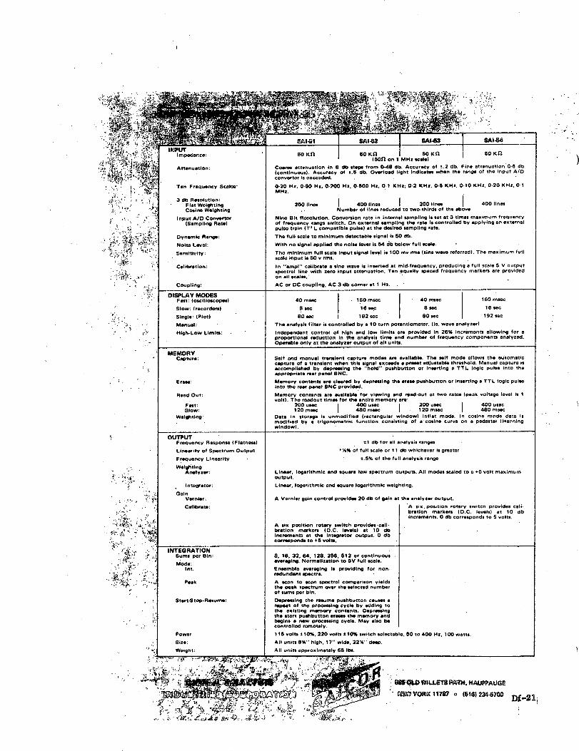
, -1' : ̀ s:," 4, . ..

SAI-64

Tan Frequency Scalos:

3 db Resolutlon:Flat WeightingCosine Weighting

Input A/D Convertor(Sampling Rate)

Dynamic Range:Nolse Level:

Sensitivity:

Calibration:

Coupling:

50 K 50s K -I · 50 K f i 50 Kn(so601 on 1 MHz acle)

Coarse attenuation In 6 db steps from 0-48 db. Accuracy of t.2 db. Fine attenuation 0.6 db(continuous). Accuracy of t.5 db. Overload light Indicates when the range of the input A/Dconvertor Ir oecooded.

0-20 H., 0-60 Ha, 0-200 Ha, 0O500 Ha. 0.1 KH:; 02 KHs, 0-. KHz, 0.10 KH., 0-20 KHZ. 0,1mm.,

200 lines I 400 lines I 200 lines J 400 linesNumber of lnes reduced to two-thirds of the above

Nino Bit Reoolutlon. Convronion rate in Internal saompling is set at 3 times maximum frequencyof lrequency range witch. On external sampling the rate Is controlled by applying an externalpulto train (T' L compatible pulws) at the desired sampilng rate.The full scole to minimum detectable signal is 50 db.

With no signal applied the noise level is 64 db below full wcale.

Tho minimum full rale Input signal level is 100 mv rms (sine wave referred). The maximum fullscalo Input Is 50 v rms.

In "ampi" calibrate a sine wave is inserted at mid-frequency, producing a full scale 5 V outputspoctrol line with zero input attenuation. Tan equally spaced frequency marketr are providedon all scoles.

AC or DC coupling. AC 3 db corner at 1 Hz.

. DISPLAY MODESFast: (oscilloscopel) 40 msac 160 msec 40 macc 160 msec

Slow: (recordor) 8 sec 16 sec 8 sac 16 sec

Single: (Plot) 80 sac 192 sec 80 sc 192 sac

Manual: The analysis filter is controlled by a 10 turn potentiometer. (tl. wave analyzer)

High-Low Limits: Independent control of high and low limits ore provided In 25% increments allowing for aproportional reduction in the analysis time and number of frequency components analyzed.Operable only at tho analyzer output of all units.

iMEMORY .Capture: Self and manual transient capture modes are available. The self mode allows the automatic

capture of a transient when this signal exceeds a preet adjustable threshold. Manual capture isaccomplished by depressing the "hold" pushbutton or Inserting a TTL logic pulse into theapproprlate rear panel BNC.

Erase: Memory contents are cleared by depressing the arm pushbutton or Inserting a TTL logic pulzeInto the rear panel SNC provided.

Read Out: Memory contents are avallable for viewing and reed-out at two rates (peak voltage level It 1volt). The readout times for the entire memory are:

Pest: 200 usec 400 usa I 300 uec 400 usecslow: 120 mMte 480 mesc 120 maec 480 mrec

Weighting: Data in storage is unmodified (rectangular window) Inflat mode. In cosine mode data ismodified by a trigonometric function consisting of a cosine curve on a pedestal (Henningwindow).

OUTPUTFrequency Response (Flatness) t1 db for all analysis ranges

Linearity of Spectrum Output t% of full scale or t I db whichever iS greater

Frequency Linearity t.5% of the full analysis range

WeightingAnalyzer: Linear, logarithmic and square law spectrum outputs. All modes scalod to a +5 volt maximum

output.

Intogrator: Linear, logarithmic and square logarithmic weighting.

GainVernier: A Vernier gain control provides 20 db of gain at the analyzear output.

Callbrate: A six position rotary switch provides cali-bration marken (D.C. levels) at 10 dbincrements. 0 db corresponds to 5 volts.

A six poaltion rotary switch provides-ceali-bration marker (D.C. levels) at 10 dbincrements at the lntegrator output. 0 dbcorresponds to +6 volts.

INTEGRATIONSums per Bin:Mode:

Int.

Peak

Start-Stop-Resume:

Power:

Site:

Weight:

8. 16. 32. 64, 128, 256. 512 or continuou.averaging. Normalization to 5V full scale.Ensemble averaging Is providing for non.redundent spectre.

A soon to scan spectral comparison yieldsthe peak spectrum over the selected numberof sums per bin.Depnresing the resume pushbutton causes arepeat of the processing cycle by adding tothe exliting memory contnns. Depresslngthe start pushbutton erases the memory andbegins a new processing cycle. May also becontrolled rmotrely.

15 volts t 10% 220 volts t 10% Switch slectableo, 0 to 400 Hz, 100 watts.

All units 81" high, 17" wide. 22X" deep.

All units approximately 55 Ibs.

)

' . 'G WiLLETS PATH HAUPPAUGE

C 'C YORCK11787 o (616)234-67 00Di-2

-1.

, 4;.:

X Lt

:A ?; ''*i

i .s,; :,

·,,":.'.. -,j ·r..,

,? :

:~~·~: :

....

_ :,

·. -: ;4 - ,::.i ;;,t%,(

· . .

. .

- .; C,i;'..\. -

I~

'l,:g

4

Rea1irme signal analysisMlodel 3721A

DescriptionModel 3721A Correlator is an all-digital, dc-to-250 kHz

signal analyzer which combines four major measurementcapabilities in one instrument. It measures autocorrelation,crosscorrelation, probability distributions, and signal aver-aging (signal recovery), the process of recovering the wave-shape of repetitive signals buried in. noise (described, withreference to the Model 5480A Signal Analyzer, on psve42 ). All results are displayed on built-in CRT.

In general, using the 3721A Correlator is similar to usingan oscilloscope. Essentially an "on-line" instrument, it caneasily be carried from place to place, yet has the flexibilityof much larger data processing systems . . . for example, aselection of averaging time constants from a few millisec-onds to many days. With the 3721A Correlator comes theability to observe statistical behavior in real time, and tomonitor changing phenomena continuously.

The computed function is displayed using 100 points:however, if more resolution is required in correlation mea-surements, Option series 01 provides additional delay inbatches of 100 points, up to a maximum of 900 point . Thispre-computational delay gives an effective resolution of I

point in 1000 over a selected portion of the display.The major axis of the display is scaled five points to each

centimeter and is calibrated in time per millimeter: this ap-plies to all displays other than probability, for which thehorizontal axis is calibrated in volts per centimeter. (Notethat for correlation functions the horizontal axis representstime rhift between input signals rather than real time.) Thetime per millimeter can be switched from 1 u.s to 1 second:other, intermediate, sweep rates may be obtained using anexternal timebase (the time/mm can be increased withoutlimit).Df-22

Being a digital instrument, the Correlator is easily inter-faced with a computer: Option 020 provides interface hard-ware for reading out displayed data in 16 bit parallel binaryform to any computer in the Hewlett-Packard range. Analogoutputs are provided, as standard features, for both X-Yrecorder and external oscilloscope.

Digital AveragingCorrelation, signal recovery and probability measurements

are all processes in which the end result is the average ofmany samples. In the Model 3721A Correlator averaging isper',rmed by two methods: SUMMATION and EXPO-NENTIAL, one or the other being selected by a front panelswitch. In the summation mode, the computed function isaveraged by summing N samples and then dividing the totalby N: N is selectable (front panel control) from 2; to2'.Summation averaging anticipates the number of samplescontributing to the computed function's final value, and istherefore a process of pre-established length: it is particu-larly useful for the analysis of a limited quantity of data.

The second averaging mode, exponential averaging, is acontinuous filtering process which forgets old informationand thus follows changing phenomena. If A,,, is the currentvalue of the running average and a new sample 1, arrives,the new average would be A,, = A,,_ + (I,,-A,,_,)/N,where N is a number selectable from 2- to 21' in binarysteps. This running average algorithm is the digital equiva-lent of an RC smoothing filter, but with greater stabilityand flexibility. Stable because it is not subject to the driftnormally associated with long time constant analog circuits,and flexible because changing of the time constant entailsnot a change of physical components, but a changed divisor,N, in the averaging algorithm. Digital averaging has the

:, :

3721A

I)

I

added advantage that it makes possible very long timeconstants, and hence low frequency analysis, without physi-cally large components.

The easily variable time constant is used with great effectto provide a quick-look facility. A long averaging timeconstant, essential for accurate statistical measurements, nor-mally means a long wait before the computed function

arrives at its final value . and hence the possibility of anabortive experiment being discovered only after a lengthytime interval. The quick-look facility in the 3721A, how-ever, gives an immediate approximation to the final value,regardless of the length of time constant selected; and theapproximation is progressively refined as the experimentproceeds.

SpecificationsInput Characteristics

Two separate input channels, A and B, with identical ampli-fiers.

Bandwidth: dc to 250 kHz nominal. Lower cut-off frequencyselectable, dc or 1 Hz.

Input range: accepts signals from 40 mV rms to 4 V rmsover six ranges.

Analog-to-digital conversion: fine quantizer; 7 bits. Coarsequantizer (feeds delayed channel); 3 bits. Coarse quantizerlinearized by internally-generated wideband noise (dither).

Overload: maximum permissible voltage at input; dc coupled120 V peak, ac coupled 400 V = dc + peak ac.

Input impedance: nominally 100 pF to ground, shunted by1 Mo.

Correlation ModeComputes the following functions:

Autocorrelation of A input.Autocorrelation of B input.Crosscorrelation of A and B inputs, A delayed.Crosscorrelation of A and B inputs, B delayed.Simultaneous computation and display of 100 values of auto

or crosscorrelation function. Display sensitivity indicated di-rectly in V'/cm on illuminated panel. Non-destructive read-out; computed function can be displayed for an unlimitedperiod without deterioration. (Non-permanent storage; datacleared on switch-off.)

Timescale: (time/mm = delay increment At) 1 ps to I sec-ond (total delay span 100 ss to 100 seconds) in 1, 3.33,10 sequence, plus external clock; minimum increment 1 us(I MHz), no upper limit.

Dolay offset: option series 01 provides delay offset (precompu-tation delay) facility. Without offset, first point on displayrepresents zero delay; with offset, delay represented by firstpoint is selectable from 100 At to 900 At in multiples of100 At.

Display sensitivity: 5 x 10-° V'/cm to 5 V'/cm. Calibrationautomatically displayed by illuminated panel.

Vertical resolution: depends on display sensitivity. Minimumresolution is 25 levels/cm. Interpolation facility connectspoints on display.

Averaging: two modes are provided: Summation (true averag-ing) and Exponential.

1. Summation ModeComputation automatically stopped after N process cycles,at which time each point on the display represents the aver-age of N products. N is selectable from 128 to 128 x 1024(2' to 2" in binary steps). Display calibration automaticallynormalized for all values of N. Summation time indicatedby illuminated panel.

2. Exponential ModeDigital equivalent of RC averaging, with time constantselectable from 36 ms to over 10' seconds. Approximate timeconstant indicated by illuminated panel. Display correctlycalibrated at all times during the averaging process.

Signal Recovery Mode (Channel B Only)Detects coherence in repeated events, when each event is

marked by a synchronizing pulse. After each sync pulse, aseries of 100 samples of channel B input is taken, and corre-sponding samples from each series are averaged. The 100 aver-aged samples are displayed simultaneously. Display sensitivityis indicated directly in V/cm on illuminated panel.

Synchronization: an averaging sweep is initiated either by apulse (TRIGGER) from an external source (EXT) or,in internally triggered mode (INT), by a pulse derived fromthe internal clock. In the INT mode, the start of each sweepis marked by an output pulse (STIMULUS) used to syn-chronize some external event.

Trigger input: ac coupled. Averaging sweep initiated by nega-tive-going edge; minimum swing 5 volts, maximum 12 volts;maximum fall time 2 jus; minimum pulse width 0.5 its;maximum dc voltage 200 volts.

Stimulus output: negative-going pulse at start of averagingsweep, +12 V to 0 V, duration >0.5 ,us; interval betweenstimulus output pulses equals 100 x .time/mm, plus up to270 us.

Timescale: (time/mm = interval between samples) 1 us to1 second (total display width 100 ps to 100 seconds) in1, 3.33, 10 sequence with internal clock. Other intervals(hence other display widths) with external clock; minimuminterval I us (1 MHz), no upper limit.

Display sensitivity: 50 pV/cm to 1 V/cm. Calibration auto-matically displayed by illuminated panel.

Vertical resolution: depends on display sensitivity. Minimumresolution is 25 levels/cm. Interpolation facility connectspoints on display.

Averaging: two modes are provided: Summation (true averag-ing) and Exponential.

1. Summation ModeProcess automatically stopped after N averaging sweeps, atwhich time each point on the display represents the averageof N samples of the input; taken at a particular displace-ment from the sync pulse. N is selectable from 128 to 128 x1024 (2' to 2" in binary steps). Summation time indicatedby illuminated panel.

2. Exponential ModeDigital equivalent of RC averaging, with time constantselectable from 36 ms to over 10' seconds. Approximatetime constant indicated by illuminated panel.

Probability MAode (Channel A Only)Displays either (1) amplitude probability density function

(pdf) or (2) integral of the pdf of channel A input. Signalamplitude represented by horizontal displacement on display,with zero volts at center; vertical displacement represents am-plitude probability.Dlsplay sensitivity: horizontal sensitivity 0.05 V/cm to 2 V/

cm in 5, 10, 20 sequence.Horizontal renolutlon: 100 discrete levels in 10 cm wide dis-

play-= 10 levels/cm.Df-23

Four instruments in one

Vertical resolution: 256 discrete levels in 8 cm high display =32 levels/cm.

Vertical scaling: depends on averaging method used (summa-tion or exponential).

1. Summation AveragingProcess automatically stopped by the first point to reach8 cm displacement from the baseline. In the pdf mode,8 cm vertical displacement represents approximately Noccurrences of a particular signal level, N being selectablefrom 128 to 131,072 (2: to 2' in binary steps). Area underpdf curve may be obtained by counting cycles of processclock.

2. Exponential AveragingContinuous updating of display, with time constant as givenfor correlation and signal recovery mode.

Sampling rate: I Hz to 3 kHz in 1, 3, 10 sequence with internalclock. Other sampling rates with external clock; maximumfrequency ', kHz, no lower frequency limit.

Interfacing

x-Y recorder: separate analog outputs corresponding to hori-zontal and vertical co-ordinates of the CRT display.X drive: nominal 12.5 V staircase, 270 ns dwell per step.

Alternative dwell 1.35 seconds.Y drive: nominal 1.25 V for each centimeter deflection on

3-21A CRT display.Pen control: 2 modes controlled by toggle switch on rear

panel.a. Pen lowered for entire sweep.b. Pen plots series of 100 points per sweep.

Pen lift signal: short-circuit to ground for pen down. Maxi-mum sink current 150 mA. In the pen-up condition,voltage from recorder must not exceed +40 V.

Recorder calibration: ZERO on DISPLAY/CAL switch putspen to center of paper. CAL puts pen to lower left. De-pressing the RECORD pushbutton gives a single sweepoutput to the X-Y recorder.

Oscllloscope: separate analog outputs corresponding to thehorizontal and vertical co-ordinates of the CRT display.

Noise Generator Model 3722A: control of the Correlator fromthe Model 3722A Noise Generator. The gate signal fromthe 3'22A is used to set the Correlator into RUN state. Ontermination of the gate signal, Correlator will go into HOLDstate.Gate Signal 3722Ae: + 1.5 V when gate open sets Correla-

tor into RUN state; on rising to + 12.5 V (gate closed),sets Correlator into HOLD state.

Digital computer: Option 020 provides interface hardware(buffer card ) for reading out displayed data to any Hewlett.Packard digital computer.Data output*: signals containing VERTICAL ordinate in-

formation transmitted to the computer. The 100 displayedpoints are scanned in sequence on command from thecomputer. Each point is represented by 16 bits parallelbinary information comprising 10 bits amplitude data, 2bits sign, 2 bits range factor, and 2 bits command in-formation, one denoting instrument in HOLD state andthe other "time constant reached" condition. Ordinates arepresented, to the computer, for a period of approximately130 is and a data ready signal marks the changeover fromone to the next. The data ready signal can be used toinitiate a computer interrupt.

Df-24

Computer commands*Run: signal from computer which sets Correlator into

RUN state.Hold: signal from computer which sets Correlator into

HOLD state.Reset: signal from computer which sets Correlator into

RESET state.Data: signal from computer which commands Correla-

tor to output a series of 100 data words, if Correlatoris in HOLD state.

Clock*Internal clock: all timing signals derived from crystal-

controlled oscillator: stability 40 ppm over specified am-bient temperature range. Internal clock output: train ofnegative-going pulses, +12 V to 0 V, >0.5 ps wide.period as indicated by TIMESCALE switch.

External clock: maximum frequency I MHz. Negative-going level change, minimum transition -- 5.5 V to +2.8V, initiates clock pulse. Minimum dwell at lower level0.5 us. Maximum permissible levels -13.5 V to -8 V.

Process clock: 135 ps wide negative-going pulse. Normally0 V, rises to -- 12 V at start of eachl process cycle andreturns to 0 V after 135 ,s.

Remote Control and Indication':'

Control: remote control inputs for RUN, HOLD and RESETfunctions are connected to DATA INTERFACE socket onrear panel. Command represented by negative-going levelchange, minimum transition -5.5 V to -- 2.8 V. Minimumdwell at lower level 1.5 ,s. Maximum permissible levels--13.5 V to -- 8 V.

Indication: remote indication of Correlator RUN, HOLDor RESET states is available at the DATA INTERFACEsocket on rear panel. A condition will be indicated as truewhen signal is at 0 V.

Display

Mono-accelerator tube, 3 kV accelerating potential; alumi-nized P31 phosphor; etched safety glass faceplate reducesglare, 8 x 10 cm D: allax-free internal graticule marked incm squares, 2 mm sub-':visions on major axes.

General

Ambient temperature range: 0: to 50C.Power: 115 or 230 V =10%c, 50 to -100 Hz, 150 W.Dimensions: 165/4" wide. 103/4" high, 183/4" deep overall

(426 x 272 x 4-6 mm).Weight: 45 lb (20,5 kg) net.Accessories furnlehed: detachable power cord, rack mounting

kit, trimming tool, circuit extender boards (2 supplied),special-purpose coax extender lead, 50-contact male cableplug.

Price: Model 3721A 58300 S'600 at factory in Scotland).

Options

Delay offset: option series 01. Full details to be announced.Data interface: option series 02. Option 020 Correlator with

interface for data output to computer.

Denotes signals specified as follows:Correlator output signalsTRUE or low state -- I1 V to - 1.5 V, sinking up to 12 mA.FALSE or high state - 12 V, output impedance 12 kIl.Correlator input signalsTRUE or low state --1 V to - 2.8 V.FALSE or high state -- 5.5 V to 12 V.

KROHN-HITE CORPORATION

0.001 Hz to 99.9 kHzHIGH-PASS, LOW-PASS,

BAND-PASS, BAND-REJECTVARIABLE FILTER

nrodels 3340 and 3342

All silicon solid-state

o Frequency range: 0.001 to 99.9 kHz

o Frequency accuracy: -2%

o as Band Gain: Odb or 20db

Attenuation slope: 48db/oct. (each channel)

* Battery operation

* Maximum attenuation: 80db

* Floating (ungrounded) operation

The Krohn-Hite Model 3300 Series are all silicon, solid-state, variable electronic Filters that are digitally tuned overthe range from 0.001Hz to 99.9kHz. The Models 3320(single channel) and 3322 (dual channel) provide 24db peroctave attenuation slopes, and the Models 3340 (singlechannel) and 3342 (dual channel) have slopes of 48db peroctave. Each channel can be operated in either the High-Pass or Low-Pass mode providing versatility never beforeavailable over this frequency range. Refer to separate bul-letin on the Models 3320 and 3322 for detailed specifica-tions. When the two channels in the Model 3342 are oper-ated in the same mode, set at the same cutoff frequency, andcascaded, an attenuation slope of 96db per octave is ob-tained.

The frequency response characteristic of the Models 3340and 3342 is an eighth-order Butterworth with maximal flat-ness for cleanest filtering.in the frequency domain. For pulseor transient signal filtering, a front panel switch is providedto change the frequency response to Low Q, optimum for

MODEL 3340

MODEL 3342 '

Lt ..ii. i ^ - _

so -L' .- .= ' ' =

transient-free filtering (see photo). Digital tuning permitscutoff frequency calibration accuracy of -±2% and ex-cellent resettability enabling good repeatability of filtercharacteristics.Either Odb or 20db of passband gain is provided with asmall increase in outpin noise. This improves the signal tonoise ratio. The 10 megohm input impedance and the 50ohm output impedance minimizes loading, and improveshigh-frequency performance. Battery operation makes theseFilters ideal where it is necessary to be completely isolaledfrom the line. All Filters are designed to operate fromn line orbatteries. Filters initially ordered ithoul hbalttcrics can heeasily converted to battery operation by piurchlasing specialbatteries from Krohn-Hite at a later date.These filters are designed primarily for applications in theultra-low frequency range. Their excellent cutoff frequencyaccuracy and resettability, coupled -with stable dc outputlevel and low distortion, results in a significant contributionto filter technology.

-I

I.1

.1 2 , .4 .5 1 2 3 4 $ tO .t .2 .X A4.5 I 2 3 4 atORAIZrw[ Vnr NOALIaEDuZtO MrEQUWt4CY

Cuirv A. tnphnl chomnne. Curve : Ouai1 ctlnnel MODEL 3342: Minimum bondwthLtA, dt/oe o .e o caocodad Low-Pena oonoe In Band.Pooo opermton.~(4db/aeM. . raopenso (Odbloctovo).

~7s*Pto-

Response (in Low-Pass mode) toI Hz square wave, with cut-off atI kHz in Butterworth position.

10

dth roResponse to same square wave inLow Q position.

Df-25

FILTER

1

-M- =1 .-

0 X Y' v ;

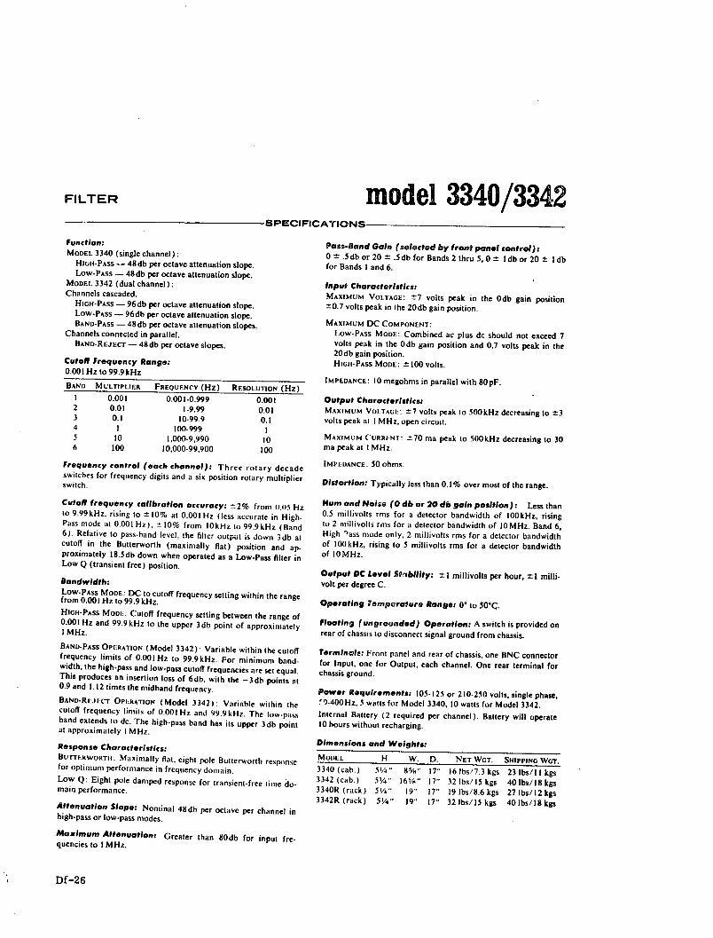
model 3340/3342FILTER

Function:MODEL 3340 (single channel):

HIGH-PASS - 48db per octave attenuation slope.Low-PASS - 48db per octave attenuation slope.

MODEL 3342 (dual channel):Channels cascaded.

HIGH-PASS - 96db per octave attenuation slope.Low-PASS - 96db per octave attenuation slope.BAND-PASS - 48db per octave attenuation slopes.

Channels connected in parallel.BAND-REJECT - 48db per octave slopes.

Cutoff Frequency Range:0.001 Hz to 99.9 kHz

BAND

I

23456

MULTIPLIER

0.0010.010.1

110100

FREQUENCY (Hz)

0.001-0.9991-9.99

10-99.9100-999

1,000-9,99010,000-99,900

RESOLUTION (Hz)0.0010.010.1

10100

Frequency control (each channel): Three rotary decadeswitches for frequency digits and a six position rotary multiplierswitch.

Cutoff frequency calibration accuracy: +2% from o.o5 Hzto 9.99kHz, rising to ± 10% at 0.001 Hz (less accurate in High-Pass mode at 0.001 Hz), - 10% from 10kHz to 99.9kHz (Band6). Relative to pass-band level, the filter output is down 3db atcutoff in the Butterworth (maximally flat) position and ap-proximately 18.5db down when operated as a Low-Pass filter inLow Q (transient free) position.

Bandwidth:Low-PAss MODE: DC to cutoff frequency setting within the rangefrom 0.001 Hz to 99.9 kHz.

HIGH-PASS MODI.: Cutoff frequency setting between the range of0.001 Hz and 99.9kHz to the upper 3db point of approximatelyI MHz.

BAND-PASS OPERATION (Model 3342): Variable within the cutofffrequency limits of 0.001Hz to 99.9kHz. For minimum band-width, the high-pass and low-pass cutoff frequencies are set equal.This produces an insertion loss of 6db, with the -3dh points at0.9 and I. 12 times the midband frequency.

BAND-REJECT OPIERATION (Model 33421: Variable within thecutoff frequency limits of 0.001 Hz and 99.9kHz, The low-passband extends to de. The high-pass band has its upper 3db pointat approximately I MHz.

Response Characteristics:BUTrrTERWORTII: Maximally fiat, eight pole Butterworth responsefor optimum performance in frequency domain.

Low Q: Eight pole damped response for transient-free time do-main performance.

Attenuation Slope: Nominal 48db per octave per channel inhigh-pass or low-pass modes.

Maximum Attenuation: Greater than 80db for input fre-quencies to I MHz.

Pass-Band Gain (selected by front panel control):0 -+ .5db or 20 - .5db for Bands 2 thru 5, 0 + I db or 20 + I dbfor Bands I and 6.

Input Characteristics:MAXIMUM VOLTAGE: '7 volts peak in the Odb gain position-0.7 volts peak in the 20db gain position.

MAXIMUM DC COMPONENT:

Low-PAss MODE: Combined ac plus dc should not exceed 7volts peak in the Odb gain position and 0.7 volts peak in the20db gain position.HIGH-PASS MODE: + 100 volts.

IMPEDANCE: 10 megohms in parallel with 80pF.

Output Characteristics:MAXIMUM VolTAGE: ±7 volts peak to 500kHz decreasing to -+3volts peak at I MHz, open circuit.

MAXIMUM CURRFINT: +70 ma peak to 500kHz decreasing to 30ma peak at I MHz.

IMPEDANCE: 50 ohms.

Distortion: Typically less than 0. 1% over most of the range.

Hum and Noise (O db or 20 db gain position): Less than0.5 millivolts rms for a detector bandwidth of 100kHz, risingto 2 millivolts rms for a detector bandwidth of 10MHz. Band 6,High lass mode only, 2 millivolts rms for a detector bandwidthof 100kHz, rising to 5 millivolts rms for a detector bandwidthof O1MHz.

Output DC Level Siwbillity: 1 I millivolts per hour, 1 I milli-volt per degree C.

Operating Temporature Range: 0° to 50C.

Floating (ungrounded) Operation: A switch is provided onrear of chassis to disconnect signal ground from chassis.

Terminals: Front panel and rear of chassis, one BNC connectorfor Input, one for Output, each channel. One rear terminal forchassis ground.

Power Requirements: 105-125 or 210-250 volts, single phase,")-400Hz, 5 watts for Model 3340, 10 watts for Model 3342.

Internal Battery (2 required per channel). Battery will operate10 hours without recharging.

Dimensions and Weights:

MODEL H. W. D. NET WGT. SHIPPING WGT.

3340 (cab.) 54" 81%" 17" 16 1bs/7.3 kgs 23 lbs/lI kgs3342 (cab.) 51/4" 16" 17" 321bs/15kgs 401bs/18kgs3340R (rack) 5'/4" 19 17" 19 lbs/8.6 kgs 27 lbs/12 kgs3342R (rack) 51/4" 19" 17" 32 lbs/15 kgs 401bs/18 kgs

Df-26

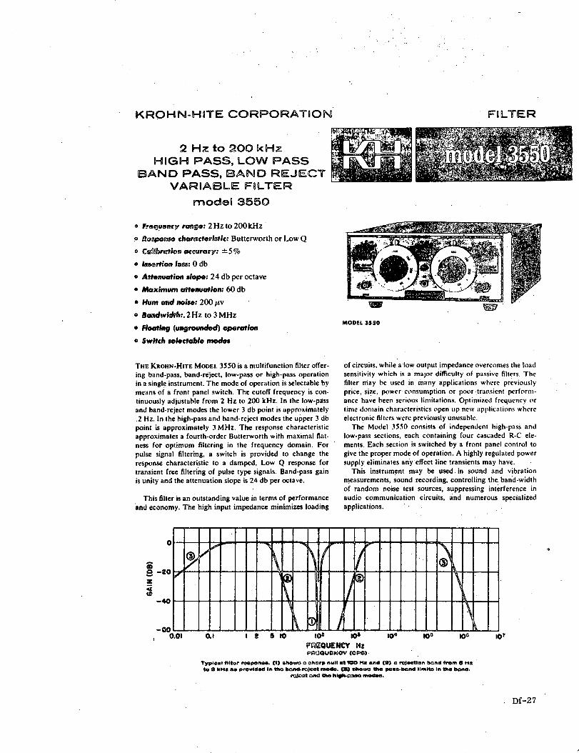
KROHN-HITE CORPORATION

2 Hz to 200 kHzHIGH PASS, LOW PASS

BAND PASS, BAND REJECTVARIABLE FILTER

model 3550

o Frequencty range: 2Hz to 200kHz'

9o Rosponao characteristic: Butterworth or Low Q

° Cslhbr(ation accuracy: ± 5 %

* Inertion loss: 0 db

o Attenuation slope: 24 db per octave

* Maximum attenuation: 60 db

* Hum and noise: 200 /.v

* Bandwidth:. 2Hz to 3 MHz

* Floating (ungrounded) operation

* Switch selectable modes

THE KROHN-HITE MODEL 3550 is a multifunction filter offer-ing band-pass, band-reject, low-pass or high-pass operationin a single instrument. The mode of operation is selectable bymeans of a front panel switch. The cutoff frequency is con-tinuously adjustable from 2 Hz to 200 kHz. In the low-passand band-reject modes the lower 3 db point is approximately.2 Hz. In the high-pass and band-reject modes the upper 3 dbpoint is approximately 3 MHz. The response characteristicapproximates a fourth-order Butterworth with maximal flat-ness for optimum filtering in the frequency domain. Forpulse signal filtering, a switch is provided to change theresponse characteristic to a damped, Low Q response fortransient free filtering of pulse type signals. Band-pass gainis unity and the attenuation slope is 24 db per octave.

This filter is an outstanding value in terms of performanceand economy. The high input impedance minimizes loading

_ -2

S

MODEL 35sS

of circuits, while a low output impedance overcomes the loadsensitivity which is a major difficulty of passive filters. Thefilter may he used in many applications where previouslyprice, size, power- consumption or poor transient perform-ance have been serious limitations. Optimized frequency ortime domain characteristics open up new applications whereelectronic filters were previously unusable.

The Model 3550 consists of independent high-pass andlow-pass sections, each containing four cascaded R-C ele-ments. Each.section is switched by a front panel control togive the proper mode of operation. A highly regulated powersupply eliminates any effect line transients may have.

This instrument may be used in sound and vibrationmeasurements, sound -recording, controlling the band-widthof random noise test sources, suppressing interference inaudio communication circuits, and numerous specializedapplications.

IfIrQUENCY HzFRC2QUgiOV (CPO)

Typilco flitor roSpo"nc. C1) showo o hnerP null a 100 Ha and (t) a r)jeotlon b:nd from t Hato S kln &o provld·ed In tho bea-roje:t nmode. (IC fowo thue p&.o-bald limito In the band.

roIc'e n o tho bip.a:eo modoe.

FILTER

I0'

Df-27

model 3550SPECIFICATIONS

Function:

Low-pass, high-pass, band-pass, band-reject

Cutoff frequency range:

BAND MIULTIPI.IEFI FREQUENCY (Hz)

I 0.1 2-202 1 20- 2003 10 200 -2,0004 100 2,000- 20,0005 1,000 20,000 - 200,000

Frequency control:One decade dial and 5 position multiplier switch for low-cutoffand high-cutoff functions. Effectively a 30 inch long scale for the5 bands.

Cutoff frequency calibration accuracy:

-±5% bands I thru 4, - 10% band 5 with "Response" switch in"max-flat" (Butterworth) position; less accurate in "Low Q"position. Relative to mid-band level, the filter output is down3db at cutoff in "max-flat" position, and approximately 12db in"Low Q" position.

Bandwidth:

LOW-PASS MODE - Approximately 0.2Hz to cutoff setting be-tween 2.0Hz to 200 kHz.HIGH-PASS MODE - Cutoff setting between 2.0 Hz to NOkHzto approximately 3 MHz.BAND-PASS - Both cutoffs adjustable from 2.0Hz to 200kHz.For minimum bandwidth (Butterworth response) both cutofffrequencie.s are set to coincide. This produces an insertion loss of6db, with the 3db points at 0.8 and 1.25 times the mid-bandfrequency.BAND-REJECT - Both cutoff frequencies adjustable front2.0Hz to 200kHz. Lower pass-band to approximately 0.2Hz,higher pass-band to approximately 3 N1Hz. A sharp null can beobtained by setting the LOW CUTOFF FREQUENCY to abouttwice the null frequency, and the HIGH CUTOFF FRE-QUENCY to about half the null frequency, and alternatelyadjusting both dials for minimum response.

Response characteristics:

Choice of 4 pole Butterworth (maximally flat response) for fre-quency domain operation and Low Q (damped response) fortransient-free time domain operation, selected by means of aswitch on the rear panel.

Attenuation slope:

Nominal 24 db per octave in all modes of operation.

Maximum attenuation:Greater than 60db.

Input characteristics:

MAX VOI.TAGE '7 V peak to 2 MHz.MAX DCCONIIPONI:NT 100V.INPUTr IMPEDANCE - IOM ohms in parallel with 5Opf.

Output characteristics:

MAX VOLTAGE 7 V peak to 2MHz.MAXCURRENT -15mapeak.INTERNAL IMPEDANCE - approximately 50 ohms.

Hum and noise:

Less than 200Zv, except 400v on Band Reject mode.

Output DC level stability:

- I mv/°C, + I mv,'hr

Operating temperature range:O'C to 500C

Front panel controls:

LOW-CUTOFF FREQUENCY Hz dial and multiplier switchHIGH-CUTOFF FREQUENCY Hz dial and multiplier switchFUNCTION switchPower ON switch

Rear panel controls:

RESPONSE switchGROUND sw itchDC LEVEL potentiomet 'r

Floating (ungrounded) operation:

A switch is provided on rear of chassis to disconnect signalground from chassis.

Terminals:

Front and rear panels, one BNC connector for INPUT, one forOUTPUT. One rear terminal for chassis grounding.

Power requirements:

105 to 125 or 210-250 volts, single phase, 50-400 Hz, 10 watts.

Dimensions and weighta:

Standard bench Model 3550 - 31,/" high, 81/" wide, 13" deep;91bs./4kgs. net, 14lbs./7kgs. shipping.

Rack-mounting Model 3550R - 31h" high, 19" wide, 13" deep;I I lbs./5 kgs. net, 16lbs./8 kgs. shipping.

Insertion loss:0 ±- db.

Df-28

FILTER

INSTRUMENTATION TAPE RECORDER/REPRODUCERGENERAL CHARACTERISTICS 1

SIZE: 13-15/16 x 15-3/16 x 6-1/2 inches.131X-

WEIGHT: Less than 30 pounds with 8 electronic modules and tape.

TAPE SPEEDS: 3 3/4, 7 1!2, 15 ips or 7 1/2, 15, 30 ips.DIMENSIONS: 1/2 - inch tape. Accepts 1.0 mil base tape. 7 - inch diameter reels.

Cover closes with reels in place.CONTROLS Pushbutton operation for OFF, RECORD, PLAY, REWIND, FAST FORWARD.

Electronic modules may be intermixed to provide any combination of Direct and FMrecord or reproduce channels. Recorder provides either 7-track record with switchablereproduce, or 7-track reproduce. Up to 4 tracks of simultaneous record-reproduce (7tracks optional). Meter provided for optimum direct-record level adjust and battery"state-of-charge" monitoring.

START TIME: 10 seconds or less at 30 ips from STOP to stable speed.8 seconds or less at 15 ips from STOP to stable speed.5 seconds or less at 7% ips and below from STOP to stable speed.

STOP TIME: 5 seconds or less from any running speed.

REWIND AND FORWARD TIME:

TAPE RUNNING TIME:

INTERNALPOWER CONSUMPTION:

BATTERY CHARGING:

MAXIMUMCUMULATIVE FLUTTER:

5 minutes for 1,800 feet of tape.'

TAPE SPEED 1800 feettips) 1.0 mil

3-3/4 90 min.7-1/2 45 min.15 22 min.30 11 min.

Averages 25 watts @ - 17 volts, with transport and all electronics operating at 30 ips.Internal Ni-Cd battery provides 1.0 hour operation on one charge (larger batteryoptional). Automatic low - voltage cutoff.Charging time 14.hours at 120 ma (20 volts dc). BACPAC Battery Charger andAuxiliary Power Supply (Catalog No. 1020 WB) available as optional equipment.Permits Recorder operation from 115/220 volts 50 to 400 Hz. Also chargesbattery.

PEAK-PEAK FLUTTER IN %

UPPER BAND CARRIER FREQUENCYLIMIT 625 1260 2500 5000 FOR FLUTTER(HZ.) MEASUREMENT - HZ.

SPEED lIPS)3-3/4 .8 67607-1/2 .6 13500

15 .5 2700030 .5 64000

V 6 l

i516

r

6n

Im

a

z1

Z

A DIVISION OF LOCKHEED AIRCRAFT CORP.

INDUSTRIAL TECHNOLOGY DIVISIONU.S. ROUTE #22, PLAINFIELD, N. J. 07061

Df-29

SPECI FICATIONSMODEL 417 WIDEBAND

TAPE

* /

0

ENVIRONMENTAL

TEMPERATURE: 32' to 120'F operating.-20 to 160'F non-operating

HUMIDITY: To 96% without condensation.

DIRECT RECORD/REPRODUCE SYSTEM

FREOUENCY RESPONSE:

SIGNAL.TO-NOISE RATIO:

INPUT LEVEL:

OUTPUT LEVEL:

INPUT IMPEDANCE:

OUTPUT IMPEDANCE:

HARMONIC DISTORTION:

CROSSTALK:

TAPE SPEED FREOUENCY RESPONSE SIGNAL-toNOISE-lip.l 1-3 dbl

30 500 to 375 KH 30 db16 500 to 187 KMH 30 db7.1/2 50s to 93 KHa 28 db3'3/4 W0 to 46 KIHt 27 db

nnma itO to r nob - 1000 H. tj rtsorded to 1.5% total hamonic diltotion.Meenad pee IRIGO 104P9.

Nominal sign:al level for 1.5% total harmonic distortion (1,000 Hz fundamental):Noise measurements include circuit and media noise. Measurements made with 18db/octave attenuation bandpass filter at output of reproduce amplifier.

100 mv to 10 volts rms.

1.0 volts rms (nominal across a 75 ohm load at normal recording level).

1,000 ohms nominal

0.5 ohm maximum.

1.5% (measured at 1,000 Hz).

-35 db (below nominal signal level at 1 kHz).

FM RECORD/REPRODUCE SYSTEM

SIGNAL CHARACTERISTICS TAPE SPEED CENTER FREQUENCY FREQUENCY RESPONSE SIGNAL-to-l(1l) (. n ) 1-Hi db i NOISE'

30 225,000 0 to 100,000 36 db15 112,00 0 to 50.000 3k db7-1/2 586,20 0 to 25.000 33 db3-3/4 20.125 0 to 12.500 32 db

INPUT LEVEL:

OUTPUT LEVEL:

HARMONIC DISTORTION:

INPUT IMPEDANCE:

OUTPUT IMPEDANCE:

AC/DC LINEARITY:

TEMPERATURE STABILITY:

SERVO SYSTEM

DESCRIPTION:

SPEED ACCURACY:

SERVO DRIFT:

* rmn Salp to ntn no-e. Measired pn IRIO 10-60.

+1.414 volts for full deviation (+30%).

+1.414 volts peek-to-peak (nominal when loaded w;t 75 ohms).

1.5% maximum for modulation indices greater than 3, a% for less than 3.

1,000 ohms nominal.

0.5 ohms maximum.

+ 1% of full scale.

Center frequency or output drift ' 0.5% par 10'C over operating temperaturerange.

Multiple-loop servo containing a coarse velocity-sensitive loop and a fine, high-resolution locked-phase servo. System integrated with supply and takeup reelmotor control to provide ov -rall maximum efficiency.

+0.25% at 70'F.

+ 1.0% over operating temperature range. Special oscillator availablo to provide0.1%.

Spscifications are subject to change without notice.

YOUR REPRESENTATIVE IS

(201) 757-1600 EXT. 2735

TWX 910 710 (941

PRINTED IN U.S.A.INS 50-261

Df-30

I

Specifications:

Model 5600Portable

Magnetic TapeSystem

The Honeywell Model 5600 Magnetic Tape Systemis a full 14-channel instrumentation grade recorderwhich handles virtually any tape recording requirementin both laboratory and field applications.

Extensive use of aerospace technology and elec-tronics enable true laboratory performance in a port-able package weighing approximately 65 pounds. Thebasic recorder accommodates sixteen data cards forany combination of record/reproduce channels total-ing sixteen. An auxiliary housing is available for expan-sion to a total of 32 data cards.

Built-in features permit easy on-the-spot conversionof tape width, power source, and recording techniqueto meet a variety of special requirements at remotelocations. Plug-in equalizers and center frequency as-semblies permit original investment to be minimizedwhile providing added capability for future expansion.Two equalizers or center frequency assemblies areelectrically switched with the rotary tape speed selector.In addition, the capability to use thin base tape on101/2 inch reels provides recording time equal to thatof larger systems.

* Low mass - high performance Phase Lock ServoDrive System

o A full 1" - 14 channel recorder in a package23" x 13" x 9"

o Universal Reel Adapters 1/4" - 1" tape, 5/16"or 3" hubs

* Seven electrically switched speeds from 15/16to 60 ips

* Plug-in equalizers and center frequencyassemblies

0 Direct electronics to 300 KHz

F.M. electronics to 40 KHzLow. bandIntermediate bandWideband Group I

e Serial Digital to 600 BPI

* Choice of power from 115/230 V-48 to 420 Hz.10 to 15 VDC or 22 to 30 VDC.

A complete line of auxiliary components is availableto extend the flexibility of the Model 5600. including:

* Meter Monitors

· Attenuators

* Differential Inputs

* Alternate Power Supplies

* Remote Control Units

* Auxiliary Housing

* Time Code & Search Systems

HONEYWELL TEST INSTRUMENTS DIVISION, 4800 E. DRY CREEK ROAD, DENVER, COLORADO 80217

Df-31'

GeneralSize:

Portable Configuration: 23" x 133/8" x 9"Horizontal Rack Mounting: 153/4" panel space in 19" rack

(edges of 10112" reels overhangvertical frame of rack).

Vertical Rack Mounting: 223 /4" panel space in 19" rack.

Weight:65 Ibs. for seven channel direct record/reproduce configura-tion, excluding magnetic tape.

Input Supply: 3 availableAC: 105-129 VAC or 210-240 VAC (input voltage range field

selectable) 48.420 HzDC: (a) 10.15 VDC

(b) 22*30 VDC

Power Consumption:250 watts

Temperature:Operating: 0°C to 50°CStorage: -40'C to 70°CDrift and other operational specifications apply with a singlecalibration from 10' to 35'C.

Altitude:Operating: to 15,000 feetNon-operating: to 50,000 feet

Humidity:5% to 95% non-condensing

All above specifications apply to basic 16 Data Module Configuratronunless otherwise noted.

Tape TransportBasic Configurations:

Two available-- /2" to 1" or i/4" to 1/2"Easily field convertible between basic configurations

Tape Speeds:60, 30, 15, 7'/, 33/, 17/e, 15/16 ipsbidirectional and electrically selectable by rotary switch.

Hubs, Reels and Tape Width:

Reel ReelOutside Hole Tape

Diameter Size Width

5" 5/16" NAB 1/4"7' 5/16" NAB %4"8" 3" NAB /4, /2%, 1-

101/2" 3" NAB 1/4, . 110/2'" 5/16" NAB 'A/"

Universal adapter accepts all of above combinations. Spacerrequired for 1/4" reels with 3" hub. ASCII and non-standardadapters available.

Start Time: 3 seconds maximum at 60 ips.

Stop Time: 3 seconds maximum at 60 ips.

Fast Mode Speed: 200 ips for 1/4'" tape150 ips minimum for 1/2" or 1" tape.

Static Skew:Adjustable record and reproduce head azimuth to reducestatic skew to less than 2 microseconds between outsidetracks on a single 1" head stack at 60 ips.

Df-32

Dynamic Shew (ITDE):

Less than , 3 microseconds between outside tracks on asingle 1" head stack at 60 ips over a 10 second period. Pro-portionally higher at lower tape speeds.

Flutter:

Measured per IRIG 106-66. Servoed from capstan motortachometer in record and reproduce.

Tape Speed Bandwidth Cumulative Flutter % PK to PKtips) (Hz) (2 Sigma)

60 0.2 10,000 0.330 0.2. 5,000 0.415 0.2 2,000 0.571/2 0.2 1,250 0.633/4 0.2 625 0.71 7/ 0.2 312 0.9

15/16 0.2 156 1.1

Local Control:

Pushbutton control of: POWER, DRIVE FORWARD, DRIVEREVERSE, RECORD, STOP, FAST FORWARD, and FAST RE-VERSE. Rotary switch selection of tape speed. Manual short-ing pins to determine equalizer/speed relationship.

Remote Control:Remote connector allows duplication of all controls with localspeed switch in REMOTE position.

Remote Indicators:

End of Tape: -5 VDC at 40 ma maximumLow tape sensors (optional): +5 VDC at 40 ma maximum

Transport Auxiliary Features:Mechanically coupled tape footage counter.Automatic shutdown at end of tape or tape separation.

Tape Drive SystemCapstan System:

Tri-Capstan: Bi-directional and equivalent to closed loop inhigh frequency flutter suppression.D.C. drive motor is directly coupled to center capstan.

Capstan Servo:Phase lock from tape or motor tachometer. Servo system willgenerate standard or 2X standard IRIG constant amplitudeservo frequencies. The servo system will remove a staticrecorded speed error of -50% and -30% at all speeds.Servo operable from tape at 15/16 ips only with 2X standardIRIG constant amplitude frequencies.

Servo Reference Frequency:100 KHz at 60 ips crystal controlled. Proportional at otherspeeds per IRIG 106-66. Operable at 2X IRIG frequencies withpin jumper change on reference generator card.Accuracy: 3 parts in 10' (0.03%)Stability: 5 parts in 10' (0.05%) over a 25°C temperature

range.

Speed Accuracy: (Over operating temperature range)

Capstan Rotational Accuracy: 0.1% when servo is operatingfrom motor tachometer.Tape: Within 0.15% of selected when servo is operating frommotor tachometer.Within 0.1 % of recorded reference when operating from tape.

Time Displacement Error (TDE or TBE)Servoed from tape recorded on machine with similar fluttercharacteristics.

Speed TSE Microseconds(UPs) (Zero to Peak)

60 1.030 2.015 3.071/7 5.0

33/4 10.01'/a 12.0

15/16 15.0

Slewing Rate:A family of attenuation curves is available upon request.

Magnetic HeadsFive Standard Configurations Available:

3/4", 4 track, 0.040 wide, 0.068 C to C1/4", 7 track, 2X IRIG, 0.025" wide, 0.035 C to C, no edgetrack.1/2". 7 track IRIG, 0.050" wide, 0.070 C to C, with 1 edgetrack.1/2". 14 track, 2X IRIG, 0.025 wide, 0.035 C to C.1", 14 track IRIG, 0.050 wide, 0.070 C to C, with 2 edgetracks.

Minimum Life: 1500 hours at 60 ips.Complies with IRIG specifications for gap scatter, gap azimuthand interstack spacing. r

Preamplifiers: Maximum of 16 preamplifiers, four per card.

Direct Record/ReproduceDynamic Characteristics:

Based on standard IRIG head configuration without an FMchannel on an adjacent track, and with recommended ironoxide tapes. Capable of operation with chromium dioxidetapes.

Tape Speed Bandwidth RMS Signael/RiS Noisetips) (Hi + 3db) (db filtered)*(db unfiltered)

60 300 - 300,000 32 3030 150- 150,000 32 3015 100- 75,000 32 30

71/, 50- 37,500 30 2833/4 50- 18,750 30 281 7/ 50 - 9,300 28 26

15/16 50- 4.700 28 26

*Measured at the output of a bandpass filter having 18 db/octave attenuation beyond bandwidth limits.

Harmonic Distortion:Normal record level set for 1% third harmonic distortion ofa 1KHz signal recorded at 60 ips.

Input Level:0.3 vrms fixed at recorder input terminals, with gain trimadjustment.

Input Impedance:100K ohms resistive paralleled by 100pf, unbalanced toground.

Output Level:1.0 vrms fixed into 10K ohms, with gain trim adjustment.

Output Impodance:Less than 100 ohms.

Equalization:Mounted on plug-in equalizer cards. Each reproduce amplifieraccepts two equalizers with the correct one being selectedby the speed control switch.

FM Record/Reproduce (-40% deviation)

Record Amplifier:

Incorporates nine center frequencies, selected by speedswitch and shorting pin for mode selection. Bias recorded.

Reproduce Amplifier:

Accepts two center frequency/filter units, selectable by speedswitch. Filters convertible from flat to transient response bypin change.

Dynamic Characteristics:

S/N Ratio vs. BandwidthTape Speed Standard Extended OX

60 46 (10KHz) 44 (20KHz) 42 (40KHz)30 45 (5KHz) 43 (10KHz) 41 (20KHz)15 44 (2.5KHz) 43 (5KHz) 40 (10KHz)

7 1/2 43 (1.25KHz) 41 (2.5KHz) 39 (5KHz)33/4 42 (625 Hz) 40 (1.25KHz) 38 (2.5KHz)17/8 40 (312Hz) 38 (625Hz) 36 (1.25KHz)

15/16 40 (156Hz) 36 (312Hz) 34 (625Hz)

Total Harmonic Distortion:

1.5% maximum.

Linearity:

=1% of full deviation from best straight line through zero.

Drift:

1% of full deviation over 10 days and 10°C to 35°C ambient.

Input Level:

1.0 vrms fixed for -* 40% deviation with zero and gain trimadjustments.

Input Impedance:

Nominal 20K ohiims paralleled by 100 pf maximilumli unbalancedto ground.

Output Level:

1 vrms fixed into 10K ohms with zero and gain trim adjust.ments.

Output Impedance:

100 ohms maximum.

Voice ChannelInput:

Low impedance microphone or 600 ohm balanced input forline matching.

Input Level:

0 dbm into 600 ohm for normal record level.

Output:

600 ohm balanced for headphones or line matching.

Output Level:

' 3 dbm maximum.

Distortion:

3% third harmonic distortion at 1 KHz at rated output.

Frequency Reponse:

NAB equalized 50 Hz to 15 KHz at 7X/2 ips. Other standardequalizers available.

Bias Oscillator:

Self contained for voice annotation during reproduce. Keyeaby microphone button.

Df-33

* 2-mV/inch and 0.2-/,A/inch sensitivity* 65-inch/second writing speed* 0.25% linearity, 0.5% accuracy* programmable writing functions* plug-in versatility: grounded or

differential input

Bench model shown with 1522-P1 Preamplifier.

Imagine an automatic testing system that is pro-grammed by its own analog recorder. As the output dataare plotted, the recorder programs test conditions andmeasurement ranges, activates and synchronizes other re-cording devices, and controls its own writing functions.Triggered by timing marks printed on the chart paper, theGR 1522 DC Recorder will control companion instrumentsand itself, changing chart speed, rewinding the chart foroverplotting, quickly advancing to a fresh graph, all thewhile remembering to lift the pen when not plotting. Withoptional limit switches, the 1522 can operate sort/selectmechanisms, activate additional recorders, or alert anoperator if the plotted data exceed preset high or lowlimits.

As an accessory to the GR 1921 Real-Time Analyzer,for example, the 1522 Recorder will plot the band levelsagainst frequency much faster than conventional X-Yplotters. Operating synchronously with the 1921, the re-corder pauses briefly as each band level is selected toallow the pen to settle, producing a neat bar graph witha standard scale factor.

The 1522 is a fine program director; it is first a superbdc recorder, combining accuracy, high sensitivity, and fastwriting speed. It will plot a full-scale (5-inch) transientin under 100 ms, respond to a 200-jV or 20-nA change

specifINPUT WITH 1522-P1 PREAMPLIFIERRanges: Controlled by range switches, polarity switch, and con-tinuous control with calibrated position that operates on all ranges.DC Voltage, 2 mV/in. to 100 V/in.; 15 ranges, 1-2-5 sequence. DCCurrent, 0.2 1aA/in. to 100 mA/in.; 18 ranges, 1-2-5 sequence.

Accuracy: '0.5% of full scale.

with a 1-division deflection, and remain linear to withinV8 of a division (0.25%).

The recorder accepts one of two plug-in preamplifiers.The 1522-P1 Preamplifier provides a wide range of voltageand current measurements at an economical price. The1522-P2 Differential Preamplifier provides the same ver-satility with the added feature of a differential input sothat measurements from ungrounded sources can be made.This plug-in offers up to 180-dB of common-mode rejectionat inputs up to ±500 volts.

DESCRIPTIONThe 15;. is convenient. A chart take-up reel is in-

cluded, but the chart paper can feed directly out for im-mediate inspection and use. Controls are few and obvious;the pen, for instance, is lifted electrically by a manualswitch and automatically when the chart is being posi-tioned in either its fast-scan or slow-scan mode. For re-liability, there are no gears or clutches; speed changesand control of the stepping drive motor are all done withintegrated circuits.

The pen in the GR 1522 is the General Radio fastrak®marker with the fibre plastic point for clog-free operationin a disposable cartridge that eliminates messy refilling.Cartridges are easi ly interchanged and come in three colors.

icationsStability: <0.01%/day drift typical in 0.2 V/in. range after warmup.

Input Resistance: 1 MO.

Input Isolation: >1000 MO dc from LOW to GROUND terminaltypical at 200 V dc; 0.22 ,,F ac. Voltage, 200 V max dc or peak ac.Common-Mode Rejection: 70 dB dc typical with 1-kO source imped-ance; 40 dB ac typical at 60 Hz.

Df-34

- ; it at !$ '4' . *v·. :

,., " '.4 ,,*.,.X ,'

3. I, -

0 / *

1522-Pa Differontial Preamplifier

-'I

Offset and Drift: Voltage, Adjustable to zero. Drift, ±25 RV/ C fromO to 50°C after warmup; warmup drift <0.5 mV, Current (bias),0.1 nA at 25°C; doubles each rise of 11°C.

INPUT WITH 1522-P2 DIFFERENTIAL PREAMPLIFIERRanges: Controlled by range switches, polarity switch, and con-tinuous control with calibrated position that operates on all ranges.Voltage, 2 mV/in. to 100 V/in.; 15 ranges, 1-2-5 sequence. Current,0.2 pA/in. to 100 mAlin.; 18 ranges, 1-2-5 sequence.

Accuracy: ±0.5% of full scale.

Linearity: ±0.25% of full scale.

Input Resistance between HIGH and LOW terminals: Voltage, 1 Mo.Current, 0.11 to 50.06 0 depending on scale as follows:

Input Isolation: -10,1 a from GUARD terminal to ground, in parallelwith <500 pF. Voltage, V dc or peak ac.

Common-Mode Rejection: 160 dB dc, 80 dB 60 Hz, undriven guard,typical; 180 dB ac up to 20 kHz, driven guard, typical.

Offset and Drift: Voltage, Adjustable to zero. Drift, - (25 pV/ Cfrom 0.005% of full scale/°C) from 0 to 75*C. Current (bias), 0.1nA at 25'C: doubles each rise of 11°C.

Scale Reslstance

0.2 stA/ in. to 0.2 mA/ in. + 0.06 scale in 1 A/ln.

0.5 mA/in. to 10 mA/in.scale in mA/in.

20 mA/in. to 100 mA/in.1 In

RECORDER RESPONSEFast Writing Speed: 65 in./s with <2% overshoot.

Slow Writing Speeds: 60 30 20 10 52 i 1 0.5 in/sServo Bandwidth (3dB) 30 20 15 7.5 4 |1.5 1 0.75 1 0.4 Hz

(for /4-in. excursions)

Linearity: -0.25% of full scale.

Deadband: ±0.15% of full scale.

Zero Adjustment: 10-turn pot, can be set over full range.

Chart Speeds: 0.5, 1, 2, 5, 10, 20 seconds, minutes, hours perinch; 18 speeds.

Chart-Speed Synchronization: Sync outputs permit other 1522 re-corders to run at identical speed or at other standard speeds insynchronization with master recorder.

Programmability: All Fhart control functions fully programmableand outputs provided for full system integration.

Remote-Control Functions: Require switch or solid-state closure toground. Controls: pen lift; two event markers; 18 chart speeds;chart start, stop. forward, reverse; fast scan (2 in/s) with pen-lift;slow scan (2 in./min) with pen-lift; record commend (drops pon,starts chart at selected speed); pen motion stopped in position byservo blanking.

Remote-Control Outputs: Start, stop, forward, reverse, servo-posi-tion error voltage, retransmitting potentiometer, three independentsolid-state closures corresponding to lines printed on paper.

Other Outputs: Power for two additional stepper motors, power forexternally controlled dc reference voltage.

Accessories Supplied: 274-NQ 3-ft double-plug patch cord, fastrak®Marker Set of 12 assorted-color pens, Event-Marker Set of 4 red,4 black pens, 2 chart-paper rolls type 1522-9640, 2 potentiometercontacts, 2 paper cap assemblies, power cord, spare fuses.

Accessories Available: 1522-P11 Limit-Switch Set provides two ad-justable limit stops i pen at limit closes reed-relay contacts with50-V, 500-mA dc rating, 117-V, 100-mA ac rating, 210-V breakdownrating.

Power. 100 to 125 or 200 to 250 V, 50-60 Hz, 90 W.

Mechanical: Bench or rack cabinets. Dimensions (w x h x d):Bench, 19Y2 x 7 x 17 in. (495 x 180 x 435 mm); rack, 19 x 51/4 x 15/4in. (485 x 135 x 370 mm). Weight: Bench, 42.5 lb. (19.5 kg) net, 58lb (27 kg) shipping; rack 38.5 lb (17.5 kg) net, 54 lb (24.5 kg)shipping; -P1, 1.5 lb (0.7 kg) net, 8 lb (3.7 kg) shipping; -P2, 3.25lb (1.5 kg) net, 10 lb (4.6 kg) shipping.

Description

1522 DC Recorder, less preampliflerBench ModelRack Model

1522-P1 Preamplifier1522-P2 Difforontial Preamplifier1522-PI Limit-Switch Set, for two adjustable limit

stops1522-9613 Extender Board Kit, for servicing easet 22-9670 Cable Set, for connection to 19211 522-9612 Event-Marker Set, 4 black. 4 red Densfastraek Marker Sets

1522-9446 Red, 12 pens1522-9447 Green, 12 pens1522-9448 Blue, 12 pens1522-9449 Assorted, 4 of each color

Chart Paper Ideal for use with 1921 Real-Time Ana-lyzer; 140-ft rolls with 25-dB/decade scale factors.Inch-ruled charts have 2.08-in/decade abscissas,centimeter-ruled -charts have 5-cm/decade abscis-sas. Bands are ANSI preferred ½3-octave.

Ordinate AbscissaChart Scale Bands Frequencies

1522-9640 *Linear Linear, 5 div/in.1522-9647 lOdB/in. 30 bands--not marked1522-9646 12dB/in. 30 bands--not marked1522-9652 12dB/in. 5-34 3.15 Hz-2.5 kHz1522-9648 12dB/in. 5-49 3.15 Hz-80 kHz1522-9645 12dB/in. 11-40 12.59 Hz-10 kHz1522-9644 12dB/in. 14-43 25 Hz-20 kHz1522-9658 58Bl/cm 30 bands-not marked1522-9656 5dB/cm 5-34 3.15 Hz-2.5 kHz1522-9654 5dB/cm 5-49 3.15 Hz-gO kHz1522-9657 5dB/cm 11-40 12.59 Hz-10 kHz1522-9655 5dB/cm 14-43 25 Hz-20 kHz

*Total ordinate range Is 60 dB,. except for -9640 which Is linear 50and -9647 which is 50 dB.

div

Df-35

... I ,

I- .

'L. '. .

. ... .

, I ,. , , . r- I

.. .

I .

-, * , -

DATA SYSTEM ELEMENTSInstruments for data acquisition systems -I.

Input Scanners

2912A Reed Scanner is a multi-function scanner whichswitches guarded 3-wire inputs at speeds to 40 channelsper second. Interchangeable modules plug into the main-frame:

10 channels of low level dc with the 2921A10 channels of high level dc and ac with the 2922A9 channels of frequency with the 2923A

Up to four modules can be installed; further input ex-pansion is through 2920A Scanner Extenders which holdup to 10 modules each. As many as 10 extenders can becontrolled by a 2912A, for 1000 channel scanning capacity.

Integrity of millivolt level signals, such as those fromstrain gage bridges or thermocouples, is preserved throughthe scanner.

System programmling capability is .I built-in feature ofthe 2912A. I)iode pinboards, comcnie ntly located behindthe front panel, prosvide easy tootrol of .alI )VM fun tifinis.Additionally, channels may be individually slected for Inea-suremelt or skip-over by front panll switch slection. (;Grolpsof I0 channels may be handled in the same i nl:anr. I lpplrlower scan limits select the first and last channel address,and operating modes include single and continuous scan,manual scan, and single channel monitor.

Optional interface for Hewlett-Packard computer is avail-able. Panel height of 2912A or 2920A 51/4" (113 mm).

Prices: 2912A Scanner, $3500; 2921A Low-Level DCModule, $600; 2922A DC AC Module, $600; 2923AFrequency Module, $600; 2920A Extender, $1500.

2911 Guarded Crossbar Scanner offers user choice of 600I-wire, 300 2-wire, 200 3-wire, or 100 6-wire inputs. Per-mits guarded 2-wire voltage or 4-wire resistance measure-ments. Lower and upper scan limits selectable at front panel,with random access to any channel. Roller-mounted switchwithdraws from rear for easy cabling. Maximum scanningrate is 3( channels/second. Interface for Hewlett-PackardcoimllLiters avalilable. P;anel height 14" ( 355 mi).

Prie- 291 1, s560t.

.'9(1 A Input S(ainnr,l'/nlr.riunler stanlls 25 i-wire in-

puits anrd prIgrl.as a111 iun tonLs of ass lliated system. Maybe Ixpir1ilu.di to Ist) (hu.nis with 29i02 Slasi. I/nits. Easysy)'stlem t iliu with individual .lUic k-relcase iinput (onnreCLtorrand piushlbuttonl sclection of chainnels to be scanned. SystemI'lntitullns 1an1d Ilcalsurement delary .re -programmed indi-vilduall) for each channel with built-in pinboard. Maximumsc:mning rate is 12 channels'second. Panel height 7" (178mmin).

Prices: 2901A Master, S2375; 2902 Slaves (25 chan-nels each ), S1975.

Df-36

(

!~ ~ ~~ - a .0 0*_ _. _ __ _ __J _ . _ fi

2912A

__ >_ Y___

v --- a: .. 1.-m 0nd W0 'i

- =

i

$1/

2911

2901A

/

_- -r~~gai~P

I

"l-

i11 ll ig .

Peripheral Equipment

2930A Low-Level Multiplexer (page 104) is a fast, solid-state analog signal scanner that enables analog-to-digitalconverters to make usable low-level measurements in fast-sampling computer-automated data acquisition systems. Itaccepts up to 64 differential analog inputs with 20 kHzmultiplex rate. Eleven input ranges programmable in binaryincrements to 1024 provide full scale inputs from +10 mVto ±-10 V. A choice of input filters provides rejection ofundesired signal frequencies and superimposed noise; aninternally-driven guard provides common mode rejection.Digital interface for analog-to-digital converters and Hew-lett-Packard computers is available. Panel height 7" (178mm).

Signal converters

2410B AC/Ohms Converter (page 214) is used in con-junction with 2401C Digital Voltmeter for measurement ofac voltages and resistances. Converter features floated,guarded input compatible with the voltmeter. Combinedcommon mode rejection is 110 dB at 60 Hz. 2410B is fullyprogrammable for systems use. Converter function and rangeinformation included in voltmeter display and recordingoutputs. Panel height 7" (178 mm).

Price: HP 2410B, $2350.

Analog-to-digital converters

2401C Integrating Digital Voltmeter (page 214) fea-tures floated and guarded input and is average-reading,yielding an effective common mode noise rejection betterthan 140 dB at all frequencies, including dc. All operatingfunctions may be controlled manually or by external con-tact closures to ground, enabling it to be used on the benchor in systems. BCD outputs provided. Panel height 7" (.178rnm).

Price: 2401C, $4300.

2402A Integrating Digital Voltmeter (page 212) com-bines 40 samples per second system measuring speed with5 digit resolution. Get low-level measurements without pre-amplification. Common mode noise rejection >120 dB isprovided by guarding and integration. Optional plug-incircuit cards for ac, resistance and frequency measurementsyield a multimeter useful for both bench and system ap-plications. Panel height 51/4" (133 mm).

Price: 2402A, $5450.

3450A Digital Multi-Flunction Meter (page 208) is basi-cally a five-digit integrating DVM with five dc voltageranges from 100 mV to 1000 V. Guarding and integrationprovide 14( dB CMR at dc, 120 dB at 60 Hz, at systemspeeds to 10 measurements per second. Isolated four termi-nal dc voltage ratio measurements are standard; options ex-

pand instrument to ac and ac ratio (true rms response),ohms and ohms ratio. Panel height 31/2" (88 mm).

Price from $3150.

5610A High-Speed A to D Converter (page 99) formeasurements at rates to 100 kHz of signals to -+-1I V fullscale (optionally 42.5 V, +10 V). Used in data systemsemploying a digital computer. Resolution is 9 bits plus sign,and aperture time with sample and hold is 50 ns. Multi-plexer capability available for 8 or 16 channels with 100kHz throughput rate. Panel height 5¼l/4" (133 mm).

Price: $2000.

12564A High-Speed A to D Converter (page 103) is aplug-in circuit card for use with HP 2116B, 2115A and2114B Digital Computers. Makes -+1 V or -+-10 V (switchselectable) full scale single-ended measurements at rates to50 kHz. Resolution is 9 bits plus sign, and aperture time is17.6 pts with 2116B, 22 ias with 2115A or 2114B.

Price: 12564A, $1100.

System controllers

2114B, 2115A or 2116B Digital Computers (page 67)provide methods for flexible, sophisticated system control.Timing and sequencing of the input scanning, measuringand recording functions is controlled by the computer. Itcan also perform limit comparison, code conversion and out-put formatting otherwise accomplished by separate instru-ments. Data manipulation such as solving multiple variableequations on stored data or measured inputs from one ormore channels is easy when the system includes one of thesedevices.

In high speed system applications, the computer servesadditionally as a data buffer storage unit to permit accumu-lation of data at rates beyond that of the fastest recordingdevices.

Price: 2114B with 4096 word memory, $9950; 2115Awith 4096 word memory; $14,500; 2116B with 8192word memory, $24,000.

Output coupler, recorders

2547A Coupler (page i05) operates with a variety ofinput and output devices. As a data acquisition system ele-ment, it translates BCD information from. a digital volt-meter into the correct code and format for the followingdigital recorders.

Price: 2547A Magnetic Tape output, $7325 to S10,050:2547A Punched Tape output, $6275; 2547A Teleprinteroutput, $4500 to $7100; 2547A Typewriter output,$5100; 2547A Flexowriter output, $8825; 2547A Cardpunch compatible, $3800; Manual data input, $1000;Digital clock $1500 to $2100.

Df-37/.Of -38

ADDENDUM G

FREQUENCY ANALYSERS

The following addendum was excerpted from the article "Signal Analysis Techniques

for Use in Acoustic Diagnostics" by I. D. Macleod, G. Halliwell, J. C. Hale of the

United Kingdom Atomic Energy Authority.

Dg-1

ADDENDUM G

FREQUENCY ANALYSERS

To analyse a stationary signal at a given frequency the signal is passed through a filtertuned to that frequency. The output of the filter is observed and an average value takenover a sufficiently long time to give the required degree of accuracy. This accuracymay be calculated from the standard error of the fluctuations of a signal.

where B is the bandwidth in HzT is the averaging time in seconds.

The standard error as defined refers to the power spectral density or the "engergy"of the fluctuating signal. If the amplitude level of the fluctuations are considered thenthe amplitude errors are half that of the power error ie,

C = 1

The averaging time T is defined in the equation

a =1 a(t)dt ,.... (1)To

0

where Fa2is the root mean square value of a (t). In practice this integration type

averaging is often approximated to by a simple resistance-capacitance circuit of timeconstant RC and it is shown by Bendat and Piersol that the effective averaging timeof such a time constant is given by

T = 2RC .... (2)

Parallel Filter Analysers

One way of constructing a frequency spectrum from tle measurements of filter outputdescribed above is to have -a number of filters in parallel. This is the parallel filteranalyser. If an analyser of this type is to cover a wide frequency range and have fineresolution a large number of filters will be required. These analysers therefore nor-mally have fairly course resulution, octave and 3 octave being common though thereare exceptions to this rule.

Figure 1 shows an example of spectra from such an analyzser which is used in thiscase to detect cavitation in a liquid sodiLm pump circuit, The existence of cavitationis indicated by the relatively large increase in the high frequencies. This is an idealapplication for this type of analyser as cavitation is a broad band noise source and noadvantage would be derived from having greater resolution.

If all the filters are permanently connected to the input signal and each to its own aver-aging circuit the rate at which the spectra can be determined from this type of analyseris independent of the averaging time and is determined by the physical properties of thescanning system and for a mechanical system might typically be about 1 minute. Anal-ysers of this type with high speed scanning systems are now available and are discussedin the section on Real Time Analysers.

Dg-2

iiI tI

I I

aR oV

Q2

ccWen

M i

I=Z

ti0-J

Y KL

O~~

-i. A%C I

inJ

# zI .

Vy

L Z

V-.o

UMiI-ai

Y

z

9

dG:

2MI

20U 0

Dg-3

I I I I

If on the other hand only one averaging circuit is available and this is scanned over thefilters in turn then it is necessary to dwell for at least 4 time constants on each filterand if low frequencies are involved longer scan times can result. However as the band-width of these analysers is usually large, octave or 3 octave, these do not usually ex-ceed a few minutes. The discussion of scanning rate is therefore deferred to the nextsection on Swept Filter Analysers where it is a more serious problem.

Swept Filter Analysers

To overcome the limitation on resolution achievable at reasonable cost in the parallelfilter analyser we can turn to the swept filter analyser. Here the tuning of a singlefilter is varied so that it sweeps through the range of frequencies for which analysis isrequired. Alternatively in some systems the filter tuning remains constant and thesignal frequency is translated by a varying amount so that the same result is achieved.In parallel filter analysers the bandwidth is commonly a fraction of the centre frequencyThis is of course a property of normal filters having the same selectivity and they willbe referred to here as constant percentage bandwidth filters. The use of such filtersimplies a varying resolution in absolute terms through the frequency range. Since thehuman ear also tends to resolve sounds in this octave by octave manner this is the mostappropriate type of filter for many applications particularly on the measurement ofnoise when subjective effects are to be considered.

However in the increasingly important field of structural vibration a different type offilter system is widely used. This is known by the self explanatory title of constantbandwidth filtering which has the virtue of offering fine resolution at high frequencies.

When using a sweeping filter analyser we consider the accuracy, resolution and aver-aging time as in the case of the parallel filter analyser but in addition the sweep ratehas to be selected and this determines the analysis time. The maximum scan rate isone bandwidth per averaging time to prevent any blurring of the spectrum but if RC typeaveraging is being used it is necessary to allow 4 time constants of the filter to ensurethat the output is 98'% of the input, this leads to a scalt, rate Rs

E Xs..(3)T ..... (3)

(or Rs - B for RC averaging)4RC

We also have as before

a 1

For a constant percentage bandwidth analyser using a fixed averaging time we have

B e f = kt .a= 1

T = tonat.

Dg-4

For this analyser therefore the error is largest at the low end of the frequency rangeand decreases as frequency increases. Also

R =B =kfT T

ie the maximum permissible scanning rate is proportional to frequency which can beachieved by a suitable choice of frequency scale and drive unit.

This leads to a total analysis timeD.

f2 2

fP f dfr

1

_ n (f2) fork~~~

= T df

Lf,T1

= T ln ('2)

I

RC averaging

In some of the more sophisticated analysers it is possible to programme the averagingtime so that it changes in a stepwise manner to maintain the accuracy approximatelyconstant ie by keeping B x T constant. This means of course that the averaging timedecreases as the frequency increases and so, since the scan rate is defined by equation(3), it is possible to increase the scan rate and achieve a shorter analysis time. Wehave in this case

BT - constant - 1 approximately2

T- 1e2B

and R B -B-

Analysis Time fi = I

M i22

C2B2. , 2 k 2 f 2

f2

I1 df

[~~j

or

..... (4)

..... (5)

..... (6)

Dg-5

For the constant bandwidth analyser we get by similar deduction= T (f2 - fl) ..... (7)

BThese formulae enable the analysis time for a given job to be assessed. The time willdepend greatly on the range selected and accuracy required and will be very long ifhigh resolution and accuracy are required at low frequencies.

The analysis time taken by an analogue swept filter analyser to achieve a certain fre-quency resolution B and standard error = 1 can be reduced by presenting the datato the analyser from a recirculating loop BT running at n times the original record-ing speed. This has the effect of expanding the frequency spectrum and compressingthe timescale. The resulting analysis timet' is given by the equation

' "- _n

The saving in time is determined by the maximum gearing rates which can be achieved.

n = [maximum replay speed of recordernmax - original recording speed

For tape recorders in current use, n may have values from 2 to 32 and thus analysistimes can be reduced by a factor up to 32. However, this process involves copyingtapes, is cumbersome and does not permit on line analysis.

We now consider examples of the application of theEs analyses.

Constant Percentage Bandwidth

Figure 2 shows a typical spectrum for a constant percentage bandwidth analyser. Thefigure represents the sound spectrum of boiling in a tank, the main peak on this spec-trum at 850 Hz represents the fundamental resonance of the water volume in the tankand could be used as an indication of depth. The bandwidth is constantly increasingand so a constant power spectral density signal would have a slope of + 10 dB/decade.The boiling noise actually falls away at - 10 dB per decade and so we deduce that itspower spectral density curve falls off as 1

f2

Constant Bandwidth

The ability of the constant bandwidth analyser to resolve discrete frequencies over awide frequency range is shown in Figure 3 which shows the frequency spectra of anelectrical supply line subjected to interference from thyristor controlled equipment.The filter bandwidth was 4 Hz and harmonics up to 1. 6 KHz are clearly resolved.

Dg-6

ha-J

Q :9 za

-U,

es;

Z

U,heN:

Dg-7

ij0 Q

E

e~o

a..

.69z

do

- r-III

wAd

.a

o

a

z

I.

2 I 2 2Iwo:oveApI aj qp'^A"1 lUnss$wd

o 0

00

a o 0W 0

o 0

8

Uu.

0a: 7 (~~~~ 00

" 0

,ilnllld ire

FIG. 3. HARMONICS INDUCED IN ELECTRICAL SUPPLY

BY THYRISTOR CONTROLLED EQUIPMENT.

Dg-8

-6e N

£ "

<?2

zt z 4

atIm U~

zJ Na w oUd 8Uz t> a.

ZaZOZ V Z 0

e S P.- -4 S2 mQC- U. U- 4

a 5% bandwidth analyser would have an actual bandwidth 50 Hz at all frequenciesabove 1 KHz and so would fail to resolve these harmonics.

In conclusion, parallel filters octave and 1 octave analysers offer quick analysis butpoor resolution especially at high frequencies. A constant bandwidth swept filter ana-lyser gives good resolution but for wide ranges very long analysis time. The per-centage bandwidth analyser offers a useful compromise between these extremes. Forrapid analysis and good resolution the answer lies with the real time analysers des-cribed in the next section.

REAL TIME FREQUENCY ANALYSERS

This title has been applied -to a group of analysers which have become more commonlyavailable in the past year or two. The title is earned by their ability to produce fre-quency spectra many orders of magnitude more quickly than the conventional sweptfilter analysers, and while a "real time" analyser in the sense of producing the spec-trum instantaneously is impossible these machines come within a small fraction of asecond of being genuinely real time analysers.

Broadly speaking there are two classes of these analysers, parallel filter analysers ofthe constant percentage bandwidth type and swept filter types which basically are con-stant bandwidth though, for example, adaptors to convert them to 1 octave filters areavailable. Following the order we have adopted for conventional analysers we willfirst describe the parallel filter type.

Parallel Filter Real Time Analyser

It has been observed that when each filter in a parallel filter analyser is equip-ped with its own averaging circuit the rate of output of data is determined by the scan-ning system. In some models of real time analyser the fast output is achievedbyusingmodern solid state scanning systems to scan the filters sufficiently rapidly to give acontinuous display of the spectrum on an oscilloscope so giving the ability to analysecontinuously a signal on line.

Another approach to the parallel filter real time analyser does not have rectifiers andaveraging circuits on each filter but uses a multichannel detector which samples thefilter outputs at about 1 KHz, converts to digital form and computes the root meansquare (RMS) which can then be output digitally or reconverted to analogue form foroscilloscope display. The advantage of this technique is a better dynamic range, avery flexible choice of averaging time, e.g., . 125 sec to 32 secs anci since the averag-ing is digitally a true representation of equation (1). The output is true RMS regard-less of the input waveform; signals with large crest factors can therefore be analysedwithout error.

A useful feature of real time analysers is the ability to sample and hold transient sig-nals using the appropriate averagin time. Alternatively the signal may be sampled andthe spectrum recorded as it is produced. Figures 4A and B illustrate the use of thistechnique. The experiment carried out in UKAEA was to determine the sound spectrumproduced by boiling in sodium. A feature of the noise from this boiling is that it isirregular and impulsive rather than continuous. There is therefore an analysis problem

Dg-9

A. DURING BOILING

TIME

0 . 5 SEC

D~kail60dret.

ANALYSER

I SAMPLING PERIOD

_ . L ... sl , , a..Id LA.A.. I

I

IOOHN TO 100KHz

SPECTROGRAM

DEMODULATEDSIGNAL WAVE FORM

ANALYSEROUTPUT

B. BACKGROUND

DEMODULATEDSIGNAL WAVE FORM

ANALYSEROUTPUT

ref

FIG. 4. DETECTION OF BOILING TRANSIENT WITH REAL TIMEANALYSER WITH UV RECORDER OUTPUT

Dg-10O

I

�d-

- -- -- --

to capture the short and realtively infrequent bursts of sound without including a longperiod of background noise in the sample for analysis. The real time analyser ac-complishes this admirably. The figures show sections of an ultra violet recorder out-put produced on line at the time of the experiment. The second bottom trace representsthe signal from the detector while the bottom trace is the output of the analyser show-ing histogram output. The analyser used here was a digital averaging type with aver-aging type with averaging time set to ½ sec. ie the sample time is the I see. precedingthe output. In the histogram the first two sections give the 0 dB and 60 dB calibrationvalues while the next 30 represent 3 octave filter output covering the range 100 Hz to80 KHz. Figure B shows the background spectrum where no boiling noise occurred inthe sample period.

Swept Filter Real Time Analyser

The new generation hybrid (analogue and digital) real time analysers operate at ananalysis rate of at least two orders of magnitude greater than pure analogue devices.These systems digitise the analogue data in real time, feed it into a delay line memoryand recirculate it at very high speed. Speed up factors in the range 125 to 500, 000 areachieved and are analogous with tape speed transformation. The frequency expandeddata is transformed back into analogue form and analysed with a constant bandwidthcrystal filter. The analyser based at UKAEA, Springfields produces a 500 point fre-quency analysis by stepping the filter on by one bandwidth for each pass of the data.(Analysers with finer or coarser resolution are available). Each pass of the data takes100 usecs thus a full 500 point analysis is available in 50 msecs after fillingthe memory,

In the normal mode of operation the memory updates itself continuously and so a non-stationary process may be analysed, alternatively, this sequency may be over-riddeneither manually or automatically and a short sample of information, e. g., a transientheld for detailed analysis.

The analysis system comprises the following modules.

a. real time analyserb. digital averagerc. X-Y recorder )d. paper tape output ) output devicese. oscilloscope display)

Computer interfaced analysers are now available. Stationary periodic or transientsignals may be analysed using the analyser module only and a suitable output devicebut random data requires numerous samples to be averaged to provide the requireddegree of statistical accuracy. This is the digital equivalent of RC averaging and isdone by the digital averager.

The analysis system may output into an oscilloscope, to an X-Y plotter with a choiceof logarithmic or linear scales, onto paper tape or direct to a computer.

The system has the advantages observed in the parallel filter real time analyser ofenabling

Dg-ll

a. direct operation on line without requiring tape storage, giving the ability to directand modify experiments whilst in progress;

b. automatic transient capture facilities. In addition the hybrid system has a morerapid response and finer frequency resolution than parallel filter devices operatingin real time.

Typical examples of data analysed by this system are shown in Figures 5, 6 and 7.

Figure 5 shows the spectrum obtained from a strain gauge attached to a nuclear fuelpin excited by hydraulic forces (analysis time = 32 secs). For this experiment thespectra were also digitised and processed on the central computer.

Figure 6 illustrates the transient capture capability of the equipment. Two spectrahave been obtained from two transducers attached to an aircraft structure. In the firstcase the vibration caused by normal turbulence has been measured and then the res-sponse to an impulse has been superimposed. This type of analysis shows the princi-pal modes of the structure and whether cross coupling between different modes islikely.

Figure 7 illustrates the full power and speed of this type of system when coupled witha computer. The figure shows the time history of the amplitude spectra for the spokenword "YOUR". The interval between succession spectra is 24 msecs. A computerwith a large store and fast access rate is the ideal matching device for storing thistype of analysis. This example contains 7680 data points achieved in 0. 768 sees. Otherfast output devices used with success are high speed cine cameras synchronised withthe filter sweep and X-Y-Z recorders. The figure also suggests other applications inthe medical field for example electrocardiography and electroencephalography.

Twin channel systems are available with computer backing to derive correlation andtransfer functions.

Dg-12

zc

mC

Ur

a.wwSAto

z:I

OA1

O

Ot

O,o

2 z

tw' .o

Z

01

0e~~~~~~ ~0

o

0

FIG. 5. STRAIN SPECTRUM ON NUCLEAR FUEL PINEXCITED BY HYDRAULIC FORCES.

Dg-13

I -2 4_ _

oAI -1

o I,.

oV

ftta I ~..

o D a J rz 0 -J0

V 4z _arr a z IA.w #A

I

w

w _

WZ z< z

-hi

w Z0 I wg t t3

Oc zLa0 I~ h

I fI

hIa

w v

< 0"

Zoo

4c -i cl44 ~

I 6A#A

I I

ai i

if

O

Dg-14

O U

o u.

o

.

0 -3

sa

>Q

U, w

o

0 En .

ed

. 19_

i -

- --- -I· I I

iI

i

aOaU.n-tv

FIG.7. COMPUTER-PLOTTED SEQUENCE OF AMPLITUDE SPECTRAFOR THE SPOKEN WORD 'YOUK

I

_ � _II

I

Dg-Wl-A.- -o

ADDENDUM H

STRUCTURE BORNE ACOUSTICS PROCESSOR

INTRODUCTION

This addendum is directed toward definition of a processor or logic device for the

processing of basic performance data originating at mechanical line replaceable

units (LRU) such as a pump, pneumatic regulator, valve, et al. Sensor data result-

ing from state-of-the art instrumentation techniques are examined to evaluate logic

device physical and functional configuration. Functional integration of this concept

is consistent with advanced checkout philosophies. Three logic device implementa-

tion concepts are discussed, each having application depending upon mechanical

component density, complexity, and/or similarity. Guidelines for application of

each concept are discussed.

LOGIC DEVICE APPLICATION

The deployment of a logic device which will satisfy the overall functions of readiness

assessment, monitoring, and controlling of critical components is dependent primarily

on the overall system philosophy, component density, and similarities. Although there

are many similarities between the three implementation concepts depicted in Figure 1,

the logic device discussed herein is in reference to Concept 1 which utilizes a dedicated

logic device for each critical component. The logic device described assumes that the

included functions will be performed in close proximity to the mechanical component.

System concepts may dictate that much of the processing function should be accom-

plished in a centralized processor as depicted in Concepts 2 and 3. Table 1 highlights

the conceptual differences. Sizing of a processor based on concept 3 is discussed in

Reference Addendum A, Section I, #39.

Dh-1

CONCEPT #1 - LOGIC DEVICE FOR EACH COMPONENT

BLACK BOX

EE~

AL I !AL A0 DIT SERIAL G E COMPONENT

TER DATABUS C I

CONCEPT #2 - LOGIC DEVICE FOR EACH COMPONENT- LOGIC DEVICE FOR GROUPS OF COMPONENTS

BLACK BOX 7

E

LD NCL COECPOER O

I £ ,!~AL I

I, I SR I I AL1 DATA d RW

I

CONCEPT#3- LOGIC DEVICE FOR GROUPS OF COMPONENTS

BLACK BOX

S FCO-----L D

o i EtI ' TC I I

A, I SERI AL I L Cl- irAL L

I LuHPUTILR I ATA BUS

I I

* SENSORS

** STIMULUS

S/P SERIAL/PARALLEL

J41 COMPONENT

II

I Ml C ONCEPT

CONFIGURATION CONCEPTS

Figure 1. Implementation Concepts

I CENTR

Ij CODPU

IL-,

r--I CENTR

I COMPU

! __I

Dh-2

I -I

I r iIIt..

0 z

M a3

o 0 Z

o 0

03 In c

0 422

w _1 0

U L.J30~_222

.2 0 ~'

-40

C 3 > a

Z Z

20 w

3-4

0~

30.12

0 2 .Cq

k1.3

-0 w

03

0 0

(.~.j w)

22

0.3

0 c0 2

133(L32

00>I.-

40 2.-2 j6

w

2

0

3iU. C

00'

3 N3-LI ;

C -

n00

32z 4C3<

r~

3I

U

2z

w

[3

w2

063

.3DaL.

0w

N

Ul

02

42VI

0M4

.3

'2:0

3 0

- 34

n _30

M04

w

.0

0-= 3j

c)

2

Lm

4

I

41

!22

a:w .I c3

042I 2;

0.1 0_ 3

j-o 0 412 34 2LI >

I1 -

Q.- 41

(34 0

.1

4

0j3

.t1i

0:

.12

3

0I

41

2

.3 -

co 3~

3

.1 Z

s-2

a2 -

- 4

0.12

0

41.

' _ _ _ _ ''1'

3 -0

z 0

3 -0

2 0

24

')0

a32 2-0

0.12Z

30

0

0

0-

0320

0

.3

U0w-~J0

CZ0L4

40

0

2

4.

0

I-

.3

a0'M

I-

2

In0

4-

zW

a

U0

I

U.

01

02

-r0

4z2

L.0

4C

(L

L.

2

32

coI

~33- O

Z In

0 I30

1 0

- o< 2:

.0

0A -

I0 0200 ~

Ili2

b. -01La

0

A> ->.J

z-002

z -

<

3"010.30

2 0

42-0a

0j00

3

0

0.3

Inz0

20

4]

3

4

0

U.

00

z

LJ3[I

0

V1

3

0I0

-Eo3

a

In

zw

3

6w3

~w30z4

0

2

0

410

z0

40

C

_ _ _ _ I_ I__ _ _ _ I_ _ _ _ _ _ _

0

W 00. b*-

h-Z2 0

IC 2

.3 Z.8 2

0

NI- 0

'A L.)

0-0

C.)

VIwQ.

cr004,1

.3L'i

In

3

0

0z0

0

4

23.

O

J

4144

4-n

- to

~) 3: co

-J

,= 3

4M

};4

3[-

-i 2

2 -J

a:2

00 4

I- 3

:2 -1- <

3J 332

.4

-3la. J

0 3 w

4 0N

N3 a.I

-2 <-

:3 ,:1

- cc)I- w fl

0 2=

:2 0

.%- 4

0

3

02

4z

0.

20

10

N

0. 0(L 1

13,

0

0U

(3

M4

0

.J6i

0a

0C2

In

wiCD41

41

232

0

C20

0,.

oCM4

41

Z0

I

N

3J

41

0:

0

In

20m

3

0

2-23

0

3

(3

.J

03O

0

).I.-

0zh.

0

I..

20

0,

:1

J

43

-j

z

o

z

- 3

203i-

0 -

.12 0

30u

3

4

r.

2

-V

z

2

341

o0

2

0>-Z-4

.3

0 O

2

co>W

,j~i

O 0

c3-a300 -J

>3Co4

z 2

03a:

3>co 1

.j3>

02L

,- 3

341

20 >

3 0

a-0

4 0

M 3

.j

I-,

w

C

C)

0

i.1

.i

2

II0

02El

0i

O

>41

-3z

V3d3WW

0

0

0 -

0j L--~ 3

:2.30

0 z

w 0 -i

z(l

I-

0L.3(3)z-0U3

.,4.

'~e.

0U

-. 4

.3~

(3

0

(Z 3

Q 3 '

L.)

.3

2

cr12

3

3

0

32

a

3.0 2

2 40,

2 0-0U04.Li32T

Liz

Q0.20

0

3-

~3

20U

0

41

3j0

a

CK.3

W3-

02U .41a

- 00 U-4.3-

0

2 0

0 --z

N W

- .J0

4 403J

40a~0'AZ

Dh-3

I--- I I I I ----.I---I

I

6j0

00.j

I

4

:1

x4

The typical application of the logic device may require varying degrees of dedication,

measurement acquisition, and processing capability. For this reason, the logic de-

vice design should be modularized, to the extent possible, such that the logic device

configuration can be selected based on the LRU requirements for readiness assessment.

LOGIC DEVICE FUNCTIONS

Mechanical device readiness assessment parameters can be selected, and instrumen-

tation is available, or can be developed, to provide electronic presentation of those

parameters; however, processing and interpretation of this data, to translate it into

meaningful go, no-go caution signals, must employ digital logic.

The logic device provides those functions necessary to automatically determine the

operational status of the mechanical component. These functions are:

* Measurement Acquisition.

* Data Processing.

* Status Processing.

* Memory and Software.

* Self-Test.

o Bidirectional Communications.

* Stimuli Generation and Distribution.

Figure 2 depicts the logic device and its functional interfaces.

LOGIC DEVICE CAPABILITY

Status Processing

Status processing functions within the logic device will provide the component status

continuously or when requested by an external source. The component status will be

one of go, no-go, and caution. The status of the component will be formatted into a

digital word compatible with data bus techniques. The go status indicates that the

component is well and that no degradation has been sensed either by direct measure-

ment or by the diagnostic routines within the logic device.

Dh-4

RMECHANICAL

DEVICE

PR I MARY/

SECONDARY

RESPONSE

SENSORS

LOGIC DEVICE

DEVICE STATUSSTI MULl

GENERATION

CONTROL EAS.PROCESSING ACQ.

MEMORY

STIMULI

DISTRIBUTION PROCESSOR

BI-DIRECTION COMMUNICATIONS

SPECIALIZED

ANALOGS

Low FREQ.

ANALOGS

DISCRETE

EVENTS

PR I MARY/

SECONDARY

STIMULI

POWER

SOURCE

/SERIAL

DATA/CMDBUS

/

Figure 2. Logic Device Functional Interfaces

The caution status indicates that component performance degradation has been sensedeither by direct measurement or by diagnostic routines. The caution status furtherindicates that the component is still capable of performing its intended function withinits operational limits. The caution status will be accompanied by an explanation iden-tifying the component approaching possible malfunction and the cause, determined bythe logic device, thus providing fault prediction at the component or line replaceableunit level.

The no-go status indicates that the component is not capable of operating within normaloperational limits. The no-go status will be accompanied by an identification of themalfunctioned component and the cause, determined by the logic device, thus providingfault isolation at the component or LRU level.

Dh-5

/ .

i 1

Memory and Software

Memory and software contained within the logic device must be adequate to accomplishthe processing functions. This includes memory for program storage as well as datastorage for stimulus distribution and generation, measurement acquisition, data proc-essing, status processing, bidirectional communication, and logic device self-test.

Because of the number of sensor techniques and the processing techniques required toassess the readiness of a given component, the software development will require anextensive verification program to thoroughly evaluate the logic device-mechanical

component relationship. This evaluation will be necessary to confirm the test point

location, sensor selection (sensitivity and selectivity), diagnostic routines, signalconditioning, stimulus generation, and the overall ability of the logic device to assess

the readiness, predict failures, and isolate the fault. Complete specifications of testalgorithms will require that special attention be given to each logic device input when

component assessment is completely automated.

Problems can be anticipated in the generation of algorithm specification. It is gener-ally difficult to specify necessary and sufficient test conditions or limits for all possi-ble states that may exist. Further, there are no clear-cut rules or guidelines as towhat constitutes a reasonable limit specification, as an example, complex wave-formanalysis. This means that the logic device must have the necessary flexibility to meetunspecified requirements with a minimum effort. Experience with logic devices indi-cates that programmable memory may be replaced with Read Only Memory (ROM) atthat point in time that the full test and diagnostic procedures for a particular devicehave been tested, tried, and found to be true.

Finding the most effective discriminant or discriminants for each mechanical compo-nent, in the operational environment, is a problem having two basic solutions. Statis-tically, if a sufficiently large sample of signatures from good and malfunctioning com-ponents is available, it is possible to evaluate a number of discriminants and to selectthe most effective. The success of this approach depends entirely upon a good statisti-cal sample. In many cases, such a sample is not available or would be unreasonablyexpensive to obtain. A second approach is based on the understanding of the mechani-cal component and the process by which a particular signature is generated. Thisusually requires a thorough study of the mechanics of the component, operational char-acteristics, and environment, so that a model for normal and abnormal signatures can

Dh -6

be established. Once this is done, test algorithms and limits can be selected with a

good probability of success and can be then optimized experimentally.

Logic Device Status (Self-Test)

Each logic device will be capable of determining internal status and operational readi-

ness by self-test.

Bidirectional Communications

The two-way communications function will be performed in a manner compatible with

the existing data bus concept. The data bus concept is defined as a single cable which

provides serial data transfer, in either direction, between any of the data bus parallel

interfaces. The bidirectional communication function includes receiver, decoder.verification, transmission, control, and buffer subfunctions. The data bus could be

redundant with appropriate encoding/decoding modifications to the bidirectional com-

munication function.

Stimuli Generation and Distribution

Primary stimuli are the result of commands generated at an external source, received,

decoded and verified via the bidirectional communication and then transferred to the

distributor in a form ready for execution. Secondary stimuli are commands generated

internal to the logic device and are necessary for stimulating the mechanical compo-

nent for determining readiness. Both primary and secondary stimuli can be discrete

or analog.

Measurement Acquisition and Data Processing

Accomplishing component readiness assessment is entirely dependent on determining

the component status indicators, selecting the proper sensors, and then selecting the

processing necessary to isolate the discriminant. A logic device discriminant is de-

fined as processed information, derived from data collected at the component, that

can be correlated to the performance and operational condition of the component.

Figure 3 represents discriminants based on three sensor categories, specialized ana-

logs, analogs, and discretes. The selection of the discriminants and transducers

which will provide component readiness assessment varies from component to compo-

nent. The General Electric Company study indicated that a typical component would

require six monitoring points: 1 specialized analog, 2 analogs, and 3 discretes.

Dh-7

DETECTION METHODS

DETECT RMS

DETECT LEVEL OFSELECTED FREQUENCIES

- FILTERS

DETECT OCCURRENCE OFTRANSIENTS WITHINSELECTED LEVELS

- PEAK DETECTION

DETECT TRANSIENTPATTERNS

- AUTO COMPARISON

- CROSS COMPARISON

- SUMMATION ANALYZER

DETECT AMPLITUDL

DETECT VOLTAGE CHANGEWITH RESPECT TO TIME

DETECT L :'A BETWEENIDEN1ICAL IfUNCTIONS

DETECT CORRELATIONBETWEEN DIFFERENTFUNCTIONS

DETECT CHANGE

DETECT SEQUENCE

DISCR IMINANT

* RMS VOLTAGE LEVEL (RL)· VOLTAGE LEVEL WITH

RESPECT TO COMMAND

* SIGNAL LEVEL WITHINSELECTED FREQUENCY BAND

· PEAK LEVEL (PL)* PL/RL CREST-FACTOR· NUMBER OF PEAKS

- * LEVEL OF SIGNALCORRELATION FOR SELECTEDDELAY

--- · LEVEL OF SIGNALCORRELATION WITH MODELSIGNAL

- SUMMED SIGNAL FORSELECTED TIME INTERVALSFOR PEAK TO PEAKDETECTION

*· VOLTAGE LEVEL· VOLTAGE CHANGL· VOLTAGE WITH RLSPECT

TO COMMAND

* VOLTAGE CHANGE RATE

* SLOPE POLARITY

DELTA FUNCTIONAPRESSURE,ATEMPERATURES, A FLOW,ETC.

- FUNCTION CORRELATIONPRESSURE VS. TORQUEPOSITION VS. AP

AP VS. AF, ETC.

_ · LEVEL CHANGE* CHANGE WITH RESPECT TO

COMMAND· DISCRETE SEQUENCE

Figure 3. Identification of Discriminants

Dh-8

'. 3

TRANSIENTS

AMPLI I TUDE

SLOPE

DEL TAFUNCTIONS

CORRELATIONFUNCTIONS

CHANGE

ANALOGIANSUCRET

DISCRETEITPANHLDUCER

lSEUENCE

_ __ __

_ __ __ __ _ _

r

In many instances the same computation or preprocessing function could be performed

with either analog or digital techniques. In these instances the logic device would

utilize the technique or combination of techniques that best satisfy the design objective.

a. Specialized Analogs-Specialized analogs are considered to be complex wave-

forms such as an accelerometer output used in structure borne acoustics with

a frequency content of 0 to 50 kHz. Capability of the logic device includes the

detection of:

* RMS signal levels.

* Signal levels within selected frequency bands.

* Irregular transients.

* Transient patterns.

b. Analogs-Analogs in this category are considered to be of low frequency (0 to

1 kHz); such as those resulting from temperature, pressure, and flow sensors.

Frequently, information pertaining to the mechanical component status, par-

ticularly fault prediction, can be determined by isolating those discriminants

contained in low frequency analogs. Capability of the logic device includes

the detection of:

* Amplitude.

* Slope.

* Delta between identical functions.

* Correlation between different functions.

c. Discretes-Discretes in this category are considered to be event type such as

those used for sensing discrete liquid level, valve closures, and other dis-

crete sensors used primarily for component monitoring as'opposed to readi-

ness assessment. Capability of the logic device includes the detection of:

* Discrete changes.

* Discrete sequences.

LOGIC DEVICE PHYSICAL CHARACTERISTICS AND COST

The logic device is critical to the success of automatically determining component

readiness. The logic device characteristics (size, weight, and power consumption)

are critical in determining the application or deployment of the device in a total system.

Because of this criticality, a "preliminary" assessment was made relative to its char-

acteristics and material cost based on existing technology and off-the-shelf piece parts.

Dh-9

Characteristics and cost of the logic device are based on the logic device functional

requirements previously discussed and the assumptions and supporting rationale uti-

lized to establish the characteristics which follow:

a. Logic Device Processing Capability-The capability of the device was defined

to satisfy the processing requirements for one relatively complex component,

requiring those diagnostic routines necessary to identify the discriminants as

depicted in Figure 3.

b. Dedication of Logic Device-For the purpose of this exercise, the logic device

was considered to be dedicated to the component (i.e., Concept 1). The logic

device would be capable of processing:

* 6 Transducer Inputs:

* 1 Specialized analog.* 2 Low frequency analogs.* 3 Discretes.

* 4 Output Commands:

* 2 Analog stimuli.* 2 Discrete stimuli.

* 1 Serial Bidirectional Digital Data Bus Interface with:

* Multiple inputs (commands).* Multiple outputs (status, performance data).

c. Building Block Construction-The logic device would be developed from a

family of functional modules which will take maximum advantage of the rapidly

improving large-scale integration semiconductor technology.

d. Modular Organization-The logic device would be organized in a modular ar-

rangement employing a minimum number of unique building block modules.

The functional modularity will provide overall logic device flexibility by per-

mitting incremental configurations that would: satisfy specific operational and

component readiness assessment requirements.

e. Memory Selection-Based on the functional requirements, a combination of

Read-Only-Memory (ROM) and Random-Access-Memory (RAM) was selected.

The selection criteria utilized was power consumption, size, cost, and speed

although speed was not a major consideration. The selection resulted in

2048 8-bit words of static metal-oxide semiconductor RAM and 2048 8-bit

words of ROM.

f1. Stimuli Distribution-Stimuli, both analog and discrete, would be limited to

100 milliamperes from the logic device. For those stimuli requiring addi-

tional power, the logic device will provide a pilot control to a stimuli power

source external to the logic device.

Dh-10

g. Storage-No off-line storage will be required by the logic device. Long-term

trend analysis will be accomplished by a higher level computational device.

h. Piece Part Selection-Only off-the-shelf piece parts were selected, and quan-

tity purchase prices were used.

i. Power-Regulated ±15 volts and +5 volts will be provided to the logic device.

j. Analog Conversion-Analogs were converted to 8-bit binary coded decimal

form. The 8-bit resolution or an output accuracy of +0.4 percent was felt to

be adequate for a majority of the applications.

Table 2 depicts the summary results of this exercise broken down by functional ele-

ments of the logic device.

Table 2

Logic Device Characteristics and Cost

It should be emphasized that logic chips at the component level having only fractional

"Logic Device" capability as defined in this discussion could be implemented at a con-

siderable reduction in price.

Dh-11/Dh-12

.MATERIAL COSTSIZE WEIGHT POWER

FUNCTION ESTIMATESFUNCTION (CUBIC INCHES) (POUNDS) (WATTS)

(DOLLARS)

BIDIRECTIONAL COMMUNICATION 16 0.5 1 500.00

STIMULI GENERATION AND DIST. 8 0.3 1 200.00

PROCESSING 64 4.0 4 2, 000.00

MEASUREMENT ACQUISITION 34 2.4 7.4 1, 150.00

MEMORY 20 1.0 13 1,700.00

SELF-TEST 8 0.3 1 250.00

PACKAGING 64 1 . 0 - 500.00

TOTAL 214 9.5 27.4 6, 300.00

ADDENDUM I

SBA SYSTEM HARDWARE

CHECKLIST

This addendum was excerpted from the Endevco Piezoelectric Accelerometer

Instrumentation Manual with permission from the Dynamic Instrument Division

of Endevco.

Di -I

CHECK LIST - INSTRUMENT SELECTION

Transducer

Will the accelerometer operate satisfactorily in the measurement environment?

Temperature RangeMaximum Shock and VibrationHumidityPressu reAcoustic LevelCorrosive Gases

Magnetic and RF FieldsNuclear RadiationSalt SprayTransient TemperaturesBending of Mounting Surface

Will the accelerometer characteristics provide the desired data accuracy?

SensitivityFrequency Response

Resonant FrequencyInternal Capacity

Transverse SensitivityAmplitude Linearity

Temperature DeviationWeightInternal Resistance at

Maximum TemperatureCalibration AccuracyStrain Sensitivity

Is the unit in good condition and ready to use?

C hec k: Up-to-Date CalibrationPhysical Condition

CaseMounting SurfaceConnectorMounting Threads

Inspect for Clean ConnectorInternal Resistance

Is the proper stud being used for this application?

Check: Insulating Stud Required ?Ground LoopsCalibration Simulation

Cementing Stud Required?Thread Size

Is the stud in good condition and ready to use?

Mounting Surface ConditionThread ConditionBurred End Slots

Insulated StudInsulation Resistance O. K.Stud Damage by Over Torquing

Check:

Check:

Check:

Di -2

Cable

Will the cable operate satisfactorily in the measurement of environment?

Check: Temperature Range

Will the cable characteristics provide the desired data accuracy?

Check: Low NoiseSize and WeightFlexibilitySealed Connection Required?

Is the cable in good condition and ready for use?

Check: Physical ConditionCable Kinked, Crushed?Connector Threads, Center Pin 0. K. ?

Inspect for Clean ConnectorsContinuityInsulation ResistanceCapacitance

Amplifier

Will the amplifier operate satisfactorily in the measurement environment?

Check: Temperature RangeMaximum Shock and VibrationHumidityPressu reAcoustic Level

Is this the proper amplifier for the application?

Check: Long Input Lines?Need for Driven Shield AmplifierNeed for Charge Amplifier

Long Output Lines?Need for Power Amplifier

Airborne ?Need for Solid-State Potted Ampl

Corrosive GasesMagnetic and RF FieldsNuclear RadiationSalt Spray

ifier

Di -3

Will the amplifier characteristics provide the desired data accuracy?

GainFrequency ResponseLinearityStabilityPhase Shift

Output Current and VoltageResidual NoiseInput ImpedanceTransient ResponseOverload Capability

Is the unit in good condition and ready to use?

Check: Up-to-Date CalibrationPhysical Condition

ConnectorsCaseOutput Cables

Inspect for Clean Connectors

Readout

Does the remainder of the system, including any additional amplifiers, filters, andreadout devices introduce any limitation that will tend to degrade the transducer-amplifiercharacteristics ?

Check: All of previous check items, plus adequate resolution

CHECK LIST - INSTALLATION

Transducer

Stud Mounting

Cement Mounting

Mounting Surface Clean and ritTransducer Base Surface Clean and FlatHole Drilled and Tapped Deep EnoughCorrect Tap Size?Hole Properly Aligned Perpendicular to Mounting Surface(Stud Threads Lubricated)Accelerometer Mounted with Recommended TorqueUse Light Oil for High Frequency Measurements above 5 kHz

Mounting Surface Clean and Flat(Dental Cement for Uneven Surfaces)

Cement Cured ProperlyAccelerometer Mounted to Cementing Stud with

Recommended Torque

Di -4

Check:

Cable

Cable Connected Securely to AccelerometerCable Tied Down 2 - 3" from ConnectorExcess Cable Coiled and Tied DownDrip Loop ProvidedConnectors Sealed and Potted, if RequiredCable Connected Securely to Amplifier

Amplifier

Mounted SecurelyAll Cable Connections SecureGain Hole Cover Sealed, if RequiredRecommended Grounding in Use

Di NASAKSC jUN

NASA/KSC JUN/72

Check:

Check: