!iiii _iiii!iii

NASA CR-1558

AN ANALYSIS OF FLIGHT TEST DATA

ON THE C- 14 IA AIRC RAFT

By J. H. Paterson, W. T. Blackerby, J. C. Schwanebeck,and W. F. Braddock

Distribution of this report is provided in the interest of

information exchange. Responsibility for the contents

resides in the author or organization that prepared it.

Issued by Originator as Lockheed-Georgia Co. Report No. ER-10153

Prepared under Contract No. NAS 1-8366 by

LOCKHEED-GEORGIA COMPANY

Marietta, Ga.

for Langley Research Center

........ii!iii!

i i ¸

NATIONAL AERONAUTICS AND SPACE ADMINISTRATION

For sale by the Clearinghouse for Federal Scientific and Technical InformationSpringfiend, Virginia 2215] - CFSTI price $3.00

CONTENTS

Page

SUMMARY .............................. I

INTRODUCTION ............................ 2

SYMBOLS ............................... 5TEST ARTICLE, PROCEDURE AND INSTRUMENTATION ........... 12

Test Article ........................... 12

Test Procedure .......................... 12

Instrumentation .......................... 14RESULTS AND DISCUSSION ....................... 15

Aerodynamic Considerations .................... 15

Vortex drag ........................ 16

Trim drag ......................... 17

Lift dependent profile drag ................. 18Compressibility drag .................... 18

Aeroelastic effects ..................... 19

Trim c.g. and instrumentation drag . • .......... 23TF-33 Thrust Calculation ..................... 23

Nozzle coefficients .................... 26

Model data analysis .................... 28Full scale data analysis ................... 29

Accuracy of thrust calculation ................ 31

Flight Test Results ......................... 32Results of Flexible Analysis .................... 32

Span efficiency factor ................... 33Tail-off lift coefficient ................... 34

Tall efficiency factor and downwash ............. 34

Wing profile drag increment due to flexibility ......... 34Results for five selected flights ......... ....... 35

Consideration of Other Components ................. 35

External configuration changes ................ 35

Incremental drag due to c.g. position ............. 36Equivalent Rigid Profile Drag .................... 36

Aircraft Drag Polar Analysis .................... 40

Mach Number effect on C D ................. 41

Reynolds Number effect on C D ................ 41-Accuracy of Data ......................... 42

General ......................... 42Indicator precision ..................... 43

Thrust accuracy ...................... 44

Overall accuracy ..................... 45

.+a

III;

Page

CONCLUSIONS AND RECOMMENDATIONS ..............

APPENDIX A ............................

Estimation of Wing Vortex Drag .................REFERENCES ............................

TABLES ..............................

FIGURES ..............................

47

49

49

53

5592

_v

AN ANALYSIS OF FLIGHT TEST DATA

ON THE C-141A AIRCRAFT

by

J. H. Paterson

W.T. BlackerbyJ. C. Schwanebeck

W. F. Braddock

Lockheed- Georg ia Company

SUMMARY

This study comprises part of a research program to investigate the degree of correla-tion attainable between flight test measured airplane drag levels and the full scale drag that

would be predicted on the basis of wind tunnel data. In this phase of the study the purpose

is to analyze available flight test data on the C-141A in much greater detail than hereto-

fore, and to establish the validity of the measured flight test drag.

In achieving this objective, existing flight test results obtained during the Air Force

Category I and II testing of the C-141A were used to derive drag polars and minimum pro-file drag for a rigid airplane, with proper accounting for the effects of aeroelastic distortion

on the wing induced and profile drags, and on the airplane trim drag. In addition, the

effects of airplane center of gravity location and flight test instrumentation were investigated.

An assessment of the inherent inaccuracies of flight measured thrust and other para-

meters such as weight, speed; and altitude was made and related to the resulting rigid drag.Scatter of the measured fllght test data averages around 3.5 percent of cruise drag and com-

pares with an estimated inaccuracy of 3.3 percent.

An insight into the scale effect on profile drag, defined as skin friction plus form

drag, for large subsonic aircraft is provided by the results. The profile drag is shown by the

flight test data to vary according to classical skin friction laws throughout the ReynoldsNumber range from 25 million to 86 million. This implies that the C-141A level of dlsfribu-

ted roughness is sufficiently small that a terminal value of skin friction is not sustained.

INTRODUCTION

Drag prediction in recent yearshasassumedparticular importancein the field ofsubsonicand transonicaerodynamics. Thecompetitive atmospheregeneratedby operatorsof jet transportaircraft requiresthe manufacturerto provideextremely stringent perform-ance guarantees. Thusthe task of accurately predicting payload-rangecharacteristicsandoperating costsof suchaircraft hasmagnified considerably. Theimplications of an errorin predicting aircraft drag are seriousfor the manufactureraswell as the operator. Forexample, an increaseof one drag count, ACD = 0.0001, or lessthan 0.40 percentof thecruise drag on the C-5 is equivalent to a reduction of approximately 1,000 poundsof pay-load for the designmission. In termsof fleet costsfor a ten year operating period thisamountsto severalmillions of dollars in lost revenue.

During the last decade, aerodynamicdesign techniquesfor estimatingdrag havecertainly improved, but the state-of-the-art still relies on a mixture of semi-empiricalmethodsbasedonwind tunnel data coupledwith flight test informationwheresuchdata areavailable. Generally, the approachesto full scaledrag estimation fall into two categories"(1) Thosemanufacturerswho haveaccumulateda great deal of flight test informationon afamily of aircraft of generally similar configuration, and have producedin parametricform,designcharts to predict the performanceof the newdesign. Wind tunnel testsare usedtoprovide incremental dataduring the configuration development. (2) Somemanufacturers'believe that with continuing improvementsin tunnel teststechniques, the absolutevalue ofdrag measuredat modelscale ReynoldsNumberscan beextrapolated to full scale on thebasisof classical skin friction laws. This is generally accompaniedby a detail modelbreak-down test to account for componentinterferenceand excessprofile drag.

Experiencehasshownthat neither of the above methodsnecessarilyguaranteesaccurately predicted full scale drag. Whereasmethod(1) mayhave beensuccessfulfor alimited family of aircraft, continually changingrequirementsin the air transportindustryare leading to a radically new generationof aircraft. Thus, the old establishedempiricalmethodsare no longernecessarilyapplicable. Method (2) hasalso led, in somecases, todiscrepanciesbetweenprediction and flight test, usually traceable to inadequatecare inwind tunnel test techniques, suchas transition fixing, modelsupportsysteminterference,and wall effects, and also, to flight test thrust measurements.Moreseriously, it hasoftenbeenthe casethat discrepanciesbetweenprediction and actual flight data have beenerroneouslyascribed to varioussourcesbecauseof unreliable or misunderstoodmodelandflight data.

As an exampleof the problemsassociatedwith interpreting wind tunnel result_s,testsreported in reference 1give force data from threedifferent transonictunnelson aC-5A modelwhich utilized the samesupportsting, internal balance, and transition fixingtechnique in each facility. At cruise conditions, the discrepancyin drag amountedto

0.0010 in C D between facilities. In spite of these difficulties it is evident that methodsfor predicting full scale drag should be pursued in the most scientific manner possible. Theeffort must be made to correlate in detail an accurate wind tunnel measurement with flight

data before conclusions can be made on scale effects on profile drag, roughness drag, and

drag due to lift.

An initial and vital step in this pursuit is a critical examination of an existing

store of drag information surrounding an extensive flight test investigation of a typical sub-sonic transport. By applying well known, but infrequently used, corrections to such flight

test data, together with appropriate Reynolds Number effects, a good correlation between

flight results and predictions based on wind tunnel data may be demonstrated. It is the pur-

pose of this study to analyze such data on the Lockheed C-141A aircraft in much greaterdetail than heretofore, and establ ish the val idity of the measured flight test drag.

The C-141A aircraft has been in service for a number of years with the Air Force.

During its design phase extensive wind tunnel testing on several models was conducted.

Category I and II performance flight testing was carried out during 1964-1965, from which

approximately 200 level flight cruise and climb points were obtained for verification ofperformance capability. Previous analysis of the flight data to provide handbook informa-tion did not iustify the rigorous accounting for the effects of airplane center of gravity andaeroelastic distortion, which is essential to establish correlation with prediction techniques.

Therefore, the basis for comparison of predicted and flight test drag levels was consideredsatisfactory at the time by the Lockheed-Georgia Company and the Air Force. The C-141A

aircraft is an excel lent aircraft for this study for the following reasons:

(a) Post flight test analysis of the total airplane drag data indicate modest scatter

and good agreement with previous wind tunnel data.

(b) The unique utilization of four calibrated engines during the flight test program.

(c) It is typical of the current subsonic transport configurations.

(d) The Reynolds Number based on the wing MAC extends from 25 million to 86million and provides an excellent opportunity to examine Reynolds Numbereffects.

This report presents the results of this re-analysis of the C-141A flight test drag dataand the first phase of a longer term program which will attempt to correlate predicted dragfrom wind tunnel model tests with the results of this analysis of full scale data.

In this analysis consideration is given to the changes in aircraft load distributions

from those experienced on a rigid wind tunnel model brought about by distortions of thestructure of a production aircraft under flight load conditions. Allowance is made for con-

figuration differences between the model and the production vehicle due to flight testinstrumentation, as well as variances in the trim center of gravity location existing in flight

test data.

/ i ¸

A study of thls nature would be incomplete without an examination and assessment ofthe overall accuracy of the results. Thus the scope of this investigation also includes an

evaluation of the method of determining in-flight thrust and the inaccuracies of the various

parameters and procedures used in calculating final flight test drag and lift coefficients.

During the flight test performance evaluation, generalized thrust data suitable for handbook

use were utilized to determine thrust. Consequently, for improved thrust accuracy a re-evaluation of the thrust for each flight test data point was made based on measured engine

parameters. Despite thls effort, inaccuracies are inherent in any technique which requires

extrapolation of model thrust and airflow data to full scale conditions and an attempt ismade to estimate this effect on the accuracy of the final drag results. The uncertainties

associated with all drag factors are l ikewlse assessed so that an overall prediction of the

accuracy of the data is made. Every attempt was made durTng the study to include all avail-able fllght test data which lends itself to determination of cruise configuration drag. Analy-

sis of climb and range mlssion data normally accumulated during Air Force Category I and IItype tesHng was attempted; however, some of these data do not correlate well wlth the levelflight data and has not been included with the results.

4

SYMBOLS

A aspect ratio unlessotherwisedefined

Atail horizontaI tail aspectratio

a NASA mean line designation

a o

b

two-dimensional lift curve slope

wing span, 159.67 ft.

C A vena-contracta area coefficient

CD drag coefficient unless otherwise defined

CD i

CDp

wing induced drag coefficient

primary nozzle discharge coefficient

CDF fan nozzle discharge coefficient

CDp

CDp C

CDPc L

CDtrim

Cf

profile drag coefficient

compresslbi lity drag

llft dependent profile drag

trim drag

skin friction coefficient

CG, cg center of gravity, percent MAC

C _:G nozzle thrust coefficient

5

CLA airplane trimmed llft coefficient

CLA_ h airplane tail-off lift coefficient = CLA - CLtai I

CL Ffuselage lift coefficient

CLtailtail lift coefficient based on reference area S

CL w exposed wing lift coefficient

C m pitching moment

CV velocity coefficient

AC V difference between model and full scale velocity coefficient

C chord

Cavg average chord, S/b

Cd section drag coefficient

Cdp

c I

section profile drag coefficient

section llft coefficient

D drag

error of a variable or parameter

EPR engine pressure ratio

e span efficiency factor = ratio el llptical/non-elliptical induced drag

FABD nacelle afterbody drag

Ff fuel tel ief factor

FG gross thrust

FN net thrust

FRD ram drag

FPR fan pressure ratio

g acceleration due to gravity

altitude

_H horizontal tail incidence

L lift

M Mach Number

Mf Mach Number factor

MAC mean aerodynamic chord, 266.47 inches

MV mass flow

N1 fan rotor speed

p pressure

PAM ambient pressure

PTE effective nozzle total pressure

PTEX nozzle exit total pressure

PTM measuredtotal pressure

PTO engine total pressure

PT2.5 engine fan dischargepressure

PT7 turbine dischargepressure

AP duct pressure loss including velocity profile loss

AP L duct pressure loss

APE effective duct pressure loss

dynamic pressure

RN Reynolds Number

S wing area and reference area, 3,228 ft 2

SH horizontal tail area, 483.0 ft 2

SWET wetted area

8

SF shapefactor

c thickness to chord ratio

TTO free stream total temperature

TT2.5 fan discharge temperature

V velocity, unless otherwise defined

V 0

W

free stream velocity

weight

W T total airflow

Y wing spanwise station

yc/c camber to chord ratio

a, aFR L angle of attack = angle between fuselage reference llne and relative wind.

aTL angle between thrust line and fuselage reference line

Y climb angle

F circulation

A incremental

downwash angle at the tail

9

r/ non-dimensional spanwise wing parameter, 2y/b

A sweep angle

trigonometrlc substitution for wing spanwlse station

P density

nozzle airflow parameter

¢, nozzle thrust parameter

f_J induced velocity

Subscripts:

APP appendage

BLD bleed

CALC calculated

corr corrected

FAN fan nozzle condition

flex condition for flexible airplane

fus conditions for the fuselage

HYS hysteresis

10

i induced

IND indicator

inst instrumentation

I local condition

min minimum

PRI primary nozzle condition

RED reduction

rigid condition for rigid airplane

rigid-flex conditions between rigid and flexible airplane

RN=32.5x106 conditions for an RN = 32.5x106

tail conditions for the tail

trim condition for trimmed airplane

wing conditions for the wing

2D two dimensional

11

TEST ARTICLE, PROCEDURE ANDINSTRUMENTATION

Test Article

All C-141A airplane performance test data used in this study were obtained onProduction Starlifter 6002 AF S/N 61-2776. The Starlifter, pictured in figure 1, is a long

range, subsonic speed, high altitude, swept-wing monoplane aircraft. The aircraft is de-

signed primarily for use as a heavy logistics transport, capable of carrying all types of cargo

or personnel.

The aircraft is powered by four calibrated production Pratt and Whitney Aircraft TF33-P-7 turbofan engines. These engines have twin-spool, axial flow compressors and are

flat rated at 21,000 pounds of takeoff thrust.

Table 1 contains the principle dimensions of the C-141A and a general arrangement

is shown in figure 2.

Test Procedure

The flight test program, both Category I and Category II, was conducted at Edwards

Air Force Base, California, during the period 13 October 1964 through 29 January 1965.

Performance data suitable for airplane drag evaluation consist primarily of speed power

flights where steady state level flight is maintained. Additional information is available inthe form of continuous and sawtooth climbs as well as data recorded during two long range

cruise missions.

In order to adequately define the performance of the aircraft, the range of flight

test conditions is quite extensive. The tests cover an altitude range from 7100 feet to 40,500

feet, a weight range of 176,800 pounds to 321,500 pounds and a speed range from MachNumber = 0.23 to 0.81. Lift coefficient varies from 0.12 to around 1.0 and the Reynolds

Number, based on the wing mean aerodynamic chord, extends from 25 million to 86 million.

Drag data for these flights were computed from the measured parameters by use of

the flight performance computer program described in detail in reference 2. This program

computes the parameters required for presentation on the time-history plots of the flight testruns and calculates a lift and drag coefficient for each run. The basic equations-for lift

and drag from figure 3 are

L = Wcosy-FNsin IaFRL+ aTL 1

D = FNCOS IaFRL+ aTLI -Wsiny

12

where

W = aircraft weight

FN = net thrust

aFRL = angle of attack

Y = angle of climb

aTL = angle betweenthrust line and fuselagereferenceline

= 0.0 for the C-141A

All climbs, sawtoothand continuous,were flown at forward CG Ioadings. Continu-ousdata recordswere taken from start to end of each climb. Climbswere performedwithfixed-throttle and each stabilized climb continued until either a minimumof 5 minuteshadelapsedor an altitude changeof 5000feet wasobtained.

Level flight speedpowerrunswere conductedat variousaltitudes, speeds,and con-figurations and at several powersettings. Thespeedpowerrunswere stabilized for approxi-mately 5 minutesbeforeany data recordswere taken. Double-headingspeedpowerrunswere not conducted, but an attempt wasmadeto maketheseruns in the sameair mass.

Infl ight time historiesof free air temperature,a irspeedand altitude were preparedfor climbsand speedpowerrunsto determineusability of data pertaining to temperaturelapserate and general smoothnessof the test parameters. Thismadeit possibleto determinetheactual portion of each run exhibiting the smoothestdata thusminimizing data reductiontime and enablinga determinationto be madeof the needfor immediaterepeat runs. Byusingtheseinflight data plots, certain runswere discardedwhich were unsuitablefor reduc-tion due to roughair or otherdifficulties. Thus, all runsreducedwere smoothenoughforsatisfactory computercurve fitting and calculation of CLand CD.

Theflight performancecomputerprogramalso performeda "wild" point check on theinput data for each run. Theprogramwasnot allowed to discardactual instrumentreadings;only thosevalueswhich had beeninstrumentmisreadand subsequentlyverified as such. Toaccomplishthis, the programwas first runwith the "wild" point routine operative to flag thesubject wild points. After rechecking the film, thesepointswere corrected only if they re-sulted from misreadinstruments. The programwas then resubmittedwith the "wild" pointroutine inoperative.

13

Instrumentation

Standard instrumentation was installed on the test article to measure inflight condl-

t lons relative to many facets of aircraft performance. The measurements which are pertinent

to the determination of aircraft drag are

Boom a irspeedBoom altitude

Boom total pressure

Free air temperature

Angle of pitchAngle of attackRate of climb

Engine total pressure (PTo)

Engine fan discharge pressure (PT2.5)

Engine turbine discharge pressure (PT7)

Engine fan discharge temperature (TT2.5)

The basic instrumentation consisted primarily of two automatic observer panels and

two recording oscillographs, sensing devices, signal conditioning units, power supplies, and

control systems located in the cargo area.

Instrumentation which changed the external configuration of the aircraft includes a

nose mounted airspeed boom system, takeoff and landing camera with fairings located irri-

mediately aft of the nose landing gear wheel well, a trailing cone airspeed system attached

to the top of the vertical stabillzer_ and fuselage clearance skegs and wands for over-rotation warning. A Lockheed-Georgia Company designed data correlation system was in-

stalled which gave a precise time relationship between the records taken with the photopanels

and oscillographs. This system provided a direct readout on each recorder and data correla-tion between records to better than 10 milliseconds.

All flight test systems instrumentation and transducers were calibrated in a facility

maintained under appropriate military specification requirements. Measurements requiring

a system calibration on the aircraft itself were calibrated by flight test techniques usingstandard callbration procedures. The callbration standards used are traceable to the U.S.Bureau of Standards. Precision of the various indicators is delayed until a later section

where the accuracy of the data is discussed in detail.

Initial weight and center of gravity data were derived by using the Edwards AirForce Base weighing facility for accurate pre-fllght measurement. Fuel counters were used

for gross weight computations during flight and calculation of the center of gravity was

accomplished using the standard fuel burnoff sequence. The center of gravity was adjustedfor any variance in the standard burnoff sequence due to fuel mismanagement. Post flight

weighing verified the fuel counter gross weight and center of gravity data.

Errors in the inflight data derived by use of the fuel counters during testing averaged

0.2 percent of gross weight and 0.25 percent MAC center of gravity. These errors were

determined by the post fllght welghings and were ratloed into the infllght gross weight and

center of gravity data for determination of corrected data.

14

RESULTS AND DISCUSSION

Aerodynamic Considerations

The validity of any correlation depends on the ability to correctly and accurately

identify distinctions between related but widely different sets of information. Correlation

of flight test drag data with wind tunnel results thus requires the correlator to enumerate

those factors which contribute to the disparity between the two, accurately assess thesedifferences and establish the accuracy of both drag levels. This analysis attempts to develop

aircraft drag polars and to establish the variation in minimum profile drag with ReynoldsNumber throughout the flight range for subsequent correlation with predictions based onwind tunnel data.

The component breakdown of the drag polar for a typical subsonic jet aircraft isdiagrammed in figure 4. This shows the complete drag polar as determined from a set offlight test measurements and a representation of the majo r contributing factors to the total

drag. The validity of the total drag polar will be dependent on the measured accuracy of

such items as installed engine thrust, aircraft weight, center of gravity location, static

pressure and temperature, and airspeed. Since the flight test aircraft does not fly at a con-stant condition along the drag polar, there are necessary corrections which must be made tonormalize measured data which will also affect the accuracy of any final drag values. Fur-

ther, the absolute level of measured drag will include an excess amount due to flight test

instrumentation. These items, as well as additional considerations, will be discussed sub-

sequently.

Examination of figure 4 reveals that any given flight test drag coefficient can be

expressed as:

_- + + + CDPcL + (1)CD CDPmin CDi CDtrim CDp C

where

CDPmi nMinimum profile drag comprising skin friction drag and pressure drag onall aircraft components and drag due to surface roughness. This includes

form drag and interference of all external items on the aircraft, in-

cluding non-production flight test modifications, protuberances, steps,

gaps, surface roughness, and leakage drag.

C D .I

= Vortex drag corresponding to the spanwlse distribution of lift.

15

CDtrimTrim drag which is the additional drag associated with the change in com-

ponent loads due to the tall load required to offset the pitching moment for

a given c.g. position.

CDPCL= Lift dependent profile drag; this should be small at CL'S near design

conditions.

CDp CCompressibility drag; wave drag and any shock-lnduced separation drag,especially significant at off-design conditions. Since the induced and

trim drags reflect Mach effects, CDp C is the compressibility effect onprofile drag.

For the purposes of this report, equation (1) will be converted into a convenient re-

duction form for analysis of CDPml n. Likewise, a correction equation will be developed for

use in deriving drag polar data. Before this is done, further definition and discussion of the

components in equation (1) are necessary.

Vortex drag.- In this report vortex drag is calculated, for specific llft coefficients,

using the efficiency factor, e, determined from an analysis of the fllght measured span load

distribution. In this way lift and Mach Number effects on e are included. A summary of

the procedures used to compute e is outlined in Appendix A.

Spanwise loads data used for this purpose are based on extensive flight test chord-

wise pressure distributions and strain gauge measurements obtained as part of the loads sur-vey portion of the C-141A fllght test program. During the post-test data analysis thesedata were normalized in order that they could be expanded for general use at any chosen

flight condition. Since loads data are not measured simultaneously with drag, or on the sametest aircraft, it is necessary to rely upon these data as the best representation of the actual

load distribution produced for a given flight condition. It is believed that this will notintroduce any significant errors into the analysis.

Flight pressure distributions were measured only on the exposed portion of the wing

and one problem area develops when an attempt is made to describe that portion of the loaddistribution inboard of the wing fuselage intersection. This becomes especially significant

in view of the fact that large changes in load gradient induce correspondingly large changesin local downwash and shed vorticity, thus causing significant changes in wing efficiencyfactor. Extreme caution must be exercised when extrapolating the exposed wing portion of

the load distribution inboard to the theoretical wing root.

In order to achieve consistency in this area, the following method was adopted for

this study. From a set of trimmed airplane loads data for a particular flight condition,values were obtained for:

16

where

CLA

CCw

CLtall

CL F

_clc_

_C-_vg)w ing

= airplane llft coefficient, trimmed

= exposed wing llft coefficient

= tail lift coefficient required for trim

= fuselage lift coefficient

= spanwise load distribution on the wing outboardof the wing-fuselage intersection

CLA = CLw + CL F + CLtall

A third order polynomial was then derived for the fuselage portion of the load curve

subject to the constraints:

(1) The integrated lift coefficient is equal in value to CLF.

(2) The gradient at the wing-fuselage intersection is equal to that which exists

in the exposed wing data at the intersection.

(3) The gradient at the theoretical wing root is zero corresponding to a symmetri-

cal flight condition.

Although this procedure is somewhat arbitrary and mechanical in nature it is regarded

as a necessary step in accounting for the effect of a large inefficient llft-producing body incombination with the wing. Inaccuracies are inherent in this process especially at the off-

design conditions where the carry-over load varies rapidly. However, in the cruise rangeof llft coefficients the error is only slight and should not detract from the overall analysis.

Trim drag.- In equation form the trim drag is defined as

= ACD. + CDitail + tan _ (2)C Dtri m Itrim C Lta i l

The first term represents the effect of the trim process on induced drag. An addi-tional amount of lift is generated by the wlng-body combination equal to the load on the tall

required for trim. The total lift thus generated is sometimes referred to as the tail-off llftsince it is the equivalent tail-less airplane llft corresponding to a given tail-on airplanelift.

17

Thus

and since

CLA_h= CLA - CLtaiI

then

CLA -- + +CL W CL F CLtall

CLA_h -- CLw + CLF

The value of the tail-off lift coefficient is seen to be the sum total of the wing and fuselagecomponents. The incremental induced drag due to trim is then

C 2 2= LA- h C LA

ACDitrlm rrAe - _'Ae

The tail induced drag, CDitaill is calculated from

C ] C 2C '- Ltall x S/SH 2 x SH = Ltall x S/SH

Ditail trAtail etail _ trAtail etall

where etall is computed similarly to e, using flight measured tail spanwise load distributions.

CLtai I tan ¢ = drag component of the tail lift vector. Examinationof figure 3 reveals the origin of this term.

Lift dependent profile drag.- This drag component is necessary in order to extract

the final CDPmin drag levels for a given flight test drag coefficient. The variation of thiscomponent with lift is determined from an analysis of the flight test data and is discussedin further detail in the section, "Equivalent Rigid Profile Drag".

Compressibility drag.- This term is included in order to extend the analysis to

those flight test points where Mach Number effects have become significant. In calculating

CDPmln it is of course necessary first to extract the induced drag. Since this drag is calcu-

lated from actual spanwise load distributions as measured, the effects of compressibi!ity on

these distributions is reflected in the computed efficiency factor and thus the induced drag.

Similarly, the trim drag reflects Mach effects. Consequently, this compressibility drag

increment differs from that which is obtained if the compressibility increment is determinedon the basis of total drag without recognizing Mach effects on the other drag components.

Of course this distinction is basically academic but nevertheless must be recognized to fullyunderstand the true Mach Number effects on induced, trim and profile drag components.

18

For this reasona distinction is madein this report betweenthe compressibilityeffects onCDp and CD. In either case, cross-plotsof the flight test data are madeto determinetheactual compressibilitydrag rise exhibited by the flight data.

Aeroelastic effects.- Equation (1) states the component breakdown for a typical air-

craft drag polar. Ideally this relationship would be the same for both wind tunnel and full

scale drag data and scale effects only would constitute the major disparity between the two.This is not the case, however, and aeroelastic effects must be considered. Aeroelastic or

flexibil ity effects refer to the elastic deformation of the structure caused by aerodynamicand inertia loads. The distortions of the aircraft structure result in overall redistribution

of the aerodynamic loads and corresponding shifts in aircraft center of pressure. Of parti-

cular importance is the deformation of the wing. Under the influence of aerodynamic lift,the wing deflects upward along its elastic axis. For swept wings, such as the C-141A, thisresults in a reduction in local airfoil section angle of attack compared with the unflexed

wing. Since the wing bends normal to the elastic axis, the leading edge of a streamwise

section is deflected upward an amount dependent on a more inboard station than is the casefor the trailing edge; thus, in the streamwise direction the trailing edge deflects upwardmore than the leading edge and the section angle of attack is reduced. The amount ofreduction varies from zero at the wing root to a maximum at the tip. For high load condi-

tions, a decrease in tip angle of two degrees can occur as shown in figure 5. In this analy-

sis, the C-141A unflexed or rigid configuration is defined as the jig shape.

This effective aerodynamic twisting of the wing or "wash out" directly affects the

load generated by the wing since llft is a function of angle of attack. The reduction inlocal angle of attack along the span reduces the local load with the greatest reduction

occuring at the tip. The integrated load which results is less than that of the unflexed wingand this lift loss must be retrieved by increasing the overall airplane angle of attack.

Figure 6 illustrates this characteristic for various load conditions on the C-141A.

One result of the wing deformation is the effect of the local changes in angle of

attack on the wing profile drag. The magnitude and direction of the change at any local

wing station depends on the spanwise location and the amount of wing distortion present,as well as the proximity of the local lift coefficient to its design value.

Another profile drag change arises due to the increase in overall angle of attack

required to generate the lift loss on the wing from aerodynamic wash out. This profile dragchange occurs over the entire aircraft, however, it is believed that the wing produces the

most significant change. The effect on wing profile drag can be obtained from the rigid

and flexible span load distributions corresponding to a flight condition but there is no satis-

factory method for determining the effect on the fuselage from the flight test data. Wind

tunnel test data for the C-141A fuselage indicates a rate of change of ACDPfu s -- 0.0001

19

per degreeangle of attack in the cruiserangeof lift coefficients. Since the angle of attackchangesexperiencedare generally lessthan 0.5 degreesover the rangeof test conditions,the effect on the fuselageshouldbesufficiently small that it can beexcluded from thisanalysis.

In order to determinethe incremental changein wing profile dragdue to aeroelasticdistortion it is first necessaryto computethe profile drag of a rigid wing. Methodscurrentlyavailable are not completely rigorousand are generally invalid whereseparationor shockwavesexist. Nevertheless, variousmethodscan beusedto determineincremental changesquite accurately at combinationsof CL and MachNumberwhere separationand shockwaveeffectsare small. Recentresearchat NPL, references3 through61and at GELAC, reference7, indicates that sophisticatedmeansof calculating profile drag changesmaybe possiblebasedupon improvedboundarylayer prediction techniques. Forthe purposesof this analysis,however, useis madeof two-dlmensionalairfoil section data presentedin reference8 forairfoils similar to thoseusedin the C-141A wing. It is recognizedthat thesedatawere ob-tained underconditions of natural transition and at a relatively low ReynoldsNumberthuslimiting their application. Thesedata do havethe advantage, however, of establishing theeffect of camberon NACA modified four-dlglt seriesairfoils usingan a = 0.8 meanline,over the design llft coefficient rangeof the C-141A airfoils. Since incrementaleffectsdueto llft changesare required, and not absolutedrag levels, thesedataare believed satis-factory.

Theincrementalwing profile drag can be determinedby first generatingprofile dragpolars for variouswing stations, taking into account the actual thicknessand camberof theC-141A wing.

Thesepolarsare usedin conjunction with the rigid and flexible spanload distribu-tions for a particular fllght condition. Sincethesedistributionsare knownfor the trimmedairplane, the condition of constantairplane llft coefficient is maintained. Byconvertingthe load distribution coefficients to local llft coefficients an increment in local lift coef-ficient is obtainedat any spanwlsestation; this incrementresultsfrom both the local washout angleand the overall shift in airplane angle of attack. In this way, the local profiledrag incrementobtained is the net effect on wing profile drag due to flexibility.

Byapplying simplesweeptheory the local llft coefficient and airfoil sectiongeomet-rical characteristicscan be convertedto equivalent two-dimensionalvalues. Forthe sectionlift coefficient,

cICl2D - cos'2-_h

The local thicknessratio, t/c, and camberratio, yc/C, are corrected for sweepby

(t.,/c)2D = t/'ccosA

2O

(Yc/C)2 D = yc/ccos A

For any pair of rigid and flexible spanwlse Ioadlngs the local lift coefficient incre-ment is known and, using the profile drag polars obtained above, the corresponding local

incremental profile drag coefficient, ACdp , can be determined. The total wing incrementalprofile drag is then

1

foccACDn = dp dr/ (3)

rwingrigid_flex Cavg

In addltlon to the above effects, the alteration of the spanwlse load dlstrlbution in-

fluences the induced drag since it implies a change in the spanwise dlstribution of circulationand therefore in the efficiency factor, e.

As outllned in Appendix A, the value of e is directly related to the spanwlse distri-bution of circulatlon and any change in the circulation gradlent will thus affect the efficien-

cy factor. In the case of the C-141A, the reduction in load near the tip tends to reduce the

efficiency factor, however, this effect is overcome by the resulting load shift onto the body.The exposed wing llft remains essentially constant although at an increased angle of attack.The reduced tail load due to the center of pressure shift and the increased angle of attack in-

duce a higher load on the body which tends to improve the gradient over that portion of the

wing span inboard of the wing-fuselage junction. Thls effect is shown in figure 6.

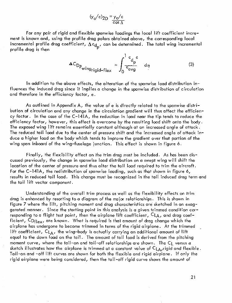
Finally, the flexibility effect on the trim drag must be included. As has been dis-

cussed previously, the change in spanwlse load distribution on a swept wing will shift the

location of the center of pressure and thus alter the tail load required to trim the aircraft.For the C-141A, the redlstrlbution of spanwise loading, such as that shown in figure 6,

results in reduced tail load. This change must be recognized in the tall induced drag term and

the tall llft vector component.

Understanding of the overall trim process as well as the flexlbillty effects on trim

drag is enhanced by resorting to a diagram of the major relationships. This is shown infigure 7 where the lift, pltching moment and drag characteristics are sketched in an exag-

gerated manner. Since the starting point in thls analysis is a given trimmed condition cor-responding to a flight test point, then the airplane lift coefficient, CLA, and drag coef-

ficient, CDflex, are known. What is required is that amount of drag change which the

airplane has undergone to become trimmed in terms of the rigid airplane. At the trimmed

llft coefficient, CL A, the wlng-body is actually carrylng an addltlonal amount of liftequal to the down load on the tail. The amount of tall load is derived from the pitching

moment curve, where the tail-on and tail-off relationshlps are shown. The CL versus a

sketch illustrates how the airplane is trimmed at a constant value of CLA, rigid and flexible.Tail-on and -off llft curves are shown for both the flexible and rigid airplane. If only therigid airplane were belng considered, then the tail-off rigid curve shows the amount of

21

lift, CLA_hrigid, being generated at the trim angle of attack, aFRLrigid. However, the

flexibility effect reduces the llft curve slope so that in order to maintain the same C L. , the

airplane angle of attack increases to aFRLfle x. There is a corresponding change in t_e

tail-off lift curve. Once again, since the airplane does not "rotate" in flight, the condition

of constant angle of attack is imposed and the value CLA_hflex is generated by the wing-body combination.

The trim effect on drag is shown also for both rigid and flexlble conditions. The

starting point is again at the value CLA. The condition of constant angle of attack is im-

posed between the tail-on and tail-off polars. The increment of induced drag, ACDitrlm,

appears on the tail-off polar as the drag difference due to the lift difference, CLA_h - CLA.

The remaining increment between the tail-on and tail-off polars is due to the induced drag of

the tail and the component, CLtal I tan ¢ . The tail profile drag is considered an increment in

the total airplane profile drag and thus is not included in the definition of trim drag, rigid

or flexible. Comparison between the rigid and flexlble trim drags yields the flexlble trim

drag increment.

In summary, three effects on drag due to flexibility have been identified as.signifl-cant: the change in vortex drag, the incremental wing profile drag due to local wing dis-

torfion, and the effect on trim drag. The equation for the rigid drag coefficient in terms of

the measured flight drag coefficient, CDfle x, can then be written:

÷ (4)CDrigld = CDfle x ACDrigld-flex

where

ACDrigld_fle x = ACD. + ACDp + ACDtrimIr ig id-fl ex _w ingr ig _d-fl ex r igld-fl ex

and

ACDi = (CLA2_

rigid-flex \-_-_e / rigid

ACDp in . = incremental wing profile dragw grlgld-flex as defined by equation (3)

ACDtrlmrlgid_fle x = CDtrimrigid - CDtrimflex

The trim drag flexibility increment can be further defined as

22

ACDtrimrig id-flex ACDitrimrig id-flex + ACDi + A(CLtail tan _1tail rig id-fl ex ig id-fl ex

c, h- A 'A\" "_--Ae rr-A-_-e rigid \ trAe rrAe

(c2 )+ ,.,Ltai I x S/S H

\rzAtall etail

+ (CLtailtan_)rigid

flex

/rigid \rtAtail etail / flex

_ (CLtai Itan E ) flex

All increments between rigid and flexible conditions are computed holding the total air-plane lift coefficient constant.

Trim c.g. and instrumentation drag.- In addition to the above considerations, cor-

rection of the drag to a common c.g. position and for instrumentation drag is desirable.Therefore:

CDrigid

c.g. = .25 MACless inst

=CDfle x+ ACDi + ACDp .rig id-fl ex w mgrigid_fle x

+ _C D - ACDins ttrimrigld_fle x+ ACDtrim c'g"(5)

where

ACDtrim = (CDtrim) - (CDtrim)c.g. c.g. = .25 MAC c.g. = flight c.g.

ACDinst

incremental drag due to flight test instrumentation

Equation (5) above is the basis for analyzing fllght test drag; however, before pro-ceeding to discuss the results for the C-141A, it is appropriate to consider the method of

computing thrust utilized during the C-141A flight test program.

TF 33 Thrust Calculation

The drag data used in this report are based upon an accurate determination of the

thrust delivered in flight by four calibrated TF33 engines. A computer program is used to

23

compute installed engine thrust for the atmospheric conditions and engine parameters re-corded during the flight test program. A detailed discussion of the thrust calculation pro-cedure and a description of the computer program can be found in reference 9.

The basic net thrust of the TF33 engine is defined by the equation

FN = FG - FRD - FAB D

where

Nozzle gross thrusts are

net thrust equation may be rewr

FN --

FG = Gross nozzle thrust

FRD = Ram drag

FAB D -- Nacelle afterbody drag

obtained separately for the fan and primary nozzles.itten

FGpRI +FGFAN - FRD - FAB D

The gross thrust for the

where

The

primary and fan nozzles are obtained from the equation

FG = ¢JA C G PAM

-- Nozzle thrust parameter

FGIDEA L

A PAM

A = Nozzle area

C G = Nozzle thrust coefficient

FGACT UA L

FGIDEAL

PAM = Ambient pressure

24

ThesubscriptACTUAL impliesmeasuredvaluesof thrustand airflow; the subscriptIDEALimplies theoretical valuesbasedon the ratio PTOTAL,/PsTATIC.

where

The ramdrag is given by the equation

FRD -- WT VOg

WT = WpRI + WFA N + WBL D = Total airflow

V O = Free stream velocity

g = Acceleration due to gravity

WBL D = Bleed flow

Airflow for both the primary and fan nozzles is given by the equation

W = _ CDA PAM/_/-T

where

= Nozzle airflow parameter

WAIDEAL T

A PAM

C D = Nozzle airflow coefficient

WAAcTUAL

WAIDEA L

A = Nozzle area

PAM = Ambient pressure

T = Nozzle air total temperature

Since nacelle afterbody drag is a function of nozzle pressure ratio, it is includedin the net thrust calculation. The data were obtained from scale model wind tunnel tests

run at the United Aircraft High Speed 8-foot wind tunnel.

25

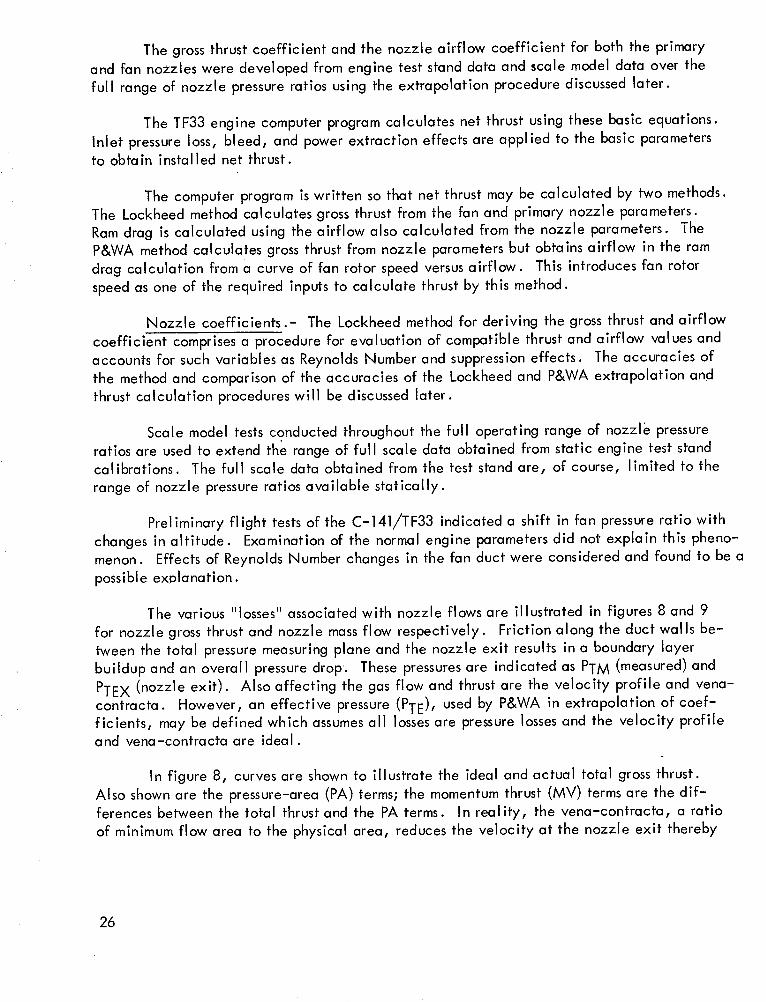
Thegrossthrust coefficient and the nozzle airflow coefficient for both the primaryand fan nozzleswere developedfrom engine test standdata and scale model data over the

full range of nozzle pressure ratios using the extrapolation procedure discussed later.

The TF33 engine computer program calculates net thrust using these basic equations.

Inlet pressure loss, bleed, and power extraction effects are applied to the basic parametersto obtain instal led net thrust.

The computer program is written so that net thrust may be calculated by two methods.The Lockheed method calculates gross thrust from the fan and primary nozzle parameters.

Ram drag is calculated using the airflow also calculated from the nozzle parameters. TheP&WA method calculates gross thrust from nozzle parameters but obtains airflow in the ram

drag calculation from a curve of fan rotor speed versus airflow. This introduces fan rotor

speed as one of the required inputs to calculate thrust by this method.

Nozzle coefficients.- The Lockheed method for deriving the gross thrust and airflow

coefficient comprises a procedure for evaluation of compatible thrust and airflow values and

accounts for such variables as Reynolds Number and suppression effects. The accuracies of

the method and comparison of the accuracies of the Lockheed and P&WA extrapolation and

thrust calculation procedures will be discussed later.

Scale model tests conducted throughout the full operating range of nozzle pressure

ratios are used to extend the range of full scale data obtained from static engine test standcalibrations. The full scale data obtained from the test stand are, of course, limited to the

range of nozzle pressure ratios available statically.

Preliminary flight tests of the C-141/TF33 indicated a shift in fan pressure ratio withchanges in altitude. Examination of the normal engine parameters did not explain this pheno-

menon. Effects of Reynolds Number changes in the fan duct were considered and found to be a

possible explanation.

The various "losses" associated with nozzle flows are illustrated in figures 8 and 9

for nozzle gross thrust and nozzle mass flow respectively. Friction along the duct walls be-

tween the total pressure measuring plane and the nozzle exit results in a boundary layerbuildup and an overall pressure drop. These pressures are indicated as PTM (measured) and

PTEX (nozzle exit). Also affecting the gas flow and thrust are the velocity profile and vena-

contracta. However, an effective pressure (PTE), used by P&WA in extrapolation of coef-flcients, may be defined which assumes all losses are pressure losses and the velocity profileand vena-contracta are ideal.

In figure 8, curves are shown to illustrate the ideal and actual total gross thrust.

Also shown are the pressure-area (PA) terms_ the momentum thrust (MV) terms are the dif-

ferences between the total thrust and the PA terms. In reality, the vena-contracta, a ratio

of minimum flow area to the physical area, reduces the velocity at the nozzle exit thereby

26

increasing the static pressure. This increases the actual PA term while reducing the MV

term. The points labeled on figure 8 are indications of the following:

Point A: Actual thrust parameter at the measured nozzle pressure ratio.

Point B: Ideal thrust parameter at the measured nozzle pressure ratio.

Point C: Actual thrust parameter at the true nozzle pressure ratio.

Point D: Ideal thrust parameter at the true nozzle pressure ratio.

Point E: Actual and ideal thrust parameter at the effective nozzle pressureratio.

Point F: Actual PA term at the true nozzle pressure ratio.

Point G: Ideal PA term at the true nozzle pressure ratio.

These points are used in the definitions of the nozzle coefficients as defined below:

A/B = CG, overall nozzle gross thrust coefficient, ratio of actual to idealgross thrust at the measured nozzle pressure ratio.

CF/DG = CV 2, velocity coefficient squared, ratio of actual to ideal momentum

at the true nozzle pressure ratio.

F - G = Change in PA term due to vena-contracta.

The nozzle airflow parameter shown in figure 9 is also affected by the vena-contractaand velocity profile. Here, as in the thrust parameter, the vena-contracta reduces the

velocity at the nozzle exit which in turn produces a lower velocity coefficient. The points

shown in figure 9 and their uses in defining the coefficients are indicated below:

Point A:

Point B:

Point C:

Point D:

Point E:

Actual airflow parameter at measured nozzle pressure ratio.

Ideal akflow parameter at measured nozzle pressure ratio.

Actual airflow parameter at the true nozzle pressure ratio.

Ideal airflow parameter at the true nozzle pressure ratio.

Actual and ideal airflow parameter at the effective nozzle pressureraHo.

27

A/B = C D, overall nozzle discharge coefficient, ratio of actual to ideal massflow at the measured nozzle pressure ratio.

C/D = CV, velocity coefficient, ratio of actual to ideal mass flow at the truenozzle pressure ratio.

Model data analysis.- Data were obtained from a 1/10 scale model with the capa-

bility of controlling and independently measuring the flow to the fan and primary nozzles.The measured thrust consisted of that produced by both nozzles. The model simulated the

actual production hardware contours from upstream of the measuring station aft to the nozzleexit.

The basic calibration of each nozzle was accomplished by flowing air through that

nozzle alone. The other flow path was plugged internally to prevent leakage through the

control valves. In the analysis of these tests, the base pressure-area of the non-flowingnozzle was subtracted from the measured thrust. The results of these model tests are shown

in figures 10 and 11.

The fan only and primary only data were used to define the effective losses of each

nozzle. The effective fan pressure losses for the model fan duct are shown in figure 12. The

nozzle gross thrust is affected by momentum, that is, it is dependent upon velocity squared,whereas nozzle flow is affected only by velocity_ therefore, the effective losses based on

measured thrust are larger than those based on flow.

True losses, of course, vary primarily with velocity and would not exhibit thecharacteristics shown. The apparent hump in the effective loss is a result of the influence

of the vena-contracta on the velocity at the nozzle exit. The data indicated the vena-contracta had no further influence on the losses above a fan nozzle pressure ratio of

approximately 2.8. Above this point the nozzle flow exhibits a Prandtb-Meyer expansion

from the physical nozzle exit_ the vena-contracta is now at the nozzle exit and the areacoefficient is 1.0. The remaining losses at this point are the duct pressure loss (APL_) and

the loss in the velocity coefficient (Cv). By an iteration process using both flow and thrust

data, the/_PL and C V can be determined for this portion of the fan nozzle pressure ratio.The actual step-by-step calculation procedure for this iteration and the remaining calcula-tions for the nozzle coefficients may be found in reference 9.

At nozzle pressure ratios less than 2.8, the minimum flow area moves aft of the

physical exit. The velocities in the duct, and therefore the pressure losses, are reduced.Pressure loss curves can be evaluated for various area coefficients, CA, as shown in figure

13. The area Coefficient, CA , is defined as the ratio of minimum flow area to the physical

nozzle area. This calculation is accomplished by fixing the duct friction factor to match

the known base point calculated by the above iteration procedure and then accounting forthe duct losses as they vary with changes in the ratio of total to static pressure at the nozzle

exit. Using the losses defined in figures 8 and 9, the AP L versus CA relationship in figure

13, and assumed vena-contractas, CV'S can be calculated for both the thrust and airflowdata. The process is repeated until both sources produce the same CV.

28

A similar processis repeatedfor the primary nozzle. In this case, however, theReynoldsNumbereffects are considerednegligible and the CV and APL are combinedasa single term. This term is called AP and is treated the sameasthe fan losses.

The final model lossesfor each of the nozzlesare shownin figures 14 through 18.The pressureloss, area and velocity coefficients for the fan duct modelare shownin figures14, 15, and 16 respectively. Figures17and 18showthe modelprimary pressureand velo-city losscombinationand the area coefficient.

Full scale data analysis.- The data obtained from full scale calibrations are limited

to the relatively low nozzle pressure ratio of approximately 1.8 obtained from an engine teststand. To obtain nozzle calibrations for cruise conditions, the full scale static data are ex-

trapolated based on model test results.

Fan nozzle: Full scale altitude test data showed an increase in fan pressure ratio

when compared to lower altitude test data. Various possible changes in engine character-

istics were considered but could not explain the phenomenon that existed. An examinationof changes in fan duct Reynolds Number with changes in altitude revealed that the increase

in fan pressure ratio correlated with the increase in fan duct pressure losses. It was foundthat the static, altitude, and model data could all be relateJ by using the smooth pipe,

turbulent flow friction factor based on a Reynolds Number using the hydraulic diameter ofthe nozzle exit.

Using the basic model data pressure loss curve, figure 14, and the calculated

Reynolds Number for various altitudes, the APb/PTM for the full scale hardware was con-structed as shown in figure 19. The area coefficient for the full scale hardware was assumed

to be the same as that for the model when they were operating at the same true nozzle

pressure ratio, PTEX/PAM.

The remaining undefined factor for full scale evaluation is the velocity coefficient.

Using the thrust data obtained from the static test stand for expansion ratios up to 1.7, anddata from figures 14 and 19, the full scale velocity coefficients were calculated. To extra-

polate the velocity coefficient, a AC V between the model and full scale was determined.

Thls parameter was relatively flat as shown in figure 20, and, therefore, very easy to extra-polate. Having defined the velocity coefficient for sea level conditions, the problem of

obtaining an altitude velocity coefficient remained. Since both the pressure loss and velo-

city profile are greatly influenced by the boundary layer, the changes in velocity coefficientwith altitude were calculated to be proportional to the changes in duct pressure losses with

altitude or Reynolds Number as shown in figure 21.

The measured flow obtained from the engine test stand did not reproduce the flowcoefficient derived from the above full scale nozzle losses; however, these differences are

accounted for as described in the following paragraph.

29

Thedifferences probablyresultedfrom severalsources. In reality, the fan nozzledoesnot exhaustthe flow directly aft; therefore, the velocity coefficient for thrustand air-flow will not be identical. Biaserrors in both thrustandairflow tend to be reflected in fanparameters. Another possibleerror could have resultedby usingthe publishedthrust coef-ficient definition of the P&WAhardwarewhich wasusedin teststo define the Lockheedhard-ware coefficients. Thisresultsbecausefan thrustand airflow are consideredasthat whichremainsafter the primary nozzle propertieshave beencalculated.

To obtain the final full scale flow coefficient, the coefficients were first calculatedbasedon figures 14, 19, and 21. Ratiosof the altitude to sealevel coefficients were thenmadebasedon thesecoefficients. To determinethe full rangesealevel flow coefficient,the measuredflow data were usedwith figure 14 to calculate a Z_Pthat included the pres-surelossand velocity coefficient. Thiswasextrapolated basedona similar modelcurve.Thealtitude ratios, determinedabove, were then applied to the sea level curve to calculatethe altitude flow coefficients.

Primarynozzle: Theprimary nozzle, being relatively shortwhencomparedto thefan duct and nozzle, wasconsideredto be independentof ReynoldsNumbereffects. Forthis reason, the pressurelossand velocity coefficient were not separatedfor the extrapola-tion process.

Whenthe primary nozzle is flowing independentlyof the fan, i.e., the nozzle isflowing without being in the _nfluenceof the fan flow, the nozzle is consideredto be un-suppressed.Thefull scale unsuppressedthrust and flow coefficients were extrapolated byusingthe area coefficient derived Fromthe modeland extrapolating theAPL curve basedon the ratio of full scale to model pressurelosses. Thefull scale Z_PL curve is shownasfigure 22.

Thefan and primary nozzle flows exit in a coaxial, near co-planar arrangement.At low primary nozzle expansion ratios, the fan exhaust, which is coned inward toward the

primary flow, reduces the primary flow. The fan flow must be turned back into the axialdirection and this is accomplished by forces exerted by the primary flow. The primary flow

in turn is suppressed such that the minimum flow area is reduced. Model and full scale datawere combined to determine the suppression factor throughout the full operating range.

This factor, shown in figure 23, is applied as an additional reduction in the primary nozzlearea coefficient. The full scale coefficients are then calculated using the appropriate

curves from figures 18, 22, and 23.

Final nozzle coefficients: The full scale fan and primary nozzle coefficients were

derived from data obtained from four sets of production hardware run on a slave engi-ne onthe engine test stand. These hardware sets were then installed on the airplane to conduct

the performance testing. The final full scale nozzle flow and thrust coefficients based onthese hardware sets are shown in figures 24 and 25 for the fan and Figures 26 and 27 for the

primary.

3O

Accuracy of thrust calculatlon.- The thrust evaluation procedure developed by

Lockheed is felt to be superior to that recommended by P&WA in reference 10 because of theadditional considerations in the Lockheed method. The P&WA method does not consider

the effects of Reynolds Number on the nozzle coefficients, neither does it subdivide thenozzle losses into various definable loss components. The extrapolation of the nozzle coef-

ficients by the Lockheed procedure is made easier and considered more reliable because the

extrapolation is based on component losses as opposed to the total losses. The most importantfactor between the two methods, however, is in the actual net thrust evaluation calculation

procedure. The Lockheed calculation uses nozzle conditions to calculate both gross thrustand inlet ram drag (engine airflow); whereas, the P&WA calculation uses nozzle conditions

for calculating gross thrust, but uses fan rotor speed to determine engine, airflow.

Figure 28 shows the basis for the P&WA extrapolation of the gross thrust coefficient.The relative pressure loss Between the model and full scale is calculated for constant valuesof _CG and plotted as shown in figure 29. This pressure loss difference is then extrapolated

and used to extend the full scale _C G curve. The actual extrapolation shown on figure 29

was determined from the "sea level" fan C G derived by the Lockheed method. The P&WA

extrapolation could easily have produced this curve.

The computer was run to reproduce engine parameters as measured on the engine teststand. The calculated and measured values of thrust and airflow are compared in figures 30

and 31, respectively. These comparisons were found to be quite satisfactory and validatedthe nozzle coefficients.

The overall nozzle thrust and airflow accuracy of the model and full scale data arein the order of one percent. Using the defined primary nozzle coefficients, the four sets of

nacelle hardware showed a variation of only 0.5 percent in the fan coefficients. The man-ipulation and extrapolation of the averaged coefficients by the Lockheed method added

approximately another 0.5 percent error to the definition of total gross thrust and airflow atcruise conditions. The possible errors introduced by improper accounting of Reynolds Number

effects are considered to have only a small effect on net thrust because they are largelyoffset by being used in both the calculation of gross thrust and ram drag. The primary noz-

zle suppression error in the low power flight region could be as large as approximately one

percent, resulting in an additional net thrust error of 0.2 to 0.5 percent. At cruise condi-

tions, however, where the primary nozzle expansion is higher, the suppression factor isalmost 1.0 and the error should be negligible.

At cruise conditions the total nozzle gross thrust is twice the magnitude of net thrust.

In considering the cruise net thrust error, appropriate factors must be applied to the nozzlegross thrust and airflow errors. Using factors of 2.0 for thrust and 1.0 for airflow, the over-

all basic net thrust accuracy at cruise due strictly to the reduction, extrapolation and ex-

pansion of the nozzle coefficients by the Lockheed method is estimated to be approximately2.5 percent. This value is based on a root-sum-square analysis. The P&WA method uses fan

speed for the evaluation of inlet airflow and does not account for any airflow changes betweenthe uninstalled and completely installed engines. This may result in an error of some magnitude

31

in calculation of ramdrag, and hencenet thrust. Basedon test data, the P&WAmethodwould increasegrossthrustat altitude, where the increasein fan pressureratio wasseentooccur, unlessmodified in somemannerto account for phenomenaoccuringwithin the fanducts. Thesamedatawould indicate a decreasein airflow when usingthe P&WAmethod.Theseerrorsare additive in the net thrust evaluation and thuswould result in greater totalerror.

Flight TestResults

In order to fully investigate the degreeof correlation attainable with flight testdata,a review of all available C-141A testdata wasmadeto provide full and sufficient coverageof a wide rangeof conditions. BothCategoryI and II flight test runswere surveyedand onlythoserunsspecified by the flight test personnelas beingaccurate and suitable for cruise con-figuration drag analysiswere Selected. Any runswhich did not have an accurate definitionof aircraft weight, fuel load, and trim condition, aswell as the additional parametersre-quired for thrust calculation, were screenedout. Forthe above reasons,all flights selectedwere part of the CategoryI test.

Table 2 providesa summaryof the 111runsfrom the 10 flights chosen. Theseflightsinclude 60 speedpowerruns (flights 106, 119, 123, 128, and 129), 21 continuousclimbruns (flights 138, 139, and 140), and 30 cruiserunsfrom rangemissions(flights 187and 190).

Speedpowerrunsare the bestsourceof data for full scale clean airplane drag due tothe nature in which theseflights are conducted. Full attention is given to thesedata in thecurrent analysis. Figure32 summarizesthe drag coefficient, lift coefficient, and MachNumbervariations for theseflights. Normal cruiseconditions for the C-141A areat CL=0.38 and M = 0.767. TheReynoldsNumberrange is seenfromtable 2 to be 24.49 millionto 86.37 million basedon the wing meanaerodynamicchord, comparedwith a nominal

cruise value of 37.5 million. Three of the speed power runs are observed to occur at liftcoefficients in excess of 0.8. These three flights (106-4F, 129-5G, and 129-6R2) were

eliminated from the analysis since they do not constitute sufficient data to analyze that

portion of the drag polar where extreme separation is known to occur.

Results of Flexible Analysis

In order to assess the aeroelastic effects on drag previously identified it is necessary

that the relationship between the rigid and flexible airplane characteristics be developed.As mentioned earlier in the section on vortex drag, extensive flight test pressure and strain

gauge data have been analyzed previously, reference 11. These data were correlated with

predicted flexible characteristics and a revised set of rigid aerodynamic data derived which,

32

in coniunction with the elastic characteristics of the structure, are used in a computer pro-

gram to calculate a complete set of trimmed airplane load distribution data for any flightcondition. Output from this program includes non-dimensionalized loads on all components

for both rigid and flexible conditions.

It is believed that the use of this program provides the most efficient means of sepa-

rating and accounting for all the variables present. In order to establish the importance andtrends of each variable, a matrix of configurations, shown in table 3, was selected for sub-

mission to the program to encompass all flight conditions at which drag data exist. The

effect of flexibility on any parameter such as lift coefficient, efficiency factor, or incre-mental drag at a particular flight test condition can then be obtained by interpolation of theresults from the matrix of conditions.

The major variables which influence the magnitude of the flexibility effects are dy-

namic pressure, lift coefficient and Mach Number, and as can be seen in table 3, the basicseries of conditions centers around these variables. Additional conditions were devised to

measure the bending relief due to increasing the wing fuel and the effect of center of gravity

location. Concurrently, five speed power points were selected to serve as check cases on

the overall results. Spanwise distributions for these five cases are shown in figure 33.

Table 3 also contains a summary of the rigid and flexible parameters for each condi-

tion. Summary curves and a discussion of the effects follows in the next section. These dataserve as the framework for a flexible analysis computer program which performs the interpola-

tion process and combines the drag components for a given flight test condition.

Span efficiency factor.- Rigid efficiency factors, shown in figure 34, were deter-

mined for a large range of lift coefficients and Mach Numbers in order to provide a firmbasis for the analysis. The airplane does not fly at all the combinations of C L and M shown

in figure 34 and consequently the flexible analysis is limited to the pertinent range of vari-

ables. For example, figure 35 shows a comparison of the rigid and flexible efficiency factorsfor several values of dynamic pressure, q, where the C L range for each q bounds the avail-

able flight data. Since this comparison is made at low speed (M-- 0.6), it is also necessaryto examine the flexibility effect on e at higher Mach Numbers. This is accomplished in

figure 36 for high and low values of C L and q over the range of test Mach Numbers. Exami-nation of these figures reveals that the flexibility effect is quite significant, especially atlow lift coefficients. The reason for this, as discussed earlier in the aeroelastic effects

section, is the resultant inboard shift of the wing load onto the fuselage. This tends to

improve the total spanwise distribution from an efficiency viewpoint. The fuel load, storedin the wing fuel tanks, affects the dead weight wing twist distribution. This effect tends torelieve the bending due to aerodynamic loading and hence reduces the amount of aeroelastic

distortion present at a given condition. Three values of fuel load were chosen, correspond-

ing to low, medium and high fuel load conditions For the purpose of investigating this

effect on flexibility. As can be seen in table 3, the effect of fuel load on span efficiency

is small, especially in the cruise range of lift coefficients (CLA = 0.35 to 0.5)where the

33

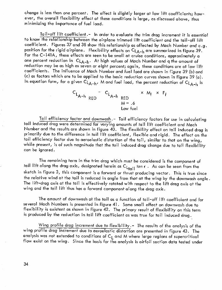
change is lessthan one percent. Theeffect is slightly larger at low llft coefficients; how-ever, the overall flexibility effect at theseconditions is large, as discussed above, thusminimizing the importance of fuel load.

Tail-off lift coefficient.- In order to evaluate the trim drag increment it is essentialto know the relationship between the airplane trimmed lift coefficient and the tail-off lift

coefficient. Figures 37 and 38 show this relationship as affected by Mach Number and c.g.

position for the rigid airplane. Flexibility effects on CLA_ h are summarized in figure 39.For the C-141A, these effects are seen to be small at cruise conditions, approximately a

one percent reduction in CLA-h. At high values of Mach Number and q the amount ofreduction may be as high as seven or e_ght percent; again, these conditions are at low lift

coefficients. The influence of Mach Number and fuel load are shown in _gure 39 (b) and(c) as factors which are to be applied to the basic reduction curves shown _n figure 39 (a).

In equation form, for a given CLA_h , M and fuel load, the percent reduction of CLA_h is

CLA_h = x Mf x FfRED CLA-h RED

M=.6

Low fuel

Tail efficiency factor and downwash.- Tail efficiency factors.for use in calculatingtail induced drag were determined for varying amounts of tall lift coefficient and Mach

Number and the results are shown in figure 40. The flexibility effect on tail induced drag isprlmarily due to the difference in tall lift coefficient, flexible and rigld. The effect on the

tail efficiency factor due to aeroelastlc distortion of the tail, similar to that on the wing,

while present, is of such magnitude that the tail induced drag change due to tall flexibilitycan be ignored.

The remaining term in the trim drag which must be considered is the component of

tail llft along the drag axis, designated herein as CLtai I tan _ . As can be seen from the

sketch in figure 3, thTs component is a forward or thrust producing vector. This is true slnce

the relative wind at the tall _s reduced in angle from that at the wing by the downwash angle.The lift-drag axis at the tail is effectively rotated with respect to the lift drag axis at the

wing and the tall lift thus has a forward component along the drag axis.

The amount of downwash at the tail as a function of tail-off llft coefficient and for

several Mach Numbers is presented in figure 41. Some small effect on downwash due to

flexibility is existent as shown in figure 42. The prTmary result of flexibility on this term

is produced by the reduction in tall lift coefficient as was true for tail induced drag.

Wing profile drag increment due to flexibility.- The results of the analysis of thewing profile drag increment due to aeroelastlc distortion are presented in figure 43. The

analysis was not extended to conditions of C L and M where large regions of supercrlticalflow exist on the wing. Since the basis for the analysis is akfoil section data tested under

34

conditions of natural transition, the duplication of shockeffects is dubiousand thusprecludesreliance on the resultsat theseconditions. In table 3, resultsfor the wing profile drag incre-mentare shownonly for the M = 0.6 casesand at CL'Sof 0.55 and below. Thesedata tendto be conservativesince the analysisdid not include considerationsof possibleshock-inducedseparation_also, on the inboardwing panel the isobarsgradually becomeunsweptand localincreasesin lift are felt due to the flexible redistributlon of load which would further aggra-vate compressibility losses. This, however, doesnot detract materially from the overallanalysissincethe major emphasisis placedon thosetest points in an operating rangenearthe minimumprofile drag point and at Mach Numberswheresucheffects shouldbe minimal.Thebasic data obtained from the low fuel configurationsare shownin figure 43 (a) and afactor which approximatesthe effect of varying amountsof fuel is contained in figure 43 (b).

Results for five selected flights.- The rigid and flexible coefficients obtained froma direct calculation for the five check cases are shown in table 4. A comparison with the

results from the interpolation program used to analyze all the flight test points shows goodagreement thus validating the interpolation procedure. A step-by-step breakdown of each

of the drag components affected by flexibility is presented in this table for the purpose of

illustrating the effects as well as comparing the interpolated and calculated results.

Considerations of Other Components

External configuration changes.- The test article was modified in certain ways from

the production configuration to suit the peculiar requirements of the performance test pro-grams. These changes are enumerated in table 5 where the estimated drag increment foreach item is shown. Figure 44 illustrates the approximate position of the major changes.

The wing vortex generators and wing leading-edge stall strips were installed during the

flight test program to control the natural stall separation progression and, subsequently,

became part of the production airplane. Drag of these items is considered part of the total

roughness drag and is not included in the total instrumentation drag increment.

The drag increments shown in table 5 were obtained using conventional methods con-tained in reference 12, considering the effects of pressure gradients, and boundary layer

thickness. A brief discussion follows, outlining the procedures for those items of major

significance to the airplane drag.

The drag increment of the nose boom is composed of the skin friction drag of theisolated boom, modified for installation effects. Reference 12 presents data for cylindricalbodies with streamlined head forms in axial flow from which the minimum skin friction value

can be determined for the boom. Incremental effects due to mutual interference between

the boom and the fuselage are small. An approximation is made based on the effect of the

pressure gradient along the boom, as outlined in chapter 8 of reference 12, using the

measured static pressures existing on the fuselage nose.

35

Dragof the takeoff and landing camerais assumedto be that for a faired appendageto a body. This is calculated usingthe relationship

CDApP = CDtr Srr (6)S

where CD_r is the drag coefficient for a similar body based on the reference frontal area, Srr.

The drag increment of the two tail skegs may be fairly significant since they are essen-

tially rectangular bodies protruding on the fuselage afterbody where they may contribute tolocal boundary layer separations. There is no appropriate method to calculate drag due tosuch separation effects on the aft fuselage however, and a minimum drag value is used based

on the drag characteristics of bluff bodies.

Another significant item of drag is due to the trailing static airspeed cone and cable.Drag of the cable was determined from the relationships of reference 12 for wires and cablesinclined against the flow direction. This was added to the cone drag estimated for a similar

isolated body using equation 6.

Drag of the remaining items in table 5 is rather small even considered in total.

Approximations for these items were obtained using methods for excrescence drag given inreference 12.

The total low speed drag increment due to the external changes for flight test opera-

tions is estimated to be ACDINS T = 0.00068.

Incremental drag due to c.g. position.- As can be seen in table 2, variations in the

location of the c.g. position of one to two percent MAC occur during most flights. Moreimportant, the c.g. position varies significantly from one series of flights to the next, withan overall range of approximately 12 percent MAC. Thus it is necessary to account for these

differences by referencing all data to a particular c.g. location. In this report all flighttest data has been corrected to trim at a c.g. location of 0.25 MAC. The effect of a shift in

c.g. position can be approximated by making use of existing wind tunnel data where such

effects were measured. A summary of these effects based on C-141A wind tunnel data, ref-erence 13, is shown in figure 45.

Equivalent Rigid Profile Drag

Analysis of the drag data from the speed power flights was accomplished utilizing

a reduction equation derived from equations (1) and (5). Equation (1) can be re-wrltten interms of the minimum profile drag as:

36

= CD - CDi - CDpCDPmi n - CDtri m - CDp cC k

In order to determine the equivalent rigid profile drag, substitution of the corrections

from equation (5) is made for CD:

CDPmi n =CDfle x - CDi - CDtri mrigid

c.g. = .25 MACless inst + AC + AC

Dirlgid-flex

- CDPc L - CDp C

DPwingrigid_flex

+ AC D + AC D - ACDins t (7)tr imr ig id-fl ex trimc, g.

All of the components in the above equation can be obtained except the lift depend-

ent profile drag, CDPcL, and the compressibility effect on profile drag, CDp C. In order to

facilitate a determination of these values an intermediate value of profile drag was calcu-

lated accounting for all components except these two. This term is designated as Cr_Prigid.Thus,

Cbp = C D + CDPcL + CDp Crigid Pmin ..,rlglac.g. = .25MACless inst

In addition, the Reynolds Number influence on profile drag exists in the data at thispoint. This influence is brought about by the reduction in boundary layer thickness and

attendant skin friction with increasing Reynolds Number. A fairly accurate estimate of thiseffect is possible from classical skin friction laws with appropriate form or shape factors.

The profile drag of each component on the aircraft is calculated from:

CDp = Cf (SF) SWETS

where

Cf

SF =

SWET =

S =

skin friction coefficient at the Reynolds Number based on the component charac--teristic length.

accounts for the supervelocity resulting from the component shape

wetted area of the component

wing planform area

37

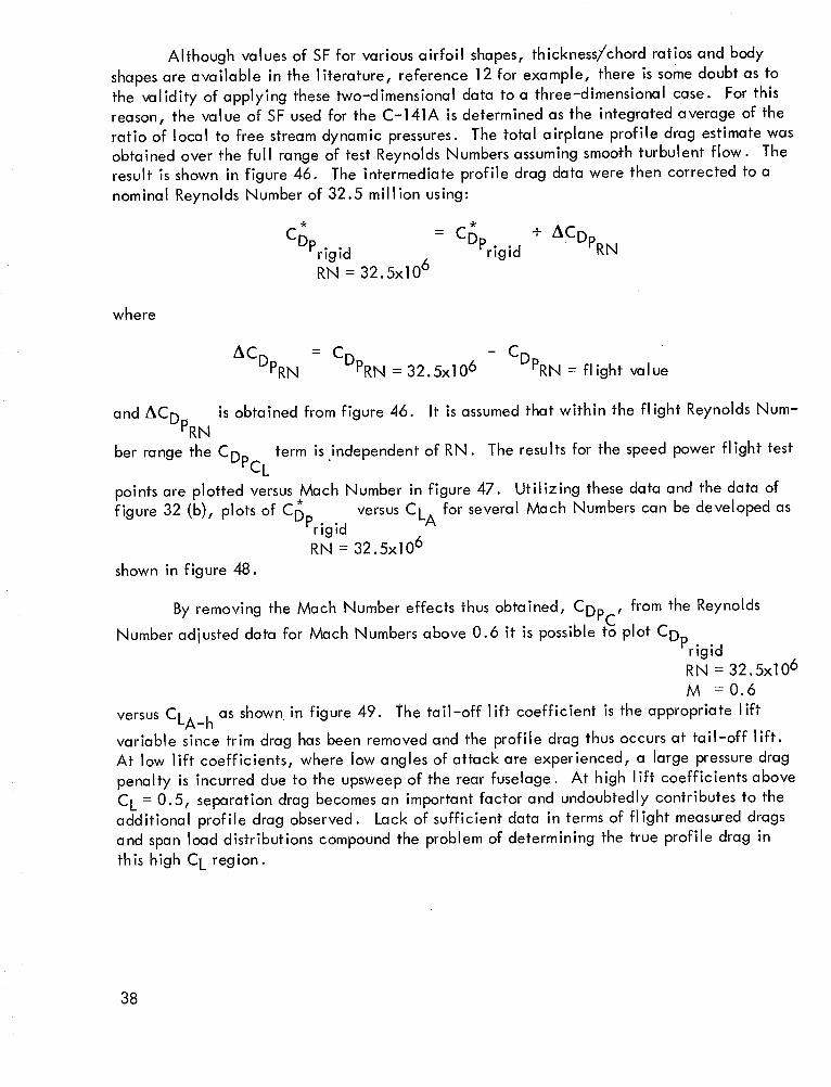
Although valuesof SFfor variousairfoil shapes,thickness/chordratiosand bodyshapesareavailable in the literature, reference 12 for example, there is somedoubtas tothe validity of applying thesetwo-dimensionaldata to a three-dimensionalcase. Forthisreason, the value of SFusedfor the C-141A is determinedasthe integratedaverageof theratio of local to free streamdynamicpressures.The total airplane profile drag estimatewasobtainedover the full rangeof test ReynoldsNumbersassumingsmoothturbulent flow. Theresult is shownin figure 46. The intermediate profile drag data were then corrected to a

nominal Reynolds Number of 32.5 million using:

CDPrigid = CDPrigid + ACDPR N

RN=32.Sx106

where

AC = CDPRN - CDPRNDPRN = 32.5x106 = flight value

and ACDPRN is obtained from figure 46. It is assumed that within the flight Reynolds Num-

ber range the CDPcL term is .independent of RN. The results for the speed power flight test

points are plotted versus Mach Number in figure 47. Utilizing these data and the data of

figure 32 (b), plots of C*DPrlgid versus CLA for several Mach Numbers can be developed as

RN=32.Sx106

shown in figure 48.

By removing the Mach Number effects thus obtained, CDn , from the Reynoldsrc

Number adjusted data for Mach Numbers above 0.6 it is possible to plot CDprigidRN = 32.5x106

M =0.6

versus CLA_h as shown in figure 49. The tail-off lift coefficient is the appropriate lift

variable since trim drag has been removed and the profile drag thus occurs at tail-off lift.At low lift coefficients, where low angles of attack are experienced, a large pressure drag

penalty is incurred due to the upsweep of the rear fuselage. At high lift coefficients above

C L = 0.5, separation drag becomes an important factor and undoubtedly contributes to theadditional profile drag observed. Lack of sufficient data in terms of flight measured drags

and span load distributions compound the problem of determining the true profile drag in

this high CL region.

38

A meancurve is faired throughthe data basedon polynomial curve fit usingthemethodof least squares. Thisaveragecurvecan thenbe usedto adjust all data points forlift effectson profile drag.

Final reductionof the test point drag coefficients to their equivalent rigid minimumprofile drag is outlined in table 6, where the data have beensegregatedby flight categorytosimplify identification. Theresultsare plotted versusReynoldsNumber in figure 50. A meancurve hasbeenfaired throughthe data of figure 50(a) to indicate the ReynoldsNumbertrend. Theestimatedprofile drag variation with ReynoldsNumberfrom figure 46 is includedin figure 50(a) for comparisonpurposes.

Thevariation of profile drag with ReynoldsNumberfrom the flight data is seentodiffer slightly from that of the estimateddata. Theincrementbetween the estimatedprofiledrag and actual is termedexcessprofile drag and is attributed primarily to roughnessdragand to separationand interference effects not included in the estimateddrag. Since theremaybe unknownReynoldsNumbereffectson this excessprofile drag, conclusionsabout theobservedflight variation becomedifficult. In addition, the amountof scatter, althoughrelatively small, and the distribution of the scatter about the meancurve, which affectthe shapeof the meanllne, compoundthis difficulty.

Mostof the data isobservedto lle in a bandfairly close to the mean llne, withinapproxlmately+AC D = .0006. Five of the points appearto be somewhatseparatedfromthe band. Qf thesepoints two are at relatively high CL_S,aboveCLA= 0.55, where it isexpected that a great deal morescatter would appeardue to separationeffects. There-maining threeare in the cruise rangeof CL'Sand Mach Numberand are believed to bewildpoints which occur in flight testanalysisdespite the bestengineeringefforts. Byeliminatingthe high CL test pointsfrom the analysisaswell as the assumedwild points, the profile dragvariation appearsasshownin figure 51. It is believed that this is the best representationofthe minimumprofile drag variation with ReynoldsNumberobtainable from the flight data.It will be observedthat thesedata now exhibit a variation with ReynoldsNumberwhichagreesvery well with the variation expectedfrom classical skin friction laws. Thesedataindicate that over the rangeof the flight test ReynoldsNumbersat least, the separationandinterferencedrag is constantand not dependent on Reynolds Number. An analysis of theaccuracy of these data is discussed in a later section of this report.

For comparison purposes, figures 50 (b) and 50 (c) illustrate the results for the rangemission and continuous climb flights. These data lend little credence to the effects illustrated

by the speed-power data since the scatter band is somewhat greater and the Reynolds Number

range is not sufficient to estab!ish a trend. However, this is not unexpected since theclimb data include the additional variables of rate of climb and pilot technique and, in

addition, it is difficult to account accurately for the effects of wind shear and temperaturegradients. The latter is especially true in the case of the range mission data since these

data were obtained over an extremely long distance and time period. Actually, these range

mission points appear to be approximately 10 drag counts higher, on the average, than thespeed power data and this is attributed directly to wind and temperature gradients not

existent in the speed power data. In a later section on the airplane total drag coefficients,

this discrepancy is also seen to occur, which indicates that the reduction process to profile

39

drag levels hasnot inducedthis difference. The significance of this is that for purposesofanalyzing airplane mln_mumprofile drag,reliance shouldbe placed on only thosedata wherethesevariables have beeneither eliminated or minimized.

In the past, flight data on someairplanes havesuggestedthat there existsa termlnalvalue of skin friction, and further that this is due to a critical roughnessheight related tocomponentlength. Theturbulent skin friction data of Nikuradse showthat terminal valuesof skin friction are introducedby the degreeof distributed roughnessexisting in the surface.Forthe C-141A, distributed roughnessof the order of 400 micro-lnches would be requiredto cause termination of the decrease in skin friction coefficient with Reynolds Number.

Optical measurements of the standard aluminum sheet finish show distributed roughness levelsof 60 to 80 mlcro-lnches and modern paint finishes, as measured on the C-141A, producevalues in the range of 30 to 50 mlcro-inches. Thus, there is no reason to expect terminalskin friction values on the basls of measured and calculated allowable distributed roughness

and the flight test data confirm the absence of terminal values.

Aircraft Drag Polar Analysis

Use is made of equation (5) to determine a set of equivalent rigid airplane drag coef-

ficlents suitable for drag polar analysls. In order to derive sufficlent data to establlsh shapes

of drag polars at several Mach Numbers it is necessary to correct the flight test measured drag

data to constant conditions of Mach Number, designated Mcorr, and Reynolds Number,

designated RNcorr. Thus, equation (5) becomes:

CDrigidc.g. =.25 MACless inst

M = Mcorr

RN = RNcorr

+ &CD. + ACDp= CDfle x Irlgld_flex wingrigld_fle x

+ - AC D

ACDtrimrigid-flex ACDtrimc.g. inst

+

+ ACDM + ACDR N(8)

The flrst six terms areas defined previously.

ACDM = CDM = Mcorr

&CDR N = CDR N = RNcorr

- CDM =

- CDR N

flight M

= flight RN

4O

The Mach Number increment is based on an analysis of the flight test data. The in-crement due to Reynolds Number is based on the estimated skin friction variation for theC-141A aircraft as shown in figure 46.

Mach Number effect on CD.- A procedure similar to that employed to analyze theMach Number effects on CDp was performed on the corrected flight drag values to determine

the variation with Mach Number. The speed power points were first corrected using equation

(8), without the Mach correction, ACDM , and the resulting data plotted versus Mach Numberfor each series of flights. The results are shown in figure 52. Figure 53 is the cross-plot of

the data at constant Mach Numbers. These data are all corrected to a Reynolds Number of

55 million and a c.g. position of 0.25 MAC. In order to increase the reliability of the curve

falrings shown in figure 53 an iteration was performed wherein each flight test point was cor-

rected to several adjacent Mach Numbers where possible, using equation (8) with ACDM in-cluded and keeping the corrections as small as possible. Table 7 lists the results of this

analysis and figure 54 shows all the points for each Mach Number investigated, These data

represent the final drag polars for the flight data corrected to RN = 55 million. A summary

plot of the faired curves is shown in figure 55 and a cross-plot of the data versus MachNumber is included in figure 56. The Mach Number effect illustrated in figure 56 is thatwhich is used in the final analysis. In addition, the results for the range mission flights and

climb flights are shown separately in figures 57 and 58. The previously faired curves are

illustrated on these figures for comparison purposes. It is apparent that the climb data agree

quite well with the speed power data, with an additional amount of scatter. The range

mission data, however, appear to be shifted approximately 10 counts as discussed previouslyunder the profile drag section.

Reynolds Number effect on CD.- In addition to the above set of drag polars, an

attempt was made to establlsh polars at several Reynolds Numbers and Mach Numbers. Dueto the scarcity of high speed data this was possible only at M = 0.6 and M = 0.7. For pur-

poses of this analysis, the data were grouped into three Reynolds Number bands and corrected

to nominal values of RN =80million, 55 million and 30 million. In this way, theRN cor-

rection applied to any individual point never exceeded that of 15 million and was generallyless than 10 million. Further, figure 57 indicates that climb data are useful for drag polaranalysis, more so than for profile drag analysis, where the larger amount of scatter over a

small Reynolds Number range was not beneficial. Thus the climb data were included in an

attempt to increase the number of data points at each Reynolds Number. The final resultsof this analysis are presented in figure 59. The faired curve for RN = 55 million is that which

was derived previously and is shown over the entire C L range. For the two extreme ReynoldsNumbers, however, the data do not extend over a sufficient range to establish the entire

polar.

41

Accuracy of Data

General .- It is not the intent of this report to discuss the statistical treatment of

experimental data in any great detail. Reference 14 is a very useful report on the subjectas related to aerodynamics and reference 15 contains a comprehensive survey of the accuracyof all sorts of measurements. A few brief definitions and explanations are in order. Accur-

acy, as the term is applied herein, is defined to be that measure of the reliability of data

as regards random errors and biased errors. Random errors are those which cause repeatedreadings to vary without any apparent reason. These errors are related to the "precision"

of the measured data and are separate from biased errors which are defined to be those errors

which cause a measurement to be made in error by an unknown fixed amount. Accuracy can

be established by statistical methods for a set, or sample, of measured data by assuming anormal distribution of the data about its mean line. Random errors are usually treated in

this manner. A standard deviation, which is called sigma, a, and defined as the radius of

gyration of the data about its mean, is calculated and a confidence level assigned in termsof this deviation. Two standard deviations from the mean should encompass 95.4 percent of

the data; this represents, however, only an examination of measured results. It is also neces-sary to predict the expected accuracy in order to conclude the overall accuracy, and estab-

lish the validity of the results achieved.

By assuming a normal clistribution of errors, whereby the possibility of all errors beingin the same direction is remote, the error of a flight test parameter, such as drag coefficient,

can be found by combining the errors of all the variables involved. This is represented

mathematical ly as

EV = V(.__Va Ea (@Eb) 2 +(_-_-Vn En (9)

where

V : f(a, b, .... ,n)

E = error of the variable or parameter

The above is generally referred to as the root-sum-square method.

For this analysis, errors due to instrument indicator accuracy are first determined.These are then combined with thrust sensitivity factors, and the sensitivity of the calculated

lift and drag coefficient to measured parameters, to determine the precision of the. final

calculated coefficients. This represents then the expected random scatter of the flight test

data. Additionally, an assessment is made of those errors which have been induced in thecalculation and reduction technique. Since these errors are most likely fixed in amount but

of unknown direction, they are treated as biased errors. Finally, the random and biased

errors are combined so that the overall accuracy can be assessed.

42

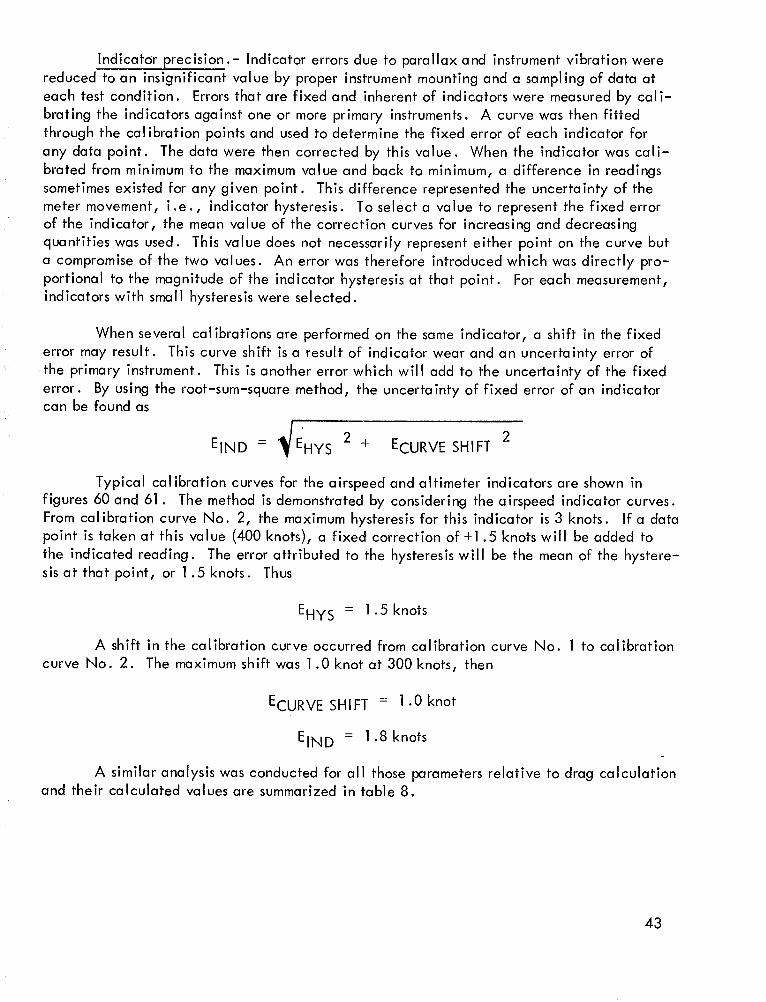
Indicator preclsion.- Indicator errors due to parallax and instrument vibration were

reduced to an insignificant value by proper instrument mounting and a sampling of data at

each test condition. Errors that are Fixed and inherent of indicators were measured by cali-brating the indicators against one or more primary instruments. A curve was then Fitted

through the callbratlon points and used to determine the fixed error of each indicator for

any data point. The data were then corrected by this value. When the indicator was cali-

brated from minimum to the maximum value and back to minimum, a difference in readings

sometimes existed For any given point. This difference represented the uncertainty of the

meter movement, i.e., indicator hysteresis. To select a value to represent the fixed errorof the indicator, the mean value of the correction curves for increasing and decreasing

quantities was used. This value does not necessarily represent either point on the curve but

a compromise of the two values. An error was therefore introduced which was directly pro-portional to the magnitude of the indicator hysteresis at that point. For each measurement,indicators with small hysteresis were selected.

When several callbratlons are performed on the same indicator, a shift in the fixed

error may result. This curve shift is a result of indicator wear and an uncertainty error of

the primary instrument. This is another error which will add to the uncertainty of the fixed

error. By using the root-sum-square method, the uncertainty of fixed error of an indicatorcan be found as

VEIND = EHYS 2 + ECURVE SHIFT 2

Typical calibration curves for the airspeed and altimeter indicators are shown in

figures 60 and 61. The method is demonstrated by considering the airspeed indicator curves.From calibration curve No. 2, the maximum hysteresis for this indicator is 3 knots. If a datapoint is taken at this value (400 knots), a fixed correction of +1.5 knots will be added to

the indicated reading. The error attributed to the hysteresis will be the mean of the hystere-sis at that point, or 1.5 knots. Thus

EHy S = 1.Sknots

A shift in the calibration curve occurred from calibration curve No. 1 to calibration

curve No. 2. The maximum shift was 1.0 knot at 300 knots, then

ECURVE SHIFT -- 1.0 knot

EIN D -- 1.8 knots

A similar analysis was conducted for all those parameters relative to drag calculationand their calculated values are summarized in table 8.

43

Thrust accuracy.- In earlier discussions, the inaccuracies built into the engine com-

puter program, i.e., gross thrust coefficient, airflow coefficient, etc., were considered.The inaccuracies associated with the measured engine parameters and their effect on the cal-

culated net thrust are now considered. Random errors, for both Lockheed and P&WA thrust

calculation methods, are included for comparison purposes.

The engine parameters measured during flight testing and used in evaluating net

thrust are engine pressure ratio (EPR), flight Mach Number (M), altitude (h), free stream

total temperature (TTO), fan rotor speed (N1), and fan pressure ratio (FPR). The fan rotor

speed is used as an input only in the P&WA method of computing thrust. An influence coef-ficient is defined as the percent change in net thrust per percent change in engine parameter.Influence coefficients were calculated for each of the engine parameters over a range of

altitudes and Mach Numbers and are tabulated in table 9.

The engine parameters were instrumented and read from a photo panel in the airplane,

thus introducing some readability error. The random errors attributed to instrument inaccuracy

and readability have been evaluated and are tabulated in table 10.

During the flight test program, FPR was not readily available for some of the testsdue to instrumentation failure and other reasons. Instead of deleting these data points, all

thrust calculations were made by inputting only EPR, M, h, TTO, and N 1 (for influence

coefficients of P&WA method only) into the computer program. In this way, a consistentset of measured engine parameters were retained. When FPR is not input into the computer

program, the program calculates FPR from the other engine parameters as described in ref-erence 9. Figure 62 shows the ratio of calculated FPR to measured FPR for a sampling of

data points. Based on these data, a random error of +_0.5 percent was chosen for FPR insteadof an error based on instrument and readability error.

The thrust error due to the random error of each parameter is found by multiplying the

influence coefficient by the random error for that parameter. Combining these thrust errors

by the root-sum-square method gives a total thrust error due to engine parameter random error.This total thrust error is tabulated in table 11 for both methods of calculating thrust. Therandom scatter due to instrumentation accuracies is larger for the P&WA thrust calculation

procedure than for the Lockheed method. This is due, primarily, to the calculation of engineairflow independently of nozzle gross thrust in the P&WA method.

In considering the overall thrust accuracy, the error due to the calculation method forthrust discussed earlier in the TF-33 thrust calculation section must be considered with the

data scatter error. For the thrust accuracy of individual data points, these errors should be

considered as separate and distinct. The error of the calculation method is a bia_ error

since it is repeatable for any given flight condition; however, it may vary significantly with

large changes in engine power setting or Mach Number. In the consideration of airplane

performance, these large changes in operating conditions may fall on any given portion of

the drag polar. Therefore, the drag coefficient would have an effective thrust accuracywhich combines the random and bias errors. A value of 2.6 percent for the effective thrust

error is obtained by the root-sum-square method.

44

Overall accuracy.- The accuracy of a particular flight test drag coefficient is in-

fluenced not only by thrust inaccuracies but also by other parameters which contribute to

the determination of the final drag coefficient. This accuracy is found by combining the

results of the thrust accuracy analysis with an analysis of the influence of all parameters

which can be identified. This is accomplished separately for the random errors due to in-strumentation inaccuracies and bias errors due to calculation methods. An estimate of the

overall maximum inaccuracy expected is represented by a combination of the two. First,the equations for the lift and drag coefficients are written

CL = Wcos Y - FN sin(a + aTL )

qS

CD = FNcos (a +aTL ) - WslnYqS

The above two equations are used in conjunction with equation (9) to evaluate thesensitivity of C D to an error in each variable considered independently. The instrumenta-tion errors affect the dynamic pressure and Mach Number as well as the calculated thrust.

Additionally, errors in weight, angle of attack, and climb angle must be considered. The

effect of obtaining a C D at an incorrect C L is included by assessing the sensitivity of C Lto the parameters and using the known variations of C D and C L. For example, the effectof an error in weight, AW, is

AC D \ _/ + AWaC L a W

Three typical flight conditions were chosen for evaluation of the amount of random

error expected in the flight test data. These are given in table 12; also tabulated are theerrors for each of the parameters, the total random error and the overall maximum error.

The root-sum-square method was used to combine all the errors. Condition number (2), from

table 12, is an approximate cruise condition, where M = 0.775 and CL = 0.35, and the ex-pected errors are seen to be

Random error in C D = +0.00031m

Overall maximum error in C D = +0.00074

In order to assess the actual scatter of the data presented herein, statistical analyses

were performed using polynomial curve fits based:on the method of least squares. An analysis

was performed first on the CDPmi n data and th_ _esults_!: are pictured in figure 63. These data

show a two-sigma deviation of +_0.00078, very clbse 'to the maximum predicted deviation.

Thus it appears, as stated earlier, that the procedures for computing thrust and reducing theflight measured drag to its profile drag component have introduced additional random errors

due to the bias errors of these procedures.

45

A similar analysisof the drag polar data was limited to an investigation of the amount

of scatter existent in the low speed data, M = 0.6 and M = 0.7, _,here the greatest concen-

tration of data points occurs. The speed power data of figure 54 (a) and (b) are reproduced in

figure 64, together with the previous faired curve, the statistical mean curve and the scatter

band. The two-slgma deviations in these data are very nearly the same as those obtained in

the profile drag analysis. This indicates that the amount of scatter existent in the test

values of C D has not been affected by the drag reduction process. This conclusion is notcertain, however, since some of the corrections such as aeroelastic effects are the same for

both drag values. It may be observed that the scatter in the data is no worse in either event

and is approximately equal to the amount predicted. The estimated amount of scatter,AC D = +_0.00074, is approximately equal to 3.3 percent of cruise drag for the C-141A. The

observed scatter ranges from AC D = +_0.00070 to ACD = +O. 00088, which corresponds to 3.1

and 3.9 percent, respectively, of cruise drag. This averages about 3.5 percent. Reference

14 reports a level of accuracy of 5 percent on thrust measurements as being reasonable with-out a detailed investigation of the entire flight test procedure. Every attempt has been made

in this study to identify and quantify the errors possible throughout the entire process, from

obtaining the measured parameters to calculating the final corrected drag coefficients.

Therefore, the accuracy level achieved is believed to be representative of that obtainableusing conventional flight test methods for large subsonic, transport type, aircraft.

46

CONCLUSIONS AND RECOMMENDATIONS

This analysis of C-141A flight test drag data has attempted to account for those

factors which generally degrade the degree of correlation achievable between wind tunnel

and flight data. A set of rlgid-alrplane drag polars has been derived by accounting for theeffects on drag of airplane elastic deformation, center of gravity location, and flight test

instrumentation. In addition, the data have been reduced to provide values of equivalent

rlg_d minimum profile drag.

The accuracy of the flight test equivalent CDPmi n as related to precision or random

scatter is established and at cruise conditions is approximately + AC D = 0.00031 or approxi-

mately +1.3 percent of cruise drag. An assessment of the bias errors which may have beeninduced by the thrust calculation method and the drag reduction technique indicates that the

overall inaccuracy of the correlation may be no larger than +AC D = 0.00074 or +3.3 per-

cent at cruise. These estimated inaccuracies compare favorably with the demonstratedscatter which averages 3.5 percent of cruise drag and is computed by statistical methods.

Thus, the degree of accuracy attainable from flight test data is sufficient to provide validcorrelation with wind tunnel data.

One important contribution of this study is the substantiation of the scale effect on

profile drag. The available flight test data covers a wlde range of Reynolds Number, fromapproximately 25 million to 86 million. The significance of the variation of the rigid

CDPmi n with Reynolds Number is obvlous since it implies that terminal values for

CDPmi n may not be reached within the tested range. Predicted values of CDPmi n for

subsonic aircraft, where the design Reynolds Number is much larger than that of the C-141Aare thus affected.

Before a true assessment can be made of the actual correlation between the flight

test data analyzed herein and wind tunnel data, it is necessary that a complete and reliableset of wind tunnel data be obtained. It is therefore recommended that addltlonal testing of

the C-141A model be conducted at high Reynolds Number, under NASA controlled condi-

tions. Such testing should include improved methods of fixing transition and accurate evalu-

ation of model support interference effects.

It is further recommended that analytical studies be conducted concurrent to the

above testing to provide additional insight into the methods currently available for the

prediction of full scale characteristics from wind tunnel tests. These should include:

(1) Validity of turbulent skin friction expressions with regard to Reynolds Numbercorrections from model to full scale.

(2) Effect of Reynolds Number on interference and excess pressure drag.

47

(3)

(4)

Effect of Reynolds Number on profile drag due to llft, as part of the total wing

span efficiency.

Methods for evaluating section profile drag with application to a three-dlmenslonal

wing.

48

APPENDIXA

Estimationof Wing Vortex InducedDrag

It is possibleto modify proceduresfor calculating spanload sothat the downwashand, hence, the induceddrag can bedeterminedfor anygiven wing geometrywhenthe loaddistribution is known. Thenormal inducedvelocity at any section on the wing, Yl' is givenby

b

f_ d £I= 1 dy

_(Yl ) 4 rr Yl - y

-2-is the local circulation aroundany section.

a ,,I

where £1section is then altered by the induced angle,

dy (AI)

The angle of incidence of the

a o = a _ a i (A2)

where

• _ (A3)V

The induced drag of the section is

= c _.____Cd. I

!

and

= a acl o o

where ao

is the two-dimensional lift curve slope. The circulation, £1

1

Yl = _ c I c V

From equation (A2), (A3), and (A4)

£1 = 1 a-'2- o

c (Va -

(A4)

, is given by

(A5)

(A6)

49

F I is determined, wing llft and induced drag are given byWhen

P V F I d y (A7)

fb/2D. = poJ £1

' J-b/2dy

By making use of Glauert's solution, the circulation may be expressed as a Fouier series.First, the substitutions are made

y = - b cos 02

dy = b sin 8 d 82

such that when y = b/2, cose = -1, 8 = 77 and when y = -b/2, cos 8 =1,8 = 0°. The Fourier series expression for circulation is

oO

b Vn___ A sin n8 (A8)£ = n

This series satisfies the condition that the circulation must fall to zero at the tips and, since

the wing is symmetrical about its mid-point, odd integral values only of n will be used inthe series.

The normal induced velocity at Yl' or 81, from equation (A1) now becomes

_0 Tr A 8

o_ V _ n cos n_ n d 8 (A9)(81 ) rt cos81 - cos8

since

0 _

equation (A9) reduces to

cos 81 sin n 81_d8 =

cos8 - cos 8 sin 81 1

(e 1) = V_n A n

sin n 81

sin 8 1

5O

Utilizing the two equations connecting circulation and normal induced velocity,

equations (A6) and (A8), we may write

b _ 1 [ _--_nA sinn_]n4 -_ V A sin n@ =- a c V a -n 2 o sin

This reduces to

'_A n sin n8 (n/x + sin0) = #asin8

where

a c/_ = o

The above fundamental equation may be solved for the coefficients, A , knowingthe wing geometry and angle of attack. Another expression may be derived f_ the coef-

ficients in terms of a given span load distribution, Cl.___c, and the wing geometry. FromCavg

equations (A5) and (A8), it follows that

b 2: 14 _ V An sin n0 =-2 ClC V

This may be reduced algebraically to

A sin n 0 = -- 1n Cavg

Recalling the equation for the lift of the airfoil, equation (A7), and substituting

from equation (A8) for F ,

L = 4 p A sin n0 sin On

d8

The value of f rr

/2. -,'0sin n0 sin 8 d0 is 0 for all values of n except n = 1, for which it is

Therefore,

L = 2rr b P V 2 A1

C L = rr A A 1

51

whereA is the aspectratio and A 1 is the first coefficient of the Fourierseries.

Similarly, it maybe shownthat the induceddrag is

D. = p n A sin n A sin n' n n

2CD. = _rA_n A n

I

Since C L = rrAA 1 thenCL 2 2A 2 2, = rr A 1 , and it follows that

1 _-_n An 2 2CD. = rr'-_" 2 CL

A 1

d_

Now let

2nA

=1+¢

Thus, CD. will bea minimum when _ =0.

duced dra b is then

e -

The wing efficiency in terms of the ideal in-

1 +

2A]

2A

n

52

REFERENCES

,

.

.

.

.

.

,

.

,

10.

Treon, S. L.; Steinle, F. W.; and Hagerman, J. R.: Data Correlation from Investi-

gations of a High-Subsonic Speed Transport Aircraft Model in Three MajorTransonic Wind Tunnels. AIAA Paper No. 69-794, presented at the Aircraft

Design and Operations Meetings, July 14- 16, 1969.

Bahr, W. C.; Ferrill, R. S.; Nichols, P. M.; and Withers, C. C.: C-141A

Engineering Flight Test Data Analysis Methods for Performance and FlyingQualities. ER-4936, Lockheed-Georgla Company, March 1966.

Osborne, J.: A Comparison Between Predicted and Measured Profile Drag for a Two-

Dimensional Aerofoil at Incompressible Speeds Over a Large Range of ReynoldsNumber. NPL Aero Report 1052, British, A.R.C. 28,720., 1963.

Nash, J. F.; Moulden, T.H.; and Osborne, J.: On the Variation of Profile Drag

Coefficient Below the Critical Mach Number. NPL Aero Report 1084, BritishA.R.C. 25,349., 1963.

Nash, J. F.; Osborne, J.; and Macdonald, A. G. J.: A Note on the Prediction of

Aerofoil Profile Drag at Subsonic Speeds. NPL Aero Report 1196, British A.R.C.28,075., 1966.

Osborne, J.: The Variation of Profile Drag with Mach Number Up to the Critical

Value; A Comparison of Recent Predictions with Early Flight and Wind Tunnel

Measurements, and a Comment on an Earlier Prediction. NPL Aero Report 1197,British A.R.C. 28,107., 1966.

Bennett, J. A.; and Goradia, S. H.: Methods for Analysis of Two-Dimensional Air _

foils with Subsonic and Transonic Applications. ER 8591 (ARO-D Project Number

398, Contract Number DA-31- 124-ARO-D-398), Lockheed-Georgla Company,July 1966.

Hemenover, Albert D.: The Effects of Camber on the Variation with Mach Number

of the Aerodynamic Characteristics of a 10-Percent-Thlck Modified NACA

Four-Digit-Serles Airfoil Section. NACA TN 2998, 1953.

Taylor, J. S.; and Schwanebeck, J. D.: C-141A Substantiating Data Report Based onFlight Test Data. ER-8330, Lockheed-Georgia Company., January 1967.

JT3D Military Turbofan Handbook, JT3D Engines, Pratt a nd Whitney Aircraft,April 1959.

53

11.

14.

15.

Wittel, W. T.; and Cooper, B.L.: Re-DefinedAerodynamicData for StructuralDesignBasedon In-Flight Measurements.ER8211, Lockheed-GeorglaCompany., February1966.

Hoerner, S. F.: Fluid-Dynamic Drag. Publishedby the Author, 1965.

Perdue, J. P.; and Maddox, B. W.: C-141 Investigationof EmpennageBullet Modifi-cations Usinga 0.044 Scale Model in the NASA-Ames11Foot Unitary WindTunnel. ER6130, Lockheed-GeorgiaCompany,July 1963.

Brown,C. E.; and Chen, C. F.: An Analysisof PerformanceEstimationMethodsfor Aircraft. NASA CR-921, 1967.

Dean, Jr., R. C.: AerodynamicMeasurements.GasTurbine Laboratory,MassachusettsInstitute of Technology. EagleEnterprises,1953.

54

TABLE 1

C-141A AIRPLANE DIMENSIONAL DATA

Wing

Airfoil section

Root (B.L. : 0.0) ................ NACA 0013 (Moct)

Break (B. L. : 404.6) ............... NACA 0011.2 (Mod)

Tip (B.L. : 959.7) ............... NACA 0010 (Mod)Average thickness ratio, percent .............. 11.5

Area, S, ft. _ 3228.• , . . • . • . . . . ° . . • • , • . • • • . •

Span, b, ft ......................... 159.92Aspect ratio, A ....................... 7.9

Taper ratio, _ ........................ 373Sweep of 0.25 chord, deg.

Inboard of construction Break ............... 23.73Outboard of construction Break ............... 25.03

Incidence, deg.

Root ........................... 4.89

Construction Break .................... 2.25Tip .......................... -0.69

Dihedral, deg.

Inboard of construction Break ............... -0.94

Outboard of construction break .............. -1.1 95Chord lengths, inches

Root ........................... 398.80MAC ......................... 266.47Inboard Break ...................... 240.70

Tip .......................... 131.89Fuselage

Length, ft .......................... 132.29

Maximum diameter, inches .................. 170.0Fineness ratio ........................ 9.34

Horizontal stabllizer

Airfoil section

Area, SFI, ft 2 ................... NACA 64A(010)010.5........................ 483.0Span, ft

. . . o . • o . . • • ° o o . ° • o ° . . • • . • .

Aspect ratio, Atail ......................

Sweep of 0.25 chord, deg ...................Vertical Stabilizer

Airfoil section NACAArea, Sv ft 2 ....................

, * . o ° • . . ° o • o ° . _ . ° . • . . ° . • .

Span, ft.• . • • • . . • • . o . . ° • o • . • . • . • • . •

Aspect ratio .........................Sweep of 0.25 chord .....................

50.17

5.21

25.0

64A(012)013416.0

22.721.24

35.0

55

TABLE 1.- Continued

C-141A AIRPLANE DIMENSIONAL DATA

Nacelles

Length, inches .......................Maximum diameter, inches ...................Fineness ratio ......................

Inlet area, ft 2 ........................

Exlt area, ft 2 ......................

Toe-ln angle, deg.Inboard ......................

Outboard .......................

Side area, ft 2 ........................

PylonsArea, ft 2

Inboard ........................

Outboard ................... .....

Span, inchesInboard ........................

Outboard ........................

MAC, inches ........................

Sweep of leading edge, deg ..................Wheel Wells

Length, inches ........................

Equivalent diameter at the maximum area, inches .........Fineness ratio .......................

Empennage BulletLength, inches ........................Maximum frontal area, inches 2

(Including horizontal and vertical effects) ...........

Maximum equivalent diameter, inches ............Fineness ratio ........................

199.22

66.03.018

12.5

9.34

2.0

1.0

86.84

46.25

47.87

33.30

34.47

200.0

73.0

404.0

70.145.76

299.84

1508.3

43.826.84

56

TABLE1.- Continued

C-141A AIRPLANEDIMENSIONAL DATA

Wetted areas, ft2Wing, basic .........................

Deduct for pylons (2 outboardat 12.17and 2 inboard at 10.72) 45.78

Deduct for fuselageand fillet inter-section 911.32

Add for planform of wing uppersurface,BL 84 left to BL84 right 424.0

Wing, net .........................

Fuse lage, basic ........................

Deduct for wing and fillet intersection 545.83

Add fillet (BL 84 left to 84 right in-

cluding wing upper surface) 642.01

Deduct from fillet planform of wing

upper surface 424.0

Deduct for wheel wells 346.0Deduct for vertical stabilizer and

dorsa I intersection 66.99

Fuselage, net .........................

Vertical stabilizer, basic ....................

Add fln plus part of vertical stabilizer 66.44

Deduct for dorsal and fuselage inter-

section 50.17

Vertical stabilizer, net ....................

Horizontal stabilizer, basic ...................

Deduct for bullet intersection 86.40

Horizontal stabilizer, net ...................

Nacelles, 4 at 259.68 .....................

Deduct for pylon intersection 53.56

Add outboard pylons (2 at 11i .62) 223.24

Add inboard pylons (2 at 107.44) 214.88

Add net stang area 60.80

Net pylon/nacelle area ....................

Wheel wells, both ......................

Bullet fairing .........................

6599.50

6066.40

5088.33

4347.52

803.13

819.40

980.14

893.74

1038.72

1484.08

822.0

136.80

Total airplane ........................ 14,569.94

57

TABLE1.- Continued

C-141A AIRPLANEDIMENSIONAL DATA

Weights, lb.Operating weight empty ...................Maximum fuel capacity ...................Maximumdesign flight weight .................Maximumrampweight ...................

132,606153,538316,100318,000

58

TABLE2

SUMMARYOF FLIGHTTESTDATA

¢,h",O

FI ightN umber

106-4A

4B4C

4D4E

4F4G

106-5A5B5C

5D

5E5F

5G

119-7.1

7.27.3

7.47.5

PressureAltitude

ft.

7,497

7,4747,399

7,2767,179

7,1018,059

15,46615,379

15,30915,216

15,115

15)30615,587

25,715

25,706

25,68225,661

25,561

Temp.

°C

Mach

N um ber

M

Weight

lb.

Fuel

Weight

lb.

Centerof

Gravity i

percentMAC

RN

based

on wing

MAC

Rateof

Climb

ft/m in

DynamicPressure

Ib/ft 2

LiftCoeff.

2.82.63.3

3.43.7

3.52.6

-10.4-10.9-10.5

-9.8

-10,0-10.6

-11.6

-40.0

-39.6-40.0

-40.0-38.8

.6736

.6412

.5850

.5315

.3989

.3208.4788

.7054

.6454•5815•5274

•4465

•3981•4832

.8069

•8003

.7897

.7672

.7107

DragCoeff.

CL C D

Speed Power Flights

321,538

317,220313,752

311,314308,639

305,695303,765

139,048134,730

131,262128,824126,149

123,205121,275

111,516107,631104,140

101,910

99,30097,913

95,429

120, 199

116,131112,406

108,926105,710

26.0626.20

26.2526.2826.32

26.2826.26

26.2026.1726.12

26.08

26.0426.00

25.87

21.9521.83

21.75

21.6521.65

85.0081.22

74.2067.58

51.1040.96

59.29

69.34

63•7857.5452.20

44.4739.43

47.51

59.62

58.9658.43

56.7652.58

•

8.

-8•

-14.

-14.-29.

2.

-9.--9•

-5.

-14.

-19.24.

-18.

-1.

-1•

4.

-3•

-3.

508.4462.9

387.8320.4

182.9116.9

252.4

409.0343.4279.7

230• 9

166•6131.2191.0

346.8

340.7

332.7313.6271.4

294,007290,122286,631

284,401

281,791280,404

277,920

• 1961

•2123.2506

•3008•5213

.8O46•3724

.2228

.2617

.3172

.3811

.5226

.6587

.4499

.2715

.2727

.2757•2890

.3300

303,815299,747

296,022

292,542289,326

• 0169• 0168

.0176

.0191•0273

•0450•0211

.0177

.0182.0197

.0215

.0273

.0352

.0242

.O244

.0225

.0209

.0197•0195

O TABLE 2.- Continued

SUMMARY OF FLIGHT TEST DATA

FlightNumber

Pressure

Altitude

ft.

Temp.

°C

MachN umber

M

Weight

lb.

Fuel

Weight

lb.

Centerof

Gravity

percentMAC

RNbased

on wing

MAC

Rateof

Climb

ft/mln

DynamicPressure

Ib/ft 2

Lift

Coeff.

CL

DragCoeff.

C D

119-8.1

8.2

8.38.4

8.58.6

123-9A

9B

9CR9D

9E9F

9G

Speed Power Flights - Continued

25,488

25,431

35,55235,552

35,53835,504

35,48235,380

11,496

11,573

20,716

20,613

20,50020,455

20,373

20,33120,239

-55.6

-55.5-55.2

-55.5-54.6

-54.8

-24.-23.

-23.

-24.-23.

-22.

-21.

.6589• 5846

.7939

.7815

.7799

.7586

.7512

.6737

.7076•6624

3 .80629 .7598

5 .6988

4 .64712 .5987

5 .5568

5 .3975

286,782284,775

277,862

275,145

272,687270,450267,992

265,135

233,365228,843

219,735

215,342208,370

205,048201,744

199,497!

196,222

103,166101,159

94,246

91,529

89,07186,83484,376

81,520

50,22345,701

36., 59332,200

25,228

21,906]8,602

16,355

]3,080

21.55

21.50

21.15

20.9720.60

20.4520.4520.20

18.55

18.52

18.4018.20

17.4018.67

18.2518.00

17.55

48.90

43.46

40.6540.02

39.8638.96

38.4234.66

78.96

73.72

68.2564.60

59.5855.45

50.8647.68

33.76

-4.

7.

.

-6•

0-3.

-8.

-10.

.

-3.

.

-1.

-2.

8.

-_5.7.

-5.

233.7184.3

213.9

2O7.5

206.4196.2192.4

155.5

482.5421.7

430.1

385.3327.5280.7

238.2

210.4106.1

.3797

.4774

.4022

.4103

.4089

.4264

.4309

.5268

.1502

.1686

.1591

.1734

.1973

.2264

.2623

.2936

.5705

.0215

.0250

.0270

.0263

.0244

.0249

.0244

•0287

.0170

.0168

• 0223.0188

.0173

.0177.0185.0182

.0314

TABLE2.- Continued

SUMMARYOF FLIGHTTESTDATA

O,,

FlightN umber

128-5A

5B

5C5D

5E5F

5GR5H

128-6A6B

6C6D

6E

6F6G

129-5AR

5B5C

5D

PressureAltitude

ft.

Temp.

°C

Mach

N umber

M

Weight

lb.

Fuel

Weight

lb.

Centerof

Gravitypercent

MAC

RN

based

on wing

MAC

Rateof

Climb

ft/mln

DynamicPressure

Ib/ft 2

Lift

Coeff.

C L

DragCoeff.

C D

Speed Power Flights - Continued

30,69930,647

30,61430,546

30,40830,410

30,45030,339

40,48140,476

40,512

40,42240,416

40,33240,328

7,518

7,4687,407

7,317

-47•0

-47•8-46.9

-47.5-46.3

-46 •4-46• 8

-47.3

-55.1-54.6

-54.2-53.9

-53.8-53.3

-54.6

6.6

5.33.6

4.9

•8096

•7871

•7593•7209•6512

.6167•5726

.4986

•7978.7835

•7736•7517

•7417•6942

•6018

•6947

•6578.6124

•5534

224,273

222,059

219,425216,792

214,295212,2971

209,449207,417

202,261

199,665197,328

195, 101193,217

191,595190,264

212,075

207,023203,020

201,011

51,47349,259

46,62543,992

41,49539,497

36,64934, 617

29,461

26,86524,528

22,30120,417

18,79517,464

39,342

34,29030,287

28,278

20.20

20.15

20.1020.0520.02

20.00

19.9519.90

19.6019•30

19•0518.75

18•50

18.2518.00

21.3721.30

21.10

20.82

49.64

48.52

46.7644.6940.63

38.23

35•5131.16

32.2731.67

31.1130.28

29.8628.03

24.49

86.3782.21

77.55

69.96

-3.

-8.

-1•

-2•

-8.

3.15.

-7•

-1.-4.

9.-1•

•

-5.

11.

.

3.

6.

-4.

279• 1

265• 1

247.1223.5184• 1

164.4141.5

107.9

171.1165.7

160.8152 •3

148.2130•7

98.3

543.5485.7

424.8

348.6

.2489

.2595

.2751

.3005

.3605

.4000

.4586

.5955

.3663.3733

•3799.3964•4034

•4532

•5976

.1213

.1324

.1484

.1788

.0245

.0215

.0201

.0198

.0216

.0225

.0254

.0335

•0260

•0249•0234

•0235

•0237•0248

• 0322

.0172

.0163

.0162

• 0168

o-

TABLE 2.- Continued

SUMMARY OF FL! GHT TEST DATA

FI ightNumber

PressureAltitude

ft.

Temp.

°C

Mach

Number

M

Weight

lb.

Fuel

Weight

lb.

Center

of

Gravity

percent

MAC

RN

based

on wing

MAC

Rateof

Climb

ft/mln

DynamicPressure

Ib/ft 2

LiftCoeff.

CL

DragCoeff.

C D

129-5E5F

5G

129-6R 16R2

Speed Power FI ights.-

7,2337,152

7,681

20,40419,994

7.57•0

5.8

-26.5-26.4

.4585

.3582

.2308

.4611•3028

197,946195,350

192,821

189,730187,535

25,213

22,717

20,088

16,99714,802

Continued

20.47 57.35

20.15 44.98

19.85 29.62

19.40 39.9719.10 26.67

-11.--7.

-55.

•

29.

239.0

145.961.7

142.462.5

.2565

.4141

.9583

•4118•9201

.0183

.0229•0591

.0235

.0581

187-12

34

567

89

10

11

Cruise Portion of Range Mission Flights

33,53633,790

34,36434, 828

35,29935,78836,458

37,26637,975

39,026

39,493

-52.9

-51.6-50.4-48.2

-47.7-48.2-48.7

-50.6-53.1

-55.9

-57.9

.7261

.7261

.7255

.7256

.7300.7344

.7242

.7228

.7241

.7246

.7252

302,779

298,436290,930284,766

278,805271,288261,731

252,520243,660

234,168

229,221

120,699116,356108,850

102,68696,725

89,20879,615

70, 44.0

61,580

52,08847, 141

29.3029.32

29.3529.1028.90

28.5028.t0

27.5827.50

27 63

27 75

40.34

39.5638.25

37.0636.2435.5734.24

33.2232.57

31.49

31.08

-11.17.

26.32.

8.14.

18.

18.13.

25.14.

197.2194.7

189.5186.2

183•0179•6

171 •0163.8

158.7151.0

147.3

•4757•4748

.4757

.4739

.472O

.4679

.4743

.4775

.4757

.4803

.4820

•0261

.0260• 0263• 0262

•0257•0261•0262

.0264•0267

• 0265• 0265

TABLE2.- Continued

SUMMARYOF FLIGHTTESTDATA

(7,f_

FlightN umber

187-121314

15

190-12

34

56

789

10

1112

1314

15

PressureAltitude

ft.

Temp.

°C

Mach

N umber

M

Cruise

39,89540,097

40, O75

39,996

34, 104

34, 81235,480

36,25937, 10037,800

38,71539,424

40,21640, 133

40, 109

40,14740,160

40,166

40,130

-59.9-61.7

-58.9-55.0

-49.3

-49.2-47.9-48.8

-49.9-51.9

-53.9

-55.7-56.3

-57.7-58.9

-55.9-52.8

-57.1-52.6

.7265

.7159

.7156

.7063

.7235

.7242

.7268

.7254•7221.7253

.7226

.7258

.7267

.7208

.7180

.7171

.7148

.7118

.7083

Weight

lb.

Fuel

IWelght

lb.

Centerof

GravitypercentMAC

RN

based

on wing

MAC

Rate

ofCIimb

ft/mln

DynamlcPressure

Ib/ft 2

Portion of Range Mission Fllghts.- Continued

223,798219,453211,809

204,519

294,937284,669

274,710265,071

255,779246,751238,065

229,658221,105

213,399

205,165198,535

191,325184,306

176,809

4i,718

37,373

29,72922,439

133,592

123,324113,365

103,72694,43485,406

76,72068,313

59,76052,054

43,820

37,19029,980

22,96115,464

27.6227.3826.78

26.17

28.8629.03

29.0929.13

28.9028.4928.02

27.5127.02

26.8027.00

27.03

27.0026.301

25.58

30.8930.6130.04

29.17

38.41

37.1535.8134.64

33.4132.73

31.5130.89

29.8529.98

30.1129.48

28.9229.39

28.73

.

0.

-1.

3.

16.

15.16.13.

13.18.14.

18.

1.-2.

1.-2.

0.0.

-1.

145.1141.0

140.0137.4

191.0

185.0179.8

173.2165.6160.9

152.4148.5

143.2141.6

140.8139.8

139.3137.4

137.7

Lift DragCoeff. Coeff.

C L C D

.4778 .0265

.4823 .0271

.4687 .0261

.4610 .0250

.4783 .0262

.4766 .0265

.4732 .0260

.4742 .0264

.4784 .0265

.4751 .0267

.4850 .0270

.4790 .0270

.4782 .0265

.4668 .0258

.4513 .0255

.4398 .0250

.4255 .0243

.4156 .0242

.3979 .0233

O_4_

FlightN umber

Pressure Temp.Altitude

ft. °C

Mach

N umber

M

TABLE 2.- Continued

SUMMARY OF FLIGHT TEST DATA

Weight

lb.

Fuel

Weight

lb.

Centerof

Gravitypercent

MAC

RNbased

on wing

MAC

Rateof

CIimb

ft/m in

Continuous Ctimb Flights

Dynamic LiftPressure Coeff.

Ib/ft 2 C L

DragCoeff.

C D

138-5.15.2

5.35.4

5.55.6

5.7

139-5.15.25.3

5.4

5.55.6

5.7

140-5.15.2

5.3

5.45.5

5.6

5.7

9,62715,760

20,254

23,93627,21630,163

33,285

14,93822, 103

27, 13530,980

34,074

35,62536,661

12,196

19,88425,188

29,36532,702

34,894

36,025

-2.3

-13 •3-24.7

-34.4-43.0

-49.8-56.4

-12.5

-29. I-41. I

-50. I

-58.0-60.5

-61.6

-7.7-25• 2

-38.1-48.6-56• 8

-61.5-63• 3

•4988

• 5586

• 6072• 6512• 6924

•7027•7053

.5540

•6333•6914

.7018

.7049•7042

.7018

• 5279

• 6030• 6687

• 6989.7024.7011

.7019

309,386308,025

306,843

305,772304,785303,882

302,942

315,368313,379

311,702310,232

308,947

307,774306,666

307,455

305,690

303,859302,260301,152

300, 128298,969

128,915127,554

126,372

125,301

124,314123,411

122,471

134,864132,8751

131,198

129,728128,443

127,270126, 162

127,450

125,685123,854

122,255121,147

120, 123118,964

22.1722.19

22.2122•19

22.1722.1522.13

22102

22.0522.08

22.11

22.1422.16

22.16

22.1522.12

22.08

22.0522.0021.98

21.96

59.5554.74

52.4050.42

48.3144.8140.40

55.9851.38

47.6643.21

39.2235.78

35.41

57.9152.81

49.62

45.6641.40

38.37

36.66

2317.1784.

1386•1153•

1005.888•619•

1698.1216.

909.

729.

418.268.

57.

1894.

1442.1001.

848•

577.362.236.

258.4251.1

247.9243.5

235• 9215.4188.0

255•8246.6

• 233• 2

207.2

180.8167•9

159•8

257.0

246.7239.4

218.4191.3

172.7163.2

•3685•3785

.3820.3878

.3991•4359• 4928

•3799•3921•4129

•4626

• 5277.5659

• 5920

.3686

.3821

.3919

•4272•4860

•5365•5655

.0188•0203

•0212.0214

•0220•0241

•0263

.0212.0216• 0229

.0249

•028'4.0301

.0333

•0222•0221

•0230

•0246•0275.0301

•0308

TABLE3

CONFIGURATION MATRIXAND RESULTSFORFLEXIBLEDRAGANALYSIS

Explanation of Itemsfor Table 3

Item

(I)

(2)

(3)

(4)

(S)

(6), (13)

(7), (14)

(8), (IS)

(9), (16)

(I0), (17)

(I I), (18)

(12), (19)

(20)

Explanation

Trimmed lift coefficient1 CLA

Mach Number, M

Dynamic pressure, q, Ib/ft 2

Center of gravity, percent MAC

Fuel, lbs.

Tail-off lift coefficient, CLA_h

Exposed wing lift coefficient, CLw

Tail lift coefficient, CLtai !

Fuselage lift coefficient, CLF

Efficiency factor, e

Trimmed angle of attack, a FRL, deg.

Downwashangle, ¢ , deg.

Incremental wing profile drag due to flexibilityr

ACDPwingrigid_flex

65

O_ TABLE 3.- Continued

CONFI GURATION MATRIX AND RESULTS FORFLEXIBLE DRAG ANALYSIS

Item

(1)(2)(3)(4)(5)

(6)(7)(8)(9)(10)(11)(12)

(13)

(14)(15)(16)

(]7)(18)(19)(20)

•600•600

100.]8.0

22,000

.6263

.5650-.0263

.0613

.9742

3.333.22

.6244

.5572-.0244

.0672

.97193.60

3.12

.700

.600100.18.0

22,000

•7277

.6540-. 0276

.0736

.9778

4.51

3.58

.7255

.6453-.0254

.0802

.96624.82

3.52

Configuration

.8OO

.600100.18.0

22,000

.25O

.600200.

18.0

22,000

.300.600200.

18.0

22,000

.4OO

.600200.

18.0

22,000

.5OO

.600200.

18.0

22,000

.55O

.600200.18.0

22,000

Rigid Results

.8291

.7429-.0291

.0862

.9765

5.68

3.94

.2751

.2547-.0244

.0204

.8542-0.84

1.95

.3249

.2986

-.0249.0263

.8955-0.27

2.12

.4262

.3877-.0262

.0385

.9468

0.892.51

.5275

.4769-.0275

.0506

.9631

2.042.89

.5782

.5217-.0283

.0566

.9655

2.63

3.07

Flexible Results

.8265

.7337-.0265

.0928

.96306.04

3.79

.2726

.2455-.0219

.0271

.9250

-0.501.82

-.00008

.3222.2886

-.0222

.0336

.9373

0.122.04

-.00005

.4226

•3758-.0226

.0468

.9437

1.362.49

-.00004

.5233

.4635-.0233

.0598

.94142.62

2.96-.00004

.5736

.5074-.0237

.0662

.93973•25

3.13-.00002

.200

.600300.

18.0

22,000

.2239•2091

-. 0246

.0148

.7689-I .45

I. 80

.2199

.1963-.0206

.0236

.9155-0.95

1.68-.00012

•25O• 600300.18.0

22,000

.2745

.2535

-. 0253.0210

.8579-0.89

1.98

.2700

.2394-.0207

.0306

.9285-0.32

1.92

-.00016

TABLE3•- Continued

CONFIGURATION MATRIXAND RESULTSFORFLEXIBLEDRAGANALYSIS

O_

Item

(I)(2)(3)(4)(5)

(6)(7)(8)(9)(io)(11)(i 2)

(13)

(14)(15)(16)(17)

(18)(19)

(20)

.300

.600300.18.0

22,000

.3248

.2977-.0259

.0271.9094-0.33

2.15

.3197

.2824-.0208

.0373

.9286

0.312.15

-.00009

Configuration

.350

.600300.

18.0

22,000

.150

.600

400.18.0

22,000

.200

.600400.

18.0

22,000

.250

.600400.

18.0

22,000

Rigid Results

.100

.600

500.18.0

22,000

.200 .416

.600 .600

500. 200.18.0 18.0

22,000 121,000

.5OO.600

200.18.0

121,000

.550

.600200.

18.0

121,000

.3752

.3421

-. 0265• 0331.9329

0.23

2.33

•1739.1648

-. 0243

.0091

.6138

-2.011.64

.2245

.2092

-.0250.0153

.7626-1.46

1.81

.2750

.2536-.0256

.0214

.8529

-0.911.99

Flexible Results

.1239.1209

-. 0236.0030

.3894-2.56

1.45

•2250

.2097-.0250

•0153

.7528-1.46

1•81

.4426

.4022-.0267

.0404

.9488

1.072.55

.5277

.4770-. 0277

•0507

.96342.042.89

.5782

.5216-.0283

.0566

.9687

2.633.07

.3695

.3252

-. 0208.0443.9231

0.952.38

.00005

.1689

.1498-.0193

.1689

.8474-1.41

1.45

-.00024

.2187

.1924-.0192

.2187•8844

-0.77

I .72-. 00018

.2686.2350

-.0192

.2686

.8886-0.12

1.95

-.00021

.1185

.1050-.0182

•0135.6927

-1.92

1.13-.00051

•2177• 1894

-.0177•0283.8386-0.60

1.69

-.00026

.4401

.3927-.0242

.0474

.9517

1.42

2.40

-. 00003 B

•5245.4662

.0245

.0583•9527

2.472•80

00003

.5746

• 5100-. 0247

.0646•95113.10

3.02

-. 00001

O_oo

TABLE 3.- Continued

CONFIGURATION MATRIX AND RESULTS FORFLEXIBLE DRAG ANALYSIS

Item Configuration

(1)(2)(3)(4)(5)

.4OO

•600

200.18.0

73,000

.5OO•600200.

18.0

73,000

.55O• 600200.

18.0

73,000

.400.600200.

22.0

22,000

.55O

.600200.

22.0

22,000

.4OO•600200.

26.0

22,000

.55O

.600200.

26.0

22,000

.400

.600200.

22.0

121,000

.550

.600200.

22.0

121,000

.400

.600200.

26.0

121,000

Rigid Results

(6)(7)(8)(9)(10)(11)(12)

.4267.3882

-.0267.0385.94290.89

2.50

.5280

.4772-.0280

•0508.9623

2.052.89

.5786

.5220-._28T

.0566

.96282.63

3.06

.4216

.3836

-.0216•0380•9418

0.832.48

.5720

.5162-.0221

.0558

.96922.563.05

.4170

.3796

-.0170•0374•9437

0.782.47

Flexible Results

•5657

.5106-.0158

• 0551.96372.48

3.01

.4309

.3919

-. 0220• 0390• 94440.94

2.52

.5720

.5161-.0221

.0459

.9643

2.55

3.03

.4201

.3824-•0174

.0377

.9406

0.82

2.48

(13)

(14)(15)(16)

(17)(18)(19)(20)

.4240

.3781

-•0240.0459

.94711.27

2.37-.00004

.5245

.4656

-. 0245

.0589• 9478

2.532.85

-. 00003

.5747

.5094

-.0248.0653.9454

3.16

3.05-.00002

.4181

.3718

-.0181.0463

.94021.31

2.55-•00005

.5674

.5019

-.0175.0655.9434

3.173.21

-.00003

.4135•3678

-.0135.0457

.94391.25

2.61-. OOO05

.5611

•4965-.0112

•O646• 93943.10

3.27

-. 00005

.4284

.3826

-.0195•0458.9519

1.272.42

-.00004

.5684

.5045

-.0185.0639

.94963.02

3.11-.00002

.4177

.3733-.0150

.0444• 9540

1.142.46

-. 00006

TABLE3.- Continued

CONFIGURATION MATRIXAND RESULTSFORFLEXIBLEDRAGANALYSIS

O_",o

Item

(1)(2)(3)(4)(5)

(6)(7)(8)(9)(1o)(11)(12)

(13)(14)(15)(16)

(17)(]8)(19)(20)

•550• 600

200.26.0

121,000

•5657

•5106-.0158

•0551

•96072.48

3.01

•5622

.4991-.0123

•0631

• 94732.94

3.19-. 00004

Configuration

.200.600

400.22.0

22,000

•250

.600400.22.0

22,000

.200

.600

400.26.0

22,000

.25O

.600

400.26.0

22,000

Rigid Results

.4OO

•700200•

18•0

22,000

.4OO

.740200.18.0

22,000

.400

.775200.

18.0

22,000

.400.813

200.18.0

22,000

.400

.840200.

18.0

22,000

.2222

.2072

-. 0227•0150

.7533-1.49

1.79

.2722

.2511

-.0228.0211

.8507

-0.94

1.98

.2199

.2052-.0204

.0147

.7506-1.51

1.79

.2693

.2486

-.0199.0207

.8449

-0.971.96

Flexible Results

.4276

.3877

-.0276

.0399

.9544

.4277

.3892

-.0277.0385

.9277

.4315

.3914

-.0315.0401

.8619

.4346

.4040

-.0346

.0306

.7355

.4349

.4103-.0349

.0246

.5567

.2164

.1905

-.0169.0259

.8848

-0.801.78

-.00020

.2656

.2326-.0163

.0330

.8928

-0.162.03

-.00017

.2142

.1885-.0147

.0257

.8825-0.83

1.85-.00022

.2629

.2302

-.0135.0327

.8907-0.19

2.13

-.00020

0.722.52

O. 57

2.47O. 532.80

O. 953.46

1.84

3.50

.4234

.3740

-.0234.0494

.95071.26

2.56

.4235•3805

-.0235

•O43O•9380

I .11

2.52

.4273

.3819

-.0273.0454

.87201.08

2.78

.43O4

.3955-.0304

.0349

.78941.62

3.42

•4270

•39400270

•0330.6630

2.65

3.76

",4O

TABLE 3•- Continued

CONFIGURATION MATRIX AND RESULTS FORFLEXIBLE DRAG ANALYSIS

Item

(1)(2)(3)(4)(5)

(6)(7)(8)(9)(I0)(11)(12)

(13)(14)

(15)(16)

(17)

(18)(19)(20)

•250.740

200.

.250

.775

200.

• 250.810200.

Configuration

.250 .250

.840 .740200. 400.

•250

.775400.

.250

.810400_

18.0

22,000

18.0

22,000

18.0

22,000

18.0

22,000

18.0

22,000

18.0

22,000

18.0

22,000

Rigid Results

.2755

.2562-.0255

.2784.2578

-. 0284

.2800

.2648

-.0300

.2813

.2707

-.0313

.2758

.2566

-.0258

.2787

.2583

-.0287

.2799

.2653-.0299

.0193

.7510-0.98

1.96

.0206

.6370

-0.962.27

• 0152

.5477-0.78

2.76

.0106.3858

-0.06

2,81

.0192•745O

-0.981.96

•0204

.6301-0.96

2.26

.0146

.5274-0.78

2.76

.2722

.2446-. 0222

.0276

.9329-0.59

I .88

.2751

.2445-.0251

.0306

.8332

-0.562.15

Flexible Results

.2750

.2512-. 0250

.0238

.7462

-0.312.68

.2752

.2557

-.0252.0195

.5548-0.53

2.80

.2684

.2360-.0184

• 0324

.8979-0.16

1.99

.2714

.2366-.0214

.0348

•8115-0.12

2.23m

.2712

•2432-.0212

• 0281•7447

0.212.77

•250

.840400.18.0

22,000

.2808

.2708-. O308

.0100

.3723-0.06

2•80

.2702

.2472-.0202

.0230

.5593

1.143.14

I--.

8£000"

OEI,O0"

89000"

8_000"

g_O00"

699 I."

gogg"6Z'_8"

8gCi_"880_"

LSZ L"

88gg"L_gS"

g L_;_"LgLi_'

89000"

ZOOOO'-

6ZOO0"

[gO00"

88000"

80 tOO"

_ZI,tO"

"lz9#'00"

i_;_00"g8 I,O0"

l,Zl,O0"

Z9[I,O"Z6_O0"

_ZZO0"ZZZO0"

#888"g_g6"

E9_6"8006"

00_8"

908g'8896"

8L68"_LBZ"

0869"

ZOg["

89Zg"

0088'

8ZZZ"

1,96['

I"9-8Z I,

9"8-61 I,

E'Z-61,I,

Vg-90 I,

Vlz-90L

S-llnSe_l pe;DlodJe;u I

#g000"

ZI,[00"8Z000"tg000"

Z_000"

pl61J• . _u.i. I

• "(]DV

®

6L9 i."

OOgg"

86#8"£'LC;_"g01,;_"

9lzZ I."6i_g£'"

8898"

99 [_"

9#000"

60000"-

6_000"#_000"

6_000"

60[00"

091,1,0"091700"I,ZZO0"

g81,O0"

ggl,O0"

l,g[l,O"06#00"g9_O0"#I,ZO0"

9988"

0"1:'96"0896"8906'6688"

8Z8g"81,/_6"

0968"9g£'z"

9gZL"

S-llnSe_lpe;olnOlo D

® ®

®-®

XalJ-p,61_ _• " "(]DV

®xOH!GD

® ®

XOlJa

®

PI6!-_o

®

z0gl,"89ZE'0088"

8ZZZ"1,96["

'V'qD

(D

L"9-CZ L9"8-6L Lg'Z-61,1,

'¢_-90 tVIz-90 I,

._q6!14

SII17S_I_I CI::iI'¢7Od_I_/NI aNV (3::II'v'717DT'CD :IO NOSI_IVdWOD - SIHOIT::I _l::l_Od C]3::IdS CI_1D313S 3AI::I_O-I SIN:IW::I_IDNI O'¢'d(] aNY SZN_IDI:I::I=IOD =lT_llX=r1:l aNY' alOl_l

I'O

TABLE 4.- Continued

RIGID AND FLEXIBLE COEFFICIENTS AND DRAG INCREMENTS FOR

FIVE SELECTED SPEED POWER FLIGHTS - COMPARISON OF CALCULATED AND INTERPOLATED RESULTS

FIight

106-4A106-5A119-7.5

119-8.6123-6. I

m

1 06-4A

106-5A

119-7.5119-8.6

123-6.1

®

ACDitrimflex

G2 -®_A(Z)

®

l_CD_,r,mrig_d_f,ex

®-®

@

CLtailrigid

@

CLfailflex

@

etailrigid

Calculated Results

.00028

.00030

.00057.00104.00027

.00019

.00021

.00016.00013

.00027

-.0205-.0205

-.0238-.0261

-.0244

-.0144

-.0147

- .01 98-.0246-.0177

•7482.7630

.8452

.8382

.8274

.00025

.00027•00052

.00108.00025

.00020

.00021.00017

.00012

.00032

Interpolated Results

-. 0190

- .0187

-.0221

-. 0265

-. 0235

-.0127-.0130

-.0179-. 0237

-.0167

.7213

.7283

.7957

.8426.8139

@

etailflex

®

Cdltailrigid

@2x S/SH,7 Atall @

.5970

.6180

.7597

.8181

.7116

.00023

.00023

.00027

.00033

.00029

.5423.5758.7216

.8025

.6803

.00020.00020

.00025

.00034

L .00028

TABLE 4•- Continued

RIGID AND FLEXIBLE COEFFICIENTS AND DRAG INCREMENTS FOR

FIVE SELECTED SPEED POWER FLIGHTS - COMPARISON OF CALCULATED AND INTERPOLATED RESULTS

FI ight

@

CDitailflex

O 2 x S/SH

tr Atall

@

A CDita ilrig id-fl ex

@-@

®

¢ rigid

deg.

®

flex

deg.

®

CLtai I tan _ )J'igid

xtan O

@

CLtai I tan ¢)flex

Q xtan Q

Calculated Results

106-4A

106-5A119-7.5

119-8.6123-6. I

.00014•00014

•00021

•00030•00018

.00009

•00008•00006

.00003

.00011

-I .77

-I .88-2.25

-2.99-I .44

-1.66

-1.85-2.20

-2.95-1.35

-.00063

-.00067-.00093

-.00136-.00061

-. 00042

-. 00047

-. 00076-. 00127-. 00042

Interpolated Results

106-4AI06-5A

119-7.5

119-8.6123-6. I

.00012•00012

.00018

.00029

•00017

.00008

.00008

.OOOO7

.00006

.00011

-I .57

-I .69-2.19

-3.06-I .39

-1.57

-1.69-2•18

-3.07-1.39

-•00052

-•00055-•00085-.00142

-.00057

-.00035

-.00038-.00068

-.00127-.00040

GO

EGO00.

ZOOOO'-

ZEO00"

9_000"

8EO00"

ZSO00"-

_0000"-

80000"-

ZLOOO'-

9ZOO0'-

9ZOO0"

80000"

90000"

LO00"

LO00'

6ZOO0"

LO00"

80000"

LO00"

IzLO00"

ZIOOO'-

g [000"-

ZLO00" -

Z [000"-

Z [000"-

L'9-8Z L9"8-6LL

g'Z-6LL

Vg-90 L

V_-90 L

s41nse_]pe4olodJe4Ul

gso00"

LO000"L8000'Z8000"

I,'LO00"

08000"-

80000;_O000"-9LOOO'-

ZZO00"-

OZO00'

ZOO00'90000"

60000"ZOO00"

8ZOO0"

_LO00"

80000"

90000"

ZOO00"

6[000"-

60000"-

ZLOOO'-

OZOOO'-

[ZOO0"-

L"9-8Z L9'8-6LL

g "Z-6 LL

vg-90 L

V_-90 L

@ +@ +®

XOlJ-pll_,JC]"" DV

@

XelJ-P!S!JSu, M.

• dad

@

V

s41nse_lpe4olno

@ +@ +@

XglJ-P!6!Jw!J.l(3DV

@

IDD

@ +@+®

@

@-@XOlJ-p!S!_

[, um l!°l7D] ,V

@

4q6! 14

sJ.-InS:l_l CI]IV-IOd_I]INI aNV O]±V-IrIDIVD :IO NOSI_IVdWOD - $1HO17:I _l:IMOd a:::l:::IdSCI:IID:IT:::IS :IAI:I

_IO:I SJ.N::IW]_IDNI OV_ICl aNV S.LN:IIDI:I:FIOD _llillX::l1:l aNV alOl_l

panuHuoD -'_ 3l@VJ. r..

TABLE5

DRAGINCREMENTSDUETO EXTERNALCONFIGURATIONCHANGESFORFLIGHTTESTOPERATIONS

ExternalChange ACD

Instrumentationnoseboomairspeedsystem

Trailing static airspeedcone, with 36 feet of cable

Takeoffand landing cameralocated immediatelyaft of nosegearwheel well

Twotail skegs, located underneaththe rear fuselageto preventskin damageduring rotation

Varioustest airspeedand free air temperatureprobes

Anti-spin drag chute, located in the aft fuselagetail conesection

Stick shaker installation with two angle of attack sensing vanes

Water ballast drain holes

Two closure plates on pedal door

Various external straps, conduit, brackets and switches

Forty vortex generators per wing spaced at intervals on the 25

percent chord line between wing station 33.5 and wingstation 644.4

One 24-inch stall strip located 6 inches outboard of each wing

leading edge air conditioning inlet scoop

0.000059

.000116

.000026

,000413

.000004

.000008

.000003

.000014

.000021

.000016

.000180 a

.000020 a

Total drag increment due to flight test instrumentation .000680

aThese items were installed during the flight test program and subsequently became part

of the production configuration; consequently, drag of these items is part of the

overall roughness drag and is not included in instrumentation drag.

75

_'90"lz[0""lzS"ldz[0""1z698[0"[ ['lz8[0"lzg_8 [0""1z[98[0'0 [_'lz[0"

g98"lz[0"[8g'lz[0"

8g_lz [ 0""lz_lrlz[ 0"

g00lz [0"8698 [0"

ZZ68LO"

LOg'lz[0"gg68[O"

g_gsLO"9gi_8 [0"[Zi_8[O"

089000"089000"

089000"

089000"089000"089000"

089000"

089000"089000"

089000"089000"

089000"089000"

089000"

089000"089000"

089000"089000"

089000"089000"

ZZ_OOO'-8g[000"-

660000"-880000"-

8ZOOOO'-9ZOOOO'-8ZOO00'-

8ZOO00"

0_8000"1,9 [000"

glzO000"080000"

Zi_O000"8i_0000"

81z0000"90_000"_80000"

8_0000"[_0000"g[o000"

g8 [000" -gO0000" -

8Zi_O00"

O'Ir9000"[0_ [00"Zg_ [00"ZiZ[00"

88[000"-ZgO[O0"

_80000"-"lrlzOOOO'-

ZZO0008[_000"

gZ_O00"

6_0000"-_[[000"-890000"

90[000'99[000"

[8_000"

.

090000"9g_o00"

g_g[o0"gZZ_O0"

0Z8800"666_00"

.

O"

O"O"

O"6Z [000"

_[ZO00"

.

O"O"O"

i_6 [000"08IzO00"

Z[O000"

880000"

98[000'OZZO00"

0_8000"_88000'Z88000"

000000"_[ZO00"080000'

ZSO000"98[000"

_0_000"

0[9000"

_go000"9ZOO00"

8_000'Zg'lzO00"[Z9000"

8ZZO00"

8Z0000"

[80000"

ZS0000"

[8[000"

[8 [000"

817[000"

g6 [000"

680000"

ZZSO00"zgo000"

8_0000"g90000"

680000'

_[000"

6_0000"

6_0000"

[Z0000"

880000'

9[[000"

[_[000"

8[9600"

ZSZ900"

8Z6_00"

zg'lzlzO0"006_00"[OOgO0"

lz_go0"

[6"1z800"Z_86 [0"

Iz[_[[0"

Z81900"

68'I_00'68i_800"

gSZi_O0"

9Z6gO0"

ggsL[O"OOL_O0"8[0800"

868_00"0_00'

916_Z0"

889[Z0'

Z6Z6[0"

_866[0"

8860Z0"

8g_EZ0"

[ZZ_Z0"

6898i_0'

98glzSO"

gi_z9zo"_gz lifO'ZSZ6 [0"

O0lz8 [0"

Z908 [0"

_SZOZ0"

gZE9Z0"

6_68[0"

0_9Z[0"

0Z[Z[0"

69ZZ[0"

L'L

9"L

g'L

lz'L8"LZ'L

['L-6[[

og..Ig

dg

Dg

8g

Vg-90 [

]lz

Dlz

V_-90 [

s4q6[I-I _°_°d Paods

B°u_!_4CIDV X°l:_-P!6!_CiDV Dda D lDdaD !a D xo ij a D 4q_!l-t

IN:IIDhI:I:IOD OV_I(] :l"ll-IO_d WNWINIW CilOI_ IN:I-IVAINb:I OJ..LN::IIDI:I:FIOD OV_Cl IS:il J.HO 1"1:1:IO NOIJ.DrlCI::I_I

9159"1zI0"8150810"

15ZS"lz10"6815"1z10"

6615"1z10"15Z0"lz1.0"

g9ZSL0 •

680810"60 I"VL0•O[6_':tO •

Ltg81.O •

g_oP10 •

60881.0 •

izSI.gl.0"

68irlz [0 •81Z'lz10 •I.Z8810 •//0g 10"

6159"1z10"

089000"089000"

089000"

089000"089000"089000"

089000"

089000 •089000"

089000'089000"

089000"

089000'

089000"089000"

089000"

089000"089000 •089000"

089000"089000"

"tsu!(3DV

6615000"-06[000 TM

8151000 TM

8[[000"-011000'-_01000"-

8159100 TM

9Z1000 •-981000'-

Z11000"-960000"-

080000"-

8150000"-

_88000 •-_8000"-988000"-8Z15000"-

1915000•-81515000•-

910000801000

015_000

z8g000188[00

_811500

8815000 •

981000 •0_15000 •

6880006zg000

088000

9681500

888000_g000

0Z0000 •990000 •9P0000 •860000"

/_.60000 •

81515000•

"- 0"

• Z_0000 •

• 8_9000"

• _68100'• 8L9_00"• 9Z9800'

0'

0"0"

• 8115000 •

• 8Z9000'• 1588100"

• 868800

• 888000

• 188000

- _151000- _g8000

- 6L01000801500

8811500

860800I

penuHu°D -" s-lq6! I=1

600000"680000"

81515000"

0158000"6Z8000"915_000"

P08000"

8815000"1598000"

9_000"

815Z000"688000 •

• 066000 •

• 0156000"

• 980[00"

• 111000"• 0 •

• 0"

• 1500000"

• 1500000"

• g00000"

JaMo d poad S

060000 •960000 •

Z01000"

P[1000"_815000"8615000'

6158000"181000"

881000'

8_1000"

0015000"

L915000'9159000"

60_000"

P815000"

6151000"PI0000"

0150000"8_0000"980000"

15150000"-

808900 •

9_9800"Z115_00"

_06800"

g_[g00"

6150_10"81z6800"1815800"

6191500"

O81515O0"

8_151500"L8_800"

0ZZI00"

81Z100'

899110 •696Z00"

886Z00"0g6Z00"680800"

8P1800"

815815150"6891150 "

15966I0"

O815O150"6"lzg[Z0"159151z150"

861_080

9L0810

1Ei7810

6Z8L[0

g6gZ [0

gLL6[0

891515150"

L15[Z[0"

8g_Z L0"

08Z8150'9881z150"

808P150"9815_150"98L9150"

g889150"

]g

(38

Dg88

Vg-815 L

• 06• --16• 11116

• (116

• _D6

• 86V6-815 L

i5'9

L"9-815 I.

9"8g'8

iz'88"815"8

1"8-6l L

XalJ-P!Sb_(3DV DdOD lDd(3D !(3D X°lJ(3 D +HSI I-I

1N:::IIDI::I::FIOD OVal(3 1]-IHOt{d WI7WINIW (3l©1_t IN::II'v'AII'IC):I Ol

IN:IIDI-I-I=IOD OVa(3 IS31 .LH©I'I:I 30 NOI.LDn(31]_t

ponu!+u°D-'9:178VI

GOTABLE 6.- Continued

REDUCTION OF FLIGHT TEST DRAG COEFFICIENTTO EQUIVALENT RIGID MINIMUM PROFILE DRAG COEFFICIENT

FIight

128-5GR5H

128-6A6B

6C6D

6E

6F6G

129-5AR

5B5C

5D5E

5F

129-6R 1

CDflex

.025286

.033124

.025996•024676

.023371•023384.023828

.025120

.032232

• 017661• 016641

.016371.016748

.017881

.022454

.022873

CD i CDtrim

.008798

.015224

.007165•006989.006898

•006866.007041

.008661

.015373

•001393

.001338

•001431•001816

.003113

.007248

.007171

.000089

.000319

.000008

.000077.000108

•000040.000063

.000106

.000409

•000339

.000251

.000198

.000160

•000117.000086

.000095

CDPcL CDPc ACDrigid-flex ACDtrimcg ACDinst

Speed Power Flights.- Continued

•000006

•000391

•000040

•000030.000023.O00011

.000006

.000004

.000419

.001278

.001187

.001066

.000853

.000401

.000002

.000002

.0

.0

•003418

.002164•001589.000841

•000675.000205

.0

•000707

•000330•000049

.0

.0

.0

.0

-. 000061•000350

.000488

.000337

.000236•000081

.000061-.000134

.000402

.000281

.000259

.000264

.000303

.000251

-.000023

-.000016

-.000522-.001203

-.000222

-.000255-•000289-.000370-.000417

-.000671-•001726

.000032

.000018

-.000002-.000038

-.000102-.000332

-. 000381

•000680

•000680

•000680.000680

.000680

.000680•000680

•000680.000680

.000680

•000680.000680

•000680.000680

.000680

.000680

C

DPmlnrigid

•015130

•015657

• 014952•014817•014021

.014657.015006

•014658.014031

.013577

.013133

.013210

•013504•013720

•014084

.014529

86_9[0"9_891,0"09091.0"6z8g1.0"889g1.0"8g¢zg1,0"g99g 1.0"99891.0"

ZI.69[0"Z6_91.0"

'Iz1.0Z1,0"og091.0"

_88g 1,0'68891,0"

i_8_91.0'_'01,91,0"

98zg 1.0"

Z9091.0"08Zg 1,0'

i_g_91.0'Z'_99/0""Iz8Z91.0"

_0891,0"

089000"

089000"089000"

089000"

089000"089000'

089000"089000"

089000"089000"

089000"089000"

089000"

089000"089000'089000"

089000"

089000"089000"

089000"089000"089000"089000"

E6Z:O00"

898000"688000"

g'_o00"

lzg'_O00"9"lrlzO00"

_g'lzO00"O'Ir'rO00"

Z [ 1.000"[6 I000"

g8EO00"i_08000"

Z;_8000"608000"

88_000"66_000"

"Irlz8000"

998000"1.i[_000"

6"lrlzO00"881z000"9ZlzO00"8ZlzO00"

6Z 1,000"-

ZOZO00" -

Z81,000"-

11,ZOO0"-

1,0ZOO0"-

90ZOO0" -

1.8i_000" -

6_000" -

6g 1,000"-

991,000"-

86 I000"-

OZ 1,000"-

g81,000"-

681,000"-

061,000'-

ZOi_O00" -

_'0_;000" -

8Z LO00" -80;_000" -

L_;_O00"-ESEO00" -ZSi_O00" -VIz_O00" -

oogo00"

"lz9"_O00'88"1z000"

8"_'_000"88"1z000"

90go00"

lzZ'VO00"Z9"lzO00"

68Z000"1,Z8000"

g88000'80gO00"

96_000"g8_o00"

_Z_O00"Z_O00"

_Z_O00"

8[9000"_ggO00"

06_000"1,6_000"6617000"OOgO00'

El,0000" EO0000"

91,0000" 1,00000"

800000" gO0000"

01,0000" 800000"-ZOO000" 900000"-

ZOO000" Z00000"-

600000" g00000"-01,0000" _00000"-

800000" 8_0000"900000_ 1,1,0000"

_[0000" ZOO000"[1,0000" 800000"-

81,0000" _00000"-_[0000" 1,00000"-

600000" 000000"-0[0000" 1,00000"

800000" _00000"-

_00000" [1,0000"-

900000" 600000"-

ZOO000" 900000"-800000" ZOOOOO'-ZOO000" Z00000"-800000" ZOO000"-

- gz9600"

- 606600"

- 9Eg600"

899600"_6_600"

Zg_600"

g89600'099600"

ZZ6800"8Z_600"86Z600"

6_9600" 6z6oo"g_Z600"

zPg600"91,9600"

g6_600"

_9_600"g1,_600"

88_600"8gg600"6Lg600"8_g600"

"_ZLZO"

ZSZZZO"

9gg9zo"

88"1,9Z0"_609Z0"

/_.98gZO"L81,9ZO

89"_'9_0"

[869Z0"

81,99Z0"

Z1,SZZO"

8_Z9ZO"

[ZZ9EO"

61,99Z0"

86[Z_0"

9ZZ9_O"

86Z9ZO"

1,81z9_0"gg[9_O"

6Z89_0"L_LL_O"

8_ZZZO"

_089_0"

ss,q5!l-I uo!ss!w gBuo_ jo uo!_._od gs!n. 0

Xalj-p_Su-• " (]DV DdG D lDd(3 D w!s_,(] D

I

"(]D

8

Z

9g

8

1-06

gL

_L8L

_L

L1,01,

6

8

Z

9

g

8

L-Z8

_qS! Id

o,,I',.

INBIDIddBOD OV_(] :l'lldO_ld WIqWINIW CII©IN INqqVAIflb] Ol

.I.N::IIDI-1-13OD ©'v"aCI lS:ll 114911-I -IO NOllDr](]::I_t

pgnuH'u°D -'9 ]I_VI

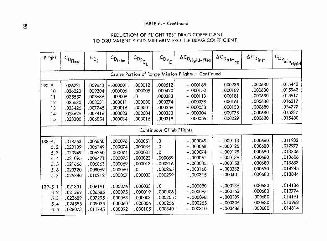
OoO

TABLE 6.- Continued

REDUCTION OF FLIGHT TEST DRAG COEFFICIENT

TO EQUIVALENT RIGID MINIMUM PROFILE DRAG COEFFICIENT

FIight CDflex CD i CDtrlmCDPcL CDPc ACDrlgid- flex ACDtrimcg A CDins t

CDPminrigid

190-910

11

121314

15

Cruise Portion of Range Mission Fllghts.- Continued

•026221

•026220

.025557•025530•023426

•023625.023300

•009643

.009204•008636

•008231.OO7745

•007416.006854

-.000001.000006

•000009

•000011•000016•000023

•000034

.000012•000005

.0

.000000

.000001•000004

.000016

.000512 -.000168

•000420 -.000152•000383 -.000113

•000374 -.000078

•000358 -•000033•000338 -.000004.000319 .000055

.000235•000189•000181

•000161

•000133•OOO078•000029

•000680

.000680•000680

•000680.000680

•000680.000680

•015442•015942

.015917•016317

•014727•015237

•015480

Continuous Climb FIights

138-55

55

5

55

139-5.1

5.2

5.35.4

5.5

.1 •018753

.2 •020109

.3 .020949

.4 •021095

.5 021666

.6 .023720

.7 •025840

•021331

•021389.022689

.024585

•028073

.005850•006149

•006260

.006471•006863

•008069

•010212

•006191.006585

•007295

.009025

.011745

•000076•000074

.000074

.000075

.000069

•000060.000057

•000076

•000075.000068

.000060

.000092

•000051

•000035

•000031.000023

•000013

.0•000033

.000033

.000019•000003

.000006

•000105

.0

.0.0

•000039.000216

.000265

•000299

.0•000006

.000205

.000256•000340

-•000049-•000068

-•000074-.000061

-.000035

-.000168-•000315

-.000080

-.000097

-.000098-.000265

-•000310

-.000113

-.000125-.000129

-.000139-.000158

-.000232

-.000401

-•000135-.000153

-.000189-•000305

-•000486

.000680•000680

•000680.000680

.000680

.000680•000680

•000680

•000680•000680

•000680

.000680

.011933

•012977•013706

•013606•013633

.014245

.013844

•014136•013774

•014151

•013988.014314

TABLE6•- Continued

REDUCTIONOF FLIGHTTESTDRAGCOEFFICIENTTO EQUIVALENTRIGID MINIMUM PROFILEDRAGCOEFFICIENT

Flight CDflex CDi CDtrim CDPcL CDpCAC

ACDrlgid-flex! Dtrlmcg ACDinst CDPminrigld

140-5.15.25.35.45.55.65.7

ContinuousCIimbFIights.- Continued

.029543

.032675

•022098.021802.022654.024210.027029

•029591.030380

.013682.015196

.005853

.006261

.006614

.007771

.009933•012166

•013663

•000166

.000243

•000076.000075

.000074•000065

.000061

.000113

.000173

.000234

.000352

•000051

.000030•000019

.0.000024

.000132

.000234

.OOO413

.000457

.0.0 _

•000097.000244

.000270•000319

.000387

-.000101

•000211

-.000048

-.000072-.000048

-.000137-.000307

-.000256-.000073

-.000560-•000646

-.000114-.000134

-•000151-.000221

-.000395-•000530

-•000599

.000680

.000680

.000680

.000680

.000680

.000680•000680

•000680.000680

•013707.015312

• 015275• 014554

.014972

.015093.015358

.015394

.014571

co

TABLE 7

FLIGHT TEST DRAG COEFFICIENTS CORRECTED TO

CONSTANT MACH NUMBERS AND TORN = 55x106/MAC AND C.G. = .25 MAC

Explanation of Items for Table 7

Item Explanation

(1)

(2)

(3)

C4)

(5)

C6)

(7)

(8)

(9)

(lo)

FIight number

Airplane trimmed lift coefficient, CLA

Flight test measured drag coefficient, CDfle x

Constant Mach Number to which data is being corrected,M

corr.

Incremental drag due to Mach Number, ACDM

Incremental drag due to Reynolds Number, ACDR N

Incremental trim drag due to c°g. position, ACDtrimc.g.

Incremental drag due to flexibility, _CDrigid_fle x

Incremental drag due to instrumentation, ACDins t

Rigid drag coefficientj corrected to a constant MachNumber, RN = 55x10°/MAC, and c.g. = .25 MAC,

CDrlgld

c.g. = .25 MACless inst

M -- McorrRN -- 55x 106/Ma c

82

_g00Z0"Z819ZO"

8898Z0"

[Z9ZZO"

869S'80"

98ZgZO"

86S'0Z0"

88Z6[0"

88Z6[0"

g_z8[o"

g[08[O"68Z6[0"

8VLSLO"

ZS'_Z[O'

Z9[OZO"

[ZSgZO"

Z086[0"

[698[0"

Zt88[O"

$_9gZ[O"

686Z[0"

ZS'OZ[O"0g6Z[0"0869[0"

(o[)

089000"089000"

089000'

089000"

089000"

089000"

089000"

089000'

089000"

089000"

089000"

089000"089000'

089000"

089000"

089000"089000"

089000"089000"089000"

089000"

089000'089000"

089000"

(6)

Zgi_ [00"Z[Z[O0"

/[L[O0"

88[000"-980[00"

Z80000"-

"Hz0000"-/_Z0000"

LZ0000"8[_000"

8[_000"

99S'000"

g9S'O00"

g9s'000"

6S'0000"-

S'[[000"-890000"

890000"90[000"

90[000"99[000"

99[000"[8_000'

[8_000"

(8)

9Z0000"-

8Z0000"-8Z0000"-

8Z0000"

0_8000'

S'9[000"

gs'0000"080000"

080000"

Z_0000"Z_O000"

8_0000"

8_0000"8_0000"

8170000"

90_000"_80000"

_80000"8Z0000"

8Z0000"[_0000'

[_0000"g[0000"

g[0000"

(Z)

90[000"

ZZ[O00"

ZZ[O00"

S'8_000'-

0S'g000"-_S'8000"-

Z80000"-690000"

690000"

6_000"6_000"

898000"

898000"

g98000"

S'[[O00"

Z[[O00"-

_8000"Z_8000"

[ZS'O00"[ZS'O00"_t9000"

_[9000"889000"

889000"

(9)

[ [0800"-

6Z8000"619[00"-

,

0"

0"

0"gggo00"

O"

[88000"6Z[000"-

[g0[00"860000"-

[66000"-

.

O"

9 [9000"

O"

8S'ZO00"

O"

6S'ZO00"

Z6[000'-

0817000"

OZgO00'-

g/.z"

0[8"008"

009"

009"009"

009"00Z"

009"

00Z"009"

0gZ"00Z"

009"

009"

009"

00Z"009"00Z"

009"00Z"

009"00Z"

009"

(s')

6888Lz0"988s'80"

gZZ9;_0"S'gZ [Z0"

Z8/_.6[0"ZSZ6 [0"

00iz8 [ 0"

00#8 [0"Z908 [0"

Z908 [0"Z9081.0"

S'SZOZ0"gLg9Z0'

6S'68[0"6S'68t0"

0S'9Z[0"0S'9L[0"O_[Z[O"

O_LZ[O"

69_Z[0"69ZZ[O"

(8)

L_Z'&"g [L'_"g LL_,"

66_"

Z889"

9ZZg"

LLS8"

ELLS"

ZLLS"

LL9Z"

LL9Z"

8ZZZ"

8Z_"

8_"

S';_Z8"8L_g"

8008"8008"

908;_"90gZ"8L_L_'

8_L_"

[96 ["[96 ["

(z)

;_'Z['Z

L'Z-6[[

©g.-Ig]g

ag

DgDg

8g

88Vg

Vg'qg-90 [

OS'

IS'as,as'

DS'DS'

8S'

8S'

VS'

'qs'-90 [

([)

03

D'V%'VgZ" = "O "D GNV DVW/9OtXgg = NM

OJ. aNY S_138WnN HDVW INVZSNOD O1 C]:IID]_EIOD SIN:IIDI:I:I]OD OV_I(] IS:11 1.HO1I:1

pgnu!-lU°D -'L ]'1871

Z8[_;50"

[06;5;50";5969;50"

898;5;50"CIz[[;50"

gOL8;50"

gLOW;50"6_8;5;50'

6Z8;580"[60L;50"699;5;50"

09_8;50"

_6;5£8;50"6980;50"09g0;50"

9L86[0"

go[6[O"_098[0"

8g_£.,;50"Zg80;50"

8ZL6LO"8[9g;50"

Z608;50"

g;5[0;50"ZOgg;50"

_008;50"

(o[)

089000"089000'

089000"089000"

089000"

089000"089000"

089000"089000"

089000'089000"

089000"089000"089000"

089000"089000"

089000"

089000"089000'

089000"089000"

089000"089000"

089000"089000"089000"

(6)

9_0000"-

9_0000"-860000"860000"

860000'

Z60000"

/.60000'Z60000"

g;5;5000"g;5;5000"

g;5;5000"

g8LOOO'-

gSLOOO'-gooooo'-gooooo'-

8Z;5000"

8L;5000"8Z;5000"

0_9000"0_9000"

0_9000"[0;5 [00"

[0;5 [00"[0;5 [00"Zg;5[00"Lg_ [00"

(8)

9£.,£.,000"-

9£.,£.,000"-

8Z;5000"-8Z;5000"-

8Z;5000"-[9_000"-

[9;5000"-[9;5000"-

8;5_000"-8;5;5000"-

8;5;5000'-

Z;5#OOO'-Z;5#OOO'-8g[ooo'-

8g[000"-660000"-

660000"-

660000"-880000"-£.,80000"-

880000"-

8ZOOOO'-

8ZOOOO'-

8ZOO00" -9ZOO00" -9ZOO00" -

(Z)

09gOOO'-09g000"-

8;5_000"-

8;sgOOO'-8;sgooo'-

9[gooo'-9[gOOO'-

9[g000"-06_000"-

06_000"-06_000"-

088000"-

08£.,000"-

Z8[OOO'-

Z8[OOO'-

[ZOOOO'-

[ZOO00._

[ZO000"-

6_0000"6_0000"6_0000"

;560000"

;560000';560000"90[000"90[000"

(9)

[g6000"

g8;5000"-880#00"

[[gO00"-98Z[00'-

6;56800"

[OZOOO'-Z;56[OO'-

Z[OZO0"6;5Z[00"

80Z;500"-

99[000"

O"

Z[;5000"

£.,60000"-

[g9000"

0;5[000"-

[;59000"-

_69800"86_000"

989000"-060_00"

gzg[o0"868[00"-

;5"Hz;500"[90000'-

gZZ"

ogz"008"

gzz"

ogz"008"

gzz"

ogz"0[8"008"

gLL"

OOZ"009"

OOZ"009"OgZ"

OOZ"

009"008"

gZZ"OgZ"

0[8"008"

gLL"0[8"008"

808K_0"

808iz;50"9g;5#;50"

9g;51:";50"9g;5_ZO"

9£.,[9;50"

9£.,[9;50"9£.,[9;50"

g899;50"_'£899;50"

g£_,g9;50"

9[6#;50"

916#;50"

889[Z0"

£.,89[;50"

Z6Z6[O"

Z6Z6[O"

Z6Z6[O"

_866[0"

_866[0"_866[0"8860;50"

8860;50"8860;50"8g_;5;50"

8g_;5;50"

(8)

680#"

680#"

680#"

80[#"

80[#"

80[#";5;50#"

;5;50#"

_LL_"

_LZ_"Z6L8"Z6LS"

00£.'£."00£.,£."

00£.,£."068;5"

068;5"068;5"

LgL;5"ZgL_"

LgL;5"Z;sL_"Z;sL;5"

(;5)

lz'8

17"8£.,'8£.,'8

£.,'8

i_'8

;5"8;5'8

['8['8

['8-6[ [

Z'Z

Z'Z9"Z

9"Zg'z

g'zg'z

_'Z_'Z

_'Z8"Z

8"Z8"Z;5"Z;5" Z-6[ [

([)

D'CW g;5" = "O'D CINV D'CW/90[xgg = NI_

OJ. aNY S_]£WnN HDVW J.N'CJ.SNOD OJ. a]J.D]_I_IOD SINqlDI:I:I]OD ov_la J.S3J. J.HOII:I

penu!.l.U°D -'Z ]1_]_1

ZLLZLO"178178tO"LS/_ZLOo

68_6 tO"ZOL8LO •

88;_Z[0"88Z8 tO"

tPgL LO'89_8_0'

8980_0"

g;5[6[0"[;_g;_0"

"1z66;_0"8986 [0'

Z;_8ZtO"

09L9 [0 •Z;_06 [0"g [/_.Z[O"

8;_99 [ O"

8889_0"

9[89_0"8688Z0"689_0"

8gLZ_0"

(oD

089000"

089000"089000"089000'

089000"089000"

089000"089000'

089000"

089000"089000"

089000"089OOO"

089000"

089000"

98[000"0#_000'0#_000"

6S8000"680000'

688000"6Zg000"

6Zg000"088000'

088000'

088000 •968_00:

968_00"968_00"

888000"

9Z[000"-

98[000"-9S[O00"-ZttOOO'-

ZttOOO'-Z[[000"-

960000"-960000"-

0g0000"-

0g0000'-080000"-

8_0000"-8_0000"-

8_0000"-

680000"-

8ZZO00

#Z[O00_[000

8[00008[0000

8[0000"[Z[O00"

[Z[O00"6_000"

6_000"

6_000"888OOO"

888000"888000"

[917000"

o__

.

#OZO00"O'

g8Z[O0"

#S9000"LE_OOO'-O#Z[O0"

ZZO000"

6#6800"088000"

688000"-

Z_6000"O08[O0'-

LSIz_O0"-

9ZS000"

009" 9L08[0"00Z" Lg#SLO"009" Lg#SLO"

0gz" 6ZSZtO"00Z" 6ZSZ[0"

009" 6Z8Z[O"0gZ" g6gZ[0"

00Z" g6_Z[0"008" SLL6LO"

S/_Z" gLL6[O"

OSZ" glL6[O"OL8" 89_0"

008" 89_0"SZZ" 89_0'

00Z" Z_LZLO"089000"

089000"089000"089000"

089000"

089000"089000"

089000"089000"

(6)

888000"

#Zg000"#_g000"

_Zg000"

0Z0000"-0Z0000"-

990000"-990000"-

990000"-

(8)

680000"-Z00000"-

Z00000"-Z00000'-

#88000'-

P88000"-

898000"-

898000"-898000"-

(Z)

L9#000"

898000"898000"

89g000"

[gZ000"-tSZ000"-

889000"-88S000"-

88g000"-

(9)

06#000"-_9LLO0"

8_[000"-

S8_[00"-

Z#LO00"

00[000"-#0_[00"

g80000"-988000"-

(s)

009"0SZ"00Z"

009'

00Z"009"gZZ"

0gZ"00Z"

L_lL[O"8g#Z[O"8g_Z [0"

8g#Z [0"

0gz8_0"0gZ8;_0"

9881z_0'

9881z;_0"988"#_0"

(8)

#g6Z"989;_"

989;_"

8Z_;_"

086 ["086 L"

68LL"68Z["

68Z["

[6S ["t6g["

L6g["

989 ["989 L"_OSL"

_OSL"ZDSL"

89_S"

89_S"608#"

608#"608"_'"

:16(]6

(]6(]6

(]6(]6

_D6

I_D6_]6

I]6

I]6V6

V6V6-SZ [

;_'9

_'9['9L'9

[' 9-8Lr t

9"8

9'8

g'8g'8S'8-6l L

(L)

oo

DVW S_" = "O'D CINV D'CW/9OLXgg = N_

OJ. (]NV S_I:I_IWI'IN HDVW INVISNOD Ol CI91D]_I_IOD SIN:IIDI-I:IaOD OV'd(] IS:ll lHOll:l

ponubl'U°D -'L ]I_]Vi

_[[_0"

8_06_0"09_g_0'/__Z_[_O"

8Z9080'9Z#8_0"

8Z[[_0"

[_60_0"8990_0"66_0_0"

ZE86 [0"8#68[0"[888 [0"

_ZgS_0"#090_0"60#6[0"

0#[9_0"8698_0"

6[80_0"

_9gg_O"#Z[8_0"

(o[)

089000"

089000"

089000"089000'

089000"

089000"089000'

089000"

089000"089000"089000"089000"

089000"089000'089000"

089000"089000'

089000'089000"089000"

089000"

089000"

089000'089000"

(6)

Z88000"

88#000"88#000'

88#000"

088000'[90000"-

[90000"-9[0000"-

9[0000"-80[000"

80[000"0_#000"

0_#000"0_#000"LSg000"LSg000"Z8g000"

[88 [00"

[gS[O0"[gS[O0"

#8 [ZOO"#8[_00"

88_000"98[000"

(8)

gg_o00"-

_000"-

_000"-_000"-

80Z[00'-

zzg000"-

Ezg000"-66Z000"-66Z000"-

06[000'-06[000"-

g_[O00"-g_[O00"-g_[000"-8[[000"-

8[[000"-8[[000"-

0[[000"-0[[000"-

0[[000"-

#0[000"-#0[000"-

(z)L_

868000'-

1798OOO'-1798OOO'-

1798OOO'-

6[6000'-

Z[ZOOO'-

Z[ZO00"-

[68000"-

[68000"-

66#000"-

66#000"-

#88000"-

#88000"-#88000"-68_000"-

68_000'-68_000"-

00_000"-

00_000'-

00_000'-_9[000"-

89[000"-

(9)

0" 009"9_9000" 00Z"

(1,)

9Z9#_0"9668_0"

9668_0"9668_0"

86_080"9[08[0"

88Z8"

8998"8998"

8998"

gg6g"

988_"988#"

000#"

000_"g098"

g098"

g008"g00g"g008"[gZ_"

LgL_"

LHZ_"g6g_"g6g_"

g6gz"

68#E"68#_"

89

'v'9V9V9-8_ [

Hg

_log

.-Ig-Ig:::lg

38Clg

C]gclgDg

DgDg

8888

88VgVg-8_, L

(L)

DVW g_" = 'O'D (]NV DVW/90LXgg = N_I

O.L CINV S_]:ISWf'IN HD_X/ J.NVISNOD Ol (]3J.D]_I_IOD SIN:IIDI:I:F]OD OV'd(] .LS:IJ. J.HOrl:l

ponuHuoD -'Z ]78V1

oo

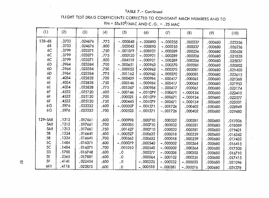
TABLE 7.- Continued

FLIGHT TEST DRAG COEFFICIENTS CORRECTED TO CONSTANT MACH NUMBERS AND TO

RN = 55x106/MAC AND C.G. = .25 MAC

oo

(1)

128-6B

6B6C

6C6C

6D6D

6D6E6E

6E6F

6F

6F6G

6G

129-5AR5AR

5AR

5B5B5C

5C

5D5E

5F

6R1

(2)

•3733•3733.3799

•3799•3799

.3964•3964

.3964•4034•4034

•4034

•4532•4532

•4532•5976

•5976

.1213•1213

•1213• 1324

• 1324• 1484

• 1484

• 1788•2565

.4141

.4118

(3)

.024676

.024676

•023371•023371

•023371•023384•023384

.023384•023828

•023828•023828

•025120

•025120• 0.25120•032232

•032232

•017661.017661

.017661•016641.016641

•016371

• 016371•016748

•017881•022454

•022873

(4)

.775

•800•750

.775

.800•700

.750

.775•700•750

•775•600

.700

.750

•600

•700

•600.700

•750•600•700

•600

•700• 600

• 600

• 600

•600

(5)

-•000848•003042

-•001079•000120•004119

-•000651-•000052

•001162-.000439

•000146•001367

-•000146•000021

.000445-.000007

•000523

-•000998

•000085

•001427-•000527

•000563

-. 00O079.001010

.0

.0

.0

.0

(6)

-.000893

-.000893-.000921

-.000921-.000921-.000963

-.000963-.000963-.000984

-.000984

-.000984

-.001079-,001079-.001079

-.001271-.001271

•000710•000710

.000710•000632•000632

•000540

.000540.000377

.000064

-.000323

-.000518

(7)

-.000255-.000255

-•000289-.000289-•000289

-.000370-.000370

-•000370-•000417

-.000417-.000417

-•000671-.000671

-.000671-.001726

-.001726

.000032

•000032•000032•000018

•000018-.000002

-.000002

-•000038-•000102

-•000332

-.000381

(8)

•000337

.000337•000236•000236

•000236•000081

.000081•000081•000061

•000061•000061

-•000134

-•000134-•000134

•000402.000402

•000281•000281.000281

•000259•000259

•000264.000264

.000303

•000251-•000023

-•000016

(9)

•000680•000680

•000680.000680•000680

•000680•000680

•000680•000680•000680

•000680

•000680.000680

•000680•000680

•000680

•000680

•000680•000680•000680

.000680•000680

•000680•000680

•000680

•000680

.000680

(10)

•022336

.026226•020638•021838

•025837•020802

•021400•022615•021368

•021953

•023174•022410

.022577•023001

•028949•029480

•017006•018089.019431

.016342•017432

.016415•017503

.016710

•017415•021096

•021278

TABLE8

INDICATORACCURACY

MeasuredParameter

Airspeed, knots

Altitude, feet

Pressure,PTO, inchesof H20

Pressure,PT2.5, inchesof H20

Pressure,PT7' inchesof H20

Temperature, TTO, degreesC

Temperature,TT2.5, degreesC

Temperature,TT7, degreesC

Root-sum-squareError

+ 1.8

+ 49.5

+ 0.28

+ 0.65

+ 0.65

+ 1.1m

+ 2.2

+ 2.2

88

TABLE 9

THRUSTINFLUENCECOEFFICIENTSa

Flight Condition EngineParameter

hfeet M EPR M h TTO N1 FPR

LockheedCalculation Method

20, 000

30,000

40, 000

0.6.7.8.6•7.8.6•7.8

1.541.581.561.481.471•501.431.441•47

O•240• 350

•420

• 235.328•428• 242

.334• 445

0o 830• 840

• 840

1.3501.3601.3501.890

1.9001• 890

0

0

0

0

0

0

0

0

0

0.832.837

•797•777•759

•690•727•694

•709

P&WA Calculation Method

20, 000 0.6.7o8

30, 000 .6.7

.8

40, 000 .6.7.8

1.62

1.63

1.651.551.53

1.571.54

1.571.58

0.243

• 359.405

.237• 348

.430• 243

• 360.422

0. 842

• 837•850

1.35O1.340

1•3401. 890

1. 880

1. 900

0.409• 638

• 747

.291•347

.414• 081

.103•395

1.2901.435

1.4691. 202

1. 2501o273

1.1311• 156

1.266

aAII values are + percent change in net thrust- percent change in parameter

89

TABLE10

TOTALRANDOM ERRORSDUETO INSTRUMENTATIONINACCURACYAND READABILITY

Fllght Condition EngineParameter

h Nfeet M EPR M h TTO 1 FPR

20,000 0.6 a0.165 0.592 0.260 0.552 1.0

30,000

40,000

.7

.8

.6

.7.8.6.7.8

•154•140.246.227•207.390.358.332

•539•493•618•565•515•655•577•538

•260•260.173.173.173.130.130.130

•552 1. 025•531 1. 005•595 1.012•595 1.012•574 0. 990•650 1.028•617 1. 005.617 1.030

0.5.5.5.5.5.5.5.5.5

aAII valuesare + (percenterror in parameter).

TABLE11

TOTALTHRUSTERRORDUETO INSTRUMENTATIONINACCURACYAND READABILITY

Flight Condition ( + ) PercentError in Thrust

h Lockheed P&WAfeet M Method Method

20,000

30,000

40,000

0.6.7.8.6.7.8.6•7.8

0.551.564•545.600•588•565.726.695.667

0. 8541.0451.120

0•818•853• 885

• 880.875

• 977

9O

TABLE12

TOTALESTIMATEDRANDOM ERRORANDMAXIMUM OVERALLERRORFOR

THREETYPICALFLIGHTCONDITIONS

Flight Conditions

Weight, lb.Air. feetM

CL

CD

ErrorsDueto InstrumentationInaccuracies

Weight, lb.Thrust, random,lb.

Thrust, _verall, lb.q, Ib/ftM

Angle of attack, deg.

Rate of climb, ft/min b

Random error in C D

Overall maximum error in C D

(1) (2) (3)

181,500 299, 00030, 000

0.80.2

O. 0214

3 0, 0000.775

0.35

0.0225

300128490

2.560.0036

0.3

8.0

a180

1305OO

2.610.0036

0.3

8.0

a0.000455 0.00031

0.00074a0.00074

300, 00030,000

0.650.5

O. 0270

300113420

2.04

O. 0036

0.3

8.0

0.00084

0.00115

aAII values are (+).

bError under level flight conditions.

91

',O

Figure 1.- Test article, C-141A Starlifter.

I0 FI 4 IN.

ED

@

-51 FT4FT

FUSELAGE REFERENCE

LINE IWL 200.0}

STATIC GROUND LINE (WL 96.0)_ j

]59FT II IN.

_'_ -- -I. 195 ° DIHEDRAL

/ [ (OUTBD OF BL 404.6)

I I -o.%°_,_o_?_D4o__8FT_ || . )

7FT51N._ / Id

, w t_,_ L f_r_.-4-:-i _V'Fr9 IN. b--/--38 FT 4IN.--

Figure 2.- C-141A general arrangement.

93

aTL

aFRL

V

Y

Horizontal

:N sin (aFR L + aTL)

FN cos (aFR LD

!

V

W cosy W

W siny

L'taiILta i l

V

V'

L'tail

= relative wind

= relative wind at the tail

= that amount of tail lift required to balance the

aircraft pitching moment.

Ltail tan¢ -- drag component of tail lift along the drag axis.

LtaiI tan¢

Figure 3.- Sketch of C-141A lift and drag vectors.

CD

Shockdrag & possible

separation drag, CDpc

Basictrimmedflight test / 1

polar _ ] Induceddrag(ellipticvortex + non-eFliptic

vortex), CDi

__' Trim draglncompress_b_ ' CDtrim

Vortex, friction, lift

dependent profile drag, CDPcL

Minimum profile drag,

CDPmi n

(skin friction, inter-

ference, pressure, flight

test instrumentation,surface roughness)I

C L

Figure 4.- Breakdown of typical subsonic jet aircraft drag polar.

95

Aa, Deg.

-2.0

-I .0 LLEE1iz_J L

0

!iF!_KF

_-- +-_+-_ --+-=+=-t--

.2

M=0.7

I:ilC L- = 0 25 --Y_7--FI-:_ _'-7

2 1-pl--,-i ,-i-__/_i -_Z _--q, ,/f! _I__,__7-__: I-

.4 .6 .8 1.01/

Figure 5.- Effect of aeroelasticity on wing twist.

c ic

Ca vg

.6

.4

.2

0

0

. _-.q._.

_ +

,41

J__L

___+_.._.+__

i i

I I

r i

96

Rigid Tail-on Tail-off

",o-.q

C L

Constant_le of attac-_ I

FRLrigid

C LFlexible

(Airplane trimmed ,,_

lift coefficien_ "

//II

1

IaFRLflex

/

_/Xexible /

//--Ae o__tt_cV-!

_ = ' " -1

I

Cmtai Iflex

Angle of attack, a FRL Pitching moment, C m

(a) Pitching moment and llft curve.

Figure 7.- Sketch of C-141A trim conditions.

Rigid

ICm "1

ta_ rigid

",OOo

Tail-off Tail-on

C

LA-hrig l

CD.

_trim

"-CL A hfle x

\(b) Drag polar.

/

CLA7(Airplane trimmed lift coefficient)

Figure 7.- Continued

COu

<((__

ii

2

Ea8_

O

CO

E

Ideal total/

J

b

c /

0

1.0

Actual total (vs. PTM/PAM)

Actual PA (vs. PTEX/PAM)

j Ideal PA

Critical PR PTE PTEX PTM

Nozzle pressure ratio, PT/PAM

Figure 8.- Nozzle gross thrust parameter

99

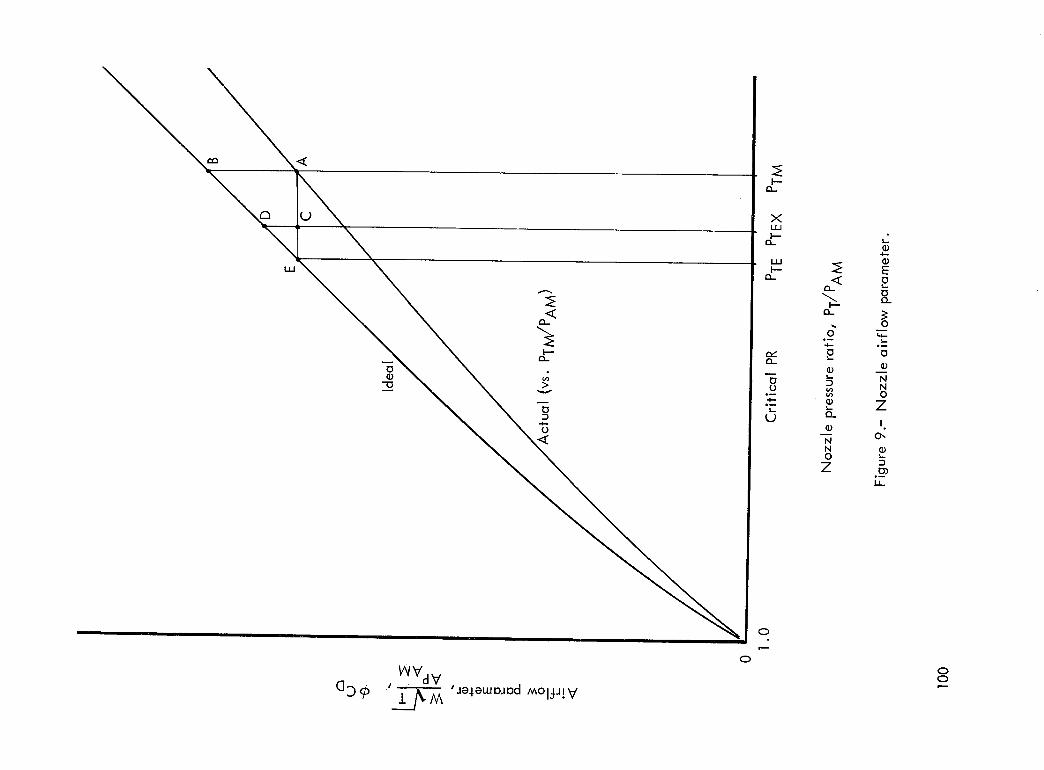
WVdVGD¢ "_M 'Je4ewDJodMOljj!V

I.--

Xu..II.--

I..uI.-.-

e,

r,

Uom.41.-.i

u

I--.

,R.i

a_

NN0

Z

L..IlJ

Ii..

Ep8_

0

Q_0

NN0

Z

Io

@.

.__

00

'S-l.Ua!O!JJao:) OlZZOU uoj alO:)s 01./I. -'0[ °Jn6!:l

o

FI-

b_J l

J

_L

[

I-_L

J

!

i-

-b-

J !

: i

!_,

li

"V'I_i ' ' I

I I I I

I IIt i

! _-!-I

±___

_[_i I-I---i

-L.l _ i

J

il !F--

I ii I

0"8

08'

_8"

88"

_6"

96"

00" I.

8-i

oNN

O

IO

mO

oO

0

<

I---

o_

I11

o

o

NN0c

>_

Ee_

&

o...

(...o

o_

oOm

0u

NN0C

oE

o

O-

t"-

u

0

!

o

.__IJ_

0 _0 ¢_1 oo0 0,, 0", oo

0

oo

s4ue!_!jjeo_ elZZOU Xaow!ad

102

oo

0 0 0 0

WI d

_dV ' WVdgl d _ WVd/'W-L d

103

iii_- <_

r_ r_

I--

<(

½I---

r_

•O3

.O2

.01

IL I CA:lO0

01.0 1.4 1.8 2.2 2.6 3.0 3.4

Fan nozzle pressure ratio, PTEx/PAM.

Figure 13.- Effect of area coefficient on duct pressure loss.

-I#<_

_xuJ

a-

I

<_a_

½

<[

.O3

.O2

.01

1.0 1.4 1.8 2.2 2.6 3.0 3.4

Fan nozzle pressure ratio, PTEX/PAM.

Figure 14.- 1/10 scale fan nozzle pressure loss.

104

<u

Ic

Om

u

11)0(J

<

1.00!]!

ii i

.95 :: :

_-v78511_ ". I Ill

1.0 1.4 1.8 2.2 2.6

Fan nozzle pressure ratio, PTE×/PAM

Figure 15.- 1/10 scale and full scale fan nozzle area coefficlenf.

3.0 3 o4

>u

.,,..-

o_

uOm

0

>..4--

o_

u0

1.0Or!!i i

i i

i i

.95 : ,.

!!!i i i

I I I

I I I

.90i!!:III,IlYI I/IIs1 I'. '. 1

.85 Jii

1.0 1.4 1.8 2.2

II I I I I I I I III I I I II I IIII lilt

lllllllllllllllI I I III I II II I I illllll -

I _ i IIII III lllllllllllllllJl llllIlll IIII III i Iil I I I I I I III I I III I I I III I III I III I I IIIIIIIIIIII llllllllllllilll

I I IIII IIIII IIII I I II}I Jill I iiiii I IIIIII

IIIII IIIIIIIIIII IIill lllllllllII ,I,,,,IIIIIIII IIII I IIIIIIIitllII IIIII IIIII It11111111 I

IIIIIIIIIIIIIIIII lllllllll I IIII I IIIII IIIiIllllll ,IIIIIIIIIIIIIIIII

IIIIIIII

2.6 3.0 3.4

Fan nozzle pressure ratio, PTEx/PAM.

Figure 16.- 1/10 scale fan nozzle velocity coefficient.

105

• 020

.015

_" 010, --_ •

_- .005CL

01.0 1.4 1.8 2,2 2.6 3.0

Primary nozzle pressure ratio, PTF_X/PAM.

Figure 17.- 1/10 scale primary nozzle pressure loss.

3.4

<(L)

¢-o

o_

oa_

oOo

13

1.00

.95

• 9O

/t

Ill Ill ItilI/Llll/

1.4 1.8 2•2 2.6 3.0 3.4

Primary nozzle pressure ratio, PTEX/PAM.

Figure 18.- 1/i0 scale and full scale primary nozzle area coefficient•

106

I

cO0 0

0

_xI---

o_

-I.,-

NN0c

_..

I.L

NNOe-

C

U

L.I-

I

d

e_

WI d X::I ld,/W ld

1dr ' WVd/X_,d _ WVd_±d

107

>u

•04

.02

01.0

I I I I I I I I I I I I I I I I I I I I I

"T'l'1--q,-4 -LI I ]__ . _: : . .... _ _ _ L J

I

1.4 1.8 2.2 2.6 3.0 3.4

Fan nozzle pressure ratio, PTEX/PAM.

Figure 20.- Velocity coefficient difference between

1/10 scale and full scale fan nozzle•

>u

.m

(JOm

0u

xu0

1.00

.95

20,000

40,000

•90 50,000

.85

I .0 I .4 I .8 2.2 2.6 3.0 3.4

Fan nozzle pressure ratio, PTEX/PAM.

Figure 21 .- Full scale fan nozzle velocity coefficient.

108

<_

W

I

<_

I--

.041_

!| i

I I

• 03, _Ei

I I

iJ

I I

N .02 _-:::

.01!!

i i: ;

0 ii

1.0 1.4 1.8 2.2 2.6

'III!!!!

I I I ',

!iii!!!!!1!!

iiiiliii!!!1JiliIIIIIIIIItit

'iI

!.

,,,'[I-'Ii!!!lJJJ

3.0

Primary nozzle pressure ratio, PTEX/PAM.

Figure 22.- Full scale primary nozzle pressure loss.

I

IIIII I

I

I-

I

I

I

I

J

I-

I

I

I

I

+--

I

3.4

U

Eo

o_o_:D

VI

1.00

.95

.90

7iIIII

.85 ii

1.0

._i II 14-.

i: ol 17: : '_I I I

ii !!iii

i i

J J .011J_; i!!ii

,,, t!!l!

:: !!!!!

'"i i

I I L,4 I: : III[

Jl J'll

II 7 !!'III I ....

IIIII

1.4

I III

I!II

III!I/

7777777 7-17_7_I I_-I- 17_-1_F 1_7-I ! I I I _ ! ! L.,__ I I I I I I I Itl IIIIIIIIIII

-'rl'-I I b4,,'_l_k"T J,_l"-I t II IJ,..,,r-I I J."T I.,fl I I I I

•,¢"drl I I_"_11JI I I I I I I I I 11 I I I I I I II I I I.,,,'r I I_1 I III II I_ i I I/I I I I I I I I I I I I I I I I I IIA I I I,VI I I J I I I I

_t I I I I/I I I I I II_ I I I III I I I I I I I

_ I I I I III I I I I I I I I I II I III_I III II I I I III I i I I I I I I I I II IIIIIIIIII IIIIIIIIIIIIIIIIIIVIIIIIIlIIII LI I ILl I III I I I II I I III I III I I I I I I I I I I I II I¥1 I I I I I I III I JI I_1 I I I I I I I I t I I I I I I I I I I I I I I I I I

I_PiT/P;25 = 6_1 / • "

/1111111111 It1111111 IItlIIIIIIIIIIIIIIIIII I

I I III t Ill'Ill, kllIIIIIIItPIltt1,,, •

IIII :

1.8 2.2 2.6

!!!!I I I Ii I I I

!!!!

iiii_

I ! I I

ilii

!!ii

JiiiJJJJ

3.0 3.4

Primary nozzle pressure ratio, PT7/PAM.

Figure 23.- Full scale primary nozzle suppression factor.

109

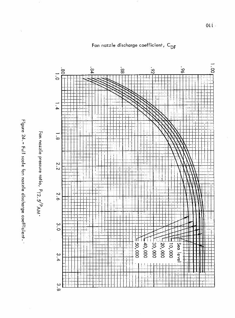
OLL.

Fan nozzle discharge coefficient, CDF

m--o

(.QC

I

mE

Q

b_

0NN

0-

0

Q

0('D

fl

"T1Q

0NN

E

a

0

"-u--IbO

>.

bO

bO

"CO

0

',00',,

0 00 00 0

O

CN

O

<

%CMF--

NN0t-

<-.

ii

r-

o--

0

e.-,,I--

o

NNO

i-

"5L.I_

!

4

4© D '.luato!jjeoo .Isnaul+ ssoJ6 elZZOU uo-I

111

oO

cO

0

oo

<

I--

ore

0

O_

0

NN0

Eo_

.41

co

Om

oo_

o0o

o

PIJc-u

e_

"lJ

NN0C

>,.

E6_

um

u..

I

,d

o_

LI_

dC]D '4ua!o!jjeoo eB.loLIos!p elZZOU XJmubl d

112

oo

co

oO

0

oo

<

I--

o_

I1)

I1;

NN0

>,..

0E

D-

i-

Om

uem

0u

,4--

£

NN0I"

E

u

ii

I

II)

t_

ii

d© D '4ue!o!jjeoo 4snaq4 ssoa6 alZZOU Xaotu!a d

113

0U

"Sii

D

E.Q

8_

I--

1.0 "_Full scale1/10 scale

1.8 2.0

Fan nozzle pressure ratio, PT2.5/PAM.

Figure 28.- 1/10 scale and full scale fan nozzle thrust parameter.

O

:E<_

I---

v

I

._1

14_

:E<_

I--

v

o

:E<_

I--

v

0.2111 t I I I I I i i i i t iIIIIIIII IIIIIIIIIIIIIIIII I IIIlllliIIllllllll IIIIIIIII IIII I I I

I liilli111llilil i _iII I I I I I I I II I I I I I I I I l.l._'r'lI IIIIIIIII _ IIII I I_.FI I I I I I I I.I I I I I I i I I i I I f iJ_,"TII I I I'I I I I I I I IJ,'1"lI I I I I I I I I ILI I I I I I I I I l.i,.'FlI I III I I I I I I I lJl'7 I I I I I I I II I I I I I I 1.1111 1 ! I I I I I III I I I I_I III I I I II I I I I_I I I I I I I I I I II i I JIFI I I I I II I_fl I I I I I I I_,,, llllilfillli,,,,,0

1.0 1.4 1.8

IIIIIIfl I I|1i IIIIIIll I' '"::_,_,,4_ 1_,,,,,_ _-,_ _,-

J._l_f't'-I I I I I i i I I I i , i I i I I

I I I i I I I I I i I i I I IIi ] r _1 IJ i i i-, I I i i i I I i I i i i I 1

III I I I I I U_ IIIlii_lllillilili

i lllt llIJlJl iIlil I IIIII I Illllilt, IIlllllliililil,, ,'"'

,,_ ill,,i,l,_,lll iiiilifllltlllllll ,I

2.2 2.6 3.0

ILf

3.4

Fan nozzle pressure ratio, PT2.5,/PAM.

Figure 29.- Extrapolation parameter from 1/10 scale to full scale fan nozzle.

114

..6

000

b_J

.<u

.<

%!

,4_

8

ce--

E

4,-,

D

u

l:Iu

25

2O

15

10

---_--+.--+I i +

Z

!Ii-_t-, 1

. Z !i i i

l I :

_---4---

[ [

___+___+_

----+---e-

l I

.---+_,__

I 1

---t-----i --

5 -'-''

II

0

I I

I I

-- -- ---t_t

I I

I ]

li- - V-i

..... __.

i..... lt-

i

I

...... __

.... T

--- --_---

/ iI

i :! I

--F

i i

' I5 15

!i-I

1-I

---4---

i-ZlZ

I

?iI

--b--

__+-.+++

---t--

il

+I

i

I---+_

t

I

I I

25

Measured engine gross thrust, (FG/_S AM)TEST' 1000 lb.

Figure 30.- Comparison of measured'and calculated total enginethrust based on engine test stand data.

115

6

OO

._J

U<(

v

O

.m

O3¢-

CJ

U

5

4

3

2

1

7--i

-f

-FI

q_

I7--"_m

I

--I---

JI

q_

I

--1--3

m

_m

5

Measured engine airflow, (W A)TEST , 100 Ib/sec.

Figure 31 .- Comparison of measured and calculated engine airflowbased on engine test stand data.

116

C D

•O4

• O3

Flight Altitude

7,300

15,000

25,000

35,500

11,500

20,000

30,500

40,500

7,300

20,000

Mach Number, M

(a) C D versus Mach Number

Figure 32.- Speed power flights.

rht No. Altitude

CL

7,30015,00025,00035,50011,50020,00030,50040,500

7,300

20,000

Mach Number, M

C L versus Mach Number

Figure 32.- Continued

(b)

118

.6

.4

ClC

cavg

.2

Rigid CLA_h

Flexible CLA_h

FI ight Conditions

Weight = 233,365 lb. MAir. 11,496 ft. RN

c.g. 18.55%MAC

• 1746

.1679

•7076= 78.96xl 06

• 1502

0 .2 .4 .6 .8fl

(a) Flight number 123-6.1.

Figure 33.- Rigid and flexible spanwise load distributions for five

selected speed power points.

1.0

ClC

cavg

6 I• I1I

•4 1IxJ

III

.2

I IIIII IIIII IIII

II1'"IIIIIIIIIIIIIIIkl I I 1.4--

Rigid C = 216Flexible _LA-h '

,_LA_h .210

Flight Conditions

Weight = 321,538 lb._AIt. = 7,497 ft.

_ C.go = 26•06°,_MAC

I I I I,,4d I -_ ....III/1111III/1tllI1,111 I1111tl I

III I111111 I

11111

['11111ItltlII11t

IIIIII

I I I I t I I 1111 I] 11177

M = 6736RN - 85.00xl06

CLA = .1961

0 .2 .4 .6 .8 1.0

(b) Flight number 106-4A.

Figure 33.- Continued•

119

ClCC

avg

.6

.4

FI ight Conditions

ht -- 289,326 lb. M

25,561 ft. RN

21.65%MAC CLA

.7107= 52.58xl 06

.3300

.2

0 .2

(c)

.4 .6r/

FI ight number 119-7.5.

Figure 33.- Continued.

.8 1.0

.6

.4

ClC

Cavg

.2

Flight Conditions --

Weight = 294,007 lb. M .7054AIt. 15,466 ft. RN = 69.34x106

c .g. 26.20%MAC CLA .2228

CLA_ h =. 2433

0 .2 .4 .677

(d) Flight number 106-5A.

Figure 33.- Continued.

.8 1.0

120

Rigid CLA_h = .5543Flexible CLA_h = .5500

FIight Conditions

Weight = 265,135 lb. M = .6737AIt. = 35,380 ft. RN =34.66xl06

c.g. = 20.20%MAC CLA = .5268

.8

.6

ClCCavg

.4

.2

0_2 .4 .6 .8 1.0

r/

(e) Flight number 119-8.6.

Figure 33.- Continued.

121

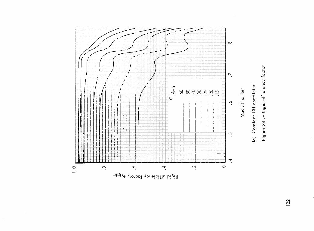
0 co -40

P!6!Jo 'Jo4.3DJ. X3uo!3Ujo pt6t_t

O4

03

"0

r,Zb

0

,,_Q

E

7._c

{J

c_

>,,,

e'-© (D

0

c_

0u

o_

LJ_

o,4o,4

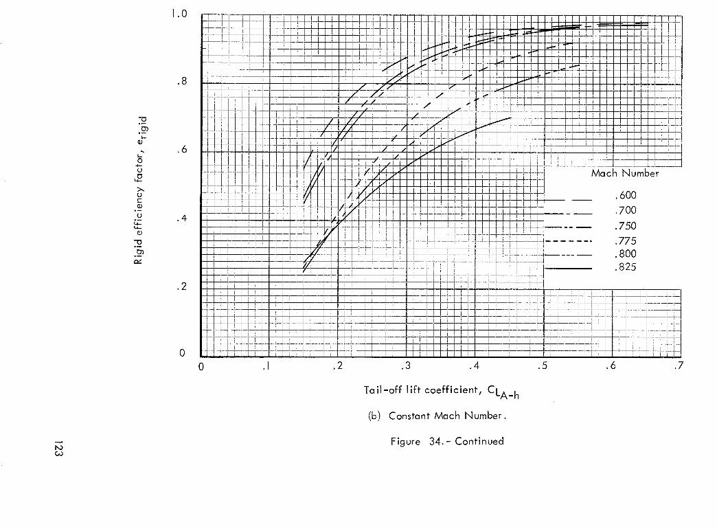
I',O

-Oo--

Ob°--

O

>,.L)c-(D

u

°--

o--

ev

1.0

•8

.6

.4

.2

0

0 .2 .3 .4

Taft-off lift coefficient, CLA_h

(b) Constant Mach Number•

Figure 34.- Continued

.5

Mach Number

•600

•700

.750

•775

• 800

• 825

.6 .7

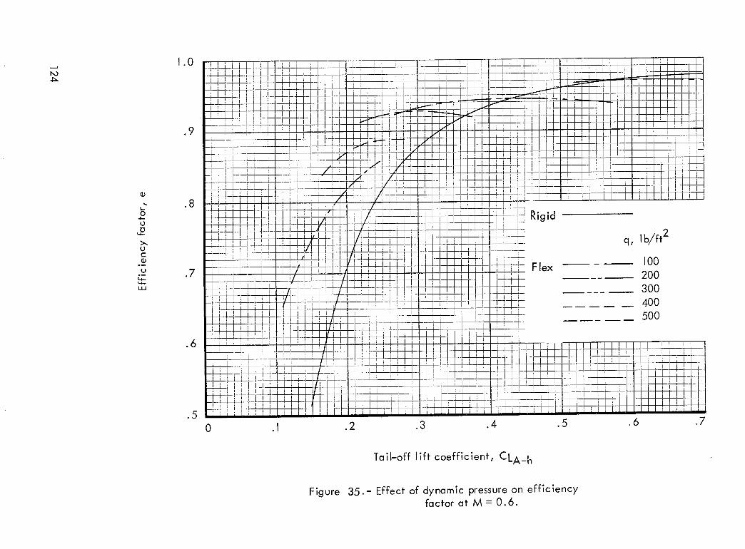
I,O

@

O

u

a>,,(J¢..(1)

°_

(3

1.0

.9

.6

.5

Flex

0 .1 .2 .3 .4 .5

I ]

!iibl,

q, Ib/ft 2

100

200

3OO

40O

50O

' _-F

i i _ /_

.6 .7

Tail-off lift coefficient, CLA_ h

Figure 35.- Effect of dynamic pressure on efficiencyfactor at M = 0.6.

S_L

panu!4u°z) -'98 eJn6!-I

_,. = _-v1_ (q)

W 'j_gwnN 4_°W

8" L"

i- F.... F-

I .... L

r-

hC

Y

'-r

]LT_

_ TI--_

- -T3 _ _-

I

b-- F k ..........L [ ................... --_--

°

-,*---I.... i"!-......

--T--

---I---

__-__ ....

--r-ii i ........7,1L

TL_:_-r

"4ua!m!JJa°a 4J!l 4ue4suo3 CD_o_oDj /oua!a!jja uo

_aflwn N HoDW pup aJnssaJd 3!wouXp jo ,toejj:l -'98

i i I

I I

_--

F-+_-- -

ill

17f-H- H4

i Ti-r

t-b!

i_- L-.i-.

I I ' '

_-<-I [..... F-I-

÷-.+-.

r+, -- r-l--

!

_!-_;LIL

a_n6!_

9" S" 17"

..... qLi

TT

_--I-I

-T_

II--_-1-LI

-P1i--I

, i

6!Il I

IIti

I I ---

_-q'-- 7

--[- .....

b___

-5-

LL_._

p$__ ,

14 -Lrrd-

°

,

0"1

,

°

0"1

m

_o

f'l

f_

8'

._cI

<(_.1

u

oOm

oom

o0o

m

O!

o_

I---

.7

.6

.5

.4

.3

.2

.1

c.g. = .18 MA(

.I .2 .3 .4 .5 .6

Airplane trimmed lift coefficient, CLA

Mach Number

0 - .750

•775

.81

.84

Figure 37.- Rigid tail--off lift coefficient variationwith trimmed lift coefficient and Mach

Number for c.g. - 0.18 MAC.

126

¢-

I

<_.__1

L.)

.4--,

(Dom

u.m

0

!--

.3 .4

L..............

i ......

!L--........

! .........

i

-----: _-e--+-- .....

I

II i _ i ---I .______+___ ....

I

2_- c.g. position-- .18 MAC

H__

m--m

11

.5

22 MAC

•26 MAC

I

.6

Airplane trimmed llft coefficient, CLA

Figure 38.- Effect of trim c.g. position ontail--off lift coefficient.

127

cO

J:L)

ii

"_ 4.0u

"--= D-

-- "aO

e_

o 2.0_-t.)

u c

o_-'0 u

8 0

c0

o.--

u_J

t.l.-

u_

2.0

1.0

0

-'1

i _,

d--t

.1 •2 .3

-_ : o.__Fuel = 22,000

_--__T_ -.... _1

12 _- 20(

__.4 •5

Tail-off lift coefficient, CLA_h.

(a) Reduction of CLA_h at M : 0.6 and low fuel.

Figure 39.- Effect of flexibility on tail-off lift coefficient.

:LI_.6

d-/

• 64 .68

_.J__

).... i

, _10,>

.6

.... d--t-Hd- i

• 72 .76 .80

Mach Number, M

(b) Mach Number effect on percent reduction•

01_

"8!-. ,_

i

F

.6 _-0

Figure 39.- Continued.

__d_, _-,-_.-

40 80 120

Fuel, 1000 lb.

4I

"_1 I L- -_ 2(

-I_ I60

.... Id--f

b/ft2_

OOffIITT_

)O-+_-

2OO

(c) Effect of fuel load on percent reduction.

Figure 39.- Continued.

128

O

I!D4e 'jo4oD j X_ue!o[jja I!D/

L I

I I

I :

--+---+-

---+----t-"

--+----_

I I

--F--+-

I :

I---q

--.+--_

[ :

Tr-!

--4_-+----

_----+----

_ L

I I

--+---+_

I "

0

0

0

-0

0

0

I

G0

0

0

0

O I

_..1U

E

°I

uom

t.l.-

0

,.l.-t.l--,I

I--.-

t,..

0

u

E¢)

Im

oJ_

E0N

o_

-rI

0

¢)

o_

LL

129

I--

O')(D

"O

C

CDEEl

._E

O

(.-

_orh

BI1}

"(3

<I

EDE13

....C

13

E

O-O

E

E(D

t-

O

E

3.0

2.0

1.0

0

.4

.2

O

-.2

-.4

i

I

1

1I

II

!

I

J.

ti-

T

1d-

+T

.I

q•

'_TI_I i I

I ,

.2

ttr

l-

T:]-,I

T.3

1

d I '

'¢

, - tl

-i It

.700

.74O

.... .775..... .810

•840

,,I.5.4 .6

Tail-off lift coefficient, CLA_h

Figure 41 .- Downwash angle at the tail for the rigid configuration.

q, Ib/ft 2, ..-.:

_ ' loo ......_÷ _,___f.L_,, _- ....200 j d-d -I_---t-t- -r

---T Tj-Tt___-_---300 ---.-I .... _...... 400 _J.... f __L_

.... J_.... _ _ ..... _:-_500 ....... _- dT__d_ ....

_- _ ....... _n-

.........!_2....... _ _-222E .......

2_7_ ..... -'dC- --i-r l H

.2 .3

- i 1--

--+-_

- ------ ..... -i ----

.4 .5 .6

Tail-off lift coefficient, CLA_h

Figure 42.- Effect of flexibility on the downwash angle.

130

0_J

XII)

I-I--

I

13}°_

L--

03e-

°--

Q_E3

u

-.0006

-. 0004

-.0O02

0

Figure

5OO

Dynamic pressure, q, Ib/ft 2

(a) Effect at low fuel.

43.- Wing profile drag increment due to aeroelastic distortion.

ii

DoL_

ii

1.0

--_---_-,--- _H-_

I I I

--4---+--4

_-_-_

TT_, : i

-_+--_---_-- --+--4 ....

--F-_--+ -- --_--4 4

-4--+--+--- --i -_P-_

0 , , , I I !

(b)

......-FF ___,.......,--+------ --t--._

...... I-- _-_

_, ........ T

--T--T- _

50

-, - _-:-L12_2_4---4--_ .....

2(Z

IO0 150

Fuel, 1000lb.

Relief factor due to fuel load.

Figure 43.- Continued

131

Angl'e of attack vanes

Bracket on top ofvertical tail 30%C

Line of vortex generators

Stall strip/

Conduit 1" dia.

6' long on rearbullet

Trailing conewith 36' cable

Spin chute installation

Skegs (on ramp door)

N ose

Boom\

Temperatureprobe (along

B.L.O)

\T.O.L. Camera

(along B.L.O)Additional items:

Water ballast drain holes

Closure plate on petal doorMicro switch on fuel drain mast

External straps

Figure 44.- Flight test instrumentation.

CD

• O4O

,. 035

.030

•025

•O2O

.015

Forwa rd

Limit°60

Aft

Limit

0 10 20 30 40 50

C.G., percent MAC

Figure 45.- Effect of center of gravity location on trimmed cruise

drag based on wind tunnel data.

133

.018

.016

CDp

.014

.012

.0104 6 8 10 20 30 40 50 :60 70

ReynoldsNumber, RN, x 10-6/M AC

Figure 46.- EstimatedC-141A profile drag variation with ReynoldsNumber.

80 90

•022

•020

FI ight

0 106-4

1 06-5

1-I 119-7

0 119-8

',0o .018

×

cO

"O IIo_

•_ Zr_

._ .016U

.014

.012

.010

.4 .5 .6 .7

Mach NumBer, M

(a) Flights 106-4, 106-5, 119-7, 119-8.

Figure 47.- Profile drag variation with Mach Number.

135

",00

×

oO

"-a H

._7__

_rm

u

•022

.020

.018

.016

.014

.012

.010.3 .4 .8

Mach Number, M

(b) Flights 123-6, 123-9, 128-5, 128-6, 129-5, and 129-6

Figure 47.- Continued

136

U

•024

.022

"4Oo .020

×Izb

d

-a II)_

.__ Z

" .018

.016

.014

.012

I , j '

.JLJ__L-_

I ! , , _

I f

-1-1- .....

__k__ __

-I _ L _-_LJ:L:F_,

.1 •2 .3 .5 .6

Tail-off lift coefficient, CLA_h

Figure 48.- Profile drag variation with lift coefficient at constant Mach Numbers.

137

(.ooo

.018

.016

CDPrigid

RN = 32.5x10 6

.014

.012

.010

I

i.6

Tall--off lift.coefficient, CLA_h

r

./

Figure 49.- Profile drag coefficient variation with tall off lift coefficient.

.018

.016

CDPminrigid

c.g. = .25 MACless inst

.014

.012

.0104

Mean curve based on

method of least squares

6 8 10 20 30 40 50 60 70 80 90

Reynolds Number, RN, x 10-6/MAC

(a) Speed power flights.

Figure 50.- Minimum profile drag coefficient variation with Reynolds Number"_O

07il jI _l

Ii ....

LLiI_H

i!I! '

J_ _

"ponut4u°3 -'Og eJn6!'l

•s4q6!l j uo!sqw e6uoJ .40 uo!4Jod as!nJ D (q)

DVW/9_0[ x 'N_I 'jeqLunN spl°uXe_d

og 017

(IbE,lL_t!, q:-_Ti-

Z! L: i L

2-lil -Jilillill

,_ __

ilil illlil_:!1111_

'N

Ot

06t

Z8 t

4q6!14

iqTF

I!ll

IIII

a.kI I I I

_,-----4-

ill;

0t0"

i_[0"

lzt0"

9tO"

8[0'

.lsu! sseI

D'_'W g_" = "6" 3

p!6!-tu,t.u• dcl D

O

e---

• panu!4u°D - "0g gjn6!-.I _.

06 08 0Z 09 0£:' 0"17

li !T

d

I

FI I

J_.

lq Lli '

__ +_I i

_TEiJm _-

j_'_

• s.rLI6!lj qw!lO snonuguoD (o)

DVW/9_0[ x 'N_I 'JaqwnN spl°uXa_l

0[0"

El'O"

#1'0"

+su! ssa 1

D'V'W _E" = "6"

910 •

8[0"

I,O

CDPminrigid

c,g, =

less inst

.018

.016

•25 MAC

.014

.012

.010

4

i,- <0

0

Flight

106-4

106-5

119-7

119-8123-6

123-9

128-5

128-6

129-5

129-6

6 8 10

Figure

Mean curve based on

method of least squares

40 50 60 70 80 90

Reynolds Number, RN, x 10-6/MAC

51 .- Minimum profile drag coefficient variation with Reynolds Number

after eliminating high C L test points and obvious wild scatter.

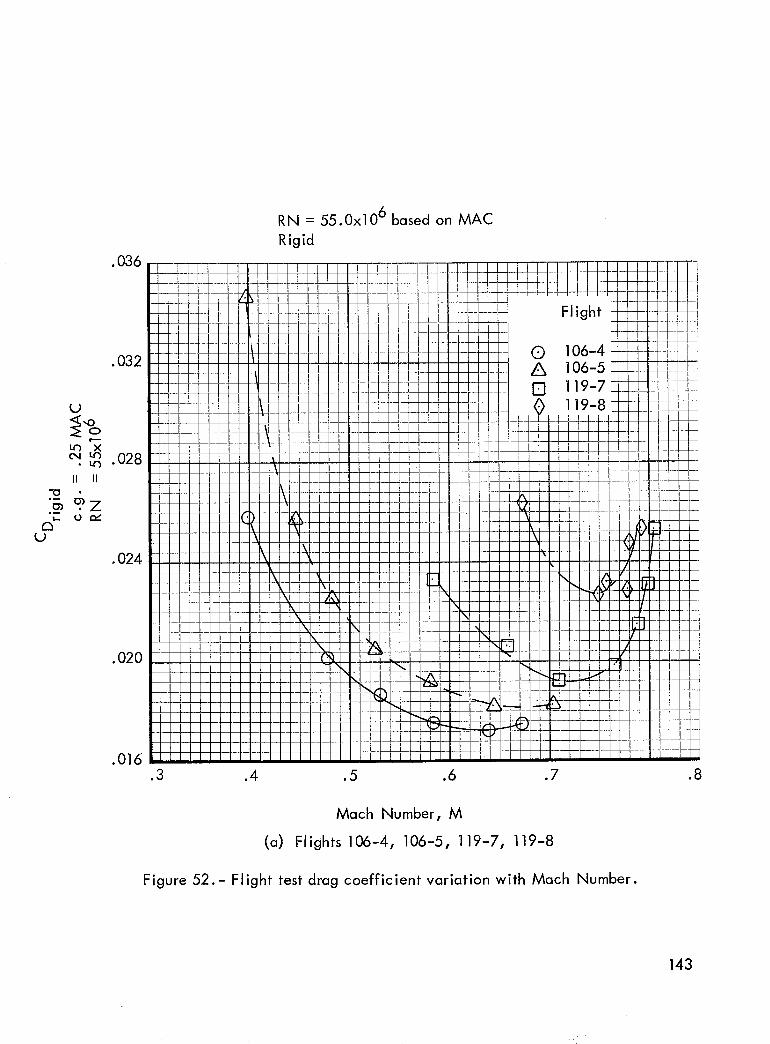
u

la")• tel

II II

.ZOm

¢_u

036

032

028

024

020

016

J

-i

I

m_

mm

m--

m--

m--

mm

m

--m

.3 .4

RN = 55.0x106 based on MAC

Rigid

.8

Mach Number, M

(a) Flights 106-4, 106-5, 119-7, 119-8

Figure 52.- Flight test drag coefficient variation with Mach Number.

143

"5,t_

U

.032

.O28

U,,o

;_ o .024X

14"b

II _ [I

.020

.016

.012

RN = 55.0x106 based on MAC

Rigid

t i

qq--4-:i

+

I

2

.N

.--+_.

--v---.

I

__+..-

I

-1

Mach Number, M

(b) Flights 123-6, 123-9, 128-5, 128-6, 129-5, 129-6

Figure 52.- Continued.

144

.7

RN = 55.0x106 based on MAC

Rigid

Mach Number

C L

.6

.5

.4

.3

.2

.1.016

•600

•700

• 750.775

• 800

•810--I

I

I

_J

ZL

/

HI

IY

i.020 .024 .028 .032 .036

CD

Figure 53.- Initial flight test results at constant Mach Numbers.

145

C

.7

.6

.5

,4

.3

.2

.1

0.016

j

-k-i

I

-k

J

T

4--

I_L_

I4-

m____

-k-

in

-C_ll

4-II I

.... RN..... Rigld

I

_=-- c.g.

i

v.-,

....

,I.020

= 55.0x106 based on MAC

•024 .032

--ram

f _--L

m

I

• 036

C D

(a) M = 0.600

Figure 54.- Flight test drag polars at constant Mach Numbers.

146

C

.7

.6

.5

.4

.3

.2

.1

0

RNRigidMc.g.

= 55.0x106 based on

= 0.700

•25 MAC

MAC

.016 .020 .024 .028 .032 .036

C D

(b) M = 0.700

Figure 54.- Continued.

147

CL

.6

.5

.4

.3

.2

.1

0.012

RN

RigidM

e.g.! .

I

1212_- ......I

J i

I

q-q .........

±L-

-4_ ......I I

I_--1 .......

I

-ti4--t-- --

-.-+_4 --

I'

I -4

i

.016

= 55.0x106 based on MAC

= 0.750

= .25 MAC

.020

Flight

•024

C D

(c) M = 0.750

F igure 54.- Continued•

.032

148

C

.6

.5

.4

.3

.2

.1

0.012

[] 119-7119-8123-9

IX, 128-5(_ 128-6

= 55.0x106 based on MAC

(d) M = 0.775

Figure 54.- Continued.

......... j

i

............ j

I........ 1

.............. i

I

I

......... I

............ J

i

•032

149

CL

.016

RNRigidMe.g.

= 55.0x106 based on MAC

C D

•024

(e) M = 0.800

Figure 54.- Continued.

•028 .032

150

.5

RNRigidMc.g.

= 55.0x106 based on MAC

= 0.810

= . 25 MAC

.4

CL

.3

.2

.1

0.016 .020 •024 .028

C D

(f) M = 0.810

Figure 54.- Continued.

.032 .036

151

CL

.7

.6

.5

.4

.3

.2

.1

0

RNRigid

e.g.

-- 55x106 based on MAC

= .25 MAC

.016

_.r

•020 .024 .028 .032C

D

•036

Figure 55.- Summary of flight test drag polars at RN = 55.0x106"

152

•036

CD

•032

.028

•O24

.020

.016

RN = 55.0x10-6 basedon MACRigidc.g. = .25MAC

CL

Mach Number, M

Figure 56.- Drag coefficient variation with Mach Numberfor constantlift coefficients at RN = 55x106.

153

C

.7

.6

.5

.4

.3

.2

.1

0•016 .020 .024

CD

Faired curve basedon speedpowerdata analysis, figure 54 (a)

J.III

III

.028 .032 .036

(a) M=0.6

Figure 57.- Continuous climb drag coefficient data corrected toconstant Mach Numbers at RN = 55x106/MAC.

154

.7

.6

.5

CL

.4

.3

.2

.1

Ic.g.= .25MAC

i

J l

•020

0

.016

(b) M = 0.7

Figure 57.- Continued.

155

9g?L

9{_0"

-H-

[--£_T_-__!_J_

!-?-I-

UZ

• panu!¢u°D -"Zg aJn6!-I

_L'O=W (_)

8_0" ?_0" 0_0"

W

p!6!_t

N_t

9[0"

0

["

t

,

,

3D

C L

.6

.5

.4

,3

.2

.1

_ RN

Rigid2M

Z c.g.

_J

.016

=0.7

: .25 MAC

I

C D

(a) M = 0.7

Figure 58.- Range mission cruise drag coefficient data corrected toconstant Mach Numbers at RN = 55x106/MAC.

J

L_

I--

!t:L

I-t_

r_I

i ....

I

.....

f.036

157

.6 = 55x106 basedon MAC

= 0.75•25 MAC

.5

CL

.4

.3

.2

.1

•016 .020 .024 .028 .032 .036CD

(b) M = O.75

Figure 58.- Continued.

158

C

.7

.6

.5

.4

.3

.2

.1

!

"4i i

L .__-

x i..... !

_1....... i

i

...... J

..... Zi

..... !

......... So id symbo Is _-Z-

........ indicate contin- ---

- uous climb data ....

i __ __ ±_ __

j .....

LL_ __-I --

2___ _1

...... --_ .... __

!-- --J

.o32•024

(a) M=0.6

Figure 59.- Drag polars for several Reynolds Numbers andat constant Mach Numbers.

k..... _qJ --__

F......

I--÷L...... -1-I

i t

! ---_-I Ii I

I

II

q__

I.... ---_-_

....k

--t-

I I

I.... +-._

I

I--

.036

159

CL

.7

.6

.5

.4

.3

.2

.1

I! :

L

I i Reynolds Number

O 80x 106/MAC

[] 55 x 106/MACA 30 x 106/MAC

ii1-

4_

-IL._-ki

t

k

-LIL.016 .020 • 024 .028

C D

(b) M = 0.7

Figure 59.- Continued.

• 032 .036

160

0017

LL.-I-I

00_'

• panu!4u°D -'09 aJnB!-I

•_ .o N o^Jn= uo!4oJCl!lOD (9)

s.lou_ 'paads.qo pa4o_!pu I

00_, 00_ O0L

4--+--t---t---f-

s4ou_ _ = slseJe4sXLI, wnwlx°w- I

• SaAJn:_ uo[4D.19[ IDa jo4oo[pu[ paadsJ!v -'09 aan6!-I

"l "ON OAJn:) uo!4oJq!loD (o)

0

__T _IlllllllIIItll

.s4ou> I 'paadsJ!o pa4oo!pu I

008 00_ 00 I. 0

i ii I l i i I

L-

0

L

o

o"--I--mO

O

O

I

(70 o

(%

_e

[ o

o

4O

c"O

Om,4--,

(J

O_3

100

0

-100

Maximum hystersis = 70 ft.

0 10 20 30 40

Indicated altitude, 1000 ft.

(a) Calibration curve No. 1.

Figure 6.- Altimeter calibration curves•

O

L_

Ou

1O0

0

-100

! aM35,OOO ft/ve shift = 35 ft.

I

0 10 20 30 40

Indicated altitude, 1000 ft.

(b) Calibration curve No. 2.

Figure 61 .- Continued.

U

<_

C_l I--

_5r_V

1.01

1.00

w

I

IIII

.9911II

I

III

II.98' '

1.0

III iL''''':ILl1iiii '"",,,,,I111111 IIII '"_'1I I I I II I I I II I IIII I I

I I I I II I I III I 1 Ill I II IIIII1_ _ _111 IIII I]• IIIIIIJ

I I I II_I _ I II I I I lIIIIIII {l Nil IIII

I I I I I I I '_ I I (._I I±I I I""'1 Ill IIIILt

"""l "i' 1LILt'i"il : !!, ll_t_I ,, IIIL '""!*'"l,,,, ,,,, IIIIILlllllt LIIIIIILlll

,1111 1, I

tl I , !!!IIIII1_ II

iiiillLTiiirrll iiii

1111 il ''"'11

"'lll.llll'"tllll

iii!!!111111t'IILIIIL LLiiLI 1111111

I[lllll

1 .2 1 .4 1 .6 1 .8 2.0 2.2

Engine pressure ratio, EPR.

Figure 62.- Comparison of measured and calculated fan

nozzle pressure ratio based on flight data.

163

O_

.018

.016

CDPmi n

.014

.012

.010

!!!! iLh!_

T'_-'- iliJ ii,IbJ, !!1! ;

q li

2i_ i,• " !T

ii

....... II

'i,I

J' li!!i ii]_,i11!!1i li

I_ ,

[Ltl

Statistical mean line

-_ Estimated overall maximum error at

approximate cruise conditions, + z_C D = .00074

Two-sigma deviation, 2a= +&CD = .00078

41i

H!!

Estimated profile drag variation

-.L_

-i ,,_ i I'1

i [1 ! II ii!l=-._-_i I l lill lq'_ _. Ilia

2LLL

--4--+-+-+- , , .--k--;-J-

il lili i

Reynolds Number, RN, x 10-6/MAC

Figure 63.- Comparison of predicted deviation and actual data scatter on

profile drag variation with Reynolds Number.

g9L

0

•

_

_

"ID

CL

.7

.6

.5

.4

.3

.2

.1

0

.016

Faired mean line

Estimated overall maximum error at

approximate cruise conditions, + ACI_

Two-sigma deviation, 2a = _+AC D =-.

•020 •024 .028

C D

(b) M = 0.7RN = 55x 106

Figure 64.- Continued.

= .00074

00070

•032 .036

166 NASA-Langley, 197o-- 2 CR-1558