19930011721.pdf - NASA Technical Reports Server

©

c_

c_©o0

o

©

I

NASA-CR-19Z619

DEPARTMENT OF ELECTRICAL & COMPUTER ENGINEERINGCOLLEGE OF ENGINEERING & TECHNOLOGYOLD DOMINION UNIVERSITY

NORFOLK, VIRGINIA 23529

By

Nicolas Alvertos, Principal Investigator

A NEW METHOD FOR RECOGNIZING QUADRIC SURFACESFROM RANGE DATA AND ITS APPLICATION TOTELEROBOTICS AND AUTOMATION

,,-" .j _? • •

,

t

Progress ReportFor the period ended February 28, 1993

Prepared forNational Aeronautics and Space AdministrationLangley Research Center

Hampton, Va 23681-0001

UnderResearch Grant NAG-l-1223

Plesent W. Goode IV, Technical Monitor

ISD-Automation Technology Branch

(AJASA-CR-192619) A NE_ METH09 FOR

-,CECOGNIZING _UA.qRIC SURFACES FROM

RANGE _ATA ANO ITS APPLICATION TO

TELER_3?,TICS ANO AUTOMATION

PFO,]FeSS Report, period ending 28F,_b. 199] (Old Donlinion Univ.)2_& F:

March 1993

G3133

N93-20910

Unclas

015i031

DEPARTMENT OF ELECTRICAL & COMPUTER ENGINEERING

COLLEGE OF ENGINEERING & TECHNOLOGY

OLD DOMINION UNIVERSITY

NORFOLK, VIRGINIA 23529

A NEW METHOD FOR RECOGNIZING QUADRIC SURFACESFROM RANGE DATA AND ITS APPLICATION TOTELEROBOTICS AND AUTOMATION

ay

Nicolas Alvertos, Principal Investigator

Progress ReportFor the period ended February 28, 1993

Prepared for

National Aeronautics and Space Administration

Langley Research Center

Hampton, Va 23681-0001

Under

Research Grant NAG-l-1223

Plesent W. Goode IV, Technical Monitor

ISD-Automation Technology Branch

March 1993

A New Method for Recognizing Quadric Surfaces from Range Data and

Its Application to Telerobotics and Automation

(phase II)

by

Nicolas Alvertos* and Ivan D'Cunha**

Abstract

The problem of recognizing and positioning of objects in three-dimensional space

is important for robotics and navigation applications. In recent years, digital range

data, also referred to as range images or depth maps, have been available for the

analysis of three-dimensional objects owing to the development of several active range

finding techniques. The distinct advantage of range images is the explicitness of the

surface information available. Many industrial and navigational robotics tasks will be

more easily accomplished if such explicit information can be efficiently interpreted.

In this research, a new technique based on analytic geometry for the recognition

and description of three-dimensional quadric surfaces from range images is pressented.

Beginning with the explicit representation of quadrics, a set of ten coefficients are

determined for various three-dimensional surfaces. For each quadric surface, a unique

set of two-dimensional curves which serve as a feature set is obtained from the various

angles at which the object is intersected with a plane. Based on a discriminant

method, each of the curves is classified as a parabola, circle, ellipse, hyperbola, or a

* Assistant Professor, Department of Electrical and Computer Engineering,

Old Dominion University, Norfolk, Virginia 23529-0246.

** Graduate Research Assistant, Department of Electrical and Computer Engineering,

Old Dominion University, Norfolk, Virginia 23529-0246.

line. Each quadric surface is shown to be uniquely characterized by a set of these

two-dimensional curves, thus allowing discrimination from the others.

Before the recognition process can be implemented, the range data have to

undergo a set of pre-processing operations, thereby making it more presentable to

classification algorithms. One such pre-processing step is to study the effect of median

filtering on raw range images. Utilizing a variety of surface curvature techniques, reli-

able sets of image data that approximate the shape of a quadric surface are determined.

Since the initial orientation of the surfaces is unknown, a new technique is developed

wherein all the rotation parameters are determined and subsequently eliminated. This

approach enables us to position the quadric surfaces in a desired coordinate system.

Experiments were conducted on raw range images of spheres, cylinders, and

cones. Experiments were also performed on simulated data for surfaces such as hyper-

boloids of one and two sheets, elliptical and hyperbolic paraboloids, elliptical and

hyperbolic cylinders, ellipsoids and the quadric cones. Both the real and simulated

data yielded excellent results. Our approach is found to be more accurate and compu-

tationally inexpensive as compared to traditional approaches, such as the three-

dimensional discriminant approach which involves evaluation of the rank of a matrix.

Finally, we have proposed one other new approach, which involves the formula-

tion of a mapping between the explicit and implicit forms of representing quadric sur-

faces. This approach, when fully realized, will yield a three-dimensional discriminant,

which will recognize quadric surfaces based upon their component surface patches.

This approach is faster than prior approaches and at the same time is invariant to pose

and orientation of the surfaces in three-dimensional space.

ii

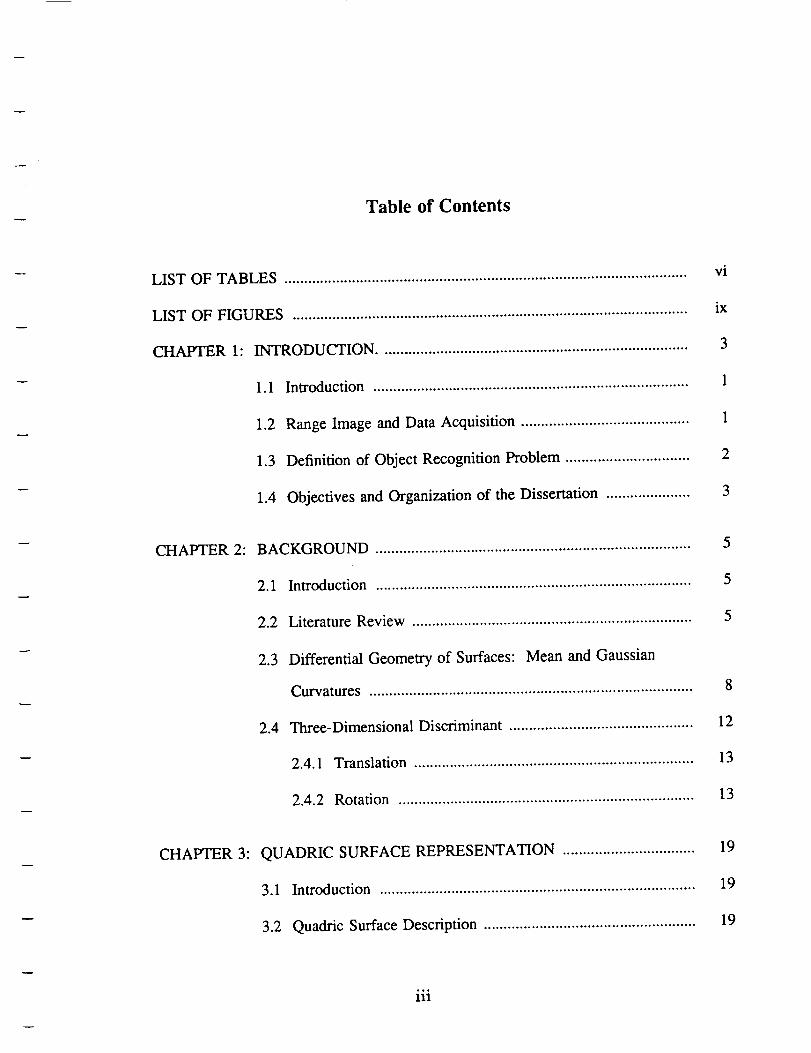
Table of Contents

LIST OF TABLES .....................................................................................................

LIST OF FIGURES ...................................................................................................

CHAPTER 1: INTRODUCTION .............................................................................

1.1 Introduction ...............................................................................

1.2 Range Image and Data Acquisition ..........................................

1.3 Definition of Object Recognition Problem ...............................

1.4 Objectives and Organization of the Dissertation .....................

vi

ix

3

1

1

2

3

CHAPTER 2: BACKGROUND ...............................................................................

2.1 Introduction ...............................................................................

2.2 Literature Review ......................................................................

2.3 Differential Geometry of Surfaces: Mean and Gaussian

Curvatures .................................................................................

2.4 Three-Dimensional Discriminant ..............................................

2.4.1 Translation ......................................................................

2.4.2 Rotation ..........................................................................

5

5

5

8

12

13

13

CHAPTER 3: QUADRIC SURFACE REPRESENTATION .................................

3.1 Introduction ...............................................................................

3.2 Quadric Surface Description .....................................................

19

19

19

°o*

111

CHAPTER 4:

3.3 Recognition Scheme .................................................................. 23

3.3.1 Median Filtering ............................................................. 24

3.3.2 Segmentation .................................................................. 28

3.3.3 Three-Dimensional Coefficients Evaluation .................. 28

3.3.4 Evaluation of the Rotation Matrix ................................. 33

3.3.5 Product Terms Elimination Method .............................. 38

3.3.6 Translation of the Rotated Object ................................. 44

QUADRIC SURFACE CHARACTERIZATION AND

RECOGNITION ................................................................................ 47

4.1 Introduction ............................................................................... 47

4.2 Two-Dimensional Discriminant ................................................ 48

4.3 Quadric Surface Description and Representation .................... 49

4.3.1 Ellipsoid .......................................................................... 49

4.3.2 Circular (Elliptic) cylinder ............................................. 55

4.3.3 Sphere ............................................................................. 62

4.3.4 Quadric circular (elliptic) cone ...................................... 66

4.3.5 Hyperboloid of one sheet ............................................... 70

4.3.6 Hyperboloid of two sheets ............................................. 82

4.3.7 Elliptic paraboloid .......................................................... 90

4.3.8 Hyperbolic paraboloid .................................................... 95

4.3.9 Hyperbolic cylinder ........................................................ 99

4.3.10

4.3.11

Parabolic cylinder ......................................................... 100

Parallelepiped ............................................................... 106

iv

CHAPTER 5:

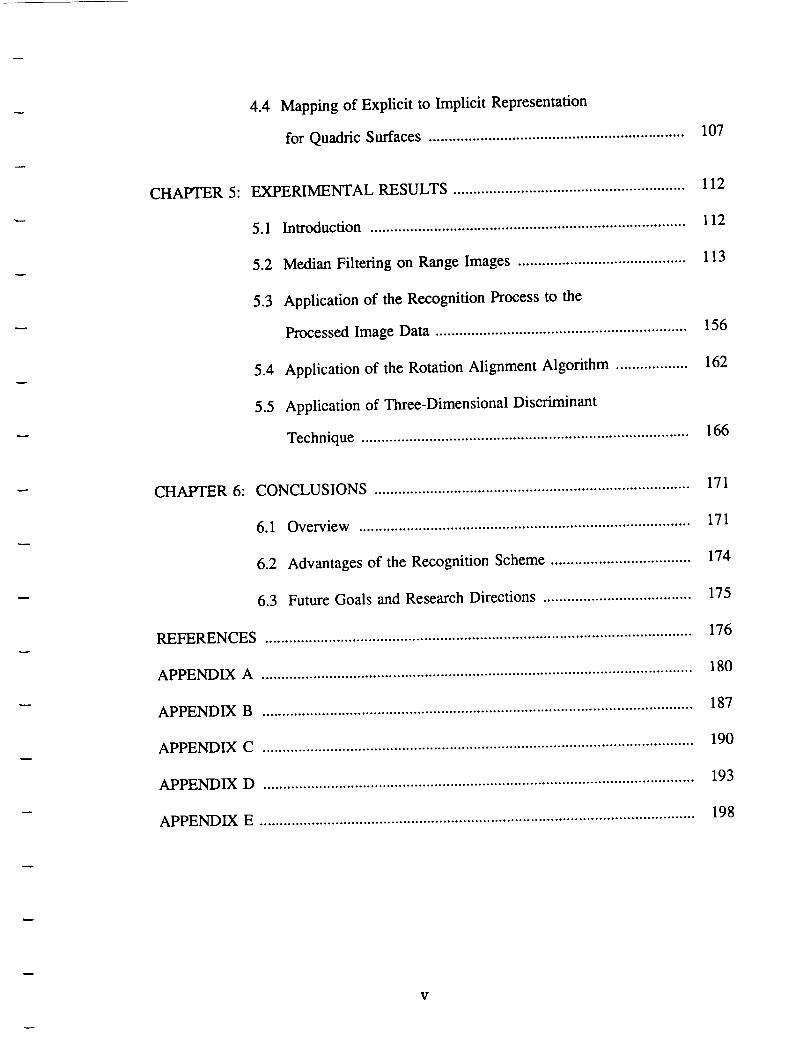
4.4 Mapping of Explicit to Implicit Representation

for Quadric Surfaces ................................................................107

EXPERIMENTAL RESULTS .......................................................... 112

1125.1 Introduction ...............................................................................

5.2 Median Filtering on Range Images .......................................... 113

5.3 Application of the Recognition Process to the

156Processed Image Data ...............................................................

5.4 Application of the Rotation Alignment Algorithm .................. 162

5.5 Application of Three-Dimensional Discriminant

166Technique ..................................................................................

CHAPTER 6:171CONCLUSIONS ...............................................................................

1716.1 Overview ...................................................................................

6.2 Advantages of the Recognition Scheme ................................... 174

6.3 Future Goals and Research Directions ..................................... 175

176REFERENCES ...........................................................................................................

180APPENDIX A ............................................................................................................

187APPENDIX B ............................................................................................................

190APPENDIX C ............................................................................................................

193APPENDIX D ............................................................................................................

198APPENDIX E .............................................................................................................

V

Table 2-1

Table 4-1

Table 4-2

Table 4-3

Table 4-4

Table 4-5

Table 4-6

Table 4-7

Table 4-8

Table 4-9

Table 4-10

Table 4-11

Table 4-12

Table 4-13

Table 5-1

LIST OF TABLES

Surface classification using the three-dimensional discriminant

approach .............................................................................................. 18

Intersection of ellipsoid with planes .................................................. 55

Intersection of quadric cylinder with planes ..................................... 62

Intersection of sphere with planes ..................................................... 64

Intersection of quadric cone with planes .......................................... 73

Intersection of hyperboloid of one sheet with planes ....................... 82

Intersection of hyperboloid of two sheets with planes ..................... 88

Intersection of elliptic paraboloid with planes .................................. 95

Intersection of hyperbolic paraboloid with planes ............................ 96

Intersection of the hyperbolic cylinder with planes .......................... 100

Intersection of the parabolic cylinder with planes ............................ 103

Intersection of the parallelepiped with planes .................................. 106

Various curves intercepted by quadric surfaces when

intersected with the planes z = k and y =k ................................... 108

Feature vector (representing the prescence or absence of curves)

for each of the quadric surfaces ........................................................ 109

Comparison of coefficients evaluated for the original and

the processed images of a sphere ...................................................... 159

vi

Table5-2

Table5-3

Table5-4

Table 5-5

Table 5-6

Table 5-7

Table 5-8

Table 5-9

Table 5-10

Table 5-11

Table5-12

Table5-13

Comparisonof coefficientsevaluatedfor theoriginal and

theprocessedimagesof a cylinder ...................................................160

Curvesinterceptedby the two planes, z = k and y = k,

with real raw andprocessedrangedataof the sphere..................... 161

Curvesinterceptedby the two planes, z = k and y = k,

with real raw and processed range data of the cylinder ................... 161

Curves intercepted by the two planes, z = k and y = k,

with real raw and processed range data of the quadric cone ........... 162

New coefficients of the raw image data of sphere after

alignment ............................................................................................ 163

New coefficients of the 3 x 3 median filtered image data of

sphere after alignment ........................................................................ 163

New coefficients of the 5 x 5 median filtered image data of

sphere after alignment ........................................................................ 164

New coefficients of the raw image data of cylinder

after alignment .................................................................................... 164

New coefficients of the 3 x 3 median filtered image

data of cylinder after alignment ........................................................ 165

New coefficients of the 5 x 5 median filtered image data

of cylinder after alignment ................................................................ 165

New coefficients of an unknown simulated data obtained

after alignment .................................................................................... 167


after alignment

vii

Table 5-14

Table 5-15


168after alignment ....................................................................................

Surface characterization using 3-D discriminant approach

169for simulated data ...............................................................................

°o.

Vlll

LIST OF FIGURES

Figure 2-1

Figure 2-2

Figure 2-3

Figure 2-4

Figure 2-5

Figure 3-1

Figure 3-2

Figure 3-3

Figure 3-4

Figure 3-5

Figure 3-6

Figure 3-7

Figure 3-8

Figure 4-1

Figure 4-2

Shape of a surface in the vicinity of an elliptic, hyperbolic,

and parabolic point .............................................................................

A set of eight view-independent surface types for a visible

surface ..................................................................... :...........................

Two right-handed rectangular coordinate systems ............................

Relation between the coordinates of P upon translation .................

Two rectangular coordinate systems having the same origin ..........

Quadric representations of Real ellipsoid, Hyperboloid of

one sheet, Hyperboloid of two sheets, and Real quadric cone ........

Quadric representations of Elliptic paraboloid, Hyperbolic

paraboloid, Elliptic cylinder, and Parabolic cylinder ........................

Quadric representations of Hyperbolic cylinder and

Parallelepiped .....................................................................................

Raw range image of the sphere .........................................................

3 x 3 median filtered image of the raw sphere .................................



Rotation transformation of the coordinate system ............................

List of all quadric surfaces ................................................................

Ellipsoid detailed view: horizontal intersections .............................

10

II

14

14

15

20

21

22

25

25

27

27

36

50

53

ix

Figure 4-3

Figure 4-4

Figure 4-5

Figure 4-6

Figure 4-7

Figure 4-8

Figure 4-9

Figure 4-10

Figure 4-11

Figure4-12

Figure 4-13

Figure4-14

Figure4-15

Figure 4-16

Figure 4-17

Figure 4-18

Figure 4-19

Figure 4-20

Ellipsoid detailed view:

Cylinder detailed view:

Cylinder detailed view:

vertical intersections .................................

horizontal intersections ..............................

vertical intersections ..................................

Cylinder: lateral view .......................................................................

Intersection of a plane and a sphere ..................................................

Quadric cone detailed view: horizontal intersections ......................

Quadric cone detailed view: vertical intersections ..........................

Quadric cone: Lateral view ..............................................................

Hyperboloid of one sheet detailed view: horizontal

intersections and z = 0 .......................................................................

Hyperboloid of one sheet detailed view: horizontal

intersections and z = -c ......................................................................

Hyperboloid of one sheet detailed view: vertical

intersections ........................................................................................

Hyperboloid of one sheet: lateral view ............................................

Hyperboloid of two sheets detailed view: horizontal

intersections ........................................................................................

Hyperboloid of two sheets detailed view: vertical

intersections ........................................................................................

Hyperboloid of two sheets: lateral view ..........................................

Elliptic paraboloid detailed view: horizontal

intersections ........................................................................................

Elliptic paraboloid detailed view: vertical intersections ..................

Hyperbolic paraboloid detailed view: horizontal

intersections ........................................................................................

X

54

58

60

61

65

69

71

72

76

78

80

81

85

87

89

92

94

97

Figure 4-21

Figure4-22

Figure 4-23

Figure4-24

Figure4-25

Figure 5-1

Figure 5-2

Figure 5-3

Figure 5-4

Figure5-5

Figure 5-6a

Figure5-6b

Figure 5-6c

Figure5-6d

Figure5-7a

Figure 5-7b

Figure 5-7c

Hyperbolicparaboloiddetailedview: vertical intersections........... 98

Hyperboliccylinderdetailedview: horizontal

intersections........................................................................................101

Hyperboliccylinderdetailedview: vertical intersections............... 102

Paraboliccylinder detailedview:

Paraboliccylinder detailedview:

horizontalintersections.............. 104

vertical intersections.................. 105

Raw rangeimageof the spherewith its background....................... 114

Raw rangeimageof the sphereafter segmentation.......................... 114

3 x 3 medianfiltered imageof theraw sphere................................. 115

5 x 5 medianfilteredimageof theraw sphere................................. 116

7 x 7 medianfilteredimageof theraw sphere................................. 116

First derivativewith respectto x-axisof the sphereraw

image ..................................................................................................117

First derivativewith respectto y-axisof the sphereraw

image ..................................................................................................118

Secondderivativewith respectto x-axisof the sphereraw

image ..................................................................................................119

Secondderivativewith respectto y-axisof the sphereraw

image ..................................................................................................120

First derivativewith respectto x-axisof the spherefiltered

with a masksizeof 3 x 3 ..................................................................121

First derivativewith respectto y-axisof the spherefiltered

spherefiltered with a masksizeof 3 x 3 ..........................................122

Secondderivativewith respectto x-axisof the spherefiltered


xi

Figure 5-7d

Figure 5-8a

Figure 5-8b

Figure5-8c

Figure 5-8d

Figure 5-9a

Figure 5-9b

Figure 5-9c

Figure 5-9d

Figure 5-10

Figure 5-11

Figure 5-12

Figure 5-13

Figure 5-14

Figure5-15

Figure 5-16

Secondderivativewith respectto y-axisof the spherefiltered















filtered with a masksizeof 7 x 7 .....................................................131


filtered with a masksizeof 7 x 7 .....................................................132

Sign plot for the original range image of the sphere ....................... 134

Sign plot for the 3 x 3 filtered image of the sphere ......................... 135



Raw range image of the cylinder with its background .................... 139

Raw range image of the cylinder after segmentation ....................... 139

3 x 3 median filtered image of the raw cylinder .............................. 140

xii

Figure 5-17

Figure 5-18a

Figure 5-18b

Figure 5-18c

Figure 5-18d

Figure5-i9a

Figure 5-19b

Figure 5-19c

Figure5-19d

Figure 5-20a

Figure 5-20b

Figure5-20

Figure 5-20d

5 x 5 medianfiltered imageof the raw cylinder .............................. 140

First derivativewith respectto x-axisof thecylinder raw

image ..................................................................................................141

First derivativewith respectto y-axisof the cylinder raw

image ..................................................................................................142

Secondderivativewith respectto x-axisof thecylinder raw

image ..................................................................................................143

Secondderivativewith respectto y-axisof the cylinder raw

image ..................................................................................................144

First derivativewith respectto x-axisof thecylinder filtered


First derivativewith respectto y-axisof thecylinder filtered


Secondderivativewith respectto x-axisof the cylinder filtered


Secondderivativewith respectto y-axisof the cylinder filtered


First derivativewith respectto x-axisof the cylinder filtered


First derivativewith respectto y-axisof the cylinder filtered


Secondderivativewith respectto x-axisof the cylinder filtered

with a mask size of 5 x 5 .................................................................. 151

Second derivative with respect to y-axis of the cylinder filtered

with a mask size of 5 x 5 .................................................................. 152

xiii

Figure 5-21

Figure 5-22

Figure 5-23

Figure 5-24

Figure 5-25

Figure 6-1

Figure6-2

Figure 6-3

Signplot for the original cylinder .....................................................153

Signplot for the 3 x 3 filtered cylinder image ................................. 154

Signplot for the 5 x 5 filtered cylinder image ................................. 155

Best-fit plot for the sphereraw image ..............................................157

Best-fit plot for the cylinder ..............................................................158

Delta rocket composedof cylindrical and conical

shapes..................................................................................................172

Conicaldomesandcylinderlike body makeup the

spaceprobe .........................................................................................173

Cylindericalspacestationwith a half spheredometop ................... 173

xiv

CHAPTER ONE

INTRODUCTION

1.1 Introduction

One of the most important tasks in computer vision is that of three-dimensional

object recognition. Success has been limited to the recognition of symmetric objects.

Recently, research has concentrated on the recognition of small numbers of asymmetric

objects as well as objects placed in complex scenes. Unlike the recognition procedure

developed for intensity-based images, the recent development of active and passive

sensors extracting quality range information has led to the involvement of explicit

geometric representations of the objects for the recognition schemes [1, 2]. Location

and description of three-dimensional objects from natural light images are often

difficult to determine. However, range images give a more detailed and direct

geometric description of the shape of the three-dimensional object. A brief introduc-

tion to range images and the laser range-finder is presented in Section 1.2. In Section

1.3, a precise global definition of the object recognition problem is discussed. The

objective of this dissertation and its relevance to the global three-dimensional problem

is presented in Section 1.4.

1.2 Range Image and Data Acquisition

Range images share the same format as intensity images, i.e., both of these

images are two-dimensional arrays of numbers, the only difference being that the

numbers in the range images represent the distances between a sensor focal plane to

points in space. The laser range-finder or tracker [3] is currently the most widely used

sensor. The laser range-finder makes use of a laser beam which scans the surfaces in

2

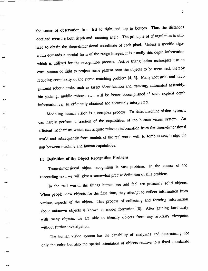
the scene of observation from left to right and top to bottom. Thus the distances

obtained measure both depth and scanning angle. The principle of triangulation is util-

ized to obtain the three-dimensional coordinate of each pixel. Unless a specific algo-

rithm demands a special form of the range images, it is usually this depth information

which is utilized for the recognition process. Active triangulation techniques use an

extra source of light to project some pattern onto the objects to be measured, thereby

reducing complexity of the stereo matching problem [4, 5]. Many industrial and navi-

gational robotic tasks such as target identification and tracking, automated assembly,

bin picking, mobile robots, etc., will be better accomplished if such explicit depth

information can be efficiently obtained and accurately interpreted.

Modeling human vision is a complex process. To date, machine vision systems

can hardly perform a fraction of the capabilities of the human visual system. An

efficient mechanism which can acquire relevant information from the three-dimensional

world and subsequently form models of the real world will, to some extent, bridge the

gap between machine and human capabilities.

1.3 Definition of the Object Recognition Problem

Three-dimensional object recognition is vast problem. In the course of the

succeeding text, we will give a somewhat precise definition of this problem.

In the real world, the things human see and feel are primarily solid objects.

When people view objects for the first time, they attempt to collect information from

various aspects of the object. This process of collecting and forming information

about unknown objects is known as model formation [8]. After gaining familiarity

with many objects, we are able to identify objects from any arbitrary viewpoint

without further investigation.

The human vision system has the capability of analyzing and determining not

only the color but also the spatial orientation of objects relative to a fixed coordinate

_7

system. Since we are interested in an automatic, computerized process to recognize

objects, the input data we use must be compatible with available digital computers.

Hence, two-dimensional matrices of numerical values usually known as digitized sen-

sor data, constitute the information that is processed to describe or recognize three-

dimensional objects. The sensor used for this process can be a passive sensor, like a

camera, or an active sensor, such as a laser range mapper. Summarizing, the three-

dimensional recognition problem constitutes a detailed completion of model formation

of the object leading to an in-depth knowledge of its shape and orientation with respect

to a fixed view of the real world.

1.4 Objectives and Organization of the Report

An approach based on two-dimensional analytic geometry to recognize a series of

three-dimensional objects is presented in this research. Among the various three-

dimensional objects considered are the hyperboloids of one and two sheets, ellipsoids,

spheres, circular and elliptical quadric cones, circular and elliptical cylinders, parabolic

and hyperbolic cylinders, elliptic and hyperbolic paraboloids, and paraUelepipeds.

The difficulties in recognizing three-dimensional objects stems from the complex-

ity of the scene, the number of objects in the database and the lack of a priori infor-

mation about the scene. Techniques vary based upon the difficulty of the recognition

problem. In our case we attempt to recognize segmented objects in range images.

Location and orientation of three-dimensional objects has always been the most

complex issue in many computer vision applications. Algorithms for a robust three-

dimensional recognition system must be view-independent. Herein, we have developed

a technique to determine the three-dimensional object location and orientation in range

images. Once the object lies in a desired stable rest position, our proposed recognition

scheme quickly and accurately classifies it as one of the objects mentioned above. In

comparison to most of the present day methods utilized for range image object

4

recognition, our proposed approach attacks the problem in a different manner and is

computationaUy inexpensive.

Chapter Two reviews some of the earlier and current work in this area. It

includes a review of some of the mathematical concepts associated with three-

dimensional object recognition. A mathematical quadric classification method based

on a three-dimensional discriminant is discussed while in this chapter. In chapters

Three and Four we discuss, in detail, our proposed three-dimensional approach.

Chapter Three addresses the various pre-processings steps involved prior to the appli-

cation of the recognition algorithm. Median filtering, segmentation, three-dimensional

coefficient evaluation, and rotation alignment being some of them. The demerits of

existing schemes in the area of three-dimensional object recognition and the unique-

ness and improvizations brought about through our recognition procedures are also dis-

cussed in Chapter Three. In Chapter Four, after a brief discussion of the practical

merits of using planar intersections, characteristic feature vectors are obtained for each

of the quadric surfaces under investigation. Results are summarized in Chapter Five.

A large set of real range images of spheres, cylinders, and cones were utilized to test

the proposed recognition scheme. Results obtained for simulated data of other quadric

surfaces, namely, hyperboloids and paraboloids are also tabulated in Chapter Five.

Chapter Six concludes with a discussion of possible areas for future investigation.

CHAPTER TWO

BACKGROUND

2.1 Introduction

Past and present research in the field of three-dimensional object recognition is

reviewed in Section 2.2. Surface curvatures which are widely utilized in this research

area are briefly reviewed in Section 2.3. Section 2.4 investigates a three-dimensional

approach to classification and reduction of quadrics as presented by Olmstead [24],

wherein various invariant features of the quadratic form under translation and rotation

are discussed.

2.2 Literature Review

Many of the currently available techniques for describing and recognizing three-

dimensional objects are based on the principle of segmentation. Segmentation is the

process in which range data is divided into smaller regions (mostly squares) [4].

These small regions are approximated as planar surfaces or curved surfaces based upon

the surface mean and Gausssian curvatures. Regions sharing similar curvatures are

subsequently merged. This process is known as region growing. Other approaches

[6-10] characterize the surface shapes while dealing with the three-dimensional recog-

nition problem. Levine et al. [11] briefly review various works in the field of segmen-

tation, where segmentation has been classified into region-based and edge-based

approaches. Again surface curvatures play an important role for characterization in

each of these approaches.

Grimson et al. [12] discuss a scheme utilizing local measurements of three-

dimensional positions and surface normals to identify and locate objects from a known

set. Objectsare modeledaspolyhedrawith a set numberof degreesof freedom with

respect to the sensors. The authors claim a low computational cost for their algorithm.

Although they have limited the experiments to one model, i.e., data obtained from one

object, they claim that the algorithm can be used for multiple object models. Also,

only polyhedral objects with a sufficient number of planar surfaces can be used in their

scheme.

Another paper by Faugeras et al. [13] describes surfaces by curves and patches

which are further represented using linear parameters such as points, lines and planes.

Their algorithm initially reconstructs objects from range data and consequently utilizes

certain constraints of rigidity to recognize objects while positioning. They arrive at the

conclusion that for an object to be recognized, at least a certain area of the object

should be visible (approx. 50%). They claim their approach could be used for images

obtained using ultrasound, stereo, and tactile sensors.

Hu and Stockman [14] have employed structured light as a technique for three-

dimensional surface recognition. The objects are illuminated using a controlled light

source of a regular pattern, thereby creating artificial features on the surfaces which are

consequently extracted. They claim to have solved the problem known as "grid line

identification." From the general constraints, a set of geometric and topological rules

are obtained which are effectively utilized in the computation of grid labels which are

further used for finding three-dimensional surface solutions. Their results infer that

consistent surface solutions are obtained very fast with good accuracy using a single

image.

Recognition of polyhedral objects involves the projection of several invariant

features of three-dimensional bodies onto two-dimensional planes [15]. Recently,

recognition of three-dimensional objects based upon their representation as a linear

combination of two-dimensional images has been investigated [16]. Transformations

such as rotation and translation have been considered for three-dimensional objects in

terms of the linear combinationof a seriesof two-dimensionalviews of the objects.

Insteadof usingtransformationsin three-dimensions,it hasbeen shownthat the pro-

cess is the equivalentof obtaining two-dimensionaltransformationsof several two-

dimensionalimagesof the objectsand combining them together to obtain the three-

dimensional transformation. This procedure appears computationally intensive.

Most of the techniques and algorithms mentioned above have a common criterion

for classifying the three-dimensional objects in the final phase. They have a database

of all the objects they are trying to recognize and hence try to match features from the

test samples to the features of the objects in the database.

Fan et al. [17] use graph theory for decomposing segmentations into subgroups

corresponding to different objects. Matching of the test objects with the objects in the

database is performed in three steps: the screener, which makes an initial guess for

each object; the graph matcher, which conducts an exhaustive comparison between

potential matching graphs and computes three-dimensional transformation between

them; and finally, the analyzer, which based upon the results from the earlier two

modules conducts a split and merge of the object graphs. The distinguishing aspect of

this scheme is that the authors used occluded objects for describing their proposed

method.

As has been mentioned, most of the present research on three-dimensional objects

utilize range imagery rather than stereo images. But at the same time, it should be

noted that it was stereo imagery which, to a large extent, was initially used to investi-

gate the problem of three-dimensional object recognition.

Forsyth et al. [18] use stereo images to obtain a range of invariant descriptors in

three-dimensional model-based vision. Initially, they demonstrate a model-based

vision system that recognizes curved plane objects irrespective of the pose. Based

upon image data, models are constructed for each object and the pose is computed.

However, they mainly describe three-dimensional objects with planar faces.

8

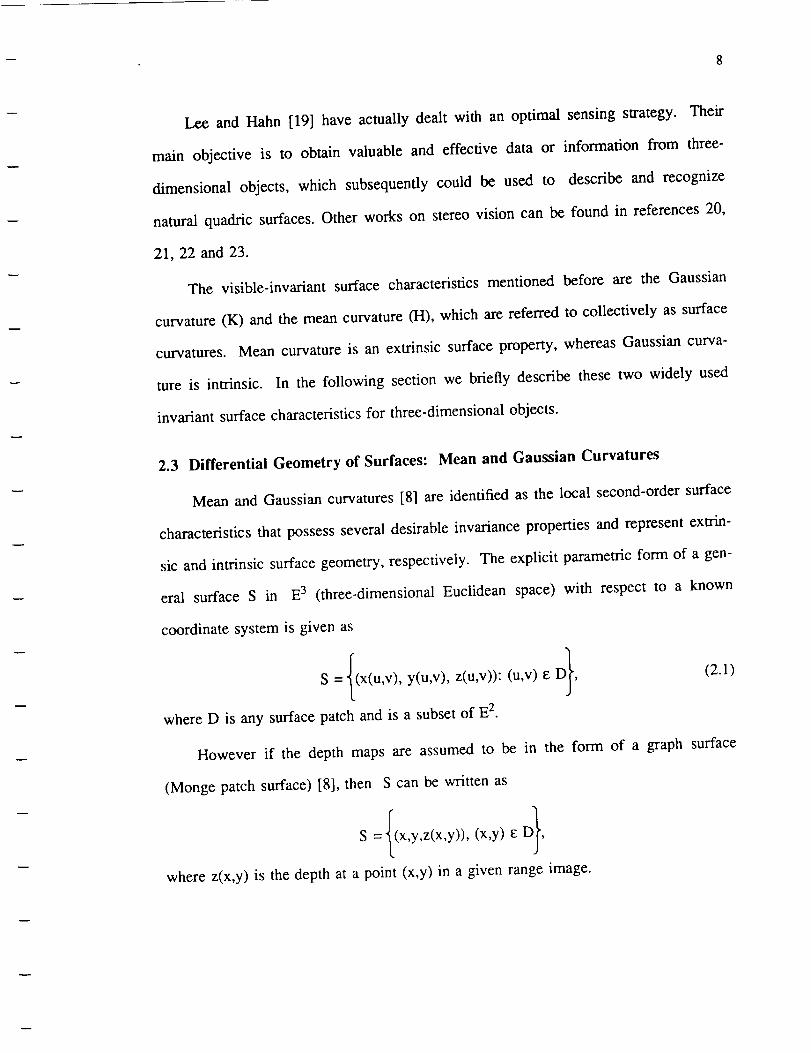
Lee and Hahn [19] haveactually dealt with an optimal sensingstrategy. Their

main objective is to obtain valuable and effective data or information from three-

dimensional objects, which subsequentlycould be used to describeand recognize

natural quadric surfaces.Other works on stereovision can be found in references20,

21, 22 and 23.

The visible-invariant surfacecharacteristicsmentionedbefore are the Gaussian

curvature(K) and themeancurvature(H), which are referredto collectively assurface

curvatures. Mean curvatureis an extrinsic surfaceproperty,whereasGaussiancurva-

ture is intrinsic. In the following sectionwe briefly describethesetwo widely used

invariant surfacecharacteristicsfor three-dimensionalobjects.

2.3 Differential Geometry of Surfaces: Mean and Gaussian Curvatures

Mean and Gaussian curvatures [8] are identified as the local second-order surface

characteristics that possess several desirable invariance properties and represent extrin-

sic and intrinsic surface geometry, respectively. The explicit parametric form of a gen-

eral surface S in E 3 (three-dimensional Euclidean space) with respect to a known

coordinate system is given as

S = {(x(u,v), y(u,v), z(u,v)): (u,v) E D}, (2.1)

where D is any surface patch and is a subset of E2.

However if the depth maps are assumed to be in the form of a graph surface

(Monge patch surface) [8], then S can be written as

S = {(x,y,z(x,y)), (x,y) E D},

where z(x,y) is the depth at a point (x,y) in a given range image.

9

The representations for the Gaussian and the mean curvatures are as follows:

Gaussian curvature, K, is defined by,

32Z 32Z

32z ] 2

3x3yJ

3x2 3Y2 lll + (___)2 + ( d_ )2) z"

(2.2)

Mean curvature, H, is defined by,

32z I3z] 2 3z 3z 32z

32Z + 32Z + 32Z (0._._] 2 3y--7(g2xJ-2 xx y 3x3y

3x2 0Y2 3x2 3z

2 1+ + _OyJJ

(2.3)

Both of these curvatures are invariant to translation and rotation of the object as long

as the object surface is visible.

Based upon the sign of the Gaussian curvature, individual points in the surface

are locally classified into three surface types as shown in Figure 2-1:

(a) K > 0 implies an elliptic surface point,

(b) K < 0 implies a hyperbolic surface point, and

(c) K = 0 implies a parabolic surface point.

Besl and Jain in their paper [8] have shown that the Gausssian and mean curva-

tures together can be utilized to give a set of eight different surfaces as shown in Fig-

ure 2-2:

1) H < 0 and K > 0 implies a peak surface.

2) H > 0 and K > 0 implies a pit surface.

3) H < 0 and K = 0 implies a ridge surface.

4) H > 0 and K = 0 implies a valley surface.

1o

(b) Hyperbolic point (K < 0)

(a) Elliptic point (K > 0) (c) Parabolic point (k = 0)

Figure 2-1. Shape of a surface in the vicinity of an elliptic, hyperbolic, and parabolic

point.

II

Peak Surface H < 0, K > 0 Flat Surface H = 0, K = 0

Pit Surface H > 0, K > 0 Minimal Surface H = 0, K < 0

Ridge Surface H < 0, K = 0 Saddle Ridge H < 0, K < 0

Valley Surface H > 0, K = 0 Saddle Valley H > 0, K < 0

Figure 2-2. A set of eight view-independent surface types for a visible surface.

12

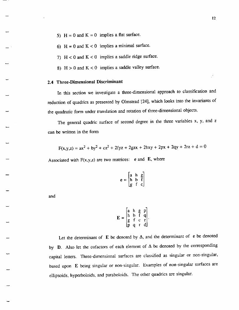
5) H = 0 andK = 0 impliesa flat surface.

6) H=0andK<0

7) H<0andK<0

8) H>0andK<0

impliesa minimal surface.

impliesa saddleridgesurface.

implies a saddlevalley surface.

2.4 Three.Dimensional Discriminant

In this section we investigate a three-dimensional approach to classification and

reduction of quadrics as presented by Olmstead [24], which looks into the invariants of

the quadratic form under translation and rotation of three-dimensional objects.

The general quadric surface of second degree in the three variables x, y, and z

can be written in the form

F(x,y,z) = ax 2 + by 2 + cz 2 + 2fyz + 2gzx + 2hxy + 2px + 2qy + 2rz + d = 0

Associated with F(x,y,z) are two matrices: e and E, where

and

e --

E _.. Ihglb ff c "

q r

Let the determinant of E be denoted by A, and the determinant of e be denoted

by D. Also let the cofactors of each element of A be denoted by the corresponding

capital letters. Three-dimensional surfaces are classified as singular or non-singular,

based upon E being singular or non-singular. Examples of non-singular surfaces are

ellipsoids, hyperboloids, and paraboloids. The other quadrics are singular.

13

Let us now considerthe two basic transformations,namelytranslationand rota-

tion, and try to arrive at someinvariant features. Considerthe two rectangularright-

handedcoordinatesystemsasshownin Figure2-3. Any point in spacehastwo setsof

coordinates,one for eachset of axes. The problemis to find a relationshipbetween

thesetwo setsof coordinatesso that one canconvert from one coordinatesystemto

the other.

2.4.1 Translation

InspectingFigure 2-4, we seethat the coordinatesof O' and P in the xyz sys-

tem are (Xo,Yo,Zo)and (x,y,z), respectively,and the coordinatesof P in the x'y'z' sys-

tem are (x',y',z'). The two setsof coordinatesof P arerelatedby the following trans-

lation equations:

x = x' + xo. (2.4)

Y = Y' + Yo. (2.5)

z = z' + zo. (2.6)

The set of equations,(2.4), (2.5), and (2.6) relatethecoordinatesof a point in the

x'y'z' systemto its coordinatesin the xyz system. Direct substitutionof equations

(2.4) - (2.6) into F(x,y,z) resultsin thefollowing theorem:

Theorem 2.1. For any quadric surface, the coefficients of the second degree terms,

and therefore the matrix e, are invariant under translation.

2.4.2 Rotation

Consider the two rectangular coordinate systems as shown in Figure 2-5. With

respect to the x'y'z' system, let the direction cosines of the x, y, and z axes be

(_.l,_ol,vl), (_.27o2,v2), and (_,3,a93,V3), respectively. Then with respect to the xyz sys-

tem, the direction cosines of the x', y', and z' axes are (_.1, _,2, _3), (vl, _02, a-)3), and

(v 1, v 2, v3), respectively.

14

y

Figure 2-3. Two fight-handed rectangular coordinate systems.

zl izX

Z

Y

y

yFigure 2-4. Relation between the coordinates of P upon translation.

15

X

P

B

Figure 2-5. Two rectangular coordinate systems having the same origin.

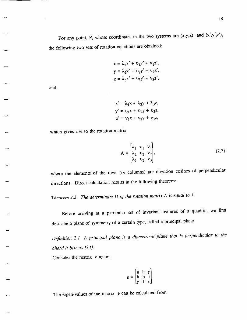
For any point, P, whosecoordinatesin the two systemsare (x,y,z)

the following two setsof rotation equationsareobtained:

16

and (x',y',z'),

and

× = _.1 x' + "OlY' + VlZ' ,

Y = _,2x' + _2Y' + v2z',

z = _,3X' + "03y' + v3z',

x' = )_lx + _,2Y + _-3z,

y' = 91 x + 132y + 1/3z,

z' = VlX + V2y + V3z,

which gives rise to the rotation matrix

1 a.)1 V]A = 'uz v2, (2.7)

'133 V

where the elements of the rows (or columns) are direction cosines of perpendicular

directions. Direct calculation results in the following theorem:

Theorem 2.2. The determinant D of the rotation matrix A is equal to 1.

Before arriving at a particular set of invariant features of a quadric, we first

describe a plane of symmetry of a certain type, called a principal plane.

Definition 2.1 A principal plane is a diametrical plane that is perpendicular to the

chord it bisects [24].

Consider the matrix e again:

f

The eigen-values of the matrix e can be calculated from

17

lahk h Ib-k g

g f c-k

=0.

This cubic equation in k is called the characteristic equation of the matrix e. Its

roots are called the characteristic roots of e. The quantities given below are found to

be invariant as a consequence of the following theorem [25].

Theorem 2.3 If the second degree equation F(x,y,z)=O is transformed by means of a

translation or a rotation with fixed origin, the following quantities are invariant:

D, A, P3, P4, I, J, k 1, k 2, and k3, where D, A are the determinants of the matrices e

and E, respectively; and P3 and P4 are the ranks of the matrices e and E, respec-

tively. Also

I=a+b+c,

J = ab + ac + bc - t,2_ g2 _ h2,

and finally k 1, k2, and k 3 are the characteristic roots of e.

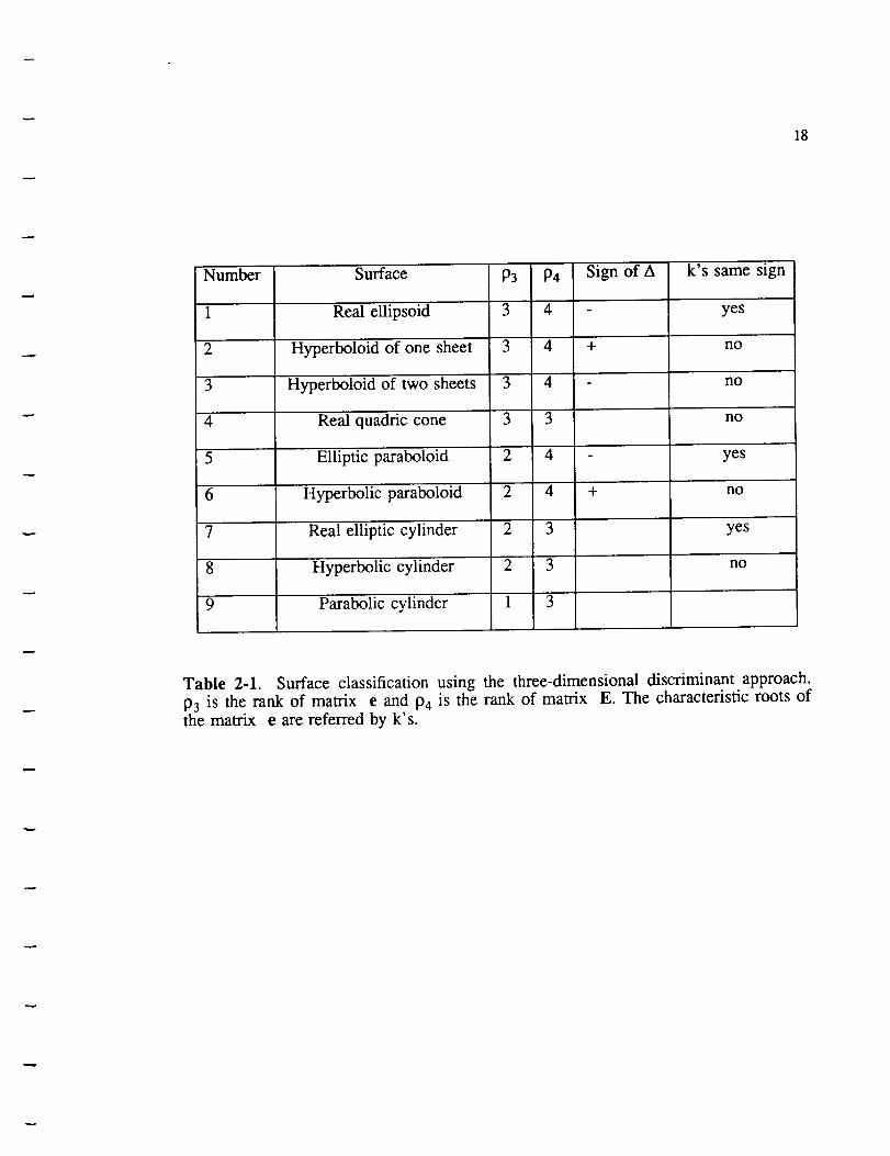
Based upon the above set of invariants, surface classifications are listed in Table

2-1.

In Chapters Three and Four, we discuss our proposed recognition scheme in

detail.

18

Number Surface

1 Realellipsoid

2 Hyperboloidof one sheet

3 Hyperboloidof two sheets

4 Realquadriccone

5 Elliptic paraboloid

6 Hyperbolic paraboloid

7 Realelliptic cylinder

8 Hyperboliccylinder

9 Paraboliccylinder

P3 P4

3 4

3 4

3 4

3 3

2 4

2 4

2 3

2 3

1 3

Sign of A k's same sign

- yes

+ no

- no

no

- yes

+ no

yes

no

Table 2-1. Surface classification using the three-dimensional discriminant approach.

P3 is the rank of matrix e and P4 is the rank of matrix E. The characteristic roots ofthe matrix e are referred by k's.

CHAPTER THREE

QUADRIC SURFACE REPRESENTATION

3.1 Introduction

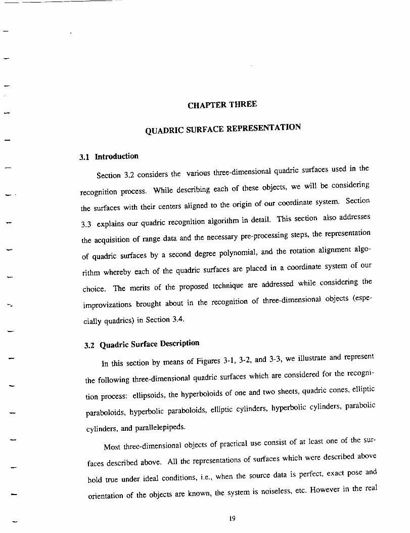
Section 3.2 considers the various three-dimensional quadric surfaces used in the

recognition process. While describing each of these objects, we will be considering

the surfaces with their centers aligned to the origin of our coordinate system. Section

3.3 explains our quadric recognition algorithm in detail. This section also addresses

the acquisition of range data and the necessary pre-processing steps, the representation

of quadric surfaces by a second degree polynomial, and the rotation alignment algo-

rithm whereby each of the quadric surfaces are placed in a coordinate system of our

choice. The merits of the proposed technique are addressed while considering the

improvizations brought about in the recognition of three-dimensional objects (espe-

cially quadrics) in Section 3.4.

3.2 Quadric Surface Description

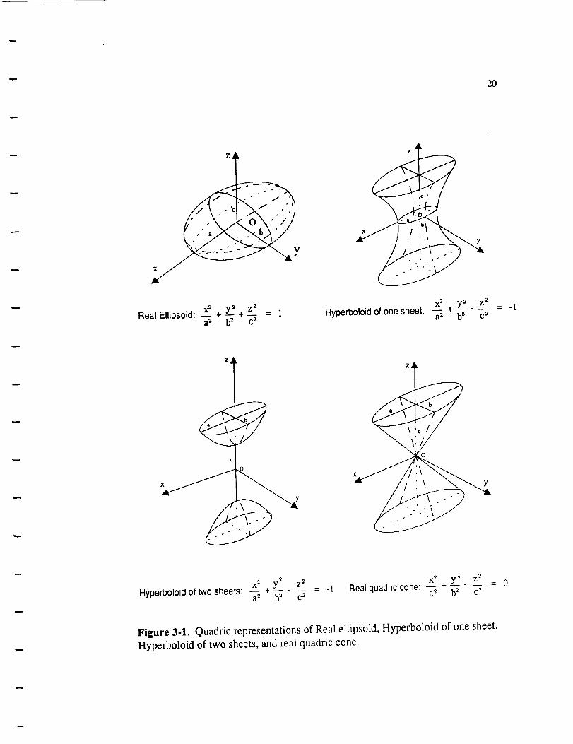
In this section by means of Figures 3-1, 3-2, and 3-3, we illustrate and represent

the following three-dimensional quadric surfaces which are considered for the recogni-

tion process: ellipsoids, the hyperboloids of one and two sheets, quadric cones, elliptic

paraboloids, hyperbolic paraboloids, elliptic cylinders, hyperbolic cylinders, parabolic

cylinders, and parallelepipeds.

Most three-dimensional objects of practical use consist of at least one of the sur-

faces described above. All the representations of surfaces which were described above

hold _ue under ideal conditions, i.e., when the source data is perfect, exact pose and

orientation of the objects are known, the system is noiseless, etc. However in the real

19

20

y2 z 2Real Ellipsoid: _ +_ +a 2 b _ c2

= Iy2 Z 2Hyperboloid of one sheet: _ + -- -

a2 b2 c2 = -i

C

Hyperboloid of two sheets: x_ y2 z2

a 2 b2 c 2= -I Real quadric cone: x= y2 z 2

= 0a2 b2 c2

Figure 3-1. Quadric representations of Real ellipsoid, Hyperboloid of one sheet,Hyperboloid of two sheets, and real quadric cone.

21

z,i

0

__ Y:Ellipticparaboloid:x2 +- + 2z = 0a2 b2

x2 y__2Hyperbolic paraboloid: a----_ - b2 + 2z = 0

I , I

/---I-:1

x 2 y_Elliptic cylinder: _ +- = 1 Parabolic cylinder" x2 + 2rz = 0

a s b2

Figure 3-2. Quadric representations of Elliptic pm'aboloid, Hyperbolic paraboloid,

Elliptic cylinder, and Parabol'lc cylinder.

22

z&

Ii

!

II'\

x y2Hyperbolic cylinder: -_ " _-_ = -1

Figure 3-3.

Z

Z

Parallelepiped

Y

Quadric representations of Hyperbolic cylinder and Parallelepiped.

23

world, practically none of these conditions hold true. Any set of data, whether it is

derived or generated from a passive (camera) or an active sensor (laser range mapper),

can at best be approximated to a second-degree polynomial. Whether this polynomial

accurately represents a surface or not, and if so, how these coefficients (representa-

tion) can be chosen to come close to recognizing a three-dimensional object, is the

whole issue of the recognition problem.

In the next few sections, while formulating our recognition scheme, we describe

one such technique which generates ten coefficients (which are sufficient under ideal

conditions) to describe all the objects of interest [26].

However, before elaborating on the recognition scheme, an overview of the tech-

nique is presented. The recognition scheme utilizes a two-dimensional discriminant

(which is a measure for distinguishing two-dimensional curves) to recognize three-

dimensional surfaces. Instead of utilizing the ten generated coefficients and attempting

to recognize the surface from its quadric representation, the quadrics are identified

using the information resulting from the intersection of the surface with different

planes. If the surface is one of those listed above, there are five possible two-

dimensional curves that may result from such intersections, (i) a circle, (ii) an ellipse,

(iii) a parabola, (iv) a hyperbola, and (v) a line. Thus, a feature or pattern vector

with five independent components can be formed for characterizing each of the sur-

faces.

3.3 Recognition Scheme

Our recognition scheme consists of the following steps:

(1) acquisition of the range data and conducting the pre-processing steps,

(2) description and representation of objects as general second degree surfaces,

(3) determination of the location and orientation of the objects with respect to a

desired coordinate system,

24

(4) performance of the rotation and translation transformations of the object so as to

place it in a stable desired coordinate system,

(5) use of the principle of two-dimensional discriminants to classify the various curves

obtained by intersecting the surfaces with planes, and

(6) acquisition of an optimal set of planes sufficient enough to distinguish and

recognize each of the quadric surfaces. Angular bounds within which every

surface yields a distinct set of curves are determined in step 6.

The range data, as mentioned in Chapter One, is a pixel-by-pixel depth value

from the point of origin of the laser to the point where the beam impinges on a sur-

face. The objects are scanned from left-to-right and top-to-bottom. A grid frame may

consist of 256 x 256 pixels. Before this range data is applied to the object classifier, it

has to undergo the following pre-processing steps:

a) median filtering, and

b) segmentation.

3.3.1 Median Filtering

Conventionally, a rectangular window of size M x N is used in two dimensional

median filtering. As in our case [27], experiments were performed with square win-

dows of mask sizes 3 x 3 and 5 x 5. Salt and pepper noise in the range images used

in this research was uniformly distributed throughout. Irrespective of the mask size,

the range information at every pixel in the image is replaced by the median of the pix-

els contained in the M x M window centered at that point. Referring to Figure 3-4

and keeping in mind that the black pixels correspond to the background and the white

pixels to the object, black pixels inside the object are referred to as pepper noise and

white pixels in the black background are referred to as salt noise. Figure 3-5 is

obtained as a result of a 3 x 3 mask being moved over the entire image. The image

looks as sharp as the original image though some of the noise still exists. A 5 x 5 and

25

Figure 3-4. Raw range image of the sphere.

Figure 3-5. 3 x 3 median filtered image of the raw sphere.

26

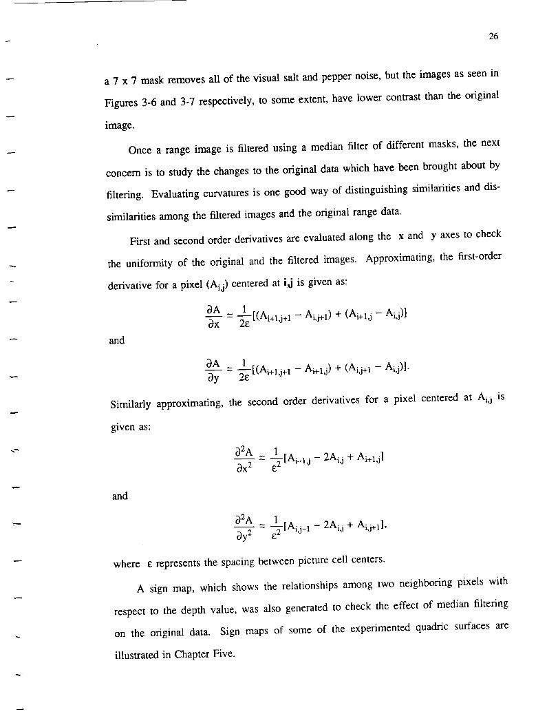
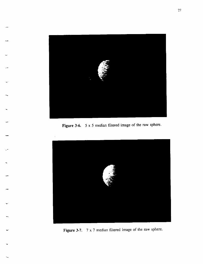
a 7 x 7 mask removes all of the visual salt and pepper noise, but the images as seen in

Figures 3-6 and 3-7 respectively, to some extent, have lower contrast than the original

image.

Once a range image is filtered using a median filter of different masks, the next

concern is to study the changes to the original data which have been brought about by

filtering. Evaluating curvatures is one good way of distinguishing similarities and dis-

similarities among the filtered images and the original range data.

First and second order derivatives are evaluated along the x and y axes to check

the uniformity of the original and the filtered images. Approximating, the first-order

derivative for a pixel (Ai, j) centered at i,j is given as:

3A 1bx 2e [(Ai+ld+l - Ai'j+l) + (Ai+l'J - Ai'j)]

and

3A 1

_y 2e [(Ai+l'j+l - Ai+l'J) + (Ai'j+l -Ai,j)]-

Similarly approximating, the second order derivatives for a pixel centered at Ai,j is

given as:

b2A 1

_x 2 E2 [Ai-l,J - 2Ai, j + Ai+l,j]

and

_2A 1

Oy2 _2 [Ai,j -1 - 2Ai,j + Ai,j+l]'

where E represents the spacing between picture cell centers.

A sign map, which shows the relationships among two neighboring pixels with

respect to the depth value, was also generated to check the effect of median filtering

on the original data. Sign maps of some of the experimented quadric surfaces are

illustrated in Chapter Five.

27



28

3.3.2 Segmentation

Since isolated objects instead of complex scenes are considered, a simple thres-

holding whereby the object is separated from the background is utilized for the seg-

mentation process. In the case where objects are irregular or a scene consists of a

cluster of objects, Gaussian and mean curvatures have to be utilized to sub-divide the

scene into planar or curved surfaces. Each surface is then recognized separately.

Range image segmentation has been extensively studied by Levine et al. [9].

Now that the available range data has been processed to eliminate salt and pepper

noise, we can now utilize the image data to obtain the quadric surface which best fits

the data. To achieve this goal, we need to determine the coefficients of a second

degree polynomial representation for the three-dimensional surface.

3.3.3 Three-Dimensional Coefficients Evaluation

Our objective is to obtain a surface described by Equation (3.1) from a given set

of data (range) points. We assume that the data is a set of range-image samples

obtained from a single surface which can be described by a quadric equation.

F(x,y,z) = ax 2 + by 2 + cz 2 + 2fyz + 2gzx + 2hxy + 2px + 2qy + 2rz + d = 0. (3.1)

We shall therefore define the best description to be the one which minimizes the

mean-squared error (MSE) between the range data and the quadric [26].

Equation (3.1) in vector notation becomes

F(x,y,z) = aTp = 0, (3.2)

where a T=[abc2f2g2h2p2q2rd]andpT=[x 2y2z 2yzzxxyxyz 1 ].

The error measure for any data point (x,y,z) can be measured by evaluating

F(x,y,z). If this point lies exactly on the surface then, F(x,y,z) = 0, meaning that the

error is zero.

29

The mean-squarederror,E, is definedas

E = min ]_IIFII2.a S

(3.3)

In vector notation, Equation (3.3) becomes

E = rnin ,_aTppTa = min aTRa, (3.4)a S a

where R is the scatter matrix for the data set equal to

R = _ppT. (3.5)

Minimizing E leads to a trivial solution of a = 0, implying all the coefficients are zero.

We therefore attempt to find the minimum of aTRa with respect to a, subject to some

constraint K(a) = k.

Let

and

G(a) = aTRa (3.6)

K(a) = aTKa,

where K is another undetermined constant matrix.

write the function

(3.7)

Using Lagrange's method [28], we

U = G(a) - _.K(a), (3.8)

where _. again is an undetermined constant. To find a minimum solution for U, we

form

_U

_a 2(R _.K)a 0. (3.9)

30

OUSolving _ = 0 and K(a)= k simultaneously,we find a and _ to give a minimum

solution. We wish to evaluatethe constraintK(a) suchthat it gives a non-zerosolu-

tion for a for all the quadricsurfacesof interest.

In order to determinethefunction of the coefficientvectora which is invariant to

translationandrotation,we write the quadricequationas

where

F(x,y,z) = F(v) = vtDv + 2vtq+ d = 0, (3.1o)

7_

D=_ h !]f

(3.11)

(3.12)

and

q = . (3.13)

After carrying out the transformations, translation and rotation, it is observed that the

second-order terms and the eigen-values are the only invariants of D under translation

and rotation, respectively.

We now derive a function of the eigen-values of D, i.e., f(_,), which will allow us

to obtain all of the quadrics of interest. The constraint should be in a quadratic form,

such that when we substitute it in

_U

= 2(R - _.K)a = 0, (3.14)Oa

we get a linear equation from which we can solve for a.

31

From reference29,a goodchoicefor theconstraintfiX) is

i.eol

f(z.)= ZX 2= 1,

_.i 2 = tr(D 2) = a2 + b 2 + c 2 + 2f 2 + 2g 2 + 2h 2.

Writing it in the form of equation K(a) = aTKa:

(3.15)

(3.16)

where the constraint matrix K 2 is

tr(D 2) = a T a, (3.17)

1 0

0 100

K2= 0 0

000

.000

0 0 0 00 0 0 01 0 0 00 1/2 0 0

0 1/2 00 0 1/,q

Equation Ra = _.Ka, can now be written as

(3.18)

[BCT A] [_] = X[O 2 _] [_]' (3.19)

where C is the 6 x 6 scatter matrix for the quadratic terms a, b, and c; B is the 6 x 4

scatter matrix for the mixed terms 2f, 2g, and 2h and A is the 4 x 4 scatter matrix for

the linear and constant term, i.e., 2p, 2q, 2r, and d. 13 is the 6 x 1 vector of the qua-

dratic coefficients and o_ is the 4 x 1 vector of the linear and the constant coefficients.

Solving Equation (3.19), we get

and

C13 + Bot = _.K2_ (3.20)

32

FromEquation(3.21)we get

BT_ + Aa = 0. (3.21)

tt = - A-1BTI_.

Substituting a in Equation (3.20), we have

Labeling ( C - BA-1B T) as

( C - BA-IB T )9 = _-K213-

M, we have

(3.22)

(3.23)

M13 = KK213,

which appears similar to an eigen-value problem. Writing K 2 as H 2 , where,

(3.24)

H

1 00 0 00 1 0 0 0

0 1 0 00 0 1/'_ 00 0 0 0 1/_/2

0 00 0 0

1 00 00 1 0 0

H_I 00 1 0=ooo4 000 0000 0

0 00 00 00 0

oo

0000 '0

(3.25)

(3.26)

We can write M[3 = _LK2_ as MI3 = _.HH[3, or H-1MH-IH13 = XJql3.

Let 13' = H_3 and M" = H-1MH -1, where M' is a real symmetric matrix, then

M'_' = _.B'.

M' has six ki's and six corresponding Bi's.

(3.27)

33

For the minimum error solution,we choosetheeigen-vectorcorrespondingto the

smallesteigen-value,i.e.,

_i = H-1B'i • (3.28)

Solving for 0q = -A-1BTBi, we have our solution.

Once the procedure described in Section 3.3.3 has been performed, the median

filtered range data can be described as

F(x,y,z) = ax 2 + by 2 + cz 2 + 2fyz + 2gzx + 2hxy + 2px + 2qy + 2rz + d = 0, (3.29)

where the values of the coefficients a, b, c, f, g, h, p, q, r, and d are known. Generally

speaking, all of the objects in the experiments generate all ten coefficients as is shown

in Chapter Five. The question now is: How can we distinguish one object from the

another and how accurately can we describe the recognized object? In the following

sections of this chapter and Chapter Four, we describe the necessary scheme to solve

the recognition problem of quadric surfaces.

3.3.4 Evaluation of the Rotation Matrix

The determination of the location and orientation of a three-dimensional object is

one of the central problems in computer vision applications. It is observed that most

of the methods and techniques which try to solve this problem require considerable

pre-processing such as detecting edges or junctions, fitting curves or surfaces to seg-

mented images and computing high order features from the input images. Since

three-dimensional object recognition depends not only on the shape of the object but

also the pose and orientation of the object as well, any definite information about the

object's orientation will aid in selecting the right features for the recognition process.

In this research we suggest a method based on analytic geometry, whereby all the

rotation parameters of any object placed in any orientation in space are determined and

w

34

eliminated systematically. With this approach we are in a position to place the three-

dimensional object in a desired stable position, thereby eliminating the orientation

problem. We can then utilize the shape information to explicitly represent the three-

dimensional surface.

Any quadric surface can be represented by Equation

degree polynomial of variables x, y, and z.

(3.29) in terms of a second

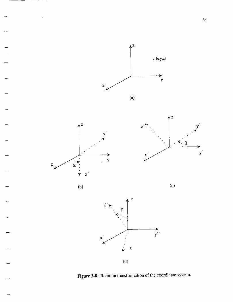
Let (x,y,z) describe the coordinates of any point in our coordinate system. As

shown in Figure 3-8(b), consider a rotation of angle o_ about the z axis, i.e. in the

xy-plane. Then the new coordinates in terms of the old are represented as

x = x'cos_ + y'sino_

and

i.e., the rotation matrix is

y = -x'sinct + y'coso_;

R_

cos0_ sinct il-SoOt COS(/,O "

Next, as shown in Figure 3-8(c), consider a rotation about the x' axis by an angle 13,

i.e., in the y'z plane, of the same point. The resultant coordinates and the old coordi-

nates are now related by the following equations:

y' = y"cos13 + z'sin13

and

where the rotation matrix is

z = -y"sin13 + z'cos13,

35

01RI3= cos_ sinl3 .

-sinl3 cosl3]

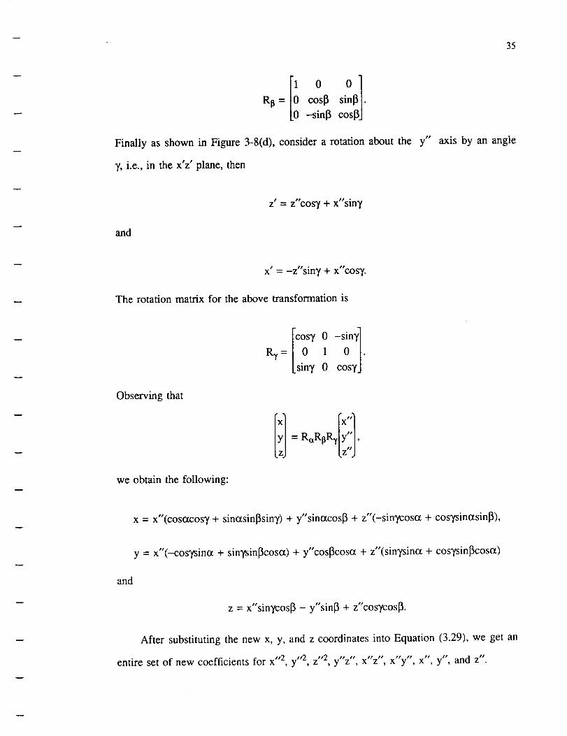
Finally as shown in Figure 3-8(d), consider a rotation about the

Y, i.e., in the x'z' plane, then

z' = z"cosy + x"siny

and

y" axis by an angle

x' = -z"siny + x"cos?.

The rotation matrix for the above transformation is

Observing that

we obtain the following:

[CoS ° 1Rq,= 1 .

Lsiny 0 cosyj

x = x"(cos_cos? + sino_sinl3sinT) + y'sinotcos[3 + z'(-sinycoscz + cosTsinczsinl3),

y = x'(--cosTsinot + sinysin_coso0 + y'cos[3cosc_ + z'(sinTsinot + cosysin[3coso0

and

z = x'sinycosl3 - y"sin_ + z"cosycos_.

After substituting the new x, y, and z coordinates into Equation (3.29), we get an

_,,2 y,,2, _,,2 " " " " " " " " Z"entire set of new coefficients forx , _ ,y z ,x z ,x y ,x ,y ,and .

w

36

Z

• {x.y,z)

f

Y

(a)

Z

r

Y-.g

xt

Yf

X

f

y

Z

_Z

y"

Y

(b) (c)

i I

-f

Z'

X

, J

y

(d)

Figure 3-8. Rotation transformation of the coordinate system.

37

These new coefficients are listed below.

a" = cos_ [a-cos2a + b-sin2a] + sin213sin2y [a-sin2a + b-cos2a]

+ 2sinotsinl3sin_oso_cosT (a - b) + c-sinZycos2_

- sin2a [h.sin213sinZ'/] - sin2y [f-sinotcosl3 + g-cosacosl3

+ h-cos2asinl3 - h'sinl3sin2a ]+ sin213sinZy (f-cosa - g.sina) + h.sin2_.cos2T.

b" = (a'sin2c_ + b.cos2ot)cos2_ + c.sin213 + sin213 [-f.coso_ - g.sinot ]

+ h.sin2acos213.

(3.30)

(3.31)

c" = sin2y (a-cos2o_ + b-sin2oO + (a.sin2ct + b-cos2ot)cos23sin2_

+ 2sinotsin_3sinTcosacosy (a - b) + c'cosZw, os2_3 + sin2a [h.cosZysin2_3 - h'sinZT] (3.32)

+ cos_sin2_ [f-cosoc + g.sinoq + sin2y [-f.sinotcos[_ + g'cosotcosl3+ h.cos2otsin[3].

2f"= [(b'cos2ot + a.sin2a + h.sin20t - c)sin2[3 + (2g.sinot + 2f-coso0cos213]cosy

+ [((a - b)sin2o_ + 2h.cos2o0cosl3 - (2g-cosot - 2f.sino0sinl3] sin 7 . (3.33)

r

2g" = sin2y[-cos2ot(a + b-sin2J3) - sin2_(a.sin2_ + b) - c.cos213

- sin[3eos[3(f-cosot + g.sinot) + h.sinotcosotcosl3

+ 2cos[_cos27(f.sinoc - g.cosot) + 2h-sin_(sinZotsin27 - cosZotcos27).

(3.34)

[- q

2h"= sin2(xlcoso_cosl3(b - a)- h-sinl3sinNosl3 [ + sin213sinq,(a.sin2a - b-cos2a + c)

+ cos"tsinl3(2g-cosot - 2f-sinot) + sinZl3sin_2g.sinot + 2f.cosot) (3.35)

- 2h.cos2otcos_cosl3.

2p" = 2cosy [-p-cosot + q-sinoq - 2sinl3siny [p.sinot + q-cosot] - 2r'sinycosl3. (3.36)

2q" = 2cos13 [p.sino_ + q-cos_] - 2r.sinl3. (3.37)

2r" = 2cosysinl3 [p.sinot + q-cosot] + 2siny [p.cosc_ - q.sinoq + 2r-cos_osl3. (3.38)

d" = d. (3.39)

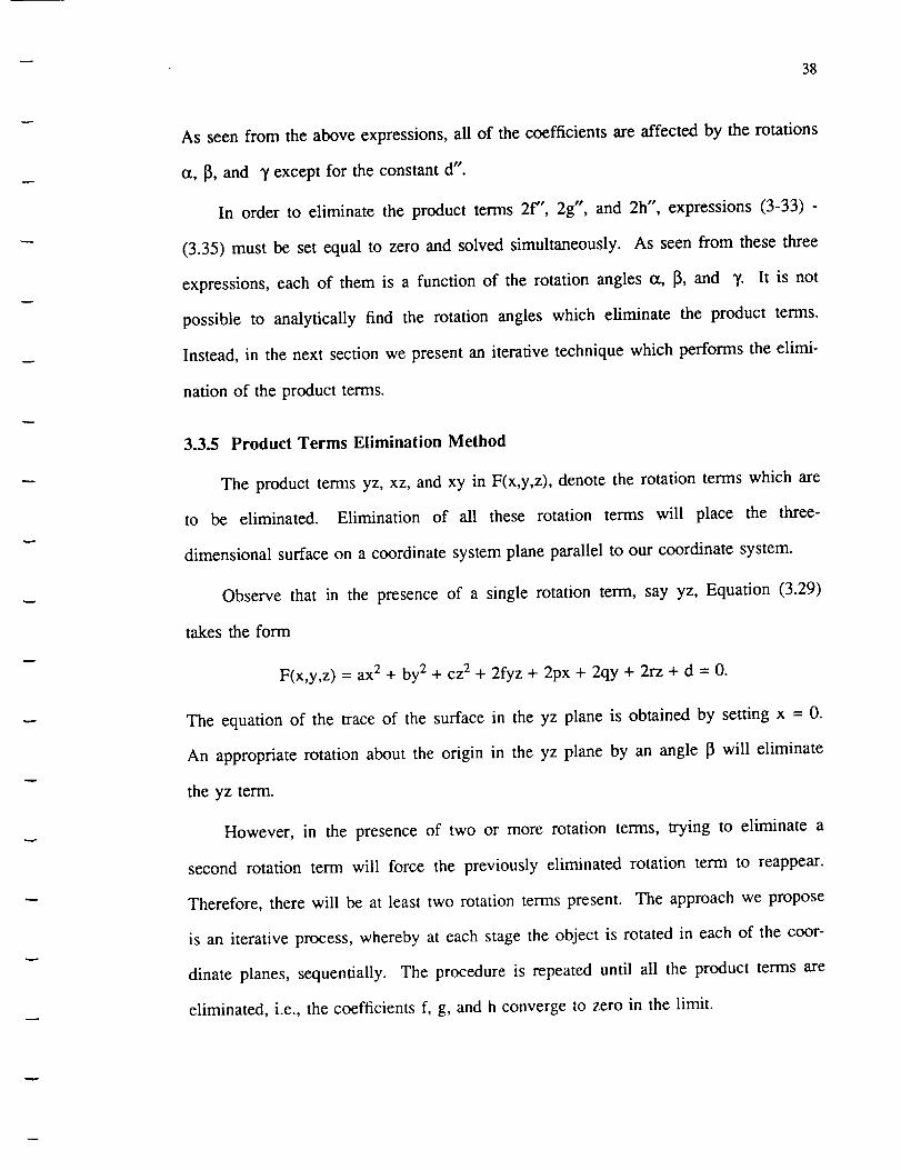
38

As seenfrom theaboveexpressions,all of the coefficients are affected by the rotations

or, [3, and _, except for the constant d".

In order to eliminate the product terms 2f", 2g", and 2h", expressions (3-33) -

(3.35) must be set equal to zero and solved simultaneously. As seen from these three

expressions, each of them is a function of the rotation angles 0_, [3, and _,. It is not

possible to analytically find the rotation angles which eliminate the product terms.

Instead, in the next section we present an iterative technique which performs the elimi-

nation of the product terms.

3.3.5 Product Terms Elimination Method

The product terms yz, xz, and xy in F(x,y,z), denote the rotation terms which are

to be eliminated. Elimination of all these rotation terms will place the three-

dimensional surface on a coordinate system plane parallel to our coordinate system.

Observe that in the presence of a single rotation term, say yz, Equation (3.29)

takes the form

F(x,y,z) = ax 2 + by 2 + cz 2 + 2fyz + 2px + 2qy + 2rz + d = 0.

The equation of the trace of the surface in the yz plane is obtained by setting x = 0.

An appropriate rotation about the origin in the yz plane by an angle [3 will eliminate

the yz term.

However, in the presence of two or more rotation terms, trying to eliminate a

second rotation term will force the previously eliminated rotation term to reappear.

Therefore, there will be at least two rotation terms present. The approach we propose

is an iterative process, whereby at each stage the object is rotated in each of the coor-

dinate planes, sequentially. The procedure is repeated until all the product terms are

eliminated, i.e., the coefficients f, g, and h converge to zero in the limit.

39

Sinceour aim is to eliminate the rotation terms xy, yz, and xz, let's exclusively

consider the coefficients of these rotation terms, namely f, g, and h evaluated in Sec-

tion 3.3.4. In our iterative procedure we are able to eliminate all of the product terms.

For example, suppose we wish to eliminate the term xy. By a specific rotation of o_

about the z axis, we will be able to accomplish our goal. However, while executing

this process, the orientation of the object about the two planes yz and zx, i.e., the

angles the object make with these two planes have been changed. If we wish to elim-

inate the yz term, the object has to be rotated about the x axis by an angle _. How-

ever, in this instance, while performing the process, the previously eliminated xy term

reappears though the magnitude of its present orientation has been reduced. Hence by

iterating the above process, an instance occurs when all the coefficients of the product

terms converge to zero in the limit.

Consider the Equations (3.33), (3.34), and (3.35). First eliminate the coefficient h,

i.e, the xy term. This can be accomplished by rotating the object about the z axis by

an angle ct, whereas I3---T=0. Under these circumstances the new coefficients are as

shown below.

2fll = 2g'sinoq + 2f-cosoq,

and

b-a

where cot2oq - 2h

2g11 = 2g'cosoq - 2f-sintz I,

2hll = (a - b)sin2oq + 2h.cos2c_ 1 = 0,

As seen above, the coefficient h has been forced to 0. The first digit of the subscript

refers to the iteration number, whereas the second digit of the subscript denotes the

number of times the object has been rotated by a specific angle. The remaining

coefficients a, b, c, p, q, and r also reflect changes brought about by the above rotation.

w

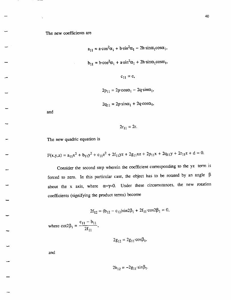
40

The new coefficients are

all = a.cos2otl + b-sin2otl - 2h.sinalcosotl,

bll = b.cos20q + a.sin2ctl + 2h.sinotlCOSCt 1,

Cll = c,

2pl 1 = 2p'cosoq - 2q'sint_ 1,

and

2ql 1 = 2p.sina 1 + 2q.cosoq,

2rl 1 = 2r.

The new quadric equation is

F(x,y,z) = all X2 + blly 2 + Cll z2 + 2fl_yz + 2gllxz + 2pllx + 2qlly + 2rllz + d = 0.

Consider the second step wherein the coefficient corresponding to the yz term is

forced to zero. In this particular case, the object has to be rotated by an angle

about the x axis, where 0_--T=0. Under these circumstances, the new rotation

coefficients (signifying the product terms) become

where cot2131 -

and

2f12 = (b12 - c12)sin2_l + 2fll.COS2_l = 0,

Cll - bll

2fl 1

2g12 = 2g ll'cos[_l,

2h12 = -2g11.sin_l.

41

At the same time the other coefficients become

a12 = a11,

b12 = Cll-sin2_l + blfCOS2_l - 2fll.sin_lcos[51 ,

c12 = bll.sin2_l + Cll-COS2_l + 2flfsinl31cos_31,

2p12 = 2P11,

and

2ql 2 = 2q11-cos_l - 2rlfsinI31,

2r12 = 2qlfsini31 + 2rll.COS_l.

The new quadric equation is:

F(x,y,z) = a12x 2 + b12y 2 + c12z 2 + 2g12xz + 2h12xy + 2p12x + 2q12y + 2r12z + d = 0.

In the final step of the initial iteration, the coefficient corresponding to the xz term is

forced to zero. In this case, the object is to be rotated by an angle _, about the y

axis, whereas ot=15----0. Under these circumstances, the new rotation coefficients beco-

men

2f13 = 2h12-sin_/1 = -2gll.sin131sin', h,

2g13 =(a13 - Cl3)sin2Yl + (2gll.COSOt 1 - fll-sinoq)cos_lcos2Y1 = 0,

where cot271 -c12 -- a12

2g12

and

2h13 = 2h12-cos71 = -2gll.sin_lcos71.

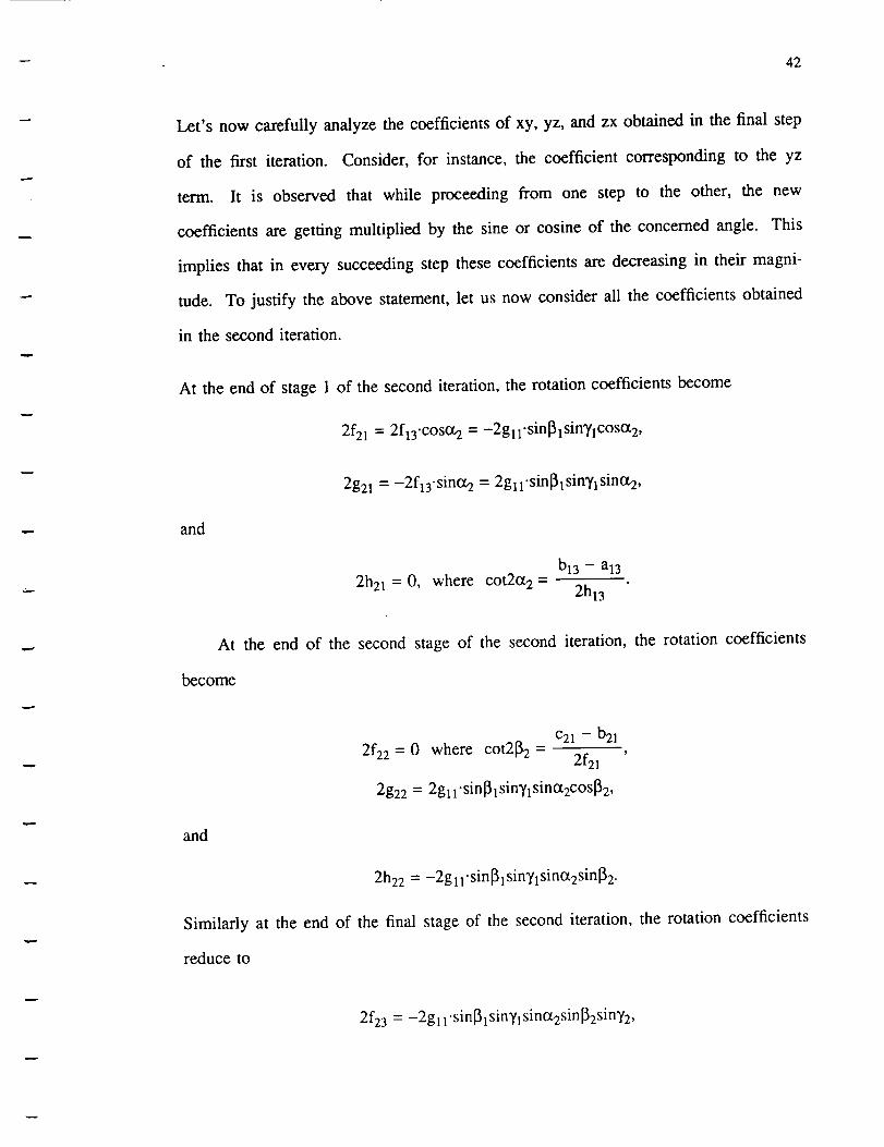
42

Let's now carefully analyzethecoefficientsof xy, yz, and zx obtainedin the final step

of the first iteration. Consider,for instance,the coefficient correspondingto the yz

term. It is observed that while proceedingfrom one step to the other, the new

coefficientsare getting multiplied by the sineor cosineof the concernedangle. This

implies that in every succeedingstepthesecoefficientsaredecreasingin their magni-

tude. To justify the abovestatement,let us now considerall the coefficientsobtained

in the seconditeration.

At the endof stage1 of the seconditeration,therotationcoefficientsbecome

2f21= 2fl3-COSO.2 = -2g ll-sin131sinTlcostx2,

and

2g21= -2f13"sintz2 = 2g 1l"sin131sinT1 sinot2,

2h21 = 0, where cot20t 2 -b13 - a13

2h13

At the end of the second stage of the second iteration, the rotation coefficients

become

and

c21 - b212f22-" 0 where cot2_2 =

2f21

2g22 = 2gl 1"sin [31sinY1sinct2cos[32,

2h22 = -2gl 1"sin131sinY1 sinct2sin[32.

Similarly at the end of the final stage of the second iteration, the rotation coefficients

reduce to

2f23 = -2g 1l'sin[31sinYlsinot2sin132sin72,

-v

43

2g23 = 0 where cot2ct 2 -b13 - a13

2h13

and

The terms ot2, 152, and

2h23 = -2gl 1"sin _t sin?l sintx2sin 152cos72 '

?2 are the respective rotation angles along the z, x, and y axes

in the second iteration. Hence it is observed with each iteration that the rotation

coefficients get smaller and smaller in magnitude and eventually disappear in the limit.

We are now in a position to formulate a rotation matrix whose elements

correspond to the directional cosines of the x, y, and z axes of the rotated object.

The rotation matrix = R.tR_R a,

where

and

coso: sintx 0

-sintx coso_ ,

0 0

0]RI_= cos_ sin15 ,

-sin[_ cos15J

R -'- Io -011

Lsin? 0 cosT.]

44

Subsequently,

RvRI R =

where

osc_tcos_, - sinotsinl3siny cosysin_ + sin_inl3coso_ -sin_os_]

---cosl3sinot cosl]cosot sinl3 [,inyzosot + cos_inotsinl3 sinotsiny--cosysinl]cos0t cosl3cosy]

(3.40)

n n n

a = Zc ,13= Zl3i,and =i=l i=l i=l

tion terms go to zero in the limit.

n corresponds to the iteration where all the rota-

Once the rotation terms, i.e., xy, yz, and xz are eliminated, the three-

dimensional surface has the representation of

F(x,y,z) = Ax 2 + By 2 + Cz 2 + 2Px + 2Qy + 2Rz + D = 0, (3.41)

where A, B, C, P, Q, and R are the coefficients resulting after the elimination of the

rotation terms. A natural question to ask is: Can the terms of the first degree be elim-

inated by means of a translation? The answer is sometimes they can and sometimes

they cannot. The case, where the term can be eliminated, is supported by the follow-

ing theorem.

3.3.6 Translation of the Rotated Object

Theorem 3.2. The terms of the first degree of an equation of a quadric surface

can be eliminated by means of a translation if and only if the surface has a center, in

which case the first degree terms are eliminated if and only if the new origin is a

center [24].

The method of completing squares is the easiest to determine the coordinates of

the new origin. Consider Equation (3.41). Grouping the like terms:

Ax 2 +2Px +By 2 + 2Qy + Cz 2 + 2Rz + D = 0 =>

45

AIx2 2P B y2 20 Clz2 2R 1Upon completing squares, we get

+D=0.

A + +B + +C + +D- +---if-+

where -P/A, -Q/B, and -R/C are the coordinates of the new origin.

= 0, (3.42)

3.4 Summary and Problem Identification

All of the above procedures performed until now result in a second degree poly-

nomial describing an unknown object, the center of the object lying at the origin of

our coordinate system. Had the test data been simulated, the three-dimensional

discriminant approach which was mentioned in Chapter One could be used to describe

and recognize the object. Since the test data is not simulated, we should utilize a

recognition algorithm which will distinguish and recognize each of the test surfaces

from one another.

The intersection of a surface with a plane generates a curve. The nature of this

curve depends solely on what type of object is intersected and with which particular

plane and in which orientation. Since we have no knowledge of the surface type, a

priori, one approach is to intersect the surface with a series of planes. We need to

determine the optimum number of planes which will uniquely characterize each of the

quadric surfaces.

Our goal is to derive a consistent method for determining the minimum number

of planes necessary to intersect a given quadric surface so that the generated conics

uniquely characterize the surface. This goal includes the derivation and formulation of

the angular bounds for which a particular plane intersecting a surface generates the

same two-dimensional curve. In summary, each of the quadric surfaces is represented

46

by a uniquefive-tuple, whoseelementssignify the presenceor absenceof the follow-

ing curves: circle, ellipse,hyperbola,parabola,anda line.

Chapter Four covers the description and recognition of each of the three-

dimensionalsurfaceswe haveabovementionedin Section3.2. A distinct patternvec-

tor is obtainedfor eachof the surfaces.

CHAPTER FOUR

QUADRIC SURFACE CHARACTERIZATION AND RECOGNITION

4.1 Introduction

Our proposed method utilizes a two-dimensional discriminant which is a measure

for distinguishing curves. Since the ten generated coefficients described in Section

3.3.3 of Chapter Three give a three-dimensional representation of the surfaces, we pro-

pose to identify the quadrics using the information resulting from the intersection of

the surface with different planes. If the surface is one of those considered for the

recognition process (see figures 3-1, 3-2, and 3-3), there are five possible two-

dimensional curves that may result from such intersections: (i) a circle, (ii) an ellipse,

(iii) a parabola, (iv) a hyperbola, and (v) a line. Thus, a feature or pattern vector with

five independent components can be formed for characterizing each of the surfaces.

The two-dimensional discriminant criteria we use to recognize each of the two-

dimensional curves created by planes intersecting the various quadric surfaces is dis-

cussed in Section 4.2. In Section 4.3 the results of Chapter Three are used to com-

pletely implement our recognition algorithm. Concomitantly, we derive a consistent

method for determining the minimum number of planes that are necessary to intersect

a given three-dimensional surface so that the generated conics uniquely characterize

the surface. The formulation of a three-dimensional discriminant similar to the two-

dimensional discriminant is presented in Section 4.4. The mapping between the expli-

cit and implicit representations of quadric surfaces is also examined in this section.

47

m

48

4.2 Two-Dimensional Discriminant

Given a conic of the form

F(x,y) = Ax 2 + Bxy + Cy 2 + Dx + Ey + F = 0,

the discriminant 5 = B 2 - 4AC characterizes it as one of the following [30]:

If _i = B 2 - 4AC < 0, then the conic is an ellipse or a circle.

If _ = B 2 - 4AC = 0, then the conic is a parabola.

If _ = B 2 - 4AC > 0, then the conic is a hyperbola.

Our objective is to derive a consistent method for determining the minimum

number of planes required to intersect a given three-dimensional surface so that the

generated conics uniquely characterize the surface. This includes the derivation and

formulation of the angular bounds for which a particular intersecting plane yields the

same two-dimensional curve.

The three-dimensional surfaces (objects) to be recognized are listed below:

(a) an ellipsoid,

(b) a circular cylinder,

(c) a sphere,

(d) a quadric cone,

(e) a hyperboloid of one sheet,

(f) a hyperboloid of two sheets,

(g) an elliptic paraboloid,

(h) a hyperbolic cylinder,

(i) a parabolic cylinder,

(j) a hyperbolic paraboloid, and

(k) a parallelepiped.

49

4.3 Quadric Surface Description and Representation

As discussed in Section 3.2 of Chapter Three, we now assume that the three-

dimensional objects have undergone two basic transformations, rotation and translation.

Consequently the product terms in the representation F(x,y,z) for a particular surface

have been eliminated and the center of the surface lies at the origin of our specified

coordinate system. As illustrated in Figure 4-1, all of the surfaces are contained in the

xy plane with their centers at O (the origin). For each surface, the characterization is

performed in two steps. Initially we consider the intersection of each object with two

planes (horizontal and vertical). This step does not require that the surface undergoes a

translation transformation. We refer to plane 1 as the one that intersects the object

parallel to the xy plane, i.e., z constant. Also refer to plane 2 as the one that inter-

sects the object parallel to the xz plane, i.e., y constant. In the second step, the

minimum set of intersecting planes needed to yield a unique feature vector (the various

curves serve as features) is determined. In this step we assume that the object has

undergone the translation transformation. The following sections describe the

representation procedure for each of the quadric surfaces listed in Section 4.2.

4.3.1 Ellipsoid

Step 1"

Consider the equation of an ellipsoid resting on a plane parallel to the xy plane

and its axis of revolution parallel to the z axis. Equation (3.1) reduces to the form

F(x,y,z) = ax 2 + by 2 + cz 2 + 2px + 2qy + 2rz + d = 0, (4.1)

which further reduces to

50

x

Y

z

I.:- J -.

o

X

Figure 4-1. Quadric surfaces from left to right and top to bottom: ellipsoid,

quadfic cone, hyperboloid of one sheet, elliptic cylinder, hyperboloid of two

sheets, hyperbolic cylinder, hyperbolic paraboloid, elliptic paraboloid, and

parabolic cylinder.

51

+ +1 1 1

a b c

1 = O, (4.2)

,,2 rwhere a > 0, b > 0, c > 0 and we have assumed the scaling d = .r__ + _ + -- - 1.

a b c

that the coefficients a, b, c, p, q, r, and d are all known; _--la,It should be noted

G, and _f-_ are the semi-major and minor axes of the ellipsoid, respectively; and

[-p/a, -q/b, -r/c] are the coordinates of the center of the ellipsoid.

-r

c

Consider the intersection of the ellipsoid with plane

---_f_-<k<-'--Lr + _cl--'then'c

1, i.e., z = k, where

(y + _)2 (x + P_.)2a+ - 1 = 0, (4.3)

1 (ck + r) 2 1 (ck + r) 2

b bc a ac

which is the equation of an ellipse.

Let's now consider the intersection of the ellipsoid with plane

b-_ G -q +G 'then'where - < k < b

2, i.e., y= k,

(x + P__)2 (z + L)2a c

+ -1=0,1 (bk + q)2 1 (bk + q)2

a ab c bc

(4.4)

which is again the equation of an ellipse. For the case when the two minor axes are

equal, the surface is called a spheroid. Also, when all the axes are equal, i.e., a = b =

c, the surface is a sphere. Intersection of the sphere with planes is discussed in Sec-

tion 4.3.3.

52

Step 2:

As mentioned before, we assume that the ellipsoid has undergone a translation,

such that its center aligns with the origin of our desired coordinate system as shown in

Figure 4-2. Hence its representation can be assumed as

X 2 y2 Z 2

A2 +-_+ C2 = 1, (4.5)

where A, B, and C are the major and minor semi-axes, respectively, of the ellipsoid.

As seen in step l, intersection of the ellipsoid with any Z = ] k [, --C < k _< C, will be

an ellipse. Let us now determine the bounds within which inclined sub-planes of Z =

]k [still result in an elliptic intersection with the ellipsoid.

Consider the points E(A,0,0), F(0,B,0), and G(0,0,K), where K > 0. The equa-

tion of the plane containing these points is:

BKX + AKY + ABZ - ABK = 0.

Solving for Z and substituting in Equation (4.5) yields the curve of intersection:

X2(B2C 2 + B2K 2) + y2(A2C2 + A2K 2) + 2AK2BXY + • • • = 0. (4.6)

In the above equation only terms which are necessary to determine the intercepted

curve are retained. Proceeding with the discriminant test,

8 = 4A2B2[-C 4 - 2C2K2].

Since the discriminant is always negative, the intercepts are ellipses. Angular bounds

in terms of an angle are not needed in this case, since the only occasion the intercepts

are different than ellipses is when two of the semi-axes are equal. Under that cir-

cumstance, we arrive at a circular intercept. Figure 4-3 illustrates vertical planes inter-

secting the ellipsoid. Table 4-1 summarizes the result obtained above.

53

DETAILED VIEW: HORIZONTAL INTERSECTIONS

X

Z

= •

Y

Figure 4-2. The plane parallel to the x-axis and all its inclined sub-planes generate

ellipses. In the case of a spheroid all intersections are ellipses except when the

plane is parallel to one of the axes under which case the intersection is a circle.

54

DETAILED VIEW: VERTICAL INTERSECTIONS

X

Z

b •

I

#

Y

Figure 4-3. The plane parallel to the z-axis and all its inclined sub-planes generate

ellipses. In the case of a spheroid all intersections are ellipses except when the

plane is parallel to one of the axes under which case the intersection is a circle.

55

PLANE INTERSECTION

Z=K

Y=K

Any inclined sub-planesto Z=K, Y=K

Ellipse

Ellipse

Ellipse

Table 4-1. Intersectionof ellipsoid with planes.

4.3.2 Circular (elliptic) cylinder

Step 1:

Consider the general representation of a circular cylinder resting on a plane paral-

lel to the xy plane and its axis of revolution parallel to the z axis. It's representation

then reduces to

F(x,y,z) = bx 2 + by 2 + 2px + 2qy + d = 0, (4.7)

which is the same as

y+ x+

F(x,y,z) - + 1 = 0, (4.8)1 1

b b

q2 p2only if d = -- +

b b--- 1 and alsob>0.

In the case of the elliptic cylinder, Equation (4.7) becomes

F(x,y,z) = ax 2 + by 2 + 2px + 2qy + d = O,


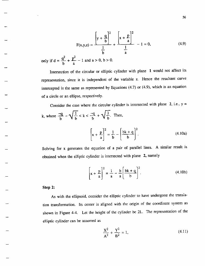
56

F(x,y,z) =1

b

q2only if d = -- + - 1 and a > 0, b > O.

b a

+ 1 = O, (4.9)1

a

Intersection of the circular or elliptic cylinder with plane 1 would not affect its

representation, since it is independent of the variable z. Hence the resultant curve

intercepted is the same as represented by Equations (4.7) or (4.9), which is an equation

of a circle or an ellipse, respectively.

Consider the case where the circular cylinder is intersected with plane 2, i.e., y =

k, where - < k < + Then,

+Solving for x generates the equation of a pair of parallel lines.

obtained when the elliptic cylinder is intersected with plane

(4.10a)

A similar result is

2, namely

Step 2:

aba bk b+ q ] 2.

(4.10b)

As with the ellipsoid, consider the elliptic cylinder to have undergone the transla-

tion transformation. Its center is aligned with the origin of the coordinate system as

shown in Figure 4-4. Let the height of the cylinder be 2L. The representation of the

elliptic cylinder can be assumed as

X 2 y2+--= 1, (4.11)

A 2 B 2

57

where A and B are the major and minor semi-axes of the cylinder. Intersection of the

cylinder with any plane Z = I k I,-L < k < L, is an ellipse. The angular bounds

within which an inclined plane will still result in an elliptic intersection is determined

next.

Consider the intersection of the plane passing through the points E(A,0,0),

F(-A,0,K), and G(0,-B,0) with the cylinder as shown in Figure 4-4. The equation of

the plane containing these points is:

BKX - AKY + 2ABZ - ABK = 0.

Solving for X,

X

AKY - 2ABZ + ABK

BK

Substituting X in Equation (4.11) results in

2K2y 2 + 4B2Z 2 - 4BKYZ +... = 0.

The discriminant results in a quantity less than zero. Hence the intersection is an

ellipse.

Given any two planes, alx + bly + clz + dl = 0, and a2x + b2Y + c2z + d2 = 0,

the angle of intersection is given as

cos0 =lala 2 + bib 2 + clc21

"_al2 + bl2 + cHa22 + b_ + c22"

Hence, in the above case the intersections with respect to the plane z = 0 and all the

planes inclined to it (which we will refer to as inclined-sub planes), yield ellipses for

cos0 <2AB

N/(A2K 2 + 4A2B 2 + B2K 2)

m

58


X

Z

plane 2

F .•

a

0

b

C ._." ................

• I". - o " . .

plane 1

YA

plane 3

Figure 4-4. Plane 1 and the planes parallel to it within the range -L to L

(length of the cylinder) intersect the cylinder in parallel lines. Plane 2 and

plane 3 are the inclined sub-planes of plane 1 which determine the maxi-

mum range or inclination (with plane 1) wherein similar curves (ellipses)

are generated. 0 is the angular bound for the inclination in terms of an

angle.

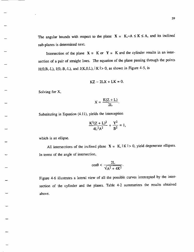
59

The angular bounds with respect to the plane X = K,-A < K < A, and its inclined

sub-planes is determined next.

Intersection of the plane X = K or Y = K and the cylinder results in an inter-

section of a pair of straight lines. The equation of the plane passing through the points

H(0,B,-L), I(0,-B,-L), and J(K,0,L), I K I> 0, as shown in Figure 4-5, is

KZ - 2LX + LK = 0.

Solving for X,

X - K(Z + L)2L

Substituting in Equation (4.11), yields the interception

K2(Z + L)2 y2+_=l,

4L2A 2 B 2

which is an ellipse.

All intersections of the inclined plane X = K, I K I> 0, yield degenerate ellipses.

In terms of the angle of intersection,

2Lcos0 <

"_A 2 + 4K 2

Figure 4-6 illustrates a lateral view of all the possible curves intercepted by the inter-

section of the cylinder and the planes. Table 4-2 summarizes the results obtained

above.

60

DETAILED VIEW" VERTICAL INTERSECTIONS

- -. plane 3 plane 1 plane 2

X

°

. Y

Ik

H

Figure 4-5. Plane 1 and the planes parallel to it within the range -a to a

intersect the cylinder in parallel lines. Plane 2 and plane 3 are the inclined

sub-planes of plane 1 which determine the maximum range or inclination

(with plane 1) wherein similm" curves (degenerate ellipses) are generated.

0is the angular bound for this inclination in terms of an angle.

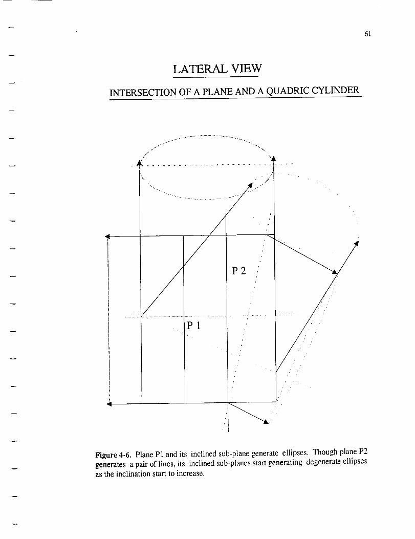
61

LATERAL VIEW

INTERSECTION OF A PLANE AND A QUADRIC CYLINDER

P2

P1

Figure 4-6. Plane P1 and its inclined sub-plane generate ellipses. Though plane P2

generates a pair of lines, its inclined sub-planes start generating degenerate ellipses

as the inclination start to increase.

62

PLANE INTERSECTION

Z=K

X=K

Inclined sub-planes of Z=K

Inclined sub-planes of X=K

Circle, Ellipse

Lines

Ellipse

Lines

Table 4-2. Intersection of quadric cylinder with planes.

4.3.3 Sphere

Step 1:

As mentioned in Section 4.1., the sphere is a special case of an ellipsoid, where

the three semi axes are all equal. Equation (4.1) thus reduces to

F(x,y,z) = ax 2 + ay 2 + az 2 + 2px + 2qy + 2rz + d = 0, (4.12)


1 1 1

a a a

p2 q2 r2only if d = -- + -- + -- -

a b a.

Consider the case when the sphere is intersected with plane

-ra _al-- < k < ---sr + _ Then'a "

1 = 0, (4.13)

1, i.e., z = k, where

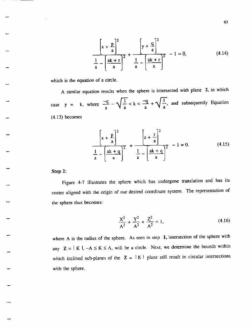
63

2+ I;t2I 1 ak r

a a

- 1 - O, (4.14)

which is the equation of a circle.

A similar equation results when the sphere is intersected with plane 2, in which

case y = k, where --q-_<k<a -'q+_'a and subsequently Equation

(4.13) becomes

2+ 21 1

a a

- 1 = 0. (4.15)

Step 2:

Figure 4-7 illustrates the sphere which has undergone translation and has its

center aligned with the origin of our desired coordinate system. The representation of

the sphere thus becomes:

X2 y2 z 2-_- + -_- + "-_ = 1, (4.16)

where A is the radius of the sphere. As seen in step 1, intersection of the sphere with

any Z = I K I, -A < K < A, will be a circle. Next, we determine the bounds within

which inclined sub-planes of the Z = I K I plane still result in circular intersections

with the sphere.

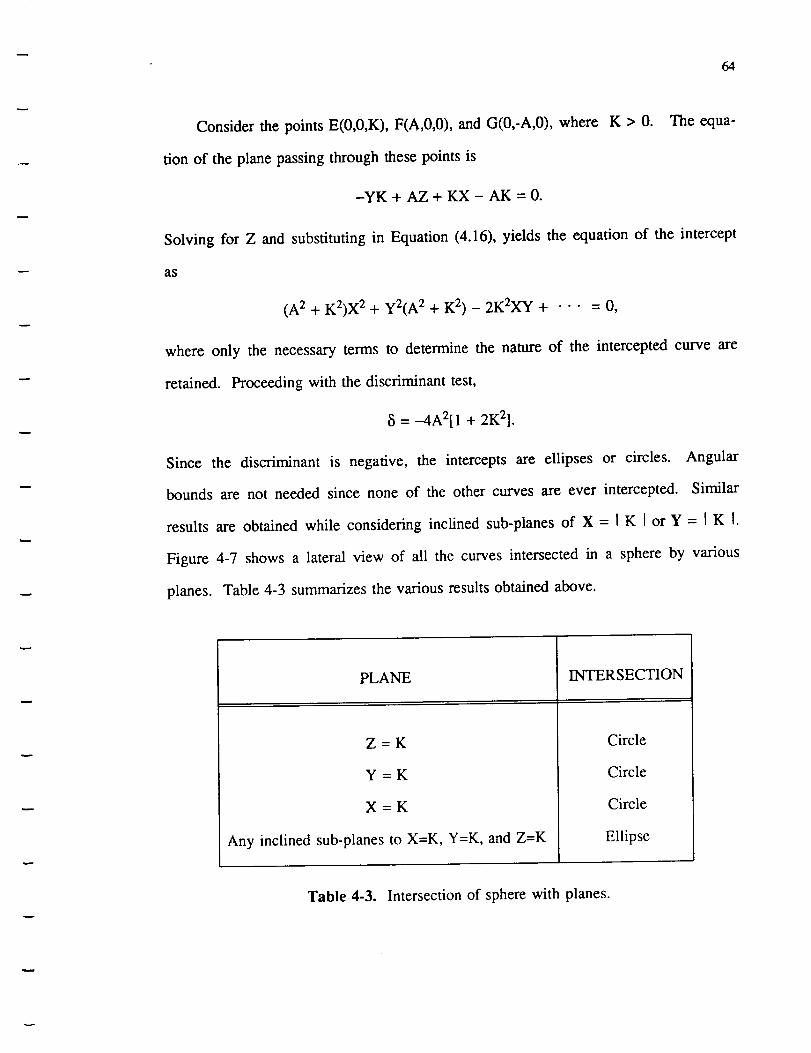
64

Consider the points E(0,0,K), F(A,0,0), and G(0,-A,0), where K > 0. The equa-

tion of the plane passing through these points is

-YK + AZ + KX - AK = 0.

Solving for Z and substituting in Equation (4.16), yields the equation of the intercept

as

(A 2 + K2)X 2 + y2(A2 + K 2) - 2K2Xy + • • • = 0,

where only the necessary terms to determine the nature of the intercepted curve are

retained. Proceeding with the discriminant test,

_i = --4A2[ 1 + 2K2].

Since the discriminant is negative, the intercepts are ellipses or circles. Angular

bounds are not needed since none of the other curves are ever intercepted. Similar

results are obtained while considering inclined sub-planes of X = I K [ or Y = [ K I.

Figure 4-7 shows a lateral view of all the curves intersected in a sphere by various

planes. Table 4-3 summarizes the various results obtained above.

PLANE

Z=K

Y=K

X=K

Any inclined sub-planes to X=K, Y=K, and Z--K

INTERSECTION

Circle

Circle

Circle

Ellipse

Table 4-3. Intersection of sphere with planes.

65

INTERSECTION OF A pLANE AND A sPHERE

X

Figure 4-7. The intersection of plane and a sphere results in a circular

line of intersection.

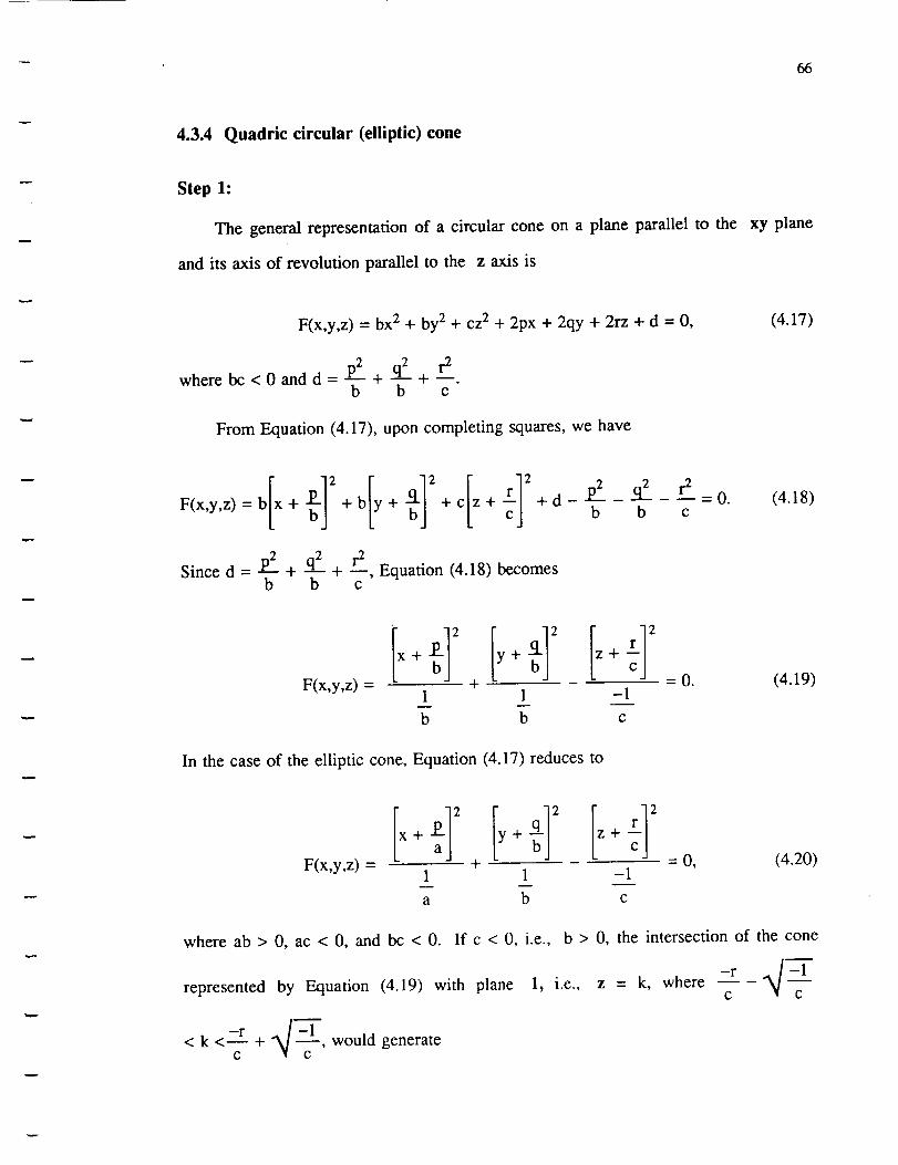
-- 66

4.3.4 Quadric circular (elliptic) cone

Step 1:

The general representation of a circular cone on a plane parallel to the

and its axis of revolution parallel to the z axis is

xy plane

F(x,y,z) = bx 2 + by 2 + cz 2 + 2px + 2qy + 2rz + d = 0,

p2 q2 r2where bc < 0 and d = -- + -- + --.

b b c

From Equation (4.17),upon completing squares,we have

(4.17)

F(x,y,z)=b + +b + +c z++d_p2_q 2 r2

b b c

p2 q2 r2 Equation (4.18) becomesSinced=--+ _+--,b b c

-- _ _ 0. (4.18)

+ + Z+

+ -0.F(x,y,z) - 1 1 -1

b b c

In the case of the elliptic cone, Equation (4.17) reduces to

(4.19)

x+ y+ z+

F(x,y,z) = 1 + 1 -1 - 0,

a b c

(4.20)

whereab> 0, ac<0, and bc < 0. Ifc < 0, i.e., b> 0, the intersection of the cone

represented by Equation (4.19) with plane 1, i.e., z = k, where ----!r---_/--_-c -7-

r< k <-- + , would generateC

67

1

b

+1 1

b c

(4.21)

1where --- is a positive quantity.

cThe above equation is that of a circle. The elliptic

cone on the other hand which is represented by Equation (4.20), upon intersection with

plane 1, i.e., z= k, where---s-r-4_-_l <k<'-r +4_ -_1 ,wouldgenerateC C

which is an ellipse.

where -q _b

1

a

+1 1

b c

(4.22)

The intersection of the circular cone with plane 2, i.e., y=k,

/-i-k < -q + "_ -;:-, would generate

b _ D

1 -1 1

b c b

1where --- is a positive quantity.

CEquation (4.23) represents a hyperbola.

result is obtained when the elliptic cylinder is intersected with plane 2.

(4.23)

A similar

Step 2:

The quadric representation of the elliptic cone illustrated in Figure 4-8 is

X 2 y2 Z 2--+A 2 B2 C 2

-0. (4.24)

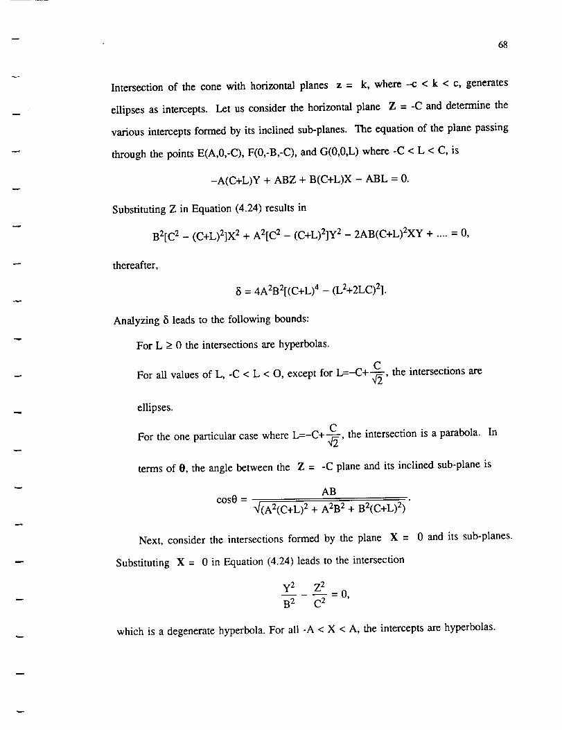
68

Intersection of the cone with horizontal planes z = k, where --c < k < c, generates

ellipses as intercepts. Let us consider the horizontal plane Z = -C and determine the

various intercepts formed by its inclined sub-planes. The equation of the plane passing

through the points E(A,0,-C), F(0,-B,-C), and G(0,0,L) where -C < L < C, is

-A(C+L)Y + ABZ + B(C+L)X - ABL = 0.

Substituting Z in Equation (4.24) results in

B2[C 2 - (C+L)2]X 2 + A2[C 2 - (C+L)2]Y 2 - 2AB(C+L)2Xy + .... = 0,

thereafter,

8 = 4A2B2[(C+L) 4 - (L2+2LC)2].

Analyzing 8 leads to the following bounds:

For L > 0 the intersections are hyperbolas.

For all values of L, -C < L < O, except for L=-C+_22 , the intersections are

ellipses.

For the one particular case where L=-C+_22 , the intersection is a parabola. In

terms of 0, the angle between the Z = -C plane and its inclined sub-plane is

ABCOS0 =

X/(A2(C+L) 2 + A2B 2 + B2(C+L) 2)

Next, consider the intersections formed by the plane X = 0 and its sub-planes.

Substituting X = 0 in Equation (4.24) leads to the intersection

y2 Z 2-- 0,

B 2 C 2

which is a degenerate hyperbola. For all -A < X < A, the intercepts are hyperbolas.

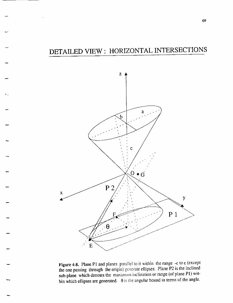
69

DETAILED VIEW" HORIZONTAL INTERSECTIONS

a

x

Figure 4-8. Plane P1 and planes parallel to it within the range -c to c (except

the one passing through the origin) generate ellipses. Plane P2 is the inclined

sub-plane which denotes the maximunl inclination or range (of plane P1) wit-

hin which ellipses are generated. 0 is the angular bound in terms of the angle.

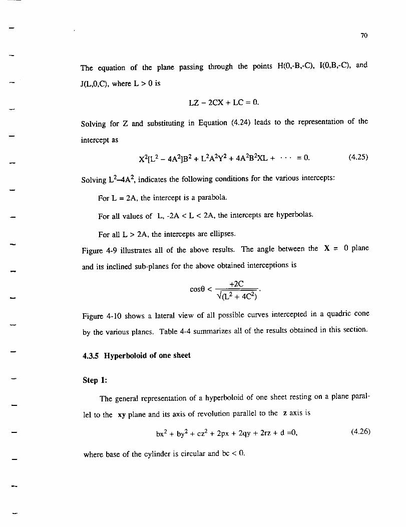
70

The equation of the plane passing through the points H(0,-B,-C), I(0,B,-C), and

J(L,0,C), where L > 0 is

LZ - 2CX + LC = 0.

Solving for Z and substituting in Equation (4.24) leads to the representation of the

intercept as

X2[L 2 - 4A2]B 2 + L2A2y 2 + 4A2B2XL + • • • = 0. (4.25)

Solving L2-4A 2, indicates the following conditions for the various intercepts:

For L = 2A, the intercept is a parabola.

For all values of L, -2A < L < 2A, the intercepts are hyperbolas.

For all L > 2A, the intercepts are ellipses.

Figure 4-9 illustrates all of the above results. The angle between the X = 0 plane

and its inclined sub-planes for the above obtained interceptions is

+2Ccos0 <

"_(L 2 + 4C2) "

Figure 4-10 shows a lateral view of all possible curves intercepted in a quadric cone

by the various planes. Table 4-4 summarizes all of the results obtained in this section.

4.3.5 Hyperboloid of one sheet

Step 1:

The general representation of a hyperboloid of one sheet resting on a plane paral-

lel to the xy plane and its axis of revolution parallel to the z axis is

bx 2 + by 2 + CZ2 + 2px + 2qy + 2rz + d =0, (4.26)

where base of the cylinder is circular and bc < 0.

71

DETAILED VIEW : VERTICAL INTERSECTIONS

r

X

P2

, P3 :

°

Figure 4.9. Plane P1 and planes parallel to it within the range-b to b generates

degenerate hyperbolas. Plane P2 is the inclined sub-plane which shows the outer

region or the maximum inclination (of plane P1) within which hyperbolas are int-

ercepted. 0is the angular bound in terms of the angle. Plane P3 is the only exce-

ption where the intersection is a parabola. In this case the inclination of the plane

P3 is equal to the base angle of the cone.

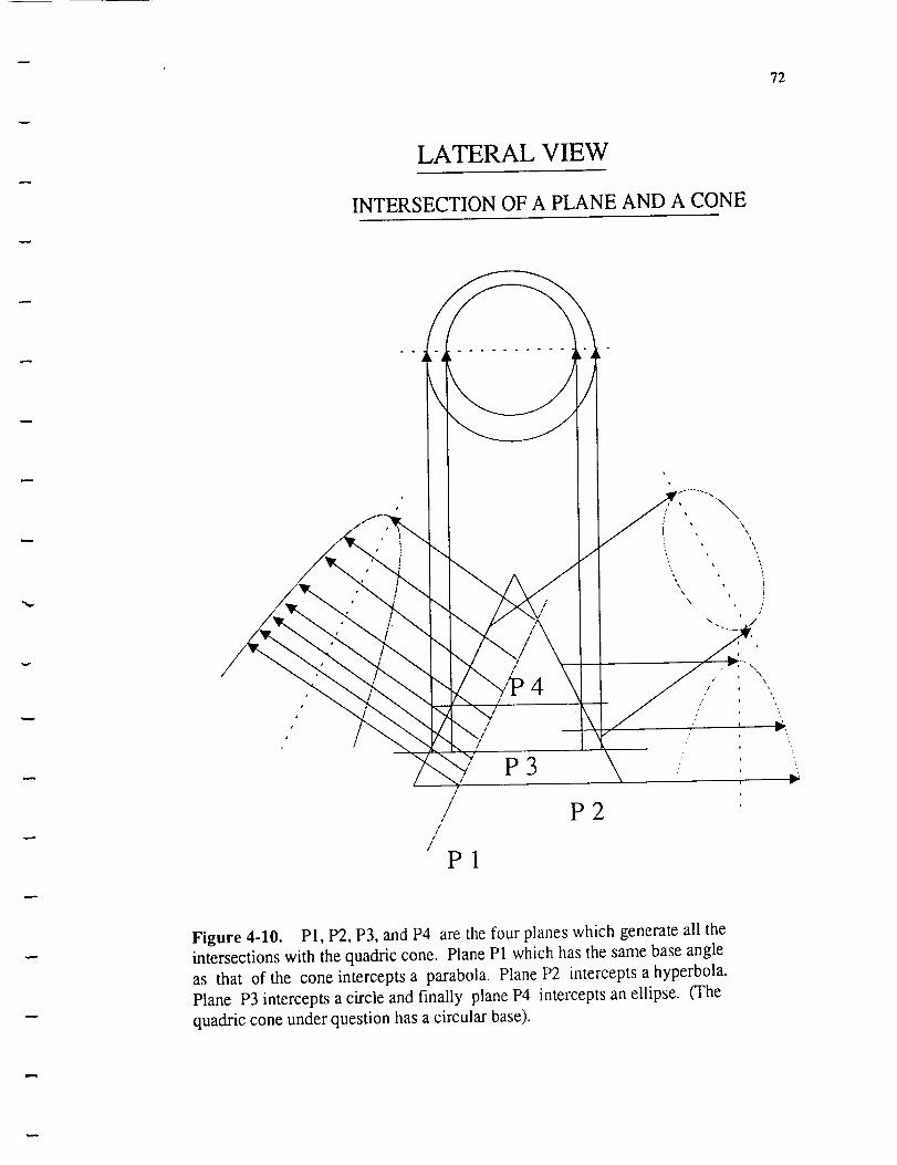
LATERAL VIEW

INTERSECTION OF A PLANE AND A CONE

72

,/

r

\

\

\

\

k°d

\i 1

\\

\

,< .,,#

P3

/

\\

\

_k f • v,

i v

/

// P2

P1

/

/

I

Figure 4-10. Pl, P2, P3, and P4 are the four planes which generate all the

intersections with the quadric cone. Plane P1 which has the same base angle

as that of the cone intercepts a parabola. Plane P2 intercepts a hyperbola.

Plane P3 intercepts a circle and finally plane P4 intercepts an ellipse. (The

quadric cone under question has a circular base).

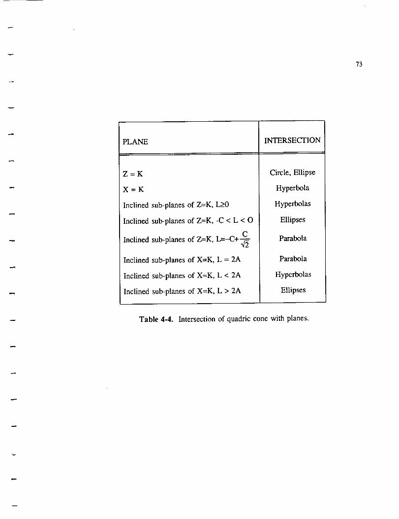
73

PLANE

Z=K

X=K

Inclined sub-planes of Z=K, L>_0

Inclined sub-planes of Z=K, -C < L < O

q2Inclined sub-planes of Z=K, L=-C+---

Inclined sub-planes of X=K, L = 2A

Inclined sub-planes of X=K, L < 2A

Inclined sub-planes of X=K, L > 2A

INTERSECTION

Circle, Ellipse

Hyperbola

Hyperbolas

Ellipses

Parabola

Parabola

Hyperbolas

Ellipses

Table 4-4. Intersection of quadric cone with planes.

Equation(4.26) upon completion of squares reduces to

74

N,,

(X + pb)2 (y + b_') 2 -(z + r)2c

F(x,y,z) = + +1 1 -1

b b c

.2 r2whered ==- + + m

b b c1.

=1,

If c < 0, i.e., b > 0, intersection of the hyperboloid with plane 1, i.e.,

-r/c - t < k < -r/c + , results in

z = k, where

(y+ b_-)2 (x+ bP')2 (k+r) 2+ = I + , (4.27)

l l -l

b b c

where -1/c is a positive quantity. Equation (4.27) represents a circle. For a hyper-

boloid with elliptic base, this intersection will be an ellipse.

Intersection of the hyperboloid with plane 2, i.e.,y= k, where-q/b-_/_'bl <

k<-q/b +_/_-, generates

(x + p--b)2 (z + r)2c (k + -g-)q 2-1

1 -1 -1

b c b

where -1/c is a positive quantity. This equation is that of a hyperbola.

are obtained when the hyperboloid has elliptic bases.

Similar results

75

Step 2:

As in the case of the other quadric surfaces, the elliptic hyperboloid of one sheet

shown in Figure 4-I1 is assumed to have undergone translation such that its center is

aligned with the origin of the coordinate system. The axis of the hyperboloid coincides

with the z axis.

is

Under these conditions the quadric representation of the hyperboloid

X 2 y2 Z 2+ = 1. (4.28)

A 2 B2 C 2

The intersection of the hyperboloid with horizontal planes ranging from Z = 0 to Z

= I K _ are ellipses, where -C < K < C and A, B, and C are the semi-axes of the sur-

face. The angular bounds of the various sub-planes with respect to the Z = 0 plane

which intersects the hyperboloid in ellipses is determined next.

As shown in Figure 4-11, the equation of the plane passing through the points

D(A,0,0), E(0,-B,0), and F(K,0,C) where I K I> 0 is

-ACY + B(A-K)Z - BCX - ABC = 0.

Solving for Z and substituting in Equation (4.28) results in

X2[B2(A-K) 2 - A2B 2] + yE[AE(A-K)2 - A 4] - 2A3BXY +

Proceeding with the discriminant test,

8 = 4A2B2[A 2 + K 2 - 2AK][A 2 - K 2 + 2AK].

Since A and K are always positive, based upon the term

[A 2 - K 2 + 2AK],

=0.

76

DETAILED VIEW : HORIZONTAL INTERSECTIONS

Z=0

Z

plan_ 2s

plane 1

X

o

plane 3

Figure 4-11. Plane 1 (z = 0) and all sub-planes parallel to it intersect the

hyperboloid in ellipses. Plane 2 and plane 3 denote the maximum bound

or inclination, within which the hyperboloid still intercepts ellipses.

77

a decisioncan be madewhetherthe intersectionis an ellipse, a hyperbolaor a para-

bola. Solving for K, we determinethatfor

K = A(-'_ + 1), the intersectionis a parabola,

K > A(-x/2 + 1), the intersectionis anellipse,and

K < A(-42 + 1), the intersectionsarehyperbolas.

eachof theseintersectionsis givenas

cos0=

The inclination of the planeat

B(A - K)

"_B2(A-K) 2 + A2C 2 + B2C 2

Next, consider intersection of the plane Z = -C with the hyperboloid as shown

in Figure 4-12. Substituting Z = -C in Equation (4.28) results in the intersection

X 2 y2--+ _=2,A 2 B 2

which is an ellipse as expected. To determine the bounds at which the inclined Z =

-C plane still generates ellipses, consider the plane passing through the points

G(L,0,-C), H(0,-B,-C), and I(M,0,K), where -C < K < C, I L I > I A [ The equation of

the plane results in

B(C + K)X - L(C + K)Y - B(L - M)Z - (2BCL + BLK - BCM) = 0.

Solving for Z and substituting in Equation (4.28) results in the intersection

X2[C2B2(L - M) 2 - A2B2(C + K) 2] + y2[C2B2(L - M) 2 - A2L2(C + K) 2]

+2LBA2(C+K)2XY+ "'" =0.

Evaluating the discriminant leads to the following:

= 4A2BZ[L2A2(C + K) 4 - [C2(L - M) 2 - A2(C + K)2][C2(L - M) 2 - L2(C + K)2]]

The bounds for the various intercepts are obtained as follows:

M = L, the intersection is a parabola,

78


Z -- -c

z I plane,,2.."

• _ a •S

X

\

G

Figure 4-12. Plane 1 (z = -c) and all sub-planes parallel to it intersect the

hyperboloid in ellipses. Plane 2 denotes the maximum bound or inclination,

within which the hyperboloid still intercepts ellipses.

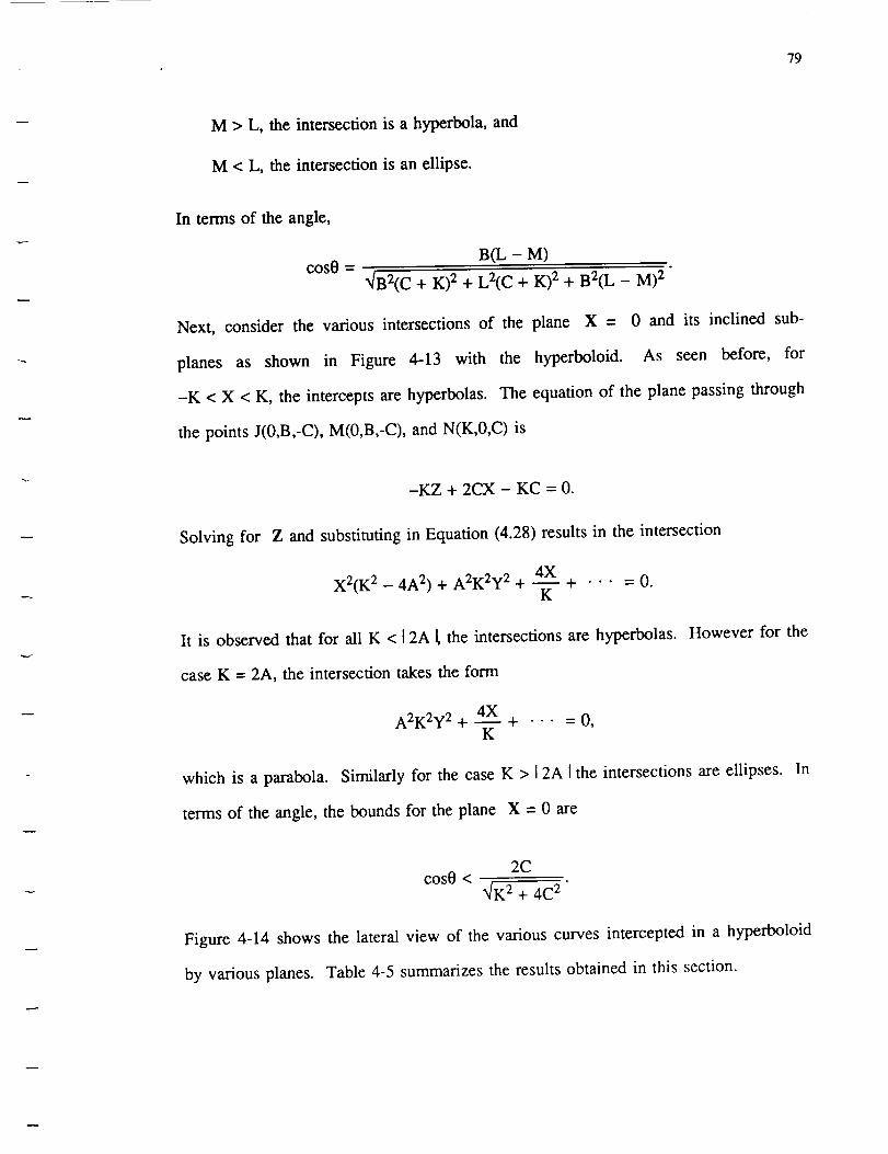
79

M > L, the intersectionis a hyperbola,and

M < L, the intersectionis anellipse.

In terms of the angle,

cos0 = B(L - M)

_B2(C + K) 2 + L2(C + K) 2 + B2(L - M) 2

Next, consider the various intersections of the plane X = 0 and its inclined sub-

planes as shown in Figure 4-13 with the hyperboloid. As seen before, for

-K < X < K, the intercepts are hyperbolas. The equation of the plane passing through

the points J(0,B,-C), M(0,B,-C), and N(K,0,C) is

-KZ + 2CX - KC = 0.

Solving for Z and substituting in Equation (4.28) results in the intersection

X2(K 2 - 4A 2) + A2K2y 2 +4X

+''" =0.K

It is observed that for all K < 12A [ the intersections are hyperbolas. However for the

case K = 2A, the intersection takes the form

A2K2y2+ 4..__XX+ ... =0,K

which is a parabola. Similarly for the case K > 12A I the intersections are ellipses. In

terms of the angle, the bounds for the plane X = 0 are

2Ccos0 <

_K 2 + 4C 2

Figure 4-14 shows the lateral view of the various curves intercepted in a hyperboloid

by various planes. Table 4-5 summarizes the results obtained in this section.

80


Z

plane 1

plane 2

N

X

J

Y

Figure 4-13. Plane 1 and all sub-planes parallel to it intersect the hyperboloid in

hyperbolas. The inclined sub-planes of plane 1 which are denoted in the above

figure by plane 2 and plane 3 determine the maximum range or bound wherein

hyperbolas are still intercepted. Beyond this range the hyperboloid intersects

various planes in ellipses except the case when the plane makes an angle of 5,

under which case the intercepted curve is a parabola.

81

LATERAL VIEW

INTERSECTION OF A PLANE AND HYPERBOLOID OF ONE SHEET

P3

/ !

Figure 4-14. Plane P1 intersects the hyperboloid in a parabola, plane P2

and all planes parallel to it intersect the hyperboloid in hyperbolas. Plane

P3 and all planes parallel to it in the range -c to +c intersect the hyperbo-

loid in ellipses.

82

PLANE INTERSECTION

Z=K

X=K

Inclinedsub-planesof








Z--0,K=A(-x/2 + 1)

Z--0,K>A(-_/2 + 1)

Z---0,K<A(-'_ + 1)

Z=-C, IZI< C

Z=-C, IZl> C

X=K, K < 12AI

X=K, K = 2A

X=K, K > 12AI

Circle, Ellipse

Hyperbola

Parabola

Ellipse

Hyperbola

Ellipse

Hyperbola

Hyperbola

Parabola

Ellipses

Table 4-5. Intersectionof hyperboloidof onesheetwith planes.

4.3.6 Hyperboloid of two sheets

Step 1:

Unlike the hyperboloid of one sheet, the hyperboloid of two sheets consists of

two separate pieces. The quadric representation of a hyperboloid of two sheets lying

on a plane parallel to the xy plane is

bx 2 + by 2 + cz 2 + 2px + 2qy + 2rz + d = 0, (4.29)

where the base of the hyperboloid is circular, bc < 0. Completing squares results in

(x + pb )2 (y + _)2 -(z + r)2cF(x,y,z) = + +

1 1 -1

b b c

# ,12 ,.2where d = x__+ .a__ + "__ + 1, and -1/c is a positive quantity.

b b c

object with the plane 1, i.e., z = k, where k I> ,fL"_, results in

= --1,

83

Intersection of the

(x + pb)2 (y + _)2 (k + r)2c+ =-1 +

1 1 -1

b b c

where -1/c is a positive quantity. This equation is of a circle. For a hyperboloid with

an elliptic base, this intersection will be an ellipse. However, when I kl= q'(-1/c), the

intersection will result in a point.

Consider the case when the object is intersected with the plane

where - q/b - _f_ < k < -q/b +_--_. This intersection results in

2, i.e., y = k,

-(x + P)2 -(z + r)2c (k + _-)q 2

+ - +1,1 -1 -1

b c b

which is an equation of a hyperbola. Similar results are obtained for a hyperboloid

with an elliptic base.

Step 2:

As in the case of the hyperboloid of one sheet, the elliptic hyperboloid of two

sheets is assumed to have undergone translation so that its center is aligned with the

origin of the coordinate system as shown in Figure 4-15. The axis of the hyperboloid

coincides with the z axis. Under these conditions the quadric representation of the

hyperboloid is

84

X2 y2 Z2+ = -1. (4.30)

A2 B2 C 2

The intersection of the hyperboloid with the horizontal plane Z = K, [ K J< C, is an

imaginary ellipse. For I K I> C, the horizontal plane will intersect ellipses as seen

from Equation (4.30).

Consider the ease where Z = -T, where T refers to the length of segment OG.

Substituting in Equation (4.30) leads to the intersection

X 2 y2 T2_+ - 1,A 2 B2 C 2

which is an ellipse. Let us now determine the bounds wherein the inclined sub-planes

of the plane Z = - T still intersect the hyperboloid in an ellipse. Equation of the

plane passing through the points D(A,0,-T), E(0,-B,-T), and G(0,0,L), where -T < L <

T is

A(T + L)Y - ABZ - B(T + L)X + ABL = 0.

Solving for Z, and substituting in Equation (4.30) yields

B2(C 2 - (T + L)2)X 2 + A2(C 2 - (T + L)2)Y 2 + 2AB(T + L)2Xy+ • • • = 0.

Discriminant

= 4A2B2[(T+L) 4 - [(C 2 - (T+L)2)2]].

The bounds for the various curves are obtained as follows:

CFor L - T, the intersection is a parabola,

CforL > _ - T, the intersection is a hyperbola, and

for L < _ -C

T, the intersection is an ellipse.

85


C

O

F

• plane 2

plane 1

Y

Figure 4-15. Plane 1 (z=-k, 1k 1> I c 1) and all its inclined sub-planes

which span angle 0 intersect the hyperboloid (of two sheets) in ellipses.

86

Angle 0 at each of these values of L is determined as

ABcos0 =

_/-A2(-T+C) 2 + A2B 2 + B2(-T+C) 2

Next, consider the vertical plane X = 0 and its inclined sub-planes. Substituting X

= 0 in Equation (4.30) yields the equation of a hyperbola.

To determine the angular bounds of the various intercepts formed through the

intersection of the inclined sub-planes and the hyperboloid, consider the plane shown

in Figure 4-16. The equation of the plane passing through the points H(0,B,-T),

I(0,-B,-T), and J(L,0,T) is

LZ + 2TX + LT = 0.

Solving for Z and substituting in Equation (4.30) yields

X 2 y2 [2TX + LT] 2

A 2 B 2 L2C 2

Expanding and re-arranging the terms, leads to the equation of the intercept as

B2(L2C2 - 4A2T2)X 2 + A2L2C2y 2 + 4T2A2B2LX - A2B2L2(C2-T 2) + • • • = 0.

Based upon the term L2C 2 - 4A2T 2 which is the coefficient of X 2, a decision can be

made about the nature of the intercept. Since C < T, for all values L _< 2A, the inter-

cept will be a hyperbola.2AT

The coefficient of X 2 will disappear when L -C

, which

case the intersection is a parabola. For all other cases, i.e., L > 2A, the intersections

are ellipses.

In terms of 0, where hyperbolas are intersected, the angle between the two planes

is

COS0 =2T

"_L 2 + 4T 2"

87


Z

plane 1 C

r

,plane 2

Y

H

Figure 4-16. Plane 1 (x=0) and all its inclined sub-planes, plane 2 being

one of them, spans angle 0 while intersecting the hyperboloid (of two

sheets) in hyperbolas.

88

Figure 4-17 shows the lateral view of all the curves intercepted in a hyperboloid of

two sheets by various planes. Table 4-6 summarizes the results obtained above.

PLANE INTERSECTION

Z=K

Z=K, IKI>c

Z=K, IKI=c

Z=K, IKI<c

Z = -T

X=K

Inclined sub-planes of Z=-T, L = -C

Inclined sub-planes of Z=-T, L-C

T

Inclined sub-planes of Z=-T, L >C

Inclined sub-planes of Z=-T, L < -- -C

Inclined sub-planes of X = K, L<_<_2A

Inclined sub-planes of X = K, L<_2AT

C

Inclined sub-planes of X = K, I_2_2A

m-T

T

Circle, Ellipse

Circle, ellipse

Point

Imaginary ellipse

Ellipse

Hyperbola

Hyperbola

Parabola

Hyperbola

Ellipse

Hyperbola

Parabola

Ellipse

Table 4-6. Intersection of hyperboloid of two sheets with planes.

89

LATERAL VIEW

INTERSECTION OF THE HYPERBOLOID OF TWO SHEETS

WITH PLANES

'\ ./

"\ ...-'

Figure 4-17. Plane Pl intersects the hyperbolid in a parabola, plane P3 and

all planes parallel to it intersect the hyperboloid in ellipses, and finally, plane

P2 and all planes parallel to it intersect the hyperboloid in hyperbolas.

w

90

4.3.7 Elliptic paraboloid

Step 1:

The quadric representation of the elliptic paraboloid resting on a plane parallel to

the xy plane is

ax 2 + by 2 + 2px + 2qy + 2rz + d = 0. (4.31)

Equation (4.31) upon completing squares, reduces to the form

(x + P)2a (Y + b)q 2 z+ +_=0

1 1 1

a b 2r

only if d = m + __ are the semi-major and minor axes of the para-a b

boloid, whereas 1/2r is the height of the paraboloid.

Consider the intersection of the elliptic pamboloid with the plane 1, i.e., z -- k,

where 0 < k < 1/2r. The equation of the intercept is

(x + .p_)2 (y + _)2a -k+ - (4.32)

1 1 1 '

a b 2r

-kwhere _ is a positive quantity.

liltEquation (4.32) is that of an ellipse.

Consider the intersection of the surface with the plane 2, i.e., y =

_f-'_ < k < + "_1 .'--. The curve intercepted is the parabola

/'7-q

b _ b

r

(x+P)2a [ z (k+ _-)q 2

1/a = ['l/2r 1/b

k, where --qb

91

Step 2:

Unlike step 1, the elliptic paraboloid in this section has undergone translation.

Hence, its center is aligned with the origin of the coordinate system as shown in Fig-

ure 4-18. The axis of the paraboloid coincides with the z axis. Thus, the quadric

representation of the surface is

X 2 y2

A2 + _ + 2Z = 0. (4.33)

Intersection of the elliptic paraboloid with planes X = K and Y = K where

-A < K < A, and -B <__K< B, respectively, will yield parabolas as discussed in step

1. Also, the planes Z = K, where K < 0, intersect the paraboloid in ellipses. Con-

sider the intersection of the horizontal plane Z = -L (where L is the length of the seg-

ment OG) and its inclined sub-planes with the paraboloid. The equation of the plane

passing through the points D(A,0,-L) (where L is the length of the segment OG, and

"a" is the semi-minor axis), E(0,-B,-L), and F(0,0,K), I K I _>0, is

-A(K+L)Y + ABZ + B(L+K)X - ABK = 0.

Solving for Z and substituting in Equation (4.32) yields the equation of the intercept

as

X__.__2 y2 A(K+L)Y - B(K+L)X + ABK

A2 + _ + 2( AB )= 0.

Substituting K = -L will intercept the ellipse

X 2 y2_+_=2L.A 2 B 2

Consider the case where K = 0. Under this condition the resultant intercept is

X 2 y2 LY LX_ 0_

A 2 + B 2 + B A

which is an ellipse. Hence in the range -L < Z < 0, the inclined sub-planes of

92


X

E

Z

0

\

\

\ P2

" G" P1

Figure 4-18. Plane P1 and planes parallel to it intersect the paraboloid in

ellipses. Plane P2 is one of the inclined sub-planes which determines the

maximum inclination or range (of plane P1) within which ellipses are still

generated. 0 is the angular bound in terms of the angle•

93

Z = -L, intercept ellipses.

bounds:

0 < cos0 <

Analyzing the discriminant fi leads to the following

AB

-_'A2(K+L) 2 - A2B 2 _ B2(L+K)2) "

Next, consider the various intersections made by the plane X = 0 and its

inclined sub-planes as illustrated in Figure 4-19. The plane X = 0 generates the

intercept

y2+2Z=0,

B 2

which is a parabola. Consider the plane passing through the points H(0,-B,-L),

I(0,B,-L), and J(N,0,M), where -L < M < 0, and 0 < N < A. The equation of the

plane is found to be

NZ - (L+M)X + LN = 0.

Solving for X and substituting in Equation (4.32) yields the intercept

N2Z 2 2LN2Z y2+ +2Z+ _=0,

(L+M)2A 2 A2(L+M) B2

which represents ellipses, except when N = 0.

Hence all inclined sub-planes of the plane X = K, where -A < K < A, yield

intercepts as ellipses. In terms of 0,

cos0 < +(L+M) (4.34)

N/(N 2 _ eL+M)2) "

Equation (4.34) denotes the angular bounds within which the intersections are all

ellipses. Table 4-7 summarizes the various conics obtained when various planes inter-

sect the elliptic paraboloid.

94


X

0

Z

P2

Figure 4-19. Plane P1 (x=0) and all planes parallel to it intersect the paraboloid in

parabolas. The inclined plane P2 determines the range within which parabolas are

still intersected. After an angular span of @,the plane intersects the paraboloid in

ellipses.

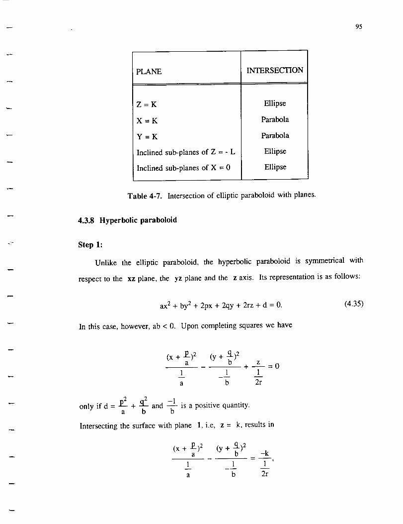
95

PLANE INTERSECTION

Z=K

X=K

Y=K

Inclined sub-planes of Z = - L

Inclined sub-planes of X = 0

Ellipse

Parabola

Parabola

Ellipse

Ellipse

Table 4-7. Intersection of elliptic paraboloid with planes.

4.3.8 Hyperbolic paraboloid

Step 1:

Unlike the elliptic paraboloid, the hyperbolic paraboloid is symmetrical with

respect to the xz plane, the yz plane and the z axis. Its representation is as follows:

ax 2 + by 2 + 2px + 2qy + 2rz + d = 0.

In this case, however, ab < 0. Upon completing squares we have

(4.35)

(x + P)2 (y + b.._.)2a z

+_1 1 1

a b 2r

=0

only ifd = p2 + q2 and -1a b y is a positive quantity.

Intersecting the surface with plane 1, i.e, z = k, results in

(x + _P_)2 (y + _)2a -k

1 1 1

a b 2r

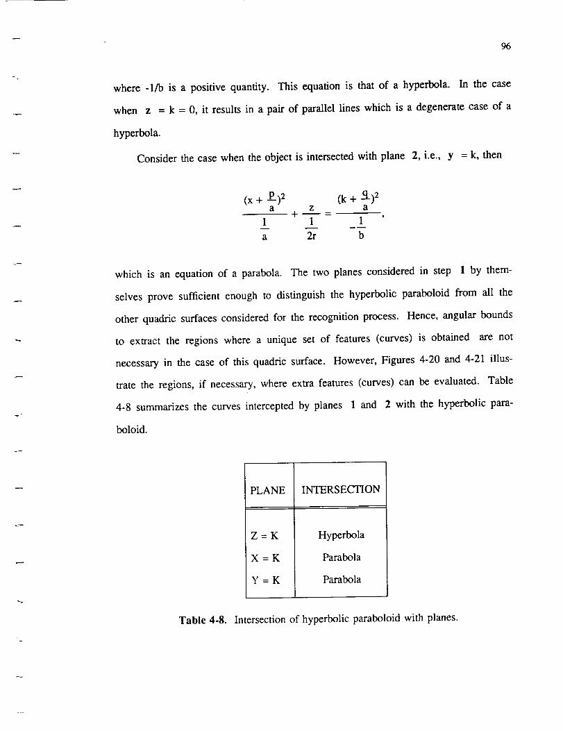
96

where -1/b is a positive quantity. This equation is that of a hyperbola. In the case

when z = k = 0, it results in a pair of parallel lines which is a degenerate case of a

hyperbola.

Consider the case when the object is intersected with plane 2, i.e., y = k, then

(x + P)2 (k + q)2a z a

+1 1 1

a 2r b

which is an equation of a parabola. The two planes considered in step 1 by them-

selves prove sufficient enough to distinguish the hyperbolic paraboloid from all the

other quadric surfaces considered for the recognition process. Hence, angular bounds

to extract the regions where a unique set of features (curves) is obtained are not

necessary in the case of this quadric surface. However, Figures 4-20 and 4-21 illus-

trate the regions, if necessary, where extra features (curves) can be evaluated. Table

4-8 summarizes the curves intercepted by planes 1 and 2 with the hyperbolic para-

boloid.

Table 4-8.

PLANE INTERSECTION

Z=K

X=K

Y=K

Hyperbola

Parabola

Parabola

Intersection of hyperbolic paraboloid with planes.

97


X

Z

Y

Figure 4-20. Planes parallel to the xy-plane (z=k) and all its inclined sub-planes

intersect the hyperbolic paraboloid in hyperbolas.

98


v .

Z

/I

//

f/"

!

,• \ i

k" ', \ i

¢ ", " ''1• O !I

/

f ,

Figure 4-21. Planes parallel to the xz-plane (y=k) and all its inclined sub-planes

intersect the hyperbolic paraboloid in parabolas.

_- 99

4.3.9 Hyperbolic cylinder

Step 1:

As in the case of a regular circular or elliptic cylinder, the surface of the hyper-

bolic cylinder is parallel to the z axis. Subsequently, the variable z is not present in

its quadric representation. It's general representation when resting on a plane parallel

to the xy plane is

where ab < 0.

ax 2 + by 2 + 2px + 2cly + d = O,

Completing squares

(4.36)

p2 q2only if d=--+--+ 1.

a b

(X + P)2a (Y + b")q 2

1 1

a b

+1=0

Also, -1/b is a positive quantity. Intersection of the

cylinder with plane 1, i.e., z = k, generates a hyperbola. Since Equation (4.36) is

independent of the variable z, the curve intercepted is the one represented by Equation

(4.36).

Intersection of the hyperbolic cylinder with plane 2, i.e., y = k results in the

equation

(X + .P_)2 (k + q)2a a

1 -1

a b

-I,

which when solved results in a pair of straight lines. As in the case of the hyperbolic

paraboloid, angular bounds to extract the regions where a unique set of features

(curves) are determined are not necessary, since the two planes considered in step 1

by themselves prove sufficient to distinguish this surface from all the other quadric

10o

surfacesconsideredin the recognition process. A follow-up on the various inclined

sub-planes of the z = k and y = k planes leads to a similar set of intercepts as with

the x = k plane. Figures 4-22 and 4-23 illustrate the regions, if required, where extra

features (curves) can be determined. Table 4-9 displays the intercepts formed when

the hyperbolic cylinder is intersected with the two planes.

PLANE INTERSECTION

Z=K

X=K

Y=K

Hyperbola

Lines

Lines

Table 4-9. Intersection of the hyperbolic cylinder with planes.

4.3.10 Parabolic cylinder

Step 1:

Unlike the two quadric cylinder considered before, i.e., the circular (elliptic) and

the hyperbolic, this surface is parallel to the y axis. Hence the variable y is not

present in its quadric representation. It's general representation when resting on a

plane parallel to the xy plane is

f(x,y,z) = ax 2 + 2px + 2rz + d = 0.

Upon completing squares it reduces to

(x + p)2a Z

1/a 1/2r

(4.37)

- 0 (4.38)

I01


'Z

I

x_ ......................._____.....:/


intersect the hyperbolic cylinder in hyperbolas.

102

DETAILED VIEW" VERTICAL INTERSECTIONS

I

ILi \

\I \

I

zL

t

',,A

, / t

i

I

i

/


intersect the hyperbolic cylinder in lines.

103

only if d = t)2 Intersection of the parabolic cylinder with plane 1, i.e., z = k, 0 <a

k < 2r/ab, where b is any finite positive quantity signifying the width of the base of

the cylinder, yields

(x + p)2a k

1 1 '

a 2r

which, when solved, results in a pair of parallel lines.

Consider the intersection of the parabolic cylinder with plane 2, i.e., y = k.

Since Equation (4.37) is independent of the variable y, the resultant curve intersected

is the same as Equation (4.37), which is a equation of a parabola. As in the case of

the hyperbolic paraboloid and the hyperbolic cylinder, angular bounds to extract the

regions wherein a unique set of features (curves) are determined are is not necessary.

The two planes considered in step 1 by themselves proved sufficient enough to distin-

guish this surface from all the other quadric surfaces considered from the recognition

process. Figures (4-24) and (4-25) illustrate the regions, if required, where extra

features (curves) can be determined. Table 4-10 displays the intercepts formed when

the parabolic cylinder is intersected with the two planes.

PLANE INTERSECTION

Z=K

Y=K

Lines

Parabola

Table 4-10. Intersection of the parabolic cylinder with planes.

104


Z

/

• // \

X -. \Y

/ f

/


intersect the parabolic cylinder in lines.

105


//

//

:// Z

/

/x / x Y

/

/


intersect the parabolic cylinder in parabolas•

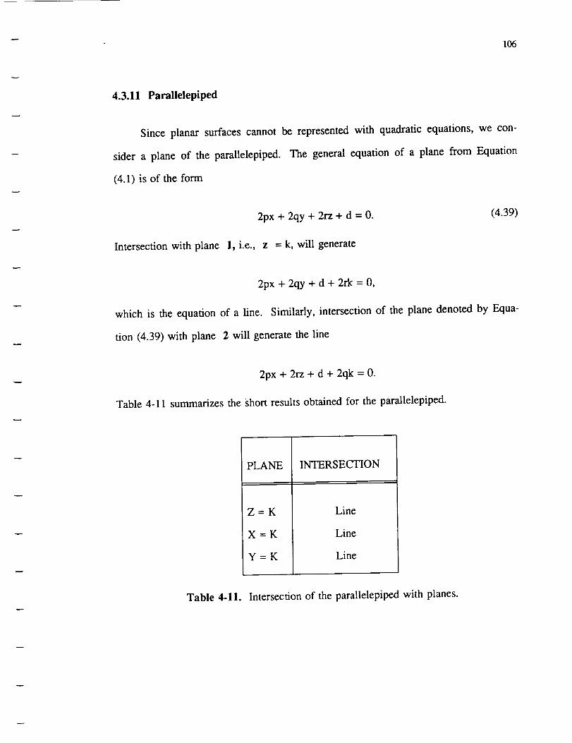
106

4.3.11 Parallelepiped

Since planar surfaces cannot be represented with quadratic equations, we con-

sider a plane of the parallelepiped. The general equation of a plane from Equation

(4.1) is of the form

Intersection with plane 1, i.e.,

2px + 2qy + 2rz + d = 0.

z = k, will generate

(4.39)

2px + 2qy + d + 2rk = 0,

which is the equation of a line. Similarly, intersection of the plane denoted by Equa-

tion (4.39) with plane 2 will generate the line

2px + 2rz + d + 2qk = 0.

Table 4-I 1 summarizes the short results obtained for the parallelepiped.

PLANE INTERSECTION

Z=K

X=K

Y=K

Line

Line

Line

Table 4-11. Intersection of the parallelepiped with planes.

107

Table 4-12 summarizes the various curves (conics) derived from intersecting each

of the eleven surfaces with the two planes z = k and y = k. These observations fol-

low the results obtained in step 1 of each of the quadric surfaces. As seen from

Table 4-12, the quadric cone and the hyperboloid of one and two sheets all generate

similar curves. However, after using the results of step 2 (where angular bounds have

been determined), we are able to distinguish each of the quadric surfaces from one

another. Each of the quadric surfaces can be represented by a binary five-tuple, where

the numeral 1 indicates the presence of a particular curve and the numeral 0 refers to

the non-existence of that curve. Table 4-13 below presents the feature vector for each

of the quadric surfaces.

Quadric surfaces which seem to have identical feature vectors in the table above,

get differentiated when the angular bounds theory as defined and derived for each of

the surfaces (step 2) is applied. The next section briefly presents one other surface

recognition approach which is very similar to the two-dimensional discriminant

approach utilized to distinguish two-dimensional curves. It is one of our primary areas

for future investigation.

4.4 Mapping of Explicit to Implicit Representations for Quadric Surfaces

Another objective which should be discussed is the formulation of a three-

dimensional discriminant similar to the two-dimensional discriminant described earlier

as means of recognizing three-dimensional objects. Consider the general quadratic

representation of quadrics again, i.e.,

F(x,y,z) = ax 2 + by 2 + cz 2 + 2fyz + 2gzx + 2hxy + 2px + 2qy + 2rz + d = 0. (4.40)

This equation can be written implicidy, such that

z = F(x,y) = Ax 2 + By 2 + Cxy + Dx + Ey + F. (4.41)

108

OBJECT

Ellipsoid

Circular cylinder

Sphere

Quadric cone

Hyperboloid of one sheet

Hyperboloid of two sheets

Elliptic paraboloid

Hyperbolic cylinder

Parabolic cylinder

Hyperbolic paraboloid

Parallelepiped

PLANE 1 :x=k

Ellipse

Circle

Circle

Circle

Circle

Circle, Point

PLANE 2 : y = k

Circle

Line

Circle

Hyperbola, Parabola

Hyperbola, Parabola

Hyperbola, Parabola

Ellipse

Hyperbola

Line

Hyperbola

Line

Parabola

Line

Parabola

Line

Line

Table 4-12. The various curves intercepted by the quadric surfaces when intersectedwith the planes z=kand y=k.

109

3-D SURFACE

Ellipsoid

Circular cylinder

Sphere

Quadric cone

Hyperboloid of one sheet

Hyperboloid of two sheets

Elliptic paraboloid

Hyperbolic cylinder

Parabolic cylinder

Hyperbolic paraboioid

Parallelepiped

CIRCLE

1

1

1

1

1

1

1

0

0

0

0

ELLIPSE PARABOLA

0

0

0

1

1

1

1

0

1

1

0

HYPERBOLA

0 0

0 1

0 0

1 1

1 0

1 0

0 0

1 1

0 1

1 1

0 1

LINE

Table 4-13. Feature vectors (representing the prescence or absence of curves) for each

of the quadric surfaces.

110

Equation (4-40) characterizes the complete surface through its representation, whereas

Equation (4-41) characterizes surface patches on three-dimensional surfaces. As dis-

cussed in Chapter Two, where surface curvatures are utilized to describe surface

patches as being planar or curved (hyperbolic, parabolic, or elliptic), we wish to utilize

the ten coefficients of Equation (4.40) in the form of a discriminant to represent

patches on three-dimensional surfaces. In case we justify the existence of the implicit

form, we would like to derive a mapping from F(x,y,z) to F(x,y); i.e., we would like to

investigate the relations between A, B, C, D, E, and F and a, b, c, d, p, q, r and d. If

this is possible, then we can attempt to derive a discriminant using A, B, C, D, E, and

F, the combination of which can distinguish three-dimensional objects.

We approach this problem in two directions. In the first approach we would

numerically solve and derive relations for each coefficient in Equation (4-41) in terms

of the coefficients of Equation (4-40). For example, while solving for F we arrive at its

representation as

F

-2r + _/4r 2 - 4cd

2c

Similarly, expressions for the coefficient B have been found to be

B = + _/2 (f+g+r) 2 - 4c(a+b+2h+2p+2q+d)4c

Each of the above coefficients were derived while setting the variables x and y as

zero. Similarly the remaining coefficients can be derived after solving several linear

and non-linear equations. In the second approach, derivatives are utilized to obtain a

pattern vector based on the coefficients of Equation (4-40). Rewriting Equation (4-40)

in terms of a quadratic of z,

-[cz 2 + 2fyz + 2rz + 2gxz] = f(x,y) = ax 2 + by 2 + 2hxy + 2px + 2qy + d, (4.42)

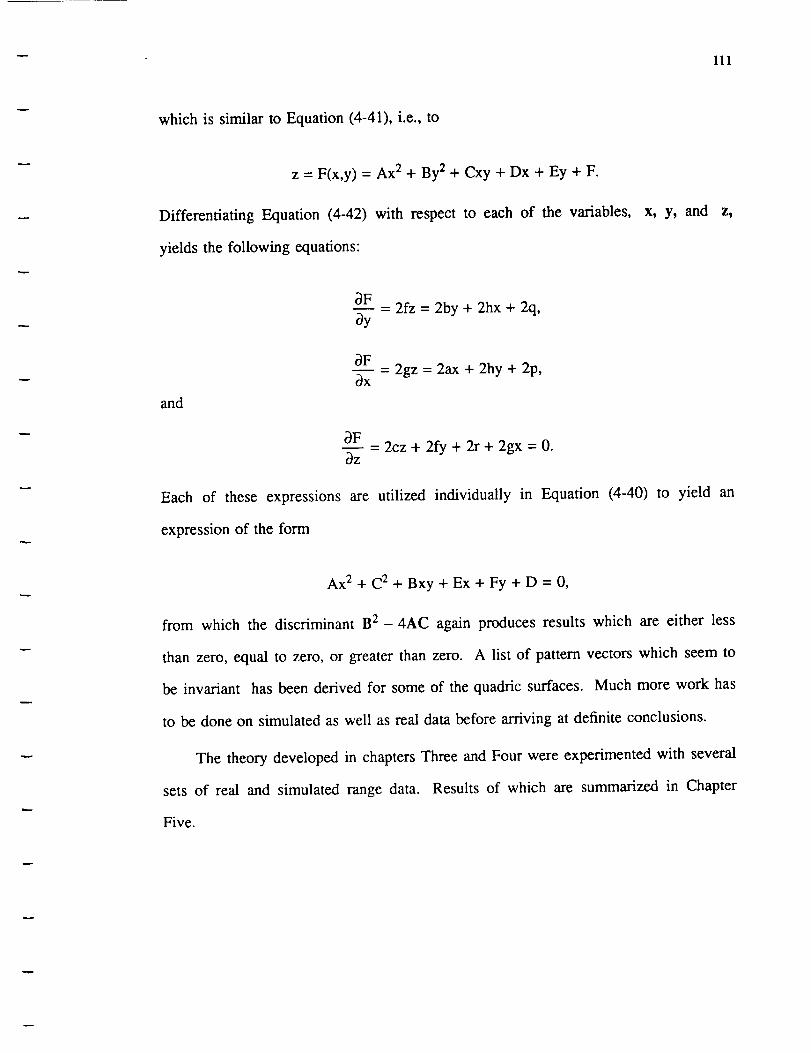
111

which is similar to Equation (4-41), i.e., to

z = F(x,y) = Ax 2 + By 2 + Cxy + Dx + Ey + F.

Differentiating Equation (4-42) with respect to each of the variables,

yields the following equations:

= 2fz = 2by + 2hx + 2q,by

X, y, arid Z,

_F

bx 2gz 2ax+2hy+2p,

and

_F= 2cz + 2fy + 2r + 2gx = 0.

bz

Each of these expressions are utilized individually in Equation (4-40) to yield an

expression of the form

Ax 2 + C 2 + Bxy + Ex + Fy + D = 0,

from which the discriminant B 2- 4AC again produces results which are either less

than zero, equal to zero, or greater than zero. A list of pattern vectors which seem to

be invafiant has been derived for some of the quadric surfaces. Much more work has

to be done on simulated as well as real data before arriving at definite conclusions.

The theory developed in chapters Three and Four were experimented with several

sets of real and simulated range data. Results of which are summarized in Chapter

Five.

CHAPTER FIVE

EXPERIMENTAL RESULTS

5.1 Introduction

Section 5.2 discusses our study of median filtering on range images. Section 5.3

explains the process whereby filtered range images of spheres, cylinders, and quadric

cones undergo the recognition criterion. Subsequently, Section 5.4 discusses the appli-

cation of the rotation alignment algorithm to the processed as well as simulated range

images. Section 5.5 briefly presents the results obtained while using the three-

dimensional discriminant approach to simulated and real range data.

Range data obtained using a laser radar three-dimensional vision system is similar

to intensity images obtained from a normal camera. However, instead of intensity

(brightness) information, range (depth) information is available. Thus it is possible to

interpret intensity information as range information when a range image is displayed

on a image processing monitor. The nearer the object, the brighter it appears on the

screen.

The experimental work was performed in the following order :

(i) The effect of median filtering on range images was studied.

(ii) The proposed recognition scheme was applied to filtered range images.

(iii) The quadric alignment algorithm was applied to simulated and real data.

(iv) The three-dimensional discriminant approach was tested with simulated data.

112

m

113

5.2 Median Filtering on Range Images

Range images of objects like spheres, cylinders and cones were segmented in

order to separate the object from its background. The resulting image, which is

referred to as the raw image, was then median filtered with mask sizes 3 x 3, 5 x 5

and 7x7.

Consider Figure 5-1 which is the actual range image of a sphere with its back-

ground. Figure 5-2 is the image after segmentation. The effect of median filtering on

Figure 5-2 can be observed in Figure 5-3 (3 x 3 mask), Figure 5-4 (5 x 5 mask), and

Figure 5-5 (7 x 7 mask). The curvature sign map, which is discussed in Chapter

Three, was then utilized to study the effect of median filtering on the original range

image shown in Figure 5-2. Evaluating the first and second derivatives with respect to

the x and y axes and comparing each of these maps determines whether or not the

median filtering has altered the original range data to any extent. Figures 5-6a, 5-6b,

5-6c, and 5-6d are the first and second derivatives with respect to the x and y axes,

respectively, for figure 5-2. Similarly figures 5-7a, 5-7b, 5-7c, 5-7d; figures 5-8a, 5-

8b, 5-8c, 5-8d; and figures 5-9a, 5-9b, 5-9c, 5-9d are the first and second derivatives

for the images in figures 5-3, 5-4, and 5-5, respectively.

In all of these figures, "+" is assigned to a particular pixel position if the magni-

tude of the derivative (first or second) of that pixel is greater than the magnitude of the

derivative (first or second) of the pixel to its right. Similarly "-" is assigned to a par-

ticular pixel position if the magnitude of the derivative (first or second) of that pixel is

less than the magnitude of the derivative (first or second) of the pixel to its right. In

the case when the magnitudes of the derivatives (first or second) of either pixels is the

same, a blank is assigned.

Sign maps are also generated to check the integrity of the image data before and

after the filtering process. Based on the magnitude of the depth value of a pixel and

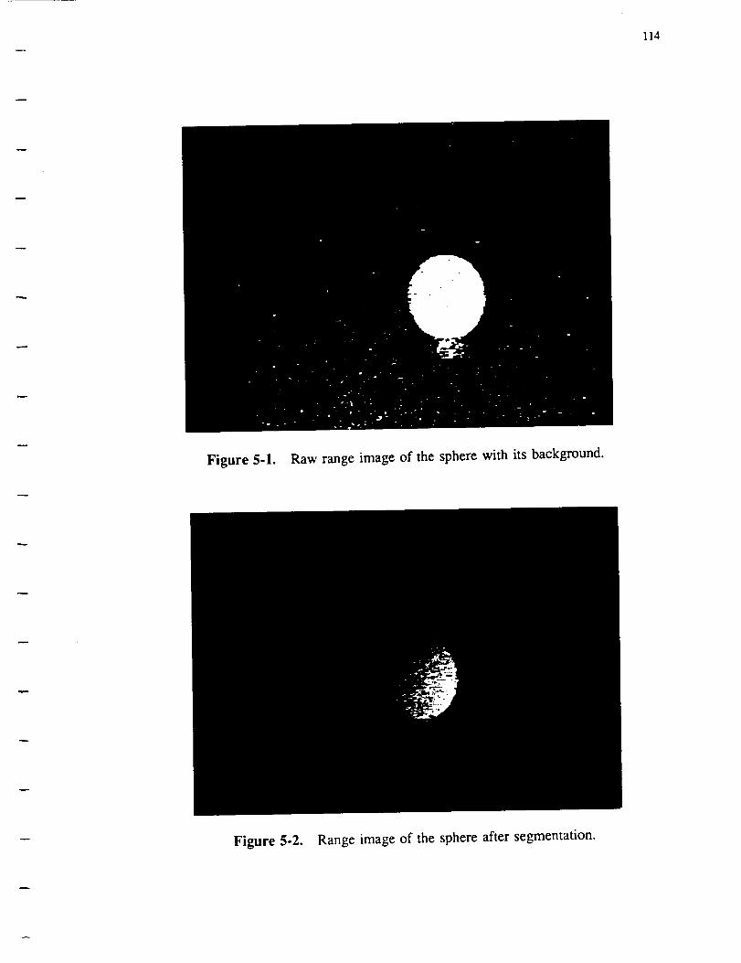
114

Figure 5-1. Raw range image of the sphere with its background.

Figure 5-2. Range image of the sphere after segmentation.

115

Figure 5-3. 3 x 3 medianfiltered imageof the raw sphere.

116



117

--÷ ..... ÷ ......... ÷÷----÷-÷÷÷_---_---÷ ........ ÷÷-_ .... _÷÷ ..... ÷

-÷÷W---÷+ .... ÷÷--W÷÷---÷÷_W_÷_ .... W---WW .... ÷÷÷÷W-÷÷--÷÷÷÷ ..... ÷

÷÷÷÷÷_÷_÷÷÷÷÷÷÷÷÷÷÷÷÷÷÷÷÷÷÷÷÷_----÷÷÷---÷-÷÷÷÷÷W_÷-÷+_-÷÷÷÷÷÷÷-_÷

÷÷÷---÷ ..... ÷÷÷÷ ........ ÷÷÷÷÷÷---÷÷---÷-÷----_-÷ .... _÷+÷+÷÷_---÷

.............. _ .................. + ............ ÷ ............... ÷

.............................................. _÷ .............. ÷

...................... ÷ ....................... ÷ ............... ÷

--+-_-÷+÷+÷W÷_--÷---÷-÷ ..... +÷W÷---_÷÷÷ ..... ÷÷÷-++÷---+++++÷÷÷+

+÷+÷--_-_ ..... ÷ ..................... _ ......... ÷--÷÷+---+-_+÷_+-

-.--.,-.-,-.--.-.--.---... .......... ÷ ......... ÷_+_++W-_+÷_÷÷-

÷--+ ...... +W÷+÷ .......... W ......... W÷-_--÷--÷%--÷-÷++÷÷+÷÷--÷÷-

-÷ .............. +--+---÷++++-÷+ .... + .... ,---.--,,-.--.--,-.,.--

................ + .......... ÷÷_ ..... ÷ ................. ÷--÷--+---

_÷÷÷÷---_÷ ...... ÷_÷---+---_÷÷--+÷---+ ..... _---÷--÷ ...... ÷--÷

--+÷-÷---_ .... ÷_+--W--_--÷÷÷ .... ÷--++-W-÷-+ .... ++--÷-÷ ...... +-+

....... W-_ .... ÷÷ ........ + ..... ÷÷-÷+--÷++ .... ÷---+-+-+++--+-+--÷

.... ÷ ......... ÷ ............... + ..... _ ....... + ..... _---+_+-_-+--

÷ ........ _-_-+÷÷ .................... _ .... ÷÷-÷÷---÷+ ..... ÷---++-

÷ - .---.,,--.-.-.---.--.--.--... ................... _W_ ..... ÷-÷

÷ -÷-_ - ÷ .... _÷ .... ÷--÷--+--+-+---++++ ..... ÷-+ .... ÷÷+ ..... ÷+÷

-_÷÷%++÷÷÷_+W+÷+÷--÷-÷÷---++--+--÷_-_÷++--+++÷ ..... ++++÷+---_÷+

..... _ ........................................ W ..... W ..........

Figure 5-6(a). First derivative w.r.t x-axis of the original sphere.

118

÷+÷+ ...... ++÷+--- +++++ - ÷÷ ++++÷÷ --- +++ +++ ÷÷ ....... ÷

÷ ......................... ÷+÷+++-++÷---+÷++ .....................

+---+÷÷++÷÷+ ...... ++++-÷+++++÷+-+--+++÷÷+++÷++++÷++÷++++÷÷÷÷÷+÷

--- +÷++++ ÷++÷++ + ++÷+÷++++++÷ ........... + -

-+++ .... +++ ............................ +++ ..... + ........... ++--

÷+++++++ ..... +++++++++÷++++÷+++++++++++÷++++÷++÷+÷++++++++++÷++

......... ++ .......... + ---++++++ ---

+÷+++++÷÷++++÷---++ ............................................

+ ....... + ..... +++÷ .... ÷+ ...... ++-+++ ...... +-+--+÷++÷÷+++++÷÷++-

-++++÷+÷---+++++ .... ÷++ ..... +++÷+++++++---+++++÷+++++÷+++÷÷++++÷

..... ÷+++-- ÷+ - __ ÷ ......... +++

+÷ .... ÷++÷++---++++÷++÷÷+÷+÷++ ....... +++-----÷÷++ ................

+÷÷ +÷ ......... + +÷ ............... +

.... ++ .........................................................

++ .... ÷_++++++ .... +++ ...... ++÷ ................. +÷÷+÷+++-++÷+++-

--+-÷÷+++÷++÷++++÷+++++++++÷+++++++÷++++++÷+÷+÷+++÷÷÷++÷+÷+÷+÷+

+++÷+++++÷÷÷++++++++÷+++++++++++++++++÷++++÷+++ .... ÷+++++÷-÷++÷

-÷+÷÷+ ....... ++++÷++++÷+++++÷+++-÷+++÷+++÷+++÷+ ................

........ ÷÷÷+ ..................................................

..... ÷++++÷++++++++÷++÷++÷+÷++÷++÷++++÷++++++÷+++÷÷÷+++++÷+++÷+

++++ ....... ÷+++++++÷÷÷÷++÷+++÷+÷+-÷+÷++++÷++÷÷++÷+÷÷+++÷++++÷++

+--+--+++++ ...... +++++++++++++++++÷++++ .................... +++÷

............. ÷ ......... ++++÷+--++++++÷÷+++÷++ ..... +++ ...... ÷---

+÷÷++÷--+---++÷+÷÷-÷-++ ...... ÷÷÷÷+++-÷++++++÷÷+++_+ .... ÷+÷÷++++

................................... +---++--+÷++-+÷÷÷+++÷+ ......

........ ++ ....... + .... ++-++++++++++ ...... ÷+++++++÷+++++++÷+++++

+++÷+-÷++ ........ + ..... ÷+++++++÷---+++++ ....... +÷++++÷+_+++++++

++ .............................................................

-÷++++÷+÷÷++++++-÷++++ .................................... ++-+

....... ++÷++++÷++--+ ..... + ....................................

+÷+÷++++÷++÷+++++++++++++++++++++÷+++÷+++++++++÷+++++++++÷÷÷+÷÷

....... ÷+÷++++÷++++÷+--++÷+++++ ....... +++ .... ++ ....... +++÷+++++

............. ÷+++÷++÷++--++--÷+++++÷÷ ....... ++++ ...............

........ ÷ .......... +++++++++++-++--++÷÷+++++ ...... ++÷+-++÷++++÷

++++÷++++++++++÷+++ ............................................

......................... ÷+++++ .... ÷+++++--+÷+++++÷÷++++ .... +--

++÷÷+÷÷+÷÷÷÷+÷÷+÷÷+÷÷÷++++++++++÷÷+++++÷+÷÷÷++++++÷++÷+++÷+++÷÷

..... ++÷÷+÷++++++++÷÷÷++++++++÷+++++++++++÷+++++÷++++++÷++++++÷

++÷ ............ + ........................... ++++++ ..............

---++ ..........................................................

.... +++++++++÷+÷ ...................................... ++÷+++--

+÷++ .... +÷+÷++÷+++++++ .......... + ....... +÷+++ ....... +++---++++

++ ............... + .... ÷-÷++÷ ............ + ......................

-+÷+÷+++++++÷÷+÷++++÷÷++÷+++++-÷÷+÷+ ......... +++ ....... ++÷ .....

---÷+--++++÷+÷÷ .... ++++++÷++++÷++++÷++++-÷ ......... ++++ ........

+ ........... +--÷÷++++ .... +---+÷+++++++÷÷++++++-÷ .......... ++++-

..................... ++++÷+ .............. +÷++++--÷+++ ..........

++++++---++++÷++++++++++++++++++++++++++÷+÷+++++++++++++++++---

Figure 5-6b. First derivative w.r.t y-axis of the original sphere.

119

+++++++++++++++++++++++++++++++++++++++++++++++-+++++++++++++++

+++++++++++++++++++++++++++++++++++++++++++++++-+++++++++++++++

+++++++++++++++++++++++++++++++++++++++++++++++-+++++++++++++++

+++++++++++++++++++++++++++++++++++++++++++++++-+++++++++++++++

+++++++++++++++++++++++++++++++++++++++++++++++-+++++++++++++++

+++++++++++++++++++++++++++++++++++++++++++++++-+++++++++++++++

+++++++++++++++++++++++++++++++++++++++++++++++-+++++++++++++++

+++++++++++++++÷+++++++++++++++++++++++++÷+++++-+++++++++++++++

++++++++++++++++++++++÷++++++++++++++++++++++++-+++++++++++++++

+++++++++++++++++++++++++++++++++++++++++++++++-+++++++++++++++

+++++++++++++++++++++++++++++++++++++++++++++++-+++++++++++++++

++++++++++++++++++++++÷++++++++++++++++++++++++-+++++++++++++++

+++++++++++++++++++++++++++++++++++++++++++++++-+++++++++++++++

+++++++++++++++++++++++++++++++++++++++++++++++-++++++÷++++++++

.............................................. + ............... +

...................................... + ....................... +

............................................ ÷ ................. +

.............................................. + .... + .......... +

.............................................. + ............... +

.............................................. + ................

................... +_--+ .......................................

++++-+++++++++++++++++++++-++++++++++++++++++++++++++++++++++++

+++++++++÷-++++++++++++++++++++++-+++++++++++++++++++++++++++++

++++++++++++++++-++++++++++++++++++++++-+++++++++++++++++++++++

+++++++++++++++÷++++++-++++++++++++++++++++++-+++++++++++++++++

++++++++++++++++++++++++++++-++++++++++++++++++++++-+++++++++++

++++++++++++++++++++++++++++++++++-++++++++++++++++++++++-+++++

++++++++++++++++++++++++++++++++++++++++-++++++++++++++++÷+++++

++++++++++++++++++++++++++++++++++++++++++++++-++++++++++++++++

..... + ................. + ............................. + ........ +

....... +- --+ ........... + ................................... +-_+

................. + ........ + ....................................

-++++++++++++++++++++++++++++++-++-++++++++++++++++++++++++++++

++++++-++++++++++++++++++++++++++++++++++-+++++++++++++++++++++

++++++++++++-+++++++++++++++++++++++++++++++++++-++++++++++++++

++++++++++++++++++-+++++++++++++++++++++++++++++÷+++++-++++++++

........................ + ....................... + ........ + -+-++

.............................. + ....................... + ........

_ _ -+ ................................ + ................... + -+ -+ - _

++++-++++++++++++++++++++++++++++++++++++++++++++++++++++++++++

+++++++++++++++++++++++++++++++++++++++++++++++++++++++++++++++

.... +-+-+ ........ +-+-+ ................................ + ....... +

.......... +_+__+ ..... +-+--_+ .... +-+ ......................... +-+

................ +_+__+ ..... +__+__+ .... ++-+ .................... +

...................... +_+-_+ ........ +--_+-_-++-++ ............. +

............................ +__+_+ ...... +_+___+-_-++-+-+ ...... +

.................................. +__+_+ ........ +___+ .... +-+--+

........................................ +__+-+ ........ + ....... +

...............................................................

Figure 5-6c. Second derivative w.r.t x-axis of the original sphere.

120

-+++++++++++++++++ ....... ++ ..... +++++++++++++++++++++++++++++++

-++++÷÷++-++++++++++++++++ ...... +--+++ ..... ++++++++++++++++++++

+ .......................... +++++-++---++++ .....................

+++ ....... + ........ + ............ ++++++++++++++-++++++++++++++++

.... ++++++-++++++++++++++++++++++ +++-+++++++++++--++

-++ ..... +++++ ..................................................

++++++++ ..... ++++++++++++++++++++++++++++++++++++++++++++++++++

.............. ++---+++++++++++++++++++-++++++++--++++++++++++++

++++++++++++++ .... + ...... + .....................................

+ ....... ++ .... +++++---+++-+ ........... +++ ...... +++--++++++ .....

++++++++--+++++ .... +++ ..... +++-+++++++---++++++++++++++++++++-+

--+_++ ...... +++ ............... +++-+++---+++ .... +++---+++---++++

+ ..... +--+++---+++++++++++++++ ....... +++---++++-+---++++++++---

++++--++++++++++++++++++++++++++++++++++++++++++-+++ ......... ++

---+++ ................. ++ .............. ++++++++ ................

++ ............................................. ++++++++ ........

.... +++++++++++++++++++++++++++++++++++++++++--++++ .... +++++++-

+++++++++++++++++++++++++++++++++++++++++++++++ .... ++++++++++++

+ ...... ++++++ .................................. ++++++++++++++++

-+++++ ....... ++++++++++++++++++++++++++++++++++ ................

+++ ............................................................

.... ++++++++++++++++++++++-++++++++++++++++++++++++++++++++++++

-+++ ....... ++++++--+-++++++++++++ ...... +++++++++++++++++++++---

+++++++++++ ...... ++++++--++++++++++++++ ...... +++ ...... +++---+++

....................... ++++++ ...... +++-++++++ ...... ++++ ........

+++++++++++++++++++++++ ...... ++++++--++++++++++++++ ...... ++++++

................................... ++++++--+ .... +++++++++ ......

..... +---++--++++++++++---++++-++++ ...... ++++++--++--++++++++++

+-+++++++++++++++++++++++++++++++++++++++++++++++++++++++++++++

++ ................................................... + .... + ....

-++++++++++ ...... ++-+++++-++++++++++++ ..... +++++++++ ...... ++++

.......................... + ....................................

+++++++++++++++++++++++++÷-++-+++++++++++++++++++++++++++++++++

....... ++++++++++--++--+++++++ ........ ++++++ ......... ++++++++++

.... ++ ....... ++++++_-++--+---+++++++ ........ ++++++ .... + ........

................... +++++++++++++++++++++++++ .... +++++++++++++++

+++++++++++++++++++ ........................................... +

......................... ++++++ .................. ++++++ ........

+++++ .................................................. ++-+++--

..... +++++++++++++++++++++++++++++++++++++++++++++++++++++÷++++

+++ ........ ++++++++++++++++++++++++++++++++++++++++++++++++++++

___++ ................ ++ ........................................

.... ++++++-++++ ....... ++++++++++-+++++++ ..... + ........ ++++++--

-++++++++++++++++-++++ ........ +++++++++--++++++++++++++++++++++

+ ................ + .... +-++++ ........ +++++++++ ...... ++++ ........

-++++++++ ...... ++++--++++++++--+++-+ .... +-+++++++++ .... +++++++-

-++++++++++++++ ...... ++++++++++++++--+++-+ ...... ++++++++++ .... +

+++++++++++++++++++++ ...... ++++++++++++++--+++-+ ...... +++++++++

...... +++ ................................ ++___+--++++ ....... +++

Figure 5-6d. Second derivative w.r.t y-axis of the original sphere.

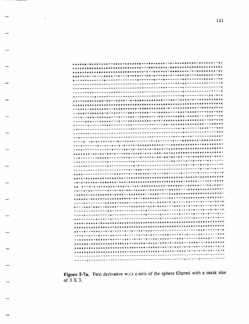
121

++++++-++++-+++--++++-+++++++---++-++++--+-+++++++++-++++++--++

+++++++++++++++++++++++++++++---++-+++++-++++++++++++++++++++++

++++++++++++++++++++++++++++++-+--+++-++-++++++++-+-++++++++-++

+++---+--+---++++--+---+-++++--++-+---÷+-+--+++++---+++++++--++

+ ............ + ............. + ...... +---+ ++ ....... ++++---+

.............................................. ++ .............. +

.............................................. + ............... +

.............................................. + ............... +

......... + ..... _ .............................. + .......... ++ -+ -+

++--+++++++++-++--++++--+-++++++++++++---++--++++-+--++++++++++

+++++++++++++++++++++++++++++++++++++++++++++++++++++++++++++++

--++++-++++++++--+++++-++++-+++++++++++-+---++++++++--+++++++++

--+++--++++++-+--+-+---+++--++++ .... +++++---+++-++++ .... +++-+++

---+--+++-++++++---+---+++--+++++---++--+--++++-_++++---+++--++

..... +++---+++++_--+---++++++++++-+-+-+++++++++++++++++--++-+++

...... + ....... ++ ........ + ............. ++-++++++++++++++---+++++

............................................ +-+ ...... ++++---+++

.............................................. + ............. +++

_-+ ........................................... + .......... +++++-

.... + -+-+ ..... +_-+ ..... + ......... ++ ..... +---+++++++-++++++++-

__-+ ...... + ..... +--+-+---+-+++++++++++---++++++++++++-++++++++-

___+ ............ + .... ++--+-++-+-+-++++--++++++++++++++++++++++-

+++++++-++-++-++-+---+++-++++-+-+-+++-++-+++++++++++++++++++++-

__+ ....... +++++ ...... +-+ .... + .... +-++-++-++-++--+-++++++++-+++-

.............. + .......... + ............... ++-+_-+--+--+--++ .....

.............. + .......... +-+ ................... +-_+--+-_+ ......

....................... +--+++--+ ..................... +__+__+-_-

++++ ............. +++__-+__++++++-_+___++ ..... + ...... + ...... +--+

++-+-++++++++-+++++++--+++++++++++++++++++++++-+++++-++++++++++

-+-+-+++++-+++++++-+++-+++++++++++++++++++++++-+++++ .... ++-++++

++ +--+-+-+-+++++-+++-+--++-++++++++++-++++++--+++++---++-+++-

-+--+-++ ...... +-_+-++-++--++++--++++++--+++++---++++++++++++++-

-+++++-+++++++++-++++--+++++++--++++ .... ++++++++++++++++++++++-

++++++-+++++-+++++++++-+-++--+++++++ .... ++ .... +++++++++-++++++-

.... + ........ +++++-++++---+ ..... +--++++-+-+ .... ++ .... +-_-+-++-+

+---+÷+-+++--+++++ ...... ++++++-+++-++++---+++-+-+--+-+---+-+--+

.............. ++ ........ + ..... + ....... + ..... +__-+_+---+--+-+--+

.... + .......... + .............. + ..... + ....... + ..... +___+_+___+_-

......... + ..... + .................... + ..... + ....... + ..... +___+__

++++-+++++-++++++++++++++++++++++++++++++++++++++++++++++++++++

++++++++++++++++-++++++++++++++++++++++++++++++++++++++++++++++

++--+---+++--+-+ ..... +--+--++-+++ ................... +++ ..... +-+

___+__+___+ .... ++ .... + ..... +-_+-+ .... +++ .... +_-+ .... ++ ...... +++

--++++++-+++++-++ .... ++--+-+--+--++-++++---++÷ ...... +++++---+++

++++++-++++++++++++++++--+++++-++++-+++-+-++++--++++---++++++++

++++++++++++++++++++++++++++++-+++++-++-+-+++-+-+-++---+++--+-+

++++++++++++++++÷+++++-+++++++++++++-+++++-++++-+-+-+-+-++--+-+

...............................................................

..... + ........................................ + ..... + ..........

Figure 5-7a. First derivative w.r.t x-axis of the sphere filtered with a mask sizeof 3X3.

122

+++ + - + ....... ++++ ++ ++ ....

++ .... + ................. +-++++++-++--+++++++ ........ + ......... +

.... ++--++--+ .......... +-+++--+++ ................. +++++++++ ....

---+ ++ +++ + ++++++++++ ........... +++++

.... +++++++++++++++++++++++++++++++++++++++--+++-+ .... +++++++++

................ ++ --- ++++++++ .........

+ - + ..... ++ --

+++ ++++++++ ++ + ............ ++++ + --

+++++++++++++++++++ ....... ++--+++++++ ..... ++++++++++++++++++++-

+++++++++-+++++ .... +++---++++++++++++++-+++++++++++++++++++++++

+++ - ++++++ ++ + - ++++ ...... +++

....... +++ ...... ++-+++++++-++ ........ + .........................

+ ..... + ............... + ........................................

-+-+++ .........................................................

+-+-+-+--+-++++++++++++++-+++++++++++++ ........ +÷++++++++++++++

---++++++++++++++++++++++++++++++++++++++++++++++++++++++++++++

- -+ +++++ ++_ - ++++ + + ++ .... +++++++-++++

+++++ ....... ++++-+-++++++++++++ ..... + .... +++++ ................

__+ ..... ++++ ..................................................

..... ++++++++++++++++++++++++++++++++++++++++++++++++++++++++++

-+++ ....... ++++++++++++++++++++++-+++++++++++++++++++++++++-+++

+++ ..... +++ ...... ++++++++++++++++++++++ .... + ........ ++--+-+++++

....................... +++++++-++++++++++++++ ................. +

.............. + .............. ++++++--++++++++++++++ .... ++++++++

................................... ++++++--++++++++++++++ ......

................. + ..... ++++++++++++ ...... ++++++++++++++++++++++

+++ ..... + ............... +++++++-+++ ............ ++++++++++++++++

++ .............................................................

--+++++++++++++++-+++++ .................................... ++++

....... ++++++++++--+ ..... + ....................................

-++++++++++++++++++++++++++++++++++++++++++++++++++++++++++++++

+ ...... ++++++++++++++++++++++++ ....... +++ .... + ....... ++++++++++

............. +÷++++++++--++--++++++++ ....... ++++ ...............

........ +++++ ...... +++++++++++++++++++++++++ ...... ++++-++++++++

+++++++++++++++++++ ............................................

............ + ............ +++++++++++++++++++++++++++++++ .... +__

+++++++++++++++++++++++++++++++++++++++++++++++++++++++++++++++

..... ++++++++++++++++++++++++++++++++++++++++++++++++++++++++++

+++ ............ + ........................... ++++++ ..... + ........

---++ ..........................................................

---++++++++++++++ ...................................... ++++++--

++++++---++++++++++++++ .......... + ....... +-++ ........ + ....... ++

++ ............... + .... +-++++ ............ + ......................

++++++++++++++++++++++++++++++-+++++ ......... +++ ....... +÷++ ....

......... ++++++---++++++++++++++++++++++-+ ......... ++++ ........

+++++-+++++++--++++++ .... +++++++++++++++++++++++ .......... ++++-

..................... ++++++ .............. ++++++--++++ ..........

++++++---+++++++++++++++++++++++++++++++++++++++++++++++++++---

Figure 5-7b. First derivative w.r.t y-axis of the sphere filtered with amask size of 3 X 3.

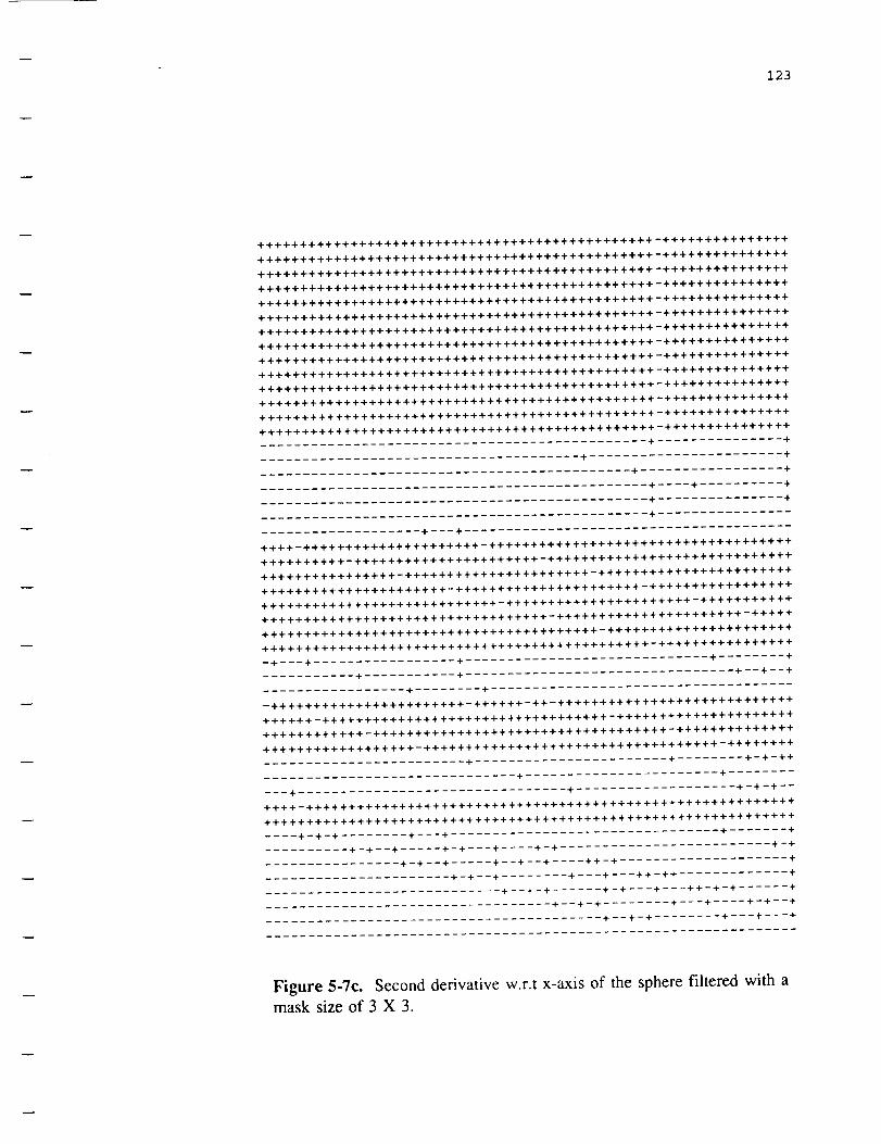
123

+++++++++++++++++++++++++++++++++++++++++++++++-+++++++++++++++

+++++++++++++++++++++++++++++++++++++++++++++++-+++++++++++++++

+++++++++++++++++++++++++++++++++++++++++++++++-+++++++++++++++

+++++++++++++++++++++++++++++++++++++++++++++++-+++++++++++++++

+++++++++++++++++++++++++++++++++++++++++++++++-+++++++++++++++

+++++++++++++++++++++++++++++++++++++++++++++++-+++++++++++++++

+++++++++++++++++++++++++++++++++++++++++++++++-+++++++++++++++

+++++++++++++++++++++++++++++++++++++++++++++++-+++++++++++++++

+++++++++++++++++++++++++++++++++++++++++++++++-+++++++++++++++

+++++++++++++++++++++++++++++++++++++++++++++++-+++++++++++++++

+++++++++++++++++++++++++++++++++++++++++++++++-+++++++++++++++

+++++++++++++++++++++++++++++++++++++++++++++++-+++++++++++++++

+++++++++++++++++++++++++++++++++++++++++++++++-+++++++++++++++

+++++++++++++++++++++++++++++++++++++++++++++++-+++++++++++++++

.............................................. + ............... +

...................................... + ....................... +

............................................ + ................. +

.............................................. + .... + .......... +

.............................................. + ............... +

.............................................. + ................

................... +- --+ .......................................

++++-+++++++++++++++++++++-++++++++++++++++++++++++++++++++++++

++++++++++-++++++++++++++++++++++-+++++++++++++++++++++++++++++

++++++++++++++++-++++++++++++++++++++++-+++++++++++++++++++++++

++++++++++++++++++++++-++++++++++++++++++++++-+++++++++++++++++

++++++++++++++++++++++++++++-++++++++++++++++++++++-+++++++++++

++++++++++++++++++++++++++++++++++-++++++++++++++++++++++-+++++

++++++++++++++++++++++++++++++++++++++++-++++++++++++++++++++++

++++++++++++++++++++++++++++++++++++++++++++++-++++++++++++++++

-+--_+ ................. + ............................. + ........ +

........... + ........... + ................................ +-_+--+

................. + ........ + ....................................

-+++++++++++++++++++++++-++++++-++-++++++++++++++++++++++++++++

++++++-++++++++++++++++++++++++++++++++++-+++++++++++++++++++++

++++++++++++-+++++++++++++++++++++++++++++++++++-++++++++++++++

++++++++++++++++++-+++++++++++++++++++++++++++++++++++_++++++++

........................ + ....................... + ........ +-+-++

.............................. + ....................... + ........

___+ ................................ + ................... +-+-+--

++++-++++++++++++++++++++++++++++++++++++++++++++++++++++++++++

+++++++++++++++++++++++++++++++++++++++++++++++++++++++++++++++

.... +-+-+ ........ +___+ ................................ + ....... +

.......... +-+_-+ ..... +_+___+ .... +-+ ......................... +-+

................ +-+ --+ ..... +- -+ --+ .... ++-+ .................... +

...................... +_+__ + ........ +___+ __ -+ +-++ ............. +

............................ + --+-+ ...... +-+ -- -+-- -++-+-+ ...... +

.................................. +__+_+ ........ +___+ .... +-+--+

........................................ +-_+-+ ........ +_-_+-_-+

...............................................................

Figure 5-7c. Second derivative w.r.t x-axis of the sphere filtered with amask size of 3 X 3.

124

-+++++++++++++++++ ....... ++ ..... +++++++++++++++++++++++++++++++

++++++--++++++--+++++++--+ ...... +--++++--++-++++++++-+++--++++_

++ .... + ................. +--++++--++--+++++++ ..... +--+ ...... +--+

+++-++--++ ..................... ++-+++-+++++ ....... ++++++++ .....

---+--++---+++ .... + ...... +++ ................ +---+-++++ ....... +_

+++++++++++++++++++++++++++++++++++ .......... ++++++---+++++++++

................. ++ +--- +++++++++++ ++ ........ ++ -

........ +++++- +++++---++++ - + -++ .... ++

+---+-++++++-_++_+ ...... ++ ............ ++++ ...... +--+ ...........

-+++++--++--+++++++ .... ++-++ ........... + ..... +++ ....... ++++ ....

+--++++++-+++++ .... +++---+++++-+++++++--++++++-++++++++++++++++

+++++++---++++++--+ ....... +-+++++++++-+++++++++++++++++++++++++

-++ .... ++++-++--++++++++++++++_+-++-++++--++++-+ ...... ++___+___

+ ..... ++++++--+++++++++---++++++++++++++---++++ ................

-+-+-+ ................... + ............. ++++++++ ................

+++ .................... ++ ...................... ++++++++ ........

---++++-++---+++++++_+++++---++++++++++++++++--++++ .... +++++++-

+++++++++++++++++++++++++++++++++++++++++++++++ .... ++++++++++++

...... +++++++ .................................. ++++++++++++++++

+++++ ....... ++++++++++++++++++++++++++++++++++ ................

+--+ ...........................................................

..... +++++++÷+++++++++++++-++++++++++++++++++++++++++++++++++++

-+++ ...... ++++++ ...... ++++++++++ ...... ++++++++++++++ +++++ ....

+++++++++++ ...... ++++++-+++++++++++++++ ...... +++ .... +++++++++++

___+__++ .... + .......... ++++++ ...... ++++++++++ ...... ++++ ........

++++++++++++++_++++++++ ...... ++++++--+++-++++++++++ ...... ++++++

...................... + ............ ++++++--++--++++++++++ ......

___+_+ .... +-++++++++++-+--+ .... +++ ....... ++++++--++++++++++++++

--+++++++++++++++++++++++++++++++++++++++++++++++++++++++++++++

++ ................................................... ++__-+ ....

--++++++++++ ...... ++-+++++-+++++++++++++-+-++++++++++ ...... ++++

+ ......................... + ....................................

-++++++++++++++++++++++++--+--+++++++++++++++++++++++++++++++++

+ ...... ++++++++++ ...... +++++++ ........ ++++++ ........ +++++++++++

............. ++++++--++ ...... +++++++ ........ ++++++ .... + ........

................... +++++++++++++++++++++++++ .... +++++++++++++++

+++++++++++++++++++ ........................................... +

......................... ++++++ .................. ++++++ ........

+++++ .................................................. ++-+++--

..... ++++++++++++++++++++++++++++++++++++++++++++++++++++++++++

+++ ........ ++++++++++++++++++++++++++++++++++++++++++++++++++++

___++ ................ ++ ........................................

.... +++++++-++++ ....... ++++++++++-+++++++ ..... ++++-+---++++++--

+++++++++++++++++-++++ ........ +++++++++--++++++++++++++++++++++

................. + .... +-++++ ........ +++++++++ ...... ++++ ........

+++++++++ ...... ++++++++++++++--+++-+ .... +-+++++++++ .... +++++++-

..... +---++++++ ...... +++++-++++++++--+++-+ ...... ++++++++++ .... +

+++++++++++++++++++++ ...... ++++++++++++++--+++-+ ...... +++++++++

...... +++ ................................ ++---+--++++ ....... +++

Figure 5-7d. Second derivative w.r.t y-axis of the sphere filtered with amask size of 3 X 3.

125

-+-++---+-+-++_--++++-__+++++ .... +-+++-+-+-++++++-+---+++++__++

++-++++-+++-+++-++++++++++++++---+-+++---++++++++++-+++++++++++

++-++ .... ++-+++---++---++÷+++ ...... ++++---+++++++---+-++++++_++

-+ ....................... ÷++ .................. +++ ...... ++ .... ++

-+ ....................... + .............. + ..... +++ .... +-++-+--++

....................................... ++ ..... +-+ ...... ++ ..... +

+ ...................................... + ...... +-+ ..... +++ ..... +

+ ...................................... + ...... + ....... +++-++-++

....................................... + ...... + ...... +-++-+++++

.............................................. ++ ........ +++++++

....................................... ++ ...... +-+++++++

---++++-+_++++ .... +++ ..... +-+++-+++-++-+ .... ++++++++ .... +++++++

+-++++++++++++++--++--+-+++-++++++++++-++---++++++++-+-++++++++

+-+++++++++++-+-+-++--÷-++++++++++-+++-++---+++-++++-+--+++++++

+-+++++++++++---+++---++++++-++++-+++++++++++++++++++++-+++++++

+-+-++++++-+-+-+-++---++++++-++-+++++-+++++++++++++++++++++++++

+---++++++---+++--+---++++++ .... +++++---++++++++++-++++++++++++

.... ÷ .................................. + ..... +--+-++++++

.............................................. + .......... +--++_

+--+-++-+_+ ..... +-_+ ..... ++ ................... ++++++++++++++++-

++++-++-+++++---+--+++---+-++++-++++++++++++++÷+++++++++++++++-

...................... +--+_++-_-+-++++ ..... +++++-++--+--++-+++-

............................ +-_-+-++--+ .... +++++-++-++-+++++++-

+ ........ +-++++ ..... ++_+--+--+-+--++--+_-++-+++-++++++++++++++-

.............. + .......................... +-_+ ..... +--+ ....... +-

............................................... + - -+ - -+ - -+ ......

.......................... +-++ ....................... +--+--+---

+-+ .... + .......... ++ ..... +++++++---+--++ ............. + ..... +_-+

++-+-+++++++++++++++++-+++++++++++++++++++++++-+++++-++++++++++

++-+-+++-+++++++++-+++-+++++++++++++++++++++++++++++-+++++-++++

-+ ..... +---+-+++-+-+++-+--+-++++++++-+-+++-+ ...... +-+++-+--+++-

.............. +--+--++-+--++++--++++++++-+++ ...... +++---++-+++-

.... ++-++_-+-_+ ..... +__+--++-+__++++ .... +++++++-++++++++++++++-

.... ++-+ ..... +++--+ ..... +_+__+__+-_+ .... ++ ..... +++++++++-+++++-

.... + ........ ...,._-,,__.-__.-__.-_.-,,_--. .... + ..... + ..... ++-+

+---++-+--+--+++++ ...... +-+++++++++++++-+-+++---+ .... + ..... +--+

+ .... +-++-+--+++++++---++--++++++++++++++++++-+-+++-+-+--+-+--+

.... +__+ ........ + ............. + ..... .__.__.__.._._.__-...---..-

........... + ........................ + ..... + ............. +_-_+--

++++-+++++-++++++++++++++++++++++++++++++++++++++++++++++++++++

++++++++++++++++-÷+++++++++++++++++++++++++++++++++++++++++++++

.... +___+_+ .... + ..... + ...... +-__+ ..................... + ..... +-+

___+__+_+_+ .... ++ .... + ..... + .... +--+--++ .................... +-+

+++++++++++++++++--+-++--+++--++-++-+-++-+++++--++-+++-++---+++

++++++-++++++++++++++++--+++++-++++-+++-+-++++--++++---++++++++

++++++++++++++++++++++++++++++-+++++-++-+-+++-+--+++---+++--+-+

+++++++++++++++++÷++++++++++++++++++-+++++-++++--++-+--+++--+-+

...............................................................

..... + .............................................. + ..........

Figure 5-8a. First derivative w.r.t x-axis of the sphere filtered with amask size of 5 X 5.

126

++ +++ ........ +++++++ + +++

+ ..... +__+ ............ + ............................ ++ ..........

__+ .... + ............. +-+++++--++++ .............................

_ _ + ++ +++++ +++++++- + + +

--+--+-+-++++--++++++++++++++++++++--++++-+-+++++++++++++++++++

+++ ++++ ++++ ..........

......... + ............... + -

-+++++++--+--+--+--+ ..... ++++++++++++++++++++++++++++++++++++++

++++ ......... + +++

++ + ++ + + + - + - + +++++++

+ - + ++ +++ - ++++ ....

+++ ..........................

+ .................... ++-+++ ....................................

+++ ++++++÷+ - +++++ + + + .....

-+++++ ..... +++++++++++++++ .... +++++++++ ........ ++++++++++++++++

+ ............ ++ ........................ +++++++++++++++++++++++-

........... ++ ................. + .............. ++ .... ++++÷++ .... +

............................................................ + --

-- +++ .........................................................

++++ ...... +++ ..................................................

..... ++++++++++++++++++++++++++++++++++++++++++++++++++++++++++

........... ++++++++++++++++++++++-+++++++++++++++++++++++-+++++

+++++++++++ ...... ++++++++++++++++++++++--+++++-++++++++++++++++

....................... ++++++++++++++++++++++ ........ +--+-+++++

............................. ++++++++++++++++++++++ ............

............... + ....... ++++++ ...... ++++++++++++++++++++++ ..... +

++++++++--++---++++ .... ++++++++++++ ...... ++++++++++++++++++++++

+ ........................... +-+ ................ ++++++++++++++++

++ .............................................................

--+++++++++++++++-++ ........................................ +++

....... +++++++++++-+++---+ ....................................

+++++++++++++++++++++++++++++++++++++++++++++++++++++++++++++++

....... ++++++++++++++++++++++++ ....... ++++++++++++ ........ +++-+

............. +++++++++++++++++++++++++ ...... +++++++++++++++++++

......... ++++ ...... +++++++++++++++++++++++++ ...... ++++-++++++++

+++÷+++++++++++++++ ............................................

__+_+ ................. +++++++++++++++++÷++++++++++++++++ .... +__

-++++++++++++++++++++++++++++++++++++++++++++++++++++++++++++++

..... ++++++++++++++++++++++++++++++++++++++++++++++++++++++++++

++++ ........... ++ .......................... ++++++ ...... + .......

-_-++ ..........................................................

..... ++++++++++++ ........... + .......................... ++++++--

+++++++++ +++++++++++++ .......... + ........................... ++

................. + .... +-++++ ............ + ......................

++++++++++++++++++++++++++++++-+++++ ......... +++ ....... ++++++++

__+ ...... ++++++---++++++++++++++++++++++-+ ......... ++++ ........

.............. +++++++ .... +++++++++++++++++++++++ .......... ++++-

..................... ++++++ .............. ++++++--++++ ..........

++++++---+++++++++++++++++++++++++++++++++++++++++++++++++++---

Figure 5-8b. First derivative w.r.t y-axis of the sphere filtered with amask size of 5 x 5.

127

+++++++++++++++++++++++++++++++++++++++++++++++-+++++++++++++++

+++++++++++++++++++++++++++++++++++++÷+++++++++-+++++++++++++++

++++++++++++++++++++++++++++++++++++÷++++++++++-+++++++++++++++

+++++++++++++++++++++++++++++÷+++++++++++++++++-+++++++++++++++

+++++++++++++++++++++++++++++++++++++++++++++++-+++++++++++++++

+++++++++++++++++++++++++++++++++++++++++++++++-+++++++++++++++

++÷+++++++++++++++++++++÷++++++++++++÷+++++++++-+++++++++++++++

+++++++++++++++++++++++++++++++++++++++++++++++-+++++++++++++++

+++++++++++++++++++++++++++++++++++++++++++++++-+++++++++++++++

++++++++++++++++++++++++++++++++++÷++++++++++++-+++++++++++++++

+++++++++++++++++++++++++++++++++++++++++++++++-+++++++++++++++

+++++++÷+++++++++++++++++++++++++++++++++++++++-+++++++++++++++

+++++++++++++++++++++++++++++++++++++++++++++++-+++++++++++++++

++÷++++++++++++++++++++++++++++++++++++++++++++-+++++++++++++++

.............................................. + ............... +

...................................... + ....................... +

............................................ + ................. +

.............................................. + .... + .......... +

.............................................. + ............... +

.............................................. + ................

................... + - _-+ .......................................

++++-+++++++++++++++++++++-++++++++++++++++++++++++++++++++++++

++++++++++-++++++++++++++++++++++-+++++++++++++++++++++++++++++

++++++++++++++++-++++++++++++++++++++++-+++++++++++++++++++++++

++++++++++++++++++++++-++++++++++++++++++++++-+÷+++++++++++++++

++++++++++++++++++++++++++++-++++++++++++++++++++++-+++++++++++

++++++++++++++++++++++++++++++++++-++++++++++++++++++++++-+++++

++++++++++++++++++++++++++++++++++++++++-++++++++++++++++++++++

++++++++++++++++++++++++++++++++++++++++++++++-++++++++++++++++

..... + ................. + ............................. + ........ +

........... + ........... + ................................... +- -+

................. + ........ + ....................................

-+++++++++++++++++++++++-++++++-++-++++++++++++++++++++++++++++

++++++-++++++++++++++++++++++++++++++++++-+++++++++++++++++++++

++++++++++++-+++++++++++++++++++++++++++++++++++-++++++++++++++

++++++++++++++++++-+++++++++++++++++++++++++++++++++++-++++++++

........................ + ....................... + ........ +-+-++

.............................. + ....................... + ........

___+ ................................ + ................... +-+-+--

++++-++++++++++++++++++++++++++++++++++++++++++++++++++++++++++

+++++++++++++++++++++++++++++++++++++++++++++++++++++++++++++++

.... +-+-+ ........ +___+ ................................ + ....... +

.......... +-+--+ ..... +_+-_-+ .... +-+ ......................... +-+

................ +_+__+ ..... +__+__+ .... ++-+ .................... +

...................... +_+_-+ ........ +_-_+---++-++ ............. +

............................ +__+_+ ...... +_+_-_+_-_++_+-+ ...... +

.............. + ................... +--+-+ ........ +___+ .... +-+--+

.................... + ................... +--+-+ ........ +___+---+

...............................................................

Figure 5-8c. Second derivative w.r.t x-axis of the sphere filtered with amask size of 5 X 5.

128

--+++++++++++++++++ ....... +++ .... +++++++++++++++++++++++++++++++

++++++-++-+++++--+++++-+--+-++---++++++++++++++++++--++++++++++

+ ..... +--+ ...... + ..... + ............ ++++-++ ......... ++++--++---+

--+ .... +-+--+ .... +---+-+--+ ..... ++ ........ + ....................

++-++-+-+ .... ++ ......... ++ .... ++---+++++++-+ ...................

--+--+----++ .... +++++++++--+++++++++-+++++-+++++++++++++++++++++

+++ +++ +++++ - ++++++++++++ ...... +++ ....... +-+

+ ++ .... ++-++-++++ .......................................

--+ .... ++--+--+--+-++++++-++++++++++++++++++++++++++++++++++++++

-++ + ............ + + --++ .....

++-+ ++ + + + - --+ .... + -+-- +-++++ +++++++

---+ ++ -+++++++ ++ ++ ++ +++ -+ ++++ -++++++++++

++++++++--+++++ ........ + .... ++++++++---++-+++++++++--+-++++++++

+ .................... +--+++-+ ..................................

+ .... ++++++ ..... +-++++++--++-+ ..... +++-++++++++ ................

-++++++++++++-++++++++÷++++++++++++++++ ........ ++++++++ ....... +

+-+-++ ....... ++ ...... + .... + ..... + ...... ++++++--+++++---+++++++-

+++++++++++++++++++++++++++++++++++++++++++++++ .... +++++++---++

...... +++++++ ........................... + ...... ++++++++++++++++

---+++ ....... ++++++++++++++++++++++++++++++++++ ................

+++++ ..........................................................

+ .... +++++++++++++++++++++-++++++++++++++++++++++++++++++++++++

........... ++++++ ..... +++++++++++ ...... +++++++++--+--+--+--+---

+++++++++++ ...... +++++++-+-++++++++++++ ...... ++++++++-++-++-+--

++++++++++-+++-++ ...... ++++++++-+++++++++++++ ...... ++++++++++++

............................. ++++++ ....... +++++++++ ...... +-+++-

.......................... + ........ ++++++ ....... +++++++++ ......

+++++++++++++++++++++++++++++++++++ ...... ++++++++++++++++++++++

--+++++++++++++++++++++++++++++++++++++++++++++++++++++++++++++

++ ................................................... ++++++ ....

--++++++++++ ....... +---+++-+++++++-+++++++++-++++++++ ...... ++++

.......................... + ....................................

+++++++++++++++++++++++++ ..... +++++++++++++++++++++++++++++++++

....... ++++++-+ ...... +++++++++ ........ ++++++ .... ++ ......... ++-+

-+ .......... ++++++--+-+---+++++++++ ........ ++++++ .... + ........

................... +++++++++++++++++++++++++ .... +++++++++++++++

+++++++++++++++++++ ........................................... +

+-+ ...................... ++++++ .................. ++++++ ........

+++++ .................................................. ++-+++--

..... ++++++++++++++++++++++++++++++++++++++++++++++++++++++++++

+++--+ ..... ++++++++++++++++++++++++++++++++++++++++++++++++++++

---++ ................ ++ ........................................

..... ++++++-++++ ....... ++++++++++-+++++++-++ .... ++--+++++++++--

+++++++++++++++++-++++ ........ +++++++++--++++++++++++++++++++++

................. + .... +-++++ ........ +++++++++ ...... ++++ ........

+++++++++ ...... ++++++++++++++--+++-+ .... +-+++++++++ .... ++++++÷+

-++++ .... ++++++ ...... +++++---++++++--+++-+ ...... ++++++++++ .... +

+++++++++++++++++++++ ...... ++++++++++++++--+++-+ ...... +++++++++

...... +++ ................................ ++---+--++++ ....... +++

Figure 5-8d. Second derivative w.r.t y-axis of the sphere filtered with amask size of 5 X 5.

129

_--÷_-÷ ..... +++-++--÷÷+++++ .... ÷+--+-÷+÷--++-+_++--÷+-+++÷-÷++-+

---÷--++-+---++-+--÷÷÷+++-+-+-++ .... ++--+-÷-+-÷+--+÷-+-+÷-+++++

+ .... ++ ...... ÷+÷÷---+++÷+-+-÷--÷÷--+-+++-÷---+÷÷-÷+--÷÷+-÷÷--÷+-_÷

................................... +---÷-÷ ..... ÷---÷+

.... ÷-÷-÷--+ ..... +-÷++

.............................................. +---+-+--÷--+-+-+

.............................................. ÷---+-÷--_--÷-_÷

.............................................. ÷ ........ + ...... +

.............................................. ÷ ........ + ...... +

.............................................. + ...... +-÷--÷---÷

............................................. +÷ ...... +-++--+-++

............................................. +÷ ...... +-+ ..... ++

............................................. +÷ .............. ++

............................................. ÷÷ .... + ......... ++

...................................... ÷+÷÷÷+÷÷+÷÷+÷÷÷÷+ ....... +

...................................... ÷+÷++÷÷+++÷÷+÷÷++÷+++++++

............................................ ++++÷+-÷+++++++++÷+

--÷ ........................................... + .... ÷-÷---÷+÷+++

-+ ......................................... ÷ .......... +--++-

÷ - +-+-+ ..... ÷--÷ .......................... ÷+++÷++++÷÷+÷÷÷÷-

---+--+ .... +--+-+--÷+ .... +-+÷++++++÷++++++++÷+++++++++++++÷+++-

_--÷ .... ++-+--+--÷÷-+-+--+-÷÷---+-÷+÷+÷+++÷÷++++÷_÷÷÷+++++÷+++-

......... + .................. .---,--._-,.-...-.--.---.--..-..---

................................... +--_--÷--++ .................

........................... + ............. +_-+--÷--÷-+ ..........

......... ++ ............ +÷÷++--÷--÷ ............. +--+-÷+--+-+÷÷--

.... + .... ÷++---++--++--÷÷÷++++++++--+-+--+--++ ..... +-+--+++÷---

++÷÷÷ .... +-++---+--++--++++++÷++÷++++÷÷÷-+-÷----÷---÷-+--++++--+

++---++++++-++-++-++---+÷++++++++++++++÷÷+++÷÷-÷++++--+-++÷---+

+---+++÷-+++++÷+--+÷--÷÷+÷+÷++÷÷+++++++÷÷÷÷÷÷÷+++++-++-÷÷- -÷

÷- + ÷---++++--÷-+÷+-÷--++÷+÷+++++_++÷÷++++÷÷++++++÷÷÷+÷-÷÷÷-

.............. +--++-+--+--++++--~+-+÷+---÷++÷÷+-÷-+÷--+--+-+ ....

.................... +--÷--+--+---+-+ .... ++---+-+--+--+--+-+ ....

.......................... +--÷--÷--+ .... ÷÷ ..... ÷÷-÷+-÷--W-÷--+-

÷--+--÷ .... +-++-+---÷-÷ ....... +-÷--++++--÷÷ .... + ..... ÷--+-÷---÷

++++++++++++++++++-+++÷++++++÷+++++÷++÷--+÷+÷-++÷--+++ ..... +---+

+÷÷÷+÷+++++++++++++++++÷÷+÷++÷++÷++÷÷+÷++÷÷+÷-+÷+++++++--÷+÷--+

+--÷+--÷--+-++÷+÷++++++++++++÷++÷÷+++++++÷÷+÷+++++÷+÷+÷+÷-++++-

÷÷ ....... ÷_++-÷÷ .... ÷-÷÷-++_-+÷--÷--++÷-++÷+++++÷÷+++÷÷++---++-

++++-+÷++÷-++÷+÷÷÷÷+÷÷÷÷++++++÷÷÷+++÷÷+÷+÷÷+÷÷++÷++++÷÷++÷÷÷+++

÷+++++++++-+++++-++++÷+++++++++++++++++÷+++÷++÷+÷÷+÷÷+÷+++÷+÷++

+++++-+-+÷+--+++---÷-+ ..... ++-+-+---+--++÷++-++++---++÷+-÷+++++

+÷+-÷-++ ++ .... +÷---++--++-+ .... +--÷-+++-+÷--÷+++-+--+++-++-+÷+

+++++÷+++÷++++++÷---++÷---++--÷+-++--+++-++÷÷+--++++÷÷÷++÷÷+++÷

+÷+++÷++++++++++++++++÷-++++++-++++-++÷-+-++++--++++---+++÷÷+++

+÷÷++++++++++++÷++÷+++÷+++++++-+++++-++-+-+++-+--+++---+++--+-+

÷+++÷+++++++++++++++++++++++++++++++-+++++-++++--÷+-+--+++--+-+

Figure 5-9a. First derivative w.r.t x-axis of a sphere filtered with a

mask size of 7 x 7.

130

....... + ++ ++ + +

+ + + - __ ++++ + + + ++ + + -- + +

--+-+---+-+-+ ............................ + .....................

+ + + --

.......... ++++++++ .....

+ - ++ + ++ + - + +

- + - + + + -

++ + ++ + - _ _ +

++++ + .... + + - +

+++ +++ ++ ++ + +

+ ++ + + +++++ + + -- -++ - _

............ ++ ++ - _ _ +

+ - + + + ++ +

-- ++ + +

+++ + ++ - _ _

++ + + +++ +

---+-++++++++++++++++---+--++-+++++-++-++++++++++++++++++++++++

+ + - + + + ++ .... ++++++++++++

...............................................................

.............................................................

+++++++++ ...................................................

..... ++++++++++++++++++++++++++++++++++++++++++++++++++++++++++

........... ++++++++++++++++++++++-++++-++++++++++++++++++++++++

......... ++ ...... ++++++++++++++++++++++--++++++++++++++++++++++

....................... ++++++++++++++++++++++ .... ++--+++-++-+++

.... +++-+++-+++++++++++ ...... ++++++++++++++++++++++ .... +++++++-

+++++++++++++++++++++++++++++ ...... ++++++++++++++++++++++++---+

........... + .... +---+-+++++++++++++ ...... ++++++++++++++++++++++

............................................... + .... +++++-+-+++

++ .............................................................

++++++++++++++++++ ....................................... ++++

+ ---+++++++++++-+++---+ ....................................

-++++++++++++++++++++++++++++++++++++++++++++++++++++++++++++++

....... +++++++++++++++++++++++++ ...... ++++++++++++++++++++++++-

+++++++ ...... +++++++++++++++++++++++++ ...... +++++++++++++++++++

................... +++++++++++++++++++++++++ ...... ++++-++++++++

++++++++++++++÷++++ ............................................

................... +-++--+++++++++++++++++++++++++++++++ .... +_-

-++++++++++++++++++++++++++++++++++++++++++++++++++++++++++++++

..... ++++++++++++++++++++++++++++++++++++++++++++++++++++++++++

+++ ............ ++ .......................... ++++++ ..............

___+÷ ..........................................................

+++++++++++++++++ ...................................... ++++++++

..... ++++++++++++++++++ .......... + ........................... ++

+++ .............. + .... +-++++ ............ + ......................

---+++++++++++++++++++++++++++-+++++ ......... +++ ...............

......... +++++++++++++++++++++++++++++++-+ ......... ++++ ........

............... +++++++++++++++++++++++++++++++++ .......... ++++-

..................... ++++++ .............. ++++++--++++ ..........

++++++---+++++++++++++++++++++++++++++++++++++++++++++++++++---

Figure 5-9b. First derivative w.r.t y-axis of a sphere fdtered with amask size of 7 x 7.

131

+++++++++++++++++++++++++++++++++++++++++++++++-+++++++++++++++

+++++++++++++++++++++++++++++++++++++++++++++++-+++++++++++++++

+++++++++++++++++++++++++++++++++++++++++++++++-+++++++++++++++

+++++++++++++++++++++++++++++++++++++++++++++++-+++++++++++++++

+++++++++++++++++++++++++++++++++++++++++++++++-+++++++++++++++

+++++++++++++++++++++++++++++++++++++++++++++++-+++++++++++++++

+++++++++++++++++++++++++++++++++++++++++++++++-+++++++++++++++

+++++++++++++++++++++++++++++++++++++++++++++++-+++++++++++++++

+++++++++++++++++++++++++++++++++++++++++++++++-+++++++++++++++

+++++++++++++++++++++++++++++++++++++++++++++++-+++++++++++++++

+++++++++++++++++++++++++++++++++++++++++++++++-+++++++++++++++

+++++++++++++++++++++++++++++++++++++++++++++++-+++++++++++++++

+++++++++++++++++++++++++++++++++++++++++++++++-+++++++++++++++

+++++++++++++++++++++++++++++++++++++++++++++++-+++++++++++++++

.............................................. + ............... +

...................................... + ....................... +

............................................ + ................. +

.............................................. + .... + .......... +

.............................................. + ............... +

.............................................. + ................

................... +- --+ .......................................

++++-+++++++++++++++++++++-++++++++++++++++++++++++÷+++++++++++

++++++++++-++++++++++++++++++++÷+-+++++++++++++++++++++++++++++

++++++++++++++++-++++++++++++++++++++++-+++++++++++++++++++++++

++++++++++++++++++++++-++++++++++++++++++++++-+++++++++++++++++

++++++++++++++++++++++++++++-++++++++++++++++++++++-+++++++++++

++++++++++++++++++++++++++++++++++-++++++++++++++++++++++-+++++

++++++++++++++++++++++++++++++++++++++++-++++++++++++++++++++++

++++++++++++++++++++++++++++++++++++++++++++++-++++++++++++++++

..... + ................. + ............................. + ........ +

........... + ........... + ................................... +- -+

................. + ........ + ....................................

-+++++++++++++++++++++++-++++++-++-++++++++++++++++++++++++++++

++++++-+++++++++++++++++++++++-++++++++++-+++++++++++++++++++++

++++++++++++-+++++++++++++++++++++++++++++++++++-++++++++++++++

++++++++++++++++++-+++++++++++++++++++++++++++++++++++-++++++++

........................ + ....................... + ........ +-+-++

.............................. + ....................... + ........

--_++ ............................... + ................... + -+-+ --

++++-++++++++++++++++++++++++++++++++++++++++++++++++++++++++++

+++++++++++++++++++++++++++++++++++++++++++++++++++++++++++++++

.... +-+_+ ........ +___+ ................................ + ....... +

.......... +-+_-+ ..... +_+___+ .... +-+ ......................... +-+

................ +_+__+ ..... +__+__+ .... ++-+ .................... +

...................... +_+__+ ........ +_-_+-_-++-++ ............. +

............................ +__+_+ ...... +_+___+___++_+_+ ...... +

.................................. +__+_+ ........ +_--+ .... +-+--+

.................... _ ................... +-_+_+ ........ +___+___+

...............................................................

Figure 5-9c. Second derivative w.r.t x-axis of the sphere filtered with amask size of 7 x 7.

132

-444444+444++4+44+ ....... +44 .... 4+4+++++4++++++++++++4++++4++++

...... 4 4+ ....... 4 .... 4+ ++ + -+ -

+4++-+++-4-+-+++--++++4++4++444++++++++++-444+++++++-++++++++++

--+--+---+--+--+ ....... + .................... + ............ + ........

- 4 + - + - -+4-+ ++ + - + 4

4 ........ 4 -4 + 4 + -+ + - -

4 +4 + 4+ + ..... 4+ 4+ - - +- - 4

+ -- 4 + +44+---+ ..... + --+ - 4 4 +

......... +4+-44+-4+ ++ ++-+--- 4 +

44 4 ++4+ +++ 4 + -+++44 ---4 4 + + 4-- -+4 + -+-4

-- -+---44 4+ +4 + -+ -+ +- + -+ - -

.... + + + 4 - - -4 ......

+ +4 +-4 -+ -4+ + --+ - - -+ - ++ + ++ 4

4-4 ..... + 4+ 4 + + + + - -+ - +- ++-

...... ++ -+ 4+ -+ --+ ++ -+ ++++++++ ........ +-+-+++

+44-4-+-++4---+ ...... +4+-++--+ ..... +--+ ........ ++++++++ ........

---4-44++44+4+++++++4---+--++-4++++-++-+4+4++--44++++++++++++4-

+++++++++44++4+++++++++4+++++++++4+++++++++++++ .... 4+++++++++++

...... ++4++++ ......... ++ ............ +---4---+4-++4+4++++++++++4

........... +++4++++++++++++++++++++++++++++++ ................

4+4++ ..........................................................

..... 44+++++4+++44++++44++-+++4+4++4++4++++++++4+++4++++++4++++

4+++ 44+4+++++++-+++++4+4++ ...... ++44-44+4+4++++++-++- -+

.... 4++-44+ ...... 4+++444+4+--+++4+4++++ ...... ++4+-+4++--+--++ -

....................... ++++++-4+ .... +4+4+++++ ...... 44++ ....... +

..... 4+ ...................... +++++++++++--+++++++++ ...... +++++-

+4++++++4++++++44++++++4+++-+ ...... ++++4++++4+--+4+4+++++ ......

4++++++4+++4++++++++++++++++++4+++4 ...... ++++++++++++++++++++++

--+4+44+4+++444+4+4+++++++++++++++++++44++4+4++++++++++++++++++

+4 ................................................... ++++++ ....

+++++++++4 ....... 4---+++-++++-+-+4--+ .... +-+-+---++ ...... ++++

4 ......................... + ....................................

-4++4+4+4444+++++4+4+4++4 ..... ++444++++++4++4+++++++++++++44+++

....... +++4++ ........ +4+++++++ ........ ++++++ ...................

++4+444 ...... ++44+++++++++++++++4+++ ........ ++++++ .... + ........

................... ++++444++++444++++4+44+++ .... ++++++++++4++++

+++++++4+++4+444+4+ ........................................... +

+ ........................ 4+++++ .................. ++++++ ........

4+4++ .................................................. 4+-+++--

..... +4+4++++++++++++++++++++++++++++++++++++++++++++++++++++++

++4 ........ ++++4++++++4++++++++++++++++++++++4+++++++++++++++++

---4+ ................ ++ ........................................

44+++4++++4-++++ ....... ++++++++++-++++++++++-++++++-+++++++++--

---+++4+4++++4+++-++++ ........ +++++++4+--++++++++++++++++++++++

+++ .............. + .... +-++++ ........ +++++++++ ...... ++++ ........

++++++4++ ....... +-+++++++++++-_+++-4 .... +-+++++++++ .... +++++++-

4++44--+-++4++4 ......... +++++++++++--4++-+ ...... ++++++++++ .... +

+4+++4+44+4++++++++++ ...... ++++++++++4+++--+++-+ ...... +++++++++

...... +++ ................................ ++---+--++++ ....... +++

Figure 5-9d. Second derivative w.r.t y-axis of the sphere filtered with amask size of 7 x 7.

133

its adjacent neighbor, a "+" or "-" or .... (blank) is assigned to the pixel location in the

sign map. Figure 5-10 is the sign map generated for the original raw image data of the

sphere. Similarly figures 5-11, 5-12, and 5-13 are the sign maps generated for the 3 x

3, the 5 x 5, and the 7 x 7 filtered images of the sphere. A careful observation of

these sign maps suggests that only a small variation has been brought about due to the

filtering process.

The prime objective of median filtering is to remove salt and pepper noise in the

range images and thus present a noise free range image for the evaluation of the

objects coefficients [27]. It can be seen from figures 5-3, 5-4, and 5-5 that these filters

met the objective. However, looking at the curvature maps it is observed that as the

filter size increases, the apparent curvature is distorted relative to the original curva-

ture. The 3 x 3 filtered image, being the closest to the original raw image, can be

utilized for further processing and for describing the surface features. The validity of

the curvature map calculations were checked using a "best fit" analysis.

Once the data files were obtained for each of the filtered images, the depth infor-

mation of each of these files was converted into rectangular coordinates. The opera-

tion manual for the laser radar three-dimensional vision system [31] describes the

equations used for the transformations of the range information from spherical coordi-

nates to rectangular coordinates:

X = (R - L)sin0f, (5.1)

and

Y = (R - _---_0f-- L)sin0gCOS0f, (5.2)cos

Z = (R - 8--_--0f--- L)cos0gcos0f,cos

where Of is the horizontal scanning angle and 0g is the vertical scanning angle.

(5.3)

134

...... + ............ + - __ + --++ +

-- ++ ..... + ......... ++ - + .... ++++ .... +

-- + ........... + .... + ..... + ++++ .... +

...... + ............. + -- ++ -- + -- + +

...... ++ ............ + --- ++ ...... + +

............ ++ -- ++ .... + -- ++ -- + + +

_ __ + ............ + ..... ++ + -- + + -+

__ _ + ....... ++ ......... + +++ .... + - + --++ .... +

_ __ + ....... + ....... +++ .... +__ ++--+ + -+

+ --++ .... + ........ ++ ---+ ++ --- + .... + .... +

+ --++ ..... + .... + ....... ++ .... ++ + +

.... ÷ - _ + --- + + ....... +++ ---+++ .... + - -+

...... + .... ++++ ....... +++--- + -- + - +

+ .............. ++ ....... + .... +

+ ........ + ......... +_ - +

+ .... + ....... + ..... ++ .... ++ ...... ÷

+ ..... + ...... ++ ..... + -- ++ ....... ++ +

-- + ......... ++ -- + +++ ---+ .... + + + .... +

--++ ......... + --++ +++ ---+---+ ++ + + .... + +

................ ++ + .... + --+

........ + ..... + ....... ++ + .... + + --+

-- + .... + ..... + + - +-_- +---+++++---+ --+ - +++

-_-+ ....... + + ...... +++++---+ --+ __ ++

-- +- + --- + ....... ++ ++ ...... ++ +

+ ..... +++ .... ++ - __ ++ +

....... ++ ..... ++ -- + ++++ .... +- +-- + - -_+

...... ++ ........... +++ --- + ++++--- +-- +-- + --+

....... ++++---++ .... + ..... + --- +++ ++ - + -- +++

..... +++++___++ ........ ++ --- ++ +++ - + + +

++ ......... + -- ++ - ++++-_-++-_ +--- +

+ ..... + .... + + ..... + -- + ++++---++-- + ..... +

--+ - __ ++ ....... +++ ....... ++ --- + -- ++

- + ..... +++ ....... +÷+ ..... ++ --- ++

+ ..... ++ ---+++ ....... + - + -- + ---+

+ ..... ++ + ...... + - __ + - + .... +

- + .......... +++ ........... + + + ++ + -+

- ++ ....... +++ ........... ++ - + --- + +

+ ............. + --- ++ + +

-+ ......... + + .... + -- -+ _- +-+

......... +++ + ...... + ........ + .... +

......... +++ ........... + -- ++ ..... +

-_ _ + ..... + .... + ..... + +___ + ---+

--- + ....... + -- + ++ -- _ ++ --- + .... +

_ _ + ....... ++ - ++++--- +-- ++ ..... + +

......... ++ - ++÷+--_ +-- ++- + ..... ÷++

.......... ++ -- ++ ..... +++ ...... + +

.... + ++ --- + + .... ++ ...... + ++ - _ ÷ +

............. + + -- -+ + - + ++ +++

Figure 5-10. Sign map generated for the original raw image of the sphere taking into

consideration the magnitude of the depth value at a particular pixel and its neighboring

pixel.

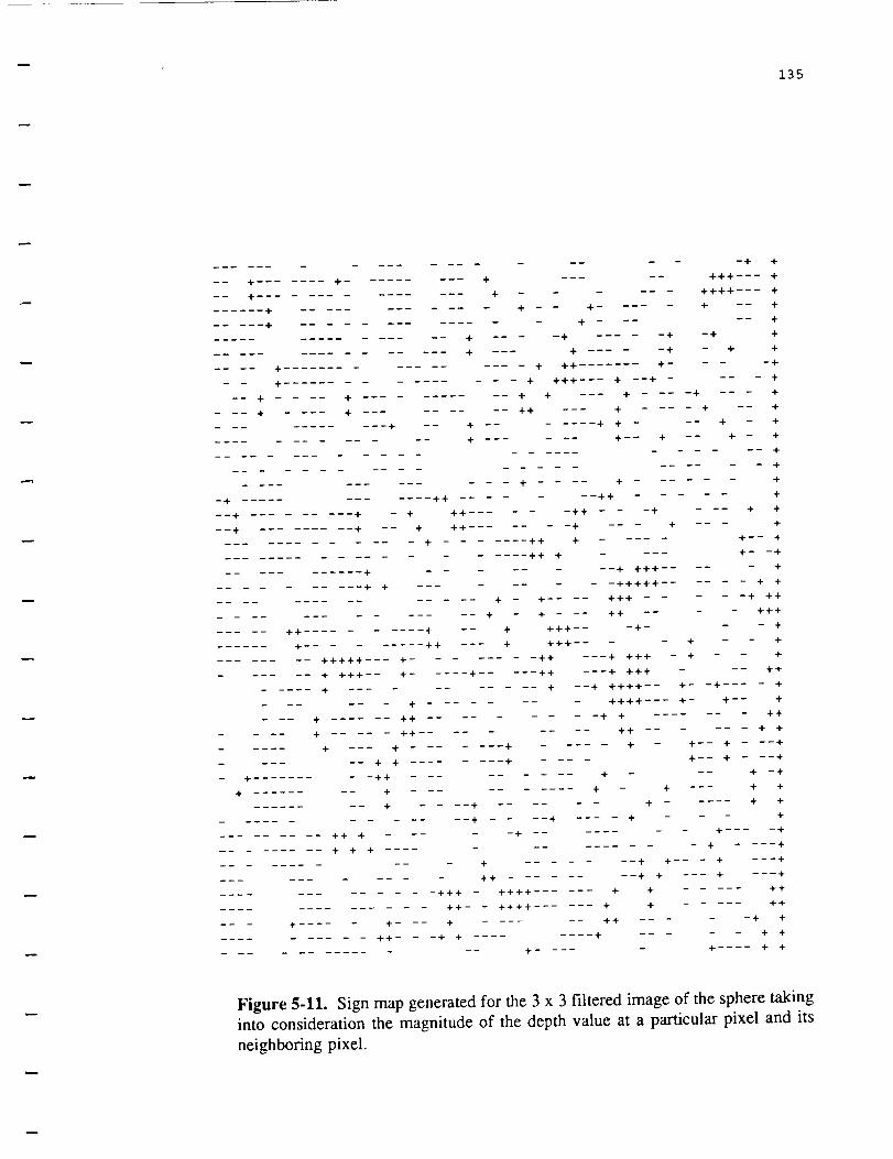
135

............... + +

-- + ....... + ......... + ..... +++---- +

-- + ............... + ...... ++++---- +

...... + ............ + +- + -- +

.... + .............. + -- +

................ + -+ ..... + -+ +

..... + --- + ..... + - + +

.... + ............. + ++ ....... + .... +

+ ............... + +++--- + --+ .... +

4- .... 4- ---

........ .#.

-_+ ......... +

--- + + --- + .... + +

...... ++ --- + .... + -- +

-- + ....... + + - __ + - +

-- + ...... +-- + -- + - +

............. +

_ _ + .... + ......

.... ++ ....... ++ - _ _

+ ++ ...... ++ - _ -+

--+ ...... + -- + ++- + -- +

............. + ....... ++ + .....

.................... ++ +

........... + ....... + +++ ....

....... + + ........ +++++ ....

............... + - + .... +++ - _

............ + - + - __ ++ -- _

..... ++ .......... + -- + +++-- -+-

...... + ......... ++ --- + +++ .... +

- +

+

+

+ +

+

+-- +

+- -+

- +

- + +

-+ ++

+++

_ _ +

- - 4-

........ +++++--- + ........ ++

- -4-.......

4- ......

......... ++ + --

......... + + + ....

............ +++

.......... ++-

__ _ + ..... +- -- +

---+ +++ - + - +

..... + +++-- + ..... + ..... ++ ---+ +++ - __ ++

..... + ....... + --+ ++++-- +- -+ .... +

+ ....... ++++---- +- +-- +

+ ...... ++ -+ + ....... ++

+ ..... ++ ........ ++ -- _ + +

.... + --- + ...... + ..... + - +-- + - --+

__ + + ........ + - __ +-- + - --+

- -++ ........ + - -- 4- -+

-- + ......... + - + --- + +

-- + .... + .... + ..... + +

.... + - --+ .... + - +

- + ...... + ..... _.

......... + .... 4-

+ ...... + + -- - + ---+

++ ........ + + --- + ---+

++++ ...... + + ..... ++

++++ ...... + + ..... ++

_ _ ++ -+ +

...... ++ - _ -+ + ........ + - _ + +

........... + .... + .... + +

Figure 5-11. Sign map generated for the 3 x 3 filtered image of the sphere taking

into consideration the magnitude of the depth value at a particular pixel and its

neighboring pixel.

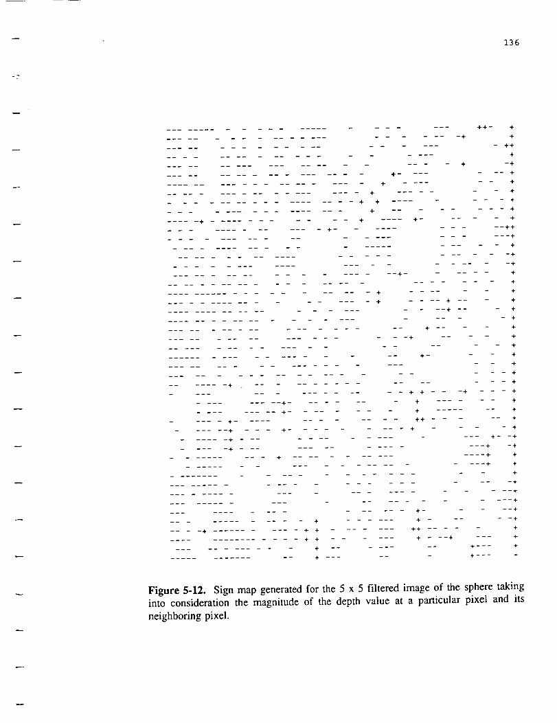
136

.... 4- ........... + + ....... ++ - - -

............... + + 4- - --4-

....... 4- ........

.............. 9- ......



neighboring pixel.

137

..................... +-

+

+

+

- +

- +

- -+

- +

- +

--+

_ _ +

- +

+

+

-+

- +

- +

-+

+

+

-+

- +

- +

- +

- +

- +

- -+

- +

- +

- -+

- -4-

-+

+

+

-+

+

+

+

+

- +

-+

+

- -+

- +

- -4-

+

+

+

-+



neighboring pixel.

138

"Z.

Of = 25 ° - (horizontal pixel #) (0.1961 deg/pixel). (5.4)

0g = (vertical pixel #) (0.1961 deg/pixel) -25 °. (5.5)

L = 0.362m. (5.6)

R is Range in meters = (0.00459 m/pixel)(Range pixel) + (n - 1/2), (5.7)

where n is the electronic range in meters set by the operator. The cartesian coordi-

nate information was then utilized for determining the coefficients which describe each

of the three-dimensional surfaces.

Experiments were conducted on range data for spheres and cylinders. Results of

median filtering for one such set of range data is presented.

Figure 5-14 is the actual range image of a cylinder. Figure 5-15 is the range

image after segmentation. Similarly, figures 5-16 and 5-17 illustrate the 3 x 3 and the

5 x $ median filtered images of the cylinder range data.

Curvature maps for studying the effect of median filtering on the range data are illus-

trated in figures 5-18(a,b,c,d), figures 5-19(a,b,c,d), and figures 5-20(a,b,c,d), which are

the first and second derivatives with respect to the x and y axes for the original

cylinder image, the 3 x 3 filtered cylinder image, and the 5 x 5 filtered cylinder

image, respectively.

Sign maps similar to the ones derived for the sphere are generated for the

cylinder and are shown in figures (5-21), (5-22), and (5-23). The figures correspond to

the original, the 3 x 3 filtered image, and the 5 x $ filtered images of the cylinder,

respectively. Analyzing the curvature maps for the cylinder indicates the filtering pro-

cess removed the noise and smoothed the image data without effecting significant dis-

tortions. The sign maps, much like the curvature maps, seem not much affected by the

filtering process other than some information (range data) being lost at the edges.

Listed in tables 5-1 and 5-2 are the coefficients obtained for the original range images,

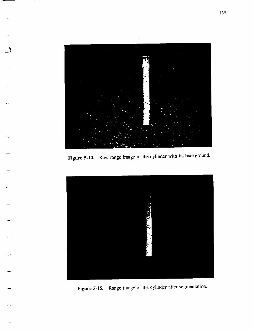
139

Figure 5.14. Raw range image of the cylinder with its background.

Figure 5-15. Range image of the cylinder after segmentation.

140

Figure 5-16. 3 x 3 median filtered image of the raw cylinder.

Figure 5-17. 5 x 5 median filtered image of the raw cylinder.

141

++++++++++++++++++

++++++++++++++++++

++++++++++++++++++

++++++++++++++++++

++++++++++++++++++

++++++++++++++++++

++++++++++++++++++

++++++++++++++++++

++++++++++++++++++

++++++++++++++++++

++++++++++++++++++

++++++++++++++++++

++++++++++++++++++

++++++++++++++++++

++++++++-+++++--++

++++++++--++++-+++

............... +++

++++++++++++++++++

++++++++++++++++++

++++++++++++++++++

++++++++++++++++++

+++-++++++++++++++

++---+++++++++++++

+++-++++-+++++++++

++++++++-+++++++++

++++++++++++++++++

++++++++++++++++++

++++++++++++++++++

++++++++++++++++++

++++++++++++++++++

++++++++++++++++++

++++++++++++++++++

++++++++++++++++++

++++++++++++++++++

++++++++++++++++++

++++++++++++++++++

++++++++++++++++++

++++++++++++++++++

++++++++++++++++++

++++++++++++++++++

++++++++++++++++++

++++++++++++++++++

++++++++++++++++++

++++++++++++++++++

+++++++++--+++++++

++++++++++++++++++

++++++++++++++++++

Figure 5-18a. First derivative w.r.t x-axis of the original cylinder.

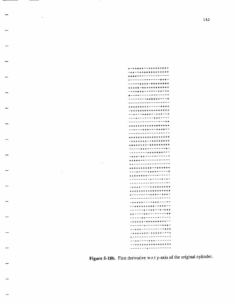
142

+-+++++--+++++++++

-++--+++++++++++++

++++ ..............

.............. +++-

..... ++++-++++++++

+++++-++++++++++++

---++++ ...... ++---+

+ .................

++++++---+

+++++++++ ..... ++++

-+++++++++++++++++

--+---++++---+++--+

--_+ ....... +++ ....

................ ++

++++++++++++++++++

...... +++---++++--

++++++++++++++++++

-+++++++--++++++++

++++++++-+++++++++

..... +++ ........ +-

........ +++++++---

-+++-++ ...........

+++++ .............

++++++++++--++++++

_-_+ .... ++++ ..... +

++++++++ ..........

......... + .... +-+-

-++++ .... +++++++++

++++++++++++++++++

+ ........ +++--+++-

-+++++ .... +++ .....

--+++++++++--+++--

...... +--++--+-+++

++ .... ++ ........ ++

..... ++ ...........

-+++++-+++++++++--

...... + ....... +++-

--+++ .......... +++

-+++++++-+++++---+

+ .................

--++ .... +++ .......

--++++++++++++++++

....... + ..........

Figure 5-18b. First derivative w.r.t y-axis of the original cylinder.

143

++++++++++++++++++

++++++++++++++++++

++++++++++++++++++

++++++++++++++++++

++++++++++++++++++

++++++++++++++++++

++++++++++++++++++

++++++++++++++++++

++++++++++++++++++

++++++++++++++++++

+++++++++++++++++-

++++++++++++++++++

++++++++++++++++++

++++++++++++++++++

++++++++++++++++++

++++++++++++++++++

++++++++++++++++++

--++ ........... +++

............... ++-

++++++++++++++++++

++++++++++++++++++

++++++++++++++++++

++++++++++++++++++

++++++++++++++++++

++++++++++++++++++

++++++++++++++++++

++++++++++++++++++

++++++++++++++++++

++++++++++++++++++

................. +

................. +

................. +

................. +

................. +

................. +

................. +

................. +

................. +

................. +

................. +

................. +

................. +

................. +

................. +

Figure 5-18c. Second derivative w.r.t x-axis of the original cylinder.

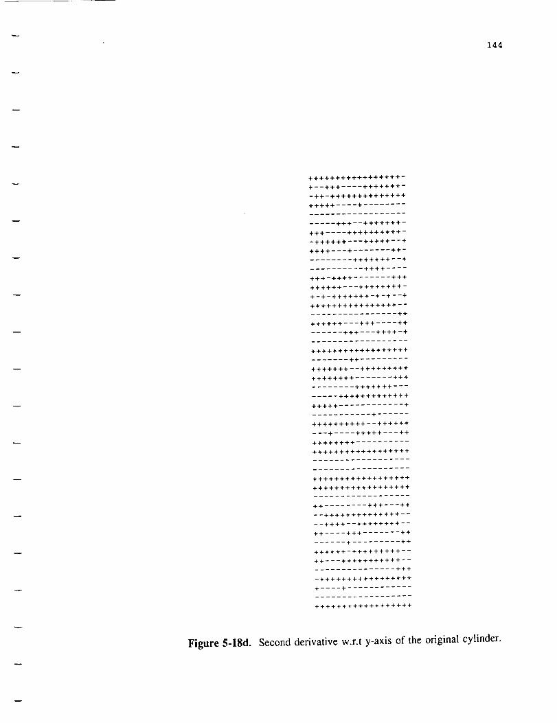
144

+++++++++++++++++-

+--+÷+ .... +++++++-

-++-++++++++++÷+++

+++++ .... + ........

..... +++--+++++++-

+++ .... ÷+÷++÷+÷++-

-++++++---++++÷--+

+++÷---÷ ....... ++-

........ ÷÷+++++--+

.......... ++++ ....

+++-÷+++ ....... ÷++

÷+++÷+---++++++++-

+-+-+++++++-+-+--+

÷++÷+++÷+++÷÷+÷÷--

÷÷+_++---÷++ .... ++

...... +÷+---++÷+-+

+÷÷+÷÷÷÷÷+++÷÷÷+÷+

....... • w .........

+++++++--÷+÷÷+÷+w+

++++++++ ....... +++

........ +÷++++÷---

+++++ ............ +

+++÷w+++++--++++++

___+ .... +++++---++

+_÷++÷÷+ ..........

+÷+++++++÷++++++++

++÷+++++++++++++++

++++++÷+++++÷+++++

÷+ ........ +++---++

--++++++++++++++--

--++++--+÷++++++--

++ .... +++ ....... ++

...... + ......... ++

÷+++++-÷+++++÷÷+--

++---÷+++++++++÷--

............... +++

-+++÷++÷+++÷+÷÷+++

+ .... + ............

+++++÷++++++++++++

Figure 5-18d. Second derivative w.r.t y-axis of the original cylinder.

++++++++++++++++++

++++++++++++++++++

++++++++++++++++++

++++++++++++++++++

++++++++++++++++++

++++++++++++++++++

++++++++++++++++++

++++++++++++++++++

++++++++++++++++++

++++++++÷+++++++++

++++++++++++++++++

++++++++++++++++++

++++++++++++++++++

++++++++++++++++++

++++++++++++++++++

+++++++--+++++_+++

+-+++++--+++++-+++

--+++---++-+++++++

--+++--++++++-++++

++++++++++++++++++

++++++++++++++++++

++++++++++++++++++

-+--++++++++++++++

-+---+++-+++++++++

-+-++++--+++++++++

+++++++--+++++++++

++++++++++++++++++

++++++++++++++++++

++++++++++++++++++

++++++++++++++++++

++++++++++++++++++

++++++++++++++++++

++++++++_+++++++++

++++++++++++++++++

++++++++++++++++++

++++++++++++++++++

++++++++++++++++++

++++++++++++++++++

++++++++++++++++++

++++++++++++++++++

++++++++++++++++++

++++++++++++++++++

++++++++++++++++++

++++++++++++++++++

++++++++++++++++++

+++++++++-++++++++

++++++++++++++++++

++++++++++++++++++

Figure 5-19a. First derivative w.r.t x-axis of the cylinder filtered with amask size of 3 X 3.

146

-+--++ ..... +++++++

+---+++----++ .... +++

+-+ ...............

-+--+---+++ .... ++++

...... +----++++++++

.... +-+ .... ++-++++

+-++++ ....... ÷----+

................. +

+ .... ++--+++++++++

.... +++ +-+

+++++++++++++-++++

---+---++-++++---+

......... + ........

................ ++

...... +++---++++--

-++++++++++ .... +--

++--++-+-+ .... +--+

++++++++++++++++++

++++++++++++++++++

.......... +-+ .....

....... ++++++++---

+-+ ...... + ........

-++++ .............

++++-+-+ ........ ++

-+++++++++++++++++

--++++ .... + ...... +

+-+--++ ...........

++ ........... + ....

++++++++++++++++++

++++++++++++++++++

---+++-+++++++-+++

--++++--++++++++--

-+++--+++ ..... ++++

...... + ...........

+ ....... ++-+++---+

-+++++++++++++++++

-_-+ ..............

--+ ............. ++

................. +

+ .................

..... ++ .......... +

-+++++++++++++++++

...... ++--+++++---

Figure 5-19b. First derivative w.r.t y-axis of the cylinder filtered

a mask size of 3 X 3.

with

147

++++++++++++++++++

++++++++++++++++++

++++++++++++++++++

++++++++++++++++++

++++++++++++++++++

++++++++++++++++++

++++++++++++++++++

++++++++++++++++++

++++++++++++++++++

+++++++++++++÷++++

+++++++++++++++++-

++++++++++++++++++

++++++++++++++++++

++++++++++++++++++

++++++++++++++++++

+++++++-++++++++++

+++++++-+++++--+++

+-++++-+++++++++++

+++++++++++++++++-

++++++++++++++++++

++++++++++++++++++

++++++++++++++++++

++++++++++++++++++

++-+++++++++++++++

++-+++++++++++++++

+++++++-++++++++++

++++++++++++++++++

+++++++÷++++++++++

++++++++++++++++++

................. +

................. +

................. +

................. +

................. +

................. +

................. +

................. +

................. +

................. +

................. +

................. +

................. +

................. +

................. +

................. +

................. +

................. +

Figure 5-19c. Second derivative w.r.t x-axis of the cylinder filtered with a

mask size of 3 X 3.

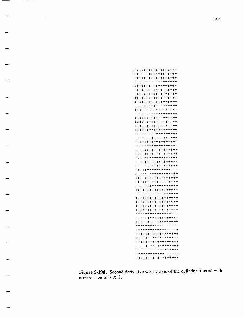
148

+++++++++++++++++-

-++--++++--++++++-

++-+++++++++++++++

+-+ ...............

++++++++++ .... +-+-

-+-+-+-++-+++++++-

-+--+-+++++++-+++-

++++++++++++++++++

+-++++++-+++--+---

........ + .........

+++--+++-+++++++++

+++++++-++ .... +++-

+++++++++-++++++++

++++++++++++++++--

++++++--+++++--+++

...... +++---+++--+

-++++++++-++++-++-

+++++++++++++++++-

++++++++++++++++++

-+++-+ ......... +++

.... +++++++++++---

+ .... +++++++++++++

-++++ ..... + .......

+ .... + .......... ++

+++-++++++++++++++

-+-+++-+++++++++++

__+-+++ ......... ++

++++++++++++++++--

++++++++++++++++++

++++++++++++++++++

++++++++++++++++++

++++++++++++++++++

--+÷++--+++++++---

++++++++++++++++++

...... + ...........

+ ................ +

++++++++++++++++++

++-++ .... +++++++--

++++++++++-+++++++

.... +---+++ ..... ++

+ .......... +-++---

+ .................

-+++++++++++++++++

Figure 5-19d. Second derivative w.r.t y-axis of the cylinder filtered witha mask size of 3 X 3.

149

++÷+++++++++++++++

+++++++÷++++++++++

++++++++++++++++++

++++++++++++++++++

++++++++++++++++++

++++++++++++++++++

++++++++++++++++++

++++++++++++++++++

++++++++++++++++++

++++++++++++++++++

++++++++++++++++++

++++++++++++++++++

++++++++++++++++++

++++++++++++++++++

++++++++++++++++++

++++++++++++++++++

-+++++--++++++++++

++++++++++++++++++

++++++++++++++++++

++++++++++++++++++

++++++++++++++++++

--++++++++++++++++

..... +++--++++++++

--++++++++++++++++

+-++++++++++++++++

--++++++++++++++++

++++++++++++++++++

++++++++++++++++++

++++++++++++++++++

++++++++++++++++++

++++++++++++++++++

++++++++++++++++++

++++++++++++++++++

++++++++++++++++++

++++++++++++++++++

++++++++++++++++++

++++++++++++++++++

++++++++++++++++++

++++++++++++++++++

++++++++++++++++++

++++++++++++++++++

++++++++++++++++++

++++++++++++++++++

++++++++++++++++++

++++++++++++++++++

++++++++++++++++++

++++++++++++++++++

++++++++++++++++++

Figure 5-20a. First derivative w.r.t x-axis of the cylinder filtered with amask size of 5 X 5.

150

-+-++---+÷+-+-++++

--+ .... ÷-

..... +----+--++÷+++

++÷-+---++-+÷-++--+

...... ÷+ .... ÷÷-+÷+

........... ÷ ..... +

-+--+-+-+++÷++++++

+++++++++÷++÷÷÷+++

+-++++++÷ ..... ++--

+++++÷+÷÷+÷÷++++++

+++++++÷÷÷+++÷++++

-+++++++++++++++++

....... ÷-+++++++÷÷

+ .................

................. +

+÷ ...... + ....... ++

+ .... ++ ...........

--++++ ............

++ .... +÷+ .........

++ ....... +++ ......

+++++++÷++++++++++

+++++++÷÷+++++++++

- -÷ .............. +

......... + -++ .....

+ .................

-÷+--+-÷++--+-+++-

-+++++++++++++++++

+÷++++++++++++++++

-+÷+++--+÷++++÷+-+

................. +

................ ++

-+++++++++ .... ++++

..... +-++++ .......

.... + ........ + ....

Figure 5-20b. First derivative w.r.t y-axis of the cylinder filtered witha mask size of 5 X 5.

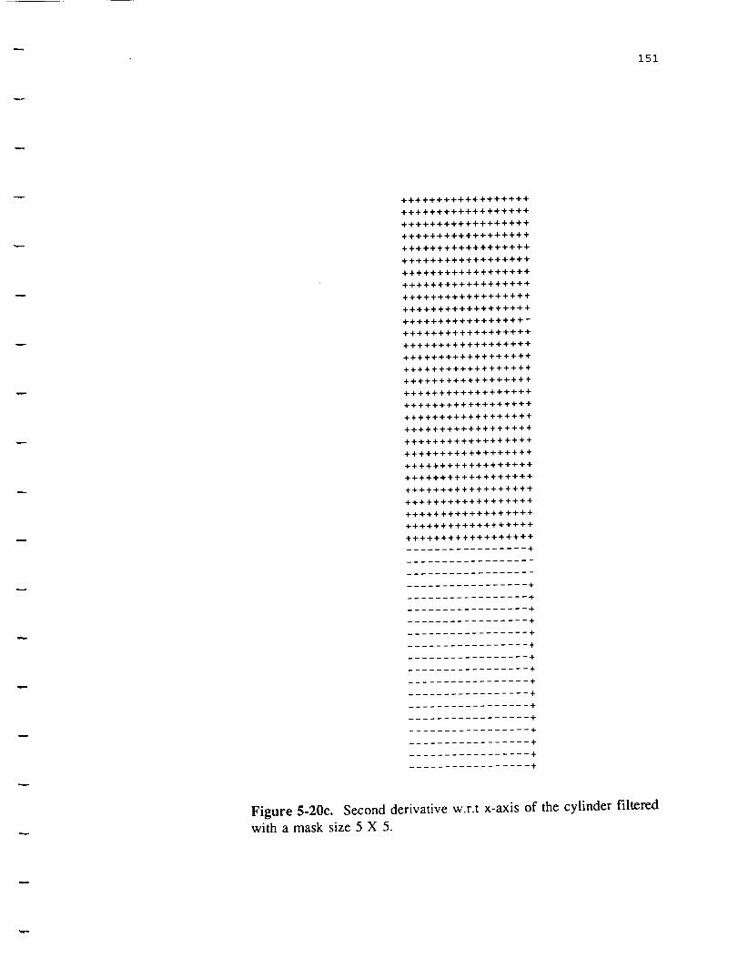
151

÷÷+÷÷÷÷+++÷++÷÷÷÷+

+÷÷÷++÷÷+++++÷++÷÷

+÷++÷+++÷÷÷++++÷+÷

++÷÷_÷+÷_÷÷++÷÷+÷

÷÷÷÷÷+÷++++÷++÷++÷

÷+++÷÷++÷+÷÷÷÷+÷÷÷

+÷÷+÷÷+÷+++÷++÷÷÷+

÷+÷+÷++++++++++÷++

+÷÷+++÷++++÷+++++÷

÷÷÷+÷+÷++÷÷÷++÷÷+_

÷+÷+÷+÷+++÷÷÷++++÷

++++++++÷_++÷+÷÷++

÷÷+÷÷÷÷+÷++÷++÷÷+÷

+÷÷++÷+++++÷+÷+÷÷÷

+÷+÷++++÷÷+÷÷+÷+÷÷

+++÷÷+÷+÷++÷÷÷+++_

+++÷++++÷+÷÷++++÷+

++÷+÷+++++÷+÷+÷+++

÷÷+÷+÷++÷+÷÷+++÷++

+÷+÷+÷++÷+÷++÷÷÷+÷

+÷+++÷+++÷÷++÷÷+÷+

++++÷÷÷÷+÷÷+÷+++÷+

+++÷÷÷_++÷++÷++÷÷+

+÷÷++÷+++++÷++++++

÷÷÷+÷÷÷_+_÷+÷+÷+++

÷÷+_÷+++++÷++÷÷_+÷

+++÷÷÷++÷÷÷+++÷+÷÷

+++++++_+÷+÷++++÷+

Figure 5-20c. Second derivative w.r.t x-axis of the cylinder filteredwith a mask size 5 X 5.

152

+++++++++++++++++-

+-+--+++ ..........

++-+++++++++++++-+

__+ ...............

---+-++--+--++-++-

++++++-+++++-++---

+++++++++++-+++++-

-+-+-+--++-+++++++

+ ...... +++++++ ....

++++++++++++++++++

+++++++++++++++++-

++---++++ ..... ++++

++++++++++++++++-+

++++++++++++++++++

......... +++++--++

---+++++ ...... ++--

+++++++++++++++++-

-+++++++++++++++++

--+-+++++++++++++-

-+---++---+-++++++

+++ ..... +--++--++-

--++++++-+++++++--

-++++--+++++++++++

+ ..... + ...........

--++++---++++-++++

++-+++++++++-+-+++

--+++++++---+++---

++++++++++++++++++

++++++++++++++++++

+++++++++-+--+÷+++

++++++++++++++++++

+ .................

-++++++++--+-+--++

++++++++++++++++++

++++++++++++++++++

++-+++++++++++++--

................. +

................ +-

++++++++++-+++++++

++---++++++++-+++-

Figure 5-20d. Second derivative w.r.t y-axis of the cylinder f'dtered witha mask size of 5 X 5.

153

_ _ +++++

- ++ - ++++

+++ -- ++++

+ ..... +++

..... +- +++

+++ .... +++++

+ --- ++++

-+ ...... + +++++

-+ ...... + +++++

-+ _- + --- +++

-+ ..... + --- +++

..... +++---+++++

-+ ...... +++-- +++++

-+- +++---+++ ---++

+++---+++ .... ++

---++-- +_- + ++++

__+ __ + - ++++

++ --+++++

+ --+++++

-- + .... +++++

__-++ .... +++++

++ ....... + ++++++

++ .... +___ ++++++

-+--+++--- +--+++++

-+- +++ .... +--+++++

.... + .... +++

..... + + -- -+++

-+ --++++ + -- ++++

-+ --+++ ++ --+++++

-++ .... + -- +++++

-+ .... + -- +++++

_-_+ __ + - + ++

___+ __ +++

__ _ + +++

+ +++ +++

.... ++___ + --+++++

.... ++ -- + - +++++

-+ .... +++ --- ++

-+ .... ++ .... +++

Figure 5-21. Sign plot for the original cylinder. The sign "+" or "-" is

assigned depending whether the adjacent pixel has a range value lesser

or greater than the pixel to its left.

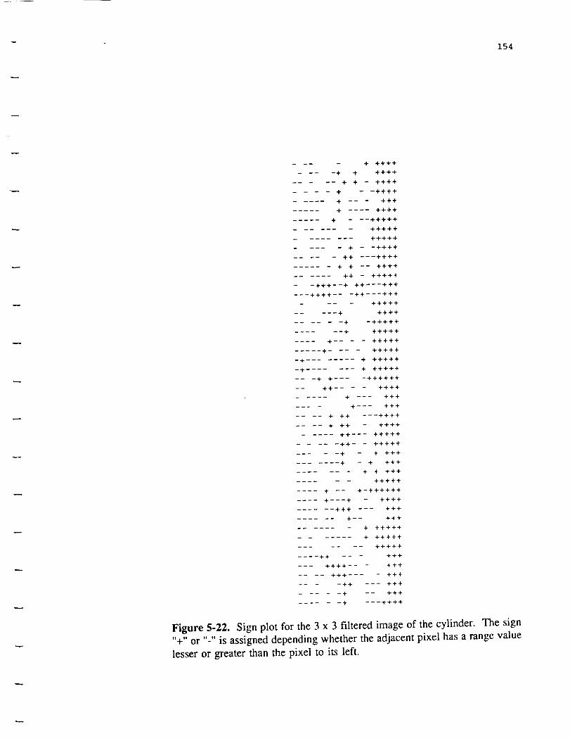
154

.... + ++++

-+ + ++++

.... + + ++++

.... + - --++++

..... + +++

..... + .... ++++

..... + -- ----+++++

- -- +++++

........ +++++

+ - --++++

..... ++ ----++++

...... + + -- ++++

...... ++ - +++++

-- -+++---+ ++---+++

---++++--- -++---+++

- +++++

..... + ++++

..... + -+++++

...... + +++++

.... + .... +++++

..... +- +++++

-+ ........ + +++++

-+ .... + +++++

-- -+ + ..... _+++++

--- ++ .... ++++

..... + +++

.... +--- +++

.... + ++ ---++++

.... + ++ - ++++

..... ++---- +++++

..... ++- - +++++

-+ - + +++

....... + - + +++

....... + + +++

.... +++++

.... + --- +-++++++

.... +----+ - ++++

...... +++ --- +++

...... +-- +++

....... + +++++

....... + +++++

....... +++++

---++ -- - +++

--- ++++-- - +++

+++ .... +++

.... ++ +++

..... + -- +++

...... + ---++++

Figure 5-22. Sign plot for the 3 x 3 filtered image of the cylinder. The sign

"+" or "-" is assigned depending whether the adjacent pixel has a range value

lesser or greater than the pixel to its left.

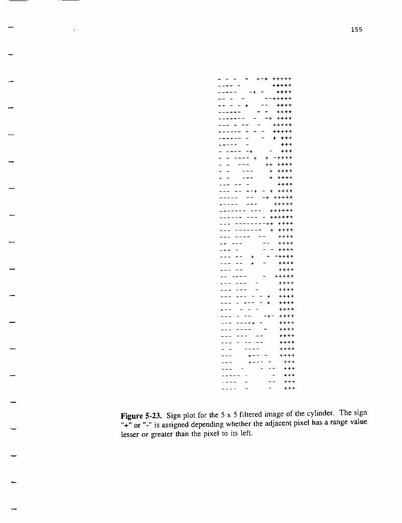
155

+--÷ ÷÷÷++

..... ÷÷+÷+

...... + - +÷÷÷

...... +÷÷++

.... ÷ -- ÷÷++

........ +÷+÷

......... + ÷+÷÷

....... +÷÷+÷

......... ÷+÷++

........ + ÷÷+

...... ++÷

...... + - +++

...... ÷ + -+÷÷÷

..... ÷+ ÷+÷+

_ _ + ++++

..... ÷ ÷÷÷+

..... ÷+++

.... + - + ++÷+

......... @ ÷++÷+

.... +++++

.......... ÷÷+÷+÷

.......... ÷÷÷÷÷÷

........... ÷÷ ++÷÷

.......... + ÷+÷+

......... ÷÷÷÷

__ -- ++÷+

...... +÷÷+

..... + - -++++

..... + +++÷

..... +÷+÷

....... +++÷+

....... +÷++

....... ++÷÷

.... + ÷+++

..... ÷ +÷++

++++

__ -+- ÷÷÷÷

....... + - ++++

........ ++÷÷

........ ÷÷++

........ +÷÷÷

..... ÷÷+÷

+_- - ++÷+

+ .... ++÷

-- +++

....... ÷++

....... +++

...... +÷+

Figure 5-23. Sign plot for the 5 x 5 filtered image of the cylinder. The sign

"+" or "-" is assigned depending whether the adjacent pixel has a range value

lesser or greater than the pixel to its left.

156

the 3 x 3 filtered images, the 5 x 5 filtered images and finally the 7 x 7 filtered

images of a sphere and a cylinder.

These tables show that none of the coefficient sets describe a real sphere or

cylinder with any certainty. The following procedure was utilized to determine which

particular set of coefficients best describes the original range data of the object. A

small surface patch of the object is chosen. In the quadratic form,

F(x,y,z) = ax 2 + by 2 + cz 2 + 2fyz + 2gzx + 2hxy + 2px + 2qy + 2rz + d = 0,

the coefficients a, b, c, d, f, g, h, p, q, and r are inserted and for each (x,y,z) of the

object patch, the error is evaluated for each set of coefficients. A plot is generated in

which every point of the surface patch is replaced with the numerals 1, 3, 5, and 7

signifying that the minimum error was obtained for that particular set of coefficients.

Figure 5-24 is one such plot for the raw segmented image of the sphere. Numeral 1

refers to the situation when the original set of coefficients fits best, and similarly

numerals 3, 5, and 7 are used depending whether the 3 x 3 or the 5 x 5 or the 7 x

7 set of coefficients, listed in Table 5-1, of the sphere fits best. As seen from Figure

5-24, the presence of excess number of the numeral 3 confirms the results obtained

from the curvature maps for the sphere range data. Figure 5-25 is the plot using the

coefficients listed in Table 5-2 for the cylinder. Both of these plots validate our

findings from the analysis of the curvature maps.

The experiments mentioned above were performed on a large number of real

range data sets for spheres, cylinders, and cones, the results of which are shown in

appendix A.

5.3 Application of the Recognition Process to the Processed Image Data

The next objective was to apply our recognition schemes to the processed images

of a sphere, a cylinder and a quadric cone. Each of the processed images of the

sphere, the cylinder, and the cone were intersected with two planes (one parallel to the

157

6056666666666664446664_

666666666464.444444444444_

66666666644444444_44444444433336366666663636666666666566666_

6666666666_,4_4_4_4_4d43333333336333_

66666666_.__444_433333333363_66666666_.44_44_4_4_3333333333333165122666666666666666666

6666666664_44444_444433333333333333131121262666666666666666

666664_44_4_4_454111133333323332323222222262266666666

66666664.44444444444444344113133333333332333232222222266666666

666664_44_4_4_4333333333333333333312222222222222266666

6666_.44444_4545555444443333333333333331312121222121222222626666666_,4_444_4_454443333333333333333131133332222222222222626

666666_._44_4_43333333333333333133333332322222222222622

566554_444_44_4_4333131111133333131113111211112212111212

65655444_4_444_4_3433333331333333333333333133312112222122222

64654554_44_444_443333333333333333133333111123221222221211

666545544_44444_33333333333131133131113111111231212221211

6464444444454554444431333333333331311133313111111112212111112

666_._44_33333333333333333333333313111111111122121111

6646_.4444_4_4_444_3333333333333333333131311111111111111111212

6'!444_4_44444_433333333333333331333331311111111111111111212

_444444_4444_44333333333331333333333333333333313331111222222

_44_44444_444_333333333331333331333131333331311111111112222

4444444444444444333333333333333333333131133333313111112122212

_4444_333333333333333333333131333331313111112131212

65444_444_44433333555115333311313333333333131111111111331312

4545544444444443333551155113313113333333333131111111111331312

_4_4_5444434333333313333333333333331311111111131111111122

_44_44444_4435333333313333333333333331313111111331113111122

4544444545454545555535111333311113313111111113313131111111111

_44_4_445454435353335333333313113333111111133333131111131211

5554444444453333333333333333333131313133333131313111111111111

55544444_454333333333333333313111111133333131111111111111111

554544444544333333333333333333333333333131111111111111111111154444_4_4433333333333333333333333333333333331311111311111111

4545554444443335353333333331311111311111313111311111111111111

5545544444333335333333333331311113313111333333313111113111111

5555454555453555533333333333333333333333311333333133313133333

Figure 5-24. Best fit plot for the sphere raw image.

158

1111111113111111337

1111333111131153337

1111111111111153537

1135335115311111137

1155151175711111117

1111111177111777757

1111111177111777777

1155557777177777711

1355555777711777717

1111111111777777137

11311111133777771171131113111111111137

1131351111131111737

1131155357511117111

11313555577113553111111111333131133155

1131131333131133155

3113311353133315315

3115111157111111117

1355355157771137317

1135555137771177117

1131155111777777115

1131135311177777135

1135311315777777135

1135313513577777135

1131331353177177115

1131331333137177711

1111333771111117773

1111155777111111175

1355557777771177711

1555557777771177735

1531113777111777115

1333133177711777111

7315533577777771113

7513551577777777775

1351155317771171111

1155555111777771113

1135355337777777111

11111511177711771111355555777777777773

1555555777777777775

Figure 5-25. Best fit plot obtained for the cylinder belonging to set A. Numerals

"1, 3, 5, 7" denote the original image, the 3 x 3 image, the 5 x 5 image, and the

7 x 7 image respectively.

159

COMPARISON OF COEFFICIENTS EVALUATED FOR THE ORIGINAL

AND THE PROCESSED IMAGES OF A SPHERE

COEFFICIENT RAW IMAGE 3 X 3 lILT. IMAGE 5 X 5 lILT. IMAGE 7 X 7 lILT. IMAGE

A, COEFF. OF Xz

B, COEFF. OF Y:

C, COEFF. OF Z 2

F, COEFF. OF YZ

G, COEFF. OF XZ

H, COEFF. OF XY

P, COEFF. OF X

Q, COEFF. OF Y

R, COEFF. OF Z

D, CONSTANT

0.3026

0.2734

0.6545

0.22 i I

0.2802

0.7747

-0.3260

-0.4860

-0.3338

0.5310

0.6357

0.3524

0.3036

0.4199

-0.8172

0.2847

-0.5348

-0.4860

0.2339

0.1999

0.4401

-1.0163

0.3717

0.4834

0.7194

-0.5801

-0.3159

-0.3524

0.3191

-0.0973

0.4242

0.2178

0.5845

-0.3417

-0.7452

0.4353

0.3127

0.1996

-0.5858

0.1516

Table 5-1. Comparison of the coefficients evaluated for the original and the processed

images of a sphere.

160

COMPARISON OF COEFFICIENTS EVALUATED FOR THE ORIGINAL

AND THE PROCESSED IMAGES OF A CYLINDER

COEFFICIENT RAW IMAGE 3 X 3 FILTERED IMAGE 5 X 5 FILTERED IMAGE

A, COEFF. OF X 2

B, COEFF. OF y2

C, COEFF. OF Z 2

F, COEFF. OF YZ

G, COEFF. OF XZ

H, COEFF. OF XY

P, COEFF. OF X

Q, COEFF. OF Y

R, COEFF. OF Z

D, CONSTANT

0.8338

0.004 I

0.059

-0.00103

-0.636

0.4437

-0.0141

-0.189

0.193

-0.1341

0,6636

0.0209

-0.0923

-0.0219

-0.7604

0.7727

0,4242

-0.2155

0.374

-0,253

0.0572

0.599

0.4416

-0.807

0.459

-0.149

-0.5915

1.089

-I.019

0.664

Table 5-2. Comparison of the coefficients evaluated for tile original and the

processed images of a cylinder.

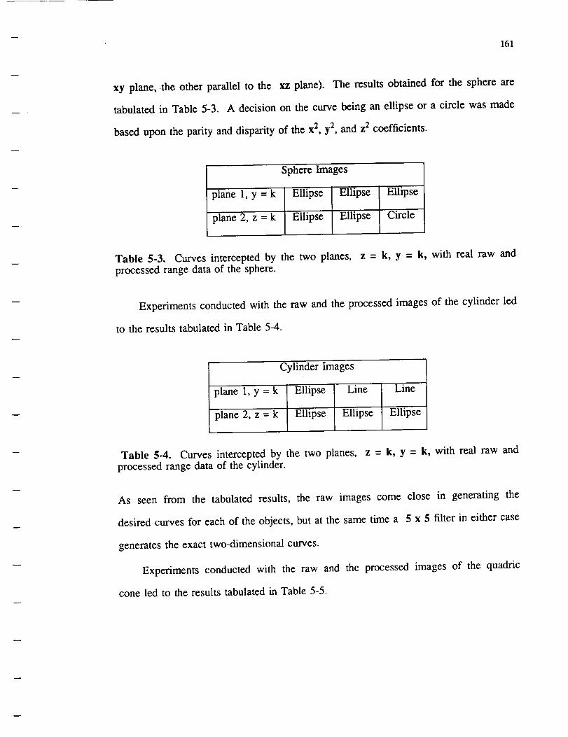
161

xy plane, the other parallel to the xz plane). The results obtained for the sphere are

tabulated in Table 5-3. A decision on the curve being an ellipse or a circle was made

based upon the parity and disparity of the x 2, y2, and z2 coefficients.

Sphere Images

plane 1, y = k Ellipse Ellipse Ellipse

plane 2, z = k Ellipse Ellipse Circle

Table 5-3. Curves intercepted by the two planes, z = k, y = k, with real raw andprocessed range data of the sphere.

Experiments conducted with the raw and the processed images of the cylinder led

to the results tabulated in Table 5-4.

Cylinder Images

plane 1, y = k Ellipse Line Line

l_lane 2, z = k Ellipse Ellipse Ellipse

Table 5-4. Curves intercepted by the two planes, z = k, y = k, with real raw andprocessed range data of the cylinder.

As seen from the tabulated results, the raw images come close in generating the

desired curves for each of the objects, but at the same time a 5 x 5 filter in either case

generates the exact two-dimensional curves.

Experiments conducted with the raw and the processed images of the quadric

cone led to the results tabulated in Table 5-5.

162

QuadricconeImages

plane 1, z -- k Ellipse Ellipse Ellipse

plane2, y = k Ellipse Hyperbola Hyperbola

Table 5-5. Curvesinterceptedby the two planes, z = k, y = k, with real raw andprocessedrangedataof thequadriccone.

As seenfrom thetabulatedresults,the raw imagesdo not comeclosein generatingthe

desiredcurvesfor eachof the objects,but at the sametime the 3 x 3 as well as the

5 x 5 filter in either casegeneratesthe exact two-dimensionalcurves. Coefficients

generatedfor the raw imagedataof the coneaswell asthe 3 x 3 and 5 x 5 median

filtered imagedataof thequadricconearelisted in AppendixB.

5.4 Application of the Rotation Alignment Algorithm

The rotation alignment algorithm which determines the orientation of the quadric

surfaces in space and then aligns them in accordance to our desired coordinate system

was applied to simulated data as well as real data.

Consider tables 5-6, 5-7, and 5-8, which compare the coefficients of the sphere

range data before and after rotation alignment.

Each of the image data sets, i.e., the original raw image of the sphere and the 3

x 3 and the 5 x 5 median filtered images of the sphere, required three iterations to

eliminate the product terms. Since a sphere is symmetric about all coordinate axes, no

rotation alignment should be needed. The alignment algorithm was performed just to

see how the coefficients relate to each other before and after the rotation. The

coefficients were basically invariant as expected.

Similarly, tables 5-9, 5-10, and 5-1 1, show the coefficients obtained before and

after the rotation alignment for the cylinder range data. However, in these cases, each

of the image data sets, i.e., the original raw image of the cylinder, the 3 x 3 and the

163

COEFFICIENT BEFORE AFTER ALIGNMENT

A, COEFF. OF X 2

B, COEFF. OF y2

C, COEFF. OF Z 2

F, COEFF. OF YZ

G, COEFF. OF XZ

H, COEFF. OF XY

P, COEFF. OF X

Q, COEFF. OF Y

R, COEFF. OF Z

D, CONSTANT

0.3026

0.2734

0.6545

0.5310

0.6357

0.3524

0.3036

0.4199

-0.8172

0.2847

0.3206466

0.184263

0.7999953

0.0

0.0

0.0

0.252

0.41686

-0.8623

0.2847

Table 5-6. New coefficients of the raw image data of sphere after alignment.


A, COEFF. OF X 2

B, COEFF. OF y2

C, COEFF. OF Z 2

F, COEFF. OF YZ

0.264

0.129

0.5738

-0.6275

G, COEFF. OF XZ

H, COEFF. OF XY

P, COEFF. OF X

Q, COEFF. OF Y

R, COEFF. OF Z

D, CONSTANT

-0.783

0.4014

0.4826

0.3670

-0.7218

0.2210

0.249

0.1311

0.634

0.0

0.0

0.0

0.4405

0.3746

-0.7401

0.2210

Table 5-7. New coefficients of the 3 x 3 median filtered image data of sphere

after alignment.

164


A, COEFF. OF X 2

B, COEFF. OF y2

C, COEFF. OF Z 2

F, COEFF. OF YZ

G, COEFF. OF XZ

H, COEFF. OF XY

P, COEFF. OF X

Q, COEFF. OF Y

R, COEFF. OF Z

D, CONSTANT

0.303

0.392

0.6526

-0.4487

-0.8376

0.2416

0.4047

0.2214

-0.7089

0.1913

0.3765

0.372

0.6417

0.0

0.0

0.0

0.4259

0.2184

-0.7423

0.1913

Table 5-8. New coefficients of the 5 x 5 median filtered image data of sphere

after alignment.


A, COEFF. OF X 2

B, COEFF. OF y2

C, COEFF. OF Z 2

F, COEFF. OF YZ

G, COEFF. OF XZ

H, COEFF. OF XY

P, COEFF. OF X

Q, COEFF. OF Y

R, COEFF. OF Z

D, CONSTANT

0.8338

0.00411

0.059

-0.00103

-0.636

0.4437

-0.0141

-0.189

0.193

-0.1341

0.9812

-0.1143

0.03255

0.0

0.0

0.0

-0.0876

-0.2478

-0.01125

-0.1341

Table 5-9. New coefficients of the raw image data of cylinder after alignment.

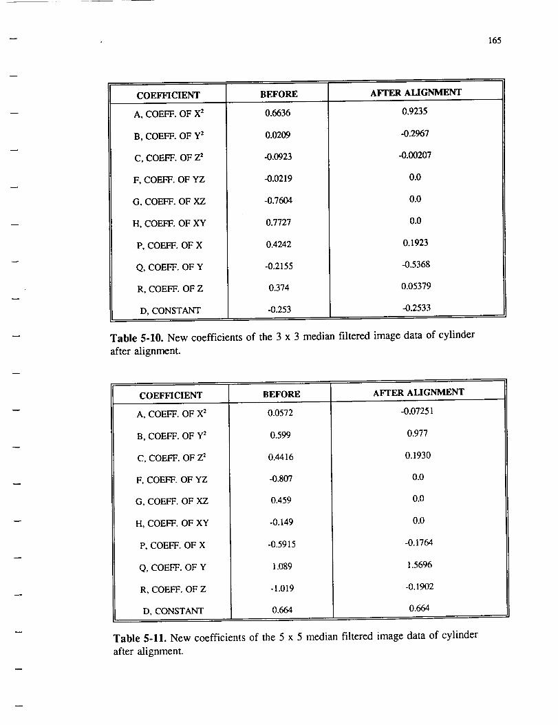
w

165


A, COEFF. OF X 2

B, COEFF. OF y2

C, COEFF. OF Z 2

F, COEFF. OF YZ

G, COEFF. OF XZ

H, COEFF. OF XY

P, COEFF. OF X

Q, COEFF. OF Y

R, COEFF. OF Z

D, CONSTANT

0.6636

0.0209

-0.0923

-0.0219

-0.7604

0.7727

0.4242

-0.2155

0.374

-0.253

0.9235

-0.2967

_.00207

0.0

0.0

0.0

0.1923

_.5368

0_5379

_.2533

Table 5-10. New coefficients of the 3 x 3 median filtered image data of cylinder

after alignment.


A, COEFF. OF X 2

B, COEFF. OF y2

C, COEFF. OF Z 2

O.0572

0.599

0.4416

F, COEFF. OF YZ

G, COEFF. OF XZ

H, COEFF. OF XY

P, COEFF. OF X

-0.807

0.459

-0.149

-0.5915

Q, COEFF. OF Y

R, COEFF. OF Z

D, CONSTANT

1.089

-1.019

0.664

-0.07251

0.977

0.1930

0.0

0.0

0.0

-0.17_

1.5696

-0.1902

0.664

Table 5-11, New coefficients of the 5 x 5 median filtered image data of cylinder

after alignment.

m

166

5 X 5 median filtered images of the cylinder, required four iterations to eliminate the

product terms. Except for the coefficients of the raw image data, both the 3 x 3 and

5 x 5 filtered coefficients after alignment yielded the desired curves when intersected

with various planes. Making use of the coefficients of the 5 x 5 filtered image, the

diameter of this particular cylinder was calculated to be 4.99 centimeters. The actual

diameter of the cylinder was 5 centimeters. Appendix C contains more results

obtained while carrying out the rotation alignment algorithm for other cylinder range

images.

The rotation alignment technique was utilized for a large group of simulated data.

Listed in tables 5-12, 5-13, and 5-14 are several upon which the utilization of our

recognition scheme correctly identified the surfaces. Upon application of our recogni-

tion scheme the quadric surfaces represented in Tables 5-12, 5-13, and 5-14 were

correctly recognized as an ellipsoid, a hyperboloid of one sheet, and a hyperbolic

cylinder, respectively.

All the simulated data Sets of quadric surfaces could be recognized after conduct-

ing the rotation alignment technique on the original quadratic representation. The

three-dimensional discriminant approach which was described in Chapter Two was

applied to several simulated data of quadrics.

5.5 Application of Three-Dimensional Discriminant Technique

Results for the simulated data are illustrated in Table 5-15 and are very effective

as predicted by the theory. Object (1) refers to a parabolic cylinder, (2) refers to a

hyperbolic paraboloid, (3) refers to a hyperboloid of one sheet, (4) refers to an ellip-

soid, (5) refers to a hyperbolic cylinder, (6) refers to a quadric cone, (7) refers to a

hyperboloid of two sheets, and (8) refers to an elliptic paraboloid. A listing of a sam-

ple data file is included in Appendix D. However, as expected, unsatisfactory results

were obtained while experimenting with real data. A listing of all the programs

167


A, COEFF. OF X 2

B, COEFK OF Y2

C, COEFF. OF Z 2

F, COEFF. OF YZ

G, COEFF. OF XZ

H, COEFF. OF XY

P, COEFF. OF X

Q, COEFF. OF Y

R, COEFF. OF Z

D, CONSTANT

103

125

66

-60

-12

-48

0.0

0.0

0.0

-294

49.84

96.887

145.3905

0.0

0.0

0.0

0.0

0.0

0.0

-294

Table 5-12, New coefficients of an unknown simulated data obtained after alignment.


A, COEFF. OF X 2

B, COEFF. OF Y:

C, COEFF. OF Z _

F, COEFF. OF YZ

G, COEFF. OF XZ

H, COEFF. OF XY

P, COEFF. OF X

Q, COEFF. OF Y

R, COEFF. OF Z

D, CONSTANT

0.0

2.0

1.0

-4.0

-4.0

0.0

0.0

0.0

0.0

-4.0

2.0

-4.0

-1.0

0.0

0.0

0.0

0.0

0.0

0.0

-4.0

_ Table 5-13. New coefficients of an unknown simulated data obtained after alignment.

i

168


A, COEFF. OF X 2

B, COEFF. OF y2

C, COEFF. OF Z 2

F, COEFF. OF YZ

0.0

0.0

0.0

-1.414

G, COEFF. OF XZ

H, COEFF. OF XY

P, COEFF. OF X

Q, COEFF. OF Y

R, COEFF. OF Z

D, CONSTANT

0.0

1.0

0.0

0.0

0.0

-3.0

3.0

0.0

-3.0

0.0

0.0

0.0

0.0

0.0

0.0

-3.0

Table 5-14. New coefficients of an unknown simulated data obtained after alignment.

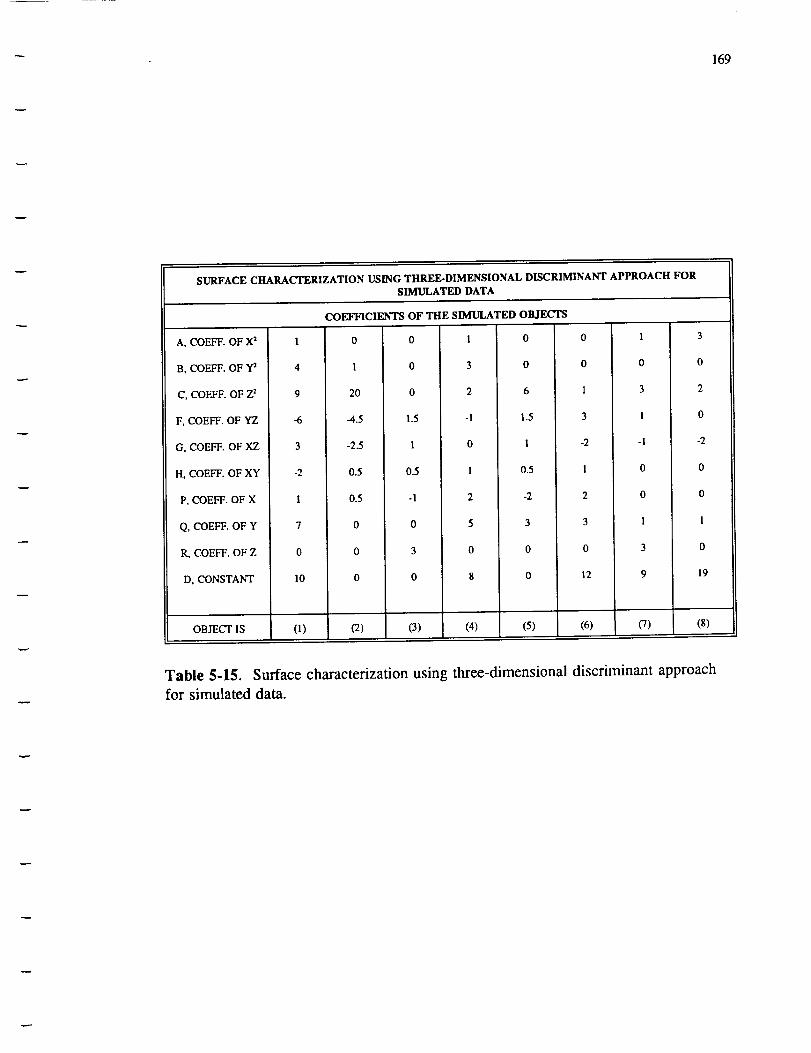
169

SURFACE CHARACTERIZATION USING THREE-DIMENSIONAL DISCRIMINANT APPROACH FORSIMULATED DATA

COEFFICIENTS OF THE SIMULATED OBJECTS

A. COEFF. OF X:

B, COEFF. OF Y_

C, COEFF. OF Z2

F, COEFF. OF YZ

G, COEFF. OF XZ

H, COEFF. OF XY

P, COEFF. OF X

Q, COEFF. OF Y

R, COEFF. OF Z

D, CONSTANT

OBIECT IS

1

4

9

-6

3

-2

1

7

0

10

(1)

o

1

20

-4.5

-2.5

0.5

0.5

0

0

o

(2)

0

0

0

1.5

1

0.5

-1

0

3

0

(3) (4)

0

o

6

1.5

1

0.5

-2

3

0

0

(5)

0

0

1

3

-2

1

2

3

0

12

(6)

1

0

3

I

-I

0

0

1

3

9

fT)

-2

0

0

1

0

19

(8)

Table 5-15. Surface characterization using three-dimensional discriminant approach

for simulated data.

170

utilized in this research is included in Appendix E. The program that generates the ten

coefficients for quadric surfaces and the program which aligns the quadric surfaces to a

desired coordinate system are among those listed.

CHAPTER SIX

CONCLUSIONS

6.1 Overview

We have presented a new approach based on two-dimensional analytic geometry

to recognize a series of three-dimensional objects. Among the various three-

dimensional objects considered are the hyperboloids of one and two sheets, the ellip-

soids, the spheres, the circular and elliptical quadric cones, the circular and elliptical

cylinders, the parabolic and hyperbolic cylinders, the elliptic and hyperbolic para-

boloids, and the parallelepipeds.

Our proposed method utilizes a two-dimensional discriminant which is a measure

for distinguishing curves. Instead of evaluating the ten generated coefficients and

attempting to recognize the surface from its quadric representation, we can identify

the quadrics using the information resulting from the intersection of the surface with

different planes. If the surface is one of those listed above, there are five possible

two-dimensional curves that may result from such intersections: (i) a circle, (ii) an

ellipse, (iii) a parabola, (iv) a hyperbola, and (v) a line. Thus, a feature or pattern

vector with five independent components can be formed for characterizing each of the

surfaces.

Although all of the quadric surfaces considered have been symmetric, our recog-

nition system can be extended to other three-dimensional objects. Figures 6-1, 6-2,

and 6-3 are examples of these surfaces which exist in the real world. To recognize

complex objects a suitable segmentation technique is required for the isolation of each

individual surface.

171

172

Figure 6-1.NASA).

This delta rocket is composed of cylindrical and conical shapes (Courtesy

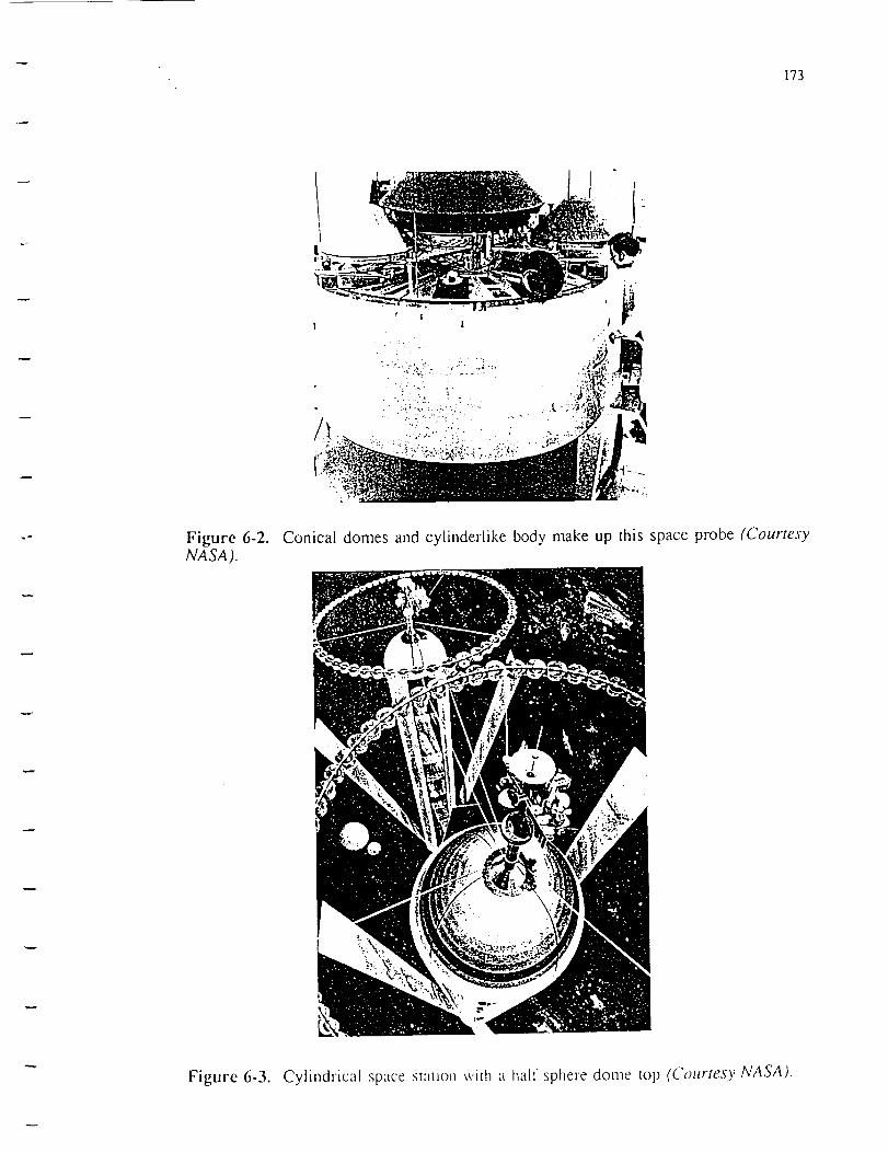
173

Figure 6-2.NASA).

•

Conical domes and cylinderlike body make up this space probe (Courtesy

Figure 6-3. Cylindrical space station v,'ith :t half sphere dome top (Courtesy NASA).

174

6.2 Advantages of the Recognition Scheme

Some of the advantages of our recognition scheme are listed below:

(1) Recognition systems using the curvature approach (evaluation of the mean and

Gaussian curvatures) are very computationally intensive. These approaches never

really describe the quadric surface in question. Our proposed recognition system is

computationally efficient. All of the quadric surfaces are recognized as well as

described in terms of their dimensions.

(2) The three-dimensional discriminant approach discussed in Chapter Two works

only on ideal or simulated data. It is not useful for real range data. Our recognition

system is shown to work for both simulated and real range data.

(3) The best-fit plot technique used for analyzing processed range images is a new

and efficient technique to determine the validity and integrity of the processed range

images.

(4) The rotation alignment technique is a new method which systematically and

effectively eliminates the product terms and aligns the quadric surfaces in our desired

coordinate system through an iterative technique.

(5) The curvature analysis technique and the best-fit plot can be used to determine

performances of various laser range mappers.

The equations of the planes which determine distinct feature vectors for each of

the quadric surfaces are very sensitive to the quality of the digitized range data. In

case the coefficient determining algorithm does not perform as expected, errors might

be encountered while forming the feature sets. Active sensors like laser range mappers

have only recently been developed. Much improvement is expected in the quality of

range images in the near future. This will make the various recognition schemes much

more reliable and flexible.

175

6.3 Future Goals and Research Directions

As seen from the best-fit plot in Chapter Five, regions within the range images

have been marked to indicate which particular filter size (median) fits the image data

the best at a particular pixel. While arriving at the coefficients of a second degree

polynomial which describe a quadric surface, the range data considered were either the

original, the 3 x 3, the 5 x 5, or the 7 x 7 median filtered range images. A filter

whose mask size varies from region to region could possibly be a more effective filter

which would not significantly distort the images.

Though experiments were performed on a large sample of range images belong-

ing to spheres, cylinders, and cones, the effectiveness and accuracy of the developed

recognition system can be tested further by using real range images of paraboloids,

hyperboloids and cylinders (hyperbolic and parabolic). The recognition algorithm,

however, has been very accurate when applied to simulated data.

We propose to extend our recognition algorithm to recognize quadric surfaces

from complex scenes (scenes composed of more than two objects). This can be

achieved by first utilizing an effective (existing) segmentation process, whereby range

data of various surfaces will be separated. We could extend our recognition system to

recognize irregular surfaces which are made up piece-by-piece of regular quadric sur-

faces.

Finally, we would like to investigate fully the mapping of the extrinsic and intrin-

sic representations of quadric surfaces. This process will lead to a three-dimensional

discriminant analogous to the two-dimensional discriminant, which will distinguish all

of the quadric surfaces considered for the recognition process in the course of this

research. The development of such a discriminant will not only reduce the computa-

tional complexity, but will also eliminate the process of eliminating the product terms

(rotation parameters) from the representation of the quadric surfaces. This approach

will be invariant to pose and orientation.

REFERENCES

[1] P.J. Besl and R. C. Jain, "Three-Dimensional Object Recognition," ACM Corn-

put. Surveys, vol 17, pp. 77-145, March 1985.

[2] R.A. Jarvis, "A Perspective on Range Finding Techniques for Computer Vision,"

IEEE Trans. on Pattern Analysis and Machine Intelligence, PAMI-5, pp. 122-139,

March 1983.

[3] M. Ishii and T. Nagata, "Feature Extraction of Three-Dimensional Objects and

Visual Processing in a Hand-Eye System using Laser Tracker," Pattern Recogni-

tion vol. 8, pp. 229-237, 1976.

[4] O. D. Faugeras et.al, "Towards a Flexible Vision System," Robot Vision, U.K.,

1982.

[5] M. Oshima and Y. Shirai, "Object Recognition using Three-Dimensional informa-

tion," IEEE Trans. on Pattern Analysis and Machine Intelligence, PAMI-5, No.

4, pp. 353-361, July 1983.

[6] B. Bhanu, "Representation and Shape Matching of 3-D Objects," IEEE Trans. on

Pattern Analysis and Machine Intelligence, PAMI-6, No. 3, pp. 340-350, 1984.

[7] R. Nevatia and T. O. Binford, "Description and Recognition of Curved Objects,"

Artificial Intelligence, 8, pp. 77-98, 1977.

[8] I.K. Sethi and S. N. Jayaramamurthy, "Surface Classification using Characteristic

Contours," Proc. 7th Intl. Conf. on Pattern Recognition, Montreal-Canada, pp.

438-440, 1984.

_ 176

177

[9] P.J. Besl and R. C. Jain, "Invariant Surface Characteristics for 3D Object Recog-

nition in Range Images," IEEE Trans. on Computer Vision, Graphics and Image

Processing, 33, 1, pp. 33-80, January 1986.

[10] N. Alvertos and I. D'Cunha, "Three-Dimensional Description of Symmetric

Objects from Range Images," SPIE vol 1382, Intelligent Robots and Computer

Vision IX: Neural, Biological, and 3-D Methods, pp. 388-396, 1990.

[11] N. Yokoya and M. D. Levine, "Range Image Segmentation based on Differential

Geometry: A Hybrid Approach," McRCIM-TR-CIM 87-16, 1987.

[12] W. E. L. Grimson and T. Lozano-Perez, "Model Based Recognition and Localiza-

tion from Sparse Range data," Techniques for 3-D Machine perception, Elsevier

Science Publishers (North Holland), pp. 113-148, 1986.

[13] O. D. Faugeras and M. Hebert, "The Representation, Recognition, and Positioning

of 3-D Shapes from Range Data," Techniques for 3-D Machine Perception,

Elsevier Science Publishers (North Holland), 1986.

[14] G. Hu and G. Stockman, "3-D Surface Solution using Structured Light and Con-

straint Propagation," IEEE Trans. on Pattern Analysis and Machine Intelligence,

vol. 11, No. 4, April 1989.

[15] M. Nagao, S. Hashimoto, and T. Saka, Automatic Model Generation and Recog-

nition of Simple Three-Dimensional Bodies, " New York: Academic Press, Inc.,

1973.

[16] S. Ullman and R. Basri, "Recognition by Linear Combination of Models," IEEE

Trans. on Pattern Analysis and Machine Intelligence, vol. 13, No. 10, pp. 992-

1006, October 1991.

[17] T. J. Fan, G. Medioni, and R. Nevatia, "Recognizing 3-D Objects using Surface

Descriptors," IEEE Trans. on Pattern Analysis and Machine Intelligence, vol.

11, No. 11, pp. 1140-1157, November 1989.

178

[18] D. Forsyth, J. L. Mundy, A. Zisserman, C. Coelho, A. Heller, and C. Rothwell,

"Invariant Descriptors for 3-D Object Recognition and Pose," IEEE Trans. on

Pattern Analysis and Machine Intelligence, vol. 13, No. 10, pp. 971-991, October

1991.

[19] S. Lee and H. Hahn, "An Optimal Sensing Strategy for Recognition and Localiza-

tion of 3-D Natural Quadric Objects," IEEE Trans. on Pattern Analysis and

Machine Intelligence, vol. 13, No. 10, pp. 1018-1037, October 1992.

[20] N. C. Grisworld and C. P. Yeh, "A New Stereo Vision Model Based upon the

Binocular Fusion Concept," IEEE Trans. on Computer Vision, Graphics, and

Image Processing, 41, pp. 153-171, 1988.

[21] D. Mart and T. Poggio, "A Computational Theory of Human Stereo Vision,"

Proc. R. Soc. London, B 204, pp. 301-308, 1979.

[22] W. E. L. Grimson, "Computational Experiments with Feature Based Stereo Algo-

rithms," IEEE Trans. on Pattern Analysis and Machine Intelligence, PAMI-7, pp.

17-34, 1985.

[23] R. P. Wilder, "Qualitative Three-Dimensional Shape from Stereo," Proc. SPIE,

Intelligent Robots and Computer Vision IX: Neural, Biological, and 3-D

Methods, vol 13382, pp. 453-463, 1990.

[24] J. M. H. Olmstead, Solid Analytical Geometry. New York: Appleton-Century-

Crofts. Inc., 1947.

[25] B. Spain, Analytical Quadrics. London: Pergamon press Ltd., 1960.

[26] B. Groshong and G. Bilbro, "Fitting a Quadric Surface to Three-Dimensional

Data," technical Report, January 1986.

[27] N. Alvertos and I. D'Cunha, "Curvature Effect of Median Filtering on Range

Images," IEEE proc. of Southeastcon 1991, vol. 2, pp. 910- 914, 1991. %.br

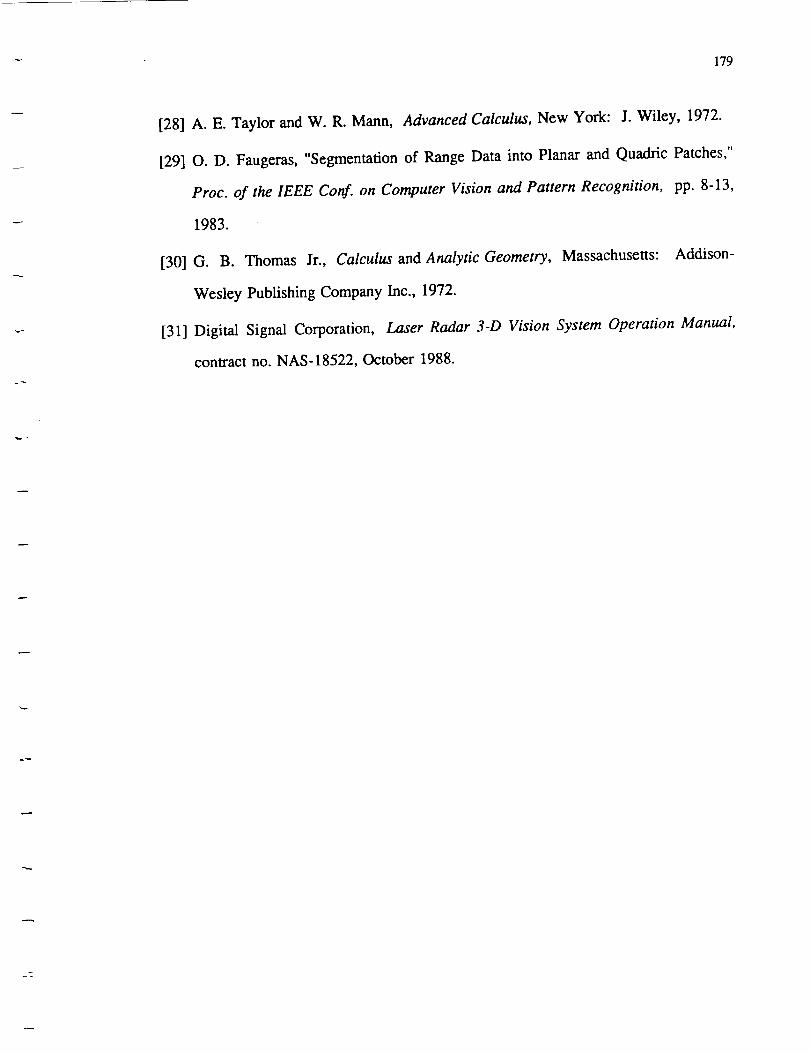
179

[28] A. E. Taylor and W. R. Mann, Advanced Calculus, New York: J. Wiley, 1972.

[29] O. D. Faugeras, "Segmentation of Range Data into Planar and Quadric Patches,"

Proc. of the IEEE Conf. on Computer Vision and Pattern Recognition, pp. 8-13,

1983.

[30] G. B. Thomas Jr., Calculus and Analytic Geometry, Massachusetts: Addison-

Wesley Publishing Company Inc., 1972.

[31] Digital Signal Corporation, Laser Radar 3-D Vision System Operation Manual,

contract no. NAS-18522, October 1988.

APPENDIX A

Appendix A consistsof the ten coefficientsgeneratedfor the original and pro-

cessedrangeimagesof a sphereanda cylinderwhosedata is mappedusinga different

type of laser range mapper. Files with extension*.cod refer to the range datacon-

verted into cartesian coordinates,and files with extension *.coe consist of the

coefficientsgeneratedfor eachof the images.

180

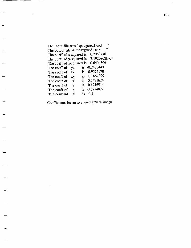
181

The

The

The

The

The

The

The

The

The

The

The

The

input file was "spavgmedl.cod "

output file is "spavgmedl.coe "

coeff of x-squared is 0.2963710

coeff of y-squared is -7.1920902E-03

coeff of z-squared is 0.6404306

coeff of yzcoeff of zx

coeff of xycoeff of x

coeff of ycoeff of z

constant d

is -0.2438449

ls -0.9575970

ts 0.1657399

is 0.5431624

is 0.1216914

is -0.6774822

is 0.1

Coefficients for an averaged sphere image.

182

The

The

The

The

The

The

The

The

The

The

The

The

input file was "SPAMED31.COD "

output file is "SPAMED31.COE "





coeff of xy

coeff of x

coeff of y

coeff of z

constant d

,s -0.1474224

,s -0.9272834

is 5.9526406E-02

is 0.6028971

is 6.9603384E-02

Is -0.8269780

,s 0.2249310

Coefficients for a 3 x 3 median filtered averaged sphere image.

w

183

The

The

The

The

The

The

The

The

The

The

The

The

input file was "SPAMED51.COD

output file is "SPAMED51.COE


coeff of y-squared is 0.1832946



coeff of xy

coeff of x


constant d

xs 0.8267535

Is -0.2360811

is -0.4166962

is -0.2436151

is -0.4302364

is -0.4764909

is 9.0547577E-02

o!

eo

Coefficients for a 5 x 5 median filtered averaged sphere image.

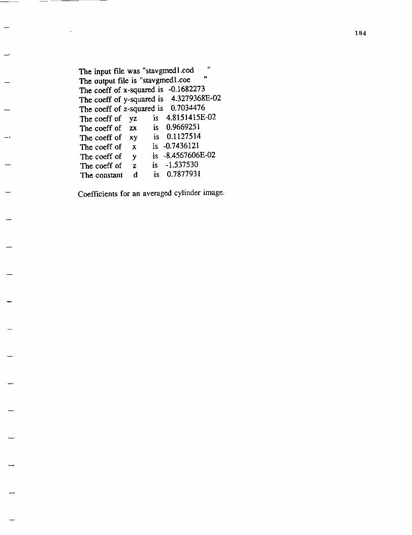
184

The

The

The

The

The

The

The

The

The

The

The

The

input file was "stavgmedl.cod

output file is "stavgmedl.coe

coeff of x-squared is

coeff of y-squared is

coeff of z,squared is

coeff of

coeff of

coeff of

coeff of

coeff of

coeff of

constant

yz IsZX IS

xy isX IS

y ,sZ 1S

d ,s

II

tl

-0.1682273

4.3279368E-02

0.7034476

4.8151415E-02

0.9669251

0.1127514

-0.7436121

-8.4567606E-02

-1.537530

0.7877931

Coefficients for an averaged cylinder image.

185

The

The

The

The

The

The

The

The

The

The

The

The

input file was "STAMED31.COD "

output file is "STAMED31.COE "


coeff of y-squared is 2.7527343E-02





constant d

_s 0.1449835

Is -0.9098228

ts -9.6383080E-02

is 0.5634921

is -8.9731783E-02

is -0.8506840

is 0.2536311

Coefficients for a 3 x 3 median filtered averaged cylinder image.

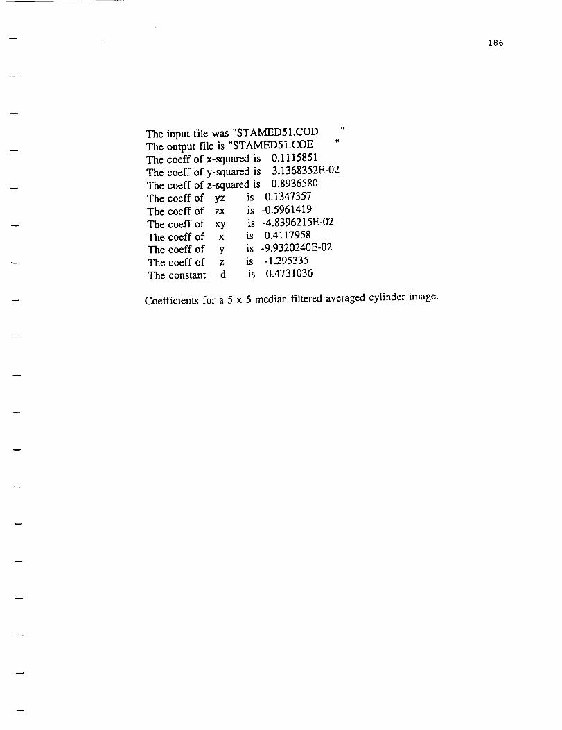
w

186

The

The

The

The

The

The

The

The

The

The

The

The

input file was "STAMED51.COD "

output file is "STAMED51.COE "


coeff of y-squared is 3.1368352E-02





constant d

IS

IS

IS

1S

1S

IS

IS

0.1347357

-0.5961419

-4.8396215E-02

0.4117958

-9.9320240E-02

-1.295335

0.4731036

Coefficients for a 5 x 5 median filtered averaged cylinder image.

APPENDIX B

This appendix consists of the ten coefficients generated for the original and pro-

cessed range images of a quadric cone. Files with extension *.cod refer to the range

data converted into cartesian coordinates, and files with extension *.coe consists of the

coefficients generated for each of the images.

187

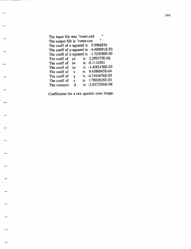
188

The

The

The

The

The

The

The

The

The

The

The

The

input file was "coner.cod "

output file is "coner.coe "



coeff of z-squared is -1.723930E-03




constant d

IS

IS

IS

1S

IS

1S

1S

2.299275E-02

-0.1116501

- 1.4285150E-02

9.4580045E-04

-4.7494676E-03

1.7082826E-03

-2.6372296E-04

Coefficients for a raw quadric cone image.

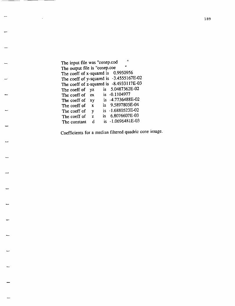
189

The

The

The

The

The

The

The

The

The

The

The

The

input file was "conep.cod "

output file is "conep.coe "



coeff of z-squared is -8.4933117E-03

coeff of yz is 5.0487362E-02coeff of zx is -0.1104977

coeff of xy is -4.7736488E-02coeff of x is 9.5897805E-04

coeff of y is -1.6880523E-02

coeff of z is 6.8076607E-03

constant d is - 1.0696481E-03

Coefficients for a median filtered quadric cone image.

APPENDIX C

This appendix consists of a sample executed file generated using the surface

alignment algorithm. The coefficients considered are that of a 3 x 3 filtered image of

a raw cylinder.

190

191

OUTPUT DATA FILE OF THE SURFACE ALIGNMENT PROGRAM

THE COEFFICIENTS CONSIDERED ARE OF THE 3 X 3 FILTERED IMAGE OF THE RAW

CYLINDER.

THE NUMBER OF ITERATIONS COMPLETED IS : 3

COEFF. OF X SQUARE TERM IS : -0.5819000

COEFF. OF Y SQUARE TERM IS : -2.5060000E-02

COEFF. OF Z SQUARE TERM IS : -0.4078000

COEFF. OF YZ SQUARE TERM IS : -9.1289997E-02

COEFF. OF XZ SQUARE TERM IS : 0.9860000

COEFF. OF XY SQUARE TERM IS : 8.9539997E-02COEFF. OF X TERM IS : -0.3951000

COEFF. OF Y TERM IS : 4.5000002E-02COEFF. OF Z TERM IS : 0.3026000

CONSTANT OF PROP. IS : -4.4810001E-02

-0.5854765 -2.1506138E-02-0.4078000 -1.2481645E-02 0.9838626

0.0000000E+00 -0.3974287 1.3208531E-02 0.3026000

-0.5854765 -2.1405339E-02 -0.4079008 0.0000000E+O0 0.9837343

-1.5888708E-02-0.3974287 8.3200261E-03 0.3027738

-0.9965052 -2.1405339E-02

-1.2192142E-02 -0.4991140

-0.9965433 -2.1367228E-02

0._E+00 -0.4990523

-0.9965433 -2.2384373E-02

- 1.2471168E-05 -0.4990523

-0.9965433 -2.2384373E-02

- 1.2471168E-05 -0.4990530

-0.9965433 -2.2384373E-02

0.0000000E+00 -0.4990530

-0.9965433 -2.2384373E-02

3.1279027E-03 - 1.0188361E-02 0.0000000E+O0

8.3200261E-03 -2.2511929E-02

3.1279027E-03 - 1.0188161E-02 -6.3691252E-05

1.1440012E-02 -2.2511929E-02

4.1450467E-03 0.0000000E+00 -6.2458355E-05

6.8105781E-03 -2.4316186E-02

4.1450476E-03 3.8919640E-10 0.0000000E+00

6.8105781E-03 -2.4300613E-02

4.1450476E-03 3.8919640E- 10 2.491243 IE- 15

6.8137725E-03 -2.4300613E-02

4.1450476E.03 0.0000000E+O0 2.4912431E-15

-1.8273728E-23 -0.4990530 6.8137725E-03 -2.4300613E-02

0._E+00 0.0000000E+00 0.0000000E+00 0.0000000E+O0 0.0000000E+00

0.0000000E+00 0.0000000E+00 0.0000000E+00 0.0000000E+00

THE NEW COEFF. OF X SQUARE TERM IS : -0.9965433

THE NEW COEFF. OF Y SQUARE TERM IS : -2.2384373E-02

THE NEW COEFF. OF Z SQUARE TERM IS : 4.1450476E-03THE NEW COEFF. OF X TERM IS : -0.4990530

THE NEW COEFF. OF Y TERM IS : 6.8137725E-03

THE NEW COEFF. OF Z TERM IS : -2.4300613E-02

THE NEW CONSTANT OF PROP. IS : -4.4810001E-02**************************************************** :_* _t _****:****

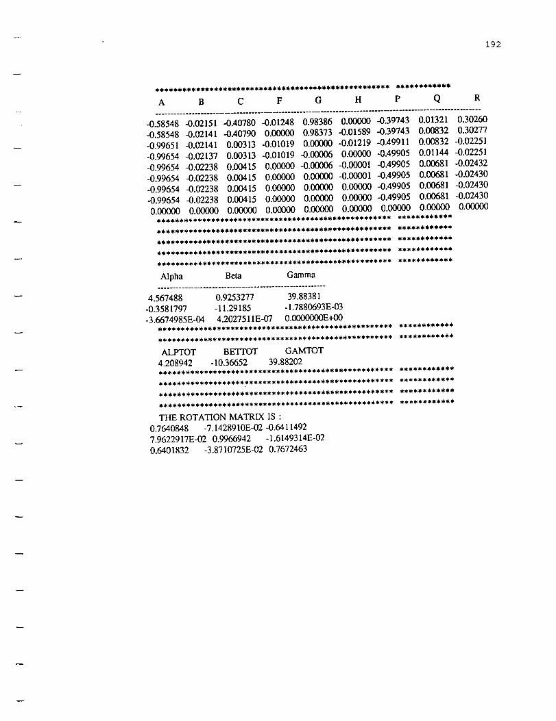
192

A B C F G H P Q R

-0.58548 -0.02151 -0.40780 -0.01248 0.98386 0.00000 -0.39743 0.01321 0.30260

-0.58548 -0.02141 -0.40790 0.00000 0.98373 -0.01589 -0.39743 0.00832 0.30277

-0.99651 -0.02141 0.00313 -0.01019 0.00000 -0.01219 -0.49911 0.00832 -0.02251

-0.99654 -0.02137 0.00313 -0.01019 -0.00006 0.00000 -0.49905 0.01144 -0.02251

-0.99654 -0.02238 0.00415 0.00000 -0.00006 -0.00001 -0.49905 0.00681 -0.02432

-0.99654 43.02238 0.00415 0.00000 0.00000 -0.00001 -0.49905 0.00681 -0.02430

-0.99654 -0.02238 0.00415 0.00000 0.00000 0.00000 -0.49905 0.00681 -0.02430

-0.99654 -0.02238 0.00415 0.00000 0.00000 0.00000 -0.49905 0.00681 -0.02430

0.00000 0.00(_ 0.130000 0.00000 0.00000 0.00000 0.000(0 0.00000 0.0000(3

Alpha Beta Gamma........................................................

4.567488 0.9253277 39.88381-0.3581797 - 11.29185 - 1.7880693E-03

-3.6674985E-04 4.2027511E-07 0.0000000E+00

ALPTOT BETrOT GAMTOT

4.208942 - 10.36652 39.88202

THE ROTATION MATRIX IS :

0.7640848 -7.1428910E-02 -0.64 11492

7.9622917E-02 0.9966942 -1.6149314E-02

0.6401832 -3.8710725E-02 0.7672463

APPENDIX D

This appendix consists of a sample data file which is generated while executing

the 3-D discriminant algorithm. The unknown quadric surface is later classified as a

parabolic cylinder.

193

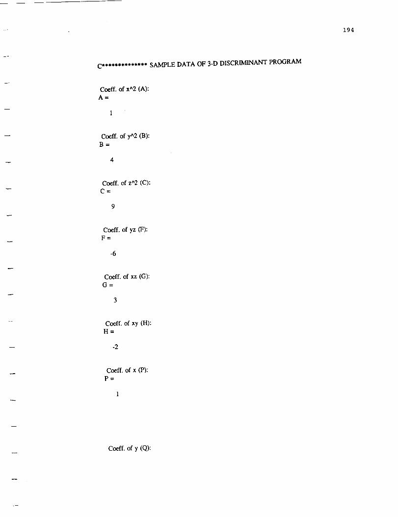
194

C************** SAMPLE DATA OF 3-D DISCRIMINANT PROGRAM

Coeff. of x^2 (A):

A=

Coeff. of y^2 (B):B=

Coeff.ofz^2 (C):

C=

Coeff. of yz (F):F=

-6

Coeff. of xz (G):

G=

Coeff.of xy (H):H=

-2

Coeff. of x (P):P=

Coeff. of y (Q):

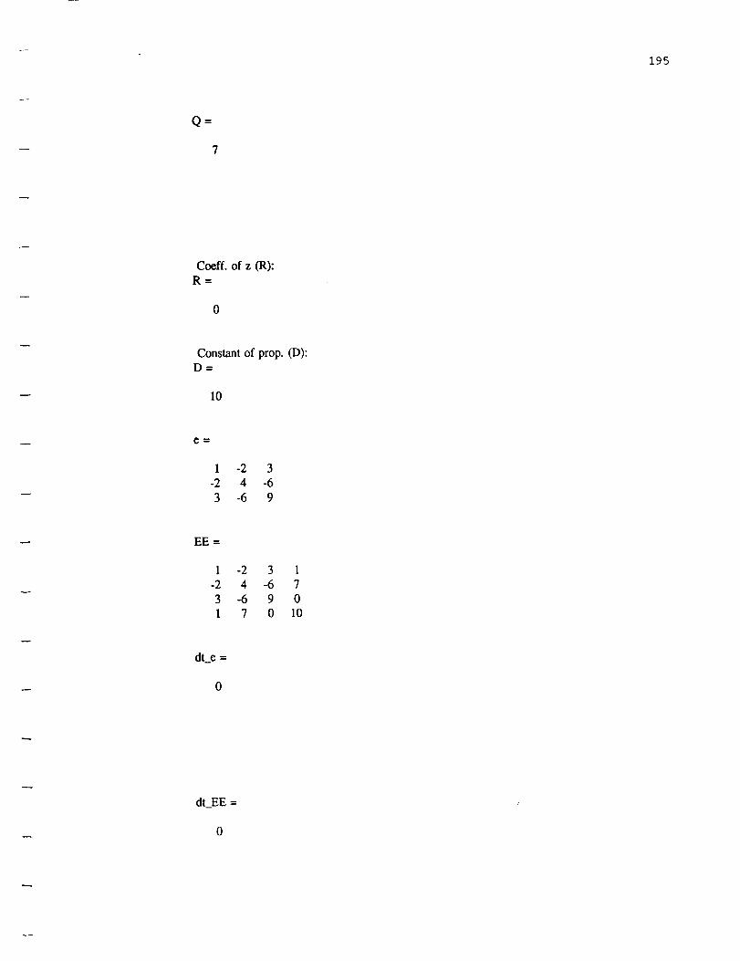
195

Q

7

Coeff. of z (R):R=

0

Constant of prop. (D):D=

I0

e _

1 -2 3-2 4 -6

3 -6 9

EE =

1 -2 3 1-2 4 -6 73 -6 9 01 7 0 10

dt._e =

0

dt_EE =

0

196

K_K =

49.00000.000014.0000

rho_3 =

rho_4 =

3

s_d_EE =

0

sl =

-1

s2 =

s3=

1

flag =

0

197

The sign of the ch. roots are not the same

The rank of EE is : 1.0000

The rank of e is : 3.0000

The sign of the determinant of EE is : 0.0000

The characterstics roots have the same sign? : 0.0000

The object is a PARABOLIC CYLINDER

APPENDIX E

This appendix consists of the listings of the following programs:

1. Program "Median Filtering", which performs the 3 x 3 and 5 x 5 median filtering

on range images.

2. Program "Derivatives" that evaluates the first and second derivative with respect

to x and y axes of the data files and then transforms it into a sign map.

3. Program "RangedifF' that generates the sign map for each of the range images

based upon the magnitude of the range value of neighboring pixels.

4. Program "Surface" that generates the ten coefficients which describe each of the

range images.

5. Program "Surface Alignment" which eliminates the product terms from the

representation of quadric surfaces thereby aligning them according to a desired

coordinate system.

6. Program "3-D discriminant" which implements the classification of the quadrics

based upon the discriminant procedure.

198

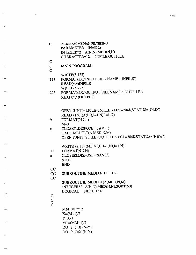
199

C

C

C

C

123

223

9

11

C

CC

CC

CC

C

C

C

PROGRAM MEDIAN FILTERING

PARAMETER (N=512)

INTEGER*2 A(N,N),MED(N,N)

CHARACTER* 12 INFILE,OUTFILE

MAIN PROGRAM

WRITE(*,123)

FORMAT(5X,'INPUT FILE NAME : INFILE')

READ(*,*)INFILE

WRITE(* ,223)

FORMAT(5X,'OUTPUT FILENAME : OUTFILE')

READ(*,*)OUTFILE

OPEN (UNIT= 1,FILE=INFILE, RECL=2048,STATUS ='OLD')

READ (1,9)((A(I,J),J= 1,N),I=I,N)

FORMAT(51214)M=3

CLOSE(1,DISPOSE='SAVE')

CALL MEDFLT(A,MED,N,M)

OPEN CUNIT=2,FILE=OUTFILE,RECL=2048,STATUS ='NEW')

WRITE (2,11)((MED(I,J),J=I,N),I=I,N)

FORMAT(51214)

CLOSE(2,DISPOSE='SAVE')

STOP

END

SUBROUTINE MEDIAN FILTER

SUBROUTINE MEDFLT(A,MED,N,M)

INTEGER*2 AON,N),MED(N,N),SORT(50)LOGICAL NEXCHAN

MM=M ** 2

X=fM+D/2Y=X-1

M 1 =(MM+ 1)/2

DO 7 I=X,(N-Y)

DO 9 J=X,(N-Y)

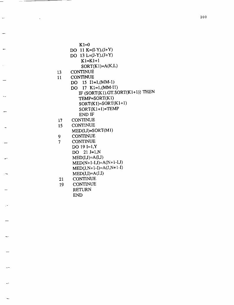
.... 200

13

11

17

15

21

19

K1--0

DO II K=(I-Y),(I+Y)

DO 13 L=(J-Y),(J+Y)

KI=KI+I

SORT(K1)=A(K,L)

CONTINUE

CONTINUE

DO 15 II=I,(MM-1)

DO 17 KI=I,(MM-I1)

IF (S ORT(K 1).GT. SORT(K 1+ 1)) THEN

TEMP=SORT(K1)

SORT(K1)=SORT(KI+I)

SORTCKI+I)=TEMP

END IF

CONTINUE

CONTINUE

MED(I,J)=SORT(M 1)

CONTINUE

CONTINUE

DO 19 I=I,Y

DO 21 J=I,N

MED(I,J)=A(I,J)

MED(N+I-I,J)=A(N+I-I,J)

MED(J,N+I-I)=A(J,N+I-I)

MED(J,I)=A(J,I)

CONTINUE

CONTINUE

RETURN

END

201

C*****

C*****

PROGRAM DERIVATIVES

This program determines the derivative along the x and the

y axes. A group of files can be compared to see whether a

a particular location has the same curvature or not.

20

100

815

811

300

C**

Cl111

C908

C

C9008

INTEGER*2

REAL

REAL

REAL

REAL

INTEGER*2

CHARA(ITER* 12

CHARA(,q'ER*2

CHARA('.TER*2

WRITE(*,20)

I1,J1,Ti,P1,K,L,I,J

DX 1,DX2,DX3,DY 1,DY2,DY3

DX11,DX22,DX33,DY 11,DY22,DY33

D(70,350),E(70,350),A(1000,3),AA(60,50)

D 1(70,350),E 1(70,350)

STREC,ENDREC

INFILE 1,INFILE2,INFILE3,POINT

GRAPH 1(70,100),GRAPH2(70,100),GRAPH3(70,100)

GRAPH4(70,100)

FORMAT(5X,'INPUT FILE NAME : INFILEI')

READ(*,*)INFILE1

OPEN(UNIT=l, FILE=INFILE1, STATUS='UNKNOWN')

DO 100 I=1,969

READ(1,*)(A(I,J),J=I,3)CONTINUE

DO 811 K=1,51

DO 815 L=1,19

AA(K,L)=A(L+(19*(K- 1)),3)CONTINUE

CONTINUE

FORMAT(51214)

TO FIND THE DERIVATIVE ALONG X-AXIS

WRITE(*,908)

FORMAT('INPUT THE STARTING RECORD NUMBER: STREC')

READ(*,*)STREC

FORMAT('INPUT THE ENDING RECORD NUMBER: ENDREC')

OPEN(UNIT=2,FI LE=' FILE 1. X ',S TATU S=' U NKNOWN')

OPEN(UNIT=3,FILE=' FILE 1.Y' ,STATUS= 'UNKNOWN')

202

11178

OPEN(UNIT--4,FILE='FILE 1.XX',STATUS=' UNKNOWN')

OPEN(UNIT=8,FILE='FILE 1. YY',STATUS=' UNKNOWN')

DO 1104 11=1,51

DO 1204 Jl=l,19

D(I1,J1)---0.5*((AA(I1,J I+I)-AA(I1,J1))+(AA(II+I,J1 + 1)-AA(II+I,J1)))

D1 (I1,J1)=(AA(II,JI-1)-2*(AA(I1,J1))+AA(I1,J1 +1))

1204

1104

1965

11104

324

326

325

EI(I1,J1)=(AA(II+I,J1)-2*(AA(I1,J1))+AA(II-I,J1))

E(I1,J1)=0.5*((AA(I1,JI+I)-AA(I1,JI+I))+(AA(I1,J1)-AA(II+I,J1)))CONTINUE

CONTINUE

DO 11104 I1=1,51

WRITE(2, *) (D (I 1,J 1),J 1= 1,19)

WRITE(3,*) (E(1131 ),J1 = 1,19)

WRITE(4,*)(D 1 (I 1,J 1),J 1= 1,19)

WR1TE(8,*)(E 1(I 1,J 1)31 = 1,19)

CONTINUE

CLOSE(2)

CLOSE(3)

CLOSE(4)

CLOSE(8)

OPEN(UNIT=2, FILE= 'FILE I. X',STATUS = 'UNKNOWN')

OPEN(UNIT=3, FILE= 'FILE 1. Y',S TATU S = 'UNKNOWN')

OPEN(U NIT---4, FILE= 'FILE 1. XX', STATU S =' U NKN OWN ")

OPEN(UNIT=5 ,FILE= 'FILE 1. YY',STATUS =' UNKNOWN')

DO 324 I1=1,51,1

READ(2,*)(D(I1,J1),J 1= 1,19)

CONTINUE

DO 325 I1=1,51,1

DO 326 Jl=l,19

IF (D(I1,J1).GT.D(I1,JI+I))THEN

GRAPHI(I1,J1)= ' 'ENDIF

IF (D(I1,J1).LT.D(I 1,JI+I))THEN

GRAPH I (I1,J1)= '+'

ENDIF

IF (D(I 1,J 1).EQ.D(-I 1,JI+I))THEN

GRAPHI(I1,J1)= ' '

ENDIF

CONTINUE

CONTINUE

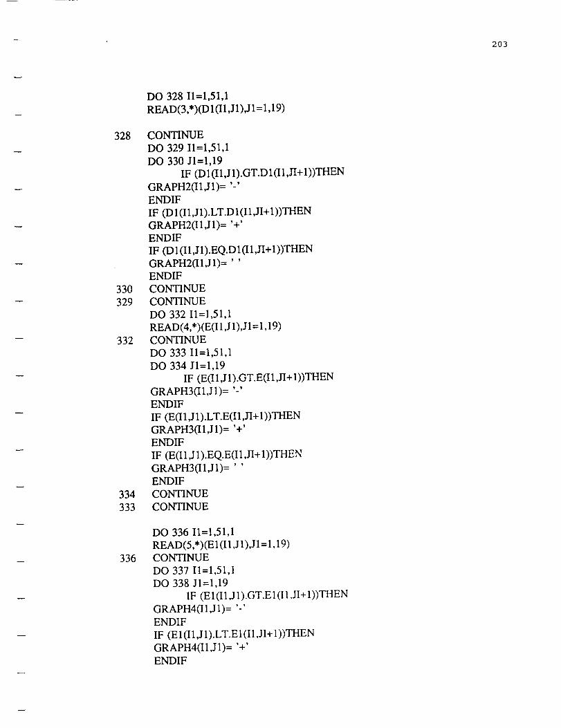
203

328

330

329

332

334

333

336

DO 328 I1=1,51,1

READ(3,*)(D 1(I 1,J 1),J 1= 1,19)

CONTINUE

DO 329 11=1,51,1

DO 330 Jl=l,19

IF (D 1(I 1,J 1).GT. D 1(I 1,JI+ 1))THEN

GRAPH2('I1,J1)= ' 'ENDIF

IF (D I(I1,J1).LT.D 1(I 1,JI+I))THEN

GRAPH2(I1,JI)= '+'

ENDIF

IF (D I (I 1,J I). EQ. D 1(I l,JI+ I))THEN

GRAPH2fI1J1)= ' 'ENDIF

CONTINUE

CONTINUE

DO 332 I1=1,51,1

READ(4,*)(E(I1,J1),J1=l,19)

CONTINUE

DO 333 I1=1,51,1

DO 334 Jl=l,19

IF (E(I1,J1).GT.E(I1,JI+I))THEN

GRAPH3(I1,J1)= '-'ENDIF

IF (E(I 1,J 1).LT.E(I 1,YI+ 1))THEN

GRAPH3(I1,J 1)= '+'

ENDIF

IF (E(I 1,J 1).EQ.E(I 1,JI+ 1))THEN

GRAPH301j1)= ' '

ENDIF

CONTINUE

CONTINUE

DO 336 I1=1,51,1

READ(5,*) (E 1(I 1,J 1),J 1= 1,19)CONTINUE

DO 337 I1=1,51,1

DO 338 Jl=l,19

IF (E 1 (I 1,J 1).GT.E 1(I 13I+ 1))THEN

GRAPH401,JI)= ' '

ENDIF

IF (E 1(I 1,J 1).LT. E 1(I 1,JI+ 1))THEN

GRAPH4(I1,J1)= '+'ENDIF

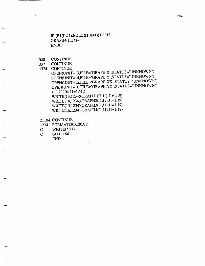
204

IF (E I (I I ,J1).EQ.E I (I1,JI + I ))THEN

GRAPH4(I1,J1)= ' 'ENDIF

338

337

1324

21104

1234

C

C

CONTINUE

CONTINUE

CONTINUE

OPEN(UNIT=13,FILE='GRAPH.X',STATUS='UNKNOWN')

OPEN(UNIT=I4,FILE='GRAPH.Y',STATUS='UNKNOWN')

OPEN(UNIT= 15,FILE='G RAPH.XX' ,STATUS =' UNKNOWN')

OPEN(UNIT= 16,FILE='GRAPH.YY' ,STATUS='UNKNOWN ')

DO 21104 11=1,51,1

WRITE(13,1234) (GRAPH 1(I 1,J 1),J 1--1,19)

WRITE(14,1234)(GRAPH2(I 1,J 1),J 1= 1,19)

WRITE( 15,1234)(GRAPH3(I 1,J 1),J 1= 1,19)

WRITE(16,1234)(GRA PH4(I 1,J 1),J 1= 1,19)

CONTINUE

FORMAT(30X,20A1)

WRITE(*,21)

GOTO 64

END

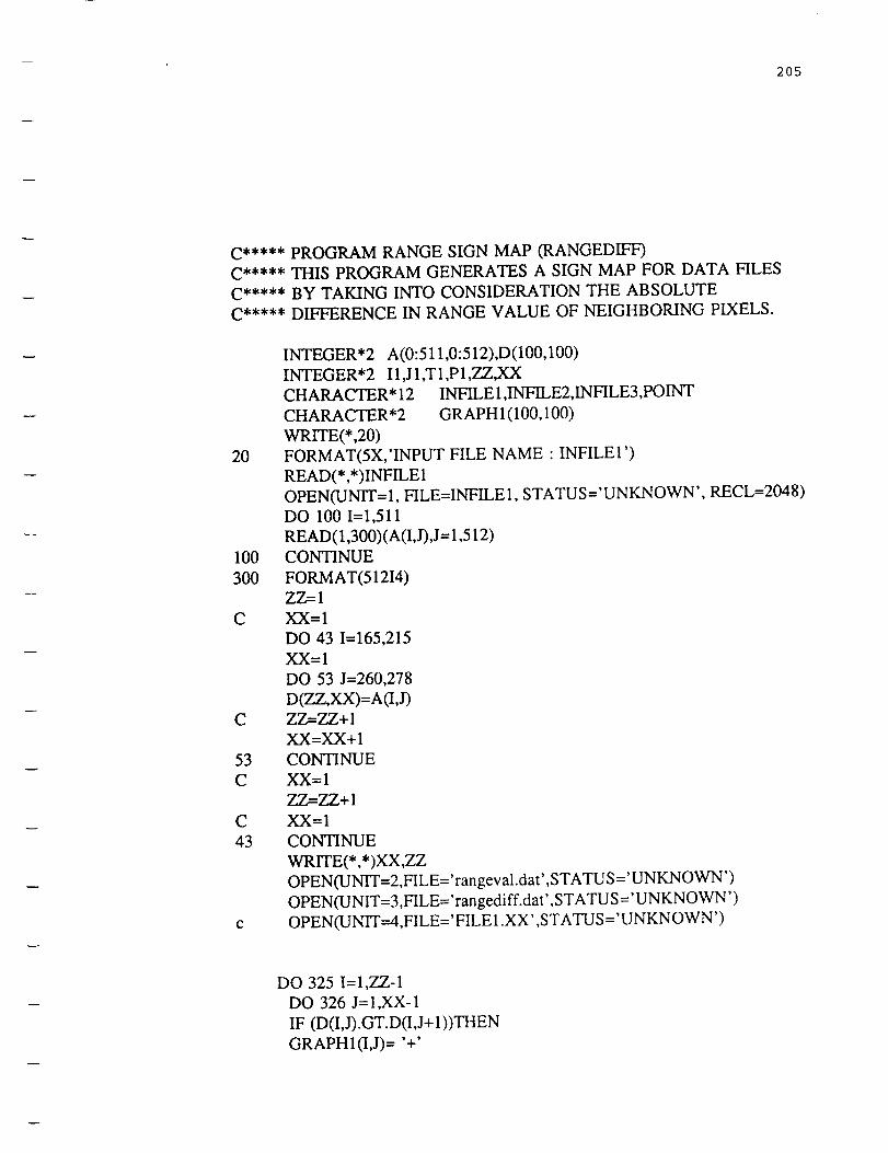
205

C***** PROGRAM RANGE SIGN MAP (RANGEDIFF)

C***** THIS PROGRAM GENERATES A SIGN MAP FOR DATA FILES

C***** BY TAKING INTO CONSIDERATION THE ABSOLUTE

C***** DIFFERENCE IN RANGE VALUE OF NEIGHBORING PIXELS.

20

100

300

C

C

53

C

C

43

INTEGER*2 A(0:511,0:512),D(100,100)

INTEGER*2 I1,J 1,T1,P1,ZZ,XX

CHARACTER* 12 INFILE 1,INFILE2,INFILE3,POINT

CHARACTER*2 GRAPH I (100,100)

WRITE(*,20)

FORMAT(5X,'INPUT FILE NAME : INFILEI')

READ(*,*)INFILE1

OPEN(UNIT=l, FILE=INFILE1, STATUS='UNKNOWN', RECL=2048)

DO 100 I=1,511

READ(1,300) (h(I,J),J= 1,512)

CONTINUE

FORMAT(51214)ZZ=I

XX=I

DO 43 I=165,215

XX-1

DO 53 J=260,278

D(ZZ,XX)=A(I,J)

ZZ=ZZ+ 1

XX-XX+I

CONTINUE

XX=I

ZZ=ZZ+I

XX=I

CONTINUE

WRITE(*,*)XX,ZZ

OPEN(UNIT=2,FILE='rangeval.dat',STATUS='UNKNOWN')

OPEN(UNIT=3,FILE='rangediff.dat',STATUS='UNKNOWN')

OPEN(UNIT---4,FIL E='FILE 1.XX',STATUS=' UNKNOWN')

DO 325 I= 1,ZZ- 1

DO 326 J= 1,XX- l

IF (D(I,J).GT.D(I,J+ 1))THEN

GRAPHI(I,J)= "+'

-- 206

326

325

21104

1234

3000

ENDIF

IF (D(I,/).LT.D(I,J+ 1))THEN

GRAPHI(I,J)= ' '

ENDIF

IF (D(Ij).EQ.D(I,J+ 1))THEN

GRAPHI(I,J)= ' '

ENDIF

CONTINUE

CONTINUE

DO 21104 I=I,ZZ-1

WR1TE(3,1234)(GRAPH 1(I,J),J= 1 ,XX- 1)

WR1TE(2,3000)(D (I,J),J= 1,XX-1)

CONTINUE

FORMAT(35X,20A 1)

FORMAT(I4)

STOP

END

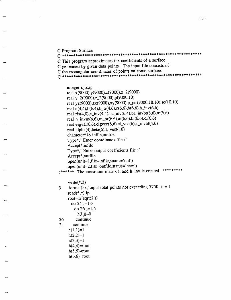
207

C Program SurfaceC _**_***_**_***_**_***_***_*_***_********_******_*** _**_******_

C This program approximates the coefficients of a surface

C generated by given data points. The input file consists of

C the rectangular coordinates of points on some surface.C _***_**_***_***_**_**_**_*_**_***_*_**_**_*_*_***_*_***

integer i,j,k,ip

real x(9000),y(9000),z(9000),x_2(9000)

real y_2(9000),z_2(9000),p(9000,10)

real yz(9000),zx(9000),xy(9000),p_ptr(9000,10,10),sc(10,10)

real a(4,4),b(6,4),b_tr(4,6),c(6,6),h(6,6),h_inv (6,6)

real ris(4,8),a_inv(4,4),ba_inv(6,4),ba_invbt(6,6),m(6,6)

real h_invm(6,6),m_pr(6,6),ai(6,6),bi(6,6),ci(6,6)

real eigval(6,6),eigvec(6,6),ei_vec(6),a_invbt(4,6)

real alpha(4),beta(6),a_vect(10)

character* 18 infile,outfile

Type*,' Enter coordinates file :'

Accept*,infile

Type*,' Enter output coefficients file :'

Accept*,outfile

open(unit= I,file=infile,status='old')

open(unit=2,file=outfile,status='new')

c****** The constraint matrix h and h_inv is created *********

3

26

24

write(* ,3)

format(5x,'Input total points not exceeding 7750: ip=')

read(*,*) ip

root= 1/(sqrt(2.))

do 24 i=I,6

do 26 j=l,6

h(i,j)=Ocontinue

continue

h(1,1)=l

h(2,2)=1

h(3,3)=1

h(4,4)=root

h(5,5)=root

h(6,6)=root

208

22

20

rootl =sqrt(2.)

do 20 i=1,6

do 22 j=l,6

h_inv(ij)=O

continue

continue

h_inv(1,1)=l

h_inv(2,2)=l

h_inv(3,3)=l

h_inv(4,4)=rootl

h inv(5,5)=rootl

h_inv(6,6)=rootl

30

do 30 i=l,ip

read(l,*) (x(i),y(i),z(i))

continue

c ****** the vector P for scatter matrix is formed here *****

32

34

do 32 i=l,ip

x_2(i)=x(i)**2

y_2(i)=y(i)**2

z_2(i)=z(i)**2

yz(i)=y(i)*z(i)

zx(i)=z(i)*x(i)

xy(i)=x(i)*y(i)

continue

do 34 i=l,ip

p(i, 1)=x_2(i)

p(i,2)=y_2(i)

p(i,3)=z_2(i)

p(i,4)=yz(i)

p(i,5)=zx(i)

p(i,6)=xy(i)

p(i,7)=x(i)

p(i,8)=y(i)

p(i,9)=z(i)

p(i, lO)=lcontinue

do 36 i=l,ip

do 38 j=l,lO

do 40 k=l,lO

p_ptr(i,j,k)=p(i,j)*p(i,k)

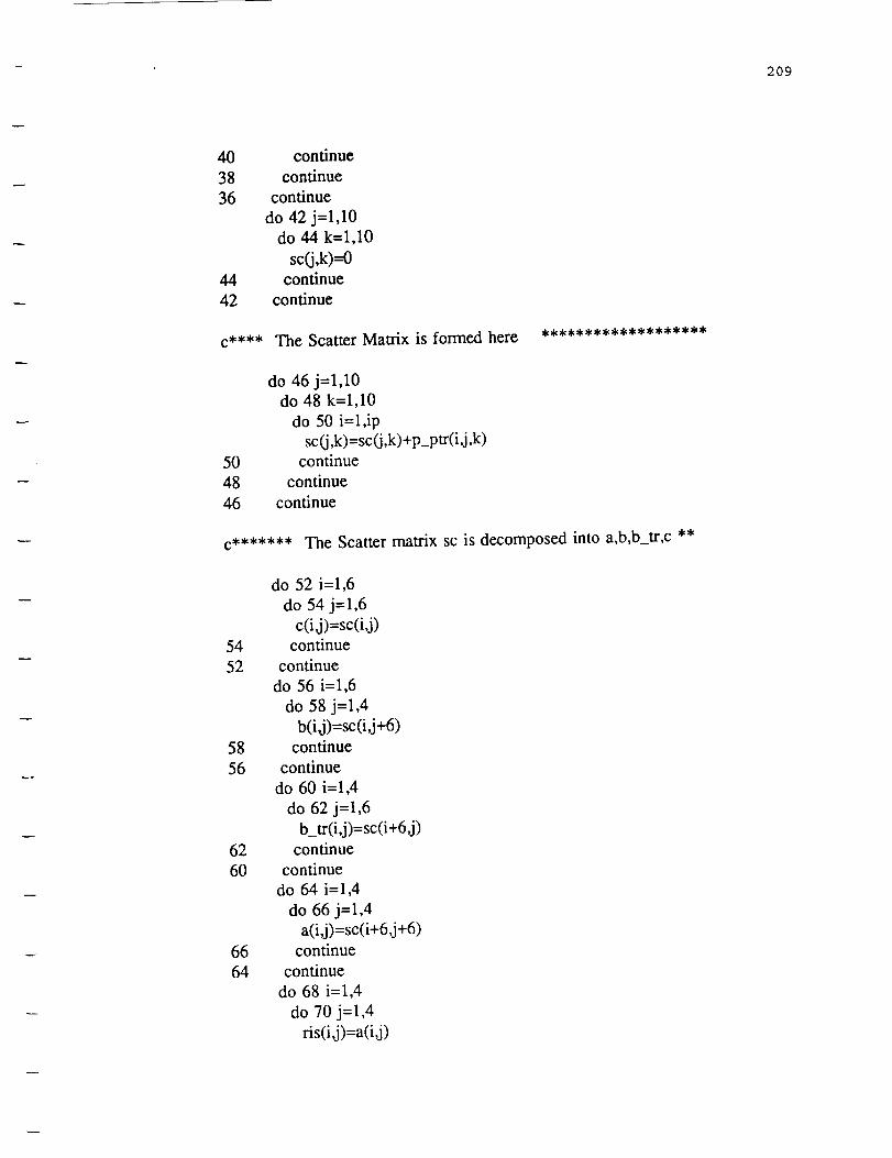
209

40 continue

38 continue

36 continue

do 42 j=l,10

do 44 k=l,10

sc(j,k)=O44 continue

42 continue

c**** The Scatter Matrix is formed here *******************

50

48

46

do 46 j=l,lO

do 48 k=l,lO

do 50 i=l,ip

sc(j,k)=sc(j,k)+p_ptr(i,j,k)continue

continue

continue

c******* The Scatter matrix sc is decomposed into a,b,b_tr,c **

do 52 i=1,6

do 54 j=l,6

c(i,j)=sc(i,j)

54 continue

52 continue

do 56 i=1,6

do 58 j=l,4

b(i,j)=sc(i,j+6)58 continue

56 continue

do 60 i=1,4

do 62 j=l,6

b_tr(i,j)=sc(i+6,j)62 continue

60 continue

do 64 i=1,4

do 66 j=l,4

a(i,j)=sc(i+6,j+6)66 continue

64 continue

do 68 i=1,4

do 70 j=l,4

ris(i,j)=a(i,j)

210

70 continue

68 continue

call invers(ris,4,4,8)

do 72 i=1,4

do 74 j=l,4

a_inv(i,j)=ris(i,j)74 continue

72 continue

c *************** Now to compute M *******************

do 76 i=1,6

do 78 j=l,4

ba_inv(i,j)---078 continue

76 continue

do 80 i= 1,6

do 82 j=l,4

do 84 k=l,4

ba_inv(i,j)=ba inv(i,j)+b(i,k)*a_inv(k,j)

84 continue

82 continue

80 continue

do 86 i=1,6

do 88 j=l,6

ba_invbt(i,j)=0

88 continue

86 continue

do 90 i=1,6

do 92 j=l,6

do 94 k=l,4

ba_invbt(i,j)=ba_invbt(i,j)+ba_inv(i,k)*b_tr(k,j)94 continue

92 continue

90 continue

do 96 i=1,6

do 98 j=l,6

m(i,j)=c(i,j)-ba_invbt(i,j)98 continue

96 continue

C

c ******** Now to compute M' ****************C

do 100 i=1,6

do 102 j=l,6

211

h_invm(i,j)=O

102 continue

100 continue

do 104 i=1,6

do 106 j=1,6

do 108 k=1,6

h invm(i,j)=h_invm(i,j)+h inv(i,k)*m(k,j)108 continue

106 continue

104 continue

do 110 i=1,6

do 112 j=l,6

112

110

118

116

114

C

C

C

m_pr(i,j)=0continue

continue

do 114 i=1,6

do 116 j=l,6

do 118 k=l,6

m_pr0d)=m_pr0d)+h_invm(i,k)*h_inv(k,j)continue

continue

continue

********* Now to find the eigen values of M' **********

nd=6

call eig(nd,m_pr,eigval,eigvec)

C

c ******* To find the smallest eigen value and its corresponding **

c ******* eigen vector

C

s_eig=eigval(1,1)

kount=l

do 120 i=2,6

120

122

if (s_eig.gt.eigval(i,i)) then

s_eig=eigval(i,i)kount=i

endif

continue

do 122 i=1,6

ei_vec(i)=eigvec(i,kount)continue

do 124 i=1,6

w

212

bcm(i)----O

do 126 j=l,6

bcta(i)=bcta(i)+h_inv(ij)*ei_vcc(j)

126 continue

124 continue

do 128 i--1,4

do 130 j=l,6

a_invbt(i,j)=0

do 132 k=l,4

a_invbt(i,j)=a_invbt(ij)+a_inv(i,k)*b_tr(k,j)132 continue

130 continue

128 continue

do 134 i=1,4

alpha(i)=0

do 136 j=l,6

alpha(i)=alpha(i)+a_invbt(i,j)*beta(j)

136 continue

alpha(i)=-alpha(i)134 continue

do 138 i=1,6

a_vect(i)=beta(i)138 continue

do 140 i=1,4

a_vect(i+6)=alpha(i)

140 continue

c do 142 i=l,10

write(2,*) (' The

wnte(2,*)

wnte(2,*)

write(2,*)

write(2,*)

write(2,*)

wnte(2,*)

wnte(2,*)

write(2,*)

wnte(2,*)

wnte(2,*)

wnte(2,*)c142 continue

(" The

(' The

(' The coeff of

(' The coeff of

(" The coeff of

(' The coeff of

(' The coeff of

(' The coeff of

(' The coeff of

(' The coeff of

(' The constant

close(unit=2,dispose='save')

close(unit= 1,dispose= 'save')end

input file was "',infile,'"')

output file is "',outfile,'"')

coeff of x-squared is ',a_vect(1))

y-squared is ',a_vect(2))

z-squared is ',a_vect(3))

yz is ',a vect(4))

zx is ',a_vect(5))

xy is ',a_vect(6))

x is ',a vect(7))

y is ',a vect(8))

z is ',a_vect(9))

d is ',a_vect(10))

213

Subroutine Invers(ris,N,Nx,Mx)

Dimension ris(Nx,Mx)

NI=N-1

N2=2*N

Do 2 i=l,N

Do 1 j=I,N

jl=j+N

1 ris(i,j 1)--0.

j 1=i+N

2 ris(i,jl)=l.

Do 10 k=l,N1

C=ris(k,k)

If (Abs(C)-0.000001) 3,3,5

5 kl=k+l

Do 6 j=kl,N2

6 ris(k,j)=ris(k,j)/C

Do 10 i=kl,N

C=ris(i,k)

Do 10 j=kl,N2

ds(i,j)=ris(i,j)-C*ris(k,j)

10 Continue

Npl=N+I

If (Abs(ris(N,N))-0.000001) 3,3,19

19 Do 20 j=Npl,N2

20 ris CN,j)=ris(N,j)/ris(N,N)Do 200 I=I,N1

k=N-I

kl =k+l

Do 200 i=Npl,N2

Do 200 j=kl,N

200 ris(k,i)=ris(k,i)-ris(k,j)*ris(j,i)

Do 250 i=l,N

Do 250 j=I,N

jl=j+N

250 ris(i,j)=ris(i,j l)

Return

3 Type*,'Singularity in row found'

Return

End

Subroutine eig(nd,ai,bi,ci)

dimension ai(nd,nd),bi(nd,nd),ci(nd,nd)

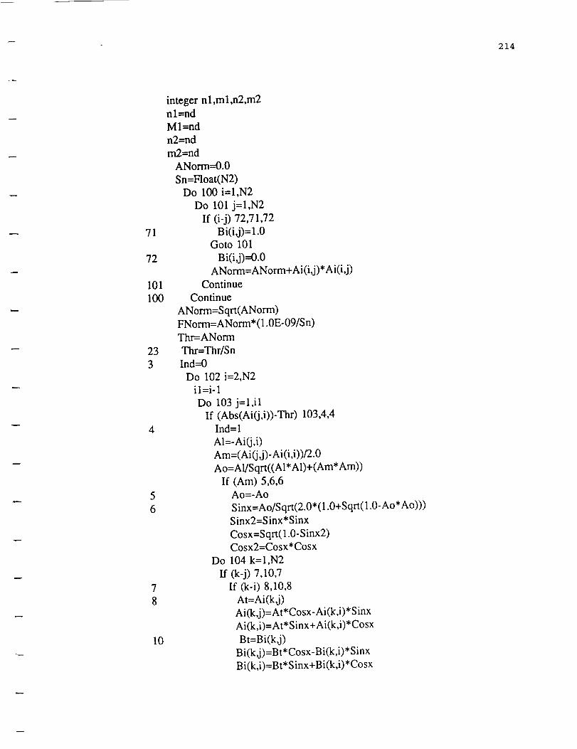
214

integer nl,ml,n2,m2

nl=nd

Ml=nd

n2=nd

m2=nd

ANorm=0.0

Sn--Float(N2)

Do 100 i=l,N2

Do 101 j=I,N2

If (i-j) 72,71,72

71 Bi(i,j)--1.0Goto 101

72 Bi(i,j)=0.0

ANorm=ANorm+Ai(i,j)*Ai(i,j)101 Continue

100 Continue

ANorm=Sqrt(ANorm)

FNorm=ANorm*(1.0E-09/Sn)Thr=-ANorm

23 Thr=Thr/Sn

3 Ind----0

Do 102 i=2,N2il=i-1

Do 103 j=l,il

If (Abs(Ai(j,i))-Thr) 103,4,44 Ind=l

Al=-Ai(j,i)

Am=(Ai(j,j)- Ai(i,i))/2.0

Ao=AI/Sqrt((AI*A1)+(Am*Am))

If (Am) 5,6,6

5 Ao=-Ao

6 Sinx=Ao/S qrt(2.0* (I .0+Sqrt(1.0- Ao* Ao)))Sinx2=Sinx*Sinx

Cosx=Sqrt(1.0-Sinx2)

Cosx2=Cosx*Cosx

Do 104 k=l,N2

ff (k-j) 7,10,7

7 If (k-i) 8,10,8

8 At=Ai(k,j)

Ai(k,j)=At*Cosx-Ai(k,i)*Sinx

Ai(k,i)=At*Sinx+Ai(k,i)*Cosx

10 Bt=Bi(k,j)

Bi(k,j)=Bt*Cosx-Bi(k,i)*Sinx

Bi(k,i)=Bt*Sinx+Bi(k,i)*Cosx

215

104 Continue

Xt=2.0*Ai(j,i)*Sinx*Cosx

At=Ai(j,j)

Bt=Ai(i,i)

Ai(j j)=At*Cosx2+Bt*Sinx2-Xt

Ai(i,i)=At*Sinx2+Bt*Cosx2+Xt

Ai(j,i)=(At-B t)*Sinx*Cosx+Ai(j,i)*(Cosx2-Sinx2)

ii(i,j)=ii(j,i)

Do 105 k=l,N2

hi(j,k)=ii(k,j)

hi(i,k)=hi(k,i)

105 Continue

103 Continue

102 Continue

If (Ind) 20,20,3

20 If (Thr-FNorm) 25,25,23

25 Do 110 i=2,N2

j=i29 If ((Abs(Ai(j- 1,j- 1)))-(Abs(Ai(j,j)))) 30,110,110

30 At=Ai(j- 1,j-l)

Ai(j-l,j- 1)=Ai(j,j)

Ai(j,j)=AtDo 111 k= 1,N2

At=Bi(k,j- 1)

Bi(k,j-1)=Bi(k,j)

Bi(k,j)=At111 Continue

j=j-1

If (j-l) 110,110,29

110 Continue

do 112 i=l,N2

do 114 j=I,N2

ci(i,j)=bi(i,j)

bi(i,j)=ai(i,j)

114 continue

112 continue

return

end

216

C**** PROGRAM SURFACE ALIGNMENT

C**** This program is used to eliminate the product terms

C**** from the quadratic representation of any 3D surface.

C**** The new coefficents generated consisits of the square terms,

C**** the x, y, z, and the constant term.

C

C

C

REAL AA,BB,CC,DD,FF,GG,HH,PP,QQ,RR,D,Test_f,Test_g,test_h

REAL A(50,50),B(50,50),C(50,50),F(50,50)

REAL G(50,50),H(50,50),ALPHA(100),BETA(100)

REAL RESULT(200,200),P(50,50),Q(50,50),R(50,50)

REAL AAA,BBB,CCC,DDD,EEE,FFF,GGG,HHH,III,ROT(3,3)

REAL DEL 1,DEL2,DEL3,A_A,B_B,C_C,F_F,G_G,H_H,GAMMA(100)

REAL VV,VVV,VVVV,VVVVV,THRESHLD,INITMIN,ABSA,ABSB,ABSC

REAL A AA,B_BB ,C_CC,D_DD,P PP,Q_QQ,R_RR

REAL AB SF,ABSG,ABSH,ABSP,AB SQ,ABSR,RRR(50),alptot,bettot

REAL gamtot

INTEGER N,M,I,J

F(X,Y,Z)=Ax**2+By**2+Cz**2+2Fyz+2Gxz+2Hxy+2Px+2Qy+2Rz+D

=0

PARAMETER (THRESHLD= 0.00000000000000001)

OPEN(UNIT= 1,FILE='CONV ERGENCE.DAT',STATUS='NEW')

TYPE*,'ENTER VALUE FOR THRESHLD:'

ACCEPT*,THRESHLD

Type*,'Enter coef. of x ** 2 :'

Accept*,AA

Type*,'Enter coef. of y ** 2 :'

Accept*,BB

Type*,'Enter coef. of z ** 2 :'

Accept*,CC

Type*,'Enter coef. of yz :'

Accept*,FF

Type*,'Enter coef. of xz :'

Accept*,GG

Type*,' Enter coef. of xy :'

Accept*,HH

Type*,'Enter coef. of x :'

Accept*,PP

Type*,'Enter coef. of y :'

Accept*,QQ

Type*,'Enter coef. of z :'

217

Accept*,RR

Type*, ' Enter constant of prop. :'

Accept*,D

3980

+

A(1,1)=AA

B(1,1)=BB

C(1,D=ccF(I,1)=FF

G(1,1)---GG

H(1,1)=HH

P(1,1)=PP

Q(1,1)=QQ

R(I,1)=RR

ABSA--ABS(AA)

ABSB=ABS(BB)

ABSC=ABS(CC)

ABSF=ABS(FF)

ABSG=ABS(GG)

ABSH=ABS(HH)

ABSP=ABS(PP)

ABSQ=ABS(QQ)

ABSR=ABS(RR)

RRR(1)=ABSARRR(2)=ABSB

RRR(3)=ABSC

RRR(4)=ABSF

RRR(5)=ABSG

RRR(6)=ABSH

RRR(7)=ABSP

RRR(8)=ABSQ

RRR(9)=ABSR

DO 3980 I=l,9

IF (RRR(I).EQ.0)THEN

RRR(I)=10000

ENDIF

CONTINUE

INITMIN-AMIN I(RRR(1),RRR(2),RRR(3),RRR(4),RRR(5),RRR(6),RRR(7)

,RRR(8),RRR(9))

WRITE(*,*)INITMIN

IF (ABS(INITMIN).LT. 1.0)THEN

A(1,1)=A(1,1)/INITM IN

B(1, Â)=B(I, 1)/INITMIN

218

3405

C(1,1)=C(1,1)/INITMIN

F(1,1)=F(1,1 )/INITMIN

G(1,1)--G(1,1)/INITMIN

H(1,1)=H(1,1)/INITMIN

P(1,1)=P(1,1)/INITMIN

Q(1,1)=Q(1,1)nNITM Q(1,1)=Q(1,1)/INITMIN

DD_D=D/INITMIN

ELSE

GOTO 3405

ENDIF

A(I,I)=AA

B(I,])=BB

C(1,1)=CC

F(1,1)=FF

G(I, 1)---GG

H(1,1)=HH

P(1,1)=PP

Q(1,1)=QQ

R(1,1)=RR

345

C

C

C

57

+

+

+

+

if (b(1,1).eq.a(1,1)) then

goto 1167else

goto 57endif

else

goto 57endif

alpha(1)=(0.5*ATAND((H(I,1)/(B(1,1)-A(1,1)))))

A(1,1)=A(1,1)*COSD(ALPHA(1))*COSD(ALPHA(1))+B(1,1)*

SIND(ALPHA(1))*SIND(ALPHA(1))- H(1,1)*SIND(ALPHA(1))*

COSD(ALPHA(1))

B(1,1)=B(1,1)*COSD(ALPHA(1))*COSD(ALPHA(1))+A(1,1)*

SIND(ALPHA(1))*SIND(ALPHA(1))+H(1,1)*SIND(ALPHA(1))*

COSD(ALPHA(1))

C(1,1)=C(1,1)

F(1,1)--(3(1,1)*SIND(ALPHA(1))+F(1,1)*COSD(ALPHA(1))

G(1,1)=G(1,1)*COSD(ALPHA(1))-F(1,1)*SIND(ALPHA(1))

H(1,1)=0

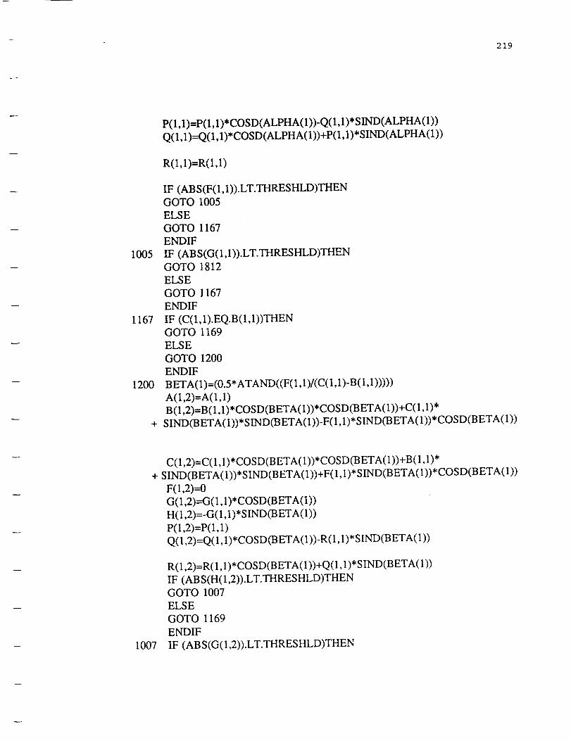
219

I005

1167

1200

+

P(I,I)=P(I,I)*COSD(ALPHA(1))-Q(I,I)*SIND(ALPHA(1))

Q(1,1)=Q(I,I)*COSD(ALPHA(1))+P(I,I)*SIND(ALPHA(1))

R(1,1)=R(1,1)

IF (ABS(F(I, I)).LT.THRESHLD)THEN

GOTO 1005

ELSE

GOTO 1167

ENDIF

IF (AB S(G(I,I)).LT.THRESHLD)THEN

GOTO 1812

ELSE

GOTO 1167

ENDIF

IF (C(1,1).EQ.B(1,1))THENGOTO 1169

ELSE

GOTO 1200

ENDIF

BETA(1)=(0.5*ATAND((F(1,1)/(C(1,1)-B(1,1)))))

h(1,2)=i(1,1)

B(1,2)=B(1,1)*COSD(BETA(1))*COSD03ETA(1))+C(1,1)*

SIND(BETA(1))*SIND(BETA(1))-F(1,1)*SIND03ETA(1))*COSD(BETA(1))

1007

C(1,2)=C(1,1)*COS D(BETA(1))*COSD03 ETA(1))+B (1,1)*

+ SIND(BETA(1))*SIND(BETA(1))+F(1,1)*SIND(BETA(1))*COSD(BETA(1))

F(1,2)=0

G(1,2)---G(1,1)*COSD03 ETA(l))

H(1,2)=-G(1,1)*SIND(BETA(1))

P(I,2)-P(1,1)

Q(1,2)=Q(I, 1)*COSD(BETA(1))-R(1,1)*SIND(BETA(I))

R(1,2)=R(1,1)*COSD(BETA(1))+Q(1,1)*SIND(BETA(1))

IF (ABS(H(1,2)).LT.THRESHLD)THENGOTO 1007

ELSE

GOTO 1169

ENDIF

IF (ABS(G(1,2)).LT.THRESHLD)THEN

220

1169

GOTO 1812

ELSE

GOTO 1169

ENDIF

/F (C(1,2).EQ.A(1,2))THENGOTO 67

ELSE

GOTO 1235

ENDIF

1235 GAMMA(1)=(0.5*ATAND((G(I,2)/(C(1,2)-A(1,2)))))

A(I,3)=A(I,2)*COSD(GAMMA(1))*COSD(GAMMA(1))+C(1,2)*

+ SIND(GAMMA(1))*SIND(GAMMA(1))-G(1,2)*S IND(GAMMA(1))

+ *COSD(GAMMA(1))

B(1,3)=B(12)

C(1,3)=C(1,2)*COSD(GAMMA(1))*COSD(GAMMA(1))+A(1,2)*

+ SIND(GAMMA(1))*SIND(GAMMA(1))+G(1,2)*SIND(GAMMA(1))

+ *COSD(GAMMA(1))

F(1,3)=H(1,2)*SIND(GAMMA(1))

G(1,3)=0

H(1,3)=H(1,2)*COSD(GAMMA(1))

P(1,3)=P(1,2)*COSD(GAMMA(1))-R(1,2)*SIND(GAMMA(1))

Q(1,3)=Q(1,2)

R(1,3)=R(1,2)*COSD(GAMMA(1))+P(1,2)*SIND(GAMMA(1))

1009

IF (ABS(F(1,3)).LT.THRESHLD)THENGOTO 1009

ELSE

GOTO 67

ENDIF

IF (ABS(H(1,3)).LT.THRESHLD)THEN

GOTO 1812

ELSE

GOTO 67

ENDIF

221

67

C

71

C

C

177

+

+

+

+

1011

167

DO 10 1=2,100

DO 20 J=l

if((b(i- 1,3).eq.a(i- 1,3)))then

goto 167else

if(h(i,3).eq.0)then

goto 67else

goto 67endif

else

goto 177endif

alpha0)=(0.5*ATAND((H(I- 1,3)/(B(I-1,3)-A(I-1,3)))))

A(I,I)=A(I-1,3)*COSD(ALPHA0))*COSD(ALPHA(1))+(B (I-1,3))*

SIND(ALPHA(1))*SIND(ALPHA(1))- H(I-1,3)*SIND(ALPHA(1))*

COSD(ALPHA(1))

B(I,I)=B (I-1,3)*COSD(ALPHA(1))*COSD(ALPHA(1))+A(I- 1,3)*

SIND(ALPHA(1))*S IND(ALPHA(1))+H(I- 1,3)*SIND(ALPHA(1))*

COSD(ALPHA(1))

Cfl,1)=Cfl-l,3)F(I,1)=F(I-1,3)*COSD(ALPHA(I))

G(I,1)=-F(I-1,3)*SIND(ALPHA(I))

H(I,1)=0

P(I,1)=P(I-1,3)*COSD(ALPHA(I))-Q(I-1,3)*SIND(ALPHA(I))

Q(I,1)=Q(I- 1,3)*COSD(ALPHA(I))+P(I- 1,3)*SIND(ALPHA(I))

R(I,1)=R(I-1,3)

IF (ABS(F(I, 1)).LT.THRESHLD)THEN

GOTO 1011

ELSE

GOTO 167

ENDIF

IF (ABS(G(I, 1)).LT.THRESHLD)THEN

N=I

GOTO 666

ELSE

GOTO 167

ENDIF

if((c(i, 1).eq.b(i, 1)))then

L

222

C

C

(2

59

+

goto 69else

goto 59endif

else

goto 59endif

B ETA(I)=(0.5*ATAND((F(I, 1)/(C(I, 1)-B(I, 1)))))

A(I,2)=A(I,1)

B(I,2)=B(I,1)*COSD(BETA(I))*COSD(BETA(I))+C(I, 1)*

SIND(BETA(I))*SIND(B ETA(I))-F(I, 1)*SIND(BETA(I))*COS D(BETA(I))

+

C(/,2)=C(I, 1) *COS D(B ETA (I) )*COS D(B ETA (I) )+ B (I, 1)*

SIND(BETA(I))*SIND(BETA(I))+F(I,1)*SIND(B ETA(I))*COSD(BETA(I))

F(I,2)=0

G(I,2)--G(I, 1)*COSD(BETA(I))

H(I,2)=-G(I, 1)*SIND(BETA(I))

P(I,2)=P(I,1)

Q(I,2)=Q(I, 1)*COSD(BETA(I))-R(I, 1)*S IND(B ETA(I))

R(I,2)=R(I, 1)*COSD(BETA (I) )+Q(I, 1)*SIND(BETA(I) )

1013

c69

69

C

C

IF (ABS(G(I,2)).LT.THRESHLD)THEN

GOTO 1013

ELSE

GOTO 69

ENDIF

IF (ABS(H(I,2)).LT.THRESHLD)THENN=I

GOTO 666

ELSE

GOTO 69

ENDIF

if(g(i,2).eq.0)then

if((c(i,2).eq.a(i,2)))then

goto 10else

goto 63endif

223

63

+

+

+

+

1015

else

goto 63endif

GAMMA(I)=(0.5*ATAND((G(I,2)/(C(I,2)-A(I,2)))))

A(I,3)=A(I,2)*COSD(GAMMA(I))*COSD(GAMMA(I))+C(I,2)*

SIND(GAMMA. (I))*SIND(GAMMA(I))-G(I,2)*S IND(GAMMA(I))

*COSD(GAMMA(I))

B(I,3)=B(I,2)

C0,3)=C(I,2)*COSD(GAMMA(I))*COSD(GAMMA(I))+A(I,2)*

SIND(GAMMA(I))*SIND(GAMMA(I))+G(I,2)*SIND(GAMMA(I))

*COSD(GAMMA(I))

F(I,3)=H(I,2)*SIND(GAMMA(I))

G(I,3)=0

H(I,3)=H(I,2)*COSD(GAMMA(I))

p(I,3)=P(I,2)*COSD(GAMMA(I))-R(I,2)*SIND(GAMMA(I))

O(I,3)=O(I,2)

R(I,3)=R(I,2)*COSD(GAMMA(I))+P(I,2)*SIND(GAMMA(I))

IF (ABS(F(I,3)).LT.THRESHLD)THEN

GOTO 1015

ELSE

GOTO 10

ENDIF

IF (AB S(H(I,3)).LT.THRESHLD)THENN=I

GOTO 666

ELSE

GOTO 10

ENDIF

20

10

1812

666

123

+

CONTINUE

CONTINUE

N=I

WR1TE(*,*)N

WRITE(*,123)

FORMAT(5X,'****************************************************

WRITE(*,*)('THE NUMBER OF ITERATIONS COMPLETED IS:',N)

224

1001

1000

M=N*3

DO 1000 I=I,N

DO 1001 J=l,3

RESULT(3*(I-1)+J,1)=A(I,J)

RESULT(3*(I-1)+J,2)=B(I,J)

RESULT(3*(I-1)+J,3)=C0,J)

RESULT(3*(I- 1)+J,4)=F(I,J)

RESULT(3*(I- 1)+J,5)=G(I,J)

RESULT(3*(I- 1)+J,6)=H(I,J)

RESULT(3*(I- 1)+J,7)=P(I,J-')

RESULT(3*(I-I)+J,8)=Q(I,J)

RESULT(3*(I-1)+J,9)=R(I,J)

CONTINUE

CONTINUE

WRITE(1,*)('THE NUMBER OF ITERATIONS COMPLETED IS :',N)

WRITE(I,123)

198

298

398

498

598

2000

WRITE(1

WRITE(1

WRITE(1

WRITE(1

WRITE(I

WRITE(1

,*)('COEFF. OF X SQUARE TERM IS : ', AA)

,*)('COEFF. OF Y SQUARE TERM IS : ', BB)

,*)('COEFF. OF Z SQUARE TERM IS : ', CC)

,*)('COEFF. OF YZ SQUARE TERM IS : ", FF)

,*)('COEFF. OF XZ SQUARE TERM IS : ' ,GG)

,*)('COEFF. OF XY SQUARE TERM IS : ' ,HH)

WRITE(1,*)('COEFF. OF X TERM IS : ', PP)

WRITE(1,*)('COEFF. OF Y TERM IS : ', QQ)

WRITE(1,*)('COEFF. OF Z TERM IS : ', RR)

WRITE(1,*)('CONSTANT OF PROP. IS : ', D)

write(I,123)

write(I,123)

write(I,123)

DO 2000 I=I,M

WRITE(1,*)(RESULT(I,J),J= 1,9)CONTINUE

A AA=RESULT(M-2,1 )

B_BB=RESULT(M-2,2)

C CC=RESULT(M-2,3)

P_PP=RESULT(M-2,7)

225

30001

3001

1278

+

1897

2001

1234

3000

1908

4000

Q_QQ=RESULT(M-2,8)

R_RR=RESULT(M-2,9)

D_DD=D

do 30001 i=1,3

write(I,123)

continue

WRITE(1,*)('THE NEW COEFF. OF X SQUARE TERM IS : ', A_AA)

WRITE(1,*)('THE NEW COEFF. OF Y SQUARE TERM IS : ', B_BB)

WRITE(1,*)('THE NEW COEFF. OF Z SQUARE TERM IS : ', C CC)

WRITE(1,*)('THE NEW COEFF. OF X TERM IS : ', P_PP)

WRITE(1,*)('THE NEW COEFF. OF Y TERM IS : ', Q_QQ)

WRITE(1,*)('THE NEW COEFF. OF Z TERM IS : ', R_RR)

WRITE(1,*)('THE NEW CONSTANT OF PROP. IS : ',D_DD)

do 3001 i=1,3

write(I,123)

continue

write(I,1278)

format(6x,'A',9x,'B',9x'C',9x,'F',9x,'G',9x,'H',9x,'P',

9x,'Q',9x,'R')

write(I,1897)

format(5x,' ........................................................

"!- .......... _)

DO 2001 I=I,M

WR1TE(1,1234)(RESULT(I,J),J=l,9)

CONTINUE

format(9F10.5)

DO 3000 I=1,5

WRITE(I,123)

CONTINUE

write(l,1908)

format(6x,' Alpha' ,9 x,' Beta' ,9 x,' G amm a' )

write(I,1897)

DO 4000 I=I,N

WRITE(1,*)ALPHA(I),BETA(I),GAMMA(I)

CONTINUE

226

alptot=alpha(1)+alpha(2)+alpha(3)

bettot=beta(1)+beta(2)+beta(3)

gamtot=gamma(1)+gamma(2)+gamma(3)

write(I,123)

write(I,123)

write(I,1998)

1998 format(6x,'ALPTOT',9x,'BETI'OT',9x,'GAMTOT')

write(1,*)alptot, bettot, gamtot

write(I,123)

c***** To evaluate coeff, of yz, xz, and xy once alpha, beta

c***** and gamma are evaluated.

write(* ,*)alpha( I ),beta( I ), gamma( I )

AAA=BB*cosd(alpha(1))*cosd(alpha(1))+(AA*sind(alpha(1))

+ *sind(alpha(1)))+((HH/2)*sind(2*alpha(1)))-CC

BBB=gg*sind(alpha(1))+(if*cosd(alpha(1)))

CCC=((aa-bb))*sind(2*alpha(1))+(hh*cosd(2*alpha(1)))

DDD=gg*cosd(alpha(1))-(ff*sind(alpha(1)))

EEE=aa*(cosd(alpha(1))*cosd(alpha(1))-(sind(alpha(1))

+ *sind(alpha(1))*sind(beta(1))*sind(beta(1))))

FFF=bb*(sind(alpha(1))*sind(alpha(1))-(cosd(alpha(1))

+ *cosd(alpha(1))*sind(beta(1))*sind(beta(1))))

GGG=cc*cosd(beta(1))*cosd(beta(1))

HHH=(gg/2)*sind(alpha(1))*sind(2*beta(1))+((ff/2)*cosd(alpha(1))*

+ sind(2*beta(1)))

III=(hh/2)*sind(2*alpha(I))*(l+sind(beta(1))*

+ sind(beta(1)))

Test_F=(AAA*sind(2*beta(1))+BBB*cosd(2*beta(1)))*

+ cosd(gamma(1))+(CCC*cos(beta(1))-DDD*sind(beta(1)))

+ *sind(gamma(1))

Test__G=CEEE+FFF-GGG-HHH-III)*SIND(2*GAMMA(1)) +

+ (CCC*SIND(BETA(1))+COSD(BETA(1))*DDD)*COSD(2*GAMMA(1))

TEST_H=(CCC*COS D(B ETA( 1))- DDD*S IND(B ETA( 1)))*COS D(GAMMA( 1)) -

+ (AAA*SIND(2*BETA(1))+BBB*COSD(2*BETA(1)))*SIND(GAMMA(I))

write(I,123)

write(I,123)

227

C

C

C

124

+

+

+

+

989

write(I,124)

write(1,*)tesLf, test__g,test_h

write(I,123)

write(I,123)

write(I,124)

format(5x,'THE ROTATION MATRIX IS : ')To evaluate the rotation matrix

rot(1,1)=cosd(alpha(1))*cosd(gamma(1))-(sind(alpha(1))*

sind(beta(1))*sind(gamma(1)))

rot(1,2)=-sind(alpha(1))*cosd(gamma(1))-(cosd(alpha(1))*

sind(beta(1))*sind(gamma(1)))

rot(1,3)=-sind(gamma(1))*cosd(beta(1))

rot(2,1)=sind(alpha(1))*cosd(beta(1))

rot(2,2)=cosd(beta(1))*cosd(alpha(1))

rot(2,3)=-sind(beta(1))

rot(3,1)=cosd(alpha(1))*sincl(gamma(1))+(sind(alpha(1))*

sind(beta(1))*cosd(gamma(1)))

rot(3,2)---cosd(alpha(1))*cosd(gamma(1))*sind(beta(1))

-(sind(alpha(1))*sind(gamma(1)))

rot(3,3)=cosd(gamma(1))*cosd(beta(1))

DO 989 I=1,3

WRITE(1,*)(ROT(I,J),J=I,3)

CONTINUE

stopend

228

C***** PROGRAM 3-D DISCRIMINANT

C***** Implementation of the 3-D discriminant approach

C***** Implemented on MATLAB

diary on

mput('Coeff, of x^2 (A): ');A=ans

mput('Coeff, of y^2 (B): ");B=ans

mput('Coeff, of z^2 (C): ');C=ans

mput('Coeff, of yz (F): ');F=ans

mput('Coeff, of xz (G): ');G=ans

mput('Coeff, of xy (H): ');H=ans

,nput('Coeff. of x (P): ');P=ans

mput('Coeff, of y (Q): ');

Q=ans

mput('Coeff, of z (R): ');R=ans

mput('Constant of prop. (D): ");D=ans

F=F[2;

G=G/2;

H=H/'2;

P=P/2;

Q=-Q/2;R=R/2,

e=[A H GH B F

GFCI

EE=[A H G P

H B FQGFCR

PQR D ]

dt_e=det(e)

dt_EE=det(EE)

K_K=eig(e)rho_3=rank(e)

rho_4=rank(EE)

s_d_EE=sign(dt__EE)

229

sl=sign(K_K(1))

s2=sign(K_K(2))

s3=sign(K_K(3))

flag=0if sl _ s2;

flag=flag+lend;

if sl _--- s3;

flag=flag+ 1end;

if flag == 2;an_w=I,

fprintf('S,nXnelse;

an_w=0;end;

fprintf('XnXn

fprinff('XnXn

fpmtf(",n_fprintf('XnXn

fprintf(",n',n

The sign of the ch. roots are the same Xn')

The sign of the ch. roots are not the same Xn')The rank of EE is : %9.4f Xn ', rho_3 )

The rank of e is : %9.4f Xn ', rho_4 )

The sign of the determinant of EE is : %9.4f Xn',s d_EE )The characterstics roots have the same sign? : %9.4f Xn', an_w)

if rho_3=3

if rho_4-_-4if s d EE==-I

if an_w= 1

fprintf('XnXn The object is an ELLIPSOID XnXn')end

end

end

end

if rho_3=3

if rho_4_----4

if s_d_EE== 1

if an w_---0

fprintf('XnXn The object is a HYPERBOLOID OF ONE SHEET XnXn')end

end

end

end

if rho_3=3

if rho_4_--4if s d EE==-I

if an_w_---"=--0

tpriatf("_nend

end

end

The object is a HYPERBOLOID OF TWO SHEETS ',n')

230

end

if rho_3_3

if rho_4_--_-3

if an_w_---0

fprintf('XnXn The object is a REAL QUADRIC CONE Xn')end

end

end

if rho_3_2

if rho_4--4

if s_d_EE==- 1

if an_w_--_-0

fprintf('XnXnend

end

end

end

if rho_3_2

if rho_4_

if s_d_EE== 1if an_w_---0

fprintf('XnXnend

end

end

end

if rho_3_-.-_-2

if rho_4_3

if an_w_ 1

fprintf('XnXnend

end

end

if rho_3-.-_-2

if rho_4_3if an_w_---0

fprintf('_nend

end

end

The object is an ELLIPTIC PARABOLOID Xn')

The object is a HYPERBOLIC PARABOLOID 'm')

The object is an ELLIPTIC CYLINDER Xn')

The object is a HYPERBOLIC CYLINDER Xn')

if rho_3_ 1

if rho 4_---3

fprintf('XnXnend

end

diary off

The object is a PARABOLIC CYLINDER M')

19930011721.pdf - NASA Technical Reports Server

Documents

Transcript of 19930011721.pdf - NASA Technical Reports Server