General Disclaimer

One or more of the Following Statements may affect this Document

This document has been reproduced from the best copy furnished by the

organizational source. It is being released in the interest of making available as

much information as possible.

This document may contain data, which exceeds the sheet parameters. It was

furnished in this condition by the organizational source and is the best copy

available.

This document may contain tone-on-tone or color graphs, charts and/or pictures,

which have been reproduced in black and white.

This document is paginated as submitted by the original source.

Portions of this document are not fully legible due to the historical nature of some

of the material. However, it is the best reproduction available from the original

submission.

Produced by the NASA Center for Aerospace Information (CASI)

rl

NASA CONTRACTOR REPORT 166514 2 2 3 Z4

^0^^ ^p S E^ .^ P^cESS pEpj. ^'L .

Integrated Resource Inventory for Southcentral Alaska (INTRISCA)Final Report

(.N AS A-CR- 1665 14) -1NTZGftA1ED RESOURCE N83-32150INVENTOR.Y FUR SCUIHCENTEAL ALASKAFinal Report (Municipality of Anchoraq4-) k 4

165 p HC A I 21M.FA01 CSL" 05B U Licla s63/43 13326

Tony BurnsCharlotte Carson-HenryLeslie A. Morrissey

CONTRACT NAS2-11101July 1981

fi

NASA CONTRACTOR REPORT 1bb514

0

u.

Integrated Resource Inventory for Southcentral Alaska(INTRISCA) Final Report

Tony BurnsMunicipality of Anchorage h

Planning Department632 W. 6th AvenueAnchorage, Alaska

Charlotte Carson-HenryLeslie A. MorrisseyTechnicolor Government Services, Inc.MIS 242-4NASA/Ames Research Center H

rMoffett Field, CA

Prepared for Ames Research Centerin partial fulfillment of Contract NAS2-11101 3

IVASANational Aeronautics and

i Space Administrationi Ames Research Center -`

Moffett Field, California 94035

t

.k

fht

ABSTRACT

The Integrated Resource Inventory for SouthcentralAlaska (INTRISCA) Project comprised an integrated setof activities related to the land use planning andresource management requirements of the participatingagencies within the southcentral region of Alaska. Onesubproject involved generating a region-wide land coverinventory of use to all participating agencies. Towardthis end, participants first obtained a broad overviewof the entire region and identified reasonableexpectations of a Landsat-based land cover inventorythrough evaluation of an earlier classificationgenerated during the Alaska Water Level B Study.Classification of more recent Landsat data was thenundertaken by INTRISCA participants. The latterclassification produced a land cover data set that wasmore specifically related to individual agency needs,concurrently providing a comprehensive trainingexperience for Alaska agency personnel. Othersubprojects employed multi-level analysis techniquesranging from refinement of the region-rideclassification and photointerpretation, to digital edgeenhancement and integration of land cover data into ageographic information system (GIS).

TABLE OF CONTENTS

Page

List of Figures ivList of Tables viAcknowledgements vii

CHAPTER I: INTRODUCTION (T. Burns) 1* Scope of the Final Report 1

Background 1* NASA's Role 2

Needs and Mandates for the Demonstration Project 3Legislative Mandates 4

* Alaska Remote Sensing Subcommittee 8* Project Objectives 10

Participating Agencies 11

CHAPTER II: PROTECT CONSIDERATIONS, ORGANIZATION, ANDPLANNING (T. Burns) 12

* Approach 12* Project Overview 12

Subprojects 14* Alaska Remote Sensing Subcommittee 14* Project Pre-planning and Methodology Overview 14

* Training 14Personnel 17

* Study Area Selection 18Description of Demonstration Area 18

* Selection of a Classification System 22Classification Scheme 23

* Field Data Collection Considerations 26Training Site Data Forms 27

* Minimum-Area Mapping Units 31 t

CHAPTER III: CHARACTERISTICS OF LANDSAT AND CIR PHOTOGRAPHYAND IMAGE PROCESSING SYSTEMS (T. Burns) 32

* Landsat 32 a* Color Infrared Photography 33

'' * Image Analysis Systems 34* Peripheral Output Devices 35

CHAPTER IV:: TECHNICAL APPROACH (T. Burns) 38Introduction 38Data Acquisition 41

* Preprocessing 41Digital Analysis 42* Anchorage/Eastern Scene 4,2

* Susitna Scene 46Evaluation of Spectral Classes 49Post-processing 49Output Products 51

ia

^: z

CHAPTER V: SUBPROJECTS (T,. Burns) 55* Introduction 55

Road Network Mapping 55* Sea Surface Circulation Mapping 55* Integration of Landsat Digital Data with a

Geographic Information System 56* Floodplain and Landform Mapping 57* Urban Land Use Mapping 57

Appendix A: Acquisition of Imagery (L..Morrissey) 58

Appendix B: Ground Data Collection (L. Morrissey) 62.. j9

Appendix C: Digital Analysis of Susitna Scene (L. Morrissey) 73

Appendix D: Digital Analysis of the Eastern/Anchorage Scene

i

3(C. Carson-Henry) 86

Appendix E: Stratification of Southcentral Water Level BStudy (L. Morrissey) 98

^A

Appendix F: Interpreting Color Enhanced Landsat Single jChannel Images of Water Bodies (L.V. Maness) 103 y

Appendix G: Water Circulation Images of Upper Cook Inlet,Alaska (L.V. Maness) 107

Appendix H: Interpretation and Analysis of Upper Cook InletCirculation Study Using Landsat Imagery(D. Burbank) 115

j

Appendix I: One-Dimensional Edge Enhancements on IDIMS:t

Description, Procedures, Explanation, andInterpretation (L.V. Maness) 126

Appendix J: Stream Corridor Physiography of the SusitnaRiver Valley (K. Dean) 138

Appendix K: Accuracy Assessment of the INTRISCA Region(L. Morrissey, D. Card, M. McDonald) 165 a'

Appendix L: Geographic Information System Integration(J. Dangermond) 182

Appendix M: Georeferenced Landsat Classified Images forGIS Integration (C. Carson-Henry) 224

r

s

P^

T.

Figure 1.Figure 2.Figure 3.Figure 4.Figure 5.Figure 6.Figure 7.Figure 8.Figure 9.Figure 10.

Figure 11.Figure 12.Figure 13.Figure 14.Figure 15.Figure 16.Figure 17.Figure 18.

Figure 19.

Figure 20.Figure 21.Figure 22.Figure 23.Figure 24.Figure 25.

Figure 26.Figure 27.

Figure 28.

Figure 29.

Figure 30.

Figure 31.

Figure 32.Figure 33.Figure 34.Figure 35.Figure 36.

Figure 37.Figure 38.Figure 39.

k

^s

LIST OF FIGURES

Page

Study AreaGround Truth Classification SchemeTraining Site Data SheetLand Cover at Selected Training SitesLand Cover at Selected Training SitesVersatec Electrostatic Plotter MapTechnical Work Flow ChartLevel B Stratification ResultsSteps in Digital AnalysisIntegrated Resource Inventory forSouthcentral AlaskaLand Cover Inventory Using Satellite DataCluster DiagramExample of INTRISCA Project Output ProductsLandsat Color CompositeFlight LinesGround Truth Data FormsPhoto Key for Paper BirchComparison Chart for Visual Estimationof Percent CoverComparison Chart for Estimation of Percentageof Delineation Area and Percentage CoverHistogramComposite Supervised Statistics FileUnsupervised Clusters for Upland StrataSusitna SceneClassification of Land Cover in Susitna SceneCook Inlet Color-Enhanced Single-ChannelImage, Band 5Upper Cook Inlet, Alaska (NOS Chart 16660)Relative Surface Suspended Load (Turbidity),8 August 1978Relative Surface Suspended Load (Turbidity),27 August 1978One-dimensional Edge Enhancement Image,Band 6Location of Stream Corridors in the SusitnaRiver ValleyTypical Transition from an Active Floodplainto a TerraceHillside Test SiteIntegrated Terrain UnitsGeographic Overlay and Grid Coding MethodologySoil Expansion Codes and LegendsCoastal Management Resource Inventory andEnvironmental Analysis Flow ChartLand Use MapsVegetation MapGeneral Slope Map

iv

i

212428293037394043

444548525960.6768

69

707981828485

106118

119

120

135

143

156187189190191

193210212213

t

Figure 40. Landform Map 214Figure 41. Geologic Hazards Map 215Figure 42. Soil Drainage Map 216Figure 43. Specific Soil Slope Map 217Figure 44. Watershed and Stream Order Map 218Figure 45. Road Network Map 219Figure 46. Map of Soil Limitations for Dwellings

With and Without Basements 220Figure 47. Capability for Accessed Large Lot

Residential Use (map) 221Figure 48. Soil Limitations for Septic Tanks (map) 222Figure 49. Map of Suitability for Individual On-Site

Wastewater Treatment 223Figure 50. Hillside GIS Integration Image Rotation 243Figure 51. Hillside GIS Integration Image Relationships 244

aaI

I

I; LIST OF TABLES

Page

Table 1. Legislative Mandates 9Table 2. Subprojects 15Table 3. Subproject Rankings 16Table 4. Project Personnel 19Table 5. Tabular Summary of Pixels: Big Lake to Susitna

River, from IBM 360 53Table 6. Tabular Summary of Pixels: Big Lake to Susitna

River, from IDIMS 54Table 7. Distribution of CIR Photography 61Table 8. Ground Truth Scheme 63Table 9. Procedures for Establishing Training Sites 65Table 10. INTRISCA Training Site Selection Nov.26-Dec.7 75Table 11. Total Number of Training Sites and Pixels for

Each Land Cover Category 77Table 12. Training Class Descriptions 87Table 13. ANCHOR.EAST Clustering Results 87Table 14. Class Identification 91Table 15. ANCHOR.EAST Final Grouping, Class Identification 96 jTable 16. Stratification Refinements 100Table 17. Final Level B Classification Legend 102Table 18. Landform Map Explanation 148Table 19. Comparison of Floodplain Categories Interpreted

from Landsat Imagery &.High-Altitude Photography 162Table 20. Comparison of Landsat and SCS Classification

Schemes 166Table 21. Contingency Table I 170Table 22. Contingency Table II 171Table 23. Probability Table I 172Table 24. Probability Table II 173Table 25. Probability Table III 174Table 26. Probability Table IV 175Table 27. Aggregation of Categories to Units 178Table 28. Map Manuscript Composition 188Table 29. Model Outline - Land Capability for Accessed

Large Lot Residential Development 197Table 30. Statistical Tabulations 198Table 31. Landsat Integration Aggregation Table I 200Table 32. Landsat Integration Aggregation Table II 201

r Table 33. Landsat Integration Aggregation Table ILI 202Table'34. Big Lake Control Point File Listing 227

! Table 35. Big Lake ALLCOORD Listing 233Table 36. Big Lake First-order Transformations 234Table 37. Big Lake Final Transformation Listing 237Table 38. Big Lake GIS Integration Class Identification 240Table 39. Hillside ALLCOORD Listing 249Table 40. Hillside Final Transformation Listing 251r .. T. Table 41. Hillside GIS Integration Class Identification 255

vi

ACKNOWLEDGEMENTS

The INTRISCA Project benefitted substan0' ally from theparticipation of and support by the following personsand agencies: Dale R. Lumb, Branch Chief, Susan D.Norman, Assistant Branch Chief, and Benjamin R. Briggs,Richard D. Johnson, and Donald E. Wilson, ProjectManagers, NASA/Ames Technology Applications Branch;James R. Anderson, Alaska Department of NaturalResources, NASA State Coordinator (IPA); FrankWesterlund, University of Washington, State ProgramLiason to NASA (IPA); and the dedication of thepersonnel in all of the participating agencies.

if

-t

i

CHAPTER IINTRODUCTION

SCOPE OF THE FINAL REPORT

This report documents the efforts and accomplishments of theINTRISCA project and participating team members from itsinception through its completion. The 'focus will bethreefold: how the project team conducted its investigationand met the project objectives, what conclusions evolvedfrom the investigations, and how the technical aspects of theproject were carried out. In addition to documentingINTRISCA ativities, it is hoped that this report may assistfuture users and technical support staff in accomplishingtheir own projects more expeditiously while avoiding dif-ficulties encountered by the project team. Finally, it ishoped that this document will assist decision makers andadministrators in assessing the role remote sensing mightplay in an operational mode within their own agencies.

The report is divided into two primary sections. The appen-dices contain the technical papers which describe the tech-nical processes and analyses conducted for the project.Chapters I through VI are intended to provide a brief non-technical overview of the demonstration project.

BACKGROUND: The Integrated Resource Inventory forSouthcentral Alaska (INTRISCA)

A cooperative project has been undertaken by the NationalAeronautics and Space Administration (NASA) and variousstate and local government agencies in southcentral Alaska.The Alaska State and Local Remote Sensing DemonstrationProgram is an Applications Systems Verification and Transfer(ASVT) project. This demonstration project employed thetechnical capabilities of the NASA AMES RESEARCH CENTER todemonstrate to potential users from state and localgovernment agencies in Southcentral Alaska, the utility ofLandsat derived information in land use planning and in themanagement of natural resources. The goal ofthe demonstra-tion project was to provide users with hands-on experienceand training in the actual extraction, manipulation, andevaluation of remotely sensed data.

The main objective of the INTRISCA project was to providevarious user groups with uniform data sets (standard landcover classifications, plotter maps, Dicomed prints and sta-tistical summaries) on land use and land cover derived fromLandsat imagery and high altitude aircraft photography. TheINTRISCA project has provided for user evaluation, usertraining, and critique; of land use/land cover informationderived from the demonstration project.

il

-1-

State and local agencies are faced with a continuing geedfor obtaining and keeping current land cover/land use andnatural resource information. Alaska has over 47,000 milesof,coastline but 1/5 of 1 percent of the total coastal areasupports 60% of the entire state population. The demonstra-tion project concentrated on this area of SouthcentralAlaska.

NASA'S ROLE

NASA's Regional Remote Sensing Program is designed to facil-itate user assessment and adoption of Landsat technology byproviding assistance primarily to state and localgovernments. *The program includes:

° A liaison and awareness effort, which seeks toacquaint prospective users with the many oppor-tunities for using remotely sensed data. Severalbriefings and meetings were held in Anchorage toacquaint agency personnel with such opportunitiesand programs. As a result of these early meetingsin 1979, the INTRISCA project and project team wasestablished.

• NASA-provided orientation and training in techniquesof analyzing remotely sensed data. All par-ticipating agencies have now received several hands-on training workshops in both aerial photographicinterpretation and digital analysis.

• Cooperative user/NASA demonstration projects (suchas INTRISCA) are conducted to show Landsat's capabi-lity as a land use and resource management tool.

Technical assistance to help user agencies locatesources of services and systems, to help them applythe technology to their own projects, and to keepthem informed on advances in technology. TheINTRISCA project had many common goals and projects,but also provided for specific agency subprojects.This allowed various agencies to apply remotesensing technology to their own specific in-houseprojects.

The Regional Remote Sensing Applications Program is con-centrated at three NASA field installations, each covering aspecific geographical area of the United States. AmesResearch Center, located at Moffett Field, California servesthe western states, including Alaska and Hawaii through itsWestern Regional Applications Program (WRAP). The primeobjectives of WRAP are:

-2-

t

F

1. to provide an opportunity for state and localgovernment agencies to test and evaluate remotesensing technology,

2. assist user agencies in its transition to opera-`_ tional use, and

3. transfer high technlogy to these groups.

The INTRISCA project is the result of such an effort byNASA. The following table illustrates NASA's role and therole the participating agencies are expected to take sincesuch demonstration projects are user driven and are based onactive agency participation.

NASA'S ROLE

° Information and Training

1° Demonstration Project Support° Image Analysis Processing

User Needs Survey Assistance j° Definition of Operational Alternatives j4i° Assistance in the Use of Future Satellite

Data

rf

USERS' ROLE

° State Coordinating Functions° Identification of Applications Problems° Active Participation° Commitment of Personnel and Fiscal

Resources° Technology Evaluation° Sharing of Project Experiences with

others.L

11a

THE NEEDS AND MANDATES FOR THE DEMONSTRATION PROJECT

Southcentral Alaska is experiencing rapid growth anddevelopment, and much of the land area is inaccessible byconventional ground transportation means. For example, theMunicpality of Anchorage covers approximately 2,000 squaremiles but only 15 percent of the area is accessible by road.The Matanuska-Susitna Borough, north of Anchorage, contains23,000 square miles and less than 1 percent of it isaccessible by road. Within the boundaries of these twolocal governments numerous potentials exist for :he develop-ment of natural resources. Large coal deposits, landssuitable and planned for agricultural development ., commer-cial forestry potential, critical wildlife habitat, andlands suitable for residential, commercial and industrial

-3-

1Source Department of Natural Resources, Division ofForest, Land and Water Management, "Lana forAlaskans; 1978. I

-4-

ir

development are present throughout the region. However, thenatural resources of the area have not previously beencompletely inventoried or mapped. A need existed toinventory, classify and map the land use and land cover sothat it could be used in the preparation of land use andresource management plans necessary before such developmentproceeds.

LEGISLATIVE MANDATES

The State of Alaska is unique in that recent and impendinglegislative mandates require the transfer of millions ofacres of federal, state, local and native-selected lands.Land transfer requirements of these Acts dictate statewideland inventory and use-classification, now largely non-existent in Alaska. To address these critical inventoryneeds, the Alaska ASVT was designed to demonstrate andtransfer methods for regional land inventory based onLandsat digital data and U-2 high altitude photography. Adetailed description of major land transfer mandates followsas stated in an Alaska Department of Natural Resourcesdocument l . As of December, 1978, land ownership was distri-buted as follows:

Private (Non-Native) 01.0%

Native Corporations 12.0%

State government 27.0% jj

Federal government 60.0% :?

The effect of federal policies and actions is most clearlydemonstrated by the pattern of land ownership that existedwhen the Statehood Act was passed in 1958. In that year,99.8 percent of the land was still owned by the federalgovernment. The Statehood Act, passed in 1958, marked thebeginning of dramatic shifting in these land ownershippatterns. First, it entitled the State to select a total of103.35 of the 367 million acres of land in Alaska.. Theseselections were to be of two kinds. The first, generalland grants, entitled the state to select up to 102.55million acres of unreserved federal land by January, 1984.The second, community land grants, allowed the state toselect 400,000 acres from the national forests and another400,000 from the public domain lands to meet communityneeds.

1

1

if

3'

wE ^^

In passing the Statehood Act, Congress cited economic inde-pendence and the need to open Alaska to economic developmentas the primary purposes for large Alaska land grants. TheAlaska Constitution, on the other hand, speaks of both con-servation and development as key factors in managing anddisposing of land, with the dominant theme beingdevelopment.

The state ' s initial land selections were small and carefullycalculated, largely due to the young s .tate's precariousfinancial position. The State simply could not afford toselect the whole 103.35 million acres. By 1968, the Statehad selected about 26 million acres of its statehoodentitlement. Most of these lands were chosen for theirimmediate potential to bolster the Alaska economy and theirproximity to existing transportation routes.

Native leaders, first prompted by the State selections ofNative hunting grounds near Minto in the mid-1960's,asserted Native claims to large areas of the state. Actingto protect Native land rights, Secretary of the InteriorStuart Udall froze "final action" on federal landtransaction (including State selections) in 1966. In 1968,oil was discovered on the North Sope and the need for an oilpipeline right-of-way provided impetus for the settlement ofNative Claims. The issue of Native claims in Alaska wascleared with passage of the Alaska Native Claims SettlementACT (ANCSA) on December 18, 1971. This Act, the result of atremendous struggle by Natives and their supporters, createdAlaska Native village and regional corporations and gavethem nearly one billion dollars-and the right to select 44million acres of land. The land selected, as defined by theAct, is mainly in the vicinity of Native villages, which arelargely located along major rivers or on the coast.However, in the demonstration study area several hundredthousand acres have been transferred to Native VillageCorporations and Regional Corporations.

Section 17 (d)(2) of the Settlement Act allowed theSecretary of the Interior to withdraw up to 80 million acresfor further study leading to classification as nationalparks, wildlife refuges, forests, and wild and scenicrivers. The Act also directed the withdrawal of s:ub9tantial- -areas (ultimately totaling some 116 million acres) to form apool from which the Natives were to chose their lands.

A month after the passage of the Settlement Act, the Statefiled selections of some 77 million acres of land before thecreation of the Native and federal pools. The Department ofthe Interior refused to allow these selections, and, inSeptember, 1972, the litigation initiated by the State wasresolved by a settlement affirming state selection of 41million acres. The State's next selection in 1973-4 was 2.5million acres, primarily selected for mineral potential.

-5

After the expiration of some Native selection rights in late1976, the state selected 3.6 million acres, following anextensive evaluation and public review process.

The completion of state land selections was blocked untilCongress acted to resolve the (d)(2) issue; to decide whichof the withdrawn lands would be put into federal managementsystems. In order to protect the states interests, in May,1978, after widespread public review, Alaska identified 41million acres of "state interest areas," and requested thatthey be conveyed to the state by Congress as part of thefinal (d)(2) legislation.

of the 220 million acres which the federal government waslikely to retain in Alaska, about 72 million acres havealready been designated as National Forest, National Parks,Wildlife Refuges, and Petroleum Reserves.

In December of 1980 President Carter signed The Alaska LandsBill settling the (d)(2) issue.

Territorial trust grants plus the generous statehood grantswill see the State of Alaska with title to 104.55 millionacres, an area larger than the State of California.Although the State has selected over 72 million acres of itsstatehood entitlement, only 21 million acres have beenpatented (final title) by the federal government. Thesepatented lands, plus the 15 million acres which have beententatively approved for patent, comprise the 36 millionacres which the State now manages (and may offer under dispo-sal programs).

In 1963, the Legislature passed the Mandatory Borough Act,with the intention of granting land to the municipalitiesfor the same reason land was given to the State uponstatehood--to establish an economic base. The Act allowedmunicipalities to select ten percent of the vacant andunappropriate state general grant land within theirboundaries. Dispute over the handling of these lands led tolitigation, which was settled by an act passed in 1978 thatallocated 860,000 acres to the existing eleven boroughs.

Private land in Alaska, excluding land held by Nativecorporations, is estimated to be over one million acres.Much of this land passed into private hands through thefederal homestead acts and the land disposal programs of thestate, boroughs or communities.

Most private land is located along Alaska's road network..Compared to other categories of land it is highly accessibleand constitutes some of the prime settlement land in thestate.

The present state policy of Alaskan land management is found

-6 a

)

st

d

in Chapter 181, SLA 1978, the culmination of an effort by tGovernor Jay S..Hammond, the Legislature and the Federal-State Land Use Planning Commission. The provisions of thisAct were signed into law July 18, 1978. To implement theAct the Division of Lands must inventory all state land and

k'

water, and identify and classify their resources and othervalues. These inventories, which are to be kept up to date,are to be used to develop regional or area land use planswhich will guide the management of State-owned lands..

To meet the goal of putting State land into private hands,the Act ordered the Division of Lands to designate by Nov.1, 1978 30,000 acres of State land for disposal undereither the homesite or open-to-entry programs. This landwas part of the 50,000 acres which was to be madeavailable during fiscal year 1979 (July 1, 1978 to July 1,1979). After this first year, the Legislature will annuallydecide on the amount of land to be offered.

This State land policy is reflected in the land classifica-tion system, which is the step following the inventory and Jland planning process. Upon selection by the State, land isinventoried for its resources, and a land management plan isprepared. The plan then recommends classification of theland into one of the existing 16 classification categories.There are currently eight retention categories. They are:Watershed, Public Recreation, Reserved Use, Grazing, aMaterial, Mineral, Timber and Resource Management. All ofthese are multiple-use categories which allow both dominant'and nonconflicting uses. There are also eight disposalcategories. They are: Homesite, Agricultural, Commercial,Industrial, Private Recreation, Residential, Utility andOpen to Entry. Land will be selected for future disposalprograms from these'categories.

The Homesite Program was enacted by the Legislature in 1977and amended in 1978. The program allows residents of thestate who have lived in Alaska three years or longer tosecure title to parcels up to five acres in size. TheLegislature has directed that 30,000 acres of State land bedesignated for disposal in fiscal year 1979 under a com-bination of Homesite Entry and Open-to-Entry programs.

In an effort to protect Alaska's limited agricultural landbase, and to encourage the development of agriculture, the1976 Legislature provided that 650,000 acres of land were tobe designated for agricultural use by 1979. This land maybe used only for agricultural purposes, and.will be sold atfair market value at either public auction or by lottery.Ownership of 68,200 acres were transferred to private hands

t in 1978.

The State of Alaska passed the Alaska Coastal Management _Actin 1977. The Alaska Coastal Management Act, like the

-7-

tFederal Act, tries to balance human use of coastal resourceswhile maintaining natural systems. Coastal management is ajoint effort by local, state and federal government agenciesand the private sector to manage coastal resources and pro-mote their wise and balanced use. In Alaska, local govern-ments have the responsibility of preparing coastalmanagement plans. State standards and guidelines requireboth a thorough resource inventory and analysis.

These and other resource management programs have necessi-tated a need for more efficient means of conducting large-scale inventories. Table 1 summarizes these mandates.

ALASKA REMOTE SENSING SUBCOMMITTEE

For these reasons, the local governments of the Cook Inletregion, in cooperation with various state agencies, werecommitted to developing a remote sensing demonstration planfor an integrated resource inventory to meet their resourcemanagement objectives and information needs, and to coopera-tively acquire the knowledge needed for the planning andmanagement of their land and water resources. The mostefficient and cost effective method for obtaining thisinformation is the implementation of remote sensingtechniques, as this method offers great flexibility inextending its applications to complex projects requiringanalysis of various levels and intensities.

In consideration of this the Alaska Remote SensingSubcommittee (composed of federal, state, and local govern-ment personnel) has entered into an agreement with theNational Aeronautics and Space Administration (NASA) toformulate and evaluate plans and alternatives for the appli-cation of remotely sensed data in the planning and decision-making processes.

Because of the multi-jurisdictional operations and programsin southcentral Alaska, as well as this geographic area con-taining a majority of the state's population and associatedproblems resulting from it, it was deemed appropriate thatthe local government entities should lead the project. Thelocal government entities are in many cases larger than somestates, and planning is a mandatory power of first and usecond-class boroughs and home-rule municipalities. -a

Several Congressional and legislative mandates have createdother land programs which are causing the land ownershippicture to change drastically in Alaska. The Alaska NativeClaims Settlement Act, for example, is conveying title ofcertain lands to Alaska Native Corporations. These landswill no longer be in Federal ownership but, instead, beprivately-owned lands subject to borough and municipalplanning authority. The State of Alaska has passedlegislation to transfer title of certain state lands to

_g_

A

TABLE i

i^

LEGISLATIVE MANDATES

Legislative Mandates Responsibility Actions required

Statehood Act Department of Natural ibsources Selection of 103.35 mil I ionacres for development of an

1

econom is base.

Alaska Native ClaimsSettlement Act (ANCSA) Native corporations Selection of 44 million acres

ANCSA Department of Interior Selection of 80 million acres

for parkland development

Mandatory Borough Act Municipal Boroughs Selection of 860,000 acres fordevelopment of an economic base

Land Fb I icy Act Department of Natural Resources Disposal of 98,200 acres ( FY79)to private sector.

Homestead Entry R-ogram Disposal of 30,000 acres (FY79)for homesteads.

Agricultural Land. Classification Act Disposal of 68,200 acres (FY79) 1

for agricultural development.I

Alaska Coastal %nagement Act Local governments Resource inventory and assess-ment and analysis of wetlands,

habitats, Hazardous areas,

Land cover, etc.

Municipal Entitlements Act Local governments Selection of 10% of state landswithin local service area for

urban expansion

%tanuska-Susitna Borough Selection of 50,000 acres

° Minicipality of Anchorage Selection of 15,000 acres plus$9 million

State Forest Pr actices Act Department of Natural (sources Inventory and assessment offorest lands within state

I

jurisdiction

A

r•

^t^f

r,

boroughs and municipalities. These lands will be patentedto local governments. However, vast amounts of both Federaland State land remains. The management and use of theselands often depend upon the goals, needs, and desires of thelocal residents. A cooperative planning and managementprogram is needed and it is anticipated that thesouthcentral area could be the catalyst for initiating sucha program. Vocal governments feel that they should be theinitiating entities of the program plan in order that theirspecific needs are recognized and incorporated into theprogram at the state level.

State resource management issues, mandated by both federaland state legislation, require identification of resourcevalues, inventorying, classification, analysis and mappingof natural resources. Many of the State-owned land areas ofinterest are located within the two local governmententities, thus creating a need for coordinated, cooperativeplanning and management.

In order to carry out these objectives and tasks, represen-tatives of all participating agencies have formed an ad hoccommittee on remote sensing. One member of the Ad HocCommittee is also a member of the Alaska Remote SensingSubcommittee and coordinates the activities and interests ofLocal government. The Ad Hoc Committee's primary respon-sibility is to assess the potentials of remote sensing insouthcentral Alaska. This assessment will be accomplishedthrough the preparation and implementation of the demonstra-tion plan and the evaluation of the technical and adminstraLive results of utilizing the technology.

PROJECT OBJECTIVES

The following are the objectives adopted by the par-ticipatinq user agencies:

1. Assess the utility of remote sensing techniques tocurrent and projected coastal and other land andwaster use management problems and needs.

2. Assess the utility of remote sensing techniques todetermine and create urban and rural Land use andland cover maps.

3. Train state and local personnel to analyze and util-ize Landsat and other remote sensing data for landuse and resource management planning.

44 Demonstrate the feasibility of using computer-aidedanalysis of L,andsat data with other interpreteddata to aggregate the land use and land coverinformation by various planning boundaries (e.g.,traffic analysis zones, census tracts, river

-10-

f basins, etc.) for tabular output. This objectivemay be partially met through cooperative agreementswith other Federal agencies to pool resources andshare output data.

5. Evaluate existing systems and processes for themanipulation of remotely sensed data and to incor-porate the use of such systems and techniques intocurrent and proposed land use and resource manage-ment programs.

6. Analyze the cost effectiveness of utilizing remotesensing as a tool compazed to conventional means ofacquiring, mapping and manipulating data.

7. Develop a horizontally and vertically integratedagency environment in order to provide the foun-dation for a comprehensive state-wide remotesensing program.

DEMONSTRATION PROJECT PARTICIPATING AGENCIES

The following federal, state and local agencies have activ-ely participated in this demonstration project:

° Matanuska-Susitna Borough, Planning Department

° Municipality of Anchorage, Planning Department

° Alaska Department of Fish and Game

° Alaska Department of Natural ResourcesDivision of ForestryLand and Resource Planning

U.S. Department of Agriculture, Soil ConservationService

a NASA/Ames Research Center, Technology Application Branchr

CHAPTER IIPROJECT CONSIDERATIONS, ORGANIZATION AND PLANNING

APPROACH

In order to meet the program objectives as listed inChapter I, two local governments, in cooperation with stateagencies, have conducted demonstration subprojects in eachborough and municipality. Each demonstration subprojectinvolved the identification of user needs, identificationand analysis of appropriate remotely sensed data and eval-uation of the data with respect to all user requirements.Each demonstration task has provided for the practicalrequirements and commensurate application of current remotesensing techniques. Determination of the level of detailavailable through digital analysis of Landsat data has alsobeen accomplished, as well as an analysis of the bestmethods applicable to individual local problems. Results ofthe demonstration subprojects will be used to formulatefuture program recommendations, advance projectapplications, and suggestions of the operational mechanismfor implementing remote sensing techniques in future landuse and resource management programs. Where possible,cooperative agreements have been and will be written,allowing the sharing of resources among several agencies.

PROJECT OVERVIEW

INTRISCA has been conceived as an integrated set of activi-ties related td the land-use planning and resource manage-ment requirements of the participating agencies within thesouthcentral region of Alaska.

The fir^t objective of all participants was to obtain abroad overview of the entire region such as that provided bya!Landsat digital land cover inventory. This general inven-tory served three purposes, (1) It provided a source ofdata that supports regional land use planning functions ofeach agency; (2) it offered a basis for intergovernmentalcooperation and horizontal data integration among the twocontiguous local governments which occupy the study area,and (3) it provided a basis for vertical data integration inwhich both state and local agencies combine Landsat, aerialphotography, ground truth, and other existing information inanalyses that range from large-area (borough-wide) inven-tories to site-specific problems. Some existing work had

1

t

i

j

i

ti

ii

previously been done in the development of a Landsat land acover inventory of the study area through the SouthcentralAlaska Water Level B Study. I

Products were produced from this (Level B) data set that" could be evaluated by the agency participants and used to

demonstrate the feasibility of a regional land coverinventory. Following this evaluation, a new refined classi-fication was undertaken as part of the INTRISCA Project toproduce a land cover data set that was more recent, more

} specifically related to individual agency needs, and whichcould provide a comprehensive training experience for agencypersonnel.

In addition to the land cover inventory of the entire regioninvolving all project participants, a number of subprojectswere identified that concerned specific uses, and refine-ments of this data set were made for particular agencies anddesignated subareas. These subprojects also included

;j subarea analyses that relied on multi-level remote sensing(e.g., high-altitude photography in addition to Landsatimagery) or on the development of multi-theme data setsincorporating other geographic data. Many of these analyseswere relatively simple and occurred independently of, or inparallel with, the production of the overall Landsat-derivedland cover data set; for example, manual photo-interpretations of multi-date Landsat imagery for measure-ment of inter-tidal zones and photo-interpretations ofLandsat and RBV imagery to monitor urban development. Othersubprojects, such as land suitability analyses and changedetection, relied on completion and refinement of theLandsat data set and its incorporation with other data in ageographic information system. In all cases the subprojectsought to apply an appropriate set of technologies andmethods to the agency needs.

Some of the subprojects involved single agencies; others werecooperative between local and state agencies with relatedinterests in a common geographic area. The following sec-tion identifies each subproject and its agency involvement.

i Krebs, Paula V., J. Page Spencer, Kenneson G. Dean andStuart E. Rawlinson, "Natural Resource Map of SouthcentralAlaska: Landforms and Surficial Deposits, Geologic hazards,Land cover, Final Report: User's Guide", GeophysicalInstitute, University of Alaska, Fairbanks, Alaska, undated.

.' -13-

-14-

SUBPROJECTS

The INTRISCA demonstration project has been designed arounda number of unique subprojects which respond to agencyneeds. An attempt has been made to preserve as much com-monality as possible among the various subprojects; however,due to the number of agencies involved and their diverseland management problems, a complex set of requirementsnecessarily resulted (Table 2 lists the subprojects).Although it appeared that there was an unrealistically largenumber of proposed subprojects, there was a great deal ofcommonality among many of them (as shown in Table 3).

Table 3 shows the subprojects aggregated through commoninterest into thematic subprojects, with the various govern-mental agencies which required products from each. Thegeneral land cover subproject is a common need of all agen-cies and thus received the highest priority. Subprojectswhich involved lower levels of interagency participationwere consequently assigned lower priorities within theoverall demonstration project. Also shown is an indicationof the analysis method most likely to be used in generatingfinal products. As can be seen, two of the subprojects uti-lized only photointerpretive techniques while two requiredthe use of a relatively .sophisticated geographic informationsystem. It should be noted that, while the AlaskaDepartment of Fish and Game would have liked a wetlandsinventory as part of this demonstration, that work has beendeferred to a separate research project.

ALASKA REMOTE SENSING SUBCOMMITTEE

The Alaska Remote Sensing Task Force has recently been madea subcommittee of the committee on Natural ResourceInformation Management which, in turn, is a part of theAlaska Land Managers Cooperative Task Force. The RemoteSensing Subcommittee has served as the lead group for theprogram.

PROJECT PREPLANNING AND METHODOLOGY OVERVIEW

Training

As a means of accomplishing the project objectives, NASAprovided a series of training sessions for participatingagency team members. An intensive workshop format evolved;the principal goal of each workshop was to provide team per-sonnel with hands-on training and field experience whilemeeting the other project objectives. Ground truth sitesand training materials were selected to correspond with theplanned work. NASA and its contractors, AirviewSpecialists and Technicolor Graphic Services, conducted aweek-long air photo-interpretation workshop at AnchorageCommunity College to acquaint team members with the principles

TABLE 2

AGENCY SUBPROJECTS

Municipality of Anchorage

° General Land Cover.° Land Use Mapping° Land Use Change Detectionn 208 Water Quality Management Analysis/Land Use

Suitability

Matanuska-Susitna Borough

• General Land Cover• Land Use Mapping• Land Use Suitability• Land Use Change Detection• Road Network Mapping

State of Alaska

Department of Natural ResourcesLand and Resource Planning

• General Land Cover of Lower Susitna Basin• Land Capability Analysis in Susitna Basin

Department of Natural ResourcesDivision of Forest, Land and Water Management

° General Land Cover of Lower Susitna Basin

Department of Fish and Game

• Cook Inlet Intertidal Zone Measurement and ChangeDetection

• Habitat Classification in Lower Susitna Basin• Wetlands Inventory in Lower Susitna Basin• General Land Cover

^j

a

I

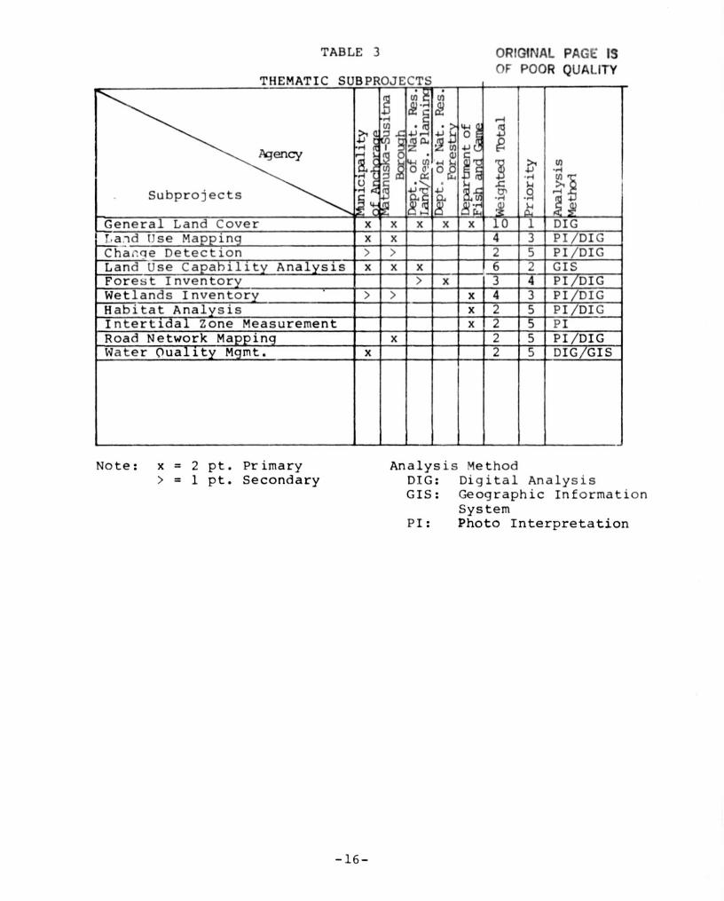
TABLE 3

ORIGINAL PAGE ISOF POOR QUALITY

TRF MATT(' Sf1RPPn .TF ('Tti

z U, 11 I

Subprojects '^4

r'. r, v

G enera l Land Cover-- x x x I x I x 10 1 DIG' ',a.-id [Ise Mapping x x 4 3 PI /DIG

Cha,-ne Detection > > 2 5 PI/DIGLand Use Capability Anal sis x x x 6 2 CISForest Inventor > x 3 4 PI DIGWetl ands Inventory > > x 4 3 PI/DIGHabitat Analysis x 2 5 PI/DIG_Intertidal Zone Measurement x 2 5 PIRoad Network Ma ing x

_2 5 PI/DIG

Water Oual—ity M mt. x 2 5 1 DIG GIS

i

Note: x = 2 pt. Primary> = 1 pt. Secondary

Analysis MethodDIG: Digital AnalysisGIS: Geographic Information

SystemPI: Photo Interpretation

-16-

R

of aerial photographic interpretation using Landsatimagery, U-2 high altitude color infrared photography, and

alow altitude natural color aerial photography. Instructionwas given in the use and care of mirror stereoscopes andzoom transfer scopes. As part of the training effort, itproved beneficial to make reconnaissance visits to thefield. Eagle River, a community ten miles north ofAnchorage, was selected for this purpose because it provided

4 a diversity of training sites, vegetation types, and landuses. This procedure proved to be advantageous not only forinterpretation, but also for field checking. Due to the lowaccessibility of much of the study area, an aerial flightwas made over much of the region at low altitude and 35 mmpictureswere taken. Each photographed site was predeter-mined from examination of the U -2 photographs and wasplotted on a USGS base map.

By conducting these preliminary reconnaissance missions andby photographing areas from the air and ground, anticipatedproblems were alleviated during the interpretation process.The agency field teams were provided with interpretationkeys which could prove helpful in identifying problem cases.

Another advantage of the reconnaissance phase of trainingwas that it allowed agency personnel to become more famil-iar with.the study area. It allowed the agency personnelto learn what types of phenomena were likely to appear onthe imagery as well as how they would appear. The result ofthis activity was a considerable savings in interpretationtime.

In addition to NASA providing air photo-interpretationtraining, a digital analysis workshop was held at NASA/AmesResearch Center to acquaint users with digital imageenhancement, classification, and statistical methods. Thisaspect of the training provided users with the ability tobegin looking at land use/land cover in terms of spectralreflectance differences, and to understand the limitationsof utilizing Landsat imagery. Training was provided on theIDIMS system, which was used for training site selection andclassification evaluation.

In addition, the State of Alaska, through the University ofAlaska Geophysical Institute in Fairbanks, conducted a oneweek seminar on introductory remote sensing. In alltraining situations, team members were given materials andmanuals for use during the project as well as for use infuture projects.

r Personnel

,. The personnel of the project team fluctuated to some extent.Because of other priorities at the time, Kodiak IslandBorough was able to send a staff person to only one training

-17-

_ .0

session. The Kenai peninsula Borough %fas also unable tosend staff to training sessions and withdrew from theproject. Staff assigned from the Department of Fish andGame also changed as the project got underway. Overall,however, the project team has remained constant. Toward theend of the project two NASA personnel resigned and a newproject manager was assigned. However, this caused nosignificant delays or changes to the overall project.Project team members are listed in Table 4.

rSTUDY AREA SELECTION

The study area originally envisioned during preplanningmeetings was to include both-the upper and lower Cbok Inletof Southcentral Alaska. Geographically, this area includedKodiak Island Borough, the Kenai Peninsula Borough, theMunicipality of Anchorage, and the Matanuska-SusitnaBorough. As previously mentioned, Kodiak Island Bor(aughstaff utilized only the color infrared aerial photography tomeet their objectives and did not participate in the classi-fication of land cover using Landsat data. Kenai PeninsulaBorough did not have the staff, available to participate.Thus, the final study area boundaries were limited to theMunicipality of Anchorage and a portion of theMatanuska-Susitna Borough. Fig. 1 shows the final boun-daries of the study area, covering some 22,000 sq. miles.

DESCRIPTION OF DEMONSTRATION-AREA

The southcentral study region includes areas draining intothe upper Cook Inlet. The area, approximately 22,000 squaremiles, is characterized by rugged, mountainous terrain withimportant exceptions in the lowlands bordering upper CoopInlet, the Susitna Basin and Anchorage lowland. Thetowering Alaska Range forms the western and northern boun-daries of the region, and the Talkeetna and ChugachMountains bound the region on the northeastern, eastern andsouthern borders.

The Susitna Basin is dominated by the Susitna River and itstributaries, which originate in the Alaska Range andTalkeetna Mountains. The Susitna lowlands feature notableconcentrations of lakes, a majority of which were formed byglacial processes.

The Anchorage peninsula occupies a roughly triangular pieceof 'land. The western portion of the Municipality is alowland area which is part of the Cook Inlet--Susitnalowlands physiographic province. The Anchorange lowland isan area of generally low relief that slopes gently westwardfrom the Chugach Mountains in the east.

The Cook Inlet-Susitna lowland, with an elevational rangefrom sea level to 500 ft., is a broad basin with local

-18-

TABLE 4PERSONNEL

ADMINISTRATIVE SUPPORT

r A Richard D. Johnson Frank WesterlundAlaska Project Manager State Program LiaisonTechnology Applications Branch to NASA (IPA)NASA/Ames Research Center University of WashingtonMS 242-4 Seattle, WashingtonMoffett Field, California 94035 (Resigned August 1980)

:t(Resigned August 1980)

Donald E. WilsonAlaska Project Manager (effective Sept. 1980)Technology Applications BranchNASA/Ames Research CenterMS 242-4Moffett Field, California 94035

`zTECHNICAL SUPPORT

Charlotte Carson-Henry, Leslie A. MorrisseyData Analyst

_—^Technical Manager

Technicolor Graphic Services, Inc. Technicolor Graphic Services, Inc.NASA/Ames Research Center NASA/Ames Research CenterMS 242-4 MS 242-4Moffett Field, California 94035 Moffett Field, California 94035

Lindsey Van Maness Michael MacDonaldData Analyst Data AnalystTechnicolor Graphic Services, Inc. Technicolor Graphic Services, Inc.NASA/Ames Research Center NASA,/Ames Research CenterMS 242-4 MS 242-4Moffett Field, California 94035 Moffett Field, California 94035

Donald H. CardStatisticianTechnology Applications BranchNASA/A-nes Research CenterMoffett Field, California 94035

INTRISCA PROTECT TEAM MEMBERS

James R. Anderson Tony BurnsNASA State Coordinator (IPA) Instate Project Coordinator toState of Alaska NASA (IPA)Department of Natural Resources Municipality of AnchorageDivision of Technical Services Planning Department, Pouch 6-.650703 W. Northern Lights Blvd. Anchorage, Alaska 99502Anchorage, Alaska 99502

_19- (continued on next page)}

Table 4, continued

PERSONNEL

Ellen Wycoffi Planner

Matanuska-Susitna BoroughPlanning ipart^mentPalmer, Alaska

Lee WyattPlanning DirectorMatanuska-Susitna BoroughPlanning DepartmentPalmev, Alaska

Christopher EstesSusitna Basin CoordinatorState of AlaskaDepartment of fish and (lameHabitat Section333 Raspberry RoadAnchorage, Alaska 99502

Dick SellerGame BiologistState of AlaskaDepart, ►lent of fish and CameCame Division333 Raspberry RoadAnchorage, Alaska 99502

Dan T hnState of AlaskaDepartnnent of Fish and CameHabitat Section333 .Raspberry RoadAnchorage, Alaska 99502

Randy CowartPlannerState of AlaskaDepartment of Natural :ResourcesDivision of research & DevelopmentLand and I;Lsource Planning Section323 E. 4th Ave.Anchorage, Alaska

F, eqU McNee sPlannerState of AlaskaDepartment of Natural .resourcesDivision of research & Developmentland and resource Planning Section323 E. 4th Ave.Anchorage, Alaska

Richard CannonState PlannerState of AlaskaDeparbiient of fish and CameHabitat Section333 Raspberry RoadAnchorage, Alaska 99502

Dave BurbankHabitat BiologistState of AlaskaDepartment of Fish and CameHabitat Section333 Raspberry IbadAnchorage, Alaska 99502

Joe WehrmanForesterState of Alaskanepartment of Natural ResourcesDivision of Purest, Land andWater Management323 E. 4th Ave.Anchorage, Alaska

Merlin WibbenmeyerForesterState of AlaskaDepartment of Natural ResourcesDivision of [brest, Land and WaterManagement323 E. 4th Ave.Anchorage, Alaska

Bob LoefflerPinnerState of AlaskaDeparbnent of Natural lesourcesDivision of Research & DevelopmentLand and resource Planning Section323 E. 4th Ave.Anchorage, Alaska

_20

#y} Y

OWGINAL PAGE NOV POOR QUALITY

' .^Ir,., —'v N. \n•r N _ ^j'.iv^il^ol)d r 11.rurM,n,nam'^ 1p•

I).. . •,.. \luulr) VI 1 -^ \ \lu lal.•.l• 'Mn. 11..1 Syrrry• _ I

I • 1 Kunlr^h r ^

—'+1'•''f r^;ir11i' ^"•'• ^

r`.

vl..lr. NT ^^hINUV^ ^ I ^NI ^•, ; Lr q ^Y"1^^ ^`9^ t ,41 ^ !'^^. ',"••1 ^ + rrI/\.^ U.nwlr• \ _ 1 I i ♦ 1$. p.,r i ♦

\r. I ^l+ nll P

Y. '

+r/., ;^\ `.^, F^ l'urr •Y ^• ' ^'^ `. :A^ say..htlqti 1 s r ,/ 1, 1.^•1

•Nr \.y_ ' I I ` 'hr. A.lr.., n^^^ {{ ^,•Ily . r / .rN•K

J', ..V'. (\ W'^IIY yr u,ryYYn 1:

' -gym `•. ,) ). u.^L !- :^iVl ^`^^.,^r``• 1Hl'^'J •

.. 1r.1• ^ -• \ ^--^ Nr y.\' l•,,:

^1.^

^.a^^. ;tllin^,'!^ ; ..^,y`r ^

illl

_` ^y.^y,:+';Ihtirrl,^ \ • .!)Yq;A , `I^jl. Nw ^'. '1Yl ^;\. 4 \ iW u.hi • . t' ••wr .. vt•^, •.'. - \ hrnwl•• \ 1-'J h. ^ ^ '^. 1.+' ^'r t +^ ^ Jr,ter'

' r- , 7 ) .... ^ ` ; ^. '^'yti, l^l^ "^r5i ^` „ u,.,r: ^r,r: Jul ^eMl ^r r l \ n,^,tr ^' w- ,. ^ r'^'' ..t i`^ ^rI`K ---III lr.^m r"v,. 1v ^, - `r, ^"^^`'r~1+,^,^ w: • + / tv ,.\ ^ 1 ^^ ^ ^ ,"" ^,' ' :V Kwchmboo! I v^rW^w

rt :^11r,.^o • a;-. r_P . ^^ \^a4ao tau 1

•^ ^F: -.. - ` rr Mr l ' ♦ N. •I, ^•rurrJ l ._' Ywnl. tu. l--^j• ^' ^- l^ ^ . t , ; • n !i }}}7` ^r `^' r ^. YrYr ^' 1 j IIIr ,.rJ 1 ^•.r.

• • O ` YIAdIQ"n 1

it

.1 h. „ 1',r+,,r.IN.y.^Nwl.l. rA' 1Prr I.

•4.'y • 1...r

...r- IchuV.h 1! yr .a,•

1 ^'((^^ ♦ t rN

' P A/r^ + Mumnll

FI(^1R1? 1. STUDY .al

21

i

rR

relief of 50 to 250 ft. The retreat of past glaciers left atopography dominated by such glacial features as groundmorains, drumlin fields, eskers, outwash plains and kettles.Large portions of the basin are not well drained, and lakesand wetlands are abundant. In addition to glacialdeposits, stream and terrace gravels are prevalent alongmany of the drainages.

The lowland has two main arms, the largest of which is theMatanuska Valley south of the Talkeetna Mountains. Thesecond is the Susitna River Valley which extends from CookInlet north to the Alaska Range.

SELECTION OF A CLASSIFICATION SYSTEM

Because the primary objective of the INRISCA project was toprovide various user groups with uniform data sets (standardland cover classifications) derived from Landsat imagery andhigh altitude aircraft photography, it was mandatory that aland cover classification system be used to meet all agen- 'cies'needs and objectives.

The collection of land use/land cover data has been the con-cern of many agencies throughout Southcentral Alaska. Toooften, data have been collected independently and withoutcoordination, resulting in duplication of effort, incom-patible land use/land cover classifications, and short termvalidity. Alaska has some unique vegetative types that donot accurately fit into standardized classification systemsof the lower 48 states.

1

The land use classification system developed for theInter-Agency Steering committee on Land Use Information andClassification by James R. Anderson, and published by theGeological Survey under the title, A Land Use ClassificationSystem for Use with Remote-Sensor Data, Geological SurveyCircular 671, (1972), has been found by numerous user agen-cies in Alaska to be inappropriate and not applicable foruse in Alaska. As a result of this finding an interagencytask group set out in 1975 to develop a vegetative classifi-cation system for use in Alaska. In December, 1975 a firstdraft had been prepared for broad distribution statewide.The system selected for consideration was that of LesViereck of the Institute of Northern Forestry. After con-siderable review a second version was drafted in January of1976 entitled, A Provisional Classification Framework forAlaskan Vegetation. This version was again distributed forcomment and review, and changes were made. This resulted ina third and fourth revision which were completed on June 1,1979. On November 20, 1979 a meeting of federal and stateagencies statewide was held to finalize the classificationand test its applicability to agency needs. The fourth ver-sion was selected for adoption, down to the third level. Ameeting scheduled in January of 1980 was held for the pur-pose of selecting and adopting this classification system.

-22-

This has provided for the first time, a standardized anduniform vegetation classification for interagency usestatewide and has begun to resolve problems previouslymentioned.

The INTRISCA project has adopted a modified version of theViereck Vegetation Classification System as the one to beused by participating agencies in an attempt to establish astandardized Remote Sensing Land Cover classificationusable at all levels of government, and in an attempt to becompatible with the statewide system adopted in January of1980. Figure 2 illustrates the system used.

CLASSIFICATION SCHEME

The classification scheme used in the digital analysis ofthe Susitna basin was initially based on levels II and IIIof the Viereck and Dyrness system. The classificationscheme evolved to reflect the spectral data, and availableground data information. The information classes attainedin the classification correspond to the quantity and qualityof training sites, spectral characteristics of the digitaldata, and the verification of spectral class assignmentsduring the evaluation workshops.

The classification scheme is based on physiognomy, that is,plant communities which are similar in lifeform. The landcover categories are described according to dominant life-form, site moisture, and associated landscape elements.Within the same land cover category local variations in spe-cies composition may be present; however, the overallappearance will be similar. The classification scheme devel-oped for the Susitna basin, based on analysis of Landsatsatellite data, resulted in the following seventeen landcover/land use categories:

Shallow and Sedimented WaterShallow lake shelves, turbid lakes, deltaic plumes,and rivers and lakes with high sediment loads comprisethis class. Emergent and aquatic vegetation may alsobe present.

Deep and Clear WaterIncludes many of the hundreds of inland lakes in theSusitna basin.

Black Spruce BogThat community comprised of a Black Spruce overstorywith an understory of mosses, berries and small shrubs.Also includes bogs with a major shrub component. Thiscover type is characterized by impeded drainage,saturated soils and in many cases, underlain withpermafrost.

-23-

1

_

r'

Cd

ri n

( $•+N a) cbCd I:) E+

bo d A

b }4 ^ rd a) 44 0 w 0Cd .0 ^-r 9 r•1 .,.q r-4 •rl .r-4

0 U) r•1 cd p cd O Cd U) W

b0 1O+ U U

HN ^ 3 t0-+ 'd Ucd O r- 44 .0 4.4 44 p 44 9

z O H rZ cd Cd Cd cd Cd AO a) ^4 O H ^-q a) a) t-+ a) H Cd z a)H U H a) Q) rl ri O (1) e-4 E+ i-j d UE- cd 10 r-1 N •d b 4i 44 b b 44 (44 b U) b Cd Hd rd r c ;3 a) Cd • ri •r4 cd cd - ri •rl cd z 9 :2:" .^E-rp$+E♦ NNx 0 99 0b0 990 OO`er ObW CO (1) 4'- ri ri • r+ $-+ O O $-i 9 F+ O O ^-4O H z g i-r

W r--4xEn%0%0, NPaUUPQ Cd=UL)

u Q V)

Cd Q)> 130 a) rd

fA-z

.0 Z •r i .4 r up ri N M 1.4 r-I N M.0 O r-i N M et z F+ f•r a d O cd

04 0ri ri ri ON ,NNN 0 t MMM = a).t~ri H g rlQ ^O co %0 W ^c c0 %0 NO ^c %0 1 0 c0 co H U) d z U] C.7 1

HO O O OriNM 0.00d ri N M -it W r•i N

z 1 0 c-- t--

0 00 0

i

i W3

I W ^

Ua

U]

N ds

tC7 H H cd C/1 +^

w 0 sirz

4-)C ¢aa cn ++ fl cn >

^Cd 4J d Aa) V) W

^4 $-4 r. ^ a i0 4-+ b •rl ^' b d u7

+-+ to 9 O a) P^Cd Cd r-.4 • r 1 +-) O V)

9 ¢ H'^. H cd rrq$ Cd O r-♦ +j ?. i-+ +^ + z t-4

,x () f-+ cd +j !4 1.f u 4-J V)V) Z 1"r m • •r^ UI 0 a) .

vAcdLa Cd ti

0 JZaD +->Z M+J^a a)t-r Q) .14 N +^ a) A b fn (1)

r= Cd cd r-♦ b O O P' 4a a cd'd r ri A a b b • H Cd U) 4a E-+

' Q) ''d z u r-I 4 , -r (1) • r-I i1) N a)f (n U) $-4 a) F 4 d u7' • ri Cd do 3 N r-4 a) to ^4

r-1 O W (1) N Q) 1-7 ^4 •rd •r1 O a) cd \ O A +j •rlU) • r-1 P., U +- \ +-) b w +) z Z w41 O x p--, cd 3 cd .4 cd 9 u u

A cd w (1) A 3 O 3 Cd^

(1) b i 4 (1) a) +->z r-, o r-, ,.O ri ^4 rd ,-, N (1) a) rH b w a ^+ to<4 ^ ^ W NQQ)) Cad H o

,N0 ^ > ^C=) CD .a

'' " ^ Cd a)F , 4E O cd cd ^Y. (1) 4 E+ a ^4 +1 0 ri r-1 O O cd O • H E-4 4J r-i O

aaaa z9:u :E: u 4z ^ACn w UVO z ^^ra

cioo EW-000 moo qo Cl0000 E-.000v ' d r1 N M d e-i N M C7 e-1 N tY. ri N M t0 M

P^ T- r-I T--I N N N d M M 7 d• d' ^• VT d ct w Ln Ln LO

O O O O OO O O O Ori N M in

-24-a

i4

Grass and ShrubEncompasses those communities with a major vegetativecomponent of shrubs, grasses and sedges. This classoccurs as tundra above the treeline, as the primarysuccessional community on timber cuts, and within tidalmarsh areas.

Coniferous ForestThis class includes any areas which have a dominantcrown cover of coniferous trees (white and blackspruce). Includes open and closed coniferous forestsand may have up to approximately one-third deciduouscrown cover.

Mixed Coniferous/Deciduous ForestThis class occurs whenever the Deciduous or Coniferousvegetative components cover at least one-third of theoverall vegetative cover.

Deciduous ForestEncompasses open and closed forests with deciduoustrees as the major vegetative component. This classcan include up to one-third coverage of conifers;usually the conifers present are shorter than the decid-uous crown canopy. Main species found include birchand aspen with an understory of various fortis, grassesand shrubs.

BarrensAll bare rock or soil surfaces with less than one-third {vegetative cover. Includes bare rock outcrops on themajor mountain ranges, tidal mudflats, floodplains,sandbars, and gravel pits.

Alpine Tundra aBasically, mat and cushion, loco-lying vegetation com-monly found above the treeline (berries, prostrateshrubs, lichens, etc).

Snow and IceThis class includes all perennial snow and ice fieldsin the major mountain ranges surrounding the Susitnabasin.

Agricultural Fields yGrowing crops, pastures and fallow fields are includedin this class. A large proportion of agricultural ifields can be found in the Mat-Su Valley between Wasillaand Palmer.

Commercial and IndustrialEncompasses all commercial centers, industrialcomplexes, shopping centers, airport complex and portfacilities found in Anchorage, Eagle River and Palmer.

-25-

IV

Transportation FacilitiesMajor highways, roadways, and airport runways comprisethis class._ a

c; High Density ResidentialThis class includes condominiums, apartment complexes,mobile home parks, and other multiple family dwellings.

Low Density ResidentialBasically, this class encompasses single family .dwelling neighborhoods.

Cloud and Cloud Shadow

The information classes were generalized, when necessary,to maintain a high level of accuracy. Spectral classeswhich were not consistently identified during the evaluationworkshops by agency participants were grouped into a moregeneralized information class. ,For instance, spectral con-fusion between Black and White Spruce necessitated groupingthese two species into one (more accurate) class: conifer.However, these two species could be manually differentiatedwith a map overlaid on the color-coded classification if theinterrelationship of vegetation and terrain is known. Inthis case, Black Spruce occupy depressional basins withimpeded drainage, while White Spruce are found on slopeswith integrated drainage. The Landsat classification willprovide the most reliable and useful information when usedin conjunction with ancillary data. During the final phaseof analysis, the information classes for the two.data setswere examined in overlapping sections of the data to iden-tify classification discontinuities. Minor discontinuitiesbetween scenes were expected, considering the changing phe-nology of vegetation between the beginning and end ofAugust, the dates of the Landsat scenes. Differences be-tween the two data sets were minimized by renaming ofspectral clases in one data set to coincide with iden-tification in the other data set.

The classification scheme which was used to characterize theSusitna basin was devised to satisfy the needs of a numberof state agencies in an effort to demonstrate the use ofLandsat satellite data, while providing a reliable landcover inventory for the region. The classification schemewas generalized to maintain a high degree of accuracy andconsistency in both Landsat scenes, although greater detailexists in each individual scene.

FIE"LD DATA COLLECTION CONSIDERATIONS

After training courses and preliminary field reconnaissance

-26-;a

missions were completed, training sites were selected andplotted on acetate overlays on the U-2 color infrared photo-graphy and on USGS-topographic maps:- A training siteis a geographic location on the ground. The use or landcover at that site is recorded and used to assist inclassifying the Landsat digital data. Because of the largearea covered within the demonstration project, the tasks ofselecting training sites, doing air photo-interpretation,and conducting field work were distributed among the variousagencies. For example, the Municipality of Anchorage didall the air photo interpretation and field checking withinits jurisdictional boundaries. Particular emphasis wasplaced on urban and rural land uses, although severaltraining sites did include vegetative land cover. TheMatanuska-Susitna Borough Planning Department concentratedon selecting training sites within the corporate limits ofPalmer and Wasilla which included primarily rural land usesand agricultural areas. The State of Alaska, Department ofNatural Resources, Division of Forestry selected trainingsites in areas which had commercial forest potential in theSusitna Basin. The Land and Resource Planning Section,also within the Department of Natural Resources, con-centrated on selecting training sites in the Susitna Basinthat did not have commercial forest potential, and limitedtheir efforts to the Parks Highway corridor betweenTalkeetna and Wasilla. The State of Alaska, Department ofFish and name, participated in several subprojects, most ofwhich required only photo-interpretation of high altitudeaerial photography and which did not require digital classi-fication of Landsat imagery.

Because of the diversity in land cover types found withinthe project area, it was decided early on that user selec-tion of the sampling area would be most efficient andaccurate in producing the desired classification.

TRAINING SITE DATA FORMS

A standardized training site data sheet was prepared for useby each agency (Figure 3). The form was designed so that itserved as an index for both low and high altitude aerialphotography and topographic maps. Space was provided for anotation of each frame giving mission number, roll number,date, project area, scale and film type. The forms weredesigned to be used in conjunction with the land use/landcover classification system and they permitted a sum-marization of each training site in terms of land covertype, percentage of cover, community type and physiography.Each agency assigned a code number to each training site forfuture use and reference. (Figures _4 and 5 illustrate someof the land cover studied in the training sites).

?i

Ir

i

-27-

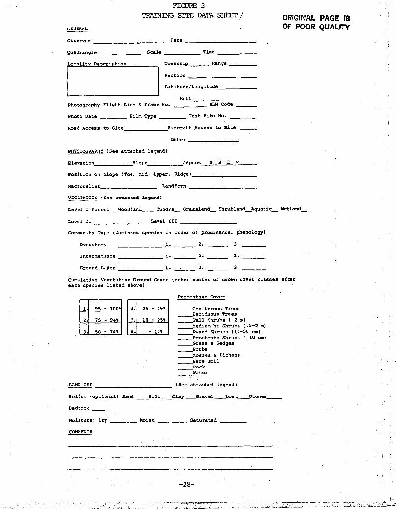
FIGURE 3

TRAINING SITE DATA SM=-1f

GENERAL

Observer Date

Quadrangle Scale Time

ORIGINAL PAGE 13OF POOR QUALITY

n

Locality Description

Township Range

Section

Latitude/Longitude

RollPhotography Flight Line & Frame No. BLM Code

Photo Date Film Type Test Site No.

Road Access to Site Aircraft Access to Site

Other

PHYSIOGRAPHY (See attached legend)

Elevation Slope Aspect N S E W

Position on Slope (Toe, Mid, Upper, Ridge)

Macrorelief Landform

VEGETATION (See attached legend)

Level I Forest_ Woodland Tundra_ Grassland_ Shrubland Aquatic Wetland_

Level II Level III

Community Type (Dominant species in order of prominance, phenology)r{ Overstory 1. 2.- 3.

Intermediate 1. 2. 3.

Ground Layer 1. 2. 3.

Cumulative Vegetative Ground Cover (enter number of crown cover classes aftereach species listed above)

Percentage Cover

1 95 - 100 4. 25 - 496 Coniferous Trees

i Deciduous Trees

2. 75 - 946 5. 10 - 256 Tall Shrubs ( 2 m)Medium ht Shrubs (.5-2 m)

3 50 - 746 6 - 10i Dwarf Shrubs (10-50 cm)

i Prostrate Shrubs ( 10 cm)Grass & SedgesForbs

:.

Mosses & LichensBare soilRockWater

} LAND USE (See attached legend)i

Soils. (optional) Sand _Silt Clay Gravel Loam Stones

Bedrock

ORIGINAL PAGE fSOF POOR QUALITY

ut

Q

ai

rU

wI o

.4

z rho,; ^ ! ^'

ry MI ^. . Y!-1M

14

O

p^av

Ni7

i

i

i

i

Q

I- I(V'u: 4 1AM) (l)VIN NI' tiMWITI) '11211MM I, SITES

-29-

ORIGINAL PAGE

COLOR PHOTOGRAPH

1)InQ)N

c^

pp^a7w

Ln

r.

cgLn

v

u

s

0

cq

^Q

Ln

EH"

-30-

ai

t2-

a

x

as

E

MINIMUM-AREA MAPPING UNITS

For photo interpretation and training site sampling the con-cept of the minimum-area mapping unit was used to alleviatepotential problems due to significant resolution loss.Pixel size is restricted to approximately 1.1 acres onLandsat, and because of the extraordinary amount of time andexpense involved with classifying training sites on IDIMS,it was felt necessary to develop an acceptable minimum areamapping unit. This is simply a minimum area measure definedin terms of the dimension of any land use/land cover atmapping scale. A land use/land cover occupying a smallertotal area on the map would not be mapped as a distinct landuse or land cover, but would be merged with a land cover inthe most logical manner possible. In this case, land coverswith similar spectral reflectances or values would be merged-during the statistical clustering process.

For purpose of photo-interpretation of land cover, par-ticularly vegetation, 40 acres was selected as the optimumsize for training sites. For urban land uses, trainingsites were kept to a 5 acre minimum area mapping unit, andlarger if possible. Urban land uses were more difficult tomap because of their small size and diversity. For example,in the Palmer/Wasilla area of the Matanuska-Susitna Borough,many training sites were less than 5 acres in size and insome cases could not be located on the IDIMS display.

^ 1

CHAPTER III

CHARACTERISTICS OF LANDSAT AND CIR PHOTOGRAPHYAND IMAGE PROCESSING SYSTEMS

To provide the non-technical users of this document with anunderstanding of remote sensing, a brief description of theLandsat system and other remotely sensed data is presentedin this section. The systems used in this demonstrationproject to process, manipulate, analyze, classify and outputthe data are also described.

LANDSAT

Remote sensing is not a new concept in land use and resourcemanagement. Aerial photography has been used for many yearsas a basic tool in surveying land areas. The completeLandsat system consists of an observatory or observatoriesin near-polar Earth orbit and ground installations toreceive, process and disribute the data provided by the sen-sors carried on the satellites.

The acquisition of remote-sensor imagery depends upon thedetection and recording of electromagnetic energy reflectedor emitted from surfaces of natural or man-made featuresthat are within the field of view of the sensor. Whenenergy (sunlight) strikes a feature it is either reflected,absorbed, or transmitted. The degree of reflection, absorp-tion or transmission is a function of the properties of thematerial and the wavelength of the energy. Various earthresources and features respond differently to energy ofvarious wavelengths depending upon their chemical and physi-cal properties, surface configuration and roughness, inten-sity of illumination and angle of incidence. When earthresources and features are recorded on remote sensorimagery, the various responses of earth features form pat-terns which provide means for discrimination. Through anal-ysis of these patterns and their relationship to eachother, an individual can deduce the identification of thesepatterns. Various types of remote sensors record in dif-ferent energy bands. The multispectral scanner onboardLandsat records data in four different bands of theelectromagnetic spectrum.

Landsat produces images of Earth--not with a camera but with• multispectral scanner (MSS). The multispectral scanner is• line-scanning device that uses an oscillating mirror tocontinuously scan perpendicular to the spacecraft's orbitalpath.

The MSS records information in both visible wave lengths andi in parts of the electromagnetic spectrum which are invisible

to the eye (near-infrared). The MSS records differences in

-32-

sun reflectance from earth-surface features.

Water, vegetation, minerals, and other natural and man-madefeatures reflect light or emit radiation in different inten-sities for different bands of the electromagnetic spectrum.Each feature has its own unique reflection pattern, an iden-tifying signature that makes it possible for remote sensersto differentiate surface features. The MSS takes fourreadings for each 1.1 acre area on the-ground: one for theintensity of green light reflected, one for the intensity ofred light reflected, and two for the intensity of infrared.These intensity levels are converted into electronic signals(digital form) that are sent to ground stations. This digi-tal data is stored on computer tapes that can be used toanalyze the 115-mile-square Earth scene (although the MSSscans a continuous path, the data is cut into a standardfilm format, thus providing a film product coverage for115 miles on each side).

Landsat's singular advantage over conventional photographicsystems is that it gathers data in a computer-compatibleformat that facilitates processing and use of the data.Landsat data can be used in either its photographic form orin its computer--tape (digital) form. If the photographicproducts are chosen for analysis the procedures are almostidentical to those used for interpreting conventional aerialphotographs. Approximately 5,000 frames of CIR photography(stereo coverage at 1:60,000 scale) are required to cover onescene of Landsat data.

Computer processing (computer-aided analysis techniques) ismore complicated than photo-interpretation but can be fasterand can yield more detailed results. The computer can nor-mally identify objects of as little as 1.1 acre (pixel)while photo-interpretation techniques are generally limitedto objects of 5 to 10 acres or larger. Using the computer,data can be analyzed statistically and used to provide"classified" imagery highlighting specific types of landcover with arbitrarily chosen colors as on maps.

At an altitude of approximately 570 miles, Landsat circlesthe earth 14 times daily, scanning a particular geographiclocale every 18 days. This high volume of information,broad-area coverage, and repetitive sweeping provides avariety of opportunities for practical application of thedata to resource and land use planning related tasks andproblems.

COLOR INFRARED PHOTOGRAPHY

The State of Alaska in conjunction with various federalagencies has undertaken a high altitude aerial survey of theentire State of Alaska. For the past three years, the U-2and WB57 aircraft have been flying the state taking color

-33-

4

infrared aerial. photographs. The University of Alaska,Geophysical Institute, Fairbanks and the Bureau of LandManagement, Anchorage are the repositories for all filmproducts. The color infrar(t6 photography was extensivelyused throuq hout the INTRISCA project.

The Lockheed U-2 is a single place aircraft designed forsustained operation at high altitude. At its normal cruisealtitude of 65,000 feet the 0-2 is above most atmosphericturbulence and wind factors providing an exceptionallystable platform for remote sensor operation.

Color infrared film is sensitive to the careen, red and near-infrared (500-900 nanometer) portions of the spectrum and iswidely used in aerial and space photographic surveys forland use and vegetation analysis. Living vegetationreflects light in the green portion of the visible spectrumto which the human eye is sensitive. Additionally, itreflects up to ten times as much in the near-infrared(700-1100 nanometer) portion of the spectrum, which is justbeyond the range of human vision. When there is a decreasein photosynthesis, whether caused by normal maturation orstress, there is a corresponding decrease in near-infraredreflectance. Living or healthy vegetation appears asvarious hues of red in color infrared film. If diseased orstressed, the color response will shift to browns or yellowsdue to the decrease in near infrared reflectance. This filmis also effective at haze penetration since blue light iseliminated by filtration.

IMAGE ANALYSIS SYSTEMS

E'.

DESCRIPTION OF SYSTEMS USED FOR CLASSIFYING

INTRISCA project team members were given hands-on trainingon the Interactive Digital Image Manipulation System(IDIMS). IDIMS is comprised of several interactive ter-minals and a COh1TAL CRT display unit which is capable ofdisplaying color composite images, graylevels, and pseudocoloredgraylevel images. A 512 x 512 display area allows a portionof a Landsat scene to be viewed and displayed either as rawdigital data or as false color images, or aspseudocolored classified scenes. A track-ball cursor allowsuser selection of subareas of each scene, which can beenlarged. The HP3000 computer and two tape drives facili-tate magnetic tape input; disc drives serve as additionalmemory and as working storage. Output devices include theCRT, terminals, tape drives, a Dunn camera system, a Dicomedfilm recorder, and a line printer.

The clustering algorithm operates on data that may begenerated through either a random ,sample or an operatorselected sampling area, or a combination of both. The

-34-

... .. _. ^.....uw.......R.. _ t .. _.. .. ... ,_ _,z ....,u ^.^.a.,... _<..:Y .......s .. ..a.^ . a... ...ww...a... ... .... _ t__. ., a ...«^.a.[.. ..,.^ ..uu ..wa.vst.,Ain:.aIIPi

system utilizes a maximum likelihood classifier and offers aN wide range of data manipulation software.

n d data can e aggregated b MS intoonce classified, by IDI pout-ical units, such as traffic analysis zones, census tractsor game management units. This is accomplished on IDIMSthrough the Geographic Entry System (GES).

EDITOR (E RTS Data Interpreter and TENEX Operations Recorder)is a system of software that has developed and evolved intoa complete image processing software system, useful for-anal-yzing Landsat digital data. The system, installed on theI4-TENEX system at NASA/Ames Research Center, provides ananalyst with the tools necessary to perform all phases ofLandsat digital analysis.

The EDITOR System was developed at the Center for AdvancedComputation, University of Illinois at Urbana-Champaign, andis designed to provide a three-fold system for interactiveimage processing, file management, and ILLIAC IVinterfacing. First, the interactive image processing systemallows for the manipulation and display of LANDSAT digitaldata by the analyst at a local level. Second, the filemanagement system controls both input/output of data andediting of file structures. Third, files are structuredthrough the two preceding parts of the system for submittingdata to the ILLIAC IV for batch processing. All three areaccessed and controlled through the.EDITOR softwarestructure.

PERIPHERAL OUTPUT DEVICES

DICOMED 0-47 FILM RECORDER

The D-47 is a film recorder manufactured by the DicomedCorporation. It is an output device capable of generating asingle black-and-white or color negative, a single colorpositive transparency, or individual black-and-white orcolor Polaroid prints on standard 4x5 Polaroid film. Input

` is via a magnetic tape with three separate files, one foreach color filter: blue, green, and red.

Programs run on the HP3000 computer allow users to selectcolors for the land cover classes in the classified imageprior to the generation of the DICOMED products. The D-47was used to generate many of the output products for the

s' INTRISCA project.

DUNN 631 COLOR CAMtRA

The Dunn 631 Color Graphic Camera Svstem is an output devicet6 _

designed for recording photohraphic hard copy from the

e,-35-

r 1

ti

signal generated in a CRT, through display on a black-and-white monitor. Full color, black-and-white, and colorseparation images can be recorded on 8 x 10 print film and35 mm slide film. The camera system is an efficient andrapid means of transferring computer images from a CRTdisplay to film.

VERSATEC ELECTROSTATIC PLOTTER

An electrostatic plotter is an output device which offershigh output speed, reliability, and low plotting costs.The plotter prints in widths ranging from 22 to 72 inches.A Ve rsatec plotter was used for this project and includesthe following capabilities:

1) A character generator (standard) allows the unit tooperate as a line printer as well as a plotter. A simul-taneous print-plot option (SPP) allows hardware-generatedcharacters to be overlayed onto the plot patterns.

All Versatec wide plotters utilize a dual array writing headwhich writes an overlapping dot structure. This producessolid, continuous plotted lines and patterns. The highresolution writing head also permits generation of variousdegrees of shading, from light gray to solid black.

The wide plotters employ a shaft encoder to ensure a ver-tical accuracy of 0.2% or 15 mils, operating at maximumspeed. An equivalent horizontal accuracy is assured by theprecision-engineered stationary writing head. The shaftencoder and servo system decelerate the paper gradually toavoid overshoot.

Output scales can be varied so that plotter maps overlayvarious scale base maps. Figure 6 illustrates a sample ofthe output capability.

Other peripherals and systems utilized include an ALTER digi-tizer and COMPLOT plotter (tied in to the EDITOR System),IBM 360/67 computer, CDC 7600 computer and SEL computer.

........... -

OF POORUAL'^'T'Y' Q ---.sis=.i: :a......... ....

... • - ii:: - =seic

s:' .iii:~; :^a^^• -

' S - - : i i,' - - - - iii =' - - : i . - - -""°^'"'."_ •^•.^^..,-n-.,^.,-.-.^^^^...-..•.,,...^TMr,'- .:: ' • • .. • ^ .. :: 3 ... . -.... ^ • • S i • i.: 2'--z;;•.;. i 1 i .. _ is S S 2 • • •c--^.^,-o.,^.,^,^..n,n.w•. r.v.r,,.,—r.. _

.• rirr r... -_ o .. - _

•:: «:•

_ ------

:^^. :3.11««.r.-...-»-.-- "."°"°.000-'^e^-ie^...."•»-••"'"•Si-...'°"°.'°oL"7 _

^^•'.: :j:ij . «'-'ii ..*.:,22^ - ice.w.«.+^...

••-j:o °_o:n«T__ li ^.-.^-

.-. ^i^^-.^.7^ «.=.-.:...ii221.-........_..~"::i:ii:+_21i :: 2.-...._.... • ...^.«i21x^•Vi i•-- - • - .•_-••.•••••••••. •...^....-.••V.•••••. .,..-•:..: •-^M_•••..«

•: ^-:: .i:: :• ,mow ::y -°:-+ -•-0.^.r rte.: '^ •-.+,.-.tip`:....+.n.,

't: ::.R- -2.^n,.,. -..'-'.^.'^.+7.:`« .`.-".^-_:_ e^^'^ - _ n..21.2•i^:f3i2•.•-."•:,^.::::::^•i.%^.::::2'_3:_ "^^2^^

................... ...... .....'SSiS2S'«.,,..3:^.''"-"" .S2ii ^»

y",.-.:..;^..:a:,:;-.-«........-.^^.,:^^,--... ^w:^^ ...--.._.:: .....;;... .,.,., ^..^_^.

^.e-.-.•.ice. ,•. •122 k ,.,.•...^..•::::" f a-

,• _ +.++-«-.^_•_.-..--.--..ate. ^. ••-K+-+++TM ..• •^••••-,r.._^i-..

+...yo.: ^^..^ey :^e•::3Y7.---ate :• ~^:^^ "r'^.:^ :^^._231ii1^!- •••.r..^..•.• _

.. .: .:""':^°^ y. \ ..-..^ «. •• .ter,-. .. .-.

. ._. e°r- o•^. ..+.. .. ^..+. +-.+^«.o : V I—. • k.. __ on

.. . . .r cri.-«++-..••._, ..-o••••:ii.........

Z --->

FIC73R° 6. V7—PSTEC ELECTRW=C PI,07MER MAP

CLASSIFICATION OF 1978 DATA.INTRISCA, SUSITNA SCENE GROUPED DATA

—37—

CHAPTER IVTECHNICAL APPROACH

INTRODUCTION

The following is a generalized representation of the workflow in the digital analysis of Landsat data. Technicalpapers describing various phases in the analysis of theINTRISCA Landsat data appear in the appendices. (Figure 7illustrates the technical work flow for the INTRISCAproject). The INTRISCA project is due in part to theSouthcentral Alaska Water Level B study which utilizedLandsat digital data to provide land use/land cover infor-mation for future management of land and water resources.The land cover classification for the Water Resource Studywas completed by Dr. P. Krebs and P. Spencer of theUniversity of Alaska. Products from the classification wereevaluated by NASA and participating agencies to determinetheir usefulness in meeting state agency needs. As part ofthe INTRISCA project, NASA corrected major classificationerrors through the use of stratification techniques.Following the evaluation, NASA began a new classification toproduce a more recent data set which was more specificallyrelated to individual agency needs.

One source of classification error in Landsat analysis workis the result of spectral confusion between two distinctland cover categories. Each spectral class is supposed torepresent a specific land cover category. However, problemsarise when two distinct land cover categories have similarspectral reflectance values. Stratification techniques havebeen developed to resolve this type of classification error.Where problem areas exist, boundaries are delineated toencompass the misclassified spectral classes. Conflictingspectral classes within specified polygons are reassignedto the correct land cover category.

Preliminary stratification strategies involved reassignmentand reidentification of spectral classes within physic-graphic provinces, Anchorage and Eagle River urbanizedareas, and the Palmer agricultural region. Refinements tothe Level B classification (originally with 43 spectralclasses) separated an additional six land cover categories:grasslands, alpine tundra, commercial/industrial, low- andhigh-density residential, and agricultural fields. Color-coded Dicomeds of the Level B classification before andafter stratification have been generated for the Anchorageurban area (Figure 8).

The following chapter briefly describes the technical pro-cesses utilized to generate the new classifications, datasets, and other products of the demonstration project.

R

-38-

A

E

iI

FIGURE 7 TECHNICAL W= FLOW CHART

DATAACOUISITION

CCT

CCT ORIGINAL PAGE IS

"MOSAIC

OF POOR QUALITY

PREPROCESSING

ALTERNATE

STUDYROTATIONAREA -----^—^^ ETC.CCT

TRAINING FIELDSITEDATASELECTION

CLUSTERINGOF TRAINING

SITES

CLUSTEREVAL. AEDITING

` STATISTICSDIGITAL FILE

ANALYSIS

STUDYAREACCT

eCLASSIFICATION

CLASS FIELD DATAIDENTIFICATION PHOTOGRAPHY

STRATIFICATION 4

ROTATIONTO

NORTH

POST-PROCESSING GROUPING

I'

SMOOTHING

FINAL CLASSIDENVEVAL

GENERATIONOUTPUT OF

PRODUCTS OUTPUT PROD.

-39-

1 ^^

A minimum of four kinds of data are usually acquired in pre-paration for the generation of a Landsat land coverclassification: 1) Landsat digital data, in the form ofcomputer-compatible tapes (CCTs), 2) false-color pho-tographic representations of the digital data, 3) fielddata, and 4) color infrared U-2 photography. Lower-altitudephotography may also be gathered, if available, dependingupon the types of land cover classes'to be identified.Appendix A, Imagery Acquisition, pertains to the acquisitionof data for the INTRISCA classification. Team members con-ducted low altitude overflights of portions of the studyarea. 35 mm oblique photographs were taken of both homo-geneous land cover types and transitional vegetative zones.Many of the field test sites where visited in person andphotographed on the ground.

PREPROCESSING

Preprocessing is a term used to specify those processingsteps to which the digital data are subjected prior toclustering and classification. One type of preprocessinginvolves the mosaicking together of two Landsat scenes intheir digital form. Mosaicking is performed when a studyarea is encompassed by two Landsat scenes, provided that thetwo scenes are adjacent to one another and provided that thescenes were imaged by Landsat on the same day. Themosaicked Landsat data can be generated so that the entirestudy area is covered by a single data set, thereby reducingthe cost of digital processing.

Another type of digital preprocessing involves the repair ofartifacts or inconsistencies in the data that are attribut-able to scanner malfunction rather than to informationreceived from the ground by the satellite. Scanner malfunc-tion can result in missing data or in the recording of falseinformation ("noise" or "bad scan lines"). This type ofpreprocessing replaces missing or bad data lines with newvalues adjusted to those of the other scanners, and isreferred to as radiometric correction.

A third type of preprocessing that is commonly performed isgeometric correction, in which the Landsat digital data setis either registered digitally to a map base, or is at leastrotated to north so that columns within the data aredirectly north-south. During the correction process skew,caused by the rotation of the earth under the satellite, isremoved.

The radiometric and geometric corrections performed on theINTRISCA data are described in Appendix C, Digital Analysisof the Susitna Scene, and in Appendix D Digital Analysis ofthe Anchorage/Eastern Scene.

;_ -41-

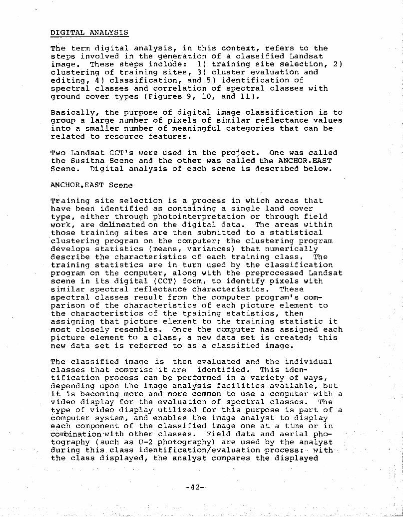
DIGITAL ANALYSIS

The term digital analysis, in this context, refers to thesteps involved in the generation of a classified Landsatimage. These steps include: 1) training site selection, 2)clustering of training sites, 3) cluster evaluation andediting, 4) classification, and 5) identification ofspectral classes and correlation of spectral classes withground cover types (Figures 9, 10, and 11).

Basically, the purpose of digital image classification is togroup a large number of pixels of similar reflectance valuesinto a smaller number of meaningful categories that can berelated to resource features.

Two Landsat CCT's were used in the project. One was calledthe Susitna Scene and the other was called the ANCHOR.EASTScene. Digital analysis of each scene is described below.

ANCHOR.EAST Scene

Training site selection is a process in which areas thathave been identified as containing a single land covertype, either through photointerpretation or through fieldwork, are delineated on the digital data. The areas withinthose training sites are then submitted to a statisticalclustering program on the computer; the clustering programdevelops statistics (means, variances) that numericallydescribe the characteristics of each training class. Thetraining statistics are in turn used by the classificationprogram on the computer, along with the preprocessed Landsatscene in its digital (CCT) form, to identify pixels withsimilar spectral reflectance characteristics. Thesespectral classes result from the computer program's com-parison of the characteristics of each picture element tothe characteristics of the training statistics, thenassigning that picture element to the training statistic itmost closely resembles. Once the computer has assigned eachpicture element to a class, a new data set is created; thisnew data set is referred to as a classified image.

The classified image is then evaluated and the individualclasses that comprise it are identified. This iden-tification process can be performed in a variety of ways,depending upon the image analysis facilities available, butit is becoming more and more common to use a computer with avideo display for the evaluation of spectral classes. Thetype of video display utilized for this purpose is part of acomputer system, and enables the image analyst to displayeach component of the classified image one at a time or incombination-with other classes. Field data and aerial pho-tography (such as U-2 photography) are used by the analystduring this class identification/evaluation process: withthe class displayed, the analyst compares the displayed

-42-

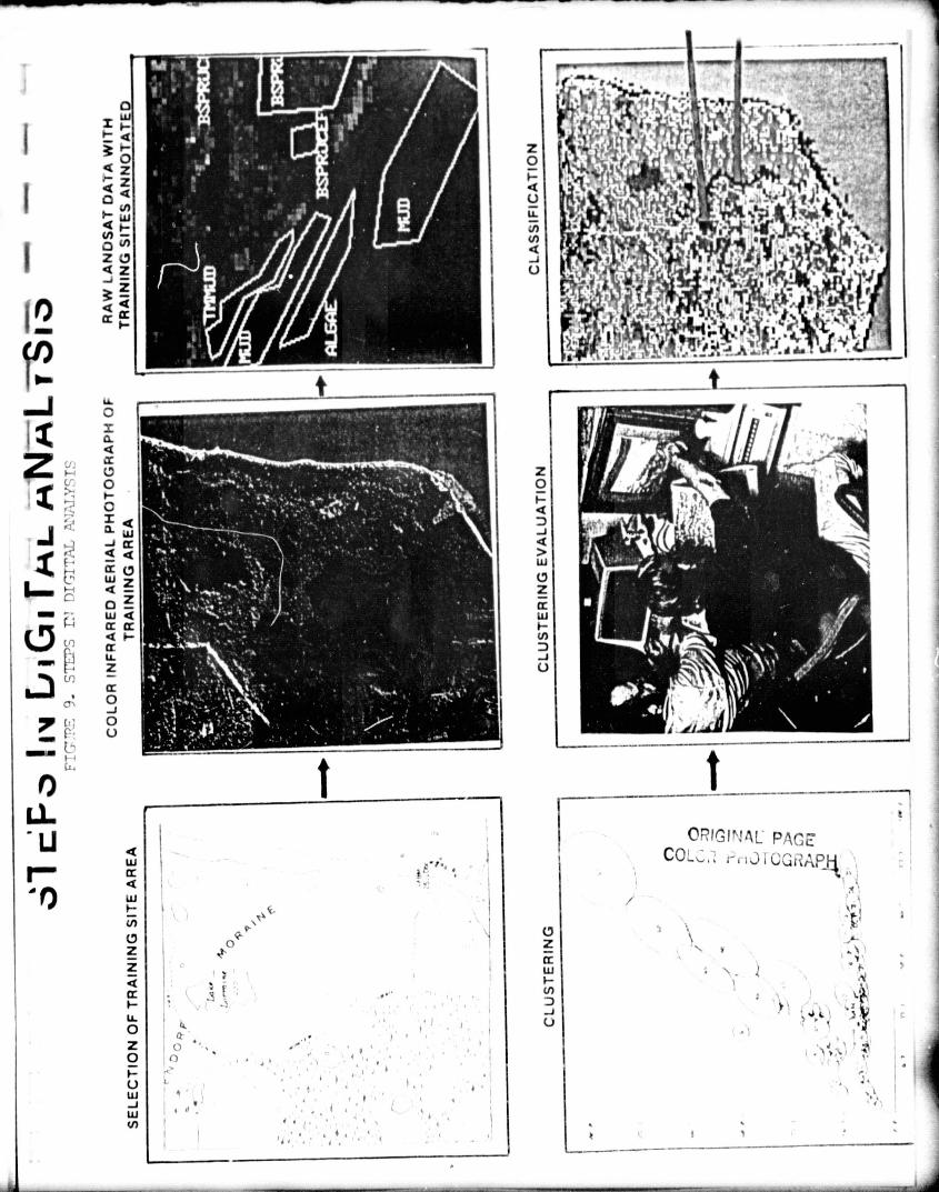
= WIi ►-

r QrOZ

aza^Na u'N -

I ^ N

z 0Q z

^ Q

12Q

C)

z vi cc

P-4 0

j

J

U O

^: r

d z w

Lr

J Qi

E

Q Q

^ W Z

^ ^ Z

w QQ

cc

4./ can Q ^"

H ZU

oJ

7 c.3 oU

n ta.

LL_u

r.^

aw

Qw

1 p

c

f

cL

i

)

i

z0

Q

J

Q

w

0z

ccwf-NDJ

t

ORKSINAL PACE

ti

CO ;^ • ; r„J I CGRAp „

iart

c^z

w

` nlNJ .^ 1 • S

U

1 r \I

e

t Z

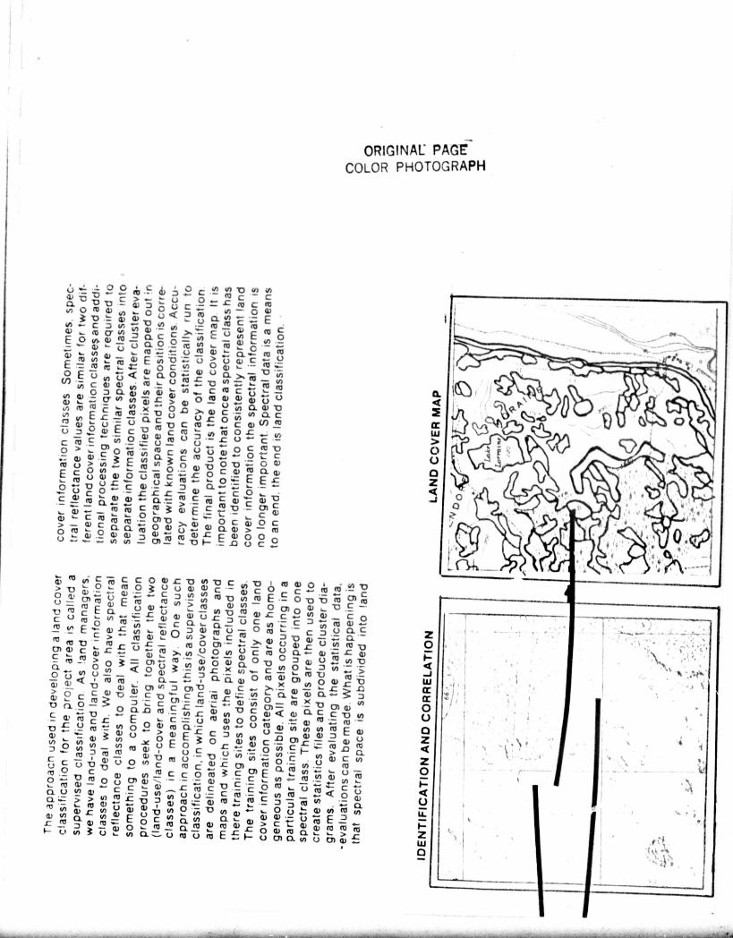
l ^ 1

^r

I •^

• I

.,\tilt

' 7 ;

- I

2O

aJWmmOU

OZaZ_O

a

ULL

1-

2w0

ORIGINAL PAGECOLOR PHOTOGRAPH

^?o^^=apouc0=^ mc ca

,n O J a M M 3, - p3 v = y °i n '?m E

OL

C cn ;n ^, J) m ^; `acE D vii d l a c C N E `} u) E oao o- N a)

ro Z U _ro w OL ro caE^° E0^;n''oy(uE^v^ f c w a ca ^ v ro ^ ^ 'n ^ ro ^ ^N O O Ci y ^n a) ,n c ca V ro

N N y 47 t > p M a) a) y V Uro E c ) . x^ or, >.w c aQLc

" v U v a c -0 c m L o c W^ ro07^(uEc v`°cro nmot> of 0 'D-- m C iv H a c c m u v° c M

o r c^vc°'i - f o .0ov cL: Q)0 (D c) L;Mc^^ocvEaL

vO D U L C a) - 7 G. o .^ E

U c 0 « L L C Q zC ^'m , Q_ caC Cw a)'Dm c:°3wEc1°t'E°'^Cc ^v ^ o _

>O ca CL Q is ° 0 V O N Q m >- mV N a) 7 v is m N L E p p 0in v) (M- - F- t^ v c

dv N m Q 3 v v C y O co a3 O co 10

V rp131 M furo c U a) H> ro a7 N- - Q -'c Cc v c E a u L'D y a) U L `a 4) i c Q a y CE f a, N v p aa) c°v u° ro E c u a c

ro ro^ ` c>a t m c m0ch- >.a)va)iuinMC a) C v L v >, cn U o ,n c m v a- a, tC> 0 3 to " ro N p N p U Q 7 a v ro v_)

Q ^, ° v, Q o U 3 cn t x a c cn 0 7 rn >° a a ro ^a a_^ 7 a a a) o ro v M `° o `° vaJ a) O) V% 7 (MID _ C .-a)

>..x ih ` t L 1. O c C O L c-0 c C L .- to Q a) Q 7m 7 C L ro- W ^_ ro x O7 (D NC.n_o 3oa m . _ cnt cn'oc vQtiaCc ,nC.

v L trot— o-0 mat V) L) m )^n NN ivEa))n u) 0 3 N V Y° N E 3 c 7 a) h C ^ O) a) a) 7 UO N V) v E o t n) c ro ca

_ro 7 ro ro a1 U C V N {n .O v7 (_ ~ In > Dv c Uv^Q0(nc ro mp We ro°_v).U^mv)

O0 O p m O O N m C C O ro C_ E N O nof ca

C1 U V) a) `^ C C `^ a) ^ A-- ro C D C C •C ro U to ~ C Uu7 ro In N U c:c0 C N m h Q _C a

^ N r^ U ^^^ N ^ N ^^ r ►. O U ^ O N m yL n a, ro °) E o C N acn a a, a) a) v E?

7 p ro p ro d ro _ > C a) N m ca► ^^u,3u Na = vcavroE^F-°o7oa°U8)>

I

ry ^ a`^ t

^ M adc o ^^OW

0.

w V

0 I2 ^•

Ij

FTMIRE 10. integrated Resource Inventoryfor Seth Central Alaska

ORIGINAL' PACE

..Q4_ COLOR PHOTOGRAPH

FI GURE I ti LAND COVER I NVENTOR 3 USING SATELLITE DATA

-45-ORIGINAL PAGE

COLOR PHOTOGRAPH

canputerclass with the ground cover types seen on the pho-tography and field data for the same location. Multiplegeographic locations of the same computer class providevaried contexts within which to evaluate that class.

once the computer classes have been identified, they arecorrelated with ground cover types, so that each computerclass is assigned to one of the categories in the land coverclassification scheme that was devised at the onset of theproject. Concurrently, confusion that has occurred betweenspectrally-similar land cover types is noted for use inpost-processing. The classified image is then ready forpost-processing.

SUSITNA Scene

In supervised classification, the analyst selects areas thatare spectrally homogeneous for each resource category.Because of variations in spectral characteristics of landcover types, more than one training area is usually selectedfor each land cover category. Training statistics,including the mean brightness value within the trainingarea, variance about the mean, and the covariance betweendata channels are calculated for each training area. Aclustering technique is used to identify a unique number ofspectral classes within each training area.

The training areas were located on the Landsat data andall pixels within the training areas were clustered into alarge number of spectral classes. A line printer map ofeach training area was compared with color infrared pho-tographs and each spectral cluster was assigned to one the17 ground cover classes. The statistics for all spectralclusters were used to calculate a statistical measure of theseparability between spectral clusters in multidimensionalspace. The separability statistics and the interpretedcover class for each spectral cluster were then used todetermine which spectral clusters could be combined.

The training area statistics and the Landsat data were inputto a maximum likelihood classifier. Evaluation of initialresults indicated confession between such features as mud-flats and the central business district. The Landsat digi-tal data had to be stratified to remove the confusion and tocreate separate land cover classes. The spectral clusterswere then displayed on a color terminal. Using aerialphotographs, ground data, and other supporting data, theanalyst identified the land cover types associated with eachspectral cluster. In the example shown (Figure 12) .fifty-one spectral clusters were identified in the sample data.Using this approach to derive training statistics, it wasassumed that the sample data represented all of the covertypes in the area. It was further assumed that each majorcover category (deciduous, coniferous, mixed forest, etc.)

-46- t_ ,

r

z

FIGURE 12

Position of Information Classes in Spectral Space

(Cluster Diagram on Page 48)

Landsat has four (4) channels; however, one cannot imaginefour-dimensional space in graphical terms. By using twochannels, a two-dimensional representation of spectral spacecan be produced. in Figure 12, Channel 2 corresponds toRand 5.(0.6-0.7 microfts) and Channel 3 corresponds to Rand6(0.7-0.8 microns). Spectral classes tend to group in atrianqular shape beginning in the Lower left corner andspreading to the upper right. various types of land coverspread out along the horizontal axis (conifers, mixedforest, deciduous forest, grasses). This is because mosttypes of vegetation are equally low in red light reflectance(Channel. 2) and very different in infrared reflectance(Channel 3). Alonq the 45 0 diagonal axis (lower left toupper right) the spread of water classes, barren areas,snow, ice and clouds occurs. For example, a tree leaf mayreflect only 10 to 15 percent in the green portion of thespectrum, and as much as 40 to 50 percent in the nearinfrared. Wet soil produces a dark tone (low reflectance)and cry soil produces a light tone. Spectral reflectance isthe ratio of reflected energy to incident radiation as afunction of wavelength.

HAND 3

A pl.at is shown.rOix-osealLs the

locCit-ioll Of 11 mall, while t1lograpilic Portcay"l l of Variance.

FIGURE 12,

t,^.Or. tl^'4NCENTRATION FOR BANDS 2 AND 2I *' NSUIFF^RVISE.D 8T-,\7,q r-f-)P -^-Z l IOTTKIA

i AN!. 0

i i3. "I

9

LN

would be represented by at least one spectral cluster andthat each spectral cluster, would represent only one covertype.

A mean brightness value and its variance for each spectralband and a covariance matrix was calculated for eachspectral cluster. These statistics were used in a maximumlikelihood algorithm to classify each picture element intoone of 51 cluster classes. Color infrared photographs andfield data were used to assign each cluster class into oneof seventeen land cover classes. The data were colorencoded and recorded on film with both a film recordingdevice and a Dunn ,-'- camera system.

EVALUATION OF SPECTRAL CLASSES

Following classification, a series of four User EvaluationWorkshops were conducted at Ames. The first of these fourday workshops was attended by Lee Wyatt from the Mat-Su(Matanuska-Susitna) Borough and any Tony Burns, the InstateCoordinator, who attended the entire series of workshops.The second of the workshops was attended by Peggy McNees ofthe Planning and Classification Section of Alaska StateDepartment of Natural Resources (DNR); the third, by MerlinWibbenmeyer of DNR/Forestry. The fourth workshop was con-ducted with and for Tony Burns, and focused upon Anchorageand other urban areas, as well as coastal wetlands under thejurisdiction of the Municipality of Anchorage. The objec-tive of each of these workshops was to provide an oppor-tunity for agency personnel to identify the spectral classesresulting from the classification of both 1978 scenes and toevaluate the classifications as a whole, using the IDIMSdisplay as a tool. Since each of these agency personnel hadexpertise in different types of land cover, and in eval-uation of most of the areas of interest that comprised thestudy area (such as Point McKenzie, the Eagle River Valley,Big Lake, and the Palmer/Wasilla area). Vegetation types --in particular, forest and wetland cover types --and urbanland cover types were carefully examined and evaluated inthese and other areas using U-2 photography and field dataas ,ground information. Available specialized landcover/land use maps were also consulted in evaluating thespectral classes, particularly in Anchorage and in thecoastal wetland areas on the north side of Turnagain Arm.

POST-PROCESSING

Post-processing is a general term that refers to any digitalprocessing that is performed after classification. Geometriccorrection, mentioned in the Preprocessing section, is-some-times performed on the classified image rather than on theoriginal Landsat data in order to reduce the time and cost

-49-

t

required for the correction. Stratification that is per-formed in order to refine a classification and to reduceconfusion between spectrally-similar land cover types isalso referred to as a part of post-processing. The terms"grouping" and "smoothing" specify two additional types ofpost-processing that may be performed on a classified image.

Stratification, when performed in order to refine aclassification, involves the digital separation of somegeographic areas from surrounding portions of the digitalclassified image. This separation is effected through thedrawing of digital lines around the area to be delineated;the lines are drawn either with a digitizer or with a cursoron a computer video.display of the type describedpreviously. Classes within the area that were separated or"lifted out" are then renamed from one computer category toanother. The need for this type of stratification ariseswhen land.cover types are spectrally similar: two or threeland cover types reflect light to the same degree, so thatthey look alike to the sensors aboard Landsat. Light greybare rocks, for example, look the same as light grey pave-ment to the satellite because both reflect light similarly.If the classification scheme seeks to identify urban streetsand paved areas, it is therefore necessary to digitallyseparate the urban area from surrounding natural areas con-taining bare rock, by stratifying. The same is true inclassification schemes that include the distinction betweenshrub/grass tundra and occurrences of shrubs and grasses inlowland areas: stratification to separate altitude-dependent vegetative communities is common practice and,like geometric correction, may be performed either before orafter classification. Appendix D deals with the actualstratifications performed-on the INTRISCA classification.Additional information on the stratification process canalso be found in Appendix E, regarding the stratificationperformed on the Level B Classification.

If stratification is performed for the purpose of refiningthe classification, grouping and smoothing processes followthe completion of the stratification. Grouping involves theaggregation of the computer (or spectral) classes into landcover categories that correspond with the classificationscheme selected for the project. The grouping process is asimple assignment of one set of digital numbers to a secondset of analyst-specified numbers. Smoothing is a processwhich, if used, follows grouping. Smoothing programs on thecomputer examine each picture element in the context of itsneighbors and reassign categories into the predominantclasses that surround them when isolated incidences ofclasses are located. The effect of smoothing is two-fold:it eliminates the salt-and-pepper effect found in mostclassified images, and it simulates a minimum mapping unitthat corresponds to the neighborhood size. For example, anine-picture-element neighborhood mimics a nine-acre minimum

-50-

dmapping unit because each one-acre picture element is examinein the context of the eight acres (picture elements)surrounding it. The class reassignments that occur duringsmoothing then approximate the class assignments that wouldresult from field work that classified land cover in nine-acre blocks or parcels. A description of the grouping andsmoothing performed on the INTRISCA classification can befound in Appendix C, Digital Analysis of the Anchorage/Eastern Scene.

OUTPUT PRODUCTS

Following the completion of all post-processing, theclassified image is ready for the generation of outputproducts. The type of output products available from aclassification is dependent upon the resources at the imageprocessing facility. Line printer maps or maps from anelectrostatic printer/plotter (in which computer classes arerepresented by symbols) and photographic products generatedfrom a film recorder are two common types of outputproducts. A third output product, frequently generatedfrom classified imagery, is a tabular summary of pictureelements by land cover class, converted into acreages perclass and into the percentage of the classified image allo-cated to each computer class. (Figure 13 and Tables 5 and 6illustrate some of the products produced for the INTRISCAproject).

Various combinations of these types of output products maybe generated for a single classification in order to meetthe needs of participating agencies. Line printer andplotter maps can be generated at a variety of map scales,and selected geographic areas of interest from the sameclassification may be printed at different map scalesaccording to user agency base maps. For example, the EagleRiver area of the INTRISCA classification was printed at amap scale of 1:24,000 to correspond to existing base maps atthat scale. By the same token, photographic negatives ofthe classification can be generated on a film recorder andsubsequently enlarged to match specific map scales.Negatives of selected areas of the INTRISCA classification,for example, were photographically enlarged to scales ofapproximately 1:25,000; 1:250,000; 1:63,360; and 1:1,000,000to correspond to the scales of existing maps for thoseareas. User agencies were also provided with negatives ofphotographic output products, enabling them to generateadditional photographic enlargements as required.

The delivery of final output products to user agencies pro -vides the necessary materials for them to quantitativelyevaluate, or conduct a verification/assessment of^ the classi-fication accuracy.

-51-

7

I'Itail:l; 1 I, 1:N,11111)10 Of INTRISCA Output i'rcuiurt(1) icc^med ( , n 1 arycnu'ttt )

ORIGINAL PAGECOLOR PHOTOGHAPH

TABLE 5, TABULAR SUMARY OF PI.MS :BIG LAKE TO SUSITNA RIVER

N= I251.«=7255, 5=.'__^ i^,==3.1,Z 1L 919—LA CE-to SUSITNA-RIVER_^vTr:: na1 ^

P I X : L S AC? .S CLASSCAT 1 65882 737B6 sedimented waterCAT 2 K boS 34348 clear waterCAT 3 15548) 174136 shrub/moss bogCAT 4 362n2 4• L 54 6 black spruce bogCAT 5 977u 1';049 grass(:AT 6 263136 Z94(- 3 shrub

L C"T 7 14)C,597 1126x5 coniferCAT 8 22 6438 2531:11 mixed forestC oT c 16",428 179679 deciduousCA f 1( 314oi+ 3 524^ barrens

CAT 11 1691 1894 alpine tundraCAT 12 4 4 glacierC AT 13 5 6 snow

CAT 16 b S r 773 commercial/industrialCAT 17 231 29 transportation facilitiesCAT 16 586 65;.) high-density residentialCAT 19 508 569 low density residentialCAT 21 1 C3 115 commercial

TMTAB A.+7 "SS 44.A7r,A

NOTE: Classes with pixel count of 0

are not listed by this program.

t

PIXEL COUNT

i FROM IBM-360

1978 DATA - SUSITNA SCENE

j

A

(SMSUS)

i,

TABLE 6. -TABULAR SUMMARY OF PIY= FROM IDIMS**Rt k #0 k 4*#t'# 4#R*#Rt A A. it it A..t #w # rt #*'AA W 4 0 ^ , .* N k W#. A • ♦ • kx.Rxx RR 4.x R11

r' ^` t L {; r ' = i BIG LAKE to SUSITNA RIVER

TOi , 4L r ('( 1 i,, 1 P, "1 1 zt:,+

* * * # * ,t '# * # # # 1 / # # # # It * * # # R 4 A # 4 # #' * 4 # t ^ # i R #. t Y t + . i A' ► } * * ► * # t = * * * 11 * fi ►CL A S S CLASS NAME

,; ;^ ^^ , ;t ;, n background1 5 r r 7 /7 sedimented water

i,,%• ^'* .'r S te= l clear water{ '.) U +'i . 1 n S shrub/moss bogu ? {, t ? '7 black spruce bog

a / 1 c, r i. l '^ .i grassshrub

7 1 . 1 14 1 , 1 1 ;, 7- conifer? S r . ? 7 ? ? mixed forest

^? 1^ i y 5 y deciduous1 1 S 1 1! r, 4 .0 17l ,I barrens11 1 o y 1 rt? ,1; t alpine tundra1 'a . ,r n j +, -i glacier1 ? 9 . ti ;, 0 i snow

(};:,; cloud1 t . 1 r I ; ;i r n shadow

I r rj t ,,;, , commercial/industrial1 J1 a i; ,7 transportation facilities1 ~ ^' : c high density residential

9 O low density residentialG .r10O'i , central business district

- ? 1 c 5 ri r? 1 commercial,, , 0 0 background

()=RCGINAL PACE ISOF POOR QUALITY

CHAPTER VSUBPROJECTS

In addition to producing a general land cover classificationand map of the project area, several of the participatingagencies had agency-specific projects which were designed toevaluate the usefulness of remote sensing techniques tospecific problems. These projects included:

• Road Network Mapping• Sea Surface Circulation Pattern Mapping° Integration of Landsat Digital Data into a

Geographic Information System• Floodplain and Landform Mapping• Urban Land Use Mapping

ROAD NETWORK MAPPING

one-dimensional edge enhancements performed on the iDIMSsystem were used by Matanuska-Susitna Borough for iden-tifying road network patterns. Because of recent and veryrapid growth within the Borough, planners wanted to knowwhere all the new subdivisions were and where all the newroads were located. By utilizing this enhancementprocedure, lineal features are optimally enhanced. Roads,railroads, powerlines, pipelines, seismic survey lines, andother linear cultural features can be differentiated throughanalysis of different MSS single-band or multi-band photoproducts derived from enhancement techniques on IDIMS.Technical documentation describing this procedure is con-tained in Appendix I. A set of computer generated pho-tographic products were developed and provided to theborough for their use and application.

SEA SURFACE CIRCULATION MAPPING

Varying degrees of knowledge about water clarity, depth,circulation patterns, suspended sediment load, algaedistribution, etc. can be derived from both raw andenhanced Landsat imagery. As part of the demonstrationproject, NASA enhanced four of the Landsat MSS bands todescribe the meaning of reflectance values of water.Interpretation of color enhanced Landsat single channel ima-ges could provide useful information about circulation con-ditions in Upper Cook Inlet. The Alaska Department of Fishand Game, Matanuska-Susitna Borough and Municipality ofAnchorage were participants in this subproject.Mr. Dave Burbank of the Department of Fish and Game con-ducted the analysis and interpretation of the data productssupplied by NASA. Both the technical papers prepared byNASA and the interpretations conducted by Mr. Burbank canbe found in Appendices G_and H, respectively.

-55-

INTEGRATION OF LANDSAT DIGITAL DATA WITH A GEOGRAPHICINFORMATION SYSTEM

Landsat digital data can frequently be enhanced when it isvertically integrated with other types of data such astopography, slope, soils, and landforms. This is bestaccomplished using a geographic information system (GIS).

Two test sites were selected for this demonstration; one inAnchorage and the other in the Matanuska-Susitna Borough.Both test sites were selected to demonstrate two differentsets of applications.

Anchorage Test Site

A twenty-five square mile area in Anchorage was selected.This test site corresponded to an area where concurrentstudies were being conducted by a-n independent consultingfirm. The Hillside area of Anchorage presently does nothave sewer systems, but instead relies on septic tanks.Increased growth in the Hillside area has brought about aneed for higher densities; however, ground water pollutionis considered a problem if densities increase. The con-sultant is therefore conducting a wastewater management planfor this ara. The use of a geographic information systemwill permit digitizing thematic data (geology, soils,drainage conditions, slope, etc.)-and integrating thesedata sets with Landsat digital data to produce land usesuitability/capability maps. The consultant is performing asimilar study, but using manual techniques in addition towell log data. The results of both projects can thus becompared and an assessment of the results made.

Matanuska-Susitna Borough

The Wasilla/Big Lake area is a rapidly growing area and ispresently used extensively for recreational activities.Both permanent and recreational homes are being built in thearea. The phy-ical area has also been previously glaciated,thus creating a landscape of lakes, moraines, and wetlands.

The Soil Conservation Service has recently completed a soilsurvey for this area and prepared land usesuitability/capability maps (using a GIS approach).However, Soil Conservation Service land cover was photo-interpreted and collected on the ground as part of the soilsurvey. The purpose of the Landsat/GIS demonstration inthis area was to assess the accuracy of land cover derivedfrom Landsat with the land cover maps developed by SCS.Secondly, the project was intended to demonstrate thatLandsat digital data in conjunction with collateral datacould he used as a viable tool for determining land usesuitability/capability and to compare the resultant land usesuitability/capability maps with those of SCS. That is, do

-56-

t

land cover maps derived from the analyais and interpretationof Landsat imagery correspond favorably with land covermaps developed from field work, and do the resultant landuse suitability/capability maps produced by SCS comparefavorably with those produced as a result of this demonstra-tion project. A favorable correlation would indicate thatthis approach could be utilized in an operational mode.

FLOODPLAIN AND LANDFORM MAPPING

The purpose of this subproject was to study and map thelandforms within a corridor along select streams inthe Susitna River Valley. The investigation utilized colorinfrared-aerial photography, Landsat imagery, USEStopographic maps and aerial and ground verification

! procedures. The results of the project provided land mana-gers with an initial data base to establish riparian manage-ment zones or buffer zones to protect fish and wildlife andtheir habitats from disturbance or damage. A secondaryobjective of the study was to compare the minimum size offloodplains and number of floodplain categories derived fromaerial photography to that derived from Landsat imagery.This project was conducted by Mr. henneson G. Dean, NorthernRemote Sensing Laboratory, Geophysical Institute, Universityof Alaska under a NASA/Ames Research Center ConsortiumAgreement for the Alaska Department of Fish and Game.

URBAN LAND USE MAPPING

The Municipality of Anchorage was particularly interested ininvestigating to what extent urban land use could be iden-tified and mapped using Landsat imagery. Several hundredground training sites were plotted and used to classify theLandsat digital data. Output products included Dicomedgenerated film prints and Dunn Polaroid prints of the urbanarea. These color-coded maps or prints were then checkedagainst existing land use maps. This accuracy assessment isstill going on. It is hoped that an acceptable level ofaccuracy is determined so that other Landsat imagery can beused to measure growth change, rate and direction. Thisprocess is called change detection, and if successfulwould provide the Municipality with a relatively inexpen-sive and rapid means of measuring urban growth and change

H

3

-57-

I

APPENDIX AINTRISCA PROJECT

AQUISITION OF IMAGERY

L. MORRISSEY

Landsat digital data in the form of computer compatibletapes and color composite photographic images (Figure 14)were used in the analysis of the Susitna Basin. Landsatcolor composites were used for delineation of environmentalstrata, the selection of training sites, and as a naviga-tional tool during aerial overflights of the study region.The computer compatible tapes were used in the digital pro-cessing of the Landsat data.

Landsat scenes were selected on the basis of percent: ofcloud cover, season of the year, and orbital path. Completecoverage of the study region was obtained with portions ofthe following three Landsat scenes:

2.1288-20250 August 2, 1978

21288-20253 August 2, 1978

30175-20345 August 27, 1978

Two of these scenes (21288-20250 and 21288-20253) are withinthe same orbital path, and the third (30175-20345) is froman orbital path to the east. Computer compatible tapes wereacquired from EROS (Earth Resources Observation Systems)Data Center.

Color-infrared photography (CIR) provided a necessary kinkbetween ground visits and the Landsat digital data with thedevelopment of photo-interpretation keys which allow theanalyst to extrapolate information gathered during groundvisits over larger areas. The CIR photography is primarilyuseful for collection of ground data and spectral classverification.

A search of available CIR photography was made at the U-2Data Facility located at Ames Research Center. Flight linesof all CIR photography falling within the study region wereplotted on 1:1,000,000-scale quadrangles (Figure 15). Thephotography was viewed eliminating those frames that hadexcessive cloud cover. Each of the participating agencieswere given selected photographic coverage (Table 7) of areasthey had designated high priority. NASA also maintained aduplicate set of photographs for evaluation of theclassifications.

fJ

f.

V

t^

fU

u

ti

C7

Q

il si

ar.^

a a

Ln

3

Z

9TQI

cs

^cs

f'1

fI

11

U1

I

k

FIGURE 14. IANUSIVr COLOR ODMPOSITEOR IGI NAL PAGE

COLOR PHOTOGRAPH

-59-

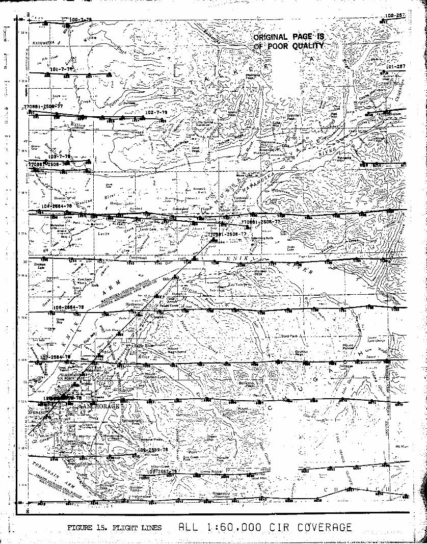
• .N. ^'-'_ 1 " ---,-Soh 100- ^ ° _ _ _ _- r : ^ .—_ - - .. .. -- '_ '

[ 22N •. I y^ \.tom `\ . - v .r _rR

t tiff ` r% `^lll/ll -^ ^ l>SkfyGINAL PAGE',r^^

Y ,t ,_,^^^\ _K.1.,zHwrr A ,^ I - .i^ ^. , i f• _

-­Via, r ^^. ^... .•-•C"PF

,^,,. :^ ! ^? 4 F ,r- ifi ? ^r, '{%}pf^.,.-1 n `. :{ ^y-^^,r{ 1r^1 0 :p..• ={ tph I C,ea T ' t"' ^`_ .^• ^!r ^^ Lllt ^.; -\1 i A v f ^: J , rya •".0 t`E

. I ^^^. i: o ^f \•, T'l `, f s, r? > ` yr, .

// 101 267- l Ir^( rA Ivy l L I4 S^•

'^ p - - Mor to'ca ^J, t i `t P 1 `•. t` ^' - ^n t 1^„^r! r a

n :^t1.a ` ; p3 \1 1^- , r J V ' vi ^ j j♦w,• , ^o,. y^t\`

r ^C----- I}i , r-• r :.^ ^' ^ ^ ,.;C.l;' u^^f!" L4 , L )` •"'dr+t `, 3

_ t t Irua }r \. _ /_^---„ :7 rl ,^" ' ,.({` (1 ^l }°f 1• j ; - _ ,,,,^•^ 1/ I, .e, •^

I R • Crack -•^^ ^^^. • _-[,. ti •^..t3';!, i y1 i " 1 • t - ^' 3 1>^• 1. r"r ' 'r v

,,770ee1-2sge'77 I^ C a ^' y. \ ^J FZr,4 ^^^ !J, tx I ; ^t . L=a+ rI 1 ^ ^• IOZ 7 79 ^ ^^ ^.^ r ; el n"^' Wsho ^ r ^a " Y^'^ Grinitar [c ya -Mtn I ^`` r, .~ ' {tO..-.-

irw // "' \ .Ji ,. 6,,,,/`^ (^7 lk. 1^ rr^ptwlt/ v / • • Y ^'`:e }:."^u^''-rf I 1 I 4w1 1 +-, ,• 1 tl4 \w w n,.,., i C ' \) 3 /'` EsIM ••+t r«s `•- I•twr!1 L ,I -' IL"purr .'I "", i^ ,. .t: tl. ,r l w.4a r.•

(YAoe `4 G} ^- -"" ' Mtn' t c R x.L:-' ^l!"

n. ' ...w I"'p ' ' 4 _ .^ •.. •tw k i^ TC Y'r i..,fr^„ : Y\"3:i,c ,d ^J ^.2'^,;.^ la „""'.`.c-a lalaY^lr; .q

`CC

.^% a^.-°'^.J^ c,.,f .^• •yy , • N ^„oo^

9n{InLr gcTt^ Y f_ t

IP^Y 'I . 1

V tl r ^^.•'j3r ^ ^ ttrrr, 1(13 -7 -^ ^- .^_ - - n ^J ? : I L .rr- i^^ttbn R P:r^atvP k. r\ee 80e- „, - a - I, O - Mtn - '3 t. r7 I 'y I I. ^^ 1^ T a-.

=t. ` my i -7 - -- ., I r r"i` I ! M .e (t^A♦n'- I 5^.•v t t•. ^ `•L'rry , - I y. I

s I mot. I ^M'\ % GP fir.• ( ^ ^ ^^-ti

I `i ^-^ .m I lab ' `.. 1 d.n X•n.d.L I •(''°% F^A.r9_'I L t " .^ \ •a♦ + f. > r,^l rt ^:,.

Ie n i I \ .. t _ .. R I . . •1 . , r. . u'rn I. ' 'v • IPv A !"tn•P• - „^i . `^' •• _ S c/c-t.^!^ / G^; Ivei .m _ I a,. I ♦7. ' I / l "r.. I:3 '7^+^ C3_'! I II I .^ I K ... Il, .ou y, xdm..•r,• satyr:. t P4hhwk:.. I

to % ,. •^' ^ i ,' r`3^ ^•I r I t ..7,.t, k•, ,y. 1r l;^ r tlm I 'l.,ry-': ; r-^ - '}J, fq b'- ' /'r. I, 11ad1

h7e

I .I /rrt:(nn .Lnk,a I _ .:. r It ter: ,^^ G , 1 ( 'L r• `i '1 ^ • ~ / r _,S (r f'f^ 9

' I r 26e4 -7e ^ ^ t k'r re 1.,L ,,, t' u . ' d ':R t.aaF' Ulmer !q . `. `17 _1 • ^rZI ^ ^ ^ Zti^^ \ _ ^-.- -••r 1 •

r.. L:r

uke 1 .:Ills"1 a-rr-l- :._^.I,•r^. y.. .i:>_10

I

^j-

,.,,r, y \. -`1"--• I n an t 'r , Cumrrs 1 r -\^ ^- /•'.`^, Y ! ^r ..

I^ ^•L, ♦ rNek^ ••'--. ^p 1•ll r. L95 I- AP Sway . .770 el ' s0E-7.1 - - _ ^tis ..• a^. .r. tlA,-aFw •^I^..i r L'i.n^l. q irra Lrro L^ n LLt u,^..r .. d

^ M y^^,r ^/ t rya+ I . L nrr Lakr s t t . .r,y 1. + yr^ I _r r, ...• • l ^' ^ \n 1_ ^^^3 ^^ / ( 1 ^(^--^ '/" .,LC j

r 17n '•rl - • 1 Lari le 1 I :7•'._., ..{ l 'Z ^J^6^77,I..rt... L^i^^,=r[^LC ' r I'r u,`.^°a I V/.^ 1 y

i'^V

t a-h L (^_^ I 1 ' ir0 • Z f o amt. tr r " I µa .^•' I II a i^ 'v`°a I Iliska t ..; TI %k;It 's 4,

-. +•a t w .^'r4."_,^,^ `^•., /^.k. `^^r• 1 c^J1^^ . .^,dlC t1^ ,.TT• I •.. L ' •roo (CJ ^^.^ ^' 4N

1 va,^.,ll I • - 1

I '• h jleu r ..^..a•----- I - -.,_ -i-r I L_-- - --I- .•k ^u[tbnaon,l T \ r•a n• ln•i• ^< ^r

^.30SIIp/att

I • tF L^R I , IH- 7 at • I7 11 ou... Fla 'ts h \' II 7 ..y_^`, \ \ I ] r

T . IG N - I R ..rm / w - y - s..-i^., :Peak ,^. r //^/ ^' A^- ...t^l-'1 (-..._.. ^ rkl.ia. ^ /' Eklu .. r, ,^^^_'--.A!"' lam-`.-,\ b ^...I , L t,'\ ^l^/•-'__lll

1c,,•Lr.L^lKnik tei'aa^oii•H •.i^:-^~ vst^sl"r In P..k1, ^

1

,^

•,.l I(\^G^•-L

- --.m•j w 1 ^ ^' ♦ M F t' +%. ^r 'rn rvr Fkvw \ i ` `\- ^i. .• "^-. r ^,^^•- '",-_-- I .a=-_ a.^ Q° wA iIKI'^^ ^' ri M a I ^' Aram.:. I ' ^♦ . \ _. -` .:__—_-- -

/^µQ!-'tF Birchwood F lr. ry\^ 'S,w• .:-. I! `r,^ ♦.,.1^' fir.G

IlOe-zAE , rr ; Pefne'Cmk rX.rcnr... ,-7

7TW

I 15 N 1 Roo„ / r.nrn, L I • L9 6Iw.aak^ -\ - `tI B it^- . tl' I 'a^•n/rr •c ' t t ` 1

f 1/ ^ I• a ^^n r.• _ tBdd Pyah L - Itmrr_t^-^ 7^a-- r tPq^ + a ! '. ,3-^^ ` r '• ' .. •, ^ 1 • ^^ J r.rk.G«,ryr_ .l y__cZ' '^'/ a.

« •"' ..y 1,+-^4 eat

Rt^i• aA mr.m ^,- ' •-.\^ ) ` y.>I Mh t t I 1 ?rr. .^1. P .

// 91e^ c c: ` ` Mae Acent E 6PSh(ut , u^Rtl<^

4)1~

an ^.lg;•zee^7t' wl x Hrnerw ^ ^= \ , {` Ipah. I Inrr,•r . ``♦i t a: /' •. ^,^y.r ovr-/ ^ .• ^ ^.' it

-. •' 1 . ^ ^.^ 11) ^`'• •. _ 7..+a. n'r rrvrtrr

`^^` -^^• - 4 z^. //c,..y^, i5 an r ^! Y ^ '^-.:^: _ \.o,.e-3 \ ^".' \ ^^• \ ^;'7f/^r { V C f i -.i r t. I, -1^• 'a,.j a / `/^-u eeruo k ' }^ ^^t s La Mount <. ^ ^ . .^,t G H s ^` 4

^. P

1^ L

Itir \

. yr !• 'rIJ •I 1/ `TioMOn On\•1 ti

, .5.,^,.a 15 ^.Y \ I ^{ .'^. G, -'! • . G 9 /L ~ ^f 1;Ik }OkCt SE^' {^t# I :.r. }r' _ _J^j^S^ ^s- ISrJ,% r •f t _ t^,r

^-y/^^—^^.^^t

l` ..ss \. \ 'L r' Belt.,cPak

' Par d Ph

^^ f x \,

`, • `

\• • N t /fir///.! ' t ^ <<.

! ^ •P'tr[^r. : G 'll r L}r.^ .aL^ /'..^.4. e0 Pad (.^ ^T\ ^ `1 .rJ ^^. `t V; /^ ^ : t_ / ^ ^'''- °t• I

1/ r 'we- ^.. S4(P \ \.r.4

♦ r . •.

}}1177 I V _u

rn '1 `•' 7y^ ^ .• ^ ,_ . • t .. • . v` g-, A OR GE ^ 1 fL - \ ^ _:^ M nn c ._^ G • 1 ^ ^ r^ • _ 3

SPENARwrf ry,nrf _Y'. : E.. JS:

^- ^^.. S ^c^^^ Y , t ^YUh1a l%^'I 1^ ' yl.^'^ T '^^a-y {rerk 'Y 14 7 y^, r i La7r.{ t.., r \tenH^ R 3. "^^ , r l r - r _ l t +^

._ _t ^r { mmqu T ..:-Peak F `. ^^ /,: -i

•I

_^C

1f 1 # ^ '!•L.^medM I: '\^ ^,^ 1\C y ^ .4 ^j I^.\ ''' ', _ r I ,5

' 1 {I ..y y i ^'7; ^rj7't•rs•-. iwo er .'R*I;: 't O^7 e= \ ^^ o.san 1 ^ [ t _ , i

r. 1 ir, l`a^4 VII i } ^ Y ii ^,. .wr ^^` ^^-•.Zanalna PeaM t:. 2..^ Mtn ^C^•a^ ^` \ ^^. -

^I ,

t r 121i^.. r- Jn'AtA? ^I h r; r te. . :^nr

:^ L L :1 1_ Mt Mu^^I.^ le^trt^Atse 7a k^ ' -w ay. gf I u • t1 . rp $4 • 1• Mtnto^.. r ^^ PassCtrah r}s rte \ I c .

9Prsw V "^ I 1 ] ' 1 -2662--79 l [ amoRobber '` 24 .. 1 ,ca .

I'

Pot J . \ r' \ . -Po ♦u ^^ - t Mt - \+f Ttq v L r ^v .r"'r {`^ .may, P• Q' _ r . S \ I ii 5U. t Mtn

t tI rr ^. !1'yr 7 '9tl ;^cHy1

'uen' 'r.rr ;Surc,oc. /

^^'• 1 . ^•-.Lr er Peah~. "+ C 11 (' \III.NON 1^./'1..,-Q^.^ intlfanngl/isa•'" ,' _Matt afn _l !. r

4:• at

FIGURE 15. FLIG1T I R L L 1: 6 0. 000 C I R C 0•'V E R R G E

Flight line Frames

78-115 6443, 6445

78-119 7018, 7020, 7022, 7024

74-104 9816, 9818, 9859, 9866,9868, 9886, 9888, 9900

77-088 5942, 5944, 5968, 5972,5974

78-119 7014, 7016, 7018, 7020,7022, 7024, 7138, 7140,7142, 7144, 7146, 7149,7151, 7175, 7177, 7319,7321, 7409, 7411, 7413,7415, 7420, 7422, 7424,7426, 7430, 7432

78-115 6382, 6384, 6386, 6388,6390, 6443, 6445, 6452,6454, 6456, 6476, 6478,6480

78-119 7138, 7140, 714n, 7430,7432

74-104 9866, 9868, 9886, 9888

77-088 5942, 5944,

Agency

Anchorage

DNR-Forestry

Mat-Su Borough

Table 7

Distribution of CIR Photography

DNR-Land Resource 77-088 5942,Planning

74-104 9816,9886,

78-119 7136,7177

5944, 5972, 5974

9818, 9866, 9868,9888

7140, 7142, 7175,7409 7411 7413

7415, 7430, 7432

Fish and Game 78-115• 6382, 6384, 6386, 6388,6390, 6392

74-104 9859

78-119 7014, 7016, 7138, 71407142, 7149, 7151, 7430,7432

,' -61-

APPENDIX B

INTRISCA PROJECTGROUND DATA COLLECTION

v Leslie A. Morrissey

The accurate classification of land use and land coverinformation with Landsat multispectral data requires thecareful collection of ground data in selected areas of astudy region. In the supervised clustering approach thisground data is utilized in the development of spectral sta-tistics representative of informational land covercategories. Additionally, the ground data also provides thebasis for evaluation and verification of the spectralclasses. Ground excursions coupled with the recognition ofspectral response on the aerial photos provides photo-interpretation training for state agency personnel.

In order to maximize the collection of ground data, person-nel from each agency participated in the 1979 summer fieldseason. Nine critical zones within the study region werechosen for collection of ground data during the short fieldseason. Each agency was responsible for certain land covercategories within specific critical zones to avoid duplica-tion and to successfully utilize the professional expertiseof agency personnel. Agency assignments were as follows:

DNR-Forestry-s-Mainly forest, woodlands, some rangeland

DNR-Planning and Classification--Rangeland, wetlands,forests

Municipality of Anchorage--Mainly urban, some rangelandand forest

Fllat-Su Borough--Agricultural and urban

r

Selection of Training Sites. Training sites selected forthe collection of ground truth information should meet cer-tain basic criteria. Most importantly, the training sitesmust encompass all known cover types, as well as allpossible spectral variation within each cover type. Theanalyst must, therefore, be knowledgeable of the covertypes which exist within the study region. The preliminary

i° classification scheme (Table 8) for the INTRISCA project was€Y' devised to attain maximum detail with Landsat digital data

I_ while satisfying the needs of the state agencies.

'

The supervised approach requires the location of a number ofsites of known land cover. These training sites must be

i, -62-x

O O O O Or-i N M ^M

Table 8. INTRISCA Ground Truth Scheme

-63-

3 A 44H 44;4 M

b p Ab v N 44 r7 ..44(a .t. — )4 r- -H • r-I r-1 .H za) U) H 4 (a ro z ro z 0 M

rib N ^ 0U ^^rO90U vU) rd r-1 r1 $ M )-1 \ )-I \ U) ro 0 O H0 r. M M O Z 4-I q 4-4 44 A 4-1 0 z 0 .r1O a) &I M M \ (d (13 \ M O 0 +) 4 0

O a) H p (1) ^4 > 4 (1) a) )4 P Q) Q) A En a)H U U) r--I a) (1) ri r-I (L) (1) r-1 U 41 0 UH (d U) H N ro RJ 44 4-4 rO rO 4-4 4-I rO (a A 0 U H4 ro A (13 • (L) (a •ri -H (a (a • r-i •r4 (a 4 0 •r1 3E4 1~ ^4 ^4 ^-IN N x 0 r. 0 0 r o 9 z o >4 >-4 wb 0 r

-4

w (a (1)to4 r-S^ - U) W

,-i ,.H

W 2: N w G C) as^4 0 0^41~^4 00 ^4 a)Ar49

M as U U a4 ( x CO 4

cdzG^4U3 (13W ^

>g r-I N M }4 1-4 N M !T 0 r4 N M !W r.. N M O (d(d r-i r-1 r-i O N N N N O M M M M 0 -W H $:: r-1Ix w w kc (s.( W ^v .c 3 ^o ^c ^o E-+ ^o ^o z W O

"z-+W D w

Z^ o w o wU

O OO

41

H'n'

r-"1

a aE-4 '0,

r,7 4-+ 0 E(a 04 r-1Q

4n

HH Q) U). f 4

^z4 U)

0r-i Q) D Ul

• ro M 0 r-i 41 >t r-I ?-I W 4-I z ?-1154 a) 4-) (d ^rl 4J (a 4-3 ^4 )-I U)U 4-► () (1) ^I U) -ri .r{ U) O Q) tz3 Rs (a

a) 0 0 a) (d ^:5 s~ cn 4j 0 a H a)H W 4-J a) >~ I~ ro N a) ;H tr+ ?A^] (d H rO Q) Q) r- I~ 4-I R5 (a(a ro -H r-I ro ^j rO rO •ri M U) 44 E-(

N MEn

En cn ^4 H —11 (mod 0) 3 N H^ r rO N N^r-i 0 w (L) u) (1) a N -H rA O a) (d \ 0 0 Q 9 41 -r-i

U) -H w U -P 4-) ro tP 4 x a 34 - H -W 0 0 •H ::J 4-+

InMU)Q) X 303 ^M (1) b^-iQ)a).1 +-)r-1 Q .-i ri: r-I )4 Co r-1 N (1) (1) r H ro W P 4 H U)44 Q)ro

(1) U)w

Q, r-1 N a Q) QH• r^ a) -H a)^+ HW H

-r-i (d Q)14 4+ 4 (1))(d-1 a) ox U) O O o >Ax0 (d (a 04 a) 4 ^4 a )4 4-1 Q) r-i r-1 O O M O -H H 4-) H 0WX:ww a Qu)w ^Uo Zza^^r3va

p

ucnuw

CD C) C) C) aao Wo Oo00o H OO OW r-i r-I rl 3

ri NMN N N

Ur H"

M MPYr-4 NMd' LO l0

'd'r-4 c,4

,"^ q" ei' C dr IV W Ln Ln Ln

O O O p p

trrf

1

r

uniform in spectral response and representative of a homo-geneous cover or vegetative community. Homogeneity caninclude a uniform mix of species within a training site.For instance, a mixed forest with equal proportions of coni-fers and deciduous trees is considered homogeneous.Transitional areas such as ecotones or boundaries whichgrade into nearby cover types or along roads, should beavoided. (Procedures used for training site selection areshown in Table 9).

Training sites which are utilized in digital analysis mustmeet minimum size and shape considerations. Sites should beat least 10 acres for urban and other non-extensive covertypes, 40 acres for natural vegetation, and a minimum of 5acres in width. At least five training sites for each covertype should be distributed throughout the study region. Insome instances, unique cover types may not meet minimum sizerequirements. However, these training sites can be utilizedin the development of photo-interpretation keys.

Spectral reflectance values for each cover type can beaffected by a number of landscape variables. Therefore,selection of training sites must encompass all possiblevariations for each cover type. Such factors include:

° Degree and aspect of slope

• Species (broadleaf vs. needles)

• Plant vigor and age

° Understory cover

° Soil moisture

A few examples follow which will illustrate spectralvariation of vegetation based on differing landscape charac-teristics. For instance, a birch stand of similar age andsize will appear much brighter spectrally than a pure birchstand of varying size despite an identical crown cover.Likewise, a stand of conifers on a north-facing slope inshadow will be much darker spectrally than the same stand ona lowland. Typical temperate grasslands have a high IR(infrared) response; however, if the soil is saturated, thespectral response becomes much lower. Many times the com-ponents of the overall cover will produce unexpected reflec-tance values. Often in marsh areas, the spectral responseof the saturated soil will overwhelm the high IR response ofthe grasses and the overall spectral response will be low,similar to that of conifers.

Reflectance values of natural vegetation ate affected byleaf or blade type. Broadleaf trees have much higher

EE."t

TABLE 9

PROCEDURE FOR ESTABLISHING TRAINING SITES

PRE-FIELD STEPS:1. Obtain stereo model prints (sets of 3 per location)

of aerial photography to be used in the field withF mylar overlay.

2. Scotch tape photo and mylar to sleeve. On mylaroverlay indicate north arrow, frame number andfiducial marks.

3. Locate a number of homogeneous training sites foreach landcover type (or spectral signature) on thecenter frame of the stereo prints on aerial

` photography. Sites should be distributed overentire test region.a. Locate sites in relation to prominent !surface

features which can be found in the field(roadways, intersections, creeks, power lines,railroads tracks, lakes, houses, etc.).

b. Training sites should be at least 10 acres insize, preferably 40 acres. Avoid linear sites;

` at least 5 acres in width (40 acre field isroughly 1/4" x 1/4" 1:62,500 photo) .

c. Check for road access to sites. Will four-wheel drive be required?

d. Concentrate training sites for maximum use offield time.

4. Outline each homogeneous training site on mylarover aerial photography. Assign a field numberalong side of boundary.

5. Transfer training site boundaries to topographicmaps.

6. Delineate training site locations on maps anddetermine best route. (With an auto approximately10 sites can be visited per day.)

FIELD WORK:^ 1.For each homogeneous training site outlined & ref-

erenced on an aerial photograph, fill out a groundtruth data form from information readily available ?

^. on topo maps and aerial photographs. s2. If on field examination, area selected does not

meet criteria, reject area and select another.3. Horizontal and vertical ground photos will provide

a permanent record of each site.

-65-

x

A

reflectance values than needleleaf trees of similar crowndensity. Likewise, grasses are much brighter in the IR thansedges. The analyst must be aware of the cover types,spectral variation within each cover, and the interaction oflandscape variables with vegetation to coordinate thecollection of ground data for a supervised classification.

Delineation of Training Sites. Training sites should bedelineated on mylar attached to a photo print and assigned afield number. Check for road access to each site if fixedwing aircraft are not to be utilized during the fieldseason. Locating training sites in the field can often bequite a time consuming problem. To maximize time andeffort, training sites should be located near prominent sur-face features (i.e., roads, creeks, lakes, power lines etc.)and should be concentrated whenever possible to cut down ontravel time between sites. Clear cuts in forested areasoften produce distinct vegetation boundaries in whichtraining sites can be located on both sides of the boundary.

After training sites have been delineated on mylar, theyshould be referenced to the corresponding aerial photo andpreliminary information which can be gleaned from the aerialphoto or topographic maps can be completed on the grounddata forms (Figure 16).

Ground Truth Packets. To.familiarize agency personnel inthe recognition of major vegetative species, a photo key wascompleted containing ground photos of major tree speciesalong with written descriptions. An example of the photokey is shown in Figure 17. Ground truth packets alsoincluded U-2 CIR photography, U-2 flight summary reports,area and proportion diagrams (Figures 18, 19), guidelinesfor selection of training sites, data collection forms, and

!µ preliminary classification scheme.

Orientation of Agency Personnel. Prior to the beginning ofactual gorund data collection, all state project team mem-bers participating in the field season attended a two-dayorientation workshop. Data collection forms were discussed

:Yand training site selection was begun. One day was spent in

f

the field to familiarize all participants with major vegeta-tive species and most importantly, to standardize the comple-tion of the data collection forms. The field trip provedinvaluable for refining the land cover classification

` scheme.

Data Collection. Project team members accompanied a TGS Manalyst into the field the second week. The first threedays, personnel from DNR-Planning and Classification andForestry received instruction in data collection proceduresand visited approximately 30 training sites. The fourth day

66

t

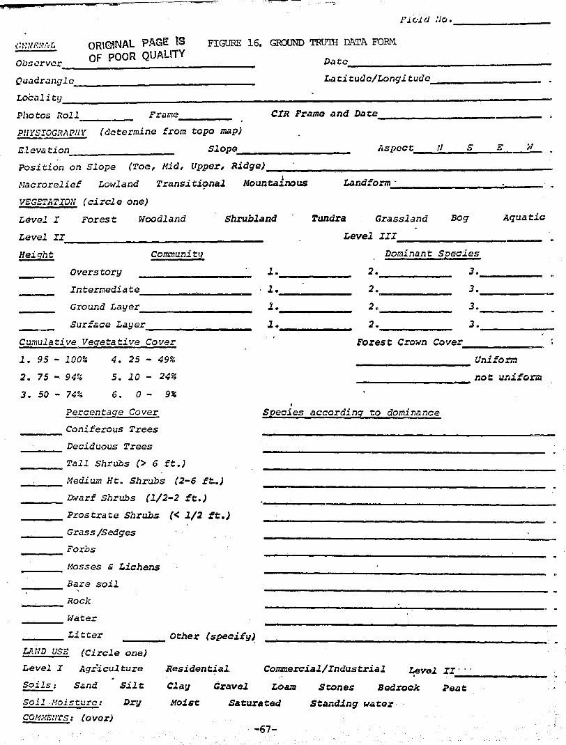
Field ::o.

ORIGINAL PAGE 19 FIGURE 16. GROUND TRUTH DATA FORM

Off' POOR QUALITYO^sorver Data

Quadrangle Latitude/Longitude

Locality _ _ ---

Photos Poll Frame CIR Frame and Date

PHYSIOGRAPHY (determine from topo map)

Elevation Slope Aspect N S E _ W

Position on Slope (Toe, Mid, Upper, Ridge)

Macrorelief Lowland Transitional Mountainous Landform-

VEGETATION (circle one)

Level I Forest Woodland Shrubland Tundra Grassland Bog Aquatic

Level II

Xei gh t Community

Overs Cory

Intermediate

Ground Layer

Surface Layer

Cumulative Vegetative Cover

1. 95 - 100% 4. 25 - 49%

2. 75 9400'

5. 10 24%

Level III

Dominant Species

1. 2. 3.

Z. 2. 3.

Z. 2. 3.

1. 2. 3.

Forest Crown Cover

Uniformnot uniform

3. 50 - 74%

6. 0 - 9%

Percentaqe Cover

Coniferous Trees

Deciduous Trees

Tall Shrubs (> 6 ft.)

Medium Ht. Shrubs (2-6 ft..)

Dwarf Shrubs (112-2 ft.)

Prostrate Shrubs (< 112 ft.)

Grass /Sedges

Species according to dominance

Forbs

Mosses & Lichens

Bare soil

Rock

' Water .

Litter Other (specify)

LAND USE (Circle one)

Commercial/Industrial Level IILevel I Agriculture Residential " 'Soils: Sand Silt Clay Gravel Loam Stones Bedrock ?eatSoil Moisture: _Dry Moist Saturated Standing wator

CGMVE cS: (ovor)-67-

PalCanoe Birch

ORI(}tnIAL PAGE ISOF POOR OWA! ITYFI=- 17. PHO`IIO -?EY FOR PAPER BIRQ?

Li -68-

I •^_ r

A

FICAJR7 18. CONP 1RISON (HART MR VISUALEXTL+ATION OF PERC=AGE COVER

CRi'GINAL PAGE ISOF POOR QUALITY

;L 3./

7ti► 5

2 5 ::

^ . ^ •—^ ,.1_:' ice.

•

♦ • • • • • ^ , ^ • \ .•fir•. •^, ^• ^•.•

dor• vr` ^

• .^ • . ,,^ C • . eQ ' gyp• ^' .1 ^ `+ <'

2 % S% 10%20% 30%

4C%

^ d v

i

J0%

Comparison charts for visual estimation of percentagecover, Adapted from Terry And Chilingar (1955).

-69-

^ ^ I

1 I1

i ^ I

1

I

O^.-. I

D

E- W.

r

O Q I

1

a II

azd

d1 (

4

1

N

I•

^t

7

I

1

© I

i 11

i I

-70-

ORIGIINAL PAGE IS

OF POOR QUALITY

^•r

A'A

to

^Ido

VV

7

C J

C.0

Gv Gc ^,

R uC

tiG3

C, c.4

Crca uR L:

u Ci

G C

G

a.

w uO

10 GL N

N Vf

U CJ

►. G

v. cn

l:u F

OC ►.

V,.p

r qE^U

was allotted to the collection of data for .urban and agri-cultural training sites with planners from the Municipalityof Anchorage and Mat-Su Borough. The final day required theuse of fixed-wing aircraft for overflights to inaccessibleareas within the study region. Trained in data collectionprocedures, each agency was requested to continue datacollection throughout the summer. .Each agency was requestedto secure ground data for approximately 50 training sites.

At the beginning of each day, training sites were plotted onavailable maps and routes were determined. Ground truthforms were completed for each training site. The vegetationcommunity is assigned to one of the land cover categories(Level I). Each successive (community) level is describedwith a listing of species by areal dominance. The percen-tage of areal cover of the individual cover components isvery important in Landsat analysis. This refers to theoverall cover if one were above the canopy looking down(tabletop view). The final assignment of each training siteis largely dependent on the areal dominance of individualcomponents.

Ground photographs provided a permanent record of eachtraining site. A vertical shot records the specific groundcover components and a horizontal shot gives an indicationof the general overall appearance characteristics of thevegetation. It's advisable to always include some objectfor scale.

When collecting site information by aircraft a teamapproach is advisable. One individual takes camera shotsand the other records the location of the camera shot, vege-tation type, and any other pertinent information on the CIRphotography. Flight lines should be determined prior toactual flight time and plotted on topographic maps. Thefirst flight line should overfly sites previously visited onthe ground to correlate vegetative communities at groundlevel and overhead. Locate sites near prominent featuresfor easy location.

Completion of Data Collection. With completion of the fieldseason, copies of all ground truth forms, location oftraining sites, and ground photos from each agency were sentto NASA for evaluation and editing in preparation forupcoming workshops. Tallies of the trainin g sites were madeby agency and for each cover type. The total number oftraining sites visited by each state agency are as follows:

-71

IL

-72-

,s

DNR-Forestry 56

DNR-Planning and Classification 307

Municipality of Anchorage 132

Mat-Su Borough 46

Certain land cover categories were found to be lacking asufficient number of training sites (tundra, water, tidalmarsh). These categories were supplemented with trainingsites delineated through photo-interpretation of U-2 and lowaltitude natural color photography. Availability of U.S.Dept. of Agriculture, Soil Conservation Service (SCS) datawill provide additional ground data information for evalu-ation of the classification. (SCS was also conducting ariver basin and soil mapping project in the study area.

The classification scheme evolved during the field season toencompass cover types not anticipated prior to the fieldseason. During clustering of the multispectral data, theanalysts will strive for additional cover informationrelating to density, species, understory: information whichwas not specifically trained upon during clustering.

The usefulness and quality of the training sites selectedwill greatly affect the accurate classification of landcover categories in the study region. Although a greatnumber of training sites were visited during the fieldseason, there is no way to verify that the training sites doindeed encompass all possible spectral variations in theLandsat scene. Therefore, the supervised statistics will bemerged with statistics generated during unsupervisedclustering of the full Landsat scene. Unique land covercategories will be extracted in the unsupervised clustering.

The training sites will be utilized in the upcomingworkshops involving state agency personnel. It is felt thatagency involvement in every step of the digital analysisprocess will give agency personnel a clear understanding ofthe advantages, as well as limitations, of Landsat digitaldata. A photo-interpretation key and instructionalmaterials are also being prepared for distribution to agencyusers.

DIGITAL ANALYSIS OF SUSITNA SCENE

L. Morrissey

TRAINING SITE SELECTION WORKSHOPS

Following completion of ground data collection in the summer a

of 1979, a series of three-day workshops was held at AmesResearch Center to delineate training sites on the IDIMSCOMTAL display. T. Burns, Municipality of Anchorage, pro-vided training sites for the Anchorage urbanized area, EagleRiver valley, and sections of the Mat-Su Borough. R.Loeffler, Department of Natural Resources-Planning andClassification, and M. Wibbenmeyer, Department of NaturalResources-Forestry, delineated training sites throughout thestudy region. Although unable to attend a workshop,training site information gathered by E. Wycoff, Mat-SuBorough, was also incorporated. A total of 264 trainingsites were delineated on the COMTAL display by participating ?agency personnel with the following agency breakdown:

DNR-Forestry 56

DNR-Planning and Classification 30

Municipality of Anchorage 132 t

Mat-Su Borough 46

Utilization of the COMTAL display for training site selec-tion facilitated refinement of training sites proposedduring visual examination of the MSS data. Training siteboundaries were often extended when the spectral categoriesencompassed an adjacent area, while spectral anomaliesoccurring within proposed site boundaries were eliminated aduring actual delineation of boundaries. Thus, visualexamination of the MSS data maintained spectral homogeneitywithin training sites. In addition, agency users were ableto associate spectral signatures with resource categories byvisual examination of the MSS data. Agency involvement inthis phase of the project was beneficial for users who wereable to learn by participation.

Training sites were duplicated on overlapping portions ofthe two La ndsat data sets used in the analysis. Examinationof the number and distribution of training sites by landcover type revealed certain discrepancies. Various cover

-73-

types were not adequately represented. Specifically, in the

4

uplands alpine tundra, bare rock, snow and ice wereoverlooked, while floodplain barrens and sedimented water inthe lowlands needed additional training. These training

!

sites were incorporated by project analysts through photointerpretation of available CIR photography. In addition,some cover types had too few training sites and/or too fewpixels for cluster analysis. For example, only one trainingsite for aspen forest was found. Clustering of cover typeswith too few pixels often produces a cluster with extremelyhigh or extremely low variances--both extremes are unsatis-factory for a maximum likelihood classifier and were elimi-nated in the statistical editing process. Training siteinformation by cover type for the Susitna scene is given inTable 10.

COMPUTER SYSTEMS USED IN THE ANALYSIS

OF THE SUSITNA SCENE

Analysis of the Susitna scene utilized several computersystems available at Ames Research Center. The EDITOR (E RTSData Interpreter and TENEX Operations Recorder) softwarepackage developed by the Center for Advance Computation(CAC) provided the mainstay for interactive image analysis.The EDITOR package is available on the TENEX PDP-10 at thecomputer facility of Bolt,Beranek, and Newman (BBN) inBoston and is accessed through telephone lines via the ARPA(Advanced Research Projects Agency) Network. Initialtraining site selection and evaluation of the spectralclasses ware completed using the IDIMS (Interactive DigitalImage Manipulation System) software and COMTAL displayimplemented on an HP 3000 computer at Ames. Large-scaleclustering and classification required the use of the ILLIACIV, also on the ARPA Network. Preprocessing, reformatting,and generation of output products were completed using theIBM 360/67. Access to several computers allowed use of themost efficient system for each specific processing task.'

ACQUISITION AND PREPROCESSING OF LANDSAT DATA

Landsat scenes were selected on the basis of cloud cover,season of the year, and orbital path. Complete coverageof the study region was obtained with portions of threeLandsat scenes. Two of these scenes (21288-20250 and21288-20253) are within the same orbital path and the third(30175-20345) is from an orbital path to the east. Computercompatible tapes were acquired from EROS (Earth ResourcesObservation Systems) Data Center.

`

Preprocessing of the data prior to classification includedremoval of bad data lines. , geometric correction, and rotationr

-74-

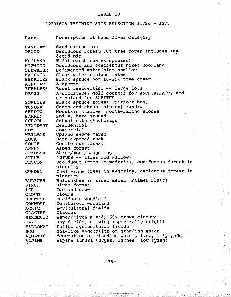
TABLE 10

INTRISCA TRAINING SITE SELECTION 11/26 - 12/7

4

Label Description of Land Cover Category

SANDEXT Sand extractionDECID Deciduous forest,-50% tree cover;includes any

decid mixWETLAND Tidal marsh (carex species)MIXWOOD Deciduous and coniferous mixed woodlandSEDWATER Sedimented water/also shallowWATERCL Clear water (inland lakes)BSPRUCEB Black spruce bog 10-25% tree coverAIRPORT AirportsRURALRES Rural residential -- large lotsGRASS Aqriculture, golf courses for ANCHOR.EAST, and

grassland for SUSITNASPRUCEB Black spruce forest (without bog)TUNDRA Grass and shrub (alpine) tundraSHADOW Mountain shadows; north-facing slopesBARREN Soils, bare groundSCHOOL School site (Anchorage)RESIDENT ResidentialCOM CommercialWETLAND Upland sedge marshROCK Bare exposed rockCONIF Coniferous forestASPEN Aspen forestSHMOSSB Shrub/moss/sedge bogSHRUB Shrubs -- alder and willow,DECCON Deciduous trees in majority, coniferous forest in

minorityCONDEC Coniferous trees in majority, deciduous forest in

minorityBULRUSH Bullrushes in tidal marsh (Palmer Flatn)BIRCH Birch forestICE Ice and snowCLOUD CloudsDECWDLD Deciduous woodlandCONWDLD Coniferous woodlandAGRIC Agricultural fieldsGLACIER GlacierMIXDECID Aspen/birch mixed; 60% crown closure

.HAY Hay fields, growing (spectrally bright)FALLOWAG Fallow agricultural fieldsBOG Mat-like vegetation on standing waterAQUATIC Vegetation on standing water, i.e., lily padsALPINE Alpine tundra (dryas, liches, low lying)

-75-

Ji

1

of the data to north. Preprocessing functions for theeastern and two western scenes differed and will bedescribed in separate sections.

Preprocessing of the two western scenes included an initialmosaicking of the two scenes, removal of skew, and rotation.All preprocessing of the Susitna scene was completed on theIBM 360/67. The southern half of-the northern scene andnorthern half of the southern scene were mosaicked.Concurrently, the mosaicked scene, referred to here as theSusitna scene, was geometrically corrected to remove distor-tion inherent in the data and to permit registration to amap base. The data were reformatted to remove skew causedby the earth"s rotation beneath the satellite. Inaddition, the data were rotated to north for ease of use.Parameters for correction of the data, computed by using aprogram available on the IBM 360/67, were based on the lati-tude of the center point of the Susitna scene.

DIGITAL ANALYSIS OF SUSITNA SCENE

The supervised approach develops statistical clusters basedon the spectral content of selected land cover sites.Success of the supervised approach is' based on the qualityof training site selection, of ground data collection andanalysis methodology. Sites visited during the previoussummer met all requirements of spectral homogeneity withinland cover categories required for a supervised approach.Spectral variation exists within training sites of the sameland cover-category and, therefore, may contain severalspectral signatures.which represent differences in density,slope, soils, or other terrain variables which affect thespectral", response of vegetation.

Prior to clustering, coordinates of the training sites delin-eated on the IDIMS COMTAL display were transferred via theIBM 360/67 to the TENEX computer at BBN. Table 11 gives thenumber of training sites and number of pixels within eachland cover category. A program available at BBN convertsthe IDIMS training file into a coordinate file compatible^awith the EDITOR software. A tape containing the MSS data ofthe mosaicked Susitna scene was also sent to BBN, for

r' retrieval of MSS data during clustering.

MSS data for each training site was retrieved from the dataa tape and grouped by land cover category. The MSS data of3- each of these files was displayed in the form of a frequency

distribution (histogram) to analyze the data for homogeneityand to determine the number of spectral classes present.

" Generally, the histogram i analyzed to determine the numberof nodes or peaks in the data distribution, the spread ordispersion of the MSS values about the Mean, and the range

f:-76-

.,,r .^. ... .

rTABLE ll

Training Sites Number of Pixels

DECCON 9 1, 417r MIXWOOD 2 106

SHRUB 5 360BIRCH 12 731DECID 3 2,640GRASS 11 505WATERCL 7 895MOSSBOG 1 152

`- TUNDRA 6 41395SEDWATER 9 50,816ICE 3 32,485CLOUD 1 7,606CONDEC 3 104DECWDLD 9 11149SPRUCEB 3 112CONIF . 4 360MIXDECID 4 919

- WETLAND 8 190 a

BSPRUCEB 3 131ASPEN 1 22BARREN 1 19BULRUSH 3 361GLACIER 2 1,656ROCK 3 837ALPINE (TUNDRA) 8 430MUD 4 2,225 a.

f.TABLE 11 -- Total number of training sites and pixels for

each land cover category.

F

i

{

r

5

-77-

of values. The histogram shown in Figure 20 has a signaturecharacteristic of the red band for a birch forest; that is,a low variance with one node, and low range of reflectance(dn) values. However, the same MSS data displayed in anear-infrared band (Figure 20) shows two distinct nodes, anda large range of do values. The infrared bands are muchmore sensitive to green vegetation and are, therefore, usedmore often to determine the optimal number of spectralclasses present for clustering. In this same way, eachfile of MSS data by land cover category was histogrammed andexamined to determine the optimal numer of clusters. -

Clustering was performed on each file of MSS data to developcluster statistics--means, variances and separability (ameasure of distance between clusters). Followingclustering, the statistics were examined. Clusters repre-senting the same land cover category with extremely lowvariances and low separability were pooled, while clusterswith high variances and a low number of pixels werereclustered or deleted. Initial clusterings which resultedin clusters with low variances, low separability and a lownumber of pixels were unsatisfactory. These data werereclustered a second time, partitioning the MSS data into asmaller number of clusters. Each of the MSS files wasclustered and reclustered as necessary to develop a prelimi-nary set of statistics representative of all land covercategories found in the training sites.

A preliminary statistics file which contained one to severalspectral classes was created for each land cover category.For further analysis, each statistics file was graphicallydisplayed as a two dimensional plot representing means andvariances. As shown in Figure 21,the axes represent thereflectances values in the red (MSS 5) and near-infraredband ( MSS 6 ) .

Means are represented by the cluster number (alpha-numeric)and variances by the surrounding circle. Potentialproblems, such as clusters with high variances or lowseparability, were easily identified on the plot.

Confusion between clusters of different land cover cate-gories was examined next. Spectral confusion results whentwo distinct land cover categories encompass the samespecral reflectance values in the four bands. Statisticsfiles representing different land cover categories weremerged and the separability measure was used to determinepossible spectral confusion. Confusion clusters are eitherpooled, deleted, or reclustered. Many analysis decisionsat this point are highly subjective. Each analyst has devel-oped a method for analysis based on experience, training,and intuition. Invariably, this portionof the analysis,

-78-,a

Figure 2 0Histogram OKKMAL PAGE 13

,A T C OF POOR QUALITYG R. 9 ► P O I

Brightness Level

+ X X:,..,.ell, r". X X :;", X X , X X Xi X X X X X X XX X. X

x x xX X X:"." "

j X " X :. : ,.. X X X '- X'% M ., x1e.-I. 11 11111-11 1. X III XXXXX I-X1111-11'. MX11:01 I xX I ..., X e) C, el e% el ell ell ell'. e

x le. ev, x x'}:ielfV x X , ell x M-111 x x xf x x x I x VV V,

x x e..."

el

I

— — — — - — — — — — — — — — - — — — —

5 3 14

5 i.i5is cl 5 0 5 0L+ P .:Ei- S)

Band 5 Visible Red

-7 :7 1 H T ::; T Fi R R, 9 , ,l P IJ TNITSBrightnes . s Levels

1 : X

X

-C,X -ell X 'X X X "l

X::, X X 'e*.,: X V X X X X :-11,1 X X %., l XX .1 %j

X ,e- *--" X ,', i ii' 'i i ', e':

".-C.,^1 X 'I-,"

X X" '1-4 X X X X X ,..,..:

X .i i x

X X 'J". X

MI,

X, e", X M. " X::", X X, X

X X

M-111 t".11 ell, X X "I., el X

X

Xje'. ell 1,

eili5 il:

"l X X

X

5 +

+ x

N

i.e., development of the spectral clusters, is the most dif-ficult task and can produce a wide range of results. Thisprocess of merging statistics files, editing, and recheckingcontinues until all statistics files have been merged into a

k composite statistics file.

To evaluate the integrity of the statistical clusters, thetraining sites were classified with the composite statisticsfile representing all land cover. categories. Tabulations byland cover category gave an indication of the number ofpixels correctly classified within each land cover category.Based on these tabulations, spectral confusion was evidentbetween deciduous forest classes and deciduous/coniferousforest classes; woodland classes and shrub classes; andshrub, qrass and tundra classes. The analyst had to deter-mine at this point whether the confusion was due to 1) in-adequate training site selection (heterogeneous sites), 2)conflicting land cover classes which were spectrally iden-tical and therefore not statistically separable, or 3)overlapping land cover category descriptions leading tooverlapping class names which represent the same cover type.Spectral confusion which existed between shrub, grass, andtundra classes was due to confusion in classificaitonterminology. On the uplands, the training sites labeledtundra actually consisted of shrub and grass occurring abovethe treeline. Once again the statistics were modified bydeletinq,•pooling, or reclustering and then used toreclassify the training sites. The iterative editing pro-cess continued until the analyst felt the statistics were asspectrally distinct as the MSS data would allow. The com-posite supervised statistics file for the Susitna scene isshown in Figure 21.

Spectral variation within the scene which may have beenoverlooked was supplemented with statistics generated duringunsupervised clustering. The MSS data were retrieved fromthe data tape by strata (upland and lowland) and clusteredin an unsupervised mode. In an unsupervised clusteringapproach, the MSS data are partitioned into an arbitrarynumber of spectrally distinct groups or clusters. Due tothe large number of pixels in each of the strata, a data +?reduction program was run. The data.reduction program in 2EDITOR enables clustering of an entire Landsat scene on theILLIAC IV. The program maintains a count of the number ofpixels which have the same reflectance values in the fourbands. For the Susitna scene, the MSS data were retrievedby strata and then compressed from 1,727,711 individualpixels to 29,368 different MSS values for the lowlandstrata. Unsupervised clusters were displayed as two dimen-sional plots (Figure 22) for examination.

The unsupervised statistical plots were overlaid on the asupervised statistical plot for comparison. When an unsu-pervised cluster occupied spectral space not represented by

-80-

.:..NCNT FAT ICN ELLIPSES FGR BANDS i AND 2

"L,FF-RVISED STATS FGR SL;SITNA SCENE

sl

ORIGINAL PAGE 19OF POOR QUALITY

2-3. -3 -^

I

Son

^ SNawIOU

^ _^ c icuc^s

49d

42

Mike

Ulf 9 A2RtuS—47

u '33. 3 - •i

5 ecl i mtN; ^tk: 4 O^PIN r^NORR

r, go HQ u 6

v' kR^ mixed D Gl,"ss(:s/sed,)escoti^13 L,L F; .,k EsT FO R ES T

^. Ci-?pw ire.6. 7 '33.:3 SR. P. 66.7 E3.:3 1Pr'. c3

(M55 G^ exz, 3 IN F&fN RE 0)

FIGLM 21, COMPOSITE SUPERVIS::D STATISTICS FILE

M. a

66.7

1 J

j

16.7 -

FIGURE 22s UNSUPERVISED CLUSTERS FOR UPLANDSTRATA

Z. z.6.7 T-1. 3 GO. 01 66.7 G3.3 i OZ. Z*

w.

A

4F3 AN 0 6

*Cross hatch lines indicate clusters added to the final supervised statistics.

—82—

a supervised cluster, the unsupervised cluster was added tothe composite supervised statistics file. Snow, ice andcloud clusters from the unsupervised clustering of theupland strata (Figure 22) were added to the final supervisedstatistics for the Susitna scene. All other land covercategories were represented with supervised clusters.

The data tape and final supervised statistics file with 56clusters were input to a maximum likelihood classifier,whereby the MSS vzAues of each pixel were examined and it wasassigned to the cluster that it most nearly resembled inspectral space. Masked classification of the Susitna scenewith 113 classes (56 clusters plus 57 clusters generated onthe HP3000 for the Anchorage urbanized area) were completedin 481 seconds on the ILLIAC IV parallel processor.

Digital analysis of the Susitna scene encompassed two majorsteps: clustering of the MSS data to develop statistics,and classification, a process in which each pixel wasassigned to the statistical cluster it most nearlyresembled. The combination of supervised and unsupervisedclustering maximized computer and analyst time withoutsacrificing quality. However, to assess the integrity ofthe spectral classes, CIR photography and the classificationwere compared in a number of workshops involving Stateagency personnel. (Figures 23 and 24 show the final classi-fication results for the Susitna scene).

p

;a

1♦

14 \ ^i. ^^ T

cIq

^ \ . `1 \ , y ,,,^,^, "^ ' • ^ ^• l '^ 1. ►^ ^!

f `^.. r^^ _,,.. 4y;•3j:44,fZr,y^;.c'^` ' •" y►^ST7 ' ^l'^ :^it

^' fir• .^Y+ ^ •.;.f^ ^ • :f^^ ^^ ^,^+

• . • v^ .r t

r f^•+T . Al ..,.CZ'L•^

^^;•^,:., _moo ' 'j,^1ir^ ^if(^l^'ai 01^ f 1 ~T

4' L^LA s 1+' '^^;'r^, ^^t!•y

l'L I ^t , ^.^, ^' pf' t 0f

\lit—

I ij / ! } r• Z • S i o •.^ rte►

' `^' 4^_ '^^►,.• f F t 1 ^^ ', ^' ^,J f;.^ mow...

^ ^ r'!1`'^P Y 0 ^ ' t/!

ft. NIL

IL

At

' z^ll . ^, '^{ ^ 4 I r) ^, ^ / 1 i ^

r ►r 4 ; ^ ^%'!`.. ,• vl7 1r 'o

ORIGINAL Pt ^)

AGE

COLOR PHOTOG,RAP.w • 1

fr.

FIGURE 23,SUSITNA SCENE

t FICiIIRF 9d ('I ACRIFIf ATilllu nr I Akin rnvcn J&J 1n1—ORlOtNAL PAGE IS

^' h

f APPENDIX D

INTRISCA PROJECTC

DIGITAL ANALYSIS OF THE EASTERN/ANCHORAGE SCENE

ICharlotte Carson-Henry

TRAINING, CLUSTERING, AND CLASSIFICATION

The selection of training sites for the eastern(ANCHOR.EAST) scene portion of the South Central Alaskaanalysis area was conducted concurrently with training siteselection for the Susitna scene, during the November 26 -December, 27, 1979 user workshops. Tony Burns, of theMunicipality of Anchorage, provided training sites for theurbanized areas of Anchorage and Eagle River, along withportllnns of the Matanuska-Susitna Borough. Ellen Wycoff

j;

of Matanuska-Susitna Borough provided additional trainingsites from that borough although unable to attend the

^.

workshops; those sites were delineated by Tony Burns.Robert Loeffler, representing the Planning andClassification section of the Department of NaturalResources (DNR), provided and delineated largely vegetativecover training sites; representations of forest cover typeswere provided and delineated by Merlin Wibbenmeyer of theForestry Section of DNR. In all, over two hundred trainingsites were delineated by these users during the series ofthree-day workshops at NASA/Ames.

Training site delineation was accomplished on the IDIMSsystem, using the COMTAL display. Each site was displayedat an expanded level and was outlined on the display using acursor and trackball; the coordinates for the vertices ofthe outlined irregular polygons were then stored by thesystem in a file, under a user-designated training classname. This capability permits the storage of multiple poly-gons under the same training class name, thereby allowingtraining on a specific cover type to include spectral dif-ferences per cover type and non-contiguous geographic loca-tions of the same cover type. '(See Table 12 for adescription of the training classes delineated).

The use of a display during training site selectionencouraged visual examination of the spectral variationsinherent in MSS data; for example, varying spectral respon-ses can occur within a homogeneous stand of timber. 3Refinement of training site boundaries, relative to thiskind of spectral variation, went hand-in-hand with deline-ation and was made possible by the use of a display. The

-86-3

TABLE 12

Training Class Descriptions

Training Class Name Description of Land Cover Types

SANDEXT Barren: sand/gravel extraction siteWETLAND Marshy ground; either tidal marshes or upland sedgesMI)WOOD Coniferous & deciduous mixed woodlandSEDWATER Sedimented water, shallow or turbid water (spectrally

light)WATERCL Clear water, deep water (spectrally dark)AIRPORT Larger airportsGRASS Golf coursesSPRUCEB Black spruce forest (without bog)TUNDRA Upland tundra & shrub/grass tundraSHADOW Shadows and north-facing slopesBARREN Bare rock and soil (non-agricultural) and mudflatsRESIDENT Urban residential arasCOM Urban commercial areasTUNDRA2 Upland tundra with bad data linesWETLAND2 Wetlands, as above, but with bad data linesCONIF Coniferous forestASPEN Aspen forestSHMOSSB Shrub/moss bog (includes sedges)DECCON Deciduous/coniferous forest, primarily deciduousSHRUB Shrubs, e.g. alder and willowCONDEC Coniferous/deciduous forest, primarily coniferousBULLRUSH Bullrushes in tidal marsh areasDECWDLD Deciduous woodland (understory reflectances included)BIRCH Birch forestAGRIC Agricultural fields, other than hay and fallowGLACIER GlaciersICE Snow and ice, other than glaciersHAY Green, growing hay fieldsFALLOWAG Fallow agricultural fieldsBOG Mat-like vegetation growing on standing waterAQUATIC Standing water with vegetation like lily padsMIXDECID Mixed deciduous forest: aspen & birch; 60% crown

closureDECID Deciduous forest; 50% crown closureBSPRUCEB Black spruce bog with 10-25% tree coverage of bogRURALRES Rural residential areas, i.e. Eagle River ValleySCHOOL School sites in Anchorage properROCK Barrens rocks aloneCONWDLD Coniferous woodland (understory reflectances included)

-87-

visibility of these spectral variations within and betweencover type enabled the users to gain an appreciation ofspectral reflectances and the complexity of clusteranalysis, and added to their understanding of the limita-tions of Landsat classifications.

In using the IDIMS display for training site selection,anomalies occurring in the data became visible when expan-sions were performed to faclitate the outlining of polygons.The Landsat imagery corresponding to some of the trainingsites provided by the users contained these anomalies; insome instances, these training sites were-nonetheless-delin-eated on IDIMS but were assigned different training classnames to assure that they would be stored separately fromunaffected sites. They were subsequently clustered but thecluster statistics were affected by the inclusion of theanomalies in the training sites; those clusters were notused in classification.

Clustering for the ANCHOR.EAST scene was performed on theIDIMS system using the CLUSTER portion of TSSELECT. Thatsoftware utilizes the IDIMS ISOCLS clustering algorithm.ISOCLS (CLUSTER) is a function which allows user specifica-tion of a number of parameters; defaults have been writteninto the software for use by the algorithm when the analystmakes no specification for a given parameter. Most of-theparameters were defaulted when the ANCHOR.EAST trainingclasses were clustered. (Descriptions herein will pertainto the use of the ISOCLS function only as it was employed inthis analysis.)

The ISOCLS algorithm begins by placing all pixels in a singlecluster, then computes the statistics that describe thatcluster. For each band, the mean grey level, the standarddeviation in grey level units, and the distance betweenclusters in terms of grey level units are computed andprinted on the line printer. The algorithm then selectsthe band with the largest standard deviation, and adds orsubtracts that standard deviation value to or from the meanfor that band, creating the "seed" of a new cluster. Pixelsare then assigned to either the original cluster or to thenew -luster, depending upon which cluster center the pixel'sreflectance value most resembles; resemblance is judged onthe basis of the absolute value of the grey level distancesbetween the pixel's values and those of 'either cluster.Once all pixels in the image have been assigned to onecluster or the other, the statistics (means, standard

-^ deviations and distan es) for each cluster are recom tedc puThis process of creating two clusters from a single clusteris referred to as "splitting" the algorithm continuessplitting clusters until one of two criteria is met: 80% ofthe clusters have: 1) standard deviations that are less

C• r^ •-88

-p

L4

r

than the value entered for the parameter STDMAX, or 2) con-tain too few pixels to be able to be split and still remainwithin the lower limit set by the parameter NMIN (minimumnumber of pixels per cluster). Once one of these criteriais met, ISOCLS begins alternating between splitting andcombining: one iteration will split clusters, the next will `Icombine any qualified clusters, the next will again-split,

4 and so on. Combining can occur when the computed distancebetween two clusters (this distance is defined as a weightedmeasure based on cluster means and standard deviationssummed over all the bands) is less than the value specifiedfor the DLMIN parameter. (In this analysis, a value of 3.2grey levels was used for DLMIN.) Iterations alternate be-tween splitting and combining until one of two conditions isattained: either no clusters qualified for splitting orcombining remain, or the number of iterations has reachedthe maximum limit set by the ISTOP parameter. The attain-ment of one of these conditions causes the algorithm toenter into the final iteration, which is always a splittingiteration. 9

For each iteration, cluster statistics are recomputed afterthe splitting or combining has been performed, and thosestatistics are printed on the line printer for evaluation bythe analyst. In addition, a tabulation of the number ofpixels in each cluster, and a map of each training site, aregenerated on the line printer.

Each training class (BIRCH, ASPEN, SEDWATER, and so on aslisted in Table 12) was clustered individually and theresultant cluster statistics were directed to a statisticsfile bearing the same name as the training class. Thecluster statistics (output on the line printer) were thenanalyzed solely in light of the ISOCLS 80% criteria men-tioned previously. Those clusters whose standard deviationsfailed to meet the 80% criteria were re-clustered,iteratively, until they did indeed meet those criteria. Inaddition, classes whose cluster statistics were well withinthe 80% criterion were examined and were re-clustered, in anattempt to bring the standard deviations of the individualclusters closer to the STDMAX value while still meeting thecriteria. Each re-clustering was generated so as to create'a new and separate statistics file for later ease ofmanipulation.

Once clustering was completed, the statistics files wereedited and merged. The IDIMS function SMART was utilized inthe statistics editing and in the creation of a master sta-tistics file, and the statistics files containing all otherCLUSTER outputs were deleted. The statistics for severaltraining classes were deleted at this point due to the factthat the sites contained too few pixels to generate validclusters.

-8g'_

The master statistics file created on the IDIMS system con-tained more than 100 clusters; this file, however, was notconsidered to be the final statistics file. Actual evalu-ation of the clusters was performed on the EDITOR system atBBN by means of cluster plots. In order to generate theseplots, the means and variances fov each of the 100-plusclusters were manually entered on EDITOR, generating a sta-tistics file. Swain-Fu Distances (a measure of separabilitybetween cluster pairs) were generated on that system: someeditinq of clusters was performed, thereby reducing thenumber of clusters to 87; and a PLOT file was subsequentlycreated. An ellipse for each cluster was plotted from thatfile, for MSS Bands 5 And 7. The ellipses reflected boththe mean of each cluster and the variance of that cluster,in two-dimensional space. Final statistics editing deci-sions were based upon evaluation of these elliptical plots.The editing performed on EDITOR was then dupl?.cated on theInIMS system, using SMART to edit the master statisticsfile. See Table 13 for a summary of the clustering per-formed on the ANCHOR.EAST scene.

As a. preparation for classification, the ANCHOR.EAST imagewas submitted to the FIXLINE function on IDIMS for "repair"of lines in which data were missing. The output image fromFIXLINE and the master statistics file were then written totape and submitted to the CDC 7600 maximum likelihoodclassifier. This classsification program evaluates thespectral reflectance values in all four MSS bands for eachpixel, then places that pixel into the class whose statisti-cal characteristics it most resembles.

f^

Following classification, a series of four User EvaluationWorkshops were conducted at Ames. The first of these four-day workshops was attended by Lee Wyatt fromMatanuska-Susitna Borough and by Tony Burns, the InstateCoordinator, who attended the entire series of workshops.The second of the workshops was attended by Peggy McNees ofthe Planning and Classification Section of DNR; the third,by Merlin Wibbenmeyer of DNR/Forestry. The fourth workshopwas conducted with and for Tony Burns, and focused uponAnchorage and other urban areas, as well as coastal wetlandsunder the -jurisdiction of the Municipality of Anchorage.The objective of each of these workshops was to provide , anopportunity for agency personnel to identify the spectralclasses resulting from the classification of both 1978 scenesand to evaluate the classifications as a whole, using theIDIMS display as a tool. Since each of these agency person-nel had expertise in different types of land cover and dif-fering geographic areas, the series of workshops taken as anentity resulted in evaluation of most of theareas ofinterest that comprs:sn_d the study area (such as PointMcKenzie, the Eagle River valley, the town of Eagle River,

-90

r ... .......aay.^... #ae .: ^. .. i::. . ^... ...axx w,..ra,e^.':wmw..w..,r3ss a^.. s,.. .w..w w._.,,..mssmwu m......:.:^... Fd.w......,^..i......ds.. ..i. .r:il..e,..s.. 3^_sa _..s......a:....vMSarr-

E`e

,I TABLE 13

ANCHOR.EASTClustering Results

Training Class # of Pixels in # of Clusters # of ClustersName

l

Training Class Generated Used in Clas'n.

SANDEXT 132 3 -WETLAND 424 4 4MIXWOOD 272 4 3SEDWATER 589 3 1WATERCL 711 4 1AIRPORT 137 2 1GRASS 19 1 -SPRUCEB 256 1 1TUNDRA 857 10 7SHADOW 212 3 3BARREN 255 5 4RESIDENT 248 5 4COM 185 4 1TUNDRA2 ** 126 3 -WETLAND2 ** 258 2 -

' CONIF 694 3 2ASPEN 61 1

-

SHMOSSB 1245 5 5DECCON 621 1 1

} SHRUB 204 4 2CONDEC 40 1 -BULLRUSH 553 3 1DECWDLD 457 2 1BIRCH 329 4 1AGRZC 45 1 - aGLACIER 3203 20 19ICE 2240 7 5HAY 184 4 3FALLOWAG 93 2 1BOG 159 3 2

z; AQUATIC 146 2 1MIXDECID 578 1 1^DECID 905 5 5BSPRUCEB 327 4 4RURALRES 497 5 4SCHOOL _20 1 -ROCK 45 1 -CONWDLD 22 1 -

ar,

** Training classes within which missing data lines occurred

-91-

is

N "

X

Big Lake, and the Palmer-Wasilla area). Vegetation types --in_particular, forest and wetland cover types -- and urbanland cover types were carefully examined and evaluated inthese and other areas using U-2 photography and field dataas ground information. Available specialized landcover/land use maps were also consulted in evaluating thespectral classes, particularly in Anchorage and in thecoastal wetland areas on the north side of Turnagain Arm.Table 14 reflects the preliminary identifications made.

POST-PROCESSING

During the evaluation workshops, extensive records were maderegarding the type and location of blatantly incorrectclasses, as preparation for stratification to refine theclassification.

Fairly extensive stratifications were requested by the usersin the urban areas of Palmer, Wasilla, and Eagle River;along the lowlands on the north side of Turnagain Arm, suchas Alyeska, Portage, and Girdwood; and in the upland areas,in which barrens had been incorrectly classified as water.Conflicts between natural vegetation types and agriculturalfields and between urban and barren cover types occurred, asexpected, and conflicts between minor transportation corri-dors and shrub/grass categories emerged as well„

Stratifications for the purpose of changing classes within aspecific area were accomplished with the function ZIP onthe IDIMS system. ZIP allows the analyst, using a cursorand trackball, to outline on the display the area withinwhich the class changes are to be made. The program thenrecords the vertices of the polygon in a training file.(ZIP utilizes the software described in the section of thispaper regarding training site selection.) Although a tem-porary hardware failure severely hampered the use of the ZIPfunction (thereby extending the time required to completestratification), ZIP does nonetheless provide a preferablealternative to the standard method of stratification --which requires the digitizing of polygons and the transla-tion of the polygon information into strata that aresubsequently merged with the Landsat classified data. TheZIP function does contain a trap, however: since the outputfrom each ZIP becomes the input to the next ZIP, any errorthat is made tends to be perpetuated as subsequent ZIPs areperformed.

Following completion of the iterative stratifications per-formed on the ANCHOR.EAST classified image, the process ofidentification of individual classes was repeated pertainingto the*ZIPped image. U-2 photography and field data wereagain used in the identification of classes and in the

1

-92-

TABLE 14

Class Identification

Preliminary identification, following preliminary groupingof Tundra, Glacier, and Ice categories:

Class Label Class Number(s)

Deciduous 1-5Wetland 6-8

i' Mixed woodland/Mixed forest 9-11Sedimented water 12Clear water 13Black spruce bog 14-17Airport/Barren 18Rural residential/Sedges/Grasses 19-22Black spruce 23Tundra 24Shadow 25-27Barren 28-31

i Residential/Sedges/Grasses 32-35Commercial/Barren 36Coniferous 37-38Shrub/Moss bog 39-43Dec iduous/Coniferous 44Shrub 45-46Bullrush 47Deciduous woodland 48Birch 49,Hay 50-52Fallow agriculture/Barren 53Bog/Clear water 54-55Aquatic 56Mixed deciduous 57'* 58.

** 59** 60** 61** 62

63Glacier 64ICe

65

a

correlation of these spectral classes with ground covertypes. The IDIMS display was again used; concurrently,

9 groupings of spectral classes into information categories 4

were assigned, preparatory to the running of a program toactually aggregate the classes.

Post-processing continued with the running of the program• ROTATE on the IBM 360/67. This program deskewed the

classified, stratified image and rotated it so that ai north/south line drawn through the image was vertical. The{ extent of rotation to be applied to the image was calculated

on the IBM 360 using a program called SKEW; the parameterj used to specify the extent of rotation was the same as that

used in the rotation of the Susitna imagery for the INTRISCAclassification of 1978 data.

ll' Following rotation, the ANCHOR.EAST image was submitted to the1 GROUP program on the IBM 360 to aggregate the classes into

the information categories mentioned above. In addition tothe aggregation of spectral classes into informationcategories, GROUP was used to change class numbers (foraggregated groups); the result was that information cate-gories were identified by the same class numbers in both theANCHOR.EAST and Susitna scenes. This scheme was adapted to

y later facilitate a photomosaic output product. The outputfrom GROUP was then smoothed, using the RECLAS program onthe CDC 7600. RECLAS utilizes a nine-pixel neighborhoodwhose weighting factors are specified by the analyst; in

' this instance, the center pixel was assigned a factor of 4,the pixels adjacent to the center were assigned a factor of2, and pixels in a position diagonal to the center pixel

j were assigned a factor of 1. The program moves this nine-pixel neighborhood through the image, reassigning categoriesaccording to the specified neighborhood weighting factors.In addition, the analyst is abate to specify weightings forindividual categories; these category weightings will

t override the neighborhood weighting factors to cause speci-fied categories to assume lesser importance as they contri-bute to a neighborhood. This program mimics a nine-acreminimum mapping unit, and tends to merge isolated inci-dental pixels with the categories by which they aresurrounded. The effect of RECLAS on the ANCHOR.EAST imagerywas to reduce the number of pixels that had beenspuriously classified due to the banding in the raw data, aswell as to eliminate the speckled appearance caused by iso-lated occurrences of classes.

The effects of these post-processing steps were evaluated onIDIMS, again using the COMTAL display as a tool. It is <'important to note at this point that a major objective inthe post-processing steps was the :facilitation of a photo-mosaic of the ANCHOR.EAST scene with the Susitna 'scene. In

-94-

order for the photo-mosaic to be successful, it was essen-tial that the two scenes be processed similarly and that theclassifications in the overlapping area between the twoscenes be as consistent as possible. It was thereforedetermined, when examining the smoothed form of theANCHOR.EAST classification, that the grouping and smoothingthat had been performed had been unsatisfactory. Using theIDIMS display capability, several additional aggregationschemes were evaluated and the most promising was then usedin re-running GROUP. The RECLAS program was subsequentlyre-run on the new GROUP output, utilizing the capability forweighting individual categories (which had not been used thefirst time RECLAS was run)(Table 15). Classes comprised ofan insignificant number of pixels, and classes that hadresulted from anomalies and which bore no relation to agiven land cover type, were weighted in a fashion thatessentially caused them to be reclassified according to theneighborhood weighting factors mentioned previously.Classes 1.5, 46, 55, 56 and 68 were assigned an individualweight of 0.5, while class 25 was assigned an individualweight of 0.1. The use of these weights caused occurrencesof these classes to be either reduced or eliminated, withthe weighted classes having been reassigned to categoriesthat were more accurate when verified with ground data andphotography. The output from the second grouping andsmoothing was also much more satisfactory in terms of com-patibility with the classification of the Susitna scene, inlight of the planned photo--mosaic.

f

OUTPUT PRODUCTS

Due to the complexity of potential user requirements foroutput products--regarding geographic areas of coverage,class aggregations, and map scales of both photo productsand computer-generated maps--a determination was made that astandard set of output products would be generated and wouldserve as samples, to the users, of the types of productsavailable. This set of products was designed to focus upongeographic areas of concern to the largest number of users,with products to be generated at scales corresponding toexisting base maps. The set included:

Point McKenzie subsection, color Dicomed enlargedto scale of 1:63,360

Susitna River to Big Lake subsection, color Dicomedenlarged to scale of 1:250,000

Anchorage Peninsula subsection, color Dicomedenlarged to scale of 1:25,000

Palmer agricultural area subsection, color Dicomedenlargement at scale of 1:63,360

-95-

TABLE 15

ANCHOR.EASTFinal Grouping

Class Identification

After completion of stratification, prior to smoothing:

Grouped Class Numbers CombinedClass Label Class Number to Comprise Grouped Classes

Deciduous 9 1-3,48-49Sedges/grasses* 2-7 19-20,34-60Mixed forest 8 49-10,26-27,44,57Sedimented water 1 12Clear water 2 13,47,54-55Black spruce bog** 4 14Residential, low density 19 61Tundra, alpine*** 11 6-8Shadow 15 68Barren # 10 18,28-31,36,53Residential, high density 18 58Commercial/industrial/trans.16 59Coniferous 7 5,11,15,17,22-23,25,32-33,

350,37-38,46Shrub/moss bog** 3 16,21,40-43$6Shrub* 6 39,45Hay 23 62Fallow agriculture 24 63Glacier 12 64Ice, snow 13 65 1Mud # 25 67Grass* 5 50-52Shrub/grass tundra*** 26 24,66

'r q

* Th be grouped together in output products** To be grouped together in output products*** To be grouped together in output products# Zb be grouped together in output products

3

`s3a

1

-96-

--I

Eagle River subsection, line printer map at scaleof 1:24,000

Anchorage Peninsula subsection, line printer map atscale of 1: 24, 000

Susitna River to Big Lake subsection, pixel count onIBM 360 for acreage tabulations

Susitna River to Big Lake subsection, pixel count onIDIMS for percentage of coverage tabulations

In addition to the above products, the set included aDicomed print of the two classified scenes photo-mosaickedtogether. Color bars will be manually attached to eachphoto product. A major feature of this set of output pro-ducts is that the set also includes a negative of each ofthe photo products, enabling users to generate photographicenlargements of areas or subsections not included in thestandard set--according to their individual needs and at thetime their additional requirements emerge.

Plotter maps, to be generated on the SEL, had been intendedfor inclusion in the output products set as well as theitems mentioned above. The plotter maps of the Palmer agri-cultural area and of the Susitna River to Big Lake subsec-tion were, however, not generated due to hardwarelimitations: the smallest print size of SEL plotter symbolsis too large to produce a map at a scale of 1:63,360, as hadbeen planned. Although multiple attempts were made togenerate plotter maps at this scale, the horizontal and ver-tical shifts required to make the plotter map overlay a basemap varied from 1/4 11 to several inches over a distance of 8linear inches. The line printer maps generated at 1:24,000scale will, nonetheless, suffice to illustrate the capabil-ity of producing maps of the classified data.

A

-97-

Lfik.,

MIRN

APPENDIX E

INTRISCA PROJECT

STRATIFICATION OF

SOUTHCENTRAL WATER LEVEL B STUDY

L. Morrissey

1State, federal, and local agencies in the Cook Inlet Regionare working in cooperation with NASA to implement state-of-the-art remote sensing techniques to develop a regionalresource data base. Integrated Resource Inventory forSouthcentral Alaska (INTRISCA) is a multifaceted demonstra-tion project undertaken to meet regional resource.managementobjectives and informational needs. The main objective ofthe project will be to demonstrate the feasibility of pro-ducing a land cover inventory with Landsat digital data.

The Southcentral Alaska Water (Level B) Study utilizedLandsat digital data to provide land use/land cover infor-mation for future management of land and water resources.The land cover classification for the Water Resource Studywas completed by Dr. P. Krebs and P. Spencer of theUniversity of Alaska. Products from the classificationwill be evaluated by NASA and participating agencies todetermine their usefulness in meeting state agency needs.As part of the INTRISCA project, NASA will correct majorclassification errors through the use of a number of strati-fication techniques. The stratification of the WaterResources Study (Level B) classification are documented inthis paper. Following the evaluation, NASA will begin a newclassification to produce a more recent data set which ismore specifically related to individual agency needs.*

One source of classification errors in Landsat analysis workis the result of spectral confusion between two distinctland cover categories. Each spectral class is supposed torepresent a specific land cover category. However, problemsarise when two distinct land cover categories have similarspectral reflectance values. Stratification techniques havebeen developed to resolve this type of classification error.Where problem areas exist, boundaries are delineated toencompass the misclassified spectral classes. Conflictingspectral classes within specified polygons are reassigned tothe correct land cover category.

Evaluation of the Level B work was begun in the spring of1979 by NASA: Utilizing the IDIMS COMTAL display, spectralclass assignments were verified based on available U-2

See Appendices C and D. i

-98-

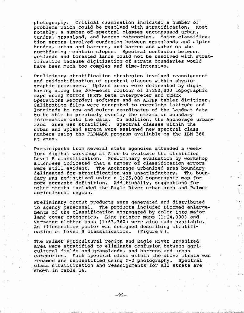
fr

photography. 'Critical examination indicated a number of

problems which could be resolved with stratification. Mostnotably, a number of spectral classes encompassed urban,tundra, grassland, and barren categories. Major classifica-tion errors involved confusion between grasslands and alpinetundra, urban and barrens, and barren and water on thenorthfacing mountain slopes. Spectral confusion betweenwetlands and forested lands could not be resolved with staat-ification because digitization of strata boundaries wouldhave been much too complex and time-intensive.

Preliminary stratification strategies involved reassignmentand reidentification of spectral classes within physio-graphic provinces. Upland areas were delineated by digi-tizing along the 200-meter contour of 1:250,000 topographicmaps using EDITOR (E RTS Data Interpreter and TENEXOperations Recorder) software and an ALTEK tablet digitizer.Calibration files were generated to correlate latitude andlongitude to row and column coordinates of the Landsat datato be able to precisely overlay the strata or boundaryinformation onto the data. In addition, the Anchorage urban-ized area was stratified. Spectral classes within theurban and upland strata were assigned new spectral classnumbers using the FLDMASK program available on the IBM 360at Ames.

Participants from several state agencies attended a week-long digital workshop at Ames to evaluate the stratifiedLevel B classification. Preliminary evaluation by workshopattendees indicated that a number of classification errorswere still evident. The Anchorage urbanized area boundarydelineated for stratification was unsatisfactory. The boun-dary was redigitized using a 1:25,000 topographic map formore accurate definition. Additionally, suggestions forother strata included the Eagle River urban area and Palmeragricultural region.

Preliminary output products were generated and distributed ^-to agency personnel. The products included Dicomed enlarge-ments of the classification aggregated by color into majorland cover categories. Line printer maps (1:24,000) andVersatec plotter maps (1:63,360) were also made available.An illustration poster was designed describing stratifi-cation of Level B classification. (Figure 8).

The Palmer agricultural region and Eagle River urbanizedarea were stratified to eliminate confusion between agri-cultural fields and grasslands, and barrens and urban zcategories. Each spectral class within the above strata wasrenamed and reidentified using U-2 photography. Spectralclass stratification and reassignments for all strata areshown in Table 16.

Original Spectral Class

UPLAND STRATUM

4, 5, 7, 11, 12, 13, 20, 25,26, 28, 30, 31, 32, 37

33

8, 15, 17, 24, 29

EAGLE RIVER STRATUM

5

15, 32

7, 13, 17, 20, 31

FORT RICHARDSON STRATUM

5, 7, 13, 22, 29, 31

17

21

ANCHORAGE URBAN STRATUM

5, 7, 13, 22, 29, 31, 32

20

17

PALMER AGRICULTURAL STRATUM

15, 17, 20, 21, 24, 29, 33

Renamed Class

44 Barrens

45 Mixed Rangeland

46 Alpine Tundra

44 Barrens

48 residential--low-density

49 Commercial/Industrial

50 Commercial/Industrial

51 Residential--high-density

52 Residential--low-density

53 Commercial/Indust.ral

54 Residential--high-density

55 residential--low-density

47 Agricultureys

Refinements to the Level B classification (originally with43 spectral. classes) separated an additional six land covercategories: grasslands, alpine tundra,commercial/industrial, low- and high-density residential,and agricultural fields (Table 17). Color-coded Dicomeds ofthe Level B classification before and after stratificationhave been generated for the entire Landsat scene, Anchorageurban area, Eagle River Valley, and Palmer agriculturalregion. Numerous Dunn 35mm slides have been generated todocument the stratification process.

Stratification of the Level B classification provided newinsight into the potential problems which may be encounteredwith the upcoming 1978 I.,andsat analysis. Strategies forclassification of the 1978 Landsat data involve clusteringand classification within major ecological and urban stratato minimize spectral confusion. The MSS data will be stra-tified prior to clustering and classification to reducepost-processinq stratification requirements.

TABLE 17

FINAL LEVEL B CLASSIFICATION LEGEND

Land Cover Category Spectral Classes

Coniferous Forest 9

Deciduous Forest 2, 6, 10

Deciduous Forest/Wetlands 23

Mixed Forest/Wetlands 3

Mixed Rangelands 1, 14, 19, 21, 27, 45

Grasslands 17, 24, 29, 23

Wetlands (includes Black Spruce Bog) 16, 26

Alpine Tundra 46

Barrens 5, 7, 12, 13, 15, 20,22, 25, 31, 32, 35,37, 40, 44

Deep Water 34

Freshwater Lakes 4, 18, 28, 30, 36

Shallow/Turbid Water 8, 11

Commercial/Industrial 49, 50, 53

Residential--high-density 51, 54

Residential--low-density 4_8, 52, 55

Snow/Ice 38, 39, 41, 42, 43

Agriculture 47

NOTE: Spectral classes (44-55) created through stratifica-

E APPENDIX F

INTRISCA PROJECT

INTERPRETING COLOR ENHANCED LANDSAT SINGLE CHANNEL IMAGES. OF WATER BODIES

Lindsey V. Maness, Jr.

Varying degrees of knowledge about water clarity, depth, xcirculation patterns, suspended sediment load, algaldistribution, etc., can be derived from either raw orenhanced Landsat imagery. This document describes generalprinciples for the interpretation of one specific type ofdigitally enhanced Landsat image, that for which a differentcolor has been assigned each Dn (or reflectance value) perMSS band.

At the present time, the NASA/Ames Research Center remotesensing facility has the capability to assign thirty-ninedifferent colors on photo products generated by the Dicomedfilm recorder. In the INTRISCA Project, the general orderof grouping of colors used for water studies is violets,blues, greens, yellows, oranges, reds, browns, and greys.On the images so generated, a black is equivalent to a zero,a white to a one, a violet a two, ... and a dark grey a i

r .thirty-eight.

On the right hand side of each image is a color bar with thereflectance values corresponding to each color indicated.It is a simple matter to cross reference a color observed inthe water with its Dn (reflectance) on the color bar. Inthis way, the more time-consuming and less accurate micro-densitometry method can be avoided entirely. Using enhancedLandsat imagery, water circulation models which include spa-tial information about suspended sediment transport, -ashallowness, turbulent flow patterns, etc. can be quicklyconstructed and evaluated by planners.

The annotated legend at the bottom of each image includesr information about the MSS band, the geographic location,^N Landsat Scene ID, project title, etc.. The most important of

these for analytical purposes is the MSS band, whether 4, 5,6, or 7. MSS4 measures reflected green light, 5 reflectedred, and 6 and 7 two parts of the near-infrared. In termsof water depth penetration, MSS4 penetrates deepest,followed by MSS5, 6, and 7. While depth penetration isnegligible (a few centimeters) on MSS7, MSS4 penetrates muchdeeper, as much as fifty meters under exceptional cir-cumstances with high gain settings and high sun angle (e.g.,the Bahamas) but is probably less than two meters in highlysedimented Alaskan waters, such as Upper Cook Inlet.

-103-

^z"C

i^

s

The following is a generalized description of the meaning ofthe reflectance of water as measured by each of the fourLandsat MSS bands. To be valid, interpretations of theenhanced imagery should be made in conjunction with othersources of data such as topographic/bathymetric maps, tidalstages, etc..

s The general principle for MSS4 is depth delineation. If thebottom is visible,the shallower the water, the brighter thereflected light, all other variables held constant. Forexample, this principle does not hold true in areas withvariable suspended sediment loads, algal concentrations, or

" colors of river bottom sediments. In deep water, the greenlight usually scatters from suspended sediment and planktonwithout (noticeably) penetrating to the bottom, so thatbeyond a certain depth MSS4 loses its utility as a depthmapping tool. Studies have found good inverse correlationsbetween MSS4 reflectance and secchi disc depth in clearwaters. For image 30175-20345 MSS4, there are severalwashed-out bluish-colored lakes (e.g., Big Lake) in thenorthwest portion of the photograph with reflectances of 10and 11; this indicates relatively deep, clear water withlittle sediment. In the northeastern portion is anelongated red lake (Eklutna Lake) with reflectances in thehigh 20s; this indicates either a very high suspended sedi-ment load (glacial flour?) or shallowness, or both.

The general principle for MSS5 is a hybrid of depth penetra-tion and sensitivity to suspended sediment. MSS5 reflec-tance correlates directly and well with suspended sedimentturbidity. Note that in the areas north and south of FireIsland several dark green areas (Dn=17, 18) are surroundedby lighter greens and yellows (Dn=19, 20) showing two regi-mens of suspended sediment transport; turbulent flow northof Fire Island and laminar flow to the south of Fire Island.These flow patterns are not evident on MSS4. Their presenceon MSS5 implies that this is more than simply a surface phe-nomenon (as on MSS7). Subaqueous near-shore sedimenttransport near marshes and mud flats is also delineated withdifferent colors (Dn's) on MSS5.

The general principle for MSS6 is near-surface (perhaps one -half meter or less) depth penetration with extremely goodsensitivity to chlorophyll and good sensitivity to suspendedsediment, if present in sufficient quantity (as it is inthese images) . Near-surface sediment transport patterns areeasily discerned with the interpretation principle beingthat the higher the reflectance, the larger the near-surfacesuspended sediment load.

The general principle for MSS7 is the surface (a few cen-timeters maximum depth penetration) measurement of

-104-

,

chlorophyll (extremely good) and suspended sediment (good).If there is no chlorophyll and no suspended sediment, the Dnof MSS7 over water is at or near zero since MSS7 absorbsnear infrared radiation very effectively. With increases inchlorophyll and/or suspended sediment, the reflectance increases.

Users who are familiar with the sediment loads, depths, andother variables in the rivers and lakes near Anchorage shouldfind these images a useful ancillary source of data formodelling and planning purposes.

Figure 25 is an example of a color enhanced single channelimage of scene 21288-20253, MSS 5.

-105-

f IIiIIFli 2S.000K INI FT COLOR ENIIANCED SINGLE CHANNELIMAI;E DANA 5

ORIGINAL PAGC( 010R Pt to l o) ,,, .1PH

-106-

APPENDIX G

INTRISCA PROJECT

'rWATER CIRCULATION IMAGES OF UPPER COOK INLET, ALASKA:

LANDSAT DIGITAL ENHANCEMENT TECHNIQUES ON IDIMS

Lindsey V. Maness, Jr.

a This document describes the steps necessary to create onIDIMS the type of images delivered to Alaska/INTRISCA to aidin the analysis of water circulation in the Upper Cook Inletregion.

PLANNING SESSION PRECEDING TECHNIQUE APPLICATION

Initially, instructions were given to treat each separate imageas if it were a classified image, assigning colors toenhance water circulation. Upon trying this approach, itbecame immediately apparent that the similarity in spectral

E

characteristics between land and water, especially on MSS 4and 5, and to a certain extent on MSS 6, would result inimages that would be very difficult or even impossible toanalyze. The next question asked was: "Is there any way to

j mask out the land so that only the water remains unchangedon each band?" Several strategies were discussed but even-tually the decision was made to follow the strategy ofcreating an image with the characteristic that all waterpixels have a value of unity {one) and all land pixels havea value of zero; to multiply this image with the raw Landsatimage to create an image with unchanged numerical values forwater and all zero values for land (e.g. any number timeszero = zero; any number times one = that number) . Then eachMSS band was to be treated as a separate classified image,colors assigned to ('class') numbers, and photo productsgenerated.

OPERATIONAL STEPS

Log onto IDIMS and bring the raw image on line for displaypurposes. All you really need to work with at this time isMSS 7. The water pixels and land pixels should be easilydifferentiable visually on MSS 7. Use the display MAPfunction to determine where to make the numerical breakpoint between land and water on the mask to be generated.Do this by typing in at the terminal the following commandsuntil the image you see has water all in white and land allin black:

MAP 0 1 10 11 255 TO 0 255 255"0 0MAP 0 1 11 12 255 TO 0 255 255 0 0MAP 0 1 12 13 255 TO 0 255 255 0 0MAP 0 1 13 14 255 TO 0 255 255 0 0

and so forth .

Next, mark down for future reference the break point numberbetween land and water. In the case of scene AK30175-20345,the break point was 18; this is the example used in thisdocument.

In other words, when the command:

MAP 0 1 18 19 255 TO 0 255 255 0 0

was typed in, all the water on the screen was white and allthe land was black, which told us that only water had Dn's(digital numbers) values between 1 and 18, inclusive. Inthis case, the zero value pixels were edge-of-frame(non-image) areas and Dn's greater than 18 were land.

Doing the actual masking interactively is a waste ofvaluable operator and display device (CRT) time. I recom-mend very, very strongly that the job be done overnight inthe batch mode when no other users will be inconvenienced;this will give you, the analyst-user, time to spend onanother task. To set up the batch job to (1) create themask and (2) to mask out the land, do the following steps inthe sequence presented.

CREATING THE MASKED IMAGE

(1) :HELLO username,userid.IDIMS(2) :EDITOR(3) Add 1(4) !JOB jobname,userid.IDIMS,groupname(5) :RUN IDIMS.PUB;LIB=P

-108-

i

a

G

(6) raw.image.n.ame>LOAD(7) raw.image.name[41>MAP(FP.OM=O 1 18 19 255 TO=O 1 1 0 +

0 ) >mask(8) raw.image.name[1] mask>MULTIPLY>masked.MSS4.REAL(9) masked.MSS4.REAL>CONVERT(OUTYPE=BYTE SPECTYPE=BB)>+

masked.MSS4.BYTE(10) masked.MSS4.REAL>DELETE

(11) raw.image.name[2] mask>MULTIPLY>masked.MSS5.REAL

(12) masked.MSS5.REAL>CONVERT(OUTYPE=BYTE SPECTYPE=BB)>+masked.MSS5.BYTE

(13) masked.MSS5.REAL>DELETE

(14) raw.image.name[3] mask>masked.MSS6.REAL

(15) masked.MSS6. REAL>CONVERT(OUTYPE=BYTE SPECTYPE=BB) >+masked.MSS6.BYTE

(16) masked.MSS6.REAL>DELETE

(17) raw.image.name[4] mask>MULTIPLY>masked.MSS7.REAL

(18) masked .MSS7. REAL>CONVERT(OUTYPE=BYTE SPECTYPE=BB) >+masked.MSS7.BYTE

(19) masked.MSS7.REAL>DELETE

(20) masked.MSS4.BYTE masked.MSS5.BYTE masked.MSS6.BYTE +masked.MSS7.BYTE>UNITE(S PECTYPE=BB)>AK30175.20345.MASKED

(21) >LISTCAT(FORM=COMPLETE)

(22) raw.image.name mask masked.MSS4.BYTE masked.MSS5.BYTE +masked.MSS6.BYTE masked.MSS7.BYTE AK30175.20345.masked>STORE

(23) >END

(24) !EOJ

(25) put two slashes in here to get out of ADD mode in 'TextEditor

(26) GATHER ALL;KEEP jobname,UNN;LISTALL,OFFLINE;END

(27) :BYE

(28) You have just completed creating a STREAMJOB file. Goto the System Operator. Tell him you have a STREAMJOByou wish to be run-in the evening; tell him the file-name (same as jobname on step 26 above), userid, and

s

-109-

that the STREAM (batch) job will create new images forhim to store prior to his SYSDUMP the next morning. Hecan determine the STORE tape(s) to mount by typing=RECALL on the System HP console. Be prepared to showhim a copy of what you just did. Also, the SystemsManager or Operator should be able to explain to youthe rudiments of the EDITOR system you have to use tocreate the STREAMJOB file, such as modifying or deletinglines, etc.. (Note: The in the =RECALL four linesabove refers to the CONTROL A symbol [shows up as = onmost HP terminals].)

EXPLANATION OF STEPS USED IN CREATING THE MASKED IMAGE

(1) Log on procedure

(2) Getting into the IDIMS Text Editor mode to create aSTREAM (batch) job file.

(3) To start a new file, use the command ADD 1.

(4) Line #1 of the STREAMJOB. I am using the conventionhere that capital .Letters denote mandatory words;lower-case letters denote assigned words that willvary from user to user. While this is a conventionfollowed throughout this document, I have labeled inlater steps the MSS band and datatype in capital let-ters on image names to emphasize the importance offollowing some naming convention that is understandableto you and to anybody else who might be working withyou.

a(5) Commands to enter the IDIMS package of computer

software, same as that used for interactive work.

(6) This is one of the many ways to bring an image on -lineon IDIMS. Using the command LOAD informs the computerthe image is not to be displayed on the TV screen assoon as it has been loaded.

(7) Creating the mask from the break-point parameters yderived during the earlier interactive session usingthe display device. Note: Please look underOPERATIONAL STEPS section, paragraph 2, this paper, forbreak-point numbers. (Note: One of the reviewers (R.Wrigley) of this document stated that a better way ofdoing the same thing without creating intermediate REALform images would be to create a mask with land valuesequal to zero and water values equal to 255, and thento use the mask and raw images with the IDIMS functionAND to create directly each single-banded masked imagein BYTE form. I haven't tried this technique, but if

-110-

r

t

,t

it works as it should, about 80% less computer (CPU)time will be needed to do the work described in this

4 document.

(8) Multiplying the mask with the raw data image creates amasked image (in this case, MSS4) that is in REALform.REALform data are very system unfriendly, so wheneverit is possible, you want to convert them to a morefriendly data type. By system unfriendly, I mean thatREALform data take up tremendous amounts of disc spaceand burn up extraordinary amounts of.computer time;but on IDIMS, any time the MULTIPLY function is run,the output image will be REALform. Also, pleasereview the note in step 7 regarding a way to avoidcreation of REALform images and the comments in steps 4regarding image naming conventions.

(10) Delete the unneeded previously-converted REALformimage.

E(11) See comment in step 8.

i(12) See comment in step 9.

(13) See comment in step 10.

(14) See comment in step 8.

(15) See comment in step 9.

(16) See comment in step 10.

(17) See comment in step S.

(18) See comment in step 9.

(19) See comment in step 10.

(20) Unite the created masked images into a single four-bandmasked image. It is advisable to unite them in thesequence MSS 4, 5, 6, and 7 to minimize laterconfusion. The single-band masked images will not bedeleted at this time because it sometimes happens thata problem will occur in a STREAM job resulting in non-generation of an image; just in case all four imageswere not created, one does not want to delete thosethat were. Besides, after you confirm during a laterinteractive session that the final four-banded maskimage (AK30175.10345.MASKED here) was created, you caneasily delete the unneeded duplicate single-bandedimages. The justifications for creating a single four-banded masked ,image are (1) that it makes it easy to

remember which image is associated with which image andthe origin of each, and (2) the four-banded maskedimage will be on one store tape, making the retrievaleasier and faster and multi-band display much easier.

(21) An IDIMS session history will be produced by theSTREAMJOB. In it, the LISTCAT command will generate afist of those images on line with a description of eachimage for your records. If any problems occur ,.,ed inthe STREAMJOB sequence, you will know exactly where tolook and the remaining work to be done.

(22) STORE created images. See comments in step 20.

(23) Ending the IDIMS portion of the STREAMJOB.

(24) The !EOJ command ends the STREAMJOB (E OJ meansend-of-job).

(25) Two slashes is an EDITOR command indicating to the com-puter that you are either through creating lines of --text (as here), or desire to make a modification beforeresuming, etc..

(26) All of these are EDITOR commands. The GATHER ALL com-mand renumbers all lines in increments of one, startingat one. The KEEP jobname,UNN (remember, the jobnameis anything you want it to be) names the file in anUNNumbered status; keeping Editor files in an unnum-bered status minimizes systems problems. The END com-mand exits you from the Text Editor and returns you tothe M PE mode.

(27) hogs you off the system.

(28) Self-explanatory instructions.

CONCLUDING STEPS

The three remaining steps in Water Circulation DigitalEnhancement Techniques are: (1) Choice of Colors, (2)Assignment of Colors, and (3) Generation of Photo Products,Analysis of the enhanced photo products is described in analready delivered document titled: "Interpreting ColorEnhanced Landsat Single Channel Images of Water Bodies."(Appendix F) .

(1) The Choice of Colors.

The choice of colors to use in a Water CirculationStudy of the Upper Cook Inlet type can be expedited by

-112

Y

interactively bringing the image(s) up onto the IDIMSdisplay device (color TV) and using the TCC commands tomanipulate them. At any rate, you should confirm inadvance that the color scheme you contemplate will giveyou the optimum useful product for your situation. Forexample, the commands:

AK30175. 20345 [4l >TCC NEW BLACK 'OTCC DKBLUE 1TCC LTBLUE 2

a

TCC LTRED 18TCC WHITE 63 Note: When you annotate,

make text value 63 and theannotation text will be whitewhen you type in TCC WHITE63.)

When you have determined the color combinations or acolor scheme that is most appropriate for you, you canmove on to the function COLR (if at NASA/Ames) orDICOTAPE.UTILS, to create color images for generation

P4 into photo products. But you should, if you have theopportunity, look at various color combinations on thedisplay device at this stage of the analysis.

There are two basic approaches to take in assigningcolors; one I have labeled the Gradational Color BarApproach and the other I have labeled the MaximumContrast Color Bar.

The simplest, fastest, and most esthetically pleasingis the Gradational Color Bar scheme. The GradationalColor Bar places the colors in the natural spectralwavelength sequence or its inverse. I used the inversesequence of Blues, Greens, Yellows, Oranges and Reds inthe Upper Cook Inlet Study because the Project TaskMonitor thought this made the most pleasing appearanceon the MSS 7 image. Using the Gradational Color Barresulted in a gradual transition (e.g. light blue todark blue) of colors across the water with little imagestriping apparent. This approach, while easy tointerpret and esthetically very pleasing, obscuresdetails in the water circulation that may be quiteimportant.

The other alternative is to interactively customize onthe display device the sequence of colors such that avisual "clash" of adjacent colors occurs across the

-113-

water. Be forewarned that this approach visuallyaccentuates not only the fine detail in water cir-culation but also the striping present; it also may bemore difficult to quantify due to the scatter of simi-lar colors across the reference color bar. Fordetailed work, however, this is probably the betterchoice of approaches to use.

(2) Assignment of Colors.

Since each IDIMS facility has its own 'customized'arrangement for assigning colors to classified images,it is not practical to list the idiosyncrasies of allof them. A generalized description follows, however.

The function used at NASA/Ames to assign colors to adigital image is COLR: it was the function used toassign the colors in the Water Circulation Study ofUpper Cook Inlet. The color bars along the margins ofthe images were generated using the functions ANNOTATE,MOSAIC, and INSERT. The annotation along the bottomsof the images was generated using the functionsANNOTATE and MOSAIC.

The function COLR used at NASA/Ames is a computersubroutine on IDIMS written by Robert (Buzz) Slye;since it is not a standard IDIMS function, questionsabout it should be addressed to NASA/Ames/WRAP person-nel rather than to IDIMS personnel. It should be notedthat the function COLR allows the generation of alarger number of colors than the IDIMS utility functionDICOTAPE. DICOTAPE is the "standard" documented IDIMSmethod for generating a color classified image from asingle-banded digital image.

(3) Generation of Photo products.

Once you have used the locally available function(s) togenerate a color image, you are ready to generate onthe Dicomed or OPTRONIX machine (or whatever system isavailable to you) the desired photo products.

-114-

APPENDIX H

I INTERPRETATION AND ANALYSIS:UPPER COOK INLET CIRCULATION STUDY

USING LANDSAT IMAGERY

David BurbankMarine/Coastal Habitat, Management Project

j Alaska Department of Fish and Game

INTRODUCTION

The currents and circulation in Upper Cook Inlet (Figure 26)have never been thoroughly studied, yet knowledge of the

' area's circulation would be of great benefit to developmentplanning in the Upper Inlet. Major projects needing this 1

information to adequately evaluate their feasibility and/orimpacts include the proposed Susitna Hydroelectric Projectand Knik A--m/Turnagain Arm Tidal Power Generation Project.

Study of the Upper Inlet circulation has posed exceptionalfield data collection difficulties because of the extremetidal range, fast currents, dangerous rips, and extensiveshoals. The intent of the present study is to assess the -jpossibility of utilizing Landsat imagery to assist indeducing or interpreting the circulation based on thedistribution pattern of the surface suspended load.Suspended sediment concentrations as high as 1-2 gm/l (1-2part per thousand) are found in Upper Cook Inlet and providea potential tracer for current movements. The surface waterreflectance registered on Landsat imagery has been shown byprevious investigators to closely correspond to the surfacesuspended load which, in Upper_ Cook Inlet, is comprisedalmost entirely of sediments. The distribution of thesurface suspended load has furthermore been observed to

F correspond closely with the surface water circulation inother coastal regions of Alaska.

The National Aeronautics and Space Administration providedessential support for this project. The NASA/Ames Research

., Center analyzed two Landsat scenes (ID 21288-20253 and ID,30175-20345) using digital enhancement techniques on IDIMS,and furnished this project with the color prints and slidesnecessary to conduct our analysis. The IDIMS analyticaltechniques were thoroughly documented (Appendix G) to ensurereproduceability.

METHOD

The analytical technique which we -anticipated using at theoutset of the project was to:

-115-

jt

1. project the 35 mm slides of the IDIMS color enhancedimagery onto base maps, and

2. contour the reflectance (which is a function of the tur-bidity or relative suspended load concentration) on thebase map to provide a relatively accurate composite ofthe bathymetry, mud flats, and turbidity.

This composite could then be used to accurately compare andanalyze the interrelationship between the turbidity, chartedbathymetry, mudflats and shoals, river inputs, transportpatterns, and possibly other factors.

A variation of this technique was used in an earlier NASAproject titled "Sea-Surface Circulation, Sediment Transport,and Marine Mammal Distribution, Alaska Continental Shelf"(Sharma et al., 1974). In that project the positivetransparencies of each black and white image were colordensity sliced with a VP-8 Image Analyzer which incorporateda vidicon camera and color TV. The color TV was pho-tographed with a Pentax Spotmatic camera and the 35 mm colorslides were projected onto base maps with a conventional 35mm projector adjusted to provide the necessary scale. Thistechnique proved to be fairly successful with only minorproblems with image distortion or mismatch, due largely tomap projections which were not.equal area.

Attempts to utilize this technique with the color slides,generated from the system with the present project, encoun-tered a large mismatch when observed when comparing theIDIMS slide to NASA's black and white prints of the samescene. It is presumed that this distortion in the IDIMS,digitally enchanced scenes generated for this project repre-sents a need to correct the digital data for satellitesystem variations such as attitude of the satellite.

This distortion in the IDIMS generated scenes was suf-ficiently great that it was considered impractical toattempt to overlay the data from the IDIMS scene onto thebase map with any degree of accuracy. Because of this dif-ficulty it was necessary to intercompare the turbidity data(provided by IDIMS) with the water depth and other featuresby means of a careful visual comparison of the imagery andnautical chart.

Additional difficulties were encountered because the dodgedblack and white prints were not included with the IDIMSproducts. There was insufficient time to order the printsand no copies were available in Alaska. As we had earlierindicated, the dodged prints are essential for interpreta-tion of the color products. MSS Band 4 in particular is

t necessary to delineate cloud cover and atmospheric haze.

116-F-

ff

C.

These data needs were partially fulfilled by productsavailable locally (MSS Band 5 transparencies from theUniversity of Alaska Geophysical Institute and MSS Band 7standard black and white prints from the Alaska ResourcesLibrary), however, the results obtained in using these pro-ducts were not entirely satisfactory. Specifically thedelineation of cloud cover, haze, and mud flats is somewhatquestionable because of unavailability of,the dodged blackand white prints.

Although this alternate technique precluded analyzing theIDIMS products in as accurate a manner as might otherwise

` have been possible, the analysis did provide significantresults. These are described in the following section.

RESULTS AND DISCUSSION

Two Landsa'. scenes, ID 21288-20253 (8 August 1978) and ID30175-20345 (27 August 1978), were digitally enhanced onIDIMS. For the two IDIMS color products which were most

j representative of the suspended load (turbidity)distribution, the data was contoured and drafted to produceFigures 27 and 28, which show the relative suspended loaddistribution in Upper Cook Inlet on 8 and 27 August 1978.

E The figures are based on Band 7 (near infrared) which hasvery little water penetration, and consequently the relativesuspended load distributions portrayed by Figures 27 & 28are representative of only the very near-surface water.

In the northeast half of Upper Cook Inlet, a correlationbetween water depth and surface turbidity (reflectance) canbe observed in a number of areas. Submerged shoal areasappear to correlate relatively well with the turbidity ofthe overlying water. This is probably largely a consequenceof increased turbulance and vertical mixing over shoal areas,which result in an increase in the suspended load con-centration at the water surface. For example, the increasedturbidity over the shoal west of Fire Island, noted as A inFigures 27 and 28, is apparent even though the water depthover the shoal was in excess of about 15 ft. at the time theimagery was acquired.

y Waters overlying the deeper channels generally appear lessturbid. For example, the region of low turbidity (B inFigure 28) overlying the channel located north of Fire Islandclosely corresponds to the bathymetry as seen in Figure 26.

In the southwest half of the Upper Inlet, there appears tobe considerably less correlation between water depth and

-117-

3

k^

ti

i

h ^,

ORIGINAL PAGE IS `^^ \IF

•^, ^^ OF POOR QUALITY ^^^ ;•.'^

0 CD

, ! J ^` ^1`^•-.rte ' ,.^ t °^ O

[^rt--t, 1• • n ^ N N

. f 11't ^i'^s

, v s

r^ t ^ , •^^I

Ilh I ^:`

^Jonu

oil

^ ^/t• _ ^, it ^ ^ ^ ^!^ :

froQ

^ ^ z Z ^^ ^E ,{^ I r:::: ,r...

tie 1 • t • ^ ^ ' ,'^, . - •..^'

^^ ^\L ^^ •,:• ^ •I''^ --1^—ems.. ^...' •-_t, 1 !_ ^..

x,•r R i

Ix t i• •il ^I^li jilt { I^ ^i: It

{ 1

1 T

mv

a

ULd

L

T1

NON

N_

N

YQ

O

dgaE1-QN2QJW

NyCEducqLCdA

f

cODda

CnT

N

aQcc

c0

a

c

00vLdnnc

cc

LN

N

aL

vAO

VvvcanNWUA

L

d

d

Q

'T

a vo°ooO .- w

fn MO p,

v

OR-n-iN L PAGC 15

OF POOR QUALITY 3Y qQ N l ^{

OG

y cV ^[

O

^ O EI ` Z

f

•W ^ n

Y ^

I

Q R`

^ ' V

Z

MTN

U^ O

^ GW m y^ ^ vZ c

•Y CO -

OU ^

7

m

C L ^ o

2 ~+J ^ c

^ U•

—120—

^

ClCl

CL

N

qO^

E

N

NQ

J

w

C

dV

LC

A

d

0

0dNA

Q

O^

N

Q

Nc

s0V

•Q

C

CO

7DL1n

C

T

rd

7

OAO

Tdrcd

N

11

wL

i

T

da'

Z

I

surface turbidity with the exception of Middle Ground Shoal(C in Fi g ures 27 an.? 28) .

Although there is consider-able cloud interference in bothscenes, the surface eater sur,pended load (retlectance)distribution observed in Figures 27 anti 28 does not offer anyclear evidence or stio,lestion of a not circulation ( net watermovement averaged over a number of tidal cycles) pattern inthe tipper Inlet. In the absence of a not circulation, theobserved turbidity patterns would simply reflect dispersionanti mixin q resulting from tidal currents. This would sup-port tht' Speculation offered by .I number of investWatorsthat circulation in Upper Cook Inlet may consist only of an.^rthe^a:;t-southwest oscillation in response to the t lood andt'hb of ttlo tide. t i ther upper Cclok Inlet I,andsat lmatleryanalyzed by earlier investigators (Burbank, 1974; Gatto,1 1)7t,; Sharma tit al . , 1 1174) had sutltlt'Stt'd a possible tlyrt:system in the tipper inlet in addition to the oscillationproduced by the tidal currents. As observed in bower Cook11110t (Ilurbank, 1 11 77), it is alSO tZuite probable that thel l ppor Cook Inlet circulation re ,l im p' varies in respon.,t' tovariation rostl l t intl from such factors as river fresh waterdischar,ie, the lunar cycle, and seasonal winds.

Tht' pltlmO of turbid water discharood by tho Su:;itila isevident (Fitture 27) over the extensive mudtlats at the mouthof the river. Tidal hei g ht at the time of the image isapproximately +22 f t . , so that most of the rltl(it lats S houldbe submertied in this scene. 11eVOnd the mu.iflats the "LlSitll.lRiver plume is dispersed rabidly is it reaches deeper water.

Fitlui-es 27 and 28 both show relatively hitlh slit taresu::pe'tldt'd loads ( indicated by 1) in the fi,itires) alontl thenortheI'll short, betwt't'n tilt , mouth:: of tht' ; , usitna River .111.1Kn i k Arm, wht'reat: .1 lower suspt'rldt'd load (indicated by E) isobserved in the vicinity of the mouth of t;n ik Arm. hec.lu: :eKnik Arm does not show a S urtace stl:-,ponded load It its mouth( al't1.1 17) IS 111,111 AS that f0Llnd in the (h) bC t \-Well tilt`months of tilt' Susitna laver and 1:n ik Arm, tht' 11011 SLISJ'011dedload concentration in area P may represent ", LlS1tn.1 Rivetwater which was carried eastward on the tlood tide.HOWeVer, tht' h1,111 till - bidity In are. 1 P COUld also I"esUlt tr'ol'lvortical turbulence and resu::pensioil of bottom or heal -

-hottom sediments as the currants pass over shoals in thearea.

No dis tinct plume from Kilik Arm is observable. `l'he turbidwatt'I- input from tht' 1At'1 ,_1c1a Rivt'r forms a distinct plumewhich is rapidly dispersed by the tidal Current!, within att'w miles of its mouth.

It is `.ignificant to note that the correlation between thecharted water depth and tht , turbidity near the he.id of the

-121-

F

Inlet was observed even though the scenes were obtained nearthe time of high tide when the shoal areas were covered bymore than 15 ft. of water. This would suggest that imageryobtained near the time of low water might be extremely use-ful for locating shoals in the vicinity of the shippingchannels at the head of the Inlet. Although the surfaceturbidity would not by itself be sufficient to preciselylocate or define a shoal area, the imagery could alter orassist pilots in locating rapidly accreting shoals and otherchanges in the shipping channels.

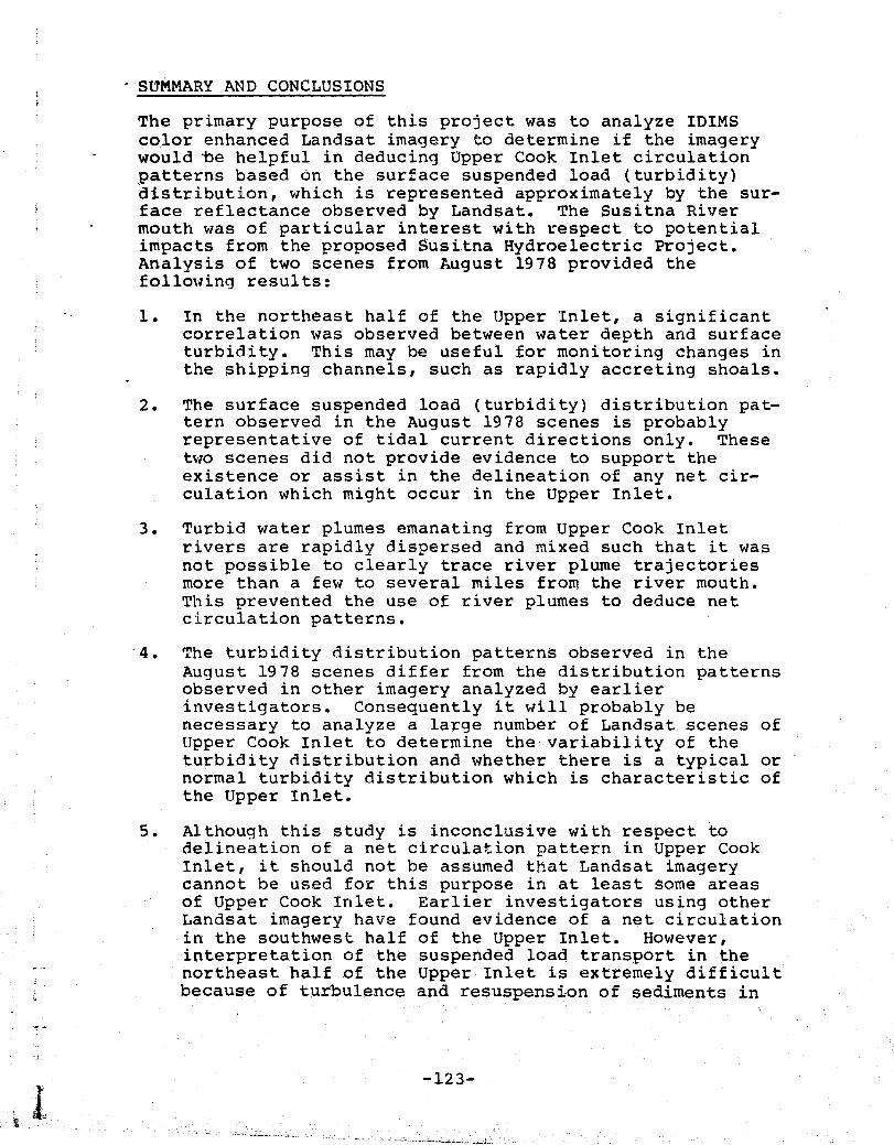
SLTMMARY AND CONCLUSIONS

The primary purpose of this project was to analyze IDIMScolor enhanced Landsat imagery to determine if the imagerywould 'be helpful in deducing Upper Cook Inlet circulationpatterns based on the surface suspended load (turbidity)distribution, which is represented approximately by the sur-face reflectance observed by Landsat. The Susitna River

` mouth was of particular interest with respect to potentialrimpacts from the proposed 5usitna Hydroelectric Project.Analysis of two scenes from August 1978 provided thefollowing results:

1. In the northeast half of the Upper Inlet, a significantcorrelation was observed between water depth and surfaceturbidity. This may be useful for monitoring changes inthe shipping channels, such as rapidly accreting shoals.

2. The surface suspended load (turbidity) distribution pat-tern observed in the August 1978 scenes is probablyrepresentative of tidal current directions only. Thesetwo scenes did not provide evidence to support theexistence or assist in the delineation of any net cir-culation which might occur in the Upper Inlet.

3. Turbid water plumes emanating from Upper Cook Inletrivers are rapidly dispersed and mixed such that it wasnot possible to clearly trace river plume trajectoriesmore than a few to several miles from the river mouth.This prevented the use of river plumes to deduce netcirculation patterns.

4. The turbidity distribution patterns observed in theAugust 1978 scenes differ from the distribution patternsobserved in other imagery analyzed by earlierinvestigators. Consequently it will probably benecessary to analyze a large number of Landsat scenes ofUpper Cook Inlet to determine the , variability of theturbidity distribution and whether there is a typical ornormal turbidity distribution which is characteristic ofthe Upper Inlet.

5. Although this study is inconclusive with respect todelineation of a net circulation pattern in Upper CookInlet, it should not be assumed that Landsat imagerycannot be used for this purpose in at least some areasof Upper Cook Inlet. Earlier investigators using otherLandsat imagery have found evidence of a net circulationin the southwest half of the Upper Inlet. However,interpretation of the suspended load transport in thenortheast half of the Upper Inlet is extremely difficultbecause of turbulence and resuspension of sediments in

-123-

shoal areas, and the utility of Landsat imagery fordelineation of net circulation in this region is at bestmarginal durinq the summer. It may be possible,however, to use Landsat imagery of winter ice distribu-tions to interpret circulation at the head of the Inlet.

RECOMMENDATIONS

1. Data Processing

a. The dodged 9.5" x 9.5" black and white prints forMSS Bands 4 through 7 are essential for analysis ofall color enhanced products.

b. IDIMS products should be corrected for areal distor-tion to facilitate intercomparison of the Landsatimagery with other map products.

c. Use of similar colors during enhancement of a sceneshould be avoided. It is extremely difficult todifferentiate closely between similar colors.

2. Future Study

a. The feasibility and practicality of using Landsatimagery to assist piloting vessels through the UpperInlet shipping channels should be investigated.

b. The Susitna Hydroelectric Project should investigatethe potential for eastward net transport of SusitnaRiver water. Landsat imagery suggest eastward nettransport may occur, and if true the increasedwinter discharge of fresh water from the SusitnaHydroelectric Project could increase ice problems inthe Anchorage shipping channels.

c. Coastal Habitat mapping programs in Upper Cook Inletshould attempt to locate Landsat imagery obtained atlow tide for use in accurately delineating theextent of mudflats and shoals.

d. Analysis of Landsat imagery showing winter icedistribution should be strongly considered as analternative method for delineation of circulationthroughout Upper Cook Inlet.

REFERENCES

Burbank,, D. 1974. Suspended Sediment Transport andDeposition in Alaskan Coastal Waters with SpecialEmphasis on Remote Sensing by the ERTS-1 Satellite.Unpublished Master's Thesis. Institute of MarineScience, University of Alaska. Fairbanks, Alaska.

a

-124-

Burbank, D.C. 1977. Circulation Studies in Kachemak Bayand Lower Cook Inlet. Volume 3 of EnvironmentalStudies of Kachemak Bay and Loner Cook Inlet (editedby L.i,. Trasky, L.B. Flagg, and D.C. Burbank).Alaska Department of Fish and Game. Anchorage,Alaska.

Gatto, L.W. 1976. Baseline data on the oceanography ofCook Inlet, Alaska. CRREL Report 76-25. ColdRegions Research and Engineering Laboratory, U.S.Army Corps of Engineers. Hanover, New Hampshire.

Sharma, G.D. F.F. Wright, J.J. Burns, and D.C. Burbank.1974. Seasurface Circulation, Sediment Transport,and Marine Mammal Distribution, Alaska ContinentalShelf. Final Report to NASA, Contract NAS5-21833,Task 7; ERTS Project 110-H. Institute of MarineScience, University of Alaska. Fairbanks, Alaska.

1

APPENDIX I

INTRISCA PROJECT

ONE-DIMENSIONAL EDGE ENHANCEMENTS ON IDIMS:

DESCRIPTION, PROCEDURES, EXPLANATION, AND INTERPRETATION

Lindsey V. Maness, Jr.

For maximum precision, sensitivity to subtle local changes,and optimal cost effectiveness, one-dimensional edge enhance-ments are preferable to multi-dimensional edge enhancementssuch as Fast Fourier Transforms, data convolution, etc.. Thesimplicity and utility of the procedures utilized are ideal asan introduction to both edge enhancements and related IDIMSfunctions. This document is meant to acquaint both the noviceand the sophisticated user-analyst w th one-dimensional edgeenhancements, how to accomplish the enhancements digitally onIDIMS, and the general photo-interpretation guidelines.

I. Description

One-dimensional edge enhancements transform a one-pixel anom-aly in the raw data into a two-pixel anomaly in the enhancedimage. In comparison, multi-dimensional edge enhancements ofthree by three matrices transform a one-pixel anomaly in theraw data into a much more subtle and less precise nine-pixelanomaly in the enhanced image.

Additionally, differences in local detector sensitivitycalibration (striping) are often of comparable magnitude tothe data anomalies, which serves to further obscure the spa-tial inhomogeneities in the data when multi-dimensional edgeenhancements are applied. When operations are confined towithin a line (along the X-axis), differences between detectorcalibrations are not being measured and, therefore, do notappear as anomalies on a one-dimensional edge enhancementimage. However, one-dimensional edge enhancements acrosslines, the Y-axis, XY-axis, X-minus-Y-axis, and their respec-tive orthogonals, do enhance differences in detector sen-sitivities resulting in image striping.

In the demonstration tasks involving one-dimensional edgeenhancements of Landsat data conducted at NASA/Ames Research dCenter on the X, XY, Y, and X-minus-Y axis, the followinggeneral descriptions apply to ` image quality and usefulness.The X-axis imagery is very clear, easily interpretable, doesnot suffer from striping and is a compromise between optimalenhancement of cultural versus physiographic features.

-326-

.r

1

XY-axis imagery suffers from moderate striping and enhancescultural lineaments optimally by obscuring physiographicchanges in the imagery; this is caused by sampling withinslopes with comparable lighting due to the location of the sunto the southeast (in the X-minus-Y direction). On the Y-axisimagery, neither cultural nor physiographic edges have optimalvisual enhancement as a result of striping, which can beextreme. The X-minus-Y axis enhances physiographic edgesoptimally since sampling across the boundaries between welllit and shadowed areas occurs most frequently using thistechnique; the identical amount of digital information aboutcultural lineaments is present as in the XY-axis but is not asapparent since so much more information about physiographicedges is seen on the imagery by the analyst.

The IDIMS functions used in the Alaska (INTRISCA Project) one-dimensional edge enhancements, PLENTER (to de-skew and enterraw data in IDIMS format while retaining image-related files),COPY (to prepare subsets of the data), COPYIRF (to copy imagerelated files from one image to another), ADD (to subtract onIDIMS, use the ADD function), UNITE (to make four single-banded images into one four-banded image), MAP (to add aconstant to an image or to stretch the data values to enhancethe digital anomalies), CONVERT (to change the data to system-friendly eight-bit byte data in a band-interleaved format),MAGNIFY (to approximate geo-correction), ANNOTATE (to appendexplanatory text about MSS channels, Scene IDs, etc. to theimage), MOSAIC (to append the annotation legend to the image),and DICOM.ED (to acquire color or black and whitephoto products) are simple, frequently used, andwell-documented. If the function ROTATE had been applied withtheta=-11 degrees, just before DICOMED was run, the imagewould have been oriented to very near true north. Most of thesteps described above were performed in a batch (on IDIMS,STREAM) mode to minimize interactive console work. The actualIDIMS functions (with clock, not CPU, time) are presented inthe following serial flowchart to document how the Alaska edgeenhancements were accomplished on the IDIMS system.

II. Procedures

Total ClockTime

Hrs,./Mins. # IDIMS Function

2: 45

1 >PLENTER(SL=1 NL=2340 NS=3480 BANDS=4 LISTDEV=TERM +UPSCALE=1 TAPES=1 SPECTYPE=BB +SKIPSIAT=NO BAND4FAC=2)>AK30175.20345.RAW

0:50

2 AK30175.20345.RAW(l 1 2340 3297)>COPY>AKXL

f

0:01

3 AK30175.20345.RAW AKXL>COPYIRF

-127-

F.

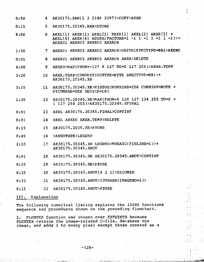
l:bu

0:01

4:00

3:20

3:15

1:25

0:01

0:01

0:15

0 :45

2:10

t

4 AK30175.RAW(1 2 2340 3297) >COPY >AKXR

5 AK30175.20345.RAW>STORE

6 AKXL[1] AKXR[l] SKXL[2] SKXR[2] AKXL[3] AKXR[3] +AKXL [ 4 ] AKXR [ 4 ] ADDSA( FACTORS =1 -1 1 -1 1 -1 1 -1) >+AKXRU1 AKXRU2 AKXRU3 AKXRU4

7 AKXRUl AKXRU2 AKXRU3 AKXRU4>UNITE(SPECTYPE=BBh>AKXRU

8 AKXRUI AKXRU2 AKXRU3 AKXRU4 AKXR>DELETE

9 AKXRU>MAP(FROM=-127 0 127 TO=O 127 255)>AKXR.TEMP

10 AKXR.TEMP>CONVERT(OUTYPE =BYTE SPECTYPE=BB)>+AK30175.20345.XB

11 AK30175.20345.XB>HISTOG(NUMBINS =256 CUMHIST=BOTH +PICTMEAN=YES DEVICE=LP)

12 AK30175.20345.XB>MAP(FROM =O 120 127 134 255 TO=O +1 127 254 255)>AK30175.20345.XFINAL

13 AKXL AK30175.20345.FINAL>COPYIRF

14 AKXL AKXRU AKXR.TEMP>DELETE

15 AK30175.2035.XB>STORE

16 >ANNOTATE>LEGEND

17 AK30175.20345.XB LEGEND>MOSAIC(PINLINE=1)>+AK30175.20345.ANOT

i 0:01 18 AK30175.20345.XB AK30175.20345.ANOT>COPYIRFa

0:15 19 AK30175.20345.XB>STORE

0:25 20 AK30175.20345.ANOT[4 2 11>DICOMED

0:33 21 AK30175.20345.ANOT>IDTRANS(IMAGENO=1)>

0:15 22 AK30175.20345.ANOT>STORE

t III. Explanation

The following numerical listing explains the IDIMS functionssequence and procedures shown on the preceding flowchart.

1. PLENTER function was chosen over ERTSENTR becausea

PLENTER retains the image-related C-file, de-skews theimage, and adds 1 to every pixel except those created as a

-128-

,

result of image skewing (which are assigned a 0 value);ERTSENTR does none of these things. PLENTER and ERTSENTRare used to reformat raw data from an Earth ResourcesObservation System (EROS) computer compatible tape (CCT)into IDIMS format. Tapes which have been preprocessedelsewhere probably will have to be entered using another ofthe enter functions.

If a C-file is appended to the image in IDIMS format, and itis full, the IDIMS function PGC can be used in the finalstages to apply a "precision geometric correction" to theimage. AK30175.20345.RAW is the image name and translatesto Alaska, Scene ID, and type of data. Note that properimage naming conventions, when followed by the user--analyst,can eliminate unnecessary confusion, especially when eithermore than one person is involved or the analysis occurs overa long-period of time.

2. The desired area for edge enhancement is extracted(subset) and named AKXL. AKXL is an acronym for Alaska,X-axis, left side.

3. All image-related files are copied from the raw image toAKXL except for P (picture) and H (history) files, which areassigned permanently to the image as long as it remains inthe user catalog. In edge enhancement operations, the'onlysignificant file to be copied is the C-file (see 1 above).

r If COPYIRF is not run, the only files associated with theimage are the P and H files. To get a list of on-linefiles, the command "LISTF @.userid,2" may be typed inMPE mode. The MPE mode is active when the computer promptsthe user terminal with a colon (:), as when logging on oroff the HP3000 system.

4. A subset area with the same line and column dimensionsbut offset one to the right from AKXL along the X-axis isextracted and named AKXR. AKXR is an acronym for Alaska,X-axis, right side. The existence of two images offset one(or more) pixels from each other allows numerous types ofcomparisons to be made on IDIMS: however, only one ofthese, subtractions, is discussed in this document. Theoffset can be made along any axis and for any distance butthe most common offsets are the X, XY, Y and X-minus-Y axes,as described on page 1, paragraphs 3 and 4.

5. The raw image is no longer needed for edge enhancementpurposes so it is stored in case of future need. Images arebrought back on line (with all image-related files) muchmore quickly from an IDIMS store tape than in any otherform. If it is not possible to STORE the image at thefacility, for administrative reasons, a good alternative isto IDTRANS (see step 21) and then delete the raw image.

-129

6. Image AKXR is subtracted from AKXL, one channel at atime, starting with channel one and progressing to channelfour. Channel one is the same as Land .,kt multi-spectralscanner (MSS) 4; channel two is MSS 5; channel three is MSS

j 6; and channel four is MSS 8. The FACTORS parameterincludes one number for each image specified to the left ofthe word ADD and performs operations in pairs. Itmultiplies the appropriate FACTORS numbers by theappropriate images, pixel-by-pixel, and then adds the resultin a pairwise fashion. Obviously, multiplying the secondnumber by minus one and adding to the first is equivalent toa subtraction of the second image from the first. Thenumber of output images is always equal to exactly one-halfthe number of input images or the job will not run. Theoutput images are named AKXRU plus the channel number. TheAKXRUI acronym, for example, means Alaska, X-axis, REAL-formunstretched data of channel 1. In terms of CPU time, clocktime, disc-space and tape-length utilized, it is most unfor-tunate that a subtraction of byte data on IDIMS generates aREAL-form image rather than an INTEGER-form image.REAL-form data are VERY system unfriendly, INTEGER-form lessso, and BYTE-form most system friendly on the IDIMS/HP-3000.

7. The subtracted images are UNITEd to form a single, four-band image to minimize processing redundancy. If the workis done batch (termed STREAM on IDIMS), it is preferable todo all operations up to and including step number 10 priorto uniting the images since a UNITE of byte data is bothfaster and requires less disc space than data of REAL-form.

S. The preceding intermediate-stage images are deleted assoon as possible to minimize load on the disc. Note thatimage AKXL is kept on-line to transfer image-related files instep 13.

9 The MAP function of IDIMS is used, in this example, toadd a constant, 127, to the data so that conversion toBYTE-form can occur. Please note that the MAP function onIDIMS has nothing whatsoever to do with maps; it refersstrictly to what are more commonly termed "data stretches"

- on other remote sensing systems. A topographic quadranglemap or other hard-copy map is referred to as a "spatial map"in IDIMS documentation. The MAP function on IDIMS creates

j` a'look-up table and, in effect, instructs the computer thus:"Every time you see this number, change it to the specifiednew number." The (data stretch) MAP function is one of themost used in IDIMS; it is a multi-purpose function.

10. The previously stretched (step 9) data, all Dn values(digital number values) which fall between 0 and 255(eight bit byte data) are converted to system-friendly band-interleaved byte data.

-130-

if

t

s

li

11. The data are histogrammed to determine the spread aboutthe peak of the mode, preparatory to step number 12.

12. A stretch, one Dn removed from both sides of the baseof the mode along the tail, is usually at or near optimum.In the example given, the mode ends and tails begin at Dnvalues of 121 and 133; therefore, the parameters specifiedin the stretch are 120 and 134. The actual input parameters

R

are (FROM=O 120 127 134 255 TO=O 1 127 254 255): in thisexample, a 0 remains a 0, all numbers between 1 and 119become either 0 or 1 depending on whether the number iscloser to 0 or 120, a 120 becomes a 1 in the output image,values between 121 and 126 (inclusive) become theinterpolated values between 2 and 126, 127 remains the samevalue, and so forth. Note that 127 is by far the most com-mon value since that is the Dn of the highest point on thehistogram; this relationhsip is true because before 127 wasadded to the image in step 9, the value of these pixels was0, the most common value when subtracting adjacent pixels.

13. The image-related C-file is copied onto the final x-axis edge-enhanced image. The function PGC could now be runto resample and rotate to true north the image (if the C-file is not empty) such that a given number of pixels eitherhorizontally or vertically covers the same distance on theground. Since each resampled pixel covers the same distancevertically as horizontally, each pixel after the PGCfunction is run becomes a square pixel.

14. Images not needed are deleted.

15. The byte image which hasn't undergone any enhancementstretching is stored. If at some later date, a differentdata stretch or annotation is desired, it is an easy matterto retrieve this image with the command:AK30175.20345.XB>LOAD.

16. An annotation is created for appending to the finalimage. Information in the annotation should include MSSband(s), state or country, Scene ID, project title, etc..Since the annotation procedure would require a lengthyexplanation and is best done interactively, interested usersare referred to IDIMS documentation.

17. The annotation legend is mosaicked to the image.

18. The image-related files are copied onto the new anno-tated image (see step 2).

s

'. 19. The -un-annotated X-axis edge-enhanced image is stored.

20. A three-channel annotated image is recorded on film bythe DICOMED File Recorder. In the example given, [4 2 1],

^, u

r -131-

channel 4 (MSS 7) is portrayed as red, channel 2 (MSS 5) asgreen, and channel 1 (MSS4) as blue. Single-band black andwhite images can be 'Created by specifying only one band inthe channels parameter. The default, if no bands are

1 specified, is [1 2 31.

21. An IDTRANS tape of the annotated X-axis edge-enhancedimage is acquired. If there are system (or other)- problemsthat result in the deletion of the image just created, theimage will not have to be recreated from scratch; the com-mand >IDENTER(IMAGENO =1)>AK30175.20345.ANOT will bring itback on line from the IDTRANS tape. If IDENTER is used, thecommand AK30175.20345:ANOT>FIXHIST should be run imme-diately afterwards to append the stored H-file (historyfile) to the image, which will minimize catalog errorsand cut down on unnecessary work by systems personnel. IfFIXHIST is not run, an HX file will be left on line on theuser account and will have to be purged by systempersonnel; in addition, the past processing history of theimage will be lost to the user.

22. The annotated X-axis edge-enhanced image is stored. Itis also possible to store the images created during thenormal END sequence on IDIMS. IDIMS prompts for every on-line image asking for instructions about whether to delete(D) or store (S) .

IV. Interpretation: Analysis Principles

Several phenomena are either of analytical interest orunique to one-dimensional edge enhancements: these pheno-mena are an apparent relief illusion, enhancement of linearfeatures relative to axis direction such that identicalfeatures appear different as a function of orientation,pronounced enhancement of subtle linear or curvilinear anoma-lies (as in water body "fronts"), the influence of the MSSbands upon enhancement, etc..

1. Apparent Relief Illusion.'j

The apparent relief on imagery, whether appearing as a deepcleft (roads on MSS 5) or as a blister or depression (lakeson MSS 7), is caused by the gross contrast in brightness of

` the two immediately proximal lines along the edges. A pho-tographic enlargement of the left shoreline of lakesdisplays a very bright outer line and a dark inner line; theopposite relationship exists on the right side of the RTakes. The very bright ring on the left side of waterbodies is caused by the difference (a positive number) inbrightness values between vegetation (bright) and water(dark) on MSS 7 being greatly enhanced. On the right sideof lakes the difference (a negative number) between water

-132-

r !

(dark) and vegetation (bright) becomes a dark line afterenhancement. That the relief effect is an illusion can beverified by looking at large rivers with variable sedimentloads. On the edge enhanced imagery, the rivers appear tocontain pronounced ridges and valleys. The presence ofrivers is enhanced on MSS 6 and 7 due to, in part, the illu-sion of relief created by adjacent light and dark strips onthe edge enhanced imagery.s

2. Axial Direction Enhancement.

F

Accordinq to their orientation relative to axial samplingdirection, features such as roads, urban/suburban areas,rivers, and glaciers exhibit significantly different aspectsand textures.

a

Roads, when sampled orthogonally, are enhanced optimallybecause of the increased probability of fewer local edgepixels (see page 1, paragraph 2). As the axis directionbecomes more similar to the road direction, the edge effectdecreases; when the axis direction parallels the road, theroad disappears from the enhanced image.

Roads, railroads, trails, powerlines, pipelines, seismicsurvey lines, and other linear cultural features can be dif-ferentiated through careful analysis of different. MSSsingle-band (black and white) or multi-band (color)photoproducts, by cross referencing with published mapsources, and by field checking.

Roads and railroads, while appearing very similar on allfour MSS bands, can be differentiated somewhat on largescale photographic blow-ups by analyzing the branchingpatterns of the suspected transportation arteries.Railroads generally have a much simpler and more smoothlycurved aspect than roads. Unfortunately forphotointerpreters, roads and railroads often follow the samecourse, side by side.

Roads and trails can be difficult to differentiate withabsolute accuracy on single-band Landsat one-dimensionaledge enhanced imagery but can be mapped with a fair level ofconfidence with black and white MSS 4 and 5 photo products.MSS 5 delineates roads and trails quite well and, while theintensity of the lines may be suggestive of the relativesizes'of the transportation arteries, MSS 5 alone is oftennot sufficient to differentiate roads from trails. Acomparison with MSS 4 will often remove much of the con-fusion since most smaller roads and trails either disappearentirely or become more subtle than the larger roads in thearea.

-133-

Transportation arteries can usually be differentiated frompowerlines, pipelines, and seismic survey lines by analysisof spatial patterns and by a careful comparison of thefeatures of MSS 5 with those of MSS 6 or 7. Non-road linearfeatures generally have vegetation growing within the edgepixels, unlike transportation arteries, which leads to a(sometimes pronounced) difference in appearance on colorimagery. Powerlines cross rivers and marshes withoutbridges, do not have complex networking, and generally gofrom community to community in as near a straight line aspossihle. Pipelines generally end at a river or outlet tothe sea, may go to a refinery, don't necessarily go directlyfrom community to community, usually have en-route pumpingstations, do not necessarily go in a straight line, and havefairly simple networking. Seismic survey lines' spatial pat-terns vary considerably according to age, area of the world,geological and property considerations, company doing thesurvey, etc., but can usually be differentiated from otherlinear features with a high level of confidence by aninterpreter with knowledqe of the area's petroleum.

Similarly, and more noticeably, urban/suburban areasgenerally have a very distinctive pattern of slightlyinclined parallel lines. if on an X-axis enhanced image,the lines trend in a somewhat Y-axis direction; if on an Y-axis enhanced image, the lines trend in a somewhat X-axisdirection, and so forth. This effect is an extension of theenhancements of roads, described above.

Rivers, when sampled orthogonal to flow direction, enhancedifferences in suspended sediment as a function of flowregime across the river. A vector component modelling ofwater flow downstream between boundaries could be inferredwith proper on-site calibration measurements. Similarly,when sampled parallel to flow direction, differences inwater hodies between fronts are enhanced as a function ofdownstream flow regime; in this case, a vector componentmodel of water flow across the river between boundariescould be inferred with sufficient on-site calibrationmeasurements.

Glaciers, when sampled orthogonal to flow direction, havemedial moraines enhanced (parallel straight lines) and cre-vasses obscured; when sampled parallel to flow direction,have crevasses enhanced (chevron shapes) and medial morainesobscured; and, if neither solely orthoqonal nor parallel,are influenced by both medial moraines and crevasses as afunction of the sine of the angle of the sampling directionaxis with the glacier.

-134-

FIGURE 29. One-dimensional edgeenhancement, MSS 6 UNIGINAL PAGE IS

-135-OF POOR QUALITY

u"a.

r-

y

N

at#

S

za

F

. .

3. Enchancement of Subtle Curvilinear or Linear Anomalies

Subtle curvilinear anomalies, whether they be ultimatelycaused by changes in cultural influences, vegetation, waterclarity, geology, etc., are made more apparent by enhanceddifference imagery. whereas only a few pixels of changescattered randomly might not attract a photointerpreter'seye, when the same amount of change is arranged in a coherentpattern, the result is a strikingly obvious feature due bothto differences with surrounding pixels and to similaritywith other pixels of the curvilinear anomaly. This is truewhether the enhanced differences reflect changes within orbetween vegetative, hydrological, geological, cultural, orother groupings. The boundaries between groupings as shownon the enhanced difference images (one-dimensional edgeenhancements) display real boundaries betweenecozones,water types, soil types, geology, etc.; however, roads andcultural features may be only man-made boundaries across anecotone, water type, etc..

4. O p timum MSS Band Choice for S pecific Purposes.

MSS 4 and 5 are most useful for mapping road networks andcultural features. While MSS 4 shows roads with less visualclutter than MSS 5 due to less enhancement of water boun-daries on MSS 4 than on 5, MSS 5 is the preferred choicesince roads and cultural features are sharper, clearer, andmore enhanced than on MSS 4. Presence or absence(relative) of plants are a significant factor in the sharp-ness of MSS 5 due to the inverse relationship betweenchlorophyll and brightness (see IV.3,paragraph 5). Theedge enhanced imagery can be used for updating maps with aZoom Transfer Scope. Probably, at least in informationtransfer activities, the greatest use of edge enhanced im-ahery will be in the field of cartography as a support toland use planners.

MSS 6 and 7 display changes in vegetation type and cover(ecozone bounaries) very well.

MSS 5, 6,and 7 display water boundaries based upon variablesuspended sediment load quite well.

MSS 4 and 5 are useful for mapping marsh/water boundariesand give some indication of the boundary between bottom andwater column reflection.

MSS 4, 5, 6, and 7 are all useful in glacier studies. Thebands can be used either singly as black and white images orin combination as color photo products. Different types ofice-snow pack at the heads of glaciers can be differentiatedusing color photo products; it is hypothesized that these

-136

colors reflect differences in mega-roughness,recrystallization, etc..

V. Conclusion

one-dimensional edge enhanced imagery can be very useful formany remote sensing applications. The boundaries betweenvegetative ecozones., water bodies, glacial features; andthe precise delineation of cultural features, especiallyroads; can often be accomplished using the differencingtechniques described in this document. As in other remotesensing techniques, different MSS bands enhance differentlyand the imagery derived must be evaluated and used withproper precautions and knowledge of the nature of the datato avoid incorrect conclusions. Furthermore, the imageryshould be used in conjunction with as many other types ofsupporting information as possible to maximize the probabil-ity of correct conclusions.

The different types of one-dimensional edge enhancementseach have their own distinctive advantages anddisadvantages. A good compromise of possible axes withminimal noise is the X-axis. The XY-axis is best fordisplaying cultural features with the least possibleinfluence from physiographic variations but suffers fromacross-detector striping. The X-minus-Y-axis is best fordelineating physiographic variations but suffers from cross-detector striping. The Y-axis suffers the most visuallyfrom striping of the imagery.

The flowchart of IDIMS functions with explanations should beespecially useful to user-analysts interested in creatinged ge-enhanced imagery. Although the software functionslisted are IDIMS, equivalent programs exist on most otherremote sensing systems; consequently, the processesdescribed in this document have general applicability.

ii

APPENDIX J

STREAM CORRIDOR PHYSIOGRAPHY OF THE

SUSITNA RIVER VALLEY, ALASKAFinal Report

NASA-AMES Research Center ConsortiumAgreement #NCA2-OR020-001

in conjunction with theAlaska Department of Fish and Game

t

E

Kenneson G. Deant NORTHERN REMOTE SENSING LABORATORYf

Geophysical InstituteUniversity of Alaska

Fairbanks, Alaska 99701

4

December 1980

-138-

I

TABLE OF CONTENTS

Page

ABSTRACT. . . . . . . . . . . . . . . . . . . 1,40

INTRODUCTION . . . . . . . . . . . . . . . . . . . • • 141

PHYSICAL SETTING . . . . . . . . . . . . . . . . . . 142

REGIONAL SURFICIAL GEOLOGY . . . . `. . . . . . . . . . 145

MATERIALS AND METHOD OF INVESTIGATION . . . . . . . • 147

DESCRIPTION OF MAP UNITS . . . . . . . . . . . . . • • 148

Glacial Land°orms . . . . . . . . . . . . . • • • 148Fluvial Landforms . . . . . . . . . . . . • • • 150Delta-Plain Landforms . . . . . . . . . . . 152

DESCRIPTION OF STREAMS . . . • • • • • • • • • • . 153

DISCUSSION. . . . . . . . . . . . . . . . . . . . . . 155

CONCLUSIONS . . . . . . . . . . . . . . . . . . . 158

RECOMMENDATION . . . . . . . . . . . . . . . . . • 159

REFERENCES . . . . . . . . . . . . . . . . . . . . . . 160

APPENDIX: Comparison--Landsat Imagery vs. Aerial Photography

ABSTRACT

Floodplains in the vicinity of a stream form a corridor which is a

primary habitat zone. Knowledge of surficial geology along this corri-

dor will provide a data base to aid land-management decisions.

Generally, streams in the Susitna River Valley are incised into

glacial deposits and are braided and sediment ladened. Floodplains and

,terraces develop as the streams migrate, downcut and deposit alluvium.

The floodplains are divided into four categories based on surface mor-

phology including presence of channels or sloughs, density and type of

forest cover, and proximity to height above stream channel(s). These

divisions include active, partly active, infrequently active and abandoned

floodplain surfaces.

A traverse from the existing stream channel to the limit of the

floodplain demonstrates a slight increase in elevation, increase in the

density of the forest canopy, a decrease in number of sloughs and aban-

doned channels, and a gradation from deciduous to coniferous forests.

This trend parallels a decrease in flood susceptibility away from the

stream.

INTRODUCTION

`k

The land surface in the vicinity of a stream is a primary habitat

zone because of its proximity to water, shallow water table, and gently,

sloping terrain. The purpose of this project is to study and map the

landforms within a corridor along select streams in the Susitna River

Valley. The results will provide land managers with an initial data

base to establish riparian management zones or buffer zones to protect

fish and wildlife and their habitats from disturbance or damage.

A secondary purpose is to compare the minimum size of floodplains

and number of floodplain categories derived from aerial photography to

that derived from Landsat imagery '(see Appendix)•

Landforms are studied and mapped along the Yenta, Susitna, Skwen=na,

Kahiltna Rivers and Lake Creek in the Susitna River Valley. The results

of the project are displayed on 17 USGS topographic quadrangles (scale

1:63,360), including Tyonek B-2, C-1&2, D-1 thru D-6 and Talkeetna A-1

thru A-4 and B-1 thru.B-3.

Va .. T

i

PHYSICAL SETTING

The Susitna River Valley is located in southcentral Alaska north-

west of Anchorage (Fig. 29). The valley grades southward to sea level

at Cook Inlet and is bounded by the Talkeetna Mountains on the east

and the Alaska Range on the north and west. These mountains hinder the

northward migration of storms from the north Pacific Ocean, producing

74 cm (29 inches) of precipitation annually (Rieger, 1979), the largest

amount of precipitation in the state_ excluding areas immediately adjacent

to the coast.

Major streams within the study area include the Susitna, Yentna,

Kahiltna, Chulitna, Tokositna, and Talkeetna Rivers. The Susitna River,

which is the largest in the area, drains southward into Cook Inlet.

Glaciers including the Dall, Yentna, Kahiltna, Lacuna, Tokositna, Ruth

and Eldridge are located in the nearby Alaska Range at the headwaters of

rivers and several subordinate tributaries.

Numerous south trending lakes, wetlands and forested ridges of low

relief are typical bn the valley floor. Most of the present topography

has resulted from glacial, g.laciofluvial and fluvial processes (Dean, 1980).

Transportation corridors include the Parks Highway and the Alaska

Railroad along the eastern margin of the study area. A secondary road

to Petersville and surrounding mines traverses the central portion of the

area. Some agricultural, timber harvesting, and mining enterprises are

located near Talkeetna. Lode and placer mining operations are active

in the hills and mountains surrounding the valley. The minerals or

ORICINAL PAGE 19OF POOR QUALITY

"IN coolr 9-Wft Lai'.

Lake Creek

3%1

T C0C

'AKahiltna River coellSusitna River

Gebm^­Z.41t-

TA

gna

A

2 LL0

I

14k I -i

NIV

N

Mc ou all

1.

9I

t,UTION Kas .-a

,Skwentna River

I ccum 71 0 1110.

- 46094 Yenta River

BELL —MOUNTA.N

.., _­ ., I

IN4 Was

Y17MOUNT C0 ttonwwsrrN

,^39

WAI*xa^d C,

ay COT

E.

;QF

ORAGE

ZN,

Ladd27.)

9

Scale 1:1,000,000

n of stream corridors in the Susitnaalley.

-143-

elements being mined include molybdenum, capper, chromium, gold,

uranium, platinum, tin coal and thorium (Reed and others, 1978).

The region is generally sparsely populated. Clusters of small

settlements occur along the Parks Highway especially in the vicinity

of Willow and to the south where newly developed subdivisions are

prevalent. These subdivisions reflect the pressure for land develop-

ment along the Parks Highway.

3

3,a

f

V REGIONAL SURFICIAL GEOLOGY

The surficial geology of the Susitna River Valley is dominated by

glaciation (Caulter, and others, 1965, Reger, 1976). This area is a

trough into which mountain glaciers and drainages from the surrounding

Alaska Range and Talkeetna Mountains are funneled.

At least .five glacial advances (Nelson and Reed, 1978) have altered

the landscape in the Susitna River Valleyt

Glacial advances in the Cook Inlet Basin.

Glaciation Age Sources

Alaskan 200-4800 yrs. ago l (Nelson & Reed 1978)

Naptowne 6,000-30,000 yrs ago l (Pewe, 1975)

Knik 38,000-65,000 yrs ago` (Karlstrom, 1964)

Eklutna 25,0001-110,0002 yrs. ago (Karlstrum, 1964)

Mt. Susitna Pre- Illonian (Karlstrom, 1964)

The Mt. Susitna glaciation is the oldest and most extensive glacial

advance documented in the Susitna River Valley by Nelson and Reed (1978)

and in the Cook Inlet basin by Karlstrom (1964). Each successive glacia-

tion was less extensive.. The Mt. Susitna and Eklutna Glaciations com-

pletely filled the Susitna Valley and Cook Inlet basin, but during the

Knik and Naptowne Glaciations coalescing glacial lobes in valleys did

not completely fill the basin (Nelson and Reed, 1978). The Alaskan

Glaciation was generally confined to narrow mountain valleys where end

moraines were commonly deposited at the confluence with broader valleys.

The Susitna River Valley contains landforms that resulted from

glacial, fluvial, lacustrine, periglacial and paludal processes. Duringf

Pleistocene glacial advances bedrock was scoured and debris was trans-

9

ported and deposited by the glaciers and streams. Most of the presentiE

topography on the valley floors resulted from the southward advance

of the Naptowne glaciation (Nelson and Reed, 1978) which terminated

between McDougall and Talkeetna (Karlstrom 1964).

After retreat of the Naptowne glaciers, streams in the Susitna

River Valley incised the glacial drift, attempting to re-establish a

I

lower gradient stream profile by transporting eroded material down-

stream and redepositing it below the terminus of the Naptowne advance.

Erosional and depositional processes have resulted in incised stream

F, channels in the northern Susitna Valley and the aggradation of alluvium1y

in the valley south of the limit of the Naptowne Glacial advance.

. i

a ^

a

r,

146—

MATERIALS AND METHOD OF INVESTIGATION

The investigation utilized color-infrared aerial photography,

Landsat imagery, USGS topographic maps and aerial and ground verifi-

cation procedures. NASA aerial photography acquired in 1974, 1976 and

1977 at the scale of 1:120,000 was the primary data source for inter-

preting and mapping landforms. Landsat images were used to obtain an

understanding of regional relationships of landforms.

Landform interpretations were performed through a mirror stereo-

scope with a X3 magnification lens and the results were mapped on an

overlay. The overlay was displayed and enlarged through a vertical

projector onto the mylar topographic maps so that the map units could be

transferred to the map base. Mylar copies of USGS quadrangles at the

scale of 1:63,360 were used as a final map base.

a

s

DESCRIPTION OF MAP UNITS

Glacial Landforms

Deposits in the Susitna River Valley are composed of unconsolidated

glacial drift. Drift is composed of unsorted silt, sand, gravel, cobbles

and boulders (till) and is intermixed with stratified silt, sand and

gravel of fluvioglacial origin.

The resulting landforms include undifferentiated hummocky terrain

(d), fluted till ridges (r), zones of standing water (.J.), eskers (e)

and outwash fans (ow). All of these map units are located on the Susitna

Valley floor beyond the floodplains (Table 18).'

The undifferentiated hummocky terrain (d) is composed of glacial

drift which protrudes above the surrounding terrain. Depressions or

kettles are typical on the surface and trap surface water. Segmented,

abandoned drainage-channels traverse the drift sheet. These drainage

channels are remnant of previous drainges and often contain standing

water. Vegetative growth on the drift consists mostly of deciduous and

coniferous forests. In some localities in the vicinity of Talkeetna,

eolian sand blankets the drift deposits.

Fluted till ridges (r) parallel the direction of glacial movement.

Ridges have low relief and are better drained than the lower surrounding

landscape as indicated by deciduous tree growth.

Extensive areas of standing water (_J) lie between fluted till

ridges and drift 'deposits. The terrain is low and flat with small

undifferentiated deposits of drift scattered throughout. Poor drainage

is a result of a low gradient and the impermeable till. Discontinuous

permafrost is suspected in swampy areas.

-148-

Table 1 8. Landform map explanation.

fa

fl

f2

f3

f

t

ox

d

r

ow

e

b

ac

of

al

`rc1

tbe

s

s

active floodplain

party active floodplain

infrequently active floodplain

abandoned floodplain

undifferentiated floodplain

terrace(s)

standing water

oxbow

undifferentiated, hummocky terrain composedof till and fluvioglacial deposits

fluted till ridge

glacial outwash fan

esker

prominant scarp

scoured bedrock

alluvial cone

alluvial fan

undifferentiated landscape composedalluvium and colluvium

coastal lowland

beach ridge(s)

sand or silt dune

sparse undifferentiated dunes

i * - incised stream

subordinate drainage channels with standing waterEr

map unit needs further field verification tfi

f

149-

. - ;

Eskers (e) and remnant outwash (ow) fans occur in some areas. They

consist of fiuvioglacial deposits which are exellent sand and gravel

sources and are well drained. Deciduous forests typically grow on these

surfaces.

Along the margins of the valley the surrounding mountains have been

scoured by glacial advances. Ice-scoured bedrock (bs) is often blanketed

by a thin layer of till. At lower elevations alluvial cones (ac) and

fans (af) extend onto the valley floor.

Fluvial Landforms

Streams in the Susitna Valley are typically incised into the land-

scape reworking the glacial drift and depositing stratified silt, sand

and gravel as point bars, islands, overbank deposits or channel fill

forming floodplains in the vicinity of the streams.

The floodplains are divided into six categories: active (fa),

partly active (f 1), infrequently active (f 2 ), abandoned (f 3 ), terraces

(tr), and undifferentiated (fd).

Active floodplains (fa) include the existing stream channel(s),

prominent sloughs, recently abandoned stream channels, sand and gravel

bars, vegetated and unvegetated islands. Adjacent shore areas include

exposed silt, sand and gravel deposits or are with standing water.

Vegetation includes uncrowded deciduous forests, typically cottonwood,

with a broken canopy and willows. Understory is sparse in some areas.

rPartly active floodplains (f l) are intricately laced with sub-

ordinate sloughs and drainage channels usually connected to the dominant

stream. These channels contain flowing or standing water, or swamp

deposits. The floodplain surface is vegetated by mature mixed deciduous

-150-

- _­: x

ttSI~1F'

r

n

Y

S

S

Ig

forests which generally are uncrowded and ha-:e broken canopies. The

floodplain surface may extend several feet above the normal stream

stage.

Infrequently active floodplains (f 2 ) are dissected by abaudoned

channels and sloughs, which often are not connected to the parent stream.

A few oxbows (ox) are also present. The floodplain surface is vegetated

by mature deciduous and mixed forests and is slightly elevated. These

forests in contrast to forests on more active floodplains, are generally

denser and the canopy is only occasionally broken.

Abandoned floodplains (f 3 ) have few readily apparent channels,

oxbows or sloughs. Coniferous forests tend to prevail and the forest

canopy is dense and not usually broken. Areas of standing water are

minimal or absent.

Terraces (tr) are remnant floodplains at higher elevations than

other floodplain categories and indicate a former floodplain level.

They are separated from present floodplains by steeply sloping scarps

and are predominantly vegetated by coniferous and mixed coniferous and

deciduous forests with a dense, unbroken canopy. Standing water is

minimal to non-existent. Often several levels of terraces are included

within one map unit.f

The undifferentiated floodplain (fd) classification is used along

subordinate streams and is generally less than 300m (1000 ft.) wide.

Stream flow is often restricted between steep banks. Previously des-

cribed floodplain divisions are included within this unit and are dis-

tinguishable on the photography but too small to be delineated.

r - -151-

Delta--Plain Landforms

In the southern portion of the study area where the Susitna River

empties into Cook Inlet aggradation rather than downcutting is dominant.

This results in the deposition of large quantities of alluvium and hence

more expansive floodplains than to the north. Landforms include coastal

lowlands (cl), beach ridges (be) and dunes (s & sd).

Generally, the surface is mapped as coastal lowlands (cl). The

area is low, near sea level, and very gently sloping. Standing water is

prevalent in many areas and mudflats are extensive during low-tides.1

Coastal lowlands and the floodplains bear beach ridges (be) along

the coast and eolian dunes (s & sd) further inland. Typically, beach a

ridges are defined as subparallel ridges of sand, shell or pebble gen-

erally varying in amplitude from a few inches to many feet (Davies,

1068) and mark former shorelines. In the study area these ridges support ?9

deciduous vegetation which contrasts with the surrounding vegetation on

the coastal lowlands.

The eolian dunes are wind deposited ridges composed of vegetated

sand and silt and encroach upon areas of standing water. The (s)

designation refers to individual dunes and the (sd) designation refers

to dune complexes which are typically separated by areas off standing

water.

DESCRIPTION OF STREAMS I

Susitna River: The Susitna River extends from Susitna and West

Fork Glaciers in the Alaska Range to Cook Inlet and most streams in the

Susitna Valley drain into this river. That portion of the river in the

vicinity of Talkeetna and south to Cook Inlet is included in the study

area.

The associated floodplain of the Susitna River is broad and the

stream is extensively braided. Islands composed of exposed silt, sand,

and gravel are numerous but often temporary while vegetated islands are

more stable. The floodplain is divided into five categories: active,

partly active, infrequently active, abandoned and terraces. Scarps

often border the floodplain north of Willow but from there south the

floodplains become very broad with standing water and grade into coastal

lowlands (Krebs, and others, 1978 and 1978b). Windblown silt and sand

is typical on the coastal lowlands, and dunes in the area are vegetated

which indicates some degree of stability. The Susitna River is sus-

ceptible to glacial outburst floods north of the Parks Highway crossing

(Post and Mayo, 1971).

Yenta River: The Yenta River extends from the Yenta, Lacuna and

Dall Glaciers to the Susitna River and is moderately braided with braid-

ing decreasing downstream. Floodplain categories predominantly include:

active, party active and infrequently active. The floodplains are

broadest near the headwaters and narrow downstream and include many

vegetated islands. Areas with standing water are numerous and most

extensive in the upper reaches. The Yentna River is susceptible to the

effects of glacial outburst floods upstream from the confluence with the

Skwentna River (Post and Mayo, 1971)

-153-,

Kahiltna River: The Kahiltna River is a braided stream which ex-

tends from the Kahiltna Glacier to the Yentna River. Near the headwaters,

the floodplain is broad with extensive areas of standing water and is

divided into active and partly active categories. Downstream, the

floodplain is divided into active, partly active and infrequently active

categories with many terraces along the margins. The active floodplain

becomes very narrow such that in some areas only the stream channel is

present. The Kahiltna River is susceptible to the effects of outburst

floods near Kahiltna Glacier (Post and Mayo, 1971).

Skwentna River: The headwaters of the Skwentna River are located

in the Alaska Range where glaciers contribute water to many subordinate

tributaries. The portion of the stream east of Porcupine Butte to the

confluence with the Yentna River is included in the study. The flood-

plain divisions include active, partly active, infrequently active and

abandoned, with few terraces evident. Generally, the floodplain is wide

but constrained between glacial-scoured, mountain slopes in its western

portions but to the east the floodplain is very broad at its confluence

with the Yentna River. Extensive areas of standing water are present

east of the Old Skwentna Road House. The stream is susceptible to

glacial outburst floods upstream from the Old Skwentna Road House (Post

and Mayo, 1971).

Lake Creek: Lake Creek drains Chelatna Lake into the Yentna River

and is not glacial fed. The .associated floodplain is narrow and incised

into the glacial landscape especially along a portion centrally located

between its headwaters and confluence with the Yentna River. Most of

the floodplain is classified as undifferentiated with many terracesr

along the margins. The meandering stream becomes braided near its

confluence with the Yentna River and is the only stream in the study

which is clear of suspended sediment.

-154

if

DISCUSSION

The floodplain classification is based on landform and vegetation

including the existence of stream channels and their relationship to the

parent stream, proximity to height above the dominant stream channel,

density of vegetative canopy, and type of vegetation. Ideally, flood-

plain categories geographically progress from active in the immediate

vicinity of the existing stream to party active, infrequently active,

abandoned and terraces at the farthest extent (Figure 30).

Susceptibility of floodplain surfaces to flood events, decreases

away from the active floodplains, as indicated by the landforms and

variations in vegetation. In the vicinity of the stream surfaces have

numerous active and abandoned stream channels which are typically con-

nected with existing stream channels. The presence of these channels

gradually decrease on floodplain surfaces away from the stream until

they are non-existent. Those abandoned channels furthest from the

stream often have no obvious relationship to existing stream channels.

These channels indicate former positions of the active floodplain in the

recent past. Height of floodplain surfaces slightly increase away from

the stream channel as expected.

The active floodplain is sensitive to migrations of stream channels

and fluctuation in stream discharge. Abandoned channels on this surface

become active during increase discharge phases, likely annually and land

surfaces are often flooded.

The partly active floodplain has numerous abandoned channels which

also become active during flood events, but not necessarily annually.

The land surface is subject to flooding during flood stages greater than

annual high water.

-155-

U

N

U^OLv1ECmCEO0

n^Uc9

m

O

C

Z7

i

a,N

Lrc:

a^wa

OWGiNAL PAGE IS

OF POOR (QUALITY

—156—

;f

a

On the active and partly active floodplains, cottonwood forests are

typical, often with relatively sparse understory consisting of willows,

especially along the Susitna River. These forests tend to prevent

erosion of fine grained materials by dissipating the higher velocity s

of floodwater and thus inhibit the transport of coarse material. Studies

of the Missouri River (Schmudde, 1963) also indicate that scouring of

channels or beaches decrease on cleared floodplains beyond a fringe of

trees along the stream.

The infrequently active floodplain is the final floodplain surface

to have abandoned channels. Unlike channels on previous surfaces, these

are often separated from the active floodplain. Annual flooding events

may affect existing channels and sloughs but not the floodplain surface

which is affected by periodic flooding of larger than normal water dis-

charges.

Abandoned floodplains and terraces have iew if any abandoned chan-

nels oxbows or sloughs. These surfaces are least susceptible to flood

events. Most terraces are not likely to be flooded because of their

height above oLner floodplain surfaces.

Floodplains with numerous active and abandoned channels are close

to the existing stream, only slightly elevated above the existing streams

:k and hence, most susceptible to flooding. The trend of decreasing chan-

nels away from the stream parallels not only flood susceptibility but - ?;

also a change in the type and character of vegetation. Generally,

forests are deciduous with broken canopies on younger floodplain sur-

faces near the stream and coniferous on floodplain surfaces furthest

from the stream. Studies by Viereck (1970) in interior Alaska have

found a similar trend with respect to coniferous vegetation on older

floodplain surfaces. Density of the forest canopy also increases away

from the stream.s

_-157-

...^... _...^.•«..... .. °rr Y.; .... _.v __.'. _. .,.-. .,_.....Y:_.._.e,y _:. _ .,.e ._::: ... ...,^..._5.,.......... _,.. ..... ....a z. 4e'.bvxberY

CONCLUSIONS

'loodplains interpreted on aerial photography were divided into

ztegories. Typically, the following divisions would be encoun-

from the existing stream channel and proceeding across the flood-

active, partly active, infrequently active, abandoned and

terraces (Fig. 3101. Each floodplain category is distinguished by spe-

cific surficial conditions, including flowing and standing water, sub-

ordinate channels or sloughs (active and abandoned), vegetation type,

density of the forest canopy and height above existing stream surfaces.

Generally, flowing and standing water and subordinate channels and

sloughs are typical in the vicinity of streams and vegetative landcover

consists of deciduous forests with open canopies. Away from the primary

stream-channel the number of subordinate channels and sloughs decrease,

coniferous trees appear, the mixed forest develops a more closed canopy,

the elevation of the floodplain surface increases and standing water is

F. less prevalent.

The decrease of stream channels and appearance of coniferous

vegetation away from the stream parallels the decrease in flood susr

ceptibility of floodplain surfaces.

_158

_ .+-o,r. e^++^'.nn+su3-y.-+m^ _ .^syr..^zo-"^`'Y.?.YXl".S^`63'.C`1'%'3fYkM1^..^^. •. muw"lue."^ ..a. .,.c ,.. _'.c. _^v- ram.. n.... _: ..ewe..^^...trY.«...,.._....ae^_,ar.,..ou.»nv.d....rv:.r.H._»u.uaf,zX1u. ¢.enewn4n"IW2@I

one purpose of this study is to describe stream corridor physio-

graphy to aid decisions relating to floodplain management. This report

provides geogrpahically mapped data concerning relative flood suscepti-

bility, geographic relationships of floodplains, surface morphology and

generalized vegetative cover. Further studies which could provide addi-

tional complementary data are:

i(1) Detailed analysis of vegetation including type and

density of forests and understory prepared from CIRaerial photography with field verification.

(2) Tree ring analysis for dating flood frequency andthe age of the floodplain.

(3) Correlate transverse ground profiles of floodplainsat stream gage locations for further correlationsof surface morphology with the areal extent of majorhistoric floods.

(4) Map soils and soil moisture on floodplain surfaces.

(5) Record depth to water table where information isavailable.

Recommendation #1 is a routine remote sensing investigation pro-

cedure. Recommendation #2 thru #5 are detailed analysis techniques

which if applied to a specific accessible study area (such as the

Susitna River) would further describe the physical conditions of each

floodplain surface. These physical conditions could be used to model

each type of floodplain and then be extrapolated to other floodplain

surfaces mapped from aerial photography.

s1

159—

F.a

REFERENCES

Caulter, H. W., T. L. Pewe, D. M. Hopkins, C. Wahrnaftig, T. N. V. Karlstrom,and J. R. Williams. 1965. Map showing extent of glaciations inAlaska. U.S. Geol. Surv. Misc. Geol. Invest. Map I-415.

Davies, J. L. 1968. Beach Ridges in the Encyclopedia of Geomorphologyedited by R. W. Fairbridge. Dawden, Hutchinson and Ross, Inc.,Itraudsburg, Penn. p. 70.

Dean, K. G. 1980. Surficial geology of the Susitna-Chulitna River Area,Alaska. Land and Resource Planning Section, Div. Res. and Devel.Sect., Ak. Dept. Nat. Res. 35pp.

Karlstrom, T. N. V. 1964. Quaternary geology of the Kenai lowland andglacial history of Cook Inlet region, Alaska. U.S. Geol. Surv.Prof. Paper 443, 69pp.

Krebs, P. V., K. G. Dean, and W. S. Lonn. 1978. Geomorphology and .vegetation of the lower Susitna River basin. Geophysical Institute,University of Alaska, 53pp. and maps.

Krebs, P. V., J. P. Spencer, K. G. Dean, and S. E. Rawlinson. 1978b.Natural resource maps of southcentral Alaska: landforms andsurficial deposits, geologic hazards and landcover. GeophysicalInstitute, University of Alaska, 83pp. and maps.

Nelson, S. W. and B. L. Reed. 1978. Surficial deposits map of theTalkeetna quadrangle, Alaska. U.S. Geol. Surv., Misc. FieldStudies Map, MF870J, Scale 1:250,000.

Pewe, T. L. 1975. Quaternary geology of Alaska. U.S. Geol. Surv.,Prof. Paper 835, 145pp.

Post, A. and L. R. Mayo. 1971. Glacier dammed lakes and outburst floodsin Alaska. U.S. Geol. Surv. Hydrologic Investigations Atlas HA-455.

Reed, B. L., S. W. Nelson, G. C. Curtin and D. A. Singer. 1978. Mineralresource map of the Talkeetna quadrangle, Alaska. U.S. Geol. Surv.Misc. Field Studies Map MF870-D, Scale 1:250,000.

Reger, R. D. 1976. Geologic map of the Talkeetna-Kashuitna River area.Ak. Div. Geophy. and Geol. Surv. Report AOF-107a, map.

Rieger, S., D. B. Schoephorster and C. E. Furbush. 1979. Exploratorysoil survey of Alaska. U.S. Dept. of Agriculture, Soil ConservationService, 213pp.

Schmudde, T. H. 1963.River floodplain.

Viereck, L. A. 1970.to the Chena RiveV.2 (1) P. 1-26.

Some aspects of landforms of the lower MissouriAnn. of Assoc. Am. Geog., V.53, (1) p. 60-73.

Forest succession and soil development adjacentr in interior Alaska. Arctic and Alpine Research,

-160-

i

APPENDIX!

Comparison

Landsat Imagery vs. Aerial Photography

a

COMPARISON

Landsat Imagery vs. Aerial Photography

Floodplain map units in this study were compared to those mapped

from 1:125,000 scale Landsat imagery on a previous study (Dean, 1980).

Although the objective of the previous study involved regional surf icial

geology, the comparison is informative.

Floodplains interpreted on Landsat imagery are divided into three

categories; fa-active, f l-partly or infrequently active, and f2-abandoned.

Criteria used to distinguish these categories are: contrast with sur-

rounding cover types, geometric patterns, geographic position and

shadows caused by scarps.

Floodplains mapped on the aerial photography are divided into five

categories; fa-active, fl partly active, f 2-infrequently active, f3-

abandoned and tr-terraces. Criteria used to distinguish these categories

are the same as those based on Landsat interpretations plus vertical

relief from the stereo coverage and density of forest canopy.

Comparing the floodplain maps indicate that there is close agree-

ment between the boundaries of the active floodplains and the boundaries

defining the extent of floodplains. The intervening floodplain surfaces

between these two extremes are also similar in that those interpreted

from Landsat imagery are divided into two categories, and those inter-

preted from the aerial photography are divided into four categories.

Generally, partly active and infrequently active photographic categories

are equivalent to the partly or infrequently active Landsat category of

floodplains, and abandoned and terrace photographic categories are

equivalent to abandoned Landsat category of floodplains (Table 19).

-162-

r

LANDSAT Active Partly or Infrequently Active Abandoned

PHOTOGRAPHY ActiveA

Partly Active Infrequently Active Abandoned Terrace

yb

TablejL9. A comparison of floodplain categories interpreted fromLandsat imagery and high-altitude aerial photography.

is

-163-

Generally, on Landsat imagery (1:250,000 scale), a mappable flood-

plain is greater than lkm wide but on 1:125,000 scale imagery (the

largest visually interpretable scale which can be efficiently utilized)

floodplains as small as ;I km wide are mappable. Interpretable flood-

plains mapped from 1:120,000 scale aerial photography are greater than

100m wide.

These estimates are based upon floodplain measurements alongthe Susitna and Kahiltna Rivers.

9

APPENDIX K

INTRISCA PROJECT

ACCURACY ASSESSMENT OF THE INTRISCA STUDY REGION

L. Morrissey, D. Card, M. McDonald

As part of NASA's technology transfer demonstration programand in conjunction with numerous state agencies, NASA hasmapped generalized land use and land cover for a region insouthcentral Alaska using digital analysis of Landsatsatellite data. Accuracy assessment was performed for onearea within the study region based on the Soil ConservationService (SCS) vegetation map produced for the Willowsubbasin.1

To estimate the accuracy of the Landsat-derived classifica-tion,a number of cluster samples randomly located throughouta representative subsection of the map were compared withSCS mapped units available for the same areas. Althoughaccuracy is referred to throughout the paper, thisassessment is only valid to the extent that the verifica-tion data base (SCS map) is an accurate representation ofthe land cover. Two types of comparison were made betweenthe Landsat-derived classification and SCS mapped data sets:1) the creation of contingency tables or confusion matrices,and 2) calculation of percentage correct for each resourceclass.

Due to major time and budget constraints and the availabil-ity of photo-interpreted land cover maps produced by theSoil Conservation Service (SCS), NASA decided to foregoexpensive field reconnaissance to collect ground data infor-mation for an accuracy assessment. Therefore, vegetationmaps prepared by SCS were utilized as "ground truth" toaccess the accuracy of the Landsat derived classification.High altitude color infrared photography (1:65,000) was usedas the primary data base, supplemented with field checks.

The SCS land cover classes were generalized to a ten acreminimum mapping unit for forest land and 160 acres for nonforest lands. Classification schemes forthe SCS map andLandsat-derived classification appeared to correspondinitially,

1 As part of the Cooperation River Basin Studies, the SoilConservation Service (U.S. Department of Agriculture) isparticipating with the state of Alaska in a study of waterand land resources within the Susitna River Basin.

-165-

Methodology

A random sampling cluster approach was utilized in theaccuracy assessment. Cluster sampling was chosen in orderto minimize the effect of single pixel location errors.Taking into account the time constraints of the project andthe amount of computer processing required, other decisionsrelated to sample size are summarized as follows:

1. Cluster sampling was used rather than single pixelsampling in order to minimize the number of centerpoints that needed to be located.

2. A cluster size of 5 pixels by 5 pixels was chosen.

3. The number of clusters was chosen to be 60 orgreater as defined by time availability.

With the aid of a computer, 62 pixels were randomly locatedwithin the study area. Using these pixels as center points,the surrounding 5 x 5 cluster samples were defined. Classifiedmaps (50 x 50-pixel size) centered on each clustersample.were produced to overlay onto the SCS cover map. 'The50 x 50-pixel size was chosen to allow the interpreter to doa "visual fit" of the lineprinter (LP) map to the SCS coverdata to overcome any center point locational inaccuracies.The row and column values for each of the center points werethen translated into latitude and longitude using thegeometric transform information previously generated for theclassified image. These were then plotted onto 1:30,000scale (photographically enlarged) USGS-15' quads. The SCSmaps were overlaid onto these maps and the center pointstransferred.

Due to the differences in the land cover categories of theLandsat classification and SCS land cover maps certainclasses from both data sets were grouped so as to ensureequivalence of land cover class definitions. Aggregationof the SCS units to correspond to the Landsat-derived cate-gories was of limited success: a direct correspondence wasnot possible; overlapping class definitions and the affectof different minimum mapping units contributed to a lowcorrespondence between the two classification schemes. Thislow correspondence seriously impacts the validity of theaccuracy assessment. For instance, based on primary vegeta-tion categories, a mixed coniferous/deciduous forest does notexist in the SCS . classification scheme. Therefore, primaryand secondary vegetation units of combined deciduous andconiferous classes were assigned 'Co correspond to a mixedforest class in the Landsat-derived scheme. The correspon-dence between SCS map units and Landsat land cover cate-gories is summarized in Table 20.

-166-. ._

i

ITABLE 20

fComparison of Landsat and SCS Classification Schemes

LandsatScheme SCS Classification Scheme

tFOREST AND WOODLAND

Closed Forest

* 21 = Coniferous Forest, White Spruce, Short StandsDeciduous 22 = Deciduous Forest, Mixed Forest, Young StandsDeciduous 24 = Deciduous Forest, Mixed Forest, Medium-Aged Stands

* 25 = Coniferous Forest, White Spruce, Tall Stands26 = Deciduous Forest, Mixed Fbrest, old Stands27 = Cottonwood, Young Stands

* 28 = Cottonwood, Medium-Aged Stands* 29 = Cottonwood, Old Stands

Open Forest-Woodland

Coniferous,

31 = Coniferous Forest, White Spruce, Short StandsDeciduous 32 = Deciduous Forest, Mixed Forest, Medium-Aged Stands

* 33 = Coniferous Forest, White Spruce, Tall Stands* 34 = Deciduous Forest, Mixed Forest, Old Stands* 35 = Cottonwood, Medium-Aged Stands* 36 = Cottonwood, Old Stands a

Closed Forest (Black Spruce Mountain Hemlock){4

Coniferous 41 = Black Spruce, Short StandsConiferous 42 = Black Spruce, Tall Stands

45 = Mountain Hemlock, Short Stands a* 46 = Mountain Hemlock, Tall Stands

Open Forest-Woodland (Black Spruce)

* 43 = Black Spruce, Short Stands

NON FORESTED {

Salt Water Wetlands

Bog 50 = Salt Grassland bogBog 51 = Tow Shrub

* 52 = Tidal Marsh

Tall Shrubs -

Shrub & Grass 60 = AlderShrub & Grass 61 = Alder Willow (streamside veg.)

(continued on next page)

-167-

TABLE 20 (continued)

Low Shrub

Shrub Grass 62 = Willow Resin Birch

Grassland

* 63 = Upland Gass

Tundra

Shrub & Grass 64 = Sedge-GrassShrub & Grass 65 = Herbacious

* 66 = Shrub* 67 = Mat and Cushion

Freshwater Wetlands

Bog 68 = Sphagnum BogBog 69 = Sphagnum-Shrub Bog

Cultural Features

* 70 = Cultural Influences sa

Barren

Barrens 80 = Mud FlatsBarrens 81 = Rock

Permanent Snow and Ice

* 82 = Snowfield* 83 = Glacier

Water

Water 91 = Lakes greater than 40 ac.Water 92 = Lakes at least 10 ac., but less than 40 ac. '<Water 96 = Streams and Rivers at least 165 feet wide, but less

than 660 feetWater 97 ='Rivers greater than 660 feet wide

Using the fitted 5 x 5 cluster windows, the interpretationwas done on a pixel by pixel basis within each clustersample. The center point for each cluster sample waslocated on the SCS cover map and the 50 x 50-pixel LP (lineprinter) map was overlaid and visually fitted to obviousregistration features (water and pronounced vegetationboundaries). Where registration features were absent, anote was made on the data sheet for its later checking ordeletion. Once the sample was located, the correspondingdominant land cover category for each pixel was determinedfrom the map and recorded on computer coding forms.

Statistical Analysis

The appropriate statistical analysis for cluster samplingfor proportions is given in the second reference (Cochran,1977). For a given category, the proportion correct issimply the sum over all the clusters of those pixels whichmatched for the categoryr divided by a total that depends onthe kind of estimate being made.

.

P= a n^'

rnL

where a i number pixels matched for the category(PI is the same category call as Landsat) forcluster i

m i = total number of pixels belonging to the cate-gory in cluster i

n'= number of sampled clusters

The number m. can be the number of Landsat pixels belongingto the category in cluster i, the number of PI pixels in thecluster, or the total number of pixels in the cluster,depending on how one defines the term "probability correct."These three estimators reflect the difference betweenomission and commission errors for each category and overallproportion correct without regard to category. Forexample, if one considers the commission error to beimportant, one would take mi to be the number of Landsat;pixels for the given class in cluster i. In terms of proba-bility theory, this would be called the probability correct,given the Landsat category. On the other hand, if omissionerror is considered to be more critical, one would take theestimate with m. the number of PI pixels in ' cluster i. Thiswould give the probability correct for the category, given thePI class. The user must decide whether over-estimating orunder-estimating the number of pixels in a class is the mostcritical. The third estimate, in which_ m is the total

-169

number of pixels in cluster i, gives an estimate of overallproportion correct not broken down by category. It reflectstotal error, both commission and omission.

For each estimate p, an approximate 95% confidence intervalis given by p t 2 ;r-Vi—(P) where the variance V(p) i s:

1-f Za i 2- -2_P Zatm L + P ZV ( p ) ;F ^.

n_Iand the finite population correction f is taken to be zero,since the number'of clusters, n, is small in proportion tothe total number of clusters in the population. The numbersa, m•, P. and n are defined as above, and m is the mean numberof p xels per cluster for the category in question.

The data from the 62 clusters are summarized in Table 20.Since there were 62 clusters, and each cluster had 25pixels, there should have been 1550 total pixels sampled.The reason that there are only 1042 pixels in Table 20 isthat two SCS map categories had no logical correspondenceto any Landsat categories, and so pixels with those ca.te-qories as labels were eliminated. The overall percentcorrect was 67, as measured by the sum of the diagonalentries in Table 21 divided by the total number of pixels.

In order to determine how much a coarser grouping mightimprove classification accuracies, categories bog andgrass/shrub were combined into a new category called non-forest vegetation and categories conifer, mixed forest, anddeciduous were combined into a new category called forest.The results are summarized in Table 22. As shown in thetable, the percent correct increased to 84%.

Tables 23 and 24 show individual category probabilitiescorrect and associated confidence intervals for the 7 Cateqory case, and Tables 25 and 26 show them for the original 7_categories grouped into 4.

Results

The contingency table (Table 21) is useful in recognizingwhere and why errors occur. Certain predictable errorsmany not affect the usefulness of the land cover map forspecific purposes. For example, the percent of water bodiescorrectly classified on the Landsat derived map was 73%(omission) and 98% (commission) respectively. The ten-acreminimum mapping unit used by SCS in preparation of the vege-tation maps would tend to eliminate many lakes and ponds.However, the Landsat-derived map could have mapped the small

i

I.TABLE 21

Contingency Table of Computer Assigned Category versusActual Category as Determined by the SCS Base Map

Canputer Assigned Category

SCS Grass/ MixedCategory Water Bog Shrub Conifer Forest Deciduous Barren Total

Water 53 4 4 4 2 2 4 73

Bog 0 45 5 0 2 0 0 52

Grass/Shrub 0 16 118 0 7 5 16 162

Conifer 0 0 0 14 3 0 0 17

M3,:xY«a Forest 0 52 9 54 229 104 3 451

Deciduous 0 1 6 5 15 52 0 79

Barren 1 13 11 0 0 0 183 208

1042Zbtal 54 131 153 77 258 163 206

Total Proportion Correct = 67Standard Error = .0438

TABLE 22

Contingency Table of Computer Assigned Category versusActual Category as Determined by the SCS Erase Map

(Categories grouped from Table 21)

Computer Assigned Category

Non-SCS Water forest Forest Barren Total

Category Vegetation

Water 53 8 8 4 73

Non-forestVegetation 0 184 31 16 231

Forest 0 68 459 3 530

Barren 1 24 0 183 208

Total 54 284 498 206 1042

Total Proportion Correct = . S4Standard Error = .0285

yy

A

a

^e

^ Fk

TABLE 23

Probability of Correct Classification and Confidence Bounds,given Actual. Category,

for 7 Category Classification(1 - p is the omissionerror for each category)

pProbability 95%

SCS Correct ConfidenceCategory Classification Interval

Water .726 (.382, 1.0)

Bog .865 (.661, 1.0)

Grass/Shrub .728 (.439, 1.0)

Conifer .824

Mixed Forest .508 (.393, .623)

Deciduous .658 (.364, .952)

Barren .880 (.757, 1.0)

* Insufficient number of clusters to estimate variance

- TABLE 24

Probability of Correct Classification and Confidence Bounds,Given Computer Designated Category,

for 7 Category Classification(1 -p is the commission error for each category)

PProbability of 95%

SCS Correct ConfidenceCategory Classification Interval

` Water .982 (.933, 1.0)

Bog .344 (.004, .684)

Grass/Shrub .771 (.585, .957)

Conifer .182 (.045, .319)

T Mixed Forest .888 (.794, .982)

Deciduous .319 (.025, .613)

E Barren .888 (.749, 1.0)

J

j

i

y

3

3

i

-174-

;e>

F

r

TABLE 2.5

Probability of Correct Classification and Confidence Bounds,Given Actual Category,

for 4 Category Classification3 (1 - p is the omission error for each category)

rr

PProbability of 95%

SCS Correct_ ConfidenceCategory Classification Interval

Water .726 (.382, 1.0)

Non-ForestVegetation .796 (.594, .998)

Forest .866 (.817, .915)

Barren .880 (.757, 1.0)

r

r

I

^. a

TABLE 26

Probability of Correct Classification and Confidence Bounds,Given Computer Designated Category,

for 4 Category Classification(1 - p is the commission error for e-ch category)

PProbability of 95%

SCS Correct ConfidenceCategory Classification Interval

Water .982 (.933, 1.0)

Non-ForestVegetation .648 (.457, .839)

Forest .922 (.847, .997)

Barren .888 (.7491 1.0)

a

a

ponds and lakes correctly, yet.showed a low correspondencewith the SCS map; hence the . high omission errors.Therefore, it is helpful for the user to know not only howaccurate the map is, but also what kinds of error occurredand why.

lj

E

Ideally, the SCS and Landsat—derived classification schemesshould have categories that have a high correspondence.This, unfortunately, was not the case. For instance, theSCS woodland category is "land with 10 - 50 percent of thearea having tree crown cover or formerly having'10 - 50 per-cent cover. In contrast, the classification scheme for theLandsat analysis defined a woodland as having at least 30%crown cover (due to the limitations of the satellitesensors). Therefore, an area located near treeline, withperhaps 10% tree cover and 90% grasses and shrubs would beclassified as a woodland on the SCS map and as a shrub andgrassland on the Landsat-derived map. As a result, manyomission and commission errors attributed to the Landsatmap may in fact actually reflect a low correspondence to SCSland cover categories.

Examination of the contingency table highlights those cate-gories that are most in error because of the overlappingdefinition of the cover categories. For example; of the SCSdefined coniferous sample points (Table 23), most (82%) werecorrectly identified on the Landsat map. Those samplepoints which were not correctly identified as conifer wereassigned to the Mixed Forest category, implying that the SCSconfier class may have encompassed some deciduous trees.Other errors due to differing category definitions includeconfusion between bog and grass/shrub categories. Of thoseactual bog classes, 86% were correctly identified (Table 23)on the Landsat map. Those sample units in error were iden-tified as grass and shrub on the Landsat map; Consideringthe vegetative composition of a typical bog, with a highproportion of grasses and shrubs, it is understandable thatthis type of confusion would occur: that the spectralreflectance of these two classes would be similar. Anothersource of error is related to the data bases (CIR photo-graphy and satellite imagery used) in preparation of eachmap. Again based on spectral reflectance, grass and shrubswill be spectrally identical whether they occur above thetreeline (tundra), within a tidal marsh, or as th% primarysuccessional community on a timber cut. The satellitecharacterizes the reflectance of vegetation based' on themajor vegetative components within each community. Hence,the level of detail achieved on the SCS maps is not alwayscompatible with satellite—derived resource information.

Evaluation of classification accuracy necessitates samplingeach of the cover classes (Rohde, 1978). Based on.the ran-

-177-

n

_

dom sampling within the area encompassed by the SCS database, only 21 of the 41 SCS categories were sampled(Table 26. In addition, the areal coverage of the SCS mapin the Willow subbasin was not representative of allenvironments found within the (Landsat) study region. Thatis, of the 13 million acres within the Susitria basin, theWillow subbasin represents approximately 1 million acres.Therefore, sampling of all categories would not be possibleunless additional data bases were available. In addition,of the twenty-two Landsat classes, only ten were sampled(Table 27) .

Utilization of the SCS map for determining the accuracy ofthe Landsat-derived map assumes that the SCS base map is100% correct. As a result, any error that may exist withinthe SCS base map will decrease the percentage correct of theLandsat-derived resource classes. A review of SCS computerprintouts listing information derived from ground visitsreveal a number of inconsistent identifications of landcover categories between ground visit class and classassigned during actual photo-interpretation of photography.Therefore, there is a possibility that some error may haveoccurred during preparation of the SCS maps. These errorswhich were the iesult of inaccurate photo interpretationwill detrimentally affect the accuracy of the Landsat-derived map.

Two sources of error to be found in the interpretation por-tion of the accuracy assessment are: 1) locational errorsand 2) errors in interpreters'judgment. Locational dif-ficulties occur whenever map-to-map registration isrequired. The image calibration file used to loco• e thelatitude and longitude of each cluster sample center pointhas a root mean square error of 3 pixels. In addition,location of cluster samples is made more difficult becauseof the ten acre minimum mapping used in the SCS map. As aresult, land features used in the registration procedures,smaller than 10 acres, have been eliminated. Since both the jUSGS quads and SCS cover maps were not precision enlargedthere was a registration/scale error of approximately 1/4inch from top to bottom between the maps. The registrationdifficulties caused by this were minimized, whereverpossible, by doing a visual fit of the SCS map to theUSGS quad using lakes as mutual reference points. Once thecalibration points were transferred onto the SCS maps the

I 50 x 50 windows were "visually fitted" to their most.prob-able location. In many cases (those containing a nearbywater body) a fit could be made within one pixel, thus ='alleviating most of the previous locational errors; in otherinstances, the locational error could be + 2 pixels, aresult of homogeneous terrain or cover. It can be seen thatwherever a ''visual fit" was done, the judgment of the

I

-178-

s

TABLE 2'7

Aggregation of Landsat Categoriesto Correspond to SCS Map Units

Landsat Categories Aggregated Categories

Sedimented/Shallow water WaterDeep water WaterShrub bog BogBlack spruce bog BogGrass Grass and ShrubShrub Grass and ShrubConiferous Forest Coniferous ForestMixed Forest Mixed ForestDeciduous Forest Deciduous ForestBarrens BarrensAlpine tundraGlaciersSnowCloudShadowCommercial/IndustrialTransportation FacilitiesHigh density residentialLow density residentialCentral business districtCommercialAgricultural Fields

* Landsat categories not sampled in accuracy assessment

interpreter affects the validity of the location. Thisjudgment error also comes into play in the decisions con-cerning the dominance of a land cover within a pixel. Forthis project, the dominant land over type for each pixel wasthe land cover type that represented the greater portion ofthe around cover within the pixel. As one might imagine,small locational differences might drastically change thedecisions of the interpreter with regards to dominance.

Conclusions

An estimate of accuracy of the Landsat derived land covermap was based on cluster samples distributed throughout anarea encompassed within the SCS map (Willow subbasin). Acontingency table was generated for each resource classgiving the probability of correct classification (commissionand omission), with the appropriate confidence interval. Acoarser grouping of land cover classes was found to increaseoverall accuracy.

The overall percentage correct does not necessarily reflectthe accuracy of the-Landsat derived map, but may represent apoor correspondence between the SCS and Landsat classifica-tion schemes. The principal sources of classification errorare due to:

t,.

1) Overlapping land cover category definitions,2) Minimum mapping unit differences,3) Possible photo-interpretation errors,4) Locational and interpretation errors,5) Spectral confusion between land cover categories,

and6) Incorrect identification of Landsat land cover

categories

A rigorous statistical analysis of accuracy would haverequired ground checks utilizing only one classificationscheme. Due to budget limitations, ground visits were notpossible. Therefore, this paper has documented the correla-tion of SCS units.to Landsat land cover categories, rattierthan provide a statement of map accuracy.

References

Addendum, Alaska Rivers Cooperative Study, Susitna RiverBasin, Willow Subbasin, Plan of Work, U.S. Department ofAgriculture, State of Alaska, April 1980.

Cochran, W.G., 1977, Sampling Techniques, 3rd Edition, JohnWiley and Sons, pages 64 - 66.

-180-

Rohde, W., 1978, "Digital image analysis techniques requiredfor natural resource inventories," Proceedings of theNational Computer Conference, Volume 47, pages 93 - 106.

Susitna River Basin Study, Willow Subbasin, Draft Report,December 1980.

Todd, W., D. Gehring, J. Haman, 1980, "Landsat WildlandMapping Accuracy," Photogrammetric Engineering and RemoteSensing, Volume 46, Number 4, April 1980, pages 509 - 520.

APPENDIX L

GEOGRAPHIC INFORMATION SYSTEM INTEGRATION

Jack Dangermond

R •

c1_ r

r ^^

-_ F ^i ^^cL}M.•'•{may..- . ^(; ^

/!•

tk t^k%

]v r-jrpvg

J .•t.,:w<y...^j", ,; •_*^. ^.;JI } !tom •► ;+^. .rS weel

41V Q _

ccl

C1 m q Via'

IF

•.a

cc

li Q tmV

a C t.^ L

C ^

O G^ Q

Cc

O cc J

1 10

c Q= ^r^

c III

. ,_ t.4

m .00W0s cv m ^

Q m0

m o0 `n aCD

S crL m

vc u tC C u

C- a Q

ORIGINAL PAGE IS

• ^R

OF POOR QUALITY

s r r t t^,^ ,^ _^-- _ „ - .^ -.—^ •+w - _-- .ter ...^,_ •--' --_. -., fir•^' r

r N N C7 C1 C) CO) m Cl O r N f-r r r N N N N N

L

CO 0... rn Q.V Cc N cn CO t 0 _o

CL

y v c : c a..

0 CL

° c '•J C3 ci

CCD

cmC13

;

L

ev_O

OQ c 7m

: ON

Q dC ,^ C ^, mC y c ^ a a^° = y V O ; a L C V

ai C OC

m U y iQ

O O V C O OV

=

d O yd y

V_ y d

V :7yO

0O y ^„ t4

yO O b- E C

o a L -V^, y

- ^ ¢ 5 o dm O m C eo t a

E 2 :^ O w CDM a h- Q cn J U h- x Q <

-184-

CO

MCEVavv4aN

C ^w _ CV C _O^ U

C0c U U0

— O LL

O N

Z< M

d

0L CU y ^a N

° a Q(L oo L

a)a_ c cc_U ' C t O

C C ° L0 U

^aa°OQ

1

fftolv:

N p ^ ^ N _m N ^ C f0C ^ O m ^r

O' f0 m `^ L L m io m" .0 m 60o °

a E c" u a N E ^ 'x c> U .. =°E m m m m

C y m C13 C m C` ` N N O C3 m

to 0 3 o c _c m c m aE ^ ac =cc L 1- 0N `° c ^. ° E am. NcUo m ^,Em_^^

cc a m:.

y r a 0Ei EN N c cco c c o o° m eO. m m o

CO CL m y '^ t0 ^. N

v, E c '^ cco m (D y ca m` ° E a Oc o am O E o

N _° E c E >. ^, O N - E

C cm •- v C c m L O E Qm N m m m U C O O^ V m m y C p m L mV ci, c_ E m 'a ai

o m m ^ a c

0 Cl-a C m N co N m a N> r O m —0

O... o' Ica a._ pN—_-E.0CL O m -0 CO = O m C t0 O N c^' o L .'^ Lm. E cco m CL Cr c m c co CD a- 3m m o .a m C Cp N c i m y c E c p w

`° = E c c

p ° w U E__L _ a w N 3- Q C

a: m O Z N p O cm N D N ° o m •°c c co

_o E E w; °' N ^'o f .y me °° ui

c- y o c >; ° r aN m a

N m t m E c °- rn m ., N m a c cc .r o E O m m ^' c c^ O N m ca o N as m a o c^ m ». E

or aCi E^ me ou o u E t E m o° c i; mr m m p E •- N cC >' O a ° L r E O O p C

> o M o m a 4)r E N t m a

wE2 :E u) Z' :EE F-:°.° cE yEcm

L C N cC w C 0 am r-

O

CC_

m ea °: E m N . mr p^ ^ •iy O N C EM r° O U fC C`Cf L ` "' ^ coc a m QCL c na s v) '3 E m ^cC L

E o o a a^i d m= 3E ZO m a w m

`^ a m Go, o> cCO ° o^ o°, c E

U `c mE .^ C y L O M 'm C

N Dm m^ E Q °' °' ^ m 'y ^a L wN C ° C N*ccN 0

CL N m E 3 0 .o m Q aU) d H C m m C N N NM c m m o J L a m

U o> o ca —•

co 0= a .= 0 0 E 3 6m 1c ° m U N OfO NN a .N C

G

p

5+

C W

a y C13 m C Q .0 m N 4) m_ L > Ec^,^o o o'^t-0Oy

c6 i° y w d O

m o 6a E.E- -y

O N O.E c ° m c c a .c Em N

_N p N. m N O N p. ` i Ec m a ct m o L a m `-° ch- c I- o rn m m eo

m m m m y to Vj m O C L C N >• to L ui E m m m to 3 to.y. Nm c io a c o U m E c t a y ° ° m° m tt; M a: c °: m is d z3 in 3 «. a o ai `° v°, E L m F- ca r o m w c a "o m E aoi a, -m a L E a ^. 3 a y 3 >. 'D U a _o L E m o

E E E °' a io ° m o y t o E ° m w z °o `° p c

°' 0 0

N O V Ca` C 7 c fl V C V N U E C N d m .. t7 L m m N a m to I c a to aC c m o c -> E o - m co c o L E m c >- ^(a C16 to ° m :a O N

I mo° O> ^mcv

^E^aca°i°'^m0myyCOC Xo ~aCiE _ Oa''°°'t°` m

> L a C to > N y y O m O d C_ 3 c +- e`6 ° .. m p m m O t^ y « to ym 3^ C t`C ^ _N L,^ « m .. L m m N N ^ m m 0 N m a y m to cm 3: -0 O C V CX ai m y F c m 3 m m Don ?^ m t° c y m m m E E _o my V pa.. L H a o a to C m C H N T m M m 0 C m m'o N_ o« m y

E m '^ m m E c v E a- H o m >` xa y a c m 3 0 two x

L > ° N a m ° .. c to m eD •- m o ^, m O m as m vi = o O a, C.° w °` « o m c -c o v tyo m n" to -0 E • m N >' E c° '0 N m a

CO

-t°n `^ m w w E- a =m y ° ami -'0 ^ y ac, y m tca m o m o a t' 'c a, m = ° mm E s c m ^ L cis m E^ 'L a to E -- a) m L >°, o N n,

~ 0 a° y m a y.E

aUi w c c co a 0 E o c a o « o a, io 0 vE

E .n E 3 a_' m 3 m m e :: o m m ,y o, co tca ° -0 c ami a, o E a° a t`o m O m y L CC)

O C U U 6- C O

E o m 3 tmm L m o, m c E a°' io o U ct3 m 3 c m ,^ Eaci a h ` ° ccOi o m

0 °_ w e 'v m ° a o O 0 ca io m° O

caL E m N E °vi

m E a io c m O m m cm 0 0 ayi :' x ^, to '~ y c m c o •` o N

cnn° ._ = m U c n a«mi rn m ._ = y 3 m= c m M 6.

•` m m 'a d m c m

^^ io c eao a,0 o s c°'cm o^' a ul

cc= mco^ 03 ^ ai u°i'° 3 ^ ^ Eea v^om^'_^ ^

h: .0 E E o cc 3 0 my m t-o ° m c E co L N N o° cc eo c ° ` Q m} mc

° m>

m m c E L m c ^? m m a_ c o m en -0m m V y^ c ECC

0 FL. O a d too O 'io

w O O m — co E M t ai O co r X m J U 'v,E a, - 0 c Nv^ cc E o x; _ c c°o m m tan 3 a °'. y °,^' m a d c N

cc

m a

m m m E °: m rn co 0

y to C M N a CO CO)m m f- O m m y C— m co y ,. to C m c«0 ? y O to y y H j

c a r°io + na' o m^Ea >c^ 0 m0u; ^ym^^a, tr, E^«^mmcocyo>c

Q. c to tr, E E ° ° ° a aEi > o m t o cao E y a m m '^ t .^ ° d ° m ° too E

cc

o= - v :: m ¢ 3 o eoo .E t.° a 3 a m E c.0 axi E' H "^ v ^_' 3 N Q m> U U

i

L U m '0 N N m O, m m Q i to «^ ` C 0 co M p Q^c a m E a) _ .. c a, i

^0«? 0to °'m ^^ ^^^ooa^ ^ co° a^^c3y• c'Q

3 L m '^ m .^ c m 5. Z E 0 L .E

tUOo __ E N y N oa

O E C O co

y to a> U tm _ S L N C ca O 0- y E

rn o c m ~ co = n ° U m 0= io 1° x c m m «o. w o a m o m mU c .. E >. m °° .. E w m `° E O m •^ •^ .E L Q 0 a y a^O o O m C r y L N m. c O 'U ° tm m o a- O- m to N y N> > a) a ^, m a,L U

0 o (A o o a, °' m o w m c w o m CC > La 3 0 a, o ° -a^i E 9v to ° N E •-x °' t co °' N .;° L O m a L E o— E n cbv L N 0 N N E mw

E to C A w o c «^ %- m m c y U .. c to "' m >, 0 m m F- d a, O m

m m N c N 0- c L ° m 3 ;n 3 `? ° m E an d 0 N ` -N ¢ >. aci a, N

O m t0 N m p m ^' m C O L m .^. N m° y U U C :a io E ,i

.^ EO m ° V >+ « m x O L L O N i O, ` t0 ._ d O O N C 0 C r

G C m co O_ Q1 m N_ °' C O_ °, y M -O m c C cc ca o o E m €o C13

o a n° c; eo cL° o c c Q cv °> o c^ a a, V c m my V c m co 0 ^^ NV 3 N m N V Ocd m

C O m O O V m to C a o mz v to m M m w m c L t •- m e o m c_ E c c w im -5 a

0 3 a'a J v N 7 m m Q) m co y o I-- 3 v co m °° a' m a, co ycc E(M w

^a c° ^°' cco m ^.w CL E 3 =° vi

c0 c ^_ o y> > m L E Q Q 'v L 3

m" o rn co m a E N c.r

N o° m c Uy m N 49 y L c •^ ^.. n Q N m co m m >. to U° U y m c o ^. m° - 7c to m ^- ° 3 ^, ai o E 3 ZE m c t> m a •_ E J NO O 0 R1 .0 D

c O .. a, a QcO :L O to > m in co N a d` a m to N c m

G my m Q c v-0 "v, -- c > 3 Cl co m w m L m a° c(D to f0 0) m U m 3 tri ° = Z ^_ _ a m a; U • d m a, m '« E 3 0 cc a,^. cyo

3 E o o _°-' a 0= L 3 a ai m a^^i L c U c aa)

o -o a o o ma m °_' (D oC Q 3 m `^° '^ co c, ami m E m c°i t « N =°- c 0 L .0 c, a .0 0 t m e °,

3 m E v 0-0 0 (D a)a

Q Q .. m E c 0 3 c c o c .N

tLo co ~ 0 t' ma 3 E m° two ° m E-> LZ a E. E O 0 m. o y^Y >. E c U c 0) Co io cL io^L oa^ Q o^

v m a o 0 0 a N ^ N ° o o c m m m ° a E °-' =° m ^. ° to« ° L '- a to an y

w

== a :ti _0 0 E aEi c ° y E a^ o a ro c v

.0 m o c'C c

to N > io _ Q v, U 0 ,. 9 >^ c m-N = 3 C.4 C O c y m C Nm L C C Cl a)ri ` m` Jp e o E m a E :°. = L m d == O a a= c -y `m 5, -o L a a, _- m m m x o .''. o o m _O m E Q m E c m a > i a a, r m o o c c c m m N > w'a, m e

° o L m o L° m m o r, m o L c m c tC 0 L a u, E N N a H 0 m t- o N ., E rn t-- a m Q co L ._ o

-186-

1 # ^

Ol Nk NMY

^ F ^ +}ia^ ^ ++Q

Y L^ L I- i 1

Y

DINA11A AVE^ 1

f CIONTS BLVD 1

r

TuDDA A0A0 ^..

1

Awwr .aloNtor

— -1

FIGURE 32

HILLSIDE TEST SITE ORIGINAL PAGE IS

IIMA"IIIIIY NO" t ^, YTN AVET

• // I

cAfMiftt rnAVr ° o • ^ i^^ c.wSut qu\ I I

rI0U1D RoAO° ^

f.3

.oA^-7 W $ j , 1 ^ ^ \ ^ — ^^J

li ac ., j^ ko iJ dj1 a0. i

., 1

it C.a•rf ^• * A"OTT ROAD

tOD7N AWE

II \`•^t

Aoo

W l ^I/rWrfAIAN 110.0

1^ 7 Of A11NOUN ROAD t \

I1-1^ 11UMIT 110AD

\ 7MRSN ^ 1

-187-

a

CLA M

v w

c

n >

4A p

a

c

>,a o Q

Nc

N do o a e ^,

m

t

n — a^ oN c m a^ n m

a'

^' ► CDa, c n coa) 0) 0 2 U a^ cJ.. =t aE n N—

m C~ a a> A tE0 41 YH

CL T7 c ..- c6. Wo LL CC W c c dc

GcnJ C9 WtoJ>= r.

N rn3 d 2 0 J !-Oiq

a

•^ w c^,c^

n.^n a a

y

H7 a v v u

MmMn

m

Q. n n am

Q a? 0 =u > N wa0im c Cl O n b ^,N n U N

cd 3_

lC Nm Y cN OE o o b v Eb c a^o c c Z c o

CLo

'cy v o)M

m o n 'S ^m >

s E b mb

in E c m v; vw

O c E oo

E Eb c o id0— v cn c_ co o — m o° v w a)

c a) . a .- c M -j c a ar o

° u° O ^' a^ ° m° y 1a ^'

C N `v o r ,^ o ,^ a

O O N U N O N Q) UN O

]tC4)m E N

d

M to cp > c0 ._ OU N n C

p..

L6

.N-

N Fm O

C

a

d C l0

t ^, o v_`9lU N O w w-c E ^' w m ao,c ^, '^ rn 1

U) MQl N c 3 C ^ 4) W

uiN

NE

a Q>o p `+

N NO o m a`

> E N > b CL Cm m

O OO ._

•

> O> mC C N O c :p > N aUO

m NO O N

`O O

mf0.

w m U « m ^O C) U m Q it U O N. O N N wd

.° ^i = w o w O n E .Sm_ 0 m a J N w o ocn a) m

b0ip a ,N c.a cd cn _ Q m

^- ? a b O n C w •tiO

cu O CO> V C CLa) v ca

CC o O E -- m i > ►L N r o, 'E m

I m a mcn>>

°) m c^ O cv OO

cb N

y U O -

a 'UUD I J ,Dw m e T} C N

O O U1Q1 bCD, c

'> L J. ;` > C7,.J Cn U) to (n U) J.: ,.

^' ._ N N cO (C

/ mO r

O ro ^Q t

TO N

O^ O

O Cf

•- a0

\ \ N 10

\ O in

\ N c c

\^ q N E O

ORIGINAL PAGI5 19OF POOR QUALITY

TR

0

C)

UQ

r—

^aa —_Qy ^ Q1

t/! W

Za Q

H^u w

CLQ

a

•^ W

O Vc ym (DN a

C) O O

O 4) CL y>00 2 p ai o

Cin C ca c O ej c

cE y E `o O a _ y o' c^O O cn O y N O

aco

O C) of O 4? U ... .N 0 0 O C1 U E N

mN N

1 U O U in O O U ° c O ' O N a C N Co rCL CL

> c o m m c0 cn 0 M cn E cci

W(D ° c

m coi R _m C7 c N R m v o

E U

° o ° ti O > u° M u j - J U 04 ,U 3 e~~ o v) a 3 Z 'o

u u u u aZ cn

r^z U V w aci u u HQ .__ n u u u n c u u u u .- N co c

0 0 0 0 < E„W OO N Q1 O ° O O O O d ^- N H Q

.y r- N _^ WW fn N m ^- N W 4 J Q Z y N N m

N rn 4c _ ;

NCE0U c-i m

c c CE E

.a S a co cCcg L EU U c o

Q ^ (A a.^:

}

C

m o o v o

cas ^ ^

V `° C G O C —

^

'U > j 00° •mY coa >

f ^cot^ C-4N a^ ^^ ^ W JH ^O D ^^C7

fm

o m r• cm CC `^° o =_ ° cif It 11 it it it It

0m It u it

0 p ^_EL o c.- N O,0 0 cdOia c ^_ OW m

G u ii nv •- •- N

LL 'N n n i t n m 5 •- N O M

i ihC Ln

v cf r-m co co C)

O`0 cm cn = a .- cm 'n c ^ Q Cc 3

i N J7

`:,-189-

c^

NOrMOco

ONcoNtiNtoNLONIV O)NN ON ~N

:0►N ZO dN V

cor'- atD c

Er ^r Oco UNTr CO ^

OCD Uco ti N

ca :*rLo D.

V v

CNT

0

J

0

W

V

Za00

NCL

cmC

m

13m

cmdG

isc

OU

G

U

coNcor

Oc^

O1Nco

r mN ^'ON 10

NLLN WN C 0N JNN CNTc Or aT`^ cTLo E,Tr Oc*^ UNTr CO ^

c U

cD ^rL a

wco

N cT G

r

wa

a

ccaC

e^NmrcnOmenNcoNr-NONONlwNcoNNN aTN WN N

co e J

cET

r Oco UN

CDTr GO O

c U

c0 ^rLo D.

V

CNT

a M

cc

H

a`44

Z

AcW

0V ^

= 0IL

a 0cc

O QW ''

T N (+^ et

a a a a^ v v v

!c! c c5^

L ^

\V

5L

^^H

r

0t. p

^i

r

J

-190-

1

H ir.^^n a— a QmU^w^C7

ZW ORKNNAL PAGE IS

OF POOR QUALITYW

O C ,^ N

> Im e o

H c N °_ ^. c o i. ai^

j Z t^ V G1 O O^

se m Ln

I^ N o m^ `QQ ° W 'a 3 C ° N

/^

W r O ~ym m ° O O ti CL

c0 O)` O C I 41 GV - m -^ ^

J u)2(n3 LUU) na>3 z°cc >

V r N c O N- N Cl v W) tp t,- O 0 N cn v to tp 1^

C C CO) Of C1

J J J

^. V)M

Wa C

^ ^ r ^ r- ^ r N C7Hw

^J

V!

D xO Cl) CUM

'V

ON

l9 IN

p 4i

m

Qa N m {.

IL tm

F m N Ln

W m (D y ^U. o ^^

y E S

CD

N

Q Em mU3

ym^`^

H om O a3 'V

X33 E^ cEW cccn

U 2 m

c c m<flUa

0 cc

EcncnO°cnJ°cncn J

-l^l-

aka

i

O c L la ^, O a) C C "' m ^- U Q) d C ^. y'-" y 0 a) NZ U C o y O r +- N C C ^o O O t C t9 L C-0 "^ U E to toN . 0) to m e - 3 3.U .o c14 m^ °f^?aw.0°^,^N,o>

. °^y^m^c; -coa ;EEo ma c a o ^a o c O c v, r t°n a`) > a m E a o c° :' ea o a

y 3 y c_ c N a ` ° m 0 m :'. c °> m a a `° y `° `° c `° e°o

c Es

ea ° H °c o) m W °' ^o o v m n^ ^' ° N a'a o a o to

°•' C O d co a) a) a) O 'p C t r •` m O m a y a ` _N w I`• E E d ea co a w ° w -° ca a c a^ o f p E cOa ° o a E

0.

m o c aci o oC

c ^, w o ai > d o 3 o c ^' y d c m E o d- r y a a ` %-° ^; L ear c N p o eO a^ a m a) N o c m°- L > >.2 L a a a O H = r en y ^_ c O c r 0is y v) m O U Q 1

I, L a^ ca m U t/j w N c fa a c a^ ca L +- a^ Y d o a) y L N y ea ea N1

s a r .` E s ° c° o C O N ^ c d

c a Q y ca aai o is c rn a v M o aa)) o f d a En ui -- a) aa) o p o « m cr Cu ° ea c a m' O r a :. c) N ca a •c d " L a -- a • >, is ea

m c, o - -0 r rn ^, ca to >..> d a y is L°• a vi o y m a a) O c a m a— ci T L 3 C E E ' 6 3 d 0) a) 4) a ° o) U'

O O L... y a a -p C la t d d tOo O A d N N a) a) >, WoCD CL - cm

m cis O p ° a^i

O c m o CD 0) o C a "" o t j c- 'C a L a_ >. O c ea O c to

C O O L a) A C O ^ O "— -` >^ 0 r NL c to a a^ - t_° N o CD ° rn 6. cm c c) m a y to ° c E v°i ° to ° U a^ a cCL *0 o is N o R ac c c ca -0 O O a^ c is c ea ea c d to c c d °

F : o c y 0) U a a^ L co 4) c '"• w p c^ L°.o c o c o m o c y i

ca m a `c c > a w

ea N to >^ O to y is ca y .^ a a c{ a) .2 c c a^ N d ca c ° a=

a r _ c to E E y a°E y

M 0 - c a c U m cis c W E y a^ to o o m o. ° w

a) L

c .-- c 0 ato co o) ° M a) a) ea c c) is a W '0 = c o 0 C o w a c 3

ca c to c a; to c=° c° D a o c n v to c° c a^ ° 3 c m mV 3 ca j E

> U ° ,C D u. to

Mp 0 U U a) 'O m O o

t C a—' a ey0 a y s> ;^o y o N Q o ^• N c ° E ca N a ° 0)c L oc o a m c N ca Q> c c C> c •a, E r N a) N o'D c E _°' a d y ^' > >% o

ca a) E .^ 7 e0 ca 6. U p ti. C a) O O C C to a) O a) O L N t0 L ea C a)i C c O. d O D F- i- c) ca N a) Y E N w L :^ O to 'D C A c) U a U w a O F- F- L to L

i

y y i C a) >. N O C a) to ^[ a) a) c4 ` , L .. iO O w- y ca L to N Q L to N N O t6 C C

L M >. a N O) m N > C t9 ca "^' L a) O > .O Da^ ea to ca r N .c y E a n^ o" c H a) o f c° _

c w c o -- c a E 3 t'0

N c a-0 -_ .y cn r o c c c

c °>r C • w 0 O ca to "0 E .- y >, O Q N is en a a F- O a) O O C

O C N N N E C R C 7 to .^ = c E to - Om O L O) _

U° °' o CD a) to a) O C c U O U O^.` m' a C -rn

eti to UO a- O N rn m ,0 m a H o C cq in5, ' is

ya a to a) cn c o aci o c c t ^ t a d^ o a 0 nccaa? v, a a' a^ rn a c E y to ea °' B. `^ "° r E aai a) CD a

E L > a^ y c. ^, _ t d E a a^ L d>y o _ E L Q C N C -0 L L F E d O E o C E c Lc L°._°c' w we ° ots H aaa^c^a Y oto QtoC c O c X m o, a to 0 3 m o a^ to c °0 C > H E U O

d to N C d aL N '^ ,,, L E O— O° a) ca c _O= y m Z7 0— ° ca c ° a) 3c a c o ea o ? O c Cl)a' a a^ to ca a^ c ° c ° ^a^i o ° °

m e o v m y a: 3 E v U_ a E c U LE0.

° c `c a =^ E E ca ca c a °' 'a ` ro ca y a

H°= o ayi m a)

y `` O c 3 d o c r O E c c ccc

' U c c ` a a^ c y o _ a) to ea dw c o ca Q L °` cn o Y f° ^'

a o> ° d U _c ^, > E cato a ca rn C ca :^ O a to N 0 L a a^

Y «M U NC o

C a) U a) (a C ,._ c0 y' 'O >+ Q Ca.0

N V C C

CC a) U U O y « E O N y C L w ca O N L m _ ~

o U c w m vi = d ^° ca N'0 c m v 3 c o to ° c°H Na aQ oc > c -0 .- o ^ c cmcci c^0 a ac L 'c°^

0 N O a) C O ], ro a) O eca 'y y Ca c a U O Q. a)> > L a) a) y m m a) to a)

a^ a^ a 3 D O c N o N o m E -° E

aci Y°

9y6.

E to ^.a) to U Y Y C a « C. N

O V d.. d L a) "' 1

•Cy 3 L o N y a c c a o N COo y toc c N a m ^o

t ° ` L F- ° N _o `) =°- m ° a 'o ° ` c E >, v y > ca `^°

(^ . t a) .. N Y ^. U a) a Y . N. Y N 7 to Y U N O > 4) -O H to •^ O d U a) . o N N_

^. y a)..2 U d. N .- O N ._ « to ei N y E .M ^. N C > to y

4 `.

ea to L •. cc S L to L U to L ty a) > .r C U L d O la L

E— W a = 1- !- 3 .a? O H 1- a H H co ca F F- a °_' ` E N y N f- d a E to F- ._ - H F- L

-192-

ORIGINAL PAGE iSOF POOR QUALITY

asW ^ >F H ^

H 1

C0 b..=

^^Ou<Z " •+^=i

gc0 re

2 'j u a 0Z2 a C Ca 0

'Cc

r .b Cr.^ i^ ^! O C tV

Cn0 0 r w N Nx

_G-= p N p- 0 i n0 5: 6 C p,s a^^3 .•^ m g, Q W h ACC ii n .<I

c; C a 'wW< a 4^^;^Q$^v Y ^a w a N N c

mwooE M s

`uarEo

MY r

v La4 7 m0i mn`3

41 v

0< > ^ O r C

O w; Z o a _ o fV c0.E m ^ t0 oua E m=v ^ ^ ^avac oo^c

<J to3 J0 to(n >J

MassJZ<aZ

• 4i ILL <n!

JhZW

Z Q

3 3 r •aiiv'.°.:li

3i:a

wU;.Uini r

t ` O =^QI*. Z ;cR^WU

W3oU.N

_N Z> oJ ►

2 ^2

w N ^^ v0

t ^O

W

ZOQ

Lu

ZQy

:. `! W O~

a.

(^ N W

w

Um s

Sc

j.. =W

W

.uSZoo0

. NWQF-2

1! W

W3 {.

: a^^;S ZA

oI.

y ` a3$ ;i

WS

!

r ^ O

i

—193—

-a.

a^ a c eo N c dd m ro a^ c >. d c a) _ ._ a^ c m oco °'o aci r io E a^ r c ro a^i ' c - p r c

oa t Nm n r E >. or'E r- oc m ^r'HC ean How_^I ro^-ro^a^Um o aroro o co..ro ^o a)a E c o r o Up ~ o rn c io = ° c ro r> '; 4) U c a o vi c-

S' d•=N.0 0 CL roc`s.°a.2Z 0, c^ 0 "^cdmc a 0

^'>'y W O N r ro t C W cm E

ro O O C 716 w E N N y ro

C ro ro 0 l0 O a 4)U C V ro ro H 'O

-Q,-roc^ro'°° o° ^oeon-`°aa•caoioccoc0E0`-°°ro C `° a U C C ro > C 'rn N N >, 10 > a p

a U C 4) C p w

^' ^0 C o ai C ,, p c m c o o °O aEi CLL° E o n^ `° a Ch ° aF

a r c ro > >, - = c= D c y c o r a co E y ) V 1 c C a >. h ro o 0

ai _y M d 0` d V c Q« X° C ep ro '' C C C, C C ro= E C :. N 'r) 0`{ cE^ro 0 ^yc^ _ .`NroarowEEaa^arownc^ccv-^ eco m-0 M M aawcroy^a0^ >. ^ aci cn -Wa^i^c'c`o^ ^ ^a0c° H N o U> c N ro a°° aco H ro v :.. a N a r N- N o c ro roo c 'ro v c c ;° o c E° '> C ro N ro c ° - ro _^ p ., o n c c a;

r c 3M' C y `^`° j `° L >p, n U E ro W= a^ E a) ` c E r c

_ C a x ro ° ° E

°3 v d

ro E N ; ro t ro° ro° c E m r O „M G 3 ro ro o) >' ° ro U ro C

CL C O = p N D O ro C E N C >. C C >. ro m .w. >' co O

'i Wcrocrhaaio, h CL-wy^oocr r °°o:3^E0Eo•°-°or 3t0a'yEro> ro U _ y y c W r c a .. W ro U p r O ro is io a .. U N C ro >, ro

CD •' N V co aL+ p ro C ro ro ro N

_ ; O C y a N C L' C O t a ro ~- bo U_ r r r N `° ro y a E'

° I N`rN.00c^: °o"raocasau;Etroccaraa= a; Ec o CD

'co c-°o n) > c o 3 E ro m a' f- ° a m D c L a°,

v v) '- N o U n o r o o r ro o E c E o ro a M s d ro c> c° r -' r r

E^°roro'> ro > Nc ^r ro c+ E --E mc^`° s M 'c .n o) o° 5 c> Q n E

ac) N ° a° o

a) ro ^, a. c o a ai a Ni• L ° o _U a ro o) Y ro v 'c c p ?> ro N ro c m ^o N c o ro 4) _. r> ro c^^.Ua-o00°.N ^rorcc3roN`-'c °roo^oo3°,=^E--CUr *'r^'^c^ui

_ n - c :°

a) ro ro ro N ro Of a H r 'N roCL n = 4)3' U C .O a a) V y C ro .y a U a) Y C

G E° a E a^ v E in o H H;" o E- N N c E w o a d c a 'o Fr- v .^' H O o :° E

C 'n N >- cmm t7) ro ro a) Ca c'a¢ ro ro ro N v m aO aC C : C y 'O r. .N M CV r C 'V C c O ro C C H N c > E a) m T

ca a U ro '.. > y c E c °' .y °' y C ro H c ro c °' .N n Z7 E ro ro o• ro-0 QE co ro - ro o o E ^, `° >.._ m a^ c o- ro ro (D'c a a^ ° E a) c E o c ^' x

c ° roo o) vi U a c ° ^o o co •v U C '° ^o rn t a ro c p row

, a a) ro a) U >;

ro - °° ro c c c o U ro E E U ro c y. r v) o X ao c y a N r N r co . ro ro ro _ N M o ro a ro R7 ro c U ti u_ ro ro N

` O` `° C N n a) a C -

N Cf

7 O U ro a) U y ro a c O a> C C r oa N o 0 14 aci c o ° °roc Q N y L r o °' c c MCD

E U L°, m •" ro '^ .o U Ga, m r ' a, ro E ro ro a) a a, a y a .^ t o N

y y ton > >. U Q 0 y c t >, ^> a c ai ;- ro o E ro E c^ o ^ ^ y c E N

j a) a 4) ro ' a,el,a ro ^O ro a O = ro ° c ro U H— C ` ' ro

>. N o oa N N C"0 o wCl

y ° c E m e o :.. coi U E c`a ._ O M Q.

° N 1o_^ roon°iNC^a`°ocopooaUC rac ^y'o m°rro ;1C ro a.0 C ro

y t U O Zj U 7 = E o, • U U ° O C ° cc 0) •^ N

o ro io ; c ro ro > c o) ro _ ro ro ro ro ro oj c N ro ro ^ ^„ >^ ro p _c ro> a) _> ^_ - ai C CM r u°i aI y tp U O y V O N a^ N O O N y E - N 0° C .. ; a^ N a °^ ro O v N a .^.1 ;a E c N ro N E ro ro N a ca :° °' >, ro ro s c ro

I+is

ro; C. m croi ° c cc> _° m e "° 0 m c c D r ro o c 6- o M S c a°) 3 v o ;o_ c `o4) ro N - E E o c = p ro co o ^a a) O c a `° o C ro c ro 0° axi 0) U cn N ro ro O 'c

tc y ro o _> E a) o a) M 0) ro 0 (D `^ a^ is °• a'a .N c t n'. c •^ C a C

w >. ^. a ro ^` ^. •y ^. p .- y E N v U cC) p c pa t0 O C >^ U 0 L .. ro N Nr U E= 0 _ c N rn E w o E 3 n U Q. U o- c r ° ° v N p) yr ro rn a° o) •N ro o o vi N c a_ o (1)ro .: c Q. o vi r ro- c roa^ ro c a ,^ U o n o- _ _

m aUi = c° N c ,° " m c E o N _ o ro " o-o E ro v rca U a N a: wa•.` N M Q. a •- M O) a

wU c d a) p ` U w

"D ^. 01 ro ,e U ro m U N ECL a o c N c t E ro-0-o o a ro a= N N E> `^° =°

j ^.. ^. ro o CD " C 0^ ti -c a) •^ •> N O c° CD U _c ro w y w a) = ro O c -aE'` E

v>i r °v .^ ro _a >. 'E 3 ro c ^' c r^ o E m'D- c r c n N roro _a E 4)) m ° N} N: >Z oa -L° ro c

Q..- c0 ' c `).^

o w c rn t o a) E ?►

ro a)eC U E o y a `) X ^' D _^ ro ° N t a c d c .c to ai r% E'R ' y N c °' roCU cc C O) c a c U ro ro c— C N H = 0 ro ro N N O N a ro U ro C HE C 'D a ° X CcE` ^. ro ro ^• .. r N _0 O c N y

U

wQ c v E> O a O O °) C a r y p O C m Y

>O ro N ro O C U '^ ro?E a p o ro ro E_ c ; m c c ° c N c r ro >. U o >. o a^ ro_ _ .. - ._ -

Y a) ro ^. G C C). . cu ^ `. ro „_, E y U ,,^, t0 O' ^. ID« r O ro ro_..C. C U U a r° o E m. a) 0 -- n ro ro a F-

a ^^^ r 00 ch M apUi a ^ roc `o c '^ ^ E^ v ^ c Eo t c .ro a s o .2 a s^ E ^ a)

1- O o v U ._ a N M C7 o a ro N a Eo ro Q- .. ro E F- F- ; m F- ro c v a v ,c

19a-

tt

y.

0 Q) a (1) 4) c oC o M 73 c Q 0

0 y.— m E m 0 m 0 o -o4) cc E 0 CL c >0 E 0 .- 3: .->, E u c 0 0 0 o a

CL 0-3 C o 0 .0 C 4) 0 0 M Q)C

CJ a-CO a - y E a)

N C CL

ell*- a M :t , — 0 CL .0 Mm E w 0 o 4) 'A

4) rL0 o ZW " M a a 0 W r_ Mc M CL C cc 0 4) 0 cm mw o 0 0 C 0 . E0 Q cc 0 C5 ca ej0 00 >0 M 'D , M

00 M E 0 -z w 4) 0 CL 6.0

M 0 m> c — M 0 c E CLoE 0 0

(D 0 0 0 w a)0 'o > a) Z 0 13M 0 m 0 E m" m CL 0 0 CL

43 0 0 a *C^ w10 cc C 4) M Q CL 4) a — c C M EE M c 3: M cis 5 0 4) 0 E um) 10 '—O

2 caCL cm M m 0 Z, N

.2 0 0 E o 0t- CLcc o E a) -E - - M 0 0 r- E o Q ro c m m > 'a

Q.

a0w

CD 10 4) — CL CL Q 4) 0 0 (D L- E '-- Z m0

M CL CJ 0 r — a)CL 0 E E Mcc 0 M 'M o CL o= 0 0 0 0 0 0 0) ~ ~ 0. 4; a 0 toV

E la I—a cc %-C Q 0 cc

IM 0.C c E x (Da M cc ~ C z 0 0

(j M 4) 03 0 (D m m E 0CD(D e, 0 04) 0 'o 4) 79 E (D

4) M cm E 0C r U, *- r- CCc 4) 0 IV CLYCL — — — 0 .2 m W

G cr3M > Q M r CIS (M 4) 0 CL

M 0 > — ~ — > 0 CL — 04) 4) r m . E CL 04) 00 cr 4) E -- c "a 'a M a 0 CL CL M 4)cm 0 (MV >, W cc

ro

(M x0 E a E • r 4) cm 0

CL 0 (a 0 c a (D (D 0Cc — 0 CL 4) ID .— .0(D 4) M 0 c 0 M 0 0 0 a , T o 0 o >, CL= CJ 4) 4) 4)W rj) 0 4) 4) E 'x— = 6.> > (M -

ca 0.— 0 Uco CL M — ) 4) 0 CL 0

o E ~ m in o 0) E- — >- cc ci cc

0 a 4) 0 C 4) 0c E cc 4) E E E

0 -CL E .2 a 0 -60E n 'S Ln 4) 4) S -0 4) = 0 — Cc Cc CL a M 0-0 ; .6

:_°_ N cc 0 0 0 "aC x M .0 M 0 a.2 2 - = m E CL w

CL 2 .2 m 11 cts•U

0 .0 W EO. C

E ECM CL = .0 0> ci C to m 0 CLa z M CL '0 (D 4)

- -C 0 M 4) 0 r0 CC M 0 M CL 0 CL0 cc (D q

a w o c E a Uj

r- c -0 -00 0 -0 lo 0 c 0 0

0 0 'a M C > cZ . 02 0 (-D Q —0 a 0 a 0 o o00 c 0 >% M = — U, — .—

> c 0 E 0 cc

M c 00 Q) W - N E 0 3:0 O . E 0 0 - w E a o >= - C 0 0 (M 'a M 0 a 0 E 74) M EE

crM (A CL ca) o CL o W:cm 5,

4) c o CD C 00 cr 0. O. CL ; = C = — = = > Ea) 0 CL > a) 4) (D '- li IE 'a o m M a) ; s -0 (Ub- N cm

o v .2 4) " = >4)w 0— 0 M 0 0

0 0 0.o0

a CL (D.0 4) •0 0 0 CE (D o M

roM

T;Na 0 0 O. a 0 (M 0 V

a M W 0 a. ;; C, >, r r- " M CL CN 0 > >0 0 CL .— — w 0 0 oo c c CL E 0 0

4, 4) C13m

r0 CL (D -0 0100 CCOL ~4) -0 %0- Mo 4)0. o E 0 E a)

0 0 N 0 U. c c c CLw m 0 c E w 75 M C 00 -Z CL 4) a 0 CL E c 0 0 0M > - 0

0

0E ma 0 Z CD CO —

C t- r

0> oCL 'a o 0M Q 0 .- a) c >, > 0) 0 CL > CL 0

4) o W r E C -0ci ej CD E ;5 0 'A

0;E (D 0 -0 e, 0 = cc CL CDo CIS (D 210C > .0 a C.; 0 CL w

cc cr cm E c3: CL a a Q (D 4) cm4) an> CCD cts 0 M. (D 0 C cu aW

U r . < cc M

.0 c b- cm 010 M — = 0 0 0

0 ui —c Cn CD r. > CD 'ri M M > C m CL%- ~,0 0 0 cc 6- CL c c a q)E

ro= E= (D

cts >. 0 0 0 (M 0 0to w M 0 M E a m > 0 0 c cist 0 0 - -a) 10 -> 0 C

E cc 0 m c 0 n m ow (D um cmcc Wto 2 0 0 j C

> CL 0 Q cc c0 0 cc Cc < U) 0 w 0

0U Y Of D7

CL a a > C Cc 7a (D 0 C>- CL -a' -0 ZtC

a Q CL 0 0 C; — cacc to 0 C0 M cc CLE 0 E Z E m0 0

C0 ccE m E cmU— C CD n Q = 3: cD j= a 0 0 CD 0 0

E W 4) (D 0 0 Cc M 0 0'0 Q -- to cis> Q 0 cm - ~ - -0 E a0 o 0 0 m CL '@ .2 o CL 0 a U 'E(D cc = Cc cc

0 0 .!: = 0

Mu, C-L M 4) cc 6.

CL M

0 rM

M 0 a FA .—o 0 -,; a- CLo

LSE '0 x 00-6 a a x

CL 0 aCL4) (J a M 0 5 E ICL

-195-

H h ,p `_ ; d t i0cy O 0 C tU C d y in

co _ N Uc ^NVy,> . . yf-^^^ EcacayccEarb0 10 N m a) C G ZI c c y y E m O c _o, rt

ma Z ^ ^d°'rn J U E CM U^a cc -° = c' m a) aci N °' o° 0 m z

C m N V U m t O N d m O ..w 3 cu c o a) O c c E L -^ !A U N Cca o 0 a mp °' H c 0 m m eo c 3 L o0

m E a^i ^ c^a o 3 ^, E 0) c «. CL mm 0 0

c y r ^ wos Q rn p o p 0 a m° m mo Woo ma >> o m3a^n)- c c4)N^J (D 0

3 ` a) U U N L 0) m Q7 y d m A

ta-- a v) y>aca«. mc)..n)rnm^rtta° r%4 d ami m 0 E 0 cr? U) c ^? 0) .. p H

4 c in y o m o d CM LL a) m V p C

_y cu 3 ca O y c a)

a 3 o m ca - is = a) m D 0 0 c v cd cd a° CD O N — U L E a 0 N O O) 07 3

tEo 3 N m N a) N a ca H y ° o 3 H 0 .LO„ O C mV y C O °_' a) `_° A L m E O c `y-' d 3 °° m a 0) ai D dV c m ._ a ` d ra C 0 c o co O C m L 0 C L U c' cca

`0 c _^ 0 a) 3 Ea d o ^' ° ? ~Co E •_ :a U 'c ~ ai NC m° a) :^ 0 C rr ca cn .U-► O c m p = E m c a)

^. c y m '^ O) y vi O i > C d N `. 41 t L— m N co flE 3 3- c m a: ;

mc, c a)=0m c c^o=O F.. N^ O E m d °> N 0)

--- :°Oy>, m 'c._o N E_ = m H C c°) a) 3 a) cc 0 m °a c E .°-^ ca^4 a► .!2 c O m a U — - c ca c Q' H e >. 0' c X y HU Q d a) O E° E m a) m O U m c o o m mch 0

•N " 0 ° V C cNa d N 1L C 3 Na G0) 3

H y' C O

p y a) G m C is C .. cccc d` m t] m , CD

H a) mo= o L(D C co a c 0'a 3 y ai m

CD

_ _ E c c cF- 0 N Q m- '00 a t- J> E m J N 0 c°) 0 :0 3 ° c y 0 c°) M

° O c y O 0 a a m m L m ^. '- Z7 O C N N 0) i— ya c° a) 3 c ($-DE c 0 E =_ ° a^i

r 0 ° c ^, m y 'v o> 0N m aEi ° t ^_ ° E eya y o `o m

O- M C Ne° c a °' c °^ = f0 0a) r. O +- N N - 7 m C O N E ^_ a) N U

y L a) y `p' a C a) 0) N >, U d a) a—.0 0 O N a a t=if O a)

U) 4 3

E a) r U m H o° E _> axi ° ?' m 0 H _Z -p c`0 c 3CD E ca L «. a O a) c a) L y aD N UC ` N "- .: O to m Mf _ a c) N a a° O L C .. O C 'p m eU) 0 ;^ ° > °n) co

^ E .a E d 'o = ° m 0 _ ° a) ° a N N a) °o O oN y a) cu d o

3 o E E Ny o _ E ^- a -° c a) a •- m 3 0

m Q

1; Cc Ma) '. p ea ?^ >^ L d° A

U C C .L. N N d 0 c m ^O N _^ C UN m

r p U m L p = C •N >? >' M O` m_ d p a U O N 0 ch 0 aa) >

U; 3 eV0 0 °' c N _p m ^° o L- a) a c rn N 'c °' an dt m y p m l^ O C N' y Y N m p C

C= t a) O Of U a > M ° c0 E 0 0 0 U m_ C N m t c a ai U a ,O D L eca m ^_ a) 0 C C m O O _ U o c a) C O U 3 7 0 rn ca co O O

O ai a a) a M y 0 ° 'c m y a, F' Ch •E m 'o o m U N a E a c c o y E cNac c'E >.rn N

^ a)^^ ^c a^a0O a) Y..

^ -_oo°U 'Ur

n

ro,coN O 0 p U N m C° O d 0 N N O N w '- O m - C

O v0, 0 0 0 __ o c °CL c c 0 c c_ cmn w o- •^ _ cc E 3 c ° 3 .o p '^ c N c

° a) a) a) a a) — O a m N ` C i N N. C a N 3 N 0 y C N 0 ^. L U O r=a 0 o is 3 .

m

o cZ m 0 ^

° H U n E ..

m o 3 m

O '.' o0 c° -_ Y m c '^ t4 ocm a

Q a ^' ,, ^; c U m 'E N c a c m y m N 0 .. N •- U z a c of>, m a N c.0 m o ° a) ^' o L c ai .ia D y c m y o N m Q 0a c 3 >. m o = o 0 y - y E N m t m- o- cn .E o a U a) U- cm

C c0 E 0 Q ^' 'o 3 - ai cc .0 °) ^ ^ F- 3 m 1 - ^ o ^'• 3 - ^ c m U (D m rn U 0eQ 0 -E (D y N N c w am) 0)) .E •^ Esc ^` = E 0 a H = ° cn is c Cca .`H a t 'Q N m o U- N .- d o m - m o c w

O 1- U L c '- v— m J c m O m .. L _ ° O CD E •y N O m c cn^y V

W a) a-

O O _m c a) N « 0 c

0 C a O O a 0 y 6-J N L m d ° C

Cc 03

m O 0 E E y. '_^ ^' h 7 r- U (Oj •a L °. N C '°) U N 47. p lY E °

C came cco m c y d

aci •^ c c c y `^° o r°n y m` O 5 2 m °' N°

^^ d 0'a d 0 `° a) R^q O p L 'O M O O 7 C O L 0 U N L cc to 0 O = O d 0 p `O a) C VQ O m U E N U 1- N E m m 2 Q N ._ m m 3 m rn U> Q U co• 1-- a 3 .. ar °) is -0-o .0

—196—

ORIGINAL PAGE 19TABLE 29

OF POOR QUALMY 'IMODEL OUTLINE i

LAND CAPABILITY FOR ACCESSED LARGE LOT RESIDENTIAL aDEVELOPMENT h

Value Value Soil Charac- Septic Tank Limitation:.Consideration Specific Dole Class pncidencel (Proximity) teristics Slight H

Landform Glacial Moderate MSevere L

Type MoraineT H Limitations forTill

Drumlin H Dwellings

`Drumlin/Drumloid H With lf,asements

Slight Hi Rock Drumlin NR Moderate M

4 Flu t cial Severe MwasOutwash H Limitations forAbandoned Outwash Dwellings Without

''Channel H Basements

a Remnant Subglacial Slight HStream Valley H ModerateKame Complex H LSevere L

Esker

Crevasse FillingH Limitations for LocalLim

Side Glacial Drainage Roads and Streetsy Channel H Moderate HFlute H Severe M I

AeolianDrainage

Dune

L ittoral

L Excessively Drained MIo Longshore Bar L Somewhat Exces-

Beach L sively Drained HBarrier Spit L Well Drained H IDelta L Moderately WellTidal Flat U Drained MCoastal Plain NR Somewhat Poorly

FluvialDrained L z

Active Channel U Poorly Drained URiver Bar U Poorly UVery Drained

° Floodplain Water Avail- Potential Well YieldActive U ability AreaAbandoned NR Area 1 L l

° Alluvial Plain H Area 2 or 3 HAlluvial Fan/Cone H MODEL SUMMATION RULESLacustrine Deposit H

Mass Wasting Ratings are scanned within each general category encom-Colluvium U passing more than one factor and the most severely con-

= Talus U straining rating is used to provide the overall rating forthe 1Landslide Deposit U category. In effect, each general consideration - land- MRock Glacier U form, soils. water availability, etc., - has s single ratingMine Tailings U when summation begins. The following summation pro-

Tectonic Uplift cedures are used:Upland Valley H High Capability GE111 and Not EO M L or UMountain Sideslope NR Moderate Capability E01 or 2M and Not EO L or UMountain Ridgetop NR Low Capability GT2M or E01 or 2L and Not EO U j

Waterbody U Incapable GT2L or GE 11.1Ice and Snow U Where GE '= Greater than or equal to

Slope Gradient Average Slope Gradient H = High 11H1 one high (2H) 2 highv 0 - 3 D o H EO = Equal to

3- 71•6 H M = Moderate (2M)2 moderates,7-12S H L=Low

12 - 20% M U = Unsuitable20 . 30%

LGT 'Greater than

430 - 45% L

A

. GT45 %b

U

Specific Slope Phase0 - 3% H

= 3- 7% Hs 3 7-12% H

12-20% M

20- 30 0,o M. 30 - 45 0,o L

GT45o o U-

.Geologic Primary Potential

Hazard Flood Zone U` Secondary Potential

Flood Zone NRt a w Outburst Flood Zone U

Catastrophic Wave'. ^. Zone U

i l Landslide Zone UYVarying Particle Size NRUnstable Ground NRAvalanche Track U

^.r: —197—

ORIGINAL PAGE ISOF POOR QUALITY

WO

WO

WC7

Nr O ^ ^1^ N O O

HZ

Ct r t0 f^N IV: C\! O Z

V0) a)

O WN N N 0

W

WQW

QiNCL d a

b coC "„dE

a0 t/1

WQ` NOOaph N O Q

a 0 .O.m .. Q

W d+Q tatSOOLo r N et

O 0►E

W»

Q a 06 N 4h to lA

y Q a N 4 uA ^Q N r

d Qd Q a

X enCc cmX

O" 3 ^= O`er W— OVH H:E 0 ch

3 c coY! O O

c W tC ^,y

C Cd3- a

Cas

A^ o °`o

Om

^

YC^ H

Q a

M 2LO

U F- ccc

a a

Om

co — C c rn aco .. a s

E J ^H O y

N^J jp

O dH Cc

N

ad `

^a °'CA

Q_ Or d m ca

v ^ 2 n-3 v cn2 ,3 v

C0r.a

c0EdOCO

a

Ol Q4r d

^^

U,

lz

'wgn

04J r IM

aa

13 OW W Vf.7 H J C

H M x O& 0 C

a4J a^

U) N

O

aCO

EJ

^.a

Oy

f

_lqg_

cO

.aNcO mE 26! Q

^ yC ^O N

mOlW v^ rn^

cn O

c^ uQ C

a

n O^ Tc _

J m iCL

CL Um .-

C

CO

myLDy

,y

O

COU

Orh

Wa

E+

cO

^v

cOE y

oac ^+O 2

a

0 Z_y

C ^— rn

C7 zQ UCis aw^ OC >

J '-a+ O_

_u

C

NcciUmOOarC7

cO

A

ulC mO aC QyO ^'c 'NO

is 2

rn yy ^C 1°

NOLUC

Q Q

m O

Cm iqJ a

^ CC c(O

ON

ORIGINAL PAGE ISOF POOR QUALITY

wC^QHcn 0 O Co Q .- a) N O v r-Z r` , c) - O 00 v n in O cD OW IT cn v O m m m (D m- m OU (n¢wa

rna ,_W in V O CO O-7 (D Q m Q v m¢ 00 aO cD 60 (D c Ln O K (D N VQ m r- N O = cam') c^ O m 00 v co vJ u O^ r` - M ^ (D N (D O

a y cn N N U') U (D O N (n

O '"H

JO Y

N X F- x 4_ O:^ Y (i c Q mm

m

Ocn V-J

(17 U 3) ti

D L u J x_ y

m (^ c oa LL

y N a

3 ai cn y 0, w

y E ¢ cD Q Ur`

— c 3 E D a

3 m O y c r y a^Q v o= L— - j > >J m Q - V L 'U 0 C1 y miJ ^cncn3Qf-(n >-

wUaZ v O v 0W CO - O OU a)

wa

a ..W w (D (D O m¢ Ln (C) m Qa m (D (D CD VJ U CO (D NQ ar `^^ = tD

OF-

JO xm

(n X c

U)

mCON

OOO

^V10 W m

m Acn "r -cn m C ,n

J O C mU Z a. 3

wC7aF- (D CO (D un (DZ u^ N (O r^ 0 a) r` O

W O- f •- O cn v OU cD _

¢wa

aw--¢ `^ CO N (D N O O v aD

Q f` n S N (D N VQ ^(D m a) I-)M (n ? ?

-j r` M O LoQ M ^- S a)^ = vO —

JO .x

m Q Y O_ N mcnY

W

NN

x v ow 3 a

^ T 3)> m y m o

> Z Lcn ; ° ;

nN m da U E y o E O-^ x O O O vU w cn Z 2 (n a > S

-199-

ORIGINAL PAGE ISOF POOR QUALITY

TABLE 31

ROWS. VEGETATION COLUMNS LANDSAT UNGROUPED HILLSIDE1 2 3 4 S 4 7 9 9 10 11 12 13 16 19 23 29 ALL

2 + 81 400 25 0 215 223 155 102 151 19 68 2 365 243 0 182 2112. 4 350 17 70 1 06 - 11 89 165 6 70 4 41 6 53 82 3 81 09 15 79 10 51 - 7 87 10000

22 75 29 41 41 67 - 46 85 13 63 11 43 18 72 25 46 13 10 27 24 is 38 22 73 35 84 - 33 96 22 81a1 s0 3 95 25 - 2 71 2 20 1 53 1 01 1 49 9 87 02 360 2 40 1 60 22 81

3 n 231 3 0 13 68 19 S 103 71 32 8 418 126 3 1 12001 : 6 42 19 25 25 - 1 08 7 33 1 58 42 6 58 5 92 2 67 67 34 83 10 50 25 as 100 006.1 21 63 16 99 500 - 221 5 38 1 40 92 17 37 4897 991 61 54 2603 16 58 33 33 19 11 8402 76 2.29 03 - 13 87 19 05 102 70 32 08 412 124 03 01 1184

4 1 6 3 0 1 0 2 0 1 2 2 0 0 28 1 0 a 442 2' 13 64 - - 2 27 - 4 55 - 2.27 4 55 4 55 - - 63 64 2 27 - - 100 00

1 1 69 - - 7 69 - 12 - 18 34 1 38 - - 1 74 15 - - 4301 06 - - 01 - 02 - 01 02 02 - -- 28 01 - - 43

s 3 1 31 0 0 1 10 1 2 6 3 0 0 25 6 0 0 s6- 1 16 360S - - i 16 1 1 63 1.16 233 698 349 - - 2907 6 38 - - 10000- 28 2 28 - - 17 61 07 37 1 01 2 07 - - 1 56 58 •- - 85- 01 31 - - 01 10 01 02 06 03 - - 25 06 - - 85

7 1 9 6 0 0 1 11 4 1 13 3 2 0 61 17 0 0 12973 698 4 65 - - 78 8 53 3 10 78 10.06 2.33 1 55 - 47 29 13 18 - - 100 Oa31 2.S3 44 - - 17 67 29 18 2 19 2.07 62 - 3 80 2 St - -- 1 2701 09 06 - - 01 11 04 01 13 33 32 - 80 17 - - 1.27

6 0 0 6 0 0 3 4 1 0 45 0 0 0 26 14 0 0 99- -- 6 06 - -- 3.03 4 04 1 01 - 45 45 - - - 25 26 14 14 -- - 100 00- - 44 - - 51 24 07 - 7 59 - -- - 1 62 206 - - 98- - 06 - - 03 04 01 - 44 - - - 26 14 - - 98

11 5 7 1 0 0 1 0 0 0 S 3 0 0 1s 3 0 0 4012 50 17 50 2 50 - •- 2.50 •- - -- 12 50 7 50 - •- 37 SO 7 50 -- - 100 00

1 57 1 97 07 _ .- 17 - - -- 84 2 07 - -- 93 44 -- -- 39as 07 01 - - 01 - -- - 05 03 - -- 15 33 -- -- 39

12 0 0 0 a 0 0 0 a 0 0 0 0 0 5 1 0 0 8- '- - - -- - - - •- - -- - - 83 33 16 67 -- - 10000

- -- -- - - - - - -- - -- -- - 05 01 - -- 0621 0 29 134 4 0 64 257 167 43 18 18 18 0 119 52 0 33 954

- 304 1405 42 - 6 71 2694 17 51 451 89 1 89 1 88 •- 12.47 5 45 -- 3 46 10000-- 613 985 667 -- 1090 15.71 1232 789 304 1241 495 - 741 767 -- 616 941- 29 1 32 C4 - 63 2.54 1 67 42 18 18 16 - 1 17 51 - 33 941

22 0 6 S2 1 8 31 20 78 +9 36 1 8 a 87 36 0 16 357- 1 68 14 57 28 1 68 6 66 560 1064 5 32 1008 28 2.24 - 24 37 1008 - 4 48 20000- + 69 3 82 1 67 46 15 5 28 1 22 2 80 3 49 8 07 69 2.46 - 5 42 5 31 - 2 99 152- 06 51 01 06 31 20 37 19 36 01 as - 86 36 - 16 3.52

24 0 41 292 4 1 59 576 272 43 58 12 50 3 154 90 0 6 1661- 2.47 17 58 24 06 3.55 3468 16 as 2 59 3 49 72 3 01 18 9 27 S 42 -- 36 10000

- 11 52 21 47 8 67 7 69 1005 35 21 2006 7 89 9 78 8 28 is 46 23 08 9 59 13 27 -- 1 12 16 39- 40 2.68 04 01 58 5 68 268 42 57 12 49 03 + 52 69 - 06 1539

25 0 29 37 2 0 23 246 299 35 20 6 53 0 114 18 0 a 896- 3 24 413 22 - 2.57 27 46 33 37 3.91 2 90 89 5 92 - 12 72 1 79 - 89 10000- 8 is 2.72 3 33 - 3.92 15 04 22 05 6 42 4 38 5 52 16.41 - 7 10 2 36 - 1 49 9 84- 29 37 02 - 23 2 43 295 35 26 00 52 - 1 12 16 - 08 9 84

50 J 3 10 1 4 10 2 0 9 6 0 2 0 15 9 0 30 101- 2.97 990 99 396 990 1 98 -- 991 594 - 1.98 - 1465 6 91 -- 29 70 10000- 84 74 1 87 30 77 1 70 12 - 1 63 1 01 - 62 - 93 1 33 - 5 60 1 00- 03 10 01 04 10 02 - 09 06 - 02 - 15 09 -- 30 100

51 0 1t S 1 1 25 28 1 10 16 0 6 0 23 2 0 0 129- 8 53 3 88 78 78 1938 21 71 76 7 75 12 40 -- 4 65 - 17 83 1 55 -- - 10000- 309 37 1 67 769 428 1 71 07 + 83 2 70 - 1 88 - 1 43 29 -- - 1 22- 11 05 Ot 01 25 28 01 10 16 - 06 -- 23 02 - - 1 22

S2 16 18 5 0 a 11 0 0 3 8 0 1S 0 55 27 2 9 1699.70 1091 103 - -- 6 87 - - 1 82 4 85 - 909 - 33 33 13 94 1 21 5.45 10000S.-2 5 06 37 - - 1 87 - - 55 1 35 - 464 - 3 42 339 22 22 168 1 69

18 16 05 - - 11 - - 03 08 - 1S - 54 23 02 09 1 6960 0 2 28 9 0 39 55 270 227 8 4 7 0 23 16 0 226 910

- 22 307 99 - 4 28 603 2961 2489 66 44 77 - 2.52 1 75 - 24 78 100 CO- 56 2 06 1500 - $84 336 1991 41 65 1 01 2.76 2.17 -- 1 43 2.36 - 42.16 900- 02 28 09 - 36 54 266 2.24 06 04 07 - 23 16 - 2.23 900

62 3 0 1 0 0 1 8 2 3 1 0 0 0 2 J 0 0 10-- -- 5 34 - - S 56 44 44 11 11 1667 5 56 - - - 11 11 -- -- 10000- -- 07 - ._ 17 49 15 55 17 - - -- 12 -_ _ __ '0- -- 01 -- 01 08 02 03 01 - - -. 02 - -- •- 10

63 0 0 20 3 0 8 12 8 9 4 0 0 0 25 6 0 6 100- - 1980 2 97 - 792 11 88 7 92 891 3 96 - -- - 24 75 594 - S 94 10000- - 1 47 S 00 - 1 36 73 59 1 65 67 - -- - + 58 88 - 1 12 1 00-- - 20 03 - 08 12 08 09 04 - - - 25 06 - as 1 00

69 0 2 '00 7 0 22 91 116 33 9 1 1 0 24 +3 0 18 430- 46 22 88 + 80 - 503 20 82 26 54 7 SS 2 06 23 23 - 5 49 2.97 - 4 12 10000- 55 7 35 11 87 - 3 75 S 58 8 55 606 1 52 69 31 - 1 49 1 92 - 336 4 30- 02 99 07 - 22 90 1 14 33 09 01 01 - 24 13 - t8 4 30

30 293 34 0 a 0 0 0 0 0 90 0 43 0 22 4 4 1 4860 91 7 07 - - -- - - -- -- 1663 - 8.94 - 4 57 93 53 21 100 00it as 9 55 - - •- - - -- -- 13 49 - 1331 - + 37 59 44 44 19 4 70

2 89 34 -- -- - - - -- -- 79 - 42 - 22 04 04 01 4 70

92 3 0 1 '7 0 0 3 3 0 0 0 0 0 0 0 0 0-- -- 14 29 - -- - 42 86 42 86 - - -- - -- •- -- -- - -10000-- 37 - -- - 18 22 - -- -- -- -- -- - 00-• -- 01 - - - 03 `1 -- -- - -- - •- -- •- 30

ALL 319 356 1360 50 13 587 1636 1356 54S 593 14s 323 13 '606 578 9 536 1013315 3 51 •3 42 59 13 5 79 ' 8 14 13 38 5 38 5 85 1 43 3 19 13 ' S 85 5 59 09 5 29 '00 00

' 00 00 '0000 10000 10000 1 0a 00 10000 '00 00 10000 10000 1 0000 ' 00 00 1 0000 1 0000 1 0000 1 000() 100 00 10000 ' 00 003 +s 3 51 1342 59 •3 5 79 '6 14 13 38 5 38 5 65 43 3 19 13 15 95 3 89 J9 5 29 1 00 00

-200-

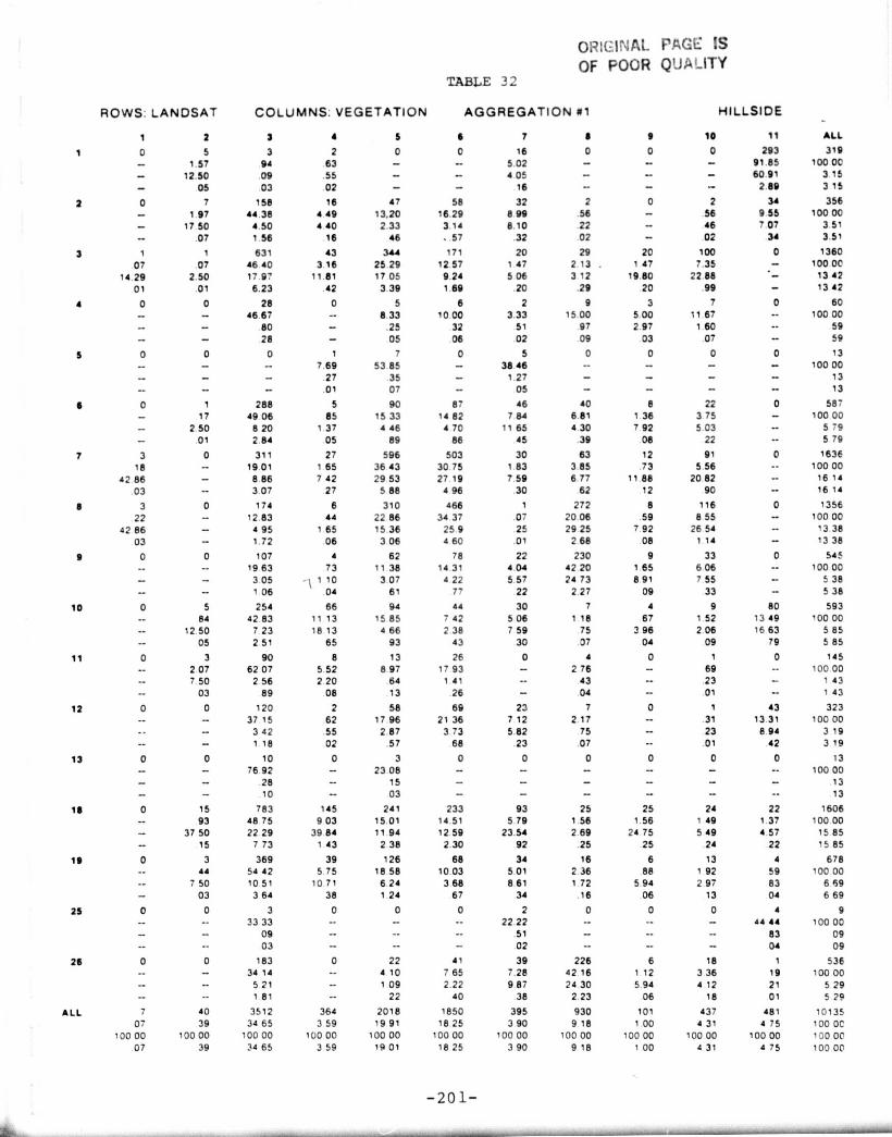
ORIG'INAl_ PAGL IS

OF POOR QUALITYTABLE 32

ROWS LANDSAT COLUMNS. VEGETATION AGGREGATION x1 HILLSIDE

1 2 3 4 5

1 0 5 3 2 0— 1 57 94 63 -- 12 50 09 55 -- 05 03 02 —

2 0 7 158 16 47- 1 97 44 38 449 13.20- 17 50 4 50 440 2 33

07 1 56 16 46

3 1 631 43 344

07 07 4640 3 16 25 29

1429 250 179' 1181 1705

01 01 6.23 42 339

4 0 0 28 0 5- - 46 67 -- 8 33

- 80 - .25- - 28 - 05

f 0 0 0 1 7-- - -- 7 69 53.85

- - 27 .35

-- - O1 07

6 0 1 288 5 90- 17 49 06 85 15 33

2 50 8 20 1 37 4 46

- O1 2 84 05 89

7 3 0 311 27 59618 -- 1901 1 65 3643

42 86 - 8 86 7 42 29 5303 -- 3 07 27 5 88

9 3 0 174 6 31022 - 12 83 44 22 86

42 86 - 4 95 1 65 15 3603 — 1 72 06 3 06

9 0 0 107 4 621 963 73 11 38

— — 305 , 1 10 307-- — 1 06 04 61

10 0 5 254 66 94__ 84 42 83 11 13 15 85

1250 723 1813 46605 251 65 93

11 0 3 90 8 13-- 2 07 62 07 5 52 6 97

7 50 2 56 2 20 64-- 03 89 08 13

12 0 0 120 2 58-- — 37 15 62 17 96

3 42 55 2 87-- — 1 18 02 57

13 0 0 10 0 3— — 76 92 — 23 09— — 28 15— — 10 -- 03

18 0 15 783 145 241

-- 93 48 75 9 03 15 O137 50 22 29 39 84 11 94

— 15 7 73 1 43 2 38

19 0 3 369 39 126-- 44 54 42 5 75 18 58

750 1051 1071 624— 03 3 64 38 1 24

25 0 0 3 0 0-- -- 33 33 -- --- — 09

-- -- 03 — --

26 0 0 183 0 22-- — 34 14 4 10

5 21 1 09— -- 1 el -- 22

ALL 7 40 3512 364 201807 39 34 65 3 59 19 91

10000 10000 10000 10000 100 00

07 39 34 65 3 59 1901

6 7 8 9 10 11 ALL

16 0 0 0 293 319

5 02 — -- — 91 as 100 OC

4 05 — -- — 6091 3 15— 16 -- — -- 289 3 15

58 32 2 0 2 34 356

16 29 8 99 56 — 56 9 55 100003 14 8 10 22 — 46 7 07 3 51

57 32 02 — 02 34 3 51

171 20 29 20 100 0 1360

12 57 1 47 2 13 1 47 7 35 — 100 OC

924 506 312 1980 2288 — 1342

1 69 20 29 20 99 — 13 42

6 2 9 3 7 0 60

1 000 3 33 1500 500 11 67 -- 100 00

32 51 97 2 97 1 60 59

06 02 09 03 07 -- 59

0 5 0 0 0 0 13

— 3846 -- — — — 10000— 1 27 — — — — 13

-- 05 — — — -- 13

87 46 40 8 22 0 58714 82 7 84 6 81 1 36 3 75 — 100 004 70 11 65 4 30 7 92 5 03 5 79

86 45 39 08 22 5 79

503 30 63 12 91 0 1636

30 75 1 83 3 85 73 5 56 1000027 19 7 59 6 77 11 88 2082 16 14

4 96 .30 62 12 90 -- 16 14

466 1 272 8 116 0 135634 37 07 2006 59 8 55 -- 10000

25 9 25 29 25 7 92 26 54 -- 13 38460 01 268 08 1 14 — 13 38

78 22 230 9 33 0 545

14.31 4 04 4220 1 65 606 10000

4.22 5 57 24 73 8 91 7 55 5 3877 22 2 27 09 33 5 38

44 30 7 4 9 80 5937 42 5 06 1 18 67 1 52 13 49 `00 00238 759 75 396 206 1663 585

43 30 .07 04 09 19 5 85

26 0 4 0 1 0 14517 93 — 2 76 — 69 -- 10000

1.41 -- 43 -- 23 - 1 43

26 - 04 -- 01 -- 1 43

69 23 7 0 1 43 32321 36 7 12 2 17 -- 31 13 31 t 00 00

3 73 5 82 75 23 6 94 3 1968 23 07 -- 01 42 319

0 0 0 0 0 0 13- - - -- - 100 00

- - - - - 13

- - - -- -- -- 13

233 93 25 25 24 22 160614 51 5 79 1 56 1 56 49 1.37 t 00 0012 59 23 54 2 69 24 75 5 49 4 57 15 852 30 92 25 25 24 22 15 85

68 34 16 6 13 4 6781003 5 01 2 36 86 1 92 59 100 00368 861 1 72 594 297 83 659

67 34 16 06 13 04 6 69

0 2 0 0 0 4 9-- 22.22 •- -- - 44 a 100 00

.51 83 09-- 02 -- -- -- 04 09

41 39 226 6 18 1 5367 65 7 28 42 16 112 3 36 19 10000222 987 2430 594 412 21 529

40 38 2 23 06 18 01 5 29

1850 395 930 101 437 481 1013518 25 3 90 9 18 1 00 4 31 4'5 100 OC

10000 10000 10000 10000 100 00 10000 100 0018 25 3 90 9 18 1 00 4 31 4 75 10000

-201-

ROWS LANDSAT

1

s

7

10

It

12

13

1S

t9

25

26

ALL

1 2

0 ^1 57

12 50J5

0 7-- 1 97

17 5007

1 1

07 07

14 29 2 5001 01

0 0

0 5- 84

12 5005

0 3— 2 07- 7 so

— 03

0 0

0 0

0 tS93

37 50.- t 5

0 344

7 5003

0 0

0 0

40

J7 3910000 10000

37 39

0 1

-- 172 5001

] 0

1e —

42 86 -

03 --

3 022 --

42 56

03 --

0 0

0 0

^+^ .. ^1lulll PR.GC ^ ^

TABLE 33 OF POOR QI+AL_ rrfCOLUMNS VEGETATION AGGREGATION 02 HILLSIDE

3 4 ] • 7 a 9 ALL

3 2 0 0 16 0 .'93 319

94 63 -- 5 02 9185 100 Jo

J9 55 — 4 05 6091 315

03 02 16 289 315

158 18 99 32 2 34 356

44 38 449 2 2n 27 81 E 99 56 955 10000

4 50 4 40 5R 2 2 8 a 10 46 7 07 3 51

1 56 16 08 98 32 02 34 351

631 43 101 463 20 100 0 1360

46 40 3 16 7 43 3404 1 47 7 35 -- 100 0017 97 11 81 7 28 13 19 5,16 22 88 13 42

6.23 42 1 00 4 57 20 99 13 42

26 0 13 10 2 7 0 60

46 67 — 21 67 1667 3 33 11 67 — 100 00

80 — 94 28 51 1 60 — 59

t3 10 02 07 59

0 1 a 1 5 0 0 13-- 7 69 46 15 769 36 46 -- 10000

27 43 03 1 27 13

01 06 01 05 -- — 13

:88 5 79 146 46 22 0 Sal'

49 06 85 13 46 24 87 7 84 3 75 — 100 00

8 20 1 37 5 69 4 16 11 65 503 — 5 79

2 64 05 7s 1 44 45 22 -- 5 79

311 27 95 1079 30 91 0 1636

1901 1 65 S 61 8595 1 83 5 56 — 10000

$86 7 42 684 30 73 59 20 82 — 16 14

307 27 94 1065 30 90 -- 16 14

174 6 318 7]a 1 116 0 1356

12 83 44 23 45 54 42 07 8 55 -- 100 00

495 1 65 22 91 21 U2 25 :6 54 1338

1,2 06 3 14 7 28 o 1 1 14 - 13 38

107 4 258 121 22 33 0 545

19 63 73 47 34 22 20 4 04 606 10000

305 1 10 18 59 3 45 5 57 7 55 — 5 38

1 06 04 2 55 1 19 22 33 -- 5 38

254 66 47 102 30 9 80 593

42 83 11 13 7 93 17 20 5 06 1 52 13 49 10000

7 23 1a 13 3 39 2 91 7 59 2 06 1663 5 85

2 51 65 46 1 01 30 09 79 5 85

90 8 5 38 0 1 0 145

62 07 5 52 3 45 26 21 69 — 10000

2 58 2 20 36 1 08 23 1 43

89 08 05 37 -- 01 — 1 43

120 2 15 119 13 1 43 323

37 15 62 464 36 84 7 1 2 31 13 31 100 00

3 42 55 1 08 3 39 5 82 23 8 94 3.191 18 02 15 1.17 23 01 42 319

10 0 0 3 0 0 0 13

76 92 — — 23 08 — -- — 0000

09 — — 13

10 — -- 03 — -- — 13

'83 145 137 387 93 24 22 1606

4E 75 903 8 53 24 10 5 79 1 49 1 37 10000

22 29 3984 9.87 It 02 23 54 5 49 4 57 15 85

773 1 43 1 35 3 82 92 2J 22 1 S 85

369 39 58 158 34 13 4 678

54 42 5 75 8 55 23 30 5 01 1 92 59 10000

1051 1071 418 450 a61 297 83 669

364 38 57 1 56 34 13 04 669

3 J 0 0 2 0 4 933 33 — — 22 22 -- 44 44 10000

09 — - — 51 — 83 09

33 — — 02 -- 04 J9

183 0 :48 47 39 18 1 536

34 14 — 46 27 8 77 7 28 336 19 100 00

5 21 — 1 7 87 1 34 987 4 12 21 5 119i61- 2 45 46 38 t6 01 5 29

3512 364 1388 3511 395 437 481 10135

34 65 J 59 13 70 34 64 3 90 4 31 4 7S 10000

'0000 '0000 10000 10000 10000 10000 10000 1000034 85 359 13 70 34 64 390 4 31 4 75 0000

—202—

N _

E O y 0 c E° y m L O p c L a C O p an y N y m m Y>= y y= E u E w as- y C o m - c N a j O y N m D c= y oo`

9 c c m N m ^> - u o N c^ o- c c v _m ° a c 3°^ 3 H o mm y O D m m m 0 _m = U O m C N m a) N Wy U - a 7^ C - N D 7 m a) O c O U a) Of c m y

as

o y ° c o a o c L o > .S m° a0i a c 0 E m a _° as m ui a

o r>m = m F- - a) N'm E 0 E O y y y as U 7 L r y E y-

.c t _u uoi c- >- c o a^ 0 c N °' c u v ui i N E c c o 0 Q? - > o0' Q c m D E o >. m Q- ,, m N my Q C E o y c m m w y D c

ro 3 N % c L E m y E m m E m `a o yN L o E G y a r N c N U a) m' w y .0 ti L° y c y N cn

C (nHc30 E^La^°N' cap

00 E -0 asoasz n co or 0LOO^E aci.^

N N W mc y° a m m CL u N ao) a E

o a_ E m 3>- ^; a rn° D>y y m _. m o o E N E y >. N _u E o o f _° y c=> c Q c ?^ m

D a v v c)

cn y ami N c

c >' cn o c D N a) as y m c°i E _c a D c =°

L y u o m RL c

`y' ` .H = m m c o ?, ya `° _^ L Q O N Q y- asai L G v c c C'L w ,c aui a_m m E cs o c u m _o _0 0 ^, u m >>. 0 E E _° c v y

m L C m ~ Q m - N'0 w o f L N y D c

`n v N -- u n; c y-0) _m Of H N a) c° c c m O a D a o m o a Q) c ` 0.0 - n 0

CL a) L a

T, 2 En U C C N L L C9 C m` y T m m auj L C> C > ` D-o I >W C Q) -,n rJ - V O O p >. N E o` m U V c L N m C m _` y= = 0= as Q

m t7 ` 0 p U c p u n L L y E y i L - m `° 0 0 a) ^° c c O D N m m-c > c y D c m N y as - cmi c y o o cn o c E° a a a m L c _c w vE >` _ C as m O m Q) L Q U L m C1 ^' C C C) N H ° j O 0 C C vi N C = a) y Eo- m a E c c y G o N o 0 _) N c 0) --_ o c .-

ac a^ c y c E m c a c c -- c aEi 44) u i C - c c m al

E U c C c = m " _ o c ^, c° c m ? 0 N o o c -° ° yy `° a^i a c a sm- m N N m 0 u m m m L N >' m G > o U ai -> y mL c c 0 a N >. L >^ N y` a m n c o 'n c a^ a c o c C) E_ ? N m y m rn° E > c y c p c o m - N 0 m m L 3 °n c m o)cm

CL y j `v c cv

° y o ° o o D 10 E ° m N u a as C ^. L U O m C

a- > u m m a) > L ° c0 0 0 m r N m e .c ai a^ ° m s m E_ c n o> m_ m C) ci L u a L >. >' ) o t° E m m o O o a c c a m 3 > c c o mc c u L m m . c - m ._ y° y N c o c a- o N= ai - o as3 o E N E ° Q c S a m M o as -C E a ° C_

aui Cl c y c m

as E

0 M a a m N D Q a

E_ L m 0 F- t

y = N> m y o o c J L o y m y N N Q) o)m >. O n-` L m = m U L D] y C m O m 4 0) y N LL a) - as a) c a~ ti - u O O 7 O c C L U C ° C a Uy y

C =' j E >. ai p c O 3 a y C` m _^C N O (1) y uyi m U L

°' Q c > o m 3 E L_ E oo C^ c° n L ° v a3 d > o c o Q 3 m _ = 3v-- - u E a^ _ o y o m m G u a. a °= E U o Q) u o 0

ago p °y-D y^ cLN^L?'m oo C c^^ocGCc -as

c c ^^ o L c c u m L m 0 o c `o c y o m °' - ¢ ao N c N 3- o= m y L O 0 c o u c cv C mUIs 0

E~ 0) c o N y m =_ o ai E m o N ^` c u c E as N L 3a) C N y m y L p m N 0 "aO m y C N a) o N

as O UO m 0) C L C) x CN <° y c U N N D O c > m 0 U L c y 0 U y m

0 umi a Q ^a o Cl o c ac) v u° 1) t o E °^ o O 3 c E z ^ a c m C c La N m° v u m U m o m _ E L m C E = Nm U C _ E y > N N `D `° r 0 u u c ^' t c m c m a° ° ._

E o L c= c, v m 0 ti o c u 5 N y o n E u Nym m C C a) a 0) E N a _O m a) N 0) 10 m 1 V - m t y-0 c C

N c- -^ t E vi o c a^ a) c m a) N tm c D aia > C u> m D R c y°L v c" o c y y c> > 0 u c c c y o c o c - o o `° m^

C c c >' N ci u a t m c o N a= >. C D C u °^ c o (M O n. c= o m

h _0 m m y j c L- D C _ p m i O c y O m-o N v .^ a- c p o 3 0- o ai m= "s a)a a o c G^ c N -c .N m _y E u cy a N o y o m m N - C u o c- y c >. m 0 ~' y m m m 0 y m xo m c a u G E ?? .° o y s^ c c m m o a E O E_ E I- Q) E vma E - E c> ^, o'a y m ° c c a^ ° p 3 N C d a as E -C u v v; c aE m° u a^ c c c c y a m J p o E o a o y ° O m y c c a^ m EW uyi > U^> o `° m o m = c _O a 13 0 c O c U y ^. > N D cm E C c 0

Q :°_ v o N E 0 O > m >. N m O C > 7 0 E o _ uy D m c y m a) = a) 0 N C D ,Q = U _> m a) ^, U .O U C N O O > m O Yas

y u 'a a_ > o N m m >; 0- > a y 0) o U o .. u as m u D m ._ NO) C O a 0 0 C .`^ U m_ a D m C C C U m U .^? V - mC p a) y m y ual a) v o m 0 in ^ m m m L z a) m o> ") c a) N

O° L u L m N E 0 y .N Q U N N > m m y c ^ ~ u

c O V D E m m

c m = c N o10 M

_O ° c t >. > .m E o L U E U N

a m c U

° o c c m oa a c m` upi y a c c M-

a^ cn

L .J V G O N >. c a) v c y y N m m U a) N Q a c U m y N y -

V y u- c 0 c E c D a' o m L L = u m y _ E y Q m y as y c > 9 EC E m- - m E c o m m N c o o N L - E o oJ m N > O a a) L G y >. a) c m c O a C U Of y 3

1 O C O = N N Q` C1 y a)U t- m a) H- L >` C 0 O o L D m E c O m U m t _C p U U m U m? D U D

no _ u 3 m a c v u c O - N 0 c> a= c°( m yf" ^C C7 r Q- u m a m

-203-

Cm O o m 4 ` O a 0 ^' c v' o _m E n j co V >. E N 2 O -6 aN

E E o m a N N m c^ c m e o m u m c c c o m `^ m H v.o E V = a C o c E `_° y a) u E i

a) — p m o cza, > c m^^ a t o m ac CN c c a) a - m t c c E u o o >. v x c n c a) " uE u o > v o, c ,n 0 y m m 3 a _° m a) m m r ra

N a) C N 0n '7)C m R' y

TL ° m 3 V y

o ^' c L C w— C E C o> u, a) m C> cn m = N Oc c m u i^ o c n^ m ^' c a 3 m = W m m `° a

C

> a a m o a C u > C m u E c E y m m- m >. c m ea s c ^-C m co a a, N v H > m a, is awi m E vE

> c a N " o m m E a o c `' c m —'

U y 3 m L L m E 0 m ecn a) - mm ^ _ n C c m _ M m a

o w cno f c u c c m > c U m m o m > ' a> m m D aU c a `^ a`) io a) = o, n •, E ^' n tr, m N 3 E a m mN m

o c c = v m V c m° o= m cn L -

m E f° m c m

>m c- c m c u, E L o f ,,; L c v c o c E E a=

c a) m c m >> O m a c c c

J m E_ E_

^E N a n c i o a c o u o N o N ,r Cl d m

> C° n a a m m m c o r m m m ^ c N E t °

0 0 > m O L m C m Q, m m u m o L _>. C C

'o E_ m n M aa) o ^,, c o u, m- c= 4n > Q) n mm c° o >. n

ID a)c °= m m L E c>c > O ° > m n a "' o u E >. ° C E

C L C N C L m w -j O N= C m -- — v U w^ — a O H C

N = E mo

�v o c- C 0 0 o `-° U a _> u fO o m -C a U `c O ,GnC N C O .= C N m m U

- cco

Cl t m 3 m c°v c c o ^ o N M t c o o m m y LM ' `-° c=n vin a;i u, mO > m U m O m L m ^ O r v C C _a m m m _ o a= E m a m o a, a Q .c m E com °, v 2 Q E O E 3 %- c> c °, c o_ u; m a ° Inv, c m m u, = a)

Clz 3 Q --) E c m cn ^ ^ c — ^ c° ^ v ^ tu o m e — m = a) m v,c L m cn c cm m m cv, cc) c_ d c, a) U m M a, o . m mu

Q cc r am a 3 n m c-E E cD m E m E -j- N n -j d m

a)°,^ o o

j T 3 o o E o o w o N C- O, Oc mro a ccaN

sC

o= nN

c>—L Q m>m

° m o >=

U>

Cc u_° u, =° n c ° v m E m

v m> m a m m m D t 3 O m C O cp m C CO m y 7 C v, O O G a C m O Lm y a o L ,n ; L o a a ui y E cco ° m ° m _o m3

m ao _ _ _ _ m _

ca, E c m F aa

mv_c`v

o o^; N-0 c u > —_ o m a m m m ti o >U o mc m

.T—

C;L c

m N?m

cC9O m

7 iO E m ai > p m L :° 'pO

C_

m •- Ou

O^o

d)v= o f° °- ° iv

--m .^o` c a`, u, r `° t o m d E

co E

°>

Q c a) co o c mv, ai J c c

o c m n >Nc c=a a t > n. ac

o v,w U cc3 m — n co- a

U

;= a om c

m m m .N m

aa)a)

G y N Lm

L <n o c m % Eo, i^ cf°

o 1 > oc

m mE o, p, a- m y o, c y m 0

oa o E m o m a m Y ai m o c ^' c_ m m m m a) o f .c c odv m c % c v mE nc `° C

m e-

^ u = o .ccc°

c3

E m a)N=o c L

D- m >a n a

o ccN

c m .ca`

mo c 0 m - `n m mm y Cl a m y o ^n O' -

> am

E m r c u

o E= a)m 0 d

U—tea, c Q, t

a, a

c c c m or a) 0 Q E c c oN o°

0 In N N Y m

°O C_

mc o m 0- m E m 3 D U m a) c

om°

a c a)a

o m.0 m> U c mD `^

°-a) >

a—a a`)

.o ° yc° L

o_ m m c o a)u,

> a,:Do

N m N cm

; ma

cm

m a)u^ U c

cm

N— m a _O t p c

o, Oa) E N ° o

a) E D L E a c v, ° o c °m

m E N =° m^` o m o a (n ° c c° c m

m m m o m-0 U E - m o o E a E= E C. ? o>- E m ° 0 0 °),n a C Lu O on

i m L y o s O, u, C a 0 E c - m a, c 3> _> E m e-Evn `° L E a `_° a U o m Ic m c m m o a) m p ° c L ,

1]U V> o z_ m a Y v) a) N c O c a c m> i '^ m m O a m yC C '' U O=

Cum) L L

'o0 m 3 C 0 a>) ^. O C O c N m C o'`

o —° wQ1c c v, c _ m =

NiOm 3 y m e c a) 3 L E a c ° c c m c> ,"'„ E m ° hc c E_ m m c a _o m u U a c p= c a n c c

d c° w n _m _c m E m m%

a (n Cl c m a m = m oa ,n a na m

c9 L a) na)

c=a cn -N _

E o =

mCl o

c m

1 E p E Nm a)d

mt

E °—

Eamt m

mt > c ° E

I m-0> c c

y m c= L m

m = E a o ,n a) c E v 0 t ° ca o m ^, c t_ co U _ ^, E a o .^, mL cn

m o o o c j a ^„ acn) y 70 a° c E r. > c y E L > cce 3Qo

c a) m > c E m a c c, = o a m mate) r-

m j w a o> a m o a` r a`a

^'o; N

m E U U 3 M o C ° oc

U C to m> _ N > Um Oa a) u o-

U m o c O a,cL c •c

C:c n _ cc `

= c:c L) c m U m c^ E 3 U E Q z o ^ m 3 cc _o—_ t E_ 3 _ 3 a > m v s _ U a m U m

-204-

na Ly m y m a) m L a) y -> a s Q y m ^, a v y Q y m N C y Ua V O E a V > N a 7 = N ? N w E a a c 'n t L > ` ` 9 L > ^_ _ _ a _ _ __

C N m N o c m N v c y J a 'R N 3 'vN mN

C N 7 C am ? n y G rQ ma s y '' a> o c ^, °' U E c X o a c L N n m a n _m o E o m o m^, m L N m N N v o E m ^, O ^' ? y 1 m L o m v a c° a ° a E 3 0L a G N C E E a) -M N U 7 n C y L - a m C U - C C U m m

° m L C C C m ° ^ :. N m- m a m a - y J U C N ac y a_ _c' In ai E c c 0 0 m= N E m 0 o ^, N Q >, m D ° c ^ ^ m o c E ° aO 0) o_ >` _` m Q-0 m m O C U C Y 0 C t)T y v m Z C m

C L OC N= y w > a) m O O m m - L p - a E- a) E

m O L C >` v _~ N c C a 0 0 L L E U y a y a c 3 m

C a p

m Cl o a c 2 mm -v ° 0 c c' a^ E a o y _> > m o o N E l a m C L c L N o c ca v a^ CJ a^ E m m >. u, m e t; L m m E a a° c `-° L o m y o L c- yN y c

, >. o N o a R `v ~ a° m r> o c m a ° E y cQ1 N o m cE ° L 0 -' a c o m_ c rj _ >. E_- m c

m o a n ° R= ° 0 ^- 3 acv y a= E N m m m N o N o m% w = c y oy m U o a > L D a m m >. p m c c> _ cn - N C N a^m °° a _N m >, U c p a E_ v E N m O) J m m O> p>

a cn y> v c a L W m L c 3° Q m E c c o m ° c^ a°i y E N_m m a w a^ m N 3 > m F- m e > m a^

.y a^ _ N y 0 0 0 E c L .o Q ° m yCL m O m o m n L m L D o J 9 ca >> U- n ^

m y 0 .0 c a U cO N y L - o L a) E° m _^ m _ U Q _ m >, D m N U m m a .T ^ C L

N U m e O N > a - L« N c G a) m C m a)

y of C O I: a m a) N C m J_ O G E m° a C m L a) a N ^ a C m O N Cc m m U 3:c ^° t > o c^= a u m Q ._ o ° ; m c m m N 0 m m c c N o ° o

v _N °, " m -° E ° m ^ -v o m m N o^ ` 0 o p m m o 0a c U m L C >, E i^ 0. `^' E E m -° a

c c E m o `° c_ m a° c w m °° Cl c L N N m > a a E y° m a0 c m N a) - m U C a^ E U a L o a m m a y m Q m E N> w

E a o y N m n _c 0 E° m ° °- a i m-o Ln u _N E 3 m V) ^' >? a^ o 0 0 °a o>

cn N v ° t W ;^ ? ma c o a m" `° Q a ti 3 E L c +c c m .^_' E W m 'o c w - m> °?^ c ^- a m c c c o E v 6 L o c °' W ^' ° L > L c ^' ^' c' ° a > E° nV S O E L m c C U O E O_ °= in >` L a '' O m N C . N C a C -^ m 3 N -j m- c N 0 m U E ^- - c c °^ 3 >. N m c m a) m c w N m m c c3 cu c °o v m e n c E p L L- N m ~ o 0 c

E o a ti v o m ° C. N° °oy L cp = o ` - y a °N' a c L U L c c a^ _ a^ - _In

>, ^, = c ° ° = c^tNV ai w uLi E

L >, m a) L C ... L - U a) ry 'm ` m- cO n m a 3 C .ny a N L 0 a 3 3 c n v]i aci E_ o N o_ LL o• Q ^, c° a c o m p s

m G a) N v mt m ? E-7 Nc L N , - m m c o y c c c c° 0 3 c ro EE>_ p N._ m F- m m a) d o Y y m m- N a) c a) ` E m

" L Q m U ° m E E E m y TO ° O ^, m om e c 0c c 0

mm x > m L a m 2 c >. U c

_ N 0CL

N M t o a^i - c c m c a > p m o p m n ° N m mo_ >.^ m L y c o Q) Ina E m a= ^ o m° Q N 2 L m

Cv a O U Q O y m w Qy c c Q L > L c CL N -0 a E c -° U N w m c N m m Q ^- cc m N N © " c o c L N D c L c 0 m _ a .0 E oa y L E xo m m o = m y ate E U o >._ m c 3 a c'^ a' m _ c a

3 E v M v o a m y E -v ° ai v Nm m o- (n m n m L m o`

c u° E o E„ E L° E` a c a a > c ° L a m vii c Ep U m U = Ca^ C o m c ; o N m o o N_ r E L m m° >. U m E c yn y m 9 m m N N v ° N

m a^c a o o m c N H w 0 o o a

Ln `° v aDi `° C N C m Y c` `° v 'm a m N 0 C O _N

^; c c 0 _- m ? c m o= j m= E m t cn N N= N Q >' m a N o m °" 0 L oa a 0 _ M _G v =- v " " o E m cr c cn 0 m a E `c o m0,J a)c 4 a m a` ° y m o cyi c m °^ _o c a m ^- Q° M° c c a c

c E U- E E m U c °' 0 c o c 0 0 c' ^' x V) - E Z E N _m ° m m a^ o mm a U m o a E m` N c o c m 9 N N m m o m o n c> U a v N o NE c = N° y ^' o m a o° c a c_ a _ o

E_ E N y _ N -M a E a L c c

m G N 0 TJ 03 am) O o M^ m >

CO a O N Q ° 0 v to = u-i m Oc 'v = a a v 0 ° C _ c 9 m m a` c a " a" E m w a^ xCL =' (A^ m m a c a 3 c °v ^' O v E N- L E E m c m t m m E CO

E a°-0 0 __ o D a a c> m ^, a c o rn o c x 3 a o o a 3 m a>>, m _ c Z. 3 c N t0 U ` US Q L m o c m a m ° a m o ° `° ,_ c° Jc

°- 3 C ao 3 3 c - a te o m c o^ m o m- U - Q L u a E a C _°m e =° a U m` E o a^ a m m 9 m o c

°Ti C° a

a N `N° 'a 3 -° m p m m m m N m c oc m >. L y v m m m ; 0 3 m m _U m y m m C ; C C c c= T O

c m; 9 c 0 c p E N Q 'D= c c L o 0 0 0 0 m N Dc o >. a 0 c 0_ L c a L c^ m N L m N a- m -°° E O a _U L m 9 L 9 ° _°' m L N UO m

m cC m >, E co W L 3 ^ 0°

N

bo v m c 3 L _N E = c 3 _a __ m a 0. N_ - am m- U a) m N C L m m 0 C c Lf O m m U CV a ° U a N N a) N c V m y m >. m aJ c J :/I ° y °

U= y y 3 m c N c c o c- c c ° t v; a~ C) > ci c_ y y J y O O c J O m - y c 7 -- m cn L

- C n C w.0 o = ° a ° N a E n m S a o U :° 0 aw m E° U m a

-205-

U c

Eo a)

o crE0)

_o

co

'oa)t

c ow

a) 70 a

U3 m c^^ c —

' ° 3

EC) cna

a^ cno

N °c

CDc

LO o. a) aCL:v

—M c

acv

E E Ec L

0om.^ E

cm -o o

E0

U a) ^ U

cI a

^.cn o

a

a) cn c U c

= a) :3.0Lo

a)L cn

O Ucn U

(1 W p

• • •

a)

CD °c a

^ a^^ a

s _oEa)a ..

O c EO o

oL a a

a ^'^' c oQ ^' o

co .^ cU

c0 U cv m U

U C.V 0 C ca

m— 0 CL CID .D

a

EO cv

^'U

E o ^' U

^ = a'O

^ L cn

^O C

oL ao ^t L

n)

-206-

L p C O.

a)•

c°O E oco ^ .'-' ^ U c0

m E ^C

o a)a)

EC

o c a^— v Y

C U > ca> - `° o EC

UOE C U

U O O C —

U cC . C c0 cvC E a a)n R7 ca >

E o E ai

aca

OCL

E E o oE7C)o — ^-- '^ ^ `°

^ c o a a^

o_ ^' a) m a)

o o a) a) m

U cam

o

aCIO ,O

Cm '-

C1cn p

O O a 70

CLp c cO

o-- E >.-.

t cm ?. o L

^'c c°a) m a a

07 ` cn L U a) L_

U

C a)U

X a)> cn N - - a) L

NL•._ .^

a)m a^C

>` U

O — — L O —> C

U -0 O^ ° a o 0Uc^

a) cc^

c <n

a)a)--

c—

^a

—_

CU

O O O O ,= O 0 0O F- U t— I-

• • • • • • •

-207-

i

i

ct3 ^ • ^

C O cn

> EO 1]

U U Q. a d

O (n C U(n U O O

(n O U a

E c^,O^' a -0 70

UU U

ErI^ ^ ^n o ^, a^vA^ c 0) 0 C CL cv

W" '^ ^ O3 Q^ U w Q a) c^ ^

^• c c cn O (n c OC c4

C-(S! 70 a)

-Y a

.^+ E _ U E a) -0 C:

O.^(n

.^a)

UQ'e > v,C U Q Cw (n (n a) M 0 E'

3cn w a v cn cn

70 W O '- U a) L

ccv

a

C c O cn Y U a Ua U cQ- cCi U c^

CL-_

a) 0 >. C C Q1 a) co

_

Ca) ca cn -0 O cr cv cn

O cn <n C C — CD CC w

OZ7 c0

E UU C c^

LOU

U — (ncu c

>o

a) C

-_^

.a

CC Cl. oc E o a c E r E

o^

- CQ U ^- E C7 ^,...

_ O am m m cc v C c^ ^, N o '^ (n c c^

-a ^ E .- LCD c E >,

ECL,'a

(ncct ^.

cn^. O c o o a ..a }. c .c ^ o L c (n C a

a^• . • • • • .

a^• c • •

—208—

c

n^U

COn

wa^3NCA.mE

Q

x

c

GG

a^L

c

10Gc

iocUUd

c^N

N yGM QEcm Lc U

XT3

WCLCLa

r`c(vE n^QJ NNmCD W

^ C Uo d a^

t ^ oN

t

3O N

M

cO-

N

N O)

ao

(n—

4)

O

E

cn

^Ccfl

Y

p

Nmc

^,

3

^ON

_O

J

'D0NG7UUQO

CwF-

U

aLn

ONCO

ENC

7COU

co

Nco

w

L

E

O

cW oN^ m

c>

O^n

o

c-j

=

O

0

o—

cvCA

con

ocn

U,r

ycn

L

3

;

Z

¢

m-

ifl

E_

con

,

=

cv

G-

m

E

con

E

cv

M

>a>

-- N c7 V vi t0 f- a', Qf C) r- N

3O yO ^G

EL OF- U

—209—

OR194 SAL PAGE 11OF POOR QUALITY

a

cD^a

a^

Ua

AM d

U D

ra

Ca

V a I

a

a

n 1 r^ I

rn

FIGURE 37(4): LAND USE

-210-

ORIGINAL PAGE fSOF POOR QUALITY OF

^T r w - w 'nil - .a^^ a ate- ^,o

Ir Iw W tw r Iw ^ ]f !WO w a ^ Irf^ a

am--owi D.]+ I Iw Im r^>io^ w w — o ^; M I1 1w 11 ~r 1 '^ ^^^ a w

,r Iwr .w a am." ,— .u]aro ,r i a~ as .w

1 ]- y

!^I o w 1 s .w am]s^ .r Iw .rIr 'I

I/11^J d allaw

!—Iw Iw w w-+^ :— ,w to a

^Ir Ir Ir Ir ' a 1.60m '- Ir I^ ' w - 4111 r a.111111'41111 im

pow _^___Z6—^^ "ti.0 air f

(am^° ` I40p r a0 a^m •'^ N^ a a 'momg a C 1 r ,— ^ rs

. 411111 ^s rs Ir .o !— a °]w ,^ Y a , to a

j^n^-1}' ^/ I ^

MMman

lu,up 1 to

1 ;w i° ^ / 'w ° Ir to f rs4111111:a a ,olr ' wam

o to n to Iv►s a^^ a w

Iw a an a^ Ir !r Am

lr _i '- ^a '^f7i ^ aa. to ^ Iw "°' /\ 'w w,o a ,w 1 '— a a L. !s ,r to

1 a ^ ^^_ o

1toto a a a a a r 1 O ^— a a

lwp .wI as :701"" a ,r,r a r]r 1! a a Wall,' — =A '—,

^! a ^o►]^^° °^

]m lw .r-311, a^ I to Ina

,^ .:^ nIw

.mr ]s ]a I »e a ,w as a I— aw a r ^ ]s ]^ *^ Lo'r9 M r

]r w a ^`( a °r rA ^.00r I^1 ^o Lm '— IwI

7 M

am

an Mal

M v ' w'I^^"]^j^ I Ir J 1 r I am]011111111 All ne sryry]I/m, r]►^ to rmm ]F].. a no ne w--f'° \* ^ '—.R, a r^ a ° ^p ^1a iA IW

^, a ^'—fl/Jr1^ rA 1'pl Ir Iw I° 'S :R^^O Iwa J^ C ^ I^ a T11

!— i J.O fl1 '^^ \ X70 ^J^ r.OJ :0

/\:]0 ra 11 1wa ^ a V :A ;O

lO^a a a \ 1 a o 0

aM

M 011111

'—Teo-^r]o ao]y .^oarw rw l0 1—'—^ Ir '' 60, to "__ f ' a.A '^i 'p a^Y Ir IIYI\r Irk r a ^ ]]r r 1° ^o

l^ll^r A rlLw ^^u ^0a ^ l a 1 ,r-^ 411111 t

r ~ lat. o tea.. a w =140sv ,^rV ' ,o r '-' a Iw

all",o , _Ir .Im ^rw^,o ° ^ ^ Iw Iw

^^ ^y^ a 'r r ^r Iwto l '° .r.1110 _ wono ria a rs '° '— _ 'r ,rr^r r'^°tle T° ^rMlr o ,e

FIGURE 37(B): LAND USE

-211-

FIGURE 38:ORIGINAL PAGE IS

VEGETATION OF POOR QUALITY

LANDSAT/AGIS INTEGRATION DEMONSTRATIONMUNICIPALITY OF ANCHORAGE, ALASKAHILLSIDE AREA

n MUDFLATn SALT GRASSLAND. LOW SHRUB, TIDAL MARSHn SPHAGNUM-SHRUB BOGn WILLOW RESIN BIRCH0 ALDER0 TALL WHITE SPRUCEM SHORT WHITE SPRUCE9 MEDIUM-AGED MIXED FORESTM YOUNG MIXED FOREST0 UPLAND GRASSI] DEVELOPEDD WATER -212-

_

1y^^^^rr

yR (^ ^ • ^ tc r^

No

f ^^

ORIGINAL PAGE 19FIGURE it): OF POOR QUALITY

GENERAL SLOPE

LRNDSOT/RGIS INT - EGRRTION DEMONSTRATIONMUNICIPALITY OF ANCHORRGE. ALASKAHILLSIDE AREA

0 - 3%3 - 7x

L9 7 - 12%® 12 - 20%

i 0 - .30%n 30 - 45%n GREATER THAN 457.

-213-

FIGURE 40: Okl; iiNAL PAGE iS

LANDFORM TYPE OF POOR QUALITY

LANDSRT/RGIS INTEGRATION DEMONSTRATIONMUNICIPALITY OF ANCHORAGE, ALASKAHILLSIDE AREA

M TIDAL FLATn ACTIVE FLOOD PLAIN® COASTAL PLAIN3 ALLUVIAL FAN/CONEf ALLUVIAL PLAIN

TILL0 GROUND MORAINE,ZI END MORAINE

WATER-214-

L ^ -7 J•1 1. - ^, - J _ - ' ^Li. L 1 -

s "^--s^S ^'Z•rgsss'rfr-__ S`•_ s: T -'f _ _'r r -^^i.:. ^ - - _- - ter _'

L +i. .. Z•L: i ^'l :l^:if.r rYt •`? lr ^.s : J+.^a:.J--. _..t^_^ - - F^..^' ;• - Wit.: K* Z.-._ ^.t r ^ . . i. r... C

.^, .. -"'fir ^ rr t•1<'^.^^=-^^^^_^ '_'af': ^..s G^.-x3 ^ _ .^._•: 'i z r+' - .'W.

-•st. - t..^^ _ is z •.^ z _`^ i s _sas-r:.^:_:'--r--a_a ,i_r' x..

r -lo•rrx. -iry+1...... ^-zi r--r>si- a ' i a ;=as i ^-ra• y? i { -r •+!;^" r^._...zrr•3t L L _1.. i. L sii 9i =.12 t_ Jis=^ 3 ^j.S S _: ^:^L \ ^ a • R w,,.. ya _ ^ s.

ZF_ :^.. -__.iT.__ - ^ _ _ :^ ^-.ice?. _r"" 3x.,>.- r.^ -->__. - ___ - __^ ►__. .. ri `'a T .^ : - rc`-

_:Z.._. - __.- •fC_S:_-. •i^i:+f ,^ . :tom L , - ti

_z ^-c ^-:;fi ^__ -{"3'}i:= ._- ^ ^c-_ :t. '^ - ':•r+s^-_y'^- 3='i[ ^^-; .-^: ^' :^.'+s- .'•t t f ..''.y -_ ,: ^ ;

_-.: —_^-=-iii"'^:-_ i^ ..,`iy=2 ,►xy^-.. 'T^^'- ' ^•..y ! .ac-- .c t " t • -.:i -

-

^^

t?..s^r- ^ .x ^- sir -. L J iA T.sis. .^ti: ^^ =^ a ♦ •}r.y-^ ^ _ ^

•s; y .^. : ^_: i rr T__ .{,•yt^ % ^^ ai_s:» i; 'vG_a z .,tt_ 3-M-i r s= .1tc_: _: , y +^.

_ _ rL. ^ s iT'r^ iii:_. T: .': ^^tn1^-_L'iv^i^ ^ ^ .wa %rZ-^•- -^'.1_ "; ^1^ ZL

i - '^ ^'^ _ ^_--4'- j is .e=•'^"-^ '• I :' srJ. s ,- i l ^7'.. ^'•^:

.Lr. .^rf-z. --s `.z - -' - - _ - •_ "LT•'j _ ^ %_'-f"r=•ts s :s a 7 ^i t._.._ r i-r. y- _ _ • a

• - - 's=""'^-_ - _- _^-_.• -. •.t_ -=VL fN dye t4lr •• •-f j•.r`

=icefie

Ar ag-

Z __T i : ^.a i Jr raL r^Y%4 'y..ar.=i?^ -`

.ai = _ .r! _ - ^ ^ •

- _ -1 = `t-t 7• - -J a^a ro -^ - '^--.-.• . .:^ - .aa - s JK 1 _ - t ♦ - -

iii 7i ^`•-^ _ '••`"^^ .I^L^ _ -

_ Z= _ ' - ,^T _.3 -'^- Tom' 7^ -i'i}' = i,^- '^. 1 •' • r-_

^.-^ r _ .-mot T :Y.- :-„ ra . ~ + ._ -

Op^^'^R'.Q! F'?C'!' ^3

FIGURE 41: Cr Q,!P,',-lTY

GEOLOGIC HAZARDS

LANDSATiAGIS INTEGRATION DEMONSTRATIONMUNICIPALITY OF ANCHORAGE. ALASKAHILLSIDE AREA

q NO HAZARD3 POTENTIAL FLOOD ZONE2-J LANDSLIDE ZONEq WATER

-215-

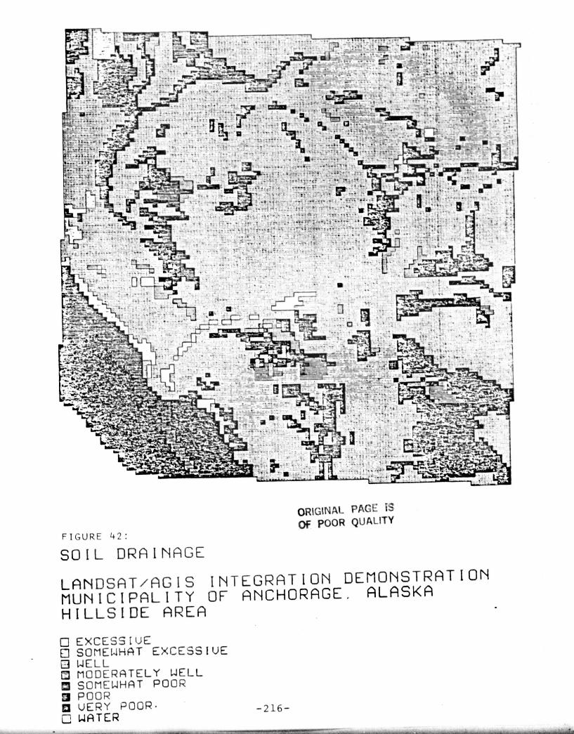
- € :..rte ^`'+^ -^_ } - .. . t _ ^ !^

asa r IaS -- '^

am :r. ►. ^ _ .,^ _ =^_^s-

s

j.

An

LZ

S_ L

— A'

^s''^sz 1 ..L S11 . rte-

rz- L

oi

fad` I 3: Ck!' ~4L^ a

ORIGINAL PACE: iSOf p00R QUALITY

FIGURE 42:

SOIL DRAINAGE

LANDSAT/RGIS INTEGRATION DEMONS TRATION

MUNICIPALITY OF ANCHORAGE. AL A SKAHILLSIDE AREA

7 EXCESS(UEE] SOMEWHAT EXCESS t UE

WELLMODERATEL Y WELL

® SO MEWHA T POOR3 POOR© UERY POOR • -216-7 WATER

_`

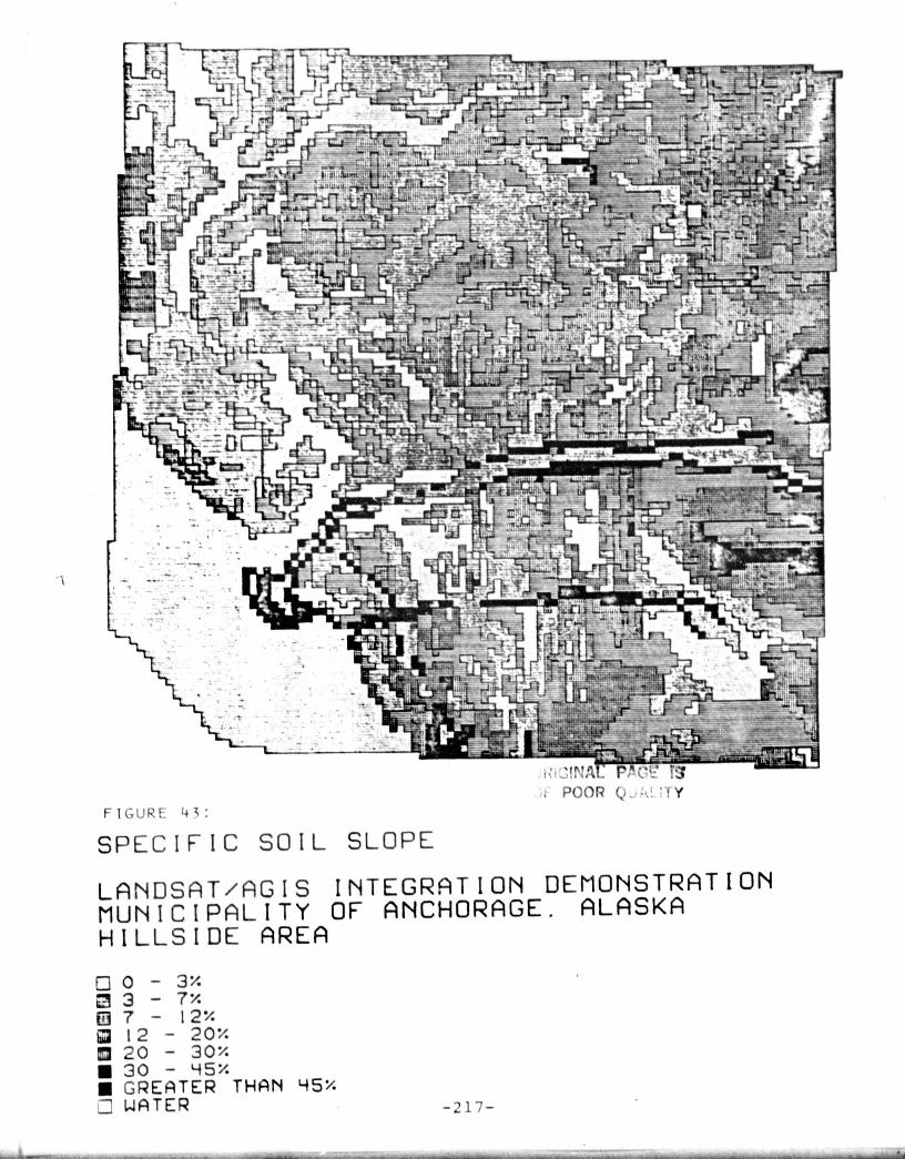
POOR Q- :,. i Y YFIGURE 43:

SPECIFIC SOIL SLOPE

LANDSAT/AGIS INTEGR g TION DEMONSTRATIONMUNICIPALITY OF ANCHORAGE, ALASKAHILLSIDE AREA

7 0 - 3i3 - 7%

t^ 7 - 1212 - 20%20 - 30%

n 30 - 95Xn GREATER THAN 4 5"

WATER -217-

FIGURE 44: WATERSHED AND STREAM ORDER

-218-

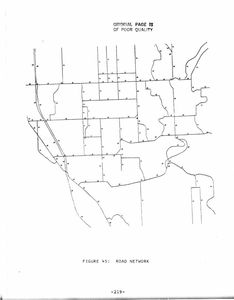
OP!'741NAL PAGE (S

CF PC'CR QUALITY

FIGURE 45: ROAD NETWORK

-219-

ORIGINAL PAGE ISr%r nr%^ ] AI 1.% 1 IT/

FIGURE 46:

SOIL LIMITATIONS FOR DWELLINGSBUILDINGS WITH/WITHOUT BASEMENTS

LANDSAT/PGIS INTEGRATION DEMONSTRATIONMUNICIPALITY OF ANCHORAGE. ALASKAHILLSIDE AREA

SLIGHTM MODERATE0 SEUERE

WATER-220-

OR'GINA! P,,&%GzP,,&%0 IS

OF POOR QUALITY

FIGURE 47:

CAPABILI TY FOR ACCESSE D LARGE LOTRESIDENTIAL DEVELOPMENT

LANDSAT/PGIS INTEGRATION DEMONSTRATIONMUNICIPALITY OF ANCHORAGE. ALASKAHILLSIDE AREA

-221-Q HIGH

MODERATEn L 0 lJn VERY LOW

ORIGINAL PAGE ISOF POOR QUALITY

FIGURE 48: ISOIL LIMITATIONS FOR SEPTIC TANKS

LANOSAT/RGIS INTEGRATION DEMONSTRATIONMUNICIPALITY OF RNCHORAGE . ALASKAHILLSIDE AREA

SL 1 GHT0 MODERATEn SEVERE

WATER

iW4

-222-

-223-

APPENDIX M

Georeferenced Landsat Classified Imagesfor

GIS Integration

INTRISCA ProjectMay 1981

Charlotte Carson-Henry

Introduction

As a final phase in the INTRISCA Project analysis of 1978 Landsat imagery,a test GIS integration was performed by the Environmental Systems ResearchInstitute (ES-11). This integration utilized two test sites, one from eachof the two 1978 scenes classified — the Anchorage/Eastern scene and theSusitna scene — along with ancillary data provided by various Alaskapersonnel and agencies.

ESRI had generated a data base registered to UTM; the inclusion ofLandsat classified data in this data base therefore required that the Landsatdata be likewise registered to UTM. Toward this end, ESRI worked with theAlaska users and with Ames personnel to select two test sites that couldserve both as a test of the vertical data integration as well as sites onwhich accuracy assessments could be made by the Alaska users. ESRIobtained exact UTM coordinates defining the boundaries of the two testsites and provided Ames personnel with those coordinates. The two testsites were then registered to the UTM map base, using the boundarycoordinates to define the spaces into which the classified Landsat datasets were registered.

The following papers describe the digital processing steps thataccomplished this georeferencing of the Big Lake portion of the Susitnascene and the Hillside portion of the Eastern or Anchorage scene to a UTMmap base.

-224-

Georeferencing a Portion of the Susitna Image

INTRISCA Project

Alaska/ESRI GIS Integration Effort

Charlotte Carson-Henry

March 1981

BIG LAKE TEST SITE

I. Control Point Selection

1. Control points were selected using the IDIMS display, the image LLSUS(line-by-line deskewed rotated Susitna mosaic, 1978 data used forclassification) and four USGS quad sheet maps at 1:63,360 scale. Thestudy area had been previously located on a 1:250,000 scale map usingUTM coordinates provided by F.SRI. On this second iteration, a total ofnineteen control points were selected; some were identical to or withinseveral pixels of previously-used control points, but many were totallynew point locations. Those which were identical to old control pointsretained the name originally assigned; those points that were withinseveral pixels of old control points were assigned names similar to thenames used previously, except that an "A" was added to the name. Thosepoints which were altogether new were assigned names including numbersbeginning at, and ascending from, twenty.

Control point locations were marked concurrently on the 1:63,360 maps asthey were located on the screen. Image coordinates for each point werealso recorded, along with a description of the location of the point, thequality of the point, and an evaluation of any move of the point ifrequired.

2. A Text Editor file was then created on IDIMS, containing the control pointnames and the sample/line coordinates noted while viewing the image onthe display scre--n.

:HELLO CARSON,NDAKOTA.GISwelcome message:EDITORwelcome message/ADD

-225-

(NOT PART OF TEXT FILE: )Name Samp/Line Description Qual. Move

1 BL1A 3183 lb03 (Small lake SW of BenchLake) Excel. W 1

2 BL20 3100 1544 (Small lake SW of Decep-tion Creek, Section 35) Good W 1

3 BL21 3014 1596 (Lake in Section 18) Excel. none

4 BL10 2964 1524 (NW point of lake, E ofNancy Lake, Section 25) Excel. SE

5 BL22 2902 1546 (Peninsula in Lake Na ncy)Good ? maybe W

6 BL11A 2949 1610 (Small lake, Section 14) Good E 1

7 BL9A 2949 1714 (Pothole W of Horse LakeN shore, Section 11) Excel. none

8 BL23 3048 1694 (w. Beaver Take, NWShure inlet) Good none

9 BL3A 3151 1713 (Y intersection, Ilwy 3,Section 12) Good N or W

10 BL24 3219 1680 tLake in Section 4) Good none or E 1

11 BL4 3177 1789 (3rd in vertical stringof 4 lakes, Sec. 31) Good N 1, E 1

1-1 BLSA 3117 1829 (S. shore '-Mile Lake) Good N 1, E 1

13 BL25 3057 1798 (SW corner molar-shapedlake, Section 33) Good none

14 BL6A 2999 1818 (Lake Marion) Good none

15 BL26 2987 1857 (Small lake, SE of LakeMarion, Section 13) Excel. none

16 BL27 2884 1844 (Tiny lake, Section 8) Excel. none

17 BL12A 2921 1779 (Water, NE Flat Lake) Good W 1 or done

18 BL28 3050 1752 (Lake in Section 21) ? Good ???

19 BL29 3009 1769 (Island tip, Section 30) Good none

20/LISTALL,OFFLINF./KEEP BLIMGCP2.NDAK0TA.GIS,1JNN/EXIT:BYE

-226-

Table 34: Big Lake Cc

-22

^= Ltrr -jAc.A q . 32201A.7, 1)4 r- ')IT/ t i t ) '•I l' Np M A k 4, 19'i1, 4:23

-ILI A al b"= 17.tii i_ ? -1 3 l ? k ► 1 n 4 4 Big Lake Control PointsiL2 I S^ 1 1 1 ^a^

Text Editor File

L 1 1 a9Laa

4 ti244a

1-311714

( Points taken from LLSUS )

3 )ti ! ^y49 L j .i 3 1-31 1 1 1 3 Second runAL?4 3?14 1n304;.4 3177 11ja-'L '5 3117 1j ,>0

,iL23 30'17 1 1zi9 Filename: BLIMGCP2.DMAKOTA.GIS 2 4 1 1-4

3L2 ;-3 2477 l^'57{L a 1 C A^i ♦ 144:4

't_1^'t a^.^t 111a

' L 24 3,, ,;a 17.) a

PAjt 1

i

34

1

41 ,il'.t^l31»

I^

ORIMAL PAGE 13OF POOR QUALITY

P1141 ,•tl.lt I o I I\ , inI 1. w r,'t 41,I ,`tl 1111 , 11 1 1 M;; Nt'l een .it 1,t tilt el r,i Itltt , .1

t ext t t l r weir t Witt ,11,1 t t i n"t u:: 1 71,7 t hr F. I641t ,,1 t . ► 1'h t - t?nt ry . ; ysI 411111

!;tit t w.tt'e , 1 11 t lit , lit' 101 1 1'. I it 0 it'I t 0 ,11 , 1 1 t ire t-olit 1,,l 1`, , t lit :71 111 ta;;;,

.l ,lt,.,l,l,`,'k Ittll` : t be ,lee tllt`,i 1. ► lt' . 1 wlthill w hich .i lttlt 1:.111,1 wl 11 , ,'t • Ilt 1 ,

t t 141!1 mtl::t hr n.un41,l, .In,t 111.11'1. 11111::t hr t 4 1 ,7 1 ::t c, t r,i to t hr ,11 , l l t t :tit .

TT. l l it] tti'itg 1_'I t 1111 t`t,trlt

ttl?i.l.1 1 t'A1::;t`N,Nl1AKt`'l':1.,:1:;

RUN

4'111 1 , 1, ,m1'1 r. with .1110stt, , nt: le ' l.tt,i111.1 t41tnlill.11 type, Ai,lit 1:411 type,

nIA w ith I:e,t I::t411 M41nn I, , nt tnr':. 1'Al.tl:; Ato tt tart us"I in this .11 , 1 , 1 t,'.1t to".1

IAbbl evI. ► t 41,t 1 , 1,`m1 , t :.: 1

,:t',,l,l,t,•k I'll rt • t,`t y FI Iv N.ullo. I7l,taa1171.K

Pl om}'t t,`t I..I ► , c' 1 t ` J::I t tolls. , N (1'111 K ,`} t 1.`Il 117-0 i wlt 11 poly`1,`t1'j

:; t x-. 11.11 . 1:41,`0 l. l .^k N.unr; t ►t:1.AKl'.

, a ,., ► ll.,t'I. 1 1 111N`1tt:l.`I1N; 1,.11 I.on ,`1

l,.`wt • I I,rt t 1', , t 11411 .' t, l 1111 N1 '. 1t 11,, 00 W

W I ' ll It, H41 l,lllt t 1 n Ill I nut 41•: 1 .'11, _'11

At 41. ► VI I ( , ,'.11 , . ► , itN', irt. ► ult

To l t , t .111"0 ' i r l. l u l t

t`l 4 • 1 1 t Nnnt1`41t l1 11, • l'ypt . • I' 11',' t nt 1

li:t`,I t t:t 411 M. ► 1 , Rout I no::)

1', , t '1'yt , twk N- l , ut:41,1 I.I. po i nt . ( , I ' 01 1 N 1 ' , 1 0', 01 1 W

t l l::t. ► Iwv I , t , tw41rn 11, .111,t 111'1'411 1:41 , 1. Pt . , mtnittt'

011't't't 1:41,7. I't . — MAt'I:E6. - 1 , 1 7 1 1 , h l N . l' , t l . 1 '` 1 1 1 1 10

MAt'k1?,; 7 . t,l 10 00 N 1',11 1 1 0 00 1J

DtAI'ta'..:•1: t , l 1111 N 1',1) 01 1 00 W

'1'41.1 c',I 1\, l Ilt 1 , t t`, 1 l of I At l, , il \ '411 \ , 1 ,, , ,, i. Pe t .1111 t I'd , , lit , , I l;t , ,l 1 .'.t t'I ?1.11' I ,'%It Int`•:.

ENTER

1

} , .1t 1. 1.`tttt i', , 1nt W.'

171,s

I l i , t .1111 t 41,1 , , ut o t I'N'l'ION m.`,t41 : I l l.. ml l y ,'I' , , n t 11.1t m. ► }`.

1:41.7 1 .I c M.1} , !, , t A11,1101 I,;( , 1;-ti ,111. ► .i r,h41et .

I.. 1wel 1 ,. , i tlt : t, I , 00 N ; l',0 00 1 1 0 W

l l I ::1 . ► 17, 41 ► a , t wrt'n t WO 1•t, 1 lit , Ill I llllt es

ll l l pe p 1%(',1 . Pt 1, l 10 1 1 1 1 N 1''11 1 1 1 1 1 1 1 1 W)

M..'\ PR • 't; l : t, l 711 1 1 1 1 N I •I' l ', , 1 011 W

?u1t'Rt1:•I : t , 1 011 N l •1 0 ' , t l 01 1 W

?tAl'Fa 1;' , : 1' l 7,1 00 N l •1'' .111 00 W

MAPKI?t:1, : 1' l 1111 N 110 •il l 00 W

-:28-

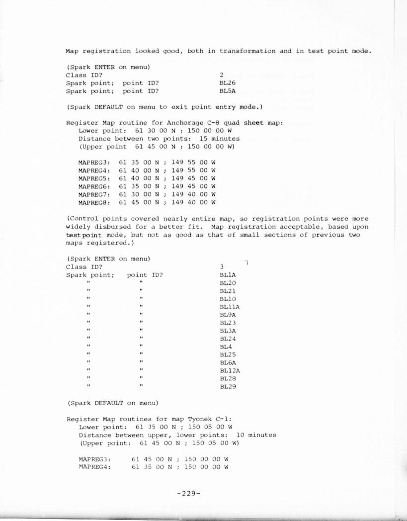
Map registration looked good, both in transformation and in test point mode.

(Spark ENTER on menu)Class ID? 2Spark point; point ID? BL26Spark point; point ID? BL5A

(Spark DEFAULT on menu to exit point entry mode.)

Register Map routine for Anchorage C-8 quad sheet map:Lower point: 61 30 00 N ; 150 00 00 WDistance between two points: 15 minutes(Upper point 61 45 00 N ; 150 00 00 W)

MAPREG3: 61 35 00 N 149 55 00 WMAPREG4: 61 40 00 N 149 55 00 WMAPREG5: 61 40 00 N 149 45 00 WMAPREG6: 61 35 00 N 149 45 00 WMAPREG7: 61 30 00 N 149 40 00 WMAPREG8: 61 45 00 N 149 40 00 W

(Control points covered nearly entire map, so registration points were morewidely disbursed for a better fit. Map registration acceptable, based upontestpoint mode, but not as good as that of small sections of previous twomaps registered.)

(Spark ENTER on menu)Class ID? 3Spark point; point ID? BL1A

" BL20" BL21

" BL10" BL11A" BL9A" BL2 3" BWA

BL24" BL4" BL2 5" BL6A" BL12A" BL28" BL29

(Spark DEFAULT on menu)

Register Map routines for map Tyonek C-1:Lower point: 61 35 00 N ; 150 05 00 WDistance between upper, lower points: 10 minutes(Upper point: 61 45 00 N ; 150 05 00 W)

MAPREG3: 61 45 00 N 150 00 00 WMAPREG4: 61 35 00 N 150 00 00 W

-229-

Based on map registration test points, registration was qood.

(Spark DEFAULT on menu)

(Spark ENTER on menu)Class ID? 4Spark point; point ID? BL22

(Defaulted out of ENTER mode; BL22 only CP on that map.)

(Spark STOP on menu to exit GES.)

The control points here digitized will subsequently be transformedinto the 80-metre grid to be built in the next step, and thattransformation will be used by the IDIMS function REGISTER increating the georeferenced output image.

-230-

III. Construction of 80-metre UTM Grid

1. The program ALLCOORD on the HP 3000 was then used to construct a gridof 80-metre cells in a UTM base. The digitized control points weresubsequently transformed into this grid.

:HELLO CARSON,NDAKOTA.GISwelcome message:RUN ALLCOORD.UTILS.IDIMSwelcome message

(Abbreviated prompts:)

Line printer listing of output required?Input Coordinates are in the form of?Name of Geoblock File?Name of desired Geoblock?Class ID (CR for all)?Output text file desired?Name of file to receive output?Capacity limit?Store coordinates as?State Plane Zone (CR to omit)

6176UTM F ALASKA, ZONE 4

XMIN=-540124. YMIN= 221340.FINISHED; 20 POINTS PROCESSED

END OF PROGRAM

:RUN ALLCOORD.UTILS.IDIMSwelcome message

(Abbreviated prompts:)

Line printer listing of output required?Input coordinates are?Input coordinates are in the form of?Name of file containing input coordinates?Output text file desired?Name of file to receive output?Capacity limit?Store coordinates as?State Plane Zone (CR to omit)UTM coordinates of X,Y of grid origin?Dimension of grid cell, in metres?

XMIN= 3974. YMIN= -59.XMAX= 4226. YMAX= 246.

FINISHED; 20 POINTS PROCESSED.END OF PROGRAM

-231-

YP (GES control points)BLGF.OBLKBGLAKECRYBLTOTSECCRS (Total seconds lat/lon)6176

YF (Text file)S (Total seconds)BLTOTSECYBLTSUTMCRG (Grid)CR340000,684000080

Since the first point in the digitized control point file, point B1,27,falls in UTM Zone 5, the system places the entire set of control pointsin Zone 5, while all but two of the points are actually in Zane u. Towork around this problem, the Text Editor was used to move the firstpoint to the en.i of the file; the result of so doing was to allow thefirst point encountered in the file to be in Zone 6, so that all pointswere placed in the appropriate UTM zone.

: EDITORwelc".'me messa.le

TEXT BLTOTSECJOIN LALTOyTSECD^) 1

LIST ALL'D` 40

/LIST ALL

/KEEP LK:TOrTSEC,UNNEX IT

:RUN ALLC.O0RD.UTILS.IDIMSwelcome message

Line printer listing of output required?Input coordinates are?Input coordinates are in form of?Name of file containing input coordinates?I:; an output text file required?Name of file to receive output:Capacity limit?Store coordinates as?State Plane :,one (CR to omit)?

617bL ►TM F ALASKA, ZONE 4

Enter UTM c,vordinates of grid origin?Dimension of grid cell, in metres?

XMTN= -19. YMIN= -5.1.XMAX= 247. \MIN= 251.

FINISHED; 20 POINTS PROCESSED.END OF MNIRAM

(accessing ALLCOORD .output)(appends 2nd copy, same tile:)(deletes record #1; no echo)

(deletes records 22/40: recot s#' through last of 'nd copy)(demonstrates that BL-7 is atthe end of the list)

Y

F (Text file)S (Total seconds)BGTOTSECYBGS 0MC G (Grid)bl7o

340000,684000080

-232-

ORIGINAL PAGE IS

OF POOR QUALITY

?Er, .,ACC 1 1 , 1931, 1 1 : 4q A'4

I`, t T COk).;}(,-ATFS "EAJ AS TfiTA SFCt1."'1)SI , ai,T TE X I F I L E y„T0 5

7'_ T 2 1 T Tt%T F ILE ci,Fn^'r ic r 1 s T a-c jTC g EO k5 1.T..i Gk II) ,5 T ATc P L -4 LCNE 13 b17bUTN F ALASKA, ZONE 4:T • ' C ATcS Q RF , In O Q I,Iv 3u1ir00. b8401100.5 i ^t 1: c ^^ IJ C_lc I" '•4 E < <F S 90.u w 70 .1E F

^L2 .. .., ^:•t'c, : -1:.e, T(IT'.L 5EC'. r CS

z; > ?13 4 '? 3 4 a 7 AUT'+ (''ETEk5)

g2.3^`^=L •

s ;.:•;^» la4 ,15 . 9,. ,..2 1 u 3 27. 1, 0:R212 1 7.

P^i^^ tcz22

^ L ^ •c 1 <^.^^.. ^q u x. ~( ^3 35 +'_ <.•yjl- +x-115

?19 3-i2P1750

35794`;35c7 1.

6r_i77-i,b 31u5^.;;L' 1 1 _' 1 » (1u 5c • 5t " ;ia 7_ I 2?213'^ 3u5i a3 0 1..• 1,3c a...f..

•

;13 5?'i5 •• -<..ccc :21457 3,17..c^ f.it+_a,

i^ t t ^ 1-,. t ^ S7 . f. »57 1 'N

-S;C'ic.

^3'=-Y7271J^5

=1n7eZ:1t:^ui<^z17^

`r ist^h•ae,-3,.=;7.

-. _J' 1 ... 7V • 1 _G t.y^u 1 r11.1 ^ t.r 5 'f 7 ^• 04 2; <

"'-'' ^' `^•'-' i•'^ 5^'^:" --:c1^s :21'2 1 iu^2o^. ^.315uf;ma c-

_^-1 j l ).'• 1.1'^ u. .u^.,..

- L-i ^• jc • 7

53•ta"., -=raccti ??15u 3ut,u5rc12,

b= 2^+0:•s.a._:^^^

-4^. <<•'"'.^ ?r

113 5^ • ^t » . , _cigaj3 c']I^aa t`v1'65P7lu4 u3'?^" -=3oCt'^ . 21 572 i^c,i3i; 61"797 ` 7.^i- '^•._"): 1 s7 57 . 17 » . _-(c. Zj c' 7 1 A l 2 7

1 2 . ?2130 13..4.14, Em,?rQP5

91ITF vLAr;F- ( F EET) TRavSFOt? ►»EO INPUT514977, ?73414,4.7^ tw ^5. 21390-145.53 4 1-^. 250435•+.555.41c ?74474A.So2 7. 2775vJU.I. 1 , , ' ; 4. 2"1u370.3?1 1 c' Q . 2790,315.^'" PAU 05. 279150k.c J79a1. 27tiA242.517119. 27u?713.

`?7^3 ?1. 27731te.553 9,-;. 2714gA91L.°Q1 '). 275251 Q.51 y u3-, ;)754u,,5.5;!79 ­ ?_75Na51.^ 4a 31^. 27^7^S5.5 ,17 4 1. 27oR262.140O 27 11. 2909194.14 g 39A0. 2736577.

Table 35. Big Lake ALLCOORD Listing

-233-

ORMAL PAGES 13OF POOR QUALITY

On the first runs of TRNSFORM to generate the transformation to be used byREGISTER, several points emerged with residuals higher than .9; these pointswere evaluated and decisions were made regarding the movability of the pointsin the image control point file. As a result, the Text Editor was used tochange the values of two points. One change was later negated or reverseddue Lo the behavior of all points on subsequent TRNSFORM runs. The finaldecision was that all points would remain as originally chosen and noted,except BL25, which was changed as follows:

BL25 3056.5 1798

The file was Kept, in Text Editor, as BLI1MGCP2.

In addition, two points were subsequently deleted from the transformation:these deletions were performed during the interactive running of the TRNSFORMprogram.

IV. Computing Transformation

:RUN TRNSFORM.UTILS.IDIMSwelcome message

INSTRUCTIONS?Origin for Source Control Points?X,Y Biases?Name of text file?Origin for Destination Control Points?X,Y Biases?Name of text file?

Print matching points on line printer?Enter name of TRNSMTX file?File open error, etc.Capacity?Desired filename or CR for T3BLTMTX?

N3 (Text file)0,0BG 8 0M30,0BLIMGCP2YT3BLTMTXB (Build)100CR

First- and second-order fits were computed. It was decided to deletepoints.

Do you wish to alter points? YAdd, change, delete, list, or end? DLine number to delete? 1 (point BL26)Add, change, delete, list, or end? E

First- and second-order fits wthis point. Another, point waswithout jeapardizing the point

Do you wish to alter points?Add, change, delete, list, or end?Line number to delete?Add, change, delete, list, or end?

ere again computed, withoutselected for deletion, hopefullydistribution.

YD14 (point BL29)E

-234-

ORIGINAL PAGE 13

CF POOR Qv 41_ TY

RESIDUAL MEANS: .364315 .299101

NUMBER AM B(N)

1 1586.81 2887.392 1.07568 .918829 E-013 -.603553 E-01 1.30376

Do you wish to alter points?

NDo you wish this to be the highest order

transform?

N

RESIDUAL MEANS:

NUMBER AM

1 1586.602 1.083823 -.530228 E-014 -.360800 E-045 -.305048 E-046 -.130868 E-04

.303165 .232048

B(N)

2887.90.912392 E-011.29289-.630983 E-05.367189 E-04.189268 E-04

Do you wish to alter points?Do you wish this to be the highest order

( transform?Enter name of transmatrix record?Enter description of transmatrix record?

Do you wish the inverse transform?END OF PROGRAM

N

YT3BLTMTXControl X, followed by:

T3 17 OF 19 NEW CPS 31181 CCH

N

RELEASE T3BLTMTXBYE

(The RELEASE command allows the file T3BLTMTX to be accessed from other log-onaccounts; the REGISTER program is an IDIMS function and must access the trans-matrix file from an IDIMS account/log-on.)

-235-

ORIOMA'L f'AM- S

OF POOR QUALrrY

'I Sx yY r,x . t ► T .4x Kr

1 »^7 , 7 2 1 55 4 -1. 3 3.1131)7 ? :l)1 1^ <n n -t .l• -L2' <t1, L. 21, ', lie - • z .3_Li.t 2%4 2y 31r3 z 31'3 10 '3 - 2^L=• cui lnl ?214 ^- i^jy 16xr 3

'^! ! ^3 -5a 2q^,^: t ;:, :.cc =12u -,u .c1" zr.l.. t;-_ <^,14 1505 .?2y 7'^y r zc4ti lnl l 1 -.: _` G4u I 7j :cyU 1711 _: u •'

1 '•L 219 ; oqo =r,^n 1 4 15 .F1 1 ^L25 1 15 203 =1:51 z:r i,,c„ 17ga 1 .0 -.212 iL?3 11E 05 ".4 - i ^µ 3'_Cu 1-c3 -.5- 1t 3 ^Lu 2 )5 2 :11 3177 1 7,a 3; 7 7 17^c i - ^^174 ?1 11 2 1770

1 ` ^l.2° 31 ' 7^ 3rt,c 1 7.c 3r. o 1771 Sl lu 15c 3rc0. t lj? :tt^51" 1751

1 7 ^__=; 193 tic 3151 17t3 3151 1713 z_ 7 lu :i; 2q r, t;cs 2c^p 15uktL +tA = .4=4216. .5:1= •'

First-order transformation

(Decision to move points was based on this output.,

3r p,c ;r Tx Tr 4x ;4r

1 _^' 1^1 X35 3117 1 X117 1^3;^ -.1 -.t^ `^ 1'-G -31 it n r^ t'j1a i11t^ 1541 - ^ 1

11241 .4 3-,1a 1_:, 3; 14 15 1- z

7 P1 2WA"; 1• I .; 2au4 1 1 ^t . 1171' =a - L t.1 7 L -

1 ^ L.?5 115 ?iJS t15i7 17'x. ACr"1 1 70 ,u11 til_23 1 i^ 105 z')uh -^^ z11uo 1"3 -,:. 31' 3177 3177 17^c •` 1 Q-1 12 1711 %°21 77: 2, 177: ,0

'i1 175 301.4 177 i ,u -,01 114 159 3o5;, , 7ti2 36 5,, 17511 143 12`7 3151 j7t: 311 1713 ,31 7 .. 1 s -37 24 0.? t 54r . u -1 N 1 7 -10 2i1 ^a'17 ^J ?RAIj I3u4 - ,1 - t

Q^SJ._y i

.3>>0?5 .3344`

First-order transformation,

after point BL26 deleted

Table 36. Big Lake First-order Transformations

-236-

.1 .•1 •. .1 1. r T: T rZY hY

1 t.-. ; ,. Y) 1 - - X11 i l =, -•^1 7

5 `, • -L 1 V J- L y t 24 - 1

• 1 ^ i V •. ^ I ♦ 11,E V t 2•i I1 v 1 1^ 1 1 I l17 1

t ,, I c ^,' * zl;s7 I -.: it 1 7 0 - G 111 ► 1 t i r _ ^^+'• 1 -'. j.+c', 1oQZ 1,)lc ' c ?177 1 3177 17^?^

:^4

P 1 1 71 •• Q3r'. 177= 1. _1 -'- l r ^`- Yl; r i 1 7:^ i<,1Gir 17^) -•V ^rt; .-L<„ 1^^ ^:: it5t trl 31^t t71• .3 -.j

FINAL TRANSFORMATION

iFirst-order transformation

After deletion of points BL26 and BL29,and after Text File BLIMGCPS modified

E

i

1

with new coordinates for point BL25.

t Table 37. Big Lake Final Transformation Listing

-237-

V. Creating Georeferenced Image

The IDIMS function REGISTER, when used in the mode about to be illustrated,accesses a pre-existing transformation matrix file and uses the coefficientsstored in that file to create the output image. In this case, the transfor-mation matrix reflects the relationship between the classified image andthe 80-metre grid apace built in the ALLCOORD program. The net result, then,is that REGISTER writes the test site portion of the overall classified imageinto the 80-metre grid, using the transformation just created.

:HELLO CARSON,ALASKA.IDIMS:RUN IDIMS.PUB;LIB=P

SMSJS>LOAD

SMSUS>REGISTER>BIGLAKE.REG.NEWCPS

PLEASE SUeFLy PARAMETER VALUES FOR FUNCTION REGISTER:MAXTYPE: CRMIPTS: CRDIPTS: lCRNLOUT: 2244NSOUT: 270NOOUT: NOINTERPOL: NNTMTXREC: T3BLTMTXTMTXFILE: T3BLTMTX.NDAKOTA.GIS

T3BLTMTX T3 17 OF 19 NEW CPS 31181 CCH(System prints out contents of TMTX record comment.)

Coefficients of T3BLTMTX are echoed on user terminal. They are, ofcourse, the same coefficients listed from the TRNSFORM program.

END FUNCTION REGISTER

VI. Generating Output Products for Transmittal to ESRI

The first output product to be generated, once the REGISTER output imagewas viewed on the display and visually evaluated, was a line printer mapwhich was overlaid on the ESRI-generated map of ESRI Photointerpreted data.

BIGLAKE.REG.NEWCPS>LPMAP

NSOUT was calculated by finding the number of metres represented by the N/Sdirection of the study area/80-metre grid space, and dividing by 80.

2 ' NSOUT was calculated by finding the number of metres represented by the E/Wdirection of the study area/80-metre grid space, and dividing by 80.

-239-

PLEASE SUPPLY PARAMETER VALUES FOR FUNCTIO14 LPMAP:CHARS: ' WW (Assigns blanks to all but waterSTEPSZ: CRDEVICE: CRCOMMENT: 'BIG LAKE AREA INTRISCA REGISTER OUTPUT NEW CPS +

ESRI GIS INTEGRATION'COPIES: 2

END FUNCTION LPMAP

(One copy of the LP map was generated for ESRI and one for Ames.)

The REGISTER output line printer map was overlaid on the ESRI map andthe fit was satisfactory.

The second output product to be generated was the tape via which thegeoreferenced data was to be transmitted to ESRI.

BIGLAKE.REG.NEWCPS>TRANSFER(FILENO= 1 SPECTYPE=SAME REALFORM=HP)

END FUNCTION TRANSFER

The georeferenced image was then stored on the IDIMS system on a Store Tape,on the ALASKA.IDIMS account, for future reference. The Transfer tape andone of the LP maps were transmitted to ESRI on March 11, 1981. A list ofclass identifications for the Susitna scene was also transmitted (Table 38).

CCH/c

-239-

Big Lake (Alaska) GIS Integration

CLASS IDENTIFICATION

Class Number Color Cover Type

1 Aqua Sedimented water

2 Medium blue Clear water

3 Brown Shrub/moss bog

4 Brown Black spruce bog

5 Yellow Grass

6 Yellow Shrub

7 Dark green Conifer

8 Olive Mixed forest

9 Light green Deciduous

10 Black Barren

11 Dark grey Alpine tundra

12 Grey Glacier

13 White Snow

14 White Cloud

15 Black Shadow

16 Purple Commercial/industrial

17 Violet Transportation facilities

18 Reddish brown High-density residential

19 Red Low-density residential

20 Purple Central business district

21 Purple Commercial

22 Black Background

Image on tape: 244 records, each 270 bytes long

single bandone file

Table 38

-240-

Georeferencing a Portion of the Anchorage Image

TNTRISCA PwoFrr

Alaska/LSRI GIS Integration Effort

Charlotte Carson-Henry

May 1981

HILLSIDE TEST SITE

I. Data Preuaration

Evaluation of the classified data set for the Eastern/Anchorage test sitedemonstrated that control points could not be selected, with any relia-bility, from the classified data set. The raw data had not been deskewed/rotated prior to classification; the clas_^ified data set was instead sub-mitted to the 360/TSS ROTATE program following the completion of stratifi-cation. Parameter values affecting rotation (HSKEW and VSKEW) wereobtained for that ROTATE job by running SKEW un the 360/TSS.

For purposes of the GIS integration effort, control points were requiredto be selected from the raw data, rotated to exactly overlay the classifieddata. Since the ROTATE program operates only oil data, theDESKEW program on the 360/TSS was utilized to generate the required rotationof the raw .iata. DESKEW and ROTATE utilize the same algorithm (RECTFY3) aswell as the parameters HSKEW and VSKEW; the parameter values HSKEW=.4()8 andVSKEW= .-'57 were ,ised in DESKEW as they had been for the ROTATE on the class-ified data. The DESKEW output was in EDITOR-compatible format, and wasreformatted using the 360/TSS program LL so that it could be read by IDIMS.The output tape was then entered oil and subsequently used for controlpoint selection.

During control point selection, it came to light that although the samealgorithm had operated on both the raw and classified data sets, using thesame parameters for skew to determine degree of rotation, the newly-rotatedraw data did not overlay the rotated classified data. Rotated output on thetwo data sets was, in fact, markedly different in size. Investigationidentified the cause: when DESKEW was run on the raw data, the full CCT wasrequired/used as input .ind the RECTFY3 algorittun calculated the centerpointof the scene -- around which to rotate. When ROTATE was run o il classifieddata, a full scene data set was neithei needed nor available, so a subset wasused as input; the RECTFY3 algorithm calculated the center point of thatsubset — around which to rotate. The center points of the twos scenes werenot, of course, in the same location.

Rather than incur the expense required to re-rotate one data set or the other,an attempt was made to transfer the control points from the raw data to theclassified data by means of line printer maps of corresponding subsectionsfrom the two, data sets. These maps were overlaid and local fits were attemptedmanually. 'Pile presence of cloud cover in the southwestern portion of the

-241-

AI1h'hoi aot , i'rnlnr:ttl.t, ,•.•u}•lr,t with t hr . ► b::ell"t. , , t h • le.tr 1.111d use } , . 1t t et tt:: tit

t lit , , ent t .1 l 1 •h , I t I,nl , N t t ht' •:t uhiy al oa , } , t t'\ ent C,i t I awI f rt't'a 1 of .1ppi ox 1111.1t t' l y

h.l1 i . , t t hr nmit wl 1%=Lmi wt Ill ,Illy WoI eC h o t , , , nt t,irnh r . ► llhi an .1l It e1 n.It

.t111 1 1 h , . ► h • h w.1 • : 4 1 11,tht .

A NA.,A i , t ,uI t ,unntt't 1 , t , v I.it • hI tar mv.ln:: t , , t :h , l V I I1,1 t ht' i , t . , 1 , l rm. Fte tu:(hi . ► 11.41 ,l

o1,y .,t the la :I"1'!'1' t h, dtl Ain ' t veI I t Lehi tb •, nt.11111a I .. ► lh'ul.tt Ion) t hat t hr 1 , 1, , ,11 ,till

hAA h • h , t I t'h t I h'h mput Chi t hr , t'nt et i , , , tnt , , l e.1, 11 rile. It( , t he'll CI e.1t rht an

KI I I'l\ t ;( ,VA1, l, • bl 1,im , ,' . tl I I li . 1t I, , ll ) t t it' II:.Itl,I t hr aII , h.1 and lwt.1 v.Ilues ,I:.

h • 01111 1 ut I'd by I 1 N.: ; KV%q RVCTF'Y I , . 1ll,t t he'll 11sth! t ht' Ca I -Ill at o "001 ,1 1 Ilat t':: I , , Itt I nt'".

Ln I1tl'1'01t t tI.1n::th , tIII Iaw AM h • 00t,i1 11.11e:: tilt, , I)F ,: KVw , • tit1 ,ut "001,i1 11.1to,.

1'hI:. enal , Io i t I all.;I.tt Ioll , , I t he gent t'I i • h , tlit , , h I I.IIliat e • :: h o t t lit , unt, , t at t',i

l

l. ► ssII I"t At I a Into the , th , tate,i Iaw .t.1t,1 nl , , ► e •e, wh1 11 In " 1 It a I I 'wr,t f lit'

it. Utu.t 1 I hnn} tit . ► t I t t hr .1 t t t rI rn, t' l , t't wren . hr , ha h t hi t n.1t t' :y :t rm . t the

t w1 , Inl.t.l4 :1 , .1, t' :. '!'he h h , nt I 1 Iti , I nt :• 1 e • ,' t rhi t t , ,m t he I .1w .i.1t .1 wt's t hen

nLlnu.tlly tt.Ilt::l.Itehi Into, I, , I.ltrht 1.1s ItItht Alt .1 ., , h , IAI11.1(os, t, , I ww III the

1 r,l I :t t at toll t , be } • t'1 th , I me,t. t;:rr 1' L,lu1 r:: 5l 1 aliki ' , I t h , I an i l lust t .tt ioll

tit they pl-V ,Item. 1

trm

. rn>. .

LULL

0

_T x

^U N

^ = Q ' rOL Jw av

0^^ a

x

l^ w

_7

pRiGl"•Al- pl\(' IS07 pvUR QUAL"

^ Y

ArOtt

sd3 Le 3 1 3

Tf*---j,

~ ^COL

.- A

U s ^^t Q 4

%—it

cC pa

-Jr

to

S^^ M

T

W QLA - .3JJ

JvJ

Figure 50. Hillside GIS Integration Image RotationProcess

-243- 4Q

ORIGINAL PAGE ISOF POOR QUALITY

Relationship between scenes, based on EDITOR Calculate Coordinates routine

"Goddard" "Oblique"

1,1 1, Scene II Scene3112 #Isles

ANCH AROTLL

117v,^f.20 133{,,M93 '

" Obl^4}^e.ly-roUsd

K

Fu,11- ^rorKe. ^u 4'1i ^...^a (raw

1 1 1' 1 1, 3000

x+12 ANCHOR.EAST ; 1 3,es may,

rrr ,

11Nroik^ ebbsi^i.d

1^ 1 ^,18%,U'78

z4So 1 ' 50, 3000

"Goddard" coordinates "Oblique Coordinates(Unrotated raw & classified scenes) (Rotated raw scene)

1;2278 ANCHOR.EAST (clasd) = 337,3119 AROTLL

1876,1 ANCHOR.EAST = 1625,239 AROTLL

1876,2778 ANCHOR.EAST = 2212,2242 AROTLL

1170,1620 ANCH (raw) = 1336,1993 AROTLL

ANCHOR.EAST centerpoint:

938,1139 ANCHOR.EAST = 980,1679 AROTLL

ANCSM2 rotated output image size = 2450 x 3000

One-half of each dimension = centerpoint of output obliquely-rotated image;therefore:

2450 2 = 1225 (1225 also equals zOUTH value on RECTFY3)

3000 2 = 1500 (1500 also equals XOUTH value on RECTFY3)

.3

a4S liwsObliquely-rotated ANCHOR.EASTcenterpoint coordinates, in (N) (W)full-frame space 980 1679

MINUS

Centerpoint coordinates ofANCSM2 (classified data),in its own space - 1225 - 1500

YIELDS difference between245 179

two spaces -

ni

174

I

3185 swwOti

Figure 51. Hillside GIS Integration Image Relationships

-244-

II. Control Point Selection

Control points were selected using the IDIMS display and a 1:63,360 scale quadsheet map on which the Hillside study area had been located using UTM coordi-nates supplied by ESRI as described previously. Ten points were located onthe raw data and on the map, and their sample/line coordinates were noted forcreation of a text file. The HP 3000 Text Editor was then used to create thattext file, containing control point names and the noted coordinates for thosepoints, after the points had been translated manually into the coordinatesystem of the classified rotated imagery as discussed in Section I of thisportion of the paper.

:HELLO CARSON,NDAKOTA.GISwelcome message:EDITORwelcome message/ADD

1

HS1

1442 1687

2

HS2

1440 1685

3

HS3

1384 1629

4

HS4

1336 1581

5

HS5

1601 1846

6

HS6

1526 1771

7

HS7

1672 1917

8

HS8

1801 2046

9

HS9

1353 1598

10

HS10

1413 1658

11

NOTE: NOT PART OF TEXT FILE:Description Quality Move

Lake Hideaway Fair M p) ??

Intersect. O'Malley & Birch Excel. none

Sm. lake N. of S.Fork OK NE 1

Lake Otis OK S 1

McHugh Creek & Turnagain Arm Fair ?

Junction 2 forks Rabbit Creek Good ?

Gull Rock #1, Kenai Peninsula Good W 1

S. end landing strip, pipeline Excel. N 1 or none

Hood Lake, Anchorage Good none

Jewel Lake, S. shore Excel. NE 1

/KEEP HSIMGCPS.NDAKOTA.GIS,UNN

/EXIT

The coordinates used above are the translated coordinates for the controlpoints; the coordinates as recorded from the raw data were as follows:

Name Sample # Line # Name Sample # Line #

HS1 1242 1442 HS6 1302 1526HS2 1216 1440 HS7 1214 1672HS3 1241 1384 HS8 1056 1801HS4 1158 1336 HS9 1051 1353HS5 1249 1601 HS10 1054 1413

-245-

These coordinates were translated into the values entered into the text fileby subtracting 178 from the sample numbers and adding 245 to the line numbers,those being the numbers that represent the relationship between the raw imagespace and the classified image space, after both data sets were rotated asdescribed in Section I of this portion of the paper. A brief description ofthe derivation of these two numbers is as follows:

Coordinates of center point of theobliquely-rotated subsection image,in obliquely-rotated full-framespace: Line 980 Sample 1679

MINUS

Coordinates of center point of theobliquely-rotated subsection image,in its own space: - Line 1225 Sample 1500

-245 179

III. Digitizing Control Points

The control points selected on the IDIMS screen and concurrently marked onthe 1:63,360 maps (Anchorage A-8 and Seward D-8) were then digitized usingthe TAUS digitizer and the GES software on the HP 3000. Required by thisprogram are: definition of a Geoblock (area within which digitizinq willoccur), definition of files, and menu registration. Control points weredigitized as follows:

:RUN GES.PUBwelcome messagePrompts regardinq terminal type, digitizer type, digitizing tolerance, and

coordinate system in which digitizing information will be entered, then:

(Abbreviated prompts:)

Geoblock Directory File Name?Prompt for Label Positions?Six-character Geoblock Name?Geoblock Dimensions:

Lat/lon of lower left corner?

Width, height (in minutes) ?Area File Capacity?Tolerance?Overlay Number ?New OVLY. Proceed?OV Type?

HSGEOBLKN (Used w/ polygons only)HILSID

60 45 00 N150 00 00 w25,30CRCR1YP (Point)

-246-

(Register Map routines)For Seward D-8, used lower point of 60 50 00 N ; 150 00 00 WDistance between upper and lower points: 10 minutes(Upper Reg. Pt. — MAPREG2 — 61 00 00 N ; 150 00 00 W)

MAPREG3: 60 00 00 N 149 40 00 WMAPREG4: 60 50 00 N 149 40 00 WMAPREGS: 60 50 00 N 149 50 00 WMAPREG6: 61 00 00 N 149 50 00 W

Tested points; registration looked to be within a maximum of 1-second error,which could be attributed to cursor placement during digitization. Defaultedout of Register Map routines.

Spark ENTER on menu.Class ID? 1Spark point; point ID? HS8Spark point; point ID? HS7

Defaulted out of Enter mode, since additional control points on different map.

Mounted Anchorage A-8 quad sheet on digitizer bed, sparked Register Map.

(Register Map routines)For Anchorage D-d, used lower point of 61 00 00 N ; 150 00 00 WDistance between lower and upper points: 15 minutes(Upper Reg. Pt. — MAPREG2 — 61 15 00 N ; 150 00 00 W)

Do you Desire a Higher OrderBegin with What Order?Registration Point Interval

MAPREG3: 61 15 00 NMAPREG4: 61 15 00 NMAPREG5: 61 00 00 NMAPREG6: 61 00 00 NMAPREG7: 61 10 00 NMAPREG8: 61 05 00 N

Transform? Y1

(minutes) ? 10

149 50 00 W149 40 00 W149 40 00 W149 50 00 W149 45 00 W149 45 00 W

Since the control points covered a large portion of this map, registrationpoints were more widely disbursed to ensure a better fit. Map registrationseemed to be acceptable, with a maximum of one-second errors when points were ,.tested.

Defaulted out of the Register Map routines.

Spark ENTER on menu.Class ID? 1Spark point; point ID? HS3

HS1HS2HS4HS9HS10HS6

HS5

-247-

Spark DEFAULT on menu to escape Enter mode.

Since all points have now been digitized, STOP is sparked on the menu toterminate the GES program.

The control points here digitized were subsequently transformed into the80-metre grid space built with ALLCOORD, and that transformation was usedby the IDIMS REGISTER function in creating the georeferenced output image.These processes will be illustrated in the next few sections of the paper.

III. Construction of 80-metre UTM grid

The program ALLCOORD on the HP 3000 was used to create a grid of 80-metrecells in a UTM base. The digitized control points were subsequentlytransformed into this grid space coordinate system.

:HELLO CARSON,NDAKOTA.GISwelcome message:RUN ALLCOORD.UTILS.IDIMSwelcome message

(Abbreviated prompts:)

Line printer listing of output desired?Input coordinates are in the form of?Name of Geoblock File?Name of desired Geoblock?Class ID? (CR for all)Output text file desired?Name of file to receive output?Capacity limit?Store coordinates as?State Plane Zone? (CR to omit)UTM coordinates of grid origin?Dimension of grid cells, in metres?

XMIN= -62. YMIN= -65.X.MAX= 137. YMAX= 364.

FINISHED; 10 POINTS PROCESSED.

EI4D OF PROGRAM

YP (GES control point file)HSGEOBLKHILSIDCRYHLSID80MCRG (Grid option)CR345000,678200080

-248-

PAGE fSOF POOR OUALITY

GEObLOCK FILEGtO8LGCK

CLASS IU:

OuTPuT TEXT FILECOORDINATES STORED AS

UTM CUU R UINATES OF GRID ORIGINS<<E OF GRID CELL IN METERS

UT M ZONE

TUE. MAY 5, 1981,

HSGEUBLKHILSIDALL

HLS1080MUTM GRID

345000. 6782000.80.

6

1:00 PM

CUi)KL)INAIE: TOTAL SECUNL)b UTM (MtTEKS)HSH 6U 52'51 "% l ay 56'46 "^^j -539908 219171 340064. b752899.H,°i 7 b1) 5L" b" a 149 u6' 1" % 'j -534161 219u8b 350224• 6762204.H53 61 9'11 "N lu g 44 . 4 () "8 -539080 220181 352343. b7e3bbq.HS1 51 7 . 23 "^ 149 44'27 ".% -534nb7 22u0 u 3 352354. 6779387.H52 61 7'25 ": 149 46 . 20 "A -539180 220()45 350667. 6779510.HS4 61 11 0 26 " 1\1 149 50'35 -^N -53Q436 220288 347176. 678721)6.H59 61 JU 0 47 "N 149 58' 1 ".v -539?dl 220247 340468. 6766216.H510 bl 8'20 "N 149 57'48 "A -53Qn68 2201uU 340460. 6721566.H56 61 4' 1"N 149 40' 9".. -536Qe9 219d41 355960. 6772901.H55 61 U 0 59 "w 149 43'42 ".v -539022 219h5 9 352542. 6767494.

ALLCOORD output

Table 39. Hillside ALLCOORD Listing

-249-

ORIGINAL PAGE ISOF POOR QUALITY

IV. Computation of Transformation

In order to translate image control point coordinates into 80-metre-grid-relative coordinates, a transformation between the two spaces was constructedusing the HP 3000 program TRNSFORM.

:RUN TRNSFORM.UTILS.IDIMSwelcome message

(Abbreviated prompts:)

Instructions?Origin for Source control points?X,Y Biases?Name of Source text file?Origin for Destination control points?X,Y Biases?Name of text file?Print matching points on LP?Enter name of TRNSMTX file?FOPEN ERR, etc.Capacity?Desired filename, or CR for T3HILSID?

N3 (Text file)0,0HLSIDSOM (80-metre grid text file3 (Text file)0,0HSIMGCPS (Image CP coordinates)YT3HILSIDB (Build option)100 (100-record capacity for file)CR

First- and second-order fits were computed. One point emerged with apoint residual exceeding 1.0; reference to notes taken during controlpoint selection revealed that the point in question was noted as havingthe potential for a move one pixel to the south. The Text Editor filecontaining image control point coordinates was accessed and modifiedso that the coordinates for control point HS4 were effectively movedsouth by one pixel, from 1336,1581 to 1336,1582. The first-ordertransformation was again computed, and residual errors improved through-out. No points were deleted from the transformation, and no residualerror exceeded 0.9 in either the X or Y direction. The first-ordertransformation was used.

RESIDUAL MEANS: .333203 .426270

NUMBF'. AM B (N)

1 1653.02 947.0372 1.07534 .253392 E-013 -.211641 E-01 1.26854

Do you wish to alter points?Do you wish this to be the highest

order transform?Enter name of TRNSMTX record?Enter description of record?

Do you wish the inverse transformation?END OF PROGRAM

N

YT3HILSIDControl X, followed by:80M GRD TO ANCSM2 58 81 CCHN

-250--

OPtGINAL PAGE ISPOOR QUAt "I

POINT 5x Sr UX UY Tx Tr Rx PT

1 M58 -62 364 876 ?U46 87d 2045 .0 .52 H57 65 241 1u3ti I Q I I la3b 1418 -.1 '.73 H53 4d -21 1Ub3 1#129 1Ut3 1b29 .1 .4u r51 42 33 1ubu 1tA7 1064 lb8b -.5 .b5 HS2 11 31 1038 10: a5 1438 IL-d5 . 3 ^.00 HSu 21 -b5 9du 15b2 960 1582 1 -.57 HS9 -57 -53 b73 1598 874 1598 -.8 .58 HS10 -57 4 87b 1#1501 875 105Q .Q -.79 F+Sb 13/ 113 1124 1771 1124 1111 .3 -.21 H55 94 181 lull 101 446 loll 184b -.2 -.0

RESIDUAL MEA y 5 = .333203 .42b270

Final Hillside TRNSFORM Listing

Table 40. Hillside Transformation

-251-

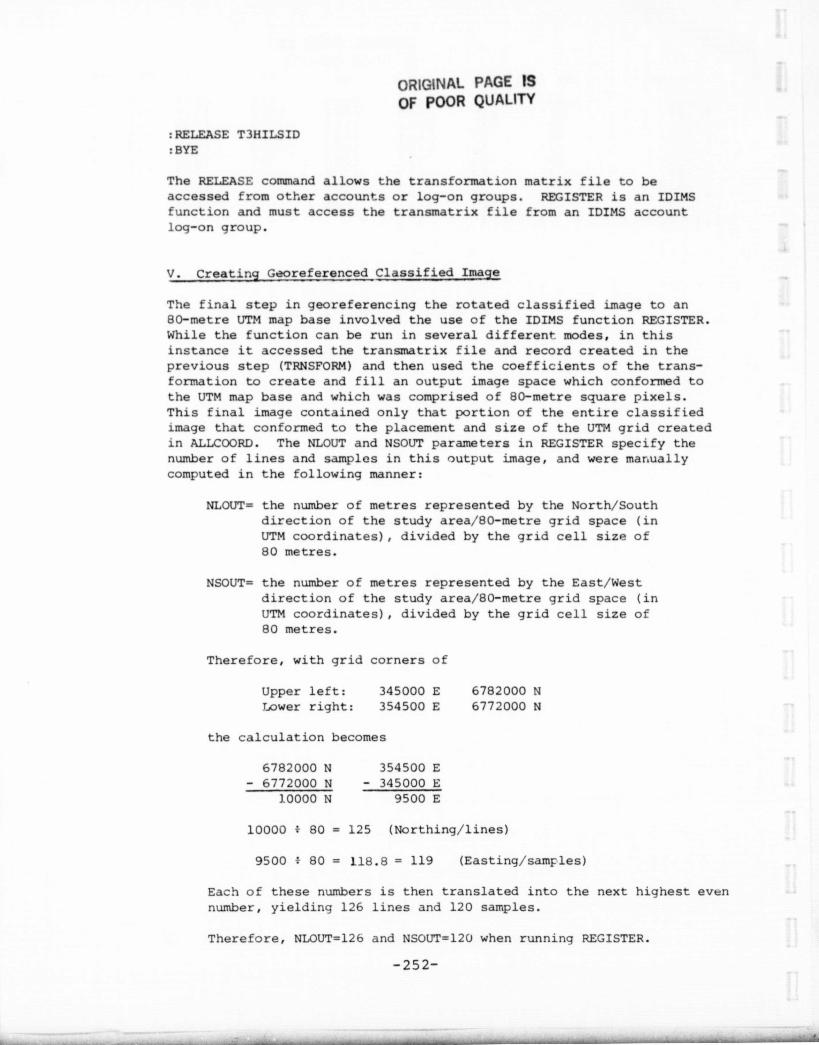
ORIGINAL PAGE ISOF POOR QUALITY

:RELEASE TMILSID:BYE

The RELEASE command allows the transformation matrix file to beaccessed from other accounts or log-on groups. REGISTER is an IDIMSfunction and must access the transmatrix file from an IDIMS accountlog-on group.

V. Creating Georeferenced Classified Image

The final step in georeferencing the rotated classified image to an80-metre UTM map base involved the use of the IDIMS function REGISTER.While the function can be run in several different modes, in thisinstance it accessed the transmatrix file and record created in theprevious step (TRNSFORM) and then used the coefficients of the trans-formation to create and fill an output image space which conformed tothe UTM map base and which was comprised of 80-metre square pixels.This final image contained only that portion of the entire classifiedimage that conformed to the placement and size of the UTM grid createdin ALLCOORD. The NLOUT and NSOUT parameters in REGISTER specify thenumber of lines and samples in this output image, and were manuallycomputed in the following manner:

NLOUT= the number of metres represented by the North/Southdirection of the study area/80-metre grid space (inUTM coordinates), divided by the grid cell size of80 metres.

NSOUT= the number of metres represented by the East/Westdirection of the study area/80-metre grid space (inUTM coordinates), divided by the grid cell size of80 metres.

Therefore, with grid corners of

Upper left: 345000 E 6782000 Nr.,ower right: 354500 E 6772000 N

the calculation becomes

6782000 N 354500 E

- 6772000 N - 345000 E

1.0000 N 9500 E

10000 : 80 = 125 (Northing/lines)

9500 : 80 = 118.8 = 119 (Easting/samples)

Each of these numbers is then translated into the next highest evennumber, yielding 126 lines and 120 samples.

Therefore, NLOUT=126 and NSOUT= 120 when running REGISTER.

-252-

ORIGINAL PAGE ISOF POCIF? QUALITY

HELLO CARSON,ALASKA.IDIMSRUN IDIMS.PUB;LIB=P

ANCSM2>LOAD (Brings classified, rotated image on-line)

ANCSM2>REGISTER>HILLSICE.REGPLEASE SUPPLY PARAMETER VALUES FOR FUNCTION REGISTER:MAXTYPE: CR (These first three parameters not used whenMIPTS: CR REGISTER accesses an existing transformation.)DIPTS : CRNLOUT: 126NSOUT: 120NOOUT: NO (Output image wanted)INTERPOL: NN (Nearest-neighbor)TMTXREC: T3HILSIDTMTXFILE: T3HILSID.NDAKOTA.GIS

T3HILSID 80M GRD TO ANCSM2 58 81 CCH

(System prints out transformation matrix record comment.)

The system will then print the coefficients from the transformation matrixfile and record, on the user's terminal, and proceed to create the 126 x 120output georeferenced image. The coefficients, of course, are identical withthose listed during the running of the TRNSFORM program.

END FUNCTION REGISTER

VI. Verification of Registration and Preparation for Transmittal

In order to assess the accuracy of the registration, a line printer map ofthe georeferenced image was generated and compared to maps of correspondingportions of the raw data using Bands 4 and 7, which were generated previously.A second copy of the LP map was venerated for transmittal, with the tapecontaining the georeferenced image. to ESRI..

HILLSIDE.REG>LPMAPPLEASE SUPPLY PARAMETER VALUES FOR F'.INCTION LPMAP:CHARS: ' WW (Assigning blanks to all but water)STEPSZ: CRDEVICE: CRCOMMENT`: 'HILLSIDE AREA INTRISCA REGISTER OUTPUT ESRI GIS +

INTEGRATION'COPIES: 2

END FUNCTION LPMAP

A transfer tapa was then written for transmittal of the image to ESRI.

-253-

HIL.LSIDE.REG>TRANSFERPLEASE SUPPLY PARAMETER VALUES FOR FUNCTION TRANSFER:FILENO: 1SPECTYPE: CR (Same)REALFORM: CR (HP)

END FUNCTION TRANSFER

Following completion of the transfer, the REGISTER output image waswritten to an IDIMS Store Tape, on the ALASKA.IDIMS account, forfuture reference.

A cover letter was prepared and transmitted to ESRI along with thetransfer tape, one copy of the line printer map, and a class identi-fication list (Table 41) corresponding to the classes in the Anchorage/Eastern scene. The materials were sent to Huss Michel of ESRI onMay 12, 1981.

5/13/81

-254-

C?r t^1NA! P,GLr !STable 41 Or PQGP ^1J/;! ! rY

Hillside (Anchorage, Alaska) GIS Integration

CLASS IDENTIFICATION

Cover Type Class Number(s) Color

Sedimented water 1 Aqua

Clear water 2 Medium blue

Shrub/moss bog 3 Brown

Black spruce bog 4 Brown

Grass 5, 27 Yellow

Shrub 6 Yellow

Conifer 7 Dark green

Mixed forest 8 Olive

Deciduous 9 Light green

Barren / mud 10, 25 Black

Alpine tundra 11 Dark grey

Glacier 12 Grey

Snow / ice 13 White

Cloud lY White

Shadow 15 Black

Commercial / industrial 16, 17 Purple

High-density residential 18 Reddish brown

Low-density residential 19 Red

Hay / growing crops 23 Peach

Fallow - riculture 24 Tan

Shrub/grass tundra 26 Yellow

NOTE: There are no classes 20-22; those class numbers were used in the

Susitna scene.

j-255-

!

i