Predicate control: synchronization in distributed computations with look-ahead

Predicate Control: Synchronization in Distributed

Computations with Look-ahead ∗

Ashis Tarafdar Vijay K. Garg

Akamai Technologies, Inc. † Dept. of Electrical and Computer Engg.

8 Cambridge Center University of Texas at Austin

Cambridge, MA 02142 Austin, TX 78712

([email protected]) ([email protected])

Abstract

The predicate control problem involves synchronizing a distributed com-

putation to maintain a given global predicate. In contrast with many popular

distributed synchronization problems such as mutual exclusion, readers writers,

and dining philosophers, predicate control assumes a look-ahead, so that the

computation is an off-line rather than an on-line input. Predicate control is tar-

geted towards applications such as rollback recovery, debugging, and optimistic

computing, in which such computation look-ahead is natural.

We define predicate control formally and show that, in its full generality, the

problem is NP-Complete. We find efficient solutions for some important classes

of predicates including “disjunctive predicates”, “mutual exclusion predicates”,

and “readers writers predicates”. For each class of predicates, we determine the

necessary and sufficient conditions for solving predicate control and describe an

efficient algorithm for determining a synchronization strategy. In the case of

“independent mutual exclusion predicates”, we determine that predicate control

is NP-Complete and describe an efficient algorithm that finds a solution under

certain constraints.

∗supported in part by the NSF ECS-9414780, CCR-9520540, a General Motors Fellowship, TexasEducation Board ARP-320 and an IBM grant

†This work was done while the author was at the Dept. of Computer Sciences, University ofTexas at Austin

1

Run−timeEnvironment

Control

Application

Observation

Figure 1: Observation and Control

1 Introduction

The interactions between an application and its run-time environment can be di-

vided into two categories: observation and control . Examples of observation include

monitoring load, detecting failures, checking variable values for debugging, and log-

ging usage characteristics. Examples of control include dynamically balancing load,

recovering from failures, resetting variable values during debugging, and terminating

processes which violate usage restrictions. Such a duality between observation and

control has also been noted in other areas, such as systems analysis.

In distributed applications, the problems of observation and control are made

more difficult. In the case of distributed observation, this is because no one process

has a global view of the system. Therefore, a global view must be correctly de-

duced from the local observations of each process. Distributed observation has been

formalized as the widely-studied predicate detection problem [CL85, CM91, GW96].

In the case of distributed control, the difficulty lies in ensuring global conditions

through appropriate local control actions. While there are many forms of control,

our focus is on an important form of control – synchronization – involving control of

the relative timing among processes. In this paper we define and study the predicate

control problem that formalizes this form of distributed control.

In contrast to existing distributed synchronization problems [BA90] such

as mutual exclusion, readers writers, and dining philosophers, predicate control

assumes a look-ahead, so that the computation is known a priori . In other words, the

computation is an off-line rather than an on-line input, and so, the predicate control

problem is an off-line variant of on-line synchronization problems. Such a form of

look-ahead is natural for certain applications, such as rollback recovery, debugging,

and optimistic computing, in which the computation look-ahead is determined from

2

a previous run. An important advantage of solving the off-line rather than the on-

line synchronization problem is that, given a pre-knowledge of the computation, it

is possible to solve the off-line problem in a general context under which the on-line

problem would be impossible to solve. For example, the on-line mutual exclusion

problem [Ray86] is solvable under the assumption that critical sections do not block,

whereas, as we will show, off-line mutual exclusion can be solved without such an

assumption.

Informally, the predicate control problem is to determine how to add synchro-

nizations to a distributed computation so that it maintains a global predicate. As an

example, consider the computation shown in Figure 2(a) with three processes, P1,

P2, and P3. The processes have synchronized by sending messages to one another.

Suppose the stated global predicate is the mutual exclusion predicate, so that no

two processes are to be in critical sections (labeled CS1, CS2, CS3, and CS4) at the

same time. Clearly, the given computation does not maintain mutual exclusion at all

times. Figure 2(b) shows the same computation with added synchronizations that

ensure that mutual exclusion is maintained at all times. We call such a computation

a “controlling computation”. The main difficulty in determining such a controlling

computation lies in adding the synchronizations in such a manner as to maintain

the given property without causing deadlocks with the existing synchronizations.

Overview

We first define the model and state the predicate control problem formally in Sec-

tion 2. Informally, modeling a computation as a partially ordered set of events, the

predicate control problem is to determine how to add edges to a computation (that

is, make the partial order of events stricter) so that it maintains a global predicate.

In its full generality, the predicate control problem deals with any predicates

added synchronizations

P3

CS1

CS2

CS3

CS4P1

P2

P3

CS1

CS2

CS3

CS4P1

P2

(b) controlling computation(a) original computation

Figure 2: The Predicate Control Problem

3

Generalized Mutual Exclusion

Readers Writers Independent Mutual Exclusion

Mutual Exclusion

Figure 3: Variants of Mutual Exclusion Predicates

and it would, therefore, be expected that it is hard to solve. We establish in Section 3

that it is NP-Complete. However, as we will see, there are useful predicates for which

the problem can be solved efficiently.

The first class of predicates that we study in Section 4.1 is the class of

“disjunctive predicates” that are specified as a disjunction of local predicates. Intu-

itively, these predicates can be used to express a global condition in which at least

one local condition has occurred, or, in other words, in which a bad combination of

local conditions has not occurred. For example: “at least one server is available”.

First, we show that a necessary condition to solve the problem for disjunctive pred-

icates is the absence of a clique of n false intervals in the interval graph. Next,

we design an algorithm for solving the problem when the necessary condition is

satisfied, thus establishing that the condition is also sufficient. The algorithm is of

complexity O(np), where n is the number of processes and p is the number of false

intervals in the interval graph.

The next class of predicates is that of “mutual exclusion predicates” which

state that no two processes are in critical sections at the same time. Mutual exclusion

predicates are particularly useful in software fault tolerance since they correspond to

races, a very common type of synchronization faults. In Section 4.2, our two results

show that the necessary and sufficient conditions for solving predicate control for

mutual exclusion predicates is the absence of a non-trivial cycle of critical sections

in the interval graph. We also design an algorithm of complexity O(np), where p is

the number of critical sections in the computation.

We can generalize the mutual exclusion predicates to “readers writers predi-

cates” specifying that only “write” critical sections must be exclusive, while “read”

critical sections need not be exclusive. Another generalization is the “independent

mutual exclusion predicates” where critical sections have “types” associated with

them, such that no two critical sections of the same type can execute simultane-

ously. Finally, “generalized mutual exclusion predicates” allow read and write crit-

ical sections and multiple types of critical sections. Figure 3 illustrates the relative

4

generality of the four problems.

In Section 4.3, we find that the necessary and sufficient conditions for solving

predicate control for readers writers predicates is the absence of a non-trivial cycle of

critical sections with at least one write critical section. For independent mutual ex-

clusion, however, we discover that the problem is NP-Complete in general. We show

this in Section 4.4, and also show that a sufficient condition for solving the problem

is the absence of a non-trivial cycle of critical sections with two critical sections of

the same type. However, in general, this condition is not necessary. The results for

generalized mutual exclusion follow along similar lines. We do not describe indi-

vidual algorithms for readers writers and independent mutual exclusion predicates.

Instead, in Section 4.5, we describe a general O(np) algorithm that solves predicate

control for general mutual exclusion predicates (under the sufficient conditions).

This algorithm can be applied to solving readers writers predicates (in general) and

independent mutual exclusion predicates (under the sufficient conditions).

The predicate control problem is targeted for applications in which look-

ahead is natural. In Section 5 we discuss two such applications: software fault

tolerance and debugging. Finally, we give an outline of related research in Section 6,

and we make some concluding remarks in Section 7. In this paper, we present

the shorter proofs in full and, for the longer proofs, we present a proof outline

together with a proof intuition where necessary. The complete proofs may be found

in [TG03].

2 Model and Problem Statement

The predicate control problem is based on a model of distributed computations and

concepts related to distributed computations. Our model is similar to the happened

before model [Lam78], described in more detail in [BM93, Gar96].

2.1 Computations

Since we are concerned mainly with distributed computations, we drop the qualifier

distributed and call them simply computations.

• computation : A computation is a tuple 〈E1, E2, · · ·En,→〉 where the Ei’s

are disjoint finite sets of “events” and → (precedes) is an irreflexive partial

order on E =⋃

i Ei such that, for each i, →i (→ restricted to Ei) is a total or-

der. We abbreviate 〈E1, E2, · · ·En,→〉 to 〈E,→〉 with the understanding that

n is always used to represent the size of the partition of E into E1, E2, · · ·En.

5

Informally, each Ei represents a process, and the partial order → represents a partial

ordering of events such that e → f means that the event e may have directly or

indirectly caused the event f . We say e “causally precedes” f . Note that, in

general, the → relation is merely an approximation of causality. An example of

approximating causality to obtain a → relation on events is given by the happened

before model [Lam78], in which → is defined as the smallest relation satisfying the

following: (1) If e and f are events in the same process and e comes before f

according to the local process clock, then e → f , (2) If e is the send event of a

message and f is the receive event for the same message by another process, then

e → f , and (3) If e → f and f → g, then e → g.

A special class of computations are runs, defined as:

• run : A computation 〈E,→〉 is a run if → is a total order.

A run corresponds to an interleaving of all the events in the distributed

computation. Finally, we define some notation concerning computations:

• → : (e→f) ≡ (e = f) ∨ (e → f)

In a similar way, we represent a corresponding reflexive relation for any given

relation, e.g.: (e � f) ≡ (e = f) ∨ (e ≺ f)

• e.proc : (e.proc = i) ≡ (e ∈ Ei)

Informally, e.proc is the identifier for the process containing e.

2.2 Cuts

• cut : A cut is a subset of E containing at most one event from each Ei.

A cut corresponds to the intuitive notion of a global state. Sometimes a cut has

been defined to correspond to the notion of a history (all events preceding a global

state). In such definitions, the frontier of a cut corresponds to our cut . Since, we

will be dealing more frequently with the notion of a global state than a history, we

formalize the notion of history in terms of global state rather than the other way

around.

If a cut intersects a process at an event e, then the local state on that process

corresponding to the cut is the one reached by executing event e. If the cut does not

intersect a process, then the local state on that process corresponding to the cut is

the initial state on that process. To represent an initial state explicitly, we augment

our model with initialization events:

6

• ⊥i : Corresponding to each Ei we define a special event ⊥i (⊥i /∈ E).

• ⊥ : Let ⊥ =⋃

i {⊥i}.

Each ⊥i corresponds to a special “dummy” event that initializes the state of process

Ei. Note that ⊥i is not a real event. Introducing the dummy events, ⊥, allows a

one-to-one correspondence between the informal notion of local states corresponding

to a process Ei and the formal notion of Ei ∪ {⊥i}, in which an event corresponds

to the local state that follows it. We next define a local ordering between events

and dummy events:

• ≺i : For each i, let ≺i be the smallest relation on Ei ∪ {⊥i} such that:

∀e ∈ Ei : ⊥i ≺i e, and

∀e, f ∈ Ei : e →i f ⇒ e ≺i f .

• ≺ : Let ≺=⋃

i ≺i.

Thus, the ≺ relation augments the →i relation by ordering the initialization event

⊥i before all events in Ei. Using the initialization events ⊥, we can now define, for

any cut, a unique event/initialization event corresponding to each process as:

• C[i] : For a cut C, define C[i] ∈ E ∪ ⊥ such that:

C[i] = e, if C ∩ Ei = {e}, and

C[i] = ⊥i, if C ∩ Ei = ∅.

Finally, we define a relation ≤ on cuts as follows:

• ≤ : For two cuts C1 and C2 define a relation ≤ as:

C1 ≤ C2 ≡ ∀i : C1[i] � C2[i]

2.3 Predicates

Predicates represent the informal notion of properties on local or global states:

• local predicate : A local predicate of an Ei in a computation is a

(polynomial-time computable) boolean function on Ei ∪ {⊥i}.

• global predicate : A global predicate of a computation 〈E,→〉 is a

(polynomial-time computable) boolean function on the set of cuts of the com-

putation.

7

Local predicates are used to define properties local to a process, such as: whether

the process is in a critical section, whether the process has a token, or whether,

for a process variable x, x < 4. Global predicates define properties across multiple

processes, such as: whether two processes are in critical sections, whether at least

one process has a token, or whether, for variables x and y on different processes,

(x < 4) ∧ (y < 3). We use predicate instead of global predicate, when the meaning

is clear from the context.

2.4 Consistent Cuts

All cuts in a computation do not correspond to global states that may have happened

in the computation. To see why this is true, consider the set of events which causally

precede any event in a given cut, which we call the causal past of the cut:

• G.past : The causal past of a set of events G ⊆ E in a computation 〈E,→〉

is G.past = {e ∈ E : ∃f ∈ G : e→f}

Suppose there is an event e in the causal past of a cut C and suppose e has not yet

occurred in the global state corresponding to C. Since a cause must always precede

the effect, the cut C does not represent a global state that may have happened.

Cuts which represent global states that may have happened are called consistent

global states. The reason we say that a consistent global state may have happened

is that its occurrence depends on the particular interleaving of the partially ordered

set of events that occurred in real time.

• consistent cut : A cut C is consistent if ∀e ∈ C.past : C[e.proc] 6≺ e.

We now prove two useful results about consistent cuts. The first one allows

us to extend a single event to a consistent cut that contains it. This corresponds

to the intuition that the local state following the event must have occurred at some

time. Therefore, there must be some consistent cut (global state that may have

happened) that contains it.

Lemma 1 (Extensibility) Let C be the set of consistent cuts of a computation

〈E,→〉, then:

∀e ∈ E : ∃C ∈ C : e ∈ C

Proof: Let e be an event in E. Consider a maximal (w.r.t. ≤) cut C contained in

{e}.past. Since C is maximal, it must contain e. Consider any event f in C.past.

Since C is contained in {e}.past, f is also in {e}.past. Suppose C[f.proc] ≺ f . Then

8

since f is in {e}.past, C is not maximal and we have a contradiction. Therefore,

C[f.proc] 6≺ f . So, C is consistent. 2

The next result tells us that a cut that is consistent in a computation is

also consistent in any computation that is less strict (that is, the partial ordering of

events in the latter is less strict than the first).

Lemma 2 If 〈E,→′〉 and 〈E,→〉 are computations such that →⊆→′, then any cut

that is consistent in 〈E,→′〉 is also consistent in 〈E,→〉.

Proof: Let C be a consistent cut in 〈E,→′〉. Let e be any event in the causal past

of C with respect to →. Since →⊆→′, e is also in the causal past of C with respect

to →′. Therefore, C[e.proc] 6≺ e. So, C is consistent in 〈E,→〉. 2

We define the next and previous event of an event e as:

• e.next : For e ∈ Ei ∪ {⊥i}, e.next denotes the immediate successor to e in

the total order defined by the ≺i relation. If no successor exists, e.next = null,

where null does not belong to E ∪⊥.

• e.prev : For e ∈ Ei ∪ {⊥i}, e.prev denotes the immediate predecessor

to e in the total order defined by the ≺i relation. If no predecessor exists,

e.prev = null, where null does not belong to E ∪ ⊥.

Note that null (not an event) should not be confused with ⊥i (the initialization

event). In fact, ⊥i.prev = null.

The following result shows us an alternative way of proving that a cut is

consistent. 1

Lemma 3 In a computation 〈E,→〉:

a cut C is consistent ≡ ∀i, j : C[i].next, C[j] ∈ E : C[i].next 6→ C[j]

Proof: (1) Suppose C is consistent. We show by contradiction that:

∀i, j : C[i].next, C[j] ∈ E : C[i].next 6→ C[j].

Suppose there is an i and j such that C[i].next → C[j]. Then C[i].next ∈ C.past.

But C[i] ≺ C[i].next contradicting the consistency of C.

(2) Suppose C is not consistent. We prove by contradiction that:

∃i, j : C[i].next, C[j] ∈ E : C[i].next → C[j].

Since C is not consistent, there is an event, say e, such that e ∈ C.past and

1We sometimes use the notation – quantifier free-var-list : range-condition : expr – which isequivalent to – quantifier free-var-list : range-condition ⇒ expr.

9

C[e.proc] ≺ e. Therefore, C[e.proc].next � e. By transitivity, C[e.proc].next ∈

C.past. Therefore, ∃j : C[j] ∈ E : C[e.proc].next → C[j]. 2

The next is a well-known result about the set of consistent cuts in a compu-

tation [Mat89]. It is easy to verify that:

Lemma 4 The set of consistent cuts of a computation forms a lattice under ≤.

It can further be verified that the lattice is distributive. This result allows us

to define the consistent cut that is the greatest lower bound or least upper bound of a

non-empty set of consistent cuts. Consider the set A of consistent cuts containing an

event e. Lemma 1 tells us that A is non-empty. By Lemma 4, there is a consistent

cut that is the greatest lower bound of A. Further, it is easy to check that this

consistent cut contains e. Therefore, we can define the following:

• lcc(e) : For each event e in a computation, let lcc(e) denote the least

consistent cut that contains e.

Informally, lcc(e) represents the earliest global state for which e has occurred. It is

verifiable that lcc(e) is the maximum cut contained in {e}.past (similar to the proof

of Lemma 1). Therefore, we have:

Lemma 5 lcc(e).past = {e}.past.

This result shows us that lcc(e), which corresponds to the earliest global state for

which e has occurred, is formed by the “frontier” of the causal past of e (that is,

the set of last events per process in the causal past of e).

There can be only one global state that occurs immediately before lcc(e) and

it is represented by the following cut:

• lccprev(e) : For each event e in a computation, let lcc-prev(e) denote the

cut formed from lcc(e) by deleting e, and then by adding e.prev if e.prev /∈ ⊥.

To show that lcc-prev(e) is indeed the global state that occurs immediately before

lcc(e), we must show that it is consistent.

Lemma 6 For any event e in a computation, lcc-prev(e) is consistent.

Proof: We prove by contradiction. Let f be any event in lcc-prev(e).past such that

lcc-prev(e)[f.proc] ≺ f . Clearly, by the definition of lcc-prev(e) we have f.proc 6=

e.proc. Therefore, lcc-prev(e)[f.proc] = lcc(e)[f.proc] (by the defn. of lcc-prev(e)).

Further, since f is in lcc-prev(e).past, it is also in lcc(e).past. This contradicts the

consistency of lcc(e). 2

10

2.5 Runs

In this section we state some definitions and results specific to runs. In the case of

a run, we can make a stronger assertion about the set of consistent cuts than the

fact that it forms a lattice (Lemma 4):

Lemma 7 The set of consistent cuts of a run is totally ordered under ≤.

Proof: We prove by contradiction. Suppose that C1 and C2 are two consistent

cuts in a computation 〈E,→〉 such that C1 6≤ C2 and C2 6≤ C1. Therefore, there

must exist i and j such that C1[i] ≺ C2[i] and C2[j] ≺ C1[j]. Since → is a total

order, without loss of generality, let C2[i] → C1[j]. Therefore, C2[i] is in C1.past

contradicting the consistency of C1. 2

This corresponds to the intuition that since the events in a run are totally

ordered, the global states must also occur in sequence. Further, for any global state

that occurs, there is a unique event that can lead up to it. This unique event is

defined as:

• ge(C) : For each consistent cut C of a run 〈E,→〉, such that C 6= ∅, let the

greatest event in C with respect to → be denoted by ge(C).

The next result shows us that there is a one-to-one correspondence between the

consistent cuts (excluding ∅) and the events in a run.

Lemma 8 In a given run, ge and lcc are inverses of each other.

Proof: Consider a computation, 〈E,→〉. It follows directly from Lemma 5 that

∀e ∈ E : ge(lcc(e)) = e. Therefore, it remains to prove that lcc(ge(C)) = C,

for a consistent cut C 6= ∅. We prove by contradiction. Suppose lcc(ge(C)) 6= C,

then there is an i such that lcc(ge(C))[i] 6= C[i]. By the definition of lcc, we

must have: lcc(ge(C))[i] ≺ C[i]. By the definition of ge, C[i] → ge(C) and so,

C[i] ∈ lcc(ge(C)).past. This contradicts the consistency of lcc(ge(C)). 2

2.6 Interval Graphs

Let 〈E,→〉 be a computation and let α1, α2, · · ·αn be a set of local predicates. Each

local predicate αi defines a partition of the sequence of events 〈Ei ∪ {⊥i},≺i〉 into

“intervals” in which αi is alternately true and false. Formally:

• interval : An interval I is a non-empty subset of an Ei∪{⊥i} corresponding

to a maximal subsequence in the sequence of events in 〈Ei ∪ {⊥i},≺i〉, such

that all events in I have the same value for αi.

11

We next introduce a few notations and definitions related to intervals.

• Ii : Let Ii denote the set of intervals of Ei ∪ {⊥i}.

• I : Let I =⋃

i Ii.

• I.proc : (I.proc = i) ≡ (I ⊆ (Ei ∪ {⊥i}))

• I.first : For an interval I, I.first denotes the minimum event in I with

respect to ≺I.proc.

• I.last : For an interval I, I.last denotes the maximum event in I with

respect to ≺I.proc.

• ≺i (for intervals) : For any i, let the ≺i relation on events apply to intervals

as well, such that I1 ≺i I2 ≡ I1.f irst ≺i I2.f irst.

• I.next : I.next denotes the immediate successor interval of interval I with

respect to ≺I.proc, or null if none exists (null is distinct from all intervals).

• I.prev : I.prev denotes the immediate predecessor interval of interval I with

respect to ≺I.proc, or null if none exists (null is distinct from all intervals).

• local predicate (on intervals) : A local predicate αi also applies to an

interval I ⊆ Ei ∪ {⊥i} such that αi(I) ≡ αi(I.first).

• true interval : An interval I is called a true interval if αI.proc(I).

• false interval : An interval I is called a false interval if ¬αI.proc(I).

The following relation on the set of intervals, I, is defined so that I1 7→ I2

represents the intuitive notion that: “I1 must enter before I2 can leave”.

• 7→ : 7→ is a relation on intervals defined as :

I1 7→ I2 ≡

{

I1.f irst → I2.next.first if I1.prev 6= null and I2.next 6= null

true if I1.prev = null or I2.next = null

Note that, the conditions I1.prev 6= null and I2.next 6= null imply that I1.f irst /∈ ⊥

(so → is defined) and I2.next.first is defined. If I1.prev = null or I2.next = null,

then we define I1 7→ I2 to be true. Since the execution starts in the first interval of

every process and ends in the last interval of every process, this corresponds to the

intuition that I1 must enter before I2 can leave. Further, note that the relation 7→

12

is reflexive, corresponding to the intuition that an interval must enter before it can

leave. Unlike many of the relations we deal with, the relation 7→ is not transitive

and may have cycles.

The set of intervals I together with the relation 7→ forms a graph, called an

interval graph.

• interval graph : 〈I, 7→〉 is called the interval graph of computation 〈E,→〉

under the set of local predicates α1, α2, · · ·αn.

The interval graph represents a higher granularity view of a computation, in which

the intervals may be viewed as “large events”. However, there is one important dif-

ference — an interval graph may be cyclic, while a computation is partially ordered.

2.7 Problem Statement

In order to state the problem, we first require the concept of a “controlling computa-

tion”. Informally, given a predicate and a computation, a controlling computation is

a stricter computation for which all consistent cuts satisfy the predicate. Formally:

• controlling computation : Given a computation 〈E,→〉 and a global

predicate φ, a computation 〈E,→c〉 is called a controlling computation of φ in

〈E,→〉, if: (1) →⊆→c, and

(2) for all consistent cuts C in 〈E,→c〉: φ(C)

Given this definition, the predicate control problem is:

The Predicate Control Problem: Given a computation 〈E,→〉 and a global

predicate φ, is there a controlling computation of φ in 〈E,→〉?

The search problem corresponding to the predicate control problem is to find such

a controlling computation, if one exists.

We have now stated the problem and defined all the concepts necessary for

the remainder of our study. We begin our study of the problem by addressing how

difficult it is to solve in full generality.

3 Predicate Control is NP-Complete

We prove that predicate control is NP-Complete in two steps. We first define the

predicate control problem for runs and show that it is equivalent to the predicate

control problem. We next show that the predicate control problem for runs is NP-

Complete.

13

The Predicate Control Problem for Runs: Given a computation 〈E,→〉 and

a global predicate φ, is there a controlling run of φ in 〈E,→〉?

Lemma 9 The Predicate Control Problem is equivalent to the Predicate Control

Problem for Runs.

Proof: Let 〈E,→〉 be a computation and φ be a global predicate. We have to show

that a controlling computation of φ in 〈E,→〉 exists if and only if a controlling run

of φ in 〈E,→〉 exists.

Since a run is a special case of a computation, the “if” proposition follows.

For the “only if” proposition, suppose a controlling computation 〈E,→c〉 of

φ in 〈E,→〉 exists. Let <c be any linearization of →c (a linearization of a partial

order is a totally ordered superset). If C is a consistent cut of 〈E,<c〉, then C is also

a consistent cut of 〈E,→c〉 (Lemma 2). Since, 〈E,→c〉 is a controlling computation,

we have φ(C). Therefore, 〈E,<c〉 is also a controlling computation of φ in 〈E,→〉.

2

Lemma 10 The Predicate Control Problem for Runs is NP-Complete.

Proof Outline: Since all the cuts of a run can be enumerated in polynomial time,

the problem is in NP. A transformation from SAT proves the NP-Hardness. 2

Theorem 1 The Predicate Control Problem is NP-Complete.

Proof: Follows directly from Lemmas 9 and 10. 2

Having established that the general form of the Predicate Control Problem

is NP-Complete, we next address certain specialized forms of the problem and show

how they can be solved efficiently.

4 Solving Predicate Control

4.1 Disjunctive Predicates

• disjunctive predicates : Given n local predicates α1, α2, · · · , αn, the

disjunctive predicate φdisj is defined as:

φdisj(C) ≡∨

i∈{1,···,n}

αi(C[i])

14

Some examples of disjunctive predicates are:

(1) At least one server is available: avail1 ∨ avail2 ∨ . . . availn(2) x must happen before y: after x ∨ before y

(3) At least one philosopher is thinking: think1 ∨ think2 ∨ . . . thinkn

(4) (n − 1)-mutual exclusion: ¬cs1 ∨ ¬cs2 ∨ . . . ¬csn

Note how we can even achieve the fine-grained control necessary to cause a spe-

cific event to happen before another as in property (3). This was done using local

predicates to check if the event has happened yet. (n − 1)-mutual exclusion is a

special case of k-mutual exclusion, which states that at most k processes can be in

the critical sections at the same time.

We next determine a necessary condition for solving the predicate control

problem for disjunctive predicates.

Theorem 2 Let 〈I, 7→〉 be the interval graph of a computation 〈E,→〉 under local

predicates α1, α2, · · · , αn. If 〈I, 7→〉 contains a clique of n false intervals, then there

is no controlling computation of φdisj in 〈E,→〉.

Proof Intuition and Outline:

• Intuition: I 7→ I ′ means “I must enter before I’ can leave”. Therefore, before

any interval in the clique can leave, all the other intervals must enter. Thus, there

must be a time when each process is within the corresponding interval of the clique.

• Outline: Given the existence of a clique, clearly the n intervals must be on

distinct processes. Any cut that intersects each interval of the clique does not satisfy

φdisj . We show that at least one such cut is consistent in any stricter computation.

Therefore, no controlling computation exists. 2

Algorithm Description

In order to show that the necessary condition is also sufficient, we design an al-

gorithm that finds a controlling computation whenever the condition is true. The

algorithm is shown in Figure 4.

The algorithm takes as input the n sequences of intervals for each of the

processes. The output contains a sequence of added edges. The central idea is that

this sequence of added edges links true intervals into a continuous “chain” from the

start of the computation to the end. Any cut must either intersect this chain in a

true interval, in which case it satisfies the disjunctive predicate, or in an edge, in

which case the cut is made inconsistent by the added edge.

15

Types:

event: (proc: int; v: vector clock) (L1)interval: (proc: int; α: boolean; first: event; last: event) (L2)

Input:

I1, I2, · · · , In: list of interval, initially non-empty (L3)

Output:

O: list of (event, event), initially null (L4)

Vars:

I1, I2, · · · , In: interval, initially ∀i : Ii = Ii.head (L5)valid pairs: set of (interval, interval) (L6)chain: list of interval (L7)anchor, crossed: interval (L8)prev, curr: interval (L9)

Notation:

Ni =

{

min X ∈ Ii : Ii �i X ∧ X.α = false, if existsnull, otherwise

(L10)

select(Z) =

{

arbitrary element of set Z, if Z 6= ∅null, otherwise

(L11)

Procedure:

while (∀i : Ni 6= null) do (L12)valid pairs := {(Ii, Nj)| (Ii.α = true) ∧ (Ni 67→ Nj)} (L13)if (valid pairs = ∅) (L14)

exit(“no controlling computation exists”) (L15)(anchor, crossed) := select(valid pairs) (L16)if (anchor.prev = null) then (L17)

chain := null (L18)chain.add head(anchor) (L19)for (i ∈ {1, · · · n}: i 6= crossed.proc) do (L20)

while (Ii.next 6= null ∧ Ii.next 7→ crossed) (L21)Ii := Ii.next (L22)

Icrossed.proc := crossed.next (L23)anchor := select({Ii : i ∈ {1, · · ·n} ∧ Ni = null}) (L24)if (anchor.prev = null) then (L25)

chain := null (L26)chain.add head(anchor) (L27)prev := chain.delete head() (L28)while (chain 6= null) do (L29)

curr := chain.delete head() (L30)O.add head( (prev.first, curr.next.first) ) (L31)prev := curr (L32)

Figure 4: Algorithm for Predicate Control of the Disjunctive Predicate

16

The purpose of each iteration of the main loop in lines L12-L23 is to add one

true interval, anchor, to the chain of true intervals. The intervals I1, · · · , In form a

“frontier” of intervals that start at the beginning of the computation and continue

until one of them reaches the end. In each iteration, a valid pair, consisting of a

true interval, anchor, and a false interval, crossed, is selected at line L13, such that

anchor does not have to leave before crossed leaves. If no such valid pair, we can

(and will) show that the necessary condition must be true so that an n-sized clique

of false intervals exists in the interval graph. Next, the anchor is added to the

chain of true intervals at line L19. Finally, the frontier advances such that crossed

is crossed and all intervals which must enter as a result of this are entered (lines L20

- L23). After the loop terminates, the output is constructed from the chain of true

intervals by connecting them in reverse order.

The time complexity of the algorithm is O(np) where p is the number of false-

intervals in the computation. The naive implementation of the algorithm would

be O(n2p) because the outer while loop iterates O(p) times and calculating the

set valid pairs can take O(n2) time to check every pair of processes. However,

an optimized implementation avoids redundant comparisons in computing the set

valid pairs. In this approach, the set valid pairs would be maintained across itera-

tions and updated whenever a current interval Ii advances (line L22). Each update

involves deleting at most n − 1 existing pairs (assuming each delete is O(1) in the

data structure) and comparing the new false-interval with the n − 1 current false

intervals. Since there are at most p such updates (line L22) over all iterations, the

time complexity is O(np).

We have assumed, of course, that the algorithm is correct. We now establish

this. In doing so, we also prove that the necessary condition – the existence of an

n-sized clique of false intervals – is also a sufficient one for solving predicate control

for disjunctive predicates.

We first show that the algorithm is well-specified so that it is indeed an

algorithm – all the terms used are well-defined and it terminates.

Lemma 11 The algorithm in Figure 4 is well-specified.

Proof Outline: It can be verified that each term in the algorithm (especially the

term curr.next.first at line L31) is well-defined. The algorithm terminates since

the main loop in the algorithm crosses at least one interval in each iteration. 2

Next, we prove two useful invariants maintained by the algorithm.

Lemma 12 The algorithm in Figure 4 maintains the following invariants on I1, I2 · · · , In

17

(except in lines L20-L23 while Ii’s are being updated):

INV1: ∀i, j : if Ii.next 6= null and Ij .prev 6= null then Ii.next 67→ Ij .prev

INV2: ∀i : if Ii.prev 6= null then Ii.α = true ∨ (∃j : Ii 7→ Ij .prev ∧ Ij .α = true)


• Intuition: Intuitively, INV1 means that for any pair Ii and Ij , it is not the case

that Ii must leave before Ij enters. The key observation that leads to INV1 is that,

in each iteration, L20-L23 advances I1, I2, · · · , In only across the intervals that must

leave before crossed.next enters.

Intuitively, INV2 means that any Ii is either a true interval or there is another

true interval Ij such that Ii must enter before Ij can enter. The key observation

that leads to INV2 is that, in each iteration, L20-L23 advances I1, I2, · · · , IN such

that Icrossed.proc becomes a true interval and all the other Ij’s that are entered, must

enter before Icrossed.proc can enter.

• Outline: Each invariant is independently proved by structural induction treating

L20-L23 as atomic. The base cases are trivial.

To prove the inductive case for INV1, consider two possibilities: Ij is either

updated or remains constant. If Ij is updated, then it can be verified that L20-L23

ensures that INV1 is true. If Ij remains constant, then INV1 is true by the inductive

hypothesis.

To prove the inductive case for INV2, consider two possibilities: Ii is either

updated or remains constant. If Ii is updated, then it is easy to check that L20-L23

ensures that INV2 is true. If Ii remains constant, then the inductive hypothesis im-

plies that, previously, there was an interval Ij so that INV2 is maintained. However,

Ij may have been advanced. If so, then L20-L23 ensures that selecting Icrossed as

the corresponding interval satisfies INV2. 2

We next show that if the algorithm exits abnormally at line L15, failing to

produce a controlling computation, then no controlling computation exists for the

problem instance.

Lemma 13 If the algorithm in Figure 4 exits at line L15, then no controlling com-

putation exists.

Proof: If ∀i, j : Ni 7→ Nj then we have a clique of n false intervals and the result

follows from Theorem 2. Therefore, let i and j be such that Ni 67→ Nj. Since the set

valid pairs = ∅ (line L14), we must have Ii.α = false (from line L13). –[A]

Therefore, by the definition of Ni, we have: Ii = Ni. So, since Ni 67→ Nj, we

have: Ii.prev 6= null –[B]

18

Applying INV2 and using [A] and [B] let k be such that: Ii 7→ Ik.prev ∧

Ik.α = true. Since Ni 67→ Nj and Ni = Ii and Ii 7→ Ik.prev we have: Nk 67→ Nj . This

contradicts the fact that valid pairs = ∅ (line L14). 2

Finally, we show that the output does form a controlling computation.

Lemma 14 If the algorithm in Figure 4 terminates normally, then 〈E,→c〉 is a

controlling computation of φdisj in 〈E,→〉, where →c is the transitive closure of the

union of → with the set of edges in O.


• Intuition: For two anchors A and A′ in successive iterations, INV1 ensures that

it is not true that A must leave before A′ can enter. So, it is possible to ensure that

A′ enters before A leaves, by adding an edge from A′.f irst to A.next.first. Each

added edge ensures that the following anchor must enter before the previous anchor

leaves. Therefore, at any given time during a run of the computation, at least one

process must be within an anchor.

• Outline: We prove that the output edges define a valid computation by showing

that the existence of a cycle would contradict INV1. The computation is proved to

be a controlling computation by showing that any consistent cut must intersect one

of the anchors, and therefore satisfies φdisj . 2

Our final theorem in this section states the sufficient condition for solving

disjunctive predicate control as demonstrated by the correctness of our algorithm.


predicates α1, α2, · · · , αn. If 〈I, 7→〉 does not contain a clique of n false intervals,

then there is a controlling computation of φdisj in 〈E,→〉.

Proof: By Lemmas 11, 13, and 14, the algorithm in Figure 4 determines a control-

ling computation if 〈I, 7→〉 does not contain a clique of n false intervals. 2

4.2 Mutual Exclusion Predicates

• mutual exclusion predicates : Let critical1, critical2, · · · , criticaln be n

local predicates and let critical(e) ≡ criticale.proc(e). The mutual exclusion

predicate φmutex is defined as:

φmutex(C) ≡ ∀ distinct i, j : ¬ ( critical(C[i]) ∧ critical(C[j]) )

19

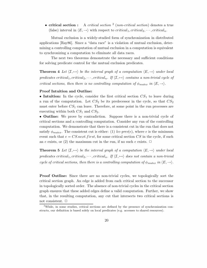
• critical section : A critical section 2 (non-critical section) denotes a true

(false) interval in 〈E,→〉 with respect to critical1, critical2, · · · , criticaln.

Mutual exclusion is a widely-studied form of synchronization in distributed

applications [Ray86]. Since a “data race” is a violation of mutual exclusion, deter-

mining a controlling computation of mutual exclusion in a computation is equivalent

to synchronizing a computation to eliminate all data races.

The next two theorems demonstrate the necessary and sufficient conditions

for solving predicate control for the mutual exclusion predicates.


predicates critical1, critical2, · · · , criticaln. If 〈I, 7→〉 contains a non-trivial cycle of

critical sections, then there is no controlling computation of φmutex in 〈E,→〉.


• Intuition: In the cycle, consider the first critical section CS1 to leave during

a run of the computation. Let CS2 be its predecessor in the cycle, so that CS2

must enter before CS1 can leave. Therefore, at some point in the run processes are

executing within both CS1 and CS2.

• Outline: We prove by contradiction. Suppose there is a non-trivial cycle of

critical sections and a controlling computation. Consider any run of the controlling

computation. We demonstrate that there is a consistent cut in the run that does not

satisfy φmutex. The consistent cut is either: (1) lcc-prev(e), where e is the minimum

event such that e = CS.next.first, for some critical section CS in the cycle, if such

an e exists, or (2) the maximum cut in the run, if no such e exists. 2


predicates critical1, critical2, · · · , criticaln. If 〈I, 7→〉 does not contain a non-trivial

cycle of critical sections, then there is a controlling computation of φmutex in 〈E,→〉.

Proof Outline: Since there are no non-trivial cycles, we topologically sort the

critical section graph. An edge is added from each critical section to the successor

in topologically sorted order. The absence of non-trivial cycles in the critical section

graph ensures that these added edges define a valid computation. Further, we show

that, in the resulting computation, any cut that intersects two critical sections is

not consistent. 2

2While, in some studies, critical sections are defined by the presence of synchronization con-structs, our definition is based solely on local predicates (e.g. accesses to shared resources).

20

Types:

event: (proc: int; v: vector clock) (L1)interval: (proc: int; critical: boolean; first: event; last: event)(L2)

Input:

I1, I2, · · · , In: list of interval, initially non-empty (L3)

Output:


Vars:

I1, I2, · · · , In: interval, initially ∀i : Ii = Ii.head (L5)valid cs: set of interval (L6)chain: list of interval (L7)crossed: interval (L8)prev, curr: interval (L9)

Notation:

CSi =

{

min X ∈ Ii : Ii �i X ∧ X.critical = true, if existsnull, otherwise

(L10)

CS = { CSi | (1 ≤ i ≤ n) ∧ (CSi 6= null) } (L11)

select(Z) =

{


(L12)

Procedure:

while (CS 6= ∅) do (L13)valid cs := { c ∈ CS | ∀c′ ∈ CS : (c′ 6= c) ⇒ (c′ 67→ c) } (L14)if (valid cs = ∅) (L15)

exit(“no controlling computation exists”) (L16)crossed := select(valid cs) (L17)chain.add head(crossed) (L18)Icrossed.proc := crossed.next (L19)

if (chain 6= null) (L20)prev := chain.delete head() (L21)

while (chain 6= null) do (L22)curr := chain.delete head() (L23)O.add head( (curr.next.first, prev.first) ) (L24)prev := curr (L25)

Figure 5: Algorithm for Predicate Control of the Mutual Exclusion Predicate

21


The proof of the above theorem provides a simple algorithm for finding a controlling

computation based on topologically sorting the interval graph of critical sections.

We provide a more efficient algorithm in Figure 5, making use of the fact that the

critical sections in a process are totally ordered. The key idea used in the algorithm

is to maintain a frontier of critical sections (CS1, · · · , CSn) that advances from the

start of the computation to the end. Instead of finding a minimal critical section

of the whole interval graph, we merely find a minimal critical section in the current

frontier. It is guaranteed to be a minimal critical section of the remaining critical

sections in the interval graph at that point. Therefore, this procedure achieves a

topological sort.

The main while loop of the algorithm executes p times in the worst case,

where p is the number of critical sections in the computation. Each iteration takes

O(n2), since it must compute the valid cs. Thus, a simple implementation of the

algorithm will have a time complexity of O(n2p). However, a better implementation

of the algorithm would be O(np) by avoiding redundant computations in computing

valid cs over multiple iterations of the loop. An example of such an implementation

is to maintain a reference count with each critical section in CS indicating the

number of smaller critical sections (with respect to 7→) in CS. The set valid cs

is maintained as the set of critical sections with a reference count of 0. In each

iteration, the update of Icrossed.proc (line L19) also involves updating the reference

counts and valid cs. The update would involve deleting a critical section, which is

O(n), and adding a critical section, which is also O(n). Since there are O(p) critical

sections in all, this implementation has a time complexity of O(np). Note that a

naive algorithm based directly on the constructive proof of the sufficient condition

in Theorem 5 would take O(p2). We have reduced the complexity significantly by

using the fact that the critical sections in a process are totally ordered.

We next prove the correctness of the algorithm.


Proof Outline: It can be shown that each term in the algorithm (especially

curr.next.first at line L23) is well-defined. The algorithm terminates since the

main loop in the algorithm crosses at least one critical section in each iteration. 2

Lemma 16 If the algorithm in Figure 5 exits at line L16, then no controlling com-

putation exists.

22

Proof: At the point of exit at line 16 valid cs = ∅. Therefore, the graph 〈CS, 7→

〉 has no minimal element. Since CS 6= ∅ (by the terminating condition at line

L13), there must be a non-trivial cycle in 〈CS, 7→〉. Therefore, by Theorem 4, no

controlling computation exists. 2


controlling computation of φmutex in 〈E,→〉, where →c is the transitive closure of

the union of → with the set of edges in O.

Proof Outline: We show that, at the termination of loop L13-L19, chain is a

topological sort of the graph 〈C, 7→〉. Then, as in the proof of Theorem 5, the

computation defined by the added edges is a controlling computation. 2

Theorem 6 The algorithm in Figure 5 solves the predicate control problem for the

mutual exclusion predicate.

Proof: This follows directly from Lemmas 15, 16, and 17. 2

4.3 Readers Writers Predicates

Let critical1, critical2, · · · , criticaln be n local predicates and let critical(e) ≡

criticale.proc(e) and let a critical section (non-critical section) denote a true (false)

interval in 〈E,→〉 with respect to critical1, critical2, · · · , criticaln.

• read-critical/write-critical : A critical section is either read-critical or

write-critical .

• write critical(I) : We define write critical(I) to be true for a write-critical

section I and false for all other intervals. We also say write critical(e) for all

events e in a write-critical section.

• read critical(I) : We define read critical(I) to be true for a read-critical

section I and false for all other intervals. We also say read critical(e) for all

events e in a read-critical section.

• readers writers predicate : The readers writers predicate φrw is defined

as:

φrw(C) ≡ ∀ distinct i, j : ¬ ( critical(C[i]) ∧ write critical(C[j]) )

23

The readers writers predicate is a generalized form of mutual exclusion al-

lowing critical sections to be read or write-critical. Two critical sections cannot be

occupied at the same time if one of them is write-critical. The next two theorems

establish the necessary and sufficient conditions for solving the predicate control

problem for readers writers predicates. Since the algorithm that will be presented

in Section 4.5 is applied to readers writers predicates without significant simplifica-

tion, we do not present a specialized algorithm for readers writers predicates.


predicates critical1, critical2, · · · , criticaln. If 〈I, 7→〉 contains a non-trivial cycle

of critical sections containing at least one write-critical section, then there is no

controlling computation of φrw in 〈E,→〉.


• Intuition: In the cycle, consider any write critical section W . Consider the

point when W leaves. There are two possibilities: either (Case 1) at least one

critical section has not yet left, or (Case 2) all the critical sections have left. (Case

1:) The predecessor of W in the cycle must have entered. If it has left, then its

predecessor must have entered. Repeating this argument, we determine at least one

critical section which must have entered but not left. Therefore, the readers writers

predicate is violated. (Case 2:) Consider the point when the successor of W left.

At that time, W must have entered, thereby violating the readers writers predicate.

• Outline: We prove by contradiction. Suppose there is a non-trivial cycle of critical

sections with at least one write critical section and a controlling computation exists.

Consider any run of the controlling computation. We demonstrate that there is a

consistent cut in the run that does not satisfy φrw.

The consistent cut is determined as follows. Consider any write critical

section W and its successor CS in the cycle. The consistent cut is one of: (1)

lcc-prev(W.next.first), (2) lcc-prev(CS.next.first), or (3) the maximum cut in the

run. At least one of these cuts is well-defined and does not satisfy φrw. 2



cycle of critical sections containing at least one write-critical section, then there is

a controlling computation of φrw in 〈E,→〉.

Proof Outline: We topologically sort the strongly connected components (scc’s)

of the critical section graph. An edge is added from each critical section in one scc

24

to each critical section in the successor scc in topologically sorted order. We show

that the added edges define a valid computation. Further, we show that, in the

resulting computation, any cut that intersects a write-critical section and another

critical section is not consistent. 2

4.4 Independent Mutual Exclusion Predicates

Let critical1, critical2, · · · , criticaln be n local predicates and let critical(e) ≡

criticale.proc(e) and let a critical section (non-critical section) denote a true (false)

interval in 〈E,→〉 with respect to critical1, critical2, · · · , criticaln.

• k-critical : A critical section is k-critical for some k ∈ {1, · · ·m}.

• k critical(I) : We define k critical(I) to be true for a k-critical section I

and false for all other intervals. We also say k critical(e) for all events e in a

k-critical section.

• independent mutual exclusion predicate : The independent mutual

exclusion predicate φind is defined as:

φind(C) ≡ ∀ distinct i, j : ∀ k : ¬ ( k critical(C[i]) ∧ k critical(C[j]) )

The independent mutual exclusion predicate is a generalized form of mutual

exclusion allowing critical sections to have types in k ∈ {1, · · ·m}. Two critical

sections cannot enter at the same time if they are of the same type. Note, however,

that the model does not allow two critical sections of different types to overlap within

the same process. Our study is confined to the simpler non-overlapping model.

The next result shows us that the problem becomes hard for this generaliza-

tion. However, we will determine sufficient conditions for solving it that allow us to

solve the problem efficiently under certain conditions.

Theorem 9 The predicate control problem for the independent mutual exclusion

predicate is NP-Complete.

Proof Outline: The problem is in NP since the general predicate control problem

is in NP. The NP-Hardness is established by a transformation from 3SAT. 2

Although the problem is NP-Complete, the next result states a sufficient

condition under which it can be solved. The condition is the absence of cycles

containing two critical sections of the same type. Under these conditions, we can

25

construct an efficient algorithm. Since the algorithm that will be presented in Sec-

tion 4.5 is applied to independent mutual exclusion predicates without significant

simplification, we do not present a specialized algorithm in this section.



cycle of critical sections containing two k-critical section for some k, then there is

a controlling computation of φind in 〈E,→〉.

Proof: The proof is along similar lines to the proof of Theorem 8. 2

To give an idea of why this condition is not necessary, consider the following

example in which the condition does not hold. There are three critical sections CS1,

CS2, and CS3 on three different processes and CS1 7→ CS2 7→ CS3 7→ CS1 forms

a cycle in the interval graph. Two of the critical sections CS1 and CS2 are of the

same type, while CS3 is of a different type. In this case, we can form a controlling

computation by adding an edge from CS1.next.first to CS2.f irst. However, in a

general computation, following such a strategy may cause cycles. In practice, in

applications in which the sizes of critical sections are relatively small with respect

to the time between communication events, the sizes and frequency of cycles in the

interval graph would both be smaller and, therefore, cycles induced by added control

edges would be less likely.

4.5 Generalized Mutual Exclusion Predicates

Using the definitions of the previous two sections:

• generalized mutual exclusion predicate : The generalized mutual ex-

clusion predicate φgen mutex is defined as:

φgen mutex(C) ≡ ∀ distinct i, j :

¬ ( critical(C[i]) ∧ write critical(C[j]) ) ∧

∀ k : ¬ ( k critical(C[i]) ∧ k critical(C[j]) )

Generalized mutual exclusion predicates allow critical sections to have types

and be read/write-critical. Clearly the predicate control problem is NP-Complete for

generalized mutual exclusion predicates. Further, a similar sufficient condition can

be proved combining the sufficient conditions for readers writers and independent

mutual exclusion predicates.

26


Based on the proof of the sufficient conditions, we can design a simple algorithm

based on determining the strongly connected components in the critical section

graph and then topologically sorting them. Instead, we present a more efficient

algorithm in Figure 6.

In order to understand how the algorithm operates, we require the concept

of a “general interval”. A general interval is a sequence of intervals in a process that

belong to the same strongly connected component of the interval graph. For the

purposes of the algorithm, it is convenient to treat such sequences of intervals as a

single general interval. We now define general intervals and define a few notations.

• general interval : Given an interval graph 〈I, 7→〉, a general interval is a

contiguous sequence of intervals in an 〈Ii,≺i〉 subgraph.

• g.first/g.last : For a general interval g, let g.first (g.last) represent the

first and last intervals in g.

• g.set : Let g.set represent the set of intervals in the sequence g.

• 7→ (for general intervals) : Let G denote the set of general intervals in a

computation. We define the (overloaded) relation 7→ for general intervals as:

∀g, g′ ∈ G : g 7→ g′ ≡ g.first 7→ g′.last

• α(g) : We say that a general interval g is true under a local predicate α if

α(g.first). In particular, if g is true under a local predicate critical, we call

g a general critical section.

• ↪→ : Let G1 ⊆ G be a set of general intervals. Let SG1be the set of strongly

connected components in the graph 〈G1, 7→〉. We define a relation ↪→ on SG1

as follows:

∀s, s′ ∈ SG1: s ↪→ s′ ≡ ∃g ∈ s, g′ ∈ s′ : g 7→ g′

Clearly, 〈SG1, ↪→〉 has no cycles.

The algorithm maintains a frontier of general critical sections that advances

from the beginning of the computation to the end. In each iteration, the algorithm

finds the strongly connected components (scc’s) of the general critical sections in

the frontier. Then, it picks a minimal strongly connected component, candidate,

from among them (line L22). However, the candidate is not necessarily a minimal

27

Types:

event: (proc: int; v: vector clock) (L1)gen interval: (proc: int; critical: boolean; first: event; last: event) (L2)str conn comp: set of gen interval (L3)

Input:

I1, I2, · · · ,In: list of gen interval, initially non-empty (L4)

Output:


Vars:

I1, I2, · · · , In: gen interval, initially ∀i : Ii = Ii.head (L6)scc set: set of str conn comp (L7)valid scc: set of str conn comp (L8)chain: list of str conn comp (L9)candidate: str conn comp (L10)prev scc, curr scc: str conn comp (L11)prev, curr: gen interval (L12)

Notation:

CSi =

{

min X ∈ Ii : Ii �i X ∧ X.critical = true, if existsnull, otherwise

(L13)

CS = { CSi | (1 ≤ i ≤ n) ∧ (CSi 6= null) } (L14)get scc(CS) = set of strongly connected components in 〈CS, 7→〉 (L15)

select(Z) =

{


(L16)

not valid(X) = X has a non-trivial cycle of critical sections with eitherone write critical section or two k-critical sections (L17)

merge(c, c′) = (c.last := c′.last; c.next := c′.next) (L18)

Procedure:

while (CS 6= ∅) do (L19)scc set := get scc(CS) (L20)valid scc := { s ∈ scc set | ∀s′ ∈ scc set : (s′ 6= s) ⇒ (s′ 6↪→ s) } (L21)candidate := select(valid scc) (L22)mergeable := { c.next.next | c ∈ candidate ∧ c.next.next 6= null ∧

∃c′ ∈ candidate : c.next.next 7→ c′} (L23)if (mergeable = ∅) (L24)

if (not valid(candidate)) (L25)exit(“cannot find controlling computation”) (L26)

chain.add head(candidate) (L27)for (c ∈ candidate) do (L28)

Ic.proc := c.next (L29)else (L30)

for (c ∈ mergeable) do (L31)merge(CSc.proc, c) (L32)

if (chain 6= null) (L33)prev scc := chain.delete head() (L34)

while (chain 6= null) do (L35)curr scc := chain.delete head() (L36)

for (curr ∈ curr scc, prev ∈ prev scc) do (L37)O.add head( (curr.next.first, prev.first) ) (L38)prev scc := curr scc (L39)

Figure 6: Algorithm for Generalized Mutual Exclusion Predicate Control

28

scc of the entire critical section graph. In fact, it need not even be an scc of the

entire graph. To determine if it is, we find the mergeable set of critical sections that

immediately follow the general critical sections and belong to the same scc (line

L23). If mergeable is not empty, the critical sections in mergeable are merged with

the general critical sections in candidate to give larger general critical sections (line

L32) and the procedure is repeated. If mergeable is empty, then it can be shown

that candidate is a minimal scc of the graph. Therefore, we check that it meets

the sufficient conditions of validity (line L25), and then append it to the chain (line

L27).

Finally, after the main loop terminates, the scc’s in the chain are connected

using added edges which define the controlling computation (lines L33-L39). Note

how the use of general critical sections allows us to reduce the number of edges that

need to connect two consecutive scc’s as compared to the simple algorithm that

would be defined by the proof of Theorem 8.

The main while loop of the algorithm executes p times in the worst case,

where p is the number of critical sections in the computation. Each iteration takes

O(n2), since it must compute the scc’s. Thus, a simple implementation of the algo-

rithm will have a time complexity of O(n2p). However, a better implementation of

the algorithm would be O(np) by avoiding redundant computations while comput-

ing valid scc over multiple iterations of the loop. The optimized implementation

is similar to the one described for the algorithm for mutual exclusion predicates in

section 4.2. Note that a naive algorithm based directly on the constructive proof

of the sufficient condition in Theorem 8 would take O(p2). We have reduced the

complexity significantly by using the fact that the critical sections in a process are

totally ordered.

Finally, we prove the correctness of the algorithm.


Proof Outline: It can be verified that each term in the algorithm (especially the

term curr.next.first at line L37) is well-defined. The algorithm terminates since, in

each iteraction of the main loop, either one critical section is crossed or two distinct

critical sections are merged into one. 2

Lemma 19 If the algorithm in Figure 6 exits at line L26, then there is a non-trivial

cycle of critical sections with:

(1) at least one write-critical, or

(2) two k-critical sections for some k ∈ {1, · · · ,m}.

29

Proof: Follows directly from the condition at line L25. 2


controlling computation of φgen mutex in 〈E,→〉, where →c is the transitive closure

of the union of → with the set of edges in O.

Proof Outline: Consider the graph of regular critical sections 〈C, 7→〉 and the

corresponding graph of scc’s 〈S, ↪→〉. We first prove that any two regular critical

sections within the same general critical section belong to the same scc of S. This

follows from the way in which two critical sections are merged into one in L32.

Next, we show that when a candidate scc of general critical sections is added

to chain at L27, then it corresponds to a valid scc of regular critical sections. Fur-

ther, we show that it also corresponds to a minimal scc of regular critical sections

in the remaining critical section graph.

Therefore, at the termination of loop L19-L32, chain corresponds to a topo-

logical sort of the graph 〈S, ↪→〉. Then, as in the proof of Theorem 8, the computa-

tion defined by the added edges is a controlling computation. 2

Theorem 11 The algorithm in Figure 6 solves the predicate control problem for the

generalized mutual exclusion predicate if the input computation has no non-trivial

cycles of critical sections containing two k-critical sections for some k ∈ {1, · · · ,m}.

Proof: By Lemma 18, the algorithm always terminates, and by Lemma 20, if it

terminates normally then it outputs a controlling computation. By Lemma 19, if it

terminates at line L26, then there is a non-trivial cycle with:

(1) at least one write-critical, or

(2) two k-critical sections for some k ∈ {1, · · · ,m}.

In case (1), Theorem 7 indicates that no controlling computation exists. Therefore,

it is only in case (2) that the algorithm fails to find a controlling computation

that does exist, (which is to be expected since the problem is NP-Complete by

Theorem 9). 2

5 Applications

In this section, we first discuss some general issues that arise in applying the pred-

icate control algorithms. We then describe two specific application domains – soft-

ware fault-tolerance and distributed debugging.

30

5.1 General Issues

We have stated and solved the predicate control problem in an abstract model. Some

issues arise while mapping the abstract concepts used in the model – computation,

global predicate and controlling computation – to real-world scenarios.

Computation: A partially-ordered set of events is a common model of computation

in distributed systems [Lam78]. It has been used in system scenarios as var-

ied as: distributed message-passing [NM92], parallel shared-memory [Net93],

distributed shared-memory [RZ97] and multi-threaded [CS98]. Tracing the

computation is a prerequisite for applying predicate control, and the time and

space costs of tracing the computation are particularly relevant. In each of the

system scenarios, one must intercept each relevant communication (e.g. mes-

sages, shared-object accesses) and determine the partial order among them.

For example, in a pure message-passing distributed application, piggy-backing

vector-clocks [Mat89, Fid91] on messages together with intercepting the send

and receive events of the messages is sufficient to trace the computation.

Global Predicate: In predicate control, a global predicate is used to specify an

unwanted global condition (e.g. multiple processes in critical sections) from

the point of view of synchronization. This would typically involve a shared

resource (e.g. shared file system, shared memory objects, shared clock). There

are two ways in which such shared resources may interact with the system:

Shared resources external to the system: By external, we mean that the

shared resource does not provide a causal channel for the system and

therefore need not be traced as part of the computation. For example,

in distributed message-passing applications sharing a network file sys-

tem (e.g. scientific applications [KN94, AHKM96, Fin97]) that use only

write accesses (e.g. for logging), the files may be viewed as being exter-

nal to the system since they don’t cause causal dependencies within the

system. Another class of examples are applications that use read-write

accesses to shared objects, but in which the read values do not influence

the communication pattern (e.g. matrix multiplication).

Shared resources internal to the system: By internal, we mean that the

shared resource provides a causal channel for the system and therefore is

a part of the computation. In such cases, the causal dependencies caused

by the shared resource must be traced while determining the computa-

tion. For example, in a distributed message-passing system in which the

31

processes use read and write accesses to shared files to communicate in

addition to the regular messages, the read and write accesses must be

intercepted and their causal order must be determined.

Controlling Computation: Implementing a controlling computation requires re-

playing the traced computation and overlaying the added synchronizations.

Typically the mechanisms for adding the extra synchronizations would be

similar to the mechanisms for replaying the computation itself. Replaying a

traced computation has been extensively studied in the literature in multiple

system scenarios [NM92, Net93, NM95, RC96, RZ97, CS98].

5.2 Software Fault-tolerance

Distributed programs often encounter failures, such as races, owing to the presence

of synchronization faults (bugs). Rollback recovery [HK93, WHF+97, CC98] is an

important technique that is used to tolerate such faults. It involves rolling back

the program to a previous state and re-executing, in the hope that the failure does

not recur. The disadvantage of this approach is that it cannot guarantee that the

re-execution will itself be failure-free.

By tracing relevant state information during the first execution, the look-

ahead required by predicate control can be achieved. It is then possible to solve

the predicate control problem for the traced computation and for the predicate

expressing that the failure does not recur. For example, a mutual exclusion predicate

expresses that a data race failure does not occur. If a controlling computation exists,

it is used to synchronize the computation during re-execution to guarantee that a

failure does not recur. If no controlling computation exists, then a failure must

always occur during any re-execution of the computation.

An implementation of a rollback recovery system based on predicate con-

trol for tolerating data races in distributed MPI applications has been described in

[Tar00]. The data races were file corruptions due to synchronous write accesses to a

shared network file system in the absence of locks. The communication was through

MPI messages. The applications were synthetic applications whose communication

and file access patterns were based on the NPB 2.0 Benchmark Suite [BHS+95].

The experiments showed that the tracing costs involved less than 1% time overhead

and that the space cost was less than 3 MB/hour per process.

We also compared three different recovery methods for their relative abilities

to successfully recover : (1) simple re-execution: involving simply re-executing in

the hope that the race does not recur, (2) locked re-execution involving applying

32

file system locks to each access during re-execution, and (3) controlled re-execution

using added synchronizing messages to implement predicate control. The ability to

recover was measured by the mean-time-to-failure, where failure is a race in (1), a

deadlock in (2), and a cycle in (3). We found that in controlled re-execution the

mean-time-to-failure was substantially higher than in the other two methods under

varying communication and file access patterns. For example, an application with

a 200 ms mean file access period and a 50 ms mean communication period had a

mean-time-to-failure of 0.5 sec in (1), 1.3 sec in (2), and 43.9 sec in (3).

5.3 Distributed Debugging

Software faults (bugs) in distributed programs are difficult to detect and eliminate

since they are often difficult to reproduce. An example of such software faults are

synchronization faults such as races which depend on the relative timing among pro-

cesses. In order to facilitate the localization of software faults, trace-replay methods

have been developed in many different environments: message-passing parallel pro-

grams [NM92], shared-memory parallel programs [Net93], distributed shared mem-

ory programs [RZ97], and multi-threaded programs [CS98]. These methods involve

tracing the non-deterministic events during execution and replaying them during

re-execution.

Applying existing trace-replay methods leads to a cycle of replay and passive

observation to determine the cause of the anomaly. A more active process would

involve the user specifying a constraint that is imposed on the replayed computation.

A common constraint is that of mutual exclusion of various functions. The user

could then replay the computation with the added constraint to observe whether

the anomaly occurs under mutual exclusion. Since tracing is already carried out for

the purposes of replay, look-ahead is available. Predicate control can, therefore, be

applied [TG98, MG00] to determine a controlling computation that can be replayed

to present an observation under the specified constraints. Note that in debugging

it is more acceptable to incur tracing costs than in software fault-tolerance.

For example, suppose the anomaly is that of a corrupted log file. The pro-

grammer knows that the log file may be corrupted because of a race while simultane-

ously writing to the file or because of memory corruption within the program. While

debugging the system, the programmer may replay the execution with an added con-

straint of mutual exclusion on all accesses to the file. In this scenario, controlled

re-execution has a significantly better chance of achieving this re-execution than a

simple lock-based or retry-based mechanism (as per our experiments for software

fault-tolerance above).

33

6 Related Work

The results in this paper were first published in [TG98] and [TG99]. We are aware

of two previous studies of controlling distributed systems to maintain classes of

global predicates. One study [MSWW81] allows global properties within the class of

conditional elementary restrictions [MSWW81]. Unlike our model of a distributed

system, their model uses an off-line specification of pair-wise mutually exclusive

states and does not use causality. [Ray88] and [TG94] study the on-line maintenance

of a class of global predicates based on ensuring that a sum or sum-of-product

expression on local variables does not exceed a threshold. In contrast to these

approaches, our focus is on general global boolean predicates, disjunctive predicates,

and mutual exclusion predicates.

Since our results in predicate control were published, some advances in solv-

ing predicate control have been made in [MG00]. The authors present an equivalent

formulation of the predicate control problem in terms of “admissible sequences”.

Based on this, they provide an algorithm for disjunctive predicates that has the

same time complexity as the algorithm presented in this paper, but has the added

advantage of generating the minimum synchronizations. They also solve the pred-

icate control problem for the class of “region predicates” that can express such

conditions as deadlock and termination.

Relation to Predicate Detection

Since observation and control are duals of each other, it is not surprising that there

is a relation between predicate detection, a formalization of observation, and predi-

cate control, a formalization of control. To understand the relationship, consider a

computation in which definitely : ¬φ is detected, where the modality definitely for a

predicate [CM91] implies that the predicate is true in any possible execution (run)

corresponding to the computation. Clearly, there can be no controlling computa-

tion of φ in the computation since any execution corresponding to the controlling

computation is also an execution corresponding to the original computation. There-

fore, a controlling computation of a predicate φ in a given computation exists if

and only if definitely : ¬φ is not detected in the computation. As evidence of this,

the necessary and sufficient conditions for detecting definitely : φ for conjunctive

predicates were demonstrated in [GW96], and are similar to our results in predi-

cate control for disjunctive predicates. An important difference between the two

problems is that, though the predicate detection problem for definitely : ¬φ can be

used to determine whether a controlling computation of φ exists, it is not concerned

34

with actually finding the controlling computation. Another interesting conclusion

is that all of our predicate control algorithms can be used to solve a corresponding

predicate detection problem.

Relation to On-line Synchronization

The predicate control problem is an off-line synchronization problem since it assumes

that the computation is known a priori . In contrast, existing synchronization prob-

lems [BA90] such as mutual exclusion, readers writers, and dining philosophers are

on-line and require synchronization without such pre-knowledge. The predicate con-

trol problem for each of the predicates we have studied has a corresponding on-line

synchronization problem, in which the computation is an on-line rather than an

off-line input. Predicate control for mutual exclusion predicates corresponds to the

widely-studied distributed mutual exclusion problem [Ray86, BA90, Vel93, Sin93].

Predicate control for readers writers predicates corresponds to the readers writ-

ers problem [CHP71, Lam77, BA90]. Predicate control for independent mutual

exclusion predicates does not correspond to a new on-line problem. Instead, mul-

tiple distributed mutual exclusion protocols operate independently assuming that

deadlocks are prevented using a programming discipline such as two-phase locking.

Predicate control for disjunctive predicates corresponds to a special case of the k-

mutual exclusion problem [Ray89, SR92, MBB+92, HJK93, BV95] (that allows up

to k processes inside a critical section at the same time) in which k = (n − 1).

The on-line problems above make assumptions about the programming dis-

cipline such as non-blocking critical sections or two-phase locking. In a general

context without such assumptions, it can be shown that the on-line synchronization

problems are impossible to solve [TG98] and therefore, it is impossible to maintain

the predicate while avoiding deadlocks. Our solutions to the predicate control prob-

lems do not make such assumptions. Instead, we make use of pre-knowledge of the

computation to maintain the predicate while avoiding deadlocks. Thus, off-line syn-

chronization is, inherently, a more powerful technique than on-line synchronization.

Another distinction between the on-line and off-line problems is that the

predicate control problems operate on a single computation of the distributed pro-

gram. The on-line synchronization problems, on the other hand, operate at the

level of the programming language and must, therefore, correctly synchronize for all

possible computations of the program.

35

7 Conclusions

The interaction between an application and its run-time environment has conven-

tionally been perceived as a passive one consisting primarily of observation. The

dual function of control has existed only in simple forms such as application ter-

mination. In this paper we have aimed at demonstrating a more active interaction

in which the control function of the environment is enhanced. As a first step in

this direction, we have studied how one form of control – synchronization – can be

achieved. Predicate control formalizes the problem of synchronizing a distributed

computation with look-ahead (that is, the computation is an off-line input). The

look-ahead allows for improved control with respect to existing synchronization tech-

niques. The predicate control problem is, therefore, targeted to applications like dis-

tributed debugging and rollback recovery for which such a computation look-ahead

occurs naturally. We have demonstrated efficient algorithms for solving predicate

control for some important classes of predicates. This is encouraging, especially

since the corresponding on-line synchronization problems are impossible to solve

without constraining assumptions.

An interesting future direction would be to generalize predicate control to

include other forms of control. Some examples are: controlling the order of message

delivery, controlling the allocation and deallocation of memory, and controlling the

physical location of the application in a distributed system.

In the study of the predicate control problem, there are some interesting open

questions. We have solved predicate control for mutual exclusion predicates and for

disjunctive predicates. These are two extreme subcases of the more general k-mutual

exclusion predicates. The k-mutual exclusion predicates specify that at most k of

the processes can enter critical sections together. Thus, we have solved the cases

where k is 1 and (n−1). We know of a necessary condition for solving the predicate

control problem for k-mutual exclusion – the existence of a set of critical sections in

which each critical section has at least k incoming 7→ edges from the other critical

sections. Note that from this, we can derive the necessary and sufficient conditions

for both 1-mutual exclusion and (n− 1)-mutual exclusion. However, it still remains

an open question whether the k-mutual exclusion problem can be efficiently solved.

It would also be useful to solve the predicate control problem in the context of

relational predicates [Gar96]. An example of such a predicate is (x1 +x2 + · · ·+xn >

k), where xi’s are integer variables in different processes and k is a constant. This

allows us to express conditions such as “the usage of a limited shared resource is

within acceptable bounds”.

36

References

[AHKM96] R. Ahuja, A. Ho, S. Konstantinidou, and P. Messina. A quantitative

study of parallel scientific applications with explicit communication.

The Journal of Supercomputing, 10(1):5–24, 1996.

[BA90] M. Ben-Ari. Principles of concurrent and distributed programming.

Prentice Hall, 1990.

[BHS+95] David Bailey, Tim Harris, William Saphir, Rob van der Wijngaart,

Alex Woo, and Maurice Yarrow. The NAS Parallel Benchmarks 2.0.

Technical Report NAS-95-020, NASA Ames Research Center, 1995.

[BM93] O. Babaoglu and K. Marzullo. Consistent global states of distributed

systems: fundamental concepts and mechanisms. In S. Mullender, ed-

itor, Distributed Systems, chapter 4. Addison-Wesley, 1993.

[BV95] S. Bulgannawar and N. H. Vaidya. A distributed K-mutual exclusion

algorithm. In Proceedings of the 15th International Conference on Dis-

tributed Computing Systems, pages 153–160. IEEE, 1995.

[CC98] S. Chandra and P. M. Chen. How fail-stop are faulty programs? In

Proc. of the Symposium on Fault-tolerant Computing (FTCS), Munich,

Germany, June 1998. IEEE.

[CHP71] P. J. Courtois, F. Heymans, and D. L. Parnas. Concurrent control with

“readers” and “writers”. Communications of the ACM, 14(10):667–668,

October 1971.

[CL85] K. M. Chandy and L. Lamport. Distributed snapshots: Determining

global states of distributed systems. ACM Transactions on Computer

Systems, 3(1):63 – 75, February 1985.

[CM91] R. Cooper and K. Marzullo. Consistent detection of global predicates.

In Proceedings of the ACM/ONR Workshop on Parallel and Distributed

Debugging, pages 163 – 173, Santa Cruz, California, 1991.

[CS98] J. D. Choi and H. Srinivasan. Deterministic replay of Java multi-

threaded applications. In 2nd SIGMETRICS Symp. on Parallel and

Distr. Tools, pages 48 – 59, Aug. 1998.

37

[Fid91] C. Fidge. Logical time in distributed computing systems. IEEE Com-

puter, 24(8):28 – 33, August 1991.

[Fin97] S. A. Fineberg. NAS Application I/O (BTIO) Benchmark.

http://parallel.nas.nasa.gov/MPI-IO/btio/index.html, 1997.

[Gar96] V. K. Garg. Principles of Distributed Systems. Kluwer Academic Pub-

lishers, 1996.

[GW96] V. K. Garg and B. Waldecker. Detection of strong unstable pred-

icates in distributed programs. IEEE Transactions on Parallel and

Distributed Systems, 7(12):1323 – 1333, December 1996.

[HJK93] S.-T. Huang, J.-R. Jiang, and Y.-C. Kuo. k-coteries for fault-tolerant

k entries to a critical section. In Proceedings of the 13th International

Conference on Distributed Computing Systems, pages 74 – 81. IEEE,

1993.

[HK93] Y. Huang and C. Kintala. Software implemented fault tolerance: tech-

nologies and experience. In Proc. IEEE Fault-Tolerant Comp. Symp.,

pages 138 – 144, June 1993.

[KN94] D. Kotz and N. Nieuwejaar. Dynamic file-access characteristics of a

production parallel scientific workload. In Proc. Supercomputing ’94,

pages 640–649, 1994.

[Lam77] L. Lamport. Concurrent reading and writing. Communications of the

ACM, 20(11):806–811, November 1977.

[Lam78] L. Lamport. Time, clocks, and the ordering of events in a distributed

system. Communications of the ACM, 21(7):558 – 565, July 1978.

[Mat89] F. Mattern. Virtual time and global states of distributed systems. In

Parallel and Distributed Algorithms: Proc. of the International Work-

shop on Parallel and Distributed Algorithms, pages 215 – 226. Elsevier

Science Publishers B. V. (North Holland), 1989.

[MBB+92] K. Makki, P. Banta, K. Been, N. Pissinou, and E. Park. A token

based distributed k mutual exclusion algorithm. In Proceedings of the

Symposium on Parallel and Distributed Processing, pages 408 – 411.

IEEE, December 1992.

38

[MG00] N. Mittal and V. K. Garg. Debugging distributed programs using con-

trolled re-execution. In Proc. of the 19th ACM Symposium on Prin-

ciples of Distributed Computing, pages 239–248, Portland, USA, July

2000.

[MSWW81] A. Maggiolo-Schettini, H. Wedde, and J. Winkowski. Modeling a solu-

tion for a control problem in distributed systems by restrictions. The-

oretical Computer Science, 13(1):61 – 83, January 1981.

[Net93] R. H. B. Netzer. Optimal tracing and replay for debugging shared-

memory parallel programs. In Proc. of ACM/ONR Workshop on Par-

allel and Distributed Debugging, pages 1 – 11, San Diego, USA, May

1993. Also available as ACM SIGPLAN Notices Vol. 28, No. 12.

[NM92] R. H. B. Netzer and B. P. Miller. Optimal tracing and replay for

debugging message-passing parallel programs. In Supercomputing ’92,

pages 502 – 511, November 1992.

[NM95] R. H. B. Netzer and B. P. Miller. Optimal tracing and replay for

debugging message-passing programs. The Journal of Supercomputing,

8(4):371 – 388, 1995.

[Ray86] M. Raynal. Algorithms for Mutual Exclusion. MIT Press, 1986.

[Ray88] M. Raynal. Distributed Algorithms and Protocols. John Wiley and Sons

Ltd., 1988.

[Ray89] K. Raymond. A distributed algorithm for multiple entries to a critical

section. Information Processing Letters, 30:189–193, February 1989.

[RC96] M. Russinovich and B. Cogswell. Replay for concurrent non-

deterministic shared-memory applications. In Proc. ACM SIGPLAN

Conf. on Programming Languages and Implementation (PLDI), pages

258–266, 1996.

[RZ97] M. Ronnse and W. Zwaenepoel. Execution replay for TreadMarks. In

Proc. of the 5th EUROMICRO Workshop on Parallel and Distributed

Processing (PDP’97), pages 343–350, January 1997.

[Sin93] M. Singhal. A taxonomy of distributed mutual exclusion. Journal of

Parallel and Distributed Computing, 18:94 – 101, 1993.

39

[SR92] P. K. Srimani and R. L. Reddy. Another distributed algorithm for

multiple entries to a critical section. Information Processing Letters,

41:51–57, January 1992.

[Tar00] A. Tarafdar. Software Fault Tolerance in Distributed Systems us-

ing Controlled Re-execution. PhD thesis, University of Texas at

Austin, August 2000. Available as technical report CS-TR-00-38 at

the Dept. of Computer Sciences, University of Texas at Austin, on-line

at www.cs.utexas.edu.

[TG94] A. I. Tomlinson and V. K. Garg. Maintaining global assertions on

distributed sytems. In Computer Systems and Education, pages 257 –

272. Tata McGraw-Hill Publishing Company Limited, 1994.

[TG98] A. Tarafdar and V. K. Garg. Predicate control for active debugging

of distributed programs. In Proc. of the 9th Symposium on Parallel

and Distributed Processing, pages 763–769, Orlando, USA, April 1998.

IEEE.

[TG99] A. Tarafdar and V. K. Garg. Software fault tolerance of concurrent pro-

grams using controlled re-execution. In Proc. of the 13th International

Symposium on Distributed Computing, pages 210–224, Bratislava, Slo-

vak Republic, September 1999.

[TG03] Ashis Tarafdar and Vijay K. Garg. Predicate control: Synchronization

in distributed computations with look-ahead. Technical Report ECE-

PDS-2003-005, Parallel and Distributed Systems Laboratory, ECE

Dept., University of Texas at Austin, 2003. available via ftp or WWW

at maple.ece.utexas.edu as technical report TR-PDS-2003-005.

[Vel93] Martin G. Velazquez. A survey of distributed mutual exclusion algo-

rithms. Technical Report 93-116, Computer Science Dept., Colorado

State University, 1993.

[WHF+97] Y. M. Wang, Y. Huang, W. K. Fuchs, C. Kintala, and G. Suri. Progres-

sive retry for software failure recovery in message-passing applications.

IEEE Trans. on Computers, 46(10):1137–1141, October 1997.

40

Predicate control: synchronization in distributed computations with look-ahead

Documents

Transcript of Predicate control: synchronization in distributed computations with look-ahead