Effects of shear flows on nonlinear waves in excitable media

Journal of Biological Physics25: 101–113, 1999.© 1999Kluwer Academic Publishers. Printed in the Netherlands.

101

Effects of Shear Flows on Nonlinear Waves inExcitable Media

V.N. BIKTASHEV1,†, I.V. BIKTASHEVA 1,†, A.V. HOLDEN1,M.A. TSYGANOV1,‡, J. BRINDLEY2 and N.A. HILL2

1 School of Biomedical Sciences and2 Department of Applied Mathematics, University of Leeds,Leeds LS2 9JT, UK† On leave from Institute for Mathematical Problems in Biology, Pushchino, Moscow region,142292, Russia‡ Also with Institute for Theoretical and Experimental Biophysics, Pushchino, Moscow region,142292, Russia

Accepted in final form 14 January 1999

Abstract. If an excitable medium is moving with relative shear, the waves of excitation may bebroken by the motion. We consider such breaks for the case of a constant linear shear flow. Themechanisms and conditions for the breaking of solitary waves and wavetrains are essentially differ-ent: the solitary waves require the velocity gradient to exceed a certain threshold, whilst the breakingof repetitive wavetrains happens for arbitrarily small velocity gradients. Since broken waves evolveinto new spiral wave sources, this leads to spatio-temporal irregularity.

1. Introduction

Excitable medium models, in the form of partial differential equations of the reaction-diffusion type, have been used to account for nonlinear wave phenomena in manyareas of biology – intracellular calcium waves, excitation in nerve, muscle and car-diac muscle, morphogenesis in the slime mold [1, 2] and in population dynamics.An excitable system responds to a small subthreshold perturbation by a graded,decremental response, and to a suprathreshold perturbation by a large amplitudepulse or pulse train; the best known example is the action potential. This thresholdproperty is characteristic of a cubic nonlinearity, as in the FitzHugh-Nagumo equa-tions for an excitation processE and a recovery processg

∂E

∂t= c1E(E − a)(1− E)− g,

∂g

∂t= ε(c2E − g). (1)

In a spatially extended system the suprathreshold response is a non-decrementaltravelling wave or a wave train. When such a cubic nonlinearity is included in areaction-diffusion equation

jobp328.tex; 19/07/1999; 20:43; p.1WTB: jobp328; pips: 205490; GSB 708017; web2c; (jobpkap:mathfam) v.1.15

102 V.N. BIKTASHEV ET AL.

∂E

∂t= c1E(E − a)(1− E)− g +D∇2E,

∂g

∂t= ε(c2E − g)+ δD∇2g, (2)

in a two-dimensional medium, appropriate initial conditions can lead to a spiralwave. Such spiral waves (or scroll waves in three-dimensions) have been observedin many biological excitable media.

Truscott and Brindley have proposed that plankton dynamics may be repres-ented by an excitable system, with the phytoplankton concentration behaving asthe excitation process, and the zooplankton concentration behaving as a slower re-covery variable. Just as high order cardiac excitation equations, with variables thatchange over many time scales, can be idealised by the FitzHugh-Nagumo systemfor modelling excitation processes in the heart, the temporal behaviour of planktonpopulations can be caricatured by a simple two or three variable system [3, 4].These models have been used to account for plankton blooms [5] and the triggeringof blooms in the Ironex II experiment [6, 7]. In this case the ocean provides themedium within which the plankton dynamics evolves in time. Although plank-ton blooms exhibit the properties of an excitable system, propagating wave trainsand spiral and scroll wave behaviour are not apparent in plankton spatio-temporaldynamics.

Cardiac muscle is another example of a moving excitable medium. Heart mo-tion is a consequence of muscle contraction which is triggered by excitation, andexcitation propagation may depend on the motion of the muscle, thus there is amechano-electric feed-back loop. The majority of experiments on propagation ofexcitation in cardiac muscle are made on immobilised preparations. However,invivo this feedback is present, and theoretical considerations show that motion ofthe muscle can significantly alter the excitation propagation patterns [8].

In this paper, we consider the effects of medium motion, represented by simpleshear flows, on wave behaviours in excitable media, and show that, although asolitary wave can be stable in a shear flow, repetitive activity, including spiral waveactivity, is broken down by arbitrarily small shear flows, and so spatio-temporalirregularity (a frazzle gas, or autowave turbulence) is the expected wave behaviourin a moving excitable medium.

2. Plane Waves in Linear Shear Flows

The generic reaction-diffusion system in a shear flow in the(x, y) plane can bewritten in the form

∂u

∂t= f (u)+ αy ∂u

∂x+D

(∂2u

∂x2+ ∂

2u

∂y2

), (3)

whereu is the column vector of reacting species,f represents the nonlinear reac-tion rates,D is the diffusion matrix andα is the gradient of the advection velocity,

jobp328.tex; 19/07/1999; 20:43; p.2

EFFECTS OF SHEAR FLOWS ON EXCITATION WAVES 103

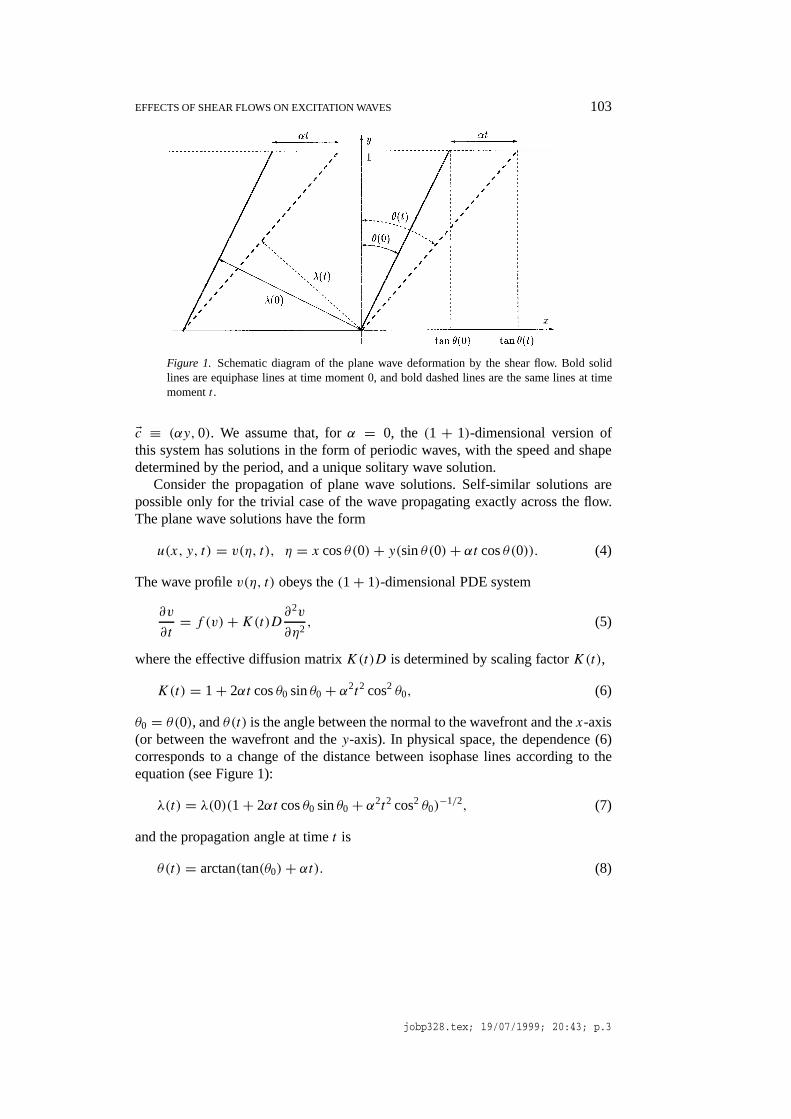
Figure 1. Schematic diagram of the plane wave deformation by the shear flow. Bold solidlines are equiphase lines at time moment 0, and bold dashed lines are the same lines at timemomentt .

Ec ≡ (αy,0). We assume that, forα = 0, the (1 + 1)-dimensional version ofthis system has solutions in the form of periodic waves, with the speed and shapedetermined by the period, and a unique solitary wave solution.

Consider the propagation of plane wave solutions. Self-similar solutions arepossible only for the trivial case of the wave propagating exactly across the flow.The plane wave solutions have the form

u(x, y, t) = v(η, t), η = x cosθ(0)+ y(sinθ(0)+ αt cosθ(0)). (4)

The wave profilev(η, t) obeys the(1+ 1)-dimensional PDE system

∂v

∂t= f (v)+K(t)D∂

2v

∂η2, (5)

where the effective diffusion matrixK(t)D is determined by scaling factorK(t),

K(t) = 1+ 2αt cosθ0 sinθ0+ α2t2 cos2 θ0, (6)

θ0 = θ(0), andθ(t) is the angle between the normal to the wavefront and thex-axis(or between the wavefront and they-axis). In physical space, the dependence (6)corresponds to a change of the distance between isophase lines according to theequation (see Figure 1):

λ(t) = λ(0)(1+ 2αt cosθ0 sinθ0+ α2t2 cos2 θ0)−1/2, (7)

and the propagation angle at timet is

θ(t) = arctan(tan(θ0)+ αt). (8)

jobp328.tex; 19/07/1999; 20:43; p.3


Thus, for plane waves, the problem reduces to that for propagation of excitationwaves in a 1-dimensional cable, with diffusion depending explicitly on time. Nowwe consider the conditions under which this dependence can cause a propagationblock, and hence a break in the wave.

3. Propagation Block of a Solitary Wave

We assume the following properties of the unperturbed version of this equation(K ≡ 1):

1. There exists a stable solitary wave solutionv(η, t) = V (η−cvt), whose widthL = Lnorm, is defined, for example, as the separation between points in whichsome component ofv has a selected value.

2. This solitary wave can develop from initial conditions in the form of thissame wave laterally squeezed, i.e.v(η,0) = V (kη), k > 1, with width,Linit = Lnorm/k, shorter than normal but longer than some minimal width,Lmin(Lmin < Linit < Lnorm), but if Linit < Lmin, the wave decays.

3. The typical time for development/establishment of the wave profile isτprof. If,as is often the case, the excitation waves are supported by processes of differ-ent time scales, thenτprof will be the slowest of them (i.e. the time constant ofthe limiting stage). The significance of this parameter will emerge below.

If K 6= 1 but is any positive constant, then assumption 1 implies that (5) has astationary solitary wave solutionv(η, t) = V (K−1/2η−cvt), with widthLstat(K) =LnormK

1/2. If K(t) is not constant but changes slowly, we may expect that the solu-tion will have the same form as this wave, slowly adjusting its width accordingly.If K(t) changes too rapidly, only then may the wave solution collapse.

With the assumptions listed above, we can formalise a phenomenological model.Let us assume, for simplicity, that the dynamics of the wave width is linear with aconstant relaxation timeτprof. As the instantaneous equilibrium state should changein accordance withK(t), this gives

L̇ = τ−1prof(K

1/2(t)Lnorm− L), L(0) = Lnorm, L(t) ≥ K1/2Lmin∀t. (9)

This equation is in terms of the spatial variableη used in (5), which physically cor-responds to the width measured in the direction of the flow. The rescaled widthL̄ =K−1/2L, corresponding to real width measured perpendicularly to the wavefront,then obeys

˙̄L = τ−1prof(Lnorm− L̄)− K̇

2KL̄, L̄ ≥ Lmin. (10)

The starting and the final asymptotic value ofL̄ is Lnorm. In between, it decreasesbelowLnorm but always remains positive. The minimal value ofL̄ is achieved at˙̄L = 0 which gives

jobp328.tex; 19/07/1999; 20:43; p.4


1+ τprofK̇

2K= Lnorm

Lmin. (11)

The system of Equations (9, 11) determines, in principle, the critical shearα∗at which a break occurs and the corresponding timet∗ of the break; however, theexact solution is rather tedious.

To obtain a simple analytical estimate, let us consider the case of practicalinterest, when the ratio of the excitation timescale to the recovery timescale is

τexc/τrec= ε � 1. (12)

Propagation of excitation waves in this limit is described by the Fife approximation[2]. In particular, the limiting stage of wave formation is establishment of its width,which happens on the time scale ofτprof ∝ τrec, and minimal possible width fromwhich the wave can recover is of the order of the excitation front width,Lmin ∝cvτexc, whereas, in contrast, the normal wave width is, obviously,Lnorm∝ cvτrec.

In this limit we should expect that the breakup occurs only if the effectivediffusivity changes very quickly compared withτprof = τrec. Assuming, in a self-consistent way, thatτ∗ ∝ τexc and neglecting the change ofL(t) during this timeinterval,L(t) ≈ Lnorm, to leading order we obtain a system:

Lnorm/Lmin = ε−1 = K1/2 =(

1+ τprofK̇

2K

). (13)

Using (6) in (13), tanθ(t∗) ≈ α∗t∗ ≈ ε−1, then (13) impliesτprof/t∗ ≈ ε−1, and sothe solution is

t∗ ≈ ετprof = τexc,

θ(t∗) ≈ π/2− ε,

α∗ ≈ τ−1profε

−2 = τrec

τ 2exc

, (14)

in agreement with the original assumptions. This result can also be substantiated bynumerical simulation and by accurate asymptotic analysis of the phenomenologicalODE model; this however is beyond the scope of this communication and will bepublished elsewhere.

Thus there is acritical shear, above which a solitay wave is quenched, and thevalue of this shear depends on the difference between the time scales of excitationand recovery processes, which is a measure of the excitability of the system; themore excitable the system, the greater the shear needed to destroy the wave.

4. Propagation Block of Periodic Waves

For periodic wavetrains the situation is completely different, as the spatial periodmeasured in terms of the variableη (the period in the direction of the flow) is fixed.

jobp328.tex; 19/07/1999; 20:43; p.5


In physical space, if measured in the instantaneous direction of propagation, thespatial period changes according to (7). But in excitable media, there is alwaysa minimal wavelength,λ∗ at which a periodic wavetrain can propagate, and soλ(t) decreasing below this value is a sufficient condition for the propagation block.From (7) we obtain the following estimate of the time and the angle for which thebreak will occur, for any value of the shear however small:

θ0∗ = arctan(1/k), t∗ = α−1(k − 1/k), θ(t∗) = arctan(k), (15)

where

k = λ(0)/λ∗. (16)

5. Numerical Illustrations

So far we have considered only plane waves. To verify the estimates and ana-lyse the effect of the shear flow on more complicated autowave patterns, we haveperformed numerical simulations for the FitzHugh-Nagumo system with the flowincorporated, in the following form

∂E

∂t= c1E(E − a)(1− E)− g + αy ∂E

∂x+D∇2E,

∂g

∂t= ε(c2E − g)+ αy ∂g

∂x+ δD∇2g. (17)

We shall refer to the space and time units of this equation as s.u. and t.u. respect-ively. The parameter values were chosenc1 = 10, a = 0.02, ε = 0.1, c2 = 5,δ = 1 andD = 1. We solved this system with an explicit Euler scheme (forwardtime, centered space), with space stephs = 0.5 s.u., in a rectangular medium(x, y) ∈ [0, L]×[−M/2,M/2] with periodic boundary conditions atx = 0, L andnon-flux boundary conditions aty = ±M/2. The sizes of the medium,L andM,the velocity gradient,α, and the time step,ht , were varied in different experiments.The minimum wavelength of a periodic train in medium with no shear(α = 0) is19.0 t.u. and the wavelength of the spiral wave is 41.0 s.u.

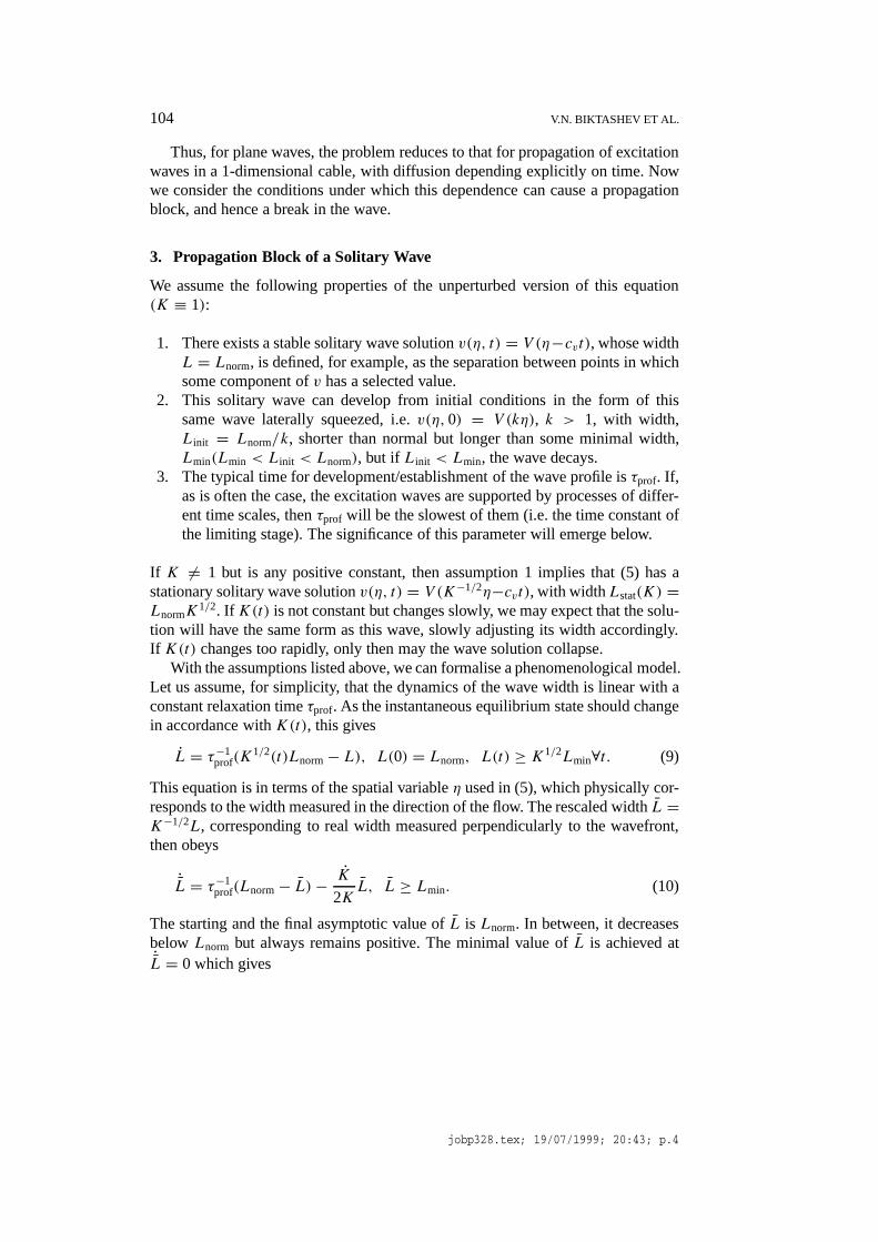
The evolution of a solitary plane wave is shown in Figure 2. The horizontallypropagating wave was initiated in the medium with no shear and then the shear flowwas switched on, which corresponds to the conditions of the analytical estimation.The excitation and recovery variables areE andg and their characteristic times are,respectively,τexc ∝ 1 t.u. andτrec ∝ 1/ε = 10 t.u. According to (14), this meansthatα∗ ∝ 10 t.u.−1 for our choice of parameters. The threshold value of the velocitygradient necessary for breaking a single plane wave was found numerically to beα∗ = 6 t.u.−1, the timet∗ = 1.5 t.u. and the wave orientation at the moment ofthe break tanθ(t∗) = 15, which, to this order of magnitude, is consistent with theanalytical estimates of (14),α∗ = 10 t.u.−1, t∗ = 1 t.u. and tanθ(t∗) = 10.

jobp328.tex; 19/07/1999; 20:43; p.6


Figure 2. Conduction block of a solitary plane wave in the linear shear flow. Velocity gradientα = 10 t.u.−1, medium size 450 s.u.×30 s.u., time stepht = 5·10−5 t.u. Shown are snapshotsof theE field with interval 0.5 t.u.

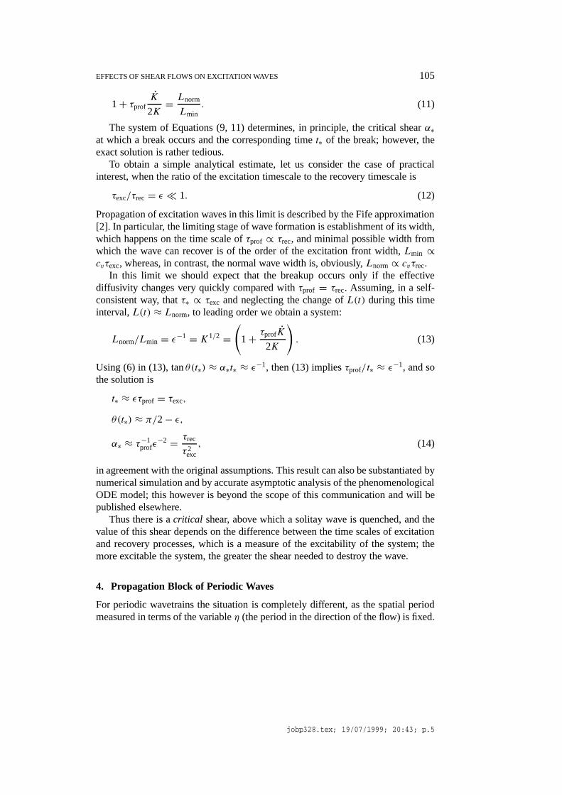
Figure 3. Breakup of a target pattern. Velocity gradientα = 0.06 t.u.−1, medium size200 s.u.×200 s.u., time stepht = 5 · 10−3 t.u. Shown are snapshots of theE field withinterval 27 t.u.

We have studied what happens to autowave structures at velocity gradientsmuch less than this threshold. According to (15) and (16), we have for this mediumk ≈ 2.16, and atα = 0.06 t.u.−1 the wavebreak of the periodic train occurs att∗ ≈ 28 t.u. at the angle ofθ(t∗) ≈ 1.14 rad. These predictions, obtained for planewaves, agree, in order of magnitude, with simulations of the evolution of morecomplicated autowave patterns, the spiral wave and the target pattern.

Figure 3 illustrates the evolution of a series of topologically circular wavesinitiated by periodic stimulation of a point in the medium, with the period equal

jobp328.tex; 19/07/1999; 20:43; p.7


to the period of the spiral wave. It can be seen that while the first wave propagateswithout problems, the propagation of the second is suppressed and the third wave isblocked. This block occurs not for the whole wave but at some points only, leadingto wavebreaks which curl up into spirals. The first breaks occur to the third wave,at timet ≈ 63 t.u., that is 19.4 t.u. after its initiation, and at a propagation angle ofaboutθ ≈ 1.3 rad, in good correspondence with the theory.

Similar numerical experiment has been made with a spiral wave initiated ina medium with(α = 0) and then the shear flow switched on. The spiral wavehas broken, at a time(t∗ ≈ 48) and orientation of the wave(θ(t∗) = 1.3 rad),similar to the previous example. The correspondence in this case would be betterbut for the phenomenon of ‘plasticity’ of the excitation wave: as the process is non-stationary, the visual break-up happens later than the time at which conditions ofstationary propagation are violated. This explanation was confirmed by numericalexperiments when the flow was stopped before the wave broke, but after it wouldhave happened according to the analytical estimate; the wave subsequently broke,despite the absence of the flow.

These two examples show that, at least for the particular model chosen, theconditions of the wavebreak are almost the same whatever the origin and shape ofthe pattern is, and the order of magnitude of the time required for the wavebreakagrees with the estimate (15) obtained for plane periodic waves based on quasi-stationary arguments.

When a spiral wave succumbs to wavebreaks, those develop into new spiralwaves. Thus, in a linear shear flow a ‘chain reaction’ of spiral wave births anddeaths leads to a ‘frazzle gas’ of excitation wavelets. The mechanism for genera-tion of this ‘frazzle gas’ is different from that described in [9]. As this mechanismrequires only a finite deformation of the medium, we may expect that it can playits role not only in constant flows, but in a more wide variety of situations. Ifoceanic plankton dynamics are considered as an excitable medium then currentscan influence their spatial dynamics.

6. Development of the Frazzle Gas

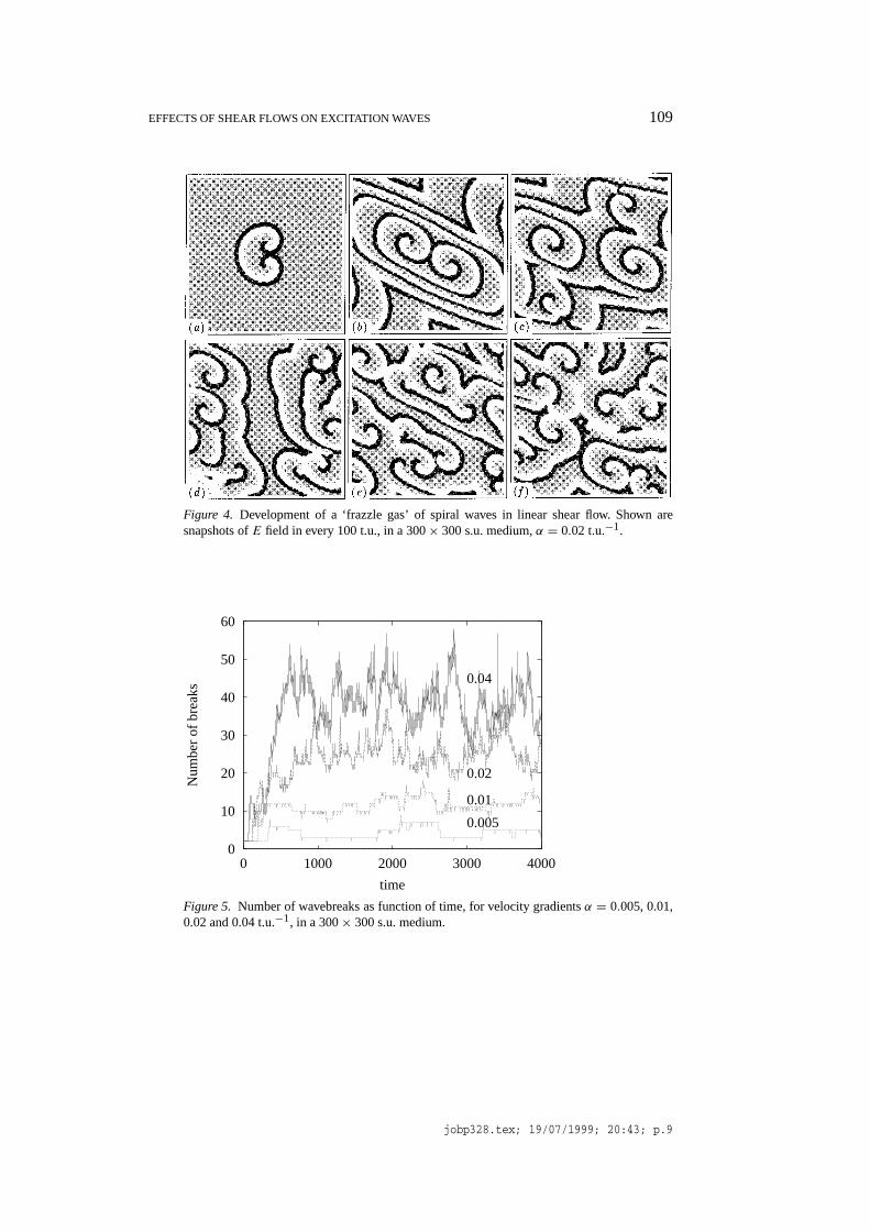
The phenomenon of the conduction block of periodic wavetrains has macroscopicconsequences for the properties of large-scale two dimensional excitable mediawith shear flow. Since this conduction block is dependent on the orientation of thewaves, in case of a complicated autowave pattern it will lead to breaks of some ofthe waves. In an excitable medium, the wavebreaks typically lead to the generationof spiral waves, which are sources of new periodic wavetrains. This leads to a‘chain reaction’ of the spiral wave births, shown on Figure 4.

A local finite initial perturbation of a resting medium with a shear flow has led tothe transition of the whole medium into a turbulent-like state, the ‘frazzle gas’. Tocharacterise quantitatively the frazzle gas solution, we counted the number of thewavebreaks, defined as intersections of the isolinesE = 0.2 andg = 0.48. Some

jobp328.tex; 19/07/1999; 20:43; p.8


Figure 4. Development of a ‘frazzle gas’ of spiral waves in linear shear flow. Shown aresnapshots ofE field in every 100 t.u., in a 300× 300 s.u. medium,α = 0.02 t.u.−1.

0

10

20

30

40

50

60

0 1000 2000 3000 4000

Num

ber

of b

reak

s

time

0.04

0.02

0.01

0.005

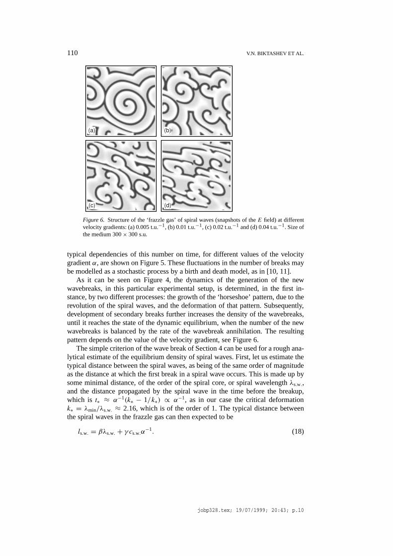
Figure 5. Number of wavebreaks as function of time, for velocity gradientsα = 0.005, 0.01,0.02 and 0.04 t.u.−1, in a 300× 300 s.u. medium.

jobp328.tex; 19/07/1999; 20:43; p.9


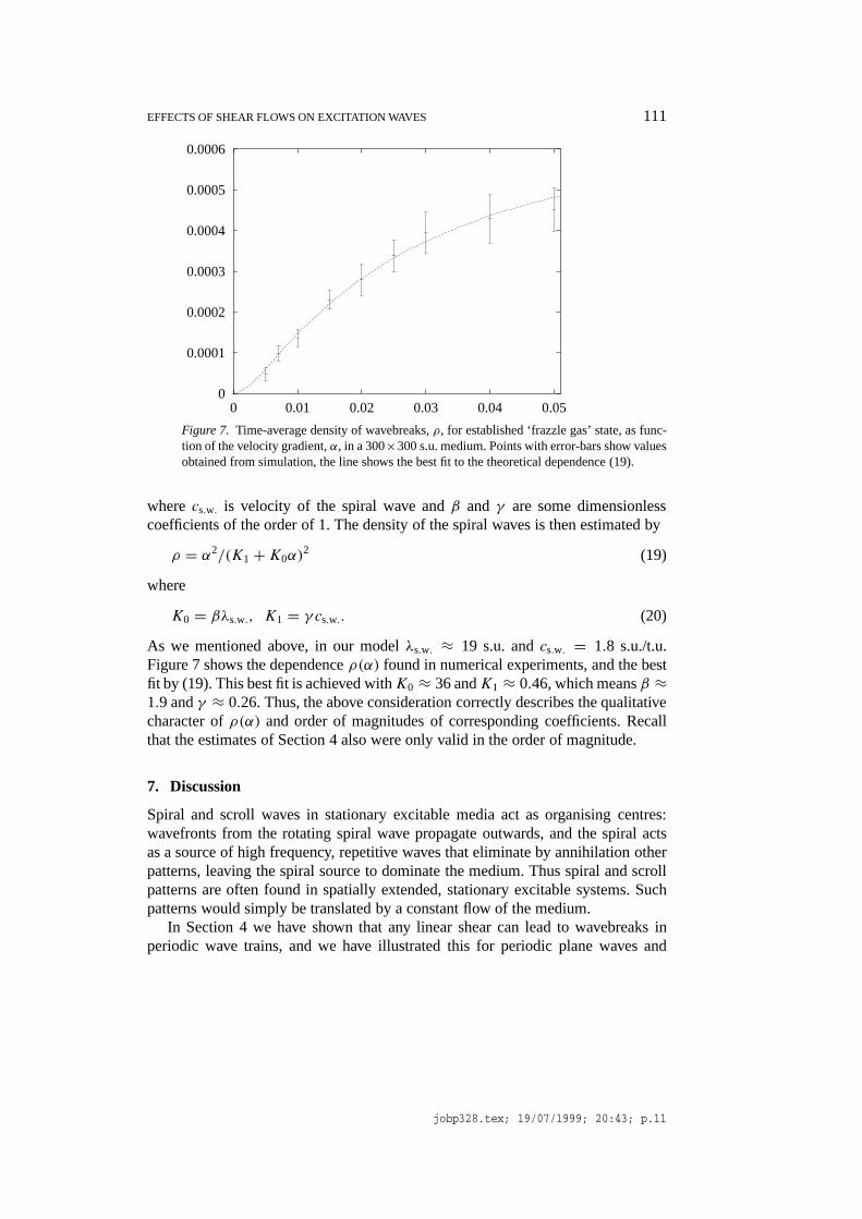
Figure 6. Structure of the ‘frazzle gas’ of spiral waves (snapshots of theE field) at differentvelocity gradients: (a) 0.005 t.u.−1, (b) 0.01 t.u.−1, (c) 0.02 t.u.−1 and (d) 0.04 t.u.−1. Size ofthe medium 300× 300 s.u.

typical dependencies of this number on time, for different values of the velocitygradientα, are shown on Figure 5. These fluctuations in the number of breaks maybe modelled as a stochastic process by a birth and death model, as in [10, 11].

As it can be seen on Figure 4, the dynamics of the generation of the newwavebreaks, in this particular experimental setup, is determined, in the first in-stance, by two different processes: the growth of the ‘horseshoe’ pattern, due to therevolution of the spiral waves, and the deformation of that pattern. Subsequently,development of secondary breaks further increases the density of the wavebreaks,until it reaches the state of the dynamic equilibrium, when the number of the newwavebreaks is balanced by the rate of the wavebreak annihilation. The resultingpattern depends on the value of the velocity gradient, see Figure 6.

The simple criterion of the wave break of Section 4 can be used for a rough ana-lytical estimate of the equilibrium density of spiral waves. First, let us estimate thetypical distance between the spiral waves, as being of the same order of magnitudeas the distance at which the first break in a spiral wave occurs. This is made up bysome minimal distance, of the order of the spiral core, or spiral wavelengthλs.w.,and the distance propagated by the spiral wave in the time before the breakup,which is t∗ ≈ α−1(k∗ − 1/k∗) ∝ α−1, as in our case the critical deformationk∗ = λmin/λs.w. ≈ 2.16, which is of the order of 1. The typical distance betweenthe spiral waves in the frazzle gas can then expected to be

ls.w. = βλs.w. + γ cs.w.α−1. (18)

jobp328.tex; 19/07/1999; 20:43; p.10


0

0.0001

0.0002

0.0003

0.0004

0.0005

0.0006

0 0.01 0.02 0.03 0.04 0.05

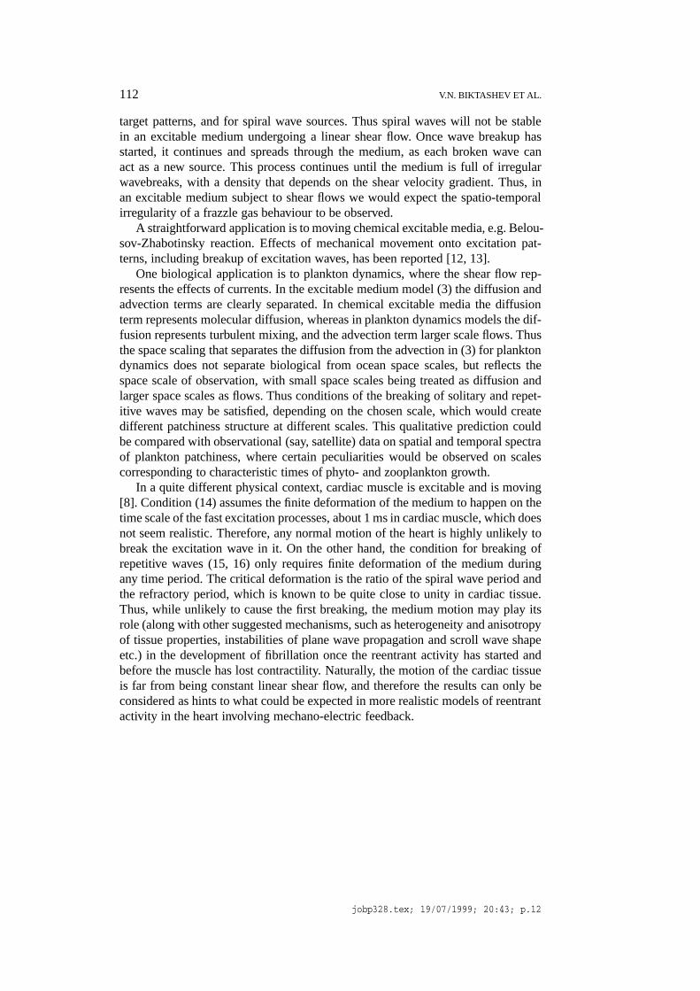
Figure 7. Time-average density of wavebreaks,ρ, for established ‘frazzle gas’ state, as func-tion of the velocity gradient,α, in a 300×300 s.u. medium. Points with error-bars show valuesobtained from simulation, the line shows the best fit to the theoretical dependence (19).

wherecs.w. is velocity of the spiral wave andβ and γ are some dimensionlesscoefficients of the order of 1. The density of the spiral waves is then estimated by

ρ = α2/(K1+K0α)2 (19)

where

K0 = βλs.w., K1 = γ cs.w.. (20)

As we mentioned above, in our modelλs.w. ≈ 19 s.u. andcs.w. = 1.8 s.u./t.u.Figure 7 shows the dependenceρ(α) found in numerical experiments, and the bestfit by (19). This best fit is achieved withK0 ≈ 36 andK1 ≈ 0.46, which meansβ ≈1.9 andγ ≈ 0.26. Thus, the above consideration correctly describes the qualitativecharacter ofρ(α) and order of magnitudes of corresponding coefficients. Recallthat the estimates of Section 4 also were only valid in the order of magnitude.

7. Discussion

Spiral and scroll waves in stationary excitable media act as organising centres:wavefronts from the rotating spiral wave propagate outwards, and the spiral actsas a source of high frequency, repetitive waves that eliminate by annihilation otherpatterns, leaving the spiral source to dominate the medium. Thus spiral and scrollpatterns are often found in spatially extended, stationary excitable systems. Suchpatterns would simply be translated by a constant flow of the medium.

In Section 4 we have shown that any linear shear can lead to wavebreaks inperiodic wave trains, and we have illustrated this for periodic plane waves and

jobp328.tex; 19/07/1999; 20:43; p.11


target patterns, and for spiral wave sources. Thus spiral waves will not be stablein an excitable medium undergoing a linear shear flow. Once wave breakup hasstarted, it continues and spreads through the medium, as each broken wave canact as a new source. This process continues until the medium is full of irregularwavebreaks, with a density that depends on the shear velocity gradient. Thus, inan excitable medium subject to shear flows we would expect the spatio-temporalirregularity of a frazzle gas behaviour to be observed.

A straightforward application is to moving chemical excitable media, e.g. Belou-sov-Zhabotinsky reaction. Effects of mechanical movement onto excitation pat-terns, including breakup of excitation waves, has been reported [12, 13].

One biological application is to plankton dynamics, where the shear flow rep-resents the effects of currents. In the excitable medium model (3) the diffusion andadvection terms are clearly separated. In chemical excitable media the diffusionterm represents molecular diffusion, whereas in plankton dynamics models the dif-fusion represents turbulent mixing, and the advection term larger scale flows. Thusthe space scaling that separates the diffusion from the advection in (3) for planktondynamics does not separate biological from ocean space scales, but reflects thespace scale of observation, with small space scales being treated as diffusion andlarger space scales as flows. Thus conditions of the breaking of solitary and repet-itive waves may be satisfied, depending on the chosen scale, which would createdifferent patchiness structure at different scales. This qualitative prediction couldbe compared with observational (say, satellite) data on spatial and temporal spectraof plankton patchiness, where certain peculiarities would be observed on scalescorresponding to characteristic times of phyto- and zooplankton growth.

In a quite different physical context, cardiac muscle is excitable and is moving[8]. Condition (14) assumes the finite deformation of the medium to happen on thetime scale of the fast excitation processes, about 1 ms in cardiac muscle, which doesnot seem realistic. Therefore, any normal motion of the heart is highly unlikely tobreak the excitation wave in it. On the other hand, the condition for breaking ofrepetitive waves (15, 16) only requires finite deformation of the medium duringany time period. The critical deformation is the ratio of the spiral wave period andthe refractory period, which is known to be quite close to unity in cardiac tissue.Thus, while unlikely to cause the first breaking, the medium motion may play itsrole (along with other suggested mechanisms, such as heterogeneity and anisotropyof tissue properties, instabilities of plane wave propagation and scroll wave shapeetc.) in the development of fibrillation once the reentrant activity has started andbefore the muscle has lost contractility. Naturally, the motion of the cardiac tissueis far from being constant linear shear flow, and therefore the results can only beconsidered as hints to what could be expected in more realistic models of reentrantactivity in the heart involving mechano-electric feedback.

jobp328.tex; 19/07/1999; 20:43; p.12


Acknowledgements

This work has been supported by an equipment grant from the Wellcome Trust,and by grants EPSRC GR/L73364 and INTAS-96-2033.

References

1. Holden, A.V., Markus, M. and H.G. Othmer (eds):Nonlinear Wave Processes in ExcitableMedia, Plenum, New York, 1991.

2. Fife, P.C.: Singular perturbation and wave front techniques in reaction-diffusion problems,SIAM-AMS Proc.10 (1976), 23–50.

3. Truscott, J.E. and Brindley, J.: Equilibria, stability and excitability in a general-class of planktonpopulation-models,Phil. Trans. Roy. Soc. ser. A347(1994), 703–718.

4. Edwards, A.M. and Brindley, J.: Oscillatory behaviour in a three-component plankton-population model,Dynamics and stability of Systems11 (1996), 347–370.

5. Truscott, J.E. and Brindley, J.: Ocean plankton populations as excitable media,Bull. Math. Biol.56 (1994), 981–998.

6. Coale, K.H., Johnson, K.S., Fitzwater, S.E., Gordon, R.M., Tanner, S., Chauvez, F.P., Ferioli,L., Sakamoto, C., Rogers, P., Millero, F., Steinberg, P., Nightingale, P., Cooper, D., Coch-lan, W.P., Landry, M.R., Constantinou, J., Rollwagen, G., Trasvina, A. and Kudela, R.: Amassive phytoplankton bloom induced by an ecosystem-scale iron fertilization experiment inthe equatorial Pacific Ocean,Nature383(1996), 495–501.

7. Pitchford, J.W. and Brindley, J.: Iron limitation, grazing pressure and oceanic HNLC regions,J. Plankton Research, 21 (1999).

8. Hunter, P.J., Nash, M.P. and Sands, G.B.: Computational electromechanics of the heart, Chapter12 in Holden, A.V. and Panfilov, A.V. (eds),Computational Biology of the Heart, J. Wiley &Sons, Chichester, 1997, pp. 345–409.

9. Markus, M., Kloss, G. and Kusch, I.: Disordered Waves in a Homogeneous, MotionlessExcitable Medium,Nature371(6496) (1994), 402–404.

10. Gil, L., Lega, J. and Meunier, J.L.: Statistical properties of defect-mediated turbulence,Phys.Rev. A41 (1990), 1138–1141.

11. Hildebrand, M., Bar, M. and Eiswirth, M.: Statistics of topological defects and spatiotemporalchaos in a reaction-diffusion system,Phys. Rev. Lett.75 (1995), 1503–1506.

12. Winfree, A.T.: Scroll-shaped waves of chemical activity in three dimensions,Science181(1973), 937–939.

13. Agladze, K.I., Krinsky, V.I. and Pertsov, A.M.: Chaos in the non-stirred Belousov Zhabotinskyreaction is induced by interaction of waves and stationary dissipative structures,Nature308(1984), 834–835.

jobp328.tex; 19/07/1999; 20:43; p.13

jobp328.tex; 19/07/1999; 20:43; p.14

Effects of shear flows on nonlinear waves in excitable media

Documents

Transcript of Effects of shear flows on nonlinear waves in excitable media