This paper presents in-depth analysis of the excitable membranes of a biological system. We rigorously prove from the Chay neuron

model that the state dependent voltage-sensitive potassium ion-channel and calcium sensitive potassium ion-channel in excitable cells are

in-fact generic memristors and state independent mixed sodium and calcium ion-channel is non-memristive (nonlinear resistor) element

in the perspective of electrical circuit theory. The mechanism to give the rise of the periodic oscillation, aperiodic (chaotic) oscillation,

spikes and bursting in excitable cells are also analyzed via the small-signal model, pole-zero diagram, local-activity principle, edge of

chaos and Hopf-bifurcation theorem. It is also shown that the presence of complex-conjugate and positive real part of zeros (equivalent

to the Eigen values) of the admittance function inside the two bifurcation points lead to the generation of complicated electrical signals in

excitable membrane.

Keywords: Memristor; excitable cells; oscillation; chaos; spikes; bursting; Chay model; small-signal model; pole-zero diagram; local

activity; edge of chaos; Hopf bifurcation

1. Introduction

The generation of voltage oscillation, action potential,

spikes, chaos and bursting in biological membranes have been

studied, investigated and observed experimentally by many

researchers over a century. The popular mathematical and

electrical circuit model developed by Hodgkin-Huxley(HH) in

1952 [Hodgkin & Huxley, 1952] consisting the membrane

voltage, potassium conductance, sodium conductance and

leakage conductance describes the propagation of action

potential based on the experimental data of squid giant axon. It

was identified that the potassium ion and the sodium ion in the

HH model misidentified as a time-varying potassium

conductance and a time-varying sodium conductance are in

fact generic memristors respectively from the perspective of

electrical circuit theory [Chua & Kang, 1976, Chua et al.,

2012a, 2012b; Sah et al., 2014, Chua, 2015]. The HH model

attracted enormous interests to design a model and observe the

experimental results in the wide varieties of complex system of

the membrane potential, nervous system, barnacle giant

muscle fibre, Purkinje fibers, solitary hair cells, auditory

periphery and so on[Hodgkin & Keynes 1956; Morris &

Lecar, 1981; Noble, 1962; Hudspeth & Lewis, 1988; Giguère

& Woodland, 1994]. Similarly, extensive researches have

been conducted to observe the varieties of oscillations in

β-cells of the pancreas inspired by the HH model. The model

of excitable membrane in pancreatic β–cells [Plant, 1981;

Chay 1983; Chay & Keizer 1983] consist voltage-sensitive

channels that allow the Na+ and Ca2+ to enter the cell and,

voltage-sensitive K+ channels and voltage-insensitive K+

channel which allow to leave K+ ion and activate intracellular

calcium ion respectively. Therefore, the

outward current carried by K+ ions passes through the voltage

and calcium-sensitive channels, and inward current carried by

Na+ and Ca2+ passes through the voltage-sensitive Na+ and

Ca2+ channels. However, the above models consist of

complicated nonlinear differential equations associated with

membrane voltage. Later a modified model was presented by

Chay [Chay, 1985], assuming the β-cells of the

voltage-sensitive Na+ conductance is almost inactive, and the

inward current is almost exclusively carried by Ca2+ ions

through the voltage-sensitive Ca2+ channel. Therefore, the

assumption of a mixed effective conductance was formulated

without affecting the results by expressing the total inward

current in terms of a single mixed conductance gI, and reversal

potential EI of the two functionally independent Na+ and Ca2+

channels. The model consists of three nonlinear differential

equations in contrast to the other complicated model of the

excitable membrane of pancreatic β-cells. In this paper, our

study is focused in the simplified Chay model [Chay, 1985].

Fig. 1(a) shows the typical circuit of Chay model with

external current stimulus I1. It consists membrane potential V

of capacitance Cm, potentials EI , EK and EL for mixed

Na+-Ca2+ ions, K+ and leakage ions respectively, and gI, gK,V,

gK,Ca, and gL, are the conductance of the voltage-sensitive

mixed ion-channel, voltage-sensitive potassium ion-channel,

calcium-sensitive potassium ion-channel and leakage channel

respectively. The equivalent memristive model of gK,V, gK,Ca

1 Electrical model is not given in the original Chay paper [Chay, 1985]. We

have designed the typical circuit following the differential equation of the

membrane potential. The symbolic representation of the conductance and

potentials which are assumed slightly in different notations compared to the

original representation. Fig. 1(a) has shown following the conventional

assumption of HH model. The external stimulus I is assumed zero throughout

this study.

Maheshwar Sah and Ram Kaji Budhathoki

Memristive Model of Excitable Cells

Corresponding Author: Maheshwar Sah(sahmaheshwar@gmail.com)

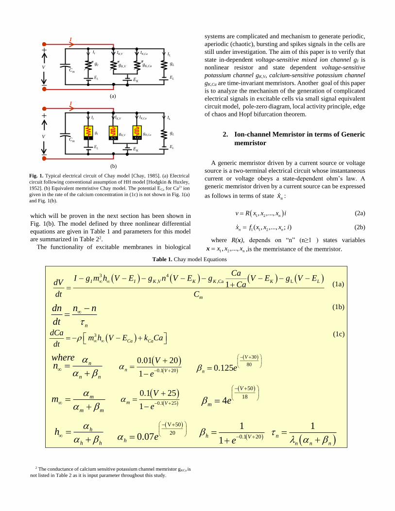
which will be proven in the next section has been shown in

Fig. 1(b). The model defined by three nonlinear differential

equations are given in Table 1 and parameters for this model

are summarized in Table 22.

The functionality of excitable membranes in biological

2 The conductance of calcium sensitive potassium channel memristor gKCa is

not listed in Table 2 as it is input parameter throughout this study.

systems are complicated and mechanism to generate periodic,

aperiodic (chaotic), bursting and spikes signals in the cells are

still under investigation. The aim of this paper is to verify that

state in-dependent voltage-sensitive mixed ion channel gI is

nonlinear resistor and state dependent voltage-sensitive

potassium channel gK,V, calcium-sensitive potassium channel

gK,Ca are time-invariant memristors. Another goal of this paper

is to analyze the mechanism of the generation of complicated

electrical signals in excitable cells via small signal equivalent

circuit model, pole-zero diagram, local activity principle, edge

of chaos and Hopf bifurcation theorem.

2. Ion-channel Memristor in terms of Generic

memristor

A generic memristor driven by a current source or voltage

source is a two-terminal electrical circuit whose instantaneous

current or voltage obeys a state-dependent ohm’s law. A

generic memristor driven by a current source can be expressed

as follows in terms of state nx :

1 2, ,..., nv R x x x i (2a)

1 1 2( , ,..., ; )n nx f x x x i (2b)

where R(x), depends on “n” (n≥1 ) states variables

1 2, ,..., nx x xx ,is the memristance of the memristor.

Cm

EL

gI

II

_

+

V

I

IK,V IK,Ca

gK,VgK,Ca

EKEL

gL

IL

Cm

EL

gI

II

_

+

V

I

IK,VIK,Ca

gK,VgK,Ca

EKEL

gL

IL

I K,V K,Ca

(a)

(b)

Fig. 1. Typical electrical circuit of Chay model [Chay, 1985]. (a) Electrical

circuit following conventional assumption of HH model [Hodgkin & Huxley,

1952]. (b) Equivalent memristive Chay model. The potential ECa for Ca2+ ion

given in the rate of the calcium concentration in (1c) is not shown in Fig. 1(a)

and Fig. 1(b).

Table 1. Chay model Equations

3 4

, ,Ca L1

I I K V K K K L

m

CaI g m h V E g n V E g V E g V E

dV Ca

dt C

n

dn n n

dt

h

h h

h

m

m m

m

n

n n

n

3

Ca Ca

dCam h V E k Ca

dt

V 50

200.07h e

0.1 20

0.01 20

1n V

V

e

0.1 20

1

1h V

e

0.1 25

0.1 25

1m V

V

e

50

184

V

m e

30

800.125

V

n e

1

n

n n n

(1a)

(1b)

(1c)

where

Similarly, a voltage-controlled memristor is defined in terms

of the memductance G(x) and the state variables 1 2, ..., nx x x , as

follows:

1 2, ,..., ni G x x x v (3a)

1 1 2( , ,..., ; )n nx f x x x v (3b)

Eqs. (2) and (3) are the core equations to distinguish the

memristive and non-memristive system and are used to prove

the voltage-sensitive potassium ion-channel and

calcium-sensitive potassium ion-channel are in fact

time-invariant generic memristors and voltage-sensitive mixed

ion channel is non-memrisitve (nonlinear resistor) element.

2.1 Voltage-sensitive potassium ion-channel memristor

Let us define the voltage across the voltage-sensitive

potassium ion-channel shown in third (from left) element in

Fig. 1(a) is vK,V and current is iK,V , then

,K K VV E v (4a)

and current entering to the channel is

, , ,( )K V K v K Vi G n v (4b)

where the memductance is given by

4

, ,( )K V K VG n g n (4c)

and the state equation describing the channel in terms n can

be simplified from 1(b) as,

,

,

30

80,

, 0.1 20

0.01 20( ; ) 1 0.125

1

K V K

K V K

v E

K V K

K V n v E

v Ednf n v n e n

dt e

(4d)

Note that (4b)-(4d) are identical to the voltage controlled

generic memristor defined in (3a)-(3b) with first order

differential equation. Hence, the time-varying conductance

shown in Fig. 1(a) of voltage-sensitive potassium ion-channel

is replaced with voltage-sensitive potassium ion-channel

memristor as shown in the third element (from left) in Fig.

1(b).

We observed the memristive fingerprint of the

voltage-sensitive potassium ion-channel memristor by

applying sinusoidal bipolar signal under different frequencies.

This property asserts that beyond some frequency f*, the

pinched hysteresis loops characterized by a memristor shrinks

to a single-valued function through the origin as frequency f >

f* tends to infinity. To verify this property, a sinusoidal

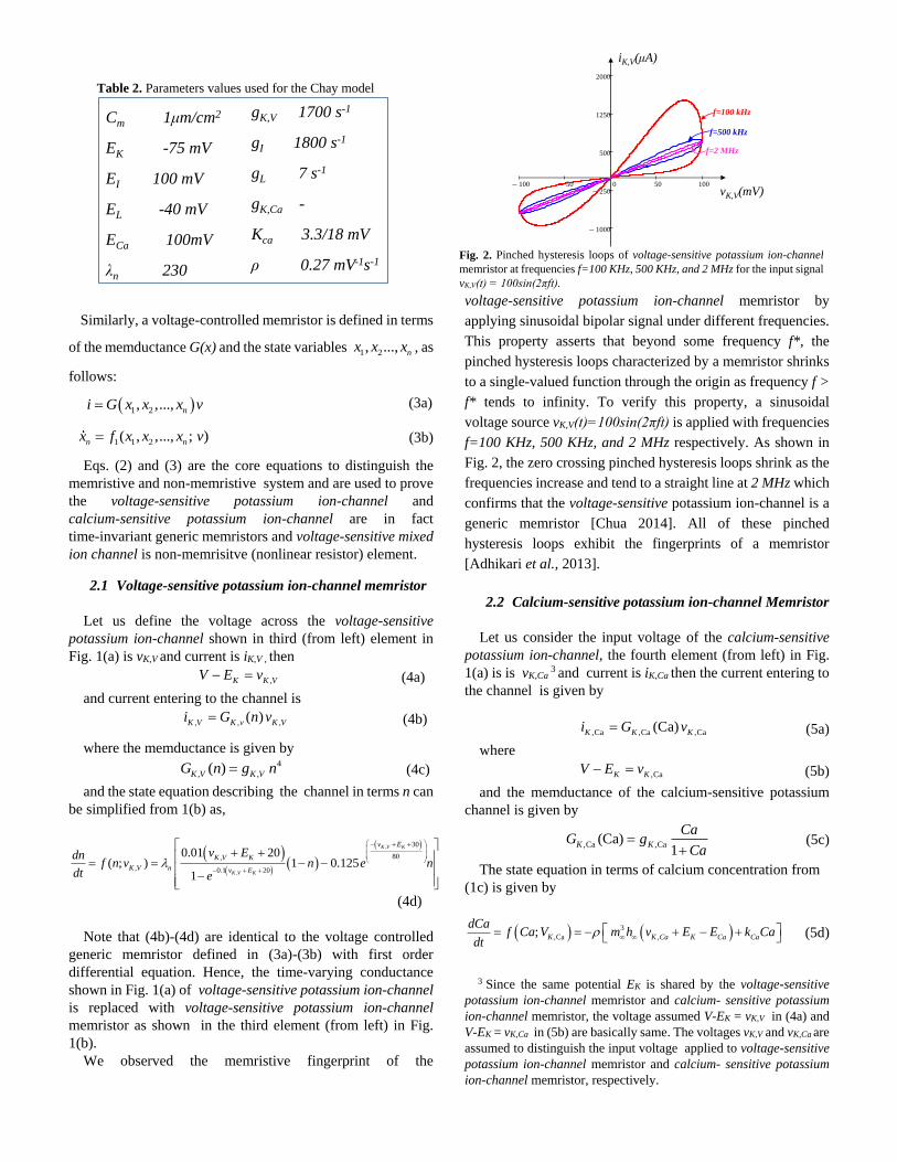
voltage source vK,V(t)=100sin(2πft) is applied with frequencies

f=100 KHz, 500 KHz, and 2 MHz respectively. As shown in

Fig. 2, the zero crossing pinched hysteresis loops shrink as the

frequencies increase and tend to a straight line at 2 MHz which

confirms that the voltage-sensitive potassium ion-channel is a

generic memristor [Chua 2014]. All of these pinched

hysteresis loops exhibit the fingerprints of a memristor

[Adhikari et al., 2013].

2.2 Calcium-sensitive potassium ion-channel Memristor

Let us consider the input voltage of the calcium-sensitive

potassium ion-channel, the fourth element (from left) in Fig.

1(a) is is vK,Ca 3 and current is iK,Ca then the current entering to

the channel is given by

,Ca ,Ca ,Ca(Ca)K K Ki G v (5a)

where

,CaK KV E v (5b)

and the memductance of the calcium-sensitive potassium

channel is given by

,Ca ,Ca(Ca)1

K K

CaG g

Ca

(5c)

The state equation in terms of calcium concentration from

(1c) is given by

3

,Ca ,; K K Ca K Ca Ca

dCaf Ca V m h v E E k Ca

dt (5d)

3 Since the same potential EK is shared by the voltage-sensitive

potassium ion-channel memristor and calcium- sensitive potassium

ion-channel memristor, the voltage assumed V-EK = vK,V in (4a) and

V-EK = vK,Ca in (5b) are basically same. The voltages vK,V and vK,Ca are

assumed to distinguish the input voltage applied to voltage-sensitive

potassium ion-channel memristor and calcium- sensitive potassium

ion-channel memristor, respectively.

Table 2. Parameters values used for the Chay model

Cm 1μm/cm2

EK -75 mV

EI 100 mV

EL -40 mV

ECa 100mV

λn 230

gK,V 1700 s-1

gI 1800 s-1

gL 7 s-1

gK,Ca -

Kca 3.3/18 mV

ρ 0.27 mV-1s-1

100 50 0 50 100

1000

250

500

1250

2000

iK,V(μA)

vK,V(mV)

f=100 kHz

f=500 kHz

f=2 MHz

Fig. 2. Pinched hysteresis loops of voltage-sensitive potassium ion-channel

memristor at frequencies f=100 KHz, 500 KHz, and 2 MHz for the input signal

vK,V(t) = 100sin(2πft).

Observe that (5b)–(5d) are an example of a

voltage-controlled memristor defined in (3a)–(3b) in terms of

the calcium concentration channel Ca. Since only one state

equation is defined in terms of Ca, we call this memristor as a

first order calcium-sensitive potassium ion-channel generic

memristor. Therefore the time varying calcium-sensitive

potassium ion-channel is replaced with calcium-sensitive

potassium ion-channel memristor as shown in the fourth

element (from left) in Fig. 1(b).

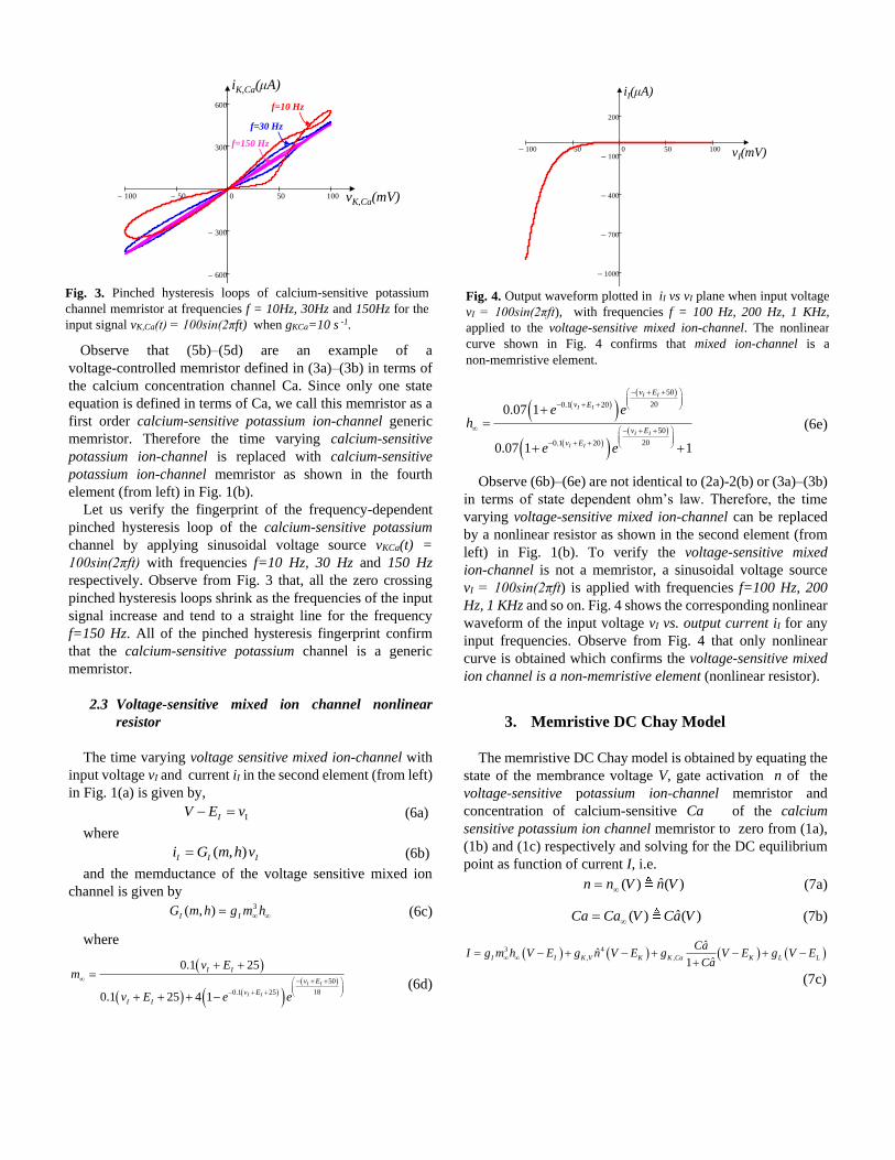
Let us verify the fingerprint of the frequency-dependent

pinched hysteresis loop of the calcium-sensitive potassium

channel by applying sinusoidal voltage source vKCa(t) =

100sin(2πft) with frequencies f=10 Hz, 30 Hz and 150 Hz

respectively. Observe from Fig. 3 that, all the zero crossing

pinched hysteresis loops shrink as the frequencies of the input

signal increase and tend to a straight line for the frequency

f=150 Hz. All of the pinched hysteresis fingerprint confirm

that the calcium-sensitive potassium channel is a generic

memristor.

2.3 Voltage-sensitive mixed ion channel nonlinear

resistor

The time varying voltage sensitive mixed ion-channel with

input voltage vI and current iI in the second element (from left)

in Fig. 1(a) is given by,

IIV E v (6a)

where

( , )I I Ii G m h v (6b)

and the memductance of the voltage sensitive mixed ion

channel is given by

3( , )I IG m h g m h (6c)

where

50

180.1 25

0.1 25

0.1 25 4 1

I I

I I

I I

v E

v E

I I

v Em

v E e e

(6d)

50

200.1 20

50

200.1 20

0.07 1

0.07 1 1

I I

I I

I I

I I

v E

v E

v E

v E

e eh

e e

(6e)

Observe (6b)–(6e) are not identical to (2a)-2(b) or (3a)–(3b)

in terms of state dependent ohm’s law. Therefore, the time

varying voltage-sensitive mixed ion-channel can be replaced

by a nonlinear resistor as shown in the second element (from

left) in Fig. 1(b). To verify the voltage-sensitive mixed

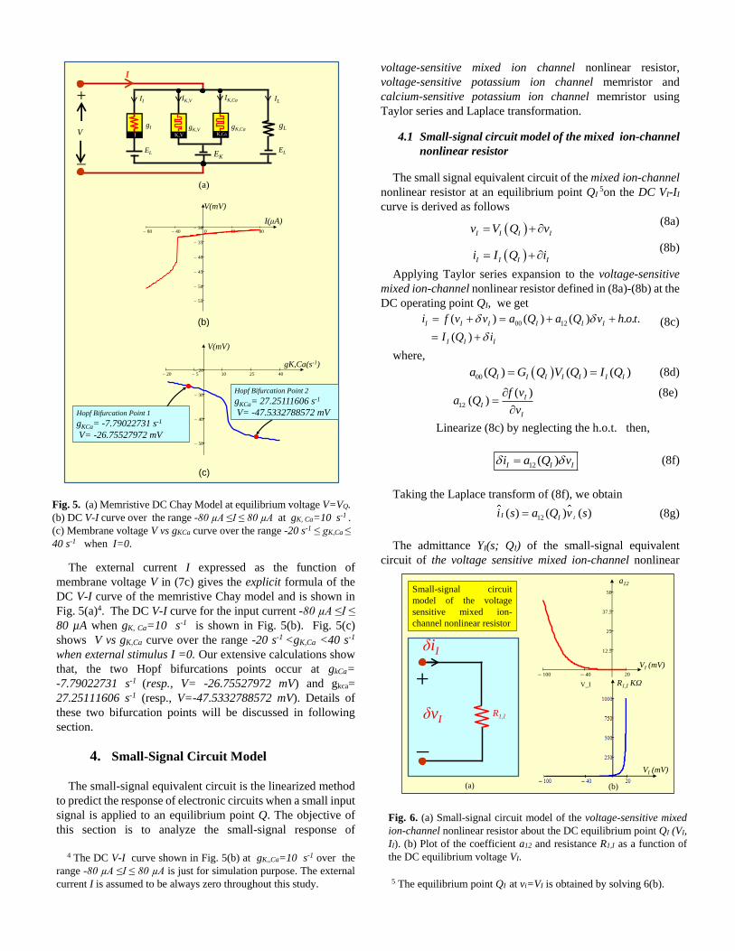
ion-channel is not a memristor, a sinusoidal voltage source

vI = 100sin(2πft) is applied with frequencies f=100 Hz, 200

Hz, 1 KHz and so on. Fig. 4 shows the corresponding nonlinear

waveform of the input voltage vI vs. output current iI for any

input frequencies. Observe from Fig. 4 that only nonlinear

curve is obtained which confirms the voltage-sensitive mixed

ion channel is a non-memristive element (nonlinear resistor).

3. Memristive DC Chay Model

The memristive DC Chay model is obtained by equating the

state of the membrance voltage V, gate activation n of the

voltage-sensitive potassium ion-channel memristor and

concentration of calcium-sensitive Ca of the calcium

sensitive potassium ion channel memristor to zero from (1a),

(1b) and (1c) respectively and solving for the DC equilibrium

point as function of current I, i.e.

ˆ( ) ( )n n V n V (7a)

ˆ( ) ( )Ca Ca V Ca V (7b)

3 4

, ,

ˆˆ

ˆ1I I K V K K Ca K L L

CaI g m h V E g n V E g V E g V E

Ca

(7c)

100 50 0 50 100

600

300

300

600 f=10 Hz

f=150 Hz

f=30 Hz

iK,Ca(μA)

vK,Ca(mV)

Fig. 3. Pinched hysteresis loops of calcium-sensitive potassium

channel memristor at frequencies f = 10Hz, 30Hz and 150Hz for the

input signal vK,Ca(t) = 100sin(2πft) when gKCa=10 s -1.

100 50 0 50 100

1000

700

400

100

200

iI(μA)

vI(mV)

Fig. 4. Output waveform plotted in iI vs vI plane when input voltage

vI = 100sin(2πft), with frequencies f = 100 Hz, 200 Hz, 1 KHz,

applied to the voltage-sensitive mixed ion-channel. The nonlinear

curve shown in Fig. 4 confirms that mixed ion-channel is a

non-memristive element.

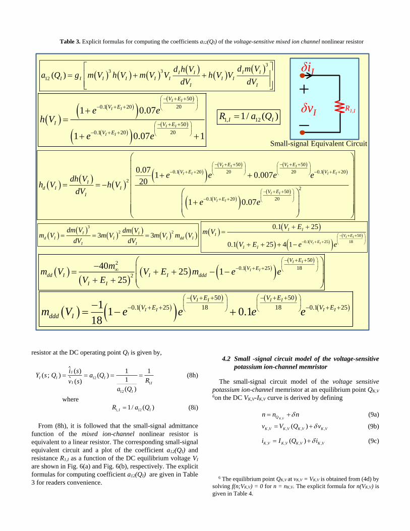
The external current I expressed as the function of

membrane voltage V in (7c) gives the explicit formula of the

DC V-I curve of the memristive Chay model and is shown in

Fig. 5(a)4. The DC V-I curve for the input current -80 µA ≤I ≤

80 µA when gK, Ca=10 s-1 is shown in Fig. 5(b). Fig. 5(c)

shows V vs gK,Ca curve over the range -20 s-1 <gK,Ca <40 s-1

when external stimulus I =0. Our extensive calculations show

that, the two Hopf bifurcations points occur at gkCa=

-7.79022731 s-1 (resp., V= -26.75527972 mV) and gkca=

27.25111606 s-1 (resp., V=-47.5332788572 mV). Details of

these two bifurcation points will be discussed in following

section.

4. Small-Signal Circuit Model

The small-signal equivalent circuit is the linearized method

to predict the response of electronic circuits when a small input

signal is applied to an equilibrium point Q. The objective of

this section is to analyze the small-signal response of

4 The DC V-I curve shown in Fig. 5(b) at gK,,Ca=10 s-1 over the

range -80 µA ≤I ≤ 80 µA is just for simulation purpose. The external

current I is assumed to be always zero throughout this study.

voltage-sensitive mixed ion channel nonlinear resistor,

voltage-sensitive potassium ion channel memristor and

calcium-sensitive potassium ion channel memristor using

Taylor series and Laplace transformation.

4.1 Small-signal circuit model of the mixed ion-channel

nonlinear resistor

The small signal equivalent circuit of the mixed ion-channel

nonlinear resistor at an equilibrium point QI 5on the DC VI-II

curve is derived as follows

I I I Iv V Q v

(8a)

I I I Ii I Q i

(8b)

Applying Taylor series expansion to the voltage-sensitive

mixed ion-channel nonlinear resistor defined in (8a)-(8b) at the

DC operating point QI, we get

00 12( ) ( ) ( ) . . .

( )

I I I I I I

I I I

i f v v a Q a Q v h o t

I Q i

(8c)

where,

00 ( ) ( ) ( )I I I I I I Ia Q G Q V Q I Q (8d)

12

( )( ) I

I

I

f va Q

v

(8e)

Linearize (8c) by neglecting the h.o.t. then,

12 ( )I I Ii a Q v (8f)

Taking the Laplace transform of (8f), we obtain

12( ) ( ) ( )II Ii s a Q v s (8g)

The admittance YI(s; QI) of the small-signal equivalent

circuit of the voltage sensitive mixed ion-channel nonlinear

5 The equilibrium point QI at vi=VI is obtained by solving 6(b).

EL

gI

II

_

+

V

IK,VIK,Ca

gK,VgK,Ca

EKEL

gL

IL

I K,V K,Ca

I

(a)

(b)

80 40 0 40 80

55

50

45

40

35

30

I(μA)

V(mV)

20 5 10 25 40

50

40

30

20gK,Ca(s-1)

V(mV)

(c)

Hopf Bifurcation Point 2

gKCa= 27.25111606 s-1

V= -47.5332788572 mVHopf Bifurcation Point 1

gKCa= -7.79022731 s-1

V= -26.75527972 mV

Fig. 5. (a) Memristive DC Chay Model at equilibrium voltage V=VQ.

(b) DC V-I curve over the range -80 µA ≤I ≤ 80 µA at gK, Ca=10 s-1 .

(c) Membrane voltage V vs gKCa curve over the range -20 s-1 ≤ gK,Ca ≤

40 s-1 when I=0.

R1,I

_

+

δvI

δiI

(a) (b)

Small-signal circuit

model of the voltage

sensitive mixed ion-

channel nonlinear resistor

100 40 20

12.5

25

37.5

50

V_I

a12

VI (mV)

R1,I KΩ

VI (mV)

Fig. 6. (a) Small-signal circuit model of the voltage-sensitive mixed

ion-channel nonlinear resistor about the DC equilibrium point QI (VI,

II). (b) Plot of the coefficient a12 and resistance R1,I as a function of

the DC equilibrium voltage VI.

resistor at the DC operating point QI is given by,

12

1

12

( ) 1 1( ; ) ( )

1( )

( )

I

I I I

I I

I

i sY s Q a Q

Rv sa Q

(8h)

where

1, 121/ ( )I IR a Q (8i)

From (8h), it is followed that the small-signal admittance

function of the mixed ion-channel nonlinear resistor is

equivalent to a linear resistor. The corresponding small-signal

equivalent circuit and a plot of the coefficient a12(QI) and

resistance R1,I as a function of the DC equilibrium voltage VI

are shown in Fig. 6(a) and Fig. 6(b), respectively. The explicit

formulas for computing coefficient a12(QI) are given in Table

3 for readers convenience.

4.2 Small -signal circuit model of the voltage-sensitive

potassium ion-channel memristor

The small-signal circuit model of the voltage sensitive

potassium ion-channel memristor at an equilibrium point QK,V 6on the DC VK,V-IK,V curve is derived by defining

,K VQn n n (9a)

, , , ,( )K V K V K V K Vv V Q v (9b)

, , , ,( )K V K V K V K Vi I Q i (9c)

6 The equilibrium point QK,V at vK,V = VK,V is obtained from (4d) by

solving f(n;VK,V) = 0 for n = nK,V. The explicit formula for n(VK,V) is

given in Table 4.

Table 3. Explicit formulas for computing the coefficients a12(QI) of the voltage-sensitive mixed ion channel nonlinear resistor

3

3 3

12 ( )I II I

I I I I I I I I

I I

d m Vd h Va Q g m V h V m V V h V V

dV dV

50

180.1 25

0.1 25

0.1 25 4 1

I I

I I

I I

I V E

V E

I I

V Em V

V E e e

50

200.1 20

50

200.1 20

1 0.07

1 0.07 1

I I

I I

I I

I I

V E

V E

I V E

V E

e eh V

e e

3

2 23 3

I I

d I I I dd I

I I

dm V dm Vm V m V m V m V

dV dV

1, 121/ ( )I IR a QR1,I

_

+δvI

δiI

Small-signal Equivalent Circuit

50 50

20 200.1 20 0.1 20

2

250

200.1 20

0.071 0.007

20

1 0.07

I I I I

I I I I

I I

I I

V E V E

V E V E

I

d I IV E

IV E

e e e edh Vh V h V

dV

e e

50

2180.1 25

2

4025 1

25

I I

I I

V E

V E

dd I I I ddd

I I

mm V V E m e e

V E

50 50

18 180.1 25 0.1 2511 0.1

18

I I I I

I I I I

V E V E

V E V E

ddd Im V e e e e

Expanding , , ,( )K V K V K Vi G n v from (4b) in a Taylor

series about the equilibrium point (N(QK,V), VK,V(QK,V)), we

obtain,

, 00 , 11 , 12 , ,

, , ,

( ) ( ) ( ) . . .

( )

K V K V K V K V K V

K V K V K V

i a Q a Q n a Q v h o t

I Q i

(9d)

where

,K VQn n n , , , ,( )K V K V K V K Vv v V Q ,

, , , ,( )K V K V K V K Vi i I Q (9e)

and

00 , , , , , , ,( ) ( ) ( )K V K V K V K V K V K V K Va Q G Q V Q I Q (9f)

,11 , , , ,( ) ( )

K VK V K V K V K V Qa Q V Q G n (9g)

,12 , ,( )

K VK V K V Qa Q G n (9h)

and h.o.t denotes the higher-order terms. Let us linearize the

nonlinear equation by neglecting the h.o.t. in (9d), then:

11 , 12 , ,( ) ( )K K V K V K Vi a Q n a Q v (9i)

Similarly, expanding the state equation K ,V K ,Vf n ,V in

(4d) using a Taylor series about the equilibrium point

(n(QK,V),VK,V(QK,V)), we

obtain

,

,

, , ,

, , 11 , 12 , ,

( , ( ) )

( , ( )) ( ) ( ) . . .

K V

K V

Q K V K V K V

Q K V K V K V K V K V

f n n V Q v

f n V Q b Q n b Q v h o t

(9j)

where

,

,

11 ,

,( )

K V

n K V

K V

Q

f n vb Q

n

(9k)

,

,

12 ,

,

,( )

K V

N K V

K V

K VQ

f n vb Q

v

(9l)

Linearizing the nonlinear state equation (9j) by neglecting

the h.o.t., we get

11 , 12 , ,( ) ( )K V K V K V

d nb Q n b Q v

dt

(9m)

Taking Laplace transform of (9i) and (9m), we obtain

, 11 , 12 , ,ˆ ˆ( ) ( )n( ) ( ) ( )

K V K V K V K Vi s a Q s a Q v s (9n)

11 , 12 , ,ˆ ˆ ˆ( ) ( ) ( ) ( ) ( )K V K V K Vs n s b Q n s b Q v s (9o)

Solving (9o) for ˆ( )n s and substituting the result into (9n), we

obtain the following admittance YK,V(s; QK,V) of the

small-signal equivalent circuit of the voltage sensitive

potassium ion-channel memristor at equilibrium point QK,V:

,

, ,

,

11 ,

12 ,11 , 12 , 11 , 12 ,

( )( ; )

( )

1 1

( ) 1

( )( ) ( ) ( ) ( )

K V

K V K V

K V

K V

K VK V K V K V K V

i sY s Q

v s

b Qs

a Qa Q b Q a Q b Q

(9p)

, ,

2 ,, 1 ,

1 1;K V K V

K VK V K V

Y s QRsL R

(9q)

where

,

11 , 12 ,

1

( ) ( )K V

K V K V

La Q b Q

(9r)

11 ,

1 ,

11 , 12 ,

( )

( ) ( )

K V

K V

K V K V

b QR

a Q b Q (9s)

2 ,

12 ,

1

( )K V

K V

Ra Q

(9t)

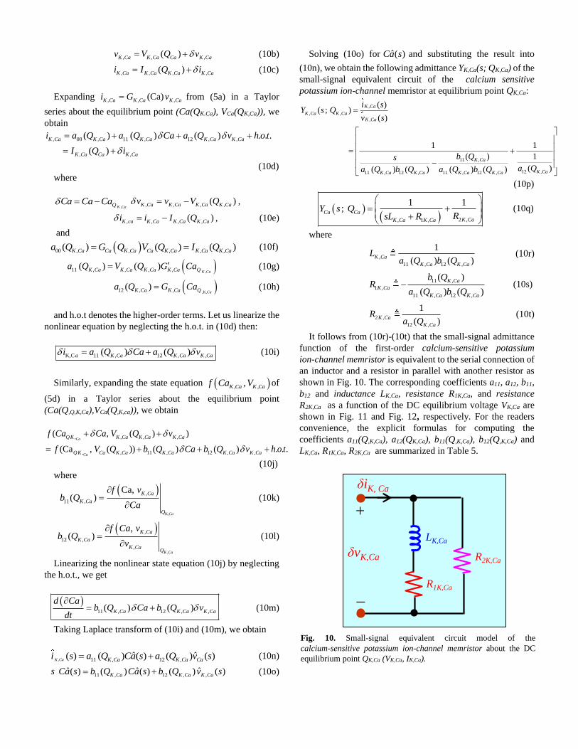
It follows from (9r)-(9t) that the small-signal admittance

function of the first-order voltage sensitive potassium

ion-channel memristor is equivalent to the serial connection of

an inductor and a resistor in parallel with another resistor as

shown in Fig. 7. The corresponding coefficients a11, a12, b11,

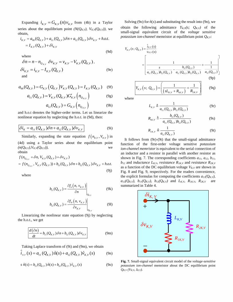
b12 and inductance LK,V, resistance R1K,V and resistance R2K,V

as a function of the DC equilibrium voltage VK,V are shown in

Fig. 8 and Fig. 9, respectively. For the readers convenience,

the explicit formulas for computing the coefficients a11(QK,V),

a12(QK,V), b11(QK,V), b12(QK,V) and LK,V, R1K,V, R2K,V are

summarized in Table 4.

_

+

δvK,V

δiK, V

R1K,V

LK,V

R2K,V

Fig. 7. Small-signal equivalent circuit model of the voltage-sensitive

potassium ion-channel memristor about the DC equilibrium point

QK,V (VK,V, IK,V).

4.3 Small -signal circuit model of the calcium-sensitive

potassium ion-channel memristor

The small-signal circuit model of the calcium-sensitive

potassium-channel memristor at an equilibrium point QK,Ca 7in

the DC VK,Ca-IK,Ca curve is derived by defining

,K CaQCa Ca Ca (10a)

7 The equilibrium point QK,Ca at vK,Ca = VK,Ca is obtained from (5a)

by solving f(Ca;VK,Ca) = 0 for Ca = CaK,Ca. The explicit formula for

Ca(VK,Ca) is given in Table 5.

(a) (b)

(c) (d)

100 0 100 200 300 400

0.2

0.4

0.6

0.8

VK,V(mV)

b12

200 100 0 100 200 300

800

600

400

200

b11

VK,V(mV)

100 0 100 200 300 400

500

1000

1500

2000

VK,V(mV)

a12

100 0 100 200

5 105

5 105

1 106

1.5 106

VK,V(mV)

a11

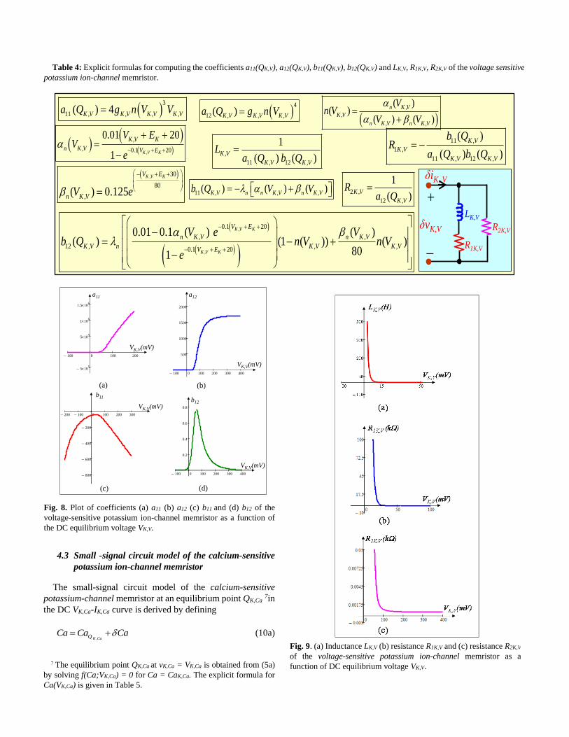
Fig. 8. Plot of coefficients (a) a11 (b) a12 (c) b11 and (d) b12 of the

voltage-sensitive potassium ion-channel memristor as a function of

the DC equilibrium voltage VK,V.

Fig. 9. (a) Inductance LK,V (b) resistance R1K,V and (c) resistance R2K,V

of the voltage-sensitive potassium ion-channel memristor as a

function of DC equilibrium voltage VK,V.

Table 4: Explicit formulas for computing the coefficients a11(QK,V), a12(QK,V), b11(QK,V), b12(QK,V) and LK,V, R1K,V, R2K,V of the voltage sensitive

potassium ion-channel memristor.

3

11 , , , ,( ) 4K V K V K V K Va Q g n V V 4

12 , , ,( )K V K V K Va Q g n V

,

11 , 12 ,

1

( ) ( )K V

K V K V

La Q b Q

11 ,

1 ,

11 , 12 ,

( )

( ) ( )

K V

K V

K V K V

b QR

a Q b Q

2 ,

12 ,

1

( )K V

K V

Ra Q

11 , , ,( ) ( ) ( )K V n n K V n K Vb Q V V

,

,

, 0.1 20

0.01 20

1 K V K

K V K

n K V V E

V EV

e

, 30

80

,( ) 0.125

K V KV E

n K VV e

_

+

δvK,V

δiK, V

R1K,V

LK,V

R2K,V

,

,

, ,

( )( )

( ) ( )

n K V

K V

n K V n K V

Vn V

V V

,

,

0.1 20

, ,

12 , , ,0.1 20

0.01 0.1 ( ) ( )( ) (1 ( )) ( )

801

K V K

K V K

V E

n K V n K V

K V n K V K VV E

V e Vb Q n V n V

e

, , ,( )K Ca K Ca Ca K Cav V Q v (10b)

, , , ,( )K Ca K Ca K Ca K Cai I Q i (10c)

Expanding , , ,(Ca)K Ca K Ca K Cai G v from (5a) in a Taylor

series about the equilibrium point (Ca(QK.Ca), VCa(QK,Ca)), we

obtain

, 00 , 11 , 12 , ,

, ,

( ) ( ) ( ) . . .

( )

K Ca K Ca K Ca K Ca K Ca

K Ca Ca K Ca

i a Q a Q Ca a Q v h o t

I Q i

(10d)

where

,K CaQCa Ca Ca , , , ,( )K Ca K Ca K Ca K Cav v V Q ,

, , , ,( )K ca K Ca K Ca K Cai i I Q , (10e)

and

00 , , , , ,( ) ( ) ( )K Ca Ca K Ca Ca K Ca K Ca K Caa Q G Q V Q I Q (10f)

,11 , , , ,( ) ( )

K CaK Ca K Ca K Ca K Ca Qa Q V Q G Ca (10g)

,K,12 , ,( )

CaK Ca K Ca Qa Q G Ca (10h)

and h.o.t denotes the higher-order terms. Let us linearize the

nonlinear equation by neglecting the h.o.t. in (10d) then:

K,C 11 , 12 , ,( ) ( )a K Ca K Ca K Cai a Q Ca a Q v (10i)

Similarly, expanding the state equation K ,Ca K ,Caf Ca ,V of

(5d) in a Taylor series about the equilibrium point

(Ca(Q,Q,K,Ca),VCa(Q,K,ca)), we obtain

, , , ,

, , 11 , 12 , ,

( , ( ) )

(Ca , ( )) ( ) ( ) . . .

Ca

Ca

QK K Ca K Ca K Ca

QK Ca K Ca K Ca K Ca K Ca

f Ca Ca V Q v

f V Q b Q Ca b Q v h o t

(10j)

where

K,

,

11 ,

Ca,( )

Ca

K Ca

K Ca

Q

f vb Q

Ca

(10k)

,

,

12 ,

,

,( )

K Ca

K Ca

K Ca

K CaQ

f Ca vb Q

v

(10l)

Linearizing the nonlinear state equation (10j) by neglecting

the h.o.t., we get

11 , 12 , ,( ) ( )K Ca K Ca K Ca

d Cab Q Ca b Q v

dt

(10m)

Taking Laplace transform of (10i) and (10m), we obtain

, 11 , 12 ,ˆ ˆ( ) ( ) ( ) ( ) ( )

K Ca K Ca K Ca Cai s a Q Ca s a Q v s (10n)

11 , 12 , ,ˆ ˆ ˆ( ) ( ) ( ) ( ) ( )K Ca K Ca K Cas Ca s b Q Ca s b Q v s (10o)

Solving (10o) for ˆ( )Ca s and substituting the result into

(10n), we obtain the following admittance YK,Ca(s; QK,Ca) of the

small-signal equivalent circuit of the calcium sensitive

potassium ion-channel memristor at equilibrium point QK,Ca:

,

, ,

,

11 ,

12 ,11 , 12 , 11 , 12 ,

( )( ; )

( )

1 1

( ) 1

( )( ) ( ) ( ) ( )

K Ca

K Ca K Ca

K Ca

K Ca

K CaK Ca K Ca K Ca K Ca

i sY s Q

v s

b Qs

a Qa Q b Q a Q b Q

(10p)

2 ,, 1 ,

1 1;Ca Ca

K CaK Ca K Ca

Y s QRsL R

(10q)

where

,

11 , 12 ,

1

( ) ( )K Ca

K Ca K Ca

La Q b Q

(10r)

11 ,

1 ,

11 , 12 ,

( )

( ) ( )

K Ca

K Ca

K Ca K Ca

b QR

a Q b Q (10s)

2 ,

12 ,

1

( )K Ca

K Ca

Ra Q

(10t)

It follows from (10r)-(10t) that the small-signal admittance

function of the first-order calcium-sensitive potassium

ion-channel memristor is equivalent to the serial connection of

an inductor and a resistor in parallel with another resistor as

shown in Fig. 10. The corresponding coefficients a11, a12, b11,

b12 and inductance LK,Ca, resistance R1K,Ca, and resistance

R2K,Ca as a function of the DC equilibrium voltage VK,Ca are

shown in Fig. 11 and Fig. 12, respectively. For the readers

convenience, the explicit formulas for computing the

coefficients a11(Q,K,Ca), a12(QK,Ca), b11(Q,K,Ca), b12(Q,K,Ca) and

LK,Ca, R1K,Ca, R2K,Ca are summarized in Table 5.

_

+

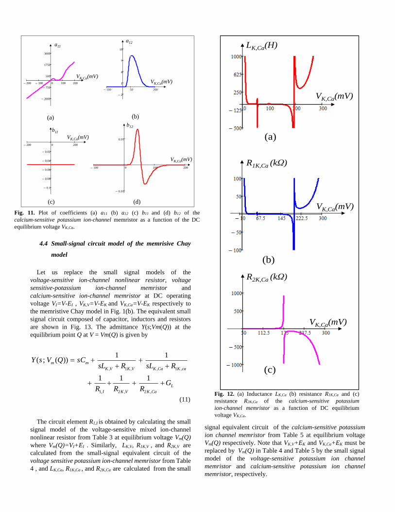
δvK,Ca

δiK, Ca

R1K,Ca

LK,Ca

R2K,Ca

Fig. 10. Small-signal equivalent circuit model of the

calcium-sensitive potassium ion-channel memristor about the DC

equilibrium point QK,Ca (VK,Ca, IK,Ca).

4.4 Small-signal circuit model of the memrisive Chay

model

Let us replace the small signal models of the

voltage-sensitive ion-channel nonlinear resistor, voltage

sensitive-potassium ion-channel memristor and

calcium-sensitive ion-channel memristor at DC operating

voltage VI=V-EI , VK,V=V-EK and VK,Ca=V-EK respectively to

the memristive Chay model in Fig. 1(b). The equivalent small

signal circuit composed of capacitor, inductors and resistors

are shown in Fig. 13. The admittance Y(s;Vm(Q)) at the

equilibrium point Q at V = Vm(Q) is given by

, 1 , , 1 ,

1, 2 , 2 ,

1 1( ; ( ))

1 1 1

m m

K V K V K Ca K ca

L

I K V K Ca

Y s V Q sCsL R sL R

GR R R

(11)

The circuit element R1,I is obtained by calculating the small

signal model of the voltage-sensitive mixed ion-channel

nonlinear resistor from Table 3 at equilibrium voltage Vm(Q)

where Vm(Q)=VI+EI . Similarly, LK,V, R1K,V , and R2K,V are

calculated from the small-signal equivalent circuit of the

voltage sensitive potassium ion-channel memristor from Table

4 , and LK,Ca, R1K,Ca , and R2K,Ca are calculated from the small

signal equivalent circuit of the calcium-sensitive potassium

ion channel memristor from Table 5 at equilibrium voltage

Vm(Q) respectively. Note that VK,V+EK and VK,Ca+EK must be

replaced by Vm(Q) in Table 4 and Table 5 by the small signal

model of the voltage-sensitive potassium ion channel

memristor and calcium-sensitive potassium ion channel

memristor, respectively.

(a) (b)

(c) (d)

200 100 0 100 200

2000

750

500

1750

3000

VK,Ca(mV)

a11

100 50 200

2

1

4

7

10

VK,Ca(mV)

a12

200 0 200

0.1

0.08

0.06

0.04

0.02

b11

VK,Ca(mV)

100 0 100 200

0.01

0.01

VK,Ca(mV)

b12

Fig. 11. Plot of coefficients (a) a11 (b) a12 (c) b11 and (d) b12 of the

calcium-sensitive potassium ion-channel memristor as a function of the DC

equilibrium voltage VK,Ca.

(a)

(c)

VK,Ca(mV)

R2K,Ca (kΩ)

VK,Ca(mV)

LK,Ca(H)

(b)

VK,Ca(mV)

R1K,Ca (kΩ)

Fig. 12. (a) Inductance LK,Ca (b) resistance R1K,Ca and (c)

resistance R2K,Ca of the calcium-sensitive potassium

ion-channel memristor as a function of DC equilibrium

voltage VK,Ca.

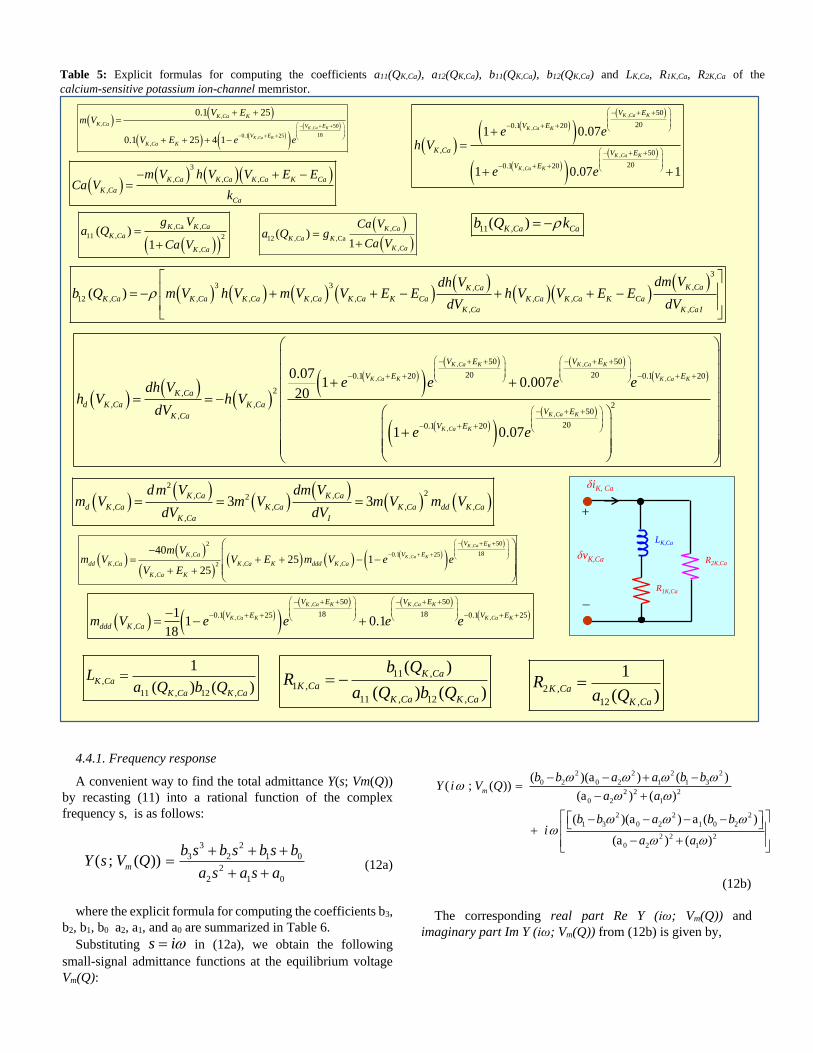
4.4.1. Frequency response

A convenient way to find the total admittance Y(s; Vm(Q))

by recasting (11) into a rational function of the complex

frequency s, is as follows:

3 2

3 2 1 0

2

2 1 0

( ; ( ))m

b s b s b s bY s V Q

a s a s a

(12a)

where the explicit formula for computing the coefficients b3,

b2, b1, b0 a2, a1, and a0 are summarized in Table 6.

Substituting s i in (12a), we obtain the following

small-signal admittance functions at the equilibrium voltage

Vm(Q):

2 2 2 2

0 2 0 2 1 1 3

2 2 2

0 2 1

2 2 2

1 3 0 2 1 0 2

2 2 2

0 2 1

( )(a ) ( )( ; ( ))

(a ) ( )

( )(a ) a ( )

(a ) ( )

m

b b a a b bY i V Q

a a

b b a b bi

a a

(12b)

The corresponding real part Re Y (iω; Vm(Q)) and

imaginary part Im Y (iω; Vm(Q)) from (12b) is given by,

Table 5: Explicit formulas for computing the coefficients a11(QK,Ca), a12(QK,Ca), b11(QK,Ca), b12(QK,Ca) and LK,Ca, R1K,Ca, R2K,Ca of the

calcium-sensitive potassium ion-channel memristor.

,

,

,

, 50

180.1 25

,

0.1 25

0.1 25 4 1

K Ca K

K Ca K

K Ca K

K Ca V E

V E

K Ca K

V Em V

V E e e

2

2, ,2

, , , ,

,

3 3K Ca K Ca

d K Ca K Ca K Ca dd K Ca

K Ca I

dm V dm Vm V m V m V m V

dV dV

, ,

, ,

,

,

50 50

20 200.1 20 0.1 20

2,

, , 250

,200.1 20

0.071 0.007

20

1 0.07

K Ca K K Ca K

K Ca K K Ca K

K Ca K

K Ca K

V E V E

V E V E

K Ca

d K Ca K CaV E

K Ca

V E

e e e edh Vh V h V

dV

e e

,

,

502

18, 0.1 25

, , ,2

,

4025 1

25

K Ca K

K Ca K

V E

K Ca V E

dd K Ca K Ca K ddd K Ca

K Ca K

m Vm V V E m V e e

V E

, ,

, ,

50 50

18 180.1 25 0.1 25

,

11 0.1

18

K Ca K K Ca K

K Ca K K Ca K

V E V E

V E V E

ddd K Cam V e e e e

,Ca ,

11 , 2

,

( )1

K K Ca

K Ca

K Ca

g Va Q

Ca V

,

12 , ,Ca

,

( )1

K Ca

K Ca K

K Ca

Ca Va Q g

Ca V

11 ,( )K Ca Cab Q k

3

3 3 ,,

12 , , , , , , ,

, ,

( )K CaK Ca

K Ca K Ca K Ca K Ca K Ca K Ca K Ca K Ca K Ca

K Ca K Ca I

dm Vdh Vb Q m V h V m V V E E h V V E E

dV dV

,

,

,

,

50

200.1 20

, 50

200.1 20

1 0.07

1 0.07 1

K Ca K

K Ca K

K Ca K

K Ca K

V E

V E

K Ca V E

V E

e eh V

e e

_

+

δvK,Ca

δiK, Ca

R1K,Ca

LK,Ca

R2K,Ca

3

, , ,

,

K Ca K Ca K Ca K Ca

K Ca

Ca

m V h V V E ECa V

k

,

11 , 12 ,

1

( ) ( )K Ca

K Ca K Ca

La Q b Q

11 ,

1 ,

11 , 12 ,

( )

( ) ( )

K Ca

K Ca

K Ca K Ca

b QR

a Q b Q

2 ,

12 ,

1

( )K Ca

K Ca

Ra Q

Small-signal circuit

model of the voltage

sensitive potassium ion

channel memristor

Small signal circuit

model of calcium-sensitive

potassium Channel

memristor memristor

R1K,V

LK,V

R2K,VR1,I

_

+

δv

δi

Cm

R1K,Ca

LK,Ca

R2K,Ca GL

Small-signal circuit model

of the mixed ion channel

nonlinear resistor

Fig. 13. Small-signal equivalent circuit model of the memristive Chay model.

Table 6: Explicit formulas for computing the coefficients of Y(s;Vm(Q)).

3 2

3 2 1 0

2

2 1 0

( ; ( ))m

b s b s b s bY s V Q

a s a s a

3 , , 1, 2 , 2 ,K V K Ca I K V K Ca mb L L R R R C

2 , 1 , , 1 , 1, 2 , 2 , , , 2 , 2 ,

, , 1, 2 , , , 1, 2 , , , 1, 2 , 2 ,

K V K ca K Ca K V I K V K Ca m K V K Ca K V K Ca

K V K Ca I K Ca K V K Ca I K V K V K Ca I K V K Ca L

b L R L R R R R C L L R R

L L R R L L R R L L R R R G

1 1, 1 , 1 , 2 , 2 , , 1, 2 , 2 , , 1, 2 , 2 ,

, 1 , , 1 , 2 , 2 , , 1 , , 1 , 1, 2 ,

, 1 , , 1 , 1, 2 , , 1 , , 1 ,

I K V K ca K V K Ca m K Ca I K V K Ca K V I K V K Ca

K V K ca K Ca K V K V K Ca K V K ca K Ca K V I K Ca

K V K ca K Ca K V I K V K V K ca K Ca K V

b R R R R R C L R R R L R R R

L R L R R R L R L R R R

L R L R R R L R L R

1, 2 , 2 ,I K V K Ca LR R R G

0 1, 1 , 2 , 2 , 1, 1 , 2 , 2 , 1 , 1 , 2 , 2 ,

1, 1 , 1 , 2 , 1, 1 , 1 , 2 , 1, 1 , 1 , 2 , 2 ,

I K ca K V K Ca I K V K V K Ca K V K ca K V K Ca

I K V K ca K Ca I K V K ca K V I K V K ca K V K Ca L

b R R R R R R R R R R R R

R R R R R R R R R R R R R G

2 , , 1, 2 , 2 ,K V K Ca I K V K Caa L L R R R

1 , 1 , , 1 , 1, 2 , 2 ,K V K ca K Ca K V I K V K Caa L R L R R R R

0 1, 1 , 1 , 2 , 2 ,I K V K ca K V K Caa R R R R R

2 2 2 2

0 2 0 2 1 1 3

2 2 2

0 2 1

2 2 2

1 3 0 2 1 0 2

2 2 2

0 2 1

( )(a ) ( )Re ( ; ( ))

(a ) ( )

( )(a ) a ( )Im ( ; ( ))

(a ) ( )

m

m

b b a a b bY i V Q

a a

b b a b bY i V Q

a a

(12c)

Fig. 14(a) and Fig. 14(b) show ReY(iω; Vm(Q)) versus ω, Im

Y(iω; Vm(Q)) versus ω, and the Nyquist plot Im Y(iω; Vm(Q))

versus Re Y(iω; Vm(Q)) at the DC equilibrium voltage Vm=

-26.75527972 mV(resp., gK,Ca= -7.79022731 s-1), and

Vm=-47.5332788572 mV(resp., gK,Ca=27.25111606 s-1),

respectively. Observe from Fig. 14(a) and Fig. 14(b) that

ReY(iω; Vm(Q))<0, thereby confirming the memristive Chay

model is a locally active at the above two equilibria. Our

extensive numerical computations show that the two DC

equilibria coincide with two-Hopf bifurcation points which is

mechanism to generate voltage oscillation, spikes, chaos and

bursting in excitable cells. We will discuss these two

bifurcation points in next section with pole-zeros and Eigen

values diagram.

4.4.2. Pole-zero diagram of the small-signal admittance

function Y(s; Vm(Q)) and Eigen values of the Jacobean Matrix

The location of the poles and zeros of the small signal

admittance function Y(s; Vm(Q)) of (12a) is computed by

factorizing it’s denominator and numerators as

At Hopf Bifurcation Point 1

Vm= -26.75527972 mV

gK,Ca= -7.79022731 s-1

200 100 0 100 200

0

100

200

Re Y(ω;Vm(Q))

ω

200 100 0 100 200150

75

0

75

150

Im Y(ω;Vm(Q))

ω

Re Y(ω;Vm(Q))

50 25 100 175 250150

75

0

75

150

ω=0

ω=+33.3

ω=-33.3

ω= 100

Im Y(ω;Vm(Q))

ω=-∞

ω=+∞

Re Y(iω; Vm(Q)) < 0

5 2.5 0 2.5 50.5

0

0.5

Re Y(ω;Vm(Q))

ω

Im Y(ω;Vm(Q))

ω

5 2.5 0 2.5 512

6

0

6

12

5 2.5 10 17.5 2512

6

0

6

12

Im Y(ω;Vm(Q))

ω=0

ω=+0.049

ω= 1.1

ω=-0.049

ω=

-∞ω=+∞

Re Y(ω;Vm(Q))

At Hopf Bifurcation Point 2

Vm=-47.5332788572 mV

gK,Ca=27.25111606 s-1Re Y(iω; Vm(Q)) < 0

(a) (b) Fig. 14. Small-signal admittance frequency response and Nyquist plot of the memristive Chay model at (a) Vm= -26.75527972 mV(resp., gK,Ca=

-7.79022731 s-1) and (b) Vm=-47.5332788572 mV(resp., gK,Ca=27.25111606 s-1). Observe that ReY(iω;Vm(Q))<0 at the two Hopf-bifurcation

points.

1 2 3

1 2

( )( )( )( ; ( ))

( )( )m

k s z s z s zY s V Q

s p s p

(13)

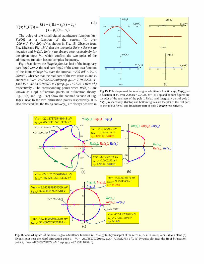
The poles of the small-signal admittance function Y(s;

Vm(Q)) as a function of the current Vm over

-200 mV<Vm<200 mV is shown in Fig. 15. Observe from

Fig. 15(a) and Fig. 15(b) that the two poles Re(p1), Re(p2) are

negative and Im(p1), Im(p2) are always zero respectively for

the given input Vm, which confirm the two poles of the

admittance function has no complex frequency.

Fig. 16(a) shows the Nyquist plot, i.e. loci of the imaginary

part Im(zi) versus the real part Re(zi) of the zeros as a function

of the input voltage Vm over the interval −200 mV ≤ Vm ≤

200mV . Observe that the real part of the two zeros z2 and z3

are zero at Vm= -26.75527972mV(resp. gkCa=-7.79022731 s-1

) and Vm= -47.5332788572 mV (resp. gkCa =27.25111606 s-1 )

respectively . The corresponding points when Re(zi)=0 are

known as Hopf bifurcation points in bifurcation theory.

Fig. 16(b) and Fig. 16(c) show the zoomed version of Fig,

16(a) near to the two bifurcation points respectively. It is

also observed that the Re(z2) and Re(z3) are always positive in

Vm= -22.1378795486045 mV

gK,Ca= -45.5241957133932 s-1

Vm= -26.75527972 mV

gK,Ca= -7.79022731 s-1

z2= 0+97.171320482i

Vm= -26.75527972 mV

gK,Ca= -7.79022731 s-1

z3= 0-97.171320482i

Vm= -22.1378795486045 mV

gK,Ca= -45.5241957133932 s-1

Re(z1), Re(z2), Re(z3) Re(z1)

Re(z2), Re(z3)0 5 10

105

52.5

52.5

105

Im(z1), Im(z2), Im(z3)

260 182.5 105 27.5 50

450

225

225

450

Im(z1), Im(z2), Im(z3)

(a) (b)

1 0 1

1.2

0.6

0.6

1.2

Re(z1)

Re(z2), Re(z3)

Im(z1), Im(z2),

Im(z3)

Vm= -47.5332788572 mV

gK,Ca= 27.25111606 s-1

z2= 0+1.06i

Vm= -47.5332788572 mV

gK,Ca= 27.25111606 s-1

z3= 0-1.06i

Vm= -48.2459999459569 mV

gK,Ca= 32.4605269226518 s-1

Vm= -48.2459999459569 mV

gK,Ca= 32.4605269226518 s-1

(c)

Vm=-46.70873

Vm=-46.70873

Vm=-97.35 mV

Vm=-100.11 mV

Fig. 16. Zeros diagram of the small-signal admittance function Y(s; Vm(Q)) (a) Nyquist plot of the zeros z1, z2, z3 in Im(zi) versus Re(zi) plane (b)

Nyquist plot near the Hopf-bifurcation point 1, Vm= -26.75527972(resp. gkCa=-7.79022731 s-1 ). (c) Nyquist plot near the Hopf-bifurcation

point 2, Vm= -47.5332788572 mV (resp. gkCa =27.25111606 s-1).

200 100 0 100 200

600

450

300

150

Re(p1)

Vm(mV)

200 100 0 100 200

1

0.5

0.5

1

Im(p1)

Vm(mV)

(a)

200 100 0 100 200

1

0.5

0.5

1

Im(p2)

Vm(mV)

200 100 0 100 200

0.04955

0.0495

0.04945

Re(p2)

Vm(mV)

(b)

Fig.15. Pole diagram of the small-signal admittance function Y(s; Vm(Q)) as

a function of Vm over-200 mV<Vm<200 mV (a) Top and bottom figures are

the plot of the real part of the pole 1 Re(p1) and Imaginary part of pole 1

Im(p1) respectively. (b) Top and bottom figures are the plot of the real part

of the pole 2 Re(p2) and Imaginary part of pole 2 Im(p2) respectively.

open-half plane between the bifurcation points

-26.75527972>Vm>-47.5332788572 mV(resp. -7.79022731 s-1

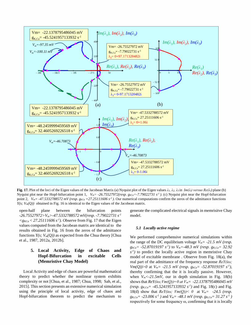
<gKCa < 27.25111606 s-1). Observe from Fig. 17 that the Eigen

values computed from the Jacobean matrix are identical to the

results obtained in Fig. 16 from the zeros of the admittance

functions Y(s; Vm(Q)) as expected from the Chua theory [Chua

et al., 1987, 2012a, 2012b].

5. Local Activity, Edge of Chaos and

Hopf-Bifurcation in excitable Cells

(Memristive Chay Model)

Local Activity and edge of chaos are powerful mathematical

theory to predict whether the nonlinear system exhibits

complexity or not [Chua, et al., 1987; Chua, 1998; Sah, et al.,

2015]. This section presents an extensive numerical simulation

using the principle of local activity, edge of chaos and

Hopf-bifurcation theorem to predict the mechanism to

generate the complicated electrical signals in memrisitve Chay

model.

5.1 Locally active regime

We performed comprehensive numerical simulations within

the range of the DC equilibrium voltage Vm= -21.5 mV (resp.

gkCa= -52.87019197 s-1) to Vm=-48.3 mV (resp. gK,Ca= 32.92

s-1) to predict the locally active region in memristive Chay

model of excitable membrane . Observe from Fig. 18(a), the

real part of the admittance of the frequency response ReY(iω;

Vm(Q))>0 at Vm= -21.5 mV (resp. gkCa= -52.87019197 s-1),

thereby confirming that the it is locally passive. However,

when Vm<-21.5mV, our in depth simulation in Fig. 18(b)

shows that ReY(iω;Vm(Q))=0 at Vm= -22.1378795486045 mV

(resp. gK,Ca= -45.5241957133932 s-1) and Fig. 18(c) and Fig.

18(d) show that ReY(iω; Vm(Q))< 0 at Vm= -24.5 (resp.

gK,Ca= -23.006 s-1 ) and Vm= -48.1 mV (resp. gK,Ca= 31.27 s-1 )

respectively for some frequency ω, confirming that it is locally

Vm= -22.1378795486045 mV

gK,Ca= -45.5241957133932 s-1

Vm= -26.75527972 mV

gK,Ca= -7.79022731 s-1

λ2= 0+97.171320482i

Vm= -26.75527972 mV

gK,Ca= -7.79022731 s-1

λ3= 0-97.171320482i

Vm= -22.1378795486045 mV

gK,Ca= -45.5241957133932 s-1

Re(λ1), Re(λ2), Re(λ3) Re(λ1)

Re(λ2), Re(λ3)0 5 10

105

52.5

52.5

105

Im(λ1), Im(λ2), Im(λ3)

260 182.5 105 27.5 50

450

225

225

450

Im(λ1), Im(λ2), Im(λ3)

(a) (b)

1 0 1

1.2

0.6

0.6

1.2

Re(λ1), Re(λ2),

Re(λ3)

Im(λ1), Im(λ2),

Im(λ3)

Vm= -47.5332788572 mV

gK,Ca= 27.25111606 s-1

λ2= 0+1.06i

Vm= -47.5332788572 mV

gK,Ca= 27.25111606 s-1

λ3= 0-1.06i

Vm= -48.2459999459569 mV

gK,Ca= 32.4605269226518 s-1

Vm= -48.2459999459569 mV

gK,Ca= 32.4605269226518 s-1

(c)

Vm=-46.70873

Vm=-46.70873

Vm=-97.35 mV

Vm=-100.11 mV

Fig. 17. Plot of the loci of the Eigen values of the Jacobean Matrix (a) Nyquist plot of the Eigen values λ1, λ2, λ3 in Im(λi) versus Re(λi) plane (b)

Nyquist plot near the Hopf-bifurcation point 1, Vm= -26.75527972(resp. gkCa=-7.79022731 s-1 ). (c) Nyquist plot near the Hopf-bifurcation

point 2, Vm= -47.5332788572 mV (resp. gkCa =27.25111606 s-1 ). Our numerical computations confirm the zeros of the admittance functions

Y(s; Vm(Q)) obtained in Fig. 16 is identical to the Eigen values of the Jacobean matrix.

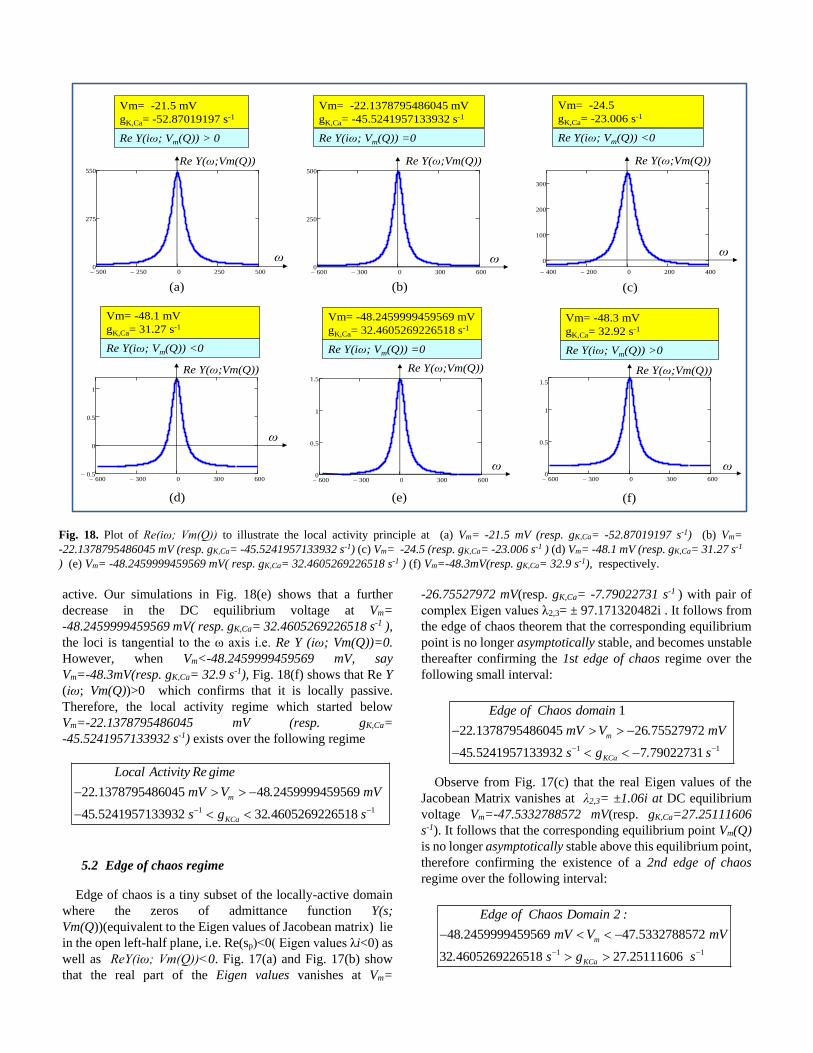
active. Our simulations in Fig. 18(e) shows that a further

decrease in the DC equilibrium voltage at Vm=

-48.2459999459569 mV( resp. gK,Ca= 32.4605269226518 s-1 ),

the loci is tangential to the ω axis i.e. Re Y (iω; Vm(Q))=0.

However, when Vm<-48.2459999459569 mV, say

Vm=-48.3mV(resp. gK,Ca= 32.9 s-1), Fig. 18(f) shows that Re Y

(iω; Vm(Q))>0 which confirms that it is locally passive.

Therefore, the local activity regime which started below

Vm=-22.1378795486045 mV (resp. gK,Ca=

-45.5241957133932 s-1) exists over the following regime

1 1

22 1378795486045 48 2459999459569

45 5241957133932 32 4605269226518

m

KCa

. mV V . mV  

. s g

Local Activity Re gime

. s

5.2 Edge of chaos regime

Edge of chaos is a tiny subset of the locally-active domain

where the zeros of admittance function Y(s;

Vm(Q))(equivalent to the Eigen values of Jacobean matrix) lie

in the open left-half plane, i.e. Re(sp)<0( Eigen values λi<0) as

well as ReY(iω; Vm(Q))<0. Fig. 17(a) and Fig. 17(b) show

that the real part of the Eigen values vanishes at Vm=

-26.75527972 mV(resp. gK,Ca= -7.79022731 s-1 ) with pair of

complex Eigen values λ2,3= ± 97.171320482i . It follows from

the edge of chaos theorem that the corresponding equilibrium

point is no longer asymptotically stable, and becomes unstable

thereafter confirming the 1st edge of chaos regime over the

following small interval:

1 1

22 1378795486045 26 75527972

45 5241957133932 7 79022731

1

m

KCa

. mV V . mV  

.

Edge of Chaos doma

s

i

s g .

n

Observe from Fig. 17(c) that the real Eigen values of the

Jacobean Matrix vanishes at λ2,3= ±1.06i at DC equilibrium

voltage Vm=-47.5332788572 mV(resp. gK,Ca=27.25111606

s-1). It follows that the corresponding equilibrium point Vm(Q)

is no longer asymptotically stable above this equilibrium point,

therefore confirming the existence of a 2nd edge of chaos

regime over the following interval:

1 1

48 2459999459569 47 5332788572

32 4605269226518 27 25111606

m

KCa

Edge of

. mV V . mV  

Chaos Domain 2

. s . s

:

g

500 250 0 250 5000

275

550

Re Y(ω;Vm(Q))

ω

Vm= -21.5 mV

gK,Ca= -52.87019197 s-1

Re Y(iω; Vm(Q)) > 0

600 300 0 300 6000

250

500

Re Y(ω;Vm(Q))

ω

Vm= -22.1378795486045 mV

gK,Ca= -45.5241957133932 s-1

Re Y(iω; Vm(Q)) =0

400 200 0 200 400

0

100

200

300

Re Y(ω;Vm(Q))

ω

Vm= -24.5

gK,Ca= -23.006 s-1

Re Y(iω; Vm(Q)) <0

(a) (b) (c)

600 300 0 300 6000

0.5

1

1.5

Re Y(ω;Vm(Q))

ω

Vm= -48.2459999459569 mV

gK,Ca= 32.4605269226518 s-1

Re Y(iω; Vm(Q)) =0

Vm= -48.1 mV

gK,Ca= 31.27 s-1

Re Y(iω; Vm(Q)) <0

600 300 0 300 6000.5

0

0.5

1

ω

Re Y(ω;Vm(Q))

600 300 0 300 6000

0.5

1

1.5

Re Y(ω;Vm(Q))

ω

Vm= -48.3 mV

gK,Ca= 32.92 s-1

Re Y(iω; Vm(Q)) >0

(d) (e) (f)

Fig. 18. Plot of Re(iω; Vm(Q)) to illustrate the local activity principle at (a) Vm= -21.5 mV (resp. gK,Ca= -52.87019197 s-1) (b) Vm=

-22.1378795486045 mV (resp. gK,Ca= -45.5241957133932 s-1) (c) Vm= -24.5 (resp. gK,Ca= -23.006 s-1 ) (d) Vm= -48.1 mV (resp. gK,Ca= 31.27 s-1

) (e) Vm= -48.2459999459569 mV( resp. gK,Ca= 32.4605269226518 s-1 ) (f) Vm=-48.3mV(resp. gK,Ca= 32.9 s-1), respectively.

5.3 Hopf-Bifurcation

Hopf-bifurcation is a locally bifurcation phenomenon in

which an equilibrium point changes its stability as the

parameter of the nonlinear system changes under certain

conditions. There are two types of Hopf-bifurcations namely:

super-critical Hopf bifurcation and sub-critical Hopf

bifurcation. An unstable equilibrium point surrounded by a

stable limit cycle results to a super-critical Hopf bifurcation

and unstable limit cycle surrounded by a stable equilibrium

point results to a sub-critical Hopf bifurcation. Our careful

simulation at Hopf-bifurcation point 1 at Vm= -26.75527972

mV(resp. gK,Ca= -7.79022731 s-1 ) 8 shows that gKCa chosen

within very small edge of chaos domain 1, where the real part

of the Eigen values are negative, the result converges to DC

equilibrium for any initial conditions. Likewise, gKCa selected

within the bifurcation point 1, where the real part of Eigen

values are positive, the result converges to a stable limit cycle.

Therefore, it follows from the bifurcation theory that

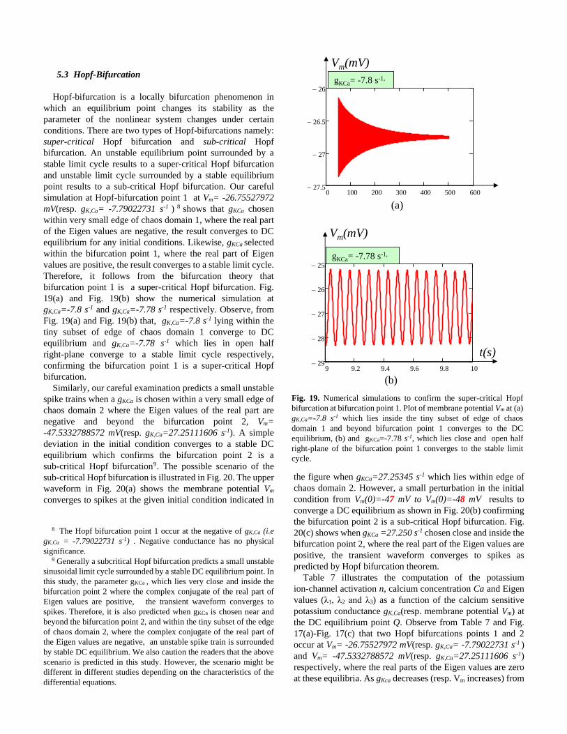
bifurcation point 1 is a super-critical Hopf bifurcation. Fig.

19(a) and Fig. 19(b) show the numerical simulation at

gK,Ca=-7.8 s-1 and gK,Ca=-7.78 s-1 respectively. Observe, from

Fig. 19(a) and Fig. 19(b) that, gK,Ca=-7.8 s-1 lying within the

tiny subset of edge of chaos domain 1 converge to DC

equilibrium and gK,Ca=-7.78 s-1 which lies in open half

right-plane converge to a stable limit cycle respectively,

confirming the bifurcation point 1 is a super-critical Hopf

bifurcation.

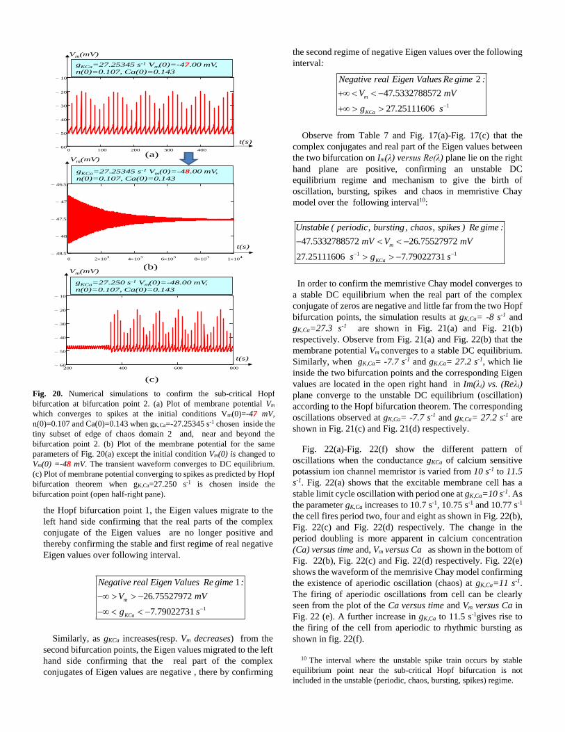
Similarly, our careful examination predicts a small unstable

spike trains when a gKCa is chosen within a very small edge of

chaos domain 2 where the Eigen values of the real part are

negative and beyond the bifurcation point 2, Vm=

-47.5332788572 mV(resp. gK,Ca=27.25111606 s-1). A simple

deviation in the initial condition converges to a stable DC

equilibrium which confirms the bifurcation point 2 is a

sub-critical Hopf bifurcation9. The possible scenario of the

sub-critical Hopf bifurcation is illustrated in Fig. 20. The upper

waveform in Fig. 20(a) shows the membrane potential Vm

converges to spikes at the given initial condition indicated in

8 The Hopf bifurcation point 1 occur at the negative of gK,Ca (i.e

gK,Ca = -7.79022731 s-1) . Negative conductance has no physical

significance. 9 Generally a subcritical Hopf bifurcation predicts a small unstable

sinusoidal limit cycle surrounded by a stable DC equilibrium point. In

this study, the parameter gKCa , which lies very close and inside the

bifurcation point 2 where the complex conjugate of the real part of

Eigen values are positive, the transient waveform converges to

spikes. Therefore, it is also predicted when gKCa is chosen near and

beyond the bifurcation point 2, and within the tiny subset of the edge

of chaos domain 2, where the complex conjugate of the real part of

the Eigen values are negative, an unstable spike train is surrounded

by stable DC equilibrium. We also caution the readers that the above

scenario is predicted in this study. However, the scenario might be

different in different studies depending on the characteristics of the

differential equations.

the figure when gKCa=27.25345 s-1 which lies within edge of

chaos domain 2. However, a small perturbation in the initial

condition from Vm(0)=-47 mV to Vm(0)=-48 mV results to

converge a DC equilibrium as shown in Fig. 20(b) confirming

the bifurcation point 2 is a sub-critical Hopf bifurcation. Fig.

20(c) shows when gKCa =27.250 s-1 chosen close and inside the

bifurcation point 2, where the real part of the Eigen values are

positive, the transient waveform converges to spikes as

predicted by Hopf bifurcation theorem.

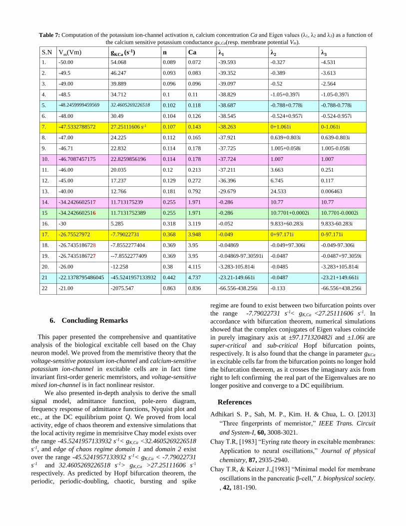
Table 7 illustrates the computation of the potassium

ion-channel activation n, calcium concentration Ca and Eigen

values (λ1, λ2 and λ3) as a function of the calcium sensitive

potassium conductance gK,Ca(resp. membrane potential Vm) at

the DC equilibrium point Q. Observe from Table 7 and Fig.

17(a)-Fig. 17(c) that two Hopf bifurcations points 1 and 2

occur at Vm= -26.75527972 mV(resp. gK,Ca= -7.79022731 s-1 )

and Vm= -47.5332788572 mV(resp. gK,Ca=27.25111606 s-1)

respectively, where the real parts of the Eigen values are zero

at these equilibria. As gKca decreases (resp. Vm increases) from

0 100 200 300 400 500 60027.5

27

26.5

26

Vm(mV)

gKCa= -7.8 s-1,

(a)

9 9.2 9.4 9.6 9.8 1029

28

27

26

25

gKCa= -7.78 s-1,

Vm(mV)

t(s)

(b)

Fig. 19. Numerical simulations to confirm the super-critical Hopf

bifurcation at bifurcation point 1. Plot of membrane potential Vm at (a)

gK,Ca=-7.8 s-1 which lies inside the tiny subset of edge of chaos

domain 1 and beyond bifurcation point 1 converges to the DC

equilibrium, (b) and gKCa=-7.78 s-1, which lies close and open half

right-plane of the bifurcation point 1 converges to the stable limit

cycle.

the Hopf bifurcation point 1, the Eigen values migrate to the

left hand side confirming that the real parts of the complex

conjugate of the Eigen values are no longer positive and

thereby confirming the stable and first regime of real negative

Eigen values over following interval.

1

26 75527972

7 79022

1

731

m

KCa

Negative real E

V . mV

igen Values Re gi

 

g . s

me :

Similarly, as gKCa increases(resp. Vm decreases) from the

second bifurcation points, the Eigen values migrated to the left

hand side confirming that the real part of the complex

conjugates of Eigen values are negative , there by confirming

the second regime of negative Eigen values over the following

interval:

1

47 5332788572

27 251

2

11606

m

KCa

Negative real Ei

V . mV  

g

gen Values R

.

e gime

s

:

Observe from Table 7 and Fig. 17(a)-Fig. 17(c) that the

complex conjugates and real part of the Eigen values between

the two bifurcation on Im(λ) versus Re(λ) plane lie on the right

hand plane are positive, confirming an unstable DC

equilibrium regime and mechanism to give the birth of

oscillation, bursting, spikes and chaos in memristive Chay

model over the following interval10:

1 1

47 5332788572 26 75527972

27 25111606 7 79022731

m

KCa

. mV V . mV

Unstable ( periodic, bursting, chao

 

. s g

s, spikes

.

) Re gim

s

e :

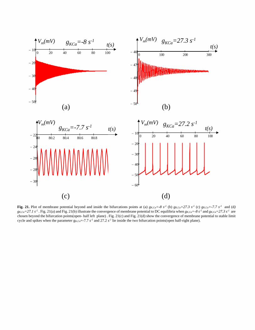
In order to confirm the memristive Chay model converges to

a stable DC equilibrium when the real part of the complex

conjugate of zeros are negative and little far from the two Hopf

bifurcation points, the simulation results at gK,Ca= -8 s-1 and

gK,Ca=27.3 s-1 are shown in Fig. 21(a) and Fig. 21(b)

respectively. Observe from Fig. 21(a) and Fig. 22(b) that the

membrane potential Vm converges to a stable DC equilibrium.

Similarly, when gK,Ca= -7.7 s-1 and gK,Ca= 27.2 s-1, which lie

inside the two bifurcation points and the corresponding Eigen

values are located in the open right hand in Im(λi) vs. (Reλi)

plane converge to the unstable DC equilibrium (oscillation)

according to the Hopf bifurcation theorem. The corresponding

oscillations observed at gK,Ca= -7.7 s-1 and gK,Ca= 27.2 s-1 are

shown in Fig. 21(c) and Fig. 21(d) respectively.

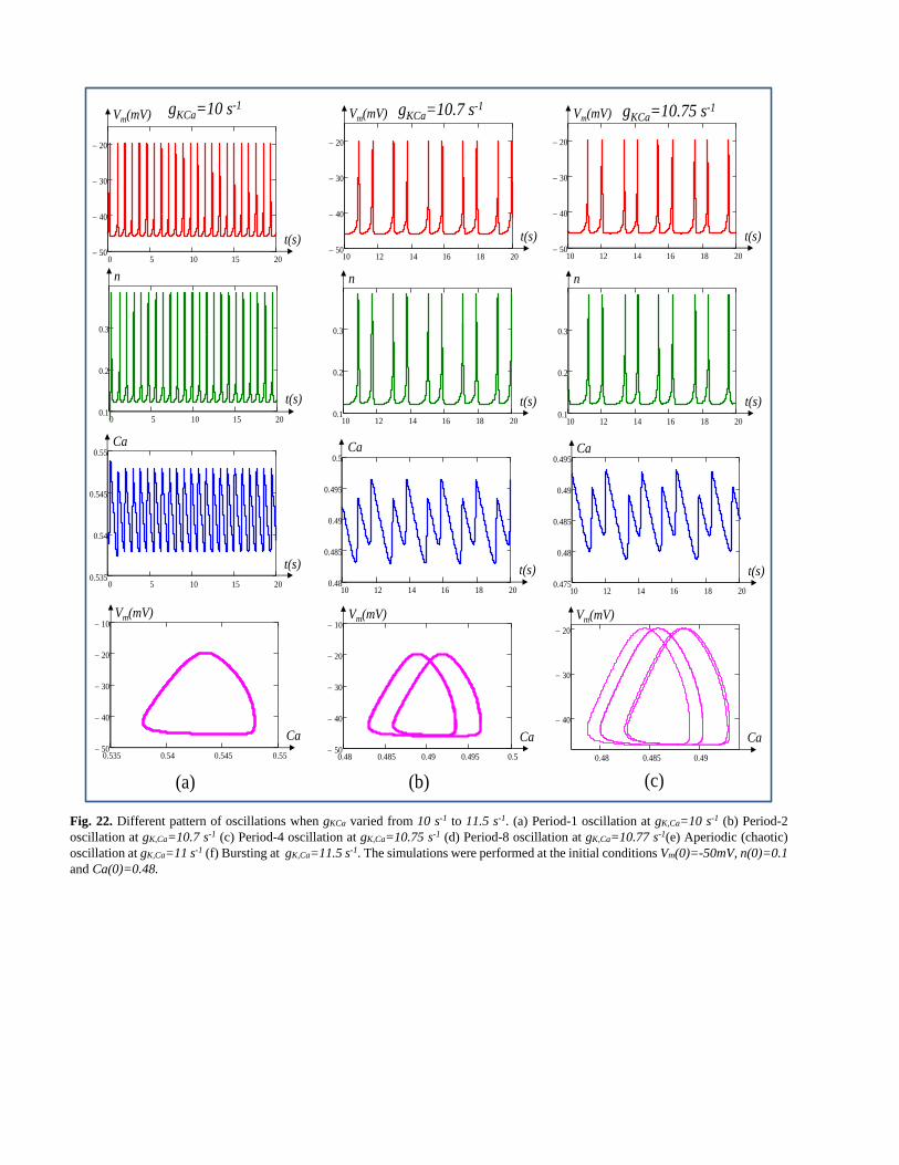
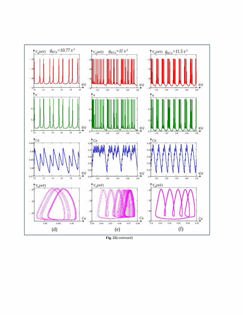
Fig. 22(a)-Fig. 22(f) show the different pattern of

oscillations when the conductance gKCa of calcium sensitive

potassium ion channel memristor is varied from 10 s-1 to 11.5

s-1. Fig. 22(a) shows that the excitable membrane cell has a

stable limit cycle oscillation with period one at gK,Ca=10 s-1. As

the parameter gK,Ca increases to 10.7 s-1, 10.75 s-1 and 10.77 s-1

the cell fires period two, four and eight as shown in Fig. 22(b),

Fig. 22(c) and Fig. 22(d) respectively. The change in the

period doubling is more apparent in calcium concentration

(Ca) versus time and, Vm versus Ca as shown in the bottom of

Fig. 22(b), Fig. 22(c) and Fig. 22(d) respectively. Fig. 22(e)

shows the waveform of the memrisive Chay model confirming

the existence of aperiodic oscillation (chaos) at gK,Ca=11 s-1.

The firing of aperiodic oscillations from cell can be clearly

seen from the plot of the Ca versus time and Vm versus Ca in

Fig. 22 (e). A further increase in gK,Ca to 11.5 s-1gives rise to

the firing of the cell from aperiodic to rhythmic bursting as

shown in fig. 22(f).

10 The interval where the unstable spike train occurs by stable

equilibrium point near the sub-critical Hopf bifurcation is not

included in the unstable (periodic, chaos, bursting, spikes) regime.

0 100 200 300 40060

50

40

30

20

10

Vm(mV)

gKCa=27.25345 s-1 Vm(0)=-47.00 mV,

n(0)=0.107, Ca(0)=0.143

t(s)

(a)Vm(mV)

t(s)

gKCa=27.25345 s-1 Vm(0)=-48.00 mV,

n(0)=0.107, Ca(0)=0.143

(b)

0 2 103

4 103

6 103

8 103

1 104

48.5

48

47.5

47

46.5

200 400 600 80060

50

40

30

20

10

Vm(mV)

t(s)

gKCa=27.250 s-1 Vm(0)=-48.00 mV,

n(0)=0.107, Ca(0)=0.143

(c)

Fig. 20. Numerical simulations to confirm the sub-critical Hopf

bifurcation at bifurcation point 2. (a) Plot of membrane potential Vm

which converges to spikes at the initial conditions Vm(0)=-47 mV,

n(0)=0.107 and Ca(0)=0.143 when gK,Ca=-27.25345 s-1 chosen inside the

tiny subset of edge of chaos domain 2 and, near and beyond the

bifurcation point 2. (b) Plot of the membrane potential for the same

parameters of Fig. 20(a) except the initial condition Vm(0) is changed to

Vm(0) =-48 mV. The transient waveform converges to DC equilibrium.

(c) Plot of membrane potential converging to spikes as predicted by Hopf

bifurcation theorem when gK,Ca=27.250 s-1 is chosen inside the

bifurcation point (open half-right pane).

0 20 40 60 80 100

50

40

30

20

10

Vm(mV)t(s)gKCa=-8 s-1

80 80.2 80.4 80.6 80.8

30

28

26

24

22

Vm(mV)t(s)gKCa=-7.7 s-1

Vm(mV)

0 20 40 60 80 100

60

50

40

30

20

10

t(s)gKCa=27.2 s-1

0 100 200 300

50

49

48

47

46

Vm(mV)

t(s)gKCa=27.3 s-1

(a) (b)

(c) (d)

Fig. 21. Plot of membrane potential beyond and inside the bifurcations points at (a) gK,Ca=-8 s-1 (b) gK,Ca=27.3 s-1 (c) gK,Ca=-7.7 s-1 and (d)

gK,Ca=27.1 s-1 . Fig. 21(a) and Fig. 21(b) illustrate the convergence of membrane potential to DC equilibria when gK,Ca=-8 s-1 and gK,Ca=27.3 s-1 are

chosen beyond the bifurcation points(open- half left plane) . Fig. 21(c) and Fig. 21(d) show the convergence of membrane potential to stable limit

cycle and spikes when the parameter gK,Ca=-7.7 s-1 and 27.2 s-1 lie inside the two bifurcation points(open half-right plane).

0 5 10 15 2050

40

30

20

Vm(mV)

t(s)

gKCa=10 s-1

0 5 10 15 200.535

0.54

0.545

0.55

t(s)

Ca

0.535 0.54 0.545 0.5550

40

30

20

10

Ca

Vm(mV)

0 5 10 15 200.1

0.2

0.3

t(s)

n

10 12 14 16 18 2050

40

30

20

t(s)

Vm(mV)

10 12 14 16 18 200.1

0.2

0.3

t(s)

n

10 12 14 16 18 200.48

0.485

0.49

0.495

0.5

t(s)

Ca

0.48 0.485 0.49 0.495 0.550

40

30

20

10

Ca

Vm(mV)

gKCa=10.7 s-1

10 12 14 16 18 2050

40

30

20

t(s)

Vm(mV) gKCa=10.75 s-1

10 12 14 16 18 200.1

0.2

0.3

t(s)

n

10 12 14 16 18 200.475

0.48

0.485

0.49

0.495

t(s)

Ca

0.48 0.485 0.49

40

30

20

Ca

Vm(mV)

(a) (b) (c)

Fig. 22. Different pattern of oscillations when gKCa varied from 10 s-1 to 11.5 s-1. (a) Period-1 oscillation at gK,Ca=10 s-1 (b) Period-2

oscillation at gK,Ca=10.7 s-1 (c) Period-4 oscillation at gK,Ca=10.75 s-1 (d) Period-8 oscillation at gK,Ca=10.77 s-1(e) Aperiodic (chaotic)

oscillation at gK,Ca=11 s-1 (f) Bursting at gK,Ca=11.5 s-1. The simulations were performed at the initial conditions Vm(0)=-50mV, n(0)=0.1

and Ca(0)=0.48.

(d) (e) (f)

gKCa=10.77 s-1

10 12 14 16 18 2050

40

30

20

t(s)

Vm(mV)

10 12 14 16 18 200.1

0.2

0.3

t(s)

n

t(s)

Ca

10 12 14 16 18 200.475

0.48

0.485

0.49

0.495

0.48 0.485 0.49

40

30

20

Ca

Vm(mV)

110 120 130 140 15050

40

30

20

t(s)

Vm(mV) gKCa=11 s-1

110 120 130 140 1500.43

0.44

0.45

0.46

0.47

0.48

t(s)

Ca

110 120 130 140 1500.1

0.2

0.3

t(s)

n

0.43 0.44 0.45 0.46 0.47 0.4850

40

30

20

Ca

Vm(mV)

110 120 130 140 15050

40

30

20

t(s)

Vm(mV) gKCa=11.5 s-1

110 120 130 140 1500.1

0.2

0.3

t(s)

n

110 120 130 140 1500.4

0.41

0.42

0.43

0.44

0.45

t(s)

Ca

Ca

Vm(mV)

0.4 0.41 0.42 0.43 0.44 0.4550

40

30

20

Fig. 22(continued)

6. Concluding Remarks

This paper presented the comprehensive and quantitative

analysis of the biological excitable cell based on the Chay

neuron model. We proved from the memristive theory that the

voltage-sensitive potassium ion-channel and calcium-sensitive

potassium ion-channel in excitable cells are in fact time

invariant first-order generic memristors, and voltage-sensitive

mixed ion-channel is in fact nonlinear resistor.

We also presented in-depth analysis to derive the small

signal model, admittance function, pole-zero diagram,

frequency response of admittance functions, Nyquist plot and

etc., at the DC equilibrium point Q. We proved from local

activity, edge of chaos theorem and extensive simulations that

the local activity regime in memrisitve Chay model exists over

the range -45.5241957133932 s-1< gK,Ca <32.4605269226518

s-1, and edge of chaos regime domain 1 and domain 2 exist

over the range -45.5241957133932 s-1< gK,Ca < -7.79022731

s-1 and 32.4605269226518 s-1> gK,Ca >27.25111606 s-1

respectively. As predicted by Hopf bifurcation theorem, the

periodic, periodic-doubling, chaotic, bursting and spike

regime are found to exist between two bifurcation points over

the range -7.79022731 s-1< gK,Ca <27.25111606 s-1. In

accordance with bifurcation theorem, numerical simulations

showed that the complex conjugates of Eigen values coincide

in purely imaginary axis at ±97.171320482i and ±1.06i are

super-critical and sub-critical Hopf bifurcation points,

respectively. It is also found that the change in parameter gKCa

in excitable cells far from the bifurcation points no longer hold

the bifurcation theorem, as it crosses the imaginary axis from

right to left confirming the real part of the Eigenvalues are no

longer positive and converge to a DC equilibrium.

References

Adhikari S. P., Sah, M. P., Kim. H. & Chua, L. O. [2013]

“Three fingerprints of memristor,” IEEE Trans. Circuit

and System-I, 60, 3008-3021.

Chay T.R, [1983] “Eyring rate theory in excitable membranes:

Application to neural oscillations,” Journal of physical

chemistry, 87, 2935-2940.

Chay T.R, & Keizer J.,[1983] “Minimal model for membrane

oscillations in the pancreatic β-cell,” J. biophysical society.

, 42, 181-190.

Table 7: Computation of the potassium ion-channel activation n, calcium concentration Ca and Eigen values (λ1, λ2 and λ3) as a function of

the calcium sensitive potassium conductance gK,Ca(resp. membrane potential Vm).

S.N Vm(Vm) gKCa (s-1) n Ca λ1 λ2 λ3

1. -50.00 54.068 0.089 0.072 -39.593 -0.327 -4.531

2. -49.5 46.247 0.093 0.083 -39.352 -0.389 -3.613

3. -49.00 39.889 0.096 0.096 -39.097 -0.52 -2.564

4. -48.5 34.712 0.1 0.11 -38.829 -1.05+0.397i -1.05-0.397i

5. -48.2459999459569 32.4605269226518 0.102 0.118 -38.687 -0.788+0.778i -0.788-0.778i

6. -48.00 30.49 0.104 0.126 -38.545 -0.524+0.957i -0.524-0.957i

7. -47.5332788572 27.25111606 s-1 0.107 0.143 -38.263 0+1.061i 0-1.061i

8. -47.00 24.225 0.112 0.165 -37.921 0.639+0.803i 0.639-0.803i

9. -46.71 22.832 0.114 0.178 -37.725 1.005+0.058i 1.005-0.058i

10. -46.7087457175 22.8259856196 0.114 0.178 -37.724 1.007 1.007

11. -46.00 20.035 0.12 0.213 -37.211 3.663 0.251

12. -45.00 17.237 0.129 0.272 -36.396 6.745 0.117

13. -40.00 12.766 0.181 0.792 -29.679 24.533 0.006463

14. -34.2426602517 11.713175239 0.255 1.971 -0.286 10.77 10.77

15 -34.2426602516 11.7131752389 0.255 1.971 -0.286 10.7701+0.0002i 10.7701-0.0002i

16. -30 5.285 0.318 3.119 -0.052 9.833+60.283i 9.833-60.283i

17. -26.75527972 -7.79022731 0.368 3.948 -0.049 0+97.171i 0-97.171i

18. -26.7435186728 -7.8552277404 0.369 3.95 -0.04869 -0.049+97.306i -0.049-97.306i

19. -26.7435186727 --7.8552277409 0.369 3.95 -0.04869-97.30591i -0.0487 -0.0487+97.3059i

20. -26.00 -12.258 0.38 4.115 -3.283-105.814i -0.0485 -3.283+105.814i

21 -22.1378795486045 -45.5241957133932 0.442 4.737 -23.21-149.661i -0.0487 -23.21+149.661i

22 -21.00 -2075.547 0.863 0.836 -66.556-438.256i -0.133 -66.556+438.256i

Chay T.R, [1985] “Chaos in a three-variable model of an

excitable cell,” Physics D, 16, 233-242.

Chua, L. O. & Kang, S. M. [1976] “Memristive devices and

systems,” Proc. of the IEEE, 64, 2, 209-223.

Chua, L. O., Desoer, C. A., Kuh, E. S. [1987] Linear

and Nonlinear Circuits (McGraw-Hill book Co., New

York).

Chua, L., Sbitnev, V. & Kim, H. [2012a] “Hodgkin-Huxley

axon is made of memristor,” Int. J. Bifurcation and Chaos

22, 1230011-1- 48.

Chua, L. O. [1998] "CNN: A paradigm for Complexity,"

World Scientific, Singapore.

Chua, L., Sbitnev, V. & Kim, H. [2012b] “Neurons are poised

near the edge of chaos,” Int. J. Bifurcation and Chaos 22,

1250098-1- 49.

Chua, L. [2014] “If it’s pinched it’s a memristor,” Semicond.

Sci. Technol. 29, 104001-1-42.

Chua, L. [2015] “Everything you wish to know about

memristor but are afraid to ask,” Radioengineering 24,

319-368.

Giguère C. & Woodland P.C. [1994] “A computational model

of the auditory periphery for speech and hearing research”

The Journal of the Acoustical Society of America , 95,

343-349.

Hodgkin, A. L. & Huxley, A. F. [1952] “A quantitative

description of membrane current and its application to

conduction and excitation in nerve,” J. Physiol. 117,

500-544.

Hodgkin, A. L. & Keynes, R.D. [1956] “Experiments on the

injection of substances into squid giant axons by means of

microsyringe,” J. Physiol. London 131, 592-616.

Hudspeth, A. J & Lewis R.S. [1988] “A model for electrical

resonance and frequency tuning in saccular hair cells of the

bull-frog Rana catesbeiana,” J. Physiology, 400, 275-297.

Morris, C. & Lecar, H. [1981] “Voltage oscillations in the

Barnacle giant muscle fiber,” J. of Biophysical Society, 35,

193-213.

Noble, D. [1962] “A modification of the Hodgkin-Huxley

equations applicable to Purkinje fibre action and

peacemaker potentials”, J. of Physiology 160, 317–352.

Plant R.E, [1981] “Bifurcation and resonance in a model for

bursting nerve cells,” Journal of mathematical biology, 11,

15-32.

Sah M. P., Kim, H. & Chua, L. O. [2014] “Brains are made of

memristors,” IEEE circuits and systems magazine, 1,

12-36.

Sah M. P., Mannan, Z. I., Kim, H. & Chua, L. [2015]

“Oscillator Made of Only One Memristor and One

Battery,” Int. J. Bifurcation and Chaos 25,

1530010(1)-(28).