Noncommutative Involutive Bases - arXiv
389
arXiv:math/0602140v1 [math.RA] 7 Feb 2006 Noncommutative Involutive Bases Thesis submitted to the University of Wales in support of the application for the degree of Philosophiæ Doctor by Gareth Alun Evans School of Informatics The University of Wales, Bangor September 2005
-
Upload
khangminh22 -
Category
Documents
-
view
9 -
download
0
Transcript of Noncommutative Involutive Bases - arXiv

arX
iv:m
ath/
0602
140v
1 [
mat
h.R
A]
7 F
eb 2
006 Noncommutative Involutive Bases
Thesis submitted to the University of Wales in support of
the application for the degree of Philosophiæ Doctor
by
Gareth Alun Evans
School of Informatics
The University of Wales, Bangor
September 2005

DECLARATION
This work has not previously been accepted in substance for any degree and is not being
concurrently submitted in candidature for any degree.
Signed . . . . . . . . . . . . . . . . . . . . . . . . . . . . . . . . . . . . . . . . . . . . . . . . . . . . . . . (candidate)
Date . . . . . . . . . . . . . . . . . . . . . . . . . . . . . . . . . . . . . . . . . . . . . . . . . . . . . . . .
STATEMENT 1
This thesis is the result of my own investigations, except where otherwise stated.
Other sources are acknowledged by explicit references. A bibliography is appended.
Signed . . . . . . . . . . . . . . . . . . . . . . . . . . . . . . . . . . . . . . . . . . . . . . . . . . . . . . . (candidate)
Date . . . . . . . . . . . . . . . . . . . . . . . . . . . . . . . . . . . . . . . . . . . . . . . . . . . . . . . .
STATEMENT 2
I hereby give consent for my thesis, if accepted, to be available for photocopying and
for inter-library loan, and for the title and summary to be made available to outside
organisations.
Signed . . . . . . . . . . . . . . . . . . . . . . . . . . . . . . . . . . . . . . . . . . . . . . . . . . . . . . . (candidate)
Date . . . . . . . . . . . . . . . . . . . . . . . . . . . . . . . . . . . . . . . . . . . . . . . . . . . . . . . .

Summary
The theory of Grobner Bases originated in the work of Buchberger [11] and is now con-sidered to be one of the most important and useful areas of symbolic computation. Agreat deal of effort has been put into improving Buchberger’s algorithm for computing aGrobner Basis, and indeed in finding alternative methods of computing Grobner Bases.Two of these methods include the Grobner Walk method [1] and the computation ofInvolutive Bases [58].
By the mid 1980’s, Buchberger’s work had been generalised for noncommutative poly-nomial rings by Bergman [8] and Mora [45]. This thesis provides the correspondinggeneralisation for Involutive Bases and (to a lesser extent) the Grobner Walk, with themain results being as follows.
(1) Algorithms for several new noncommutative involutive divisions are given, includingstrong; weak; global and local divisions.
(2) An algorithm for computing a noncommutative Involutive Basis is given. When usedwith one of the aforementioned involutive divisions, it is shown that this algorithmreturns a noncommutative Grobner Basis on termination.
(3) An algorithm for a noncommutative Grobner Walk is given, in the case of conversionbetween two harmonious monomial orderings. It is shown that this algorithm gener-alises to give an algorithm for performing a noncommutative Involutive Walk, againin the case of conversion between two harmonious monomial orderings.
(4) Two new properties of commutative involutive divisions are introduced (stability andextendibility), respectively ensuring the termination of the Involutive Basis algorithmand the applicability (under certain conditions) of homogeneous methods of comput-ing Involutive Bases.
Source code for an initial implementation of an algorithm to compute noncommutativeInvolutive Bases is provided in Appendix B. This source code, written using ANSI C anda series of libraries (AlgLib) provided by MSSRC [46], forms part of a larger collection ofprograms providing examples for the thesis, including implementations of the commutativeand noncommutative Grobner Basis algorithms [11, 45]; the commutative Involutive Basisalgorithm for the Pommaret and Janet involutive divisions [58]; and the Knuth-Bendixcritical pairs completion algorithm for monoid rewrite systems [39].
ii

Acknowledgements
Many people have inspired me to complete this thesis, and I would like to take thisopportunity to thank some of them now.
I would like to start by thanking my family for their constant support, especially myparents who have encouraged me every step of the way. Mae fy nyled yn fawr iawn i chi.
I would like to thank Prof. Larry Lambe from MSSRC, whose software allowed me totest my theories in a way that would not have been possible elsewhere.
Thanks to all the Mathematics Staff and Students I have had the pleasure of working withover the past seven years. Particular thanks go to Dr. Bryn Davies, who encouraged meto think independently; to Dr. Jan Abas, who inspired me to reach goals I never thoughtI could reach; and to Prof. Ronnie Brown, who introduced me to Involutive Bases.
I would like to finish by thanking my Supervisor Dr. Chris Wensley. Our regular meetingskept the cogs in motion and his insightful comments enabled me to avoid wrong turningsand to get the little details right. Diolch yn fawr!
This work has been gratefully supported by the EPSRC and by the School of Informaticsat the University of Wales, Bangor.
Typeset using LATEX, XFig and XY-pic.
iii

“No one has ever done anything like this.”
“That’s why it’s going to work.”
The Matrix [54]
iv

Contents
Summary ii
Acknowledgements iii
Introduction 1
Background . . . . . . . . . . . . . . . . . . . . . . . . . . . . . . . . . . . . . . 1
Structure and Principal Results . . . . . . . . . . . . . . . . . . . . . . . . . . . 5
1 Preliminaries 9
1.1 Rings and Ideals . . . . . . . . . . . . . . . . . . . . . . . . . . . . . . . . 9
1.1.1 Groups and Rings . . . . . . . . . . . . . . . . . . . . . . . . . . . . 9
1.1.2 Polynomial Rings . . . . . . . . . . . . . . . . . . . . . . . . . . . . 10
1.1.3 Ideals . . . . . . . . . . . . . . . . . . . . . . . . . . . . . . . . . . 12
1.2 Monomial Orderings . . . . . . . . . . . . . . . . . . . . . . . . . . . . . . 14
1.2.1 Commutative Monomial Orderings . . . . . . . . . . . . . . . . . . 14
1.2.2 Noncommutative Monomial Orderings . . . . . . . . . . . . . . . . 16
1.2.3 Polynomial Division . . . . . . . . . . . . . . . . . . . . . . . . . . 17
2 Commutative Grobner Bases 22
2.1 S-polynomials . . . . . . . . . . . . . . . . . . . . . . . . . . . . . . . . . . 22
2.2 Dickson’s Lemma and Hilbert’s Basis Theorem . . . . . . . . . . . . . . . . 27
2.3 Buchberger’s Algorithm . . . . . . . . . . . . . . . . . . . . . . . . . . . . 30
v

2.4 Reduced Grobner Bases . . . . . . . . . . . . . . . . . . . . . . . . . . . . 32
2.5 Improvements to Buchberger’s Algorithm . . . . . . . . . . . . . . . . . . . 34
2.5.1 Buchberger’s Criteria . . . . . . . . . . . . . . . . . . . . . . . . . . 35
2.5.2 Homogeneous Grobner Bases . . . . . . . . . . . . . . . . . . . . . . 39
2.5.3 Selection Strategies . . . . . . . . . . . . . . . . . . . . . . . . . . . 40
2.5.4 Basis Conversion Algorithms . . . . . . . . . . . . . . . . . . . . . . 42
2.5.5 Optimal Variable Orderings . . . . . . . . . . . . . . . . . . . . . . 43
2.5.6 Logged Grobner Bases . . . . . . . . . . . . . . . . . . . . . . . . . 43
3 Noncommutative Grobner Bases 46
3.1 Overlaps . . . . . . . . . . . . . . . . . . . . . . . . . . . . . . . . . . . . . 47
3.2 Mora’s Algorithm . . . . . . . . . . . . . . . . . . . . . . . . . . . . . . . . 52
3.2.1 Termination . . . . . . . . . . . . . . . . . . . . . . . . . . . . . . . 53
3.3 Reduced Grobner Bases . . . . . . . . . . . . . . . . . . . . . . . . . . . . 54
3.4 Improvements to Mora’s Algorithm . . . . . . . . . . . . . . . . . . . . . . 56
3.4.1 Buchberger’s Criteria . . . . . . . . . . . . . . . . . . . . . . . . . . 56
3.4.2 Homogeneous Grobner Bases . . . . . . . . . . . . . . . . . . . . . . 59
3.4.3 Selection Strategies . . . . . . . . . . . . . . . . . . . . . . . . . . . 62
3.4.4 Logged Grobner Bases . . . . . . . . . . . . . . . . . . . . . . . . . 63
3.5 A Worked Example . . . . . . . . . . . . . . . . . . . . . . . . . . . . . . . 63
3.5.1 Initialisation . . . . . . . . . . . . . . . . . . . . . . . . . . . . . . . 63
3.5.2 Calculating and Reducing S-polynomials . . . . . . . . . . . . . . . 64
3.5.3 Applying Buchberger’s Second Criterion . . . . . . . . . . . . . . . 66
3.5.4 Reduction . . . . . . . . . . . . . . . . . . . . . . . . . . . . . . . . 68
4 Commutative Involutive Bases 70
4.1 Involutive Divisions . . . . . . . . . . . . . . . . . . . . . . . . . . . . . . . 71
4.1.1 Involutive Reduction . . . . . . . . . . . . . . . . . . . . . . . . . . 73
vi

4.1.2 Thomas, Pommaret and Janet divisions . . . . . . . . . . . . . . . . 74
4.2 Prolongations and Autoreduction . . . . . . . . . . . . . . . . . . . . . . . 77
4.3 Continuity and Constructivity . . . . . . . . . . . . . . . . . . . . . . . . . 80
4.4 The Involutive Basis Algorithm . . . . . . . . . . . . . . . . . . . . . . . . 86
4.5 Improvements to the Involutive Basis Algorithm . . . . . . . . . . . . . . . 96
4.5.1 Improved Algorithms . . . . . . . . . . . . . . . . . . . . . . . . . . 96
4.5.2 Homogeneous Involutive Bases . . . . . . . . . . . . . . . . . . . . . 96
4.5.3 Logged Involutive Bases . . . . . . . . . . . . . . . . . . . . . . . . 102
5 Noncommutative Involutive Bases 104
5.1 Noncommutative Involutive Reduction . . . . . . . . . . . . . . . . . . . . 105
5.2 Prolongations and Autoreduction . . . . . . . . . . . . . . . . . . . . . . . 110
5.3 The Noncommutative Involutive Basis Algorithm . . . . . . . . . . . . . . 112
5.4 Continuity and Conclusivity . . . . . . . . . . . . . . . . . . . . . . . . . . 112
5.4.1 Properties for Strong Involutive Divisions . . . . . . . . . . . . . . . 114
5.4.2 Properties for Weak Involutive Divisions . . . . . . . . . . . . . . . 117
5.5 Noncommutative Involutive Divisions . . . . . . . . . . . . . . . . . . . . . 119
5.5.1 Two Global Divisions . . . . . . . . . . . . . . . . . . . . . . . . . . 119
5.5.2 An Overlap-Based Local Division . . . . . . . . . . . . . . . . . . . 124
5.5.3 A Strong Local Division . . . . . . . . . . . . . . . . . . . . . . . . 135
5.5.4 Alternative Divisions . . . . . . . . . . . . . . . . . . . . . . . . . . 142
5.6 Termination . . . . . . . . . . . . . . . . . . . . . . . . . . . . . . . . . . . 148
5.7 Examples . . . . . . . . . . . . . . . . . . . . . . . . . . . . . . . . . . . . 149
5.7.1 A Worked Example . . . . . . . . . . . . . . . . . . . . . . . . . . . 149
5.7.2 Involutive Rewrite Systems . . . . . . . . . . . . . . . . . . . . . . 154
5.7.3 Comparison of Divisions . . . . . . . . . . . . . . . . . . . . . . . . 157
5.8 Improvements to the Noncommutative Involutive Basis Algorithm . . . . . 158
5.8.1 Efficient Reduction . . . . . . . . . . . . . . . . . . . . . . . . . . . 158
vii

5.8.2 Improved Algorithms . . . . . . . . . . . . . . . . . . . . . . . . . . 161
5.8.3 Logged Involutive Bases . . . . . . . . . . . . . . . . . . . . . . . . 162
6 Grobner Walks 165
6.1 Commutative Walks . . . . . . . . . . . . . . . . . . . . . . . . . . . . . . 166
6.1.1 Matrix Orderings . . . . . . . . . . . . . . . . . . . . . . . . . . . . 166
6.1.2 The Commutative Grobner Walk Algorithm . . . . . . . . . . . . . 167
6.1.3 A Worked Example . . . . . . . . . . . . . . . . . . . . . . . . . . . 169
6.1.4 The Commutative Involutive Walk Algorithm . . . . . . . . . . . . 176
6.2 Noncommutative Walks . . . . . . . . . . . . . . . . . . . . . . . . . . . . 176
6.2.1 Functional Decompositions . . . . . . . . . . . . . . . . . . . . . . . 177
6.2.2 The Noncommutative Grobner Walk Algorithm for HarmoniousMonomial Orderings . . . . . . . . . . . . . . . . . . . . . . . . . . 179
6.2.3 A Worked Example . . . . . . . . . . . . . . . . . . . . . . . . . . . 182
6.2.4 The Noncommutative Involutive Walk Algorithm for HarmoniousMonomial Orderings . . . . . . . . . . . . . . . . . . . . . . . . . . 185
6.2.5 A Worked Example . . . . . . . . . . . . . . . . . . . . . . . . . . . 187
6.2.6 Noncommutative Walks Between Any Two Monomial Orderings? . 190
7 Conclusions 191
7.1 Current State of Play . . . . . . . . . . . . . . . . . . . . . . . . . . . . . . 191
7.2 Future Directions . . . . . . . . . . . . . . . . . . . . . . . . . . . . . . . . 192
A Proof of Propositions 5.5.31 and 5.5.32 194
A.1 Proposition 5.5.31 . . . . . . . . . . . . . . . . . . . . . . . . . . . . . . . . 194
A.2 Proposition 5.5.32 . . . . . . . . . . . . . . . . . . . . . . . . . . . . . . . . 203
B Source Code 212
B.1 Methodology . . . . . . . . . . . . . . . . . . . . . . . . . . . . . . . . . . 212
B.1.1 MSSRC . . . . . . . . . . . . . . . . . . . . . . . . . . . . . . . . . 213
viii

B.1.2 AlgLib . . . . . . . . . . . . . . . . . . . . . . . . . . . . . . . . . . 214
B.2 Listings . . . . . . . . . . . . . . . . . . . . . . . . . . . . . . . . . . . . . 215
B.2.1 README . . . . . . . . . . . . . . . . . . . . . . . . . . . . . . . . 216
B.2.2 arithmetic functions.h . . . . . . . . . . . . . . . . . . . . . . . . . 219
B.2.3 arithmetic functions.c . . . . . . . . . . . . . . . . . . . . . . . . . 220
B.2.4 file functions.h . . . . . . . . . . . . . . . . . . . . . . . . . . . . . 226
B.2.5 file functions.c . . . . . . . . . . . . . . . . . . . . . . . . . . . . . . 227
B.2.6 fralg functions.h . . . . . . . . . . . . . . . . . . . . . . . . . . . . . 238
B.2.7 fralg functions.c . . . . . . . . . . . . . . . . . . . . . . . . . . . . . 240
B.2.8 list functions.h . . . . . . . . . . . . . . . . . . . . . . . . . . . . . 268
B.2.9 list functions.c . . . . . . . . . . . . . . . . . . . . . . . . . . . . . . 271
B.2.10 ncinv functions.h . . . . . . . . . . . . . . . . . . . . . . . . . . . . 290
B.2.11 ncinv functions.c . . . . . . . . . . . . . . . . . . . . . . . . . . . . 291
B.2.12 involutive.c . . . . . . . . . . . . . . . . . . . . . . . . . . . . . . . 340
C Program Output 356
C.1 Sample Sessions . . . . . . . . . . . . . . . . . . . . . . . . . . . . . . . . . 356
C.1.1 Session 1: Locally Involutive Bases . . . . . . . . . . . . . . . . . . 356
C.1.2 Session 2: Involutive Complete Rewrite Systems . . . . . . . . . . . 358
C.1.3 Session 3: Noncommutative Involutive Walks . . . . . . . . . . . . . 361
C.1.4 Session 4: Ideal Membership . . . . . . . . . . . . . . . . . . . . . . 365
Bibliography 368
Index 374
ix

List of Algorithms
1 The Commutative Division Algorithm . . . . . . . . . . . . . . . . . . . . . 19
2 The Noncommutative Division Algorithm . . . . . . . . . . . . . . . . . . . 20
3 A Basic Commutative Grobner Basis Algorithm . . . . . . . . . . . . . . . 31
4 The Commutative Unique Reduced Grobner Basis Algorithm . . . . . . . . 35
5 Mora’s Noncommutative Grobner Basis Algorithm . . . . . . . . . . . . . . 52
6 The Noncommutative Unique Reduced Grobner Basis Algorithm . . . . . . 57
7 The Commutative Involutive Division Algorithm . . . . . . . . . . . . . . . 73
8 The Commutative Autoreduction Algorithm . . . . . . . . . . . . . . . . . 78
9 The Commutative Involutive Basis Algorithm . . . . . . . . . . . . . . . . 87
10 The Noncommutative Involutive Division Algorithm . . . . . . . . . . . . . 108
11 The Noncommutative Autoreduction Algorithm . . . . . . . . . . . . . . . 110
12 The Noncommutative Involutive Basis Algorithm . . . . . . . . . . . . . . 113
13 The Left Overlap Division O . . . . . . . . . . . . . . . . . . . . . . . . . . 127
14 ‘DisjointCones’ Function for Algorithm 15 . . . . . . . . . . . . . . . . . . 136
15 The Strong Left Overlap Division S . . . . . . . . . . . . . . . . . . . . . . 137
16 The Two-Sided Left Overlap Division W . . . . . . . . . . . . . . . . . . . 145
17 The Commutative Grobner Walk Algorithm . . . . . . . . . . . . . . . . . 168
18 The Commutative Involutive Walk Algorithm . . . . . . . . . . . . . . . . 175
19 The Noncommutative Grobner Walk Algorithm for Harmonious Monomial
Orderings . . . . . . . . . . . . . . . . . . . . . . . . . . . . . . . . . . . . 180
20 The Noncommutative Involutive Walk Algorithm for Harmonious Mono-
mial Orderings . . . . . . . . . . . . . . . . . . . . . . . . . . . . . . . . . 185
x

Introduction
Background
Grobner Bases
During the second half of the twentieth century, one of the most successful applications of
symbolic computation was in the development and application of Grobner Basis theory
for finding special bases of ideals in commutative polynomials rings. Pioneered by Bruno
Buchberger in 1965 [11], the theory allowed an answer to the question “What is the
unique remainder when a polynomial is divided by a set of polynomials?”. Buchberger’s
algorithm for computing a Grobner Basis was improved and refined over several decades
[1, 10, 21, 29], aided by the development of powerful symbolic computation systems over
the same period. Today there is an implementation of Buchberger’s algorithm in virtually
all general purpose symbolic computation systems, including Maple [55] and Mathematica
[57], and many more specialised systems.
What is a Grobner Basis?
Consider the problem of finding the remainder when a number is divided by a set of
numbers. If the dividing set contains just one number, then the problem only has one
solution. For example, “5” is the only possible answer to the question “What is 20÷ 4?”.
If the dividing set contains more than one number however, there may be several solutions,
as the division can potentially be performed in more than one way.
Example. Consider a tank containing 21L of water. Given two empty jugs, one with
a capacity of 2L and the other 5L, is it possible to empty the tank using just the jugs,
assuming only full jugs of water may be removed from the tank?
1

2
2L5L21L
Trying to empty the tank using the 2L jug only, we are able to remove 10 × 2 = 20L of
water from the tank, and we are left with 1L of water in the tank. Repeating with the
5L jug, we are again left with 1L of water in the tank. If we alternate between the jugs
however (removing 2L of water followed by 5L followed by 2L and so on), the tank this
time does become empty, because 21 = 2 + 5 + 2 + 5 + 2 + 5.
The observation that we are left with a different volume of water in the tank dependent
upon how we try to empty it corresponds to the idea that the remainder obtained when
dividing the number 21 by the numbers 2 and 5 is dependent upon how the division is
performed.
This idea also applies when dividing polynomials by sets of polynomials — remainders
here will also be dependent upon how the division is performed. However, if we divide
a polynomial with respect to a set of polynomials that is a Grobner Basis, then we will
always obtain the same remainder no matter how the division is performed. This fact,
along with the fact that any set of polynomials can be transformed into an equivalent set
of polynomials that is a Grobner Basis, provides the main ingredients of Grobner Basis
theory.
Remark. The ‘Grobner Basis’ for our water tank example would be just a 1L jug,
allowing us to empty any tank containing nL of water (where n ∈ N).
Applications
There are numerous applications of Grobner Bases in all branches of mathematics, com-
puter science, physics and engineering [12]. Topics vary from geometric theorem proving
to solving systems of polynomial equations, and from algebraic coding theory to the design
of experiments in statistics.

3
Example. Let F := x + y + z = 6, x2 + y2 + z2 = 14, x3 + y3 + z3 = 36 be a set
of polynomial equations. One way of solving this set for x, y and z is to compute a
lexicographic Grobner Basis for F . This yields the set G := x+ y+ z = 6, y2+ yz+ z2−
6y−6z = −11, z3−6z2+11z = 6, the final member of which is a univariate polynomial
in z, a polynomial we can solve to deduce that z = 1, 2 or 3. Substituting back into the
second member of G, when z = 1, we obtain the polynomial y2−5y+6 = 0, which enables
us to deduce that y = 2 or 3; when z = 2, we obtain the polynomial y2 − 4y + 3 = 0,
which enables us to deduce that y = 1 or 3; and when z = 3, we obtain the polynomial
y2 − 3y + 2 = 0, which enables us to deduce that y = 1 or 2. Further substitution into
x+y+ z = 6 then enables us to deduce the value of x in each of the above cases, enabling
us to give the following table of solutions for F .
x 3 2 3 1 2 1
y 2 3 1 3 1 2
z 1 1 2 2 3 3
Involutive Bases
As Grobner Bases became popular, researchers noticed a connection between Buchberger’s
ideas and ideas originating from the Janet-Riquier theory of Partial Differential Equations
developed in the early 20th century (see for example [44]). This link was completed for
commutative polynomial rings by Zharkov and Blinkov in the early 1990’s [58] when they
gave an algorithm to compute an Involutive Basis that provides an alternative way of
computing a Grobner Basis. Early implementations of this algorithm (an elementary
introduction to which can be found in [13]) compared favourably with the most advanced
implementations of Buchberger’s algorithm, with results in [25] showing the potential of
the Involutive method in terms of efficiency.
What is an Involutive Basis?
Given a Grobner Basis G, we know that the remainder obtained from dividing a polyno-
mial with respect to G will always be the same no matter how the division is performed.
With an Involutive Basis, the difference is that there is only one way for the division to
be performed, so that unique remainders are also obtained uniquely.
This effect is achieved through assigning a set ofmultiplicative variables to each polynomial

4
in an Involutive Basis H , imposing a restriction on how polynomials may be divided
by H by only allowing any polynomial h ∈ H to be multiplied by its corresponding
multiplicative variables. Popular schemes of assigning multiplicative variables include
those based on the work of Janet [35], Thomas [52] and Pommaret [47].
Example. Consider the Janet Involutive Basis H := xy − z, yz + 2x + z, 2x2 + xz +
z2, 2x2z + xz2 + z3 with multiplicative variables as shown in the table below.
Polynomial Janet Multiplicative Variables
xy − z x, y
yz + 2x+ z x, y, z
2x2 + xz + z2 x
2x2z + xz2 + z3 x, z
To illustrate that any polynomial may only be involutively divisible by at most one member
of any Involutive Basis, we include the following two diagrams, showing which monomials
are involutively divisible by H , and which are divisible by the corresponding Grobner
Basis G := xy − z, yz + 2x+ z, 2x2 + xz + z2.
yy
Grobner Basis Involutive Basis
x2 x2
x2z
yz yz
x x
xy xy
z z
Note that the irreducible monomials of both bases all appear in the set 1, x, yi, zi, xzi,
where i > 1; and that the cube, the 2 planes and the line shown in the right hand diagram
do not overlap.

5
Noncommutative Bases
There are certain types of noncommutative algebra to which methods for commutative
Grobner Bases may be applied. Typically, these are algebras with generators x1, . . . , xn
for which products xjxi with j > i may be rewritten as (xixj+ other terms). For example,
version 3-0-0 of Singular [31] (released in June 2005) allows the computation of Grobner
Bases for G-algebras.
To compute Grobner Bases for ideals in free associative algebras however, one must turn to
the theory of noncommutative Grobner Bases. Based on the work of Bergman [8] and Mora
[45], the theory answers the question “What is the remainder when a noncommutative
polynomial is divided by a set of noncommutative polynomials?”, and allows us to find
Grobner Bases for such algebras as path algebras [37].
The final piece of the jigsaw is to mirror the application of Zharkov and Blinkov’s Involu-
tive methods to the noncommutative case. This thesis provides the first extended attempt
at accomplishing this task, improving the author’s first basic algorithms for computing
noncommutative Involutive Bases [20] and providing a full theoretical foundation for these
algorithms.
Structure and Principal Results
This thesis can be broadly divided into two parts: Chapters 1 through 4 survey the
building blocks required for the theory of noncommutative Involutive Bases; the remain-
der of the thesis then describes this theory together with different ways of computing
noncommutative Involutive Bases.
Part 1
Chapter 1 contains accounts of some necessary preliminaries for our studies – a review
of both commutative and noncommutative polynomial rings; ideals; monomial orderings;
and polynomial division.
We survey the theory of commutative Grobner Bases in Chapter 2, basing our account
on many sources, but mainly on the books [7] and [22]. We present the theory from
the viewpoint of S-polynomials (for example defining a Grobner Basis in terms of S-

6
polynomials), mainly because Buchberger’s algorithm for computing a Grobner Basis
deals predominantly with S-polynomials. Towards the end of the Chapter, we describe
some of the theoretical improvements of Buchberger’s algorithm, including the usage of
selection strategies, optimal variable orderings and Logged Grobner Bases.
The viewpoint of defining Grobner Bases in terms of S-polynomials continues in Chapter
3, where we encounter the theory of noncommutative Grobner Bases. We discover that
the theory is quite similar to that found in the previous chapter, apart from the definition
of an S-polynomial and the fact that not all input bases will have finite Grobner Bases.
In Chapter 4, we acquaint ourselves with the theory of commutative Involutive Bases.
This is based on the work of Zharkov and Blinkov [58]; Gerdt and Blinkov [25, 26]; Gerdt
[23, 24]; Seiler [50, 51]; and Apel [2, 3], with the notation and conventions taken from a
combination of these papers. For example, notation for involutive cones and multiplicative
variables is taken from [25], and the definition of an involutive division and the algorithm
for computing an Involutive Basis is taken from [50].
As for the content of Chapter 4, we introduce the Janet, Pommaret and Thomas divisions
in Section 4.1; describe what is meant by a prolongation and autoreduction in Section 4.2;
introduce the properties of continuity and constructivity in Section 4.3; give the Involutive
Basis algorithm in Section 4.4; and describe some improvements to this algorithm in
Section 4.5. In between all of this, we introduce two new properties of involutive divisions,
stability and extendibility, that ensure (respectively) the termination of the Involutive
Basis algorithm and the applicability (under certain conditions) of homogeneous methods
of computing Involutive Bases.
Part 2
The main results of the thesis are contained in Chapter 5, where we introduce the theory
of noncommutative Involutive Bases. In Section 5.1, we define two methods of performing
noncommutative involutive reduction, the first of which (using thin divisors) allows the
mirroring of theory from Chapter 4, and the second of which (using thick divisors) allows
efficient computation of involutive remainders. We also define what is meant by a non-
commutative involutive division, and give an algorithm for performing noncommutative
involutive reduction.
In Section 5.2, we generalise the notions of prolongation and autoreduction to the non-

7
commutative case, introducing two different types of prolongation (left and right) to
reflect the fact that left and right multiplication are different operations in noncommuta-
tive polynomial rings. These notions are then utilised in the algorithm for computing a
noncommutative Involutive Basis, which we present in Section 5.3.
In Section 5.4, we introduce two properties of noncommutative involutive divisions. Con-
tinuity helps ensure that any Locally Involutive Basis is an Involutive Basis; conclusivity
ensures that for any given input basis, a finite Involutive Basis will exist if and only if
a finite Grobner Basis exists. A third property is also introduced for weak involutive
divisions to ensure that any Locally Involutive Basis is a Grobner Basis (Involutive Bases
with respect to strong involutive divisions are automatically Grobner Bases).
Section 5.5 provides several involutive divisions for use with the noncommutative Involu-
tive Basis algorithm, including two global divisions and ten local divisions. The properties
of these divisions are analysed, with full proofs given that certain divisions satisfy certain
properties. We also show that some divisions are naturally suited for efficient involutive
reduction, and speculate on the existence of further involutive divisions.
In Section 5.6, we briefly discuss the topic of the termination of the noncommutative
Involutive Basis algorithm. In Section 5.7, we provide several examples showing how
noncommutative Involutive Bases are computed, including examples demonstrating the
computation of involutive complete rewrite systems for groups. Finally, in Section 5.8, we
discuss improvements to the noncommutative Involutive Basis algorithm, including how
to introduce efficient involutive reduction and Logged Involutive Bases.
Chapter 6 introduces and generalises the theory of the Grobner Walk, where a Grobner
Basis with respect to one monomial ordering may be computed from a Grobner Basis
with respect to another monomial ordering. In Section 6.1, we summarise the theory of
the commutative Grobner Walk (based on the papers [1] and [18]), and we describe a
generalisation of the theory to the Involutive case due to Golubitsky [30]. In Section 6.2,
we then go on to partially generalise the theory to the noncommutative case, giving algo-
rithms to perform both Grobner and Involutive Walks between two harmonious monomial
orderings.
After some concluding remarks in Chapter 7, we provide full proofs for two Propositions
from Section 5.5 in Appendix A. Appendix B then provides ANSI C source code for an
initial implementation of the noncommutative Involutive Basis algorithm, together with

8
a brief description of the AlgLib libraries used in conjunction with the code. Finally, in
Appendix C, we provide sample sessions showing the program given in Appendix B in
action.

Chapter 1
Preliminaries
In this chapter, we will set out some algebraic concepts that will be used extensively in
the following chapters. In particular, we will introduce polynomial rings and ideals, the
main objects of study in this thesis.
1.1 Rings and Ideals
1.1.1 Groups and Rings
Definition 1.1.1 A binary operation on a set S is a function ∗ : S × S → S such that
associated with each ordered pair (a, b) of elements of S is a uniquely defined element
(a ∗ b) ∈ S.
Definition 1.1.2 A group is a set G, with a binary operation ∗, such that the following
conditions hold.
(a) g1 ∗ g2 ∈ G for all g1, g2 ∈ G (closure).
(b) g1 ∗ (g2 ∗ g3) = (g1 ∗ g2) ∗ g3 for all g1, g2, g3 ∈ G (associativity).
(c) There exists an element e ∈ G such that for all g ∈ G, e ∗ g = g = g ∗ e (identity).
(d) For each element g ∈ G, there exists an element g−1 ∈ G such that g−1∗g = e = g∗g−1
(inverses).
9

CHAPTER 1. PRELIMINARIES 10
Definition 1.1.3 A group G is abelian if the binary operation of the group is commuta-
tive, that is g1 ∗ g2 = g2 ∗ g1 for all g1, g2 ∈ G. The operation in an abelian group is often
written additively, as g1 + g2, with the inverse of g written −g.
Definition 1.1.4 A rng is a set R with two binary operations + and×, known as addition
and multiplication, such that addition has an identity element 0, called zero, and the
following axioms hold.
(a) R is an abelian group with respect to addition.
(b) (r1 × r2)× r3 = r1 × (r2 × r3) for all r1, r2, r3 ∈ R (multiplication is associative).
(c) r1×(r2+r3) = r1×r2+r1×r3 and (r1+r2)×r3 = r1×r3+r2×r3 for all r1, r2, r3 ∈ R
(the distributive laws hold).
Definition 1.1.5 A rng R is a ring if it contains a unique element 1, called the unit
element, such that 1 6= 0 and 1× r = r = r × 1 for all r ∈ R.
Definition 1.1.6 A ring R is commutative if multiplication (as well as addition) is com-
mutative, that is r1 × r2 = r2 × r1 for all r1, r2 ∈ R.
Definition 1.1.7 A ring R is noncommutative if r1 × r2 6= r2 × r1 for some r1, r2 ∈ R.
Definition 1.1.8 If S is a subset of a ring R that is itself a ring under the same binary
operations of addition and multiplication, then S is a subring of R.
Definition 1.1.9 A ring R is a division ring if every nonzero element r ∈ R has a
multiplicative inverse r−1. A field is a commutative division ring.
1.1.2 Polynomial Rings
Commutative Polynomial Rings
A nontrivial polynomial p in n (commuting) variables x1, . . . , xn is usually written as a
sum
p =
k∑
i=1
aixe1i1 x
e2i2 . . . x
enin , (1.1)
where k is a positive integer and each summand is a term made up of a nonzero coefficient
ai from some ring R and a monomial xe1i1 x
e2i2 . . . x
enin in which the exponents e1i , . . . , e
ni are

CHAPTER 1. PRELIMINARIES 11
nonnegative integers. It is clear that each monomial may be represented in terms of its
exponents only, as a multidegree ei = (e1i , e2i , . . . , e
ni ), so that a monomial may be written
as a multiset xei over the set x1, . . . , xn. This leads to a more elegant representation of
a nontrivial polynomial,
p =∑
α∈Nn
aαxα, (1.2)
and we may think of such a polynomial as a function f from the set of all multidegrees
Nn to the ring R with finite support (only a finite number of nonzero images).
Example 1.1.10 Let p = 4x2y + 2x+ 1980
be a polynomial in two variables x and y with
coefficients in Q. This polynomial can be represented by the function f : N2 → Q given
by
f(α) =
4, α = (2, 1)
2, α = (1, 0)1980, α = (0, 0)
0 otherwise.
Remark 1.1.11 The zero polynomial p = 0 is represented by the function f(α) = 0R for
all possible α. The constant polynomial p = 1 is represented by the function f(α) = 1R
for α = (0, 0, . . . , 0), and f(α) = 0R otherwise.
Remark 1.1.12 The product m1 × m2 of two monomials m1, m2 with corresponding
multidegrees e1, e2 ∈ Nn is the monomial corresponding to the multidegree e1 + e2. For
example, if m1 = x21x2x
33 and m2 = x1x2x
23 (so that e1 = (2, 1, 3) and e2 = (1, 1, 2)), then
m1 ×m2 = x31x
22x
53 as e1 + e2 = (3, 2, 5).
Definition 1.1.13 Let R[x1, x2, . . . , xn] denote the set of all functions f : Nn → R such
that each function f represents a polynomial in n variables x1, . . . , xn with coefficients
over a ring R. Given two functions f, g ∈ R[x1, x2, . . . , xn], let us define the functions
f + g and f × g as follows.
(f + g)(α) = f(α) + g(α) for all α ∈ Nn;
(f × g)(α) =∑
β+γ=α
f(β)× g(γ) for all α ∈ Nn.
Then the set R[x1, x2, . . . , xn] becomes a ring, known as the polynomial ring in n variables
over R, with the functions corresponding to the zero and constant polynomials being the
respective zero and unit elements of the ring.

CHAPTER 1. PRELIMINARIES 12
Remark 1.1.14 In R[x1, x2, . . . , xn], R is known as the coefficient ring.
Noncommutative Polynomial Rings
A nontrivial polynomial p in n noncommuting variables x1, . . . , xn is usually written as a
sum
p =k∑
i=1
aiwi, (1.3)
where k is a positive integer and each summand is a term made up of a nonzero co-
efficient ai from some ring R and a monomial wi that is a word over the alphabet
X = x1, x2, . . . , xn. We may think of a noncommutative polynomial as a function
f from the set of all words X∗ to the ring R.
Remark 1.1.15 The zero polynomial p = 0 is the polynomial 0Rε, where ε is the empty
word in X∗. Similarly 1Rε is the constant polynomial p = 1.
Remark 1.1.16 The product w1 × w2 of two monomials w1, w2 ∈ X∗ is given by con-
catenation. For example, if X = x1, x2, x3, w1 = x23x2 and w2 = x3
1x3, then w1 × w2 =
x23x2x
31x3.
Definition 1.1.17 Let R〈x1, x2, . . . , xn〉 denote the set of all functions f : X∗ → R
such that each function f represents a polynomial in n noncommuting variables with
coefficients over a ring R. Given two functions f, g ∈ R〈x1, x2, . . . , xn〉, let us define the
functions f + g and f × g as follows.
(f + g)(w) = f(w) + g(w) for all w ∈ X∗;
(f × g)(w) =∑
u×v=w
f(u)× g(v) for all w ∈ X∗.
Then the set R〈x1, x2, . . . , xn〉 becomes a ring, known as the noncommutative polynomial
ring in n variables over R, with the functions corresponding to the zero and constant
polynomials being the respective zero and unit elements of the ring.
1.1.3 Ideals
Definition 1.1.18 Let R be an arbitrary commutative ring. An ideal J in R is a subring
of R satisfying the following additional condition: jr ∈ J for all j ∈ J , r ∈ R.

CHAPTER 1. PRELIMINARIES 13
Remark 1.1.19 In the above definition, if R is a polynomial ring in n variables over
a ring R (R = R[x1, . . . , xn]), the ideal J is a polynomial ideal. We will only consider
polynomial ideals in this thesis.
Definition 1.1.20 Let R be an arbitrary noncommutative ring.
• A left (right) ideal J in R is a subring of R satisfying the following additional
condition: rj ∈ J (jr ∈ J) for all j ∈ J , r ∈ R.
• A two-sided ideal J in R is a subring of R satisfying the following additional condi-
tion: r1jr2 ∈ J for all j ∈ J , r1, r2 ∈ R.
Remark 1.1.21 Unless otherwise stated, all noncommutative ideals considered in this
thesis will be two-sided ideals.
Definition 1.1.22 A set of polynomials P = p1, p2, . . . , pm is a basis for an ideal J of
a noncommutative polynomial ring R if every polynomial q ∈ J can be written as
q =
k∑
i=1
ℓipiri (ℓi, ri ∈ R, pi ∈ P ). (1.4)
We say that P generates J , written J = 〈P 〉.
Remark 1.1.23 The above definition has an obvious generalisation for left and right
ideals of noncommutative polynomial rings and for ideals of commutative polynomial
rings.
Example 1.1.24 LetR be the noncommutative polynomial ringQ〈x, y〉, and let J = 〈P 〉
be an ideal in R, where P := x2y + yx − 2, yxy − x + 4y. Consider the polynomial
q := 2x3y+yx2y+2xyx−4x2y+x3−2xy−4x, and let us ask if q is a member of the ideal.
To answer this question, we have to find out if there is an expression for q of the type
shown in Equation (1.4). In this case, it turns out that q is indeed a member of the ideal
(because q = 2x(x2y+ yx− 2)+ (x2y+ yx− 2)xy−x2(yxy− x+4y)), but how would we
answer the question in general? This problem is known as the Ideal Membership Problem
and is stated as follows.
Definition 1.1.25 (The Ideal Membership Problem) Given an ideal J and a poly-
nomial q, does q ∈ J?

CHAPTER 1. PRELIMINARIES 14
As we shall see shortly, the Ideal Membership Problem can be solved by dividing a poly-
nomial with respect to a Grobner Basis for the ideal J . But before we can discuss this,
we must first introduce the notion of polynomial division, for which we require a fixed
ordering on the monomials in any given polynomial.
1.2 Monomial Orderings
A monomial ordering is a bivariate function O which tells us which monomial is the larger
of any two given monomials m1 and m2. We will use the convention that O(m1, m2) = 1 if
and only if m1 < m2, and O(m1, m2) = 0 if and only if m1 > m2. We can use a monomial
ordering to order an arbitrary polynomial p by inducing an order on the terms of p from
the order on the monomials associated with the terms.
Definition 1.2.1 A monomial ordering O is admissible if the following conditions are
satisfied.
(a) 1 < m for all monomials m 6= 1.
(b) m1 < m2 ⇒ mℓm1mr < mℓm2mr for all monomials1 m1, m2, mℓ, mr.
By convention, a polynomial is always written in descending order (with respect to a given
monomial ordering), so that the leading term of the polynomial (with associated leading
coefficient and leading monomial) always comes first.
Remark 1.2.2 For an arbitrary polynomial p, we will use LT(p), LM(p) and LC(p) to
denote the leading term, leading monomial and leading coefficient of p respectively.
1.2.1 Commutative Monomial Orderings
A monomial ordering usually requires an ordering on the variables in our chosen polyno-
mial ring. Given such a ring R[x1, x2, . . . , xn], we will assume this order to be x1 > x2 >
· · · > xn.
We shall now consider the most frequently used monomial orderings, where throughoutm1
andm2 will denote arbitrary monomials (with associated multidegrees e1 = (e11, e21, . . . , e
n1 )
1For a commutative monomial ordering, we can ignore the monomial mr.
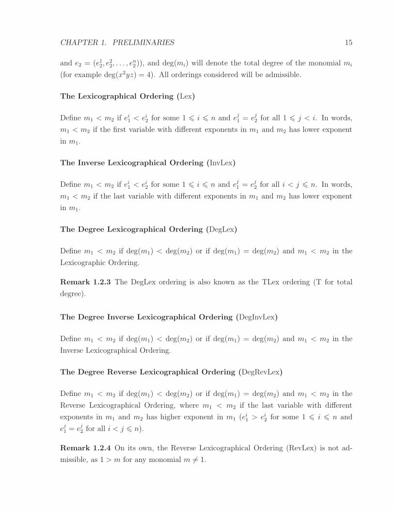
CHAPTER 1. PRELIMINARIES 15
and e2 = (e12, e22, . . . , e
n2 )), and deg(mi) will denote the total degree of the monomial mi
(for example deg(x2yz) = 4). All orderings considered will be admissible.
The Lexicographical Ordering (Lex)
Define m1 < m2 if ei1 < ei2 for some 1 6 i 6 n and ej1 = ej2 for all 1 6 j < i. In words,
m1 < m2 if the first variable with different exponents in m1 and m2 has lower exponent
in m1.
The Inverse Lexicographical Ordering (InvLex)
Define m1 < m2 if ei1 < ei2 for some 1 6 i 6 n and ej1 = ej2 for all i < j 6 n. In words,
m1 < m2 if the last variable with different exponents in m1 and m2 has lower exponent
in m1.
The Degree Lexicographical Ordering (DegLex)
Define m1 < m2 if deg(m1) < deg(m2) or if deg(m1) = deg(m2) and m1 < m2 in the
Lexicographic Ordering.
Remark 1.2.3 The DegLex ordering is also known as the TLex ordering (T for total
degree).
The Degree Inverse Lexicographical Ordering (DegInvLex)
Define m1 < m2 if deg(m1) < deg(m2) or if deg(m1) = deg(m2) and m1 < m2 in the
Inverse Lexicographical Ordering.
The Degree Reverse Lexicographical Ordering (DegRevLex)
Define m1 < m2 if deg(m1) < deg(m2) or if deg(m1) = deg(m2) and m1 < m2 in the
Reverse Lexicographical Ordering, where m1 < m2 if the last variable with different
exponents in m1 and m2 has higher exponent in m1 (ei1 > ei2 for some 1 6 i 6 n and
ej1 = ej2 for all i < j 6 n).
Remark 1.2.4 On its own, the Reverse Lexicographical Ordering (RevLex) is not ad-
missible, as 1 > m for any monomial m 6= 1.

CHAPTER 1. PRELIMINARIES 16
Example 1.2.5 With x > y > z, consider the monomials m1 := x2yz; m2 := x2 and
m3 := xyz2, with corresponding multidegrees e1 = (2, 1, 1); e2 = (2, 0, 0) and e3 = (1, 1, 2).
The following table shows the order placed on the monomials by the various monomial
orderings defined above. The final column shows the order induced on the polynomial
p := m1 +m2 +m3 by the chosen monomial ordering.
Monomial Ordering O O(m1, m2) O(m1, m3) O(m2, m3) p
Lex 0 0 0 x2yz + x2 + xyz2
InvLex 0 1 1 xyz2 + x2yz + x2
DegLex 0 0 1 x2yz + xyz2 + x2
DegInvLex 0 1 1 xyz2 + x2yz + x2
DegRevLex 0 0 1 x2yz + xyz2 + x2
1.2.2 Noncommutative Monomial Orderings
In the noncommutative case, because we use words and not multidegrees to represent
monomials, our definitions for the lexicographically based orderings will have to be adapted
slightly. All other definitions and conventions will stay the same.
The Lexicographic Ordering (Lex)
Define m1 < m2 if, working left-to-right, the first (say i-th) letter on which m1 and m2
differ is such that the i-th letter of m1 is lexicographically less than the i-th letter of m2
in the variable ordering. Note: this ordering is not admissible (counterexample: if x > y
is the variable ordering, then x < xy but x2 > xyx).
Remark 1.2.6 When comparing two monomials m1 and m2 such that m1 is a proper
prefix of m2 (for example m1 := x and m2 := xy as in the above counterexample), a
problem arises with the above definition in that we eventually run out of letters in the
shorter word to compare with (in the example, having seen that the first letter of both
monomials match, what do we compare the second letter of m2 with?). One answer is to
introduce a padding symbol $ to pad m1 on the right to make sure it is the same length
as m2, with the convention that any letter is greater than the padding symbol (so that
m1 < m2). The padding symbol will not explicitly appear anywhere in the remainder of
this thesis, but we will bear in mind that it can be introduced to deal with situations
where prefixes and suffixes of monomials are involved.

CHAPTER 1. PRELIMINARIES 17
Remark 1.2.7 The lexicographic ordering is also known as the dictionary ordering since
the words in a dictionary (such as the Oxford English Dictionary) are ordered using the
lexicographic ordering with variable (or alphabetical) ordering a < b < c < · · · . Note
however that while a dictionary orders words in increasing order, we will write polynomials
in decreasing order.
The Inverse Lexicographical Ordering (InvLex)
Define m1 < m2 if, working left-to-right, the first (say i-th) letter on which m1 and m2
differ is such that the i-th letter of m1 is lexicographically greater than the i-th letter of
m2. Note: this ordering (like Lex) is not admissible (counterexample: if x > y is the
variable ordering, then xy < x but xyx > x2).
The Degree Reverse Lexicographical Ordering (DegRevLex)
Define m1 < m2 if deg(m1) < deg(m2) or if deg(m1) = deg(m2) and m1 < m2 in the
Reverse Lexicographical Ordering, where m1 < m2 if, working in reverse, or from right-
to-left, the first (say i-th) letter on which m1 and m2 differ is such that the i-th letter of
m1 is lexicographically greater than the i-th letter of m2.
Example 1.2.8 With x > y > z, consider the noncommutative monomials m1 := zxyx;
m2 := xzx and m3 := y2zx. The following table shows the order placed on the monomials
by various noncommutative monomial orderings. As before, the final column shows the
order induced on the polynomial p := m1 +m2 +m3 by the chosen monomial ordering.
Monomial Ordering O O(m1, m2) O(m1, m3) O(m2, m3) p
Lex 1 1 0 xzx + y2zx+ zxyx
InvLex 0 0 1 zxyx+ y2zx+ xzx
DegLex 0 1 1 y2zx+ zxyx+ xzx
DegInvLex 0 0 1 zxyx+ y2zx+ xzx
DegRevLex 0 1 1 y2zx+ zxyx+ xzx
1.2.3 Polynomial Division
Definition 1.2.9 Let R be a polynomial ring, and let O be an arbitrary admissible
monomial ordering. Given two nonzero polynomials p1, p2 ∈ R, we say that p1 divides

CHAPTER 1. PRELIMINARIES 18
p2 (written p1 | p2) if the lead monomial of p1 divides some monomial m (with coefficient
c) in p2. For a commutative polynomial ring, this means that m = LM(p1)m′ for some
monomial m′; for a noncommutative polynomial ring, this means that m = mℓLM(p1)mr
for some monomials mℓ and mr (LM(p1) is a subword of m).
To perform the division, we take away an appropriate multiple of p1 from p2 in order to
cancel off LT(p1) with the term involving m in p2. In the commutative case, we do
p2 − (cLC(p1)−1)p1m
′;
in the noncommutative case, we do
p2 − (cLC(p1)−1)mℓp1mr.
It is clear that the coefficient rings of our polynomial rings have to be division rings in
order for the above expressions to be valid, and so we make the following assumption
about the polynomial rings we will encounter in the remainder of this thesis.
Remark 1.2.10 From now on, all coefficient rings of polynomial rings will be fields unless
otherwise stated.
Example 1.2.11 Let p1 := 5z2x + 2y2 + x + 4 and p2 := 3xyxz2x3 + 2x2 be two
DegLex ordered polynomials over the noncommutative polynomial ring Q〈x, y, z〉. Be-
cause LM(p2) = xyx(z2x)x2, it is clear that p1 | p2, with the quotient and the remainder
of the division being
q :=(
35
)
xyx(5z2x+ 2y2 + x+ 4)x2
and
r := 3xyxz2x3 + 2x2 −(
35
)
xyx(5z2x+ 2y2 + x+ 4)x2
= 3xyxz2x3 + 2x2 − 3xyxz2x3 −(
65
)
xyxy2x2 −(
35
)
xyx4 −(
125
)
xyx3
= −(
65
)
xyxy2x2 −(
35
)
xyx4 −(
125
)
xyx3 + 2x2
respectively.
Now that we know how to divide one polynomial by another, what does it mean for a
polynomial to be divided by a set of polynomials?
Definition 1.2.12 Let R be a polynomial ring, and let O be an arbitrary admissible

CHAPTER 1. PRELIMINARIES 19
monomial ordering. Given a nonzero polynomial p ∈ R and a set of nonzero polynomials
P = p1, p2, . . . , pm, with pi ∈ R for all 1 6 i 6 m, we divide p by P by working through
p term by term, testing to see if each term is divisible by any of the pi in turn. We
recursively divide the remainder of each division using the same method until no more
divisions are possible, in which case the remainder is either 0 or is irreducible.
Algorithms to divide a polynomial p by a set of polynomials P in the commutative and
noncommutative cases are given below as Algorithms 1 and 2 respectively. Note that they
take advantage of the fact that if the first N terms of a polynomial q are irreducible with
respect to P , then the first N terms of any reduction of q will also be irreducible with
respect to P .
Algorithm 1 The Commutative Division Algorithm
Input: A nonzero polynomial p and a set of nonzero polynomials P = p1, . . . , pm over
a polynomial ring R[x1, . . . xn]; an admissible monomial ordering O.
Output: Rem(p, P ) := r, the remainder of p with respect to P .
r = 0;
while (p 6= 0) do
u = LM(p); c = LC(p); j = 1; found = false;
while (j 6 m) and (found == false) do
if (LM(pj) | u) then
found = true; u′ = u/LM(pj); p = p− (cLC(pj)−1)pju
′;
else
j = j + 1;
end if
end while
if (found == false) then
r = r + LT(p); p = p− LT(p);
end if
end while
return r;
Remark 1.2.13 All algorithms in this thesis use the conventions that ‘=’ denotes an
assignment and ‘==’ denotes a test.

CHAPTER 1. PRELIMINARIES 20
Algorithm 2 The Noncommutative Division Algorithm
To divide a nonzero polynomial p with respect to a set of nonzero polynomials P =
p1, . . . , pm, where p and the pi are elements of a noncommutative polynomial ring
R〈x1, . . . , xn〉, we apply Algorithm 1 with the following changes.
(a) In the inputs, replace the commutative polynomial ring R[x1, . . . xn] by the noncom-
mutative polynomial ring R〈x1, . . . , xn〉.
(b) Change the first if condition to read
if (LM(pj) | u) then
found = true;
choose uℓ and ur such that u = uℓLM(pj)ur;
p = p− (cLC(pj)−1)uℓpjur;
else
j = j + 1;
end if
Remark 1.2.14 In Algorithm 2, if there are several candidates for uℓ (and therefore for
ur) in the line ‘choose uℓ and ur such that u = uℓLM(pj)ur’, the convention in this thesis
will be to choose the uℓ with the smallest degree.
Example 1.2.15 To demonstrate that the process of dividing a polynomial by a set of
polynomials does not necessarily give a unique result, consider the polynomial p := xyz+x
and the set of polynomials P := p1, p2 = xy − z, yz + 2x+ z, all polynomials being
ordered by DegLex and originating from the polynomial ring Q[x, y, z]. If we choose to
divide p by p1 to begin with, we see that p reduces to xyz+x− (xy− z)z = z2+x, which
is irreducible. But if we choose to divide p by p2 to begin with, we see that p reduces to
xyz + x − (yz + 2x + z)x = −2x2 − xz + x, which is again irreducible. This gives rise
to the question of which answer (if any!) is the correct one here? In Chapter 2, we will
discover that one way of obtaining a unique answer to this question will be to calculate a
Grobner Basis for the dividing set P .
Definition 1.2.16 In order to describe how one polynomial is obtained from another
through the process of division, we introduce the following notation.
(a) If the polynomial r is obtained by dividing a polynomial p by a polynomial q, then
we will use the notation p → r or p →q r (with the latter notation used if we wish to

CHAPTER 1. PRELIMINARIES 21
show how r is obtained from p).
(b) If the polynomial r is obtained by dividing a polynomial p by a sequence of polyno-
mials q1, q2, . . . , qα, then we will use the notation p∗
−→ r.
(c) If the polynomial r is obtained by dividing a polynomial p by a set of polynomials Q,
then we will use the notation p →Q r.
Chapter 2
Commutative Grobner Bases
Given a basis F generating an ideal J , the central idea in Grobner Basis theory is to use
F to find a basis G for J with the property that the remainder of the division of any
polynomial by G is unique. Such a basis is known as a Grobner Basis.
In particular, if a polynomial p is a member of the ideal J , then the remainder of the
division of p by a Grobner Basis G for J is always zero. This gives us a way to solve the
Ideal Membership Problem for J – if the remainder of the division of a polynomial p by
G is zero, then p ∈ J (otherwise p /∈ J).
2.1 S-polynomials
How do we determine whether or not an arbitrary basis F generating an ideal J is a
Grobner Basis? Using the informal definition shown above, in order to show that a basis
is not a Grobner Basis, it is sufficient to find a polynomial p whose remainder on division
by F is non-unique. Let us now construct an example in which this is the case, and let
us analyse what can to be done to eliminate the non-uniqueness of the remainder.
Let p1 = a1 + a2 + · · ·+ aα; p2 = b1 + b2 + · · ·+ bβ and p3 = c1 + c2 + · · ·+ cγ be three
polynomials ordered with respect to some fixed admissible monomial ordering O (the ai,
bj and ck are all nontrivial terms). Assume that p1 | p3 and p2 | p3, so that we are able
to take away from p3 multiples s and t of p1 and p2 respectively to obtain remainders r1
22

CHAPTER 2. COMMUTATIVE GROBNER BASES 23
and r2.
r1 = p3 − sp1
= c1 + c2 + · · ·+ cγ − s(a1 + a2 + · · ·+ aα)
= c2 + · · ·+ cγ − sa2 − · · · − saα;
r2 = p3 − tp2
= c2 + · · ·+ cγ − tb2 − · · · − tbβ.
If we assume that r1 and r2 are irreducible and that r1 6= r2, it is clear that the remainder
of the division of the polynomial p3 by the set of polynomials P = p1, p2 is non-unique,
from which we deduce that P is not a Grobner Basis for the ideal that it generates. We
must therefore change P in some way in order for it to become a Grobner Basis, but what
changes are required and indeed allowed?
Consider that we want to add a polynomial to P . To avoid changing the ideal that is being
generated by P , any polynomial added to P must be a member of the ideal. It is clear
that r1 and r2 are members of the ideal, as is the polynomial p4 = r2 − r1 = −tp2 + sp1.
Consider that we add p4 to P , so that P becomes the set
a1 + a2 + · · ·+ aα, b1 + b2 + · · ·+ bβ, −tb2 − tb3 − · · · − tbβ + sa2 + sa3 + · · ·+ saα.
If we now divide the polynomial p3 by the enlarged set P , to begin with (as before) we
can either divide p3 by p1 or p2 to obtain remainders r1 or r2. Here however, if we assume
(without loss of generality1) that LT(p4) = −tb2, we can now divide r2 by p4 to obtain a
new remainder
r3 = r2 − p4
= c2 + · · ·+ cγ − tb2 − · · · − tbβ − (−tb2 − tb3 − · · · − tbβ + sa2 + sa3 + · · ·+ saα)
= c2 + · · ·+ cγ − sa2 − · · · − saα
= r1.
It follows that by adding p4 to P , we have ensured that the remainder of the division
of p3 by P is unique2 no matter which of the polynomials p1 and p2 we choose to divide
1The other possible case is LT(p4) = sa2, in which case it is r1 that reduces to r2 and not r2 to r1.2This may not strictly be true if p3 is divisible by p4; for the time being we shall assume that this is
not the case, noting that the important concept here is of eliminating the non-uniqueness given by the

CHAPTER 2. COMMUTATIVE GROBNER BASES 24
p3 by first. This solves our original problem of non-unique remainders in this restricted
situation.
At first glance, the polynomial added to P to solve this problem is dependent upon the
polynomial p3. The reason for saying this is that the polynomial added to P has the form
p4 = sp1 − tp2, where s and t are terms chosen to multiply the polynomials p1 and p2 so
that the lead terms of sp1 and tp2 equal LT(p3) (in fact s = LT(p3)LT(p1)
and t = LT(p3)LT(p2)
).
However, by definition, LM(p3) is a common multiple of LM(p1) and LM(p2). Because all
such common multiples are multiples of the least common multiple of LM(p1) and LM(p2)
(so that LM(p3) = µ(lcm(LM(p1),LM(p2))) for some monomial µ), it follows that we can
rewrite p4 as
p4 = LC(p3)µ
(
lcm(LM(p1),LM(p2))
LT(p1)p1 −
lcm(LM(p1),LM(p2))
LT(p2)p2
)
.
Consider now that we add the polynomial p5 = p4LC(p3)µ
to P instead of adding p4 to P .
It follows that even though this polynomial does not depend on the polynomial p3, we
can still obtain a unique remainder when dividing p3 by p1 and p2, because we can do
r3 = r2 − LC(p3)µp5. Moreover, the polynomial p5 solves the problem of non-unique
remainders for any polynomial p3 that is divisible by both p1 and p2 (all that changes is
the multiple of p5 used in the reduction of r2); we call such a polynomial an S-polynomial3
for p1 and p2.
Definition 2.1.1 The S-polynomial of two distinct polynomials p1 and p2 is given by the
expression
S-pol(p1, p2) =lcm(LM(p1),LM(p2))
LT(p1)p1 −
lcm(LM(p1),LM(p2))
LT(p2)p2.
Remark 2.1.2 The terms lcm(LM(p1),LM(p2))LT(p1)
and lcm(LM(p1),LM(p2))LT(p2)
can be thought of as the
terms used to multiply the polynomials p1 and p2 so that the lead monomials of the
multiples are equal to the monomial lcm(LM(p1),LM(p2)).
Let us now illustrate how adding an S-polynomial to a basis solves the problem of non-
unique remainders in a particular example.
choice of dividing p3 by p1 or p2 first.3The S stands for Syzygy, as in a pair of connected objects.

CHAPTER 2. COMMUTATIVE GROBNER BASES 25
Example 2.1.3 Recall that in Example 1.2.15 we showed how dividing the polynomial
p := xyz+x by the two polynomials in the set P := p1, p2 = xy− z, yz+2x+ z gave
two different remainders, r1 := z2 + x and r2 := −2x2 − xz + x respectively. Consider
now that we add S-pol(p1, p2) to P , where
S-pol(p1, p2) =xyz
xy(xy − z)−
xyz
yz(yz + 2x+ z)
= (xyz − z2)− (xyz + 2x2 + xz)
= −2x2 − xz − z2.
Dividing p by the enlarged set, if we choose to divide p by p1 to begin with, we see that p
reduces (as before) to give xyz + x− (xy − z)z = z2 + x, which is irreducible. Similarly,
dividing p by p2 to begin with, we obtain the remainder xyz + x − (yz + 2x + z)x =
−2x2 − xz + x. However, whereas before this remainder was irreducible, now we can
reduce it by the S-polynomial to give −2x2 − xz + x− (−2x2 − xz − z2) = z2 + x, which
is equal to the first remainder.
Let us now formally define a Grobner Basis in terms of S-polynomials, noting that there
are many other equivalent definitions (see for example [7], page 206).
Definition 2.1.4 Let G = g1, . . . , gm be a basis for an ideal J over a commutative
polynomial ring R = R[x1, . . . , xn]. If all the S-polynomials involving members of G
reduce to zero using G (S-pol(gi, gj) →G 0 for all i 6= j), then G is a Grobner Basis for J .
Theorem 2.1.5 Given any polynomial p over a polynomial ring R = R[x1, . . . , xn], the
remainder of the division of p by a basis G for an ideal J in R is unique if and only if G
is a Grobner Basis.
Proof: (⇒) By Newman’s Lemma (cf. [7], page 176), showing that the remainder
of the division of p by G is unique is equivalent to showing that the division process is
locally confluent, that is if there are polynomials f , f1, f2 ∈ R with f1 = f − t1g1 and
f2 = f − t2g2 for terms t1, t2 and g1, g2 ∈ G, then there exists a polynomial f3 ∈ R such
that both f1 and f2 reduce to f3. By the Translation Lemma (cf. [7], page 200), this in
turn is equivalent to showing that the polynomial f2 − f1 = t1g1 − t2g2 reduces to zero,
which is what we shall now do.
CHAPTER 2. COMMUTATIVE GROBNER BASES 26
There are two cases to deal with, LT(t1g1) 6= LT(t2g2) and LT(t1g1) = LT(t2g2). In the
first case, notice that the remainders f1 and f2 are obtained by cancelling off different
terms of the original f (the reductions of f are disjoint), so it is possible, assuming
(without loss of generality) that LT(t1g1) > LT(t2g2), to directly reduce the polynomial
f2 − f1 = t1g1 − t2g2 in the following manner: t1g1 − t2g2 →g1 −t2g2 →g2 0. In the
second case, the reductions of f are not disjoint (as the same term t from f is cancelled
off during both reductions), so that the term t does not appear in the polynomial t1g1 −
t2g2. However, the term t is a common multiple of LT(t1g1) and LT(t2g2), and thus the
polynomial t1g1 − t2g2 is a multiple of the S-polynomial S-pol(g1, g2), say
t1g1 − t2g2 = µ(S-pol(g1, g2))
for some term µ. Because G is a Grobner Basis, the S-polynomial S-pol(g1, g2) reduces to
zero, and hence by extension the polynomial t1g1 − t2g2 also reduces to zero.
(⇐) As all S-polynomials are members of the ideal J , to complete the proof it is sufficient
to show that there is always a reduction path of an arbitrary member of the ideal that
leads to a zero remainder (the uniqueness of remainders will then imply that members of
the ideal will always reduce to zero). Let f ∈ J = 〈G〉. Then, by definition, there exist
gi ∈ G and fi ∈ R (where 1 6 i 6 j) such that
f =
j∑
i=1
figi.
We proceed by induction on j. If j = 1, then f = f1g1, and it is clear that we can use g1
to reduce f to give a zero remainder (f → f − f1g1 = 0). Assume that the result is true
for j = k, and let us look at the case j = k + 1, so that
f =
(
k∑
i=1
figi
)
+ fk+1gk+1.
By the inductive hypothesis,∑k
i=1 figi is a member of the ideal that reduces to zero. The
polynomial f therefore reduces to the polynomial f ′ := fk+1gk+1, and we can now use
gk+1 to reduce f ′ to give a zero remainder (f ′ → f ′ − fk+1gk+1 = 0).
We are now in a position to be able to define an algorithm to compute a Grobner Basis.
However, to be able to prove that this algorithm always terminates, we must first prove

CHAPTER 2. COMMUTATIVE GROBNER BASES 27
a result stating that all ideals over commutative polynomial rings are finitely generated.
This proof takes place in two stages – first for monomial ideals (Dickson’s Lemma) and
then for polynomial ideals (Hilbert’s Basis Theorem).
2.2 Dickson’s Lemma and Hilbert’s Basis Theorem
Definition 2.2.1 A monomial ideal is an ideal generated by a set of monomials.
Remark 2.2.2 Any polynomial p that is a member of a monomial ideal is a sum of terms
p =∑
i ti, where each ti is a member of the monomial ideal.
Lemma 2.2.3 (Dickson’s Lemma) Every monomial ideal over the polynomial ringR =
R[x1, . . . , xn] is finitely generated.
Proof (cf. [22], page 47): Let J be a monomial ideal over R generated by a set of
monomials S. We proceed by induction on n, our goal being to show that S always has
a finite subset T generating J . For n = 1, notice that all elements of S will be of the
form xj1 for some j > 0. Let T be the singleton set containing the member of S with the
lowest degree (that is the xj1 with the lowest value of j). Clearly T is finite, and because
any element of S is a multiple of the chosen xj1, it is also clear that T generates the same
ideal as S.
For the inductive step, assume that all monomial ideals over the polynomial ring R′ =
R[x1, . . . , xn−1] are finitely generated. Let C0 ⊆ C1 ⊆ C2 ⊆ · · · be an ascending chain of
monomial ideals over R′, where4
Cj = 〈Sj〉 ∩ R′, Sj =
s
gcd(s, xjn)
| s ∈ S
.
Let the monomial m be an arbitrary member of the ideal J , expressed as m = m′xkn,
where m′ ∈ R′ and k > 0. By definition, m′ ∈ Ck, and so m ∈ xknCk. By the inductive
hypothesis, each Ck is finitely generated by a set Tk, and so m ∈ xkn〈Tk〉. From this we
can deduce that
T = T0 ∪ xnT1 ∪ x2nT2 ∪ · · ·
is a generating set for J .
4Think of C0 as the set of monomials m ∈ J which are also members of R′; think of Cj (for j > 1) ascontaining all the elements of Cj−1 plus the monomials m ∈ J of the form m = m′xj
n, m′ ∈ R′.

CHAPTER 2. COMMUTATIVE GROBNER BASES 28
Consider the ideal C = ∪Cj for j > 0. This is another monomial ideal over R′, and so by
the inductive hypothesis is finitely generated. It follows that the chain must stop as soon
as the generators of C are contained in some Cr, so that Cr = Cr+1 = · · · (and hence
Tr = Tr+1 = · · · ). It follows that T0 ∪ xnT1 ∪ x2nT2 ∪ · · · ∪ xr
nTr is a finite subset of S
generating J .
Example 2.2.4 Let S = y4, xy4, x2y3, x3y3, x4y, xk be an infinite set of monomials
generating an ideal J over the polynomial ring Q[x, y], where k is an integer such that
k > 5. We can visualise J by using the following monomial lattice, where a point (a, b)
in the lattice (for non-negative integers a, b) corresponds to the monomial xayb, and the
shaded region contains all monomials which are reducible by some member of S (and
hence belong to J).
b
a
To show that J can be finitely generated, we need to construct the set T as described in
the proof of Dickson’s Lemma. The first step in doing this is to construct the sequence
of sets Sj =
sgcd(s, yj)
| s ∈ S
for all j > 0.
S0 = y4, xy4, x2y3, x3y3, x4y, xk = S
S1 = y3, xy3, x2y2, x3y2, x4, xk
S2 = y2, xy2, x2y, x3y, x4, xk
S3 = y, xy, x2, x3, x4, xk
S4 = y0 = 1, x, x2, x3, x4, xk
Sj+1 = Sj for all j + 1 > 5.
Each set Sj gives rise to an ideal Cj consisting of all monomials m ∈ 〈Sj〉 of the form
m = xi for some i > 0. Because each of these ideals is an ideal over the polynomial ring
Q[x], we can use an inductive hypothesis to give us a finite generating set Tj for each Cj .

CHAPTER 2. COMMUTATIVE GROBNER BASES 29
In this case, the first paragraph of the proof of Dickson’s Lemma tells us how to apply
the inductive hypothesis — each set Tj is formed by choosing the monomial m ∈ Sj of
lowest degree such that m = xi for some i > 0.
T0 = x5
T1 = x4
T2 = x4
T3 = x2
T4 = x0 = 1
Tj+1 = Tj for all k + 1 > 5.
We can now deduce that
T = x5 ∪ x4y ∪ x4y2 ∪ x2y3 ∪ y4 ∪ y5 ∪ · · ·
is a generating set for J . Further, because Tj+1 = Tj for all k+1 > 5, we can also deduce
that the set
T ′ = x5, x4y, x4y2, x2y3, y4
is a finite generating set for J (a fact that can be verified by drawing a monomial lattice
for T ′ and comparing it with the above monomial lattice for the set S).
Theorem 2.2.5 (Hilbert’s Basis Theorem) Every ideal J over a polynomial ring R =
R[x1, . . . , xn] is finitely generated.
Proof: Let O be a fixed arbitrary admissible monomial ordering, and define LM(J) =
〈LM(p) | p ∈ J〉. Because LM(J) is a monomial ideal, by Dickson’s Lemma it is finitely
generated, say by the set of monomials M = m1, . . . , mr. By definition, each mi ∈ M
(for 1 6 i 6 r) has a corresponding pi ∈ J such that LM(pi) = mi. We claim that
P = p1, . . . , pr is a generating set for J . To prove the claim, notice that 〈P 〉 ⊆ J so
that f ∈ 〈P 〉 ⇒ f ∈ J . Conversely, given a polynomial f ∈ J , we know that LM(f) ∈ 〈M〉
so that LM(f) = αmj for some monomial α and some 1 6 j 6 r. From this, if we define
α′ = LC(f)LC(pj)
α, we can deduce that LM(f−α′pj) < LM(f). Since f−α′pj ∈ J , and because
of the admissibility of O, by recursion on f − α′pj (define fk+1 = fk − α′kpjk for k > 1,
where f1 − α′1pj1 := f − α′pj), we can deduce that f ∈ 〈P 〉 (in fact f =
∑Kk=1 α
′kpjk for
some finite K).
CHAPTER 2. COMMUTATIVE GROBNER BASES 30
Corollary 2.2.6 (The Ascending Chain Condition) Every ascending sequence of ide-
als J1 ⊆ J2 ⊆ · · · over a polynomial ring R = R[x1, . . . , xn] is eventually constant, so
that there is an i such that Ji = Ji+1 = · · · .
Proof: By Hilbert’s Basis Theorem, each ideal Jk (for k > 1) is finitely generated.
Consider the ideal J = ∪Jk. This is another ideal over R, and so by Hilbert’s Basis
Theorem is also finitely generated. From this we deduce that the chain must stop as soon
as the generators of J are contained in some Ji, so that Ji = Ji+1 = · · · .
2.3 Buchberger’s Algorithm
The algorithm used to compute a Grobner Basis is known as Buchberger’s Algorithm.
Bruno Buchberger was a student of Wolfgang Grobner at the University of Innsbruck,
Austria, and the publication of his PhD thesis in 1965 [11] marked the start of Grobner
Basis theory.
In Buchberger’s algorithm, S-polynomials for pairs of elements from the current basis are
computed and reduced using the current basis. If the S-polynomial does not reduce to
zero, it is added to the current basis, and this process continues until all S-polynomials
reduce to zero. The algorithm works on the principle that if an S-polynomial S-pol(gi, gj)
does not reduce to zero using a set of polynomials G, then it will certainly reduce to zero
using the set of polynomials G ∪ S-pol(gi, gj).
Theorem 2.3.1 Algorithm 3 always terminates with a Grobner Basis for the ideal J .
Proof (cf. [7], page 213): Correctness. If the algorithm terminates, it does so with
a set of polynomials G with the property that all S-polynomials involving members of
G reduce to zero using G (S-pol(gi, gj) →G 0 for all i 6= j). G is therefore a Grobner
Basis by Definition 2.1.4. Termination. If the algorithm does not terminate, then an
endless sequence of polynomials must be added to the set G so that the set A never
becomes empty. Let G0 ⊂ G1 ⊂ G2 ⊂ · · · be the successive values of G. If we consider
the corresponding sequence LM(G0) ⊂ LM(G1) ⊂ LM(G2) ⊂ · · · of lead monomials, we
note that these sets generate an ascending chain of ideals J0 ⊂ J1 ⊂ J2 ⊂ · · · because
each time we add a monomial to a particular set LM(Gk) to form the set LM(Gk+1), the
monomial we choose is irreducible with respect to LM(Gk), and hence does not belong to
the ideal Jk. However the Ascending Chain Condition tells us that such a chain of ideals

CHAPTER 2. COMMUTATIVE GROBNER BASES 31
Algorithm 3 A Basic Commutative Grobner Basis Algorithm
Input: A Basis F = f1, f2, . . . , fm for an ideal J over a commutative polynomial ring
R[x1, . . . xn]; an admissible monomial ordering O.
Output: A Grobner Basis G = g1, g2, . . . , gp for J .
Let G = F and let A = ∅;
For each pair of polynomials (gi, gj) in G (i < j),
add the S-polynomial S-pol(gi, gj) to A;
while (A is not empty) do
Remove the first entry s1 from A;
s′1 = Rem(s1, G);
if (s′1 6= 0) then
Add s′1 to G and add all the S-polynomials S-pol(gi, s′1) to A (gi ∈ G, gi 6= s′1);
end if
end while
return G;
must eventually become constant, so there must be some i > 0 such that Ji = Ji+1 = · · · .
It follows that the algorithm will terminate once the set Gi has been constructed, as all
of the S-polynomials left in A will now reduce to zero (if not, some S-polynomial left in A
will reduce to a non-zero polynomial s′1 whose lead monomial is irreducible with respect to
LM(Gi), allowing us to construct an ideal Ji+1 = 〈LM(Gi)∪LM(s′1)〉 ⊃ 〈LM(Gi)〉 = Ji,
contradicting the fact that Ji+1 = Ji.)
Example 2.3.2 Let F := f1, f2 = x2 − 2xy + 3, 2xy + y2 + 5 generate an ideal
over the commutative polynomial ring Q[x, y], and let the monomial ordering be DegLex.
Running Algorithm 3 on F , there is only one S-polynomial to consider initially, namely
S-pol(f1, f2) = y(f1)−12x(f2) = −5
2xy2 − 5
2x+ 3y. This polynomial reduces (using f2) to
give the irreducible polynomial 54y3 − 5
2x+ 37
4y =: f3, which we add to our current basis.
This produces two more S-polynomials to look at, S-pol(f1, f3) = y3(f1) −45x2(f3) =
−2xy4+2x3− 375x2y+3y3 and S-pol(f2, f3) =
12y2(f2)−
45x(f3) =
12y4+2x2− 37
5xy+ 5
2y2,
both of which reduce to zero. The algorithm therefore terminates with the set x2−2xy+
3, 2xy + y2 + 5, 54y3 − 5
2x+ 37
4y as the output Grobner Basis.
Here is a dry run for Algorithm 3 in this instance.

CHAPTER 2. COMMUTATIVE GROBNER BASES 32
G i j A s1 s′1
f1, f2 1 2 ∅
S-pol(f1, f2)
f1, f2, f3 1 ∅ −52xy
2 − 52x+ 3y f3
2 S-pol(f1, f3)
S-pol(f2, f3), S-pol(f1, f3)
S-pol(f1, f3)12y
4 + 2x2 − 375 xy +
52y
2 0
∅ −2xy4 + 2x3 − 375 x
2y + 3y3 0
2.4 Reduced Grobner Bases
Definition 2.4.1 Let G = g1, . . . , gp be a Grobner Basis for an ideal over the poly-
nomial ring R[x1, . . . , xn]. G is a reduced Grobner Basis if the following conditions are
satisfied.
(a) LC(gi) = 1R for all gi ∈ G.
(b) No term in any polynomial gi ∈ G is divisible by any LT(gj), j 6= i.
Theorem 2.4.2 Every ideal over a commutative polynomial ring has a unique reduced
Grobner Basis.
Proof: Existence. By Theorem 2.3.1, there exists a Grobner Basis G for every ideal
over a commutative polynomial ring. We claim that the following procedure transforms
G into a reduced Grobner Basis G′.
(i) Multiply each gi ∈ G by LC(gi)−1.
(ii) Reduce each gi ∈ G by G \ gi, removing from G all polynomials that reduce to
zero.
It is clear that G′ satisfies the conditions of Definition 2.4.1, so it remains to show that
G′ is a Grobner Basis, which we shall do by showing that the application of each step of
instruction (ii) above produces a basis which is still a Grobner Basis.
Let G = g1, . . . , gp be a Grobner Basis, and let g′i be the reduction of an arbitrary

CHAPTER 2. COMMUTATIVE GROBNER BASES 33
gi ∈ G with respect to G \ gi, carried out as follows (the tk are terms).
g′i = gi −κ∑
k=1
tkgjk . (2.1)
Set H = (G\gi)∪g′i if g′i 6= 0, and set H = G\gi if g′i = 0. As G is a Grobner Basis,
all S-polynomials involving elements of G reduce to zero using G, so there are expressions
taga − tbgb −
µ∑
u=1
tugcu = 0 (2.2)
for every S-polynomial S-pol(ga, gb) = taga − tbgb, where ga, gb, gcu ∈ G. To show that H
is a Grobner Basis, we must show that all S-polynomials involving elements of H reduce
to zero using H . For distinct polynomials ga, gb ∈ H not equal to g′i, we can reduce the
S-polynomial S-pol(ga, gb) using the reduction shown in Equation (2.2), substituting for
gi from Equation (2.1) if any of the gcu in Equation (2.2) are equal to gi. This gives a
reduction to zero of S-pol(ga, gb) in terms of elements of H .
If g′i = 0, our proof is complete. Otherwise consider the S-polynomial S-pol(g′i, ga). We
claim that S-pol(gi, ga) = t1gi−t2ga ⇒ S-pol(g′i, ga) = t1g′i−t2ga. To prove this claim, it is
sufficient to show that LT(gi) = LT(g′i). Assume for a contradiction that LT(gi) 6= LT(g′i).
It follows that during the reduction of gi we were able to reduce its lead term, so that
LT(gi) = tLT(gj) for some term t and some gj ∈ G. By the admissibility of the chosen
monomial ordering, the polynomial gi − tgj reduces to zero without using gi, leading to
the conclusion that g′i = 0, a contradiction.
It remains to show that S-pol(g′i, ga) →H 0. We know that S-pol(gi, ga) = t1gi−t2ga →G 0,
and Equation (2.2) tells us that t1gi − t2ga −∑µ
u=1 tugcu = 0. Substituting for gi from
Equation (2.1), we obtain5
t1
(
g′i +
κ∑
k=1
tkgjk
)
− t2ga −
µ∑
u=1
tugcu = 0
or
t1g′i − t2ga −
(
µ∑
u=1
tugcu −κ∑
k=1
t1tkgjk
)
= 0,
5Substitutions for gi may also occur in the summation∑µ
u=1 tugcu ; these substitutions have not beenconsidered in the displayed formulae.

CHAPTER 2. COMMUTATIVE GROBNER BASES 34
which implies that S-pol(g′i, ga) →H 0.
Uniqueness. Assume for a contradiction that G = g1, . . . , gp and H = h1, . . . , hq are
two reduced Grobner Bases for an ideal J , with G 6= H . Let gi be an arbitrary element
from G (where 1 6 i 6 p). Because gi is a member of the ideal, then gi must reduce
to zero using H (H is a Grobner Basis). This means that there must exist a polynomial
hj ∈ H such that LT(hj) | LT(gi). If LT(hj) 6= LT(gi), then LT(hj)×m = LT(gi) for some
nontrivial monomial m. But hj is also a member of the ideal, so it must reduce to zero
using G. Therefore there exists a polynomial gk ∈ G such that LT(gk) | LT(hj), which
implies that LT(gk) | LT(gi), with k 6= i. This contradicts condition (b) of Definition
2.4.1, so that G cannot be a reduced Grobner Basis for J if LT(hj) 6= LT(gi). From this
we deduce that each gi ∈ G has a corresponding hj ∈ H such that LT(gi) = LT(hj).
Further, because G and H are assumed to be reduced Grobner Bases, this is a one-to-one
correspondence.
It remains to show that if LT(gi) = LT(hj), then gi = hj. Assume for a contradiction
that gi 6= hj, and consider the polynomial gi − hj . Without loss of generality, assume
that LM(gi − hj) appears in gi. Because gi − hj is a member of the ideal, then there is a
polynomial gk ∈ G such that LT(gk) | LT(gi − hj). But this again contradicts condition
(b) of Definition 2.4.1, as we have shown that there is a term in gi that is divisible by
LT(gk) for some k 6= i. It follows that G cannot be a reduced Grobner Basis if gi 6= hj ,
which means that G = H and therefore reduced Grobner Bases are unique.
Given a Grobner Basis G, we saw in the proof of Theorem 2.4.2 that if the lead term of
any polynomial gi ∈ G is reducible by some polynomial gj ∈ G (where gj 6= gi), then gi
reduces to zero. We can use this information to refine the procedure for finding a unique
reduced Grobner Basis (as given in the aforementioned proof) by allowing the removal of
any polynomial gi ∈ G whose lead monomial is a multiple of some other lead monomial
LM(gj). This process, which if often referred to as minimising a Grobner Basis (as in
finding a Grobner Basis with the minimal number of elements), is incorporated into our
refined procedure, which we state as Algorithm 4.
2.5 Improvements to Buchberger’s Algorithm
Nowadays, most general purpose symbolic computation systems possess an implemen-
tation of Buchberger’s algorithm. These implementations often take advantage of the

CHAPTER 2. COMMUTATIVE GROBNER BASES 35
Algorithm 4 The Commutative Unique Reduced Grobner Basis Algorithm
Input: A Grobner Basis G = g1, g2, . . . , gm for an ideal J over a commutative polyno-
mial ring R[x1, . . . xn]; an admissible monomial ordering O.
Output: The unique reduced Grobner Basis G′ = g′1, g′2, . . . , g
′p for J .
G′ = ∅;
for each gi ∈ G do
Multiply gi by LC(gi)−1;
if (LM(gi) = uLM(gj) for some monomial u and some gj ∈ G (gj 6= gi)) then
G = G \ gi;
end if
end for
for each gi ∈ G do
g′i = Rem(gi, (G \ gi) ∪G′);
G = G \ gi; G′ = G′ ∪ g′i;
end for
return G′;
numerous improvements made to Buchberger’s algorithm over the years, some of which
we shall now describe.
2.5.1 Buchberger’s Criteria
In 1979, Buchberger published a paper [10] which gave criteria that enable the a priori
detection of S-polynomials that reduce to zero. This speeds up Algorithm 3 by drastically
reducing the number of S-polynomials that must be reduced with respect to the current
basis.
Proposition 2.5.1 (Buchberger’s First Criterion) Let f and g be two polynomials
over a commutative polynomial ring ordered with respect to some fixed admissible mono-
mial ordering O. If the lead terms of f and g are disjoint (so that lcm(LM(f),LM(g)) =
LM(f)LM(g)), then S-pol(f, g) reduces to zero using the set f, g.

CHAPTER 2. COMMUTATIVE GROBNER BASES 36
Proof (Adapted from [7], Lemma 5.66): Assume that f =∑α
i=1 si and g =∑β
j=1 tj ,
where the si and the tj are terms. Because s1 and t1 are disjoint, it follows that
S-pol(f, g) ≡ t1f − s1g
= t1(s2 + · · ·+ sα)− s1(t2 + · · ·+ tβ). (2.3)
We claim that no two terms in Equation (2.3) are the same. Assume to the contrary
that t1si = s1tj for some 2 6 i 6 α and 2 6 j 6 β. Then t1si is a multiple of both t1
and s1, which means that t1si is a multiple of lcm(t1, s1) = t1s1. But then we must have
t1si > t1s1, which gives a contradiction (by definition s1 > si).
As every term in t1(s2+ · · ·+ sα) is a multiple of t1, we can use g to eliminate each of the
terms t1sα, t1sα−1, . . ., t1s2 in Equation (2.3) in turn:
t1(s2 + · · ·+ sα)− s1(t2 + · · ·+ tβ)
→ t1(s2 + · · ·+ sα)− s1(t2 + · · ·+ tβ)− sαg
= t1(s2 + · · ·+ sα−1)− s1(t2 + · · ·+ tβ)− sα(t2 + · · ·+ tβ)
→ t1(s2 + · · ·+ sα−2)− (s1 + sα−1 + sα)(t2 + · · ·+ tβ)
...
→ −(s1 + s2 + · · ·+ sα)(t2 + · · ·+ tβ)
= −s1(t2 + · · ·+ tβ)− · · · − sα(t2 + · · ·+ tβ). (2.4)
We do this in reverse order because, having eliminated a term t1sγ (where 3 6 γ 6 α), to
continue the term t1sγ−1 must appear in the reduced polynomial (which it does because
t1sγ−1 > sδtη for all γ 6 δ 6 α and 2 6 η 6 β).
CHAPTER 2. COMMUTATIVE GROBNER BASES 37
We now use the same argument on −s1(t2 + · · · + tβ), using f to eliminate each of its
terms in turn, giving the following reduction sequence.
−s1(t2 + · · ·+ tβ)− · · · − sα(t2 + · · ·+ tβ)
→ −s1(t2 + · · ·+ tβ)− · · · − sα(t2 + · · ·+ tβ) + t2f
= −s1(t2 + · · ·+ tβ)− · · · − sα(t2 + · · ·+ tβ) + t2(s1 + · · ·+ sα)
= −s1(t3 + · · ·+ tβ)− · · · − sα(t3 + · · ·+ tβ)
→ −s1(t4 + · · ·+ tβ)− · · · − sα(t4 + · · ·+ tβ)
...
→ 0.
Technical point: If some term sitj (for i, j > 2) cancels the term s1tk (for k > 3) in
Equation (2.4), then as we must have j < k in order to have sitj = s1tk, the term s1tk will
reappear as sitj when the term s1tj is eliminated, allowing us to continue the reduction
as shown. This argument can be extended to the case where a combination of terms of
the form sitj cancel the term s1tk, as the term s1tk will reappear after all the terms s1tκ
(for 2 6 κ < k) have been eliminated.
Proposition 2.5.2 (Buchberger’s Second Criterion) Let f , g and h be three mem-
bers of a finite set of polynomials P over a commutative polynomial ring satisfying the
following conditions.
(a) LM(h) | lcm(LM(f),LM(g)).
(b) S-pol(f, h) →P 0 and S-pol(g, h) →P 0.
Then S-pol(f, g) →P 0.
Proof: If LM(h) | lcm(LM(f),LM(g)), then mhLM(h) = lcm(LM(f),LM(g)) for some
monomial mh. Assume that lcm(LM(f),LM(g)) = mfLM(f) = mgLM(g) for some mono-
mials mf and mg. Then it is clear that mfLM(f) = mhLM(h) is a common multiple of
LM(f) and LM(h), and mgLM(g) = mhLM(h) is a common multiple of LM(g) and
LM(h). It follows that lcm(LM(f),LM(g)) is a multiple of both lcm(LM(f),LM(h)) and
lcm(LM(g),LM(h)), so that
lcm(LM(f),LM(g)) = mfhlcm(LM(f),LM(h)) = mghlcm(LM(g),LM(h)) (2.5)

CHAPTER 2. COMMUTATIVE GROBNER BASES 38
for some monomials mfh and mgh.
Because the S-polynomials S-pol(f, h) and S-pol(g, h) both reduce to zero using P , there
are expressions
S-pol(f, h)−α∑
i=1
sipi = 0
and
S-pol(g, h)−
β∑
j=1
tjpj = 0,
where the si and the tj are terms, and pi, pj ∈ P for all i and j. It follows that
mfh
(
S-pol(f, h)−α∑
i=1
sipi
)
= mgh
(
S-pol(g, h)−
β∑
j=1
tjpj
)
;
mfh
(
lcm(LM(f),LM(h))
LT(f)f −
lcm(LM(f),LM(h))
LT(h)h−
α∑
i=1
sipi
)
=
mgh
(
lcm(LM(g),LM(h))
LT(g)g −
lcm(LM(g),LM(h))
LT(h)h−
β∑
j=1
tjpj
)
;
mfh
(
lcm(LM(f),LM(g))
mfhLT(f)f −
lcm(LM(f),LM(g))
mfhLT(h)h−
α∑
i=1
sipi
)
=
mgh
(
lcm(LM(f),LM(g))
mghLT(g)g −
lcm(LM(f),LM(g))
mghLT(h)h−
β∑
j=1
tjpj
)
;
lcm(LM(f),LM(g))
LT(f)f −mfh
α∑
i=1
sipi =lcm(LM(f),LM(g))
LT(g)g −mgh
β∑
j=1
tjpj;
S-pol(f, g)−α∑
i=1
mfhsipi +
β∑
j=1
mghtjpj = 0.
To conclude that the S-polynomial S-pol(f, g) reduces to zero using P , it remains to show
that the algebraic expression −∑α
i=1mfhsipi +∑β
j=1mghtjpj corresponds to a valid re-
duction of S-pol(f, g). To do this, it is sufficient to show that no term in either of the sum-
mations is greater than lcm(LM(f),LM(g)) (so that LM(mfhsipi) < lcm(LM(f),LM(g))
and LM(mghtjpj) < lcm(LM(f),LM(g)) for all i and j). But this follows from Equation
(2.5) and from the fact that the original reductions of S-pol(f, h) and S-pol(g, h) are valid,
so that LM(sipi) < lcm(LM(f),LM(h)) and LM(tjpj) < lcm(LM(g),LM(h)) for all i and
j.

CHAPTER 2. COMMUTATIVE GROBNER BASES 39
2.5.2 Homogeneous Grobner Bases
Definition 2.5.3 A polynomial is homogeneous if all its terms have the same degree. For
example, the polynomial x2y+4yz2+3z3 is homogeneous, but the polynomial x3y+4x2+45
is not homogeneous.
Of the many systems available for computing commutative Grobner Bases, some (such as
Bergman [6]) only admit sets of homogeneous polynomials as input. This restriction leads
to gains in efficiency as we can take advantage of some of the properties of homogeneous
polynomial arithmetic. For example, the S-polynomial of two homogeneous polynomials
is homogeneous, and the reduction of a homogeneous polynomial by a set of homogeneous
polynomials yields another homogeneous polynomial. It follows that if G is a Grobner
Basis for a set F of homogeneous polynomials, then G is another set of homogeneous
polynomials.
At first glance, it seems that a system accepting only sets of homogeneous polynomials
as input is not able to compute a Grobner Basis for a set of polynomials containing one
or more non-homogeneous polynomials. However, we can still use the system if we use an
extendible monomial ordering and the processes of homogenisation and dehomogenisation.
Definition 2.5.4 Let p = p0 + · · · + pm be a polynomial over the polynomial ring
R[x1, . . . , xn], where each pi is the sum of the degree i terms in p (we assume that pm 6= 0).
The homogenisation of p with respect to a new (homogenising) variable y is the polynomial
h(p) := p0ym + p1y
m−1 + · · ·+ pm−1y + pm,
where h(p) belongs to a polynomial ring determined by where y is placed in the lexico-
graphical ordering of the variables.
Definition 2.5.5 The dehomogenisation of a polynomial p is the polynomial d(p) given
by substituting y = 1 in p, where y is the homogenising variable. For example, the
dehomogenisation of the polynomial x31 + x1x2y + x1y
2 ∈ Q[x1, x2, y] is the polynomial
x31 + x1x2 + x1 ∈ Q[x1, x2].
Definition 2.5.6 A monomial ordering O is extendible if, given any polynomial p =
t1 + · · · + tα ordered with respect to O (where t1 > · · · > tα), the homogenisation of p
preserves the order on the terms (t′i > t′i+1 for all 1 6 i 6 α−1, where the homogenisation

CHAPTER 2. COMMUTATIVE GROBNER BASES 40
process maps the term ti ∈ p to the term t′i ∈ h(p)).
Of the monomial orderings defined in Section 1.2.1, two of them (Lex and DegRevLex)
are extendible as long as we ensure that the new variable y is lexicographically less than
any of the variables x1, . . . , xn; another (InvLex) is extendible as long as we ensure that
the new variable y is lexicographically greater than any of the variables x1, . . . , xn.
The other monomial orderings are not extendible as, no matter where we place the new
variable y in the ordering of the variables, we can always find two monomials m1 and m2
such that, if p = m1+m2 (with m1 > m2), then in h(p) = m′1+m′
2, we have m′1 < m′
2. For
example, m1 := x1x22 and m2 := x2
1 provides a counterexample for the DegLex monomial
ordering.
Definition 2.5.7 Let F = f1, . . . , fm be a non-homogeneous set of polynomials. To
compute a Grobner Basis for F using a program that only accepts sets of homogeneous
polynomials as input, we proceed as follows.
(a) Construct a homogeneous set of polynomials F ′ = h(f1), . . . , h(fm).
(b) Compute a Grobner Basis G′ for F ′.
(c) Dehomogenise each polynomial g′ ∈ G′ to obtain a set of polynomials G.
As long as the chosen monomial ordering O is extendible, G will be a Grobner Basis for
F with respect to O [22, page 113]. A word of warning however – this process is not
necessarily more efficient that the direct computation of a Grobner Basis for F using a
program that does accept non-homogeneous sets of polynomials as input.
2.5.3 Selection Strategies
One of the most important factors when considering the efficiency of Buchberger’s algo-
rithm is the order in which S-polynomials are processed during the algorithm. A particular
choice of a selection strategy to use can often cut down substantially the amount of work
required in order to obtain a particular Grobner Basis.
In 1979, Buchberger defined the normal strategy [10] that chooses to process an S-
polynomial S-pol(f, g) if the monomial lcm(LM(f),LM(g)) is minimal (in the chosen

CHAPTER 2. COMMUTATIVE GROBNER BASES 41
monomial ordering) amongst all such lowest common multiples. This strategy was refined
in 1991 to give the sugar strategy [29], a strategy that chooses an S-polynomial to pro-
cess if the sugar of the S-polynomial (a value associated to the S-polynomial) is minimal
amongst all such values (the normal strategy is used in the event of a tie).
Motivation for the sugar strategy comes from the observation that the normal strategy
performs well when used with a degree-based monomial ordering and a homogeneous ba-
sis; the sugar strategy was developed as a way to proceed based on what would happen
when using the normal strategy in the computation of a Grobner Basis for the correspond-
ing homogenised input basis. We can therefore think of the sugar of an S-polynomial as
representing the degree of the corresponding S-polynomial in the homogeneous computa-
tion.
The sugar of an S-polynomial is computed by using the following rules on the sugars
of polynomials we encounter during the computation of a Grobner Basis for the set of
polynomials F = f1, . . . , fm.
(1) The sugar Sugfi of a polynomial fi ∈ F is the total degree of the polynomial fi (which
is the degree of the term of maximal degree in fi).
(2) If p is a polynomial and if t is a term, then Sugtp = deg(t) + Sugp.
(3) If p = p1 + p2, then Sugp = max(Sugp1 , Sugp2).
It follows that the sugar of the S-polynomial S-pol(g, h) = lcm(LM(g),LM(h))LT(g)
g− lcm(LM(g),LM(h))LT(h)
h
is given by the formula
SugS-pol(g,h) = max(Sugg − deg(LM(g)), Sugh − deg(LM(h))) + deg(lcm(LM(g),LM(h))).
Example 2.5.8 To illustrate how a selection strategy reduces the amount of work re-
quired to compute a Grobner Basis, consider the ideal generated by the basis x31 −x6 −
x−y, x8− z, x10− t over the polynomial ring Q[x, y, z, t]. In our own implementation of
Buchberger’s algorithm, here is the number of S-polynomials processed during the algo-
rithm when different selection strategies and different monomial orderings are used (the
numbers quoted take into account the application of both of Buchberger’s criteria).

CHAPTER 2. COMMUTATIVE GROBNER BASES 42
Selection Strategy Lex DegLex DegRevLex
No strategy 640 275 320
Normal strategy 123 63 61
Sugar strategy 96 55 54
2.5.4 Basis Conversion Algorithms
One factor which heavily influences the amount of time taken to compute a Grobner
Basis is the monomial ordering chosen. It is well known that some monomial orderings
(such as Lex) are characterised as being ‘slow’, while other monomial orderings (such as
DegRevLex) are said to be ‘fast’. In practice what this means is that it usually takes far
more time to calculate (say) a Lex Grobner Basis than it does to calculate a DegRevLex
Grobner Basis for the same generating set of polynomials.
Because many of the useful applications of Grobner Bases (such as solving systems of
polynomial equations) depend on using ‘slow’ monomial orderings, a number of algorithms
were developed in the 1990’s that allow us to obtain a Grobner Basis with respect to one
monomial ordering from a Grobner Basis with respect to another monomial ordering.
The idea is that the time it takes to compute a Grobner Basis with respect to a ‘fast’
monomial ordering and then to convert it to a Grobner Basis with respect to a ‘slow’
monomial ordering may be significantly less than the time it takes to compute a Grobner
Basis for the ‘slow’ monomial ordering directly. Although seemingly counterintuitive, the
idea works well in practice.
One of the first conversion methods developed was the FGLM method, named after the
four authors who published the paper [21] introducing it. The method relies on linear
algebra to do the conversion, working with coefficient matrices and irreducible monomials.
Its only drawback lies in the fact that it can only be used with zero-dimensional ideals,
which are the ideals containing only a finite number of irreducible monomials (for each
variable xi in the polynomial ring, a Grobner Basis for a zero-dimensional ideal must
contain a polynomial which has a power of xi as the leading monomial). This restriction
does not apply in the case of the Grobner Walk [18], a basis conversion method we shall
study in further detail in Chapter 6.

CHAPTER 2. COMMUTATIVE GROBNER BASES 43
2.5.5 Optimal Variable Orderings
In many cases, the ordering of the variables in a polynomial ring can have a significant
effect on the time it takes to compute a Grobner Basis for a particular ideal (an example
can be found in [17]). This is worth bearing in mind if we are searching for any Grobner
Basis with respect to a certain ideal, so do not mind which variable ordering is being used.
A heuristically optimal variable ordering is described in [34] (deriving from a discussion
in [9]), where we order the variables so that the variable that occurs least often in the
polynomials of the input basis is the largest variable; the second least common variable
is the second largest variable; and so on (ties are broken randomly).
Example 2.5.9 Let F := y2z2+x2y, x2y4z+xy2z+y3, y7+x3z generate an ideal over
the polynomial ring Q[x, y, z]. Because x occurs 8 times in F , y occurs 19 times and z
occurs 5 times, the heuristically optimal variable ordering is z > x > y. This is supported
by the following table showing the times taken to compute a Lex Grobner Basis for F
using all six possible variable orderings, where we see that the time for the heuristically
optimal variable ordering is close to the time for the true optimal variable ordering.
Variable Order Time Size of Grobner Basis
x > y > z 1:15.10 6
x > z > y 0:02.85 7
y > x > z 2:19.45 7
y > z > x 2:16.09 7
z > x > y 0:05.91 8
z > y > x 5:44.38 8
2.5.6 Logged Grobner Bases
In some situations, such as in the algorithm for the Grobner Walk, it is desirable to be
able to express each member of a Grobner Basis in terms of members of the original basis
from which the Grobner Basis was computed. When we have such representations, our
Grobner Basis is said to be a Logged Grobner Basis.
Definition 2.5.10 Let G = g1, . . . , gp be a Grobner Basis computed from an initial
basis F = f1, . . . , fm. We say that G is a Logged Grobner Basis if, for each gi ∈ G, we

CHAPTER 2. COMMUTATIVE GROBNER BASES 44
have an explicit expression of the form
gi =
β∑
α=1
tαfkα ,
where the tα are terms and fkα ∈ F for all 1 6 α 6 β.
Proposition 2.5.11 Given a finite basis F = f1, . . . , fm, it is always possible to com-
pute a Logged Grobner Basis for F .
Proof: We are required to prove that every polynomial added to the input basis F =
f1, . . . , fm during Buchberger’s algorithm has a representation in terms of members of
F . But any such polynomial must be a reduced S-polynomial, so it follows that the first
polynomial fm+1 added to F will always have the form
fm+1 = S-pol(fi, fj)−
β∑
α=1
tαfkα,
where fi, fj, fkα ∈ F and the tα are terms. This expression clearly gives a representation
of our new polynomial in terms of members of F , and by induction (using substitution) it
is also clear that each subsequent polynomial added to F will also have a representation
in terms of members of F .
Example 2.5.12 Let F := f1, f2, f3 = xy − z, 2x + yz + z, x + yz generate an
ideal over the polynomial ring Q[x, y, z], and let the monomial ordering be Lex. In
obtaining a Grobner Basis for F using Buchberger’s algorithm, three new polynomials
are added to F , giving a Grobner Basis G := g1, g2, g3, g4, g5, g6 = xy − z, 2x + yz +
z, x+yz, −12yz+ 1
2z, −2z2, −2z. These three new polynomials are obtained from the S-
polynomials S-pol(2x+yz+z, x+yz), S-pol(xy−z,−12yz+ 1
2z) and S-pol(xy−z, 2x+yz+z)

CHAPTER 2. COMMUTATIVE GROBNER BASES 45
respectively:
S-pol(2x+ yz + z, x+ yz) =1
2(2x+ yz + z)− (x+ yz)
= −1
2yz +
1
2z;
S-pol
(
xy − z, −1
2yz +
1
2z
)
= z(xy − z) + 2x
(
−1
2yz +
1
2z
)
= xz − z2
→f2 xz − z2 −1
2z (2x+ yz + z)
= −1
2yz2 −
3
2z2
→g4 −1
2yz2 −
3
2z2 − z
(
−1
2yz +
1
2z
)
= −2z2;
S-pol(xy − z, 2x+ yz + z) = (xy − z)−1
2y (2x+ yz + z)
= −1
2y2z −
1
2yz − z
→g4 −1
2y2z −
1
2yz − z − y
(
−1
2yz +
1
2z
)
= −yz − z
→g4 −yz − z − 2
(
−1
2yz +
1
2z
)
= −2z.
These reductions enable us to give the following Logged Grobner Basis for F .
Member of G Logged Representation
g1 = xy − z f1
g2 = 2x+ yz + z f2
g3 = x+ yz f3
g4 = −12yz + 1
2z 1
2f2 − f3
g5 = −2z2 zf1 + (x− z)f2 + (−2x+ z)f3
g6 = −z f1 + (−y − 1)f2 + (y + 2)f3

Chapter 3
Noncommutative Grobner Bases
Once the potential of Grobner Basis theory started to be realised in the 1970’s, it was only
natural to try to generalise the theory to related areas such as noncommutative polynomial
rings. In 1986, Teo Mora published a paper [45] giving an algorithm for constructing a
noncommutative Grobner Basis. This work built upon the work of George Bergman; in
particular his “diamond lemma for ring theory” [8].
In this chapter, we will describe Mora’s algorithm and the theory behind it, in many
ways giving a ‘noncommutative version’ of the previous chapter. This means that some
material from the previous chapter will be duplicated; this however will be justified when
the subtle differences between the cases becomes apparent, differences that are all too
often overlooked when an ‘easy generalisation’ is made!
As in the previous chapter, we will consider the theory from the point of view of S-
polynomials, in particular defining a noncommutative Grobner Basis as a set of polyno-
mials for which the S-polynomials all reduce to zero. At the end of the chapter, in order
to give a flavour of a noncommutative Grobner Basis program, we will give an extended
example of the computation of a noncommutative Grobner Basis, taking advantage of
some of the improvements to Mora’s algorithm such as Buchberger’s criteria and selection
strategies.
46

CHAPTER 3. NONCOMMUTATIVE GROBNER BASES 47
3.1 Overlaps
For a (two-sided) ideal J over a noncommutative polynomial ring, the concept of a Grobner
Basis for J remains the same: it is a set of polynomials G generating J such that remain-
ders with respect to G are unique. How we obtain that Grobner Basis also remains the
same (we add S-polynomials to an initial basis as required); the difference comes in the
definition of an S-polynomial.
Recall (from Section 2.1) that the purpose of an S-polynomial S-pol(p1, p2) is to ensure
that any polynomial p reducible by both p1 and p2 has a unique remainder when divided by
a set of polynomials containing p1 and p2. In the commutative case, there is only one way
to divide p by p1 or p2 (giving reductions p− t1p1 or p− t2p2 respectively, where t1 and t2
are terms); this means that there is only one S-polynomial for each pair of polynomials. In
the noncommutative case however, a polynomial may divide another polynomial in many
different ways (for example the polynomial xyx− z divides the polynomial xyxyx+ 4x2
in two different ways, giving reductions zyx + 4x2 and xyz + 4x2). For this reason, we
do not have a fixed number of S-polynomials for each pair (p1, p2) of polynomials in the
noncommutative case – that number will depend on the number of overlaps between the
lead monomials of p1 and p2.
In order to explain what an overlap is, we first need the following preliminary definitions
allowing us to select a particular part of a noncommutative monomial.
Definition 3.1.1 Consider a monomial m of degree d over a noncommutative polynomial
ring R.
• Let Prefix(m, i) denote the prefix of m of degree i (where 1 6 i 6 d). For example,
Prefix(x2yz, 3) = x2y; Prefix(zyx2, 1) = z and Prefix(y2zx, 4) = y2zx.
• Let Suffix(m, i) denote the suffix of m of degree i (where 1 6 i 6 d). For example,
Suffix(x2yz, 3) = xyz; Suffix(zyx2, 1) = x and Suffix(y2zx, 4) = y2zx.
• Let Subword(m, i, j) denote the subword of m starting at position i and finishing
at position j (where 1 6 i 6 j 6 d). For example, Subword(zyx2, 2, 3) = yx;
Subword(zyx2, 3, 3) = x and Subword(y2zx, 1, 4) = y2zx.
Definition 3.1.2 Let m1 and m2 be two monomials over a noncommutative polynomial
ring R with respective degrees d1 > d2. We say that m1 and m2 overlap if any of the

CHAPTER 3. NONCOMMUTATIVE GROBNER BASES 48
following conditions are satisfied.
(a) Prefix(m1, i) = Suffix(m2, i) (1 6 i < d2);
(b) Subword(m1, i, i+ d2 − 1) = m2 (1 6 i 6 d1 − d2 + 1);
(c) Suffix(m1, i) = Prefix(m2, i) (1 6 i < d2).
We will refer to the above overlap types as being prefix, subword and suffix overlaps
respectively; we can picture the overlap types as follows.
Prefix Subword Suffix
oom1
//
oo
m2
//
oom1
//
oo
m2
//
oom1
//
oo
m2
//
Remark 3.1.3 We have defined the cases where m2 is a prefix or a suffix of m1 to be
subword overlaps.
Proposition 3.1.4 Let p be a polynomial over a noncommutative polynomial ring R that
is divisible by two polynomials p1, p2 ∈ R, so that ℓ1LM(p1)r1 = LM(p) = ℓ2LM(p2)r2 for
some monomials ℓ1, ℓ2, r1, r2. As positioned in LM(p), if LM(p1) and LM(p2) do not
overlap, then no matter which of the two reductions of p we apply first, we can always
obtain a common remainder.
Proof: We picture the situation as follows (u is a monomial).
oou
//
ooℓ1
// oo
LM(p1)// oo
r1//
oo
LM(p)//
ooℓ2
// oo
LM(p2)// oo
r2//
We construct the common remainder by using p2 to divide the remainder we obtain by
dividing p by p1 (and vice versa).

CHAPTER 3. NONCOMMUTATIVE GROBNER BASES 49
Reduction by p1 first
p → p− (LC(p)LC(p1)−1)ℓ1p1r1
= (p− LT(p))− (LC(p)LC(p1)−1)ℓ1(p1 − LT(p1))r1
= (p− LT(p))− (LC(p)LC(p1)−1)ℓ1(p1 − LT(p1))uLM(p2)r2
∗→ (p− LT(p))− (LC(p)LC(p1)
−1LC(p2)−1)ℓ1(p1 − LT(p1))u(p2 − LT(p2))r2
Reduction by p2 first
p → p− (LC(p)LC(p2)−1)ℓ2p2r2
= (p− LT(p))− (LC(p)LC(p2)−1)ℓ2(p2 − LT(p2))r2
= (p− LT(p))− (LC(p)LC(p2)−1)ℓ1LM(p1)u(p2 − LT(p2))r2
∗→ (p− LT(p))− (LC(p)LC(p1)
−1LC(p2)−1)ℓ1(p1 − LT(p1))u(p2 − LT(p2))r2
Let p, p1, p2, ℓ1, ℓ2, r1 and r2 be as in Proposition 3.1.4. As positioned in LM(p), in
general the lead monomials of p1 and p2 may or may not overlap, giving four different
possibilities, each of which is illustrated by an example in the following table.
LM(p) ℓ1 LM(p1) r1 ℓ2 LM(p2) r2 Overlap?
x2yzxy3 x2yz xy3 1 x2y zx y3 Prefix overlap
x2yzxy3 x xyzxy y2 x2 yzx y3 Subword overlap
x2yzxy3 x xyz xy3 x2y zx y3 Suffix overlap
x2yzxy3 x2 y zxy3 x2yz xy2 y No overlap
In the cases that LM(p1) and LM(p2) do overlap, we are not guaranteed to be able to
obtain a common remainder when we divide p by both p1 and p2. To counter this, we
introduce (as in the commutative case) an S-polynomial into our dividing set to ensure
a common remainder, requiring one S-polynomial for every possible way that LM(p1)
and LM(p2) overlap, including self overlaps (where p1 = p2, for example Prefix(xyx, 1) =
Suffix(xyx, 1)).
Definition 3.1.5 Let the lead monomials of two polynomials p1 and p2 overlap in such a
way that ℓ1LM(p1)r1 = ℓ2LM(p2)r2, where ℓ1, ℓ2, r1 and r2 are monomials chosen so that
at least one of ℓ1 and ℓ2 and at least one of r1 and r2 is equal to the unit monomial. The
S-polynomial associated with this overlap is given by the expression
S-pol(ℓ1, p1, ℓ2, p2) = c1ℓ1p1r1 − c2ℓ2p2r2,

CHAPTER 3. NONCOMMUTATIVE GROBNER BASES 50
where c1 = LC(p2) and c2 = LC(p1).
Remark 3.1.6 The monomials ℓ1 and ℓ2 are included in the notation S-pol(ℓ1, p1, ℓ2, p2)
in order to differentiate between distinct S-polynomials involving the two polynomials p1
and p2 (there is no need to include r1 and r2 in the notation because r1 and r2 are uniquely
determined by ℓ1 and ℓ2 respectively).
Example 3.1.7 Consider the polynomial p := xyz+2y and the set of polynomials P :=
p1, p2 = xy − z, yz − x, all polynomials being ordered by DegLex and originating
from the polynomial ring Q〈x, y, z〉. We see that p is divisible (in one way) by both of the
polynomials in P , giving remainders z2 + 2y and x2 + 2y respectively, both of which are
irreducible by P . It follows that p does not have a unique remainder with respect to P .
Because there is only one overlap involving the lead monomials of p1 and p2, namely
Suffix(xy, 1) = Prefix(yz, 1), there is only one S-polynomial for the set P , which is the
polynomial (xy − z)z − x(yz − x) = x2 − z2. When we add this polynomial to the set
P , we see that the remainder of p with respect to the enlarged P is now unique, as the
remainder of p with respect to p2 (the polynomial x2 + 2y) is now reducible by our new
polynomial, giving a new remainder z2 + 2y which agrees with the remainder of p with
respect to p1.
Let us now give a definition of a noncommutative Grobner Basis in terms of S-polynomials.
Definition 3.1.8 Let G = g1, . . . , gm be a basis for an ideal J over a noncommutative
polynomial ring R = R〈x1, . . . , xn〉. If all the S-polynomials involving members of G
reduce to zero using G, then G is a noncommutative Grobner Basis for J .
Theorem 3.1.9 Given any polynomial p over a polynomial ring R = R〈x1, . . . , xn〉, the
remainder of the division of p by a basis G for an ideal J in R is unique if and only if G
is a Grobner Basis.
Proof: (⇒) Following the proof of Theorem 2.1.5, we need to show that the division
process is locally confluent, that is if there are polynomials f , f1, f2 ∈ R with f1 =
f − ℓ1g1r1 and f2 = f − ℓ2g2r2 for terms ℓ1, ℓ2, r1, r2 and g1, g2 ∈ G, then there exists a
polynomial f3 ∈ R such that both f1 and f2 reduce to f3. As before, this is equivalent to
showing that the polynomial f2 − f1 = ℓ1g1r1 − ℓ2g2r2 reduces to zero.

CHAPTER 3. NONCOMMUTATIVE GROBNER BASES 51
If LT(ℓ1g1r1) 6= LT(ℓ2g2r2), then the remainders f1 and f2 are obtained by cancelling
off different terms of the original f (the reductions of f are disjoint), so it is possible,
assuming (without loss of generality) that LT(ℓ1g1r1) > LT(ℓ2g2r2), to directly reduce
the polynomial f2 − f1 = ℓ1g1r1 − ℓ2g2r2 in the following manner: ℓ1g1r1 − ℓ2g2r1 →g1
−ℓ2g2r2 →g2 0.
On the other hand, if LT(ℓ1g1r1) = LT(ℓ2g2r2), then the reductions of f are not disjoint
(as the same term t from f is cancelled off during both reductions), so that the term t does
not appear in the polynomial ℓ1g1r1−ℓ2g2r2. However, the monomial LM(t) must contain
the monomials LM(g1) and LM(g2) as subwords if both g1 and g2 cancel off the term t,
so it follows that LM(g1) and LM(g2) will either overlap or not overlap in LM(t). If they
do not overlap, then we know from Proposition 3.1.4 that f1 and f2 will have a common
remainder (f1∗
−→ f3 and f2∗
−→ f3), so that f2−f1∗
−→ f3−f3 = 0. Otherwise, because of
the overlap between LM(g1) and LM(g2), the polynomial ℓ1g1r1−ℓ2g2r2 will be a multiple
of an S-polynomial, say ℓ1g1r1−ℓ2g2r2 = ℓ3(S-pol(ℓ′1, g1, ℓ
′2, g2))r3 for some terms ℓ3, r3 and
some monomials ℓ′1, ℓ′2. But G is a Grobner Basis, so the S-polynomial S-pol(ℓ′1, g1, ℓ
′2, g2)
will reduce to zero, and hence by extension the polynomial ℓ1g1r1− ℓ2g2r2 will also reduce
to zero.
(⇐) As all S-polynomials are members of the ideal J , to complete the proof it is sufficient
to show that there is always a reduction path of an arbitrary member of the ideal that
leads to a zero remainder (the uniqueness of remainders will then imply that members of
the ideal always reduce to zero). Let f ∈ J = 〈G〉. Then, by definition, there exist gi ∈ G
(not necessarily all different) and terms ℓi, ri ∈ R (where 1 6 i 6 j) such that
f =
j∑
i=1
ℓigiri.
We proceed by induction on j. If j = 1, then f = ℓ1g1r1, and it is clear that we can use
g1 to reduce f to give a zero remainder (f →g1 f − ℓ1g1r1 = 0). Assume that the result
is true for j = k, and let us look at the case j = k + 1, so that
f =
(
k∑
i=1
ℓigiri
)
+ ℓk+1gk+1rk+1.
By the inductive hypothesis,∑k
i=1 ℓigiri is a member of the ideal that reduces to zero.
The polynomial f therefore reduces to the polynomial f ′ := ℓk+1gk+1rk+1, and we can

CHAPTER 3. NONCOMMUTATIVE GROBNER BASES 52
now use gk+1 to reduce f ′ to give a zero remainder (f ′ →gk+1f ′ − ℓk+1gk+1rk+1 = 0).
Remark 3.1.10 The above Theorem forms part of Bergman’s Diamond Lemma [8, The-
orem 1.2].
3.2 Mora’s Algorithm
Let us now consider the following pseudo code representing Mora’s algorithm for comput-
ing noncommutative Grobner Bases [45].
Algorithm 5 Mora’s Noncommutative Grobner Basis Algorithm
Input: A Basis F = f1, f2, . . . , fm for an ideal J over a noncommutative polynomial
ring R〈x1, . . . xn〉; an admissible monomial ordering O.
Output: A Grobner Basis G = g1, g2, . . . , gp for J (in the case of termination).
Let G = F and let A = ∅;
For each pair of polynomials (gi, gj) in G (i 6 j), add an S-polynomial S-pol(ℓ1, gi, ℓ2, gj)
to A for each overlap ℓ1LM(gi)r1 = ℓ2LM(gj)r2 between the lead monomials of LM(gi)
and LM(gj).
while (A is not empty) do
Remove the first entry s1 from A;
s′1 = Rem(s1, G);
if (s′1 6= 0) then
Add s′1 to G and then (for all gi ∈ G) add all the S-polynomials of the form
S-pol(ℓ1, gi, ℓ2, s′1) to A;
end if
end while
return G;
Structurally, Mora’s algorithm is virtually identical to Buchberger’s algorithm, in that we
compute and reduce each S-polynomial in turn; we add a reduced S-polynomial to our
basis if it does not reduce to zero; and we continue until all S-polynomials reduce to zero
— exactly as in Algorithm 3. Despite this, there are major differences from an implemen-
tation standpoint, not least in the fact that noncommutative polynomials are much more
difficult to handle on a computer; and noncommutative S-polynomials need more com-
plicated data structures. This may explain why implementations of the noncommutative
Grobner Basis algorithm are currently sparser than those for the commutative algorithm;
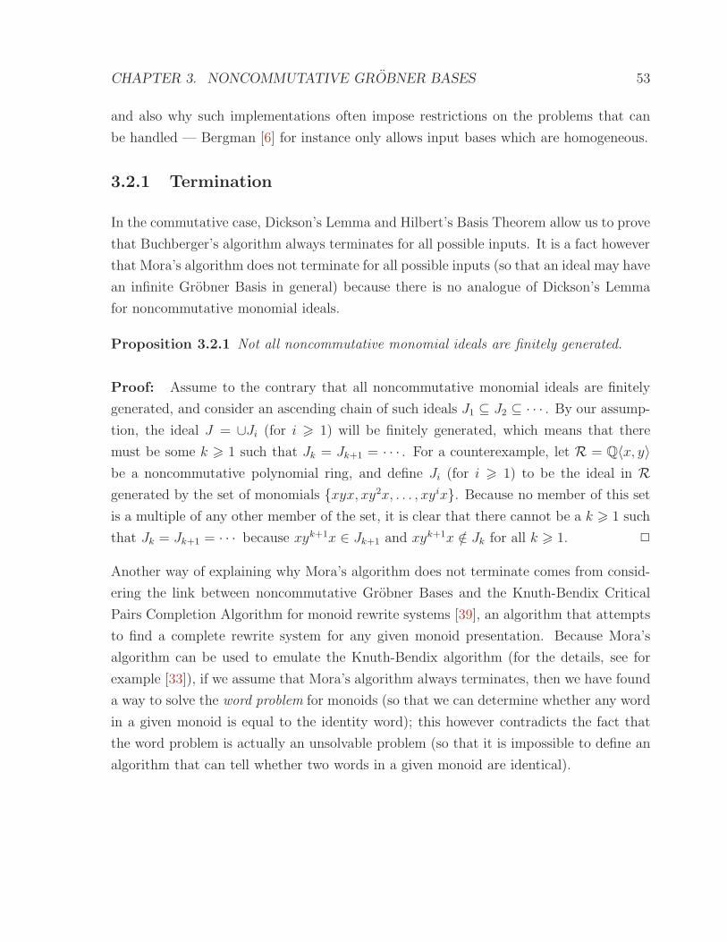
CHAPTER 3. NONCOMMUTATIVE GROBNER BASES 53
and also why such implementations often impose restrictions on the problems that can
be handled — Bergman [6] for instance only allows input bases which are homogeneous.
3.2.1 Termination
In the commutative case, Dickson’s Lemma and Hilbert’s Basis Theorem allow us to prove
that Buchberger’s algorithm always terminates for all possible inputs. It is a fact however
that Mora’s algorithm does not terminate for all possible inputs (so that an ideal may have
an infinite Grobner Basis in general) because there is no analogue of Dickson’s Lemma
for noncommutative monomial ideals.
Proposition 3.2.1 Not all noncommutative monomial ideals are finitely generated.
Proof: Assume to the contrary that all noncommutative monomial ideals are finitely
generated, and consider an ascending chain of such ideals J1 ⊆ J2 ⊆ · · · . By our assump-
tion, the ideal J = ∪Ji (for i > 1) will be finitely generated, which means that there
must be some k > 1 such that Jk = Jk+1 = · · · . For a counterexample, let R = Q〈x, y〉
be a noncommutative polynomial ring, and define Ji (for i > 1) to be the ideal in R
generated by the set of monomials xyx, xy2x, . . . , xyix. Because no member of this set
is a multiple of any other member of the set, it is clear that there cannot be a k > 1 such
that Jk = Jk+1 = · · · because xyk+1x ∈ Jk+1 and xyk+1x /∈ Jk for all k > 1.
Another way of explaining why Mora’s algorithm does not terminate comes from consid-
ering the link between noncommutative Grobner Bases and the Knuth-Bendix Critical
Pairs Completion Algorithm for monoid rewrite systems [39], an algorithm that attempts
to find a complete rewrite system for any given monoid presentation. Because Mora’s
algorithm can be used to emulate the Knuth-Bendix algorithm (for the details, see for
example [33]), if we assume that Mora’s algorithm always terminates, then we have found
a way to solve the word problem for monoids (so that we can determine whether any word
in a given monoid is equal to the identity word); this however contradicts the fact that
the word problem is actually an unsolvable problem (so that it is impossible to define an
algorithm that can tell whether two words in a given monoid are identical).

CHAPTER 3. NONCOMMUTATIVE GROBNER BASES 54
3.3 Reduced Grobner Bases
Definition 3.3.1 Let G = g1, . . . , gp be a Grobner Basis for an ideal over a polynomial
ring R〈x1, . . . , xn〉. G is a reduced Grobner Basis if the following conditions are satisfied.
(a) LC(gi) = 1R for all gi ∈ G.
(b) No term in any polynomial gi ∈ G is divisible by any LT(gj), j 6= i.
Theorem 3.3.2 If there exists a Grobner Basis G for an ideal J over a noncommutative
polynomial ring, then J has a unique reduced Grobner Basis.
Proof: Existence. We claim that the following procedure transforms G into a reduced
Grobner Basis G′.
(i) Multiply each gi ∈ G by LC(gi)−1.
(ii) Reduce each gi ∈ G by G \ gi, removing from G all polynomials that reduce to
zero.
It is clear that G′ satisfies the conditions of Definition 3.3.1, so it remains to show that
G′ is a Grobner Basis, which we shall do by showing that the application of each step of
instruction (ii) above produces a basis which is still a Grobner Basis.
Let G = g1, . . . , gp be a Grobner Basis, and let g′i be the reduction of an arbitrary
gi ∈ G with respect to G \ gi, carried out as follows (the ℓk and the rk are terms).
g′i = gi −κ∑
k=1
ℓkgjkrk. (3.1)
Set H = (G\gi)∪g′i if g′i 6= 0, and set H = G\gi if g′i = 0. As G is a Grobner Basis,
all S-polynomials involving elements of G reduce to zero using G, so there are expressions
cbℓagara − caℓbgbrb −
µ∑
u=1
ℓugcuru = 0 (3.2)
for every S-polynomial S-pol(ℓa, ga, ℓb, gb) = cbℓagara − caℓbgbrb, where ca = LC(ga); cb =
LC(gb); the ℓu and the ru are terms (for 1 6 u 6 µ); and ga, gb, gcu ∈ G. To show that H is

CHAPTER 3. NONCOMMUTATIVE GROBNER BASES 55
a Grobner Basis, we must show that all S-polynomials involving elements of H reduce to
zero using H . For polynomials ga, gb ∈ H not equal to g′i, we can reduce an S-polynomial
of the form S-pol(ℓa, ga, ℓb, gb) using the reduction shown in Equation (3.2), substituting
for gi from Equation (3.1) if any of the gcu in Equation (3.2) are equal to gi. This gives a
reduction to zero of S-pol(ℓa, ga, ℓb, gb) in terms of elements of H .
If g′i = 0, our proof is complete. Otherwise consider all S-polynomials S-pol(ℓ′i, g′i, ℓb, gb)
involving the pair of polynomials (g′i, gb), where gb ∈ G \ gi. We claim that there exists
an S-polynomial S-pol(ℓ1, gi, ℓ2, gb) = cbℓ1gir1 − ciℓ2gbr2 such that S-pol(ℓ′i, g′i, ℓb, gb) =
cbℓ1g′ir1 − ciℓ2gbr2. To prove this claim, it is sufficient to show that LT(gi) = LT(g′i).
Assume for a contradiction that LT(gi) 6= LT(g′i). It follows that during the reduction of
gi we were able to reduce its lead term, so that LT(gi) = ℓLT(gj)r for some terms ℓ and r
and some gj ∈ G. Because LM(gi− ℓgjr) < LM(gi), the polynomial gi− ℓgjr must reduce
to zero without using gi, so that g′i = 0, giving a contradiction.
It remains to show that S-pol(ℓ′i, g′i, ℓb, gb) →H 0. We know that S-pol(ℓ1, gi, ℓ2, gb) =
cbℓ1gir1−ciℓ2gbr2 →G 0, and Equation (3.2) tells us that cbℓ1gir1−ciℓ2gbr2−∑µ
u=1 ℓugcuru =
0. Substituting for gi from Equation (3.1), we obtain1
cbℓ1
(
g′i +
κ∑
k=1
ℓkgjkrk
)
r1 − ciℓ2gbr2 −
µ∑
u=1
ℓugcuru = 0
or
cbℓ1g′ir1 − ciℓ2gbr2 −
(
µ∑
u=1
ℓugcuru −κ∑
k=1
cbℓ1ℓkgjkrkr1
)
= 0,
which implies that S-pol(ℓ′i, g′i, ℓb, gb) →H 0. The only other case to consider is the case of
an S-polynomial coming from a self overlap involving LM(g′i). But because we now know
that LT(g′i) = LT(gi), we can use exactly the same argument as above to show that the
S-polynomial S-pol(ℓ1, g′i, ℓ2, g
′i) reduces to zero using H because an S-polynomial of the
form S-pol(ℓ1, gi, ℓ2, gi) will exist.
Uniqueness. Assume for a contradiction that G = g1, . . . , gp and H = h1, . . . , hq are
two reduced Grobner Bases for an ideal J , with G 6= H . Let gi be an arbitrary element
from G (where 1 6 i 6 p). Because gi is a member of the ideal, then gi must reduce
to zero using H (H is a Grobner Basis). This means that there must exist a polynomial
1Substitutions for gi may also occur in the summation∑µ
u=1 ℓugcuru; these substitutions have notbeen considered in the displayed formulae.

CHAPTER 3. NONCOMMUTATIVE GROBNER BASES 56
hj ∈ H such that LT(hj) | LT(gi). If LT(hj) 6= LT(gi), then ℓ× LT(hj) × r = LT(gi) for
some monomials ℓ and r, at least one of which is not equal to the unit monomial. But hj
is also a member of the ideal, so it must reduce to zero using G. Therefore there exists
a polynomial gk ∈ G such that LT(gk) | LT(hj), which implies that LT(gk) | LT(gi), with
k 6= i. This contradicts condition (b) of Definition 3.3.1 so that G cannot be a reduced
Grobner Basis for J if LT(hj) 6= LT(gi). From this we deduce that each gi ∈ G has a
corresponding hj ∈ H such that LT(gi) = LT(hj). Further, because G and H are assumed
to be reduced Grobner Bases, this is a one-to-one correspondence.
It remains to show that if LT(gi) = LT(hj), then gi = hj. Assume for a contradiction
that gi 6= hj and consider the polynomial gi − hj . Without loss of generality, assume
that LM(gi − hj) appears in gi. Because gi − hj is a member of the ideal, then there is a
polynomial gk ∈ G such that LT(gk) | LT(gi − hj). But this again contradicts condition
(b) of Definition 3.3.1, as we have shown that there is a term in gi that is divisible by
LT(gk) for some k 6= i. It follows that G cannot be a reduced Grobner Basis if gi 6= hj ,
which means that G = H and therefore reduced Grobner Bases are unique.
As in the commutative case, we may refine the procedure for finding a unique reduced
Grobner Basis (as given in the proof of Theorem 3.3.2) by removing from the Grobner
Basis all polynomials whose lead monomials are multiples of the lead monomials of other
Grobner Basis elements. This leads to the definition of Algorithm 6.
3.4 Improvements to Mora’s Algorithm
In Section 2.5, we surveyed some of the numerous improvements of Buchberger’s algo-
rithm. Let us now demonstrate that many of these improvements can also be applied in
the noncommutative case.
3.4.1 Buchberger’s Criteria
In the commutative case, Buchberger’s first criterion states that we can ignore any S-
polynomial S-pol(f, g) in which lcm(LM(f),LM(g)) = LM(f)LM(g). In the noncommuta-
tive case, this translates as saying that we can ignore any ‘S-polynomial’ S-pol(ℓ1, f, ℓ2, g) =
LC(g)ℓ1fr1 − LC(f)ℓ2gr2 such that LM(f) and LM(g) do not overlap in the monomial
ℓ1LM(f)r1 = ℓ2LM(g)r2. We can certainly show that such an ‘S-polynomial’ will reduce
to zero by utilising Proposition 3.1.4, but we will never be able to use this result as, by

CHAPTER 3. NONCOMMUTATIVE GROBNER BASES 57
Algorithm 6 The Noncommutative Unique Reduced Grobner Basis Algorithm
Input: A Grobner Basis G = g1, g2, . . . , gm for an ideal J over a noncommutative
polynomial ring R〈x1, . . . xn〉; an admissible monomial ordering O.
Output: The unique reduced Grobner Basis G′ = g′1, g′2, . . . , g
′p for J .
G′ = ∅;
for each gi ∈ G do
Multiply gi by LC(gi)−1;
if (LM(gi) = ℓLM(gj)r for some monomials ℓ, r and some gj ∈ G (gj 6= gi)) then
G = G \ gi;
end if
end for
for each gi ∈ G do
g′i = Rem(gi, (G \ gi) ∪G′);
G = G \ gi; G′ = G′ ∪ g′i;
end for
return G′;
definition, an S-polynomial is only defined when we have an overlap between LM(f) and
LM(g). It follows that an ‘S-polynomial’ of the above type will never occur in Mora’s
algorithm, and so Buchberger’s first criterion is redundant in the noncommutative case.
The same cannot be said of his second criterion however, which certainly does improve
the efficiency of Mora’s algorithm.
Proposition 3.4.1 (Buchberger’s Second Criterion) Let f , g and h be three mem-
bers of a finite set of polynomials P over a noncommutative polynomial ring, and consider
an S-polynomial of the form
S-pol(ℓ1, f, ℓ2, g) = c2ℓ1fr1 − c1ℓ2gr2. (3.3)
If LM(h) | ℓ1LM(f)r1, so that
ℓ1LM(f)r1 = ℓ3LM(h)r3 = ℓ2LM(g)r2 (3.4)
for some monomials ℓ3, r3, then S-pol(ℓ1, f, ℓ2, g) →P 0 if all S-polynomials corresponding
to overlaps (as placed in the monomial ℓ1LM(f)r1) between LM(h) and either LM(f) or
LM(g) reduce to zero using P .

CHAPTER 3. NONCOMMUTATIVE GROBNER BASES 58
Proof (cf. [37], Appendix A): To be able to describe an S-polynomial corresponding
to an overlap (as placed in the monomial ℓ1LM(f)r1) between LM(h) and either LM(f)
or LM(g), we introduce the following notation.
• Let ℓ13 be the monomial corresponding to the common prefix of ℓ1 and ℓ3 of maximal
degree, so that ℓ1 = ℓ13ℓ′1 and ℓ3 = ℓ13ℓ
′3. (Here, and similarly below, if there is no
common prefix of ℓ1 and ℓ3, then ℓ13 = 1, ℓ′1 = ℓ1 and ℓ′3 = ℓ3.)
• Let ℓ23 be the monomial corresponding to the common prefix of ℓ2 and ℓ3 of maximal
degree, so that ℓ2 = ℓ23ℓ′′2 and ℓ3 = ℓ23ℓ
′′3.
• Let r13 be the monomial corresponding to the common suffix of r1 and r3 of maximal
degree, so that r1 = r′1r13 and r3 = r′3r13.
• Let r23 be the monomial corresponding to the common suffix of r2 and r3 of maximal
degree, so that r2 = r′′2r23 and r3 = r′′3r23.
We can now manipulate Equation (3.3) as follows (where c3 = LC(h)).
c3(S-pol(ℓ1, f, ℓ2, g)) = c3c2ℓ1fr1 − c3c1ℓ2gr2
= c3c2ℓ1fr1 − c1c2ℓ3hr3 + c1c2ℓ3hr3 − c3c1ℓ2gr2
= c2(c3ℓ1fr1 − c1ℓ3hr3)− c1(c3ℓ2gr2 − c2ℓ3hr3)
= c2(c3ℓ13ℓ′1fr
′1r13 − c1ℓ13ℓ
′3hr
′3r13)
− c1(c3ℓ23ℓ′′2gr
′′2r23 − c2ℓ23ℓ
′′3hr
′′3r23)
= c2ℓ13(c3ℓ′1fr
′1 − c1ℓ
′3hr
′3)r13 − c1ℓ23(c3ℓ
′′2gr
′′2 − c2ℓ
′′3hr
′′3)r23.
As placed in ℓ1LM(f)r1 = ℓ3LM(h)r3, if LM(f) and LM(h) overlap, then the S-polynomial
corresponding to this overlap is2 S-pol(ℓ′1, f, ℓ′3, h). Similarly, if LM(g) and LM(h) overlap
as placed in ℓ2LM(g)r2 = ℓ3LM(h)r3, then the S-polynomial corresponding to this overlap
is S-pol(ℓ′′2, g, ℓ′′3, h). By assumption, these S-polynomials reduce to zero using P , so there
are expressions
c3ℓ′1fr
′1 − c1ℓ
′3hr
′3 −
α∑
i=1
uipivi = 0 (3.5)
2For completeness, we note that the S-polynomial corresponding to the overlap can also be of the formS-pol(ℓ′3, h, ℓ
′
1, f); this (inconsequentially) swaps the first two terms of Equation (3.5).

CHAPTER 3. NONCOMMUTATIVE GROBNER BASES 59
and
c3ℓ′′2gr
′′2 − c2ℓ
′′3hr
′′3 −
β∑
j=1
ujpjvj = 0, (3.6)
where the ui, vi, uj and vj are terms; and pi, pj ∈ P for all i and j. Using Proposition
3.1.4, we can state that these expressions will still exist even if LM(f) and LM(h) do not
overlap as placed in ℓ1LM(f)r1 = ℓ3LM(h)r3; and if LM(g) and LM(h) do not overlap as
placed in ℓ2LM(g)r2 = ℓ3LM(h)r3. It follows that
c3(S-pol(ℓ1, f, ℓ2, g)) = c2ℓ13(c3ℓ′1fr
′1 − c1ℓ
′3hr
′3)r13 − c1ℓ23(c3ℓ
′′2gr
′′2 − c2ℓ
′′3hr
′′3)r23
= c2ℓ13
(
α∑
i=1
uipivi
)
r13 − c1ℓ23
(
β∑
j=1
ujpjvj
)
r23
=
α∑
i=1
c2ℓ13uipivir13 −
β∑
j=1
c1ℓ23ujpjvjr23;
S-pol(ℓ1, f, ℓ2, g) =
α∑
i=1
c−13 c2ℓ13uipivir13 −
β∑
j=1
c−13 c1ℓ23ujpjvjr23.
To conclude that the S-polynomial S-pol(ℓ1, f, ℓ2, g) reduces to zero using P , it remains
to show that the algebraic expression −∑α
i=1 c−13 c2ℓ13uipivir13 +
∑β
j=1 c−13 c1ℓ23ujpjvjr23
corresponds to a valid reduction of S-pol(ℓ1, f, ℓ2, g). To do this, it is sufficient to show
that no term in either of the summations is greater than the term ℓ1LM(f)r1 (so that
LM(ℓ13uipivir13) < ℓ1LM(f)r1 and LM(ℓ23ujpjvjr23) < ℓ1LM(f)r1 for all i and j). But
this follows from Equation (3.4) and from the fact that the reductions of the expressions
c3ℓ′1fr
′1 − c1ℓ
′3hr
′3 and c3ℓ
′′2gr
′′2 − c2ℓ
′′3hr
′′3 in Equations (3.5) and (3.6) are valid, so that
LM(uipivi) < LM(ℓ′1fr′1) and LM(ujpjvj) < LM(ℓ′′2gr
′′2) for all i and j.
Remark 3.4.2 The three polynomials f , g and h in the above proposition do not neces-
sarily have to be distinct (indeed, f = g = h is allowed) — the only restriction is that the
S-polynomial S-pol(ℓ1, f, ℓ2, g) has to be different from the S-polynomials S-pol(ℓ′1, f, ℓ′3, h)
and S-pol(ℓ′′2, g, ℓ′′3, h); for example, if f = h, then we cannot have ℓ′1 = ℓ′3.
3.4.2 Homogeneous Grobner Bases
Because it is computationally more expensive to do noncommutative polynomial arith-
metic than it is to do commutative polynomial arithmetic, gains in efficiency due to
working with homogeneous bases are even more significant in the noncommutative case.

CHAPTER 3. NONCOMMUTATIVE GROBNER BASES 60
For this reason, some systems for computing noncommutative Grobner Bases will only
work with homogeneous input bases, although (as in the commutative case) it is still
sometimes possible to use these systems on non-homogeneous input bases by using the
concepts of homogenisation, dehomogenisation and extendible monomial orderings.
Definition 3.4.3 Let p = p0 + · · · + pm be a polynomial over the polynomial ring
R〈x1, . . . , xn〉, where each pi is the sum of the degree i terms in p (we assume that
pm 6= 0). The left homogenisation of p with respect to a new (homogenising) variable y is
the polynomial
hℓ(p) := ymp0 + ym−1p1 + · · ·+ ypm−1 + pm;
and the right homogenisation of p with respect to a new (homogenising) variable y is the
polynomial
hr(p) := p0ym + p1y
m−1 + · · ·+ pm−1y + pm.
Homogenised polynomials belong to polynomial rings determined by where y is placed in
the lexicographical ordering of the variables.
Definition 3.4.4 The dehomogenisation of a polynomial p is the polynomial d(p) given
by substituting y = 1 in p, where y is the homogenising variable.
Definition 3.4.5 A monomial ordering O is extendible if, given any polynomial p =
t1 + · · · + tα ordered with respect to O (where t1 > · · · > tα), the homogenisation of p
preserves the order on the terms (t′i > t′i+1 for all 1 6 i 6 α−1, where the homogenisation
process maps the term ti ∈ p to the term t′i).
In the noncommutative case, an extendible monomial ordering must specify how to ho-
mogenise a polynomial (by multiplying with the homogenising variable on the left or on
the right) as well as stating where the new variable y appears in the ordering of the vari-
ables. Here are the conventions for those monomial orderings defined in Section 1.2.2 that
are extendible, assuming that we start with a polynomial ring R〈x1, . . . , xn〉.
Monomial Ordering Type of Homogenisation Position of the new variable y
in the ordering of the variables
InvLex Right y < xi for all xi
DegLex Left y < xi for all xi
DegInvLex Left y > xi for all xi
DegRevLex Right y > xi for all xi

CHAPTER 3. NONCOMMUTATIVE GROBNER BASES 61
Noncommutativity also provides the possibility of the new variable y becoming ‘trapped’
in the middle of some monomial forming part of a polynomial computed during the course
of Mora’s algorithm. For example, working with DegRevLex, consider the homogenised
polynomial hr(x21 + x1) = x2
1 + x1y and the S-polynomial
S-pol(x1, x21 + x1y, 1, x
21 + x1y) = x1(x
21 + x1y)− (x2
1 + x1y)x1 = x21y − x1yx1.
Because y appears in the middle of the monomial x1yx1, the S-polynomial does not
immediately reduce to zero as it does in the non-homogenised version of the S-polynomial,
S-pol(x1, x21 + x1, 1, x
21 + x1) = x1(x
21 + x1)− (x2
1 + x1)x1 = 0.
We must therefore make certain that y only appears on one side of any given mono-
mial by introducing the set of polynomials H = h1, h2, . . . , hn = yx1 − x1y, yx2 −
x2y, . . . , yxn − xny into our initial homogenised basis, ensuring that y commutes with
all the other variables in the polynomial ring. This way, the first S-polynomial will reduce
to zero as follows:
x21y − x1yx1 →h1
x21y − x2
1y = 0.
Which side y will appear on will be determined by whether LM(yxi − xiy) = yxi or
LM(yxi − xiy) = xiy in our chosen monomial ordering (pushing y to the right or to the
left respectively). This side must match the method of homogenisation, which explains
why Lex is not an extendible monomial ordering — for Lex to be extendible, we must
homogenise on the right and have y < xi for all xi, but then because LM(yxi−xiy) = xiy
with respect to Lex, the variable y will always in practice appear on the left.
Definition 3.4.6 Let F = f1, . . . , fm be a non-homogeneous set of polynomials over
the polynomial ring R〈x1, . . . , xn〉. To compute a Grobner Basis for F using a program
that only accepts sets of homogeneous polynomials as input, we use the following proce-
dure (which will only work in conjunction with an extendible monomial ordering).
(a) Construct a homogeneous set of polynomials F ′ = hℓ(f1), . . . , hℓ(fm) or F ′ =
hr(f1), . . . , hr(fm) (dependent on the monomial ordering used).
(b) Compute a Grobner Basis G′ for the set F ′ ∪ H , where H = yx1 − x1y, yx2 −
x2y, . . . , yxn − xny.
(c) Dehomogenise each polynomial g′ ∈ G′ to obtain a Grobner Basis G for F , noting

CHAPTER 3. NONCOMMUTATIVE GROBNER BASES 62
that no polynomial originating from H will appear in G (d(hi) = 0 for all hi ∈ H).
3.4.3 Selection Strategies
As in the commutative case, the order in which S-polynomials are processed during Mora’s
algorithm has an important effect on the efficiency of the algorithm. Let us now generalise
the selection strategies defined in Section 2.5.3 for use in the noncommutative setting,
basing our decisions on the overlap words of S-polynomials.
Definition 3.4.7 The overlap word of an S-polynomial S-pol(ℓ1, f, ℓ2, g) = LC(g)ℓ1fr1−
LC(f)ℓ2gr2 is the monomial ℓ1LM(f)r1 (= ℓ2LM(g)r2).
Definition 3.4.8 In the noncommutative normal strategy, we choose an S-polynomial to
process if its overlap word is minimal in the chosen monomial ordering amongst all such
overlap words.
Definition 3.4.9 In the noncommutative sugar strategy, we choose an S-polynomial to
process if its sugar (a value associated to the S-polynomial) is minimal amongst all such
values (we use the normal strategy in the event of a tie).
The sugar of an S-polynomial is computed by using the following rules on the sugars
of polynomials we encounter during the computation of a Grobner Basis for the set of
polynomials F = f1, . . . , fm.
(1) The sugar Sugfi of a polynomial fi ∈ F is the total degree of the polynomial fi (which
is the degree of the term of maximal degree in fi).
(2) If p is a polynomial and if t1 and t2 are terms, then Sugt1pt2 = deg(t1)+Sugp+deg(t2).
(3) If p = p1 + p2, then Sugp = max(Sugp1 , Sugp2).
It follows that the sugar of the S-polynomial S-pol(ℓ1, g, ℓ2, h) = LC(h)ℓ1gr1−LC(g)ℓ2hr2
is given by the formula
SugS-pol(ℓ1,g,ℓ2,h) = max(deg(ℓ1) + Sugg + deg(r1), deg(ℓ2) + Sugh + deg(r2)).

CHAPTER 3. NONCOMMUTATIVE GROBNER BASES 63
3.4.4 Logged Grobner Bases
Definition 3.4.10 Let G = g1, . . . , gp be a noncommutative Grobner Basis computed
from an initial basis F = f1, . . . , fm. We say that G is a Logged Grobner Basis if, for
each gi ∈ G, we have an explicit expression of the form
gi =
β∑
α=1
ℓαfkαrα,
where the ℓα and the rα are terms and fkα ∈ F for all 1 6 α 6 β.
Proposition 3.4.11 Let F = f1, . . . , fm be a finite basis over a noncommutative poly-
nomial ring. If we can compute a Grobner Basis for F , then it is always possible to
compute a Logged Grobner Basis for F .
Proof: We refer to the proof of Proposition 2.5.11, substituting
S-pol(ℓ1, fi, ℓ2, fj)−
β∑
α=1
ℓαgkαrα
for fm+1 (the ℓα and the rα are terms).
3.5 A Worked Example
To demonstrate Mora’s algorithm in action, let us now calculate a Grobner Basis for the
ideal J generated by the set of polynomials F := f1, f2, f3 = xy−z, yz+2x+z, yz+x
over the polynomial ring Q〈x, y, z〉. We shall use the DegLex monomial ordering (with
x > y > z); use the normal selection strategy; calculate a Logged Grobner Basis; and use
Buchberger’s criteria.
3.5.1 Initialisation
The first part of Mora’s algorithm requires us to find all the overlaps between the lead
monomials of the three polynomials in the initial basis G := g1, g2, g3 = xy − z, yz +
2x+ z, yz + x. There are three overlaps in total, summarised by the following table.
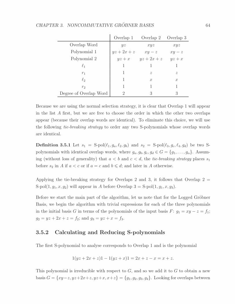
CHAPTER 3. NONCOMMUTATIVE GROBNER BASES 64
Overlap 1 Overlap 2 Overlap 3
Overlap Word yz xyz xyz
Polynomial 1 yz + 2x+ z xy − z xy − z
Polynomial 2 yz + x yz + 2x+ z yz + x
ℓ1 1 1 1
r1 1 z z
ℓ2 1 x x
r2 1 1 1
Degree of Overlap Word 2 3 3
Because we are using the normal selection strategy, it is clear that Overlap 1 will appear
in the list A first, but we are free to choose the order in which the other two overlaps
appear (because their overlap words are identical). To eliminate this choice, we will use
the following tie-breaking strategy to order any two S-polynomials whose overlap words
are identical.
Definition 3.5.1 Let s1 = S-pol(ℓ1, ga, ℓ2, gb) and s2 = S-pol(ℓ3, gc, ℓ4, gd) be two S-
polynomials with identical overlap words, where ga, gb, gc, gd ∈ G = g1, . . . , gα. Assum-
ing (without loss of generality) that a < b and c < d, the tie-breaking strategy places s1
before s2 in A if a < c or if a = c and b 6 d; and later in A otherwise.
Applying the tie-breaking strategy for Overlaps 2 and 3, it follows that Overlap 2 =
S-pol(1, g1, x, g2) will appear in A before Overlap 3 = S-pol(1, g1, x, g3).
Before we start the main part of the algorithm, let us note that for the Logged Grobner
Basis, we begin the algorithm with trivial expressions for each of the three polynomials
in the initial basis G in terms of the polynomials of the input basis F : g1 = xy − z = f1;
g2 = yz + 2x+ z = f2; and g3 = yz + x = f3.
3.5.2 Calculating and Reducing S-polynomials
The first S-polynomial to analyse corresponds to Overlap 1 and is the polynomial
1(yz + 2x+ z)1− 1(yz + x)1 = 2x+ z − x = x+ z.
This polynomial is irreducible with respect to G, and so we add it to G to obtain a new
basis G = xy−z, yz+2x+z, yz+x, x+z = g1, g2, g3, g4. Looking for overlaps between

CHAPTER 3. NONCOMMUTATIVE GROBNER BASES 65
the lead monomial of x+ z and the lead monomials of the four elements of G, we see that
there is one such overlap (with g1) whose overlap word has degree 2, so this overlap is
added to the beginning of the list A to obtain A = S-pol(1, xy−z, 1, x+z), S-pol(1, xy−
z, x, yz + 2x+ z), S-pol(1, xy − z, x, yz + x). As far as the Logged Grobner Basis goes,
g4 = x+ z = 1(yz + 2x+ z)1 − 1(yz + x)1 = f2 − f3.
The next entry in A produces the polynomial
1(xy − z)1− 1(x+ z)y = −zy − z.
As before, this polynomial is irreducible with respect to G, so we add it to G as the fifth
element. There are also four overlaps between the lead monomial of −zy− z and the lead
monomials of the five polynomials in G:
Overlap 1 Overlap 2 Overlap 3 Overlap 4
Overlap Word zyz zyz yzy yzy
Polynomial 1 yz + 2x+ z yz + x yz + 2x+ z yz + x
Polynomial 2 −zy − z −zy − z −zy − z −zy − z
ℓ1 z z 1 1
r1 1 1 y y
ℓ2 1 1 y y
r2 z z 1 1
Degree of Overlap Word 3 3 3 3
Inserting these overlaps into the list A, we obtain
A = S-pol(z, yz + 2x+ z, 1,−zy − z), S-pol(z, yz + x, 1,−zy − z),
S-pol(1, yz + 2x+ z, y,−zy − z), S-pol(1, yz + x, y,−zy − z),
S-pol(1, xy − z, x, yz + 2x+ z), S-pol(1, xy − z, x, yz + x) .
The logged representation of the fifth basis element again comes straight from the S-
polynomial (as no reduction was performed), and is as follows: g5 = −zy − z = 1(xy −
z)1 − 1(x+ z)y = 1(f1)1− 1(f2 − f3)y = f1 − f2y + f3y.
The next entry in A yields the polynomial
−z(yz + 2x+ z)1− 1(−zy − z)z = −2zx − z2 + z2 = −2zx.

CHAPTER 3. NONCOMMUTATIVE GROBNER BASES 66
This time, the fourth polynomial in our basis reduces the S-polynomial in question, giving
a reduction −2zx →g4 2z2. When we add this polynomial to G and add all five new
overlaps to A, we are left with a six element basis G = xy − z, yz + 2x+ z, yz + x, x +
z,−zy − z, 2z2 and a list
A = S-pol(1, 2z2, z, 2z2), S-pol(z, 2z2, 1, 2z2),
S-pol(z,−zy − z, 1, 2z2), S-pol(z, yz + x, 1,−zy − z),
S-pol(1, yz + 2x+ z, y, 2z2), S-pol(1, yz + x, y, 2z2),
S-pol(1, yz + 2x+ z, y,−zy − z), S-pol(1, yz + x, y,−zy − z),
S-pol(1, xy − z, x, yz + 2x+ z), S-pol(1, xy − z, x, yz + x) .
We obtain the logged version of the sixth basis element by working backwards through
our calculations:
g6 = 2z2
= −2zx+ 2z(x+ z)
= (−z(yz + 2x+ z)1 − 1(−zy − z)z) + 2z(x+ z)
= (−z(f2)− (f1 − f2y + f3y)z) + 2z(f2 − f3)
= −f1z + zf2 + f2yz − 2zf3 − f3yz.
3.5.3 Applying Buchberger’s Second Criterion
The next three entries in A all yield S-polynomials that are either zero or reduce to
zero (for example, the first entry corresponds to the polynomial 2(2z2)z − 2z(2z2)1 =
4z3 − 4z3 = 0). The fourth entry in A, S-pol(z, yz + x, 1,−zy − z), then enables us (for
the first time) to apply Buchberger’s second criterion, allowing us to move on to look
at the fifth entry of A. Before we do this however, let us explain why we can apply
Buchberger’s second criterion in this particular case.
Recall (from Proposition 3.4.1) that in order to apply Buchberger’s second criterion for
the S-polynomial S-pol(z, yz + x, 1,−zy − z), we need to find a polynomial gi ∈ G such
that LM(gi) divides the overlap word of our S-polynomial, and any S-polynomials cor-
responding to overlaps (as positioned in the overlap word) between LM(gi) and either
LM(yz + x) or LM(−zy − z) reduce to zero using G (which will be the case if those

CHAPTER 3. NONCOMMUTATIVE GROBNER BASES 67
particular S-polynomials have been processed earlier in the algorithm).
Consider the polynomial g2 = yz+2x+ z. The lead monomial of this polynomial divides
the overlap word zyz of our S-polynomial, which we illustrate as follows.
ooLM(g3)
//
ooLM(g5)
//
z y z
ooLM(g2)
//
As positioned in the overlap word, we note that LM(g2) overlaps with both LM(g3)
and LM(g5), with the overlaps corresponding to the S-polynomials S-pol(1, g2, 1, g3) =
S-pol(1, yz + 2x + z, 1, yz + x) and S-pol(z, g2, 1, g5) = S-pol(z, yz + 2x + z, 1,−zy − z)
respectively. But these S-polynomials have been processed earlier in the algorithm (they
were the first and third S-polynomials to be processed); we can therefore apply Buch-
berger’s second criterion in this instance.
There are now six S-polynomials left in A, all of whom either reduce to zero or are
ignored due to Buchberger’s second criterion. Here is a summary of what happens during
the remainder of the algorithm.
S-polynomial Action
S-pol(1, yz + 2x+ z, y, 2z2) Reduces to zero using the division algorithm
S-pol(1, yz + x, y, 2z2) Ignored due to Buchberger’s second criterion
(using yz + 2x+ z)
S-pol(1, yz + 2x+ z, y,−zy − z) Reduces to zero using the division algorithm
S-pol(1, yz + x, y,−zy − z) Ignored due to Buchberger’s second criterion
(using yz + 2x+ z)
S-pol(1, xy − z, x, yz + 2x+ z) Ignored due to Buchberger’s second criterion
(using x+ z)
S-pol(1, xy − z, x, yz + x) Ignored due to Buchberger’s second criterion
(using yz + 2x+ z)
As the list A is now empty, the algorithm terminates with the following (Logged) Grobner
Basis.

CHAPTER 3. NONCOMMUTATIVE GROBNER BASES 68
Input Basis F Grobner Basis G
f1 = xy − z g1 = xy − z = f1
f2 = yz + 2x+ z g2 = yz + 2x+ z = f2
f3 = yz + x g3 = yz + x = f3
g4 = x+ z = f2 − f3
g5 = −zy − z = f1 − f2y + f3y
g6 = 2z2 = −f1z + zf2 + f2yz − 2zf3 − f3yz
3.5.4 Reduction
Now that we have constructed a Grobner Basis for our ideal J , let us go on to find the
unique reduced Grobner Basis for J by applying Algorithm 6 to G.
In the first half of the algorithm, we must multiply each polynomial by the inverse of
its lead coefficient and remove from the basis each polynomial whose lead monomial is a
multiple of the lead monomial of some other polynomial in the basis. For the Grobner
Basis in question, we multiply g5 by −1 and g6 by 12; and we remove g1 and g2 from the
basis (because LM(g1) = LM(g4) × y and LM(g2) = LM(g3)). This leaves us with the
following (minimal) Grobner Basis.
Input Basis F Grobner Basis G
f1 = xy − z g3 = yz + x = f3
f2 = yz + 2x+ z g4 = x+ z = f2 − f3
f3 = yz + x g5 = zy + z = −f1 + f2y − f3y
g6 = z2 = −12f1z +
12zf2 +
12f2yz − zf3 −
12f3yz
In the second half of the algorithm, we reduce each gi ∈ G with respect to (G \ gi)∪G′,
placing the remainder in the (initially empty) set G′ and removing gi from G. For the
Grobner Basis in question, we summarise what happens in the following table, noting that
the only reduction that takes place is the reduction yz+ x →g4 yz+ x− (x+ z) = yz− z.

CHAPTER 3. NONCOMMUTATIVE GROBNER BASES 69
G G′ gi g′i
yz + x, x+ z, zy + z, z2 ∅ yz + x yz − z
x+ z, zy + z, z2 yz − z x+ z x+ z
zy + z, z2 yz − z, x+ z zy + z zy + z
z2 yz − z, x+ z, zy + z z2 z2
∅ yz − z, x+ z, zy + z, z2
We can now give the unique reduced (Logged) Grobner Basis for J .
Input Basis F Unique Reduced Grobner Basis G′
f1 = xy − z yz − z = −f2 + 2f3
f2 = yz + 2x+ z x+ z = f2 − f3
f3 = yz + x zy + z = −f1 + f2y − f3y
z2 = −12f1z +
12zf2 +
12f2yz − zf3 −
12f3yz

Chapter 4
Commutative Involutive Bases
Given a Grobner Basis G for an ideal J over a polynomial ring R, we know that the
remainder of any polynomial p ∈ R with respect to G is unique. But although this
remainder is unique, there may be many ways of obtaining the remainder, as it is possible
that several polynomials in G divide our polynomial p, giving several reduction paths for
p.
Example 4.0.2 Consider the DegLex Grobner Basis G := g1, g2, g3 = x2 − 2xy +
3, 2xy + y2 + 5, 54y3 − 5
2x + 37
4y over the polynomial ring R := Q[x, y] from Example
2.3.2, and consider the polynomial p := x2y + y3 + 8y ∈ R. The remainder of p with
respect to G is 0 (so that p is a member of the ideal J generated by G), but there are two
ways of obtaining this remainder, as shown in the following diagram.
x2y + y3 + 8yg1
uukkkkkkkkkkkkkg2
**TTTTTTTTTTTTTT
2xy2 + y3 + 5y
g2
−12xy2 + y3 − 5
2x+ 8y
g2
0 54y3 − 5
2x+ 37
4y
g3
0
(4.1)
An Involutive Basis is a Grobner Basis G for J such that there is only one possible
reduction path for any polynomial p ∈ R. In order to find such a basis, we must restrict
70

CHAPTER 4. COMMUTATIVE INVOLUTIVE BASES 71
which reductions or divisions may take place by requiring, for each potential reduction of
a polynomial p by a polynomial gi ∈ G (so that LM(p) = LM(gi)× u for some monomial
u), some extra conditions on the variables in u to be satisfied, namely that all variables
in u have to be in a set of multiplicative variables for gi, a set that is determined by a
particular choice of an involutive division.
4.1 Involutive Divisions
In Definition 1.2.9, we saw that a commutative monomial u1 is divisible by another mono-
mial u2 if there exists a third monomial u3 such that u1 = u2u3; we also introduced the
notation u2 | u1 to denote that u2 is a divisor of u1, a divisor we shall now refer to as a
conventional divisor of u1. For a particular choice of an involutive division I, we say that
u2 is an involutive divisor of u1, written u2 |I u1, if, given a partitioning (by I) of the
variables in the polynomial ring into sets of multiplicative and nonmultiplicative variables
for u2, all variables in u3 are in the set of multiplicative variables for u2.
Example 4.1.1 Let u1 := xy2z2; u′1 := x2yz and u2 := xz be three monomials over the
polynomial ring R := Q[x, y, z], and let an involutive division I partition the variables in
R into the following two sets of variables for the monomial u2: multiplicative = y, z;
nonmultiplicative = x. It is true that u2 conventionally divides both monomials u1 and
u′1, but u2 only involutively divides monomial u1 as, defining u3 := y2z and u′
3 := xy
(so that u1 = u2u3 and u′1 = u2u
′3), we observe that all variables in u3 are in the set of
multiplicative variables for u2, but the variables in u′3 (in particular the variable x) are
not all in the set of multiplicative variables for u2.
More formally, an involutive division I works with a set of monomials U over a polynomial
ring R[x1, . . . , xn] and assigns a set of multiplicative variables MI(u, U) ⊆ x1, . . . , xn
to each element u ∈ U . It follows that, with respect to U , a monomial w is divisible by a
monomial u ∈ U if w = uv for some monomial v and all the variables that appear in v
also appear in the set MI(u, U).
Definition 4.1.2 Let M denote the set of all monomials in the polynomial ring R =
R[x1, . . . , xn], and let U ⊂ M . The involutive cone CI(u, U) of any monomial u ∈ U with
respect to some involutive division I is defined as follows.
CI(u, U) = uv such that v ∈ M and u |I uv.

CHAPTER 4. COMMUTATIVE INVOLUTIVE BASES 72
Remark 4.1.3 We may think of an involutive cone of a particular monomial u as con-
taining all monomials that are involutively divisible by u.
Up to now, we have not mentioned any restriction on how we may assign multiplicative
variables to a particular set of monomials. Let us now specify the rules that ensure that a
particular scheme of assigning multiplicative variables may be referred to as an involutive
division.
Definition 4.1.4 Let M denote the set of all monomials in the polynomial ring R =
R[x1, . . . , xn]. An involutive division I onM is defined if, given any finite set of monomials
U ⊂ M , we can assign a set of multiplicative variables MI(u, U) ⊆ x1, . . . , xn to any
monomial u ∈ U such that the following two conditions are satisfied.
(a) If there exist two monomials u1, u2 ∈ U such that CI(u1, U) ∩ CI(u2, U) 6= ∅,
then either CI(u1, U) ⊂ CI(u2, U) or CI(u2, U) ⊂ CI(u1, U).
(b) If V ⊂ U , then MI(v, U) ⊆ MI(v, V ) for all v ∈ V .
Remark 4.1.5 Informally, condition (a) above ensures that a monomial can only appear
in two involutive cones CI(u1, U) and CI(u2, U) if u1 is an involutive divisor of u2 or
vice-versa; while condition (b) ensures that the multiplicative variables of a polynomial
v ∈ V ⊂ U with respect to U all appear in the set of multiplicative variables of v with
respect to V .
Definition 4.1.6 Given an involutive division I, the involutive span CI(U) of a set of
monomials U with respect to I is given by the expression
CI(U) =⋃
u∈U
CI(u, U).
Remark 4.1.7 The (conventional) span of a set of monomials U is given by the expression
C(U) =⋃
u∈U
C(u, U),
where C(u, U) = uv | v is a monomial is the (conventional) cone of a monomial u ∈ U .
Definition 4.1.8 If an involutive division I determines the multiplicative variables for a
monomial u ∈ U independent of the set U , then I is a global division. Otherwise, I is a
local division.

CHAPTER 4. COMMUTATIVE INVOLUTIVE BASES 73
Remark 4.1.9 The multiplicative variables for a set of polynomials P (whose terms are
ordered by a monomial ordering O) are determined by the multiplicative variables for the
set of leading monomials LM(P ).
4.1.1 Involutive Reduction
In Algorithm 7, we specify how to involutively divide a polynomial p with respect to a
set of polynomials P .
Algorithm 7 The Commutative Involutive Division Algorithm
Input: A nonzero polynomial p and a set of nonzero polynomials P = p1, . . . , pm over a
polynomial ring R[x1, . . . xn]; an admissible monomial ordering O; an involutive division
I.
Output: RemI(p, P ) := r, the involutive remainder of p with respect to P .
r = 0;
while (p 6= 0) do
u = LM(p); c = LC(p); j = 1; found = false;
while (j 6 m) and (found == false) do
if (LM(pj) |I u) then
found = true; u′ = u/LM(pj); p = p− (cLC(pj)−1)pju
′;
else
j = j + 1;
end if
end while
if (found == false) then
r = r + LT(p); p = p− LT(p);
end if
end while
return r;
Remark 4.1.10 The only difference between Algorithms 1 and 7 is that the line “if
(LM(pj) | u) then” in Algorithm 1 has been changed to the line “if (LM(pj) |I u) then”
in Algorithm 7.
Definition 4.1.11 If the polynomial r is obtained by involutively dividing (with respect
to some involutive division I) the polynomial p by one of (a) a polynomial q; (b) a sequence

CHAPTER 4. COMMUTATIVE INVOLUTIVE BASES 74
of polynomials q1, q2, . . . , qα; or (c) a set of polynomials Q, we will use the notation
pI q
// r; pI
∗ // r and pI Q
// r respectively (matching the notation introduced in
Definition 1.2.16).
4.1.2 Thomas, Pommaret and Janet divisions
Let us now consider three different involutive divisions, all named after their creators in
the theory of Partial Differential Equations (see [52], [47] and [35]).
Definition 4.1.12 (Thomas) Let U = u1, . . . , um be a set of monomials over a poly-
nomial ring R[x1, . . . , xn], where the monomial uj ∈ U (for 1 6 j 6 m) has corresponding
multidegree (e1j , e2j , . . . , e
nj ). The Thomas involutive division T assigns multiplicative vari-
ables to elements of U as follows: the variable xi is multiplicative for monomial uj (written
xi ∈ MT (uj, U)) if eij = maxk eik for all 1 6 k 6 m.
Definition 4.1.13 (Pommaret) Let u be a monomial over a polynomial ring
R[x1, . . . , xn] with multidegree (e1, e2, . . . , en). The Pommaret involutive division P as-
signs multiplicative variables to u as follows: if 1 6 i 6 n is the smallest integer such that
ei > 0, then all variables x1, x2, . . . , xi are multiplicative for u (we have xj ∈ MP(u) for
all 1 6 j 6 i).
Definition 4.1.14 (Janet) Let U = u1, . . . , um be a set of monomials over a polyno-
mial ring R[x1, . . . , xn], where the monomial uj ∈ U (for 1 6 j 6 m) has corresponding
multidegree (e1j , e2j , . . . , e
nj ). The Janet involutive division J assigns multiplicative vari-
ables to elements of U as follows: the variable xn is multiplicative for monomial uj (written
xn ∈ MJ (uj, U)) if enj = maxk enk for all 1 6 k 6 m; the variable xi (for 1 6 i < n) is mul-
tiplicative for monomial uj (written xi ∈ MJ (uj, U)) if eij = maxk eik for all monomials
uk ∈ U such that elj = elk for all i < l 6 n.
Remark 4.1.15 Thomas and Janet are local involutive divisions; Pommaret is a global
involutive division.
Example 4.1.16 Let U := x5y2z, x4yz2, x2y2z, xyz3, xz3, y2z, z be a set of mono-
mials over the polynomial ring Q[x, y, z], with x > y > z. Here are the multiplicative
variables for U according to the three involutive divisions defined above.
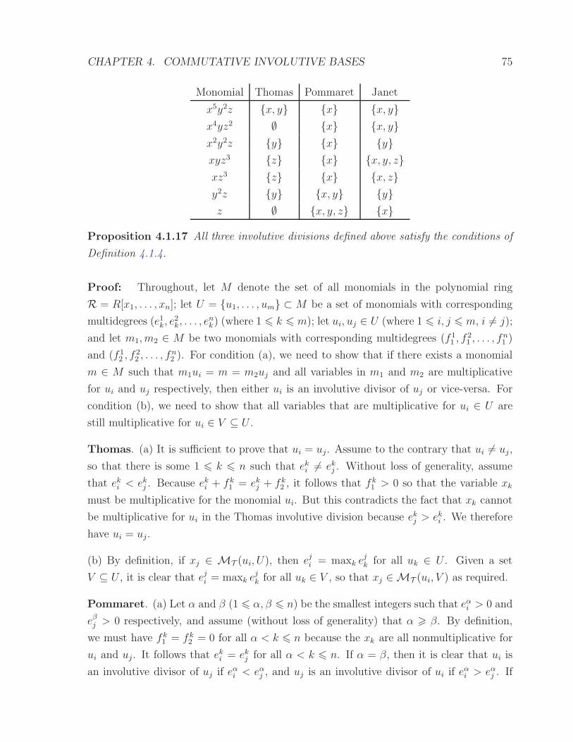
CHAPTER 4. COMMUTATIVE INVOLUTIVE BASES 75
Monomial Thomas Pommaret Janet
x5y2z x, y x x, y
x4yz2 ∅ x x, y
x2y2z y x y
xyz3 z x x, y, z
xz3 z x x, z
y2z y x, y y
z ∅ x, y, z x
Proposition 4.1.17 All three involutive divisions defined above satisfy the conditions of
Definition 4.1.4.
Proof: Throughout, let M denote the set of all monomials in the polynomial ring
R = R[x1, . . . , xn]; let U = u1, . . . , um ⊂ M be a set of monomials with corresponding
multidegrees (e1k, e2k, . . . , e
nk) (where 1 6 k 6 m); let ui, uj ∈ U (where 1 6 i, j 6 m, i 6= j);
and let m1, m2 ∈ M be two monomials with corresponding multidegrees (f 11 , f
21 , . . . , f
n1 )
and (f 12 , f
22 , . . . , f
n2 ). For condition (a), we need to show that if there exists a monomial
m ∈ M such that m1ui = m = m2uj and all variables in m1 and m2 are multiplicative
for ui and uj respectively, then either ui is an involutive divisor of uj or vice-versa. For
condition (b), we need to show that all variables that are multiplicative for ui ∈ U are
still multiplicative for ui ∈ V ⊆ U .
Thomas. (a) It is sufficient to prove that ui = uj. Assume to the contrary that ui 6= uj,
so that there is some 1 6 k 6 n such that eki 6= ekj . Without loss of generality, assume
that eki < ekj . Because eki + fk1 = ekj + fk
2 , it follows that fk1 > 0 so that the variable xk
must be multiplicative for the monomial ui. But this contradicts the fact that xk cannot
be multiplicative for ui in the Thomas involutive division because ekj > eki . We therefore
have ui = uj.
(b) By definition, if xj ∈ MT (ui, U), then eji = maxk ejk for all uk ∈ U . Given a set
V ⊆ U , it is clear that eji = maxk ejk for all uk ∈ V , so that xj ∈ MT (ui, V ) as required.
Pommaret. (a) Let α and β (1 6 α, β 6 n) be the smallest integers such that eαi > 0 and
eβj > 0 respectively, and assume (without loss of generality) that α > β. By definition,
we must have fk1 = fk
2 = 0 for all α < k 6 n because the xk are all nonmultiplicative for
ui and uj. It follows that eki = ekj for all α < k 6 n. If α = β, then it is clear that ui is
an involutive divisor of uj if eαi < eαj , and uj is an involutive divisor of ui if eαi > eαj . If
CHAPTER 4. COMMUTATIVE INVOLUTIVE BASES 76
α > β, then fα2 = 0 as variable xα is nonmultiplicative for uj, so it follows that eαi 6 eαj
and hence ui is an involutive divisor of uj.
(b) Follows immediately because Pommaret is a global involutive division.
Janet. (a) We prove that ui = uj. Assume to the contrary that ui 6= uj, so there exists
a maximal 1 6 k 6 n such that eki 6= ekj . Without loss of generality, assume that eki < ekj .
If k = n, we get an immediate contradiction because Janet is equivalent to Thomas for
the final variable. If k = n− 1, then because en−1i + fn−1
1 = en−1j + fn−1
2 , it follows that
fn−11 > 0 so that the variable xn−1 must be multiplicative for the monomial ui. But
this contradicts the fact that xn−1 cannot be multiplicative for ui in the Janet involutive
division because en−1j > en−1
i and enj = eni . By induction on k, we can show that eki = ekj
for all 1 6 k 6 n, so that ui = uj as required.
(b) By definition, if xj ∈ MJ (ui, U), then eji = maxk ejk for all monomials uk ∈ U such
that eli = elk for all i < l 6 n. Given a set V ⊆ U , it is clear that eji = maxk ejk for all
uk ∈ V such that eli = elk for all i < l 6 n, so that xj ∈ MJ (ui, V ) as required.
The conditions of Definition 4.1.4 ensure that any polynomial is involutively divisible
by at most one polynomial in any Involutive Basis. One advantage of this important
combinatorial property is that the Hilbert function of an ideal J is easily computable
with respect to an Involutive Basis (see [4]).
Example 4.1.18 Returning to Example 4.0.2, consider again the DegLex Grobner Basis
G := x2 − 2xy + 3, 2xy + y2 + 5, 54y3 − 5
2x + 37
4y over the polynomial ring Q[x, y]. A
Pommaret Involutive Basis for G is the set P := G ∪ g4 := −5xy2 − 5x + 6y, with
the variable x being multiplicative for all polynomials in P , and the variable y being
multiplicative for just g3. We can illustrate the difference between the overlapping cones
of G and the non-overlapping involutive cones of P by the following diagram.

CHAPTER 4. COMMUTATIVE INVOLUTIVE BASES 77
Grobner Basis Gy
x
Pommaret Basis Py
x
g3
g4
g2
g1
The diagram also demonstrates that the polynomial p := x2y + y3 + 8y is initially con-
ventionally divisible by two members of the Grobner Basis G (as seen in Equation (4.1)),
but is only involutively divisible by one member of the Involutive Basis P , starting the
following unique involutive reduction path for p.
x2y + y3 + 8y
g2
−12xy2 + y3 − 5
2x+ 8y
g4
y3 − 2x+ 375y
g3
0
4.2 Prolongations and Autoreduction
Whereas Buchberger’s algorithm constructs a Grobner Basis by using S-polynomials, the
involutive algorithm will construct an Involutive Basis by using prolongations and autore-
duction.
Definition 4.2.1 Given a set of polynomials P , a prolongation of a polynomial p ∈ P is
a product pxi, where xi /∈ MI(LM(p),LM(P )) with respect to some involutive division I.
Definition 4.2.2 A set of polynomials P is said to be autoreduced if no polynomial p ∈ P
exists such that p contains a term which is involutively divisible (with respect to P ) by
some polynomial p′ ∈ P \ p. Algorithm 8 provides a way of performing autoreduction,

CHAPTER 4. COMMUTATIVE INVOLUTIVE BASES 78
and introduces the following notation: Let RemI(A,B,C) denote the involutive remainder
of the polynomial A with respect to the set of polynomials B, where reductions are only
to be performed by elements of the set C ⊆ B.
Remark 4.2.3 The involutive cones associated to an autoreduced set of polynomials are
always disjoint, meaning that a given monomial can only appear in at most one of the
involutive cones.
Algorithm 8 The Commutative Autoreduction Algorithm
Input: A set of polynomials P = p1, p2, . . . , pα; an involutive division I.
Output: An autoreduced set of polynomials Q = q1, q2, . . . , qβ.
while (∃ pi ∈ P such that RemI(pi, P, P \ pi) 6= pi) do
p′i = RemI(pi, P, P \ pi);
P = P \ pi;
if (p′i 6= 0) then
P = P ∪ p′i;
end if
end while
Q = P ;
return Q;
Proposition 4.2.4 Let P be a set of polynomials over a polynomial ringR = R[x1, . . . , xn],
and let f and g be two polynomials also in R. If P is autoreduced with respect to an in-
volutive division I, then RemI(f, P ) + RemI(g, P ) = RemI(f + g, P ).
Proof: Let f ′ := RemI(f, P ); g′ := RemI(g, P ) and h′ := RemI(h, P ), where h := f +g.
Then, by the respective involutive reductions, we have expressions
f ′ = f −A∑
a=1
pαata;
g′ = g −B∑
b=1
pβbtb
and
h′ = h−C∑
c=1
pγctc,

CHAPTER 4. COMMUTATIVE INVOLUTIVE BASES 79
where pαa , pβb, pγc ∈ P and ta, tb, tc are terms which are multiplicative (over P ) for each
pαa , pβband pγc respectively.
Consider the polynomial h′ − f ′ − g′. By the above expressions, we can deduce1 that
h′ − f ′ − g′ =
A∑
a=1
pαata +
B∑
b=1
pβbtb −
C∑
c=1
pγctc =:
D∑
d=1
pδdtd.
Claim: RemI(h′ − f ′ − g′, P ) = 0.
Proof of Claim: Let t denote the leading term of the polynomial∑D
d=1 pδdtd. Then
LM(t) = LM(pδktk) for some 1 6 k 6 D since, if not, there exists a monomial LM(pδk′ tk′) =
LM(pδk′′ tk′′) =: u for some 1 6 k′, k′′ 6 D (with pδk′ 6= pδk′′ ) such that u is involutively
divisible by the two polynomials pδk′ and pδk′′ , contradicting Definition 4.1.4 (recall that
our set P is autoreduced, so that the involutive cones of P are disjoint). It follows that
we can use pδk to eliminate t by involutively reducing h′ − f ′ − g′ as shown below.
D∑
d=1
pδdtd I pδk
//
k−1∑
d=1
pδdtd +
D∑
d=k+1
pδdtd. (4.2)
By induction, we can apply a chain of involutive reductions to the right hand side of
Equation (4.2) to obtain a zero remainder, so that RemI(h′ − f ′ − g′, P ) = 0.
To complete the proof, we note that since f ′, g′ and h′ are all involutively irreducible, we
must have RemI(h′ − f ′ − g′, P ) = h′ − f ′ − g′. It therefore follows that h′ − f ′ − g′ = 0,
or h′ = f ′ + g′ as required.
Remark 4.2.5 The above proof is based on the proofs of Theorem 5.4 and Corollary 5.5
in [25].
Let us now give a definition of a Locally Involutive Basis in terms of prolongations. Later
on in this chapter, we will discover that the Involutive Basis algorithm only constructs
Locally Involutive Bases, and it is the extra properties of each involutive division used with
the algorithm that ensures that any computed Locally Involutive Basis is an Involutive
Basis.
Definition 4.2.6 Given an involutive division I and an admissible monomial ordering
1For 1 6 d 6 A, pδdtd = pαata (1 6 a 6 A); for A + 1 6 d 6 A + B, pδdtd = pβb
tb (1 6 b 6 B); andfor A+B + 1 6 d 6 A+B + C =: D, pδdtd = pγc
tc (1 6 c 6 C).

CHAPTER 4. COMMUTATIVE INVOLUTIVE BASES 80
O, an autoreduced set of polynomials P is a Locally Involutive Basis with respect to I
and O if any prolongation of any polynomial pi ∈ P involutively reduces to zero using P .
Definition 4.2.7 Given an involutive division I and an admissible monomial ordering
O, an autoreduced set of polynomials P is an Involutive Basis with respect to I and O
if any multiple pit of any polynomial pi ∈ P by any term t involutively reduces to zero
using P .
4.3 Continuity and Constructivity
In the theory of commutative Grobner Bases, Buchberger’s algorithm returns a Grobner
Basis as long as an admissible monomial ordering is used. In the theory of commutative
Involutive Bases however, not only must an admissible monomial ordering be used, but
the involutive division chosen must be continuous and constructive.
Definition 4.3.1 (Continuity) Let I be an involutive division, and let U be an arbi-
trary set of monomials over a polynomial ring R[x1, . . . , xn]. We say that I is continuous
if, given any sequence of monomials u1, u2, . . . , um from U such that for all i < m,
we have ui+1 |I uixji for some variable xji that is nonmultiplicative for monomial mi (or
xji /∈ MI(ui, U)), no two monomials in the sequence are the same (ur 6= us for all r 6= s,
where 1 6 r, s 6 m).
Proposition 4.3.2 The Thomas, Pommaret and Janet involutive divisions are all con-
tinuous.
Proof: Throughout, let the sequence of monomials u1, . . . , ui, . . . , um have corre-
sponding multidegrees (e1i , e2i , . . . , e
ni ) (where 1 6 i 6 m).
Thomas. If the variable xji is nonmultiplicative for monomial ui, then, by definition,
ejii 6= maxt ejit for all ut ∈ U . Variable xji cannot therefore be multiplicative for monomial
ui+1 if ejii+1 6 ejii , so we must have ejii+1 = ejii + 1 in order to have ui+1 |T uixji . Further,
for all 1 6 k 6 n such that k 6= ji, we must have eki+1 = eki as, if eki+1 < eki , then xk cannot
be multiplicative for monomial ui+1 (which contradicts ui+1 |T uixji). Thus ui+1 = uixji ,
and so it is clear that the monomials in the sequence u1, u2, . . . , um are all different.
Pommaret. Let αi (1 6 αi 6 n) be the smallest integer such that eαi
i > 0 (where
1 6 i 6 m), so that eki = 0 for all k < αi. Because ui+1 |P uixji for all 1 6 i < m,

CHAPTER 4. COMMUTATIVE INVOLUTIVE BASES 81
and because (by definition) ji > αi, it follows that we must have eki+1 = 0 for all k < αi.
Therefore αi+1 > αi for all 1 6 i < n. If αi+1 = αi, we note that eαi
i+1 6 eαi
i because
variable xαiis multiplicative for monomial ui+1. If then we have eαi
i+1 = eαi
i , then because
the variable xji is also nonmultiplicative for monomial ui+1, we must have ejii+1 = ejii + 1.
It is now clear that the monomials in the sequence u1, u2, . . . , um are all different because
(a) the values in the sequence α = α1, α2, . . . , αm monotonically increase; (b) for consec-
utive values αs, αs+1, . . . , αs+σ in α that are identical (1 6 s < m, s+ σ 6 m), the values
in the corresponding sequence E = eαss , eαs
s+1, . . . , eαss+σ monotonically decrease; (c) for
consecutive values eαst , eαs
t+1, . . . , eαst+τ in E that are identical (s 6 t < s+σ, t+ τ 6 s+σ),
the degrees of the monomials ut, ut+1, . . . , ut+τ strictly increase.
Janet. Consider the monomials u1, u2 and the variable xj1 that is nonmultiplicative for
u1. We will first prove (by induction) that ei2 = ei1 for all j1 < i 6 n. For the case
i = n, we must have en2 = en1 otherwise (by definition) variable xn is nonmultiplicative
for monomial u2 (we have en2 < en1 ), contradicting that fact that u2 |J u1xj1 . For the
inductive step, assume that ei2 = ei1 for all k 6 i 6 n, and let us look at the case i = k−1.
If ek−12 < ek−1
1 , then (by definition) variable xk−1 is nonmultiplicative for monomial u2,
again contradicting the fact that u2 |J u1xj1. It follows that we must have ek−12 = ek−1
1 .
Let us now prove that ej12 = ej11 + 1. We can rule out the case ej12 < ej11 immediately
because this implies that the variable xj1 is nonmultiplicative for monomial u2 (by defi-
nition), contradicting the fact that u2 |J u1xj1. The case ej12 = ej11 can also be ruled out
because we cannot have ei2 = ei1 for all j1 6 i 6 n and variable xj1 being simultaneously
nonmultiplicative for monomial u1 and multiplicative for monomial u2. Thus ej12 = ej11 +1.
It follows that u1 < u2 in the InvLex monomial ordering (see Section 1.2.1) and so, by
induction, u1 < u2 < · · · < um in the InvLex monomial ordering. The monomials in the
sequence u1, u2, . . . , um are therefore all different.
Proposition 4.3.3 If an involutive division I is continuous, and a given set of polyno-
mials P is a Locally Involutive Basis with respect to I and some admissible monomial
ordering O, then P is an Involutive Basis with respect to I and O.
Proof: Let I be a continuous involutive division; let O be an admissible monomial
ordering; and let P be a Locally Involutive Basis with respect to I and O. Given any
polynomial p ∈ P and any term t, in order to show that P is an Involutive Basis with
respect to I and O, we must show that ptI P
// 0.

CHAPTER 4. COMMUTATIVE INVOLUTIVE BASES 82
If p |I pt we are done, as we can use p to involutively reduce pt to obtain a zero remainder.
Otherwise, ∃ y1 /∈ MI(LM(p),LM(P )) such that t contains y1. By Local Involutivity, the
prolongation py1 involutively reduces to zero using P . Assuming that the first step of this
involutive reduction involves the polynomial p1 ∈ P , we can write
py1 = p1t1 +
A∑
a=1
pαatαa , (4.3)
where pαa ∈ P and t1, tαa are terms which are multiplicative (over P ) for p1 and each pαa
respectively. Multiplying both sides of Equation (4.3) by ty1, we obtain the equation
pt = p1t1t
y1+
A∑
a=1
pαatαa
t
y1. (4.4)
If p1 |I pt, it is clear that we can use p1 to involutively reduce the polynomial pt to
obtain the polynomial∑A
a=1 pαatαa
ty1. By Proposition 4.2.4, we can then continue to
involutively reduce pt by repeating this proof on each polynomial pαatαa
ty1
individually
(where 1 6 a 6 A), noting that this process will terminate because of the admissibility
of O (we have LM(pαatαa
ty1) < LM(pt) for all 1 6 a 6 A).
Otherwise, if p1 does not involutively divide pt, there exists a variable y2 ∈ ty1
such
that y2 /∈ MI(LM(p1),LM(P )). By Local Involutivity, the prolongation p1y2 involutively
reduces to zero using P . Assuming that the first step of this involutive reduction involves
the polynomial p2 ∈ P , we can write
p1y2 = p2t2 +
B∑
b=1
pβbtβb
, (4.5)
where pβb∈ P and t2, tβb
are terms which are multiplicative (over P ) for p2 and each pβb
respectively. Multiplying both sides of Equation (4.5) by t1ty1y2
, we obtain the equation
p1t1t
y1= p2t2
t1t
y1y2+
B∑
b=1
pβbtβb
t1t
y1y2. (4.6)
Substituting for p1t1ty1
from Equation (4.6) into Equation (4.4), we obtain the equation
pt = p2t2t1t
y1y2+
A∑
a=1
pαatαa
t
y1+
B∑
b=1
pβbtβb
t1t
y1y2. (4.7)

CHAPTER 4. COMMUTATIVE INVOLUTIVE BASES 83
If p2 |I pt, it is clear that we can use p2 to involutively reduce the polynomial pt to obtain
the polynomial∑A
a=1 pαatαa
ty1
+∑B
b=1 pβbtβb
t1ty1y2
. As before, we can then use Proposition
4.2.4 to continue the involutive reduction of pt by repeating this proof on each summand
individually.
Otherwise, if p2 does not involutively divide pt, we continue by induction, obtaining a
sequence p, p1, p2, p3, . . . of elements in P . By construction, each element in the sequence
divides pt. By continuity, each element in the sequence is different. Because P is finite and
because pt has a finite number of distinct divisors, the sequence must be finite, terminating
with an involutive divisor p′ ∈ P of pt, which then allows us to finish the proof through
use of Proposition 4.2.4 and the admissibility of O.
Remark 4.3.4 The above proof is a slightly clarified version of the proof of Theorem 6.5
in [25].
Definition 4.3.5 (Constructivity) Let I be an involutive division, and let U be an
arbitrary set of monomials over a polynomial ring R[x1, . . . , xn]. We say that I is con-
structive if, given any monomial u ∈ U and any nonmultiplicative variable xi /∈ MI(u, U)
satisfying the following two conditions, no monomial w ∈ CI(U) exists such that uxi ∈
CI(w,U ∪ w).
(a) uxi /∈ CI(U).
(b) If there exists a monomial v ∈ U and a nonmultiplicative variable xj /∈ MI(v, U)
such that vxj | uxi but vxj 6= uxi, then vxj ∈ CI(U).
Remark 4.3.6 Constructivity allows us to consider only polynomials whose lead mono-
mials lie outside the current involutive span as potential new Involutive Basis elements.
Proposition 4.3.7 The Thomas, Pommaret and Janet involutive divisions are all con-
structive.
Proof: Throughout, let the monomials u, v and w that appear in Definition 4.3.5 have
corresponding multidegrees (e1u, e2u, . . . , e
nu), (e
1v, e
2v, . . . , e
nv ) and (e1w, e
2w, . . . , e
nw); and let the
monomials w1, w2, w3 and µ that appear in this proof have corresponding multidegrees
(e1w1, e2w1
, . . . , enw1), (e1w2
, e2w2, . . . , enw2
), (e1w3, e2w3
, . . . , enw3) and (e1µ, e
2µ, . . . , e
nµ).
To prove that a particular involutive division I is constructive, we will assume that a
monomial w ∈ CI(U) exists such that uxi ∈ CI(w,U ∪ w). Then w = µw1 for some

CHAPTER 4. COMMUTATIVE INVOLUTIVE BASES 84
monomial µ ∈ U and some monomial w1 that is multiplicative for µ over the set U
(ekw1> 0 ⇒ xk ∈ MI(µ, U) for all 1 6 k 6 n); and uxi = ww2 for some monomial w2
that is multiplicative for w over the set U ∪ w (ekw2> 0 ⇒ xk ∈ MI(w,U ∪ w) for all
1 6 k 6 n). It follows that uxi = µw1w2. If we can show that all variables appearing in
w2 are multiplicative for µ over the set U (ekw2> 0 ⇒ xk ∈ MI(µ, U) for all 1 6 k 6 n),
then µ is an involutive divisor of uxi, contradicting the assumption uxi /∈ CI(U).
Thomas. Let xk be an arbitrary variable (1 6 k 6 n) such that ekw2> 0. If ekw1
> 0, then
it is clear that xk is multiplicative for µ. Otherwise ekw1= 0 so that ekw = ekµ. By definition,
this implies that xk ∈ MT (µ, U) as xk ∈ MT (w,U ∪ w). Thus xk ∈ MT (µ, U).
Pommaret. Let α and β (1 6 α, β 6 n) be the smallest integers such that eαµ > 0
and eβw > 0 respectively. By definition, β 6 α (because w = µw1), so for an arbitrary
1 6 k 6 n, it follows that ekw2> 0 ⇒ k 6 β 6 α ⇒ xk ∈ MP(µ, U) as required.
Janet. Here we proceed by searching for a monomial ν ∈ U such that uxi ∈ CJ (ν, U),
contradicting the assumption uxi /∈ CJ (U). Let α and β (1 6 α, β 6 n) be the largest
integers such that eαw1> 0 and eβw2
> 0 respectively (such integers will exist because if
deg(w1) = 0 or deg(w2) = 0, we obtain an immediate contradiction uxi ∈ CJ (U)). We
claim that i > maxα, β.
• If i < β, then eβw < eβu which contradicts xβ ∈ MJ (w,U ∪ w) as eγw = eγu for all
γ > β. Thus i > β.
• If i < α, then as β 6 i we must have eγµ = eγu for all α < γ 6 n. Therefore
eαµ < eαu ⇒ xα /∈ MJ (µ, U), a contradiction; it follows that i > α.
• If i = α, then either β < α or β = α. If β = α, then as eiw1> 0; eiw2
> 0 and
eiu + 1 = eiµ + eiw1+ eiw2
, we have eiu > eiµ ⇒ xα /∈ MJ (µ, U), a contradiction. If
β < α, then eiu + 1 = eiµ + eiw1. If eiw1
> 2, we get the same contradiction as before
(xα /∈ MJ (µ, U)). Otherwise eiw1= 1 so that eγu = eγµ for all α 6 γ 6 n. If w = µxi,
then as eβw < eβu we have xβ /∈ MJ (w,U ∪ w), a contradiction. Else let δ (where
1 6 δ < α) be the second greatest integer such that eδw1> 0. Then, as eδµ < eδu and
eγµ = eγu for all δ < γ 6 n, we have xδ /∈ MJ (µ, U), another contradiction. It follows
that i > maxα, β, so that eγu = eγµ for all i < γ 6 n and eiu + 1 = eiµ.
If uxi /∈ CJ (U), then there must exist a variable xk (where 1 6 k < i) such that ekw2> 0
and xk /∈ MJ (µ, U). Because eαw1> 0, we can use condition (b) of Definition 4.3.5 to give

CHAPTER 4. COMMUTATIVE INVOLUTIVE BASES 85
us a monomial µ1 ∈ U and a monomial w3 multiplicative for µ1 over U (eγw3> 0 ⇒ xγ ∈
MJ (µ1, U) for all 1 6 γ 6 n) such that
uxi = µw1w2
= µxkw1
(
w2
xk
)
= µ1w3w1
(
w2
xk
)
.
If µ1 |J uxi, then the proof is complete, with ν = µ1. Otherwise there must be a variable
xk′ appearing in the monomial w1(w2
xk) such that xk′ /∈ MJ (µ1, U). To use condition (b)
of Definition 4.3.5 to yield a monomial µ2 ∈ U and a monomial w4 multiplicative for µ2
over U such that
µ1w3w1
(
w2
xk
)
= µ2w4
(
w1w2
xkxk′
)
w3,
it is sufficient to demonstrate that at least one variable appearing in the monomial
w3w1(w2
xk) is multiplicative for µ1 over the set U . We will do this by showing that
xα ∈ MJ (µ1, U) (recall that eαw1> 0).
By the definition of the Janet involutive division,
eγµ1= eγµ for all k < γ 6 n (4.8)
and
ekµ1= ekµ + 1, (4.9)
so that µ < µ1 in the InvLex monomial ordering. If we can show that α > k, then it is
clear from Equation (4.8) and xα ∈ MJ (µ, U) that xα ∈ MJ (µ1, U).
• If α > β, then α > k because k 6 β by definition.
• If α = β, then α > k if k < β; otherwise k = β in which case xα ∈ MJ (µ, U) is
contradicted by Equations (4.8) and (4.9).
• If α < β, then eγµ = eγw for all α < γ 6 n. Thus k 6 α otherwise xk ∈ MJ (w,U ∪
w) ⇒ xk ∈ MJ (µ, U), a contradiction. Further, k = α is not allowed because
xα ∈ MJ (µ, U) and xk /∈ MJ (µ, U) cannot both be true; therefore α > k again.

CHAPTER 4. COMMUTATIVE INVOLUTIVE BASES 86
If µ2 |J uxi, then the proof is complete, with ν = µ2. Otherwise we proceed by induction
to obtain the sequence shown below (Equation (4.10)), which is valid because µσ−1 < µσ
(for σ > 2) in the InvLex monomial ordering allows us to prove that the variable xα (that
appears in the monomial w1) is multiplicative (over U) for the monomial µσ; this in turn
enables us to construct the next entry in the sequence by using condition (b) of Definition
4.3.5.
µw1w2 = µ1w3w1
(
w2
xk
)
= µ2w4
(
w1w2
xkxk′
)
w3 = µ3w5
(
w1w2w3
xkxk′xk′′
)
w4 = · · · (4.10)
Because µ < µ1 < µ2 < · · · in the InvLex monomial ordering, elements of the sequence
µ, µ1, µ2, . . . are distinct. It follows that the sequence in Equation (4.10) is finite (ter-
minating with the required ν) because µ and the µσ (for σ > 1) are all divisors of the
monomial uxi, of which there are only a finite number of.
Remark 4.3.8 The above proof that Janet is a constructive involutive division does not
use the property of Janet being a continuous involutive division, unlike the proofs found
in [25] and [50].
4.4 The Involutive Basis Algorithm
To compute an Involutive Basis for an ideal J with respect to some admissible monomial
ordering O and some involutive division I, it is sufficient to compute a Locally Involutive
Basis for J with respect to I and O if I is continuous; and we can compute this Locally
Involutive Basis by considering only prolongations whose lead monomials lie outside the
current involutive span if I is constructive. Let us now consider Algorithm 9, an algorithm
to construct an Involutive Basis for J (with respect to I and O) in exactly this manner.
The algorithm starts by autoreducing the input basis F using Algorithm 8. We then con-
struct a set S containing all the possible prolongations of elements of F , before recursively
(a) picking a polynomial s from S such that LM(s) is minimal in the chosen monomial
ordering; (b) removing s from S; and (c) finding the involutive remainder s′ of s with
respect to F .
If during this loop a remainder s′ is found that is nonzero, we exit the loop and autoreduce
the set F ∪ s′, continuing thereafter to construct a new set S and repeating the above
process on this new set. If however all the prolongations in S involutively reduce to zero,

CHAPTER 4. COMMUTATIVE INVOLUTIVE BASES 87
Algorithm 9 The Commutative Involutive Basis Algorithm
Input: A Basis F = f1, f2, . . . , fm for an ideal J over a commutative polynomial
ring R[x1, . . . xn]; an admissible monomial ordering O; a continuous and constructive
involutive division I.
Output: An Involutive Basis G = g1, g2, . . . , gp for J (in the case of termination).
G = ∅;
F = Autoreduce(F );
while (G == ∅) do
S = xif | f ∈ F, xi /∈ MI(f, F );
s′ = 0;
while (S 6= ∅) and (s′ == 0) do
Let s be a polynomial in S whose lead monomial is minimal with respect to O;
S = S \ s;
s′ = RemI(s, F );
end while
if (s′ 6= 0) then
F = Autoreduce(F ∪ s′);
else
G = F ;
end if
end while
return G;

CHAPTER 4. COMMUTATIVE INVOLUTIVE BASES 88
then by definition F is a Locally Involutive Basis, and so we can exit the algorithm with
this basis. The correctness of Algorithm 9 is therefore clear; termination however requires
us to show that each involutive division used with the algorithm is Noetherian and stable.
Definition 4.4.1 An involutive division I is Noetherian if, given any finite set of mono-
mials U , there is a finite Involutive Basis V ⊇ U with respect to I and some arbitrary
admissible monomial ordering O.
Proposition 4.4.2 The Thomas and Janet divisions are Noetherian.
Proof: Let U = u1, . . . , um be an arbitrary set of monomials over a polynomial ring
R = R[x1, . . . , xn] generating an ideal J . We will explicitly construct an Involutive Basis
V for U with respect to some arbitrary admissible monomial ordering O.
Janet (Adapted from [50], Lemma 2.13). Let µ ∈ R be the monomial with multi-
degree (e1µ, e2µ, . . . , e
nµ) defined as follows: eiµ = maxu∈U eiu (1 6 i 6 n). We claim that the
set V containing all monomials v ∈ J such that v | µ is an Involutive Basis for U with
respect to the Janet involutive division and O. To prove the claim, first note that V is a
basis for J because U ⊆ V and V ⊂ J ; to prove that V is a Janet Involutive Basis for J
we have to show that all multiples of elements of V involutively reduce to zero using V ,
which we shall do by showing that all members of the ideal involutively reduce to zero
using V .
Let p be an arbitrary element of J . If p ∈ V , then trivially p ∈ CJ (V ) and so p involutively
reduces to zero using V . Otherwise set X = xi such that eiLM(p) > eiµ, and define
the monomial p′ by eip′ = eiLM(p) for xi /∈ X ; and eip′ = eiµ for xi ∈ X (so that eip′ =
mineiLM(p), eiµ). By construction of the set V and by the definition of µ, it follows
that v′ ∈ V and X ⊆ MJ (p′, V ). But this implies that LM(p) ∈ CJ (p
′, V ), and thus
pJ p′
// (p− LM(p)). By induction and by the admissibility of O, pJ V
// 0 and thus V
is a finite Janet Involutive Basis for J .
Thomas. We use the same proof as for Janet above, replacing “Janet” by “Thomas”
and “J ” by “T ”.
Proposition 4.4.3 The Pommaret division is not Noetherian.
Proof: Let J be the ideal generated by the monomial u := xy over the polynomial ring
Q[x, y]. For the Pommaret division, MP(u) = x, and it is clear that MP(v) = x for

CHAPTER 4. COMMUTATIVE INVOLUTIVE BASES 89
all v ∈ J as v ∈ J ⇒ v = (xy)p for some polynomial p. It follows that no finite Pommaret
Involutive Basis exists for J as no prolongation by the variable y of any polynomial p ∈ J
is involutively divisible by some other polynomial p′ ∈ J ; the Pommaret Involutive Basis
for J is therefore the infinite basis xy, xy2, xy3, . . ..
Definition 4.4.4 Let u and v be two distinct monomials such that u | v. An involutive
division I is stable if RemI(v, u, v, u) = v. In other words, u is not an involutive
divisor of v with respect to I when multiplicative variables are taken over the set u, v.
Proposition 4.4.5 The Thomas and Janet divisions are stable.
Proof: Let u and v have corresponding multidegrees (e1u, . . . , enu) and (e1v, . . . , e
nv ). If
u | v and if u and v are different, then we must have eiu < eiv for at least one 1 6 i 6 n.
Thomas. By definition, xi /∈ MT (u, u, v), so that RemT (v, u, v, u) = v.
Janet. Let j be the greatest integer such that eju < ejv. Then, as eku = ekv for all j < k 6 n,
it follows that xj /∈ MJ (u, u, v), and so RemJ (v, u, v, u) = v.
Proposition 4.4.6 The Pommaret division is not stable.
Proof: Consider the two monomials u := x and v := x2 over the polynomial ring Q[x].
Because MP(u, u, v) = x, it is clear that u |P v, and so the Pommaret involutive
division is not stable.
Remark 4.4.7 Stability ensures that any set of distinct monomials is autoreduced. In
particular, if a set U of monomials is autoreduced, and if we add a monomial u /∈ U to U ,
then the resultant set U ∪u is also autoreduced. This contradicts a statement made on
page 24 of [50], where it is claimed that if we add an involutively irreducible prolongation
uxi of a monomial u from an autoreduced set of monomials U to that set, then the resultant
set is also autoreduced regardless of whether or not the involutive division used is stable2.
For a counterexample, consider the set of monomials U := u1, u2 = xy, x2y2 over the
polynomial ring Q[x, y], and let the involutive division be Pommaret.
u MP(u, U)
xy x
x2y2 x
2This claim is integral to the proof of Theorem 6.4 in [50], a theorem that states than an algorithmcorresponding to Algorithm 9 in this thesis terminates.

CHAPTER 4. COMMUTATIVE INVOLUTIVE BASES 90
Because the variable y is nonmultiplicative for the monomial xy, it is clear that the set U
is autoreduced. Consider the prolongation xy2 of the monomial u1 by the variable y. This
prolongation is involutively irreducible with respect to U , but if we add the prolongation
to U to obtain the set V := v1, v2, v3 = xy, x2y2, xy2, then v3 will involutively reduce
v2, contradicting the claim that the set V is autoreduced.
v MP(v, V )
xy x
x2y2 x
xy2 x
Proposition 4.4.8 Algorithm 9 always terminates when used with a Noetherian and sta-
ble involutive division.
Proof: Let I be a Noetherian and stable involutive division, and consider the computa-
tion (using Algorithm 9) of an Involutive Basis for a set of polynomials F with respect to
I and some admissible monomial ordering O. The algorithm begins by autoreducing F to
give a basis (which we shall denote by F1) generating the same ideal J as F . Each pass of
the algorithm then produces a basis Fi+1 = Autoreduce(Fi ∪ s′i) generating J (i > 1),
where each s′i 6= 0 is an involutively reduced prolongation. Consider the monomial ideal
〈LM(Fi)〉 generated by the lead monomials of the set Fi. Claim:
〈LM(F1)〉 ⊆ 〈LM(F2)〉 ⊆ 〈LM(F3)〉 ⊆ · · · (4.11)
is an ascending chain of monomial ideals.
Proof of Claim: It is sufficient to show that if an arbitrary polynomial f ∈ Fi does not
appear in Fi+1, then there must be a polynomial f ′ ∈ Fi+1 such that LM(f ′) | LM(f). It is
clear that such an f ′ will exist if the lead monomial of f is not reduced during autoreduc-
tion; otherwise a polynomial p reduces the lead monomial of f during autoreduction, so
that LM(p) |I LM(f). If there exists a polynomial p′ ∈ Fi+1 such that LM(p′) = LM(p),
we are done; otherwise we proceed by induction on p to obtain a polynomial q such that
LM(q) |I LM(p). Because deg(LM(f)) > deg(LM(p)) > deg(LM(q)) > · · · , this process
is guaranteed to terminate with the required f ′.
By the Ascending Chain Condition (Corollary 2.2.6), the chain in Equation (4.11) must

CHAPTER 4. COMMUTATIVE INVOLUTIVE BASES 91
eventually become constant, so there must be an integer N (N > 1) such that
〈LM(FN )〉 = 〈LM(FN+1)〉 = · · · .
Claim: If Fk+1 = Autoreduce(Fk ∪ s′k) for some k > N , then LM(s′k) = LM(fxi) for
some polynomial f ∈ Fk and some variable xi /∈ MI(f, Fk) such that s′k = RemI(fxi, Fk).
Proof of Claim: Assume to the contrary that LM(s′k) 6= LM(fxi). Then because
s′k = RemI(fxi, Fk), it follows that LM(s′k) < LM(fxi). But 〈LM(Fk)〉 = 〈LM(Fk+1)〉, so
that LM(s′k) = LM(f ′u) for some f ′ ∈ Fk and some monomial u containing at least one
variable xj /∈ MI(f′, Fk) (otherwise s′k can be involutively reduced with respect to Fk, a
contradiction).
Because O is admissible, 1 6 uxj
and therefore xj 6 u, so that LM(f ′xj) 6 LM(f ′u) <
LM(fxi). But the prolongation fxi was chosen so that its lead monomial is minimal
amongst the lead monomials of all prolongations of elements of Fk that do not involu-
tively reduce to zero; the prolongation f ′xk must therefore involutively reduce to zero, so
that LM(f ′xj) = LM(f ′′u′) for some polynomial f ′′ ∈ Fk and some monomial u′ that is
multiplicative for f ′′ over Fk. But s′k is involutively irreducible with respect to Fk, so a
variable x′j /∈ MI(f
′′, Fk) must appear in the monomial uxj.
It is now clear that we can construct a sequence f ′xj , f′′x′
j , . . . of prolongations. But I is
continuous, so all elements in the corresponding sequence LM(f ′), LM(f ′′), . . . of mono-
mials must be distinct. Because Fk is finite, it follows that the sequence of prolongations
will terminate with a prolongation that does not involutively reduce to zero and whose
lead monomial is less than the monomial LM(fxi), contradicting our assumptions. Thus
LM(s′k) for k > N is always equal to the lead monomial of some prolongation of some
polynomial f ∈ Fk.
Consider now the set of monomials LM(Fk+1). Claim: LM(Fk+1) = LM(Fk)∪ LM(s′k)
for all k > N , so that when autoreducing the set Fk ∪ s′k, no leading monomial is
involutively reducible.
Proof of Claim: Consider an arbitrary polynomial p ∈ Fk ∪ s′k. If p = s′k, then
(by definition) p is irreducible with respect to the set Fk, and so (by condition (b) of
Definition 4.1.4) p will also be irreducible with respect to the set Fk ∪ s′k. If p 6= s′k,
then p is irreducible with respect to the set Fk (as the set Fk is autoreduced), and so
(again by condition (b) of Definition 4.1.4) the only polynomial in the set Fk ∪ s′k

CHAPTER 4. COMMUTATIVE INVOLUTIVE BASES 92
that can involutively reduce the polynomial p is the polynomial s′k. But I is stable, so
that s′k cannot involutively reduce LM(p). It follows that a polynomial p′ will appear in
the autoreduced set Fk+1 such that LM(p′) = LM(p), and thus LM(Fk+1) = LM(Fk) ∪
LM(s′k) as required.
For the final part of the proof, consider the basis FN . Because I is Noetherian, there exists
a finite Involutive Basis GN for the ideal generated by the set of lead monomials LM(FN ),
where GN ⊇ LM(FN). Let fxi be the prolongation chosen during the N -th iteration of
Algorithm 9, so that LM(fxi) /∈ CI(FN ). Because GN is an Involutive Basis for LM(FN ),
there must be a monomial g ∈ GN such that g |I LM(fxi). Claim: g = LM(fxi).
Proof of Claim: We proceed by showing that if g 6= LM(fxi), then g ∈ CI(LM(FN ))
so that (because of condition (b) of Definition 4.1.4) LM(fxi) ∈ CI(GN) ⇒ LM(fxi) ∈
CI(g,LM(FN) ∪ g), contradicting the constructivity of I (Definition 4.3.5).
Assume that g 6= LM(fxi). Because 〈GN〉 = 〈LM(FN)〉, there exists a polynomial f1 ∈ FN
such that LM(f1) | g. If LM(f1) |I g with respect to FN , then we are done. Otherwise
LM(g) = LM(f1)u1 for some monomial u1 6= 1 containing at least one variable xj1 /∈
MI(f1, FN). Because deg(g) < deg(LM(fxi)) and LM(f1)xj1 | LM(fxi), we must have
LM(f1)xj1 < LM(fxi) with respect to our chosen monomial ordering, so that LM(f1)xj1 ∈
CI(FN) by definition of how the prolongation fxi was chosen. It follows that there exists
a polynomial f2 ∈ FN such that LM(f2) |I LM(f1)xj1 with respect to FN . If LM(f2) |I g
with respect to FN , then we are done. Otherwise we iterate (LM(f1)xj1 = LM(f2)u2 for
some monomial u2 containing at least one variable xj2 /∈ MI(f2, FN). . . ) to obtain the
sequence (f1, f2, f3, . . .) of polynomials, where the lead monomial of each element in the
sequence divides g and LM(fk+1) |I LM(fk)xjk with respect to FN for all k > 1. Because
I is continuous, this sequence must be finite, terminating with a polynomial fk ∈ FN (for
some k > 1) such that fk |I g with respect to FN .
It follows that during the N -th iteration of the algorithm, a polynomial is added to the
current basis FN whose lead monomial is a member of the Involutive Basis GN . By
induction, every step of the algorithm after the N -th step also adds a polynomial to the
current basis whose lead monomial is a member of GN . Because GN is a finite set, after a
finite number of steps the basis LM(Fk) (for some k > N) will contain all the elements of
GN . We can therefore deduce that LM(Fk) = GN ; it follows that LM(Fk) is an Involutive
Basis, and so Fk is also an Involutive Basis.

CHAPTER 4. COMMUTATIVE INVOLUTIVE BASES 93
Theorem 4.4.9 Every Involutive Basis is a Grobner Basis.
Proof: Let G = g1, . . . , gm be an Involutive Basis with respect to some involutive
division I and some admissible monomial ordering O, where each gi ∈ G (for all 1 6 i 6
m) is a member of the polynomial ring R[x1, . . . , xn]. To prove that G is a Grobner Basis,
we must show that all S-polynomials
S-pol(gi, gj) =lcm(LM(gi),LM(gj))
LT(gi)gi −
lcm(LM(gi),LM(gj))
LT(gj)gj
conventionally reduce to zero using G (1 6 i, j 6 m, i 6= j). Because G is an Involu-
tive Basis, it is clear thatlcm(LM(gi),LM(gj))
LT(gi)gi I G
// 0 andlcm(LM(gi),LM(gj))
LT(gj)gj I G
// 0. By
Proposition 4.2.4, it follows that S-pol(gi, gj)I G
// 0. But every involutive reduction is
a conventional reduction, so we can deduce that S-pol(gi, gj) →G 0 as required.
Lemma 4.4.10 Remainders are involutively unique with respect to Involutive Bases.
Proof: Given an Involutive Basis G with respect to some involutive division I and
some admissible monomial ordering O, Theorem 4.4.9 tells us that G is a Grobner Basis
with respect to O and thus remainders are conventionally unique with respect to G. To
prove that remainders are involutively unique with respect to G, we must show that the
conventional and involutive remainders of an arbitrary polynomial p with respect to G are
identical. For this it is sufficient to show that a polynomial p is conventionally reducible
by G if and only if it is involutively reducible by G. (⇒) Trivial as every involutive
reduction is a conventional reduction. (⇐) If a polynomial p is conventionally reducible
by a polynomial g ∈ G, it follows that LM(p) = LM(g)u for some monomial u. But G is
an Involutive Basis, so there must exist a polynomial g′ ∈ G such that LM(g)u = LM(g′)u′
for some monomial u′ that is multiplicative (over G) for g′. Thus p is also involutively
reducible by G.
Example 4.4.11 Let us return to our favourite example of an ideal J generated by the
set of polynomials F := f1, f2 = x2 − 2xy+ 3, 2xy+ y2 + 5 over the polynomial ring
Q[x, y, z]. To compute an Involutive Basis for F with respect to the DegLex monomial
ordering and the Janet involutive division J , we apply Algorithm 9 to F , in which the first
task is to autoreduce F . This produces the set F = f2, f3 = 2xy+y2+5, x2+y2+8
as output (because f1 = x2 − 2xy + 3J f2
// x2 + y2 + 8 =: f3 and f2 is involutively
irreducible with respect to f3), with multiplicative variables as shown below.

CHAPTER 4. COMMUTATIVE INVOLUTIVE BASES 94
Polynomial MJ (fi, F )
f2 = 2xy + y2 + 5 x, y
f3 = x2 + y2 + 8 x
The first set of prolongations of elements of F is the set S = f3y = x2y + y3 + 8y.
As this set only has one element, it is clear that on entering the second while loop of the
algorithm, we must remove the polynomial s = x2y + y3 + 8y from S and involutively
reduce s with respect to F to give the polynomial s′ = 54y3 − 5
2x+ 37
4y as follows.
s = x2y + y3 + 8yJ f2
// x2y + y3 + 8y −1
2x(2xy + y2 + 5)
= −1
2xy2 + y3 −
5
2x+ 8y
J f2
// −1
2xy2 + y3 −
5
2x+ 8y +
1
4y(2xy + y2 + 5)
=5
4y3 −
5
2x+
37
4y = s′ =: f4.
As the prolongation did not involutively reduce to zero, we exit from the second while
loop of the algorithm and proceed by autoreducing the set F ∪f4 = 2xy+y2+5, x2+
y2 + 8, 54y3 − 5
2x + 37
4y. This process does not alter the set, so now we consider the
prolongations of the three element set F = f2, f3, f4.
Polynomial MJ (fi, F )
f2 = 2xy + y2 + 5 x
f3 = x2 + y2 + 8 x
f4 =54y3 − 5
2x+ 37
4y x, y
We see that there are 2 prolongations to consider, so that S = f2y, f3y = 2xy2+ y3+
5y, x2y + y3 + 8y. As xy2 < x2y in the DegLex monomial ordering, we must consider
the prolongation f2y first.
f2y = 2xy2 + y3 + 5yJ f4
// 2xy2 + y3 + 5y −4
5
(
5
4y3 −
5
2x+
37
4y
)
= 2xy2 + 2x−12
5y =: f5.
As before, the prolongation did not involutively reduce to zero, so now we autoreduce the
set F ∪ f5 = 2xy + y2 + 5, x2 + y2 + 8, 54y3 − 5
2x+ 37
4y, 2xy2 + 2x− 12
5y. Again this
leaves the set unchanged, so we proceed with the set F = f2, f3, f4, f5.

CHAPTER 4. COMMUTATIVE INVOLUTIVE BASES 95
Polynomial MJ (fi, F )
f2 = 2xy + y2 + 5 x
f3 = x2 + y2 + 8 x
f4 =54y3 − 5
2x+ 37
4y x, y
f5 = 2xy2 + 2x− 125y x
This time, S = f2y, f3y, f5y = 2xy2 + y3 + 5y, x2y + y3 + 8y, 2xy3 + 2xy − 125y2,
and we must consider the prolongation f2y first.
f2y = 2xy2 + y3 + 5yJ f5
// 2xy2 + y3 + 5y −
(
2xy2 + 2x−12
5y
)
= y3 − 2x+37
5y
J f4
// y3 − 2x+37
5y −
4
5
(
5
4y3 −
5
2x+
37
4y
)
= 0.
Because the prolongation involutively reduced to zero, we move on to look at the next
prolongation f3y (which comes from the revised set S = f3y, f5y = x2y + y3 +
8y, 2xy3 + 2xy − 125y2).
f3y = x2y + y3 + 8yJ f2
// x2y + y3 + 8y −1
2x(2xy + y2 + 5)
= −1
2xy2 + y3 −
5
2x+ 8y
J f5
// −1
2xy2 + y3 −
5
2x+ 8y +
1
4
(
2xy2 + 2x−12
5y
)
= y3 − 2x+37
5y
J f4
// y3 − 2x+37
5y −
4
5
(
5
4y3 −
5
2x+
37
4y
)
= 0.

CHAPTER 4. COMMUTATIVE INVOLUTIVE BASES 96
Finally, we look at the prolongation f5y from the set S = 2xy3 + 2xy − 125y2.
f5y = 2xy3 + 2xy −12
5y2
J f4
// 2xy3 + 2xy −12
5y2 −
8
5x
(
5
4y3 −
5
2x+
37
4y
)
= 4x2 −64
5xy −
12
5y2
J f3
// 4x2 −64
5xy −
12
5y2 − 4(x2 + y2 + 8)
= −64
5xy −
32
5y2 − 32
J f2
// −64
5xy −
32
5y2 − 32 +
32
5(2xy + y2 + 5)
= 0.
Because this prolongation also involutively reduced to zero using F , we are left with
S = ∅, which means that the algorithm now terminates with the Janet Involutive Basis
G = 2xy + y2 + 5, x2 + y2 + 8, 54y3 − 5
2x+ 37
4y, 2xy2 + 2x− 12
5y as output.
4.5 Improvements to the Involutive Basis Algorithm
4.5.1 Improved Algorithms
In [58], Zharkov and Blinkov introduced an algorithm for computing an Involutive Basis
and proved its termination for zero-dimensional ideals. This work led other researchers to
produce improved versions of the algorithm (see for example [4], [13], [23], [26], [27] and
[28]); improvements made to the algorithm include the introduction of selection strategies
(which, as we have seen in the proof of Proposition 4.4.8, are crucial for proving the
termination of the algorithm in general), and the introduction of criteria (analogous to
Buchberger’s criteria) allowing the a priori detection of prolongations that involutively
reduce to zero.
4.5.2 Homogeneous Involutive Bases
When computing an Involutive Basis, a prolongation of a homogeneous polynomial is
another homogeneous polynomial, and the involutive reduction of a homogeneous poly-
nomial by a set of homogeneous polynomials yields another homogeneous polynomial.
It would therefore be entirely feasible for a program computing Involutive Bases for ho-
CHAPTER 4. COMMUTATIVE INVOLUTIVE BASES 97
mogeneous input bases to take advantage of the properties of homogeneous polynomial
arithmetic.
It would also be desirable to be able to use such a program on input bases containing non-
homogeneous polynomials. The natural way to do this would be to modify the procedure
outlined in Definition 2.5.7 by replacing every occurrence of the phrase “a Grobner Basis”
by the phrase “an Involutive Basis”, thus creating the following definition.
Definition 4.5.1 Let F = f1, . . . , fm be a non-homogeneous set of polynomials. To
compute an Involutive Basis for F using a program that only accepts sets of homogeneous
polynomials as input, we proceed as follows.
(a) Construct a homogeneous set of polynomials F ′ = h(f1), . . . , h(fm).
(b) Compute an Involutive Basis G′ for F ′.
(c) Dehomogenise each polynomial g′ ∈ G′ to obtain a set of polynomials G.
Ideally, we would like to say that G is always an Involutive Basis for F as long as the
monomial ordering used is extendible, mirroring the conclusion reached in Definition 2.5.7.
However, we will only prove the validity of this statement in the case that the set G is
autoreduced, and also only for certain combinations of monomial orderings and involutive
divisions — all combinations will not work, as the following example demonstrates.
Example 4.5.2 Let F := x21 + x3
2, x1 + x33 be a basis generating an ideal J over the
polynomial ring Q[x1, x2, x3], and let the monomial ordering be Lex. Computing an
Involutive Basis for F with respect to the Janet involutive division using Algorithm 9, we
obtain the set G := x32 + x6
3, x1x22 + x2
2x33, x1x2 + x2x
33, x
21 − x6
3, x1 + x33.
Taking the homogeneous route, we can homogenise F (with respect to Lex) to obtain the
set F ′ := x21y + x3
2, x1y2 + x3
3 over the polynomial ring Q[x1, x2, x3, y]. Computing an
Involutive Basis for F ′ with respect to the Janet involutive division, we obtain the set
G′ := x32y
3+x63, x1x
22y
3+x22x
33y, x1x2y
3+x2x33y, x1y
3+x33y, x1y
2+x33, x1x
33y−x3
2y2, x2
1x23y+
x32x
23, x
21x3y+x3
2x3, x21y+x3
2, x1x33−x3
2y. Finally, if we dehomogenise G′, we obtain the set
H := x32+x6
3, x1x22+x2
2x33, x1x2+x2x
33, x1+x3
3, x1x33−x3
2, x21x
23+x3
2x23, x
21x3+x3
2x3, x21+x3
2;
however this set is not a Janet Involutive Basis for F , as can be verified by checking that
(with respect to H) the variable x3 is nonmultiplicative for the polynomial x32 + x6
3, and

CHAPTER 4. COMMUTATIVE INVOLUTIVE BASES 98
the prolongation of the polynomial x32 + x6
3 by the variable x3 is involutively irreducible
with respect to H .
The reason why H is not an Involutive Basis for J in the above example is that the Janet
multiplicative variables for the set G′ do not correspond to the Janet multiplicative vari-
ables for the set H = d(G′). This means that we cannot use the fact that all prolongations
of elements of G′ involutively reduce to zero using G′ to deduce that all prolongations of
elements ofH involutively reduce to zero using H . To do this, our involutive division must
satisfy the following additional property, which ensures that the multiplicative variables
of G′ and d(G′) do correspond to each other.
Definition 4.5.3 Let O be a fixed extendible monomial ordering. An involutive division
I is extendible with respect to O if, given any set of polynomials P , we have
MI(p, P ) \ y = MI(d(p), d(P ))
for all p ∈ P , where y is the homogenising variable.
In Section 2.5.2, we saw that of the monomial orderings defined in Section 1.2.1, only Lex,
InvLex and DegRevLex are extendible. Let us now consider which involutive divisions
are extendible with respect to these three monomial orderings.
Proposition 4.5.4 The Thomas involutive division is extendible with respect to Lex,
InvLex and DegRevLex.
Proof: Let P be an arbitrary set of polynomials over a polynomial ring containing vari-
ables x1, . . . , xn and a homogenising variable y. Because the Thomas involutive division
decides whether a variable xi (for 1 6 i 6 n) is multiplicative for a polynomial p ∈ P
independent of the variable y, it is clear that xi is multiplicative for p if and only if xi
is multiplicative for d(p) with respect to any of the monomial orderings Lex, InvLex and
DegRevLex. It follows that MT (p, P ) \ y = MT (d(p), d(P )) as required.
Proposition 4.5.5 The Pommaret involutive division is extendible with respect to Lex
and DegRevLex.
Proof: Let p be an arbitrary polynomial over a polynomial ring containing variables
x1, . . . , xn and a homogenising variable y. Because we are using either the Lex or the

CHAPTER 4. COMMUTATIVE INVOLUTIVE BASES 99
DegRevLex monomial orderings, the variable y must be lexicographically less than any
of the variables x1, . . . , xn, and so we can state (without loss of generality) that p belongs
to the polynomial ring R[x1, . . . , xn, y]. Let (e1, e2, . . . , en, en+1) be the multidegree corre-
sponding to the monomial LM(p), and let 1 6 i 6 n+1 be the smallest integer such that
ei > 0.
If i = n + 1, then the variables x1, . . . , xn will all be multiplicative for p. But then d(p)
will be a constant, so that the variables x1, . . . , xn will also all be multiplicative for d(p).
If i 6 n, then the variables x1, . . . , xi will all be multiplicative for p. But because y is the
smallest variable, it is clear that i will also be the smallest integer such that f i > 0, where
(f 1, f 2, . . . , fn) is the multidegree corresponding to the monomial LM(d(p)). It follows
that the variables x1, . . . , xi will also all be multiplicative for d(p), and so we can conclude
that MP(p, P ) \ y = MP(d(p), d(P )) as required.
Proposition 4.5.6 The Pommaret involutive division is not extendible with respect to
InvLex.
Proof: Let p := yx2 + x21 be a polynomial over the polynomial ring Q[y, x1, x2], where
y is the homogenising variable (which must be greater than all other variables in order
for InvLex to be extendible). As LM(p) = yx2 with respect to InvLex, it follows that
MP(p) = y. Further, as LM(d(p)) = LM(x2+x21) = x2 with respect to InvLex, it follows
that MP(d(p)) = x1, x2. We can now deduce that the Pommaret involutive division is
not extendible with respect to InvLex, as MP(p) \ y 6= MP(d(p)), or ∅ 6= x1, x2.
Proposition 4.5.7 The Janet involutive division is extendible with respect to InvLex.
Proof: Let P be an arbitrary set of polynomials over a polynomial ring containing
variables x1, . . . , xn and a homogenising variable y. Because we are using the InvLex
monomial ordering, the variable y must be lexicographically greater than any of the
variables x1, . . . , xn, and so we can state (without loss of generality) that p belongs to
the polynomial ring R[y, x1, . . . , xn]. But the Janet involutive division will then decide
whether a variable xi (for 1 6 i 6 n) is multiplicative for a polynomial p ∈ P independent
of the variable y, so it is clear that xi is multiplicative for p if and only if xi is multiplicative
for d(p), and so (with respect to InvLex) MJ (p, P ) \ y = MJ (d(p), d(P )) as required.

CHAPTER 4. COMMUTATIVE INVOLUTIVE BASES 100
Proposition 4.5.8 The Janet involutive division is not extendible with respect to Lex or
DegRevLex.
Proof: Let U := x21y, x1y
2 be a set of monomials over the polynomial ring Q[x1, y],
where y is the homogenising variable (which must be less than x1 in order for Lex and
DegRevLex to be extendible). The Janet multiplicative variables for U (with respect to
Lex and DegRevLex) are shown in the table below.
u MJ (u, U)
x21y x1
x1y2 x1, y
When we dehomogenise U with respect to y, we obtain the set d(U) := x21, x1 with
multiplicative variables as follows.
d(u) MJ (d(u), d(U))
x21 x1
x1 ∅
It is now clear that Janet is not an extendible involutive division with respect to Lex or
DegRevLex, as MJ (x1y2, U) \ y 6= MJ (x1, d(U)), or x1 6= ∅.
Proposition 4.5.9 Let G′ be a set of polynomials over a polynomial ring containing vari-
ables x1, . . . , xn and a homogenising variable y. If (i) G′ is an Involutive Basis with respect
to some extendible monomial ordering O and some involutive division I that is extendible
with respect to O; and (ii) d(G′) is an autoreduced set, then d(G′) is an Involutive Basis
with respect to O and I.
Proof: By Definition 4.2.7, we can show that d(G′) is an Involutive Basis with respect
to O and I by showing that any multiple d(g′)t of any polynomial d(g′) ∈ d(G′) by any
term t involutively reduces to zero using d(G′). Because G′ is an Involutive Basis with
respect to O and I, the polynomial g′t involutively reduces to zero using G′ by the series
of involutive reductions
g′tI g′α1
// h1I g′α2
// h2I g′α3
// . . .I g′αA
// 0,
CHAPTER 4. COMMUTATIVE INVOLUTIVE BASES 101
where g′αi∈ G′ for all 1 6 i 6 A.
Claim: The polynomial d(g′)t involutively reduces to zero using d(G′) by the series of
involutive reductions
d(g′)tI d(g′α1
)// d(h1) I d(g′α2
)// d(h2) I d(g′α3
)// . . .
I d(g′αA)
// 0,
where d(g′αi) ∈ d(G′) for all 1 6 i 6 A.
Proof of Claim: It is clear that if a polynomial g′j ∈ G′ involutively reduces a polynomial
h, then the polynomial d(g′j) ∈ d(G′) will always conventionally reduce the polynomial
d(h). Further, knowing that I is extendible with respect to O, we can state that d(g′j)
will also always involutively reduce d(h). The result now follows by noticing that d(G′)
is autoreduced, so that d(g′j) is the only possible involutive divisor of d(h), and hence the
above series of involutive reductions is the only possible way of involutively reducing the
polynomial d(g′)t.
Open Question 1 If the set G returned by the procedure outlined in Definition 4.5.1 is
not autoreduced, under what circumstances does autoreducing G result in obtaining a set
that is an Involutive Basis for the ideal generated by F ?
Let us now consider two examples illustrating that the set G returned by the procedure
outlined in Definition 4.5.1 may or may not be autoreduced.
Example 4.5.10 Let F := 2x1x2+x21+5, x2
2+x1+8 be a basis generating an ideal J
over the polynomial ring Q[x1, x2], and let the monomial ordering be InvLex. Ordinarily,
we can compute an Involutive Basis G := x22 + x1 +8, 2x1x2 + x2
1 +5, 10x2 − x31 − 4x2
1 −
37x1, x41 + 4x3
1 + 42x21 + 25 for F with respect to the Janet involutive division by using
Algorithm 9.
Taking the homogeneous route (using Definition 4.5.1), we can homogenise F to obtain
the basis F ′ := 2x1x2 + x21 + 5y2, x2
2 + yx1 + 8y2 over the polynomial ring Q[y, x1, x2],
where y is the homogenising variable (which must be greater than all other variables).
Computing an Involutive Basis for the set F ′ with respect to the Janet involutive division
using Algorithm 9, we obtain the basis G′ := x22+yx1+8y2, 2x1x2+x2
1+5y2, 10y2x2−x31−
4yx21 − 37y2x1, x
41 + 4yx3
1 +42y2x21 +25y4. When we dehomogenise this basis, we obtain
the set d(G′) := x22+x1+8, 2x1x2+x2
1+5, 10x2−x31−4x2
1−37x1, x41+4x3
1+42x21+25.

CHAPTER 4. COMMUTATIVE INVOLUTIVE BASES 102
It is now clear that the set d(G′) is autoreduced (and hence d(G′) is an Involutive Basis
for J) because d(G′) = G.
Example 4.5.11 Let F := x22+2x1x2+5, x2+x2
1+8 be a basis generating an ideal J
over the polynomial ring Q[x1, x2], and let the monomial ordering be InvLex. Ordinarily,
we can compute an Involutive Basis G := x22 − 2x3
1 − 16x1 + 5, x2 + x21 + 8, x4
1 − 2x31 +
16x21 − 16x1 + 69 for F with respect to the Janet involutive division by using Algorithm
9.
Taking the homogeneous route (using Definition 4.5.1), we can homogenise F to obtain
the basis F ′ := x22 + 2x1x2 + 5y2, yx2 + x2
1 + 8y2 over the polynomial ring Q[y, x1, x2],
where y is the homogenising variable (which must be greater than all other variables).
Computing an Involutive Basis for the set F ′ with respect to the Janet involutive division
using Algorithm 9, we obtain the basis G′ := x22 + 2x1x2 + 5y2, x2
1x2 + 2x31 − 8yx2
1 +
16y2x1 − 69y3, yx1x2 + x31 + 8y2x1, yx2 + x2
1 + 8y2, x41 − 2yx3
1 + 16y2x21 − 16y3x1 + 69y4.
When we dehomogenise this basis, we obtain the set d(G′) := x22 + 2x1x2 + 5, x2
1x2 +
2x31−8x2
1+16x1−69, x1x2+x31+8x1, x2+x2
1+8, x41−2x3
1+16x21−16x1+69. This time
however, because the set d(G′) is not autoreduced (the polynomial x1x2+x31+8x1 ∈ d(G′)
can involutively reduce the second term of the polynomial x22 + 2x1x2 + 5 ∈ d(G′)), we
cannot deduce that d(G′) is an Involutive Basis for J .
Remark 4.5.12 Although the set G returned by the procedure outlined in Definition
4.5.1 may not always be an Involutive Basis for the ideal generated by F , because the set
G′ will always be an Involutive Basis (and hence also a Grobner Basis), we can state that
G will always be a Grobner Basis for the ideal generated by F (cf. Definition 2.5.7).
4.5.3 Logged Involutive Bases
Just as a Logged Grobner Basis expresses each member of the Grobner Basis in terms
of members of the original basis from which the Grobner Basis was computed, a Logged
Involutive Basis expresses each member of the Involutive Basis in terms of members of
the original basis from which the Involutive Basis was computed.
Definition 4.5.13 Let G = g1, . . . , gp be an Involutive Basis computed from an initial
basis F = f1, . . . , fm. We say that G is a Logged Involutive Basis if, for each gi ∈ G,
CHAPTER 4. COMMUTATIVE INVOLUTIVE BASES 103
we have an explicit expression of the form
gi =
β∑
α=1
tαfkα ,
where the tα are terms and fkα ∈ F for all 1 6 α 6 β.
Proposition 4.5.14 Given a finite basis F = f1, . . . , fm, it is always possible to com-
pute a Logged Involutive Basis for F .
Proof: Let G = g1, . . . , gp be an Involutive Basis computed from the initial basis
F = f1, . . . , fm using Algorithm 9 (where fi ∈ R[x1, . . . , xn] for all fi ∈ F ). If an
arbitrary gi ∈ G is not a member of the original basis F , then either gi is an involutively
reduced prolongation, or gi is obtained through the process of autoreduction. In the
former case, we can express gi in terms of members of F by substitution because
gi = hxj −
β∑
α=1
tαhkα
for a variable xj ; terms tα and polynomials h and hkα which we already know how to
express in terms of members of F . In the latter case,
gi = h−
β∑
α=1
tαhkα
for terms tα and polynomials h and hkα which we already know how to express in terms
of members of F , so it follows that we can again express gi in terms of members of F .

Chapter 5
Noncommutative Involutive Bases
In the previous chapter, we introduced the theory of commutative Involutive Bases and
saw that such bases are always commutative Grobner Bases with extra structure. In this
chapter, we will follow a similar path, in that we will define an algorithm to compute a
noncommutative Involutive Basis that will serve as an alternative method of obtaining a
noncommutative Grobner Basis, and the noncommutative Grobner Bases we will obtain
will also have some extra structure.
As illustrated by the diagram shown below, the theory of noncommutative Involutive
Bases will draw upon all the theory that has come before in this thesis, and as a con-
sequence will inherit many of the restrictions imposed by this theory. For example, our
noncommutative Involutive Basis algorithm will not be guaranteed to terminate precisely
because we are working in a noncommutative setting, and noncommutative involutive
divisions will have properties that will influence the correctness and termination of the
algorithm.
Commutative Grobner Bases //
Commutative Involutive Bases
Noncommutative Grobner Bases // Noncommutative Involutive Bases
104

CHAPTER 5. NONCOMMUTATIVE INVOLUTIVE BASES 105
5.1 Noncommutative Involutive Reduction
Recall that in a commutative polynomial ring, a monomial u2 is an involutive divisor of a
monomial u1 if u1 = u2u3 for some monomial u3 and all variables in u3 are multiplicative
for u2. In other words, we are able to form u1 from u2 by multiplying u2 with multiplicative
variables.
In a noncommutative polynomial ring, an involutive division will again induce a restricted
form of division. However, because left and right multiplication are separate processes in
noncommutative polynomial rings, we will require the notion of left and right multiplicative
variables in order to determine whether a conventional divisor is an involutive divisor, so
that (intuitively) a monomial u2 will involutively divide a monomial u1 if we are able to
form u1 from u2 by multiplying u2 on the left with left multiplicative variables and on the
right by right multiplicative variables.
More formally, let u1 and u2 be two monomials over a noncommutative polynomial ring,
and assume that u1 is a conventional divisor of u2, so that u1 = u3u2u4 for some monomials
u3 and u4. Assume that an arbitrary noncommutative involutive division I partitions the
variables in the polynomial ring into sets of left multiplicative and left nonmultiplicative
variables for u2, and also partitions the variables in the polynomial ring into sets of right
multiplicative and right nonmultiplicative variables for u2. Let us now define two methods
of deciding whether u2 is an involutive divisor of u1 (written u2 |I u1), the first of which
will depend only on the first variable we multiply u2 with on the left and on the right in
order to form u1, and the second of which will depend on all the variables we multiply u2
with in order to form u1.
Definition 5.1.1 Let u1 = u3u2u4, and let I be defined as in the previous paragraph.
• (Thin Divisor) u2 |I u1 if the variable Suffix(u3, 1) (if it exists) is in the set of left
multiplicative variables for u2, and the variable Prefix(u4, 1) (again if it exists) is in
the set of right multiplicative variables for u2.
• (Thick Divisor) u2 |I u1 if all the variables in u3 are in the set of left multiplicative
variables for u2, and all the variables in u4 are in the set of right multiplicative
variables for u2.
Remark 5.1.2 We introduce two methods for determining whether a conventional di-
visor is an involutive divisor because each of the methods has its own advantages and

CHAPTER 5. NONCOMMUTATIVE INVOLUTIVE BASES 106
disadvantages. From a theoretical standpoint, using thin divisors enables us to follow the
path laid down in Chapter 4, in that we are able to show that a Locally Involutive Basis is
an Involutive Basis by proving that the involutive division used is continuous, something
that we cannot do if thick divisors are being used. On the other hand, once we have
obtained our Locally Involutive Basis, involutive reduction with respect to thick divisors
is more efficient than it is with respect to thin divisors, as less work is required in order to
determine whether a monomial is involutively divisible by a set of monomials. For these
reasons, we will use thin divisors when presenting the theory in this chapter (hence the
following definition), and will only use thick divisors when, by doing so, we are able to
gain some advantage.
Remark 5.1.3 Unless otherwise stated, from now on we will use thin divisors to deter-
mine whether a conventional divisor is an involutive divisor.
Example 5.1.4 Let u1 := xyz2x; u′1 := yz2y and u2 := z2 be three monomials over the
polynomial ring R = Q〈x, y, z〉, and let an involutive division I partition the variables in
R into the following sets of variables for the monomial u2: left multiplicative = x, y;
left nonmultiplicative = z; right multiplicative = x, z; right nonmultiplicative =
y. It is true that u2 conventionally divides both monomials u1 and u′1, but u2 only
involutively divides monomial u1 as, defining u3 := xy; u4 := x; u′3 = y and u′
4 = y (so
that u1 = u3u2u4 and u′1 = u′
3u2u′4), we observe that the variable Suffix(u3, 1) = y is in
the set of left multiplicative variables for u2; the variable Prefix(u4, 1) = x is in the set of
right multiplicative variables for u2; but the variable Prefix(u′4, 1) = y is not in the set of
right multiplicative variables for u2.
Let us now formally define what is meant by a (noncommutative) involutive division.
Definition 5.1.5 LetM denote the set of all monomials in a noncommutative polynomial
ring R = R〈x1, . . . , xn〉, and let U ⊂ M . The involutive cone CI(u, U) of any monomial
u ∈ U with respect to some involutive division I is defined as follows.
CI(u, U) = v1uv2 such that v1, v2 ∈ M and u |I v1uv2.
Definition 5.1.6 LetM denote the set of all monomials in a noncommutative polynomial
ring R = R〈x1, . . . , xn〉. A strong involutive division I is defined on M if, given any finite
set of monomials U ⊂ M , we can assign a set of left multiplicative variables MLI (u, U) ⊆

CHAPTER 5. NONCOMMUTATIVE INVOLUTIVE BASES 107
x1, . . . , xn and a set of right multiplicative variables MRI (u, U) ⊆ x1, . . . , xn to any
monomial u ∈ U such that the following three conditions are satisfied.
• If there exist two elements u1, u2 ∈ U such that CI(u1, U) ∩ CI(u2, U) 6= ∅, then
either CI(u1, U) ⊂ CI(u2, U) or CI(u2, U) ⊂ CI(u1, U).
• Any monomial v ∈ CI(u, U) is involutively divisible by u in one way only, so that
if u appears as a subword of v in more than one way, then only one of these ways
allows us to deduce that u is an involutive divisor of v.
• If V ⊂ U , then MLI (v, U) ⊆ ML
I (v, V ) and MRI (v, U) ⊆ MR
I (v, V ) for all v ∈ V .
If any of the above conditions are not satisfied, the involutive division is called a weak
involutive division.
Remark 5.1.7 We shall refer to the three conditions of Definition 5.1.6 as (respectively)
the Disjoint Cones condition, the Unique Divisor condition and the Subset condition.
Definition 5.1.8 Given an involutive division I, the involutive span CI(U) of a set of
noncommutative monomials U with respect to I is given by the expression
CI(U) =⋃
u∈U
CI(u, U).
Remark 5.1.9 The (conventional) span of a set of noncommutative monomials U is given
by the expression
C(U) =⋃
u∈U
C(u, U),
where C(u, U) = v1uv2 such that v1, v2 are monomials is the (conventional) cone of a
monomial u ∈ U .
Definition 5.1.10 If an involutive division I determines the left and right multiplicative
variables for a monomial u ∈ U independent of the set U , then I is a global division.
Otherwise, I is a local division.
Remark 5.1.11 The multiplicative variables for a set of polynomials P (whose terms
are ordered by a monomial ordering O) are determined by the multiplicative variables for
the set of leading monomials LM(P ).

CHAPTER 5. NONCOMMUTATIVE INVOLUTIVE BASES 108
In Algorithm 10, we specify how to involutively divide a polynomial p with respect to a set
of polynomials P using thin divisors. Note that this algorithm combines the modifications
made to Algorithm 1 in Algorithms 2 and 7.
Algorithm 10 The Noncommutative Involutive Division Algorithm
Input: A nonzero polynomial p and a set of nonzero polynomials P = p1, . . . , pm
over a polynomial ring R〈x1, . . . xn〉; an admissible monomial ordering O; an involutive
division I.
Output: RemI(p, P ) := r, the involutive remainder of p with respect to P .
r = 0;
while (p 6= 0) do
u = LM(p); c = LC(p); j = 1; found = false;
while (j 6 m) and (found == false) do
if (LM(pj) |I u) then
found = true;
choose uℓ and ur such that u = uℓLM(pj)ur, the variable Suffix(uℓ, 1) (if it exists)
is left multiplicative for pj , and the variable Prefix(ur, 1) (again if it exists) is
right multiplicative for pj ;
p = p− (cLC(pj)−1)uℓpjur;
else
j = j + 1;
end if
end while
if (found == false) then
r = r + LT(p); p = p− LT(p);
end if
end while
return r;
Remark 5.1.12 Continuing the convention from Algorithm 2, we will always choose the
uℓ with the smallest degree in the line ‘choose uℓ and ur such that. . .’ in Algorithm 10.
Example 5.1.13 Let P := x2 − 2y, xy − x, y3 + 3 be a set of polynomials over the
polynomial ring Q〈x, y〉 ordered with respect to the DegLex monomial ordering, and
assume that an involutive division I assigns multiplicative variables to P as follows.

CHAPTER 5. NONCOMMUTATIVE INVOLUTIVE BASES 109
p MLI (LM(p),LM(P )) MR
I (LM(p),LM(P ))
x2 − 2y x, y x
xy − x y x, y
y3 + 3 x ∅
Here is a dry run for Algorithm 10 when we involutively divide the polynomial p :=
2x2y3 + yxy with respect to P to obtain the polynomial yx− 12y, where A; B; C and D
refer to the tests (p 6= 0)?; ((j 6 3) and (found == false))?; (LM(pj) |I u)? and (found
== false)? respectively.
p r u c j found uℓ ur A B C D
2x2y3 + yxy 0 true
x2y3 2 1 false true false
2 true false
3 true true
yxy − 6x2 true x2 1 false false
true
yxy 1 1 false true false
2 true true
−6x2 + yx true y 1 false false
true
x2 −6 1 false true true
yx− 12y true 1 1 false false
true
yx 1 1 false true false
2 true false
3 true false
4 false true
−12y yx true
y −12 1 false true false
2 true false
3 true false
4 false true
0 yx− 12y false

CHAPTER 5. NONCOMMUTATIVE INVOLUTIVE BASES 110
5.2 Prolongations and Autoreduction
Just as in the commutative case, we will compute a (noncommutative) Locally Involutive
Basis by using prolongations and autoreduction, but here we have to distinguish between
left prolongations and right prolongations.
Definition 5.2.1 Given a set of polynomials P , a left prolongation of a polynomial p ∈
P is a product xip, where xi /∈ MLI (LM(p),LM(P )) with respect to some involutive
division I; and a right prolongation of a polynomial p ∈ P is a product pxi, where
xi /∈ MRI (LM(p),LM(P )) with respect to some involutive division I.
Definition 5.2.2 A set of polynomials P is said to be autoreduced if no polynomial p ∈ P
exists such that p contains a term which is involutively divisible (with respect to P ) by
some polynomial p′ ∈ P \ p.
Algorithm 11 The Noncommutative Autoreduction Algorithm
Input: A set of polynomials P = p1, p2, . . . , pα; an involutive division I.
Output: An autoreduced set of polynomials Q = q1, q2, . . . , qβ.
while (∃ pi ∈ P such that RemI(pi, P, P \ pi) 6= pi) do
p′i = RemI(pi, P, P \ pi);
P = P \ pi;
if (p′i 6= 0) then
P = P ∪ p′i;
end if
end while
Q = P ;
return Q;
Remark 5.2.3 With respect to a strong involutive division, the involutive cones of an
autoreduced set of polynomials are always disjoint.
Remark 5.2.4 The notation RemI(pi, P, P \ pi) used in Algorithm 11 has the same
meaning as in Definition 4.2.2.
Proposition 5.2.5 Let P be a set of polynomials over a noncommutative polynomial ring
R = R〈x1, . . . , xn〉, and let f and g be two polynomials also in R. If P is autoreduced with
respect to a strong involutive division I, then RemI(f, P )+RemI(g, P ) = RemI(f+g, P ).

CHAPTER 5. NONCOMMUTATIVE INVOLUTIVE BASES 111
Proof: Let f ′ := RemI(f, P ); g′ := RemI(g, P ) and h′ := RemI(h, P ), where h := f +g.
Then, by the respective involutive reductions, we have expressions
f ′ = f −A∑
a=1
uapαava;
g′ = g −B∑
b=1
ubpβbvb
and
h′ = h−C∑
c=1
ucpγcvc,
where pαa , pβb, pγc ∈ P and ua, va, ub, vb, uc, vc are terms such that each pαa , pβb
and pγc
involutively divides each uapαava, ubpβbvb and ucpγcvc respectively.
Consider the polynomial h′ − f ′ − g′. By the above expressions, we can deduce1 that
h′ − f ′ − g′ =
A∑
a=1
uapαava +
B∑
b=1
ubpβbvb −
C∑
c=1
ucpγcvc =:
D∑
d=1
udpδdvd.
Claim: RemI(h′ − f ′ − g′, P ) = 0.
Proof of Claim: Let t denote the leading term of the polynomial∑D
d=1 udpδdvd. Then
LM(t) = LM(ukpδkvk) for some 1 6 k 6 D since, if not, there exists a monomial
LM(uk′pδk′vk′) = LM(uk′′pδk′′vk′′) =: w
for some 1 6 k′, k′′ 6 D (with pδk′ 6= pδk′′ ) such that w is involutively divisible by the two
polynomials pδk′ and pδk′′ , contradicting Definition 5.1.6 (recall that I is strong and P is
autoreduced, so that the involutive cones of P are disjoint). It follows that we can use
pδk to eliminate t by involutively reducing h′ − f ′ − g′ as shown below.
D∑
d=1
udpδdvd I pδk
//
k−1∑
d=1
udpδdvd +D∑
d=k+1
udpδdvd. (5.1)
By induction, we can apply a chain of involutive reductions to the right hand side of
Equation (5.1) to obtain a zero remainder, so that RemI(h′ − f ′ − g′, P ) = 0.
1For 1 6 d 6 A, udpδdvd = uapαava (1 6 a 6 A); for A + 1 6 d 6 A + B, udpδdvd = ubpβb
vb(1 6 b 6 B); and for A+B + 1 6 d 6 A+B + C =: D, udpδdvd = ucpγc
vc (1 6 c 6 C).

CHAPTER 5. NONCOMMUTATIVE INVOLUTIVE BASES 112
To complete the proof, we note that since f ′, g′ and h′ are all involutively irreducible, we
must have RemI(h′ − f ′ − g′, P ) = h′ − f ′ − g′. It therefore follows that h′ − f ′ − g′ = 0,
or h′ = f ′ + g′ as required.
Definition 5.2.6 Given an involutive division I and an admissible monomial ordering O,
an autoreduced set of noncommutative polynomials P is a Locally Involutive Basis with
respect to I and O if any (left or right) prolongation of any polynomial pi ∈ P involutively
reduces to zero using P .
Definition 5.2.7 Given an involutive division I and an admissible monomial ordering O,
an autoreduced set of noncommutative polynomials P is an Involutive Basis with respect
to I and O if any multiple upiv of any polynomial pi ∈ P by any terms u and v involutively
reduces to zero using P .
5.3 The Noncommutative Involutive Basis Algorithm
To compute a (noncommutative) Locally Involutive Basis, we use Algorithm 12, an algo-
rithm that is virtually identical to Algorithm 9, apart from the fact that at the beginning
of the first while loop, the set S is constructed in different ways.
5.4 Continuity and Conclusivity
In the commutative case, when we construct a Locally Involutive Basis using Algorithm
9, we know that the algorithm will always return a commutative Grobner Basis as long
as we use an admissible monomial ordering and the chosen involutive division possesses
certain properties. In summary,
(a) Any Locally Involutive Basis returned by Algorithm 9 is an Involutive Basis if the
involutive division used is continuous (Proposition 4.3.3);
(b) Algorithm 9 always terminates if (in addition) the involutive division used is con-
structive, Noetherian and stable (Proposition 4.4.8);
(c) Every Involutive Basis is a Grobner Basis (Theorem 4.4.9).
In the noncommutative case, we cannot hope to produce a carbon copy of the above
results because a finitely generated basis may have an infinite Grobner Basis, leading to

CHAPTER 5. NONCOMMUTATIVE INVOLUTIVE BASES 113
Algorithm 12 The Noncommutative Involutive Basis Algorithm
Input: A Basis F = f1, f2, . . . , fm for an ideal J over a noncommutative polynomial
ring R〈x1, . . . xn〉; an admissible monomial ordering O; an involutive division I.
Output: A Locally Involutive Basis G = g1, g2, . . . , gp for J (in the case of termina-
tion).
G = ∅;
F = Autoreduce(F );
while (G == ∅) do
S = xif | f ∈ F, xi /∈ MLI (f, F ) ∪ fxi | f ∈ F, xi /∈ MR
I (f, F );
s′ = 0;
while (S 6= ∅) and (s′ == 0) do
Let s be a polynomial in S whose lead monomial is minimal with respect to O;
S = S \ s;
s′ = RemI(s, F );
end while
if (s′ 6= 0) then
F = Autoreduce(F ∪ s′);
else
G = F ;
end if
end while
return G;

CHAPTER 5. NONCOMMUTATIVE INVOLUTIVE BASES 114
the conclusion that Algorithm 12 does not always terminate. The best we can therefore
hope for is if an ideal generated by a set of polynomials F possesses a finite Grobner
Basis with respect to some admissible monomial ordering O, then F also possesses a
finite Involutive Basis with respect to O and some involutive division I. We shall call any
involutive division that possesses this property conclusive.
Definition 5.4.1 Let F be an arbitrary basis generating an ideal over a noncommutative
polynomial ring, and let O be an arbitrary admissible monomial ordering. An involutive
division I is conclusive if Algorithm 12 terminates with F , I and O as input whenever
Algorithm 5 terminates with F and O as input.
Of course it is easy enough to define the above property, but much harder to prove that a
particular involutive division is conclusive. In fact, no involutive division defined in this
thesis will be shown to be conclusive, and the existence of such divisions will be left as
an open question.
5.4.1 Properties for Strong Involutive Divisions
Here is a summary of facts that can be deduced when using a strong involutive division.
(a) Any Locally Involutive Basis returned by Algorithm 12 is an Involutive Basis if the
involutive division used is strong and continuous (Proposition 5.4.3);
(b) Algorithm 12 always terminates whenever Algorithm 5 terminates if (in addition) the
involutive division used is conclusive;
(c) Every Involutive Basis with respect to a strong involutive division is a Grobner Basis
(Theorem 5.4.4).
Let us now prove the assertions made in parts (a) and (c) of the above list, beginning by
defining what is meant by a continuous involutive division in the noncommutative case.
Definition 5.4.2 Let I be a fixed involutive division; let w be a fixed monomial; let U be
any set of monomials; and consider any sequence (u1, u2, . . . , uk) of monomials from U
(ui ∈ U for all 1 6 i 6 k), each of which is a conventional divisor of w (so that w = ℓiuiri
for all 1 6 i 6 k, where the ℓi and the ri are monomials). For all 1 6 i < k, suppose that
the monomial ui+1 satisfies exactly one of the following conditions.

CHAPTER 5. NONCOMMUTATIVE INVOLUTIVE BASES 115
(a) ui+1 involutively divides a left prolongation of ui, so that deg(ℓi) > 1; Suffix(ℓi, 1) /∈
MLI (ui, U); and ui+1 |I (Suffix(ℓi, 1))ui.
(b) ui+1 involutively divides a right prolongation of ui, so that deg(ri) > 1; Prefix(ri, 1) /∈
MRI (ui, U); and ui+1 |I ui(Prefix(ri, 1)).
Then I is continuous at w if all the pairs (ℓi, ri) are distinct ((ℓi, ri) 6= (ℓj, rj) for all i 6= j);
I is a continuous involutive division if I is continuous for all possible w.
Proposition 5.4.3 If an involutive division I is strong and continuous, and a given set
of polynomials P is a Locally Involutive Basis with respect to I and some admissible
monomial ordering O, then P is an Involutive Basis with respect to I and O.
Proof: Let I be a strong and continuous involutive division; let O be an admissible
monomial ordering; and let P be a Locally Involutive Basis with respect to I and O.
Given any polynomial p ∈ P and any terms u and v, in order to show that P is an
Involutive Basis with respect to I and O, we must show that upvI P
// 0.
If p |I upv we are done, as we can use p to involutively reduce upv to obtain a zero
remainder. Otherwise, either ∃ y1 /∈ MLI (LM(p),LM(P )) such that y1 = Suffix(u, 1),
or ∃ y1 /∈ MRI (LM(p),LM(P )) such that y1 = Prefix(v, 1). Without loss of generality,
assume that the first case applies. By Local Involutivity, the prolongation y1p involutively
reduces to zero using P . Assuming that the first step of this involutive reduction involves
the polynomial p1 ∈ P , we can write
y1p = u1p1v1 +A∑
a=1
uαapαavαa , (5.2)
where pαa ∈ P and u1, v1, uαa , vαa are terms such that p1 and each pαa involutively divide
u1p1v1 and each uαapαavαa respectively. Multiplying both sides of Equation (5.2) on the
left by u′ := Prefix(u, deg(u)− 1) and on the right by v, we obtain the equation
upv = u′u1p1v1v +A∑
a=1
u′uαapαavαav. (5.3)
If p1 |I upv, it is clear that we can use p1 to involutively reduce the polynomial upv to
obtain the polynomial∑A
a=1 u′uαapαavαav. By Proposition 5.2.5, we can then continue

CHAPTER 5. NONCOMMUTATIVE INVOLUTIVE BASES 116
to involutively reduce upv by repeating this proof on each polynomial u′uαapαavαav in-
dividually (where 1 6 a 6 A), noting that this process will terminate because of the
admissibility of O (we have LM(u′uαapαavαav) < LM(upv) for all 1 6 a 6 A).
Otherwise, if p1 does not involutively divide upv, either ∃ y2 /∈ MLI (LM(p1),LM(P )) such
that y2 = Suffix(u′u1, 1), or ∃ y2 /∈ MRI (LM(p1),LM(P )) such that y2 = Prefix(v1v, 1).
This time (again without loss of generality), assume that the second case applies. By
Local Involutivity, the prolongation p1y2 involutively reduces to zero using P . Assuming
that the first step of this involutive reduction involves the polynomial p2 ∈ P , we can
write
p1y2 = u2p2v2 +
B∑
b=1
uβbpβb
vβb, (5.4)
where pβb∈ P and u2, v2, uβb
, vβbare terms such that p2 and each pβb
involutively divide
u2p2v2 and each uβbpβb
vβbrespectively. Multiplying both sides of Equation (5.4) on the
left by u′u1 and on the right by v′ := Suffix(v1v, deg(v1v)− 1), we obtain the equation
u′u1p1v1v = u′u1u2p2v2v′ +
B∑
b=1
u′u1uβbpβb
vβbv′. (5.5)
Substituting for u′u1p1v1v from Equation (5.5) into Equation (5.3), we obtain the equation
upv = u′u1u2p2v2v′ +
A∑
a=1
u′uαapαavαav +
B∑
b=1
u′u1uβbpβb
vβbv′. (5.6)
If p2 |I upv, it is clear that we can use p2 to involutively reduce the polynomial upv to
obtain the polynomial∑A
a=1 u′uαapαavαav+
∑Bb=1 u
′u1uβbpβb
vβbv′. As before, we can then
use Proposition 5.2.5 to continue the involutive reduction of upv by repeating this proof
on each summand individually.
Otherwise, if p2 does not involutively divide upv, we continue by induction, obtaining a
sequence p, p1, p2, p3, . . . of elements in P . By construction, each element in the sequence
divides upv. By continuity (at LM(upv)), no two elements in the sequence divide upv in
the same way. Because upv has a finite number of subwords, the sequence must be finite,
terminating with an involutive divisor p′ ∈ P of upv, which then allows us to finish the
proof through use of Proposition 5.2.5 and the admissibility of O.
Theorem 5.4.4 An Involutive Basis with respect to a strong involutive division is a
Grobner Basis.

CHAPTER 5. NONCOMMUTATIVE INVOLUTIVE BASES 117
Proof: Let G = g1, . . . , gm be an Involutive Basis with respect to some strong in-
volutive division I and some admissible monomial ordering O, where each gi ∈ G (for
all 1 6 i 6 m) is a member of the polynomial ring R〈x1, . . . , xn〉. To prove that G is
a Grobner Basis, we must show that all S-polynomials involving elements of G conven-
tionally reduce to zero using G. Recall that each S-polynomial corresponds to an overlap
between the lead monomials of two (not necessarily distinct) elements gi, gj ∈ G. Consider
such an arbitrary overlap, with corresponding S-polynomial
S-pol(ℓi, gi, ℓj , gj) = c2ℓigiri − c1ℓjgjrj .
Because G is an Involutive Basis, it is clear that c2ℓigiri I G// 0 and c1ℓjgjrj I G
// 0.
By Proposition 5.2.5, it follows that S-pol(ℓi, gi, ℓj, gj) I G// 0. But every involutive
reduction is a conventional reduction, so we can deduce that S-pol(ℓi, gi, ℓj, gj) →G 0 as
required.
Lemma 5.4.5 Given an Involutive Basis G with respect to a strong involutive division,
remainders are involutively unique with respect to G.
Proof: Let G be an Involutive Basis with respect to some strong involutive division I
and some admissible monomial ordering O. Theorem 5.4.4 tells us that G is a Grobner
Basis with respect to O and thus remainders are conventionally unique with respect to
G. To prove that remainders are involutively unique with respect to G, we must show
that the conventional and involutive remainders of an arbitrary polynomial p with respect
to G are identical. For this it is sufficient to show that a polynomial p is conventionally
reducible by G if and only if it is involutively reducible by G. (⇒) Trivial as every
involutive reduction is a conventional reduction. (⇐) If a polynomial p is conventionally
reducible by a polynomial g ∈ G, it follows that LM(p) = uLM(g)v for some monomials
u and v. But G is an Involutive Basis, so there must exist a polynomial g′ ∈ G such that
LM(g′) |I uLM(g)v. Thus p is also involutively reducible by G.
5.4.2 Properties for Weak Involutive Divisions
While it is true that the previous three results (Proposition 5.4.3, Theorem 5.4.4 and
Lemma 5.4.5) do not apply if a weak involutive division has been chosen, we will now
show that corresponding results can be obtained for weak involutive divisions that are
also Grobner involutive divisions.

CHAPTER 5. NONCOMMUTATIVE INVOLUTIVE BASES 118
Definition 5.4.6 A weak involutive division I is a Grobner involutive division if every
Locally Involutive Basis with respect to I is a Grobner Basis.
It is an easy consequence of Definition 5.4.6 that any Involutive Basis with respect to a
weak and Grobner involutive division is a Grobner Basis; it therefore follows that we can
also prove an analog of Lemma 5.4.5 for such divisions. To complete the mirroring of
the results of Proposition 5.4.3, Theorem 5.4.4 and Lemma 5.4.5 for weak and Grobner
involutive divisions, it remains to show that a Locally Involutive Basis with respect to a
weak; continuous and Grobner involutive division is an Involutive Basis.
Proposition 5.4.7 If an involutive division I is weak; continuous and Grobner, and if
a given set of polynomials P is a Locally Involutive Basis with respect to I and some
admissible monomial ordering O, then P is an Involutive Basis with respect to I and O.
Proof: Let I be a weak; continuous and Grobner involutive division; let O be an
admissible monomial ordering; and let P be a Locally Involutive Basis with respect to I
and O. Given any polynomial p ∈ P and any terms u and v, in order to show that P is
an Involutive Basis with respect to I and O, we must show that upvI P
// 0.
For the first part of the proof, we proceed as in the proof of Proposition 5.4.3 to find an
involutive divisor p′ ∈ P of upv using the continuity of I at LM(upv). This then allows
us to involutive reduce upv using p′ to obtain a polynomial q of the form
q =A∑
a=1
uapαava , (5.7)
where pαa ∈ P and the ua and the va are terms.
For the second part of the proof, we now use the fact that P is a Grobner Basis to find
a polynomial q′ ∈ P such that q′ conventionally divides q (such a polynomial will always
exist because q is clearly a member of the ideal generated by P ). If q′ is an involutive
divisor of q, then we can use q′ to involutively reduce q to obtain a polynomial r of the
form shown in Equation (5.7). Otherwise, if q′ is not an involutive divisor of q, we can
use the fact that I is continuous at LM(q) to find such an involutive divisor, which we
can then use to involutive reduce q to obtain a polynomial r, again of the form shown in
Equation (5.7). In both cases, we now proceed by induction on r, noting that this process
will terminate because of the admissibility of O (we have LM(r) < LM(q)).

CHAPTER 5. NONCOMMUTATIVE INVOLUTIVE BASES 119
To summarise, here is the situation for weak and Grobner involutive divisions.
(a) Any Locally Involutive Basis returned by Algorithm 12 is an Involutive Basis if the
involutive division used is weak; continuous and Grobner (Proposition 5.4.7);
(b) Algorithm 12 always terminates whenever Algorithm 5 terminates if (in addition) the
involutive division used is conclusive;
(c) Every Involutive Basis with respect to a weak and Grobner involutive division is a
Grobner Basis.
5.5 Noncommutative Involutive Divisions
Before we consider some examples of useful noncommutative involutive divisions, let us
remark that it is possible to categorise any noncommutative involutive division somewhere
between the following two extreme global divisions.
Definition 5.5.1 (The Empty Division) Given any monomial u, let u have no (left
or right) multiplicative variables.
Definition 5.5.2 (The Full Division) Given any monomial u, let u have no (left or
right) nonmultiplicative variables (in other words, all variables are left and right multi-
plicative for u).
Remark 5.5.3 It is clear that any set of polynomials G will be an Involutive Basis
with respect to the (weak) full division as any multiple of a polynomial g ∈ G will be
involutively reducible by g (all conventional divisors are involutive divisors); in contrast
it is impossible to find a finite Locally Involutive Basis for G with respect to the (strong)
empty division as there will always be a prolongation of an element of the current basis
that is involutively irreducible.
5.5.1 Two Global Divisions
Whereas most of the theory seen so far in this chapter has closely mirrored the correspond-
ing commutative theory from Chapter 4, the commutative involutive divisions (Thomas,
Janet and Pommaret) seen in the previous chapter do not generalise to the noncommu-
tative case, or at the very least do not yield noncommutative involutive divisions of any

CHAPTER 5. NONCOMMUTATIVE INVOLUTIVE BASES 120
value. Despite this, an essential property of these divisions is that they ensure that the
least common multiple lcm(LM(p1),LM(p2)) associated with an S-polynomial S-pol(p1, p2)
is involutively irreducible by at least one of p1 and p2, ensuring that the S-polynomial
S-pol(p1, p2) is constructed and involutively reduced during the course of the Involutive
Basis algorithm.
To ensure that the corresponding process occurs in the noncommutative Involutive Basis
algorithm, we must ensure that all overlap words associated to the S-polynomials of a
particular basis are involutively irreducible (as placed in the overlap word) by at least
one of the polynomials associated to each overlap word. This obviously holds true for the
empty division, but it will also hold true for the following two global involutive divisions,
where all variables are either assigned to be left multiplicative and right nonmultiplicative,
or left nonmultiplicative and right multiplicative.
Definition 5.5.4 (The Left Division) Given any monomial u, the left division as-
signs no left nonmultiplicative variables to u, and assigns no right multiplicative variables
to u (in other words, all variables are left multiplicative and right nonmultiplicative for
u).
Definition 5.5.5 (The Right Division) Given any monomial u, the right division
assigns no left multiplicative variables to u, and assigns no right nonmultiplicative vari-
ables to u (in other words, all variables are left nonmultiplicative and right multiplicative
for u).
Proposition 5.5.6 The left and right divisions are strong involutive divisions.
Proof: We will only give the proof for the left division – the proof for the right division
will follow by symmetry (replacing ‘left’ by ‘right’, and so on).
To prove that the left division is a strong involutive division, we need to show that the
three conditions of Definition 5.1.6 hold.
• Disjoint Cones Condition
Consider two involutive cones C(u1) and C(u2) associated to two monomials u1, u2
over some noncommutative polynomial ring R. If C(u1) ∩ C(u2) 6= ∅, then there
must be some monomial v ∈ R such that v contains both monomials u1 and u2 as
subwords, and (as placed in v) both u1 and u2 must be involutive divisors of v. By

CHAPTER 5. NONCOMMUTATIVE INVOLUTIVE BASES 121
definition of , both u1 and u2 must be suffices of v. Thus, assuming (without loss
of generality) that deg(u1) > deg(u2), we are able to draw the following diagram
summarising the situation.
oov
//
oou1
//
oou2
//
But now, assuming that u1 = u3u2 for some monomial u3, it is clear that C(u1) ⊂
C(u2) because any monomial w ∈ C(u1) must be of the form w = w′u1 for some
monomial w′; this means that w = w′u3u2 ∈ C(u2).
• Unique Divisor Condition
As a monomial v is only involutively divisible by a monomial u with respect to the
left division if u is a suffix of v, it is clear that u can only involutively divide v in at
most one way.
• Subset Condition
Follows immediately due to the left division being a global division.
Proposition 5.5.7 The left and right divisions are continuous.
Proof: Again we will only treat the case of the left division. Let w be an arbitrary fixed
monomial; let U be any set of monomials; and consider any sequence (u1, u2, . . . , uk)
of monomials from U (ui ∈ U for all 1 6 i 6 k), each of which is a conventional divisor
of w (so that w = ℓiuiri for all 1 6 i 6 k, where the ℓi and the ri are monomials). For
all 1 6 i < k, suppose that the monomial ui+1 satisfies condition (b) of Definition 5.4.2
(condition (a) can never be satisfied because never assigns any left nonmultiplicative
variables). To show that is continuous, we must show that no two pairs (ℓi, ri) and
(ℓj , rj) are the same, where i 6= j.
Consider an arbitrary monomial ui from the sequence, where 1 6 i < k. Because
assigns no right multiplicative variables, the next monomial ui+1 in the sequence must
be a suffix of the prolongation ui(Prefix(ri, 1)) of ui, so that deg(ri+1) = deg(ri) − 1.
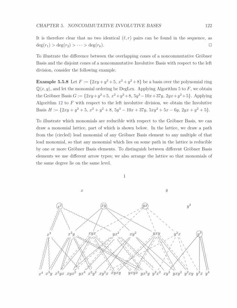
CHAPTER 5. NONCOMMUTATIVE INVOLUTIVE BASES 122
It is therefore clear that no two identical (ℓ, r) pairs can be found in the sequence, as
deg(r1) > deg(r2) > · · · > deg(rk).
To illustrate the difference between the overlapping cones of a noncommutative Grobner
Basis and the disjoint cones of a noncommutative Involutive Basis with respect to the left
division, consider the following example.
Example 5.5.8 Let F := 2xy+ y2+5, x2+ y2+8 be a basis over the polynomial ring
Q〈x, y〉, and let the monomial ordering be DegLex. Applying Algorithm 5 to F , we obtain
the Grobner Basis G := 2xy+y2+5, x2+y2+8, 5y3−10x+37y, 2yx+y2+5. Applying
Algorithm 12 to F with respect to the left involutive division, we obtain the Involutive
Basis H := 2xy + y2 + 5, x2 + y2 + 8, 5y3 − 10x+ 37y, 5xy2 + 5x− 6y, 2yx+ y2 + 5.
To illustrate which monomials are reducible with respect to the Grobner Basis, we can
draw a monomial lattice, part of which is shown below. In the lattice, we draw a path
from the (circled) lead monomial of any Grobner Basis element to any multiple of that
lead monomial, so that any monomial which lies on some path in the lattice is reducible
by one or more Grobner Basis elements. To distinguish between different Grobner Basis
elements we use different arrow types; we also arrange the lattice so that monomials of
the same degree lie on the same level.
1
x y
?>=<89:;x2
IIIIIIII
IIIIIIII
VVVVVVVV
'g'g'g'g
'g'g'g'g
'g'g'g'g
'g'g'g'g
'g'g'g
?>=<89:;xy
AAAA
AAAA
AAAA
AAAA
A
NNNNNNNNNNNNNNNNNNNNNNNNNNN ?>=<89:;yx
p p p p p p p p p p p p p p
,,
,,
,,
,
CC
CC
CC
CC
C y2
x3
LLLLLLLLLLLL
LLLLLLLLLLLL
OOOOOOOOOOOO
\\\\\\\\\\\\\\\
x2y
0000
0000
0000
0000
0000
JJJJJJJJJJJJ
&f&f&f&f
&f&f&f&f
&f&f&f&f
&f&f&f&f
&f&f&f&f
&f&f&f&f
&f
FFFFFFFFFFFFF
WWWWWWWWWWWWW
NNNNNNNNNNNNNNNNNNNNNNNNNNNNNNNNNNNNNN xyx
2222
2222
2222
2222
2222
2
@@@@
@@@@
@@@@
@@@@
@@@@
@@@@
@@
22
22
22
22
22
2
@@
@@
@@
@@
@@
@@
@ yx2
@@
@@
@@
@@
@@
@@
@
77
77
77
77
77
7
AAAAAAAAAAAAAAA
=================
` `
` `
` `
` `
` `
` `
` `
` `
[[[[[[[[[[[[[[
xy2
~~~~
~~~~
~~~~
~~~~
~~~~
~~~~
~
::::
::::
::::
::::
::::
::
CCCC
CCCC
CCCC
CCCC
CCCC
CCCC
CCyxy
~~~~
~~~~
~~~~
~~~~
~~~~
~~~~
~~
0000
0000
0000
0000
0000
9999
9999
9999
9999
9999
999
~~
~~
~~
~~
~~
~~
~
00
00
00
00
00
99
99
99
99
99
99
y2x
))
))
))
))
)
11
11
11
11
11
p p p p p p p p p p p p p p p p p p p?>=<89:;y3
x4 x3y x2yx xyx2 yx3 x2y2 xy2x xyxy yxyx yx2y y2x2 xy3 yxy2 y2xy y3x y4

CHAPTER 5. NONCOMMUTATIVE INVOLUTIVE BASES 123
Notice that many of the monomials in the lattice are reducible by several of the Grobner
Basis elements. For example, the monomial x2yx is reducible by the Grobner Basis
elements 2xy + y2 + 5; x2 + y2 + 8 and 2yx + y2 + 5. In contrast, any monomial in the
corresponding lattice for the Involutive Basis may only be involutively reducible by at
most one element in the Involutive Basis. We illustrate this by the following diagram,
where we note that in the involutive lattice, a monomial only lies on a particular path if
a member of the Involutive Basis is an involutive divisor of that monomial.
1
x y
?>=<89:;x2
IIIIIIII
'g'g'g'g
'g'g'g'g
'g'g'g'g
'g'g'g'g
'g'g'g
?>=<89:;xy
NNNNNNNNNNNNNNNNNNNNNNNNNNN ?>=<89:;yx
p p p p p p p p p p p p p p
CC
CC
CC
CC
C y2
x3
LLLLLLLLLLLL
\\\\\\\\\\\\\\\
x2y
NNNNNNNNNNNNNNNNNNNNNNNNNNNNNNNNNNNNNN xyx
@@
@@
@@
@@
@@
@@
@ yx2
=================
` `
` `
` `
` `
` `
` `
` `
` `
GFED@ABCxy2
yxy
~~~~
~~~~
~~~~
~~~~
~~~~
~~~~
~~
9999
9999
9999
9999
9999
999 y2x
11
11
11
11
11
p p p p p p p p p p p p p p p p p p p?>=<89:;y3
x4 x3y x2yx xyx2 yx3 x2y2 xy2x xyxy yxyx yx2y y2x2 xy3 yxy2 y2xy y3x y4
Comparing the two monomial lattices, we see that any monomial that is conventionally
divisible by the Grobner Basis is uniquely involutively divisible by the Involutive Basis.
In other words, the involutive cones of the Involutive Basis form a disjoint cover of the
conventional cones of the Grobner Basis.
Fast Reduction
In the commutative case, we can sometimes use the properties of an involutive division
to speed up the process of involutively reducing a polynomial with respect to a set of
polynomials. For example, the Janet tree [27, 28] enables us to quickly determine whether
a polynomial is involutively reducible by a set of polynomials with respect to the Janet
involutive division.

CHAPTER 5. NONCOMMUTATIVE INVOLUTIVE BASES 124
In the noncommutative case, we usually use Algorithm 10 to involutively reduce a poly-
nomial p with respect to a set of polynomials P . When this is done with respect to the
left or right divisions however, we can improve Algorithm 10 by taking advantage of the
fact that a monomial u1 only involutively divides another monomial u2 with respect to
the left (right) division if u1 is a suffix (prefix) of u2.
For the left division, we can replace the code found in the first if loop of Algorithm 10 with
the following code in order to obtain an improved algorithm.
if (LM(pj) is a suffix of u) then
found = true;
p = p− (cLC(pj)−1)uℓpj, where uℓ = Prefix(p, deg(p)− deg(pj));
else
j = j + 1;
end if
We note that only one operation is required to determine whether the monomial LM(pj)
involutively divides the monomial u here (test to see if LM(pj) is a suffix of u); whereas in
general there are many ways that LM(pj) can conventionally divide u, each of which has
to be tested to see whether it is an involutive reduction. This means that, with respect
to the left or right divisions, we can determine whether a monomial u is involutively
irreducible with respect to a set of polynomials P in linear time (linear in the number of
elements in P ); whereas in general we can only do this in quadratic time.
5.5.2 An Overlap-Based Local Division
Even though the left and right involutive divisions are strong and continuous (so that any
Locally Involutive Basis returned by Algorithm 12 is a noncommutative Grobner Basis),
these divisions are not conclusive as the following example demonstrates.
Example 5.5.9 Let F := xy − z, x + z, yz − z, xz, zy + z, z2 be a basis over the
polynomial ring Q〈x, y, z〉, and let the monomial ordering be DegLex. Applying Algorithm
5 to F , we discover that F is a noncommutative Grobner Basis (F is returned to us as
the output of Algorithm 5). When we apply Algorithm 12 to F with respect to the
left involutive division however, we notice that the algorithm goes into an infinite loop,
constructing the infinite basis G := F ∪zyn−z, xyn+z, zym+z, xym−z, where n > 2,
n even and m > 3, m odd.

CHAPTER 5. NONCOMMUTATIVE INVOLUTIVE BASES 125
The reason why Algorithm 12 goes into an infinite loop in the above example is that the
right prolongations of the polynomials xy− z and zy+ z by the variable y do not involu-
tively reduce to zero (they reduce to the polynomials xy2 + z and zy2 − z respectively).
These prolongations are the only prolongations of elements of F that do not involutively
reduce to zero, and this is also true for all polynomials we subsequently add to F , thus
allowing Algorithm 12 to construct the infinite set G.
Consider a modification of the left division where we assign the variable y to be right
multiplicative for the (lead) monomials xy and zy. Then it is clear that F will be a
Locally Involutive Basis with respect to this modified division, but will it also be true
that F is an Involutive Basis and (had we not known so already) a Grobner Basis?
Intuitively, for this particular example, it would seem that the answer to both of the
above questions should be affirmative, because the modified division still ensures that
all the overlap words associated with the S-polynomials of F are involutively irreducible
(as placed in the overlap word) by at least one of the polynomials associated to each
S-polynomial. This leads to the following idea for a local involutive division, where we
refine the left division by choosing right nonmultiplicative variables based on the overlap
words of S-polynomials associated to a set of polynomials only (note that there will also
be a similar local involutive division refining the right division called the right overlap
division).
Definition 5.5.10 (The Left Overlap Division O) Let U = u1, . . . , um be a set of
monomials, and assume that all variables are left and right multiplicative for all elements
of U to begin with.
(a) For all possible ways that a monomial uj ∈ U is a subword of a (different) monomial
ui ∈ U , so that
Subword(ui, k, k + deg(uj)− 1) = uj
for some integer k, if uj is not a suffix of ui, assign the variable Subword(ui, k +
deg(uj), k + deg(uj)) to be right nonmultiplicative for uj.
(b) For all possible ways that a proper prefix of a monomial ui ∈ U is equal to a proper
suffix of a (not necessarily different) monomial uj ∈ U , so that
Prefix(ui, k) = Suffix(uj, k)

CHAPTER 5. NONCOMMUTATIVE INVOLUTIVE BASES 126
for some integer k and ui is not a subword of uj or vice-versa, assign the variable
Subword(ui, k + 1, k + 1) to be right nonmultiplicative for uj.
Remark 5.5.11 One possible algorithm for the left overlap division is presented in Al-
gorithm 13, where the reason for insisting that the input set of monomials is ordered with
respect to DegRevLex is in order to minimise the number of operations needed to discover
all the subword overlaps (a monomial of degree d1 can never be a subword of a different
monomial of degree d2 6 d1).
Example 5.5.12 Consider again the set of polynomials F := xy − z, x + z, yz −
z, xz, zy + z, z2 from Example 5.5.9. Here are the left and right multiplicative vari-
ables for LM(F ) with respect to the left overlap division O.
u MLO(u,LM(F )) MR
O(u,LM(F ))
xy x, y, z x, y
x x, y, z x
yz x, y, z x
xz x, y, z x
zy x, y, z x, y
z2 x, y, z x
When we apply Algorithm 12 to F with respect to the DegLex monomial ordering and the
left overlap division, F is returned to us as the output, an assertion that is easily verified
by showing that the 10 right prolongations of elements of F all involutively reduce to zero
using F . This means that F is a Locally Involutive Basis with respect to the left overlap
division; to show that F (and indeed any Locally Involutive Basis returned by Algorithm
12 with respect to the left overlap division) is also an Involutive Basis with respect to
the left overlap division, we need to show that the left overlap division is continuous and
either strong or Grobner; we begin (after the following remark) by showing that the left
overlap division is continuous.
Remark 5.5.13 In the above example, the table of multiplicative variables can be con-
structed from the table T shown below, a table that is obtained by applying Algorithm
13 to LM(F ).

CHAPTER 5. NONCOMMUTATIVE INVOLUTIVE BASES 127
Algorithm 13 The Left Overlap Division O
Input: A set of monomials U = u1, . . . , um ordered by DegRevLex (u1 > u2 > · · · >
um), where ui ∈ R〈x1, . . . , xn〉.
Output: A table T of left and right multiplicative variables for all ui ∈ U , where each
entry of T is either 1 (multiplicative) or 0 (nonmultiplicative).
Create a table T of multiplicative variables as shown below:
xL1 xR
1 xL2 xR
2 · · · xLn xR
n
u1 1 1 1 1 · · · 1 1u2 1 1 1 1 · · · 1 1...
......
......
. . ....
...um 1 1 1 1 · · · 1 1
for each monomial ui ∈ U (1 6 i 6 m) do
for each monomial uj ∈ U (i 6 j 6 m) do
Let ui = xi1xi2 . . . xiα and uj = xj1xj2 . . . xjβ ;
if (i 6= j) then
for each k (1 6 k < α− β + 1) do
if (Subword(ui, k, k + β − 1) == uj) then
T (uj, xRik+β
) = 0;
end if
end for
end if
for each k (1 6 k 6 β − 1) do
if (Prefix(ui, k) == Suffix(uj, k)) then
T (uj, xRik+1
) = 0;
end if
if (Suffix(ui, k) == Prefix(uj, k)) then
T (ui, xRjk+1
) = 0;
end if
end for
end for
end for
return T ;

CHAPTER 5. NONCOMMUTATIVE INVOLUTIVE BASES 128
Monomial xL xR yL yR zL zR
xy 1 1 1 1 1 0
x 1 1 1 0 1 0
yz 1 1 1 0 1 0
xz 1 1 1 0 1 0
zy 1 1 1 1 1 0
z2 1 1 1 0 1 0
The zero entries in T correspond to the following overlaps between the elements of LM(F ).
Table Entry Overlap
T (xy, zR) Suffix(xy, 1) = Prefix(yz, 1)
T (x, yR) Subword(xy, 1, 1) = x
T (x, zR) Subword(xz, 1, 1) = x
T (yz, yR) Suffix(yz, 1) = Prefix(zy, 1)
T (yz, zR) Suffix(yz, 1) = Prefix(z2, 1)
T (xz, yR) Suffix(xz, 1) = Prefix(zy, 1)
T (xz, zR) Suffix(xz, 1) = Prefix(z2, 1)
T (zy, zR) Suffix(zy, 1) = Prefix(yz, 1)
T (z2, yR) Suffix(z2, 1) = Prefix(zy, 1)
T (z2, zR) Suffix(z2, 1) = Prefix(z2, 1)
Proposition 5.5.14 The left overlap division O is continuous.
Proof: Let w be an arbitrary fixed monomial; let U be any set of monomials; and
consider any sequence (u1, u2, . . . , uk) of monomials from U (ui ∈ U for all 1 6 i 6 k),
each of which is a conventional divisor of w (so that w = ℓiuiri for all 1 6 i 6 k, where
the ℓi and the ri are monomials). For all 1 6 i < k, suppose that the monomial ui+1
satisfies condition (b) of Definition 5.4.2 (condition (a) can never be satisfied because O
never assigns any left nonmultiplicative variables). To show that O is continuous, we
must show that no two pairs (ℓi, ri) and (ℓj, rj) are the same, where i 6= j.
Consider an arbitrary monomial ui from the sequence, where 1 6 i < k. By definition of
O, the next monomial ui+1 in the sequence cannot be either a prefix or a proper subword
of ui. This leaves two possibilities: (i) ui+1 is a suffix of ui (in which case deg(ui+1) <
deg(ui)); or (ii) ui+1 is a suffix of the prolongation uivi of ui, where vi := Prefix(ri, 1).

CHAPTER 5. NONCOMMUTATIVE INVOLUTIVE BASES 129
Example of possibility (i) Example of possibility (ii)
ooui
//vi
oo
ui+1
//
ooui
//vi
oo
ui+1
//
In both cases, it is clear that we have deg(ri+1) 6 deg(ri), so that deg(r1) > deg(r2) >
· · · > deg(rk). It follows that no two (ℓ, r) pairs in the sequence can be the same, because
for each subsequence ua, ua+1, . . . , ub such that deg(ra) = deg(ra+1) = · · · = deg(rb), we
must have deg(ℓa) < deg(ℓa+1) < · · · < deg(ℓb).
Having shown that the left overlap division is continuous, one way of showing that every
Locally Involutive Basis with respect to the left overlap division is an Involutive Basis
would be to show that the left overlap division is a strong involutive division. However,
the left overlap division is only a weak involutive division, as the following counterexample
demonstrates.
Proposition 5.5.15 The left overlap division is a weak involutive division.
Proof: Let U := yz, xy be a set of monomials over the polynomial ring Q〈x, y, z〉.
Here are the multiplicative variables for U with respect to the left overlap division O.
u MLO(u, U) MR
O(u, U)
yz x, y, z x, y, z
xy x, y, z x, y
Because yzxy ∈ CO(yz, U) and yzxy ∈ CO(xy, U), one of the conditions CO(yz, U) ⊂
CO(xy, U) or CO(xy, U) ⊂ CO(yz, U) must be satisfied in order for O to be a strong
involutive division (this is the Disjoint Cones condition of Definition 5.1.6). But neither
of these conditions can be satisfied when we consider that xy /∈ CO(yz, U) and yz /∈
CO(xy, U), so O must be a weak involutive division.
The weakness of the left overlap division is the price we pay for refining the left division
by allowing more right multiplicative variables. All is not lost however, as we can still
show that every Locally Involutive Basis with respect to the left overlap division is an
Involutive Basis by showing that the left overlap division is a Grobner involutive division.
Proposition 5.5.16 The left overlap division O is a Grobner involutive division.

CHAPTER 5. NONCOMMUTATIVE INVOLUTIVE BASES 130
Proof: We are required to show that if Algorithm 12 terminates with O and some
arbitrary admissible monomial ordering O as input, then the Locally Involutive Basis
G it returns is a noncommutative Grobner Basis. By Definition 3.1.8, we can do this
by showing that all S-polynomials involving elements of G conventionally reduce to zero
using G.
Assume that G = g1, . . . , gp is sorted (by lead monomial) with respect to the DegRevLex
monomial ordering (greatest first), and let U = u1, . . . , up := LM(g1), . . . ,LM(gp) be
the set of leading monomials. Let T be the table obtained by applying Algorithm 13 to
U . Because G is a Locally Involutive Basis, every zero entry T (ui, xΓj ) (Γ ∈ L,R) in
the table corresponds to a prolongation gixj or xjgi that involutively reduces to zero.
Let S be the set of S-polynomials involving elements of G, where the t-th entry of S
(1 6 t 6 |S|) is the S-polynomial
st = ctℓtgirt − c′tℓ′tgjr
′t,
with ℓtuirt = ℓ′tujr′t being the overlap word of the S-polynomial. We will prove that every
S-polynomial in S conventionally reduces to zero using G.
Recall (from Definition 3.1.2) that each S-polynomial in S corresponds to a particular type
of overlap — ‘prefix’, ‘subword’ or ‘suffix’. For the purposes of this proof, let us now split
the subword overlaps into three further types — ‘left’, ‘middle’ and ‘right’, corresponding
to the cases where a monomial m2 is a prefix, proper subword and suffix of a monomial
m1.
Left Middle Right
oom1
//
oo
m2
//
oom1
//
oo
m2
//
oom1
//
oo
m2
//
This classification provides us with five cases to deal with in total, which we shall process
in the following order: right, middle, left, prefix, suffix.
(1) Consider an arbitrary entry st ∈ S (1 6 t 6 |S|) corresponding to a right overlap
where the monomial uj is a suffix of the monomial ui. Because O never assigns any left
nonmultiplicative variables, uj must be an involutive divisor of ui. But this contradicts
the fact that the set G is autoreduced; it follows that no S-polynomials corresponding to

CHAPTER 5. NONCOMMUTATIVE INVOLUTIVE BASES 131
right overlaps can appear in S.
(2) Consider an arbitrary entry st ∈ S (1 6 t 6 |S|) corresponding to a middle overlap
where the monomial uj is a proper subword of the monomial ui. This means that st =
ctgi − c′tℓ′tgjr
′t for some gi, gj ∈ G, with overlap word ui = ℓ′tujr
′t. Let ui = xi1 . . . xiα ; let
uj = xj1 . . . xjβ ; and choose D such that xiD = xjβ .
ui = xi1
___xiD−β
xiD−β+1xiD−β+2
___xiD−1
xiDxiD+1
___xiα
uj =xj1
xj2
___xjβ−1
xjβ
Because uj is a proper subword of ui, it follows that T (uj, xRiD+1
) = 0. This gives rise to
the prolongation gjxiD+1of gj. But we know that all prolongations involutively reduce
to zero (G is a Locally Involutive Basis), so Algorithm 10 must find a monomial uk =
xk1 . . . xkγ ∈ U such that uk involutively divides ujxiD+1. Assuming that xkγ = xiκ , we can
deduce that any candidate for uk must be a suffix of ujxiD+1(otherwise T (uk, x
Riκ+1
) = 0
because of the overlap between ui and uk). This means that the degree of uk is in the
range 1 6 γ 6 β + 1; we shall illustrate this in the following diagram by using a squiggly
line to indicate that the monomial uk can begin anywhere (or nowhere if uk = xiD+1) on
the squiggly line.
ui = xi1
___xiD−β
xiD−β+1xiD−β+2
___xiD−1
xiDxiD+1
___xiα
uj =xj1
xj2
___xjβ−1
xjβ
uk = /o/o/o/o/o/o/o/o/o/o/o/o/o/o/o/o/o/o/o/o/o/o/oxkγ
We can now use the monomial uk together with Buchberger’s Second Criterion to simplify
our goal of showing that the S-polynomial st reduces to zero. Notice that the monomial
uk is a subword of the overlap word ui associated to st, and so in order to show that st
reduces to zero, all we have to do is to show that the two S-polynomials
su = cugi − c′u(xi1xi2 . . . xiD+1−γ)gk(xiD+2
. . . xiα)
and2
sv = cv(xj1 . . . xiD+1−γ)gk − c′vgjxiD+1
2Technical point: if γ 6= β + 1, the S-polynomial sv could in fact appear as sv = cvgjxiD+1−
c′v(xj1 . . . xiD+1−γ)gk and not as sv = cv(xj1 . . . xiD+1−γ
)gk − c′vgjxiD+1; for simplicity we will treat both
cases the same in the proof as all that changes is the notation and the signs.

CHAPTER 5. NONCOMMUTATIVE INVOLUTIVE BASES 132
reduce to zero (1 6 u, v 6 |S|).
For the S-polynomial sv, there are two cases to consider: γ = 1, and γ > 1. In the
former case, because (as placed in ui) the monomials uj and uk do not overlap, we can
use Buchberger’s First Criterion to say that the ‘S-polynomial’ sv reduces to zero (for
further explanation, see the paragraph at the beginning of Section 3.4.1). In the latter
case, we know that the first step of the involutive reduction of the prolongation gjxiD+1is
to take away the multiple ( cvc′v)(xj1 . . . xiD+1−γ
)gk of gk from gjxiD+1to leave the polynomial
gjxiD+1− ( cv
c′v)(xj1 . . . xiD+1−γ
)gk = −( 1c′v)sv. But as we know that all prolongations invo-
lutively reduce to zero, we can conclude that the S-polynomial sv conventionally reduces
to zero.
For the S-polynomial su, we note that if D = α−1, then su corresponds to a right overlap.
But we know from part (1) that right overlaps cannot appear in S, and so st also cannot
appear in S. Otherwise, we proceed by induction on the S-polynomial su to produce a
sequence uqD+1, uqD+2
, . . . , uqα of monomials, so that su (and hence st) reduces to zero
if the S-polynomial
sη = cηgi − c′η(xi1 . . . xiα−µ)gqα
reduces to zero (1 6 η 6 |S|), where µ = deg(uqα).
ui = xi1
___xiD−β
xiD−β+1
___xiD
xiD+1xiD+2
___xiα−1
xiα
uj =xj1
___xjβ
uqD+1= uk = /o/o/o/o/o/o/o/o/o/o/o
xkγ
uqD+2= /o/o/o/o/o/o/o/o/o/o/o/o/o/o/o/o
. . .
uqα = /o/o/o/o/o/o/o/o/o/o/o/o/o/o/o/o/o/o/o/o/o/o/o/o/o/o/o/o/o
But sη always corresponds to a right overlap, so we must conclude that middle overlaps
(as well as right overlaps) cannot appear in S.
(3) Consider an arbitrary entry st ∈ S (1 6 t 6 |S|) corresponding to a left overlap where
the monomial uj is a prefix of the monomial ui. This means that st = ctgi − c′tgjr′t for

CHAPTER 5. NONCOMMUTATIVE INVOLUTIVE BASES 133
some gi, gj ∈ G, with overlap word ui = ujr′t. Let ui = xi1 . . . xiα and let uj = xj1 . . . xjβ .
ui = xi1xi2
___xiβ−1
xiβxiβ+1
___xiα−1
xiα
uj =xj1
xj2
___xjβ−1
xjβ
Because uj is a prefix of ui, it follows that T (uj, xRiβ+1
) = 0. This gives rise to the
prolongation gjxiβ+1of gj . But we know that all prolongations involutively reduce to
zero, so there must exist a monomial uk = xk1 . . . xkγ ∈ U such that uk involutively
divides ujxiβ+1. Assuming that xkγ = xiκ , any candidate for uk must be a suffix of ujxiβ+1
(otherwise T (uk, xRiκ+1
) = 0 because of the overlap between ui and uk). Further, any
candidate for uk cannot be either a suffix or a proper subword of ui (because of parts (1)
and (2) of this proof). This leaves only one possibility for uk, namely uk = ujxiβ+1.
ui = xi1xi2
___xiβ−1
xiβxiβ+1
___xiα−1
xiα
uj =xj1
xj2
___xjβ−1
xjβ
uk = xk1xk2
___xkγ−2
xkγ−1xkγ
If α = β+1, then it is clear that uk = ui, and so the first step in the involutive reduction
of the prolongation gjxiα is to take away the multiple ( ctc′t)gi of gi from gjxiα to leave the
polynomial gjxiα − ( ctc′t)gi = −( 1
c′t)st. But as we know that all prolongations involutively
reduce to zero, we can conclude that the S-polynomial st conventionally reduces to zero.
Otherwise, if α > β + 1, we can now use the monomial uk together with Buchberger’s
Second Criterion to simplify our goal of showing that the S-polynomial st reduces to zero.
Notice that the monomial uk is a subword of the overlap word ui associated to st, and
so in order to show that st reduces to zero, all we have to do is to show that the two
S-polynomials
su = cugi − c′ugk(xiβ+2. . . xiα)
and
sv = cvgk − c′vgjxiβ+1
reduce to zero (1 6 u, v 6 |S|).
The S-polynomial sv reduces to zero by comparison with part (2). For the S-polynomial
su, we proceed by induction (we have another left overlap), eventually coming across a
left overlap of ‘type α = β + 1’ because we move one letter at a time to the right after
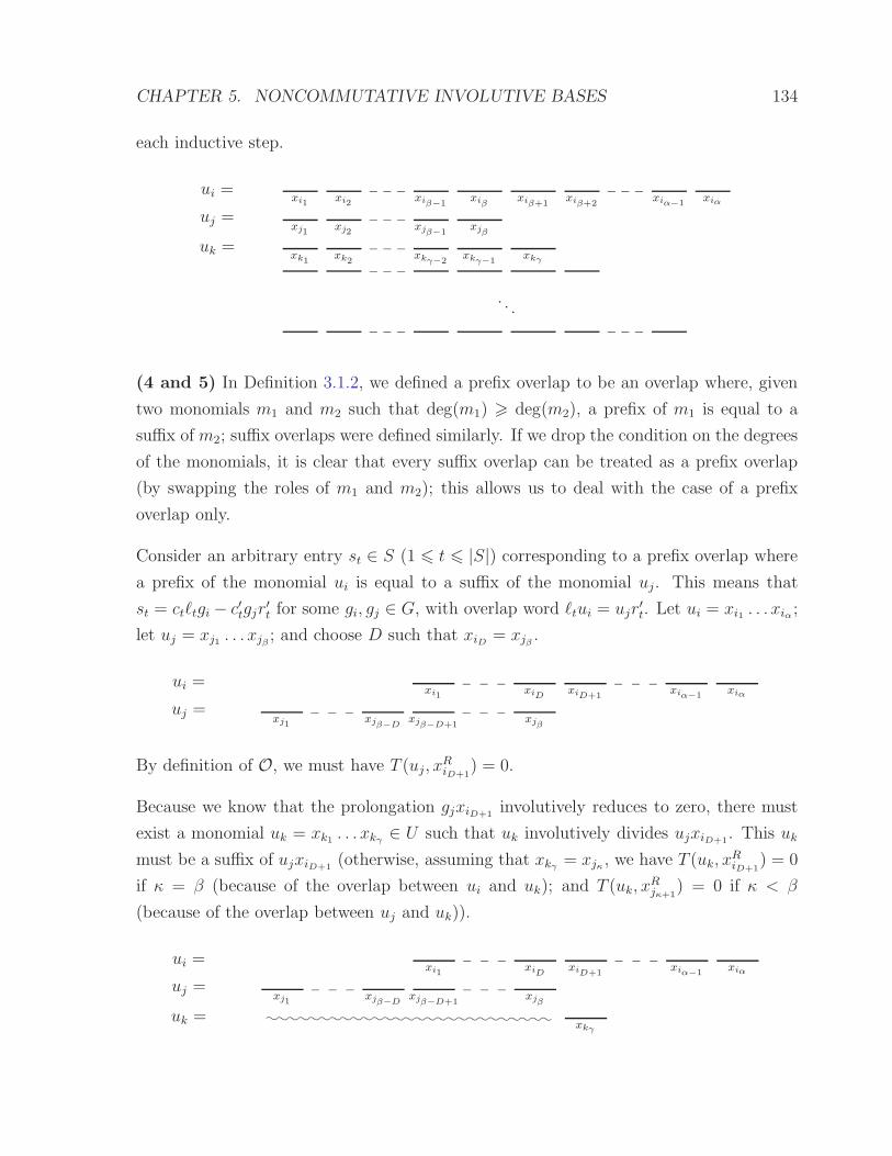
CHAPTER 5. NONCOMMUTATIVE INVOLUTIVE BASES 134
each inductive step.
ui = xi1xi2
___xiβ−1
xiβxiβ+1
xiβ+2
___xiα−1
xiα
uj =xj1
xj2
___xjβ−1
xjβ
uk = xk1xk2
___xkγ−2
xkγ−1xkγ
___
. . .___ ___
(4 and 5) In Definition 3.1.2, we defined a prefix overlap to be an overlap where, given
two monomials m1 and m2 such that deg(m1) > deg(m2), a prefix of m1 is equal to a
suffix of m2; suffix overlaps were defined similarly. If we drop the condition on the degrees
of the monomials, it is clear that every suffix overlap can be treated as a prefix overlap
(by swapping the roles of m1 and m2); this allows us to deal with the case of a prefix
overlap only.
Consider an arbitrary entry st ∈ S (1 6 t 6 |S|) corresponding to a prefix overlap where
a prefix of the monomial ui is equal to a suffix of the monomial uj. This means that
st = ctℓtgi − c′tgjr′t for some gi, gj ∈ G, with overlap word ℓtui = ujr
′t. Let ui = xi1 . . . xiα ;
let uj = xj1 . . . xjβ ; and choose D such that xiD = xjβ .
ui = xi1
___xiD
xiD+1
___xiα−1
xiα
uj =xj1
___xjβ−D
xjβ−D+1
___xjβ
By definition of O, we must have T (uj, xRiD+1
) = 0.
Because we know that the prolongation gjxiD+1involutively reduces to zero, there must
exist a monomial uk = xk1 . . . xkγ ∈ U such that uk involutively divides ujxiD+1. This uk
must be a suffix of ujxiD+1(otherwise, assuming that xkγ = xjκ , we have T (uk, x
RiD+1
) = 0
if κ = β (because of the overlap between ui and uk); and T (uk, xRjκ+1
) = 0 if κ < β
(because of the overlap between uj and uk)).
ui = xi1
___xiD
xiD+1
___xiα−1
xiα
uj =xj1
___xjβ−D
xjβ−D+1
___xjβ
uk = /o/o/o/o/o/o/o/o/o/o/o/o/o/o/o/o/o/o/o/o/o/o/o/o/o/o/oxkγ

CHAPTER 5. NONCOMMUTATIVE INVOLUTIVE BASES 135
Let us now use the monomial uk together with Buchberger’s Second Criterion to simplify
our goal of showing that the S-polynomial st reduces to zero. Because uk is a subword
of the overlap word ℓtui associated to st, in order to show that st reduces to zero, all we
have to do is to show that the two S-polynomials
su =
cu(xk1 . . . xjβ−D)gi − c′ugk(xiD+2
. . . xiα) if γ > D + 1
cugi − c′uℓ′ugk(xiD+2
. . . xiα) if γ 6 D + 1
and
sv = cvgjxiD+1− c′v(xj1 . . . xjβ+1−γ
)gk
reduce to zero (1 6 u, v 6 |S|).
The S-polynomial sv reduces to zero by comparison with part (2). For the S-polynomial
su, first note that if α = D + 1, then either uk is a suffix of ui, ui is a suffix of uk, or
uk = ui; it follows that su reduces to zero trivially if uk = ui, and (by part (1)) su (and
hence st) cannot appear in S in the other two cases.
If however α 6= D + 1, then either su is a middle overlap (if γ < D + 1), a left overlap
(if γ = D + 1), or another prefix overlap. The first case leads us to conclude that st
cannot appear in S; the second case is handled by part (3) of this proof; and the final case
is handled by induction, where we note that after each step of the induction, the value
α+ β − 2D strictly decreases, so we are guaranteed at some stage to find an overlap that
is not a prefix overlap, enabling us either to verify that the S-polynomial st conventionally
reduces to zero, or to conclude that st can not in fact appear in S.
5.5.3 A Strong Local Division
Thus far, we have encountered two global divisions that are strong and continuous, and one
local division that is weak, continuous and Grobner. Our next division can be considered
to be a hybrid of these previous divisions, as it will be a local division that is continuous
and (as long as thick divisors are being used) strong.
Definition 5.5.17 (The Strong Left Overlap Division S) Let U = u1, . . . , um be
a set of monomials. Assign multiplicative variables to U according to Algorithm 15, which
(in words) performs the following two tasks.
(a) Assign multiplicative variables to U according to the left overlap division.

CHAPTER 5. NONCOMMUTATIVE INVOLUTIVE BASES 136
(b) Using the recipe provided in Algorithm 14, ensure that at least one variable in every
monomial uj ∈ U is right nonmultiplicative for each monomial ui ∈ U .
Remark 5.5.18 As Algorithm 15 expects any input set to be ordered with respect to
DegRevLex, we may sometimes have to reorder a set of monomials U to satisfy this
condition before we can assign multiplicative variables to U according to the strong left
overlap division.
Algorithm 14 ‘DisjointCones’ Function for Algorithm 15
Input: A set of monomials U = u1, . . . , um ordered by DegRevLex (u1 > u2 > · · · >
um), where ui ∈ R〈x1, . . . , xn〉; a table T of left and right multiplicative variables for
all ui ∈ U , where each entry of T is either 1 (multiplicative) or 0 (nonmultiplicative).
Output: T .
for each monomial ui ∈ U (m > i > 1) do
for each monomial uj ∈ U (m > j > 1) do
Let ui = xi1xi2 . . . xiα and uj = xj1xj2 . . . xjβ ;
found = false;
k = 1;
while (k 6 β) do
if (T (ui, xRjk) = 0) then
found = true;
k = β + 1;
else
k = k + 1;
end if
end while
if (found == false) then
T (ui, xRj1) = 0;
end if
end for
end for
return T ;

CHAPTER 5. NONCOMMUTATIVE INVOLUTIVE BASES 137
Algorithm 15 The Strong Left Overlap Division S
Input: A set of monomials U = u1, . . . , um ordered by DegRevLex (u1 > u2 > · · · >
um), where ui ∈ R〈x1, . . . , xn〉.
Output: A table T of left and right multiplicative variables for all ui ∈ U , where each
entry of T is either 1 (multiplicative) or 0 (nonmultiplicative).
Create a table T of multiplicative variables as shown below:
xL1 xR
1 xL2 xR
2 · · · xLn xR
n
u1 1 1 1 1 · · · 1 1u2 1 1 1 1 · · · 1 1...
......
......
. . ....
...um 1 1 1 1 · · · 1 1
for each monomial ui ∈ U (1 6 i 6 m) do
for each monomial uj ∈ U (i 6 j 6 m) do
Let ui = xi1xi2 . . . xiα and uj = xj1xj2 . . . xjβ ;
if (i 6= j) then
for each k (1 6 k < α− β + 1) do
if (Subword(ui, k, k + β − 1) == uj) then
T (uj, xRik+β
) = 0;
end if
end for
end if
for each k (1 6 k 6 β − 1) do
if (Prefix(ui, k) == Suffix(uj, k)) then
T (uj, xRik+1
) = 0;
end if
if (Suffix(ui, k) == Prefix(uj, k)) then
T (ui, xRjk+1
) = 0;
end if
end for
end for
end for
T = DisjointCones(U, T ); (Algorithm 14)
return T ;

CHAPTER 5. NONCOMMUTATIVE INVOLUTIVE BASES 138
Proposition 5.5.19 The strong left overlap division is continuous.
Proof: We refer to the proof of Proposition 5.5.14, replacing O by S.
Proposition 5.5.20 The strong left overlap division is a Grobner involutive division.
Proof: We refer to the proof of Proposition 5.5.16, replacing O by S.
Remark 5.5.21 Propositions 5.5.19 and 5.5.20 apply either when using thin divisors or
when using thick divisors.
Proposition 5.5.22 With respect to thick divisors, the strong left overlap division is a
strong involutive division.
Proof: To prove that the strong left overlap division is a strong involutive division, we
need to show that the three conditions of Definition 5.1.6 hold.
• Disjoint Cones Condition
Let CS(u1, U) and CS(u2, U) be the involutive cones associated to the monomials u1
and u2 over some noncommutative polynomial ring R, where u1, u2 ⊂ U ⊂ R. If
CS(u1, U) ∩ CS(u2, U) 6= ∅, then there must be some monomial v ∈ R such that v
contains both monomials u1 and u2 as subwords, and (as placed in v) both u1 and
u2 must be involutive divisors of v. By definition of S, both u1 and u2 must be
suffices of v. Thus, assuming (without loss of generality) that deg(u1) > deg(u2),
we are able to draw the following diagram summarising the situation.
oov
//
oou1
//
oou2
//
For S to be strong, we must have CS(u1, U) ⊂ CS(u2, U) (it is clear that CS(u2, U) 6⊂
CS(u1, U) because u2 /∈ CS(u1, U)). This can be verified by proving that a variable
is right nonmultiplicative for u1 if and only if it is right nonmultiplicative for u2.
(⇒) If an arbitrary variable x is right nonmultiplicative for u2, then either some
monomial u ∈ U overlaps with u2 in one of the ways shown below (where the
variable immediately to the right of u2 is the variable x), or x was assigned right

CHAPTER 5. NONCOMMUTATIVE INVOLUTIVE BASES 139
nonmultiplicative for u2 in order to ensure that some variable in some monomial
u ∈ U is right nonmultiplicative for u2.
Overlap (i) Overlap (ii)
oou
//
oou2
//
oou
//
oou2
//
If the former case applies, then it is clear that for both overlap types there will be
another overlap between u1 and u that will lead S to assign x to be right nonmulti-
plicative for u1. It follows that after we have assigned multiplicative variables to U
according to the left overlap division (which we recall is the first step of assigning
multiplicative variables to U according to S), the right multiplicative variables of
u1 and u2 will be identical. It therefore remains to show that if x is assigned right
nonmultiplicative for u2 in the latter case (which will happen during the final step
of assigning multiplicative variables to U according to S), then x is also assigned
right nonmultiplicative for u1. But this is clear when we consider that Algorithm
14 is used to perform this final step, because for u1 and u2 in Algorithm 14, we will
always analyse each monomial in U in the same order.
(⇐) Use the same argument as above, replacing u1 by u2 and vice-versa.
• Unique Divisor Condition
Given a monomial u belonging to a set of monomials U , u may not involutively
divide an arbitrary monomial v in more than one way (and hence the Unique Divisor
condition is satisfied) because (i) S ensures that no overlap word involving only u
is involutively divisible in more than one way by u; and (ii) S ensures that at least
one variable in u is right nonmultiplicative for u, so that if u appears twice in v
as subwords that are disjoint from one another, then only the ‘right-most’ subword
can potentially be an involutive divisor of v.
• Subset Condition
Let v be a monomial belonging to a set V of monomials, where V itself is a subset of
a larger set U of monomials. Because S assigns no left nonmultiplicative variables,
it is clear that MLS(v, U) ⊆ ML
S(v, V ). To prove that MRS (v, U) ⊆ MR
S (v, V ), note
that if a variable x is right nonmultiplicative for v with respect to U and S (so
that x /∈ MRS (v, U)), then (as in the proof for the Disjoint Cones Condition) either
some monomial u ∈ U overlaps with v in one of the ways shown below (where the

CHAPTER 5. NONCOMMUTATIVE INVOLUTIVE BASES 140
variable immediately to the right of v is the variable x), or x was assigned right
nonmultiplicative for v in order to ensure that some variable in some monomial
u ∈ U is right nonmultiplicative for v.
Overlap (i) Overlap (ii)
oou
//
oov
//
oou
//
oov
//
In both cases, it is clear that, with respect to the set V , the variable x may not be
assigned right nonmultiplicative for v if u /∈ V , so that MRS (v, U) ⊆ MR
S (v, V ) as
required.
Proposition 5.5.23 With respect to thin divisors, the strong left overlap division is a
weak involutive division.
Proof: Let U := xy be a set of monomials over the polynomial ring Q〈x, y〉. Here are
the multiplicative variables for U with respect to the strong left overlap division S.
u MLS(u, U) MR
S (u, U)
xy x, y y
For S to be strong with respect to thin divisors, the monomial xy2xy, which is conven-
tionally divisible by xy in two ways, must only be involutively divisible by xy in one way
(this is the Unique Divisor condition of Definition 5.1.6). However it is clear that xy2xy
is involutively divisible by xy in two ways with respect to thin divisors, so S must be a
weak involutive division with respect to thin divisors.
Example 5.5.24 Continuing Examples 5.5.9 and 5.5.12, here are the multiplicative vari-
ables for the set LM(F ) of monomials with respect to the strong left overlap division S,
where we recall that F := xy − z, x+ z, yz − z, xz, zy + z, z2.

CHAPTER 5. NONCOMMUTATIVE INVOLUTIVE BASES 141
u MLS(u,LM(F )) MR
S (u,LM(F ))
xy x, y, z y
x x, y, z ∅
yz x, y, z ∅
xz x, y, z ∅
zy x, y, z y
z2 x, y, z ∅
When we apply Algorithm 12 to F with respect to the DegLex monomial ordering, thick
divisors and the strong left overlap division, F (as in Example 5.5.12) is returned to us
as the output Locally Involutive Basis.
Remark 5.5.25 In the above example, even though we know that S is continuous, we
cannot deduce that the Locally Involutive Basis F is an Involutive Basis because we are
using thick divisors (Proposition 5.4.3 does not apply in the case of using thick divisors).
What this means is that the involutive cones of F (and in general any Locally Involutive
Basis with respect to S and thick divisors) will be disjoint (because S is strong), but will
not necessarily completely cover the conventional cones of F , so that some monomials
that are conventionally reducible by F may not be involutively reducible by F . It follows
that when involutively reducing a polynomial with respect to F , the reduction path will
be unique but the correct remainder may not always be obtained (in the sense that some
of the terms in our ‘remainder’ may still be conventionally reducible by members of F ).
One remedy to this problem would be to involutively reduce a polynomial p with respect
to F to obtain a remainder r, and then to conventionally reduce r with respect to F
to obtain a remainder r′ which we can be sure contains no term that is conventionally
reducible by F .
Let us now summarise (with respect to thin divisors) the properties of the involutive
divisions we have encountered so far, where we note that any strong and continuous
involutive division is by default a Grobner involutive division.
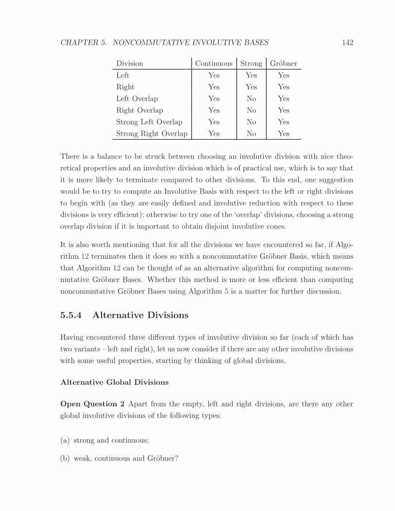
CHAPTER 5. NONCOMMUTATIVE INVOLUTIVE BASES 142
Division Continuous Strong Grobner
Left Yes Yes Yes
Right Yes Yes Yes
Left Overlap Yes No Yes
Right Overlap Yes No Yes
Strong Left Overlap Yes No Yes
Strong Right Overlap Yes No Yes
There is a balance to be struck between choosing an involutive division with nice theo-
retical properties and an involutive division which is of practical use, which is to say that
it is more likely to terminate compared to other divisions. To this end, one suggestion
would be to try to compute an Involutive Basis with respect to the left or right divisions
to begin with (as they are easily defined and involutive reduction with respect to these
divisions is very efficient); otherwise to try one of the ‘overlap’ divisions, choosing a strong
overlap division if it is important to obtain disjoint involutive cones.
It is also worth mentioning that for all the divisions we have encountered so far, if Algo-
rithm 12 terminates then it does so with a noncommutative Grobner Basis, which means
that Algorithm 12 can be thought of as an alternative algorithm for computing noncom-
mutative Grobner Bases. Whether this method is more or less efficient than computing
noncommutative Grobner Bases using Algorithm 5 is a matter for further discussion.
5.5.4 Alternative Divisions
Having encountered three different types of involutive division so far (each of which has
two variants – left and right), let us now consider if there are any other involutive divisions
with some useful properties, starting by thinking of global divisions.
Alternative Global Divisions
Open Question 2 Apart from the empty, left and right divisions, are there any other
global involutive divisions of the following types:
(a) strong and continuous;
(b) weak, continuous and Grobner?

CHAPTER 5. NONCOMMUTATIVE INVOLUTIVE BASES 143
Remark 5.5.26 It seems unlikely that a global division will exist that affirmatively an-
swers Open Question 2 and does not either assign all variables to be left nonmultiplicative
or all right nonmultiplicative (thus refining the right or left divisions respectively). The
reason for saying this is because the moment you have one variable being left multiplica-
tive and another variable being right multiplicative for the same monomial globally, then
you risk not being able to prove that your division is strong; similarly the moment you
have one variable being left nonmultiplicative and another variable being right nonmulti-
plicative for the same monomial globally, then you risk not being able to prove that your
division is continuous.
Alternative Local Divisions
So far, all the local divisions we have considered have assigned all variables to be mul-
tiplicative on one side, and have chosen certain variables to be nonmultiplicative on the
other side. Let us now consider a local division that modifies the left overlap division by
assigning some variables to be nonmultiplicative on both left and right hand sides.
Definition 5.5.27 (The Two-Sided Left Overlap Division W) Consider a set U =
u1, . . . , um of monomials, where all variables are assumed to be left and right multiplica-
tive for all elements of U to begin with. Assign multiplicative variables to U according to
Algorithm 16, which (in words) performs the following tasks.
(a) For all possible ways that a monomial uj ∈ U is a subword of a (different) monomial
ui ∈ U , so that
Subword(ui, k, k + deg(uj)− 1) = uj
for some integer k, assign the variable Subword(ui, k−1, k−1) to be left nonmultiplica-
tive for uj if uj is a suffix of ui; and assign the variable Subword(ui, k + deg(uj), k +
deg(uj)) to be right nonmultiplicative for uj if uj is not a suffix of ui.
(b) For all possible ways that a proper prefix of a monomial ui ∈ U is equal to a proper
suffix of a (not necessarily different) monomial uj ∈ U , so that
Prefix(ui, k) = Suffix(uj, k)
for some integer k and ui is not a subword of uj or vice-versa, use the recipe provided in
the second half of Algorithm 16 to ensure that at least one of the following conditions

CHAPTER 5. NONCOMMUTATIVE INVOLUTIVE BASES 144
are satisfied: (i) the variable Subword(ui, k + 1, k + 1) is right nonmultiplicative for
uj; (ii) the variable Subword(uj, deg(uj)− k, deg(uj)− k) is left nonmultiplicative for
ui.
Remark 5.5.28 For task (b) above, Algorithm 16 gives preference to monomials which
are greater in the DegRevLex monomial ordering (given the choice, it always assigns
a nonmultiplicative variable to whichever monomial out of ui and uj is the smallest);
it also attempts to minimise the number of variables made nonmultiplicative by only
assigning a variable to be nonmultiplicative if both the variables Subword(ui, k+1, k+1)
and Subword(uj, deg(uj) − k, deg(uj) − k) are respectively right multiplicative and left
multiplicative. These refinements will become crucial when proving the continuity of the
division.
Example 5.5.29 Consider the set of monomials U := zx2yxy, yzx, xy over the poly-
nomial ring Q〈x, y, z〉. Here are the left and right multiplicative variables for U with
respect to the two-sided left overlap division W.
u MLW(u, U) MR
W(u, U)
zx2yxy x, y, z x, y, z
yzx y, z y, z
xy x y, z
The above table is constructed from the table T shown below, a table which is obtained
by applying Algorithm 16 to U .
Monomial xL xR yL yR zL zR
zx2yxy 1 1 1 1 1 1
yzx 0 0 1 1 1 1
xy 1 0 0 1 0 1
The zero entries in T correspond to the following overlaps between the elements of U
(presented in the order in which Algorithm 16 encounters them).

CHAPTER 5. NONCOMMUTATIVE INVOLUTIVE BASES 145
Algorithm 16 The Two-Sided Left Overlap Division W
Input: A set of monomials U = u1, . . . , um ordered by DegRevLex (u1 > u2 > · · · >
um), where ui ∈ R〈x1, . . . , xn〉.
Output: A table T of left and right multiplicative variables for all ui ∈ U , where each
entry of T is either 1 (multiplicative) or 0 (nonmultiplicative).
Create a table T of multiplicative variables as shown below:
xL1 xR
1 xL2 xR
2 · · · xLn xR
n
u1 1 1 1 1 · · · 1 1...
......
......
. . ....
...um 1 1 1 1 · · · 1 1
for each monomial ui ∈ U (1 6 i 6 m) do
for each monomial uj ∈ U (i 6 j 6 m) do
Let ui = xi1xi2 . . . xiα and uj = xj1xj2 . . . xjβ ;
if (i 6= j) then
for each k (1 6 k 6 α− β + 1) do
if (Subword(ui, k, k + β − 1) == uj) then
if (k < α− β + 1) then T (uj, xRik+β
) = 0;
else T (uj, xLik−1
) = 0;
end if
end if
end for
end if
for each k (1 6 k 6 β − 1) do
if (Prefix(ui, k) == Suffix(uj, k)) then
if (T (ui, xLjβ−k
) + T (uj, xRik+1
) == 2) then T (uj, xRik+1
) = 0;
end if
end if
if (Suffix(ui, k) == Prefix(uj, k)) then
if (T (ui, xRjk+1
) + T (uj, xLiα−k
) == 2) then T (uj, xLiα−k
) = 0;
end if
end if
end for
end for
end for
return T ;

CHAPTER 5. NONCOMMUTATIVE INVOLUTIVE BASES 146
Table Entry Overlap
T (yzx, xR) Prefix(zx2yxy, 2) = Suffix(yzx, 2)
T (yzx, xL) Suffix(zx2yxy, 1) = Prefix(yzx, 1)
T (xy, xR) Subword(zx2yxy, 3, 4) = xy
T (xy, yL) Subword(zx2yxy, 5, 6) = xy
T (xy, zL) Suffix(yzx, 1) = Prefix(xy, 1)
Notice that the overlap Prefix(yzx, 1) = Suffix(xy, 1) does not produce a zero entry for
T (xy, zR), as by the time that we encounter this overlap in the algorithm, we have already
assigned T (yzx, xL) = 0.
Proposition 5.5.30 The two-sided left overlap division W is a weak involutive division.
Proof: We refer to the proof of Proposition 5.5.15, making the obvious changes (for
example replacing O by W).
For the following two propositions, we defer their proofs to Appendix A due to their
length and technical nature.
Proposition 5.5.31 The two-sided left overlap division W is continuous.
Proof: We refer to Appendix A.
Proposition 5.5.32 The two-sided left overlap division W is a Grobner involutive divi-
sion.
Proof: We refer to Appendix A, noting that the proof is similar to the proof of Propo-
sition 5.5.16.
Remark 5.5.33 Because a variable is sometimes only assigned nonmultiplicative if two
other variables are multiplicative in Algorithm 16, the subset condition of Definition 5.1.6
will not always be satisfied with respect to the two-sided left overlap division. This will
still hold true even if we apply Algorithm 14 at the end of Algorithm 16, which means
that the two-sided left overlap division cannot be converted to give a strong involutive
division in the same way that we converted the left overlap division to give the strong left
overlap division.

CHAPTER 5. NONCOMMUTATIVE INVOLUTIVE BASES 147
To finish this section, let us now consider some further variations of the left overlap
division, variations that will allow us to assign more multiplicative variables than the left
overlap division (and hence potentially have to deal with fewer prolongations when using
Algorithm 12), but variations that cannot be modified to give strong involutive divisions
in the same way that the left overlap division was modified to give the strong left overlap
division (this is because there are other ways beside a monomial being a suffix of another
monomial that two involutive cones can be non-disjoint with respect to these modified
divisions).
Definition 5.5.34 (The Prefix-Only Left Overlap Division) Let U = u1, . . . , um
be a set of monomials, and assume that all variables are left and right multiplicative for
all elements of U to begin with.
(a) For all possible ways that a monomial uj ∈ U is a proper prefix of a monomial ui ∈ U ,
assign the variable Subword(ui, deg(uj)+1, deg(uj)+1) to be right nonmultiplicative
for uj.
(b) For all possible ways that a proper prefix of a monomial ui ∈ U is equal to a proper
suffix of a (not necessarily different) monomial uj ∈ U , so that
Prefix(ui, k) = Suffix(uj, k)
for some integer k and ui is not a subword of uj or vice-versa, assign the variable
Subword(ui, k + 1, k + 1) to be right nonmultiplicative for uj.
Definition 5.5.35 (The Subword-Free Left Overlap Division) Consider a set U =
u1, . . . , um of monomials, where all variables are assumed to be left and right multi-
plicative for all elements of U to begin with.
For all possible ways that a proper prefix of a monomial ui ∈ U is equal to a proper suffix
of a (not necessarily different) monomial uj ∈ U , so that
Prefix(ui, k) = Suffix(uj, k)
for some integer k and ui is not a subword of uj or vice-versa, assign the variable
Subword(ui, k + 1, k + 1) to be right nonmultiplicative for uj.
Proposition 5.5.36 Both the prefix-only left overlap and the subword-free left overlap
divisions are continuous, weak and Grobner.

CHAPTER 5. NONCOMMUTATIVE INVOLUTIVE BASES 148
Proof: We leave these proofs as exercises for the interested reader, noting that the
proofs will be based on (and in some cases will be identical to) the proofs of Propositions
5.5.14, 5.5.15 and 5.5.16 respectively.
Remark 5.5.37 To help distinguish between the different types of overlap division we
have encountered in this chapter, let us now give the following table showing which types
of overlap each overlap division considers.
Type A Type B Type C Type D
oo //
oo //
oo //
oo //
oo //
oo //
oo //
oo //
Overlap Division Type Overlap Type
A B C D
Left X X X ×
Right X × X X
Strong Left X X X ×
Strong Right X × X X
Two-Sided Left X X X X
Two-Sided Right X X X X
Prefix-Only Left X X × ×
Suffix-Only Right X × × X
Subword-Free Left X × × ×
Subword-Free Right X × × ×
5.6 Termination
Given a basis F generating an ideal over a noncommutative polynomial ring R, does there
exist a finite Involutive Basis for F with respect to some admissible monomial ordering
O and some involutive division I? Unlike the commutative case, where the answer to the
corresponding question (for certain divisions) is always ‘Yes’, the answer to this question
can potentially be ‘No’, as if the noncommutative Grobner Basis for F with respect to
O is infinite, then the noncommutative Involutive Basis algorithm will not find a finite
Involutive Basis for F with respect to I and O, as it will in effect be trying to compute
the same infinite Grobner Basis.
CHAPTER 5. NONCOMMUTATIVE INVOLUTIVE BASES 149
However, a valid follow-up question would be to ask whether the noncommutative In-
volutive Basis algorithm will terminate in the case that the noncommutative Grobner
Basis algorithm terminates. In Section 5.4, we defined a property of noncommutative
involutive divisions (conclusivity) that ensures, when satisfied, that the answer to this
secondary question is always ‘Yes’. Despite this, we will not prove in this thesis that
any of the divisions we have defined are conclusive. Instead, we leave the following open
question for further investigation.
Open Question 3 Are there any conclusive noncommutative involutive divisions that
are also continuous and either strong or Grobner?
To obtain an affirmative answer to the above question, one approach may be to start by
finding a proof for the following conjecture.
Conjecture 5.6.1 Let O be an arbitrary admissible monomial ordering, and let I be
an arbitrary involutive division that is continuous and either strong or Grobner. When
computing an Involutive Basis for some basis F with respect to O and I using Algorithm
12, if F possesses a finite unique reduced Grobner Basis G with respect to O, then after
a finite number of steps of Algorithm 12, LM(G) appears as a subset of the set of leading
monomials of the current basis.
To prove that a particular involutive division is conclusive, we would then need to show
that once LM(G) appears as a subset of the set of leading monomials of the current basis,
then the noncommutative Involutive Basis algorithm terminates (either immediately or
in a finite number of steps), thus providing the required finite noncommutative Involutive
Basis for F .
5.7 Examples
5.7.1 A Worked Example
Example 5.7.1 Let F := f1, f2 = x2y2 − 2xy2 + x2, x2y − 2xy be a basis for an
ideal J over the polynomial ring Q〈x, y〉, and let the monomial ordering be DegLex. Let
us now compute a Locally Involutive Basis for F with respect to the strong left overlap
division S and thick divisors using Algorithm 12.

CHAPTER 5. NONCOMMUTATIVE INVOLUTIVE BASES 150
To begin with, we must autoreduce the input set F . This leaves the set unchanged,
as we can verify by using the following table of multiplicative variables (obtained by
using Algorithm 15), where y is right nonmultiplicative for f2 because of the overlap
LM(f2) = Subword(LM(f1), 1, 3); and x is right nonmultiplicative for f1 because we need
to have a variable in LM(f2) being right nonmultiplicative for f1.
Polynomial MLS(fi, F ) MR
S (fi, F )
f1 = x2y2 − 2xy2 + x2 x, y y
f2 = x2y − 2xy x, y x
The above table also provides us with the set S = f1x, f2y = x2y2x−2xy2x+x3, x2y2−
2xy2 of prolongations that is required for the next step of the algorithm. As x2y2 < x2y2x
in the DegLex monomial ordering, we involutively reduce the element f2y ∈ S first.
f2y = x2y2 − 2xy2S f1
// x2y2 − 2xy2 − (x2y2 − 2xy2 + x2)
= −x2.
As the prolongation did not involutively reduce to zero, we now exit from the second
while loop of Algorithm 12 and proceed by autoreducing the set F ∪ f3 := −x2 =
x2y2 − 2xy2 + x2, x2y − 2xy, −x2.
Polynomial MLS(fi, F ) MR
S (fi, F )
f1 = x2y2 − 2xy2 + x2 x, y y
f2 = x2y − 2xy x, y ∅
f3 = −x2 x, y ∅
This process involutively reduces the third term of f1 using f3, leaving the new set
f4 := x2y2 − 2xy2, f2, f3 whose multiplicative variables are identical to the multi-
plicative variables of the set f1, f2, f3 shown above.
Next, we construct the set S = f4x, f2x, f2y, f3x, f3y of prolongations, processing the
element f3y first.
f3y = −x2yS f2
// −x2y + (x2y − 2xy)
= −2xy.

CHAPTER 5. NONCOMMUTATIVE INVOLUTIVE BASES 151
Again the prolongation did not involutively reduce to zero, so we add the involutively
reduced prolongation to our basis to obtain the set f4, f2, f3, f5 := −2xy.
Polynomial MLS(fi, F ) MR
S (fi, F )
f4 = x2y2 − 2xy2 x, y y
f2 = x2y − 2xy x, y ∅
f3 = −x2 x, y ∅
f5 = −2xy x, y ∅
This time during autoreduction, the polynomial f2 involutively reduces to zero with re-
spect to the set f4, f3, f5:
f2 = x2y − 2xyS f5
// x2y − 2xy +1
2x(−2xy)
= −2xy
S f5
// −2xy − (−2xy)
= 0.
This leaves us with the set f4, f3, f5 after autoreduction is complete.
Polynomial MLS(fi, F ) MR
S (fi, F )
f4 = x2y2 − 2xy2 x, y y
f3 = −x2 x, y ∅
f5 = −2xy x, y ∅
The next step is to construct the set S = f4x, f3x, f3y, f5x, f5y of prolongations, from
which the element f5y is processed first.
f5y = −2xy2 =: f6.
When the set f4, f3, f5, f6 is autoreduced, the polynomial f4 now involutively reduces
to zero, leaving us with the autoreduced set f3, f5, f6 = −x2, −2xy, −2xy2.
Polynomial MLS(fi, F ) MR
S (fi, F )
f3 = −x2 x, y ∅
f5 = −2xy x, y ∅
f6 = −2xy2 x, y y

CHAPTER 5. NONCOMMUTATIVE INVOLUTIVE BASES 152
Our next task is to process the elements of the set S = f3x, f3y, f5x, f5y, f6x of
prolongations. The first element f5y we pick from S involutively reduces to zero, but the
second element f5x does not:
f5y = −2xy2S f6
// −2xy2 − (−2xy2)
= 0;
f5x = −2xyx =: f7.
After constructing the set f3, f5, f6, f7, autoreduction does not alter the contents of
the set, leaving us to construct our next set of prolongations from the following table of
multiplicative variables.
Polynomial MLS(fi, F ) MR
S (fi, F )
f3 = −x2 x, y ∅
f5 = −2xy x, y ∅
f6 = −2xy2 x, y y
f7 = −2xyx x, y ∅
Whilst processing this (7 element) set of prolongations, we add the involutively irreducible
prolongation f6x = −2xy2x =: f8 to our basis to give a five element set which in unaffected
by autoreduction.
Polynomial MLS(fi, F ) MR
S (fi, F )
f3 = −x2 x, y ∅
f5 = −2xy x, y ∅
f6 = −2xy2 x, y y
f7 = −2xyx x, y ∅
f8 = −2xy2x x, y ∅
To finish, we analyse the elements of the set
S = f3x, f3y, f5x, f5y, f6x, f7x, f7y, f8x, f8y

CHAPTER 5. NONCOMMUTATIVE INVOLUTIVE BASES 153
of prolongations in the order f5y, f5x, f3y, f3x, f6x, f7y, f7x, f8y, f8x.
f5y = −2xy2O f6
// −2xy2 − (−2xy2)
= 0;...
f8x = −2xy2x2
O f3
// −2xy2x2 − 2xy2(−x2)
= 0.
Because all prolongations involutively reduce to zero (and hence S = ∅), the algorithm
now terminates with the Involutive Basis
G := −x2, −2xy, −2xy2, −2xyx, −2xy2x
as output, a basis which can be visualised by looking at the following (partial) involutive
monomial lattice for G.
1
x y
?>=<89:;x2
IIIIIIII
'g'g'g'g
'g'g'g'g
'g'g'g'g
'g'g'g'g
'g'g'g
?>=<89:;xy
NNNNNNNNNNNNNNNNNNNNNNNNNNN yx y2
x3
LLLLLLLLLLLL
\\\\\\\\\\\\\\\
x2y
NNNNNNNNNNNNNNNNNNNNNNNNNNNNNNNNNNNNNN?>=<89:;xyx
@@
@@
@@
@@
@@
@@
@ yx2
=================
` `
` `
` `
` `
` `
` `
` `
` `
GFED@ABCxy2 yxy
~~~~
~~~~
~~~~
~~~~
~~~~
~~~~
~~
9999
9999
9999
9999
9999
999 y2x y3
x4 x3y x2yx xyx2 yx3 x2y2 ONMLHIJKxy2x xyxy yxyx yx2y y2x2 xy3 yxy2 y2xy y3x y4
For comparison, the (partial) monomial lattice of the reduced DegLex Grobner Basis H

CHAPTER 5. NONCOMMUTATIVE INVOLUTIVE BASES 154
for F is shown below, where H := x2, xy is obtained by applying Algorithm 6 to G.
1
x y
?>=<89:;x2
IIIIIIII
IIIIIIII
VVVVVVVV
'g'g'g'g
'g'g'g'g
'g'g'g'g
'g'g'g'g
'g'g'g
?>=<89:;xy
AAAA
AAAA
AAAA
AAAA
A
NNNNNNNNNNNNNNNNNNNNNNNNNNN yx y2
x3
LLLLLLLLLLLL
LLLLLLLLLLLL
OOOOOOOOOOOO
\\\\\\\\\\\\\\\
x2y
0000
0000
0000
0000
0000
JJJJJJJJJJJJ
&f&f&f&f
&f&f&f&f
&f&f&f&f
&f&f&f&f
&f&f&f&f
&f&f&f&f
&f
FFFFFFFFFFFFF
WWWWWWWWWWWWW
NNNNNNNNNNNNNNNNNNNNNNNNNNNNNNNNNNNNNN xyx
2222
2222
2222
2222
2222
2
@@@@
@@@@
@@@@
@@@@
@@@@
@@@@
@@yx2
AAAAAAAAAAAAAAA
=================
` `
` `
` `
` `
` `
` `
` `
` `
[[[[[[[[[[[[[[
xy2
~~~~
~~~~
~~~~
~~~~
~~~~
~~~~
~
::::
::::
::::
::::
::::
::
CCCC
CCCC
CCCC
CCCC
CCCC
CCCC
CCyxy
~~~~
~~~~
~~~~
~~~~
~~~~
~~~~
~~
0000
0000
0000
0000
0000
9999
9999
9999
9999
9999
999
y2x y3
x4 x3y x2yx xyx2 yx3 x2y2 xy2x xyxy yxyx yx2y y2x2 xy3 yxy2 y2xy y3x y4
Looking at the lattices, we can verify that the involutive cones give a disjoint cover of the
conventional cones up to monomials of degree 4. However, if we were to draw the next
part of the lattices (monomials of degree 5), we would notice that the monomial xy3x is
conventionally reducible by the Grobner Basis, but is not involutively reducible by the
Involutive Basis. This fact verifies that when thick divisors are being used, a Locally
Involutive Basis is not necessarily an Involutive Basis, as for G to be an Involutive Basis
with respect to S and thick divisors, the monomial xy3x has to be involutively reducible
with respect to G.
5.7.2 Involutive Rewrite Systems
Remark 5.7.2 In this section, we use terminology from the theory of term rewriting that
has not yet been introduced in this thesis. For an elementary introduction to this theory,
we refer to [5], [19] and [36].
Let C = 〈A | B〉 be a monoid rewrite system, where A = a1, . . . , an is an alphabet
and B = b1, . . . , bm is a set of rewrite rules of the form bi = ℓi → ri (1 6 i 6 m;
ℓi, ri ∈ A∗). Given a fixed admissible well-order on the words in A compatible with C, the

CHAPTER 5. NONCOMMUTATIVE INVOLUTIVE BASES 155
Knuth-Bendix critical pairs completion algorithm [39] attempts to find a complete rewrite
system C ′ for C that is Noetherian and confluent, so that any word over the alphabet
A has a unique normal form with respect to C ′. The algorithm proceeds by considering
overlaps of left hand sides of rules, forming new rules when two reductions of an overlap
word result in two distinct normal forms.
It is well known (see for example [33]) that the Knuth-Bendix critical pairs completion
algorithm is a special case of the noncommutative Grobner Basis algorithm. To find a
complete rewrite system for C using Algorithm 5, we treat C as a set of polynomials
F = ℓ1−r1, ℓ2−r2, . . . , ℓm−rm generating a two-sided ideal over the noncommutative
polynomial ring Z〈a1, . . . , an〉, and we compute a noncommutative Grobner Basis G for
F using a monomial ordering induced from the fixed admissible well-order on the words
in A.
Because every noncommutative Involutive Basis (with respect to a strong or Grobner
involutive division) is a noncommutative Grobner Basis, it is clear that a complete rewrite
system for C can now also be obtained by computing an Involutive Basis for F , a complete
rewrite system we shall call an involutive complete rewrite system.
The advantage of involutive complete rewrite systems over conventional complete rewrite
systems is that the unique normal form of any word over the alphabet A can be obtained
uniquely with respect to an involutive complete rewrite system (subject of course to
certain conditions (such as working with a strong involutive division) being satisfied), a
fact that will be illustrated in the following example.
Example 5.7.3 Let C := 〈Y,X, y, x | x3 → ε, y2 → ε, (xy)2 → ε, Xx → ε, xX →
ε, Y y → ε, yY → ε〉 be a monoid rewrite system for the group S3, where ε denotes the
empty word, and Y > X > y > x is the alphabet ordering. If we apply the Knuth-Bendix
algorithm to C with respect to the DegLex (word) ordering, we obtain the complete
rewrite system
C ′ := 〈Y,X, y, x | xyx → y, yxy → X, x2 → X, Xx → ε, y2 → ε, Xy → yx, xX →
ε, yX → xy, X2 → x, Y → y〉.
With respect to the DegLex monomial ordering and the left division, if we apply Algorithm
12 to the basis F := x3−1, y2−1, (xy)2−1, Xx−1, xX−1, Y y−1, yY−1 corresponding
to C, we obtain the following Involutive Basis for F (which we have converted back to a

CHAPTER 5. NONCOMMUTATIVE INVOLUTIVE BASES 156
rewrite system to give an involutive complete rewrite system C ′′ for C).
C ′′ := 〈Y,X, y, x | y2 → ε, Xx → ε, xX → ε, Y y → ε, y2x → x, Y → y, Y x →
yx, Xxy → y, Y yx → x, x2 → X, X2 → x, xyx → y, Xy → yx, Xyx → xy, x2y →
yx, yX → xy, yxy → X, Y xy → X, Y X → xy〉.
With the involutive complete rewrite system, we are now able to uniquely reduce each
word over the alphabet Y,X, y, x to one of the six elements of S3. To illustrate this,
consider the word yXY x. Using the 10 element complete rewrite system C ′ obtained by
using the Knuth-Bendix algorithm, there are several reduction paths for this word, as
illustrated by the following diagram.
yXY xyX→xy
zzuuuu
uuuu
uu Y→y
$$IIII
IIII
II
xyY x
Y→y$$HH
HHHH
HHHH
yXyx
yX→xyzzuuuuuuuuu
Xy→yx
##FFFF
FFFF
F
xy2x
y2→ε$$HHHHHHHHHH
y2x2
y2→ε
xxxx
xxxx
xxx2→X
""DDDD
DDDD
D
x2
x2→X##GGGGGGGGGG y2X
y2→ε||yy
yyyy
yyy
yX→xy
""DDDD
DDDD
D
X yxy
yxy→X
X
However, by involutively reducing the word yXY x with respect to the 19 element invo-
lutive complete rewrite system C ′′, there is only one reduction path, namely
yXY x
Y x→yx
yXyx
Xyx→xy
yxy
yxy→X
X

CHAPTER 5. NONCOMMUTATIVE INVOLUTIVE BASES 157
5.7.3 Comparison of Divisions
Following on from the S3 example above, consider the basis F := x4 − 1, y3− 1, (xy)2−
1, Xx− 1, xX − 1, Y y− 1, yY − 1 over the polynomial ring Q〈Y,X, y, x〉 corresponding
to a monoid rewrite system for the group S4. With the monomial ordering being DegLex,
below we present some data collected when, whilst using a prototype implementation
of Algorithm 12 (as given in Appendix B), an Involutive Basis is computed for F with
respect to several different involutive divisions (the reduced DegLex Grobner Basis for F
has 21 elements).
Remark 5.7.4 The program was run using FreeBSD 5.4 on an AMD Athlon XP 1800+
with 512MB of memory.
Key Involutive Division Key Involutive Division
1 Left Division 7 Subword-Free Left Overlap Division
2 Right Division 8 Right Overlap Division
3 Left Overlap Division 9 Strong Right Overlap Division
4 Strong Left Overlap Division 10 Two-Sided Right Overlap Division
5 Two-Sided Left Overlap Division 11 Suffix-Only Right Overlap Division
6 Prefix-Only Left Overlap Division 12 Subword-Free Right Overlap Division
Division Size of Basis Number of Number of Time
Prolongations Involutive Reductions
1 73 104 15947 0.77
2 73 104 13874 0.74
3 65 64 10980 8.62
4 73 94 15226 23.14
5 77 70 12827 16.04
6 65 64 10980 8.97
7 65 64 10980 7.13
8 73 76 11046 13.27
9 73 95 13240 26.16
10 87 80 13005 24.53
11 73 76 11046 13.40
12 69 82 10458 9.52

CHAPTER 5. NONCOMMUTATIVE INVOLUTIVE BASES 158
We note that the algorithm completes quickest with respect to the global left or right
divisions, as (i) we can take advantage of the efficient involutive reduction with respect
to these divisions (see Section 5.5.1); and (ii) the multiplicative variables for a particular
monomial with respect to these divisions is fixed (each time the basis changes when us-
ing one of the other local divisions, the multiplicative variables have to be recomputed).
However, we also note that more prolongations are needed when using the left or right
divisions, so that, in the long run, if we can devise an efficient way of finding the multi-
plicative variables for a set of monomials with respect to one of the local divisions, then
the algorithm could (perhaps) terminate more quickly than for the two global divisions.
5.8 Improvements to the Noncommutative Involu-
tive Basis Algorithm
5.8.1 Efficient Reduction
Conventionally, we divide a noncommutative polynomial p with respect to a set of poly-
nomials P using Algorithm 2. In this algorithm, an important step is to find out if a
polynomial in P divides one of the monomials u in the polynomial we are currently re-
ducing, stated as the condition ‘if (LM(pj) | u) then’ in Algorithm 2. One way of finding
out if this condition is satisfied would be to execute the following piece of code, where
α := deg(u); β := deg(LM(pj)); and we note that α − β + 1 operations are potentially
needed to find out if the condition is satisfied.
i = 1;
while (i 6 α− β + 1) do
if (LM(pj) == Subword(u, i, i+ β − 1)) then
return true;
else
i = i+ 1;
end if
end while
return false;
When involutively dividing a polynomial p with respect to a set of polynomials P and
some involutive division I, the corresponding problem is to find out if some monomial

CHAPTER 5. NONCOMMUTATIVE INVOLUTIVE BASES 159
LM(pj) is an involutive divisor of some monomial u. At first glance, this problem seems
more difficult than the problem of finding out if LM(pj) is a conventional divisor of u, as
it is not just sufficient to discover one way that LM(pj) divides u (as in the code above)
— we have to verify that if we find a conventional divisor of u, then it is also an involutive
divisor of u. Naively, assuming that thin divisors are being used, we could solve the
problem using the code shown below, code that is clearly less efficient than the code for
the conventional case shown above.
i = 1;
while (i 6 α− β + 1) do
if (LM(pj) == Subword(u, i, i+ β − 1)) then
if ((i == 1) or ((i > 1) and (Subword(u, i − 1, i − 1) ∈ MLI (LM(pj),LM(P ))))
then
if ((i == α − β + 1) or ((i < α − β + 1) and (Subword(u, i + β, i + β) ∈
MRI (LM(pj),LM(P )))) then
return true;
end if
end if
else
i = i+ 1;
end if
end while
return false;
However, for certain involutive divisions, it is possible to take advantage of some of the
properties of these divisions in order to make it easier to discover whether LM(pj) is an
involutive divisor of u. We have already seen this in action in Section 5.5.1, where we
saw that LM(pj) can only involutively divide u with respect to the left or right divisions
if LM(pj) is a suffix or prefix of u respectively.
Let us now consider an improvement to be used whenever (i) an ‘overlap’ division that
assigns all variables to be either left multiplicative or right multiplicative is used (ruling
out any ‘two-sided’ overlap divisions); and (ii) thick divisors are being used. For the case
of such an overlap division that assigns all variables to be left multiplicative (for example
the left overlap division), the following piece of code can be used to discover whether or
not LM(pj) is an involutive divisor of u (note that a similar piece of code can be given
for the case of an overlap division assigning all variables to be right multiplicative).

CHAPTER 5. NONCOMMUTATIVE INVOLUTIVE BASES 160
k = α; skip = 0;
while (k > β + 1) do
if (Subword(u, k, k) /∈ MRI (LM(pj),LM(P ))) then
skip = k; k = β;
else
k = k − 1;
end if
end while
if (skip == 0) then
i = 1;
else
i = skip− β + 1;
end if
while (i 6 α− β + 1) do
if (LM(pj) == Subword(u, i, i+ β − 1)) then
return true;
else
i = i+ 1;
end if
end while
return false;
We note that the final section of the code (from ‘while (i 6 α − β + 1) do’ onwards)
is identical to the code for conventional reduction; the code before this just chooses the
initial value of i (we rule out looking at certain subwords by analysing which variables in
u are right nonmultiplicative for LM(pj)). For example, if u := xy2xyxy; LM(pj) := xyx;
and only the variable x is right nonmultiplicative for pj, then in the conventional case
we need 4 subword comparisons before we discover that LM(pj) is a conventional divisor
of u; but in the involutive case (using the code shown above) we only need 1 subword
comparison before we discover that LM(pj) is an involutive divisor of u (this is because
the variable Subword(u, 6, 6) = x is right nonmultiplicative for LM(pj), leaving just two
subwords of u that are potentially equal to LM(pj) in such a way that LM(pj) is an
involutive divisor of u).

CHAPTER 5. NONCOMMUTATIVE INVOLUTIVE BASES 161
Conventional Reduction Involutive Reduction
x y y x y x y
i = 1 x y x
i = 2 x y x
i = 3 x y x
i = 4 x y x
x y y x y x y
i = 4 x y x
Of course our new algorithm will not always ‘win’ in every case (for example if u :=
xyx2yxy and LM(pj) := xyx), and we will always have the overhead from having to
determine the initial value of i, but the impression should be that we have more freedom
in the involutive case to try these sorts of tricks, tricks which may lead to involutive
reduction being more efficient than conventional reduction.
5.8.2 Improved Algorithms
Just as Algorithm 9 was generalised to give an algorithm for computing noncommutative
Involutive Bases in Algorithm 12, it is conceivable that other algorithms for computing
commutative Involutive Bases (as seen for example in [24]) can be generalised to the
noncommutative case. Indeed, in the source code given in Appendix B, a noncommutative
version of an algorithm found in [23, Section 5] for computing commutative Involutive
Bases is given; we present below data obtained by applying this new algorithm to our S4
example from Section 5.7.3 (the data from Section 5.7.3 is given in brackets for comparison;
we see that the new algorithm generally analyses more prolongations but performs less
involutive reduction).
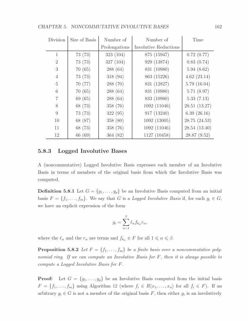
CHAPTER 5. NONCOMMUTATIVE INVOLUTIVE BASES 162
Division Size of Basis Number of Number of Time
Prolongations Involutive Reductions
1 73 (73) 323 (104) 875 (15947) 0.72 (0.77)
2 73 (73) 327 (104) 929 (13874) 0.83 (0.74)
3 70 (65) 288 (64) 831 (10980) 5.94 (8.62)
4 73 (73) 318 (94) 863 (15226) 4.62 (23.14)
5 70 (77) 288 (70) 831 (12827) 5.79 (16.04)
6 70 (65) 288 (64) 831 (10980) 5.71 (8.97)
7 69 (65) 288 (64) 833 (10980) 5.33 (7.13)
8 68 (73) 358 (76) 1092 (11046) 28.51 (13.27)
9 73 (73) 322 (95) 917 (13240) 6.39 (26.16)
10 68 (87) 358 (80) 1092 (13005) 28.75 (24.53)
11 68 (73) 358 (76) 1092 (11046) 28.54 (13.40)
12 66 (69) 364 (82) 1127 (10458) 28.87 (9.52)
5.8.3 Logged Involutive Bases
A (noncommutative) Logged Involutive Basis expresses each member of an Involutive
Basis in terms of members of the original basis from which the Involutive Basis was
computed.
Definition 5.8.1 Let G = g1, . . . , gp be an Involutive Basis computed from an initial
basis F = f1, . . . , fm. We say that G is a Logged Involutive Basis if, for each gi ∈ G,
we have an explicit expression of the form
gi =
β∑
α=1
ℓαfkαrα,
where the ℓα and the rα are terms and fkα ∈ F for all 1 6 α 6 β.
Proposition 5.8.2 Let F = f1, . . . , fm be a finite basis over a noncommutative poly-
nomial ring. If we can compute an Involutive Basis for F , then it is always possible to
compute a Logged Involutive Basis for F .
Proof: Let G = g1, . . . , gp be an Involutive Basis computed from the initial basis
F = f1, . . . , fm using Algorithm 12 (where fi ∈ R〈x1, . . . , xn〉 for all fi ∈ F ). If an
arbitrary gi ∈ G is not a member of the original basis F , then either gi is an involutively

CHAPTER 5. NONCOMMUTATIVE INVOLUTIVE BASES 163
reduced prolongation, or gi is obtained through the process of autoreduction. In the
former case, we can express gi in terms of members of F by substitution because either
gi = xjh−
β∑
α=1
ℓαhkαrα
or
gi = hxj −
β∑
α=1
ℓαhkαrα
for a variable xj ; terms ℓα and rα; and polynomials h and hkα which we already know
how to express in terms of members of F . In the latter case,
gi = h−
β∑
α=1
ℓαhkαrα
for terms ℓα, rα and polynomials h and hkα which we already know how to express in
terms of members of F , so it follows that we can again express gi in terms of members of
F .
Example 5.8.3 Let F := f1, f2 = x3 + 3xy − yx, y2 + x generate an ideal over the
polynomial ring Q〈x, y〉; let the monomial ordering be DegLex; and let the involutive divi-
sion be the left division. In obtaining an Involutive Basis for F using Algorithm 12, a poly-
nomial is added to F ; f1 is involutively reduced during autoreduction; and then four more
polynomials are added to F , giving an Involutive Basis G := g1, g2, g3, g4, g5, g6, g7 =
x3 + 2yx, y2 + x, xy − yx, y2x+ x2, xyx− yx2, y2x2 − 2yx, xyx2 − 2x2.
The five new polynomials were obtained by involutively reducing the prolongations f2y,

CHAPTER 5. NONCOMMUTATIVE INVOLUTIVE BASES 164
f2x, g3x, g4x and g5x respectively.
f2y = y3 + xy
f2
// y3 + xy − y(y2 + x)
= xy − yx;
f2x = y2x+ x2;
g3x = xyx− yx2;
g4x = y2x2 + x3
g1// y2x2 + x3 − (x3 + 2yx)
= y2x2 − 2yx;
g5x = xyx2 − yx3
g1// xyx2 − yx3 + y(x3 + 2yx)
= xyx2 + 2y2x
g4// xyx2 + 2y2x− 2(y2x+ x2)
= xyx2 − 2x2.
These reductions (plus the reduction
f1 g3// x3 + 3xy − yx− 3(xy − yx)
= x3 + 2yx
of f1 performed during autoreduction after g3 is added to F ) enable us to give the following
Logged Involutive Basis for F .
Member of G Logged Representation
g1 = x3 + 2yx f1 − 3f2y + 3yf2
g2 = y2 + x f2
g3 = xy − yx f2y − yf2
g4 = y2x+ x2 f2x
g5 = xyx− yx2 f2yx− yf2x
g6 = y2x2 − 2yx −f1 + f2x2 + 3f2y − 3yf2
g7 = xyx2 − 2x2 yf1 + 3y2f2 + f2yx2 − 2f2x− yf2x
2 − 3yf2y

Chapter 6
Grobner Walks
When computing any Grobner or Involutive Basis, the monomial ordering that has been
chosen is a major factor in how long it will take for the algorithm to complete. For
example, consider the ideal J generated by the basis F := −2x3z + y4 + y3z − x3 +
x2y, 2xy2z+ yz3+2yz2, x3y+2yz3−3yz2+2 over the polynomial ring Q[x, y, z]. Using
our test implementation of Algorithm 3, it takes less than a tenth of a second to compute
a Grobner Basis for F with respect to the DegRevLex monomial ordering, but 90 seconds
to compute a Grobner Basis for F with respect to Lex.
The Grobner Walk, introduced by Collart, Kalkbrener and Mall in [18], forms part of
a family of basis conversion algorithms that can convert Grobner Bases with respect to
‘fast’ monomial orderings to Grobner Bases with respect to ‘slow’ monomial orderings (see
Section 2.5.4 for a brief discussion of other basis conversion algorithms). This process is
often quicker than computing a Grobner Basis for the ‘slow’ monomial ordering directly,
as can be demonstrated by stating that in our test implementation of the Grobner Walk,
it only takes half a second to compute a Lex Grobner Basis for the basis F defined above.
In this chapter, we will first recall the theory of the (commutative) Grobner Walk, based
on [18] and a paper [1] by Amrhein, Gloor and Kuchlin; the reader is encouraged to read
these papers in conjunction with this Chapter. We then describe two generalisations of
the theory to give (i) a commutative Involutive Walk (due to Golubitsky [30]); and (ii)
noncommutative Walks between harmonious monomial orderings.
165

CHAPTER 6. GROBNER WALKS 166
6.1 Commutative Walks
To convert a Grobner Basis with respect to one monomial ordering to a Grobner Basis
with respect to another monomial ordering, the Grobner Walk works with the matrices
associated to the orderings. Fortunately, [48] and [56] assert that any commutative mono-
mial ordering has an associated matrix, allowing the Grobner Walk to convert between
any two monomial orderings.
6.1.1 Matrix Orderings
Definition 6.1.1 Let m be a monomial over a polynomial ring R[x1, . . . , xn] with as-
sociated multidegree (e1, . . . , en). If ω = (ω1, . . . , ωn) is an n-dimensional weight vector
(where ωi ∈ Q for all 1 6 i 6 n), we define the ω-degree of m, written degω(m), to be the
value
degω(m) = (e1 × ω1) + (e2 × ω2) + · · ·+ (en × ωn).
Remark 6.1.2 The ω-degree of any term is equal to the ω-degree of the term’s associated
monomial.
Definition 6.1.3 Let m1 and m2 be two monomials over a polynomial ring R[x1, . . . , xn]
with associated multidegrees e1 = (e11, . . . , en1) and e2 = (e12, . . . , e
n2 ); and let Ω be an N×n
matrix. If ωi denotes the n-dimensional weight vector corresponding to the i-th row of Ω,
then Ω determines a monomial ordering as follows: m1 < m2 if degωi(m1) < degωi
(m2)
for some 1 6 i 6 N and degωj(m1) = degωj
(m2) for all 1 6 j < i.
Definition 6.1.4 The corresponding matrices for the five monomial orderings defined in
Section 1.2.1 are
Lex =
1 0 0 . . . 0 0
0 1 0 . . . 0 0
0 0 1 . . . 0 0...
......
. . ....
...
0 0 0 . . . 1 0
0 0 0 . . . 0 1
; InvLex =
0 0 0 . . . 0 1
0 0 0 . . . 1 0...
...... . .
. ......
0 0 1 . . . 0 0
0 1 0 . . . 0 0
1 0 0 . . . 0 0
;

CHAPTER 6. GROBNER WALKS 167
DegLex =
1 1 1 . . . 1 1
1 0 0 . . . 0 0
0 1 0 . . . 0 0
0 0 1 . . . 0 0...
......
. . ....
...
0 0 0 . . . 1 0
; DegInvLex =
1 1 1 . . . 1 1
0 0 0 . . . 0 1
0 0 0 . . . 1 0...
...... . .
. ......
0 0 1 . . . 0 0
0 1 0 . . . 0 0
;
DegRevLex =
1 1 1 . . . 1 1
0 0 0 . . . 0 −1
0 0 0 . . . −1 0...
...... . .
. ......
0 0 −1 . . . 0 0
0 −1 0 . . . 0 0
.
Example 6.1.5 Let m1 := x2y2z2 and m2 := x2y3z be two monomials over the polyno-
mial ring R := Q[x, y, z]. According to the matrix
1 1 1
1 0 0
0 1 0
representing the DegLex monomial ordering with respect to R, we can deduce that m1 <
m2 because degω1(m1) = degω1
(m2) = 6; degω2(m1) = degω2
(m2) = 2; and degω3(m1) =
2 < degω3(m2) = 3.
Definition 6.1.6 Given a polynomial p and a weight vector ω, the initial of p with
respect to ω, written inω(p), is the sum of those terms in p that have maximal ω-degree.
For example, if ω = (0, 1, 1) and p = x4 + xy2z + y3 + xz2, then inω(p) = xy2z + y3.
Definition 6.1.7 A weight vector ω is compatible with a monomial ordering O if, given
any polynomial p = t1+· · ·+tm ordered in descending order with respect to O, degω(t1) >
degω(ti) holds for all 1 < i 6 m.
6.1.2 The Commutative Grobner Walk Algorithm
We present in Algorithm 17 an algorithm to perform the Grobner Walk, modified from
an algorithm given in [1].

CHAPTER 6. GROBNER WALKS 168
Algorithm 17 The Commutative Grobner Walk Algorithm
Input: A Grobner Basis G = g1, g2, . . . , gm with respect to an admissible monomial or-
dering O with an associated matrix A, where G generates an ideal J over a commutative
polynomial ring R = R[x1, . . . , xn].
Output: A Grobner Basis H = h1, h2, . . . , hp for J with respect to an admissible
monomial ordering O′ with an associated matrix B.
Let ω and τ be the weight vectors corresponding to the first rows of A and B;
Let C be the matrix whose first row is equal to ω and whose remainder is equal to the
whole of the matrix B;
t = 0; found = false;
repeat
Let G′ = inω(gi) for all gi ∈ G;
Compute a reduced Grobner Basis H ′ for G′ with respect to the monomial ordering
defined by the matrix C (use Algorithms 3 and 4);
H = ∅;
for each h′ ∈ H ′ do
Let∑j
i=1 pig′i be the logged representation of h′ with respect to G′ (where g′i ∈ G′
and pi ∈ R), obtained either through computing a Logged Grobner Basis above or
by dividing h′ with respect to G′;
H = H ∪ ∑j
i=1 pigi, where inω(gi) = g′i;
end for
Reduce H with respect to C (use Algorithm 4);
if (t == 1) then
found = true;
else
t = min(s | degω(s)(p1) = degω(s)(pi), degω(0)(p1) 6= degω(0)(pi),
h = p1 + · · ·+ pk ∈ H ∩ (0, 1]), where ω(s) := ω + s(τ − ω) for 0 6 s 6 1;
end if
if (t is undefined) then
found = true;
else
G = H ; ω = (1− t)ω + tτ ;
end if
until (found = true)
return H ;

CHAPTER 6. GROBNER WALKS 169
Some Remarks:
• In the first iteration of the repeat . . .until loop, G′ is a Grobner Basis for the ideal1
inω(J) with respect to the monomial ordering defined by C, as ω is compatible with
C. During subsequent iterations of the same loop, G′ is a Grobner Basis for the
ideal inω(J) with respect to the monomial ordering used to compute H during the
previous iteration of the repeat . . .until loop, as ω is compatible with this previous
ordering.
• The fact that any set H constructed by the for loop is a Grobner Basis for J with
respect to the monomial ordering defined by C is proved in both [1] and [18] (where
you will also find proofs for the assertions made in the previous paragraph).
• The section of code where we determine the value of t is where we determine the
next step of the walk. We choose t to be the minimum value of s in the interval
(0, 1] such that, for some polynomial h ∈ H , the ω-degrees of LT(h) and some other
term in h differ, but the ω(s)-degrees of the same two terms are identical. We say
that this is the first point on the line segment between the two weight vectors ω and
τ where the initial of one of the polynomials in H degenerates.
• The success of the Grobner Walk comes from the fact that it breaks down a Grobner
Basis computation into a series of smaller pieces, each of which computes a Grobner
Basis for a set of initials, a task that is usually quite simple. There are still cases
however where this task is complicated and time-consuming, and this has led to the
development of so-called path perturbation techniques that choose ‘easier’ paths on
which to walk (see for example [1] and [53]).
6.1.3 A Worked Example
Example 6.1.8 Let F := xy − z, yz + 2x + z be a basis generating an ideal J over
the polynomial ring Q[x, y, z]. Consider that we want to obtain the Lex Grobner Basis
H := 2x + yz + z, y2z + yz + 2z for J from the DegLex Grobner Basis G := xy −
z, yz + 2x+ z, 2x2 + xz + z2 for J using the Grobner Walk. Utilising Algorithm 17 to
do this, we initialise the variables as follows.
1The ideal inω(J) is defined as follows: p ∈ J if and only if inω(p) ∈ inω(J).

CHAPTER 6. GROBNER WALKS 170
A =
1 1 1
1 0 0
0 1 0
; B =
1 0 0
0 1 0
0 0 1
; ω = (1, 1, 1); τ = (1, 0, 0); C =
1 1 1
1 0 0
0 1 0
0 0 1
;
t = 0; found = false.
Let us now describe what happens during each pass of the repeat. . .until loop of Al-
gorithm 17, noting that as A is equivalent to C to begin with, nothing substantial will
happen during the first pass through the loop.
Pass 1
• Construct the set of initials: G′ := g′1, g′2, g
′3 = xy, yz, 2x2 + xz + z2 (these
are the terms in G that have maximal (1, 1, 1)-degree).
• Compute the Grobner Basis H ′ of G′ with respect to C.
S-pol(g′1, g′2) =
xyz
xy(xy)−
xyz
yz(yz)
= 0;
S-pol(g′1, g′3) =
x2y
xy(xy)−
x2y
2x2(2x2 + xz + z2)
= −1
2xyz −
1
2yz2
→g′1
−1
2yz2
→g′2
0;
S-pol(g′2, g′3) = 0 (by Buchberger’s First Criterion).
It follows that H ′ = G′.
• As H ′ = G′, H will also be equal to G, so that H := h1, h2, h3 = xy − z, yz +
2x+ z, 2x2 + xz + z2.
• Let
ω(s) := ω + s(τ − ω)
= (1, 1, 1) + s((1, 0, 0)− (1, 1, 1))
= (1, 1, 1) + s(0,−1,−1)
= (1, 1− s, 1− s).

CHAPTER 6. GROBNER WALKS 171
To find the next value of t, we must find the minimum value of s such that the
ω(s)-degrees of the leading term of a polynomial in H and some other term in the
same polynomial agree where their ω-degrees currently differ.
The ω-degrees of the two terms in h1 differ, so we can seek a value of s such that
degω(s)(xy) = degω(s)(z)
1 + (1− s) = (1− s)
1 = 0 (inconsistent).
For h2, we have two choices: either
degω(s)(yz) = degω(s)(x)
(1− s) + (1− s) = 1
2− 2s = 1
s =1
2;
or
degω(s)(yz) = degω(s)(z)
(1− s) + (1− s) = (1− s)
(1− s) = 0
s = 1.
The ω-degrees of all the terms in h3 are the same, so we can ignore it.
It follows that the minimum value of s (and hence the new value of t) is 12. As
this value appears in the interval (0, 1], we set G = H ; set the new value of ω
to be (1 − 12)(1, 1, 1) + 1
2(1, 0, 0) = (1, 1
2, 12) (and hence change C to be the matrix
1 12
12
1 0 0
0 1 0
0 0 1
); and embark upon a second pass of the repeat. . .until loop.
Pass 2
• Construct the set of initials: G′ := g′1, g′2, g
′3 = xy, 2x+ yz, 2x2 (these are the

CHAPTER 6. GROBNER WALKS 172
terms in G that have maximal (1, 12, 12)-degree).
• Compute the Grobner Basis of G′ with respect to C.
S-pol(g′1, g′2) =
xy
xy(xy)−
xy
2x(2x+ yz)
= −1
2y2z =: g′4;
S-pol(g′1, g′3) =
x2y
xy(xy)−
x2y
2x2(2x2)
= 0;
S-pol(g′2, g′3) =
x2
2x(2x+ yz)−
x2
2x2(2x2)
=1
2xyz
→g′1
0;
S-pol(g′1, g′4) =
xy2z
xy(xy)−
xy2z
−12y2z
(
−1
2y2z
)
= 0;
S-pol(g′2, g′4) = 0 (by Buchberger’s First Criterion);
S-pol(g′3, g′4) = 0 (by Buchberger’s First Criterion).
It follows that G′ = g′1, g′2, g
′3, g
′4 = xy, 2x+yz, 2x2, −1
2y2z is a Grobner Basis
for inω(J) with respect to C.
Applying Algorithm 4 to G′, we can remove g′1 and g′3 from G′ (because LM(g′1) =
y×LM(g′2) and LM(g′3) = x×LM(g′2)); we must also multiply g′2 and g′4 by12and −2
respectively to obtain unit lead coefficients. This leaves us with the unique reduced
Grobner Basis H ′ := h′1, h
′2 = x+ 1
2yz, y2z for inω(J) with respect to C.
• We must now express the two elements of H ′ in terms of members of G′.
h′1 = x+
1
2yz =
1
2g′2;
h′2 = y2z = −2
(
(xy)−1
2y(2x+ yz)
)
(from the S-polynomial)
= −2
(
g′1 −1
2yg′2
)
.
Lifting to the full polynomials, h′1 lifts to give the polynomial h1 := x + 1
2yz + 1
2z;
h′2 lifts to give the polynomial h2 := −2((xy − z) − 1
2y(2x + yz + z)) = −2xy +

CHAPTER 6. GROBNER WALKS 173
2z + 2xy + y2z + yz = y2z + yz + 2z; and we are left with the Grobner Basis
H := h1, h2 = x+ 12yz + 1
2z, y2z + yz + 2z for J with respect to C.
• Let
ω(s) := ω + s(τ − ω)
=
(
1,1
2,1
2
)
+ s
(
(1, 0, 0)−
(
1,1
2,1
2
))
=
(
1,1
2,1
2
)
+ s
(
0,−1
2,−
1
2
)
=
(
1,1
2(1− s),
1
2(1− s)
)
.
Finding the minimum value of s, for h1 we can have
degω(s)(x) = degω(s)(z)
1 =1
2(1− s)
s = −1 (undefined: we must have s ∈ (0, 1]).
Continuing with h2, we can either have
degω(s)(y2z) = degω(s)(yz)
3
(
1
2(1− s)
)
= 2
(
1
2(1− s)
)
1
2(1− s) = 0
s = 1;
or
degω(s)(y2z) = degω(s)(z)
3
(
1
2(1− s)
)
=1
2(1− s)
1− s = 0
s = 1.
It follows that the minimum value of s (and hence the new value of t) is 1. As
this value appears in the interval (0, 1], we set G = H ; set the new value of ω

CHAPTER 6. GROBNER WALKS 174
to be (1 − 1)(1, 12, 12) + 1(1, 0, 0) = (1, 0, 0) (and hence change C to be the matrix
1 0 0
1 0 0
0 1 0
0 0 1
≡
1 0 0
0 1 0
0 0 1
); and embark upon a third (and final) pass of the
repeat. . .until loop.
Pass 3
• Construct the set of initials: G′ := g′1, g′2 = x, y2z + yz + 2z (these are the
terms in G that have maximal (1, 0, 0)-degree).
• Compute the Grobner Basis H ′ of G′ with respect to C.
S-pol(g′1, g′2) = 0 (by Buchberger’s First Criterion).
It follows that H ′ = G′.
• As H ′ = G′, H will also be equal to G, so that H := h1, h2 = x+ 12yz+ 1
2z, y2z+
yz + 2z. Further, as t is now equal to 1, we have arrived at our target ordering
(Lex) and can return H as the output Grobner Basis, a basis that is equivalent to
the Lex Grobner Basis given for J at the beginning of this example.
We can summarise the path taken during the walk in the following diagram.
(1, 1, 1)Pass 1
Pass 3(1, 0, 0)
Pass 2(1, 1
2, 12)
y
x
12
z
11
1
12
12

CHAPTER 6. GROBNER WALKS 175
Algorithm 18 The Commutative Involutive Walk Algorithm
Input: An Involutive Basis G = g1, g2, . . . , gm with respect to an involutive division I
and an admissible monomial ordering O with an associated matrix A, where G generates
an ideal J over a commutative polynomial ring R = R[x1, . . . , xn].
Output: An Involutive Basis H = h1, h2, . . . , hp for J with respect to I and an admis-
sible monomial ordering O′ with an associated matrix B.
Let ω and τ be the weight vectors corresponding to the first rows of A and B;
Let C be the matrix whose first row is equal to ω and whose remainder is equal to the
whole of the matrix B;
t = 0; found = false;
repeat
Let G′ = inω(gi) for all gi ∈ G;
Compute an Involutive Basis H ′ for G′ with respect to the monomial ordering defined
by the matrix C (use Algorithm 9);
H = ∅;
for each h′ ∈ H ′ do
Let∑j
i=1 pig′i be the logged representation of h′ with respect to G′ (where g′i ∈ G′
and pi ∈ R), obtained either through computing a Logged Involutive Basis above
or by involutively dividing h′ with respect to G′;
H = H ∪ ∑j
i=1 pigi, where inω(gi) = g′i;
end for
if (t == 1) then
found = true;
else
t = min(s | degω(s)(p1) = degω(s)(pi), degω(0)(p1) 6= degω(0)(pi),
h = p1 + · · ·+ pk ∈ H ∩ (0, 1]), where ω(s) := ω + s(τ − ω) for 0 6 s 6 1;
end if
if (t is undefined) then
found = true;
else
G = H ; ω = (1− t)ω + tτ ;
end if
until (found = true)
return H ;

CHAPTER 6. GROBNER WALKS 176
6.1.4 The Commutative Involutive Walk Algorithm
In [30], Golubitsky generalised the Grobner Walk technique to give a method for convert-
ing an Involutive Basis with respect to one monomial ordering to an Involutive Basis with
respect to another monomial ordering. Algorithmically, the way in which we perform this
Involutive Walk is virtually identical to the way we perform the Grobner Walk, as can be
seen by comparing Algorithms 17 and 18. The change however comes when proving the
correctness of the algorithm, as we have to show that each G′ is an Involutive Basis for
inω(J) and that each H is an Involutive Basis for J (see [30] for these proofs).
6.2 Noncommutative Walks
In the commutative case, any monomial ordering can be represented by a matrix that
provides a decomposition of the ordering in terms of the rows of the matrix. This decom-
position is then utilised in the Grobner Walk algorithm when (for example) we use the
first row of the matrix to provide a set of initials for a particular basis G (cf. Definition
6.1.6).
In the noncommutative case, because monomials cannot be represented by multidegrees,
monomial orderings cannot be represented by matrices. This seems to shut the door on
any generalisation of the Grobner Walk to the noncommutative case, as not only is there
no first row of a matrix to provide a set of initials, but no notion of a walk between two
matrices can be formulated either.
Despite this, we note that in the commutative case, if the first rows of the source and
target matrices are the same, then the Grobner Walk will complete in one pass of the
algorithm, and all that is needed is the first row of the source matrix to provide a set of
initials to work with.
Generalising to the noncommutative case, it is possible that if we can find a way to
decompose a noncommutative monomial ordering to provide a set of initials to work
with, then a noncommutative Grobner Walk algorithm could complete in one pass if the
source and target monomial orderings used the same method to compute sets of initials.

CHAPTER 6. GROBNER WALKS 177
6.2.1 Functional Decompositions
Considering the monomial orderings defined in Section 1.2.2, we note that all the orderings
are defined step-by-step. For example, the DegLex monomial ordering compares two
monomials by degree first, then by the first letter of each monomial, then by the second
letter, and so on. This provides us with an opportunity to decompose each monomial
ordering into a series of steps or functions, a decomposition we shall term a functional
decomposition.
Definition 6.2.1 An ordering function is a function
θ : M −→ Z
that assigns an integer to any monomialm ∈ M , whereM denotes the set of all monomials
over a polynomial ring R〈x1, . . . , xn〉. We call the integer assigned by θ to m the θ-value
of m.
Remark 6.2.2 The θ-value of any term will be equal to the θ-value of the term’s asso-
ciated monomial.
Definition 6.2.3 A functional decomposition Θ is a (possibly infinite) sequence of order-
ing functions, written Θ = θ1, θ2, . . ..
Definition 6.2.4 Let O be a monomial ordering; let m1 and m2 be two arbitrary mono-
mials such that m1 < m2 with respect to O; and let Θ = θ1, θ2, . . . be a functional
decomposition. We say that Θ defines O if and only if θi(m1) < θi(m2) for some i > 1
and θj(m1) = θj(m2) for all 1 6 j < i.
To describe the functional decompositions corresponding to the monomial orderings de-
fined in Section 1.2.2, we first need the following definition.
Definition 6.2.5 Let m be an arbitrary monomial over a polynomial ring R〈x1, . . . , xn〉.
The i-th valuing function of m, written vali(m), is an ordering function that assigns an
integer to m as follows.
vali(m) =
j if Subword(m, i, i) = xj (where 1 6 j 6 n).
n+ 1 if Subword(m, i, i) is undefined.

CHAPTER 6. GROBNER WALKS 178
Let us now describe the functional decompositions corresponding to those monomial or-
derings defined in Section 1.2.2 that are admissible.
Definition 6.2.6 The functional decomposition Θ = θ1, θ2, . . . corresponding to the
DegLex monomial ordering is defined (for an arbitrary monomial m) as follows.
θi(m) =
deg(m) if i = 1.
n + 1− vali−1(m) if i > 1.
Similarly, we can define DegInvLex by
θi(m) =
deg(m) if i = 1.
vali−1(m) if i > 1.
and DegRevLex by
θi(m) =
deg(m) if i = 1.
valdeg(m)+2−i(m) if i > 1.
Example 6.2.7 Let m1 := xyxz2 and m2 := xzyz2 be two monomials over the poly-
nomial ring Q〈x, y, z〉. With respect to DegLex, we can work out that xyxz2 > xzyz2,
because θ1(m1) = θ1(m2) (or deg(m1) = deg(m2)); θ2(m1) = θ2(m2) (or n+1−val1(m1) =
n + 1 − val1(m2), 3 + 1 − 1 = 3 + 1 − 1); and θ3(m1) > θ3(m2) (or n + 1 − val2(m1) >
n + 1 − val2(m2), 3 + 1 − 2 > 3 + 1 − 3). Similarly, with respect to DegInvLex, we can
work out that xyxz2 < xzyz2 (because θ3(m1) < θ3(m2), or 2 < 3); and with respect to
DegRevLex, we can work out that xyxz2 < xzyz2 (because θ4(m1) < θ4(m2), or 1 < 2).
Definition 6.2.8 Given a polynomial p and an ordering function θ, the initial of p with
respect to θ, written inθ(p), is made up of those terms in p that have maximal θ-value. For
example, if θ is the degree function and if p = x4+zxy2+y3+z2x, then inθ(p) = x4+zxy2.
Definition 6.2.9 Given an ordering function θ, a polynomial p is said to be θ-homogeneous
if p = inθ(p).
Definition 6.2.10 An ordering function θ is compatible with a monomial ordering O if,
given any polynomial p = t1 + · · · + tm ordered in descending order with respect to O,
θ(t1) > θ(ti) holds for all 1 < i 6 m.

CHAPTER 6. GROBNER WALKS 179
Definition 6.2.11 An ordering function θ is extendible if, given any θ-homogeneous poly-
nomial p, any multiple upv of p by terms u and v is also θ-homogeneous.
Remark 6.2.12 Of the ordering functions encountered so far, only the degree function,
val1 and2 valdeg(m) (for any given monomial m) are extendible.
Definition 6.2.13 Two noncommutative monomial orderings O1 and O2 are said to be
harmonious if (i) there exist functional decompositions Θ1 = θ11 , θ12 , . . . and Θ2 =
θ21 , θ22 , . . . defining O1 and O2 respectively; and (ii) the ordering functions θ11 and θ21
are identical and extendible.
Remark 6.2.14 The noncommutative monomial orderings DegLex, DegInvLex and De-
gRevLex are all (pairwise) harmonious.
6.2.2 The Noncommutative Grobner Walk Algorithm for Har-
monious Monomial Orderings
We present in Algorithm 19 an algorithm to perform a Grobner Walk between two har-
monious noncommutative monomial orderings.
Termination of Algorithm 19 depends on the termination of Algorithm 5 as used (in Al-
gorithm 19) to compute a noncommutative Grobner Basis for the set G′. The correctness
of Algorithm 19 is provided by the following two propositions.
Proposition 6.2.15 G′ is always a Grobner Basis for the ideal3 inθ(J) with respect to
the monomial ordering O.
Proof: Because θ is compatible with O (by definition), the S-polynomials involving
members of G will be in one-to-one correspondence with the S-polynomials involving
members of G′, with the same monomial being ‘cancelled’ in each pair of corresponding
S-polynomials.
Let p be an arbitrary S-polynomial involving members of G (with corresponding S-
polynomial q involving members of G′). Because G is a Grobner Basis for J with respect
2Think of valdeg(m) as finding the value of the final variable in m (as opposed to val1 finding the valueof the first variable in m).
3The ideal inθ(J) is defined as follows: p ∈ J if and only if inθ(p) ∈ inθ(J).

CHAPTER 6. GROBNER WALKS 180
Algorithm 19 The Noncommutative Grobner Walk Algorithm for Harmonious MonomialOrderings
Input: A Grobner Basis G = g1, g2, . . . , gm with respect to an admissible monomial
ordering O with an associated functional decomposition A, where G generates an ideal
J over a noncommutative polynomial ring R = R〈x1, . . . , xn〉.
Output: A Grobner Basis H = h1, h2, . . . , hp for J with respect to an admissible
monomial ordering O′ with an associated functional decomposition B, where O and O′
are harmonious.
Let θ be the ordering function corresponding to the first ordering function of A;
Let G′ = inθ(gi) for all gi ∈ G;
Compute a reduced Grobner Basis H ′ for G′ with respect to the monomial ordering O′
(use Algorithms 5 and 6);
H = ∅;
for each h′ ∈ H ′ do
Let∑j
i=1 ℓig′iri be the logged representation of h′ with respect to G′ (where g′i ∈ G′
and the ℓi and the ri are terms), obtained either through computing a Logged Grobner
Basis above or by dividing h′ with respect to G′;
H = H ∪ ∑j
i=1 ℓigiri, where inθ(gi) = g′i;
end for
Reduce H with respect to O′ (use Algorithm 6);
return H ;

CHAPTER 6. GROBNER WALKS 181
to O, p will reduce to zero using G by the series of reductions
p →gi1p1 →gi2
p2 →gi3· · · →giα
0,
where gij ∈ G for all 1 6 j 6 α.
Claim: q will reduce to zero using G′ (and hence G′ is a Grobner Basis for inθ(J) with
respect to O by Definition 3.1.8) by the series of reductions
q →inθ(gi1 )q1 →inθ(gi2 )
q2 →inθ(gi3 )· · · →inθ(giβ )
0,
where 0 6 β 6 α.
Proof of Claim: Let w be the overlap word associated to the S-polynomial p. If
θ(LM(p)) < θ(w), then because θ is extendible it is clear that q = 0, and so the proof is
complete. Otherwise, we must have q = inθ(p), and so by the compatibility of θ with O,
we can use the polynomial inθ(gi1) ∈ G′ to reduce q to give the polynomial q1. We now
proceed by induction (if θ(LM(p1)) < θ(LM(p)) then q1 = 0, . . . ), noting that the process
will terminate because inθ(pα = 0) = 0.
Proposition 6.2.16 The set H constructed by the for loop of Algorithm 19 is a Grobner
Basis for J with respect to the monomial ordering O′.
Proof: By Definition 3.1.8, we can show that H is a Grobner Basis for J by showing
that all S-polynomials involving members of H reduce to zero using H . Assume for a
contradiction that an S-polynomial p involving members of H does not reduce to zero
using H , and instead only reduces to a polynomial q 6= 0.
As all members of H are members of the ideal J (by the way H was constructed as
combinations of elements of G), it is clear that q is also a member of the ideal J , as all we
have done in constructing q is to reduce a combination of two members of H with respect
to H . It follows that the polynomial inθ(q) is a member of the ideal inθ(J).
Because H ′ is a Grobner Basis for the ideal inθ(J) with respect to O′, there must be a
polynomial h′ ∈ H ′ such that h′ | inθ(q). Let∑j
i=1 ℓig′iri be the logged representation of

CHAPTER 6. GROBNER WALKS 182
h′ with respect to G′. Then it is clear that
j∑
i=1
ℓig′iri | inθ(q).
However θ is compatible with O′, so that
j∑
i=1
ℓigiri | q.
It follows that there exists a polynomial h ∈ H dividing our polynomial q, contradicting
our initial assumption.
6.2.3 A Worked Example
Example 6.2.17 Let F := x2 + y2 + 8, 2xy + y2 + 5 be a basis generating an ideal J
over the polynomial ring Q〈x, y〉. Consider that we want to obtain the DegLex Grobner
Basis H := 2xy + y2 + 5, x2 + y2 + 8, 5y3 − 10x + 37y, 2yx + y2 + 5 for J from the
DegRevLex Grobner Basis G := 2xy−x2 − 3, y2+ x2 +8, 5x3 +6y+35x, 2yx−x2 − 3
for J using the Grobner Walk. Utilising Algorithm 19 to do this, we initialise θ to be the
degree function and we proceed as follows.
• Construct the set of initials: G′ := g′1, g′2, g
′3, g
′4 = −x2+2xy, x2+y2, 5x3, −x2+
2yx (these are the terms in G that have maximal degree).
• Compute the Grobner Basis of G′ with respect to the DegLex monomial ordering
(for simplicity, we will not provide details of those S-polynomials that reduce to zero

CHAPTER 6. GROBNER WALKS 183
or can be ignored due to Buchberger’s Second Criterion).
S-pol(1, g′1, 1, g′2) = (−x2 + 2xy)− (−1)(x2 + y2)
= 2xy + y2 =: g′5;
S-pol(1, g′1, 1, g′4) = (−1)(−x2 + 2xy)− (−1)(−x2 + 2yx)
= −2xy + 2yx
→g′5
−2xy + 2yx+ (2xy + y2)
= 2yx+ y2 =: g′6;
S-pol(y, g′1, 1, g′6) = 2y(−x2 + 2xy)− (−1)(2yx+ y2)x
= 4yxy + y2x
→g′5
4yxy + y2x− 2y(2xy + y2)
= y2x− 2y3
→g′6
y2x− 2y3 −1
2y(2yx+ y2)
= −5
2y3 =: g′7.
After g′7 is added to the current basis, all S-polynomials now reduce to zero, leaving
the Grobner BasisG′ = g′1, g′2, g
′3, g
′4, g
′5, g
′6, g
′7 = −x2+2xy, x2+y2, 5x3, −x2+
2yx, 2xy + y2, 2yx+ y2, −52y3 for inθ(J) with respect to O′.
Applying Algorithm 6 to G′, we can remove g′1, g′2 and g′3 from G′ (because their
lead monomials are all multiplies of LM(g′4)); we must multiply g′4, g′5, g
′6 and g′7 by
−1, 12, 1
2and −2
5respectively (to obtain unit lead coefficients); and the polynomial
g′4 can (then) be further reduced as follows.
g′4 = x2 − 2yx
→g′6
x2 − 2yx+ 2
(
yx+1
2y2)
= x2 + y2.
This leaves us with the unique reduced Grobner Basis H ′ := h′1, h
′2, h
′3, h
′4 =
x2 + y2, xy + 12y2, yx+ 1
2y2, y3 for inθ(J) with respect to O′.

CHAPTER 6. GROBNER WALKS 184
• We must now express the four elements of H ′ in terms of members of G′.
h′1 = x2 + y2 = g′2;
h′2 = xy +
1
2y2 =
1
2(g′1 + g′2) (from the S-polynomial);
h′3 = yx+
1
2y2 =
1
2(−g′1 + g′4 + (g′1 + g′2))
=1
2(g′2 + g′4);
h′4 = y3 = −
2
5
(
2y(g′1) + (g′2 + g′4)x− 2y(g′1 + g′2)−1
2y(g′2 + g′4)
)
= −2
5
(
g′2x−5
2yg′2 + g′4x−
1
2yg′4
)
.
Lifting to the full polynomials, we obtain the Grobner Basis H := h1, h2, h3, h4
as follows.
h1 = g2
= x2 + y2 + 8;
h2 =1
2(g1 + g2)
=1
2(−x2 + 2xy − 3 + x2 + y2 + 8)
= xy +1
2y2 +
5
2;
h3 =1
2(g2 + g4)
=1
2(x2 + y2 + 8− x2 + 2yx− 3)
= yx+1
2y2 +
5
2;
h4 = −2
5
(
g2x−5
2yg2 + g4x−
1
2yg4
)
= −2
5
(
x3 + y2x+ 8x−5
2yx2 −
5
2y3 − 20y
−x3 + 2yx2 − 3x+1
2yx2 − y2x+
3
2y
)
= y3 − 2x+37
5y.
The set H does not reduce any further, so we return the output DegLex Grobner
Basis x2 + y2 + 8, xy + 12y2 + 5
2, yx + 1
2y2 + 5
2, y3 − 2x + 37
5y for J , a basis

CHAPTER 6. GROBNER WALKS 185
that is equivalent to the DegLex Grobner Basis given for J at the beginning of this
example.
6.2.4 The Noncommutative Involutive Walk Algorithm for Har-
monious Monomial Orderings
We present in Algorithm 20 an algorithm to perform an Involutive Walk between two
harmonious noncommutative monomial orderings.
Algorithm 20 The Noncommutative Involutive Walk Algorithm for Harmonious Mono-mial Orderings
Input: An Involutive Basis G = g1, g2, . . . , gm with respect to an involutive divi-
sion I and an admissible monomial ordering O with an associated functional decom-
position A, where G generates an ideal J over a noncommutative polynomial ring
R = R〈x1, . . . , xn〉.
Output: An Involutive Basis H = h1, h2, . . . , hp for J with respect to I and an admis-
sible monomial ordering O′ with an associated functional decomposition B, where O
and O′ are harmonious.
Let θ be the ordering function corresponding to the first ordering function of A;
Let G′ = inθ(gi) for all gi ∈ G;
Compute an Involutive Basis H ′ for G′ with respect to I and the monomial ordering
O′ (use Algorithm 12);
H = ∅;
for each h′ ∈ H ′ do
Let∑j
i=1 ℓig′iri be the logged representation of h′ with respect to G′ (where g′i ∈
G′ and the ℓi and the ri are terms), obtained either through computing a Logged
Involutive Basis above or by involutively dividing h′ with respect to G′;
H = H ∪ ∑j
i=1 ℓigiri, where inθ(gi) = g′i;
end for
return H ;
Termination of Algorithm 20 depends on the termination of Algorithm 12 as used (in Al-
gorithm 20) to compute a noncommutative Involutive Basis for the set G′. The correctness
of Algorithm 20 is provided by the following two propositions.

CHAPTER 6. GROBNER WALKS 186
Proposition 6.2.18 G′ is always an Involutive Basis for the ideal inθ(J) with respect to
I and the monomial ordering O.
Proof: Let p := ugv be an arbitrary multiple of a polynomial g ∈ G by terms u and v.
Because G is an Involutive Basis for J with respect to I and O, p will involutively reduce
to zero using G by the series of involutive reductions
pI gi1
// p1 I gi2
// p2 I gi3
// · · ·I giα
// 0,
where gij ∈ G for all 1 6 j 6 α.
Claim: The polynomial q := uinθ(g)v will involutively reduce to zero using G′ (and hence
G′ is an Involutive Basis for inθ(J) with respect to I and O by Definition 5.2.7) by the
series of involutive reductions
qI inθ(gi1 )
// q1 I inθ(gi2 )// q2 I inθ(gi3 )
// · · ·I inθ(giβ )
// 0,
where 1 6 β 6 α.
Proof of Claim: Because θ is extendible, it is clear that q = inθ(p). Further, because θ
is compatible with O (by definition), the multiplicative variables of G and G′ with respect
to I will be identical, and so it follows that because the polynomial gi1 ∈ G was used to
involutively reduce p to give the polynomial p1, then the polynomial inθ(gi1) ∈ G′ can be
used to involutively reduce q to give the polynomial q1.
If θ(LM(p1)) < θ(LM(p)), then because θ is extendible it is clear that q1 = 0, and so
the proof is complete. Otherwise, we must have q1 = inθ(p1), and so (again) by the
compatibility of θ with O, we can use the polynomial inθ(gi2) ∈ G′ to involutively reduce
q1 to give the polynomial q2. We now proceed by induction (if θ(LM(p2)) < θ(LM(p1))
then q2 = 0, . . . ), noting that the process will terminate because inθ(pα = 0) = 0.
Proposition 6.2.19 The set H constructed by the for loop of Algorithm 20 is an Invo-
lutive Basis for J with respect to I and the monomial ordering O′.
Proof: By Definition 5.2.7, we can show that H is an Involutive Basis for J by showing
that any multiple upv of any polynomial p ∈ H by any terms u and v involutively reduces
to zero using H . Assume for a contradiction that such a multiple does not involutively
reduce to zero using H , and instead only involutively reduces to a polynomial q 6= 0.

CHAPTER 6. GROBNER WALKS 187
As all members of H are members of the ideal J (by the way H was constructed as
combinations of elements of G), it is clear that q is also a member of the ideal J , as all
we have done in constructing q is to reduce a multiple of a polynomial in H with respect
to H . It follows that the polynomial inθ(q) is a member of the ideal inθ(J).
Because H ′ is an Involutive Basis for the ideal inθ(J) with respect to I and O′, there must
be a polynomial h′ ∈ H ′ such that h′ |I inθ(q). Let∑j
i=1 ℓig′iri be the logged representation
of h′ with respect to G′. Then it is clear that
j∑
i=1
ℓig′iri |I inθ(q).
However θ is compatible with O′ (in particular the multiplicative variables for H ′ and H
with respect to I and O′ will be identical), so that
j∑
i=1
ℓigiri |I q.
It follows that there exists a polynomial h ∈ H involutively dividing our polynomial q,
contradicting our initial assumption.
6.2.5 A Worked Example
Example 6.2.20 Let F := x2+y2+8, 2xy+y2+5 be a basis generating an ideal J over
the polynomial ring Q〈x, y〉. Consider that we want to obtain the DegRevLex Involutive
Basis H := 2xy − x2 − 3, y2 + x2 + 8, 5x3 + 6y + 35x, 5yx2 + 3y + 10x, 2yx− x2 − 3
for J from the DegLex Involutive Basis G := 2xy + y2 + 5, x2 + y2 + 8, 5y3 − 10x +
37y, 5xy2 + 5x− 6y, 2yx+ y2 + 5 for J using the Involutive Walk, where H and G are
both Involutive Bases with respect to the left division . Utilising Algorithm 20 to do
this, we initialise θ to be the degree function and we proceed as follows.
• Construct the set of initials:
G′ := g′1, g′2, g
′3, g
′4, g
′5 = y2 + 2xy, y2 + x2, 5y3, 5xy2, y2 + 2yx
(these are the terms in G that have maximal degree).
• Compute the Involutive Basis of G′ with respect to and the DegRevLex monomial

CHAPTER 6. GROBNER WALKS 188
ordering. Step 1: autoreduce the set G′.
g′1 = y2 + 2xy
g′2
// y2 + 2xy − (y2 + x2)
= 2xy − x2 =: g′6;
G′ = (G′ \ g′1) ∪ g′6;
g′2 = y2 + x2
g′5
// y2 + x2 − (y2 + 2yx)
= −2yx+ x2 =: g′7;
G′ = (G′ \ g′2) ∪ g′7;
g′3 = 5y3
g′5
// 5y3 − 5y(y2 + 2yx)
= −10y2x
g′7
// −10y2x− 5y(−2yx+ x2)
= −5yx2 =: g′8;
G′ = (G′ \ g′3) ∪ g′8;
g′4 = 5xy2
g′5
// 5xy2 − 5x(y2 + 2yx)
= −10xyx
g′7
// −10xyx− 5x(−2yx+ x2)
= −5x3 =: g′9;
G′ = (G′ \ g′4) ∪ g′9;
g′5 = y2 + 2yx
g′7
// y2 + 2yx+ (−2yx+ x2)
= y2 + x2 =: g′10;
G′ = (G′ \ g′5) ∪ g′10.
Step 2: process the prolongations of the set G′ = g′6, g′7, g
′8, g
′9, g
′10. Because all ten
of these prolongations involutively reduce to zero using G′, we are left with the Invo-
lutive Basis H ′ := h′1, h
′2, h
′3, h
′4, h
′5 = 2xy−x2, −2yx+x2, −5yx2, −5x3, y2+

CHAPTER 6. GROBNER WALKS 189
x2 for inθ(J) with respect to and O′.
• We must now express the five elements of H ′ in terms of members of G′.
h′1 = 2xy − x2 = g′1 − g′2 (from autoreduction);
h′2 = −2yx+ x2 = g′2 − g′5;
h′3 = −5yx2 = g′3 − 5yg′5 − 5y(g′2 − g′5)
= −5yg′2 + g′3;
h′4 = −5x3 = g′4 − 5xg′5 − 5x(g′2 − g′5)
= −5xg′2 + g′4;
h′5 = y2 + x2 = g′5 + (g′2 − g′5)
= g′2.
Lifting to the full polynomials, we obtain the Involutive BasisH := h1, h2, h3, h4, h5
as follows.
h1 = g1 − g2
= (y2 + 2xy + 5)− (y2 + x2 + 8)
= 2xy − x2 − 3;
h2 = g2 − g5
= (y2 + x2 + 8)− (y2 + 2yx+ 5)
= −2yx+ x2 + 3;
h3 = −5yg2 + g3
= −5y(y2 + x2 + 8) + (5y3 + 37y − 10x)
= −5yx2 − 3y − 10x;
h4 = −5xg2 + g4
= −5x(y2 + x2 + 8) + (5xy2 − 6y + 5x)
= −5x3 − 6y − 35x;
h5 = g2
= y2 + x2 + 8.
We can now return the output DegRevLex Involutive Basis H = 2xy − x2 −
3, −2yx + x2 + 3, −5yx2 − 3y − 10x, −5x3 − 6y − 35x, y2 + x2 + 8 for J with

CHAPTER 6. GROBNER WALKS 190
respect to , a basis that is equivalent to the DegRevLex Involutive Basis given for
J at the beginning of this example.
6.2.6 Noncommutative Walks Between Any Two Monomial Or-
derings?
Thus far, we have only been able to define a noncommutative walk between two harmo-
nious monomial orderings, where we recall that the first ordering functions of the func-
tional decompositions of the two monomial orderings must be identical and extendible.
For walks between two arbitrary monomial orderings, the first ordering functions need
not be identical any more, but it is clear that they must still be extendible, so that (in an
algorithm to perform such a walk) each basis G′ is a Grobner Basis for each ideal inθ(J)
(compare with the proofs of Propositions 6.2.15 and 6.2.18). This condition will also ap-
ply to any ‘intermediate’ monomial ordering we will encounter during the walk, but the
challenge will be in how to define these intermediate orderings, so that we generalise the
commutative concept of choosing a weight vector ωi+1 on the line segment between two
weight vectors ωi and τ .
Open Question 4 Is it possible to perform a noncommutative walk between two admis-
sible and extendible monomial orderings that are not harmonious?

Chapter 7
Conclusions
7.1 Current State of Play
The goal of this thesis was to combine the theories of noncommutative Grobner Bases
and commutative Involutive Bases to give a theory of noncommutative Involutive Bases.
To accomplish this, we started by surveying the background theory in Chapters 1 to 4,
focusing our account on the various algorithms associated with the theory. In particular,
we mentioned several improvements to the standard algorithms, including how to compute
commutative Involutive Bases by homogeneous methods, which required the introduction
of a new property (extendibility) of commutative involutive divisions.
The theory of noncommutative Involutive Bases was introduced in Chapter 5, where
we described how to perform noncommutative involutive reduction (Definition 5.1.1 and
Algorithm 10); introduced the notion of a noncommutative involutive division (Definition
5.1.6); described what is meant by a noncommutative Involutive Basis (Definition 5.2.7);
and gave an algorithm to compute noncommutative Involutive Bases (Algorithm 12).
Several noncommutative involutive divisions were also defined, each of which was shown
to satisfy certain properties (such as continuity) allowing the deductions that all Locally
Involutive Bases are Involutive Bases; and that all Involutive Bases are Grobner Bases.
To finish, we partially generalised the theory of the Grobner Walk to the noncommuta-
tive case in Chapter 6, yielding both Grobner and Involutive Walks between harmonious
noncommutative monomial orderings.
191

CHAPTER 7. CONCLUSIONS 192
7.2 Future Directions
As well as answering a few questions, the work in this thesis gives rise to a number of
new questions we would like the answers to. Some of these questions have already been
posed as ‘Open Questions’ in previous chapters; we summarise below the content of these
questions.
• Regarding the procedure outlined in Definition 4.5.1 for computing an Involutive
Basis for a non-homogeneous basis by homogeneous methods, if the set G returned
by the procedure is not autoreduced, under what circumstances does autoreducing
G result in obtaining a set that is an Involutive Basis for the ideal generated by the
input basis F ?
• Apart from the empty, left and right divisions, are there any other global noncom-
mutative involutive divisions of the following types:
(a) strong and continuous;
(b) weak, continuous and Grobner?
• Are there any conclusive noncommutative involutive divisions that are also contin-
uous and either strong or Grobner?
• Is it possible to perform a noncommutative walk between two admissible and ex-
tendible monomial orderings that are not harmonious?
In addition to seeking answers to the above questions, there are a number of other di-
rections we could take. One area to explore would be the development of the algorithms
introduced in this thesis. For example, can the improvements made to the involutive
algorithms in the commutative case, such as the a priori detection of prolongations that
involutively reduce to zero (see [23]), be applied to the noncommutative case? Also, can we
develop multiple-object versions of our algorithms, so that (for example) noncommutative
Involutive Bases for path algebras can be computed?
Implementations of any new or improved algorithms would clearly build upon the code
presented in Appendix B. We could also expand this code by implementing logged versions
of our algorithms; implementing efficient methods for performing involutive reduction (as
seen for example in Section 5.8.1); and implementing the algorithms from Chapter 6

CHAPTER 7. CONCLUSIONS 193
for performing noncommutative walks. These improved algorithms and implementations
could then be used (perhaps) to help judge the relative efficiency and complexity of the
involutive methods versus the Grobner methods.
Applications
As every noncommutative Involutive Basis is a noncommutative Grobner Basis (at least
for the involutive divisions defined in this thesis), applications for noncommutative Invo-
lutive Bases will mirror those for noncommutative Grobner Bases. Some areas in which
noncommutative Grobner Bases have already been used include operator theory; systems
engineering and linear control theory [32]. Other areas in noncommutative algebra which
could also benefit from the theory introduced in this thesis include term rewriting; Petri
nets; linear logic; quantum groups and coherence problems.
Further applications may come if we can extend our algorithms to the multiple-object
case. It would be interesting (for example) to compare a multiple-object algorithm to a
(standard) one-object algorithm in cases where an Involutive Basis for a multiple-object
example can be computed using the one-object algorithm by adding some extra relations.
This would tie in nicely with the existing comparison between the commutative and
noncommutative versions of the Grobner Basis algorithm, where it has been noticed that
although commutative examples can be computed using the noncommutative algorithm,
taking this route may in fact be less efficient than when using the commutative algorithm
to do the same computation.

Appendix A
Proof of Propositions 5.5.31 and
5.5.32
A.1 Proposition 5.5.31
(Proposition 5.5.31) The two-sided left overlap division W is continuous.
Proof: Let w be an arbitrary fixed monomial; let U be any set of monomials; and
consider any sequence (u1, u2, . . . , uk) of monomials from U (ui ∈ U for all 1 6 i 6 k),
each of which is a conventional divisor of w (so that w = ℓiuiri for all 1 6 i 6 k, where the
ℓi and the ri are monomials). For all 1 6 i < k, suppose that the monomial ui+1 satisfies
exactly one of the conditions (a) and (b) from Definition 5.4.2 (where multiplicative
variables are taken with respect to W over the set U). To show that W is continuous, we
must show that no two pairs (ℓi, ri) and (ℓj, rj) are the same, where i 6= j.
Assume to the contrary that there are at least two identical pairs in the sequence
((ℓ1, r1), (ℓ2, r2), . . . , (ℓk, rk)),
so that we can choose two separate pairs (ℓa, ra) and (ℓb, rb) from this sequence such that
(ℓa, ra) = (ℓb, rb) and all the pairs (ℓc, rc) (for a 6 c < b) are different. We will now show
that such a sequence ((ℓa, ra), . . . , (ℓb, rb)) cannot exist.
To begin with, notice that for each monomial ui+1 in the sequence (u1, . . . , uk) of mono-
194

APPENDIX A. PROOF OF PROPOSITIONS 5.5.31 AND 5.5.32 195
mials (1 6 i < k), if ui+1 involutively divides a left prolongation of the monomial ui (so
that ui+1 |W (Suffix(ℓi, 1))ui), then ui+1 must be a prefix of this prolongation; if ui+1 invo-
lutively divides a right prolongation of the monomial ui (so that ui+1 |W ui(Prefix(ri, 1))),
then ui+1 must be a suffix of this prolongation. This is because in all other cases, ui+1
is either equal to ui, in which case ui+1 cannot involutively divide the (left or right) pro-
longation of ui trivially; or ui+1 is a subword of ui, in which case ui+1 cannot involutively
divide the (left or right) prolongation of ui by definition of W.
Following on from the above, we can deduce that ub is either a suffix or a prefix of a
prolongation of ub−1, leaving the following four cases, where xℓb−1 = Suffix(ℓb−1, 1) and
xrb−1 = Prefix(rb−1, 1).
Case A (deg(ub−1) > deg(ub)) Case B (deg(ub−1) + 1 = deg(ub))
xℓb−1
ooub−1
//
oo
ub
//
xℓb−1
ooub−1
//
oo
ub
//
Case C (deg(ub−1) > deg(ub)) Case D (deg(ub−1) + 1 = deg(ub))
ooub−1
//
xrb−1
oo
ub
//
ooub−1
//
xrb−1
oo
ub
//
These four cases can all originate from one of the following two cases (starting with a left
prolongation or a right prolongation), where xℓa = Suffix(ℓa, 1) and xr
a = Prefix(ra, 1).
Case 1 Case 2
xℓa
ooua
// ooua
//
xra
So there are eight cases to deal with in total, namely cases 1-A, 1-B, 1-C, 1-D, 2-A, 2-B,
2-C and 2-D.
We can immediately rule out cases 1-C and 2-A because we can show that a particular
variable is both multiplicative and nonmultiplicative for monomial ua = ub with respect
to U , a contradiction. In case 1-C, the variable is xℓa: it has to be left nonmultiplicative
to provide a left prolongation for ua, and left multiplicative so that ub is an involutive
divisor of the right prolongation of ub−1; in case 2-A, the variable is xra: it has to be
right nonmultiplicative to provide a right prolongation for ua, and right multiplicative

APPENDIX A. PROOF OF PROPOSITIONS 5.5.31 AND 5.5.32 196
so that ub is an involutive divisor of the left prolongation of ub−1. We illustrate this in
the following diagrams by using a tick to denote a multiplicative variable and a cross to
denote a nonmultiplicative variable.
Case 1-C Case 2-A
xℓa
×oo
ua//
...
ooub−1
//
xrb−1
xℓa
X
ooub = ua
//
ooua
//
×
xra
...xℓb−1
ooub−1
//
ooub = ua
//
xra
X
For all the remaining cases, let us now consider how we may construct a sequence
((ℓa, ra), . . . , (ℓb, rb) = (ℓa, ra)). Because we know that each uc+1 is a prefix (or suf-
fix) of a left (or right) prolongation of uc (where a 6 c < b), it is clear that at some stage
during the sequence, some uc+1 must be a proper suffix (or prefix) of a prolongation, or
else the degrees of the monomials in the sequence (ua, . . .) will strictly increase, meaning
that we can never encounter the same (ℓ, r) pair twice. Further, the direction in which
prolongations are taken must change some time during the sequence, or else the degrees
of the monomials in one of the sequences (ℓa, . . .) and (ra, . . .) will strictly decrease, again
meaning that we can never encounter the same (ℓ, r) pair twice.
A change in direction can only occur if uc+1 is equal to a prolongation of uc, as illustrated
below.
Left Prolongation Turn Right Prolongation Turn
xℓc
×oo
uc//
oouc+1
//
xrc+1
×
oouc
//
×
xrc
xℓc+1
×oo
uc+1//
However, if no proper prefixes or suffixes are taken during the sequence, it is clear that
making left or right prolongation turns will not affect the fact that the degrees of the
monomials in the sequence (ua, . . .) will strictly increase, once again meaning that we can
never encounter the same (ℓ, r) pair twice. It follows that our only course of action is to

APPENDIX A. PROOF OF PROPOSITIONS 5.5.31 AND 5.5.32 197
make a (left or right) prolongation turn after a proper prefix or a suffix of a prolongation
has been taken. We shall call such prolongation turns prefix or suffix turns.
Prefix Turn Suffix Turn
xℓc
×oo
uc//
xℓc+1
×oo
uc+1//
xrc+2
X
oouc+2
//
xrc+2
×
oouc
//
×
xrc
xℓc+2
X
oouc+1
//
×
xrc+1
×
xℓc+2
oouc+2
//
Claim: It is impossible to perform a prefix turn when W has been used to assign multi-
plicative variables.
Proof of Claim: It is sufficient to show that W cannot assign multiplicative variables
to U as follows:
xℓc /∈ ML
W(uc, U); xrc+2 ∈ MR
W(uc+1, U); xrc+2 /∈ MR
W(uc+2, U). (A.1)
Consider how Algorithm 16 can assign the variable xrc+2 to be right nonmultiplicative for
monomial uc+2. As things are set up in the digram for the prefix turn, the only possibility
is that it is assigned due to the shown overlap between uc and uc+2. But this assumes
that these two monomials actually overlap (which won’t be the case if deg(uc+1) = 1);
that uc is greater than or equal to uc+2 with respect to the DegRevLex monomial ordering
(so any overlap assigns a nonmultiplicative variable to uc+2, not to uc); and that, by the
time we come to consider the prefix overlap between uc and uc+2 in Algorithm 16, the
variable xℓc must be left multiplicative for monomial uc. But this final condition ensures
that Algorithm 16 will terminate with xℓc being left multiplicative for uc, contradicting
Equation (A.1). We therefore conclude that the variable xrc+2 must be assigned right
nonmultiplicative for monomial uc+2 via some other overlap.
There are three possibilities for this overlap: (i) there exists a monomial ud ∈ U such that
uc+2 is a prefix of ud; (ii) there exists a monomial ud ∈ U such that uc+2 is a subword of
ud; and (iii) there exists a monomial ud ∈ U such that some prefix of ud is equal to some
suffix of uc+2.
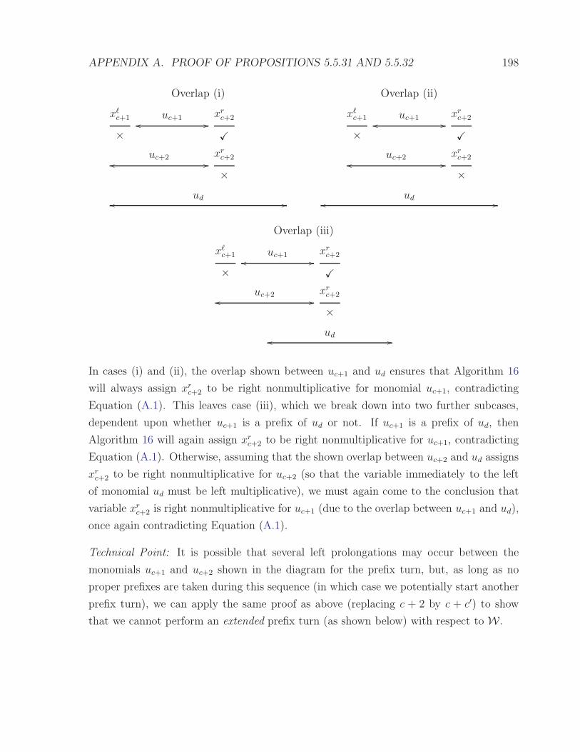
APPENDIX A. PROOF OF PROPOSITIONS 5.5.31 AND 5.5.32 198
Overlap (i) Overlap (ii)
xℓc+1
×oo
uc+1//
xrc+2
X
oouc+2
//
xrc+2
×
ooud
//
xℓc+1
×oo
uc+1//
xrc+2
X
oouc+2
//
xrc+2
×
ooud
//
Overlap (iii)
xℓc+1
×oo
uc+1//
xrc+2
X
oouc+2
//
xrc+2
×
ooud
//
In cases (i) and (ii), the overlap shown between uc+1 and ud ensures that Algorithm 16
will always assign xrc+2 to be right nonmultiplicative for monomial uc+1, contradicting
Equation (A.1). This leaves case (iii), which we break down into two further subcases,
dependent upon whether uc+1 is a prefix of ud or not. If uc+1 is a prefix of ud, then
Algorithm 16 will again assign xrc+2 to be right nonmultiplicative for uc+1, contradicting
Equation (A.1). Otherwise, assuming that the shown overlap between uc+2 and ud assigns
xrc+2 to be right nonmultiplicative for uc+2 (so that the variable immediately to the left
of monomial ud must be left multiplicative), we must again come to the conclusion that
variable xrc+2 is right nonmultiplicative for uc+1 (due to the overlap between uc+1 and ud),
once again contradicting Equation (A.1).
Technical Point: It is possible that several left prolongations may occur between the
monomials uc+1 and uc+2 shown in the diagram for the prefix turn, but, as long as no
proper prefixes are taken during this sequence (in which case we potentially start another
prefix turn), we can apply the same proof as above (replacing c + 2 by c + c′) to show
that we cannot perform an extended prefix turn (as shown below) with respect to W.

APPENDIX A. PROOF OF PROPOSITIONS 5.5.31 AND 5.5.32 199
Extended Prefix Turn
xℓc
×oo
uc//
xℓc+1
×oo
uc+1//
xrc+c′
X
×oo //
×oo //
. ..
×oo //
oouc+c′
//
xrc+c′
×
Having ruled out prefix turns, we can now eliminate cases 1-D, 2-C and 2-D because
they require (i) a proper prefix to be taken during the sequence (allowing deg(rb−1) =
deg(rb) + 1); and (ii) the final prolongation to be a right prolongation, ensuring that a
turn has to follow the proper prefix, and so an (extended) prefix turn is required.
For Cases 1-A and 1-B, we start by taking a left prolongation, which means that some-
where during the sequence a proper suffix must be taken. To do this, it follows that we
must change the direction that prolongations are taken. Knowing that prefix turns are
ruled out, we must therefore turn by using a left prolongation turn, which will happen
after a finite number a′ > 1 of left prolongations.
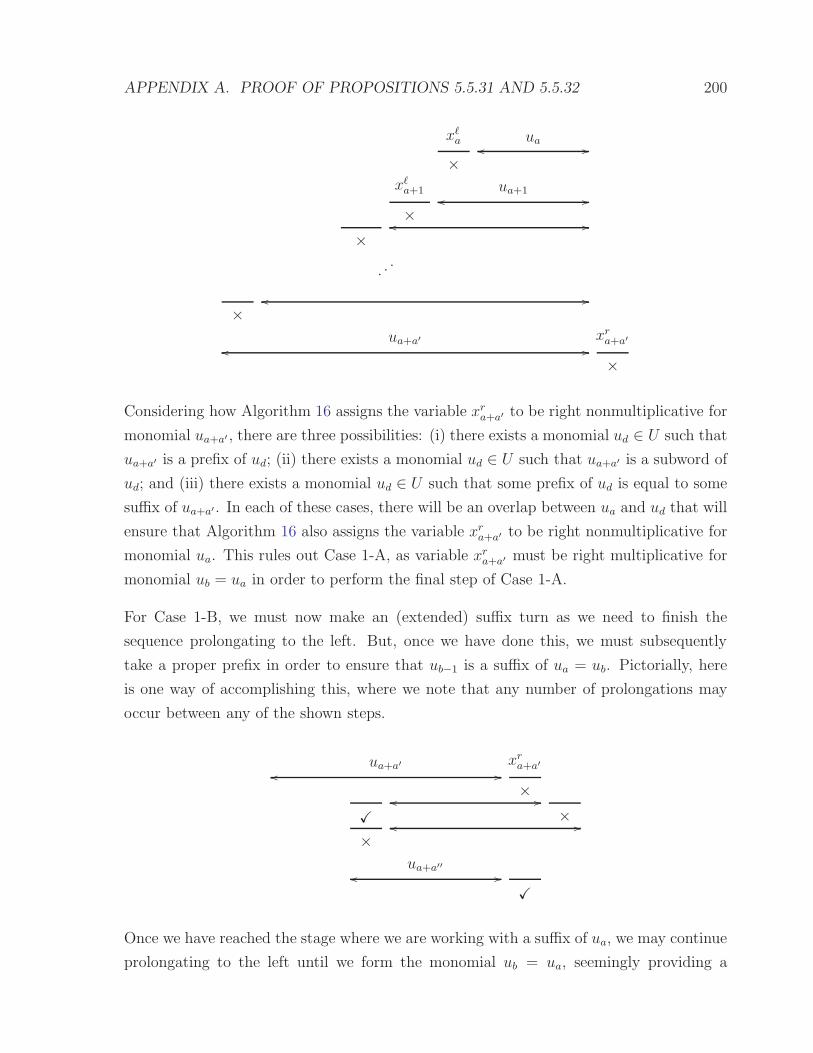
APPENDIX A. PROOF OF PROPOSITIONS 5.5.31 AND 5.5.32 200
xℓa
×oo
ua//
xℓa+1
×oo
ua+1//
×oo //
. ..
×oo //
ooua+a′
//
xra+a′
×
Considering how Algorithm 16 assigns the variable xra+a′ to be right nonmultiplicative for
monomial ua+a′ , there are three possibilities: (i) there exists a monomial ud ∈ U such that
ua+a′ is a prefix of ud; (ii) there exists a monomial ud ∈ U such that ua+a′ is a subword of
ud; and (iii) there exists a monomial ud ∈ U such that some prefix of ud is equal to some
suffix of ua+a′. In each of these cases, there will be an overlap between ua and ud that will
ensure that Algorithm 16 also assigns the variable xra+a′ to be right nonmultiplicative for
monomial ua. This rules out Case 1-A, as variable xra+a′ must be right multiplicative for
monomial ub = ua in order to perform the final step of Case 1-A.
For Case 1-B, we must now make an (extended) suffix turn as we need to finish the
sequence prolongating to the left. But, once we have done this, we must subsequently
take a proper prefix in order to ensure that ub−1 is a suffix of ua = ub. Pictorially, here
is one way of accomplishing this, where we note that any number of prolongations may
occur between any of the shown steps.
ooua+a′
//
xra+a′
×
X
oo //
×
×oo //
ooua+a′′
//
X
Once we have reached the stage where we are working with a suffix of ua, we may continue
prolongating to the left until we form the monomial ub = ua, seemingly providing a

APPENDIX A. PROOF OF PROPOSITIONS 5.5.31 AND 5.5.32 201
counterexample to the proposition (we have managed to construct the same (ℓ, r) pair
twice). However, starting with the monomial labelled ua+a′′ in the above diagram, if we
follow the sequence from ua+a′′ via left prolongations to ub = ua, and then continue with
the same sequence as we started off with, we notice that by the time we encounter the
monomial ua+a′ again, an extended prefix turn has been made, in effect meaning that the
first prolongation of ua we took right at the start of the sequence was invalid.
×oo
ua+a′′//
X
×oo //
. ..
xℓb−1
×oo
ub−1//
xℓa
×oo
ub = ua//
xℓa+1
×oo
ua+1//
×oo //
. ..
×oo //
ooua+a′
//
xra+a′
×
This leaves Case 2-B. Here we start by taking a right prolongation, meaning that some-
where during the sequence a proper prefix must be taken. To do this, it follows that we
must change the direction that prolongations are taken. There are two ways of doing this:
(i) by using an (extended) suffix turn; (ii) by using a right prolongation turn.
In case (i), after performing the (extended) suffix turn, we need to take a proper prefix
so that the next monomial (say uc) in the sequence is a suffix of ua; we then continue
by taking left prolongations until we form the monomial ub = ua. This provides an
apparent counterexample to the proposition, but as for Case 1-B above, by taking the
right prolongation of ua the second time around, we perform an extended prefix turn,
rendering the first right prolongation of ua invalid.

APPENDIX A. PROOF OF PROPOSITIONS 5.5.31 AND 5.5.32 202
Case (i)
×oo
uc//
X
×oo //
. ..
xℓb−1
×oo
ub−1//
ooub = ua
//
xra
×
In case (ii), after we make a right prolongation turn (which may itself occur after a finite
number of right prolongations), we may now take the required proper prefix. But as we
are then required to take a proper suffix (in order to ensure that we finish the sequence
taking a left prolongation), we need to make a turn. But as this would entail making an
(extended) prefix turn, we conclude that case (ii) is also invalid.
An Example of Case (ii)
ooua
//
xra
×
xℓa+1
×oo
ua+1//
xℓa+2
×oo
ua+2//
X
ooua+3
//
×
As we have now accounted for all eight possible sequences, we can conclude that W is
continuous.

APPENDIX A. PROOF OF PROPOSITIONS 5.5.31 AND 5.5.32 203
A.2 Proposition 5.5.32
(Proposition 5.5.32) The two-sided left overlap division W is a Grobner involutive
division.
Proof: We are required to show that if Algorithm 12 terminates with W and some
arbitrary admissible monomial ordering O as input, then the Locally Involutive Basis
G it returns is a noncommutative Grobner Basis. By Definition 3.1.8, we can do this
by showing that all S-polynomials involving elements of G conventionally reduce to zero
using G.
Assume that G = g1, . . . , gp is sorted (by lead monomial) with respect to the DegRevLex
monomial ordering (greatest first), and let U = u1, . . . , up := LM(g1), . . . ,LM(gp) be
the set of leading monomials. Let T be the table obtained by applying Algorithm 16 to
U . Because G is a Locally Involutive Basis, every zero entry T (ui, xΓj ) (Γ ∈ L,R) in
the table corresponds to a prolongation gixj or xjgi that involutively reduces to zero.
Let S be the set of S-polynomials involving elements of G, where the t-th entry of S
(1 6 t 6 |S|) is the S-polynomial
st = ctℓtgirt − c′tℓ′tgjr
′t,
with ℓtuirt = ℓ′tujr′t being the overlap word of the S-polynomial. We will prove that every
S-polynomial in S conventionally reduces to zero using G.
Recall (from Definition 3.1.2) that each S-polynomial in S corresponds to a particular type
of overlap — ‘prefix’, ‘subword’ or ‘suffix’. For the purposes of this proof, let us now split
the subword overlaps into three further types — ‘left’, ‘middle’ and ‘right’, corresponding
to the cases where a monomial m2 is a prefix, proper subword and suffix of a monomial
m1.
Left Middle Right
oom1
//
oo
m2
//
oom1
//
oo
m2
//
oom1
//
oo
m2
//
This classification provides us with five cases to deal with in total, which we shall process
in the following order: right, middle, left, prefix, suffix.

APPENDIX A. PROOF OF PROPOSITIONS 5.5.31 AND 5.5.32 204
(1) Consider an arbitrary entry st ∈ S (1 6 t 6 |S|) corresponding to a right overlap
where the monomial uj is a suffix of the monomial ui. This means that st = ctgi − c′tℓ′tgj
for some gi, gj ∈ G, with overlap word ui = ℓ′tuj. Let ui = xi1 . . . xiα; let uj = xj1 . . . xjβ ;
and let D = α− β.
ui = xi1xi2
___xiD
xiD+1xiD+2
___xiα−1
xiα
uj =xj1
xj2
___xjβ−1
xjβ
Because uj is a suffix of ui, it follows that T (uj, xLiD) = 0. This gives rise to the prolon-
gation xiDgj of gj. But we know that all prolongations involutively reduce to zero (G is
a Locally Involutive Basis), so Algorithm 10 must find a monomial uk = xk1 . . . xkγ ∈ U
such that uk involutively divides xiDuj. Assuming that xkγ = xiκ , we can deduce that
any candidate for uk must be a suffix of xiDuj (otherwise T (uk, xRiκ+1
) = 0 because of the
overlap between ui and uk). But if uk is a suffix of xiDuj, then we must have uk = xiDuj
(otherwise T (uk, xLiα−γ
) = 0 again because of the overlap between ui and uk). We have
therefore shown that there exists a monomial uk = xk1 . . . xkγ ∈ U such that uk is a suffix
of ui and γ = β + 1.
ui = xi1xi2
___xiD
xiD+1xiD+2
___xiα−1
xiα
uj =xj1
xj2
___xjβ−1
xjβ
uk = xk1xk2
xk3
___xkγ−1
xkγ
In the case D = 1, it is clear that uk = ui, and so the first step in the involutive reduction
of the prolongation xi1gj of gj is to take away the multiple ( ctc′t)gi of gi from xi1gj to leave
the polynomial xi1gj−( ctc′t)gi = −( 1
c′t)st. But as we know that all prolongations involutively
reduce to zero, we can conclude that the S-polynomial st conventionally reduces to zero.
For the case D > 1, we can use the monomial uk together with Buchberger’s Second
Criterion to simplify our goal of showing that the S-polynomial st reduces to zero. Notice
that the monomial uk is a subword of the overlap word ui associated to st, and so in order
to show that st reduces to zero, all we have to do is to show that the two S-polynomials
su = cugi − c′u(xi1xi2 . . . xiD−1)gk
and
sv = cvgk − c′vxiDgj

APPENDIX A. PROOF OF PROPOSITIONS 5.5.31 AND 5.5.32 205
reduce to zero (1 6 u, v 6 |S|). But sv is an S-polynomial corresponding to a right overlap
of type D = 1 (because γ−β = 1), and so sv reduces to zero. It remains to show that the
S-polynomial su reduces to zero. But we can do this by using exactly the same argument
as above — we can show that there exists a monomial uπ = xπ1. . . xπδ
∈ U such that uπ
is a suffix of ui and δ = γ + 1, and we can deduce that the S-polynomial su reduces to
zero (and hence st reduces to 0) if the S-polynomial
sw = cwgi − c′w(xi1xi2 . . . xiD−2)gπ
reduces to zero (1 6 w 6 |S|). By induction, there is a sequence uqD , uqD−1, . . . , uq2 of
monomials increasing uniformly in degree, so that st reduces to zero if the S-polynomial
sη = cηgi − c′ηxi1gq2
reduces to zero (1 6 η 6 |S|).
ui = xi1xi2
___xiD−1
xiDxiD+1
xiD+2
___xiα−1
xiα
uj =xj1
xj2
___xjβ−1
xjβ
uqD = uk = ___
uqD−1= uπ = ___
... . ..
uq2 = ___ ___
But sη is always an S-polynomial corresponding to a right overlap of type D = 1, and so
sη reduces to zero — meaning we can conclude that st reduces to zero as well.
(2) Consider an arbitrary entry st ∈ S (1 6 t 6 |S|) corresponding to a middle overlap
where the monomial uj is a proper subword of the monomial ui. This means that st =
ctgi − c′tℓ′tgjr
′t for some gi, gj ∈ G, with overlap word ui = ℓ′tujr
′t. Let ui = xi1 . . . xiα ; let
uj = xj1 . . . xjβ ; and choose D such that xiD = xjβ .
ui = xi1
___xiD−β
xiD−β+1xiD−β+2
___xiD−1
xiDxiD+1
___xiα
uj =xj1
xj2
___xjβ−1
xjβ
Because uj is a proper subword of ui, it follows that T (uj, xRiD+1
) = 0. This gives rise to

APPENDIX A. PROOF OF PROPOSITIONS 5.5.31 AND 5.5.32 206
the prolongation gjxiD+1of gj. But we know that all prolongations involutively reduce
to zero, so there must exist a monomial uk = xk1 . . . xkγ ∈ U such that uk involutively
divides ujxiD+1. Assuming that xkγ = xiκ , any candidate for uk must be a suffix of ujxiD+1
(otherwise T (uk, xRiκ+1
) = 0 because of the overlap between ui and uk). Unlike part (1)
however, we cannot determine the degree of uk (so that 1 6 γ 6 β+1); we shall illustrate
this in the following diagram by using a squiggly line to indicate that the monomial uk
can begin anywhere (or nowhere if uk = xiD+1) on the squiggly line.
ui = xi1
___xiD−β
xiD−β+1xiD−β+2
___xiD−1
xiDxiD+1
___xiα
uj =xj1
xj2
___xjβ−1
xjβ
uk = /o/o/o/o/o/o/o/o/o/o/o/o/o/o/o/o/o/o/o/o/o/o/oxkγ
We can now use the monomial uk together with Buchberger’s Second Criterion to simplify
our goal of showing that the S-polynomial st reduces to zero. Notice that the monomial
uk is a subword of the overlap word ui associated to st, and so in order to show that st
reduces to zero, all we have to do is to show that the two S-polynomials
su = cugi − c′u(xi1xi2 . . . xiD+1−γ)gk(xiD+2
. . . xiα)
and1
sv = cv(xj1 . . . xiD+1−γ)gk − c′vgjxiD+1
reduce to zero (1 6 u, v 6 |S|).
For the S-polynomial sv, there are two cases to consider: γ = 1, and γ > 1. In the
former case, because (as placed in ui) the monomials uj and uk do not overlap, we can use
Buchberger’s First Criterion to say that the ‘S-polynomial’ sv reduces to zero (for further
explanation, see the paragraph at the beginning of Section 3.4.1). In the latter case,
note that uk is the only involutive divisor of the prolongation ujxiD+1, as the existence
of any suffix of ujxiD+1of higher degree than uk in U will contradict the fact that uk is
an involutive divisor of ujxiD+1; and the existence of uk in U ensures that any suffix of
ujxiD+1that exists in U with a lower degree than uk will not be an involutive divisor of
ujxiD+1. This means that the first step of the involutive reduction of gjxiD+1
is to take away
the multiple ( cvc′v)(xj1 . . . xiD+1−γ
)gk of gk from gjxiD+1to leave the polynomial gjxiD+1
−
1Technical point: if γ 6= β + 1, the S-polynomial sv could in fact appear as sv = cvgjxiD+1−
c′v(xj1 . . . xiD+1−γ)gk and not as sv = cv(xj1 . . . xiD+1−γ
)gk − c′vgjxiD+1; for simplicity we will treat both
cases the same in the proof as all that changes is the notation and the signs.

APPENDIX A. PROOF OF PROPOSITIONS 5.5.31 AND 5.5.32 207
( cvc′v)(xj1 . . . xiD+1−γ
)gk = −( 1c′v)sv. But as we know that all prolongations involutively
reduce to zero, we can conclude that the S-polynomial sv conventionally reduces to zero.
For the S-polynomial su, we note that if D = α−1, then su corresponds to a right overlap,
and so we know from part (1) that su conventionally reduces to zero. Otherwise, we
proceed by induction on the S-polynomial su to produce a sequence uqD+1, uqD+2
, . . . , uqα
of monomials, so that su (and hence st) reduces to zero if the S-polynomial
sη = cηgi − c′η(xi1 . . . xiα−µ)gqα
reduces to zero (1 6 η 6 |S|), where µ = deg(uqα).
ui = xi1
___xiD−β
xiD−β+1
___xiD
xiD+1xiD+2
___xiα−1
xiα
uj =xj1
___xjβ
uqD+1= uk = /o/o/o/o/o/o/o/o/o/o/o
xkγ
uqD+2= /o/o/o/o/o/o/o/o/o/o/o/o/o/o/o/o
. . .
uqα = /o/o/o/o/o/o/o/o/o/o/o/o/o/o/o/o/o/o/o/o/o/o/o/o/o/o/o/o/o
But sη always corresponds to a right overlap, and so sη reduces to zero — meaning we
can conclude that st reduces to zero as well.
(3) Consider an arbitrary entry st ∈ S (1 6 t 6 |S|) corresponding to a left overlap where
the monomial uj is a prefix of the monomial ui. This means that st = ctgi − c′tgjr′t for
some gi, gj ∈ G, with overlap word ui = ujr′t. Let ui = xi1 . . . xiα and let uj = xj1 . . . xjβ .
ui = xi1xi2
___xiβ−1
xiβxiβ+1
___xiα−1
xiα
uj =xj1
xj2
___xjβ−1
xjβ
Because uj is a prefix of ui, it follows that T (uj, xRiβ+1
) = 0. This gives rise to the
prolongation gjxiβ+1of gj . But we know that all prolongations involutively reduce to
zero, so there must exist a monomial uk = xk1 . . . xkγ ∈ U such that uk involutively
divides ujxiβ+1. Assuming that xkγ = xiκ , any candidate for uk must be a suffix of ujxiβ+1

APPENDIX A. PROOF OF PROPOSITIONS 5.5.31 AND 5.5.32 208
(otherwise T (uk, xRiκ+1
) = 0 because of the overlap between ui and uk).
ui = xi1xi2
___xiβ−1
xiβxiβ+1
___xiα−1
xiα
uj =xj1
xj2
___xjβ−1
xjβ
uk = /o/o/o/o/o/o/o/o/o/o/o/o/o/o/o/o/o/o/oxkγ
If α = γ, then it is clear that uk = ui, and so the first step in the involutive reduction
of the prolongation gjxiα is to take away the multiple ( ctc′t)gi of gi from gjxiα to leave the
polynomial gjxiα − ( ctc′t)gi = −( 1
c′t)st. But as we know that all prolongations involutively
reduce to zero, we can conclude that the S-polynomial st conventionally reduces to zero.
Otherwise, if α > γ, we can now use the monomial uk together with Buchberger’s Second
Criterion to simplify our goal of showing that the S-polynomial st reduces to zero. Notice
that the monomial uk is a subword of the overlap word ui associated to st, and so in order
to show that st reduces to zero, all we have to do is to show that the two S-polynomials
su = cugi − c′u(xi1 . . . xiβ+1−γ)gk(xiβ+2
. . . xiα)
and
sv = cv(xi1 . . . xiβ+1−γ)gk − c′vgjxiβ+1
reduce to zero (1 6 u, v 6 |S|).
The S-polynomial sv reduces to zero by comparison with part (2). For the S-polynomial
su, first note that if α = β + 1, then su corresponds to a right overlap, and so we know
from part (1) that su conventionally reduces to zero. Otherwise, if γ 6= β + 1, then su
corresponds to a middle overlap, and so we know from part (2) that su conventionally
reduces to zero. This leaves the case where su corresponds to another left overlap, in which
case we proceed by induction on su, eventually coming across either a middle overlap or a
right overlap because we move one letter at a time to the right after each inductive step.
ui = xi1xi2
___xiβ−1
xiβxiβ+1
xiβ+2
___xiα−1
xiα
uj =xj1
xj2
___xjβ−1
xjβ
uk = /o/o/o/o/o/o/o/o/o/o/o/o/o/o/o/o/o/o/o/oxkγ
/o/o/o/o/o/o/o/o/o/o/o/o/o/o/o/o/o/o/o/o/o/o/o/o/o
. . ./o/o/o/o/o/o/o/o/o/o/o/o/o/o/o/o/o/o/o/o/o/o/o/o/o/o/o/o/o/o/o/o/o/o/o/o/o/o

APPENDIX A. PROOF OF PROPOSITIONS 5.5.31 AND 5.5.32 209
(4 and 5) In Definition 3.1.2, we defined a prefix overlap to be an overlap where, given
two monomials m1 and m2 such that deg(m1) > deg(m2), a prefix of m1 is equal to a
suffix of m2; suffix overlaps were defined similarly. If we drop the condition on the degrees
of the monomials, it is clear that every suffix overlap can be treated as a prefix overlap
(by swapping the roles of m1 and m2); this allows us to deal with the case of a prefix
overlap only.
Consider an arbitrary entry st ∈ S (1 6 t 6 |S|) corresponding to a prefix overlap where
a prefix of the monomial ui is equal to a suffix of the monomial uj. This means that
st = ctℓtgi − c′tgjr′t for some gi, gj ∈ G, with overlap word ℓtui = ujr
′t. Let ui = xi1 . . . xiα ;
let uj = xj1 . . . xjβ ; and choose D such that xiD = xjβ .
ui = xi1
___xiD
xiD+1
___xiα−1
xiα
uj =xj1
___xjβ−D
xjβ−D+1
___xjβ
By definition of W, at least one of T (ui, xLjβ−D
) and T (uj, xRiD+1
) is equal to zero.
• Case T (uj, xRiD+1
) = 0.
Because we know that the prolongation gjxiD+1involutively reduces to zero, there
must exist a monomial uk = xk1 . . . xkγ ∈ U such that uk involutively divides ujxiD+1.
This uk must be a suffix of ujxiD+1(otherwise, assuming that xkγ = xjκ, we have
T (uk, xRiD+1
) = 0 if γ = β (because of the overlap between ui and uk); T (uk, xLjβ−γ
) =
0 if γ < β and κ = β (because of the overlap between uj and uk); and T (uk, xRjκ+1
) =
0 if γ < β and κ < β (again because of the overlap between uj and uk)).
ui = xi1
___xiD
xiD+1
___xiα−1
xiα
uj =xj1
___xjβ−D
xjβ−D+1
___xjβ
uk = /o/o/o/o/o/o/o/o/o/o/o/o/o/o/o/o/o/o/o/o/o/o/o/o/o/o/oxkγ
Let us now use the monomial uk together with Buchberger’s Second Criterion to
simplify our goal of showing that the S-polynomial st reduces to zero. Because uk is
a subword of the overlap word ℓtui associated to st, in order to show that st reduces
to zero, all we have to do is to show that the two S-polynomials
su =
cu(xk1 . . . xjβ−D)gi − c′ugk(xiD+2
. . . xiα) if γ > D + 1
cugi − c′uℓ′ugk(xiD+2
. . . xiα) if γ 6 D + 1

APPENDIX A. PROOF OF PROPOSITIONS 5.5.31 AND 5.5.32 210
and
sv = cvgjxiD+1− c′v(xj1 . . . xjβ+1−γ
)gk
reduce to zero (1 6 u, v 6 |S|).
The S-polynomial sv reduces to zero by comparison with part (2). For the S-
polynomial su, first note that if α = D + 1, then either uk is a suffix of ui, ui is a
suffix of uk, or uk = ui; it follows that su reduces to zero trivially if uk = ui, and su
reduces to zero by part (1) in the other two cases.
If however α 6= D + 1, then either su is a middle overlap (if γ < D + 1), a left
overlap (if γ = D+1), or another prefix overlap. The first two cases can be handled
by parts (2) and (3) respectively; the final case is handled by induction, where we
note that after each step of the induction, the value α + β − 2D strictly decreases
(regardless of which case T (uj, xRiD+1
) = 0 or T (ui, xLjβ−D
) = 0 applies), so we are
guaranteed at some stage to find an overlap that is not a prefix overlap, enabling
us to verify that the S-polynomial st conventionally reduces to zero.
• Case T (ui, xLjβ−D
) = 0.
Because we know that the prolongation xjβ−Dgi involutively reduces to zero, there
must exist a monomial uk = xk1 . . . xkγ ∈ U such that uk involutively divides xjβ−Dui.
This uk must be a prefix of xjβ−Dui (otherwise, assuming that xkγ = xiκ , we have
T (uk, xLjβ−D
) = 0 if γ = α (because of the overlap between uj and uk); T (uk, xLiκ−γ
) =
0 if γ < α and κ = α (because of the overlap between ui and uk); and T (uk, xRiκ+1
) = 0
if γ < α and κ < α (again because of the overlap between ui and uk)).
ui = xi1
___xiD
xiD+1
___xiα−1
xiα
uj =xj1
___xjβ−D
xjβ−D+1
___xjβ
uk = xk1
/o/o/o/o/o/o/o/o/o/o/o/o/o/o/o/o/o/o/o/o/o/o/o/o/o/o/o/o/o/o/o/o
Let us now use the monomial uk together with Buchberger’s Second Criterion to
simplify our goal of showing that the S-polynomial st reduces to zero. Because uk is
a subword of the overlap word ℓtui associated to st, in order to show that st reduces
to zero, all we have to do is to show that the two S-polynomials
su = cuxk1gi − c′ugk(xiγ . . . xiα)

APPENDIX A. PROOF OF PROPOSITIONS 5.5.31 AND 5.5.32 211
and
sv =
cvgj(xiD+1. . . xkγ )− c′v(xj1 . . . xjβ−D−1
)gk if γ > D + 1
cvgj − c′v(xj1 . . . xjβ−D−1)gkr
′v if γ 6 D + 1
reduce to zero (1 6 u, v 6 |S|).
The S-polynomial su reduces to zero by comparison with part (2). For the S-
polynomial sv, first note that if β −D = 1, then either uk is a prefix of uj, uj is a
prefix of uk, or uk = uj; it follows that sv reduces to zero trivially if uk = uj, and
sv reduces to zero by part (3) in the other two cases.
If however β − D 6= 1, then either sv is a middle overlap (if γ < D + 1), a right
overlap (if γ = D+1), or another prefix overlap. The first two cases can be handled
by parts (2) and (1) respectively; the final case is handled by induction, where we
note that after each step of the induction, the value α + β − 2D strictly decreases
(regardless of which case T (uj, xRiD+1
) = 0 or T (ui, xLjβ−D
) = 0 applies), so we are
guaranteed at some stage to find an overlap that is not a prefix overlap, enabling
us to verify that the S-polynomial st conventionally reduces to zero.

Appendix B
Source Code
In this Appendix, we will present ANSI C source code for an initial implementation of the
noncommutative Involutive Basis algorithm (Algorithm 12), together with an introduction
to AlgLib, a set of ANSI C libraries providing data types and functions that serve as
building blocks for the source code.
B.1 Methodology
A problem facing anyone wanting to implement mathematical ideas is the choice of lan-
guage or system in which to do the implementation. The decision depends on the task
at hand. If all that is required is a convenient environment for prototyping ideas, a
symbolic computation system such as Maple [55], Mathematica [57] or MuPAD [49] may
suffice. Such systems have a large collection of mathematical data types, functions and
algorithms already present; tools that will not be available in a standard programming
language. There is however always a price to pay for convenience. These common systems
are all interpreted and use a proprietary programming syntax, making it it difficult to
use other programs or libraries within a session. It also makes such systems less efficient
than the execution of compiled programs.
The AlgLib libraries can be said to provide the best of both worlds, as they provide data
types, functions and algorithms to allow programmers to more easily implement certain
mathematical algorithms (including the algorithms described in this thesis) in the ANSI
C programming language. For example, AlgLib contains the FMon [41] and FAlg [40]
212

APPENDIX B. SOURCE CODE 213
libraries, respectively containing data types and functions to perform computations in
the free monoid on a set of symbols and the free associative algebra on a set of symbols.
Besides the benefit of the efficiency of compiled programs, the strict adherence to ANSI
C makes programs written using the libraries highly portable.
B.1.1 MSSRC
AlgLib is supplied by MSSRC [46], a company whose Chief Scientist is Prof. Larry Lambe,
an honorary professor at the University of Wales, Bangor. For an introduction to MSSRC,
we quote the following passage from [42].
Multidisciplinary Software Systems Research Corporation (MSSRC) was con-
ceived as a company devoted to furthering the long-term effective use of math-
ematics and mathematical computation. MSSRC researches, develops, and
markets advanced mathematical tools for engineers, scientists, researchers,
educators, students and other serious users of mathematics. These tools are
based on providing levels of power, productivity and convenience far greater
than existing tools while maintaining mathematical rigor at all times. The
company also provides computer education and training.
MSSRC has several lines of ANSI C libraries for providing mathematical sup-
port for research and implementation of mathematical algorithms at various
levels of complexity. No attempt is made to provide the user of these libraries
with any form of Graphical User Interface (GUI). All components are compiled
ANSI C functions which represent various mathematical operations from basic
(adding, subtracting, multiplying polynomials, etc.) to advanced (operations
in the free monoid on an arbitrary number of symbols and beyond). In order
to use the libraries effectively, the user must be expert at ANSI C program-
ming, e.g., in the style of Kernighan and Richie [38] and as such, they are not
suited for the casual user. This does not imply in any way that excellent user
interfaces for applications of the libraries cannot be supplied or are difficult
to implement by well experienced programmers.
The use of MSSRC’s libraries has been reported in a number of places such
as [43], [14], [16], [15] and elsewhere.

APPENDIX B. SOURCE CODE 214
B.1.2 AlgLib
To give a taste of how AlgLib has been used to implement the algorithms considered in this
thesis, consider one of the basic operations of these algorithms, the task of subtracting
two polynomials to yield a third polynomial (an operation essential for computing an
S-polynomial). In ordinary ANSI C, there is no data type for a polynomial, and certainly
no function for subtracting two polynomials; AlgLib however does supply these data types
and functions, both in the commutative and noncommutative cases. For example, the
AlgLib data type for a noncommutative polynomial is an FAlg, and the AlgLib function
for subtracting two such polynomials is the function fAlgMinus. It follows that we can
write ANSI C code for subtracting two noncommutative polynomials, as illustrated below
where we subtract the polynomial 2b2 + ab+ 4b from the polynomial 2× (b2 + ba+ 3a).
Source Code
# include <fralg.h>
int
main( argc, argv )
int argc;
char ∗argv[];
// Define Variables
FAlg p, q, r;
QInteger two;
// Set Monomial Ordering (DegLex)
theOrdFun = fMonTLex;
// Initialise Variables
p = parseStrToFAlg("b^2 + b*a + 3*a");
q = parseStrToFAlg("2*b^2 + a*b + 4*b");
two = parseStrToQ("2");
// Perform the calculation and display the result on screen
r = fAlgMinus( fAlgScaTimes( two, p ), q );
printf("2*(%s) - (%s) = %s\n", fAlgToStr( p ), fAlgToStr( q ), fAlgToStr( r ) );
return EXIT SUCCESS;
Program Output
ma6:mssrc−aux/thesis> fAlgMinusTest
2∗(bˆ2 + b a + 3 a) − (2 bˆ2 + a b + 4 b) = 2 b a − a b −4 b + 6 a
ma6:mssrc−aux/thesis>

APPENDIX B. SOURCE CODE 215
B.2 Listings
Our implementation of the noncommutative Involutive Basis algorithm is arranged as
follows: involutive.c is the main program, dealing with all the input and output and calling
the appropriate routines; the ‘ functions’ files contain all the procedures and functions
used by the program; and README describes how to use the program, including what
format the input files should take and what the different options of the program are used
for.
In more detail, arithmetic functions.c contains functions for dividing a polynomial by
its (coefficient) greatest common divisor and for converting user specified generators to
ASCII generators (and vice-versa); file functions.c contains all the functions needed to
read and write polynomials and variables to and from disk; fralg functions.c contains
functions for monomial orderings, polynomial division and reduced Grobner Bases com-
putation; list functions.c contains some extra functions needed to deal with displaying,
sorting and manipulating lists; and ncinv functions.c contains all the involutive routines,
for example the Involutive Basis algorithm itself and associated functions for determining
multiplicative variables and for performing autoreduction.
Contents
B.2.1 README . . . . . . . . . . . . . . . . . . . . . . . . . . . . . . . . . . . . . . . . . . . . . . . . . . . . . 216
B.2.2 arithmetic functions.h . . . . . . . . . . . . . . . . . . . . . . . . . . . . . . . . . . . . . . . . . 219
B.2.3 arithmetic functions.c . . . . . . . . . . . . . . . . . . . . . . . . . . . . . . . . . . . . . . . . . . 220
B.2.4 file functions.h . . . . . . . . . . . . . . . . . . . . . . . . . . . . . . . . . . . . . . . . . . . . . . . . . 226
B.2.5 file functions.c . . . . . . . . . . . . . . . . . . . . . . . . . . . . . . . . . . . . . . . . . . . . . . . . . 227
B.2.6 fralg functions.h . . . . . . . . . . . . . . . . . . . . . . . . . . . . . . . . . . . . . . . . . . . . . . . 238
B.2.7 fralg functions.c . . . . . . . . . . . . . . . . . . . . . . . . . . . . . . . . . . . . . . . . . . . . . . . 240
B.2.8 list functions.h . . . . . . . . . . . . . . . . . . . . . . . . . . . . . . . . . . . . . . . . . . . . . . . . . 268
B.2.9 list functions.c . . . . . . . . . . . . . . . . . . . . . . . . . . . . . . . . . . . . . . . . . . . . . . . . . 271
B.2.10 ncinv functions.h . . . . . . . . . . . . . . . . . . . . . . . . . . . . . . . . . . . . . . . . . . . . . . 290
B.2.11 ncinv functions.c . . . . . . . . . . . . . . . . . . . . . . . . . . . . . . . . . . . . . . . . . . . . . . . 291
B.2.12 involutive.c . . . . . . . . . . . . . . . . . . . . . . . . . . . . . . . . . . . . . . . . . . . . . . . . . . . . 340

APPENDIX B. SOURCE CODE 216
B.2.1 README
∗∗∗∗∗∗∗∗∗∗∗∗∗∗∗∗∗∗∗∗∗∗∗∗∗∗∗∗∗∗∗∗∗∗∗∗∗∗∗∗∗∗∗∗∗∗∗∗∗∗∗∗∗∗∗∗∗∗∗∗∗∗∗∗
∗ HOW TO USE THE INVOLUTIVE PROGRAM − QUICK GUIDE ∗
∗∗∗∗∗∗∗∗∗∗∗∗∗∗∗∗∗∗∗∗∗∗∗∗∗∗∗∗∗∗∗∗∗∗∗∗∗∗∗∗∗∗∗∗∗∗∗∗∗∗∗∗∗∗∗∗∗∗∗∗∗∗∗∗
NAME
involutive − Computes Noncommutative Involutive Bases for ideals.
SYNOPSIS
involutive [ OPTION]... [FILE]...
DESCRIPTION
Here are the options for the program.
−a
e. g. > involutive −d −a file. in
Optimises the lexicographical ordering according to
the frequency of the variables in the input basis
(most frequent = lexicographically smallest).
−c(n)
e. g. > involutive −c2 file . in
Chooses which involutive algorithm to use.
n is a required number between 1 and 2.
1: ∗DEFAULT ∗ Gerdt’s Algorithm
2: Seiler ’ s Algorithm
−d
e. g. > involutive −d file . in
Allows the user to calculate a DegLex
Involutive Basis for the basis in file . in.
−e(n)
e. g. > involutive −e2 −s2 file. in
Allows the user to select the type of Overlap
Division to use. n is a required number between
1 and 5. Note: Must be used with either the
−s1 or −s2 options.
Left Overlap Division:
A B C D
−−−−− −−−−−−− −−−−−−−−− −−−−−−
−−−−−x −−−−x −−−−x x−−−
1: ∗ DEFAULT ∗ A, B, C (weak, Gr\”obner)
2: A, B, C, Strong (strong if used with −m2)
3: A, B, C, D (weak, Gr\”obner)
4: A, B (weak, Gr\”obner)
5: A (weak, Gr\”obner)

APPENDIX B. SOURCE CODE 217
Right Overlap Division:
A B C D
−−−−− −−−−−−− −−−−−−−−− −−−−−−
x−−−−− x−−− x−−−− −−−x
1: ∗ DEFAULT ∗ A, B, C (weak, Gr\”obner)
2: A, B, C, Strong (strong if used with −m2)
3: A, B, C, D (weak, Gr\”obner)
4: A, B (weak, Gr\”obner)
5: A (weak, Gr\”obner)
−f
e. g. > involutive −f file . in
Removes any fractions from the input basis.
−l
e. g. > involutive −l file . in
Allows the user to calculate a Lex
Involutive Basis for the basis in file . in.
Warning: program may go into an infinite loop
(Lex is not an admissible monomial ordering).
−m(n)
e. g. > involutive −m2 file.in
Selects which method of deciding whether a monomial
involutively divides another monomial is used.
n is a required number between 1 and 2.
1: ∗ DEFAULT ∗ 1st letters on left and right (thin divisor )
2: All letters on left and right (thick divisor )
−o(n)
e. g. > involutive −o2 file . in
Allows the user to select how the basis is sorted
during the algorithm. n is a required number between
1 and 3.
1: ∗ DEFAULT ∗ DegRevLex Sorted
2: No Sorting
3: Sorting by Main Ordering
−p
e. g. > involutive −l −p file . in
An interactive Ideal Membership Problem Solver.
There are two ways the solver can be used:
either a file containing a list of polynomials
(e. g. x∗y−z;
xˆ2−zˆ2+yˆ2; ) can be given, or the
polynomials can be input
manually (e.g. x∗y−z). The solver tests to see
whether the Involutive Basis computed in the
algorithm reduces the polynomials given to zero.

APPENDIX B. SOURCE CODE 218
−r ∗ DEFAULT ∗
e. g. > involutive −r file . in
Allows the user to calculate a DegRevLex
Involutive Basis for the basis in file . in.
−s(n)
e. g. > involutive −s2 file . in
Allows the user to select the type of Involutive
Basis to calculate . n is a required number between
1 and 5. Note: If an ‘Overlap’ Division is selected ,
the type of Overlap Division can be chosen with
the −e(n) option.
1: Left Overlap Division (local , cts , see −e option)
2: Right Overlap Division (local , cts , see −e option)
3: ∗ DEFAULT ∗ Left Division (global, cts, strong)
4: Right Division (global, cts , strong)
5: Empty Division (global, cts , strong)
−v(n)
e. g. > involutive −v3 file . in
Changes the amount of information given out by the
program (i.e. the ‘ verbosity’ of the program).
n is a number between 0 and 9. Rough Guide:
0: Silent (no output given).
1: ∗ DEFAULT ∗
2: Returns Number of Reductions Carried Out,
Prints Out Every Polynomial Found
3: More Autoreduction Information,
Prolongation Information
4: More Details of Steps Taken in Algorithm
5: More Global Division Information
6: Step−by−Step Reduction, Overlap Information
7: Shows Multiplicative Grids
8: More Overlap Division Information
9: All Other Information
−w
e. g. > involutive −w file. in
Allows the user to calculate an Involutive Basis
for the basis in file . in using the Wreath
Product Monomial Ordering.
−x
e. g. > involutive −x file . in
Ignores any prolongations of degree greater than or
equal to 2d, where d is a value determined by the degree
of the largest degree lead monomial in the current minimal basis.
Warning: May not return a valid Involutive Basis
(only a valid Gr\”obner Basis).

APPENDIX B. SOURCE CODE 219
FILE FORMATS
There is one file format for the input basis :
IDEALS:
−−−−−−−−−−−−−−
x; y; z;
x∗y − z;
2∗x + y∗z + z;
−−−−−−−−−−−−−−
First line = List of variables in order. In the
above, x; y; z; represents x > y > z.
Remaining lines = Polynomial generators (which must be
terminated by semicolons).
OUTPUT
As output, the program provides a reduced Gr\”obner Basis and
an Involutive Basis for the input ideal (if it can calculate it ).
For the following , assume that our input basis was given as file . in.
∗ If a DegRevLex Gr\”obner Basis is calculated, it is stored as file . drl .
∗ If a DegLex Gr\”obner Basis is calculated, it is stored as file . deg.
∗ If a Lex Gr\”obner Basis is calculated, it is stored as file . lex.
∗ If a Wreath Product Gr\”obner Basis is calculated, it is stored as file . wp.
The Involutive Basis is given as <Gr\”obner Basis>.inv.
For example, if a DegLex Involutive Basis is calculated ,
it is stored as file . deg.inv.
Note that the program has the ability to recognise the . in suffix and
replace it with .drl , . deg, . lex or . wp as necessary.
If your input file does not have a . in suffix then the program will
simply append the appropriate suffix onto the end of the file name.
For example, using the command
> involutive FILE
we obtain file . drl if FILE = file.in
and obtain e.g. file . other. drl if FILE = file.other.
B.2.2 arithmetic functions.h
1 /∗
2 ∗ File: arithmetic functions.h
3 ∗ Author: Gareth Evans
4 ∗ Last Modified: 29th September 2004
5 ∗/
6
7 // Initialise file definition
8 # ifndef ARITHMETIC FUNCTIONS HDR
9 # define ARITHMETIC FUNCTIONS HDR
10

APPENDIX B. SOURCE CODE 220
11 // Include MSSRC Libraries
12 # include <fralg.h>
13
14 //
15 // Numerical Functions
16 //
17
18 // Returns the numerical value of a 3 letter word
19 ULong ASCIIVal( String );
20 // Returns the 3 letter word of a numerical value
21 String ASCIIStr( ULong );
22 // Returns the monomial corresponding to the 3 letter word of a numerical value
23 FMon ASCIIMon( ULong );
24
25 //
26 // QInteger Functions
27 //
28
29 // Calculate Alternative LCM of 2 QIntegers
30 QInteger AltLCMQInteger( QInteger, QInteger );
31
32 //
33 // FAlg Functions
34 //
35
36 // Divides the input FAlg by its common GCD
37 FAlg findGCD( FAlg );
38 // Returns maximal degree of lead term for the given FAlgList
39 ULong maxDegree( FAlgList );
40 // Returns the position of the smallest LM(g) in the given FAlgList
41 ULong fAlgListLowest( FAlgList );
42
43 # endif // ARITHMETIC FUNCTIONS HDR
B.2.3 arithmetic functions.c
1 /∗
2 ∗ File: arithmetic functions.c
3 ∗ Author: Gareth Evans
4 ∗ Last Modified: 11th February 2005
5 ∗/
6
7 /∗
8 ∗ ===================
9 ∗ Numerical Functions
10 ∗ ===================
11 ∗/
12
13 /∗
14 ∗ Function Name: ASCIIVal
15 ∗
16 ∗ Overview: Returns the numerical value of a 3 letter word

APPENDIX B. SOURCE CODE 221
17 ∗
18 ∗ Detail: Given a String containing 3 letters from the set
19 ∗ A, B, ..., Z, this function returns the numerical
20 ∗ value of the String according to the following rule:
21 ∗ AAA = 1, AAB = 2, ..., AAZ = 26, ABA = 27, ABB = 28,
22 ∗ ..., ABZ = 52, ACA = 53, ...
23 ∗
24 ∗/
25 ULong
26 ASCIIVal( word )
27 String word;
28
29 ULong back = 0;
30
31 // Add on 17576∗value of 1st letter (A = 0, B = 1, ...)
32 back = back + 17576∗( (ULong)( (int)word[0] − (int)’A’ ) );
33 // Add on 26∗value of 2nd letter (A = 0, B = 1, ...)
34 back = back + 26∗( (ULong)( (int)word[1] − (int)’A’ ) );
35 // Add on the value of the 3rd letter (A = 1, B = 2, ...)
36 back = back + (ULong)( (int)word[2] − (int)’A’ + 1 );
37
38 return back;
39
40
41 /∗
42 ∗ Function Name: ASCIIStr
43 ∗
44 ∗ Overview: Returns the 3 letter word of a numerical value
45 ∗
46 ∗ Detail: Given a ULong, this function returns the
47 ∗ 3 letter String corresponding to the following rule:
48 ∗ 1 = AAA, 2 = AAB, ..., 26 = AAZ, 27 = ABA, 28 = ABB,
49 ∗ ..., 52 = ABZ, 53 = ACA, ...
50 ∗
51 ∗/
52 String
53 ASCIIStr( number )
54 ULong number;
55
56 String back = strNew();
57 int i = 0, j = 0, k;
58
59 // Take away multiples of 26ˆ2 to get the first letter
60 while( number > 17576 )
61
62 i++;
63 number = number − 17576;
64
65
66 // Take away multiples of 26 to get the second letter
67 while( number > 26 )
68
69 j++;

APPENDIX B. SOURCE CODE 222
70 number = number − 26;
71
72
73 // We are now left with the third letter
74 k = (int) number − 1;
75
76 // Convert the numbers to a String
77 sprintf( back, "%c%c%c", (char)( (int)’A’ + i ),
78 (char)( (int)’A’ + j ),
79 (char)( (int)’A’ + k ) );
80
81 // Return the three letters
82 return back;
83
84
85 /∗
86 ∗ Function Name: ASCIIStr
87 ∗
88 ∗ Overview: Returns the monomial corresponding to the
89 ∗ 3 letter word of a numerical value
90 ∗
91 ∗ Detail: Given a ULong, this function returns the
92 ∗ monomial corresponding to the following rule:
93 ∗ 1 = AAA, 2 = AAB, ..., 26 = AAZ, 27 = ABA, 28 = ABB,
94 ∗ ..., 52 = ABZ, 53 = ACA, ...
95 ∗
96 ∗/
97 FMon
98 ASCIIMon( number )
99 ULong number;
100
101 // Obtain the String corresponding to the input
102 // number and change it to an FMon
103 return parseStrToFMon( ASCIIStr( number ) );
104
105
106 /∗
107 ∗ ==================
108 ∗ QInteger Functions
109 ∗ ==================
110 ∗/
111
112 /∗
113 ∗ Function Name: AltLCMQInteger
114 ∗
115 ∗ Overview: Calculates an ’alternative’ LCM of 2 QIntegers
116 ∗
117 ∗ Detail: Given two QIntegers a = an/ad and b = bn/bd,
118 ∗ this function calculates the LCM given
119 ∗ by alt lcm(a, b) = (a∗b)/(alt gcd(a, b))
120 ∗ = (an∗bn∗ad∗bd)/(ad∗bd∗gcd(an, bn)∗gcd(ad, bd))
121 ∗ = (an∗bn)/(gcd(an, bn)∗gcd(ad, bd)).
122 ∗

APPENDIX B. SOURCE CODE 223
123 ∗/
124 QInteger
125 AltLCMQInteger( a, b )
126 QInteger a, b;
127
128 Integer an = a −> num,
129 ad = a −> den,
130 bn = b −> num,
131 bd = b −> den;
132
133 return qDivide( zToQ( zTimes( an, bn ) ),
134 zToQ( zTimes( zGcd( an, bn ), zGcd( ad, bd ) ) ) );
135
136
137 /∗
138 ∗ ==============
139 ∗ FAlg Functions
140 ∗ ==============
141 ∗/
142
143 /∗
144 ∗ Function Name: findGCD
145 ∗
146 ∗ Overview: Divides the input FAlg by its common GCD
147 ∗
148 ∗ Detail: Given an FAlg, this function divides the
149 ∗ polynomial by its common GCD so that the output
150 ∗ polynomial g cannot be written as g = cg’, where
151 ∗ g’ is a polynomial and c is an integer, c > 1.
152 ∗
153 ∗/
154 FAlg
155 findGCD( input )
156 FAlg input;
157
158 FAlg output = input, process = input;
159 QInteger coef;
160 Integer GCD = zOne, numerator, denominator;
161 Bool first = 0, allNeg = qLess( fAlgLeadCoef( input ), qZero() );
162
163 if( (ULong) fAlgNumTerms( input ) == 1 ) // If poly has just 1 term
164
165 // Return that term with a unit coefficient
166 return fAlgMonom( qOne(), fAlgLeadMonom( input ) );
167
168 else // Poly has more than 1 term
169
170 while( process ) // Go through each term
171
172 coef = fAlgLeadCoef( process ); // Read the lead coefficient
173 numerator = coef −> num; // Break the coefficient down
174 denominator = coef −> den; // into a numerator and a denominator
175 process = fAlgReductum( process ); // Get ready to look at the next term

APPENDIX B. SOURCE CODE 224
176
177 if( zIsOne( denominator ) != (Bool) 1 ) // If we encounter a fraction
178
179 return input; // We cannot divide through by a GCD so just return the input
180
181 else // The coefficient was an integer
182
183 if( first == 0 ) // If this is the first term
184
185 first = (Bool) 1;
186 GCD = numerator; // Set the GCD to be the current numerator
187
188 else // Recursively calculate the GCD
189 GCD = zGcd( GCD, numerator );
190
191
192
193 if( zLess( GCD, zZero ) == (Bool) 1 ) // If the GCD is negative
194 GCD = zNegate( GCD ); // Negate the GCD
195 if( zLess( zOne, GCD ) == (Bool) 1 ) // If the GCD is > 1
196 output = fAlgZScaDiv( output, GCD ); // Divide the poly by the GCD
197
198
199 if( allNeg == (Bool) 1 ) // If the original coefficient was negative
200 return fAlgZScaTimes( zMinusOne, output ); // Return the negated polynomial
201 else
202 return output;
203
204
205 /∗
206 ∗ Function Name: maxDegree
207 ∗
208 ∗ Overview: Returns maximal degree of lead term for the given FAlgList
209 ∗
210 ∗ Detail: Given an FAlgList, this function calculates the degree
211 ∗ of the lead term for each element of the list and returns
212 ∗ the largest value found.
213 ∗
214 ∗/
215 ULong
216 maxDegree( input )
217 FAlgList input;
218
219 ULong test, output = 0;
220
221 while( input ) // For each polynomial in the list
222
223 // Calculate the degree of the lead monomial
224 test = fMonLength( fAlgLeadMonom( input −> first ) );
225 if( test > output ) output = test;
226 input = input −> rest; // Advance the list
227
228

APPENDIX B. SOURCE CODE 225
229 // Return the maximal value
230 return output;
231
232
233 /∗
234 ∗ Function Name: fAlgListLowest
235 ∗
236 ∗ Overview: Returns the position of the smallest LM(g) in the given FAlgList
237 ∗
238 ∗ Detail: Given an FAlgList, this function looks at all the leading
239 ∗ monomials of the elements in the list and returns the position of
240 ∗ the smallest lead monomial with respect to the monomial ordering
241 ∗ currently being used.
242 ∗
243 ∗/
244 ULong
245 fAlgListLowest( input )
246 FAlgList input;
247
248 ULong output = 0, i, len = fAlgListLength( input );
249 FMon next, lowest;
250
251 if( input ) // Assume the 1st lead monomial is the smallest to begin with
252
253 lowest = fAlgLeadMonom( input −> first );
254 output = 1;
255
256 for( i = 1; i < len; i++ ) // For the remaining polynomials
257
258 input = input −> rest;
259 // Extract the next lead monomial
260 next = fAlgLeadMonom( input −> first );
261
262 // If this lead monomial is smaller than the current smallest
263 if( theOrdFun( next, lowest ) == (Bool) 1 )
264
265 // Make this lead monomial the smallest
266 output = i+1;
267 lowest = fAlgScaTimes( qOne(), next );
268
269
270
271 // Return position of smallest lead monomial
272 return output;
273
274
275 /∗
276 ∗ ===========
277 ∗ End of File
278 ∗ ===========
279 ∗/

APPENDIX B. SOURCE CODE 226
B.2.4 file functions.h
1 /∗
2 ∗ File: file functions.h
3 ∗ Author: Gareth Evans
4 ∗ Last Modified: 14th July 2004
5 ∗/
6
7 // Initialise file definition
8 # ifndef FILE FUNCTIONS HDR
9 # define FILE FUNCTIONS HDR
10
11 // Include MSSRC Libraries
12 # include <fralg.h>
13
14 // MAXLINE denotes the length of the longest allowable line in a file
15 # define MAXLINE 5000
16
17 //
18 // Low Level File Handling Functions
19 //
20
21 // Read a line from a file; return length
22 int getLine( FILE ∗, char[], int );
23 // Pick an integer from a list such as ”2, 5, 6,”
24 int intFromStr( char[], int, int ∗ );
25 // Pick a variable from a list such as ”a; b; c;”
26 String variableFromStr( char[], int, int ∗ );
27 // Pick an FMon from a list such as ”a; b; c;”
28 FMon fMonFromStr( char[], int, int ∗ );
29 // Pick an FAlg from a string such as ”x∗y − z;”
30 FAlg fAlgFromStr( char[], int, int ∗ );
31
32 //
33 // High Level File Reading Functions
34 //
35
36 // Routine to read an FMonList from the first line of a file
37 FMonList fMonListFromFile( FILE ∗ );
38 // Routine to read an FAlgList from a file
39 FAlgList fAlgListFromFile( FILE ∗ );
40
41 //
42 // High Level File Writing Functions
43 //
44
45 // Writes an FMon (in parse format) followed by a semicolon to a file
46 void fMonToFile( FILE ∗, FMon );
47 // Writes an FMonList to a file on a single line
48 void fMonListToFile( FILE ∗, FMonList );
49
50 //
51 // File Name Modification Functions

APPENDIX B. SOURCE CODE 227
52 //
53
54 // Appends ”.drl” onto a string (except in special case ”∗.in”)
55 String appendDotDegRevLex( char[] );
56 // Appends ”.deg” onto a string (except in special case ”∗.in”)
57 String appendDotDegLex( char[] );
58 // Appends ”.lex” onto a string (except in special case ”∗.in”)
59 String appendDotLex( char[] );
60 // Appends ”.wp” onto a string (except in special case ”∗.in”)
61 String appendDotWP( char[] );
62 // Calculates the length of an input string
63 int filenameLength( char[] );
64
65 # endif // FILE FUNCTIONS HDR
B.2.5 file functions.c
1 /∗
2 ∗ File: file functions.c
3 ∗ Author: Gareth Evans
4 ∗ Last Modified: 16th August 2004
5 ∗/
6
7 /∗
8 ∗ ==================================
9 ∗ Low Level File Handling Functions
10 ∗ (Used in the high level functions)
11 ∗ ==================================
12 ∗/
13
14 /∗
15 ∗ Function Name: getLine
16 ∗
17 ∗ Overview: Read a line from a file; return length
18 ∗
19 ∗ Detail: Given a file infil , we read the first line
20 ∗ of the file, placing the contents into the string s .
21 ∗ The third parameter lim determines the maximum length
22 ∗ of any line to be returned (when we call the function
23 ∗ this is usually MAXLINE); the returned integer tells
24 ∗ us the length of the line we have just read.
25 ∗
26 ∗ Known Issues: The length of a line is sometimes returned
27 ∗ incorrectly when a file saved in Windows is used
28 ∗ on a UNIX machine. Resave your file in UNIX.
29 ∗/
30 int
31 getLine( infil, s, lim )
32 FILE ∗infil;
33 char s[];
34 int lim;
35

APPENDIX B. SOURCE CODE 228
36 int c, i;
37
38 /∗
39 ∗ Place characters in s as long as (1) we do not exceed lim number of
40 ∗ characters; (2) the end of the file is not encountered; (3) the end of the
41 ∗ line is not encountered.
42 ∗/
43 for( i = 0; ( i < lim−1 ) && ( ( c = fgetc(infil) ) != −1 ) && ( c != (int)’\n’ ); i++ )
44
45 s[i] = (char)c;
46
47 if( c == (int)’\n’ ) // if the for loop was terminated due to reaching end of line
48
49 s[i] = (char)c; // add the newline character to our string
50 i++;
51
52 s[i] = ’\0’; // ’\0’ is the null character
53
54 return i−1; // The −1 is used to compensate for the null character
55
56
57 /∗
58 ∗ Function Name: intFromStr
59 ∗
60 ∗ Overview: Pick an integer from a list such as ”2, 5, 6,”
61 ∗
62 ∗ Detail: Starting from position j in a string s ,
63 ∗ read in an integer and return it. Note that the integer
64 ∗ in the string must be terminated with a comma and that
65 ∗ the sign of the integer is taken into account.
66 ∗ Once the integer has been read, place the position we
67 ∗ have reached in the string in the variable pk .
68 ∗/
69 int
70 intFromStr( s, j, pk )
71 char s[];
72 int j, ∗pk;
73
74 char c;
75 int n = 0, sign = 1, k = j;
76 c = s[k];
77
78 // Traverse through any empty space
79 while( c == ’ ’ )
80
81 k++;
82 c = s[k];
83
84
85 // If a sign is present, process it
86 if( c == ’+’ )
87
88 k++;

APPENDIX B. SOURCE CODE 229
89 c = s[k];
90
91 else if( c == ’-’ )
92
93 sign = −1;
94 k++;
95 c = s[k];
96
97
98 // Until a comma is encountered (signalling the
99 // end of the integer)
100 while( c != ’,’ )
101
102 if( ( c >= ’0’ ) && ( c <= ’9’ ) )
103
104 n = 10∗n + (int)(c − ’0’); // the ”− ’0’” is needed to get the correct integer
105
106 else
107
108 printf("Error: Incorrect Input in File (%c is not a number).\n", c);
109 exit( EXIT FAILURE );
110
111 k++;
112 c = s[k];
113
114 ∗pk = k+1; // return the finishing position
115
116 /∗
117 ∗ Note: In this function we return ∗pk = k+1 and not ∗pk = k as
118 ∗ in subsequent functions because this function has a slightly
119 ∗ different structure due to having to deal with the + and −
120 ∗ characters at the beginning of the string.
121 ∗/
122
123 return sign∗n; // return the integer
124
125
126 /∗
127 ∗ Function Name: variableFromStr
128 ∗
129 ∗ Overview: Pick a variable from a list such as ”a; b; c;”
130 ∗
131 ∗ Detail: Starting from position j in a string s ,
132 ∗ read in a String and return it. Note that the String
133 ∗ in the string must be terminated with a semicolon.
134 ∗ Once the String has been read, place the position we
135 ∗ have reached in the string in the variable pk .
136 ∗/
137 String
138 variableFromStr( s, j, pk )
139 char s[];
140 int j, ∗pk;
141

APPENDIX B. SOURCE CODE 230
142 char c = ’ ’;
143 int i = 0, k = j;
144 String back = strNew(), concat;
145
146 sprintf( back, "" ); // Initialise back
147
148 // Until a semicolon is encountered
149 while( c != ’;’ )
150
151 c = s[k]; // Pick a character from the string
152
153 // If a semicolon was encountered
154 if( c == ’;’ )
155
156 concat = strNew();
157 sprintf( concat, "%c", ’\0’ );
158 back = strConcat( back, concat ); // Finish with the null character
159
160 else if( c != ’ ’ )
161
162 concat = strNew();
163 sprintf( concat, "%c", c );
164 // Transfer character to output String
165 if( i == 0 ) back = strCopy( concat );
166 else back = strConcat( back, concat );
167 i++;
168
169 k++;
170
171 ∗pk = k; // Place finish position in the variable pk
172
173 return back; // Return the String
174
175
176 /∗
177 ∗ Function Name: fMonFromStr
178 ∗
179 ∗ Overview: Pick an FMon from a list such as ”a; b; c;”
180 ∗
181 ∗ Detail: Starting from position j in a string s ,
182 ∗ read in an FMon and return it. Note that the FMon
183 ∗ in the string must be terminated with a semicolon.
184 ∗ Once the FMon has been read, place the position we
185 ∗ have reached in the string in the variable pk .
186 ∗/
187 FMon
188 fMonFromStr( s, j, pk )
189 char s[];
190 int j, ∗pk;
191
192 char c = ’ ’, a[MAXLINE];
193 int i = 0, k = j;
194 FMon back;

APPENDIX B. SOURCE CODE 231
195
196 // Until a semicolon is encountered
197 while( c != ’;’ )
198
199 c = s[k]; // Pick a character from the string
200
201 // If we have found a semicolon
202 if( c == ’;’ )
203
204 a[i] = ’\0’; // Finish the string with the null character
205
206 else
207
208 a[i] = c; // Continue to process...
209 i++;
210
211 k++;
212
213 ∗pk = k; // Place the finish position in the variable pk
214
215 back = parseStrToFMon( a ); // Convert the string to an FMon
216 return back; // Return the FMon
217
218
219 /∗
220 ∗ Function Name: fAlgFromStr
221 ∗
222 ∗ Overview: Pick an FAlg from a string such as ”x∗y − z;”
223 ∗
224 ∗ Detail: Starting from position j in a string s ,
225 ∗ read in an FAlg and return it. Note that the FAlg
226 ∗ in the string must be terminated with a semicolon.
227 ∗ Once the FAlg has been read, place the position we
228 ∗ have reached in the string in the variable pk .
229 ∗/
230 FAlg
231 fAlgFromStr( s, j, pk )
232 char s[];
233 int j, ∗pk;
234
235 char c = ’ ’, a[MAXLINE];
236 int i = 0, k = j;
237 FAlg back;
238
239 // Until a semicolon is encountered
240 while( c != ’;’ )
241
242 c = s[k]; // Read a character from the string
243
244 // If a semicolon is encountered
245 if( c == ’;’ )
246
247 a[i] = ’\0’; // Finish with the null character
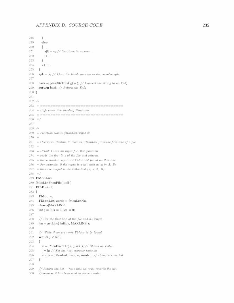
APPENDIX B. SOURCE CODE 232
248
249 else
250
251 a[i] = c; // Continue to process...
252 i++;
253
254 k++;
255
256 ∗pk = k; // Place the finish position in the variable pk
257
258 back = parseStrToFAlg( a ); // Convert the string to an FAlg
259 return back; // Return the FAlg
260
261
262 /∗
263 ∗ =================================
264 ∗ High Level File Reading Functions
265 ∗ =================================
266 ∗/
267
268 /∗
269 ∗ Function Name: fMonListFromFile
270 ∗
271 ∗ Overview: Routine to read an FMonList from the first line of a file
272 ∗
273 ∗ Detail: Given an input file, this function
274 ∗ reads the first line of the file and returns
275 ∗ the semicolon separated FMonList found on that line.
276 ∗ For example, if the input is a list such as a; b; A; B;
277 ∗ then the output is the FMonList (a, b, A, B).
278 ∗/
279 FMonList
280 fMonListFromFile( infil )
281 FILE ∗infil;
282
283 FMon w;
284 FMonList words = fMonListNul;
285 char s[MAXLINE];
286 int j = 0, k = 0, len = 0;
287
288 // Get the first line of the file and its length
289 len = getLine( infil, s, MAXLINE );
290
291 // While there are more FMons to be found
292 while( j < len )
293
294 w = fMonFromStr( s, j, &k ); // Obtain an FMon
295 j = k; // Set the next starting position
296 words = fMonListPush( w, words ); // Construct the list
297
298
299 // Return the list − note that we must reverse the list
300 // because it has been read in reverse order.

APPENDIX B. SOURCE CODE 233
301 return fMonListFXRev( words );
302
303
304 /∗
305 ∗ Function Name: fAlgListFromFile
306 ∗
307 ∗ Overview: Routine to read an FAlgList from a file
308 ∗
309 ∗ Detail: Given an input file, this function
310 ∗ takes each line of the file in turn, pushing one FAlg from
311 ∗ each line onto an FAlgList. This process is
312 ∗ continued until there are no more lines in the file
313 ∗ to process. For example, if the input is a list such as
314 ∗
315 ∗ 2∗x − 4∗y;
316 ∗ 5∗x∗y;
317 ∗ 4 + 5∗x + 60∗y;
318 ∗
319 ∗ then the output is the FAlgList
320 ∗ (2x−4y, 5xy, 4+5x+60y).
321 ∗/
322 FAlgList
323 fAlgListFromFile( infil )
324 FILE ∗infil;
325
326 FAlg entry;
327 FAlgList back = fAlgListNul;
328 char s[MAXLINE];
329 int j = 0, k = 0, len;
330
331 // Get the first line of the file
332 len = getLine( infil, s, MAXLINE );
333
334 // While there are still lines to process
335 while( len > 0 )
336
337 entry = fAlgFromStr( s, j, &k ); // Obtain an FAlg from a line
338 back = fAlgListPush( entry, back ); // Push the FAlg onto the list
339 len = getLine( infil, s, MAXLINE ); // Get a new line
340
341
342 // Return the list − note that we must reverse the list
343 // because it has been read in reverse order.
344 return fAlgListFXRev( back );
345
346
347 /∗
348 ∗ =================================
349 ∗ High Level File Writing Functions
350 ∗ =================================
351 ∗/
352
353 /∗

APPENDIX B. SOURCE CODE 234
354 ∗ Function Name: fMonToFile
355 ∗
356 ∗ Overview: Writes an FMon (in parse format) followed by a semicolon to a file
357 ∗
358 ∗ Detail: Given an input file and an FMon, this function
359 ∗ writes the FMon to file in parse format followed by a semicolon.
360 ∗/
361 void
362 fMonToFile( infil, w )
363 FILE ∗infil;
364 FMon w;
365
366 FMon wM;
367 ULong length;
368
369 // If the FMon is non−empty
370 if ( fMonEqual( w, fMonOne() ) != (Bool) 1 )
371
372 // While there are letters left in the FMon
373 while ( w )
374
375 wM = fMonLeadPowFac( w ); // Obtain a factor
376 fprintf( infil, "%s", fMonToStr( wM ) ); // Write the factor to file
377 length = fMonLength( wM );
378 w = fMonSuffix( w, fMonLength( w ) − length );
379 if ( fMonEqual( w, fMonOne() ) != (Bool) 1 )
380
381 // In parse format, to separate variables we use an asterisk
382 fprintf( infil, "*" );
383
384
385 fprintf( infil, ";" ); // At the end write a semicolon to file
386
387 else // Just write a semicolon to file
388
389 fprintf( infil, ";" );
390
391
392
393 /∗
394 ∗ Function Name: fMonListToFile
395 ∗
396 ∗ Overview: Writes an FMonList to a file on a single line
397 ∗
398 ∗ Detail: Given an input file and an FMonList, this function
399 ∗ writes the list to file as l1; l2; l3; ...
400 ∗/
401 void
402 fMonListToFile( infil, L )
403 FILE ∗infil;
404 FMonList L;
405
406 ULong i, length = fMonListLength( L );

APPENDIX B. SOURCE CODE 235
407
408 // For each element of the list
409 for( i = 1; i <= length; i++ )
410
411 // Write an FMon to file
412 fMonToFile( infil, L −> first );
413
414 // If there are more FMons left to look at
415 if( i < length )
416
417 fprintf( infil, " " ); // Provide a space between elements
418
419 else // else terminate the line
420
421 fprintf( infil, "\n" );
422
423 L = L −> rest;
424
425
426
427 /∗
428 ∗ ================================
429 ∗ File Name Modification Functions
430 ∗ ================================
431 ∗/
432
433 /∗
434 ∗ Function Name: appendDotDegRevLex
435 ∗
436 ∗ Overview: Appends ”.drl” onto a string (except in special case ”∗.in”)
437 ∗
438 ∗ Detail: Given an input character array, this function
439 ∗ appends the String ”.drl” onto the end of the character array.
440 ∗ In the special case that the input ends with ”.in”, the function
441 ∗ replaces the ”.in” with ”.drl”.
442 ∗/
443 String
444 appendDotDegRevLex( input )
445 char input[];
446
447 int length = (int) strlen( input );
448 String back = strNew();
449
450 // First check for .in at the end of the file name
451 if ( input[length−1] == ’n’ & input[length−2] == ’i’ & input[length−3] == ’.’ )
452
453 input[length−2] = ’d’;
454 input[length−1] = ’r’;
455 sprintf( back, "%s%s", input, "l" );
456
457 else // Just append with ”.drl”
458
459 sprintf( back, "%s%s", input, ".drl" );

APPENDIX B. SOURCE CODE 236
460
461
462 return back;
463
464
465 /∗
466 ∗ Function Name: appendDotDegLex
467 ∗
468 ∗ Overview: Appends ”.deg” onto a string (except in special case ”∗.in”)
469 ∗
470 ∗ Detail: Given an input character array, this function
471 ∗ appends the String ”.deg” onto the end of the character array.
472 ∗ In the special case that the input ends with ”.in”, the function
473 ∗ replaces the ”.in” with ”.deg”.
474 ∗/
475 String
476 appendDotDegLex( input )
477 char input[];
478
479 int length = (int) strlen( input );
480 String back = strNew();
481
482 // First check for .in at the end of the file name
483 if ( input[length−1] == ’n’ & input[length−2] == ’i’ & input[length−3] == ’.’ )
484
485 input[length−2] = ’d’;
486 input[length−1] = ’e’;
487 sprintf( back, "%s%s", input, "g" );
488
489 else // Just append with ”.deg”
490
491 sprintf( back, "%s%s", input, ".deg" );
492
493
494 return back;
495
496
497 /∗
498 ∗ Function Name: appendDotLex
499 ∗
500 ∗ Overview: Appends ”.lex” onto a string (except in special case ”∗.in”)
501 ∗
502 ∗ Detail: Given an input character array, this function
503 ∗ appends the String ”.lex” onto the end of the character array.
504 ∗ In the special case that the input ends with ”.in”, the function
505 ∗ replaces the ”.in” with ”.lex”.
506 ∗/
507 String
508 appendDotLex( input )
509 char input[];
510
511 int length = (int) strlen( input );
512 String back = strNew();

APPENDIX B. SOURCE CODE 237
513
514 // First check for .in at the end of the file name
515 if ( input[length−1] == ’n’ & input[length−2] == ’i’ & input[length−3] == ’.’ )
516
517 input[length−2] = ’l’;
518 input[length−1] = ’e’;
519 sprintf( back, "%s%s", input, "x" );
520
521 else // Just append with ”.lex”
522
523 sprintf( back, "%s%s", input, ".lex" );
524
525
526 return back;
527
528
529 /∗
530 ∗ Function Name: appendDotWP
531 ∗
532 ∗ Overview: Appends ”.wp” onto a string (except in special case ”∗.in”)
533 ∗
534 ∗ Detail: Given an input character array, this function
535 ∗ appends the String ”.wp” onto the end of the character array.
536 ∗ In the special case that the input ends with ”.in”, the function
537 ∗ replaces the ”.in” with ”.wp”.
538 ∗/
539 String
540 appendDotWP( input )
541 char input[];
542
543 int length = (int) strlen( input );
544 String back = strNew();
545
546 // First check for .in at the end of the file name
547 if ( input[length−1] == ’n’ & input[length−2] == ’i’ & input[length−3] == ’.’ )
548
549 input[length−2] = ’w’;
550 input[length−1] = ’p’;
551 sprintf( back, "%s", input );
552
553 else // Just append with ”.wp”
554
555 sprintf( back, "%s%s", input, ".wp" );
556
557
558 return back;
559
560
561 /∗
562 ∗ Function Name: filenameLength
563 ∗
564 ∗ Overview: Calculates the length of an input string
565 ∗

APPENDIX B. SOURCE CODE 238
566 ∗ Detail: Given an input character array, this function
567 ∗ finds the length of that character array
568 ∗/
569 int
570 filenameLength( s )
571 char s[];
572
573 int i = 0;
574
575 while( s[i] != ’\0’ ) i++;
576
577 return i;
578
579
580 /∗
581 ∗ ===========
582 ∗ End of File
583 ∗ ===========
584 ∗/
B.2.6 fralg functions.h
1 /∗
2 ∗ File: fralg functions.h
3 ∗ Author: Gareth Evans
4 ∗ Last Modified: 10th August 2005
5 ∗/
6
7 // Initialise file definition
8 # ifndef FRALG FUNCTIONS HDR
9 # define FRALG FUNCTIONS HDR
10
11 // Include MSSRC Libraries
12 # include <fralg.h>
13
14 // Include System Libraries
15 # include <limits.h>
16
17 // Include ∗ functions Libraries
18 # include "list_functions.h"
19 # include "arithmetic_functions.h"
20
21 //
22 // External Variables Required
23 //
24
25 extern ULong nRed; // Stores how many reductions have been performed
26 extern int nOfGenerators, // Holds the number of generators
27 pl; // Holds the ”Print Level”
28
29 //
30 // Functions Defined in fralg functions.c

APPENDIX B. SOURCE CODE 239
31 //
32
33 //
34 // Ordering Functions
35 //
36
37 // Returns 1 if 1st arg < Lex 2nd arg
38 Bool fMonLex( FMon, FMon );
39 // Returns 1 if 1st arg < InvLex 2nd arg
40 Bool fMonInvLex( FMon, FMon );
41 // Returns 1 if 1st arg < DegRevLex 2nd arg
42 Bool fMonDegRevLex( FMon, FMon );
43 // Returns 1 if 1st arg < WreathProduct 2nd arg
44 Bool fMonWreathProd( FMon, FMon );
45
46 //
47 // Alphabet Manipulation Functions
48 //
49
50 // Substitutes ASCII generators for original generators in a list of polynomials
51 FAlgList preProcess( FAlgList, FMonList );
52 // Substitutes original generators for ASCII generators in a given polynomial
53 String postProcess( FAlg, FMonList );
54 // As above but gives back its output in parse format
55 String postProcessParse( FAlg, FMonList );
56 // Adjusts the original generator order (1st arg) according to frequency of generators in 2nd arg
57 FMonList alphabetOptimise( FMonList, FAlgList );
58
59 //
60 // Polynomial Manipulation Functions
61 //
62
63 // Returns all possible ways that 2nd arg divides 1st arg; 3rd arg = is division possible?
64 FMonPairList fMonDiv( FMon, FMon, Short ∗ );
65 // Returns the first way that 2nd arg divides 1st arg; 3rd arg = is division possible?
66 FMonPairList fMonDivFirst( FMon, FMon, Short ∗ );
67 // Finds all possible overlaps of 2 FMons
68 FMonPairList fMonOverlaps( FMon, FMon );
69 // Returns the degree−based initial of a polynomial
70 FAlg degInitial( FAlg );
71 // Reverses a monomial
72 FMon fMonReverse( FMon );
73
74 //
75 // Groebner Basis Functions
76 //
77
78 // Returns the normal form of a polynomial w.r.t. a list of polynomials
79 FAlg polyReduce( FAlg, FAlgList );
80 // Minimises a given Groebner Basis
81 FAlgList minimalGB( FAlgList );
82 // Reduces each member of a Groebner Basis w.r.t. all other members
83 FAlgList reducedGB( FAlgList );

APPENDIX B. SOURCE CODE 240
84 // Tests whether a given FAlg reduces to 0 using the given FAlgList
85 Bool idealMembershipProblem( FAlg, FAlgList );
86
87 # endif // FRALG FUNCTIONS HDR
B.2.7 fralg functions.c
1 /∗
2 ∗ File: fralg functions.c
3 ∗ Author: Gareth Evans
4 ∗ Last Modified: 10th August 2005
5 ∗/
6
7 /∗
8 ∗ ======================================
9 ∗ Global Variables for fralg functions.c
10 ∗ ======================================
11 ∗/
12
13 static int bigVar = 1; // Keeps track of iteration depth in WreathProd
14
15 /∗
16 ∗ ==================
17 ∗ Ordering Functions
18 ∗ ==================
19 ∗/
20
21 /∗
22 ∗ Function Name: fMonLex
23 ∗
24 ∗ Overview: Returns 1 if 1st arg < Lex 2nd arg
25 ∗
26 ∗ Detail: Given two FMons x and y, this function
27 ∗ compares the two monomials using the lexicographic
28 ∗ ordering, returning 1 if x < y and 0 if x >= y.
29 ∗
30 ∗ Description of the Lex ordering:
31 ∗
32 ∗ x < y iff (working left−to−right) the first (say ith)
33 ∗ letter on which x and y differ is
34 ∗ such that x i < y i in the ordering of the variables.
35 ∗
36 ∗ External Variables Required: int pl;
37 ∗
38 ∗ Note: This code is based on L. Lambe’s ”fMonTLex” code.
39 ∗/
40 Bool
41 fMonLex( x, y )
42 FMon x, y;
43
44 ULong lenx, leny, min, count = 1;
45 int j;

APPENDIX B. SOURCE CODE 241
46 Bool back;
47
48 if( pl > 8 ) printf("Entered to compare x = %s with y = %s... \n", fMonToStr( x ), fMonToStr( y ) );
49 if( x == (FMon) NULL ) // If x is empty we only have to check that y is non−empty
50
51 if( pl > 8 ) printf("x is NULL so testing if y is NULL...\n");
52 return (Bool) ( y != (FMon) NULL );
53
54 else if( y == (FMon) NULL ) // If y is empty x cannot be less than it so just return 0
55
56 if( pl > 8 ) printf("y is NULL so returning 0...\n");
57 return (Bool) 0;
58
59 else // Both non−empty
60
61 lenx = fMonLength( x );
62 leny = fMonLength( y );
63
64 if( lenx < leny ) // x has minimum length
65
66 min = lenx;
67 back = (Bool) 1; // If limit reached we know x < y so return 1
68
69 else // y has minimum length
70
71 min = leny;
72 back = (Bool) 0; // if limit reached we know x >= y so return 0
73
74
75 while( count <= min ) // For each generator
76
77 if( pl > 8 )
78
79 printf("Comparing %s with %s\n", fMonLeadVar( fMonSubWordLen( x, count, 1 ) ),
80 fMonLeadVar( fMonSubWordLen( y, count, 1 ) ) );
81
82 // Compare generators
83 if( ( j = strcmp( fMonLeadVar( fMonSubWordLen( x, count, 1 ) ),
84 fMonLeadVar( fMonSubWordLen( y, count, 1 ) ) ) ) < 0 )
85
86 if( pl > 8 ) printf("x is less than y... \n");
87 return (Bool) 1;
88
89 else if( j > 0 )
90
91 if( pl > 8 ) printf("y is less than x... \n");
92 return (Bool) 0;
93
94 count++;
95
96
97
98 // Limit now reached; return previously agreed solution

APPENDIX B. SOURCE CODE 242
99 if( pl > 8 ) printf("Returning %i... \n", (int) back);
100 return back;
101
102
103 /∗
104 ∗ Function Name: fMonInvLex
105 ∗
106 ∗ Overview: Returns 1 if 1st arg < InvLex 2nd arg
107 ∗
108 ∗ Detail: Given two FMons x and y, this function
109 ∗ compares the two monomials using the inverse lexicographic
110 ∗ ordering, returning 1 if x < y and 0 if x >= y.
111 ∗
112 ∗ Description of the InvLex ordering:
113 ∗
114 ∗ x < y iff (working right−to−left) the first (say ith)
115 ∗ letter on which x and y differ is
116 ∗ such that x i < y i in the ordering of the variables.
117 ∗
118 ∗ External Variables Required: int pl;
119 ∗
120 ∗ Note: This code is based on L. Lambe’s ”fMonTLex” code.
121 ∗/
122 Bool
123 fMonInvLex( x, y )
124 FMon x, y;
125
126 ULong lenx, leny, min, count = 0;
127 int j;
128 Bool back;
129
130 if( pl > 8 ) printf("Entered to compare x = %s with y = %s... \n", fMonToStr( x ), fMonToStr( y ) );
131 if( x == (FMon) NULL ) // If x is empty we only have to check that y is non−empty
132
133 if( pl > 8 ) printf("x is NULL so testing if y is NULL...\n");
134 return (Bool) ( y != (FMon) NULL );
135
136 else if( y == (FMon) NULL ) // If y is empty x cannot be less than it so just return 0
137
138 if( pl > 8 ) printf("y is NULL so returning 0...\n");
139 return (Bool) 0;
140
141 else // Both non−empty
142
143 lenx = fMonLength( x );
144 leny = fMonLength( y );
145
146 if( lenx < leny ) // x has minimum length
147
148 min = lenx;
149 back = (Bool) 1; // If limit reached we know x < y so return 1
150
151 else // y has minimum length

APPENDIX B. SOURCE CODE 243
152
153 min = leny;
154 back = (Bool) 0; // if limit reached we know x >= y so return 0
155
156
157 while( count < min ) // For each generator
158
159 if( pl > 8 )
160
161 printf("Comparing %s with %s\n", fMonLeadVar( fMonSubWordLen( x, lenx−count, 1 ) ),
162 fMonLeadVar( fMonSubWordLen( y, leny−count, 1 ) ) );
163
164 // Compare generators in reverse
165 if( ( j = strcmp( fMonLeadVar( fMonSubWordLen( x, lenx−count, 1 ) ),
166 fMonLeadVar( fMonSubWordLen( y, leny−count, 1 ) ) ) ) < 0 )
167
168 if( pl > 8 ) printf("x is less than y... \n");
169 return (Bool) 1;
170
171 else if( j > 0 )
172
173 if( pl > 8 ) printf("y is less than x... \n");
174 return (Bool) 0;
175
176 count++;
177
178
179
180 // Limit now reached; return previously agreed solution
181 if( pl > 8 ) printf("Returning %i... \n", (int) back);
182 return back;
183
184
185 /∗
186 ∗ Function Name: fMonDegRevLex
187 ∗
188 ∗ Overview: Returns 1 if 1st arg < DegRevLex 2nd arg
189 ∗
190 ∗ Detail: Given two FMons x and y, this function
191 ∗ compares the two monomials using the degree reverse lexicographic
192 ∗ ordering, returning 1 if x < y and 0 if x >= y.
193 ∗
194 ∗ Description of the DegRevLex ordering:
195 ∗
196 ∗ x < y iff deg(x) < deg(y) or deg(x) = deg(y)
197 ∗ and x < RevLex y, that is, working right to left,
198 ∗ the first (say ith) letter on which x and y differ is
199 ∗ such that x i > y i in the ordering of the variables.
200 ∗
201 ∗ External Variables Required: int pl;
202 ∗
203 ∗ Note: This code is based on L. Lambe’s ”fMonTLex” code.
204 ∗/

APPENDIX B. SOURCE CODE 244
205 Bool
206 fMonDegRevLex( x, y )
207 FMon x, y;
208
209 ULong lenx, leny, count;
210 int j;
211
212 if( pl > 8 ) printf("Entered to compare x = %s with y = %s... \n", fMonToStr( x ), fMonToStr( y ) );
213
214 if( x == (FMon) NULL ) // If x is empty we only have to check that y is non−empty
215
216 if( pl > 8 ) printf("x is NULL so testing if y is NULL...\n");
217 return (Bool) ( y != (FMon) NULL );
218
219 else if( y == (FMon) NULL ) // If y is empty x cannot be less than it so just return 0
220
221 if( pl > 8 ) printf("y is NULL so returning 0...\n");
222 return (Bool) 0;
223
224 else // Both non−empty
225
226 lenx = fMonLength( x );
227 leny = fMonLength( y );
228
229 // In DegRevLex, compare the degrees first...
230 if( lenx < leny )
231
232 if( pl > 8 ) printf("x is less than y... \n");
233 return (Bool) 1;
234
235 else if( leny < lenx )
236
237 if( pl > 8 ) printf("y is less than x... \n");
238 return (Bool) 0;
239
240 else // The degrees are the same, now use RevLex...
241
242 count = lenx; // lenx is arbitrary (because lenx = leny)
243
244 while( count > 0 ) // Work in reverse
245
246 if( pl > 8 )
247
248 printf("Comparing %s with %s\n", fMonLeadVar( fMonSubWordLen( x, count, 1 ) ),
249 fMonLeadVar( fMonSubWordLen( y, count, 1 ) ) );
250
251 if( ( j = strcmp( fMonLeadVar( fMonSubWordLen( x, count, 1 ) ),
252 fMonLeadVar( fMonSubWordLen( y, count, 1 ) ) ) ) > 0 )
253
254 if( pl > 8 ) printf("x is less than y... \n");
255 return (Bool) 1;
256
257 else if( j < 0 )

APPENDIX B. SOURCE CODE 245
258
259 if( pl > 8 ) printf("y is less than x... \n");
260 return (Bool) 0;
261
262 count−−;
263
264
265
266
267 // No differences found so monomials must be the same
268 if( pl > 8 ) printf("Same, returning 0... \n");
269 return (Bool) 0;
270
271
272 /∗
273 ∗ Function Name: fMonWreathProd
274 ∗
275 ∗ Overview: Returns 1 if 1st arg < WreathProduct 2nd arg
276 ∗
277 ∗ Detail: Given two FMons x and y, this function
278 ∗ compares the two monomials using the wreath product
279 ∗ ordering, returning 1 if x < y and 0 if x >= y.
280 ∗ This function is recursive.
281 ∗
282 ∗ Description of the Wreath Product Ordering:
283 ∗
284 ∗ Let the alphabet have a total order (e.g. a < b < ...)
285 ∗ Count the number of occurrences of the highest weighted letter (e.g. z),
286 ∗ the string with the most is bigger.
287 ∗ If both strings have the same number of those letters, they can
288 ∗ be written uniquely:
289 ∗ s1 = x0 z x1 z x2 ... z xn
290 ∗ s2 = y0 z y1 z y2 ... z yn
291 ∗
292 ∗ Then s1 < s2 if
293 ∗ x0 < y0 or
294 ∗ x0 = y0 and x1 < y1, etc.
295 ∗ (< = wreath product ordering ’on y’; iterate as needed)
296 ∗
297 ∗ Examples:
298 ∗ aˆ100 < abaˆ2 because 1 < b
299 ∗ abaˆ2 < aˆ2ba because b = b and a < aˆ2
300 ∗ aˆ2ba < bˆ2a because b < bˆ2
301 ∗ bˆ2a < bab because bˆ2 = bˆ2 and 1 < a (s1 = 1b1ba and s2 = 1bab1)
302 ∗ bab < abˆ2 because bˆ2 = bˆ2 and 1 < a (s1 = 1bab1 and s2 = ab1b1)
303 ∗
304 ∗ External Variables Required: int pl, nOfGenerators;
305 ∗ Global Variables Used: int bigVar;
306 ∗
307 ∗ Note: This code is based on L. Lambe’s ”fMonTLex” code.
308 ∗/
309 Bool
310 fMonWreathProd( x, y )

APPENDIX B. SOURCE CODE 246
311 FMon x, y;
312
313 FMonList xList = fMonListNul, yList = fMonListNul;
314 FMon xPad = fMonOne(), yPad = fMonOne(), xLetter, yLetter, bigMon;
315 ULong xCount = 0, yCount = 0, i = 0;
316
317 /∗
318 ∗ Note: the global variable ’bigVar’ is used to keep
319 ∗ track of the iteration depth. The algorithm is designed
320 ∗ so that the value of bigVar is always returned to its
321 ∗ original value (which is usually 1)
322 ∗/
323
324 if( pl > 8 ) printf("Entered fMonWreathProd (%i) to compare x = %s with y = %s... \n",
325 bigVar, fMonToStr( x ), fMonToStr( y ) );
326
327 // Fail safe check − cannot have more iterations than generators;
328 // value 1 chosen by convention (in the case of equality)
329 if( !( nOfGenerators−bigVar >= 0 ) ) return (Bool) 1;
330
331 // Deal with special cases first
332 if( x == (FMon) NULL ) // If x is empty we only have to check that y is non−empty
333
334 if( pl > 8 ) printf("x is NULL so testing if y is NULL...\n");
335 return (Bool) ( y != (FMon) NULL );
336
337 else if( y == (FMon) NULL ) // If y is empty x cannot be less than it so just return 0
338
339 if( pl > 8 ) printf("y is NULL so returning 0...\n");
340 return (Bool) 0;
341
342 else if ( fMonEqual( x, y ) == (Bool) 1 ) // If x == y just return 0
343
344 if( pl > 8 ) printf("x = y so returning 0...\n");
345 return (Bool) 0;
346
347 else // Both non−empty and not equal
348
349 // Construct the generator for this iteration
350 bigMon = ASCIIMon( (ULong) nOfGenerators − (ULong) bigVar + 1 );
351
352 // Process x letter by letter, creating lists of intermediate terms
353 while( fMonIsOne( x ) != (Bool) 1 )
354
355 xLetter = fMonPrefix( x, 1 ); // Look at the first letter
356 if( fMonEqual( xLetter, bigMon ) == (Bool) 1 ) // if xLetter == bigMon
357
358 xCount++; // Increase the number of elements in the list
359 xList = fMonListPush( xPad, xList );
360 xPad = fMonOne(); // Reset
361
362 else
363

APPENDIX B. SOURCE CODE 247
364 xPad = fMonTimes( xPad, xLetter ); // Build up next element
365
366 x = fMonSuffix( x, fMonLength( x ) − 1 ); // Look at next letter
367
368 xList = fMonListPush( xPad, xList ); // Flush out the remainder
369
370 // Process y letter by letter
371 while( fMonIsOne( y ) != (Bool) 1 )
372
373 yLetter = fMonPrefix( y, 1 ); // Look at the first letter
374 if( fMonEqual( yLetter, bigMon ) == (Bool) 1 ) // if yLetter == bigMon
375
376 yCount++; // Increase the number of elements in the list
377 yList = fMonListPush( yPad, yList );
378 yPad = fMonOne(); // Reset
379
380 else
381
382 yPad = fMonTimes( yPad, yLetter ); // Build up next element
383
384 y = fMonSuffix( y, fMonLength( y ) − 1 ); // Look at next letter
385
386 yList = fMonListPush( yPad, yList ); // Flush out the remainder
387
388 /∗
389 ∗ Assuming representations
390 ∗ x = x0 z x1 z x2 ... z xn and
391 ∗ y = y0 z y1 z y2 ... z ym,
392 ∗
393 ∗ We now have
394 ∗ xList = (xn, ..., x2, x1, x0),
395 ∗ yList = (ym, ..., y2, y1, y0),
396 ∗ and xCount and yCount hold the number of
397 ∗ z’s in x and y respectively.
398 ∗
399 ∗/
400
401 // If xCount != yCount then we have a result...
402 if( xCount < yCount )
403
404 if( pl > 8 ) printf("x has less of the highest weighted letter so returning 1...\n");
405 return (Bool) 1;
406
407 else if( xCount > yCount )
408
409 if( pl > 8 ) printf("x has more of the highest weighted letter so returning 0...\n");
410 return (Bool) 0;
411
412 else // ...otherwise we have to look at the intermediate terms
413
414 // Reverse the lists to obtain
415 // xList = (x0, x1, x2, ..., xn) and
416 // yList = (y0, y1, y2, ..., yn)

APPENDIX B. SOURCE CODE 248
417 xList = fMonListFXRev( xList );
418 yList = fMonListFXRev( yList );
419
420 // Increase the iteration value −− we will now compare the
421 // elements of the lists w.r.t. the next highest variable
422 bigVar++;
423 while( xList )
424
425 i++;
426 if( fMonWreathProd( xList −> first, yList −> first ) == (Bool) 1 )
427
428 if( pl > 8 ) printf("On component %u, x < y...\n", i);
429 bigVar−−; // reset before return
430 return (Bool) 1;
431
432 else if( fMonWreathProd( yList −> first, xList −> first ) == (Bool) 1 )
433
434 if( pl > 8 ) printf("On component %u, y < x...\n", i);
435 bigVar−−; // reset before return
436 return (Bool) 0;
437
438 else // (equal)
439
440 // Look at the next values in the sequence
441 xList = xList −> rest;
442 yList = yList −> rest;
443
444
445 /∗
446 ∗ Note: we should never reach this part of the code
447 ∗ because we know that at least one list comparison
448 ∗ will return a result (not all list comparisons will
449 ∗ return ’equal’ because we know by this stage that
450 ∗ x is not equal to y). However we carry on for
451 ∗ completion.
452 ∗/
453 bigVar−−; // Reset
454
455
456
457 printf("Executing Unreachable Code\n");
458 exit( EXIT FAILURE );
459 return (Bool) 0;
460
461
462 /∗
463 ∗ ===============================
464 ∗ Alphabet Manipulation Functions
465 ∗ ===============================
466 ∗/
467
468 /∗
469 ∗ Function Name: preProcess

APPENDIX B. SOURCE CODE 249
470 ∗
471 ∗ Overview: Substitutes ASCII generators for original generators in a list of polynomials
472 ∗
473 ∗ Detail: This function takes a list of polynomials originalPolys
474 ∗ in a set of generators originalGenerators and returns the
475 ∗ same set of polynomials in ASCII generators, where the first
476 ∗ element of originalGenerators is replaced by ’AAA’, the
477 ∗ second element by ’AAB’, etc.
478 ∗
479 ∗ For example, if originalGenerators = (x, y, z) so that the
480 ∗ generator order is x < y < z, and if originalPolys = (x∗y−z, 4∗xˆ2−5∗z),
481 ∗ the output list is (AAB∗AAB−AAC, 4∗AAAˆ2−5∗AAC).
482 ∗
483 ∗/
484 FAlgList
485 preProcess( originalPolys, originalGenerators )
486 FAlgList originalPolys;
487 FMonList originalGenerators;
488
489 FAlgList newPolys = fAlgListNul;
490 FAlg oldPoly, newPoly, adder;
491 ULong i, oldPolySize, genLength, position;
492 FMon firstTermMon, newFirstTermMon, multiplier, gen;
493 QInteger firstTermCoef;
494
495 // Go through each polynomial in turn...
496 while( originalPolys )
497
498 oldPoly = originalPolys −> first; // Extract a polynomial
499 originalPolys = originalPolys −> rest;
500 oldPolySize = (ULong) fAlgNumTerms( oldPoly ); // Obtain the number of terms
501 newPoly = fAlgZero(); // Initialise the new polynomial
502
503 for( i = 1; i <= oldPolySize; i++ ) // For each term in the polynomial
504
505 firstTermMon = fAlgLeadMonom( oldPoly ); // Extract monomial
506 firstTermCoef = fAlgLeadCoef( oldPoly ); // Extract coefficient
507 oldPoly = fAlgReductum( oldPoly ); // Get ready to look at the next term
508 newFirstTermMon = fMonOne(); // Initialise the new monomial
509
510 // Go through each term replacing generators as required
511 while( fMonIsOne( firstTermMon ) != (Bool) 1 )
512
513 gen = fMonPrefix( firstTermMon, 1 ); // Take the first letter ’x’
514 position = fMonListPosition( gen, originalGenerators ); // Find the position of the letter in the list
515 multiplier = ASCIIMon( position ); // Obtain the ASCII generator corresponding to x
516 genLength = fMonLeadExp( firstTermMon ); // Find the exponent ’a’ as in xˆa
517 // Multiply new monomial by (ASCII) xˆa
518 newFirstTermMon = fMonTimes( newFirstTermMon, fMonPow( multiplier, genLength ) );
519 // Lose xˆa from original monomial
520 firstTermMon = fMonSuffix( firstTermMon, fMonLength( firstTermMon ) − genLength );
521
522

APPENDIX B. SOURCE CODE 250
523 adder = fAlgMonom( firstTermCoef, newFirstTermMon ); // Construct the new ASCII term
524 newPoly = fAlgPlus( newPoly, adder ); // Add the new ASCII term to the output polynomial
525
526 newPolys = fAlgListPush( newPoly, newPolys ); // Push new polynomial onto output list
527
528
529 // Return the reversed list (it was read in reverse)
530 return fAlgListFXRev( newPolys );
531
532
533 /∗
534 ∗ Function Name: postProcess
535 ∗
536 ∗ Overview: Substitutes original generators for ASCII generators in a given polynomial
537 ∗
538 ∗ Detail: This function takes a polynomial oldPoly in ASCII generators
539 ∗ and returns the same polynomial in a corresponding set of generators
540 ∗ originalGenerators . The output is returned as a String
541 ∗ in fAlgToStr( ... ) format.
542 ∗
543 ∗ For example, if originalGenerators = (x, y, z) so that the
544 ∗ generator order is x < y < z, and if oldPoly = A∗B−Cˆ2, then
545 ∗ the output String is ”x y − zˆ2”.
546 ∗
547 ∗/
548 String
549 postProcess( oldPoly, originalGenerators )
550 FAlg oldPoly;
551 FMonList originalGenerators;
552
553 FAlg adder;
554 Bool result;
555 FMon firstTermMon, gen, newFirstTermMon, multiplier;
556 QInteger firstTermCoef;
557 ULong i, match, oldPolySize, genLength;
558 String back = strNew();
559
560 sprintf( back, "" ); // Initialise back
561
562 // Obtain the number of terms in the polynomial
563 oldPolySize = (ULong) fAlgNumTerms( oldPoly );
564
565 for( i = 1; i <= oldPolySize; i++ ) // For each term
566
567 firstTermMon = fAlgLeadMonom( oldPoly ); // Obtain the lead monomial
568 firstTermCoef = fAlgLeadCoef( oldPoly ); // Obtain the lead coefficient
569 result = qLess( firstTermCoef, qZero() ); // Test if coefficient is −ve
570 oldPoly = fAlgReductum( oldPoly ); // Get ready to look at the next term
571 newFirstTermMon = fMonOne(); // Initialise the new monomial
572
573 // Go through the term replacing generators as required
574 while( fMonIsOne( firstTermMon ) != (Bool) 1 )
575

APPENDIX B. SOURCE CODE 251
576 gen = fMonPrefix( firstTermMon, 1 ); // Obtain the first letter ’x’
577 genLength = fMonLeadExp( firstTermMon ); // Obtain ’a’ as in xˆa
578 // Calculate the ASCII value (’AAA’ = 1, ’AAB’ = 2, ...)
579 match = ASCIIVal( fMonToStr( gen ) );
580 multiplier = fMonListNumber( match, originalGenerators ); // Find the original generator
581 multiplier = fMonPow( multiplier, genLength );
582 newFirstTermMon = fMonTimes( newFirstTermMon, multiplier ); // Multiply new monomial by the original xˆa
583 // Remove ASCII xˆa from original monomial
584 firstTermMon = fMonSuffix( firstTermMon, fMonLength( firstTermMon ) − genLength );
585
586
587 // Now add the term to the output string
588 if( i == 1 ) // First term
589 back = strConcat( back, fAlgToStr( fAlgMonom( firstTermCoef, newFirstTermMon ) ) );
590 else // Must insert the correct sign (plus or minus)
591
592 if( result == 0 ) // Coefficient is +ve
593
594 adder = fAlgMonom( firstTermCoef, newFirstTermMon ); // Construct the new term
595 back = strConcat( back, " + " );
596 back = strConcat( back, fAlgToStr( adder ) );
597
598 else // Coefficient is −ve
599
600 adder = fAlgMonom( qNegate( firstTermCoef ), newFirstTermMon ); // Construct the new term
601 back = strConcat( back, " - " );
602 back = strConcat( back, fAlgToStr( adder ) );
603
604
605
606
607 return back;
608
609
610 /∗
611 ∗ Function Name: postProcessParse
612 ∗
613 ∗ Overview: As above but gives back its output in parse format
614 ∗
615 ∗ Detail: This function takes a polynomial oldPoly in ASCII generators
616 ∗ and returns the same polynomial in a corresponding set of generators
617 ∗ originalGenerators . The output is returned as a String in
618 ∗ parse format (with asterisks).
619 ∗
620 ∗ For example, if originalGenerators = (x, y, z) so that the
621 ∗ generator order is x < y < z, and if oldPoly = A∗B−Cˆ2, then
622 ∗ the output String is ”x∗y − zˆ2”.
623 ∗
624 ∗/
625 String
626 postProcessParse( oldPoly, originalGenerators )
627 FAlg oldPoly;
628 FMonList originalGenerators;

APPENDIX B. SOURCE CODE 252
629
630 Short first = 1, written;
631 FMon firstTermMon, gen, multiplier;
632 QInteger firstTermCoef;
633 ULong i, match, oldPolySize, genLength;
634 String back = strNew();
635
636 sprintf( back, "" ); // Initialise back
637
638 if( !oldPoly ) // If input is NULL output the zero polynomial
639
640 back = strConcat( back, "0" );
641 return back;
642
643
644 // Obtain the number of terms in the polynomial
645 oldPolySize = (ULong) fAlgNumTerms( oldPoly );
646
647 for( i = 1; i <= oldPolySize; i++ ) // For each term
648
649 // Assume to begin with that nothing has been added to
650 // the String regarding the term we are now looking at
651 written = 0;
652
653 // Break down a term of the polynomial into its pieces
654 firstTermMon = fAlgLeadMonom( oldPoly ); // Obtain the lead monomial
655 firstTermCoef = fAlgLeadCoef( oldPoly ); // Obtain the lead coefficient
656
657 if( qLess( firstTermCoef, qZero() ) == (Bool) 1 ) // If the coefficient is −ve
658
659 if( first == 1 ) // If this is the first term encountered
660
661 first = 0; // Set to avoid this loop in future
662
663 // Note: there is no need for a space before the minus sign
664 back = strConcat( back, "-" );
665
666 else // This is not the first term
667
668 // Separate two terms with a minus sign
669 back = strConcat( back, " - " );
670
671
672 // Now that we have written the negative sign we can make
673 // the coefficient positive
674 firstTermCoef = qNegate( firstTermCoef );
675
676 else // The coefficient is +ve
677
678 if( first == 1 ) // If this is the first term encountered
679
680 first = 0; // Set to avoid this loop in future
681

APPENDIX B. SOURCE CODE 253
682 // Recall that there is no need to write out a plus
683 // sign for the first term in a polynomial
684
685 else // This is not the first term
686
687 // Separate two terms with a plus sign
688 back = strConcat( back, " + " );
689
690
691
692 if( qIsOne( firstTermCoef ) != (Bool) 1 ) // If the coefficient is not one
693
694 written = 1; // Denote that we are going to write the coefficient to the String
695 if( fMonEqual( firstTermMon, fMonOne() ) != (Bool) 1 ) // If the lead monomial is not 1
696
697 // Provide an asterisk to denote that the coefficient is
698 // multiplied by the monomial
699 back = strConcat( back, qToStr( firstTermCoef ) );
700 back = strConcat( back, "*" );
701
702 else
703
704 // As the monomial is 1 there is no need to write the
705 // monomial out and we can just write out the coefficient
706 back = strConcat( back, qToStr( firstTermCoef ) );
707
708
709
710 // If the lead monomial is not one
711 if( fMonIsOne( firstTermMon ) != (Bool) 1 )
712
713 written = 1; // Denote that we are going to write the monomial to the String
714
715 // Go through the term replacing generators as required
716 while( firstTermMon )
717
718 gen = fMonPrefix( firstTermMon, 1 ); // Obtain the first letter ’x’
719 genLength = fMonLeadExp( firstTermMon ); // Obtain ’a’ as in xˆa
720
721 // Calculate the ASCII value (’AAA’ = 1, ’AAB’ = 2, ...)
722 match = ASCIIVal( fMonToStr( gen ) );
723 multiplier = fMonListNumber( match, originalGenerators ); // Find the original generator
724 multiplier = fMonPow( multiplier, genLength );
725
726 // Add multiplier onto the String
727 back = strConcat( back, fMonToStr( multiplier ) );
728
729 // Move the monomial onwards
730 firstTermMon = fMonSuffix( firstTermMon, fMonLength( firstTermMon ) − genLength ); // Remove ASCII xˆa
731 if( firstTermMon ) back = strConcat( back, "*" );
732
733
734

APPENDIX B. SOURCE CODE 254
735 // If the coefficient is 1 and the monomial is 1 and nothing
736 // has yet been written about this term, write ”1” to the String
737 // (This is to catch the case where the term is −1)
738 if( ( qIsOne( firstTermCoef ) == (Bool) 1 )
739 && ( fMonIsOne( firstTermMon ) == (Bool) 1 )
740 && ( written == 0 ) )
741
742 back = strConcat( back, "1" );
743
744
745 oldPoly = fAlgReductum( oldPoly ); // Get ready to look at the next term
746
747
748 return back;
749
750
751 /∗
752 ∗ Function Name: alphabetOptimise
753 ∗
754 ∗ Overview: Adjusts the original generator order (1st arg) according to
755 ∗ frequency of generators in 2nd arg
756 ∗
757 ∗ Detail: Given an FMonList oldGens storing the given generator
758 ∗ order, this function optimises this order according to the
759 ∗ frequency of the generators in the polynomial list polys .
760 ∗ More specifically, the most frequently occurring generator
761 ∗ is set to be the smallest generator, the second most frequently
762 ∗ occurring generator is set to be the second smallest generator, ...
763 ∗ For the reasoning behind this optimisation, see a paper called
764 ∗ ”A case where choosing a product order makes the
765 ∗ calculations of a Groebner basis much faster” by
766 ∗ Freyja Hreinsdottir (Journal of Symbolic Computation).
767 ∗
768 ∗ Note: This function is designed to be used before the
769 ∗ generators and polynomials are converted to ASCII order.
770 ∗
771 ∗ External variables needed: int pl;
772 ∗
773 ∗/
774 FMonList
775 alphabetOptimise( oldGens, polys )
776 FMonList oldGens;
777 FAlgList polys;
778
779 ULong i, j, letterLength, size = fMonListLength( oldGens ), scores[size];
780 FMon monomial, letter, theLetters[size];
781 FAlg poly;
782 FMonList newGens = fMonListNul;
783
784 if( pl > 0 )
785
786 printf("Old Ordering = ");
787 fMonListDisplayOrder( oldGens );

APPENDIX B. SOURCE CODE 255
788 printf("\n");
789
790
791 // Set up arrays
792 for( i = 0; i < size; i++ )
793
794 theLetters[i] = oldGens −> first; // Transfer generator to array
795 oldGens = oldGens −> rest;
796 scores[i] = 0; // Initialise scores
797
798
799 // Analyse the generators found in each polynomial
800 while( polys )
801
802 poly = polys −> first; // Extract a polynomial
803 if( pl > 2 ) printf("Counting generators in poly %s\n", fAlgToStr( poly ) );
804 polys = polys −> rest;
805
806 while( poly ) // For each term in the polynomial
807
808 monomial = fAlgLeadMonom( poly ); // Extract the lead monomial
809 poly = fAlgReductum( poly );
810
811 while( fMonIsOne( monomial ) != (Bool) 1 )
812
813 letter = fMonPrefix( monomial, 1 ); // Take the first letter ’x’
814 letterLength = fMonLeadExp( monomial ); // Find the exponent ’a’ as in xˆa
815 j = 0;
816 while( j < size ) // Locate the letter in the generator array
817
818 if( fMonEqual( letter, theLetters[j] ) == (Bool) 1 )
819
820 // Match found, increase scores appropriately
821 scores[j] = scores[j] + letterLength;
822 j = size; // Shortcut search
823
824 else j++;
825
826 monomial = fMonSuffix( monomial, fMonLength( monomial ) − letterLength ); // Lose xˆa from old monomial
827
828
829
830
831 if( pl > 0 ) // Provide some information on screen
832
833 printf("Frequencies = ");
834 for( i = 0; i < size; i++ )
835
836 printf("%u, ", scores[size−1−i] );
837
838 printf("\n");
839
840

APPENDIX B. SOURCE CODE 256
841 // Sort scores by a quicksort algorithm, adjusting the generators as we go along
842 alphabetArrayQuickSort( scores, theLetters, 0, size−1 );
843
844 // Build up new alphabet
845 for( i = 1; i <= size; i++ )
846 newGens = fMonListPush( theLetters[size−i], newGens );
847
848 if( pl > 0 )
849
850 printf("New Ordering = ");
851 fMonListDisplayOrder( newGens );
852 printf("\n");
853
854
855 // Return the sorted alphabet list
856 return newGens;
857
858
859 /∗
860 ∗ =================================
861 ∗ Polynomial Manipulation Functions
862 ∗ =================================
863 ∗/
864
865 /∗
866 ∗ Function Name: fMonDiv
867 ∗
868 ∗ Overview: Returns all possible ways that 2nd arg divides 1st arg;
869 ∗ 3rd arg = is division possible?
870 ∗
871 ∗ Detail: Given two FMons a and b , this function returns all possible
872 ∗ ways that b divides a in the form of an FMonPairList. The third
873 ∗ parameter flag records whether or not (true/false) any divisions
874 ∗ are possible. For example, if t = abdababc and b = ab, then the
875 ∗ output FMonPairList is ((abdab, c), (abd, abc), (1, dababc)) and we
876 ∗ set flag = true.
877 ∗
878 ∗ External variables needed: int pl;
879 ∗
880 ∗/
881 FMonPairList
882 fMonDiv( t, b, flag )
883 FMon t, b;
884 Short ∗flag;
885
886 ULong i, tl, bl, diff;
887 FMonPairList back = ( FMonPairList )theAllocFun( sizeof( ∗back ) );
888
889 back = fMonPairListNul; // Initialise the output list
890
891 ∗flag = false; // Assume there are no possible divisions to begin with
892 tl = fMonLength( t );
893 bl = fMonLength( b );

APPENDIX B. SOURCE CODE 257
894
895 if( tl < bl ) // There can be no possible divisions if |t| < |b|
896
897 return back;
898
899 else // Me must now consider each possibility in turn
900
901 diff = tl−bl;
902 for( i = 0; i <= diff; i++ ) // Working left to right
903
904 // Is the subword of t of length |b| starting at position i+1 equal to b?
905 if( fMonEqual( b, fMonSubWordLen( t, i+1, bl ) ) == (Bool) 1 )
906
907 // Match found; push the left and right factors onto the output list
908 back = fMonPairListPush( fMonPrefix( t, i ), fMonSuffix( t, tl−bl−i ), back );
909 if( pl > 6 ) printf("i = %i: %s = %s*(%s)*%s\n", i+1, fMonToStr( t ),
910 fMonToStr( fMonPrefix( t, i ) ), fMonToStr( b ), fMonToStr( fMonSuffix( t, tl−bl−i ) ) );
911
912
913
914
915 // If we found some matches set flag to be true
916 if( back ) ∗flag = true;
917 return back; // Return the output list
918
919
920 /∗
921 ∗ Function Name: fMonDivFirst
922 ∗
923 ∗ Overview: Returns the first way that 2nd arg divides 1st arg;
924 ∗ 3rd arg = is division possible?
925 ∗
926 ∗ Detail: Given two FMons a and b , this function returns the first
927 ∗ way that b divides a in the form of an FMonPairList. The third
928 ∗ parameter flag records whether or not (true/false) any divisions
929 ∗ are possible. For example, if t = abdababc and b = ab, then the
930 ∗ output FMonPairList is ((1, dababc)) and we
931 ∗ set flag = true.
932 ∗
933 ∗ External variables needed: int pl;
934 ∗
935 ∗/
936 FMonPairList
937 fMonDivFirst( t, b, flag )
938 FMon t, b;
939 Short ∗flag;
940
941 ULong i, tl, bl, diff;
942 FMonPairList back = ( FMonPairList )theAllocFun( sizeof( ∗back ));
943
944 back = fMonPairListNul; // Initialise the output list
945
946 ∗flag = false; // Assume there are no possible divisions to begin with

APPENDIX B. SOURCE CODE 258
947 tl = fMonLength( t );
948 bl = fMonLength( b );
949
950 if( tl < bl ) // There can be no possible divisions if |t| < |b|
951
952 return back;
953
954 else // Me must now consider each possibility in turn
955
956 diff = tl−bl;
957 for( i = 0; i <= diff; i++ ) // Working left to right
958
959 // Is the subword of t of length |b| starting at position i+1 equal to b?
960 if( fMonEqual( b, fMonSubWordLen( t, i+1, bl ) ) == (Bool) 1 )
961
962 // Match found; push the left and right factors onto the output list and return it
963 back = fMonPairListPush( fMonPrefix( t, i ), fMonSuffix( t, tl−bl−i ), back );
964 if( pl > 6 ) printf("i = %i: %s = %s*(%s)*%s\n", i+1, fMonToStr( t ),
965 fMonToStr( fMonPrefix( t, i ) ), fMonToStr( b ), fMonToStr( fMonSuffix( t, tl−bl−i ) ) );
966 ∗flag = true; // Indicate that we have found a match
967 return back;
968
969
970
971
972 return back; // Return the empty output list − no matches were found
973
974
975 /∗
976 ∗ Function Name: fMonOverlaps
977 ∗
978 ∗ Overview: Finds all possible overlaps of 2 FMons
979 ∗
980 ∗ Detail: Given two FMons, this function returns all
981 ∗ possible ways in which the two monomials overlap.
982 ∗ For example, if a = abcabc and b = cab, then
983 ∗ the output FMonPairList is
984 ∗ ((1, 1), (ab, c), (c, 1), (1, cabc), (1, ab), (abcab, 1))
985 ∗ as in
986 ∗ 1∗(abcabc)∗1 = ab∗(cab)∗c,
987 ∗ c∗(abcabc)∗1 = 1∗(cab)∗cabc,
988 ∗ 1∗(abcabc)∗ab = abcab∗(cab)∗1.
989 ∗
990 ∗ External variables needed: int pl;
991 ∗
992 ∗/
993 FMonPairList
994 fMonOverlaps( a, b )
995 FMon a, b;
996
997 FMon still, move;
998 Short type;
999 ULong la, lb, ls, lm, i;

APPENDIX B. SOURCE CODE 259
1000 FMonPairList back = ( FMonPairList )theAllocFun( sizeof( ∗back ));
1001
1002 back = fMonPairListNul; // Initialise the output list
1003
1004 la = fMonLength( a );
1005 lb = fMonLength( b );
1006
1007 // Check for the trivial monomial
1008 if( ( la == 0 ) || ( lb == 0 ) ) return back;
1009
1010 // Determine which monomial has the greater length
1011 if( la < lb )
1012
1013 still = b; ls = lb;
1014 move = a; lm = la;
1015 type = 1; // Remember that |a| < |b|
1016
1017 else
1018
1019 still = a; ls = la;
1020 move = b; lm = lb;
1021 type = 2; // Remember that |a| >= |b|
1022
1023
1024 // First deal with prefix and suffix overlaps
1025 for( i = 1; i <= lm−1; i++ )
1026
1027 // PREFIX overlap − is a prefix of still equal to a suffix of move?
1028 if( fMonEqual( fMonPrefix( still, i ), fMonSuffix( move, i ) ) == (Bool) 1 )
1029
1030 if( type == 1 ) // still = b, move = a
1031
1032 // Need to multiply a on the right and b on the left to construct the overlap
1033 back = fMonPairListPush( fMonPrefix( a, la−i ), fMonOne(), back ); // b
1034 back = fMonPairListPush( fMonOne(), fMonSuffix( b, lb−i ), back ); // a
1035 if( pl > 5 ) printf("Left Overlap Found for (%s, %s): (%s, %s, %s, %s)\n",
1036 fMonToStr( a ), fMonToStr( b ), fMonToStr( fMonOne() ),
1037 fMonToStr( fMonSuffix( b, lb−i ) ), fMonToStr( fMonPrefix( a, la−i ) ),
1038 fMonToStr( fMonOne() ) );
1039
1040 else // still = a, move = b
1041
1042 // Need to multiply a on the left and b on the right to construct the overlap
1043 back = fMonPairListPush( fMonOne(), fMonSuffix( a, la−i ), back ); // b
1044 back = fMonPairListPush( fMonPrefix( b, lb−i ), fMonOne(), back ); // a
1045 if( pl > 5 ) printf("Left Overlap Found for (%s, %s): (%s, %s, %s, %s)\n",
1046 fMonToStr( a ), fMonToStr( b ), fMonToStr( fMonPrefix( b, lb−i ) ),
1047 fMonToStr( fMonOne() ), fMonToStr( fMonOne() ),
1048 fMonToStr( fMonSuffix( a, la−i ) ) );
1049
1050
1051
1052 // SUFFIX overlap − is a suffix of still equal to a prefix of move?
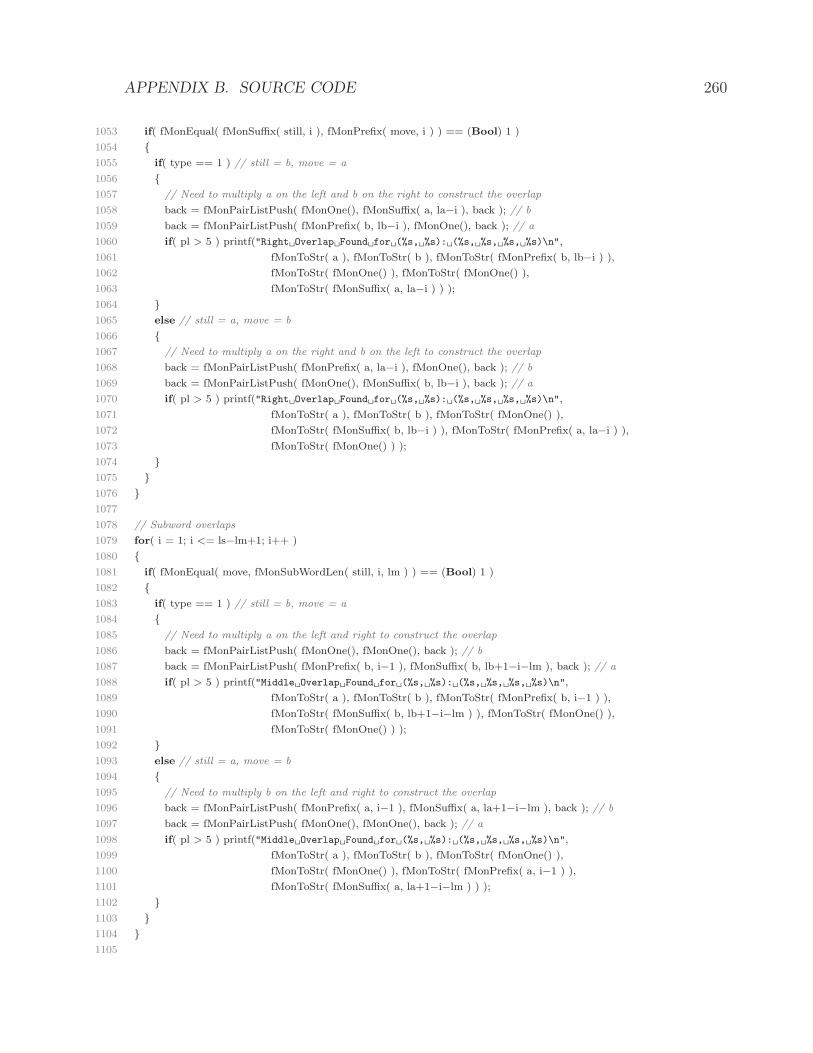
APPENDIX B. SOURCE CODE 260
1053 if( fMonEqual( fMonSuffix( still, i ), fMonPrefix( move, i ) ) == (Bool) 1 )
1054
1055 if( type == 1 ) // still = b, move = a
1056
1057 // Need to multiply a on the left and b on the right to construct the overlap
1058 back = fMonPairListPush( fMonOne(), fMonSuffix( a, la−i ), back ); // b
1059 back = fMonPairListPush( fMonPrefix( b, lb−i ), fMonOne(), back ); // a
1060 if( pl > 5 ) printf("Right Overlap Found for (%s, %s): (%s, %s, %s, %s)\n",
1061 fMonToStr( a ), fMonToStr( b ), fMonToStr( fMonPrefix( b, lb−i ) ),
1062 fMonToStr( fMonOne() ), fMonToStr( fMonOne() ),
1063 fMonToStr( fMonSuffix( a, la−i ) ) );
1064
1065 else // still = a, move = b
1066
1067 // Need to multiply a on the right and b on the left to construct the overlap
1068 back = fMonPairListPush( fMonPrefix( a, la−i ), fMonOne(), back ); // b
1069 back = fMonPairListPush( fMonOne(), fMonSuffix( b, lb−i ), back ); // a
1070 if( pl > 5 ) printf("Right Overlap Found for (%s, %s): (%s, %s, %s, %s)\n",
1071 fMonToStr( a ), fMonToStr( b ), fMonToStr( fMonOne() ),
1072 fMonToStr( fMonSuffix( b, lb−i ) ), fMonToStr( fMonPrefix( a, la−i ) ),
1073 fMonToStr( fMonOne() ) );
1074
1075
1076
1077
1078 // Subword overlaps
1079 for( i = 1; i <= ls−lm+1; i++ )
1080
1081 if( fMonEqual( move, fMonSubWordLen( still, i, lm ) ) == (Bool) 1 )
1082
1083 if( type == 1 ) // still = b, move = a
1084
1085 // Need to multiply a on the left and right to construct the overlap
1086 back = fMonPairListPush( fMonOne(), fMonOne(), back ); // b
1087 back = fMonPairListPush( fMonPrefix( b, i−1 ), fMonSuffix( b, lb+1−i−lm ), back ); // a
1088 if( pl > 5 ) printf("Middle Overlap Found for (%s, %s): (%s, %s, %s, %s)\n",
1089 fMonToStr( a ), fMonToStr( b ), fMonToStr( fMonPrefix( b, i−1 ) ),
1090 fMonToStr( fMonSuffix( b, lb+1−i−lm ) ), fMonToStr( fMonOne() ),
1091 fMonToStr( fMonOne() ) );
1092
1093 else // still = a, move = b
1094
1095 // Need to multiply b on the left and right to construct the overlap
1096 back = fMonPairListPush( fMonPrefix( a, i−1 ), fMonSuffix( a, la+1−i−lm ), back ); // b
1097 back = fMonPairListPush( fMonOne(), fMonOne(), back ); // a
1098 if( pl > 5 ) printf("Middle Overlap Found for (%s, %s): (%s, %s, %s, %s)\n",
1099 fMonToStr( a ), fMonToStr( b ), fMonToStr( fMonOne() ),
1100 fMonToStr( fMonOne() ), fMonToStr( fMonPrefix( a, i−1 ) ),
1101 fMonToStr( fMonSuffix( a, la+1−i−lm ) ) );
1102
1103
1104
1105

APPENDIX B. SOURCE CODE 261
1106 return back;
1107
1108
1109 /∗
1110 ∗ Function Name: degInitial
1111 ∗
1112 ∗ Overview: Returns the degree−based initial of a given polynomial
1113 ∗
1114 ∗ Detail: Given a polynomial input , this function returns the
1115 ∗ initial of that polynomial w.r.t. degree. In other words,
1116 ∗ all terms of highest degree are returned.
1117 ∗
1118 ∗/
1119 FAlg
1120 degInitial( input )
1121 FAlg input;
1122
1123 FAlg output = fAlgZero();
1124 ULong max = 0, next;
1125
1126 // If the input is trivial, the output is trivial
1127 if( !input ) return input;
1128
1129 // For each term in the input polynomial
1130 while( input )
1131
1132 // Find the degree of the next term in the polynomial
1133 next = fMonLength( fAlgLeadMonom( input ) );
1134
1135 // If we find a term of higher degree
1136 if( next > max )
1137
1138 // Set a new maximum
1139 max = next;
1140 // Start building up the output polynomial again
1141 output = fAlgLeadTerm( input );
1142
1143 // Else if we find a term of equal maximum degree
1144 else if( next == max )
1145
1146 // Add the term to the output polynomial
1147 output = fAlgPlus( output, fAlgLeadTerm( input ) );
1148
1149
1150 // Get ready to look at the next term of the input polynomial
1151 input = fAlgReductum( input );
1152
1153
1154 // Return the initial
1155 return output;
1156
1157
1158 /∗

APPENDIX B. SOURCE CODE 262
1159 ∗ Function Name: fMonReverse
1160 ∗
1161 ∗ Overview: Reverses a monomial
1162 ∗
1163 ∗ Detail: Given a monomial m = x 1x 2...x n, this
1164 ∗ function returns the monomial m’ = x nx n−1...x 2x 1.
1165 ∗
1166 ∗/
1167 FMon
1168 fMonReverse( input )
1169 FMon input;
1170
1171 FMon output = fMonOne();
1172
1173 // For each variable in the input monomial
1174 while( input )
1175
1176 output = fMonTimes( fMonPrefix( input, 1 ), output );
1177 input = fMonRest( input );
1178
1179
1180 // Return the reversed monomial
1181 return output;
1182
1183
1184 /∗
1185 ∗ ========================
1186 ∗ Groebner Basis Functions
1187 ∗ ========================
1188 ∗/
1189
1190 /∗
1191 ∗ Function Name: polyReduce
1192 ∗
1193 ∗ Overview: Returns the normal form of a polynomial w.r.t. a list of polynomials
1194 ∗
1195 ∗ Detail: Given an FAlg and an FAlgList, this function
1196 ∗ divides the FAlg w.r.t. the FAlgList, returning the
1197 ∗ normal form of the input polynomial w.r.t. the list.
1198 ∗
1199 ∗ External Variables Required: int pl;
1200 ∗ Global Variables Used: ULong nRed;
1201 ∗
1202 ∗/
1203 FAlg
1204 polyReduce( poly, list )
1205 FAlg poly;
1206 FAlgList list;
1207
1208 ULong i, numRules = fAlgListLength( list );
1209 FAlg back = fAlgZero(), lead, upgrade, LHSA[numRules];
1210 FMon leadMonomial, leadLoopMonomial, LHSM[numRules];
1211 FMonPairList factors;
APPENDIX B. SOURCE CODE 263
1212 QInteger leadQ, leadLoopQ, lcmQ, LHSQ[numRules];
1213 Short flag, toggle;
1214
1215 // Convert the input list of polynomials to an array and
1216 // create arrays of lead monomials and lead coefficients
1217 for( i = 0; i < numRules; i++ )
1218
1219 if( pl > 5 ) printf("Poly %u = %s\n", i+1, fAlgToStr( list −> first ) );
1220 LHSA[i] = list −> first;
1221 LHSM[i] = fAlgLeadMonom( list −> first );
1222 LHSQ[i] = fAlgLeadCoef( list −> first );
1223 list = list −> rest;
1224
1225
1226 // We will now recursively reduce every term in the polynomial
1227 // until no more reductions are possible
1228 while( fAlgIsZero( poly ) != (Bool) 1 )
1229
1230 if( pl > 5 ) printf("Looking at Lead Term of %s\n", fAlgToStr( poly ) );
1231 toggle = 1; // Assume no reductions are possible to begin with
1232 lead = fAlgLeadTerm( poly );
1233 leadMonomial = fAlgLeadMonom( lead );
1234 leadQ = fAlgLeadCoef( lead );
1235 i = 0;
1236
1237 while( i < numRules ) // For each polynomial in the list
1238
1239 leadLoopMonomial = LHSM[i]; // Pick a test monomial
1240 flag = false;
1241 // Does the ith polynomial divide our polynomial?
1242 factors = fMonDivFirst( leadMonomial, leadLoopMonomial, &flag );
1243
1244 if( flag == true ) // i.e. leadMonomial = factors −> lft ∗ leadLoopMonomial ∗ factors −> rt
1245
1246 if( pl > 1 ) nRed++; // Increase the number of reductions carried out
1247 if( pl > 5 ) printf("Found %s = (%s) * (%s) * (%s)\n", fMonToStr( leadMonomial ),
1248 fMonToStr( factors −> lft ), fMonToStr( leadLoopMonomial ),
1249 fMonToStr( factors −> rt ) );
1250 toggle = 0; // Indicate a reduction has been carried out to exit the loop
1251 leadLoopQ = LHSQ[i]; // Pick the divisor’s leading coefficient
1252 lcmQ = AltLCMQInteger( leadQ, leadLoopQ ); // Pick ’nice’ cancelling coefficients
1253
1254 // Construct poly #i ∗ −1 ∗ coefficient to get lead terms the same
1255 upgrade = fAlgTimes( fAlgMonom( qOne(), factors −> lft ), LHSA[i] );
1256 upgrade = fAlgTimes( upgrade, fAlgMonom( qNegate( qDivide( lcmQ, leadLoopQ ) ), factors −> rt ) );
1257
1258 // Add in poly ∗ coefficient to cancel off the lead terms
1259 upgrade = fAlgPlus( upgrade, fAlgScaTimes( qDivide( lcmQ, leadQ ), poly ) );
1260
1261 // We must also now multiply the current discarded remainder by a factor
1262 back = fAlgScaTimes( qDivide( lcmQ, leadQ ), back );
1263 poly = upgrade; // In the next iteration, we will be reducing the new polynomial upgrade
1264 if( pl > 5 ) printf("New Word = %s; New Remainder = %s\n", fAlgToStr( poly ), fAlgToStr( back ) );

APPENDIX B. SOURCE CODE 264
1265
1266 if( toggle == 1 ) // The ith polynomial did not divide poly
1267 i++;
1268 else // A reduction was carried out, exit the loop
1269 i = numRules;
1270
1271
1272 if( toggle == 1 ) // No reductions were carried out; now look at the next term
1273
1274 // Add lead term to remainder and reduce the rest of the polynomial
1275 back = fAlgPlus( back, lead );
1276 poly = fAlgReductum( poly );
1277 if( pl > 5 ) printf("New Remainder = %s\n", fAlgToStr( poly ) );
1278
1279
1280
1281 return back; // Return the reduced and simplified polynomial
1282
1283
1284 /∗
1285 ∗ Function Name: minimalGB
1286 ∗
1287 ∗ Overview: Minimises a given Groebner Basis
1288 ∗
1289 ∗ Detail: Given an input Groebner Basis, this function
1290 ∗ will eliminate from the basis any polynomials whose
1291 ∗ lead monomials are multiples of some other lead
1292 ∗ monomial.
1293 ∗
1294 ∗ External variables required: int pl;
1295 ∗
1296 ∗/
1297 FAlgList
1298 minimalGB( G )
1299 FAlgList G;
1300
1301 FAlgList G Minimal = fAlgListNul, G Copy = fAlgListCopy( G );
1302 ULong i, p, length = fAlgListLength( G );
1303 FMon checker[length];
1304 FMonPairList sink;
1305 Short flag, blackList[length];
1306
1307 // Create an array of lead monomials and initialise blackList
1308 // which will store which monomials are to be deleted from the basis
1309 for( i = 0; i < length; i++ )
1310
1311 blackList[i] = 0;
1312 checker[i] = fAlgLeadMonom( G Copy −> first );
1313 G Copy = G Copy −> rest;
1314
1315
1316 // Test divisibility of each monomial w.r.t all other monomials
1317 for( i = 0; i < length; i++ )

APPENDIX B. SOURCE CODE 265
1318
1319 p = 0;
1320 while( p < length )
1321
1322 // If p is different from i and p has not yet been ’deleted’ from the basis
1323 if( ( p != i ) && ( blackList[p] != 1 ) )
1324
1325 flag = false;
1326 sink = fMonDiv( checker[i], checker[p], &flag );
1327 if( flag == true ) // poly i’s lead term is a multiple of poly p’s lead term
1328
1329 blackList[i] = 1; // Ensure polynomial i is deleted later on
1330 break; // Exit from the while loop
1331
1332
1333 p++;
1334
1335
1336
1337 // Push onto the output list elements not blacklisted
1338 for( i = 0; i < length; i++ )
1339
1340 if( blackList[i] == 0 ) // Not to be deleted
1341
1342 G Minimal = fAlgListPush( G −> first, G Minimal );
1343
1344 G = G −> rest; // Advance the list
1345
1346
1347 // As it was constructed in reverse, we must reverse G Minimal before returning it
1348 return fAlgListFXRev( G Minimal );
1349
1350
1351 /∗
1352 ∗ Function Name: reducedGB
1353 ∗
1354 ∗ Overview: Reduces each member of a Groebner Basis w.r.t. all other members
1355 ∗
1356 ∗ Detail: Given a list of polynomials, this function takes each
1357 ∗ member of the list in turn, reducing the polynomial w.r.t. all
1358 ∗ other members of the basis.
1359 ∗
1360 ∗ Note: This function does not check whether a polynomial reduces to
1361 ∗ zero or not (we usually want to delete polynomials that reduce to
1362 ∗ zero from our basis) − it is assumed that no member of the basis will
1363 ∗ reduce to zero (which will be the case if we start with a minimal Groebner
1364 ∗ Basis). Also, at the end of the algorithm, the total number of reductions
1365 ∗ carried out during the ∗whole program∗ is reported if the print level
1366 ∗ (pl) exceeds 1.
1367 ∗
1368 ∗ External variables required: int pl;
1369 ∗
1370 ∗/

APPENDIX B. SOURCE CODE 266
1371 FAlgList
1372 reducedGB( GBasis )
1373 FAlgList GBasis;
1374
1375 FAlg poly;
1376 FAlgList back = fAlgListNul, old G, new G;
1377 ULong i, sizeOfInput = fAlgListLength( GBasis );
1378
1379 if( sizeOfInput > 1 ) // If |GBasis| > 1
1380
1381 i = 0; // i keeps track of which polynomial we are looking at
1382
1383 // Start by making a copy of G for processing
1384 old G = fAlgListCopy( GBasis );
1385
1386 while( old G ) // For each polynomial
1387
1388 i++;
1389 poly = old G −> first; // Extract a polynomial
1390 old G = old G −> rest; // Advance the list
1391 if( pl > 2 ) printf("\nLooking at element p = %s of basis\n", fAlgToStr( poly ) );
1392
1393 // Construct basis without ’poly’ by appending
1394 // the remaining polynomials to the reduced polynomials
1395 new G = fAlgListAppend( back, old G );
1396
1397 poly = polyReduce( poly, new G ); // Reduce poly w.r.t. new G
1398 poly = findGCD( poly ); // Divide out by the GCD
1399
1400 if( pl > 2 ) printf("Reduced p to %s\n", fAlgToStr( poly ) );
1401 // Add the reduced polynomial to the list
1402 back = fAlgListAppend( back, fAlgListSingle( poly ) );
1403
1404
1405 else // else |GBasis| = 1 and there is no point in doing any reduction
1406
1407 return GBasis;
1408
1409
1410 // Report on the total number of reductions carried out during the ∗whole program∗
1411 if( pl > 1 ) printf("Number of Reductions Carried out = %u\n", nRed );
1412
1413 return back;
1414
1415
1416 /∗
1417 ∗ Function Name: idealMembershipProblem
1418 ∗
1419 ∗ Overview: Tests whether a given FAlg reduces to 0 using the given FAlgList
1420 ∗
1421 ∗ Detail: Given a list of polynomials, this function tests whether
1422 ∗ a given polynomial reduces to zero using this list. This is
1423 ∗ done using a modified version of the function polyReduce in that

APPENDIX B. SOURCE CODE 267
1424 ∗ the moment an irreducible monomial is encountered, the algorithm
1425 ∗ terminates with the knowledge that the polynomial will not
1426 ∗ reduce to 0.
1427 ∗
1428 ∗ External variables required: int pl;
1429 ∗
1430 ∗/
1431 Bool
1432 idealMembershipProblem( poly, list )
1433 FAlg poly;
1434 FAlgList list;
1435
1436 ULong i, numRules = fAlgListLength( list );
1437 FAlg back = fAlgZero(), lead, upgrade, LHSA[numRules];
1438 FMon leadMonomial, leadLoopMonomial, LHSM[numRules];
1439 FMonPairList factors;
1440 QInteger leadQ, leadLoopQ, lcmQ, LHSQ[numRules];
1441 Short flag, toggle;
1442
1443 // Convert the input list of polynomials to an array and
1444 // create arrays of lead monomials and lead coefficients
1445 for( i = 0; i < numRules; i++ )
1446
1447 if( pl > 5 ) printf("Poly %u = %s\n", i+1, fAlgToStr( list −> first ) );
1448 LHSA[i] = list −> first;
1449 LHSM[i] = fAlgLeadMonom( list −> first );
1450 LHSQ[i] = fAlgLeadCoef( list −> first );
1451 list = list −> rest;
1452
1453
1454 // We will now recursively reduce every term in the polynomial
1455 // until an irreducible term is encountered or no more reductions are possible
1456 while( fAlgIsZero( poly ) != (Bool) 1 )
1457
1458 if( pl > 5 ) printf("Looking at Lead Term of %s\n", fAlgToStr( poly ) );
1459 toggle = 1; // Assume no reductions are possible to begin with
1460 lead = fAlgLeadTerm( poly );
1461 leadMonomial = fAlgLeadMonom( lead );
1462 leadQ = fAlgLeadCoef( lead );
1463 i = 0;
1464
1465 while( i < numRules ) // For each polynomial in the list
1466
1467 leadLoopMonomial = LHSM[i]; // Pick a test monomial
1468 flag = false;
1469 // Does the ith polynomial divide our polynomial?
1470 factors = fMonDivFirst( leadMonomial, leadLoopMonomial, &flag );
1471
1472 if( flag == true ) // i.e. leadMonomial = factors −> lft ∗ leadLoopMonomial ∗ factors −> rt
1473
1474 if( pl > 5 ) printf("Found %s = (%s) * (%s) * (%s)\n", fMonToStr( leadMonomial ),
1475 fMonToStr( factors −> lft ), fMonToStr( leadLoopMonomial ),
1476 fMonToStr( factors −> rt ) );

APPENDIX B. SOURCE CODE 268
1477 toggle = 0; // Indicate a reduction has been carried out to exit the loop
1478 leadLoopQ = LHSQ[i]; // Pick the divisor’s leading coefficient
1479 lcmQ = AltLCMQInteger( leadQ, leadLoopQ ); // Pick ’nice’ cancelling coefficients
1480
1481 // Construct poly #i ∗ −1 ∗ coefficient to get lead terms the same
1482 upgrade = fAlgTimes( fAlgMonom( qOne(), factors −> lft ), LHSA[i] );
1483 upgrade = fAlgTimes( upgrade, fAlgMonom( qNegate( qDivide( lcmQ, leadLoopQ ) ), factors −> rt ) );
1484
1485 // Add in poly ∗ coefficient to cancel off the lead terms
1486 upgrade = fAlgPlus( upgrade, fAlgScaTimes( qDivide( lcmQ, leadQ ), poly ) );
1487
1488 // We must also now multiply the current discarded remainder by a factor
1489 back = fAlgScaTimes( qDivide( lcmQ, leadQ ), back );
1490 poly = upgrade; // In the next iteration, we will be reducing the new polynomial upgrade
1491 if( pl > 5 ) printf("New Word = %s; New Remainder = %s\n", fAlgToStr( poly ), fAlgToStr( back ) );
1492
1493 if( toggle == 1 ) // The ith polynomial did not divide poly
1494 i++;
1495 else // A reduction was carried out, exit the loop
1496 i = numRules;
1497
1498
1499 /∗
1500 ∗ If toggle == 1, this means that no rule simplified the lead term of ’poly’
1501 ∗ so that we have encountered an irreducible monomial. In this case, the polynomial
1502 ∗ we are reducing will not reduce to zero, so we can now return 0.
1503 ∗/
1504 if( toggle == 1 )
1505 return (Bool) 0;
1506
1507
1508 // If we reach here, the polynomial reduced to 0 so we return a positive result.
1509 return (Bool) 1;
1510
1511
1512 /∗
1513 ∗ ===========
1514 ∗ End of File
1515 ∗ ===========
1516 ∗/
B.2.8 list functions.h
1 /∗
2 ∗ File: list functions.h
3 ∗ Author: Gareth Evans
4 ∗ Last Modified: 9th August 2005
5 ∗/
6
7 // Initialise file definition
8 # ifndef LIST FUNCTIONS HDR
9 # define LIST FUNCTIONS HDR

APPENDIX B. SOURCE CODE 269
10
11 // Include MSSRC Libraries
12 # include <fralg.h>
13
14 //
15 // External Variables Required
16 //
17
18 extern int pl; // Holds the ”Print Level”
19
20 //
21 // Display Functions
22 //
23
24 // Displays an FMonList in the format l1\n l2\n l3\n...
25 void fMonListDisplay( FMonList );
26 // Displays an FMonList in the format l1 > l2 > l3...
27 void fMonListDisplayOrder( FMonList );
28 // Displays an FMonPairList in the format (l1, l2)\n (l3, l4)\n...
29 void fMonPairListMultDisplay( FMonPairList );
30 // Displays an FAlgList in the format p1\n p2\n p3\n...
31 void fAlgListDisplay( FAlgList );
32
33 //
34 // List Extraction Functions
35 //
36
37 // Returns the ith member of an FMonList (i = 1st arg)
38 FMon fMonListNumber( ULong, FMonList );
39 // Returns the ith member of an FMonPairList (i = 1st arg)
40 FMonPair fMonPairListNumber( ULong, FMonPairList );
41 // Returns the ith member of an FAlgList (i = 1st arg)
42 FAlg fAlgListNumber( ULong, FAlgList );
43
44 //
45 // List Membership Functions
46 //
47
48 // Does the FAlg appear in the FAlgList? (1 = yes)
49 Bool fAlgListIsMember( FAlg, FAlgList );
50
51 //
52 // List Position Functions
53 //
54
55 // Gives position of 1st appearance of FMon in FMonList
56 ULong fMonListPosition( FMon, FMonList );
57 // Gives position of 1st appearance of FAlg in FAlgList
58 ULong fAlgListPosition( FAlg, FAlgList );
59
60 //
61 // Sorting Functions
62 //

APPENDIX B. SOURCE CODE 270
63
64 // Swaps 2 elements in arrays of ULongs and FMons
65 void alphabetArraySwap( ULong[], FMon[], ULong, ULong );
66 // Sorts an array of ULongs (largest first) and applies the same changes to the FMon array
67 void alphabetArrayQuickSort( ULong[], FMon[], ULong, ULong );
68 // Swaps 2 elements in arrays of FAlgs and FMons
69 void fAlgArraySwap( FAlg[], FMon[], ULong, ULong );
70 // Sorts an array of FAlgs using DegRevLex (largest first)
71 void fAlgArrayQuickSortDRL( FAlg[], FMon[], ULong, ULong );
72
73 // Sorts an array of FAlgs using theOrdFun (largest first)
74 void fAlgArrayQuickSortOrd( FAlg[], FMon[], ULong, ULong );
75 // Sorts an FAlgList (largest first)
76 FAlgList fAlgListSort( FAlgList, int );
77 // Swaps 2 elements in arrays of FMons, ULongs and ULongs
78 void multiplicativeArraySwap( FMon[], ULong[], ULong[], ULong, ULong );
79 // Sorts input data to OverlapDiv w.r.t. DegRevLex (largest first)
80 void multiplicativeQuickSort( FMon[], ULong[], ULong[], ULong, ULong );
81
82 //
83 // Insertion Sort Functions
84 //
85
86 // Insert into list according to DegRevLex
87 FAlgList fAlgListDegRevLexPush( FAlg, FAlgList );
88 // As above, but also returns the insertion position
89 FAlgList fAlgListDegRevLexPushPosition( FAlg, FAlgList, ULong ∗ );
90 // Insert into list according to the current monomial ordering
91 FAlgList fAlgListNormalPush( FAlg, FAlgList );
92 // As above, but also returns the insertion position
93 FAlgList fAlgListNormalPushPosition( FAlg, FAlgList, ULong ∗ );
94
95 //
96 // Deletion Functions
97 //
98
99 // Removes the (1st arg)−th element from the list
100 FMonList fMonListRemoveNumber( ULong, FMonList );
101 // Removes the (1st arg)−th element from the list
102 FMonPairList fMonPairListRemoveNumber( ULong, FMonPairList );
103 // Removes the (1st arg)−th element from the list
104 FAlgList fAlgListRemoveNumber( ULong, FAlgList );
105
106 //
107 // Normalising Functions
108 //
109
110 // Removes any fractions found in the FAlgList by scalar multiplication
111 FAlgList fAlgListRemoveFractions( FAlgList );
112
113 # endif // LIST FUNCTIONS HDR

APPENDIX B. SOURCE CODE 271
B.2.9 list functions.c
1 /∗
2 ∗ File: list functions.c
3 ∗ Author: Gareth Evans, Chris Wensley
4 ∗ Last Modified: 9th August 2005
5 ∗/
6
7 /∗
8 ∗ =================
9 ∗ Display Functions
10 ∗ =================
11 ∗/
12
13 /∗
14 ∗ Function Name: fMonListDisplay
15 ∗
16 ∗ Overview: Displays an FMonList in the format l1\n l2\n l3\n...
17 ∗
18 ∗ Detail: Given an FMonList, this function displays the
19 ∗ elements of the list on screen in such a way that if the
20 ∗ list is (for example) L = (l1, l2, l3, l4), the output is
21 ∗
22 ∗ l1
23 ∗ l2
24 ∗ l3
25 ∗ l4
26 ∗
27 ∗/
28 void
29 fMonListDisplay( L )
30 FMonList L;
31
32 while( L )
33
34 printf( "%s\n", fMonToStr( L −> first ) );
35 L = L −> rest;
36
37
38
39 /∗
40 ∗ Function Name: fMonListDisplayOrder
41 ∗
42 ∗ Overview: Displays an FMonList in the format l1 < l2 < l3...
43 ∗
44 ∗ Detail: Given an FMonList, this function displays the
45 ∗ elements of the list on screen in such a way that if the
46 ∗ list is (for example) L = (l1, l2, l3, l4), the output is
47 ∗
48 ∗ l4 > l3 > l2 > l1
49 ∗
50 ∗ External variables required: int pl;
51 ∗

APPENDIX B. SOURCE CODE 272
52 ∗/
53 void
54 fMonListDisplayOrder( L )
55 FMonList L;
56
57 ULong i = 1, j = fMonListLength( L );
58
59 L = fMonListRev( L );
60
61 while( L )
62
63 if( pl >= 1 )
64 printf( "%s", fMonToStr( L −> first ) );
65 if( pl > 1 )
66
67 printf( " (%s)", ASCIIStr( j + 1 − i ) );
68 i++;
69
70 L = L −> rest;
71 if( L ) // If there is another element left provide a ” > ”
72
73 printf( " > " );
74
75
76
77
78 /∗
79 ∗ Function Name: fMonPairListMultDisplay
80 ∗
81 ∗ Overview: Displays an FMonPairList in the format (l1, l2)\n (l3, l4)\n...
82 ∗
83 ∗ Detail: Given an FMonPairList, this function displays the
84 ∗ elements of the list on screen in such a way that if the
85 ∗ list is (for example) L = ((l1, l2), (l3, l4), (l5, l6)), the output is
86 ∗
87 ∗ (l1, l2)
88 ∗ (l3, l4)
89 ∗ (l5, l6)
90 ∗
91 ∗ Remark: The ”Mult” stands for multiplicative − this function is primarily
92 ∗ used to display (Left, Right) multiplicative variables.
93 ∗/
94 void
95 fMonPairListMultDisplay( L )
96 FMonPairList L;
97
98 while( L )
99
100 printf( "(%s, %s)\n", fMonToStr( L −> lft ), fMonToStr( L −> rt ) );
101 L = L −> rest;
102
103
104
APPENDIX B. SOURCE CODE 273
105 /∗
106 ∗ Function Name: fAlgListDisplay
107 ∗
108 ∗ Overview: Displays an FAlgList in the format p1\n p2\n p3\n...
109 ∗
110 ∗ Detail: Given an FAlgList, this function displays the
111 ∗ elements of the list on screen in such a way that if the
112 ∗ list is (for example) L = (p1, p2, p3, p4), the output is
113 ∗
114 ∗ p1
115 ∗ p2
116 ∗ p3
117 ∗ p4
118 ∗
119 ∗/
120 void
121 fAlgListDisplay( L )
122 FAlgList L;
123
124 while( L )
125
126 printf( "%s\n", fAlgToStr( L −> first ) );
127 L = L −> rest;
128
129
130
131 /∗
132 ∗ =========================
133 ∗ List Extraction Functions
134 ∗ =========================
135 ∗/
136
137 /∗
138 ∗ Function Name: fMonListNumber
139 ∗
140 ∗ Overview: Returns the ith member of an FMonList (i = 1st arg)
141 ∗
142 ∗ Detail: Given an FMonList, this function returns the
143 ∗ ith member of that list, where i is the first argument number .
144 ∗
145 ∗/
146 FMon
147 fMonListNumber( number, list )
148 ULong number;
149 FMonList list;
150
151 ULong i;
152 FMon back = newFMon();
153
154 for( i = 1; i < number; i++ )
155
156 list = list −> rest; // Traverse list
157

APPENDIX B. SOURCE CODE 274
158
159 back = list −> first;
160 return back;
161
162
163 /∗
164 ∗ Function Name: fMonPairListNumber
165 ∗
166 ∗ Overview: Returns the ith member of an FMonPairList (i = 1st arg)
167 ∗
168 ∗ Detail: Given an FMonPairList, this function returns the
169 ∗ ith member of that list, where i is the first argument number .
170 ∗
171 ∗/
172 FMonPair
173 fMonPairListNumber( number, list )
174 ULong number;
175 FMonPairList list;
176
177 FMonPair back;
178 ULong i;
179
180 for( i = 1; i < number; i++ )
181
182 list = list −> rest; // Traverse list
183
184
185 back.lft = list −> lft;
186 back.rt = list −> rt;
187
188 return back;
189
190
191 /∗
192 ∗ Function Name: fAlgListNumber
193 ∗
194 ∗ Overview: Returns the ith member of an FAlgList (i = 1st arg)
195 ∗
196 ∗ Detail: Given an FAlgList, this function returns the
197 ∗ ith member of that list, where i is the first argument number .
198 ∗
199 ∗/
200 FAlg
201 fAlgListNumber( number, list )
202 ULong number;
203 FAlgList list;
204
205 ULong i;
206 FAlg back = newFAlg();
207
208 for( i = 1; i < number; i++ )
209
210 list = list −> rest; // Traverse list

APPENDIX B. SOURCE CODE 275
211
212
213 back = list −> first;
214 return back;
215
216
217 /∗
218 ∗ =========================
219 ∗ List Membership Functions
220 ∗ =========================
221 ∗/
222
223 /∗
224 ∗ Function Name: fAlgListIsMember
225 ∗
226 ∗ Overview: Does the FAlg appear in the FAlgList? (1 = yes)
227 ∗
228 ∗ Detail: Given an FAlgList, this function tests whether
229 ∗ a given FAlg appears in the list. This is done by
230 ∗ moving through the list and checking each entry
231 ∗ sequentially. Once a match is found, a positive result
232 ∗ is returned; otherwise once we have gone through the
233 ∗ entire list, a negative result is returned.
234 ∗
235 ∗/
236 Bool
237 fAlgListIsMember( w, L )
238 FAlg w;
239 FAlgList L;
240
241 while( L )
242
243 if( fAlgEqual( w, L −> first ) == (Bool) 1 )
244
245 return (Bool) 1; // Match found
246
247 L = L −> rest;
248
249 return (Bool) 0; // No matches found
250
251
252 /∗
253 ∗ =======================
254 ∗ List Position Functions
255 ∗ =======================
256 ∗/
257
258 /∗
259 ∗ Function Name: fMonListPosition
260 ∗
261 ∗ Overview: Gives position of 1st appearance of FMon in FMonList
262 ∗
263 ∗ Detail: Given an FMonList, this function returns the

APPENDIX B. SOURCE CODE 276
264 ∗ position of the first appearance of a given FMon in that
265 ∗ list. If the FMon does not appear in the list,
266 ∗ 0 is returned.
267 ∗
268 ∗/
269 ULong
270 fMonListPosition( w, L )
271 FMon w;
272 FMonList L;
273
274 ULong pos = 0; // Current position in list
275
276 if( fMonListLength( L ) == 0 )
277
278 return (ULong) 0; // List is empty so no match
279
280 while( L ) // While there are still elements in the list
281
282 pos++;
283 if( fMonEqual( w, L −> first ) == (Bool) 1 )
284
285 return pos; // Match found; return position
286
287 L = L −> rest;
288
289 return (ULong) 0; // No match found in the list
290
291
292 /∗
293 ∗ Function Name: fAlgListPosition
294 ∗
295 ∗ Overview: Gives position of 1st appearance of FAlg in FAlgList
296 ∗
297 ∗ Detail: Given an FAlgList, this function returns the
298 ∗ position of the first appearance of a given FAlg in that
299 ∗ list. If the FAlg does not appear in the list, 0 is returned.
300 ∗
301 ∗/
302 ULong
303 fAlgListPosition( w, L )
304 FAlg w;
305 FAlgList L;
306
307 ULong pos = 0; // Current position in list
308
309 if( fAlgListLength( L ) == 0 )
310
311 return (ULong) 0; // List is empty so no match
312
313 while( L ) // While there are still elements in the list
314
315 pos++;
316 if( fAlgEqual( w, L −> first ) == (Bool) 1 )

APPENDIX B. SOURCE CODE 277
317
318 return pos; // Match found; return position
319
320 L = L −> rest;
321
322 return (ULong) 0; // No match found in the list
323
324
325 /∗
326 ∗ =================
327 ∗ Sorting Functions
328 ∗ =================
329 ∗/
330
331 /∗
332 ∗ Function Name: alphabetArraySwap
333 ∗
334 ∗ Overview: Swaps 2 elements in arrays of ULongs and FMons
335 ∗
336 ∗ Detail: Given an array of ULongs and an array of FMons,
337 ∗ this function swaps the ith and jth elements of both arrays.
338 ∗
339 ∗/
340 void
341 alphabetArraySwap( array1, array2, i, j )
342 ULong array1[];
343 FMon array2[];
344 ULong i, j;
345
346 ULong swap1;
347 FMon swap2 = newFMon();
348
349 swap1 = array1[i];
350 swap2 = array2[i];
351 array1[i] = array1[j];
352 array2[i] = array2[j];
353 array1[j] = swap1;
354 array2[j] = swap2;
355
356
357 /∗
358 ∗ Function Name: alphabetArrayQuickSort
359 ∗
360 ∗ Overview: Sorts an array of ULongs (largest first) and
361 ∗ applies the same changes to the array of FMons
362 ∗
363 ∗ Detail: Using a QuickSort algorithm, this function
364 ∗ sorts an array of ULongs. The 3rd and 4th arguments
365 ∗ are used to facilitate the recursive behaviour of
366 ∗ the function −− the function should initially be called
367 ∗ as alphabetArrayQuickSort( A, B, 0, |A|−1 ).
368 ∗ It is assumed that |A| = |B| and the changes made to A
369 ∗ during the algorithm are also applied to B.

APPENDIX B. SOURCE CODE 278
370 ∗
371 ∗ Reference: ”The C Programming Language”
372 ∗ by Brian W. Kernighan and Dennis M. Ritchie
373 ∗ (Second Edition, 1988) Page 87.
374 ∗
375 ∗/
376 void
377 alphabetArrayQuickSort( array1, array2, start, finish )
378 ULong array1[];
379 FMon array2[];
380 ULong start, finish;
381
382 ULong i, last;
383
384 if( start < finish )
385
386 alphabetArraySwap( array1, array2, start, ( start + finish )/2 ); // Move partition elem
387 last = start; // to array[0]
388
389 for( i = start+1; i <= finish; i++ ) // Partition
390
391 if( array1[start] < array1[i] )
392
393 alphabetArraySwap( array1, array2, ++last, i );
394
395
396 alphabetArraySwap( array1, array2, start, last ); // Restore partition elem
397 if( last != 0 )
398
399 if( start < last−1 ) alphabetArrayQuickSort( array1, array2, start, last−1 );
400
401 if( last+1 < finish ) alphabetArrayQuickSort( array1, array2, last+1, finish );
402
403
404
405 /∗
406 ∗ Function Name: fAlgArraySwap
407 ∗
408 ∗ Overview: Swaps 2 elements in arrays of FAlgs and FMons
409 ∗
410 ∗ Detail: Given an array of FAlgs and an associated array
411 ∗ of FMons, this function swaps the ith and jth elements
412 ∗ of the arrays.
413 ∗
414 ∗/
415 void
416 fAlgArraySwap( polynomials, monomials, i, j )
417 FAlg polynomials[];
418 FMon monomials[];
419 ULong i, j;
420
421 FAlg swapA = newFAlg();
422 FMon swapM = newFMon();

APPENDIX B. SOURCE CODE 279
423
424 swapA = polynomials[i];
425 swapM = monomials[i];
426 polynomials[i] = polynomials[j];
427 monomials[i] = monomials[j];
428 polynomials[j] = swapA;
429 monomials[j] = swapM;
430
431
432 /∗
433 ∗ Function Name: fAlgArrayQuickSortDRL
434 ∗
435 ∗ Overview: Sorts an array of FAlgs using DegRevLex (largest first)
436 ∗
437 ∗ Detail: Using a QuickSort algorithm, this function
438 ∗ sorts an array of FAlgs by sorting on the associated array
439 ∗ of FMons which store the lead monomials of the polynomials.
440 ∗ The 3rd and 4th arguments are used to facilitate the recursive
441 ∗ behaviour of the function −− the function should initially be
442 ∗ called as fAlgArrayQuickSortDRL( A, B, 0, |A|−1 ).
443 ∗
444 ∗ Reference: ”The C Programming Language”
445 ∗ by Brian W. Kernighan and Dennis M. Ritchie
446 ∗ (Second Edition, 1988) Page 87.
447 ∗
448 ∗/
449 void
450 fAlgArrayQuickSortDRL( polynomials, monomials, start, finish )
451 FAlg polynomials[];
452 FMon monomials[];
453 ULong start, finish;
454
455 ULong i, last;
456
457 if( start < finish )
458
459 fAlgArraySwap( polynomials, monomials, start, ( start + finish )/2 ); // Move partition elem
460 last = start; // to array[0]
461
462 for( i = start+1; i <= finish; i++ ) // Partition
463
464 if( fMonDegRevLex( monomials[start], monomials[i] ) == (Bool) 1 )
465
466 fAlgArraySwap( polynomials, monomials, ++last, i );
467
468
469 fAlgArraySwap( polynomials, monomials, start, last ); // Restore partition elem
470 if( last != 0 )
471
472 if( start < last−1 ) fAlgArrayQuickSortDRL( polynomials, monomials, start, last−1 );
473
474 if( last+1 < finish ) fAlgArrayQuickSortDRL( polynomials, monomials, last+1, finish );
475

APPENDIX B. SOURCE CODE 280
476
477
478 /∗
479 ∗ Function Name: fAlgArrayQuickSortOrd
480 ∗
481 ∗ Overview: Sorts an array of FAlgs using theOrdFun (largest first)
482 ∗
483 ∗ Detail: Using a QuickSort algorithm, this function
484 ∗ sorts an array of FAlgs by sorting on the associated array
485 ∗ of FMons which store the lead monomials of the polynomials.
486 ∗ The 3rd and 4th arguments are used to facilitate the recursive
487 ∗ behaviour of the function −− the function should initially be
488 ∗ called as fAlgArrayQuickSortOrd( A, B, 0, |A|−1 ).
489 ∗
490 ∗ Reference: ”The C Programming Language”
491 ∗ by Brian W. Kernighan and Dennis M. Ritchie
492 ∗ (Second Edition, 1988) Page 87.
493 ∗
494 ∗/
495 void
496 fAlgArrayQuickSortOrd( polynomials, monomials, start, finish )
497 FAlg polynomials[];
498 FMon monomials[];
499 ULong start, finish;
500
501 ULong i, last;
502
503 if( start < finish )
504
505 fAlgArraySwap( polynomials, monomials, start, ( start + finish )/2 ); // Move partition elem
506 last = start; // to array[0]
507
508 for( i = start+1; i <= finish; i++ ) // Partition
509
510 if( theOrdFun( monomials[start], monomials[i] ) == (Bool) 1 )
511
512 fAlgArraySwap( polynomials, monomials, ++last, i );
513
514
515 fAlgArraySwap( polynomials, monomials, start, last ); // Restore partition elem
516 if( last != 0 )
517
518 if( start < last−1 ) fAlgArrayQuickSortOrd( polynomials, monomials, start, last−1 );
519
520 if( last+1 < finish ) fAlgArrayQuickSortOrd( polynomials, monomials, last+1, finish );
521
522
523
524 /∗
525 ∗ Function Name: fAlgListSort
526 ∗
527 ∗ Overview: Sorts an FAlgList (largest first)
528 ∗

APPENDIX B. SOURCE CODE 281
529 ∗ Detail: This function sorts an FAlgList by
530 ∗ converting the list to an array, sorting the array
531 ∗ with a QuickSort algorithm, and converting
532 ∗ the array back to an FAlgList which is then returned.
533 ∗
534 ∗/
535 FAlgList
536 fAlgListSort( L, type )
537 FAlgList L;
538 int type;
539
540 FAlgList back = fAlgListNul;
541 ULong length = fAlgListLength( L ), i;
542 FAlg polynomials[length];
543 FMon monomials[length];
544
545 // Check for empty list or singleton list
546 if( ( !L ) || ( length == 1 ) ) return L;
547
548 // Transfer elements into array
549 for( i = 0; i < length; i++ )
550
551 polynomials[i] = L −> first;
552 monomials[i] = fAlgLeadMonom( L −> first );
553 L = L −> rest;
554
555
556 // Sort the array (smallest −> largest)
557 if( type == 1 ) // Sort by DegRevLex
558 fAlgArrayQuickSortDRL( polynomials, monomials, 0, length−1 );
559 else // Sort by theOrdFun
560 fAlgArrayQuickSortOrd( polynomials, monomials, 0, length−1 );
561
562 // Transfer elements back ∗in reverse∗ onto an FAlgList
563 for( i = length; i >= 1; i−− )
564
565 back = fAlgListPush( polynomials[i−1], back );
566
567
568 // Return the sorted list
569 return back;
570
571
572 /∗
573 ∗ Function Name: multiplicativeArraySwap
574 ∗
575 ∗ Overview: Swaps 2 elements in arrays of FMons, ULongs and ULongs
576 ∗
577 ∗ Detail: Given an array of FMons and two associated arrays
578 ∗ of ULongs, this function swaps the ith and jth elements
579 ∗ of the arrays.
580 ∗
581 ∗/

APPENDIX B. SOURCE CODE 282
582 void
583 multiplicativeArraySwap( monomials, lengths, positions, i, j )
584 FMon monomials[];
585 ULong lengths[], positions[], i, j;
586
587 FMon swapM = newFMon();
588 ULong swapU1, swapU2;
589
590 swapM = monomials[i];
591 swapU1 = lengths[i];
592 swapU2 = positions[i];
593 monomials[i] = monomials[j];
594 lengths[i] = lengths[j];
595 positions[i] = positions[j];
596 monomials[j] = swapM;
597 lengths[j] = swapU1;
598 positions[j] = swapU2;
599
600
601 /∗
602 ∗ Function Name: multiplicativeQuickSort
603 ∗
604 ∗ Overview: Sorts input data to OverlapDiv w.r.t. DegRevLex (largest first)
605 ∗
606 ∗ Detail: Using a QuickSort algorithm, this function
607 ∗ sorts an array of FMons w.r.t. DegRevLex and applies the same
608 ∗ changes to two associated arrays of ULongs.
609 ∗ The 4th and 5th arguments are used to facilitate the recursive
610 ∗ behaviour of the function −− the function should initially be
611 ∗ called as multiplicativeQuickSort( A, B, C, 0, |A|−1 ).
612 ∗
613 ∗ Reference: ”The C Programming Language”
614 ∗ by Brian W. Kernighan and Dennis M. Ritchie
615 ∗ (Second Edition, 1988) Page 87.
616 ∗
617 ∗/
618 void
619 multiplicativeQuickSort( monomials, lengths, positions, start, finish )
620 FMon monomials[];
621 ULong lengths[], positions[], start, finish;
622
623 ULong i, last;
624
625 if( start < finish )
626
627 // Move partition elem to array[0]
628 multiplicativeArraySwap( monomials, lengths, positions, start, ( start + finish )/2 );
629 last = start;
630
631 for( i = start+1; i <= finish; i++ ) // Partition
632
633 if( fMonDegRevLex( monomials[start], monomials[i] ) == (Bool) 1 )
634

APPENDIX B. SOURCE CODE 283
635 multiplicativeArraySwap( monomials, lengths, positions, ++last, i );
636
637
638 multiplicativeArraySwap( monomials, lengths, positions, start, last ); // Restore partition elem
639 if( last != 0 )
640
641 if( start < last−1 ) multiplicativeQuickSort( monomials, lengths, positions, start, last−1 );
642
643 if( last+1 < finish ) multiplicativeQuickSort( monomials, lengths, positions, last+1, finish );
644
645
646
647 /∗
648 ∗ ========================
649 ∗ Insertion Sort Functions
650 ∗ ========================
651 ∗/
652
653 /∗
654 ∗ Function Name: fAlgListDegRevLexPush
655 ∗
656 ∗ Overview: Insert into list according to DegRevLex
657 ∗
658 ∗ Detail: This functions inserts the polynomial poly
659 ∗ into the FAlgList input so that the list remains
660 ∗ sorted by DegRevLex (largest first).
661 ∗
662 ∗/
663 FAlgList
664 fAlgListDegRevLexPush( poly, input )
665 FAlg poly;
666 FAlgList input;
667
668 FAlgList output = fAlgListNul; // Initialise the return list
669 FMon lead = fAlgLeadMonom( poly );
670
671 if( !input ) // If there is nothing in the input list
672
673 // Return a singleton list
674 return fAlgListSingle( poly );
675
676 else
677
678 // While the next element in the list is larger than lead
679 while( ( fAlgListLength( input ) > 0 )
680 && ( fMonDegRevLex( lead, fAlgLeadMonom( input −> first ) ) == (Bool) 1 ) )
681
682 // Push the list element onto the output list
683 output = fAlgListPush( input −> first, output );
684 input = input −> rest; // Advance the list
685
686 // Now push the new element onto the list
687 output = fAlgListPush( poly, output );

APPENDIX B. SOURCE CODE 284
688 // Reverse the output list (it was constructed in reverse)
689 output = fAlgListFXRev( output );
690 // If there is anything left in the input list, tag it onto the output list
691 if( input ) output = fAlgListAppend( output, input );
692
693 return output;
694
695
696
697 /∗
698 ∗ Function Name: fAlgListDegRevLexPushPosition
699 ∗
700 ∗ Overview: As above, but also returns the insertion position
701 ∗
702 ∗ Detail: This functions inserts the polynomial poly
703 ∗ into the FAlgList input so that the list remains
704 ∗ sorted by DegRevLex (largest first). The position in
705 ∗ which the insertion took place is placed in the
706 ∗ variable pos .
707 ∗
708 ∗/
709 FAlgList
710 fAlgListDegRevLexPushPosition( poly, input, pos )
711 FAlg poly;
712 FAlgList input;
713 ULong ∗pos;
714
715 FAlgList output = fAlgListNul; // Initialise the return list
716 FMon lead = fAlgLeadMonom( poly );
717 ULong position = 1;
718
719 if( !input ) // If there is nothing in the input list
720
721 ∗pos = 1; // Inserted into the first position
722 // Return a singleton list
723 return fAlgListSingle( poly );
724
725 else
726
727 // While the next element in the list is larger than lead
728 while( ( fAlgListLength( input ) > 0 )
729 && ( fMonDegRevLex( lead, fAlgLeadMonom( input −> first ) ) == (Bool) 1 ) )
730
731 // Push the list element onto the output list
732 output = fAlgListPush( input −> first, output );
733 input = input −> rest; // Advance the list
734 position++; // Increment the insertion position
735
736 // We now know the insertion position
737 ∗pos = position;
738 // Push the new element onto the list
739 output = fAlgListPush( poly, output );
740 // Reverse the output list (it was constructed in reverse)

APPENDIX B. SOURCE CODE 285
741 output = fAlgListFXRev( output );
742 // If there is anything left in the input list, tag it onto the output list
743 if( input ) output = fAlgListAppend( output, input );
744
745 return output;
746
747
748
749 /∗
750 ∗ Function Name: fAlgListNormalPush
751 ∗
752 ∗ Overview: Insert into list according to the current monomial ordering
753 ∗
754 ∗ Detail: This functions inserts the polynomial poly
755 ∗ into the FAlgList input so that the list remains
756 ∗ sorted by the current monomial ordering (largest first).
757 ∗
758 ∗/
759 FAlgList
760 fAlgListNormalPush( poly, input )
761 FAlg poly;
762 FAlgList input;
763
764 FAlgList output = fAlgListNul; // Initialise the return list
765 FMon lead = fAlgLeadMonom( poly );
766
767 if( !input ) // If there is nothing in the input list
768
769 // Return a singleton list
770 return fAlgListSingle( poly );
771
772 else
773
774 // While the next element in the list is larger than lead
775 while( ( fAlgListLength( input ) > 0 )
776 && ( theOrdFun( lead, fAlgLeadMonom( input −> first ) ) == (Bool) 1 ) )
777
778 // Push the list element onto the output list
779 output = fAlgListPush( input −> first, output );
780 input = input −> rest; // Advance the list
781
782 // Now push the new element onto the list
783 output = fAlgListPush( poly, output );
784 // Reverse the output list (it was constructed in reverse)
785 output = fAlgListFXRev( output );
786 // If there is anything left in the input list, tag it onto the output list
787 if( input ) output = fAlgListAppend( output, input );
788
789 return output;
790
791
792
793 /∗

APPENDIX B. SOURCE CODE 286
794 ∗ Function Name: fAlgListNormalPushPosition
795 ∗
796 ∗ Overview: As above, but also returns the insertion position
797 ∗
798 ∗ Detail: This functions inserts the polynomial poly
799 ∗ into the FAlgList input so that the list remains
800 ∗ sorted by the current monomial ordering (largest first).
801 ∗ The position in which the insertion took place is placed
802 ∗ in the variable pos .
803 ∗
804 ∗/
805 FAlgList
806 fAlgListNormalPushPosition( poly, input, pos )
807 FAlg poly;
808 FAlgList input;
809 ULong ∗pos;
810
811 FAlgList output = fAlgListNul; // Initialise the return list
812 FMon lead = fAlgLeadMonom( poly );
813 ULong position = 1;
814
815 if( !input ) // If there is nothing in the input list
816
817 ∗pos = 1; // Inserted into the first position
818 // Return a singleton list
819 return fAlgListSingle( poly );
820
821 else
822
823 // While the next element in the list is larger than lead
824 while( ( fAlgListLength( input ) > 0 )
825 && ( theOrdFun( lead, fAlgLeadMonom( input −> first ) ) == (Bool) 1 ) )
826
827 // Push the list element onto the output list
828 output = fAlgListPush( input −> first, output );
829 input = input −> rest; // Advance the list
830 position++; // Increment the insertion position
831
832 // We now know the insertion position
833 ∗pos = position;
834 // Push the new element onto the list
835 output = fAlgListPush( poly, output );
836 // Reverse the output list (it was constructed in reverse)
837 output = fAlgListFXRev( output );
838 // If there is anything left in the input list, tag it onto the output list
839 if( input ) output = fAlgListAppend( output, input );
840
841 return output;
842
843
844
845 /∗
846 ∗ ==================

APPENDIX B. SOURCE CODE 287
847 ∗ Deletion Functions
848 ∗ ==================
849 ∗/
850
851 /∗
852 ∗ Function Name: fMonListRemoveNumber
853 ∗
854 ∗ Overview: Removes the (1st arg)−th element from the list
855 ∗
856 ∗ Detail: Given an FMonList list , this function removes
857 ∗ from list the element in position number .
858 ∗
859 ∗/
860 FMonList
861 fMonListRemoveNumber( number, list )
862 ULong number;
863 FMonList list;
864
865 FMonList output = fMonListNul;
866 ULong i;
867
868 for( i = 1; i < number; i++ )
869
870 // Push the first (number−1) elements onto the list
871 output = fMonListPush( list −> first, output );
872 list = list −> rest;
873
874
875 // Delete the number−th element by skipping past it
876 list = list −> rest;
877
878 // Push the remaining elements onto the list
879 while( list )
880
881 output = fMonListPush( list −> first, output );
882 list = list −> rest;
883
884
885 // Return the reversed list (it was constructed in reverse)
886 return fMonListFXRev( output );
887
888
889 /∗
890 ∗ Function Name: fMonPairListRemoveNumber
891 ∗
892 ∗ Overview: Removes the (1st arg)−th element from the list
893 ∗
894 ∗ Detail: Given an FMonPairList list , this function removes
895 ∗ from list the element in position number .
896 ∗
897 ∗/
898 FMonPairList
899 fMonPairListRemoveNumber( number, list )

APPENDIX B. SOURCE CODE 288
900 ULong number;
901 FMonPairList list;
902
903 FMonPairList output = fMonPairListNul;
904 ULong i;
905
906 for( i = 1; i < number; i++ )
907
908 // Push the first (number−1) elements onto the list
909 output = fMonPairListPush( list −> lft, list −> rt, output );
910 list = list −> rest;
911
912
913 // Delete the number−th element by skipping past it
914 list = list −> rest;
915
916 // Push the remaining elements onto the list
917 while( list )
918
919 output = fMonPairListPush( list −> lft, list −> rt, output );
920 list = list −> rest;
921
922
923 // Return the reversed list (it was constructed in reverse)
924 return fMonPairListFXRev( output );
925
926
927 /∗
928 ∗ Function Name: fAlgListRemoveNumber
929 ∗
930 ∗ Overview: Removes the (1st arg)−th element from the list
931 ∗
932 ∗ Detail: Given an FAlgList list , this function removes
933 ∗ from list the element in position number .
934 ∗
935 ∗/
936 FAlgList
937 fAlgListRemoveNumber( number, list )
938 ULong number;
939 FAlgList list;
940
941 FAlgList output = fAlgListNul;
942 ULong i;
943
944 for( i = 1; i < number; i++ )
945
946 // Push the first (number−1) elements onto the list
947 output = fAlgListPush( list −> first, output );
948 list = list −> rest;
949
950
951 // Delete the number−th element by skipping past it
952 list = list −> rest;

APPENDIX B. SOURCE CODE 289
953
954 // Push the remaining elements onto the list
955 while( list )
956
957 output = fAlgListPush( list −> first, output );
958 list = list −> rest;
959
960
961 // Return the reversed list (it was constructed in reverse)
962 return fAlgListFXRev( output );
963
964
965 /∗
966 ∗ =====================
967 ∗ Normalising Functions
968 ∗ =====================
969 ∗/
970
971 /∗
972 ∗ Function Name: fAlgListRemoveFractions
973 ∗
974 ∗ Overview: Removes any fractions found in the FAlgList by scalar multiplication
975 ∗
976 ∗ Detail: Given a list of polynomials, this function analyses
977 ∗ each polynomial in turn, multiplying a polynomial by an
978 ∗ appropriate integer if a fractional coefficient is
979 ∗ found for any term in the polynomial. For example, if one
980 ∗ polynomial in the list is (2/3)xy + (1/5)x + 2y,
981 ∗ then the polynomial is multiplied by 3∗5 = 15 to remove
982 ∗ the fractional coefficients, and the output polynomial
983 ∗ is therefore 10xy + 3x + 30y.
984 ∗
985 ∗/
986 FAlgList
987 fAlgListRemoveFractions( input )
988 FAlgList input;
989
990 FAlgList output = fAlgListNul;
991 FAlg p, LTp, new;
992 Integer denominator;
993
994 while( input ) // For each polynomial in the list
995
996 p = input −> first; // Extract a polynomial
997 input = input −> rest; // Advance the list
998
999 new = fAlgZero(); // Initialise the new polynomial
1000 while( p ) // For each term of the polynomial p
1001
1002 LTp = fAlgLeadTerm( p ); // Extract the lead term
1003 p = fAlgReductum( p ); // Advance the polynomial
1004
1005 denominator = fAlgLeadCoef( LTp ) −> den; // Extract the denominator

APPENDIX B. SOURCE CODE 290
1006 if( zIsOne( denominator ) == 0 ) // If the denominator is not 1
1007
1008 // Multiply the whole polynomial by the denominator
1009 if( p ) p = fAlgZScaTimes( denominator, p ); // Still to be looked at
1010 LTp = fAlgZScaTimes( denominator, LTp ); // Looking at
1011 new = fAlgZScaTimes( denominator, new ); // Looked at
1012
1013 new = fAlgPlus( new, LTp ); // Add the term to the output polynomial
1014
1015 output = fAlgListPush( new, output ); // Add the new polynomial to the output list
1016
1017
1018 // The new list was read in reverse so we must reverse it before returning it
1019 return fAlgListFXRev( output );
1020
1021
1022 /∗
1023 ∗ ===========
1024 ∗ End of File
1025 ∗ ===========
1026 ∗/
B.2.10 ncinv functions.h
1 /∗
2 ∗ File: ncinv functions.h
3 ∗ Author: Gareth Evans
4 ∗ Last Modified: 6th July 2005
5 ∗/
6
7 // Initialise file definition
8 # ifndef NCINV FUNCTIONS HDR
9 # define NCINV FUNCTIONS HDR
10
11 // Include MSSRC Libraries
12 # include <fralg.h>
13
14 //
15 // External Variables Required
16 //
17
18 extern ULong nOfProlongations, // Stores the number of prolongations calculated
19 nRed; // Stores how many reductions have been performed
20 extern int degRestrict, // Determines whether of not prolongations are restricted by degree
21 EType, // Stores the type of Overlap Division
22 IType, // Stores the involutive division used
23 nOfGenerators, // Holds the number of generators
24 pl, // Holds the ”Print Level”
25 SType, // Determines how the basis is sorted
26 MType; // Determines involutive division method
27
28 //

APPENDIX B. SOURCE CODE 291
29 // Functions Defined in ncinv functions.c
30 //
31
32 //
33 // Overlap Functions
34 //
35
36 // Returns the union of (non−)multiplicative variables (1st arg) and a generator (2nd arg)
37 FMon multiplicativeUnion( FMon, FMon );
38 // Does the generator (1st arg) appear in the list of multiplicative variables (2nd arg)?
39 int fMonIsMultiplicative( FMon, FMon );
40 // Does the 1st arg appear as a subword in the 2nd arg (yes (1)/no (0))
41 int fMonIsSubword( FMon, FMon );
42 // Is the 1st arg a subword of the 2nd arg; if so, return start pos in 2nd arg
43 ULong fMonSubwordOf( FMon, FMon, ULong );
44
45 // Returns size of smallest overlap of type (suffix of 1st arg = prefix of 2nd arg)
46 ULong fMonPrefixOf( FMon, FMon, ULong, ULong );
47 // Returns size of smallest overlap of type (prefix of 1st arg = suffix of 2nd arg)
48 ULong fMonSuffixOf( FMon, FMon, ULong, ULong );
49
50 //
51 // Multiplicative Variables Functions
52 //
53
54 // Returns no (’empty’) multiplicative variables
55 void EMultVars( FMon, ULong ∗, ULong ∗ );
56 // All variables left mult., no variables right mult.
57 void LMultVars( FMon, ULong ∗, ULong ∗ );
58 // All variables right mult., no variables left mult.
59 void RMultVars( FMon, ULong ∗, ULong ∗ );
60 // Returns local overlap−based multiplicative variables
61 FMonPairList OverlapDiv( FAlgList );
62
63 //
64 // Polynomial Reduction and Basis Completion Functions
65 //
66
67 // Reduces 1st arg w.r.t. 2nd arg (list) and 3rd arg (vars)
68 FAlg IPolyReduce( FAlg, FAlgList, FMonPairList );
69 // Autoreduces an FAlgList recursively until no more reductions are possible
70 FAlgList IAutoreduceFull( FAlgList );
71 // Implements Seiler’s original algorithm for computing locally involutive bases
72 FAlgList Seiler( FAlgList );
73 // Implements Gerdt’s advanced algorithm for computing locally involutive bases
74 FAlgList Gerdt( FAlgList );
75
76 # endif // NCINV FUNCTIONS HDR
B.2.11 ncinv functions.c
1 /∗
APPENDIX B. SOURCE CODE 292
2 ∗ File: ncinv functions.c
3 ∗ Author: Gareth Evans
4 ∗ Last Modified: 10th August 2005
5 ∗/
6
7 /∗
8 ∗ ======================================
9 ∗ Global Variables for ncinv functions.c
10 ∗ ======================================
11 ∗/
12
13 int headReduce = 0; // Controls type of polynomial reduction
14 ULong d, // Stores the bound on the restriction of prolongations
15 twod; // Stores 2∗d for efficiency
16
17 /∗
18 ∗ =================
19 ∗ Overlap Functions
20 ∗ =================
21 ∗/
22
23 /∗
24 ∗ Function Name: multiplicativeUnion
25 ∗
26 ∗ Overview: Returns the union of (non−)multiplicative variables
27 ∗ (1st arg) and a generator (2nd arg)
28 ∗
29 ∗ Detail: This function inserts a generator into a monomial representing
30 ∗ (non−)multiplicative variables so that the ASCII ordering of the
31 ∗ monomial is preserved. For example, if a = A∗B∗C∗E∗F and b = D,
32 ∗ then the output monomial is A∗B∗C∗D∗E∗F.
33 ∗
34 ∗/
35 FMon
36 multiplicativeUnion( a, b )
37 FMon a, b;
38
39 FMon output = fMonOne();
40 ULong test, insert = ASCIIVal( fMonLeadVar( b ) ),
41 len = fMonLength( a );
42
43 // If a is empty there is no problem − we just return b
44 if( !a ) return b;
45 else
46
47 // Go through each generator in a
48 while( len > 0 )
49
50 len−−;
51 // Obtain the numerical value of the first generator
52 test = ASCIIVal( fMonLeadVar( a ) );
53
54 if( test < insert ) // We must skip past this generator

APPENDIX B. SOURCE CODE 293
55 output = fMonTimes( output, fMonPrefix( a, 1 ) );
56 else if( test == insert ) // b is already in a so we just return the original a
57 return fMonTimes( output, a );
58 else // We insert b in this position and tag on the remainder
59 return fMonTimes( output, fMonTimes( b, a ) );
60
61 // Get ready to look at the next generator
62 a = fMonTailFac( a );
63
64
65
66 // Deal with the case ”insert > everything in a”
67 return fMonTimes( output, b );
68
69
70 /∗
71 ∗ Function Name: fMonIsMultiplicative
72 ∗
73 ∗ Overview: Does the generator a appear in the list of multiplicative variables b ?
74 ∗
75 ∗ Detail: Given a generator a , this function tests to see whether
76 ∗ a appears in a list of multiplicative variables b .
77 ∗
78 ∗/
79 int
80 fMonIsMultiplicative( a, b )
81 FMon a, b;
82
83 ULong lenb = fMonLength( b ), i;
84
85 // For each possible overlap
86 for( i = 1; i <= lenb; i++ )
87
88 if( fMonEqual( a, fMonSubWordLen( b, i, 1 ) ) == (Bool) 1 )
89 return 1; // Match found
90
91
92 return 0; // No match found
93
94
95 /∗
96 ∗ Function Name: fMonIsSubword
97 ∗
98 ∗ Overview: Does a appear as a subword in b (yes (1)/no (0))
99 ∗
100 ∗ Detail: This function answers the question ”Is a a subword of b ?”
101 ∗ The function returns 1 if a is a subword of b and 0 otherwise.
102 ∗
103 ∗/
104 int
105 fMonIsSubword( a, b )
106 FMon a, b;
107

APPENDIX B. SOURCE CODE 294
108 ULong lena = fMonLength( a ), lenb = fMonLength( b ), i;
109
110 // For each possible overlap
111 for( i = 1; i <= lenb−lena+1; i++ )
112
113 if( fMonEqual( a, fMonSubWordLen( b, i, lena ) ) == (Bool) 1 )
114 return 1; // Overlap found
115
116
117 return 0; // No overlap found
118
119
120 /∗
121 ∗ Function Name: fMonSubwordOf
122 ∗
123 ∗ Overview: Is the 1st arg a subword of the 2nd arg; if so, return start pos in 2nd arg
124 ∗
125 ∗ Detail: This function can answer the question ”Is small a subword of large ?”
126 ∗ The function returns i if small is a subword of large ,
127 ∗ where i is the position in large of the first subword found,
128 ∗ and returns 0 if no overlap exists. We start looking for subwords starting
129 ∗ at position start in large and finish looking for subwords when
130 ∗ all possibilities have been exhausted (we work left−to−right). It follows
131 ∗ that to test all possibilities the 3rd argument should be 1, but note that
132 ∗ you should use the above function (fMonIsSubword) if you only want to know
133 ∗ if a monomial is a subword of another monomial and are not fussed
134 ∗ where the overlap takes place.
135 ∗
136 ∗/
137 ULong
138 fMonSubwordOf( small, large, start )
139 FMon small, large;
140 ULong start;
141
142 ULong i = start, sLen = fMonLength( small ), lLen = fMonLength( large );
143
144 // While there are more subwords to test for
145 while( i <= lLen−sLen+1 )
146
147 // If small is equal to a subword of large
148 if( fMonEqual( small, fMonSubWordLen( large, i, sLen ) ) == (Bool) 1 )
149
150 return i; // Subword found
151
152 i++;
153
154 return 0; // No subwords found
155
156
157 /∗
158 ∗ Function Name: fMonPrefixOf
159 ∗
160 ∗ Overview: Returns size of smallest overlap of type (suffix of 1st arg = prefix of 2nd arg)
APPENDIX B. SOURCE CODE 295
161 ∗
162 ∗ Detail: This function can answer the question ”Is left a prefix of right ?”
163 ∗ The function returns i if a suffix of left is equal to a prefix of right ,
164 ∗ where i is the length of the smallest overlap, and returns 0 if no overlap exists.
165 ∗ The lengths of the overlaps we look at are controlled by the 3rd and 4th
166 ∗ arguments − we start by looking at the overlap of size start and finish
167 ∗ by looking at the overlap of size limit . It is the user’s responsibility
168 ∗ to ensure that these bounds are correct − no checks are made by the function.
169 ∗ To test all possibilities, the 3rd argument should be 1 and the fourth
170 ∗ argument should be min( |left|, |right| ) − 1.
171 ∗
172 ∗/
173 ULong
174 fMonPrefixOf( left, right, start, limit )
175 FMon left, right;
176 ULong start, limit;
177
178 ULong i = start;
179
180 while( i <= limit ) // For each overlap
181
182 if( fMonEqual( fMonSuffix( left, i ), fMonPrefix( right, i ) ) == (Bool) 1 )
183
184 return i; // Prefix found
185
186 i++;
187
188 return 0; // No prefixes found
189
190
191 /∗
192 ∗ Function Name: fMonSuffixOf
193 ∗
194 ∗ Overview: Returns size of smallest overlap of type (prefix of 1st arg = suffix of 2nd arg)
195 ∗
196 ∗ Detail: This function can answer the question ”Is left a suffix of right ?”
197 ∗ The function returns i if a prefix of left is equal to a suffix of right ,
198 ∗ where i is the length of the smallest overlap, and returns 0 if no overlap exists.
199 ∗ The lengths of the overlaps we look at are controlled by the 3rd and 4th
200 ∗ arguments − we start by looking at the overlap of size start and finish
201 ∗ by looking at the overlap of size limit . It is the user’s responsibility
202 ∗ to ensure that these bounds are correct − no checks are made by the function.
203 ∗ To test all possibilities, the 3rd argument should be 1 and the fourth
204 ∗ argument should be min( |left|, |right| ) − 1.
205 ∗
206 ∗/
207 ULong
208 fMonSuffixOf( left, right, start, limit )
209 FMon left, right;
210 ULong start, limit;
211
212 ULong i = start;
213

APPENDIX B. SOURCE CODE 296
214 while( i <= limit ) // For each overlap
215
216 if( fMonEqual( fMonPrefix( left, i ), fMonSuffix( right, i ) ) == (Bool) 1 )
217
218 return i; // Suffix found
219
220 i++;
221
222 return 0; // No suffixes found
223
224
225 /∗
226 ∗ ==================================
227 ∗ Multiplicative Variables Functions
228 ∗ ==================================
229 ∗/
230
231 /∗
232 ∗ Function Name: EMultVars
233 ∗
234 ∗ Overview: Returns no (’empty’) multiplicative variables
235 ∗
236 ∗ Detail: Given a monomial, this function assigns
237 ∗ no multiplicative variables.
238 ∗
239 ∗ External Variables Required: int nOfGenerators;
240 ∗
241 ∗/
242 void
243 EMultVars( mon, max, min )
244 FMon mon;
245 ULong ∗max, ∗min;
246
247 // Nothing is right multiplicative
248 ∗max = (ULong)nOfGenerators + 1;
249 // Nothing is left multiplicative
250 ∗min = 0;
251
252
253 /∗
254 ∗ Function Name: LMultVars
255 ∗
256 ∗ Overview: All variables left mult., no variables right mult.
257 ∗
258 ∗ Detail: Given a monomial, this function assigns
259 ∗ all variables to be left multiplicative and all
260 ∗ variables to be right nonmultiplicative.
261 ∗
262 ∗ External Variables Required: int nOfGenerators;
263 ∗
264 ∗/
265 void
266 LMultVars( mon, max, min )

APPENDIX B. SOURCE CODE 297
267 FMon mon;
268 ULong ∗max, ∗min;
269
270 // Nothing is right multiplicative
271 ∗max = (ULong)nOfGenerators + 1;
272 // Everything is left multiplicative
273 ∗min = (ULong)nOfGenerators + 1;
274
275
276 /∗
277 ∗ Function Name: RMultVars
278 ∗
279 ∗ Overview: All variables right mult., no variables left mult.
280 ∗
281 ∗ Detail: Given a monomial, this function assigns
282 ∗ all variables to be right multiplicative and all
283 ∗ variables to be left nonmultiplicative.
284 ∗
285 ∗ External Variables Required: int nOfGenerators;
286 ∗
287 ∗/
288 void
289 RMultVars( mon, max, min )
290 FMon mon;
291 ULong ∗max, ∗min;
292
293 // Everything is right multiplicative
294 ∗max = 0;
295 // Nothing is left multiplicative
296 ∗min = 0;
297
298
299 /∗
300 ∗ Function Name: OverlapDiv
301 ∗
302 ∗ Overview: Returns local overlap−based multiplicative variables
303 ∗
304 ∗ Detail: This function implements various algorithms
305 ∗ described in the thesis ”Noncommutative Involutive Bases”
306 ∗ for finding left and right multiplicative variables
307 ∗ for a set of polynomials based on the overlaps
308 ∗ between the leading monomials of the polynomials.
309 ∗
310 ∗ External Variables Required: int EType, IType, nOfGenerators, pl, SType;
311 ∗
312 ∗/
313 FMonPairList
314 OverlapDiv( list )
315 FAlgList list;
316
317 FMonPairList output = fMonPairListNul;
318 FMon generator;
319 ULong listLen = fAlgListLength( list ),
APPENDIX B. SOURCE CODE 298
320 monLength[listLen], tracking[listLen],
321 i, j, first, limit, result, len,
322 letterVal1, letterVal2;
323 FMon monomials[listLen], monExcl,
324 leftMult[listLen], rightMult[listLen];
325 short grid[listLen][(ULong)nOfGenerators ∗ 2],
326 thresholdBroken, excludeL, excludeR;
327
328 // Give some initial information
329 if( pl > 3 )
330
331 printf("OverlapDiv’s Input = \n");
332 fAlgListDisplay( list );
333
334
335 if( !list ) return output;
336
337 // Set up arrays
338 i = 0;
339 while( list ) // For each polynomial
340
341 monomials[i] = fAlgLeadMonom( list −> first ); // Extract lead monomial
342 monLength[i] = fMonLength( monomials[i] ); // Find monomial length
343 leftMult[i] = fMonOne(); // Initialise left multiplicative variables
344 rightMult[i] = fMonOne(); // Initialise right multiplicative variables
345 for( j = 0; j < (ULong) nOfGenerators∗2; j++ )
346
347 /∗
348 ∗ Fill the multiplicative grid with 1’s,
349 ∗ where the columns of the grid are
350 ∗ gen 1ˆL, gen 1ˆR, gen 2ˆL, gen 2ˆR, ..., gen nOfGeneratorsˆR
351 ∗ and the rows of the grid are
352 ∗ monomials[0], monomials[1], ..., monomials[listLen].
353 ∗/
354 grid[i][j] = 1;
355
356 // If SType > 1 we need to sort the basis first, keeping track of the changes made
357 if( SType > 1 ) tracking[i] = i;
358 i++;
359 list = list −> rest; // Advance the list
360
361
362 if( pl > 7 ) printf("Arrays Set Up (size of input basis = %u)\n", listLen);
363
364 // If SType > 1 and there is more than one polynomial in the basis,
365 // we need to sort the basis w.r.t. DegRevLex (Greatest first) in order
366 // to be able to apply the algorithm.
367 if( ( SType > 1 ) && ( listLen > 1 ) )
368
369 multiplicativeQuickSort( monomials, monLength, tracking, 0, listLen − 1 );
370
371 if( pl > 6 )
372

APPENDIX B. SOURCE CODE 299
373 printf("Sorted Input = \n");
374 for( i = 0; i < listLen; i++ ) printf("%s\n", fMonToStr( monomials[i] ) );
375
376
377
378 /∗
379 ∗ Now exclude multiplicative variables based on overlaps
380 ∗/
381
382 // For each monomial
383 for( i = 0; i < listLen; i++ )
384
385 thresholdBroken = 0;
386 for( j = i; j < listLen; j++ ) // For each monomial less than or equal to monomial i in DRL
387
388 /∗
389 ∗ To look for subwords, the length of monomial j has to
390 ∗ be less than the length of monomial i. We use the variable
391 ∗ thresholdBroken to store whether monomials of length less
392 ∗ than the length of monomial i have been encountered yet,
393 ∗ and obviously we must have j > i for this to be the case.
394 ∗/
395 if( ( j > i ) && ( thresholdBroken == 0 ) )
396
397 if( monLength[j] < monLength[i] )
398 thresholdBroken = 1; // if deg(j) < deg(i) we can now start to consider subwords
399
400 if( ( thresholdBroken == 1 ) && ( EType != 5 ) ) // Stage 1: Look for subwords
401
402 first = 1;
403 // There are monLength[i] − monLength[j] + 1 test subwords in all
404 limit = monLength[i] − monLength[j] + 1;
405 // Test whether monomial j is a subword of monomial i, starting with the first subword
406 result = fMonSubwordOf( monomials[j], monomials[i], first );
407 if( pl > 8 ) printf("fMonSubwordOf( %s, %s, %u ) = %u\n", fMonToStr( monomials[j] ),
408 fMonToStr( monomials[i] ), first, result );
409
410 while( result != 0 ) // While there are subwords to be processed
411
412 if( IType == 1 ) // Left Overlap Division
413
414 if( result < limit )
415
416 if( ( EType < 4 ) || ( ( EType == 4 ) && ( result == 1 ) ) )
417
418 /∗
419 ∗ Exclude right multiplicative variable − overlap of type ’B’ or ’C’
420 ∗ −−−−−−−−−−−−− monomial[i]
421 ∗ −−−−−−−−−x monomial[j] (space on the right)
422 ∗ Note: the above diagram (and the following diagrams) may
423 ∗ not appear correctly in Appendix B due to using flexible columns.
424 ∗ The correct diagrams (referenced by the letters ’A’ to ’D’ can
425 ∗ be found in the README file in Appendix B.
APPENDIX B. SOURCE CODE 300
426 ∗/
427 generator = fMonSubWordLen( monomials[i], result + monLength[j], 1 );
428 letterVal1 = ASCIIVal( fMonLeadVar( generator ) ) − 1;
429 grid[j][2∗letterVal1+1] = 0; // Set right non multiplicative
430
431
432 else if( EType == 3 )
433
434 /∗
435 ∗ Exclude left multiplicative variable − overlap of type ’D’
436 ∗ −−−−−−−−−−−−− monomial[i]
437 ∗ x−−−−−−−− monomial[j] (no space on the right)
438 ∗/
439 generator = fMonSubWordLen( monomials[i], result−1, 1 );
440 letterVal1 = ASCIIVal( fMonLeadVar( generator ) ) − 1;
441 grid[j][2∗letterVal1] = 0; // Set left non multiplicative
442
443
444 else // Right Overlap Division
445
446 if( result > 1 )
447
448 if( ( EType < 4 ) || ( ( EType == 4 ) && ( result == limit ) ) )
449
450 /∗
451 ∗ Exclude left multiplicative variable − overlap of type ’B’ or ’C’
452 ∗ −−−−−−−−−−−−− monomial[i]
453 ∗ x−−−−−− monomial[j] (space on the left)
454 ∗/
455 generator = fMonSubWordLen( monomials[i], result−1, 1 );
456 letterVal1 = ASCIIVal( fMonLeadVar( generator ) ) − 1;
457 grid[j][2∗letterVal1] = 0; // Set left non multiplicative
458
459
460 else if( EType == 3 )
461
462 /∗
463 ∗ Exclude right multiplicative variable − overlap of type ’D’
464 ∗ −−−−−−−−−−−−− monomial[i]
465 ∗ −−−−−−−−−x monomial[j] (no space on the left)
466 ∗/
467 generator = fMonSubWordLen( monomials[i], result + monLength[j], 1 );
468 letterVal1 = ASCIIVal( fMonLeadVar( generator ) ) − 1;
469 grid[j][2∗letterVal1+1] = 0; // Set right non multiplicative
470
471
472
473 // We will now look for the next available subword
474 first = result + 1;
475 if( first <= limit ) // If the limit has not been exceeded
476
477 result = fMonSubwordOf( monomials[j], monomials[i], first ); // Look for more subwords
478 if( pl > 8 ) printf("fMonSubwordOf( %s, %s, %u ) = %u\n", fMonToStr( monomials[j] ),

APPENDIX B. SOURCE CODE 301
479 fMonToStr( monomials[i] ), first, result );
480
481 else // Otherwise exit from the loop
482 result = 0;
483
484
485
486 // Stage 2: Look for prefixes
487 first = 1;
488 // There are monLength[j] − 1 test prefixes in all
489 limit = monLength[j] − 1;
490 // Test whether a suffix of monomial j is a prefix of monomial i, starting with the prefix of length 1
491 result = fMonPrefixOf( monomials[j], monomials[i], first, limit );
492 if( pl > 8 ) printf("fMonPrefixOf( %s, %s, %u, %u ) = %u\n", fMonToStr( monomials[j] ),
493 fMonToStr( monomials[i] ), first, limit, result );
494
495 while( result != 0 ) // While there are prefixes to be processed
496
497 /∗
498 ∗ Possibly exclude right multiplicative variable − overlap of type ’A’
499 ∗ 1−−−−−−−−−−−−− monomial[i]
500 ∗ −−−−−−−−−2 monomial[j]
501 ∗/
502 generator = fMonSubWordLen( monomials[j], monLength[j] − result, 1 );
503 letterVal1 = ASCIIVal( fMonLeadVar( generator ) ) − 1;
504 generator = fMonSubWordLen( monomials[i], result + 1, 1 );
505 letterVal2 = ASCIIVal( fMonLeadVar( generator ) ) − 1;
506
507 if( IType == 1 ) // Left Overlap Division
508
509 if( EType != 3 ) // Assign right nonmultiplicative
510
511 grid[j][2∗letterVal2+1] = 0; // Set j right non multiplicative for ’2’
512
513 else // Assign nonmultiplicative only if both currently multiplicative
514
515 // If monomial i is left multiplicative for ’1’ and j right multiplicative for ’2’
516 if( grid[i][2∗letterVal1] + grid[j][2∗letterVal2+1] == 2 )
517 grid[j][2∗letterVal2+1] = 0; // Set j right non multiplicative for ’2’
518
519
520 else // Right Overlap Division
521
522 if( EType != 3 ) // Assign left nonmultiplicative
523
524 grid[i][2∗letterVal1] = 0; // Set i left non multiplicative for ’1’
525
526 else // Assign nonmultiplicative only if both currently multiplicative
527
528 // If monomial i is left multiplicative for ’1’ and j right multiplicative for ’2’
529 if( grid[i][2∗letterVal1] + grid[j][2∗letterVal2+1] == 2 )
530 grid[i][2∗letterVal1] = 0; // Set i left non multiplicative for ’1’
531

APPENDIX B. SOURCE CODE 302
532
533
534 // We will now look for the next available suffix
535 first = result + 1;
536 if( first <= limit ) // If the limit has not been exceeded
537
538 result = fMonPrefixOf( monomials[j], monomials[i], first, limit ); // Look for more prefixes
539 if( pl > 8 ) printf("fMonPrefixOf( %s, %s, %u, %u ) = %u\n", fMonToStr( monomials[j] ),
540 fMonToStr( monomials[i] ), first, limit, result );
541
542 else // Otherwise exit from the loop
543 result = 0;
544
545
546 // Stage 3: Look for suffixes
547 first = 1;
548 // There are monLength[j] − 1 test suffixes in all
549 limit = monLength[j] − 1;
550 // Test whether a prefix of monomial j is a suffix of monomial i, starting with the suffix of length 1
551 result = fMonSuffixOf( monomials[j], monomials[i], first, limit );
552 if( pl > 8 ) printf("fMonSuffixOf( %s, %s, %u, %u ) = %u\n", fMonToStr( monomials[j] ),
553 fMonToStr( monomials[i] ), first, limit, result );
554
555 while( result != 0 ) // While there are suffixes to be processed
556
557 /∗
558 ∗ Possibly exclude left multiplicative variable − overlap of type ’A’
559 ∗ −−−−−−−−−−−−−1 monomial[i]
560 ∗ 2−−−−−−−−− monomial[j]
561 ∗/
562 generator = fMonSubWordLen( monomials[j], result + 1, 1 );
563 letterVal1 = ASCIIVal( fMonLeadVar( generator ) ) − 1;
564 generator = fMonSubWordLen( monomials[i], monLength[i] − result, 1 );
565 letterVal2 = ASCIIVal( fMonLeadVar( generator ) ) − 1;
566
567 if( IType == 1 ) // Left Overlap Division
568
569 if( EType != 3 ) // Assign right nonmultiplicative
570
571 grid[i][2∗letterVal1+1] = 0; // Set i right non multiplicative for ’1’
572
573 else // Assign nonmultiplicative only if both currently multiplicative
574
575 // If monomial i is right multiplicative for ’1’ and j left multiplicative for ’2’
576 if( grid[i][2∗letterVal1+1] + grid[j][2∗letterVal2] == 2 )
577 grid[i][2∗letterVal1+1] = 0; // Set i right non multiplicative for ’1’
578
579
580 else // Right Overlap Division
581
582 if( EType != 3 ) // Assign left nonmultiplicative
583
584 grid[j][2∗letterVal2] = 0; // Set j left non multiplicative for ’2’

APPENDIX B. SOURCE CODE 303
585
586 else // Assign nonmultiplicative only if both currently multiplicative
587
588 // If monomial i is right multiplicative for ’1’ and j left multiplicative for ’2’
589 if( grid[i][2∗letterVal1+1] + grid[j][2∗letterVal2] == 2 )
590 grid[j][2∗letterVal2] = 0; // Set j left non multiplicative for ’2’
591
592
593
594 // We will now look for the next available suffix
595 first = result + 1;
596 if( first <= limit ) // If the limit has not been exceeded
597
598 result = fMonSuffixOf( monomials[j], monomials[i], first, limit ); // Look for more suffixes
599 if( pl > 8 ) printf("fMonSuffixOf( %s, %s, %u, %u ) = %u\n", fMonToStr( monomials[j] ),
600 fMonToStr( monomials[i] ), first, limit, result );
601
602 else // Otherwise exit from the loop
603 result = 0;
604
605
606
607
608 if( EType == 2 )
609
610 // Ensure all cones are disjoint
611 for( i = listLen; i > 0; i−− ) // For each monomial (working up)
612
613 for( j = listLen; j > 0; j−− ) // For each monomial
614
615 /∗
616 ∗ We will now make sure that some variable in monomial[j] is
617 ∗ right (left) nonmultiplicative for monomial[i].
618 ∗/
619
620 // Assume to begin with that the above holds
621 if( IType == 1 )
622
623 first = 1; // Used to find the first variable
624 excludeL = 0;
625
626 else excludeR = 0;
627
628 monExcl = monomials[j−1]; // Extract a monomial for processing
629 len = fMonLength( monExcl ); // Find the length of monExcl
630
631 while( ( len > 0 ) && ( ( excludeL + excludeR ) != 1 ) ) // For each variable in monomial[j]
632
633 len = len − fMonLeadExp( monExcl );
634
635 // Extract a variable
636 letterVal1 = ASCIIVal( fMonLeadVar( monExcl ) ) − 1;
637

APPENDIX B. SOURCE CODE 304
638 if( IType == 1 )
639
640 if( first == 1 )
641
642 letterVal2 = letterVal1; // Store the first variable encountered
643 first = 0; // To ensure this code only runs once
644
645
646
647 if( IType == 1 ) // Left Overlap Division
648
649 // If this variable is right nonmultiplicative for monomial[i], change excludeL
650 if( grid[i−1][2∗letterVal1+1] == 0 ) excludeL = 1;
651
652 else // Right Overlap Division
653
654 // If this variable is left nonmultiplicative for monomial[i], change excludeR
655 if( grid[i−1][2∗letterVal1] == 0 ) excludeR = 1;
656
657 monExcl = fMonTailFac( monExcl ); // Get ready to look at the next variable
658
659
660 if( IType == 1 ) // Left Overlap Division
661
662 // If no variable was right nonmultiplicative for monomial[i]...
663 if( excludeL == 0 )
664 grid[i−1][2∗letterVal2+1] = 0; // ...set the first variable encountered to be right nonmultiplicative
665
666 else // Right Overlap Division
667
668 // If no variable was left nonmultiplicative for monomial[i]...
669 if( excludeR == 0 )
670 grid[i−1][2∗letterVal1] = 0; // ...set the last variable encountered to be left nonmultiplicative
671
672
673
674
675
676 // Provide some intermediate output information
677 if( pl > 6 )
678
679 printf("Multiplicative Grid:\n");
680 for( i = 0; i < listLen; i++ )
681
682 printf("Monomial %u = %s:\n", i, fMonToStr( monomials[i] ) );
683 for( j = 0; j < (ULong) nOfGenerators ∗ 2; j++ ) printf("%i, ", grid[i][j] );
684 printf("\n");
685
686 printf("\n");
687
688
689 /∗
690 ∗ Convert the grid to 2 arrays of FMons, where

APPENDIX B. SOURCE CODE 305
691 ∗ each FMon stores a list of multiplicative variables
692 ∗ in increasing variable order
693 ∗/
694
695 if( SType > 1 ) // Need to sort as well
696
697 // Convert the grid to monomial data
698 for( i = 0; i < listLen; i++ ) // For each monomial
699
700 for( j = 0; j < (ULong) nOfGenerators; j++ ) // For each variable
701
702 if( grid[i][2∗j] == 1 ) // LEFT Assigned
703
704 // Multiply on the left by a multiplicative variable
705 leftMult[tracking[i]] = fMonTimes( leftMult[tracking[i]], ASCIIMon( j+1 ) );
706
707 if( grid[i][2∗j+1] == 1 ) // RIGHT Assigned
708
709 // Multiply on the left by a multiplicative variable
710 rightMult[tracking[i]] = fMonTimes( rightMult[tracking[i]], ASCIIMon( j+1 ) );
711
712
713
714
715 else // No sorting required
716
717 // Convert the grid to monomial data
718 for( i = 0; i < listLen; i++ ) // For each monomial
719
720 for( j = 0; j < (ULong) nOfGenerators; j++ ) // For each variable
721
722 if( grid[i][2∗j] == 1 ) // LEFT Assigned
723
724 // Multiply on the left by a multiplicative variable
725 leftMult[i] = fMonTimes( leftMult[i], ASCIIMon( j+1 ) );
726
727 if( grid[i][2∗j+1] == 1 ) // RIGHT Assigned
728
729 // Multiply on the left by a multiplicative variable
730 rightMult[i] = fMonTimes( rightMult[i], ASCIIMon( j+1 ) );
731
732
733
734
735
736 // Convert the two arrays of FMons to an FMonPairList
737 for( i = 0; i < listLen; i++ )
738 output = fMonPairListPush( leftMult[i], rightMult[i], output );
739
740 // Provide some final output information
741 if( pl > 3 )
742
743 printf("OverlapDiv’s Output (Left, Right) = \n");

APPENDIX B. SOURCE CODE 306
744 fMonPairListMultDisplay( fMonPairListRev( output ) );
745
746
747 // Return the reversed list (it was constructed in reverse)
748 return fMonPairListFXRev( output );
749
750
751 /∗
752 ∗ ===================================================
753 ∗ Polynomial Reduction and Basis Completion Functions
754 ∗ ===================================================
755 ∗/
756
757 /∗
758 ∗ Function Name: IPolyReduce
759 ∗
760 ∗ Overview: Reduces 1st arg w.r.t. 2nd arg (list) and 3rd arg (vars)
761 ∗
762 ∗ Detail: Given a polynomial poly , this function involutively
763 ∗ reduces the polynomial with respect to the given FAlgList list
764 ∗ with associated left and right multiplicative variables vars .
765 ∗ The type of reduction (head reduction / full reduction) is
766 ∗ controlled by the global variable headReduce.
767 ∗ If IType > 3, we can take advantage of fast global reduction.
768 ∗
769 ∗ External Variables Required: ULong nRed;
770 ∗ int IType, pl;
771 ∗ Global Variables Used: int headReduce;
772 ∗
773 ∗/
774 FAlg
775 IPolyReduce( poly, list, vars )
776 FAlg poly;
777 FAlgList list;
778 FMonPairList vars;
779
780 ULong i, numRules = fAlgListLength( list ), len,
781 cutoffL, cutoffR, value, lenOrig, lenSub;
782 FAlg LHSA[numRules], back = fAlgZero(), lead, upgrade;
783 FMonPairList factors = fMonPairListNul;
784 FMon LHSM[numRules], LHSVL[numRules], LHSVR[numRules],
785 leadMonomial, leadLoopMonomial, JLeft, JRight,
786 facLft, facRt, JMon;
787 QInteger LHSQ[numRules], leadQ, leadLoopQ, lcmQ;
788 short flag, toggle, M;
789 int appears;
790
791 // Catch special case list is empty
792 if( !list ) return poly;
793
794 // Convert the input list of polynomials to an array and
795 // create arrays of lead monomials and lead coefficients
796 for( i = 0; i < numRules; i++ )

APPENDIX B. SOURCE CODE 307
797
798 if( pl > 5 ) printf("Poly %u = %s\n", i+1, fAlgToStr( list −> first ) );
799 LHSA[i] = list −> first;
800 LHSM[i] = fAlgLeadMonom( list −> first );
801 LHSQ[i] = fAlgLeadCoef( list −> first );
802 if( IType < 3 ) // Using Local Division
803
804 // Create array of multiplicative variables
805 LHSVL[i] = vars −> lft;
806 LHSVR[i] = vars −> rt;
807 vars = vars −> rest;
808
809 list = list −> rest;
810
811
812 // We will now recursively reduce every term in the polynomial
813 // until no more reductions are possible
814 while( fAlgIsZero( poly ) == (Bool) 0 )
815
816 if( pl > 5 ) printf("Looking at Lead Term of %s\n", fAlgToStr( poly ) );
817 toggle = 1; // Assume no reductions are possible to begin with
818 lead = fAlgLeadTerm( poly );
819 leadMonomial = fAlgLeadMonom( lead );
820 leadQ = fAlgLeadCoef( lead );
821 i = 0;
822
823 while( i < numRules ) // For each polynomial in the list
824
825 if( IType >= 3 ) lenOrig = fMonLength( leadMonomial );
826 leadLoopMonomial = LHSM[i]; // Pick a test monomial
827 flag = 0;
828
829 if( IType < 3 ) // Local Division
830
831 // Does the ith polynomial divide our polynomial?
832 // If so, place all possible ways of doing this in factors
833 factors = fMonDiv( leadMonomial, leadLoopMonomial, &flag );
834
835 else
836
837 if( IType == 5 )
838 factors = fMonPairListNul; // No divisors w.r.t. Empty Division
839 else
840
841 lenSub = fMonLength( leadLoopMonomial );
842
843 // Check if a prefix/suffix is possible
844 if( lenSub <= lenOrig )
845
846 if( IType == 3 ) // Left Division; look for Suffix
847
848 if( fMonEqual( leadLoopMonomial, fMonSuffix( leadMonomial, lenSub ) ) == (Bool) 1 )
849

APPENDIX B. SOURCE CODE 308
850 if( lenOrig == lenSub )
851 factors = fMonPairListSingle( fMonOne(), fMonOne() );
852 else
853 factors = fMonPairListSingle( fMonPrefix( leadMonomial, lenOrig−lenSub ), fMonOne() );
854 flag = 1;
855
856
857 else if( IType == 4 ) // Right Division; look for Prefix
858
859 if( fMonEqual( leadLoopMonomial, fMonPrefix( leadMonomial, lenSub ) ) == (Bool) 1 )
860
861 if( lenOrig == lenSub )
862 factors = fMonPairListSingle( fMonOne(), fMonOne() );
863 else
864 factors = fMonPairListSingle( fMonOne(), fMonSuffix( leadMonomial, lenOrig−lenSub ) );
865 flag = 1;
866
867
868
869
870
871
872 if( flag == 1 ) // i.e. leadLoopMonomial divides leadMonomial
873
874 M = 0; // Assume that the first conventional division is not an involutive division
875
876 // While there are conventional divisions left to look at and
877 // while none of these have yet proved to be involutive divisions
878 while( ( fMonPairListLength( factors ) > 0 ) && ( M == 0 ) )
879
880 // Assume that this conventional division is an involutive division
881 M = 1;
882 if( IType < 3 ) // Local Division
883
884 // Extract the ith left & right multiplicative variables
885 JLeft = LHSVL[i];
886 JRight = LHSVR[i];
887
888 // Extract the left and right factors
889 facLft = factors −> lft;
890 facRt = factors −> rt;
891
892 // Test all variables in facLft for left multiplicability in the ith monomial
893 len = fMonLength( facLft );
894
895 // Decide whether one/all variables in facLft are left multiplicative
896 if( MType == 1 ) // Right−most variable checked only
897
898 if( len > 0 )
899
900 JMon = fMonSuffix( facLft, 1 );
901 appears = fMonIsMultiplicative( JMon, JLeft );
902 // If the generator doesn’t appear this is not an involutive division

APPENDIX B. SOURCE CODE 309
903 if( appears == 0 ) M = 0;
904
905
906 else // All variables checked
907
908 while( len > 0 )
909
910 len = len − fMonLeadExp( facLft );
911 // Extract a generator
912 JMon = fMonPrefix( facLft, 1 );
913 // Test to see if the generator appears in the list of left multiplicative variables
914 appears = fMonIsMultiplicative( JMon, JLeft );
915 // If the generator doesn’t appear this is not an involutive division
916 if( appears == 0 )
917
918 M = 0;
919 break; // Exit from the while loop
920
921 facLft = fMonTailFac( facLft ); // Get ready to look at the next generator
922
923
924
925 // Test all variables in facRt for right multiplicability in the ith monomial
926 if( M == 1 )
927
928 len = fMonLength( facRt );
929
930 // Decide whether one/all variables in facRt are left multiplicative
931 if( MType == 1 ) // Left−most variable checked only
932
933 if( len > 0 )
934
935 JMon = fMonPrefix( facRt, 1 );
936 appears = fMonIsMultiplicative( JMon, JRight );
937 // If the generator doesn’t appear this is not an involutive division
938 if( appears == 0 ) M = 0;
939
940
941 else // All variables checked
942
943 while( len > 0 )
944
945 len = len − fMonLeadExp( facRt );
946 // Extract a generator
947 JMon = fMonPrefix( facRt, 1 );
948 // Test to see if the generator appears in the list of right multiplicative variables
949 appears = fMonIsMultiplicative( JMon, JRight );
950 // If the generator doesn’t appear this is not an involutive division
951 if( appears == 0 )
952
953 M = 0;
954 break; // Exit from the while loop
955

APPENDIX B. SOURCE CODE 310
956 facRt = fMonTailFac( facRt );
957
958
959
960
961 else // Global division
962
963 M = 1; // Already potentially found an involutive divisor,
964 // but include code below for reference
965
966 /∗
967 // Obtain global cutoff positions
968 if( IType == 3 ) LMultVars( leadLoopMonomial, &cutoffL, &cutoffR );
969 else if( IType == 4 ) RMultVars( leadLoopMonomial, &cutoffL, &cutoffR );
970 else EMultVars( leadLoopMonomial, &cutoffL, &cutoffR );
971 if( pl > 4 ) printf(”cutoff(%s) = (%u, %u)\n”, fMonToStr( leadLoopMonomial ), cutoffL, cutoffR );
972
973 // Extract the left and right factors
974 facLft = factors −> lft;
975 facRt = factors −> rt;
976
977 // Test all variables in facLft for left multiplicability in the ith monomial
978 len = fMonLength( facLft );
979
980 // Decide whether one/all variables in facLft are left multiplicative
981 if( MType == 1 ) // Right−most variable checked only
982
983 if( len > 0 )
984
985 JMon = fMonSuffix( facLft, 1 );
986 value = ASCIIVal( fMonLeadVar( JMon ) );
987 if( value > cutoffR ) M = 0;
988
989
990 else // All variables checked
991
992 while( len > 0 )
993
994 len = len − fMonLeadExp( facLft );
995 // Obtain the ASCII value of the next generator
996 value = ASCIIVal( fMonLeadVar( facLft ) );
997 if( value > cutoffR ) // If the generator is not left multiplicative
998
999 M = 0;
1000 break; // Exit from the while loop
1001
1002 facLft = fMonTailFac( facLft );
1003
1004
1005
1006 // Test all variables in facRt for right multiplicability in the ith monomial
1007 len = fMonLength( facRt );
1008
APPENDIX B. SOURCE CODE 311
1009 // Decide whether one/all variables in facRt are left multiplicative
1010 if( MType == 1 ) // Left−most variable checked only
1011
1012 if( len > 0 )
1013
1014 value = ASCIIVal( fMonLeadVar( facRt ) );
1015 if( value < cutoffL ) M = 0;
1016
1017
1018 else // All variables checked
1019
1020 while( len > 0 )
1021
1022 len = len − fMonLeadExp( facRt );
1023 // Obtain the ASCII value of the next generator
1024 value = ASCIIVal( fMonLeadVar( facRt ) );
1025 if( value < cutoffL ) // If the generator is not right multiplicative
1026
1027 M = 0;
1028 break; // Exit from the while loop
1029
1030 facRt = fMonTailFac( facRt );
1031
1032
1033 ∗/
1034
1035
1036 // If this conventional division wasn’t involutive, look at the next division
1037 if( M == 0 ) factors = factors −> rest;
1038
1039
1040 // If an involutive division was found
1041 if( M == 1 )
1042
1043 if( pl > 1 ) nRed++; // Increase the number of reductions carried out
1044 if( pl > 5 ) printf("Found %s = (%s) * (%s) * (%s)\n", fMonToStr( leadMonomial ),
1045 fMonToStr( factors −> lft ), fMonToStr( leadLoopMonomial ),
1046 fMonToStr( factors −> rt ) );
1047 toggle = 0; // Indicate a reduction has been carried out to exit the loop
1048 leadLoopQ = LHSQ[i]; // Pick the divisor’s leading coefficient
1049 lcmQ = AltLCMQInteger( leadQ, leadLoopQ ); // Pick ’nice’ cancelling coefficients
1050
1051 // Construct poly #i ∗ −1 ∗ coefficient to get lead terms the same
1052 upgrade = fAlgTimes( fAlgMonom( qOne(), factors −> lft ), LHSA[i] );
1053 upgrade = fAlgTimes( upgrade, fAlgMonom( qNegate( qDivide( lcmQ, leadLoopQ ) ), factors −> rt ) );
1054
1055 // Add in poly ∗ coefficient to cancel off the lead terms
1056 upgrade = fAlgPlus( upgrade, fAlgScaTimes( qDivide( lcmQ, leadQ ), poly ) );
1057
1058 // We must also now multiply the current discarded remainder by a factor
1059 back = fAlgScaTimes( qDivide( lcmQ, leadQ ), back );
1060 poly = upgrade; // In the next iteration we will be reducing the new polynomial upgrade
1061 if( pl > 5 ) printf("New Word = %s; New Remainder = %s\n", fAlgToStr( poly ), fAlgToStr( back ) );

APPENDIX B. SOURCE CODE 312
1062
1063
1064 if( toggle == 1 ) // The ith polynomial did not involutively divide poly
1065 i++;
1066 else // A reduction was carried out, exit the loop
1067 i = numRules;
1068
1069
1070 if( toggle == 1 ) // No reductions were carried out; now look at the next term
1071
1072 // If only head reduction is required, return reducer
1073 if( headReduce == 1 ) return poly;
1074
1075 // Otherwise add lead term to remainder and simplify the rest
1076 lead = fAlgLeadTerm( poly );
1077 back = fAlgPlus( back, lead );
1078 poly = fAlgPlus( fAlgNegate( lead ), poly );
1079 if( pl > 5 ) printf("New Remainder = %s\n", fAlgToStr( poly ) );
1080
1081
1082
1083 return back; // Return the reduced and simplified polynomial
1084
1085
1086 /∗
1087 ∗ Function Name: IAutoreduceFull
1088 ∗
1089 ∗ Overview: Autoreduces an FAlgList recursively until no more reductions are possible
1090 ∗
1091 ∗ Detail: This function involutively reduces each
1092 ∗ member of an FAlgList w.r.t. all the other members
1093 ∗ of the list, removing the polynomial from the list
1094 ∗ if it is involutively reduced to 0. This process is
1095 ∗ iterated until no more such reductions are possible.
1096 ∗
1097 ∗ External Variables Required: int degRestrict, IType, pl, SType;
1098 ∗ Global Variables Used: ULong d, twod;
1099 ∗
1100 ∗/
1101 FAlgList
1102 IAutoreduceFull( input )
1103 FAlgList input;
1104
1105 FAlg oldPoly, newPoly;
1106 FAlgList new, old, oldCopy;
1107 FMonPairList vars = fMonPairListNul;
1108 ULong pos, pushPos, len = fAlgListLength( input );
1109
1110 // If the input basis has more than one element
1111 if( len > 1 )
1112
1113 // Start by reducing the final element (working backwards means
1114 // that less work has to be done calculating multiplicative variables)

APPENDIX B. SOURCE CODE 313
1115 pos = len;
1116 // If we are using a local division and the basis is sorted by DegRevLex,
1117 // the last polynomial is irreducible so we do not have to consider it.
1118 if( ( IType < 3 ) && ( SType == 1 ) ) pos −−;
1119
1120 // Make a copy of the input basis for traversal
1121 old = fAlgListCopy( input );
1122
1123 while( pos > 0 ) // For each polynomial in old
1124
1125 // Extract the pos−th element of the basis
1126 oldPoly = fAlgListNumber( pos, old );
1127 if( pl > 2 ) printf("Looking at element p = %s of basis\n", fAlgToStr( oldPoly ) );
1128
1129 // Construct basis without ’poly’
1130 oldCopy = fAlgListCopy( old ); // Make a copy of old
1131
1132 // Calculate Multiplicative Variables if using a local division
1133 if( IType < 3 )
1134
1135 vars = OverlapDiv( oldCopy );
1136 vars = fMonPairListRemoveNumber( pos, vars );
1137
1138
1139 new = fAlgListFXRem( old, oldPoly ); // Remove oldPoly from old
1140 old = fAlgListCopy( oldCopy ); // Restore old
1141
1142 // To recap, old is now unchanged whilst new holds all
1143 // the elements of old except oldPoly .
1144
1145 // Involutively reduce the old polynomial w.r.t. the truncated list
1146 newPoly = IPolyReduce( oldPoly, new, vars );
1147
1148 // If the polynomial did not reduce to 0
1149 if( fAlgIsZero( newPoly ) == (Bool) 0 )
1150
1151 // Divide the polynomial through by its GCD
1152 newPoly = findGCD( newPoly );
1153 if( pl > 2 ) printf("Reduced p to %s\n", fAlgToStr( newPoly ) );
1154
1155 // Check for trivial ideal
1156 if( fAlgIsOne( newPoly ) == (Bool) 1 ) return fAlgListSingle( fAlgOne() );
1157
1158 // If the old polynomial is equal to the new polynomial
1159 // (no reduction took place)
1160 if( fAlgEqual( oldPoly, newPoly ) == (Bool) 1 )
1161
1162 pos−−; // We may proceed to look at the next polynomial
1163
1164 else // Otherwise some reduction took place so we have to start again
1165
1166 // If we are restricting prolongations based on degree,...
1167 if( degRestrict == 1 )

APPENDIX B. SOURCE CODE 314
1168
1169 // ...and if the degree of the lead term of the new
1170 // polynomial exceeds the current bound...
1171 if( fMonLength( fAlgLeadMonom( newPoly ) ) > d )
1172
1173 // ...we must adjust the bound accordingly
1174 d = fMonLength( fAlgLeadMonom( newPoly ) );
1175 if( pl > 1 ) printf("New value of d = %u\n", d );
1176 twod = 2∗d;
1177
1178
1179
1180 // Add the new polynomial onto the list
1181 if( IType < 3 ) // Local division
1182
1183 if( SType == 1 ) // DegRevLex sorted
1184
1185 // Push the new polynomial onto the list
1186 old = fAlgListDegRevLexPushPosition( newPoly, new, &pushPos );
1187 // If it is inserted into the same position we may continue and look at the next polynomial
1188 if( pushPos == pos ) pos−−;
1189 // If it is inserted into a later position we continue from one position above
1190 else if( pushPos > pos ) pos = pushPos − 1;
1191 // Note: the case pushPos < pos cannot occur
1192
1193 else if( SType == 2 ) // No sorting
1194
1195 // Push the new polynomial onto the end of the list
1196 old = fAlgListAppend( new, fAlgListSingle( newPoly ) );
1197 // Return to the end of the list minus one
1198 // (we know the last element is irreducible)
1199 pos = fAlgListLength( old ) − 1;
1200
1201 else // Sorted by main ordering
1202
1203 // Push the new polynomial onto the list
1204 old = fAlgListNormalPush( newPoly, new );
1205 // Return to the end of the list
1206 pos = fAlgListLength( old );
1207
1208
1209 else // Global division
1210
1211 // Push the new polynomial onto the end of the list
1212 old = fAlgListAppend( new, fAlgListSingle( newPoly ) );
1213 // Return to the end of the list minus one
1214 // (we know the last element is irreducible)
1215 pos = fAlgListLength( old ) − 1;
1216
1217
1218
1219 else // The polynomial reduced to zero
1220

APPENDIX B. SOURCE CODE 315
1221 // Remove the polynomial from the list
1222 old = fAlgListCopy( new );
1223 // Continue to look at the next element
1224 pos−−;
1225 if( pl > 2 ) printf("Reduced p to 0\n");
1226
1227
1228
1229 else // The input basis is empty or consists of a single polynomial
1230 return input;
1231
1232 // Return the fully autoreduced basis
1233 return old;
1234
1235
1236 /∗
1237 ∗ Function Name: Seiler
1238 ∗
1239 ∗ Overview: Implements Seiler’s original algorithm for computing locally involutive bases
1240 ∗
1241 ∗ Detail: Given a list of polynomials, this algorithm computes a
1242 ∗ Locally Involutive Basis for the input basis by the following
1243 ∗ iterative method: find all prolongations, choose the ’lowest’
1244 ∗ one, autoreduce, find all prolongations, ...
1245 ∗
1246 ∗ External Variables Required: int degRestrict, IType, nOfGenerators, pl, SType;
1247 ∗ ULong nOfProlongations;
1248 ∗ Global Variables Used: ULong d, twod;
1249 ∗
1250 ∗/
1251 FAlgList
1252 Seiler( FBasis )
1253 FAlgList FBasis;
1254
1255 FAlgList H = fAlgListNul, HCopy = fAlgListNul, soFar = fAlgListNul, S;
1256 FAlg g, gNew, h;
1257 FMonPairList vars = fMonPairListNul, varsCopy,
1258 factors = fMonPairListNul;
1259 FMon all, LMh, Lmult, Rmult, nonMultiplicatives;
1260 ULong precount, count, degTest, len, i, cutoffL, cutoffR;
1261 short escape, degBound, flag, trip;
1262
1263 if( pl > 0 ) printf("\nComputing an Involutive Basis...\n");
1264
1265 if( IType < 3 ) // Local division
1266
1267 // Create a monomial containing all generators
1268 all = fMonOne();
1269 for( i = 1; i <= (ULong) nOfGenerators; i++ )
1270 all = fMonTimes( all, ASCIIMon( i ) );
1271
1272
1273 // If prolongations are restricted by degree

APPENDIX B. SOURCE CODE 316
1274 if( degRestrict == 1 )
1275
1276 d = maxDegree( FBasis ); // Initialise the value of d
1277 if( pl > 1 ) printf("Initial value of d = %u\n", d );
1278
1279 /∗
1280 ∗ There is no point in looking at prolongations of length
1281 ∗ 2∗d or more as these cannot possibly be associated with
1282 ∗ S−Polynomials − they are in effect ’disjoint overlaps’.
1283 ∗/
1284 twod = 2∗d;
1285
1286
1287 // Turn head reduction off
1288 headReduce = 0;
1289
1290 // Remove duplicates from the input basis
1291 FBasis = fAlgListRemDups( FBasis );
1292
1293 // If the basis should be kept sorted, do the initial sorting now
1294 if( ( IType < 3 ) && ( SType != 2 ) ) FBasis = fAlgListSort( FBasis, SType );
1295
1296 // Now Autoreduce FBasis and place the result in H
1297 if( pl > 1 ) printf("Autoreducing...\n");
1298 precount = fAlgListLength( FBasis ); // Determine size of basis before autoreduction
1299 H = IAutoreduceFull( FBasis ); // Fully autoreduce the basis
1300 count = fAlgListLength( H ); // Determine size of basis after autoreduction
1301 if( ( pl > 0 ) && ( count < precount ) )
1302 printf("Autoreduction reduced the basis to size %u...\n", count );
1303
1304 // Check for trivial ideal
1305 if( ( count == 1 ) & ( fAlgIsOne( H −> first ) == (Bool) 1 ) )
1306 return fAlgListSingle( fAlgOne() );
1307
1308 /∗
1309 ∗ soFar will store all polynomials that will appear in H
1310 ∗ at any time so that we do not introduce duplicates into the set.
1311 ∗ To begin with, all we have encountered are the polynomials
1312 ∗ in the autoreduced input basis.
1313 ∗/
1314 soFar = fAlgListCopy( H );
1315
1316 escape = 1; // To enable the following while loop to begin
1317 while( escape == 1 )
1318
1319 if( IType < 3 ) // Calculate multiplicative variables for GBasis
1320
1321 vars = OverlapDiv( H );
1322 varsCopy = fMonPairListCopy( vars ); // Make a copy for traversal
1323
1324
1325 HCopy = fAlgListCopy( H ); // Make a copy of H for traversal
1326

APPENDIX B. SOURCE CODE 317
1327 // S will hold all the possible prolongations
1328 S = fAlgListNul;
1329
1330 while( HCopy ) // For each $h \in H$
1331
1332 h = HCopy −> first; // Extract a polynomial
1333 LMh = fAlgLeadMonom( h ); // Find the lead monomial
1334 if( pl == 3 ) printf("Analysing %s...\n", fMonToStr( LMh ) );
1335 if( pl > 3 ) printf("Analysing %s...\n", fAlgToStr( h ) );
1336 HCopy = HCopy −> rest; // Advance to the next polynomial
1337
1338 // Assume to begin with that any prolongations of this polynomial are OK
1339 degBound = 0;
1340 if( degRestrict == 1 ) // If we are restricting prolongations by degree...
1341
1342 // ...and if the length of any prolongation of g exceeds the bound...
1343 if( fMonLength( LMh ) + 1 >= twod )
1344
1345 // ..ignore all prolongations involving this polynomial
1346 degBound = 1;
1347 if( pl > 2 ) printf("Degree of lead term exceeds 2*d-1\n");
1348 if( IType < 3 ) // Local division − advance to the next polynomial
1349 varsCopy = varsCopy −> rest;
1350
1351
1352
1353 // Step 1 − find all prolongations
1354
1355 if( ( IType < 3 ) && ( degBound == 0 ) ) // Local division
1356
1357 // Extract the left and right multiplicative variables for this polynomial
1358 Lmult = varsCopy −> lft;
1359 Rmult = varsCopy −> rt;
1360 varsCopy = varsCopy −> rest;
1361
1362 // LEFT PROLONGATIONS
1363
1364 // Construct the left nonmultiplicative variables
1365 nonMultiplicatives = all;
1366 while( fMonIsOne( Lmult ) != (Bool) 1 ) // For each left multiplicative variable
1367
1368 // Eliminate one multiplicative variable
1369 factors = fMonDivFirst( nonMultiplicatives, fMonPrefix( Lmult, 1 ), &flag );
1370 nonMultiplicatives = fMonTimes( factors −> lft, factors −> rt );
1371 Lmult = fMonRest( Lmult );
1372
1373 Lmult = nonMultiplicatives;
1374 // Find the number of left nonmultiplicative variables
1375 len = fMonLength( Lmult );
1376
1377 // For each variable $x i$ that is not Left Multiplicative for $LM(g)$
1378 for( i = 1; i <= len; i++ )
1379
APPENDIX B. SOURCE CODE 318
1380 if( pl == 3 ) printf("Adding Left Prolongation by variable #%u to S...\n", i );
1381 if( pl > 3 ) printf("Adding Left Prolongation by %s to S...\n", fMonLeadVar( Lmult ) );
1382 S = fAlgListPush( fAlgTimes( fAlgMonom( qOne(), fMonPrefix( Lmult, 1 ) ), h ), S );
1383 Lmult = fMonRest( Lmult );
1384
1385
1386 // RIGHT PROLONGATIONS
1387
1388 // Construct the right nonmultiplicative variables
1389 nonMultiplicatives = all;
1390 while( fMonIsOne( Rmult ) != (Bool) 1 ) // For each right multiplicative variable
1391
1392 // Eliminate one multiplicative variable
1393 factors = fMonDivFirst( nonMultiplicatives, fMonPrefix( Rmult, 1 ), &flag );
1394 nonMultiplicatives = fMonTimes( factors −> lft, factors −> rt );
1395 Rmult = fMonRest( Rmult );
1396
1397 Rmult = nonMultiplicatives;
1398 // Find the number of right nonmultiplicative variables
1399 len = fMonLength( Rmult );
1400
1401 // For each variable $x i$ that is not Right Multiplicative for $LM(g)$
1402 for( i = 1; i <= len; i++ )
1403
1404 if( pl == 3 ) printf("Adding Right Prolongation by variable #%u to S...\n", i );
1405 if( pl > 3 ) printf("Adding Right Prolongation by %s to S...\n", fMonLeadVar( Rmult ) );
1406 S = fAlgListPush( fAlgTimes( h, fAlgMonom( qOne(), fMonPrefix( Rmult, 1 ) ) ), S );
1407 Rmult = fMonRest( Rmult );
1408
1409
1410 else if( ( IType >= 3 ) && ( degBound == 0 ) ) // Global division
1411
1412 // Find the multiplicative variables for this monomial
1413 if( IType == 3 ) LMultVars( LMh, &cutoffL, &cutoffR );
1414 else if( IType == 4 ) RMultVars( LMh, &cutoffL, &cutoffR );
1415 else EMultVars( LMh, &cutoffL, &cutoffR );
1416 if( pl > 4 ) printf("cutoff(%s) = (%u, %u)\n", fMonToStr( LMh ), cutoffL, cutoffR );
1417
1418 // LEFT PROLONGATIONS
1419
1420 // For each variable $x i$ that is not Left Multiplicative for $LM(g)$
1421 for( i = cutoffR; i < (ULong) nOfGenerators; i++ )
1422
1423 // Construct a nonmultiplicative variable
1424 Lmult = ASCIIMon( i+1 );
1425
1426 if( pl == 3 ) printf("Adding Left Prolongation by variable #%u to S...\n", i );
1427 if( pl > 3 ) printf("Adding Left Prolongation by %s to S...\n", fMonToStr( Lmult ) );
1428 S = fAlgListPush( fAlgTimes( fAlgMonom( qOne(), Lmult ), h ), S );
1429
1430
1431 // RIGHT PROLONGATIONS
1432

APPENDIX B. SOURCE CODE 319
1433 // For each variable $x i$ that is not Right Multiplicative for $LM(g)$
1434 for( i = 1; i < cutoffL; i++ )
1435
1436 // Construct a nonmultiplicative variable
1437 Rmult = ASCIIMon( i );
1438
1439 if( pl == 3 ) printf("Adding Right Prolongation by variable #%u to S...\n", i−1 );
1440 if( pl > 3 ) printf("Adding Right Prolongation by %s to S...\n", fMonToStr( Rmult ) );
1441 S = fAlgListPush( fAlgTimes( h, fAlgMonom( qOne(), Rmult ) ), S );
1442
1443
1444
1445
1446 // Step 2 − Find the lowest prolongation w.r.t. chosen monomial order
1447
1448 // Turn head reduction on when finding a suitable prolongation
1449 headReduce = 1;
1450
1451 // If there are no prolongations we may exit the loop
1452 if( !S ) escape = 0;
1453 else
1454
1455 // Sort the list of prolongations w.r.t. the chosen monomial order
1456 S = fAlgListSort( S, 3 );
1457 // Reverse the list so that the ’lowest’ prolongation comes first
1458 S = fAlgListFXRev( S );
1459
1460 // Obtain the first non−zero head−reduced element of the list
1461 g = S −> first; // Extract a prolongation
1462 trip = 0;
1463 // While there are prolongations left to look at and while we have
1464 // not yet found a non−zero head−reduced prolongation
1465 while( ( fAlgListLength( S ) > 0 ) && ( trip == 0 ) )
1466
1467 // Involutively head−reduce the prolongation
1468 gNew = IPolyReduce( g, H, vars );
1469 if( fAlgIsZero( gNew ) == (Bool) 0 ) // If the prolongation did not reduce to zero
1470
1471 // Turn off head reduction
1472 headReduce = 0;
1473 // ’Fully’ involutively reduce
1474 gNew = IPolyReduce( gNew, H, vars );
1475 gNew = findGCD( gNew ); // Divide through by the GCD
1476 // Turn head reduction back on
1477 headReduce = 1;
1478 // If we have not encountered this polynomial before
1479 if( fAlgListIsMember( gNew, soFar ) == (Bool) 0 )
1480
1481 trip = 1; // We may exit the loop
1482 headReduce = 0; // We do not need head reduction any more
1483
1484 else // Otherwise we go on to look at the next prolongation
1485

APPENDIX B. SOURCE CODE 320
1486 S = S −> rest; // Advance the list
1487 if( S ) g = S −> first; // If there are any more prolongations extract one
1488
1489
1490 else // Otherwise we go on to look at the next prolongation
1491
1492 S = S −> rest; // Advance the list
1493 if( S ) g = S −> first; // If there are any more prolongations extract one
1494
1495
1496
1497 // If no suitable prolongations were found we may exit the loop
1498 if( !S ) escape = 0;
1499 else
1500
1501 // Step 3 − Add the polynomial to the basis
1502
1503 if( pl > 2 ) printf("First Non-Zero Reduced Prolongation = %s\n", fAlgToStr( g ) );
1504 if( pl > 2 ) printf("Prolongation after reduction = %s\n", fAlgToStr( gNew ) );
1505 nOfProlongations++; // Increase the counter for the number of prolongations processed
1506
1507 // Check for trivial ideal
1508 if( fAlgIsOne( gNew ) == (Bool) 1 ) return fAlgListSingle( fAlgOne() );
1509
1510 // Adjust the prolongation degree bound if necessary
1511 if( degRestrict == 1 )
1512
1513 if( fAlgEqual( g, gNew ) == (Bool) 0 ) // If the polynomial was reduced...
1514
1515 degTest = fMonLength( fAlgLeadMonom( gNew ) );
1516 if( degTest > d ) // ...and if the degree of the new polynomial exceeds the bound...
1517
1518 // ...adjust the bound accordingly
1519 d = degTest;
1520 if( pl > 1 ) printf("New value of d = %u\n", d );
1521 twod = 2∗d;
1522
1523
1524
1525
1526 // Push the new polynomial onto the list
1527 if( IType < 3 ) // Local division
1528
1529 if( SType == 1 ) H = fAlgListDegRevLexPush( gNew, H ); // DegRevLex sort
1530 else if( SType == 2 ) H = fAlgListAppend( H, fAlgListSingle( gNew ) ); // No sorting − just append
1531 else H = fAlgListNormalPush( gNew, H ); // Sort by monomial ordering
1532
1533 else H = fAlgListAppend( H, fAlgListSingle( gNew ) ); // Just append onto end
1534
1535 count++; // Increase the counter for the number of polynomials in the basis
1536 if( pl > 1 ) printf("Added Polynomial #%u to Basis, namely\n %s \n", count, fAlgToStr( gNew ) );
1537 if( pl == 1 ) printf("Added Polynomial #%u to Basis...\n", count );
1538 // Indicate that we have encountered a new polynomial for future reference

APPENDIX B. SOURCE CODE 321
1539 soFar = fAlgListPush( gNew, soFar );
1540
1541 // Step 4 − Autoreduce
1542
1543 precount = count; // Determine size of basis before autoreduction
1544 H = IAutoreduceFull( H ); // Fully autoreduce the basis
1545 count = fAlgListLength( H ); // Determine size of basis after autoreduction
1546 if( ( pl > 0 ) && ( count < precount ) )
1547 printf("Autoreduction reduced the basis to size %u...\n", count );
1548
1549 // Check for trivial ideal
1550 if( ( count == 1 ) && ( fAlgIsOne( H −> first ) == (Bool) 1 ) )
1551 return fAlgListSingle( fAlgOne() );
1552
1553
1554
1555 if( pl > 0 ) printf("...Involutive Basis Computed.\n");
1556
1557 headReduce = 0; // Reset the value of headReduce
1558 return H;
1559
1560
1561 /∗
1562 ∗ Function Name: Gerdt
1563 ∗
1564 ∗ Overview: Implements Gerdt’s advanced algorithm for computing locally involutive bases
1565 ∗
1566 ∗ Detail: Given a list of polynomials, this algorithm computes a
1567 ∗ Locally Involutive Basis for the input basis using the method
1568 ∗ outlined in the paper ”Involutive Division Technique:
1569 ∗ Some generalisations and optimisations” by V. P. Gerdt.
1570 ∗
1571 ∗ External Variables Required: int degRestrict, IType, nOfGenerators, pl, SType;
1572 ∗ ULong nOfProlongations;
1573 ∗ Global Variables Used: ULong d, twod;
1574 ∗ int headReduce;
1575 ∗
1576 ∗/
1577 FAlgList
1578 Gerdt( FBasis )
1579 FAlgList FBasis;
1580
1581 FAlgList GBasis = fAlgListNul, soFar = fAlgListNul,
1582 Tp = fAlgListNul, Qp = fAlgListNul,
1583 Tp2 = fAlgListNul, Qp2 = fAlgListNul;
1584 FAlg f, g, h, gDotx, candidatePoly, testPoly;
1585 FMonPairList Tv = fMonPairListNul, Qv = fMonPairListNul,
1586 Tv2 = fMonPairListNul, vars = fMonPairListNul;
1587 FMonList Tm = fMonListNul, Qm = fMonListNul,
1588 Tm2 = fMonListNul;
1589 FMonPair P, fVars, gVars, hVars;
1590 FMon PL, PR, fVarsL, fVarsR, gVarsL, gVarsR, hVarsL, hVarsR,
1591 LMf, LMg, LMh, all, DL, DR, gen, NML, NMR, u,
APPENDIX B. SOURCE CODE 322
1592 candidateVariable, mult, compare;
1593 ULong i, j, candidatePos, count, cutoffL, cutoffR,
1594 degTest, lowest, precount, pos;
1595 short add, escape, LorR;
1596 Bool balance;
1597
1598 if( pl > 0 ) printf("\nComputing an Involutive Basis...\n");
1599
1600 if( IType < 3 ) // Local division
1601
1602 // Create a monomial containing all generators
1603 all = fMonOne();
1604 for( i = 1; i <= (ULong) nOfGenerators; i++ )
1605 all = fMonTimes( all, ASCIIMon( i ) );
1606
1607
1608 // If prolongations are restricted by degree
1609 if( degRestrict == 1 )
1610
1611 d = maxDegree( FBasis ); // Initialise the value of d
1612 if( pl > 1 ) printf("Initial value of d = %u\n", d );
1613
1614 /∗
1615 ∗ There is no point in looking at prolongations of length
1616 ∗ 2∗d or more as these cannot possibly be associated with
1617 ∗ S−Polynomials − they are in effect ’disjoint overlaps’.
1618 ∗/
1619 twod = 2∗d;
1620
1621
1622 // Turn head reduction off
1623 headReduce = 0;
1624
1625 // Remove duplicates from the input basis
1626 FBasis = fAlgListRemDups( FBasis );
1627
1628 // If the basis should be kept sorted, do the initial sorting now
1629 if( ( IType < 3 ) && ( SType != 2 ) ) FBasis = fAlgListSort( FBasis, SType );
1630
1631 // Now Autoreduce FBasis and place the result in FBasis
1632 if( pl > 1 ) printf("Autoreducing...\n");
1633 precount = fAlgListLength( FBasis ); // Determine size of basis before autoreduction
1634 FBasis = IAutoreduceFull( FBasis ); // Fully autoreduce the basis
1635 count = fAlgListLength( FBasis ); // Determine size of basis after autoreduction
1636 if( ( pl > 0 ) && ( count < precount ) )
1637 printf("Autoreduction reduced the basis to size %u...\n", count );
1638
1639 // Check for trivial ideal
1640 if( ( count == 1 ) & ( fAlgIsOne( FBasis −> first ) == (Bool) 1 ) )
1641 return fAlgListSingle( fAlgOne() );
1642
1643 /∗
1644 ∗ soFar will store all polynomials that will appear

APPENDIX B. SOURCE CODE 323
1645 ∗ at any time so that we do not introduce duplicates into the set.
1646 ∗ To begin with, all we have encountered are the polynomials
1647 ∗ in the autoreduced input basis.
1648 ∗/
1649 soFar = fAlgListCopy( FBasis );
1650
1651 // Choose g \in F with lowest LM(g) w.r.t. <
1652 g = fAlgListNumber( ( fAlgListLowest( FBasis ) ), FBasis );
1653
1654 // Add entry (g, LM(g), (\emptyset, \emptyset)) to T
1655 Tp = fAlgListPush( g, Tp );
1656 Tm = fMonListPush( fAlgLeadMonom( g ), Tm );
1657 Tv = fMonPairListPush( fMonOne(), fMonOne(), Tv );
1658
1659 // Add entry to G
1660 GBasis = fAlgListPush( g, GBasis );
1661 if( pl > 1 ) printf("Adding %s to G (%u)...\n", fAlgToStr( g ), fAlgListLength( GBasis ) );
1662 else if( pl == 1 ) printf("Added a first polynomial to G...\n");
1663
1664 // For each f \in FBasis\setminus g...
1665 while( FBasis )
1666
1667 f = FBasis −> first;
1668 if( fAlgEqual( g, f ) == (Bool) 0 )
1669
1670 // Add entry (f, LM(f), (\emptyset, \emptyset)) to Q
1671 Qp = fAlgListPush( f, Qp );
1672 Qm = fMonListPush( fAlgLeadMonom( f ), Qm );
1673 Qv = fMonPairListPush( fMonOne(), fMonOne(), Qv );
1674
1675 FBasis = FBasis −> rest;
1676
1677 if( pl > 3 ) printf("Constructed Q...\n");
1678
1679 do // Repeat until Q is empty
1680
1681 h = fAlgZero();
1682
1683 // While Q is not empty and h is not equal to 0
1684 while( ( fAlgListLength( Qp ) > 0 ) && ( fAlgIsZero( h ) == (Bool) 1 ) )
1685
1686 // Choose the g in (g, u (PL, PR) ) \in Q with lowest LM(g) w.r.t. <
1687 lowest = fAlgListLowest( Qp );
1688 g = fAlgListNumber( lowest, Qp );
1689 u = fMonListNumber( lowest, Qm );
1690 P = fMonPairListNumber( lowest, Qv );
1691 if( pl > 2 ) printf("Testing g = %s...\n", fAlgToStr( g ) );
1692
1693 // Remove entry from Q
1694 Qp = fAlgListRemoveNumber( lowest, Qp );
1695 Qm = fMonListRemoveNumber( lowest, Qm );
1696 Qv = fMonPairListRemoveNumber( lowest, Qv );
1697

APPENDIX B. SOURCE CODE 324
1698 if( IType < 3 ) // Find Local Multiplicative Variables for GBasis
1699 vars = OverlapDiv( GBasis );
1700
1701 // If the criterion is false... (to be implemented in the future...)
1702 // if( NCcriterion( g, u, Tp, Tm, GBasis, vars ) == 0 )
1703
1704 // ...then find the normal form of g w.r.t. GBasis
1705 soFar = fAlgListPush( g, soFar );
1706 h = IPolyReduce( g, GBasis, vars ); // Find the involutive normal form
1707 h = findGCD( h ); // Divide through by the GCD
1708 if( pl > 2 ) printf("...Reduced g to h = %s...\n", fAlgToStr( h ) );
1709
1710 // else if( pl > 2 ) printf(”... Criterion used to discard g...\n”);
1711
1712
1713 // If h \neq 0
1714 if( fAlgIsZero( h ) == (Bool) 0 )
1715
1716 // Add h to GBasis and recalculate multiplicative variables if necessary
1717 if( IType < 3 )
1718
1719 pos = 1;
1720 if( SType == 1 ) GBasis = fAlgListDegRevLexPushPosition( h, GBasis, &pos ); // DegRevLex sort
1721 else if( SType == 2 ) GBasis = fAlgListAppend( GBasis, fAlgListSingle( h ) ); // No sorting − just append
1722 else GBasis = fAlgListNormalPush( h, GBasis ); // Sort by monomial ordering
1723
1724 vars = OverlapDiv( GBasis ); // Full recalculate
1725
1726 else GBasis = fAlgListAppend( GBasis, fAlgListSingle( h ) ); // Just append onto end
1727
1728 if( pl > 1 ) printf("Added %s to G (%u)...\n", fAlgToStr( h ), fAlgListLength( GBasis ) );
1729 else if( pl == 1 ) printf("Added a polynomial to G (%u)...\n", fAlgListLength( GBasis ));
1730
1731 LMh = fAlgLeadMonom( h );
1732
1733 if( degRestrict == 1 ) // If we are restricting prolongations by degree...
1734
1735 degTest = fMonLength( LMh );
1736 if( degTest > d ) // ...and if the degree of the new polynomial exceeds the bound...
1737
1738 // ...adjust the bound accordingly
1739 d = degTest;
1740 if( pl > 1 ) printf("New value of d = %u\n", d );
1741 twod = 2∗d;
1742
1743
1744
1745 // If LM(h) == LM(g)
1746 if( fMonEqual( fAlgLeadMonom( g ), LMh ) == (Bool) 1 )
1747
1748 // Add entry to T
1749 Tp = fAlgListPush( h, Tp );
1750 Tm = fMonListPush( u, Tm );

APPENDIX B. SOURCE CODE 325
1751 if( pl > 4 ) printf("Modifying T (size %u)...\n", fAlgListLength( Tp ) );
1752
1753 // Find intersection of P and NM I(h, G)
1754 // (Note: NM I(h, G) = nonmultiplicative variables)
1755 PL = P.lft;
1756 PR = P.rt;
1757
1758 if( IType < 3 ) // Local division
1759
1760 // Find NM I(h, GBasis)
1761 pos = fAlgListPosition( h, GBasis );
1762 hVars = fMonPairListNumber( pos, vars );
1763 hVarsL = hVars.lft;
1764 hVarsR = hVars.rt;
1765
1766 NML = fMonOne();
1767 NMR = fMonOne();
1768 j = 1;
1769
1770 // Calculate the intersection
1771 while( j <= (ULong) nOfGenerators )
1772
1773 gen = ASCIIMon( j );
1774
1775 // If gen appears in PL (nonmultiplicatives) but not in hVarsL (multiplicatives)
1776 if ( ( fMonIsMultiplicative( gen, PL ) == 1 ) && ( fMonIsMultiplicative( gen, hVarsL ) == 0 ) )
1777 NML = fMonTimes( NML, gen ); // gen appears in the left intersection
1778 // If gen appears in PR (nonmultiplicatives) but not in hVarsR (multiplicatives)
1779 if ( ( fMonIsMultiplicative( gen, PR ) == 1 ) && ( fMonIsMultiplicative( gen, hVarsR ) == 0 ) )
1780 NMR = fMonTimes( NMR, gen ); // gen appears in the right intersection
1781
1782 j++; // Get ready to look at the next variable
1783
1784
1785 else if( IType >= 3 ) // Global division
1786
1787 // Find the multiplicative variables
1788 if( IType == 3 ) LMultVars( LMh, &cutoffL, &cutoffR );
1789 else if( IType == 4 ) RMultVars( LMh, &cutoffL, &cutoffR );
1790 else EMultVars( LMh, &cutoffL, &cutoffR );
1791 NML = fMonOne();
1792 NMR = fMonOne();
1793
1794 // Calculate the left intersection
1795 for( j = cutoffR+1; j <= (ULong) nOfGenerators; j++ )
1796
1797 gen = ASCIIMon( j ); // Obtain a nonmultiplicative variable
1798 // If it appears in PL it appears in the intersection
1799 if( fMonIsMultiplicative( gen, PL ) == 1 )
1800 NML = fMonTimes( NML, gen );
1801
1802
1803 // Calculate the right intersection

APPENDIX B. SOURCE CODE 326
1804 for( j = 1; j < cutoffL; j++ )
1805
1806 gen = ASCIIMon( j ); // Obtain a nonmultiplicative variable
1807 // If it appears in PR it appears in the intersection
1808 if( fMonIsMultiplicative( gen, PR ) == 1 )
1809 NMR = fMonTimes( NMR, gen );
1810
1811
1812
1813 // Add an entry to Tv
1814 Tv = fMonPairListPush( NML, NMR, Tv );
1815
1816 else // Add entry to T and adjust the lists
1817
1818 // Add entry to T
1819 Tp = fAlgListPush( h, Tp );
1820 Tm = fMonListPush( LMh, Tm );
1821 Tv = fMonPairListPush( fMonOne(), fMonOne(), Tv );
1822 if( pl > 4 ) printf("Modifying T (size %u)...\n", fAlgListLength( Tp ) );
1823
1824 // Set up lists for next operation
1825 Tp2 = fAlgListNul;
1826 Tm2 = fMonListNul;
1827 Tv2 = fMonPairListNul;
1828
1829 // For each (f, v, (DL, DR)) \in T
1830 if( pl > 4 ) printf("Adjusting Multiplicative Variables...\n");
1831 while( Tp )
1832
1833 f = Tp −> first; // Extract a polynomial
1834 LMf = fAlgLeadMonom( f );
1835
1836 if( pl > 4 ) printf("Testing (%s, %s)\n", fMonToStr( LMh ), fMonToStr( LMf ) );
1837
1838 // If LM(h) < LM(f)
1839 if( theOrdFun( LMh, LMf ) == (Bool) 1 )
1840
1841 // Add entry to Q
1842 Qp = fAlgListPush( Tp −> first, Qp );
1843 Qm = fMonListPush( Tm −> first, Qm );
1844 Qv = fMonPairListPush( Tv −> lft, Tv −> rt, Qv );
1845
1846 // Discard f from GBasis
1847 GBasis = fAlgListFXRem( GBasis, f );
1848 if( pl > 1 ) printf("Discarded %s from G (%u)...\n", fAlgToStr( f ), fAlgListLength( GBasis ) );
1849 else if ( pl == 1 ) printf("Discarded a polynomial from G (%u)...\n", fAlgListLength( GBasis ) );
1850
1851 else
1852
1853 // Keep entry in T
1854 Tp2 = fAlgListPush( Tp −> first, Tp2 );
1855 Tm2 = fMonListPush( Tm −> first, Tm2 );
1856 Tv2 = fMonPairListPush( Tv −> lft, Tv −> rt, Tv2 );

APPENDIX B. SOURCE CODE 327
1857
1858 // Advance the lists to the next entry
1859 Tp = Tp −> rest;
1860 Tm = Tm −> rest;
1861 Tv = Tv −> rest;
1862
1863
1864 // Set up lists for next operation
1865 Tp = fAlgListNul;
1866 Tm = fMonListNul;
1867 Tv = fMonPairListNul;
1868
1869 // Recalculate multiplicative variables
1870 if( IType < 3 ) vars = OverlapDiv( GBasis );
1871
1872 // For each (f, v, (DL, DR)) \in T
1873 while( Tp2 )
1874
1875 // Keep f and v as they are
1876 f = Tp2 −> first;
1877 Tp = fAlgListPush( f, Tp );
1878 Tm = fMonListPush( Tm2 −> first, Tm );
1879 DL = Tv2 −> lft;
1880 DR = Tv2 −> rt;
1881
1882 // Find intersection of D and NM I(f, G)
1883 if( IType < 3 ) // Local division
1884
1885 // Find NM I(f, GBasis)
1886 pos = fAlgListPosition( f, GBasis );
1887 fVars = fMonPairListNumber( pos, vars );
1888 fVarsL = fVars.lft;
1889 fVarsR = fVars.rt;
1890
1891 NML = fMonOne();
1892 NMR = fMonOne();
1893 j = 1;
1894
1895 // Calculate the intersection
1896 while( j <= (ULong) nOfGenerators )
1897
1898 gen = ASCIIMon( j );
1899
1900 // If gen appears in DL (nonmultiplicatives) but not in fVarsL (multiplicatives)
1901 if ( ( fMonIsMultiplicative( gen, DL ) == 1 ) && ( fMonIsMultiplicative( gen, fVarsL ) == 0 ) )
1902 NML = fMonTimes( NML, gen ); // gen appears in the left intersection
1903 // If gen appears in DR (nonmultiplicatives) but not in fVarsR (multiplicatives)
1904 if ( ( fMonIsMultiplicative( gen, DR ) == 1 ) && ( fMonIsMultiplicative( gen, fVarsR ) == 0 ) )
1905 NMR = fMonTimes( NMR, gen ); // gen appears in the right intersection
1906
1907 j++; // Get ready to look at the next variable
1908
1909

APPENDIX B. SOURCE CODE 328
1910
1911 else if ( IType >= 3 ) // Global division
1912
1913 // Find the multiplicative variables
1914 if( IType == 3 ) LMultVars( fAlgLeadMonom( f ), &cutoffL, &cutoffR );
1915 else if( IType == 4 ) RMultVars( fAlgLeadMonom( f ), &cutoffL, &cutoffR );
1916 else EMultVars( fAlgLeadMonom( f ), &cutoffL, &cutoffR );
1917 NML = fMonOne();
1918 NMR = fMonOne();
1919
1920 // Calculate the left intersection
1921 for( j = cutoffR+1; j <= (ULong) nOfGenerators; j++ )
1922
1923 gen = ASCIIMon( j ); // Obtain a nonmultiplicative variable
1924 // If it appears in DL it appears in the intersection
1925 if( fMonIsMultiplicative( gen, DL ) == 1 )
1926 NML = fMonTimes( NML, gen );
1927
1928
1929 // Calculate the right intersection
1930 for( j = 1; j < cutoffL; j++ )
1931
1932 gen = ASCIIMon( j ); // Obtain a nonmultiplicative variable
1933 // If it appears in DR it appears in the intersection
1934 if( fMonIsMultiplicative( gen, DR ) == 1 )
1935 NMR = fMonTimes( NMR, gen );
1936
1937
1938
1939 // Add the nonmultiplicative variables to Tv
1940 Tv = fMonPairListPush( NML, NMR, Tv );
1941
1942 // Advance the lists
1943 Tp2 = Tp2 −> rest;
1944 Tm2 = Tm2 −> rest;
1945 Tv2 = Tv2 −> rest;
1946
1947
1948
1949
1950 // Recalculate multiplicative variables
1951 if( IType < 3 ) vars = OverlapDiv( GBasis );
1952
1953 // While exist (g, u, (PL, PR)) \in T and x \in NM I(g, GBasis)\P and,
1954 // if Q \neq \emptyset, s.t. LM(prolongation) < LM(f) for all f in
1955 // (f, v, (DL, DR)) \in Q do...
1956 escape = 0;
1957 while( escape == 0 )
1958
1959 // Construct a candidate set for (g, u, (PL, PR)), x
1960 if( pl > 3 ) printf("Finding candidates for (g, u, (PL, PR)), x...\n");
1961
1962 // Initialise variables

APPENDIX B. SOURCE CODE 329
1963 Tp2 = fAlgListCopy( Tp );
1964 Tm2 = fMonListCopy( Tm );
1965 Tv2 = fMonPairListCopy( Tv );
1966 candidatePos = 0;
1967 candidatePoly = fAlgZero();
1968 candidateVariable = fMonOne();
1969 LorR = 0;
1970 if( IType < 3 ) vars = OverlapDiv( GBasis );
1971
1972 // For each (g, u, (PL, PR)) in T
1973 i = 1;
1974 while( Tp2 )
1975
1976 // Extract information about the first entry in T
1977 g = Tp2 −> first;
1978 LMg = fAlgLeadMonom( g );
1979 PL = Tv2 −> lft;
1980 PR = Tv2 −> rt;
1981
1982 // Advance the copy of T
1983 Tp2 = Tp2 −> rest;
1984 Tm2 = Tm2 −> rest;
1985 Tv2 = Tv2 −> rest;
1986
1987 if( IType < 3 ) // Local division
1988
1989 pos = fAlgListPosition( g, GBasis );
1990 gVars = fMonPairListNumber( pos, vars );
1991 gVarsL = gVars.lft;
1992 gVarsR = gVars.rt;
1993
1994 j = 1;
1995 while( j <= (ULong) nOfGenerators ) // For each generator
1996
1997 gen = ASCIIMon( j );
1998
1999 // LEFT PROLONGATIONS
2000
2001 // Look for nonmultiplicative variables not in PL (unprocessed)
2002 if( ( fMonIsMultiplicative( gen, PL ) == 0 ) && ( fMonIsMultiplicative( gen, gVarsL ) == 0 ) )
2003
2004 add = 1; // Candidate found
2005 mult = fMonTimes( gen, fAlgLeadMonom( g ) ); // Construct x.g
2006
2007 // If Q is not empty
2008 if( Qp )
2009
2010 // Make sure that LM(x.g) < LM(f) for all f in (f, v, D) \in Q
2011 Qp2 = fAlgListCopy( Qp ); // Make a copy of Q for processing
2012 while( ( fAlgListLength( Qp2 ) > 0 ) && ( add == 1 ) ) // For all f in (f, v, D) \in Q
2013
2014 // Extract a lead monomial
2015 compare = fAlgLeadMonom( Qp2 −> first );

APPENDIX B. SOURCE CODE 330
2016 Qp2 = Qp2 −> rest;
2017
2018 // If LM(x.g) not less than LM(f) ignore this candidate
2019 if( theOrdFun( mult, compare ) == (Bool) 0 ) add = 0;
2020
2021
2022
2023 if( add == 1 ) // Candidate found for (g, u, (PL, PR)), x
2024
2025 if( candidatePos > 0 ) // This is not the first candidate tried
2026 // Returns 1 if mult < fAlgLeadMonom( candidatePoly )
2027 balance = theOrdFun( mult, fAlgLeadMonom( candidatePoly ) );
2028
2029 // If we are restricting prolongations by degree
2030 if( degRestrict == 1 )
2031
2032 // If the degree bound is not exceeded and the candidate is valid
2033 if( ( fMonLength( LMg ) + 1 < twod ) && ( ( balance == (Bool) 1 ) || ( candidatePos == 0 ) ) )
2034
2035 // Construct a candidate prolongation
2036 testPoly = fAlgTimes( fAlgMonom( qOne(), gen ), g );
2037 // If we have not yet encountered this polynomial
2038 if( fAlgListIsMember( testPoly, soFar ) == (Bool) 0 )
2039
2040 // We have found a new candidate
2041 candidatePos = i;
2042 candidatePoly = testPoly;
2043 candidateVariable = gen;
2044 LorR = 0; // Left prolongation
2045
2046
2047
2048 // If we are not restricting prolongations by degree, proceed if
2049 // the candidate is valid (if this is the first candidate
2050 // encountered or LM(x.g) < LM(current candidate))
2051 else if( ( balance == (Bool) 1 ) | ( candidatePos == 0 ) )
2052
2053 // Construct a candidate prolongation
2054 testPoly = fAlgTimes( fAlgMonom( qOne(), gen ), g );
2055 // If we have not yet encountered this polynomial
2056 if( fAlgListIsMember( testPoly, soFar ) == (Bool) 0 )
2057
2058 // We have found a new candidate
2059 candidatePos = i;
2060 candidatePoly = testPoly;
2061 candidateVariable = gen;
2062 LorR = 0; // Left prolongation
2063
2064
2065
2066
2067
2068 // RIGHT PROLONGATIONS
APPENDIX B. SOURCE CODE 331
2069
2070 // Look for nonmultiplicative variables not in PR (unprocessed)
2071 if( ( fMonIsMultiplicative( gen, PR ) == 0 ) && ( fMonIsMultiplicative( gen, gVarsR ) == 0 ) )
2072
2073 add = 1; // Candidate found
2074 mult = fMonTimes( fAlgLeadMonom( g ), gen ); // Construct g.x
2075
2076 // If Q is not empty
2077 if( Qp )
2078
2079 // Make sure that LM(g.x) < LM(f) for all f in (f, v, D) \in Q
2080 Qp2 = fAlgListCopy( Qp ); // Make a copy of Q for processing
2081
2082 while( ( fAlgListLength( Qp2 ) > 0 ) && ( add == 1 ) ) // For all f in (f, v, D) \in Q
2083
2084 // Extract a lead monomial
2085 compare = fAlgLeadMonom( Qp2 −> first );
2086 Qp2 = Qp2 −> rest;
2087
2088 // If LM(g.x) not less than LM(f) ignore this candidate
2089 if( theOrdFun( mult, compare ) == (Bool) 0 ) add = 0;
2090
2091
2092
2093 if( add == 1 ) // Candidate found for (g, u, (PL, PR)), x
2094
2095 if( candidatePos > 0 ) // This is not the first candidate tried
2096 // Returns 1 if mult < fAlgLeadMonom( candidatePoly )
2097 balance = theOrdFun( mult, fAlgLeadMonom( candidatePoly ) );
2098
2099 // If we are restricting prolongations by degree
2100 if( degRestrict == 1 )
2101
2102 // If the degree bound is not exceeded and the candidate is valid
2103 if( ( fMonLength( LMg ) + 1 < twod ) && ( ( balance == (Bool) 1 ) || ( candidatePos == 0 ) ) )
2104
2105 // Construct a candidate prolongation
2106 testPoly = fAlgTimes( g, fAlgMonom( qOne(), gen ) );
2107
2108 // If we have not yet encountered this polynomial
2109 if( fAlgListIsMember( testPoly, soFar ) == (Bool) 0 )
2110
2111 // We have found a new candidate
2112 candidatePos = i;
2113 candidatePoly = testPoly;
2114 candidateVariable = gen;
2115 LorR = 1; // Right prolongation
2116
2117
2118
2119 // If we are not restricting prolongations by degree, proceed if
2120 // the candidate is valid (if this is the first candidate
2121 // encountered or LM(g.x) < LM(current candidate))

APPENDIX B. SOURCE CODE 332
2122 else if( ( balance == (Bool) 1 ) | ( candidatePos == 0 ) )
2123
2124 // Construct a candidate prolongation
2125 testPoly = fAlgTimes( g, fAlgMonom( qOne(), gen ) );
2126 // If we have not yet encountered this polynomial
2127 if( fAlgListIsMember( testPoly, soFar ) == (Bool) 0 )
2128
2129 // We have found a new candidate
2130 candidatePos = i;
2131 candidatePoly = testPoly;
2132 candidateVariable = gen;
2133 LorR = 1; // Right prolongation
2134
2135
2136
2137
2138 j++; // Move onto the next variable
2139
2140
2141 else if( IType >= 3 ) // Global division
2142
2143 // Obtain the multiplicative variables for this polynomial
2144 if( IType == 3 ) LMultVars( fAlgLeadMonom( g ), &cutoffL, &cutoffR );
2145 else if( IType == 4 ) RMultVars( fAlgLeadMonom( g ), &cutoffL, &cutoffR );
2146 else EMultVars( fAlgLeadMonom( g ), &cutoffL, &cutoffR );
2147
2148 // LEFT PROLONGATIONS
2149
2150 // For each left nonmultiplicative variable
2151 for( j = cutoffR+1; j <= (ULong) nOfGenerators; j++ )
2152
2153 gen = ASCIIMon( j );
2154
2155 if( fMonIsMultiplicative( gen, PL ) == 0 ) // Not in P (unprocessed)
2156
2157 add = 1; // Candidate found
2158 mult = fMonTimes( gen, fAlgLeadMonom( g ) ); // Construct x.g
2159
2160 // If Q is not empty
2161 if( Qp )
2162
2163 // Make sure that LM(x.g) < LM(f) for all f in (f, v, D) \in Q
2164 Qp2 = fAlgListCopy( Qp ); // Make a copy of Q for processing
2165
2166 while( ( fAlgListLength( Qp2 ) > 0 ) && ( add == 1 ) ) // For all f in (f, v, D) \in Q
2167
2168 // Extract a lead monomial
2169 compare = fAlgLeadMonom( Qp2 −> first );
2170 Qp2 = Qp2 −> rest;
2171
2172 // If LM(x.g) not less than LM(f) ignore this candidate
2173 if( theOrdFun( mult, compare ) == (Bool) 0 ) add = 0;
2174

APPENDIX B. SOURCE CODE 333
2175
2176
2177 if( add == 1 ) // Candidate found for (g, u, (PL, PR)), x
2178
2179 if( candidatePos > 0 ) // This is not the first candidate tried
2180 // Returns 1 if mult < fAlgLeadMonom( candidatePoly )
2181 balance = theOrdFun( mult, fAlgLeadMonom( candidatePoly ) );
2182
2183 // If we are restricting prolongations by degree
2184 if( degRestrict == 1 )
2185
2186 // If the degree bound is not exceeded and the candidate is valid
2187 if( ( fMonLength( LMg ) + 1 < twod ) && ( ( balance == (Bool) 1 ) || ( candidatePos == 0 ) ) )
2188
2189 // Construct a candidate prolongation
2190 testPoly = fAlgTimes( fAlgMonom( qOne(), gen ), g );
2191 // If we have not yet encountered this polynomial
2192 if( fAlgListIsMember( testPoly, soFar ) == (Bool) 0 )
2193
2194 // We have found a new candidate
2195 candidatePos = i;
2196 candidatePoly = testPoly;
2197 candidateVariable = gen;
2198 LorR = 0; // Left prolongation
2199
2200
2201
2202 // If we are not restricting prolongations by degree, proceed if
2203 // the candidate is valid (if this is the first candidate
2204 // encountered or LM(x.g) < LM(current candidate))
2205 else if( ( balance == (Bool) 1 ) | ( candidatePos == 0 ) )
2206
2207 // Construct a candidate prolongation
2208 testPoly = fAlgTimes( fAlgMonom( qOne(), gen ), g );
2209 // If we have not yet encountered this polynomial
2210 if( fAlgListIsMember( testPoly, soFar ) == (Bool) 0 )
2211
2212 // We have found a new candidate
2213 candidatePos = i;
2214 candidatePoly = testPoly;
2215 candidateVariable = gen;
2216 LorR = 0; // Left prolongation
2217
2218
2219
2220
2221
2222
2223 // RIGHT PROLONGATIONS
2224
2225 // For each right nonmultiplicative variable
2226 for( j = 1; j < cutoffL; j++ )
2227

APPENDIX B. SOURCE CODE 334
2228 gen = ASCIIMon( j );
2229 mult = fMonTimes( fAlgLeadMonom( g ), gen ); // Construct g.x
2230
2231 if( fMonIsMultiplicative( gen, PR ) == 0 ) // Not in P (unprocessed)
2232
2233 add = 1; // Candidate found
2234
2235 // If Q is not empty
2236 if( Qp )
2237
2238 // Make sure that LM(g.x) < LM(f) for all f in (f, v, D) \in Q
2239 Qp2 = fAlgListCopy( Qp ); // Make a copy of Q for processing
2240
2241 while( ( fAlgListLength( Qp2 ) > 0 ) && ( add == 1 ) ) // For all f in (f, v, D) \in Q
2242
2243 // Extract a lead monomial
2244 compare = fAlgLeadMonom( Qp2 −> first );
2245 Qp2 = Qp2 −> rest;
2246
2247 // If LM(g.x) not less than LM(f) ignore this candidate
2248 if( theOrdFun( mult, compare ) == (Bool) 0 ) add = 0;
2249
2250
2251
2252 if( add == 1 ) // Candidate found for (g, u, (PL, PR)), x
2253
2254 if( candidatePos > 0 ) // This is not the first candidate tried
2255 // Returns 1 if mult < fAlgLeadMonom( candidatePoly )
2256 balance = theOrdFun( mult, fAlgLeadMonom( candidatePoly ) );
2257
2258 // If we are restricting prolongations by degree
2259 if( degRestrict == 1 )
2260
2261 // If the degree bound is not exceeded and the candidate is valid
2262 if( ( fMonLength( LMg ) + 1 < twod ) && ( ( balance == (Bool) 1 ) || ( candidatePos == 0 ) ) )
2263
2264 // Construct a candidate prolongation
2265 testPoly = fAlgTimes( g, fAlgMonom( qOne(), gen ) );
2266 // If we have not yet encountered this polynomial
2267 if( fAlgListIsMember( testPoly, soFar ) == (Bool) 0 )
2268
2269 // We have found a new candidate
2270 candidatePos = i;
2271 candidatePoly = testPoly;
2272 candidateVariable = gen;
2273 LorR = 1; // Right prolongation
2274
2275
2276
2277 // If we are not restricting prolongations by degree, proceed if
2278 // the candidate is valid (if this is the first candidate
2279 // encountered or LM(g.x) < LM(current candidate))
2280 else if( ( balance == (Bool) 1 ) | ( candidatePos == 0 ) )

APPENDIX B. SOURCE CODE 335
2281
2282 // Construct a candidate prolongation
2283 testPoly = fAlgTimes( g, fAlgMonom( qOne(), gen ) );
2284 // If we have not yet encountered this polynomial
2285 if( fAlgListIsMember( testPoly, soFar ) == (Bool) 0 )
2286
2287 // We have found a new candidate
2288 candidatePos = i;
2289 candidatePoly = testPoly;
2290 candidateVariable = gen;
2291 LorR = 1; // Right prolongation
2292
2293
2294
2295
2296
2297
2298 i++; // Move onto the next polynomial
2299
2300 if( pl > 3 ) printf("...Element %u chosen as the candidate (0 = none found).\n", candidatePos );
2301
2302 // If there is a candidate
2303 if( candidatePos > 0 )
2304
2305 // Construct the candidate
2306 g = fAlgListNumber( candidatePos, Tp );
2307 u = fMonListNumber( candidatePos, Tm );
2308 P = fMonPairListNumber( candidatePos, Tv );
2309 if( pl > 2 )
2310
2311 if( LorR == 0 )
2312 printf("Analysing left prolongation ( (%s), %s )...\n",
2313 fAlgToStr( g ), fMonToStr( candidateVariable ) );
2314 else
2315 printf("Analysing right prolongation ( (%s), %s )...\n",
2316 fAlgToStr( g ), fMonToStr( candidateVariable ) );
2317
2318
2319 // Adjust T − Remove (g, u, P) from T and add (g, u, (enlarged P))
2320 Tp = fAlgListRemoveNumber( candidatePos, Tp );
2321 Tp = fAlgListPush( g, Tp );
2322 Tm = fMonListRemoveNumber( candidatePos, Tm );
2323 Tm = fMonListPush( u, Tm );
2324 Tv = fMonPairListRemoveNumber( candidatePos, Tv );
2325
2326 if( LorR == 0 ) // Left prolongation
2327 P.lft = multiplicativeUnion( P.lft, candidateVariable );
2328 else // Right prolongation
2329 P.rt = multiplicativeUnion( P.rt, candidateVariable );
2330
2331 Tv = fMonPairListPush( P.lft, P.rt, Tv );
2332
2333 // Construct the prolongation

APPENDIX B. SOURCE CODE 336
2334 if( LorR == 0 )
2335 gDotx = fAlgTimes( fAlgMonom( qOne(), candidateVariable ), g );
2336 else
2337 gDotx = fAlgTimes( g, fAlgMonom( qOne(), candidateVariable ) );
2338
2339 // If the criterion is false...
2340 // if( NCcriterion( gDotx, u, Tp, Tm, GBasis, vars ) == 0 )
2341
2342 // ...then find the normal form of the prolongation w.r.t. GBasis
2343 soFar = fAlgListPush( gDotx, soFar ); // Indicate we have encountered another polynomial
2344 h = IPolyReduce( gDotx, GBasis, vars ); // Involutively reduce gDotx w.r.t. GBasis
2345 h = findGCD( h ); // Divide through by the GCD
2346 if( pl > 2 ) printf("...Reduced prolongation to %s...\n", fAlgToStr( h ) );
2347 nOfProlongations++; // Increment the number of prolongations processed
2348
2349 // Check for trivial ideal
2350 if( fAlgIsOne( h ) == (Bool) 1 ) return fAlgListSingle( fAlgOne() );
2351
2352 if( fAlgIsZero( h ) == (Bool) 0 ) // If the prolongation did not reduce to 0
2353
2354 // Add h to GBasis and recalculate multiplicative variables if necessary
2355 if( IType < 3 )
2356
2357 pos = 1;
2358 if( SType == 1 ) GBasis = fAlgListDegRevLexPushPosition( h, GBasis, &pos ); // DegRevLex sort
2359 else if( SType == 2 ) GBasis = fAlgListAppend( GBasis, fAlgListSingle( h ) ); // Just append
2360 else GBasis = fAlgListNormalPush( h, GBasis ); // Sort by monomial ordering
2361
2362 vars = OverlapDiv( GBasis ); // Full recalculate
2363
2364 else GBasis = fAlgListAppend( GBasis, fAlgListSingle( h ) ); // Just append onto end
2365
2366 if( pl > 1 ) printf("Added %s to G (%u)...\n", fAlgToStr( h ), fAlgListLength( GBasis ) );
2367 else if( pl == 1 ) printf("Added a polynomial to G (%u)...\n", fAlgListLength( GBasis ));
2368
2369 LMh = fAlgLeadMonom( h );
2370
2371 if( degRestrict == 1 ) // If we are restricting prolongations by degree...
2372
2373 degTest = fMonLength( LMh );
2374 if( degTest > d ) // ...and if the degree of the new polynomial exceeds the bound...
2375
2376 // ...adjust the bound accordingly
2377 d = degTest;
2378 if( pl > 2 ) printf("New value of d = %u\n", d );
2379 twod = 2∗d;
2380
2381
2382
2383 // if LM(h) == LM(prolongation)
2384 if( fMonEqual( fAlgLeadMonom( gDotx ), LMh ) == (Bool) 1 )
2385
2386 // Add entry (h, u, (\emptyset, \emptyset)) to T

APPENDIX B. SOURCE CODE 337
2387 Tp = fAlgListPush( h, Tp );
2388 Tm = fMonListPush( u, Tm );
2389 Tv = fMonPairListPush( fMonOne(), fMonOne(), Tv );
2390
2391 else // Add entry to T and adjust lists
2392
2393 // Add entry to T
2394 Tp = fAlgListPush( h, Tp );
2395 Tm = fMonListPush( LMh, Tm );
2396 Tv = fMonPairListPush( fMonOne(), fMonOne(), Tv );
2397 if( pl > 3 ) printf("Modifying T (size %u)...\n", fAlgListLength( Tp ) );
2398
2399 // Set up lists for next operation
2400 Tp2 = fAlgListNul;
2401 Tm2 = fMonListNul;
2402 Tv2 = fMonPairListNul;
2403
2404 // For each (f, v, (DL, DR)) \in T
2405 if( pl > 4 ) printf("Adjusting Multiplicative Variables...\n");
2406 while( Tp )
2407
2408 f = Tp −> first; // Extract a polynomial
2409 LMf = fAlgLeadMonom( f );
2410
2411 if( pl > 4 ) printf("Testing (%s, %s)\n", fMonToStr( LMh ), fMonToStr( LMf ) );
2412
2413 // If LM(h) < LM(f)
2414 if( theOrdFun( LMh, LMf ) == (Bool) 1 )
2415
2416 // Add entry to Q
2417 Qp = fAlgListPush( Tp −> first, Qp );
2418 Qm = fMonListPush( Tm −> first, Qm );
2419 Qv = fMonPairListPush( Tv −> lft, Tv −> rt, Qv );
2420
2421 // Discard f from GBasis
2422 GBasis = fAlgListFXRem( GBasis, f );
2423 if( pl > 1 ) printf("Discarded %s from G (%u)...\n", fAlgToStr( f ), fAlgListLength( GBasis ) );
2424 else if( pl == 1 ) printf("Discarded a polynomial from G (%u)...\n", fAlgListLength( GBasis ) );
2425
2426 else
2427
2428 // Keep entry in T
2429 Tp2 = fAlgListPush( Tp −> first, Tp2 );
2430 Tm2 = fMonListPush( Tm −> first, Tm2 );
2431 Tv2 = fMonPairListPush( Tv −> lft, Tv −> rt, Tv2 );
2432
2433 // Advance the lists to the next entry
2434 Tp = Tp −> rest;
2435 Tm = Tm −> rest;
2436 Tv = Tv −> rest;
2437
2438
2439 // Set up lists for next operation

APPENDIX B. SOURCE CODE 338
2440 Tp = fAlgListNul;
2441 Tm = fMonListNul;
2442 Tv = fMonPairListNul;
2443
2444 // Recalculate multiplicative variables
2445 if( IType < 3 ) vars = OverlapDiv( GBasis );
2446
2447 // For each (f, v, (DL, DR)) \in T
2448 while( Tp2 )
2449
2450 // Keep f and v as they are
2451 f = Tp2 −> first;
2452 Tp = fAlgListPush( f, Tp );
2453 Tm = fMonListPush( Tm2 −> first, Tm );
2454 DL = Tv2 −> lft;
2455 DR = Tv2 −> rt;
2456
2457 // Find intersection of D and NM I(f, GBasis)
2458 if( IType < 3 ) // Local division
2459
2460 // Find NM I(f, GBasis)
2461 pos = fAlgListPosition( f, GBasis );
2462 fVars = fMonPairListNumber( pos, vars );
2463 fVarsL = fVars.lft;
2464 fVarsR = fVars.rt;
2465
2466 NML = fMonOne();
2467 NMR = fMonOne();
2468 j = 1;
2469
2470 // Calculate the intersection
2471 while( j <= (ULong) nOfGenerators )
2472
2473 gen = ASCIIMon( j );
2474
2475 // If gen appears in DL (nonmultiplicatives) but not in fVarsL (multiplicatives)
2476 if ( ( fMonIsMultiplicative( gen, DL ) == 1 )
2477 && ( fMonIsMultiplicative( gen, fVarsL ) == 0 ) )
2478 NML = fMonTimes( NML, gen ); // gen appears in the left intersection
2479 // If gen appears in DR (nonmultiplicatives) but not in fVarsR (multiplicatives)
2480 if ( ( fMonIsMultiplicative( gen, DR ) == 1 )
2481 && ( fMonIsMultiplicative( gen, fVarsR ) == 0 ) )
2482 NMR = fMonTimes( NMR, gen ); // gen appears in the right intersection
2483
2484 j++; // Get ready to look at the next variable
2485
2486
2487 else if ( IType >= 3 ) // Global division
2488
2489 // Find the multiplicative variables
2490 if( IType == 3 ) LMultVars( fAlgLeadMonom( f ), &cutoffL, &cutoffR );
2491 else if( IType == 4 ) RMultVars( fAlgLeadMonom( f ), &cutoffL, &cutoffR );
2492 else EMultVars( fAlgLeadMonom( f ), &cutoffL, &cutoffR );

APPENDIX B. SOURCE CODE 339
2493 NML = fMonOne();
2494 NMR = fMonOne();
2495
2496 // Calculate the left intersection
2497 for( j = cutoffR+1; j <= (ULong) nOfGenerators; j++ )
2498
2499 gen = ASCIIMon( j ); // Obtain a nonmultiplicative variable
2500 // If it appears in DL it appears in the intersection
2501 if( fMonIsMultiplicative( gen, DL ) == 1 )
2502 NML = fMonTimes( NML, gen );
2503
2504
2505 // Calculate the right intersection
2506 for( j = 1; j < cutoffL; j++ )
2507
2508 gen = ASCIIMon( j ); // Obtain a nonmultiplicative variable
2509 // If it appears in DR it appears in the intersection
2510 if( fMonIsMultiplicative( gen, DR ) == 1 )
2511 NMR = fMonTimes( NMR, gen );
2512
2513
2514
2515 // Add the nonmultiplicative variables to Tv
2516 Tv = fMonPairListPush( NML, NMR, Tv );
2517
2518 // Advance the lists
2519 Tp2 = Tp2 −> rest;
2520 Tm2 = Tm2 −> rest;
2521 Tv2 = Tv2 −> rest;
2522
2523
2524
2525
2526 // else if( pl > 2 ) printf(”...Criterion used to discard prolongation...\n”);
2527
2528 else // exit from loop − no suitable prolongations found
2529
2530 escape = 1;
2531
2532
2533
2534 while( Qp );
2535
2536 if( pl > 0 ) printf("...Involutive Basis Computed.\n");
2537
2538 return GBasis;
2539
2540
2541 /∗
2542 ∗ ===========
2543 ∗ End of File
2544 ∗ ===========
2545 ∗/
APPENDIX B. SOURCE CODE 340
B.2.12 involutive.c
1 /∗
2 ∗ File: involutive.c (Noncommutative Involutive Basis Program)
3 ∗ Author: Gareth Evans
4 ∗ Last Modified: 10th August 2005
5 ∗/
6
7 // Include MSSRC Libraries
8 # include <fralg.h>
9
10 // Include ∗ functions Libraries
11 # include "file_functions.h"
12 # include "list_functions.h"
13 # include "fralg_functions.h"
14 # include "arithmetic_functions.h"
15 # include "ncinv_functions.h"
16
17 /∗
18 ∗ ========================================
19 ∗ External Variables for ncinv functions.c
20 ∗ ========================================
21 ∗/
22
23 ULong nOfProlongations; // Stores the number of prolongations calculated
24 int degRestrict = 0, // Determines whether of not prolongations are restricted by degree
25 IType = 3, // Stores the involutive division used (1,2 = Left/Right Overlap, 3,4, = Left/Right, 5 = Empty)
26 EType = 0, // Stores the type of Overlap Division
27 SType = 1, // Determines how the basis is sorted
28 MType = 1; // Determines method of involutive division
29
30 /∗
31 ∗ ==============================================================
32 ∗ External Variables for fralg functions.c AND ncinv functions.c
33 ∗ ==============================================================
34 ∗/
35
36 ULong nRed = 0; // Stores how many reductions have been carried out
37 int nOfGenerators, // Holds the number of generators
38 pl = 1; // Holds the ”Print Level”
39
40 /∗
41 ∗ ======================================
42 ∗ Global Variables for ncinv functions.c
43 ∗ ======================================
44 ∗/
45
46 FMonList gens = fMonListNul; // Stores the generators for the basis
47 FMonPairList multVars = fMonPairListNul; // Stores multiplicative variables
48 FAlgList F = fAlgListNul, // Holds the input basis
49 G = fAlgListNul, // Holds the Groebner Basis
50 G Reduced = fAlgListNul, // Holds the Reduced Groebner Basis
51 IB = fAlgListNul, // Holds the Involutive Basis

APPENDIX B. SOURCE CODE 341
52 IMPChecker = fAlgListNul; // Stores a list of polynomials for the IMP
53 FMon allVars; // Stores all the variables
54 int AlgType = 1, // Stores which involutive algorithm to use
55 order switch = 1; // Stores the monomial ordering used
56
57 /∗
58 ∗ Remark: Here are the possible values of order switch:
59 ∗ 1: DegRevLex
60 ∗ 2: DegLex
61 ∗ 3: Lex
62 ∗ 9: Wreath Product
63 ∗/
64
65 /∗
66 ∗ Function Name: NormalBatch
67 ∗
68 ∗ Overview: Calculates an Involutive Basis and a
69 ∗ Reduced Minimal Groebner Basis
70 ∗
71 ∗ Detail: Given an input basis, this function uses the
72 ∗ functions in fralg functions.c and ncinv functions.c
73 ∗ to calculate an Involutive Basis and a minimal
74 ∗ reduced Groebner Basis for the input basis.
75 ∗
76 ∗ External Variables Used: int pl;
77 ∗ Global Variables Used: FAlgList F, G, G Reduced;
78 ∗
79 ∗/
80 static void
81 NormalBatch( )
82
83 FAlgList Display = fAlgListNul;
84 int plSwap = pl;
85
86 // Output some initial information to screen
87 if( pl > 0 )
88
89 printf("\nPolynomials in the input basis:\n");
90 Display = fAlgListCopy( F );
91 while( Display )
92
93 // If pl == 1, display the polynomial using the original generators
94 if( pl == 1 ) printf("%s,\n", postProcess( Display −> first, gens ) );
95 // Otherwise, if pl > 1, display the polynomial using ASCII generators
96 else if( pl > 1 ) printf("%s,\n", fAlgToStr( Display −> first ) );
97 Display = Display −> rest; // Advance the list
98
99 printf("[%u Polynomials]\n", fAlgListLength( F ) );
100
101
102 // Calculate an Involutive Basis for F
103 if( AlgType == 1 ) G = Gerdt( F );
104 else G = Seiler( F );

APPENDIX B. SOURCE CODE 342
105
106 // Display calculated basis
107 if( pl > 0 )
108
109 if( pl > 1 ) printf("Number of Prolongations Considered = %u\n", nOfProlongations );
110 if( IType < 3 ) // Local division
111
112 printf("\nHere is the Involutive Basis\n((Left, Right) Multiplicative Variables in Brackets):\n");
113 IB = fAlgListCopy( G );
114 Display = fAlgListCopy( G );
115
116 // We will now calculate the multiplicative variables silently
117 pl = 0; // Set silent print level
118 if( IType < 3 ) multVars = OverlapDiv( G );
119 pl = plSwap; // Restore original print level
120
121 while( Display )
122
123 // If pl == 1, display the polynomial using the original generators
124 if( pl == 1 ) printf("%s, (%s, %s),\n", postProcess( Display −> first, gens ),
125 postProcess( fAlgMonom( qOne(), fMonReverse( multVars −> lft ) ), gens ),
126 postProcess( fAlgMonom( qOne(), fMonReverse( multVars −> rt ) ), gens ) );
127 // Otherwise, if pl > 1, display the polynomial using ASCII generators
128 else if( pl > 1 ) printf("%s, (%s, %s),\n", fAlgToStr( Display −> first ),
129 fMonToStr( fMonReverse( multVars −> lft ) ),
130 fMonToStr( fMonReverse( multVars −> rt ) ) );
131 Display = Display −> rest; // Advance the polynomial list
132 multVars = multVars −> rest; // Advance the multiplicative variables list
133
134 printf("[%u Polynomials]\n", fAlgListLength( G ) );
135
136 else // Global division
137
138 printf("\nHere is the Involutive Basis\n((Left, Right) Multiplicative Variables in Brackets):\n");
139 IB = fAlgListCopy( G );
140 Display = fAlgListCopy( G );
141 while( Display )
142
143 if( IType == 3 ) // Left Division
144
145 // If pl == 1, display the polynomial using the original generators
146 if( pl == 1 ) printf("%s, (%s, 1),\n", postProcess( Display −> first, gens ), fMonToStr( allVars ) );
147 // Otherwise, if pl > 1, display the polynomial using ASCII generators
148 else if( pl > 1 ) printf("%s, (all, none),\n", fAlgToStr( Display −> first ) );
149
150 else if( IType == 4 ) // Right Division
151
152 // If pl == 1, display the polynomial using the original generators
153 if( pl == 1 ) printf("%s, (1, %s),\n", postProcess( Display −> first, gens ), fMonToStr( allVars ) );
154 // Otherwise, if pl > 1, display the polynomial using ASCII generators
155 else if( pl > 1 ) printf("%s, (none, all),\n", fAlgToStr( Display −> first ) );
156
157 else if( IType == 5 ) // Empty Division

APPENDIX B. SOURCE CODE 343
158
159 // If pl == 1, display the polynomial using the original generators
160 if( pl == 1 ) printf("%s, (1, 1),\n", postProcess( Display −> first, gens ) );
161 // Otherwise, if pl > 1, display the polynomial using ASCII generators
162 else if( pl > 1 ) printf("%s, (none, none),\n", fAlgToStr( Display −> first ) );
163
164 Display = Display −> rest; // Advance the list
165
166 printf("[%u Polynomials]\n", fAlgListLength( G ) );
167
168
169
170 // Calculate a reduced and minimal Groebner Basis
171 if( pl > 0 ) printf("\nComputing the Reduced Groebner Basis...\n");
172 G = minimalGB( G ); // Minimise the basis
173 G Reduced = reducedGB( G ); // Reduce the basis
174 if( pl > 0 ) printf("...Reduced Groebner Basis Computed.\n");
175
176 // Display some information on screen
177 if( pl > 0 )
178
179 printf("\nHere is the Reduced Groebner Basis:\n");
180 Display = fAlgListCopy( G Reduced );
181 while( Display )
182
183 // If pl == 1, display the polynomial using the original generators
184 if( pl == 1 ) printf("%s,\n", postProcess( Display −> first, gens ) );
185 // Otherwise, if pl > 1, display the polynomial using ASCII generators
186 else if( pl > 1 ) printf("%s,\n", fAlgToStr( Display −> first ) );
187 Display = Display −> rest;
188
189 printf("[%u Polynomials]\n", fAlgListLength( G Reduced ) );
190
191
192
193 /∗
194 ∗ Function Name: IMPSolver
195 ∗
196 ∗ Overview: Solves the Ideal Membership Problem for polynomials
197 ∗ sourced from disk or from user input
198 ∗
199 ∗ Detail: Given a polynomial sourced from disk or from user
200 ∗ input, this function solves the ideal membership problem
201 ∗ for that polynomial by reducing the polynomial w.r.t.
202 ∗ a minimal reduced Groebner Basis (using a specially
203 ∗ adapted function) and testing to see whether the
204 ∗ polynomial reduces to zero or not.
205 ∗
206 ∗ External Variables Used: FAlgList IMPChecker;
207 ∗ FMonList gens;
208 ∗ int pl;
209 ∗/
210 static void

APPENDIX B. SOURCE CODE 344
211 IMPSolver( )
212
213 FAlgList polynomials = fAlgListNul;
214 FAlg polynomial;
215 int sink;
216 Short dk = 2; // Convention: 1 = disk, 2 = keyboard
217 Bool answer;
218 String inputChar = strNew(), inputStr = strNew(),
219 polyFileName = strNew(), outputString = strNew();
220 FILE ∗polyFile;
221
222 // Determine whether the input will come from disk or from the keyboard
223 printf("*** IDEAL MEMBERSHIP PROBLEM SOLVER ***\n\n");
224 printf("Source: Disk (d) or Keyboard (k)? ...");
225 sink = scanf( "%s", inputChar );
226
227 // If the user hasn’t entered ’d’ or ’k’, ask for another letter
228 while( ( strEqual( inputChar, "d" ) == 0 ) & ( strEqual( inputChar, "k" ) == 0 ) )
229
230 printf("Error: Please enter d or k ...");
231 sink = scanf( "%s", inputChar );
232
233 printf("\n");
234
235 // If the polynomials are to be obtained from disk
236 if( strEqual( inputChar, "d" ) == (Bool) 1 )
237
238 dk = 1; // Set input from disk
239 printf("Please enter the file name of the input polynomials ...");
240 sink = scanf( "%s", polyFileName );
241
242 // Read file from disk
243 if( ( polyFile = fopen( polyFileName, "r" ) ) == NULL )
244
245 printf("%s\n", "Error opening the polynomial input file.");
246 exit( EXIT FAILURE );
247
248
249 // Obtain the polynomials from the file
250 polynomials = fAlgListFromFile( polyFile );
251 polynomials = preProcess( polynomials, gens ); // Change to ASCII order
252 sink = fclose( polyFile );
253
254 else // Else obtain the first polynomial from the keyboard
255
256 if( pl < 2 ) // Require polynomial using original generators
257 printf("Please enter a polynomial (e.g. x*y^2-z)\n");
258 else // Require polynomial using ASCII generators
259 printf("Please enter a polynomial (e.g. AAA*AAB^2-AAC)\n");
260 printf("(A semicolon terminates the program)...");
261 sink = scanf( "%s", inputStr );
262
263 if( ( strEqual( inputStr, "" ) == (Bool) 1 ) | ( strEqual( inputStr, ";" ) == (Bool) 1 ) )

APPENDIX B. SOURCE CODE 345
264 polynomials = fAlgListNul; // No poly given, terminate program
265 else
266
267 // Push the given polynomial onto the list
268 polynomials = fAlgListPush( parseStrToFAlg( inputStr ), polynomials );
269 if( pl < 2 ) // Need to convert to ASCII order
270 polynomials = preProcess( polynomials, gens );
271
272
273
274 // For each polynomial in the list (for keyboard entry the list will have 1 element)
275 while( polynomials )
276
277 polynomial = polynomials −> first; // Extract a polynomial to test
278 polynomials = polynomials −> rest; // Advance the list
279
280 // Solve the Ideal Membership Problem for the polynomial
281 // using the Groebner Basis stored in IMPChecker
282 answer = idealMembershipProblem( polynomial, IMPChecker );
283
284 // Prepare to report the result correctly
285 if( pl < 2 ) outputString = postProcess( polynomial, gens );
286 else outputString = fAlgToStr( polynomial );
287
288 // Return the results
289 if( answer == (Bool) 0 )
290 printf("Polynomial %s is NOT a member of the ideal.\n", outputString );
291 else
292 printf("Polynomial %s IS a member of the ideal.\n", outputString );
293
294 if( dk == 2 ) // Obtain another poly from keyboard
295
296 if( pl < 2 ) // Require polynomial using original generators
297 printf("Please enter a polynomial (e.g. x*y^2-z)\n");
298 else // Require polynomial using ASCII generators
299 printf("Please enter a polynomial (e.g. AAA*AAB^2-AAC)\n");
300 printf("(A semicolon terminates the program)...");
301 sink = scanf( "%s", inputStr );
302
303 if( ( strEqual( inputStr, "" ) == (Bool) 1 ) | ( strEqual( inputStr, ";" ) == (Bool) 1 ) )
304 polynomials = fAlgListNul; // No poly given, terminate program
305 else
306
307 // Push the given polynomial onto the list
308 polynomials = fAlgListPush( parseStrToFAlg( inputStr ), polynomials );
309 if( pl < 2 ) // Need to convert to ASCII order
310 polynomials = preProcess( polynomials, gens );
311
312
313
314
315
316 /∗

APPENDIX B. SOURCE CODE 346
317 ∗ Function Name: main
318 ∗
319 ∗ Overview: A Noncommutative Involutive Basis Program
320 ∗
321 ∗ Detail: This function deals with the inputs and outputs
322 ∗ of the program. In particular, the command line arguments are
323 ∗ processed, the input files are read, and once the Involutive
324 ∗ Basis has been calculated, it is output to disk together with
325 ∗ the reduced minimal Groebner Basis.
326 ∗
327 ∗ External Variables Used: int nOfGenerators, pl;
328 ∗ Global Variables Used: FAlgList F;
329 ∗ FMonList gens;
330 ∗ int order switch;
331 ∗/
332 int
333 main( argc, argv )
334 int argc;
335 char ∗argv[];
336
337 String filename = strNew(), // Used to create the output file name
338 filename2 = strNew(); // Used to create the involutive output file name
339 FAlg zeroOrOne; // Used to test for trivial basis elements
340 FMonList gens copy = fMonListNul; // Holds a copy of the generators
341 ULong k; // Used as a counter
342 int i, // Used as a counter
343 length; // Used to store the length of a command line argument
344 Short alpha switch = 0, // Do we optimise the generator order lexicographically?
345 fractions = 0, // Do we eliminate fractions from the input basis?
346 IMP = 0, // At the end of the algorithm, do we solve the IMP?
347 p; // Used to navigate through the command line arguments
348 FILE ∗grobdata, // Stores the input file
349 ∗outputdata; // Used to construct the output file
350
351 // Process Command Line Arguments
352 if( argc < 2 )
353
354 printf("\nInvalid Input - wrong number of parameters.");
355 printf("\nSee README for more information.\n\n");
356 exit( EXIT FAILURE );
357
358
359 p = 1; // p will step through all the command line arguments
360 while( argv[p][0] == ’-’ ) // While there is another command line argument
361
362 length = (int) strlen( argv[p] ); // Determine length of argument
363 if( pl > 8 ) printf("Looking at parameter %i of length %i\n", p, length );
364
365 if( length == 1 ) // Just a ”−” was given
366
367 printf("\nInvalid Input - empty parameter (position %i).", p);
368 printf("\nSee README for more information.\n\n");
369 exit( EXIT FAILURE );

APPENDIX B. SOURCE CODE 347
370
371
372 // We will now deal with the different allowable parameters
373 switch( argv[p][1] )
374
375 case ’a’:
376 alpha switch = 1; // Optimise the generator order lexicographically
377 break;
378 case ’c’: // Choose the algorithm used to construct the involutive basis
379 if( length != 3 )
380
381 printf("\nInvalid Input - incorrect length on code parameter.");
382 printf("\nSee README for more information.\n\n");
383 exit( EXIT FAILURE );
384
385 switch( argv[p][2] ) // Choose the algorithm type
386
387 case ’1’ :
388 case ’2’ :
389 AlgType = ( (int) argv[p][2] ) − 48;
390 break;
391 default:
392 printf("\nInvalid Parameter (%c is an invalid code selection character).", argv[p][2]);
393 printf("\nSee README for more information.\n\n");
394 exit( EXIT FAILURE );
395 break;
396
397 break;
398 case ’d’:
399 order switch = 2; // Use the DegLex Monomial Ordering
400 break;
401 case ’e’: // Choose the Overlap Division type
402 if( length != 3 )
403
404 printf("\nInvalid Input - incorrect length on type of Overlap Division parameter.");
405 printf("\nSee README for more information.\n\n");
406 exit( EXIT FAILURE );
407
408 switch( argv[p][2] ) // Assign the type
409
410 case ’1’ :
411 case ’2’ :
412 case ’3’ :
413 case ’4’ :
414 case ’5’ :
415 EType = ( (int) argv[p][2] ) − 48;
416 break;
417 default:
418 printf("\nInvalid Parameter (%c is an invalid -e character).", argv[p][2]);
419 printf("\nSee README for more information.\n\n");
420 exit( EXIT FAILURE );
421 break;
422

APPENDIX B. SOURCE CODE 348
423 break;
424 case ’f’:
425 fractions = 1; // Eliminate fractions from the input basis
426 break;
427 case ’l’:
428 order switch = 3; // Use the Lexicographic Monomial Ordering
429 break;
430 case ’m’: // Choose method of involutive division
431 if( length != 3 )
432
433 printf("\nInvalid Input - incorrect length on method parameter.");
434 printf("\nSee README for more information.\n\n");
435 exit( EXIT FAILURE );
436
437 switch( argv[p][2] ) // Choose the method
438
439 case ’1’ :
440 case ’2’ :
441 MType = ( (int) argv[p][2] ) − 48;
442 break;
443 default:
444 printf("\nInvalid Parameter (%c is an invalid method character).", argv[p][2]);
445 printf("\nSee README for more information.\n\n");
446 exit( EXIT FAILURE );
447 break;
448
449 break;
450 case ’o’: // Choose how the basis is stored
451 if( length != 3 )
452
453 printf("\nInvalid Input - incorrect length on sort parameter.");
454 printf("\nSee README for more information.\n\n");
455 exit( EXIT FAILURE );
456
457 switch( argv[p][2] ) // Choose the sorting method
458
459 case ’1’ :
460 case ’2’ :
461 case ’3’ :
462 SType = ( (int) argv[p][2] ) − 48;
463 break;
464 default:
465 printf("\nInvalid Parameter (%c is an invalid sort character).", argv[p][2]);
466 printf("\nSee README for more information.\n\n");
467 exit( EXIT SUCCESS );
468 break;
469
470 break;
471 case ’p’: // Calls the Interactive Ideal Membership Problem
472 IMP = 1; // Solver after the Groebner Basis has been found.
473 break;
474 case ’r’: // Use the DegRevLex Monomial Ordering
475 break; // (we do nothing here − this is default option)

APPENDIX B. SOURCE CODE 349
476 case ’s’: // Choose an involutive division
477 if( length != 3 )
478
479 printf("\nInvalid Input - incorrect length on selection parameter.");
480 printf("\nSee README for more information.\n\n");
481 exit( EXIT SUCCESS );
482
483 switch( argv[p][2] ) // Assign the involutive division type
484
485 case ’1’ :
486 case ’2’ :
487 case ’3’ :
488 case ’4’ :
489 case ’5’ :
490 IType = ( (int) argv[p][2] ) − 48;
491 break;
492 default:
493 printf("\nInvalid Parameter (%c is an invalid involutive division character).", argv[p][2]);
494 printf("\nSee README for more information.\n\n");
495 exit( EXIT FAILURE );
496 break;
497
498 break;
499 case ’v’: // Choose the amount of information given to screen
500 if( length != 3 )
501
502 printf("\nInvalid Input - incorrect length on verbose parameter.");
503 printf("\nSee README for more information.\n\n");
504 exit( EXIT FAILURE );
505
506 switch( argv[p][2] )
507
508 case ’0’ :
509 case ’1’ :
510 case ’2’ :
511 case ’3’ :
512 case ’4’ :
513 case ’5’ :
514 case ’6’ :
515 case ’7’ :
516 case ’8’ :
517 case ’9’ :
518 pl = ( (int) argv[p][2] ) − 48;
519 break;
520 default:
521 printf("\nInvalid Parameters (%c is an invalid verbose character).", argv[p][2]);
522 printf("\nSee README for more information.\n\n");
523 exit( EXIT FAILURE );
524 break;
525
526 break;
527 case ’w’:
528 order switch = 9; // Use the Wreath Product Monomial Ordering

APPENDIX B. SOURCE CODE 350
529 break;
530 case ’x’:
531 degRestrict = 1; // Turns on restriction of prolongations by degree
532 break;
533 default:
534 printf("\nInvalid Parameter (%c is an invalid character).", argv[p][1]);
535 printf("\nSee README for more information.\n\n");
536 exit( EXIT FAILURE );
537 break;
538
539 p++; // Get ready to look at the next parameter
540
541
542 p = p−1; // p now holds the number of parameters processed
543
544 // Test overloading of switches
545 if( filenameLength( argv[1+p] ) > 59 )
546
547 printf("\nError: The input filename must not\n");
548 printf("exceed 59 characters. Exiting...\n\n");
549 exit( EXIT SUCCESS );
550
551
552 if( ( EType > 0 ) && ( IType >= 3 ) )
553
554 printf("\nError: The -e(n) option must be used with\n");
555 printf("either the -s1 or -s2 options. Exiting...\n\n");
556 exit( EXIT SUCCESS );
557
558
559 if( ( EType == 2 ) && ( MType == 1 ) )
560
561 printf("\n*** Warning: The Selected Overlap Division Type is not a ***\n");
562 printf("*** strong involutive division when used with the -m1 option. ***\n");
563
564
565 // Open file specified on the command line
566 if( ( grobdata = fopen ( argv[1+p], "r" ) ) == NULL )
567
568 printf("Error opening the input file.\n");
569 exit( EXIT FAILURE );
570
571
572 /∗
573 ∗ The first line of the input file should contain the
574 ∗ generators in the format a; b; c; ...
575 ∗ (representing a > b > c > ...). We will now read the
576 ∗ generators from file and calculate the number of
577 ∗ generators obtained.
578 ∗/
579 gens = fMonListFromFile( grobdata );
580
581 /∗

APPENDIX B. SOURCE CODE 351
582 ∗ As the rest of the program assumes a generator order
583 ∗ a < b < c < ... (for ASCII comparison), we now reverse
584 ∗ the list of generators.
585 ∗/
586 gens = fMonListFXRev( gens );
587
588 k = fMonListLength( gens );
589 if( k >= (ULong) INT MAX ) // Check limit
590
591 printf("Error: INT_MAX Exceeded (in main)\n");
592 exit( EXIT FAILURE );
593
594 else nOfGenerators = (int) k;
595
596 // Check generator bound
597 if( nOfGenerators > 17576 )
598
599 printf("Error: The number of generators must not exceed 17576\n");
600 exit( EXIT FAILURE );
601
602
603 if( IType >= 3 ) // Global division
604
605 // Create a monomial storing all the generators in order
606 gens copy = fMonListCopy( gens );
607 allVars = fMonOne();
608 while( gens copy )
609
610 allVars = fMonTimes( allVars, gens copy −> first );
611 gens copy = gens copy −> rest;
612
613 allVars = fMonReverse( allVars );
614
615
616 // Welcome
617 if( pl > 0 )
618
619 if( IType < 3 ) printf("\n*** NONCOMMUTATIVE INVOLUTIVE BASIS PROGRAM (LOCAL DIVISION) *** \n");
620 else printf("\n*** NONCOMMUTATIVE INVOLUTIVE BASIS PROGRAM (GLOBAL DIVISION) *** \n");
621
622
623 // We will now choose the monomial ordering to be used.
624 switch( order switch )
625
626 case 1:
627 theOrdFun = fMonDegRevLex;
628 if( pl > 0 ) printf("\nUsing the DegRevLex Ordering with ");
629 break;
630 case 2:
631 theOrdFun = fMonTLex;
632 if( pl > 0 ) printf("\nUsing the DegLex Ordering with ");
633 break;
634 case 3:

APPENDIX B. SOURCE CODE 352
635 theOrdFun = fMonLex;
636 if( pl > 0 ) printf("\nUsing the Lex Ordering with ");
637 break;
638 case 9:
639 theOrdFun = fMonWreathProd;
640 if( pl > 0 ) printf("\nUsing the Wreath Product Ordering with ");
641 break;
642 default:
643 break;
644
645
646 // Output the generator order to screen...
647 if( pl > 0 )
648
649 fMonListDisplayOrder( gens );
650 printf("\n");
651
652
653 // Now read the polynomials from disk
654 F = fAlgListFromFile( grobdata );
655
656 // If necessary, optimise the generator order
657 if( alpha switch == 1 ) gens = alphabetOptimise( gens, F );
658
659 /∗
660 ∗ Now substitute original generators for ASCII generators in all
661 ∗ basis polynomials. This is done because all the monomial
662 ∗ orderings use ASCII string comparisons for efficiency.
663 ∗ For example, if the original monomial ordering is x > y > z
664 ∗ and a polynomial x∗y−2∗z is in the basis, then the polynomial
665 ∗ we get after substituting for the ASCII order (AAC > AAB > AAA) is
666 ∗ AAC∗AAB−2∗AAA.
667 ∗/
668 G = preProcess( F, gens ); // Note: placed in G for processing
669 F = fAlgListNul;
670
671 // If we are asked to remove all fractions from the input basis, do so now.
672 if( fractions == 1 ) G = fAlgListRemoveFractions( G );
673
674 // Test the list for special cases (trivial ideals)
675 while( G )
676
677 zeroOrOne = G −> first; // Extract a polynomial
678 if( fAlgIsZero( zeroOrOne ) == (Bool) 0 ) // If the polynomial is not equal to 0...
679 F = fAlgListPush( zeroOrOne, F ); // ...add to the input list
680 // Now divide by the leading coefficient to get a unit coefficient
681 zeroOrOne = fAlgScaDiv( zeroOrOne, fAlgLeadCoef( zeroOrOne ) );
682 if( fAlgIsOne( zeroOrOne ) == (Bool) 1 ) // If the polynomial is equal to 1...
683
684 // ... we have a trivial ideal
685 F = fAlgListSingle( fAlgOne() );
686 break;
687

APPENDIX B. SOURCE CODE 353
688 G = G −> rest; // Advance the list
689
690 F = fAlgListFXRev( F ); // Reverse the list (it was constructed in reverse)
691
692 G = fAlgListNul; // Reset for later use
693
694 // Calculate the number of polynomials in the input basis
695 k = fAlgListLength( F );
696 if( k >= (ULong) INT MAX ) // Check limit
697
698 printf("Error: INT_MAX Exceeded (in main)\n");
699 exit( EXIT FAILURE );
700
701
702 // Calculate an Involutive Basis for F followed by a
703 // reduced and minimal Groebner Basis for F
704 NormalBatch();
705
706 // Write Reduced Groebner Basis to Disk
707 if( pl > 0 ) printf("\nWriting Reduced Groebner Basis to Disk... ");
708
709 // Choose the correct suffix for the filename (argv[1+p] is the original filename)
710 switch( order switch )
711
712 case 1:
713 filename = appendDotDegRevLex( argv[1+p] );
714 break;
715 case 2:
716 filename = appendDotDegLex( argv[1+p] );
717 break;
718 case 3:
719 filename = appendDotLex( argv[1+p] );
720 break;
721 case 9:
722 filename = appendDotWP( argv[1+p] );
723 break;
724 default:
725 printf("\nERROR DURING SUFFIX SELECTION\n\n");
726 exit( EXIT FAILURE );
727 break;
728
729 filename2 = strConcat( filename, ".inv" );
730
731 // Now open the output file
732 if( ( outputdata = fopen ( filename, "w" ) ) == NULL )
733
734 printf("%s\n", "Error opening / creating the (first) output file.");
735 exit( EXIT FAILURE );
736
737
738 // Write the (reversed) generator order to disk
739 fMonListToFile( outputdata, fMonListRev( gens ) );
740

APPENDIX B. SOURCE CODE 354
741 // Write Polynomials to disk
742 G = fAlgListNul;
743
744 // If we are required to solve the Ideal Membership Problem,
745 // let us make a copy of the output basis now
746 if( IMP == 1 ) IMPChecker = fAlgListCopy( G Reduced );
747
748 // We will now convert all polynomials in the basis
749 // from ASCII order back to the user’s order, writing
750 // the converted polynomials to file as we go.
751 while( G Reduced )
752
753 fprintf( outputdata, "%s;\n", postProcessParse( G Reduced −> first, gens ) );
754 G Reduced = G Reduced −> rest;
755
756
757 // Close off the output file
758 i = fclose( outputdata );
759
760 if( pl > 0 ) printf("Done.\nWriting Involutive Basis to Disk... ");
761
762 // Now write the Involutive Basis to disk
763 if( ( outputdata = fopen ( filename2, "w" ) ) == NULL )
764
765 printf("%s\n", "Error opening / creating the (second) output file.");
766 exit( EXIT FAILURE );
767
768
769 // Write the (reversed) generator order to disk
770 fMonListToFile( outputdata, fMonListRev( gens ) );
771
772 // If we are using a local division we need to find the multiplicative variables now
773 if( IType < 3 ) multVars = OverlapDiv( IB );
774
775 while( IB )
776
777 fprintf( outputdata, "%s; ", postProcessParse( IB −> first, gens ) );
778 if( IType < 3 ) // Overlap−based Division
779
780 fprintf( outputdata, "(%s, %s);\n",
781 postProcess( fAlgMonom( qOne(), fMonReverse( multVars −> lft ) ), gens ),
782 postProcess( fAlgMonom( qOne(), fMonReverse( multVars −> rt ) ), gens ) );
783
784 else if( IType == 3 ) // Left Division
785
786 fprintf( outputdata, "(%s, 1);\n", fMonToStr( allVars ) );
787
788 else if( IType == 4 ) // Right Division
789
790 fprintf( outputdata, "(1, %s);\n", fMonToStr( allVars ) );
791
792 else if( IType == 5 ) // Empty Division
793

APPENDIX B. SOURCE CODE 355
794 fprintf( outputdata, "(1, 1);\n" );
795
796
797 IB = IB −> rest; // Advance the list of rules
798 // If need be, advance the multiplicative variables list
799 if( IType < 3 ) multVars = multVars −> rest;
800
801
802 // Close off the output file
803 i = fclose( outputdata );
804
805 if( pl > 0 ) printf("Done.\n\n");
806
807 // If the Ideal Membership Problem Solver is required, run it now.
808 if( IMP == 1 ) IMPSolver();
809
810 return EXIT SUCCESS; // Exit successfully
811
812
813 # include "file_functions.c"
814 # include "list_functions.c"
815 # include "fralg_functions.c"
816 # include "arithmetic_functions.c"
817 # include "ncinv_functions.c"
818
819 // End of File

Appendix C
Program Output
In this Appendix, we provide sample sessions showing how the program given in Appendix
B can be used to compute noncommutative Involutive Bases with respect to different
involutive divisions and monomial orderings.
C.1 Sample Sessions
C.1.1 Session 1: Locally Involutive Bases
Task: If F := x2y2−2xy2+x2, x2y−2xy generates an ideal J over the polynomial ring
Q〈x, y〉, compute a Locally Involutive Basis for F with respect to the strong left overlap
division S; thick divisors; and the DegLex monomial ordering.
Origin of Example: Example 5.7.1.
Input File:
x; y;
xˆ2∗yˆ2 − 2∗x∗yˆ2 + xˆ2;
xˆ2∗y − 2∗x∗y;
Plan: Apply the program given in Appendix B to the above file, using the ‘-c2’ option
to select Algorithm 12; the ‘-d’ option to select the DegLex monomial ordering; the
‘-m2’ option to select thick divisors; and the ‘-e2’ and ‘-s1’ options to select the strong
left overlap division.
356

APPENDIX C. PROGRAM OUTPUT 357
Program Output:
ma6:mssrc−aux/thesis> time involutive −c2 −d −e2 −m2 −s1 thesis1.in
∗∗∗ NONCOMMUTATIVE INVOLUTIVE BASIS PROGRAM (LOCAL DIVISION) ∗∗∗
Using the DegLex Ordering with x > y
Polynomials in the input basis:
xˆ2 yˆ2 − 2 x yˆ2 + xˆ2,
xˆ2 y − 2 x y,
[2 Polynomials]
Computing an Involutive Basis...
Added Polynomial #3 to Basis...
Added Polynomial #4 to Basis...
Autoreduction reduced the basis to size 3...
Added Polynomial #4 to Basis...
Autoreduction reduced the basis to size 3...
Added Polynomial #4 to Basis...
Added Polynomial #5 to Basis...
...Involutive Basis Computed.
Here is the Involutive Basis
((Left, Right) Multiplicative Variables in Brackets):
x yˆ2 x, (x y, 1),
x yˆ2, (x y, y),
x y x, (x y, 1),
x y, (x y, 1),
xˆ2, (x y, 1),
[5 Polynomials]
Computing the Reduced Groebner Basis...
...Reduced Groebner Basis Computed.
Here is the Reduced Groebner Basis:
x y,
xˆ2,
[2 Polynomials]
Writing Reduced Groebner Basis to Disk... Done.
Writing Involutive Basis to Disk... Done.
0.000u 0.007s 0:00.15 0.0% 0+0k 0+2io 16pf+0w
ma6:mssrc−aux/thesis>
Output File:
x; y;
x∗yˆ2∗x; (x y, 1);
x∗yˆ2; (x y, y);
x∗y∗x; (x y, 1);
x∗y; (x y, 1);

APPENDIX C. PROGRAM OUTPUT 358
xˆ2; (x y, 1);
C.1.2 Session 2: Involutive Complete Rewrite Systems
Task: If F := x3 − 1, y2 − 1, (xy)2 − 1, Xx − 1, xX − 1, Y y − 1, yY − 1 generates
an ideal J over the polynomial ring Q〈Y,X, y, x〉, compute an Involutive Basis for F with
respect to the left division and the DegLex monomial ordering.
Origin of Example: Example 5.7.3 (F corresponds to a monoid rewrite system for the
group S3; we want to compute an involutive complete rewrite system for S3).
Input File:
Y; X; y; x;
xˆ3 − 1;
yˆ2 − 1;
(x∗y)ˆ2 − 1;
X∗x − 1;
x∗X − 1;
Y∗y − 1;
y∗Y − 1;
Plan: Apply the program given in Appendix B to the above file, using the ‘-c2’ option
to select Algorithm 12 and the ‘-d’ option to select the DegLex monomial ordering (the
left division is selected by default).
Program Output:
ma6:mssrc−aux/thesis> time involutive −c2 −d thesis2.in
∗∗∗ NONCOMMUTATIVE INVOLUTIVE BASIS PROGRAM (GLOBAL DIVISION) ∗∗∗
Using the DegLex Ordering with Y > X > y > x
Polynomials in the input basis:
xˆ3 − 1,
yˆ2 − 1,
x y x y − 1,
X x − 1,
x X − 1,
Y y − 1,
y Y − 1,
[7 Polynomials]
Computing an Involutive Basis...
Added Polynomial #8 to Basis...
Added Polynomial #9 to Basis...

APPENDIX C. PROGRAM OUTPUT 359
Added Polynomial #10 to Basis...
Added Polynomial #11 to Basis...
Added Polynomial #12 to Basis...
Added Polynomial #13 to Basis...
Autoreduction reduced the basis to size 11...
Added Polynomial #12 to Basis...
Added Polynomial #13 to Basis...
Added Polynomial #14 to Basis...
Added Polynomial #15 to Basis...
Added Polynomial #16 to Basis...
Added Polynomial #17 to Basis...
Added Polynomial #18 to Basis...
Added Polynomial #19 to Basis...
Added Polynomial #20 to Basis...
Added Polynomial #21 to Basis...
Added Polynomial #22 to Basis...
Added Polynomial #23 to Basis...
Autoreduction reduced the basis to size 19...
Added Polynomial #20 to Basis...
Autoreduction reduced the basis to size 19...
Added Polynomial #20 to Basis...
Added Polynomial #21 to Basis...
Added Polynomial #22 to Basis...
Added Polynomial #23 to Basis...
Added Polynomial #24 to Basis...
Added Polynomial #25 to Basis...
Added Polynomial #26 to Basis...
Added Polynomial #27 to Basis...
Added Polynomial #28 to Basis...
Added Polynomial #29 to Basis...
Added Polynomial #30 to Basis...
Added Polynomial #31 to Basis...
Added Polynomial #32 to Basis...
Added Polynomial #33 to Basis...
Added Polynomial #34 to Basis...
Added Polynomial #35 to Basis...
Added Polynomial #36 to Basis...
Added Polynomial #37 to Basis...
Added Polynomial #38 to Basis...
Added Polynomial #39 to Basis...
Added Polynomial #40 to Basis...
Autoreduction reduced the basis to size 29...
Added Polynomial #30 to Basis...
Autoreduction reduced the basis to size 19...
...Involutive Basis Computed.
Here is the Involutive Basis
((Left, Right) Multiplicative Variables in Brackets):
yˆ2 − 1, (Y X y x, 1),
X x − 1, (Y X y x, 1),
x X − 1, (Y X y x, 1),
Y y − 1, (Y X y x, 1),
yˆ2 x − x, (Y X y x, 1),

APPENDIX C. PROGRAM OUTPUT 360
Y − y, (Y X y x, 1),
Y x − y x, (Y X y x, 1),
X x y − y, (Y X y x, 1),
Y y x − x, (Y X y x, 1),
xˆ2 − X, (Y X y x, 1),
Xˆ2 − x, (Y X y x, 1),
x y x − y, (Y X y x, 1),
X y − y x, (Y X y x, 1),
X y x − x y, (Y X y x, 1),
xˆ2 y − y x, (Y X y x, 1),
y X − x y, (Y X y x, 1),
y x y − X, (Y X y x, 1),
Y x y − X, (Y X y x, 1),
Y X − x y, (Y X y x, 1),
[19 Polynomials]
Computing the Reduced Groebner Basis...
...Reduced Groebner Basis Computed.
Here is the Reduced Groebner Basis:
yˆ2 − 1,
X x − 1,
x X − 1,
Y − y,
xˆ2 − X,
Xˆ2 − x,
x y x − y,
X y − y x,
y X − x y,
y x y − X,
[10 Polynomials]
Writing Reduced Groebner Basis to Disk... Done.
Writing Involutive Basis to Disk... Done.
0.105u 0.000s 0:00.16 62.5% 197+727k 0+2io 0pf+0w
ma6:mssrc−aux/thesis>
Output File:
Y; X; y; x;
yˆ2 − 1; (Y X y x, 1);
X∗x − 1; (Y X y x, 1);
x∗X − 1; (Y X y x, 1);
Y∗y − 1; (Y X y x, 1);
yˆ2∗x − x; (Y X y x, 1);
Y − y; (Y X y x, 1);
Y∗x − y∗x; (Y X y x, 1);
X∗x∗y − y; (Y X y x, 1);
Y∗y∗x − x; (Y X y x, 1);
xˆ2 − X; (Y X y x, 1);
Xˆ2 − x; (Y X y x, 1);
x∗y∗x − y; (Y X y x, 1);

APPENDIX C. PROGRAM OUTPUT 361
X∗y − y∗x; (Y X y x, 1);
X∗y∗x − x∗y; (Y X y x, 1);
xˆ2∗y − y∗x; (Y X y x, 1);
y∗X − x∗y; (Y X y x, 1);
y∗x∗y − X; (Y X y x, 1);
Y∗x∗y − X; (Y X y x, 1);
Y∗X − x∗y; (Y X y x, 1);
C.1.3 Session 3: Noncommutative Involutive Walks
Task: If G′ := y2 + 2xy, y2 + x2, 5y3, 5xy2, y2 + 2yx generates an ideal J over
the polynomial ring Q〈x, y〉, compute an Involutive Basis for G′ with respect to the left
division and the DegRevLex monomial ordering.
Origin of Example: Example 6.2.20 (G′ corresponds to a set of initials in the non-
commutative Involutive Walk algorithm; we want to compute an Involutive Basis H ′ for
G′).
Input File:
x; y;
yˆ2 + 2∗x∗y;
yˆ2 + xˆ2;
5∗yˆ3;
5∗x∗yˆ2;
yˆ2 + 2∗y∗x;
Plan: Apply the program given in Appendix B to the above file, using the ‘-c2’ option to
select Algorithm 12 (the DegRevLex monomial ordering and the left division are selected
by default).
Program Output:
ma6:mssrc−aux/thesis> time involutive −c2 thesis3.in
∗∗∗ NONCOMMUTATIVE INVOLUTIVE BASIS PROGRAM (GLOBAL DIVISION) ∗∗∗
Using the DegRevLex Ordering with x > y
Polynomials in the input basis:
yˆ2 + 2 x y,
yˆ2 + xˆ2,
5 yˆ3,
5 x yˆ2,
yˆ2 + 2 y x,
[5 Polynomials]

APPENDIX C. PROGRAM OUTPUT 362
Computing an Involutive Basis...
...Involutive Basis Computed.
Here is the Involutive Basis
((Left, Right) Multiplicative Variables in Brackets):
2 y x − xˆ2, (x y, 1),
y xˆ2, (x y, 1),
xˆ3, (x y, 1),
2 x y − xˆ2, (x y, 1),
yˆ2 + xˆ2, (x y, 1),
[5 Polynomials]
Computing the Reduced Groebner Basis...
...Reduced Groebner Basis Computed.
Here is the Reduced Groebner Basis:
2 y x − xˆ2,
xˆ3,
2 x y − xˆ2,
yˆ2 + xˆ2,
[4 Polynomials]
Writing Reduced Groebner Basis to Disk... Done.
Writing Involutive Basis to Disk... Done.
0.005u 0.000s 0:00.07 0.0% 0+0k 0+2io 0pf+0w
ma6:mssrc−aux/thesis>
More Verbose Program Output: (we select the ‘-v3’ option to obtain more informa-
tion about the autoreduction that occurs at the start of the algorithm).
ma6:mssrc−aux/thesis> time involutive −c2 −v3 thesis3.in
∗∗∗ NONCOMMUTATIVE INVOLUTIVE BASIS PROGRAM (GLOBAL DIVISION) ∗∗∗
Using the DegRevLex Ordering with x (AAB) > y (AAA)
Polynomials in the input basis:
AAAˆ2 + 2 AAB AAA,
AAAˆ2 + AABˆ2,
5 AAAˆ3,
5 AAB AAAˆ2,
AAAˆ2 + 2 AAA AAB,
[5 Polynomials]
Computing an Involutive Basis...
Autoreducing...
Looking at element p = AAAˆ2 + 2 AAA AAB of basis
Reduced p to AAB AAA − AAA AAB
Looking at element p = 5 AAB AAAˆ2 of basis
Reduced p to AAB AAA AAB

APPENDIX C. PROGRAM OUTPUT 363
Looking at element p = AAB AAA − AAA AAB of basis
Reduced p to AAB AAA − AAA AAB
Looking at element p = 5 AAAˆ3 of basis
Reduced p to AAAˆ2 AAB
Looking at element p = AAB AAA AAB of basis
Reduced p to AAB AAA AAB
Looking at element p = AAB AAA − AAA AAB of basis
Reduced p to AAB AAA − AAA AAB
Looking at element p = AAAˆ2 + AABˆ2 of basis
Reduced p to 2 AAA AAB − AABˆ2
Looking at element p = AAAˆ2 AAB of basis
Reduced p to AAA AABˆ2
Looking at element p = 2 AAA AAB − AABˆ2 of basis
Reduced p to 2 AAA AAB − AABˆ2
Looking at element p = AAB AAA AAB of basis
Reduced p to AABˆ3
Looking at element p = AAA AABˆ2 of basis
Reduced p to AAA AABˆ2
Looking at element p = 2 AAA AAB − AABˆ2 of basis
Reduced p to 2 AAA AAB − AABˆ2
Looking at element p = AAB AAA − AAA AAB of basis
Reduced p to 2 AAB AAA − AABˆ2
Looking at element p = AABˆ3 of basis
Reduced p to AABˆ3
Looking at element p = AAA AABˆ2 of basis
Reduced p to AAA AABˆ2
Looking at element p = 2 AAA AAB − AABˆ2 of basis
Reduced p to 2 AAA AAB − AABˆ2
Looking at element p = AAAˆ2 + 2 AAB AAA of basis
Reduced p to AAAˆ2 + AABˆ2
Looking at element p = 2 AAB AAA − AABˆ2 of basis
Reduced p to 2 AAB AAA − AABˆ2
Looking at element p = AABˆ3 of basis
Reduced p to AABˆ3
Looking at element p = AAA AABˆ2 of basis
Reduced p to AAA AABˆ2
Looking at element p = 2 AAA AAB − AABˆ2 of basis
Reduced p to 2 AAA AAB − AABˆ2
Analysing AAA AAB...
Adding Right Prolongation by variable #0 to S...
Adding Right Prolongation by variable #1 to S...
Analysing AAA AABˆ2...
Adding Right Prolongation by variable #0 to S...
Adding Right Prolongation by variable #1 to S...
Analysing AABˆ3...
Adding Right Prolongation by variable #0 to S...
Adding Right Prolongation by variable #1 to S...
Analysing AAB AAA...
Adding Right Prolongation by variable #0 to S...
Adding Right Prolongation by variable #1 to S...
Analysing AAAˆ2...
Adding Right Prolongation by variable #0 to S...
Adding Right Prolongation by variable #1 to S...

APPENDIX C. PROGRAM OUTPUT 364
...Involutive Basis Computed.
Number of Prolongations Considered = 0
Here is the Involutive Basis
((Left, Right) Multiplicative Variables in Brackets):
2 AAA AAB − AABˆ2, (all, none),
AAA AABˆ2, (all, none),
AABˆ3, (all, none),
2 AAB AAA − AABˆ2, (all, none),
AAAˆ2 + AABˆ2, (all, none),
[5 Polynomials]
Computing the Reduced Groebner Basis...
Looking at element p = 2 AAA AAB − AABˆ2 of basis
Reduced p to 2 AAA AAB − AABˆ2
Looking at element p = AABˆ3 of basis
Reduced p to AABˆ3
Looking at element p = 2 AAB AAA − AABˆ2 of basis
Reduced p to 2 AAB AAA − AABˆ2
Looking at element p = AAAˆ2 + AABˆ2 of basis
Reduced p to AAAˆ2 + AABˆ2
Number of Reductions Carried out = 34
...Reduced Groebner Basis Computed.
Here is the Reduced Groebner Basis:
2 AAA AAB − AABˆ2,
AABˆ3,
2 AAB AAA − AABˆ2,
AAAˆ2 + AABˆ2,
[4 Polynomials]
Writing Reduced Groebner Basis to Disk... Done.
Writing Involutive Basis to Disk... Done.
0.000u 0.005s 0:00.04 0.0% 0+0k 0+2io 0pf+0w
ma6:mssrc−aux/thesis>
Output File:
x; y;
2∗y∗x − xˆ2; (x y, 1);
y∗xˆ2; (x y, 1);
xˆ3; (x y, 1);
2∗x∗y − xˆ2; (x y, 1);
yˆ2 + xˆ2; (x y, 1);

APPENDIX C. PROGRAM OUTPUT 365
C.1.4 Session 4: Ideal Membership
Task: If F := x + y + z − 3, x2 + y2 + z2 − 9, x3 + y3 + z3 − 24 generates an ideal
J over the polynomial ring Q〈x, y, z〉, are the polynomials x + y + z − 3; x + y + z − 2;
xz2 + yz2 − 1; zyx+ 1 and x10 members of J?
Input File:
x; y; z;
x + y + z − 3;
xˆ2 + yˆ2 + zˆ2 − 9;
xˆ3 + yˆ3 + zˆ3 − 24;
Plan: To solve the ideal membership problem for the five given polynomials, we first
need to obtain a Grobner or Involutive Basis for F . We shall do this by applying the
program given in Appendix B to compute an Involutive Basis for F with respect to
the DegLex monomial ordering and the right division (this requires the ‘-d’ and ‘-s4’
options respectively). Once the Involutive Basis has been computed (which then allows
the program to compute the unique reduced Grobner Basis G for F ), we can start an
ideal membership problem solver (courtesy of the ‘-p’ option) which allows us to type in
a polynomial p and find out whether or not p is a member of J (the program reduces p
with respect to G, testing to see whether or not a zero remainder is obtained).
Program Output:
ma6:mssrc−aux/thesis> involutive −c2 −d −p −s4 thesis4.in
∗∗∗ NONCOMMUTATIVE INVOLUTIVE BASIS PROGRAM (GLOBAL DIVISION) ∗∗∗
Using the DegLex Ordering with x > y > z
Polynomials in the input basis:
x + y + z − 3,
xˆ2 + yˆ2 + zˆ2 − 9,
xˆ3 + yˆ3 + zˆ3 − 24,
[3 Polynomials]
Computing an Involutive Basis...
Added Polynomial #4 to Basis...
Added Polynomial #5 to Basis...
Added Polynomial #6 to Basis...
Added Polynomial #7 to Basis...
Added Polynomial #8 to Basis...
Added Polynomial #9 to Basis...
Added Polynomial #10 to Basis...
Added Polynomial #11 to Basis...
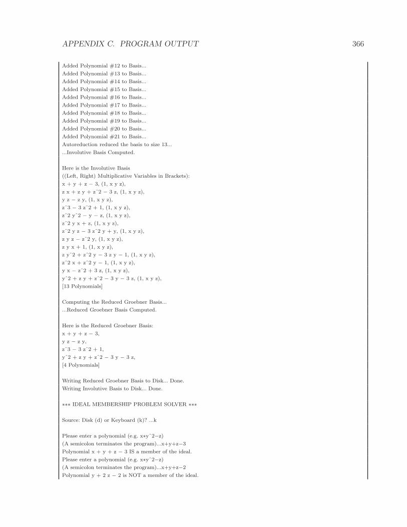
APPENDIX C. PROGRAM OUTPUT 366
Added Polynomial #12 to Basis...
Added Polynomial #13 to Basis...
Added Polynomial #14 to Basis...
Added Polynomial #15 to Basis...
Added Polynomial #16 to Basis...
Added Polynomial #17 to Basis...
Added Polynomial #18 to Basis...
Added Polynomial #19 to Basis...
Added Polynomial #20 to Basis...
Added Polynomial #21 to Basis...
Autoreduction reduced the basis to size 13...
...Involutive Basis Computed.
Here is the Involutive Basis
((Left, Right) Multiplicative Variables in Brackets):
x + y + z − 3, (1, x y z),
z x + z y + zˆ2 − 3 z, (1, x y z),
y z − z y, (1, x y z),
zˆ3 − 3 zˆ2 + 1, (1, x y z),
zˆ2 yˆ2 − y − z, (1, x y z),
zˆ2 y x + z, (1, x y z),
zˆ2 y z − 3 zˆ2 y + y, (1, x y z),
z y z − zˆ2 y, (1, x y z),
z y x + 1, (1, x y z),
z yˆ2 + zˆ2 y − 3 z y − 1, (1, x y z),
zˆ2 x + zˆ2 y − 1, (1, x y z),
y x − zˆ2 + 3 z, (1, x y z),
yˆ2 + z y + zˆ2 − 3 y − 3 z, (1, x y z),
[13 Polynomials]
Computing the Reduced Groebner Basis...
...Reduced Groebner Basis Computed.
Here is the Reduced Groebner Basis:
x + y + z − 3,
y z − z y,
zˆ3 − 3 zˆ2 + 1,
yˆ2 + z y + zˆ2 − 3 y − 3 z,
[4 Polynomials]
Writing Reduced Groebner Basis to Disk... Done.
Writing Involutive Basis to Disk... Done.
∗∗∗ IDEAL MEMBERSHIP PROBLEM SOLVER ∗∗∗
Source: Disk (d) or Keyboard (k)? ...k
Please enter a polynomial (e.g. x∗yˆ2−z)
(A semicolon terminates the program)...x+y+z−3
Polynomial x + y + z − 3 IS a member of the ideal.
Please enter a polynomial (e.g. x∗yˆ2−z)
(A semicolon terminates the program)...x+y+z−2
Polynomial y + 2 z − 2 is NOT a member of the ideal.

APPENDIX C. PROGRAM OUTPUT 367
Please enter a polynomial (e.g. x∗yˆ2−z)
(A semicolon terminates the program)...x∗zˆ2+y∗zˆ2−1
Polynomial x zˆ2 + y zˆ2 − 1 IS a member of the ideal.
Please enter a polynomial (e.g. x∗yˆ2−z)
(A semicolon terminates the program)...z∗y∗x+1
Polynomial z y x + 1 IS a member of the ideal.
Please enter a polynomial (e.g. x∗yˆ2−z)
(A semicolon terminates the program)...xˆ10
Polynomial xˆ10 is NOT a member of the ideal.
Please enter a polynomial (e.g. x∗yˆ2−z)
(A semicolon terminates the program)...;
ma6:mssrc−aux/thesis>
Output File:
x; y; z;
x + y + z − 3; (1, x y z);
z∗x + z∗y + zˆ2 − 3∗z; (1, x y z);
y∗z − z∗y; (1, x y z);
zˆ3 − 3∗zˆ2 + 1; (1, x y z);
zˆ2∗yˆ2 − y − z; (1, x y z);
zˆ2∗y∗x + z; (1, x y z);
zˆ2∗y∗z − 3∗zˆ2∗y + y; (1, x y z);
z∗y∗z − zˆ2∗y; (1, x y z);
z∗y∗x + 1; (1, x y z);
z∗yˆ2 + zˆ2∗y − 3∗z∗y − 1; (1, x y z);
zˆ2∗x + zˆ2∗y − 1; (1, x y z);
y∗x − zˆ2 + 3∗z; (1, x y z);
yˆ2 + z∗y + zˆ2 − 3∗y − 3∗z; (1, x y z);

Bibliography
[1] B. Amrhein, O. Gloor and W. Kuchlin. On the Walk. Theoret. Comput. Sci. 187 (1-
2) (1997) 179–202.
URL http://dx.doi.org/10.1016/S0304-3975(97)00064-9
[2] J. Apel. A Grobner Approach to Involutive Bases. J. Symbolic Comput. 19 (5)
(1995) 441–457.
URL http://dx.doi.org/10.1006/jsco.1995.1026
[3] J. Apel. The Computation of Grobner Bases Using an Alternative Algorithm. Progr.
Comput. Sci. Appl. Logic 15 (1998) 35–45.
[4] J. Apel. The Theory of Involutive Divisions and an Application to Hilbert Function
Computations. J. Symbolic Comput. 25 (6) (1998) 683–704.
URL http://dx.doi.org/10.1006/jsco.1997.0194
[5] T. Baader and N. Tobias. Term Rewriting and All That . Cambridge University Press
(1998).
[6] J. Backelin, S. Cojocaru and V. Ufnarovski. Bergman 1.0 User Manual (1998).
URL http://servus.math.su.se/bergman/
[7] T. Becker and V. Weispfenning. Grobner Bases: A Commutative Approach to Com-
mutative Algebra. Springer-Verlag (1993).
[8] G. M. Bergman. The Diamond Lemma for Ring Theory. Adv. in Math. 29 (2) (1978)
178–218.
URL http://dx.doi.org/10.1016/0001-8708(78)90010-5
[9] W. Boge, R. Gebauer and H. Kredel. Some Examples for Solving Systems of Algebraic
Equations by Calculating Groebner Bases. J. Symbolic Comput. 2 (1) (1986) 83–98.
368

BIBLIOGRAPHY 369
[10] B. Buchberger. A Criterion for Detecting Unnecessary Reductions in the Construc-
tion of Grobner Bases. In Symbolic and Algebraic Computation (EUROSAM ’79, Int.
Symp., Marseille, 1979), volume 72 of Lecture Notes in Comput. Sci., 3–21. Springer,
Berlin (1979).
[11] B. Buchberger. An Algorithmic Criterion for the Solvability of a System of Alge-
braic Equations. Translation of PhD thesis by M. Abramson and R. Lumbert. In B.
Buchberger and F. Winkler, editors, Grobner Bases and Applications, volume 251 of
Proc. London Math. Soc., 535–545. Cambridge University Press (1998).
[12] B. Buchberger and F. Winkler, editors. Grobner Bases and Applications , volume 251
of Proc. London Math. Soc.. Cambridge University Press (1998).
[13] J. Calmet, M. Hausdorf and W. M. Seiler. A Constructive Introduction to Involution.
In R. Akerkar, editor, Proc. Int. Symp. Applications of Computer Algebra – ISACA
2000 , 33–50. Allied Publishers, New Delhi (2001).
[14] J. A. Camberos, L. A. Lambe and R. Luczak. Hybrid Symbolic-Numeric Methodol-
ogy for Fluid Dynamic Simulations. In 34th AIAA Fluid Dynamics Conference and
Exhibit , volume 2004-2330. Portland, OR (2004).
[15] J. A. Camberos, L. A. Lambe and R. Luczak. Computational Physics with Hybrid
Symbolic-Numeric Methodology with Multidisciplinary Applications. Department of
Defense HPC User’s Group Meeting (2005).
[16] J. A. Camberos, L. A. Lambe and R. Luczak. Hybrid Symbolic-Numeric Methodol-
ogy: Views and Visions. In 43rd AIAA Aerospace Sciences Meeting , volume 2005-
0092. Reno, NV (2005).
[17] J. F. Carlson. Cohomology, Computations, and Commutative Algebra. Notices
Amer. Math. Soc. 52 (4) (2005) 426–434.
[18] M. Collart, M. Kalkbrener and D. Mall. Converting Bases with the Grobner Walk.
J. Symbolic Comput. 24 (3-4) (1997) 465–469.
URL http://dx.doi.org/10.1006/jsco.1996.0145
[19] N. Dershowitz. A Taste of Rewrite Systems. In P. E. Lauer, editor, Functional
Programming, Concurrency, Simulation and Automated Reasoning , volume 693 of
Lecture Notes in Comput. Sci., 199–228. Springer (1993).

BIBLIOGRAPHY 370
[20] G. A. Evans. Noncommutative Involutive Bases. In Q.-N. Tran, editor, Proc. 10th
Int. Conf. Applications of Computer Algebra, 49–64. Beaumont, Texas, USA (2004).
[21] J. C. Faugere, P. Gianni, D. Lazard and T. Mora. Efficient Computation of Zero-
dimensional Grobner Bases by Change of Ordering. J. Symbolic Comput. 16 (4)
(1993) 329–344.
URL http://dx.doi.org/10.1006/jsco.1993.1051
[22] R. Froberg. An Introduction to Grobner Bases . John Wiley & Sons (1998).
[23] V. P. Gerdt. Involutive Division Technique: Some Generalizations and Optimizations.
J. Math. Sci. (N. Y.) 108 (6) (2002) 1034–1051.
URL http://dx.doi.org/10.1023/A:1013596522989
[24] V. P. Gerdt. Involutive Algorithms for Computing Grobner Bases. In S. Cojo-
caru, G. Pfister and V. Ufnarovski, editors, Computational Commutative and Non-
Commutative Algebraic Geometry , volume 196 of NATO Science Series: Computer
and Systems Sciences , 199–225. IOS Press (2005).
[25] V. P. Gerdt and Yu. A. Blinkov. Involutive Bases of Polynomial Ideals. Math.
Comput. Simulation 45 (5-6) (1998) 519–541.
URL http://dx.doi.org/10.1016/S0378-4754(97)00127-4
[26] V. P. Gerdt and Yu. A. Blinkov. Minimal Involutive Bases. Math. Comput. Simulation
45 (5-6) (1998) 543–560.
URL http://dx.doi.org/10.1016/S0378-4754(97)00128-6
[27] V. P. Gerdt, Yu. A. Blinkov and D. A. Yanovich. Construction of Janet Bases I.
Monomial Bases. In V. G. Ghanzha, E. W. Mayr and E. V. Vorozhtsov, editors,
Computer Algebra in Scientific Computing (CASC) 2001 , 233–247. Springer-Verlag,
Berlin (2001).
[28] V. P. Gerdt, Yu. A. Blinkov and D. A. Yanovich. Construction of Janet Bases II.
Polynomial Bases. In V. G. Ghanzha, E. W. Mayr and E. V. Vorozhtsov, editors,
Computer Algebra in Scientific Computing (CASC) 2001 , 249–263. Springer-Verlag,
Berlin (2001).
[29] A. Giovini, T. Mora, G. Niedi, L. Robbiano and C. Traverso. “One sugar cube,
please” OR Selection Strategies in Buchberger Algorithm. In ISSAC ’91: Proc. Int.

BIBLIOGRAPHY 371
Symp. Symbolic and Algebraic Computation, 49–54. ACM Press, New York (1991).
URL http://dx.doi.org/10.1145/120694.120701
[30] O. D. Golubitsky. Involutive Grobner Walk. Fundam. Prikl. Mat. 7 (4) (2001)
993–1001.
[31] G. M. Greuel, G. Pfister and H. Schonemann. Singular 3.0.0. A Computer Algebra
System for Polynomial Computations, Centre for Computer Algebra, University of
Kaiserslautern (2005).
URL http://www.singular.uni-kl.de
[32] J. W. Helton and M. Stankus. NCGB 3.1: NonCommutative Grobner Basis Package
(2002).
URL http://math.ucsd.edu/~ncalg/
[33] A. Heyworth. Rewriting as a special case of Grobner Basis Theory. In M. Atkinson,
N. D. Gilbert, J. Howie, S. A. Linton and E. F. Robertson, editors, Computational
and Geometric Aspects of Modern Algebra (Edinburgh, 1998), volume 275 of Proc.
London Math. Soc., 101–105. Cambridge University Press (2000).
[34] F. Hreinsdottir. A case where choosing a product order makes the calculation of a
Grobner Basis much faster. J. Symbolic Comput. 18 (4) (1994) 373–378.
URL http://dx.doi.org/10.1006/jsco.1994.1053
[35] M. Janet. Lecons sur les systemes d’equations aux derivees partielles . Gauthier-
Villars, Paris (1929).
[36] J.-P. Jouannaud. Rewrite Proofs and Computations. In H. Schwichtenberg, editor,
Proof and Computation, volume 139 of Computer and Systems Sciences . Springer-
Verlag (1995).
[37] B. J. Keller. Algorithms and Orders for Finding Noncommutative Grobner Bases.
PhD thesis, Virginia Tech (1997).
[38] B. W. Kernighan and D. M. Ritchie. The C Programming Language (2nd Edition).
Prentice Hall (1988).
[39] D. E. Knuth and P. B. Bendix. Simple word problems in universal algebras. In
J. Leech, editor, Computational Problems in Abstract Algebra, 263–297. Pergamon
Press (1970).

BIBLIOGRAPHY 372
[40] L. A. Lambe. FAlg (An ANSI C Library for Free Associative Algebra Calculations):
User Guide (2001).
[41] L. A. Lambe. FMon (An ANSI C Library for Free Monoid Calculations): User
Guide (2001).
[42] L. A. Lambe. Letter of Support for Research at the University of Wales, Bangor
(2005).
[43] L. A. Lambe, R. Luczak and J. Nehrbass. A new finite difference method for the
Helmholtz equation using symbolic computation. Int. J. Comput. Eng. Sci. 4 (1)
(2003) 121–144.
URL http://dx.doi.org/10.1142/S1465876303000739
[44] E. Mansfield. Differential Grobner Bases. PhD thesis, University of Sydney (1991).
[45] T. Mora. Grobner Bases for non-commutative polynomial rings. In J. Calmet, editor,
AAECC-3: Proc. 3rd Int. Conf. on Algebraic Algorithms and Error-Correcting Codes
(Grenoble, France, July 15–19, 1985), volume 223 of Lecture Notes in Comput. Sci.,
353–362. Springer (1986).
[46] MSSRC (Multidisciplinary Software Systems Research Corporation).
URL http://www.mssrc.com
[47] J. F. Pommaret. Systems of Partial Differential Equations and Lie Pseudogroups .
Gordon and Breach Science Publishers (1978).
[48] L. Robbiano. Term Orderings on the Polynomial Ring. In EUROCAL ’85: Re-
search Contributions from the European Conference on Computer Algebra – Volume
2 , volume 204 of Lecture Notes in Comput. Sci., 513–517. Springer (1985).
[49] SciFace Software. MuPAD Version 3.1. Paderborn, Germany (2005).
URL http://www.mupad.com/
[50] W. M. Seiler. A Combinatorial Approach to Involution and δ-Regularity I: Invo-
lutive Bases in Polynomial Algebras of Solvable Type (2002). Preprint Universita
Mannheim.
[51] W. M. Seiler. A Combinatorial Approach to Involution and δ-Regularity II: Structure
Analysis of Polynomial Modules with Pommaret Bases (2002). Preprint Universita
Mannheim.

BIBLIOGRAPHY 373
[52] J. M. Thomas. Differential Systems . AMS, New York (1937).
[53] Q.-N. Tran. A Fast Algorithm for Grobner Basis Conversion and its Applications.
J. Symbolic Comput. 30 (4) (2000) 451–467.
URL http://dx.doi.org/10.1006/jsco.1999.0416
[54] A. Wachowski and L. Wachowski. The Matrix. Film (Warner Bros.) (1999).
[55] Waterloo Maple Inc. Maple Version 10. Waterloo, Ontario, Canada. (2005).
URL http://www.maplesoft.com
[56] V. Weispfenning. Admissible orders and linear forms. ACM Sigsam Bull. 21 (2)
(1987) 16–18.
URL http://doi.acm.org/10.1145/24554.24557
[57] Wolfram Research, Inc. Mathematica Version 5.1. Champaign, Illinois (2004).
URL http://www.wolfram.com/
[58] A. Yu. Zharkov and Yu. A. Blinkov. Involution Approach to Investigating Polynomial
Systems. Math. Comput. Simulation 42 (4-6) (1996) 323–332.
URL http://dx.doi.org/10.1016/S0378-4754(96)00006-7

Index
Symbols
< . . . . . . . . . . . . . . . . . . . . . . . . . . . . . . . . . 14
. . . . . . . . . . . . . . . . . . . . . . . . . . . . . . . .120
. . . . . . . . . . . . . . . . . . . . . . . . . . . . . . . .120
// . . . . . . . . . . . . . . . . . . . . . . . . . . . . . 20∗ // . . . . . . . . . . . . . . . . . . . . . . . . . . . . . 21
I// . . . . . . . . . . . . . . . . . . . . . . . . . . . . . 74
I
∗ // . . . . . . . . . . . . . . . . . . . . . . . . . . . . . 74
C(U) . . . . . . . . . . . . . . . . . . . . . . . . . 72, 107
C(u, U). . . . . . . . . . . . . . . . . . . . . . .72, 107
CI(U) . . . . . . . . . . . . . . . . . . . . . . . . 72, 107
CI(u, U) . . . . . . . . . . . . . . . . . . . . . . 71, 106
degω . . . . . . . . . . . . . . . . . . . . . . . . . . . . . 166
inω . . . . . . . . . . . . . . . . . . . . . . . . . . . . . . 167
inθ . . . . . . . . . . . . . . . . . . . . . . . . . . . . . . .178
J . . . . . . . . . . . . . . . . . . . . . . . . . . . . . . . . .74
LC(p) . . . . . . . . . . . . . . . . . . . . . . . . . . . . .14
LM(J) . . . . . . . . . . . . . . . . . . . . . . . . . . . . 29
LM(p) . . . . . . . . . . . . . . . . . . . . . . . . . . . . 14
LT(p) . . . . . . . . . . . . . . . . . . . . . . . . . . . . . 14
MI(u, U) . . . . . . . . . . . . . . . . . . . . . . . . . 72
MLI (u, U). . . . . . . . . . . . . . . . . . . . . . . .106
MRI (u, U) . . . . . . . . . . . . . . . . . . . . . . . 107
O . . . . . . . . . . . . . . . . . . . . . . . . . . . . . . . .125
P . . . . . . . . . . . . . . . . . . . . . . . . . . . . . . . . . 74
R[x1, x2, . . . , xn] . . . . . . . . . . . . . . . . . . .11
R〈x1, x2, . . . , xn〉 . . . . . . . . . . . . . . . . . . 12
S . . . . . . . . . . . . . . . . . . . . . . . . . . . . . . . . 135
T . . . . . . . . . . . . . . . . . . . . . . . . . . . . . . . . . 74
θ-homogeneous . . . . . . . . . . . . . . . . . . 178
vali . . . . . . . . . . . . . . . . . . . . . . . . . . . . . . 177
W . . . . . . . . . . . . . . . . . . . . . . . . . . . . . . . 143
A
abelian . . . . . . . . . . . . . . . . . . . . . . . . . . . 10
admissible monomial ordering . . . . . 14
ascending chain condition . . . . . . . . . 29
autoreduction . . . . . . . . . . . . . . . . 77, 110
B
basis . . . . . . . . . . . . . . . . . . . . . . . . . . . . . . 13
Grobner . . . . . . . . . . . . . . . 22, 25, 50
involutive . . . . . . . . . . . . . . . . 80, 112
Bergman, George . . . . . . . . . . . . . . . . . 46
binary operation . . . . . . . . . . . . . . . . . . . 9
Bruno Buchberger . . . . . . . . . . . . . . . . 30
Buchberger’s algorithm . . . . . . . . . . . 30
Buchberger’s first criterion . . . . 35, 56
Buchberger’s second criterion . .37, 57
Buchberger, Bruno . . . . . . . . . . . . . . . . 30
C
coefficient . . . . . . . . . . . . . . . . . . . . . 10, 12
leading . . . . . . . . . . . . . . . . . . . . . . . .14
coefficient ring . . . . . . . . . . . . . . . . . . . . 12
commutative Grobner basis . . . . . . . 25
commutative polynomial ring . . . . . 11
commutative ring . . . . . . . . . . . . . . . . . 10
compatible ordering function . . . . . 178
compatible weight vector. . . . . . . . .167
374

INDEX 375
complete rewrite system . . . . . . . . . 155
involutive . . . . . . . . . . . . . . . . . . . . 155
conclusive involutive division. . . . .114
cone
conventional. . . . . . . . . . . . . .72, 107
involutive . . . . . . . . . . . . . . . . 71, 106
constructive involutive division . . . . 83
continuous involutive division 80, 115
conventional cone . . . . . . . . . . . . 72, 107
conventional divisor . . . . . . . . . . 71, 105
conventional span . . . . . . . . . . . . 72, 107
criterion
Buchberger’s first. . . . . . . . . .35, 56
Buchberger’s second . . . . . . . 37, 57
D
degree . . . . . . . . . . . . . . . . . . . . . . . . . . . . 15
degree inverse lexicographic ordering15
degree lexicographic ordering. . . . . .15
degree reverse lex. ordering. . . .15, 17
dehomogenisation. . . . . . . . . .39, 60, 97
Dickson’s lemma . . . . . . . . . . . . . . . . . . 27
division
involutive . . . . . . . . . . . . . . . . 72, 106
polynomial . . . . . . . . . . . . . . . . . . . . 17
division ring . . . . . . . . . . . . . . . . . . . . . . 10
divisor
conventional. . . . . . . . . . . . . .71, 105
involutive . . . . . . . . . . . . . . . . 71, 105
thick. . . . . . . . . . . . . . . . . . . . . . . . .105
thin. . . . . . . . . . . . . . . . . . . . . . . . . .105
E
empty division . . . . . . . . . . . . . . . . . . . 119
extended prefix turn . . . . . . . . . . . . . 198
extendible involutive division. . . . . .98
extendible monomial ordering . 39, 60
extendible ordering function . . . . . 179
F
FGLM. . . . . . . . . . . . . . . . . . . . . . . . . . . . 42
field . . . . . . . . . . . . . . . . . . . . . . . . . . . . . . 10
full division . . . . . . . . . . . . . . . . . . . . . . 119
functional decomposition. . . . . . . . .177
G
George Bergman . . . . . . . . . . . . . . . . . . 46
global involutive division . . . . . 72, 107
Grobner basis . . . . . . . . . . . . . . . . . . . . . 22
commutative . . . . . . . . . . . . . . . . . . 25
logged . . . . . . . . . . . . . . . . . . . . . 43, 63
minimal . . . . . . . . . . . . . . . . . . . 34, 57
noncommutative . . . . . . . . . . . . . . 50
reduced . . . . . . . . . . . . . . . . . . . 32, 54
Grobner involutive division . . . . . . 118
Grobner walk . . . . . . . . . . . 42, 165, 179
group . . . . . . . . . . . . . . . . . . . . . . . . . . . . . . 9
H
harmonious monomial ordering . . 179
Hilbert’s basis theorem. . . . . . . . . . . .29
homogeneous . . . . . . . . . . . . . . . . . . . . . 39
homogenisation . . . . . . . . . . . . 39, 60, 97
I
ideal . . . . . . . . . . . . . . . . . . . . . . . . . . . . . . 12
left . . . . . . . . . . . . . . . . . . . . . . . . . . . 13
monomial . . . . . . . . . . . . . . . . . . . . . 27
right . . . . . . . . . . . . . . . . . . . . . . . . . . 13
two-sided . . . . . . . . . . . . . . . . . . . . . 13
ideal membership problem . . . . . . . . 13
initial . . . . . . . . . . . . . . . . . . . . . . . 167, 178
inverse lexicographic ordering . 15, 17

INDEX 376
involutive basis. . . . . . . . . . . . . . .80, 112
locally . . . . . . . . . . . . . . . . . . . 79, 112
logged . . . . . . . . . . . . . . . . . . 102, 162
involutive complete rewrite system155
involutive cone . . . . . . . . . . . . . . . 71, 106
involutive division . . . . . . . . . . . . 72, 106
conclusive. . . . . . . . . . . . . . . . . . . .114
constructive . . . . . . . . . . . . . . . . . . . 83
continuous . . . . . . . . . . . . . . . 80, 115
empty . . . . . . . . . . . . . . . . . . . . . . . 119
extendible. . . . . . . . . . . . . . . . . . . . .98
full . . . . . . . . . . . . . . . . . . . . . . . . . . 119
global . . . . . . . . . . . . . . . . . . . . 72, 107
Grobner . . . . . . . . . . . . . . . . . . . . . 118
Janet . . . . . . . . . . . . . . . . . . . . . . . . . 74
left . . . . . . . . . . . . . . . . . . . . . . . . . . 120
left overlap . . . . . . . . . . . . . . . . . . 125
local . . . . . . . . . . . . . . . . . . . . . 72, 107
Noetherian . . . . . . . . . . . . . . . . . . . . 88
Pommaret . . . . . . . . . . . . . . . . . . . . 74
prefix-only left overlap . . . . . . . 147
right . . . . . . . . . . . . . . . . . . . . . . . . . 120
stable . . . . . . . . . . . . . . . . . . . . . . . . . 89
strong . . . . . . . . . . . . . . . . . . . . . . . 106
strong left overlap . . . . . . . . . . . 135
subword-free left overlap . . . . . 147
Thomas . . . . . . . . . . . . . . . . . . . . . . . 74
two sided left overlap . . . . . . . . 143
weak. . . . . . . . . . . . . . . . . . . . . . . . .107
involutive divisions . . . . . . . . . . . 71, 119
involutive divisor . . . . . . . . . . . . . 71, 105
involutive span . . . . . . . . . . . . . . . 72, 107
involutive walk . . . . . . . . . . . . . . 176, 185
J
Janet division . . . . . . . . . . . . . . . . . . . . . 74
K
Knuth-Bendix algorithm . . . . . . . . . . 53
L
leading coefficient . . . . . . . . . . . . . . . . . 14
leading monomial . . . . . . . . . . . . . . . . . 14
leading term . . . . . . . . . . . . . . . . . . . . . . 14
left division . . . . . . . . . . . . . . . . . . . . . . 120
left ideal . . . . . . . . . . . . . . . . . . . . . . . . . . 13
left overlap division . . . . . . . . . . . . . . 125
left prolongation . . . . . . . . . . . . . . . . . 110
left prolongation turn . . . . . . . . . . . . 196
lexicographic ordering . . . . . . . . . 15, 16
local involutive division . . . . . . 72, 107
locally confluent . . . . . . . . . . . . . . . 25, 50
locally involutive basis . . . . . . . 79, 112
logged Grobner basis . . . . . . . . . . 43, 63
logged involutive basis . . . . . . 102, 162
M
minimal Grobner basis . . . . . . . . 34, 57
monomial . . . . . . . . . . . . . . . . . . . . . 10, 12
leading . . . . . . . . . . . . . . . . . . . . . . . .14
monomial ideal . . . . . . . . . . . . . . . . . . . 27
monomial ordering . . . . . . . . . . . . . . . . 14
admissible . . . . . . . . . . . . . . . . . . . . 14
degree inverse lexicographic . . . 15
degree lexicographic . . . . . . . . . . . 15
degree reverse lexicographic15, 17
extendible . . . . . . . . . . . . . . . . . 39, 60
harmonious . . . . . . . . . . . . . . . . . . 179
inverse lexicographic. . . . . . .15, 17
lexicographic . . . . . . . . . . . . . . 15, 16
Mora’s algorithm . . . . . . . . . . . . . . . . . 52
Mora, Teo . . . . . . . . . . . . . . . . . . . . . . . . 46
multidegree . . . . . . . . . . . . . . . . . . . . . . . 11

INDEX 377
multiplicative variables. . . . . . . . . . . .72
N
Noetherian involutive division . . . . . 88
noncommutative Grobner basis. . . .50
noncommutative polynomial ring . .12
noncommutative ring . . . . . . . . . . . . . 10
normal strategy . . . . . . . . . . . . . . . 40, 62
O
ordering
monomial . . . . . . . . . . . . . . . . . . . . . 14
ordering function . . . . . . . . . . . . . . . . 177
compatible . . . . . . . . . . . . . . . . . . . 178
extendible . . . . . . . . . . . . . . . . . . . 179
overlap . . . . . . . . . . . . . . . . . . . . . . . . . . . 47
self . . . . . . . . . . . . . . . . . . . . . . . . . . . 49
overlap word . . . . . . . . . . . . . . . . . . . . . . 62
P
padding symbol . . . . . . . . . . . . . . . . . . . 16
polynomial . . . . . . . . . . . . . . . . . . . . 10, 12
polynomial division . . . . . . . . . . . . . . . 17
polynomial ring
commutative . . . . . . . . . . . . . . . . . . 11
noncommutative . . . . . . . . . . . . . . 12
Pommaret division . . . . . . . . . . . . . . . . 74
prefix . . . . . . . . . . . . . . . . . . . . . . . . . . . . . 47
prefix turn . . . . . . . . . . . . . . . . . . . . . . . 197
extended. . . . . . . . . . . . . . . . . . . . . 198
prefix-only left overlap division. . .147
prolongation . . . . . . . . . . . . . . . . . . . . . . 77
left . . . . . . . . . . . . . . . . . . . . . . . . . . 110
right . . . . . . . . . . . . . . . . . . . . . . . . . 110
prolongation turn
left . . . . . . . . . . . . . . . . . . . . . . . . . . 196
right . . . . . . . . . . . . . . . . . . . . . . . . . 196
R
reduced Grobner basis . . . . . . . . .32, 54
remainder
unique . . . . . . . . . . . . 25, 50, 93, 117
right division . . . . . . . . . . . . . . . . . . . . 120
right ideal . . . . . . . . . . . . . . . . . . . . . . . . 13
right prolongation . . . . . . . . . . . . . . . 110
right prolongation turn . . . . . . . . . . 196
ring . . . . . . . . . . . . . . . . . . . . . . . . . . . . . . .10
coefficient . . . . . . . . . . . . . . . . . . . . . 12
commutative . . . . . . . . . . . . . . . . . . 10
division . . . . . . . . . . . . . . . . . . . . . . . 10
noncommutative . . . . . . . . . . . . . . 10
sub-. . . . . . . . . . . . . . . . . . . . . . . . . . .10
rng . . . . . . . . . . . . . . . . . . . . . . . . . . . . . . . 10
S
S-polynomial . . . . . . . . . . . . . . . . . . 24, 49
selection strategies . . . . . . . . .40, 62, 96
self overlap . . . . . . . . . . . . . . . . . . . . . . . 49
span
conventional. . . . . . . . . . . . . .72, 107
involutive . . . . . . . . . . . . . . . . 72, 107
stable involutive division . . . . . . . . . . 89
strategy
normal . . . . . . . . . . . . . . . . . . . . 40, 62
sugar . . . . . . . . . . . . . . . . . . . . . . 41, 62
tie-breaking . . . . . . . . . . . . . . . . . . . 64
strong involutive division . . . . . . . . 106
strong left overlap division . . . . . . . 135
subring . . . . . . . . . . . . . . . . . . . . . . . . . . . 10
subword . . . . . . . . . . . . . . . . . . . . . . . . . . 47
subword-free left overlap division.147
suffix . . . . . . . . . . . . . . . . . . . . . . . . . . . . . 47
suffix turn . . . . . . . . . . . . . . . . . . . . . . . 197
sugar strategy . . . . . . . . . . . . . . . . . 41, 62

INDEX 378
T
Teo Mora . . . . . . . . . . . . . . . . . . . . . . . . . 46
term . . . . . . . . . . . . . . . . . . . . . . . . . . 10, 12
leading . . . . . . . . . . . . . . . . . . . . . . . .14
thick divisor . . . . . . . . . . . . . . . . . . . . . 105
thin divisor . . . . . . . . . . . . . . . . . . . . . . 105
Thomas division . . . . . . . . . . . . . . . . . . 74
tie-breaking strategy . . . . . . . . . . . . . . 64
two sided left overlap division . . . . 143
two-sided ideal . . . . . . . . . . . . . . . . . . . . 13
U
unique remainder . . . . . 25, 50, 93, 117
W
walk
Grobner . . . . . . . . . . . . . 42, 165, 179
involutive . . . . . . . . . . . . . . . 176, 185
weak involutive division . . . . . . . . . . 107
word problem . . . . . . . . . . . . . . . . . . . . . 53