arX

iv:2

108.

0268

3v2

[m

ath-

ph]

19

Nov

202

1

Noncommutative (A)dS and Minkowski spacetimes

from quantum Lorentz subgroups

Angel Ballesteros1, Ivan Gutierrez-Sagredo1,2 and Francisco J. Herranz1

1Departamento de Fısica, Universidad de Burgos, 09001 Burgos, Spain

2Departamento de Matematicas y Computacion, Universidad de Burgos, 09001 Burgos, Spain

e-mail: angelb@ubu.es, igsagredo@ubu.es, fjherranz@ubu.es

Abstract

The complete classification of classical r-matrices generating quantum deformations of the(3+1)-dimensional (A)dS and Poincare groups such that their Lorentz sector is a quantum sub-group is presented. It is found that there exists three classes of such r-matrices, one of thembeing a novel two-parametric one. The (A)dS and Minkowskian Poisson homogeneous spacescorresponding to these three deformations are explicitly constructed in both local and ambientcoordinates. Their quantization is performed, thus giving rise to the associated noncommu-tative spacetimes, that in the Minkowski case are naturally expressed in terms of quantumnull-plane coordinates, and they are always defined by homogeneous quadratic algebras. Fi-nally, non-relativistic and ultra-relativistic limits giving rise to novel Newtonian and Carrolliannoncommutative spacetimes are also presented.

PACS: 02.20.Uw 03.30.+p 04.60.-m

KEYWORDS: quantum groups; Minkowski spacetime; (A)dS spacetimes; cosmological constant;noncommutative spaces; Lie bialgebras; Poisson-Lie groups; Poisson homogeneous spaces; contrac-tions; Galilei; Carroll

1

Contents

1 Introduction 2

2 (A)dS and Poincare groups: a joint description 4

3 Lie bialgebras and Poisson homogeneous spaces 6

4 (A)dS and Poincare bialgebras with a Lorentz sub-bialgebra 8

4.1 The (2+1)-dimensional case . . . . . . . . . . . . . . . . . . . . . . . . . . . . . . . . 11

5 Noncommutative (A)dS and Minkowski spacetimes 12

5.1 Type I spacetimes . . . . . . . . . . . . . . . . . . . . . . . . . . . . . . . . . . . . . 14

5.1.1 Subfamily with z = 0 . . . . . . . . . . . . . . . . . . . . . . . . . . . . . . . 15

5.1.2 Subfamily with z′ = 0 . . . . . . . . . . . . . . . . . . . . . . . . . . . . . . . 16

5.2 Type II spacetimes . . . . . . . . . . . . . . . . . . . . . . . . . . . . . . . . . . . . . 17

5.3 Type III spacetimes . . . . . . . . . . . . . . . . . . . . . . . . . . . . . . . . . . . . 18

6 Noncommutative Newtonian and Carrollian spacetimes 19

6.1 Non-relativistic limit . . . . . . . . . . . . . . . . . . . . . . . . . . . . . . . . . . . . 20

6.2 Ultra-relativistic limit . . . . . . . . . . . . . . . . . . . . . . . . . . . . . . . . . . . 22

7 Concluding remarks 24

References 26

1 Introduction

It is well-known that quantum Poincare and (anti-)de Sitter (hereafter (A)dS) groups (see [1–11] andreferences therein) provide Hopf algebra deformations of relativistic symmetries which can be usedto construct Deformed Special Relativity (DSR) models [12–17] in which the quantum deformationparameter is assumed to be related to the Planck scale. In this setting, quantum gravity effects areassumed to be described in a schematic way through the associated noncommutative Minkowskiand (A)dS spacetimes. Moreover, in the (A)dS case the interplay between the non-vanishingcosmological constant Λ and the Planck scale parameter can be explicitly described.

In this approach, the natural question concerning the complete classification of quantum Poincareand (A)dS groups in (3+1) dimensions arises, since solving this problem will provide the full set ofavailable Hopf algebra deformations of relativistic symmetries. In the Poincare case, such classifi-cation was given in [7] at the quantum group level, while classical r-matrices generating all possiblequantum deformations were classified in [8]. However, to the best of our knowledge, similar resultsare not available for the (A)dS case yet. Besides its intrinsic mathematical relevance, the latterresult would be indeed relevant for DSR Hopf algebra models dealing with the propagation ofparticles on quantum spacetimes at cosmological distances.

2

The aim of this paper is to contribute to fill this gap, at least partially, by providing the completeclassification of classical r-matrices of the Poincare and (A)dS groups endowed with an outstandingcondition: that their so(3, 1) Lorentz sector has to be a Hopf subalgebra after the full quantum groupis constructed. As we will show, this problem can be fully and explicitly solved by considering thatthe complete classification of classical r-matrices of the so(3, 1) Lorentz group is known [18], andthe answer leads to only three families of r-matrices generating quantum Lorentz subgroups. One ofthem is a novel biparametric r-matrix whose associated noncommutative spacetime is constructedand analysed in detail. Remarkably enough, the cosmological constant parameter Λ does not appearin any of the three r-matrices, which means that these three solutions are invariant under the flatlimit Λ → 0. Moreover, it is also explicitly shown that there does not exist any non-trivial quantumPoincare or (A)dS group for which the Lorentz sector is a non-deformed one.

It is worth stressing that the well-known κ-deformations [1–4, 10, 19, 20] do not belong to theclass of quantum groups here studied. Therefore, the new noncommutative Minkowski and (A)dSspacetimes here presented would be worth to be considered in order to construct new DSR models.As we will see in detail, in the Minkowskian case these novel noncommutative spacetimes are definedthrough a homogeneous quadratic algebra of spacetime operators, and the natural setting for themis to consider noncommutative null-plane coordinates. Consequently, these new noncommutativeMinkowskian spacetimes are quite different from the κ-Minkowski noncommutative spacetime [2]and from its linear-algebraic generalizations [21–23] (see also references therein).

The paper is organized as follows. In the next Section the family of (3+1)-dimensional (A)dSand Poincare Lie algebras, Lie groups and classical homogeneous spacetimes is presented in a unifiedsetting by making use of the cosmological constant Λ, where these three Lie groups are collectivelydenoted by GΛ. After recalling in Section 3 the basic tools and concepts needed for the paper, wepresent our main results in Section 4 by taking into account that any quantum deformation for GΛ

has to be generated by an underlying coboundary Lie bialgebra structure coming from a solution ofthe modified classical Yang–Baxter equation. In particular, we firstly prove that there does not existany quantum deformation for the family GΛ with an undeformed Lorentz subgroup. Secondly, weexplicitly compute all classical r-matrices for the Poincare and (A)dS groups that present a Lorentzsub-Lie bialgebra structure. It comes out that there only exist three types of such r-matrices, whichare explicitly obtained: two of them depends on a single deformation parameter, while the otherone is a two-parametric deformation. The (2+1)-dimensional counterpart of this classification isalso presented in Section 4.1 and the differences that arise between both dimensions are anal-ysed. Furthermore, our results entail a classification of (3+1)-dimensional (A)dS and Minkowskinoncommutative spacetimes associated to deformations with a quantum Lorentz subgroup, whosesemiclassical counterpart corresponds to Poisson homogeneous spaces of Poisson Lorentz subgrouptype. The latter are deduced in Section 5 for the three types of quantum deformations by consid-ering both local and ambient coordinates, and are summarized in Table 2. In addition, we performin Section 6 the non-relativistic and ultra-relativistic limits of the above classification, giving riseto Newtonian and Carrollian quantum deformations, for which the relevant role formerly playedby the Lorentz subgroup is now replaced by the three-dimensional (3D) Euclidean one generatedby rotations and boost transformations. Their corresponding noncommutative spacetimes are alsoderived and presented in Table 3. Finally some remarks and open problems close the paper.

3

2 (A)dS and Poincare groups: a joint description

In our framework we will consider the (3+1)D Poincare and (A)dS Lie algebras expressed in aunified setting as a one-parametric family of Lie algebras denoted by gΛ depending explicitly onthe cosmological constant parameter Λ. In the usual kinematical basis, spanned by the generators oftime translations P0, spatial translations P = (P1, P2, P3), boost transformations K = (K1,K2,K3)and rotations J = (J1, J2, J3), the commutation relations of gΛ read

[Ja, Jb] = ǫabcJc, [Ja, Pb] = ǫabcPc, [Ja,Kb] = ǫabcKc,

[Ka, P0] = Pa, [Ka, Pb] = δabP0, [Ka,Kb] = −ǫabcJc,

[P0, Pa] = −ΛKa, [Pa, Pb] = ΛǫabcJc, [Ja, P0] = 0.

(2.1)

From now on sum over repeated indices will be understood unless otherwise stated. Hereafter,Latin indices run as a, b, c = 1, 2, 3, and Greek ones as µ = 0, 1, 2, 3. The family of Lie algebrasgΛ encompasses the dS algebra so(4, 1) when Λ > 0, the AdS algebra so(3, 2) if Λ < 0 and thePoincare one iso(3, 1) for Λ = 0. As a vector space, gΛ can be decomposed in the form

gΛ = h⊕ t, h = span {K,J} = so(3, 1), t = span {P0,P}, (2.2)

where h is the Lorentz subalgebra and t is the translation sector.

A faithful representation of gΛ (2.1), ρ : gΛ → End(R5), for a generic element X ∈ gΛ is givenby [20]

ρ(X) = xµρ(Pµ) + ξaρ(Ka) + θaρ(Ja) =

0 Λx0 −Λx1 −Λx2 −Λx3

x0 0 ξ1 ξ2 ξ3

x1 ξ1 0 −θ3 θ2

x2 ξ2 θ3 0 −θ1

x3 ξ3 −θ2 θ1 0

. (2.3)

The corresponding exponentiation provides a one-parametric family of Lie groups, denoted by GΛ,with Lie algebra gΛ. Hence GΛ contains the dS group SO(4, 1) for Λ > 0, the AdS group SO(3, 2)for Λ < 0, and the Poincare one ISO(3, 1) for Λ = 0. Note that the exponentiation of (2.3) onlyrecovers the connected component to the identity of these three Lie groups, but the completedescription of these groups can be obtained by considering the parity and time-reversal involutiveautomorphisms. The family GΛ can be parametrized in terms of local coordinates {xµ, ξa, θa} inthe form

GΛ = expx0ρ(P0) expx1ρ(P1) expx

2ρ(P2) expx3ρ(P3)

× exp ξ1ρ(K1) exp ξ2ρ(K2) exp ξ

3ρ(K3) exp θ1ρ(J1) exp θ

2ρ(J2) exp θ3ρ(J3).

(2.4)

These coordinates are the so-called exponential coordinates of the second kind on GΛ.

Therefore GΛ comprises the isometry Lie groups of the (3+1)D Minkowski and (A)dS space-times, which we denote collectively by MΛ and have a constant sectional curvature given by −Λ.For each of these three spacetimes, the stabilizer of a point is the Lorentz subgroup H with Liealgebra h (2.2). Thus there exists a global isometry between MΛ and the left coset space GΛ/H,so that we write

MΛ = GΛ/H, H = SO(3, 1) = 〈K,J〉. (2.5)

Hence MΛ is a family of symmetric homogeneous spaces, and we can identify their tangent spaceat every point m = gH ∈ MΛ, g ∈ GΛ, with the translation sector, i.e.

Tm(MΛ) = TgH(GΛ/H) ≃ gΛ/h ≃ t = span {P0,P}. (2.6)

4

The four Lie group local coordinates xµ in (2.4), associated to the translation generators Pµ, descendto coordinates on MΛ.

The representation of GΛ (2.4), coming from (2.3), allows us to consider GΛ as the isometrygroup of the 5D linear space (R5, IΛ), with canonical linear ambient coordinates (s4, sµ), such thatIΛ is the bilinear form given by

IΛ = diag(+1,−Λ,Λ,Λ,Λ), (2.7)

fulfilling that GTΛ IΛGΛ = IΛ. The point with ambient coordinates O = (1, 0, 0, 0, 0) is invariant

under the action of the Lorentz subgroup H, and will be taken as the origin of MΛ. The orbitpassing through O corresponds to the (3+1)D spacetime MΛ (2.5) defined by the pseudosphere

ΣΛ ≡ (s4)2 − Λ(s0)2 + Λ(

(s1)2 + (s2)2 + (s3)2)

= 1, (2.8)

determined by IΛ (2.7). In the flat limit Λ → 0, the Minkowski spacetime will be identified withthe hyperplane s4 = +1 containing O. We remark that the coordinates

qµ =sµ

s4(2.9)

are just the Beltrami projective coordinates in MΛ which can be obtained through the projec-tion with pole (0, 0, 0, 0, 0) ∈ R

5 of a point with ambient coordinates (s4, sµ) onto the projectivehyperplane with s4 = +1 (see [24] for details).

Now the set of spacetime local coordinates xµ can be introduced through the following actiononto the origin O of the one-parameter subgroups of GΛ (2.4) [20]

(s4, sµ)T = expx0ρ(P0) expx1ρ(P1) expx

2ρ(P2) expx3ρ(P3)O

T , (2.10)

thus yielding

s4 = cos(ηx0) cosh(ηx1) cosh(ηx2) cosh(ηx3),

s0 =sin(ηx0)

ηcosh(ηx1) cosh(ηx2) cosh(ηx3),

s1 =sinh(ηx1)

ηcosh(ηx2) cosh(ηx3),

s2 =sinh(ηx2)

ηcosh(ηx3),

s3 =sinh(ηx3)

η,

(2.11)

where the parameter η is defined byη2 := −Λ. (2.12)

Thus η is real for the AdS space and a pure imaginary number for the dS one. The four spacetimecoordinates xµ are called geodesic parallel coordinates [25], and can be regarded as a generalizationof the flat Cartesian coordinates to non-zero curvature. In fact, under the vanishing cosmologicalconstant limit, η → 0, the ambient (2.11) and Beltrami (2.9) coordinates reduce to the usualCartesian ones in the Minkowski spacetime:

(s4, sµ) ≡ (1, qµ) ≡ (1, xµ). (2.13)

5

In ambient coordinates, the time-like metric on the (3+1)D MΛ spacetime comes from the pseudo-sphere (2.8) and turns out to be [24]

dσ2Λ =

1

−Λ

(

(ds4)2 − Λ(

(ds0)2 − (ds1)2 − (ds2)2 − (ds3)2)

)∣

∣

∣

∣

ΣΛ

=−Λ

(

s0ds0 − s1ds1 − s2ds2 − s3ds3)2

1 + Λ(

(s0)2 − (s1)2 − (s2)2 − (s3)2) + (ds0)2 − (ds1)2 − (ds2)2 − (ds3)2. (2.14)

From this expression the metric in terms of Beltrami coordinates (2.9) can be obtained [24], andin geodesic parallel coordinates (2.11) the metric reads [20]

dσ2Λ = cosh2(ηx1) cosh2(ηx2) cosh2(ηx3)(dx0)2 − cosh2(ηx2) cosh2(ηx3)(dx1)2

− cosh2(ηx3)(dx2)2 − (dx3)2 . (2.15)

Indeed, when η → 0 expressions (2.14) and (2.15) reduce to the usual metric on the Minkowskispacetime:

dσ20 = (ds0)2 − (ds1)2 − (ds2)2 − (ds3)2 = (dx0)2 − (dx1)2 − (dx2)2 − (dx3)2. (2.16)

3 Lie bialgebras and Poisson homogeneous spaces

Let us briefly recall the basic notions needed for the paper, and set up the notation; for more detailswe refer to [26]. A Lie bialgebra is a pair (g, δ) where g is a Lie algebra and

δ : g → g ∧ g (3.1)

is a linear map called cocommutator and satisfying the following conditions

∑

cycl

(δ ⊗ id) ◦ δ(X) = 0, ∀X ∈ g,

δ([X,Y ]) = adXδ(Y )− adY δ(X), ∀X,Y ∈ g.

(3.2)

The first expression is called co-Jacobi condition since this is equivalent to requiring that thetranspose map tδ : g∗ ∧ g∗ → g∗ satisfies the Jacobi identity. The second relation states that themap δ is a 1-cocycle in the Chevalley–Eilenberg cohomology with values in g ∧ g. Given a Liebialgebra (g, δ) and a Lie subalgebra h of g, the pair (h, δ|h) is said to be a sub-Lie bialgebra of(g, δ) in the case that δ(h) ⊂ h ∧ h.

For some Lie bialgebra structures the cocommutator map can be completely defined in termsof an element r ∈ g ∧ g. In these cases, called 1-coboundaries, the map

δr(X) = adX(r) (3.3)

defines a Lie bialgebra structure if and only if r fulfils the modified classical Yang–Baxter equation(mCYBE)

adX [[r, r]] = 0, ∀X ∈ g, (3.4)

where the algebraic Schouten bracket is defined by

[[r, r]] := [r12, r13] + [r12, r23] + [r13, r23]. (3.5)

6

Therefore an element r ∈ g ∧ g satisifes the mCYBE (3.4) if and only if

[[r, r]] ∈

( 3∧

g

)

g

, (3.6)

i.e. if its algebraic Schouten bracket is a g-invariant element of∧3

g. Particular solutions of themCYBE are those which fulfil the classical Yang–Baxter equation (CYBE)

[[r, r]] = 0, (3.7)

that is, the algebraic Schouten bracket vanishes identically. Solutions of the CYBE are called tri-angular (or nonstandard) classical r-matrices, while solutions of the mCYBE that are not solutionsof the CYBE are called quasitriangular (or standard) classical r-matrices. A Lie bialgebra (g, δ) isthen called a coboundary one if its cocommutator δ is of the form (3.3) for some solution of themCYBE (3.4).

A Poisson–Lie (PL) group is the global object integrating a Lie bialgebra structure. Moreexplicitly, a PL group is a pair (G,Π) where G is a Lie group and Π is a Poisson structure suchthat the Lie group multiplication µ : G×G → G is a Poisson map with respect to Π on G and theproduct Poisson structure ΠG×G = Π ⊕ Π on G × G. The relation between the Poisson bivectorfield and the Poisson bracket is given by

(df1 ⊗ df2)Π = {f1, f2}Π . (3.8)

A Lie subgroup H of G is said to be a PL subgroup of (G,Π) if (H,Π|H) is a Poisson submanifoldof (G,Π). A PL group is called coboundary if its tangent Lie bialgebra is a coboundary one. Let(G,Π) be a coboundary PL group with tangent Lie bialgebra (g, δr) (3.3), then the Poisson bivectoron G is given by the Sklyanin bivector

Π = rij(

XLi ⊗XL

j −XRi ⊗XR

j

)

, (3.9)

where XLi and XR

i denote the left- and right-invariant vector fields, respectively.

A Poisson manifold (M,π) is a manifold M endowed with a Poisson structure π on M . APoisson homogeneous space (PHS) for a PL group (G,Π) is a Poisson manifold (M,π) which isendowed with a transitive group action α : (G×M,Π⊕π) → (M,π) which is a Poisson map. Whenthe manifold is a homogeneous space, M = G/H, there does exist a distinguished class of PHS forwhich the Poisson structure π on M can be obtained by canonical projection of the PL structureΠ on G. In terms of the underlying Lie bialgebra (g, δ) of (G,Π), this requirement corresponds toimposing the so-called coisotropy condition for the cocommutator δ with respect to the isotropysubalgebra h of H that is given by [27–29]

δ(h) ⊂ h ∧ g. (3.10)

A particular case fulfilling the above condition is obtained when the Lie subalgebra h is also asub-Lie bialgebra:

δ (h) ⊂ h ∧ h, (3.11)

which implies that the PHS is constructed through an isotropy subgroup H such that (H,Π|H) isa PL subgroup of (G,Π) and this is called a “PHS of Poisson subgroup type”.

We recall that since a quantum group is the quantization of a PL group (G,Π), the quantizationof a coisotropic PHS (M = G/H, π) fulfilling (3.10) provides a quantum homogeneous space (or

7

noncommutative space) onto which the quantum group co-acts covariantly [30]. The coisotropycondition (3.10) ensures that the commutation relations that define the noncommutative space atthe first-order in all the quantum coordinates close on a Lie subalgebra which is just the annihilatorh⊥ of h on the dual Lie algebra g∗ [28, 31, 32].

By taking into account the above concepts, we would like to remark that in the next Sectionwe shall deduce all the possible Lie bialgebra structures for the family gΛ (2.2) such that theLorentz subalgebra h is a sub-Lie bialgebra of (gΛ, δ). We will find three types of such bialgebrasbeing all of them coboundaries (3.3), so coming from solutions r ∈ gΛ ∧ gΛ of the mCYBE (3.4).Consequently, each of them provides a PL group (GΛ,Π) for the family GΛ (2.4) through theSklyanin bivector (3.9) and, by construction, the Lorentz subgroup H becomes a PL subgroup(H,Π|H) of (GΛ,Π). Furthermore, each of these PL groups leads to a PHS (MΛ = GΛ/H, π)where the Poisson structure π on MΛ is obtained by canonical projection of the PL structure Π onGΛ. In Section 5 we will first compute explicitly all such PHS and, secondly, we will provide theircomplete quantum versions, thus obtaining all the (3+1)D noncommutative (A)dS and Minkowskispacetimes which are covariant under the only quantum (A)dS and Poincare groups for which theLorentz subalgebra has a quantum subgroup structure.

4 (A)dS and Poincare bialgebras with a Lorentz sub-bialgebra

We proceed to obtain all the PL groups (GΛ,Π) associated with Lie bialgebras (gΛ, δ) for whichthe Lorentz Lie algebra has a sub-Lie bialgebra structure. With this aim, let us recall that

Remark 1. All possible Lie bialgebra structures for the family gΛ (2.1) are coboundary ones.

This fact is straightforward for so(3, 2) and so(4, 1) since it is well-known that all Lie bialgebrastructures for semisimple Lie algebras are coboundaries. For the Poincare algebra iso(3, 1) thisproperty was proven in [5, 7, 8], which is a particular case of the more general result stating thatall Lie bialgebras for inhomogeneous pseudo-orthogonal Lie algebras iso(p, q) with p + q ≥ 3 arecoboundaries [33].

Since PL groups (GΛ,Π) are in one-to-one correspondence to Lie bialgebras and for gΛ these arealways coboundaries (gΛ, δr) (3.3), we thus face the problem consisting in obtaining all the possiblesolutions r of the mCYBE (3.4) such that the Lorentz sub-bialgebra condition (3.11) is fulfilled,namely that δr(h) ⊂ h ∧ h.

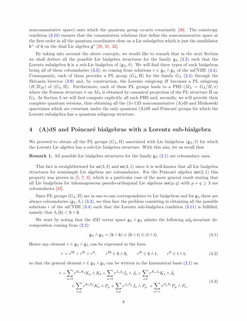
We start by noting that the 45D vector space gΛ ∧ gΛ admits the following adh-invariant de-composition coming from (2.2):

gΛ ∧ gΛ = (h ∧ h)⊕ (h ∧ t)⊕ (t ∧ t). (4.1)

Hence any element r ∈ gΛ ∧ gΛ can be expressed in the form

r = rhh + rht + rtt, rhh ∈ h ∧ h, rht ∈ h ∧ t, rtt ∈ t ∧ t, (4.2)

so that the general element r ∈ gΛ ∧ gΛ can be written in the kinematical basis (2.1) as

r =∑

a<b

rKaKbKa ∧Kb +∑

a<b

rJaJbJa ∧ Jb +∑

a,b

rKaJbKa ∧ Jb

+∑

a,µ

rKaPµKa ∧ Pµ +∑

a,µ

rJaPµJa ∧ Pµ +∑

µ<ν

rPµPνPµ ∧ Pν .(4.3)

8

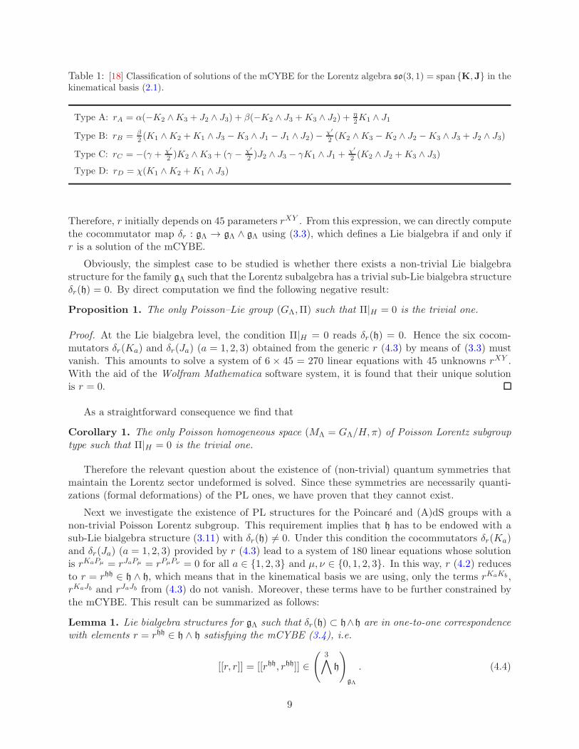
Table 1: [18] Classification of solutions of the mCYBE for the Lorentz algebra so(3, 1) = span {K,J} in thekinematical basis (2.1).

Type A: rA = α(−K2 ∧K3 + J2 ∧ J3) + β(−K2 ∧ J3 +K3 ∧ J2) +η2K1 ∧ J1

Type B: rB = β2(K1 ∧K2 +K1 ∧ J3 −K3 ∧ J1 − J1 ∧ J2)−

χ′

2(K2 ∧K3 −K2 ∧ J2 −K3 ∧ J3 + J2 ∧ J3)

Type C: rC = −(γ + χ′

2)K2 ∧K3 + (γ − χ′

2)J2 ∧ J3 − γK1 ∧ J1 +

χ′

2(K2 ∧ J2 +K3 ∧ J3)

Type D: rD = χ(K1 ∧K2 +K1 ∧ J3)

Therefore, r initially depends on 45 parameters rXY . From this expression, we can directly computethe cocommutator map δr : gΛ → gΛ ∧ gΛ using (3.3), which defines a Lie bialgebra if and only ifr is a solution of the mCYBE.

Obviously, the simplest case to be studied is whether there exists a non-trivial Lie bialgebrastructure for the family gΛ such that the Lorentz subalgebra has a trivial sub-Lie bialgebra structureδr(h) = 0. By direct computation we find the following negative result:

Proposition 1. The only Poisson–Lie group (GΛ,Π) such that Π|H = 0 is the trivial one.

Proof. At the Lie bialgebra level, the condition Π|H = 0 reads δr(h) = 0. Hence the six cocom-mutators δr(Ka) and δr(Ja) (a = 1, 2, 3) obtained from the generic r (4.3) by means of (3.3) mustvanish. This amounts to solve a system of 6 × 45 = 270 linear equations with 45 unknowns rXY .With the aid of the Wolfram Mathematica software system, it is found that their unique solutionis r = 0.

As a straightforward consequence we find that

Corollary 1. The only Poisson homogeneous space (MΛ = GΛ/H, π) of Poisson Lorentz subgrouptype such that Π|H = 0 is the trivial one.

Therefore the relevant question about the existence of (non-trivial) quantum symmetries thatmaintain the Lorentz sector undeformed is solved. Since these symmetries are necessarily quanti-zations (formal deformations) of the PL ones, we have proven that they cannot exist.

Next we investigate the existence of PL structures for the Poincare and (A)dS groups with anon-trivial Poisson Lorentz subgroup. This requirement implies that h has to be endowed with asub-Lie bialgebra structure (3.11) with δr(h) 6= 0. Under this condition the cocommutators δr(Ka)and δr(Ja) (a = 1, 2, 3) provided by r (4.3) lead to a system of 180 linear equations whose solutionis rKaPµ = rJaPµ = rPµPν = 0 for all a ∈ {1, 2, 3} and µ, ν ∈ {0, 1, 2, 3}. In this way, r (4.2) reducesto r = rhh ∈ h ∧ h, which means that in the kinematical basis we are using, only the terms rKaKb ,rKaJb and rJaJb from (4.3) do not vanish. Moreover, these terms have to be further constrained bythe mCYBE. This result can be summarized as follows:

Lemma 1. Lie bialgebra structures for gΛ such that δr(h) ⊂ h∧h are in one-to-one correspondencewith elements r = rhh ∈ h ∧ h satisfying the mCYBE (3.4), i.e.

[[r, r]] = [[rhh, rhh]] ∈

(

3∧

h

)

gΛ

. (4.4)

9

We stress that the classification of the solutions of the mCYBE for the Lorentz algebra so(3, 1)was given in [18] (see also [34, 35] for the classification of the Euclidean and Kleinian analogues, and[36] for their corresponding contractions leading to (2+1)D Poincare and 3D Euclidean classical r-matrices). This result shows that there exists, up to Lie algebra isomorphisms, four multiparametricfamilies of solutions which are presented in Table 1 in the kinematical basis (2.1). We point outthat rB and rD are solutions of the CYBE (3.7), while rA and rC are solutions of the mCYBE (3.6)with non-vanishing algebraic Schouten bracket.

The previous Lemma together with the classification of solutions of the mCYBE for the Lorentzalgebra [18] allow us to state the following main result.

Proposition 2. There exist three classes of Poisson homogeneous spaces (MΛ = GΛ/H, π) for eachof the maximally symmetric spacetimes of constant curvature (Minkowski and (A)dS) such that theisotropy Lorentz subgroup H is a Poisson–Lie subgroup of (GΛ,Π). All of them are obtained fromcoboundary Poisson–Lie structures on their respective isometry group GΛ which are determined, upto gΛ-isomorphisms, by the classical r-matrices

rI = z (K1 ∧K2 +K1 ∧ J3 −K3 ∧ J1 − J1 ∧ J2)

− z′ (K2 ∧K3 −K2 ∧ J2 −K3 ∧ J3 + J2 ∧ J3),

rII = z K1 ∧ J1,

rIII = z (K1 ∧K2 +K1 ∧ J3),

(4.5)

where z and z′ are free parameters. These three r-matrices are solutions of the CYBE.

Proof. A PHS of Poisson subgroup type (GΛ/H, π) can be obtained by canonical projection froma PL group (GΛ,Π). We already know that any PL structure Π on GΛ is a coboundary one, sothat it is completely determined by a solution of the mCYBE whose algebraic Schouten bracket isgΛ-invariant (3.4). Therefore, using Lemma 1 and the standard inclusion h → gΛ it follows thatthere exists a one-to-one correspondence between PHS of Poisson Lorentz subgroup type and theelements r ∈ h ∧ h in Table 1 fufilling (3.4) and (4.4). The triangular classical r-matrices rB andrD already satisfy this condition, since their Schouten bracket vanishes, and lead to the solutionsrI and rIII, respectively. On the other hand, the quasitriangular classical r-matrix rC verifies therelations (3.4) and (4.4) if and only if γ = 0 reducing to the particular case of rI with z = 0.Finally, rA fulfils (3.4) and (4.4) whenever α = β = 0, thus yielding rII which is also a solution ofthe CYBE (3.7).

Consequently, we have proven that there only exist three types of (3+1)D Poincare and (A)dSquantum deformations endowed with a non-trivial quantum Lorentz subgroup, whose underlyingLie bialgebras are determined by rI, rII and rIII. The three classes correspond to triangular ornonstandard deformations. Types II and III are one-parametric deformations, while type I is atwo-parametric one with arbitrary deformation parameters z and z′.

In the Poincare case, the correspondence between the results given by Proposition 2 with the21 multiparametric PL structures presented in [8] can be easily established. The two-parametricdeformation of type I for the Poincare PL group (GΛ=0,Π) is just case 5 of Table 1 in [8]. Theclassical r-matrix rII is provided by a Reshetikhin twist, since both generators in rII (4.5) docommute, which can be identified with case 1 with parameters α = α = 0 in the same Table.Finally, the deformation of type III comes from the lower dimensional Lorentz subalgebra so(2, 1)spanned by {J3,K1,K2} and rIII corresponds to case 6 with parameters β1 = β2 = 0 in [8].

10

4.1 The (2+1)-dimensional case

For the sake of completeness, it is worth comparing the (2+1)D case with the (3+1)D one charac-terized by Propositions 1 and 2. As it will be shown in the following, the classification in (2 + 1)Dis significantly different.

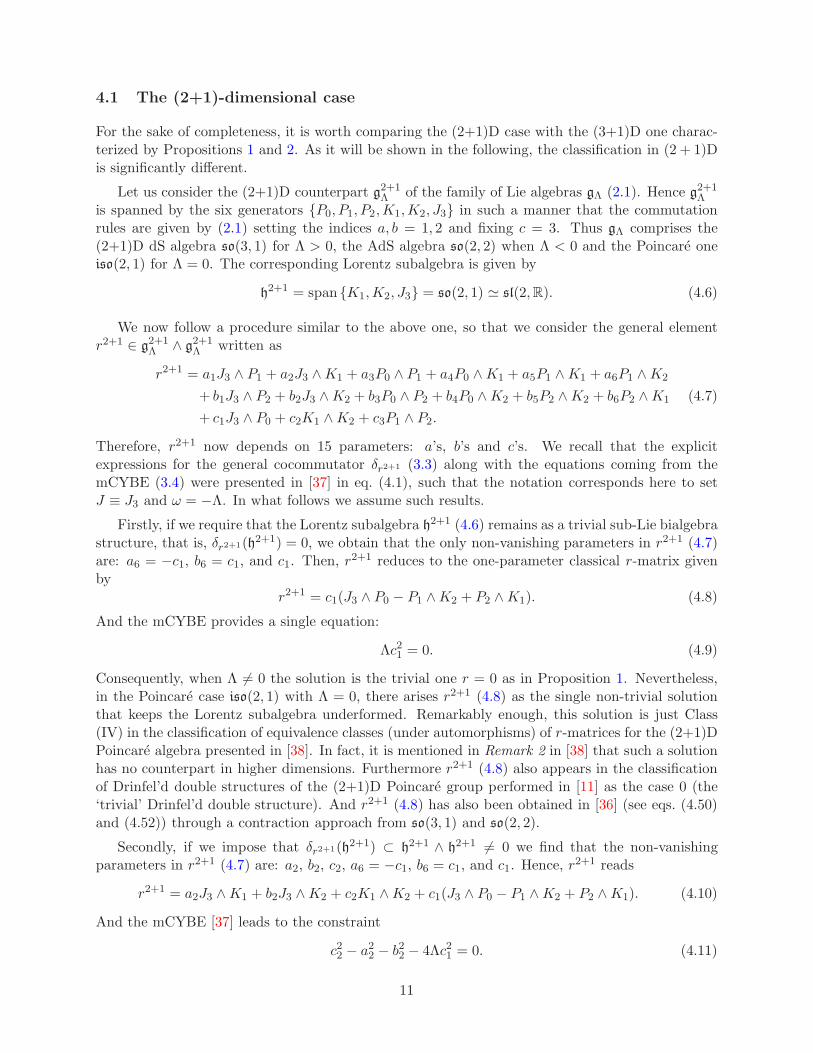
Let us consider the (2+1)D counterpart g2+1Λ

of the family of Lie algebras gΛ (2.1). Hence g2+1Λ

is spanned by the six generators {P0, P1, P2,K1,K2, J3} in such a manner that the commutationrules are given by (2.1) setting the indices a, b = 1, 2 and fixing c = 3. Thus gΛ comprises the(2+1)D dS algebra so(3, 1) for Λ > 0, the AdS algebra so(2, 2) when Λ < 0 and the Poincare oneiso(2, 1) for Λ = 0. The corresponding Lorentz subalgebra is given by

h2+1 = span {K1,K2, J3} = so(2, 1) ≃ sl(2,R). (4.6)

We now follow a procedure similar to the above one, so that we consider the general elementr2+1 ∈ g2+1

Λ∧ g2+1

Λwritten as

r2+1 = a1J3 ∧ P1 + a2J3 ∧K1 + a3P0 ∧ P1 + a4P0 ∧K1 + a5P1 ∧K1 + a6P1 ∧K2

+ b1J3 ∧ P2 + b2J3 ∧K2 + b3P0 ∧ P2 + b4P0 ∧K2 + b5P2 ∧K2 + b6P2 ∧K1 (4.7)

+ c1J3 ∧ P0 + c2K1 ∧K2 + c3P1 ∧ P2.

Therefore, r2+1 now depends on 15 parameters: a’s, b’s and c’s. We recall that the explicitexpressions for the general cocommutator δr2+1 (3.3) along with the equations coming from themCYBE (3.4) were presented in [37] in eq. (4.1), such that the notation corresponds here to setJ ≡ J3 and ω = −Λ. In what follows we assume such results.

Firstly, if we require that the Lorentz subalgebra h2+1 (4.6) remains as a trivial sub-Lie bialgebrastructure, that is, δr2+1(h2+1) = 0, we obtain that the only non-vanishing parameters in r2+1 (4.7)are: a6 = −c1, b6 = c1, and c1. Then, r2+1 reduces to the one-parameter classical r-matrix givenby

r2+1 = c1(J3 ∧ P0 − P1 ∧K2 + P2 ∧K1). (4.8)

And the mCYBE provides a single equation:

Λc21 = 0. (4.9)

Consequently, when Λ 6= 0 the solution is the trivial one r = 0 as in Proposition 1. Nevertheless,in the Poincare case iso(2, 1) with Λ = 0, there arises r2+1 (4.8) as the single non-trivial solutionthat keeps the Lorentz subalgebra underformed. Remarkably enough, this solution is just Class(IV) in the classification of equivalence classes (under automorphisms) of r-matrices for the (2+1)DPoincare algebra presented in [38]. In fact, it is mentioned in Remark 2 in [38] that such a solutionhas no counterpart in higher dimensions. Furthermore r2+1 (4.8) also appears in the classificationof Drinfel’d double structures of the (2+1)D Poincare group performed in [11] as the case 0 (the‘trivial’ Drinfel’d double structure). And r2+1 (4.8) has also been obtained in [36] (see eqs. (4.50)and (4.52)) through a contraction approach from so(3, 1) and so(2, 2).

Secondly, if we impose that δr2+1(h2+1) ⊂ h2+1 ∧ h2+1 6= 0 we find that the non-vanishingparameters in r2+1 (4.7) are: a2, b2, c2, a6 = −c1, b6 = c1, and c1. Hence, r

2+1 reads

r2+1 = a2J3 ∧K1 + b2J3 ∧K2 + c2K1 ∧K2 + c1(J3 ∧ P0 − P1 ∧K2 + P2 ∧K1). (4.10)

And the mCYBE [37] leads to the constraint

c22 − a22 − b22 − 4Λc21 = 0. (4.11)

11

In the Poincare case with Λ = 0, the solution can be reduced, via automorphisms, to b2 = 0 anda2 = −c2:

r2+1 = c2K1 ∧ (K2 + J3) + c1(J3 ∧ P0 − P1 ∧K2 + P2 ∧K1). (4.12)

This two-parametric solution is just Class (I) in the classification [38] and corresponds to theDrinfel’d double structure of case 1 in [11]. For c1 = 0 one recovers the solution rIII in Proposition 2,which has also been obtained via contraction in [36] (see eqs. (4.27) and (4.41)).

Finally, from the classification of classical r-matrices for so(3, 1) obtained in [18] and displayed inTable 1, it follows for Λ = +1 that, under automorphisms, r2+1 (4.12), subjected to the constraint(4.11), gives rise to two solutions:

• If b2 = 0, a2 = −c2, then Λc21 = c21 = 0. Hence

r2+1 = c2K1 ∧ (K2 + J3), (4.13)

which is type D in Table 1 and rIII in Proposition 2.

• If a2 = b2 = 0, then c22 − 4c21 and c2 = 2c1. This leads to

r2+1 = c1(

2K1 ∧K2 + J3 ∧ P0 − P1 ∧K2 + P2 ∧K1

)

, (4.14)

which is the particular case of type C in Table 1 for γ = χ′/2 ≡ c1 and has no (3+1)Dcounterpart as shown in Proposition 2.

5 Noncommutative (A)dS and Minkowski spacetimes

In this Section we first present explicitly the three non-isomorphic PHS defined by Proposition 2and afterwards we perform their quantization.

The three PL structures (GΛ,Π) provided by (4.5) can be explicitly obtained by computingthe left- and right-invariant vector fields on GΛ (2.4) and then constructing the Sklyanin bivectorΠ (3.9). The pushforward of Π on GΛ by the canonical projection p : GΛ → GΛ/H gives rise to thefundamental Poisson brackets for the PHS in terms of the geodesic parallel coordinates xµ. Fromthem the corresponding expressions in terms of ambient coordinates (s4, sµ) (2.11) can be deduced.The resulting fundamental Poisson brackets for the three classes of PHS are displayed in Table 2both in terms of local (geodesic parallel) xµ and ambient coordinates (s4, sµ), where the latter aresubjected to the pseudosphere constraint (2.8).

Nevertheless, it turns out that the ambient coordinate s4 is always a central element for allthree Poisson structures

{s4, sµ} = 0. (5.1)

This fact means that all the PHS can be defined in terms of the (3+1) spacetime coordinates sµ

and that the pseudosphere condition (2.8) can be rewritten as

(s0)2 −(

(s1)2 + (s2)2 + (s3)2)

=(s4)2 − 1

Λ. (5.2)

Hence this relation, automatically, yields a common quadratic Casimir for the three types of PHSin Table 2, which is given by

C = (s0)2 − (s1)2 − (s2)2 − (s3)2. (5.3)

12

Table 2: The three types of (A)dS and Minkowski Poisson homogeneous spaces with Poisson Lorentzsubgroups expressed in geodesic parallel xµ and ambient sµ spacetime coordinates (2.11) such that thecosmological constant Λ = −η2. The ambient coordinate s4 always Poisson-commutes with sµ.

Type I rI = z(K1 ∧K2 +K1 ∧ J3 −K3 ∧ J1 − J1 ∧ J2)− z′(K2 ∧K3 −K2 ∧ J2 −K3 ∧ J3 + J2 ∧ J3)

{x0, x1} = zA cos(ηx0)tanh(ηx2)

η

{x0, x2} = −zcos(ηx0)

cosh(ηx1)

(

Asinh(ηx1)

η+

tanh2(ηx3)

η2

)

− z′Acos(ηx0) cosh(ηx2)

cosh(ηx1)

tanh(ηx3)

η

{x0, x3} = zcos(ηx0)

cosh(ηx1)

tanh(ηx2)

η

tanh(ηx3)

η+ z′A

cos(ηx0)

cosh(ηx1)

sinh(ηx2)

η

{x1, x2} = −z

(

Asin(ηx0)

η−B

tanh2(ηx3)

η2

)

+ z′AB cosh(ηx2)tanh(ηx3)

η

{x1, x3} = −zBtanh(ηx2)

η

tanh(ηx3)

η− z′AB

sinh(ηx2)

η{x2, x3} = zA

tanh(ηx3)

η+ z′A2 cosh(ηx2)

{s0, s1} = z(s0 + s1)s2 {s0, s2} = −z[

(s0 + s1)s1 + (s3)2]

− z′(s0 + s1)s3

{s0, s3} = zs2s3 + z′(s0 + s1)s2 {s1, s2} = −z[

(s0 + s1)s0 − (s3)2]

+ z′(s0 + s1)s3

{s1, s3} = −zs2s3 − z′(s0 + s1)s2 {s2, s3} = z(s0 + s1)s3 + z′(s0 + s1)2

Type II rII = zK1 ∧ J1

{x0, x1} = 0 {x0, x2} = z cos(ηx0)tanh(ηx1)

ηcosh(ηx2)

tanh(ηx3)

η

{x0, x3} = −z cos(ηx0)tanh(ηx1)

η

sinh(ηx2)

η{x1, x2} = z

sin(ηx0)

ηcosh(ηx2)

tanh(ηx3)

η

{x1, x3} = −zsin(ηx0)

η

sinh(ηx2)

η{x2, x3} = 0

{s0, s1} = 0 {s0, s2} = zs1s3 {s0, s3} = −zs1s2

{s2, s3} = 0 {s1, s2} = zs0s3 {s1, s3} = −zs0s2

Type III rIII = z(K1 ∧K2 +K1 ∧ J3)

{x0, x1} = zA cos(ηx0)tanh(ηx2)

η{x0, x2} = −zA cos(ηx0)

tanh(ηx1)

η

{x1, x2} = −zAsin(ηx0)

η{x3, xµ} = 0

{s0, s1} = z(s0 + s1)s2 {s0, s2} = −z(s0 + s1)s1 {s1, s2} = −z(s0 + s1)s0 {s3, sµ} = 0

A := A(x0, x1) =sin(ηx0)

ηcosh(ηx1) +

sinh(ηx1)

ηB := B(x0, x1) = cosh(ηx1) + sin(ηx0) sinh(ηx1)

13

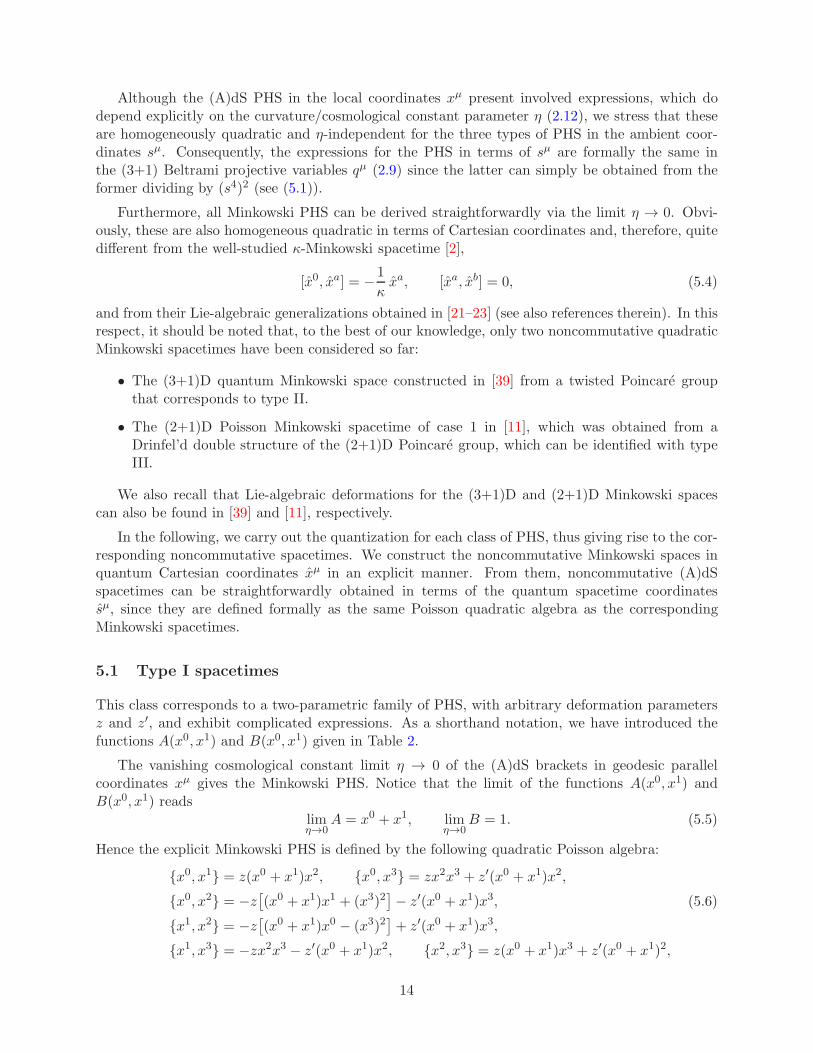
Although the (A)dS PHS in the local coordinates xµ present involved expressions, which dodepend explicitly on the curvature/cosmological constant parameter η (2.12), we stress that theseare homogeneously quadratic and η-independent for the three types of PHS in the ambient coor-dinates sµ. Consequently, the expressions for the PHS in terms of sµ are formally the same inthe (3+1) Beltrami projective variables qµ (2.9) since the latter can simply be obtained from theformer dividing by (s4)2 (see (5.1)).

Furthermore, all Minkowski PHS can be derived straightforwardly via the limit η → 0. Obvi-ously, these are also homogeneous quadratic in terms of Cartesian coordinates and, therefore, quitedifferent from the well-studied κ-Minkowski spacetime [2],

[x0, xa] = −1

κxa, [xa, xb] = 0, (5.4)

and from their Lie-algebraic generalizations obtained in [21–23] (see also references therein). In thisrespect, it should be noted that, to the best of our knowledge, only two noncommutative quadraticMinkowski spacetimes have been considered so far:

• The (3+1)D quantum Minkowski space constructed in [39] from a twisted Poincare groupthat corresponds to type II.

• The (2+1)D Poisson Minkowski spacetime of case 1 in [11], which was obtained from aDrinfel’d double structure of the (2+1)D Poincare group, which can be identified with typeIII.

We also recall that Lie-algebraic deformations for the (3+1)D and (2+1)D Minkowski spacescan also be found in [39] and [11], respectively.

In the following, we carry out the quantization for each class of PHS, thus giving rise to the cor-responding noncommutative spacetimes. We construct the noncommutative Minkowski spaces inquantum Cartesian coordinates xµ in an explicit manner. From them, noncommutative (A)dSspacetimes can be straightforwardly obtained in terms of the quantum spacetime coordinatessµ, since they are defined formally as the same Poisson quadratic algebra as the correspondingMinkowski spacetimes.

5.1 Type I spacetimes

This class corresponds to a two-parametric family of PHS, with arbitrary deformation parametersz and z′, and exhibit complicated expressions. As a shorthand notation, we have introduced thefunctions A(x0, x1) and B(x0, x1) given in Table 2.

The vanishing cosmological constant limit η → 0 of the (A)dS brackets in geodesic parallelcoordinates xµ gives the Minkowski PHS. Notice that the limit of the functions A(x0, x1) andB(x0, x1) reads

limη→0

A = x0 + x1, limη→0

B = 1. (5.5)

Hence the explicit Minkowski PHS is defined by the following quadratic Poisson algebra:

{x0, x1} = z(x0 + x1)x2, {x0, x3} = zx2x3 + z′(x0 + x1)x2,

{x0, x2} = −z[

(x0 + x1)x1 + (x3)2]

− z′(x0 + x1)x3, (5.6)

{x1, x2} = −z[

(x0 + x1)x0 − (x3)2]

+ z′(x0 + x1)x3,

{x1, x3} = −zx2x3 − z′(x0 + x1)x2, {x2, x3} = z(x0 + x1)x3 + z′(x0 + x1)2,

14

which is formally identical with the (A)dS expressions given in Table 2 in ambient variables sµ

(2.13) (recall that s4 does not appear in the Poisson brackets). The quadratic Casimir C (5.3) forthis Poisson algebra yields

C = (x0)2 − (x1)2 − (x2)2 − (x3)2, (5.7)

for any z and z′.

Although this two-parametric family is quite involved, it can be regarded as the superpositionof two particular “subfamilies” that we proceed to quantize separately.

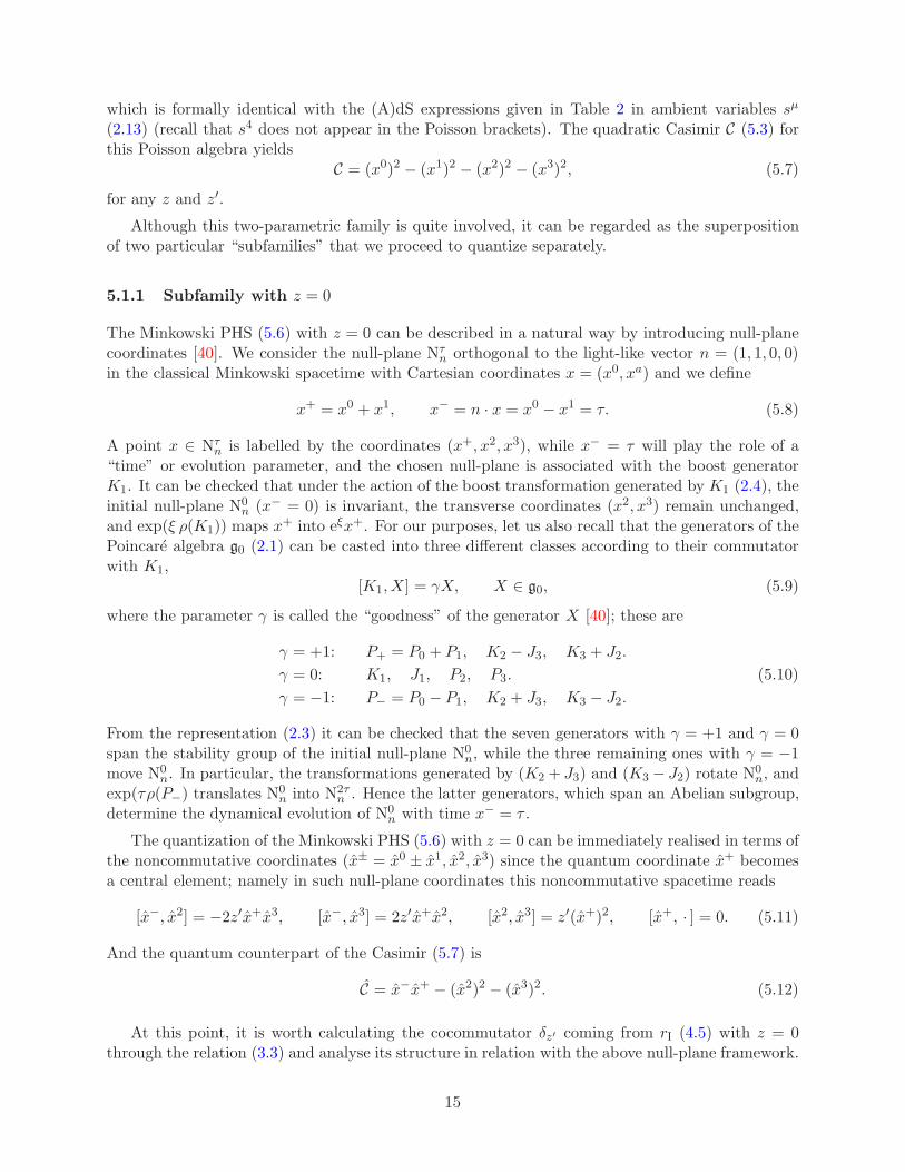
5.1.1 Subfamily with z = 0

The Minkowski PHS (5.6) with z = 0 can be described in a natural way by introducing null-planecoordinates [40]. We consider the null-plane Nτ

n orthogonal to the light-like vector n = (1, 1, 0, 0)in the classical Minkowski spacetime with Cartesian coordinates x = (x0, xa) and we define

x+ = x0 + x1, x− = n · x = x0 − x1 = τ. (5.8)

A point x ∈ Nτn is labelled by the coordinates (x+, x2, x3), while x− = τ will play the role of a

“time” or evolution parameter, and the chosen null-plane is associated with the boost generatorK1. It can be checked that under the action of the boost transformation generated by K1 (2.4), theinitial null-plane N0

n (x− = 0) is invariant, the transverse coordinates (x2, x3) remain unchanged,and exp(ξ ρ(K1)) maps x+ into eξx+. For our purposes, let us also recall that the generators of thePoincare algebra g0 (2.1) can be casted into three different classes according to their commutatorwith K1,

[K1,X] = γX, X ∈ g0, (5.9)

where the parameter γ is called the “goodness” of the generator X [40]; these are

γ = +1: P+ = P0 + P1, K2 − J3, K3 + J2.

γ = 0: K1, J1, P2, P3.

γ = −1: P− = P0 − P1, K2 + J3, K3 − J2.

(5.10)

From the representation (2.3) it can be checked that the seven generators with γ = +1 and γ = 0span the stability group of the initial null-plane N0

n, while the three remaining ones with γ = −1move N0

n. In particular, the transformations generated by (K2 + J3) and (K3 − J2) rotate N0n, and

exp(τρ(P−) translates N0n into N2τ

n . Hence the latter generators, which span an Abelian subgroup,determine the dynamical evolution of N0

n with time x− = τ .

The quantization of the Minkowski PHS (5.6) with z = 0 can be immediately realised in terms ofthe noncommutative coordinates (x± = x0 ± x1, x2, x3) since the quantum coordinate x+ becomesa central element; namely in such null-plane coordinates this noncommutative spacetime reads

[x−, x2] = −2z′x+x3, [x−, x3] = 2z′x+x2, [x2, x3] = z′(x+)2, [x+, · ] = 0. (5.11)

And the quantum counterpart of the Casimir (5.7) is

C = x−x+ − (x2)2 − (x3)2. (5.12)

At this point, it is worth calculating the cocommutator δz′ coming from rI (4.5) with z = 0through the relation (3.3) and analyse its structure in relation with the above null-plane framework.

15

Explicitly, δz′ is given by:

δz′(P0) = z′P2 ∧ (K3 − J2)− z′P3 ∧ (K2 + J3),

δz′(P1) = z′P2 ∧ (K3 − J2)− z′P3 ∧ (K2 + J3),

δz′(P2) = z′(P0 − P1) ∧ (K3 − J2),

δz′(P3) = −z′(P0 − P1) ∧ (K2 + J3),

δz′(K1) = 2z′(K2 + J3) ∧ (K3 − J2), (5.13)

δz′(K2) = −z′K1 ∧ (K3 − J2)− z′J1 ∧ (K2 + J3),

δz′(K3) = z′K1 ∧ (K2 + J3)− z′J1 ∧ (K3 − J2),

δz′(J1) = 0,

δz′(J2) = z′K1 ∧ (K2 + J3)− z′J1 ∧ (K3 − J2),

δz′(J3) = z′K1 ∧ (K3 − J2) + z′J1 ∧ (K2 + J3).

These expressions clearly exhibit the underlying null-plane symmetry determined by the boostgenerator K1 according to the goodness γ (5.10). It can be checked that, besides J1, the threegenerators with γ = −1, have a vanishing cocommutator:

δz′(P−) = δz′(K2 + J3) = δz′(K3 − J2) = 0. (5.14)

Moreover, in this null-plane basis rI (4.5) with z = 0 adopts the simple form

rI = z′(K3 − J2) ∧ (K2 + J3). (5.15)

Consequently, rI corresponds to a Reshetikhin twist generated by two commuting operators, whichmeans that the quantum Poincare algebra Uz′(g0) can be easily constructed. It can also be checkedfrom δz′ (5.13) that

δz′(t) ⊂ t ∧ h, δz′(h) ⊂ h ∧ h 6= 0, (5.16)

as it should be. In addition, the relations (5.16) mean that δz′ does not contain any term in t ∧ t,i.e. Pµ ∧ Pν , and by quantum duality this fact implies that all the commutators [xµ, xν ] vanish atthe first-order in the quantum coordinates xµ, although higher-order terms could exist. The latteris exactly the case here with the noncommutative Minkowski space (5.11) which is defined by ahomogeneous quadratic algebra. We stress that the relations (5.16) and so the first-order brackets[xµ, xν ] = 0 are satisfied by the three types I, II and III of deformations and hold for any value ofΛ.

5.1.2 Subfamily with z′ = 0

We now consider the Minkowski PHS (5.6) with z′ = 0 together with the same null-plane co-ordinates (5.8) associated with K1. By taking the ordered monomials (x−)k(x+)l(x3)m(x2)n thecorresponding noncommutative Minkowski space is found to be

[x−, x+] = 2zx+x2, [x−, x2] = zx−x+ − 2z(x3)2, [x−, x3] = 2zx3x2,

[x2, x3] = zx+x3, [x+, x2] = −z(x+)2, [x+, x3] = 0 ,(5.17)

where associativity is ensured by the Jacobi identity. Although the resulting expressions are morecomplicated than in the previous case, the quantum null-plane coordinates (x+, x2, x3) again closea subalgebra and the quantum Casimir (5.12) is the same.

16

The cocommutator δz can be obtained from rI (4.5) with z′ = 0 applying (3.3) and its structureturns out to be naturally adapted to the null-plane Poincare generators (5.10). However, thegenerators J1 and P− are no longer primitive and only (K2 + J3) and (K3 − J2) have a vanishingcocommutator. Again rI (4.5) with z′ = 0 has a simple expression in this null-plane basis:

rI = zK1 ∧ (K2 + J3) + zJ1 ∧ (K3 − J2). (5.18)

Observe that this r-matrix is not defined through Reshetikhin twists and therefore is a morecomplicated solution of the CYBE than the previous case.

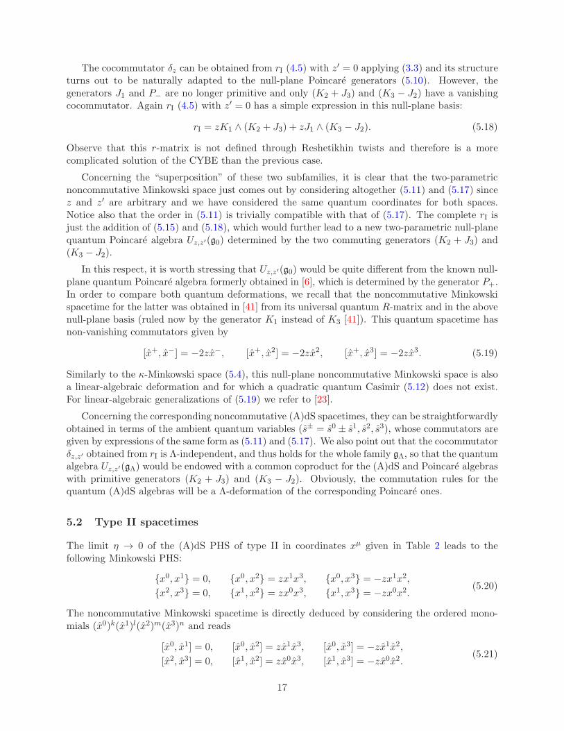
Concerning the “superposition” of these two subfamilies, it is clear that the two-parametricnoncommutative Minkowski space just comes out by considering altogether (5.11) and (5.17) sincez and z′ are arbitrary and we have considered the same quantum coordinates for both spaces.Notice also that the order in (5.11) is trivially compatible with that of (5.17). The complete rI isjust the addition of (5.15) and (5.18), which would further lead to a new two-parametric null-planequantum Poincare algebra Uz,z′(g0) determined by the two commuting generators (K2 + J3) and(K3 − J2).

In this respect, it is worth stressing that Uz,z′(g0) would be quite different from the known null-plane quantum Poincare algebra formerly obtained in [6], which is determined by the generator P+.In order to compare both quantum deformations, we recall that the noncommutative Minkowskispacetime for the latter was obtained in [41] from its universal quantum R-matrix and in the abovenull-plane basis (ruled now by the generator K1 instead of K3 [41]). This quantum spacetime hasnon-vanishing commutators given by

[x+, x−] = −2zx−, [x+, x2] = −2zx2, [x+, x3] = −2zx3. (5.19)

Similarly to the κ-Minkowski space (5.4), this null-plane noncommutative Minkowski space is alsoa linear-algebraic deformation and for which a quadratic quantum Casimir (5.12) does not exist.For linear-algebraic generalizations of (5.19) we refer to [23].

Concerning the corresponding noncommutative (A)dS spacetimes, they can be straightforwardlyobtained in terms of the ambient quantum variables (s± = s0 ± s1, s2, s3), whose commutators aregiven by expressions of the same form as (5.11) and (5.17). We also point out that the cocommutatorδz,z′ obtained from rI is Λ-independent, and thus holds for the whole family gΛ, so that the quantumalgebra Uz,z′(gΛ) would be endowed with a common coproduct for the (A)dS and Poincare algebraswith primitive generators (K2 + J3) and (K3 − J2). Obviously, the commutation rules for thequantum (A)dS algebras will be a Λ-deformation of the corresponding Poincare ones.

5.2 Type II spacetimes

The limit η → 0 of the (A)dS PHS of type II in coordinates xµ given in Table 2 leads to thefollowing Minkowski PHS:

{x0, x1} = 0, {x0, x2} = zx1x3, {x0, x3} = −zx1x2,

{x2, x3} = 0, {x1, x2} = zx0x3, {x1, x3} = −zx0x2.(5.20)

The noncommutative Minkowski spacetime is directly deduced by considering the ordered mono-mials (x0)k(x1)l(x2)m(x3)n and reads

[x0, x1] = 0, [x0, x2] = zx1x3, [x0, x3] = −zx1x2,

[x2, x3] = 0, [x1, x2] = zx0x3, [x1, x3] = −zx0x2.(5.21)

17

This structure can be regarded as a nonlinear generalization of two coupled 2D quadratic Euclideanalgebras, for which x0 and x1 play the role of rotation operators on the 2-vector (x2, x3). Thebehaviour of the quantum coordinate pairs (x0, x1) and (x2, x3) is somehow inherited from theReshetikhin twist defined by rII (4.5) which is given by the commuting generators K1 and J1. Itcan be checked that these are the only primitive generators within the Lie bialgebra (gΛ, δII).

We remark that (5.21) corresponds to the quadratic noncommutative Minkowski space con-structed in [39] by following a different approach which consists of starting with a representationof the universal quantum R-matrix for the twisted quantum Poincare group and then applying theFRT procedure.

Note also that the obtention of the corresponding quantum (A)dS algebra Uz(gΛ) is straight-forward via the Reshetikhin twist associated to rII.

5.3 Type III spacetimes

The third type of PHS are written in Table 2 in local coordinates xµ by using the function A(x0, x1)as a shorthand notation. Before performing its quantization, let us relate these (A)dS PHS withη 6= 0 to some results already obtained in the literature.

Since x3 Poisson-commutes with all the remaining coordinates, we are dealing in fact with a(2+1)D (A)dS PHS which can be expressed in a more symmetric manner as

{x0, x1} = ztanh(ηx2)

ηΘ, {x0, x2} = −z

tanh(ηx1)

ηΘ, {x1, x2} = −z

tan(ηx0)

ηΘ, (5.22)

where we have introduced the function Θ = cos(ηx0)A(x0, x1):

Θ(x0, x1) = cos(ηx0)

(

sin(ηx0)

ηcosh(ηx1) +

sinh(ηx1)

η

)

. (5.23)

In this form, the PHS (5.22) deeply resembles the (2+1)D AdS PHS constructed in [42] by consider-ing the AdS Lie algebra so(2, 2) as a Drinfel’d double arising from the Drinfel’d–Jimbo deformationof sl(2,R) and taking into account the results formerly obtained in [43]. In the notation of [42] theAdS PHS reads

{x0, x1} = −ξtanh(ηx2)

ηΥ, {x0, x2} = ξ

tanh(ηx1)

ηΥ, {x1, x2} = ξ

tan(ηx0)

ηΥ. (5.24)

such that ξ is the deformation parameter, η2 = −Λ > 0, and

Υ(x0, x1) = cos(ηx0)(

cos(ηx0) cosh(ηx1) + sinh(ηx1))

. (5.25)

The apparent similarity between (5.22) and (5.24) disappears when both PHS are expressed inambient coordinates sµ, and this fact becomes more evident when the Minkowski limit η → 0 iscalculated: in that case Θ → (x0+x1) (see (5.5)), while Υ → 1. In particular, the Minkowski PHSobtained from (5.24) is given by [42]

{x0, x1} = −ξx2, {x0, x2} = ξx1, {x1, x2} = ξx0. (5.26)

Hence this structure provides a Lie-algebraic deformation of the (2+1)D Minkowski space whichcorresponds to the Lie algebra so(2, 1). We remark that such a noncomutative Minkowski space was

18

formerly considered in [44] in a (2+1) quantum gravity framework. This also appears as the case 0in the classification of Drinfel’d double structures for the (2+1)D Poincare group performed in [11].The noncomutative Minkowski space so(2, 1) ≃ sl(2,R) (5.26), linked to the (2+1)D Poincaregroup, together with its Euclidean counterpart corresponding to the Lie algebra so(3) ≃ su(2),associated with the 3D Euclidean group, have been extensively studied in (2+1)-gravity [44–49](see also references therein).

In contrast to (5.26), the limit η → 0 of the (A)dS PHS (5.22) gives the following quadratic(2+1)D Minkowski PHS

{x0, x1} = z(x0 + x1)x2, {x0, x2} = −z(x0 + x1)x1, {x1, x2} = −z(x0 + x1)x0, (5.27)

which is naturally adapted to the null-plane description associated with K1 that was presentedin Section 5.1. This Poisson structure has been obtained previously within the case 1 of theclassification of (2+1)D Poincare Drinfel’d double structures in [11].

If we now consider the noncommutative coordinates (x± = x0± x1, x2, x3) and take the orderedmonomials (x−)k(x+)l(x2)n we get the noncommutative Minkowski spacetime given by

[x2, x+] = z(x+)2, [x2, x−] = −zx−x+, [x−, x+] = 2zx+x2, [x3, xµ] = 0 . (5.28)

The quantization of the Casimir (5.7) reads

C = x−x+ − (x2)2, (5.29)

which is the (2+1)D version of (5.12), where obviously one could trivially add the central term(x3)2. Hence C is related to a (1+1)D dS space associated with the Lorentz algebra so(2, 1) inagreement with the (2+1)D character of this deformation. The primitive generators with vanishingcocommutator of the Lie bialgebra (gΛ, δIII), determined by rIII (4.5), are (K2+J3) and, as expected,P3.

Finally, we stress that the quantum deformation determined by rIII (4.5), coming from the lowerdimensional Lorentz subalgebra so(2, 1) spanned by {J3,K1,K2} (see Section 4.1), can be relatedto the well-known nonstandard (or Jordanian) quantum deformation of sl(2,R) ≃ so(2, 1) [50–54].Explicitly, if we define new generators in such subalgebra of gΛ as

A = −2K1, A± = K2 ± J3, (5.30)

we find that they close the commutation relations of sl(2,R) while rIII (4.5) turns out to be theso-called Jordanian twist for sl(2,R) [51], namely

[A,A±] = ±2A±, [A+, A−] = A, rIII = −z

2A ∧A+. (5.31)

In this respect, it is worth noting that the nonstandard quantum algebra Uz(sl(2,R)) has alreadybeen considered in [55, 56] as the cornerstone to obtain higher-dimensional quantum (A)dS algebrasby imposing to keep Uz(sl(2,R)) as a Hopf subalgebra, which is exactly the situation here. Suchresults were deduced by working in a conformal basis, and they would provide the complete quantumalgebra Uz(gΛ) through an appropriate change of basis from the conformal to the kinematical one.

6 Noncommutative Newtonian and Carrollian spacetimes

So far we have obtained all the PHS (GΛ/H, π) such that the Lorentz subgroup H is a PL subgroupof (GΛ,Π) and then we have constructed the corresponding noncommutative (A)dS and Minkowski

19

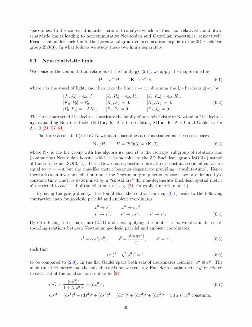
spacetimes. In this context it is rather natural to analyse which are their non-relativistic and ultra-relativistic limits leading to noncommutative Newtonian and Carrollian spacetimes, respectively.Recall that under such limits the Lorentz subgroup H becomes isomorphic to the 3D Euclideangroup ISO(3). In what follows we study these two limits separately.

6.1 Non-relativistic limit

We consider the commutation relations of the family gΛ (2.1), we apply the map defined by

P → c−1P, K → c−1K, (6.1)

where c is the speed of light, and then take the limit c → ∞ obtaining the Lie brackets given by

[Ja, Jb] = ǫabcJc, [Ja, Pb] = ǫabcPc, [Ja,Kb] = ǫabcKc,

[Ka, P0] = Pa, [Ka, Pb] = 0, [Ka,Kb] = 0,

[P0, Pa] = −ΛKa, [Pa, Pb] = 0, [P0, Ja] = 0.

(6.2)

The three contracted Lie algebras constitute the family of non-relativistic or Newtonian Lie algebrasnΛ: expanding Newton–Hooke (NH) n+ for Λ > 0, oscillating NH n− for Λ < 0 and Galilei n0 forΛ = 0 [24, 57–64].

The three associated (3+1)D Newtonian spacetimes are constructed as the coset spaces

NΛ/H, H = ISO(3) = 〈K,J〉, (6.3)

where NΛ is the Lie group with Lie algebra nΛ and H is the isotropy subgroup of rotations and(commuting) Newtonian boosts, which is isomorphic to the 3D Euclidean group ISO(3) (insteadof the Lorentz one SO(3, 1)). These Newtonian spacetimes are also of constant sectional curvatureequal to η2 = −Λ but the time-like metric becomes degenerate providing “absolute-time”. Hencethere arises an invariant foliation under the Newtonian group action whose leaves are defined by aconstant time which is determined by a “subsidiary” 3D non-degenerate Euclidean spatial metricg′ restricted to each leaf of the foliation (see, e.g. [24] for explicit metric models).

By using Lie group duality, it is found that the contraction map (6.1) leads to the followingcontraction map for geodesic parallel and ambient coordinates

x0 → x0, xa → c xa,

s0 → s0, sa → c sa, s4 → s4. (6.4)

By introducing these maps into (2.11) and next applying the limit c → ∞ we obtain the corre-sponding relations between Newtonian geodesic parallel and ambient coordinates:

s4 = cos(ηx0), s0 =sin(ηx0)

η, sa = xa, (6.5)

such that(s4)2 + η2(s0)2 = 1, (6.6)

to be compared to (2.8). In the flat Galilei space both sets of coordinates coincide: sµ ≡ xµ. Themain time-like metric and the subsidiary 3D non-degenerate Euclidean spatial metric g′ restrictedto each leaf of the foliation turn out to be [24]

dσ2Λ =

(ds0)2

1 + Λ(s0)2= (dx0)2, (6.7)

dσ′2 = (ds1)2 + (ds2)2 + (ds3)2 = (dx1)2 + (dx2)2 + (dx3)2 with s0, x0 constants.

20

Table 3: Noncommutative Newtonian and Carrollian spaces with quantum Euclidean subgroups in terms ofquantum xµ and sµ spacetime coordinates (6.5) and (6.16) coming via contraction from the noncommutative(A)dS and Minkowski spaces with quantum Lorentz subgroups.

Noncommutative Newtonian spacetimes

• Type I: rI = zK1 ∧K2 − z′K2 ∧K3

[x0, xa] = 0 [x1, x2] = −zsin2(ηx0)

η2[x1, x3] = 0 [x2, x3] = z′

sin2(ηx0)

η2

[s0, sa] = 0 [s1, s2] = −z(s0)2 [s1, s3] = 0 [s2, s3] = z′(s0)2

• Type II: rII = zK1 ∧ J1

[x0, xa] = 0 [x1, x2] = zsin(ηx0)

ηx3 [x1, x3] = −z

sin(ηx0)

ηx2 [x2, x3] = 0

[s0, sa] = 0 [s1, s2] = zs0s3 [s1, s3] = −zs0s2 [s2, s3] = 0 C = (s2)2 + (s3)2

Noncommutative Carrollian spacetimes

• Type I: rI = zK1 ∧K2 − z′K2 ∧K3

[xµ, xν ] = [sµ, sν ] = 0

• Type II: rII = zK1 ∧ J1

[x0, x1] = 0 [x0, x2] = ztanh(ηx1)

ηcosh(ηx2)

tanh(ηx3)

η[x0, x3] = −z

tanh(ηx1)

η

sinh(ηx2)

η

[s0, s1] = 0 [s0, s2] = zs1s3 [s0, s3] = −zs1s2 [sa, sb] = [xa, xb] = 0 C = (s2)2 + (s3)2

With all of these ingredients we analyse the contractions of the three types of Lie bialgebrasdetermined by Proposition 2. We apply the Lie bialgebra contraction (LBC) approach introducedin [65]: starting from a given Lie algebra contraction, here (6.1), the transformation of the quantumdeformation parameter (z and z′) that ensures a well-defined and non-trivial Lie bialgebra structureafter contraction has to be found. Such a transformation should be studied for r and δ separately,since they could behave differently. In our case, the transformation of the deformation parameteris exactly the same for the three types of r (4.5) and their cocommutators δ (3.3). This means thatwe obtain fundamental and coboundary LBC in such a manner that the contracted δ coincides withthe one provided by the contracted r through the relation (3.3). The resulting LBC are given by

Type I: z → c2 z, z′ → c2z′, rI = zK1 ∧K2 − z′K2 ∧K3.

Type II: z → c z, rII = zK1 ∧ J1.

Type III: z → c2 z, rIII = zK1 ∧K2.

(6.8)

Hence the Newtonian deformation of type III is the particular case of type I with z′ = 0. Therefore,all of them are just twisted Reshetikhin deformations (the boosts now commute) and the type IIis the only one that remains invariant under contraction with respect to Proposition 2.

The Newtonian PHS in local and ambient coordinates (6.5) can be deduced either by contract-ing the (A)dS and Minkowski PHS given in Table 2 by applying the maps (6.4) and (6.8), or by

21

computing the left- and right-invariant vector fields and then using the Sklyanin bivector (3.9) withrI and rII. The resulting PHS can be directly quantized since there are no ordering ambiguities.Obviously, the contractions can also be applied to the noncommutative spaces obtained in Sec-tions 5.1 and 5.2, but observe that for the type I deformation this should be done by working inthe basis xµ instead of the null-plane basis, since the latter is not applicable in the non-relativisticspaces. Such quantum Newtonian spaces are presented in Table 3.

It is worth stressing that the quantum time coordinate s0 becomes a central element (and so x0 aswell) reminding the “time-absolute” character of the Newtonian spaces. This fact is consistent withthe contraction (6.4) of the Casimir (5.3) which reduces to C = (s0)2. However the noncommutativespaces do not split into s0 plus a quantum 3-space subalgebra sa, since the latter involves s0.

Let us briefly comment on the results presented in Table 3 by writing the explicit noncom-mutative spaces for the Galilei case corresponding to the limit η → 0, such that sµ ≡ xµ. Thenon-vanishing commutators of the type I space read

[x1, x2] = −z(x0)2, [x2, x3] = z′ (x0)2, (6.9)

which, surprisingly enough, can be regarded as two coupled Heisenberg–Weyl algebras sharing thequantum space coordinate x2, and whose central element is determined by the square of the quan-tum time coordinate x0. For each subfamily with either z or z′ equal to zero the coupling disappearsleaving a single Heisenberg–Weyl algebra. Thus (6.9) provides the non-relativistic reminiscences ofthe null-plane noncommutative Minkowski spaces (5.11) and (5.17).

The noncommutative Galilei space of type II is given by

[x1, x2] = zx0x3, [x1, x3] = −zx0x2, [x2, x3] = 0, (6.10)

which for a given eigenvalue of x0 can be interpreted as a quadratic 2D Euclidean algebra with x1

playing the role of a rotation on the quantum 2-space (x2, x3). Hence the quadratic Casimir forthis space is given by

C = (x2)2 + (x3)2. (6.11)

Thus, under the non-relativistic limit, the noncommutative Minkowski spacetime (5.21) is decoupledat the central quantum time coordinate x0 and the noncommutative space (6.10).

Finally, regarding the Newtonian Lie bialgebras determined by (6.8) note that, as a result ofour approach, both types I and II have a non-trivial Euclidean sub-Lie bialgebra h = span {K,J} =iso(3), i.e. δ(h) = h ∧ h 6= 0. For the two-parametric Lie bialgebra of type I (nΛ, δI) the primitivegenerators are P and K, while for the type II (nΛ, δII) these are {K1, J1, P1}. Their quantumalgebras can be straightforwardly constructed via the corresponding Reshetikhin twists.

6.2 Ultra-relativistic limit

We now introduce the speed of light c in the family gΛ (2.1) through the map [57, 66]

P0 → c P0, K → cK. (6.12)

The ultra-relativistic limit c → 0 gives rise to the contracted commutation relations

[Ja, Jb] = ǫabcJc, [Ja, Pb] = ǫabcPc, [Ja,Kb] = ǫabcKc,

[Ka, P0] = 0, [Ka, Pb] = δabP0, [Ka,Kb] = 0,

[P0, Pa] = −ΛKa, [Pa, Pb] = ΛǫabcJc, [P0, Ja] = 0,

(6.13)

22

corresponding to the family of three Carrollian algebras cΛ. This comprises the para-Euclideanc+ ≃ iso(4) for Λ > 0, the para-Poincare c− ≃ iso(3, 1) for Λ < 0, and the (proper) Carroll algebrac0 for Λ = 0 [24, 57, 61–64, 66–74].

The three (3+1)D Carrollian spacetimes are identified with the coset spaces

CΛ/H, H = ISO(3) = 〈K,J〉, (6.14)

where CΛ is the Lie group with Lie algebra cΛ and H is the isotropy subgroup isomorphic toISO(3) spanned by rotations and (commuting) Carrollian boosts. We stress that the main metricfor the Carrollian spacetimes is again degenerate and has constant sectional curvature equal to−η2 = +Λ [24], instead of η2 = −Λ (as in the Lorentzian and Newtonian spacetimes), providinga 3D “absolute-space”; this is therefore spherical in the para-Euclidean space with Λ > 0 andhyperbolic in the para-Poincare one with Λ < 0. There does also exist an invariant foliation underthe Carrollian group action characterized by a “subsidiary” 1D time metric g′ restricted to eachleaf of the foliation [24].

In this case the contraction map (6.12) yields the following transformations for geodesic paralleland ambient coordinates

x0 → c−1x0, xa → xa,

s0 → c−1s0, sa → sa, s4 → s4. (6.15)

By introducing them into (2.11) and applying the limit c → 0 we find the relations betweenCarrollian geodesic parallel and ambient coordinates, namely

s4 = cosh(ηx1) cosh(ηx2) cosh(ηx3),

s0 = x0 cosh(ηx1) cosh(ηx2) cosh(ηx3),

s1 =sinh(ηx1)

ηcosh(ηx2) cosh(ηx3), (6.16)

s2 =sinh(ηx2)

ηcosh(ηx3),

s3 =sinh(ηx3)

η,

fulfilling(s4)2 − η2

(

(s1)2 + (s2)2 + (s3)2)

= 1, η2 = −Λ, (6.17)

(see (2.8)), showing the spherical (η imaginary) or hyperbolic (η real) nature of the underlying3-space. Observe that for the flat Carroll space both sets of coordinates coincide sµ ≡ xµ.

The 3D spatial main metric in ambient coordinates sa was introduced in [24] and by means ofthe parametrization (6.16) this can also be written in terms of geodesic parallel coordinates xa as

dσ2Λ =

Λ(

s1ds1 + s2ds2 + s3ds3)2

1− Λ(

(s1)2 + (s2)2 + (s3)2) + (ds1)2 + (ds2)2 + (ds3)2

= cosh2(ηx2) cosh2(ηx3)(dx1)2 + cosh2(ηx3)(dx2)2 + (dx3)2. (6.18)

The metric structure on the Carrollian spacetime is completed with the “subsidiary” 1D time metricg′ restricted to each leaf of the foliation (the “absolute-space”) and reads

dσ′2 = (ds0)2 = cosh2(ηx1) cosh2(ηx2) cosh2(ηx3)(dx0)2 on sa, xa = constant. (6.19)

23

Now we proceed to study the ultra-relativistic limit of the solutions of the mCYBE from Proposi-tion 2 by analysing their LBC. We again obtain simultaneous fundamental and coboundary LBC [65]which are defined by

Type I: z → z/c2, z′ → z′/c2, rI = zK1 ∧K2 − z′K2 ∧K3.

Type II: z → z/c, rII = zK1 ∧ J1.

Type III: z → z/c2, rIII = zK1 ∧K2.

(6.20)

Consequently, the result is formally the same as in the Newtonian cases (6.8), so that, again, thetype III deformation is included in the type I for z′ = 0. The corresponding Carrollian PHS in localand ambient coordinates (6.16) can be derived through contraction from the Lorentzian PHS inTable 2 by taking into account the transformations (6.15) and (6.20). They can also be constructedby means of the left- and right-invariant vector fields and the Sklyanin bivector (3.9). The resultingPHS have no ordering problems so that their quantization is immediate. The same result followsby applying the contractions (6.15) and (6.20) to the noncommutative spaces given in Sections 5.1and 5.2. The noncommutative Carrollian spaces are presented in Table 3.

The noncommutative Carrollian spaces of type I are trivial ones, since all their Poisson bracketsvanish. Hence there are no Heisenberg–Weyl algebras with central quantum time coordinate s0, afact that could be expected since, in the classical picture, time is no longer absolute and its role isreplaced by space.

In the noncommutative spaces of type II, all the spatial coordinates commute, thus remindingthe “absolute-space” feature of the Carrollian spaces. Moreover, the quantum spatial coordinates1 becomes a central generator (such a role was played by the quantum time coordinate s0 in thenoncommutative Newtonian spaces). In the proper Carroll case with η → 0 we find that

[x0, x2] = zx1x3, [x0, x3] = −zx1x2, [x0, x1] = 0. (6.21)

Hence for a fixed eigenvalue of s1 this noncommutative space can be seen as a quadratic 2DEuclidean algebra with the quantum time coordinate x0 behaving as a rotation on the quantum2-space (x2, x3). Thus (6.21) has a quadratic Casimir given by

C = (x2)2 + (x3)2. (6.22)

Therefore, under the ultra-relativistic limit, the noncommutative Minkowski space (5.21) is nowdecoupled as a central quantum spatial coordinate x1 plus the noncommutative Carroll space (6.21).Notice that the contraction (6.15) of the Casimir (5.3) gives C = (s1)2 + (s2)2 + (s3)2 but here s1

is a central element.

As far as the Carrollian Lie bialgebras provided by (6.20) are concerned, we remark that theyare again endowed with a non-trivial Euclidean sub-Lie bialgebra δ(h) = h ∧ h 6= 0. For the two-parametric Lie bialgebra of type I (cΛ, δI) the primitive generators are P0 and K, while for thetype II (cΛ, δII) these are {K1, J1, P0}. Again, the corresponding quantum algebras can be easilydeduced through twist operators.

7 Concluding remarks

The fate of Lorentz invariance in the context of deformed symmetries is a long-standing question. Inthis paper, we have studied this problem from a quantum group approach. Namely, we have proven

24

that there are no possible quantum group deformations of the classical spacetime symmetries forthe three maximally symmetric spacetimes of constant curvature such that the Lorentz subgroup iskept undeformed. Furthermore, we have proved that there are only three families of non-isomorphicquantum group deformations that keep the Lorentz sector as a quantum subgroup. This directlyimplies that there is no (non-trivial) covariant noncommutative spacetime with an undeformedLorentz isotropy subgroup, and that there are three families of non-isomorphic noncommutativespacetimes endowed with a quantum Lorentz subgroup. These results differ from the (2+1)D casefor which we have shown that only for the Poincare group there exists a deformation keeping theLorentz subgroup undeformed.

Moreover, we have explicitly constructed the Poisson version of these three noncommutativespacetimes by using both ambient and local coordinates. In terms of ambient coordinates the threePoisson bivectors give rise to PHS which are formally identical for any value of the cosmologicalconstant, something that in our kinematical approach is indeed related to the fact that the cos-mological parameter Λ does not appear explicitly on the Lorentz subgroup. However, by usinglocal coordinates the spacetime curvature explicitly arises in the noncommutative structures thusdistinguishing the (A)dS and Minkowski cases. We stress that in the flat Minkowski space the threenoncommutative spacetimes that we obtain are quadratic homogeneous, in striking difference withrespect to the well-known κ-Minkowski spacetime. In addition, we have studied the non-relativisticand ultra-relativistic limits, obtaining the Newtonian and Carrollian noncommutative spacetimesin which, respectively, their absolute time and absolute space structure is preserved.

An interesting open problem is indeed the construction of the full Hopf algebra structures asso-ciated with the three families of quantum groups here presented, together with their correspondingquantum R-matrices. In fact, family II can be straightforwardly quantized through the corre-sponding Reshetikhin twist operator. On the other hand, a Hopf algebra structure of the type IIIwas constructed in [53, 54] for so(2, 1) and for higher dimensional (A)dS algebras in [55, 56]. Thequantum algebra corresponding to the biparametric r-matrix of type I will be indeed more involvedfrom a technical viewpoint, but this problem is worth to be faced since its associated DSR Hopfalgebra model would be a novel one that would be relevant in situations when null-plane symmetryis physically relevant.

Furthermore, in order to make use of the results here presented in a General Relativistic frame-work, it would be essential to face the issue of general covariance for a noncommutative field theoryin which any of the three novel noncommutative spacetimes here introduced is assumed as the ba-sic local structure of the noncommutative spacetime, and whose ten-dimensional local covariancewould be provided by the corresponding quantum Hopf algebras here characterized (see [75] andreferences therein). In this sense, the fact that the three spacetimes here introduced come fromclassical r-matrices which are skewsymmetric solutions to the CYBE makes it possible to constructtheir associated Hopf algebras from Drinfel’d twist operators F [76] and, from the latter, to obtainthe corresponding ∗-products for both the noncommutative spacetimes and the full quantum groupsof local covariance [77]. This would open the path to the quantization-deformation of the completegroup of diffeomorphisms for a General Relativistic noncommutative theory by following the ap-proach presented in [75], where the hypersurface deformation algebroid (HDA) is constructed, andwhere the ∗-product on the background noncommutative spacetime plays an essential role in orderto define Drinfel’d twists of spacetime diffeomorphisms and their deformed actions. In particular,the building block for this approach in the deformation of type III would be given by the so-calledJordanian twist operator, whose ∗-product was explicitly given in [50]. Moreover, the ∗-productsfor the noncommutative Minkowski spacetimes of both the first subfamily of type I and the typeII deformation should be relatively simple to construct, since both deformations are generated by

25

a Reshetikhin twist. Also, an alternative route to an emergent Gravity theory with general co-variance in a noncommutative setting would be provided by the construction of matrix models ofthe type [78] (see also [79] and references therein) where the covariant Euclidean quantum spacesprovided by 4D fuzzy spheres would be substituted by the Lorentzian noncommutative spacetimeswith quantum group symmetry here presented. Indeed, within this approach the complete study ofthe representation theory of the chosen spacetime algebra and of the associated covariance quantumgroup would be necessary as the first step in order to analyse the feasibility of the full constructionof nocommutative gauge and matter fields on this background.

Acknowledgements

This work has been partially supported by Agencia Estatal de Investigacion (Spain) under grantPID2019-106802GB-I00/AEI/10.13039/501100011033, and by Junta de Castilla y Leon (Spain)under grants BU229P18 and BU091G19. The authors would like to acknowledge the contributionof the European Cooperation in Science and Technology COST Action CA18108.

References

[1] J. Lukierski, H. Ruegg, A. Nowicki, and V. N. Tolstoy. q-deformation of Poincare algebra. Phys. Lett.B, 264:331–338, 1991. doi:10.1016/0370-2693(91)90358-W.

[2] P. Maslanka. The n-dimensional κ-Poincare algebra and group. J. Phys. A: Math. Gen., 26:L1251–L1253, 1993. doi:10.1088/0305-4470/26/24/001.

[3] S. Majid and H. Ruegg. Bicrossproduct structure of κ-Poincare group and non-commutative geometry.Phys. Lett. B, 334:348–354, 1994. doi:10.1016/0370-2693(94)90699-8.

[4] S. Zakrzewski. Quantum Poincare group related to the κ-Poincare algebra. J. Phys. A: Math. Gen.,27:2075–2082, 1994. doi:10.1088/0305-4470/27/6/030.

[5] S. Zakrzewski. Poisson Poincare groups. In Quantum groups, formalism and applications, J. Lukierski,Z. Popowicz and J. Sobczyk (Eds). Polish Scientific Publishers PWN, Warsaw, 1995, pp. 433–439.arXiv:hep-th/9412099.

[6] A. Ballesteros, F. J. Herranz, M. A. del Olmo, and M. Santander. A new “null-plane” quantum Poincarealgebra. Phys. Lett. B, 351:137–145, 1995. doi:10.1016/0370-2693(95)00386-Y.

[7] P. Podles and S. L. Woronowicz. On the classification of quantum Poincare groups. Commun. Math.Phys., 178:61–82, 1996. doi:10.1007/BF02104908.

[8] S. Zakrzewski. Poisson structures on the Poincare group. Commun. Math. Phys., 185:285–311, 1997.doi:10.1007/s002200050091.

[9] A. Ballesteros, F. J. Herranz and C. Meusburger. Drinfel’d doubles for (2+1)-gravity. Class. QuantumGravity, 30:155012, 2013. doi:10.1088/0264-9381/30/15/155012.

[10] A. Ballesteros, F. J. Herranz, F. Musso and P. Naranjo. The κ-(A)dS quantum algebra in (3+1)dimensions. Phys. Lett. B, 766:205–211, 2017. doi:10.1016/j.physletb.2017.01.020.

[11] A. Ballesteros, I. Gutierrez-Sagredo and F. J. Herranz. The Poincare group as a Drinfel’d double. Class.Quantum Gravity, 36:025003, 2019. doi:10.1088/1361-6382/aaf3c2.

26

[12] G. Amelino-Camelia. Testable scenario for relativity with minimum-length. Phys. Lett. B, 510:255–263,2001. doi:10.1016/S0370-2693(01)00506-8.

[13] J. Kowalski-Glikman. Observer-independent quantum of mass. Phys. Lett. A, 286:391–394, 2001.doi:10.1016/S0375-9601(01)00465-0.

[14] G. Amelino-Camelia. Relativity in spacetimes with short-distance structure governed byan observer-independent (Planckian) length scale. Int. J. Mod. Phys. D, 11:35–59, 2002.doi:10.1142/S0218271802001330.

[15] J. Magueijo and L. Smolin. Lorentz invariance with an invariant energy scale. Phys. Rev. Lett.,88:190403, 2002. doi:10.1103/PhysRevLett.88.190403.

[16] J. Lukierski and A. Nowicki. Doubly special relativity versus κ-deformation of relativistic kinematics.Int. J. Mod. Phys. A, 18:7–18, 2003. doi:10.1142/S0217751X03013600.

[17] G. Amelino-Camelia. Doubly-special relativity: Facts, myths and some key open issues. Symmetry,2:230–271, 2010. doi:10.3390/sym2010230.

[18] S. Zakrzewski. Poisson structures on the Lorentz group. Lett. Math. Phys., 32:11–23, 1994.doi:10.1007/BF00761120.

[19] G. Amelino-Camelia, L. Smolin, and A. Starodubtsev. Quantum symmetry, the cosmologi-cal constant and Planck-scale phenomenology. Class. Quantum Gravity, 21:3095–3110, 2004.doi:10.1088/0264-9381/21/13/002.

[20] A. Ballesteros, I. Gutierrez-Sagredo, and F. J. Herranz. The κ-(A)dS noncommutative spacetime. Phys.Lett. B, 796:93–101, 2019. doi:10.1016/j.physletb.2019.07.038.

[21] M. Daszkiewicz. Canonical and Lie-algebraic twist deformations of κ-Poincare and contractions toκ-Galilei algebras. Int. J. Mod. Phys. A, 23:4387–4400, 2008. doi:10.1142/S0217751X08042262.

[22] A. Borowiec and A. Pachol. κ-Minkowski spacetime as the result of Jordanian twist deformation. Phys.Rev. D, 79:045012, 2009. doi:10.1103/PhysRevD.79.045012.

[23] A. Borowiec and A. Pachol. κ-Deformations and extended κ-Minkowski spacetimes. Symmetry, Integr.Geom. Methods Appl., 10:107, 2014. doi:10.3842/SIGMA.2014.107.

[24] A. Ballesteros, G. Gubitosi, and F. J. Herranz. Lorentzian Snyder spacetimes and theirGalilei and Carroll limits from projective geometry. Class. Quantum Gravity, 37:195021, 2020.doi:10.1088/1361-6382/aba668.

[25] A. Ballesteros, F. J. Herranz, C. Meusburger, and P. Naranjo. Twisted (2+1) κ-AdS algebra, Drinfel’ddoubles and non-commutative spacetimes. Symmetry, Integr. Geom. Methods Appl., 10:052, 2014.doi:10.3842/SIGMA.2014.052.

[26] V. Chari and A. Pressley. A guide to Quantum Groups. Cambridge University Press, Cambridge, 1994.

[27] J.-H. Lu. Multiplicative and affine Poisson structures on Lie groups. Ph.D. Thesis, University ofCalifornia, Berkeley, 1990.

[28] N. Ciccoli and F. Gavarini. A quantum duality principle for coisotropic subgroups and Poisson quotients.Adv. Math., 199:104–135, 2006. doi:10.1016/j.aim.2005.01.009.

[29] A. Ballesteros, C. Meusburger, and P. Naranjo. AdS Poisson homogeneous spaces and Drinfel’d doubles.J. Phys. A: Math. Theor., 50:395202, 2017. doi:10.1088/1751-8121/aa858c.

[30] M.S. Dijkhuizen and T.H. Koornwinder. Quantum homogeneous spaces, duality and quantum 2-spheres.Geom. Dedicata, 52:291–315, 1994. doi:10.1007/BF01278478.

27

[31] A. Ballesteros, I. Gutierrez-Sagredo and F. Mercati. Coisotropic Lie bialgebras and com-plementary dual Poisson homogeneous spaces. J. Phys. A Math. Theor., 54:315203, 2021.doi:10.1088/1751-8121/ac0b8a.

[32] I. Gutierrez-Sagredo and F. J. Herranz. Cayley–Klein Lie bialgebras: Noncommutative spaces, Drinfel’ddoubles and kinematical applications. Symmetry (Basel), 13:1249, 2021. doi:10.3390/sym13071249.

[33] P. Podles and S. L. Woronowicz. On the structure of inhomogeneous quantum groups. Commun. Math.Phys., 185:325–358, 1997. doi:10.1007/s002200050093.

[34] A. Borowiec, J. Lukierski, and V. N. Tolstoy. Quantum deformations of D = 4 Euclidean, Lorentz,Kleinian and quaternionic o⋆(4) symmetries in unified o(4;C) setting. Phys. Lett. B, 754:176–181, 2016.doi:10.1016/j.physletb.2016.01.016.

[35] A. Borowiec, J. Lukierski, and V. N. Tolstoy. Addendum to “Quantum deformations ofD = 4 Euclidean,Lorentz, Kleinian and quaternionic o⋆(4) symmetries in unified o(4;C) setting” [Phys. Lett. B 754 (2016)176–181]. Phys. Lett. B, 770:426–430, 2017. doi:10.1016/j.physletb.2017.04.070.

[36] J. Kowalski-Glikman, J. Lukierski, and T. Trzesniewski, Quantum D = 3 Euclidean and Poincare sym-metries from contraction limits. J. High Energy Phys., 2020:96, 2020. doi:10.1007/JHEP09(2020)096.

[37] A. Ballesteros, F. J. Herranz, and F. Musso. On quantum deformations of (anti-)de Sitter algebras in(2+1) dimensions. J. Phys.: Conf. Ser., 532:012002, 2014. doi:10.1088/1742-6596/532/1/012002.

[38] P. Stachura. Poisson-Lie structures on Poincare and Euclidean groups in three dimensions. J. Phys. A:Math. Gen., 31:4555–4564, 1998. doi:10.1088/0305-4470/31/19/018.

[39] J. Lukierski and M. Woronowicz. New Lie-algebraic and quadratic deformations ofMinkowski space from twisted Poincare symmetries. Phys. Lett. B, 633:116–124, 2006.doi:10.1016/j.physletb.2005.11.052.

[40] H. Leutwyler and J. Stern. Relativistic dynamics on a null plane. Ann. Phys., 112:94–164, 1978.doi:10.1016/0003-4916(78)90082-9.

[41] A. Ballesteros, F. J. Herranz, and C. M. Perena. Null-plane quantum universal R-matrix. Phys. Lett. B,391:71–77, 1997. doi:10.1016/S0370-2693(96)01435-9.

[42] A. Ballesteros, F.J. Herranz, and C. Meusburger. A (2+1) non-commutative Drinfel’d double spacetimewith cosmological constant. Phys. Lett. B, 732:201–209, 2014. doi:10.1016/j.physletb.2014.03.036.

[43] A. Ballesteros, F. J. Herranz, and C. Meusburger. Three-dimensional gravity and Drinfel’d dou-bles: spacetimes and symmetries from quantum deformations. Phys. Lett. B, 687:375–381, 2010.doi:10.1016/j.physletb.2010.03.043.

[44] H. J. Matschull and M. Welling. Quantum mechanics of a point particle in (2 + 1)-dimensional gravity.Class. Quantum Gravity, 15:2981–3030, 1998. doi:10.1088/0264-9381/15/10/008.

[45] F. A. Bais and N. M. Muller. Topological field theory and the quantum double of SU(2). Nucl. Phys. B,530:349–400, 1998. doi:10.1016/S0550-3213(98)00572-0.

[46] F. A. Bais, N. M. Muller, and B. J. Schroers. Quantum group symmetry and particle scattering in (2+1)-dimensional quantum gravity. Nucl. Phys. B, 640:3–45, 2002. doi:10.1016/S0550-3213(02)00572-2.

[47] E. Batista and S. Majid. Noncommutative geometry of angular momentum space U(su(2)).J. Math. Phys., 44:107–137, 2003. doi:10.1063/1.1517395.

[48] S. Majid. Noncommutative model with spontaneous time generation and Planckian bound. J. Math.Phys., 46:103520, 2005. doi:10.1063/1.2084748.

28

[49] E. Joung, J. Mourad, and K. Noui. Three dimensional quantum geometry and deformed symmetry.J. Math. Phys., 50:052503, 2009. doi:10.1063/1.3131682.

[50] C. Ohn. A ∗-product on SL(2) and the corresponding nonstandard quantum-U(sl(2)). Lett. Math.Phys., 25:85–88, 1992. doi:10.1007/BF00398304.

[51] O. Ogievetsky. Hopf structures on the Borel subalgebra of sl(2). Rendiconti Cir. Math. Palermo, ser. II,suppl., 37:185–199, 1994. https://dml.cz/handle/10338.dmlcz/701555.

[52] A. Ballesteros, F. J. Herranz, M. A. del Olmo, and M. Santander. Non-standard quantum so(2, 2) andbeyond. J. Phys. A: Math. Gen., 28:941–955, 1995. doi:10.1088/0305-4470/28/4/018.

[53] A. Ballesteros and F. J. Herranz. Universal R-matrix for non-standard quantum sl(2,R). J. Phys. A:Math. Gen., 29:L311–L316, 1996. doi:10.1088/0305-4470/29/13/001.

[54] A. Shariati, A. Aghamohammadi, and M. Khorrami. The universal R-matrix for the Jordaniandeformation of sl(2), and the contracted forms of so(4). Mod. Phys. Lett. A, 11:187–197, 1996.doi:10.1142/S0217732396000229.

[55] F. J. Herranz. New time-type and space-type non-standard quantum algebras and discrete symmetries.J. Phys. A: Math. Gen., 33:8217–8230, 2000. doi:10.1088/0305-4470/33/46/305.

[56] F. J. Herranz. New quantum conformal algebras and discrete symmetries. Phys. Lett. B, 543:89–97,2002. doi:10.1016/S0370-2693(02)02452-8.

[57] H. Bacry and J. M. Levy-Leblond. Possible kinematics. J. Math. Phys., 9:1605–1614, 1968.doi:10.1063/1.1664490.

[58] F. J. Herranz and M. Santander. Casimir invariants for the complete family of quasisimple orthogonalalgebras. J. Phys. A: Math. Gen., 30:5411–5426, 1997. doi:10.1088/0305-4470/30/15/026.

[59] R. Aldrovandi, A. L. Barbosa, L. C. B. Crispino, and J. G. Pereira. Non-relativistic spacetimes withcosmological constant. Class. Quantum Gravity, 16:495–506, 1999. doi:10.1088/0264-9381/16/2/013.

[60] F. J. Herranz and M. Santander. (Anti)de Sitter/Poincare symmetries and representations fromPoincare/Galilei through a classical deformation approach. J. Phys. A: Math. Theor., 41:015204, 2008.doi:10.1088/1751-8113/41/1/015204.

[61] C. Duval, G. W. Gibbons, P. A. Horvathy, and P. M. Zhang. Carroll versus Newton andGalilei: two dual non-Einsteinian concepts of time. Class. Quantum Gravity, 31:085016, 2014.doi:10.1088/0264-9381/31/8/085016.

[62] J. M. Figueroa-O’Farrill. Kinematical Lie algebras via deformation theory. J. Math. Phys., 59:061701,2018. doi:10.1063/1.5016288.

[63] J. Gomis, A. Kleinschmidt, J. Palmkvist, and P. Salgado-Rebolledo. Newton-Hooke/Carrollianexpansions of (A)dS and Chern-Simons gravity. J. High Energy Phys., 2020:9, 2020.doi:10.1007/JHEP02(2020)009.

[64] A. Ballesteros, G. Gubitosi, I. Gutierrez-Sagredo, and F. J. Herranz. The κ-Newtonian andκ-Carrollian algebras and their noncommutative spacetimes. Phys. Lett. B, 805:135461, 2020.doi:10.1016/j.physletb.2020.135461.

[65] A. Ballesteros, N. A. Gromov, F. J. Herranz, M. A. del Olmo, and M. Santander. Lie bialgebracontractions and quantum deformations of quasi-orthogonal algebras. J. Math. Phys., 36:5916–5937,1995. doi:10.1063/1.531368.

[66] J. M. Levy-Leblond. Une nouvelle limite non-relativiste du groupe de Poincare. Ann. Inst. HenriPoincare A, 3:1–12, 1965, http://www.numdam.org/item/AIHPA_1965__3_1_1_0/.

29

[67] E. Bergshoeff, J. Gomis, and G. Longhi. Dynamics of Carroll particles. Class. Quantum Gravity,31:205009, 2014. doi:10.1088/0264-9381/31/20/205009.

[68] J. Kowalski-Glikman and T. Trzesniewski. Deformed Carroll particle from 2+1 gravity. Phys. Lett. B,737:267–271, 2014. doi:10.1016/j.physletb.2014.08.066.

[69] J. Hartong. Gauging the Carroll algebra and ultra-relativistic gravity. J. High Energy Phys., 2015:69,2015. doi:10.1007/JHEP08(2015)069.

[70] B. Cardona, J. Gomis, and J. M. Pons. Dynamics of Carroll strings. J. High Energy Phys., 2016:50,2016. doi:10.1007/JHEP07(2016)050.

[71] E. Bergshoeff, J. Gomis, B. Rollier, J. Rosseel, and T. ter Veldhuis. Carroll versus Galilei gravity. J.High Energy Phys., 2017:165, 2017. doi:10.1007/JHEP03(2017)165.

[72] T. Trzesniewski. Effective Chern–Simons actions of particles coupled to 3D gravity. Nucl. Phys. B.,928: 448–468, 2018. doi:10.1016/j.nuclphysb.2018.01.023.

[73] M. Daszkiewicz. Canonical and Lie-algebraic twist deformations of Carroll, Para-Galilei and static Hopfalgebras. Mod. Phys. Lett. A, 34:1950181, 2019. doi:10.1142/S0217732319501815.

[74] L. Marsot. Planar Carrollean dynamics, and the Carroll quantum equation.arXiv:2110.08489.

[75] M. Bojowald, S. Brahma, U. Buyukcam, and M. Ronco. Extending general covariance: Moyal-typenoncommutative manifolds. Phys. Rev. D, 98:026031, 2018. doi:10.1103/PhysRevD.98.026031.

[76] V. G. Drinfel’d. Quantum Groups. In Proc. Int. Congr. Math. (Berkeley 1986), A. Gleason (Ed.).American Mathematical Society, Providence RI, 1987, pp. 798–820,

[77] V. G. Drinfel’d. On constant quasiclassical solutions of the Yang–Baxter quantum equation. Sov. Math.Dokl., 28:667–671, 1983.

[78] H. C. Steinacker. Emergent gravity on covariant quantum spaces in the IKKT model. J. High EnergyPhys. 2016:156, 2016. doi:10.1007/JHEP12(2016)156.

[79] H. C. Steinacker. On the quantum structure of space-time, gravity, and higher spin in matrix models.Class. Quant. Grav., 37:113001, 2020. doi:10.1088/1361-6382/ab857f.

30