arX

iv:m

ath/

0003

037v

2 [

mat

h.D

G]

11

Jan

2002 Geodesic connectedness and conjugate points in

GRW spacetimes.

Jose Luis Flores and Miguel Sanchez ∗

Depto. Geometrıa y Topologıa, Fac. Ciencias, Univ. Granada,Avda. Fuentenueva s/n, 18071-Granada, Spain.

February 1, 2008

Abstract

Given two points of a Generalized Robertson-Walker spacetime, the exis-

tence, multiplicity and causal character of geodesics connecting them is char-

acterized. Conjugate points of such geodesics are related to conjugate points

of geodesics on the fiber, and Morse-type relations are obtained. Applications

to bidimensional spacetimes and to GRW spacetimes satisfying the timelike

convergence condition are also found.

∗Research partially supported by a MEC grant number PB97-0784-C03-01.

1

1 Introduction

Recently, geodesic connectedness of Lorentzian manifolds has been widely studied,and some related questions appear with great interest, among them: to determinethe existence, multiplicity and causal character of geodesics connecting two points,to study their conjugate points and to find Morse-type relations. These questionshave been answered, totally or partially, for stationary or splitting manifolds (see,for example, [Ma], [BF], [GMPa], [GMPT], [Uh]). Our purpose is to answer themtotally in the class of Generalized Robertson-Walker (GRW) spacetimes.

GRW spacetimes (see Section 2 for precise definitions) are warped products(I × F, gf = −dt2 + f 2g) which generalizes Robertson-Walker ones because no as-sumption on their fiber is done, and they have interesting properties from both, themathematical and the physical point of view [ARS], [Sa97], [Sa98], [Sa99]. GRWspacetimes are also particular cases of multiwarped spacetimes, whose geodesic con-nectedness has been recently studied by using a topological method [FS]. They canbe also seen as splitting type manifolds, studied in [Ma, Chapter 8], or as a type ofReissner Nordstrom Intermediate spacetimes, studied in [Gi], [GM]. Nevertheless,we will see here that the results for GRW spacetimes can be obtained in a simplerapproach, and are sharper. In fact, we will develop the following direct point ofview.

Given a geodesic γ(t) = (τ(t), γF (t)) of the GRW spacetime, the componentγF is a pregeodesic of its fiber. So, if dτ/dt does not vanish, we can considerthe reparameterization γF (τ), and γ will cross a point z0 = (τ0, x0) if and only ifx0 = γF (τ0). This simple fact yields a result on connectedness by timelike and causalgeodesics [Sa97, Theorems 3.3, 3.7]. For spacelike geodesics, the reparameterizationγF (τ) may fail. This problem can be skipped sometimes by simple arguments oncontinuity [Sa98, Theorem 3.2], but we will study systematically it in order to solvecompletely the problem of geodesic connectedness. Moreover, this will be also thekey to solve the other related problems (multiplicity, conjugate points, etc.)

After some preliminaries in Section 2, we state the conditions for geodesic con-nectedness in Section 3. In fact, we give three Conditions (A), (B), (C) of increasinggenerality, and a fourth Condition (R) which covers a residual case. All these con-ditions are imposed on the warping function f ; on the fiber, we assume just a weakcondition on convexity (each two points x0, x

′0 can be joined by a minimizing F–

geodesic γF ), which is known to be completely natural (see [Sa97, Remark 3.2]).These Conditions are somewhat cumbersome, because they yield not only sufficientbut also necessary hypotheses for geodesic connectedness; however, they yield verysimple sufficient conditions. For example, (Lemmas 3, 9) if the GRW spacetime isnot geodesically connected then f must admit a limit at some extreme of the inter-val I = (a, b); if this extreme is b (resp. a) then f ′ must be strictly positive (resp.

2

negative) in a non-empty subinterval (b, b) ⊆ (a, b) (resp. (a, a) ⊆ (a, b)) (moreover,in this case Table 1 can be used). Condition (A) collects when the warping functionf has a “good behavior” at the extremes of I = (a, b), in order to obtain geodesicconnectedness. This condition is equal to the one obtained in [FS] for multiwarpedspacetimes; nevertheless, we will reprove it because a simpler proof is now availableand the ideas in this proof will be used in the following more general conditions.Condition (B) takes into account that, when the diameter of the fiber is finite, even a“not so good” behaviour of f at a extreme, say b, may allow the following situation:a fixed point z0 = (τ0, x0) can be connected to z′0 = (τ ′

0, x′0), where τ ′

0 is close enoughto b, by means of a geodesic γ(t) = (τ(t), γF (t)) such that τ(t) points out from τ0 tob and, perhaps, “bounces” close to b. Condition (C) takes into account that, evenwhen Condition (B) does not hold, the following situation in the previous case mayhold: a geodesic which points out from τ0 to the extreme a, bounces close to a andcomes back towards b, may connect z0 and z′0. Condition (C) is shown to be themore general condition for geodesic connectedness, except in a case: if the limit off at both extremes a, b is equal to the supremum of f , and this supremum is notreached at I, then z0 and z′0 perhaps could be joined by geodesics which bouncesmany times close to a and b. Examples of the strict implications between the dif-ferent Conditions are provided. In Section 3 we also state our results on existenceof connecting geodesics, which are proven in Section 4:

1. either condition (C) or (R) is sufficient for geodesic connectedness (Theorem 1)

2. if we assume a stronger condition of convexity on the fiber (each geodesic γF

above is assumed to be the only geodesic which connects x0, x′0) then one of

this two conditions (C) or (R) is also necessary (Theorem 2); the necessity ofthis stronger convexity assumption is also discussed,

3. under Condition (A) (or, even in some cases (B)), if the topology of F isnot trivial then each two points z0 = (τ0, x0), z

′0 = (τ ′

0, x′0) can be joined by

infinitely many spacelike geodesics (Theorem 3) and

4. for causal geodesics: (i) if z0 and z′0 are causally related then there exist acausal geodesic joining them (this result was previously proven in [Sa97]), (ii)if z0 and z′0 are not conjugate (or even if just x0 and x′

0 are not conjugate,which will be shown to be less restrictive), then there are at most finitely manytimelike geodesics joining them (Theorem 3) and (iii) if the fiber is stronglyconvex then there exist at most one connecting causal geodesic (Theorem 2).

This machinery is used in Section 5 to obtain a precise relation between the con-jugate points of a geodesic in I × F and its projection on F (Theorem 4, Corollary1). From this result, Morse-type relations, which relate the topology of the space

3

of curves joining two non-conjugate points and the Morse indexes of the geodesicsjoining them, are obtained (see Corollary 2 and the discussion above it). We remarkthat Morse indexes are defined here in the geometrical sense “sum of the orders ofconjugate points” because, for any spacelike geodesic, its index form is positive def-inite and negative definite on infinite dimensional subspaces (if dimF > 1). Aboutthis kind of problem, the following previous references should be taken into account.Conjugate points of null geodesics in globally hyperbolic spacetimes were studied byUhlenbeck [Uh], and we also make some remarks in Section 5 relating our results.In a general setting, conjugate points on spacelike geodesics were studied by Helfer[He], who also considered the Maslov index of a geodesic. He showed that these con-jugate points may have very different properties to conjugate points for Riemannianmanifolds (unstability, non-isolation...), but these problems can be skipped in ourstudy. In [BM] (see also [Ma, Section 5]), an attempt to obtain a Morse Theoryfor standard stationary manifolds is carried out, and in [GMPT], an index theorem(in terms of the Maslov index) appliable in particular to stationary manifolds, isobtained. On the other hand, some recent articles study a Morse theory for timelikeor lightlike geodesics joining a point and a timelike curve, see [GMPb] and referencestherein. Tipically, these results are stated for strongly causal spacetimes (includingso all GRW spacetimes), and they need an assumption on coercivity which not nec-essarily holds under our hypotheses. It is not difficult to check that our results arealso appliable to face this problem.

In Section 6 we particularize the previous results to two cases. First, Subsec-tion 6.1, when the fiber is also an interval of R. In this bidimensional case, theopposite metric −gf is standard static, and we reobtain and extend the Theoremin [BGM]. We recall that the proof in this reference is obtained by a completelydifferent method, which relies in the function spectral flow on a geodesic (see theRemark (2) to Theorem 4 for noteworthy comments about this approach). Finally,in Subsection 6.2 we consider the case Ric(∂t, ∂t) ≥ 0. This condition is naturalfrom a physical point of view. In fact, the stronger condition Ric(v, v) ≥ 0 forall timelike v, is called the timelike convergence condition, and says that gravity,on average, attracts. Condition Ric(∂t, ∂t) ≥ 0 is equivalent to f ′′ ≤ 0, and thisinequality implies Condition (A) if f cannot be continuously extended to positivevalues at any extreme. Corollary 6 summarizes our results in this case. We finishwith an extension, in our ambient, of a result in [Uh] (Corollary 7).

2 Preliminaries

Let (F, g) be a Riemannian manifold, (I,−dτ 2) an open interval of R with I = (a, b)and its usual metric reversed, and f > 0 a smooth function on I. A GRW spacetime

4

with base (I,−dτ 2), fiber (F, g) and warping function f > 0 is the product manifoldI × F endowed with the Lorentz metric:

gf = −π∗Idτ 2 + (f πI)

2π∗F g ≡ −dτ 2 + f 2g (1)

where πI and πF are the natural projections of I × F onto I and F , respectively,and will be omitted when there is no possibility of confusion.

A Riemannian manifold will be called weakly convex if any two of its points canbe joined by a geodesic which minimize the distance; if, in addition, this geodesic isthe only one which joins the two points it will be called strongly convex (recall thatthese names does not coincide with those in [Sa97]). Of course, if the Riemannianmanifold (F, g) is complete then it is weakly convex by the Hopf-Rinow theorem, butthe converse is not true; a detailed study of when a (incomplete) Riemannian mani-fold is weakly convex can be seen in [BGS]. It is well-known that Cartan-Hadamardmanifolds (i.e. complete, simply connected and with non-positive curvature) arestrongly convex and, of course, so are locally all Riemannian manifolds; more re-sults on strong convexity can be seen in [GMPa]. We will denote by d the distance onF canonically associated to the Riemannian metric g, and by diam(F ) its diameter(the supremum, possibly infinity, of the d-distances between points of F ).

Given a vector X tangent to I ×F we will say that X is timelike (resp. lightlike,causal, spacelike) if gf(X, X) < 0 (resp. = 0,≤ 0, > 0); the timelike vector field∂/∂τ fixes the canonical future orientation in I ×F . Given z, z′ ∈ I ×F , we will saythat they are causally [resp. chronologically] related if they can be joined (z withz′ or viceversa) by a future-pointing non-spacelike [resp. timelike] piecewise smoothcurve.

Let γ : J → I × F , γ(t) = (τ(t), γF (t)) be a (smooth) curve on the interval J .It is well-known that γ is a geodesic with respect to gf if and only if

d2τ

dt2= − c

f 3 τ· df

dτ τ (2)

D

dt

dγF

dt= − 2

f τ· d(f τ)

dt· dγF

dt(3)

on J , where D/dt denotes the covariant derivate associated to γF and c is theconstant (f 4 τ) · g(dγF/dt, dγF/dt). From (2),

dτ

dt= ǫ

√

−D +c

f 2 τ(4)

with D = gf(dγ/dt, dγ/dt) and ǫ ∈ ±1. Note that if c = 0 then d2τ/dt2 ≡ 0, thatis, the geodesics on the base I are naturally lifted to geodesics of the GRW spacetime,

5

as in any warped product. For all the other geodesics, it is natural to normalizechoosing them with c = 1. This normalization will be always chosen, except inSection 5 where the formulas will be explicitly taken with a different normalization.All geodesics will be also assumed inextendible, that is, with a maximal domain.

By equation (3), each (non-constant) γF is a pregeodesic of (F, g), so if weconsider the reparametrization γF (r) = γF (t(r)) where

dt

dr= f 2 τ t (5)

(in a maximal domain) we obtain that γF is a geodesic of (F, g) being

g(dγF

dr,dγF

dr) = 1. (6)

.From now on, we will assume that (F, g) is weakly convex for any result where

geodesic connectedness is involved; such assumption has proven to be completelynatural [Sa97], [Sa98], [FS]. In fact, as an immediate consequence of (2) and (3) wehave:

Lemma 1 There exists a geodesic joining z0 = (τ0, x0) and z′0 = (τ ′0, x

′0), τ0 ≤ τ ′

0 ifτ0 = τ ′

0 and ddτ

1f2 (τ0) = 0.

Now, the case when the geodesic γF can be reparameterized by using τ ∈ (a∗, b∗)as a parameter (for some interval (a∗, b∗)) will be considered. Putting γ(τ) ≡ γr(τ)we have dγ/dτ = hǫ

D(τ) · dγ/dr where hǫD ≡ hǫ : (a⋆, b⋆) ⊆ I → R is defined as:

hǫ = ǫf−2(−D +1

f 2)−1/2, (7)

and ǫ = ±1. When this reparameterization can be done in such a way that if τ goesfrom τ0 to τ ′

0 the integral of hǫ is exactly equal to the distance between x0, x′0 ∈ F ,

then a geodesic joining (τ0, x0) and (τ ′0, x

′0) can be constructed, yielding so:

Lemma 2 There exists a geodesic connecting z0 = (τ0, x0) and z′0 = (τ ′0, x

′0), τ0 ≤ τ ′

0

if there is a constant D ∈ R (D = gf(dγdt

, dγdt

)) such that,(i) Either 1

f2(τ0)6= D or if this equality holds then d

dτ1f2 (τ0) 6= 0 and

(ii) the maximal domain (a⋆, b⋆) of hǫ includes (τ0, τ′0) and

∫ τ ′

0

τ0

hǫ = L. (8)

where L = d(x0, x′0).

6

(In this case ǫ = 1.) When the reparameterization γ(τ) fails then the points wherethe denominator of hǫ goes to zero must be especially taken into account. Firstly,we will specify the maximal domain of hǫ. Fix D ∈ R such that 1/f 2(τ0) ≥ D andconsider the subsets

A+ = τ ∈ (a, b) : τ0 ≤ τ,1

f 2(τ)= D ∪ b (9)

A− = τ ∈ (a, b) : τ0 ≥ τ,1

f 2(τ)= D ∪ a (10)

Define a⋆ ≡ a⋆(D), b⋆ ≡ b⋆(D) by:

Ifd

dτ

1

f 2(τ0)

> 0< 0= 0

then b⋆ =

min(A+ − τ0)min(A+),min(A+)

a⋆ =

max(A−)max(A− − τ0)

max(A−)(11)

Now, it is not difficult to check that Lemma 2 also holds if we assume thefollowing convention for the integral (8).

Convention 1 From now on integral (8) will be understood in the following gen-

eralized sense: for ǫ = 1, if∫ b⋆

τ0hǫ=1 ≥ L, then the first member of (8) denotes the

usual integral and we will also follow the notation +[0]

∫ τ ′

0

τ0hǫ; otherwise and if b⋆ 6= b,

we can follow integrating, by reversing the sense of integration (recall τ ′0 ≤ b⋆) and,

if∫ b⋆

τ0hǫ=1 −

∫ a⋆

b⋆hǫ=1 ≥ L then the first member of (8) means

∫ b⋆

τ0hǫ=1 −

∫ τ ′

0

b⋆hǫ=1

which we denote by +[1]

∫ τ ′

0

τ0hǫ. If this last inequality does not hold and a⋆ 6= a,

then the procedure must follow reversing the sense of integration (τ ′0 ≥ a∗) as many

times as necessary in the obvious way. Analogously, when ǫ = −1, first mem-

ber of (8) means either∫ τ ′

0

τ0hǫ=−1 ≡−[0]

∫ τ ′

0

τ0hǫ (in this case if τ0 < τ ′

0 the integral

is negative; so equality (8) cannot hold) or∫ a⋆

τ0hǫ=−1 −

∫ τ ′

0

a⋆hǫ=−1 ≡−[1]

∫ τ ′

0

τ0hǫ or

∫ a⋆

τ0hǫ=−1 −

∫ b⋆

a⋆hǫ=−1 +

∫ τ ′

0

b⋆hǫ=−1 ≡−[2]

∫ τ ′

0

τ0hǫ, etc.

Remark 1 From (7), fixed ǫ ∈ ±1, for each D ∈ R we have at most one τ ′0

such that equation (8) holds, possibly under Convention 1. Let us introduce theparameter K ≡ K(D, ǫ) by means of K = 1

f2(τ0)− D if ǫ = 1, K = D − 1

f2(τ0)if

ǫ = −1. So, fixed L, a function τ(K) = τ ′0 is defined for K in certain domain D of

R.

7

3 Conditions for geodesic connectedness

Now, we are ready to stablish four conditions (Conditions (A), (B), (C), (R)) onthe warping function f which, independently, ensure the geodesic connectedness ofthe GRW spacetime (Lemma 8, Lemma 9 and Theorem 1). Roughly, Condition (A)implies not only the geodesic connectedness but also that every (τ0, x0) ∈ I ×F canbe joined with any point (τ ′

0, x′0) with τ ′

0 close enough to b (resp. a) by means of ageodesic (τ(t), γF (t)) with dτ/dt > 0 (resp. < 0) near τ ′

0. Condition (B) is weakerthan Condition (A), and implies not only geodesic connectedness but also that ifCondition (A) does not hold at b (resp. a) then any (τ0, x0) ∈ I × F can be joinedwith a point (τ ′

0, x′0) with τ ′

0 close enough to b (resp. a) by means of a geodesic withǫ = 1 (resp. ǫ = −1), and perhaps using Convention 1 once close to τ ′

0. Condition(C) is the most general condition for geodesic connectedness, which just drops aresidual case covered by Condition (R).

Definition 1 Let f : (a, b) → R be a smooth function and let mb = lim infτ→bf(τ)[resp. ma = lim infτ→af(τ)]. The extreme b [resp. a] is a (strict) relative minimumof f if:

(a) When b < ∞ [resp. a > −∞], there exists ǫ > 0 such that if 0 < ǫ′ < ǫ, thenf(b − ǫ′) > mb [resp. f(a + ǫ′) > ma].

(b) When b = ∞ [resp. a = −∞], there exist M > 0 such that if M ′ > M thenf(M ′) > mb [resp. f(−M ′) > ma].

Condition (A) for f . Either 1/f 2 does not reach at b [resp. a] a relativeminimum in the sense of Definition 1 or, otherwise,

∫ b

c

f−2(1

f 2− mb)

−1/2 = ∞ [resp.

∫ c

a

f−2(1

f 2− ma)

−1/2 = ∞]

for some c ∈ (a, b) close to b (resp. a), i.e. c ∈ (b − ǫ, b) [resp. c ∈ (a, a + ǫ)] if theextreme b (resp. a) is finite or c > M [resp. c < −M ] if this extreme is infinite,where ǫ and M are given in Definition 1.

The following definition is needed to state Condition (B). Recall that this defi-nition is appliable just when Condition (A) does not hold.

Definition 2 Assume that the function 1/f 2 reaches at b [resp. at a] a relative

minimum such that∫ b

cf−2( 1

f2 − mb)−1/2 < ∞ [resp.

∫ c

af−2( 1

f2 − ma)−1/2 < ∞] for

some c ∈ (a, b). Then we define

db = lim supD→mb

(∫ b⋆

c

f−2(1

f 2− D)−1/2

)

−∫ b

c

f−2(1

f 2− mb)

−1/2

8

[resp. da = lim supD→ma

(∫ c

a⋆

f−2(1

f 2− D)−1/2

)

−∫ c

a

f−2(1

f 2− ma)

−1/2]

where b∗ ≡ b∗[D] (resp. a∗ ≡ a∗[D]) is given by (11).

Remark. (1) Note that the uniform convergence of f−2( 1f2 −D)−1/2 on compact

subsets of (a, b) when D varies, ensures that db and da are independent of c.(2) It is easy to check that db, da ≥ 0. As when D → mb then b∗ → b, where b

is a relative minimum, it is clear that if there were continuity of the integrals withD at mb [resp. ma] then db = 0 [resp. da = 0]. But as we will see in the examplebelow, there exist cases in which the inequalities are strict, and db, da can reach eventhe value ∞.

Condition (B) for f . Either 1/f 2 does not reach at b [resp. a] a relative

minimum or, otherwise, it verifies either∫ b

cf−2( 1

f2 −mb)−1/2 = ∞ for some c ∈ (a, b)

as in Condition (A), or 2db ≥ diam(F ) ∈ (0,∞] (resp. either∫ c

af−2( 1

f2 −ma)−1/2 =

∞ or 2da ≥ diam(F ) ∈ (0,∞]).

Obviously Condition (A) implies Condition (B), but the converse is not true asthe following example shows.

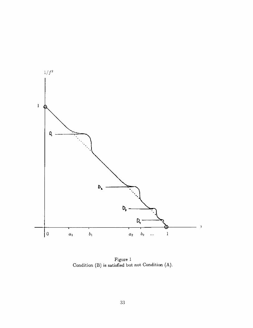
Example. Consider the function 1/g2(τ) = 1 − τ defined on (0, 1). Modify thisfunction smoothly on Inn∈N, In = (an, bn), an, bn → 1, an < bn < an+1 in such away that the modified function 1/f 2 satisfies 1/f 2 > 1/g2 on In, ∀n ∈ N and

∫ bn∗

0

f−2(1

f 2− Dn)−1/2 ≥ 2L (12)

where∫ 1

0f−1 = L and Dn is chosen decreasing to 0 and such that bn∗ = an+bn

2; this is

possible by taking 1/f 2 with derivative small enough in (an,an+bn

2) (for example, if

this derivative vanishes at an+bn

2the integral (12) will be infinite). Then, as db ≥ L,

it is sufficient to take (F, g) such that 2db ≥ diam(F ) (see Fig. 1).

Lemma 3 If Condition (B) does not hold at b (resp. a) then there exist limτ→bf ∈(0,∞] (resp. limτ→af ∈ (0,∞]) and f ′ > 0 on (b− δ, b) or (M,∞) [resp. f ′ < 0 on(a, a + δ) or (−∞,−M)] for some δ > 0 small or M > 0 big.

Proof. Reasoning for b < ∞, assume that Condition (B) does not hold at b.

Then 1f2 reaches a relative minimum at b and

∫ b

τ0f−2( 1

f2 − mb)−1/2 < ∞ for certain

τ0 ∈ I, see Definition 1. It is sufficient to prove that f ′ > 0 on (b− δ, b). Otherwise,there exist a sequence τnn∈N, τ0 < τn ∈ I, τn → b such that f ′(τn) ≤ 0. Ifwe choose a maximum τn of f on [τ0, τn], then f ′(τn) = 0 for n big enough. Thus,

9

∫ b∗

τ0f−2( 1

f2 −Dn)−1/2 = ∞ for Dn = 1f2(τn)

. The choice of τn implies that Dn → mb,which contradicts that db < ∞. 2

Remark. If Condition (B) does not hold at b (resp. a) then limτ→b1f2 = mb (resp.

limτ→a1f2 = ma).

From Lemma 3 it is natural to construct Table 1, where it is assumed that f iscontinuously extendible to b (the Table for a would be analogous, but reversing thesign of the corresponding β).

The following definition, necessary to state Condition (C), is appliable whenCondition (B) does not hold.

Definition 3 Assume that the function 1/f 2 reaches at b [resp. a] a relative min-imum such that 2db < diam(F ) and m < mb [resp. 2da < diam(F ) and m < ma]where m is the infimum value of 1/f 2 in (a, b). Choose τ0 ∈ (b − ǫ, b) or τ0 > M[resp. τ0 ∈ (a, a + ǫ) or τ0 < −M ] where ǫ, M are given in Definition 1. Then wedefine

ib = infD∈(m,mb]∫ b

a⋆

f−2(1

f 2− D)−1/2

[resp. ia = infD∈(m,ma]∫ b⋆

a

f−2(1

f 2− D)−1/2]

where b∗ ≡ b∗[D] (resp. a∗ ≡ a∗[D]) is given by (11).

Note that this definition is independent of the choice of τ0.Condition (C). Either 1/f 2 does not reach at b [resp. a] a relative minimum or,

otherwise, either∫ b

cf−2( 1

f2 −mb)−1/2 = ∞ for some c ∈ (a, b) as in Condition (A), or

2db ≥ diam(F ), or db ≥ ib [resp. either∫ c

af−2( 1

f2 −ma)−1/2 = ∞ or 2da ≥ diam(F )

or da ≥ ia].

Again Condition (B) implies obviously Condition (C), and a counterexample tothe converse is shown.

Example. Let 1/f 2 be the function in previous example. We have that thesmooth function f defined on (−1/N, 1) such that limτ→−1/N 1/f 2 = 0, 1/f 2(0) =N + 1 and 1/f 2(τ) = N + 1/f 2(τ) for τ ∈ (0, 1) satisfies that ib ≤ db for N bigenough. Then it is sufficient to take (F, g) such that 2db < diam(F ) (see Fig. 2).

For the remaining residual case, we need the following definition, where Conven-tion 1 is explicitly used.

Definition 4 Assume 1f2 > m for τ ∈ (a, b) and ma = mb = m. Then we define

10

rni (τ0) = limǫց0lim infDցm(−)n[n−1]

∫ a∗

τ0f−2( 1

f2 − D)−1/2 +∫ b−ǫ

a∗

f−2( 1f2 − D)−1/2

rns (τ0) = limǫց0lim supDցm(−)n[n]

∫ b∗τ0

f−2( 1f2 − D)−1/2 +

∫ b∗b−ǫ

f−2( 1f2 − D)−1/2

lni (τ0) = limǫց0lim infDցm(−)n−1[n−1]

∫ b∗τ0

f−2( 1f2 − D)−1/2 +

∫ b∗a+ǫ

f−2( 1f2 − D)−1/2

lns (τ0) = limǫց0lim supDցm(−)n−1[n]

∫ a∗

τ0f−2( 1

f2 − D)−1/2 +∫ a+ǫ

a∗

f−2( 1f2 − D)−1/2

(13)for n ≥ 1, and

r0i (τ0) = limǫց0lim infDցm

∫ b−ǫ

τ0f−2( 1

f2 − D)−1/2r0s(τ0) = limǫց0lim supDցm

∫ b∗τ0

f−2( 1f2 − D)−1/2 +

∫ b∗b−ǫ

f−2( 1f2 − D)−1/2

l0i (τ0) = limǫց0lim infDցm∫ τ0

a+ǫf−2( 1

f2 − D)−1/2l0s(τ0) = limǫց0lim supDցm

∫ τ0a∗

f−2( 1f2 − D)−1/2 +

∫ a+ǫ

a∗

f−2( 1f2 − D)−1/2

(14)

If some extreme of I is infinite, previous definition must be understood in thenatural way (see comments above formula (27))

Recall that r0i (τ0) =

∫ b

τ0f−2( 1

f2−m)−1/2 (resp. l0i (τ0) =∫ τ0

af−2( 1

f2−m)−1/2). It is

also clear that rni (τ0) ≤ rn

s (τ0) (resp. lni (τ0) ≤ lns (τ0)) and the sequence rni (τ0)n∈N

is strictly increasing to ∞ (resp. replacing i or r by s or l).Condition (R). Assume 1

f2 > m for τ ∈ (a, b) and ma = mb = m, then

[r0i (τ0), diam(F )] ⊆ ∪n≥0[r

ni (τ0), r

ns (τ0)] and [l0i (τ0), diam(F )] ⊆ ∪n≥0[l

ni (τ0), l

ns (τ0)]

for every τ0 ∈ I.

Remark 2 When 1f2 > m for τ ∈ (a, b) and ma = mb = m, it is clear that

Condition (C) holds if and only if Condition (B) holds; moreover Condition (R) isless restrictive than Condition (B). In fact, when Condition (A) holds then r0

i (τ0) =∞ = l0i (τ0) for all τ0 ∈ I, thus Condition (R) is automatically satisfied. WhenCondition (A) does not hold then if 2db ≥ diam(F ) (i.e. Condition (B) holds at b)then r0

s(τ0) ≥ diam(F ) for all τ0 ∈ I (and, thus Condition (R) holds).

Condition (C) and Condition (R) provides us accurate sufficient hypotheses forgeodesic connectedness, as the following two theorems show. (For the sake of com-pleteness, we also state the result on connection by causal geodesics, already con-tained in [Sa97, Theorems 3.3, 3.7]).

Theorem 1 Let (I ×F, gf = −dτ 2 + f 2g) be a GRW spacetime with weakly convexfiber (F, g). Then:

11

(i) Two points z0 = (τ0, x0), z′0 = (τ ′

0, x′0), τ0 < τ ′

0 are chronologically (resp.

causally) related if and only if∫ τ ′

0

τ0f−1 > dF (x0, x

′0) (resp. ≥ dF (x0, x

′0)) and, in this

case, they can be joined with at least one timelike (resp. non-spacelike) geodesic.(ii) If Condition (C) or Condition (R) holds then the GRW spacetime is geodesi-

cally connected.

When the fiber is strongly convex, Condition (C) or Condition (R) becomes alsonecessary:

Theorem 2 Let (I×F, gf = −dτ 2 +f 2g) be a GRW spacetime with strongly convexfiber (F, g). Then:

(i) Each two causally related points can be joined with exactly one (necessarilynon-spacelike) geodesic.

(ii) The GRW spacetime is geodesically connected if and only if either Condition(C) or Condition (R) holds.

From its proof, it is clear the naturality of the strong convexity assumption.However we discuss, below the proof of Theorem 2, what happens if just weakconvexity is assumed.

As a consequence of our technique, we also obtain the following result on multi-plicity:

Theorem 3 Let (I ×F, gf = −dτ 2 + f 2g) be a GRW spacetime with weakly convexfiber (F, g) and assume that either Condition (A) or Condition (B) with da, db (ifdefined) equal to infinity, holds.

Then there exist a natural surjective map between geodesics connecting z0 =(τ0, x0), z′0 = (τ ′

0, x′0) ∈ I × F and F-geodesics connecting x0 and x′

0.Moreover, if (F, g) is complete and F is not contractible in itself then any

z0, z′0 ∈ I × F can be joined by means of infinitely many spacelike geodesics. If

the corresponding x0, x′0 are not conjugate in (F, g), then there are at most finitely

many causal geodesics connecting z0, z′0 in I × F .

Remark. From results in Section 5, it will be clear that to impose the non–conjugacy of x0, x

′0 as above, is less restrictive than to impose the non–conjugacy

of z0, z′0. On the other hand, the completeness of the fiber in Theorem 3 can be

replaced for a convexity assumption of the Cauchy boundary, as in [BGS].

12

4 Proof of Theorems

Consider a GRW spacetime (I × F,−dτ 2 + f 2g) with weakly convex fiber (F, g).Fixed τ0 ∈ I put

mr = Inf1/f 2(τ) | τ ∈ [τ0, b), ml = Inf1/f 2(τ) | τ ∈ (a, τ0]. (15)

Lemma 4 Using the notation (11), the function in D

∫ b⋆

τ0

f−2(1

f 2− D)−1/2, b∗ ≡ b∗(D) [resp.

∫ τ0

a∗

f−2(1

f 2− D)−1/2, a∗ ≡ a∗(D)]

with values in (0,∞] is continuous when D varies in (mr,1

f2(τ0)) [resp. (ml,

1f2(τ0)

)].

Proof. We will check that every convergent sequence Dkk∈N, Dk → D∞,

D∞ ∈ (mr,1

f2(τ0)) satisfies

∫ bk∗

τ0f−2( 1

f2 − Dk)−1/2 →∫ b∞

∗

τ0f−2( 1

f2 − D∞)−1/2 (the case

with a∗ is analogous). We can consider the following possibilities:(i) If d

dτ1f2 |b∞

∗6= 0 then the sequence of intervals [τ0, b

k∗) converges to [τ0, b

∞∗ ) and

the integrands converge uniformly on [τ0, b∞∗ − δ] for δ > 0 small, which implies

the convergence of the integrals in [τ0, b∞∗ − δ]. Thus, the result follows because the

integrals on [b∞∗ − δ, b∞∗ ] goes to zero when δ → 0.(ii) If d

dτ1f2 |b∞

∗= 0 then the uniform convergence of f−2( 1

f2 −Dk)−1/2 to f−2( 1f2 −

D∞)−1/2 on compact subsets of [τ0, b∞∗ ) implies that

∫ bk∗

τ0f−2( 1

f2 − Dk)−1/2 → ∞ =∫ b∞

∗

τ0f−2( 1

f2 − D∞)−1/2 . 2

Recall that the integrals not necessarily varies continuously when D = mr, ml.In what follows we will use the function τ(K) defined in Remark 1, and follow

the notation: τ− = τ(K−), τ+ = τ(K+)

Lemma 5 Consider (τ0, x0) ∈ I × F and x′0 ∈ F such that d(x0, x

′0) = L > 0. The

function τ(K) is continuous on its domain D. Moreover, if ddτ

|τ=τ01

f2(τ)= 0 then

τ(K) can be continuously extended to K = 0 by τ(0) = τ0.As a consequence, if [K−, K+] ⊂ D then we can connect (τ0, x0) with [τ−, τ+] ×

x′0 (or [τ+, τ−] × x′

0).

Proof. Firstly, we will check that every convergent sequence Knn∈N, Kn →

K∞ > 0 (< 0 analogous), Kn, K∞ ∈ D for all n, satisfies that τn → τ∞, whereτn = τ(Kn), τ∞ = τ(K∞). Assume first K∞ 6= 0, then:

(i) If ddτ

1f2 |b∞

∗,a∞

∗6= 0, then easily an

∗ → a∞∗ , bn

∗ → b∞∗ , so the proof follows fromLemma 4.

13

(ii) If ddτ

1f2 |b∞

∗= 0 then, as

∫ b∞∗

τ0f−2( 1

f2 − D∞)−1/2 = ∞, we have τ∞ < b∞⋆ and

the uniform convergence of the integrand on a compact set [τ0, τ∞ + δ] (δ > 0 small)

proves the result.(iii) If b∞∗ = b then again τ∞ < b and the result follows from the convergence on

[τ0, τ∞ + δ].

(iv) The remaining cases follows from combinations of the previous ones.Now, consider the case that K∞ = 0 ∈ D and (necessarily) d

dτ1f2 |τ0 6= 0. Then

it is easy to check that Lemma 4 can be extended to D = 1f2(τ0)

, which implies thecontinuity of τ at 0.

So, we have just to prove that if ddτ

1f2 |τ0= 0, then τ(K) can be continuously

extended as τ(0) = τ0. Fixed ǫ > 0, the limit of∫ τ0+ǫ

τ0f−2( 1

f2 − D)−1/2 and∫ τ0

τ0−ǫf−2( 1

f2 −D)−1/2 (for the values of D where they are well defined) are ∞ when

D ր 1f2(τ0)

(and, thus, K → 0), from which the result follows. 2

Lemma 6 If K+ > 0 [resp. K− < 0] belongs to the domain D of τ(K) but K+−ǫ ≥0 [resp. K− + ǫ ≤ 0] for some ǫ > 0, does not belong, then we can connect (τ0, x0)with (a, τ+]×x′

0 [resp. [τ−, b)×x′0] by means of geodesics with K ∈ (K+−ǫ, K+]

[resp. K ∈ [K−, K− + ǫ)].

Proof. Reasoning for K+, define K0 = infK ≤ K+ : [K, K+] ⊆ D. As0 ≤ K0 < K+, the fact that K0 is the infimum implies that b∗(D0) 6= b whereD0 = 1

f2(τ0)− K0. Therefore, limKցK0

τ(K) = a (otherwise, it would contradict

that K0 is the infimum again) and the the result follows from the first assertion inLemma 5. 2

Lemma 7 If the domain D contains K+ > 0 and K− < 0, and the inequalityτ− < τ+ holds, then we can connect (τ0, x0) with, at least, [τ−, τ+]×x′

0 by choosingK ∈ [K−, K+].

Proof. If τ is defined in [K−, K+] then Lemma 5 can be applied. Otherwise, letK0 ∈ (K−, K+) be such that K0 6∈ D. If, say , K0 ≥ 0 Lemma 6 can be applied toK+. 2

Now, a first result on geodesic connectedness can be stated.

Lemma 8 A GRW spacetime (I × F,−dτ 2 + f 2g) with weakly convex fiber (F, g)and satisfying Condition (A) is geodesically connected.

Proof. Let (τ0, x0), (τ′0, x

′0) ∈ I × F , L = d(x0, x

′0), L > 0 be. We consider the

following cases according to the values of ml, mr in (15):

14

(i) Case ml, mr < 1f2(τ0)

. Then∫ b⋆

τ0f−2( 1

f2 −mr)−1/2 = ∞ ,

∫ τ0a∗

f−2( 1f2 −ml)

−1/2 =

∞ and, thus, there exist a∗ < τ− < τ0 < τ+ < b∗ such that∫ τ+

τ0f−2( 1

f2 −mr)−1/2 =

L,∫ τ0

τ−f−2( 1

f2 −ml)−1/2 = L; so (τ0, x0) can be joined with (τ±, x′

0). By using Lemma

7 we can connect (τ0, x0) with [τ−, τ+]×x′0 taking K ∈ [K−, K+]. Moreover, fixed

ǫ > 0 such that τ+ + ǫ < b (resp. τ− − ǫ > a) the limit of∫ τ++ǫ

τ0f−2( 1

f2 − D)−1/2

(resp.∫ τ0

τ−−ǫf−2( 1

f2 − D)−1/2) is greater than L when D → mr (resp. D → ml)

and the limit is 0 when D → −∞; so, (τ0, x0) can be connected with (τ+ + ǫ, x′0)

and (τ− − ǫ, x′0). Therefore, we can also connect (τ0, x0) with [τ+, b) × x′

0 and(a, τ−] × x′

0 taking K ∈ [K+,∞) and K ∈ (−∞, K−], respectively. In particular,(τ0, x0), (τ ′

0, x′0) can be joined.

(ii) Case ml = mr = 1f2(τ0)

. Assume, say, τ0 < τ ′0; then

∫ τ ′

0

τ0f−2( 1

f2 − D)−1/2 goes

to 0 if D → −∞ and to ∞ if D ր 1f2(τ0)

. Therefore, there exist D∗ < 1f2(τ0)

such

that∫ τ ′

0

τ0f−2( 1

f2 − D∗)−1/2 = L and the proof is over.

(iii) Case ml = 1f2(τ0)

and mr < 1f2(τ0)

(the remaining case is analogous). If, for

certain δ > 0,∫ τ0

af−2( 1

f2 −ml−δ)−1/2 > L then we can follow an argument as in (i).

Otherwise, let τ+ be such that∫ τ+

τ0f−2( 1

f2 −mr)−1/2 = L. Fixed ǫ > 0, the limit of

∫ τ++ǫ

τ0f−2( 1

f2 −D)−1/2 is 0 when D → −∞ and it is greater than L when D → mr;

thus, we can connect (τ0, x0) with (τ+ + ǫ, x′0) and, therefore, with [τ+, b)×x′

0, bymeans of geodesics with K ∈ [K+,∞). Finally, from Lemma 6, we can also connect(τ0, x0) with (a, τ+] × x′

0 taking K ∈ (0, K+]. 2

Lemma 9 A GRW spacetime (I × F,−dτ 2 + f 2g) with weakly convex fiber (F, g)and satisfying Condition (B) is geodesically connected.

Proof. Let (τ0, x0), (τ′0, x

′0) ∈ I × F , L = d(x0, x

′0), L > 0 be. Firstly, suppose

the case∫ b⋆

τ0

f−2(1

f 2− mr)

−1/2 ≤ L

∫ τ0

a⋆

f−2(1

f 2− ml)

−1/2 ≤ L (16)

mr = mb, ml = ma and 2db ≥ L, 2da ≥ L.Note that

1

f 2(τ0)≥ Maxma, mb, (17)

and we consider first that this inequality is strict. Then, fixed δ > 0 such thata + δ < τ0, τ

′0 and τ0, τ

′0 < b− δ, there exist 0 < Kr

δ < 1f2(τ0)

−mb and ma − 1f2(τ0)

<

K lδ < 0 such that τ(Kr

δ ) > b − δ and τ(K lδ) < a + δ; recall that, otherwise, say

2∫ b∗

b−δf−2( 1

f2 − D)−1/2 < L ≤ 2db =

2lim supD→mb(∫ b∗

b−δf−2( 1

f2 − D)−1/2) − 2∫ b

b−δf−2( 1

f2 − mb)−1/2

15

for all D > mb (with b∗(D) > b− δ), which is a contradiction because∫ b

b−δf−2( 1

f2 −mb)

−1/2 > 0.So, the geodesics corresponding to Kr

δ and K lδ join (τ0, x0) with (τ r, x′

0) and(τ l, x′

0), where τ r = τ(Krδ ), τ l = τ(K l

δ). From Lemma 7 we can connect (τ0, x0)with [τ l, τ r]×x′

0 taking K ∈ [K lδ, K

rδ ] and, thus, the connectedness of (τ0, x0) with

(τ ′0, x

′0) is obtained.

If (17) holds with equality, then, because of (16) we have ma 6= mb (say, ma >mb), and K = 0 does not belong to the domain D of τ(K). Reasoning as aboveK+ ∈ D, K+ > 0 is found, and the result follows from Lemma 6.

Finally, the reimaning cases (where not necessarily both inequalities (16) hold)are combinations of this one and the cases in Lemma 8. 2

Now, we are ready to prove our main result on connectedness. The proof of (ii) inTheorem 1 is the consequence of the following two Propositions.

Proposition 1 Let (I × F,−dτ 2 + f 2g) be a GRW spacetime with weakly convexfiber (F, g) and satisfying Condition (C). Then it is geodesically connected.

Proof. Let (τ0, x0), (τ′0, x

′0) ∈ I × F , L = d(x0, x

′0), L > 0 be. Suppose

∫ b⋆

τ0

f−2(1

f 2− mr)

−1/2 ≤ L

∫ τ0

a⋆

f−2(1

f 2− ml)

−1/2 ≤ L

ma = ml < mr = mb, 2db < L ≤ diam(F ), 2da ≥ L and db ≥ ib (from Lemma 9 thisis the only relevant case to study). As db ≥ ib there exist Dr

1 ≤ mb such that

∫ τ0

a∗

f−2(1

f 2− Dr

1)−1/2 +

∫ b

a∗

f−2(1

f 2− Dr

1)−1/2 < 2db < L.

On the other hand, as 2da ≥ L, for Dr2 < Dr

1 near enough to ml we have

∫ τ0

a∗

f−2(1

f 2− Dr

2)−1/2 +

∫ b

a∗

f−2(1

f 2− Dr

2)−1/2 > L.

Therefore, the domain D of τ(K) contains Kr2 = Dr

2− 1f2(τ0)

but not Kr1 = Dr

1− 1f2(τ0)

.

From Lemma 6, (τ0, x0) can be connected with [τ(Kr2), b) × x′

0. Choose Kr =Dr − 1

f2(τ0)∈ [Kr

2 , Kr1) such that τ(Kr) > b− δ, for δ small. As 2da ≥ L, there exist

Dl, ma < Dl < Dr such that τ(K l) < a + δ (K l = Dl − 1f2(τ0)

). Thus, the resultfollows from Lemma 7. 2

Proposition 2 Let (I × F,−dτ 2 + f 2g) be a GRW spacetime with weakly convexfiber (F, g) and satisfying Condition (R). Then it is geodesically connected.

16

Proof. We will use sistematically that if D is close enough to m and D > m thenK+ = 1/f 2(τ0)−D(> 0) and K− = D− 1/f 2(τ0)(< 0) satisfy [K−, K+] ⊂ D; thus,Lemma 5 can be claimed. Let (τ0, x0), (τ

′0, x

′0) ∈ I ×F , L = d(x0, x

′0), L > 0 be, and

consider the following two cases:(i) Suppose rn

i (τ0) ≤ L ≤ rns (τ0), ln

′

i (τ0) ≤ L ≤ ln′

s (τ0) for certain n, n′ ≥ 0. Fixǫ > 0 such that a + ǫ < τ ′

0 < b − ǫ. Then for some Dri , D

rs close to m, chosen such

that m < Dri < Dr

s , we have

(−)n[n−1]

∫ a∗(Dr

i)

τ0f−2( 1

f2 − Dri )

−1/2 +∫ b−ǫ

a∗(Dr

i)f−2( 1

f2 − Dri )

−1/2 < L

(−)n[n]

∫ b∗(Drs)

τ0f−2( 1

f2 − Drs)

−1/2 +∫ b∗(Dr

s)

b−ǫf−2( 1

f2 − Drs)

−1/2 > L(18)

if n ≥ 1, or

∫ b−ǫ

τ0f−2( 1

f2 − Dri )

−1/2 < L∫ b∗(Dr

s)

τ0f−2( 1

f2 − Drs)

−1/2 +∫ b∗(Dr

s)

b−ǫf−2( 1

f2 − Drs)

−1/2 > L(19)

if n = 0. Reasoning similarly to the left, we obtain analogous Dli, D

ls, with m <

Dli < Dl

s. From Lemma 4 there exist Dr, Dl, with Dri < Dr < Dr

s , Dli < Dl < Dl

s

such that τ(Kr) > b − ǫ, τ(K l) < a + ǫ, where Kr = (−1)n( 1f2(τ0)

− Dr), K l =

(−1)n′−1( 1f2(τ0)

−Dl). Therefore, as a + ǫ < τ ′0 < b− ǫ, the connectedness of (τ0, x0)

with (τ ′0, x

′0) is a consequence of Lemma 5.

(ii) Suppose now L < r0i (τ0)(< rn

i (τ0)) and L < l0i (τ0)(< lni (τ0)). As we saw

below Definition 4, r0i (τ0) =

∫ b

τ0f−2( 1

f2 − m)−1/2 (analogoussly for l0i ), thus, thereexist ǫ > 0, a + ǫ < τ ′

0 < b − ǫ such that

∫ b−ǫ

τ0

f−2(1

f 2− m)−1/2 > L,

∫ τ0

a+ǫ

f−2(1

f 2− m)−1/2 > L.

But the limit of∫ b−ǫ

τ0f−2( 1

f2 − D)−1/2 when D → −∞ is 0, thus we obtain Dr < m

such that∫ b−ǫ

τ0f−2( 1

f2 − Dr)−1/2 = L. So, taking Kr = 1f2(τ0)

− Dr(> 0), we obtain

τ(Kr) = b− ǫ. Analogously, there exist K l < 0 such that τ(K l) = a + ǫ. Therefore,we obtain the connectedness of (τ0, x0) with (τ ′

0, x′0) from Lemma 5 again.

The remaining cases are combinations of the previous ones. 2

Proof of Theorem 2. For (i) assume that z0 = (τ0, x0), z′0 = (τ ′0, x

′0) are causally

related and τ0 < τ ′0. From Theorem 1 there exist a non-spacelike geodesic γ : J →

I × F , γ(t) = (τ(t), γF (t)) joining them. As (F, g) is strongly convex, necessarily

∫ τ ′

0

τ0

f−2(1

f 2− D0)

−1/2 = d(x0, x′0) (20)

17

being D0 = g(dγdt

, dγdt

) ≤ 0. But the integral∫ τ ′

0

τ0f−2( 1

f2 −D)−1/2 is strictly increasingwith D, for D ≤ 0; thus, γ is the only causal geodesic joining z0 and z′0. Moreover,when D > 0 the integral (possibly under Convention 1) is bigger than when D = 0;so, no spacelike geodesic joins z0 and z′0.

In order to prove (ii) assume that neither Condition (C) nor Condition (R)hold and consider the following cases. In the first three ones we will assume thatCondition (R) is not appliable, and Condition (C) does not hold at b (at a would beanalogous). Recall that, from Lemma 3, 1/f 2 is decreasing at b; in the first case b isa non-unique absolute minimum; in the second, b is the unique absolute minimum,which is simpler; in the third, b is not an absolute minimum, which oblies to useproperly the definition of ib. In the fourth case, Condition (R) is appliable, but itdoes not hold (neither does Condition (C), see Remark 2).

(i) Assume that b is a relative minimum of 1/f 2 and m = mb is reached at apoint τm ∈ (a, b). As 2db < diam(F ), choose L > 0 such that 2db < L < diam(F ).From this choice, there exist τ r

0 > τm, close to b such that

2

∫ b∗(D)

τr

0

f−2(1

f 2− D)−1/2 < L, ∀D ∈ (m,

1

f 2(τ r0 )

). (21)

As τm is a minimum, ddτ

1f2 |τm

= 0. Thus, there exist τ l0 near enough to b such that

2

∫ τ l

0

a⋆(D)

f−2(1

f 2− D)−1/2 > L ∀D ∈ (m,

1

f 2(τ l0)

). (22)

Now, taking any τ0 > Maxτ r0 , τ l

0, τ ′0 > τ0 and x0, x

′0 with d(x0, x

′0) = L, it is clear

that (21) and (22) forbid to connect (τ0, x0), (τ ′0, x

′0) by means of a geodesic.

(ii) Assume that b is a relative minimum, m = mb < ma and 1f2(τ)

> m for all

τ ∈ (a, b). Then, necessarily, 2db < diam(F ). Choose again τ r0 such that (21) hold.

Recall that we can impose now, aditionally, that τ r0 is the strict minimum of 1/f 2

on (a, τ r0 ]. So, clearly, (τ r

0 , x0) and (τ ′0, x

′0) cannot be joined by a geodesic, if τ r

0 < τ ′0

and d(x0, x′0) = L.

(iii) Assume that b is a relative minimum and m < mb. As db < ib there exist τ l0

such that

2

∫ τ l

0

a∗(D)

f−2(1

f 2− D)−1/2 ≥ 2db + 2ǫ, ∀D ∈ (m, mb] (23)

for some ǫ > 0 such that 2db +2ǫ < diam(F ). From the continuity stated in Lemma4, there exist δ > 0 such that inequality (23) holds if the right member is replacedby L = 2db + ǫ, for all D ∈ (m, mb + δ].

Now, as in case (i) we can take τ0(= τ r0 ) > τ l

0, with 1f2(τ0)

< mb + δ and such

that (21) holds for all D. Thus, for any τ ′0 > τ0 we cannot connect (τ0, x0), (τ ′

0, x′0)

by means of a geodesic, if d(x0, x′0) = L.

18

(iv) Assume that 1f2(τ)

> m for τ ∈ (a, b) and ma = mb = m. Suppose that

Condition (R) is not fulfilled by, say, the r′s, that is, rns (τ0) < rn+1

i (τ0) with rns (τ0) <

diam(F ) for certain n ≥ 0 and τ0 ∈ I (see the comments below Definition 4). FixL = d(x0, x

′0)(≤ diam(F )) with rn

s (τ0) < L < rn+1i (τ0). These inequalities imply for

n ≥ 1 that there exist ǫ > 0 such that

lim infDցm(−)k [k−1]

∫ a∗

τ0f−2( 1

f2 − D)−1/2 +∫ b−ǫ

a∗

f−2( 1f2 − D)−1/2 > L

lim supDցm(−)k′ [k′]

∫ b∗τ0

f−2( 1f2 − D)−1/2 +

∫ b∗b−ǫ

f−2( 1f2 − D)−1/2 < L

(24)

for k = n + 1, k′ = n and, thus, for all k ≥ n + 1 and k′ ≤ n. But this implies that,for some δ > 0 with b∗(D = m + δ) > b − ǫ, if m < D < m + δ then

(−)k [k−1]

∫ a∗

τ0f−2( 1

f2 − D)−1/2 +∫ b−ǫ

a∗

f−2( 1f2 − D)−1/2 > L

(−)k′ [k′]

∫ b∗τ0

f−2( 1f2 − D)−1/2 +

∫ b∗b−ǫ

f−2( 1f2 − D)−1/2 < L

(25)

for k ≥ n + 1, k′ ≤ n (there are analogous inequalities when n = 0). Therefore,(τ0, x0) cannot be geodesically connected with (τ ′

0, x′0) if τ ′

0 > b − ǫ. 2

Discussion. Next, we will see what happens if we assume just weak convexityin Theorem 2 and Condition (R) is appliable (a similar study could be done ifCondition (C) is appliable instead). As a consequence, we will give a proof of the(well-known) non-geodesic connectedness of de Sitter spacetime. It should be noticedthat previous proofs use the high degree of symmetry of this spacetime [CM], [Sc].In our proof we will see what is the exact role of this symmetry.

Fix z0 = (τ0, x0) ∈ I × F, x′0 ∈ F, x0 6= x′

0 and ǫ > 0. Put r0i,ǫ(τ0), r

ns,ǫ(τ0)

etc. equal to the quantities in Definition 4 but without taking the limit ǫ → 0 (theextension of this new definition when a = −∞ or b = ∞ is obvious, see de Sitterspacetime below). Now, consider:

Aǫ = ∪n≥0[rni,ǫ(τ0), r

ns,ǫ(τ0)] ∪ [0, r0

i,ǫ(τ0)], Bǫ = ∪n≥0[lni,ǫ(τ0), l

ns,ǫ(τ0)] ∪ [0, l0i,ǫ(τ0)],

and also

L = length(γF ) | γF is a F-geodesic which joins x0 and x′0 ⊂ (0,∞).

From the proof of Theorem 2 z0 can be joined with [a + ǫ0, b − ǫ0] × x′0 if

L ∩ Aǫ ∩ Bǫ 6= ∅,

for some ǫ < ǫ0. Moreover, it is also clear that z0 cannot be joined with the pointsin (a, a + ǫ0) × x′

0 ∪ (b − ǫ0, b) × x′0 if

L ∩ Aǫ0 = ∅ and L ∩ Bǫ0 = ∅. (26)

19

For de Sitter spacetime, I = R, f = cosh and the fiber is the usual sphere ofradius 1. Recall that when the interval I is not bounded, we must replace b − ǫ (ifb = ∞) and −(a + ǫ) (if a = −∞) by M > 0, and the limit ǫ → 0 must be replacedby M → ∞. Take z0 = (0, x0); by Definition 4 (M → ∞) we have:

rni (0) = rn

s (0) =π

2+ nπ = lni (0) = lns (0). (27)

For M = 0, the new definitions r0i,ǫ(0), rn

s,ǫ(0) (ǫ ≡ ∞) reads:

rni,ǫ(0) = nπ = lni,ǫ(0)

rns,ǫ(0) = (n + 1)π = lns,ǫ(0).

(28)

Now, choose x′0 as the antipodal point of x0, that is:

L = (2n + 1)π | n = 0, 1, 2 . . ..

From the two limit cases (27), (28), it is clear that condition (26) is fulfilled for anyM > 0. So z0 cannot be joined by means of a geodesic with (−∞, 0) × x′

0 ∪(0,∞) × x′

0.Summing up, for de Sitter spacetime the “symmetries” of its warping function

are essential in order to have enough “holes” in Aǫ0 and Bǫ0 , where all the elementsof L lie. But the only relevant symmetry of the fiber is that there are two pointsx0, x

′0 such that the lengths of the geodesics which joins them has a constant gap.

In our case, this gap (2π) and the symmetries of f fits well when d(x0, x′0) = π.

Proof of Theorem 3. For the first assertion consider a F-geodesic γF (r), r ∈ [0, L]with L = longγF , γF (0) = x0 and γF (L) = x′

0. From our hypotheses, if 1f2 reaches

a relative minimum at b (resp. a) and b∗(mr) = b (resp. a∗(ml) = a) then

either∫ b∗(mr)

τ0f−2( 1

f2 − mr)−1/2 > L or 2db > L

(resp. either∫ τ0

a∗(ml)f−2( 1

f2 − ml)−1/2 > L or 2da > L).

(29)

As we checked in Lemma 8 and Lemma 9, inequalities (29) allow us to obtain ageodesic joining z0 and z′0 with component on the fiber a reparameterization of γF (r)(recall that in these lemmas γF (r) was always taken as a minimizing F−geodesic, butthe minimizing property was used just to ensure that (29) hold). It is straightforwardto check that these inequalities also hold if b∗(mr) < b or a < a∗(ml), because thecorresponding integral is then infinite.

If (F, g) is complete and F is not contractible then, fixed x0, x′0 ∈ F , there exist

a sequence of geodesics γmF (r) joining x0 and x′

0, with diverging lengths Lm (see forexample [Ma, Th.2.11.9]). Let γm(t) = (τm(t), γm

F (t)) be the geodesic connectingz0, z

′0 constructed from γm

F (r), and assume τ0 ≤ τ ′0. If γm(t) is causal, then necessarily

20

(8), (7) hold with L = Lm. But in this case D ≤ 0 and, thus, Lm ≤∫ τ ′

0

τ01f(< ∞). As

the sequence Lm is diverging, all the geodesics but a finite number are spacelike.The last assertion is also a direct consequence of the fact that the lengths of

the F−pregeodesics corresponding to causal geodesics are bounded by∫ τ ′

0

τ01f, and

Lemma 10. 2

Lemma 10 If (M, g) is a complete Riemannian manifold and p, q ∈ M are noconjugate then for all L > 0 there exist at most finitely many geodesics with lengthsmaller than L connecting p and q.

Proof. Otherwise, from the compactness of v ∈ TpM :| v |≤ L, we wouldobtain a sequence vnn∈N, vn → v0, vn, v0 ∈ TpM such that expp(vn) = expp(v0) =q for all n. Then, v0 would be a singular point of expp and, thus, p and q would beconjugate for the geodesic γ(t) = expp(t · v0) t ∈ R, which is a contradiction. 2

Remark. In the proof of Theorem 3 we have used that, for a complete Riemannianmanifold which is non–contractible in itself, infinitely many geodesics joining p andq exist, and there is a sequence of them with diverging lengths. So, in this case,Lemma 10 says that if p, q are not conjugate then any sequence of geodesics joiningthem have diverging lengths. In particular, the number of geodesics joining twonon-conjugate points of a complete Riemannian manifold must be enumerable.

5 Conjugate points and Morse-type inequalities.

In order to prove results on conjugate points, it seems more natural to consider allthe geodesics obtained by varying a fixed one with the same speed D. So, we willdrop previous normalization c = 1 for geodesics non-tangent to the base. The onlymodification in previous formulae which we will have to bear in mind is that, now,(5) reads

dt

dr=

1√c· f 2 τ t (30)

so, the definition of h in (7) must be changed to

hǫ = ǫ√

c · f−2(−D +c

f 2)−1/2. (31)

Theorem 4 Let z0 = (τ0, x0), z′0 = (τ ′0, x

′0) be two points of the GRW spacetime

(I×F,−dτ 2 +f 2g) with n–dimensional fiber (F, g). Assume that γ(t) = (τ(t), γF (t))is a geodesic which joins them, being γF (t) the reparameterization of a non-constantF -geodesic γF , and that z0, z

′0 are conjugate along γ with multiplicity m ∈ 0, 1 . . . n

(m = 0 means no conjugate).

21

(i) Then x0, x′0 are conjugate points of multiplicity m′ ∈ m, m−1 along γF (at

the corresponding points of the domain). In particular, if z0, z′0 are non-conjugate

then so are x0 and x′0.

(ii) If γ is a causal geodesic (or any geodesic without zeroes in dτ/dt) thenm′ = m.

Remark. (1) The following direct computation shows that, even in the excluded caseγF ≡ x0 = x′

0 (γF is constant), the points z0, z′0 are not conjugate. Thus this case

can be included in Theorem 4 with the convention “a constant geodesic γF has noconjugate points”. Assume τ0 < τ ′

0 and consider the geodesic γ(t) = (t, x0), t ∈[τ0, τ

′0]. Let Ei(t), i ∈ 1, . . . n be orthonormal parallel fields along γ which span

the orthogonal to γ′. A vector field J(t) =∑

i ai(t)Ei(t) along γ is a Jacobi field ifand only if each function ai(t) is a solution of the Sturm differential equation:

a′′(t) − f ′′(t)

f(t)a(t) = 0, t ∈ [τ0, τ

′0]. (32)

But, clearly, f(t) is also a strictly positive solution of (32). Thus, if a(τ0) = 0 anda′(τ0) 6= 0 then a(τ) cannot vanish on (τ0, τ

′0], as required.

(2) Moreover, for any τ > τ0, replace (32) by the spectral equation (see [BGM]):

a′′(t) − f ′′(t)

f(t)a(t) + λτa(t) = 0, (33)

λτ ∈ R, with boundary conditions a(τ0) = a(τ) = 0. A simple Sturm argumentshows that if τ < τ then λτ > λτ ; that is, the spectral flow λ(τ) ≡ λτ is decreasing.This also holds for the static bidimensional case (see the next section), and shouldbe compared with [BGM]. At any case, the main result of [BGM] can be reobtained,as we will see in the next section; independently, it is also reobtained in [GMPT],in the general setting of geodesics admitting a timelike Jacobi field.

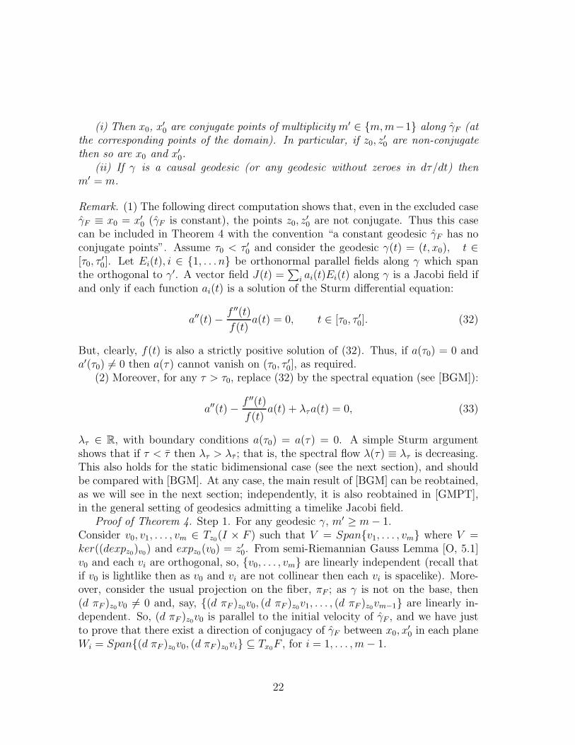
Proof of Theorem 4. Step 1. For any geodesic γ, m′ ≥ m − 1.Consider v0, v1, . . . , vm ∈ Tz0

(I × F ) such that V = Spanv1, . . . , vm where V =ker((dexpz0

)v0) and expz0

(v0) = z′0. From semi-Riemannian Gauss Lemma [O, 5.1]v0 and each vi are orthogonal, so, v0, . . . , vm are linearly independent (recall thatif v0 is lightlike then as v0 and vi are not collinear then each vi is spacelike). More-over, consider the usual projection on the fiber, πF ; as γ is not on the base, then(d πF )z0

v0 6= 0 and, say, (d πF )z0v0, (d πF )z0

v1, . . . , (d πF )z0vm−1 are linearly in-

dependent. So, (d πF )z0v0 is parallel to the initial velocity of γF , and we have just

to prove that there exist a direction of conjugacy of γF between x0, x′0 in each plane

Wi = Span(d πF )z0v0, (d πF )z0

vi ⊆ Tx0F , for i = 1, . . . , m − 1.

22

Defining αi(s) = v0 + svi we have dds

|s=0 expz0(αi(s)) = 0 and, thus,

d

ds|s=0 πF expz0

(αi(s)) = 0. (34)

There exist a non-constant continuous curve βi(s) ∈ Wi i = 1, . . . , m−1 such that

expx0(βi(s)) = πF expz0

(αi(s)). (35)

In fact, we take

βi(s) = µi(s)dπF (αi(s))

| dπF (αi(s)) |, (36)

where µi(s) is the length of the pregeodesic t → πF expz0(t · αi(s)) on [0, 1].

Recall that (d πF )z0v0 is paralell to βi(0) ≡ ω0, and we had to prove that

(dexpx0)w0

restricted to Wi is singular. Otherwise, βi(s) would be smooth around 0from (35). From (36), 0 6= β ′

i(0) ∈ Wi, and from (34) and (35), β ′i(0) ∈ ker(dexpx0

)ω0,

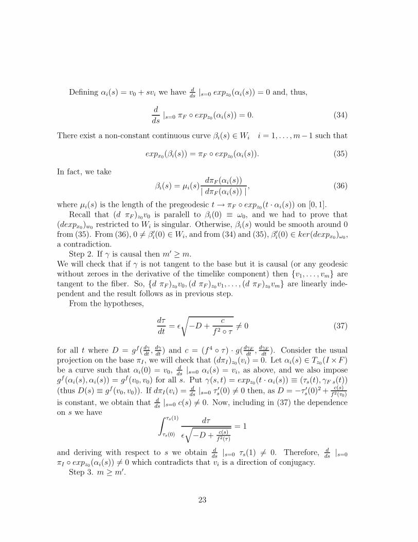
a contradiction.Step 2. If γ is causal then m′ ≥ m.

We will check that if γ is not tangent to the base but it is causal (or any geodesicwithout zeroes in the derivative of the timelike component) then v1, . . . , vm aretangent to the fiber. So, d πF )z0

v0, (d πF )z0v1, . . . , (d πF )z0

vm are linearly inde-pendent and the result follows as in previous step.

From the hypotheses,

dτ

dt= ǫ

√

−D +c

f 2 τ6= 0 (37)

for all t where D = gf(dγdt

, dγdt

) and c = (f 4 τ) · g(dγF

dt, dγF

dt). Consider the usual

projection on the base πI , we will check that (dπI)z0(vi) = 0. Let αi(s) ∈ Tz0

(I ×F )be a curve such that αi(0) = v0,

dds

|s=0 αi(s) = vi, as above, and we also imposegf(αi(s), αi(s)) = gf(v0, v0) for all s. Put γ(s, t) = expz0

(t · αi(s)) ≡ (τs(t), γF s(t))

(thus D(s) ≡ gf(v0, v0)). If dπI(vi) = dds

|s=0 τ ′s(0) 6= 0 then, as D = −τ ′

s(0)2 + c(s)f2(τ0)

is constant, we obtain that dds

|s=0 c(s) 6= 0. Now, including in (37) the dependenceon s we have

∫ τs(1)

τs(0)

dτ

ǫ√

−D + c(s)f2(τ)

= 1

and deriving with respect to s we obtain dds

|s=0 τs(1) 6= 0. Therefore, dds

|s=0

πI expz0(αi(s)) 6= 0 which contradicts that vi is a direction of conjugacy.

Step 3. m ≥ m′.

23

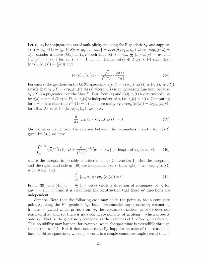
Let x0, x′0 be conjugate points of multiplicity m′ along the F-geodesic γF and suppose

γ(0) = z0, γ(1) = z′0. If Spanw1, . . . , wm′ = ker((d expx0)w0

) where expx0(w0) =

x′0, consider a curve βi(s) in Tx0

F such that βi(0) = w0,dds

|s=0 βi(s) = wi and| βi(s) |=| w0 | for all s, i = 1, . . .m′. Define αi(s) ∈ Tz0

(I × F ) such that(dπI)z0

(αi(s)) = dτdt

(0) and

(dπF )z0(αi(s)) =

√c

f 2(τ0)· βi(s)

| w0 |. (38)

For each s, the geodesic on the GRW spacetime γ(s, t) = expz0(t·αi(s)) ≡ (τs(t), γF s(t)),

satisfy that γF s(t) = expx0(rs(t)·βi(s)) where rs(t) is an increasing function, because

γF s(t) is a pregeodesic on the fiber F . But, from (4) and (30), rs(t) is determined justby c(s) ≡ c and D(s) ≡ D, so, rs(t) is independent of s, i.e. rs(t) ≡ r(t). Computingfor s = 0, it is clear that r−1(1) = 1 thus, necessarily πF expz0

(αi(s)) = expx0(βi(s))

for all s. As wi ∈ ker((d expx0)w0

), we have:

d

ds|s=0 πF expz0

(αi(s)) = 0. (39)

On the other hand, from the relation between the parameters τ and r for γ(s, t)given by (31) we have

∫ τ ′

0(s)

τ0

√cf−2(τ)(−D +

c

f 2(τ))−1/2dτ =| w0 | (= length of γFs

for all s), (40)

where the integral is possibly considered under Convention 1. But the integrandand the right hand side in (40) are independent of s, thus, τ ′

0(s) = πI expz0(αi(s))

is constant, andd

ds|s=0 πI expz0

(αi(s)) = 0. (41)

From (39) and (41) vi = dds

|s=0 αi(s) yields a direction of conjugacy of γ, forany i = 1, . . .m′, and it is clear from the construction that these m′ directions areindependent. 2

Remark. Note that the following case may hold: the point x0 has a conjugatepoint x1 along the F− geodesic γF , but if we consider any geodesic γ emanatingfrom z0 = (τ0, x0) which projects on γF , the reparameterization γF of γF does notreach until x1 and, so, there is no a conjugate point z1 of z0 along γ which projectsonto x1. That is, the geodesic γ “escapes” at the extremes of I before γF reaches x1.This possibility may happen, for example, when the spacetime is extendible throughthe extremes of I. But it does not necessarily happens because of this reason; infact, de Sitter spacetime, where f = cosh, is a simple counterexample (recall that if

24

∫ b

cf = ∞ all null geodesics are future-complete [Sa98] and the GRW spacetime not

only is not extendible through b as a GRW spacetime but also it is not extendible asa spacetime; compare all this discussion with [Uh, p. 73]). When the fiber is weaklyconvex the necessary and sufficient conditions to ensure that, for any geodesic γnon-tangent to the base, γF will cover all γF are the “non–escape” equalities

∫ c

a

f−2(1

f 2+ 1)−1/2 = ∞

∫ b

c

f−2(1

f 2+ 1)−1/2 = ∞ (42)

for certain c ∈ (a, b) (see [FS, Lemma 4]). Recall that this condition implies Condi-tion (A) and, so, the spacetime will be geodesically connected. Summing up:

Corollary 1 Consider a GRW spacetime with weakly convex fiber where the “non–escape” equalities (42) hold. Then the spacetime is geodesically connected and anycausal geodesic γ(t) = (τ(t), γF (t)) starting at z0 have conjugate points in bijectivecorrespondence (including multiplicities) with the conjugate points of the inextendiblegeodesic γF (r) obtained from the projection γF (t) on the fiber.

Remark. This result allows to extend, in our ambient, the ones by Uhlenbeckfor null geodesics [Uh] to all causal geodesics. For instance, normalize all causalgeodesics (non tangent to the base) such that c ≡ (f 4 τ) · g(dγF

dt, dγF

dt) = 1 and

choose D ≤ 0; all future-pointing causal geodesics starting at z0 = (τ0, x0) andhaving associated the fixed value of D = gf(dγ

dt, dγ

dt), are in bijective correspondence

with the F−geodesics starting at x0, being the conjugate points preserved. So:

Under the assumptions of Corollary 1, and fixed D ≤ 0, if x0 and x1

are not conjugate the loop space of F is homotopic to a cell complexconstructed with a cell for each causal D-geodesic (with c = 1) from z0

to the line Lx1= (t, x1) : t ∈ I with the dimension of the cell equal to

the index of the D-geodesic.

Recall that in [Uh] the conformal invariance of null conjugate points is explicitlyused, but this invariance does not hold for timelike geodesics (bidimensional anti-de Sitter spacetime, which is globally conformal to a strip in Lorentz-Minkowskispacetime, is a simple example); this makes necessary our approach.

Theorem 4 and equalities (42) can be also combined to yield Morse relations asfollows. Fix two non-conjugate points z0 = (τ0, x0), z

′0 = (τ ′

0, x′0) and a field K. Let

Ω(z0, z′0) (resp. Ω(x0, x

′0)) be the space of continuous paths joining z0, z

′0 in I × F

(resp. x0, x′0 in F ). Let Pz0,z′

0(t) (resp. Px0,x′

0(t)) be the Poincare polinomial of

Ω(z0, z′0) (resp. Ω(x0, x

′0)); that is, Pz0,z′

0(t) is the formal series

Pz0,z′0(t) = β0 + β1t + β2t

2 + · · ·

25

where βq is the q–th Betti number of Ω(z0, z′0) for homology with coefficients in K,

βq = dimHq(Ω(z0, z′0),K). Clearly, Pz0,z′

0(t) ≡ Px0,x′

0(t). Let

Mz0,z′0(t) = a0 + a1t + a2t

2 + · · ·

(resp. Mx0,x′

0(t) = a0 + a1t + a2t

2 + · · ·)be the Morse polinomials of z0, z

′0 (resp. x0, x

′0), i.e. aq (resp aq) is the number of

geodesics joining z0 and z′0 (resp. x0 and x′0) with Morse index equal to q, where

the Morse index of a geodesic connecting two fixed non-conjugate points is the sumof the indexes of conjugate poins to the first point along the geodesic. Then, underthe hypotheses of Theorem 3 and from Theorem 4:

aq ≤ aq + aq+1, ∀q ≥ 0, (43)

a0 > 0 ⇒ a0 > 0; aq > 0 ⇒ aq−1 + aq > 0; ∀q ≥ 1. (44)

In particular, if the polinomials are finite then Mz0,z′0(t) ≥ Mx0,x′

0(t), ∀t ≥ 1. But

if (F, g) is a complete Riemannian manifold, then the well-known Morse relationsimplies the existence of a formal polinomial, with non-negative integer coefficientsQ(t) such that

Mx0,x′

0(t) = Px0,x′

0(t) + (1 + t)Q(t). (45)

Remark. In general, it is not true that a0 ≥ a0 or aq−1 + aq ≥ aq. Recall thatmany geodesics in the GRW spacetime connecting z0, z

′0 may project on the same

pregeodesic of F . A simple counterexample of this is de Sitter spacetime (with astraightforward modification, one can also get that hypotheses in Theorem 3 arefulfilled). So, inequalities (44) cannot be improved.

Summing up,

Corollary 2 In a globally hyperbolic GRW spacetime satisfying either Condition(A) or Condition (B) with da, db (if defined) equal to infinity the Morse inequalities(43), (44) (with (45)) hold.

As a consequence, if the Morse polinomial Mz0,z′0(t) is finite then, for each pair

of non–conjugate points z0, z′0 there exist a polinomial Q(t) with non–negative integer

coefficients and computable from the fiber such that

Mz0,z′0(t) ≥ Pz0,z′

0(t) + (1 + t)Q(t), ∀t ≥ 1.

6 Applications

26

6.1 Two dimensional case

Next we will particularize previous results to bidimensional GRW spacetimes withstrongly convex fiber (necessarily an interval (J, dx2)). Recall that in this casethe opposite metric −gf is also Lorentzian and, in fact, it corresponds to a static(standard) spacetime. The chronological relation can be now extended for non-causally related points, just defining that two points are spacelike related if they arechronologically related for −gf . In fact, we will simplify our terminology with thefollowing (re-)definition.

Definition 5 Consider a bidimensional GRW (or static) spacetime. Two points(τ0, x0), (τ

′0, x

′0) are spacelike [resp. timelike, lightlike] related iff there exists a space-

like [resp. timelike, lightlike with non-vanishing derivative] curve joining them.

From a direct computation (see also [Sa97, Th.3.3 and Lemma 3.5]) we have:

Lemma 11 Given (τ0, x0), (τ′0, x

′0) ∈ (I × J,−dτ 2 + f 2dx2), they are

(i) spacelike related if and only if∫ τ ′

0

τ0f−1 < d(x0, x

′0)

(ii) lightlike related if and only if∫ τ ′

0

τ0f−1 = d(x0, x

′0)

(iii) timelike related if and only if∫ τ ′

0

τ0f−1 > d(x0, x

′0)

Now, as a consequence of Lemma 11 and Theorem 2 we have:

Corollary 3 In a GRW spacetime (I × J,−dτ 2 + f 2dx2):(i) If (τ0, x0), (τ ′

0, x′0) are timelike [resp lightlike] related then there exist a unique

geodesic (necessarily timelike [resp lightlike]) which joins them.(ii) All (τ0, x0), (τ ′

0, x′0) which are spacelike related can be joined by a geodesic

(necessarily spacelike) if and only if Condition (C) or Condition (R) holds.

From Theorem 4 and the fact that there are no conjugate points on a manifoldof dimension 1, we have:

Corollary 4 In a GRW spacetime (I×J,−dτ 2+f 2dx2) no geodesic γ(t) = (τ(t), γF (t))without zeroes in dτ/dt have conjugate points.

In particular, causal geodesics are free of conjugate points.

Now, consider a bidimensional static spacetime, say (K × J ⊆ R2, gS = dy2 −

f 2(y)dx2) where gS can be seen as the reversed metric of a GRW spacetime. Sum-marizing the conclusions of Lemma 11 and Corollaries 3, 4, the following extensionof Theorem 1.1 in [BGM] can be given (see also [GMPT, Prop. 6.6]).

27

Corollary 5 Given (y0, x0), (y′0, x

′0) in the static spacetime (K × J ⊆ R

2, gS =dy2 − f 2(y)dx2), they are

(i) spacelike related if and only if∫ y′

0

y0f−1 > d(x0, x

′0). In this case there exist a

unique geodesic which joins them; this geodesic is necessarily spacelike and withoutconjugate points.

(ii) lightlike related if and only if∫ y′

0

y0f−1 = d(x0, x

′0). In this case there exist a

unique geodesic which joins them; this geodesic is necessarily lightlike and withoutconjugate points.

(iii) timelike related if and only if∫ y′

0

y0f−1 < d(x0, x

′0). All points which are time-

like related can be joined by a geodesic (necessarily timelike) if and only if Condition(C) or Condition (R) holds.

Remark. In fact, no geodesic of the static spacetime without zeroes in the deriva-tive of its spacelike component has conjugate points. Anti de-Sitter spacetime is anexample of static spacetime where all the timelike geodesics have conjugate points.Moreover, it is not geodesically connected.

6.2 Conditions on curvature

As commented in the Introduction, it is natural to assume, for a realistic GRWspacetime, that Ric(∂t, ∂t) ≥ 0, and it is straightforward to check that this conditionis equivalent to f ′′ ≤ 0 (see [O, Cor. 7.43]). Recall that in this case limτ→a,bf

′ andlimτ→a,bf always exist. So taking into account the cases in Table 1 we see thatCondition (A) always holds except when b < ∞ (resp. a > −∞) and f ′(b) > 0(resp. f ′(a) < 0). In this case, although the GRW spacetime is not geodesicallyconnected, it is possible to extend the warping function f through b (resp. a)obtaining so a extended spacetime, which is also GRW. The GRW spacetime will becalled inextendible if whenever an extreme of I is finite, then f cannot be extendedcontinuously at these extremes to a real value α > 0. It seems clear that from aphysical viewpoint just inextendible GRW spacetimes must be taken into account.

Therefore, Theorems 1 and 3 are appliable to these inextendible GRW space-times, yielding the points (ii) and (iv) in the following Corollary (the other two areincluded for the sake of completeness).

Corollary 6 An inextendible GRW spacetime with Ric(∂t, ∂t) ≥ 0 and weakly con-vex fiber satisfies

(i) Each two causally related points can be joined with one non-spacelike geodesic,which is unique if the fiber is strongly convex.

(ii) The spacetime is geodesically connected. Moreover, each strip (a, b) × F ⊂I × F , a < a < b < b with the restricted metric is geodesically connected if and onlyif f ′(a) ≥ 0 and f ′(b) ≤ 0 (i.e. f ′(a) · f ′(b) ≤ 0).

28

(iii) There exist a natural surjective map between geodesics connecting z0 =(τ0, x0), z′0 = (τ ′

0, x′0) ∈ I × F and F-geodesics connecting x0 and x′

0. Under thismap, when the geodesic connecting z0 and z′0 is causal then the multiplicity of itsconjugate points is equal to the multiplicity for the corresponding geodesic connectingx0, x′

0.(iv) If (F, g) is complete and F is not contractible in itself, then any z0, z

′0 ∈ I×F

can be joined by means of infinitely many spacelike geodesics. If x0, x′0 are not

conjugate there are at most finitely many causal geodesics connecting them.

For the last assertion (ii), recall that it is straightforward from Theorem 2 understrongly convexity. But, from the proof of this theorem, this assumption can bedropped because f ′′ ≤ 0 (recall that then Conditions (A), (B), (C) are equivalentand Condition (R) is not appliable).

Finally, we give a further consequence of equalities (42):

Corollary 7 Consider a GRW spacetime (I × F, gf) which is globally hyperbolicand satisfies the non-escape equalities (42), and fix D0 ≤ 0. If any geodesic γ(t) =(τ(t), γF (t)) starting at z0 = (t0, x0) and having associated values D, c equal to D0,1, respectively, is free of conjugate points then the fiber can be covered topologicallyby R

n, being n = dimF .

Proof. Under this assumption the F-geodesics starting at x0 have no conjugatepoints and so, as F is complete, expx0

: Tx0F ≡ R

n → F is a surjective localdiffeomorphism. Taking the pull-back metric on Tx0

F , a local isometry with domaina complete manifold (and so a Riemannian covering) is obtained. 2

Remark. The assumption on conjugate points when D0 = 0 holds if in thefuture of z0 we have R(X, Y, Y, X) ≤ 0 whenever X, Y span a degenerate plane ona lightlike geodesic starting at z0 (see [BEE, Th. 10.77]); moreover, the non-escapeinequalities (42) can be reduced to

∫ c

a

f−1 = ∞∫ b

c

f−1 = ∞ (46)

when just null geodesics are considered, so we reobtain [Uh, Theorem 5.3] in ourambient.

References

[ARS] L.J. Alıas, A. Romero, M. Sanchez, Uniqueness of complete spacelike hyper-surfaces of constant mean curvature in Generalized Robertson-Walker space-times Gen. Relat. Gravit. 27 (1995) 71–84.

29

[BEE] J.K. Beem, P.E. Ehrlich and K.L. Easley, Global Lorentzian geometry, Mono-graphs Textbooks Pure Appl. Math. 202 (Dekker Inc., New York, 1996).

[BF] V. Benci, D. Fortunato, Existence of geodesics for the Lorentz metric of astationary gravitational field, Ann. Inst. Henri Poincare, 7 (1990) 27-35.

[BGM] V. Benci, F. Giannoni, A. Masiello, Some properties of the spectral flow insemiriemannian geometry, J. Geom. Phys. 27 (1998) 267–280.

[BGS] R. Bartolo, A. Germinario and M. Sanchez, Convexity of domains of Rie-mannian manifolds, Ann. Global Anal. Geom., to appear.

[BM] V. Benci, A. Masiello, A Morse index for geodesics in static Lorentzian man-ifolds, Math. Ann. 293 (1992) 433–442.

[CM] E. Calabi, L. Markus, Relativistic space forms, Ann. Math. 75 (1962) 63-76.

[FS] J.L. Flores, M. Sanchez, Geodesic connectedness of multiwarped spacetimes,J. Diff. Equat., to appear.

[Gi] F. Giannoni, Geodesics on non static Lorentz manifolds of Reissner-Nordstromtype, Math. Ann. 291 (1991) 383-401.

[GM] F. Giannoni, A. Massiello, Geodesics on Lorentzian manifolds with quasi-convex boundary, Manuscripta Math. 78 (1993) 381-396.

[GMPa] F. Giannoni, A. Masiello, P. Piccione, Convexity and the finiteness of thenumber of geodesics: Applications to the multiple-image effect, Class. Quant.Grav. 16 (1999) 731–748.

[GMPb] F. Giannoni, A. Masiello, P. Piccione, A Morse theory for massive particleand photons in General Relativity, J. Geom. Phys., to appear.

[GMPT] F. Giannoni, A. Masiello, P. Piccione, D. Tausk, A generalized index the-orem for Morse-Sturm systems and applications to semi-Riemannian geometry,preprint (1999).

[He] A.D. Helfer, Conjugate points on spacelike geodesics or pseudo-self-adjointMorse-Sturm-Liouville systems, Pac. J. Math. 164 (1994) 321–350.

[Ma] A. Masiello, Variational methods in Lorentzian Geometry, Pitman ResearchNotes in Mathematics Series 309, Longman Scientific and Technical, Harlow,Essex (1994).

30

[O] B. O’Neill, Semi-Riemannian Geometry with applications to Relativity, Seriesin Pure and Applied Math. 103 Academic Press, N.Y. (1983).

[Sa97] M. Sanchez, Geodesic connectedness in Generalized Reissner-Nordstrom typeLorentz manifolds, Gen. Relat. Gravit. 29 (1997) 1023–1037.

[Sa98] M. Sanchez, On the Geometry of Generalized Robertson-Walker spacetimes:Geodesics, Gen. Relat. Gravit. 30 (1998) 915–932.

[Sa99] M. Sanchez, On the Geometry of Generalized Robertson-Walker spacetimes:Curvature and Killing fields, J. Geom. Phys. 31 (1999) 1–15.

[Sc] H.-J. Schmidt, How should we measure spatial distances? Gen. Relat. Gravit.28 No. 7 (1996) 899-903.

[Uh] K. Uhlenbeck, A Morse Theory for geodesics on Lorentz manifolds, Topology14 (1975) 69–90.

31

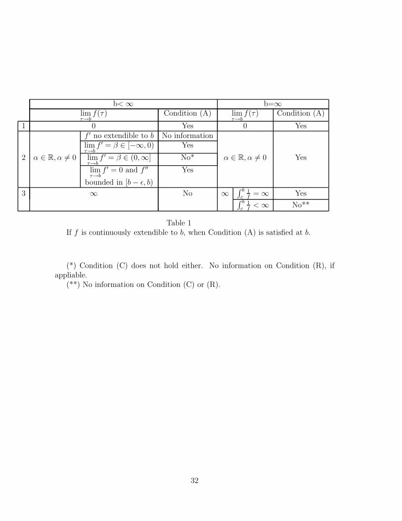
b< ∞ b=∞limτ→b

f(τ) Condition (A) limτ→b

f(τ) Condition (A)

1 0 Yes 0 Yesf ′ no extendible to b No informationlimτ→b

f ′ = β ∈ [−∞, 0) Yes

2 α ∈ R, α 6= 0 limτ→b

f ′ = β ∈ (0,∞] No* α ∈ R, α 6= 0 Yes

limτ→b

f ′ = 0 and f ′′ Yes

bounded in [b − ǫ, b)

3 ∞ No ∞∫ b

c1f

= ∞ Yes∫ b

c1f

< ∞ No**

Table 1If f is continuously extendible to b, when Condition (A) is satisfied at b.

(*) Condition (C) does not hold either. No information on Condition (R), ifappliable.

(**) No information on Condition (C) or (R).

32

33

34