This article was downloaded by: [University of South Carolina ]On: 06 December 2013, At: 08:23Publisher: Taylor & FrancisInforma Ltd Registered in England and Wales Registered Number: 1072954 Registered office: Mortimer House,37-41 Mortimer Street, London W1T 3JH, UK

Cartography and Geographic Information SciencePublication details, including instructions for authors and subscription information:http://www.tandfonline.com/loi/tcag20

Mapping family connectedness across space and timeCaglar Koylua, Diansheng Guoa, Alice Kasakoffa & John W. Adamsa

a Department of Geography, University of South Carolina, 709 Bull Street, Columbia, SC29208, USAPublished online: 04 Dec 2013.

To cite this article: Caglar Koylu, Diansheng Guo, Alice Kasakoff & John W. Adams , Cartography and Geographic InformationScience (2013): Mapping family connectedness across space and time, Cartography and Geographic Information Science, DOI:10.1080/15230406.2013.865303

To link to this article: http://dx.doi.org/10.1080/15230406.2013.865303

PLEASE SCROLL DOWN FOR ARTICLE

Taylor & Francis makes every effort to ensure the accuracy of all the information (the “Content”) containedin the publications on our platform. However, Taylor & Francis, our agents, and our licensors make norepresentations or warranties whatsoever as to the accuracy, completeness, or suitability for any purpose of theContent. Any opinions and views expressed in this publication are the opinions and views of the authors, andare not the views of or endorsed by Taylor & Francis. The accuracy of the Content should not be relied upon andshould be independently verified with primary sources of information. Taylor and Francis shall not be liable forany losses, actions, claims, proceedings, demands, costs, expenses, damages, and other liabilities whatsoeveror howsoever caused arising directly or indirectly in connection with, in relation to or arising out of the use ofthe Content.

This article may be used for research, teaching, and private study purposes. Any substantial or systematicreproduction, redistribution, reselling, loan, sub-licensing, systematic supply, or distribution in anyform to anyone is expressly forbidden. Terms & Conditions of access and use can be found at http://www.tandfonline.com/page/terms-and-conditions

Mapping family connectedness across space and time

Caglar Koylu*, Diansheng Guo, Alice Kasakoff and John W. Adams

Department of Geography, University of South Carolina, 709 Bull Street, Columbia, SC 29208, USA

(Received 25 July 2013; accepted 25 October 2013)

Understanding the structure and evolution of family networks embedded in space and time is crucial for various fields suchas disaster evacuation planning and provision of care to the elderly. Computation and visualization can potentially play akey role in analyzing and understanding such networks. Graph visualization methods are effective in discovering networkpatterns; however, they have inadequate capability in discovering spatial and temporal patterns of connections in a networkespecially when the network exists and changes across space and time. We introduce a measure of family connectednessthat summarizes the dynamic relationships in a family network by taking into account the distance (how far individuals liveapart), time (the duration of individuals’ coexistence within a neighborhood), and the relationship (kinship or kin proximity)between each pair of individuals. By mapping the family connectedness over a series of time intervals, the methodfacilitates the discovery of hot spots (hubs) where family connectedness is strong and the changing patterns of suchspots across space and time. We demonstrate our approach using a data set of nine families from the US North. Our resultshighlight that family connectedness reflects changing demographic processes such as migration and population growth.

Keywords: space-time visualization; family connectedness; network measure; social network; family tree

We dedicate this article to John W. Adams whose idea itwas to make use of published genealogies for socialscience research, and who developed the data we use inour article. He worked on compiling and organizing thedata throughout his lifetime, adding information fromother sources and obtaining funding to expand it. Hewas one of the first to see the usefulness of genealogicalmaterial for the social sciences. He understood howimportant longitudinal data was for understanding socialprocesses and documenting the lives of migrants. Hiswisdom made it possible for us to study the expansionof families over several hundred years.

Introduction

The interaction between geography and social relation-ships has long been studied by researchers (e.g.,Festinger, Schachter, and Back 1963; Hägerstrand 1976;Michelson 1970). Due to the wide use of social network-ing applications (e.g., Facebook and LinkedIn) and gen-ealogy applications (e.g., Family Search and Ancestry),large social networks with geographic information havebecome increasingly available. Using such data, recentstudies have proposed new ways of quantifying relation-ships, some of which make use of geography to infersocial interactions (Backstrom, Sun, and Marlow 2010;Crandall et al. 2010), while others examine how geogra-phy and migration (or movement) influence relationshipsbetween individuals (Onnela et al. 2011;Phithakkitnukoon et al. 2011). Understanding of how

relationships (e.g., kinship, friendship) evolve acrossspace and time is crucial for decision making in variousfields such as disaster evacuation planning and provisionof care to the elderly.

In a social network, each individual is represented by anode and each edge represents the relationship betweentwo individuals. The weight of an edge can be quantifiedin a variety of ways such as the degree of kinship in afamily tree; co-authorship in a scientific collaboration net-work; and the frequency of phone calls, text messages ore-mails exchanged in a communication network. A socialnetwork is dynamic because it evolves (changes) overspace and time as individuals move (migrate), new indi-viduals are added or removed, and relationships developand change over time. In this article, we use the term“dynamic geo-social network” to refer to a dynamic socialnetwork embedded in space and time. Understanding thechanging aspects of a dynamic geo-social networkrequires methods that can simultaneously account for thespatial, temporal and relational (network) dimensions ofthe network.

In order to understand the dynamics of social networksembedded in geographic space, a variety of computationaland statistical methods such as graph theoretical measures(Scellato et al. 2011), random graph modeling (Schaefer2012), factor analysis (Hipp, Faris, and Boessen 2012),simulation (Butts et al. 2012), and regression analysis(Viry 2012) have been introduced by studies in socialnetworks. A similarity between these studies is that they

*Corresponding author. Email: koylu@email.sc.edu

Cartography and Geographic Information Science, 2013http://dx.doi.org/10.1080/15230406.2013.865303

© 2013 Cartography and Geographic Information Society

Dow

nloa

ded

by [

Uni

vers

ity o

f So

uth

Car

olin

a ]

at 0

8:23

06

Dec

embe

r 20

13

consider geography as a background variable to interpretthe results of network analysis. However, the methodolo-gies introduced by these studies have limited capability inanalyzing the spatial, temporal and relational aspects ofdynamic geo-social networks.

With the advancement of graph drawing algorithms,current methods of graph visualization (Lewis, Gonzalez,and Kaufman 2012; Patil 2011) are effective in discover-ing network (connection) patterns, e.g., clusters of con-nected members, or commonalities between friends whoshare interests and groups in a social networking applica-tion. However, existing graph visualization methods areinadequate for discovering the spatial and temporal pat-terns in social networks. On the other hand, spatiotem-poral visualization methods (Andrienko et al. 2010; Fyfe,Holdsworth, and Weaver 2009) have been successfullyapplied to identify temporal variation of spatial patterns,which often do not adequately consider the networkdimension (connections between individuals). Therefore,there is still a lack of methodology that can incorporate therelational aspect (sophisticated relations between indivi-duals) of geographically embedded and time-varyingsocial networks.

We introduce a measure and mapping approach toanalyze connectedness in a dynamic family network andits changing patterns across space and time. Our approachdiffers from the current methods in that it takes intoaccount the time that each pair of individuals spendtogether, the distance that they live apart, and the strengthof their relationship (e.g., the degree of kinship). Todemonstrate the approach, we use a data set of familytrees derived from the published genealogies of ninefamilies in the US North over a span of 300 years. Thedata also include information on migration of individuals.The remainder of the paper is organized as follows. First,we review the related work in the next section. We thenintroduce our data and describe our methodology in detail.Finally, we present the results and conclude with a sum-mary and a discussion for the future research.

Related work

This article introduces a methodology to understand thespatial, temporal and relational (network) aspects of adynamic geo-social network. A dynamic geo-social net-work evolves (changes) over space and time as the actorsof the network move (migrate), new actors are added orremoved, and relationships between the actors developand change over time. We demonstrate our approachusing a dynamic family network embedded in space andtime. Previous approaches to analyzing geo-social net-works span a variety of themes and methodologies. Inthis section, we review the studies that aim at bridgingsocial network analysis and spatial analysis in certainaspects.

Computational and statistical methods

There are various studies on geo-social networks withinthe social network domain. For example, a number ofstudies (Daraganova et al. 2012; Lomi and Pallotti 2012;Sailer and McCulloh 2012; Schaefer 2012) used exponen-tial random graph models to account for geographicembeddedness of individuals in modeling social networksand investigate the effects of social and spatial distance onthe network structure. Doreian and Conti (2012) analyzeda set of empirical networks to understand how networksare shaped by social and spatial contexts using a variety ofmodeling strategies. Butts et al. (2012) conducted anexploratory simulation study to examine the influence ofspatial variability of background population on the net-work structure and the social ties.

Viry (2012) examined the relationship between spatialdispersion of personal networks, residential mobility andnetwork composition by conducting regression analyses.Cho, Myers, and Leskovec (2011) and Scellato et al. (2011)focused on online geo-social networks to describe the rela-tionship between geography and social interaction usinggraph theoretical methods. Similarly, Radil, Flint, and Tita(2010) introduced a spatialized positional analysis to revealspatial patterns of social relations. Hipp et al. (2012), andMennis and Mason (2012) performed factor analyses todelineate neighborhood boundaries by taking into accountthe density of social ties and the physical distances betweenthe members of a social network. A similarity between thestudies that focus on geo-social networks in the social net-work domain is that they consider geography as a back-ground variable to interpret the results of network analysis.However, the methodologies introduced by these studieshave limited capability in analyzing the spatial, temporal,and relational aspects of dynamic social networks.

Visualization

Alternative to modeling, graph theoretical and statisticalapproaches, network visualization methods have beendeveloped to examine the dynamic nature of social net-works. Dynamic network visualization methods allow thediscovery of complex patterns in a network over timeusing animation (network movies) (Moody, McFarland,and Bender-deMoll 2005) and “small multiple displays”(Robertson et al. 2008). The layout of a graph is con-structed by a graph drawing algorithm which often placesnodes (individuals) that have strong relationships closer toeach other. To enhance the perception of changes in asequence of graph layouts, a collection of methods aredeveloped by considering additional criteria such as mini-mizing edge crossings and ensuring repeatability and sta-bility (Bender-deMoll and McFarland 2005). However,such graph layouts represent only the topological structureof the network while disregarding its geographicdimension.

2 C. Koylu et al.

Dow

nloa

ded

by [

Uni

vers

ity o

f So

uth

Car

olin

a ]

at 0

8:23

06

Dec

embe

r 20

13

To incorporate a geographic dimension into the net-work space, a number of studies (Faust et al. 2000; Nag2009; Todo et al. 2011) mapped actors (people) based ontheir geographic location and drew edges between thoseactors using different width and color intensity to reflectrelative strength of each relationship. However, a graphlayout that positions nodes based on their geographiccoordinates suffers from the visual cluttering problem.Moreover, with a relatively large network, it is difficultto perceive network structures that involve multipledimensions (i.e., space, time, and social connections).Because social network data are highly dynamic, it ischallenging to reveal how social relationships changeacross geographies and time by simply displaying asequence of graphs.

Alternatively, some studies (Luo et al. 2011; Onnelaet al. 2011) introduced integrated approaches that usedynamically linked views of network space and geo-graphic space and allow user interactions to demonstratethe interplay of topological structure and geography.Discovering the interaction between geography and thenetwork is useful in extracting microscale (individuallevel) patterns. However; there is also a need to summar-ize spatial, temporal, and relational aspects of such net-works in order to provide a general overview of the data.

Hägerstrand (1976) introduced a space-time frame-work to conceptualize and represent human interactionsover space and time. Adopting this framework, manyspatiotemporal visualization approaches (e.g., space-timepath, density surface, computational, and interactiveapproaches) have been introduced (Aigner et al. 2011).The space-time path approach (Chen et al. 2011; Lee andKwan 2011) identifies human activity patterns in a socialnetwork by visualizing individuals’ paths in a three-dimensional surface. Alternatively, the density surfaceapproach summarizes the activity patterns by a densitysurface which is represented with either an animatedsequence of continuous surfaces (Rana and Dykes 2003)or a three-dimensional surface of the space-time conti-nuum (Demšar and Virrantaus 2010; Nakaya and Yano2010). Additionally, some computational and interactiveapproaches such as self-organizing maps (Agarwal andSkupin 2008) have been used to identify temporal varia-tion of spatial patterns.

The space-time approach by Shaw, Yu, and Bombom(2008), Fyfe, Holdsworth, and Weaver (2009) andAndrienko et al. (2010) examine geo-social interactionpatterns across space and time, but it does not adequatelyconsider the network dimension (connections betweenindividuals). Therefore, there is still a lack of methodologythat can incorporate the relational aspect (sophisticatedrelations between individuals) of geographicallyembedded and time-varying social networks. Anotherchallenge in analyzing geographically embedded andtime-varying social networks is the small area problem,

where a single node or connection is often too small (withinsufficient data) for deriving stable statistical measures.Koylu and Guo (2013) introduced a smoothing approachto mapping graph measures in geographic space. In thisresearch, we introduce a different space-time smoothing orinterpolation method for visualizing both network mea-sures and social relations in space and time.

Data

To demonstrate our approach, we use family tree dataderived from published genealogies of nine families fromthe US North over a span of 300 years. These books werecompiled by family members with the help of professionalgenealogists. More information on migration has beenadded by linking the genealogies to the US censusesusing data from Ancestry.com. A series of demographicevents (e.g., births, deaths, migrations) were coded fromthe genealogy, including the places where events hadoccurred. From these event locations and dates, we caninfer the migration paths of each individual in the families.

For the simplicity of methodology presentation andresult explanation, in this article we only report the ana-lysis results with the Chaffee family (Chaffee 1909),which was selected over eight other genealogies on thebasis of better temporal resolution and information onmigration. The Chaffee family includes 1225 males des-cended in the male line from the founder who came toHull, Massachusetts from England in 1635. All men borninto the family up to 1860 were included along with allsiblings of men born through 1840. There were 2387 geo-coded moves and 856 distinct locations where the familymembers lived in 296 years.

The family data involve only males because womenchanged their names at marriage; they were more difficultto follow. Although life expectancy changed over time, itwas largely due to changes in infant and child mortality(Kasakoff and Adams 2000). This study included onlymen who survived to at least age 20. If we includedthose who had died young, we might have biased thestudy toward families with high infant and child mortality.Life expectancy at age 20 was remarkably moved west-ward, albeit at greater and greater distances (Egerbladh,Kasakoff, and Adams 2007).

Information on moves comes from records of vitalevents. If an event occurred in a place where a personhad not previously lived, the move was assigned at a dateclose to the vital event. Most moves occurred before thevital event and thus the dates are approximate. The mostaccurate move dates come from the child bearing yearsbecause this population had children approximately everytwo years. Also only about 65% of the men had deathdates recorded in the genealogy. For the rest, the last dateon record was considered a death date. The animation ofthe migration of nine families including the Chaffee (CFE)

Cartography and Geographic Information Science 3

Dow

nloa

ded

by [

Uni

vers

ity o

f So

uth

Car

olin

a ]

at 0

8:23

06

Dec

embe

r 20

13

family in the US can be viewed at the link: http://129.252.37.169:8400/flowvis/trajectories/index.html(Koylu 2013a).

Methodology

We introduce a measure and mapping approach to analyzethe relationships in a family network embedded in spaceand time. Given a space-time window, the measure quan-tifies the family connectedness of each individual, consid-ering his/her kinship to other family members coexisted inthe window, their geographic distances, and the time dura-tion of their coexistences. We then interpolate the measurevalues for all locations, map a series of space-time win-dows to examine the changing dynamics of the familyrelationships across space and time. Specifically, theapproach consists of three steps. First, the time dimensionis partitioned into a sequence of time intervals. Second,within each time interval, we calculate the measure offamily connectedness for each individual at each locationwhere he/she was present, considering the closeness (thedegree of kinship) of his/her connections he/she has withina geographic distance threshold and the temporal durationof each connection. Third, given the family connectednessvalue for each individual at each unique location within atime window, a surface of family connectedness is pro-duced using a smoothing and interpolation method basedon inverse-distance weighting. In the following subsec-tions, we introduce each of the steps.

Time interval

To allow for a temporal analysis of connectedness in afamily network, one can employ a data-driven approachsuch as sliding windows, top-down or bottom-up segmen-tation algorithms (Keogh et al. 2001; Warren Liao 2005)to obtain time intervals. For our case study, we employeda domain-specific approach to partition time series datainto equal intervals and reflect meaningful stages of thefamily tree data. Because some patterns may fall betweentime windows and not appear, we use a sliding windowapproach.

In the family data set, the minimum period needed fora connection (coexistence) to occur is one year. On aver-age a man is 35 years old when a son is born and 20 yearsis nearly the smallest generation, i.e., the youngest a manmight be when he has a son. Also, a period of 20 yearsdivides the life course into meaningful stages: age 1–20would be before marriage; child bearing should stop byage 60 (Adams and Kasakoff 1984). So people in different20-year windows should be in different life stages.Therefore, we partition the data into a time window (inter-val) length of 20 years. Theoretically, we can move this20-year window one year at a time to obtain a smoothtime series. To reduce the size of time series (and data

redundancy), we move the window 10 years each step. Inother words, there is a 10-year (i.e., 50%) overlap betweenneighboring time windows.

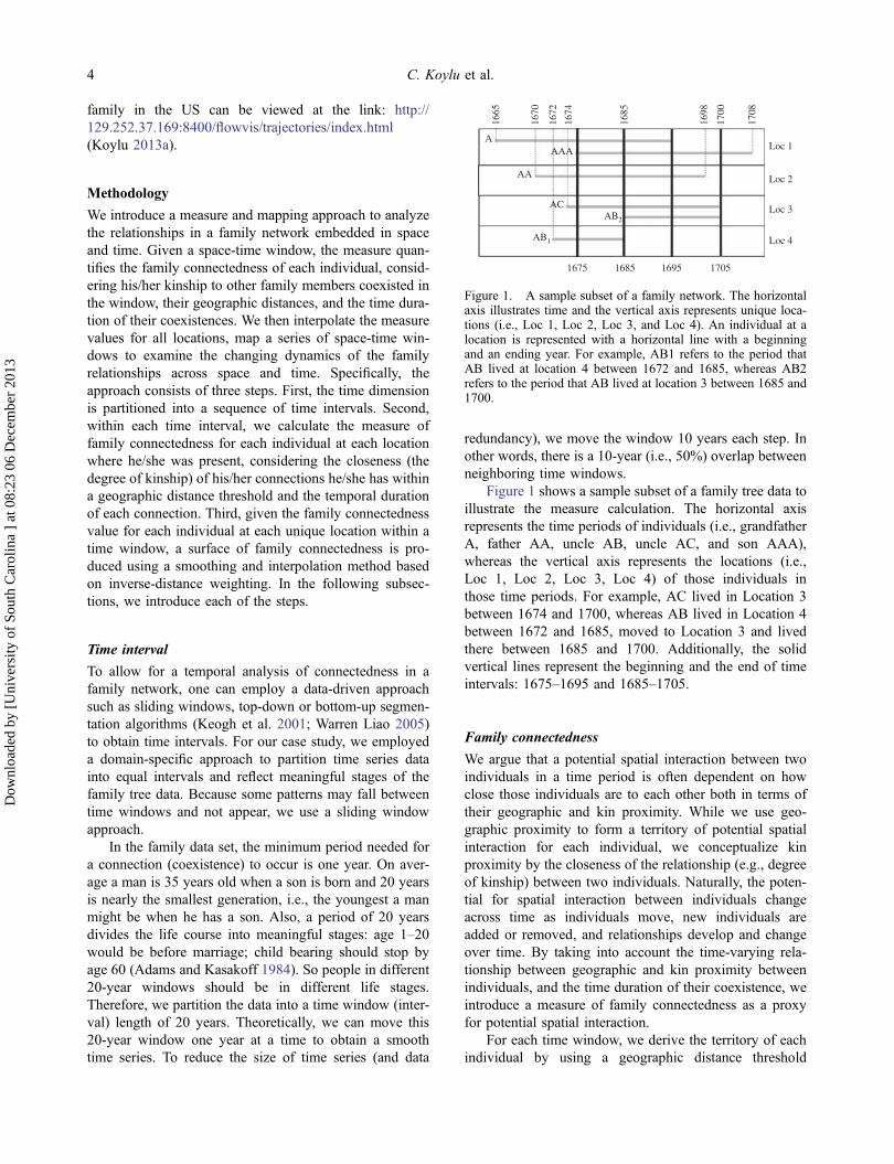
Figure 1 shows a sample subset of a family tree data toillustrate the measure calculation. The horizontal axisrepresents the time periods of individuals (i.e., grandfatherA, father AA, uncle AB, uncle AC, and son AAA),whereas the vertical axis represents the locations (i.e.,Loc 1, Loc 2, Loc 3, Loc 4) of those individuals inthose time periods. For example, AC lived in Location 3between 1674 and 1700, whereas AB lived in Location 4between 1672 and 1685, moved to Location 3 and livedthere between 1685 and 1700. Additionally, the solidvertical lines represent the beginning and the end of timeintervals: 1675–1695 and 1685–1705.

Family connectedness

We argue that a potential spatial interaction between twoindividuals in a time period is often dependent on howclose those individuals are to each other both in terms oftheir geographic and kin proximity. While we use geo-graphic proximity to form a territory of potential spatialinteraction for each individual, we conceptualize kinproximity by the closeness of the relationship (e.g., degreeof kinship) between two individuals. Naturally, the poten-tial for spatial interaction between individuals changeacross time as individuals move, new individuals areadded or removed, and relationships develop and changeover time. By taking into account the time-varying rela-tionship between geographic and kin proximity betweenindividuals, and the time duration of their coexistence, weintroduce a measure of family connectedness as a proxyfor potential spatial interaction.

For each time window, we derive the territory of eachindividual by using a geographic distance threshold

1675

AB1

AB2

AC

AA

AAAA

1665

1670

1672

1674

1685

1698

1700

1685 1695 1705

1708

Loc 4

Loc 3

Loc 2

Loc 1

Figure 1. A sample subset of a family network. The horizontalaxis illustrates time and the vertical axis represents unique loca-tions (i.e., Loc 1, Loc 2, Loc 3, and Loc 4). An individual at alocation is represented with a horizontal line with a beginningand an ending year. For example, AB1 refers to the period thatAB lived at location 4 between 1672 and 1685, whereas AB2refers to the period that AB lived at location 3 between 1685 and1700.

4 C. Koylu et al.

Dow

nloa

ded

by [

Uni

vers

ity o

f So

uth

Car

olin

a ]

at 0

8:23

06

Dec

embe

r 20

13

around his location at the time and then calculate thefamily connectedness of an individual by considering hisgeographic closeness, temporal overlapping and familyrelationship to other individuals within the territory.Figure 2 illustrates the individual AA’s family connectionsthat are determined by his territory (gray circle). Weprovide a discussion on how to determine the territory ofindividuals using the distance threshold in the followingparagraph. While the nodes with labels illustrate

connections of individual AA, empty nodes illustrate indi-viduals that do not have any family relationship with theindividual of interest. For the family tree data in this study,we define relationship as kinship and two individuals donot have a relationship if they are not members of thesame family tree. For individual AA at location 2, he hadfive family connections, which are A, AAA, AC and AB(at two locations, noted as AB1 and AB2) for the giventime interval 1675–1695. Notice that, although individualssuch as AD, AE, ADA, and AF were from the samefamily with AA, they are not considered as connectionsbecause they lived outside the neighborhood buffer of AA.

The choice of the distance threshold (bandwidth) andwhat constitutes a connection are two important decisionsfor determining potential connections of an individual at alocation and time. To select an appropriate bandwidth, weevaluated the distribution of move distances over time.Figure 3 illustrates the box-plots of distances by timeintervals. Migration was highly skewed toward shorterdistances, as is always the case. Over time, the longestdistances increased, but moves at such distances wererelatively rare and overall median distance is approxi-mately 60 km. Still these distances are much greater thanthey were in Europe (Pooley and Turnbull 1998), wherepopulation density was higher and people were more aptto remain in their local areas and reflect the Westwardexpansion of the US population.

Considering the temporal resolution of the data whichis composed of recorded events from the late seventeenthcentury till the mid-twentieth century, increasing trend ofmigration distance could be attributed to what transporta-tion medium was available for the given time period. Untilthe mid-nineteenth century when the first railway system

AG1

AG2AGA

AAE

AD,ADA

AF

A, AAA

AA

AC,AB2

AB1

Figure 2. The potential connections of individual AA from thesample network given in Figure 1. The circular buffer illustratesthe neighborhood of individual AA which is used to determinehis/her potential connections. Nodes with labels within the neigh-borhood are potential connections of AA, whereas empty nodesymbols and labeled nodes outside the neighborhood are indivi-duals that are not connected to AA. A subscript (e.g., AB1, AB2)for an individual indicates his/her existence at each unique loca-tion given the time interval.

1634–1654

010

0020

0030

0040

00

Mov

e D

ista

nce

(in k

ilmet

ers)

5000

6000

1674–1694 1714–1734 1754–1774 1794–1814 1834–1854 1874–1894 1914–1934 1954–1974

Figure 3. The distribution of move distances over time intervals. The median move distance is approximately 60 km and there is anincreasing trend of individuals moving greater distances over time.

Cartography and Geographic Information Science 5

Dow

nloa

ded

by [

Uni

vers

ity o

f So

uth

Car

olin

a ]

at 0

8:23

06

Dec

embe

r 20

13

was built in the northeastern states, traveling was limitedto the capability of horse carriages. Along the railwaylines the ability to travel long distances greatly increased.However, horse carriage remained to be a major transpor-tation medium. On average horse quality, terrain andweather conditions, a horse carriage was able to travel32–64 km a day (Bogart 2005). Assuming that a potentialfor a consistent spatial interaction is possible withoutmoving homes, we chose 60 km as a threshold distanceto identify potential connections for each individual. Thesecond important decision is to determine what constitutesa connection between individuals in a family network. Inthis study, we define connection as kinship and we assumethat two individuals are connected if they are from thesame family tree. Given the connections, we use Equation(1) to calculate each individual’s family connectedness at aspecific time interval and a specific location

FCrtðiÞ ¼X

j2Nrt

Trtði; jÞ � KPði; jÞ (1)

where FCrtðiÞ is the family connectedness for individual iat location r and in time interval t. Individual i may havemore than one locations (one at a time) in the time inter-val. Nrt are family members within the neighborhood ofthe individual i’s location (r) and the time interval t;Trt i; jð Þ is the duration of time that individuals i and jcoexisted within the neighborhood of r and the timeinterval t; KP i; jð Þ is the kin proximity which describesthe degree of kinship between the family members i and j.

We use consanguinity (Leutenegger et al. 2011) toquantify the degree of kinship (relation) between themembers of a family, which is widely used in law andgenetics. Figure 4 represents a family tree of four genera-tions where A is the ancestor of all members in the family.The relation among two people is called lineal consangui-nity if one is descendant from the other such as theson and the father (e.g., A-AA), or the grand-father (e.g.,A-AAA), and so upward in a direct ascending line. The

degree of lineal consanguinity is directly measured by thenumber of lines (e.g., edges in Figure 4) between thetwo family members. For example, father-son relations(e.g., A-AA, AAB-AABA) are first degree; grand-father-grandson relations (e.g., A-AAA, AB-ABBB) aresecond degree, and great grandfathergreat grandson rela-tions (A-AAAA, A-ABBA) are third degree.

The relation between individuals who descend fromthe same ancestor, but not from each other (e.g., cousins oruncles-nephews) is called collateral consanguinity. Thedegree for collateral relationship is calculated by findingthe common ancestor then counting the number of stepsdownwards to reach the two individuals. If one of theindividuals is more distant (remote) to the ancestor, thenumber of steps to the more remote person determines thedegree of consanguinity. For example, a relation betweenbrothers (e.g., AA-AB, AAB-AAC) is considered as a firstdegree consanguinity since there is only one step from thefather to each of them, whereas an unclenephew relation(e.g., AA-ABA, AAB-AACA) is a second degree consan-guinity because the nephew is two steps away from thecommon ancestor, and the rule of calculating the degree isextended to the more remote person of the collateralrelationship. After determining the degree of relation (con-sanguinity) between two individuals, we assign a kinproximity value to each relation by simply taking theinverse of the degree. For example, the kin proximity ofa first degree relationship (e.g., father-son, brothers) is1/1 = 1, whereas the kin proximity of a second degreerelationship (e.g., grandparent-grandchildren, cousins) is1/2 = 0.5, and a third degree relationship (e.g., greatuncle/grandnephew: AA and ABBA) is 1/3 = 0.33, andso on.

Spatial interpolation of family connectedness

The components of the measure, which are cumulativekinship and time for an individual at a location, are highlycorrelated with the presence of individuals that live withina close distance to that location. We discuss that morepeople living close by increases the chance of potentialinteractions, thus the correlation between the presence ofindividuals and the measure components is appropriateand does not necessitate normalization. As we are notinterested in family connectedness as a cumulative mea-sured quantity, we produce a geographically weightedaverage surface of family connectedness by using a spatialsmoothing and interpolation method rather than a cumu-lative density surface of family connectedness.

Given the family connectedness for each individual ateach unique location within a time window, a surface offamily connectedness is produced using a smoothing andinterpolation method based on inverse-distance weighting(IDW). IDW assumes that each measured value has aninfluence on the prediction by applying weights that are

A

AB

A

AA

AABAAA

AAAA AAAB AABA AABB AACA

AAC ABBABA

ABBA ABCAABBB

ABC

Figure 4. A sample family tree with four generations thatdescend from the ancestor, A. The relation among two peopleis called lineal consanguinity if one is descendant from the othersuch as the son and the father (e.g., A-AA), or the grandfather(e.g., A-AAA), and so upwards in a direct ascending line. Forpeople who descend from the same ancestor, but not from eachother (e.g., cousins or uncles-nephews), the relation is calledcollateral consanguinity.

6 C. Koylu et al.

Dow

nloa

ded

by [

Uni

vers

ity o

f So

uth

Car

olin

a ]

at 0

8:23

06

Dec

embe

r 20

13

proportional to the inverse of the distance between theprediction location and the measured data point. Theequation for smoothing and interpolation method isgiven below:

FC x; tð Þ ¼X

i2Nxt

wi xð ÞFCr2Nxt i; tð ÞPNj¼0wj xð Þ þWc

(2)

wiðxÞ ¼ 1

dðx; riÞp (3)

where FC x; tð Þis the interpolated value of family connected-ness at location x in time interval t; Nxt is the observations(existence of individuals at unique locations) within theneighborhood of x in time interval t; FCr2Nxt i; tð Þ is thefamily connectedness value for individual i at location r intime interval t; wi xð Þ is a weighting function based on thedistance d x; rið Þ from the location of the observation ri to theunknown point x; p is a positive real number called the powerparameter; Wc is a constant penalty weight added to eachestimation to remove the edge effect (Lawson et al. 1999).

We determine the neighborhood for each estimationpoint x by using the same distance threshold (60 km) weused in the previous step to identify connections betweenindividuals. Because there are many observations (thecoexistence of individuals) at the same or close by loca-tions, the traditional IDW creates an interpolated surfacewhich is greatly influenced by the edge effect(Figure 5(a)). After applying the penalty weight for loca-tions with no or few observations the edge effect isremoved (Figure 5(b)). A constant penalty weight doesnot have a significant effect on the estimation where thereare many observed values by the estimation point; how-ever, it does affect the estimation where there is a few orno observed points close by the estimation point. Tobalance between over-smoothing and under-smoothing,we empirically chose a value of 0.1 for the constantweight Wc.

Results and discussion

We produced 29 surfaces of family connectedness each ofwhich corresponds to a 20 year time window. Each surfacewas produced using a constant divergent classificationscheme to enable comparison between each time window.While blue hue illustrates places with low family connect-edness (i.e., low potential for spatial interactions), red hueillustrates places where family connectedness is higher.

The animations of family connectedness including allfamilies and the Chaffee family can be viewed at thefollowing link: http://www.spatialdatamining.org/family-connectedness (Koylu 2013b). For the simplicity of resultexplanation, in this article we only report the analysisresults with the Chaffee family, which was selected overeight other genealogies on the basis of better temporalresolution and information on migration. Due to the lim-ited space we only report a small subset of the timewindows that we selected based on their relevance tohistorical events in chronological order.

The surfaces of family connectedness from the firsttime window (1634–1654) to the time window of 1854–1864 illustrate the demographic and spatial expansion of acolonizing population. Colonization proceeded in spurtswith a family member moving out of the settled area andthen most of his descendants remaining in the new loca-tion for three generations before spawning new settle-ments. It takes many years in a new location forconnectedness to peak.

Before the American Revolution, the earlier window(Figure 6(a)), there is only a few individuals in the newlysettled areas such as Scipio, Warren, Chittenden, Westminsterand Berkshire. Sixty years later (Figure 6(b)), the core of thefamily stayed in the area between Woodstock and Becketwhile new hubs started to develop in Berkshire and Scipioas the family moved North and West after the Revolution. Ascompared to Chittenden and Westminster there were fewerindividuals in Berkshire in 1824–1844 but Berkshire becamea stronger hub than Chittenden and Westminster.

When the new hubs were created, it took severalgenerations to achieve the degree of family connectedness

Family Connectedness

0–11

12–35

36–66

67–106

107–154

155–211

212–273

274–357

358–561

Observations

Figure 5. The comparison of the traditional IDW (a) with the modified IDW (b). The edge effect is noticeable throughout the traditionalIDW surface (a). By applying additional weight that penalizes locations with no observations or few observations, the edge effect isremoved in the modified IDW surface (b).

Cartography and Geographic Information Science 7

Dow

nloa

ded

by [

Uni

vers

ity o

f So

uth

Car

olin

a ]

at 0

8:23

06

Dec

embe

r 20

13

of the places that had been settled by the earliest genera-tions. Due to the new births and new migrations of closekin into the area, Berkshire was able to increase itsstrength as a family hub in the later periods (Figure 7).

Family connectedness is a composite measure ofshared time (coexistence of individuals in a neighbor-hood) and kin proximity (e.g., the closeness of theirkinship). To better understand the relationship betweenshared time and kin proximity, one could decompose thefamily connectedness of an individual at a location and

time interval (Equation (1)) into its components of totalshared time (Equation (4)) and total kin proximity(Equation (5)). We plot these components for two dis-tinct time intervals (i.e., 1764–1784 and 1844–1864) tocapture the temporal variation of the relationshipbetween time and kin proximity (Figure 8). Both com-ponents are correlated with and influenced by the pre-sence of individuals at close by locations (i.e., 60 km);thus time and kin proximity were highly correlated inboth time intervals. The difference between the intervals

(a)

1764–1784

(b)

1824–1844

Figure 6. Family connectedness after the American revolution: 1764–1784 (a), 1824–1844 (b).

8 C. Koylu et al.

Dow

nloa

ded

by [

Uni

vers

ity o

f So

uth

Car

olin

a ]

at 0

8:23

06

Dec

embe

r 20

13

of 1764–1784 (Figure 8(a)) and 1844–1864(Figure 8(b)) suggests that over time individuals spendmore time in close by locations, whereas the availabilityof kin in their territory stayed the same. This trendcould partially be explained by increased coexistenceof individuals with distant kin.

Total kin proximityrtðiÞ ¼X

j2Nrt

KP i; jð Þ (4)

Total shared timertðiÞ ¼X

j2Nrt

Trt i; jð Þ (5)

The contribution of kin proximity and the shared timeto the measure result vary across space and time. Forexample, an area with high family connectedness might

be a result of high shared time but low kinship due to thecoexistence of a large group of distant relatives (e.g.,cousins, 2nd level cousins). In an opposite case, an areawith high family connectedness might be a result of lowshared time but high kinship because of the coexistence ofclose relatives (e.g., parent-children, siblings) in shorterperiods of time.

To examine the spatial variation of the relationshipbetween shared time and kin proximity, we performedbivariate local indicators of spatial association (LISA)(Anselin 1995). Bivariate LISA examines whether localcorrelations between values of a variable (e.g., time) at alocation and those of its neighboring values of anothervariable (e.g., kinship) are significantly different fromwhat you would observe under conditions of spatial ran-domness. For example, a significant low-high clustermeans that low values of a variable such as shared time

1844–1864

Figure 7. Family connectedness throughout the process of urbanization (1844–1864).

0 0

0 0

500

500

1000

1000

1500

1500

Tim

e

Tim

e

2000

2000

2500

2500

10 1020 20

1764–1784(a) (b)

1824–1844

30 30

Kin Proximity Kin Proximity

40 4050 5060 60

Figure 8. Relationship between the total shared time and the total kin proximity (kinship) of each individual’s connections within aneighborhood in time intervals 1764–1784 (a) and 1824–1844 (b). The vertical axis represents the total shared time, whereas thehorizontal axis represents the total kinship.

Cartography and Geographic Information Science 9

Dow

nloa

ded

by [

Uni

vers

ity o

f So

uth

Car

olin

a ]

at 0

8:23

06

Dec

embe

r 20

13

(a)

Bi-variate LISA AssociationsLow time / High kinship

High time / Low kinship

Other

1764 – 1784

1824 – 1844

(b)

Figure 9. High-low and low-high associations of shared time and kinship in time intervals 1764–1784 (a) and 1824–1844 (b). Whilered diamonds represent low shared time and high kinship, blue squares represent high shared time and low kinship. The contrastingassociations of cumulative shared time and kinship vary across space and time throughout the spatial and demographic expansion of thepopulation.

10 C. Koylu et al.

Dow

nloa

ded

by [

Uni

vers

ity o

f So

uth

Car

olin

a ]

at 0

8:23

06

Dec

embe

r 20

13

are significantly correlated with high neighboring valuesof another variable such as kin proximity.

We are particularly interested in understanding con-trasting patterns of kin proximity (kinship) and sharedtime, thus, in this article, we only report statistically sig-nificant associations with high kinship-low time, and lowkinship-high time for the time intervals 1764–1784(Figure 9(a)) and 1824–1844 (Figure 9(b)). In the earlystages of the expansion (1764–1784) we observe a clusterof low time–high kinship values especially aroundAshford, whereas Rehoboth continued to be a locationwith high time and low kinship. In the later period afterthe American Revolution (1824–1844) the family hubslocated around Ashford still had low time but high kinshipvalues, but the spatial extent of the hubs became moredispersed.

Moreover, we start to see the formation of new hubsaround Scipio and Chittenden which have high time butlow kinship values. Low kinship and high time associa-tions occurred in especially Scipio and Chittenden becauseyounger individuals which were distant relatives moved tothese new hubs, whereas patriarchs stayed around the oldestablished hubs. On the contrary, we observe a contrast-ing pattern, high kinship–low time (red diagonals), aroundBerkshire in the later time period of the expansion(1824–1844). This is because Berkshire became an estab-lished hub as a result of in-migration of close relatives andhigh presence of patriarchs.

Conclusion

We introduced a measure of family connectedness thatsummarizes the dynamic relationships in a family networkembedded in space and time. The new measure is uniquebecause it takes into account the duration of time that eachpair of individuals spend together, the distance that theylive apart, and the strength of their relationship (e.g., thedegree of kinship). By mapping the relational aspects of afamily network across space and time, our method facil-itates the discovery of hot spots (hubs) where potential forspatial interaction between individuals is relatively higheracross space and time.

One aspect of social context that is often not consid-ered by the studies that incorporate social network analy-sis and spatial analysis is the addition or removal ofmembers (e.g., birth/death, entry/exit) of the network.Our work has shown that especially deaths of individuals(e.g., patriarchs) who link many others together cangreatly affect family connectedness particularly in thelocations where those individuals live. The family dataset we analyzed had a very high rate of demographicincrease as was characteristic of the US North at thetime. If death rates were higher, presumably there wouldbe fewer hubs or hot spots. In other words, hot spots

would disappear much more quickly with those inEurope where death rates were much higher.

We are studying potential, not actual, interaction andthis is one limitation of our work. We do not have ameasure of actual interaction that we could compare withthe potential interaction we have described. But there areother historical data sets which do have such measures.One example would be data on witnesses to marriages orother events, which exist for several European countries inthe past (Bras 2011). Our measure could also be computedusing current kinship networks and then compared withthe actual interactions of family members obtained fromquestionnaires or by other means.

We demonstrated our approach using a family treedata set from a population that was growing and coloniz-ing the Northern part of the US. This measure has demon-strated how important migration, birth, and death ofindividuals to family connectedness. In this study, wedefine relationship as kinship and assume that two indivi-duals have a relationship if they are from the same family.Our methodology can readily be extended to develop ameasure of social connectedness using other forms ofrelationships, such as friendship and coworkers.

Depending upon the context of the social network, onecan define the connections in any form of interaction andquantify those interactions in a variety of ways such asusing the frequency of the shared content, common friendsin an online social network; the number of emailexchanges or meetings held together in a business net-work. In this regard, the voluminous data collected fromsocial networking platforms such as Twitter, Flickr andFoursquare and genealogy applications such as FamilySearch and Ancestry provide an excellent opportunity tostudy online social networks and family trees using ourapproach.

AcknowledgmentsThis work was supported in part by The National ScienceFoundation under Grant No. 0748813. We greatly appreciatethe constructive comments and suggestions from anonymousreviewers. The data set for the US North has been compiledwith funds from NICHD Center for Population Research forthe grants “Migration and Intergenerational Processes,” and“Spatial and Family Processes in the Transmission of Wealth”;a fellowship from the National Endowment for the Humanitiesawarded by the Newberry Library; an EPSCOR grant and grantsfrom the National Science Foundation (Geography RegionalScience Program) and the Anthropology Program; a NewberryLibrary Fellowship (Spring 1987); and a research award from theCollege of Liberal Arts, University of South Carolina.

ReferencesAdams, J. W., and A. B. Kasakoff. 1984. “Migration and the

Family in Colonial New England: The View from

Cartography and Geographic Information Science 11

Dow

nloa

ded

by [

Uni

vers

ity o

f So

uth

Car

olin

a ]

at 0

8:23

06

Dec

embe

r 20

13

Genealogies.” Journal of Family History 9 (1): 24–43.doi:10.1177/036319908400900102.

Agarwal, P., and A. Skupin. 2008. Self-Organising Maps:Applications in Geographic Information Science. WestSussex: Wiley.

Aigner, W., S. Miksch, H. Schumann, and C. Tominski. 2011.Visualization of Time-Oriented Data. New York: Springer.

Andrienko, G., N. Andrienko, U. Demsar, D. Dransch, J. Dykes,S. I. Fabrikant, M. Jern, M. Kraak, H. Schimann, and C.Tominski. 2010. “Space, Time and Visual Analytics.”International Journal of Geographical Information Science24 (10): 1577–1600. doi:10.1080/13658816.2010.508043.

Anselin, L. 1995. “Local Indicators of Spatial Association –LISA.” Geographical Analysis 27 (2): 93–115.doi:10.1111/j.1538-4632.1995.tb00338.x.

Backstrom, L., E. Sun, and C. Marlow. 2010. “Find Me if YouCan: Improving Geographical Prediction with Social andSpatial Proximity.” Paper presented at the Proceedings ofthe 19th international conference on World Wide Web,Raleigh, NC, April 26–30.

Bender-deMoll, S., and D. McFarland. 2005. “The Art andScience of Dynamic Network Visualization.” Journal ofSocial Structure 7 (2): 1–38.

Bogart, D. 2005. “Turnpike Trusts and the TransportationRevolution in 18th Century England.” Explorations inEconomic History 42 (4): 479–508. doi:10.1016/j.eeh.2005.02.001.

Bras, H. 2011. “Intensification of Family Relations? Changes inthe Choice of Marriage Witnesses in the Netherlands,1830–1950.” Tijdschrift voor Sociale en EconomischeGeschiedenis 8 (4): 102–135.

Butts, C. T., R. M. Acton, J. R. Hipp, and N. N. Nagle. 2012.“Geographical Variability and Network Structure.” SocialNetworks 34 (1): 82–100. doi:10.1016/j.socnet.2011.08.003.

Chaffee, W. 1909. The Chaffee Genealogy. New York: PrivatelyPrinted.

Chen, J., S.-L. Shaw, H. Yu, F. Lu, Y. Chai, and Q. Jia. 2011.“Exploratory Data Analysis of Activity Diary Data: A Space–Time GIS Approach.” Journal of Transport Geography 19 (3):394–404. doi:10.1016/j.jtrangeo.2010.11.002.

Cho, E., S. A. Myers, and J. Leskovec. 2011. “Friendship andMobility: User Movement in Location-Based SocialNetworks.” Paper presented at the Proceedings of the 17thACM SIGKDD international conference on Knowledge dis-covery and data mining, San Diego, CA, August 21–24.

Crandall, D. J., L. Backstrom, D. Cosley, S. Suri, D.Huttenlocher, and J. Kleinberg. 2010. “Inferring Social Tiesfrom Geographic Coincidences.” Proceedings of theNational Academy of Sciences 107 (52): 22436–22441.doi:10.1073/pnas.1006155107.

Daraganova, G., P. Pattison, J. Koskinen, B. Mitchell, A. Bill, M.Watts, and S. Baum. 2012. “Networks and Geography:Modelling Community Network Structures as the Outcomeof Both Spatial and Network Processes.” Social Networks 34(1): 6–17. doi:10.1016/j.socnet.2010.12.001.

Demšar, U., and K. Virrantaus. 2010. “Space–Time Density ofTrajectories: Exploring Spatio-Temporal Patterns inMovement Data.” International Journal of GeographicalInformation Science 24 (10): 1527–1542. doi:10.1080/13658816.2010.511223.

Doreian, P., and N. Conti. 2012. “Social Context, SpatialStructure and Social Network Structure.” Social networks34 (1): 32–46. doi:10.1016/j.socnet.2010.09.002.

Egerbladh, I., A. B. Kasakoff, and J. W. Adams. 2007. “GenderDifferences in the Dispersal of Children in Northern Sweden

and the Northern USA in 1850.” The History of the Family12 (1): 2–18. doi:10.1016/j.hisfam.2007.05.001.

Faust, K., B. Entwisle, R. R. Rindfuss, S. J. Walsh, andY. Sawangdee. 2000. “Spatial Arrangement of Social andEconomic Networks Among Villages in Nang Rong District,Thailand.” Social Networks 21 (4): 311–337. doi:10.1016/S0378-8733(99)00014-3.

Festinger, L., S. Schachter, and K. W. Back. 1963. SocialPressures in Informal Groups: A Study of Human Factorsin Housing. Stanford, CA: Stanford University Press.

Fyfe, D. A., D. W. Holdsworth, and C. Weaver. 2009. “HistoricalGIS and Visualization: Insights from Three Hotel GuestRegisters in Central Pennsylvania, 1888–1897.” SocialScience Computer Review 27 (3): 348–362. doi:10.1177/0894439308329762.

Hägerstrand, T. 1976. “Geography and the Study of Interactionbetween Nature and Society.” Geoforum 7 (5–6): 329–334.doi:10.1016/0016-7185(76)90063-4.

Hipp, J. R., R. W. Faris, and A. Boessen. 2012. “Measuring‘Neighborhood’: Constructing Network Neighborhoods.”Social Networks 34 (1): 128–140. doi:10.1016/j.socnet.2011.05.002.

Kasakoff, A. B., and J. W. Adams. 2000. “The Effects ofMigration, Place, and Occupation on Adult Mortality in theAmerican North, 1740–1880.” Historical Methods:A Journal of Quantitative and Interdisciplinary History 33(2): 115–130. doi:10.1080/01615440009598954.

Keogh, E., S. Chu, D. Hart, and M. Pazzani. 2001. “An OnlineAlgorithm for Segmenting Time Series.” Paper presented atthe Data Mining, 2001. Proceedings of IEEE InternationalConference on ICDM 2001, San Jose, CA, November 29–December 2.

Koylu, C. (Producer). 2013a. Animation of Family Migration.Accessed May 5. http://129.252.37.169:8400/flowvis/trajectories/index.html

Koylu, C. 2013b. Family Connectedness. Accessed October 22.http://www.spatialdatamining.org/familyconnectedness

Koylu, C., and D. Guo. 2013. “Smoothing Locational Measures inSpatial Interaction Networks.” Computers, Environment andUrban Systems 41: 12–25. doi:10.1016/j.compenvurbsys.2013.03.001.

Lawson, A., A. Biggeri, D. Böhning, E. Lesaffre, J.-F. Viel, andR. Bertollini. 1999. Disease Mapping and Risk Assessmentfor Public Health. Chichester: John Wiley & Sons.

Lee, J. Y., and M. Kwan. 2011. “Visualisation of Socio‐SpatialIsolation Based on Human Activity Patterns and SocialNetworks in Space‐Time.” Tijdschrift voor economische ensociale geografie 102 (4): 468–485.

Leutenegger, A. L., M. Sahbatou, S. Gazal, H. Cann, andE. Génin. 2011. “Consanguinity Around the World: WhatDo the Genomic Data of the HGDP-CEPH Diversity PanelTell Us?” European Journal of Human Genetics 19 (5):583–587. doi:10.1038/ejhg.2010.205.

Lewis, K., M. Gonzalez, and J. Kaufman. 2012. “SocialSelection and Peer Influence in an Online Social Network.”Proceedings of the National Academy of Sciences 109 (1):68–72. doi:10.1073/pnas.1109739109.

Lomi, A., and F. Pallotti. 2012. “Relational CollaborationAmong Spatial Multipoint Competitors.” Social Networks34 (1): 101–111. doi:10.1016/j.socnet.2010.10.005.

Luo, W., A. M. MacEachren, P. Yin, and F. Hardisty. 2011.“Spatial-Social Network Visualization for Exploratory DataAnalysis.” Paper presented at the Proceedings of the 3rdACM SIGSPATIAL International Workshop on Location-Based Social Networks, Chicago, IL, November 1–4.

12 C. Koylu et al.

Dow

nloa

ded

by [

Uni

vers

ity o

f So

uth

Car

olin

a ]

at 0

8:23

06

Dec

embe

r 20

13

Mennis, J., and M. J. Mason. 2012. “Social and GeographicContexts of Adolescent Substance Use: The ModeratingEffects of Age and Gender.” Social Networks 34 (1):150–157.

Michelson, W. M. 1970. Man and His Urban Environment:A Sociological Approach. Reading, MA: Addison-Wesley.

Moody, J., D. McFarland, and S. Bender-deMoll. 2005.“Dynamic Network Visualization.” American Journal ofSociology 110 (4): 1206–1241. doi:10.1086/421509.

Nag, M. 2009. “Mapping Networks: A New Method forIntegrating Spatial and Network Data.” Unpublished manu-script, Department of Sociology, Princeton University.

Nakaya, T., and K. Yano. 2010. “Visualising Crime Clusters in aSpace-Time Cube: An Exploratory Data-Analysis ApproachUsing Space-Time Kernel Density Estimation and ScanStatistics.” Transactions in GIS 14 (3): 223–239.doi:10.1111/j.1467-9671.2010.01194.x.

Onnela, J.-P., S. Arbesman, M. C. González, A.-L. Barabási, andN. A. Christakis. 2011. “Geographic Constraints on SocialNetwork Groups.” PLoS ONE 6 (4): e16939. doi:10.1371/journal.pone.0016939.

Patil, D. J. (Producer). 2011. Visualize Your LinkedIn Network withInMaps. Accessed 19 August, 2012. http://www.youtube.com/watch?v=PC99Nw2JX8w&feature=player_embedded

Phithakkitnukoon, S., F. Calabrese, Z. Smoreda, and C. Ratti. 2011.“Out of Sight Out of Mind – How Our Mobile Social NetworkChanges During Migration.” Paper presented at the 2011 IEEEthird international conference on Privacy, security, risk and trust(passat) and 2011 IEEE third international conference on socialcomputing (socialcom), Boston, MA, October 9–11.

Pooley, C. G., and J. Turnbull. 1998. Migration and Mobility inBritain Since the Eighteenth Century. London: UCL Press.

Radil, S. M., C. Flint, and G. E. Tita. 2010. “Spatializing SocialNetworks: Using Social Network Analysis to InvestigateGeographies of Gang Rivalry, Territoriality, and Violence in Los

Angeles.” Annals of the Association of American Geographers100 (2): 307–326. doi:10.1080/00045600903550428.

Rana, S., and J. Dykes. 2003. “A Framework for Augmenting theVisualization of Dynamic Raster Surfaces.” InformationVisualization 2 (2): 126–139. doi:10.1057/palgrave.ivs.9500043.

Robertson, G., R. Fernandez, D. Fisher, B. Lee, and J. Stasko.2008. “Effectiveness of Animation in Trend Visualization.”IEEE Transactions on Visualization and Computer Graphics14 (6): 1325–1332. doi:10.1109/tvcg.2008.125.

Sailer, K., and I. McCulloh. 2012. “Social Networks and SpatialConfiguration – How Office Layouts Drive SocialInteraction.” Social Networks 34 (1): 47–58. doi:10.1016/j.socnet.2011.05.005.

Scellato, S., A. Noulas, R. Lambiotte, and C. Mascolo. 2011.“Socio-Spatial Properties of Online Location-Based SocialNetworks.” Proceedings of ICWSM 11: 329–336.

Schaefer, D. R. 2012. “Youth Co-Offending Networks: AnInvestigation of Social and Spatial Effects.” SocialNetworks 34 (1): 141–149.

Shaw, S. L., H. Yu, and L. S. Bombom. 2008. “A Space-TimeGIS Approach to Exploring Large Individual-BasedSpatiotemporal Datasets.” Transactions in GIS 12 (4):425–441. doi:10.1111/j.1467-9671.2008.01114.x.

Todo, Y., D. M. Yadate, P. Matous, and R. Takahashi. 2011.“Effects of Geography and Social Networks on Diffusionand Adoption of Agricultural Technology: Evidence fromRural Ethiopia.” Paper presented at the CSAE 25thAnniversary Conference, Oxford, March 20–22.

Viry, G. 2012. “Residential Mobility and the Spatial Dispersionof Personal Networks: Effects on Social Support.”SocialNetworks 34 (1): 59–72. doi:10.1016/j.socnet.2011.07.003.

Warren Liao, T. 2005. “Clustering of Time Series Data –A Survey.” Pattern Recognition 38 (11): 1857–1874.doi:10.1016/j.patcog.2005.01.025.

Cartography and Geographic Information Science 13

Dow

nloa

ded

by [

Uni

vers

ity o

f So

uth

Car

olin

a ]

at 0

8:23

06

Dec

embe

r 20

13