arX

iv:0

810.

5045

v2 [

mat

h.A

P] 2

0 M

ar 2

009

Well-Posedness of the Einstein–Euler System in

Asymptotically Flat Spacetimes

Uwe Brauer and Lavi Karp

Departamento Matematica Aplicada Department of Mathematics

Universidad Complutense Madrid ORT Braude College

28040 Madrid, Spain P. O. Box 78, 21982 Karmiel, Israel

E-mail: oub@mat.ucm.es E-mail: karp@braude.ac.il

Abstract

We prove a local in time existence and uniqueness theorem of classical solutions ofthe coupled Einstein–Euler system, and therefore establish the well posedness of thissystem. We use the condition that the energy density might vanish or tends to zeroat infinity and that the pressure is a certain function of the energy density, conditionswhich are used to describe simplified stellar models. In order to achieve our goalswe are enforced, by the complexity of the problem, to deal with these equations in anew type of weighted Sobolev spaces of fractional order. Beside their construction,we develop tools for PDEs and techniques for elliptic and hyperbolic equations inthese spaces. The well posedness is obtained in these spaces. The results obtainedare related to and generalize earlier works of Rendall [35] for the Euler-Einsteinsystem under the restriction of time symmetry and of Gamblin [17] for the simplerEuler–Poisson system.

1 Introduction

This paper deals with the Cauchy problem for the Einstein-Euler system describing arelativistic self-gravitating perfect fluid, whose density either has compact support or fallsoff at infinity in an appropriate manner, that is, the density belongs to a certain weightedSobolev space.

The evolution of the gravitational field is described by the Einstein equations

Rαβ −1

2gαβR = 8πTαβ (1.1)

where gαβ is a semi Riemannian metric having a signature (−,+,+,+), Rαβ is the Riccicurvature tensor, these are functions of gαβ and its first and second order partial derivatives

1

and R is the scalar curvature. The right hand side of (1.1) consists of the energy-momentumtensor of the matter, Tαβ and in the case of a perfect fluid the latter takes the form

T αβ = (ǫ+ p)uαuβ + pgαβ, (1.2)

where ǫ is the energy density, p is the pressure and uα is the four-velocity vector. The vectoruα is a unit timelike vector, which means that it is required to satisfy the normalizationcondition

gαβuαuβ = −1. (1.3)

The Euler equations describing the evolution of the fluid take the form

∇αTαβ = 0, (1.4)

where ∇ denotes the covariant derivative associated to the metric gαβ. Equations (1.1) and(1.4) are not sufficient to determinate the structure uniquely, a functional relation betweenthe pressure p and the energy density ǫ (equation of state) is also necessary. We choose anequation of state that has been used in astrophysical problems. It is the analogue of thewell known polytropic equation of state in the non-relativistic theory, given by

p = f(ǫ) = Kǫγ , K, γ ∈ R+, 1 < γ. (1.5)

The sound velocity is denoted by

σ2 =∂p

∂ǫ. (1.6)

The unknowns of these equations are the semi Riemannian metric gαβ, the velocity vectoruα and the energy density ǫ. These are functions of t and xa where xa (a = 1, 2, 3) are theCartesian coordinates on R3. The alternative notation x0 = t will also be used and Greekindices will take the values 0, 1, 2, 3 in the following.

The common method to solve the Cauchy problem for the Einstein equations consistsusually of two steps. Unlike ordinary initial value problems, initial data must satisfyconstraint equations intrinsic to the initial hypersurface. Therefore, the first step is toconstruct solutions of these constraints. The second step is to solve the evolution equationswith these initial data, in the present case these are first order symmetric hyperbolicsystems. As we describe later in detail, the complexity of our problems forces us to consideran additional third step, that is, after solving the constraint equations, we have to constructthe initial data for the fluid equations.

The nature of this Einstein-Euler system (1.1), (1.4) and (1.5) forces us to treat both theconstraint and the evolution equations in the same type of functional spaces. Under theabove consideration, we have established the well posedness of this Einstein-Euler systemin weighted Sobolev spaces of fractional order. Oliynyk has recently studied the Newtonianlimit of this system in weighted Sobolev spaces of integer order [34]

We will briefly resume the situation in the mathematical theory of self gravitation perfectfluids describing compact bodies, such as stars: For the Euler-Poisson system Makino

2

proved a local existence theorem in the case the density has compact support and it vanishesat the boundary, [29]. Since the Euler equations are singular when the density ρ is zero,Makino had to regularize the system by introducing a new matter variable (w = M(ρ)).His solution however, has some disadvantages such as the fact they do not contain staticsolutions and moreover, the connection between the physical density and the new matterdensity remains obscure.

Rendall generalized Makino’s result to the relativistic case of the Einstein–Euler equations,[35]. His result however suffers from the same disadvantages as Makino’s result and more-over it has two essential restrictions: 1. Rendall assumed time symmetry, that means thatthe extrinsic curvature of the initial manifold is zero and therefore the Einstein’s constraintequations are reduced to a single scalar equation; 2. Both the data and solutions are C∞

0

functions. This regularity condition implies a severe restriction on the equation of statep = Kǫγ , namely γ ∈ N.

Similarly to Makino and Rendall, we have also used the Makino variable

w = M(ǫ) = ǫγ−1

2 . (1.7)

Our approach is motivated by the following observation. As it turns out, the system ofevolution equations have the following form

A0∂tU +3∑

k=1

Ak∂kU = Q(ǫ, ..), (1.8)

where the unknown U consists of the gravitational field gαβ the velocity of the fluid uα andthe Makino variable w, and the lower order term Q contains the energy density ǫ. Thus,we need to estimate ǫ by w in the corresponding norm of the function spaces. Combiningthis estimation with the Makino variable (1.7), it results in an algebraic relation betweenthe order of the functional space k and the coefficient γ of the equation of state (1.5) ofthe form

1 < γ ≤ 2 + k

k. (1.9)

This relation can be easily derived by considering ‖∂αw‖L2, |α| ≤ k. Moreover, it can beinterpreted either as a restriction on γ or on k. Thus, unlike typical hyperbolic systemswhere often the regularity parameter is bounded from below, here we have both lowerand upper bounds for differentiability conditions of the sort 5

2< k ≤ 2

γ−1. A similar

phenomenon for the Euler-Poisson equations was noted by Gamblin [17].

We want to interpret (1.9) as a restriction on k rather than on γ. Therefore, insteadof imposing conditions on the equation of state and in order to sharpen the regularityconditions for existence theorems, we are lead to the conclusion of considering functionspaces of fractional order, and in addition, the Einstein equations consist of quasi linearhyperbolic and elliptic equations. The only function spaces which are known to be usefulfor existence theorems of the constraint equations in the asymptotically flat case, are the

3

weighted Sobolev spaces Hk,δ, k ∈ N, δ ∈ R, which were introduced by Nirenberg andWalker, [33] and Cantor [6], and they are the completion of C∞

0 (R3) under the norm

(‖u‖k,δ)2 =∑

|α|≤k

∫ ((1 + |x|)δ+|α||∂αu|

)2dx. (1.10)

Hence we are forced to consider new function spaces Hs,δ, s ∈ R which generalize the spacesHk,δ to fractional order. The well posedness of the Einstein-Euler system is obtained inthese spaces. In order to achieve this, we have to solve both the constraint and the evolutionequations in the Hs,δ spaces.

Another difficulty which arises from the non-linear equation of state (1.5) is the compati-bility problem of the initial data for the fluid and the gravitational field. There are threetypes of initial data for the Einstein-Euler system:

• The gravitational data is a triple (M,h,K), where M is space-like manifold, h = habis a proper Riemannian metric on M and K = Kab is a second fundamental form onM (extrinsic curvature). The pair (h,K) must satisfy the constrain equations

R(h) −KabK

ab + (habKab)2 = 16πz,

(3)∇bKab − (3)∇b(hbcKbc) = −8πja,

(1.11)

where R(h) = habRab is the scalar curvature with respect to the metric h.

• The matter variables, consisting of the energy density z and the momentum densityja, appear in the right hand side of the constraints (1.11).

• The initial data for Makino’s variable w and the velocity vector uα of the perfectfluid.

The projection of the velocity vector uα, uα, on the tangent space of the initial manifoldM leads to the following relations

z = ǫ+ (ǫ+ p)habu

aub

jα = (ǫ+ p)ua√

1 + habuaub(1.12)

between the matters variable (z, ja) and (w, ua). We cannot give w, ub and by relations(1.5) and (1.12) solve for z and jα, since this is incompatible with the conformal scaling

(see Section 4.1). In order to overcome this obstacle, we let z = y2

γ−1 and jα = vα/z, then(1.12) is equivalent to (4.10) and the last one is invertible.

The paper is organized as follows: In the next section we perform the reduction of theEinstein-Euler system into a first order symmetric hyperbolic system. Choquet-Bruhatshowed that the choice of harmonic coordinates converts the field equations (1.1) intowave equations which then can be written as a first order symmetric hyperbolic system

4

[10], [13], [19]. Reducing the Euler equations (1.4) to a first order symmetric hyperbolicsystem is not a trivial matter. We use a fluid decomposition and present a new reductionof the Euler equations. Beside having a very clear geometric interpretation, we give acomplete description of the structure of the characteristics conformal cone of the system,namely, it is a union of a three-dimensional hyperplane tangent to the initial manifold andthe sound cone.

In Section 3 we define the weighted Sobolev spaces of fractional order Hs,δ and present ourmain results. These include a solution of the compatibility problem, the construction ofinitial data and a solution to the evolution equations in the Hs,δ spaces. The announcementof the main results has been published in [5].

Section 4 deals with the constructions of the initial data. The common Lichnerowicz-Yorkscaling method for solving the constraint equations cannot be applied here directly [13],[7], [42], since it violates the relations (1.12). We need to invert of (1.12) in order constructthe initial data and there are two conditions which guarantee it: the dominate energycondition habj

ajb ≤ z2, this is invariant under scaling; and the causality condition, thisis the speed of sound (1.6) less than speed of light. Unfortunately the last condition isnot invariant under scaling. It is also necessary to restrict the matter variables (z, ja) toa certain region. We show the inversion of (1.12) exists provided that (z, ja) belong to acertain region. This fact enables us to construct initial data for the evolution equations.

The local existence for first order symmetric hyperbolic systems in Hs,δ is discussed inSection 5. The known existence results in the Hs space [16], [24], [21], [38], [37], [28]cannot be applied to the Hs,δ spaces. The main difficulty here is the establishment ofenergy estimates for linear hyperbolic systems. In order to achieve it we have defined aspecific inner-product in Hs,δ and in addition the Kato-Ponce commutator estimate [25],[38], [37] has an essential role in our approach. Once the energy estimates and other toolshave been established in the Hs,δ space, we follow Majda’s [28] iteration procedure andshow existence, uniqueness and continuity in that norm.

In Section 6 we study elliptic theory in Hs,δ which is essential for the solution of theconstraint equations. We will extend earlier results in weighted Sobolev spaces of inte-ger order which were obtained by Cantor [7], Choquet-Bruhat and Christodoulou [11],Choquet-Bruhat, Isenberg and York [12], and Christodoulou and O’Murchadha [14] to thefractional ordered spaces. The central tool is a priori estimate for elliptic systems in theHs,δ spaces (6.21). Its proof requires first the establishment of analogous a priori estimatein Bessel potential spaces Hs. Our approach is based on the techniques of pseudodiffer-ential operators which have symbols with limited regularity and in order to achieve thatwe are adopting ideas being presented in Taylor’s books [38] and [39]. A different methodwas derived recently by Maxwell [30] who also showed existence of solutions to Einsteinconstraint equations in vacuum in Hs,δ with the best possible regularity condition, namelys > 3

2. The semi-linear elliptic equation is solved by following Cantor’s homotopy argument

[7] and generalized to the Hs,δ spaces.

Finally, in the Appendix we deal with of the construction, properties and tools for PDEs

5

in the weighted Sobolev spaces of fractional order Hs,δ. Triebel extended the Hk,δ spacesgiven by the norm (1.10) to a fractional order [40], [41]. We present three equivalent norms,one of which is a combination of the norm (1.10) and the norm of Lipschitz-Sobolevskijspaces [36]. This definition is essential for the understanding of the relations between theinteger and the fractional order spaces (see (7.3)). However the double integral makes italmost impossible to establish any property needed for PDEs. Throughout the effort tosolve this problem, we were looking for an equivalent definition of the norm: we let ψj∞j=0

be a dyadic resolution of unity in R3 and set

(‖u‖Hs,δ

)2=

∞∑

j=0

2( 32+δ)2j‖(ψju)2j‖2

Hs, (1.13)

where (f)ǫ(x) = f(ǫx). When s is an integer, then the norms (1.10) and (1.13) areequivalent. Our guiding philosophy is to apply the known properties of the Bessel potentialspaces Hs term-wise to each of the norms in the infinite sum (1.13) and in that way toextend them to the Hs,δ spaces. Of course, this requires a careful treatment and a soundconsideration of the additional parameter δ. Among the properties which we have extendedto the Hs,δ spaces are the algebra, Moser type estimates, fractional power, the embeddingto the continuous and an intermediate estimate.

2 The Initial Value Problem for the Euler-Einstein

System

This section deals with the reduction of the coupled evolution equations (1.1), (1.4) and(1.5) into a first order symmetric hyperbolic system.

2.1 The Euler equations written as a symmetric hyperbolic sys-

tem

It is not obvious that the Euler equations written in the conservative form ∇αTαβ = 0

are symmetric hyperbolic. In fact these equations have to be transformed in order tobe expressed in a symmetric hyperbolic form. Rendall presented such a transformationof these equations in [35], however, its geometrical meaning is not entirely clear and itmight be difficult to generalize it to the non time symmetric case. Hence we will present adifferent hyperbolic reduction of the Euler equations and discuss it in some details, for wehave not seen it anywhere in the literature. The basic idea is to perform the standard fluiddecomposition and then to modify the equation by adding, in an appropriate manner, thenormalization condition (1.3) which will be considered as a constraint equation.

The fluid decomposition method consists of:

6

1. The equation ∇νTνβ = 0 is once projected orthogonal onto uα which leads to

uβ∇νTνβ = 0. (2.1)

2. The equation ∇νTνβ = 0 is projected into the rest pace O orthogonal to uα of a fluid

particle gives us:

Pαβ∇νTνβ = 0 with Pαβ = gαβ + uαuβ, Pαβu

β = 0. (2.2)

Inserting this decomposition into (1.2) results in a system in the following form:

uν∇νǫ+ (ǫ+ p)∇νuν = 0; (2.3a)

(ǫ+ p)Pαβuν∇νu

β + P να∇νp = 0. (2.3b)

Note that we have beside the evolution equations (2.3a) and (2.3b) the following constraintequation: gαβu

αuβ = −1. We will show later, in subsection 2.1.1 that this constraintequation is conserved under the evolution equation, that is, if it holds initially at t = t0,then it will hold for t > t0. Note that in most textbooks, the equation (2.3b) is presented as(ǫ+p)gαβu

ν∇νuβ+P ν

α∇νp = 0, which is an equivalent form, since due to the normalizationcondition (1.3) we have uβ∇νu

β = 0.

In order to obtain a symmetric hyperbolic system we have to modify it in the following way.The normalization condition (1.3) gives that uβu

ν∇νuβ = 0, so we add (ǫ+p)uβu

ν∇νuβ = 0

to equation (2.3a) and uαuβuν∇νu

β = 0 to (2.3b), which together with (1.6) results in,

uν∇νǫ+ (ǫ+ p)P νβ∇νu

β = 0 (2.4a)

Γαβuν∇νu

β +σ2

(ǫ+ p)P ν

α∇νǫ = 0, (2.4b)

where Γαβ = Pαβ + uαuβ = gαβ + 2uαuβ. As mentioned above we will introduce a newnonlinear matter variable which is given by (1.7). The idea which is behind this is thefollowing: The system (2.4a) and (2.4b) is almost of symmetric hyperbolic form, it wouldbe symmetric if we multiply the system by appropriate factors, for example, (2.4a) by∂p∂ǫ

= σ2 and (2.4b) by (ǫ+ p). However, doing so we will be faced with a system in whichthe coefficients will either tend to zero or to infinity, as ǫ → 0. Hence, it is impossible torepresent this system in a non-degenerate form using these multiplications.

The central point is now to introduce a new variable w = M(ǫ) which will regularize theequations even for ǫ = 0. We do this by multiplying equation (2.4a) by κ2M ′ = κ2 ∂M

∂ǫ.

This results in the following system which we have written in matrix form:

κ2uν κ2(ǫ+ p)M ′P νβ

σ2

(ǫ+p)M ′Pνα Γαβu

ν

∇ν

(wuβ

)=

(00

). (2.5)

7

In order to obtain symmetry we have to demand

M ′ =σ

(ǫ+ p)κ, (2.6)

where κ ≫ 0 has been introduced in order to simplify the expression for w. We choose κso that √

f ′(ǫ)

(ǫ+ p)κ=

2

γ − 1

ǫγ−1

2

ǫ, (2.7)

which gives the Makino variable (1.7). Taking into account the equation of state (1.5), wesee that

κ =γ − 1

2

√Kγ

1 +Kǫγ−1≫ 0. (2.8)

Finally we have obtained the following system

κ2uν σκP νβ

κσP να Γαβu

ν

∇ν

(wuβ

)=

(00

), (2.9)

which is both symmetric and non-degenerated. The covariant derivative ∇ν takes in localcoordinates the form ∇ν = ∂ν + Γ(gγδ, ∂gαβ) which expresses the fact that the fluid uα iscoupled to equations (1.1) for the gravitational field gαβ. In addition, from the definitionof the Makino variable (1.7) we see that ǫγ−1 = w2, so from the expression (1.6), is followsthat σ =

√γKw and κ –which is given by (2.8)– are C∞ functions of w. Thus the

fractional power of the equation of state (1.5) does not appear in the coefficients of thesystem (2.9), and these coefficients are C∞ functions of the scalar w, the four vector uα

and the gravitational field gαβ .

Let us now recall a general definition of symmetric hyperbolic systems.

Definition 2.1 (First order symmetric hyperbolic systems) A quasilinear, sym-metric hyperbolic system is a system of differential equations of the form

L[U ] =

4∑

α=0

Aα(U ; x)∂αU +B(U ; x) = 0 (2.10)

where the matrices Aα are symmetric and for every arbitrary U ∈ G there exists a covectorξ such that

ξαAα(U ; x) (2.11)

is positive definite. The covectors ξα for which (2.11) is positive definite, are spacelike withrespect to the equation (2.10). Both matrices Aα, B satisfy certain regularity conditions,which are going to be formulated later.

8

Usually ξ is chosen to be the vector (1, 0, 0, 0) which implies via the condition (2.11) thatthe matrix A0 has to be is positive definite.

Now we want to show that A0 of our system (2.9) is indeed positive definite. We do thisin several steps.

1. Explicit computation of the principle symbol (2.9);

2. We show that −uα is a space like covector with respect to the equations;

3. Then we apply a deformation argument and show that the covector tα := (1, 0, 0, 0)is a space like covector with respect to the equation.

For each ξα ∈ T ∗xV the principle symbol is a linear map from R ×Ex to R × Fx, where Ex

is a fiber in TxV and Fx is a fiber in the cotangent space T ∗xV . Since in local coordinates

∇ν = ∂ν + Γ(gγδ, ∂gαβ), the principle symbol of system (2.9) is

ξνAν =

κ2(uνξν) σκP νβξν

σκP ναξν (uνξν)Γαβ

(2.12)

and the characteristics are the set of covectors for which (ξνAν) is not an isomorphism.

Hence the characteristics are the zeros of Q(ξ) := det(ξνAν).

The geometric advantages of the fluid decomposition are the following. The operatorsin the blocks of the matrix (2.12) are P ν

α, the projection on the rest hyperplane O andΓαβ, that is the reflection with respect to the same hyperplane. Therefore, the followingrelations hold:

ΓαγΓγβ = δβα, ΓαγPγ

ν = P αν and PβαPα

ν = P νβ,

which yields

1 0

0 Γαγ

(ξνA

ν) =

κ2(uνξν) σκP νβξν

σκP ανξν (uνξν)(δαβ)

. (2.13)

It is now fairly easy to calculate the determinate of the right hand side of (2.13) and wehave

det

κ2(uνξν) σκP νβξν

σκP ανξν (uνξν)(δαβ)

= κ2(uνξν)

3((uνξν)

2 − σ2P ανξνPναξν).

9

Since P αβ is a projection,

P ανξνPναξν = gνβξνP

αβ P

ναξν = gνβξνP

νβξν = P ν

βξνξβ (2.14)

and since Γγβ : R4 → R4 is a reflection with respect to a hyperplane,

det

(1 00 Γαγ

)= det

(gαβΓγβ

)= det

(gαβ)det(Γγβ)

= − (det (gαβ))−1 . (2.15)

Consequently,

Q(ξ) := det(ξνAν) = −κ2 det(gαβ)(u

νξν)3(uνξν)

2 − σ2P αβξαξ

β

(2.16)

and therefore the characteristic covectors are given by two simple equations:

ξνuν = 0; (2.17)

(ξνuν)2 − σ2P α

βξαξβ = 0. (2.18)

Remark 2.2 (The structure of the characteristics conormal cone of ) Thecharacteristics conormal cone is therefore a union of two hypersurfaces in T ∗

xV . One ofthese hypersurfaces is given by the condition (2.17) and it is a three dimensional hyperplaneO with the normal uα. The other hypersurface is given by the condition (2.18) and formsa three dimensional cone the so called sound cone.

Remark 2.3 Equation (2.18) plays an essential role in determining whether the equationsform a symmetric hyperbolic system.

Let us now consider the timelike vector uν and the linear combination −uνAν , with Aν

from equation (2.9), we then obtain that

− uνAν =

κ2 0

0 Γαβ

(2.19)

is positive definite. Indeed, Γαβ is a reflection with respect to a hyperplane. The nor-mal of this hyperplane is a timelike vector. Hence, −uν is for the hydrodynamical equa-tions a spacelike covector in the sense of partial differential equations. Herewith one hasshowed relatively elegant and elementary that the relativistic hydrodynamical equationsare symmetric–hyperbolic.

Now we want however to show that the covector tα = (1, 0, 0, 0) is spacelike with respectto the system (2.9). Since P α

βuα = 0, the covector −uν belongs to the sound cone

(ξνuν)2 − σ2P α

βξαξβ > 0. (2.20)

10

Inserting tν = (1, 0, 0, 0) the right hand side of (2.20) yields

(u0)2(1 − σ2) − σ2g00. (2.21)

Since the sound velocity is always less than the light speed, that is σ2 = ∂p∂ǫ< c2 = 1, we

conclude from (2.21) that tν also belongs to the sound cone (2.20). Hence, the vector −uνcan be continuously deformed to tν while condition (2.20) holds along the deformationpath. Consequently, the determinant of (2.16) remains positive under this process andhence tνA

ν = A0 is also positive definite.

2.1.1 Conservation of the constraint equation gαβuαuβ = −1

Now it will be shown that the condition gαβuαuβ = −1, which acts as a constraint equation

for the evolution equation, is conserved along stream lines uα. Because, if for t = t0 thecondition gαβu

αuβ = −1 holds and if it is conserved a long stream lines, then gαβuαuβ = −1

holds also for t > t0. So let c(t) be a curve such that c′(t) = uα and set Z(t) = (uc)β(uc)β,then we need to establish

d

dtZ(t) = 2uβ∇c′(t)u

β = 2uνuβ∇νuβ = 0. (2.22)

Multiplying the last four last rows of the Euler system (2.9) by uα and recalling that P να

is the projection on the rest space O orthogonal to uα, we have

0 = uα(Γαβu

ν∇νuβ + κσP ν

α∇νw)

= uαPαβuν∇νu

β − uνuβ∇νuβ + κσuαP ν

α∇νw

= −uνuβ∇νuβ.

2.2 The reduced Einstein field equations

In this paper we study the field equations (1.1) with the choice of the harmonic coordinatecondition which takes the form

Hα ≡ gαβgγδ(∂γgβδ −1

2∂δgβγ) = 0. (2.23)

When (2.23) is imposed, then the Einstein equations (1.1) convert to

gµν∂µ∂νgαβ = Hαβ(g, ∂g) − 16πTαβ + 8πgµνTµνgαβ. (2.24)

Hawking and Ellis proved the conservation of the harmonic coordinates for Einstein equa-tions with matter including a perfect fluid [19]. Since (2.24) are quasi linear wave equations,the introducing auxiliary variables

hαβγ = ∂γgαβ , (2.25)

11

reduce them into a first order symmetric hyperbolic system:

∂tgαβ = hαβ0

gab∂thγδa = gab∂ahγδ0−g00∂thγδ0 = 2g0a∂ahγδ0 + gab∂ahγδb

+Cǫζηκλµγδαβρσhǫζηhκλµg

αβgρσ − 16πTγδ + 8πgρσTρσgγδ

(2.26)

The object Cǫζηκλµγδαβρσ is a combination of Kronecker deltas with integer coefficients. We

therefore conclude:

Conclusion 2.4 (The evolution equations in a first order symmetric hyper-bolic form) The equations for Einstein gravitational field (1.1) coupled with the Eulerequations (1.4) with the normalization conditions (1.3) and the equation of state (1.5), areequivalent to the system (2.26) and (2.9). The coupled systems (2.26) and (2.9) take theform of a first order symmetric hyperbolic system in accordance with Definition 2.1 andwhere A0 is a positive definite matrix.

3 New Function Spaces and the Principle Results

Our principle results concern the solution of the compatibility of the initial data for theequations of the fluid and the gravitational field (1.12), solution to Einstein constraintequations (1.11) and solution to the coupled evolution equations (1.1) and (1.4).

The coupled evolution equations (1.1) and (1.4) are equivalent to the first order symmetrichyperbolic systems (2.9) and (2.26) as we have shown in section 2.1. The initial data forthese coupled systems cannot be given freely, therefore they are constructed in the followingway. Firstly the compatibility of the initial data for the fluid and the gravitational field(1.12) have to be solved and next the constraint equations (1.11), which lead to an ellipticsystem. The presence of an equation of state (1.5) compels us to treat both the ellipticand hyperbolic equations in the weighted Sobolev spaces of fractional order.

The Bessel potential spaces Hs which are the natural choice for the hyperbolic systems areinappropriate for the solutions of the constraint equations in asymptotically flat manifolds.Roughly speaking, because the Laplacian is not invertible in these spaces.

As we explained in the introduction, the Nirenberg-Walker-Cantor weighted Sobolev spacesof integer order Hm,δ [6], [33] are suitable for the solutions of the constraints in asymptot-ically flat manifolds. Their norm is given by (1.10).

We first define the weighted fractional Sobolev spaces. We make a dyadic resolution of theunity in R

3 as follows. Let Kj = x : 2j−3 ≤ |x| ≤ 2j+2, (j = 1, 2, ...) and K0 = x : |x| ≤4. Let ψj∞j=0 be a sequence of C∞

0 (R3) such that ψj(x) = 1 on Kj, supp(ψj) ⊂ ∪j+3l=j−4Kl,

for j ≥ 1 and supp(ψ0) ⊂ K0 ∪K1.

12

We denote by Hs the Bessel potential spaces with the norm (p = 2)

‖u‖2Hs = c

∫(1 + |ξ|2)s|u(ξ)|2dξ,

where u is the Fourier transform of u. Also, for a function f , fε(x) = f(εx).

Definition 3.1 (Weighted fractional Sobolev spaces: infinite sum of seminorms) For s ≥ 0 and −∞ < δ <∞,

(‖u‖Hs,δ

)2=∑

j

2( 32+δ)2j‖(ψju)(2j)‖2

Hs . (3.1)

The space Hs,δ is the set of all temperate distributions with a finite norm given by (3.1).

3.1 The principle results

3.1.1 The compatibility of the initial data for the fluid and the gravitationalfield

The matter data (non-gravitational) (z, j) which appear in the right hand side of (1.11)are coupled to the initial data of the perfect fluid (1.2) via the relations (1.12). Thus,an indispensable condition for obtaining a solution of the Einstein-Euler system is theinversion of (1.12). This system is not invertible for all (z, ja) ∈ R+ × R3, but the inversedoes exist in a certain region.

Theorem 3.2 (Reconstruction theorem for the initial data) There is a realfunction S : [0, 1) → R such that if

0 ≤ z < S(√habjajb/z), (3.2)

then system (1.12) has a unique inverse. Moreover, the inverse mapping is continuous inHs,δ norm.

Remark 3.3 The matter initial data (z, ja) for the Einstein-Euler system with the equa-tion of state (1.5) cannot be given freely. They must satisfy condition (3.2). This conditionincludes the inequality

z2 ≥ habjajb, (3.3)

which is known as the dominate energy condition.

13

3.1.2 Solution to the constraint equations

The gravitational data is a triple (M,h,K), where M is a space-like asymptotically flatmanifold, h = hab is a proper Riemannian metric on M , and K = Kab is the secondfundamental form on M (extrinsic curvature). The metric hab and the extrinsic curva-ture K must satisfy Einstein’s constraint equations (1.11). The free initial data is a set(hab, Aab, y, v

a), where hab is a Riemannian metric, Aab is divergence and trace free form, yis a scalar function and va is a vector.

Theorem 3.4 (Solution of the constraint equations) Given free data(hab, Aab, y, v

a) such that (hab − I) ∈ Hs,δ, Aab ∈ Hs−1,δ+1, (y, va) ∈ Hs−1,δ+2,52< s <

2γ−1

+ 32

and −32< δ < −1

2.

(i) Then there exists two positive functions α and φ such that (α− 1), (φ− 1) ∈ Hs,δ, avector field W ∈ Hs,δ such that the gravitational data

hab = (φα)4hab and Kab = (φα)−2Aab + φ−2L(W ) (3.4)

satisfy the constraint equations (1.11) with z = φ−8y2

γ−1 and jb = φ−10y2

γ−1 vb as theright hand side, here L is the Killing vector field operator. In addition, the Hs,δ ×Hs−1,δ+1 norms of (hab−I,Kab) depend continuously on the Hs,δ×Hs−1,δ+1×Hs−1,δ+2

norms of (hab − I, Aab, y, ja).

(ii) Let hab = α4hab, z = y2

γ−1 , ja = y2

γ−1 va and Ω−1 denote the inverse of relations(1.12). If (hab, z, j

a) satisfies (3.2), then the data for the four velocity vector andMakino variable are given by: z = φ−8z, ja = φ−10ja,

(w, ua) := Ω−1(z, ja) and u0 = 1 + habuaub (3.5)

and they satisfy the compatibility conditions (1.12). In addition, the Hs−1,δ+2 normsof (w, ua, u0−1) depend continuously on the Hs,δ×Hs−1,δ+2 norms of (hab− I, y, ja).

3.1.3 Solution to the evolution equations

The unknowns of the evolution equations are the gravitational field gαβ and its first orderpartial derivatives ∂αgγδ, the Makino variable w and the velocity vector uα. We repre-sent them by the vector U = (gαβ − ηαβ , ∂agγδ, ∂0gγδ, w, u

a, u0 − 1), here ηαβ denotes theMinkowski metric. The initial data for equation (2.26) are

gab|M = hab, g0b|M = 0, g00|M = −1, −1

2∂0gab|M = Kab, (3.6)

where (hab, Kab) are given by (3.4), and (3.5) for equation (2.9). Theorem 3.4 guaranteesthat they satisfy the constraints (1.11) and the compatibility condition (1.12).

14

Theorem 3.5 (Solutions of the evolution equations (2.26) and (2.9)) Let 72<

s < 2γ−1

+ 32

and −32< δ < −1

2. Given the solutions of the constraint equations as described

in Theorem 3.4, then there exists a T > 0, a unique semi-Riemannian metric gαβ solutionto (2.26) and a unique pair (w, uα) solution to (2.9)

(gαβ − ηαβ) ∈ C ([0, T ], Hs,δ) ∩ C1 ([0, T ], Hs−1,δ+1) (3.7)

(w, ua, u0 − 1) ∈ C ([0, T ], Hs−1,δ+2) ∩ C1 ([0, T ], Hs−2,δ+3) . (3.8)

4 The Initial Data

The Cauchy problem for Einstein fields equations (1.1) coupled with the Euler system(1.4) consists of solving coupled hyperbolic systems (2.26) and (2.9) with given initialdata. There are two types of data for equations (1.1), gravitational and matter data.

The gravitational data is a triple (M,h,K), where M is a space-like manifold, h = hab isa proper Riemannian metric on M and K = Kab is the second fundamental form on M(extrinsic curvature).

Let n be the unit normal to the hypersurface M , δαβ + nαnβ be the projection on M anddefine

z = Tαβnαnβ, (4.1)

jα = (δαγ + nαnγ)Tγβnβ . (4.2)

The scalar z is the energy density and the vector jα is the momentum density. Thesequantities are called matter variables and they appear as sources in the constraint equations(4.7) and (4.8) below.

In conjunction with these we must supply initial data for the velocity vector uα. So weapply the projection to uα and set uα = (δαβ + nαnβ)u

β. Then from the relation of theperfect fluid (1.2) , (4.1), and (4.2) we see that

z = (ǫ+ p)(nβuβ)2 − p, (4.3)

jα = (ǫ+ p)uα(nβuβ). (4.4)

The vectors jα and uα are tangent to the initial surface and so they can be identified withvectors ja and ua intrinsic to this surface. Recalling the normalization condition (1.3), wehave −1 = −(nβu

β)2 + habuaub. Thus the matter data (z, ja) can be identified with the

initial data for the velocity vector as follow:

z = ǫ+ (ǫ+ p)habuaub, (4.5)

jα = (ǫ+ p)ua√

1 + habuaub. (4.6)

15

These two types of data cannot be given freely, because the hypersurface (M,h) is asub-manifold of (V, g), therefore the Gauss Codazzi equations lead to Einstein constraintequations

R(h) −KabKab + (habKab)

2 = 16πz (Hamiltonian constaint) (4.7)(3)∇bK

ab − (3)∇b(hbcKbc) = −8πja ( momentum constraint). (4.8)

Here R(h) = habRab is the scalar curvature with respect to the metric h.

We turn now to the conformal method which allows us to construct the solutions of theconstraint equations (4.7) and (4.8). Before entering into details we have to discuss therelations between the initial data for the system of Einstein gravitational fields (1.1) andEuler equations (1.4) which are given by (4.5) and (4.6). As it turns out this relations isby no means trivial, and indeed they will force us to modify the conformal method.

4.1 The compatibility problem of the initial data for the fluidand the gravitational fields

On the one hand, the initial data for the Euler equations are w(ǫ) and uα. On the otherhand z = F (w(ǫ), ua) and ja = H(w(ǫ), ua), which are given by (4.5) and (4.6) respectively,appear as sources in the constraint equations (4.7) and (4.8). There we have the possibilityof either to consider w and uα as the fundamental quantities and construct then z and ja

or, vice verse, to consider z and ja as the fundamental quantities and construct then wand uα.

The first possibility does not work because the geometric quantities which occur on theleft hand side of the constraint equations are supposed to scale with some power of a scalarfunction φ. So z and ja, which are the sources in the constraint equations, must also scalewith a definite power of φ. If ǫ is scaled with a certain power of φ, then p would be scaled,according to the equation of state (1.5), to a different power. Hence, by (4.5) z is a sum ofdifferent powers. Thus, the power which ǫ and p are scaled would have to be zero and theywould be left unchanged by the rescaling. Similarly it can be seen that ua would remainunchanged. So in fact z would be unchanged and this is inconsistent with the scaldingused in the conformal method.

Instead of constructing (w, ua) from (z, ja) it is more useful to introduce some auxiliary

quantities. Beside the Makino variable w = ǫγ−1

2 , we set

y = zγ−1

2 and va =ja

z. (4.9)

Now we consider the following map

Φ

(wua

)=

(w[1 + (1 +Kw2)habu

aub)]γ−1

2

(1+Kw2)ua√

1+hbcubuc

1+(1+Kw2)hbcubuc

)=

(yva

), (4.10)

16

which is equivalent to equations (4.5) and (4.6). The initial data (w, ua) for the fluid arereconstructed through the inversion of Φ above.

Theorem 4.1 (Reconstruction theorem for the initial data) There is a func-tion s : [0, 1) → R such that the map Φ defined by (4.10) is a diffeormophism from

[0, (√γK)−

12 ) × R3 to Ω, where

Ω = (y, va) : 0 ≤ y < s(√

habvavb), habv

avb < 1. (4.11)

Proof (of theorem 4.1) Let ρ =√habuaub, u0 be a unit vector and Rua be the rotation

with respect to the metric hab such that ua = ρRua u0. Then

Φ

(wua

)= Φ

(w

ρRua u0

)=

(w[1 + (1 +Kw2)ρ2]

γ−12

(1+Kw2)Rua u0ρ√

1+ρ2

1+(1+Kw2)ρ2

). (4.12)

Therefore, we can first invert the two dimensional map

Θ

(wρ

):=

(w[1 + (1 +Kw2)ρ2]

γ−12

(1+Kw2)ρ√

1+ρ2

1+(1+Kw2)ρ2

)(4.13)

for ρ ≥ 0 and then apply again the rotation. For w > 0, we decompose Θ of (4.13) asfollows:

(wρ

)7→(ǫρ

)7→(

ǫ+ (ǫ+ p(ǫ))ρ2

(ǫ+ p(ǫ))ρ√

1 + ρ2

)=:

(zr

)7→(z

γ−12

rz

). (4.14)

In order to show that this is a one to one map, we need to show that the Jacobian ofG(ǫ, ρ) := (ǫ+ (ǫ+ p(ǫ))ρ2, (ǫ+ p(ǫ))ρ

√1 + ρ2) does not vanish. This computation results

with

det

(1 + (1 + p′)ρ2 (1 + p′)ρ

√1 + ρ2

(ǫ+ p)2ρ (ǫ+ p) 1+2ρ2√1+ρ2

)=

(ǫ+ p)√1 + ρ2

(1 + ρ2(1 − p′)

). (4.15)

Recall that is the speed of sound is given by (1.6), therefore the causality condition σ2 <c2 = 1 imposes the below restriction of the domain of definition of the map Θ:

σ2 = p′ =∂p

∂ǫ=

∂

∂ǫ(Kǫγ) = γKǫγ−1 = γKw2 < 1. (4.16)

Let S be the strip 0 ≤ w < (√γK)−

12 , 0 ≤ ρ < ∞. We now want to show that

Θ : S → Θ(S) is a bijection. Clearly, Θ(0, ρ) = (0, ρ√1+ρ2

) maps 0× [0,∞) to 0× [0, 1)

17

in a one to one manner, and Θ(w, 0) = (w, 0) is of course a bijection. The line (√γK)−

12 , ρ)

is mapped to the curve

(y(ρ)x(ρ)

)=

(

√γK)−

12 (1 + 2ρ2)

γ−12

2ρ√

1+ρ2

1+2ρ2

. (4.17)

Since dxdρ> 0, there exists a function s : [0, 1) → R such that the curve (4.17) is given by

the graph of s and the image of Θ is the set below this graph, that is,

Θ(S) = (y, x) : y < s(x), 0 ≤ x < 1. (4.18)

By (4.14), (4.15) and (4.16) we conclude that the Jacobian of the map Θ does not vanishin the interior of S, hence Θ : S → Θ(S) is locally one to one map. It is well known thata locally one to one map between two simply connected sets is a bijective map.

4.2 Cantor’s conformal method for solving the constraint equa-

tions

In principle there are two possibilities for solving the constraint equation for an asymptot-ically flat manifold:

• Either to adapt directly the method of York et all, but then one is forced to im-pose certain relations between R(h) and the second fundamental form (see Choquet-Bruhat and York [13] for details).

• These undesirable conditions can be substituted by a method developed by Cantorand we will describe it in the following. (This method has been discussed in detailin the literature, see for example [2], [13], [7] [14] and reference therein.)

In this method parts of the data are chosen (the so-called free data), and the remainingparts are determined by the constraint equations (4.7) and (4.8). The free initial dataare

(hab, Aab, z, j

), where Aab is a divergence and trace free 2-tensor. The main idea is to

consider two conformal scaling functions, α and φ.

1. We start with hab = α4hab. If α is a positive solution to (4.24), then R(h) = 0. TheBrill-Cantor condition (see Definition 4.5) is necessary and sufficient for the existenceof positive solutions. Having solved equation (4.24), we now adjust the given datato the new metric: Aab = α−10Aab, z = α−8z and ja = α−10ja.

2. The second step here is solve the Lichnerowicz Laplacian (4.28) and set

Kab = (L(W ))ab + α−10Aab, (4.19)

where (L(W ))ab is the Killing operator giving by (4.26).

18

3. The third step is: If φ is a solution to the Lichnerowicz equation (4.29), then it followsfrom (4.30) that the data hab = φ4hab, K

ab = φ−10Kab, z = φ−8z and ja = φ−10ja

satisfy the constraint equations (4.7) and (4.8).

For the Einstein-Euler system with the equation of state (1.5) it is essential that the initialdata will satisfy condition (4.11) of Theorem 4.1. Therefore in this case it is necessary toadjust this method.

Here the free initial data are: (hab, Aab, y, v

b). (4.20)

where Aab is trace and divergence free, that is, DaAab = habA

ab = 0, where Da is thecovariant derivative with respect to the metric hab. We require that the matter data(y, va), will satisfy the condition

0 ≤ y < s

(√habvavb

), (4.21)

where s(·) is given by (4.18). The remaining initial data are determined by the constraintequations (4.7) and (4.8), relations (4.9) and Theorem 4.1.

Remark 4.2 The distinction between the gravitational data (hab, Aab) and the matter data(z, jb) is caused by condition (4.11). For if we make the scaling hab = φ4hab, z = φ−8z,and jb = φ−10jb, then vb = φ−2vb, y = φ−4(γ−1)y and habv

avb = habvavb. Thus under this

conformal transformation, the argument of s in (4.11) is invariant, while the left handside will be affected. Therefore the free initial data are partially invariant under conformaltransformations.

Now, if we perform the conformal transformation

hab = α4hab, (4.22)

then the scalar curvature with respect to the metric hab, R(h), satisfies

− 8∆hα +R(h)α = R(h)α5. (4.23)

Therefore, if there exists a nonnegative solution to the equation

− ∆hα +1

8R(h)α = 0, (4.24)

then the metric hab given by (4.22) will have zero scalar curvature. We continue theconstruction as follow. Let Aab = α−10Aab, Da denotes the covariant derivative withrespect to the metric hab, since DaA

ab = α−10DaAab, Aab is a divergence and trace free 2

tensor.

19

Assume K is a symmetric covariant 2-tensor which satisfies the maximal slice condition,that is habK

ab = 0. Then we split K by writing it for some vector W :

Kab = Aab + Lab(W ), (4.25)

where L is the Killing field operator

(L(W )

)ab=(£W h

)ab− 1

3habTr£W h = DaW

b + DbWa − 1

3habTr£W h, (4.26)

and £W h is the Lie derivative. The momentum constraint (4.8) is now equivalent to

DaKab = Da

(L(W )

)ab= −8πjb, (4.27)

that is, W is a solution to the Lichnerowicz Laplacian system

(∆L

hW)b

:= Da

(L(W )

)ab= ∆hW +

1

3Db(DaW

a)

+ RbaW

a = −8πjb, (4.28)

here Rba is the Ricci curvature tensor with respect to the metric hab.

Having solved the Lichnerowicz Laplacian (4.28), we consider the Lichnerowicz equation

− ∆hφ = 2πzφ−3 +1

8KbaK

ab φ

−7. (4.29)

Now we put hab = φ4hab, Kab = φ−2Kab, z = φ−8z and jb = φ−10jb. Since

− ∆hφ = φ51

8R(h) = φ5

(2πz +

1

8KbaK

ab

)= φ5

(2πzφ−8 +

1

8KbaK

ab φ

−12

), (4.30)

the Hamiltonian constraint (4.7) is valid, and since

DaKab = φ−10DaK

ab = −8πφ−10jb = −8πjb (4.31)

the data (hab, Kab, z, jb) satisfy the constraint equations (4.7) and (4.8). In order that

the matter variables and (z, j) satisfy the compatibility conditions (4.5) and (4.6) it is

necessary to check that y = zγ−1

2 = (φ−8z)γ−1

2 = φ−4(γ−1)y and vb = jb

z= φ−2vb satisfy

condition (4.11). Indeed,

0 ≤ y < s(√

habvavb)⇔ 0 ≤ φ−4(γ−1)y < s

(√habvavb

), (4.32)

but since φ ≥ 1, φ−4(γ−1)y ≤ y and thus assumption (4.21) assures condition (4.11).

20

Theorem 4.3 (Construction of the gravitational data) Given the free data(hab, Aab, y, v

b) such that (hab − I) ∈ Hs,δ, Aab ∈ Hs−1,δ+1, (y, vb) ∈ Hs−1,δ+2,52< s <

2γ−1

+ 32

and −32< δ < −1

2. Then the gravitational data:

hab = (φα)4hab and Kab = (φα)−2Aab + φ−2L(W )

satisfy the constraint equations (4.7) and (4.8) with z = φ−8y2

γ−1 and jb = φ−10y2

γ−1 vb asthe right hand side. In addition, (hab − I) ∈ Hs,δ and Kab ∈ Hs−1,δ+1 and therefore if72< s < 2

γ−1+ 3

2, then these data have the needed regularity so they can serve as initial

data for the evolution equations of the reduced Einstein equations (2.26).

Proof (of Theorem 4.3)

• The free data are (hab, Aab, y, vb), where (hab−I) ∈ Hs,δ, Aab ∈ Hs−1,δ+1 a divergence

a trace free 2-tensor and (y, vb) ∈ Hs−1,δ+2.

• The function α satisfies equation (4.24), so by Theorem 4.6 α > 0 and (α−1) ∈ Hs,δ

provided that s ≥ 2 and δ > −32. Since α is continuous and lim|x|→∞α(x) − 1 = 0,

there is a compact set D of R3 such that α(x) ≥ 12

for x 6∈ D and minD α(x) ≥ t0 > 0.

• The function F (t) := 1−tt

has bounded derivatives in [mint0, 12,∞), so by Moser

type estimate, Theorem 8.11, α−1 − 1 = 1−αα

∈ Hs,δ.

• Now, by algebra (Proposition 8.8), (hab−I) = (α4hab−I) ∈ Hs,δ and Aab = α−10Aab ∈Hs−1,δ+1.

• The matter variables (z, jb) are given by z = y2

γ−1 , jb = zvb. Therefore Proposition8.9 implies that z ∈ Hs−1,δ+2, provided that 3

2< s−1 < 2

γ−1+ 1

2and also jb ∈ Hs−1,δ+2

by the Proposition 8.8.

• The vector W is a solution of the Lichnerowicz Laplacian (4.28), thus according toTheorem 4.8 below, W ∈ Hs,δ if s ≥ 2. Hence Kab given in (4.25) belongs to Hs−1,δ+1.

Again, by Proposition 8.8, KbaK

ab ∈ Hs−2,δ+2 if s ≥ 2 and δ ≥ −3

2.

• Setting u = φ− 1, then Lichnerowicz equation (4.30) becomes

− ∆hu = 2πz(u+ 1)−3 +1

8KbaK

ab (u+ 1)−7. (4.33)

• So applying Theorem 6.12 with s′ = s and δ′ = δ results that (φ− 1) = u ∈ Hs,δ and(φ− 1) = u ≥ 0.

Combining our results of Section 4.1 with Theorem 4.3 we obtain the following corollary:

21

Corollary 4.4 (Construction of the data for the fluid) Given the free data(hab, Aab, y, v

b) such that (hab − I) ∈ Hs,δ, Aab ∈ Hs−1,δ+1, (y, vb) ∈ Hs−1,δ+2,52< s <

2γ−1

+ 32, −3

2< δ < −1

2and (y, va) ∈ Ω, where Ω is given by (4.11). Then the data of the

four velocity vector uα and the Makino variable w are: y = φ−4(γ−1)y, vb = φ−2vb,

(w, ua) := Φ−1(y, va) and u0 = 1 + habuaub

and the data for the energy and momentum densities are: z = y2

γ−1 , ja = zva. These datasatisfy the compatibility conditions (4.5) and (4.6). In addition, by Moser type estimateTheorem 8.11 and Proposition 8.8, (w, ua) ∈ Hs−1,δ+2 and u0 − 1 ∈ Hs−1,δ+2 and thereforeif 7

2< s < 2

γ−1+ 3

2, then these data have the needed regularity so they can serve as initial

data for the hyperbolic system (2.9) for the perfect fluid.

4.3 Solutions to the elliptic systems

This section is devoted to the solutions the linear elliptic systems (4.24) and (4.28). Theassumption on the given metric hab is that (hab − I) ∈ Hs,δ. So according to Theorem6.7 of Section 6, the operator ∆h : Hs,δ → Hs−2,δ+2 is semi Fredholm. In fact, it is anisomorphism, this can be shown in a similar manner to Step 1 of Section 6.3. We nowconsider the operator

L := −∆h +1

8R(h) : Hs,δ → Hs−2,δ+2, (4.34)

which is also a semi Fredholm operator. If R(h) ≥ 0, then L is injective. However, a weakercondition is that L does not have non-positive eigenvalues, the variational formulation ofthis property known as the Brill-Cantor condition [8].

Let us first introduce few notations. For a Riemannian metric hab, we set (Du,Dv)h =hab∂au∂bv, |Du|2h = (Du,Du)h and µh is the volume element with respect to the metrichab.

Definition 4.5 (Brill-Cantor condition) A metric hab satisfies the Brill-Cantorcondition if

infu 6=0

∫ (|Du|2

h+ 1

8R(h)u2

)dµh∫

u2dµh> 0, (4.35)

where the infimum is taken over all u ∈ C10 (R3).

This condition is invariant under conformal transformations, a fact that has been provedfor example in [12]

Theorem 4.6 (Construction of a metric having zero scalar curvature) As-sume the given metric hab satisfies (hab − δab) ∈ Hs,δ, s ≥ 2, δ > −3

2and hab satisfies the

Brill-Cantor condition (4.35). Then there exists a scalar function α such that α−1 ∈ Hs,δ,

α(x) > 0 and the metric hab = α4hab has a scalar curvature zero.

22

Proof (of Theorem 4.6) The desired α is a solution to the elliptic equation (4.24). Bysetting u = α + 1 this equation goes to

Lu = −∆hu+1

8R(h)u = −1

8R(h). (4.36)

We define for τ ∈ [0, 1], Lτu = −∆hu+ τ8R(h)u. If Lτu = 0, then by Lemma 6.9, u ∈ Hs,−1

so

0 = (u, Lτu) =

∫ (|Du|2h +

τ

8R(h)u2

)dµh. (4.37)

Now, if∫R(h)u2dµh ≥ 0, then obviously (4.37) implies that u ≡ 0. Otherwise∫

R(h)u2dµh < 0, then there is sequence un ⊂ C∞0 such that un → u in Hs,−1 - norm

and ∫ (|Du|2h +

1

8R(h)u2

)dµh = lim

n

∫ (|Dun|2h +

1

8R(h)u2

n

)dµh > 0 (4.38)

by the Brill-Cantor condition (4.35). Substitution of (4.38) in (4.37) yields

0 =

∫ (|Du|2h +

1

8R(h)u2

)dµh +

(τ − 1)

8

∫R(h)u2dµh, (4.39)

this is certainly a contradiction. Thus Lτ is injective for each τ ∈ [0, 1], L0 = −∆h isisomorphism, hence L1 = −∆h + 1

8R(h) is isomorphism by Theorem 6.8. Having proved

the existence, we now show that α = u + 1 is nonnegative. The set x : α(x) < 0has compact support since limx→∞ u(x) = 0 by the embedding Theorem 8.15. So lettingw = −min(α, 0), we have w ∈ H1

0 (R3) and if the set x : α(x) < 0 is not empty, thenw 6≡ 0 and then the Brill-Cantor condition gives

∫

α<0

(|Dw|2h +

1

8R(h)w2

)dµh > 0. (4.40)

On the other hand, according to Definition 6.10 of weak solutions,

0 =

∫ ((Dα,Dw)h +

1

8R(h)αw

)dµh = −

∫

α<0

(|Dw|2h +

1

8R(h)w2

)dµh. (4.41)

So we conclude that α ≥ 0. Since α ≥ 0, we have by Harnack’s inequality

supBr

α ≤ C infBr

α

provided that Br is sufficiently small ball. Hence, the set α(x) = 0 is both open andclosed, which is impossible. Thus α(x) > 0.

Remark 4.7 The conditions for applying Harnack’s inequality to a second order ellipticoperator

Lu = ∂a (Aab(x)∂bu) + C(x)u

23

are boundedness of the coefficients (see e. g. [18]; Section 8) However, following carefullythe proofs we found it can be applied also when the zero order coefficient belongs to Lqloc(R

3)with q > 3

2. In local coordinates equation (4.24) takes the form

Lα = ∂a

(√|h|hab∂bα

)+√|h|R(h)α = 0.

For s ≥ 2,√

|h|hab are bounded and non-degenerate, while√

|h|R(h) ∈ L2loc(R

3).

We turn now the Lichnerowicz Laplacian system (4.28).

Theorem 4.8 (Solution of Lichnerowicz Laplacian) Let hab be a Riemannianmetric in R

3 so that (h − I) ∈ Hs,δ. Let vector jb ∈ Hs−2,δ+2, s ≥ 2 and δ > −32. Then

equation (4.28) has a unique solution W ∈ Hs,δ.

Proof (of theorem 4.8) In order to verify condition (H1) of Section 6.2 we compute the

principle symbol of L∆h

in (4.28). For each ξ ∈ T ∗xM , the principle symbol

(∆L

h(ξ))ba

isa linear map from Ex to Fx, where Ex and Fx are a fibers in TxM . In local coordinates∆h = hab∂a∂b + lower terms and Da = ∂a + Γ(hab, ∂hab), hence

(∆L

h(ξ))ba

= |ξ|2hδba +

1

3ξbξa. (4.42)

Therefore

((∆L

h(ξ))η, η)h

= hbc(L∆

h(ξ))baηaηc = |ξ|2

h|η|2

h+

1

3(ξaη

a)2 ≥ |ξ|2h|η|2

h. (4.43)

Thus(∆L

h(ξ))ba

has positive eigenvalues and therefore L∆h

is strongly elliptic. Further-

more, by Proposition 8.8 and Remark 8.12 we have that if (hab − I) ∈ Hs,δ, s ≥ 2 andδ > −3

2, then

∆Lh

: Hs,δ → Hs−2,δ+2.

Hence, we may apply Theorem 6.8 in order to obtain existence of the elliptic system (4.28).For the given metric hab we define one parameter family of metrics ht = (1 − t)I + th,0 ≤ t ≤ 1, and the following associated operators with respect to these metrics: (Da)t thecovariant derivative, Lt the Killing operator and Lt = ∆Lht

= (D)t · Lt the LichnerowiczLaplacian. We want to show that Lt is injective. We recall that −2Lt is the formal adjointof Dt (see e. g. [3]), in addition, if Lt(W ) = 0, then by Lemma 6.9 implies W ∈ Hs,−1.Thus we may use integration by parts and get

0 = (W,LtW )ht=

∫(ht)abW

aLt(W )bdµht =

∫(ht)abW

a(Dc)t · (LtW )cb dµht

= −2

∫(ht)ab (ht)dc (LtW )ad(LtW )cbµht = −2

∫|LtW )|2ht

µht

(4.44)

24

Now, if let h = |ht|−13ht, then

£W h = |ht|−13

(£Wht − ht

2

3(Da)tW

a

)= |ht|−

13Lt(W ). (4.45)

Thus Lt(W ) = ∆Lht(W ) = 0 implies W ≡ 0 if and only if there are no non-trivial Killing

vector fields W in Hs,−1. This fact has been proved by G. Choquet and Y.Choquet-Bruhat[9] for s > 7

2, D. Christodoulou and N. O’Murchadha for s > 3 + 3

2[14], and Bartnik for

s ≥ 2 [1] (See also Maxwell [30], where he obtained the minimum regularity s > 32

). NowL0 = ∆LI

is an operator with constant coefficients, so by Lemma 6.5 is an isomorphism.

5 Local Existence for Hyperbolic Equations

In this section we prove an existence theorem (locally in time) for quasi linear symmetrichyperbolic system in the Hs,δ spaces. The known existence results in the Hs space ofFisher and Marsden [16] and Kato [24] (see also [38], [37]), cannot be applied to theHs,δ spaces. The main difficulty here is the establishment of energy estimates for linearhyperbolic systems. In order to achieve it we have defined a specific inner-product in Hs,δ

(see Definition 5.3) and in addition the Kato-Ponce commutator estimate [25], [38], hasan essential role in our approach. Once the energy estimates have been established in theHs,δ space, we follow Majda’s [28] iteration procedure and show existence, uniqueness andcontinuity in that norm.

We consider the Cauchy problem for a quasi linear (uniform) symmetric hyperbolic systemof the form

A0(u; t, x)∂tu+

3∑

a=1

Aa(u; t, x)∂au+B(u; t, x)u+ F (u; t, x) = 0,

u(0, x) = u0(x).

(5.1)

under the following assumptions:

(H1) Aα are symmetric matrices for α = 0, 1, 2, 3;

(H2) Aα(u; t, x), B(u; t, x), F (u; t, x) are smooth in their arguments;

(H3) (A0(0; t, ·) − I) , Aa(0; t, ·), B(0; t, ·), F (0; t, ·) ∈ Hs,δ;

(H4) ∂tA0(u; t, ·) ∈ L∞.

The main result of this section is the well posedness of the system (5.1) in Hs,δ spaces:

25

Theorem 5.1 (Well posedness of first order hyperbolic symmetric systems inHs,δ) Let s > 5

2, δ ≥ −3

2and assume hypotheses (H1)-(H4) holds. If the initial condition

u0 belongs to Hs,δ and satisfies

1

µδαβu

α0u

β0 ≤ A0

αβuα0u

β0 ≤ µδαβu

α0u

β0 , µ ∈ R

+ (5.2)

then there exits a positive T which depends on the Hs,δ-norm of the initial data and thereexists a unique u(t, x) a solution to (5.1) which in addition satisfies

u ∈ C([0, T ], Hs,δ) ∩ C1([0, T ], Hs−1,δ+1). (5.3)

Remark 5.2 Condition (H3) is sometime too restrictive for applications. We may replaceit by

(H3’) (A0(U0; t, ·) − I) , Aa(U0; t, ·), B(U0; t, ·), F (U0; t, ·) ∈ Hs,δ,

where U0 is a constant vector. Setting u = U0 + v, then v satisfies

A0(v; t, x)∂tv =

∑3a=1 A

a(u; t, x)∂av + B(v; t, x)v + F (v; t, x)

v(0, x) = u0(x) − U0(5.4)

where Aα(v; t, x) = Aα(U0 + v; t, x), B(v; t, x) = B(U0 + v; t, x) and F (v; t, x) = F (U0 +v; t, x)+ B(U0 + v; t, x). The Moser type estimates are valid under assumptions (H3’) (seeRemark 8.12).

5.1 Strategy

We will proceed with the following strategy:

1. The establishment of energy estimates for linear systems in the fractional weightedspaces Hs,δ.

2. We approximate the initial data by a C∞0 sequence and then construct an iteration

process which consists of solutions to a linear system having a C∞0 initial data.

3. We show that the sequence which is constructed by the iteration process is boundedin Hs,δ-norm and weakly converges to a solution.

4. At the final stage we prove uniqueness and continuity in Hs,δ-norm.

26

5.2 Energy estimates in the fractional weighted spaces

The energy estimates are indispensable means for the proof of well posedness of hyperbolicsystems. In order to achieve it we introduce an inner product which depends on a matrixA. We assume A = A(t, x) is m×m symmetric matrix which satisfies

1

µUTU ≤ UTAU ≤ µUTU (5.5)

for some positive µ. Here BT denotes the transpose matrix. We recall that fǫ(x) = f(ǫx),the sequence ψj is a dyadic resolution of the unity in R

3 which is defined the Appendix7 and that Λsu = F−1

((1 + |ξ|2) s

2Fu), where F denotes the Fourier transform. In this

section the expression (5.6) below will serve as a norm of the space Hs,δ:

‖u‖2Hs,δ

:=∞∑

j=0

2( 32+δ)2j‖(ψ2

ju)(2j)‖2Hs . (5.6)

Corollary 7.6 implies that (5.6) is equivalent to the norm of Definition 3.1.

Definition 5.3 (Inner Product) For a symmetric matrix A = A(t, x) which satisfies(5.5) we let

〈u, v〉s,δ,A :=

∞∑

j=0

2( 32+δ)2j

⟨Λs((ψ2

ju)(2j)

), (A)2j Λs

((ψ2

j v)(2j)

)⟩L2

=∞∑

j=0

2( 32+δ)2j

∫ [Λs((ψ2

ju)(2j)

)]T(A)2j

[Λs((ψ2

j v)(2j)

)]dx (5.7)

and its associated norm ‖u‖2Hs,δ,A

= 〈u, u〉s,δ,A.

Obviously 〈u, v〉s,δ,A = 〈v, u〉s,δ,A and from (5.5) we obtain the equivalence,

1

µ‖u‖2

Hs,δ≤ ‖u‖2

Hs,δ,A≤ µ‖u‖2

Hs,δ. (5.8)

We come now to the crucial estimate of this section.

Lemma 5.4 (An energy estimate) Let s > 52, δ ≥ −3

2, Aα = Aα(t, x) be m × m

symmetric matrices such that (A0(t, ·)− I), Aa(t, ·) ∈ Hs,δ and A0 satisfies (5.5). If u(t) =u(t, ·) is a C∞

0 solution of the linear hyperbolic system

A0(t, x)∂tu =

3∑

a=1

Aa(t, x)∂au, (5.9)

thend

dt‖u(t)‖2

Hs,δ,A0≤ C

(µ‖u(t)‖2

Hs,δ,A0+ 1), (5.10)

where C = C(‖A0 − I‖Hs,δ, ‖Aa‖Hs,δ

, ‖∂tu‖Hs−1,δ, ‖∂tA0‖L∞).

27

An essential tool for deriving these estimates is the Kato & Ponce Commutator Estimate[25], [38].

Theorem 5.5 (Kato and Ponce) Let s > 0, f ∈ Hs ∩ C1, g ∈ Hs−1 ∩ L∞, then

‖Λs(fg) − fΛsg‖L2 ≤ C ‖∇f‖L∞‖g‖Hs−1 + ‖f‖Hs‖g‖L∞ . (5.11)

This estimate will be used term wise in the inner product (5.7).

Proof (of Lemma 5.4) Since u is C∞0 we may interchange the derivation with respect

to t with the inner-product (5.7) and get

d

dt〈u, u〉s,δ,A0 = 2 〈u, ∂tu〉s,δ,A0

+∞∑

j=0

2( 32+δ)2j

∫ [Λs((ψ2

ju)(2j)

)]T (∂tA

0)2j

[Λs((ψ2

ju)(2j)

)]dx

≤ 2 〈u, ∂tu〉s,δ,A0 + ‖∂tA0‖L∞

(∞∑

j=0

2( 32+δ)2j‖(ψ2

ju)(2j)‖2Hs

)

= 2 〈u, ∂tu〉s,δ,A0 + ‖∂tA0‖L∞‖u‖2Hs,δ

(5.12)

We turn now to the hard task of the proof, namely, the estimation of 〈u, ∂tu〉s,δ,A0. Put

E(j) =⟨Λs((ψ2ju)2j

),((A0)2j

)Λs((ψ2j∂tu

)2j

)⟩L2

(5.13)

and let Ψk = 1P

ψj(x)ψk(x), where ψj is defined in Appendix 7. It follows from the

properties of this sequence that

Ψkψ2j 6= 0 only when k = j − 3, ..., j + 4. (5.14)

Hence,

E(j) =

⟨Λs((ψ2ju)2j

),((A0)2j

)Λs

((∞∑

k=0

Ψk

)

2j

(ψ2j∂tu

)2j

)⟩

L2

=

j+4∑

k=j−3

⟨Λs((ψ2ju)2j

),((A0)2j

)Λs((Ψk)2j

(ψ2j∂tu

)2j

)⟩L2

=

j+4∑

k=j−3

⟨Λs((ψ2ju)2j

), (A0)2j

[Λs((Ψk)2j

(ψ2j∂tu

)2j

)− (Ψk)2j Λs

(ψ2j∂tu

)2j

]⟩L2

+

j+4∑

k=j−3

⟨Λs((ψ2ju)2j

), (ΨkA

0)2jΛs(ψ2j∂tu

)2j

⟩L2

= E1(j, k) + E2(j, k).

28

This splitting will enable us to estimate E2(j, k) in terms of the Hs,δ norm of A0 − I whileby Theorem 5.5,

|E1(j, k)|≤

∥∥∥Λs((ψ2ju)2j

)∥∥∥L2

∥∥A0∥∥L∞

∥∥∥Λs((Ψk)2j

(ψ2j∂tu

)2j

)− (Ψk)2j Λs

(ψ2j∂tu

)2j

∥∥∥L2

≤∥∥∥(ψ2ju)2j

∥∥∥Hs

∥∥A0∥∥L∞

‖∇ (Ψk)2j‖L∞

∥∥∥(ψ2j∂tu

)2j

∥∥∥Hs−1

+ ‖(Ψk)2j‖Hs

∥∥∥(ψ2j∂tu

)2j

∥∥∥L∞

≤ C∥∥A0

∥∥L∞

(∥∥∥(ψ2ju)2j

∥∥∥Hs

∥∥∥(ψ2j∂tu

)2j

∥∥∥Hs−1

). (5.15)

In the last step above we have used the below useful estimates. First, by (7.4) and (5.14),

‖∇ (Ψk)2j‖L∞ = 2j ‖∇Ψk‖L∞ ≤ C2j2−k ≤ 8C. (5.16)

Secondly, it is well known that for any smooth function f ,

‖fu‖Hs ≤ C(‖f‖CN )‖u‖Hs, (5.17)

where the integer N is not less than s. In addition, from (7.12) we see that

‖fǫ‖2Hs .

ǫ−3‖f‖2

Hs, ǫ ≤ 1ǫ2s−3‖f‖2

Hs, ǫ ≥ 1. (5.18)

Recalling that ψk(x) = ψ1(2−kx) and (ψk(x))2j = (ψ1(x))2j−k , applying the above and

combing this with (5.14) and (5.17), we have

‖(Ψk)2j‖Hs =

∥∥∥∥∥∥

(∑

j

ψj

)−1

2j

(ψk)2j

∥∥∥∥∥∥Hs

≤ C ‖(ψk)2j‖Hs

= C∥∥∥(ψ1)2(j−k)

∥∥∥Hs

≤ C2(s− 32)3 ‖ψ1‖Hs . (5.19)

Finally, by the Sobolev embedding

‖v‖L∞ ≤ C ‖v‖Hs , (5.20)

we obtain∥∥∥(ψ2j∂tu

)2j

∥∥∥L∞

≤ C∥∥∥(ψ2j∂tu

)2j

∥∥∥Hs−1

.

In order to use equation (5.9) we split E2(j, k) as follows:

E2(j, k) =⟨Λs((ψ2ju)2j

),((ΨkA

0)2j

)Λs((ψ2j∂tu

)2j

)⟩L2

=⟨Λs((ψ2ju)2j

),[(

ΨkA0)2j Λs

((ψ2j∂tu

)2j

)− Λs

((ΨkA

0)2j

(ψ2j∂tu

)2j

)]⟩L2

+⟨Λs((ψ2ju)2j

),Λs

((ΨkA

0)2j

(ψ2j∂tu

)2j

)⟩L2

= E3(j, k) + E4(j, k).

29

In the estimation of the first term E3(j, k), the Kato-Ponce commutator estimate (5.11) isbeing used again:

|E3(j, k)|≤ C

∥∥∥(ψ2ju)2j

∥∥∥Hs

∥∥∇(ΨkA

0)2j

∥∥L∞

∥∥∥(ψ2j∂tu

)2j

∥∥∥Hs−1

+∥∥(ΨkA

0)2j

∥∥Hs

∥∥∥(ψ2j∂tu

)2j

∥∥∥L∞

.

From (5.16) and the embedding (5.20), we have∥∥∇(ΨkA

0)2j

∥∥L∞ = 2j

∥∥(∇(ΨkA

0 − I))

2j

∥∥L∞ + 2j ‖∇(Ψk)2j‖L∞

≤ C

2j∥∥(∇Ψk

(A0 − I

))2j

∥∥Hs−1

+ 1

and from (5.19)∥∥(ΨkA

0)2j

∥∥Hs

≤∥∥(Ψk

(A0 − I

))2j

∥∥Hs

+ ‖∇ (Ψk)2j‖Hs ≤∥∥(Ψk

(A0 − I

))2j

∥∥Hs

+ C.

Thus

|E3(j, k)|≤ C

∥∥∥(ψ2ju)2j

∥∥∥Hs

∥∥∥(ψ2j∂tu

)2j

∥∥∥Hs−1

2j∥∥(∇Ψk

(A0 − I

))2j

∥∥Hs−1 + 1

+ C∥∥∥(ψ2ju)2j

∥∥∥Hs

∥∥∥(ψ2j∂tu

)2j

∥∥∥L∞

∥∥(Ψk

(A0 − I

))2j

∥∥Hs

+ 1

≤ C∥∥∥(ψ2ju)2j

∥∥∥Hs

∥∥∥(ψ2j∂tu

)2j

∥∥∥Hs−1

2j∥∥(∇Ψk

(A0 − I

))2j

∥∥Hs−1

+ 1

(5.21)

+ C∥∥∥(ψ2ju)2j

∥∥∥Hs

∥∥(Ψk

(A0 − I

))2j

∥∥Hs

‖∂tu‖L∞

+ C∥∥∥(ψ2ju)2j

∥∥∥Hs

∥∥∥(ψ2j∂tu

)2j

∥∥∥Hs−1

.

Now equation (5.9) is being utilized and

E4(j, k) =⟨Λs((ψ2ju)2j

),Λs

((Ψkψ

2j

)2j

(A0∂tu

))2j

⟩L2

=

⟨Λs((ψ2ju)2j

),Λs

((Ψkψ

2j

)2j

(3∑

a=1

Aa∂au

)

2j

)⟩

L2

=3∑

a=1

⟨Λs((ψ2ju)2j

),Λs

((ΨkA

a)2j

(ψ2j∂au

)2j

)⟩L2

(5.22)

=3∑

a=1

⟨Λs((ψ2ju)2j

),[Λs((ΨkA

a)2j

(ψ2j∂au

)2j

)− (ΨkA

a)2j Λs((ψ2j∂au

)2j

)]⟩L2

+3∑

a=1

⟨Λs((ψ2ju)2j

),[(ΨkA

a)2j Λs((ψ2j∂au

)2j

)]⟩L2

= E5(j, k, a) + E6(j, k, a).

30

Again, by Kato-Ponce commutator estimate (5.11),

|E5(j, k, a)|≤ C

∥∥∥(ψ2ju)2j

∥∥∥Hs

‖∇ (ΨkA

a)2j‖L∞

∥∥∥(ψ2j∂au

)2j

∥∥∥Hs−1

+ ‖(ΨkAa)2j‖Hs

∥∥∥(ψ2j∂au

)2j

∥∥∥L∞

≤ C∥∥∥(ψ2ju)2j

∥∥∥Hs

‖∇Aa‖L∞ + ‖Aa‖L∞ 2j∥∥∥(ψ2j∂au

)2j

∥∥∥Hs−1

(5.23)

+ C∥∥∥(ψ2ju)2j

∥∥∥Hs

‖(ΨkAa)2j‖Hs ‖∂au‖L∞ .

Using the commutation ∂aΛs = Λs∂a and the fact that Λs

(ψ2ju)

is rapidly decreasing, wesee that

0 =

∫∂a

[Λs((ψ2ju)2j

)]T(ΨkA

a)2j

[Λs((ψ2ju)2j

)]dx

= 2j∫ [

Λs((ψ2j∂au

)2j

)]T(ΨkA

a)2j

[Λs((ψ2ju)2j

)]dx

+ 2j∫ [

Λs((ψ2ju)2j

)]T(ΨkA

a)2j

[Λs((ψ2j∂au

)2j

)]dx

+ 2j2

∫ [Λs(((∂aψj)ψju)2j

)]T(ΨkA

a)2j

[Λs((ψ2ju)2j

)]dx

+ 2j2

∫ [Λs((ψ2ju)2j

)]T(ΨkA

a)2j

[Λs(((∂aψj)ψju)2j

)]dx

+ 2j∫ [

Λs((ψ2ju)2j

)]T(∂a (ΨkA

a))2j

[Λs((ψ2ju)2j

)]dx.

Now E6(j, k, l) is equal to the second term, but since Aa is a symmetric matrix, the firstand the second terms are equal and also the third and the forth. Hence by (5.17) andCauchy Schwarz inequality,

|2E6(j, k, a)| ≤ 2 ‖(ΨkAa)2j‖L∞

∥∥(∂aψjψju)2j

∥∥Hs

∥∥∥(ψ2ju)2j

∥∥∥Hs

+ ‖(∂a (ΨkAa))2j‖L∞

∥∥∥(ψ2ju)2j

∥∥∥2

Hs

≤ C ‖Aa‖L∞

∥∥(ψju)2j

∥∥Hs

∥∥∥(ψ2ju)2j

∥∥∥Hs

+ ‖∂aAa‖L∞ + C ‖Aa‖L∞∥∥∥(ψ2ju)2j

∥∥∥2

Hs.

Taking the sum∑

2( 32+δ)2jE(j) we are coming across three types of summations:

31

1. Given v ∈ Hs1,δ, w ∈ Hs2,δ and γi equals 1 or 2, then

∞∑

j=0

2( 32+δ)2j

∥∥(ψγ1j v)2j

∥∥Hs1

∥∥(ψγ2j w)2j

∥∥Hs2

≤ 1

2

(∞∑

j=0

2( 32+δ)2j

∥∥(ψγ1j v)2j

∥∥2

Hs1+ 2( 3

2+δ)2j

∥∥(ψγ2j w)2j

∥∥2

Hs2

)

≤ C(‖v‖2

Hs1,δ+ ‖w‖2

Hs2,δ

),

where in the last inequality the equivalence of the norms, (see Corollary 7.6), wasinvolved.

2. Given v ∈ Hs,δ and w ∈ Hs,δ, then from the scaling property (5.18) and (5.17) wehave

∞∑

j=0

j+4∑

k=j−3

2( 32+δ)2j

∥∥(ψ2j v)2j

∥∥Hs ‖(Ψkw)2j‖Hs

≤ 1

2

∞∑

j=0

j+4∑

k=j−3

2( 32+δ)2j

∥∥(ψ2j v)2j

∥∥2

Hs +1

2

∞∑

j=0

j+4∑

k=j−3

2( 32+δ)2j ‖(Ψkw)2j‖2

Hs

≤ 7

2‖v‖2

Hs,δ+ C

∞∑

j=0

j+4∑

k=j−3

2( 32+δ)2j ‖(Ψkw)2k‖2

Hs

≤ 7

2‖v‖2

Hs,δ+ C

∞∑

j=0

j+4∑

k=j−3

2( 32+δ)2k ‖(ψkw)2k‖2

Hs

≤ C(7‖v‖2

Hs,δ+ 7‖w‖2

Hs,δ

).

3. Given v ∈ Hs1,δ, w ∈ Hs2,δ, z ∈ Hs3,δ and γi equals 1 or 2, then by Holder inequality,

32

Corollary 8.2 and the same arguments as in type 2, we get

∞∑

j=0

j+4∑

k=j−3

2( 32+δ)2j

∥∥(ψγ1j v)2j

∥∥Hs1

∥∥(ψγ2j w)2j

∥∥Hs2

2j ‖(∇ (Ψkz))2j‖Hs3−1

≤∞∑

j=0

j+4∑

k=j−3

2( 32+δ)j

∥∥(ψγ1j v)2j

∥∥Hs1

2( 32+δ)j

∥∥(ψγ2j w)2j

∥∥Hs2

2( 32+δ+1)j ‖(∇ (Ψkz))2j‖Hs3−1

≤

(

∞∑

j=0

j+4∑

k=j−3

(2(3

2+δ)2j

∥∥∥(ψγ1j v

)2j

∥∥∥2

Hs1

)2)1

2

12

×

(

∞∑

j=0

j+4∑

k=j−3

(2(3

2+δ)2j

∥∥∥(ψγ2j w

)2j

∥∥∥2

Hs2

)2) 1

2

12

× C

(∞∑

j=0

j+4∑

k=j−3

2( 32+δ+1)2j ‖(∇(ψkz))2k‖2

Hs3−1

) 12

≤(

∞∑

j=0

j+4∑

k=j−3

2( 32+δ)2j

∥∥∥(ψγ1j v

)2j

∥∥∥2

Hs1

) 12

×(

∞∑

j=0

j+4∑

k=j−3

2( 32+δ)2j

∥∥∥(ψγ2j w

)2j

∥∥∥2

Hs2

) 12

× C

(∞∑

j=0

j+4∑

k=j−3

2( 32+δ+1)2k ‖(∇(ψkz))2k‖2

Hs3−1

) 12

≤ C‖v‖Hs1,δ‖w‖Hs2,δ

‖∇z‖Hs3−1,δ+1

≤ C‖v‖Hs1,δ‖w‖Hs2,δ

‖z‖Hs3,δ

≤ C

(‖v‖2

Hs1,δ+(‖w‖Hs2,δ

‖z‖Hs3,δ

)2).

Applying these three types of inequalities we have,

∞∑

j=0

j+4∑

k=j−3

2( 32+δ)2j |2E6(j, k, a)| ≤ C (‖Aa‖L∞ + ‖∂aAa‖L∞) ‖u‖2

Hs,δ, (5.24)

33

∞∑

j=0

j+4∑

k=j−3

2( 32+δ)2j |E5(j, k, a)|

≤ C (‖∇Aa‖L∞ + ‖Aa‖L∞)‖u‖2

Hs,δ+ ‖∂au‖2

Hs−1,δ+1

+ C

‖u‖2

Hs,δ+ ‖Aa‖2

Hs,δ‖∂au‖2

L∞

≤ C (‖∇Aa‖L∞ + ‖Aa‖L∞)‖u‖2

Hs,δ+ ‖u‖2

Hs,δ

+ C

‖u‖2

Hs,δ+ ‖Aa‖2

Hs,δ‖∂au‖2

Hs−1,δ+1

≤ C

2 ‖∇Aa‖L∞ + 2 ‖Aa‖L∞ + ‖Aa‖2Hs,δ

+ 1‖u‖2

Hs,δ, (5.25)

here we have applied Corollary 8.2 and Theorem 8.15 to ∂au. Applying again Theorem8.15 to ‖∂tu‖L∞ we have

∞∑

j=0

j+4∑

k=j−3

2( 32+δ)2j |E3(j, k)|

≤ C‖u‖2

Hs,δ+ ‖∂tu‖2

Hs−1,δ

∥∥∇(A0 − I

)∥∥2

Hs−1,δ+1

+ 2C

‖u‖2

Hs,δ+ ‖∂tu‖2

Hs−1,δ

+ C‖u‖2

Hs,δ+∥∥(A0 − I

)∥∥2

Hs,δ‖∂tu‖2

L∞

(5.26)

≤ 2C‖u‖2

Hs,δ+ ‖∂tu‖2

Hs−1,δ

(1 +

∥∥A0 − I∥∥2

Hs,δ

)

and finally

∞∑

j=0

2( 32+δ)2j |E1(j)| ≤ C

∥∥A0∥∥L∞

‖u‖2

Hs,δ+ ‖∂tu‖2

Hs−1,δ

. (5.27)

Recalling that

〈u, ∂tu〉s,δ,A0 =∞∑

j=0

2( 32+δ)2jE(j) =

∞∑

j=0

2( 32+δ)2j

⟨Λs((ψ2ju)2j

),((A0)2j

)Λs((ψ2j∂tu

)2j

)⟩L2,

then inequalities (5.24), (5.25), (5.27) and (5.27) imply that

〈u, ∂tu〉s,δ,A0 ≤ C(‖Aα‖L∞, ‖∇Aa‖L∞, ‖Aa‖Hs,δ

, ‖A0 − I‖Hs,δ, ‖∂tu‖Hs−1,δ

)‖u‖2

Hs,δ+ 1.

Since s > 52

and δ ≥ −32

we can use Theorem 8.15 (of the Appendix 8) and bound thenorms ‖Aα‖L∞ and ‖∇Aα‖L∞ by the norms ‖A0 − I‖Hs,δ

and ‖Aa‖Hs,δ. Thus, combining

these bounds with above inequality and inequality (5.12), we have obtained

d

dt〈u(t), u(t)〉s,δ,A0 ≤ C

(‖u(t)‖2

Hs,δ+ 1), (5.28)

where C = C(‖Aa‖Hs,δ, ‖A0 − I‖Hs,δ

, ‖∂tu‖Hs−1,δ, ‖∂tA0‖L∞). Inserting the equivalence of

norms ‖u‖2Hs,δ

≤ µ ‖u‖2H

s,δ,A0in (5.28), we obtain (5.10) which completes the proof of

Lemma 5.4.

34

We may extend the energy estimate (5.10) to a non-homogeneous symmetric hyperbolicsystems.

Lemma 5.6 (An energy estimate) Let s > 52, δ ≥ −3

2, Aα = Aα(t, x) be m × m

symmetric matrices such that (A0(t, ·) − I), Aa(t, ·) ∈ Hs,δ and A0 satisfies (5.5). LetB(t, ·), F (t, ·) ∈ Hs,δ. If u(t, ·) is a C∞

0 solution of the linear hyperbolic system

A0(t, x)∂tu =3∑

a=1

Aa(t, x)∂au+B(t, x)u+ F (t, x), (5.29)

thend

dt‖u(t)‖2

Hs,δ,A0

≤ C(µ‖u(t)‖2

Hs,δ,A0

+ 1), (5.30)

where the constant C depends on ‖Aa‖Hs,δ, ‖A0 − I‖Hs,δ

, ‖∂tu‖Hs−1,δ, ‖∂tA0‖L∞, ‖B‖Hs,δ

and ‖F‖Hs,δ.

Proof (of Lemma 5.6) This proof is precisely as the previous one expect the two terms

⟨Λs((ψ2ju)2j

),Λs

((ΨkB)2j

(ψ2ju)2j

)⟩L2

(5.31)

and ⟨Λs((ψ2ju)2j

),Λs

((Ψkψ

2jF)2j

)⟩L2

(5.32)

which are added to (5.22). Using the algebra properties of Hs spaces, we see that (5.31) isless than

C∥∥∥(ψ2ju)2j

∥∥∥2

Hs‖(ΨkB)2j‖Hs ≤ C

∥∥∥(ψ2ju)2j

∥∥∥2

Hs‖B‖Hs,δ

;

and by Cauchy Schwarz inequality (5.32) is less than

C∥∥∥(ψ2ju)2j

∥∥∥Hs

∥∥∥(Ψkψ

2jF)2j

∥∥∥Hs

≤ C1

2

∥∥∥(ψ2ju)2j

∥∥∥2

Hs+∥∥∥(ψ2jF)2j

∥∥∥2

Hs

.

Multiplying (5.31) and (5.32) by 2( 32+δ)2j and taking the sum, it results with two quantities

less than ‖u‖2Hs,δ

‖B‖Hs,δand

(‖u‖2

Hs,δ+ ‖F‖2

Hs,δ

)respectively.

5.3 Construction of the iteration

We assume u0(x), the initial value of (5.1), is contained in G1, where the origin belongs toG1 and G1 is a compact subset of an open set G of Rm. In addition we assume,

1

µUTU ≤ UTA0(U ; t, x)U ≤ µUTU for all U ∈ G2, (5.33)

where G2 is a compact set of G such that G1 ⋐ G2 and µ > 0.

35

Remark 5.7 Since the matrix A0 is continuous, the initial condition (5.2) guarantees theexistence of a domain G2.

The initial data u0 will be approximated by a sequence uk0 of smooth functions withcompact support, which converges to u0 in Hs,δ(R

3). It follows from the embedding‖v‖L∞ ≤ C‖v‖Hs,δ

(see Theorem 8.15, and the density Theorem 8.16, that there is apositive R, u0

0 ∈ C∞0 (R3) and uk0∞k=1 ⊂ C∞

0 (R3) such that

‖u00‖Hs+1,δ

≤ C‖u0‖Hs,δ, (5.34)

‖u00 − u0‖Hs,δ

≤ R

µ8, (5.35)

‖u− u00‖Hs,δ

≤ R ⇒ u ∈ G2 (5.36)

and

‖uk0 − u0‖Hs,δ≤ 2−k

R

µ8. (5.37)

The iteration procedure is defined as follows: u0(t, x) = u00(x) and uk+1(t, x) is a solution

to the linear initial value problem

A0(uk; t, x)∂tu

k+1 =∑3

a=1Aa(uk; t, x)∂au

k+1 +B(uk; t, x)uk+1 + F (uk; t, x),

uk+1(0, x) = uk+10 (x).

(5.38)

The existence of uk(t, x) ⊂ C∞0 (R3) follows from:

Theorem 5.8 (Existence of classical solutions of a linear symmetric hyper-bolic system) Let Aα, B and F be C∞ functions and v0 ∈ C∞

0 (R3) be an initial datum.Then the linear system

A0(t, x)∂tv =

∑3a=1A

a(t, x)∂av +B(t, x)v + F (t, x)

v(0, x) = v0(x)(5.39)

has a unique solution v(t, x) such that v(t, x) ∈ C∞ and it has compact support in R3 foreach fixed t.

For the proof we refer to John [22]. It is evident from Theorem 5.8 and inequalities (5.33)and (5.36) that for each k: uk(t, x) is well defined, uk(t, x) ∈ C∞, uk(t, x) has compactsupport in R3 and uk(t, x) ∈ G2 for some positive T . We put

Tk = supT : sup0<t<T

‖uk(t) − u00‖Hs,δ

≤ R. (5.40)

Our next issue is to show the existence of T ∗ > 0 such that Tk ≥ T ∗ for k = 1, 2, 3, ...

36

5.4 Boundedness in the Hs,δ norm

We introduce the following notations: u(t) := u(t, x) and

|||u|||s,δ,T := sup‖u(t)‖Hs,δ: 0 ≤ t ≤ T. (5.41)

The main result of this subsection is:

Lemma 5.9 (Boundedness in the Hs,δ norm) There are positive constants T ∗ andL such that

(A) |||uk − u00|||s,δ,T ∗ ≤ R

(B) |||∂tuk|||s−1,δ+1,T ∗ ≤ L.

Proof (of Lemma 5.9) We first prove (B). Let

Gk+1 =3∑

a=1

Aa(uk; t, x)∂auk+1 +B(uk; t, x)uk+1 + F (uk; t, x),

then by Proposition 8.8 and Moser type estimate, Theorem 8.11 with Remark 8.12,

‖Gk+1‖Hs−1,δ+1

≤3∑

a=1

‖Aa(uk)‖Hs,δ‖∂auk‖Hs−1,δ+1

+ ‖B(uk)‖Hs,δ‖uk‖Hs,δ

+ ‖F (uk)‖Hs,δ

≤3∑

a=1

(C‖uk‖Hs,δ

+ ‖Aa(0)‖Hs,δ

)‖uk‖Hs,δ

+(C‖uk‖Hs,δ

+ ‖B(0)‖Hs,δ

)‖uk‖Hs,δ

+ C‖uk‖Hs,δ+ ‖F (0)‖Hs,δ

. (5.42)

The constant C here depends on ‖Aa‖CN+1(G2), ‖B‖CN+1(G2), ‖F‖CN+1(G2) and ‖uk‖L∞ (see(8.17)). Since

‖uk(t)‖Hs,δ≤ ‖uk(t) − u0

0‖Hs,δ+ ‖u0

0‖Hs,δ, (5.43)

the induction assumption (A) and inequality (5.34) imply that ‖uk‖Hs,δ≤ R + C‖u0‖Hs,δ

.Using the embedding ‖uk‖L∞ ≤ C‖uk‖Hs,δ

, we see that ‖Gk+1‖Hs−1,δ+1≤ C1(R), where the

constant C1(R) depends upon R, condition (H3) and the initial data, but it is independentof k. From (5.38) we have

∂tuk+1 =

(A0(uk; t, x)

)−1Gk+1 =

((A0(uk; t, x)

)−1 − I)Gk+1 +Gk+1.

Repeating same arguments as above, we conclude that

‖((A0(uk; t, x)

)−1 − I)Gk+1‖Hs−1,δ+1

≤ C2(R)

37

and the constant C2(R) does not depend on k. We take L = C1(R) + C2(R). Here

we have used Moser estimate with F (u) = A−1(u) − I, and the formula ∂A−1(u)∂u

=

A−1(u)∂A(u)∂u

A−1(u). Thus the constant C(R) depends on ‖A0‖CN+2(G2) and µ.

We turn now to show (A). Let V k+1 = uk+1 − u00, then inserting it in the equation (5.38)

we have obtained

A0(uk; t, x)∂tVk+1 = A0(uk; t, x)uk+1

t =

3∑

a=1

Aa(uk; t, x)∂auk+1 +B(uk; t, x)uk + F (uk; t, x)

=

3∑

a=1

Aa(uk; t, x)∂aVk+1 +B(uk; t, x)V k+1 + F (uk; t, x) (5.44)

+

3∑

a=1

Aa(uk; t, x)∂au00 +B(uk; t, x)u0

0

and V k+1(0, x) = uk+10 (0, x) − u0

0(x). At this stage we would like employ the energyestimate Lemma 5.6. Due the fact that the coefficients of (5.44) depend on uk, it isobligatory to control the constant of (5.30) in terms of ‖uk‖Hs,δ

. Therefore we need to

bound ‖(A0(uk; t, x) − I

)‖Hs,δ

, ‖Aa(uk; t, x)‖Hs,δ, ‖B(uk; t, x)‖Hs,δ

, ‖F (uk; t, x)‖Hs,δand

‖ ∂∂tA0(uk; t, x)‖L∞ by ‖uk‖Hs,δ

. The first four are similar, so take for example Aa(uk; t, x):We use assumption (H2), Moser type estimate, Theorem 8.11 with Remark 8.12 and getthat

‖Aa(uk; t, x)‖Hs,δ≤ C

‖Aa‖CN+1(G2)

(1 + ‖uk‖NL∞

)‖uk‖Hs,δ

+ ‖Aa(0; t, ·)‖Hs,δ. (5.45)

For the last one we have

‖ ∂∂tA0(uk; t, x)‖L∞ = ‖ ∂

∂uA0(uk; t, x)∂tu

k(t, x) + ∂tA0(uk; t, x)‖L∞

≤‖ ∂∂uA0(uk; t, x)‖L∞‖∂tuk(t, x)‖L∞ + ‖∂tA0(uk; t, x)‖L∞

≤ C‖ ∂∂uA0(uk; t, x)‖L∞‖∂tuk(t, x)‖Hs−1,δ+1

+ ‖∂tA0(uk; t, x)‖L∞.

(5.46)

We conclude from inequalities (5.45) and (5.46), Theorem 8.15, the inductions hypothesis(A) and (B), (5.36) and (H4) that the constant of (5.30) depends on R, L, ‖u0‖Hs,δ

andthe Hs,δ-norm of the coefficients, but it is independent of k. Hence, the energy estimateLemma 5.6 implies that

d

dt‖V k+1(t)‖2

Hs,δ,A0≤ C(R,L)

(µ‖V k+1(t)‖2

Hs,δ,A0+ 1), (5.47)

38

Applying Gronwall’s inequality, (5.35), (5.37) and the equivalence (5.8) results in

|||V k+1|||2s,δ,T ≤ µeC(R,L)µT(µ‖V k+1(0)‖2

Hs,δ+ C(R,L)T

)

= µeC(R,L)µT(µ‖uk+1

0 − u00‖2Hs,δ

+ C(R,L)T)

≤ µeC(R,L)µT(µ(‖uk+1

0 − u0‖2Hs,δ

+ ‖u00 − u0‖2

Hs,δ

)+ C(R,L)T

)

≤ eC(R,L)µT

(2µ2

(R

µ8

)2

+ µC(R,L)T

). (5.48)

Therefore |||V k+1|||2s,δ,T ≤ R2, if µC(R,L)T ≤ minlog 2, 1532R2. Thus taking T ∗ =

(µC(R,L))−1 minlog 2, 1532R2 proves (A) and completes the proof of Lemma 5.9.

5.5 Contraction in the lower norm

We show here thatuk

has a contraction property in ‖ · ‖0,δ,T ∗∗ for a positive T ∗∗ (see(5.41)). In order to achieved it we need an energy estimate in H0,δ ∽ L2

δ . For that purposewe introduce the below inner-product in L2

δ : for two vectors u and v in L2δ , we set

〈u, v〉L2δ,A0 =

∫(1 + |x|)2δ

(uTA0v

)dx, (5.49)

and its associated norm ‖u‖2L2

δ,A0 = 〈u, u〉L2

δ,A0. The ordinary norm is denoted by ‖u‖2

L2δ

=

〈u, u〉L2δ,I . Since A0 satisfies (5.33),

1

µ‖u‖2

Lδ≤ 〈u, u〉L2

δ,A0 ≤ µ‖u‖2

Lδ, (5.50)

and hence by Theorem we obtain 7.2, ‖u‖2L2

δ,A0 ≃ ‖u‖H0,δ

.

Proposition 5.10 (Energy estimate in L2δ) Suppose u satisfies the linear hyperbolic

system (5.39), then

d

dt〈u(t), u(t)〉L2

δ,A0 ≤ µC〈u(t), u(t)〉L2

δ,A0 + ‖F‖2

L2δ, (5.51)

where C = C(‖∂tA0‖L∞, ‖Aa‖L∞, ‖B‖L∞, ‖∂aAa‖L∞).

39

Proof (of Proposition 5.10) Taking the derivative of (5.49) with respect to t, we get

d

dt〈u, u〉L2

δ,A0 = 2〈u, ∂tu〉L2

δ,A0 +

∫(1 + |x|)2δ

(uT∂tA

0u)dx

= 2

3∑

a=1

∫(1 + |x|)2δ (uTAa∂au

)dx+ 2

∫(1 + |x|)2δ

(uTBu

)dx

+ 2

∫(1 + |x|)2δ (uTF

)dx+

∫(1 + |x|)2δ (uT∂tA0u

)dx

= 23∑

a=1

L1,a + 2L2 + 2L3 + L4.

Clearly,

|L2| ≤ ‖B‖L∞

∫(1 + |x|)2δ |u|2dx ≤ ‖B‖L∞‖u‖2

L2δ

and in a similar way we obtain the estimates of L4 while by Cauchy-Schwarz inequality,

|L3| ≤ ‖u‖L2δ‖F‖L2

δ≤ 1

2

(‖u‖2

L2δ+ ‖F‖2

L2δ

).

Now,

0 =

∫∂a

((1 + |x|)2δ (uTAau

))dx

= 2δ

∫(1 + |x|)2δ−1 xa

|x|(uTAau

)dx+

∫(1 + |x|)2δ ((∂au)TAau

)dx

+

∫(1 + |x|)2δ (uT∂aAau

)dx+

∫(1 + |x|)2δ

(uTAa∂au

)dx,

and since A0 is symmetric, the second and the fourth terms are equal to L1,a. Hence,

2|L1,a| ≤ 2δ

∫(1 + |x|)2δ |A0|

1 + |x|(|u|2)dx+

∫(1 + |x|)2δ |∂aAa||u|2dx

≤ (‖Aa‖L∞ + ‖∂aA‖L∞) ‖u‖2L2

δ.

In order to proof the contraction we shall also need the following proposition.

Proposition 5.11 (Difference estimate in L2δ) Let G : R

m → Rm be a C1 mapping.

Then‖G(u) −G(v)‖2

L2δ≤ ‖∇G‖2

L∞‖u− v‖2L2

δ. (5.52)

40

Proof (of Proposition 5.11)

‖G(u) −G(v)‖2L2

δ=

∫(1 + |x|)2δ (G(u) −G(v))2 dx

=

∫(1 + |x|)2δ

(∫ 1

0

∇G (su+ (1 − s)v) (u− v)ds

)2

dx ≤ ‖∇G‖2L∞‖u− v‖2

L2δ.

Lemma 5.12 (Contraction in a lower norm) There is a positive T ∗∗, 0 < Λ < 1and a positive sequence βk with

∑βk <∞ such that

|||uk+1 − uk|||0,δ,T ∗∗ ≤ Λ|||uk − uk−1|||0,δ,T ∗∗ + βk. (5.53)

Here |||u|||0,δ,T ∗∗ = sup‖u(t)‖H0,δ: 0 ≤ t ≤ T ∗∗.

Proof (of Lemma 5.12) Since uk satisfies equation (5.38), the difference[uk+1 − uk

]will

satisfy

A0(uk; t, x)∂t[uk+1 − uk

]=

3∑

a=1

Aa(uk; t, x)∂a[uk+1 − uk

]

+B(uk; t, x)[uk+1 − uk

]+ F k,

(5.54)

where

F k = −[A0(uk; t, x) −A0(uk−1; t, x)

]∂tu

k +3∑

a=1

[Aa(uk; t, x) −Aa(uk−1; t, x)

]∂au

k

+[B(uk; t, x) − B(uk−1; t, x)

]uk +

[F (uk; t, x) − F (uk−1; t, x)

].

Applying Proposition 5.10 to equation (5.54) above we have

d

dt〈[uk+1 − uk

],[uk+1 − uk

]〉L2

δ,A0 ≤ µC〈

[uk+1 − uk

],[uk+1 − uk

]〉L2

δ,A0 + ‖F k‖2

L2δ. (5.55)

Thus Gronwall’s inequality yields,

‖[uk+1(t) − uk(t)

]‖2L2

δ,A0 ≤ eµCt

[‖[uk+1(0) − uk(0)

]‖2L2

δ,A0 +

∫ t

0

‖F k(s)‖L2δds

]. (5.56)

The constant C in inequalities (5.55) and (5.56) depends on ‖Aa(uk; t, x)‖L∞,‖B(uk; t, x)‖L∞, ‖∂t(A0(uk; t, x))‖L∞ and ‖∂a

(Aa(uk; t, x)

)‖L∞. The first two of them are

bounded by a constant independent of k, since it follows from (A) of Lemma 5.9 that

41

uk ∈ G2. The estimation of ‖∂t(A0(uk; t, x))‖L∞ is done in (5.46) and for the last one,since s− 1 > 3

2, we can use Theorem 8.15 and Corollary 8.2 and get

‖∂a(Aa(uk; t, x)

)‖L∞ ≤ ‖ ∂

∂uAa(uk; t, x)∂au

k‖L∞ + ‖∂aAa(uk; t, x))‖L∞

≤ C‖ ∂∂uAa(uk; t, x)‖L∞‖∂auk‖Hs−1,δ+1

+ ‖∂aAa(uk; t, x))‖L∞

≤ C‖ ∂∂uAa(uk; t, x)‖L∞‖uk‖Hs,δ

+ ‖∂aAa(uk; t, x))‖L∞

Lemma 5.9 (A) implies that ‖uk‖Hs,δis bounded and uk ∈ G2, therefore the above inequal-

ity shows that ‖∂a(Aa(uk; t, x)

)‖L∞ is bounded by a constant independent of k. From

Proposition 5.11 we obtain

∥∥F k∥∥2

L2δ

≤ 2

‖∇A0‖2

L∞(G2)

∥∥∂tuk∥∥2

L∞ +

3∑

a=1

‖∇Aa‖2L∞(G2)

∥∥∂auk∥∥2

L∞

+ ‖∇B‖2L∞(G2)

∥∥uk∥∥2

L∞ + ‖∇F‖2L∞(G2)

∥∥[uk − uk−1]∥∥2

L2δ

,

(5.57)

here ∇ is the gradient with respect to u. Since by Theorem 8.15 and Corollary 8.2,∥∥∂tuk∥∥L∞ ≤ C

∥∥∂tuk∥∥Hs−1,δ+1

,∥∥∂auk

∥∥L∞ ≤ C

∥∥uk∥∥Hs−1,δ+1

≤ C∥∥uk∥∥Hs,δ

and∥∥uk∥∥L∞ ≤

C∥∥uk∥∥Hs,δ

, it follows from (5.57) and Lemma 5.9 that

∥∥F k(s)∥∥2

L2δ

≤ C1

∥∥[uk(s) − uk−1(s)]∥∥2

L2δ

, (5.58)

where the constant C1 depends upon R and L of Lemma 5.9, but it is independent of k.By the equivalence ‖u‖2

L2δ,A0 ≃ ‖u‖H0,δ

, (5.58) and (5.56) above, we conclude that

∥∥[uk+1(t) − uk(t)∥∥2

H0,δ

≤ C2eµCt

[∥∥[uk+1(0) − uk(0)]∥∥2

H0,δ+ C1

∫ t

0

∥∥[uk(s) − uk−1(s)∥∥2

H0,δ

]

≤ C2eµCt

[∥∥[uk+1(0) − uk(0)]∥∥2

H0,δ+ C1t sup

0≤s≤t

∥∥[uk(s) − uk−1(s)∥∥2

H0,δ

],

where C1, C2 and C do not depend on k. Hence

|||[uk+1 − uk|||0,δ,T ∗∗

≤√C2eµCT

∗∗

2

∥∥[uk+1(0) − uk(0)]∥∥H0,δ

+

√C1eµCT

∗∗

2|||[uk − uk−1]|||

0,δ,T ∗∗.

Thus, taking T ∗∗ sufficiently small so that Λ :=√

C1eµCT∗∗

2< 1 and putting βk =√

C2eµCT∗∗

2

∥∥[uk+1(0) − uk(0)]∥∥H0,δ

completes the proof of the Lemma.

42

Lemma 5.12 implies that uk is a Cauchy sequence in C([0, T ∗∗], H0,δ). Combing this with

the intermediate estimates ‖u‖Hs′,δ≤ ‖u‖

s′

s

Hs,δ‖u‖1− s′

s

H0,δ(see Proposition 8.7) and Lemma 5.9

(A), we conclude that uk is a Cauchy sequence in C([0, T ∗∗], Hs′,δ) for any s′ < s.Therefore there is a unique u ∈ C([0, T ∗∗], Hs′,δ) such that

|||uk − u|||s′,δ,T ∗∗ → 0 for any s′ < s. (5.59)

Taking 52< s′ < s and utilizing the embedding Theorem 8.15, we have

uk → u in C([0, T ∗∗], C1

β(R3))

for any β ≤ δ +3

2,

where C1β(R

3) is the class for which the norm

supR3

((1 + |x|)β|u(x)| +

3∑

a=1

(1 + |x|)β+1|∂au(x)|)

is finite. From (5.38)

∂tuk+1 =

(A0(uk; t, x)

)−1

[3∑

a=1

Aa(uk; t, x)∂auk+1 +B(uk; t, x)uk+1 + F (uk; t, x)

],

therefore by Corollary 8.13 and Proposition 8.7, we obtain ∂tuk → ∂tu in Hs−1,δ+1. Hence

∂tuk → ∂tu in C

([0, T ∗∗], Cβ+1(R

3))

for any β ≤ δ +3

2.

Thus u ∈ C1 (R3 × [0, T ∗∗]) is a classical solution of the nonlinear system (5.1). Moreover,it follows from Lemma 5.9 (B) that u ∈ Lip ([0, T ∗∗], Hs−1,δ+1). Our next task is to showthat uk converges weakly to u in Hs,δ.

5.6 Weak Convergence

We first define the standard inner-product on Hs,δ. For two vector valued functions v, φ ∈Hs, the expression

〈v, φ〉s =

∫(Λsv)T Λs(φ)dx =

∫(1 + |ξ|2)svT φdξ.

is an inner-product on Hs. Utilizing Definition 3.1 and Corollary 7.6 we see that

〈v, φ〉s,δ =∑

j

2( 32+δ)2j

⟨(ψ2

j v)(2j), (ψ2jφ)(2j)

⟩s

is inner-product on Hs,δ. This definition coincides with Definition 5.3 in the case where Ais the identity matrix.

43

Lemma 5.13 (Weak Convergence) For any φ ∈ Hs,δ, we have

limk

⟨uk(t), φ

⟩s,δ

= 〈u(t), φ〉s,δ (5.60)

uniformly for 0 ≤ t ≤ T ∗∗. Consequently

‖u(t)‖Hs,δ≤ lim

kinf ‖uk(t)‖Hs,δ

(5.61)

and hence the solution u of the initial value problem (5.1) belongs to L∞ ([0, T ∗∗], Hs,δ).

In order to show Lemma 5.13 we need the below property.

Proposition 5.14 Let s < s′+s′′

2, v ∈ Hs′,δ, φ ∈ Hs′′,δ. Then we have

∣∣∣〈v, φ〉s,δ∣∣∣ ≤ ‖v‖Hs′,δ

‖φ‖Hs′′,δ. (5.62)

Proof (of Proposition 5.14) Elementary arguments show that

|〈v, φ〉s| ≤ ‖v‖Hs′‖φ‖Hs′′.

Applying it term-wise and using the Cauchy-Schwarz inequality we have

∣∣∣〈v, φ〉s,δ∣∣∣ ≤

∞∑

j=0

2( 32+δ)2j

∣∣∣⟨(ψ2j v)2j ,(ψ2jφ)2j

⟩s

∣∣∣

≤∞∑

j=0

(2(3

2+δ)j

∥∥∥(ψ2j v)2j

∥∥∥Hs′

)(2( 3

2+δ)j

∥∥∥(ψ2jφ)2j

∥∥∥Hs′′

)

≤(

∞∑

j=0

2( 32+δ)2j

∥∥∥(ψ2j v)2j

∥∥∥2

Hs′

) 12(

∞∑

j=0

2( 32+δ)2j

∥∥∥(ψ2jφ)2j

∥∥∥2

Hs′′

)12

= ‖v‖Hs′,δ‖φ‖Hs′′,δ

Proof (of Lemma 5.13) Take s′ and s′′ such that s′ < s < s′′ and s < s′+s′′

2. For a given

φ ∈ Hs,δ and positive ǫ, we may find by Theorem 8.16 (b), φ ∈ Hs′′,δ such that

‖φ− φ‖Hs,δ≤ ǫ

2Rand ‖φ‖Hs′′,δ

≤ C(ǫ)‖φ‖Hs,δ, (5.63)

where R is the positive number appearing in (5.36). Now,

⟨uk(t) − u(t), φ

⟩s,δ

=⟨uk(t) − u(t), φ

⟩s,δ

+⟨uk(t) − u(t),

(φ− φ

)⟩s,δ

= Ik + IIk.

44

Therefore Proposition 5.14, (5.63) and (5.59) imply that

|Ik| ≤ ‖uk(t) − u(t)‖Hs′,δ‖φ‖Hs′′,δ

≤ ‖uk(t) − u(t)‖Hs′,δC(ǫ)‖φ‖Hs,δ

→ 0.

While in the second estimate we use Lemma 5.9 (A) and get

|IIk| ≤ ‖uk(t) − u(t)‖Hs,δ‖φ− φ‖Hs,δ

≤(‖uk(t) − u0

0‖Hs,δ+ ‖u(t) − u0

0‖Hs,δ

)‖φ− φ‖Hs,δ

≤ 2Rǫ

2R= ǫ.

Thus,

lim supk

∣∣∣⟨uk(t) − u(t), φ

⟩s,δ

∣∣∣ ≤ ǫ

which completes the proof of the limit (5.60).

For each k,⟨uk(t), φ

⟩s,δ

is continuous for t ∈ [0, T ∗∗] and by Lemma 5.13 it convergences

uniformly to 〈u(t), φ〉s,δ, hence 〈u(t), φ〉s,δ is a continuous function of t for any φ ∈ Hs,δ

and we have obtained the following:

Theorem 5.15 (Existence) Under conditions (H1)-(H4) and (5.33) there is u ∈C1 (R3 × [0, T ∗∗]) a classical solution to the hyperbolic system (5.1) such that u(t, x) ∈ G2

andu ∈ L∞ ([0, T ∗∗], Hs,δ) ∩ Cw ([0, T ∗∗], Hs,δ) ∩ Lip ([0, T ∗∗], Hs−1,δ+1) , (5.64)

where Cw means continuous in the weak topology of Hs,δ.

5.7 Well-posedness

In this subsection we well prove continuity in Hs,δ-norm and uniqueness.

Theorem 5.16 (Uniqueness) Assume conditions (H1)-(H4) and (5.33) hold. Ifu1(t, x) and u2(t, x) are classical solutions to the hyperbolic system (5.1) such that u1, u2 ∈G2, then u1 ≡ u2.

Proof (of Theorem 5.16) Let u1 and u2 be a solutions to the hyperbolic system hyper-bolic system (5.1) with the same initial data and let V (t, x) = u1(t, x) − u2(t, x). Then Vsatisfies the equation

A0(u1; t, x)∂tV =

3∑

a=1

Aa(u1; , x)∂aV +B(u1; t, x)V +G (5.65)

with the initial condition V (0, x) = 0 and where

G =[A0(u1; t, x) − A0(u2)

]∂tu1 +

3∑

a=1

[Aa(u1; t, x) −Aa(u2; t, x))]∂au1

+ [B(u1; t, x) − B(u2; t, x)] u1 + [F (u1; t, x) − F (u2; t, x))].

45

Applying Proposition 5.10 to (5.65), we have

d

dt〈V, V 〉L2

δ,A0(u1) ≤ µC〈V, V 〉L2

δ,A0(u1) + ‖G‖2

L2δ.

Let T ≤ T ∗, then Gronwall’s inequality and the equivalence (5.50) imply

|||V |||20,δ,T ≤ C1eCµT

∫ T

0

‖G(t)‖2L2

δdt.

Similar estimation as done in (5.57) yield that ‖G(t)‖2L2

δ

≤ C2‖V (t)‖2L2

δ

. Hence,

|||V |||20,δ,T ≤ C3eCµTT |||V |||20,δ,T . (5.66)

Thus, if T is sufficiently small, then (5.66) leads to a contradiction unless V ≡ 0.

Theorem 5.17 (Continuation in norm) Under conditions (H1)-(H4) and (5.33),any solutions u to the hyperbolic system (5.1) which satisfies u(t, x) ∈ G2 and the regularitycondition (5.64), satisfies in addition

u ∈ C ([0, T ∗∗], Hs,δ) ∩ C1 ([0, T ∗∗], Hs−1,δ+1) . (5.67)

Proof (of Theorem 5.17) We first treat the continuity C ([0, T ∗∗], Hs,δ). Since u is asolution of initial value problem (5.1) which is reversible in time, is sufficient to show that

limt↓0

‖u(t) − u(0)‖Hs,δ= lim

t↓0‖u(t) − u0‖Hs,δ

= 0. (5.68)

We shall use the following known argument: suppose wn is a sequence in Hilbert spacewhich converge weakly to w0 and lim supn ‖wn‖ ≤ ‖w0‖, then limn ‖wn−w0‖ = 0. We aregoing to use the equivalence norm ‖ · ‖Hs,δ,A0(u(0))

, so we need to show

lim supt↓0

‖u(t)‖Hs,δ,A0(u(0))≤ ‖u0‖Hs,δ,A0(u(0)). (5.69)

Let uk(t) be the sequence which is defined by the iteration process (5.38). It followsfrom the uniqueness Theorem 5.16 and (5.61) that

‖u(t)‖Hs,δ,A0(u(t))≤ lim inf

k‖uk(t)‖Hs,δ,A0(u(t)), (5.70)

where the limit above is uniformly in t. Applying the energy estimate (5.30), we have

d

dt‖uk+1(t)‖2

Hs,δ,A0(uk(t))

≤ C(µ‖uk+1(t)‖2

Hs,δ,A0(uk(t))

+ 1).

So Gronwall’s inequality yields

‖uk+1(t)‖2H

s,δ,A0(uk(t))≤ eCµt

[‖uk+1(0)‖2

Hs,δ,A0(uk(0))

+ Ct]. (5.71)

46

Take now arbitrary ǫ > 0, since uk(t) → u(t) uniformly in [0, T ∗∗], we see from the inner-product (5.7) that there is k0 such that

‖v(t)‖Hs,δ,A0(u(t))≤ (1 + ǫ)‖v(t)‖H

s,δ,A0(uk(t))for k ≥ k0. (5.72)

Combing (5.70), (5.71), (5.72) and (5.37) with the fact that uk(t) → u(t) uniformly in[0, T ∗∗], we obtain

lim supt↓0

‖u(t)‖2Hs,δ,A0(0)

= lim supt↓0

‖u(t)‖2Hs,δ,A0(u(t))

≤ lim supt↓0

(lim inf

k‖uk+1(t)‖2

Hs,δ,A0(u(t))

)

≤ lim supt↓0

(lim inf

k(1 + ǫ)2‖uk+1(t)‖2

Hs,δ,A0(uk(t))

)

≤ lim supt↓0

(lim inf

keCµt

[(1 + ǫ)2‖uk+1(0)‖2

Hs,δ,A0(uk(0))

+ Ct])

= lim supt↓0

(eCµt

[(1 + ǫ)2‖u0‖2

Hs,δ,A0(u(0))+ Ct

])

=(1 + ǫ)2‖u0‖2H

s,δ,A0(u(0))

which proves (5.69).

It remains to show that limt→t0

(‖∂tu(t) − ∂tu(t0)‖Hs−1,δ+1

)= 0. Now,

∂tu =(A0(u; t, x)

)−1

3∑

a=1

Aa(u; t, x)∂au+B(u; t, x)u+ F (u; t, x)

. (5.73)

By the first step of the proof, ‖∂au(t) − ∂au(t0)‖Hs−1,δ+1→ 0 and ‖u(t) − u(t0)‖Hs,δ

→ 0.At this stage we apply Corollary 8.13 to the right hand of (5.73) and this completes theproof of Theorem 5.17.

5.8 Local existence for the evolution equations of Einstein-Euler

system

In the previous subsections we have established the well-posedness of the first order sym-metric hyperbolic system in the Hs,δ spaces. We would like to apply this result to thecoupled system (2.26) and (2.9).

The unknowns of the evolution equations are the gravitational field gαβ and its first orderpartial derivatives ∂αgγδ, the Makino variable w and the velocity vector uα. We representthem by the vector

U =(gαβ − ηαβ , ∂agγδ, ∂0gγδ, w, u

a, u0 − 1), (5.74)

47

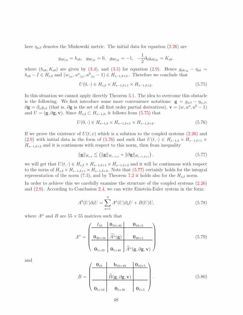
here ηαβ denotes the Minkowski metric. The initial data for equation (2.26) are

gab|M = hab, g0b|M = 0, g00|M = −1, −1

2∂0gab|M = Kab.

where (hab, Kab) are given by (3.4), and (3.5) for equation (2.9). Hence gab|M − ηab =hab − I ∈ Hs,δ and (w|M , u

a|M , u

0|M − 1) ∈ Hs−1,δ+2.. Therefore we conclude that

U(0, ·) ∈ Hs,δ ×Hs−1,δ+1 ×Hs−1,δ+2. (5.75)

In this situation we cannot apply directly Theorem 5.1. The idea to overcome this obstacleis the following. We first introduce some more convenience notations: g = gαβ − ηα,β,∂g = ∂αgγδ (that is, ∂g is the set of all first order partial derivatives), v = (w, ua, u0 − 1)and U = (g, ∂g,v). Since Hs,δ ⊂ Hs−1,δ, it follows from (5.75) that

U(0, ·) ∈ Hs−1,δ ×Hs−1,δ+1 ×Hs−1,δ+2. (5.76)

If we prove the existence of U(t, x) which is a solution to the coupled systems (2.26) and(2.9) with initial data in the form of (5.76) and such that U(t, ·) ∈ Hs−1,δ × Hs−1,δ+1 ×Hs−1,δ+2 and it is continuous with respect to this norm, then from inequality

‖g‖Hs,δ.(‖g‖Hs−1,δ

+ ‖∂g‖Hs−1,δ+1

), (5.77)

we will get that U(t, ·) ∈ Hs,δ ×Hs−1,δ+1 ×Hs−1,δ+2 and it will be continuous with respectto the norm of Hs,δ ×Hs−1,δ+1 ×Hs−1,δ+2. Note that (5.77) certainly holds for the integralrepresentation of the norm (7.3), and by Theorem 7.2 it holds also for the Hs,δ norm.

In order to achieve this we carefully examine the structure of the coupled systems (2.26)and (2.9). According to Conclusion 2.4, we can write Einstein-Euler system in the form:

A0(U)∂tU =

3∑

a=1

Aa(U)∂aU +B(U)U, (5.78)

where Aα and B are 55 × 55 matrices such that

Aα =

I10 010×40 010×5

040×10 Aα(g) 040×5

05×10 05×40 Aα(g, ∂g,v)

(5.79)

and

B =

010 b10×40 010×5

B(g, ∂g,v)

05×10 05×40 05×5

. (5.80)

48

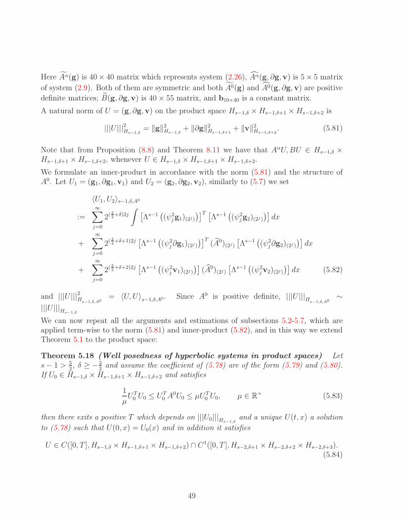
Here Aα(g) is 40× 40 matrix which represents system (2.26), Aα(g, ∂g,v) is 5 × 5 matrix

of system (2.9). Both of them are symmetric and both A0(g) and A0(g, ∂g,v) are positive

definite matrices; B(g, ∂g,v) is 40 × 55 matrix, and b10×40 is a constant matrix.

A natural norm of U = (g, ∂g,v) on the product space Hs−1,δ ×Hs−1,δ+1 ×Hs−1,δ+2 is

|||U |||2Hs−1,δ= ‖g‖2

Hs−1,δ+ ‖∂g‖2

Hs−1,δ+1+ ‖v‖2

Hs−1,δ+2. (5.81)

Note that from Proposition (8.8) and Theorem 8.11 we have that AαU,BU ∈ Hs−1,δ ×Hs−1,δ+1 ×Hs−1,δ+2, whenever U ∈ Hs−1,δ ×Hs−1,δ+1 ×Hs−1,δ+2.

We formulate an inner-product in accordance with the norm (5.81) and the structure ofA0. Let U1 = (g1, ∂g1,v1) and U2 = (g2, ∂g2,v2), similarly to (5.7) we set

〈U1, U2〉s−1,δ,A0

:=∞∑

j=0

2( 32+δ)2j

∫ [Λs−1

((ψ2

jg1)(2j)

)]T [Λs−1

((ψ2

jg2)(2j)

)]dx

+

∞∑

j=0

2( 32+δ+1)2j

[Λs−1

((ψ2

j∂g1)(2j)

)]T(A0)(2j)

[Λs−1

((ψ2

j∂g2)(2j )

)]dx

+∞∑

j=0

2( 32+δ+2)2j

[Λs−1

((ψ2

jv1)(2j)

)](A0)(2j)

[Λs−1

((ψ2

jv2)(2j)

)]dx (5.82)

and |||U |||2Hs−1,δ,A0= 〈U,U〉s−1,δ,A0. Since A0 is positive definite, |||U |||Hs−1,δ,A0

∼|||U |||Hs−1,δ

We can now repeat all the arguments and estimations of subsections 5.2-5.7, which areapplied term-wise to the norm (5.81) and inner-product (5.82), and in this way we extendTheorem 5.1 to the product space:

Theorem 5.18 (Well posedness of hyperbolic systems in product spaces) Lets− 1 > 5

2, δ ≥ −3

2and assume the coefficient of (5.78) are of the form (5.79) and (5.80).

If U0 ∈ Hs−1,δ ×Hs−1,δ+1 ×Hs−1,δ+2 and satisfies

1

µUT

0 U0 ≤ UT0 A

0U0 ≤ µUT0 U0, µ ∈ R

+ (5.83)

then there exits a positive T which depends on |||U0|||Hs−1,δand a unique U(t, x) a solution

to (5.78) such that U(0, x) = U0(x) and in addition it satisfies

U ∈ C([0, T ], Hs−1,δ ×Hs−1,δ+1 ×Hs−1,δ+2) ∩ C1([0, T ], Hs−2,δ+1 ×Hs−2,δ+2 ×Hs−2,δ+3).(5.84)

49

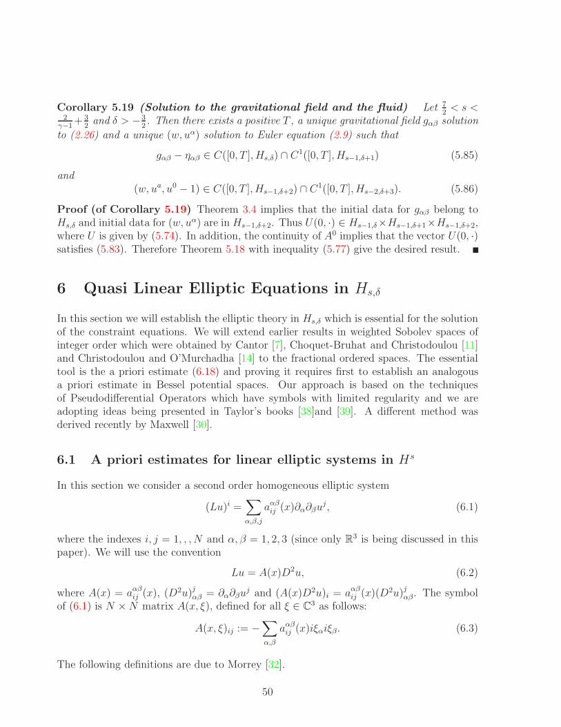
Corollary 5.19 (Solution to the gravitational field and the fluid) Let 72< s <

2γ−1

+ 32

and δ > −32. Then there exists a positive T , a unique gravitational field gαβ solution

to (2.26) and a unique (w, uα) solution to Euler equation (2.9) such that

gαβ − ηαβ ∈ C([0, T ], Hs,δ) ∩ C1([0, T ], Hs−1,δ+1) (5.85)

and(w, ua, u0 − 1) ∈ C([0, T ], Hs−1,δ+2) ∩ C1([0, T ], Hs−2,δ+3). (5.86)

Proof (of Corollary 5.19) Theorem 3.4 implies that the initial data for gαβ belong toHs,δ and initial data for (w, uα) are in Hs−1,δ+2. Thus U(0, ·) ∈ Hs−1,δ×Hs−1,δ+1×Hs−1,δ+2,where U is given by (5.74). In addition, the continuity of A0 implies that the vector U(0, ·)satisfies (5.83). Therefore Theorem 5.18 with inequality (5.77) give the desired result.

6 Quasi Linear Elliptic Equations in Hs,δ

In this section we will establish the elliptic theory in Hs,δ which is essential for the solutionof the constraint equations. We will extend earlier results in weighted Sobolev spaces ofinteger order which were obtained by Cantor [7], Choquet-Bruhat and Christodoulou [11]and Christodoulou and O’Murchadha [14] to the fractional ordered spaces. The essentialtool is the a priori estimate (6.18) and proving it requires first to establish an analogousa priori estimate in Bessel potential spaces. Our approach is based on the techniquesof Pseudodifferential Operators which have symbols with limited regularity and we areadopting ideas being presented in Taylor’s books [38]and [39]. A different method wasderived recently by Maxwell [30].

6.1 A priori estimates for linear elliptic systems in Hs

In this section we consider a second order homogeneous elliptic system

(Lu)i =∑

α,β,j

aαβij (x)∂α∂βuj, (6.1)

where the indexes i, j = 1, , , N and α, β = 1, 2, 3 (since only R3 is being discussed in this

paper). We will use the convention

Lu = A(x)D2u, (6.2)

where A(x) = aαβij (x), (D2u)jαβ = ∂α∂βuj and (A(x)D2u)i = aαβij (x)(D2u)jαβ. The symbol

of (6.1) is N ×N matrix A(x, ξ), defined for all ξ ∈ C3 as follows:

A(x, ξ)ij := −∑

α,β

aαβij (x)iξαiξβ. (6.3)

The following definitions are due to Morrey [32].

50

Definition 6.1

1. The system (6.1) is elliptic provided that

det (A(x, ξ)) = det

(∑

α,β

aαβij (x)ξαξβ

)6= 0, for all 0 6= ξ ∈ R

3; (6.4)

2. The system (6.1) is strongly elliptic provided that for some positive λ

〈A(x, ξ)η, η〉 =∑

α,β,i,j

aαβij (x)ξαξβηiηj ≥ λ|ξ|2|η|2. (6.5)

Our main task is to obtain a priori estimate in the Bessel potential spaces Hs for theoperator (6.1) whose coefficients aijαβ belong to Hs2. In case s and s2 are integers, thenone may prove (6.8) below by means of induction and the classical results of Douglas andNirenberg [15], and Morrey [32]. We will employ techniques of Pseudodifferential calculus.

If the coefficients of the matrix A belongs to Hs2, then A(x, ξ) ∈ Hs2S21,0, that is,

‖∂αξ A(·, ξ)‖Hs2 ≤ Cα(1 + |ξ|2)(2−|α|)/2). We follow Taylor and decompose

A(x, ξ) = A#(x, ξ) + Ab(x, ξ) (6.6)

in such way that a good parametrix can be constructed for A#(x, ξ), while Ab(x, ξ) willhave order less than 2. According to Proposition 8.2 in [39], for s2 >

32

there is 0 < δ < 1such that

A#(x, ξ) ∈ S21,δ, Ab(x, ξ) ∈ Hs2S2−σδ

1,δ , σ = s2 −3

2

where A#(x, ξ) =∑∞

k=0 JǫkA(x, ξ)φk(ξ), ǫk = c2−kδ. Here φk is the Littlewood-Paleypartition of unity, that is, φ0 ∈ C∞

0 (R3), φ0(0) = 1, φk(ξ) = φ0(2−kξ) − φ0(2

−k+1ξ) and∑∞k=0 φk(ξ) = 1. The smoothing operator Jǫ is defined as follows:

Jǫf(x) = φ0(ǫD)f(x) =

(1

2π

) 32∫ǫ−3φ0(

y

ǫ)f(x− y)dy,

where φ0 is the inverse Fourier transform. In order that A# will have a good parametrix weneed to verify that it is a strongly elliptic. Since the original operator is strongly elliptic,

∑

α,β,i,j

Jǫkaαβij (x)φk(ξ)ξαξβη

iηj

=

(1

2π

) 32∫ (∑

α,β,i,j

ǫ−3k φ0(

y

ǫk)(y)aαβij (y − x)φk(ξ)ξαξβη

iηj

)dy

≥(

1

2π

) 32

λφk(ξ)|ξ|2|η|2∫ǫ−3k φ0(

y

ǫk)dy = λφk(ξ)|ξ|2|η|2φ0(0)

= λφk(ξ)|ξ|2|η|2

51

for each fixed k. Summing over the k we have,

〈A#(x, ξ)η, η〉 =∞∑

k=0

∑

α,β,i,j

(Jǫka

αβij

)(x)φk(ξ)ξαξβη

iηj ≥∞∑

k=0

λφk(ξ)|ξ|2|η|2 = λ|ξ|2|η|2,

thus (6.5) holds for A#. The last step assures that ‖A#(x, ξ)−1‖ ≤ 1λ|ξ|2

and then it follows

from the identity ∂(A−1) = A−1(∂(A))A−1 that

‖∂βx∂αξ (A#(x, ξ))−1‖ ≤ Cαβ(1 + |ξ|2)(−2−|α|+δ|β|)/2,

that is, (A#(x, ξ))−1 ∈ S−21,δ . Hence, the operator A#(x,D) has a parametrix E#(x,D) ∈

OPS−21,δ satisfying

E#(x,D)A#(x,D) = I + S, (6.7)

where S ∈ OPS−∞ (See e. g. [38] Section 0.4).

Lemma 6.2 (An a priori estimates in Hs) Let Lu = A(x)D2u be a strongly ellipticsystem and assume A ∈ Hs2, s2 >

32

and 0 ≤ s− 2 ≤ s2. Then there is a constant C suchthat

‖u‖Hs ≤ C ‖Lu‖Hs−2 + ‖u‖Hs−2 . (6.8)

Proof (of Lemma 6.2) We decompose A(x,D) as in (6.2) and let E#(x,D) be the aboveparametrix, then by (6.7)

E#(x,D)A(x,D)u = u+ Su+ E#(x,D)Ab(x,D)u. (6.9)

Since E#(x,D), S : Hs−2 → Hs are bounded,

‖E#(x,D)A(x,D)u‖Hs = ‖E#(x,D)Lu‖Hs ≤ C‖Lu‖Hs−2 (6.10)

and‖Su‖Hs ≤ C‖u‖Hs−2. (6.11)

According to [39] Proposition 8.1, (see also [38] Proposition 2.1.J)

Ab(x,D) : Hs−σδ → Hs−2.

Hence,‖E#(x,D)Ab(x,D)u‖Hs ≤ C‖Ab(x,D)u‖Hs−2 ≤ C‖u‖Hs−σδ . (6.12)

Using the intermediate estimate ‖u‖Hs−σδ ≤ ǫ‖u‖Hs + C(ǫ)‖u‖Hs−2 , and combining itwith(6.9)- (6.11), we obtain the estimate (6.8).

52

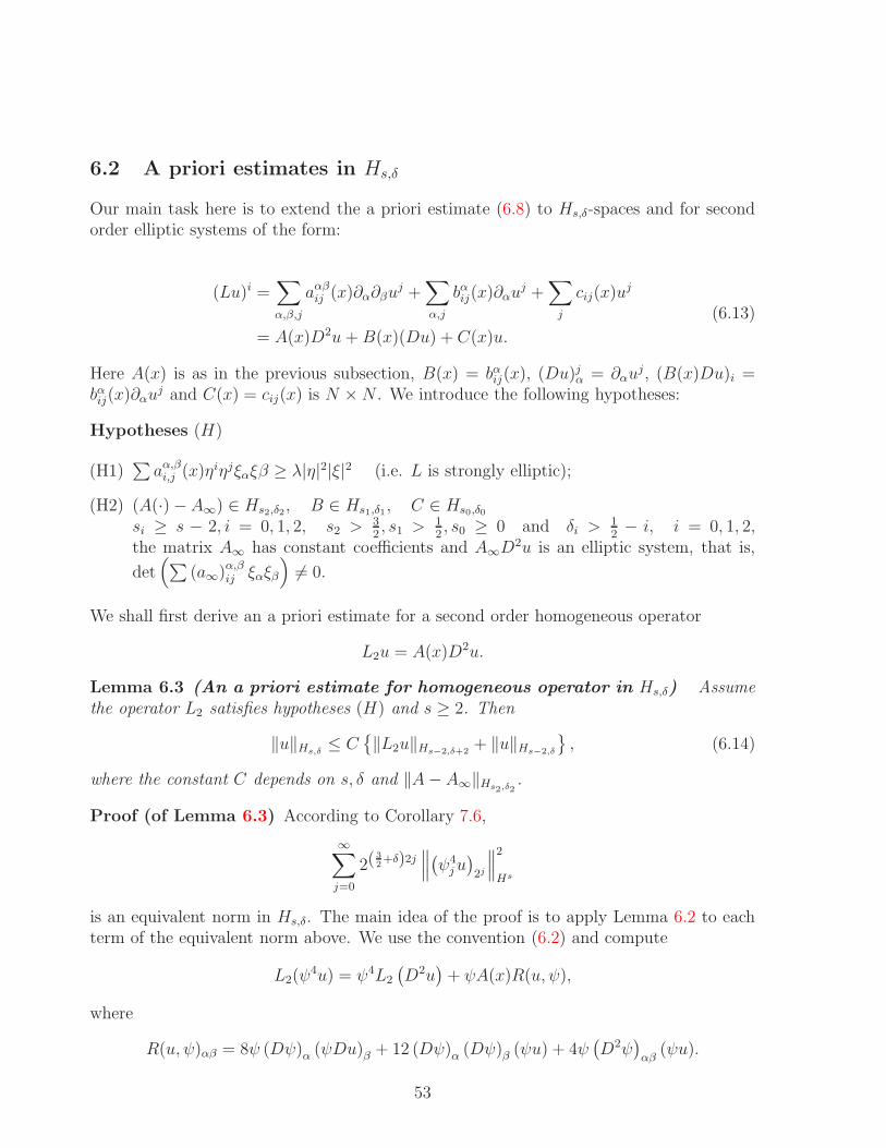
6.2 A priori estimates in Hs,δ

Our main task here is to extend the a priori estimate (6.8) to Hs,δ-spaces and for secondorder elliptic systems of the form:

(Lu)i =∑

α,β,j

aαβij (x)∂α∂βuj +∑

α,j

bαij(x)∂αuj +∑

j

cij(x)uj

= A(x)D2u+B(x)(Du) + C(x)u.

(6.13)

Here A(x) is as in the previous subsection, B(x) = bαij(x), (Du)jα = ∂αuj, (B(x)Du)i =

bαij(x)∂αuj and C(x) = cij(x) is N ×N . We introduce the following hypotheses:

Hypotheses (H)

(H1)∑aα,βi,j (x)ηiηjξαξβ ≥ λ|η|2|ξ|2 (i.e. L is strongly elliptic);

(H2) (A(·) −A∞) ∈ Hs2,δ2, B ∈ Hs1,δ1, C ∈ Hs0,δ0

si ≥ s − 2, i = 0, 1, 2, s2 > 32, s1 > 1

2, s0 ≥ 0 and δi >

12− i, i = 0, 1, 2,

the matrix A∞ has constant coefficients and A∞D2u is an elliptic system, that is,

det(∑

(a∞)α,βij ξαξβ

)6= 0.

We shall first derive an a priori estimate for a second order homogeneous operator

L2u = A(x)D2u.

Lemma 6.3 (An a priori estimate for homogeneous operator in Hs,δ) Assumethe operator L2 satisfies hypotheses (H) and s ≥ 2. Then

‖u‖Hs,δ≤ C

‖L2u‖Hs−2,δ+2

+ ‖u‖Hs−2,δ

, (6.14)

where the constant C depends on s, δ and ‖A− A∞‖Hs2,δ2.

Proof (of Lemma 6.3) According to Corollary 7.6,

∞∑

j=0

2(32+δ)2j

∥∥∥(ψ4ju)2j

∥∥∥2

Hs

is an equivalent norm in Hs,δ. The main idea of the proof is to apply Lemma 6.2 to eachterm of the equivalent norm above. We use the convention (6.2) and compute

L2(ψ4u) = ψ4L2

(D2u

)+ ψA(x)R(u, ψ),

where

R(u, ψ)αβ = 8ψ (Dψ)α (ψDu)β + 12 (Dψ)α (Dψ)β (ψu) + 4ψ(D2ψ

)αβ

(ψu).

53

Applying the a priori estimate (6.8), we have

‖u‖2Hs,δ

.

∞∑

j=0

2(32+δ)2j

∥∥∥(ψ4ju)2j

∥∥∥2

Hs

.

∞∑

j=0

2(32+δ)2j

∥∥∥L2

((ψ4

ju))2j

∥∥∥2

Hs−2+∥∥∥(ψ4ju)2j

∥∥∥2

Hs−2

.

∞∑

j=0

2(32+δ)2j

24j∥∥∥(ψ4jL2(u)

)2j

∥∥∥2

Hs−2+∥∥∥(ψ4ju)2j

∥∥∥2

Hs−2

+

∞∑

j=0

2(32+δ+2)2j

∥∥(ψjAR(u, ψj))2j

∥∥2

Hs−2

. ‖L2(u)‖2Hs−2,δ+2

+ ‖u‖2Hs−2,δ

+ ‖AR‖2Hs−2,δ+2

. (6.15)

The assumption on s2 and δ2 enable us to use Proposition 8.8 and get

‖AR‖Hs−2,δ+2≤ C

(‖(A−A∞)R‖Hs−2,δ+2

+ ‖A∞R‖Hs−2,δ+2

)

≤ C(‖(A−A∞)‖Hs2,δ2

+ ‖A∞‖)‖R‖Hs−2,δ+2

.(6.16)

Property (7.4) of ψj and inequality (8.32) imply

‖(ψjR)2j‖Hs−2 ≤ C(2−j‖(ψjDu)2j‖Hs−2 + 2−2j‖(ψju)2j‖Hs−2

)

and hence ‖R‖Hs−2,δ+2≤ C

(‖u‖Hs−1,δ

+ ‖u‖Hs−2,δ

). Thus, inequalities (6.15) and (6.16)

yields

‖u‖Hs,δ≤ C

‖L2u‖Hs−2,δ+2

+(‖A−A∞‖Hs2,δ2

+ 1) (

‖u‖Hs−1,δ + ‖u‖Hs−2,δ

). (6.17)

Invoking the intermediate estimate ‖u‖Hs−1,δ ≤√

2ǫ‖u‖Hs,δ +C(ǫ)‖u‖Hs−2,δ (see Proposi-

tion 8.6) and taking ǫ so that C(‖A−A∞‖Hs2,δ2

+ 1)√

2ǫ ≤ 12, we obtain from (6.17) the

desired estimate (6.14).

Lemma 6.4 (An a priori estimate in Hs,δ) Assume the operator L of the form(6.13) satisfies hypotheses (H) and s ≥ 2. Then

‖u‖Hs,δ≤ C

‖Lu‖Hs−2,δ+2

+ ‖u‖Hs−2,δ

, (6.18)

where the constant C depends on s, δ and the coefficients of L.

Proof (of Lemma 6.4) By Lemma 6.3,

‖u‖Hs,δ≤ C

‖L2u‖Hs−2,δ+2

+ ‖u‖Hs−2,δ

≤ C‖Lu‖Hs−2,δ+2

+ ‖u‖Hs−2,δ+ ‖(L− L2)u‖Hs−2,δ+2

,

54

where (L − L2)u = B(x)(Du) + C(x)u. Hypothesis (H2) together with Corollary 8.2 andProposition 8.8 give

‖B(x)(Du)‖Hs−2,δ+2. ‖B‖Hs1,δ1

‖Du‖Hs−2,δ+1. ‖B‖Hs1,δ1

‖u‖Hs−1,δ, (6.19)

and‖C(x)u‖Hs−2,δ+2

. ‖C|‖Hs0,δ0‖u‖Hs−2,δ

.

Finally, we apply the intermediate estimate, Proposition 8.6, to the right hand side of(6.19) and by taking ǫ sufficiently small we obtain (6.18).

Lemma 6.5 (Isomorphism of an operator with constant coefficients) LetA∞u := A∞D

2u be a homogeneous elliptic system with constant coefficients. Then for anys ≥ 2 and −3

2< δ < −1

2, the operator A∞ : Hs,δ+2 → Hs−2,δ is isomorphism satisfying

‖u‖Hs,δ≤ C‖A∞D

2u‖Hs−2,δ+2. (6.20)

Proof (of Lemma 6.5) Both statements are true when s is an integer and under thenorm (7.1) (see e. g. [11], Theorem 5.1) and by Theorem 7.2 they hold also in the Hs,δ

norm (3.1). For s between two integers m0 and m1, we have s = sθ = θm0 + (1 − θ)m1

and s − 2 = sθ − 2 = θ(m0 − 2) + (1 − θ)(m1 − 2), where 0 < θ < 1. The interpolationTheorem 8.1 implies

Hs,δ = [Hm0,δ, Hm1,δ]θ and Hs−2,δ = [Hm0−2,δ, Hm1−2,δ]θ.

Since A−1∞ : Hmi−2,δ → Hmi,δ+2, i = 0, 1, is continuous, it follows from interpolation theory

that A−1∞ : Hsθ−2,δ → Hsθ,δ+2 is also continuous (see e. g. [41]). Hence (6.20) holds.

The next lemma improves the a priori estimate (6.18).

Lemma 6.6 (Improved a priori estimate) Let L be an elliptic operator of the form(6.13) which satisfies hypotheses (H). Assume s ≥ 2 and −3

2< δ < −1

2. Then for any δ′

there is a constant C such that

‖u‖Hs,δ≤ C

‖Lu‖Hs−2,δ+2

+ ‖u‖Hs−1,δ′

. (6.21)

The constant C depends on the Hsi,δi-norm of the coefficients of L, s, δ and δ′.

Proof (of Lemma 6.6) Let χR ∈ C∞0 (R3) be a cut-off function satisfying supp(χR) ⊂

|x| ≤ 2R, χR(x) = 1 for |x| ≤ R, 0 ≤ χR(x) ≤ 1 and ‖∂αχR‖∞ ≤ CαR−|α|. For u ∈ Hs,δ

we writeu = (1 − χR)u+ χRu

and R will be determinate later on. We start with the estimation of ‖(1 − χR)u‖Hs,δand

for that purpose we use the convention (6.2) and compute

A∞(D2(1 − χR)u) = (1 − χR)A∞(D2u) − 2A∞(DχR)(Du) −A∞(D2χR)u

= (1 − χR)(Lu) + E1 + E2,(6.22)

55

whereE1 = −(1 − χR)

(A− A∞) (D2u) +B(x)(Du) + C(x)u

andE2 = −

2A∞(DχR)(Du) + A∞(D2χR)u

Applying inequality (6.20) of Lemma 6.5,

‖(1 − χR)u‖Hs,δ≤ C‖A∞D

2((1 − χR)u)‖Hs−2,δ+2

≤ C‖(1 − χR)Lu‖Hs−2,δ+2

+ ‖E1‖Hs−2,δ+2+ ‖E2‖Hs−2,δ+2

.

(6.23)

Since ‖(1 − χR)Lu‖Hs−2,δ+2. ‖Lu‖Hs−2,δ+2

(see Proposition 8.4), it remains to estimate‖E1‖Hs−2,δ+2

and ‖E2‖Hs−2,δ+2. We may choose δ′i so that δi > δ′i >

12− i, i = 0, 1, 2 and

then we put γ = mini=0,1,2(δi − δ′i). Under these conditions the application of Corollary8.2, Propositions 8.5 and 8.8 yield

‖E1‖Hs−2,δ+2≤ C

∥∥(1 − χR)(A− A∞) (D2u) +B(Du) + Cu

∥∥Hs−2,δ+2

≤ C‖(1 − χR)(A− A∞)‖Hs2,δ′2

‖D2u‖Hs−2,δ+2

+ ‖(1 − χR)B‖Hs1,δ′1

‖Du‖Hs−1,δ+1+ ‖(1 − χR)C‖Hs0,δ′

‖u‖Hs,δ

≤ C1

Rγ

(‖(A−A∞)‖Hs2,δ2

+ ‖B‖Hs1,δ1+ ‖C‖Hs0,δ0

)‖u‖Hs,δ

≤ C1Λ

Rγ‖u‖Hs,δ

,

(6.24)

where Λ =(‖A− A∞‖Hs2,δ2

+ ‖B‖Hs1,δ2+ ‖C‖Hs0,δ0

).

Next, since DχR has compact support, Remark 8.3 and Corollary 8.2 imply that

‖E2‖Hs−2,δ+2≤ C(R)

‖2A∞((DχR)(Du))‖Hs−2,δ′+1

+ ‖A∞((D2χR)u)‖Hs−2,δ′

≤ C(R)‖A∞‖

2‖Du‖Hs−2,δ′+1+ ‖u‖Hs−2,δ′

≤ C(R)‖A∞‖‖u‖Hs−1,δ′.

(6.25)

We turn now to the estimation of ‖χRu‖Hs,δ. Noting that (χRu) has compact support, we

have by Remark 8.3, (6.18) and Proposition 8.4 that

‖χRu‖Hs,δ≤ C(R)‖χRu‖Hs,δ′

≤ C(R)‖L(χRu)‖Hs−2,δ′+2+ ‖u‖Hs−1,δ′

. (6.26)

Similarly to (6.22) we compute

L(χRu) = χRL(u) + 2A(DχR)(Du) + A(D2χR)u+B(DχR)u. (6.27)

We estimate each term of (6.27) separately. Once again, since χRLu has compact support,

‖χR(Lu)‖Hs−2,δ′+2≤ C(R)‖Lu‖Hs−2,δ+2

. (6.28)

56

Next, using the second assumption of (H), Proposition 8.8 and the compactness ofsupp(χR) we get

‖2A(DχR)(Du)‖Hs−2,δ′+2

≤ 2‖(A−A∞)(DχR)(Du)‖Hs−2,δ′+2+ ‖A∞(DχR)(Du)‖Hs−2,δ′+2

≤ C(‖(A− A∞)‖Hs2,δ2

+ ‖A∞‖)‖(DχR)(Du)‖Hs−2,δ′+2

≤ C(R)(‖(A− A∞)‖Hs2,δ2

+ ‖A∞‖)‖Du‖Hs−2,δ′+1

≤ C(R)(‖(A− A∞)‖Hs2,δ2

+ ‖A∞‖)‖u‖Hs−1,δ′

.

(6.29)

In a similar manner we estimate the other terms and together with inequalities (6.23)–(6.26),(6.28) and (6.29) we have

‖u‖Hs,δ≤ ‖(1 − χR)u‖Hs,δ

+ ‖χRu‖Hs,δ

≤ C

‖Lu‖Hs−2,δ+2

+ C2‖u‖Hs−1,δ′+C1Λ

Rγ‖u‖Hs,δ

,

(6.30)

where C1 and C2 depend on the norms of the coefficients of L and in addition C2 dependsin R. We now take R such that C1Λ

Rγ ≤ 12, then (6.21) follows from (6.30).

The next two theorems are consequence of the compact embedding, Theorem 8.14, the apriori estimate (6.21) and standard arguments of Functional Analysis.

Theorem 6.7 (Semi Fredholm) Assume the operator L satisfies hypotheses(H), s ≥ 2and −3

2< δ < −1

2. Then L : Hs,δ → Hs−2,δ+2 is semi Fredholm, that is,

(i) dim(KerL) <∞;

(ii) If L is injective, then there is a constant C such that

‖u‖Hs,δ≤ C‖Lu‖Hs−2,δ+2

; (6.31)

(iii) L has a closed range.

Theorem 6.8 (A homotopy argument) Let s ≥ 2 and −32< δ < −1

2. Assume

L be an elliptic operator of the form (6.13) that fulfilled the hypotheses (H) and Lt is acontinuous family of operators which satisfy hypotheses (H) for t ∈ [0, 1], L1 = L and

Lt : Hs,δ → Hs−2,δ+2 is injective.

IfL0 : Hs,δ → Hs−2,δ+2 is an isomorphism,

then the same is true for L.

57

The next Lemma shows that solutions to the homogeneous system have lower growth atinfinity. We follow Christodoulou and O’Murchadha’s proof [14].

Lemma 6.9 (Lower growth of homogeneous solutions) Assume L satisfies hy-potheses (H), u ∈ Hs,δ, s ≥ 2 and −3

2< δ < −1

2. If Lu = 0, then u ∈ Hs,δ′ for any

−32< δ′ < −1

2.

Proof (of Lemma 6.9) We recall that if δ′ < δ, then it follows from Remark 7.4 thatHs,δ → Hs,δ′ . Hence it suffices to show the statement for δ′ > δ. The conditions on δiimply that we may find δ′ > δ so that δi+δ+ i > δ′+2− 3

2. Then applying the Proposition

8.8 tof := A∞u− Lu = (A∞ −A(x))

(D2u

)−B(x)(Du) − C(x)u,

we obtain that f belongs to Hs−2,δ′+2. Now Lu = 0, so A∞u = f and since A∞ : Hs,δ′ →Hs−2,δ′+2 is isomorphism by Lemma 6.5, we conclude that hence u ∈ Hs,δ′ . We now replaceδ by δ′ repeat the above arguments.

6.3 Semi Linear Elliptic Equations on Asymptotically Flat Man-ifolds

A Riemannian 3-manifold (M,h) is asymptotically flat (AF) if there is a compact subsetK such that M \K is diffeomorphic to R3 \B1(0) and the metric h tends to the identity Iat infinity. A natural definition of the last statement in our case is h− I ∈ Hs′,δ′ . We willhence assume here that h− I ∈ Hs′,δ′ , s

′ > 32

and δ′ > −32.

We denote by ∆h be the Laplace-Beltrami operator on (M,h). In the coordinates(x1, x2, x3) it takes the form

∆h =1√|h|∂j

(√|h|hij∂i

), (6.32)

where |h| = det(hij) and hij = (hij)−1. Inserting the identity ∂j |h| = |h|tr(hij(∂j(hij)) into

(6.32), we have

∆h = hij∂j∂i + ∂j(hij)∂i +

1

2tr(hij(∂j(hij))h

ij∂i. (6.33)

Hence, by means of Proposition 8.8, Theorem 8.11 and Remark 8.12, the elliptic operator(6.33) satisfies hypothesis (H) of Section 6.2 provided that s ≤ s′.

Let us introduce some more notations. We denote by µh =√|h|dx the Lebesgue measure

on the manifold (M,h), (Du ·Dv)h = hij∂iu∂jv, and ‖Du‖2h = (Du ·Du)h. Integration by

parts yields∫

(∆hu) vdµh =

∫∂j

(√|h|hij∂iu

)vdx

= −∫hij∂iu∂jv

√|h|dx = −

∫(Du ·Dv)hdµh.

(6.34)

58

Formula (6.34) holds whenever v ∈ H10 (R3), u ∈ Hs,δ and s ≥ 1. Therefore it enables us

to define weak solutions on the manifold (M,h).

Definition 6.10 (Weak solutions) A function u in Hs,δ is a weak solution of

−∆hu+ c(x)u = f ∈ Hs−2,δ+2

on (M,h), if ∫((Du ·Dv)h + cuv)dµh =

∫fvdµh, (6.35)

for all v ∈ H10 (R3).

Remark 6.11 In case u, v ∈ Hs,δ, s ≥ 2 and δ ≥ −1, then by algebra hij∂iu,√|h|∂jv ∈

Hs−1,0 (see subsection 8.1). Applying the Cauchy Schwarz inequality∫

|(Du ·Dv)h|dµh =

∫|hij∂iu∂jv|

√|h|dx

≤(∫

(hij∂iu)2

) 12(∫ √

|h|∂jv)2

) 12

≤ ‖hij∂iu‖Hs−1,0‖√|h|∂jv‖Hs−1,0 ,

we see that hij∂iu∂jv|√|h| ∈ L1(R3). Similarly, the integrand of the left hand side of (6.34)

belongs to L1(R3). Hence, approximating u and v by C∞0 functions and using Lebesgue’s

Dominated Convergence Theorem we have∫

(∆hu) vdµh = −∫

(Du ·Dv)hdµh, u, v ∈ Hs,δ, whenever s ≥ 2, and δ ≥ −1. (6.36)

In this section we will prove existence and uniqueness for the semi-linear equation

− ∆hu = F (x, u) :=N∑

i=1

mi(x)hi(u), (6.37)

where mi ∈ Hs0,δ0, mi(x) ≥ 0, s0 ≥ 0, δ0 > 12

and for u > −1 the functions hi aredecreasing, nonnegative and smooth. These conditions ensure F (·, u) and ∂F

∂p(·, u) are in

Hs−2,δ+2 whenever u ∈ Hs,δ and s ≥ 2.

Theorem 6.12 (Existence and uniqueness) Let h − I ∈ Hs′,δ′, s′ > 3

2, δ′ > −3

2,

2 ≤ s ≤ s′ and −32< δ < −1

2. Then equation (6.37) has a unique solution u in Hs,δ.

Furthermore, 0 ≤ u ≤ K for a nonnegative constant K.

In order to show Theorem 6.12 we need the weak maximal principle:

Proposition 6.13 (Weak maximal principle) Assume c ∈ Hs′−2,δ′+2 is nonnegative.If u ∈ Hs,δ satisfies

− ∆hu+ cu ≤ 0, (6.38)

then u ≤ 0.

59

Proof (of Proposition 6.13) For ǫ > 0 we put w = max(u − ǫ, 0). It has compactsupport since limx→∞ u(x) = 0. Further, Dw = Du a.e. in u(x) > ǫ (see e. g. [18] or[26]. Thus, w ∈ H1

0 (R3) and w ≥ 0, so by (6.35)

0 ≥∫

((Du,Dw)h + cuw)dµh =

∫

u≥ǫ

(‖Du‖2

h + cu2)dµh.

Therefore u ≡ ǫ in u(x) ≥ ǫ. Since ǫ is arbitrary, we have u ≤ 0.

Proof (of Existence) The proof will be done in several steps. We define a map Φ :Hs,δ × [0, 1], u(x) > −1 → Hs−2,δ+2 by

Φ(u, τ) = −∆hu− τF (x, u),

let u(τ) denotes a solution of Φ(u, τ) = 0 and put J = 0 ≤ s ≤ 1 : Φ(u(s), s) = 0. Wewill show that J is both open and closed set. Since 0 ∈ J , J = [0, 1] which yields theexistence result.

Step 1. The set J is open.

Let

Lw :=

(∂Φ

∂u(u, τ)

)(w) = −∆hw − τ

∂F

∂p(·, u)w

and

Ltw = −∆th+(1−t)Iw − tτ∂F

∂p(·, u)w.

If Ltw = 0, then by Lemma (6.9) w ∈ Hs,−1. So we may use (6.36) and get

∫(Ltw)wdµth+(1−t)I =

∫ (‖Dw‖2

th+(1−t)I − tτ∂F

∂p(·, u)w2

)dµth+(1−t)I.

Since ∂F∂p

≤ 0, the above yields that Ltw = 0 implies w ≡ 0 for each t ∈ [0, 1]. In additionL0 = −∆I = −∆ is an isomorphism according to Lemma 6.5. Therefore Theorem 6.8implies that L1 = L is an isomorphism too. Thus J is open by the Implicit FunctionTheorem.

Step 2. ‖u(τ)‖Hs,δ≤ C for a constant C independent of τ .

We first establish the bound in H2,δ-norm. The weak maximum principle implies u(τ) ≥ 0and since F (x, p) is decreasing in p,

‖F (·, u(τ))‖H0,δ+2≤ ‖F (·, 0)‖H0,δ+2

≤(

N∑

i=1

hi(0)2‖mi‖2H0,δ+2

) 12

:= K.

We showed in Step 1 that ∆h : Hs,δ → Hs−2,δ+2 is injective, therefore from Theorem 6.7(ii),

‖u(τ)‖H2,δ≤ C‖ − ∆hu(τ)‖H0,δ+2

≤ C‖F (·, 0)‖H0,δ+2≤ CK. (6.39)

60

Now, Theorem 8.11 implies ‖hi(u(τ))‖H2,δ≤ C‖(u(τ))‖H2,δ

and by Proposition 8.8,‖F (·, u(τ))‖H2,δ

≤ C‖u(τ)‖H2,δ. In order to improve (6.39), we take s′′ so that s′′ − 2 ≤ 2

and s′′ ≤ s. Then we may apply again (6.31) and combine it with (6.39) and Remark 7.4,we have

‖u(τ)‖Hs′′,δ≤ C‖ − ∆hu(τ)‖Hs′′−2,δ+2

≤ C‖ − ∆hu(τ)‖H2,δ+2

= C‖F (·, u(τ))‖H2,δ≤ C‖u(τ)‖H2,δ

≤ CK.(6.40)

We have proved the boundedness in case s′′ = s, otherwise we can repeat the same pro-cedure as above to improve regularity until we would reach the desired regularity. It isobvious that the bound on ‖u(τ)‖Hs,δ

does not depend on τ .

Step 3. Lipschitz continuity with respect to τ :

Differentiation of the equation Φ(u(τ), τ) = 0 with respect to τ gives

−∆huτ (τ) − τ∂F

∂pF (x, u(τ))uτ(τ) = F (x, u(τ)).

Now ∂F∂pF (x, p) ≤ 0, so in the same way as we did in Step 1 we obtain that the operator

L = −∆h − τ ∂F∂pF (x, u(τ)) : Hs,δ → Hs−2,δ+2 is injective. Hence, by Theorem 6.7 (ii),

‖uτ‖Hs,δ≤ C‖L(uτ )‖Hs−2,δ+2

= C‖F (x, u(τ))‖Hs−2,δ+2. (6.41)

Next, Step 2 implies

‖F (x, u(τ))‖Hs−2,δ+2≤ C‖u(τ)‖Hs,δ

(N∑

i=1

‖mi‖Hs0,δ0

)≤ C. (6.42)

Thus, combining (6.41) with (6.42) we get

‖u(τ1) − u(τ2)‖Hs,δ≤ C|τ1 − τ2|. (6.43)

Step 4. The set J is closed:

Take a sequence τn ⊂ J such that τn → τ0. By (6.43), u(τn) is Cauchy in Hs,δ

and therefore it converges to u0 ∈ Hs,δ. Since the map Φ is continuous, it follows thatΦ(u0, τ0) = 0, that is τ0 ∈ J . This completes the proof of the existence.

Proof (of Uniqueness) Assume u1 and u2 are solutions to (6.37). We conduct the proofby showing that Ω := x : u1(x) > u2(x) is an empty set. Note that Ω is open since u1

and u2 are continuous. Put w = u1 − u2, then −∆hw = F (x, u1) − F (x, u2) ≤ 0 in Ω.So w ≤ 0 in Ω by Proposition (6.13). That obviously leads to a contradiction unless Ω isempty.

Acknowledgement: The problem we worked out goes back to Alan Rendall and wewould like to thank him for enlightening discussions. The second author would like tothank Victor Ostrovsky for many valuable conversations.

61

Appendix

7 The construction of the Spaces Hs,δ:

The weighted Sobolev spaces of integer order below were introduced by Cantor [6] andindependently by Nirenberg and Walker [33]. Nirenberg and Walker initiate the study ofelliptic operators in these spaces, while Cantor used them to solve the constraint equationson asymptotically flat manifolds. For an nonnegative integer m and a real δ we define anorm (

‖u‖∗m,δ)2

=∑

|α|≤m

∫ (〈x〉δ+|α||∂αu|

)2dx, (7.1)

where 〈x〉 = 1 + |x|. The space Hs,m is the completion of C∞0 (R3) under the norm (7.1).

Note that the weight varies with the derivatives.

Here we will repeat Triebel’s extension of these spaces into a fractional order, [40],[41]. Lets = m+ λ, where m is a nonnegative integer and 0 < λ < 1. One possibility of extendingthe ordinary integer order Sobolev spaces is the Lipschitz-Sobolevskij Spaces, having a norm

‖u‖2m+λ,2 =

∑

|α|≤m

∫|∂αu|2dx+

∑

|α|=m

∫ ∫ |∂αu(x) − ∂αu(y)|2|x− y|3+λ2

dxdy. (7.2)

Hence, a reasonable definition of weighted fractional Sobolev norm is a combination of thenorm (7.1) with (7.2):

(‖u‖∗s,δ

)2=

∑

|α|≤m

∫|〈x〉δ+|α|∂αu|2dx, s = m

∑

|α|≤m

∫|〈x〉δ+|α|∂αu|2dx

+∑

|α|=m

∫ ∫ |〈x〉m+λ+δ∂αu(x) − 〈y〉m+λ+δ∂αu(y)|2|x− y|3+2λ

dxdy

, s = m+ λ.

(7.3)here m is a nonnegative integer and 0 < λ < 1. The space Hs,δ is the completion of C∞

0 (R3)under the norm (7.3).

The norm (7.3) is essential for the understating of the connections between the integerand the fractional order. But it has a disadvantage, namely, the double integral makes italmost impossible to establish any property (embedding, a priori estimate, etc.) neededfor PDEs. We are therefore looking for an equivalent definition of the norm (7.3).

Let Kj = x : 2j−3 ≤ |x| ≤ 2j+2, (j = 1, 2, ...) and K0 = x : |x| ≤ 4. Let ψj∞j=0 ⊂C∞

0 (R3) be a sequence such that ψj(x) = 1 on Kj , supp(ψj) ⊂ x : 2j−4 ≤ |x| ≤ 2j+3, for

62

j ≥ 1, supp(ψ0) ⊂ x : |x| ≤ 23 and

|∂αψj(x)| ≤ Cα2−|α|j, (7.4)

where the constant Cα does not depend on j.

We define now,

(‖u‖⋆

s,δ

)2

=

∞∑

j=0

2δ2j‖ψju‖2

L2 + 2(δ+m)2j∑

|α|=m

‖∂α(ψju)‖2L2

, s = m

∞∑

j=0

2δ2j‖ψju‖2

L2 + 2(δ+m)2j∑

|α|=m

‖∂α(ψju)‖2L2

+∑∞

j=0 2(δ+m+λ)2j(∑

|α|=m

∫ ∫ |∂α(ψju)(x)−∂α(ψju)(y)|2

|x−y|3+2λ dxdy),

s = m+ λ.

(7.5)

Proposition 7.1 (Equivalence of norms) There are two positive constants c0 andc1 depending only on s, δ and the constants in (7.4) such that

c0‖u‖⋆

s,δ ≤ ‖u‖∗s,δ ≤ c1‖u‖⋆

s,δ. (7.6)

This equivalence was proved in [40] (see also [4]).

We express these norms in terms of Fourier transform. Let

u(ξ) = F(u)(ξ) =1

(2π)3

∫u(x)e−ix·ξdx

denotes the Fourier transform, put

Λsu = F−1(1 + |ξ|2) s2Fu), (7.7)

and let Hs denotes the Bessel Potentials space having the norm

‖u‖2Hs = ‖Λsu‖2

L2 =

∫(1 + |ξ|2)s|u(ξ)|2dξ. (7.8)

We also set

‖u‖2hs = ‖F−1(|ξ|sFu)‖2

L2 =

∫(|ξ|s|u(ξ)|)2dξ.

It is well known that (see e. g. [20]; p. 240-241)

‖u‖2hs ≃

∑|α|=m

∫|∂αu|2dx s = m∑

|α|=m

∫ ∫ |∂αu(x)−∂αu(y)|2

|x−y|3+2λ dx s = m+ λ(7.9)

63

and since (1 + |ξ|2)s ≃ (1 + |ξ|s),

‖u‖2Hs ≃

(‖u‖2

L2 + ‖u‖2hs

). (7.10)

Hence, by (7.5),(‖u‖⋆

s,δ

)2

≃∞∑

j=0

(2δ2j‖ψju‖2

L2 + 2(δ+s)2j‖ψju‖2hs

)(7.11)

We invoke now the scaling uǫ(x) := u(ǫx) (ǫ > 0), then simple calculations yields ‖uǫ‖2L2 =

ǫ−3‖u‖2L2 and ‖uǫ‖2

hs = ǫ2s−3‖u‖2hs. Combining the later one with (7.10), we have

‖uǫ‖2Hs ≃ ǫ−3

(‖u‖L2 + ǫ2s‖u‖2

hs

). (7.12)

Setting ǫ = 2j, multiplying (7.12) by 23j and inserting it in (7.11), we conclude

(‖u‖⋆

s,δ

)2

≃∞∑

j=0

2( 32+δ)2j‖(ψju)2j‖2

Hs . (7.13)

The last one is the most convenience form of norm for applications and therefore the righthand side of (7.13) defines the norm of Hs,δ space (see Definition 3.1).

Combining Proposition 7.1 with (7.11) and (7.13) we get:

Theorem 7.2 (Equivalence of norms, Triebel) There are two positive constant c0and c1 depending only on s, δ and the constants in (7.4) such that

c0‖u‖Hs,δ ≤ ‖u‖∗s,δ ≤ c1‖u‖Hs,δ. (7.14)

Remark 7.3 Theorem 7.2 enables us to use both sorts of the norms (7.3) and (3.1), andfor each application we will use the suitable type of norm.

Remark 7.4 Let s′ ≤ s and δ′ ≤ δ, then the inclusion Hs,δ → Hs′,δ′ follows easily fromthe representations (7.8) and (3.1) of the norms.

Remark 7.5 The functions ψj are constructed by means of a composition of exponentialfunctions. Hence, for any positive γ there holds

c1(γ, α)|∂αψγj (x)| ≤ |∂αψj(x)| ≤ c2(γ, α)|∂αψγj (x)|. (7.15)

Therefore the equivalence (7.6) remains valid with ψγj replacing ψj and hence

∑

j

2( 32+δ)2j‖(ψγj u)(2j)‖2

Hs ≃(‖u‖⋆

s,δ

)2

≃∑

j

2( 32+δ)2j‖(ψju)(2j)‖2

Hs. (7.16)

Corollary 7.6 (Equivalence of norms) For any positive γ, there are two positiveconstants c0 and c1 depending on s, δ and γ such that

c0‖u‖2Hs,δ

≤∑

j

2( 32+δ)2j‖(ψγj u)(2j)‖2

Hs ≤ c1‖u‖2Hs,δ

. (7.17)

64

8 Some Properties of Hs,δ

Theorem 8.1 (Complex interpolation, Triebel)

Let 0 < θ < 1, 0 ≤ s0 < s1 and sθ = θs0 + (1 − θ)s1, then

[Hs0,δ, Hs1,δ]θ = Hsθ,δ, (8.1)

where (8.1) is a complex interpolation.

As a consequence of the interpolation Theorem 8.1 we get

Corollary 8.2 (Hs,δ-norm of a derivative)

‖∂iu‖Hs−1,δ+1≤ ‖u‖Hs,δ

(8.2)

Proof (of Corollary 8.2) Let m be a positive integer and define T : Hm,δ → Hm−1,δ+1

by T (u) = ∂iu. Using the norm (7.1) we see that ‖T (u)‖Hm−1,δ+1≤ ‖u‖Hm,δ

. So (8.2)follows from Theorem 8.1.

Remark 8.3 If supp u ⊂ |x| ≤ R, then for any δ

c1(R)‖u‖Hs ≤ ‖u‖Hs,δ≤ c2(R)‖u‖Hs. (8.3)

This follows from the integral representation of the norm (7.1) and the interpolation (8.1).

Proposition 8.4 (Multiplication by smooth functions)

Let N ≥ s be an integer. Assume f ∈ CN(R3) satisfies sup |Dkf | ≤ K for k = 0, 1, ...N ,then

‖fu‖Hs,δ≤ CsK‖u‖Hs,δ

. (8.4)

Proof (of Proposition 8.4) By the well known property of Hs

‖fu‖Hs ≤ CsK‖u‖Hs (8.5)

we have

‖fu‖2Hs,δ

=

∞∑

j=0

2( 32+δ)2j

∥∥(ψjfu)2j

∥∥2

Hs

≤ (CsK)2∞∑

j=0

2( 32+δ)2j

∥∥(ψju)2j

∥∥2

Hs = (CsK)2‖u‖2Hs,δ

.

(8.6)

65

Proposition 8.5 (Multiplication by cutoff function) Let χR ∈ C∞(R3) satisfiesχR(x) = 1 for |x| ≤ R, χR(x) = 0 for |x| ≥ 2R and |∂αχR| ≤ cαR

−|α|. Then for δ′ < δthere holds

‖(1 − χR)u‖Hs,δ′≤ C(δ, δ′)

Rδ−δ′‖u‖Hs,δ

. (8.7)

Proof (of Proposition 8.5) Let J0 be the smallest integer such that R ≤ 2J0−3. Then(1 − χR)ψj = 0 for j = 0, 1, ..., J0 − 1. Hence

‖(1 − χR)u‖2Hs,δ′

=∞∑

j=J0

2( 32+δ′)2j

∥∥(ψj(1 − χR)u)2j

∥∥2

Hs

≤ C2∞∑

j=J0

2(32+δ′)2j

∥∥(ψju)2j

∥∥2

Hs = C2∞∑

j=J0

2(32+δ)2j2(δ′−δ)2j

∥∥(ψju)2j

∥∥2

Hs

≤ C22(δ′−δ)2J0

∞∑

j=0

2( 32+δ)2j

∥∥(ψju)2j

∥∥2

Hs ≤C2

(8R)(δ−δ′)2‖u‖2

Hs,δ.

(8.8)

Proposition 8.6 (An intermediate estimate) Let 0 ≤ s0 < s < s1 and ε > 0, thenthere is a constant C = C(ε) such that

‖u‖Hs,δ≤

√2ε‖u‖Hs1,δ

+ C‖u‖Hs0,δ, (8.9)

holds for all u ∈ Hs1,δ.

Proof (of Proposition 8.6) Inequality (8.9) is well known in Hs spaces. We apply it toeach term of the norm (3.1) and get

‖u‖2Hs,δ

=

∞∑

j=0

2( 32+δ)2j

∥∥(ψju)2j

∥∥2

Hs

≤ 2ǫ2∞∑

j=0

2( 32+δ)2j

∥∥(ψju)2j

∥∥2

Hs1+ 2C2(ǫ)

∞∑

j=0

2(32+δ)2j

∥∥(ψju)2j

∥∥2

Hs0

= 2ǫ2‖u‖2Hs1,δ

+ 2C2(ǫ)‖u‖2Hs0,δ

,

Proposition 8.7 (An intermediate estimate) Let 0 < s′ < s, then

‖u‖Hs′,δ≤ ‖u‖

s′

s

Hs,δ‖u‖1− s′

s

H0,δ. (8.10)

66

Proof (of Proposition 8.7) Using Holder inequality we get ‖u‖Hs′ ≤ ‖u‖s′

s

Hs‖u‖1− s′

s

L2 andapplying it and using again Holder inequality yields

‖u‖2Hs′,δ

=∑

j

2( 32+δ)2j

∥∥(ψju)2j

∥∥2

Hs′

≤∑

j

2(32+δ)2j

“

s′

s

” ∥∥(ψju)2j

∥∥2 s′

s

Hs 2( 32+δ)2j

“

s−s′

s

” ∥∥(ψju)2j

∥∥2 s−s′

s

L2

≤(∑

j

2(32+δ)2j

∥∥(ψju)2j

∥∥2

Hs

) s′

s(∑

j

2( 32+δ)2j ‖(ψju)‖2

L2

) s−s′

s

=(‖u‖Hs,δ

) 2s′

s(‖u‖H0,δ

) 2(s′−1)s .

8.1 Algebra

Proposition 8.8 (Algebra in Hs,δ)

If s1, s2 ≥ s, s1 + s2 > s + 32

and δ1 + δ2 ≥ δ − 32, then

‖uv‖Hs,δ≤ C‖u‖Hs1,δ1

‖v‖Hs2,δ2. (8.11)

Proof (of Proposition 8.8) By Corollary 7.6,

‖uv‖2Hs,δ

≃∞∑

j=0

2(32+δ)2j

∥∥∥(ψ2juv)2j

∥∥∥2

Hs. (8.12)

We apply the classic algebra property ‖uv‖Hs ≤ C‖u‖Hs1‖v‖Hs2 (see e. g. [38] Ch. 3,Section 5), to each term of the norm (8.12) and then we use Cauchy Schwarz inequality,

‖uv‖2Hs,δ

≤ C∞∑

j=0

2( 32+δ)2j

∥∥∥(ψ2juv)2j

∥∥∥2

Hs

≤ C2

∞∑

j=0

2(32+δ)2j

∥∥(ψju)2j

∥∥2

Hs1

∥∥(ψjv)2j

∥∥2

Hs2

≤ C2∞∑

j=0

(2( 3

2+δ1)2j

∥∥(ψju)2j

∥∥2

Hs1

)(2( 3

2+δ2)2j

∥∥(ψjv)2j

∥∥2

Hs2

)

≤ C2

(∞∑

j=0

(2( 3

2+δ1)2j

∥∥(ψju)2j

∥∥2

Hs1

)2) 1

2(

∞∑

j=0

(2( 3

2+δ2)2j

∥∥(ψjv)2j

∥∥2

Hs2

)2) 1

2

≤ C2

(∞∑

j=0

(2( 3

2+δ1)2j

∥∥(ψju)2j

∥∥2

Hs1

))( ∞∑

j=0

(2( 3

2+δ2)2j

∥∥(ψjv)2j

∥∥2

Hs2

))

≤ C2‖u‖2Hs1,δ1

‖v‖2Hs2,δ2

.

67

8.2 Fractional power |u|γ

In [23] Kateb showed that if u ∈ Hs ∩ L∞, 1 < γ and 0 < s < γ + 12, then

‖|u|γ‖Hs ≤ C(‖u‖L∞)‖u‖Hs. (8.13)

Proposition 8.9 (Fractional power in Hs,δ) Let u ∈ Hs,δ∩L∞, 1 < γ, 0 < s < γ+ 12

and δ ∈ R, then‖|u|γ‖Hs,δ

≤ C(‖u‖L∞)‖u‖Hs,δ. (8.14)

Proof (of Proposition 8.9) Inequality (8.14) is a direct consequence of the Corollary7.6 and (8.13). Because

‖|u|γ‖2Hs,δ ≃

∞∑

j=0

2( 32+δ)2j‖(ψγj |u|γ)(2j )‖2

Hs

≤ (C(‖u‖L∞))2∞∑

j=0

2( 32+δ)2j‖(ψju)(2j)‖2

Hs ≤ (C(‖u‖L∞))2 ‖u‖2Hs,δ

.

(8.15)

8.3 Moser type estimates

Y. Meyer proved the below Moser type estimate [31].See also Taylor [38].

Theorem 8.10 (Third Moser inequality for Bessel potentials spaces)

Let F : Rm → Rl be CN+1 function such that F (0) = 0. Let s > 0 and u ∈ Hs∩L∞. Then

‖F (u)‖Hs ≤ K‖u‖Hs, (8.16)

whereK = KN(F, ‖u‖L∞) ≤ C‖F‖CN+1

(1 + ‖u‖NL∞

), (8.17)

here N is a positive integer such that N ≥ [s] + 1.

We generalize this important inequality to the Hs,δ spaces.

Theorem 8.11 (Third Moser inequality in Hs,δ)

Let F : Rm → Rl be CN+1 function such that F (0) = 0. Let s > 0, δ ∈ R and u ∈ Hs,δ∩L∞.Then

‖F (u)‖Hs,δ≤ K‖u‖Hs,δ

, (8.18)

The constant K in (8.18) depends on one in (8.17) and in addition on δ.

68

Proof (of Theorem 8.11) Let ψj be the sequence satisfying (7.4) and Ψj(x) =1

ϕ(x)ψj(x), where ϕ(x) =

∑∞j=0 ψj(x). From the properties of the sequence ψj, it fol-

lows that 1 ≤ ϕ(x) ≤ 7. So the sequence Ψj ⊂ C∞0 (R3) and

∑∞j=0 Ψj(x) = 1. From

(7.12) we conclude that

‖uǫ‖2Hs ≤ C maxǫ2s−3, ǫ−3‖u‖2

Hs (8.19)

and with the combination of (5.17) and Meyer’s Theorem8.10 we have,

‖F (u)‖2Hs,δ

=∞∑

j=0

2( 32+δ)2j‖(ψj(F (u))(2j)‖2

Hs

=

∞∑

j=0

2( 32+δ)2j

∥∥∥∥∥∥

(ψjF

(∞∑

k=0

Ψk(x)u

))

(2j)

∥∥∥∥∥∥

2

Hs

=∞∑

j=0

2( 32+δ)2j

∥∥∥∥∥∥

(ψjF

(j+3∑

k=j−4

Ψk(x)u

))

(2j)

∥∥∥∥∥∥

2

Hs

≤ CK2∞∑

j=0

2( 32+δ)2j

j+3∑

k=j−4

‖ (Ψku)(2j) ‖2Hs

≤ CK2∞∑

j=0

2( 32+δ)2j

j+3∑

k=j−4

‖ ((Ψku)2j−k)(2k) ‖2Hs

≤ CK2∞∑

j=0

2( 32+δ)2j

j+3∑

k=j−4

max2(2s−3)(j−k), 2−3(j−k)‖ (Ψku)(2k) ‖2Hs

≤ C(s)K2∞∑

j=0

2( 32+δ)2j

j+3∑

k=j−4

‖ (ψku)(2k) ‖2Hs

≤ C(s, δ)K2∞∑

j=0

j+3∑

k=j−4

2( 32+δ)2k‖ (ψku)(2k) ‖2

Hs

≤ 7C(s, δ)K2∞∑

k=0

2( 32+δ)2k‖ (ψku)(2k) ‖2

Hs ≤ 7C(s, δ)K2‖u‖2Hs,δ

.

(8.20)

Remark 8.12 If F (0) 6= 0 and F (0) ∈ Hs,δ, then we can apply Theorem 8.11 to F (u) :=F (u) − F (0) and get

‖F (u)‖Hs,δ≤ ‖F (u)‖Hs,δ

+ ‖F (0)‖Hs,δ≤ K‖u‖Hs,δ

+ ‖F (0)‖Hs,δ. (8.21)

We may apply Theorem 8.11 to the estimate the difference F (u) − F (v).

69

Corollary 8.13 (A difference estimate in Hs,δ) Suppose F is a CN+2 function andu, v ∈ Hs,δ ∩ L∞. Then

‖F (u) − F (v)‖Hs,δ≤ C(‖u‖L∞, ‖v‖L∞)

(‖u‖Hs,δ

+ ‖v‖Hs,δ

)‖u− v‖Hs,δ

. (8.22)

Proof (of Corollary 8.13) Put F (u) = F (u)−F (0)−DF ′(0)u, then it suffices to showinequality (8.22) for F . Now,

F (u) − F (v) =

∫ 1

0

(DF (tu+ (1 − t)v)

)(u− v)dt = G(u, v)(u− v), (8.23)

where G(u, v) =∫ 1

0DF (tu+ (1 − t)v) dt. Since G(0, 0) =

∫ 1

0DF (0)dt = 0, we can apply

Theorem 8.11 to G(u, v) and get:

‖G(u, v)‖Hs,δ≤ C(‖u‖L∞, ‖v‖L∞)

(‖u‖Hs,δ

+ ‖v‖Hs,δ

). (8.24)

Applying Proposition (8.8) to the right side of (8.23), we have

∥∥∥F (u) − F (v)∥∥∥Hs,δ

≤ C ‖G(u, v)‖Hs,δ‖(u− v)‖Hs,δ

(8.25)

and its combination with (8.24) gives (8.22).

8.4 Compact embedding

Theorem 8.14 (Compact embedding) Let 0 ≤ s′ < s and δ′ < δ, then the embedding

Hs,δ → Hs′,δ′ . (8.26)

is compact.

Proof (of Theorem 8.14) Let un ⊂ Hs,δ be a sequence with ‖un‖Hs,δ≤ 1. Since Hs,δ

is a Hilbert space there is a subsequence, denoted by un, which converges weakly to u0.We will complete the proof by showing that un → u0 strongly in Hs′,δ′ .

Let χR ∈ C∞0 such that χR(x) = 1 for |x| ≤ R and supp(χR) ⊂ B2R. For a given ǫ > 0, we

take R such that 2C(δ,δ′)

Rδ−δ′ < ǫ, where C(δ, δ′) is the constant of inequality (8.7) of Proposition

8.5. For a bounded domain Ω, it is known that the embedding Hs(Ω) → Hs′(Ω) is compactand from Remark 8.3 it follows that ‖χRun‖Hs ≤ C, where C does not depend on n . HenceχRun converges strongly to u0 in Hs′. In addition, we have that χRun → χRu0 weakly in Hs

and hence χRun → χRu0 weakly in Hs′. Thus the sequence χRun converges both stronglyto u0 and weakly to χRu0 in Hs′, hence u0 = χRu0 (because limn〈(χRun − χRu0), (u0 −

70

χRu0)〉s′ = 〈(u0−χRu0), (u0−χRu0)〉s′ = ‖u0−χRu0‖2Hs′ = 0limn ‖χRun−χRu0‖Hs′,δ′

= 0,hence we may take n sufficiently large so that ‖χRun − χRu0‖Hs′,δ′

< ǫ. Therefore

‖un − u0‖Hs′,δ′= ‖(χRun − χRu0) + (1 − χR)(un − u0)‖Hs′,δ′

≤ ‖(χRun − χRu0)‖Hs′,δ′+ ‖(1 − χR)(un − u0)‖Hs′,δ′

< ǫ+C

Rδ−δ′‖(un − u0)‖Hs,δ

≤ ǫ+C

Rδ−δ′

(‖un‖Hs,δ

+ ‖u0‖Hs,δ

)

≤ ǫ+ 2C(δ, δ′)

Rδ−δ′< 2ǫ

(8.27)

and that completes the proof.

8.5 Embedding into the continuous

We introduce the following notations. For a nonnegative integer m and β ∈ R, we set

‖u‖Cmβ

=∑

|α|≤m supx((1 + |x|)β+|α||∂αu(x)|

)

Let Cmβ be the functions space corresponding to the above norms.

Theorem 8.15 (Embedding into the continuous)

If s > 32

+m and δ + 32≥ β, then any u ∈ Hs,δ has a representative u ∈ Cm

β satisfying

‖u‖Cmβ≤ C‖u‖Hs,δ

. (8.28)

Proof (of Theorem 8.15) We first show (8.28) when m = 0. In order to make notationssimpler we will use the convention 2k = 0 if k < 0. Recall that ψj(x) = 1 on Kj := 2j−3 ≤|x| ≤ 2j+2. Using the known embedding supx |u(x)| ≤ C‖u‖Hs (see e. g. [27]),we have

supx

(1 + |x|)β|u(x)| ≤ 2β supj≥−1

(2βj sup

2j≤|x|≤2j+1

|u(x)|)

≤2β supj≥−1

(2βj sup |ψj(x)u(x)|

)= 2β sup

j≥−1

(2βj sup |ψj(2jx)u(2jx)|

)

≤2βC supj≥−1

(2βj‖(ψju)2j‖Hs

)≤ 2βC sup

j≥−1

(2( 3

2+δ)j‖(ψju)2j‖Hs

)≤ 2βC‖u‖Hs,δ

.

(8.29)

If m > 1, s > 32

+ m and δ + 32≥ β, then ∂αu ∈ Hs−|α|,δ+|α| for 1 ≤ |α| ≤ m. So we may

apply (8.29) to ∂αu and obtain ‖∂αu‖Cβ+k≤ C‖∂αu‖Hs−|α|,δ+|α|

.

71

8.6 Density

Theorem 8.16 (Density of C∞0 functions)

(a) The class C∞0 (R3) is dense in Hs,δ.

(b) Given u ∈ Hs,δ and s′ > s ≥ 0. Then for ρ > 0 there is uρ ∈ C∞0 (R3) and a positive

constant C(ρ) such that

‖uρ − u‖Hs,δ≤ ρ and ‖uρ‖Hs′,δ

≤ C(ρ)‖u‖Hs,δ. (8.30)

Property (a) was proved by Triebel [41]. We prove both of them here since (b) relies on(a).

Proof (of Theorem 8.16) Let Jǫ be the standard mollifier, that is, supp(Jǫ) ⊂ B(0, ǫ),Jǫ(ξ) = J1(ǫξ) = J(ǫξ) and J(0) = 1. It is well known that for any v ∈ Hs, ‖Jǫ∗v−v‖Hs →0 and that Jǫ ∗ v belongs to C∞(R3). In addition, we claim that there is C = C(ǫ, s, s′)such that

‖Jǫ ∗ v‖Hs′ ≤ C‖v‖Hs. (8.31)

Indeed, since J ∈ C∞0 (R3), |J(ξ)| ≤ Cm(1+ |ξ|)−m for any integer m. Therefore, for a given

s′ and ǫ, we chose m and the constant C(ǫ, s, s′) so that (1+ |ξ|2)s′−s|J(ǫξ)|2 ≤ C2(ǫ, s, s′).Hence

‖Jǫ ∗ v‖2Hs′ =

∫(1 + |ξ|2)s′|J(ǫξ)|2|v(ξ)|2dξ =

∫(1 + |ξ|2)s|v(ξ)|2(1 + |ξ|2)s′−sJ(ǫξ)|2dξ

≤C2(ǫ, s, s′)

∫(1 + |ξ|2)s|v(ξ)|2dξ = C2(ǫ, s, s′)‖v‖2

Hs.

(a) Given u ∈ Hs,δ and ρ > 0 we may chose N such that

∞∑

j=N−2

2( 32+δ)2j‖(ψj(u)(2j)‖2

Hs ≤ ρ2.

Set now uN =∑N

j=0 Ψku, where Ψk is defined as in the proof of Theorem 8.11. Weuse and get

‖fu‖Hs ≤ CsK‖u‖Hs (8.32)

‖u− uN‖2Hs,δ

≤∞∑

j=0

2( 32+δ)2j

∥∥∥∥∥∥

(ψj

(∞∑

k=N+1

Ψku

))

(2j)

∥∥∥∥∥∥

2

Hs

=∞∑

j=N−2

2( 32+δ)2j

∥∥∥∥∥∥

(j+4∑

k=j−3

ψjΨku

)

(2j )

∥∥∥∥∥∥

2

Hs

≤ C∞∑

j=N−2

2( 32+δ)2j

j+4∑

k=j−3

∥∥∥(ψju)(2j)

∥∥∥2

Hs

≤ 7C

∞∑

j=N−2

2( 32+δ)2j

∥∥∥(ψju)(2j)

∥∥∥2

Hs= 7Cρ2.

72

Now uN has compact support, therefore Jǫ ∗ uN ∈ C∞0 (R3) and

‖Jǫ ∗ uN − uN‖2Hs,δ

≤N+4∑

j=0

2( 32+δ)2j

∥∥∥(ψj(Jǫ ∗ uN − uN))(2j)

∥∥∥2

Hs→ 0 as ǫ→ 0.

(b) Let u ∈ Hs,δ and ρ > 0, then by (a) we can chose N sufficiently large and ǫ small sothat ‖Jǫ ∗ uN − u‖Hs,δ

< ρ and by (8.31)

‖Jǫ ∗ uN‖2Hs′,δ

≤N+4∑

j=0

2( 32+δ)2j

∥∥∥(ψj(Jǫ ∗ uN))(2j)

∥∥∥2

Hs′

≤ C2(ǫ, s, s′)N+4∑

j=0

2( 32+δ)2j

∥∥∥(ψjuN))(2j )

∥∥∥2

Hs≤ C2C2(ǫ, s, s′)‖u‖2

Hs,δ.

Thus, uρ = Jǫ ∗ uN .

References

[1] R. Bartnik. Phase space for the Einstein equations. Comm. Anal. Geom., 13(5):845–885, 2005.

[2] R. Bartnik and J. Isenberg. The constraint equations. In The Einstein equations andthe large scale behavior of gravitational fields, pages 1–38. Birkhauser, Basel, 2004.

[3] A. L. Besse. Einstein Manifolds, volume Band 10. Springer, New York, 1989.

[4] U. Brauer and L. Karp. Weighted spaces. Galilee Research Center for Applied Math-ematics of ORT Braude College; http://brd90.ort.org.il/mathcentre/Preprints.aspx,2006.

[5] U. Brauer and L. Karp. Local existence of classical solutions of the einstein–eulersystem using weighted sobolev spaces of fractional order. Les Comptes rendus del’Academie des sciences /Serie Mathematique, 345(1):49–54, 2007.

[6] M. Cantor. Spaces of functions with asymptotic conditions on Rn. Indiana University

Mathematics Journal, 24(9):897–902, April 1975.

73

[7] M. Cantor. A necessary and sufficient condition for york data to specify an asymp-totically flat spacetime. Journal of Mathematical Physics, 20(8):1741–1744, August1979.

[8] M. Cantor and D. Brill. The Laplacian on asymptotically flat manifolds and thespecification of scalar curvature. Compositio Math., 43(3):317–330, 1981.

[9] G. Choquet and Y.Choquet-Bruhat. Sur un probleme lie a la stabilite des donneesinitiales relativite generale. C.R. Acad. Sc. Paris, t., 287:1047–1049, 1978.

[10] Y. Choquet-Bruhat. Theoreme d’existence pour certains systemes d’equations auxderivees partelles non lineaires. Acta Math, 88:141–225, 1952.

[11] Y. Choquet-Bruhat and D. Christodoulou. Elliptic systems inHs,δ spaces on manifoldswhich are euclidian at infinity. Acta Mathematica, 146:129–150, May 1981.

[12] Y. Choquet-Bruhat, J. Isenberg, and J. W. York. Einstein constraints on asymptoti-cally euclidean manifolds. Phys. Rev. D, 61(8):20, 2000.

[13] Y. Choquet-Bruhat and J.W. York. The Cauchy Problem. In Alan Held, editor, Gen-eral relativity and Gravitation, pages 99–172, New York, 1980. International Societyof General relativity.

[14] D. Christodoulou and N. O’Murchadha. The boost problem in general relativity.Communications in Mathematical Physics, 80:271–300, 1981.

[15] A. Douglis and L. Nirenberg. Interior estimates for elliptic systems of partial differ-ential equations. Comm. Pure Appl. Math., 8:503–538, 1955.

[16] A. E. Fischer and J. E. Marsden. The Einstein Evolution Equations as a First–Order Quasi–Linear Symmetric Hyperbolic System. Communications in MathematicalPhysics, 28:1–38, May 1972.

[17] P. Gamblin. Solution reguliere a temps petit por l‘equation d‘euler–poisson. Comm.Partial Differential Equations, 18(5 & 6):731–745, 1993.

[18] D. Gilbarg and N. S. Trudinger. Elliptic Partial Differential Equations of SecondOrder. Springer, Berlin, second edition, 1983.

[19] Steven W. Hawking and G.R.W. Ellis. The large scale structure of space–time. Cam-bridge University Press, Cambridge, 1973.

[20] L. Hormander. Analysis of Linear Partial Differential Operators, volume 1. Springer,New York, 1985.

[21] T. J.R. Hughes, T. Kato, and J. E. Marsden. Well-posed quasi-linear second-order hy-perbolic systems with applications to nonlinear elastodynamics and general relativity.Arch. Rational Mech. Anal., 63(3):273–294 (1977), 1976.

74

[22] F. John. Partial differential equations. Springer, 1986.

[23] D. Kateb. On the boundedness of the mapping f 7→ |f |µ, µ > 1 on Besov spaces.Math. Nachr., 248/249:110–128, 2003.

[24] T. Kato. The Cauchy Problem for Quasi–Linear Symmetric Hyperbolic Systems.Archive for Rational Mechanics and Analysis, 58:181–205, 1975.

[25] T. Kato and G. Ponce. Commutator estimates and the Euler and Navier-Stokesequations. Comm. Pure Appl. Math., 41(7):891–907, 1988.

[26] D.S. Kinderlehrer and G. Stampacchia. An Introduction to Variational Inequalitiesand Their Applications. Society for Industrial and Applied Mathematics, Philadelphia,200.

[27] S.G. Krantz. Partial Differential Equations and Complex Analysis. Studies in Ad-vanced Mathematics. CRC Press, Boca Raton, 1992.

[28] A. Majda. Compressible Fluid Flow and Systems of Conservation Laws in SeveralSpace Variables. Springer, New York, 1984.

[29] T. Makino. On a Local Existence Theorem for the Evolution Equation of GaseousStars. In T. Nishida, M. Mimura, and H. Fujii, editors, Patterns and Waves, pages459–479, Amsterdam, 1986. North–Holland.

[30] D. Maxwell. Rough solutions of the Einstein constraint equations. J. Reine Angew.Math., 590:1–29, 2006.

[31] Y. Meyer. Regularite des solutions des equations aux derivatives patielles non lineares.Lectures Notes in Mathematics 842. Springer-Verlag, 1984.

[32] C.B. Morrey. Second order elliptic systems of partial differential equations. In Contri-butions to the Theory of Partial Differential Equations, volume 8. Ann Math. Studies,1954.

[33] L. Nirenberg and H. Walker. The null spaces of elliptic differential operators in Rn.Journal of Mathematical Analysis and Applications, 42:271–301, 1973.

[34] T. A. Oliynyk. The newtonian limit for perfect fluids. Commun. Math. Phys., 276:131-188, 2007.

[35] A. D. Rendall. The initial value problem for a class of general relativistic fluid bodies.Journal of Mathematical Physics, 33(2):1047–1053, October 1992.

[36] E.M. Stein. Singular Integrals and Differentiability Properties of Functions. PrincetonMathematical Series No. 30. Princeton University Press, Princeton, N.J., 1970.

75

[37] M. E. Taylor. Partial differential equations.Vol III, nonlinear equations. Springer,1997.

[38] M.E. Taylor. Pseudodifferential operators and nonlinear PDE. In Progress in Mathe-matics, volume 100. Birkhauser, Boston-Basel-Berlin, 1991. Second printing 1993.

[39] M.E. Taylor. Tools for PDE, volume 81. American Mathematical Society, ProvidenceRhode Island, 2000. Mathematical Surveys and Monographs.

[40] H. Triebel. Spaces of Kudrjavcev type I. Interpolation, embedding, and structure. J.Math. Anal. Appl., 56(2):253–277, 1976.

[41] H. Triebel. Interpolation Theory, Function Spaces, Differential Operators. JohannAmbrosis Barth, 1995.

[42] J.W. York. Conformally invariant orthogonal decomposition of symmetric tensors onriemannian manifolds and the initial-value problem of general relativity. J. Mathe-matical Phys., 14:456–464, 1973.

76