Well posedness and smoothing effect of Schrödinger-Poisson equation

Well posedness and smoothing effectof Schrödinger-Poisson equation

M. De Leoa� and D. RialDepartamento de Matemática, Facultad de Ciencias Exactas y Naturales,Universidad de Buenos Aires, 1428, Argentina

�Received 24 August 2006; accepted 2 August 2007; published online 20 September 2007�

In this work we take under consideration the Cauchy problem for the Schrödinger-Poisson type equation i�tu=−�x

2u+V�u�u− f��u�2�u, where f represents a local non-linear interaction �we take into account both attractive and repulsive models� andV is taken as a suitable solution of the Poisson equation V=1/2�x�� C− �u�2�,C�Cc

� is the doping profile or impurities. We show that this problem is locally wellposed in the weighted Sobolev spaces Hs

ª ��Hs�R� :��1+x2�1/2��2�� withs�1, which means the local existence, uniqueness, and continuity of the solutionwith respect to the initial data. Moreover, under suitable assumptions on the localinteraction, we show the existence of global solutions. Finally, we establish that fors�1 local in time and space, smoothing effects are present in the solution; moreprecisely, in this problem there is locally a gain of half a derivative. © 2007American Institute of Physics. �DOI: 10.1063/1.2776844�

I. INTRODUCTION

In this paper we are mainly concerned with a kind of smoothing effect which is present in thesolutions of the one-dimensional �1D� Schrödinger-Poisson equation. In addition, and since ourlocal existence analysis is developed under weaker assumptions on the decay at infinity of thesolutions, we will also consider the related well-posedness problem.

Our starting point is the one-dimensional �1D� �unscaled� Schrödinger-Poisson problem

i�tu = − �x2u + V�u�u − f��u�2�u, x � R , �1.1�

u�x,0� = ��x� , �1.2�

�x2V = C − �u�2, x � R . �1.3�

Here, C�x� denotes the fixed positively charged background ions or impurities �will be referred toas the doping profile in the sequel� and it is assumed to be a �positive� regular function withcompact support �for further details in semiconductor models, see Ref. 12 and references therein�.The term f��u�2�u represents a local interaction which is intended to take into account the Pauliexclusion principle for fermions �see Refs. 18, 11, and 6�. Among the several models proposed toinclude the exchange effects of charged particles �say, electrons�, we may cite the Schrödinger-Poisson-X� model f��u�2�u=��u�2/Nu �notice that in dimension 1, the X� model yields the “focus-ing cubic nonlinear Schrödinger” �NLS��; actually, one rather considers �u�qu with a subcriticalexponent q �which in one dimension reads 0�q�4� �for further details on the Schrödinger-Poisson-X� model, see Refs. 13 and 1 and references therein�. Before going into the details on thecoupling with the Poisson equation, let us mention that our results allow rather general interac-tions, say, f �C��R� �in the focusing case, we also impose a subcritical exponent condition�. Let

a�Electronic mail: [email protected]

JOURNAL OF MATHEMATICAL PHYSICS 48, 093509 �2007�

48, 093509-10022-2488/2007/48�9�/093509/15/$23.00 © 2007 American Institute of Physics

Downloaded 27 Feb 2008 to 129.107.75.222. Redistribution subject to AIP license or copyright; see http://jmp.aip.org/jmp/copyright.jsp

http://dx.doi.org/10.1063/1.2776844

http://dx.doi.org/10.1063/1.2776844

http://dx.doi.org/10.1063/1.2776844

W�x� be any fundamental solution of the Poisson equation in Eq. �1.3�; thus the solution must bewritten as a Hartree-type potential V=W�x�� C− �u�2�. Equation �1.1� becomes

i�tu = − �x2u + �W�x� � �C − �u�2��u − f��u�2�u, x � R . �1.4�

The H1 theory of the Cauchy problem given by Eq. �1.4� is widely developed in the work ofCazenave.3 However, the general result presented there �see Theorem 3.3.1� does not apply inlower dimensions �1 or 2� due to the fact that Green’s function W�x� is unbounded and thereforeboth the kernel W�x� and the related “external” potential �W�C��x� are not contained in Lp+L� forany p �see Examples 3.2.1 and 3.2.8�.

The well posedness of the 1D Schrödinger-Poisson equation without the doping profile C�x�was given first by Steinrück19 �who also neglected the local interaction f��u�2�u� and then byStimming20 �who adapted the proof given by the former in order to include the exchange potential�by means of semigroup theory using �ª ��H1 :x��L2� as a work space. In addition theydiscussed the related semiclassical limit �which falls into the Wigner-functions approach, which isout of the scope of our work�. Nevertheless, any kind of smoothing effect is taken under consid-eration.

Finally, the choice of Green’s function W�x� deserves some comments. Following Ref. 3,Example 3.2.8, the kernel of the Hartree-type potential is chosen to be an even function and thisleads to

V =�x�2

� �C − �u�2� . �1.5�

Despite the fact that other choices are also used in the literature, �for instance, Zhang et al.24 tookW�x�=x+ �x��, in our work this symmetry is crucial in the choice of both the operator and the workspace, and therefore in the improvement of the decay at infinity assumption. More precisely, fromdecomposition V=b��1+x2�1/2+V� �where b�� is a constant which depends on the size ofinitial data ��, the �linear� operator is taken as −�x

2+b��1+x2�1/2 defined in H1= ��H1 :��1+x2�1/2��2� +��. Since for b��0 the associated quadratic form is positive, this operator in-deed generates a semigroup. Moreover, both · H1 and the related norm are equivalent, from whereH1 appears as the energy space associated to this operator. This shows that H1 could be seen as anatural space for the problem in Eqs. �1.1�, �1.2�, and �1.5�. Furthermore, we are also interested inshowing a kind of smoothing effect which, roughly speaking, can be expressed as to gain half aderivative, so we need to investigate the well posedness of this problem in the spaces Hs

ª ��Hs :��1+x2�1/2��x��2dx��, with s�1. This means the local existence, uniqueness, and con-tinuity of the solution with respect to the initial data.

Let us now turn to the smoothing effect. From the mathematical point of view, theSchrödinger equation appears as a delicate problem, since it possesses a mixture of properties ofparabolic and hyperbolic equations. Indeed, it is almost reversible and it has conservation laws andalso some dispersive properties such as the Klein-Gordon equation, but it has infinite speed ofpropagation. On the other hand, the Schrödinger equation has a kind of smoothing effect shared byparabolic problems but the time reversibility prevents it from generating an analytic semigroup.Despite the fact that the expression smoothing effect is used when referring to the loss of singu-larity �e.g., Strichartz estimates21�, in this work, will denote the gain of derivatives. The first resultin this direction �concerning dispersive equations� was given by Kato,9 who showed that thesolutions of the 1D Korteweg-de Vries equation �tw+�x

3w+w�xw=0 satisfy

−T

T −R

R

��xw�x,t��2dxdt C�T,R,w�x,0�L2� ,

which means that the solution w�x , t� gains �locally in time and space� one derivative.

The corresponding version of the above estimate for the free Schrödinger group �eit�x2�t�R,

093509-2 M. De Leo and D. Rial J. Math. Phys. 48, 093509 �2007�


−T

T −R

R

��1 − �x2�1/4eit�x

2�0�2dxdt C�T,R,�0L2� , �1.6�

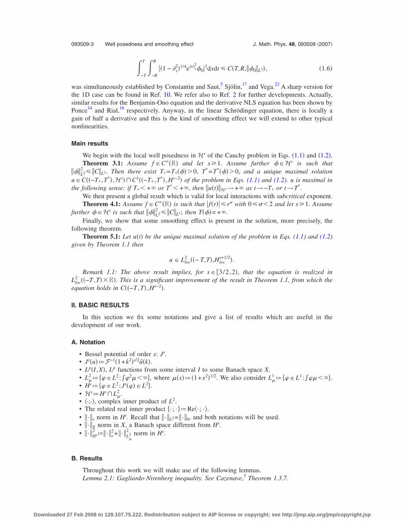
was simultaneously established by Constantin and Saut,5 Sjölin,17 and Vega.22 A sharp version forthe 1D case can be found in Ref. 10. We refer also to Ref. 2 for further developments. Actually,similar results for the Benjamin-Ono equation and the derivative NLS equation has been shown byPonce14 and Rial,16 respectively. Anyway, in the linear Schrödinger equation, there is locally again of half a derivative and this is the kind of smoothing effect we will extend to other typicalnonlinearities.

Main results

We begin with the local well posedness in Hs of the Cauchy problem in Eqs. �1.1� and �1.2�.Theorem 3.1: Assume f �C��R� and let s�1. Assume further ��Hs is such that

�L22

CL1. Then there exist T*=T*��0, T*=T*��0, and a unique maximal solutionu�C��−T* ,T*� ,Hs��C1��−T* ,T*� ,Hs−2� of the problem in Eqs. (1.1) and (1.2). u is maximal inthe following sense: if T*� +� or T*� +�, then u�t�Hs→ +� as t→−T* or t→T*.

We then present a global result which is valid for local interactions with subcritical exponent.Theorem 4.1: Assume f �C��R� is such that �f�r��r� with 0��2 and let s�1. Assume

further ��Hs is such that �L22

CL1; then T��= +�.Finally, we show that some smoothing effect is present in the solution, more precisely, the

following theorem.Theorem 5.1: Let u�t� be the unique maximal solution of the problem in Eqs. (1.1) and (1.2)

given by Theorem 1.1 then

u � Lloc2 ��− T,T�,Hloc

s+1/2� .

Remark 1.1: The above result implies, for s� �3/2 ,2�, that the equation is realized inLloc

2 ��−T ,T��R�. This is a significant improvement of the result in Theorem 1.1, from which theequation holds in C��−T ,T� ,Hs−2�.

II. BASIC RESULTS

In this section we fix some notations and give a list of results which are useful in thedevelopment of our work.

A. Notation

• Bessel potential of order s: Js.• Js�u�ªF−1�1+k2�s/2u�k�.• Lp�I ,X�, Lp functions from some interval I to some Banach space X.• L

2ª ��L2 :��2 ��, where �x�ª �1+x2�1/2. We also consider L

1ª ��L1 :�� .

• Hsª ��L2 :Js��L2�.

• HsªHs�L

2 .• �·;·�, complex inner product of L2.• The related real inner product �· ; · �ªRe�· ; · �.• · s norm in Hs. Recall that · L2 = · 0, and both notations will be used.• · X norm in X, a Banach space different from Hs.• · Hs

2ª · s

2+ · L 2

2 norm in Hs.

B. Results

Throughout this work we will make use of the following lemmas.Lemma 2.1: Gagliardo-Nirenberg inequality. See Cazenave,3 Theorem 1.3.7.

093509-3 Well posedness and smoothing effect J. Math. Phys. 48, 093509 �2007�


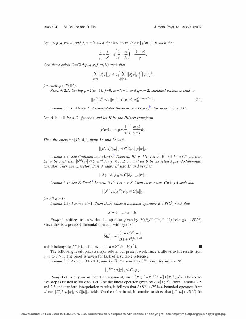
Let 1 p ,q ,r�, and j ,m�N such that 0 j�m. If �� j /m ,1� is such that

1

p=

j

N+ � 1

r−

m

N� +

�1 − ��q

,

then there exists C=C�� , p ,q ,r , j ,m ,N� such that

��k�=j

�xk�Lp C �

�k�=m

�xk�Lr��

�Lq1−�,

for each ��D�RN�.Remark 2.1: Setting p=2��+1�, j=0, m=N=1, and q=r=2, standard estimates lead to

uL2�+22�+2

�u12 + C��,��u0

�2�+4�/�2−��. �2.1�

Lemma 2.2: Calderón first commutator theorem. see Ponce,14 Theorem 2.6, p. 531.

Let A :R→R be a C� function and let H be the Hilbert transform

�H��x� ª p.v.1

� ��y�

x − ydy .

Then the operator �H ;A��x maps L2 into L2 with

�H;A��x�0 C�xAL��0.

Lemma 2.3: See Coiffman and Meyer,4 Theorem III, p. 111. Let A :R→R be a C� function.Let b be such that �b�j��k� � Cj�k�−j for j=0,1 ,2 , . . . and let B be its related pseudodifferentialoperator. Then the operator �B ;A��x maps L2 into L2 and verifies

�B;A��x�0 C�xAL��0.

Lemma 2.4: See Folland,7 Lemma 6.16. Let ��S. Then there exists C=C�� such that

�J1/2;��J1/2�0 C�0,

for all ��L2.Lemma 2.5: Assume s�1. Then there exists a bounded operator B�B�L2� such that

Js − 1 = �x � Js−1B .

Proof: It suffices to show that the operator given by F��xJs−1�−1�Js−1�� belongs to B�L2�.

Since this is a pseudodifferential operator with symbol

b�k� = − i�1 + k2�s/2 − 1

k�1 + k2��s−1�/2

and b belongs to L��R�, it follows that B=F−1b�B�L2�. �

The following result plays a major role in our present work since it allows to lift results froms=1 to s1. The proof is given for lack of a suitable reference.

Lemma 2.6: Assume 0r1, and k�N. Set ª�1+x2�1/2. Then for all ��Hk,

�Jk+r; ��0 C�k.

Proof: Let us rely on an induction argument, since �Jr ; �=Jr−1�J ; �+ �Jr−1 ; �J. The induc-tive step is treated as follows. Let L be the linear operator given by Lª�J ; �. From Lemmas 2.5,and 2.3 and standard interpolation results, it follows that L :H�→H� is a bounded operator, fromwhere J��J ; ��0C�� holds. On the other hand, it remains to show that �Jr ; ��B�L2� for



small values of r. Then take 0r1 and let B be the pseudodifferential operator with symbolb�k�=k−1��1+k2�r/2−1�. Since Jr=1+�xB and b satisfies the assumptions of Lemma 2.3, the resultis proved. �

Lemma 2.7: See Ponce,14 Lemma 2.7, p. 532. Let Jsª �1−�x

2�s/2 be the Bessel potential oforder s. If s�1 and n=1, then

�Js;��0 C�x�s�s−1.

Lemma 2.8: Moser’s inequality. See Ref. 15, Theorem 6.5, p. 87. Let A�C��C ;C� (in the real

sense) with A�0�=0; then there is a smooth function A : �0, +��→ �0, +�� so that for all u�Hs,

A�u�s A�uL��us.

Previous results on harmonic analysis yield the following quite remarkable property of the

Schrödinger group �eit��x2−A ��t�R.

Lemma 2. 9: For each (fixed) A0 the Schrödinger group �eit��x2−A ��t�R is well defined in Hs

and satisfies

• eit��x2−A ��0= �0 and

• eit��x2−A ��Hs �1+C�A , �t�s�−1��Hs.

Proof: Set TAª−�x2+A and UA�t�ªe−itTA. Since TA is a real operator it follows the conser-

vation of charge. Set now HA��ª1/2�x�L22 +A /2�L

2

2 ; a direct computation yields the conser-

vation of HA: HA�UA�t��=HA��. Since A0 it is easy to see that there exist constantsC1�A� ,C2�A� such that

C1�A�HA�� H12

C2�A�HA�� . �2.2�

This leads to the estimate UA�t��H12

C�A��H12 , and the result is true for s=1.

As it was stated before, Lemma 2.6 will be used to lift previous result to s1. Setting�ªUA�t��, one has

12�t�Js�;Js�� = ��t�;JsJs�� = �i�x

2�;JsJs�� − �iA �;JsJs�� = − �iA�Js; ��;Js�� . �2.3�

From Lemma 2.6, the estimate, �Js ; ��0C�s−1 follows, which leads to�t�s

2CA�s�s−1 and therefore to �t�sCA�s−1. The result follows from standard induc-tive argument. �

Consider now the case A=0 and the related group U0ªeit�x2.

Remark 2.2: In this case, the L 2 norm control given by UA�t��L

2

21/A�H1

2 + �L 2

2 is lost.

Lemma 2.10: U0�t� is well defined in Hs and verifies

• U0�t��s= �s, valid for all s�R, and• U0�t��L

2 C�t , ��H1�L

2 .

Proof: The first assertion follows immediately from �Js ;�x2�=0. From

U0�t��L 2

2 �L

2

2 + 20

t

��iU0�t��;�x� ��xU0�t��dt�

�L 2

2 + 2�x �0

t

U0�t��0�xU0�t��0dt�

�L 2

2 + Ct�x ��12, �2.4�

the second claim follows. �



Finally, the continuous dependence on the initial data requires some continuity of the familyUA with respect to the parameter A which is given by the following lemma.

Lemma 2.11: Let T0 and ��Hs be fixed. The map U�·��t�� : �0; +��→C��0;T� ;Hs� iscontinuous.

Proof: Assume first ��D�R�, and let g�t�=UB�−t�UA�t��−�. Taking time derivatives yieldsg��=UB�−��iTB− iTA�UA��, where TA=−�x

2+A �see Lemma 2.9�. Since g�0�=0 and TA

−TB= �A−B� , it follows that g�t�=−i�A−B��0t UB�−�� UA��d�. Taking the norm in Hs and

using that UB�·� is unitary, one has the estimate g�t�Hs �A−B � �0t UA��Hs. The assumption

��D�R� ensures that UA��Hs for any �� 0;T�, then there exists a constant C�T ,�� suchthat

supt��0;T�

g�t�Hs �A − B�C�T,�� .

Taking into account the identity UA�t��−UB�t��=UB�t�g�t�, the general result follows from a � /3argument. �

III. WELL POSEDNESS OF THE CAUCHY PROBLEM

This section is concerned with the local existence of the Cauchy problem

i�tu = − �x2u + V�u�u − f��u�2�u , �3.1�

u�x,0� = ��x� , �3.2�

posed in the weighted Sobolev Spaces Hs=Hs�L 2 with s�1, where the local interaction satisfies

f �C��R�, the doping profile C�Cc�, and V�u� is given by

V�u� =�x�2

� �C − �u�2� . �3.3�

Setting

V��u� ª �x − y� − �x�2

�C�y� − �u�y��2�dy , �3.4�

A�u� ª CL1 − u02, �3.5�

the potential V shall be written as

V�u� = 12 �x�A�u� + V��u� . �3.6�

Some remarks are listed below.Remark 3.1: Since Hs

�L 2 , both potentials V� and V are well defined.

Remark 3.2: Since V��L� (see Lemma 3.1 below) if the initial data � are such that A��0, then V�u�=O��x�� for �x�→ +�.

In the sequel we will consider initial data � such that A��0. The special case given byA��=0 leads to the identity V�=V; therefore such potential is bounded. Both instances A��0 and A��=0 will be called, respectively, the subcritical and critical cases.

A. Local existence. Critical and subcritical cases

Since the results of this subsection are obtained by means of the fixed point techniques, someestimates are needed.

Lemma 3.1: Let ��Hs and let V� be given by Eq. (3.4). Then the following properties hold:

• V��L� C− ��2L 1 .



• V��1�−V��2�L� ��1�2− ��2�2L 1 ��1L

2 + �2L

2 ��1−�2L

2 .

• �xV��Hs C�CL 1 , �Hs−1�C− ��2Hs.

• �xV��1�−�xV��2�Hs C��1Hs−1 , �2Hs−1��1−�2Hs.

Proof: From ��x−y�− �x�� y� and �u�2− �v�2= u�u−v�+v�u− v�, the first and second asser-tions follow.

Take j�Hs�L 1 and consider 1 /2ª��x−y �− �x��j�y�dy. Taking derivatives with respect to

x yields

�xV�j� = −�

x

j�y�dy −1 + �

2

y�Rj�y�dy . �3.7�

Consider now x→−�, then 1+ ��x�1/2x2, which is in L 2 . In addition,

−�

0

�x��−�

x

j�y�dy�2dx −�

0 −�

x −�

x

�x��j�y�j�z��dydz�dx

−�

0 z

0 −�

0

�y��j�y�j�z��dydxdz

−�

0 −�

0

�z� �y��j�y�j�z��dydz

jL 1 ��−�;0��

2 .

Since similar results hold for x→ +�, one has the estimate �xV�j�L 2 CjL

1 .

In order to prove the Lipschitz property, consider s�1. From Lemma 2.5 there exists apseudodifferential operator B-which satisfies the assumptions of Lemma 2.3 such that Js=1+B�xJ

s−1. It follows that Js��xV�j��=�xV�j�+BJs−1�j− 12 ��y�Rj�y�dy�, and this yields

�xV�j�s �xV�j�L2 + BB�L2��js−1 + C� �jL 1 �,

C�s�jHs−1�L 1 .

The third and fourth claims are obtained by taking, respectively, j=C− ��2 and j= ��1�2− ��2�2. �

The following conservation law will be useful in the sequel.Lemma 3.2: Charge conservation. Let N be a real function and u

�C��a ,b� ,Hs��C1��a ,b� ,Hs−2� a solution of i�tu=−�x2u+N�u�u, with s�1. Then, u�· , t�L2 is a

constant.Proof: Taking the time derivative, it follows that

�tu�t�2 = ��tu;u� = �i�x2u;u� + �iN�u�u;u� = − �i�xu;�xu� = 0.

Since N is real we get Re�iN�u��=0. On the other hand, since s�1 the boundary term in theintegration by parts vanishes. �

In the sequel we introduce the following auxiliary problem where A�0 is fixed:

i�tu = − �x2u + A u + V��u�u − f��u�2�u , �3.8�

u�x,0� = ��x� . �3.9�

Property 3.1: Assume that f �C��R� and let s�1. If ��Hs, then there exist T=T��0 anda unique maximal solution u�C��0,T�� ,Hs��C1��0,T�� ,Hs−2� of the problem in Eqs. (3.8)and (3.9). u is maximal in the following sense: if T�� +� then u�t�Hs→ +� as t→T��.



Proof: Let UA�t� be the unitary group generated by the operator i�x2− iA and let FA be the

operator yielded by Duhamel’s formula

FA�u� = UA�t�� − i0

t

UA�t − s��V��u�u − f��u�2�u�ds . �3.10�

Thus the fixed point problem is given by FA�u�=u. In the sequel, it will be shown that F is welldefined and is a contraction in Hs �from now on the subscript will be omitted�.

From Lemma 2.9, F�u�Hs C�t��0Hs + V��u�u− f��u�2�uHs�. On the other hand, Lemma

2.8 and embedding H1�L� lead to f��u�2�us f�u1�us and f��u�2�uL

2 f��u�2�L�uL

2 . This

yields

f��u�2�uHs C�f ,u1�uHs. �3.11�

Since JsV��u�u= �Js ;V��u��u+V��u�Jsu, Lemmas 2.7 and 3.1 give the estimate

V��u�us C�us−1�us + C�uH1�us.

In addition the L 2 norm estimate V��u�uL

2 V��u�L�uL

2 leads to

V��u�uHs C�uHs−1�uHs. �3.12�

Therefore, estimates �3.11� and �3.12� show well the definition of F.Set now w�u�ªV��u�u− f��u�2�u, since F�u�−F�v�=−i�0

t UA�t−s��w�u�−w�v��ds. Taking · Hs and applying Lemma 2.9 leads to the estimate

F�u� − F�v�Hs C�A,t�w�u� − w�v�Hs.

Thus, it only remains to show that the nonlinear term w�u� is a locally Lipschitz function inHs. Take then u ,v�Hs such that uHs , vHs R.

Since

f��u�2�u − f��v�2�v = 0

1 d

ds�f��z�s��2�z�s��ds

= 0

1

f��z�s��2��u − v�ds + 0

1

2f��z�s��2�z�s�Re�z�s��u − v��ds ,

where z�s�=su+ �1−s�v, Lemma 2.8 leads to

f��u�2�u − f��v�2�vs C�f ,R�u − vs.

Since f�·��C�, it follows that f��u�2�− f��v�2�L 2 C�f ,R�u−vL

2 . A suitable arrangement of

terms leads to

f��u�2�u − f��v�2�vL 2 f��u�2��u − v�L

2 + �f��u�2� − f��v�2��vL

2

f��u�2�L�u − vL 2 + vL�f��u�2� − f��v�2�L

2

C�f ,R�u − vL 2 .

Therefore,

f��u�2�u − f��v�2�vHs C�f ,R�u − vHs. �3.13�

By taking into consideration the identity



Js�V��u�u − V��v�v� = �Js;V��u� − V��v��u + �V��u� − V��v��Jsu

+ �Js;V��v��u − v� + V��v�Js�u − v�

and using Lemma 3.1, one might bound each term separately as follows:

�Js;�V��u� − V��v��u0 C�xV��u� − �xV��v�su0 C�R�u − vs,

�V��u� − V��v��Jsu0 CV��u� − V��v�L�us C�R�u − vs,

�Js;V��v��u − v�0 �xV��u�su − vs C�R�u − vs,

V��v�Js�u − v�0 V��v�L�u − vs C�R�u − vs.

Similar estimates as above lead to V��u�u−V��v�vL 2 C�R�u−vL

2 , and this gives

V��u�u − V��v�vHs C� ,R�u − vHs. �3.14�

Therefore, collecting estimates �3.13� and �3.14�, the Lipschitz property of the nonlinear termV��u�u− f��u�2�u is shown. �

The following lemma yields the continuous dependence of the iteration process given by FA

with respect to the parameter A.Lemma 3.3: The map F�·��·� : �0; +��C��0;T� ;Hs�→C��0;T� ;Hs� given by Eq. (3.10) is

continuous.Proof: It is a direct consequence of Lemma 2.11 and estimates �3.11�–�3.14�. �

The previous result leads to the well posedness of the Cauchy problem in Eqs. �3.1� and �3.2�when initial data satisfy A��0.

Theorem 3.1: Let f �C��R� and let s�1. For every ��Hs, such that �02 CL1, there

exists T=T��0 and there exists a unique, maximal solution u�C��0,T�� ,Hs��C1��0,T�� ,Hs−2� of the problem in Eqs. (3.1) and (3.2). u is maximal in the sense that ifT�� +�, then u�t�Hs→ +� as t→T��.

Proof: Let � be such that A��0 and take A= 12A��. Applying Proposition 3.1 we get a

solution u�C��0,T�� ,Hs��C1��0,T�� ,Hs−2� of the problem in Eqs. �3.8� and �3.9�. Fromthe conservation law of Lemma 3.2, it follows that A�u�=A��; finally, the definition of A�u� andV��u� �see Eqs. �3.5� and �3.4�� show that V�u�=A +V��u�, from where we conclude that u is asolution of the problem in Eqs. �3.1� and �3.2�. �

Remark 3.3: Since the function v�x , t�ª u�x ,−t� solves the problem in Eqs. (3.1) and (3.2) in�−T�� ,0�, the related backward problem is also local in time well posed.

Remark 3.4: Since A�·� depends only on the initial data, uniqueness follows directly from theuniqueness of the auxiliary problem in Eqs. (3.8) and (3.9). On the other hand, the continuousdependence of u with respect to the initial data follows from Lemma 3.3.

B. Conservation laws

The problem in Eqs. �3.1� and �3.2� presents a conserved quantity, which is given by theenergy functional �see Cazenave3�

E�� =1

2�x�2 +

1

2�V��;�� +

1

4� �x�

2� ��2��;�� −

1

2

x�RF��2�� , �3.15�

where F�= f and F�0�=0.Lemma 3.4: Conservation of energy. Let A�0, s�1, and f �C�. If

u�C��−T* ,T*� ,Hs��C1��−T* ,T*� ,Hs−2� is the unique solution of the problem in Eqs. (3.1) and(3.2), then E�u�t��=E�u�0�� for all t� �−T* ,T*�.



Proof: Let ��Hs; since s�1, it follows that �x��L2. From embedding H1�L�, it follows

that �L� C�H1 and this leads to ��x�RF��2� � fL��0;�1��02.

From identity �3.6�, one has ��V�� ;��A /2�L 2

2 + V��L��02.

Remark 3.5: the previous argument also yields ��x�� 2�� ;�� L 2

2 �02.

This shows that E is a well defined functional in Hs.Taking into consideration identity �3.3� and calling U�x�= �x� /2�C, one might write

E�� =1

2�x�2 +

1

2�U�x��;�� −

1

4� �x�

2� ��2��;�� −

1

2

x�RF��2� . �3.16�

A straightforward computation yields

�tE = �− �x2u;�tu� + �U�x�u;�tu� −

1

2� �x�

2� �u�2�u;�tu� −

1

4��t �x�

2� �u�2�u;u�

− x�R

f��u�2�Re�u�tu�dx .

On the other hand, since �x�Rf��u�2�Re�u�tu�dx= �f��u�2�u ;�tu�, one may write

�tE = ��x2u + L�u�;�tu� −

1

4��t �x�

2� �u�2�u;u� +

1

2� �x�

2� �u�2�u;�tu� .

The first term vanishes since u solves the equation; the remaining terms are equal since �x� isan even function. This shows that E is constant along the trajectory u�t�. �

IV. GLOBAL EXISTENCE IN Hs

This section is devoted to establishing a global existence result for the problem in Eqs. �3.1�and �3.2�.

Since the existence of global solutions is strongly related with the critical exponent �seeWeinstein23�, some control on the local interaction must be made. This suggests the following twobasic assumptions:

f 0, f�r� r� with 0 � � 2 �assumption �A1�� , �4.1�

f � 0, f � C�R� �assumption �A2�� . �4.2�

Remark 4.1: Since f �0 means repulsive interaction, no further assumption shall be made. Onthe opposite, since the local interaction is given by f��u�2�u, the case �=2 corresponds to thecritical exponent (see Refs. 8 and 23). Therefore, in the attractive model, assumption (A1) meanssubcritical exponent.

Theorem 4.1: Assume that assumption (A1) or (A2) holds. Let A�0, ��Hs, and s�1 andlet u�C��−T* ,T*� ,Hs��C1��−T* ,T*� ,Hs−2� be the unique (local) solution of the problem in Eqs.(3.1) and (3.2); then T� =T*= +� �i.e., u is globally defined in Hs�.

Proof: Take s=1 and let u�C��−T ,T� ,H1��C1��−T ,T� ,H−1� be the �local� solution of theproblem in Eqs. �3.1� and �3.2�. Using that both terms ��x� /2� �u�2�u ;u� and A� u ;u� are non-negative, one has

E�� = E�u� �1

2�xu0

2 +1

2�V��u�u;u� −

1

2

x�RF��u�2� .

Thus, if assumption �A1� holds, one has



� 1

2

x�RF��u�2��

1

� + 1uL2�+2

2�+2 , �4.3�

By means of estimate �2.1� �see the Gagliardo-Nirenberg inequality�, this yields

uL2�+22�+2

�u12 + C��,��u0

�2�+4�/�2−��, �4.4�

which, together with Lemma 3.1, leads to

12 �xu0

2 E��0� + CL1u02 + uL

2

2 u02 + �u1

2 + C��,��u0�2�+4�/�2−��.

Taking ��1/2 and using the conservation law of Lemma 2 one has the following estimate:

u1 C��1 + uL 2 � . �4.5�

On the other hand, following assumption �A2�, the term 1/2�x�RF��u�2� is non-negative andtherefore the previous estimate also holds in this case.

Take t� �0,T�; since u�· , t�L 2

2 = �L 2

2 +�0t d/dt��u�t��L

2

2 �dt� and u is a solution of Eq. �3.1�,it follows that u�· , t�L

2

2 = �L 2

2 +2�0t �i�x

2u ; u�dt�; note that V�u� and f��u�2� are real functions so

their related terms vanish, this leads to

u�t�L 2

2 �L

2

2 + 20

t

��iu;�x �xu��dt� �L 2

2 + 2�x �0

t

u�t��0�xu�t��0dt�

�L 2

2 + 2�x ��000

t

�xu�t��0dt�.

Now, estimate �4.5� leads to u�t�L 2

2C��1+ t+�0

t u�t��L 2 dt��. A standard ordinary differ-

ential equation argument yields u�t�H1 C��1+ t2�.Since u�t�Hs

2 = u�t�L 2

2 + u�t�s2, it will be suffice to estimate u�t�s for s1. Moreover, in

view of the inductive nature of estimate �3.12�, it is enough to use induction on �s�.Set first 1�s2. Including the nonlinear terms �V��u�+ f��u�2��u into identity �2.3� and using

estimates �3.11� and �3.12�, one has

u�t�s2 C��1 + t2�

0

t

u�t��sdt� + C��,u1��1 + t2�0

t

u�t��s2dt�.

Hence, Gronwall’s lemma yields u�t�sC�t , �0Hs�.Let now 2k�N and set k�sk+1. The same computations as before yield

u�t�s2 C��1 + t2�

0

t

u�t��sdt� + C��,uk��1 + t2�0

t

u�t��s2dt�.

From the inductive step, one has u�t�kC�t , �0Hk� and, therefore, the result proceeds fromGronwall’s lemma. �

V. SMOOTHING EFFECT

In this section we establish the kind of smoothing effect which is present in the solution of theCauchy problem

i�tu = − �x2u + V�u�u − f��u�2�u , �5.1�



u�x,0� = ��x� , �5.2�

where f �C��R�, C�Cc��R�, and V�u�ª �x� /2� �C− �u�2�. Such smoothing effect is detailed in the

following theorem.Theorem 5.1: Assume s�1 and �L2

2 CL1. Let u�t� be the unique, maximal solution of

Eqs. (5.1) and (5.2) provided by Theorem 3.1 then

u � Lloc2 ��− T,T�,Hloc

s+1/2� .

Remark 5.1: The above result implies that u�t��Hlocs+1/2 for a.e. t� �−T ,T�. Thus u�t��Cloc

s−�

for a.e. t� �−T ,T� and any �0. Moreover, for s� �3/2 ,2� we have that the equation is realizedin Lloc

2 ��−T ,T��R�. This is a significant improvement of the result in Theorem (3.1), from whichthe equation holds in C��−T ,T� ,Hs−2�.

Remark 5.2: This kind of smoothing effect represents an extension (local in space and time) ofthe result in the linear case given by Constantin and Saut, Sjölin, and Vega in Refs. 5, 17, and 22.

Proof: The proof will be given in several steps.First step. Let R�R and T1 such that �−T1 ;T1�� −T*�� ;T*�� and take ��Cc

� such thatsupp�� −R ,R�; then

−T1

T1 ��Js+1/2u�2 �L�−T1

T1 −R

R

�Js+1/2u�2,

and this shows that one is allowed to restrict to functions ��Cc� such 0�1 and ��1 in

�−R ,R�.The following identity will be useful in the sequel:

��Js+1/2u;Js+1/2u� = ��J1/2�Js − 1�u;J1/2�Js − 1�u� + 2��Js − 1�u;Ju� + 2��Js − 1�u;�J1/2;��J1/2u�

+ ��J1/2u;J1/2u� . �5.3�

Take now ��C� such that �ª�x�. Let H be the Hilbert transform �see Lemma 2.2� and letP±ª1/2�1± iH� be the projection operators �see Rial16�. We also consider the following identity:

12�t��JsP±u;JsP±u� = �i�Js�x

2P±u;JsP±u� − �i�JsP±V�u�u;JsP±u� + �i�JsP±f�u�u;JsP±u� .

�5.4�

On the other hand, the linear term can be written as follows:

�i�Js�x2P±u;JsP±u� = �i��;�x��xJ

sP±u;JsP±u� + �i��xJsP±u;�xJ

sP±u� = − �i��xJsP±u;JsP±u� .

�5.5�

Since the Hilbert transform satisfies H2=−1, −HP±= ± P±, and �H ;Js�= �H ;�x�=0, one candeduce

− �i��xJsP±u;JsP±u� = �i�HH�xJ

sP±u;JsP±u�

= �i��;H��xHJsP±u;JsP±u� + �iH�H�xJsP±u;JsP±u�

= �B1HJsP±u;JsP±u� ± ��H�xJsP±u;JsP±u� , �5.6�

where B1ª i�� ;H��x.Remark 5.3: Since �Js−1; P±�=0, identities (5.4)–(5.6) are still valid if Js is replaced by

Js−1.Remark 5.4: From Lemma 2.2 it follows that B1 is a bounded operator in L2. Furthermore,

one has the following estimate:

��B1H�Js − 1�P±u;�Js − 1�P±u�� C��us2. �5.7�



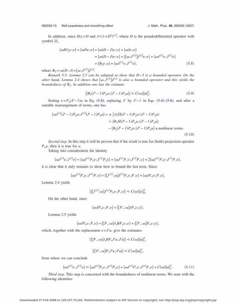
In addition, since H�x=D and J= �1+D2�1/2, where D is the pseudodifferential operator withsymbol �k�,

��H�xv;v� = ��Dv;v� = ��D − J�v;v� + ��Jv;v�

= ��D − J�v;v� + ��;J1/2�J1/2v;v� + ��J1/2v;J1/2v�

= �B2v;v� + ��J1/2v;J1/2v� , �5.8�

where B2ª��D−J�+ �� ;J1/2�J1/2.Remark 5.5: Lemma 2.5 can be adapted to show that D−J is a bounded operator. On the

other hand, Lemma 2.4 shows that �� ,J1/2�J1/2 is also a bounded operator and this yields theboundedness of B2. In addition one has the estimate

��B2�Js − 1�P±u;�Js − 1�P±u�� C��us2. �5.9�

Setting v= P±�Js−1�u in Eq. �5.8�, replacing Js by Js−1 in Eqs. �5.4�–�5.6�, and after asuitable rearrangement of terms, one has

��J1/2�Js − 1�P±u;J1/2�Js − 1�P±u� = ± 12�t��Js − 1�P±u;�Js − 1�P±u�

� �B1H�Js − 1�P±u;�Js − 1�P±u�

− �B2�Js − 1�P±u;�Js − 1�P±u� ± nonlinear terms.

�5.10�

Second step. In this step it will be proven that if the result is true for �both� projection operatorP±u, then it is true for u.

Taking into consideration the identity

��J1/2v;J1/2v� = ��J1/2P+v;J1/2P+v� + ��J1/2P−v;J1/2P−v� + 2��J1/2P+v;J1/2P−v� ,

it is clear that it only remains to show how to bound the last term. Since

��J1/2P+v;J1/2P−v� = ��J1/2;��J1/2P+v;P−v� + ��JP+v;P−v� ,

Lemma 2.4 yields

��J1/2;��J1/2P+v;P−v�� C��v02.

On the other hand, since

��JP+v;P−v� = ��P−;��JP+v;v� ,

Lemma 2.5 yields

��JP+v;P−v� = ��P−;��xBP+v;v� + ��P−;��P+v;v� ,

which, together with the replacement v=Jsu, give the estimates

��P−;��xBP+Jsu;Jsu�� C��us2,

��P−;��P+Jsu;Jsu�� C��us2,

from where we can conclude

��J1/2v;J1/2v� ��J1/2P+v;J1/2P+v� + ��J1/2P−v;J1/2P−v� + C��us2. �5.11�

Third step. This step is concerned with the boundedness of nonlinear terms. We start with thefollowing identities:



�i��Js − 1�P±f��u�2�u;�Js − 1�P±u� = �iP±�P±�Js − 1�f��u�2�u;�Js − 1�u� ,

�i��Js − 1�P±V�u�u;�Js − 1�P±u� = �iP±�P±�Js − 1�V�u�u;�Js − 1�u� .

Setting �ªP±�P± produces

�i��Js − 1�V�u�u;�Js − 1�u� = �i��Js;V�u��u;�Js − 1�u� + �i��P±;V�u��Js − 1�u;�Js − 1�P±u� ,

which after the replacement V�u�= �A /2� +V��u� becomes

�i��Js − 1�V�u�u;�Js − 1�u� = �i��Js − 1�;V��u��u;�Js − 1�u�

+ �i��P±;V��u��Js − 1�u;�Js − 1�P±u�

+A

2�i��Js − 1�; �u;�Js − 1�u�

+A

2�i��P±; ��Js − 1�u;�Js − 1�P±u� . �5.12�

From Lemmas 3.1 and 2.6 it follows that the first three terms of Eq. �5.12� are all bounded.The last term is bounded from Lemmas 2.2 and 2.5. Therefore we have the following estimate:

��i��Js − 1�V�u�u;�Js − 1�u�� C��us2. �5.13�

Finally, Lemma 2.8 yields the related estimate for the local term,

��i��Js − 1�f��u�2�u;�Js − 1�u�� C�� f�us�us2. �5.14�

Conclusion. Applying the Cauchy-Schwarz’s inequality in Eq. �5.3� yields

��Js+1/2P±u;Js+1/2P±u� ��J1/2�Js − 1�P±u;J1/2�Js − 1�P±u� + 2usu1 + C��usu0 + u1u0

��J1/2�Js − 1�P±u;J1/2�Js − 1�P±u� + C��usu1.

Using expression �5.10� and estimates �5.13� and �5.14� and integrating in a compact intervalI� �−T* ,T*� produces

I

��Js+1/2P±u;Js+1/2P±u�dt C��maxI

�u�· ,t�s2� + C��

I

u�· ,t��s2dt�

+ C��I

f�u�· ,t��s�u�· ,t��s2dt�,

from where

I

��Js+1/2P±u;Js+1/2P±u�dt C��I�,�,maxI

�u�· ,t�s�� . �5.15�

Remark 5.6: If in addition we take under consideration a priori estimates of Sec. III (with thefurther assumption (A1) or (A2)), we get

I

��Js+1/2P±u;Js+1/2P±u�dt C��I�,�,�Hs2 � .

Anyway, collecting estimates �5.11� and �5.15� produces



I ��Js+1/2u�2 C��I�,�,max

I�u�· ,t�s�� ,

which finishes the proof. �

1 Bao, W., Mauser, N. J., and Stimming, H. P., “Effective one particle quantum dynamics of electrons: A numerical studyof the Schrödinger-Poisson-X� model,” Commun. Math. Sci. 1, 809–828 �2003�.

2 Ben-Artzi, M., and Klainerman, S., “Decay and regularity for the Schrödinger equation,” J. Anal. Math. 58, 25–37�1992�.

3 Cazenave, T., Semilinear Schrödinger Equations, Courant Lecture Notes Vol. 10, American Mathematical Society,Providence, RI, 2003.

4 Coiffman, R. R., and Meyer, Y., Euclidean Harmonic Analysis, Lecture Notes in Mathematics Vol. 779 �Springer, NewYork, 1979�, pp. 106–122.

5 Constantin, P., and Saut, J.-C., “Local smoothing properties of dispersive equations,” J. Am. Math. Soc. 1, 413–446�1989�.

6 Dirac, P. A. M., “Note on exchange phenomena in the Thomas-Fermi atom,” Proc. Cambridge Philos. Soc. 26, 376–385�1931�.

7 Folland, G., Introduction to Partial Differential Equations, 2nd ed. �Princeton University Press, Princeton, NJ, 1995�.8 Glassey, R., “On the blowing up of solutions to the Cauchy problem for the nonlinear Schrödinger equation,” J. Math.Phys. 18, 1794–1797 �1977�.

9 Kato, T., Studies in Applied Mathematics, Advances in Mathematics Supplementary Studies Vol. 8 �Academic Press,New York, 1983� pp. 93–128.

10 Kenig, C., Ponce, G., and Vega, L., “Oscillatory integrals and regularity of dispersive equations,” Indiana Univ. Math. J.40, 33–69 �1991�.

11 Kohn, W., and Sham, L. J., “Self-consistent equations including exchange and correlation effects,” Phys. Rev. 140,1133–1138 �1965�.

12 Markowich, P. A., Ringhofer, C. A., Schmeiser, and C., Semiconductor Equations �Springer, Vienna, 1990�.13 Mauser, N. J., “The Schrödinger-Poisson-X� model,” Appl. Math. Lett. 14, 759–763 �2001�.14 Ponce, G., “On the global well-posedness of the Benjamin-Ono equation,” Diff. Integral Eq. 4, 527–542 �1991�.15 Rauch, J., Lectures on nonlinear geometric optics, Department of Mathematics, University of Michigan �http://

www.math.lsa.umich.edu/~rauch/courses.html�.16 Rial, D., “Weak solutions for the derivative Schrödinger equation,” Non linear Analysis 49, 149–158 �2002�.17 Sjölin, P., “Regularity of solutions to the Schrödinger equations,” Duke Math. J. 55, 699–715 �1987�.18 Slater, J. C., “A simplification of the Hartree-Fock method,” Phys. Rev. 81, 385–390 �1951�.19 Steinrück, H., “One-dimensional Wigner-Poisson problem and its relation to the Schrödinger-Poisson problem,” SIAM J.

Math. Anal. 22, 957–972 �1991�.20 Stimming, H. P., “The IVP for the Schrödinger-Poisson-X� equation in one dimension,” Math. Models Meth. Appl. Sci.

1169–1180 �2005�.21 Strichartz, R. S., “Restrictions of Fourier transforms to quadratic surfaces and decay of solutions of wave equations,”

Duke Math. J. 44, 705–714 �1977�.22 Vega, L., “The Schrödinger equation: Pointwise convergence to the initial date,” Proc. Am. Math. Soc. 102, 874–878

�1988�.23 Weinstein, M., “Nonlinear Schrödinger equations and sharp interpolation estimates,” Commun. Math. Phys. 87, 567–576

�1983�.24 Zhang, P., Zheng, Y. and Mauser, N. J., “The limit from the Schrödinger-Poisson to the Vlasov-Poisson equations with

general data in one dimension,” Commun. Pure Appl. Math. 55, 0582–0632 �2002�.



Well posedness and smoothing effect of Schrödinger-Poisson equation

Documents

Transcript of Well posedness and smoothing effect of Schrödinger-Poisson equation