arX

iv:0

912.

4642

v2 [

mat

h.A

P] 3

Aug

201

0

GLOBAL WELL-POSEDNESS FOR SCHRODINGER EQUATION

WITH DERIVATIVE IN H12 (R)

CHANGXING MIAO, YIFEI WU, AND GUIXIANG XU

Abstract. In this paper, we consider the Cauchy problem of the cubic nonlinearSchrodinger equation with derivative in H

s(R). This equation was known to bethe local well-posedness for s ≥ 1

2(Takaoka,1999), ill-posedness for s <

12(Biagioni

and Linares, 2001, etc.) and global well-posedness for s >12(I-team, 2002). In this

paper, we show that it is global well-posedness in H1

2 (R). The main approach is thethird generation I-method combined with some additional resonant decompositiontechnique. The resonant decomposition is applied to control the singularity comingfrom the resonant interaction.

1. Introduction

In this paper, we consider the Cauchy problem of the Schrodinger equation with

derivative: i∂tu+ ∂2

xu =iλ∂x(|u|2u), x ∈ R, t ∈ R,

u(0, x) =u0(x) ∈ Hs(R),(1.1)

where λ ∈ R, Hs(R) denotes the usual inhomogeneous Sobolev space of order s. It

arises from describing the propagation of circularly polarized Alfven waves in the

magnetized plasma with a constant magnetic field (see [25, 26, 28]).

The local well-posedness for (1.1) is well understood. By the Fourier restriction

norm in [3, 4] and the gauge transformation in [16, 17, 18], Takaoka obtained the

local well-posedness of (1.1) in Hs(R) for s ≥ 1/2 in [29]. This result was shown by

Biagioni and Linares [1], Bourgain [5] and Takaoka [30] to be sharp in the sense that

the flow map fails to be uniformly C0 for s < 1/2.

The global well-posedness for (1.1) was also widely studied. In [27], Ozawa made

use of two gauge transformations and the conservation of the Hamiltonian, and

showed that (1.1) was globally well-posed in H1(R) under the condition (1.2). In

[30], Takaoka used Bourgain’s “Fourier truncation method” ([6, 7]) to obtain the

global well-posedness in Hs(R) for s > 3233 , again under (1.2). In [9, 10], I-team

(Colliander-Keel-Staffilani-Takaoka-Tao) made use of the first, second generations of

2000 Mathematics Subject Classification. Primary 35Q55; Secondary 47J35.Key words and phrases. Bourgain space, DNLS equation, global well-posedness, I-method, reso-

nant decomposition,

1

2 CHANGXING MIAO, YIFEI WU, AND GUIXIANG XU

I-method to obtain the global wellposedness in Hs(R), for s > 2/3 and s > 1/2,

respectively. For other results, please refer to [14, 16, 17, 18, 19, 27, 31, 32, 33].

In this paper, we will combine the third generation of the I-method with the res-

onant decomposition to show the global well-posedness of (1.1) in H12 (R). We think

that the resonant decomposition technique may also be used to study the global

well-posedness of (1.1) in H12 (T).

Theorem 1.1. The Cauchy problem (1.1) is globally well-posed in H12 (R) under the

assumption of

‖u0‖L2 <

√2π

|λ| . (1.2)

The main approach, as described above, is the I-method. This method is based

on the correction analysis of some modified energies and an iteration of local result.

The first modified energy is defined as E(Iu), for some smoothed out operator I (see

(2.4)). Moreover, one can effectively add a “correction term” to E(Iu). This gives the

second modified energy E2I (u), and allows us to better capture the cancellations in the

frequency space. However, a further analogous procedure does not work again. Since

in this situation, a strong resonant interaction appears and this resonant interaction

will make the related multiplier to be singular. More precisely, as shown in [10], we

define the second modified energy by a 4-linear multiplier M4, which will generate a

6-linear multiplier M6 in the increment of the second modified energy. If we define

the third modified energy naturally by the 6-linear multiplier σ6 as

σ6 = −M6

α6,

where α6 = −i(ξ21 − ξ22 + ξ23 − ξ24 + ξ25 − ξ26), then α6 vanishes in some large sets but

M6 does not. So it is not suitable to define the third modified energy in this way.

Our argument is to decompose the multiplier M6 into two parts: one is relatively

small and another is non-resonant. The analogous way of resonant decomposition

was previously used in [23, 24]. However, it is of great complexity here and a ded-

icated multiplier analysis is needed in this situation. The resonant decomposition

technical was also appeared previously in [2, 8, 13]. In particular, I-team [13] made

use of the second generation “I-method”, a resonant decomposition (in order to avoid

the “orthogonal resonant interaction”) and an “angularly refined bilinear Strichartz

estimate” to obtain the global well-posedness of mass-critical nonlinear Schrodinger

equation in dimension two.

GLOBAL ROUGH SOLUTION FOR DNLS 3

Remark 1.1. Without loss of generality, we may take λ = 1 in (1.1) in the following

context. Indeed, we may first assume that λ > 0, otherwise, we may consider u for

instead. Then we may rescale the solution by the transformation

u(x, t) → 1√λu(x, t).

This deduces the general case to the case of λ = 1.

Remark 1.2. For the global well-posedness, it is natural to impose the condition

(1.2). Indeed, the solution of (1.1) (for λ = 1) enjoys the mass and energy conserva-

tion laws

M(u(t)) :=

∫|u(t)|2 dx = M(u0), (1.3)

and

H(u(t)) :=

∫ [|ux(t)|2 +

3

2Im|u(t)|2u(t)ux(t) +

1

2|u(t)|6

]dx = H(u0). (1.4)

By a variant gauge transformation

v(x, t) := e−i4

∫ x

−∞|u(y,t)|2 dyu(x, t),

we have‖v(t)‖L2

x= ‖u(t)‖L2

x,

H(u(t)) = ‖vx(t)‖2L2x− 1

16‖v(t)‖6L6

x.

Thus, the condition (1.2) guarantee the energy H(u(t)) to be positive via the sharp

Gagliardo-Nirenberg inequality

‖f‖6L6 ≤ 4

π2‖f‖4L2‖fx‖2L2 .

Remark 1.3. In [9], I-team obtained the increment bound N−1+ of the first genera-

tion modified energy, which leads to the global well-posedness in Hs(R) for s > 2/3.

In [10], the authors obtained the increment bound N−2+ of the second modified en-

ergy , which extend the exponent s to s > 1/2. In this paper, we will make use of the

resonant decomposition to show the increment bound N−5/2+ of the third generation

modified energy, which allows us to extend the exponent s to s = 1/2.

The paper is organized as follows. In Section 2, we give some notations and state

some preliminary estimates that will be used throughout this paper. In Section 3, we

introduce the gauge transformation and transform (1.1) into another equation. Then

we present the conservation law and define the modified energies. In Section 4, we

establish the upper bound of the multipliers generated in Section 3. In Section 5, we

obtain an upper bound on the increment of the third modified energy. In Section 6,

4 CHANGXING MIAO, YIFEI WU, AND GUIXIANG XU

we prove a variant local well-posedness result. In Section 7, we give a comparison

between the first and third modified energy. In Section 8, we prove the main result.

2. Notations and Preliminary Estimates

We use A . B, B & A or sometimes A = O(B) to denote the statement that

A ≤ CB for some large constant C which may vary from line to line, and may depend

on the data. When it is necessary, we will write the constants by C1(·), C2(·), · · · to

see the dependency relationship. We use A ∼ B to mean A . B . A. We use

A ≪ B, or sometimes A = o(B) to denote the statement A ≤ C−1B. The notation

a+ denotes a+ǫ for any small ǫ, and a− for a−ǫ. 〈·〉 = (1+ | · |2)1/2, Jαx = (1−∂2

x)α/2.

We use ‖f‖LptL

qxto denote the mixed norm

( ∫‖f(·, t)‖pLq dt

) 1p. Moreover, we denote

Fx to be the Fourier transformation corresponding to the variable x.

For s, b ∈ R, we define the Bourgain space X±s,b to be the closure of the Schwartz

class under the norm

‖u‖X±s,b

:=

(∫∫〈ξ〉2s〈τ ± ξ2〉2b|u(ξ, τ)|2 dξdτ

)1/2

, (2.1)

and we write Xs,b := X+s,b in default. To study the endpoint regularity, we also need

a slightly stronger space Y ±s (than X±

s, 12

),

‖f‖Y ±s

:= ‖f‖X±

s, 12

+∥∥∥〈ξ〉sf

∥∥∥L2ξL1τ

. (2.2)

These spaces obey the embedding Y ±s → C(R,Hs(R)). Again, we write Ys := Y +

s .

It motivates the space Zs related to Duhamel term under the norm

‖f‖Zs := ‖f‖Xs,− 1

2

+

∥∥∥∥∥〈ξ〉sf

〈τ + ξ2〉

∥∥∥∥∥L2ξL1τ

. (2.3)

Let s < 1 and N ≫ 1 be fixed, the Fourier multiplier operator IN,s is defined as

IN,su(ξ) = mN,s(ξ)u(ξ), (2.4)

where the multipliermN,s(ξ) is a smooth, monotone function satisfying 0 < mN,s(ξ) ≤1 and

mN,s(ξ) =

1, |ξ| ≤ N,N1−s|ξ|s−1, |ξ| > 2N.

(2.5)

Sometimes we denote IN,s and mN,s as I and m respectively for short if there is no

confusion.

It is obvious that the operator IN,s maps Hs(R) into H1(R) for any s < 1. More

precisely, there exists some positive constant C such that

C−1‖u‖Hs ≤ ‖IN,su‖H1 ≤ CN1−s‖u‖Hs . (2.6)

GLOBAL ROUGH SOLUTION FOR DNLS 5

Moreover, IN,s can be extended to a map (still denoted by IN,s) from Xs,b to X1,b,

which satisfies that for any s < 1, b ∈ R,

C−1‖u‖Xs,b≤ ‖IN,su‖X1,b

≤ CN1−s‖u‖Xs,b.

Now we recall some well-known estimates in the framework of Bourgain space (see

[10], for example). First, Strichartz’s estimate gives us

‖u‖L6xt

. ‖u‖X±

0, 12+

. (2.7)

This interpolates with the identity

‖u‖L2xt

= ‖u‖X0,0 ,

to give

‖u‖Lqxt

. ‖u‖X±0,θ+

, for θ ≥ 3

2(1

2− 1

q). (2.8)

Moreover, we have

‖f‖L∞x L∞

t. ‖f‖Y 1

2+. (2.9)

Indeed, by Young’s and Cauchy-Schwartz’s inequalities, we have

‖f‖L∞xt

≤∥∥∥f

∥∥∥L1ξL1τ

.∥∥∥〈ξ〉 1

2+f

∥∥∥L2ξL1τ

.

Lemma 2.1. Let f ∈ Y ±s for any s > 0, then we have

‖f‖L6xt

. ‖f‖Y ±s. (2.10)

Proof. We only consider Ys-norm. By the dyadic decomposition, we write f =∑∞

j=0 fj, for each dyadic component fj with the frequency support 〈ξ〉 ∼ 2j . Then,

by (2.8) and (2.9), we have

‖f‖L6xt

≤∞∑

j=0

‖fj‖L6xt

≤∞∑

j=0

‖fj‖θLqxt‖fj‖1−θ

L∞xt

≤∞∑

j=0

‖fj‖θX0, 12

‖fj‖1−θYρ

.

∞∑

j=0

2ρ(1−θ)j‖fj‖Y0 ,

where ρ > 12 , and we choose q = 6− such that θ = 1−. Choosing q close enough

to 6 such that s > ρ(1 − θ), then we have the conclusion by Cauchy-Schwartz’s

inequality.

Moreover, interpolating between (2.9) and (2.10), we have

‖f‖Lqxt

. ‖f‖Y ±sq, (2.11)

for any q ∈ (6,+∞) and sq >12(1− 6

q ).

6 CHANGXING MIAO, YIFEI WU, AND GUIXIANG XU

At last, we give some bilinear estimates. Define the Fourier integral operators

Is±(f, g) by

Is±(f, g)(ξ, τ) =

∫

⋆m±(ξ1, ξ2)

sf(ξ1, τ1)g(ξ2, τ2), (2.12)

where

∫

⋆=

∫ξ1+ξ2=ξ,

τ1+τ2=τdξ1dτ1, and

m− = |ξ1 − ξ2|, m+ = |ξ1 + ξ2|.

Then we have

Lemma 2.2. For the Schwartz functions f, g, we have

∥∥∥∥I12−(f, g)

∥∥∥∥L2xt

. ‖f‖X+

0, 12+

‖g‖X+

0, 12+

, (2.13)

∥∥∥∥I12−(f, g)

∥∥∥∥L2xt

. ‖f‖X−

0, 12+

‖g‖X−

0, 12+

, (2.14)

∥∥∥∥I12+(f, g)

∥∥∥∥L2xt

. ‖f‖X+

0, 12+

‖g‖X−

0, 12+

. (2.15)

Proof. See [23] for example.

When s = 0, by (2.8) we have

∥∥I0±(f, g)∥∥L2xt

≤ ‖f‖Lpxt‖g‖Lq

xt. ‖f‖X0,b+

‖g‖X0,b′+, (2.16)

where

1

p+

1

q=

1

2, b =

3

2

(12− 1

p

), b′ =

3

2

(12− 1

q

),

that is, b+ b′ = 34 , and b, b′ ∈

[14 ,

12

].

Interpolating between the results in Lemma 2.2 and (2.16) twice, we have

Corollary 2.1. Let Is± be defined by (2.12), then for any s ∈ [0, 12 ],

∥∥Is−(f, g)∥∥L2xt

. ‖f‖X+0,b1+

‖g‖X+0,b2+

,∥∥Is−(f, g)

∥∥L2xt

. ‖f‖X−0,b1+

‖g‖X−0,b2+

,∥∥Is+(f, g)

∥∥L2xt

. ‖f‖X+0,b1+

‖g‖X−0,b2+

.

where b1 =12(1− s′ + s), b2 =

14(2s

′ + 1) for any s′ ∈ [s, 12 ].

GLOBAL ROUGH SOLUTION FOR DNLS 7

In this paper, we just need the following crude estimates:∥∥∥∥I12−

− (f, g)

∥∥∥∥L2xt

. ‖f‖X+

0, 12−

‖g‖X+

0, 12−

, (2.17)

∥∥∥∥I12−

− (f, g)

∥∥∥∥L2xt

. ‖f‖X−

0, 12−

‖g‖X−

0, 12−

, (2.18)

∥∥∥∥I12−

+ (f, g)

∥∥∥∥L2xt

. ‖f‖X+

0, 12−

‖g‖X−

0, 12−

. (2.19)

Before the end of this section, we record the following forms of the mean value

theorem, which are taken from [11]. To prepare for it, we state a definition: Let a

and b be two smooth functions of real variables. We say that a is controlled by b if b

is non-negative and satisfies b(ξ) ∼ b(ξ′) for |ξ| ∼ |ξ′| and

a(ξ) . b(ξ), a′(ξ) .b(ξ)

|ξ| , a′′ .b(ξ)

|ξ|2 .

Lemma 2.3. If a is controlled by b and |η|, |λ| ≪ |ξ|, then we have

• (Mean value theorem)

|a(ξ + η)− a(ξ)| . |η|b(ξ)|ξ| . (2.20)

• (Double mean value theorem)

|a(ξ + η + λ)− a(ξ + η)− a(ξ + λ) + a(ξ)| . |η||λ|b(ξ)|ξ|2 . (2.21)

3. The Gause transformation, energy and the modified energies

3.1. Gauge transformation and conservation laws. First, we summarize some

results presented in [9, 10]. We start by recalling the gauge transformation used in

[27] to improve the derivative nonlinearity presented in (1.1).

Definition 3.1. We define the non-linear map G : L2(R) → L2(R) by

G f(x) := e−i∫ x−∞ |f(y)|2 dyf(x).

The inverse transformation G−1f is then given by

G−1f(x) := ei

∫ x

−∞|f(y)|2 dyf(x).

Set w0 := G u0 and w(t) := Gu(t) for all time t. Then (1.1) is transformed toi∂tw + ∂2

xw = −iw2∂xw − 1

2|w|4w, w : R× [0, T ] 7→ C,

w(0, x) = w0(x), x ∈ R, t ∈ R.(3.1)

In addition, the smallness condition (1.2) becomes

‖w0‖L2 <√2π. (3.2)

8 CHANGXING MIAO, YIFEI WU, AND GUIXIANG XU

Note that the transform G is a bicontinuous map from Hs(R) to itself for any s ∈[0, 1], thus the global well-posedness of (1.1) is equivalent to that of (3.1). Therefore,

from now on, we focus our attention to (3.1) under the assumption (3.2).

Remark 3.1. For the equation without the derivative term in (3.1) (it is just the

focusing, mass-critical Schrodinger equation):i∂tw + ∂2

xw = −|w|4w,

w(0, x) = w0(x), x ∈ R, t ∈ R,

it is global well-posedness below H12 (R) with the mass less than that of the ground

state. Indeed, in [23], the authors proved that it is global well-posedness in Hs(R) for

s > 25 . So the difficulty of the equation (3.1) comes mainly from the derivative term.

Definition 3.2. For any f ∈ H1(R), we define the mass by

M(f) =

∫|f |2 dx,

and the energy E(f) by

E(f) :=

∫|∂xf |2 dx− 1

2Im

∫|f |2f∂xf dx.

By the gauge transformation and the sharp Gagliardo-Nirenberg inequlity, we have

(see [9] for details)

‖∂xf‖L2 ≤ C(‖f‖L2)E(f)12 , (3.3)

for any f ∈ H1(R) such that ‖f‖L2 <√2π.

Moreover, the solution of (3.1) obeys the mass and energy conservation laws (see

cf. [27]):

M(w(t)) = M(w0), E(w(t)) = E(w0). (3.4)

3.2. Definition of n-linear functional. Let w be the solution of (3.1) throughout

the following contents. For an even integer n and a given function Mn(ξ1, · · · , ξn)defined on the hyperplane

Γn = (ξ1, · · · , ξn) : ξ1 + · · · + ξn = 0 , (3.5)

we define the quantity

Λn(Mn;w(t)) :=

∫

Γn

Mn(ξ1, · · · , ξn)Fxw(ξ1, t)Fxw(−ξ2, t) (3.6)

· · ·Fxw(ξn−1, t)Fxw(−ξn, t) dξ1 · · · dξn−1.

GLOBAL ROUGH SOLUTION FOR DNLS 9

Then by (3.1) and a directly computation, we have

d

dtΛn(Mn;w(t)) =Λn(Mnαn;w(t)) (3.7)

− iΛn+2

( n∑

j=1

X2j (Mn)ξj+1;w(t)

)

+i

2Λn+4

( n∑

j=1

(−1)j+1X4j (Mn);w(t)

),

where

αn = i

n∑

j=1

(−1)jξ2j ,

and

X lj(Mn) = Mn(ξ1, · · · , ξj−1, ξj + · · ·+ ξj+l, ξj+l+1, · · · , ξn+l).

Observe that if the multiplier Mn is invariant under the permutations of the even ξj

indices, or of the odd ξj indices, then so is the functional Λn(Mn;w(t)).

Notations: In the following, we shall often write ξij for ξi + ξj , ξijk for ξi + ξj + ξk,

etc.. Also we write m(ξi) = mi and m(ξi + ξj) = mij, etc..

3.3. Modified Energies. Define the first modified energy as

E1I (w(t)) :=E(Iw(t)) (3.8)

=− Λ2

(ξ1ξ2m1m2;w(t)

)+

1

4Λ4

(ξ13m1m2m3m4;w(t)

),

where we have used the Plancherel identity and (3.6).

We define the second modified energy as

E2I (w(t)) := −Λ2

(ξ1ξ2m1m2;w(t)

)+

1

2Λ4(M4(ξ1, ξ2, ξ3, ξ4);w(t)), (3.9)

where

M4(ξ1, ξ2, ξ3, ξ4) = −m21ξ

21ξ3 +m2

2ξ22ξ4 +m2

3ξ23ξ1 +m2

4ξ24ξ2

ξ21 − ξ22 + ξ23 − ξ24. (3.10)

Then by (3.7) (or see [10] for more details), we have

d

dtE2

I (w(t)) = Λ6(M6;w(t)) + Λ8(M8;w(t)), (3.11)

10 CHANGXING MIAO, YIFEI WU, AND GUIXIANG XU

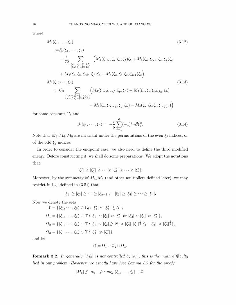
where

M6(ξ1, · · · , ξ6) (3.12)

:=β6(ξ1, · · · , ξ6)

− i

72

∑

a,c,e=1,3,5b,d,f=2,4,6

(M4(ξabc, ξd, ξe, ξf )ξb +M4(ξa, ξbcd, ξe, ξf )ξc

+M4(ξa, ξb, ξcde, ξf )ξd +M4(ξa, ξb, ξc, ξdef )ξe

),

M8(ξ1, · · · , ξ8) (3.13)

:=C8

∑

a,c,e,g=1,3,5,7b,d,f,h=2,4,6,8

(M4(ξabcde, ξf , ξg, ξh) +M4(ξa, ξb, ξcdefg, ξh)

−M4(ξa, ξbcdef , ξg, ξh)−M4(ξa, ξb, ξc, ξdefgh))

for some constant C8 and

β6(ξ1, · · · , ξ6) := − i

6

6∑

j=1

(−1)jm2jξ

2j . (3.14)

Note that M4,M6,M8 are invariant under the permutations of the even ξj indices, or

of the odd ξj indices.

In order to consider the endpoint case, we also need to define the third modified

energy. Before constructing it, we shall do some preparations. We adopt the notations

that

|ξ∗1 | ≥ |ξ∗2 | ≥ · · · ≥ |ξ∗6 | ≥ · · · ≥ |ξ∗n|.Moreover, by the symmetry of M6,M8 (and other multipliers defined later), we may

restrict in Γn (defined in (3.5)) that

|ξ1| ≥ |ξ3| ≥ · · · ≥ |ξn−1|, |ξ2| ≥ |ξ4| ≥ · · · ≥ |ξn|.

Now we denote the sets

Υ = (ξ1, · · · , ξ6) ∈ Γ6 : |ξ∗1 | ∼ |ξ∗2 | & N,

Ω1 = (ξ1, · · · , ξ6) ∈ Υ : |ξ1| ∼ |ξ3| ≫ |ξ∗3 | or |ξ2| ∼ |ξ4| ≫ |ξ∗3 |,

Ω2 = (ξ1, · · · , ξ6) ∈ Υ : |ξ1| ∼ |ξ2| & N ≫ |ξ∗3 |, |ξ1|12 |ξ1 + ξ2| ≫ |ξ∗3 |

32 ,

Ω3 = (ξ1, · · · , ξ6) ∈ Υ : |ξ∗3 | ≫ |ξ∗4 |,and let

Ω = Ω1 ∪ Ω2 ∪ Ω3.

Remark 3.2. In generally, |M6| is not controlled by |α6|, this is the main difficulty

lied in our problem. However, we exactly have (see Lemma 4.9 for the proof)

|M6| . |α6|, for any (ξ1, · · · , ξ6) ∈ Ω.

GLOBAL ROUGH SOLUTION FOR DNLS 11

For this reason, Ω is referred to the non-resonant set.

Rewrite (3.11) by

d

dtE2

I (w(t)) = Λ6(M6 · χΓ6\Ω;w(t)) + Λ6(M6 · χΩ;w(t)) + Λ8(M8;w(t)). (3.15)

Now we are ready to define the third modified energy E3I (w(t)). Let

E3I (w(t)) = Λ6(σ6;w(t)) + E2

I (w(t)), σ6 = −M6

α6· χΩ. (3.16)

Then by (3.7) and (3.15), one has

d

dtE3

I (w(t)) = Λ6(M6 · χΓ6\Ω;w(t)) + Λ8(M8 + M8;w(t)) + Λ10(M10;w(t)), (3.17)

where M6,M8 defined in (3.12), (3.13) respectively, and

M8 =− i

6∑

j=1

X2j (σ6)ξj+1, (3.18)

M10 =i

2

6∑

j=1

(−1)j+1X4j (σ6). (3.19)

Remark 3.3. By the dyadic decomposition, we restrict that

|ξ∗j | ∼ N∗j , for any j = 1, 2, · · · .

Now we give some explanations about the construction of Ωj. We keep in mind the

denominator of σ6,

α6 = −i(ξ21 − ξ22 + ξ23 − ξ24 + ξ25 − ξ26).

On one hand, for the non-resonant region, we expect |α6| has a large lower bound in

Ω. On the other hand, we expect that the multipliers M6 has a small upper bound on

the resonant region Γ6\Ω.

(a) By the definition of Ω1, we have

|α6| ∼ N∗12, for (ξ1, · · · , ξ6) ∈ Ω1.

On the other hand, in Γ6\Ω1, the following case is ruled out:

ξ∗1 = ξ1, ξ∗2 = ξ3; or ξ∗1 = ξ2, ξ∗2 = ξ4.

Therefore, to estimate M6 · χΓ6\Ω, we only need to consider

ξ∗1 = ξ1, ξ∗2 = ξ2; or ξ∗1 = ξ2, ξ∗2 = ξ1.

This is carried out in Proposition 4.1 below.

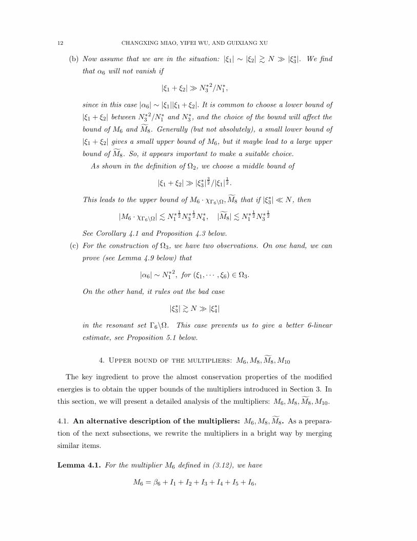
12 CHANGXING MIAO, YIFEI WU, AND GUIXIANG XU

(b) Now assume that we are in the situation: |ξ1| ∼ |ξ2| & N ≫ |ξ∗3 |. We find

that α6 will not vanish if

|ξ1 + ξ2| ≫ N∗32/N∗

1 ,

since in this case |α6| ∼ |ξ1||ξ1+ ξ2|. It is common to choose a lower bound of

|ξ1 + ξ2| between N∗32/N∗

1 and N∗3 , and the choice of the bound will affect the

bound of M6 and M8. Generally (but not absolutely), a small lower bound of

|ξ1 + ξ2| gives a small upper bound of M6, but it maybe lead to a large upper

bound of M8. So, it appears important to make a suitable choice.

As shown in the definition of Ω2, we choose a middle bound of

|ξ1 + ξ2| ≫ |ξ∗3 |32 /|ξ1|

12 .

This leads to the upper bound of M6 · χΓ6\Ω, M8 that if |ξ∗3 | ≪ N , then

|M6 · χΓ6\Ω| . N∗1

12N∗

3

12N∗

4 , |M8| . N∗1

12N∗

3

12

See Corollary 4.1 and Proposition 4.3 below.

(c) For the construction of Ω3, we have two observations. On one hand, we can

prove (see Lemma 4.9 below) that

|α6| ∼ N∗12, for (ξ1, · · · , ξ6) ∈ Ω3.

On the other hand, it rules out the bad case

|ξ∗3 | & N ≫ |ξ∗4 |

in the resonant set Γ6\Ω. This case prevents us to give a better 6-linear

estimate, see Proposition 5.1 below.

4. Upper bound of the multipliers: M6,M8, M8,M10

The key ingredient to prove the almost conservation properties of the modified

energies is to obtain the upper bounds of the multipliers introduced in Section 3. In

this section, we will present a detailed analysis of the multipliers: M6,M8, M8,M10.

4.1. An alternative description of the multipliers: M6,M8, M8. As a prepara-

tion of the next subsections, we rewrite the multipliers in a bright way by merging

similar items.

Lemma 4.1. For the multiplier M6 defined in (3.12), we have

M6 = β6 + I1 + I2 + I3 + I4 + I5 + I6,

GLOBAL ROUGH SOLUTION FOR DNLS 13

where β6 defined in (3.14) and

I1 = C6 [M4(ξ3, ξ214, ξ5, ξ6) +M4(ξ3, ξ216, ξ5, ξ4) +M4(ξ3, ξ416, ξ5, ξ2)] ξ1,

I2 = C6 [M4(ξ123, ξ4, ξ5, ξ6) +M4(ξ125, ξ4, ξ3, ξ6) +M4(ξ325, ξ4, ξ1, ξ6)] ξ2,

I3 = C6 [M4(ξ1, ξ234, ξ5, ξ6) +M4(ξ1, ξ236, ξ5, ξ4) +M4(ξ1, ξ436, ξ5, ξ2)] ξ3,

I4 = C6 [M4(ξ143, ξ2, ξ5, ξ6) +M4(ξ145, ξ2, ξ3, ξ6) +M4(ξ345, ξ2, ξ1, ξ6)] ξ4,

I5 = C6 [M4(ξ1, ξ254, ξ3, ξ6) +M4(ξ1, ξ256, ξ3, ξ4) +M4(ξ1, ξ456, ξ3, ξ2)] ξ5,

I6 = C6 [M4(ξ163, ξ2, ξ5, ξ4) +M4(ξ165, ξ2, ξ3, ξ4) +M4(ξ365, ξ2, ξ1, ξ4)] ξ6

for some constant C6.

For M8, we rewrite it as the following two formulations.

Lemma 4.2. For the multiplier M8 defined in (3.13), we have

M8 = J1 + J2 + J3 + J4 = J ′1 + J ′

2 + J ′3 + J ′

4, (4.1)

where

J1 = 2C ′8

∑

a,c,e=3,5,7b,d,f=4,6,8

[M4(ξ12abc, ξd, ξe, ξf )−M4(ξa, ξ12bcd, ξe, ξf )] ,

J2 = C ′8

∑

a,c,e=3,5,7b,d,f=4,6,8

[M4(ξa2cbe, ξd, ξ1, ξf )−M4(ξa, ξb1dcf , ξe, ξ2)] ,

J3 = C ′8

∑

a,c,e=3,5,7b,d,f=4,6,8

[M4(ξ1badc, ξ2, ξe, ξf )−M4(ξ1, ξ2abcd, ξe, ξf )] ,

J4 = 2C ′8

∑

a,c,e=3,5,7b,d,f=4,6,8

[M4(ξ1, ξ2, ξabcde, ξf )−M4(ξ1, ξ2, ξa, ξbcdef )] ,

J ′1 = 2C ′

8

∑

a,c=5,7b,d,f,h=2,4,6,8

[M4(ξ1b3da, ξf , ξc, ξh)−M4(ξa, ξb1d3f , ξc, ξh)] ,

J ′2 = C ′

8

∑

a,c=5,7b,d,f,h=2,4,6,8

[M4(ξ1badc, ξf , ξ3, ξh) +M4(ξ3badc, ξf , ξ1, ξh)] ,

J ′3 = −C ′

8

∑

a,c=5,7b,d,f,h=2,4,6,8

[M4(ξ1, ξb3daf , ξc, ξf ) +M4(ξ3, ξb1daf , ξc, ξf )] ,

J ′4 = 2C ′

8

∑

a,c,e=3,5,7b,d,f=4,6,8

[M4(ξ1, ξbadcf , ξ3, ξe)−M4(ξ1, ξb, ξ3, ξadcfe)]

for some constant C ′8.

For M8, we rewrite it as follows.

14 CHANGXING MIAO, YIFEI WU, AND GUIXIANG XU

Lemma 4.3. For the multiplier M8 defined in (3.18), we have

M8 = J1 + J2 + J3 + R8, (4.2)

where

J1 = C ′8

[σ6(ξ3, ξ214, ξ5, ξ6, ξ7, ξ8) + σ6(ξ3, ξ216, ξ5, ξ4, ξ7, ξ8)

+ σ6(ξ3, ξ218, ξ5, ξ4, ξ7, ξ6) + σ6(ξ3, ξ416, ξ5, ξ2, ξ7, ξ8)

+ σ6(ξ3, ξ418, ξ5, ξ2, ξ7, ξ6) + σ6(ξ3, ξ618, ξ5, ξ2, ξ7, ξ4)]ξ1,

J2 = C ′8

[σ6(ξ123, ξ4, ξ5, ξ6, ξ7, ξ8) + σ6(ξ125, ξ4, ξ3, ξ6, ξ7, ξ8)

+ σ6(ξ127, ξ4, ξ3, ξ6, ξ5, ξ8) + σ6(ξ325, ξ4, ξ1, ξ6, ξ7, ξ8)

+ σ6(ξ327, ξ4, ξ1, ξ6, ξ5, ξ8) + σ6(ξ527, ξ4, ξ1, ξ6, ξ3, ξ8)]ξ2,

J3 = C ′8

[σ6(ξ1, ξ234, ξ5, ξ6, ξ7, ξ8) + σ6(ξ1, ξ236, ξ5, ξ4, ξ7, ξ8)

+ σ6(ξ1, ξ238, ξ5, ξ4, ξ7, ξ6) + σ6(ξ1, ξ436, ξ5, ξ2, ξ7, ξ8)

+ σ6(ξ1, ξ438, ξ5, ξ2, ξ7, ξ6) + σ6(ξ1, ξ638, ξ5, ξ2, ξ7, ξ4)]ξ3

for some constant C ′8, and

∣∣R8

∣∣ . maxΩ

|σ6| ·max|ξ4|, · · · , |ξ8|. (4.3)

Next, we give the bounds of the multipliers one by one. First, we may assume by

symmetry that

|ξ1| ≥ |ξ2|

in the following analysis. Hence

ξ∗1 = ξ1, ξ∗2 = ξ2 or ξ3.

4.2. Known facts. In this subsection, we restate some results obtained in [10]. First,

we have

Lemma 4.4 ([10]). If N∗1 ≪ N , then we have

M4(ξ1, ξ2, ξ3, ξ4) =12 (ξ1 + ξ3), (4.4)

M6(ξ1, · · · , ξ6) = 0, M8(ξ1, · · · , ξ8) = 0. (4.5)

Second, we present some estimates on the multipliers.

Lemma 4.5 ([10]). The following estimates hold:

(1)

|M4(ξ1, ξ2, ξ3, ξ4)| . m21N

∗1 ; (4.6)

GLOBAL ROUGH SOLUTION FOR DNLS 15

(2) If |ξ1| ∼ |ξ3| & N ≫ |ξ∗3 |, then

|M4(ξ1, ξ2, ξ3, ξ4)| . m21N

∗3 ; (4.7)

(3) If |ξ1| ∼ |ξ2| & N ≫ |ξ∗3 |, then

M4(ξ1, ξ2, ξ3, ξ4) =1

2m2

1ξ1 +R(ξ1, ξ2, ξ3, ξ4), for |R| . N∗3 . (4.8)

(4) If |ξ∗3 | & N , then

|M6(ξ1, · · · , ξ6)| . m21N

∗12; (4.9)

(5) If |ξ∗3 | ≪ N , then

|M6(ξ1, · · · , ξ6)| . N∗1N

∗3 . (4.10)

4.3. An improvement upper bound of M6. The estimates (4.9) and (4.10) are

not enough for us to use, now we make some refinements.

Proposition 4.1. For the multiplier M6 defined in (3.12), the following estimates

hold:

(1) If ξ∗2 = ξ2, then

|M6(ξ1, · · · , ξ6)| . N∗1N

∗3 . (4.11)

(2) If |ξ1| ∼ |ξ2| & N ≫ |ξ∗3 |, then

M6(ξ1, · · · , ξ6) = −C6ξ1ξ12 +C ′6(m

22ξ

22 −m2

1ξ21)− C6m

21ξ1ξ12 +O(N∗

32), (4.12)

where C6 is the constant in Lemma 4.1 and C ′6 =

12C6 − i

6 .

Proof. For the sake of simplicity, we may assume that C6 = 1. Further, for (4.11),

we only consider the case N∗1 ≫ N∗

3 , otherwise it is contained in (4.9). Thus, we may

assume that |ξ1| ∼ |ξ2| ≫ |ξ∗3 | in (1).

Now we estimate (4.11) and (4.12) together. Note that

β6 = − i

6(m2

2ξ22 −m2

1ξ21) +O(N∗

32).

It suffices to estimate: I1, · · · , I6 by Lemma 4.1.

For I1, I2, by the definitions, we further divide them into three parts:

I1 := I11 + I12 + I13; I2 := I21 + I22 + I23,

where

I11 := M4(ξ3, ξ214, ξ5, ξ6)ξ1, I12 := M4(ξ3, ξ216, ξ5, ξ4)ξ1,

I13 := M4(ξ3, ξ416, ξ5, ξ2)ξ1,

I21 := M4(ξ123, ξ4, ξ5, ξ6)ξ2, I22 := M4(ξ125, ξ4, ξ3, ξ6)ξ2,

I23 := M4(ξ325, ξ4, ξ1, ξ6)ξ2.

16 CHANGXING MIAO, YIFEI WU, AND GUIXIANG XU

In order to estimate I1, . . . , I6, it is enough to prove the following three lemmas.

Lemma 4.6. If |ξ1| ∼ |ξ2| ≫ |ξ∗3 |, then we have

I13 + I23 =1

2(m2

1ξ1ξ2 +m22ξ

22) +O(N∗

32). (4.13)

Hence,

|I13 + I23| . N∗1N

∗3 . (4.14)

Proof. By the definition, we have

I13 = M4(ξ3, ξ416, ξ5, ξ2)ξ1

= −m2416ξ

2416ξ2 +m2

2ξ22ξ416 +m2

3ξ23ξ5 +m2

5ξ25ξ3

α· ξ1,

where α = ξ23 − ξ2416 + ξ25 − ξ22 . Similarly,

I23 = M4(ξ325, ξ4, ξ1, ξ6)ξ2

= −m2325ξ

2325ξ1 +m2

1ξ21ξ325 +m2

4ξ24ξ6 +m2

6ξ26ξ4

α′· ξ2,

where α′ = ξ2325 − ξ24 + ξ21 − ξ26 . Note that |ξ1| ∼ |ξ2| ≫ |ξ∗3 |, we have

|α|, |α′| ∼ N∗12, (4.15)

Then,

I13 = −m2416ξ

2416ξ2 +m2

2ξ22ξ416

α· ξ1 +O(N∗

32N∗

4 /N∗1 ),

I23 = −m2325ξ

2325ξ1 +m2

1ξ21ξ325

α′· ξ2 +O(N∗

32N∗

4 /N∗1 ),

which yield that

I13 + I23 =− m2416ξ

2416ξ2 +m2

2ξ22ξ416

α· (ξ1 + ξ2) (4.16)

+ ξ2 ·(m2

416ξ2416ξ2 +m2

2ξ22ξ416

α− m2

325ξ2325ξ1 +m2

1ξ21ξ325

α′

)

+O(N∗32N∗

4 /N∗1 )

:=II1 + ξ2 · II +O(N∗32N∗

4 /N∗1 ).

First, by the mean value theorem (2.20) and m ≤ 1, we have

|II1| . m21|ξ1 + ξ2||ξ1246| . N∗

32. (4.17)

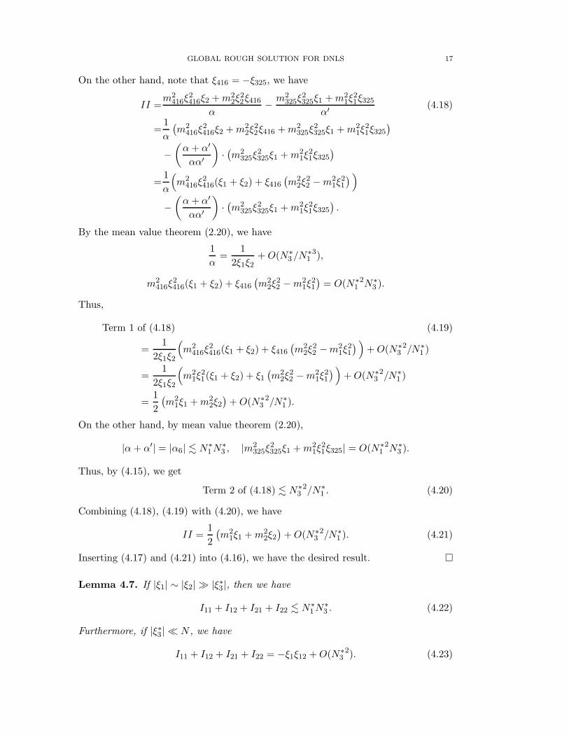
GLOBAL ROUGH SOLUTION FOR DNLS 17

On the other hand, note that ξ416 = −ξ325, we have

II =m2

416ξ2416ξ2 +m2

2ξ22ξ416

α− m2

325ξ2325ξ1 +m2

1ξ21ξ325

α′(4.18)

=1

α

(m2

416ξ2416ξ2 +m2

2ξ22ξ416 +m2

325ξ2325ξ1 +m2

1ξ21ξ325

)

−(α+ α′

αα′

)·(m2

325ξ2325ξ1 +m2

1ξ21ξ325

)

=1

α

(m2

416ξ2416(ξ1 + ξ2) + ξ416

(m2

2ξ22 −m2

1ξ21

) )

−(α+ α′

αα′

)·(m2

325ξ2325ξ1 +m2

1ξ21ξ325

).

By the mean value theorem (2.20), we have

1

α=

1

2ξ1ξ2+O(N∗

3 /N∗13),

m2416ξ

2416(ξ1 + ξ2) + ξ416

(m2

2ξ22 −m2

1ξ21

)= O(N∗

12N∗

3 ).

Thus,

Term 1 of (4.18) (4.19)

=1

2ξ1ξ2

(m2

416ξ2416(ξ1 + ξ2) + ξ416

(m2

2ξ22 −m2

1ξ21

) )+O(N∗

32/N∗

1 )

=1

2ξ1ξ2

(m2

1ξ21(ξ1 + ξ2) + ξ1

(m2

2ξ22 −m2

1ξ21

))+O(N∗

32/N∗

1 )

=1

2

(m2

1ξ1 +m22ξ2

)+O(N∗

32/N∗

1 ).

On the other hand, by mean value theorem (2.20),

|α+ α′| = |α6| . N∗1N

∗3 , |m2

325ξ2325ξ1 +m2

1ξ21ξ325| = O(N∗

12N∗

3 ).

Thus, by (4.15), we get

Term 2 of (4.18) . N∗32/N∗

1 . (4.20)

Combining (4.18), (4.19) with (4.20), we have

II =1

2

(m2

1ξ1 +m22ξ2

)+O(N∗

32/N∗

1 ). (4.21)

Inserting (4.17) and (4.21) into (4.16), we have the desired result.

Lemma 4.7. If |ξ1| ∼ |ξ2| ≫ |ξ∗3 |, then we have

I11 + I12 + I21 + I22 . N∗1N

∗3 . (4.22)

Furthermore, if |ξ∗3 | ≪ N , we have

I11 + I12 + I21 + I22 = −ξ1ξ12 +O(N∗32). (4.23)

18 CHANGXING MIAO, YIFEI WU, AND GUIXIANG XU

Proof. Since |ξ12| . N∗3 , (4.22) follows from (4.6). Moreover, if |ξ12| ≪ N , then by

(4.4), we have

I11 = I12 =1

2ξ35 · ξ1, I21 = I22 = −1

2ξ46 · ξ2,

which imply that

I11 + I12 + I21 + I22 = ξ35ξ1 − ξ46ξ2 = ξ12 · ξ235 = −ξ1ξ12 +O(N∗32).

This completes the proof of the lemma.

Lemma 4.8. If |ξ1| ∼ |ξ2| ≫ |ξ∗3 |, then we have

|I3 + I4 + I5 + I6| . N∗1N

∗3 . (4.24)

Furthermore, if |ξ∗3 | ≪ N , then

I3 + I4 + I5 + I6 = −3

2m2

1ξ1ξ12 +O(N∗32). (4.25)

Proof. (4.24) follows from (4.6). Now we consider the case |ξ∗3 | ≪ N . By (4.8), we

have

M4(ξ1, ξ2, ξ3, ξ4) =1

2m2

1ξ1 +O(N∗3 ), (4.26)

where ξ1+ ξ2+ ξ3+ ξ4 = 0, ξ1 = ξ1+O(N∗3 ), ξ2 = ξ2+O(N∗

3 ) and |ξ1| ∼ |ξ2| & N ≫|ξ∗3 |. Using (4.26), we obtain

I3 + I4 + I5 + I6 =3

2m2

1ξ1(ξ3 + ξ4 + ξ5 + ξ6) +O(N∗32)

= −3

2m2

1ξ1(ξ1 + ξ2) +O(N∗32).

This completes the proof of the lemma.

Now we finish the proof of Proposition 4.1. Indeed, (4.11) follows from (4.14),

(4.22) and (4.24). While by (4.13) and (4.25), we have,

I13 + I23 + I3 + I4 + I5 + I6 (4.27)

=1

2(m2

1ξ1ξ2 +m22ξ

22)−

3

2m2

1ξ1(ξ1 + ξ2) +O(N∗32)

=1

2(m2

2ξ22 −m2

1ξ21)−m2

1ξ1(ξ1 + ξ2) +O(N∗32).

Therefore, (4.12) follows from (4.23) and (4.27).

Corollary 4.1. If |ξ∗3 | ≪ N , then we have

|M6(ξ1, · · · , ξ6)| . N∗1

12N∗

3

12N∗

4 in Γ6\Ω. (4.28)

Proof. In this situation, ξ∗2 = ξ2 (see Remark 3.3 (a)). Then by (4.12) and the mean

value theorem (2.20), we have

|M6(ξ1, · · · , ξ6)| . |ξ1||ξ1 + ξ2|+N∗32.

GLOBAL ROUGH SOLUTION FOR DNLS 19

Moreover, since |ξ1|12 |ξ1 + ξ2| . |ξ∗3 |

32 in Γ6\Ω, we have

|M6(ξ1, · · · , ξ6)| . N∗1

12N∗

3

32 .

Then (4.28) follows by the fact that N∗3 ∼ N∗

4 in Γ6\Ω3.

4.4. A upper bound of M8.

Proposition 4.2.

|M8(ξ1, · · · , ξ8)| . N∗1 . (4.29)

Furthermore, if |ξ∗3 | ≪ N , then we have

|M8(ξ1, · · · , ξ8)| . N∗3 . (4.30)

Proof. By (4.6), we have |M4(ξ1, ξ2, ξ3, ξ4)| . N∗1 . Thus (4.29) follows. For (4.30), we

split it into two cases.

Case 1, ξ∗2 = ξ2. By (4.1), we have

M8 = J1 + J2 + J3 + J4.

So it suffices to prove: |J1|, |J2|, |J3|, |J4| . N∗3 . First, J1 follows immediately from

|ξ1 + ξ2| . N∗3 and (4.6). While J2 follows from (4.7) and J3, J4 follow from (4.26).

Case 2, ξ∗2 = ξ3. Now we adopt the formulation:

M8 = J ′1 + J ′

2 + J ′3 + J ′

4,

and it is necessary to prove: |J ′1|, |J ′

2|, |J ′3|, |J ′

4| . N∗3 . J

′1 and J ′

2 are similar to J1 and

J2. For J′3, we also use (4.26) to give

J ′3 = C(m2

1ξ1 +m23ξ3) +O(N∗

3 ) = O(N∗3 ),

where we used the mean value theorem (2.20). J ′4 is similar to J2.

4.5. A upper bound of σ6, M8. First, we prove that σ6 is uniformly bounded in Ω,

which implies that the set Ω is non-resonant.

Lemma 4.9. In Ω, we have

|σ6(ξ1, · · · , ξ6)| . 1. (4.31)

Particularly, in Ω1 ∩|ξ∗3 | ≪ N

, we have

|σ6(ξ1, · · · , ξ6)| . N∗3 /N

∗1 . (4.32)

20 CHANGXING MIAO, YIFEI WU, AND GUIXIANG XU

Proof. Recall that

σ6 = −M6

α6· χΩ, α6 = −i(ξ21 − ξ22 + ξ23 − ξ24 + ξ25 − ξ26).

In Ω1, we have

|α6(ξ1, · · · , ξ6)| ∼ N∗12.

This gives (4.32) by (4.10) and (4.31) by (4.9).

In Ω2, we have

|ξ21 − ξ22 | ∼ |ξ1||ξ1 + ξ2| ≫ |ξ∗3 |2,which yields that

|α6| ∼ |ξ1||ξ1 + ξ2|. (4.33)

While from (4.12) and the mean value theorem (2.20), we have

|M6(ξ1, · · · , ξ6)| . |ξ1||ξ1 + ξ2|+N∗32 . |ξ1||ξ1 + ξ2|.

This gives (4.31) in Ω2.

In Ω3, since ξ∗1 · ξ∗2 < 0, ξ∗2 · ξ∗3 > 0, it holds that

|ξ∗1 | = |ξ∗2 |+ |ξ∗3 |+ o(N∗3 ).

We claim that

|α6| & N∗1N

∗3 . (4.34)

Indeed, for (4.34), we divide into the following three cases:

(i) ξ∗2 = ξ2, ξ∗3 = ξ3; (ii) ξ∗2 = ξ2, ξ

∗3 = ξ4; (iii) ξ∗2 = ξ3, ξ

∗3 = ξ2.

If ξ∗2 = ξ2, ξ∗3 = ξ3, then we get

|α6| =∣∣(ξ21 − ξ22) + ξ23 + (−ξ24 + ξ25 − ξ26)

∣∣

=(ξ21 − ξ22

)+ ξ23 + o(|ξ3|2)

= − ξ1ξ3 + ξ23 + o(|ξ1||ξ3|)

∼ |ξ1||ξ3|.If ξ∗2 = ξ2, ξ

∗3 = ξ4, then we have

|α6| =∣∣(ξ21 − ξ22 − ξ24) + (ξ23 + ξ25 − ξ26)

∣∣

=(ξ21 − ξ22 − ξ24

)+ o(|ξ4|2)

=([

|ξ2|+ |ξ4|+ o(|ξ4|)]2 − ξ22 − ξ24

)+ o(|ξ4|2)

∼ |ξ2||ξ4|.If ξ∗2 = ξ3, ξ

∗3 = ξ2, then we have

|α6| =(ξ21 − ξ22 + ξ23

)+ o(|ξ3|2) ≥ ξ23 + o(|ξ3|2) ∼ ξ21 .

This proves (4.34).

GLOBAL ROUGH SOLUTION FOR DNLS 21

By (4.9) and (4.10), we have |M6(ξ1, · · · , ξ6)| . N∗12. Then (4.31) follows if N∗

1 ∼N∗

3 . Now we consider the other case: N∗1 ≫ N∗

3 . Thus we have: ξ∗2 = ξ2 in Ω3\Ω1.

Then (4.31) in Ω3\Ω1 follows from (4.11) and (4.34).

Now we give the upper bound of M8.

Proposition 4.3.

|M8(ξ1, · · · , ξ8)| . N∗1 . (4.35)

Furthermore, if |ξ∗3 | ≪ N , then we have

|M8(ξ1, · · · , ξ8)| . N∗1

12N∗

3

12 . (4.36)

Proof. Since |σ6| . 1, we have (4.35). Now we turn to (4.36). By (4.2), we shall

estimates: J1, J2, J3. For this purpose, we divide it into two cases.

Case 1, ξ∗2 = ξ2. Since |σ6| . 1, we have |J3| . N∗3 . Now we consider the other two

parts. Since σ6 = 0 for |ξ∗1 | ≪ N , we know that the first, second, third terms of J1, J2

vanish. Therefore,

M8 =C ′8

[σ6(ξ3, ξ416, ξ5, ξ2, ξ7, ξ8) + σ6(ξ3, ξ418, ξ5, ξ2, ξ7, ξ6) (4.37)

+ σ6(ξ3, ξ618, ξ5, ξ2, ξ7, ξ4)]ξ1 + C ′

8

[σ6(ξ325, ξ4, ξ1, ξ6, ξ7, ξ8)

+ σ6(ξ327, ξ4, ξ1, ξ6, ξ5, ξ8) + σ6(ξ527, ξ4, ξ1, ξ6, ξ3, ξ8)]ξ2 +O(N∗

3 ).

By (4.32), each term is bounded by N∗3 .

Case 2, ξ∗2 = ξ3. In this case, |J2| . N∗3 , so we only need to estimate J1, J3. By

permutating the terms in J1, J3, we may rewrite M8 as

M8 =∑

a,c=5,7b,d,f,h=2,4,6,8

[σ6(ξ3, ξb1d, ξa, ξf , ξc, ξh)ξ1 + σ6(ξ1, ξb3d, ξa, ξf , ξc, ξh)ξ3

]

+O(N∗3 ).

As an example, we only consider

σ6(ξ3, ξ214, ξ5, ξ6, ξ7, ξ8)ξ1 + σ6(ξ1, ξ234, ξ5, ξ6, ξ7, ξ8)ξ3,

which equals to

III · ξ1 +O(N∗3 ), (4.38)

where

III := σ6(ξ3, ξ214, ξ5, ξ6, ξ7, ξ8)− σ6(ξ1, ξ234, ξ5, ξ6, ξ7, ξ8).

We first adopt some notations for short. We denote

A := M6(ξ3, ξ214, ξ5, ξ6, ξ7, ξ8); A′ := M6(ξ1, ξ234, ξ5, ξ6, ξ7, ξ8),

B := α6(ξ3, ξ214, ξ5, ξ6, ξ7, ξ8); B′ := α6(ξ1, ξ234, ξ5, ξ6, ξ7, ξ8).

22 CHANGXING MIAO, YIFEI WU, AND GUIXIANG XU

Since

Ω2(ξ3, ξ214, ξ5, ξ6, ξ7, ξ8) = Ω2(ξ1, ξ234, ξ5, ξ6, ξ7, ξ8),

then by (4.31), (4.33) and the definition of Ω2, we have∣∣∣∣A

B

∣∣∣∣ ,∣∣∣∣A′

B′

∣∣∣∣ . 1; |B|, |B′| ∼ |ξ1234||ξ1| ≫ N∗1

12N∗

3

32 . (4.39)

Moreover,

III =A

B− A′

B′=

1

B(A+A′)− A′

B′· B +B′

B. (4.40)

On one hand, by (4.12) and (4.39), we have

A+A′ = C6ξ1234 · (2ξ2457 + ξ13)− C6ξ1234(m21ξ1 +m2

3ξ3)

+ C ′6(m

2214ξ

2214 −m2

3ξ23 +m2

234ξ2234 −m2

1ξ21) +O(N∗

32).

Further, by the mean value theorem (2.20) in the second term and by the double

mean value theorem (2.21) in the third term, we have

|A+A′| . m21|ξ1234||ξ24|+N∗

32. (4.41)

Therefore, by (4.39) and (4.41), we have∣∣∣∣1

B(A+A′)

∣∣∣∣ .m21

|ξ24||ξ1|

+N∗

32

N∗1

12N∗

3

32

(4.42)

.N∗3 /N

∗1 +N∗

3

12 /N∗

1

12 . N∗

3

12/N∗

1

12 .

On the other hand,

|B +B′| = |ξ21 − ξ2234 + ξ23 − ξ2214|+O(N∗32) = 2|ξ1234||ξ24|+O(N∗

32).

Therefore, by the similar estimates as those in (4.39) and (4.42), we have∣∣∣∣A′

B′· B +B′

B

∣∣∣∣ . N∗3

12/N∗

1

12 . (4.43)

Inserting (4.42) and (4.43) into (4.40), we have

|III| . N∗3

12 /N∗

1

12 .

which together with (4.38) yields (4.36).

5. An upper bound on the increment of E3I (u(t))

By the multilinear correction analysis, the almost conservation law of E3I (u(t)) is

the key ingredient to establish the global well-posedness below the energy space. This

is made up of the following 6-linear, 8-linear and 10-linear estimates.

Proposition 5.1. For any s ≥ 12 , we have

∣∣∣∣∫ δ

0Λ6(M6 · χΓ6\Ω;w(t)) dt

∣∣∣∣ . N− 52+ ‖Iw‖6Y1

. (5.1)

GLOBAL ROUGH SOLUTION FOR DNLS 23

Proof. By (4.5), when |ξ1|, · · · , |ξ6| ≪ N , we have M6 = 0. Therefore, we may assume

that |ξ∗1 | ∼ |ξ∗2 | & N . Note that

‖χ[0,δ](t)f‖X0, 12−. ‖f‖X

0, 12

(see Lemma 2.2 in [22] for example), (5.1) is reduce to∣∣∣∣∫

Λ6(M6 · χΓ6\Ω;w(t)) dt

∣∣∣∣ . N− 52+ ‖Iw‖X

1, 12−‖Iw‖5Y1

.

But the 0+ loss is not essential by (2.17)–(2.19) and (2.8) for q < 6, thus it will not

be mentioned. By Plancherel’s identity and f(ξ, τ) =¯f(−ξ,−τ), we only need to

show that for any fj ∈ Y +0 , j = 1, 3, 5 and fj ∈ Y −

0 , j = 2, 4, 6,∫

Γ6×Γ6

M6 · χΓ6\Ω(ξ1, · · · , ξ6)f1(ξ1, τ1) · · · f6(ξ6, τ6)〈ξ1〉m(ξ1) · · · 〈ξ6〉m(ξ6)

(5.2)

. N− 52+ ‖f1‖Y +

0‖f2‖Y −

0· · · ‖f5‖Y +

0‖f6‖Y −

0,

where Γ6 × Γ6 = (ξ, τ) : ξ1 + · · · + ξ6 = 0, τ1 + · · · + τ6 = 0, ξ = (ξ1, · · · , ξ6),τ = (τ1, · · · , τ6). Now we divide it into four regions:

A1 =(ξ, τ) ∈ (Γ6\Ω)× Γ6 : |ξ∗2 | & N ≫ |ξ∗3 |,

A2 =(ξ, τ) ∈ (Γ6\Ω)× Γ6 : |ξ∗3 | & N ≫ |ξ∗4 |,

A3 =(ξ, τ) ∈ (Γ6\Ω)× Γ6 : |ξ∗4 | & N ≫ |ξ∗5 |,

A4 =(ξ, τ) ∈ (Γ6\Ω)× Γ6 : |ξ∗5 | & N.In the following, we adopt the notation f∗

j to be one of fj for j = 1, · · · , 6 and satisfy

f∗j = f∗

j (ξ∗j , τj).

Estimate in A1. By the definition of Ω and (4.28), in (Γ6\Ω)× Γ6, we have

|ξ1| ∼ |ξ2| & N ≫ |ξ∗3 |, and |M6 · χΓ6\Ω| . N∗1

12N∗

3

12N∗

4 .

Therefore, by (2.17)–(2.19), we have

LHS of (5.2) . N2s−2

∫

A1

f1(ξ1, τ1) · · · f6(ξ6, τ6)|ξ∗1 |2s−

12 〈ξ∗3〉

12 〈ξ∗5〉〈ξ∗6〉

= N2s−2

∫

A1

|ξ∗1 |−2s− 12+〈ξ∗3〉−

12 · (|ξ∗1 |

12−f∗

1 f∗3 ) (|ξ∗2 |

12−f∗

2 f∗4 )

· (〈ξ∗5〉−1f∗5 )(〈ξ∗6〉−1f∗

6 )

. N− 52+

∥∥∥∥I12−

± (f∗1 , f

∗3 )

∥∥∥∥L2xt

∥∥∥∥I12−

± (f∗2 , f

∗4 )

∥∥∥∥L2xt

·∥∥J−1

x f∗5

∥∥L∞xt

∥∥J−1x f∗

6

∥∥L∞xt

. N− 52+ ‖f1‖Y +

0‖f2‖Y −

0· · · ‖f5‖Y +

0‖f6‖Y −

0,

where we use the relations that |ξ∗1 ± ξ∗3 | ∼ |ξ∗1 | and |ξ∗2 ± ξ∗4 | ∼ |ξ∗1 |.Estimate in A2. Note that A2 = ∅ in (Γ6\Ω3)× Γ6, thus M6 · χΓ6\Ω = 0.

24 CHANGXING MIAO, YIFEI WU, AND GUIXIANG XU

Estimate in A3. By (4.9), we have

|M6 · χΓ6\Ω| . m21N

∗12. (5.3)

Therefore, by (2.17)–(2.19) and (2.10), we have

LHS of (5.2) . N2s−2

∫

A3

f1(ξ1, τ1) · · · f6(ξ6, τ6)|ξ∗3 |s|ξ∗4 |s〈ξ∗5〉〈ξ6〉

= N2s−2

∫

A1

|ξ∗1 |−12+|ξ∗3 |−s|ξ∗4 |−s〈ξ∗5〉−1 · (|ξ∗1 |

12−f∗

1 f∗5 ) (|ξ∗2 |0−f∗

2 )

· (|ξ∗3 |0−f∗3 )(|ξ∗4 |0−f∗

4 )(〈ξ∗6〉−1f∗6 )

. N− 52+

∥∥∥∥I12−

± (f∗1 , f

∗5 )

∥∥∥∥L2xt

∥∥J0−x f∗

2

∥∥L6xt

∥∥J0−x f∗

3

∥∥L6xt

·∥∥J0−

x f∗4

∥∥L6xt

∥∥J−1x f∗

6

∥∥L∞xt

. N− 52+ ‖f1‖Y +

0‖f2‖Y −

0· · · ‖f5‖Y +

0‖f6‖Y −

0,

where we use the fact that |ξ∗1 ± ξ∗5 | ∼ |ξ∗1 | in this case.

Estimate in A4. The worst case is |ξj| & N for any j = 1, · · · , 6, we only consider

this case. Then by (5.3), (2.8) for q = 6− and (2.11) for q = 6+, we have

LHS of (5.2) . N4s−4

∫

A4

f1(ξ1, τ1) · · · f6(ξ6, τ6)|ξ∗3 |s|ξ∗4 |s|ξ∗5 |s|ξ∗6 |s

. N−4+ ‖f∗1‖L6−

xt· · · ‖f∗

5 ‖L6−xt

∥∥J0−x f∗

6

∥∥L6+xt

. N−4+ ‖f1‖Y +0‖f2‖Y −

0· · · ‖f5‖Y +

0‖f6‖Y −

0.

This gives the proof of the proposition.

Proposition 5.2. For any s ≥ 12 , we have

∣∣∣∣∫ δ

0Λ8(M8 + M8;w(t)) dt

∣∣∣∣ . N− 52+ ‖Iw‖8Y1

. (5.4)

Proof. When |ξ1|, · · · , |ξ8| ≪ N , we have M8, M8 = 0. Similar to (5.2), it suffices to

show∫

Γ8×Γ8

(M8 + M8)(ξ1, · · · , ξ8)f1(ξ1, τ1) · · · f8(ξ8, τ8)〈ξ1〉m(ξ1) · · · 〈ξ8〉m(ξ8)

(5.5)

. N− 52+ ‖f1‖Y +

0‖f2‖Y −

0· · · ‖f7‖Y +

0‖f8‖Y −

0,

where Γ8 × Γ8 = (ξ1, · · · , ξ8, τ1, · · · , τ8) : ξ1 + · · · + ξ8 = 0, τ1 + · · · + τ8 = 0. Now

we divide it into three regions:

B1 =(ξ1, · · · , ξ8, τ1, · · · , τ8) ∈ Γ8 × Γ8 : |ξ∗1 | ∼ |ξ∗2 | & N ≫ |ξ∗3 |,

B2 =(ξ1, · · · , ξ8, τ1, · · · , τ8) ∈ Γ8 × Γ8 : |ξ∗3 | & N ≫ |ξ∗4 |,

B3 =(ξ1, · · · , ξ8, τ1, · · · , τ8) ∈ Γ8 × Γ8 : |ξ∗4 | & N.

GLOBAL ROUGH SOLUTION FOR DNLS 25

Estimate in B1. By (4.30) and (4.36), we have

|M8 + M8| . N∗1

12N∗

3

12 .

Therefore, similar to the estimate in A1 in Proposition 5.1, we have

LHS of (5.5) . N2s−2

∫

B1

f1(ξ1, τ1) · · · f8(ξ8, τ8)|ξ∗1 |2s−

12 〈ξ∗3〉

12 〈ξ∗4〉 · · · 〈ξ∗8〉

. N− 52+

∥∥∥∥I12−

± (f∗1 , f

∗3 )

∥∥∥∥L2xt

∥∥∥∥I12−

± (f∗2 , f

∗4 )

∥∥∥∥L2xt

∥∥J−1x f∗

5

∥∥L∞xt· · ·

∥∥J−1x f∗

8

∥∥L∞xt

. N− 52+ ‖f1‖Y +

0‖f2‖Y −

0· · · ‖f7‖Y +

0‖f8‖Y −

0.

Estimate in B2. By (4.29) and (4.35), we have

|M8 + M8| . N∗1 . (5.6)

Moreover, it satisfies that

|ξ∗1 | − |ξ∗3 | ∼ |ξ∗1 | in B2.

Indeed, we have |ξ∗1 | = |ξ∗2 | + |ξ∗3 | + o(N∗3 ) (see the proof of Lemma 4.9 for more

details). Therefore, similar to the estimate in B1, we have

LHS of (5.5) . N3s−3

∫

B2

f1(ξ1, τ1) · · · f8(ξ8, τ8)|ξ∗1 |2s−1|ξ∗3 |s〈ξ∗4〉 · · · 〈ξ∗8〉

. N−3+

∥∥∥∥I12−

± (f∗1 , f

∗3 )

∥∥∥∥L2xt

∥∥∥∥I12−

± (f∗2 , f

∗4 )

∥∥∥∥L2xt

·∥∥J−1

x f∗5

∥∥L∞xt· · ·

∥∥J−1x f∗

8

∥∥L∞xt

. N−3+ ‖f1‖Y +0‖f2‖Y −

0· · · ‖f7‖Y +

0‖f8‖Y −

0.

Estimate in B3. We only consider the worst case: |ξj| & N for any j = 1, · · · , 8.By (5.6) and the similar estimates in A4 in Proposition 5.1, we have

LHS of (5.5) . N8s−8

∫

B3

f1(ξ1, τ1) · · · f8(ξ8, τ8)|ξ∗1 |2s−1|ξ∗3 |s · · · |ξ∗8 |s

. N−6+ ‖f∗1‖L6−

xt· · · ‖f∗

5 ‖L6−xt

∥∥J0−x f∗

6

∥∥L6+xt

∥∥∥∥J− 1

2−

x f∗7

∥∥∥∥L∞xt

∥∥∥∥J− 1

2−

x f∗8

∥∥∥∥L∞xt

. N−6+ ‖f1‖Y +0‖f2‖Y −

0· · · ‖f7‖Y +

0‖f8‖Y −

0,

This gives the proof of the proposition.

Proposition 5.3. For any s ≥ 12 , we have

∣∣∣∣∫ δ

0Λ10(M10;w(t)) dt

∣∣∣∣ . N−3+ ‖Iw‖10Y1. (5.7)

26 CHANGXING MIAO, YIFEI WU, AND GUIXIANG XU

Proof. When |ξ1|, · · · , |ξ10| ≪ N , we have M10 = 0. Therefore, we may assume that

|ξ∗1 | ∼ |ξ∗2 | & N . Further, by symmetry, we may assume |ξ1| ≥ · · · ≥ |ξ10| again.Similar to (5.2), it suffices to show

∫

Γ10×Γ10

M10(ξ1, · · · , ξ10)f1(ξ1, τ1) · · · f10(ξ10, τ10)〈ξ1〉m(ξ1) · · · 〈ξ10〉m(ξ10)

(5.8)

. N−3+ ‖f1‖Y +0‖f2‖Y −

0· · · ‖f9‖Y +

0‖f10‖Y −

0,

where Γ10 × Γ10 = (ξ1, · · · , ξ10, τ1, · · · , τ10) : ξ1 + · · · + ξ10 = 0, τ1 + · · · + τ10 = 0.Now we divide it into two regions:

D1 =(ξ1, · · · , ξ10, τ1, · · · , τ10) ∈ Γ10 × Γ10 : |ξ2| & N ≫ |ξ3|.,

D2 =(ξ1, · · · , ξ10, τ1, · · · , τ10) ∈ Γ10 × Γ10 : |ξ3| & N.Estimate in D1. By Lemma 4.9, we have |σ6| . 1 and thus

|M10| . 1. (5.9)

Similar to the estimates in A1 in Proposition 5.1, we have

LHS of (5.8) . N2s−2

∫

D1

f1(ξ1, τ1) · · · f10(ξ10, τ10)|ξ1|s|ξ2|s〈ξ3〉 · · · 〈ξ10〉

. N−3+

∥∥∥∥I12−

− (f1, f3)

∥∥∥∥L2xt

∥∥∥∥I12−

− (f2, f4)

∥∥∥∥L2xt

·∥∥J−1

x f5∥∥L∞xt· · ·

∥∥J−1x f10

∥∥L∞xt

. N−3+ ‖f1‖Y +0‖f2‖Y −

0· · · ‖f9‖Y +

0‖f10‖Y −

0.

Estimate in D2. We only consider the worst case: |ξj | & N for any j = 1 · · · 10.Thus by (5.9), and the similar estimates in B3 in Proposition 5.2, we have

LHS of (5.8) . N10s−10

∫

D2

f1(ξ1, τ1) · · · f10(ξ10, τ10)|ξ1|s|ξ2|s|ξ3|s|ξ4|s · · · |ξ10|s

. N−8+ ‖f∗1 ‖L6−

xt· · · ‖f∗

5‖L6−xt

∥∥J0−x f∗

6

∥∥L6+xt

·∥∥∥∥J

− 12−

x f∗7

∥∥∥∥L∞xt

· · ·∥∥∥∥J

− 12−

x f∗10

∥∥∥∥L∞xt

. N−8+ ‖f1‖Y +0‖f2‖Y −

0· · · ‖f9‖Y +

0‖f10‖Y −

0.

This gives the proof of the proposition.

6. A comparison between E1I (w) and E3

I (w)

In this section, we show that the third generation modified energy E3I (w) is compa-

rable to the first generation modified energy E1I (w) = E(Iw). In Section 5, we have

shown that E3I (w) is almost conserved with a tiny increment. Then the result in this

section forecasts that E1I (w) is also almost conserved with a similar tiny increment

(which will be realized in next section). Now we state the result in this section.

GLOBAL ROUGH SOLUTION FOR DNLS 27

Lemma 6.1. Let s ≥ 12 , then we have

∣∣E3I (w(t)) −E1

I (w(t))∣∣ . N0−

(‖Iw(t)‖4H1 + ‖Iw(t)‖6H1

). (6.1)

Proof. By (3.8), (3.9) and (3.16), we have

E3I (w(t)) − E1

I (w(t)) =1

2Λ4

(M4(ξ1, ξ2, ξ3, ξ4)−

1

2ξ13m1m2m3m4;w(t)

)

+Λ6(σ6;w(t)).

Therefore, it suffices to prove∣∣∣∣Λ4

(M4(ξ1, ξ2, ξ3, ξ4)−

1

2ξ13m1m2m3m4;w(t)

)∣∣∣∣ . N0−‖Iw(t)‖4H1 , (6.2)

and

|Λ6(σ6;w(t))| . N0−‖Iw(t)‖6H1 . (6.3)

For (6.2), we refer to (32) in [10]. Now we turn to prove (6.3). By Plancherel’s

identity, it suffices to show∫

Γ6

σ6(ξ1, · · · , ξ6)f1(ξ1, t) · · · f6(ξ6, t)〈ξ1〉m(ξ1) · · · 〈ξ6〉m(ξ6)

. N0− ‖f1(t)‖L2x· · · ‖f6(t)‖L2

x. (6.4)

We may assume that |ξ1| ≥ |ξ2| ≥ · · · |ξ6| by symmetry. Since σ6 = 0 when |ξj| ≪ N

for any j = 1, · · · , 6, we may assume that |ξ1| ∼ |ξ2| & N . By Lemma 4.9, we have

|σ6| . 1. Note that

〈ξ〉m(ξ) & 〈ξ〉s, for any ξ ∈ R,

we have by Sobolev’s inequality,

LHS of (6.4) . N−2+

∫

Γ6

f1(ξ1, τ1) · · · f10(ξ10, τ10)〈ξ3〉s+ · · · 〈ξ6〉s+

. N−2+ ‖f1(t)‖L2x‖f2(t)‖L2

x

∥∥∥∥J− 1

2−

x f3(t)

∥∥∥∥L∞x

· · ·∥∥∥∥J

− 12−

x f10(t)

∥∥∥∥L∞x

. N−2+ ‖f1(t)‖L2x· · · ‖f10(t)‖L2

x.

This gives the proof of the lemma.

7. The Proof of Theorem 1.1

7.1. A Variant Local Well-posedness. In this subsection, we will establish a vari-

ant local well-posedness as follows.

Proposition 7.1. Let s ≥ 12 , then Cauchy problem (3.1) is locally well-posed for the

initial data w0 satisfying Iw0 ∈ H1(R). Moreover, the solution exists on the interval

[0, δ] with the lifetime

δ ∼ ‖IN,sw0‖−µH1 (7.1)

28 CHANGXING MIAO, YIFEI WU, AND GUIXIANG XU

for some µ > 0. Furthermore, the solution satisfies the estimate

‖IN,sw‖Y1 . ‖IN,sw0‖H1 . (7.2)

Proof. By the standard iteration argument (see cf. [29]), it suffices to prove the

multilinear estimates,

‖I(w1∂xw2w3)‖Z1. ‖Iw1‖Y1‖Iw2‖Y1‖Iw3‖Y1 , (7.3)

and

‖I(w1w2w3w4w5)‖Z1. ‖Iw1‖Y1 · · · ‖Iw5‖Y1 . (7.4)

By Lemma 12.1 in [12], it suffices to prove the multilinear estimates,

‖w1∂xw2w3‖Zs. ‖w1‖Ys‖w2‖Ys‖w3‖Ys , (7.5)

and

‖w1w2w3w4w5‖Zs. ‖w1‖Ys · · · ‖w5‖Ys . (7.6)

These were proved in [29].

7.2. Rescaling. We rescale the solution of (3.1) by writing

wµ(x, t) = µ− 12w(x/µ, t/µ2); w0,µ(x) = µ− 1

2w0(x/µ).

Then wµ(x, t) is still the solution of (3.1) with the initial data w(x, 0) = w0,µ(x).

Meanwhile, w(x, t) exists on [0, T ] if and only if wµ(x, t) exists on [0, µ2T ].

By m(ξ) ≤ 1 and (3.4), we know that

‖Iwµ(t)‖L2x≤ ‖wµ(t)‖L2

x= ‖w0,µ‖L2

x= ‖w0‖L2

x<

√2π.

This together with (3.3) yields

‖∂xIuµ(t)‖2L2x∼ E1

I (wµ(t)), ‖Iwµ(t)‖2H1x. E1

I (wµ(t)) + 1. (7.7)

Moreover, by (2.6), we get that

‖∂xIw0,µ‖L2 . N1−s/µs · ‖w0‖Hs .

Hence, if we choose µ ∼ N1−ss suitably, we have ‖Iw0,µ‖H1 ≤ 5. Thus we may take

δ ∼ 1 by Proposition 7.1.

By standard limiting argument, the global well-posedness of w in Hs(R) follows if

for any T > 0, we have

sup0≤t≤T

‖w(t)‖Hs . C(‖w0‖Hs , T ).

Further, in light of (2.6) and (7.7), it suffices to show

sup0≤t≤µ2T

E1I (wµ(t)) . C(T ) (7.8)

GLOBAL ROUGH SOLUTION FOR DNLS 29

for some N. In the following subsection, we shall prove it by almost conservation law

and iteration.

7.3. Almost conservation law and iteration. By (3.17), we have

E3I (wµ(t)) = E3

I (w0,µ)+

∫ t

0

(Λ6(M6 · χΓ6\Ω;w(s)) ds

+

∫ t

0Λ8(M8 + M8;w(s)) + Λ10(M10;w(s))

)ds.

By Proposition 5.1–Proposition 5.3 and (7.2), we have for any t ∈ [0, 1],

E3I (wµ(t)) ≤E3

I (w0,µ) + C1N− 5

2+(‖Iwµ‖6Y1

+ ‖Iwµ‖8Y1+ ‖Iwµ‖10Y1

)

≤E3I (w0,µ) + C2N

− 52+.

Thus,

E1I (wµ(t)) ≤E1

I (w0,µ) +(E1

I (wµ(t))− E3I (wµ(t))

)

+(E3

I (w0,µ)− E1I (w0,µ)

)+C2N

− 52+.

Using (6.1), choosing N suitable large and applying the bootstrap argument, we

obtain that for any t ∈ [0, 1],

E1I (wµ(t)) ≤ 10.

Repeating this process M times, we obtain for any t ∈ [0,M ],

E1I (wµ(t)) ≤E1

I (w0,µ) +(E1

I (wµ(t))− E3I (wµ)

)

+(E3

I (w0,µ)− E1I (w0,µ)

)+ C2MN− 5

2+.

Therefore, by (6.1) again, we have E1I (wµ(t)) ≤ 10 provided M . N

52−, which implies

that the solution wµ exists on [0,Mδ] ∼ [0, N52−]. Hence, w exists on [0, µ2T ] with

the relation

N52− & µ2T ∼ N

2(1−s)s T.

Thus we may take T ∼ N9s−42s

−. When s ≥ 12 , we have 9s−4

2s > 0. This implies (7.8)

by choosing sufficient large N , and thus completes the proof of Theorem 1.1 .

Acknowledgements. The authors were supported by the NSF of China (No. 10725102,

No. 10801015). The second author was also partly supported by Beijing International

Center for Mathematical Research.

References

[1] Biagioni, H.; and Linares, F.: Ill-posedness for the derivative Schrodinger and generalized

Benjamin-Ono equations, Trans. Amer. Math. Soc., 353 (9), 3649–3659, (2001).[2] Bambusi, D.; Delort, J. M.; Grebert, G.; and Szeftel, J.: Almost global existence for Hamiltonian

semi-linear Klein-Gordon equations with small Cauchy data on Zoll manifolds. Comm. PureAppl. Math., 60 (11), 1665-1690, (2007).

30 CHANGXING MIAO, YIFEI WU, AND GUIXIANG XU

[3] Bourgain, J.: Fourier transform restriction phenomena for certain lattice subsets and applica-

tions to nonlinear evolution equations. I: Schrodinger Equation. Geom. Funct. Anal., 3, 107–156,(1993).

[4] Bourgain, J.: Fourier transform restriction phenomena for certain lattice subsets and applica-

tions to nonlinear evolution equations. II: the KdV-Equation. Geom. Funct. Anal., 3, 209–262,(1993).

[5] Bourgain, J.: Periodic Korteweg-de Vries equation with measures as initial data, Selecta Math.,3, 115–159, (1997).

[6] Bourgain, J.: Refinements of Strichartz inequality and applications to 2D-NLS with critical

nonlinearity, Int. Math. Research Notices, 5, 253–283, (1998).[7] Bourgain, J.: New global well-posedness results for nonlinear Schrodinger equations, AMS Pub-

lications, 1999.[8] Bourgain, J.: Remark on normal forms and the “I-method” for periodic NLS. J. Anal. Math.,

94, 127–157, (2004).[9] Colliander, J.; Keel, M.; Staffilani, G.; Takaoka, H.; and Tao, T.: Global well-posedness result

for Schrodigner equations with derivative. SIAM J. Math. Anal., 33 (2), 649–669, (2001).[10] Colliander, J.; Keel, M.; Staffilani, G.; Takaoka, H.; and Tao, T.: A refined global well-posedness

result for Schrodinger equations with derivatives. SIAM J. Math. Anal., 34, 64-86, (2002).[11] Colliander, J.; Keel, M.; Staffilani, G.; Takaoka, H.; and Tao, T.: Sharp global well-posedness

for KdV and modified KdV on R and T. J. Amer. Math. Soc., 16, 705–749, (2003).[12] Colliander, J.; Keel, M.; Staffilani, G.; Takaoka, H.; and Tao, T.: Multilinear estimates for

periodic KdV equations, and applications. J. Funct. Anal., 211 (1), 173–218, (2004).[13] Colliander, J.; Keel, M.; Staffilani, G.; Takaoka, H.; and Tao, T.: Resonant decompositions and

the I-method for cubic nonlinear Schrodinger on R2. Discrete and Contin. Dyn. Syst., 21 (3),665–686, (2008).

[14] Grunrock, A.: Bi- and trilinear Schrodinger estimates in one space dimension with applications

to cubic NLS and DNLS, Int. Math. Research Notices, 41, 2525–2558, (2005).[15] Grunrock, A.; and Herr, S.: Low regularity local well-posedness of the derivative nonlinear

Schrodinger equation with periodic initial data, SIAM J. Math. Anal., 39, 1890-1920, (2008).[16] Hayashi, N.: The initial value problem for the derivative nonlinear Schrodinger equation in the

energy space, Nonlinear Anal., 20, 823–833, (1993).[17] Hayashi, N.; and Ozawa, T.: On the derivative nonlinear Schrodinger equation, Phys. D., 55,

14–36, (1992).[18] Hayashi, N.; and Ozawa, T.: Finite energy solution of nonlinear Schrodinger equations of deriv-

ative type, SIAM J. Math. Anal., 25, 1488–1503, (1994).[19] Herr, S.: On the Cauchy problem for the Derivative nonlinear Schrodinger equation with periodic

boundary condition, Int. Math. Research Notices, 2006, 1–33, (2006).[20] Kenig, C. E.; Ponce, G; and Vega, L.: Oscillatory integrals and regularity of dispersive equations.

Indiana Univ. Math. J., 40 (1), 33–68, (1991).[21] Kenig, C. E.; Ponce, G; and Vega, L.: A bilinear estimate with applications to the KdV equation,

J. Amer. Math. Soc., 9 (2), 573–603, (1996).[22] Li, Y.; and Wu Y.: Global Attractor for Weakly Damped Forced KdV Equation in Low Regularity

on T. Preprint.[23] Li, Y.; Wu Y.; and Xu G.: Low regularity global solutions for the focusing mass-critical NLS in

R. Preprint.[24] Miao, C.; Shao S.; Wu Y.; and Xu G.: The low regularity global solutions for the critical

generalized KdV equation, arXiv:0908.0782.[25] Mio, W.; Ogino, T.; Minami, K.; and Takeda, S.: Modified nonlinear Schrodinger for Alfven

waves propagating along the magnetic field in cold plasma, J. Phys. Soc. Japan, 41, 265–271,(1976).

[26] Mjolhus, E.: On the modulational instability of hydromagnetic waves parallel to the magnetic

field, J. Plasma. Physc., 16 (196), 321–334.[27] Ozawa, T.: On the nonlinear Schrodinger equations of derivative type, Indiana Univ. Math. J.,

45, 137–163, (1996).[28] Sulem, C.; and Sulem, P.-L.: The nonlinear Schrodinger equation, Applied Math. Sciences, 139,

Pringer-Verlag, (1999).

GLOBAL ROUGH SOLUTION FOR DNLS 31

[29] Takaoka, H.: Well-posedness for the one dimensional Schrodinger equation with the derivative

nonlinearity, Adv. Diff. Eq., 4 , 561–680, (1999).[30] Takaoka, H.: Global well-posedness for Schrodinger equations with derivative in a nonlinear term

and data in low-order Sobolev spaces, Electron. J. Diff. Eqns., 42, 1–23, (2001).[31] Tsutsumi, M.; and Fukuda, I.: On solutions of the derivative nonlinear Schrodinger equation:

existence and uniqueness theorem, Funkcial. Ekvac., 23, 259–277, (1980).[32] Tsutsumi, M.; and Fukuda, I.: On solutions of the derivative nonlinear Schrodinger equation II,

Funkcial. Ekvac., 234, 85–94, (1981).[33] Yin Yin Su Win: Global well-posedness of the derivative nonlinear Schrodinger equations on T,

Preprint.

Institute of Applied Physics and Computational Mathematics, P. O. Box 8009, Bei-

jing, 100088, P. R. China,

E-mail address: miao changxing@iapcm.ac.cn

Department of Mathematics, South China University of Technology, Guangzhou,

Guangdong, 510640, P. R. China,

E-mail address: yerfmath@yahoo.cn

Institute of Applied Physics and Computational Mathematics, P. O. Box 8009, Bei-

jing, 100088, P. R. China,

E-mail address: xu guixiang@iapcm.ac.cn