Dispersive shock waves propagating in the cubic-quintic derivative nonlinear Schrodinger equation

E. Kengne, A. Lakhssassi, T. Nguyen-Ba, and R. Vaillancourt

Abstract: The propagation of a dispersive shock wave is studied in a quintic-derivative nonlinear Schrodinger (Q-DNLS)equation, which may describe, for example, the wave propagation on a discrete electrical transmission line. It is shownthat a physical system described by a Q-DNLS equation without a dissipative term may support the propagation of shockwaves. The influence of the derivative nonlinearity terms on the shock is analyzed. Using the found exact shock solutionsof the Q-DNLS equation as the initial input signal, we investigate numerically the spatiotemporal stability of the shocksignal in the network.

PACS Nos: 42.65.Tg, 42.25.Bs, 84.40.Az, 02.60.Cb

Resume : Nous etudions la propagation d’une onde de choc dispersive a l’aide d’une equation differentielle quintique nonlineaire de Schrodinger (equation Q-DNLS), qui peut decrire, par exemple, la propagation d’onde sur une ligne de trans-mission electrique discrete. Nous montrons qu’un systeme physique decrit par une equation Q-DNLS sans terme dissipatifpeut permettre la propagation d’onde de choc. Nous etudions l’influence des termes non lineaires en derivee sur l’onde dechoc. Utilisant comme signal de depart, la solution exacte pour l’onde de choc obtenue de l’equation Q-DNLS, nous etu-dions la stabilite spatiotemporelle du signal de choc dans la ligne.

[Traduit par la Redaction]

1. IntroductionSince the pioneering works by Hirota and Suzuky [1] on

electrical transmission lines simulating the Toda lattice, agrowing interest has been devoted to the use of the nonlin-ear transmission lines (NLTLs), in particular, for studyingnonlinear wave propagation. In fact, NLTLs are convenienttools for studying wave propagation in nonlinear dispersivemedia. In particular, they provide a useful way to checkhow the nonlinear excitations behave inside a nonlinear me-dium and to model the exotic properties of new systems [1–17]. Theoretical studies on the NLTLs show that the systemof equations governing the physics of the network can be re-duced to a complex cubic/cubic-quintic Ginzburg–Landauequation (with or without a derivative in the cubic term) ora pair of coupled Ginzburg–Landau equations (see for exam-ple refs. 15, 18, 19).

Most recently, Kengne and Liu [20] presented a model forwave propagation on a discrete electrical transmission linebased on the modified complex Ginzburg–Landau (MCGL)equation, derived in the small-amplitude and long-wave-length limit using the standard reductive perturbation techni-que and complex expansion [21] on the governing nonlinear

equations. This MCGL equation is also referred to as the‘‘derivative-nonlinear Schrodinger (Q-DNLS) equation’’ orthe ‘‘real cubic-quintic Ginzburg–Landau equation’’ and cantake the form

i@u

@t� P@

2u

@x2� gu� Q1juj4u

� i ðQ2 þ 2Q3Þjuj2@u

@xþ Q3u

2 @u�

@x

� �¼ 0 ð1Þ

where P, g, and qj (j = 1, 2, 3) are real transmission lineparameters, and u* stands for the complex conjugate of u.The two terms |u|2(q/q)u and u2(q/q)u* in (1) are called de-rivative nonlinear terms, and appear in the asymptotic deri-vation. Their coefficients Q2 + 2Q3 and Q3 represent therelative magnitudes of the nonlinear dispersion. Because allparameters of (1) are real, we henceforth call it the ‘‘quintic-derivative nonlinear Schrodinger equation’’. Deissler andBrand [22] showed numerically that these two terms can sig-nificantly slow down the propagating speed of the pulsesand also cause the nonsymmetry of pulses. Because g is areal number, the term gu can be removed from (1) usingthe substitution u(x, t) = w(x, t)exp(–igt). Thus, without lossof generality, we henceforth suppose that g = 0 Modula-tional instability of partially coherent signals in electricaltransmission lines that are governed by the Q-DNLS equa-tion (1) is investigated in ref. 23, and the following condi-tion on the modulational instability has been found:

PQ1 > 0 ð2Þ

It has been shown that the derivative nonlinearity Q3 de-creases the instability region, while the higher order nonli-nearity coefficient Q1 tends to increase the instability region.

Received 15 October 2009. Accepted 21 December 2009.Published on the NRC Research Press Web site at cjp.nrc.ca on12 February 2010.

E. Kengne1 and A. Lakhssassi. Departement d’informatique etd’ingenierie, Universite du Quebec en Outaouais, 101 St-Jean-Bosco, Succursale Hull, Gatineau, QC J8Y 3G5, Canada.T. Nguyen-Ba and R. Vaillancourt. Department ofMathematics and Statistics, Faculty of Science, University ofOttawa, 585 King Edward Ave., Ottawa, ON K1N 6N5, Canada.

1Corresponding author (e-mail: ekengne6@gmail.com).

55

Can. J. Phys. 88: 55–66 (2010) doi:10.1139/P09-114 Published by NRC Research Press

The Q-DNLS equation (1) is a well-known dynamicalmodel with numerous physical applications ranging fromnonlinear optics to the theory of molecular vibrations. TheQ-DNLS equation demonstrates a rich variety of dynamicalbehaviors, including bright and dark solitary waves andshock waves (SWs), that is, sharp expanding fronts followedby localized excitations and background oscillations.

Dispersive shock waves (DSWs), also called unsteady un-dular bores [24, 25], are nonlinear wave-like structures,which are generated in the breaking profiles of large-scalenonlinear waves propagating in dispersive media. TheDSWs have been observed experimentally or their existencehas been theoretically predicted in various nonlinear me-dia — water [26], plasma [27], optical fibers [28], lattices[29], and more recently in Bose–Einstein condensates [30,31]. In contrast to the usual dissipative shocks where thecombined action of nonlinear and dissipation effects leadsto sharp jumps of the wave intensity, accompanied by abruptchanges in other wave characteristics, in dispersive shocksthe viscosity effect is either absent or negligibly small com-pared with the dissipative one, and, instead of intensity

jumps, the combined action of nonlinear and dispersion ef-fects leads to the formation of an oscillatory wave region(for a review, see, for example, ref. 32). Dispersive shockwaves (DSWs) have yielded novel dynamics and interestinginteraction behavior that has only recently begun to bestudied theoretically (see, for example, ref. 33). It is wellknown (see, for example, ref. 26) that if the initial pulse isstrong enough, so that the nonlinear term dominates overthe dispersive one in the initial stage of the pulse evolution,then the dispersive shock wave develops after the wavebreaking point.

The aim of this paper is to show the possibility for ashock wave to propagate in a system described by a Q-DNLS equation without a dissipative term. If Deissler andBrand [22] have shown that the derivative nonlinear termsof a complex Ginzburg–Landau equation can significantlyslow down the propagating speed of the pulses and alsocause the nonsymmetry of pulses, we show in this workthat these two terms for a Q-DNLS equation also cause thepropagation of a dispersive shock wave.

The paper is organized as follows. In Sect. 2, we find two

Fig. 1. Velocity h of the shock wave (1) and group velocity UK (2) versus (a) the derivative nonlinearity Q3 for P = 0.4, Q1 = 0.2, Q2 = 1.3and (b) versus the derivative nonlinearity Q2 for P = 0.4, Q1 = 0.2, Q3 = 0.7.

Fig. 2. Plots (1) of V and (2) r versus the derivative nonlinearity Q3 (a), and dependence of V on r (b) for P = 1 and Q1 = –0.5. (plottedquantities are dimensionless).

56 Can. J. Phys. Vol. 88, 2010

Published by NRC Research Press

classes of exact stationary-phase modulated-shock-wave sol-utions of (1); the first class contains the solutions with onefree parameter, while the second class consists of eithertwo-parameter solutions or zero-parameter solutions. InSect. 3, we investigate numerically the stability of the shock.Section 4 concludes the paper.

2. Dispersive-shock-wave solutions of the Q-DNLS equation (1)

The shock-wave type solutions of the Q-DNLS equa-tion (1) can be sought in the generic form

uðx; tÞ ¼ aðxÞexp ½i�jðxÞ � ut

�� ð3Þ

where x = x – nt and the phase function j(x) is in general afunction of amplitude a(x).

2.1. Class of one-parameter solutionsFollowing Nozaki and Bekki [34], we seek the first class

of the shocklike solution of (1) in the form

uðx; tÞ ¼ a exp ½iðKx�UtÞ�f1þ exp ½�2mðx� htÞ�gð1=2Þþia

; ma 6¼ 0 ð4Þ

where a, K, U, m, h, and a are real parameters. Inserting re-lation (4) into (1) results in the following set of equations.

Q1a4 � KðQ2 þ Q3Þa2 � ðUþ K2PÞ ¼ 0

hþ 2PðK þ 2amÞ ¼ 0

hþ ðQ2 þ 3Q3Þa2 þ 2PðK � 2amÞ ¼ 0

Pðm2 � K2Þ �U� 2ham� 4PmaðK þ amÞ ¼ 0

2Uþ 2PðK2 þ m2Þ þ 2hamþ 4KPam

� a2Q3ðK þ 2amÞ þ a2ðK þ 2amÞðQ2 þ 2Q3Þ ¼ 0 ð5Þ

It is important to notice that a necessary condition for sys-tem (5) under condition ma = 0 to admit a nontrivial solu-tion is that |Q3| + |Q2 + 2Q3| > 0. This means that the

derivative nonlinear terms in (1) are responsible for the dis-persive shock-wave propagation in the network.

Solving system (5), we obtain

K ¼ 8PQ1 � Q3ðQ2 þ 3Q3Þ6PðQ2 þ Q3Þ

a2

h ¼ � 16PQ1 þ ðQ2 þ 3Q3ÞðQ3 þ 3Q2Þ6ðQ2 þ Q3Þ

a2

m2 ¼ � 16PQ1 þ ðQ2 þ 3Q3ÞðQ3 þ 3Q2Þ48P2

a4

a ¼ ðQ2 þ 3Q3Þ8Pm

a2

U ¼ 6½Q3ðQ2 þ 3Q3Þ � 2PQ1�ðQ2 þ Q3Þ2��� ½8PQ1 � Q3ðQ2 þ 3Q3Þ�2Þ= 36PðQ2 þ Q3Þ2

� ��a4 ð6Þ

a being a free real parameter. Since m2 > 0, the transmissionline parameters P and Qj (j = 1, 2, 3) must satisfy the rela-tionship

16PQ1 þ ðQ2 þ 3Q3ÞðQ3 þ 3Q2Þ < 0 ð7Þ

Inequality (7) is then the condition under which the prop-agation of shock waves is possible on the NLTLs. Hence,the SW exists only with both positive and negative velocityh, depending on the sign of Q2 + Q3 (see the second equa-tion in (6)). It should be noted that condition Q2 + Q3 = 0follows from our assumption m = 0 (see (5)). It followsfrom (2) and inequality (7) that the motion of shock wavesis possible in the modulational instability domain only whenthe derivative nonlinearity coefficients Q2 + 2Q3 and Q3 sat-isfy the relationship

Q2 þ 2Q3

Q3

� 2 < 0 ð8Þ

As we can see from (6), SWs in the Q-DNLS equationmove at a constant velocity that explicitly depends on thedispersive coefficient P, on the higher order nonlinearity co-efficient Q1, and on the two derivative nonlinearity coeffi-

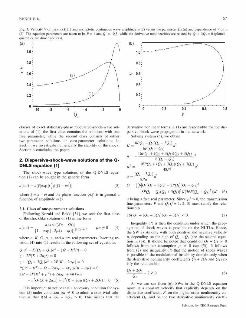
Fig. 3. Velocity V of the shock (1) and asymptotic continuous wave amplitude r (2) versus the parameter Q3 (a) and dependence of V on r

(b). The equation parameters are taken to be P = 1 and Q1 = –0.5, while the derivative nonlinearities are related by Q2 + 3Q3 = 0 (plottedquantities are dimensionless).

Kengne et al. 57

Published by NRC Research Press

cients Q2 and Q3. Using (6), one obtains the following groupvelocity:

@U

@K¼ �2KP� ðQ2 þ Q3Þa2

4

¼ � 32PQ1 þ 3Q22 þ 2Q2Q3 � 9Q2

3

12ðQ2 þ Q3Þa2 ð9Þ

In Fig. 1, we plot the shock-wave velocity (1) and thegroup velocity (2) as functions of derivative nonlinearity.

Figure 1a shows the plot versus Q3 for the equation parame-ters P = 0.4, Q1 = 0.2, Q2 = 1.3, while Fig. 1b correspondsto the plot versus Q2 for the parameters P = 0.4, Q1 = 0.2,Q3 = 0.7. The plots in Fig. 1 show that the shock-wave ve-locity as the group velocity decreases as the derivative non-linearities increase. We can then conclude that the twoderivative nonlinearity terms can significantly slow downthe propagating speed of the shock wave. Figure 1a showsthat the shock-wave velocity is always greater than thegroup velocity and this suggests that there may exist many

Fig. 4. Wave evolutions in the modulational instability region. The initial condition is taken from the first class of shock-wave solutionswith P = 0.4, Q1 = 0.2, Q2 = 1.3, and Q3 = –1. Plots of rows (a) and (b) show the wave evolutions at given times along the x-direction andat given point along the t-direction, respectively. Here, we used a = 1.

58 Can. J. Phys. Vol. 88, 2010

Published by NRC Research Press

types of structures evolving behind the shock wave for thegiven equation parameters for –1.29 £ Q3 £ –0.78757. Ascan be seen from Fig. 1b, the group velocity is alwaysgreater that the front’s speed, meaning that for the given setof equation parameters and for –0.69 £ Q2 £ –0.5, there mayexist many types of structures evolving in front the shockwave.

2.2 Class of zero-parameter and two-parameterssolutions

For both zero-parameter and two-parameters solutions, itis preferable to write solution (3) in the following genericform:

uðx; tÞ ¼ Rðx� Vt ¼ zÞexp�i

Z z

0

FðzÞdz� ir2t�

ð10Þ

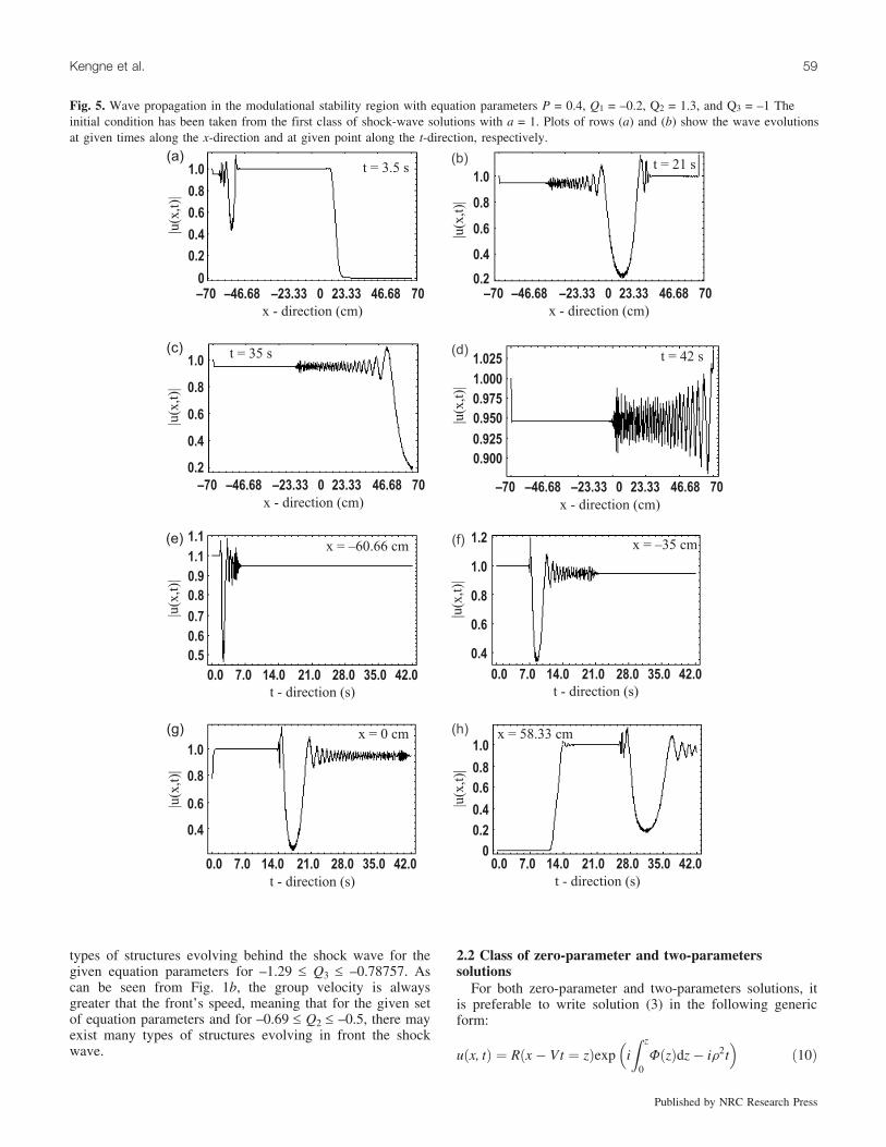
Fig. 5. Wave propagation in the modulational stability region with equation parameters P = 0.4, Q1 = –0.2, Q2 = 1.3, and Q3 = –1 Theinitial condition has been taken from the first class of shock-wave solutions with a = 1. Plots of rows (a) and (b) show the wave evolutionsat given times along the x-direction and at given point along the t-direction, respectively.

Kengne et al. 59

Published by NRC Research Press

where V is the SWs velocity, R(z) is the real amplitude withboundary values R(–?) = 0, Rðþ1Þ ¼

ffiffiffi2

pr, r being the

asymptotic continuous wave amplitude, and F(z) takes theboundary values F( ± ?) = –[(Q2 + 3Q3)r2 + V](2P)–1. Welimit ourselves to the shock waves with positive velocity(V > 0) corresponding to a situation where the zero-state do-main expands into the energy-carrying one. As in Sect. 1,we will see below that dispersive shock-wave propagationin the network is possible only if |Q3| + |Q2 + 2Q3| > 0 thatis, in the presence of at least one derivative nonlinear termin (1).

Inserting (10) into (1) and taking the boundary conditionsinto account, we obtain

R00 þ ðPþ 1ÞV � 2r2P

2P2R

þ ðPþ 2V þ 1ÞQ2 þ ð3Pþ 2V þ 3ÞQ3

4P2R3

þ 4PQ1 þ 4Q2Q3 þ Q22 þ 3Q2

3

4P2R5 ¼ 0 ð11Þ

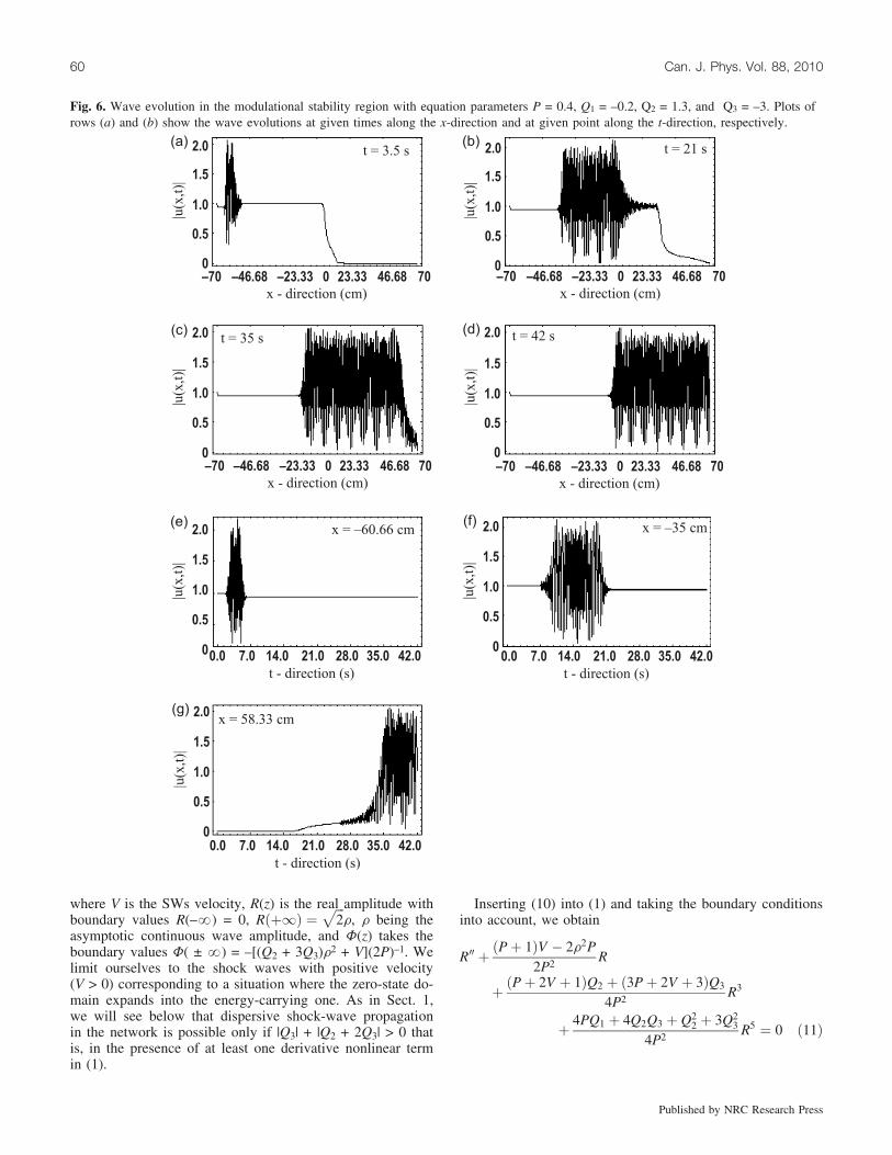
Fig. 6. Wave evolution in the modulational stability region with equation parameters P = 0.4, Q1 = –0.2, Q2 = 1.3, and Q3 = –3. Plots ofrows (a) and (b) show the wave evolutions at given times along the x-direction and at given point along the t-direction, respectively.

60 Can. J. Phys. Vol. 88, 2010

Published by NRC Research Press

FðzÞ ¼ � V

2P� Q2 þ 3Q3

4PR2ðzÞ ð12Þ

Equation (11) makes its presence felt in many contexts: itappears as a reduction equation of various nonlinear equa-tions such as the Rangawala–Rao equation, the Ablowitzequation, and the Gerdjikov and Ivanov equation (see Kong[35] and Dey et al. [36] for references). Many new solitary

wave solutions are obtained by mapping this equation intothe field equation of f6 as in field theory (see Behera andKhare [37]).

The shock-wave solution of (11) is sought in the form

RðzÞ ¼ rffiffiffiffiffiffiffiffiffiffiffiffiffiffiffiffiffiffiffiffiffiffiffi1þ tanhmz

pð13Þ

where m is a real parameter. If we substitute (13) into (11),

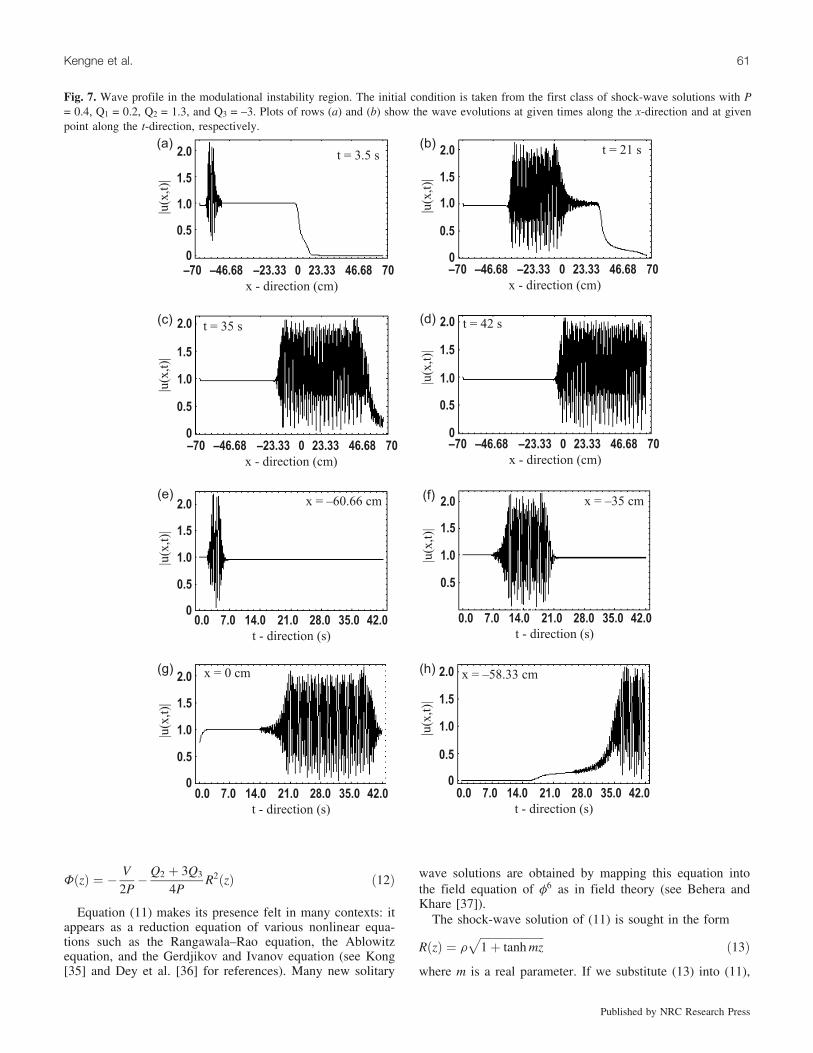
Fig. 7. Wave profile in the modulational instability region. The initial condition is taken from the first class of shock-wave solutions with P= 0.4, Q1 = 0.2, Q2 = 1.3, and Q3 = –3. Plots of rows (a) and (b) show the wave evolutions at given times along the x-direction and at givenpoint along the t-direction, respectively.

Kengne et al. 61

Published by NRC Research Press

we can obtain, after long calculations a system of equationsin V, m, and r. The different cases when the equation is sol-vable are analyzed below.

1. Case Q2 + Q3 = 0When

Q2 þ Q3 ¼ 0; PQ1 < 0; ðPþ 1ÞQ3 > 0 ð14Þ

one obtains

m2 ¼ � 3½Q3ðPþ 1Þ�264P3Q1

; r2 ¼ � 3ðPþ 1ÞQ3

16PQ1

;

V ¼ 3Q3½4P� ðPþ 1ÞQ3�2ð5Q2

3 � 16PQ1Þð15Þ

We then find that shock-wave solutions exist under thecondition Q2 + Q3 = 0 only in the modulational stability re-gion PQ1 < 0. Using (15), one can express the shock-wavevelocity in terms of the asymptotic continuous wave ampli-tude r as follows:

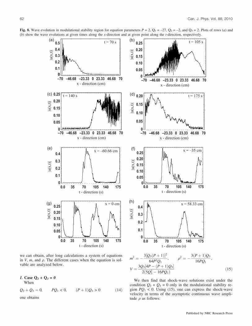
Fig. 8. Wave evolution in modulational stability region for equation parameters P = 2, Q1 = –27, Q2 = –2, and Q3 = 2. Plots of rows (a) and(b) show the wave evolutions at given times along the x-direction and at given point along the t-direction, respectively.

62 Can. J. Phys. Vol. 88, 2010

Published by NRC Research Press

V ¼ VðrÞ ¼ � 13ðPQ3 þ Q3 � 4PÞr2

2ð3þ 3Pþ 5Q3r2Þ ð16Þ

2. Case 4PQ1 þ Q22 ¼ Q3 ¼ 0

In the present case one obtains

V ¼ �Pþ 1

2ð17Þ

and solution (15) is governed by the two free parameters m

and r. For the shock-wave velocity to be positive, we musthave P + 1 < 0. The resulting two-parameter shock-wave so-lution holds only in the stability (PQ1 < 0) domains. Itshould be noted that in the present case, the shock-wave ve-locity does not depend on the asymptotic continuous-waveamplitude r; moreover, it is free from Q1, Q2, and Q3..

3. Case ðj4PQ1 þ Q22j þ jQ3jÞðQ2 þ Q3Þ > 0

In this case, we haveðQ2 þ Q3Þð4PQ1 þ 4Q2Q3 þ Q2

2 þ 3Q23Þ 6¼ 0 and

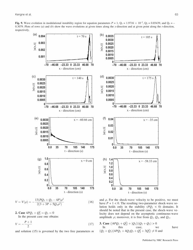
Fig. 9. Wave evolution in modulational instability region for equation parameters P = 1, Q1 = 1.9716 � 10–3, Q2 = 0.85439, and Q3 = –0.3079. Plots of rows (a) and (b) show the wave evolutions at given times along the x-direction and at given point along the t-direction,respectively.

Kengne et al. 63

Published by NRC Research Press

m2 ¼ b2r2

r2 ¼ � 6ðQ2 þ Q3ÞV þ 3ðPþ 1ÞðQ2 þ 3Q3Þ8ð4PQ1 þ 4Q2Q3 þ Q2

2 þ 3Q23Þ

ð18Þ

where

b ¼ ½ðPþ 2V þ 1ÞQ2 þ ð3Pþ 2V þ 3ÞQ3�ð4P2Þ�1

and V is any positive solution of the quadratic equation

�12ðQ2 þ Q3Þ2V2

þ 4½ðPþ 1Þð32PQ1 þ 20Q2Q3 þ 5Q22 þ 5Q2

3Þþ 12PðQ2 þ Q3Þ�V

þ 3ðPþ 1ÞðQ2 þ 3Q3Þ½8P� ðPþ 1ÞðQ2 þ 3Q3Þ� ¼ 0 ð19Þ

To obtain the conditions of validity of solution (13), onemay first find the positive solution of (19), secondly insertthe expression for V in b and into (18), and lastly, one mayimpose the condition of positivity of b and r2.

It should be noted that it is also possible to express theshock-wave velocity V in terms of the asymptotic continu-ous wave amplitude r

V ¼ VðrÞ

¼ � 4ð4PQ1 þ 4Q2Q3 þ Q22 þ 3Q2

3Þ3ðQ2 þ Q3Þ

r2

� ðPþ 1ÞðQ2 þ 3Q3Þ2ðQ2 þ Q3Þ

ð20Þ

2.3 Some characteristics of the established DSWThe most essential characteristics of the established DSW

is the dependence of its velocity V on the parameter r andderivative nonlinearities. As mentioned above, the velocityV is independent of r and of the derivative nonlinearities inthe case 4PQ1 þ Q2

2 ¼ Q3 ¼ 0.In the case of solution (15) with parameters (13), results

demonstrating the (i) V(Q3) and (ii) r(Q3) dependence aredisplayed in Fig. 2a for the the parameter values P = 1 andQ1 = –0.5. Figure 2b, obtained from Fig. 2a, shows the de-pendence of V(r) for the above values of the equation pa-rameters. An obvious inference suggested by Fig. 2 is thatthe dependence V(r) or V(Q3) is neither linear nor mono-tone. This implies that the derivative nonlinear terms in (1)cannot be neglected. Another conclusion from Fig. 2 is that,depending on the parameter values in the equations, the de-rivative nonlinearity terms in (1) may either increase or de-crease the speed of the shock wave. For the chosenparameter values P = 1 and Q1 = –0.5, the asymptotic con-tinuous-wave amplitude increases with the derivative nonli-nearity Q3 and its maximal and minimal values are obtainedfor V = 0, corresponding to two critical values of Q3 =0.42265 and Q3 = 1.5774, respectively.

Plots of Fig. 3 correspond to the shock-wave solution (15)with parameters (18) and (19). Curves (1) and (2) of Fig. 3ashow the dependence of V and r on Q3, respectively, whileFig. 3b shows the evolution of V versus r. The two plots areobtained with the equation parameters P = 1 and Q1 = –0.5when the derivative nonlinearities satisfy the relationshipQ2 + 3Q3 = 0. As in the above case, Fig. 3b is obtained

from Fig. 3a. Neither the shock velocity V nor the asymp-totic continuous-wave amplitude r is monotone as a func-tion of Q3 for –10 £ Q3 £ 0, so that for a specific choice ofequation parameters, the derivative terms in (1) can eitherincrease or decrease the propagating speed of the shock.The two plots correspond to a shock wave moving in themodulational stability domain (PQ1 = –0.5 < 0).

3. Numerical simulations of the dispersiveshock wave

Numerical simulations are carried out on the above exactshock-wave solutions within the framework of the Q-DNLSequation (1). Many sets of the equation parameters arechosen in our simulations. There exist a number of algo-rithms suitable for the numerical solution of this type ofproblem but some methods must be used with caution ifconvergence is to be assured. For now, it should be notedthat one of the best-known methods to solve the Q-DNLSequation numerically is the Crank–Nicolson method, as it isstable and accurate to second order in space and time [38].Hence, the numerical simulations of (1) are performed usingthis method. The accuracy of our numerical computations ischecked by testing different time and space steps. The vari-ables t and x are measured in units of time (second (s)) andspace (centimetre (cm)), respectively.

Using the Q-DNLS equation (1) as a model equation ofwave propagation in a semi-infinite network it is easy to ob-serve the major features of dispersive shock-wave propaga-tion. Progressive transformation of the initial dispersiveshock-wave signal into various type of waves is show inFigs. 4–9. In all these figures, plots in row (a) show thewave propagation along the x-direction for different times t,while plots in row (b) give the wave propagation along thet-direction for different x.

Plots of Fig. 4 show the wave evolution in the modula-tional instability region with the input shock signal takenfrom the first class of shock-wave solutions (4). The equa-tion parameters used are P = 0.4, Q1 = 0.2, Q2 = 1.3, andQ3 = –1. Plots of row (a) show that the waves propagatefrom the left to the right, while plots of row (b) show thatthe amplitude of the wave decreases as x increases.

In Fig. 5, we showed the wave evolution in the modula-tional stability zone with the input shock signal taken fromthe class of shock-wave solutions (4). Equation parametersP = 0.4, Q1 = –0.2, Q2 = 1.3, and Q3 = –1 are used. Theplots of this Fig. 5 show that the wave amplitude decreasesas x increases.

To show that the wave amplitude decreases as time in-creases, we plot, in Figs. 6 and 7, the wave profile in themodulational stability and modulational instability regions,respectively. For these plots, we used the exact dispersiveshock-wave solution (4) for the input signal. Plots of Fig. 6are obtained with the same equation parameters as in Fig. 5,but with derivative coefficient Q3 = –3. This same value ofQ3 has been used for Fig. 7 where the other equation param-eters are the same as in Fig. 4. These two figures, Figs. 6and 7, show that the amplitude of the wave decreases as afunction of time t when it propagates either in the modula-tional stability region or in the modulational instability re-gion. Figures 6 and 7 also show how much the derivative

64 Can. J. Phys. Vol. 88, 2010

Published by NRC Research Press

parameter Q3, and consequently the derivative coefficientsQ2 + 2Q3 and Q3 of (1) affect the wave amplitude: Compar-ing the plots of Figs. 4 and 5 with those of Figs. 7 and 6,respectively, it is seen that the wave amplitude increases asthe derivative coefficient Q3 decreases (for Figs. 4 and 5, wetook Q3 = –1 while Q3 = –3 was used for Figs. 6 and 7). Itis also seen from the plots of Figs. 4–7 that the wave ampli-tude slowly decreases as function of space variable x whenQ3 decreases (compare the plots of rows (b) of Figs. 4 and5 with those of Figs. 7 and 6, respectively). Finally, a simplecomparison of Figs. 4 and 5 with Figs. 7 and 6, respectively,shows that the DSW oscillates more as Q3 decreases.

In Figs. 8 and 9 we present the numerical solutions of (1)obtained with the use of solution (13) for the input signal, butwith different equation parameters. For Fig. 8, we used P = 2,Q1 = –27, Q2 = –2, and Q3 = 2, while for Fig. 9 we usedP = 1, Q1 = 1.9716 � 10–3, Q2 = 0.85439, and Q3 = –0.3079.These two sets of equations parameters satisfy condition (14)and (15) and condition (18) and (19), respectively. ThereforeFigs. 8 and 9 show the wave propagation in modulationalstability region and in modulational instability region, re-spectively. These two figures show that the wave amplitudedecreases as function of time t (see plots of column (a)) andincreases as function of x (see plots of column (b)) when theinput signal is taken from the second class of dispersiveshock-wave solution (13).

The combined action of dispersion and derivative nonli-nearity in (1) leads to the generation of an expanding non-linear oscillatory structure. This fact is confirmed bynumerical plots in Figs. 6–9, which present oscillatory struc-ture of stable dispersive shock wave propagating in eitherthe modulational stability region or modulational instabilityzone. From these figures, it is seen that dispersive shockwaves of (1) are generated which manifest themselves as un-dular structures [39].

4. ConclusionIn this work we have studied dispersive shock waves in a

derivative cubic-quintic nonlinear Schrodinger equationwithout dissipative term, which is derived in the small-am-plitude and long-wavelength limit using the standard reduc-tive perturbation technique and complex expansion, and candescribe wave propagation in nonlinear electrical transmis-sion lines. Seeking for dispersive shock-wave solutions ofthe equation, we found that the derivative nonlinearity termsin the equation is responsible for dispersive shock-wavepropagation in the network. Using the exact dispersiveshock-wave solutions as input signal, wave propagation insemi-infinite network has been numerically investigated.The numerical study shows that dispersive shock wavesmanifest themselves as undular structures.

References1. R. Hirota and K. Suzuki. J. Phys. Soc. Jpn. 28, 1366 (1970).

doi:10.1143/JPSJ.28.1366.; Proc. IEEE, 61, 1483 (1973).doi:10.1109/PROC.1973.9297.

2. M. Remoissenet. Waves called solitons. 3rd ed. Springer-Verlag, Berlin. 1999.

3. A.C. Scott. Active and nonlinear wave propagation in elec-tronics. Wiley-Interscience, New York. 1970.

4. J. Sakai and T. Kawata. J. Phys. Soc. Jpn. 41, 1819 (1976).doi:10.1143/JPSJ.41.1819.

5. T. Yagi and A. Noguchi. Electron. Commun. Jpn. 59A, 1(1976).

6. E. Kengne, V. Bozic, M. Viana, and R. Vaillancourt. Phys.Rev. E: Stat. Nonlin. Soft Matter Phys. 78, 026603 (2008).PMID:18850958.

7. P. Marquie, J.M. Bilbault, and M. Remoissenet. Phys. Rev.E: Stat. Phys. Plasmas Fluids Relat. Interdiscip. Topics, 49,828 (1994). PMID:9961275.

8. E. Seve, P. Tchofo Dinda, G. Millot, M. Remoissenet, J.M.Bilbault, M. Haelterman, and M. Haelterman. Phys. Rev. A,54, 3519 (1996). doi:10.1103/PhysRevA.54.3519. PMID:9913880.

9. T. Taniuti and H. Washimi. Phys. Rev. Lett. 21, 209 (1968).doi:10.1103/PhysRevLett.21.209.

10. T.B. Benjamin and J.E. Feir. J. Fluid Mech. 27, 417 (1967).doi:10.1017/S002211206700045X.

11. K.E. Lonngren. Solitons in action. Edited by K.E. Lonngrenand A.C. Scott. Academic, New York. 1978.

12. A. Hasegawa. Phys. Rev. Lett. 24, 1165 (1970). doi:10.1103/PhysRevLett.24.1165.; Phys. Fluids, 15, 870 (1972). doi:10.1063/1.1693996.

13. P. Marquie, J.M. Bilbault, and M. Remoissenet. Phys. Rev.E: Stat. Phys. Plasmas Fluids Relat. Interdiscip. Topics, 51,6127 (1995). PMID:9963352.

14. E. Kengne and R. Vaillancourt. Commun. Nonlinear Sci.Numer. Simul. 14, 3804 (2009). doi:10.1016/j.cnsns.2008.08.016.

15. E. Kengne and R. Vaillancourt. J. Infrared MillimeterWaves, 30, 679 (2009). doi:10.1007/s10762-009-9485-7.

16. E. Kengne, R. Vaillancour, and B.A. Malomed. Int. J. Mod.Phys. B, 23, 133 (2009). doi:10.1142/S0217979209049887.

17. D. Yemele, P. Marquie, and J.M. Bilbault. Phys. Rev. E:Stat. Nonlin. Soft Matter Phys. 68, 016605 (2003). PMID:12935268.

18. E. Kengne. J. Phys. Math. Gen. 37, 6053 (2004). doi:10.1088/0305-4470/37/23/007.

19. E. Kengne, S.T. Chui, W.M. Liu, and W.M. Liu. Phys. Rev.E: Stat. Nonlin. Soft Matter Phys. 74, 036614 (2006). PMID:17025771.

20. E. Kengne and W.M. Liu. Phys. Rev. E: Stat. Nonlin. SoftMatter Phys. 73, 026603 (2006). PMID:16605467.

21. T. Taniuti and N. Yajima. J. Math. Phys. 10, 1369 (1969).doi:10.1063/1.1664975.

22. R.J. Deissler and H.R. Brand. Phys. Lett. 146A, 252 (1990).23. M. Marklund and P.K. Shukla. Phys. Rev. E: Stat. Nonlin.

Soft Matter Phys. 73, 057601 (2006). PMID:16803083.24. M. Hoefer and M. Ablowitz. Dispersive shock waves, http://

www.scholarpedia.org/article/Dispersive_shock_waves.25. G.A. El, R.H.J. Grimshaw, and N.F. Smyth. Phys. Fluids, 18,

027104 (2006). doi:10.1063/1.2175152.26. G.B. Whitham. Linear and nonlinear waves. Wiley-Inter-

science, New York. 1974.27. R.Z. Sagdeev. Collective processes and shock waves in rari-

fied plasma. In Problems of plasma theory. Vol. 5. Edited byM.A. Leontovich. Atomizdat, Moscow. 1964.

28. D. Krokel, N.J. Halas, G. Giuliani, and D. Grischkowsky.Phys. Rev. Lett. 60, 29 (1988). doi:10.1103/PhysRevLett.60.29. PMID:10037859.

29. B.L. Holian and G.K. Straub. Phys. Rev. B, 18, 1593 (1978).doi:10.1103/PhysRevB.18.1593.; B.L. Holian, H. Flaschka,and D.W. McLaughlin. Phys. Rev. A, 24, 2595 (1981).doi:10.1103/PhysRevA.24.2595.; D.J. Kaup. Physica D, 25,

Kengne et al. 65

Published by NRC Research Press

361 (1987). doi:10.1016/0167-2789(87)90109-6.; S. Kamvis-sis. Physica D, 65, 242 (1993). doi:10.1016/0167-2789(93)90161-S.

30. M.A. Hoefer, M.J. Ablowitz, I. Coddington, E.A. Cornell, P.Engels, and V. Schweikhard. Phys. Rev. A, 74, 023623(2006). doi:10.1103/PhysRevA.74.023623.

31. J.J. Chang, P. Engels, and M.A. Hoefer. Phys. Lett. Rev.101, 170404 (2008). doi:10.1103/PhysRevLett.101.170404.

32. A.M. Kamchatnov. Nonlinear periodic waves and their mod-ulations — An introductory course. World Scientific, Singa-pore. 2000.

33. M.A. Hoefer and M.J. Ablowitz. Physica D, 236, 44 (2007);G.A. El and R.H.J. Grimshaw. Chaos, 12, 1015 (2002).doi:10.1063/1.1507381. PMID:12779625.

34. K. Nozaki and N. Bekki. Phys. Rev. Lett. 51, 2171 (1983).doi:10.1103/PhysRevLett.51.2171.

35. D. Kong. Phys. Lett. 196A, 301 (1995).36. B. Dey, A. Khare, and C.N. Kumar. Phys. Lett., 223A, 449

(1996). doi:10.1016/S0375-9601(96)00772-4.37. S.N. Behera and A. Khare. Pramana – J. Phys. 15, 245

(1980). doi:10.1007/BF02847222.38. W.H. Press, B.P. Flannery, S.A. Teukolsky, and W.T. Val-

lerling. Numerical recipes in Fortran. Cambridge UniversityPress, Cambridge. 1992.

39. A.J. Colosi, C.R. Beardsley, F.J. Lynch, G. Gawarkiewicz,C.-S. Chiu, and A. Scotti. J. Geophys. Res. 106, C5, 9587(2001). doi:10.1029/2000JC900124.

66 Can. J. Phys. Vol. 88, 2010

Published by NRC Research Press