Eur. Phys. J. D 62, 39–49 (2011)DOI: 10.1140/epjd/e2010-10331-8

Regular Article

THE EUROPEANPHYSICAL JOURNAL D

Can non-propagating hydrodynamic solitons be forced to move?

L. Gordillo1,a, T. Sauma1, Y. Zarate1, I. Espinoza2, M.G. Clerc1, and N. Mujica1

1 Departamento de Fısica, FCFM, Universidad de Chile, Casilla 487-3, Santiago, Chile2 Departamento de Fısica, Pontificia Universidad Catolica de Chile, Av. Vicuna Mackenna 4860, Santiago, Chile

Received 1st June 2010 / Received in final form 15 October 2010Published online 17 December 2010 – c© EDP Sciences, Societa Italiana di Fisica, Springer-Verlag 2010

Abstract. Development of technologies based on localized states depends on our ability to manipulate andcontrol these nonlinear structures. In order to achieve this, the interactions between localized states andcontrol tools should be well modelled and understood. We present a theoretical and experimental studyfor handling non-propagating hydrodynamic solitons in a vertically driven rectangular water basin, basedon the inclination of the system. Experiments show that tilting the basin induces non-propagating solitonsto drift towards an equilibrium position through a relaxation process. Our theoretical approach is derivedfrom the parametrically driven damped nonlinear Schrodinger equation which models the system. Thebasin tilting effect is modelled by promoting the parameters that characterize the system, e.g. dissipation,forcing and frequency detuning, as space dependent functions. A motion law for these hydrodynamicsolitons can be deduced from these assumptions. The model equation, which includes a constant speed anda linear relaxation term, nicely reproduces the motion observed experimentally.

1 Introduction

During the last years, emerging macroscopic particle-typesolutions or localized states in macroscopic extended dissi-pative systems have been observed in different fields, suchas: domains in magnetic materials, chiral bubbles in liq-uid crystals, current filaments in gas discharge, spots inchemical reactions, localized states in fluid surface waves,oscillons in granular media, isolated states in thermal con-vection, solitary waves in nonlinear optics, just to mentiona few. The variety of this type of phenomena evidencesthe universality of these particle-type solutions. Althoughthese states are spatially extended, they exhibit proper-ties typically associated with particles. Consequently, onecan characterize them with a family of continuous pa-rameters such as position, amplitude and width. Hence,these coherent states are particle-type solutions. This isexactly the type of description and strategy used in fun-damental physical theories like quantum mechanics andparticle physics. Indeed, localized states emerging in ex-tended dissipative systems are composed by a large num-ber of atoms or molecules (of the order of Avogadro’s num-ber) that behave coherently. The paradigmatic exampleof a macroscopic localized state is the existence of soli-tons, as those reported in fluid dynamics, nonlinear opticsand Hamiltonian systems [1]. These solitons arise from arobust balance between dispersion and nonlinearity. Thegeneralization of this concept to dissipative and out of

a e-mail: ljgordillo@gmail.com

equilibrium systems has led to several studies in the lastdecades, in particular to the definition of localized struc-tures intended as patterns appearing in a restricted regionof space [2,3].

In one-dimensional spatial systems, an adequate ge-ometrical theoretical description of localized states hasbeen established based on spatial trajectories connectinga steady state with itself. They arise as homoclinic orbitsfrom the viewpoint of dynamical systems theory (see thereview [4] and references therein), while domain walls orfronts are seen as spatial trajectories joining two differentsteady states – heteroclinic curves – of the correspond-ing spatial dynamical system [5]. Localized patterns canbe understood as homoclinic orbits in the Poincare sec-tion of the corresponding spatial-reversible dynamical sys-tem [4–7]. They can also be understood as a consequenceof the front interaction with oscillatory tails [8,9]. Thereis another type of stabilization mechanism that generateslocalized structures without oscillatory tails based on non-variational effects [10,11], where front interaction is led bythe non-variational terms [12].

Quasi-reversible systems1 are the natural theoreticalframework in which one expects to observe localized struc-tures. Time-reversible and Hamiltonian systems exhibit afamily of localized states described by a set of continu-ous parameters [1]. Thus, when one considers energy in-jection and dissipation, only few or none solutions of the

1 Time-reversible systems subjected to small injection anddissipation of energy [13–17].

40 The European Physical Journal D

family survive. The prototype model that presents local-ized structures or dissipative solitons in quasi-reversiblesystems is the parametrically driven damped nonlinearSchrodinger equation [18]. This model has been derived inseveral contexts to describe patterns and localized struc-tures, such as vertically oscillating layer of water [19–21],nonlinear lattices [22], optical fibers [23], Kerr type opti-cal parametric oscillators [24], magnetization in an easy-plane ferromagnetic exposed to an oscillatory magneticfield [25–28], and parametrically driven damped chain ofpendula [29,30].

In the last two decades, the properties and mechanismsof creation of localized structures have been establishedas well as their interactions. However, few studies havebeen focused on manipulation and control of these coher-ent states. In the pioneering work of Wu et al. [32], theauthors mention that hydrodynamic non-propagating soli-tons are sensitive to depth gradients. They found that soli-tons move toward less deep regions with an average veloc-ity of 0.05 cm/s for a 3◦ tilt angle. This fact suggests thattilting the basin can be used as a spatial control tool, as itinduces motion of solitons. A quantitative detailed studyof the dynamics of the soliton needs to be performed in or-der to achieve this. Recent efforts have been accomplishedin the context of optical cavities in semiconductors [31],through the use of a phase gradient which induces a driftof cavity solitons.

The aim of this manuscript is to characterize theoreti-cally and experimentally a method of manipulation andcontrol of non-propagating hydrodynamic solitons in avertically driven rectangular water container based. Moreprecisely, this control is attained by tilting the bottom sur-face normal with respect to gravity. Close to the Faradayinstability, the parametrically driven damped nonlinearSchrodinger equation models this system. The effect ofthe container inclination is incorporated into the ampli-tude equation through space-dependent dissipation, injec-tion and detuning. Considering that the tilt angle is small,we deduce an equation for the position of non-propagatinghydrodynamic solitons. This equation is characterized bytwo terms: a constant speed and a linear relaxation pro-cess. Therefore, at a given inclination of the cell, the dis-sipative soliton travels to an equilibrium position througha relaxation process. In the case that the inhomogeneousinjection and dissipation of energy are of the same order,the dominant mechanism in the propulsion of dissipativesolitons is governed by the inhomogeneous detuning. Ex-perimentally, we have found good agreement with the pro-posed dynamics of dissipative hydrodynamic solitons un-der the influence of tilt angle.

The manuscript is organized as follows: the descriptionof the experimental setup and the procedures used in thecharacterization of the dynamics of dissipative solitons ina tilted cell are presented in Section 2. The theoreticaldescription of the basin subjected to vertical oscillationsand deduction of the equation for the position of dissipa-tive solitons under the influence of an inclination is pre-sented in Section 3. Finally, the conclusions are presentedin Section 4.

2 Motion of non-propagating hydrodynamicsoliton in tilted container

Non-propagating hydrodynamic solitons arise when aquasi 1-D rectangular basin filled with water is excited ver-tically at certain range of frequencies and amplitudes [32].These localized states have a subharmonic nature depictedby oscillations at half the forcing frequency. They appearas localized transverse sloshing structures on the free sur-face. The dissipative solitons nucleate from disturbancesof the stable flat state. In practice, they can be createdby perturbing the water surface with a paddle in such away that the swaying resembles solitons typical sloshingmotion.

2.1 Experimental setup and procedure

The experiments are done with a rectangular plexiglasbasin, Lx = 50.0 cm long, Ly = 2.54 cm wide andLz = 10.0 cm high. The cell was carefully machined on aplexiglas block to ensure parallelism of lateral walls. Thebasin is filled up to H = 2 cm in depth with a mixtureof 252 cm3 of water, 2 cm3 of Kodak Photo Flo r© 2002

and some drops of black ink. The mixture is prepared aday before measurements are done. Free surface satura-tion with contaminants plays an important role for repro-ducibility [33].

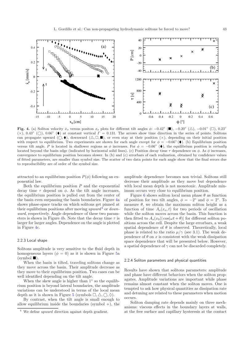
The cell is driven sinusoidally by an electromechani-cal shaker lying on a three-point leveling system whichallows longitudinal tilting (see Fig. 1). The tilt angle φ isconsidered positive for a counter-clockwise rotation of thecell with respect to the horizontal when visualized fromthe front. The shaker is fed with an amplified sinewavesignal generated by a function/arbitrary waveform gen-erator and a power amplifier. Thus, the cell vibration isalong the axis of the shaker, with form y(t) = A sin(ωt).Solitons can exist at frequencies f = ω/2π slightly below11 Hz, and normalized accelerations Γ = Aω2/g around0.15. The basin acceleration is measured using a piezo-electric accelerometer attached to its bottom surface. It isconnected to a signal conditioner, from which the accelera-tion signal is measured by a lock-in amplifier synchronizedwith the forcing signal (see Fig. 2a). Acceleration valuesare provided with precision of 0.001 g. An analog tilt sen-sor is also placed on the external bottom of the basin. ThisMEM device is connected to an analog/digital converterwhich measures angle values within an error of 0.01◦.

Two different types of measurements are made on thefree surface. Sequences of images taken with a high speedcamera provide spatial measurements. On the other hand,local measurements are done using the phase fluctuationsof the output signal of a resonant capacitive device.

2 This chemical product creates a film which improves sig-nificantly wetting at the walls.

L. Gordillo et al.: Can non-propagating hydrodynamic solitons be forced to move? 41

Fig. 1. (Color online) The basin filled with a dyed mix-ture of water and Kodak Photo Flo (a) is vibrated verticallyby an electromechanical shaker. (b). The tilt angle φ can becontrolled using a three-point level system. Positive φ meanscounter-clockwise rotation of the cell with respect to the hori-zontal when visualized from the front (c). Acceleration is mea-sured using an accelerometer (d). A high speed camera (e) ac-quires images of the fluid illuminated from behind by an arrayof LED lamps (f).

2.1.1 Profile extraction from images

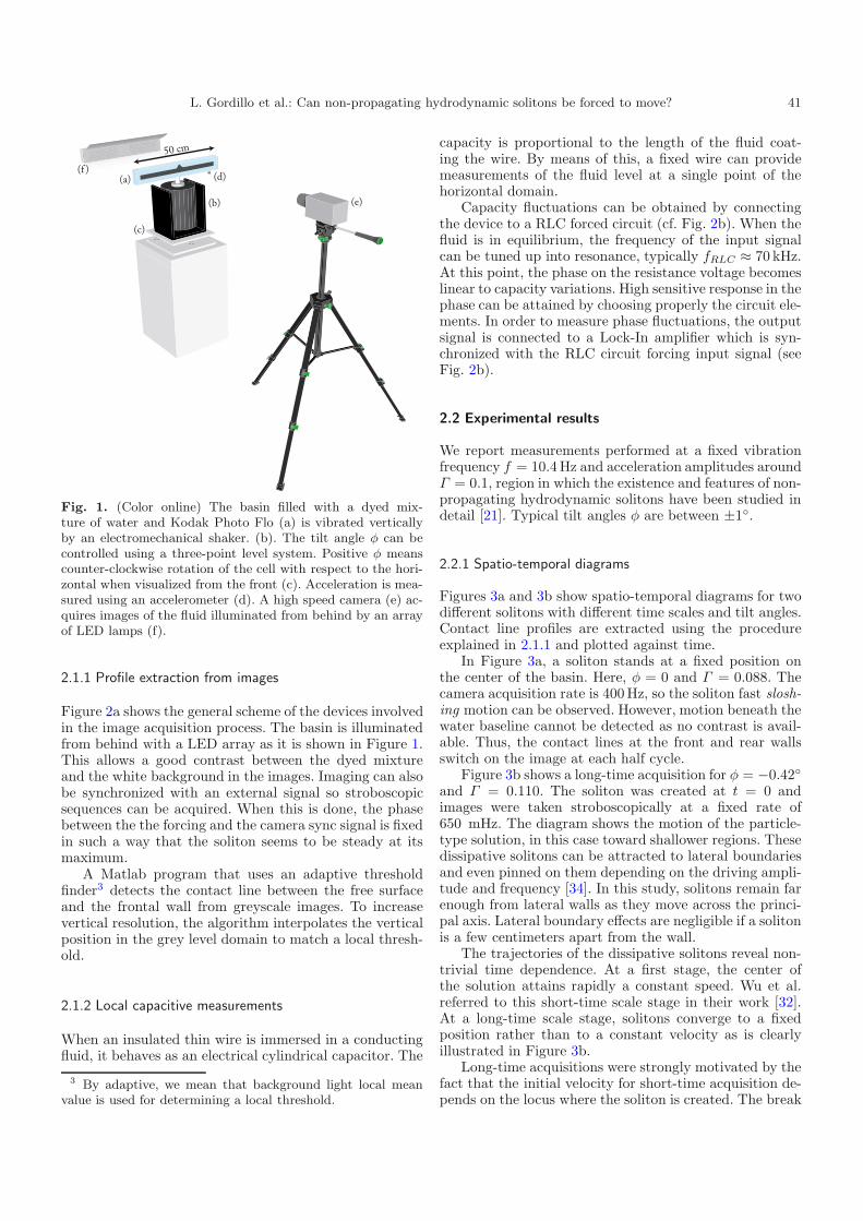
Figure 2a shows the general scheme of the devices involvedin the image acquisition process. The basin is illuminatedfrom behind with a LED array as it is shown in Figure 1.This allows a good contrast between the dyed mixtureand the white background in the images. Imaging can alsobe synchronized with an external signal so stroboscopicsequences can be acquired. When this is done, the phasebetween the the forcing and the camera sync signal is fixedin such a way that the soliton seems to be steady at itsmaximum.

A Matlab program that uses an adaptive thresholdfinder3 detects the contact line between the free surfaceand the frontal wall from greyscale images. To increasevertical resolution, the algorithm interpolates the verticalposition in the grey level domain to match a local thresh-old.

2.1.2 Local capacitive measurements

When an insulated thin wire is immersed in a conductingfluid, it behaves as an electrical cylindrical capacitor. The

3 By adaptive, we mean that background light local meanvalue is used for determining a local threshold.

capacity is proportional to the length of the fluid coat-ing the wire. By means of this, a fixed wire can providemeasurements of the fluid level at a single point of thehorizontal domain.

Capacity fluctuations can be obtained by connectingthe device to a RLC forced circuit (cf. Fig. 2b). When thefluid is in equilibrium, the frequency of the input signalcan be tuned up into resonance, typically fRLC ≈ 70 kHz.At this point, the phase on the resistance voltage becomeslinear to capacity variations. High sensitive response in thephase can be attained by choosing properly the circuit ele-ments. In order to measure phase fluctuations, the outputsignal is connected to a Lock-In amplifier which is syn-chronized with the RLC circuit forcing input signal (seeFig. 2b).

2.2 Experimental results

We report measurements performed at a fixed vibrationfrequency f = 10.4 Hz and acceleration amplitudes aroundΓ = 0.1, region in which the existence and features of non-propagating hydrodynamic solitons have been studied indetail [21]. Typical tilt angles φ are between ±1◦.

2.2.1 Spatio-temporal diagrams

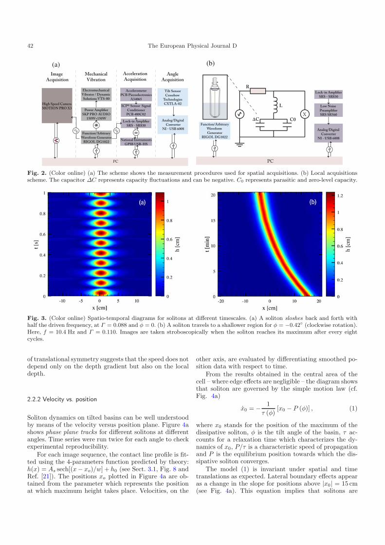
Figures 3a and 3b show spatio-temporal diagrams for twodifferent solitons with different time scales and tilt angles.Contact line profiles are extracted using the procedureexplained in 2.1.1 and plotted against time.

In Figure 3a, a soliton stands at a fixed position onthe center of the basin. Here, φ = 0 and Γ = 0.088. Thecamera acquisition rate is 400 Hz, so the soliton fast slosh-ing motion can be observed. However, motion beneath thewater baseline cannot be detected as no contrast is avail-able. Thus, the contact lines at the front and rear wallsswitch on the image at each half cycle.

Figure 3b shows a long-time acquisition for φ = −0.42◦and Γ = 0.110. The soliton was created at t = 0 andimages were taken stroboscopically at a fixed rate of650 mHz. The diagram shows the motion of the particle-type solution, in this case toward shallower regions. Thesedissipative solitons can be attracted to lateral boundariesand even pinned on them depending on the driving ampli-tude and frequency [34]. In this study, solitons remain farenough from lateral walls as they move across the princi-pal axis. Lateral boundary effects are negligible if a solitonis a few centimeters apart from the wall.

The trajectories of the dissipative solitons reveal non-trivial time dependence. At a first stage, the center ofthe solution attains rapidly a constant speed. Wu et al.referred to this short-time scale stage in their work [32].At a long-time scale stage, solitons converge to a fixedposition rather than to a constant velocity as is clearlyillustrated in Figure 3b.

Long-time acquisitions were strongly motivated by thefact that the initial velocity for short-time acquisition de-pends on the locus where the soliton is created. The break

42 The European Physical Journal D

Image Acquisition

AngleAcquisition

AccelerationAcquisition

MechanicalVibration

Electromechanical Vibrator / Dynamic Solutions VTS-80

Power AmplifierSKP PRO AUDIO

150W+150W

Function/ArbitraryWaveform Generator

RIGOL DG1022

High Speed CameraMOTION PRO X3

AccelerometerPCB Piezoelectronics

A34065

ICP® Sensor SignalConditioner

PCB 480C02

Lock-in AmplifierSRS - SR830

National InstrumentsGPIB USB-HS

Tilt SensorCrossbow

TechnologiesCXTLA-02

Analog/Digital Converter

NI - USB 6008

PC

(a)

Low Noise PreamplifierSRS SR560

R

L

C0ΔCX

Lock-in AmplifierSRS - SR830

Function/ArbitraryWaveform Generator

RIGOL DG1022

Analog/Digital Converter

NI - USB 6008

PC

(b)

Fig. 2. (Color online) (a) The scheme shows the measurement procedures used for spatial acquisitions. (b) Local acquisitionsscheme. The capacitor ΔC represents capacity fluctuations and can be negative. C0 represents parasitic and zero-level capacity.

Fig. 3. (Color online) Spatio-temporal diagrams for solitons at different timescales. (a) A soliton sloshes back and forth withhalf the driven frequency, at Γ = 0.088 and φ = 0. (b) A soliton travels to a shallower region for φ = −0.42◦ (clockwise rotation).Here, f = 10.4 Hz and Γ = 0.110. Images are taken stroboscopically when the soliton reaches its maximum after every eightcycles.

of translational symmetry suggests that the speed does notdepend only on the depth gradient but also on the localdepth.

2.2.2 Velocity vs. position

Soliton dynamics on tilted basins can be well understoodby means of the velocity versus position plane. Figure 4ashows phase plane tracks for different solitons at differentangles. Time series were run twice for each angle to checkexperimental reproducibility.

For each image sequence, the contact line profile is fit-ted using the 4-parameters function predicted by theory:h(x) = As sech[(x− xo)/w] + h0 (see Sect. 3.1, Fig. 8 andRef. [21]). The positions xo plotted in Figure 4a are ob-tained from the parameter which represents the positionat which maximum height takes place. Velocities, on the

other axis, are evaluated by differentiating smoothed po-sition data with respect to time.

From the results obtained in the central area of thecell – where edge effects are negligible – the diagram showsthat soliton are governed by the simple motion law (cf.Fig. 4a)

x0 = − 1τ (φ)

[x0 − P (φ)] , (1)

where x0 stands for the position of the maximum of thedissipative soliton, φ is the tilt angle of the basin, τ ac-counts for a relaxation time which characterizes the dy-namics of x0, P/τ is a characteristic speed of propagationand P is the equilibrium position towards which the dis-sipative soliton converges.

The model (1) is invariant under spatial and timetranslations as expected. Lateral boundary effects appearas a change in the slope for positions above |x0| = 15 cm(see Fig. 4a). This equation implies that solitons are

L. Gordillo et al.: Can non-propagating hydrodynamic solitons be forced to move? 43

Fig. 4. (a) Soliton velocity xo versus positon xo plots for different tilt angles φ: −0.42◦ (�), −0.20◦ (�), −0.01◦ (�), 0.23◦

(×), 0.43◦ (©), 0.66◦ (�) at constant vertical Γ = 0.131. The arrows show time direction in the series of points. Solitonscan propagate upward (©,�), downward (�, �, �), or even stay at their position (×), depending on their initial positionwith respect to equilibrium. Two experiments are shown for each angle except for φ = −0.66◦ (�). (b) Equilibrium positionversus tilt angle. P is located in shallower regions as φ increases. For φ = −0.66◦ (�), the equilibrium position is virtuallylocated beyond the basin edge (indicated by horizontal solid lines). (c) Position decay time τ dependence on φ. As φ increases,convergence to equilibrium position becomes slower. In (b) and (c) errorbars of each realization, obtained by confidence valuesof fitted parameters, are smaller than symbol size. The scatter of two data points for each angle show that the final errors dueto reproducibility are of order of the symbol size.

attracted to an equilibrium position P (φ) following an ex-ponential law.

Both the equilibrium position P and the exponentialdecay time τ depend on φ. As the tilt angle increases,the equilibrium position is pulled out from the center ofthe basin even surpassing the basin boundaries. Figure 4ashows phase-space tracks on which solitons get pinned attheir equilibrium positions after moving upward4 or down-ward, respectively. Angle dependence of these two param-eters is shown in Figure 4b. Note that the decay time τ islarger for larger angles. Dependence on the angle is plottedin Figure 4c.

2.2.3 Local shape

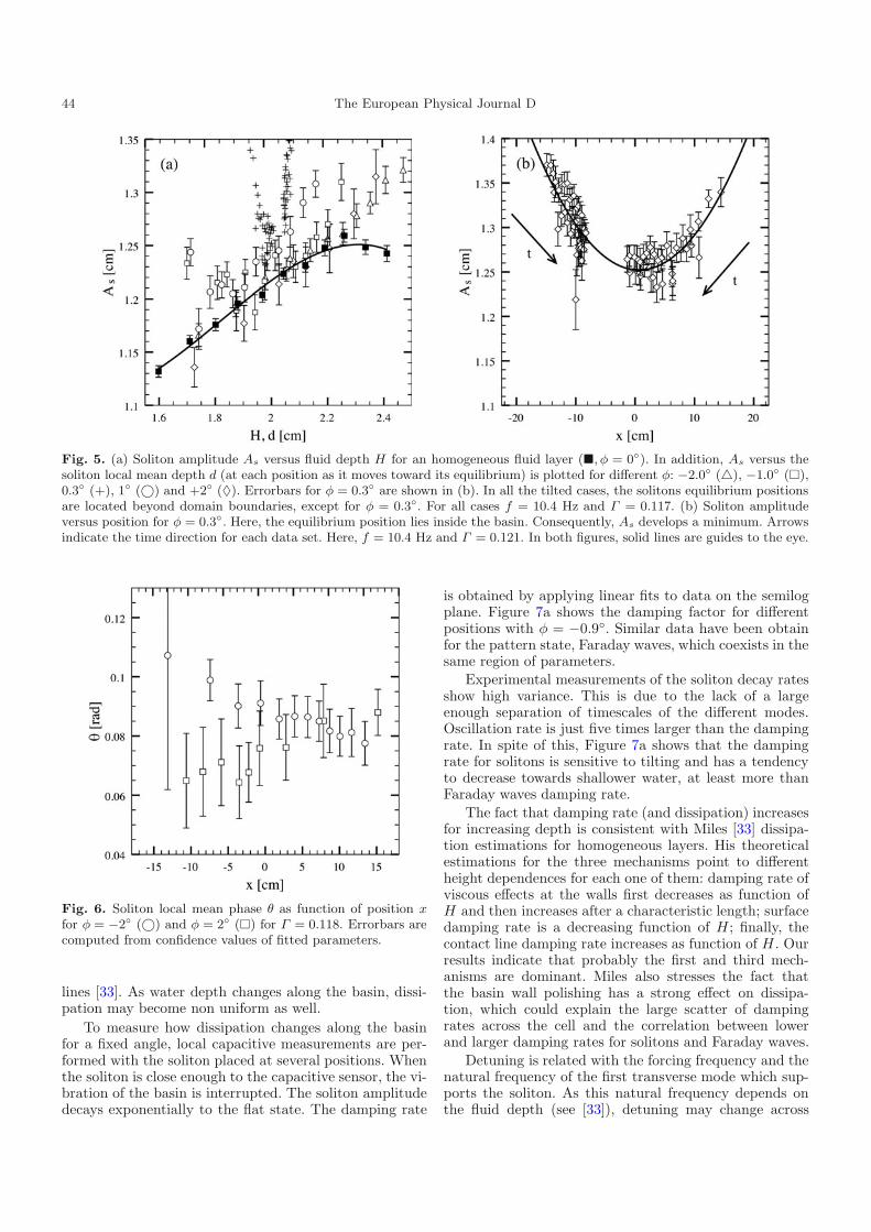
Solitons amplitude is very sensitive to the fluid depth inhomogeneous layers (φ = 0) as it is shown in Figure 5a(symbol �).

When the basin is tilted, traveling solitons change asthey move across the basin. Their amplitude decrease asthey move to their equilibrium position. Two cases can bewell identified depending on the tilt angle.

When the skew angle is higher than 1◦ so the equilib-rium position is beyond lateral boundaries, the amplitudevariations can be understood in terms of the local meandepth as it is shown in Figure 5 (symbols �,�,©,♦).

By contrast, when the tilt angle is small enough toallow equilibrium inside the boundaries (symbol +), the

4 We define upward direction against depth gradient.

amplitude dependence becomes non trivial. Solitons stilldecrease their amplitude as they move but dependencewith local mean depth is not monotonic. Amplitude min-imum occurs very close to equilibrium position.

Figure 6 shows soliton local mean phase θ as functionof position for two tilt angles, φ = −2◦ and φ = 2◦. Tomeasure θ, we obtain the maximum soliton height as afunction of time As(xo, t) for two periods of oscillationwhile the soliton moves across the basin. This function isthen fitted to As(x0)| cos(ωt+ θ)| for different soliton po-sitions across the cell. Despite the large errorbars, a weakspatial dependence of θ is observed. Theoretically, localphase is related to the ratio μ/γ (see 3.1). The weak de-pendence of θ on x is consistent with the weak dissipationspace dependence that will be presented below. However,a spatial dependence of γ can not be discarded completely.

2.2.4 Soliton parameters and physical quantities

Results have shown that solitons parameters: amplitudeand phase have different behaviors when the soliton prop-agates. Amplitude variations are important while phaseremains almost constant when the soliton moves. One istempted to ask how physical quantities as dissipation rateand detuning are related to these parameters when motionoccurs.

Soliton damping rate depends mainly on three mech-anisms: viscous effects in the boundary layers at walls,at the free surface and capillary hysteresis at the contact

44 The European Physical Journal D

Fig. 5. (a) Soliton amplitude As versus fluid depth H for an homogeneous fluid layer (�, φ = 0◦). In addition, As versus thesoliton local mean depth d (at each position as it moves toward its equilibrium) is plotted for different φ: −2.0◦ (�), −1.0◦ (�),0.3◦ (+), 1◦ (©) and +2◦ (♦). Errorbars for φ = 0.3◦ are shown in (b). In all the tilted cases, the solitons equilibrium positionsare located beyond domain boundaries, except for φ = 0.3◦. For all cases f = 10.4 Hz and Γ = 0.117. (b) Soliton amplitudeversus position for φ = 0.3◦. Here, the equilibrium position lies inside the basin. Consequently, As develops a minimum. Arrowsindicate the time direction for each data set. Here, f = 10.4 Hz and Γ = 0.121. In both figures, solid lines are guides to the eye.

Fig. 6. Soliton local mean phase θ as function of position xfor φ = −2◦ (©) and φ = 2◦ (�) for Γ = 0.118. Errorbars arecomputed from confidence values of fitted parameters.

lines [33]. As water depth changes along the basin, dissi-pation may become non uniform as well.

To measure how dissipation changes along the basinfor a fixed angle, local capacitive measurements are per-formed with the soliton placed at several positions. Whenthe soliton is close enough to the capacitive sensor, the vi-bration of the basin is interrupted. The soliton amplitudedecays exponentially to the flat state. The damping rate

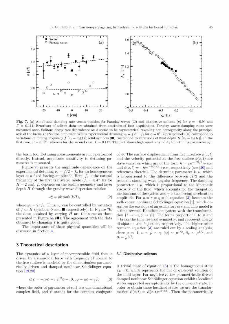
is obtained by applying linear fits to data on the semilogplane. Figure 7a shows the damping factor for differentpositions with φ = −0.9◦. Similar data have been obtainfor the pattern state, Faraday waves, which coexists in thesame region of parameters.

Experimental measurements of the soliton decay ratesshow high variance. This is due to the lack of a largeenough separation of timescales of the different modes.Oscillation rate is just five times larger than the dampingrate. In spite of this, Figure 7a shows that the dampingrate for solitons is sensitive to tilting and has a tendencyto decrease towards shallower water, at least more thanFaraday waves damping rate.

The fact that damping rate (and dissipation) increasesfor increasing depth is consistent with Miles [33] dissipa-tion estimations for homogeneous layers. His theoreticalestimations for the three mechanisms point to differentheight dependences for each one of them: damping rate ofviscous effects at the walls first decreases as function ofH and then increases after a characteristic length; surfacedamping rate is a decreasing function of H ; finally, thecontact line damping rate increases as function of H . Ourresults indicate that probably the first and third mech-anisms are dominant. Miles also stresses the fact thatthe basin wall polishing has a strong effect on dissipa-tion, which could explain the large scatter of dampingrates across the cell and the correlation between lowerand larger damping rates for solitons and Faraday waves.

Detuning is related with the forcing frequency and thenatural frequency of the first transverse mode which sup-ports the soliton. As this natural frequency depends onthe fluid depth (see [33]), detuning may change across

L. Gordillo et al.: Can non-propagating hydrodynamic solitons be forced to move? 45

Fig. 7. (a) Amplitude damping rate versus position for Faraday waves (�) and dissipative solitons (•) for φ = −0.9◦ andΓ = 0.111. Errorbars of soliton data are obtained from statistics of four acquisitions. Faraday waves damping rates weremeasured once. Solitons decay rate dependence on φ seems to be asymmetrical revealing non-homogeneity along the principalaxis of the basin. (b) Soliton amplitude versus experimental detuning νe = f/2−fo for φ = 0◦. Open symbols (♦) correspond tovariations of forcing frequency f [νe = νe(f)]; solid symbols (�) correspond to variations of fluid depth H [νe = νe(H)]. In thefirst case, Γ = 0.125, whereas for the second case, Γ = 0.117. The plot shows high sensitivity of As to detuning parameter νe.

the basin too. Detuning measurements are not performeddirectly. Instead, amplitude sensitivity to detuning pa-rameter is measured.

Figure 7b presents the amplitude dependence on theexperimental detuning νe = f/2− fo for an homogeneouslayer at a fixed forcing amplitude. Here, fo is the naturalfrequency of the first transverse mode (fo = 5.47 Hz forH = 2 cm). fo depends on the basin’s geometry and layerdepth H through the gravity wave dispersion relation

ω2o = gk tanh(kH), (2)

where ωo = 2πfo. Thus, νe can be controlled by variationof f or H (symbols ♦ and � respectively). In Figure 7b,the data obtained by varying H are the same as thosepresented in Figure 5a (�). The agreement with the dataobtained by changing f is quite good.

The importance of these physical quantities will bediscussed in Section 4.

3 Theoretical description

The dynamics of a layer of incompressible fluid that isdriven by a sinusoidal force with frequency Ω normal tothe free surface is modeled by the dimensionless paramet-rically driven and damped nonlinear Schrodinger equa-tion [19,20]

∂tψ = −iνψ − i|ψ|2ψ − i∂xxψ − μψ + γψ, (3)

where the order of parameter ψ(x, t) is a one dimensionalcomplex field, and ψ stands for the complex conjugate

of ψ. The surface displacement from flat interface h(x, t)and the velocity potential at the free surface φ(x, t) areslave variables which are of the form h = ψe−iΩt/2 + c.c.and φ(x, t) = −iψe−iΩt/2 +c.c., respectively (see [20] andreferences therein). The detuning parameter is ν, whichis proportional to the difference between Ω/2 and theresonant standing wave angular frequency. The dampingparameter is μ, which is proportional to the kinematicviscosity of the fluid, which accounts for the dissipationmechanisms of the system and γ is the forcing accelerationamplitude. For μ = γ = η = 0, equation (3) becomes thewell-known nonlinear Schrodinger equation [1], which de-scribes the envelope of an oscillatory system. This model isa time reversal Hamiltonian system with the transforma-tion {t → −t, ψ → ψ}. The terms proportional to μ andγ break the time reversal symmetry, and represent energydissipation and injection, respectively. The higher-orderterms in equation (3) are ruled out by a scaling analysis,since μ � 1, ν ∼ μ ∼ γ, |ψ| ∼ μ1/2, ∂x ∼ μ1/2, and∂t ∼ μ1/2.

3.1 Dissipative solitons

A trivial state of equation (3) is the homogeneous stateψ0 = 0, which represents the flat or quiescent solution ofthe fluid layer. For negative ν, the parametrically drivendamped nonlinear Schrodinger equation exhibits localizedstates supported asymptotically by the quiescent state. Inorder to obtain these localized states we use the transfor-mation ψ(x, t) = R(x, t)eiθ(x,t). Then the parametrically

46 The European Physical Journal D

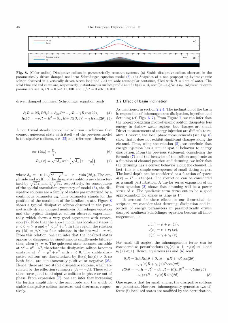
Fig. 8. (Color online) Dissipative soliton in parametrically resonant systems. (a) Stable dissipative soliton observed in theparametrically driven damped nonlinear Schrodinger equation model (3). (b) Snapshot of a non-propagating hydrodynamicsoliton observed in a vertically driven 50 cm long and 2.54 cm wide rectangular container, filled with H = 2 cm of water. Thesolid blue and red curve are, respectively, instantaneous surface profile and fit h(x) = As sech[(x−xo)/w]+h0. Adjusted relevantparameters are As/H = 0.523 ± 0.001 and w/H = 0.786 ± 0.004.

driven damped nonlinear Schrodinger equation reads

∂tR = 2∂xR∂xθ + ∂xxRθ − μR+ γR cos(2θ), (4)R∂tθ = −νR−R3 − ∂xxR+R(∂xθ)2 − γR sin(2θ).(5)

A non trivial steady homoclinic solution – solutions thatconnect quiescent state with itself – of the previous modelis (dissipative solitons, see [25] and references therein)

cos (2θ0) =μ

γ, (6)

R±(x) =√

2δ±sech(√

δ± [x− x0]), (7)

where δ± ≡ −ν ±√γ2 − μ2 = −ν − γ sin (2θ0). The am-

plitude and width of the dissipative solitons are character-ized by

√2δ± and 1/

√δ±, respectively. As consequence

of the spatial translation symmetry of model (3), the dis-sipative solitons are a family of states parameterized by acontinuous parameter x0. This parameter stands for theposition of the maximum of the localized state. Figure 8shows a typical dissipative soliton observed in the para-metrically driven damped nonlinear Schrodinger equationand the typical dissipative soliton observed experimen-tally, which shows a very good agreement with expres-sion (7). Note that the above model has localized states ifν < 0, γ ≥ μ and γ2 < μ2 +ν2. In this region, the relationcos (2θ) = μ/γ has four solutions in the interval [−π, π].From this relation, one can infer that the localized statesappear or disappear by simultaneous saddle-node bifurca-tions when |γ| = μ. The quiescent state becomes unstableat γ2 = μ2 + ν2, therefore the dissipative soliton becomesunstable at γ2 = μ2 + ν2 with ν < 0. The stable dissi-pative solitons are characterized by Re(ψ)Im(ψ) > 0, soboth fields are simultaneously positive or negative [25].Hence, there are two stable dissipative solitons, which arerelated by the reflection symmetry (A→ −A). These solu-tions correspond to dissipative solitons in phase or out ofphase. From expression (7), one can infer that increasingthe forcing amplitude γ, the amplitude and the width ofstable dissipative soliton increases and decreases, respec-tively.

3.2 Effect of basin inclination

As mentioned in section 2.2.4. The inclination of the basinis responsible of inhomogeneous dissipation, injection anddetuning (cf. Figs. 5–7). From Figure 7, we can infer thatthe non-propagating hydrodynamic soliton dissipates lessenergy in shallow water regions, but changes are small.Direct measurements of energy injection are difficult to re-alize. However, the local phase measurements (see Fig. 6)show that it does not exhibit significant changes along thechannel. Thus, using the relation (5), we conclude thatenergy injection has a similar spatial behavior to energydissipation. From the previous statement, considering theformula (7) and the behavior of the soliton amplitude asa function of channel position and detuning, we infer thatthe detuning has a convex behavior along the channel. Infact, this is a simple consequence of small tilting angles.The local depth can be considered as a function of space:d(x) = H − x tan(φ). The correction can be consideredas a small perturbation. A Taylor series expansion of ωo

from equation (2) shows that detuning will be a powerseries of x. The quadratic term turns out to be a goodapproximation for angles as large as 1◦.

To account for these effects in our theoretical de-scription, we consider that detuning, dissipation and in-jection of energy parameters in parametrically drivendamped nonlinear Schrodinger equation become all inho-mogeneous, i.e.

μ(x) = μ+ μ1 (x),ν(x) = ν + ν1 (x),γ(x) = γ + γ1 (x).

For small tilt angles, the inhomogeneous terms can beconsidered as perturbations (μ1(x) � 1, γ1(x) � 1 andν1(x) � 1). Hence, equations (4) and (5) read

∂tR = 2∂xR∂xθ + ∂xxθ − μR+ γR cos(2θ)−μ1(x)R + γ1(x)R cos(2θ),

R∂tθ = −νR−R3 − ∂xxR+R(∂xθ)2 − γR sin(2θ)−ν1(x)R − γ1(x)R sin(2θ). (8)

One expects that for small angles, the dissipative solitonsare persistent. However, inhomogeneity generates two ef-fects: (i) localized states are modified by the perturbation,

L. Gordillo et al.: Can non-propagating hydrodynamic solitons be forced to move? 47

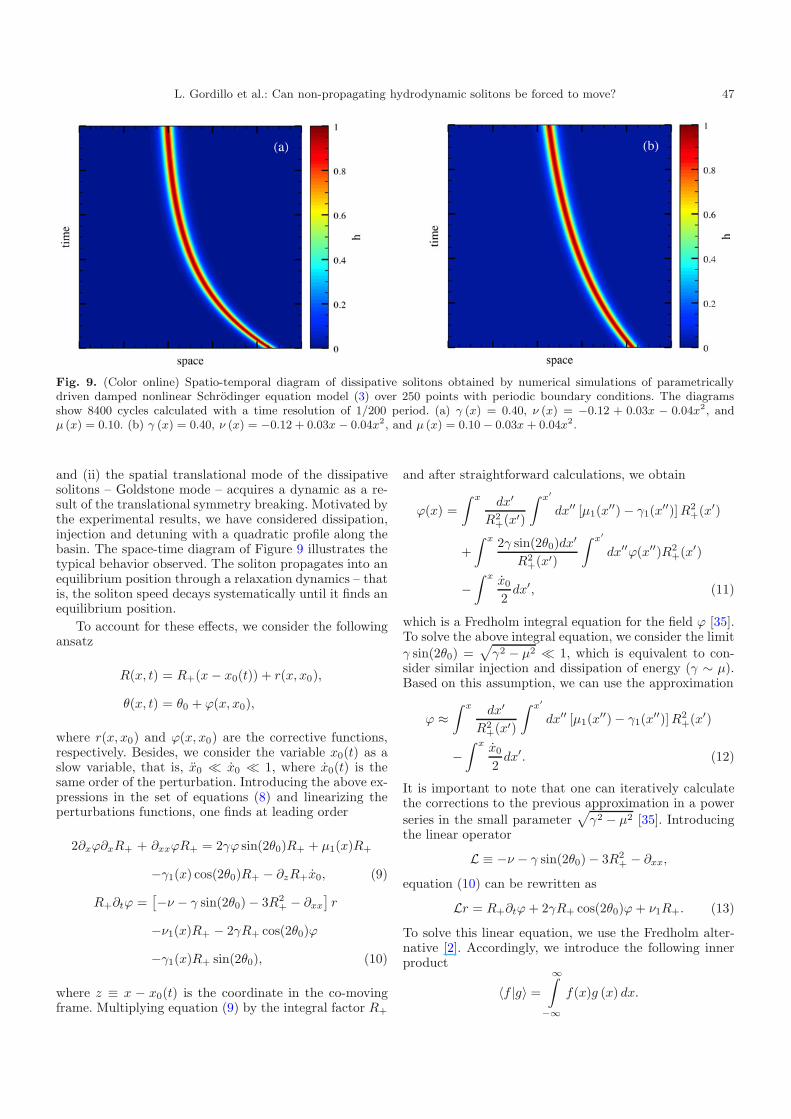
Fig. 9. (Color online) Spatio-temporal diagram of dissipative solitons obtained by numerical simulations of parametricallydriven damped nonlinear Schrodinger equation model (3) over 250 points with periodic boundary conditions. The diagramsshow 8400 cycles calculated with a time resolution of 1/200 period. (a) γ (x) = 0.40, ν (x) = −0.12 + 0.03x − 0.04x2, andμ (x) = 0.10. (b) γ (x) = 0.40, ν (x) = −0.12 + 0.03x − 0.04x2, and μ (x) = 0.10 − 0.03x + 0.04x2.

and (ii) the spatial translational mode of the dissipativesolitons – Goldstone mode – acquires a dynamic as a re-sult of the translational symmetry breaking. Motivated bythe experimental results, we have considered dissipation,injection and detuning with a quadratic profile along thebasin. The space-time diagram of Figure 9 illustrates thetypical behavior observed. The soliton propagates into anequilibrium position through a relaxation dynamics – thatis, the soliton speed decays systematically until it finds anequilibrium position.

To account for these effects, we consider the followingansatz

R(x, t) = R+(x− x0(t)) + r(x, x0),

θ(x, t) = θ0 + ϕ(x, x0),

where r(x, x0) and ϕ(x, x0) are the corrective functions,respectively. Besides, we consider the variable x0(t) as aslow variable, that is, x0 � x0 � 1, where x0(t) is thesame order of the perturbation. Introducing the above ex-pressions in the set of equations (8) and linearizing theperturbations functions, one finds at leading order

2∂xϕ∂xR+ + ∂xxϕR+ = 2γϕ sin(2θ0)R+ + μ1(x)R+

−γ1(x) cos(2θ0)R+ − ∂zR+x0, (9)

R+∂tϕ =[−ν − γ sin(2θ0) − 3R2

+ − ∂xx

]r

−ν1(x)R+ − 2γR+ cos(2θ0)ϕ

−γ1(x)R+ sin(2θ0), (10)

where z ≡ x − x0(t) is the coordinate in the co-movingframe. Multiplying equation (9) by the integral factor R+

and after straightforward calculations, we obtain

ϕ(x) =∫ x dx′

R2+(x′)

∫ x′

dx′′ [μ1(x′′) − γ1(x′′)]R2+(x′)

+∫ x 2γ sin(2θ0)dx′

R2+(x′)

∫ x′

dx′′ϕ(x′′)R2+(x′)

−∫ x x0

2dx′, (11)

which is a Fredholm integral equation for the field ϕ [35].To solve the above integral equation, we consider the limitγ sin(2θ0) =

√γ2 − μ2 � 1, which is equivalent to con-

sider similar injection and dissipation of energy (γ ∼ μ).Based on this assumption, we can use the approximation

ϕ ≈∫ x dx′

R2+(x′)

∫ x′

dx′′ [μ1(x′′) − γ1(x′′)]R2+(x′)

−∫ x x0

2dx′. (12)

It is important to note that one can iteratively calculatethe corrections to the previous approximation in a powerseries in the small parameter

√γ2 − μ2 [35]. Introducing

the linear operator

L ≡ −ν − γ sin(2θ0) − 3R2+ − ∂xx,

equation (10) can be rewritten as

Lr = R+∂tϕ+ 2γR+ cos(2θ0)ϕ+ ν1R+. (13)

To solve this linear equation, we use the Fredholm alter-native [2]. Accordingly, we introduce the following innerproduct

〈f |g〉 =

∞∫

−∞f(x)g (x) dx.

48 The European Physical Journal D

The linear operator L is self-adjoint(L = L†) under this

definition. The kernel of this linear operator – the setof functions {v} that satisfy Lv = 0 – is of dimen-sion 1. As a result of spatial translation invariance, onehas L∂xR+ = 0. Therefore, the field r has a solution ifthe following condition is satisfied5

0=〈∂xR+ | R+∂tϕ+ 2γR+ cos(2θ0)ϕ+ ν1(x)R+〉 . (14)

Using the approximation (12), and considering the dom-inant terms and after straightforward calculations, yieldsto

x0 =1

∫ ∞−∞ dx∂xR2

+(x)x

[2

∫ ∞

−∞dx∂xR

2+(x)

∫ x

dx′1

R2+(x′)

×∫ x′

dx′′ (μ1(x′′) − γ1(x′′))R2+

+∫ ∞

−∞dx∂xR

2+ · ν1(x)

μ

]. (15)

This expression gives us information of the dynamics ofdissipative soliton as a function of spatial disturbance.For small angles and considering the experimental obser-vations, we can consider as a first approximation

μ(x) = μ+ μ1x+ μ2x2,

γ(x) = γ + γ1x+ γ2x2,

ν(x) = ν + ν1x+ ν2x2.

The experimental results allow us to infer that the coef-ficients μ2, γ2 are small, and that ν2 is not small. Then,formula (15) can be rewritten

x0 =1

∫ ∞−∞ dx∂xR2

+(x)x

[2

∫ ∞

−∞dx∂xR

2+

∫ x

dx′1R2

+

×∫ x′

dz(μ1 − γ1)zR+(z)2 +∫ ∞

−∞dz∂zR+(z)2

ν1γz

+{

4∫ ∞

−∞dx∂xR

2+

∫ x

dx′1R2

+

×∫ x′

dz(μ2 − γ2)zR+(z)2

+ 2∫ ∞

−∞dz∂zR+(z)2 · ν2

γz

}x0(t)

]. (16)

5 This is known as the solvability condition or Fredholm al-ternative.

Consequently, the position of the maximum of the dissi-pative soliton is ruled by equation (1), where

τ−1 =1

∫ ∞−∞ dx∂xR2

+(x)x

[4

∫ ∞

−∞dx∂xR

2+

∫ x

dx′1R2

+

×∫ x′

dz(μ2 − γ2)zR+(z)2

+2∫ ∞

−∞dz∂zR+(z)2

ν2γzx0(t)

],

P =τ

∫ ∞−∞ dx∂xR2

+(x)x

[2

∫ ∞

−∞dx∂xR

2+

∫ x

dx′1R2

+

×∫ x′

dz(μ1 − γ1)zR+(z)2 +∫ ∞

−∞dz∂zR+(z)2

ν1γz

]

.

Therefore, model (1) allows us to capture the dynam-ics of dissipative solitons observed experimentally in theforced tilted basin with water and numerical simulationsof the equation parametrically driven damped nonlinearSchrodinger equation. Figure 9 presents numerical simula-tion results obtained considering a quadratic dependenceon space for both detuning and dissipation. The dynamicevolution shown by these numerical simulations agree verywell with experimental results.

It is important to note that when injection and dissi-pation of energy are of the same order, the system is welldescribed by model (1). However, phase does not exhibitsignificant corrections in comparison with the maximumamplitude of the soliton. This is consistent with experi-mental observations.

4 Conclusions

Localized structures are ubiquitous in nature. During thelast decade, a constant effort has been focused on thecreation mechanisms and features of localized states. Un-doubtedly, the next step to boost their potential applica-tions is to advance the manipulation and control of theseparticle-type solutions. Here, we have presented a theoret-ical and experimental study of a method of manipulationand control of hydrodynamic solitons in a vertically drivenrectangular water basin, based on the tilting of the system.

Experimentally, for a given tilt angle, solitons travel toequilibrium positions through a relaxation process. Longacquisitions are required to observe this behavior, becauseof the large decay time of the velocity. The equilibriumposition depends on the tilt angle, and can be pushed outof the basin if the angle is large enough.

In this system, dissipation, energy injection and detun-ing are inhomogeneous. Dissipation grows in the directionof depth gradient, but changes are small. Indirect evidencefrom soliton local phase indicates that energy injectionsvaries less or similarly than dissipation. In contrast, thedetuning exhibits a convex behavior along the channel andhas shown to have a strong effect on soliton dynamics.

Close to the parametric resonance, the parametricallydriven damped nonlinear Schrodinger equation models

L. Gordillo et al.: Can non-propagating hydrodynamic solitons be forced to move? 49

this system. The effects of the tilting of the basin are incor-porated into this model through space-dependent dissipa-tion, energy injection and detuning. We have deduced anequation for the position of hydrodynamic solitons. Thisequation is characterized by two terms: a constant speedand a linear relaxation term. The theoretical descriptionreproduces well the hydrodynamic soliton dynamics ob-served experimentally.

We gratefully acknowledge S. Coulibaly for fruitful discussions.M.G.C. is thankful for the financial support of FONDECYTproject 1090045. L.G. thanks the grant support of CONICYT.The authors are also grateful for the fundings of ACT project127.

References

1. A.C. Newell, Solitons in Mathematics and Physics (Societyfor Industrial and Applied Mathematics, Philadelphia,1985)

2. See, e.g., L.M. Pismen, Patterns and Interfaces inDissipative Dynamics (Springer Series in Synergetics,Berlin Heidelberg, 2006), and references therein.

3. M. Cross, H. Greenside, Pattern Formation and Dynamicsin Nonequilibrium Systems (Cambridge University Press,New York, 2009)

4. P. Coullet, Int. J. Bifur. Chaos 12, 2445 (2002)5. W. van Saarloos, P.C. Hohenberg, Phys. Rev. Lett. 64,

749 (1990)6. P.D. Woods, A.R. Champneys, Physica D 129, 147 (1999)7. G.W. Hunt, G.J. Lord, A.R. Champneys, Comput.

Methods Appl. Mech. Eng. 170, 239 (1999)8. M.G. Clerc, C. Falcon, Physica A 356, 48 (2005)9. U. Bortolozzo, M.G. Clerc, C. Falcon, S. Residori, R.

Rojas, Phys. Rev. Lett. 96, 214501 (2006)10. O. Thual, S. Fauve, J. Phys. (Paris) 49, 1829 (1988)11. O. Thual, S. Fauve, Phys. Rev. Lett. 64, 282 (1990)12. V. Hakim, Y. Pomeau, Eur. J. Mech. B S10, 137 (1991)

13. M. Clerc, P. Coullet, E. Tirapegui, Phys. Rev. Lett. 83,3820 (1999)

14. M. Clerc, P. Coullet, E. Tirapegui, Opt. Commun. 167,159 (1999)

15. M. Clerc, P. Coullet, E. Tirapegui, Prog. Theor. Phys.S139, 337 (2000)

16. M. Clerc, P. Coullet, E. Tirapegui, Int. J. Bifur. Chaos 11,591 (2001)

17. M.G. Clerc, P. Encina, E. Tirapegui, Int. J. Bifur. Chaos18, 1905 (2008)

18. I.V. Barashenkov, E.V. Zemlyanaya, Phys. Rev. Lett. 83,2568 (1999)

19. J.W. Miles, J. Fluid Mech. 148, 451 (1984)20. W. Zhang, J. Vinal, Phys. Rev. Lett. 74, 690 (1995)21. M.G. Clerc, S. Coulibaly, N. Mujica, R. Navarro, T.

Sauma, Phil. Trans. R. Soc. A 367, 3213 (2009)22. B. Denardo, B. Galvin, A. Greenfield, A. Larraza, S.

Putterman, W. Wright, Phys. Rev. Lett. 68, 1730 (1992)23. J.N. Kutz, W.L. Kath, R.D. Li, P. Kumar, Opt. Lett. 18,

802 (1993)24. S. Longhi, Phys. Rev. E 53, 5520 (1996)25. I.V. Barashenkov, M.M. Bogdan, V.I. Korobov, Europhys.

Lett. 15, 113 (1991)26. M.G. Clerc, S. Coulibaly, D. Laroze, Phys. Rev. E 77,

056209 (2008)27. M.G. Clerc, S. Coulibaly, D. Laroze, Int. J. Bifur. Chaos

19, 2717 (2009)28. M.G. Clerc, S. Coulibaly, D. Laroze, Physica D 239, 72

(2010)29. N.V. Alexeeva, I.B. Barashennkov, G.P. Tsironis, Phys.

Rev. Lett. 84, 3053 (2000)30. M.G. Clerc, S. Coulibaly, D. Laroze, Int. J. Bifur. Chaos

19, 3525 (2009)31. E. Caboche, F. Pedaci, P. Genevet, S. Barland, M. Giudici,

J. Tredicce, G. Tissoni, L.A. Lugiato, Phys. Rev. Lett.102, 163901 (2009)

32. J. Wu, R. Keolian, I. Rudnick, Phys. Rev. Lett. 52, 1421(1984)

33. J.W. Miles, Proc. Roy. Soc. A 297, 459 (1967)34. W. Wei, W. Xinlong, W. Junyi, W. Rongjue, Phys. Lett.

A 219, 74 (1996)35. G. Arfken, H. Weber, Mathematical Methods for Physicists

(Elsevier Academic Press, Burlington, 2001).