Sudan University of Science and

Technology

College of Graduate Studies

Numerical Solution of The Solitons

Propagation IN Optical Fibers Using

Sptit-Step Fourier method

ةالبصري باستخدام في المنفردة في األلياف ال العددي نتشار الموجة لالح

فورير المنفصلة الخطوة طريقة

A Thesis Submitted in Partial Fulfillment of the

Requirements for Degree of M. Sc. in Physics

Prepared By:

Hissein Hassane Baharadine

Supervisor:

Dr. Isam Ahmed Attia

I

ا :ق عالي ل اله ت

ي ﴿و اه ف ا سكن در ق ق ا من السماء ماء ت لن ز ن أ

لي رض وع اذروذ ألأ ه لق ﴾هاب ب ن َ

ون سور من : ) ،ه المو ه ب لأ 81)أ

II

DEDICTION

I dedicate this work to: - My parents who supported and encouraged me all of time.

-My wife and kids - My brothers and sisters for their patience and continues support.

- My friends - Staff at Sudan University of Science and

Technology

III

ACKNOWLEDGEMENS

First and foremost, I would like to thank God Almighty for giving

me the strength, knowledge, ability, and opportunity to undertake this

research study and to persevere and complete it satisfactorily. Without his

blessings, this achievement would not have been possible.

In my journey towards this degree, I have found a teacher, a friend,

an inspiration, a role model, and a pillar of support in my Guide, Dr. Isam

Attia He has been there providing his heartfelt support and guidance at all

times and has given me invaluable guidance, inspiration, and suggestions in

my quest for knowledge. He has given me all the freedom to pursue my

research, while silently and non-obtrusively ensuring that I stay on course

and do not deviate from the core of my research. Without his able guidance,

this thesis would not have been possible, and I shall eternally be grateful to

him for his assistance.

I am really indebted to the Sudan University of Science and

Technology.

I wish also would extend my thanks to all the teaching staff in the Faculty of

Science-Sudan University.

Finally, great appreciations are due to my parent for their encouragement and

assistance during the study and research period

IV

Abstract

Despite the vast research in the notions of Maxwell's

equations, the propagation equation of an electromagnetic wave

and the notion of soliton allowed us to derive a model known in

optics as the Nonlinear Schrodinger Equation (NLSE) which will

take into consideration the dispersion and non-linearity effects.

That most of the systems in this universe qualify to be nonlinear so

that, the immediate objective of this research project is to study

some phenomena that occur in optical fibers during the propagation

of an ultra-short pulse "Electromagnetic wave", which are

nonlinear.

One factor which has led to a numerical method is used in

the analytical solution of such equation is difficult and sometimes

impossible. As a result, the most appropriate tool to solve this type

of problem, called the Split Step Fourier Method (SSFM). To this

end, this process leads to the formation of optical solitons which

retain shape during propagation, the compression mechanism

fundamentally due to high order solution.

This a numerical simulation increases our understanding to

describe the evolution of a pulse in an optical fiber while revealing

the advantage of the coexistence of the two phenomena "dispersion

and non-linearity of the medium".

V

مستخلصال

علي الرغم من البحوث الكثيرة المنشورة في مفاهيم معادالت ماكسويل فان معادلة انتشار

سمحت باشتقاق نموذج معروف في علم الموجة المنفردة وفكرةالموجة الكهرومغناطيسية

لتأثيراتوا االعتبار التشتفي ذوالتي تأخ NLSE)البصريات باسم معادلة شرودنجرغير الخطية)

من المباشر الهدف فإن لذا غيرخطية، لتكون مؤهلة الكون هذا في األنظمةالال خطية. أن معظم

" الموجاتانتشار ثناء البصريةاأللياف التي تحد ث في بعض الظواهردراسة هوا البحث ذه

.الخطية غير جدًا، وهي القصيرة النبضا ت ذا تالكهرومغناطيسية"

أحد العوامل التي أدت إلى استخدام الطريقة العدية هو أن الحل التحليلي لمثل هذه

مالءمة لحل هذا النوع من ستحيل. ونتيجة لذلك فإن األداة األكثريكون مالمعادالت يصعب وأحيانا

(. SSFMالخطوة المنفصلة" ) -المسائل، تسمي "طريقة فورير

تحقيقا لهذه الغاية، تؤدي تكوين موجة منفردة ضوئية والتي تحتفظ بالشكل اثناء االنتشار، ميكانيكية

من الضغط تعتمد أساساعلي أن الموجات المنفردة ب عالية الت تيب. تزيد هذه المحاكاة العددية

الفهم لوصف تطور النبض في االلياف الضوئية مع الكشف عن ميزة الترابط بين الظاهرتين "

".التشتت والالخطية للوسط

VI

TABLE OF CONTENTS

Topic Page

Inductive page( (اآلية I

ACKNOWLEDGEMENTS II

DEDICTION III

Abstract (English) IV

Abstract in (Arabic) V

Table of Content VI

List of Symbols IX

List of Figure X

List of Table XI

CHAPTER ONE

1.1 Introduction 2

1.2 Statement of the problem 4

1.3 Aims 4

1.4 Methodology 5

1.5 Questions 5

1.6 Thesis layout 5

CHAPTER TWO

2.1 Literature Review 8

2.2 The origin of nonlinear optics 8

2.2.1 Electromagnetic properties of the medium 8

2.3 wave 8

2.3.1 Electromagnetic wave 9

2.4 Nonlinear propagation equation: 9

2.4.1 Maxwell's equations 9

2.4.2 Electric field polarization 10

2.4.3 Equation of propagation of an electromagnetic wave 11

2.5 The speed of propagation of electromagnetic waves 12

2.5.1 Phase speed and group speed 12

2.6 Refractive index 13

2.7 Dispersion of a physical environment 14

VII

2.7.1 The dispersion parameters 14

2.7.1.1 First order dispersion 15

2.7.1.2 Second order dispersion 16

2.7.1.3 Compromise: dispersion-non-linearity 17

2.8 Propagation of a wave in a dispersive medium: 17

2.8.1 Chromatic dispersion 19

1.8.1.1 Dispersion due to the material 19

2.7.1.2 Dispersion due to guidance 19

2.9 Non-linearity and solitons 19

2.9.1 Nonlinear optical susceptibility 20

2.9.2 Kerr effect 22

2.9.2.1 The optical Kerr effect 22

2.9.3 Stimulated Raman scattering 23

2.10 The solitons 23

2.10.1 Definition 23

2.10.2 The classes of solitons 24

2.10.2.1 Classification of solitons in bases of shape 24

2.10.2.2 Bright solitons of the time envelope 25

2.10.2.3 Solitons of the dark temporal envelope 25

2.10.2.4 Solitons of the dark temporal envelope 25

2.10.2.5 Optical path 25

2.10.3 Formation of optical solitons 26

2.10.3.1 The soliton effects 27

2.11 Equations with Soliton as solutions 28

2.11.1 Normalized non-linear Schrödinger equation for temporal

Solitons

28

CHAPTER THREE

3.1 Numerical methods 32

3.2 Optical fiber and light guiding 32

3.2.1 Physical principle Light guiding 32

3.2.2 Type of optical fibers 33

3.2.2.1 Multi-mode fiber 33

VIII

3.2.2.2 Single mode fiber 35

3.2.3 Assessment on the various optical fibers 45

3.3 Derivation of the nonlinear Schrödinger equation 36

3.4 Numerical solution methods of the nonlinear Schrödinger

equation 41

3.4.1 Fourier method with fractional Split-step 41

3.4.2 Finite difference method 42

3.4.3 The Inverse Scattering Method 43

3.4.4 Fourier method with Split-step 44

3.4.4.1 Use of the Fourier PA fractionated transform method (the

Split-Step Fourier Method)

45

3.4.4.2 Presentation of the Method 45

CHAPTER FOU

4.1 Simulation results 51

4.2 Numerical simulation of the propagation of a pulse in a single-

mode fiber optic 51

4.2.1 Propagation of an impulse in Soliton Fundamental form 52

4.2.1.1 Numerical simulation of the propagation of a pulse in a linear

medium 54

4.2.2 Numerical simulation of the propagation of a pulse in a nonlinear

medium 54

4.2.2.1 Propagation of an impulse in fundamental soliton form 54

4.2.2.1 Propagation of an impulse in Chirped Soliton Form

CHAPER FIVE

57

5.0 Conclusion 64

5.1 Conclusion

5.2 Future Work

5.3 References

IX

List of Symbols /Abbreviations

Speed of light in a vacuum.

Dispersion parameter.

Index of refraction in any medium

n𝑵𝑳 Nonlinear refractive index.

vϕ Phase speed.

v𝒈 Group speed.

propagation distance.

Time.

Linear attenuation coefficient.

, Propagation constant (wave vector).

β Derivative of order i of the propagation constant β with respect to ω.

Coefficient of non-linearity.

Wavelength in a medium.

τ Time delayed.

Pulse of the wave.

𝐷̂ Linearity operator of the SSF method.

𝑁̂ Nonlinearity operator in the SSF method.

GVD Group- Velocity Dispersion.

NLSE Nonlinear Schrödinger Equation (Nonlinear Schrödinger Equation).

SMF Single Mode Fiber.

SPM Self-phase modulation.

SSF Split- Step Fourier (iterative Fourier).

X

List of figures

Figure no. Figure Title Page

2.1 Electromagnetic wave 9

2.2 Envelope of a wave packet 18

2.3 Propagation of the wave packet 18

2.4 Illustration of the pulse modulated by propagation

(a) and its spectrum (b) 22

2.5 Fundamental soliton N = 1. 28

2.6 Temporal evolution of two solitons (N = 2, N = 3)

as a function of the Length of propagation 29

3.1 reflection / refraction 33

3.2 Step index fiber 33

3.3 graded index fiber 34

3.4 Single-mode fiber 34

3.5 Synoptic diagram of the reverse diffusion method 44

3.6 Illustration of the Fourier method with separate

steps 47

4.1 The input pulse 53

4.2 Propagation of a pulse in a medium of zero

dispersion 53

4.3 Propagation of an impulse in a dispersive medium

(normal and abnormal dispersion). 54

4.4 Represents a light pulse is chirped. 59

4.5 Propagation of a pulse in a non-linear dispersive

medium z = 1 to Ф𝑚𝑎𝑥 = 57

4.6 Propagation of a pulse in a non-linear dispersive

medium at z = 2 Ф𝑚𝑎𝑥 = 3 / 2 57

4.7

(a) Soliton pulse with chirping parameter C = 2. (b)

Soliton pulse with chirping parameter C = 3 (c) with

a chirping parameter C = -2. (d) with C = -3 60

4.8

compensation process between auto-phase

modulation (Kerr effect) and GVD chromatic

dispersion

63

XI

List of tables

Table no. Title Page

2.1 Refractive index of some substances 13

3.1 Balance sheet on the various optical fibers 34

4.1 Value of the parameters used for the simulation 58

4.2 PBR value for a constant non-linearity parameter. 60

4.3 PBR value with constant 2 61

1

Chapter one

Introduction

1.1 Introduction

A system is said to be nonlinear if its output is not linearly proportional

to input; on the basis of this definition, one can say that most of the systems

in this universe qualify to be nonlinear. The science which deals with

nonlinear systems is known as nonlinear science. In the past few decades,

nonlinear science has emerged as a tool to study all those complex natural

phenomena which cannot be studied completely by linear science. It is not a

new subject or branch of science, although it delivers a whole set of

fundamentally new ideas and surprising results. Nonlinear science qualifies

to be a revolution due to its wide scope and coverage because it finds

applications in almost all branches of science such as plasma physics,

hydrodynamics, mechanics, biology, chemistry etc. Hence, due to feasibility

of nonlinear science on system of every scale, it is possible to study same

nonlinear phenomena in very distinct way, with the corresponding

experimental tools.

The study of nonlinear system means to study the nonlinearity present in it.

Nonlinearity plays an important role in dynamics of various physical

phenomena [1, 2], such as in electronic circuits, laser physics, nonlinear

mechanical vibrations, population dynamics, astrophysics, plasma physics,

chemical reactions, nonlinear wave motions, heartbeat, nonlinear diffusion,

time-delay processes etc. Nonlinearity in any system make the system more

complex and it became very difficult to study. A small disturbance induced

in nonlinear system even by little variation in initial conditions can results

into big difference in behavior in time evolution of the system. Hence a

nonlinear system exhibits a sensitive dependence on initial conditions.

However, linear systems are generally gradual, smooth, and regular, common

example of linear system are slowly flowing streams, engines working at low

2

power, slowly reacting chemicals, etc. Any system with large input generally

shows nonlinear behavior. For example, the behavior of a spring is linear for

small displacement, but if the initial displacement is large the spring shows

nonlinear behavior.

In similar way, for small initial displacement simple pendulum behaves as

linear system however as the initial displacement become large enough, its

motion become nonlinear.

The nonlinear system which is to be studied is described by a

nonlinear evolution equation (NLEE). These NLEE’s are having complex

structures due to linear and nonlinear effects.

The non-linearity is linked to the thresholds of excitation by an electric field,

to multi-stability, to hysteresis, to phenomena which are modified

qualitatively as the excitations occur, for example the propagation of a wave

moving in a medium is determined by the properties of the medium.

Nonlinearity leads to the distortion of the shape of large amplitude waves, for

example, in turbulence. However, there is another source of distortion: the

dispersion of a wave. The influence of these effects was a limit to the

transmission of Alexandre Bell's photophone. Faced with the same problem,

Tyndall John demonstrates that light can be guided, this experiment is

currently used in optical fibers based on the "principle of total reflection".

The invention of the laser in 1958 [Mah et al89] relaunched the transmission

of information in waveguides.

The wave propagation in real mediums, for example a rolling wave in

an optical fiber is distorted by dispersive and non-linear effects. The

promising quick fix for these drawbacks is the "Soliton" concept, first

discovered by Scotsman John Scott Russell in 1885.

More than 100 years ago, the mathematical equations describing the solitary waves

were solved, among these there are the NLSE non-linear Schrodinger equations,

3

difficult to solve analytically, in this case the resolution requires a numerical

approach.

1.2 Statement of the problem:

In recent decades, soliton theory has become a very active area of

research due to its importance in many branches of physics such as nonlinear

optics. In general, the concept of soliton is always linked to nonlinear partial

differential equations, whose analytical solution is difficult, for this reason it

is necessary to use numerical methods. Which, led to study a model the

propagation in a nonlinear dispersive medium.

This modeling leads to a nonlinear partial differential equation known

optically as nonlinear Schrödinger, which requires numerical solution.

For the simulation used a method which is exclusively used to solve this kind

of problems. An application will be made for the study of propagation in a

single mono mode optical fiber. To this end two cases were investigated use

of an input pulse in fundamental soliton form and chip pulse form.

1.3 Aims:

The objectives of this research are:

a) Obtaining mathematical modeling of study, the propagation in a nonlinear

dispersive medium by the nonlinear Schrödinger Equation (NLSE).

b) Presenting numerical approach for mathematical modeling to simulate the

NLSE to analyze the properties of optical solitons.

c) An applying the modest to study of propagation in a single mono mode optical

fiber

d) Investigating the two cases: use of an input pulse in fundamental soliton form

then in the form of chip pulse.

4

1.4 Methodology :

Many physical phenomena can be modelled by partial differential

equations, but – apart from some very specific cases – it is generally not

possible to write down the solution to these problems in closed form. In order

to understand the behavior of the solution, it is thus often necessary to

construct an approximation via a numerical solution.

this research concerns on a numerical simulation to describe the evolution of

a pulse in an optical fiber while revealing the advantage of the coexistence of

the two phenomena "dispersion and non-linearity of the medium by using

Split Step Fourier Method" SSFM.

1.5 Questions:

1. What is the soliton optics?

2. How to solve nonlinear partial differential equations in solitons optics and how to

apply them?

3. How these solutions analyzed?

4. How these solutions are plotted in graphs?

1.6 Thesis lay out:

chapter one introduce the study. After a few reminders on non-linearity,

we present in the chapter two the Maxwell equations to find a propagation equation.

Then the process of propagation of an impulse in the dispersive medium, and not

linear will be studied and at the end of the chapter we presented a small recall on

the optical solitons, and how they are formed. As well as the derivation of the NLSE

non-linear Schrödinger equation system.

In Chapter three, after a little reminder on optical fibers, devote this

part to the methods of numerical resolution of the non-linear Schrodinger

equation NLSE. For which used the so-called "Fourier fractional" numerical

5

method (Split-Step Fourier in English), based on the fast Fourier transform

algorithm. Therefore, the optical fiber will be cut into thin slices. Chapter four

is devoted to simulations of the propagation of the soliton in an optical fiber

(single mode). We will complete our work with an interpretation of the

results. Then a conclusion in Chapter five.

6

Chapter two

Literature Review

2.1. Introduction

Non-linear effects are those that do not occur directly proportional

to the action. This is the case with most real-world effects, and the reason for

the difficulty in reproducing information faithfully by analog techniques.

This chapter is devoted to reminders of a few concepts related to

non-linear optics, namely the notion of Kerr effect, dispersion, soliton, and

the equation governing its propagation in a non-linear medium, emphasizing

the importance of the dispersion compromise. Non-linearity of the medium.

2.2. The origin of non-linear optics

Nonlinear optics is the discipline of physics in which the density of

the electrical polarization of the medium is studied as a nonlinear function of

the electromagnetic field of light. Being a vast field of research activity on

the propagation of electromagnetic waves, the non-linear interaction between

light and matter tracks to a wide spectrum of phenomena, such as optical

frequency conversion, optical solitons, phase conjugation and Raman

scattering. In addition, many of the analytical tools used in non-linear studies

of optics are general in nature, such as perturbation techniques and symmetry

considerations, and may just as easily be applied to other disciplines in

nonlinear dynamics. [1]

2.3 Electromagnetic properties of the medium

2.3.1. Wave

A wave is the propagation of a disturbance producing in its passage a

variation of the physical properties of the medium, it is important to note that

the wave results in a transport of energy and not of matter [2].

7

1.3.2. Electromagnetic wave:

As the name suggests, an electromagnetic wave is an electrical and

magnetic wave. It is broken down into an electric field and a magnetic field.

It takes place without transport of the material and these fields are called

disturbances. These two disturbances oscillate at the same time but in two

perpendicular planes (Figure 2.1).

An electromagnetic wave and a medium interact through three parameters

[3]: Conductivity , and Electrical permittivity and magnetic permeability

. These parameters appear clearly in the Maxwell equations.

Figure 2.1. Electromagnetic wave

2.4. Nonlinear propagation equation:

2.4.1. Maxwell's equations:

If the material is insulating (non-conductive), linear, homogeneous, isotropic, and non-

magnetic.

So, the dielectric constant (ε) is independent of orientation or location, so ε is

treated as a scalar quantity. Under such conditions Maxwell gathered all the

ideas on electromagnetic waves (their description and their interactions) in

these four equations [3].

8

o is the electric field, (Volt / m). o 𝐷̂ electrical

displacement (or induction) (Coulomb / m²). o 𝐵⃗ the

magnetic field (or induction), (Webber / m²).

o 𝐻⃗ magnetic excitation (or field). (Ampere / m).

In a dielectric medium, the response of the medium to the excitation 𝐸⃗ and

is given by:

Where 0 is the permeability of the vacuum and 𝑃⃗ is the electric polarization, is the

Magnetic polarization.

2.4-2. Electric field polarization

The polarization created by a light wave passing through a material is written

in the form:

is the order polarization in powers of the electric field. More precisely,

we can show that for i waves of frequencies 1, ···, 𝜔𝑖 we note the amplitudes

, the polarization is written in the form:

9

Where 0 is the electrical permittivity of the vacuum, and χ (i) (ω1, ···, ωi) is the

electrical susceptibility tensor of order i which depends on the material used.

This last expression shows that the wave creates a frequency different from the

waves initially present.

An interpretation of the non-linearities appearing in the polarization comes

from the microscopic aspect of the material. Each atom of a dielectric material

is surrounded by an electronic cloud which can deform under the action of

, which creates an electric dipole.

This dipole, for a small deformation, is proportional 𝐸⃗ , but if the

deformation is too large, this is no longer the case. The sum of all the dipoles

is then the polarization introduced above, hence its non-linearity. Similar

reasoning can be used in the case of metals and plasmas: the free electrons

undergo, from the excitatory field, a Lorentz force depending on the speed of

the electrons, and therefore on the polarization. Thus, these media can also

exhibit non-linear effects. [18]

2.4.3. Equation of propagation of an electromagnetic wave:

In order to study the effects of the nonlinearities of a medium on the

propagation of an electromagnetic wave, we first develop a simple wave

equation suitable for a large class of important materials (dielectrics). To do

this, we start by doing the rotational of the equation (2.3), we get [5]

Knowing that

So, we have:

10

In non-conductive materials the product

So, equation (2.7) becomes:

−∇2�⃗�⃗ = ∇⃗⃗ 𝑋 (𝜕�⃗�

𝜕𝑡) = 𝜇0

𝜕

𝜕𝑡∇⃗⃗ 𝑋�⃗⃗�⃗ (2.11)

−𝜇0𝜕

𝜕𝑡(𝜕�⃗⃗�

𝜕𝑡) = 𝜇0𝜀0 (

𝜕2�⃗�

𝜕𝑡2+

𝜕2�⃗�

𝜕𝑡2) (2.12)

The equation (2.11) is then written

With:

𝜕2�⃗� 𝑁𝐿(2)

𝜕𝑡2 +𝜕2�⃗� 𝑁𝐿

(3)

𝜕𝑡2 ⟺𝜕2�⃗� 𝑁𝐿

𝜕𝑡2 (2.14)

2.4. The speed of propagation of electromagnetic waves:

A wave is a disturbance which moves in a medium. It is possible to

associate two wave speeds with it, namely the phase speed and the group

speed which sometimes are not equal.

2. 5.1 . Phase speed and group speed:

The phase speed: let be a wave = 0 𝑐𝑜𝑠 (𝜔𝑡 - 𝑘𝑧 + 0), U is the

quantity which propagates, then the phase speed represents the speed of

displacement of the wave plane, therefore the speed of propagation of the

phase given by: = 𝜔𝑡 – 𝑘𝑧

11

Either: 𝑣𝜑 = (𝑑𝑧/𝑑𝑡) =c Where 𝑣𝜑 = 𝜔𝑘

Where: ω is the pulse of the wave and k is the number of waves, the speed of

light in a vacuum.

Group speed: Group speed is generally presented as the speed at which energy or

information is transported by a wave.

𝑣𝑔 =𝜕𝜔

𝜕𝑘 (2.15)

2.6. Refractive index:

Refraction index often noted , it is defined as the ratio of the speed of

light in a vacuum to the speed of light in this medium [.3]

(2.16)

So is a dimensionless quantity which characterizes the medium, it depends on

the measurement wavelength but also depends on the environment (pressure

and temperature).

In a material environment, the speed of light cannot exceed that in a vacuum, so a

refractive index is always greater than or equal to 1 [4].

Table 1: Refractive index of some substances.

Matter refractive

index Matter refractive

index

Air 1 Ruby 1.78

water 1.33 Diamond 2.46

Benzene 1.501 Sapphire 1.77

Quartz 1.55 Glass 1.5

Polystyrene 1.2 Pure Alcohol 1.32

Acetone 1.3 Glycerin 1.47

12

The refractive index plays an important role in extinction:

• deviation of the direction of the wave front (lens effect)

• dissipation (absorption)

2.7. Dispersion of a physical medium:

The speed of propagation of a wave in a medium can depend on its

wavelength, hence a differential propagation phenomenon leading to the

dispersion relationship.

Optics is a special case of this phenomenon for which the speed in a transparent

medium is generally different from that in a vacuum.

As a rule, a pulse with several components contains different

frequencies whose speed is not the same, which results in the distortion of the

pulse.

The propagation of a pulse in a dispersive medium is a function of the

order of dispersion, of the latter which is linked to the propagation constant

( ), It is a Taylor development determined at the central frequency of the

signal 0 [1].

2.7.1. The dispersion parameters:

Mathematically, the dispersion appears in the Taylor series development

of the propagation constant around the central 0 pulse of the pulse [4,13].

13

With is the propagation constant where ( 0 ) is the refractive index at

0.

1 is the inverse of the group speed of the wave.

2.7.1.1. First order dispersion:

In the theory of first-order dispersion by the propagation constant

( ) is equal to:

With: And

Consider an excitement in the form:

(𝑧, 𝑡) = (𝑧, 𝑡)−𝑗(𝜔0𝑡−𝛽(𝜔0)𝑧)

where ( , ) is the complex amplitude which can be determined from the Fourier

transform:

0( ′) is the complex amplitude at = 0 verifying the relation:

(𝑧 = 0, 𝑡) = 𝑈0 = 𝐴 0𝑒−(𝜔0𝑡) (2.20)

Which can show from equation (2.19) that the complex amplitude ( , )

follows the following evolution equation:

14

The solution of this last equation is:

Therefore, the complex amplitude or the wave packet ( , ) moves in the

space of the first order dispersion medium with a constant speed equal 𝑣𝑔

around the point ( ) as a single whole. without change of form. [1]

2.7.1.2. Second order dispersion:

The unchanged shape of the wave packet in first-order dispersion

theory is not exactly exact, but it is approximated. Now consider dispersal as

a real consequence. In this case, the second term must be introduced into the

propagation constant. [14], [15]

With 2 being the speed of dispersion equal to:

Let us suppose that the linear medium considered is subjected to the excitation of the

electric field:

(𝑧, 𝑡) = 𝐸⃗0(𝑧, 𝑡)𝑒−𝑗(𝜔0𝑡−𝛽(𝜔0)𝑧) (2.25)

After some calculations, we find that the complex amplitude ( , ) satisfies the

following differential equation:

It should be noted that the equation (2.26) which describes the propagation of

a pulse in a medium characterized by a second order dispersion, resembles

15

the differential equation which governs the propagation of heat. So, the

presence of the term dispersion of the second order in equation

(2.26) acts as a type of complex term generalized diffusion for the envelope of

the pulse ( , ) in the time domain.

Note that the dispersion of group speed is responsible for the appearance of

several negative effects such as the enlargement effect which reduces the

performance of transmission by optical fibers.

If 2 is zero, the development of ( ) must be pushed beyond the second

order and a term hence the dispersion of the medium is third

𝜔0

order [1].

With regard to the influence of the dispersion effect, it can be said that

a pulse propagating in a physical medium is thus deformed by the dispersion

effect because its different spectral components do not undergo the same

phase shift. This leads to an enlargement which leads to recovery of

successive pulses leading to a detection error on reception.

Therefore, natural chromatic dispersion is considered to be a major problem which

limits the performance of optical communications systems [1].

2.7.1.3. Compromise: dispersion-non-linearity:

To overcome the problem of dispersion, which is not only an

experimental fact but also a consequence of general physical principles,

theorists have proposed a solution capable of solving the problem: this new

concept is "solitons". These are nonlinear excitations localized in space-time,

and which propagate in the physical systems while retaining their original

form almost indefinitely with a rigorous compensation between two

antagonistic and inevitable characteristics: nonlinearity and dispersion.

16

2.8. Propagation of a wave in a dispersive medium:

A physical signal, of finite energy, decomposes as a sum of harmonic signals [2],

we speak then of "packet of waves". So, we will be able to write:

The figure below represents, at = 0, a "packet" of the harmonic waves of neighboring

pulses as a function of x.

Figure 2.2. Envelope of a wave packet

To propagate a wave in a dispersive medium, we start by

decomposing it into a sum of harmonic waves at time = 0, then we propagate

each harmonic component with its own phase speed, finally we reconstruct

the wave by summing its components harmonics at the desired time (t).

In general, there is a distortion of the "wave packet" because the

harmonic components do not sum up in the same way over time: this is often

manifested by a spatial spread of the "wave packet". [4]

The figure below illustrates the propagation of a packet of waves:

17

Figure (2.3): Propagation of the wave packet.

Indeed, when a wave propagates in a dispersive medium, the various

frequency components of the wave propagate at different speeds, creating a

temporal spread of the wave on arrival. This is called group speed dispersion

(Group Velocity dispersion (GVD)) or chromatic dispersion [5].

2.8.1. Chromatic dispersion:

Chromatic dispersion is expressed in 𝑝𝑠/ (𝑛𝑚 ·𝑘𝑚); it characterizes

the spread of the signal linked to its spectral width (two different wavelengths

do not propagate at exactly the same speed). This dispersion depends on the

wavelength considered and results from the sum of two effects: the dispersion

specific to the material, and the dispersion of the guide.

2.8.1.1. Dispersion due to the material:

The dispersion phenomenon results from a sensitivity of the medium to the

frequency of the wave at the microscopic level.

2.8.1.2. Dispersion due to guidance:

This case of dispersion results from the wave nature of the wave

and the desire to confine the wave in a limited volume so as to impose on the

wave a direction of propagation.

18

2.9. Non-linearity and solitons

When a material medium is placed in the presence of an electric field

�⃗�⃗ , it is likely to modify this field by creating a polarization �⃗�⃗ . This response

of the material to the excitation can depend on the field �⃗�⃗ in different ways.

The nonlinear optic groups the set of optical phenomena having a nonlinear

response with respect to this electric field, that is to say a response not

proportional to E.

In the presence of an electromagnetic wave from the optical domain

(wavelength on the order of 1000 nm), in other words light, many materials

are transparent, and some of them are non-linear, c is why nonlinear optics is

possible.

The main differences with linear optics are the possibilities of

modifying the frequency of the wave or of making two waves interact

between them via the material.

These very specific properties can only appear with strong light waves. This

is why non-linear optics experiments could not be carried out until the 1960s

thanks to the appearance of laser technology.

2.9.1. Nonlinear optical susceptibility:

The optical responses, including nonlinear ones are described as [7].

𝑃⃗(𝑡) = 𝜀{𝜒(1)𝐸⃗(𝑡) + 𝜒(2)𝐸⃗(2)(𝑡) + 𝜒(3)𝐸⃗(3)(𝑡) + ⋯ . }

= (1) + (2) + (3) + ⋯ (2.28)

Where we have expressed the polarization p (t) as a series of powers in the

field strength E (t). The quantities (1), (2), (3) are called

susceptibilities; (1) is a linear susceptibility and (2), (3) are called

nonlinear second and third order.

19

For a typical solid-state system, χ (1) is of the order of unity while χ (2) is of the

order of 1 / at, and χ (3) is of the order of 1 / is

the atomic characteristic of the electric field.

𝑎0 = 4𝜋𝜀 0ℏ2⁄𝑚𝑒 2 is the Bohr radius of the hydrogen atom. Explicitly [7].

(2) 1.94 × 10−12 /

(3) 3.78 × 10−24 2/ 2

The formal expression for third order polarization is as follows:

(𝜔0; 𝜔𝑛; 𝜔𝑚)

= 𝜀0𝐷̂ ∑ (3) (𝜔0 + 𝜔𝑛

𝐽𝐾𝐿

+ 𝜔𝑚, 𝜔0, 𝜔𝑛, 𝜔𝑚) 𝑋 (𝜔0)(𝜔𝑛)𝐸⃗𝑙(𝜔𝑚) (2.29)

Where , , , refer to the Cartesian components of the fields and the

degeneration factor D represents the number of distinct permutations of the

frequencies 0, 𝜔𝑛, 𝜔𝑚.

() ( = 1, 2,): Is the susceptibility of the j-th order. The linear susceptibility

χ (1) contributes to the linear refractive index ̅0 (real and imaginary parts; the

imaginary part being responsible for attenuation). The second order

susceptibility χ (2) is responsible for the second harmonic generation. For 𝑆𝑖𝑂2

the second order nonlinear effect is negligible since 𝑆𝑖𝑂2 has inversion

symmetry. This is why optical fibers do not exhibit second order nonlinear

effects.

The third order susceptibility χ (3) is responsible for the lower order nonlinear

effects in optical fibers. Generally, it manifests itself by a modification of the

20

refractive index with optical power or by a diffusion phenomenon. It is linked

to the optical Kerr effect, four-wave mixing, third harmonic generation,

stimulated Raman scattering, etc [9].

Assuming a linear polarization of the propagating light and neglecting the

tensor character of , we find the following relation for nonlinear

polarization:

(𝜔) = 3𝜀0(1)(𝜔 = 𝜔 + 𝜔 − 𝜔)|𝐸⃗(𝜔)|2𝐸⃗(𝜔) (2.30)

The total polarization, which consists of linear and non-linear parts, is written as

follows:

𝑃⃗(𝜔) = 3𝜀0𝜒(1)𝐸⃗(𝜔) + 3𝜀0𝜒(3)|𝐸⃗(𝜔)|2𝐸⃗(𝜔) = 𝜀0𝜒𝑒𝑓𝑓𝐸⃗(𝜔) (2.31)

The actual susceptibility depends on the field as follows

𝜒𝑒𝑓𝑓 = (1) + 3(3)|𝐸⃗(𝜔)|2 (2.32)

And it is related to the refractive index like:

𝑛 = 1 + (3) ≡ 𝑛 0 + 𝑛 2𝐼 (2.33)

Here, I indicate the mean intensity over time of the optical field. We start by

discussing the main features of nonlinear effects

2.9.2 Kerr effect:

It was discovered by J. Kerr in 1875. He discovered that a transparent liquid

becomes doubly refractory (birefringent) when placed in a strong electric

field.

21

2.9.2.1. The optical Kerr effect:

The optical Kerr effect corresponds to a birefringence induced by an

electric field varying at optical frequencies, proportional to the square of this

field. It was observed for the first time, for molecules with directions of

greater polarizability, by the French physicists Guy Mayer and François Gires

in 1963. A sufficient light intensity was obtained thanks to a triggered laser.

[7]

In general, the Kerr effect describes situations where the refractive index depends on

the electric field as follows:

𝑛 (𝑛, |𝐸⃗|2) = 𝑛 0(𝜔) + 𝑛 2(𝜔)|𝐸⃗|2 (2.33)

Figure (2.4). Illustration of the propagation-modulated pulse (a) and its

spectrum (b) Here, ̅2 is known as the Kerr coefficient and it is related to

susceptibility.

For a wave linearly polarized in the direction for silica, its value is approximately 1.3

× 10−22 2 / 2.

The Kerr effect comes from the non-harmonic movement of electrons bound

in molecules. Consequently, it is a rapid effect, the response time being of the

order of 10−15 .

22

2.9.3. Stimulated Raman scattering:

Diffusion phenomena are responsible for the Raman and Brillouin effects.

During these diffusions, the energy of the optical field is transferred to local

phonons: in Raman diffusing optical phonons are generated while in Brillouin

the acoustic phonons are scattered. [8]

Because of the non-linearity and the dispersion, the solitons are existing, so what

is a soliton.

2.10. The solitons

A solitary wave is a wave that propagates by ignoring the classical laws of

energy dispersion. As a rule, this wave is strong enough to excite a non-linear

effect which will compensate for the normal energy dispersion effect.by The

solution of nonlinear partial differential equation which represent a solitary

wave, which has permanent form.

Energy, through the nonlinear phenomenon, creates a potential well in its propagation

medium. This well traps energy and prevents it from dispersing.

•It is localized within a region

•It does not disperse

•It does not obey the superposition principle [3].

Long after Scott-Russel's observation in 1850 of these spectacular

phenomena by a wave in a canal, we realized that these energy packets could

be subjected to forces which give them material properties. Hence the name

of the word soliton stems from the geek (on), meaning particle. [10] The name

was coined by Zabusky and Norman Kruskal (ZK) due to the particle-like

behavior of the pulses they discovered.

23

2.10.1. The classes of solitons:

A rough description of a classical soliton is that of a solitary wave which

shows great stability in collision with other solitary waves. There are several

ways to classify solitons [11]. There are topological and non-topological

solitons. Regardless of the topological nature of the solitons. All solitons can

be divided into two groups considering their profile: permanent and time

dependent. The third way to classify solitons agrees with the nonlinear

equations which describe their evolution.

Here we discuss some classification of solitons [12].

2.10.1.1. Classification of solitons in bases of shape

a) bell soliton

The soliton solution of KdV equation have a bell shape and a low frequency

soliton. This soliton referred to as non-topological solitons, the soliton

solution of (NLS) equation have a bell-shaped hyperbolic secant envelope

modulated a harmonic (Cosine) wave. This solution does not depend on the

amplitude and high frequency soliton. b) Kink soliton

The solutions of (SC) equation are called kink or anti-kink solitons, and

velocity does not depend on the wave amplitude. This soliton referred to as

topological solitons.

The magnetic spins rotate from say spin down in one domain to spin up in the

adjacent domain. The transition region between down and up is called Bloch

wall.

c) breather soliton

Discrete breathers (DB), also known as intrinsic localized modes, or

nonlinear localized excitations, are an important new phenomenon in physics,

with potential applications of sufficient significance to rival or surpass the

Soliton of integrable of partial differential equations.

24

2.10.1.2. Bright temporal envelope solitons:

Light pulses of a certain shape and energy that can propagate unchanged over

large distances.

2.10.1.3. Dark temporal envelope solitons:

Pulses of "darkness" in a continuous wave, where the pulses have a

certain shape and have propagation properties similar to bright solitons.

2.10.1.4. Spatial solitons:

Beams or pulses with continuous wave, with a transverse extent of the

beam passing through the refractive index.

Changes due to Kerr optics can compensate for the direction of the beam.

Optically, the induced change in refractive index works as an efficient light

guide. [12.13]

2.10.1.5. Optical soliton:

The soliton arises from a balance between two compensating effects.

In the case of an optical soliton, these effects are essentially phase self-

modulation and abnormal dispersion. Imagine an electromagnetic pulse

propagating. The phase auto-modulation shifts towards the lowest frequencies

(therefore the longest wavelengths) the edge of the pulse, and conversely

shifts towards the short wavelengths the lag of the pulse. The abnormal

dispersion shifts the high frequencies towards the front of the pulse, the low

frequencies falling behind (red propagates here less quickly than blue, unlike

in the case of normal dispersion). Thus, between the phase self-modulation

which acts on the spectrum of the pulse tends to make the front redder and the

train more blue, and the abnormal dispersion which acts on the time profile of

25

the pulse tends to make the front more blue and drags more red, the impulse

finds a form that balances the two effects. Theory shows that it is a hyperbolic

secant form [11].

This is the class of solitons on which we will focus in this work.

2.10.2 Formation of optical solitons

A light pulse is a bundle of electromagnetic waves of finite spectrum.

Each of its spectral components propagates with a different group velocity,

and as a result, the energy of the pulse extends over time along its

propagation.

When the chromatic dispersion is negative (D <0), speak of the normal

dispersion regime. In this case, long wavelengths (red frequencies) propagate

faster than short wavelengths (blue frequencies). On the contrary, in socalled

abnormal dispersion regime, the chromatic dispersion is positive (D> 0).

Long wavelengths propagate more slowly than shorter wavelengths. In both

cases, the pulse undergoes a temporal enlargement of its envelope.

The zero of the chromatic dispersion is around 1312 nm. For wavelengths less

than this value, the dispersion is positive (normal regime). It is negative

(abnormal regime) for longer wavelengths [11,14].

In the absence of nonlinear effects, the distortion of the optical pulse

is mainly caused by chromatic dispersion and can be eliminated by the

technique of dispersion compensation.

In reality, the response of the optical medium is not linear, because

the refractive index depends on the intensity of the electric field (Kerr effect).

This dependence induces a non-linear phase variation. This is called the auto

phase modulation effect. This nonlinear effect introduces a frequency chirp.

26

In the abnormal dispersion regime, the direction of the frequency slip

produced by the phase self-modulation effect is the opposite to that produced

by the dispersion. This indicates that the frequency slip induced by the phase

auto-modulation can compensate for that induced by the chromatic

dispersion. This process leads to the formation of optical solitons which retain

shape during propagation.

2.10.2.1 The soliton effects:

The soliton is an initially symmetrical light wave propagating without

deformation of its shape in a dispersive and non-linear medium. In optics, the

soliton is used to describe an impulse (temporal soliton) or a beam (spatial

soliton). Mathematically, the soliton can be represented by the following

equation [17,18]:

(𝑧 = 0, 𝜏) = 𝑁̂. sech(𝜏) (2.34)

N is the order of the soliton which is defined by [1,2]:

Where 0, 𝐿𝐷̂, 𝐿𝑁̂𝐿 are respectively the peak power of the pulse, the dispersion

length, and the non-linear length. To determine the order of the soliton, we

always take the nearest integer value.

In the case where 𝐿𝑁̂𝐿 = 𝐿𝐷̂, that is, the linear effect of the group speed

dispersion is compensated by the non-linear effect, we will have a

fundamental (or order one) soliton. Then, for = 1, the fundamental soliton

retains its shape during the propagation. See Figure 2.5

27

Figure 2.5. Fundamental soliton N = 1

Consequently, the peak power necessary for the existence of a fundamental soliton

is:

𝑃⃗0 = √|𝛽2|

𝛾𝑇02 (2.36)

several fundamental solitons propagating in a coupled manner and at the same

group speed.

During its propagation inside an optical fiber, the fundamental solitons

making up the higher-order soliton cause periodic interactions. Figure 2.6

shows the temporal evolution of the order two and order three soliton as a

function of the propagation length. The evolution of these solitons can present

several peaks where the impulse can regain its initial form periodically.

28

Figure 2.6 Temporal evolution of two solitons (N = 2, N = 3) as a function

of the propagation length.

2.11. Equations with Soliton as solutions

In this part, we present some equations which admit the soliton as solutions.

The Korteweg and Vries equation, the nonlinear Schrödinger equation, and

the sine-Gordon equation.

2.11.1. Normalized non-linear Schrodinger equation for temporal solitons:

The starting point for the analysis of temporal solitons is the time-dependent

wave equation for the spatial envelopes of electromagnetic fields in an optical

Kerr medium, here for reasons of simplicity. For linearly polarized light in

isotropic media, the propagation equation is given by [1]:

Where, as before, 𝑣𝑔 = (𝑑𝑘/𝑑𝜔) is the speed of the linear group, and where

we have introduced the notation

For the intensity-dependent refractive index = 0 + 2 |𝐸⃗𝜔|2. Since we are

considering here the propagation of waves in isotropic media, with linearly

polarized light (for which there is no crosstalk of polarization state). The wave

equation is conveniently taken in scalar form:

The equation (2.37) consists of three interacting terms. The first two terms

contain first order derivatives of the envelope, these terms can be considered

as the homogeneous part of a wave equation for the envelope, giving solutions

29

of progressive wave which depend on the two other terms, which rather act

as source terms.

The third term contains a derivative of order 2 of the envelope, this term is

also linearly dependent on the dispersion of the medium, i.e. the variation

of the group speed of the medium compared to the frequency angular of

light. This term is generally responsible for spreading a short pulse when it

crosses a dispersive medium.

Finally, the fourth term is a non-linear source term, according to the sign of

𝑛2, will concentrate components of higher frequency either at the leading edge

or at the trailing edge of the pulse as soon as it is displayed.

30

Chapter three

Numerical Methods

3.1. Introduction

In general, there are no analytical solutions to the complete Maxwell

wave equation for a nonlinear optical system. Even numerical solutions to the

wave equation are extremely difficult to implement due to the dimensionality

of the problem. The vector form of the wave equation is a second order partial

differential equation with four dimensions (three spatial and one temporal).

Thus, approximations based on propagation conditions and experimental

results are necessary to solve an approximate scalar form of the wave

equation, i.e. the nonlinear Schrödinger equation. However, the

approximations listed in the previous chapter limit the generality and validity

of the solutions. For example, the condition of extreme non-linearity, as in

the case of the generation of super continuum, is one where the approximation

of the envelope, which varies slowly, can be violated.

The purpose of this chapter is to introduce a powerful method of numerical

resolution of the NLSE, known as the Split-step Fourier method (SSFM). The

chapter begins with a reminder on fiber optics followed by a reminder of

NLSE numerical resolution methods list the advantages of SSFM compared

to finite difference methods.

3.2. Optical fiber and light guiding:

3.2.1. Physical principle of Light guiding

The major physical principle that inspired fiber optic technology is

what is known as "Total Internal Reflection". This follows from the law of

refraction that a wave crossing through a boundary between two media of

different density, deviated.

31

However, if the wave ever tries to pass from a medium of relatively high

density to a less dense medium, there is a minimum angle between the

direction of the wave and the normal of the border for which the wave will

not be deflected but reflected. It is therefore possible for a light wave to

propagate indefinitely in a glass cylinder [20].

Figure 3.1 reflection / refraction.

3.2.2. Type of optical fibers:

A typical bare fiber consists of a core, a cladding, and a polymer jacket

(buffer coating), the fulfill the conditions for TIR in the fiber, the angle of

incidence of light launched into the fiber must be less than a certain angle,

which is defined as the acceptance angle, θacc. which can be calculated by

Snell's law.

3.2.2.1. Multi-mode fiber:

Only certain angles lead to modes. Obviously, the speed of a mode

depends on the angle. The term "multimode" means that several modes can

be guided. A typical number for a step index fiber is 1000 modes (one mode

corresponds to a beam).

32

❖ Step index:

Figure (3.2) step index fiber

It is the simplest type of fiber. Indeed, it disperses the signal. In this fiber, the

core is homogeneous and of index n1. It is surrounded by an optical cladding

with an index n2 less than n1.

As for the optical cladding, it plays an active role in the propagation and

should not be confused with the protective coating deposited on the fiber. The

ray is guided by the total reflection at the level of the core-cladding interface,

otherwise it is refracted in the cladding. [20].

❖ Graded index:

Figure (3.3) Graded index fiber

Their core, unlike step index fibers, is not homogeneous. Their core is in fact

made up of several layers of glasses whose refractive index is different with

each layer and the refractive index decreases from the axis to the cladding.

Guidance is this time due to the effect of the index gradient. The rays follow

a sinusoidal trajectory.

33

The cladding does not intervene directly but eliminates the too inclined rays.

The advantage with this type of fiber is to minimize the dispersion of the

propagation time between the rays [20].

3.2.2.2. Single mode fiber:

Figure (3.4) Single-mode fiber

The aim sought in this fiber is that the path that the beam must travel is as

direct as possible. For this we strongly reduce the diameter of the heart which

is in most cases less than 10μm. The modal dispersion is almost zero. Since

we do not break the light beam the bandwidth is therefore increased,

approximately 100 GHz * km or 1000 Mbits / s. Conventional single-mode

fiber is stepping index. Its diameter allows the propagation of only one mode,

the fundamental as only one mode propagates there is no difference in speed

unlike multimode fibers. Because of these valuable advantages, it has gained

considerable importance in long-distance transmissions [20].

3.2.3. Assessment on the various optical fibers

The following table gives a brief summary of the advantages and disadvantages of each

structure: [20]

34

Table (3)

Structures Benefits Disadvantages

Step index multi-mode Low price Ease of

implementation

Significant signal loss and

distortion

Graded index

multimode

Reasonable bandwidth -

Good transmission quality

Difficult to implement

Single mode Very high bandwidth - No

distortion

Very high price

As mentioned at the beginning of this chapter, an important application of

solitons is the transmission of information in fiber optic systems. Soliton pulses

are stable when propagated over long distances. Fiber losses are an important

limiting factor, so it becomes necessary to periodically compensate for fiber

losses.

3.3. Derivation of the nonlinear Schrödinger equation

The solitons in optical fibers are described by the equation known as

the non-linear Schrödinger equation (NSLE), which we will derive it. In the

derivation, we use the concept of Fourier spectrum for the propagation of

pulses, see Figure 2.4.

A medium in which solitons propagate there is the non-linearity of Kerr

effect. In such a medium, the refractive index depends on the intensity of the

electric field ( ) and can be written in the following form:

𝑛 (𝑡) = 𝑛 0 + 𝑛 2𝐼(𝑡) (3.1)

With [4]:

(𝑡) = 2𝑛 0𝜀0𝑐|(𝑧, 𝑡)|2 (3.2)

35

where ( , ) is the slowly varying envelope connected to the optical pulse described

by the optical pulse ( , ) as:

(𝑧, 𝑡) = (𝑧, 𝑡) (𝜔0𝑡−𝛽0𝑧) (3.3)

The Fourier transform of the optical field is [5,6]

Where ̃ ( , ) is the Fourier spectrum of the pulse, the propagation

constant and 0 the frequency at which the pulse spectrum is centered (also

called carrier frequency), (See Figure. 2.4) For quasi-monochromatic pulses

with ∆ ≡ - 0 0, it is useful to extend the propagation constant β (ω)

in a Taylor series:

Where we neglected higher order derivatives. Here ∆𝛽𝑁̂𝐿 = �̅�2𝑘0 is the nonlinear

contribution to the propagation constant.

Replace the extension (3.5) with the equivalent (3.4):

Where we have introduced:

36

The next step consists in obtaining a differential equation describing the

evolution of the amplitude ( , ) of equation (3.7) which is in integral form.

To do this, we must take partial derivatives of the equation (3.7). We obtain

When evaluating time derivatives, we have assumed in the above that ( )

does not depend on time. The addition of the above derivative combination

produces.

The term in parentheses is. […] = − ∆𝛽𝑁̂𝐿 = −𝑖�̅�2 0 the equation (3.11) therefore gives

During use (3.7). The final equation describing the solitons is therefore [24], [26].

Where defined the non-linear coefficient γ (after [3]) as follows:

37

Here, 𝐴𝑒𝑓𝑓 is the effective central zone.

The interest here lies in the evolution of the impulse during propagation and

not in the moment of arrival of the impulse. We can therefore simplify the

above equation by transforming it into a coordinate system which moves with

the group 𝑣𝑔. In this moving frame, the new time T and the new coordinate Z

are the following [24]

=

= - 1

To get the transformed equation, we need to evaluate the derivatives against new

variables as follows:

Since and from the above we find:

Using the above results, we have:

The last result is used in equation (3.13) to replace . The transformed equation is

Where, in the final step, we replaced Z with z. It is a nonlinear Schrödinger equation

(NLSE).

38

To deepen the analysis of the NLSE, we will introduce two characteristic

lengths describing the dispersion (𝐿𝐷̂) and non-linearity (𝐿𝑁̂𝐿). These are

defined as follows:

And

Where 0 is the peak power of the envelope ( , ) which varies slowly, 0

is a time characteristic value of the initial pulse which is often defined as

being half of the maximum width of the pulse (l3 dB pulse). These two

lengths characterize the distance at which an impulse must propagate to show

the respective effect.

Physically, 𝐿𝐷̂ is the propagation length at which a Gaussian pulse widens by

a factor of √2 due to the dispersion of group velocities (GVD).

GVD dominates the propagation of pulses in fibers whose length is

𝐿𝑁̂𝐿 and ≥ 𝐿𝐷̂. In such a situation, the non-linearity of the NLSE can be

ignored and the equation can be solved analytically. Non-linear effects

dominate in fibers where 𝐿𝐷̂ and ≥ 𝐿𝑁̂𝐿. Within this limit, the term

dispersal can be ignored.

The width parameter 0 is related to the maximum intensity of the input pulse in

half-maximum total width (FWHM). More precisely

After a simple algebra, Eq. (3.17) takes the form:

39

Another normalized form of the Schrödinger equation exists in the literature.

We obtain it in the lossless case, that is to say with α = 0. To calculate it, normalize the

z coordinate as follows:

After a few algebraic steps, we get:

Where N is known as the soliton order and is defined as follows:

The last popular form of NLSE is found by introducing as:

Equation (3.22) then takes the following form:

3.4. Numerical solution methods of the nonlinear Schrödinger equation

Optical pulses in media with properties of non-linearity of saturation

are modeled by the nonlinear Schrödinger (NLS) Equation [Kato, 1989] with

the following nonlinearity [Zemlyanaya and Alexeeva, 2011].

𝑗𝜕𝜓

𝜕𝑡+

1

2

𝜕2𝜓

𝜕𝑡+

|𝜓|2𝜓

1+𝑠|𝜓|2= 0 (3.27)

40

It is a partial differential equation (PDE) because it describes a relation of ψ

with regard to change in time and space. The solution to this equation is a so-

called soliton of the form.

3.4.1. Fourier method with Split step

It is assumed in the cited method that the two effects of dispersion and

non-linearity act separately. The principle of the method consists is

considered to be the two effects on the same calculation step dz (z: direction

of propagation) but in an alternating way by applying the nonlinear operator

in the middle of the discretization step. The calculation is iterative and is done

over the entire length of the fiber taking for each new calculation step as

distribution initial of the field that obtained at the end of the previous step.

This method is based on the Fourier transform [21].

3. 4.2. Finite difference method:

The finite difference method works by matching the derivatives of the

expression with finite differences. In our PDE, we have and which

must be approximated by finite differences. How approximated determines

what type of finite difference system is used, which has various implications

for accuracy, stability, and implementation.

1. The prospective difference is an explicit diagram which means that the

solution at each point at the latest at the time level can be expressed by the

solutions of the previous time levels. While this simplifies implementation,

the regime suffers from stability issues.

2. The inverse difference is an implicit scheme which means that a system

of equations must be solved in order to calculate the solution at the next time

41

level which makes the implementation non-trivial. However, this method has

the superior property that it does not suffer from stability problems.

3. The central difference method has the advantage over the front

difference and the rear difference with regard to accuracy since the error is

( 2) with respect to ( ) of the other methods. This means that the total error

of PDE 1 is ( 2+h2) where is the time step and the space. This method

has the same drawback as the prospective difference method: Questions of

stability [22].

3.4.3. The Inverse Scattering Method

The inverse diffusion method was the first method to solve the NLSE

in the specific case of the propagation of solitons by Zakharov and Shabat

[14]. The method uses the initial field ( = 0, ) to obtain the initial

diffusion data, then the propagation along z is found by solving the linear

diffusion problem. The final field ( , ) is reconstructed from the advanced

diffusion data. Typically, this method is used for the propagation of solitons

[22].

However, for the propagation of the soliton, the inverse diffusion method

reduces numerically to a problem of eigenvalue and a system of linear

equations. The complexity of this method may force the SSFM to be desired.

However, the inverse scattering method does not suffer from element

separation errors. the effects of dispersion and non-linearity of the fibers.

The form of the NLSE for the solitons to be solved by the inverse diffusion method

is as follows:

j

When

42

The above equation can be written to eliminate the soliton number

defining . . The equation Eq (3.30) can be integrated

and can be expressed in the form of two linear equations as follows:

(𝜉)(𝜉, 𝜏) = 𝜉 (𝜉, 𝜏) (3.32)

Where L (ξ) and M (ξ) are differential operators in τ. Equation (3.32) is a

problem of eigenvalue with eigenvalue ζ and Eq. (3.33) determines the

evolution ξ of the function u (ξ, τ).

The term L (ξ) corresponds to the dispersion operator D̂ , since L (ξ) evolves

so that the spectrum remains constant. L (ξ) and M (ξ) are known as a Lax

pair of the integrable system given by [13].

And

The field u (ξ = 0, τ) provides the initial diffusion information Σ (ξ = 0) from

the eigenvalue solution of Eq (3.32). The evolution of the diffusion data Σ (ξ)

is determined from Eq. (3.33). Finally, an inverse problem is solved to find

the solution of propagation u (ξ, τ) from the diffusion data. In general, it is a

question of solving a set of linear integral equations, which are reduced to a

43

set of algebraic equations for the propagation of the soliton. The reverse

diffusion method is summarized in the figure below: [3]

Figure 3.5 Block diagram of the reverse scattering method.

In the inverse scattering method, the scattering potential Σ serves as a conduit

for solving the direct propagation of the field from u (t, 0) to u (t, ξ). First, the

initial condition u (t, 0) is used with Eq (3.32) to determine the diffusion

potential Σ (0). Then Eq. (3.41) is used to determine the propagation of the

diffusion potential. Finally, the solution u (t, ξ) is found by solving the

opposite problem involving the diffusion potential Σ (ξ).

3. 4.5. Fourier method with Split Step

3.4.5.1 Use of the Fourier transform method with fractional steps (The Split Step Fourier

Method):

SSFM is the technique chosen to solve the NLSE because of its ease

of implementation and its speed compared to other methods, in particular the

finite time-domain difference methods. The finite difference method

explicitly solves the Maxwell wave equation in the time domain under the

assumption by axial approximation.

SSFM belongs to the category of pseudospectra methods, which are generally

an order of magnitude faster compared to finite difference methods. The main

difference between time domain techniques and SSFM is that it processes all

44

electromagnetic components without eliminating the carrier frequency. As

indicated in the previous chapter, the carrier frequency is removed from the

derivation of the NLSE. Thus, finite difference methods can account for

forward and backward propagation waves, while the derived NLSE for SSFM

cannot. Since the carrier frequency is not decreased in the form of an electric

field, finite difference methods allow the propagation of pulses to be

described with precision almost one cycle. While the finish may be more

precise than the SSFM method, it is only at the cost of a longer computation

time.

In practice, the method chosen to solve the NLSE depends on the problem to

be solved. For pulse propagation for telecommunication applications (~ 100

ps pulses through 80 km of fiber with dispersion and SPM) the SSFM works

extremely well and produces results which are in excellent agreement with

the experiments.

3.4.5.2 Presentation of the Method:

We will discuss the numerical solution of the nonlinear Schrödinger

equation (NSE) which describes the propagation of optical solitons using the

so-called Split Step Fourier Method (SSFM).

The propagation medium (for example, cylindrical optical fiber) is

divided into small segments of length each. In addition, each individual

segment of length is subdivided in two of equal length. The linear operator

operates on each sub-segment of the frequency domain, while the nonlinear

operator operates only locally at the central point see figure 3.2.

Operation of the linear operator 𝐿 , Eq. (3.34) on the first sub-segment is as follows:

45

That is to say, you have to transform the original Fourier amplitude from the

time domain to the frequency domain, apply the linear operator ̂ , then apply

the inverse Fourier transform to bring the amplitude back to the time domain.

The operation of the nonlinear operator defined by equation (3.35) is as follows:

(3.37)

Where 𝐴𝑖 + 1/2, is the value of the field amplitude at an infinitesimal point to the

left of + 1.

Finally, the operation of the linear operator on the second sub-segment of the

length / 2 is done exactly as follows in the same way as on the first segment.

Figure. 3.6 Illustration of the Fourier method with separate steps. (a)

Division of the optical fiber into N regions (here N = 11) of equal lengths.

b) Illustration of the operation of linear operations and nonlinear on arbitrary

segments.

SSFM is a numerical technique used to solve nonlinear partial differential

equations like NLSE. The method is based on the calculation of the solution

in small steps and on the separate considering of the linear and nonlinear

steps. The linear step (dispersion) can be done in the frequency or time

46

domain, while the nonlinear step takes place in the time domain, this method

widely used to study the nonlinear propagation of pulses in optical fibers

[27].

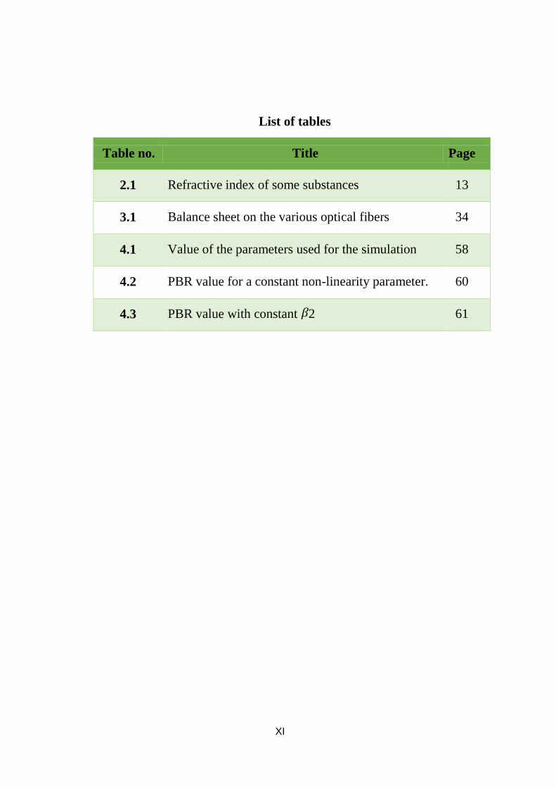
A nonlinear Schrödinger equation, Eq (3.17) contains dispersive and

nonlinear terms. To introduce SSFM, write the NLSE equation in the

following form:

Contains losses and dispersion in the linear mean and the nonlinear term.

𝑁̂ 𝐴 = 𝐽𝛾|𝐴|2𝐴 (3.40)

Non-linear effects in the environment are considered. The basis of the SSFM

is to divide a propagation from z to z + h (h is a small step) in two operations

(assuming that they act independently): during the first step, non-linear

effects are included and at during the second step, we take into account the

linear effects.

The formal solution of equation (3.36) on a small step h is therefore

(𝑧 + ℎ, 𝑡) = 𝑒ℎ(𝐿 +𝑁̂ )𝐴(𝑧, 𝑡) (3.41)

In the first order approximation, the above formula can be written as follows

(𝑧 + ℎ, 𝑡) = 𝑒ℎ𝐿 𝑒ℎ𝑁̂ (𝑧, 𝑡) + 𝑂(ℎ2) (3.42)

The basis of this approximation is established by the Baker-Hausdorf lemma

[13], namely given that operators A and B commute with

[A, B].

The basis of the method is suggested by equation (3.42). He tells us that

47

( + , ) can be determined by applying the two operators independently.

The propagation from z to z + h is divided into two operations: first the

nonlinear step and then the linear step assuming that they act independently.

If h is small enough, Eq. (3.42) gives good results.

The value of the step can be determined by assuming that the maximum

phase shift 𝜑𝑚𝑎𝑥 = 𝛾|𝐴𝐵⃗|2 , where 𝐴𝑃⃗ is the peak value of A (z, t) due to

the nonlinear operator is less than the predefined value . Iannone et al [21]

reported that 𝜑𝑚𝑎𝑥 ≤ 0.05 rad.

For a practical implementation of the SSFM, we need to establish practical

expressions for the dispersive and nonlinear terms. In what follows, we will

therefore analyze the effect of the two terms independently neglecting losses.

Let us analyze the effect of the single dispersive term. For this, we

temporarily deactivate the non-linear term. After the Fourier transform, the

linear equation "becomes

Who has the solution

𝐴 (𝑧, 𝜔) = 𝐴 (0, 𝜔)𝑒−𝜔2𝛽2⁄2 (3.44)

The action of the nonlinear term alone is described by the following equation

The "natural" solution lies in the time domain.It produces

(𝑧, 𝑡) = (0, 𝑡)|𝐴|2𝐴 (3.46)

In summary, the method on each segment of length h consists of three steps:

48

Where F indicates the Fourier transform (TF) and 𝐹−1 the inverse Fourier transform.

49

Chapter Four

Simulation results

4.1. Introduction

To understand the phenomenon that occurs during the propagation of

solitons, we will dissect the evolution of the impulse through the fiber. Its

evolution will consider the effects of dispersions, non-linear effects, then

combine these two effects in order to see them consequences on the impulse.

The modeling is done by the Step Split Fourier method to solve the

Schrödinger propagation equation in the case of a fundamental Soliton pulse

then a Chirped pulse.

This study uses silica glass fiber as a research reference and the propagation

medium because this type of fiber is widely used in several optical

communication systems.

4.2. Digital simulation of the propagation of a pulse in a single-mode optical

fiber

4.2.1 Propagation of an impulse in Soliton Fundamental form:

suppose an impulse given by: ( = 0, ) 𝑠𝑒𝑐ℎ ( ) represented by

the Figure (4.1). Its propagation in an optical fiber is modeled by the NLSE

(4.1). to understand the phenomenon that occurs during this propagation, we

will dissect the evolution of the impulse through the fiber. Its evolution will

consider the effects of dispersion, nonlinear effects, then associate these two

effects in order to see them consequences on the pulse (ultrashort wave).

50

Where and 𝑁̂𝐿 = 𝑗𝛾|𝐴|2 , D is the dispersion operator and NL

is the nonlinearity operator. Equation (4.1) takes the following form:

(4.2)

Figure 4.1: the input pulse.

4. 2.1.1 Numerical simulation of the propagation of a pulse in a linear medium.

When the distance of propagation satisfies the following parameters:

𝑧~𝐿 in this case the nonlinear part is null and consequently the

{

𝑧 ≪ 𝐿𝑁̂𝐿 dispersive effects play a preponderant role. This however applies if

the fiber and pulse parameters meet the following conditions:

The equation (4.1) becomes:

The term is replaced by the Fourier transformation of the envelope A in the

equation (4.3), which gives:

51

Or:

Let us integrate member to member, the left term from 0 to 1 and the right term

from 0 to .

Equation (4.6) gives:

Equation (4.7) has the solution:

(4.8)

Figure 4.2: Propagation of a pulse in a medium of zero dispersion.

52

Figure 4.3: Propagation of a pulse in a dispersive medium (normal and

abnormal dispersion).

The two previous figures indicate that in the two dispersion regimes

(abnormal and normal), the different frequency components of the pulse

propagate at different speeds. These different speeds create a temporal spread

of the wave at the exit of the fiber. This is called group velocity dispersion

(GVD).

On the contrary, with zero dispersion (the medium is non-dispersive), the

pulse retains its initial shape since all the waves propagate at the same speed

(Figure 4.2).

4. 2.2. Numerical simulation of the propagation of a pulse in a non-linear

medium

4.2.2.1- Propagation of an impulse in fundamental soliton form:

In this case where the nonlinear part (𝑁̂𝐿= 𝑖𝛾|𝐴|2) in equation (4.1) is

dominant (zero linear part D), i.e. the propagation satisfies the following

53

condition: the objective is to show the influence of non-linear

effects, in particular the Kerr effect which induces the phenomenon of

selfphase modulation (SPM, Self-Phase Modulation).

The equation (4.1) becomes:

Equation (4.9) becomes:

Let us integrate the left term from 0 to 1 and the right term from 0 to

The equation (4.11) becomes:

Equation (4.9) has the solution:

𝐴1 = 𝐴0𝑒 𝑗𝛾|𝐴|2ℎ (4.13)

Using the SSFM Method, with the choice of the following parameters, plus a

variation of the propagation distance and the pulse represented by figure (4.1)

as input pulse:

54

Figure 4.5: Propagation of a pulse in a non-linear dispersive medium

z = 1 to Ф𝑚𝑎𝑥 = (4.14)

Figure 4.6: Propagation of a pulse in a non-linear dispersive medium at

z = 2 Ф𝑚𝑎𝑥 = 3 / 2 (4.15)

When a pulse is propagated in a nonlinear medium, the Kerr effect induces

the phenomenon of auto phase modulation (SPM, Self-Phase Modulation)

because of the propagation of an intense beam in the optical fiber, the

55

nonlinear coefficient γ is positive producing a gradual increase in the

refractive index. This passage of the wave changes the refractive index which

in turn changes the phase of the pulse. But this produces a spectral widening

of the pulse, unlike dispersion, a widening of the spectrum of pulses. The

phase shift and this widening vary as a function of the propagation distance

as shown in the two Figures (4.5) and (4.6).

4.2.2.1 Propagation of an impulse in Chirped Soliton Form:

One of the factors that limit the performance of the transmission

capacity, the speed at which data can be transmitted, is the dispersion and

nonlinear effects that occur during the process of light propagation in an

optical fiber.

transport is limited by a widening of the pulses due to chromatic dispersion

(GVD). In addition, there is the influence of the effects of parameters such as

attenuation ( ), dispersion (β2), and non-linearity ( ).

We are going to consider all these parameters, always considering the

propagation in the optical fiber. Our simulation work is based on the SSFM

method for solving the NLSE (4.1). But this time using a chirped pulse as the

input pulse, so what does the word chirped mean.

Definition: It is said that a light pulse is “chirped” (from the English chirped)

when it undergoes a dispersion of its group velocity (GVD), as it can be

induced by the nonlinear effect of high order at namely auto phase modulation

(SPM), this causes a frequency variation over time.

The term comes from the English chirp, "chirping", by allusion to the song of

certain birds which vary the frequency of their song. The figure below shows

the electric field as a function of the time of an “chirped” optical pulse. Note

that the frequency of the oscillation increases over time.

56

Figure (4.7): Represents a light pulse is chirped

To better study the influence of the value of the parameter of the chirp on the

effect of the widening of the pulse, we propose to use a new approach based

on the calculation of an indicator called enlargement ratio of l PBR pulse and

its mean value given by the following expressions [28]:

The following table (4.1) gathers the values used for the simulation.

Table (4.1): Value of the parameters used for the simulation. Variable Value (Unit)

𝑷𝟎 (the input power) 0.0000064 W

T_0 (width of the initial pulse) 125 e-12

Ld (the dispersion length corresponding to the order of

the

Soliton)

( N 2)/(g*P0)

(Nonlinearity of the Fiber) (0.003; 0.03; 0.3) in W/m

Alpha (Fiber Losses in dB / km) 3; 2; 1; 0

N (order of Soliton) 3; 2; 1; 0.5

C (chirp parameter) 3; -2; 0; 2; 3

𝜷𝟐 (2nd order dispersion) (T_0) ^ 2 / Ld (s2 / m)

h1 (Step size) 1000

57

The parameters in table (4.1) are the GVD (Group Velocity

Dispersion) speed parameters (β2), and the non-linearity parameter . The

other approach to revealing the effect due to the parameters is a chirp (when

the constants C are positive or negative) from -3 to 3.

In addition, the Fourier method with Fractional steps (SSFM) was applied to the

system (4.1).

Figure 4.7: (a) Soliton pulse with chirping parameter C = 2. (b) Soliton pulse

with chirping parameter C = 3 (c) with a chirping parameter C = -2.

(d) with C = -3.

From the simulation results obtained with regard to the second order

dispersion and the nonlinear effects, it has been observed from Table 4.2 that

the best PBR means have been obtained when the value of the parameter of

58

the chirp is negative = −2 and that the value of the parameter of the

nonlinear remains constant at 0.003W / m.

When the mean value 𝑃⃗𝐵⃗𝑅̅̅̅̅̅̅ for C = -2 is the lowest mean value of all the results of

the simulation.

We can therefore say that the use of input pulses with a negative chirp value

(C) with a constant non-linearity value is the best solution to reduce the pulse

widening effects (reduce dispersion by GVD) and the non-linear oscillations.

Table 4.2: PBR value for a constant non-linearity parameter

Negative chirp

parameter

(C = -2)

= .𝟎𝟎𝟑

Negative chirp

parameter

(C = -3)

= .𝟎𝟎𝟑

Positive chirp

parameter

(C = 2)

= .𝟎𝟎𝟑

positive chirp

parameter

(C = 3)

= .𝟎𝟎𝟑

β2 PBR β2 PBR β2 PBR β2 PBR

-10 1.4081 -10 2.2820 -10 3.3205 -10 3.5737

-15 1.4260 -15 2.3581 -15 2.8494 -15 2.1856

-20 1.4224 -20 2.4136 -20 2.4689 -20 2.7107

-25 1.4092 -25 2.3235 -25 2.4589 -25 4.1683

For the following simulation, when the simulation system has modifications

where the nonlinearity constants have become inconsistent variables and the

2 was a constant, the simulation results are listed in the following table

TABLE 4. 3: PBR value with constant 𝜷𝟐

Negative chirp

parameter

(C = -2)

= 15

Negative chirp

parameter

(C = -3)

= 20

Positive chirp

parameter

(C = 2)

= 15

positive chirp

parameter

(C = 3)

= 20

β2 PBR β2 PBR β2 PBR β2 PBR

0.3 1.4051 0.3 2.2915 0.3 3.2110 0.3 4.1661

0.03 1.4125 0.03 2.2911 0.03 3.2171 0.03 4.1254

0.003 1.4260 0.003 2.4136 0.003 2.8494 0.003 2.7107

0.002 1.4451 0.002 2.1458 0.002 2.0481 0.002

59

According to the results of the simulation which are illustrated in figure (4.7)

to (c), the table (4.2) and the table (4.3). can see that with a certain variation

in the parameter of the chirped (C), β2, and γ. However, the opposite occurs

when the chirped process has been applied for the value C = 2 (where C > 0),

the instantaneous frequency increases linearly from its front edge to the back

edge. The opposite occurs when C = -2 (where C <0) which shows that the

instantaneous frequency decreases linearly from the trailing edge to the

leading edge.

It can be seen that the widening of the pulse depends on the sign of the GVD parameter

(β2) and the Chirp parameter (C).

Table (4.2) shows that the best value of the Chirp parameter C = -2. This

proves that its positive value and its negative value can affect the state of the

pulse during its propagation in the fiber. The advantage of using a value of

the negative chirp parameter makes it possible to lower the effect of widening

of the pulse and the nonlinear oscillations. This can be explained by the fact

that the "delay" of a longer wavelength can inhibit the effect of GVD, i.e.

when the value of GVD decreases due to the existence of a delay, the

widening effects of the pulse are minimized.

60

Chapter Five

conclusion

5.1 Introduction:

The world of telecommunications continues to be revolutionized

thanks to the advent of a jewel the size of a hair (optical fiber) which is used

to transport information by light from one end to the other. During this

transfer, there are effects leading to its distortion, in particular, chromatic

dispersion and the Kerr effect. Under certain conditions, these effects

compensate for each other and the signal propagates without distortion: it is

the solitary impulse which is called soliton solution of the NLSE equation and

known for a long time, which resists disturbances and which can in principle

spread without spreading over long distances.

In order to understand the main effects that impede the propagation of a pulse

(signal), we are interested in this thesis to numerically solve the non-linear

Schrödinger equation by the method of `` Fourier with fractional step ''.

Method introduced because of its simplicity of use, easy to develop and has

good performance in computing time; also provides natural access to the

spectral evolution of the field and is fast up to two orders of magnitude

compared to finite difference methods.

5.2 Conclusion:

From the results of the simulation, can conclude that the order of

variation of the dispersion parameter takes effect where the chirped method

was performed in the input pulse of the propagation process. Furthermore, it

has been found that the negative chirp has the best value among all the results

in terms of PBR ratio. To this end, the dispersion parameters, the nonlinearity,

61

and the input power value must be determined due to the shape, quantity,

speed, and amplitude of the input pulse which are respectively affected by

these factors.

We can conclude that in general in the abnormal dispersion regime, the

direction of frequency slip (chirping) produced by the self-phase modulation

effect (SPM) and due to the nonlinearity effect, is l opposite to that produced

by dispersion (GVD).

Figure 5.1 compensation process between self-phase modulation (Kerr

effect) and GVD chromatic dispersion.

This indicates that the frequency slip induced by the phase auto-modulation

can compensate for that induced by the chromatic dispersion (See Figure 4.8).

This process leads to the formation of optical solitons which retain shape

during propagation, the compression mechanism fundamentally due to high

order solitons.

After solution of the NLSE by the SSFM method, we studied the

effects which limit the power of the signal during its propagation in the optical

fiber. This allowed us to conclude that:

62

• When the dispersion effects dominate, the pulse undergoes a

broadening of its spectrum leading to a loss of information. These effects can

be resolved by sending the signal at the zero-dispersion wavelength.

• When non-linear effects dominate, SPM introduce a phase shift which

limits the maximum power of the signal to be transmitted over the fiber. As

well as SPM increases the enlargement rate for a normal dispersion regime

(𝛽2> 0) and reduces this rate for an abnormal dispersion regime ((𝛽2 <0)).

• When the pulse intensities are large enough to involve non-linear

effects, these can be used to compensate for dispersion.

• Following the coupling of the two effects in the fiber, two regime cases

are taken into account: normal dispersion regime, abnormal dispersion

regime, the latter is very important because the auto phase modulation can

compensate for the abnormal dispersion because it induces a phase term of

sign opposite to that introduced by the dispersion of the fiber.

• The results of our simulations using the method of "Fourier with Split-

step" for the study of the propagation of an impulse in the form of "Soliton

Chirp" allows to conclude that the negative chirp has the best value among

all the results in terms of the average of the PBR ratio. To this end, the

dispersion parameters, the non-linearity, and the input power value must be

determined due to the shape, quantity, speed, and amplitude of the input pulse

which are respectively affected by these factors.

63

5.3 Future Work

Finally, the work undertaken within the framework of this thesis has

opened a direction of research which in our opinion deserves to be deepened,

in particular:

- Solving the nonlinear Schrödinger's equation considering other nonlinear

effects, third order dispersion, the Brillouin or Raman effect.

- Study of the propagation of solitons in periodic structures, namely, optical

fibers with photonic crystals

64

REFERENCES

[1] Azzouzi Faiçal, Study of the nonlinear propagation dynamics of optical solitons

modeled by the nonlinear Schrödinger equation, Doctoral thesis. Badji Mokhtar

University -

[2] H. Benosman (2006), Interaction of an electromagnetic wave with an atomic

vapor. Thesis of Magister, Tlemcen.

[3] Math (198), Mathmatical Methods in calassical and Quantam mechanics

[4] B. Bouchenak, (2007) Study of the propagation of an impulse in a dispersive

medium of wave vector, memory of Magister, University of Tlemcen.

[5] H. Apithy, Y. Bouslimani and H. Haman, (2004), Fiber optic communications:

Limitations caused by dispersion and non-linear effects. IEEE Canadian

Review- Summer.

[6] Hasnaa El Ouazzani, Second and third order nonlinear optical properties of new

conjugated organic-pull systems. Chlassical physics, University of Tlemcen

[7] R. W. Boyd. Nonlinear Optics. Third Edition. Academic Press, Amsterdam,

2008.

[8] Marek S._Wartak, Computational Photonics an Introduction, Cambridge

University Press, 2013.

[9] R. W. Hellwarth, Third-order optical susceptibilites of liquids and solids.

Prog. Quant. Electr., 5: 1–68, 1977.

[10] J.S. Russell, Report on waves, in Rep. 14th Meet. British Assoc. Adv. Sci, 1844,

P. 311.

65

[11] Yousef Yousefi and Khikmat Kh. Muminov Physical-Technical Institute

named after S.U. Umarov Academy of Sciences of Republic of

Tajikistan Aini Ave 299/1, Dushanbe, Tajikistan a year ago

[12] D. W. Jordan and P. Smith, Nonlinear Ordinary Differential Equations, June

2007.

[13] Jonsson, Fredrik. Reading notes on nonlinear optics. 2003.

[14] Katsunari Okamoto, “Fundamentals of optical waveguides”. New York:

Academic Press (2000), p.180.

[15] Govind P. Agrawal, “Nonlinear Fiber Optics”, Academic Press. Optics and

photonics, New York, 3rd edition (2001).

[16] Govind P. Agrawal, Fiber-Optic Communications Systems, Third Edition,

2002.

[17] Govind P. Agrawal, Nonlinear Fiber Optics, Academic Press, fourth edition,

US, 2007.

[18] BOUMAZA, Nawel. Solitons in Nonlinear Optics: Study of Physical

Properties and Application in the Field of Telecommunications. Doctoral

thesis. 2012

[19] http://physique.unice.fr/sem6/2006-

2007/PagesWeb/Telecom/vulgarisation.html

[20] Weideman and Herbst, J.A.C. Weideman and B.M. Herbst, 1986. Splitstep

methods for the solution of the nonlinear Schrodinger equation.

[21] M. Delfour, M. Fortin, and G. Payr, 1981. Finite-difference solutions of a

non-linear Schrödinger equation. In Journal of computational physics, pages

277–288,

66

[22] R. W. Boyd. Nonlinear Optics. Third Edition. Academic Press, Amsterdam,

2008.

[23] G. P. Agrawal. Fiber-Optic Communication Systems. Second Edition.

Wiley, New York, 1997.

[24] A. Yariv and P. Yeh. Photonics. Optical Electronics in Modern

Communications. Sixth Edition. Oxford University Press, New York,

Oxford, 2007.

[25] G. P. Agrawal, Nonlinear Fiber Optics. Academic Press, Boston, 1989.

[26] G. P. Agrawal, Nonlinear Fiber Optics, Fourth Edition. Elsevier Science &

Technology Books, Boston, 2006.

[27] Reference: ASVIAL, Muhamad and PARAMITHA, A. A. S. Split Step