arX

iv:0

709.

3399

v1 [

nlin

.PS]

21

Sep

2007

Two-dimensional discrete solitons in rotating lattices

Jesus Cuevas,1 Boris A. Malomed,2 and P. G. Kevrekidis3

1Grupo de Fısica No Lineal, Departamento de Fısica Aplicada I,

Escuela Universitaria Politecnica, C/ Virgen de Africa, 7, 41011 Sevilla, Spain

2Department of Physical Electronics,

School of Electrical Engineering, Faculty of Engineering,

Tel Aviv University, Tel Aviv 69978, Israel

3Department of Mathematics and Statistics,

University of Massachusetts, Amherst, Massachusetts 01003-4515, USA

Abstract

We introduce a two-dimensional (2D) discrete nonlinear Schrodinger (DNLS) equation with self-

attractive cubic nonlinearity in a rotating reference frame. The model applies to a Bose-Einstein

condensate stirred by a rotating strong optical lattice, or light propagation in a twisted bundle

of nonlinear fibers. Two species of localized states are constructed: off-axis fundamental solitons

(FSs), placed at distance R from the rotation pivot, and on-axis (R = 0) vortex solitons (VSs),

with vorticities S = 1 and 2. At a fixed value of rotation frequency Ω, a stability interval for the

FSs is found in terms of the lattice coupling constant C, 0 < C < Ccr(R), with monotonically

decreasing Ccr(R). VSs with S = 1 have a stability interval, C(S=1)cr (Ω) < C < C

(S=1)cr (Ω), which

exists for Ω below a certain critical value, Ω(S=1)cr . This implies that the VSs with S = 1 are

destabilized in the weak-coupling limit by the rotation. On the contrary, VSs with S = 2, that are

known to be unstable in the standard DNLS equation, with Ω = 0, are stabilized by the rotation in

region 0 < C < C(S=2)cr , with C

(S=2)cr growing as a function of Ω. Quadrupole and octupole on-axis

solitons are considered too, their stability regions being weakly affected by Ω 6= 0.

PACS numbers: 03.75;42.65.Tg;05.45;42.70.Qs

1

I. INTRODUCTION

Discrete dynamical systems represented by nonlinear lattices in one, two, and three di-

mensions constitute a class of models which are of fundamental interest by themselves, and,

simultaneously, they find applications of paramount importance in various fields of physics.

One such example is known in nonlinear optics, where the one-dimensional (1D) discrete

nonlinear Schrodinger (DNLS) equation was predicted by Christodoulides and Joseph to sup-

port fundamental discrete solitons [1] with an even profile. Such nonlinear structures were

later created experimentally in an array of semiconductor waveguides [2]. Subsequently,

stable odd solitons, alias twisted localized modes, were predicted and studied in detail in

the same model [3], as well as in an array of photorefractive waveguides with photovoltaic

nonlinearity [4].

Another experimental realization of dynamical lattices in the optical domain is possible in

photorefractive crystals, where a quasi-discrete setting can be induced by counterpropagating

laser beams illuminating the crystal in the normal polarization, while the probe beam, which

can sustain solitary waves, is launched in the extraordinary polarization. The difference

from the array of waveguides fabricated in silica or in a semiconductor material is that the

photorefractive nonlinearity is saturable, rather than cubic. This method of the creation of

photonic lattices was proposed in Ref. [5], and results obtained by means of the technique

were reviewed in Refs. [6]. In particular, both fundamental and twisted solitons in the 1D

lattice were reported in Ref. [7], and fundamental solitons (FSs) in the 2D lattice were

created too [8], as well as 2D vortex solitons (VSs) in the same setting [9].

Recently, the progress in the technology of writing permanent arrays of channels in silica

slabs has made it possible to create 2D waveguiding lattices with the cubic nonlinearity,

which emulate a bundle of nonlinear optical fibers with linear coupling in the transverse plane

[10]. In particular, spatial lattice solitons of the surface and corner types were reported in this

setting [11] (surface solitons were reported too in the 2D photonic lattice in a photorefractive

crystal [12]). Thus, 1D and 2D discrete dynamical models have a potential for further

applications to nonlinear optical media of various types.

Another natural realization for the lattice systems is provided by a Bose-Einstein conden-

sate (BEC) trapped in an optical lattice (OL). If the OL is strong enough, the underlying

Gross-Pitaevskii equation (GPE) for the wave function in the continuum may be approxi-

2

mated by its DNLS counterpart [13, 14]; the relevance of the discrete model in this setting

has also been demonstrated experimentally in 1D by testing its predictions experimentally,

see, e.g., Ref. [15]. Higher-dimensional OLs can be easily created too [16]. Thus, the relevant

DNLS equation may be one-, two-, or three-dimensional; in particular, various species of 3D

discrete solitons, including those with intrinsic vorticity, have been predicted in this setting

[17], and their stability has been systematically analyzed [18]. Still another implementation

of the DNLS lattice in the space of any dimension, from one to three, is possible in terms of

a crystal of microcavities trapping photons [19] or polaritons [20].

Discrete solitons of various kinds have been studied in detail theoretically in 1D, 2D, and

3D versions of the DNLS equation, see an earlier review [21] and the more recent works

mentioned above. As mentioned above, some of these solitons have been created experimen-

tally in optical media equipped with fabricated or photoinduced lattices. All these localized

states have their counterparts in continuum models with periodic potentials that emulate

the lattices. In particular, 2D solitons of both the fundamental and vortex types, which are

unstable in uniform continua with the cubic self-focusing nonlinearity can be readily stabi-

lized by the periodic OL potential [22]; for the stabilization of FSs, a quasi-1D potential is

sufficient, instead of its full 2D counterpart [23]. Vortices are unstable too in the uniform

space with the saturable nonlinearity [24], in which case they can also be stabilized by the

periodic potential [9]. The relevance of these stabilization mechanisms in the continuum was

also demonstrated for higher-order vortex solitons, and so-called supervortices, i.e., arrays

of compact vortices with global vorticity imprinted onto the array, under both cubic and

saturable nonlinearities [25].

Recently, it was shown that 2D solitons obeying the GPE in the 2D continuum can

also be supported by a rotating OL [26, 27]. These solitons may be fully localized (spot-

shaped) solutions to the equation with the self-focusing/attractive cubic nonlinearity, placed

at some distance from the rotation pivot and revolving in sync with the holding 2D lattice.

In particular, the soliton can be placed at a local minimum of the rotating potential, while

the pivot is set at a local maximum. These co-rotating strongly localized solitons are stable

provided that the rotation frequency, Ω, does not exceed a critical value, (Ωcr)min. In the

same model, but with a rapidly rotating OL, stable ring-shaped solitons (with zero vorticity),

i.e., objects localized along the radius but delocalized in the azimuthal direction, have been

found too, for Ω exceeding another critical value, (Ωcr)max. Note that the model does not

3

support any stable pattern in interval (Ωcr)min < Ω < (Ωcr)max [26]. On the other hand,

stable ring-shaped states, with both zero and nonzero vorticity, have been found in the

model with the repulsive cubic nonlinearity and rotating quasi-one-dimensional (periodic)

potential, if Ω exceeds a respective critical value. Obviously, the latter model does not give

rise to any localized state in the absence of the rotation.

A rotating OL can be easily implemented in BEC experiments [28]; then, if the OL is

strong enough, it is natural to approximate the GPE in the co-rotating reference frame by

an appropriate variety of the 2D DNLS equation. In addition to that, such a model may

also describe the light propagation in a twisted bundle of nonlinear optical fibers, linearly

coupled in the transverse plane by tunneling of light between the fiber cores. The objective

of the present work is to introduce a model of the rotating discrete lattice, and find stable

discrete solitons in it, both FSs and VSs.

The paper is organized as follows. In Sec. II, we formulate the model, taking the un-

derlying GPE in the reference frame co-rotating with the OL, and replacing the continuum

equation by its discrete version corresponding to a strong periodic potential. Discrete FSs

are considered in Sec. III. We construct the solutions starting from the anti-continuum

limit, which corresponds to zero value of the coupling constant accounting for the linear

interaction between neighboring sites of the discrete lattice, C = 0. A family of FS solutions

is constructed by continuation in C; their stability is examined by computation of eigenfre-

quencies for infinitesimal perturbations around the soliton, and verified by direct simulations

of the evolution of perturbed FSs. It is found that the FS, with its center located at distance

R from the rotation pivot, is stable within an interval 0 < C < Ccr(R), with Ccr decaying as

a function of R. Section III also includes a simple analytical approximation, which makes

it possible to explain the decrease of Ccr with the growth of R. In Sec. IV, we consider

localized vortices (VSs), whose center coincides with the rotation pivot. For the VS with

vorticity S = 1, the stability region is found to be C(S=1)cr < C < C

(S=1)cr , provided that the

rotation frequency, Ω, is smaller than a critical value, Ωcr (the stability interval shrinks to

nil at Ω = Ωcr). Vortices with S = 2 are considered too. While in the ordinary (nonrotat-

ing) DNLS model, with Ω = 0, all VSs of the latter type are unstable [29], we demonstrate

that the rotation opens a stability window for them, 0 < C < C(S=2)cr , with C

(S=2)cr growing

as a function of Ω. Direct numerical simulations are also used to illustrate the dynamical

evolution of FSs and VSs when they are unstable. Results obtained in this work and related

4

open problems are summarized in Sec. V.

II. THE MODEL

The starting point is the normalized 2D GPE, which includes the potential in the form

of an OL rotating at angular velocity Ω, and thus stirring a “pancake”-shaped (quasi-flat)

Bose-Einstein condensate (BEC) trapped in a narrow gap between two strongly repelling

optical sheets. Unlike the analysis performed in Refs. [26] and [27], where simulations

were run in the laboratory reference frame, here we write the GPE in the reference frame

co-rotating with the lattice, hence the potential does not contain explicit time dependence:

i∂ψ

∂t= −

(

1

2∇2 + ΩLz

)

ψ − ǫ [cos (k (x− ξ)) + cos(k (y − υ))]ψ + σ|ψ|2ψ. (1)

Here, Lz = i(x∂y − y∂x) ≡ i∂θ is the operator of the z-component of the orbital momentum

(θ is the polar angle), and σ determines the sign of the interaction, attractive (σ = −1) or

repulsive (σ = +1). Constants ξ and υ determine a possible shift of the lattice with respect

to the rotation pivot. Note that Eq. (1) does not contain any additional trapping potential,

as we are interested in solutions localized under the action of the OL.

It is more convenient to shift the origin of the Cartesian coordinates to a lattice node,

thus replacing Eq. (1) by the translated form:

i∂ψ

∂t= −

[

1

2∇2 + iΩ((x+ ξ) ∂y − (y + υ) ∂x)

]

ψ − ǫ [cos (kx) + cos(ky)]ψ + σ|ψ|2ψ. (2)

As shown in a general form in Ref. [14], a discrete model, which corresponds to the limit of a

very deep OL, can be derived from the underlying GPE in the tight-binding approximation.

Eventually, it amounts to a straightforward discretization of the GPE. Thus, the discrete

counterpart of Eq. (2) is

idψm,n

dt= −C

2(ψm+1,n + ψm−1,n + ψm,n+1 + ψm,n−1 − 4ψm,n)

−iΩ [(m+ ξ) (ψm,n+1 − ψm,n−1) − (n + υ) (ψm+1,n − ψm−1,n)] + σ|ψm,n|2ψm,n ,(3)

where (m,n) are discrete coordinates, and C > 0 is the corresponding coupling constant,

which accounts for the linear tunneling of atoms between BEC droplets trapped in deep

nodes of the lattice. As mentioned above, Eq. (3) may also describe a twisted bundle of

nonlinear optical fibers linearly coupled by the tunneling of light in the transverse plane,

5

(m,n). In that case, t is the propagation distance along the fiber, and only σ = −1, i.e., the

attractive/focusing nonlinearity) is the relevant choice.

Equation (3) conserves the norm and Hamiltonian,

N =∑

m,n

|ψm,n|2 , (4)

H =∑

m,n

C

2

(

|ψm+1,n − ψm,n|2 + |ψm,n+1 − ψm,n|2)

+1

2σ |ψm,n|4

−iC4

Ω[

(m+ ξ)(

ψ∗

m,n (ψm,n+1 − ψm,n−1) − ψm,n

(

ψ∗

m,n+1 − ψ∗

m,n−1

))

− (n+ υ)(

ψ∗

m,n (ψm+1,n − ψm−1,n) − ψm,n

(

ψ∗

m+1,n − ψ∗

m−1,n

))]

. (5)

In addition to C, the discrete model contains three irreducible parameters: Ω, which takes

values 0 < Ω < ∞, and the coordinates of the pivot displacement, (ξ, υ), which take values

0 ≤ ξ, υ < 1, plus the sign parameter, σ = ±1. As in the usual 2D DNLS equation (with

Ω = 0), values σ = ±1 in Eq. (3) may be transformed into each other by the staggering

transformation, ψm.n → (−1)m+nψm,n, therefore we fix σ ≡ −1 (self-attraction).

Our first objective is to find stationary localized solutions to Eq. (3) in the form of FSs

(fundamental solitons) and VSs (vortex solitons). To this end, we substitute the standing

wave ansatz, ψm,n = eiΛtφm,n, where −Λ is the normalized chemical potential, in terms of

the underlying BEC model; then, the stationary lattice field φm,n obeys the equation

Λφm,n =C

2(φm+1,n + φm−1,n + φm,n+1 + φm,n−1 − 4φm,n)

+iC

2Ω [(m+ ξ) (φm,n+1 − φm,n−1) − (n + υ) (φm+1,n − φm−1,n)] + |φm,n|2φm,n .(6)

Note that solutions for φm,n are complex, unless Ω = 0. The second objective will be to

examine the stability of the discrete solitons, assuming small perturbations in the form of

δψm,n ∼ exp (iΛt+ iλt), the onset of instability indicated by the emergence of Im(λ) 6= 0.

The evolution of unstable solitons will be examined by means of direct simulations of Eq.

(3).

To parameterize the soliton families, we fix the scales by setting Λ ≡ 1; obviously, with

C > 0, only positive Λ may give rise to localized solutions), while C will be varied.

6

III. FUNDAMENTAL SOLITONS

The rotation makes the discrete lattice inhomogeneous, hence properties of solitons

strongly depend of the location of their centers. Without the rotation, Eq. (3) amounts

to the ordinary 2D DNLS equation, in which various species of discrete solitons and their

stability have been studied in detail. In particular, FSs, which are represented by real so-

lutions, are stable at C ≤ Ccr = 2Λ ≡ 2 [21]. The onset of their instability is accounted

for by a pair of eigenfrequencies of small perturbations with finite imaginary and zero real

parts, i.e., the instability leads to the exponential growth of perturbations. Accordingly, nu-

merical simulations of the instability development demonstrate spontaneous transformation

of unstable FSs into lattice breathers [30]. In this section, we first report numerical results

obtained for the stability of FSs in the model with Ω 6= 0, and then present an analytical

estimate that may explain numerical findings.

A. Numerical results

Our analysis aimed to determine the stability border for the FSs, Ccr, for each set of

values of the discrete coordinates of the soliton’s center, m0, n0. Here we present results

for angular velocity Ω = 0.1 and zero pivot displacement, ξ = υ = 0 [in Ref. [26], the rotation

pivot was fixed at a local maximum of the potential in Eq. (2), which corresponds to setting

ξ = υ = 1/2 in Eqs. (3) and (6), and the center of the soliton trapped in the lattice was

placed at a local minimum closest to the pivot, which would mean m0, n0 = 0, 0]. This

choice makes it possible to explore the existence and stability of FSs in a clear form, while

larger values of Ω give rise to a resonance with linear lattice modes, leading to Wannier-Stark

ladders and hybrid solitons [33] and making the continuation in C and identification of Ccr

difficult. We carried out the calculations on the lattice of size 21× 21, since already for this

case, the lattice was for all the considered cases sufficiently wider than the very localized FS

structures of interest. To avoid effects of the boundaries, the range of the soliton-center’s

coordinates was restricted to |m0| , |n0| ≤ 8.

The FS solutions were looked for starting at point C = 0, i.e., at the so-called anti-

continuum limit [21]. In this limit, the FS is seeded by using a nonzero value of the field at

a single point, the center of the FS, φ(C=0)m,n = δm,m0

δn,n0; obviously, this expression satisfies

7

Eq. (6) with Λ = 1 and C = 0. After the branch of the FS solutions had been found by the

continuation in C, its stability was quantified through the computation of eigenfrequencies

of small perturbations, using the equation linearized about the FS.

Figure 1 displays a typical example of the thus found dependence of eigenfrequencies

λ of small perturbations on the lattice coupling constant. As said above, the instability

corresponds to Im(λ) 6= 0, for the FS with its center set at point (m0 = 3, n0 = 2); for

comparison, the dependence of the instability growth rate, i.e., |Im(λ)|, on C is also shown

for the FS in the usual DNLS model (Ω = 0) in the top panel of the figure. It is seen that

the instability sets in at C = Ccr = 1.70, which is smaller than the critical value in the

ordinary model, C(Ω=0)cr = 2. Typical examples of stable and unstable FSs belonging to the

family presented in Fig. 1 are displayed in Figs. 2 and 3.

Results obtained for the FSs placed at different positions are summarized in Fig. 4, in the

form of dependences of Ccr on the distance of the FS’s center from the pivot, R ≡√

m20 + n2

0,

and on one coordinate, n0, while m0 is fixed. It is observed that Ccr monotonously decreases

with R, starting from Ccr = 2 at R = 0 (we recall again that C(Ω=0)cr = 2 for the FS in

the ordinary DNLS equation). Note that there are different pairs (m0, n0) which have equal

values of R =√

m20 + n2

0 and give slightly different Ccr. For instance, for the pair (5, 0),

Ccr = 1.51, while Ccr = 1.50 for (4, 3). Hence, the stability depends on the two-dimensional

structure of the solution.

Figures 1 and 3 show that the FS is destabilized, with the increase of C, through the

appearance of a pair of imaginary eigenfrequencies. Direct simulations of the dynamical

evolution of unstable FSs in the framework of Eq. (3) demonstrate that the instability

does not destroy the solitary wave. Instead, it transforms the waveform into a persistent

breathing structure, see a typical example in Fig. 5.

B. Analytical estimates

The decrease of Ccr with the increase of the distance of the FS from the pivot, R, which

is the main feature revealed by the above numerical analysis, as shown in Fig. 4, can be

explained using an estimate based on the quasi-continuum approximation. To this end, we

note that stationary solutions to the underlying continuum equation (1) are looked for as

8

0 0.5 1 1.5 2

1

2

3

4

5

6

7

8

9

10|R

e(λ)

|

C0 0.5 1 1.5 2

0

0.1

0.2

0.3

0.4

0.5

0.6

0.7

|Im(λ

)|

C

0 0.5 1 1.5 2

1

2

3

4

5

6

7

8

9

|Re(

λ)|

C0 0.5 1 1.5 2

0.1

0.2

0.3

0.4

0.5

0.6

0.7

|Im(λ

)|

C

FIG. 1: (Color online) Plots of real and imaginary parts (left and right panels) of the eigenfrequen-

cies of linearization around fundamental solitons in the ordinary non-rotating lattice, with Ω = 0

(top panels), and for their counterparts in the present model (with Ω = 0.1). In the latter case,

the soliton is centered at (m0 = 3, n0 = 2).

ψ = eiΛtφ(x, y), with the function φ obeying the stationary equation,

Λφ = −C(

1

2∇2 + ΩLz

)

φ− ǫ [cos (kx) + cos(ky)] Φ − Φ3. (7)

Here, following the discrete model, we have set ξ = υ = 0, σ = −1, and explicitly introduced

the spatial-scale parameter, 1/√C, which is a counterpart of the lattice coupling constant

in Eq. (3). Next, we assume the presence of a soliton with amplitude A and intrinsic size

l, whose center is located at distance R from the rotation pivot (tantamount to the origin,

in the present case). First, demanding a balance between terms Λφ, ∇2φ, and φ3 in Eq.

9

m

n

−10 −5 0 5 10−10

−8

−6

−4

−2

0

2

4

6

8

10

0.2

0.4

0.6

0.8

1

1.2

1.4

1.6

m

n

−10 −5 0 5 10−10

−8

−6

−4

−2

0

2

4

6

8

10

−0.1

−0.05

0

0.05

0.1

−8 −6 −4 −2 0 2 4 6 8−0.1

−0.08

−0.06

−0.04

−0.02

0

0.02

0.04

0.06

0.08

0.1

Im(λ

)

Re(λ)

FIG. 2: (Color online) Top panels: Contour plots of the real (left) and imaginary (right) parts of

a stable fundamental soliton centered at m0 = 3, n0 = 2, for C = 1.5. Bottom panel: the complex

plane of the stability eigenvalues for this soliton.

(7), and estimating them, respectively, as ΛA, A/l2, and A3, we conclude, in the lowest

approximation, that

|Λ| ∼ Cl−2 ∼ A2. (8)

Further, the soliton as a whole will be in equilibrium relative to the rotating lattice poten-

tial if the action of the centrifugal force, generated by term ∼ Ω in Eq. (7), is compensated

by the force of pinning to the periodic potential. The estimate of the latter condition yields

CΩR/l ∼ ǫ. Substituting here l ∼√

C/ |Λ|, as per Eq. (8), we arrive at a final estimate,

R ∼(

ǫ/√

|Λ|Ω)

C−1/2, which predicts dependence Ccr ∼ 1/R2 (Ccr is realized here as the

largest value of C that can provide for the balance between the centrifugal and pinning forces

at given R). The latter dependence is qualitatively consistent with the numerical findings

10

m

n

−10 −5 0 5 10−10

−8

−6

−4

−2

0

2

4

6

8

10

0.2

0.4

0.6

0.8

1

1.2

1.4

1.6

1.8

m

n

−10 −5 0 5 10−10

−8

−6

−4

−2

0

2

4

6

8

10

−0.15

−0.1

−0.05

0

0.05

0.1

0.15

−10 −5 0 5 10−0.5

−0.4

−0.3

−0.2

−0.1

0

0.1

0.2

0.3

0.4

0.5

Im(λ

)

Re(λ)

FIG. 3: (Color online) The same as in Fig. 2, but for an unstable fundamental soliton, placed at

the same position as in Fig. 2, at C = 1.8.

showing the decrease of Ccr with R in Fig. 4 (at very large C, when the analytical formula

predicts small R, it is irrelevant, as the above consideration tacitly assumed that the size of

the soliton was essentially smaller than the distance to the pivot, l ≪ R; it is irrelevant too

at very small C, as the quasi-continuum approximation cannot be used in that essentially

discrete case).

Using the quasi-continuum approximation, it is also possible to estimate the order of

magnitude of the rotation frequency, in physical units. In the application to the BEC,

assuming the lattice spacing ∼ 1 µm and the condensate of 7Li or 85Rb, which provide for

the possibility of the attraction between atoms and, thus, the formation of solitons [31, 32],

undoing of rescalings which cast the GPE in the normalized form of Eq. (1), we conclude

that Ω = 0.1 corresponds, in physical units, to the rotation frequency ∼ 100 Hz or 10

11

0 2 4 6 8 10 12

0.8

1

1.2

1.4

1.6

1.8

2C

cr

R

0 1 2 3 4 5 6 7 8

0.8

1

1.2

1.4

1.6

1.8

2

Ccr

n0

FIG. 4: (Color online) Dependence of the stability border for the fundamental solitons, Ccr, on the

distance of the soliton’s center from the rotation pivot, R (left panel), and on one of the center’s

coordinates, n0, for fixed m0 (right panel). In the latter figure, the value of n0 ∈ [0, 8] increases

progressively from top to bottom.

Hz, for lithium and rubidium, respectively. As concerns the above-mentioned realization

of the model in terms of the twisted bundle of optical fibers, an estimate shows that, for

the carrier wavelength ∼ 1 µm and separation between the fibers in the bundle ∼ 10 µm,

Ω = 0.1 corresponds to the twist pitch, which we define as a length at which the twist attains

the angle of 2π, of the order of 5 cm.

IV. VORTEX SOLITONS

Discrete vortex solitons (VSs) of the 2D DNLS equation were systematically developed

in Ref. [35] as complex stationary solutions which feature a phase circulation of 2πS around

the central point, at which the amplitude vanishes, with integer S identified as the vorticity.

Prior to that, time-periodic multibreather states that may feature a vortical structure were

found in 2D Hamiltonian lattice dynamical models [36]. The center of the VS may coincide

with a site of the lattice, or may be located in the middle of a lattice cell; the corresponding

vortices are called “crosses” (alias rhombuses) and “squares”, respectively. The stability

of these states has been studied in detail, both for S = 1 [35, 37] and S > 1 [29, 37]. In

particular, the VS crosses with S = 1 (and, as above, with Λ fixed to be 1) are stable in

12

0 100 200 300 400 5003.45

3.5

3.55

3.6

3.65

3.7

3.75

3.8

3.85

|ψ2,

3|2

t

FIG. 5: (Color online) The time dependence of the squared amplitude of a perturbed unstable

soliton from Fig. 3 at its center, (m0 = 3, n0 = 2). Notice the robust oscillatory behavior indicating

the breathing nature of the resulting solution.

the corresponding interval of values of the coupling constant, C < C(S=1)cr = 0.781, and

the instability above this points transforms the VS into an ordinary fundamental soliton,

with S = 0. While all VSs with S = 2 are unstable in the ordinary 2D DNLS equation,

the vortex solutions with S = 3 have their stability interval (more narrow than for S = 1),

C < C(S=3)cr = 0.198. In all cases, the instability sets in via the Hamiltonian Hopf bifurcation,

represented by quartets of eigenvalues [38].

We have constructed localized vortices (of the cross/rhombus type), with S = 1 and

S = 2, in the rotating-lattice model based on Eq. (3), and examined their stability. Unlike

the above analysis of the FSs, we consider here only on-axis VSs, whose centers coincide with

the rotation pivot (R = 0). We note that, while the FS with R = 0 is virtually identical to

its counterpart in the ordinary model, with Ω = 0, for VSs the situation is quite different; in

particular, the VSs centered at the rotation pivot feature quite nontrivial stability properties

with the increase of rotation frequency Ω, see below. Therefore, while the results for the

FSs were displayed for Ω = 0.1 and growing R, in this section we focus on R = 0 but vary

Ω.

13

A. Vortex solitons with S = 1

The first noteworthy effect of the rotation on the VS with S = 1 is that, for given Ω, its

stability region features not only the upper bound, C(S=1)cr , as in the usual DNLS model, but

also a lower one, C(S=1)cr :

C(S=1)cr < C < C(S=1)

cr . (9)

At a given value of Ω, VSs are exponentially unstable for C < C(S=1)cr , and they feature

an oscillatory instability, accounted for by a Hopf bifurcation, at C > C(S=1)cr . This situation

takes place up at Ω < Ω(S=1)cr = 0.037. An example is given by Fig. 6, which displays the

instability growth rate of the VS, |Im(λ)|, versus C for fixed Ω = 0.01. The plot also shows

the real part of the eigenfrequencies, |Re(λ)|, and includes, for the sake of comparison, the

same dependences in the usual DNLS equation, with Ω = 0. The figure shows that, in this

case, C(S=1)cr = 0.31 and C

(S=1)cr = 0.788.

The overall stability region for the VSs with S = 1 in the plane (C,Ω) is presented in

Fig. 7. It is observed that C(S=1)cr slightly increases with Ω, while the growth of C

(S=1)cr with

Ω is fast. As a result, at Ω > Ω(S=1)cr the stability region does not exist. In the absence of the

stable VSs, unstable ones feature coexistence of exponential and Hopf instabilities. Figure

6 displays an example of the latter regime, and shows that, for Ω = 0.04, C(S=1)cr = 0.87 and

C(S=1)cr = 0.81.

In fact, the effect of the destabilization of the VSs with S = 1 at small C [C < C(S=1)cr ,

as said above], is a higher-order phenomenon, in terms of the expansion of the stability

eigenvalues in powers of C, when it is assumed small. Indeed, comparing it with the stability

analysis for the cross vortices in the ordinary model, with Ω = 0 [39], we observe the

following. At Ω = 0, modes of small perturbations around the vortex of the cross/rhombus

type feature a pair of real eigenfrequencies, with λ = ±C at the first order in small C

(in the present notation). The same pair appears in the present context, see Fig. 6. At

larger C, these eigenfrequencies will give rise to the Hamiltonian-Hopf instability, upon their

collision with eigenfrequencies bifurcating from the phonon band of linear excitations. As

shown in Ref. [39], the DNLS equation with Ω = 0 also gives rise to a pair of higher-order

eigenfrequencies, λ ≈ ±C2 in the present notation. The effect of the rotation forces the

latter eigenfrequencies to separate along the imaginary axis, thus inducing the instability at

small C. However, for larger C, the pair again becomes real, stabilizing the configuration.

14

0 0.2 0.4 0.6 0.8 1

0.5

1

1.5

2

2.5

3

3.5

4

4.5|R

e(λ)

|

C0 0.2 0.4 0.6 0.8 1

0.05

0.1

0.15

0.2

|Im(λ

)|

C

0 0.2 0.4 0.6 0.8 1

0.5

1

1.5

2

2.5

3

3.5

4

4.5

|Re(

λ)|

C0 0.2 0.4 0.6 0.8 1

0.02

0.04

0.06

0.08

0.1

0.12

0.14

0.16

0.18

0.2

0.22

|Im(λ

)|

C

0 0.2 0.4 0.6 0.8 1

0.5

1

1.5

2

2.5

3

3.5

4

4.5

|Re(

λ)|

C0 0.2 0.4 0.6 0.8 1

0.02

0.04

0.06

0.08

0.1

0.12

0.14

0.16

0.18

0.2

0.22

|Im(λ

)|

C

FIG. 6: (Color online) Dependences on C of the real and imaginary parts (left and right panels,

respectively) of eigenfrequencies of small perturbations about vortex solitons with S = 1 in the

ordinary (non-rotating) DNLS lattice (top panels), and in the rotating one, with Ω = 0.01 (central

panels) and Ω = 0.04 (bottom panels). In the rotating case, the center of the vortex coincides with

the rotation pivot of the lattice.15

0 0.2 0.4 0.6 0.8 1 1.20

0.005

0.01

0.015

0.02

0.025

0.03

0.035

0.04

0.045

0.05

Ω

C

Exponential Hopf

E+H

Stable

FIG. 7: The full stability diagram for vortex solitons with S = 1, centered at the rotation pivot.

The E+H label holds for coexisting Hopf and exponential instabilities.

Four different regimes identified in the stability diagram in Fig. 7 are illustrated by typical

examples of the stability and instability of the VSs with S = 1 in Fig. 8 as follows: the

exponential instability, caused by the higher-order eigenfrequencies, as described above, is

shown in the top left panel; the top right panel shows a linearly stable case. The oscillatory

instability is presented in the bottom left panel (the latter case is shown for sufficiently

large C, to allow the eigenfrequencies, which originally linearly depend on C, as indicated

above, to collide with eigenfrequencies bifurcating from the phonon band). Finally, the

mixed oscillatory-exponential instability, which is possible at Ω > Ω(S=1)cr , is displayed in the

bottom right panel.

Since the destabilization of the VS at C > C(S=1)cr is accounted for by the Hopf bifurcation,

as confirmed by Fig. 6, this unstable VS is transformed into a persistent breather (not

shown here), which loses the vortical structure, i.e., is similar to the FS [35]. On the

other hand, the destabilization at C < C(S=1)cr occurs, as seen in Figs. 6, via a pair of

imaginary eigenfrequencies with zero real parts, i.e., an exponential instability. Its nonlinear

development eventually leads to a persistently pulsating localized state with zero vorticity,

as illustrated by Fig. 9. The transformation to a FS state is also observed in the region of

the coexistence of exponential and oscillatory instabilities.

16

−2 −1.5 −1 −0.5 0 0.5 1 1.5 2−0.03

−0.02

−0.01

0

0.01

0.02

0.03Im

(λ)

Re(λ)−3 −2 −1 0 1 2 3

−0.1

−0.08

−0.06

−0.04

−0.02

0

0.02

0.04

0.06

0.08

0.1

Im(λ

)

Re(λ)

−5 0 5−0.06

−0.04

−0.02

0

0.02

0.04

0.06

Im(λ

)

Re(λ)−5 0 5

−0.25

−0.2

−0.15

−0.1

−0.05

0

0.05

0.1

0.15

0.2

0.25

Im(λ

)

Re(λ)

FIG. 8: Eigenfrequencies of small perturbations around the vortex with S = 1 are shown for the

four different cases: exponential instability for Ω = 0.01 and C = 0.2 (top left panel); linear

stability at Ω = 0.01, and C = 0.5 (top right panel); oscillatory instability at Ω = 0.01 and C = 0.8

(bottom left panel); exponential and oscillatory instability at Ω = 0.05 and C = 0.85 (bottom right

panel).

B. Vortex solitons with S = 2

Another way in which the rotating lattice drastically alters the stability features of the

ordinary 2D DNLS model concerns the VSs with S = 2. At Ω = 0, all such localized

vortices are unstable due to an imaginary eigenfrequency proportional (at the leading order)

to coupling constant C [35, 37], see the top panel of Fig. 10 (which may be compared with

Fig. 4 of [37]). In the rotating lattice, the solitons with S = 2 acquire a finite stability region,

17

0 100 200 300 400 500 6001.72

1.74

1.76

1.78

1.8

1.82

1.84

1.86

1.88

|ψ1,

1|2

t

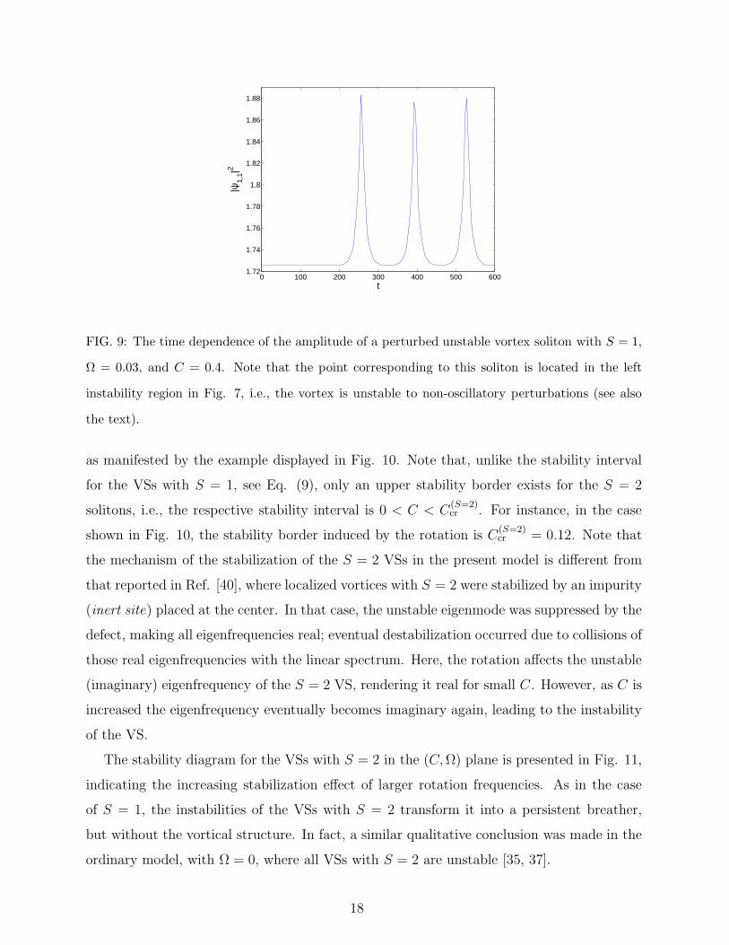
FIG. 9: The time dependence of the amplitude of a perturbed unstable vortex soliton with S = 1,

Ω = 0.03, and C = 0.4. Note that the point corresponding to this soliton is located in the left

instability region in Fig. 7, i.e., the vortex is unstable to non-oscillatory perturbations (see also

the text).

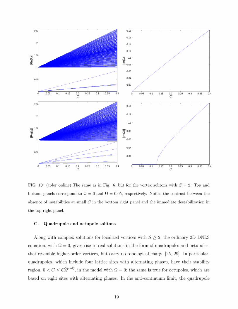
as manifested by the example displayed in Fig. 10. Note that, unlike the stability interval

for the VSs with S = 1, see Eq. (9), only an upper stability border exists for the S = 2

solitons, i.e., the respective stability interval is 0 < C < C(S=2)cr . For instance, in the case

shown in Fig. 10, the stability border induced by the rotation is C(S=2)cr = 0.12. Note that

the mechanism of the stabilization of the S = 2 VSs in the present model is different from

that reported in Ref. [40], where localized vortices with S = 2 were stabilized by an impurity

(inert site) placed at the center. In that case, the unstable eigenmode was suppressed by the

defect, making all eigenfrequencies real; eventual destabilization occurred due to collisions of

those real eigenfrequencies with the linear spectrum. Here, the rotation affects the unstable

(imaginary) eigenfrequency of the S = 2 VS, rendering it real for small C. However, as C is

increased the eigenfrequency eventually becomes imaginary again, leading to the instability

of the VS.

The stability diagram for the VSs with S = 2 in the (C,Ω) plane is presented in Fig. 11,

indicating the increasing stabilization effect of larger rotation frequencies. As in the case

of S = 1, the instabilities of the VSs with S = 2 transform it into a persistent breather,

but without the vortical structure. In fact, a similar qualitative conclusion was made in the

ordinary model, with Ω = 0, where all VSs with S = 2 are unstable [35, 37].

18

0 0.05 0.1 0.15 0.2 0.25 0.3 0.35 0.4

0.5

1

1.5

2

2.5|R

e(λ)

|

C0 0.05 0.1 0.15 0.2 0.25 0.3 0.35 0.4

0.02

0.04

0.06

0.08

0.1

0.12

0.14

0.16

0.18

|Im(λ

)|

C

0 0.05 0.1 0.15 0.2 0.25 0.3 0.35 0.4

0.5

1

1.5

2

2.5

|Re(

λ)|

C0 0.05 0.1 0.15 0.2 0.25 0.3 0.35 0.4

0.02

0.04

0.06

0.08

0.1

0.12

0.14

|Im(λ

)|

C

FIG. 10: (color online) The same as in Fig. 6, but for the vortex solitons with S = 2. Top and

bottom panels correspond to Ω = 0 and Ω = 0.05, respectively. Notice the contrast between the

absence of instabilities at small C in the bottom right panel and the immediate destabilization in

the top right panel.

C. Quadrupole and octupole solitons

Along with complex solutions for localized vortices with S ≥ 2, the ordinary 2D DNLS

equation, with Ω = 0, gives rise to real solutions in the form of quadrupoles and octupoles,

that resemble higher-order vortices, but carry no topological charge [25, 29]. In particular,

quadrupoles, which include four lattice sites with alternating phases, have their stability

region, 0 < C ≤ C(quad)cr , in the model with Ω = 0; the same is true for octupoles, which are

based on eight sites with alternating phases. In the anti-continuum limit, the quadrupole

19

0 0.05 0.1 0.15 0.2 0.25 0.3 0.350

0.01

0.02

0.03

0.04

0.05

0.06

0.07

0.08

0.09

0.1

Ω

C

Stable

Unstable

FIG. 11: The stability diagram, similarly to Fig. 7, but for vortex solitons with S = 2.

and octupole solutions are seeded, respectively, by the following configurations:, φ0,±1 =

1, φ±1,0 = −1, and φ0,2 = φ1,−1 = φ2,1 = φ−1,0 = 1, φ1,2 = φ0,−1 = φ−1,1 = φ2,0 = −1, all

other sites having φm,n = 0. Note that the latter configuration is tantamount to the necklace

soliton pattern, that was recently observed in a photorefractive crystal with a photoinduced

lattice [34].

We have constructed families of quadrupole and octupole soliton solutions in the present

model with Ω > 0, proceeding from the anti-continuum patterns to finite C. When doing

so, the rotation pivot in Eq. (6) was set at the center of the respective pattern, i.e., we set

ξ = υ = 0 and ξ = υ = 1/2, for the quadrupole and octupole solutions respectively. It was

found that the critical values of the coupling constant, C(quad)cr and C

(oct)cr , which border the

stability regions for both these families, very weakly depend on Ω, unlike the situation for

the VSs with S = 2, cf. Fig. 11, but quite similar to what was found above for the localized

vortices with S = 1, see the right stability border in Fig. 7.

V. CONCLUSION

The objective of the present work was to introduce a discrete version of the 2D model

combining the self-attractive cubic nonlinearity and rotating square-lattice potential. The

discrete model can be implemented in BEC stirred by a rotating strong optical lattice, or, in

principle, also in a twisted bundle of nonlinear optical fibers. Localized solutions of two types

20

were considered: off-axis FSs (fundamental solitons), with the center placed at distance R

from the rotation pivot, and on-axis VSs (vortex solitons), with vorticity S = 1 and 2. For

the FSs, the stability interval was found in the form of 0 < C < Ccr(R), where C is the

coupling constant of the discrete lattice, and Ccr(R) a monotonically decreasing function,

see Fig. 4. A qualitative explanation to this result was proposed, based on the analysis of

the balance between the lattice-pinning and centrifugal forces. For VSs with S = 1, the

dependence of the stability region on rotation frequency Ω was found, in the form of Eq. (9)

and Fig. 7, with the conclusion that the stability is only possible for Ω < Ωcr. A key feature,

which makes the situation different from earlier stability analyses of such structures in the

standard 2D DNLS model, is a higher-order eigenfrequency, shifted towards instability for

sufficiently weak lattice coupling, in the presence of rotation. On the other hand, VSs with

S = 2, which are always unstable in the model with Ω = 0, are stabilized by the rotation

in region 0 < C < C(S=2)cr , as shown in Fig. 11. For the vortices with S = 2, the reverse

effect happens in comparison with S = 1, namely an unstable (at Ω = 0) eigenfrequency is

tipped by the rotation in the opposite direction; i.e., for S = 1 a real eigenfrequency becomes

imaginary in the presence of Ω, while the reverse is true for S = 2. Quadrupole and octupole

solitons, with the center coinciding with the pivotal point, were briefly considered too, with

a conclusion that their stability regions are almost the same as in the ordinary model (with

Ω = 0). An estimate for relevant values of Ω in physical units was given for both physical

realizations of the model, i.e., the rotation frequency of the optical lattice stirring the self-

attractive BEC, and the pitch of the twisted bundle of optical fibers.

The analysis initiated in this work can be developed in several directions. In particular,

results obtained in the continuum model considered in Ref. [26] suggest that, at sufficiently

large Ω, the fully localized FSs, with the center shifted off the axis (i.e., continuum coun-

terparts of the discrete FSs considered in the present work), are unstable (or do not exist),

while stable ring-shaped solitons may appear instead, with the center of the ring coinciding

with the pivot. In fact, the shape of these zero-vorticity rings may be similar to that of the

vortices considered above.

Another interesting direction would be to apply techniques elaborated in Refs. [37] and

[18] to this considerably more difficult setting. It would be especially relevant to repeat the

calculation of the eigenfrequencies for the vortices with S = 1 and S = 2 by means of those

methods in the presence of rotation, and quantify the impact of Ω on the eigenvalues, to

21

rigorously investigate some effects which were outlined above in a qualitative form.

Another possibility is to consider a discrete limit of the model with the rotating quasi-1D

potential, such as the one with the repulsive cubic nonlinearity, which was introduced in Ref.

[27]. Studies along these directions are currently underway and will be reported elsewhere.

Acknowledgements. J.C. acknowledges financial support from the MECD project

FIS2004-01183. The work of B.A.M. was partially supported by the Israel Science Foun-

dation through Excellence-Center Grant No. 8006/03, and by German-Israel Foundation

through Grant No. I-884-149.7/2005. PGK gratefully acknowledges the support of NSF-

DMS-0505663, NSF-DMS-0619492 and NSF-CAREER.

[1] D. N. Christodoulides and R. I. Joseph, Opt. Lett. 13, 794 (1988).

[2] H. S. Eisenberg, Y. Silberberg, R. Morandotti, A. R. Boyd, and J. S. Aitchison, Phys. Rev.

Lett. 81, 3383 (1998).

[3] S. Darmanyan, A. Kobyakov, E. Schmidt, and F. Lederer, J. Exp. Theor. Phys. 86, 682 (1998);

P. G. Kevrekidis, A. R. Bishop, and K. Ø. Rasmussen, Phys. Rev. E 63, 036603 (2001); A.

A. Sukhorukov and Y. S. Kivshar, ibid. 65, 036609 (2002).

[4] A. Maluckov, M. Stepic, D. Kip, and L. Hadzievski, Eur. Phys. J. B 45, 539 (2005).

[5] N. K. Efremidis, S. Sears, D. N. Christodoulides, J. W. Fleischer, and M. Segev, Phys. Rev.

E 66, 046602 (2002).

[6] J. W. Fleischer, G. Bartal, O. Cohen, T. Schwartz, O. Manela, B. Freedman, M. Segev, H.

Buljan, and N. K. Efremidis, Opt. Exp. 13, 1780 (2005); A. S. Desyatnikov, N. Sagemerten,

R. Fischer, B. Terhalle, D. Trager, D. N. Neshev, A. Dreischuh, C. Denz, W. Krolikowski, and

Y. S. Kivshar, ibid. 14, 2851 (2006).

[7] J. W. Fleischer, T. Carmon, M. Segev, N. K. Efremidis, and D. N. Christodoulides, Phys.

Rev. Lett. 90, 023902 (2003); D. Neshev, E. Ostrovskaya, Y. Kivshar, and W. Krolikowski,

Opt. Lett. 28, 710 (2003).

[8] J. W. Fleischer, M. Segev, N. K. Efremidis, and D. N. Christodoulides, Nature 422, 147

(2003).

[9] D. N. Neshev, T. J. Alexander, E. A. Ostrovskaya, Y. S. Kivshar, H. Martin, I. Makasyuk,

and Z. G. Chen, Phys. Rev. Lett. 92, 123903 (2004); J. W. Fleischer, G. Bartal, O. Cohen,

22

O. Manela, M. Segev, J. Hudock, and D. N. Christodoulides, ibid. 92, 123904 (2004).

[10] A. Szameit, D. Blomer, J. Burghoff, T. Schreiber, T. Pertsch, S. Nolte, A. Tunnermann, and

F. Lederer, Opt. Exp. 13, 10552 (2005).

[11] A. Szameit, Y. V. Kartashov, F. Dreisow, T. Pertsch, S. Nolte, A. Tunnermann, and L. Torner,

Phys. Rev. Lett. 98, 173903 (2007).

[12] X. Wang, A. Bezryadina, Z. Chen, K. G. Makris, D. N. Christodoulides, and G. I. Stegeman,

Phys. Rev. Lett. 98, 123903 (2007).

[13] A. Trombettoni and A. Smerzi, Phys. Rev. Lett. 86, 2353 (2001); F. Kh. Abdullaev, B. B.

Baizakov, S. A. Darmanyan, V. V. Konotop, and M. Salerno, Phys. Rev. A64, 043606 (2001);

A. Smerzi, A. Trombettoni, P. G. Kevrekidis, and A. R. Bishop, Phys. Rev. Lett. 89, 170402

(2002); R. Carretero-Gonzalez and K. Promislow, Phys. Rev. A 66, 033610 (2002).

[14] G. L. Alfimov, P. G. Kevrekidis, V. V. Konotop, and M. Salerno, Phys. Rev. E 66, 046608

(2002).

[15] F. S. Cataliotti, S. Burger, C. Fort, P. Maddaloni, F. Minardi, A. Trombettoni, A. Smerzi,

and M. Inguscio, Science 293 , 843 (2001).

[16] M. Greiner, O. Mandel, T. Esslinger, T. W. Hansch, and I. Bloch, Nature 415, 39 (2002).

[17] P. G. Kevrekidis, B. A. Malomed, D. J. Frantzeskakis and R. Carretero-Gonzalez, Phys. Rev.

Lett. 93, 080403 (2004); R. Carretero-Gonzalez, P. G. Kevrekidis, B. A. Malomed and D. J.

Frantzeskakis, ibid. 94, 203901 (2005).

[18] M. Lukas, D. Pelinovsky and P. G. Kevrekidis, arXiv:nlin/0610070.

[19] J. E. Heebner and R. W. Boyd, J. Mod. Opt. 49, 2629 (2002); P. Chak, J. E. Sipe, and S.

Pereira, Opt. Lett. 28, 1966 (2003).

[20] D. M. Whittaker and J. S. Roberts, Phys. Rev. B 62, R16247 (2000); P. G. Savvidis and P.

G. Lagoudakis, Sem. Sci. Tech. 18, S311 (2003).

[21] P. G. Kevrekidis, K. Ø. Rasmussen, and A. R. Bishop, Int. J. Mod. Phys. B 15, 2833 (2001).

[22] B. B. Baizakov, B. A. Malomed, and M. Salerno, Europhys. Lett. 63, 642 (2003); J. K. Yang

and Z. H. Musslimani, Opt. Lett. 28, 2094 (2003).

[23] B. B. Baizakov, B. A. Malomed and M. Salerno, Phys. Rev. A 70, 053613 (2004).

[24] W. J. Firth and D. V. Skryabin, Phys. Rev. Lett. 79, 2450 (1997).

[25] H. Sakaguchi and B. A. Malomed, Europhys. Lett. 72, 698 (2005).

[26] H. Sakaguchi and B. A. Malomed, Phys. Rev. A 75, 013609 (2007)

23

[27] Y. V. Kartashov, B. A. Malomed, and L. Torner, to be published.

[28] V. Schweikhard, I. Coddington, P. Engels, S. Tung, and E. A. Cornell, Phys. Rev. Lett. 93,

210403 (2004); R. Bhat, M. J. Holland, and L. D. Carr, Phys. Rev. Lett. 96, 060405 (2006);

S. Tung, V. Schweikhard, and E. A. Cornell, ibid. 97, 240402 (2006); K. Kasamatsu and M.

Tsubota, ibid. 97, 240404 (2006).

[29] P. G. Kevrekidis, B.A. Malomed, Z. Chen, and D. J. Frantzeskakis, Phys. Rev. E 70, 056612

(2004); P. G. Kevrekidis, H. Susanto, and Z. Chen, Phys. Rev. E 74, 066606 (2006).

[30] J. Gomez-Gardenes, L. M. Florıa, and A. R. Bishop, Physica D 216, 31 (2006).

[31] K. E. Strecker, G. B. Partridge, A. G. Truscott and R. G. Hulet, Nature 417, 150 (2002); L.

Khaykovich, F. Schreck, G. Ferrari, T. Bourdel, J. Cubizolles, L. D. Carr, Y. Castin, and C.

Salomon, Science 256, 1290 (2002).

[32] S. L. Cornish, S. T. Thompson, and C. E. Wieman, Phys. Rev. Lett. 96, 170401 (2006).

[33] T. Pertsch, U. Peschel, and F. Lederer, Phys. Rev. E 66, 066604 (2002).

[34] J. Yang, I. Makasyuk, P. G. Kevrekidis, H. Martin, B.A. Malomed, D. J. Frantzeskakis, and

Z. Chen, Phys. Rev. Lett. 94, 113902 (2005).

[35] B. A. Malomed and P. G. Kevrekidis. Phys. Rev. E 64, 026601 (2001).

[36] S. Aubry, Physica D 103, 201 (1997); T. Cretegny and S. Aubry, ibid. 113, 162 (1998); M.

Johansson, S. Aubry, Y. B. Gaididei, P. L. Christiansen, and K. Ø. Rasmussen, ibid. 119, 115

(1998).

[37] D. E. Pelinovsky, P. G. Kevrekidis, and D. J. Frantzeskakis, Physica D 212, 20 (2005).

[38] J.-C. van der Meer, Nonlinearity 3, 1041 (1990).

[39] P.G. Kevrekidis and D.E. Pelinovsky, Proc. R. Soc. A 462, 2671 (2006).

[40] P. G. Kevrekidis, and D. J. Frantzeskakis. Phys. Rev. E 72, 016606 (2005).

24