arX

iv:c

ond-

mat

/060

4144

v3 [

cond

-mat

.dis

-nn]

11

Oct

201

2

Spin-glass behaviour on random lattices

M O Hase1,2,a, J R L de Almeida3,b and S R Salinas2,c

1Escola de Artes, Ciencias e Humanidades, Universidade de Sao Paulo,

Avenida Arlindo Bettio 1000, 03828-000, Sao Paulo, SP, Brazil

2Instituto de Fısica, Universidade de Sao Paulo,

Caixa Postal 66318 05315-970, Sao Paulo, SP, Brazil

3Departamento de Fısica, Universidade Federal de Pernambuco, 50670-901, Recife, PE, Brazil

amhase@usp.br, balmeida@df.ufpe.br and cssalinas@if.usp.br

The ground-state phase diagram of an Ising spin-glass model on a random graph

with an arbitrary fraction w of ferromagnetic interactions is analysed in the presence

of an external field. Using the replica method, and performing an analysis of stability

of the replica-symmetric solution, it is shown that w = 1/2, correponding to an

unbiased spin glass, is a singular point in the phase diagram, separating a region

with a spin-glass phase (w < 1/2) from a region with spin-glass, ferromagnetic,

mixed, and paramagnetic phases (w > 1/2).

I. INTRODUCTION

The mean-field formulations of the Ising spin glass[1] (an interesting introduction to spin-

glass theory based on p-spin spherical model is found in [2]) and related disordered models

on a lattice are known to lead to replica - symmetry breaking, which is in turn associated

with the existence of a large number of metastable states. The number of local minima in the

free energy landscape of these solutions grows exponentially with the size of the lattice[3, 4].

The impressive richness of these mean-field results has been a motivation to look at more

realistic spin-glass models, with the inclusion of the effects of either short-range interactions

or the finite coordination of the crystal lattices. Besides the implementation of the Ising

spin glass (SG) on a Bethe lattice[5–8], which is one of the natural ways to deal with a finite

connectivity, there is a work by Viana and Bray[9] for the Ising SG on a random graph

with a mean connectivity. According to a number of investigations[10–13], the model of

Viana and Bray (VB), which is tractable by the replica method, leads to a glassy phase

in the ground state. Finitely connected disordered models[14–16] usually lead to a set of

2

self-consistent equations that can be examined by exact numerical methods[5], while some

analytical results can be achieved for special situations[17].

The problem of a statistical model in a finitely connected graph has been mostly investi-

gated by numerical methods[18–24]. Critical phenomena associated with these systems are

known to display a much richer behaviour than that predicted by mean-field calculations[25].

It may be remarked that models with finite connectivity are closer to “realistic” Bravais lat-

tices than the analogous mean-field versions. In this article, some results for the ground

state of a frustrated ±J Ising spin glass on a random graph, in the presence of an external

magnetic field, and with an arbitrary fraction of ferromagnetic interactions are reported. A

parameter w that gauges the concentration of these ferromagnetic (J0 > 0) interactions is

introduced. For w = 1/2, this model is a pure, unbiased, spin glass; ferromagnetic (antiferro-

magnetic) interactions are favoured for w > 1/2 (w < 1/2). It is known that the presence of

an external field always increases the technical complexity of the solutions of these problems.

In this analysis, the phase diagram in the ground state for external fields that are multiples

of J0 is obtained; this resembles a choice of random fields that has already been adopted

in a previous work [17]. The absence of external fields leads to the problem of colouring

graphs, which can be treated, from the statistical physics standpoint, as the problem of

investigating the ground state of a diluted Potts antiferromagnet[26, 27]. The topology of

the random network favours the appearance of a spin-glass phase for w < 1/2. For w ≥ 1/2,

the usual spin-glass, ferromagnetic, mixed and paramagnetic phases are obtained. It should

be emphasized that even in the presence of overall antiferromagnetic interactions (w < 1/2)

the inherent disorder of the lattice still yields a spin-glass phase. This behavior is related

to the type of graph examined in this work, which belongs to the Erdos-Renyi type with-

out sublattices. Therefore, despite the fact that the model examined in this paper is a

diluted antiferromagnet in a uniform magnetic field, there is no (known) connection with

the random-field Ising model[28, 29], which has been shown in a recent work[30] to display

no spin-glass phase for Ising spins (the continuous spin version of this result is found in [31]).

II. DEFINITION OF THE MODEL

Consider the Hamiltonian

3

H({σx}) = −∑

(x,x′)∈ΛN

Jx,x′σxσx′ −H∑

x∈ΛN

σx , (1)

where σx ∈ {−1, 1} is an Ising spin on site x, belonging to a finite lattice ΛN of N sites

and H is the external magnetic field. The first sum is over all distinct pairs of lattice sites.

The exchange integrals {Jx,x′} are independent and identically distributed random variables,

associated with the distribution

pJ(Jx,x′) =(

1− c

N

)

δ(Jx,x′) +c

Nρ(Jx,x′) , (2)

where

ρ(Jx,x′) = wδ(Jx,x′ − J0) + (1− w)δ(Jx,x′ + J0) , (3)

and J0 is a positive parameter. According to the distribution (2), two sites are connected

(disconnected) with a probability c/N (1 − c/N), where c is the mean connectivity of the

lattice. In this diluted ±J model, parameter w weighs the fraction of ferromagnetic bonds.

III. REPLICA-SYMMETRIC SOLUTION

Using the replica method, the variational free energy is written as

f [G] =1

βlimn→0

c

2+

c

2

n∑

r=0

∑

(α1,··· ,αr)

brq2α1,··· ,αr

−

− ln Tr{σ} exp

[

G({σα}) + βH

n∑

α=1

σα

]}

, (4)

where

br =

∫

R

dJρ(J) coshn(βJ) tanhr(βJ) , (5)

and

4

G({σα}) = c

n∑

r=0

∑

(α1,··· ,αr)

brqα1,··· ,αrσα1

· · ·σαr(6)

is the global order parameter[12, 32], which takes into account the 2n order parameters of

this problem (in contrast to the Sherrington - Kirkpatrick (SK) model[1], which has just two

order parameters).

The stationary free energy comes from the minimization of the variational free energy (4)

with respect to the set {qα1,··· ,αr}, which leads to the stationary conditions

qα1,··· ,αr=

Tr{σ}σα1· · ·σαr

exp [G({σα}) + βH∑n

α=1 σα]

Trσ exp [G({σα}) + βH∑n

α=1 σα]. (7)

The replica-symmetric (RS) solution of this problem may be obtained from the intro-

duction of a local field h, with an effective probability distribution P (h), which is equally

applied to all of the replica spin variables. Thus, one has

qα1,··· ,αr=

∫

R

dhP (h) tanhr(βh) . (8)

Moreover, in the replica-symmetric context, one can see that G({σ}) = G(σ), where σ =∑n

α=1 σα.

Equation (8) leads to a relation between the distribution of local fields, P , and the global

order parameter, G, which is

G(iy/β) = c

∫

R

dJρ(J)

∫

R

dhP (h)eiy

βtanh−1[tanh(βJ) tanh(βh)] . (9)

The analysis will be carried out at the ground state (β → ∞). Also, in analogy to a

previous work[17], the RS solutions of this problem are restricted to the condition r = H/J0,

where r is an integer. In other words, the solutions in this work are written in the form

P (h) =∑

k∈Z

akδ(h− kJ0) , (10)

5

which takes into account the discrete part of the distribution function only; the coefficients

{ak} are given below. Under these conditions, by replacing (10) in (9), one can show that

G(iy) = limβ→∞

G(iy/β) = A+B ′eiyJ0 + C ′e−iyJ0 , (11)

where

A = ca0 , B ′ = wB + (1− w)C , C ′ = (1− w)B + wC ,

(12)

with

B = c∞∑

k=1

ak , C = c−1∑

k=−∞

ak and ak = eA−c

(

B ′

C ′

)k−r2

Ik−r(2√B ′C ′) ,

(13)

where Iν(x) is the modified Bessel function of order ν.

The solution of this problem depends on three equations, from which one can obtain A,

B and C. Using the previous equations, one finds

A = ceA−c

(

C ′

B ′

)r2

Ir(2√B ′C ′) , c = A +B ′ + C ′ ( = A +B + C) (14)

and

B ′ = ceA−c

[

wec−A − weC′

δr,0 −

−wC ′

(

C ′

B ′

)r−1

2

1∫

0

dueC′u (1− u)

r−1

2 Ir−1

(

2√

B ′C ′(1− u))

+

+ (1− w)C ′

(

C ′

B ′

)r2

1∫

0

dueC′u (1− u)

r2 Ir

(

2√

B ′C ′(1− u))

]

.

(15)

6

IV. ANALYSIS OF STABILITY

The stability analysis can be performed using the same steps as previous works[12, 17].

It is based on the search for the eigenvalues of the Hessian matrix associated with the

variational free energy. By some technical manipulations of the eigenvalue equations, which

are similar to previous calculations[17, 32], a separate analysis for the cases w 6= 1/2 and

w = 1/2 is carried out.

For w 6= 1/2, one finds the following transverse eigenvalues:

λ =1

c, −A

c+

1

c, −A

c− 1

c(1− 2w)and − A

c− 1

1− 2w

(w

c+∆±

)

,

(16)

where ∆± = ±√

[

1−wc

± a1 (1− 2w)] [

1−wc

± a−1 (1− 2w)]

. The stability of the RS solution

depends on the smallest eigenvalue,

λ0 = −A

c− w

c (1− 2w)− 1

1− 2w×

∆− , w > 12

∆+ , w < 12

. (17)

0 0.2 0.4 0.6 0.8 1w

-1

0

λ 0

From left to right (at λ0 = -1 line)

r = 0, 2, 4, 10

From top to bottom (at w = 0.6 line)r = 10, 4, 2, 0

c = 6

FIG. 1: Graph of λ0 versus w, obtained by numerical calculation of the eigenvalue.

7

The graph of λ0 versus w is shown in figure 1 for c = 6. Some limiting cases are

analytically accessible. In the pure ferromagnetic case (w = 1), one has λ0(w = 1) = −Ac+

1c−√

a1a−1, which confirms the stability of the RS solution in large external fields, in which

case λ0(w = 1, H ∼ ∞) ∼ 1/c (since, for a fixed value of k, ak goes to zero for sufficiently

large H). Moreover, by the same argument, one can make λ0 positive for any w > 1/2 if the

field is sufficiently large. On the other hand, the w = 0 (pure antiferromagnetic interactions)

case implies λ0(w = 0) = −Ac−√

[

1c+ a1

] [

1c+ a−1

]

, which is clearly negative. This means

that the RS solution for this finitely connected spin-glass model is always unstable in this

regime, even in the limit H → ∞, which yields λ0(w = 0, H → ∞) = −1/c. Note that in

the limit of infinite connectivity, c → ∞, this eigenvalue goes to zero, becoming marginally

stable as in the SK model. The instability of the RS solution even for large external fields

makes the Viana-Bray model distinct from the Bethe lattice. While the latter has fixed

connectivity, the former has fixed mean connectivity, and the degree distribution follows a

Poisson distribution. This means that there are vertices that have infinite degree in the

thermodynamic limit, and the signs of those vertices are determined not by the external

field, but the interaction with their neighbours only. Like the SK model, the external field

is not able to stabilize the RS solution[33] in the ground state in the Viana-Bray lattice.

On the other hand, the whole region where the external field is large is dominated by the

RS solution if the system is analysed on a Bethe lattice[16]. The entropy os the model, also

based on the context of RS solution and discrete field (10), is evaluated in the appendix of

this work, although no precise statements can be made in the w < 1/2 region.

The phase diagrams (figure 2), which are qualitatively similar for other choices of the

mean connectivity c, show that the RS solution is always unstable for w < 1/2, which

can also be seen from equation (17). For w > 1/2, the RS solution is stable above a

critical value w∗ of the concentration, which depends on the applied field. This behaviour

can be illustrated in the r − w phase diagram, where the SG phase is separated from the

paramagnetic phase by a de Almeida-Thouless line[33].

In zero field one can show the presence of ferromagnetic and mixed phases. This mixed

phase is characterized by the asymmetric distribution of the local field, which leads to

ak 6= a−k for some values of k ∈ Z.

For w = 1/2, the eigenvalues of the stability matrix are

8

0 0.1 0.2 0.3 0.4 0.5 0.6 0.7 0.8 0.9 1w

0

1

2

3

4

5

6

7

8

9

10

r =

H/J

0RSB RS

c = 6

FIG. 2: The replica-symmetry-breaking (RSB) and RS phases in the r − w phase diagram. The

thick line at r = 0 indicates spontaneous magnetization.

λ =1

c, −A

c+

1

cand − A

c+

1

c± 1

2(a1 + a−1) . (18)

The smallest of these eigenvalues is given by

λ0 = −A

c+

1

c− 1

2(a1 + a−1) . (19)

This eigenvalue does not have a definite sign, but it is positive (tending to 1/c) for sufficiently

large field, and agrees with equation (17) when w ↓ 1/2 (λ0(w) is continuous from the right).

On the other hand, it is easy to see that limw↑1/2 λ0(w) = −∞.

V. CONCLUSIONS

In summary, this work reports a calculation of the phase diagram in the ground state of

a diluted ±J Ising spin-glass model, in an external field, with a fraction w of ferromagnetic

bonds. For w < 1/2, which corresponds to a larger concentration of antiferromagnetic

bonds, the topology of the lattice leads to the existence of a spin-glass phase only. It

should be remarked that this behaviour has also been found in numerical calculations for

9

antiferromagnetic Ising models on free-scale graphs[19, 23] and on small-world networks[22].

For w ≥ 1/2, with a larger concentration of ferromagnetic bonds, the usual phases are found.

The authors thank the Brazilian agencies CNPq and CAPES for financial support. MOH

would like to thank the Departamento de Fısica da Universidade Federal de Pernambuco

(DF-UFPE), where this work was completed, for their kind hospitality.

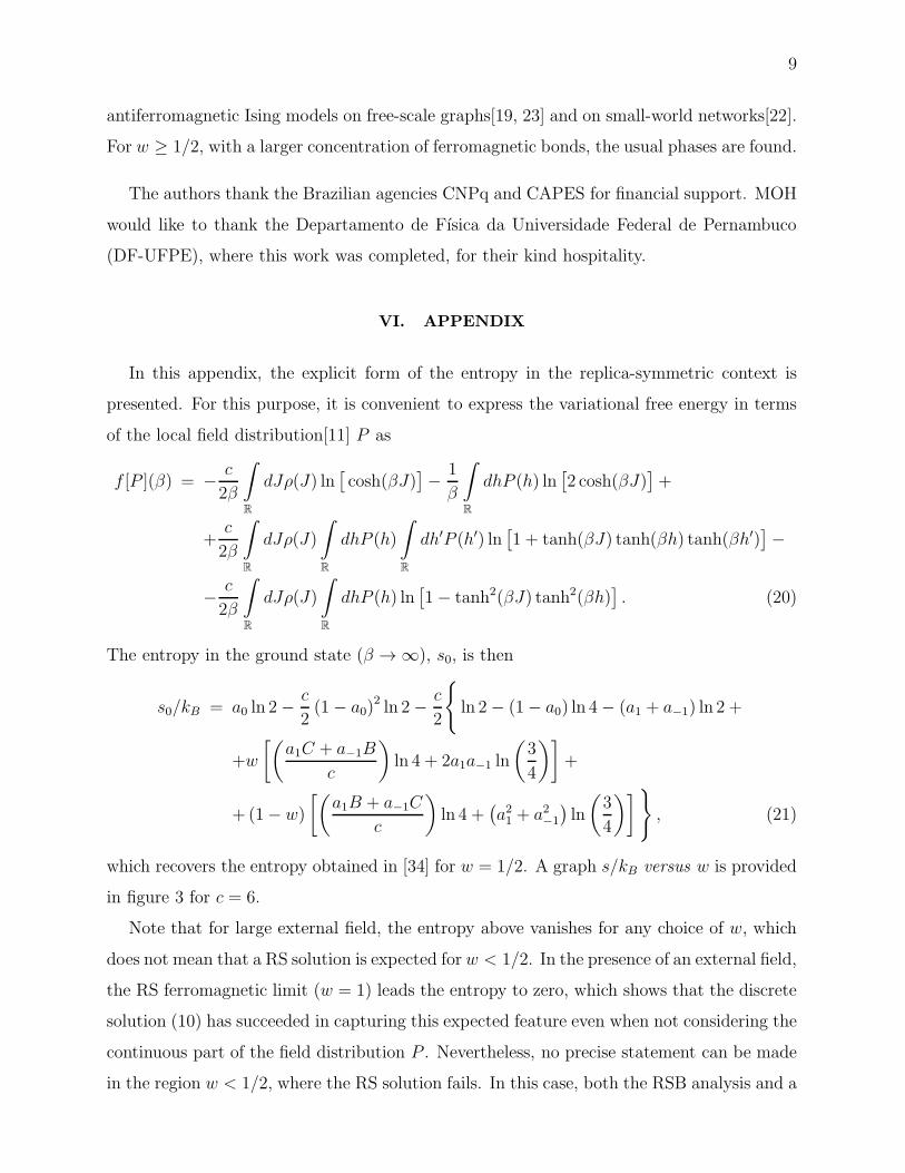
VI. APPENDIX

In this appendix, the explicit form of the entropy in the replica-symmetric context is

presented. For this purpose, it is convenient to express the variational free energy in terms

of the local field distribution[11] P as

f [P ](β) = − c

2β

∫

R

dJρ(J) ln[

cosh(βJ)]

− 1

β

∫

R

dhP (h) ln[

2 cosh(βJ)]

+

+c

2β

∫

R

dJρ(J)

∫

R

dhP (h)

∫

R

dh′P (h′) ln[

1 + tanh(βJ) tanh(βh) tanh(βh′)]

−

− c

2β

∫

R

dJρ(J)

∫

R

dhP (h) ln[

1− tanh2(βJ) tanh2(βh)]

. (20)

The entropy in the ground state (β → ∞), s0, is then

s0/kB = a0 ln 2−c

2(1− a0)

2 ln 2− c

2

{

ln 2− (1− a0) ln 4− (a1 + a−1) ln 2 +

+w

[(

a1C + a−1B

c

)

ln 4 + 2a1a−1 ln

(

3

4

)]

+

+ (1− w)

[(

a1B + a−1C

c

)

ln 4 +(

a21 + a2−1

)

ln

(

3

4

)]

}

, (21)

which recovers the entropy obtained in [34] for w = 1/2. A graph s/kB versus w is provided

in figure 3 for c = 6.

Note that for large external field, the entropy above vanishes for any choice of w, which

does not mean that a RS solution is expected for w < 1/2. In the presence of an external field,

the RS ferromagnetic limit (w = 1) leads the entropy to zero, which shows that the discrete

solution (10) has succeeded in capturing this expected feature even when not considering the

continuous part of the field distribution P . Nevertheless, no precise statement can be made

in the region w < 1/2, where the RS solution fails. In this case, both the RSB analysis and a

10

0 0.2 0.4 0.6 0.8 1w

0

0.05

0.1

0.15

0.2

0.25

0.3

s / k

B

From top to bottom (at w = 0.5 line)

H / J0 = 0,1,2,3,4,5 (respectively)

FIG. 3: Graph s/kB versus w.

satisfactory form of the solution for the field distribution (that involves also the continuous

part, which was ignored in this work in order to achieve analytical results) is required.

[1] Sherrington D, Kirkpatrick S, Phys. Rev. Lett. 35, 1792 (1975)

[2] Castellani T, Cavagna A, J. Stat. Mech. P05012 (2005)

[3] Binder K, Young A P, Rev. Mod. Phys. 58, 801 (1986)

[4] Mezard M, Parisi G, Virasoro M, Spin Glass Theory and Beyond (World Sci., 1987)

[5] Mezard M, Parisi G, Eur. Phys. J. B 20, 217 (2001)

[6] Pastor A A, Dobrosavljevic V, Horbach M L, Phys. Rev. B 66, 014413 (2002)

[7] Castellani T, Krzakala F, Ricci-Tersenghi F, Eur. Phys. J. B 47, 99 (2005)

[8] Krzakala F, Prog. Theor. Phys. Suppl. 157, 77 (2005)

[9] Viana L, Bray A J, J. Phys. C 18, 3037 (1985)

[10] Kanter I, Sompolinsky H, Phys. Rev. Lett. 58, 164 (1987)

[11] Mezard M, Parisi G, Europhys. Lett. 3, 1067 (1987)

[12] Mottishaw P, DeDominicis C, J. Phys. A 20, L375 (1987)

[13] de Almeida J R L, DeDominicis C, Mottishaw P, J. Phys. A 21, L693 (1988)

[14] de Almeida J R L, Bruinsma R, Phys. Rev. B 35, 7267 (1987)

[15] Pagnani A, Parisi G, Ratieville, Phys. Rev. E 68, 046706 (2003)

11

[16] Jorg T, Katzgraber H G, Krzakala F, Phys. Rev. Lett. 100, 197202 (2008)

[17] Hase M O, de Almeida J R L, Salinas S R, Eur. Phys. J. B 47, 245 (2005)

[18] Wemmenhove B, Nikoletopoulos T, Hatchett J P L, J. Stat. Mech. P11007 (2005)

[19] Bartolozzi M, Surungan T, Leinweber D B, Williams A G, Phys. Rev. B 73, 224419 (2006)

[20] Migliorini G, Saad D, Phys. Rev. E 73, 026122 (2006)

[21] Hasenbusch M, Pelissetto A, Vicari E, Phys. Rev. B 78, 214205 (2008)

[22] Herrero C P, Phys. Rev. E 77, 041102 (2008)

[23] Herrero C P, Eur. Phys. J. B 70, 435 (2009)

[24] Agliari E, Burioni R, Sgrignoli P, J. Stat. Mech. P07021 (2010)

[25] Dorogovtsev SN, Goltsev AV, Mendes JFF, Rev. Mod. Phys. 80, 1275 (2008)

[26] Mulet R, Pagnani A, Weigt M, Zecchina R, Phys. Rev. Lett. 89, 268701 (2002)

[27] Zdeborova L, Krzakala F, Phys. Rev. E 76, 031131 (2007)

[28] Fishman S, Aharony A, J. Phys. C 12, L729 (1979)

[29] Cardy J, Phys. Rev. B 29, 505 (1984)

[30] Krzakala F, Ricci-Tersenghi F, Zdeborova L, Phys. Rev. Lett. 104, 207208 (2010)

[31] Krzakala F, Ricci-Tersenghi F, Sherrington D, Zdeborova L, J. Phys. A 44, 042003 (2011)

[32] DeDominicis C, Mottishaw P, in Lecture Notes in Physics, vol. 268, p.121 (1987)

[33] de Almeida J R L, Thouless D J, J. Phys. A 11, 983 (1978)

[34] de Almeida J R L, Braz. J. Phys. 33, 892 (2003)