Topological states in two-dimensional optical lattices

Tudor D. Stanescu,1, 2 Victor Galitski,1 and S. Das Sarma1

1Condensed Matter Theory Center and Joint Quantum Institute, Department of Physics,University of Maryland, College Park, Maryland 20742-4111, USA

2Department of Physics, West Virginia University, Morgantown, West Virginia 26506, USA

We present a general analysis of two-dimensional optical lattice models that give rise to topologicallynon-trivial insulating states. We identify the main ingredients of the lattice models that are responsiblefor the non-trivial topological character and argue that such states can be realized within a large familyof realistic optical lattice Hamiltonians with cold atoms. We focus our quantitative analysis on theproperties of topological states with broken time-reversal symmetry specific to cold-atom settings.In particular, we analyze finite-size effects, multi-orbital phenomena that give rise to a variety ofdistinct topological states and transitions between them, the dependence on the trap geometry, andmost importantly, the behavior of the edge states for different types of soft and hard boundaries.Furthermore, we demonstrate the possibility of experimentally detecting the topological states throughlight Bragg scattering of the edge and bulk states.

I. INTRODUCTION

It has been shown recently that band structures ofnon-interacting lattice models and quadratic mean-fieldHamiltonians can be classified according to the topolog-ical character of the wave functions associated with thebands. The most complete classification of this type ofHamiltonians in the physically relevant two and threedimensions was recently presented by Kitaev [1] andby Ryu et al. [2] who identified all distinct topologicalclasses, which differ sharply depending on the presenceor absence of particle-hole symmetry and time-reversalsymmetry. The general interacting case was addressedby Volovik [3] using the Green function, rather than theHamiltonian, as the object for the topological classifica-tion [4, 5]. With this understanding achieved, a questionappears on how to realize various such topological statesin physical systems. Until now a few promising solid-state materials have been identified that are expected tohost certain topological phases. However, in solid-statesettings, we are bound to work with the existing com-pounds provided by nature and we have no choice butto rely on serendipity in our search for physical realiza-tions of topological states, rather than on a controlled”engineering” of appropriate lattice Hamiltonians thatare guaranteed to host these exotic phases.

On the other hand, optical lattices populated with coldatoms offer a very promising alternative avenue to buildtopological insulating states. Cold-atom systems pro-vide more control in constructing specific optical latticeHamiltonians by allowing both tunable hoppings andinterparticle interactions that can be adjusted as needed,hence opening the possibility of accessing interactingtopological states such as topological Mott insulators.However, cold-atom settings bring in their own spe-cific challenges associated with the trapping potential,the effective vector potential responsible for the nontriv-ial topological properties, the soft boundaries, and alsowith the fact that cold atom experiments involve neutralparticles and therefore make any transport measurement

irrelevant or very difficult, thus bringing up the questionof how to probe experimentally the topological characterof these phases. Motivated by the opportunity of creat-ing topological insulating states with cold atoms and bythe aforementioned challenges, we discuss in this arti-cle a general prescription for building certain types oftopological optical lattice models and analyze in detailthe properties of the emergent states in the presence oftrapping potentials with different geometries.

Until the discovery in the early 1980s of the quantumHall effect [6, 7], the standard way of classifying quan-tum states of condensed matter systems was to considerthe symmetries they break. The existence of extremelyrobust properties, such as the quantized Hall conduc-tance, was found to be linked to the nontrivial topologi-cal structure of the quantum Hall states. These states donot break any symmetry, hence cannot be described bythe Landau symmetry breaking theory [8], but possessa more subtle organizational structure sometimes calledtopological order [9]. In two-dimensional systems, suchas the quantum Hall fluids, the nontrivial topologicalstructure is intrinsically connected with the existence ofrobust gapless edge modes. In the three-dimensionalcase it leads to robust gapless surface or interface modes,such as the interface midgap states in heterojunctionscomposed of semiconductors with opposite band-edgesymmetry [10, 11]. In recent years a significant numberof different models and solid state systems with topo-logically ordered ground states were found and studiedboth theoretically [12–24] and experimentally [25–29].While most of the efforts are concentrated on solid statesystems, it was recently proposed to realize topologicalquantum states with cold atoms trapped in optical lat-tices [30–32]. The original focus was on the realizationof a particular model that supports topological quantumstates, the Haldane model [33]. However, to take full ad-vantage of the great flexibility in constructing an opticallattice and of the high possibility of parameter control of-fered by cold atom systems, a generalization scheme thatcan easily generate new models would come in handy.In this article we describe a very intuitive scheme to

arX

iv:0

912.

3559

v3 [

cond

-mat

.qua

nt-g

as]

9 J

ul 2

010

2

construct new families of models with nontrivial topo-logical properties starting from the model introduced byHaldane [33] in the late 1980s.

Before proceeding to the main technical part, we firstexplain our choice of the model, which as we will showbelow gives rise to topological states within the sameclass as the lattice quantum Hall state described by theHaldane model. This quantum Hall-like state explicitlybreaks time-reversal symmetry and therefore does notrepresent a time-reversal invariant topological insulatorof the type that most recently has been of main interestin the solid-state context. This focus on time-reversal-invariant systems is understandable there, because thedriving force that generates the non-trivial topologicalstructure arises from the spin-orbit coupling, which ina sense is responsible for the ”internal magnetic fields”associated with the spin-split bands. The absence of anyrequired external field is of course a huge experimen-tal simplification in solid-state experiments, which dealwith given material compounds with predeterminedproperties. It is also a limitation restricting the topolog-ical insulator states that are practically accessible. In thecold-atom context, however, the time-reversal-invarianttopological insulators and their equivalents (in the pres-ence of a pseudospin variable) are not necessarily experi-mentally preferable. A cold-atom Hamiltonian has to bebuild from scratch and typically there are no predeter-mined chiral hopping terms and spin- or pseudo-spin-orbit interactions or no relevant spin degree of freedomat all. It has been shown recently both theoretically andexperimentally that one indeed can construct an ana-log of a spin-orbit-coupled system with cold atoms [34].However, the corresponding schemes are by no meanseasier to realize than an analog of a magnetic field,dubbed a synthetic magnetic field, which may sufficeto produce the topological insulating states with brokentime-reversal symmetry. In fact, because the artificialmagnetic fields do not involve any spin (or pseudospin)degree of freedom, the broken time-reversal symmetrylattice quantum Hall states are expected to be easier torealize than the time-reversal-invariant topological insu-lators. These later systems require additional optical se-tups to produce equivalents of the spin-orbit interactionand their realization will probably represent the secondstage of building topological quantum states with coldatoms. For this reason, we focus specifically our discus-sion on the two-dimensional lattice quantum Hall states,which as explained above, are of more direct experimen-tal relevance.

A. Main results and open questions

1. Model and implementation

We show that there are infinitely many lattice mod-els, descendants of the canonical Haldane model [33],which host the same type of lattice quantum Hall states.

The topological character of such a state is associatedwith chiral hoppings, which usually are thought of inthe context of a simple honeycomb lattice. We argue in-stead that one can start with a local model that includeschiral hoppings as the main initial ingredient and thenadd other ordinary hopping terms to produce non-localdispersion on various lattices. We show that the natureof the latter is not germane to the topological nature ofthe state and that in particular, one can construct a squareoptical super-lattice, which will give rise to topologicalinsulating behavior and which may be easier to realizeby optical means with cold atoms.

The main ingredient for realizing topological insula-tors (TIs) in cold atom systems is a periodic vector poten-tial, which generates a Peierls phase for certain hoppingmatrix elements. Such vector potentials can be inducedby the interaction of atoms with spatially modulatedlight fields [35–44]. We provide the functional spatial de-pendence of the artificial vector field consistent with therealization of topological quantum states. The descrip-tion of the model and the proposed scheme for realizingit in optical lattices are presented in Sec. II.

Open questions: In this article we propose the realiza-tion of topological insulators with noninteracting spin-less atoms. The analysis can be generalized to the caseatoms with pseudo-spin degrees of freedom subjected tosynthetic SU(2) gauge fields, which allow building time-reversal invariant topological insulators[45] similar tothe quantum spin Hall state in HgTe quantum wells [25].More exotic topological phases could, in principle, berealized using various types of non-Abelian syntheticgauge fields [43, 46]. Some of these phases may haveno realization in solid-state systems. However, the maindirection that requires further study is considering theparticle-particle interactions. Given the robustness of thetopological states, weak interactions are not expected tomodify significantly the present results. In fact, most ofthe topological states found in condensed matter systems(with the exception of fractional quantum Hall states)belong to various classes of noninteracting TIs. On theother hand, the study of strongly interacting topologicalinsulators is only at the beginning and many fundamen-tal questions remain to be answered. Nonetheless, con-sidering the high capability of tuning the interaction, itis clear that ultra-cold atoms trapped in optical latticesrepresent the ideal platform for the potential realizationof strongly-interacting TIs [47, 48].

2. Edge states properties

We describe in detail the edge states of topological in-sulators that can be realized using an optical lattice im-plementation of the square super-lattice model (Sec. III).Using ideal boundaries, i.e., boundaries created by aninfinitely steep potential wall, we demonstrate that thenature of the gapless edge state mode is independent ofthe geometry of the two-dimensional system. In par-

3

ticular, we discuss the properties of the edge states forsystems with stripe (subsection III A 1) and disk (sub-section III A 2) geometries. This equivalence reflects thetopological nature of the edge states and allows for amore convenient computational treatment of large sys-tems. For example, the edge states within a small regionnear the boundary of a large disk are similar to the edgestates within a comparable region near the boundary ofa stripe.

The broken time-reversal symmetry TIs belong to dif-ferent classes labeled by an integer number (Z-type TIs).There is a direct connection between this integer and thenumber of gapless edge modes. We show explicitly thatdifferent types of topological insulators can be obtainedby filling multiple bands (subsection III B). The numberof characteristic edge modes is arbitrary, in contrast tothe case of time reversal invariant topological insulators(Z2-type TIs), which support only odd numbers of pairsof edge modes.

Open questions: The most natural and interesting man-ifestations of the nontrivial topological properties of aninsulator take place at the boundary. Exotic manifesta-tions, such as Majorana fermions, require interfaces be-tween a TI and a superconductor. Creating well definedboundaries in cold atom systems represents a significantchallenge. The requirement of an infinitely sharp edgecan be relaxed and the TI survives even in shallow traps(see below). However, a soft boundary determines thesoftening of the edge mode(s) and the proliferation ofedge states, a process which modifies some of the phys-ical properties of the system.

3. Phase transitions

We study transitions between topologically distinctband insulators (Sec. IV). Being able to drive the systemthrough these transitions is an important tool that allowsidentifying various topological states and distinguish-ing them from trivial insulating states. The transitionscan be driven by an additional staggered potential (sub-section IV A) or, in the multi-band situation, by simplytuning the system parameters (subsection IV B). The lat-ter case turns out to be especially interesting as we findthat band crossings controlled by optical lattice tunableparameters may ”transfer” or ”exchange” Chern num-bers between different bands, while conserving the totalChern number of the bands.

Open questions: A significant challenge for realizingTIs with cold atoms in optical lattices is controlling thefilling. The number of atoms has to correspond to acertain number of filled bands and the chemical potentialhas to lie within a band gap. This issue is connected withthe problem of realizing and controlling the boundary(see above).

4. Stability of the TI states

We address the very important experimental questionregarding the stability of the edge states, which representthe hallmark of the lattice TI phase (Sec. V). In particularwe focus on the finite-size effects (subsection V A) andthe effects of soft boundaries generated by a confiningpotential (subsection V B). We show that the finite sizeeffects are a consequence of the overlap between differentedge states. The amplitude of the edge states decreasesexponentially away from the boundary with a certaincharacteristic length scale. If this length scale is muchsmaller than the system size, the gaps in the edge statesspectrum scale as the inverse of the boundary length.

We also find that a shallow confining potential deter-mines a strong softening of the edge mode(s) and theproliferation of edge states, which acquire a quasi con-tinuous spectrum. Nonetheless, the TI survives even ina shallow harmonic trap, but in this case the insulatingcore is surrounded by a non-homogeneous chiral metal.The fact that TIs with hard and soft boundaries have dif-ferent physical characteristics, yet are topologically iden-tical, illustrates vividly the nature of topological order.For an arbitrary boundary potential characterized by alength scale L associated with the width of the bound-ary, we find that the edge mode velocity is rescaled by afactor a/L, where a is the lattice constant.

Open questions: If one considers the phenomenology ofthe boundary, TIs in optical lattices can be divided intotwo categories: TIs with edge states (in systems withwell defined boundaries) and TIs with inhomogeneous(chiral) metallic clouds (in systems with shallow confine-ment). Realizing experimentally well defined bound-aries is a serious challenge (see above). On the otherhand, a more detailed analysis of the properties of theinhomogeneous chiral metal is an important directionfor future study.

5. Detection of topological edge states

We propose three different methods of probing topo-logical quantum states (Sec. VI). First, we propose imag-ing the edge states with bosons. The procedure involvesloading bosons into the edge states and then imaging theatoms using a direct in situ imaging technique [49, 50].This technique does not involve the realization of anequilibrium topological insulating state, but rather a realspace analysis of the properties of the single particlestates. As the nontrivial topological properties of thesystem represent a feature of the single particle Hamil-tonian, identifying the edge states is an effective way ofseeing a topological phase.

A very convenient way of identifying an insulator isto perform density profile measurements on fermionicatomic systems. The presence of an insulator generatesa characteristic plateau in the density profile, hence theprocedure can be used for studying metal-insulator tran-

4

sitions. However, as we show explicitly by performinga model calculation, this method cannot distinguish be-tween a TI and a trivial insulator.

The chiral edge states of a TI can be detected usingoptical Bragg spectroscopy. We calculate the dynamicalstructure factor for a TI model on a square super-latticeand show that the edge mode generates a characteris-tic low-frequency peak. The chiral nature of the edgemode can be probed by inverting the scattering wavevector (or, equivalently, the vector potential responsiblefor the nontrivial Peierls phases): the characteristic peakis present for one orientation and absent for the opposite.We also discuss the effect of softening the confinementof the system.

Open questions: In the case of imaging the edge statesusing bosons, future theoretical studies are required fora quantitative estimate of the transfer probabilities andfor determining the optimal parameters of the lasers.Density profile measurements could be supplementedby probes involving perturbations with opposite angu-lar orientations. Calculations of the response of a TIwith broken time reversal symmetry to such perturba-tions are not yet available. Finally, while for strong andmoderate confinement the Bragg spectroscopy providesa direct way to observe the chiral edge states, probing theinhomogeneous chiral metal requires further analysis.

II. TOPOLOGICAL INSULATORS ON A SQUARESUPERLATTICE: THE MODEL

The goal of this section is twofold: (i) to show thatthere is an unlimited number of different families of topo-logical insulator models and describe a simple methodof constructing such models (this flexibility in buildingquantum states with nontrivial topological properties isparticularly relevant in view of their possible realizationin cold atom systems) and (ii) to introduce a particulartwo-dimensional model of a topological insulator withbroken time-reversal symmetry on a square superlattice.The properties of this model will be studied in detail inthe subsequent sections.

A. A recipe for constructing topological insulator models

The Haldane model [33] is a tight-binding represen-tation of motion on a hexagonal lattice having as keyfeature a direction-dependent complex next-nearest -neighbor hopping. A periodic vector potential A(r) thatgenerates a magnetic field with zero total flux troughthe unit cell is responsible for the imaginary compo-nents of the hopping matrix elements. The vanishingof the magnetic flux through each unit cell ensures thatthe nearest-neighbor hoppings remain unaffected by thevector potential. The quantization of the Hall conduc-tance in integer quantum Hall systems can be intuitivelylinked to the formation of Landau levels in a uniform

magnetic field. However, using the simple tight-bindingmodel Haldane showed that quantum Hall-like statesmay result from breaking time-reversal symmetry in thepresence of a periodic vector potential without having anet magnetic flux, i.e., without Landau levels. In bothcases it is the non-trivial topology of the ground statethat ensures the quantization of the Hall conductance,which can be interpreted as the topological Chern num-ber of the U(1) bundle over the Brillouin zone of the bulkstates [51]. While the value of the Chern number for agiven occupied band is far from obvious without an ex-plicit calculation, a more direct and intuitive signature ofthe non-trivial topological properties of a system is theexistence of chiral gapless edge (in two dimensions) orsurface (in three dimensions) states robust against disor-der effects and interactions. The basic features of thesestates are intrinsically linked to the topological proper-ties of the system, but their detailed structure is dictatedby the boundary. As the bulk of the system is an insula-tor, it is the edge or surface states that participate in trans-port. The quantization on the transverse Hall conduc-tance can understood within this edge states picture [52]using Laughlin’s gauge invariance argument [53].

The hexagonal (honeycomb) lattice for the Haldanemodel is shown in Fig. 1a. It consists of two inter-penetrating triangular sublattices A and B. The near-est neighbor hoppings between A-type and B-type sites(black lines) are real, while the next-nearest-neighborhoppings (red and blue/gray lines) contain imaginarycomponents due to the presence of a periodic vector po-tential A(r). The total magnetic flux generated by A(r)through each hexagonal unit cell vanishes, but the mag-netic fluxes through the white and yellow (light gray)triangles are nonzero and have equal magnitudes andopposite signs. It is crucial that, in the presence of thevector potential, A-type and B-type sites are not equiva-lent. Consequently, after changing the sign of A(r) (i.e.,exchanging the white and yellow triangles) the originalconfiguration cannot be restored by any translation or ro-tation operation. By contrast, if for example we removethe sublattice B altogether we obtain a triangular lat-tice in a staggered magnetic field. The nearest-neighborhoppings are complex. However, in this case the origi-nal configuration can be recovered after a time reversaloperation by a π/3 rotation.

Next, we modify the model while preserving the cru-cial ingredients that ensure the breaking of time rever-sal symmetry, as discussed above. For example, wecan view the two-dimensional (2D) lattice shown in Fig.1(a) as a projection of the three-dimensional (3D) modelshown in Fig. 1(b). If we use the same tight-bindingparameters, the two geometries will generate identicalresults. However, the 3D version suggests a direct wayof generalizing the Haldane model to three dimensions.For example, staking layers as the one shown in Fig. 1(b)on top of each other with the A sublattice sites directlyabove the B sites generates a family of models that rep-resents the 3D generalization of the Haldane model on a

5

a

b

FIG. 1: (Color online) (a) Two-dimensional (2D) hexago-nal lattice for the Haldane tight-binding model, consistingof real nearest-neighbor hoppings (black lines) and complexdirection-dependent next-nearest-neighbor hoppings (red andblue or gray lines). The imaginary components of the hoppingmatrix elements are generated by an effective vector poten-tial that produces a “magnetic” field with zero total magneticflux through the unit cell [i.e., the magnetic fluxes throughthe white and yellow (light gray) triangles have equal magni-tudes and opposite signs]. (b) A three-dimensional (3D) real-ization of the model obtained by translating one sub-lattice (theblue spheres) along the direction perpendicular to the plane (z-direction). Staking such layers in the z-direction with the Asub-lattice sites on top of B sites generates a 3D generalizationof the Haldane model on a diamond lattice. Alternatively, wecan treat the model as a quasi-2D lattice of triangular pyra-mids. Neglecting the hopping between the apex sites (bluelines) does not change the topological properties of the model.Pyramids with a different base will generate similar modelswith non-trivial topological properties.

diamond lattice. Different members of this family maybe obtained by making further choices for the vector po-tential. If only the original in-plane components of A(r)are considered, there are no anomalous interplane hop-pings. However, complex inter-plane hopping matrixelements can be generated by including a field compo-nent in the z-direction. Alternatively, we can simplifythe structure shown in Fig. 1(b) and reduce it to thebare essentials. For example, we can ignore the hop-ping between the B-type sites (the blue lines) and treatthe model as a quasi-2D lattice of triangular pyramidswith complex direction-dependent hoppings betweenthe base sites. Note that the system represents a triangu-lar lattice with a two-point basis. Within a single band

tight-binding model we cannot eliminate the apex siteswithout restoring the equivalence between the white andyellow (light gray) triangles. However, this eliminationis possible within a multiband model. Intuitively onecan easily understand this property if we notice thathopping between s-orbitals is isotropic, while p-orbitalsgenerate direction-dependent hopping matrix elementsthat carry the information about the nonequivalence ofwhite and yellow (light gray) triangles.

B. Topological insulator model on a square super-lattice

The fact that the pyramids in the quasi-2D model de-scribed above are triangular does not have any particu-lar significance and does not determine the topologicalproperties of the model. One can imagine for exam-ple a similar system of square pyramids, as shown inFig. 2(a). Again, we can stack such structures in thez-direction and generate a family of topological insula-tors on a cubic lattice. Alternatively, we can project thestructure onto the base plane and generate a 2D squaresuperlattice model [54–56]. As before, a periodic vectorpotential A(r) generates a staggered magnetic field withopposite flux through the yellow (light gray) and whitesquares. The unit cell consisting of one yellow (lightgray) square and one white square contains three sites.Unlike the triangular lattice case discussed previously,we can now remove the former apex sites and replacethem with an effective next-nearest-neighbor hoppingwithin a single-band model without restoring time re-versal symmetry. The unit cell of the simplified modelcontains two-sites and we can view the lattice as consist-ing of two rectangular sublattices A and B. The resulting2D square superlattice effective model is shown in Fig.2(b). The next-nearest-neighbor hoppings t2 and t′2 arereal and have different values. The nearest-neighborhopping t1 is complex and has a direction-dependentphase. If we choose a coordinate system with the axesalong the next-nearest-neighbor directions and set thenearest-neighbor distance a = 1/

√2, the tight-binding

model can be expressed analytically by the Hamiltonian

H =∑

k

(c†Ak c†Bk

) ( t2(kx, ky)[t1(k)

]∗t1(k) t2(ky, kx)

) (cAkcBk

), (1)

with

t1(k) = |t1|[e−iφ(1 + ei(kx+ky)) + eiφ(eikx + eiky )

],

t2(kx, ky) = 2t2 cos kx + 2t′2 cos ky. (2)

In Eq. (1) the operators c†Ak and c†Bk create a particle withwave vector k on the sublattices A and B, respectively.

So far we did not mention the possible role of the spin(or pseudospin) degree of freedom in generating non-trivial topological quantum states. All the topologicalinsulator models generated according the scheme de-scribed above can be easily generalized to include spin,

6

t1

2t

t2φ

b

a

e i’

FIG. 2: (Color online) (a) Quasi-2D model of a topological insu-lator with broken time-reversal symmetry on a lattice of squarepyramids. Expanding the structure in the z direction will gen-erate 3D models of topological insulators. Alternatively, onecan move the apex site into the base plane and generate a 2Dsquare superlattice model. (b) Topological insulator model ona 2D square super-lattice. Instead of extra apex sites, as in (a),we consider different next-nearest-neighbor hoppings t′2 , t2.A vector potential A(r) produces an effective ”magnetic” fieldwith opposite flux through the yellow (light gray) and whitesquares and generates a complex direction-dependent nearest-neighbor hopping t1. Hoppings with a given sign of the phaseare marked by arrows.

similar to the construction used by Kane and Mele whoproposed a tight-binding Hamiltonian for graphene [17]that generalizes Haldane’s model to include spin withtime-reversal invariant spin-orbit interactions. Basically,for spin 1/2 particles the models should include a spin-dependent vector potential Aσ(r) that has opposite ori-entations for the two spin components, A↑(r) = −A↓(r).While each spin component breaks time-reversal sym-metry, the system as a whole is time-reversal invariant.These systems form new classes of topological insula-tors [57] that cannot be classified using Chern numbers.For example, in two-dimensions one obtains a quan-tum spin Hall state [17, 18, 20, 58], which carries no netcharge current along the system edges. If a U(1) partof the SU(2) spin-rotation symmetry is preserved, par-ticles with opposite spin will propagate along a givenedge in opposite directions giving rise to a quantizedspin Hall conductance [17, 18, 20]. However, the sys-tem remains topologically ordered even in the presenceof small perturbations that break the full spin-rotationsymmetry, when the spin Hall conductance is no longerquantized. To classify these time-reversal invariant topo-logical states, Kane and Mele introduced a Z2 topologicalinvariant [18], which can be interpreted in terms of dou-blets of edge modes. In three dimensions the Z2 topolog-

ical invariant is associated with the number of Kramersdegenerate points (Dirac points) in the spectrum of thesurface states. In both two and three dimensions, the ex-istence of an odd number of Kramers degenerate pointsensures the stability of the edge or surface states againstdisorder and interactions [22, 59–62]. We note that spinplays a crucial role in solid state topological insulators asthe band gap itself is opened by strong spin-orbit inter-actions [25–29]. On the other hand, in cold atom systemsan effective spin-orbit interaction can be generated usingcertain spin-dependent vector potentials [34]. These ar-tificial light-induced vector potentials can be realized ina system of multi-level atoms interacting with a spatiallymodulated laser field [35–43]. However, as a first step inthe realization of topological insulator with cold atomsa spin-independent vector potential [44] is probably eas-ier to implement. Therefore in this article we ignore spinand focus on the relatively simpler case of topologicalinsulators with broken time-reversal symmetry.

C. Cold atom realization of the square super-lattice model

The relatively simple geometrical structure of thesquare super-lattice model described by Eq. (1) andFig. 2(b) is particularly appealing if we address theproblem of constructing topological insulators with coldatoms. The crucial ingredients for constructing topolog-ical quantum states with cold atoms are [32]: (i) the op-tical lattice (in the present case the optical super-lattice),obtained as a superposition of co-planar standing waveswith properly chosen wave-vectors; (ii) the additionalconfining potential that determines the properties of theboundary; and (iii) the effective vector potential. Thegeneral form of the effective single-particle Hamiltoniandescribing the atoms trapped in the optical lattice mov-ing in the presence of the light-induced vector potentialis

H =1

2m[p −A(r)

]2 + Vlatt(r) + Vc(r), (3)

where m is the atom mass, p = −i~∇ the momentum,A(r) the effective vector potential, Vlatt(r) the optical lat-tice potential and Vc(r) the extra confining potential.The role of Vc(r), in addition to preventing the atomsfrom escaping the optical lattice, is to create appropriateboundaries for the system and thus make possible theformation and observation of the characteristic topolog-ical edge states [32]. We start by assuming an infinitelysharp confining potential, and then in Sec. V we dis-cuss explicitly the case of smooth confining. A crucialingredient is the light-induced vector potential A(r) thatgenerates the effective ”magnetic” field with zero totalflux through the unit cell. The construction of syntheticAbelian and non-Abelian gauge potentials coupled toneutral atoms is an emerging theme in the field of coldatom systems, which has been investigated theoreticallyin some detail but is just beginning to receive experimen-tal attention [35–44, 63]. In order to realize the square

7

1

0

0 1 2

4.5 Er1

0

0x / a

1 2

max

max

B

2

y / a 2

−1−20−2

−1

−1−2−2

−1

−B

x / a

y / a

FIG. 3: (Color online) (Left) Optical super-lattice potential cor-responding to V1 = 3.4Er, V2 = 1.7Er and α = 2~/a (see maintext). A unit cell consisting of two squares with side length a ismarked with light blue (light gray) lines. Notice the π/2 rota-tion of the axes relative to lattice in Fig. 2(b). (Right) Effective”magnetic” field generated by the vector potential A(r). Thetotal flux through the unit cell is zero.

superlattice model (1) we propose a vector potential ofthe form A(r) = αA(r), where α is a parameter that mea-sures the strength of the potential and

A(r) =

sin

√2πya

, sin[ √

2πxa

] , (4)

with a being the nearest-neighbor distance of the lattice.The two-dimensional optical super-lattice, generated asa superposition of co-planar standing waves with prop-erly chosen wave-vectors [64–68], is characterized by theeffective potential

Vlatt = V1

(1 −

12

cos2

[π(x + y)√

2a

]−

12

cos2

[π(x − y)√

2a

])+ V2

(cos2

[πx√

2a

]+ sin2

[πy√

2a

]− 1

), (5)

where the amplitude V1 controls the overall depth of theoptical lattice while V2 generates the super-lattice struc-ture. The case V2 = 0 corresponds to a simple squarelattice with lattice constant a, while V2 , 0 producesthe doubling of the unit cell. Note that the first termin Eq. (3) contains a quadratic contribution in the vec-tor potential, A2/2m, which renormalizes the effectiveoptical lattice potential. One potential challenge in real-izing a topological quantum state with cold atoms is theprecise matching of the light wavelengths for the lasergenerating the optical lattice and those generating theartificial vector potential. We note here that a mismatch∆λ between the two periods leads to a pseudo-randompotential with a strength that cannot be made arbitrar-ily small. Basically, the strength of the pseudo-randompotential is controlled by the amplitude of the effectivevector potential, which also controls the magnitude ofthe insulating band gap. Consequently, in systems witha linear size larger than λ2/∆λ the pseudo-random po-tential leads to the closing of the insulating gap and the

destruction of topological quantum states. The structureof the optical superlattice potential, including the contri-butions from the A2/2m term, are shown in Fig. 3 (leftpanel).

Throughout the article we will use the recoil energyEr = (~π/a)2/2m as the energy unit. Also, the parameterα which measures the strength of the vector potential isexpressed in units of ~/a. The positions of the nodes ofthe square lattice generated by the potential in Fig. 3 aregiven by the minima of the effective potential, V(e f f )

latt (ri) ≡Vlatt(ri) + A2(ri)/2m = 0. In addition to renormalizingthe optical lattice potential, A(r) generates an effective”magnetic” field with zero total flux through the unitcell. The position dependence of the ”magnetic” field isshown in the right panel of Fig. 3. If (δx, δy) representsa small deviation away from one of the minima of theeffective optical lattice potential, we have

V(e f f )latt (xi + δx, yi + δy) (6)

≈π2

a2

(V1 ∓ V2

2+α2

m

)δx2 +

π2

a2

(V1 ± V2

2+α2

m

)δy2

=m2

(ω2

1(2)δx2 + ω22(1)δy2

),

i.e., near a minimum the effective optical potential canbe approximated by a two-dimensional anisotropic har-monic oscillator potential with characteristic frequencies

ω1(2) = π

√V1 ∓ V2

m+

2α2

m2 . (7)

Consequently, the harmonic oscillator eigenfunctionsrepresent a natural basis for a tight-binding treatmentof the quantum problem described by the Hamiltonian(3).

At this point we note that the experimental observabil-ity of topological quantum states in cold-atom systemsdepends on the energy separation between edge statesand bulk states, i.e., on the size of the bulk gap. If thegap for bulk states is not large compared to the low-est temperatures that are accessible experimentally, thestandard signature of a topological insulator cannot beobserved in any type of transport measurement, becauseof the significant contribution from thermally excitedbulk states. The scheme proposing the direct mappingof the edge states [32] is equally inapplicable, becausethe lack of energy resolution does not allow loading asignificant fraction of particles into specific edge states.Other schemes are also likely to fail. Hence systemswith large values of the bulk gap are desirable. As thegap scales with the hopping parameters and, in turn,these hopping matrix elements depend on the depth ofthe lattice potential, we conclude that rather shallow op-tical lattices may be required for observing topologicalquantum states. To capture, at least qualitatively, thisregime when solving the quantum problem (3) withinthe tight-binding approximation one has to consider notonly the orbital associated with the ground state of the

8

harmonic oscillator (6), but also higher energy states. Inour calculations we include the ground state ψ0,0 andthe first two excited states ψ1,0 and ψ0,1 with energies(ω1 + ω2)/2, (3ω1 + ω2)/2 and (ω1 + 3ω2)/2, respectively.As the square super-lattice model is defined on a latticewith a two-point basis, the three orbitals that we con-sider will generate six bands. Note that the orbitals ψn,mfor the sublattice B are rotated with π/2 relative to thoseof the sublattice A. Explicitly,

ψ(r0)n,m(r) =

ϕ(ω1)

n (x − x0)ϕ(ω2)m (y − y0), r0 ∈ A

ϕ(ω1)n (y − y0)ϕ(ω2)

m (x − x0), r0 ∈ B(8)

where r0 = (x0, y0) is the position of a certain latticesite (i.e., minimum of V(e f f )

latt ), and ϕ(ω j)n (ξ) are eigen-

states of the one-dimensional quantum harmonic oscil-lator with angular frequency ω j. We calculate the hop-ping parameters for the effective tight-binding model,t(n,m)(n′,m′)i j = 〈ψ(ri)

n,m|H|ψ(r j)n′,m′〉, and include nearest-neighbor

and next-nearest-neighbor contributions, which add upto a total of 22 different hopping parameters. We havedetermined analytic expressions for all these hoppingmatrix elements as functions of the fundamental param-eters of the model, V1, V2 and α. The key contribu-tions coming from the vector potential, 〈ψ(ri)

n,m|p ·A|ψ(r j)n′,m′〉,

are complex with an imaginary component that is max-imal for nearest-neighbor hopping. As the values ofthe hopping parameters decrease rapidly with the inter-site distance, having anomalous nearest-neighbor com-ponents represents a potential advantage of this modelover the honeycomb geometry of the original Haldanemodel, where the anomalous hopping responsible forthe non-trivial topological properties occurs betweennext-nearest-neighbors. Finally, we note that the or-bitals used as a basis for the tight-binding approxima-tion are not orthogonal, so the corresponding overlapmatrix 〈ψ(ri)

n,m|ψ(r j)n′,m′〉 has to be calculated and used in the

diagonalization procedure. To summarize, we solve thesingle-particle quantum problem

HΦq(r) = εqΦq(r), (9)

where H is the Hamiltonian given by Eq. (3) and q isa set of quantum numbers that label the single-particlestates. Within the tight-binding approximation, we lookfor solutions of the form

Φq(r) =∑

j

∑(n,m)

Ψ(n,m)q (r j)ψ

(r j)n,m(r), (10)

where the sum over j runs over all the sites of the lattice,i.e., the locations of the minima of the effective potentialV(e f f )

latt (r) = Vlatt(r)) + A2(r)/2m and the orbitals ψ(r j)n,m are

harmonic oscillators wavefunctions given by Eq. (8).In the calculations we include the components (n,m) ∈(0, 0), (1, 0), (0, 1). Within the subspace spanned by the

ba c

FIG. 4: (Color online) Spectrum of the square super-latticemodel with periodic boundary conditions (no boundaries).Only the lowest two bands are shown, although four otherbands were considered in the calculation. The wave-vectortakes values in the first Brillouin zone, 0 ≤ kx ≤ 2π/

√2a,

0 ≤ ky ≤ 2π/√

2a, and we make the choice of length unitsa = 1/

√2. (a) If V2 = 0 (no super-lattice structure), the two

bands are degenerate at k = (π, π). (b) If α = 0 (no vectorpotential), the gap closes at two Dirac points (0, π) and (π, 0).(c) For V1 = 3.4Er, V2 = 1.7Er and α = 2~/a a full gap opens.The bands are shown along the kx direction (with ky out of theplane).

orbital basis, equation (9) reduces to∑j

∑(n′,m′)

t(n,m)(n′,m′)i j Ψ(n′,m′)

q (r j) (11)

= εq

∑j

∑(n′,m′)

s(n,m)(n′,m′)i j Ψ(n′,m′)

q (r j),

with the hopping matrix t(n,m)(n′,m′)i j and the overlap ma-

trix s(n,m)(n′,m′)i j defined above. For a system with transla-

tional symmetry, the problem can be diagonalized withrespect to the position indices by a Fourier transform andthe relevant quantum numbers are q = (λ,k), where λ isa band index and k is a wave vector in the reduced Bril-louin zone associated with the super-lattice structure. Inthe case of a finite system, Eq. (11) is solved numericallyfor the full size matrices.

We emphasize that using the harmonic oscillator basisimposes no restriction on the accuracy of the numericalanalysis. By including more wave functions in the basisone can attain any desired accuracy. The results pre-sented below have quantitative relevance for the low-est band and give a qualitative picture of the higher-energy bands. To estimate the accuracy of the approx-imation, we determine the component of the effectivelowest band hopping due to virtual transitions to higherbands, δti j(n,m) = t(0,0)(n,m)

i j t(n,m),(0,0)i j /[ε(n,m)−ε(0,0)]. For the

range of parameters used in this study, the δti j(1, 0) andδti j(0, 1) represent up to 15% of the bare value t(0,0),(0,0)

i j .Consequently, one expects a strong renormalization ofthe spectrum due to the hybridization with these bands.Higher-energy bands generate corrections smaller that5% and we neglect them. Another potential source of er-rors comes from neglecting longer range hoppings. Sec-

9

(0, 0) (π, π) (π, 0) (0, 0)(k

x, k

y)

2.0

2.5

3.0

Ene

rgy

ε(

k) /

Er

FIG. 5: (Color online) Energy dispersion for the first two bandsof the square super-lattice model along the (0, 0) → (π, π) →(π, 0) → (0, 0) path in the Brillouin zone. The full lines corre-spond to the parameters from Fig. 4(c). The dashed lines showthe energy dispersion obtained if we neglect the hybridizationwith higher-energy bands.

ond neighbor hoppings are typically less that 10% of thenearest neighbor hoppings (up to 25% in a few cases) andhave a crucial role in opening the insulating gap. Con-sequently, they have to be included. However, longerrange hoppings have values that are always less that 3%of the nearest neighbor hoppings and are neglected. Theestimates presented here are valid for deep enough op-tical lattices with V1 > 3Er and V2 < 0.65V1. Note thathigher values of V2 will generate strongly anisotropic lat-tice minima with large hopping matrix elements alongcertain directions.

D. Bulk properties of the square superlattice model

Before studying the properties of the edge states forthe square superlattice model, let us convince ourselvesthat the system has nontrivial topological propertiesand therefore can support robust chiral edge states ifa boundary is present. Figure 4 shows the spectrum ob-tained by solving Eq. (11) for an infinite lattice (or byimposing periodic boundary conditions). The verticalaxis represents the energy and the horizontal axes thewave vector k taking values within the first Brillouinzone. The hopping and overlap matrix elements corre-spond to different sets of original parameters (V1,V2, α)for the optical lattice: (a) (3.4, 0, 2), (b) (3.4, 1.7, 0), and(c) (3.4, 1.7, 2), where Vi are measured in units of re-coil energy, Er, and α in units of ~/a. Notice that afull gap opens only if both the vector potential and thecomponent of the optical lattice potential responsible forthe supper-lattice structure, i.e., α and V2, are nonzero.Moreover, for a given strength α of the vector potential

Ber

ry c

urva

ture

ba

π

π0

4

2

k

−4

kk

π

π

0

−2

k

0

y

2

x

0y

2

2

20x

0

FIG. 6: (Color online) Momentum dependence of the Berrycurvature of the lowest energy bands for the same parametersas in Fig. 4(c). The integral of the Berry curvature over the firstBrillouin zone (i.e., the total flux) is 2π for the lowest energyband (a) and −2π for the second band (b), corresponding tothe Chern numbers 1 and −1, respectively. The nonvanishingChern numbers reveal the nontrivial topological properties ofthe system.

there is a critical V∗2(α) above which the full gap opens.For V2 < V∗2(α), a negative indirect gap will exist betweenthe top of the first band at (π, π) and the bottom of thesecond band at (π, 0) or (0, π). We note that four otherbands, although not shown in Fig. 4, were included inthe diagonalization procedure.

Including the higher-energy bands is crucial for ob-taining quantitatively relevant results. As mentionedabove, the energy scale in the problem is set by the val-ues of the hopping parameters, which in turn dependstrongly on the depth of the optical lattice potential.For example, the nearest-neighbor hoppings contain ex-ponential factors of the form exp

(−π2

8~ωiEr

), where ωi is

given by Eq. (7). Consequently, to have a large gap com-pared with the temperatures attainable experimentally,one has to use a lattice potential that is not very deep. Inturn, this will determine strong inter-orbital hybridiza-tion. This property is exemplified by the results shownin Fig. 5. The energy dispersion for the two lowest bandsalong a certain path in k-space was calculated, first in-cluding the mixing with higher-energy bands (full lines)and then neglecting it (dashed lines). The two sets ofcurves, although qualitatively similar, in the sense thatboth correspond to energy bands separated by a gap,show significant quantitative differences.

To unveil the topological properties of the band struc-ture described above, we calculate the Berry curva-ture associated with the momentum space gauge field(or Berry connection) defined for a given band λ as~Aλ(~k) = i〈Φ

λ~k|∇~k|Φλ~k〉 [51, 69]. The Berry curvature is theeffective ”magnetic field” generated by this momentum-space gauge field, Fλ(~k) = ∂kx Ay(~k) − ∂ky Ax(~k). The

momentum-space gauge field ~Aλ(~k), which is a prop-erty of the single-particle wave functions, should notbe confused with the real space vector potential A(r),which is an externally applied field. The distribution

10

k

Ene

rgy

E(k

)/E

r

2π1.5π0.5π π0

2.2

2.4

2.6

2.8

3.0

y

x

x

AC

B

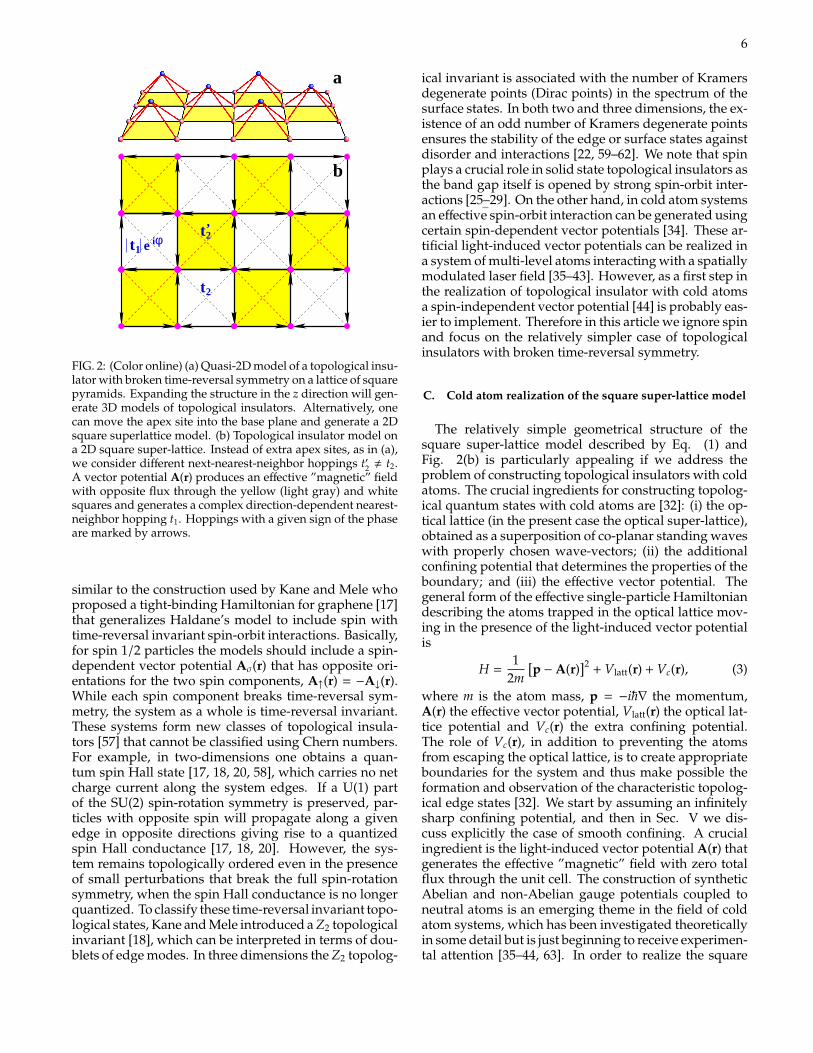
FIG. 7: (Color online) The band structure of Eq (3) in the stripegeometry. The corresponding lattice is schematically shownin the inset. Notice the edge state modes that populate thegap and merge with the bulk states. The edge modes crossthe gap connecting the lower and upper bands and intersectat kx = 0 due to Kramers degeneracy. Small perturbationscan modify the dispersion of the edge modes and the locationof the Kramers degeneracy points, but cannot open a gap forthe edge states. Notice that the bulk bands can be obtained byprojecting the two-dimensional spectrum shown in Fig. 4(c) ona plane perpendicular to the y axis. The same set of parametersas in Fig. 4(c) was used.

of Berry curvature over the Brillouin zone for the twolowest energy bands is shown in Fig. 6. Note thelarge values of Fλ in the vicinity of (kx, ky) = (π, 0) and(kx, ky) = (0, π). These are the points in momentum spacewhere the gap closes when the strength of the vector po-tential approaches zero, α→ 0, leading to the Dirac conestructure shown in Fig. 4(b). In this limit the Berrycurvature diverges at the location of the Dirac points.Similarly, if V2 → 0, the band gap closes at (π, π) and theBerry curvature diverges at that point in k-space. Thetotal flux of berry curvature over the first Brillouin zoneis an integer multiple of 2π and defines the Chern num-ber Cλ = 1

2π

∫d2k Fλ(~k) [51, 69]. A nonzero value of the

Chern number is a signature of the nontrivial topolog-ical properties of the system. In the case shown in Fig.6 the Chern numbers for the first two bands are quan-tized to C1 = 1 and C2 = −1, respectively. Changing theexternal parameters (V1,V2, α) can significantly modifythe shape of the two bands and the distribution of Berrycurvature in k-space without altering the Chern num-bers. For example, C1 can be modified only by passingthrough a critical point (V∗1,V

∗

2, α∗) where the band gap

closes at least in one point in k-space. This type of transi-tion will be addressed in Sec. IV. Having established thatthe square superlattice model supports quantum stateswith a non-trivial topology, we consider now systemswith boundaries and study in detail the properties of thestates localized in the vicinity of those boundaries.

III. EDGE STATES: PROPERTIES ANDCHARACTERIZATION

In this section we consider a two-dimensional systemdescribed by the square super-lattice model in the pres-ence of ideal boundaries, i.e., boundaries created by aninfinitely steep potential wall. We discuss the propertiesof the edge states for systems with either stripe or diskgeometry. First we concentrate on the edge states thatpopulate the gap between the lowest energy bands, thenwe discuss higher-energy edge states.

A. The s-bands edge states

One defining characteristic of topological insulatorsis the existence of gapless edge states that are robustagainst disorder and interactions. While the charac-terization of topological insulators without boundariesusing Berry curvatures and Chern numbers is mathe-matically elegant, the corresponding experimental man-ifestations are not straightforward. By contrast, theexistence of gapless edge states should be much eas-ier to address experimentally even in cold-atom sys-tems [31, 32, 70], as proved by the experiments on solidstate topological insulators [25–29]. A boundary can beformally introduced by turning on the extra confiningpotential Vc(r) in Eq. (3). We start with an idealized po-tential that vanishes in a certain region S and is infiniteoutside. The problems concerning realistic confining po-tentials will be addressed in Sec. V. We note, however,that the crucial assumption here is not the infinite valueof Vc outside S, as any finite value Vmax

c of the order ofthe total relevant bandwidth or larger produces similarconsequences. The key assumption is that the transi-tion between the region with Vc = 0 and the region withVc = Vmax

c is characterized by a length scale of the orderof the lattice constant or smaller.

Without translation symmetry, the numerical com-plexity of the problem increases significantly. Therefore,it is convenient to address the problem of characterizingthe edge states in two stages: (i) First, we consider astripe geometry, in which S is finite along one direction(y in our calculations) but infinite along the orthogonaldirection (x), and we characterize the edge states thatform near the boundaries. (ii) Second, we consider a diskgeometry and show that the basic properties of the edgestates remain the same while pointing out the propertiesthat depend on the system geometry. We start our analy-sis by focusing on the edge modes that populate the gapbetween the first two energy bands, i.e., the bands hav-ing the main contributions from s-type orbitals ψ(r j)

0,0 (r).We call these bands ”s bands” but remind the reader thatsignificant contributions from higher energy orbitals dueto strong hybridization are included.

11

D1−4

Eα = 2

Ene

rgy

E(k

)E

nerg

y E

(k)

kx

α = −2

0 0.5π 1.5π 2π2.2

2.6

2.8

3.0

2.2

2.4

2.4

2.6

2.8

3.0

π

FIG. 8: (Color online) Band structure for a stripe with inequiva-lent edges (see main text). All the sites on one boundary belongto the A sublattice, while all the sites on the other boundary areB-type. For the top panel the parameters are the same as in Fig.7, the only difference being an extra line of lattice sites at oneof the boundaries. Notice the completely different dispersionof the edge modes and the different location of the degeneracypoint. The symmetry between left-moving and right-movingstates is broken. A mirror image of the dispersion lines can beobtained by adding the extra line of lattice sites to the oppo-site edge, or by reversing the direction of the vector potential,α → −α (lower panel). A topologically trivial edge mode de-velops at the top of the second band (state E belongs to thismode).

1. Stripe geometry

Let us consider an optical lattice generated by the po-tential Vlatt given by Eq. (5) and having a real spaceprofile as shown in Fig. 3(a). In the stripe geometry,we consider the lattice as infinite in the x direction andfinite in the y direction, as shown schematically in theinset of Fig. 7. As translation invariance is preservedalong the x direction, so kx is still a good quantum num-ber. For a given value of kx each band is expected tocontain a number of states equal to the number of unitcells along the transverse direction of the stripe. The cal-culated spectrum corresponding to the first two bands isshown in Fig. 7. In a stripe geometry, the contributioncoming from bulk states can be inferred by projecting thetwo-dimensional spectrum (see Fig. 4) on a plane per-pendicular to the transverse direction of the stripe. In

C

B

A

FIG. 9: (Color online) Spatial dependence of the ”amplitude”function |Ψkx ,ν|

2 =∑

(n,m) |Ψ(n,m)kx ,ν

(y j)|2 for the states marked by theletters A, B and C in Fig. 7. The stripe has a width d = 252 (inunits of a = 1/

√2). State A, which is well inside the bulk gap, is

localized near the upper edge and decays exponentially witha characteristic length scale of a few lattice constants. StateB, which is at the gap edge, is a bulk state with a smoothlyvarying envelope function. Notice the multiplication factor of30 introduced to make the function visible on the same scale asthe edge states. State C belongs to the edge mode but is veryclose to the gap edge. It is localized near the bottom edge anddecays exponentially but has a length scale significantly largerthan state A.

Fig. 4(c) the view angle was chosen to visually facilitatethis projection. In addition to the bulk contributions, thespectrum in Fig. 7 contains edge modes that populatethe bulk gap. These modes cross the gap connecting thelower and upper bands and intersect at kx = 0 due toKramers degeneracy. As we will show below, each ofthe states having the energy inside the bulk gap is spa-tially localized near one of the two edges of the system.Small perturbations, like disorder and interactions, orchanging the boundary conditions will modify the edgemode dispersion, but the edge states will remain gap-less. Considering the Fermi energy somewhere insidethe bulk gap, it will always intersect each of the the edgemodes containing states localized either near the lowerboundary or near the upper boundary an odd numberof times, i.e., these edge modes will necessarily connectthe lower and upper bands.

A simple way to exemplify the properties describedabove is to modify the boundary conditions for thestripe. As we discussed in the previous section whenwe described the square super-lattice model (see sub-section II B), the structure of the lattice can viewed asconsisting of two inter-penetrating sublattices A and B.For an edge along the x-direction all the boundary siteswill be of the same type, A or B. Consequently, we canconstruct stripes with edges of the same type and stripeswith edges of different types. The example shown inFig. 7 belongs to the first category. We can modify one

12

D4 D3 D2 1D E

FIG. 10: (Color online) Spatial dependence of the ”amplitude”function |Ψkx ,ν|

2 =∑

(n,m) |Ψ(n,m)kx ,ν

(y j)|2 for state E and for the se-quence of states D1 → D4 from Fig. 8. D1 is positioned in themiddle of the gap, while D4 is at the gap edge and has bulkcharacter. During this transition the characteristic length scalefor the exponential decay of the edge states increases continu-ously from a value of a few lattice sites to a value comparableto the width of the stripe. The state E has a very pronouncededge character, but is not topologically protected. Note thatthe horizontal axis was translated for clarity.

of the boundaries by adding (or removing) one line ofpoints and we obtain a stripe that belongs to the sec-ond category. The corresponding spectrum is shown inFig. 8. The dispersion of the edge modes is significantlymodified as compared to Fig. 7, as well as the locationof the degeneracy point. However, the main property ofthe edge modes, namely that they connect the lower andupper bands, is not affected. This property is a signatureof the topological nature of these edge states. Figure 8also offers a counterexample, i.e., a topologically trivialedge mode. This mode, which develops at the top ofthe second band, does not connect two different bandsand is not robust, as it can be absorbed into the bulkcontinuum in the presence of small perturbations.

So far we referred to the in-gap states as edge stateswithout showing explicitly that they are indeed localizednear the boundary of the system. If for a given wavevector kx we order the single-particle states accordingto their energy so Φ1,kx is the lowest energy state, thenthe spatial properties of a generic state are given by thenorm |Φν,kx (r)|2, where Eq. (10) is used with the am-plitudes Ψ(n,m)

ν,kxbeing solutions of Eq. (11). However,

such a detailed description of the spatial dependenceof the wave function is not necessary for our purposeand instead we focus on the dependence of the envelopefunction, which does not contain the details of the orbitalstructure, on the transverse coordinate y. More precisely,for a state (ν, kx) we define the ”density” or ”amplitude”function |Ψν,kx |

2 =∑

(n,m) |Ψ(n,m)ν,kx

(y j)|2, where Ψ(n,m)ν,kx

(y j) is

the Fourier transform of Ψ(n,m)ν,kx

(x j, y j) with respect to kx.

n kAverage position <y>

ε nk

Ene

rgy

DOS

n kOrbital momentum <L>

ε nk

Ene

rgy

DOS

2/ a

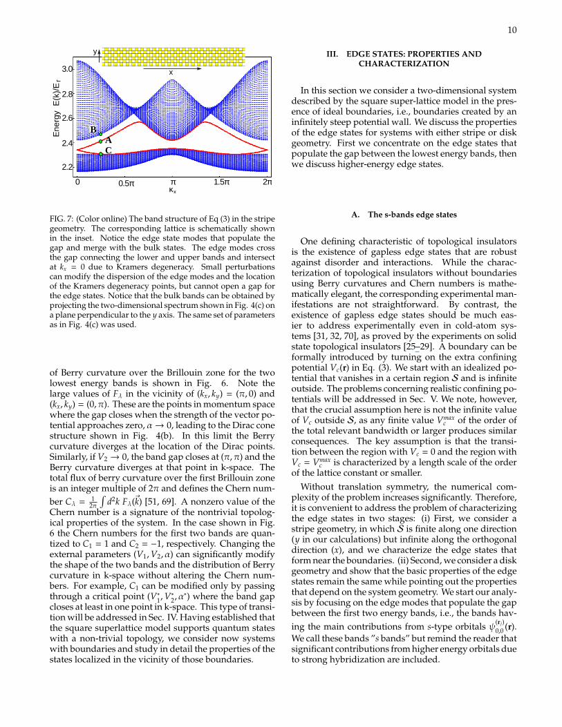
FIG. 11: (Color online) (Upper panel) Average position versusenergy for the single particle states that are solutions of Eq.(3) in the stripe geometry (with equivalent edges). The sys-tem is characterized by the parameters V1 = 3.4Er, V2 = 1.7Er

and α = 2 ~/a and has a width d = 100(√

2a). The bulk statesare characterized by 〈y〉nkx ≈ d/2, while the edge states have〈y〉nkx ≈ 0 or 〈y〉nkx ≈ d, corresponding to the positions of thetwo edges. (Lower panel) Average orbital momentum (in ar-bitrary units) versus energy for the same system. Notice thechiral nature of the topological edge states and the extra edgemodes located in the upper band. The spectrum for this systemis shown in Fig. 7 and the density of states (DOS) is shown inthe right panels.

Note that the ”density” is normalized,∑

j |Ψν,kx |2(y j) = 1.

The spatial dependence of the ”amplitude” function forthe states marked by the letters A, B and C in Fig. 7is shown in Fig. 9. The figure shows clearly that thestates within the gap (A and C) are indeed localized inthe vicinity of one of the two edges of the system anddecay exponentially away from the boundary. For stateswell inside the gap the characteristic length scale is of theorder of the lattice constant. This length scale increasesas the edge mode merges into the bulk states.

To examine further the transition from edge to bulkstates we show in Fig. 10 the ”amplitude” function forthe sequence of states D1 → D4 from Fig. 8. The state D1is positioned in the middle of the gap and in real spaceit decays exponentially away from the top edge witha length scale of a few lattice constants. As the edge

13

n kOrbital momentum <L>

ε nk

Ene

rgy

ε nk

Ene

rgy

n kAverage position <y> a/ 2

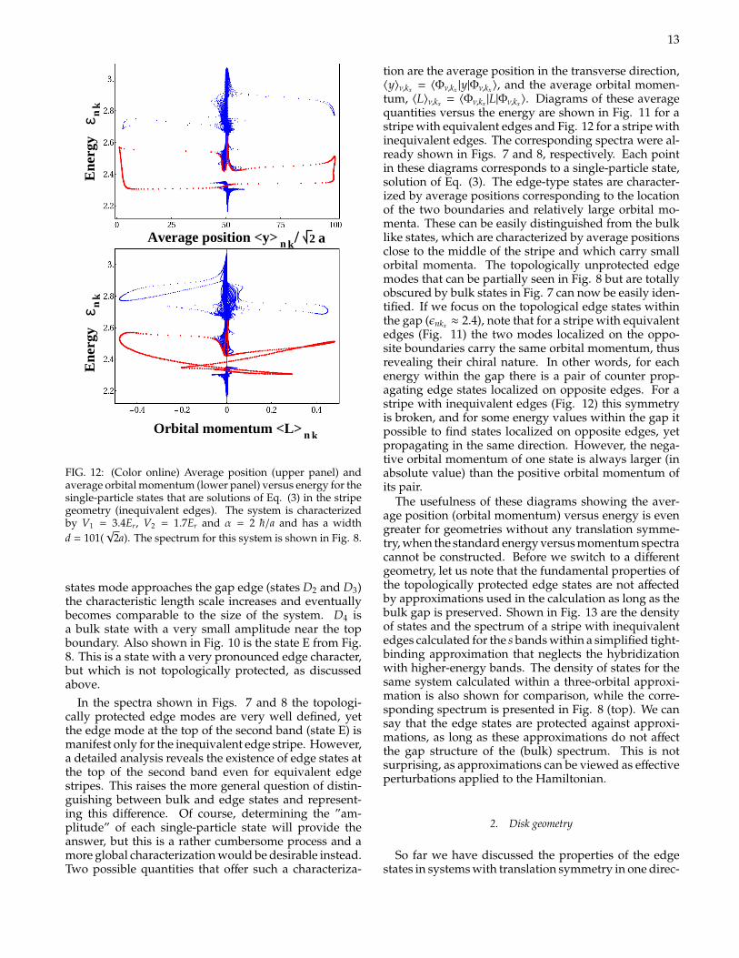
FIG. 12: (Color online) Average position (upper panel) andaverage orbital momentum (lower panel) versus energy for thesingle-particle states that are solutions of Eq. (3) in the stripegeometry (inequivalent edges). The system is characterizedby V1 = 3.4Er, V2 = 1.7Er and α = 2 ~/a and has a widthd = 101(

√2a). The spectrum for this system is shown in Fig. 8.

states mode approaches the gap edge (states D2 and D3)the characteristic length scale increases and eventuallybecomes comparable to the size of the system. D4 isa bulk state with a very small amplitude near the topboundary. Also shown in Fig. 10 is the state E from Fig.8. This is a state with a very pronounced edge character,but which is not topologically protected, as discussedabove.

In the spectra shown in Figs. 7 and 8 the topologi-cally protected edge modes are very well defined, yetthe edge mode at the top of the second band (state E) ismanifest only for the inequivalent edge stripe. However,a detailed analysis reveals the existence of edge states atthe top of the second band even for equivalent edgestripes. This raises the more general question of distin-guishing between bulk and edge states and represent-ing this difference. Of course, determining the ”am-plitude” of each single-particle state will provide theanswer, but this is a rather cumbersome process and amore global characterization would be desirable instead.Two possible quantities that offer such a characteriza-

tion are the average position in the transverse direction,〈y〉ν,kx = 〈Φν,kx |y|Φν,kx〉, and the average orbital momen-tum, 〈L〉ν,kx = 〈Φν,kx |L|Φν,kx〉. Diagrams of these averagequantities versus the energy are shown in Fig. 11 for astripe with equivalent edges and Fig. 12 for a stripe withinequivalent edges. The corresponding spectra were al-ready shown in Figs. 7 and 8, respectively. Each pointin these diagrams corresponds to a single-particle state,solution of Eq. (3). The edge-type states are character-ized by average positions corresponding to the locationof the two boundaries and relatively large orbital mo-menta. These can be easily distinguished from the bulklike states, which are characterized by average positionsclose to the middle of the stripe and which carry smallorbital momenta. The topologically unprotected edgemodes that can be partially seen in Fig. 8 but are totallyobscured by bulk states in Fig. 7 can now be easily iden-tified. If we focus on the topological edge states withinthe gap (εnkx ≈ 2.4), note that for a stripe with equivalentedges (Fig. 11) the two modes localized on the oppo-site boundaries carry the same orbital momentum, thusrevealing their chiral nature. In other words, for eachenergy within the gap there is a pair of counter prop-agating edge states localized on opposite edges. For astripe with inequivalent edges (Fig. 12) this symmetryis broken, and for some energy values within the gap itpossible to find states localized on opposite edges, yetpropagating in the same direction. However, the nega-tive orbital momentum of one state is always larger (inabsolute value) than the positive orbital momentum ofits pair.

The usefulness of these diagrams showing the aver-age position (orbital momentum) versus energy is evengreater for geometries without any translation symme-try, when the standard energy versus momentum spectracannot be constructed. Before we switch to a differentgeometry, let us note that the fundamental properties ofthe topologically protected edge states are not affectedby approximations used in the calculation as long as thebulk gap is preserved. Shown in Fig. 13 are the densityof states and the spectrum of a stripe with inequivalentedges calculated for the s bands within a simplified tight-binding approximation that neglects the hybridizationwith higher-energy bands. The density of states for thesame system calculated within a three-orbital approxi-mation is also shown for comparison, while the corre-sponding spectrum is presented in Fig. 8 (top). We cansay that the edge states are protected against approxi-mations, as long as these approximations do not affectthe gap structure of the (bulk) spectrum. This is notsurprising, as approximations can be viewed as effectiveperturbations applied to the Hamiltonian.

2. Disk geometry

So far we have discussed the properties of the edgestates in systems with translation symmetry in one direc-

14

Ene

rgy

/ E

εr

x

2.2 2.4 2.6 2.8 3Energy ε / E

r

0

1

2

3

4D

ensi

ty o

f sta

tes

(D

OS)

3-band model1-band model

k

b

a

FIG. 13: (Color online) Density of states (a) and spectrum (b)showing the s bands of a stripe with inequivalent edges cal-culated within a simplified tight-binding approximation thatneglects hybridization with higher bands. For comparison, thedensity of states calculated within a three-orbital tight-bindingapproximation is also shown. The corresponding spectrum isgiven in Fig. 8 (top panel). Note that the topology of the edgemodes is not altered, in spite of a significant redistribution inthe density of states.

tion (stripes). Because momentum along one directionis a good quantum number, spectra showing the energydispersion as a function of momentum are a very effec-tive way of characterizing the system and, in the caseof condensed matter systems, have a direct connectionwith experimentally measurable quantities. By contrast,cold-atom systems may contain a relatively small num-ber of sites, so the explicit treatment of a finite systemmay be required, and have a circle or an ellipse as themost natural shape for the boundary. This raises twoquestions: (i) What is the impact of the boundary geom-etry on the edge states? and (ii) How important are thefinite size effects for the stability of the edge states? Westart by addressing the first question, while the secondwill be discussed in Sec. V.

Let us consider the single particle quantum problemdescribed by Eq. (3) with an extra confining potentialgiven by

Vc(r) =

0 if |r| ≤ R0,∞ if |r| > R0.

(12)

The system consists of a disk-shaped piece of the square

0

DOS

rE

nerg

y

/ E

Average radial position <R> n

ε n

/a

FIG. 14: (Color online) Diagram showing the average radialposition versus energy for the single-particle states of a systemdescribed by Eq. (3) in a confining potential (12). The param-eters of the system are V1 = 3.4Er, V2 = 1.7Er, and α = 2 ~/a.The underlying lattice (i.e., the minima of the effective opticallattice potential) is shown in the inset. The edge states arecharacterized by values of 〈r〉n comparable with R0 = 29a, thedisk radius, as a result of their localization in the vicinity of theboundary. The clearly defined edge mode crosses the bulk gapand connects the lower and upper bands, thus revealing itstopological nature. The density of states (right) is practicallyidentical with that shown in Fig. 13(a) for a similar systemwith stripe geometry.

super-lattice with a boundary that contains sites fromboth sublattices, A and B with a distribution that de-pends on the radius R0. For simplicity, we solve theproblem within the single-orbital tight-binding approx-imation, as the full size matrices (i.e., N × N matrices,with N the number of lattice sites inside the disk) haveto be used in Eq. (11). To describe globally the systemwe use the type of diagrams introduced in the previoussection. More precisely, we represent the average radialposition for a given single-particle state, 〈r〉n = 〈Φn|r|Φn〉,versus the state energy, εn. The results for a disk withradius R = 29a are shown in Fig. 14. The main con-clusion suggested by the data is that the edge mode isrobust against deformations of the boundary. The stateswith energies near the middle of the gap are localizedwithin a few lattice spacings from the boundary, whilethis characteristic length increases as one approaches thegap edge. The number of edge states is proportional tothe length of the boundary (i.e., R0), while the numberof bulk states scales with the area of the system (i.e., R2

0).Finally, we note that the topologically unprotected edgestates that were present in the stripe geometry (see Figs.8, 11, and 12) do not survive in the absence of transla-tional symmetry.

To visualize the spatial dependence of the single par-ticle states in the disk geometry, we show in Fig. 15

15

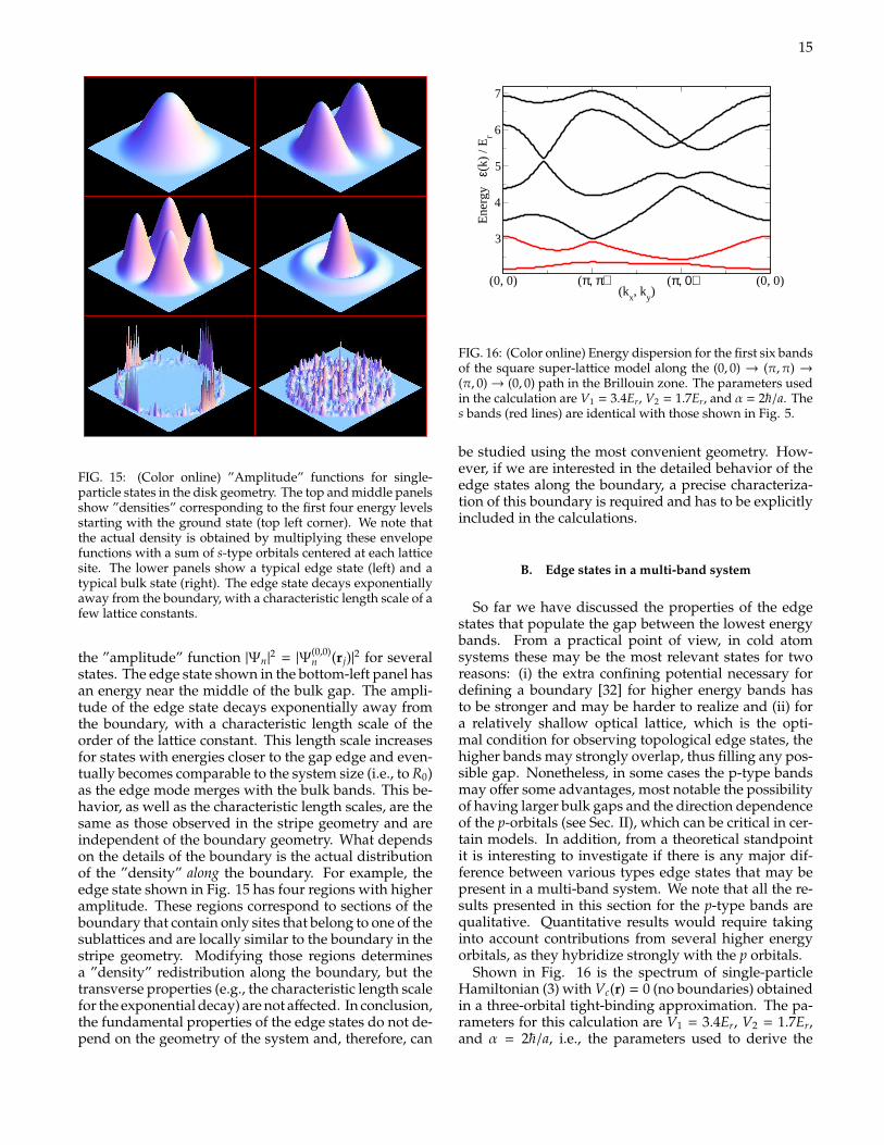
FIG. 15: (Color online) ”Amplitude” functions for single-particle states in the disk geometry. The top and middle panelsshow ”densities” corresponding to the first four energy levelsstarting with the ground state (top left corner). We note thatthe actual density is obtained by multiplying these envelopefunctions with a sum of s-type orbitals centered at each latticesite. The lower panels show a typical edge state (left) and atypical bulk state (right). The edge state decays exponentiallyaway from the boundary, with a characteristic length scale of afew lattice constants.

the ”amplitude” function |Ψn|2 = |Ψ(0,0)

n (r j)|2 for severalstates. The edge state shown in the bottom-left panel hasan energy near the middle of the bulk gap. The ampli-tude of the edge state decays exponentially away fromthe boundary, with a characteristic length scale of theorder of the lattice constant. This length scale increasesfor states with energies closer to the gap edge and even-tually becomes comparable to the system size (i.e., to R0)as the edge mode merges with the bulk bands. This be-havior, as well as the characteristic length scales, are thesame as those observed in the stripe geometry and areindependent of the boundary geometry. What dependson the details of the boundary is the actual distributionof the ”density” along the boundary. For example, theedge state shown in Fig. 15 has four regions with higheramplitude. These regions correspond to sections of theboundary that contain only sites that belong to one of thesublattices and are locally similar to the boundary in thestripe geometry. Modifying those regions determinesa ”density” redistribution along the boundary, but thetransverse properties (e.g., the characteristic length scalefor the exponential decay) are not affected. In conclusion,the fundamental properties of the edge states do not de-pend on the geometry of the system and, therefore, can

(0, 0) (π, π) (π, 0) (0, 0)(k

x, k

y)

3

4

5

6

7

Ene

rgy

ε(k

) / E

r

FIG. 16: (Color online) Energy dispersion for the first six bandsof the square super-lattice model along the (0, 0) → (π, π) →(π, 0)→ (0, 0) path in the Brillouin zone. The parameters usedin the calculation are V1 = 3.4Er, V2 = 1.7Er, and α = 2~/a. Thes bands (red lines) are identical with those shown in Fig. 5.

be studied using the most convenient geometry. How-ever, if we are interested in the detailed behavior of theedge states along the boundary, a precise characteriza-tion of this boundary is required and has to be explicitlyincluded in the calculations.

B. Edge states in a multi-band system

So far we have discussed the properties of the edgestates that populate the gap between the lowest energybands. From a practical point of view, in cold atomsystems these may be the most relevant states for tworeasons: (i) the extra confining potential necessary fordefining a boundary [32] for higher energy bands hasto be stronger and may be harder to realize and (ii) fora relatively shallow optical lattice, which is the opti-mal condition for observing topological edge states, thehigher bands may strongly overlap, thus filling any pos-sible gap. Nonetheless, in some cases the p-type bandsmay offer some advantages, most notable the possibilityof having larger bulk gaps and the direction dependenceof the p-orbitals (see Sec. II), which can be critical in cer-tain models. In addition, from a theoretical standpointit is interesting to investigate if there is any major dif-ference between various types edge states that may bepresent in a multi-band system. We note that all the re-sults presented in this section for the p-type bands arequalitative. Quantitative results would require takinginto account contributions from several higher energyorbitals, as they hybridize strongly with the p orbitals.

Shown in Fig. 16 is the spectrum of single-particleHamiltonian (3) with Vc(r) = 0 (no boundaries) obtainedin a three-orbital tight-binding approximation. The pa-rameters for this calculation are V1 = 3.4Er, V2 = 1.7Er,and α = 2~/a, i.e., the parameters used to derive the

16

x x

Ene

rgy

E (

k)/E

0 π 2π0 π

3

4

5

6

7

2π

3

4

5

6

7n

r

kk

FIG. 17: (Color online) The band structure of the Hamiltoniangiven by Eq. (3) in the stripe geometry. The left panel corre-sponds to the parameters V1 = 3.4Er, V2 = 1.7Er and α = 2~/a,while the right panel corresponds to a slightly deeper latticewith V1 = 3.7Er. Note that there are no edge states between thesecond and the third bands, but an edge mode is clearly visiblebetween the third and the fourth bands. Increasing V1 opensa gap in the spectrum (right panel) and reveals the topologicalnature of that edge mode. By contrast, the edge states thatpopulate the gap between the fourth and the fifth bands aretopologically trivial, as they do not connect the two bands.

majority of the results in the previous subsection. Forthese parameters most of the p bands overlap and nogap opens except between the fourth and the fifth bands(at energies around 5.2Er). The first question that weaddress is whether there are any other topological edgestates except those located in the gap between the firsttwo bands, which we studied in the previous subsec-tion. To answer this question, we can either considera system with boundaries and identify the edge modesor remain within a bulk description and calculate theChern numbers Cn for each band. We start with thesecond approach, as it is much easier to implement nu-merically. The Chern numbers for the first four bandsare C1 = 1, C2 = −1, C3 = 1, and C4 = −1. The last twobands are degenerate at k = (0, π) and k = (π, 0). Asthe Berry curvature diverges in the vicinity of the de-generacy points, the Chern numbers for those bands arenot defined. In principle, topological edge states existin a gap if the total curvature (i.e., the sum of the Chernnumbers) of all the bands below that gap is nonzero.The first band has non-zero curvature and topologicaledge states exist inside the gap above it, as we have seenabove. The first two bands, as a whole, have zero totalcurvature and, consequently, no topological edge statesshould be present on the top of the second band. Thisis consistent with our previous observation of the topo-logically unprotected edge states in the stripe geometry.Similarly, we expect topological edge states to exist be-tween the third and the fourth bands (if a full gap is

opened), but not between the fourth and the fifth.To confirm that the structure inferred from the values

of the Chern numbers is indeed realized, we calculate theband structure of a system with boundaries in the stripegeometry. The results are shown in Fig. 17 and offer apicture that is consistent with the above analysis. Twofeatures are worth mentioning. First, note that the topo-logical edge mode that develops inside the gap betweenthe third and fourth bands (Fig. 17, right panel) partiallysurvives the gap collapse (Fig. 17, left pane). These edgestates are protected by the translation symmetry and arerobust against perturbations that conserve this symme-try. However, they will be destroyed by the presenceof disorder. Second, we notice some very well definededge modes inside the gap between the fourth and fifthbands. These modes are good example of topologicallytrivial edge states: they do not cross the gap connectingtwo different bands, but rather start from and return tothe same band. Consequently, at any given energy therewill be an even number of such edge states near a givenboundary and any small perturbation will make them tobecome localized. By contrast, in the case of topologi-cal edge states there is an odd number of states near agiven boundary at any given energy within the gap, soeven in the presence of perturbations a dispersive modeconsisting of de-localized states is preserved.

As we mentioned at the beginning of this subsection,including higher energy orbitals is expected to modifyquantitatively our picture of the p bands. However, weexpect minor changes as far as the s bands are concerned.Therefore it is relevant and useful to have a quantitativeestimate of the s band gap and a general idea on how itdepends on the parameters of our model. Shown in Fig.18 is the gap dependence on the strength of the vectorpotential for three different values of V2. Dependingon the parameters, the system has either a direct gapat π, π) or an indirect gap between the maximum of thelower band at (π, π) and the minima of the upper band at(0, π)/(π, 0. Note that the indirect gap becomes negativefor α < α∗(V2), i.e., vector potentials with a strengthlower than a certain critical value.

IV. TRANSITIONS BETWEEN TOPOLOGICALLYDISTINCT QUANTUM STATES

In this section we give several examples of phase tran-sitions between quantum states with distinct topologicalproperties. These transitions can be induced by apply-ing certain perturbations, i.e., adding some extra termsto the Hamiltonian, or, in the case of a multi-band topo-logical insulator, by simply varying the parameters thatcharacterize the system.

The topological properties of a quantum state are notmodified by any perturbation of the Hamiltonian thatdoes not close the bulk gap. Nonetheless, when sucha perturbation determines the closing of the bulk gap,the system undergoes a phase transition to either a

17

0 0.5 1 1.5 2 2.5 3 3.5Vector potential strength α

-0.04

-0.02

0

0.02

0.04

0.06

0.08S-

band

gap

∆ /

Er

V2 = 0.85 Er

V2 = 1.70 Er

V2 = 2.00 Er

FIG. 18: (Color online) The s band gap as function of the vectorpotential strength for several values of the super-lattice gener-ating component V2. The main amplitude of the optical latticepotential is fixed, V1 = 3.4Er. Notice that each curve has asingularity point and that the slope to the left (right) of thesingularity point is positive (negative). The positive slope cor-respond to an indirect gap between the maximum of the lowerband at (π, π) and the minima of the upper band at (0, π)/(π, 0,while the negative slope corresponds to a direct gap at π, π).Note that for weak vector potentials with the strength α belowa critical value α∗(V2) the indirect gap becomes negative.

metallic state or an insulating state with possibly dif-ferent topological properties. The topological-insulator-to-metal transition can be exemplified by the band struc-ture shown in Fig. 17. Let us assume that the first threebands in the right panel are completely filled, so the onlygapless excitations are provided by the edge mode thatcrosses the gap between the third and fourth bands. Bysimply reducing the depth of the optical lattice, this bulkgap collapses (see left panel) and the system becomesmetallic. More interesting are the transitions betweentwo different insulating states. We discuss two possi-ble ways of inducing such transitions: (i) by adding anextra-term to the Hamiltonian that opens a (topologi-cally trivial) gap and (ii) by tuning the parameters V1,V2, and α that characterize the system.

A. Transitions driven by a staggered potential

The tight-binding model described by Eq. (1) is de-fined on a square super lattice consisting of two interpenetrating sublattices A and B, as discussed in Sec. I.If the second neighbor hopping is anisotropic, t′2 , t2,and the nearest-neighbor hopping is complex, φ , 0 andφ , π, a full gap ∆(k) opens in the spectrum, with anexplicit wave vector dependence given by

∆2(kx, ky) = 4(t2 − t′2)2(cos kx − cos ky)2 (13)

+ 16|t1|2[1 + cos kx cos ky + cos(2φ)(cos kx + cos ky)

].

x x

E (

k )

nx

E (

k )

nx

2ππ2π0π0

2.2

2.6

3.0

3.0

2.6

2.2

Γ = 0.075 Γ = 0.12

Γ = 0.04Γ = 0

k k

FIG. 19: (Color online) Band structure for a system with stripegeometry described by the parameters V1 = 3.4Er, V2 = 1.7Er,α = 2~/a and different values of the staggered potential Γ (givenin units of Er). Γ = 0 corresponds to the case shown in Fig.7. Applying a small staggered potential reduces the gap inthe vicinity of kx = 0 (top right panel). At the critical valueΓc ≈ 0.075Er the gap closes at kx = 0, while for Γ > Γc a fullgap opens again. At large values of Γ the system is a standardband insulator with no edge modes inside the gap. Notice thatthe spectra are shown for half of the one-dimensional Brillouinzone while the other half can be obtained by mirror symmetrywith respect to kx = π.

For the cold-atom realization of this model described byEq. (3), the condition for anisotropic second-neighborhopping becomes V2 , 0, while the imaginary compo-nents of the nearest-neighbor hopping are generated bythe effective vector potential, so the second conditionbecomes α , 0. Spectra for the Hamiltonian (3) corre-sponding to three different sets of parameters are shownin Fig. 4. Another possibility to open a gap in a squarelattice tight-binding model is to simply add a staggeredpotential, i.e., a potential that generates on-site energiesΓ and −Γ for the sublattices A and B, respectively. Thisamounts to adding a term of the form

Vstagg = Γ∑

k

(c†AkcAk − c†BkcBk

)(14)

to the Hamiltonian. In the presence of such a term, a sim-ple tight binding model with t′2 = t2 and exp(iφ) = ±1is characterized by a full gap with a minimum value∆min = 2|Γ|. If the lowest band is completely filled, thesystem represents a standard band insulator with triv-ial topological properties. The question that we wantto address concerns the evolution of the spectrum andthe fate of the edge modes as the transition between atopological insulator and a standard band insulator isinduced by tuning the staggered field strength.

In the cold-atom realization of the model described byEq. (3) the staggered potential can be introduced as anextra term. However, we want to point out the possibil-ity that such a component be generated in the process

18

Γ = 0.12

kx

E (

k )

/ Er

nx

2π1.5ππ0.5π0

2.2

2.4

2.6

2.8

3.0

FIG. 20: (Color online) Band structure for a stripe with in-equivalent edges and with the same parameters as in Fig. 19.For Γ = 0.12Er the system is a standard band insulator but, incontrast with the equivalent edge case (see Fig. 19), a well-defined edge mode populates the gap. A clean insulator withthe chemical potential inside the bulk gap supports gaplessedge excitations. However, any small perturbation (such asdisorder or interactions) will open a gap in the edge mode.

of constructing the superlattice itself. This representsa potential problem for realizing topological quantumstates. For example, if the components V1 and V2 ofthe optical lattice potential are produced by differentlasers, a misalignment corresponding to x→ x + δx andy → y + δy in the V2 term will effectively generate astaggered potential. In the calculations we neglect thedetailed effects of such a misalignment on the hoppingmatrix elements and consider only the on site staggeredcontributions parameterized by Γ. We start with a sys-tem in the stripe geometry with parameters V1 = 3.4Er,V2 = 1.7Er, α = 2~/a and Γ = 0, then we turn on Γ whilekeeping the other parameters fixed. The correspondingspectra are shown in Fig. 19. For Γ = 0 the system isa topological insulator and the corresponding spectrumis characterized by an edge mode that crosses the bulkgap. Applying a small staggered potential reduces thegap in the vicinity of kx = 0 and, eventually, at the criticalvalue Γc ≈ 0.075Er the gap closes at kx = 0. For largervalues of Γ the gap opens again but no edge states arepresent inside the gap. We conclude that the system is atopological insulator for Γ < Γc(V1,V2, α) and a standardband insulator for Γ > Γc(V1,V2, α).

The mechanism described above is quite general. Anyperturbation capable of opening a gap in the spectrumwill have similar effects and will induce a transition ata particular critical strength. This critical strength isindependent of the boundary geometry. However, thedetails that characterize the edge modes in either sideof the transition depend on the properties of the bound-aries. For example, if instead of the stripe geometry withequivalent edges considered in Fig. 19 we study a sys-tem with inequivalent edges (see Fig. 8), we observe atransition (i.e., the closing of the gap) at the same critical

(kx, k

y)

2

3

4

5

6

7

Ene

rgy

ε(k

)

V2 = 2.5 E

r

(kx, k

y)

V2 = 1.95 E

r

(kx, k

y)

V2 = 1.75 E

r

(kx, k

y)

V2 = 1.53 E

r

(kx, k

y)

V2 = 1.0 E

r

0

0

−1

1

−1

1

1

−1

1

−1

1

eb

3

a c d

FIG. 21: (Color online) Energy dispersion curves for a systemwith V1 = 3.7Er, α = 2~/a, and different values of V2 along the(0, 0)→ (π, π)→ (π, 0)→ (0, 0) path in the Brillouin zone. Thenumbers inside the yellow circles represent the Chern num-bers of the bands. Note the closing of the direct gap at certaincritical values of V2 (panels b and d) and the correspondingchange of the Chern numbers. The spectra shown in panelsa, c, and e are consistent with different insulating states: (a)topological insulator (with the first three bands filled) and con-ventional insulator (four bands filled); (c) topological insulator(one band filled) and conventional insulator (four bands filled);and (e) topological insulator I (one band filled), conventionalinsulator (two bands filled) and topological insulator II (fourbands filled).

value Γc ≈ 0.075Er. However, the band insulator withΓ > Γc has now a clearly defined edge mode, as shownin Fig. 20. In particular, this edge mode ensures the exis-tence of gapless excitations for any value of the chemicalpotential inside the gap. Nonetheless, this mode is topo-logically trivial, as revealed by the fact that it does notconnect the two bands, and consequently it is not pro-tected against disorder and interactions, in the sense thatany weak perturbation will open a gap in the edge mode.

B. Transitions in a multi-band system

The transition studied in the previous section wasdriven by the competition between the contributions tothe Hamiltonian that generate its nontrivial topologicalproperties and terms like Vstagg that tend to open a con-ventional band gap. However, the model described byEq. (3) contains three independent parameters, V1, V2,and α, and only the vector potential (i.e., α) is directlyresponsible for the nontrivial topology of the bands.Therefore, we expect several topologically distinct statesto exist in various regions of the parameter space. Wehave already seen that small variations of the parame-ters can lead to the opening/closing of the gaps corre-sponding to a topological insulator to metal transition,

19

6.5

V = 2.5 E r2 V = 1.0 E r2E

nerg

y E

(k)

kxkx

4

5

6

7

2ππ02ππ0

5.75

5.50

5.25

5.00

4.75

FIG. 22: (Color online) Detail of the band structure for a systemin the stripe geometry with the same parameters as in Fig.21(a) (left) and 21(e) (right). In the left panel notice one pairof topological edge modes inside the gap above the third bandand the topologically trivial edge states above the fourth band,consistent with the Chern numbers shown in Fig. 21(a). Onthe right we observe four pairs of edge modes inside the gapabove the fourth band. This number of pairs of edge modesis equal to the total Chern number of the bands below the gap[see Fig. 21(e)].

as shown in Fig. 17. The question that we address now iswhether insulator to insulator transitions can be inducedby tuning the parameters of the model. Our purpose isnot to determine the full phase diagram of the model,but rather to give an example showing that such transi-tions are possible. In general, the parameter space canbe characterized by two independent quantities, for ex-ample V2/V1 and α/

√2mV1. However, we fix V1 = 3.7Er

andα = 2~/a and vary V2, which corresponds to a certaincut in the parameter space. The resulting bulk spectraare shown in Fig. 21 for several values of V2. The to-tal flux of Berry curvature (i.e., the Chern number) fora given band remains unchanged as long as the directgaps separating that band from the neighboring bandsdo not vanish. When the direct gap between two bandsvanishes (see panels b and d), the total flux of Berry cur-vature is redistributed between the two bands and thetopological properties of the system change accordingly.

As we mentioned above, the topological character ofan insulating state, and hence the existence of robustedge states, is determined by the sum of the Chernnumbers of the occupied bands. An interesting caserevealed by the results shown in Fig. 21 is when the firstfour bands are completely filled. Then, for V2 < 1.53Erthe system is a conventional band insulator, while forV2 > 1.53Er it is a topological insulator with the sumof the Chern numbers of the occupied bands equal tofour. To identify the structure of the corresponding edgemodes we consider a system with boundaries in thestripe geometry and determine the spectra for V2 = 1.0Erand V2 = 2.5Er. The results are shown in Fig. 22. Asevident from these results, the number of pairs of topo-logical edge states that populate a gap equals the totalChern number of the bands that are below that gap. In

2 ay/Ψ

2(y

)y ξ

exp[

]

E(k

) / E

r

π0 2π

FIG. 23: (Color online) (Upper panel) Spectrum for the squaresuperlattice model (1) with parameters t1 = (1 + 0.2i)Er, t2 =−0.3Er, and t′2 = −0.06Er in the stripe geometry. The systemis finite in the y direction and infinite in the x direction, withthe axes are oriented along the next-nearest neighbor direc-tions (see Fig. 3). For an odd number of layers (i.e., equivalentedges) the edge states (red/dark gray lines) with kx < π arelocalized near y = 0, while the edge states with kx > π arelocalized near the opposite boundary. For an even number oflayers (i.e., inequivalent edges) the mode localized near y = 0remains unchanged, while the other mode is now character-ized by kx < π (green/light gray line). (Lower panel) Edge stateamplitudes multiplied by exponential factors to reveal the os-cillatory behavior. Blue (dark gray): edge state correspondingto kx = 0.97π/

√2a and ξ = 1.441

√2a. Orange (light gray):

edge state with kx = 0.7π/√

2a and ξ = 1.351√

2a.

the case shown in right panel of Fig. 22 four pairs oftopological edge modes populate the gap between thefourth and the fifth bands. Hence, for any given energyinside the gap at least four different edge states will existon each of the two boundaries. The stability of theseedge states is a natural question that we address next.

V. STABILITY OF THE EDGE STATES

The physics that emerges from the nontrivial topolog-ical properties of a system can be directly related to thebehavior of the edge states. The topological features arepresent as long as the spectrum is gaped for all bulk ex-

20

citations and the bulk gap is populated by gapless edgemodes. Weak local perturbations cannot induce a phasetransition to a state with different topological propertiesand, consequently, the edge or surface states are robustagainst disorder and interactions [22, 59–62]. These per-turbations modify the bulk properties of the system andgenerate extra terms in the Hamiltonian that describesits quantum mechanical properties. However, the solu-tion of a quantum mechanical problem is determined notonly by the Hamiltonian but also by the boundary con-ditions. In this section we address the question of howchanging these boundary conditions impact the prop-erties of the edge states. In particular, we discuss thestability of the edge states against finite size effects andtheir dependence on the confining potential that definesthe boundaries of the system. The answers to these ques-tions are particularly relevant for cold atom systems, butthey can shed meaningful light on the physics of solidstate topological insulators, for example, in the case oftopological insulator thin films [71–75]. or in the case oftopological insulator heterostructures.

A. Finite size effects

The chiral edge states robustness against disorder andinteractions can be linked to the absence of backscatter-ing. In a large system, counter propagating edge modesare localized near boundaries that are well separatedspatially and, consequently, have a vanishing overlap.However, as the size of the system in a certain direc-tion is reduced, edge states propagating along oppositeedges may acquire a finite overlap. Consequently, a gapopens in the edge states spectrum. The dependence ofthis gap on the size of the system depends on the spa-tial behavior of the edge states, in particular on how fastthey decay away from the boundary. As suggested bythe profiles shown in Figs. 9 and 10, the edge state ampli-tude decreases exponentially with the distance from theedge. The characteristic length scale for this exponentialdecay, ξ, depends on the size of the bulk gap, roughlyscaling as the bandwidth over the gap size, but also onthe location of the edge state within the bulk gap. In ad-dition, the exponential decay is generally non monotonicand includes one or more oscillatory components.

To illustrate this general behavior, we show in Fig. 23the spectrum for a system with a stripe geometry de-scribed by the square super-lattice model given by Eq.(1) with the parameters t1 = (1 + 0.2i)Er, t2 = −0.3Er,and t′2 = −0.06Er. The edges of the stripe are chosenalong one of the next nearest neighbor directions and, asdiscussed above, may contain sites from the same sub-lattice (what we call equivalent edges) or from differentsublattices (inequivalent edges). As shown in the upperpanel of Fig. 23, the dispersion of the edge modes is ex-tremely sensitive to changes in the boundary conditions(see also Figs. 7 and 8). In addition, different states froma given edge mode have different asymptotic behaviors,

E(k

) / E

rΨ

2(y

)y ξ

2π0 π

exp[

]

y/a

FIG. 24: (Color online) (Upper panel) Spectrum for the squaresuper-lattice model (1) in the stripe geometry for the same pa-rameters as in Fig. 23 but with the symmetry axes orientedalong the nearest neighbor directions. The dispersion of theedge modes is independent of the parity of the number of lay-ers. (Lower panel) Edge state amplitude multiplied by an ex-ponential factor with ξ = 2.396a for the state with kx = 0.97π/a.Note the even-odd oscillations and the k-dependent longwavelength oscillatory component. At kx = π/a the extra oscil-latory component is absent.

as shown in the lower panel of Fig. 23. As the parame-ters describing the asymptotic behavior of an edge statedeep inside the system depend on bulk properties butalso on the position of the state within the gap, they canbe modified by changing the boundary conditions.

If the edges of the stripe are chosen along one of thenearest neighbor directions, the corresponding spectrumdoes not exhibit any even-odd variation with the num-ber of layers in the system. The band structure for sucha stripe is shown in Fig. 24 for the same model param-eters as in Fig. 23. The amplitude of an edge state fromthe vicinity of the Dirac point is also shown in the lowerpanel. Although the bulk parameters are the same as inFig. 23, the asymptotic behavior of the edge states is gen-erally different, as a consequence of the new boundaryconditions. Note that the edge state shown in Fig. 24 ischaracterized by multiple oscillatory components, in ad-dition to the exponential decay. The relative amplitudeof those components depend on kx, the wave vector com-ponent parallel to the edge, for example at kx = π/a only

21

kx kx

E(k

) / E

rN = 12 ( )11N = 30 ( )29

0 π 2π 0 π 2π

FIG. 25: (Color online) Opening of a gap in the edge state spec-trum due to finite size effects. The system is a thin stripe withthe same geometry and hopping parameters as in Fig. 24. Thesize of the gap is determined by the overlap of edge states local-ized on opposite boundaries and, consequently, varies roughlyexponentially with the width of the stripe and inherits the os-cillatory behavior of the edge states. For large N the edge statesare gapless and independent of parity. For thin films, a finitegap opens in systems with even number of layers, while sys-tems with odd number of layers remain gapless. Note that the”bulk” spectrum varies dramatically with the system size, incontrast with the edge modes that are practically unaffected ifthe system size is much larger than their characteristic lengthscale.

the short wavelength oscillatory component is present.Knowing the precise asymptotic behavior of the edge

states for a given system is important for predicting thedependence of the finite size induced gap on the systemsize. As mentioned above, the size of the gap dependson the overlap between edge states propagating alongopposite edges. More precisely, let us consider an in-finitely wide stripe described by a certain Hamiltonianand two Kramers degenerate edge states ψ(1)

k0x

(δy) and

ψ(2)k0

x(δy), where δy is the distance from the boundaries

along which the states propagate. Next, consider a rel-atively thin stripe of width W described by the sameHamiltonian. The relevant overlap can be written as

s12(w) =

∫ w

0dy ψ(1)

k0x

(y)ψ(1)k0

x(w − y). (15)

If w ξ, where ξ is the characteristic length scale forthe exponential decay of the edge states, the overlapis negligible, but as the width of the stripe is reducedwe expect s12(w) to grow exponentially. However, thisexponential dependence is not monotonic, due to theextra oscillatory components of the wave functions.

The dependence of the spectrum on the width of thestripe is shown in Fig. 25. The model parameters and thegeometry of the stripe are the same as in Fig. 24. As thewidth of the system is varied, the bulk spectrum changesdramatically, in contrast to the edge modes that are prac-

E(k

) / E

r

N = ; ;48 24 12

ξ∆ ∆2n

w / a(w

)

exp[ w/ ]

FIG. 26: (Color online) Gap dependence on the stripe thick-ness (w) for a system with t1 = (1 + 0.05i)Er, t2 = −0.05Er, andt′2 = 0.05Er and the symmetry axes oriented along the nearestneighbor directions. Upper panel: Edge mode dispersions forstripes with w = (N−1)a, where N is the number of layers. Thegap at kx = π is almost zero for N = 48, 0.1Er for N = 24, and0.36Er for N = 12. Edge states with kx , πhave extra oscillatorycomponents (similar to that shown in the lower panel of Fig.24) that may generate a vanishing overlap between edge stateslocated on opposite edges. Consequently, for N < 44 the gapminima shift away from kx , π. (Lower panel) Dependenceof the minimum gap amplitude on the stripe thickness. Notethe even-odd oscillations. The long period extra oscillatorycomponents of the edge states (see Fig. 24) determine a devia-tion from an exponential dependence of the gap amplitude onthe stripe thickness for N < 44 in stripes with even number oflayers (red/smooth line).

tically unaffected if the number of layers exceed N = 30.For thiner stripes, s12(w) becomes finite if the number oflayers is even and a gap opens at the degeneracy point.The even-odd effect is a consequence of the oscillatoryasymptotic behavior of the edge states at kx = π.

To investigate further the consequences of the oscilla-tory asymptotic behavior on the finite size induced gapwe consider a system described by the square super-lattice model given by Eq. (1) with the parameterst1 = (1 + 0.05i)Er, t2 = −0.05Er, and t′2 = 0.05Er. The sys-tem has a stripe geometry with edges along one of thenearest neighbor directions. The asymptotic behavior ofthe edge states is qualitatively similar to that shown inFig. 24, but the characteristic length scales ξ are signif-

22

E(k

) / E

r

kx

FIG. 27: (Color online) In-gap states localized along a linedefect in a system with no boundaries described by Eq. (1)with t1 = (1 + 0.3i)Er, t2 = −0.3Er, and t′2 = 0.3Er. The one-dimensional defect is oriented along the nearest neighbor di-rection and is characterized by (see main text): δt = 0.5Er andno lattice mismatch (green/light gray lines), δt = 0.5Er and alattice mismatch (red lines and circles), δt = Re[t1] = Er and alattice mismatch (black lines and triangles). In thin stripes theedge states can overlap with states localized along extendeddefects and increase the size of the finite size induced gap.

icantly larger due to the smaller value of the bulk gap.The dispersion of the edge modes for thin stripes withthree different numbers of layers is shown in the upperpanel of Fig. 26. For N > 44 layers, a small gap opens atthe degeneracy point kx = π due to the overlap betweenthe edge states propagating on the two edges. The wave-functions at kx = π are characterized by oscillations witha period 2a, in addition to the exponential decay. Thisleads to the vanishing of the overlap, and implicitly ofthe induced gap, in stripes with odd number of layers,as shown in the lower panel of Fig. 26. By reducing thesystem size, the gap induced at kx = π increases expo-nentially if the number of layers is even. However, edgestates with kx , π are characterized by extra oscillatorycomponents, similar to the situation shown in the lowerpanel of Fig. 24, and the overlap of these states mayvanish for certain stripe widths even if the number oflayers is even. Consequently, the minimum gap shiftsaway from kx = π when N < 44 and the dependence ofthe (minimum) gap amplitude on the system size is nolonger exponential (see Fig. 26).

We have shown that the amplitude of the edge statesgap induced by finite size effects depends on the asymp-totic behavior of the edge states. Of course, the presenceof perturbations, such as impurities, will also impact thesize of this gap. For example, the exact vanishing of thegap in stripes with an odd number of layers does nothappen in the presence of impurities. More generally,in the presence of disorder one expects the amplitudeof the induced oscillatory effects to decrease. Another

interesting question concerns the effect of extended de-fects, such as a one-dimensional lattice mismatch, onthe edge states and on the finite size induced gap. Al-though in cold atom systems the relevance of these typeof defects is not clear, this type of problem is highly rele-vant for solid-state topological insulators. For example,scanning tunneling spectroscopy (STS) measurementson bulk crystals of Bi2Se3 and Bi2Te3 have revealed me-chanical instabilities of the surface due to the stronglylayered structure of these materials, which causes mi-crocracking between the layers [76, 77]. We will notaddress this issue in detail, but note that the presence ofthese extended perturbations induces states inside thebulk gap that are spatially localized in the vicinity of thedefect. As an example, we show in Fig. 27 the spec-trum of a two-dimensional square superlattice modelwith t1 = (1 + 0.3i)Er, t2 = −0.3Er and t′2 = 0.3Er. The sys-tem has no boundaries but has a one-dimensional defectalong one of the nearest-neighbor directions. The defectis modeled as a pair of lattice lines coupled by nearestneighbor hoppings δt. A lattice mismatch correspondsto the case when the nearest-neighbor hopping couplessites of the same sublattice. Note that the limit δt → 0corresponds to the stripe geometry. As shown in Fig.27, in the absence of a lattice mismatch the dispersionof the in-gap modes is similar to that of topologicallytrivial edge states, while in the presence of the latticemismatch the dispersion is similar to that of topologicaledge modes. The main difference between edge statesand these extended defect states is that the defect modesare not connected to the bulk bands. In thin stripesthese extended defect states can overlap with the edgestates modifying significantly the size of the inducedgap. Also, if such extended defect states are presentclose to the edge/surface of a topological insulator, thetransport properties of the edge states can be signifi-cantly affected.

B. Effects of the confining potential

The properties of the edge states are strongly depen-dent on the boundary conditions, as we have shownin the previous subsection. In cold-atom systems theseboundary conditions are determined by the extra con-fining potential that supplements the optical lattice con-finement, i.e., the term Vc(r) in Eq. (3). So far, in all thecalculations we have used hard wall boundary condi-tions, which for the stripe geometry are equivalent withhaving a confining potential

Vc(y) =

0 if 0 ≤ y ≤W,

∞ if y < 0, or y > W,(16)

The question that we want to address next is how arethe edge states properties modified if we relax the hardwall boundary conditions. In general, a given confin-ing potential sharply defines the boundary of a system

23

E(k

) / E

r

kx

FIG. 28: (Color online) Spectrum for a system with a softboundary described by Eq. (1) with t1 = (1+0.3i)Er, t2 = −0.3Er,and t′2 = 0.3Er in the stripe geometry. The stripe is orientedalong the nearest-neighbor directions and is finite along the ydirection. The confinement at y ≈ 0 is given by the exponen-tial potential Vc(y) = 5.0exp[−y/(2a)], while the confinementat the opposite boundary is given by an infinite potential wall.The dispersion of the edge mode near the soft boundary (or-ange/light gray lines inside the gap) differs significantly fromthe dispersion of the hard boundary edge mode (red/dark grayline inside the gap) but retains the fundamental property of atopological insulator edge mode, i.e., it connects the two bulkbands (note that kx = 2π has to be identified with kx = 0). No-tice the topologically trivial edge modes that are generated athigh energies (light green or light gray lines).

if it is characterized by values much smaller than thetopological insulator gap over a large area (volume), the”bulk” of the system, and increases to values larger thanthe bandwidth within a length scale much smaller thatthe linear size of the ”bulk.” The region defined by thislength scale is the ”boundary region.” A harmonic con-fining potential, as typically used in cold-atom experi-ments, does not contain any intrinsic length scale thatcould define a boundary. The ”boundary” of a system ofatoms in a harmonic trap potential Vc(r) has a character-istic length given by d = L∆ − LW , where L∆ is the lengthscale at which the confining potential becomes compa-rable to the bulk gap, Vc(L∆) = ∆, and LW is the lengthscale at which the confining potential becomes compa-rable to the bandwidth, Vc(LW) = W [32]. For a verysmooth potential, the ”boundary region” can representa significant fraction of the bulk. The system confinedby such a potential is an inhomogeneous system with noinsulating properties, at least in the absence of inter par-ticle interactions, which represents an inhomogeneoustopological metal [32]. Before discussing this case, it isinstructive to study the effect of a confining potentialthat has an intrinsic length scale on the properties of theedge states. The particular question that we address ishow the edge states depend on the characteristic length

kx

E(k

) / E

r

D

C

B

A

E

FIG. 29: (Color online) Detail of the band structure shownin Fig. 28. For comparison the dispersion of an edge modecorresponding to a softer boundary, Vc(y) = 5.0exp[−y/(6.5a)],is also shown (black lines).

scale of an exponential confining potential.We restrict our analysis to the stripe geometry and

consider the simple square super lattice model describedby Eq. (1). To detect easily the changes in the edge modedispersion we choose a set of model parameters thatgenerates a large bulk gap: t1 = (1 + 0.3i)Er, t2 = −0.3Er,and t′2 = 0.3Er. One edge of the stripe, y = W, is definedby a hard wall boundary condition, while the opposite”edge” is soft and generated by an exponential confiningpotential. Explicitly we have:

Vc(y) =

5Ere−

y2a if y ≤W,

∞ if y > W.(17)

Notice that the characteristic length scale for the softboundary, ξc = 2a, is larger than (but comparable to) thetypical decay length of the edge states that are localizednear the hard wall, ξ = 0.8a. The corresponding spec-trum is shown in Fig. 28. The edge mode represented bythe red line propagates along the hard boundary, whilethe orange lines represent the edge states near the softboundary. Note that the soft mode retains the fundamen-tal property of a topological edge mode to continuouslycross the gap and connect the two bulk bands.

Increasing the characteristic length scale of the bound-ary region will further soften the edge mode. For com-parison, a detail of the gap region from Fig. 28 togetherwith the edge mode corresponding to a confining poten-tial with ξc = 6.5a are shown in Fig. 29. We conclude

24

Ψ(y

)2

V (y) / 10

y / a

cABCDE

FIG. 30: (Color online) Amplitudes for the edge states localizednear a soft boundary marked in Fig. 29. The correspondingconfining potential, Vc(y) is also shown. For comparison wealso show |ΨE(W − y)|2 for the state E which is localized nearthe hard boundary.

that in a clean system and in the absence of interactions,topological edge states exist for any value of ξc. In a realsystem, because the edge mode softens with increas-ing ξc and the gaps between different branches becomesmaller, the spectrum of the edge modes will be signif-icantly renormalized by perturbations such as disorderor interactions. However, due to the topological natureof the edge states, these perturbations will not open agap in the spectrum.

The next question that we want to clarify concerns thespatial profile of the edge states in the vicinity of the softboundary. The amplitude of the states marked A-E inFig. 29 are shown in Fig. 30. Near the soft boundary, fourdifferent states, A-D, are characterized by the same wavevector, kx = π/a. Each state has a maximum amplitudeinside the boundary region and decay exponentially inthe bulk. Note that the highest energy state, ψA, has themaximum near the point y∆ where the confining poten-tial equals the bulk gap, Vc(y∆) = ∆. No topological edgestates exist in the region where the confining potentialexceeds the gap. The edge states with lower energieshave the maxima at points with decreasing values of theconfining potential and are progressively less confinedas the edge mode eventually merges with the bulk.

To have a global characterization of the spatial am-plitude distribution for all the single particle states it isuseful to represent the energy of a given state as functionof the average position. The resulting diagram is shownin Fig. 31 (left panel) together with diagram showingthe energy as function of the average angular momen-tum (right panel). This type of diagram is particularlyuseful in analyzing systems with geometries that haveno translation invariance, as, for example, the disk ge-ometry discussed above. In the left panel of Fig. 31 onecan clearly see the difference between the soft boundarynear y = 0 and the hard wall at y = 250a. Notice thatthe topological edge states are not the only edge states

E (

k) /

Er

n

n<y> / a n<L> [arbitrary units]

−4

−2

0

2

4

6

−4

−2

0

2

4

6

−1 −0.5 0 0.5 12001000

FIG. 31: (Color online) Average position (left panel) and av-erage angular momentum (right pane) for a stripe with a softboundary and same parameters as in Fig. 28.

localized in the vicinity of the soft boundary, as topo-logically trivial edge states exist at higher energies. Thesoftening of the edge mode produces a spiral-like shapeof energy versus angular-momentum curve. Note thatfor certain energies the edge states propagating alongopposite edges do not necessarily counter-propagate,as one would naively expect given their chiral nature.This is generally the case for systems with inequiva-lent edges. The consequences of this observation for thetransport properties of topological insulators with asym-metric boundaries remain an interesting open question.

We return now to the case of smooth confining poten-tials and in particular to harmonic potentials. As men-tioned above, in this case one cannot talk, strictly speak-ing, about a boundary, but rather a boundary region thatcan cover, in principle, a significant area. This bound-ary region is occupied by an inhomogeneous topologicalmetal [32]. The spectrum that characterizes this inhomo-geneous metal can be understood qualitatively from Fig.29. In the limit of a smooth confining potential, thedispersion of the ”edge” mode becomes weaker and thegaps between different branches become smaller, leadingto a quasicontinuous spectrum. Explicitly, we consider asystem in the stripe geometry characterized by the sameparameters as in Fig. 28 and confined by a harmonic po-tential Vc(y) = 1

2 ∆y2/y20, where ∆ is the bulk gap of the

uniform system and y0 = 60a. The corresponding spec-trum is shown in Fig. 32. For comparison we also showthe spectrum of a model with trivial topological prop-erties (panel b), i.e., a square superlattice model withstaggered on-site potential, which in the absence of aconfining potential would describe a standard insulatorat half filling. Note that from the overall features of thespectra no distinction can be made between the two sys-tems, unlike the hard boundary case when the presenceof the characteristic edge modes can clearly identify thetopological insulator. Nonetheless, a detailed analysisof the low energy spectrum reveals a qualitative differ-

25

k k

E(k

)E

(k)

0 π 2π 0 π 2π−0.5

0.50

−4

−2

0

2

4

−4

−2

0

4

2

−0.50.00.5

ba

FIG. 32: (Color online) Spectrum of a system with harmonicconfining potential. Panel (a) corresponds to a square superlat-tice topological ”insulator” model with the same parametersas in Fig 28, while panel (b) represents a standard insulatormodel on the square superlattice with t1 = Er, t2 = −0.3Er,t′2 = 0.3Er and a staggered on-site potential ±Γ with Γ = Er.The lower panels show the low energy spectra that character-ize the inhomogeneous topological (left) and normal (right)metals. Note that the topological metal has a spectrum con-sisting of two modes that are qualitatively the same as the softmode shown in Fig. 29 (in the present case both boundaries aresoft). By contrast, the spectrum of the normal metal containsmany disconnected modes.

ence between the two systems. Indeed, the topologicalmetal has a spectrum consisting of two modes that arequalitatively the same as the soft mode shown in Fig. 29,while the spectrum of the normal metal contains manydisconnected modes. In terms of average orbital mo-mentum, this difference would correspond to the differ-ence shown in Fig. 31between the in-gap ”spiral” andthe disconnected high-energy ”rings.” Perturbations canopen a gap in the normal metal spectrum [Fig. 32(b)] butnot in the topological metal [Fig. 32(a)].

VI. DETECTION OF TOPOLOGICAL EDGE STATES

Probing quantum Hall states in a condensed mat-ter system typically involves transport measurements.However, this is a rather difficult task in a cold-atom sys-tem. Alternatively, as the nontrivial topological proper-ties represent a feature of the single particle Hamiltonianbest revealed by the presence of chiral edge states, it wasproposed [32] to directly map out these edge states usingbosons. The procedure involves loading bosons into theedge states and then imaging the atoms. Note that thistechnique does not involve the realization of an equilib-

rium topological insulating state but rather a real-spaceanalysis of the properties of the single particle states. Insome sense, it is an effective way of ”seeing” a topologi-cal phase, something one cannot easily realize in the con-densed matter context. First, the optical lattice is loadedwith atoms and cooled so that the bosons occupy thelowest-energy single-particle states. Then, a sequence ofstaged resonance excitation processes is used to promoteatoms into states of increasing angular momentum, forexample, via a sequence of the two-photon-stimulatedRaman transitions[78]. These intermediate states pro-vide the overlap needed to make resonant Raman tran-sitions to the edge states possible. Finally, the atomsloaded into the edge states are imaged using a direct insitu imaging technique, such as the method developedby the Greiner group [49, 50].

Another possibility is to perform density profile mea-surements on fermionic atomic systems [31, 70]. Weemphasize that such a measurement can probe the exis-tence of an incompressible insulator, but cannot distin-guish between a TI and a trivial insulator, unless sup-plemented by another probe. To illustrate this point, wecalculate explicitly the density profile for a system withharmonic confinement. Note that, in the presence of asmooth confining potential the spectral analysis does notoffer much information about the system (see Fig. 32).In particular, there is no sharp criterion for distinguish-ing the ”bulk” states from the ”edge” states. However,a clear signature for the existence of an incompressible”insulating” bulk surrounded by a compressible metalcan be seen in the particle density. Assuming that thesystem contains fermions with a chemical potential µ,the particle density is defined as

ρ(r) =

εn≤µ∑n

|ψn(r)|2, (18)

where ψn(r) are single particle wave functions with en-ergies εn. In the absence of interactions, a small region ofthe system around r characterized by an effective ”chem-ical potential” µ − Vc(r) that falls within the gap corre-sponding to a uniform infinite system should be an in-sulator with one particle per site, ρ(r) = 1. Figure 33shows the results for the topological and standard in-sulator models with the same parameters as in Fig. 32.For µ = −1.2Er the effective local chemical potential willreside in the lower band or below for any given posi-tion and the system is entirely metallic. If µ = 0, theeffective chemical potential will reside inside the bulkgap for −y0 ≤ y ≤ y0. This region, characterized byρ = 1, represents the insulating incompressible ”bulk”and is surrounded by the compressible metal. Increas-ing the chemical potential further will determine the oc-cupation of bulk states from the second band and theappearance of a compressible island near the bottom ofthe trap. In conclusion measuring the density profilerepresents a possible way to probe the existence of aninsulating phase. However, such a measurement cannot

26

y/a

Den

sity

y/a

aµ = −1.2

µ = 0

µ = 1.2b

FIG. 33: (Color online) Density profiles for a fermionic systemwith harmonic confinement and different values of the chem-ical potential. Panel (a) corresponds to a topological insulatormodel, while panel (b) shows the density of a standard insula-tor. The parameters for the models are the same as in Fig. 32.Note the plateaus characterized by ρ = 1 (particles per latticesite), which correspond to the insulating phase. No qualitativedifference can be observed between the two types of models.

distinguish between a normal insulator and a topolog-ical insulator. Complete evidence should be obtainedby probing the characteristic boundary states. Howto probe them remains an important open question inthis field. We note here that there are two differentregimes in which these states can be investigated: (i)In systems with sharp boundaries there are a relativelysmall number of well-defined chiral edge states withenergies within the bulk gap and (ii) in systems withshallow trapping the insulating ”bulk” is surroundedby a boundary region populated with a large number ofboundary states which, when occupied, form a topolog-ical metal. The two regimes are adiabatically connected.A possible advantage of the shallow trapping is that theratio between the number of ”boundary” and ”bulk”states can become significant. We suggest that the chiralnature of the boundary states of a topological insulatorwith broken time reversal symmetry could help distin-guishing them from the boundary states of a standardinsulator. Perturbations with opposite angular orien-tations should determine different responses from thetopological metal, in contrast to the normal metal.

The third type of probe that we propose for detectingtopological phases is optical Bragg spectroscopy [79, 80].As in the case of the density profile measurement, usingthis probe requires the realization of an equilibrium insu-lating state. This is obtained by loading fermions into theoptical lattice so that the chemical potential lie within thebulk insulating gap. The atomic system is illuminatedwith a pair of lasers with wave vectors k1 and k2, re-spectively, and a frequency difference ω = ω1 −ω2 muchsmaller than their detuning from an atomic resonance.

The two beams create a traveling intensity modulationImod(r, t) = I cos(q · r − ωt), where q = k1 − k2. Conse-quently, the atoms experience a potential proportionalto Imod due to the ac Stark effect and may scatter. Theoptimal geometry for detecting the edge states involvesshining the lasers on a certain part of the atomic systemthat contains a portion of the boundary (see Fig. 34).Therefore, we will take into account the laser beam pro-file, which we assume to be Gaussian. The term in theHamiltonian describing the light-atom interaction canbe expressed using the second-quantized notation as

Hint = Ω

∫dr

[e−

2r2

w2 e−iq·r−iωtψ(r)†ψ(r) + h.c.], (19)

where Ω is the effective two-photon Rabi frequency, w isthe beam width, and ψ(r) is the atom field operator. Theresponse of the many body system to this perturbationcan be evaluated using Fermi’s golden rule. If we ne-glect the beam profile, light Bragg scattering measuresthe dynamical structure factor S(q, ω), i.e., the densitycorrelations. In general, we have

S(q, ω) =∑νi,ν f

∑ki,k f

[1 − f (ε f )

]f (εi) (20)

× |〈Φν f k f |Hint|Φνiki〉|2δ[~ω − ε f + εi],

where |Φνiki〉 and |Φν f k f 〉 are the initial atomic state and thestate after scattering, respectively, and f (ε) is the Fermidistribution function. We assume that the wave vectorq is oriented along the x axis and that the laser beamilluminates a sufficiently small region near the bound-ary with local properties similar to those of a stripe(Fig. 34). Taking into account the beam profile, thematrix elements in Eq. (20) become 〈Φν f k f |Hint|Φνiki〉 ∝

exp−

w2

8 (q − k f − ki)2Λ

k f kiν f νi

, where we approximate thewave functions Φνk(r) with those of a system with stripegeometry that has similar local properties, and

Λk f kiν f νi

=∑α,n

Ψ∗ν f k f(yn, α)Ψνiki (yn, α)e−

2y2n

w2 ei(k f−ki)δα . (21)

For a stripe oriented along the nearest-neighbor direc-tion which is finite in the y direction one has Φνk(r) =∑

m,n,α Ψνk(yn, α)eikxmψ(x − xm − δα, y − yn), where ψ(x, y)are orbitals localized in the vicinity of the lattice nodes.The eigenstates Ψνk(yn, α) are indexed by the wave vec-tor k (oriented along the x direction) and the discretequantum number ν and depend on the position yn andthe sublattice index α = 1, 2. The two sublattices areshifted by one lattice spacing, i.e., δ1 = 0 and δ2 = a.

First we consider the TI model on a square super-lattice described by Eq. (1) and hard wall boundaryconditions. We assume that the system has a portion ofthe boundary oriented along the nearest-neighbor direc-tion that is longer than the width of the intersecting laserbeams (Fig. 34) and focus the lasers on that edge. Note

27

r

S(q,

)ω

Eω /

FIG. 34: (Color online) Dynamical structure factor for a systemdescribed by Eq. (1) with t1 = (1 + 0.3i)Er, t2 = −0.3Er andt′2 = 0.3Er. The blue (dark gray) line corresponds to a sharpboundary, while the red (gray) line is for a soft boundary withthe same profile as in Fig. 28. The extra in-gap contributionrepresents transitions between different branches of the softedge mode. The green (light gray) line corresponds to thesame parameters as the red curve and opposite scattering wavevector −q. Note the absence of the low-energy peak. Theinset is a schematic illustration of the intersecting laser beamsilluminating a portion of the system.

that the light field will cover a significant part of the sys-tem, but no other edge. The dynamical structure factor(blue/dark gray line in Fig. 34) is characterized by a gapcorresponding to transitions between bulk states and alow-energy peak at ω ≈ qv0, where v0 is the velocity ofthe edge mode in the vicinity of the chemical potential,associated with the edge states. In addition, edge-bulktransitions generate a small in-gap contribution.

Next we consider a soft boundary. The edge modesoftens and develops multiple branches (see Fig. 28).The low-energy peak moves to lower frequencies dueto a smaller value of v0 and, in addition, an extra peakdevelops inside the gap (see the red/gray curve in Fig.34). This peak corresponds to transitions between differ-ent branches of the edge mode. The chiral character ofthe edge states can be probed by reversing the scatteringwave vector, q → −q, or by inverting the vector poten-tial that generates the Peierls phases, i.e., t1 → t∗1. As aresult, qv0 < 0 and there are no low-energy transitions.Consequently, the characteristic low energy peak in thestructure factor is absent (green/light gray line in Fig.34). Note that the secondary in-gap peak correspond-ing to interbranch transitions is weakly modified. In achiral metal generated by very soft confining (see Fig.32) inter-branch contributions that occur at low energybecome dominant and eventually destroy this signatureof the chiral character of the edge states.

VII. SUMMARY

In this article, we have presented a comprehensiveanalysis of two-dimensional optical lattice Hamiltoni-ans that give rise to topological insulating states withbroken time-reversal symmetry. We have extracted themain ingredients responsible for the appearance of suchstates and shown that there are an infinite number oflattice models that possess the non-trivial topologicalstructure. It is suggested that the choice of a model isto be dictated by experimental convenience and as such,square superlattices may be an optimal choice from theexperimental point of view. We also note here that usingthe setups to create spin-orbit-coupled systems proposedin Refs. [34, 44, 81], one can engineer in a similar waytime-reversal topological insulator systems. However,in cold-atom settings these systems would represent ahigher degree of experimental complexity (in contrast tosolid-state systems) and therefore the intimately relatedand simpler lattice quantum Hall states studied here rep-resent a natural starting point for initial experiments inthis line of research.

One particularly important question that remainsopen is how to experimentally probe the nontrivial topo-logical properties of a given optical lattice model. Wenote that our analysis here, as well as most other existinganalyses of noninteracting topological insulator models,represent essentially mathematical studies of a compli-cated single-particle Hamiltonian, which is not specificto the types of particles that would occupy the latticesites in a physical model. In fact, our calculations in thefinite-size case are basically solving for the spectrum ofa large and finite matrix, either associated with the sitesof a lattice in real space or those in dual space, whichare related to each other via discrete Fourier transform.The resulting spectrum exists in and of itself, and howto probe this spectrum and in particular its topologicalstates within the band gap is a completely separate is-sue of great physical importance. In solids, the choice ofparticles to occupy the bands is limited to electron excita-tions or fermionic quasiparticles arising in various mean-field-like treatments of interacting models (e.g., Bogoli-ubov excitations in superconductors). The experimentalsignatures there include charge or spin transport domi-nated by the edge modes or direct probes of the gaplessspectrum at the boundary, which is especially relevantin three-dimensional topological insulators. However,cold atoms are drastically different. First, because thereare many possible choices of atoms that can be loadedin the optical lattice, which could be either bosons orfermions. Second, these particles are necessarily electri-cally neutral and therefore transport like probes, whilenot impossible in principle, are probably too difficult torealize in practice especially if quantized transport is thegoal of such a measurement. Hence, other approachesneed to be developed and we point out here that cold-atoms bosons, rather than fermions, may become thefirst line of choice to visualize the topological properties

28

of the spectrum.While fermions can indeed be used to fill up the band

up to the band gap, so the Fermi level crosses the topo-logical modes, there are little observable consequencesfor e.g. time-of-flight measurement, which will gener-ally be dominated by the less interesting bulk contri-butions. One possible solution to increase the bound-ary contribution is to use shallow trapping potentials.Alternatively, one can use non-interacting or weakly-interacting bosons which occupy or condense into thelowest-energy states in the spectrum, while in thermo-dynamic equilibrium at low temperatures. Such low-energy states are not topological. However as pointedout in Ref. [32], using two-photon-stimulated Ramantransitions (such as that used in Ref. [78]), one can trans-fer a macroscopic number of bosons from the condensatespecifically into the topological edge states and then usetime-of-flight measurement to observe a vortex, asso-ciated with a few-lattice-constant-thick chiral topologi-cal modes. We emphasize here that while such a non-equilibrium measurement would not represent a ther-modynamic topological phase, it would, however, leadto an impressive and explicit manifestation of the non-trivial topology of the underlying exotic spectrum.

Another particularly interesting avenue is to use inter-acting bosons, e.g. bosons with strong on-site repulsion.Since bosons with hard-core repulsion are not equivalentto free fermions in two dimensions, the noninteractingspectrum will necessarily be modified and it is an in-teresting open problem as to what states may arise outsuch a system. However, it is conceivable that at thefillings corresponding to a Mott-insulating phase, thechiral hopping terms will constraint the bosons into atopological Mott-insulating state.

Finally, we reiterate that measuring a system with non-

trivial topological properties can be realized followingtwo possible avenues. Any successful experiment thatwould be capable of probing well defined topologicaledge states will need to address the problem of creating”sharp-enough” boundaries of the trapping potential.We have shown in this article and Ref. [32] that a stan-dard quadratic trap is not sufficient for this purpose, asit leads to an inhomogeneous metallic phase. Addingany term to the confining potential capable of introduc-ing a boundary length scale would solve this problemand should give rise to detectable edge states. Anotherpossibility would be to create a different type of inho-mogeneity in the bulk of the system, e.g., by adding astrongly repulsive potential in the center of a regular trapor by strongly altering the lattice hopping terms alonga certain line of links of the optical lattice. Topologicaledge modes are bound to appear not only at the exter-nal boundaries of the system, but in all such cases, aslong as the perturbation is larger than the relevant band-width. The second avenue toward detecting topologicalquantum states is to probe the inhomogeneous topolog-ical metal that forms in weakly confined systems. Thesignificantly increased fraction of boundary states couldlead to observable consequences in a time-of-flight ex-periment. Regardless of the boundary sharpness, theexistence of an incompressible insulating ”bulk” can berevealed by a density profile measurement. Nonethe-less, we emphasize that, while the presence of a den-sity plateau proves the existence of an insulator, it doesnot determine its topological nature. Ultimately, distin-guishing between a topological insulator and a standardinsulator requires probing the gapless states that form attheir boundaries.

This work is supported by US-ARO and JQI-NSF-PFC.

[1] A. Kitaev, e-print arXiv:0901.2686 (2009).[2] S. Ryu, A. Schnyder, A. Furusaki, and A. Ludwig, New J.

Phys. 12, 065010 (2010).[3] G. Volovik, JETP Lett. 91, 55 (2010).[4] G. Volovik and V. Yakovenko, J. Phys.: Cond. Matter N

31, 5263 (1989).[5] G. Volovik, JETP Lett. 90, 587 (2009).[6] K. v. Klitzing, G. Dorda, and M. Pepper, Phys. Rev. Lett.

45, 494 (1980).[7] D. C. Tsui, H. L. Stormer, and A. C. Gossard, Phys. Rev.

Lett. 48, 1559 (1982).[8] L. D. Landau, Phys. Z. Sowjetunion 11, 26 (1937).[9] X. G. Wen, Phys. Rev. B 44, 2664 (1991).

[10] V. Korenman and H. D. Drew, Phys. Rev. B 35, 6446 (1987).[11] D. Agassi and V. Korenman, Phys. Rev. B 37, 10095 (1988).[12] R. Moessner and S. L. Sondhi, Phys. Rev. Lett. 86, 1881

(2001).[13] L. Balents, M. P. A. Fisher, and S. M. Girvin, Phys. Rev. B

65, 224412 (2002).[14] G. Misguich, D. Serban, and V. Pasquier, Phys. Rev. Lett.

89, 137202 (2002).

[15] A. Y. Kitaev, Ann. Phys. (N.Y.) 303, 2 (2003).[16] X.-G. Wen, Phys. Rev. Lett. 90, 016803 (2003).[17] C. L. Kane and E. J. Mele, Phys. Rev. Lett. 95, 226801

(2005).[18] C. L. Kane and E. J. Mele, Phys. Rev. Lett. 95, 146802 (2005).[19] L. Fu and C. L. Kane, Physical Review B (Condensed Mat-

ter and Materials Physics) 74, 195312 (2006).[20] B. A. Bernevig and S.-C. Zhang, Physical Review Letters

96, 106802 (2006).[21] S. Murakami, Physical Review Letters 97, 236805 (2006).[22] C. Wu, B. A. Bernevig, and S.-C. Zhang, Physical Review

Letters 96, 106401 (2006).[23] J. E. Moore and L. Balents, Physical Review B 75, 121306

(2007).[24] L. Fu, C. L. Kane, and E. Mele, Phys. Rev. Lett. 98, 106803

(2007); L. Fu and C. L. Kane, Phys. Rev. B 76, 045302 (2007).[25] M. Konig, S. Wiedmann, C. Brune, A. Roth, H. Buhmann,

L. W. Molenkamp, X.-L. Qi, and S.-C. Zhang, Science 318,766 (2007).

[26] D. Hsieh, D. Qian, L. Wray, Y. Xia, Y. S. Hor, R. J. Cava,and M. Z. Hasan, Nature 452, 970 (2008).

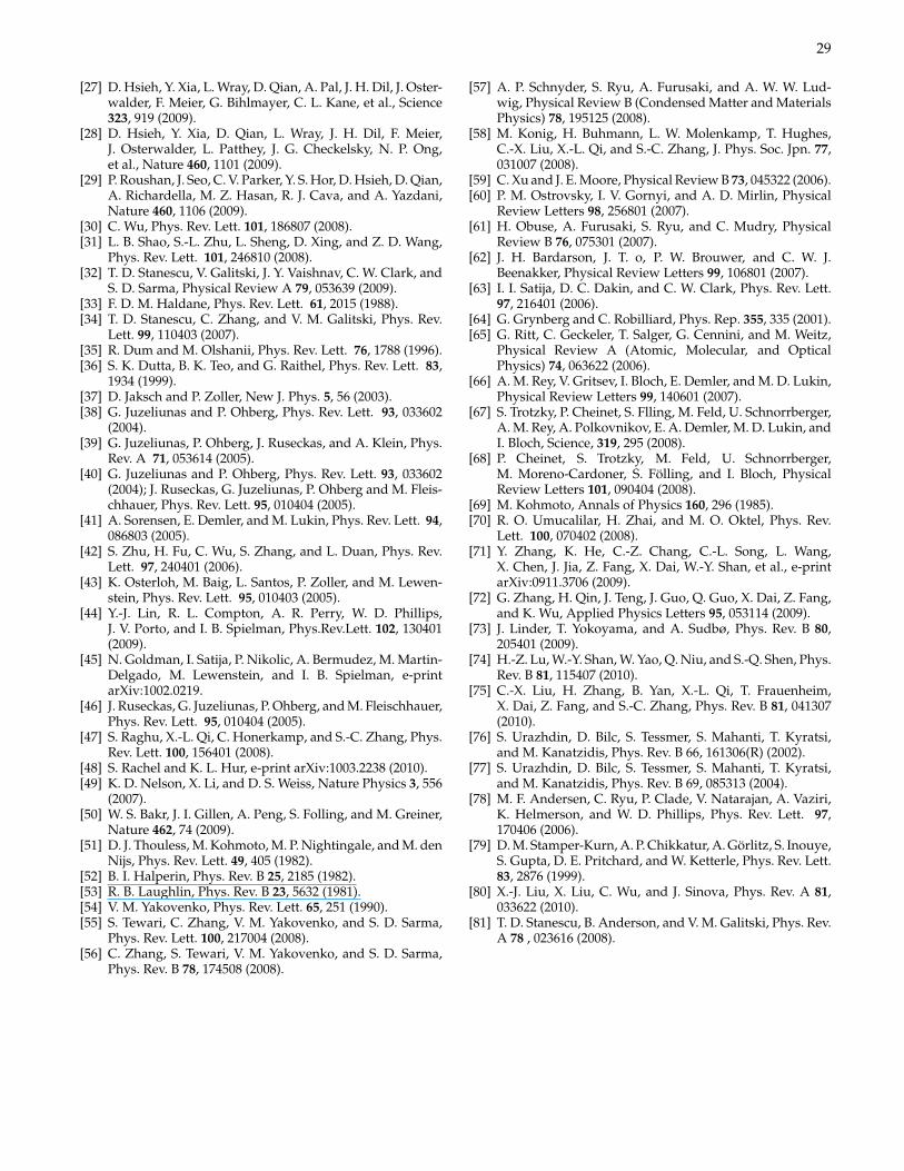
29

[27] D. Hsieh, Y. Xia, L. Wray, D. Qian, A. Pal, J. H. Dil, J. Oster-walder, F. Meier, G. Bihlmayer, C. L. Kane, et al., Science323, 919 (2009).

[28] D. Hsieh, Y. Xia, D. Qian, L. Wray, J. H. Dil, F. Meier,J. Osterwalder, L. Patthey, J. G. Checkelsky, N. P. Ong,et al., Nature 460, 1101 (2009).

[29] P. Roushan, J. Seo, C. V. Parker, Y. S. Hor, D. Hsieh, D. Qian,A. Richardella, M. Z. Hasan, R. J. Cava, and A. Yazdani,Nature 460, 1106 (2009).

[30] C. Wu, Phys. Rev. Lett. 101, 186807 (2008).[31] L. B. Shao, S.-L. Zhu, L. Sheng, D. Xing, and Z. D. Wang,

Phys. Rev. Lett. 101, 246810 (2008).[32] T. D. Stanescu, V. Galitski, J. Y. Vaishnav, C. W. Clark, and

S. D. Sarma, Physical Review A 79, 053639 (2009).[33] F. D. M. Haldane, Phys. Rev. Lett. 61, 2015 (1988).[34] T. D. Stanescu, C. Zhang, and V. M. Galitski, Phys. Rev.

Lett. 99, 110403 (2007).[35] R. Dum and M. Olshanii, Phys. Rev. Lett. 76, 1788 (1996).[36] S. K. Dutta, B. K. Teo, and G. Raithel, Phys. Rev. Lett. 83,

1934 (1999).[37] D. Jaksch and P. Zoller, New J. Phys. 5, 56 (2003).[38] G. Juzeliunas and P. Ohberg, Phys. Rev. Lett. 93, 033602

(2004).[39] G. Juzeliunas, P. Ohberg, J. Ruseckas, and A. Klein, Phys.

Rev. A 71, 053614 (2005).[40] G. Juzeliunas and P. Ohberg, Phys. Rev. Lett. 93, 033602

(2004); J. Ruseckas, G. Juzeliunas, P. Ohberg and M. Fleis-chhauer, Phys. Rev. Lett. 95, 010404 (2005).

[41] A. Sorensen, E. Demler, and M. Lukin, Phys. Rev. Lett. 94,086803 (2005).

[42] S. Zhu, H. Fu, C. Wu, S. Zhang, and L. Duan, Phys. Rev.Lett. 97, 240401 (2006).

[43] K. Osterloh, M. Baig, L. Santos, P. Zoller, and M. Lewen-stein, Phys. Rev. Lett. 95, 010403 (2005).

[44] Y.-J. Lin, R. L. Compton, A. R. Perry, W. D. Phillips,J. V. Porto, and I. B. Spielman, Phys.Rev.Lett. 102, 130401(2009).

[45] N. Goldman, I. Satija, P. Nikolic, A. Bermudez, M. Martin-Delgado, M. Lewenstein, and I. B. Spielman, e-printarXiv:1002.0219.

[46] J. Ruseckas, G. Juzeliunas, P. Ohberg, and M. Fleischhauer,Phys. Rev. Lett. 95, 010404 (2005).

[47] S. Raghu, X.-L. Qi, C. Honerkamp, and S.-C. Zhang, Phys.Rev. Lett. 100, 156401 (2008).

[48] S. Rachel and K. L. Hur, e-print arXiv:1003.2238 (2010).[49] K. D. Nelson, X. Li, and D. S. Weiss, Nature Physics 3, 556

(2007).[50] W. S. Bakr, J. I. Gillen, A. Peng, S. Folling, and M. Greiner,

Nature 462, 74 (2009).[51] D. J. Thouless, M. Kohmoto, M. P. Nightingale, and M. den

Nijs, Phys. Rev. Lett. 49, 405 (1982).[52] B. I. Halperin, Phys. Rev. B 25, 2185 (1982).[53] R. B. Laughlin, Phys. Rev. B 23, 5632 (1981).[54] V. M. Yakovenko, Phys. Rev. Lett. 65, 251 (1990).[55] S. Tewari, C. Zhang, V. M. Yakovenko, and S. D. Sarma,

Phys. Rev. Lett. 100, 217004 (2008).[56] C. Zhang, S. Tewari, V. M. Yakovenko, and S. D. Sarma,

Phys. Rev. B 78, 174508 (2008).

[57] A. P. Schnyder, S. Ryu, A. Furusaki, and A. W. W. Lud-wig, Physical Review B (Condensed Matter and MaterialsPhysics) 78, 195125 (2008).

[58] M. Konig, H. Buhmann, L. W. Molenkamp, T. Hughes,C.-X. Liu, X.-L. Qi, and S.-C. Zhang, J. Phys. Soc. Jpn. 77,031007 (2008).

[59] C. Xu and J. E. Moore, Physical Review B 73, 045322 (2006).[60] P. M. Ostrovsky, I. V. Gornyi, and A. D. Mirlin, Physical

Review Letters 98, 256801 (2007).[61] H. Obuse, A. Furusaki, S. Ryu, and C. Mudry, Physical

Review B 76, 075301 (2007).[62] J. H. Bardarson, J. T. o, P. W. Brouwer, and C. W. J.

Beenakker, Physical Review Letters 99, 106801 (2007).[63] I. I. Satija, D. C. Dakin, and C. W. Clark, Phys. Rev. Lett.

97, 216401 (2006).[64] G. Grynberg and C. Robilliard, Phys. Rep. 355, 335 (2001).[65] G. Ritt, C. Geckeler, T. Salger, G. Cennini, and M. Weitz,

Physical Review A (Atomic, Molecular, and OpticalPhysics) 74, 063622 (2006).

[66] A. M. Rey, V. Gritsev, I. Bloch, E. Demler, and M. D. Lukin,Physical Review Letters 99, 140601 (2007).

[67] S. Trotzky, P. Cheinet, S. Flling, M. Feld, U. Schnorrberger,A. M. Rey, A. Polkovnikov, E. A. Demler, M. D. Lukin, andI. Bloch, Science, 319, 295 (2008).

[68] P. Cheinet, S. Trotzky, M. Feld, U. Schnorrberger,M. Moreno-Cardoner, S. Folling, and I. Bloch, PhysicalReview Letters 101, 090404 (2008).

[69] M. Kohmoto, Annals of Physics 160, 296 (1985).[70] R. O. Umucalilar, H. Zhai, and M. O. Oktel, Phys. Rev.

Lett. 100, 070402 (2008).[71] Y. Zhang, K. He, C.-Z. Chang, C.-L. Song, L. Wang,

X. Chen, J. Jia, Z. Fang, X. Dai, W.-Y. Shan, et al., e-printarXiv:0911.3706 (2009).

[72] G. Zhang, H. Qin, J. Teng, J. Guo, Q. Guo, X. Dai, Z. Fang,and K. Wu, Applied Physics Letters 95, 053114 (2009).

[73] J. Linder, T. Yokoyama, and A. Sudbø, Phys. Rev. B 80,205401 (2009).

[74] H.-Z. Lu, W.-Y. Shan, W. Yao, Q. Niu, and S.-Q. Shen, Phys.Rev. B 81, 115407 (2010).

[75] C.-X. Liu, H. Zhang, B. Yan, X.-L. Qi, T. Frauenheim,X. Dai, Z. Fang, and S.-C. Zhang, Phys. Rev. B 81, 041307(2010).

[76] S. Urazhdin, D. Bilc, S. Tessmer, S. Mahanti, T. Kyratsi,and M. Kanatzidis, Phys. Rev. B 66, 161306(R) (2002).

[77] S. Urazhdin, D. Bilc, S. Tessmer, S. Mahanti, T. Kyratsi,and M. Kanatzidis, Phys. Rev. B 69, 085313 (2004).

[78] M. F. Andersen, C. Ryu, P. Clade, V. Natarajan, A. Vaziri,K. Helmerson, and W. D. Phillips, Phys. Rev. Lett. 97,170406 (2006).

[79] D. M. Stamper-Kurn, A. P. Chikkatur, A. Gorlitz, S. Inouye,S. Gupta, D. E. Pritchard, and W. Ketterle, Phys. Rev. Lett.83, 2876 (1999).

[80] X.-J. Liu, X. Liu, C. Wu, and J. Sinova, Phys. Rev. A 81,033622 (2010).

[81] T. D. Stanescu, B. Anderson, and V. M. Galitski, Phys. Rev.A 78 , 023616 (2008).