Topological Volume Skeletonization Using Adaptive Tetrahedralization

Shigeo TakahashiGraduate School of Arts and SciencesThe University of Tokyo, Tokyo, Japan

takahashis@acm.org

Gregory M. NielsonDepartment of Computer Science and Engineering

Arizona State University, Tempe, USAnielson@asu.edu

Yuriko TakeshimaGraduate School of Humanities and Sciences

Ochanimizu University, Tokyo, Japanyuriko@imv.is.ocha.ac.jp

Issei FujishiroGraduate School of Humanities and Sciences

Ochanimizu University, Tokyo, Japanfuji@is.ocha.ac.jp

Abstract

Topological volume skeletons represent level-set graphsof 3D scalar fields, and have recently become crucial tovisualizing the global isosurface transitions in the volume.However, it is still a time-consuming task to extract themespecially when input volumes are large-scale data and/orprone to small-amplitude noise. This paper presents an effi-cient method for accelerating the computation of such skele-tons using adaptive tetrahedralization. The present tetrahe-dralization is a top-down approach to linear interpolationof the scalar fields in that it selects tetrahedra to be subdi-vided adaptively using several criteria. As the criteria, themethod employs a topological criterion as well as a geo-metric one in order to pursue all the topological isosurfacetransitions that may contribute to the global skeleton of thevolume. The tetrahedralization also allows us to avoid un-necessary tracking of minor degenerate features that hidethe global skeleton. Experimental results are included todemonstrate that the present method smoothes out the orig-inal scalar fields effectively without missing any significanttopological features.

1 Introduction

Direct volume rendering is a powerful tool for visualiz-ing complicated inner structures in a volume, and thus help-ful to computer-aided modeling and testing as well as med-ical diagnosis and scientific simulation. However, it stillrequires significant features to be identified so that it canemphasize them individually in the final visualization im-ages. As the key to the analysis of such significant features,topological volume skeletons, which arelevel-set graphsof3D scalar fields, have recently received much attention in

the fields of volume visualization and computational geom-etry. This is because the level-set graph tracks topologicaltransitions of isosurface components according to the scalarfield, and thus serves as a landmark for exploring underly-ing inner structures. Examples can be found in [1, 13, 14].

Although the level-set graph is helpful, its complexitydepends on the number ofcritical points that invoke topo-logical changes of isosurfaces. This means that the level-setgraph may become too complicated if the resolution of theinput dataset exceeds some limit because it represents thecritical points as its nodes. The level-set graph can also cap-ture minor features such asdegeneratecritical points, whicharise from the object interiors due to the small-amplitudenoise or zero-gradient scalar fields. This is more likelyto occur if the scalar field values are quantized to a smallnumber of bits because scalar fields of small gradients arereduced to stepwise scalar fields in this case. While Taka-hashi et al. [13] presented a method for simplifying the com-plicated level-set graph to distinguish its global structure,the method still requires considerable computation time toextract an initial level-set graph if the input dataset is toocomplicated.

This paper presents a fast and robust method for com-puting the topological volume skeletons by introducing anadaptive tetrahedralization stage prior to tracking the skele-tons. The present method introduces a top-down approachto adaptive tetrahedralization, because we have to extractthe global topological skeleton of the entire volume withoutadding unnecessary tetrahedra for an appropriate interpola-tion of the scalar field. For selecting tetrahedra to be sub-divided, the method employs a criterion that takes into ac-count topological errors, in addition to the conventional cri-terion based on geometric errors. These criteria generate aninterpolation of the 3D scalar field in such a way that we cantrack all the necessary topological features to constitute the

global skeleton of the volume. Furthermore, the adaptivesubdivision scheme also prevents us from worrying aboutthe minor degenerate critical points that have little influenceon the underlying global skeleton. This is accomplishedby assigning larger tetrahedra to small-amplitude noise andzero-gradient scalar fields for the approximation. Exper-imental results are demonstrated to show that the presentmethod generates a smooth interpolation of a 3D scalar fieldwhile preserving its global topological skeleton.

This paper is organized as follows: Section 2 describesan algorithm for extracting the topological volume skele-tons and mentions the requirements for our adaptive tetra-hedralization scheme. Section 3 presents the details of theadaptive tetrahedralization method employed in our frame-work. After demonstrating several experimental results to-gether with the feasibility of the present method in Sec-tion 4, Section 5 concludes this paper and refers to futurework.

2 Topological Volume Skeletonization

The level-set graphs of 3D scalar fields were first intro-duced to the visualization community by Bajaj et al. [1].Actually, they developed a fast algorithm for extractinglevel-set graphs called thecontour trees(CTs) [15] thattrack the change in the number of connected components ofisosurfaces. This algorithm was further extended to objectsof any dimension by Carr et al. [3] in such a way that it hasO(n log n + tα(t)) time complexity. Here, the algorithmis based on the assumption that all the volume cells of theinput dataset are linearly interpolated by tetrahedralization,andn andt denote the numbers of vertices and tetrahedrathere, respectively. One of the problems with the CTs is thatthe original CTs cannot represent the topological type (i.e.genus) of an isosurface. However, this problem has recentlybeen solved by Pascucci et al. [10], where they calculate thechanges in the Euler characteristics of isosurfaces.

Our algorithm first extracts a topological volume skele-ton including relatively insignificant features, and then sim-plifies the skeleton to obtain the underlying global structureby analyzing the skeleton itself. In fact, the skeletoniza-tion algorithm we use here is newly developed by combin-ing the algorithms of Carr et al. [3], Pascucci et al. [10]and Takahashi et al. [13]. The remainder of this sectiondescribes each step of the skeletonization algorithm. Thetetrahedralization step prior to this skeletonization step willbe described in Section 3.

2.1 Constructing Join and Split Trees

Our topological volume skeletonization begins with con-structing CTs by tracking the change in the number of con-nected isosurface components as the scalar field value re-

duces. For this purpose, we use the algorithm of Carr etal. [3] in order to construct two graphs individually, whichare thejoin tree (JT) that represents the appearance andmerging of isosurface components as the scalar field valuedecreases, andsplit tree(ST) that represents the disappear-ance and splitting of isosurface components. Suppose thatwe have already generated a linear interpolation of the in-put 3D scalar field by using tetrahedralization. As shownin Figures 1(a) and (b), the JT and ST have voxels as nodesif they serve as vertices in the tetrahedralization. Note that,throughout this paper, the nodes of the graph are arrangedfrom top to bottom according to the scalar field values.Since the JT and ST are dual if we reverse the axis of thescalar field, we will consider how to construct the JT only.

Before constructing the JT, the list of voxels associatedwith the tetrahedralization is sorted in a descending orderaccording to the scalar field. If two voxels have the samescalar field value, they are compared according to the givenindices to make the total ordering of the voxels. The firstvoxel is then removed from the list and added to the JT,which can be described as follows.

Suppose thatn is the first voxel we have just pulled out ofthe list. From a set of voxels adjacent ton in the tetrahedral-ization, we extract voxels that have larger scalar field valuesthann as{u1, . . . , ul}. Since the voxelui (1 ≤ i ≤ l) hasbeen already handled earlier thann, it belongs to some con-nected componentCi of the existing JT. Let us denote thenode having the smallest scalar field value in the connectedcomponentCi by ri. If ri is identical with the noden itself,we can skip the current nodeui and turn our attention to thenext neighboring voxelui+1. Otherwise, we connectri andn with a link in the JT. If the target noden has no adjacentnodes that are larger in the scalar field, it will be inserted tothe existing JT independently as a new connected compo-nent. This process allows us to construct the JT as shownin Figure 1(a), which represents the appearance and merg-ing of isosurface components when the scalar field valuedecreases. In the same way, our skeletonization algorithmconstructs the ST as shown in Figure 1(b) to locate the dis-appearance and splitting of isosurface components.

2.2 Constructing Augmented Contour Trees

Our next step is to construct a graph called theaug-mented contour tree(ACT) as an earlier representation ofthe CT. This graph also contains all the voxels that are in-volved in the tetrahedralization as the JT and ST do.

The ACT is defined to be a graph that tracks the topo-logical transitions of isosurface components while passingthrough all the voxels as the scalar field value decreases.Carr et al. [3] proved that the ACT can be constructed fromthe JT and ST because the JT captures the top ends and up-ward branches of the ACT while the ST keeps its bottom

2

120

0

20

60

220

190

160

200210

120

0

20

60

220

190

160

200210

120

0

20

60

220

190

160

200210

0

0

00

0

1

0

0

0

120

0

20

60

100

80

0

220

190

160

200210

0

0

00

0

1

0

0

0

0

120

0

20

60

100

80

220

190

160

200210

0

0

00

0

1

0

0

0

120

0

20

60

100

80

220

190

160

200210

1200

0

(a) (b) (c) (d) (e) (f)

Figure 1. Steps for the skeletonization algorithm: (a) A join tree (JT), (b) a split tree (ST), (c) anaugmented contour tree (ACT), (d) an augmented contour tree (ACT) with isosurface genera, (e) acontour tree (CT) with isosurface genera, and (f) a volume skeleton tree (VST).

ends and downward branches. Actually, our algorithm con-structs the ACT by identifying its ends and branches fromboth its top and bottom while referring to the JT and ST.For example, suppose a node in the JT is a top end and itscorresponding node in the ST has only one downward link.In this case, the node and its downward link in the JT ismoved to the ACT, and the corresponding node in the STand its incident links are removed. If the node in the ST hasboth upward and downward incident links, we connect itsupper and lower adjacent nodes directly with a link in theST. The same process can be carried out for the node thatcorresponds to a bottom end node in the ST and has onlyone upward link in the JT.

In this way, we can construct the ACT by reducing itsundetermined part step by step because the end nodes inthe JT and ST also stand for the end nodes in the undeter-mined part of the ACT. Figure 1(c) shows the final ACTconstructed from the JT (Figure 1(a)) and ST (Figure 1(b)).

2.3 Extracting Changes in Isosurface Genus

So far we have constructed the ACT that tracks thechange in the number of connected isosurface components.However, it is possible that we have critical points thatinvoke only the change in the isosurface topological type(i.e. genus) without changing the number of its connectedcomponents. Example include the transition from a sphereto a torus and also the reverse transition. This type of crit-ical point is also very important when extracting the global

topological skeleton from the input volume.Our algorithm extracts such critical points by taking ad-

vantage of the algorithm of Pascucci et al. [10]. In fact,their algorithm calculates the change in the Euler character-istic of isosurface components when they go through eachvoxel, by calculating the change in the Euler characteristicassociated with simplices around the voxel. Here, the Eulercharacteristicχ is defined as

χ = #{vertices} −#{edges}+#{triangles} −#{tetrahedra}, (1)

where#{X} represents the number of X’s. The changein the Euler characteristic of simplices around the voxel iscalculated by finding its incident edges, triangles, and tetra-hedra. Suppose thatχl andχs are the Euler characteristicsof the simplices, where the two values correspond to theisosurface components just before and after passing throughthe target voxel, respectively. To calculateχl, our algorithmcounts simplices that have the target voxel as the vertex hav-ing the smallest scalar field value of all the corner vertices.The algorithm then applies Equation (1) for findingχl whilesetting#{vertices} = 1. The other Euler characteristicχs

is obtained by finding simplices where the target voxel isthe largest in the scalar field. At last, the change in the Eu-ler characteristic when each voxel is swept by the isosurfaceis calculated asχl − χs.

Indeed, this value allows us to detect the change in thegenus of each isosurface component. For example, if thevoxel causes the change in the Euler characteristic while

3

C3 C2 C1 C0

C3 3-C2 2-C2 3-C1 2-C1 C0

(a) (b) (c) (d) (e) (f)

Figure 2. Connectivity of the critical points inthe volume skeleton tree.

the number of isosurface components is left unchanged, itdefinitely affects the genus of the corresponding isosurfacecomponent. In this way, our algorithm can extract a spe-cific type of critical point that changes only the genus ofan isosurface component, as well as a critical point thatchanges the number of isosurface connected components.Figure 1(d) shows how the topological type (i.e. genus) ofeach isosurface component changes on the ACT.

2.4 Constructing the Contour Tree

Constructing the CT from the ACT just requires us toremove non-critical nodes from the ACT. Figure 1(e) showsan example of the CT, which is extracted from the ACT byremoving the non-critical nodes represented by the smallcircles in Figure 1(d).

In this process, our algorithm transfers the non-criticalnodes from the ACT to the remaining links in the CT. Inother words, a link of the CT possesses a list of non-criticalvoxels that originally serve as nodes in the ACT. This helpsus simplify a complicated volume skeleton for finding theglobal structure of the input volume, which will be de-scribed in Section 2.6.

2.5 Constructing the Volume Skeleton Tree

This step is devoted to finding a topological volumeskeleton having only simple critical points, by resolving allthe multiple critical points of the resultant CT into simpleones. In this paper, we call this type of level-set graph avolume skeleton tree(VST) [13]. The simple critical pointsof the VST have connectivities as shown in Figure 2, whereeach connectivity is classified according to the type and de-gree of the corresponding node.

Figure 2 suggests that isosurface transitions around sim-ple critical points are classified into six types; appearance ofa new isosurface component (Figure 2(a)), merging two iso-surface components into one (Figure 2(b)), increment of thegenus of an isosurface component (Figure 2(c)), splittingone isosurface component into two (Figure 2(d)), decrementof the genus of an isosurface component (Figure 2(e)), and

disappearance of an existing isosurface component (Fig-ure 2(f)). Here, the subscript of the symbolC representsthe number of negative eigenvalues of the Hessian matrixat the corresponding critical point. Since the critical pointsC2 andC1 have different degrees, we distinguish betweenthem by indicating the degree of each critical node such as3-C2, 2-C2, 3-C1, and2-C1. According to this classifica-tion, we can obtain the VST from the CT by resolving amultiple critical point into simple ones. When resolving themultiple critical points, we assign an empty voxel list to anewly created link. For example, in Figure 1(e), the nodeat the scalar field value 120 has three upward links in theCT. This means that we can resolve this multiple node intotwo nodes as shown in Figure 1(f) because the multiplicityof the corresponding critical point is 2.

2.6 Simplifying the Volume Skeleton Tree

For analyzing the global topological structure from theinput volume, our algorithm first extracts a VST in such away that it still contains rather minor critical points. In fact,these minor critical points themselves are less important,but still necessary for simplifying the VST appropriately.This is because it is impossible to evaluate how each criti-cal point contributes to the global structure only by lookingat its local features. Note that while an adaptive tetrahedral-ization scheme is also introduced to reduce the complexityof the extracted VST, it only tries to eliminate degeneratecritical points that have little influence on the global struc-ture of the input volume and thus are completely negligible.

In our framework, by following the scheme presented in[13], we intend to reduce the complexity of the extractedVST until the VST becomes simple enough to express theunderlying global structure of the volume. This is accom-plished by assigning a weight value to each link of the VSTand then removing the link having the smallest weight valueone by one. Takahashi et al. [13] suggest that three patternsin the VST can be candidates for the removal as shown inFigure 3. In this figure, the third pattern can contain othercritical points between the two end critical points while inthe first and second patterns the two critical points are im-mediate neighbors.

As the weight value for each link, Takahashi et al. [13]used the valueD that represents the difference in the scalarfield between the end critical points of the link. However,this definition of weight values is sometimes unsuccess-ful in extracting important topological transitions of isosur-faces because the sizes of the corresponding isosurfaces arenot taken into account. Instead of this, we define a newweight value that is given by

V ×D, (2)

where V represents the volume swept by the isosurface

4

C3–C2 C0–C1 C2–C1

C1–C2

Figure 3. Candidate patterns to be removedfrom the volume skeleton tree in the simplifi-cation process.

component that corresponds to the target link. Note that thevalueV is equivalent to the size of the interval volume [4]bounded by the two isosurface components containing theend critical points. In our framework, the valueV can becalculated easily because each link of the VST has a listof voxels assigned to it. It is clear that the volume of eachvoxel can be calculated as a quarter of the total volume of itsincident tetrahedra because a tetrahedron is shared by fourcorner voxels. Now the swept volumeV of the VST linkis obtained by summing up the volumes of the voxels thatbelong to the link.

This formulation is fully justified because the newweight valueV × D actually represents the size of the 4Dsubspace swept by the corresponding isosurface, which iscontained in the entire 4D space spanned by the(x, y, z)-coordinates and scalar field. Our experiments show that thisformulation of the weight value allows us to obtain the sim-plified version of the VST that adequately reflects the globalbehavior of isosurface transitions with respect to the scalarfield.

It is noted that while simplifying the VST, our algorithmtransfers the list of voxels from the removed link to one ofits incident link that still remains in the VST. This makesprecise extraction of the global volume skeleton because weproperly take over the interval volume removed in the sim-plification process.

3 Adaptive Tetrahedralization

This section describes a method foradaptive tetrahe-dralizationfor linear interpolation of 3D scalar fields, whichserves as an earlier stage for extracting topological volumeskeletons. As described previously, the number of primitivetetrahedra becomes enormous if we subdivide each volumecell uniformly. Thus, our method reduces the number oftetrahedra by adjusting their sizes according to the local fea-tures of the 3D scalar fields. In addition, this enables robustextraction of topological volume skeletons even when theinput volume contains high-frequency noise of small am-plitude.

Figure 4. Tetrahedral decomposition rule inthe bisection method.

Conventional adaptive tetrahedralization methods areroughly classified into two groups:top-down approachesthat adaptively subdivide a large tetrahedron into small onesas the need arises, andbottom-up approachesthat simplifytetrahedral subdivision by merging small tetrahedra into alarge one. The top-down approaches include thebisectionmethod[8] that subdivides a tetrahedron into two tetrahedraof equal size, and thered-green method[2] that introducestetrahedra of two different shapes called “red” and “green.”Gerstner et al. [5] and Grosso et al. [6] proposed techniquesfor efficient isosurface extraction using the above two top-down methods, respectively. Moreover, Holliday et al. pre-sented a method for generating smooth interpolation us-ing the Coons volume [7], even when the tetrahedralizationcontains T-vertices, i.e., the inconsistency between the facesof adjacent tetrahedra. On the other hand, as the bottom-upmethods, Zhou et al. [16] developed a method for merg-ing tetrahedra having specific connectivity generated by thebisection rule, and Staadt et al. [11] devised a method forsimplifying tetrahedra by contracting edges. In our imple-mentation, we use the bisection method that is the simplesttop-down approach introduced by Maubach [8], in order toassign fine tetrahedra adaptively to significant volume fea-tures.

3.1 The Bisection Method

Suppose that the input volume is decomposed intoN ×N × N initial volume cells, each of which contains(2n +1) × (2n + 1) × (2n + 1) voxels. This implies that theresolution of the input volume is(2nN +1)× (2nN +1)×(2nN+1), while we often setN = 1. The bisection methodfirst partitions each initial cell into six tetrahedra as shownon the left of Figure 4. Then each tetrahedron is furtherbisected if it cannot sufficiently approximate the 3D scalarfield inside it according to some appropriate error criterion.Figure 4 shows how a tetrahedron is bisected in this methodfrom left to right, where the longest edge is bisected eachtime.

This bisection rule requires that an edge we want to bi-sect must be the longest edge in every incident tetrahedron.If any of the incident tetrahedra does not satisfy this condi-tion, we turn our attention to the longest edge of that inci-

5

dent tetrahedron. We then check again if this edge is alsothe longest of all the other incident tetrahedra. If all the in-cident tetrahedra share the edge as the longest one this time,we bisect the edge together with its incident tetrahedra andthen go back to the previous edge. Otherwise, we furtherfind incident tetrahedra that violate the condition and checktheir longest edges. In this way, the process of adaptivetetrahedralization terminates when all the tetrahedra satisfythe given error criterion.

3.2 Criteria for the Adaptive Tetrahedralization

To extract the topological volume skeleton correctly, wehave to carefully formulate the criteria for estimating ap-proximation errors of tetrahedra. For this purpose, thisstudy introduces a topological error criterion as well as aconventional geometric one, so that the present method cancapture the significant volume skeleton in early stages of theadaptive tetrahedralization.

3.2.1 Geometric Error Criterion

As the geometric error criterion, this method employs theroot mean square error (RMSE) that is the most commonlyused. The RMSE is estimated for each tetrahedron as fol-lows. Suppose that a tetrahedron has a list of interior voxelsthat have the scalar field values{pi} (i = 1, 2, . . . ,m). Onthe other hand, we can calculate the corresponding approx-imate scalar field values{qi} (i = 1, 2, . . . ,m) by linearlyinterpolating the four corner voxels in the tetrahedron usingthe barycentric combination. Now the RMSE of this tetra-hedron can be written as√∑m

i=1(pi − qi)2

m. (3)

In this case, the method bisects tetrahedra where theirRMSE errors exceed the given geometric error threshold,which helps us control the final adaptive tetrahedralization.In our implementation, this is possible because each tetra-hedron possesses a list of interior voxels at the initial tetra-hedralization stage so that the method refers to the list forestimating the corresponding RMSE. Furthermore, the in-terior voxels of each tetrahedron are accurately distributedto new tetrahedra when the original tetrahedron is bisected.This implementation conveniently prevents us from recal-culating the list of interior voxels when the adaptive tetra-hedralization is performed.

3.2.2 Topological Error Criterion

The geometric error criterion based on the RMSE allowsus to assign smaller tetrahedra to 3D scalar fields of steepgradient that appear around the object boundary, and thus it

125

158(+)

142(+)

114(-)

106(-)

120(-)

115(-)

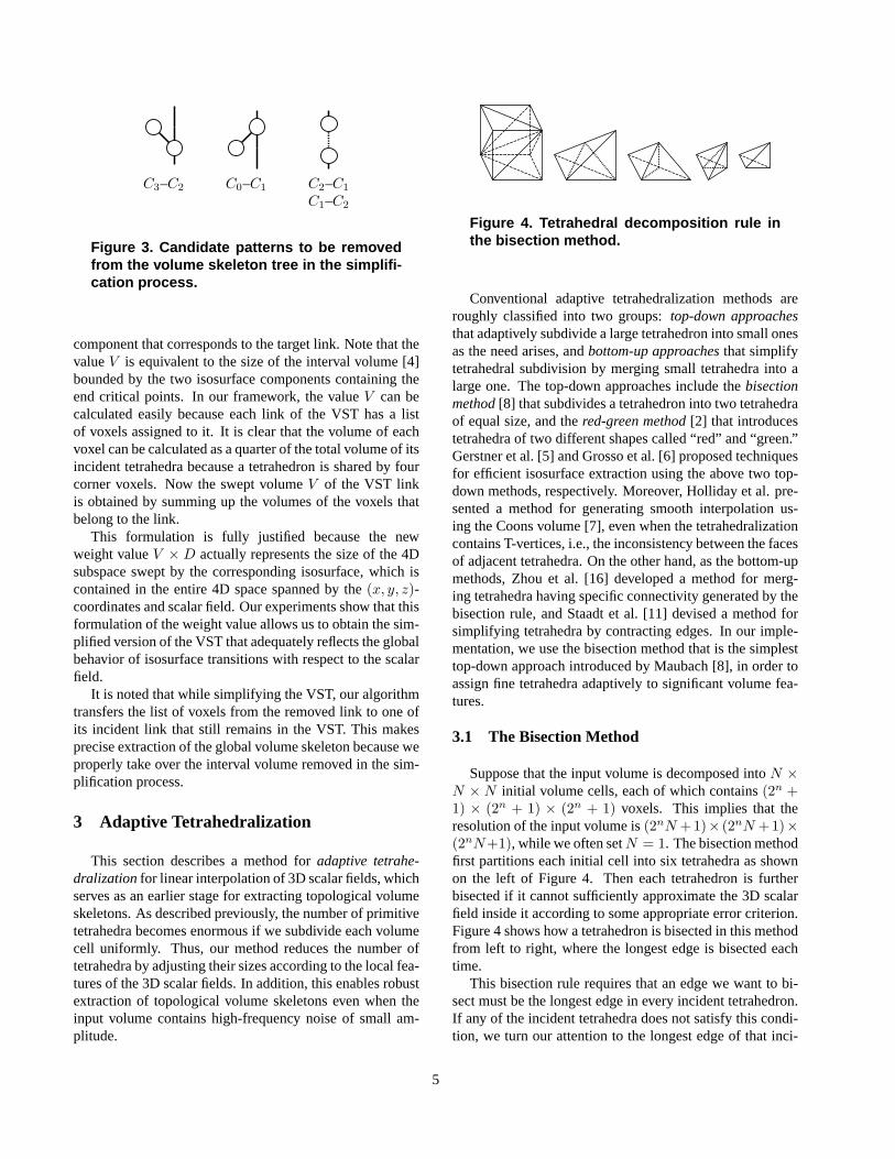
Figure 5. Topological error criteria: the inte-rior voxel having the scalar field value 125appears to be a critical point if it is adaptedto the bisection point of the edge.

generally provides a sound interpolation that reflects the un-derlying volume features with the smaller number of tetra-hedra. However, the criterion often requires more tetrahedrato capture the topological features that are indispensable forthe simplification of volume skeletons because the previousgeometric criterion only considers local geometric features.This motivates us to introduce a new topological criterionthat brings global volume features more effectively to ourtetrahedralization scheme.

The topological error criterion here has close relation-ships with that introduced by Gerstner et al. [5]. In fact,they check if critical points are contained in a set of tetrahe-dra that share the longest edge as shown in Figure 5. How-ever, their goal differs from ours in that they try to controlthe adaptive tetrahedralization to keep the topological type(genus) of the target isosurface, while our goal is to extractthe global evolution of the isosurfaces over the entire vol-ume. In addition, their method first performs the bisection-based adaptive tetrahedralization using some geometric cri-terion as a preprocessing step, and constructs the hierarchiesof critical points by traversing the refined tetrahedralizationin a bottom-up manner. Conversely, our method introducesa topological criterion that aims at a top-down tetrahedral-ization approach while following the edge-based error es-timation of Gerstner et al. For this purpose, we evaluatethe importance of topological features associated with crit-ical points as the topological errors, although Gerstner etal. only examine the existence of the critical points.

Our topological error criterion is formulated to simulatethe weight values assigned to the links of the VST (See Sec-tion 2.6). For calculating the topological errors, we first findan edge and its associated tetrahedra as shown in Figure 5,where the edge is the longest in each tetrahedron and thus

6

can be bisected immediately. In this figure, the big blackdisks represent the voxels that constitute the corner verticesof the incident tetrahedra, and small disks represent the inte-rior voxels of the tetrahedra. Actually, our topological errorcriterion tests if any of the interior voxels can serve as acritical point in the space defined by the incident tetrahedra.

Whether an interior voxel becomes a critical point ornot can be determined by evaluating the difference in thescalar field from the corner voxels (i.e., black disks) in Fig-ure 5 [5, 13]. In practice, we assign a sign “+” to the cornervoxel if it has a larger scalar field value than the interiorvoxel, and a sign “−” if it has a smaller scalar field value.We then consider the boundary edges of the neighboringtetrahedra (except the interior edge to be split), and elim-inate the edges if their endpoints has different signs. Fi-nally, we count the number of connected components foreach sign, and conclude that the interior voxel is critical ifeither of the two numbers differs from 1. Figure 5 shows acase where the voxel having the scalar field value 125 (rep-resented by small black disk) becomes critical if it is em-ployed as the interior voxel to be examined. In this case,the connected components of the corner vertices are{158}and{142} for the sign “+,” and {115, 106, 114, 120} forthe sign “−.”

It is also necessary to measure the topological error ifany of the interior voxels becomes a critical point, whichindeed provides us with an effective criterion for the top-down approach to the adaptive tetrahedralization. In orderto estimate the topological error, we first collect scalar fieldvalues of the corner voxels (black disks) and the interiorvoxel (white disk) we have just employed, and find the dif-ference between the maximum and minimum scalar fieldvalues among them. The topological error is obtained bymultiplying this difference and the volume of the space de-fined by the neighboring tetrahedra together, as shown inFigure 5. It follows from Equation (2) that the definitionof these topological errors just approximates weight valuesassigned to the VST links that are affected by the space de-fined by the neighboring tetrahedra. Note that, if the topo-logical error depends on the selection of interior voxels, thelargest topological error is used to represent the final er-ror. Moreover, this error criterion effectively avoids degen-erate critical points because the degenerate critical pointshave little difference in the scalar field in most cases. Inthis way, this formulation enables the top-down approachto the adaptive tetrahedralization while tracking all the im-portant topological features. In fact, as shown in Figure 6,the tetrahedralization with the topological error criterion re-flects topological volume skeleton more accurately than thatwith the previous geometric criterion.

3.2.3 Hybrid Error Criteria

Although the tetrahedralization generated using the abovetopological error criterion undoubtedly represents signifi-cant features of the topological volume skeleton, it still con-tains unexpectedly discontinuities of the 3D scalar field un-fortunately. In practical cases, the adaptive tetrahedraliza-tion needs to produce a smoother interpolation while pre-serving the significant topological features especially whenit is used to visualize the underlying inner structures in thevolume. For this purpose, our tetrahedralization schemeuses the hybrid error criteria that incorporate both the ge-ometric and topological error criteria. In our implementa-tion, the method first uses the topological error criterion totrack the significant global structures of the input volume,and then applies the geometric error criterion to generate asmooth interpolation of the 3D scalar field.

4 Experimental Results

This section presents several experimental results todemonstrate the applicability of our method. Our prototypesystem has been implemented on a Linux-based PC system(CPU: Pentium IV 2.4GHz, RAM: 1GB).

Suppose a 3D scalar field represented by the followingfunction:

f(x, y, z) = 4c2((x−R)2 + (z −R)2

)−

((x−R)2 + y2 + (z −R)2 + c2 − d2

)2

+ 4c2((x + R)2 + (z + R)2

)−

((x + R)2 + y2 + (z + R)2 + c2 − d2

)2, (4)

where c = 0.6, d = 0.5, and R = 0.2. By takingsamples of this function, a regular volume dataset of res-olution 65 × 65 × 65 was generated for our experiments.Figures 6(a), (b), and (c) show tetrahedralizations of thisdataset and the corresponding volume skeletons where anordinary uniform tetrahedralization scheme, an adaptivetetrahedralization scheme with the geometric criterion, andan adaptive tetrahedralization scheme with the topologi-cal criterion are applied, respectively. As shown in Fig-ure 6(a), the ordinary uniform tetrahedralization producesa large number of minor critical points due to the discretesampling and quantization whereas it can generate a smoothinterpolation of the scalar field. Figure 6(b) exhibits a resultobtained using an adaptive subdivision based on the geo-metric error criterion. Although the geometric criterion ishelpful in generating a rather smooth interpolation, it offersincorrect topological features if the number of tetrahedra islimited as shown in the figure. To the contrary, as shown inFigure 6(c), the tetrahedralization and skeletonization algo-rithm with the topological criterion can extract a correct vol-ume skeleton with a small number of tetrahedra. However,

7

(a) (b) (c)

Figure 6. Tetrahedralizations and topological volume skeletons of a 65 x 65 x 65 dataset generatedfrom the volume function of Equation (4): (a) An ordinary uniform tetrahedralization is used (No. oftetrahedra: 1,572,864). (b) An adaptive tetrahedralization based on the geometric error criterionis used (No. of tetrahedra: 960). (c) An adaptive tetrahedralization based on the topological errorcriterion is used (No. of tetrahedra: 904).

it can only produce a poor interpolation of the 3D scalarfield. It took 16 minutes to extract the topological volumeskeleton for the case in Figure 6(a) while only 5 seconds (4seconds for tetrahedralization and 1 second for skeletoniza-tion) for both Figures 6(b) and (c).

Figure 7 shows the nucleon dataset of resolution41 ×41 × 41 [9] where the two-body distribution probabilityof a nucleon in the atomic nucleus16O is simulated. Fig-ures 7(a), (b), and (c) show an adaptive subdivision with ap-proximately 10,000 tetrahedra, an adaptive subdivision withapproximately 30,000 tetrahedra, and an ordinary uniformsubdivision with 384,000 tetrahedra, respectively. These re-sults are accompanied by the initial and simplified VSTstogether with the corresponding final visualization resultswhere the topological features are accentuated [13, 14].Here, the hybrid error criteria are used to generate the adap-tive subdivision. The tetrahedralization with approximately10,000 tetrahedra in Figure 7(a) yields only a roughly ap-

proximated volume skeleton and thus the final visualizationresult is not satisfactorily refined. Nonetheless, the tetra-hedralization only with approximately 30,000 tetrahedra al-lows us to generate excellent results without worrying aboutminor degenerate critical points as shown in Figure 7(b).Surprisingly, this visualization result can be matched to thatin Figure 7(c), which is obtained using 384,000 tetrahedra.Note that when generating the visualization results on theright, we use the scalar field values assigned to the origi-nal regular volume datasets. Furthermore, we assign a newattribute value to each voxel so that we can take advantageof multi-dimensional transfer functions [14] to emphasizeinner structures in the volume. Thanks to the adaptive tetra-hedralization, our method only calculates the new attributevalues for the voxels involved in the adaptive tetrahedral-ization, and then interpolates the values for other voxels us-ing the barycentric coordinates. This actually acceleratesthe rendering process if the computational complexity for

8

(a)

(b)

(c)

Figure 7. Effects of adaptive tetrahedralization for visualizing the nucleon dataset of resolution41 x 41 x 41: Tetrahedralizations, initial volume skeleton trees, simplified volume skeleton trees,and visualization results with topological features accentuated when (a) an adaptive subdivisionwith approximately 10,000 tetrahedra is used, (b) an adaptive subdivision with approximately 30,000tetrahedra is used, and (c) an ordinary uniform subdivision with 384,000 tetrahedra is used.

Figure 8. Visualization of the antiproton-hydrogen atom collision volume dataset with resolution 129x 129 x 129: (a) An adaptive subdivision where the number of tetrahedra is approximately 40,000, (b)the corresponding volume skeleton tree after the simplification, and (c) the final visualization result.

9

calculating the new attribute values is high. Our prototypesystem extracted the initial topological volume skeletons in7 seconds (6 seconds for tetrahedralization and 1 second forskeletonization), 25 seconds (21 seconds for tetrahedraliza-tion and 4 seconds for skeletonization), and 96 seconds forFigures 7(a), (b), and (c), respectively. This implies that theoverhead for the adaptive tetrahedralization is small enoughto reduce the computation time of the entire process.

Figure 8 presents the visualization results of the vol-ume dataset that is obtained by simulating the antiproton-hydrogen collision at intermediate collision energy below50keV [12]. Since the resolution of this dataset is129 ×129 × 129, the ordinary uniform tetrahedralization schemeruns out of memory space on our computational environ-ment. However, the present adaptive tetrahedralizationscheme with the hybrid error criteria offers an interpolationas shown in Figure 8(a), which allows us to effectively ex-tract the global volume skeleton from this dataset in 60 sec-onds (53 seconds for tetrahedralization and 7 seconds forskeletonization). Actually, the method successfully identi-fies the four-fold nested inclusion relationships of isosur-faces as shown in Figure 8(b), and thus emphasizes it in thefinal visualization image as shown in Figure 8(c).

5 Conclusion

This paper has presented an accelerated method for ex-tracting topological volume skeletons using the adaptivetetrahedralization. The adaptive tetrahedralization schemeenables robust extraction of the volume skeletons by elim-inating minor degenerate critical points arising from small-amplitude noise and zero-gradient scalar fields inside ob-jects. In order to locate the significant volume featureseffectively, the topological error criterion as well as thegeometric one was introduced to the adaptive subdivisionscheme. Experimental results demonstrate that the presentmethod considerably accelerates the topological volumeskeletonization by offering an interpolation that reflects thesignificant topological features of the original 3D scalarfields.

Our future research topics include the automatic con-trol of error thresholds for the adaptive tetrahedralization.Our experiments prove that the present method can success-fully extract correct volume skeletons if it uses more than acertain number of tetrahedra to approximate the input 3Dscalar field. Nevertheless, it may be possible to reduce thenumber of tetrahedra according to the property of the inputdataset by relaxing the accuracy of the interpolation. Weplan to formulate such a control by taking advantage of thefrequency-based analysis of the input volumes.

Acknowledgements We wish to acknowledge the supportof the Office of Naval Research (N00014-02-1-0287), the

National Science Foundation (NSF IIS-9980166 & ACI-0083609), DARPA (MDA972-00-1-0027), and the JapanSociety of the Promotion of Science under Grants-in-Aidfor Young Scientists (B) No. 14780189 and No. 15700081.

References

[1] C. L. Bajaj, V. Pascucci, and D. R. Schikore. The contourspectrum. InProceedings of IEEE Visualization ’97, pages167–173, 1997.

[2] J. Bey. Tetrahedral grid refinement.Computing, 55(4):355–378, 1995.

[3] H. Carr, J. Snoeyink, and U. Axen. Computing contour treesin all dimensions.Computational Geometry, 24(2):75–94,2003.

[4] I. Fujishiro, Y. Maeda, H. Sato, and Y. Takeshima. Volu-metric data exploration using interval volume.IEEE Trans-actions on Visualization and Computer Graphics, 2(2):144–155, 1996.

[5] T. Gerstner and R. Pajarola. Topology preserving and con-trolled topology simplifying multiresolution isosurface ex-traction. InProceedings of IEEE Visualization 2000, pages259–266, 2000.

[6] R. Grosso, C. L̈urig, and T. Ertl. The multilevel finite ele-ment method for adaptive mesh optimization and visualiza-tion of volume data. InProceedings of IEEE Visualization’97, pages 387–394, 1997.

[7] D. J. Holliday and G. M. Nielson. Progressive volume mod-els for rectilinear data using tetrahedral coons volumes. InData Visualization (Proceedings of VisSym’00: Joint Euro-graphics - IEEE TCVG Symposium on Visualization), pages83–92, 2000.

[8] J. M. Maubach. Local bisection refinement forn-simplicialgrids generated by reflection.SIAM Journal of ScientificComputing, 16(1):210–227, 1995.

[9] M. Meißner. Web Page [http://www.volvis.org/].[10] V. Pascucci and K. Cole-McLaughlin. Efficient computation

of the topology of level sets. InProceedings of IEEE Visual-ization 2002, pages 187–194. IEEE Computer Society Press,2002.

[11] O. G. Staadt and M. H. Gross. Progressive tetrahedraliza-tions. InProceedings of IEEE Visualization ’98, pages 397–403, 1998.

[12] R. Suzuki, H. Sato, and M. Kimura. Antiproton-hydrogenatom collision at intermediate energy.IEEE Computing inScience and Engineering, 4(6):24–33, 2002.

[13] S. Takahashi, Y. Takeshima, and I. Fujishiro. Topologicalvolume skeletonization and its application to transfer func-tion design.Graphical Models, 66(1), 2004. (to appear).

[14] S. Takahashi, Y. Takeshima, I. Fujishiro, and G. M. Niel-son. Emphasizing isosurface embeddings in direct volumerendering. submitted.

[15] M. van Kreveld, R. van Oostrum, C. Bajaj, V. Pascucci, andD. Schikore. Contour trees and small seed sets for isosur-face traversal. In13th ACM Symposium on ComputationalGeometry, pages 212–220, 1997.

[16] Y. Zhou, B. Chen, and A. Kaufman. Multiresolution tetrahe-dral framework for visualizing regular volume data. InPro-ceedings of IEEE Visualization ’97, pages 135–142, 1997.

10